Embed Size (px)
Citation preview

Functional Programming and Parallel Graph Rewriting
Functional Programming and Parallel Graph Rewriting is a book written by Rinus Plasmeijer and Marko van Eekelen.It was published in 1993.
Preface
Part 1 FUNCTIONAL PROGRAMMING
1 Basic concepts
2 Advanced concepts: Miranda
Part 2 MODELS OF COMPUTATION
3 The l-calculus
4 Term rewriting systems
5 Graph rewriting systems
Part 3 ANALYSIS OF FUNCTIONAL PROGRAMS
6 Type assignment systems
7 Strictness analysis
Part 4 IMPLEMENTATION ON SEQUENTIAL ARCHITECTURES
8 Clean
9 Translation into Clean
10 The abstract ABC machine
11 Translating Clean into ABC code
12 Realizing the ABC machine
Part 5 CONCURRENCY ISSUES
13 Basic language concepts
14 Parallel graph rewriting
15 Concurrent Clean
16 The Parallel ABC Machine
17 Realizing the PABC machine
APPENDICES
A Syntax of the example programs
B Concurrent Clean syntax and library
C ABC machine specification
D PABC machine specification
Bibliography
Index

Rinus Plasmeijer
Marko van Eekelen
Functional Programming
and
Parallel Graph Rewriting


v
Preface
Functional languages
In a declarative programming language a computation is expressed ina static fashion, as a list of declarations. A program in such a languageis regarded as a specification that happens to be executable as well. Inthis textbook we focus on a subclass of the declarative languages, thefunctional programming languages, sometimes called applicativelanguages. In these languages a program consists of a list of functiondefinitions. The execution of a program consists of the evaluation of afunction application given the functions that have been defined.
In this book we want to show that functional programming lan-guages can be used to write compact, reliable and readable programs.As example languages we shall use the functional languages Mirandaand Concurrent Clean. We shall explain the advantages and disadvan-tages of functional languages, show how efficient implementations canbe obtained on sequential and parallel architectures, and discuss the im-portant underlying theoretical frameworks. The expressive power offunctional languages is shown not only by some small examples. Thedescriptions, transformation and compilation schemes, as well as thedefinitions of the abstract machine architectures given in this textbookare all presented in a functional style illustrating the suitability of func-tional languages as specification tools.
Graph rewriting systems
The concept of a function is a fundamental notion in mathematics. Oneof the very strong points of functional languages is the property thattheir semantics is based very directly on well-defined mathematicalmodels of computation. In fact, functional languages can be regarded assugared versions of these models. These models are very important be-cause they abstract from unimportant language details. In this way theyhelp to get a better understanding of the essential underlying concepts ofa language. This knowledge can then be used to improve the languageitself, but it can also be used to make better implementations.

vi PREFACE
The traditional model of computation used for functional lan-guages is the λ-calculus. Field and Harrison (1988) give a very good,thorough survey of several functional languages and their implementa-tions using the λ-calculus as the basic model of computation. They useHOPE as a functional language instead of Miranda and they restrictthemselves mainly to sequential implementations.
This book differs from other textbooks in that it focuses on an al-ternative model of computation: graph rewriting systems. Like the λ-calculus this model has the advantage that it is simple and that it canmodel functions. Unlike the λ-calculus it additionally contains the im-portant notions of patterns and graphs. Graphs (and the related notion ofsharing) play a key role in any efficient (parallel) implementation. Toreason about the computational complexity of a program it is essentialto know whether computations are shared or not. Furthermore, the no-tion of uniqueness in graphs gives an efficient solution for modellinginteraction and side-effects within a pure functional framework.
Implementation on sequential architectures
The implementation of functional languages is quite complex when ef-ficient code has to be generated. In this book we shall explain how suchan implementation can be achieved on traditional sequential architec-tures. The implementation of functional languages is explained in anumber of steps. Starting from Miranda, we go down in level of abstrac-tion until we reach the concrete machine level. In this compilation pro-cess the functional language Concurrent Clean (based upon graphrewriting systems) is used as intermediate language.
Concurrent programming and parallel evaluation
Another advantage of functional languages is that they are, in principle,suited for concurrent (parallel or interleaved) evaluation. However, animplementation on parallel hardware is much more difficult than on se-quential hardware, mainly because parallel machines are hard to pro-gram anyway. Concurrent functional programming is being investigatedat several research institutes but is still in its infancy. We shall demon-strate its potential power and discuss the implementation on looselycoupled parallel architectures.
About this book
This book is intended as a textbook for a one or two semester (term)course: an introductory course on functional programming, models ofcomputation and the implementation of functional programming lan-guages on traditional sequential machine architectures (Parts 1, 2 and4), optionally followed by an advanced course focused on analysis

PREFACE vii
methods (strictness analysis and type theory), concurrent functional pro-gramming and implementation on parallel architectures (Parts 3 and 5).
The prerequisite for this book is an introductory course in com-puter science including knowledge of programming in a high-level lan-guage as well as some basic understanding about (parallel) computerarchitectures and compiler construction.
This textbook is suited for advanced undergraduate students, forpostgraduate students of computer science and for researchers interestedin the area of functional programming and the implementation tech-niques on sequential and parallel architectures.
The subject of this textbook is a hot and very interesting researchtopic. It is not an easy topic because many aspects of computer scienceplay a role in it. Although much progress has been made during the lastdecade, also many problems are still to be solved and are expected toremain unsolved for quite a while. Instead of covering all existing andproposed lines of research we have chosen to base this book mainly onthe work performed by our research team at the University of Nijmegen.This has the advantage that one complete line of approach, involvingtheory, specification and implementation, can be described in detailbased upon actual experience. For example, all translation schemes pre-sented in this book are abstracts from the prototype specifications writ-ten in a functional formalism that have been used as blueprint for the ac-tual implementations. The approaches explained in this book have pro-duced good results. Furthermore, they have many things in commonwith other approaches, so one will still get a very good overall insighton the actual problems and how they can be handled.
About the Concurrent Clean software
The Concurrent Clean system, the software system developed at theUniversity of Nijmegen using the approaches described in this textbook,can be ordered separately via the authors (from the address at the end ofthe Preface). This software can be used to obtain practical experience in(concurrent) functional programming. With this system one can developreal applications.
The Concurrent Clean system contains a programming environ-ment (including text editor and project manager), an interpreter and acode generator for the lazy functional language Concurrent Clean (Bruset al., 1987; Nöcker et al., 1991b). The system is especially designed forthe Apple Macintosh (Plasmeijer et al., 1991) and generates efficientcode for any Mac. An I/O-library is available offering a very high-levelspecification of modern I/O-handling (windows, dialogues and the like).Furthermore, it is possible to generate parallel code for Macs connectedin a local area network (AppleTalk/Ethernet).
Concurrent Clean and the Concurrent Clean system are also avail-able on other platforms. The Macintosh version runs on an Atari ST

viii PREFACE
(using a Mac emulator). There is a version for Sun3 (Motorola) andSun4 (SPARC) under UNIX using an X Window System withOpen Look or OSF-Motif for the low-level I/O-handling. Clean pro-grams can run on any of these platforms without the need to modifysource code. A cross-compiler is available for ParSyTec's Supercluster(transputer). A version for the IBM-PC (look-alikes) is under develop-ment.
The Clean research team is working on the improvement of Con-current Clean and the Concurrent Clean system. Please contact the au-thors for the latest information.
Outline of this book
This book is divided into five parts. In the first two parts we focus onfunctional programming and suitable underlying models of computation.Then, in Part 3 these models are used to show how properties of func-tional programs can be analysed. Part 4 uses a particular model to showin detail how functional programs can be implemented efficiently ontraditional architectures. The final part (Part 5) covers the same kind ofsubjects as Parts 1, 2 and 4 respectively, but focuses on parallelism.Since the research in this area is less stabilized, this final part is of amore introductory and reflective nature. Exercises are given at the endof each chapter (difficult or large exercises are marked *).
Part 1: Functional programming
In this first chapter we give a description of the basic language conceptsthat most functional languages have in common (Chapter 1). Hereafterwe show in more detail the descriptive power and syntactic sugar of theadvanced language concepts as offered by one particular functionalprogramming language: Miranda (Chapter 2).
Part 2: Models of computation
In this part we concentrate on three models of computation: λ-calculus(Chapter 3) as the best known computational model and term rewritingsystems (Chapter 4) and graph rewriting systems (Chapter 5) as alterna-tive models of computation. The latter is used throughout this book as abasis for implementations and for reasoning about efficiency aspects.
Part 3: Analysis of functional programs
The models of computation introduced in Part 2 are used in Part 3 toshow how additional information can be obtained by static analysis. Inparticular, type assignment systems (Chapter 6) and strictness analysis(Chapter 7) are discussed. Type and strictness information is needed to

PREFACE ix
obtain efficient implementations. This theoretical part might be skippedby readers with a greater interest in more practical subjects.
Part 4: Implementation on sequential architectures
This part of the book covers the implementation of functional languageson traditional machine architectures. The implementation is discussed ina number of steps. In each step we go down in level of abstraction untilthe concrete machine level is reached (Figure 0.1).
Motorolacode
ABC machinesimulator
Motorolaprocessor
Functionalgraph
rewriting
Mirandaprogram
Cleanprogram ABC code
Figure 0.1 Sequential implementation of functional programming lan-guages in four levels of abstraction.
The language Clean is introduced in Chapter 8. This language isbased on functional graph rewriting systems. It is shown how a Mirandaprogram can be translated into an equivalent Clean program (Chapter9). Hereafter an abstract machine, the ABC machine, is introduced mod-elling traditional stack-based machine architectures (Chapter 10). Theuse of an abstract machine prevents us from getting lost in the details ofconcrete architectures. Step by step we shall deduce compilationschemes from Clean to the instruction set of the ABC machine (Chapter11). Finally, the remaining problems of an actual implementation onconcrete target machines are discussed (Chapter 12). As a representativetarget architecture the Motorola processor is used.
Part 5: Concurrency issues
There are several ways in which concurrency can be exploited in afunctional program. Because loosely coupled parallel architectures arebecoming widely available we concentrate on the implementation onthis type of architecture. To get an optimal performance on these ma-chines the parallelism should be explicitly specified by the programmer.
None of the existing well-known functional languages have lan-guage facilities to control parallelism. Therefore we introduce a possible

x PREFACE
extension to express concurrency in functional languages (Chapter 13).How the underlying model of computation can be extended to capturethe notion of processes and process communication is the subject ofChapter 14.
Finally, the implementation of functional languages on looselycoupled parallel machine architectures is discussed. As in Part 4 the im-plementation is explained through a series of abstraction steps down tothe concrete machine level (Figure 0.2).
Transputercode
PABC machinesimulator
Transputerprocessors
Parallelgraph
rewriting
Mirandawith
concurrency
ConcurrentClean PABC code
Figure 0.2 Parallel implementation of functional programming lan-guages in four levels of abstraction.
First, we introduce the extension of Clean to Concurrent Clean andshow how a concurrent functional program can be translated into anequivalent Concurrent Clean program (Chapter 15). Then, we extendthe ABC machine (Chapter 10) to a parallel ABC machine modellingloosely coupled machine architectures and show how Clean’s concur-rency primitives are translated to abstract machine instructions (Chapter16). Finally, we discuss the remaining problems of an actual implemen-tation (Chapter 17) on a concrete parallel target machine. As a represen-tative target architecture the transputer processor is used.

PREFACE xi
Acknowledgements
The following members of the Nijmegen research team have made im-portant contributions to specific aspects of this book: Peter Achten(Clean’s event I/O), Steffen van Bakel (type assignment systems), Johnvan Groningen (code generators and machine wizarding), HalbeHuitema (I/O library, testing), Marco Kesseler (transputer code genera-tor), Pieter Koopman (transformation schemes, (P)ABC machine), EricNöcker (transformation schemes, strictness analysis, PABC machine),Sjaak Smetsers (transformation schemes, Concurrent Clean, PFGRSs,(P)ABC machine) and Ronny Wichers Schreur (Concurrent Clean envi-ronment).
We would like to thank the following people who each in theirown way made an important contribution to the realization of this bookand to the design and the construction of the Concurrent Clean system:Christ Aarts, Erik Barendsen, Henk Barendregt, Tom Brus, Cor de Cloe,Guido van Dam, Wil Dekkers, Maurice Klein Gebbink, John Glauert,Johan Goos, Harco de Hilster, Martin van Hintum, Jeroen ter Hofstede,Richard Kennaway, Mathieu Knops, Hans Koetsier, Frank van Latum,Maarten van Leer, Mieke Massink, Paul de Mast, Angelo Melis, BetsyPepels, Leon Pillich, Ab Reitsma, Richard van Schelven, Ronan Sleep,Daniël Tuynman, Marten Wensink, Koen Wouters and Mariëlle van derZandt.
We appreciate very much the work of the referees who have helpedus with several very good suggestions for improvement of this textbook.
We are very grateful for the financial injection of the ‘DienstWetenschapbeleid’ of the Dutch Department of Science and Educationwhich initiated the research that forms the basis for this textbook. Fur-thermore, we would like to thank the ESPRIT projects Tropics andSemagraph for supporting the more advanced parts of that research.
Rinus Plasmeijer and Marko van Eekelen
April 1993
Computer Science DepartmentUniversity of NijmegenToernooiveld 16525 ED NijmegenThe Netherlands
email: [email protected]@cs.kun.nl

To Trees and Lianne

xiii
Contents
Preface v
Part 1 FUNCTIONAL PROGRAMMING 1
1 Basic concepts 3
1.1 Why functional programming? 41.2 Functions in mathematics 111.3 A functional program 141.4 The evaluation of a functional program 151.5 Functions with guarded equations and patterns 181.6 Data structures 211.7 Higher order functions and currying 251.8 Correctness proof of functional programs 291.9 Program examples 31Summary 33Exercises 34
2 Advanced concepts: Miranda 37
2.1 Defining functions 382.2 Predefined data structures 412.3 The type system 472.4 User-defined data structures and their types 552.5 The use of functions as basic building blocks 582.6 Interactive programs 642.7 Top-down functional programming 67Summary 74Exercises 75
Part 2 MODELS OF COMPUTATION 77
3 The λ-calculus 79
3.1 λ-expressions 80

xiv CONTENTS
3.2 Reduction rules for λ-expressions 853.3 Reduction sequences and normal forms 893.4 Properties of the λ-calculus 903.5 Reduction strategies 913.6 Properties of subclasses of the l-calculus 933.7 λ-calculus as a basis for functional languages 973.8 λ-calculus as a basis for implementations 102Summary 109Exercises 110
4 Term rewriting systems 113
4.1 TRSs 1154.2 Rewriting with a TRS 1194.3 Reduction sequences and normal forms 1214.4 Properties of TRSs 1234.5 Reduction strategies 1274.6 Orthogonal TRSs 1284.7 Priority rewrite systems 1374.8 TRSs as a basis for functional languages 1404.9 TRSs as a basis for implementations 143Summary 144Exercises 145
5 Graph rewriting systems 147
5.1 Extending TRSs to GRSs 1485.2 GRSs 1515.3 Rewriting with a GRS 1555.4 Reduction sequences and normal forms 1605.5 Shorthand form 1615.6 Properties of GRSs 1645.7 Reduction strategies 1685.8 Term graph rewriting 1685.9 Generalized graph rewriting systems 1765.10 GRSs as a basis for functional languages 1805.11 GRSs as a basis for implementations 180Summary 181Exercises 182
Part 3 ANALYSIS OF FUNCTIONAL PROGRAMS 185
6 Type assignment systems 187
6.1 Type assignment for the λ-calculus 1886.2 Polymorphism and recursion 1986.3 Type assignment for term rewriting systems 209

CONTENTS xv
Summary 217Exercises 218
7 Strictness analysis 219
7.1 Strictness 2207.2 Abstract interpretation 2217.3 Basic domain theory 2257.4 Strictness analysis using abstract interpretation 2287.5 Analysing function definitions 2317.6 Analysing non-flat domains 2357.7 Abstract reduction 2427.8 Strictness analysis using abstract reduction 245Summary 249Exercises 250
Part 4 IMPLEMENTATIONON SEQUENTIAL ARCHITECTURES 251
8 Clean 253
8.1 Clean, a language for functional graph rewriting 2558.2 The type system 2618.3 Strict annotations 2658.4 Modules 2708.5 Unique types and destructive updates 2738.6 Input/output handling 283Summary 295Exercises 296
9 Translation into Clean 299
9.1 About the desugaring of the language 3009.2 Simple transformations 3019.3 List comprehensions 3049.4 Local function definitions 3089.5 Translating the desugared language into Clean 3139.6 The exploitation of sharing 314Summary 317Exercises 318
10 The abstract ABC machine 319
10.1 About the ABC machine 32010.2 Machine components and micro-instructions 32410.3 The machine instructions 33010.4 Program execution 335

xvi CONTENTS
Summary 338Exercises 339
11 Translating Clean into ABC code 341
11.1 Basic graph rewriting on the ABC machine 34211.2 The run-time system 35211.3 Optimizations 356Summary 364Exercises 364
12 Realizing the ABC machine 365
12.1 Representing the ABC machine components 36712.2 Garbage collection 37112.3 The Motorola MC68020 processor 38012.4 Representing ABC components on the MC68020 38212.5 Generating MC68020 code 38612.6 Example of concrete code 39512.7 Performance 398Summary 399Exercises 400
Part 5 CONCURRENCY ISSUES 401
13 Basic language concepts 403
13.1 Concurrency and functional programming 40413.2 Annotations for concurrency 41013.3 Examples of concurrent functional programs 41913.4 Discussion 424Summary 425Exercises 426
14 Parallel graph rewriting 427
14.1 Annotations to control the reduction order 42814.2 GRSs with lazy copying 43114.3 Modelling parallel graph rewriting 439Summary 445Exercises 446
15 Concurrent Clean 447
15.1 Extending Clean to Concurrent Clean 44715.2 Specifying process structures 45115.3 Translation into Concurrent Clean 457Summary 458Exercises 458

CONTENTS xvii
16 The Parallel ABC Machine 459
16.1 About the PABC machine 46016.2 Interleaved reduction 46516.3 Parallel reduction 47116.4 Program execution 47416.5 Translating Concurrent Clean into PABC code 476Summary 477Exercises 478
17 Realizing the PABC machine 479
17.1 Representing the PABC machine components 47917.2 Garbage collection on a distributed machine 48617.3 The transputer processor 48817.4 Representing PABC components on transputers 48917.5 Generating transputer code and performance 494Summary 497Exercises 498
APPENDICES 499
A Syntax of the example programs 501
B Concurrent Clean syntax and library 503
B.1 Concurrent Clean syntax 503B.2 δ-rules 505B.3 I/O library 507
C ABC machine specification 527
C.1 The ABC instruction set 527C.2 Running ABC programs 534C.3 The ABC micro-instructions 535
D PABC machine specification 541
D.1 The PABC instruction set 541D.2 Running PABC programs 546D.3 The new micro-instructions 547
Bibliography 553
Index 563

1
Part 1Functional programming
Chapter 1 Basic concepts
Chapter 2 Advanced concepts: Miranda

2 FUNCTIONAL PROGRAMMING
This part serves as an introduction to functional programming. Since there are many different functional programming languages,
the first chapter focuses on the basic concepts most functional lan-guages have in common. By first focusing on these concepts it will berelatively easy to master the basics of any functional language with itsown syntactical sugar. The concrete examples in Chapter 1 are given ina subset of Miranda.
In Chapter 2 the more sophisticated features of Miranda are shownto demonstrate the expressive power and notational elegance of a spe-cific state-of-the-art functional programming language. More elaborateprogram examples are given with modest suggestions for a functionalprogramming methodology.
For readers who want to study the art of functional programming inmore detail good introductory books are available (e.g. Bird andWadler, 1988).

3
Chapter 1Basic concepts
1.1 Why functional programming?1.2 Functions in mathematics1.3 A functional program1.4 The evaluation of a functional
program1.5 Functions with guarded
equations and patterns
1.6 Data structures1.7 Higher order functions and
currying1.8 Correctness proof of functional
programs1.9 Program examples
This chapter first explains the advantages and drawbacks of a func-tional programming style compared with the commonly used classicalimperative style of programming (Section 1.1). The difference in objec-tives between a mathematical specification of a function and a functionspecification in a functional programming language is explained in Sec-tion 1.2.
This is followed by an overview of the basic concepts of mostfunctional programming languages (Sections 1.3–1.7). These conceptsare explained using a concrete functional programming language: Mi-randa (Turner, 1985). Functions can be defined by a single equation(Section 1.3) as well as by more than one equation using guards andpatterns to discriminate between the alternative equations (Section1.5). Other topics that are covered are: higher order functions and cur-rying (Section 1.7), lists as basic data structures (Section 1.6) and (lazyas well as eager) function evaluation (Section 1.4).
Traditional proof techniques like symbolic substitution and mathe-matical induction can be used to prove correctness of functional pro-grams (Section 1.8). Finally, some small example programs are pre-sented in Section 1.9.

4 BASIC CONCEPTS
1.1 Why functional programming?
Imagine the availability of perfect computer systems: software andhardware systems that are user-friendly, cheap, reliable and fast. Imag-ine that programs can be specified in such a way that they are not onlyvery understandable but that their correctness can easily be proven aswell. Moreover, the underlying hardware ideally supports these softwaresystems and superconduction in highly parallel architectures makes itpossible to get an answer to our problems at dazzling speed.
Well, in reality people always have problems with their computersystems. Actually, one does not often find a bug-free piece of softwareor hardware. We have learned to live with the software crisis, and haveto accept that most software products are unreliable, unmanageable andunprovable. We spend money on a new release of a piece of software inwhich old bugs are removed and new ones are introduced. Hardwaresystems are generally much more reliable than software systems, butmost hardware systems appear to be designed in a hurry and even well-established processors contain errors.
Software and hardware systems clearly have become very com-plex. A good, orthogonal design needs many person years of researchand development, while at the same time pressure increases to put theproduct on the market. So it is understandable that these systems con-tain bugs. The good news is that hardware becomes cheaper andcheaper (thanks to very large scale integration) and speed can be boughtfor prices one never imagined. But the increase of processing powerautomatically leads to an increase of the use of that power with an in-creasing complexity of the software as a result. So computers are neverfast enough, while the complexity of the systems is growing enor-mously.
The two key problems that the computer science community has tosolve are:
• How can we, at low cost, make large software systems that remainreliable and user-friendly?
• How can we increase processing power at low cost?
Researchers are looking for solutions to these problems: by investigat-ing software engineering techniques, to deal with problems related tothe management of software projects and the construction and mainte-nance of software; by designing new proof techniques to tackle theproblems in proving the correctness of systems; by developing programtransformation techniques, to transform the specification of a probleminto a program that solves it; and by designing new (parallel) computerarchitectures using many processors (thousands or more). In the meantime the quest for revolutionary new technologies (e.g. optical chips,superconduction) is always going on.

WHY FUNCTIONAL PROGRAMMING? 5
Another approach is based on the idea that the problems mentionedabove are fundamental problems that cannot be solved unless a totallydifferent approach is used and hardware and software are designed witha completely different model of computation in mind.
1.1.1 An imperative programming style
Most computer programs are written in an imperative programminglanguage in which algorithms are expressed by a sequence of com-mands. These languages, such as FORTRAN, C, Algol, COBOL, PL/1and Pascal, are originally deduced from (and form an abstraction of) thecomputer architectures they are running on (see Figure 1.1). These com-puter architectures, although different in detail, are all based on thesame architecture: the Von Neumann computer architecture (Burks etal., 1946). The Von Neumann computer architecture is based on amathematical model of computation proposed by Turing in 1937: theTuring machine.
Von Neumann architecture imperative program
abstraction
compilation
centralprocessing
unit
main memory
data
+
machineinstructions
global data
+
sequence ofcommands
Figure 1.1 Imperative programming and the Von Neumann computerarchitecture.
The great advantage of this model and the corresponding architec-ture is that they are extremely simple. The Von Neumann architectureconsists of a piece of memory that contains information that can be readand changed by a central processing unit (the CPU). Conceptually thereare two kinds of information: program instructions in the form of ma-chine code, information that is interpreted by the CPU and that controlsthe computation in the computer; and data, information that is manipu-lated by the program. This simple concept has made it possible to makeefficient realizations in hardware at a relatively low cost.
In the beginning of the computer era, the ‘high-level’ imperativeprogramming languages were designed to provide a notation to expresscomputations in a machine-independent way. Later on, one recognizedthe importance of expressing computations such that programs are

6 BASIC CONCEPTS
understandable for the human being and their correctness can be proven.It became clear that, in order to make it possible to reason about pro-grams, not every machine instruction should have a direct equivalent inthe high-level programming language. For instance, it is commonknowledge that with the use of GOTO statements, which are the directabstraction of the branch and jump instructions that are available on anycomputer, programs can be written in such a way that reasoning aboutthem is almost impossible (Dijkstra, 1968). We strongly believe that asimilar kind of problem is caused by the assignment statement.
Consider the following example written in an imperative programming style:
BOOLEAN even := TRUE;…PROCEDURE calculate (INTEGER value) : INTEGER;BEGIN
even := NOT even;IF evenTHEN value + 1ELSE value + 2ENDIF
END;…print(calculate (6));…print(calculate (6));
Both print statements in this program are syntactically the same. Still theymay produce different results. Clearly either the value 7 or 8 is printed in bothcases, but the exact value printed depends on the number of times the proce-dure calculate is called. The result returned by the procedure not only dependson the actual value of its argument, but also on the value the global booleanhas at that particular moment. This value is ‘secretly’ changed in each proce-dure call. Such side-effects cause the result of a procedure call to be contextdependent. Results become very hard to predict when, in a large program,global variables are changed all over the place.
One of the most important drawbacks of an imperative program-ming style is that an imperative program consists of a sequence ofcommands of which the dynamic behaviour must be known to under-stand how such a program works. The assignment causes problems be-cause it changes the value (and often even the meaning) of a variable.Owing to side-effects it can happen that evaluating the same expressionin succession produces different answers. Reasoning about the correct-ness of an imperative program is therefore very difficult.

WHY FUNCTIONAL PROGRAMMING? 7
Furthermore, because of the command sequence, algorithms aremore sequential than is necessary. Therefore it is hard to detect whichparts of the algorithm can or cannot be executed concurrently. This is apity, since concurrent evaluation seems to be a natural way to increaseexecution speed.
A conjecture adopted by many researchers nowadays is that thesoftware crisis and the speed problem are inherent to the nature of im-perative programming languages and the underlying model of computa-tion. Therefore, other styles of programming, such as object oriented,logical and functional styles of programming are investigated.
1.1.2 A functional programming style
John Backus (1978) pointed out that the solution for the software prob-lems has to be found in using a new discipline of programming: a func-tional programming style instead of an imperative one.
In a functional program the result of a function call is uniquelydetermined by the actual values of the function arguments. No assign-ments are used, so no side-effects are possible. As a consequence, itmakes no difference where and under what conditions a function iscalled. The result of a function will, under all conditions, be determinedsolely by the value of its arguments. For instance, in the program belowthe value printed will be 42 in both cases.
FUNCTION increment (INTEGER value) : INTEGER;BEGIN
value + 1END;…print(increment (41));…print(increment (41));
It is much easier to reason about the result produced by a function thathas no side-effects than about the result of an imperative procedure callwith side-effects (see also Section 1.8).
Advantages of functional programming languages
So perhaps a functional programming style is important and side-effects, and hence the assignment statement, should be abandoned. Butwhy should we use a functional programming language? Is it not pos-sible to use the familiar languages? The common imperative languagesalso have functions, so why not restrict ourselves and only use the func-tional subset of for instance C, Algol or Modula2?

8 BASIC CONCEPTS
Well, one can use the functional subset of imperative languages(i.e. only using functions and leaving out the assignment), but then oneis deprived of the expressive power of the new generation of functionallanguages that treat functions as ‘first class citizens’. In most imperativelanguages functions can only be used restrictively. An arbitrary func-tion cannot be passed as an argument to a function nor yielded as result.
For instance, the function twice takes a function and an argument, applies thefunction ‘twice’ to the argument and yields the result that again might be afunction. The function twice can be used in various ways, e.g. by applying theresult again as a function to respectively one or two arguments, etc.
FUNCTIONtwice (f : FUNCTION from ANYTYPE to ANYTYPE, x: ANYTYPE ) :
result ANYTYPE;BEGIN
f ( f (x) )END;…print( twice (increment, 0) );print( ( twice (twice, increment) ) (0) );print( ( twice (twice, twice) ) (increment, 0) );print( ( ( twice (twice, twice) ) (twice, increment) ) (0) );…
Functions like twice are hard to express in a classical imperative language.
Functional programming languages have the advantage that theyoffer a general use of functions which is not available in classical im-perative languages. This is a fact of life, not a fundamental problem.The restricted treatment of functions in imperative languages is due tothe fact that when these languages were designed people simply did notknow how to implement the general use of functions efficiently. It isalso not easy to change the imperative languages afterwards. For in-stance, the type systems of these languages are not designed to handlethese kinds of function. Also the compilers have to be changed dramati-cally.
In a traditional imperative language one would probably have severe problemsexpressing the type of twice. In a functional language such a function defini-tion and its application can be expressed and typed in the following way:
twice:: (* -> *) -> * -> * || type definitiontwice f x = f (f x) || function definition
?twice increment 0 || function application, yields a number

WHY FUNCTIONAL PROGRAMMING? 9
?twice twice increment 0 || function application, yields a number?twice twice twice increment 0 || function application, yields a number…
Another advantage is that in most modern functional programminglanguage(s) (FPLs) the functional programming style is guaranteed: theassignment statement is simply not available (like GOTOs are not avail-able in decent modern imperative languages). FPLs in which there areno side-effects or imperative features of any kind are called pure func-tional languages. Examples of pure functional languages are Miranda,LML (Augustsson, 1984), HOPE (Burstall et al., 1980), Haskell (Hudaket al., 1992) and Concurrent Clean (Nöcker et al., 1991b). LISP(McCarthy, 1960) and ML (Harper et al., 1986) are examples of well-known functional languages which are impure. From now on only pureaspects of FPLs are considered.
In pure FPLs the programmer can only define functions that com-pute values uniquely determined by the values of their arguments. Theassignment statement is not available, and nor is the heavily used pro-gramming notion of a variable as something that holds a value that ischanged from time to time by an assignment. Rather, the variables thatexist in purely functional languages are used in mathematics to nameand refer to a yet unknown constant value. This value can never be al-tered. In a functional style a desired computation is expressed in a staticfashion instead of a dynamic one. Due to the absence of side-effects,program correctness proofs are easier than for imperative languages (seeSection 1.8). Functions can be evaluated in any order, which makesFPLs suitable for parallel evaluation (see Section 1.4). Furthermore, theguaranteed absence of side-effects enables certain kinds of analysis of aprogram, for example strictness analysis (see Chapter 7) and uniquenessanalysis (see Chapter 8).
Besides the full availability of functions, the new generation func-tional languages also offer an elegant, user-friendly notation. Patternsand guards provide the user with simple access to complex data struc-tures; basically one does not have to worry about memory managementany more. Incorrect access of data structures is impossible. Functionalprograms are in general much shorter than their conventional counter-parts and thus in principle easier to enhance and maintain.
The question arises, is it possible to express any possible computa-tion by using pure functions only? Fortunately, this question has alreadybeen answered years ago. The concept of a function is one of the funda-mental notions in mathematics. One of the greatest advantages of func-tional languages is that they are based on a sound and well-understoodmathematical model, the λ-calculus (Church, 1932; 1933). One couldsay that functional languages are sugared versions of this calculus. Theλ-calculus was introduced at approximately the same time as the Turingmodel (Turing, 1937). Church’s thesis (Church, 1936) states that the

10 BASIC CONCEPTS
class of effectively computable functions, i.e. the functions that intu-itively can be computed, is the same as the class of functions that can bedefined in the λ-calculus. Turing formalized machine computability andshowed that the resulting notion of Turing computability is equivalent toλ-definability. So the power of both models is the same. Hence anycomputation can be expressed using a functional style only. For moreinformation on λ-calculus we refer to Barendregt (1984).
Disadvantages of functional programming languages
The advantages mentioned above are very important. But althoughfunctional languages are being used more frequently, in particular as alanguage for rapid prototyping and as a language in which studentslearn how to program, functional languages are not yet commonly usedfor general purpose programming. The two main drawbacks lie in thefields of
• efficiency and• suitability for applications with a strongly imperative nature.
Firstly, until recently programs written in a functional language ranvery, very slowly in comparison with their imperative counterparts. Themain problem is that the traditional machine architectures on whichthese programs have to be executed are not designed to support func-tional languages. On these architectures function calls are relatively ex-pensive, in particular when the lazy evaluation scheme (see Section 1.4)is used. Our computers are ideally suited for destructive updates as pre-sent in imperative languages (assignments), but these are conceptuallyabsent in functional languages. It is therefore not easy to find an effi-cient compilation scheme. Another big problem is caused by the factthat for some algorithms, due to the absence of destructive updates, thetime and space complexity can be much worse for a functional programthan for its imperative equivalent. In such a case, to retain the effi-ciency, program transformations are necessary.
As will be shown in this textbook, by using several new (and old)compilation techniques, the efficiency of (lazy) functional programs cannowadays be made acceptable in many (but certainly not all) cases. Newcompilation techniques have been developed at several research insti-tutes. These techniques are quite complex. Commercial compilers aretherefore not widely available yet. This will soon change. Anyhow, inour opinion, the advantages of functional languages are so importantthat some loss of efficiency is quite acceptable. One has to keep in mindthat decades ago we accepted a loss of efficiency when we started to usehigh-level imperative languages instead of machine assembly lan-guages.

WHY FUNCTIONAL PROGRAMMING? 11
Secondly, a very important drawback of functional languages wasthat some algorithms could not be expressed elegantly in a functionalprogramming style. In particular, this seemed to hold for applicationsthat strongly interact with the environment (interactive programs,databases, operating systems, process control). But, the problem islargely caused by the fact that the art of functional programming is stillin development. We had and still have to learn how to express the dif-ferent kinds of applications elegantly in a functional style. We nowknow that strongly interactive applications can be expressed very ele-gantly in a functional programming style. One example is the way inter-active programs that use windows, dialogs, menus and the like can bespecified in Clean (see Chapter 8). Another example is the definition ofthe abstract imperative machine given in Chapter 10.
The advantages of a functional programming style are very impor-tant for the development of reliable software. The disadvantages can bereduced to an acceptable level. Therefore we strongly believe that oneday functional languages will be used worldwide as general purposeprogramming languages.
1.2 Functions in mathematics
Before discussing the basic concepts of most functional languages, wewant to recall the mathematical concept of a function. In mathematics afunction is a mapping from objects of a set called the domain to objectsof a set called co-domain or range (see Figure 1.2).
x2
x1
x3
x4
x5
f(x1)
f(x2)
f(x3) = f(x5)
f(x4)
Domain f Range f
Figure 1.2 A function f maps objects x from the domain set to objectsf(x) in the range set.
This mapping need not be defined for all objects in the domain. If themapping is defined for an object, this object is mapped to exactly oneobject in the range. This object in the range is called the image of thecorresponding object in the domain. If all objects in the domain have an

12 BASIC CONCEPTS
image, the function is called a total function, otherwise it is called apartial function. If x is an object in domain A and f is a function de-fined on domain A, the image of x is called f(x).
The type of a function is defined as follows. If x is an object in thedomain A, x is said to be of type A. If y is an object in range B, y is saidto be of type B. If a function f maps objects from the domain A to therange B, f is said to be of type A → B, which is pronounced as ‘from Ato B’. The type of f is generally specified as:
f: A → B
In mathematics, there are several ways to define a function. The type ofa function can be specified separately from the function definition.
One way to define a function is by explicit enumeration of all ob-jects in the domain on which the function is defined with their corre-sponding images. An example of this is the following partial function(domain names Z and N are used for the domains of integers and naturalnumbers).
abs: Z → Nabs(–1) = 1abs( 0) = 0abs( 1) = 1
Another way to define functions is by using definitions that consist ofone or more (recursive) equations. For example, with this method theabs-function above can easily be defined as a total function, applicablefor all objects in the domain. Of course, the functions and operatorsused on the right-hand side must be defined on the appropriate domains.
abs: Ζ → Νabs(n) = n, n > 0
= 0, n = 0= –n, n < 0
A function like factorial can be defined as follows:
fac: Ν → Νfac(n) = 1, n = 0
= n * fac (n – 1), n > 0
or an alternative definition method is:
fac: Ν → Νfac(0) = 1fac(n) = n * fac (n – 1), n > 0

FUNCTIONS IN MATHEMATICS 13
A mathematician would consider the definitions above as very common,ordinary function definitions. But these examples are also perfect ex-amples of function definitions in a functional programming language.Notationally a function definition in a functional language has manysimilarities with a function definition in mathematics. However, there isan important difference in objective. The objective in a functional lan-guage is not only to define a function, but also to define a computationthat automatically computes the image (result) of a function when it isapplied to a specific object in its domain (the actual argument of thefunction).
Some function definitions, well-defined from a mathematical pointof view, cannot be defined similarly in a functional language, becausethe images of some functions are very difficult to compute or even can-not be computed at all.
Consider, for example, the following function definition:
halting: All_Programs → Νhalting(p) = 1, if the execution of p will stop
0, otherwise
The halting function as indicated above is a problem that is not computable,and therefore an attempt to express it will not produce the desired computa-tion. Suppose that a function in an FPL would try to calculate the image of thehalting function for an arbitrary program. The only way of doing this is moreor less running the program. But then the function would simply not terminateif the argument program does not terminate, in which case the result 0 wouldnever be produced. For another example, consider:
f: R → R, g: R → Rf '' – 6g' = 6 sin x6g'' + a2f ' = 6 cos xf(0) = 0, f '(0) = 0, g(0) = 1, g'(0) = 1
The equations for f, g and their derivatives f ', f '', g' and g'' are solvable, but itis not easy to compute such functions.
Some special purpose programming languages are able to calculatefunctions by applying special purpose calculation techniques (symboliccomputation using computer algebra techniques or formula transforma-tions). But a general purpose functional programming language uses avery simple model of computation, based on substitution. So when func-tions are defined in an FPL a computation through substitutions is de-fined implicitly (see Section 1.4).

14 BASIC CONCEPTS
1.3 A functional program
A program written in a functional language consists of a collection offunction definitions written in the form of recursive equations and aninitial expression that has to be evaluated. From now on a Miranda-based syntax (see Appendix A) will be used.
1.3.1 Function definitions
A function definition consists of one or more equations. An equationconsists of a left-hand side, an equals symbol (=) and a right-hand side.
The left-hand side defines the function name and its formal argu-ments (also called formal parameters). The right-hand side specifiesthe function result. It is also called the function body. This functionbody consists of an expression. Such an expression can be a denotationof some value, or it can be a formal argument, or a function application.
In a function application a function is applied to an expression,the actual argument. The application of a function f to an expression ais denoted as f a. So function application is denoted by simple juxtapo-sition of the function and its argument. An important syntactical con-vention is that in every expression function application has always thehighest priority (on both sides of the equations). A function definitioncan be preceded by its type definition (indicated by post-fixing thefunction name with a ‘::’ followed by its type).
Below are some examples of function definitions (now in Miranda-based no-tation). In Section 1.6 more complex definitions can be found with more thanone alternative per function and guards or patterns to indicate which alterna-tive has to be chosen. The || indicates that the rest of the line is a comment.
ident:: num -> num || ident is a function from num to num,ident x = x || the identity function on numbers
alwaysseven:: num -> num || a function from num to num,alwaysseven x = 7 || that yields 7, independent of arg. x
inc:: num -> num || a function from num to num,inc x = x + 1 || that returns the value of its arg. + 1
square:: num -> num || square functionsquare x = x * x
squareinc:: num -> num || square increment of argumentsquareinc x = square (inc x)
fac:: num -> num || the factorial functionfac x = cond (x = 0) 1 (x * fac (x – 1))

A FUNCTIONAL PROGRAM 15
In the last example cond is a predefined operator with three arguments: aboolean, a then part and an else part. Its semantics corresponds to a condi-tional choice in imperative languages.
A formal argument, such as x in the example above, is also called avariable. The word variable is used here in the mathematical sense ofthe word that is not to be confused with the use of the word variable inan imperative language. This variable does not vary. Its scope is limitedto the equation in which it occurs (whereas the defined function nameshave the whole program as scope).
Functions defined as above are called user-defined functions. Onecan also denote and manipulate objects of certain predefined types withgiven predefined operators. These predefined basic operators can be re-garded as predefined functions. For mathematical–historical reasons,and therefore also for user convenience, such primitive functions are of-ten defined as infix functions or operators. This is in contrast to the user-defined functions that are generally defined as prefix functions.
Examples of predefined types (numbers, booleans, characters), correspondingto predefined operators (functions), denotation of values (concrete objects) ofthese types, and the ‘real-life’ domain with which they can be compared.
Types Operators Denotation of values Comparable withnum +, –, *, … 0, 1, 34.7, –1.2E15, … real numbersbool and, or, … True, False truth valueschar =, <, … 'a', 'c', … characters
1.3.2 The initial expression
The initial expression is the expression whose value has to be calcu-lated.
For example, in the case that the value of 2 + 3 has to be calculated, the initialexpression 2 + 3 is written. But one can also calculate any application of user-defined functions: squareinc 7.
1.4 The evaluation of a functional program
The execution of a functional program consists of the evaluation of theinitial expression in the context of the function definitions in the pro-gram called the environment.
A functional program: a set of function definitions and an initial expression.
ident:: num -> numident x = x

16 BASIC CONCEPTS
inc:: num -> numinc x = x + 1
square:: num -> numsquare x = x * x
squareinc:: num -> numsquareinc x = square (inc x)
squareinc 7
The evaluation consists of repeatedly performing reduction orrewriting steps. In each reduction step (indicated by a ‘→’ ) a functionapplication in the expression is replaced (reduced, rewritten) by the cor-responding function body (the right-hand side of the equation), substi-tuting the formal arguments by the corresponding actual arguments. A(sub)expression that can be rewritten according to some function defini-tion is called a redex (reducible expression). The basic idea is that thereduction process stops when none of the function definitions can be ap-plied any more (there are no redexes left) and the initial expression is inits most simple form, the normal form. This is the result of the func-tional program that is then printed out.
For instance, given the function definitions above (the environment), the ini-tial expressions below can be evaluated (reduced) as follows. In the examplesthe redex that will be reduced has been underlined.
ident 42 → 42
squareinc 7 → square (inc 7) → square (7 + 1)→ square 8 → 8 * 8 → 64
square (1 + 2) → (1 + 2) * (1 + 2) → 3 * (1 + 2) → 3 * 3 → 9
However, the initial expression may not have a normal form at all.As a consequence, the evaluation of such an initial expression will notterminate. Infinite computations may produce partial results that will beprinted as soon as they are known (see Section 1.6.3).
Example of a non-terminating reduction. Take the following definition:
inf = inf
then the evaluation of the following initial expression will not terminate:
inf → inf → inf → …

THE EVALUATION OF A FUNCTIONAL PROGRAM 17
1.4.1 The order of evaluation
Because there are in general many redexes in the expression, one canperform rewrite steps in several orders. The actual order of evaluation isdetermined by the reduction strategy which is dependent on the kindof language being used. There are a couple of important things to knowabout the ordering of reduction steps.
Due to the absence of side-effects, the result of a computation doesnot depend on the chosen order of reduction (see also Chapter 3). If allredexes are vanished and the initial expression is in normal form, the re-sult of the computation (if it terminates) will always be the same: thenormal form is unique.
For instance, one can compute one of the previous expressions in a differentorder, but the result is identical:
square (1 + 2) → square 3 → 3 * 3 → 9
It is sometimes even possible to rewrite several redexes at the sametime. This forms the basis for parallel evaluation.
Reducing several redexes at the same time:
square (1 + 2) → (1 + 2) * (1 + 2) → 3 * 3 → 9
However, the order is not completely irrelevant. Some reduction ordersmay not lead to the normal form at all. So a computation may not ter-minate in one particular order while it would terminate when the rightorder was chosen (see again Chapter 3).
Example of a non-terminating reduction order. Assume that the following (re-cursive) functions are defined:
inf = inf
alwaysseven x = 7
Now it is possible to repeatedly choose the ‘wrong’ redex which causes an in-finite calculation:
alwaysseven inf → alwaysseven inf → alwaysseven inf → …
In this case another choice would lead to termination and to the unique normalform:
alwaysseven inf → 7

18 BASIC CONCEPTS
The reduction strategy followed depends on the kind of FPL. In somelanguages, e.g. LISP, ML and HOPE, the arguments of a function arealways reduced before the function application itself is considered as aredex. These languages are called eager or strict languages. In most re-cent FPLs, e.g. Miranda and Haskell, the rewriting is done lazily. Inlazy functional languages the value of a subexpression (redex) is cal-culated if and only if this value must be known to find the normal form.The lazy evaluation order will find the normal form if it exists.
Illustrating lazy rewriting:
alwaysseven inf → 7
A more complex example to illustrate lazy evaluation is shown below. Thepredefined conditional function demands the evaluation of its first argument tomake a choice between the then and else parts possible. The equality functionforces evaluation in order to yield the appropriate Boolean value. Multiplica-tion and subtraction are only possible on numbers; again evaluation is forced.
fac 2→ cond (2 = 0) 1 (2 * fac (2 – 1))→ cond FALSE 1 (2 * fac (2 – 1))→ 2 * fac (2 – 1)→ 2 * cond (2 – 1 = 0)1 ((2 – 1) * fac ((2 – 1) – 1))→ 2 * cond (1 = 0) 1 ((2 – 1) * fac ((2 – 1) – 1))→ 2 * cond FALSE 1 ((2 – 1) * fac ((2 – 1) – 1))→ 2 * (2 – 1) * fac ((2 – 1) – 1)→ 2 * 1 * fac ((2 – 1) – 1)→ 2 * fac ((2 – 1) – 1 )→ 2 * cond ((2 – 1) – 1 = 0) 1 (((2 – 1) – 1) * fac (((2 – 1) – 1) – 1))→ … → 2 * 1 * 1 → 2 * 1 → 2
1.5 Functions with guarded equations and patterns
In the previous section ordinary recursive equations were used to definea function. But often one needs a function description that depends onthe actual values of the objects in the domain, or one wants to make aseparate description for each subclass of the domain that has to be dis-tinguished. Of course, a (predefined) function can be used, like cond inthe factorial example in Section 1.3. However, it is much more conve-nient to use guarded equations or patterns for such a case analysis.
1.5.1 Guarded equations
The right-hand side of a definition can be a guarded equation. A func-tion definition using guarded equations consists of a sequence of al-

FUNCTIONS WITH GUARDED EQUATIONS AND PATTERNS 19
ternative equations, each having a guard: an expression yielding aBoolean result, the textual first alternative for which the correspondingguard is True being selected. Guards can be preceded by the keyword if.The guard of the last alternative can be just the keyword otherwise andthe corresponding alternative is chosen if and only if all other guardsevaluate to False. Although it is allowed, it is good programming stylenot to use overlapping guards.
Function definitions with guarded equations:
fac:: num -> numfac n = 1, if n = 0
= n * fac (n – 1), if n > 0
abs:: num -> numabs n = n, if n >= 0
= –n, otherwise
It is quite possible to define partial functions using guards. When afunction is called with actual parameters that do not satisfy any of theguards, it is considered to be a fatal programming error.
For example, the Fibonacci function below will cause a fatal error when it iscalled with an argument less than one (the \/-operator denotes the logical OR).
fib:: num -> numfib n = 1, if (n = 1) \/ (n = 2)
= fib (n – 1) + fib (n – 2), if n > 2
The programmer should of course avoid this situation. One way toavoid it is to specify the domain (type) of a function accurately, in sucha way that a total function is defined on that domain. The type system ofthe language should therefore allow the specification of new types or ofsubtypes (see Chapter 2). However, an arbitrary accurate specificationof the domain is generally not possible because it leads to undecidabletype systems. Total functions can be accomplished in another way byadjusting the definition of the partial function. The guards should thenalways cover the whole domain the function is defined on. To make thispossible in an easy way most languages are equipped with an error rou-tine that fits in any type.
The Fibonacci function above is now changed into a total function. It will stillyield a run-time error when it is called with an argument less than one. Butnow this situation is handled by the programmer and an appropriate error mes-sage can be given.

20 BASIC CONCEPTS
fib:: num -> numfib n = 1, if (n = 1) \/ (n = 2)
= fib (n – 1) + fib (n – 2), if n > 2= error "Fibonacci called with argument less than one", otherwise
1.5.2 Patterns
It is also possible to discriminate between alternative equations by usingpatterns on the left-hand side. These patterns are values (e.g. 0) includ-ing data constructors (see the next section) or variables. The meaningof a pattern is that the equation in question is only applicable if the ac-tual arguments of the function match the pattern. An actual argumentmatches a corresponding pattern value if it has the same value. A pat-tern variable is matched by any actual argument. An equation is onlyapplicable if all the actual arguments match the corresponding patterns.Patterns are tried from left to right, equations are tried in textual order:from top to bottom. When an actual argument is matched against a non-variable pattern, the argument is evaluated first after which the resultingvalue is compared with the specified pattern.
A function definition with patterns:
fac:: num -> numfac 0 = 1fac n = n * fac (n – 1)
0 and n are the patterns of the first two rules (a variable as formal parameterindicates that it does not matter what the value is). Calling fac (7 – 1) will re-sult in a call to the pattern-matching facility, which decides that (after theevaluation of the actual argument) only the second rule is applicable (6 ~= 0).
Patterns can also be used in combination with guarded equations.
fac:: num -> numfac 0 = 1fac n = n * fac (n – 1), if n > 0
= error "factorial called with argument less than zero", otherwise
1.5.3 The difference between patterns and guards
Patterns have a limited power: they can only be used to test whether ac-tual arguments are of a certain value or form. Using guards any functionyielding a Boolean result can be applied to the actual arguments. Soguards are more powerful than patterns, but, on the other hand, patternsare easier to read and sufficient for most definitions. Using patterns in

FUNCTIONS WITH GUARDED EQUATIONS AND PATTERNS 21
combination with guards often leads to clearer and more concise defini-tions and is highly recommended.
1.6 Data structures
In imperative languages one can define global data structures that areglobally accessible for reading and writing during execution. Since thisis not possible in functional languages it will be clear that the use ofdata structures in these languages is quite different. After creation of adata structure, the only possible access is read access. Data structurescannot be overwritten. Furthermore, data structures are not globallyavailable but they must always be passed as arguments to the functionsthat need them.
Modern functional languages allow the definition of structureddata objects like the records in Pascal. How user-defined data structurescan be defined is explained in the next chapter. In this chapter only listsare treated.
Lists are the most important basic data structure in any FPL. Listsin FPLs are actually linked lists, each element in the list has the same1type T (see Figure 1.3). The last element in the list is indicated by a spe-cial element, generally called Nil.
Nil1 2 3
Figure 1.3 An example of a list.
Because lists are so important, they are generally predefined. A list isconceptually not different from any other user-defined data structure(see Chapter 2).
Lists, like any data structure in an FPL, are built using data con-structors. A data constructor is a special constant value that is used asa tag that uniquely identifies (and is part of) an object of a certain type.So one can recognize the type of a data structure just by looking at thedata constructor it contains. Several different data constructors can beused to identify the different objects of the same type.
Lists are constructed using two data constructors (see Figures 1.4and 1.5). A list element is tagged with a constructor that is usuallynamed ‘Cons’ (prefix notation) or ‘:’ (infix notation, as used in Mi-randa). The end of a list is an empty list that just contains a tag, theconstructor ‘Nil’ or ‘ [ ]’. A non-empty list element contains, besides theconstructor ‘Cons’ (or ‘ :’), a value of a certain type T and (a reference
1 Note that in most languages all elements of a list have to be of the same type.In some other languages (e.g. LISP) the types of the list elements may differ fromeach other. In Miranda tuples are used for this purpose (see Chapter 2).

22 BASIC CONCEPTS
to) the rest of the list of that same type T. A list of elements of type T isdenoted as [T].
NilCons 1 Cons 2 Cons 3
Figure 1.4 A list prefix tagged with the constructors Cons and Nil.
Hence, in Miranda, a non-empty list element contains the infix construc-tor ‘:’, while the end of the list only contains a ‘[ ]’.
[ ]1 2 :3::
Figure 1.5 Miranda lists are infix tagged with the constructors : and [ ].
1.6.1 Denotation of lists
In Miranda, lists are denoted as follows.
Denotation of lists:
1 : (2 : (3 : (4 : (5 : [ ])))) || list of numbers from 1 up to 5True : (False : (False : [ ])) || list of booleans[ ] || denotes the empty list1 : 2 : 3 : 4 : 5 : [ ] || list of numbers from 1 up to 5
Note that the list constructor ‘:’ is right associative. For the convenienceof the programmer Miranda allows a special notation for lists, withsquare brackets:
Lists, shorthand notation:
[1, 2, 3, 4, 5] || same as 1 : 2 : 3 : 4 : 5 : [ ][True, False, False] || same as True : False : False : [ ]0 : [1, 2, 3] || same as [0, 1, 2, 3]
1.6.2 Predefined functions on lists
The data constructors ‘:’ and ‘[ ]’ are special constant values. The ele-ments of a list can therefore easily be selected by using the patternmatch mechanism in which these data constructors appear.
The (usually predefined) projection functions on lists are head (hd) and tail(tl). Projection functions like these are of general use and can be defined onlists of any type (see Chapter 2). The functions given below are restrictivelydefined on list of numbers.

DATA STRUCTURES 23
hd:: [num] -> num || hd is a function from list-of-num to numhd (first : rest) = first || yields the first element of a non-empty list
tl:: [num] -> [num] || a function from list-of-num to list-of-numtl (first : rest) = rest || returns the tail of the list
Note that the parentheses on the left-hand side are not part of the list denota-tion. They are added to disambiguate the patterns concerning the application.
This way of handling lists is very user-friendly. One does not need toworry about ‘memory management’ nor about ‘updating pointers’.
Below some other predefined operations on lists are given. Theseare: length of a list (denoted by #), subscription, followed by a numberindicating the subscript (counting from zero), and concatenation (++).
List operations:
# [2, 3, 4, 5] || length of list, yields 4[2, 3, 4, 5] ! 2 || subscription, yields 4[0, 1] ++ [2, 3] || concatenation, yields [0, 1, 2, 3]
1.6.3 Infinite lists
One of the powerful features of lazy FPLs is the possibility of declaringinfinite data structures by recursive definitions.
Definition of a function yielding an infinite list of numbers n , equal to[n, n, n, n, …]:
infnums:: num -> [num]infnums n = n : infnums n
The following program, the sieve of Eratosthenes, yields an infinite list ofprime numbers. First an infinite list of all numbers [n, n+1, n+2, …] is definedusing the function gen.
gen:: num -> [num]gen n = n : gen (inc n)
filter has two arguments: a number and a (possibly infinite) list. The filter re-moves all multiples of the given number pr from the list. Note the type of thisfunction. It is explained in the next section.
filter:: num -> [num] -> [num]filter pr (x : xs) = x : filter pr xs, if x mod pr ~= 0
= filter pr xs, otherwise

24 BASIC CONCEPTS
sieve yields an infinite list of primes. It is assumed that the first element in theinfinite list is a prime. This value is delivered as result in the head of a list.The function recursively calls itself, filtering all multiples of the found primefrom the input list.
sieve:: [num] -> [num]sieve (pr : rest) = pr : sieve (filter pr rest)
The initial expression that will yield the infinite list of all prime numbers [2, 3,5, 7, 11, …] is the following:
sieve (gen 2)
Programs having infinite data structures as results do not terminate,of course. When an infinite list is yielded, the lazy evaluation schemewill force the evaluation of the list elements from ‘left to right’. Itwould not be wise to postpone printing this list until the last element hasbeen calculated. Therefore, one after another the values of the elementsof the list are printed as soon as they have been evaluated.
Infinite data structures are of more practical importance than onemay conclude from the examples above. One has to remember that, iffunctions are evaluated with the lazy evaluation scheme, the computa-tion of a value is only started when its value is needed to produce the re-sult. For instance, if one needs a certain element of an infinite list, thecomputation will not force the evaluation of the whole list, but only ofthe part that is needed for the evaluation of the required element. There-fore, such a computation can be performed in finite time, even if an in-finite list is being used. Of course, if an attempt to find the last elementof an infinite list is made, the computation will not terminate.
So in lazy languages infinite data structures can be defined; more-over, they make elegant programs possible. For example, if a functionhas to be defined that yields the first thousand prime numbers, one cansimply take the first thousand elements of the list of all primes.
The following initial expression will yield the second prime number of an infi-nite list of all primes. The evaluation will terminate even if an infinite list isbeing used.
hd (tl (sieve (gen 2)))→ hd (tl (sieve (2 : gen (inc 2))))→ hd (tl (2 : sieve (filter 2 (gen (inc 2)))))→ hd (sieve (filter 2 (gen (inc 2))))→ hd (sieve (filter 2 (inc 2 : gen (inc (inc 2)))))→ hd (sieve (filter 2 (3 : gen (inc (inc 2)))))→ hd (sieve (3 : filter 2 (gen (inc (inc 2)))))

DATA STRUCTURES 25
→ hd (3 : sieve (filter 3 (filter 2 (gen (inc (inc 2))))))→ 3
Infinite data structures cannot be handled in eager languages, becausethey evaluate arguments regardless of whether they are needed or not,which leads to infinite computations.
The evaluation of the initial expression in the previous example in eager FPLswill not terminate.
hd (tl (sieve (gen 2)))→ hd (tl (sieve (2 : gen (inc 2))))→ hd (tl (sieve (2 : gen 3)))→ hd (tl (sieve (2 : 3 : gen (inc 3))))→ hd (tl (sieve (2 : 3 : …)
In a lazy functional programming language most functions that are de-fined on lists can also be used to handle infinite lists. For instance, thehd function (defined above) can take the head of all lists, regardless ofwhether the list is finite or infinite.
1.7 Higher order functions and currying
Compared with the traditional imperative languages, which normallyallow also the declaration of functions, functional programming lan-guages such as Miranda have a more general view of the concept offunctions: they are treated as ‘first-class citizens’, i.e. functions aretreated just like other objects in the language. As a consequence, func-tions can have functions as arguments and as results.
1.7.1 Higher order functions
Functions that have functions as actual arguments or yield a function asresult are called higher order functions, in contrast to first-orderfunctions, which have only non-function values as argument or as re-sult.
Example of a higher order function that takes a function as argument (notehow this is reflected in the type):
atzero:: (num -> num) -> numatzero f = f 0
Now consider the following initial expressions (inc, square and ident aretaken to be defined as in Section 1.3):

26 BASIC CONCEPTS
atzero inc → inc 0 → 0 + 1 → 1atzero square → square 0 → 0 * 0 → 0atzero ident → ident 0 → 0
Example of a higher order function that yields a function as result (note thetype):
funcresult:: num -> (num -> num)funcresult 0 = incfuncresult 1 = squarefuncresult n = ident
And consider the following initial expressions:
funcresult 0 6 → inc 6 → 6 + 1 → 7funcresult 1 6 → square 6 → 6 * 6 → 36funcresult 2 6 → ident 6 → 6funcresult 3 6 → ident 6 → 6
At first sight the substitutions in the example above may seem a bitstrange. But, remember that the application of a function f to an expres-sion a is denoted as f a. So if a function is applied to more than one ar-gument, say n, this can be denoted as:
( … ((f a1) a2) … an)
Function application is left associative. So this can be denoted in anequivalent, more readable way:
f a1 a2 … an
Hence, the expression funcresult 0 6 is equivalent to (funcresult 0) 6, whichimmediately explains why the substitution above is allowed. Higher or-der functions are very natural and provide a powerful programmingtool, as is shown below.
1.7.2 Currying
The possibility of yielding a function as result makes it unnecessary tohave functions with more than one argument. A function with n argu-ments can be simulated by a higher order function with one argumentthat returns a new function. Now this new function can be applied to thenext argument, and so on, until finally all n arguments are handled.
The idea of handling functions with n arguments by using a se-quence of applications of higher order functions with one argument iscalled currying (Schönfinkel, 1924; Curry and Feys, 1958), see also

HIGHER ORDER FUNCTIONS AND CURRYING 27
Chapter 3. The final result of such a sequence of applications of higherorder functions with one argument is the same as the result yielded bythe equivalent function with n arguments.
Consider a function definition, in Miranda, of a function with morethan one argument, say n. Assume that these arguments are, respec-tively, of type A1, A2, …, An and that the result of the function is of typeB. In general such a function definition has the following form:
function-name arg1 arg2 … argn = expression
In Miranda, all functions are used in a curried manner. Functions withmore than one argument are simulated by a sequence of applicationsusing currying. Therefore the definition above should be read as:
( … ((function-name arg1) arg2) … argn) = expression
The type of this function is not
function-name:: A1 x A2 x … x An -> B
which is the mathematical type with as domain the Cartesian product ofthe n argument types, but
function-name:: A1 -> (A2 -> … -> (An -> B) … )
The arrow -> is defined to be right associative, so the type can also bespecified as
function-name:: A1 -> A2 -> … -> An -> B
1.7.3 The use of currying
The question arises: why should one use this currying scheme and makethings more complicated? Well, notationally it is almost equivalent tohaving functions with more than one argument: function application isleft associative, so the parentheses can be left out. Currying enables theuse of a familiar notation; only the types of the functions are different.But a great advantage of currying is that it increases the expressivepower of a functional language.
Parametrizing functions
The currying scheme makes it possible to apply a function defined on narguments to any number of arguments from 1 up to n, resulting in aparametrized function. A function defined with n arguments can, with-out currying, only be applied when all these n arguments are available.

28 BASIC CONCEPTS
In the curried variant some of the arguments can be ‘fed’ to the func-tion; the result (a parametrized function) can be passed to anotherfunction that can fill in the remaining arguments.
Consider the following definition:
plus:: num -> num -> numplus x y = x + y
This definition is equivalent to:
plus:: num -> (num -> num)(plus x) y = x + y
Now take the following initial expression:
plus 1
Clearly, we need another argument to be able to actually perform the additionspecified in the function body. The result of this initial expression is a func-tion of type num -> num. It is a function of one argument; the function has noname.
Assuming plus to be defined as above, the function incr can be defined in twoways: as a function with an explicit formal argument:
incr:: num -> numincr x = plus 1 x
or as a parametrized version of plus:
incr:: num -> numincr = plus 1
The only difference between the two incr functions is that the second defini-tion is more concise.
It is very useful to be able to create new functions by adding parametersto more general functions. So currying enables a new way of pro-gramming by elegantly specifying general purpose functions.
Another example of parametrized functions. The function map takes a func-tion of type num -> num, a (possibly infinite) list of numbers and applies thegiven function to all numbers in the list. incr and plus are assumed to be de-fined as above.

HIGHER ORDER FUNCTIONS AND CURRYING 29
map:: (num -> num) -> [num] -> [num]map f [ ] = [ ]map f (x : xs) = f x : map f xs
A function that increments the elements of a list can now simply be con-structed as follows:
mapincr:: [num] -> [num]mapincr = map incr
or as
mapincr:: [num] -> [num]mapincr = map (plus 1)
In Miranda it is, in general, not the intention to yield a function asthe final result of a program. Functions cannot be printed. The intentionis to yield some non-function value, probably a string of characters, asthe final result. Therefore, in ordinary programs curried functions willin the end receive all arguments needed to do the computation.
The following example of an expression with mapincr as defined above (thesecond definition) shows how evaluation might actually proceed when curry-ing is used.
mapincr [1,2,3]→ map (plus 1) [1,2,3]= map (plus 1) (1 : 2 : 3 : [ ])→ plus 1 1 : map (plus 1) (2 : 3 : [ ])→ 2 : map (plus 1) (2 : 3 : [ ])→ 2 : (plus 1) 2 : map (plus 1) (3 : [ ])→ … → 2 : 3 : 4 : [ ] = [2,3,4]
1.8 Correctness proof of functional programs
A functional programming style has advantages that are common in anymathematical notation:
• There is consistency in the use of names: variables do not vary,they stand for a, perhaps not yet known, constant value throughouttheir scope.
• Thanks to the absence of side-effects, in FPLs the same expressionalways denotes the same value. This property is called referentialtransparency.

30 BASIC CONCEPTS
A definition like x = x + 1 would mean in an imperative languagethat x is incremented. In a functional language however this definitionmeans that any occurrence of x can always be substituted by x + 1.Clearly the initial expression x does not have a normal form: substitu-tion will continue forever (some systems recognize such situations incertain simple cases and report an error message).
x → x + 1 → (x + 1) + 1 → …
Due to the referential transparency1 one is allowed to replace in any ex-pression any occurrence of any left-hand side of a definition by its cor-responding right-hand side and vice versa.
Referential transparency makes it possible to use common mathe-matical techniques such as symbolic substitution and induction. With thehelp of these techniques a program can be transformed into a more effi-cient one or certain properties of a program, such as its correctness, canbe proven. Take again the factorial example:
fac:: num -> numfac 0 = 1 || (1)fac n = n * fac (n – 1), if n > 0 || (2)
= error "factorial called with argument less than zero", otherwise
The Miranda definition of this function has a great similarity to themathematical definition of factorial. In order to prove that this functionindeed calculates the mathematical factorial written as n! for n >= 0,mathematical induction is used: first it has to be proven that the functioncalculates factorial for a start value n = 0 (step 1). Then, under the as-sumption that the function calculates factorial for a certain value n (theinduction hypothesis), it has to be proven that the function also calcu-lates factorial for the value n + 1 (step 2). The proof is trivial:
step 1: fac 0 = 1 , by applying rule (1)1 = 0! , by the definition of factorial
step 2: Assume that fac n = n!, n >= 0 (induction hypothesis)fac (n + 1) = (n + 1) * fac n , by applying rule (2): n+1>0(n + 1) * n! , by the induction hypothesis(n + 1)! , by the definition of factorial
1 Sometimes the notion ‘functional programming language’ is used for lan-guages which support higher order functions and the notion ‘applicative program-ming language’ for languages which support referential transparency. Outside thefunctional programming community the notion ‘functional’ is widely used as a syn-onym for ‘useful’.

CORRECTNESS PROOF OF FUNCTIONAL PROGRAMS 31
Note that the proof assumes, as is common in mathematics, that thefunction is only applied to arguments on which it is defined: the math-ematical definition does not concern itself with ‘incorrect input’ (n < 0).In general, a proof must cover the complete domain of the function.
There is a strong correspondence between a recursive definitionand an induction proof. Recursive functions generally have the form ofa sequence of definitions: first the special cases (corresponding to thestart values in an induction proof), textually followed by the generalcases that are recursively expressed (corresponding to the inductionstep).
1.9 Program examples
This section illustrates the expressive power of the functional pro-gramming languages in two small examples.
1.9.1 Sorting a list
The function (quick) sort needs a list of numbers as argument and deliv-ers the sorted list as result.
sort:: [num] -> [num]sort [ ] = [ ]sort (x : xs) = sort (smalleq x xs) ++ [x] ++ sort (greater x xs)
The functions smalleq and greater take two arguments, namely an ele-ment and a list. This element must be of the same type as the type of theelements of the list. It is assumed that the elements are of type num; theoperators <= and > are therefore well defined.
smalleq:: num -> [num] -> [num]smalleq a [ ] = [ ]smalleq a (x : xs) = x : smalleq a xs, if x <= a
= smalleq a xs, otherwise
greater:: num -> [num] -> [num]greater a [ ] = [ ]greater a (x : xs) = x : greater a xs, if x > a
= greater a xs, otherwise
1.9.2 Roman numbers
Outline of the problemRoman numbers consist of the characters (roman ciphers) M, D, C, L, X,V and I. Each of these characters has its own value. The values of romanciphers are: M := 1000, D := 500, C := 100, L := 50, X := 10, V := 5, I := 1.

32 BASIC CONCEPTS
These characters always occur in sorted order, characters with a highervalue before characters with a lower value. Exceptions to this rule are anumber of ‘abbreviations’, given below. The value of a roman numbercan be found by adding the values of the characters that occur in theroman number (MCCLVI = 1000 + 100 + 100 + 50 + 5 + 1 = 1256). The fol-lowing abbreviations are commonly used: DCCCC := CM, CCCC := CD,LXXXX := XC, XXXX := XL, VIIII := IX, IIII := IV. These abbreviations make itless simple to calculate the value of a roman number because now thevalue of the character depends on its position in the string. Negativenumbers and the number zero cannot be expressed in roman numbers.
Task• Develop an algorithm that calculates the integer value of a roman
number, represented as a string, assuming that the string is a properroman number.
• Develop an algorithm that converts an integer value into a romannumber without abbreviations, assuming that the integer value ispositive.
SolutionFirst the value of a roman cipher is defined:
value:: char -> numvalue 'M' = 1000value 'D' = 500value 'C' = 100value 'L' = 50value 'X' = 10value 'V' = 5value 'I' = 1
The function romtonum converts a roman number to a decimal number. Itassumes that the supplied argument is a proper roman number.
romtonum:: [char] -> numromtonum ('C' : 'M' : rs) = value 'M' – value 'C' + romtonum rsromtonum ('C' : 'D' : rs) = value 'D' – value 'C' + romtonum rsromtonum ('X' : 'C' : rs) = value 'C' – value 'X' + romtonum rsromtonum ('X' : 'L' : rs) = value 'L' – value 'X' + romtonum rsromtonum ('I' : 'X' : rs) = value 'X' – value 'I' + romtonum rsromtonum ('I' : 'V' : rs) = value 'V' – value 'I' + romtonum rsromtonum ( r : rs) = value r + romtonum rsromtonum [ ] = 0

PROGRAM EXAMPLES 33
The function numtorom converts a decimal number to a roman numberby repeated subtraction of 1000, 500, 100, 50, 10, 5 and 1, in this order. Itassumes that the argument is a number greater than zero.
numtorom:: num -> [char]numtorom n = countdown n ['M','D','C','L','X','V','I']
countdown:: num -> [char] -> [char]countdown 0 rs = [ ]countdown n (r : rs) = [r] ++ countdown (n – value r) (r : rs), if n >= value r
= countdown n rs, otherwise
The style in which these algorithms were presented (bottom-up) is notthe way in which they were deduced. In Chapter 2 styles of functionalprogramming are discussed.
Summary
• A functional program consists of a collection of (predefined) func-tion definitions and an initial expression that has to be evaluatedaccording to these definitions.
• A function definition consists of a sequence of one or more alterna-tive equations. The choice between these alternatives is determinedby patterns and/or guards.
• The evaluation of a functional program is called reduction orrewriting.
• A function application that can be rewritten according to a functiondefinition is called a redex.
• In each reduction step a redex is replaced by the correspondingfunction body, substituting formal arguments by actual arguments.
• The evaluation of a functional program stops if there are no moreredexes left in the resulting expression. Then the expression is innormal form.
• Redexes can be chosen in arbitrary order; in principle it is evenpossible that they are reduced in parallel.
• A reduction strategy determines the order in which redexes are re-duced.
• In a lazy FPL redexes are only chosen if their result is needed toachieve the normal form.
• In an eager FPL the arguments of a function are reduced to normalform before the function application itself is reduced.

34 BASIC CONCEPTS
• Data structures in FPLs are not globally available but constructedin expressions, passed as arguments, decomposed and used ascomponents for the construction of new structures.
• Data structures in FPLs are composed using data constructors.With pattern matching data structures can be decomposed.
• The most important basic data structure in FPLs is a list.• Lazy FPLs can handle infinite data structures, eager FPLs cannot.• A function with n arguments can be simulated using higher order
functions with at most one argument (currying).• FPLs have a high expressive power due to the availability of higher
order functions, pattern matching and guarded equations.• Due to referential transparency traditional mathematical proof
techniques, such as induction and substitution, can be used for thecorrectness proof of functional programs.
EXERCISES
1.1 Write in your favourite imperative language a program that findsthe maximum element in a list of numbers. Rewrite the program sothat only the functional subset of the imperative language is used.
1.2 Consider the following function definition:maxi:: num -> num -> nummaxi x y = x, if x >= y
= y, if x < y
Check whether the following initial expressions are legal, and if so,give the result yielded:• maxi 5 6 • maxi (5) • maxi 5• maxi (5,6) • maxi maxi 5 6 4 • maxi [5,6]• maxi (maxi 5 6) 4 • maxi 'a' 4
1.3 Write a function maxilist that uses the function maxi of Exercise 1.2to calculate the greatest element of a list of numbers. How doesmaxilist react on the empty list? Are there lists for which your pro-gram does not terminate? Does it make any difference if youchange the order of the guards or patterns in your program?
1.4 Suppose you now want to find the smallest element of a list withminimal rewriting of the programs written in Exercise 1.3. Tosolve this problem first write a higher order function find in Mi-randa that gets a list of numbers and a function f of type num -> num

EXERCISES 35
-> num as arguments and produces a num as its result such that find[a1,a2,…,an] f = f a1 (f a2 ( … (f an–1 an ))).Then, write down the stepwise lazy evaluation of the function ap-plication find [1,2,3] s with s:: num -> num -> num and s a b = a + b.What does find list s calculate?Finally, write a function to find the smallest element of a list.
1.5 Define functions that print a list of characters on the screen in dif-ferent ways: vertically below each other; each character in thesame place; with two spaces between the characters; diagonally.
1.6 Define a function which yields the last two elements in a list.
1.7 Define a function which yields the average of a list of numbers.
1.8 Define a function search that takes two arguments of type [char]yielding a bool indicating whether the first argument is part of thesecond.
1.9 Examine the definition of the function map in this chapter. Define afunction mapfun that applies a list of functions to a number and re-turns a list of the results of the function applications. So the fol-lowing must hold: mapfun [f,g,h] x = [f x, g x, h x].
1.10 Define a function that yields all factorial numbers.

37
Chapter 2Advanced concepts: Miranda
2.1 Defining functions2.2 Predefined data structures2.3 The type system2.4 User-defined data structures and
their types
2.5 The use of functions as basicbuilding blocks
2.6 Interactive programs2.7 Top-down functional
programming
In this chapter the more sophisticated language features as found inmodern lazy functional languages are discussed. Again Miranda(Turner, 1985) is taken as example language. The intention of thischapter is to show the programming power and notational eleganceprovided by such a state-of-the-art-language.
Many of the advanced concepts treated in this chapter can alsobe found in other languages. Those who are already familiar with simi-lar languages like ML (Harper et al., 1986), LML (Augustsson, 1984),HOPE (Burstall et al., 1980), Haskell (Hudak et al., 1992) or others willrecognize most concepts.
Examples of simple function definitions using patterns andguarded equations have been shown in the previous chapter. In addi-tion Miranda allows function definitions with a local scope to support amore modular programming style (see Section 2.1). Besides lists, tu-ples are also available as predefined data structures. Furthermore, apowerful and elegant notation based on mathematics is provided togenerate all kinds of lists (Section 2.2). Miranda’s type system hasmany features useful for programming. Functions can be of polymor-phic type (Section 2.3). User-defined data structures (Section 2.4) canbe declared using algebraic type declarations or abstract type declara-tions. The use of (higher order) functions as basic building blocks(Section 2.5) is a useful and reliable method for producing more com-plex functions. Due to lazy evaluation it is possible to write fairly generalinteractive programs in a functional language (Section 2.6). Finally, inSection 2.7 some guidelines are given on how to perform a top-downdesign of a functional program.

38 ADVANCED CONCEPTS: MIRANDA
2.1 Defining functions
The basic ideas of Miranda are taken from earlier functional languagessuch as SASL (Turner, 1979b). The word ‘Miranda’ is Latin and itmeans ‘she who is to be admired’.
Miranda is a lazy functional programming language featuring thebasic concepts discussed in the previous chapter. Miranda is equippedwith many additional features such as a rich type system that helps theuser to develop meaningful, elegant and compact programs.
A Miranda program consists of two parts: a collection of declara-tions, called the script, and an initial expression to be evaluated. Thedeclarations in the script can be function definitions or type declarations.In general, a function definition has the following form:
f_name pattern1 pattern2 … patternn = expression
Some examples of valid Miranda expressions:
x || an identifier127 || a value of type num(eral)True || a value of type bool(ean)'a' || a value of type char(acter)"hello world" || a value of type [char]y * x – 17 || an expression of type num using predefined operators[1,5,7,9] || a list of nums[+, –, *, /] || a list of operators of type num -> num -> numfac 3 || a function application(any_expression) || an expression
There are a variety of predefined infix and prefix operators, of variousbinding powers (see below).
List of prefix and infix operators, in order of increasing binding power. Thetable reveals that Miranda allows functions of polymorphic type (see Section2.3). Comparison operators can be continued, e.g. 0 <= x < 5.
Left associative operators: + , – , * , / , div , mod , !Right associative operators: ++ , – – , : , ̂Associative operators: ., \/ , &Prefix operators: ~ , # , –Continuable operators: > , >= , = , ~= , <= , <
Operator Type Meaning: * -> [*] -> [*] prefix an element to a list++, – – [*] -> [*] -> [*] list concatenation,
list subtraction\/, & bool -> bool -> bool logical OR, AND

DEFINING FUNCTIONS 39
~ bool -> bool logical negation>, >=, =, ~=, <=, < * -> * -> bool greater, greater than,
equal, not equal,less than, less
+, – num -> num -> num plus, minus– num -> num unary minus*, /, div, mod num -> num -> num times, divide,
integer divide, remainder^ num -> num -> num to the power of. (** -> ***) -> (* -> **) -> * -> *** function composition# [*] -> num length of list! [*] -> num -> * list subscription
The evaluation strategy in Miranda is lazy. Function alternatives aretried in textual order and the patterns in an alternative are tried from leftto right. This strategy is intuitively easy to understand. However, it isnot truly lazy, i.e. it does not always find a normal form if it exists.
Miranda’s evaluation strategy is not truly lazy. Take the following definitions:
f 1 [ ] = 0f x (a : b) = a
inf = inf
With the initial expression f inf [1..2] the evaluation in Miranda will not termi-nate since the first argument will be evaluated first. So the strategy will notfind the normal form 1. However, one would expect that a truly lazy strategywould evaluate the second argument of f first, but the strategy of Miranda firsttries to match the patterns of the topmost rule from left to right and therefore itfirst evaluates the first argument of f.
Furthermore some specific aspects of Miranda are:• Named constants in patterns are not possible: you can define a
function linewidth = 80 for usage as a named constant throughoutyour program, but it is not possible to use this constant as a patternon the left-hand side of a function definition: syntactically it wouldbe a pattern variable.
• A string actually is a list of characters; hence "It is fun" is shorthandfor 'I' : 't' : ' ' : 'i' : 's' : ' ' : 'f' : 'u' : 'n' : [ ]. This implies that one can use thepattern match mechanism for lists to decompose strings.
2.1.1 Local function definitions
Ordinary functions defined in Miranda have a global scope. This meansthat such a function can be applied in any expression anywhere in the

40 ADVANCED CONCEPTS: MIRANDA
program script. It is also possible to define functions with a local scopeusing a where clause. Such a local function is only defined in the small-est surrounding block. Outside a block such a function is not visible. Inmost programming languages the beginning and the end of a blockstructure are indicated by special keywords such as ‘begin’ or ‘end’, or inother languages a block is surrounded by parentheses. In Miranda ablock is indicated by the layout of a program: a block consists of all ex-pressions and definitions within one function definition or where clausethat is either directly below or to the right of the first token after theequal sign of the function definition. A token that is outside the block ofa definition is said to be offside (Landin, 1966).
The boxes indicate the blocks of, respectively, the function definition and thewhere clause:
glob_func a1 … an = expr1glob_func b1 … bn = expr2
where
local_func1 c1 c2 … cm = expr3local_func2 d1 d2 … ds = expr4
A where clause can contain any number of definitions. The whereclause must be indented, to show that it is part of the right-hand side.
primes:: [num]
primes = sieve (from 2)where
sieve (p : x) = p : sieve (filter p x)from n = n : from (n + 1)filter p (a : x) = filter p x, if a mod p = 0
= a : filter p x, otherwise
A disadvantage of the offside rule is that it can lead to errors whennames are changed globally in the script.
A not-offside program:
f a = gwhere g = 3
An offside program:
a_meaningful_long_name_for_this_function a = gwhere g = 3

DEFINING FUNCTIONS 41
Actually (for purists), it is a consequence of the offside rule that a Mi-randa program is no longer referentially transparent: a uniform substitu-tion can introduce an error and hence change the meaning of a program.One can overcome this problem by using a layout that is safe with re-spect to global name changes.
An example of such a safe layout is given below:
f a= g
where g = 3
2.2 Predefined data structures
In Miranda two kinds of data structure are predefined: lists and tuples.In the first part of this section tuples are discussed and compared withlists which were already introduced in the previous chapter.
Modern languages like Miranda and Haskell furthermore offercompact alternative notations to define lists: list comprehensions. Theselist comprehensions offer the possibility of defining lists in a style com-monly used in mathematics. In the second part of this section these no-tations are discussed.
2.2.1 Tuples
The most important difference between lists and tuples is that the ele-ments of a tuple can have different types while all the elements of a listmust be of the same type. Furthermore a list is a linked list, possibly ofinfinite length. A tuple is just a record with some finite number of fields(Figure 2.1). There must be at least two fields in the tuple. Each fieldcontains an object of a certain type.In Miranda, the notation for lists andtuples is quite similar: brackets are used to denote lists, parentheses areused to denote tuples. Parentheses are also used for disambiguating thestructure of expressions. There is no concept of a 1-tuple, so the use ofparentheses for disambiguating never conflicts with their use for tu-pling.
[ ]1 2 :3::
1Tuple-3 2 3
Figure 2.1 General difference between a list and a tuple.

42 ADVANCED CONCEPTS: MIRANDA
The correspondence between the Miranda notation for lists and tuples:
[1, 2, 3] || the list 1 : 2 : 3 : [ ](1, 2, 3) || a tuple containing the elements 1, 2 and 3
In a tuple the elements can have different types. If the elements of a tu-ple are of type T1, T2 … Tn, the type of that tuple is indicated by (T1, T2,… , Tn) (see also Section 2.3).
Example of tuples and their types:
(3, 0, 'a') || 3-tuple of type (num, num, char)([0,1,2], +) || 2-tuple of type ([num], num -> num -> num)
As with any other data structure, pattern matching can be used to accesselements. In this way projection functions can be constructed that selecta certain element from a tuple.
Using pattern matching to select an element of a tuple with three elements:
first (x, y, z) = xsecond (x, y, z) = ylast (x, y, z) = z
Here follows a summary of the differences between the two prede-fined data structures lists and tuples:
• the length of lists can vary and can even be infinite, the length oftuples will always be fixed and finite;
• all the elements in a list must be of the same type, the elements in atuple need not;
• lists are enclosed in square brackets, tuples are enclosed in roundparentheses;
• in a pattern match and in a denotation all the elements in a tuplemust be enumerated, whereas for lists this is not necessary;
• subscription as in lists is not defined in tuples; however there is thepossibility of extracting elements of a tuple by using patternmatching.
As will be shown in Section 2.4, both lists and tuples could havebeen defined as ordinary user-defined algebraic data types. The reasonthat they have been predefined is that they are used so frequently thatboth data structures deserve a compact notation as well as special atten-tion in an implementation.

PREDEFINED DATA STRUCTURES 43
2.2.2 List comprehensions
Miranda offers three alternative notations to define lists in a style com-monly used in mathematics: by means of dotdot expressions, ZF-ex-pressions and recurrent generators. These notations do not offer anyadditional expressive power, but are just syntactic sugar. The advantageof the notations is that they may be used to express certain algorithmsconcisely and elegantly (although the concept of recurrent generators isa bit overdone in our opinion). A disadvantage of the notations is that itmay be less clear how the list will be computed. As a result program-mers may sometimes find their programs to be unexpectedly slow oreven non-terminating.
Dotdot expressions
The following abbreviations are provided for defining lists whose mem-bers form a finite or infinite arithmetic series.
Dotdot notations (let a, b, c stand for arbitrary numeric expressions):
[a..b] finite list of numbers from a with interval 1, last member notexceeding b
[a..] infinite list from a with interval 1[a,b..c] finite list from a with interval (b–a), last member not exceeding c[a,b..] infinite list from a with interval (b–a)
The following examples show the use of these abbreviations togetherwith an equivalent definition showing that it is all just syntactical sugar.
Two auxiliary functions that are used in the expansion of the abbreviations:
inbetween:: num -> num -> num -> [num]inbetween start limit interval= start : inbetween (start + interval) limit interval,
if (interval >= 0 & start <= limit) \/ (interval <= 0 & start >= limit)= [ ], otherwise
from:: num -> num -> [num]from start interval = start : from (start + interval) interval
Examples of the use of dotdot expressions with (on the right) an equivalentordinary definition.
The ciphers from 0 up to 9:
ciphers:: [num] ciphers:: [num]ciphers = [0..9] ciphers = inbetween 0 9 1

44 ADVANCED CONCEPTS: MIRANDA
The natural numbers:
nats:: [num] nats:: [num]nats = [1..] nats = from 1 1
Even ciphers:
evenciphers:: [num] evenciphers:: [num]evenciphers = [0, 2..9] evenciphers = inbetween 0 9 (2–0)
Even natural numbers:
evens:: [num] evens:: [num]evens = [2, 4..] evens = from 2 (4–2)
ZF-expressions
ZF-expressions give a concise syntax for a general class of iterationsover lists. The notation is adapted from the Zermelo–Fraenkel set theory(Fraenkel, 1922; Zermelo, 1908). Note that Miranda is dealing with listsand not with sets. A ZF-expression has two possible forms:
[ exp | qualifiers ] or [ exp // qualifiers ]
The above must be read as ‘list of all exp such that qualifiers’. The ex-pression yields a list with elements of the form dictated by exp. The el-ements are produced by qualifiers. When multiple qualifiers are specified,they are separated by semicolons. There are two kinds of qualifiers:generators and filters. A qualifier can be a generator, of the form:
pattern1, pattern2, … , patternn <- exp
which is a shorthand for the following multiple generators:
pattern1 <- exp; pattern2 <- exp; … ; patternn <- exp
The ‘<-’ sign denotes that the patterns, of which the variables are locallyintroduced on its left, range over all the elements of the list on its right.
The function squares yields an infinite list containing (in order) the squares ofall natural numbers. The ZF-expression is read aloud as ‘list of all n*n suchthat n is drawn from the list [1..]’. The pattern n is just a local variable.
squares:: [num]squares = [ n*n | n <- [1..] ]

PREDEFINED DATA STRUCTURES 45
The function sqlist employs a more complex pattern to yield a list of tuples.With the pattern (x, y) these tuples are generated from that list and used toyield the list of cubes, i.e. the list of all numbers to the power 3.
cubes:: [num]cubes = [ x*y | (x, y) <- sqlist ]
sqlist:: [(num,num)]sqlist = [ (n, n*n) | n <- [1..] ]
If there is more than one generator specified as qualifier, the rightmostwill vary first, as if the generators were specified as nested for loops.
Example of the use of multiple generators:
list:: [(num, num)]list = [ (x, y) | x, y <- [1..2] ]
is an abbreviation for
list = [ (x, y) | x <- [1..2]; y <- [1..2] ]
The rightmost generator varies first, so list yields the following list of tuples:[(1,1), (1,2), (2,1), (2,2)].
A qualifier can also be a filter, i.e. a Boolean expression used to imposerestrictions on the objects generated by the generators.
The function factors gives the list of all factors of a given number n using afilter qualifier.
factors:: num -> [num]factors n = [ r | r <- [1..n div 2]; n mod r = 0 ]
A nice demonstration of the elegance of ZF-expressions is given by the fol-lowing definition of the quicksort algorithm:
quick_sort:: [num] -> [num]quick_sort [ ] = [ ]quick_sort (a : x) = quick_sort [b | b <- x ; b <= a] ++
[a] ++quick_sort [b | b <- x ; b > a]
Since in the case of multiple generators the rightmost generator willvary first, other generators cannot produce new solutions if the right-most generator yields an infinite sequence. Hence, one has to be aware

46 ADVANCED CONCEPTS: MIRANDA
of the possibility that a specification looks fine at first sight, but is notproducing any result due to the way the computation is performed.
The Pythagorean numbers with multiple generators varying over infinite lists:
pyths:: [(num, num, num)]pyths = [ (a, b, c) | a, b, c <- [1..]; a^2 + b^2 = c^2]
This ‘solution’ will not yield anything because of the order in which the gen-erators vary: [(1, 1, 1), (1, 1, 2), (1, 1, 3), …]
The problem can be solved by diagonalizing generators such that allgenerators have equal priority, i.e. these generators are evaluatedbreadth-first from left to right instead of depth-first. This different typeof generator is specified by using ‘//’ instead of the ‘|’.
Example: the Pythagorean numbers with diagonalized generators:
pyths:: [(num, num, num)]pyths = [ (a, b, c) // a, b, c <- [1..]; a^2 + b^2 = c^2]
Now the generators yield a list of tuples in the following way: [(1, 1, 1), (1, 1,2), (2, 1, 1), (1, 2, 1), (2, 1, 2), (3, 1, 1), (1, 1, 3), (2, 2, 1), …].
Recurrent generators
Recurrent generators allow the construction of lists from arbitrary recur-rence relations using the dotdot notation:
pattern <- exp1, exp2 ..
The meaning of a recurrent generator is expressed by expanding it to anormal generator in the following way:
pattern <- iterate f exp1
where f pattern = exp2
iterate:: (* -> *) -> * -> [*]iterate f x = x : iterate f (f x)
The result of iterate is the infinite list [x, f x, f (f x), f (f (f x)), …]. The meaningof the type specification of iterate will be explained in the next section.
The recurrent generator combines the pattern and the second expressioninto a recurrent relation f. This f is iterated with start expression exp1
yielding a list.

PREDEFINED DATA STRUCTURES 47
With a recurrent generator the Fibonacci series can be defined as:
fibs:: [num]fibs = [ a | (a,b) <- (1,1), (b,a+b).. ]
This can be expanded to:
fibs = [ a | (a,b) <- iterate f (1,1) ]wheref (a,b) = (b, a+b)
The generator yields [(1,1), (1,2), (2,3), (3,5), (5,8),…]
Recurrent generators are special syntactical constructs for a special kindof recursive definition, generating a list.
2.3 The type system
Miranda is a strongly typed language, i.e. every expression and everysubexpression has a type. The type system of Miranda is based upon thetype assignment systems of Milner–Mycroft (Milner, 1978; Mycroft,1984). Explicit type declarations are not required. If the types are notspecified, they are inferred by the compiler by analysing the functiondefinitions. Any inconsistency in the deduced types or any conflict withthe specified types results in a compile-time error message. However,the explicit specification of types is highly recommended. It gives a lotof information about the specified functions. By choosing meaningfulnames for user-defined types (and for all other identifiers used in theprogram) the readability can be improved dramatically.
The advantages of adding a type system to a language are twofold.Firstly, it stimulates the programmer to write correct programs: onlycorrectly typed programs are accepted by the compiler. Hence, forexample, if the type of a function application is inconsistent with thetype of the corresponding function definition, a compile-time error isgenerated. In this way the type system is of help in writing programsthat make (more) sense.
Given the type of the infix + to be num -> num -> num, the expression
1 + 'a'
will be detected by the compiler as a type error.
A second advantage of having a typed language is that the type informa-tion can be used to generate efficient code. This is explained in Part 4.

48 ADVANCED CONCEPTS: MIRANDA
There are also some disadvantages in having a typed language. Toobtain the advantages claimed above, it is necessary to determine theconsistency of types at compile-time. It can be proven that it is in gen-eral impossible to determine a proper type for all sensible expressions(see also Chapter 6). Fortunately, powerful type systems such as theMilner–Mycroft scheme used in Miranda can deduce and check thetypes of most expressions. As shown in this chapter later on, some ex-pressions cannot be typed in this system and a compile-time error isgenerated even if the expression made sense. A peculiarity of the com-bination of the Milner type system (type deduction of a function that hasnot been typed) and the way the Mycroft system is used (checking atype specified by a programmer) is that in some cases expressions areaccepted when they are explicitly typed by the programmer, but rejectedotherwise (see also Section 2.3.6).
Hence, a type system always limits the number of legal programs.In most cases this limitation is of great help for the programmer, be-cause an illegal program generally contains a program error. But insome more rare cases an illegal program does not contain a program-ming error at all. It simply could not be handled by the type system. Insuch cases the programmer is obliged to change the program to make itacceptable for the type system.
2.3.1 Basic types
In Miranda three basic types are predefined: num(bers), bool(eans) andchar(acters). There is no type distinction between integer and floating-point numbers: they are both of type num. At run-time integer numbersare taken where possible. They are automatically converted into float-ing-point numbers when needed. It is important to note that due to thenature of floating-point numbers (rounding errors) this automatic con-version can create a conflict with referential transparency.
2.3.2 Type constructors
Complex types can be constructed by using type constructors. Typeconstructors make it possible to construct new types by combining ex-isting types. The available type constructors are ‘[’ and ‘]’ (for con-structing lists), ‘(’ and ‘)’ (for constructing tuples) and ‘->’ (for con-structing functions).
For these type constructors the following holds:
• If T is a type, then [T] denotes the type list of T.• If T1,…,Tn are types, then (T1,…,Tn) denotes the type tuple of
T1,…,Tn.• If T1,T2 are types, then (T1 -> T2) denotes the type function from T1
to T2.

THE TYPE SYSTEM 49
The best way to understand complex types built with the type con-structors is to read them aloud, as in the following example.
Using type constructors to build complex types:
[ [num] ] || list of list of num([char],[num] -> bool) || tuple with list of char and
|| function from list of num to boolnum -> num -> num || function from num to
|| function from num to num
2.3.3 Polymorphic types
A useful type system should not restrict the programmer too much. Theexample below illustrates this.
Function reverse:
reverse [ ] = [ ]reverse (a : as) = reverse as ++ [a]
If the function reverse is applied to a list of characters, it will yield a listin which all characters are in reversed order. On the other hand, if ap-plied to a list of numbers, it will yield this list in reversed order too.Hence it would be nice if the type system would allow the use of such afunction for any sort of list. The Miranda system allows such a typespecification. The type of reverse is denoted by
reverse:: [*] -> [*]
which indicates that reverse takes a list with elements of an arbitrarytype as an argument and yields a list with elements of the same type.
To indicate arbitrary types there is an alphabet of generic typevariables denoted by the symbols *, **, ***, and so on. A variable namecan occur more than once in a type definition. In such a case each occur-rence of the same name denotes the same type. Unequal names only in-dicate that the corresponding types can differ from each other (theycould be the same). If a type variable occurs in the type definition of afunction, the type of the function is said to be polymorphic (orgeneric) in the sense of Milner (1978).
Some examples of polymorphic functions:
ident:: * -> *ident x = x

50 ADVANCED CONCEPTS: MIRANDA
hd:: [*] -> *hd (x : xs) = x
second:: (*, **, ***) -> **second (x, y, z) = y
2.3.4 Type deduction
Generally a programmer will know the type of the function that he orshe is defining. It is not always clear what the type of a concrete func-tion is. For example, consider the function twice and try to deduce (infer)its type.
twice f x = f (f x)
In order to solve this problem the programmer actually has to performthe same kind of analysis that is performed by the type system incorpo-rated in the Miranda compiler. This is only possible in all cases if thetype system and the type inference mechanism are fully understood bythe programmer. For the moment we shall only present a basic inferencescheme that helps to derive the type of a function in most cases. Typesystems and type inference mechanisms are explained in detail inChapter 6.
The general idea of the inference scheme is the following: first theleft-hand side of a function definition is analysed, making assumptionsfor the type of the function, its arguments and its result. The next step isto analyse this right-hand side using all assumptions already made. Thetype of the result must be compatible with the type of the right-handside. Furthermore, function and arguments must be used consistently inthe right-hand side. This analysis leads to equations that have to besolved to infer the type of the function.
Below the basic inference scheme is explained in more detail. Forreasons of readability Greek characters are used for type variables in-stead of the *s that are used in Miranda.
1. Left-hand side analysis
For the general case f x1 x2 … xn = right-hand side for each argument andfor the result a new type variable is introduced leading to the followingassumptions:
x1:: α1, x2:: α2, …, xn:: αn, result:: αn+1f:: α1 -> α2 ->… -> αn -> αn+1
If a pattern is specified, the corresponding type information is incorpo-rated directly in the assumptions.

THE TYPE SYSTEM 51
Incorporating pattern information in assumptions for left-hand side type analy-sis:
hd (x : y) = x
The constructor ‘:’ is a constructor of the type list, so the following types areassumed:
(x : y):: [α1], x:: α1, y:: [α1], result:: α2, hd:: [α1] -> α2.
2. Right-hand side analysis
The right-hand side is analysed using the assumptions made so far, lead-ing to one or more equations. First of all, the assumed result type mustbe compatible with the type of the right-hand side as a whole. Further-more, every application must be type-consistent. So for every occur-rence of an application (function argument) on the right-hand side the re-quired equation for the type of the function, the argument and the resultof the application itself is:
function type = argument type -> result type.
Remember that all functions are considered to be curried. So for a func-tion with multiple arguments several applications must be considered.
Already known types of functions are used in such a way that foreach application of a polymorphic function in the assumed type freshvariables are taken. When no assumption is available new assumptionsare made introducing fresh variables. Equations are constructed thatspecify the conditions that have to be fulfilled to make every applicationtype consistent.
Right-hand side type analysis of previous example: hd (x : y) = x. Left-handside assumptions were: (x : y):: [α1], x:: α1, y:: [α1], result:: α2, hd:: [α1] -> α2.Inspecting the right-hand side shows that the result type must equal the type ofx (the right-hand side):
α2 = α1
This equation is solved in the next step.
3. Solving equations
The equations are solved by substituting for the type variables othertype variables or actual types. In general there are many solutions forthe equations. The solution we want is of course the most general solu-tion. The process of finding such a solution is called unification, and

52 ADVANCED CONCEPTS: MIRANDA
the requested solution is called the most general unifier. In Chapter 6 amethod will be given that performs the unification by solving the equa-tions during the analysis.
Solving equations for the running example: hd (x : y) = x. Assumptions: (x :y):: [α1], x:: α1, y:: [α1], result:: α2, hd:: [α1] -> α2. Equations: α2 = α1.
Solution: substitute α2 by α1, leading to the following derived types:
(x : y):: [α1], x:: α1, y:: [α1], result:: α1, hd:: [α1] -> α1
We could also substitute α1 by α2 yielding the same solution, since the namesof the type variables can be chosen freely. The compiler would have deducedthe type hd:: [*] -> *. A different solution of the equation would have beenfound by substituting both α2 and α1 by num, leading to hd:: [num] -> num.Obviously, this is not the most general solution.
These three steps complete the basic type inference scheme. In thisscheme not all syntactic constructs of Miranda, such as local definitions,type synonyms, algebraic data types, ZF-expressions etc., are taken intoaccount. It is left to the reader to extend the scheme where necessary.To illustrate the basic type inference scheme it is applied to the follow-ing examples:
doublehd x = hd (hd x)
Left-hand side analysis: x:: α1, result:: α2, doublehd:: α1 -> α2
Right-hand side analysis: generally, it is easier to do the innermost applicationfirst.Analysis of application: hd x leads to: type of hd = (type of x)->(type of (hd x))Take fresh variables for the type of hd:: [α4] -> α4. The type of x is already as-sumed to be α1. For hd x no assumption is available, so assume hd x:: α3.The resulting equation: [α4] -> α4 = α1 -> α3
The application hd (hd x) leads in the same way to the following equation:[α5] -> α5 = α3 -> α2
Solving the equations: both sides of -> have to be equal:[α4] = α1, α4 = α3, [α5] = α3, α5 = α2.Leading to the following substitutions: α1 = [ [α5] ], α2 = α5.So doublehd:: [ [α5] ] -> α5.The compiler would have deduced the type of doublehd as [ [*] ] -> *.
Another example: twice f x = f (f x)
Left-hand side analysis: f:: α1, x:: α2, result:: α3, twice:: α1 -> α2 -> α3.

THE TYPE SYSTEM 53
Right-hand side analysis:Analysis of application: f x leads to: type of f = (type of x) -> (type of (f x))For f x no assumption is available, so assume f x:: α4.The resulting equation: α1 = α2 -> α4Analysis of application: f (f x) leads to: (type of f) = (type of (f x)) -> (type of (f(f x)))f (f x) is the right-hand side, so its type is assumed to be the result type: α3.The resulting equation: α1 = α4 -> α3
Solving the equations leads to α2 = α4 = α3 and α1 = α2 -> α2.So the derived type is twice:: (α2 -> α2) -> α2 -> α2.The compiler would have deduced the type of twice as (* -> *) -> * -> *.
2.3.5 Untypable function definitions
Not all functions can be typed in Milner’s type system (see also Chapter6). Two different kinds of untypable functions are given below:
A Milner untypable function:
selfapplication f = f f
This function cannot be typed in Milner’s system because f cannot have both *and * -> * as type since the equation α1 = α1 -> α1 has no solution.
The function definition in the example above cannot be typed. In thiscase one can argue that such functions should not be written. However,although the Milner type system is very powerful compared with thetype systems generally available in more traditional languages, somevery reasonable functions also cannot be expressed.
A Milner untypable function:
length:: [*] -> numlength [ ] = 0length (a : b) = 1 + length b
fun:: ([*] -> num) -> [*] -> [*] -> numfun f list1 list2 = f list1 + f list2
missionimpossible = fun length [1,2,3] "abc"
The actual argument f is not allowed to have two different types within thebody of the function fun. In this case f has to have type [num] -> num whenapplied to list1 but type [char] -> num when applied to list2.

54 ADVANCED CONCEPTS: MIRANDA
Milner’s type inference scheme inherently does not allow internalpolymorphism, where the same object is used with different typeswithin one function definition. Although the deduction scheme used canbe improved for some cases, a satisfactory algorithm for general cases isnot possible.
The problem mentioned above can be solved by making the polymorphism ex-ternal:
fun2:: ([*] -> num) -> ([**] -> num) -> [*] -> [**] -> numfun2 f1 f2 list1 list2 = f1 list1 + f2 list2
missionpossible:: nummissionpossible = fun2 length length [1,2,3] "abc"
2.3.6 Differences between type deduction and checking
Explicit declaration of types makes it possible to declare the type oftwice more restrictively as (num -> num) -> num -> num. In this way a typedeclaration can also be used to impose additional restrictions on a func-tion (the declared type is more restrictive than the general derived type).Another difference between type deduction and type checking is due tothe fact that the type checking algorithm uses an algorithm of Mycroftthat differs from the type deduction algorithm of Milner (this is dis-cussed in more detail in Chapter 6).
Difference between type inferencing and type checking:
g x = 1 : g (g 'c')
The type deduction algorithm of Milner cannot deduce the type of g. Hence anerror message will be produced. In this case g is used polymorphically in theright-hand side of its own definition, with type instances: char -> [num] and[num] -> [num]. However, when the user explicitly specifies the type of g asg:: * -> [num] the type checker has no problems handling this case: the speci-fied type is accepted and no error message is produced.
Maybe it would be better to insist always on explicit specification oftypes and to have a type inference tool assisting with this specification.
Another example with a difference between type checking and type deduction:
g x = g 1
Type deduction yields g:: num -> * while type checking will accept g:: ** -> *.

THE TYPE SYSTEM 55
2.3.7 Type synonym declaration
In Miranda it is possible to define a new name for a given type bymeans of a type synonym declaration.
Examples of type synonym declarations:
string = = [char]matrix = = [ [num] ]
For obvious reasons (what should be substituted for what), recursivetype synonyms are not permitted. Type synonyms are entirely transpar-ent to the type system, and it is best to think of them as macros.
Using generic type variables, it is also possible to introduce a newname for a family of types.
Type synonym for a family of types:
array * = = [*]
In the examples above the predefined type [ [num] ] is renamed. It can becalled matrix, but also array (array num). In both cases, an object of thenewly defined type will be checked by the type system against the type[ [num] ], illustrating that indeed the type synonyms are entirely transpar-ent (which is the only way to handle synonym types in the case that thetype system must be able to deduce the type of the objects on its own).
Example of a type synonym declaration:
invert * ** = = (* -> **) -> (** -> *)string = = [char]
invert num string is then shorthand for (num -> [char]) -> ([char] -> num).
2.4 User-defined data structures and their types
Data structures are defined by defining new types. For this purpose it ispossible to define (polymorphic) types using algebraic type definitionsand abstract type definitions. Such a type specifies all legal occurrencesof the user-defined data structure. With an algebraic data type a newdata structure (like a record) can recursively be defined that is com-posed of existing data structures. Each record contains a discriminatingdata constructor (see also the section on lists in the previous chapter)and zero or more other objects called the arguments of the data con-structor. The data constructor is an identifier (tag) that uniquely identi-fies an object to be of a specific type. Abstract data types make it possi-

56 ADVANCED CONCEPTS: MIRANDA
ble to create data structures of which the actual implementations arehidden from the user. On such a data structure only the functionsspecified in the abstract signature can be applied. The concretedefinition of these functions can be defined elsewhere.
2.4.1 Algebraic data types
A (recursive) algebraic data type definition enumerates the new dataconstructors with their arguments. Every alternative of an algebraic typedefinition begins with a unique discriminating data constructor.
Examples of algebraic type definitions:
day :: = Mon | Tue | Wed | Thu | Fri | Sat | Sunnumlist :: = Nillist | Numlist num numlistnumtree :: = Niltree | Node num numtree numtree
In these definitions there are predefined types (num), user-defined algebraictypes (day, numlist, numtree) and user-defined data constructors (Mon, Tue,… , Sun, Nillist, Numlist, Niltree, Node). In Miranda, data constructors have tostart with a capital letter.
The data constructors defined in an algebraic type can be used in func-tion definitions. They appear in expressions to construct new objects ofthe specified algebraic type. They appear in patterns, for instance to dis-criminate between objects of the same algebraic type or to make projec-tion functions for accessing the arguments of the data constructor. Theinfluence of pattern matching on soundness criteria for type systems isdiscussed in Chapter 6. There it is shown that the use of algebraic dataconstructors as proposed here is indeed sound with respect to the typeinference mechanism.
Constructing objects of an algebraic type:
payment_day:: daypayment_day = Fri
tree1:: numtreetree1 = Node 1 (Node 3 Niltree Niltree) Niltree
Using data constructors as patterns, the following function yields the mirrorimage of a numtree.
mirror:: numtree -> numtreemirror Niltree = Niltreemirror (Node n l r) = Node n (mirror r) (mirror l)

USER-DEFINED DATA STRUCTURES AND THEIR TYPES 57
In a definition of an algebraic data type a new discriminating construc-tor is needed for every new type and for every new alternative. Conse-quently, it is impossible to define a general Nil. Every new type musthave its own special constructor to denote an empty object of that type.
2.4.2 Polymorphic algebraic types
Algebraic types can also be polymorphic. One or more generic typevariables can be used as parameters in the type definition.
Polymorphic algebraic type definition:
tree * :: = Niltree | Node * (tree *) (tree *)
This definition can be used for instance as follows:
numtree = = tree num
In this way a family of tree types can be defined (including tree num, treebool, tree char, tree (num -> num), and so on). It is important to know that,in principle, all predefined types of Miranda can be defined using poly-morphic algebraic type definitions. So in theory no built-in predefinedtypes are needed. In practice, however, representing all predefined typesalgebraically would be rather inconvenient and inefficient.
Algebraic type definition for predefined types:
bool :: = True | Falsechar :: = ‘A’ | ‘B’ | ‘C’ | …[*] = = list * :: = Nil | Cons * (list *)(*, **) = = tuple2 * ** :: = Tuple2 * **
2.4.3 Abstract data types
An abstract data type is a hidden (algebraic or synonym) type forwhich functions are defined. These functions are the only way to createand access objects of that specific abstract type. The concrete definitionof the abstract type and the concrete definitions of the functions, theconcrete signature, are not visible to the outside world. Only the ab-stract type itself and the type of its functions, called the abstract signa-ture, are visible.
Example: the well-known abstract data type stack with its signature.
abstype stack * || the abstract data typewith empty :: stack * || and its abstract signature

58 ADVANCED CONCEPTS: MIRANDA
isempty :: stack * -> boolpush :: * -> stack * -> stack *pop :: stack * -> stack *top :: stack * -> *
The concrete definition of the abstract type and the functions defined onit are specified separately. The outside world cannot make use of theparticular implementation chosen.
For example: the abstract data type stack can be implemented as a list. Theoutside world cannot make use of this fact: [ ] and empty are incomparable ob-jects of two different and unrelated types, [*] and stack * respectively.
stack * = = [*] || the concrete data typeempty = [ ] || its implementation equationsisempty [ ] = Trueisempty s = Falsepush e s = e : spop (e : s) = stop (e : s) = e
The implementation equations do not have to appear immediately afterthe corresponding abstype declaration. They can occur anywhere in thescript, but it is probably best to keep them nearby.
2.5 The use of functions as basic building blocks
In this section some important functions are given that, due to theirgeneral nature, are often used as basic building blocks in functionalprograms. The availability of higher order functions in combinationwith polymorphic types makes it possible to write very powerful func-tions that cannot be defined in most imperative languages that often usea more rigid type system. These powerful higher order functions can beused as basic building blocks for the creation of more sophisticatedfunctions. Bird and Wadler extensively show the use of higher orderfunctions as basic building blocks in the construction of functional pro-grams and their correctness proofs (Bird and Wadler, 1988).
Function composition
There is a special operator to compose two functions. This associativeoperator is denoted as a single dot ‘.’ and can be used in infix notationlike the other operators in Miranda. The composition of two functions,say f and g, is a function comp f g, such that
comp f g x = f (g x)

THE USE OF FUNCTIONS AS BASIC BUILDING BLOCKS 59
or, using the infix operator:
(f . g) x = f (g x)
The operator ‘.’ takes two functions as arguments and yields a newfunction: the composition of the two argument functions. The type ofthe composition operator is therefore (** -> ***) -> (* -> **) -> (* -> ***). Therightmost parentheses are not necessary, but they make it more clearthat the composition of two functions yields a function as result. Thistype can be deduced as follows. Look at the function body in the defini-tion of the composition operator: f (g x). Assume that x is of type *. Theng must be a function of type (* -> **). Hence f must be of type (** -> ***).The composition of f and g therefore yields a function of type (* -> ***).
Example of function composition. The function code is a predefined functionin Miranda that returns the ASCII code of a character. The function decode isalso predefined and returns the corresponding ASCII character when it is ap-plied to a number between 0 and 256. The function nextchar is constructed byusing function composition and yields the next character in the ASCII tablewhen it is applied to a character with ASCII code less than 255.
code:: char -> numdecode:: num -> char
nextchar:: char -> charnextchar = decode . (+ 1) . code
The predefined operator + is used in a special curried way here. The followingexpressions are all equivalent in Miranda: a + b, (+) a b, (a +) b, (+ b) a. Thesame holds for other predefined infix operators.
Evaluation of the function nextchar:
nextchar 'b'→ ((decode . (+ 1)) . code) 'b'→ (decode . (+ 1))(code 'b') || according to the definition of '.'→ decode ((+ 1) (code 'b')) || according to the definition of '.'→ decode ((+ 1) 98)→ decode 99→ 'c'
Three alternative definitions of nextchar that are equivalent to the one above:
nextchar1 x = (decode . (+ 1) . code) xnextchar2 x = decode ((+ 1) (code x))nextchar3 x = decode (code x + 1)

60 ADVANCED CONCEPTS: MIRANDA
The example above also illustrates that a sequence of functions can becombined as one new function using function composition. One can re-gard a composition of the form (fn . fn–1 . … . f1) x as a pipeline of func-tions applied to x, as illustrated in Figure 2.2.
fn–1fn … f2 f1 x
Figure 2.2 A ‘pipeline’ of functions created with function composition.
Functions to manipulate lists
There are several handy functions that are frequently used to manipulatelists. In this section an overview is given of these functions and their useis illustrated with some examples.
The polymorphic function map is very powerful: it applies anyfunction of appropriate type to all the elements of a list.
map:: (* -> **) -> [*] -> [**]map f [ ] = [ ]map f (x : xs) = f x : map f xs
For example, if
max:: num -> num -> nummax a b = a, if a > b
= b, otherwise
then
map (max 0) [–2, 3, –5] → … → [0, 3, 0]
The function filter has as arguments a predicate and a list. The result listwill contain only those elements from the argument list that satisfy thepredicate.
filter:: (* -> bool) -> [*] -> [*]filter pred [ ] = [ ]filter pred (x : xs) = x : filter pred xs, if pred x
= filter pred xs, otherwise
filter (> 0) [2, –3, 5, 1, –2, –100] → … → [2, 5, 1]
The function take has as arguments a number, say n, and a list and yieldsthe first n elements of that list.

THE USE OF FUNCTIONS AS BASIC BUILDING BLOCKS 61
take:: num -> [*] -> [*]take n [ ] = [ ]take n (x : xs) = x : take (n – 1) xs, if n > 0
= [ ], otherwise
take 2 [1, 2, 3, 4] → … → [1, 2]take 3 "abcd" → … → "abc"
The function drop when applied to a number, say n, and a list of ele-ments returns that list without the first n elements.
drop:: num -> [*] -> [*]drop n [ ] = [ ]drop n (x : xs) = drop (n – 1) xs, if n > 0
= x : xs, otherwise
drop 2 ['a','b','c'] → … ['c']
The function takewhile has a predicate and a list as arguments. It takeselements from the front of the input list as long as they satisfy the predi-cate, and returns these elements in a list.
takewhile:: (* -> bool) -> [*] -> [*]takewhile pred [ ] = [ ]takewhile pred (x : xs) = x : takewhile pred xs, if pred x
= [ ], otherwise
takewhile (~= "stop") ["hello","world","stop","nice"]→ … → ["hello","world"]
The function dropwhile is analogous to takewhile, but now the elementsthat satisfy the predicate are dropped. The rest of the list is the result ofthis function.
dropwhile:: (*->bool)-> [*] -> [*]dropwhile pred [ ] = [ ]dropwhile pred (x : xs) = dropwhile pred xs, if pred x
= x : xs, otherwise
dropwhile (~= "stop") ["hello","world","stop","nice"]→ … → ["stop","nice"]
The function zip2 has two lists as arguments and yields a list of pairs.The nth pair of the result list consists of the nth element of the first listtogether with the nth element of the second list. Analogous functions

62 ADVANCED CONCEPTS: MIRANDA
that ‘zip’ three, four, five or six lists together are also useful. The result-ing list of tuples is as long as the shortest of the argument lists.
zip2:: [*] -> [**] -> [(*,**)]zip2 (x : xs) (y : ys) = (x,y) : zip2 xs yszip2 xs ys = [ ]
zip2 [1..] "index" → … → [(1,'i'),(2,'n'),(3,'d'),(4,'e'),(5,'x')]
The function last yields the last element of a given list. This is the dualfunction of the function hd, which yields the head of a list.
last:: [*] -> *last (x : xs) = x, if xs = [ ]
= last xs, otherwiselast [ ] = error "last of [ ]"
last [1,2,3] … → 3
The function init is the dual function of the tail-function tl. It takes a listand yields a list of all elements of the input list without the last one.
init:: [*] -> [*]init (x : xs) = [ ], if xs = [ ]
= x : init xs, otherwiseinit [ ] = error "init of [ ]"
init ['g','r','a','v','e', 'l'] → … → ['g','r','a','v','e']
A frequently used function is the function foldr. foldr is used to apply afunction, say f, recursively in an accumulating way on all elements, saya1, a2, … an, of a list as follows:
f a1 (f a2 ( … (f an i) … ))
The initial value i indicates the value to be substituted for the empty list.
foldr:: (* -> ** -> **) -> ** -> [*] -> **foldr f i [ ] = ifoldr f i (x : xs) = f x (foldr f i xs)
Using foldr it is easy to give examples defining functions that calculate theproduct of all elements of a list, or their sum etc.
product = foldr (*) 1sum = foldr (+) 0

THE USE OF FUNCTIONS AS BASIC BUILDING BLOCKS 63
and = foldr (&) Trueor = foldr (\/) False
In these examples predefined operators are passed as arguments to the func-tion foldr. To disambiguate this use of a predefined operator with its ordinaryuse the additional parentheses are needed.
product [1, 2, 3, 4]→ foldr (*) 1 [1, 2, 3, 4]→ (*) 1 (foldr (*) 1 [2, 3, 4])→ (*) 1 ((*) 2 (foldr (*) 1 [3, 4]))→ (*) 1 ((*) 2 ((*) 3 (foldr (*) 1 [4])))→ (*) 1 ((*) 2 ((*) 3 ((*) 4 (foldr (*) 1 [ ]))))→ (*) 1 ((*) 2 ((*) 3 ((*) 4 1)))→ … → 24
On finite lists foldr is often used instead of recursion.
Example of the use of foldr
This example shows how to design an algorithm for computing thepowerset of a given set of elements with the help of the function foldr.
Example of the function :
powerset [1,2,3] = [ [ ],[1],[2],[3],[1,2],[1,3],[2,3],[1,2,3] ]
The result list represents a set of elements, so it is not allowed to have morethan one occurrence of an element. powerset [1,2,3] can be made out of pow-erset [2,3] by adding 1 to every element of the powerset [2,3] and concatenat-ing it with powerset [2,3]:
powerset [2,3] = [ [ ],[2],[3],[2,3] ]powerset [1,2,3] = [1 : [ ],1 : [2],1 : [3],1 : [2,3] ] ++ powerset [2,3]
Recursive definition of the function powerset:
powerset:: [*] -> [ [*] ]powerset [ ] = [ [ ] ]powerset (x : xs) = map (x :) (powerset xs) ++ powerset xs
The above example contains a halting criterion: powerset [ ] = [ [ ] ]. Thedefinition also clearly reflects the above described method for makingthe powerset of a list (x : xs) out of the powerset of the list xs.
The definition of foldr has three formal arguments. These argumentsare in the following way related to aspects of a recursive definition. The

64 ADVANCED CONCEPTS: MIRANDA
halting criterion, in the definition of foldr called i (derived from init), canbe defined as [ [ ] ], like the halting criterion in the recursive definition.The relation between the powerset of list (x : xs) and the list xs can berepresented by the function f from the parameter list of foldr. Define f as:
f:: * -> [ [*] ] -> [ [*] ]f x powersofar = map (x :) powersofar ++ powersofar
powersofar stands for the result of the powerset of the list without the new ele-ment x.
The new definition of the function powerset using the function foldr:
powerset:: [*] -> [ [*] ]powerset xs = foldr f [ [ ] ] xs
So combining the halting criterion with a constructive inductive recur-sion step leads to a short definition with foldr.
2.6 Interactive programs
Requiring that a functional program is interactive at first sight seems tobe in contrast with referential transparency. An interactive system doesnot always react in the same way on the same input value. Take for ex-ample a program that repeatedly gets a value as input and outputs thesum of all the values so far. Such a program reacts differently when itgets the same value two times in a row. However, it always reacts in thesame way on the whole input so far. This observation leads to the con-clusion that interactive programs can be written in a functional lan-guage by considering the input as an argument that is a conceptually in-finite list of values (called a stream). The output is also a stream: theresult of the program. Owing to lazy evaluation such infinite lists can behandled. On the input side this means that not all the input has to begiven at once. On the output side it means that those parts of the resultthat are already available can be printed. Together this allows interac-tive programs to be written.
Combining both input and output it is possible to write a programthat gives a prompt (part of the result is already evaluated), reads avalue (the head of an infinite input list is needed for the evaluation), re-sponds and prompts again. One has to take care that the rest of the inputlist is passed as a parameter to functions that require input and further-more one has to take care that no cyclic dependencies are required.

INTERACTIVE PROGRAMS 65
One way to create an interactive functional program in a lazy language:
function:: * -> [char] -> [char]function state input = response ++ function newstate restinput
whereresponse = …newstate = …restinput = …
Generally some kind of state is adapted due to the input. Furthermore, one hasto be able to indicate that a certain argument is actually the input of the pro-gram. In Miranda the input of the program can be indicated in the initial ex-pression by specifying $– as an argument. So a typical call of the functionabove would be:
function initialstate $–
in which initialstate is a function that produces the initial state.
A program that repeatedly checks an input line for palindromicity (a word orsentence is a palindrome if it is the same as its reverse, e.g. ‘able was I ere Isaw elba’ is a palindrome). The basic function is rather simple using the pre-viously defined function reverse.
palindrome:: [char] -> boolpalindrome chars = chars = reverse chars
Extending the program for interactive use requires some extra definitions inwhich the interaction with the user is defined. The program will prompt for aninput line, respond and stop when an empty line is given as input:
pal_io:: [char] -> [char]pal_io input = prompt ++ pal_react input
prompt:: [char]prompt = "Type in a line, please?\n"
pal_react:: [char] -> [char]pal_react input = "Have a good day.\n", if thisline = ""
= response ++ pal_io restlines, otherwisewhereresponse = "Is a palindrome!\n", if palindrome thisline
= "Is not a palindrome.\n", otherwise(thisline, restlines) = splitline input

66 ADVANCED CONCEPTS: MIRANDA
splitline:: [char] -> ([char], [char])splitline chars = (line, restlines)
whereline = takewhile (~= '\n') charsrestlines = tl (dropwhile (~= '\n') chars)
The function splitline is defined using the basic functions tl, takewhile anddropwhile defined previously. Note that this is not a very efficient program: itwould have been more efficient to define a new function that combined thedefinitions of takewhile and dropwhile producing both results together. Theprogram is called with the following initial expression:
pal_io $–
In Koopman (1987) it is shown how using this method one can writestrongly interactive programs like an editor. The basic structure of, forexample, such an editor is given below:
commandinterpreter:: [char] -> [char] -> [char]commandinterpreter text commands
= response ++ prompt ++ commandinterpreter newtext nextcommandswhere(commandline, rest) = splitline commandseditoperation = parse commandline(response, newtext, nextcommands) = editoperation text restprompt = …splitline x = …parse x = …
This command interpreter parses a command line and produces directly afunction (not some encoding for a function) that performs the required opera-tion.
A disadvantage of the given method for writing interactive func-tional programs is that every part of the output has to be part of the re-sult of the whole program on the top level. As a consequence it is not atrivial task to change a program in such a way that for a specific func-tion that is used somewhere in an expression the value of its argumentsis printed every time the function is called. A change like that, whichcan be of interest for tracing or debugging, requires a change of thestructure of the whole program.
Furthermore, it does not seem to be very practical to program filehandling and menu and mouse-driven applications with the facilitiesthat are provided by Miranda. In the language Concurrent Clean a dif-ferent method for writing interactive programs is given that offers therequired practical facilities for such applications (see Chapter 8).

TOP-DOWN FUNCTIONAL PROGRAMMING 67
2.7 Top-down functional programming
There is already much knowledge about programming in imperativeprogramming languages. The two most important programming stylesused are the top-down method and the bottom-up method.
Generally, when a large program is developed, several layers ofabstraction are created. Each layer of abstraction is based on layers on alower level of abstraction. Each layer has its own locally defined datastructures with operations on them and performs its own task.
In a bottom-up style one starts with the lowest layer upwards tothe next layer and finally one defines the top layer. In this style one de-signs data structures and the corresponding operations on them that aremade available for the next layer. In a top-down style it is exactly theother way around. The problems left in each layer are solved in the nextlayer. In this way one refines the problems step-wise down to the basiclevel. Generally both methods are mixed when large programs are de-veloped. One could say that with the bottom-up approach one designsthe programming tools needed on a certain level of abstraction, whereaswith the top-down approach one decides how these tools are being used.
These programming styles, commonly used to develop imperativeprograms, can also be used for the development of functional programs.For a bottom-up style of programming one can use, for instance, ab-stract data types. An example of their use was given in Section 2.4.3.The kind of data structures and operations will strongly depend on thekind of problem one has to solve. Top-down programming is based onstep-wise refinement, which means that a problem is divided into sub-problems if there is no simple way to write down the solution directlywith the help of basic language constructs. In functional programminglanguages there is an excellent way to glue those partial solutions to-gether, for solutions will consist of function definitions, and functionscan be composed using function composition or function application.And of course, there is no danger of side-effects. Furthermore the strongtyping provides an extra test of whether the functions are composedcorrectly.
2.7.1 A check-list for a top-down design
The check-list in Table 2.1 may be useful for designing functional pro-grams. The check-list consists of seven parts that reflect the commonphases of a top-down program design. Each phase consists of issues tothink about when designing a program. It is not strictly necessary towork out all the issues nor to do them in the given order: experiencedprogrammers can merge some of these steps or do them unconsciouslyor implicitly.

68 ADVANCED CONCEPTS: MIRANDA
Table 2.1 A check-list for a top-down design.
1 Analysis1.1 Work out some examples to get an understanding of the problem.1.2 Write down the essential aspects of the given problem.1.3 Give the relation between these aspects and the desired result.1.4 Work out concrete examples.1.5 Try to find general constraints and exceptions.1.6 Find out whether there are special constraints for the solution.
2 Specification2.1 Give the type of the arguments of the function(s).2.2 Give the type of the result of the function(s).2.3 Give the type of the function(s).2.4 Look for inconsistencies and missing specifications in the problem.2.5 Formulate the specification with the help of mathematics or a graphical
representation.
3 Design3.1 Make the data structure that will be used explicit.3.2 Formulate a global algorithm that will solve the problem.3.3 Decide whether the solution can be given directly with the help of
language elements and if not3.4 Divide the problem into subproblems.3.5 Apply the method of this check-list to each of the subproblems.3.6 Make alternative designs and choose the best one to implement.
4 Implementation4.1 Work out the designed algorithm (including the data structures and the
operations on them) into a Miranda script with comments,significant names and a structured layout.
4.2 Type the script into the computer.
5 Test and debug5.1 Design critical test values to test all designed functions.5.2 Test functions that solve subproblems before testing the total solution.5.3 Debug functions if necessary.
6 Documentation6.1 Check comments and names on consistency with (revised) functions.
7 Reflection7.1 Note why decisions were made, and check whether this is documented.7.2 Summarize what you have learned about designing an algorithm for the given problem.

TOP-DOWN FUNCTIONAL PROGRAMMING 69
In addition to this check-list it is useful to pay attention to the followingpoints:
• use significant names everywhere;• include meaningful comments where needed;• always write down the type of a function explicitly;• do not combine too many function compositions as this may make
a program unreadable;• use pattern matching where possible.
Example of a top-down design
Take again the roman number problem from the previous chapter. Acloser look shows that the designed function romtonum is not very ro-bust. It assumes that its argument will always be a correct roman num-ber. With the help of the check-list below a function will be designedthat decides whether a list of characters represents a correct romannumber. Not all the points of the check-list are worked out because mostof the points are trivial for experienced programmers (in an imperativelanguage) and they do not differ much from the way one could handlethem in the design of an imperative language. Names of subproblemsthat are not solved yet are printed in italic.
1 Analysis1.1 Work out some examples to get an understanding of the problem.
MDCCCLXXXVIII = 1888MCDXCII = 1492
1.2 Write down the essential aspects of the given problem.
It is important to know what exactly a roman number is. From thedescription of the problem one can find that:• Roman ciphers consist of the following characters: M, D, C, L,
X, V and I.• These characters have values, respectively: 1000, 500, 100, 50,
10, 5 and 1.• The characters in the roman numbers are always sorted from
the highest value to the lowest from left to right, with the ex-ception that some combinations of characters are abbreviated:
DCCCC = CM LXXXX = XC VIIII = IXCCCC = CD XXXX = XL IIII = IV

70 ADVANCED CONCEPTS: MIRANDA
1.3 Give the relation between these aspects and the desired result.Given: Description of roman numbers.Desired result: A function that decides whether a list of charactersis a roman number.
1.4 Work out concrete examples.
MCDXCII = MCCCCLXXXXII
1.5 Try to find general constraints and exceptions.It is not possible to denote negative numbers or zero.
2 Specification2.3 Give the type of the function(s).
Let us call the desired function isroman; it will be of type [char] ->bool.
2.4 Look for inconsistencies and missing specifications in the problem.According to the description of the problem, IVI is a correct romannumber (5). However, this is not true. An extra constraint on Ro-man numbers has to be added, namely that roman numbers are al-ways written in the shortest possible way.
2.5 Formulate the specification with the help of mathematics or agraphical representation.isroman romnumber → true <=>romnumber is a non-empty character sequence that obeys the syntaxof roman numbers. The syntax of roman numbers is as follows (aBNF-like notation (Backus–Naur form) is used; literals are put be-tween quotes):
Roman-number = Thousands;Thousands = {'M'} Fivehundreds;Fivehundreds = 'CM' Fifties | 'D' Hundreds
| 'CD' Fifties | Hundreds;Hundreds = ['C'] ['C'] ['C'] Fifties;Fifties = 'XC' Fives | 'L' Tens
| 'XL' Fives | Tens;Tens = ['X'] ['X'] ['X'] Fives;Fives = 'IX' | 'V' Ones
| 'IV' | Ones;Ones = ['I'] ['I'] ['I'];
3 Design3.1 Make the data structure that will be used explicit.

TOP-DOWN FUNCTIONAL PROGRAMMING 71
rom_num = = [char]
3.2 Formulate a global algorithm that will solve the problem.Apart from a global test for non-emptiness for each syntax rulethere is a function that handles that rule.
3.4 Divide the problem into subproblems.3.5 Apply the method of this check-list to each of the subproblems.
rom_num = = [char]
isroman:: rom_num -> boolisroman [ ] = Falseisroman roms = syntax_check roms
syntax_check:: rom_num -> boolsyntax_check roms = thousands roms
thousands:: rom_num -> boolthousands ('M' : rest) = thousands restthousands roms = fivehundreds roms
fivehundreds:: rom_num -> boolfivehundreds ('C' : 'M' : rest) = fifties restfivehundreds ('D' : rest) = hundreds restfivehundreds ('C' : 'D' : rest) = fifties restfivehundreds roms = hundreds roms
hundreds:: rom_num -> boolhundreds ('C' : 'C' : 'C' : rest) = fifties resthundreds ('C' : 'C' : rest) = fifties resthundreds ('C' : rest) = fifties resthundreds roms = fifties roms
fifties:: rom_num -> boolfifties ('X' : 'C' : rest) = fives restfifties ('L' : rest) = tens restfifties ('X' : 'L' : rest) = fives restfifties roms = tens roms
tens:: rom_num -> booltens ('X' : 'X' : 'X' : rest) = fives resttens ('X' : 'X' : rest) = fives resttens ('X' : rest) = fives resttens roms = fives roms

72 ADVANCED CONCEPTS: MIRANDA
fives:: rom_num -> boolfives ['I', 'X'] = Truefives ('V' : rest) = ones restfives ['I', 'V'] = Truefives roms = ones roms
ones:: rom_num -> boolones ['I', 'I', 'I'] = Trueones ['I', 'I'] = Trueones ['I'] = Trueones [ ] = True || all possibilities have been checked:ones roms = False || if anything is left, it must be incorrect
3.6 Make alternative designs and choose the best one to implement.It is much more efficient to combine the functions for checking andfor calculating the value described in this chapter and in the previ-ous chapter into one function that runs through the character se-quence only once. So the design (and in fact even the task defini-tion) is changed accordingly.
4 Implementation4.1 Implement the designed algorithm (including the data structures
and their operations) into a Miranda script with comments, signifi-cant names and a structured layout.
|| An efficient algorithm that computes the value of a proper roman number.|| Error messages will be given for incorrect arguments.|| Roman numbers are represented as character sequences|| rom_num = = [char]|| The main function is rom_to_num:: rom_num -> num
rom_num = = [char]
rom_to_num:: rom_num -> numrom_to_num [ ] = error "an empty sequence is not a roman number"rom_to_num roms = compute_and_check roms
compute_and_check:: rom_num -> numcompute_and_check roms = thousands roms
thousands:: rom_num -> numthousands ('M' : rest) = value 'M' + thousands restthousands roms = fivehundreds roms

TOP-DOWN FUNCTIONAL PROGRAMMING 73
fivehundreds:: rom_num -> numfivehundreds ('C' : 'M' : rest) = value 'M' – value 'C' + fifties restfivehundreds ('D' : rest) = value 'D' + hundreds restfivehundreds ('C' : 'D' : rest) = value 'D' – value 'C' + fifties restfivehundreds roms = hundreds roms
hundreds:: rom_num -> numhundreds ('C' : 'C' : 'C' : rest) = 3 * value 'C' + fifties resthundreds ('C' : 'C' : rest) = 2 * value 'C' + fifties resthundreds ('C' : rest) = value 'C' + fifties resthundreds roms = fifties roms
fifties:: rom_num -> numfifties ('X' : 'C' : rest) = value 'C' – value 'X' + fives restfifties ('L' : rest) = value 'L' + tens restfifties ('X' : 'L' : rest) = value 'L' – value 'X' + fives restfifties roms = tens roms
tens:: rom_num -> numtens ('X' : 'X' : 'X' : rest) = 3 * value 'X' + fives resttens ('X' : 'X' : rest) = 2 * value 'X' + fives resttens ('X' : rest) = value 'X' + fives resttens roms = fives roms
fives:: rom_num -> numfives ['I', 'X'] = value 'X' – value 'I'fives ('V' : rest) = value 'V' + ones restfives ['I', 'V'] = value 'V' – value 'I'fives roms = ones roms
ones:: rom_num -> numones ['I', 'I', 'I'] = 3 * value 'I'ones ['I', 'I'] = 2 * value 'I'ones ['I'] = value 'I'ones [ ] = 0ones roms = error ( "not a proper roman number: " ++
roms ++ " is the incorrect part" )
value:: char -> numvalue 'M' = 1000value 'D' = 500value 'C' = 100value 'L' = 50value 'X' = 10value 'V' = 5value 'I' = 1

74 ADVANCED CONCEPTS: MIRANDA
5 Test and debug5.1 Design critical test values to test all designed functions.
Check types, design critical test function. For example, test thefunction rom_to_num with arguments IVI, –I, IIIII, IVXLCDM, CMI, I.
6 Documentation6.1 Check comments and names on consistency with (revised) func-
tions.Check the significance of names, check the comments to see ifthey are consistent with the latest version of the program.
7 Reflection7.2 Summarize what you have learned about designing an algorithm
for the given problem.To avoid running through a list structure more times than neces-sary it is in many cases more efficient to combine function defini-tions that manipulate a list structure into new function definitionsthat produce multiple results, e.g. in a tuple. Accordingly, the algo-rithm was changed (for further reflection see Exercise 2.9).
Summary
• The functional programming language Miranda extends the basicconcepts with syntactical sugar incorporating most of the ad-vanced concepts found in modern functional languages.
• The language has a nice, purely functional notation fully based onfunction application.
• Pattern matching can be used in combination with guarded equa-tions.
• Local function definitions can be defined in a nested way inside thescope of a global function definition.
• Data structuring facilities are given by the presence of lists, tuples,list comprehensions, algebraic data types and abstract data types.
• Milner’s type inference algorithm provides strong polymorphictyping. However, for some cases Mycroft’s type checking algo-rithm is used allowing more functions to be correctly typed.
• With these sophisticated features one can write compact and ele-gant (even interactive) functional programs.
• The elegant mathematical style of programming common in thefunctional programming community still requires, of course, a pro-grammer to pay attention to a good programming methodology.

EXERCISES 75
EXERCISES
2.1 Define a function takesum that takes two functions f:: num -> num, g::num -> num and a number n to calculate
∑ i = 0
n f(gi(0)) = f(0) + f(g(0)) + f(g(g(0))) +...
For instance, if f(x) = x2, g(x) = x + 1 and n = 2 than the result mustbe: 02 + g(0)2 + g(g(0))2 = 02 + 12 + 22 = 5
Show how this function can be used to approximate e = ∑ i = 0
∞
1 i!
2.2 Write functions that compute the following lists using list compre-hensions where possible:(a) All 5-tuples of integers such that their sum is less than 7 andgreater than –7.(b) All perfect natural numbers (natural numbers that are equal tothe sum of their dividers; e.g. 6 = 1 + 2 + 3)
2.3 The function numchar yields the number of times a given characteris appearing in a finite list of characters. Define numchar (a) withrecursion, (b) with foldr and (c) with list comprehension.
2.4 Define the function map (a) with foldr and (b) with a ZF-expression.
2.5 Write a function eightqueens that yields all solutions of the eightqueens problem: the queens should be put down on a 8 * 8 chess-board such that they cannot take each other.
2.6* A binary search tree T is an AVL-tree if for every node v in T: –1<= depth (right (v)) – depth (left (v)) <= 1 with depth, right andleft defined as usual. The balance factor of a node v is: depth (right(v)) – depth (left (v)). So in an AVL-tree the balance factor of ev-ery node is –1, 0 or +1. Inserting or deleting a node cannot be donein the way it is done in ordinary binary search trees. The AVL-treemay not be balanced any more after a deletion or insertion. In sucha case there is a node with balance factor +2 or –2. Define an ab-stract data type avl_tree * with, as operations:empty delivers an empty AVL-tree.key delivers the value of the root.left, right gives the left or right subtree of an AVL-tree.is_empty tests if an AVL-tree is empty.depth gives the depth of an AVL-tree.

76 ADVANCED CONCEPTS: MIRANDA
retrieve delivers the ith value in the AVL-tree.find decides if a certain value is contained in the tree.insert inserts a given value in the AVL-tree.delete deletes a value in the AVL-tree.
2.7* Write a small editor. An editor operates on a set of lines, called thebuffer. Implement the buffer as an abstract data type with appro-priate operations (get_line, remove_ line). An editor should be able toshow lines, insert lines, delete lines and change lines (replace asubstring).
2.8* Write an interactive program that can play the Mastermind game.The program has to guess a secret code of 4 numbers (0–9). Foreach guess given by the program a player returns how many num-bers appear in the code and how many of these numbers are on acorrect position.
2.9 In the final program in Section 2.7 an error is given if the argumentis incorrect. So the function cannot be used in a context in whichthe programmer wants to specify what has to be done for incorrectarguments. Write a function that produces a tuple with a booleanindicating the correctness and a number indicating the value if theargument was correct.

77
Part 2Models of computation
Chapter 3 The λ-calculus
Chapter 4 Term rewriting systems
Chapter 5 Graph rewriting systems

78 MODELS OF COMPUTATION
This part contains an overview of three important models of computa-tion: λ-calculus, term rewriting systems and graph rewriting systems. Inthree consecutive chapters these models are compared with respect totheir ability to serve as the basic model for functional languages andtheir implementation.
The best-known model is the λ-calculus introduced by Church(1932; 1933). This calculus is a model of computation based on consis-tent substitution of variables in nameless functions. Evaluation is doneby two rules only: α-conversion and β-reduction. Many semantic prop-erties that are deduced for the λ-calculus immediately carry over tofunctional languages. Therefore, the λ-calculus is studied intensivelyand used as the basic model of computation. But, although the model isvery suitable as a model to study the basic semantics of functional lan-guages, it is in our opinion not very suitable to study implementationaspects of functional languages.
Term rewriting systems (Huet and Oppen, 1980; Klop, 1992)form a model of computation based on pattern matching on terms thatdo not contain variables. In term rewriting systems evaluation is notdone using a fixed set of reduction rules but in every term rewritingsystem a set of rules is specified that define how terms can be rewritten.Semantically, a functional program can be seen as a specific termrewriting system in a special class of term rewriting systems. Implemen-tations of functional languages are usually more close to term rewritingsystems than to the λ-calculus.
Graph rewriting systems (Barendregt et al., 1987a; 1987b) ex-tend term rewriting systems with the notion of sharing such that a modelof computation is obtained based on pattern matching on graphs notcontaining variables. Every efficient implementation of functional lan-guages avoids duplication of work by sharing subexpressions. There-fore, graph rewriting systems are considered to be best suited to serve asthe basic model for functional languages and their implementation.

79
Chapter 3The λ-calculus
3.1 λ-expressions3.2 Reduction rules for
λ-expressions3.3 Reduction sequences and
normal forms3.4 Properties of λ-calculus3.5 Reduction strategies
3.6 Properties of subclasses of theλ-calculus
3.7 λ-calculus as a basis forfunctional languages
3.8 λ-calculus as a basis forimplementations
The theory of the λ-calculus has been introduced by Church (Church,1932; 1933) to describe the properties of mathematical functions usinga textual substitution model, and has since been investigated further.All functions that are effectively computable can be expressed in thecalculus (see also Section 1.1.2). Another important property of thecalculus is the Church–Rosser property, which states that alternativeevaluation orders cannot yield different results. Many of the theoreticalproperties of functional programming can be deduced from the (known)theoretical properties of the λ-calculus. The semantics of a high-levelfunctional language can be explained by giving the translation schemesto the calculus. The close relation between the (relatively old) calculusand (relatively new) functional languages makes it clear why anyoneinterested in the underlying basic concepts of functional languagesshould study the λ-calculus.
In Sections 3.1–3.6 a short overview is given of the theory of theλ-calculus. Readers interested in a detailed overview of the λ-calculus(including proofs of the theorems discussed in this chapter) are referredto the book of Barendregt (1984).
One can regard the λ-calculus also as a very simple low-levelfunctional programming language that is as equally powerful as a high-level functional language such as Miranda. One often regards thesehigh-level functional programming languages as sugared versions ofthe λ-calculus. It is possible to translate programs written in an arbitraryfunctional programming language into an equivalent expression in the

80 THE λ-CALCULUS
λ-calculus. In Section 3.7 it is shown how, in principle, Miranda func-tions can be translated into equivalent λ-expressions.
Since the λ-calculus can be considered as a basic functional lan-guage, a λ-calculus machine should be suited to executing all functionalprograms. However, as discussed in Section 3.8 an efficient realizationof a λ-calculus machine is not so easy to achieve. The computationalmodels that are introduced in Chapters 4 and 5 are more closely relatedto functional languages and the way they are generally implemented.
3.1 λ-expressions
In the λ-calculus one can write down expressions (λ-terms or λ-ex-pressions) in which anonymous functions can be defined together withthe expressions on which these functions have to be applied. Further-more there are a couple of evaluation rules called reduction rules (orrewrite rules) defined in the calculus that specify how a λ-expressioncan be transformed into an equivalent λ-expression, i.e. an expressiondenoting the same value. In this section the λ-expressions are intro-duced, in the next section reduction rules are discussed.
Syntax definition
Syntax of λ-expressions in BNF-like notation (literals between quotes):
Lambda-expression = Lambda-abstraction | Application| Variable | Constant ;
Lambda-abstraction = '(' 'λ' Variable '.' Lambda-expression ')' ;Application = '(' Lambda-expression Lambda-expression ')' ;
Further syntactical aspects are the following: variables will always startwith a lower case character and constants with an upper case characteror some special character (a digit, an asterisk, etc.); in general, theoutermost parentheses are left out; as in Miranda, application (juxtaposi-tion) is left associative; λ-abstraction (.) is right associative; applicationhas a stronger binding than abstraction; and parentheses can be omittedwhen they are redundant (see Section 3.1.2).
3.1.1 λ-abstraction
With λ-abstraction anonymous functions are specified, i.e. functionsthat have no name. A λ-abstraction is a λ-expression with which onecan define an anonymous function of a certain variable. This variablecan be considered as the formal argument of the function. The variableis called the bound variable of the abstraction. The general form of aλ-abstraction is:

λ-EXPRESSIONS 81
λ-abstraction:
λ v . expression↑ ↑ ↑ ↑a function of variable v that returns this value
The expression behind the dot is again a λ-expression that expresses thebody of the function. In general, the value denoted by the expressionwill depend on the bound variable.
Examples of λ-abstraction. It is assumed that Inc and * are externally definedfunctions (see the end of this section on constants):
λ x . Inc x↑ ↑ ↑ ↑the function of x that increments x
λ x . * x 2↑ ↑ ↑ ↑the function of x that multiplies x by 2
In the λ-calculus only functions with one argument can be speci-fied. Functions with more than one argument are simulated by using acascade of (higher order) functions each with exactly one argument (seealso Section 1.7.2). A higher order function yielding a function can bedefined by specifying another λ-abstraction as function body.
Defining higher order functions:
λ x . (λ y . + x y)↑ ↑ ↑ ↑ ↑ ↑ ↑the function of x that yields
the function of y that adds x and y
This is equivalent to the Miranda definition:
f x y = x + y
In Miranda most functions have a name, whereas in the λ-calculus allfunctions are anonymous; in the λ-calculus all functions are specified inprefix notation.
3.1.2 Function application
As in functional programming languages, application is fundamental inthe λ-calculus and it is denoted simply by juxtaposition.

82 THE λ-CALCULUS
Function application:
f a↑ ↑f has to be applied toa
If f is a function (λ-abstraction), the expression to which the function isapplied is called the actual argument of the function.
Example of function application:
(λ x.Inc x) 5↑ ↑this function of x has to be applied to the constant5
((λx.(λy.+ x y)) 4) 5↑ ↑ ↑this function of x has to be applied to 4and the result which is a function of y has to be applied to 5
Notational conventions
Parentheses can be left out when they are redundant. The main cases aregiven below with other ways to abbreviate λ-expressions. The symbol‘ ≡’ means: ‘is an abbreviation for’.
λx.exp1 exp2 ≡ λx.(exp1 exp2)exp1 exp2 exp3 ≡ (exp1 exp2) exp3λx.λy.exp ≡ λx.(λy.exp)λxy.exp ≡ λx.λy.exp
Although functions have no name in the λ-calculus it is sometimes con-venient to use an abbreviation as a synonym for a complex λ-expres-sion. Such an abbreviation is generally an identifier in upper case char-acters. Do not confuse this notation with a (possibly recursive) functioncall in Miranda. The identifier is just an abbreviation for the correspond-ing λ-expression and nothing else.
A common abbreviation for a specific λ-expression:
TWICE ≡ (λf.λx.f (f x))
3.1.3 Constants
In the original λ-calculus model, pure λ-calculus, constants were notincluded. Nevertheless, any computable function can be expressed in

λ-EXPRESSIONS 83
pure λ-calculus. For notational convenience however, we do includeconstants in the model to represent constant values (such as numbers)or externally defined functions (such as arithmetical functions). Such afunction is called a δ-rule or a δ-function (see Section 3.2.3).
Some λ-expressions containing constant values (2, 3 and 5) and externally de-fined functions (+, *, –):
5+ 2 3λx.* (+ 2 x) (– y x)
3.1.4 Representing λ-expressions as trees
Sometimes a λ-expression is also represented as a tree, which clarifiesthe structure of an expression.
E
λv
F A
@
Figure 3.1 A tree representation of, respectively, λ-abstraction (λv.E)and application (F A).
x
λx
λx
x y
@
λx
+
y
@
x
@
λy
1
@
y
@
Figure 3.2 Tree representations of λx.x, λx.x y and λx.(λy.+ y 1) x y.
As shown in Figures 3.1 and 3.2, a λ-abstraction λv.E is represented insuch a tree by a vertical line with on the top the λv and on the bottom thetree representing E, the function body of the anonymous function of v.An application of an expression F applied to an expression A is repre-

84 THE λ-CALCULUS
sented by a binary tree with @ (indicating an application) as root, a leftsubtree representing F and a right subtree representing A.
3.1.5 Bound and free variables
A λ -expression can contain variables. Traditionally, a one-characteridentifier (x, y, z, v, w, a, b, c, …) is used to denote a variable. There arefree variables and bound variables. Informally it can be stated that avariable occurs bound in a λ-expression if and only if there is an enclos-ing λ-abstraction that binds it, i.e. the variable is the formal argument ofan enclosing λ-abstraction. Otherwise, the variable occurs free in this λ-expression. The notion of free and bound variables plays an importantrole in the reduction rules (see Section 3.2).
The precise definition of bound and free variables can easily begiven using the tree representation of a λ-expression:
• An occurrence of a variable, say x, is bound if on the path startingfrom the occurrence of the variable (this will always be a leaf inthe tree) going up to the root of the tree a λ is encountered with avariable with the same name you started with, i.e. λx. The first oc-currence of λx in the path from the leaf up to the root is said tobind the occurrence of x.
• An occurrence of a variable is free if it is not bound.
Follow this algorithm for the variables in the trees given in Figure3.2 and compare the results with the examples below.
Ιllustrating free and bound variables:
x↑free variable
λx. x y↑ ↑bound free
λx. x↑bound variable
λx.(λy. + y 1) x y↑ ↑ ↑bound bound free
Note that a variable can occur bound as well as free in one and the same ex-pression.
3.1.6 α-conversion
In the λ-calculus the term λx.x is considered to be equivalent to λz.z. Aλ-expression can be converted into another equivalent one by renamingbound variables. It can be compared to a function definition in Mirandain which the names of the formal arguments can be chosen freely

λ-EXPRESSIONS 85
(without changing the semantics) as long as they do not conflict withother names. Expressions that can be made textually equivalent by re-naming bound variables are called α-convertible or alphabeticallyequivalent. The renaming process is called α-conversion.
If names are changed, a new name which is chosen must not be inconflict with one of the old names. Therefore α-conversion only allowsus to change the name of a bound variable under the following condi-tions:
Definition of α-conversion
λx.E =α (λy.E [x:= y])
where E [x := A] means E in which all free occurrences of x (which meansoccurrences of x not bound by other λs inside E) are replaced by y. Thevariable y has to be a fresh variable, i.e. y does not occur free in E and ydoes not get bound in E by the substitution.
Here are some examples of valid and invalid α-conversions on λ-expressions (the α-converted variables are underlined):
Examples of valid α-conversions:
λx.Succ x =α λy.Succ yλx.(λy.y) x =α λy.(λy.y) y(λx.λy.* x y) y =α (λx.λz.* x z) y
Examples of invalid α-conversions:
λx.Succ x y ≠α λy.Succ y y, because y occurs free in Succ x yλx.(λy.y x) ≠α λy.(λy.y y), because y will get bound in λy. y xλy.y x ≠α λy.y z, because x is not bound
One has to be careful because the same name does not alwaysstand for the same variable. Whether or not the same name stands forthe same variable is determined by the context: when the variables arebound by the same λ or when they are both free then they also stand forthe same variable. From now on, two λ-expressions are considered to beequal if they are α-convertible to each other.
3.2 Reduction rules for λ-expressions
There are a number of reduction rules or rewrite rules that define howλ-terms can be converted to other, equivalent, λ-terms. Two transforma-tion rules are treated in this section: β-reduction and δ-reduction.

86 THE λ-CALCULUS
3.2.1 β-reduction
β-reduction is a reduction rule that describes how to evaluate an appli-cation of a function (a λ-abstraction) to its actual argument. In the λ-calculus, β-reduction states that any function applied to an argumentforms a β-redex, a reducible (sub)expression according to the β-reduc-tion rule. The result of β-reduction is the body of the λ-abstraction inwhich all occurrences of the formal argument are textually substituted(replaced, reduced, rewritten) by the actual argument on which thefunction is applied. Hence, all occurrences of the variable that are boundby the corresponding λ are replaced by the actual argument. The re-placement is also called a β-reduction step or a rewrite step.
Definition of β-reduction
(λx.E) A →β E [x := A]
where E [x := A] means E in which all free occurrences of x are replacedby expression A. Furthermore, as explained below, it is not allowed thatone of the free variables in A becomes bound when substituted in E.
As an example some λ-terms are given together with some β-reduction steps. As usual, the chosen redexes are underlined.
β-reduction on a simple λ-term:
(λx.x) 0 →β 0
Using currying to simulate functions with more than one argument:
(λx.(λy.x) ) 0 1 →β (λy.0) 1 →β 0
In the example above an anonymous function is returned after applica-tion of the function to the first argument. When λ-calculus is used tomodel currying, a new anonymous function is explicitly created eachtime a curried function is applied to another one of its arguments.
A function with another function as its argument:
(λf.f 0) (λx.x) →β (λx.x) 0 →β 0
A β-redex can easily be recognized in a tree representation. It is afunction application with as left subtree a λ-abstraction (see Figure 3.3).

REDUCTION RULES FOR λ-EXPRESSIONS 87
λx
E
A
@
Figure 3.3 A β-redex, the application (@) of a λ-abstraction (λx.E) toan expression (A).
3.2.2 α-conversion and β-reduction
According to the definition, β-reduction is only valid if the free vari-ables that are present in the actual argument remain free after substitu-tion.
Example of an illegal β-reduction: after substitution, the free variable y hasbecome a bound variable. The name of the free variable ‘conflicts’ with thename of the bound variable.
(λx.λy.x y) y →β/ λy. y y↑ ↑ ↑ ↑bound free both bound
The name conflict can be avoided by performing α-conversion first, replacingthe function of y by an equivalent function of, say z.
(λx.λy.x y) y =α (λx.λz.x z) y →β λz.y z
Note that the illegal substitution above would have changed the meaning ofthe expression: λy.y y ≠α λz.y z. For the same reason it is not allowed to avoidthe name conflict by renaming the free variable y.
The examples show why β-reduction is only allowed when the substitu-tion is ‘safe’, i.e. when no names of free variables get bound through thesubstitution. From now on it will be assumed that α-conversion will al-ways be performed where needed to make β-reduction possible.
α-conversion needed during β-reduction
At first sight it may seem possible to avoid name conflicts by choosingdifferent names for the different variables in the initial λ-expression.However, name conflicts can arise during β-reduction even if in the ini-tial expression all different variables had different names.

88 THE λ-CALCULUS
Consider the following λ-expression: TWICE ≡ (λf.λx.f (f x)). α-conversion isnecessary during β-reduction to avoid name conflicts:
(λy.y y) TWICE→β TWICE TWICE ≡ (λf.λx.f (f x)) TWICE→β λx.TWICE (TWICE x) ≡ λx.TWICE ((λf.λx.f(f x)) x)
In this term the underlined subterm is not allowed to be β-reduced since oth-erwise the free variable x would get bound. So first the names have to bechanged: α-conversion is applied, renaming all occurrences of x that arebound by the innermost λx:
λx.TWICE ((λf.λx.f(f x)) x) =α λx.TWICE ((λf.λy.f(f y)) x)→β λx.TWICE (λy.x(x y))
The example shows that changing of names can in general be necessaryafter any β-reduction because as a consequence of (self-)applicationnew conflicts can come up. Note that α-conversion is not considered tobe an explicit step in the reduction process: it is a renaming process thatdoes not change the structure of an expression and it is assumed to beperformed implicitly where needed.
Practical ways to deal with α-conversion are explained in Section3.8. Furthermore, in that section it will be shown that there are certainconditions under which α-conversion is not needed at all.
3.2.3 δ-reduction
As explained in Section 3.1, the impure λ-calculus can contain exter-nally defined functions which are called δ-rules or δ-functions. Such δ-functions can be defined on predefined constants, such as, for instance,constants that represent numbers. Although it is possible to define mostof these functions and constants directly in the pure λ-calculus (seeSection 3.7), it is sometimes more convenient for readability and illus-tration purposes to assume the availability of these external functions. δ-rules are sometimes also introduced to increase efficiency: with one δ-reduction one can obtain the same result that otherwise would have costmany β-reductions in the pure λ-calculus.
If a δ-function is applied to the number of arguments it needs andthese arguments are of the correct type, the corresponding subexpres-sion is called a δ-redex. If the external function is applied it is called aδ-reduction step.
For example, assume that an external δ-rule + is defined which re-quires that its arguments are constants of a specific type, e.g. constantnumbers. An application of the function + is not a δ-redex until this re-striction is satisfied. This implies that one first has to reduce the argu-

REDUCTION RULES FOR λ-EXPRESSIONS 89
ments of + to obtain the required constant numbers, before this δ-rulecan be applied.
Example of a δ-reduction step, assuming that +, 2, 3 and 5 are externally de-fined δ-rules:
+ 2 3 →δ+ 5
The function + cannot be applied until its arguments are constant numbers:
+ (* 1 2) 3 →δ* + 2 3 →δ+ 5
In principle, it is allowed that external functions investigate the in-ternal structure of their arguments. This means that, for instance, it ispossible to have δ-rules that can determine whether two arbitrary λ-ex-pressions are syntactically equal. Such a function cannot be defined inthe pure λ-calculus. Hence with δ-rules one can introduce arbitrarycomputational power in the λ-calculus (see also Section 3.7).
3.3 Reduction sequences and normal forms
A reduction sequence of a λ-expression consists of zero or more re-duction steps (rewrite steps) performed on that expression. If expressionE1 can be reduced to expression E2 by a reduction sequence, E2 is calleda reduct of E1. This is denoted as: E1 →∗ E2. So →∗ is the reflexivetransitive closure of →.
A λ-expression that does not contain a redex is in normal form. Aλ-expression has a normal form if there exists some sequence of reduc-tion steps starting with this expression that results in an expression innormal form. Not all expressions have a normal form. In that case thereexists an infinite reduction sequence (see the example below).
A reduction sequence (of length 1), where the reduct is in normal form:
λx.(λy.y) (λx.x) →β λx.(λx.x)
Example of an expression that has no normal form :
(λx.x x) (λx.x x) →β (λx.x x) (λx.x x) →β …
Note the difference between being in normal form and having a normal form:
x is in normal form, because it does not contain a redex.(λx.x)(λx.x) is not in normal form, but it has a normal form: λx.x.(λx.x x)(λx.x x) is not in normal form, and it has no normal form.

90 THE λ-CALCULUS
3.4 Properties of the λ-calculus
3.4.1 Church–Rosser property
A λ-expression can contain several redexes:
Example: the following expression:
(λx.(λy.y) (λz.z)) (λu.u)
contains two redexes, namely:(λx.(λy.y) (λz.z)) (λu.u)and (λx.(λy.y) (λz.z)) (λu.u)
If more than one redex occurs in an expression, different reduction se-quences are possible. Hence, the available redexes can be reduced indifferent reduction orders. An interesting question is: is it possible thatan expression has more than one normal form depending on the chosenorder of reduction?
Two alternative reduction orders leading to the same result. First method:
(λx.(λy.y) (λz.z)) (λu.u) →β (λx.λz.z) (λu.u) →β λz.z
or, with an alternative reduction order
(λx.(λy.y) (λz.z)) (λu.u) →β (λy.y) (λz.z) →β λz.z
Two different reduction sequences: one leads to a normal form, the other is aninfinite reduction sequence:
(λy.λz.z)((λx.x x)(λx.x x)) →β λz.z
(λy.λz.z)((λx.x x)(λx.x x)) →β (λy.λz.z)((λx.x x)(λx.x x)) →β …
The examples show that not all reduction orders lead to a normalform, not even if the initial expression has a normal form.
A reduction system (such as the λ-calculus) has the Church–Rosser property (Church and Rosser, 1936) or is confluent if and onlyif for every two ‘divergent’ reduction sequences E →∗ E 1 and E →∗ E 2there are two ‘convergent’ reduction sequences E1 →∗ E3 and E2 →∗ E3.The Church–Rosser property is also called the diamond property(Figure 3.4).
Theorem: The λ-calculus satisfies the Church–Rosser property.

PROPERTIES OF THE λ-CALCULUS 91
The Church–Rosser theorem has a very important consequence: in a re-duction system, in which the Church–Rosser property holds, every ex-pression has at most one normal form: the normal form is unique. As-sume that an expression has two normal forms. The Church–Rosserproperty implies that there must be a common reduct to which boththese normal forms can be reduced. Since both expressions are alreadyin normal form, they must have been the same.
E
E1 E2
E3
* *
**
Figure 3.4 The Church–Rosser property.
If a λ-term can be reduced by several reduction sequences and severalof these sequences lead to a normal form, the result is always the same,independent of the reduction order chosen. λ-expressions that have acommon reduct are β-convertible (=β). Due to the Church–Rosserproperty the following holds: if E1 →∗ E3 and E2 →∗ E3 then E1 =β E2 =βE3 and if E1 =β E2 then there is an E3 such that E1 →∗ E3 and E2 →∗ E3.
3.4.2 Computability
Conjecture (Church’s thesis): The class of effectively computablefunctions, i.e. functions that intuitively can be computed, is the same asthe class of functions that can be defined in λ-calculus (Church, 1936).
Theorem: The class of Turing computable functions is the same as theclass of λ-definable functions (Turing, 1937).
So the power of Turing machines is the same as the power of the λ-cal-culus. Both models capture the intuitive idea of computation.
3.5 Reduction strategies
A reduction strategy in the λ-calculus is a mathematical function thatprescribes which redex in a given, arbitrary λ-expression has to berewritten. When it is repeatedly applied to a λ-expression and itsreducts, a strategy defines the order in which redexes are reduced. Inthis way a (possibly infinite) reduction sequence can be defined. Anormalizing reduction strategy is a reduction strategy that results, af-ter repetitive application, in the normal form, if this normal form exists.

92 THE λ-CALCULUS
3.5.1 Normal order reduction
In the normal order reduction strategy the leftmost-outermost redex ina given expression is rewritten and therefore it is also known as theleftmost-outermost reduction strategy, or as the leftmost strategy. Theleftmost-outermost redex of a λ-expression is the redex that is not sur-rounded by any other redex (outermost) and is to the left of all the otheroutermost redexes in that expression (leftmost).
The notion leftmost-outermost redex:
((λx.x x) (λy.y)) ((λx.x x) (λx.x x))↑ r1 ↑ r2
r1 is the leftmost redex, because this redex is to the left of all other redexes inthat expression. Furthermore this redex is also an outermost redex, becausethere is no other redex in this expression that surrounds r1. Note that r2 is alsoan outermost redex, but not the leftmost one.
(λz.(λx x) z) (λz.z)↑ r1
(λz.(λx x) z) (λz.z)↑ r2
r1 is the leftmost-outermost redex. r2 is not an outermost redex.
Theorem: In the λ-calculus the normal order strategy is a normalizingstrategy (Curry and Feys, 1958).So reducing normal order will always yield the normal form if it exists.
3.5.2 Applicative order reduction
The applicative order reduction strategy prescribes rewriting the left-most-innermost redex in a given expression and therefore it is alsoknown as the leftmost-innermost reduction strategy, or the innermoststrategy. The leftmost-innermost redex of a λ-expression is the redexthat does not contain any other redex (innermost) and is to the left of allthe other innermost redexes in that expression (leftmost). Hence, the in-nermost reduction strategy will always rewrite the argument of a func-tion first, before a β-reduction is performed on that function and its ar-gument.
Innermost reduction: The third example shows that the innermost reductionstrategy is not normalizing (the expression does have a normal form: 0).
(λx.x) ((λz.z z) y) →β (λx.x) (y y) →β y y
(λx.x) ((λx.x) (λx.x)) →β (λx.x) (λx.x) →β λx.x

REDUCTION STRATEGIES 93
(λx.0) ((λx.x x) (λx.x x)) →β (λx.0) ((λx.x x) (λx.x x)) →β …
Analogous to leftmost-outermost and leftmost-innermost one candefine the notions rightmost-outermost and rightmost-innermost. Tofind leftmost, rightmost, innermost or outermost redexes, again the treerepresentation is very helpful (Figure 3.5).
λ-term as tree: (λx.λy.x y) ((λz.z) ((λx.x) z)) ((λx.x) ((λx.x) ((λx.x) z)))
y
@
@
@
λx
λy
x
@
λz
λx
x
z z
leftmostoutermost
leftmostinnermost
λx
x
rightmostoutermost
λx
x zλx
x
rightmostinnermost
Figure 3.5 Tree showing leftmost, rightmost, innermost and outermostredexes (marked with @).
3.6 Properties of subclasses of the λ-calculus
3.6.1 Combinatory logic
A combinator is a λ-expression (a λ-abstraction) without free variables.The theory of such λ-terms is the combinatory logic (Curry, 1930).
The combinators S and K:
S ≡ λx.λy.λz.x z (y z)K ≡ λx.λy.x
Combinators can be regarded as function constants, e.g. S and K arefunctions with the following property:
S x y z = x z (y z) (distributor)K x y = x (cancellator)

94 THE λ-CALCULUS
With these combinators applicative expressions can be con-structed, i.e. expressions in which only applications (of combinators)occur. It turns out that with only the two combinators, S and K, one canconstruct a system that has the same power as the pure λ-calculus: onecan construct all effectively computable functions with it:
With an applicative expression of the combinators S and K one can build forexample the identity combinator (often referred to as I), with the property
I x = x (identity)
Generally, for convenience, the I-combinator is added to the system, althoughit can be expressed in S and K (e.g. as S K S or S K K).
I e ≡ S K S e =S K e (S e) =K e
It is amazing that with only two combinators, any computablefunction can be expressed. Intuitively this can be explained as follows.The pure λ-calculus consists of variables, functions and applications.When a function is applied to an argument, the actual argument is sub-stituted for all occurrences of the formal argument, the variable boundby the corresponding λ. So actually all that matters is to get a copy of anexpression in the right place. With an S combinator an expression canbe duplicated and inserted into two subexpressions. With a K combina-tor an expression can be removed. With a proper combination of the twoone can copy any expression into another until it is in the right place. Ifa copy arrives at a place where it is not needed, it is simply removed bya K.
Transforming λ-expressions to combinators
An algorithm for translating λ-expressions into an applicative expres-sion of SKI-combinators is presented below.
All translation rules used in this textbook are presented in a func-tional style. These functions define how a (part of a) language can betranslated into another language. The objects of the translation are syn-tactic objects. To make a translation description in a functional formal-ism as short and as readable as possible a notational convenience isadded that allows specification of arbitrary syntactic objects. To empha-size that these objects are special they are placed between double squarebrackets ([ and ]). If one would like to specify these transformations di-rectly in Miranda, one would actually need a data structure (an abstractsyntax tree) that is able to represent any sentence in the language onewants to translate. The algorithm for translating λ-expressions intocombinators, known as bracket-abstraction (probably due to the use ofthe double square brackets), is defined below.

PROPERTIES OF SUBCLASSES OF THE λ-CALCULUS 95
Algorithm for bracket-abstraction: x and y are variables, c is any constant, E,E1 and E2 are λ-expressions. The rules have to be tried in textual order.
LamToSKI [ λx.x ] = ILamToSKI [ λx.y ] = K yLamToSKI [ λx.c ] = K cLamToSKI [ λx.E1 E2 ] = S (LamToSKI [ λx.E1 ]) (LamToSKI [ λx.E2 ])LamToSKI [ λx.E ] = LamToSKI [ λx.LamToSKI [ E ] ]LamToSKI [ E1 E2 ] = (LamToSKI [ E 1 ]) (LamToSKI [ E2 ])LamToSKI [ E ] = E
For example, consider the following λ-expression:
INV ≡ λx.λf.f x
The bracket-abstraction algorithm applied to this λ-expression:
LamToSKI [ INV ] ≡ LamToSKI [ λx.λf.f x ]→ LamToSKI [ λx.LamToSKI [ λf.f x ] ]→ LamToSKI [ λx.S (LamToSKI [ λf.f ])) (LamToSKI [ λf.x ]) ]→∗ LamToSKI [ λx.S I (K x) ]→ S (LamToSKI [ λx.S I ]) (LamToSKI [ λx.K x ])→ S (S (LamToSKI [ λx.S ]) (LamToSKI [ λx.I ]))(LamToSKI [ λx.K x ])→∗ S (S (K S)(K I)) (S (LamToSKI [ λx.K ]) (LamToSKI [ λx.x ]))→∗ S (S (K S)(K I)) (S (K K) I)
This complicated expression will, when it is applied to two arguments (say Xand F), yield the same result as the original λ-expression:
S (S (K S)(K I)) (S (K K) I) X F =S (S (K S)(K I) X) (S (K K) I X) F=S (K S X) (K I X) (S (K K) I X) F =K,K S I (S (K K) I X) F=S I F (S (K K) I X F) =I,S F ((K K X) (I X) F)=K F (K (I X) F) =K F (I X)=I F X
The example above shows that there is a slight disadvantage whenonly these few combinators are used: the resulting expression is of ex-ponential length with respect to the original expression. This can be im-proved by the following optimization rules (Curry and Feys, 1958):
S (K E1) (K E2) = K (E1 E2)S (K E) I = E
These equalities can be proven as follows:
S (K E1) (K E2) anything =S (K E1 anything) (K E2 anything) =K,K E1 E2

96 THE λ-CALCULUS
K (E1 E2) anything =K E1 E2
Since the combinators yield the same result for any argument, they areequal. Likewise
S (K E) I anything =S (K E anything) (I anything) =K,I E anything
So the following rules can be added to the translation scheme thatTransforms an SKI-expression inside out into a more optimal one:
Tr [ E1 E2 ] = OptiSKI [ (Tr [ E1 ]) (Tr [ E2 ]) ]Tr [ c ] = c
OptiSKI [ S (K E1) (K E2) ] = K (OptiSKI [ E1 E2 ])OptiSKI [ S (K E) I ] = EOptiSKI [ E ] = E
These optimizations can be applied to our example expression
Tr [ S (S (K S)(K I)) (S (K K) I) ]→ OptiSKI [ (Tr [ S (S (K S)(K I)) ]) (Tr [ S (K K) I ]) ]→ OptiSKI [ (Tr [ S (S (K S)(K I)) ]) (OptiSKI [ (Tr [ S (K K) ])(Tr [ I ]) ]) ]→ OptiSKI [ (Tr [ S (S (K S)(K I)) ]) (OptiSKI [ (Tr [ S (K K) ]) I ]) ]→* OptiSKI [ (Tr [ S (S (K S)(K I)) ]) (OptiSKI [ S (K K) I ]) ]→ OptiSKI [ (Tr [ S (S (K S)(K I)) ]) K ]→* S (K (S I)) K
and indeed:
S (K (S I)) K X F =S (K (S I) X) (K X) F =K S I (K X) F=S (I F) (K X F) =I,K F X
Further optimizations involve the introduction of new combinators, e.g.:
B ≡ λf.λg.λx.f (g x)C ≡ λf.λx.λy.f y x
with corresponding new optimization rules (note that only two newrules are added):
OptiSKI [ S (K E1) (K E2) ] = K (OptiSKI [ E1 E2 ])OptiSKI [ S (K E) I ] = EOptiSKI [ S (K E1) E2 ] = B E1 E2OptiSKI [ S E1 (K E2) ] = C E1 E2OptiSKI [ E ] = E

PROPERTIES OF SUBCLASSES OF THE λ-CALCULUS 97
These optimizations are easily proven to be correct. With the help ofthese new combinators and optimization rules the complexity can beimproved to O(n2), where n is the length of the original expression.
In this way INV can be expressed as B (S I) K. But on the other handthere is nothing wrong with introducing INV itself as an extra combina-tor. Many other combinators can be defined. It is an interesting line ofresearch to find out which set is the best in a certain sense.
3.7 λ-calculus as a basis for functional languages
As stated before, the λ-calculus can be seen as a desugared functionallanguage to which all existing functional languages can be translated.The same is possible for the other models of computation treated in thispart of the book. An exhaustive transformation scheme from Miranda toa graph rewriting system is given in Chapter 9. The intention of thissection is to illustrate how, in principle, the basic concepts of functionallanguages (see Chapter 1) can be expressed in the pure λ-calculus. Thiswill give the reader an intuitive idea how it can be proven that in thepure λ-calculus all recursive functions can be expressed. The transfor-mation of the more advanced language concepts can be found, forexample, in Peyton Jones (1987).
3.7.1 Functions and applications
A simple Miranda function definition without patterns and guards iseasy to translate to the λ-calculus since application is a basic operationin both languages. Furthermore, all Miranda functions are considered tobe curried so they are actually functions with one argument.
MirToLam [ f a1 a2 ... an = expression ]= λa1.λa2 ... λan. (MirToLam [ expression ])
MirToLam [ f a ] = (MirToLam [ f ]) (MirToLam [ a ])
The notation means: a function definition in a Miranda program istranslated into a λ-expression with a λ for each argument of the functiondefinition. The body of the λ-expression is the translation of the body ofthe function. The resulting λ-expression is replaced for every applica-tion of f, possibly abbreviated by a symbolic name. Furthermore, anyapplication of operands is translated directly to an application of thetranslated operands.
For instance,
twice f x = f (f x)

98 THE λ-CALCULUS
will be translated into
TWICE ≡ λf.λx.f (f x)
Since all functions are anonymous, an application of the functiontwice in Miranda results in a textual substitution of the λ-expressionTWICE in the corresponding λ-expression.
3.7.2 Booleans and the conditional
Boolean values can be translated as follows:
MirToLam [ True ] = λx.λy.xMirToLam [ False ] = λx.λy.y
The translation of True and False is not a value, but a function that is ableto select the first or second argument to which it is applied. This func-tion corresponds to the conditional in Miranda. So the conditional itselfdisappears in the translation. Hence a conditional expression can betranslated as follows:
MirToLam [ cond boolexpr thenpart elsepart ]= MirToLam [ boolexpr ] (MirToLam [ thenpart ]) (MirToLam [ elsepart ])
because
TRUE THENPART ELSEPART ≡ (λx.λy.x) THENPART ELSEPART→β (λy.THENPART) ELSEPART →β THENPART
and
FALSE THENPART ELSEPART ≡ (λx.λy.y) THENPART ELSEPART→β (λy.y) ELSEPART →β ELSEPART
The names in upper case characters are again abbreviations that represent λ-expressions that are the translation of corresponding Miranda expressions, e.g.TRUE ≡ λx.λy.x, FALSE ≡ λx.λy.y
3.7.3 Recursion
In the λ-calculus functions have no name. So recursion cannot beachieved by using recursive function calls, as in Miranda.
The factorial function in Miranda:
fac n = cond (n = 0) 1 (n * fac (n – 1))

λ-CALCULUS AS A BASIS FOR FUNCTIONAL LANGUAGES 99
cannot be translated into
FAC ≡ λn. (EQUAL n 0) 1 (TIMES n (FAC (MINUS n 1)))
In the recursive abbreviation above an infinite λ-expression is ac-tually expressed. However, the λ-calculus deals with finite terms only.There is a trick to solve this problem. There exist special λ-expressions,called fixed point combinators, having the following property (Y is afixed point combinator, f is any λ-expression):
Y f =β f (Y f)
Recursive functions now will get an additional parameter in whichsuch a special duplicate of their own code is filled in, but this time thiswill happen only when the function is applied. Hence there is a kind oflazy duplication of code. In the following Y stands for any fixed pointcombinator.
A correct translation of the factorial function:
FAC ≡ Y FF ≡ λf.λn.(EQUAL n 0) 1 (TIMES n (f (MINUS n 1)))
Now,
FAC 3 ≡ Y F 3= F (Y F) 3 ≡ (λf.λn.(EQUAL n 0) 1 (TIMES n (f (MINUS n 1)))) (Y F) 3≡ (λf.λn.(EQUAL n 0) 1 (TIMES n (f (MINUS n 1)))) FAC 3→β λn.(EQUAL n 0) 1 (TIMES n (FAC (MINUS n 1))) 3→β (EQUAL 3 0) 1 (TIMES 3 (FAC (MINUS 3 1)))→∗ FALSE 1 (TIMES 3 (FAC (MINUS 3 1)))≡ (λx.λy.y) 1 (TIMES 3 (FAC (MINUS 3 1))→∗ TIMES 3 (FAC (MINUS 3 1))≡ TIMES 3 (Y F (MINUS 3 1)), …
Each time Y F is applied, F is returned, and the original expressionY F is duplicated which guarantees that this kind of lazy code duplica-tion can be repeated in the sequel. The property of fixed point combina-tors may seem very magical at first sight. Therefore an example of thedefinition of such a fixed point combinator is given below.
θ ≡ A AA ≡ λx.λy.y (x x y)
The following reduction steps show that θ f →∗ f (θ f), which implies thatθ indeed has the fixed point property:

100 THE λ-CALCULUS
θ f ≡ A A f ≡ (λx.λy.y (x x y)) A f→β (λy.y (A A y)) f →β f (A A f) ≡ f (θ f)
3.7.4 Representation of natural numbers
In the λ-calculus one can represent natural numbers and arithmeticalfunctions. In this section every numeral n is represented by the nthChurch numeral. The Church numerals c0, c1, c2, … are defined by(f0(x) stands for x, fn+1(x) stands for f(fn(x)):
cn ≡ λf.λx.fn(x)
Hence,0 ≡ c0 ≡ λf.λx.x1 ≡ c1 ≡ λf.λx.f(x)2 ≡ c2 ≡ λf.λx.f(f(x))
Now it is possible to represent the arithmetical functions +, * and exp inthe λ-calculus. Rosser defines the following λ-expressions:
A+ ≡ λx.λy.λp.λq. x p (y p q)A* ≡ λx.λy.λp. x (y p)Aexp ≡ λx.λy. y x
Now for all n,m ∈ Ν
(i) A+ cn cm →* cn+m(ii) A
* cn cm →* cn*m
(iii) Aexp cn cm →* c(nm), except for m=0
Below it is shown that A+ yields the Church numeral representing the arith-metical sum of the two Church numerals it is applied to:
A+ cn cm ≡ (λx.λy.λp.λq. x p (y p q)) cn cm→β (λy.λp.λq. cn p (y p q)) cm→β (λp.λq. cn p (cm p q)) ≡ (λp.λq.(λf.λx.fn(x)) p (cm p q))→β (λp.λq.(λx.pn(x)) (cm p q))→β (λp.λq.pn(cm p q) ≡ (λp.λq.pn((λf.λx.fm(x)) p q)→β (λp.λq.pn((λx.pm(x)) q)→β (λp.λq.pn(pm(q)) =α (λf.λx.fn(f m(x)) ≡ cn+m
So the arithmetic operations +, * and exp on the numerals can be repre-sented respectively by the λ-terms A+ , A
* and Aexp operating on the
Church numerals. It will be clear that it is much more efficient to actu-ally use the machine representation of numerals.

λ-CALCULUS AS A BASIS FOR FUNCTIONAL LANGUAGES 101
3.7.5 Lists
The translation of lists is not as intuitively simple as the translation ofsimple function definitions. The trick is to translate every constructorwith its arguments to a λ-term representing a function that given a pro-jection as an argument produces the desired component. So the con-structors are translated as follows (implicitly defining CONS and NIL):
MirToLam [ x:xs ] = λz.z (MirToLam [ x ]) (MirToLam [ xs ])MirToLam [ [ ] ] = λx.TRUE
Functions like head and tail are translated into λ-terms that given alist as an argument apply the list to the appropriate projection (implicitlydefining HD and TL):
MirToLam [ hd ] = λx.x TRUEMirToLam [ tl ] = λx.x FALSE
such that hd (x:xs) is translated into HD (CONS X XS) ≡ (λx.x TRUE) (λz.z XXS). In an analogous way, tl (x:xs) is translated into: TL (CONS X XS) ≡ (λx.xFALSE) (λz.z X XS). Below it is shown that the translations are correct:
HD (CONS X XS)≡ (λx.x TRUE) (λz.z X XS)→β (λz.z X XS) TRUE→β TRUE X XS≡ (λx.λy.x) X XS→∗ X
TL (CONS X XS)≡ (λx.x FALSE) (λz.z X XS)→β (λz.z X XS) FALSE→β FALSE X XS≡ (λx.λy.y) X XS→∗ XS
3.7.6 Patterns
One can simulate pattern matching by using conditionals in combinationwith a test for equality.
Modelling pattern matching by conditionals:
fac 0 = 1fac n = * n (fac (– n 1))
can be written as (in which the conditional is created in λ-calculus as above):
fac n = cond (= n 0) 1 (* n (fac (– n 1)))
A test for syntactic equality is however not easy to achieve in pureλ-calculus. It can be realized in two ways.
The first way is choose a suitable representation (λ-term) such thateach constant one would like to compare can be examined via an appli-

102 THE λ-CALCULUS
cation of a specially designed test function. The comparison is done byapplying the test function to the object and reducing the application tonormal form. If the normal form is the λ-term that corresponds to TRUE,
then they are equal; if it is the λ-term that corresponds to FALSE they arenot. The disadvantage of this method is that it is sometimes hard tocome up with an appropriate representation.
For instance, define
ZERO ≡ CONS TRUE NILONE ≡ CONS FALSE ZEROTWO ≡ CONS FALSE ONE
Now a test on the equality on ZERO can be performed by taking the head ofthe representation of the numeral. A test on ONE can be performed by takingthe head of the tail, and so on.
The second way is to add additional power to the model by the in-troduction of a special δ-rule (Church’s δ) that is defined on normalforms. This δ-rule returns TRUE or FALSE depending on the syntacticequality of its arguments. The strategy has to ensure that the argumentsare reduced to normal form before the δ-rule is applied.
3.8 λ-calculus as a basis for implementations
A reducer is a piece of hardware and/or software that evaluates an ex-pression by performing reductions. Although the λ-calculus appears tobe simple, an implementation of a λ-reducer is not straightforward, par-ticularly if efficiency is important. This section discusses some of theproblems that have to be solved.
First of all, for efficiency reasons δ-rules will have to be used forpattern matching and for dealing with basic values.
Then, since our prime interest is a reducer that tries to reduce tonormal form, one of the problems is caused by the α-conversion. Im-plementation of α-conversion has a considerable impact on efficiency.Below the relevant issues related with α-conversion will be discussed.
But there are more implementation problems. During the reductionprocess the reducer has to look up the actual argument to substitute for aparticular variable. For this substitution process a rather complicatedadministration is needed. Only via the proper λ that binds the variablecan the corresponding argument be found. The consequence is that inthe actual implementation either all arguments accessible in a functionbody are passed to a function or a pointer structure has to be set up thatmakes it possible to switch back to the appropriate environment inwhich an argument can be evaluated.

λ-CALCULUS AS A BASIS FOR IMPLEMENTATIONS 103
3.8.1 α-conversion
It is clear that performing α-conversions after every reduction willnever yield an efficient implementation. De Bruijn (1972) and Berklingand Fehr (1982) have developed solutions to the problem of name con-flicts. Both their solutions are described here. They are basically equiva-lent to each other. The general idea is that in every variable name it isencoded via a counter to which λ the variable is bound.
Berkling and Fehr introduce the λ-bar operator: ‘#’. The numberof λ-bar operators in front of a variable indicates the number of sur-rounding λs, which bind variables with the same name, to skip. A λsurrounds a variable in a λ-term if the λ is above the variable in thetree representation of that λ-term. In that case the variable is in the bodyof the function corresponding to that λ. The following example illus-trates the function of this operator.
λ-bar operator:
λx.x || x is bound.
λx.#x || the # indicates to skip the first λ-occurrence|| that binds x. So x is free in this expression.
λx.λx.#x || x is bound by the indicated λ, because #↑ || indicates to ignore the first surrounding λ.
λx.λx.λx.##x || x is bound by the indicated λ.↑
λx.λy.λx.#x || x is bound by the indicated λ.↑
λx. λx. #x (λx. ##x) || both xs are bound by the same indicated λ.↑
λx.(λx. #x) (λx. #x) || both xs are bound by the same indicated λ.↑ || note that the second λ does not surround the second #x.
The following problem arises: doing a β-reduction implies that thenumber of λ-bar operators in the expression has to be adjusted in thebody of the function as well as in the argument.
Examples of the adjustment of the number of λ-bar operators:
(λx.(λy.x y)) y →β λy.#y y↑

104 THE λ-CALCULUS
It is not λy.y y, because the indicated y is a free variable of the expression andβ-reduction should not change the meaning of variables.
λy.((λy.#y y) z) →β λy.y z
Not λy.#y z, because in λy.#y z, #y is a free variable whereas #y was bound inthe expression before the β-reduction took place.
The solution of De Bruijn uses nameless dummies: instead of namedvariables. A nameless dummy is a number that replaces a named vari-able. The nameless dummy indicates by which λ the replaced variable isbound. The λs are counted starting from the nameless dummy going tothe top of the tree representation of the term. For free occurrences ofvariables nameless dummies are replaced as if extra λs binding themwere added in front of the term. In this way effectively also the namesof the free variables are modelled by the nameless dummies. Note thatDe Bruijn’s n means that the nth surrounding λ binds, while Berklingand Fehr’s #nx means to skip n surrounding λs that bind x.
Nameless dummies:
λ. 1 || 1 is a dummy for a variable bound by the indicated λ.↑
λ. 2 || 2 is a dummy for a variable that is free.
λ. λ. 2 (λ. 3) || 2 and 3 indicate the same variable, bound by indicated λ.↑
λ. (λ. 2) (λ. 2) || 2 and 2 indicate the same variable, bound by indicated λ.↑
As with the # operator, the numbers of the nameless dummies haveto be adjusted when doing a β-reduction.
Adjusting the numbers of De Bruijn:
(λ. (λ. 2 1) ) 1 →β λ. 2 1 || not λ. 1 1λ.((λ. 2 1) 2) →β λ. 1 2 || not λ. 2 2
3.8.2 Avoiding α-conversion
It has been shown that, in general, α-conversion cannot be avoidedduring β-reduction. However, if redexes are reduced in a special orderand the final result does not have to be in normal form, α-conversion

λ-CALCULUS AS A BASIS FOR IMPLEMENTATIONS 105
can be avoided. This can be used in a reducer that reduces a λ-expres-sion which is the result of a translation of a Miranda program.
Suppose, when reducing in normal order, the leftmost-outermostredex is rewritten. Starting from Miranda the initial expression is aclosed term, i.e. it does not contain free variables. So if the correspond-ing argument is substituted in the function body it is not possible thatfree variables in the argument get bound. Name conflicts cannot arise ifthe leftmost-outermost redex is repeatedly reduced in this way and thereduction process is stopped as soon as the result is a function. As longas reduction inside the body of a function (under an abstraction) doesnot occur, no α-conversion is needed.
Example: if the underlined redex inside the function body is reduced, nameconflicts arise:
(λy.(λx.λy.x y) y) (λx.λy.x y)
However, reducing in normal order will not give any problems:
(λy.(λx.λy.x y) y) (λx.λy.x y) →β (λx.λy.x y) (λx.λy.x y) →β λy.(λx.λy.x y) y
Now conversion problems would arise if reduction would continue inside thebody of the function.
So the evaluation has to be stopped as soon as the result is known to bea function. Starting from Miranda this is all right. In general, Mirandaprograms do not yield a function but a value of a basic type, e.g. astring. In the case that a function is yielded, the message <function> isprinted and no further reduction to normal form takes place. So it ispossible to proceed with reduction in the way that is described above.Below the formal foundation for this approach will be given.
An expression E in the pure λ-calculus is in head normal form if itis of the form λx1.λx2. … λxn.x E1 E2 … Em with x1, x2, … xn, x (not necessarilydifferent) variables and n, m ≥ 0. In that case x is the head variable of theexpression E. If E is of the form λx1.λx2. … λxn. (λx.E0) E1 E2 … Em with n ≥ 0, m≥ 1, then (λx.E0) E1 is called the head redex of E. An expression E in thepure λ-calculus is in weak head normal form if it is an expression ofeither the form λx.E or the form x E1 E2 … Em with m ≥ 0. A head normalform is always a weak head normal form.
A head normal form does not contain a head redex. A λ-abstractionin weak head normal form may still contain a head redex in its body. Soa (weak) head normal form does not have to be a normal form.
The notion of reduction in which reduction never takes place underan abstraction is called weak reduction (conversely, reduction under anabstraction is sometimes called strong reduction). When only weak re-duction is performed, no α-conversion is needed if initially the free

106 THE λ-CALCULUS
variables are chosen to be distinct from the bound variables. Since weakreduction cannot reduce under a λ-abstraction it generally cannot yield ahead normal form but only a weak head normal form.
Abramsky’s work on lazy λ-calculus formalizes the notion of lazy(leftmost) reduction to weak head normal form (Abramsky, 1990; Ong,1988). Lazy reduction is a form of weak reduction, so in lazy λ-calculusno α-conversion is necessary.
3.8.3 Sharing of expressions to avoid duplication of work
Consider the following expression:
(λx.+ x x) heavy-computation
Assume that the evaluation of the argument involves many reductions.The following reduction steps are performed if the expression is evalu-ated in normal order:
(λx.+ x x) heavy-computation→β + heavy-computation heavy-computation→∗ + easy-number heavy-computation→∗ + easy-number easy-number→δ+ twice-the-easy-number
The argument is substituted for each occurrence of the variable in thefunction body. But if such an argument is a complicated expression re-quiring many reductions then each additional substitution implies dupli-cation of work. This is of course a terrible waste because the result ofthe computation will be the same for each occurrence. In the exampleabove this problem can be solved by reducing the expression in ap-plicative order.
(λx.+ x x) heavy-computation→∗ (λx.+ x x) easy-number→β + easy-number easy-number→δ+ twice-the-easy-number
In general, it is much more efficient to reduce in applicative orderinstead of in normal order. But unfortunately, when reduction is per-formed in applicative order, termination is no longer guaranteed (seeSection 3.3).
There are several solutions to retain the efficiency. One solution isto analyse the arguments of a function to determine whether or not theycan be reduced in applicative order instead of in normal order. This isallowed if the termination behaviour compared with normal order re-duction is not changed (see Chapter 7). If such arguments can be found

λ-CALCULUS AS A BASIS FOR IMPLEMENTATIONS 107
a mixture of normal order and applicative order evaluation is obtained.The analysis to determine whether or not arguments can be evaluated inapplicative order is known as strictness analysis (see Chapter 7).
The problem of the duplication of work can be partly solved bychoosing a different representation for a λ-expression. A computer sci-entist would use pointers, i.e. use a graph representation instead of us-ing strings or trees. However, this changes the reduction behavioursince several redexes are now contracted at once. So it is not sufficientjust to use a different representation. The pure λ-calculus has to be ex-tended with some notion of sharing of terms. The first proposal for us-ing λ-calculus graph reduction instead of the ordinary string reduc-tion is due to Wadsworth (1971). Graphically this sharing can be ex-pressed as in Figure 3.6.
@
@
λx
x
@
+
heavy-computation
→β
@
@
+ heavy-computation
→β
@
@
+ easy-number
→β twice-the-easy-number
Figure 3.6 Sharing of λ-expressions to avoid duplication of work.
The following linear notation is chosen to indicate shared λ-expres-sions:
(λx.+ x x) S, where S ≡ heavy-computation→β + S S, where S ≡ heavy-computation→∗ + S S, where S ≡ easy-number→δ+ twice-the-easy-number
Unfortunately, the sharing has to be broken if the shared expression is afunction that is applied to different arguments (Figure 3.7).
For instance, consider the following expression:
S 3 (S 4), where S ≡ λx.+ x (Fac 1000)

108 THE λ-CALCULUS
If the argument 3 were to be substituted in the function S, this shared functionwould be corrupted. Consequently, the shared expression S has to be partiallydeshared (i.e. a copy is made of the shared structure) as shown in Figure 3.7.
4
+ x
Fac 1000
3@
@
@
@
@
@
λx4
Fac 1000
3@
@
@
@+ x
@
@
λx
x
@
@
λx
Figure 3.7 Desharing needed when the shared expression is a function.
To keep things sound, that part of theshared function has to be copied that is af-fected by a possible substitution of thevariable. This process of partly desharingis also called peeling off a copy (Wads-worth, 1971). It increases the complexityof an implementation.
The example of Figure 3.8, due to J.J.Lévy, shows that, because of the forcedcopy action, duplication of work is some-times hard to avoid. When the leftmost re-dex is reduced, there seems to be no wayto deshare (parts of) the λf expression with-out introducing a copy of a λx-redex. Thisis due to the fact that when a copy ispeeled off, a copy has to be made of allapplications above the variable to be sub-stituted up to the λ that binds it. So theapplication f 1 has to be copied but also thetwo applications above it including the λxredex.
The problem of avoiding duplication
@
@
@
f
@
λy
y
@
λx
x
λf
1
Figure 3.8 J.J. Lévy example.
of work is called the optimality problem (Lévy, 1980). Recently, inLamping (1990) an algorithm is given that solves the optimality prob-lem. However, the algorithm is very complex. A lot of administration is

λ-CALCULUS AS A BASIS FOR IMPLEMENTATIONS 109
needed to always avoid duplication of work. In practice, for most casesit may be more efficient to duplicate the work instead.
3.8.4 Implementations based on combinatory logic
The use of combinators has been studied very extensively in the contextof implementing functional languages. Combinators do not suffer fromthe problems with copying shared subexpressions that are treated in theprevious section. Expressions of these combinators do not contain vari-ables. So if combinators are implemented as basic primitives, no admin-istration for variables is needed at all.
David Turner was the first to introduce an implementation of afunctional language using combinators as an intermediate language(Turner, 1979a). He used about 15 combinators including S, K, I, B andC named above and of course some δ-rules. This paper led to a lot of re-search on the question of which set of combinators was best for imple-mentation purposes (e.g. super-combinators (Hughes, 1982) and cate-gorical combinators (Curien, 1986)) and even to research on machinearchitectures based on such sets of combinators.
Striving for ultimate efficiency recent implementations tend toemploy sharing not with a fixed set of combinators but with a dedicatedset of combinator-like definitions (rewrite rules) that are deduced fromthe program. The next chapters cover the concepts of (graph) rewriterules of which combinators are treated as a special case.
3.8.5 Translating evaluation orders
In the translation schemes given in Section 3.7 the evaluation order wasnot taken into account. Actually, when λ-terms were reduced in the ex-amples, normal order evaluation was used. This is not remarkable sinceMiranda is a lazy language. Lazy evaluation corresponds with normalorder reduction in the λ-calculus, whereas eager evaluation corre-sponds to applicative order reduction. Lazy languages can handle infi-nite lists as long as the evaluation of the last element is not being askedfor. This corresponds with normal order reduction that will find thenormal form if it exists.
Languages can also be characterized by the way parameters arepassed, the calling mechanisms. Call-by-value implies applicative or-der reduction, call-by-name corresponds with normal order reduction;and call-by-need corresponds to normal order reduction in a context inwhich the arguments are shared such that they are evaluated only once.
Summary
• The λ-calculus can be considered to be the computational basis ofall functional languages.

110 THE λ-CALCULUS
• In the λ-calculus anonymous functions are defined.• Reduction rules translate λ-expressions into equivalent ones.• The most important reduction rule is β-reduction that defines how
a function applied to an argument is evaluated by applying textualsubstitution.
• With α-conversion bound variables can be renamed.• In general α-conversion is needed when doing β-reduction.• α-conversion can be avoided when only weak reduction is done.• Lazy evaluation in functional languages corresponds to normal or-
der reduction in the λ-calculus.• Eager evaluation in functional languages corresponds to applica-
tive order reduction in the λ-calculus.• Theoretical and practical properties of functional languages can be
derived directly from the λ-calculus:– all effectively computable functions can be defined;– normal forms are unique;– not every expression has a normal form;– lazy evaluation is normalizing;– with lazy evaluation work can be duplicated while eager eval-
uation avoids duplication of work;– eager evaluation is not normalizing.
• The λ-calculus is not very well suited as a basis for efficient im-plementation for the following reasons:– full sharing of expressions is difficult to maintain;– testing on syntactic equality is not possible in the pure λ-cal-
culus. The extension of the calculus with Church’s δ-rule israther artificial. For reasoning about implementations offunctional languages it seems to be a better approach to startwith a computational model in which syntactical tests (patternmatching) are inherently present (see the next chapter).
EXERCISES
3.1 Make tree-representations of the following λ-expressions:(a) (λx.λy. x+y) ((λx. y) 1) ((λy.λz. x z) ((λx. 2*x) z) 5)(b) FAC y
where FAC is the abbreviation of the λ-expression for the factorialfunction given in Section 3.7.3.

EXERCISES 111
Mark the free variables and the leftmost-outermost, leftmost-innermost, rightmost-outermost and rightmost-innermost redexes.
3.2 Consider the λ-expression λx.x ((λx.λy.x y) y) x. Give its tree repre-sentation. Reduce the expression normal order to weak head nor-mal form and to normal form.
3.3 Reduce the following expressions in normal order, once using theλ-bar operator and once using the numbers of De Bruin.(a) λx.((λx.λy.y z x) y x)(b)* (λf.λx. f(f x)) x) ((λf.λx. f(f x)) x)
3.4 Show that Aexp cn cm ->* c(nm), except for m = 0, where cn and cm arethe Church numerals and Aexp = λx.λy.y x.
3.5 Define λ-expressions AND, OR and NOT with standard semantics.
3.6 Represent the following expression by a graph, and so build a treebut share (sub)expressions where possible.(+) (F (F 3)) (F 300) where F = λx. * (Fib 10) x
Fib represents the Fibonacci function. Show with the help of thegraph what happens when the following redexes will be β-reduced:(a) (+) (F (F 3)) (F 300)(b) (+) (F (G)) (F 300) where G stands for result of previous reduction(c) (+) (H) (F 300) where H stands for result of previous reduction
3.7* Write a reducer for λ-expressions in Miranda. This function shouldreduce a λ-expression to normal form using normal order reduc-tion. The program should accept a list of characters as input anddeliver the reduced λ-expression again as a list of characters. Takeas internal data structures to represent λ-expressions:lcalc ::= AP lcalc lcalc | ABS var lcalc | VAR var | CONST constvar = = [ char ]const = = [ char ]
Furthermore, define a parser function to parse the input string tothis data structure lcalc, a reducer (of type reduce:: lcalc -> lcalc) and adisplay function that converts the data structure back to a list ofchars. Make sure that your reducer does α-conversion when neces-sary (this is probably the most difficult part of this exercise).

113
Chapter 4Term rewriting systems
4.1 TRSs4.2 Rewriting with a TRS4.3 Reduction sequences and
normal forms4.4 Properties of TRSs4.5 Reduction strategies
4.6 Orthogonal TRSs4.7 Priority rewrite systems4.8 TRSs as a basis for functional
languages4.9 TRSs as a basis for
implementations
Term rewriting systems (TRSs) form an important computationalparadigm for which applications are found in several fields, includingformal software specification, analysis of algebraic specifications, de-sign and implementation of functional languages, computing by meansof equations and mechanizing deduction systems. Surveys of theory ofTRSs are given in Huet and Oppen (1980) and Klop (1992).
A TRS consists of a collection of rewrite rules. Rewrite rules havemany similarities with function definitions in a functional language but itis only possible to define rules on one global level. The rules in a TRSare used to rewrite a given term in the same way as function definitionsin a functional language are used to evaluate a given initial expression.In TRSs tests on syntactic equality (using pattern matching) form a keyconcept in the semantics of reduction. The left-hand side of a rewriterule consists of a pattern that determines whether or not the rule can beapplied to rewrite a (sub)term.
One can regard TRSs as the extension of combinatory logic withpattern matching. TRSs are also related to the λ-calculus. The descrip-tive power of TRSs is greater than of these systems, e.g. non-determin-ism can be expressed in a TRS but not in λ-calculus nor in combinatorylogic. TRSs are a subset of Graph rewriting systems (GRSs) which willbe explained in the next chapter. A good understanding of TRSs is aprerequisite for a good understanding of GRSs.
An important difference between TRSs and functional languagesis that in the basic semantics of TRSs there is no ordering in the rewriterules (all rules have equal priority) and furthermore no strategy is pre-

114 TERM REWRITING SYSTEMS
defined that prescribes in which order redexes in the term are rewritten.So in a certain sense one can say that TRSs are ‘more declarative’than functional languages. They just contain a collection of rules thatcan be applied to a given term. No reduction order is specified explicitlythat determines how a given term has to be evaluated.
The bad news is that in contrast with the λ-calculus, there doesnot exist a decidable normalizing strategy for a general TRS (see Sec-tion 4.5). Since the basic semantics of TRSs is quite simple (Sections4.1, 4.2 and 4.3), the emphasis of this chapter lies in a quest for an effi-ciently implementable, intuitively clear, reduction strategy that is nor-malizing for a large class of TRSs. One of the problems encountered inthis quest is caused by the possibility of defining ambiguous rules(partly due to the fact that all rewrite rules have equal priority in the ba-sic semantics). On one hand this has the advantage that TRSs allowthe expression of non-deterministic computations. But on the otherhand this has the disadvantage that (of course) the uniqueness of nor-mal forms is no longer guaranteed (Section 4.4). With certain restric-tions imposed on TRSs (orthogonal TRSs, see Sections 4.4 and 4.6),uniqueness of normal forms can be guaranteed. Also, there exists anormalizing strategy (parallel outermost) for such orthogonal systems.Unfortunately, this normalizing strategy is certainly not efficiently im-plementable. Efficiently implementable normalizing strategies are pos-sible, but they will only work for certain subclasses of orthogonal TRSs.Furthermore, it is not always intuitively clear how these strategies pro-ceed nor for which subclass they can or cannot be applied (see Section4.6).
It appeals to the intuition to take priority of rules into account. Thebasic problems encountered in a TRS with standard semantics alsoappear in TRSs extended with a functional language-like priority in theirrules (Section 4.7). Forcing evaluation of arguments to tell whether ornot they match a corresponding pattern in a rule definition now seemsto be the only sensible thing to do. The disadvantage of forcing evalua-tion is that infinite computations can occur, even if a normal form existsaccording to the priority semantics. As a special case of this generalapproach of forcing evaluation the functional strategy is presented.When reduced with the functional strategy priority rewrite systems(PRSs) capture priority of rules similar to a functional language.
A functional language is easily translated to various subclasses ofTRSs (Section 4.8). Implementations of functional languages are usu-ally more close to term rewriting systems than to the λ-calculus. An im-plementation based on TRSs causes fewer problems than an imple-mentation based on the λ-calculus. Efficient implementations of func-tional language-like PRSs can be obtained (Section 4.9). If graphs areused instead of terms even state-of-the-art efficiency is possible (seePart 4).

TRSs 115
4.1 TRSs
Term rewriting systems consist of a collection of rewrite rules. Theserewrite rules specify how a given term can be translated (reduced,rewritten) to another term.
4.1.1 Terms
A collection of terms over a set of constant symbols and a set of vari-ables is defined by the following syntactic definition (the curly bracesspecify zero or more occurrences of the enclosed objects):
Term = Variable | Constant | '(' Constant {Term} ')' ;
Variables always begin with a lower case character; constant symbolswith an upper case character or some special character (a digit, an aster-isk etc.). The outermost brackets of a term are usually omitted. The(zero or more) terms following a constant are called the arguments ofthe constant. The fixed arity of an occurrence of a particular constant isequal to its number of arguments. A term that does not contain any vari-ables is called a closed term, otherwise it is an open term.
Examples of terms:
x1000Fac xFac 1000
Reverse (Cons 2 Nil)Select 3 (Array 1 2 3 4 5 6)Sqrt (– (* b b) (* 4 (* a c)))Ap (Ap x z) (Ap y z)
A non-example:
x z (y z)
A term τ' is a subterm of a term τ iff (i.e. if and only if) τ' is containedin τ and τ' is a term in the syntactic construction of τ. A subterm τ' of τis a proper subterm if τ' and τ are not the same. Subterms do differfrom subexpressions in Miranda and in the λ-calculus. This is due to theabsence of implicit application. Implicit application would allow anytwo expressions to be put together by juxtaposition to form a new ex-pression. With explicit application one has to specify a function that de-fines application (see Section 4.1.4).
Subterms of the term Ap (Ap x K) K are (see Figure 4.1):
Ap (Ap x K) KAp x K
xK (occurs twice)

116 TERM REWRITING SYSTEMS
The following are not subterms of the term Ap (Ap x K) K:
ApAp (Ap x K)Ap x
x K(Ap x K) K
Ap
Ap
K
K
x
Figure 4.1 Tree representation (see Section 4.1.2) of Ap (Ap x K) K.
4.1.2 Representing terms as trees
A term can be represented as a tree (Figure 4.2).
Fac
1000
Reverse
Cons
Nil2
Array
1 2 3 4 5
3
Select
4
-
* *
*bb
a c
Sqrt
Ap
Ap Ap
x z y z
Figure 4.2 Tree representation of the term Fac 1000, Reverse (Cons 2Nil), Select 3 (Array 1 2 3 4 5 6), Sqrt (– (* b b) (* 4 (* a c))),Ap (Ap x z) (Ap y z).
This tree representation makes the structure of a term clearer in mostcases. A constant symbol is represented by a node labelled with thatconstant. A directed arc is drawn to each argument of a constant. Hence,the arity of a constant determines the number of outgoing arcs from thecorresponding node. A subtree of a tree consists of a node with all

TRSs 117
nodes that are reachable (following the arcs) from that node. Any sub-tree represents a subterm.
4.1.3 Term rewriting systems
A term rewriting system (TRS) is a collection of rewrite rules αi → βiover sets of constants and variables, where αi, βi are terms, such that allvariables in βi also occur in αi and none of the αi is a term consisting ofa single variable.
Example of a TRS:
Fac 0 → 1Fac n → * n (Fac (– n 1))
Cond True x y → xCond False x y → y
Non examples:
x → 1
Illegal x → y
Syntax of TRSs
TRS = {TRS-Rule} ;TRS-Rule = Left-Hand-Side '→' Right-Hand-Side ;Left-Hand-Side = Constant {Term} ;Right-Hand-Side = Term ;
The constants used in a TRS are divided in two classes. All constantsymbols in a TRS that appear as the leftmost constant on the left-handside of a rule are called (recursive) functions. The corresponding ruleis then called a rule for the function and the corresponding occurrenceof the symbol is called a defining occurrence of the symbol. All otherconstants are called constructors. The term on the left-hand side iscalled a pattern. A subterm of a left-hand side is called a (sub)pattern.
4.1.4 Notation used in this book
The notation for TRSs used in this textbook is a variant of the functionalstyle. We use an alternative bracketing, resulting in a LISP-like nota-tion. In the literature this notation is very unusual. Either an applicativestyle (like in Miranda, with implicit application functions) or a func-tional style is used. In a functional style application is written down ex-

118 TERM REWRITING SYSTEMS
plicitly as a function (say the function Ap which, of course, stands forApplication). However, traditionally, in a functional style the argumentsof functions and constructors are placed between brackets and separatedby commas.
Example of the notation used in this book (the combinatory logic example; seealso Section 3.6.1):
Ap (Ap (Ap S x) y) z → Ap (Ap x z) (Ap y z)Ap (Ap K x) y → x
The SK example in the traditional functional notation (compare this with ournotation in the example above):
Ap (Ap (Ap (S, x), y), z) → Ap (Ap (x, z), Ap (y, z))Ap (Ap (K, x), y) → x
Ap
Ap
x
Ap
y
z
S→
Ap
Ap Ap
x z y z
Ap
x
y
K
Ap
→ x
Figure 4.3 Tree representation of SK rules in (alternative) functionalstyle.
When the rewrite rules of a TRS are represented graphically (see Figure4.3) using the tree notation for terms, it is immediately clear that the dif-ference in both notations is a matter of syntax only.
In a TRS using an applicative style function applications are im-plicit. The applicative style is commonly used when application is theonly actual function that is being used and all other symbols have arityzero (Figure 4.4). When application is the only function, it can be leftout in the notation and juxtaposition can stand for application.
In this textbook we generally want to consider also other functionsthan apply (Ap) but we do not like to write down too many brackets.Therefore we have chosen a functional style with a LISP-like bracket-ing. We will use this notation throughout this textbook.

TRSs 119
The SK example in the applicative notation:
S x y z → x z (y z)K x y → x
x
y
z
S
@
@
@
→
@
x z y z
@ @
Figure 4.4 Tree representation of a TRS with implicit application func-tions (indicated by @ labels).
4.2 Rewriting with a TRS
A TRS can be used to rewrite a given closed term τ, which consists ofconstants only. This closed term can be compared with the initial ex-pression to be evaluated in Miranda.
4.2.1 Redexes
A (sub)term is a redex iff there is a left-hand side of a rule (a pattern)that matches this term. A left-hand side matches a (sub)term if this termis syntactically equal with respect to all constants in the pattern.
More formally: a redex of a closed term τ is a subterm τ' that issyntactically equal to an instance of a left-hand side αi of a rule of theTRS. An instance of a term αi is a term σ(αi) where σ is a substitutionof closed terms for all variables in αi. One also says: τ' matches αi. Byσ every variable of a left-hand side is bound to a subterm of the redex.
Example of pattern matching; consider again:
Ap (Ap (Ap S x) y) z → Ap (Ap x z) (Ap y z)Ap (Ap K x) y → x
and the term
Ap (Ap K K) (Ap S K)
This term matches the pattern Ap (Ap K x) y. The corresponding substitution isσ(x) = K, σ(y) = Ap S K, yielding σ(Ap (Ap K x) y) = Ap (Ap K K) (Ap S K).

120 TERM REWRITING SYSTEMS
Consider the following TRS:
Eq x x → True
The term Eq (+ 0 1) 1 does not match Eq x x. There is simply no substitutionfor x that achieves this. The term Eq (+ 0 1) (+ 0 1) does match Eq x x withσ(x) = + 0 1.
Consequently, whether or not a subterm is a redex now depends on thestructure of the rewrite rules in the TRS itself: a subterm is a redex iffthere exists a rule in the TRS with a pattern that matches the subterm.This is in contrast with the λ-calculus where a redex is created when-ever a function is applied to an argument.
4.2.2 Rewriting a term
A rewrite (or reduction) of a term τ is the replacement of a redex of τ,say τ', by the right-hand side of the rule using the substitution functionof the corresponding match: σ. The redex τ', which is equal to σ(αi), isreplaced by σ(βi): the right-hand side in which the substitution functionis applied on the variables (by σ every variable is bound to a subterm ofthe redex).
Consider the TRS
Hd (Cons a b) → a
The term Hd (Hd (Cons (Cons 0 Nil) Nil)) can be rewritten as follows using theonly rewrite rule in the TRS:
Hd (Hd (Cons (Cons 0 Nil) Nil)) || σ(a) = Cons 0 Nil, σ(b) = Nil→Hd Hd (Cons 0 Nil) || σ(a) = 0, σ(b) = Nil→Hd 0
where the subscript Hd on the arrow indicates that the rule for Hd is used.
This rewriting of terms is the TRS equivalent of β-reduction in the λ-calculus. The main difference is that a λ-expression like (λx.M) N is al-ways a redex and that it binds exactly one variable. For TRSs it dependson the set of rules in a concrete TRS whether a (sub)term is a redex ornot. Furthermore, in TRSs functions can be specified with more thanone argument. These rules can only be applied if all the arguments arepresent and match the pattern. Therefore, no currying is needed to simu-late functions with more than one argument.

REWRITING WITH A TRS 121
Example of functions with more than one argument:
G x y → xH x y z → G z x
The term G 2 3 →G 2, but the term G 2 will not be reduced: it is not a redexbecause it has only one argument and not two.
Name conflicts, as they occurred in the λ-calculus, cannot arise inTRSs. The initial term is a closed term and free variables cannot be in-troduced in the rewrite rules. So the term that is rewritten will nevercontain variables, therefore no name conflicts occur.
4.2.3 δ-rules
As in the λ-calculus there can exist externally defined functions andconstants. Such an externally defined function is called a δ-rule or a δ-function. If a δ-function is applied to the number of arguments it needs,the corresponding subexpression is called a δ-redex. If the externalfunction is applied it is called a δ-reduction step. Although it is possi-ble to define rewrite rules with the same behaviour directly in TRSs, itis sometimes more convenient for readability and illustration purposesto assume the availability of these external functions.
Example of a δ-reduction step, assuming that + is an externally defined δ-ruleand 2 and 3 are externally defined constants:
+ 2 3 →δ+ 5
An external function like + requires that its arguments are indeed con-stants of a specific type, in this case the arguments should be constantnumbers. If this is not the case, the corresponding subexpression is not aδ-redex until this restriction is satisfied. This implies that one first has toreduce the arguments of + before this δ-rule can be applied.
4.3 Reduction sequences and normal forms
One reduction is often called a reduction step (or rewrite step). A re-duction sequence (or rewrite sequence) of a term is a sequence of zeroor more reduction steps (or rewrites) performed on that term. If term τ1can be reduced by a sequence of reductions to expression τ2, τ2 is calleda reduct of τ1. This is denoted as τ1 →* τ2. So →* is the reflexive transi-tive closure of →.
Given a TRS, a term is in normal form if no rule in the TRSmatches the term or one of its subterms. Note that whether or not a termis in normal form depends on the concrete TRS. Given a TRS, a term

122 TERM REWRITING SYSTEMS
has a normal form if there exists some sequence of reduction steps thatresults in a term in normal form.
A term is in head normal form if the term as a whole is not a re-dex and the term as a whole will never become a redex. Such a termneed not be in normal form since it may contain subterms that are re-dexes. Whether or not a term as a whole will ever become a redex is ingeneral undecidable, so it is also undecidable whether a term is in headnormal form. In many cases, however, the head normal form property isdecidable, e.g. when the term begins with a constructor it is trivially inhead normal form.
Examples of head normal forms; take the following rules:
H (Cons a b) 0 → aH Nil 1 → Nil
Cons (H Nil 1) 1 is clearly in head normal form because the head of the termis a constructor
H (H Nil 1) 0 is in head normal form although the head is a function andthe second argument matches. However, the first argumentis a redex that reduces to Nil
H (H Nil 1) 1 is not in head normal form
Since the head normal form property is in general undecidable, the fol-lowing notion is used to define a decidable approximation. A rule par-tially matches a term if its pattern partially matches the term. A pat-tern α i partially matches a term τ if firstly the first constant of α iequals the first constant of τ and secondly for each argument τ' of thefirst constant of τ corresponding to a non-variable argument αi' of thefirst constant of αi, αi' also partially matches τ' or there exists a rulewith a pattern partially matching τ'. Intuitively, a rule partially matchesa term if by just looking at the left-hand sides the rule might after somereductions match the term. In Klop (1992), a term for which there existsa partially matching rule is called a soft term.
Illustrating the definition of a partial match:
H (Cons a b) 0 → aH Nil 1 → Nil
H Nil 0 there is no rule with a pattern partially matching thisterm
H (H Nil 1) 0 partial match for the first rule of H; H Nil 1 is a redexH (H (H Nil 1) 0) 0 partial match for the first rule of H; H (H Nil 1) 0 itself
partially matches the first rule of H

REDUCTION SEQUENCES AND NORMAL FORMS 123
A term is in strong head normal form if none of the rules partiallymatches this term. It is decidable whether or not a term is in strong headnormal form. A term in strong head normal form does not partiallymatch any rule so it is also in head normal form. A term in head normalform need not be in strong head normal form (see the examples above).
It is important to note that because of the rewrite semantics ofTRSs there is a difference between TRSs and functional languages withrespect to normal forms for the case of partial functions:
Difference between functional languages and rewriting system for a partialfunction:
F 1 → 2F 2 → 3
Suppose the term to be reduced is F 3: in a functional language this would re-sult in an error because it does not match any of the rules; in a rewriting sys-tem it is just not rewritten because it does not match, and the normal form isthen simply F 3.
A function that is applied with a number of arguments that does notcorrespond to the number of arguments specified on a left-hand side,will never be a redex. This is why one can consider occurrences of con-stants with different numbers of arguments as different constants. Thishas no influence on the semantics.
4.4 Properties of TRSs
In this section some properties of TRSs are considered that are indepen-dent of the specific term one wants to rewrite and independent of thespecific reduction strategy (see Section 4.5) that is used.
4.4.1 Ambiguity
The patterns specified in a TRS determine whether or not a (sub)term isa redex. However, it is possible that a term matches several left-handsides of the rewrite rules of the TRS. In that case there are several alter-native rewrite rules by which the term can be rewritten. A TRS is am-biguous iff it contains rules of one of the following types:
• non-deterministic rules, i.e. their left-hand sides are totally over-lapping;
• partially ambiguous rules, i.e. their left-hand sides are partiallyoverlapping.

124 TERM REWRITING SYSTEMS
Two left-hand sides of two different rules are totally overlapping if aterm exists that is an instance of both left-hand sides. Two left-handsides α1 and α2 of two (not necessarily different) rules are partiallyoverlapping if a term exists that is an instance of α1 and that is also aninstance of a non-variable, proper subterm of α2. Two such (partially)overlapping left-hand sides are also called a critical pair . Depending onthe right-hand sides the existence of a critical pair can invalidateuniqueness of normal forms.
Example of non-deterministic rules:
Choose x y → xChoose x y → y
Given this TRS, the term Choose 1 2 can be reduced to either 1 or to 2: thereis no unique normal form.
The following very familiar looking set of definitions forms a TRS that is non-deterministic. The term Fac 0 matches both left-hand sides. Unlike functiondefinitions in Miranda, in ordinary TRSs all rules have equal priority. Choos-ing the wrong rule will lead to unexpected and unwanted results.
Fac 0 → 1Fac n → * n (Fac (– n 1))
Example of partial ambiguity:
G ( K n 1 ) → 1K x y → x
Given this TRS, the term K 0 1 is a redex and an instance of the subterm K n 1in G (K n 1). The term G (K 0 1) can be reduced to either 1 or to G 0.
A more subtle example of a partial ambiguous TRS:
F ( F x ) → A
This TRS is ambiguous with itself. The term F (F 1) is a redex and an instanceof the subterm F x in F (F x). Given this TRS the following term can be re-duced as follows:
F (F (F 1)) →F F A F (F (F 1)) →F A
So the term F (F (F 1)) has two different normal forms in this TRS.

PROPERTIES OF TRSs 125
4.4.2 Comparing
A TRS is comparing iff one or more left-hand sides of the rules of theTRS is comparing, i.e. it contains a multiple occurrence of the samevariable, such as
Eq x x → True
A comparing rule is also called non-left-linear because of the corre-spondence with multiple occurrences of variables in multiplicativeterms of polynomial expressions.
Restricting a TRS to be non-comparing is natural. A rewrite ruleusing a left-hand side that contains a multiple occurrence of the samevariable induces a test on syntactic equality of the corresponding argu-ments of the term. However, it is possible that the arguments are se-mantically equal but syntactically not. In general, it is undecidablewhether two terms are semantically equal. Comparing is therefore onlysound if the two terms are in normal form, i.e. they do not contain anyredexes (this is similar to Church’s δ, see Section 3.7.6). In that caseterms that are semantically the same are also syntactically equal, be-cause the only semantics is the rewriting semantics.
In the term below the arguments are not always syntactically equal. If they arein normal form, then syntactic equality implies semantic equality.
Eq (+ 1 1) (+ 1 1) →δ+ Eq 2 (+ 1 1) →δ+ Eq 2 2 →Eq True
4.4.3 Confluency
A TRS is confluent (or has the Church–Rosser property) iff for everytwo (divergent) reduction sequences τ →∗ τ1 and τ →∗ τ2 there is a τ3such that there are two (convergent) reduction sequences τ1 →∗ τ3 and τ2→∗ τ3 (see also Section 3.4). The Church–Rosser property implies theunique normal form property. As in the λ-calculus, this does not implythat every term has a normal form. It states only that if there is a normalform, it is a unique one.
Not every term has a normal form in a confluent TRS:
F x → G xG x → F xH 0 → 1
This TRS is confluent. H 0 has as normal form 1, However, the term F 1 doesnot have a normal form.
But, in contrast with the λ-calculus, a TRS is in general not confluent.

126 TERM REWRITING SYSTEMS
The examples in the previous section show that ambiguity can in-terfere with confluency. However, ambiguity does not necessarily leadto non-confluency in all cases. Furthermore, comparing can also be asource of non-confluency. The following examples clarify this.
Ambiguity versus confluency:
• a non-ambiguous and confluent TRS:
K x y → x
• ‘parallel OR’, an ambiguous but confluent TRS:
Or True x → TrueOr x True → TrueOr False False → False
• an ambiguous and non-confluent TRS:
F 0 → 0F x → 1
The following marvellous example is due to J.W. Klop. It shows thatcomparing is also a source of non-confluency. This is caused by the factthat the terms that are compared need not be in normal form.
• a non-ambiguous and non-confluent TRS (Klop’s example):
D x x → EC x → D x (C x)A → C A
Explanation: the term C A can be reduced in the following ways:
C A→C D A (C A)→A D (C A) (C A)→D E
C A→A C (C A)→C C (D A (C A))→A C (D (C A) (C A))→D C E→C D E (C E)
The term D E (C E) cannot be reduced to E any more. Note that just before theD-reductions are done the terms can still be reduced to a common reduct.Further note that the arguments of D are not in normal form when the D-rule isapplied.

PROPERTIES OF TRSs 127
Orthogonal TRSs
A TRS is orthogonal iff it is non-ambiguous and non-comparing.
Theorem (Klop, 1992): Every orthogonal TRS is confluent.
Hence, in an orthogonal TRS a unique normal form is guaranteed. As inthe λ-calculus it depends on the chosen reduction order whether or notthe reduction process will find the normal form (if it exists). In Section4.6 a normalizing strategy for orthogonal TRSs is presented.
4.5 Reduction strategies
A reduction strategy is a function that, given a TRS and a term, pre-scribes which redexes in the term have to be rewritten next. It also pre-scribes for each redex, if there is more than one matching rule, whichone of these rules has to be applied. It is possible that the strategy func-tion prescribes more than one redex to be reduced next in arbitrary or-der. Such a strategy is called a parallel reduction strategy. It is alsopossible that the strategy function returns more than one redex or rule tochoose from. In that case the strategy function is called non-determin-istic. Note that for the λ-calculus we only considered non-parallel anddeterministic strategies. In TRSs parallel and non-deterministic strate-gies play a more important role than in the λ-calculus.
Without knowing the reduction strategy it is in general impossibleto reason about the actual evaluation of terms in a TRS: a TRS with aterm specifies many possible computations. When the reduction strat-egy is known, a term with a TRS fully specifies the computation andthen it is possible to reason about properties of this computation.
A reducer is a process that consecutively reduces the redexes thatare indicated by some strategy. The result of a reducer is reached assoon as the reduction strategy does not indicate any more redexes. A re-duction strategy is normalizing iff for any term, having a normal form,the reducer applying the strategy will terminate at a normal form.Parallel reducers are assumed to reduce the redexes indicated by aparallel reduction strategy in parallel, i.e. in arbitrary order. Non-de-terministic reducers should choose non-deterministically one of theredexes offered by a non-deterministic strategy.
If the intention of non-deterministic rules is indeed to make a non-deterministic choice between the overlapping rules, a non-deterministicreduction strategy must be used. Such a strategy will yield both rules ascandidate to rewrite a matching redex. A non-deterministic reducer willarbitrarily choose one of these rules.

128 TERM REWRITING SYSTEMS
The reduct depends on the chosen rewrite rule (the first or the second rule forChoose):
Choose x y → xChoose x y → y
Choose 1 2 →Choose1 1 Choose 1 2 →Choose2 2
Of course it is possible to define an algorithm that finds the normal formfor all TRSs: just produce breadth-first the reduction tree of a term withall possible reductions. If a normal form exists it will certainly be foundand then the algorithm can stop. This is not a very efficient algorithm.The algorithm is not a strategy since the algorithm does not just indicatewhich redexes are to be reduced next possibly in parallel, but indicateswhich possible reducts have to be investigated and remembered. In thefollowing we shall only investigate proper strategies.
A redex in a term is needed iff for all possible reduction sequencesof this term ending at a normal form this redex (or if it is copied by arule, one of these copies) must have been reduced. In confluent TRSs areduction strategy is trivially normalizing if it chooses needed redexesonly.
Needed redex: consider the following (part of a) TRS:
If True x y → xIf False x y → y
Consider the term If (= 0 0) (+ 1 1) (+ 2 2) (assume that the TRS has rules for +and =). Then it contains three redexes, namely (= 0 0), (+ 1 1) and (+ 2 2).Enumerating all possible reduction sequences shows that (= 0 0) and (+ 1 1)are needed redexes and (+ 2 2) is not.
Whether or not a redex is needed is in general undecidable. It is evenundecidable for orthogonal TRSs. So always choosing the needed re-dexes is not a practical strategy for orthogonal TRSs or indeed for con-fluent TRSs in general. However, for (subclasses of) orthogonal TRSs itis possible to define decidable strategies that are normalizing for thatclass. Sometimes it is even possible to define for a certain subclass adecidable normalizing strategy that only reduces needed redexes.
4.6 Orthogonal TRSs
Orthogonal TRSs are confluent (see Section 4.4.3). In this section vari-ous rule-based and non-rule-based reduction strategies are investigated.There is a normalizing strategy for orthogonal TRSs (parallel outer-most), but this strategy is not efficient: generally too many redexes are

ORTHOGONAL TRSs 129
indicated. There are other more efficient strategies, but they are onlynormalizing for certain subclasses of orthogonal TRSs.
4.6.1 Classes with non-rule-based normalizing strategies
In a non-rule-based strategy the decision of which redex to reduce de-pends only on the position of the redex in the term.
Given the following rule:
F x y → 1
and the following term (Figure 4.5): Triple (F 0 (F 1 2)) (F (F 3 4) 5) (F 6 7)
Triple
F
0 F
1 2 3 4
5 6 7
F
F
Fleftmost-outermost
inner-most
inner-most
outer-most
rightmost-outermostand innermost
Figure 4.5 Leftmost, rightmost, outermost and innermost redexes in thetree of the term Triple (F 0 (F 1 2)) (F (F 3 4) 5) (F 6 7).
Definitions of leftmost, rightmost, innermost, outermost redexes andstrategies are similar to the definitions for the λ-calculus (see Chapter3). For TRSs parallel versions of innermost and outermost strategies arealso considered.
Innermost strategy
Innermost strategies are not normalizing for arbitrary orthogonal TRSs.
An orthogonal TRS for which innermost strategies are not normalizing:
K x → 0W → W
Using an innermost strategy the reduction process starting with the term K Wwill not terminate. On the other hand, using the leftmost-outermost strategythe reduction process starting with K W will terminate with the normal form 0.

130 TERM REWRITING SYSTEMS
Innermost strategies are normalizing for those confluent TRSs for whichinfinite reduction sequences do not exist, called strongly normalizingTRSs. Innermost strategies correspond with eager evaluation in func-tional languages. So innermost strategies rule out concepts similar tolazy evaluation.
Leftmost-outermost strategy
The leftmost-outermost strategy chooses the leftmost of the outermostredexes. In the λ-calculus the leftmost-outermost reduction strategy isnormalizing, but even for orthogonal TRSs this is not true.
An orthogonal TRS for which a leftmost-outermost reducer is not normaliz-ing:
F x 0 → 1G → 0W → W
Leftmost-outermost does not find the normal form 1 of F W G in this TRS:
F W G →W F W G →W F W G →W …
Note the difference between this strategy (non-rule-based) and the wayredexes are chosen in Miranda (rule-based). In the example the redex Wis reduced because it happens to be the leftmost-outermost redex in theterm to be reduced. But from the pattern of the rewrite rule for F it canbe deduced that the evaluation of this argument was not needed.
Left-normal TRSs
An orthogonal TRS is called left-normal if in no left-hand side a vari-able occurs before a constant.
Example of a left-normal system:
Hd (Cons a b) → a
Not a left-normal system:
F (Cons a b) (Cons c d) → 0
The variable a on the left occurs before the second Cons.
In left-normal systems the leftmost-outermost redex is always needed.So leftmost-outermost is normalizing for left-normal systems.

ORTHOGONAL TRSs 131
The restriction that in a pattern no variable occurs before a constantis a serious restriction. It implies that many patterns are not allowed.Still, the expressive power of such systems is very high. For instance,every combinatorial system (see below) is left-normal.
Combinatorial TRSs
A subclass of left-normal systems is the class of combinatorial systems(see also Section 3.6.1). Rules in combinatorial systems all have the fol-lowing form:
Combinatorial systems, general form:
Ap (Ap… (Ap C x1)… xn–1) xn → A term with only Aps and variables
Such a rule defines the combinator C. These combinators are equivalentto those defined in the λ-calculus in the previous chapter:
Equivalent definition to the one above:
C ≡ λx1. … λxn–1.λxn.term with juxtaposition instead of Aps
Consider the following λ-calculus combinators:
S ≡ λx.λy.λz. x z (y z)K ≡ λx.λy.xI ≡ λx.x
The same combinators defined in a TRS:
Ap (Ap (Ap S x) y) z → Ap (Ap x z) (Ap y z)Ap (Ap K x) y → xAp I x → x
The only function that is present in these combinatorial TRSs is thedyadic function Ap(ply). The combinators are discriminating construc-tors: they determine which of the alternative rules for the apply functionis applicable.
An example of reduction in a combinatorial system:
Ap (Ap (Ap S K) K) X →S Ap (K X) (K X) →K X
Every combinatorial system is left-normal. Therefore, leftmost-outer-most is normalizing for the class of combinatorial systems.

132 TERM REWRITING SYSTEMS
Parallel-outermost strategy
Leftmost-outermost is not normalizing for arbitrary orthogonal TRSs. Itis even impossible to define a decidable normalizing strategy that indi-cates separately for each rule which argument has to be reduced first.The normal form can only be found using a parallel reduction strategy.
The example given by G. Berry shows that TRSs can be constructed for whichit is undecidable to indicate an argument that has to be reduced first:
B 0 1 x → 1B 1 x 0 → 2B x 0 1 → 3
Berry’s TRS is orthogonal, so it guarantees a unique normal form. Supposethe term B R1 R2 R3 has to be reduced, given that the reduction process per-formed on one of the arguments may not terminate. The strategy still has tochoose one of the arguments, but unfortunately it does not know beforehandwhich one will not terminate. So enforcing argument evaluation at one of thearguments for which a pattern is specified may start a non-terminating compu-tation. The only safe way to reach the normal form is to reduce each argumentof B a finite number of steps to see if the term as a whole has become a redex.The parallel-outermost strategy satisfies this idea of reducing each argumentof B one step at a time.
The parallel-outermost reduction strategy indicates all outermost re-dexes. It is assumed that all these redexes are reduced in parallel (i.e. inarbitrary order) in one reduction step of the reducer. The parallel-outer-most reduction strategy is not normalizing for a general TRS.
Consider the following (ambiguous) TRS:
F G 0 → WF A 0 → BG → AW → W
A parallel-outermost reducer would reduce the next term as follows:
P G (F A 0) →G,F2 P A B
Parallel-outermost does not find the normal form B of F G 0 in this TRS:
F G 0 →F W →W W →W …
Theorem (O’Donnell, 1985): Parallel outermost is normalizing fororthogonal TRSs.

ORTHOGONAL TRSs 133
By reducing all outermost redexes by one step a breadth-first reductionorder is chosen. Clearly, at least one of the outermost redexes is neededfor the reduction to normal form, but it is unknown which ones areneeded and which are not. So it is apparent that the parallel-outermoststrategy is not always the most efficient one. It indicates all outermostredexes, but not all of them might be needed.
Parallel-outermost finds the normal form of the following orthogonal TRS thatincludes Berry’s example. However, too many redexes are reduced: the W-steps performed with the parallel-outermost reduction are not needed.
B 0 1 x → 1B 1 x 0 → 2B x 0 1 → 3W → WA → 1C → A
B W 0 C →W,C B W 0 A →W,A B W 0 1 →B3 3
4.6.2 Classes with rule-based normalizing strategies
In a rule-based strategy the decision which redex to choose depends onthe kind of rules in the TRS. Since analysis of the rules that takes theright-hand side into account is bound to be undecidable, only left-handside analysis is treated. Even by looking only at the left-hand side it is ingeneral undecidable for orthogonal TRSs to indicate needed redexes, asis illustrated by Berry’s example. So, in this section, for orthogonalTRSs restrictions are imposed on the left-hand side that allow a decisiontree to be defined that is used by the reduction strategy to point out thenext needed redex.
Discriminating positions strategy
Next we will present a strategy that uses the patterns of the rewrite rulesto produce a decision tree. In contrast with the term-based strategies thedecision tree does not always indicate a redex if there is one in the termto be reduced. So the strategy will be normalizing only for certainclasses of orthogonal TRSs.
The discriminating position strategy: consider the set of all par-tially matching rules, i.e. all rules that partially match the given term;
• if this set of rules is empty no redex is indicated: the term is instrong head normal form;
• if the term is a redex for one of the rules in the set, then this redexis indicated;

134 TERM REWRITING SYSTEMS
• otherwise:- if there is a proper subterm of the given term for which in everyrule in the set in the corresponding position in the pattern a non-matching subpattern appears then this subterm is in a discriminat-ing position;- if there are subterms on discriminating positions, first the strategyis recursively applied on the leftmost-outermost of such subterms,and afterwards the strategy is recursively applied again on thegiven term;- otherwise, no redex is indicated.
If a normal form is required the strategy must recursively be applied toall subterms of obtained head normal forms.
Illustrating discriminating positions:
G (Pair a 1) 0 → aG (Pair a 0) 1 → NilA → Pair A BB → 0
For G A B both the first and the second arguments are in a discriminating posi-tion. A will be indicated since it is the leftmost-outermost redex. For G (Pair AB) B the second subargument of the pair will be indicated.
An orthogonal TRS without discriminating positions:
B 0 1 x → 1B 1 x 0 → 2B x 0 1 → 3
In Berry’s example given above there is a variable on each argument positionso no redex on these positions is indicated by the strategy. Clearly, for thisTRS the discriminating position strategy is not normalizing.
The example above shows that when discriminating positions do not ex-ist the strategy is not normalizing. The examples below show that thediscriminating position strategy is not always normalizing even if dis-criminating positions do exist. The reason for this is that the strategywhen it is recursively applied on a discriminating position does not ex-amine the term as a whole but only tries to match subterms locallyagainst the discriminating patterns.

ORTHOGONAL TRSs 135
An orthogonal TRS for which the discriminating position strategy is normaliz-ing:
F (Cons a b) (Cons 1 c) → aF (Cons a b) (Cons 2 c) → bF Nil c → c
The discriminating position strategy will first choose the first argument a1 of aterm F a1 a2 for evaluation. The second argument of F is only chosen if theterm after evaluation partially matches the first two rule alternatives.
Another orthogonal TRS for which the discriminating position strategy isnormalizing:
F (D x A) B → 1F (D A x) C → 2
In the term F a1 a2 the subterms a1 and a2 are in a discriminating position.First a1 will be chosen, then a2.
An orthogonal TRS for which the discriminating position strategy is not nor-malizing:
F (G x A) B → 1F (G A x) C → 2G D D → 3
In the term F (G a1 a2) a3 the subterm (G a1 a2) is in a discriminating posi-tion. The strategy is recursively applied on G a1 a2. Now it finds that both a1a2 are in discriminating positions in the rule for G. They are chosen next. Amore clever strategy would reduce a3 in F (G a1 a2) a3 next. Compare thiswith the example above, where this order was taken by absence of the G rule.
For left-normal systems the discriminating position strategy coincideswith the leftmost-outermost strategy. Therefore the discriminating posi-tion strategy is trivially normalizing for left-normal systems. The classof orthogonal TRSs for which the discriminating position strategy isnormalizing is called locally discriminating TRSs since each recursivecall of the strategy considers only locally the given subterm. For thisclass of TRSs the strategy always indicates a needed redex. The class ischaracterized by a decidable syntactical test that guarantees that a dis-criminating position is indeed needed.

136 TERM REWRITING SYSTEMS
Huet–Lévy strategy
Huet and Lévy (1979) have defined a class of orthogonal TRSs and acorresponding strategy (the Huet–Lévy strategy) in which they alwaystake as much of the term as a whole into account as necessary. In theirstrongly sequential or globally discriminating systems needed redexesare identified by looking at the left-hand sides of the rules. Strongly se-quential systems are a decidable subclass of sequential systems. In se-quential systems the right-hand sides are also taken into account toidentify a needed redex. Berry’s TRS is clearly not strongly sequential.Below we give examples of TRSs that are globally discriminating butnot locally discriminating. Furthermore another example of an orthogo-nal not strongly sequential TRS is given.
A strongly sequential TRS that is not locally discriminating:
F (G x A) B → 1F (G A x) C → 1G D D → 2
For this TRS it turns out to be possible to identify in every term a needed re-dex if it exists. For instance, in F (G a1 a2) a3 the subterm a3 is needed.
Another strongly sequential TRS that is not locally discriminating:
F (F x A) B → …F C (F D x) → …
For this TRS it turns out to be possible to identify in every term a needed re-dex if it exists. For instance, in F (F x1 x2) (F x3 x4) both x2 and x3 are needed.The TRS is not locally discriminating because x1 would have been indicatedwrongly by the discriminating position strategy.
An orthogonal TRS that is not strongly sequential:
F (G A x) (F B y) → …F (G x A) (F C y) → …G D D → …
In the term F (G x1 x2) (F (G x3 x4) x5) one cannot identify a needed redex(supposing the xs are complicated expressions with undecidable reducts). Ifthe second rule for F is applicable x2 has to be reduced and if the first rule forF is applicable x1 has to be reduced. Which rule for F is applicable is deter-mined by the second argument of F. It is important to note that this argumentby itself can also be a redex for one of the rules for F and that, in order to de-termine for which rule this is the case, the reduction of x5 is needed. Thismeans that on the one hand it depends on the reduction of G x3 x4 (and conse-

ORTHOGONAL TRSs 137
quently on the reduction of x3 and x4) whether the rule as a whole might be aredex for the first or the second rule for F. On the other hand it depends on thereduction of x5 whether F (G x3 x4) x5 might become a redex as a whole forone of the rules for F. So it is impossible to indicate a needed redex, i.e. tomake a choice between the xs.
Unfortunately there does not exist an efficient test to determine whethera system is strongly sequential or not. Furthermore it is hard to seewhether or not a specific TRS is strongly sequential and how evaluationwill proceed. The Huet–Lévy strategy will not be fully treated here. Itwould require extending the notions of partial match and strong headnormal form to definitions that recursively take more of the whole terminto account.
4.7 Priority rewrite systems
There are several other interesting related systems for term rewritingthat are not treated in this textbook, such as conditional rewriting sys-tems (Meinke and Tucker, 1992), in which rewriting can only proceedif a guard is fulfilled (like in Miranda) and narrowing rewriting sys-tems (De Groot and Lindstrom, 1986), in which the term that is rewrit-ten may have free variables. Narrowing means that the variable in theterm is instantiated with (is narrowed to) the value that is specified in apattern. There are various ways of using this mechanism. Narrowingrewriting systems are investigated in the context of logical program-ming languages.
This section treats term rewriting systems with priorities (Baeten etal., 1987), also called priority rewrite systems (PRSs), that try to cap-ture the theoretical basis of the order dependency in the rules. The dif-ference with an ordinary TRS is that in a PRS, whenever a rule matchesa given redex, it can only be chosen if none of the rules with higher pri-ority can ever match the (internally rewritten) term. A reduction step iscalled internal if it proceeds entirely within the arguments of the left-most symbol of the term.
In a PRS the factorial function can be defined as follows:
Fac 0 → 1> Fac n → * n (Fac (– n 1))
The greater than sign indicates that the top rule has priority over the bottomrule. If the argument of Fac is 0 then the first rule is applicable. However, if itis somehow known that the argument can never be reduced to 0, then the pri-ority of the rules makes it possible to choose the second rule without actuallyreducing the argument. So the second rule can be applied on Fac (+ 1 1) butnot on Fac (– 1 1).

138 TERM REWRITING SYSTEMS
Of course it is in general undecidable whether or not a term can ever bemade to match a pattern via internal rewrites. So a practical approxima-tion is simply to force the evaluation of the term. Forcing evaluationmeans reduction to strong head normal form via some strategy. Uni-formly forcing evaluation means that the choice for a rule with lowerpriority is only made if the subterms on ambiguous positions are re-duced to strong head normal form. In this way, no choice for a rule withlower priority is ever made wrongly.
Forcing evaluation solves the problems in examples like Fac above.Fac (+ 1 1) and Fac (– 1 1) are first reduced to, respectively, Fac 2 and Fac0, and then the choice between the prioritized rules is made. However,due to forcing evaluation non-termination may occur, although semanti-cally this was avoidable.
Non-termination caused by forcing evaluation:
G 0 → 1> G n → 2
F → G F
A very clever strategy could know that F can only reduce to G (G (…(G F)...))so never to G 0, so the second rule of G can be applied. The normal form of Fis 2. Forcing evaluation of the argument of G leads to non-termination. Theargument of G is not in strong head normal form since a partial match occurs.
Furthermore, in partially ambiguous cases a normal form may not bereached, just as was the case without priorities.
Normal forms in partially ambiguous cases not reached by forcing evaluation:
F G → 1> F A → F G
G → A
The normal form of F G is 1. However, forcing evaluation of the argument ofF would lead to non-termination.
A strategy still must indicate which of the arguments must be forced forevaluation. This is essentially the same problem as with ordinary TRSs.For orthogonal TRSs the priorities do not make a difference. It is possi-ble to investigate again various non-rule-based and rule-based strategiesfor PRSs. However, we only investigate one specific strategy: the func-tional strategy.

PRIORITY REWRITE SYSTEMS 139
4.7.1 The functional strategy
The functional strategy combines the discriminating position strategywith uniformly forcing evaluation in priority rewrite systems such thatthe reduction proceeds in a similar way to most functional languages;subtle uses of priority for only certain sets of rules are not used, but tex-tual order is assumed always to correspond to increasing priority; if anormal form is required the strategy is recursively applied to all sub-terms of obtained head normal forms. Effectively, this means that thediscriminating position strategy is applied for one rule alternative at atime, with as a consequence that each non-variable subpattern underconsideration induces a discriminating position. This leads to an effi-cient reduction strategy that is relatively easy to understand. Priorityrewrite systems with an additional restriction that the functional strategyis being used are called functional term rewriting systems (FTRSs).
In other words, the functional strategy chooses redexes as follows:if there are several rewrite rules for a particular function, the rules aretried in textual order; patterns are tested from left to right; and evalua-tion of an actual argument is always forced when this argument mustmatch a non-variable in the corresponding pattern (even in overlappingcases). This forcing of the evaluation of an argument reduces the argu-ment to strong head normal form. If in the resulting term the argumentmatches the corresponding part of the pattern, the next (sub)argument istried until the whole pattern matches and the rule can be applied. If inthe resulting term the argument does not match the corresponding partof the pattern, the left-hand side of the next rule is tried to match the re-sulting term, proceeding in the same way, enforcing evaluation of sub-terms. If in the end none of the rules matches, the whole term is instrong head normal form. If a normal form is required the strategy is re-cursively applied to all subterms of obtained head normal forms.
A natural way to define the factorial function is:
Fac 0 → 1Fac n → * n (Fac (– n 1))
This example has the intended semantics if the functional strategy is chosen.Fac (– 1 1) will be reduced to Fac 0 and the priority of the rules guaranteesthat Fac 0 matches the first rule and not the second.
If the functional strategy yields a normal form, it is a correct one withrespect to the priority semantics. Of course, the functional strategy isnot normalizing for a general PRS.

140 TERM REWRITING SYSTEMS
A (non-ambiguous) PRS for which the functional strategy is not normalizing:
F 0 0 → 1F x 1 → 2W → W
F W 1 →W F W 1 →W …
Owing to the forced evaluation the normal form 2 of F W 1 is not reached inthis PRS: owing to the priority of the rules the functional strategy does notfirst reduce the second argument of F, but first forces evaluation to establishwhether or not the first argument reduces to 0.
So the functional strategy is actually a practical compromise: it is effi-ciently implementable and it makes it possible to express computationsin a user-friendly manner. It has the following advantages:
• it is easy to explain;• it is easy to use: the priority in the rules makes alternative rules
similar to an if-then-else control structure;• it is easy to understand, such that a programmer will not often
specify unintended infinite computations;• it can be implemented very efficiently.
The class of TRSs without priority for which the functional strategy isnormalizing is characterized in Toyama et al. (1993).
4.8 TRSs as a basis for functional languages
TRSs have much in common with functional languages. Since TRSshave even greater expressive power than the λ-calculus, it will certainlybe possible to translate functional programs into equivalent rewriterules. An initial expression will be translated into a term that has to berewritten.
However, there are several translation schemes possible dependingon the kind of TRS one would like to obtain, such as an orthogonal, left-normal, combinatorial or priority system. This choice will influence:
• the complexity of the compilation scheme;• the complexity of the obtained code (the number and size of the
rewrite rules);• the reduction strategy to be used;

TRSs AS A BASIS FOR FUNCTIONAL LANGUAGES 141
• the number of reduction steps needed to reach the normal form(assuming that the compilation is correct and the normal form willbe found if it exists);
• the efficiency of the reducer.
For instance, one can choose to compile to an orthogonal TRS and usethe parallel-outermost strategy. This means that one has to make surethat patterns do not overlap, as is possible in functional languages.
Here we illustrate how the basic concepts of functional languagescan be translated to an FTRS. It should not come as a surprise that sucha compilation is a very straightforward one. Most of the details of anactual translation can be found in Chapter 9, where the translation fromMiranda to GRSs is given. In most cases these translation schemes arealso applicable to the translation to TRSs.
Booleans and the conditional
Booleans can be expressed as constants: True, False. Now a conditionalexpression can be created by
Cond True x y → xCond False x y → y
Recursion
Recursion can be expressed directly, e.g.
Fac 0 → 1Fac n → * n (Fac (– n 1)
Representation of natural numbers
In TRSs one can represent natural numbers and arithmetical functions.
Define
0 ≡ Zero1 ≡ Succ Zero2 ≡ Succ (Succ Zero)
etc. Now a function for addition can be defined as follows:
Add x Zero → xAdd x (Succ y) → Add (Succ x) y

142 TERM REWRITING SYSTEMS
It will be clear that the use of the machine representation of numeralsand δ-rules yields a much more efficient implementation.
Lists
Lists and other data structures can be defined easily using constructors.
x : y ≡ Cons x y[ ] ≡ Nil
Now functions on these lists can be defined via pattern matching on theconstructors:
Hd (Cons x y) → xTl (Cons x y) → y
Patterns
Patterns are part of TRSs as well as of FPLs.
Currying
In Miranda, all functions are curried and have at most one argument.Curried applications of functions can be realized in TRSs by introduc-ing additional rewrite rules for those functions that are actually used in acurried way. These additional rules explicitly transfer curried applica-tions of these functions into uncurried ones. Hence, currying is onlyperformed when it is needed.
For instance, consider the well-known function Map:
Map f Nil → NilMap f (Cons a b) → Cons (AP f a) (Map f b)
Assume that all elements of an integer list have to be multiplied with thenumber 2, using this function Map. Assume that * is a predefined δ-rule forinteger multiplication that is defined with arity 2. Now its curried applicationcan be realized as follows by defining the following additional rule:
AP (AP * a) b → * a b
This AP-rule transforms the curried application of the multiplication into anuncurried application as shown in the following rewrite sequence:
Map (AP * 2) (Cons 3 (Cons 4 Nil))→Map2 Cons (AP (AP * 2) 3) (Map (AP * 2) Cons 4 Nil)→AP Cons (* 2 3) (Map (AP * 2) Cons 4 Nil)

TRSs AS A BASIS FOR FUNCTIONAL LANGUAGES 143
→* Cons 6 (Map (AP * 2) Cons 4 Nil)→Map2 Cons 6 (Cons (AP (AP * 2) 4) (Map (AP * 2) Nil))→Ap Cons 6 (Cons (* 2 4) (Map (AP * 2) Nil))→* Cons 6 (Cons 8 (Map (AP * 2) Nil))→Map1 Cons 6 (Cons 8 Nil)
In general, an extra AP-rule has to be defined for every function that is actu-ally used in a curried way.
4.9 TRSs as a basis for implementations
In contrast with implementations based on the λ-calculus, name con-flicts cannot occur in an implementation based on TRSs. Still, an im-plementation of general TRSs is not straightforward, in particular whenefficiency is important. Only some subclasses and strategies can be im-plemented efficiently. Orthogonal systems require parallel-outermost asstrategy, which is inherently inefficient. Left-normal systems can beimplemented efficiently by means of the leftmost-outermost reductionstrategy. Locally and globally discriminating systems can be efficientlyimplemented, but their characterization is difficult to comprehend. Effi-cient implementations of FTRSs which use the functional strategy canbe obtained via the introduction of sharing (see the next chapter).
4.9.1 Combinators
As explained in the previous chapter, combinators (and hence also com-binatorial systems) can be implemented efficiently. However, an advan-tage of the use of more general TRSs is that pattern information is ex-plicitly present in the model allowing special kinds of analysis (for ex-ample the strictness analysis using abstract reduction in Chapter 7).
4.9.2 Sharing
To avoid unnecessary computations one can share terms in the actualimplementation. In such a case, graphs are rewritten instead of terms.Because local definitions do not exist in TRSs, the problem that parts ofthe graph sometimes have to be copied does not occur. However, usinggraphs instead of terms will change the semantics in certain cases. Thisis discussed in the next chapter.
4.9.3 The functional strategy
The functional strategy chooses redexes in a similar way as in Miranda.So, as shown in Chapter 9, a functional program can be compiled to aPRS using a functional strategy in such a way that:

144 TERM REWRITING SYSTEMS
• the compilation scheme is straightforward;• the length of the obtained code is linear with respect to the length
of the original program.
If graphs are being used instead of terms, even state-of-the-art effi-ciency is possible (see Part 4). The language Clean (introduced in Chap-ter 8) which uses the functional strategy, is based on this extension tograph rewriting. In Chapters 10, 11 and 12 it is explained how an ef-ficient implementation of Clean can be achieved.
Summary
• In TRSs tests on syntactic equality (pattern matching) are used torewrite terms according to the specified rewrite rules.
• Most notions like normal forms, strategies and rewriting are simi-lar to the corresponding notions in the λ-calculus. But for a generalTRS:– normal forms are not unique;– the head normal form property is undecidable;– the strong head normal form property is decidable;– there is no normalizing strategy.
• Ambiguity and comparing are the sources of non-confluency, soorthogonal systems are confluent.
• The parallel-outermost strategy is normalizing for orthogonal sys-tems; it is an inefficient strategy because it can indicate redexesthat are not needed.
• The leftmost-outermost strategy is normalizing for left-normal sys-tems among which are combinatorial systems; left-normal systemsallow only a very restricted use of patterns.
• The discriminating position strategy as well as the Huet–Lévystrategy are normalizing for, respectively, locally and globally dis-criminating systems. The strategies are efficient but their classes ofTRSs are difficult to characterize and it is difficult to understandhow evaluation will proceed.
• The functional strategy combines the discriminating position strat-egy with uniformly forcing evaluation to strong head normal formin systems with priority in the rules. It is similar to the way eval-uation proceeds in most lazy functional programming languages.The functional strategy is efficiently implementable and intuitivelyclear.
• Conceptually there are fewer problems in making an implementa-tion based on a TRS than on the λ-calculus:

SUMMARY 145
– there is no need for α-conversion, as name conflicts cannotarise;
– sharing of terms is easy to use as an optimization in the imple-mentation (see the next chapter).
EXERCISES
4.1 Give all subterms of the expressionAp (Ap x z) (Ap y z)
Is Ap a subterm in the expression above? If so, say why; if not canyou tell whether there is a term in which Ap is a subterm? Give anexample.
4.2 Indicate for each of the following TRSs whether it is partially am-biguous, non-deterministic, comparing, confluent or left-normal.(a) F F → 1
F F → 2(b) F x (G x) → 1
F x (H y) → 2G x → 1H x → 2
(c) F x → H xF x → GH x → F (F x)
4.3 For each of the following TRSs, give a reduction sequence of thegiven term using respectively the leftmost-outermost reductionstrategy, the parallel-outermost reduction strategy, the discriminat-ing position strategy and the functional strategy.(a) F x 0 → 0 Term: F G G
F 0 x → 1F 0 0 → 2G → 0
(b) F x (G x) → F (G x) x Term: F G GF G x → F x (G x)G → G
(c) F x y 1 → 1 Term: F (F 1 1 2) (F 1 1 2) (F 1 1 2)F x 1 2 → 2F 1 2 2 → 3
4.4 Try to translate Berry’s example into the λ-calculus and show thatfor every possible translation the resulting λ-expression can benormalized with the leftmost-outermost reduction strategy.

147
Chapter 5Graph rewriting systems
5.1 Extending TRSs to GRSs5.2 GRSs5.3 Rewriting with a GRS5.4 Reduction sequences and nor-
mal forms5.5 Shorthand form5.6 Properties of GRSs
5.7 Reduction strategies5.8 Term graph rewriting5.9 Generalized graph rewriting
systems5.10 GRSs as a basis for functional
languages5.11 GRSs as a basis for
implementations
Graph rewriting systems (GRSs) (introduced in Barendregt et al.(1987a, b) are an extension of term rewriting systems where the termsare replaced by directed graphs. The main goal is to obtain a sound ex-tension of the TRS model in which duplication of work is avoided viasharing of subgraphs (see Section 5.1). More information on this ap-proach and on related approaches can be found in Ehrig et al. (1973),Raoult (1984), Staples (1980) and Kennaway (1990).
A computation in a GRS is specified by a set of graph rewriterules that are used to rewrite a given initial graph to its final result. Therules contain graph patterns that can match some part of the graph. Ifthe graph matches a rule it can be rewritten according to the specifica-tion in that rule. This specification makes it possible to construct an ad-ditional graph structure which is linked to the existing graph by redirect-ing all arcs from the root of the redex to the root of the result (Sections5.2 and 5.3).
Many notions in GRSs are similar to the notions in TRSs and alsomany properties of subclasses carry over from TRSs to GRSs(Sections 5.4, 5.6 and 5.7). For instance, GRSs are also in general notconfluent. However, similar to the TRS world it is possible to defineconfluent subclasses with normalizing strategies. As with term rewriting,priority can be added to graph rewrite rules. The functional strategy canbe used to rewrite graphs in a GRS with priorities (Section 5.8).

148 GRAPH REWRITING SYSTEMS
A TRS can be converted (lifted) to a GRS (Section 5.8). This con-version has been made very easy by a special shorthand notation thatis defined for GRSs (Section 5.5). In most cases a GRS obtained vialifting is syntactically equivalent to the original TRS. The GRS seman-tics is then applied instead of the TRS semantics. Rewriting graphs in-stead of terms has the advantage that duplication of work is avoided.Generally, fewer rewrite steps are needed to reach a normal form. Theresulting graph in normal form can be converted back to a term again(unravelled). Under certain conditions the same reduct is obtained viathis term graph rewriting as would have been the case when the originalterm was reduced in the term world. In particular, sharing can be usedsafely in lifted FTRSs.
Graph rewriting can be generalized to allow multiple redirections(Section 5.9). Such a generalized graph rewriting model allows muchmore complex changes of a graph structure than is necessary for liftedTRSs. Generalized graph rewriting can model basic concepts of otherlanguages than pure functional languages, such as those found in logiclanguages and even in imperative languages. Generalized GRSs areused for instance to investigate the possibility of combining differentkinds of language concepts into one framework.
GRSs are referentially transparent, since in a rewrite step all arcsto the root of the subgraph matching a pattern are redirected to the re-sult. GRSs with priority and the functional strategy very much resemblea functional language and therefore can serve very well as a basis forfunctional languages (Section 5.10). Transformation schemes thatspecify the conversion of a functional program into an equivalent GRSare discussed in detail in Part 4. An efficient implementation of a gen-eralized GRS is very hard to obtain. However, efficient implementationsof functional language-like GRSs are very possible (Section 5.11). InPart 4, efficient implementations of functional languages based onGRSs are treated in detail.
5.1 Extending TRSs to GRSs
In this section the differences and correspondences between term andgraph rewriting are briefly explained in order to give the reader a firstintuition on the subject.
TRS terms can be regarded as trees (see Chapter 4). The basic mo-tivation behind the extension of TRSs to GRSs is to include the notionof sharing of computation. For this purpose the objects of rewriting be-come directed acyclic graphs instead of trees. The GRS model is evenmore general: it also allows cyclic structures to be manipulated. InTRSs rewriting of terms consists of replacing a subterm by another sub-term. In graph rewriting the natural extension of subterm replacement issubgraph replacement. This subgraph replacement is achieved via achange of the graph structure retaining as much sharing as possible.

EXTENDING TRSs TO GRSs 149
5.1.1 Terms versus graphs
There are many similarities between the tree representation of terms andthe graphs as used in GRSs. However, in order to be able to expresssharing and cycles a unique label (like an address) is added to everynode, called the node identifier or node-id (Figure 5.1). A node is thenreferred to by its node-id. A subgraph can be identified via the node-idof the root of that subgraph.
Tree representation of a closed term: A closed graph:
Reverse
Cons
Nil2
@1: Reverse
@2: Cons
@4: Nil@3: 2
Figure 5.1 Closed terms in TRSs versus closed graphs in GRSs.
5.1.2 Term rewrite rules versus graph rewrite rules
In a graph rewrite rule graphs are specified instead of terms.
Tree representation of a TRS-termin a rewrite rule:
A GRS-graph in a rewrite rule:
4
-
* *
*bb
a c
Sqrt
h: 4
e: -
f: *
b:
a: c:
g: *
i: *
d: Sqrt
Figure 5.2 Terms versus graphs in rewrite rules.
The graphs that are specified in the rewrite rules of a GRS are opengraphs, i.e. these graphs are labelled with node-id variables. The graphthat is rewritten is a closed graph, i.e. the nodes of the graph are la-belled with node-id constants. There is a difference between variables inTRSs and variables in GRSs. Variables that appear in the rewrite rulesof a TRS are bound to a whole subterm (or subtree) of the term to berewritten. Since a subgraph of a graph to be rewritten can be identified

150 GRAPH REWRITING SYSTEMS
by the node-id of the root node of that subgraph, a node-id variable in aGRS-rule is bound to just a simple node-id constant.
5.1.3 Term rewriting versus graph rewriting
An important difference between term rewriting and graph rewriting isthat with term rewriting subterms are duplicated if a correspondingvariable appears more than once on the right-hand side whereas withgraph rewriting the subterms will be shared. This is caused by the factthat the variables in graph rewriting rules stand for node-ids.
Consider the following TRS:
Double x → + x xHeavy_Computation → Easy_Number
The term Double Heavy_Computation will be reduced in this TRS as follows(using a lazy strategy):
Double Heavy_Computation→Double + Heavy_Computation Heavy_Computation→Heavy_Computation + Easy_Number Heavy_Computation→Heavy_Computation + Easy_Number Easy_Number
which is displayed in Figure 5.3. using the tree representation of TRS terms.
Heavy_Computation
Double +
Heavy_Computation Heavy_Computation
+
Easy_Number Heavy_Computation Easy_Number
+
Easy_Number
Figure 5.3 Four snapshots of the term rewriting process.
The example above shows that in term rewriting work may be dupli-cated by subtree replacement. In GRSs duplication of work is avoided.The graph structure makes it possible to share a subgraph representing acomputation that has to be performed (see also Section 5.8). If such asubgraph is replaced by the subgraph representing the result of the com-putation all arcs pointing to the computation automatically become arcspointing to that result. Subgraph replacement in GRSs is accomplishedvia redirection of arcs in the graph.

EXTENDING TRSs TO GRSs 151
Avoiding duplication of work by sharing computations.
@3: +
@2: Heavy_Computation
@3: +
@4: Easy_Number@2: Heavy_Computation
Figure 5.4 Two snapshots of the graph rewriting process.
In Figure 5.4 the same rules as above are used with graph rewriting semanticsinstead of term rewriting semantics. The snapshots in Figure 5.4 show that theright-hand side of the Double rule induced the sharing of the expression repre-senting the heavy computation. The reduction of the heavy computation to theeasy number is only done once after which all arcs to the root of the heavycomputation subgraph are redirected to the root of the result (2nd snapshot).
5.2 GRSs
A GRS consists of a collection of rewrite rules. These rewrite rulesspecify how a given graph can be rewritten (reduced) to another graph.
In a GRS there are two syntactic ways of specifying graphs andrules: the shorthand form and the canonical form. In the shorthand formthe graph structure need not be fully specified if it can be deduced fromthe notation. The shorthand notation is designed in such a way thatthose GRSs that very much resemble TRSs can also be written in a syn-tactic form that is very much like a TRS. In the canonical form every-thing is specified explicitly. Generally, the shorthand form is used forspecifying computations whereas the canonical form is mainly used toanalyse the semantics of GRSs. Keep in mind that both forms denoteexactly the same rules and objects, so they can be interchanged freely.
In this section the canonical form will be treated. This form willalso be used in explaining the semantics in Section 5.3. In Section 5.5the more readable TRS-like shorthand form will be explained.
5.2.1 Graphs
A collection of graphs over a set of constant symbols and a set of nodeidentifiers (or node-ids) is defined by the following syntactic definition:
Graph = NodeDef {',' NodeDef} ;NodeDef = Nodeid ':' Node ;Node = Symbol {Arg} | EmptyNode ;Symbol = Constant ;Arg = Nodeid ;Nodeid = NodeidVariable | NodeidConstant ;EmptyNode = '⊥' ;

152 GRAPH REWRITING SYSTEMS
Constants always begin with an upper case character or some specialcharacter (a digit, an asterisk etc.), node-id variables with a lower casecharacter, and node-id constants with the character @ (the at sign). Anempty node contains a special symbol. The role of empty nodes is dis-cussed in Section 5.6.
Some graphs in canonical form: Their pictorial equivalent:
@1: Hd @2,@2: Cons @3 @4,@3: 0,@4: Nil
@1: Hd
@2: Cons
@4: Nil@3: 0
@1: Add @2 @2,@2: Fac @3,@3: 1000
@1: Add
@2: Fac
@3: 1000
@1: Cons @2 @1@2: 1
@1: Cons
1
@1: Tuple @2 @3 @4 @5 @6,@2: 1,@3: –3,@4: 5,@5: –7,@6: 11
@1: Tuple
@2: 1 @3: -3 @4: 5 @5: -7 @6: 11
x: Add y z,y: Succ z,z: Zero
x: Add
z: Zeroy: Succ
Figure 5.5 Some graphs.
A graph consists of a set of node definitions. Each node in the graphhas a unique node-identifier or node-id associated with it (Figure 5.5).Occurrences of node-ids before a colon are defining occurrences. Eachnode consists of a constant symbol with a (possibly empty) sequenceof arguments: node-ids defining arcs pointing to (other) nodes in the

GRSs 153
graph. There are node-id constants and node-id variables. A graphthat contains no node-id variables is called a closed graph, otherwise itis called an open graph. A subgraph of a graph is a set of node defini-tions contained in the given graph. A graph can be cyclic. Symbols havefixed arities.
There is a distinguished node in every graph that is the root of thatgraph. When the set of node-id definitions is textually enumerated, thetopmost node-id definition is always the definition of the root of thegraph. A path in a graph is a sequence of node-ids of the graph suchthat each node-id is an argument of the node associated with its prede-cessor in the sequence; the path is said to be a path from A to B whereA and B are the nodes associated with respectively the first and the lastnode-id of the path. A node A is reachable from a node B if there existsa path from B to A. When all nodes in the graph are reachable from theroot of the graph, the graph is said to be a connected graph. In GRSsall graphs (also in the rules) are connected. The subgraph of a node-idn in a graph g is defined as the connected subgraph of g which is rootedat n and contains the node definitions of all nodes in g that are reachablefrom n.
Two closed graphs are considered to be equivalent when thegraphs are identical up to the node-id constants. This means that thegraphs have the same graph structure and that corresponding nodes con-tain the same symbol with the same arity. So between two equivalentgraphs there exists a rooted isomorphism. From now on graphs will beconsidered to be indistinguishable with respect to this equivalency.
From a standard graph theory point of view, a GRS graph is a con-nected directed graph in which each node is labelled with a symbolwhose set of out-arcs is given an ordering. In standard graph theory, cy-cles in directed graphs are usually referred to as circuits.
5.2.2 Graph rewriting systems
A graph rewriting system (GRS) is a collection of rewrite rules αi →βi,ϕi over sets of constant symbols and node-id variables obeying thesyntactical restrictions described below. The object that is manipulatedin a GRS is a connected closed graph called the data graph. Whenthere is no confusion, the data graph is simply called the graph.
Syntax of GRSs (canonical form)
In the notation below the square brackets specify an optional occurrenceof the enclosed objects:
CanonicalGRS = {Rule} ;Rule = RedexPattern '→' [ContractumPattern ','] Redirection ;RedexPattern = Graph ;

154 GRAPH REWRITING SYSTEMS
ContractumPattern = Graph ;Redirection = Nodeid ':=' Nodeid ;
The left-hand side αi of a rewrite rule consists of a connected opengraph that is called the redex pattern. The right-hand side βi consists ofa connected open graph called the contractum pattern (optional) and aredirection ϕi.
The patterns are open graphs not containing node-id constants(only node-id variables). Every node-id variable must have at most onedefining occurrence within a rule. A node-id variable that appears onthe right-hand side of a rule, must either have a defining occurrence onthis right-hand side or it must appear on the corresponding left-handside. Note that node-id variables are allowed only in rewrite ruleswhereas node-id constants are allowed only in the data graph.
The left node-id of the redirection is always the root of the redexpattern. The right node-id of the redirection must either be the root ofthe contractum pattern or a node-id that occurs in the redex pattern. Theredirection specifies to which node arcs to the root of the redex patternare redirected.
The first symbol in a redex pattern is called the function symbol.Function symbols can also occur at positions that are not the head of thepattern. A symbol that does not occur at the head of any pattern in theGRS is called a constructor symbol.
Example of a GRS (compare this with the example in Section 5.5 that uses themuch more readable shorthand notation):
r: Hd x,x: Cons a b → r := a
r: Fac x,x: 0 → r': 1, r := r'
r: Fac n → r': * n u,u: Fac v,v: – n w,w: 1, r := r'
r: Start → r': Fac a,a: Hd b,b: Cons c d,c: 1000,d: Nil, r: = r'

REWRITING WITH A GRS 155
5.3 Rewriting with a GRS
In this section the full operational semantics for GRSs is given. As saidbefore, a GRS is used to rewrite a given closed data graph γ. The datagraph that is to be rewritten can be compared with the initial expressionto be evaluated as present in TRSs and in Miranda.
5.3.1 The initial graph
One can specify on which data graph the set of rules has to be applied.However, since change of graph structure is obtained via redirecting ex-isting arcs, it is more convenient for the specification of the semantics toassume a fixed initial graph to be present. This initial graph consists ofthe root node that always remains the root of the data graph, even afterrewriting. The purpose of the root node is always to have an arc point-ing to the actual graph to be rewritten. Initially the root node contains anarc to the start node. A GRS should contain a rule matching the startnode to initiate the computation.
The initial graph in linear notation: In pictorial notation:
@DataRoot: Graph @StartNode,@StartNode: Start
@DataRoot: Graph
@StartNode: Start
Requiring an initial graph does not impose a serious restriction be-cause on the right-hand side of a start rule one can always specify thedesired graph one would actually like to rewrite. When such a start ruleis applied, the arc pointing from the root node to the start node will beredirected to this desired graph. This graph then becomes the object ofrewriting. For reasons of simplicity sometimes the start rule is omittedin examples and a desired graph is specified directly.
5.3.2 Redexes
As explained above, a redex pattern consists of constant symbols andnode-id variables. An instance of a redex pattern is a subgraph of thedata graph, such that there is a mapping from the pattern to this sub-graph. Such a mapping must be the identity on symbols and it has topreserve the node structure. The corresponding subgraph is called a re-dex (reducible expression). The redex pattern (and the correspondingrewrite rule) is said to match the redex. As in TRSs, it depends on therules present in the GRS whether or not a subgraph is a redex or not.
In order to define a match more formally, some terminology has tobe introduced. Let F be a set of symbols and N be a set of node-ids.Further, let C be a function (the contents function) from N to F × N*.

156 GRAPH REWRITING SYSTEMS
Then C specifies a GRS graph over F and N. Furthermore, for eachGRS graph γ there is a unique contents function: Cγ. The canonical formcan be regarded as a tabulation of the contents function. Let γ be a GRSgraph, and ρ the set of rewrite rules. Then µ is a mapping from thenode-id variables in a redex pattern π of ρ to node-id constants of thegraph γ such that for every node with node-id x in π with contents, sayCπ (x) = S x1 x2 … xn it holds that Cγ (µ(x)) = S µ(x1) µ(x2) … µ(xn). Thatis, µ preserves the node structure.
Consider the following GRS:
r: Hd x,x: Cons a b → r := a
and the following data graph:
@1: Hd @2,@2: Cons @3 @4,@3: Cons @5 @4,@4: Nil,@5: 36
@1: Hd
@2: Cons
@4: Nil@3: Cons
@5: 36
The mapping µ is defined by: µ(r) = @1, µ(x) = @2, µ(a) = @3, µ(b) = @4.
5.3.3 Rewriting a graph
The semantics of a GRS is explained using the canonical form. The op-erational semantics (Barendregt et al., 1987b) is similar to Staples’model of graph rewriting (Staples, 1980). A categorical semantics ofgraph rewriting is given in Kennaway (1990).
A rewrite (or reduction) of a graph γ and the set of rewrite rules ρis performed in a number of steps. Consider a rewrite rule and a redexthat matches the rule with a corresponding concrete mapping µ. The ba-sic idea is to construct a new data graph out of the old data graph andout of a graph called the contractum via redirection of arcs. The con-tractum is only constructed if a contractum pattern is specified on theright-hand side of the chosen rule. More precisely, the operational se-mantics of graph rewriting is defined by the following steps:
(1) Choose a redex together with a matching rule and a mapping µ.(2) When a contractum pattern is specified in the matching rule the
contractum is constructed in the following way:

REWRITING WITH A GRS 157
• invent new constant node-ids (not present in γ) for each node-id variable on a defining occurrence in the contractum pattern.This mapping is called µ'. These new node-ids correspond tothe identifiers of new nodes to be introduced during rewriting.
• apply µ", the combination of µ and µ', to the node-ids in thecontractum pattern of the rule yielding the contractum graphγ '.
If no contractum pattern is specified, then γ ' is empty.(3) A graph γ " is constructed by taking the union of γ and γ '.(4) The redirection in a rule takes the form r := n where r is the root
node of the redex pattern. Now all arcs pointing to the root node ofthe redex are redirected to the specified node-id. By applying µ",node-id constants @R and @N are determined from the node-idvariables that occur in the redirection. In terms of the syntactic rep-resentation, redirection is performed by substituting @N for everyoccurrence of @R as an argument in every node of the graph γ ".This results in the new graph γ'''. Note that the node definition of@R still remains.
(5) The graph γ ''' thus constructed may be a graph that is disconnected.In order to make the resulting new data graph connected again onlythose nodes are considered to be part of the new data graph that arereachable from @DataRoot, the root of the initial graph. All nodesthat are not reachable from the root of the graph are removed fromthe graph. This is known as garbage collection.
Since the node that is the root of the redex plays such an important rolein the rewrite, one sometimes by abuse of language speaks of rewritingor reducing a node when one means rewriting the graph of which thenode is the root.
5.3.4 A small example
When the rewriting process starts, the data graph γ always consists ofthe following initial graph:
@DataRoot : Graph @StartNode,@StartNode: Start
@DataRoot: Graph
@StartNode: Start
In the following example the data graph will be rewritten until it con-tains no redexes (to normal form) given the following graph rewriterules.

158 GRAPH REWRITING SYSTEMS
x: Add y z,y: Zero → x := z (1)
x: Add y z,y: Succ a → m: Succ n,
n: Add a z,x := m (2)
x: Start → m: Add n o,n: Succ o,o: Zero,x := m (3)
The following semantic actions are performed:
(1) The start node is the only redex matching rule (3). The mapping istrivial: µ(x) = @StartNode.
(2) Invent new node-ids for the node-id variables defined in the con-tractum pattern: µ'(m) = @A, µ'(n) = @B, µ'(o) = @C. Applying µ"(the combination of µ and µ') to the node-ids in the contractumpattern will leave this unchanged as x does not appear in it. Nowthe contractum γ ' can be constructed:
@A: Add @B @C,@B: Succ @C,@C: Zero
@A: Add
@B: Succ @C: Zero
(3) The union of contractum γ ' and graph γ is the new graph γ":
@DataRoot : graph @StartNode,@StartNode: Start,@A: Add @B @C,@B: Succ @C,@C: Zero
@A: Add
@B: Succ @C: Zero
@DataRoot: Graph
@StartNode: Start
(4) µ"(x) = @StartNode has to be redirected to µ"(m) = @A. All occur-rences of @StartNode as an argument will be replaced by occur-rences of @A. The graph γ ''' resulting after rewriting is now:

REWRITING WITH A GRS 159
@DataRoot : Graph @A,@StartNode: Start,@A: Add @B @C,@B: Succ @C,@C: Zero
@A: Add
@B: Succ @C: Zero
@DataRoot: Graph
@StartNode: Start
(5) The start node is no longer reachable from the data root node: it isgarbage. Hence it is removed:
@DataRoot: Graph @A,@A: Add @B @C,@B: Succ @C,@C: Zero
@A: Add
@B: Succ @C: Zero
@DataRoot: Graph
This completes one rewrite. The graph still contains a redex. So reduc-tion can go on:
(1) There is only one redex to choose.It matches rule 2: µ(x) = @A, µ(y) = @B, µ(z) = @C, µ(a) = @C.
(2) Invent new node-ids and map the variables as follows: µ'(m) = @D,µ'(n) = @E. The contractum can now be constructed:
@D: Succ @E,@E: Add @C @C
(3) The union of γ ' and γ is γ ":
@DataRoot: Graph @A,@A: Add @B @C,@B: Succ @C,@C: Zero,@D: Succ @E,@E: Add @C @C
(4) µ"(x) = @A is redirected to µ"(m) = @D:
@DataRoot: Graph @D,@A: Add @B @C,

160 GRAPH REWRITING SYSTEMS
@B: Succ @C,@C: Zero,@D: Succ @E,@E: Add @C @C
(5) The graph γ ''' after removing garbage is:
@DataRoot: Graph @D,@C: Zero,@D: Succ @E,@E: Add @C @C
It is now clear how this process may continue: @E is a redex and itmatches rule 1: µ(x) = @E, µ(y) = @C, µ(z) = @C. The strategy choosesthis redex; there is no new contractum graph but just a single redirectionthat takes µ"(x) = @E to µ"(z) = @C, yielding the expected normal form:
@DataRoot: Graph @D,@C: Zero,@D: Succ @C
5.3.5 δ-rules
δ-rules are used in the same way as in TRSs and λ-calculus.
5.4 Reduction sequences and normal forms
The notions defined in this section are all very similar to the corre-sponding notions in TRSs with the exception that computation is initi-ated by the start rule.
One reduction is often called a reduction step (or rewrite step). Areduction sequence (or rewrite sequence) of a graph is a sequence ofzero or more reduction steps (or rewrites) performed on that graph. Ifgraph γ1 can be reduced by a sequence of reductions to graph γ2, γ2 iscalled a reduct of γ1. This is denoted as: γ1 →∗ γ2. So →∗ is the reflexivetransitive closure of →.
Given a GRS, a graph is in normal form if no rule in the GRSmatches the graph or one of its subgraphs.
The root normal form property in GRSs is the natural generaliza-tion of the head normal form property in TRSs: a graph is in root nor-mal form if the graph as a whole is not a redex and the graph as awhole will never become a redex. In general it is undecidable whether agraph is in root normal form.
A pattern partially matches a graph if firstly the symbol of theroot of the pattern equals the symbol of the root of the graph and sec-ondly in positions where symbols in the pattern are not syntactically

REDUCTION SEQUENCES AND NORMAL FORMS 161
equal to symbols in the graph, the corresponding subgraph is a redex orthe subgraph itself is partially matching a rule. A graph is in strongroot normal form if the graph does not partially match any rule. It isdecidable whether or not a graph is in strong root normal form. A graphin strong root normal form does not partially match any rule, so it is alsoin root normal form. A graph in root normal form need not be in strongroot normal form (see also the previous chapter). In the graph world thenotions partial match and strong root normal form are only partially de-fined. The cases where these notions are not defined are cases of cycle-in-spine errors (see also Section 5.8).
Consider the following GRS:
A 0 → 1
For the term @N: A @N the notion partial match is undefined.
5.5 Shorthand form
Before some important properties and aspects of GRSs are discussed,first the shorthand notation is introduced. In the canonical form everynode has a definition and definitions are not nested. Redirection is ex-plicitly specified. In the shorthand form it is not necessary to specifyall the node-ids. Furthermore redirection need not be specified explic-itly. This notation makes it possible to use a more readable TRS-likenotation for GRSs. The shorthand notation will be used throughout therest of this chapter.
Syntax of GRS graphs and GRSs (shorthand form)
GRS = {Rule} ;Rule = RedexPattern '→' ContractumPattern [',' Redirection]
| RedexPattern '→' Redirection ;RedexPattern = Graph ;ContractumPattern = Graph ;Graph = [Nodeid ':'] Node {',' NodeDef} ;Nodeid = NodeIdVariable | NodeIdConstant ;Node = Symbol {Arg} | EmptyNode ;Symbol = Constant ;Arg = Nodeid | [Nodeid ':'] Symbol
| [Nodeid ':'] '(' Node ')' ;EmptyNode = ⊥ ;NodeDef = Nodeid ':' Node ;Redirection = Nodeid ':=' Nodeid | Nodeid ;

162 GRAPH REWRITING SYSTEMS
Some graphs in shorthand form (compare this with the equivalent examples ofSection 5.2 that use the canonical form):
Hd (Cons a b) → a
Fac 0 → 1Fac n → * n (Fac (– n 1))
Ones → n: Cons 1 n
Start → Fac (Hd (Cons 1000 Nil))
The shorthand notation is more readable and hence generally this formis used for specifying computations. Both forms denote the same rulesand objects so there is no semantic difference between them. The short-hand form is not only used in the rules, but also to denote graphs thatare being reduced:
Consider the following example in shorthand form:
Add Zero z → zAdd (Succ a) z → Succ (Add a z)
and the following data graph:
Add (Succ @1) @1, @1: Zero
The data graph can be rewritten in the following way:
Add (Succ @1) @1, @1: Zero→Add2 Succ (Add @1 @1), @1: Zero→Add1 Succ Zero
The reduction of this graph is also given in canonical form in Section 5.3.
Translating shorthand form to canonical form
The shorthand form can be translated into canonical form via two steps:
(1) Add explicit node-ids and flattenIn the canonical form all nodes have explicit node-ids and there areno nested node definitions. In each rule for every argument thatdoes not consist of a single node-id, a new node is defined with thesame contents as that argument. The new node is labelled with anew unique node-id. The original argument is replaced by this newnode-id. With this replacement brackets disappear. Adding explicit

SHORTHAND FORM 163
node definitions and replacing corresponding arguments is re-peated until there is no nesting and all node-ids are explicit.
The rules that were used before in the small example to illustrate the seman-tics of GRSs, denoted in the shorthand form:
Add Zero z → z (1)Add (Succ a) z → Succ (Add a z) (2)
Start → Add (Succ o) o,o: Zero (3)
Note the sharing on the right-hand side of the Start rule. The first transforma-tion step towards canonical form replaces the rules by:
x: Add y z,y: Zero → z (1')
x: Add y z,y: Succ a → m: Succ n,
n: Add a z (2')
x: Start → m: Add n o,n: Succ o,o: Zero (3')
(2) Make redirection explicitThe root of the redex pattern is redirected to the root of the con-tractum pattern or if the right-hand side consists of a single node-idvariable, it is redirected to that node-id variable.
The same example with explicit redirections in the canonical form:
x: Add y z,y: Zero → x := z (1'')
x: Add y z,y: Succ a → m: Succ n,
n: Add a z,x := m (2'')
x: Start → m: Add n o,n: Succ o,o: Zero,x := m (3'')

164 GRAPH REWRITING SYSTEMS
5.6 Properties of GRSs
Although there are many notions in GRSs that are similar to the notionsin TRSs and also many properties of subclasses carry over from TRSsto GRSs (Smetsers, 1993), there are also subtle differences betweenthese two worlds. These similarities and differences are discussedbriefly in this section.
5.6.1 Sources of non-confluency
A GRS is confluent (or has the Church–Rosser property) iff for everytwo ‘divergent’ reduction sequences γ →∗ γ1 and γ →∗ γ2 there are two‘convergent’ reduction sequences γ1 →∗ γ3 and γ2 →∗ γ3 (similar to thedefinition in TRS and the λ-calculus). The Church–Rosser propertyimplies the unique normal form property.
Ambiguity
Just like in a TRS (partial) overlapping patterns in a GRS give rise toambiguity and they can be a source of non-confluency. However, cyclicstructures make it also possible that a subgraph can be matched in sev-eral ways on the same partially overlapping rule.
Example of several ways of matching with a cyclic structure:
r: F x,x: F a → r := a
Take the following graph:
@1: F @2,@2: F @1
This graph matches the rule in two ways. There are two possible mappings:µ(r) = @1, µ(x) = @2, µ(a) = @1 but also µ(r) = @2, µ(x) = @1, µ(a) = @2.
Comparing is not a source of non-confluency
In a TRS multiple occurrences of a variable in the left-hand side meanthat the arguments are tested on their syntactic equality. In a GRS how-ever, this means that a test is done on the equality of the node-ids of thearguments. If the node-ids are the same, the arguments are also syntacti-cally equal. But subgraphs with the same contents need not have thesame node-id of course. We conjecture that because of the different se-mantics, in a GRS comparing is not a source of non-confluency.

PROPERTIES OF GRSs 165
Consider the following example as a GRS (see also Section 4.4.3):
D x x → EC x → D x (C x)A → C A
In the rule for C on the right-hand side for the second argument of D a newnode-id is invented for the node C x. This new node-id cannot be the same asthe node-id corresponding with x. Since there is no rule C x → x these node-ids will remain different such that the rule for D can never be applied.
Self-embedding redexes
In GRSs a very special source of non-confluency exists, called self-embedding redexes. A redex is self-embedding iff there is a mapping µfor a rule ρ with redirection ϕ such that the corresponding µ" applied tothe redirection maps both left- and right-hand sides of the redirection toone and the same node-id constant in the graph. In other words: the rootof the redex has to be redirected to itself. So such a self-embeddingredex reduces to itself.
Consider the following GRS:
I x → x
The graph @1: I @1 is a self-embedding redex. It will be reduced to itself asfollows with the semantics as described up to now:
@1: I @1 →I @1: I @1 →I …
The example below shows that with self-embedding redexes a non-confluent situation can occur.
Self-embedding redexes can give rise to a non-confluent situation:
A x → xB x → x
The graph
@1: G @2 @3,@2: A @3,@3: B @2
@1: G
@2: A @3: B
contains two redexes.

166 GRAPH REWRITING SYSTEMS
Depending on the order of evaluation two different self-embedding redexesare created:
@1: G @2 @3, @2: A @3, @3: B @2→A @1: G @3 @3, @3: B @3→B @1: G @3 @3, @3: B @3→B …
@1: G
@3: B
@1: G @2 @3, @2: A @3, @3: B @2→B @1: G @2 @2, @2: A @2→A @1: G @2 @2, @2: A @2→A …
@1: G
@2: A
In the two resulting graphs there are no other redexes than the self-embeddingredexes reducing to themselves, so the two graphs have no common reduct.
The only case in which this kind of non-confluency occurs is thecase where self-embedding redexes do not have a common reduct(Kennaway et al., 1993a). This source of non-confluency can only betaken away by changing the semantics of graph rewriting by adding aspecial empty node with the property that a self-embedding redex is re-duced to this empty node instead of to itself. Besides removing thesource of non-confluency, this solution has the advantage that it allowsa categorical description of the semantics with only one push-out in-stead of two (Kennaway, 1990).
In the operational semantics it means a slight adaptation of step 4(Section 5.3.3): a special case is inserted for a redirection of a self-embedding redex; in such a case instead of the standard redirection aredirection to an empty node is performed.
In the sequel it will always be assumed that the semantics ischanged in this way. This has as a consequence that self-embedding re-dexes are not a source of non-confluency any more.
The graph @1: G @2 @3, @2: A @3, @3: B @2 reduced with the new se-mantics and the same rules described above. Both self-embedding redexes arereduced to an empty node.
@1: G @2 @3, @2: A @3, @3: B @2→A @1: G @3 @3, @3: B @3→B @1: G @4 @4, @4: ⊥
@1: G
@3: B
→B
@1: G
@4: ⊥
@1: G @2 @3, @2: A @3, @3: B @2→B @1: G @2 @2, @2: A @2→A @1: G @4 @4, @4: ⊥
@1: G
@2: A
→A
@1: G
@4: ⊥

PROPERTIES OF GRSs 167
5.6.2 Sharing and computational complexity
Sharing can be used on the right-hand side of rewrite rules to avoid du-plication of work by creating shared subgraphs or even cyclic graphs.Node-ids can be used on the left-hand side to address subgraphs in vari-ous ways.
In the following example cyclic objects are reduced to other cyclicobjects. It is a solution for a Hamming problem: it computes an orderedlist of all numbers of the form 2n3m, with n, m ≥ 0. An efficient solutionto this problem can be obtained by means of creating cyclic sharing inthe contractum making heavy use of computations already done.
Ham → x: Cons 1 (Merge (Map (* 2) x) (Map (* 3) x))
The map and merge functions (mapping a function on a list and mergingtwo sorted lists into one sorted list with no multiple elements) can bedefined as follows (IF, <, = and * are assumed to be defined elsewhere,Cons and Nil are just constructors with no special (predefined) meaning):
Merge Nil Nil → NilMerge f: (Cons a b) Nil → fMerge Nil s: (Cons c d) → sMerge f: (Cons a b) s: (Cons c d) → IF (< a c)
(Cons a (Merge b s))(IF (= a c)
(Merge f d)(Cons c (Merge f d)))
Map f Nil → NilMap f (Cons a b) → Cons (Ap f a) (Map f b)
Ap (* a) b → * a b
Note the use of Ap for the rewriting of a curried application of * (used as aconstructor with one argument) to an application of * as a δ-rule (a functionwith two arguments). Further note that because f is specified in the redex pat-tern of Merge, both the components a and b as well as the subgraph f as awhole are available on the right-hand side.
The cyclic solution presented above has a polynomial complexity.The behaviour of this solution is much better than a solution in whichrecursion was used instead of this cyclic structure. The recursive solu-tion specified below has an exponential complexity because previouscomputations performed by a call of Ham have to be recomputed.
Ham → Cons 1 (Merge (Map (* 2) Ham) (Map (* 3) Ham))

168 GRAPH REWRITING SYSTEMS
5.6.3 Copying
GRSs are designed to exploit sharing wherever possible. As GRSs arean extension of TRSs, in GRSs one would expect a possibility of creat-ing copies of subgraphs similar to the creation of duplicates of subtermsin TRSs. However, in an ordinary GRS it is not possible to copy an arbi-trary unknown data structure since in the contractum pattern multiplereferences to node-ids always imply sharing. In Chapter 14 an extensionof GRSs is discussed that provides copying of arbitrary graph structures.
5.7 Reduction strategies
A reduction strategy is a function that, given a GRS and a graph, pre-scribes which redexes in the graph have to be rewritten next. It is pos-sible that the strategy function prescribes more than one redex to be re-duced next in arbitrary order. Such a strategy is called a parallel reduc-tion strategy. It is also possible that the strategy function returns morethan one redex or rule to choose from. In that case the strategy functionis called non-deterministic . A reducer is a process that repeatedly re-duces the redexes that are indicated by some strategy. The result of areducer is reached as soon as the reduction strategy does not indicateredexes any more. A reduction strategy is normalizing iff, for anygraph, having a normal form, the reducer applying the strategy willterminate at a normal form.
Another property a strategy can have is being hypernormalizing. Areduction strategy is hypernormalizing iff the strategy is normalizingeven if it is diluted with a finite number of arbitrary reduction steps. Thenotion of hypernormalizing strategies can in the same way be defined inthe TRS world and in the λ-calculus. However, the notion is particularlyimportant in the context of term graph rewriting (see Section 5.8). It isalso an important property when GRSs are used as the basis for a pro-gramming language. It makes it possible to deviate from the standardstrategy to allow a more efficient evaluation order (see Part 4).
Parallel reducers are assumed to reduce the redexes indicated bya parallel reduction strategy in parallel, i.e. in arbitrary order. Non-deterministic reducers should choose non-deterministically one of theredexes offered by a non-deterministic strategy.
As is the case with TRSs, there exists no normalizing strategy foran arbitrary GRS. Instead of starting another independent quest for sub-classes and normalizing strategies for GRSs, it seems to be more naturalto investigate GRSs as extensions of TRSs.
5.8 Term graph rewriting
Although it is possible to search for confluent subclasses of GRSs withcorresponding normalizing strategies we shall only investigate proper-

TERM GRAPH REWRITING 169
ties of TRSs that are converted into the GRS world to see whether it ispossible to use sharing of subterms in general. Special attention is paidto the conversion of the most important TRS subclass for functional lan-guages: priority rewrite systems with the functional strategy.
Term graph rewriting means that first a TRS and the term to berewritten is converted (lifted) to a GRS; then in the GRS world reduc-tion takes place and a normal form which is a graph is converted again(unravelled) to a term in the TRS world (Figure 5.6). Term graphrewriting (Barendregt et al., 1987a) formally connects TRSs with GRSs.
graph rewritinggraphs, GRS-rules graph normal forms
lifting term graph rewriting unravelling
terms, TRS-rules term normal formsterm rewriting
Figure 5.6 Diagram of term graph rewriting.
The conversion of a TRS to a GRS is called the lifting of a TRS toa GRS. One can easily convert a TRS to a GRS almost without any syn-tactic change in the rules, because the TRS notation is also a valid GRS(shorthand) notation. Although the rules of that GRS are syntacticallythe same as the TRS rules, semantically they get a different meaning.Note that TRSs and GRSs work on different objects and the comparingof terms in TRSs is not at all the same thing as the comparing of node-ids in GRSs. However, many properties of TRSs are inherited if TRSsare lifted. In many cases the only difference between TRSs and GRSswill be that, through sharing, fewer steps are needed to reach a normalform.
The conversion of a graph to a term is called the unravelling of thegraph. A graph is unravelled by recursively duplicating all shared sub-graphs starting from the root of the graph. This yields a tree representa-tion of the term that is the result of the unravelling. When the graph tobe unravelled is cyclic, recursive duplication goes on forever resultingin an infinite term.
There are various ways of lifting TRSs and they have led to the in-vestigation of special classes of GRSs. Since the semantics of a compar-ing rule that is lifted would change too dramatically, these classes havein common that no rule is comparing. This restriction implies that it isimpossible to pattern match on equivalency of node-ids (sharing). So aleft-hand side in these classes is always a graph without sharing (like aterm). Because of this restriction the classes are called term … rewrit-ing systems where … indicates what kind of right-hand sides are al-

170 GRAPH REWRITING SYSTEMS
lowed. The most simple subclass is term tree rewriting systems(TTRSs) in which right-hand sides must be trees. In order to expressthis properly a special semantic action for duplication of arguments onthe right-hand side is necessary (see Section 5.6.3). TTRSs are equiva-lent to TRSs.
The most natural subclass of TGRSs is term dag rewriting sys-tems (TDRSs) in which right-hand sides must be dags (directed acyclicgraphs). When a TRS is lifted to a TDRS all rules remain syntacticallythe same.
The following TRS is syntactically equal to its lifted TDRS:
Double x → + x xHeavy_Computation → Easy_Number
Figure 5.3 shows how the term Double Heavy_Computation is reduced in aTRS (using a lazy strategy). In a TRS four reduction steps are needed. Thegraph Double Heavy_Computation will be reduced in the TDRS as follows:
@2: Heavy_Computation
@1: Double @3: +
@2: Heavy_Computation
@3: +
@4: Easy_Number@2: Heavy_Computation
Figure 5.7 Sharing of computations in graph rewriting.
Figure 5.7 shows that in a GRS only three reduction steps are needed to per-form the corresponding computation. Due to sharing the Heavy_Computationis only reduced once. The results of both computations, modulo unravelling,are the same.
In Barendregt et al. (1987a) it is proven that lifted orthogonalTRSs are also confluent as TDRSs. It is shown that if strategies are hy-pernormalizing for an orthogonal TRS, these strategies are normalizingwhen they are used in the corresponding TDRS. This can be explainedas follows: if a shared subgraph is chosen by a strategy, not only is theGRS counterpart of the original term reduced, but as a side-effect (dueto the sharing) also the counterpart of other equivalent terms. If theoriginal strategy is hypernormalizing, the additional rewriting steps thatare performed cannot influence the outcome of the computation.
Lifting is not always safe for a general TRS. There are some subtledifferences between TRSs and corresponding TDRSs. It is possible thatthe corresponding TDRS has less normal forms than its original TRS.

TERM GRAPH REWRITING 171
The normal form properties can change when an ambiguous TRS is lifted to aTDRS :
A x → B x xC → DD → CB C D → E
The normal form of A C in the TRS world is E according to A C →A B C C→C B C D →B E (Figure 5.8).
A
C
→A
B
C C
→C
B
C D
→B
E
Figure 5.8 Reduction to normal form in the original TRS.
In the graph world the TDRS with the same rules will reduce the graph A C to
@1: A @2, @2: C→A @3: B @2 @2, @2: C→C @3: B @4 @4, @4: D→D @3: B @5 @5, @5: C →∗ …
There is no normal form. The double occurrence of x on the right-hand side ofthe A-rule creates sharing that (in this example) will exist forever (Figure 5.9).
@1: A
@2: C
→A
@3: B
@2: C
→C
@3: B
@4: D
→D
@3: B
@5: C
→C …
Figure 5.9 Fewer normal forms in the lifted TRS than in the originalTRS.
Via term graph rewriting in TDRSs it is proven that, independentof the chosen strategy, sharing terms is sound (i.e. an unravelled normalform of the TDRS is also a normal form for the TRS) for all TRSs andcomplete (i.e. for any normal form in the TRS, the TDRS will have anormal form that can be unravelled to it) for orthogonal TRSs.
Well-known strategies that are hypernormalizing for certain sub-classes are, for example, parallel-outermost, leftmost-outermost, thediscriminating position strategy and the Huet–Lévy strategy. So a TRSwith one of these hypernormalizing strategies can be lifted to a TDRSsafely. The result (modulo unravelling) will be the same. In general, due

172 GRAPH REWRITING SYSTEMS
to the sharing of subterms, fewer reduction steps will be needed in theTDRS to reach the normal form.
The most general subclass is the one in which no further restric-tions are given: term graph rewriting systems (TGRSs). In a TGRSright-hand sides are GRS graphs that may contain cycles. For certainsimple recursive rewrite rules in a TRS (see, for example, the solutionfor the Hamming problem in Section 5.6) rules with cycles on the right-hand side are created in the corresponding TGRS. In this way infinitedata structures can be implemented efficiently with cyclic graphs.
Lifted orthogonal TRSs are also confluent as TGRSs (due to thechanged semantics introduced in Section 5.6.1). Strategies that are hy-pernormalizing for orthogonal TRSs are also normalizing when they areused in the corresponding TGRS.
There is one important difference compared with TDRSs. The re-duction in the TGRS may yield a normal form that is a cyclic graph,while the corresponding reduction in the TRS does not terminate.
Consider the following TRS: Lifting this to a TGRS yields:
F x → A xG → F GStart → G
F x → A xG → x: F xStart → G
The normal form of the TGRS is @N: A @N. In the TRS the computationdoes not terminate. The term reduces to terms of the following form:A(A(A( ... ))).
The unravelling of a cyclic graph in normal form results in an infi-nite term. Note that it is impossible to specify infinite terms in TRSs.However, an infinite term can be seen as a limit of a non-terminatingcomputation. In a TGRS an infinite term can be specified in a cyclicgraph. But, if such a cyclic graph normal form is unravelled to a term,the unravelling process does not terminate either. If in an implementa-tion the result of the unravelled graph would be printed it is indistin-guishable from the printing of the head normal form parts of the non-terminating computation obtained via term reduction. Both prints pro-duce equal output and do not terminate.
The unravelling of an empty node results in a bottom symbol, ⊥,i.e. a special symbol in the TRS world that represents a non-terminatingcomputation producing no result. Again the results are indistinguishablesince in both cases no resulting output is produced.
So in that sense also lifting a TRS to a TGRS is sound (i.e. an un-ravelled normal form of the TGRS is also a normal form for the TRS ifthe unravelled normal form is a finite non-bottom term while the resultsare indistinguishable otherwise) for all TRSs and complete (i.e. for any

TERM GRAPH REWRITING 173
normal form in the TRS, the TGRS will have a normal form that can beunravelled to it) for orthogonal TRSs (Kennaway et al., 1993b).
Empty nodes in the context of functional languages:
f = h fh x = x
f?
F → x: H xH x → x
Start → F
In a functional language a computation corresponding to an empty node is as-sumed to be not intended. The Miranda program on the left halts with a blackhole error. The GRS reduces the initial graph to an empty node. In the func-tional graph rewriting language Clean (see Chapter 8) a cycle_in_spine errorwould be given.
So a TRS with a hypernormalizing strategy can also be lifted to aTGRS safely. Due to the presence of cycles even fewer reduction stepsmay be needed in the TGRS world than in the TDRS world.
5.8.1 Functional graph rewriting systems
FTRSs can also be lifted to a GRS class called functional graphrewriting systems (FGRSs): TGRSs with priorities added using thefunctional strategy. Lifting is accomplished in the same way as ex-plained above. FGRSs will be heavily used in this textbook. In Parts 4and 5 it is shown that efficient state-of-the-art implementations on se-quential and parallel hardware can be obtained by compiling functionallanguages to Clean, a language that is based on FGRSs.
Adding priorities in GRSs has similar semantics as in TRSs, i.e. amatching rule can only be chosen if no rule with higher priority can evermatch on the (internally rewritten) graph. As in TRSs this has the fol-lowing properties:
• it is undecidable whether a term can ever match a pattern via inter-nal rewrites;
• forcing evaluation leads to a decidable approximation of the prior-ity semantics in which reduction is always correct with respect tothe priority semantics; however, in some cases forcing evaluationleads to non-termination, although semantically it was avoidable;
• textual order is defined to correspond to increasing priority;• the functional strategy effectively applies the discriminating posi-
tion strategy to one rule alternative at a time.

174 GRAPH REWRITING SYSTEMS
Factorial as an FGRS (syntactically unchanged by the lifting process):
Fac 0 → 1Fac n → * n (Fac (– n 1))
Note that n is shared on the right-hand side of the second alternative.
The definition of the functional strategy has to be slightly adaptedfor FGRSs. Evaluation is not uniformly forced to strong head normalform but to its analogue in GRSs: strong root normal form. The func-tional strategy is efficiently implementable, intuitively clear and nor-malizing for a large class of FGRSs (see the previous chapter). Thefunctional strategy is even hypernormalizing for this class. Of course,only diluted reductions are allowed that are not in conflict with the pri-ority in the rules.
So also lifting a TRS with priorities and the functional strategy to aFGRS is sound (i.e. an unravelled normal form of the FGRS is also anormal form for the TRS if the unravelled normal form is a finite non-bottom term while the results are indistinguishable otherwise) for allTRSs and complete (i.e. for any normal form in the TRS, the FGRS willhave a normal form that can be unravelled to it).
Due to the use of the functional strategy FGRSs can be regarded asa very simple functional language with a more explicit notion of con-trolling the sharing of terms.
The functional strategy is a partial function for FGRSs
There is a subtle difference between the functional strategy in TRSs andits analogue in FGRSs: owing to the presence of cycles the functionalstrategy is a partial function for FGRSs. The explanation for this is thatit can happen that the functional strategy itself does not terminate whenit recursively searches for a redex on a cycle.
Consider the following TRS: The FGRS resulting from lifting this TRS:
F (F a) → 1G → F (F G)
initial term: G
F (F a) → 1G → x: F (F x)
Start → G
In the TRS the functional strategy tries to force the evaluation of the argumentof F (after reduction of G). Since the argument of F contains an F again, alsothis argument is forced. This leads to reduction of G resulting in further appli-cations of F. The reduction process will not terminate.
Also in the FGRS the functional strategy tries to force the evaluation ofthe argument of F (after reduction of Start and G). Since on the cycle every

TERM GRAPH REWRITING 175
node consists of F with an argument, the process of selecting a candidate forevaluation will go on for ever. Reduction will never take place.
Note that in both systems termination would have been possible if eval-uation was not forced.
Non-termination of the strategy in the FGRS corresponds to non-termi-nation of the computation with the functional strategy in the TRS.
A special aspect of the non-termination of the functional strategyin FGRSs is that non-termination can be detected as an erroneous situa-tion: whenever it occurs, the strategy is running on a cycle.
One could be tempted to change the semantics of the functionalstrategy such that when the strategy runs on a cycle, evaluation is notforced. Instead, a test could be performed to see whether the patternmatches the graph and a redex is indicated accordingly. Then, the strat-egy becomes a total function. But an important property of the func-tional strategy would be lost: the strategy would not be hypernormaliz-ing any more. The problem is caused by an interference between partialambiguity in the rule system and a cyclic graph structure that matches invarious ways.
The functional strategy would not be hypernormalizing if it would not alwaysforce evaluation:
F (F a) → 1
G 1 x → 1G x y → G x y
Take the following graph:
@1: G @2 @3,@2: F @3,@3: F @2
@1: G
@2: F @3: F
Then, the normal form would be 1 since it would be detected that the strategyruns on a cycle: forcing evaluation is stopped, the cycle matches the redex pat-tern of the F rule and reduction to normal form takes place.
@1: G @2 @3, @2: F @3, @3: F @2→F @1: G @4 @3, @4: 1, @3: F @4→G1 @4: 1
@1: G
@4: 1 @3: F
If such a reduction is diluted with reduction of the second argument of G, thenafterwards the functional strategy will not reach the normal form any more:

176 GRAPH REWRITING SYSTEMS
@1: G @2 @3, @2: F @3, @3: F @2→F @1: G @2 @4, @2: F @4, @4: 1→G2 @1: G @2 @4, @2: F @4, @4: 1→∗ …
@1: G
@2: F @4: 1
The functional strategy being a partial function for FGRSs is just anew aspect of the fact that forcing evaluation is a decidable approxima-tion of the priority semantics: for graphs that correspond to infinitecomputations in the term rewrite world, the non-termination may notonly concern the reduction process but also the strategy itself.
5.8.2 GRSs versus TRSs
We have shown that many interesting TRSs can be lifted safely toGRSs. For these systems the outcome of a computation in the TRSworld is equal to the unravelled outcome of the corresponding compu-tation in the GRS world. It has been shown that this is not a generalproperty as one might have expected.
Different behaviours between TRSs and GRSs are generally pos-sible when graphs with cyclic structures are being used. Also comparingin TRSs has quite a different meaning than comparing in GRSs and istherefore forbidden when TRSs are lifted to GRSs. But fortunately thelifting process is sound and complete for important (sub)classes of or-thogonal TRSs and TRSs with priorities.
As a consequence one can say that the most important differencebetween these kinds of TRSs and GRSs is that in the latter duplicationof work is avoided. This is an efficiency aspect: fewer rewrite steps areneeded in the GRS than in the original TRS. Although GRSs can be re-garded as an extension of TRSs one should realize that in general it isimpossible in a standard GRS to duplicate work explicitly since it is im-possible to copy arbitrary graph structures in these systems. An exten-sion of GRSs in which copying as well as sharing can be expressed isgiven in Chapter 14.
5.9 Generalized graph rewriting systems
A very high expressive power is realized in generalized graph rewrit-ing systems (Barendregt et al., 1987b) because the transformations thatcan be performed are extended. This induces a trade-off: adding restric-tions decreases expressiveness but it may yield important properties forreasoning or implementation (e.g. referential transparency or efficientfine-grain parallelism). In a generalized GRS the right-hand side of arewrite rule may contain several redirections. Any node can be redi-rected to another one. All redirections specified in the rule are done inparallel in one reduction step.

GENERALIZED GRAPH REWRITING SYSTEMS 177
This extension makes it possible to express much more complexchanges of a graph structure than simple subgraph replacement. A gen-eralized GRS can be regarded as a very powerful graph assembler. Insuch a system confluency is by no means guaranteed. Assignment canbe modelled very well. Unification can be expressed. Any concrete ma-chine language can be modelled in such a generalized system. As a con-sequence, referential transparency is no longer guaranteed.
So generalized graph rewriting can model other languages thanpure functional languages, such as logical languages and even impera-tive languages (Glauert et al., 1987). Although generalized graphrewriting systems are not of direct importance in the context of thistextbook they are explained here briefly to illustrate their conceptualpower.
5.9.1 Multiple redirections
With multiple redirections side-effects can be expressed. All redirec-tions specified in a rule are done in parallel in one reduction step. As aconsequence, parallel redirections act like parallel assignments withwhich it is possible to interchange values of variables. With parallelredirections it is possible to effectively interchange node-ids.
Illustration of parallel evaluation of multiple redirections:
r: F x y z → r := x, y := z
Take the following graph @1: F @2 @2 @1. This graph matches the rule andthe redirections that have to be performed are @1 := @2, @2 := @1. Becauseof the parallel evaluation (like in a parallel assignment) the effect will be thatthe applied occurrences of @1 and @2 are exchanged. So the result will be@1: F @1 @1 @2.
Now suppose that with the same rule the graph is @1: F @2 @1 @3.Also this graph matches the rule and now the redirections that have to be per-formed are @1 := @2, @1 := @3. Because of the parallel evaluation of thesubstitutions either all applied occurrences of @1 will be replaced by @2 orall applied occurrences of @1 will be replaced by @3. The choice betweenthese two possibilities is made non-deterministically. Note that the semanticsdoes not allow some of the applied occurrences of @1 to be replaced by @2and others to be replaced by @3. In this sense a redirection is indivisible.
It is intuitively clear that side-effects can be created with multipleredirections. This will be further illustrated by an example designed byE. Meijer: a GRS that implements a simple unification algorithm, usingmultiple redirections. It operates on representations of two types, return-ing ‘cannot unify’ in case of failure. The types are constructed fromthree basic types I(nteger), B(oolean) and V(ariable) and a composition

178 GRAPH REWRITING SYSTEMS
constructor Com(position). Different type variables are represented bydistinct nodes. References to the same shared node are taken to be refer-ences to the same type variable. The unification rule has as argumentsthe two types that have to be unified. During the unification process thegraph representing the unification is constructed and delivered as the re-sult. However, it may also turn out that unification is not possible. Then,the graph constructed so far has to be replaced by ‘cannot unify’ incases of failure. To make this possible the root of this graph is passed asa third argument such that it can be redirected when unification is notpossible.
Unify x x r → xo: Unify t1:(Com x y) t2:(Com p q) r → n: Com (Unify x p r) (Unify y q r),
o := n, t1 := n, t2 := no: Unify t1:V t2 r → o := t2, t1 := t2o: Unify t1 t2:V r → o := t1, t2 := t1
Unify (Com x y) I r → n: "cannot unify", r := nUnify (Com x y) B r → n: "cannot unify", r := nUnify I (Com x y) r → n: "cannot unify", r := nUnify B (Com x y) r → n: "cannot unify", r := nUnify I B r → n: "cannot unify", r := nUnify B I r → n: "cannot unify", r := n
For instance, find the unification of a cycle y: Com I y and the same cycleunravelled once z: Com I (Com I z). The result will be u: Com I u. Hence,assume that the start rule is
Start → x: Unify y z x,y: Com I y,z: Com I (Com I z)
After reduction of the start rule there is the following graph:
@DataRoot: Graph @1,@1: Unify @2 @3 @1,@2: Com @5 @2,@3: Com @5 @4,@4: Com @5 @3,@5: I
@1: Unify
@4: Com
@DataRoot: Graph
@5: I
@3: Com@2: Com
It can be rewritten as follows by applying the second rule for Unify:
µ(o) = @1, µ(t1) = @2, µ(t2) = @3, µ(x) = @5, µ(y) = @2, µ(p) = @5, µ(q) =@4, µ(r) = @1

GENERALIZED GRAPH REWRITING SYSTEMS 179
The contractum is:
@6: Com @7 @8, @7: Unify @5 @5 @1, @8: Unify @2 @4 @1
After redirection and garbage collection this yields
@DataRoot: Graph @6,@6: Com @7 @8,@7: Unify @5 @5 @6,@5: I,@8: Unify @6 @4 @6,@4: Com @5 @6
@7: Unify
@6: Com
@4: Com
@DataRoot: Graph
@5: I
@8: Unify
Rewriting this graph by applying the first rule for Unify to @7 yields:
@DataRoot: Graph @6,@6: Com @5 @8,@5: I,@8: Unify @6 @4 @6,@4: Com @5 @6
@6: Com
@DataRoot: Graph
@5: I
@8: Unify
@4: Com
This can be rewritten by applying the second rule for Unify to @8:
µ(o) = @8, µ(t1) = @6, µ(t2) = @4, µ(x) = @5, µ(y) = @8, µ(p) = @5, µ(q) =@6, µ(r) = @6
The contractum is
@9: Com @10 @11, @10: Unify @5 @5 @6, @11: Unify @8 @6 @6
After redirection and garbage collection this yields
@DataRoot: Graph @9,@9: Com @10 @11,@10: Unify @5 @5 @9,@5: I,@11: Unify @9 @9 @9 @10: Unify
@9: Com
@DataRoot: Graph
@5: I
@11: Unify

180 GRAPH REWRITING SYSTEMS
Finally, on this graph the first rule for Unify on @10 and on @11 can beapplied, yielding the wanted unifier:
@DataRoot: Graph @9,@9: Com @5 @9,@5: I @9: Com
@DataRoot: Graph
@5: I
Of course, this small example does not model unification in general.But, it gives an idea of the power of redirection and how it might beused to solve these kinds of problems.
5.10 GRSs as a basis for functional languages
In the previous chapter we have seen that there are several kinds ofTRSs that can be used as a basis for functional languages. Most proper-ties of a TRS are inherited if the TRS is lifted to a GRS. The most im-portant difference between TRSs and GRSs is that in the latter duplica-tion of work is avoided. This makes GRSs more suited to serve as a ba-sis for functional languages if efficiency is of interest.
As with TRSs, if a functional program is translated to a GRS thecomplexity of the compilation scheme, the complexity of the obtainedcode and the efficiency of the reducer are heavily influenced by the kindof GRS chosen. For a lazy functional language without explicit graphrewriting semantics one has to assume that sharing is created and thatfor certain recursive definitions a cyclic structure is created (which infact means that assumptions are made about some unknown graphrewriting semantics). These assumptions may be essential not only forreasoning about the efficiency of the program but in certain cases evenfor reasoning about the computational complexity of the program (seeSection 5.6.2).
The most obvious choice is to use FGRSs as a basis. Owing to theuse of the functional strategy FGRSs can be regarded as a very simplefunctional language with a more explicit notion of controlling the shar-ing of terms. Part 4 treats the translation from Miranda to the FGRSbased language Clean.
5.11 GRSs as a basis for implementations
In practice almost all implementations of functional languages usesharing in one way or another. Many implementations (e.g. of HOPE,Haskell, LML and Miranda) can therefore be regarded as implementa-

GRSs AS A BASE FOR IMPLEMENTATIONS 181
tions of GRSs. For instance, the implementation of Sasl, described inTurner (1979a), is based on the following combinatorial GRS:
Ap (Ap (Ap S x) y) z → Ap (Ap x z) (Ap y z)Ap (Ap K x) y → xAp I x → x
Note that in the S-rule sharing of the distributed argument z is main-tained. Leftmost-outermost is hypernormalizing for a combinatorialTRS and therefore this strategy can be used as normalizing strategy fora combinatorial GRS also. Of course, when an implementation is madefor a GRS, special attention is paid to make such an implementation asfast as possible. This may lead to exploiting stacks, registers, δ-rules,avoiding building of graphs whenever possible, implementation of redi-rection via overwriting of nodes or via creation of indirection nodes, etc.In Parts 4 and 5 of this book we show in detail how efficient state-of-the-art implementations of the FGRS-based language Clean is achieved.
Summary
• In GRSs graphs are being rewritten instead of terms. This makes itpossible to share computations during rewriting such that duplica-tion of work can be avoided.
• There are many similarities between TRSs and GRSs; many no-tions like normal forms, strategies and rewriting in GRSs are simi-lar to these notions in TRSs; many properties of GRSs are similarto properties of TRSs:– normal forms are not unique;– the root normal form property is undecidable;– the strong root normal form property is decidable;– there is no normalizing strategy.
• There are some important differences between TRSs and GRSs:– in GRSs connected, possibly cyclic graphs are being rewritten
instead of trees (terms);– comparing in GRSs implies a test that checks whether two
subgraphs are shared or not; two syntactically equivalent sub-graphs are considered to be unequal in GRSs if they are notshared; in TRSs two syntactically equivalent subterms are al-ways considered to be equal.
• Ambiguity is a source of non-confluency in GRSs. Comparing isconjectured to be not a source of non-confluency. The introductionof empty nodes removes self-embedding redexes as a source ofnon-confluency.

182 GRAPH REWRITING SYSTEMS
• A TRS can be lifted to a GRS; this transformation can be per-formed almost without any change in syntax.– Owing to the difference in semantics comparing is not al-
lowed in TRSs that are lifted.– If lifting is sound and complete, reduction can be performed
in the GRS world instead of the TRS world; if the resultinggraph is converted back to a term the result is equivalent withthe result that would have been obtained in the TRS world;owing to the sharing the number of reduction steps that isneeded to reach the normal form is generally decreased.
• A TRS can be lifted to a GRS without cycles (resulting in a termdag rewriting system) or to a GRS with cycles (resulting in a termgraph rewriting system).– Strategies that are hypernormalizing for an orthogonal TRS
are normalizing when they are used in the correspondingTDRS/TGRS: parallel-outermost, leftmost-outermost, the dis-criminating position strategy and the Huet–Lévy strategy arehypernormalizing and hence normalizing in a lifted context.
– When a TRS is lifted to a TDRS/TGRS, sharing of terms issound for all TRSs and complete for orthogonal TRSs; theseproperties are independent of the reduction strategy.
– Lifting a FTRS to a FGRS is sound and complete.• Graph rewriting can be generalized in such a way that non-func-
tional concepts as found in logic languages and imperative lan-guages can also be modelled.
• Graph rewriting semantics is required to make it possible to reasonabout the actual computational complexity of a lazy functionalprogram.
• The class of FGRSs seems best suited to be used as a computa-tional model for functional languages; important concepts inFGRSs also play an important role in functional languages:– pattern matching is available;– sharing is used as an optimization in the implementation;– reduction proceeds with the functional strategy.
EXERCISES
5.1 Write the GRS-rules in their canonical form.(a) F (F 5) → G 5 5(b) F x y → G x (F x y)(c) F x:5 x → G x (H 5)

EXERCISES 183
5.2 Write the GRS-rules in shorthand form, as short as possible.(a) r: F x,
x: Cons x y,y: F r → a: G r b,
b: F a(b) r: F x x,
x: Cons x r → a: Cons b c,b: Cons c b,c: Cons b r
(c) r: F x,x: Cons y z,z: Nil → y
5.3 The following GRS and initial graph is given:Eq x x → TrueEq x y → FalseF (G x y) → G (F x y) yinitial graph: @0:F @1:(G @2:(Eq @3:5 @4:5) @1)
Show all redexes in the graph. Give, for each redex, the mappingfrom the corresponding rule to the graph. Rewrite, step by step, theredex corresponding to the rule for F (the third rule).
5.4* Write a GRS-rule generating a list of pairs, each pair containing anatural number (in ascending order) and a reference to the pair inthe list containing half of that number (rounded downwards). SoCons a:(Pair 0 a) (Cons b:(Pair 1 a) (Cons c:(Pair 2 b) (Cons d:(Pair 3 b) ...
is the initial segment of this list.
5.5 Write a GRS-rule that traverses a tree from left to right, yielding alist of all nodes in this tree in the order in which they are visited.The tree is built with the constructor Tree, taking two arguments,and the constructor Leaf, which has no arguments (e.g. Tree Leaf(Tree Leaf (Tree Leaf Leaf)) is a tree).
5.6 Give the possible results of the following systems both when youconsider them as TRSs and when you consider them as GRSs.(a) F x → G x x
G (+ 0 1) 1 → 0initial expression: F (+ 0 1)
(b) F g (Cons a b) → Cons (g a) (F g b)F g Nil → Nilinitial expression: F (+ 1) (Cons 1 (Cons 0 Nil))

185
Part 3Analysis offunctional programs
Chapter 6 Type assignment systems
Chapter 7 Strictness analysis

186 ANALYSIS OF FUNCTIONAL PROGRAMS
This part treats two important kinds of static analysis of functional pro-grams: type assignment systems and strictness analysis.
The purpose of static analysis is to deduce certain properties of aparticular program at compile-time. The properties that are of interestcan vary from properties that are important for the correctness of theprogram, such as type checking, to properties that are important for anefficient execution, such as complexity analysis, termination analysis,reference count analysis and strictness analysis.
Properties are generally studied on the level of the model of com-putation. Most interesting properties turn out to be undecidable. There-fore, with a static analysis usually only a decidable approximation of thedesired property can be derived. This results in a methodology for theanalysis that can be applied on the level of the model and also in prac-tice directly on some internal data structure of a compiler. Every staticanalysis tries to deduce at compile-time as much information as possiblefrom the program.
Type systems are traditionally studied in the λ-calculus via formalschemes to infer types of λ-terms. We also study a type system forTRSs that can easily be transferred to FGRSs.
Strictness analysis is usually also studied in the λ-calculus via atechnique called abstract interpretation. We also describe a methodol-ogy for the analysis that is performed in rewriting systems via a tech-nique called abstract reduction.

187
Chapter 6Type assignment systems
6.1 Type assignment for theλ-calculus
6.2 Polymorphism and recursion
6.3 Type assignment for termrewriting systems
Adding type information to a program is important for several reasons.Type information makes a program more readable because it gives ahuman being additional information about the structure of a program.Furthermore, type information plays an essential role in the implemen-tation: the information is needed to obtain an efficient implementationand it also makes separate compilation of program modules possible(see Part 4). However, one of the most important aspects of type sys-tems is that they warn the programmer at an early stage (at compile-time) if a program contains severe errors. If a program is type-errorfree, it is assumed to be safe to run: ‘Typed programs cannot go wrong’(Milner, 1978). So a compile-time analysis of a program rejects pro-grams in which errors may occur at run-time. However, some errorsdepend on the values computed at run-time (e.g. divide by zero or stackoverflow). They cannot be detected at compile-time. So only somespecial classes of run-time errors can be found at compile-time.
Typing concerns the analysis of the domain and the range onwhich functions are defined and a check that these functions are indeedapplied consistently. The exact domain and range of a function can de-pend on its run-time behaviour and is therefore undecidable at compile-time. A decidable compile-time approximation can be found by lookingat the syntactic structure of the program only. This chapter deals withsuch type assignment systems for functional languages.
Although, as shown in Part 2, graph rewriting systems are bestsuited as a basis to reason about functional languages and their imple-mentation, a type system that exploits the special properties of GRSs(e.g. by using cyclic types) has not yet been developed. Therefore, typesystems for functional languages are still based upon type systems forthe λ-calculus. In this chapter, type systems are treated in their histori-

188 TYPE ASSIGNMENT SYSTEMS
cal context: the λ-calculus, followed by a context that is more close tofunctional languages: term rewriting systems. These type systems forthe λ-calculus and TRSs can be transferred easily to FGRSs.
The basis of every type system for the λ-calculus (Section 6.1)has been defined by H.B. Curry (Curry and Feys, 1958). Type assign-ment in this system is decidable and most type assignment algorithmsused in functional programming languages are based upon it. Unfortu-nately, the type system can only type terms that are strongly normal-izing, i.e. terms that reduce to normal form in all possible reduction or-ders. Furthermore, the type system can only type a subclass of thesestrongly normalizing terms. This subclass does not contain terms inwhich self-application occurs. Examples of terms with self-applicationare fixed point combinators which play an essential role in dealing withrecursion.
The λ-calculus, and a type assignment system for it, can be ex-tended in a natural way to incorporate recursion. In this chapter it willbe done by presenting an intermediate language Λ+ (Section 6.2) inwhich λ-terms can be named such that recursion can be expressed.Both Milner’s as well as Mycroft’s type assignment systems are pre-sented. Their properties are analysed and compared.
Finally, also type assignment on TRSs is discussed (Section 6.3)as a generalization of the Mycroft type assignment system for Λ+. Itturns out that some general properties of Mycroft’s system (like subjectreduction) are only valid for TRSs under certain restrictions.
6.1 Type assignment for the λ-calculus
H.B. Curry was the first to study typing for the pure λ-calculus. He de-signed a straightforward system that is completely syntax-directed: likethe definition of the set of λ-terms, the Curry type system also expressesabstraction (function definition) and (function) application.
First, the basic concepts of this system are explained using the con-cept of typed trees. A tree representation of a λ-term can be labelledwith types according to type assignment rules. The resulting typed treecorresponds with a formal logic deduction in standard type theory. Sucha deduction is constructed with inference rules that correspond directlyto the type assignment rules that label the tree.
Then, it is shown how intuitively a type can be derived in this sys-tem. A formal specification of several related type assignment algo-rithms is given in a functional style.
Finally, some general properties of the Curry system are discussed.
6.1.1 Basic concepts of the Curry type system
Intuitively, the Curry type system restricts all occurrences of the samebound variable to have the same type and furthermore in every applica-

TYPE ASSIGNMENT FOR THE λ-CALCULUS 189
tion the argument is of the desired domain type and the result of thefunction applied to that argument has to be of the desired range type.This means that a function definition is of type σ → τ if the function bodyis of type τ (the range) and in the body the argument is used consistentlywith type σ (the domain). For a function application this means that theapplication is of type τ when a function of type σ → τ is applied to an ar-gument of type σ.
Curry types
The set of Curry types contains all types that can be built from typevariables and the type constructor → (arrow). Its inductive definition is:
(1) all type variables ϕ0, ϕ1, … are Curry types.(2) if σ and τ are Curry types, then (σ→τ) is a Curry type.
In this chapter, σ, τ, ρ0, ρ1, … are used to name arbitrary Curry types. Mand N are used to name arbitrary λ-terms. Not all brackets are used inthe notation of a type. The arrow constructor is right associative andoutermost brackets are omitted.
Typed trees
Assigning a type to a λ-term consists of first constructing a tree repre-sentation of that term (see Chapter 3), extended with an edge to the rootnode. Then, the nodes and edges of this tree are labelled by adding la-bels of the form ‘::’, fol lowed by a type. This results in a typed tree(Figure 6.1).
x::ϕ0
::ϕ0
::ϕ0→ϕ0
x::ϕ0
::ϕ0
λx@
::(ϕ0→ϕ0)→ϕ0→ϕ0
::ϕ0→ϕ0
::ϕ0→ϕ0
λx
x::ϕ0→ϕ0
::ϕ0→ϕ0λx
x::ϕ0
::ϕ0
Figure 6.1 A typed tree for respectively, x, λx.x and (λx.x)(λx.x). Notethat in the rightmost tree x::ϕ0→ϕ0 was assumed in the leftsubtree while x::ϕ0 was assumed in the right subtree.
A typed tree is a tree representation of a λ-expression labelledwith type information in such a way that the types of variables, applica-tion nodes and abstraction nodes are consistent with respect to the Currytype restrictions mentioned above. Then, the type at the top edge of atyped tree is a correct Curry type for the λ-term involved. The leaves of

190 TYPE ASSIGNMENT SYSTEMS
the tree (containing term variables) are called assumptions, and the setof all assumptions for a term is called the basis. The combination oftype σ at the top edge and basis is called a pair for the term N. The nota-tion N::σ is called a statement and expresses the fact that σ is a suitabletype for N; the combination of this type and λ-term is called the conclu-sion of the typed tree.
Type assignment constraints
Type assignment constraints are a translation of the Curry type restric-tions to consistency requirements for typed trees: assigning types to a λ-term is consistent if it satisfies the type assignment constraints definedbelow. There are only two type assignment constraints in Curry’s sys-tem (Figure 6.2), the application constraint (@), and abstraction con-straint (λ). In the literature these constraints are defined by giving typeassignment rules respectively arrow elimination (→E) and arrow in-troduction (→I). Here, starting with typed subtrees a constraint stateshow these subtrees can be combined into other typed trees. Further-more, the type assignment constraints play an important role in the typeassignment algorithm that constructs a typed tree.
(λ)
x::σ
::σ→τ
::τλx
(@)
M N
::σ::σ→τ
::τ@
Figure 6.2 The two constraints of the Curry type system.
The type assignment constraint (@) assumes a type σ→τ was foundfor M and σ for N. Put together this gives type τ for the application M N.
In both subtrees the assumptionx::ϕ0 is made giving rise to a con-flict in the root of the tree. No con-clusion is possible since the typesdo not obey the application-con-straint (@).
@::ϕ0→ϕ0
::?
::ϕ0→ϕ0
λx
x::ϕ0
::ϕ0λx
x::ϕ0
::ϕ0
Figure 6.3 Impossible typed tree for (λx.x)(λx.x): inconsistent types.
The type assignment constraint (λ) is used to construct a type to aλ-abstraction term λx.M. It assumes that constructing the typed tree forM was successful and the type found for M was τ. If the assumption x::σ

TYPE ASSIGNMENT FOR THE λ-CALCULUS 191
is the only assumption for x needed to reach the conclusion M::τ (so noother assumption like x::ρ is used where ρ is different from σ) the (λ)-step can be performed. The result will be that finding a type for the λ-term λx.M was successful and the type found is σ→τ.
There is no separate constraint for term variables. The constraints(λ) and (@) only limit the possible combinations of typed (sub)trees (seeFigure 6.3). These constraints do not express how a type is found for aspecific λ-term: they only formalize what a consistent typed tree shouldlook like.
6.1.2 Finding a type for a term
Type assignment is decidable in Curry’s system. There is an algorithmthat, given a λ-term M, will say ‘NO’ if there is no possible typed tree forM and will yield a type for M if there is a possible typed tree for M. Inthis algorithm, unification (described below) plays a crucial role.
The basic idea of the type deduction algorithm is the following. Itstarts at the variables in the leaves of the tree. It assumes that a variableis of the most general type and assigns a fresh (i.e. new, not yet used)type variable to it. Then the tree is traversed upwards. For each visitednode the consistency of the subtree with that node as root is checkedagainst the type assignment constraints. If there is an inconsistency anattempt is made to make the tree consistent by deriving more accuratetypes. This is done by unification. If the unification succeeds the algo-rithm continues, otherwise no typed tree can be created at all.
Unification
Types consist of arrows and type variables. Types can be obtained fromother types by replacing, in a consistent way, type variables by types.An operation that uniformly replaces type variables by types (i.e. eachoccurrence of the same variable is replaced by the same type) is called asubstitution. Substitution is a sound operation on typed trees, i.e. if in atyped tree all types are replaced by a substitution with other types, thenthe resulting typed tree is consistent. A type that is produced by substi-tution is called an instance of the original type.
Two types that are not equal can have a common instance:
((ϕ6→ϕ6)→ϕ5)→ϕ6→ϕ6 can be obtained from the type ϕ2→ϕ3→ϕ3 by uni-formly replacing ϕ2 by (ϕ6→ϕ6)→ϕ5 and ϕ3 by ϕ6.((ϕ6→ϕ6)→ϕ5)→ϕ6→ϕ6 is also an instance of the type (ϕ0→ϕ1)→ϕ0.
Two types are equivalent if there exists both a substitution of typevariables to type variables such that the substitution applied to the firsttype gives the second type as well as a similar substitution from the sec-

192 TYPE ASSIGNMENT SYSTEMS
ond type to the first type. In the following, types are considered modulothis equivalency. So equivalent types are considered to be equal.
A type that is an instance of two different types is called a unifierof these types. If two types have a unifier, they also have a most gen-eral unifier, i.e. all unifiers of the two types are instances of their mostgeneral unifier. Trying to find the most general unifier for two types iscalled unification. Two types are unifiable if a (most general) unifierexists. For Curry types, unification is decidable.
Robinson’s unification algorithm
In Robinson (1965) an algorithm unify is given that takes two types σand τ and either fails, or succeeds yielding a substitution S such that:
• S σ = S τ, so S unifies σ and τ;• S σ is the most general unifier of σ and τ;• S is only defined on variables occurring in σ and τ.
For example, let
S = unify ϕ2→ϕ3→ϕ3 (ϕ0→ϕ1)→ϕ0
then S unifies ϕ2→ϕ3→ϕ3 and (ϕ0→ϕ1)→ϕ0 and
S ϕ0 = ϕ3→ϕ3S ϕ1 = ϕ1S ϕ2 = (ϕ3→ϕ3)→ϕ1S ϕ3 = ϕ3
and therefore
S ϕ2→ϕ3→ϕ3 = ((ϕ3→ϕ3)→ϕ1)→ϕ3→ϕ3S (ϕ0→ϕ1)→ϕ0 = ((ϕ3→ϕ3)→ϕ1)→ϕ3→ϕ3
which gives that ((ϕ3→ϕ3)→ϕ1)→ϕ3→ϕ3 is the most general unifier ofϕ2→ϕ3→ϕ3 and (ϕ0→ ϕ1)→ϕ 0. Another unifier of these two types is((ϕ4→ϕ4)→ϕ4→ϕ4)→ϕ4→ϕ4. It is indeed an instance of the most generalunifier by substituting ϕ1 by ϕ4→ϕ4 and ϕ3 by ϕ4.
Robinson’s algorithm, written in a functional style:
type :: = Typevar typevar | Arrow type typesubstitution = = type -> typetypevar = = num

TYPE ASSIGNMENT FOR THE λ-CALCULUS 193
unify:: type -> type -> substitutionunify (Typevar ϕ0) (Typevar ϕ1) = sub ϕ0 (Typevar ϕ1)unify (Typevar ϕ) τ = sub ϕ τ, if not_in τ ϕunify σ (Typevar ϕ) = unify (Typevar ϕ) σunify (Arrow σ0 σ1) (Arrow τ0 τ1) = res1 . res0
where res0 = unify σ0 τ0res1 = unify (res0 σ1) (res0 τ1)
sub:: typevar -> type -> substitutionsub ϕ0 τ = s
where s (Typevar ϕ1) = τ, if ϕ0 = ϕ1= Typevar ϕ1, otherwise
s (Arrow σ ρ) = Arrow ((sub ϕ0 τ) σ) ((sub ϕ0 τ) ρ)
not_in:: type -> typevar -> boolnot_in (Typevar ϕ0) ϕ1 = ϕ1 ~= ϕ0not_in (Arrow σ τ) ϕ1 = not_in σ ϕ1 & not_in τ ϕ1
In this algorithm sub ϕ σ returns the substitution that replaces the typevariable ϕ by the type σ and does not affect other type variables. R.T(the function composition of R and T) is the substitution that first per-forms T and afterwards performs R.
The result of the function unify is built by function composition ofthe substitutions found while unifying subtypes. The substitution foundwhile unifying the left-hand sides of two arrow types is first performedon the right-hand sides before unifying them.
Assigning types to trees
The general idea of the method to find the most general type for everyλ-term in Curry’s system is as follows. Start by building a tree in whichall labels are empty. Then, traverse the tree to label the nodes containingvariables and the edges with types, making use of the type assignmentconstraints. Sometimes, while trying to assign a type to a node, a unifi-cation is performed. In that case the resulting substitution is performedon the whole tree. Because substitution is a sound operation, such repla-cing of type variables by types in a correctly typed tree will always givea correctly typed tree. If unification fails, the whole term cannot betyped.
More precisely, the following algorithm is used: traverse the treedepth-first from left to right performing at each position one of the fol-lowing three steps:
• If a leaf is encountered, the variable and the edge going into thisnode are labelled with the same fresh type variable.

194 TYPE ASSIGNMENT SYSTEMS
• If an abstraction node is visited, the subtree below it is a tree that isalready typed, say M. Now an abstraction step (λ) to a variable, sayx, is performed, to type λx.M.The algorithm therefore checks the assumptions made on the corre-sponding x (all labelled) to see whether they are all typed with thesame type. If they are the same, everything is fine. If no assump-tions have been made, because the variable x did not occur in theterm, a fresh type variable will be assumed. If the assumptions on xare not the same, the algorithm tries to unify the assumed types. Ifthis succeeds, the substitution generated by this unification will beperformed on the typed subtree, giving a typed subtree in which allassumptions on x are labelled with the found unifier.In either case the result will be a typed subtree with conclusion,say, M::τ in which all assumptions on x are labelled with the sametype, say ::σ. The edge going into the abstraction node λx.M is thenlabelled with ::σ→τ.
• If an application node is visited, there are two typed subtrees withconclusions, say M::σ and N::τ. Now an application step (@) is per-formed. To perform this step, the types on both subtrees shouldmatch the requirements of (@).The algorithm employs a fresh type variable ϕ0 and unifies thetypes σ and τ→ϕ0. If this unification is successful, a substitution S isyielded such that S(σ) = S(τ→ϕ0) = ρ0→ρ1, so S(σ) = ρ0→ρ1 and S(τ)= ρ0. Applying this substitution to the two typed subtrees yields aleft subtree with conclusion M::ρ0→ρ1, and a right subtree with con-clusion N::ρ0. Now the (@)-constraint can be taken into account la-belling the edge into the application node with ::ρ1.
The type assignment algorithm returns the unused fresh variables, thetype found for the term, and the set of typed term variables that are freein the term. The algorithm is illustrated below with two examples.
Example 1: (λa.λb.a b)(λx.x). First, an untyped tree is constructed (Figure6.4(a)). Then the algorithm visits the left subtree, assuming a::ϕ1 and b::ϕ2.An (@)-step should be performed, so a new type variable ϕ3 is picked and thealgorithm unifies ϕ1 and ϕ2→ϕ3. This yields that ϕ1 will be replaced byϕ2→ϕ3. The edge going into the application node will be labelled by ϕ3. Thetwo abstraction nodes give no difficulties (this results in Figure 6.4(b)). Then,the algorithm visits the right subtree. It assumes a type variable for the as-sumption x::ϕ4. Again the abstraction node gives no difficulties. This yieldsFigure 6.4(c). Lastly, the algorithm visits the top node. It is an applicationnode so the subtree should satisfy the @-constraint. The types involved are(ϕ2→ϕ3)→ϕ2→ϕ 3 and ϕ 4→ϕ 4 ; a fresh type variable ϕ 5 is taken and(ϕ2→ϕ3)→ϕ2→ϕ3 and (ϕ4→ϕ4)→ϕ5 are unified. This yields the substitutionthat replaces both ϕ2 and ϕ3 by ϕ4, and ϕ5 by ϕ4→ϕ4 (Figure 6.4(d)).

TYPE ASSIGNMENT FOR THE λ-CALCULUS 195
@
λb
λa
a b
@
λx
x
@
λb
λa
a::ϕ2→ϕ3 b::ϕ2
::ϕ3
::(ϕ2→ϕ3)→ϕ2→ϕ3
::ϕ2→ϕ3
@
λx
x
(a) (b)
@
λb
λa
a::ϕ2→ϕ3 b::ϕ2
::ϕ3
::(ϕ2→ϕ3)→ϕ2→ϕ3
::ϕ2→ϕ3
::ϕ4→ϕ4
@
λx
x::ϕ4
@
λa
::(ϕ4→ϕ4)→ϕ4→ϕ4 ::ϕ4→ϕ4
::ϕ4→ϕ4
λx
x::ϕ4λb
a::ϕ4→ϕ4 b::ϕ4
::ϕ4
::ϕ4→ϕ4
@
(c) (d)
Figure 6.4 (a) Initial tree, (b) typed left subtree, (c) right subtree,(d) conclusion.
Example 2: λa.λb.a. In the initial tree (Figure 6.5(a)) it is assumed that a hastype ϕ0. For the first abstraction node, there is no assumption made on b yet.This means that any type can be taken for b, because the typed tree puts nolimits on the type for b. The result is shown in Figure 6.5(b).
a
λa
λb
a::ϕ0
λa
λb
::ϕ0→ϕ1→ϕ0
::ϕ1→ϕ0
(a) (b)
Figure 6.5 (a) Initial tree, (b) final typed tree.

196 TYPE ASSIGNMENT SYSTEMS
A Curry-type assignment algorithm
The function curry takes a list of fresh type variables and a λ-term andproduces as its result a triple consisting of the unused fresh type vari-ables, the required basis and the assigned type.
λ-term :: = Var var | Abstr var λ-term | Appl λ-term λ-termvar = = charassumption = = (var, type)basis = = [assumption]freshtypevars = = [typevar]typeresults = = (freshtypevars, basis, type)
curry:: freshtypevars -> λ-term -> typeresultscurry (ϕ : ftvs) (Var x)
= (ftvs, [(x, Typevar ϕ)], Typevar ϕ)curry (ϕ : ftvs) (Appl f g)
= (ftvs'', basis, s (Typevar ϕ))where basis = substitute s (basleft ++ basright)
s = unify ρ (Arrow σ (Typevar ϕ))(ftvs', basleft, ρ) = curry ftvs f(ftvs'', basright, σ) = curry ftvs' g
curry (ϕ : ftvs) (Abstr x g)= (ftvs', basis, s (Arrow (Typevar ϕ) τ))
where (basis, s) = check_assmptn (x, Typevar ϕ) bas(ftvs', bas, τ) = curry ftvs g
substitute:: substitution -> basis -> basissubstitute s [ ] = [ ]substitute s ((x, σ) : rest ) = (x, s σ) : substitute s rest
check_assmptn:: assumption -> basis -> (basis, substitution)check_assmptn ass [ ] = ([ ], identsub)check_assmptn (x, σ) ((y, τ) : rest)
= (substitute (s2 . s1) bas1, s2 . s1), if y = x= (substitute s ((y, τ) : bas), s), otherwise
where s1 = unify σ τ(bas1, s2) = check_assmptn (x, s1 σ) rest(bas, s) = check_assmptn (x, σ) rest
identsub:: substitutionidentsub σ = σ
The function check_assmptn goes through the basis and unifies thetype it has already found (initially ϕ) with the types for the term vari-able. It returns a basis that equals the original one from which all state-

TYPE ASSIGNMENT FOR THE λ-CALCULUS 197
ments for the term variable are removed, together with the substitutionthat unifies all types in the statements for the term variable.
6.1.3 Properties of the Curry system
Curry’s type assignment system satisfies the subject reduction prop-erty: if σ is a suitable type for M, and M can be reduced to N, then σ isalso a suitable type for N. So a type found for a λ-term will also be atype for any of its reducts (such as the normal form). In a way, thisproperty formalizes the notion that typed programs cannot go wrong.
Curry’s system also has the principal type property (Hindley,1969): for every closed λ-term M that is typeable, a type σM can befound such that all other types that can be found for M in Curry’s systemare instances of σM and can therefore be obtained by substitution. Thistype σM is called the principal type of M.
For open terms there exists a principal pair, consisting of theprincipal basis and the principal type. All other pairs for this open termcan be obtained from this principal pair by substitution. The algorithmpresented above returns the principal pair for each typeable λ-term: thelast part of its result is the principal type.
The principal type of λx.x is ϕ0→ϕ0. All other possible types are instances ofthis principal type. For example: (ϕ2→ϕ1)→ϕ2→ϕ1 is such a type.
The principal type of a term M can be used as a scheme for the construc-tion of the actual type of M when it occurs as a subterm in a specificcontext: the actual type must be an instance of the principal type. Thisproperty forms the basis for polymorphic type systems, as described inthe next section.
Principal types are not preserved under reduction: if σ is the princi-pal type for M, and M can be reduced to N, σ does not need to be theprincipal type for N; it can be that N has a principal type τ that is differ-ent from σ. Of course, σ and τ are in such cases related: because of sub-ject reduction, σ is a correct type for the reduct N, and because τ is itsprincipal type, σ is then an instance of τ. The intuition behind this is thefollowing: an application generally contains more information than itsreduct. So the type of an application will in general be more specificthan the type of its reduct.
The principal type of (λx.λy.λz.x z (y z)) (λa.λb.a) is (ϕ0→ϕ1)→ϕ0→ϕ0, thatof λy.λz.z is ϕ2→ϕ3→ϕ3. (λx.λy.λz.x z (y z)) (λa.λb.a) reduces in three stepsto λy.λz.z, and (ϕ0→ϕ1)→ϕ0→ϕ0 is an instance of the type ϕ2→ϕ3→ϕ3. Thefunction in the original application requires its second argument y to be appli-cable on the third argument z. The reduct does not require this any more.

198 TYPE ASSIGNMENT SYSTEMS
Drawbacks
Curry’s type assignment system is decidable but an important class ofterms is not typeable within this system.
The typed subtree x::ϕ0 uses twodifferent assumptions for x thatcannot be unified. This is easilychecked by computing the resultof unify ϕ1→ϕ0 ϕ1.
λx
x::ϕ0→ϕ1 b::ϕ0
::ϕ1
::?→ϕ4
@
Figure 6.6 λx.x x is not typeable in Curry’s type system.
Curry’s type assignment system can only type a subclass of the stronglynormalizing terms. This subclass does not contain terms in which self-application occurs (Figure 6.6). Hence, recursion cannot be modelledsince all fixed combinators contain self-application.
6.2 Polymorphism and recursion
The language Λ+ presented in this section is an extension of the λ-cal-culus that enables us to focus on polymorphism and recursion by intro-ducing names for closed λ-terms. Several solutions for finding a typefor recursive definitions are discussed.
6.2.1 Syntax of Λ+
Program = {Definition} Term ;Definition = Name '=' Term ;Term = Var | Name | Abstraction | Application ;Abstraction = '(' 'λ' Var '.' Term ')' ;Application = '(' Term Term ')' ;
Variables are characters, names are strings starting with a capital. Thissyntax allows recursive definitions. Redundant brackets will be omitted.
Example of a program written in Λ+:
S = λx.λy.λz.x z (y z)K = λx.λy.xI = λx.x
S K I

POLYMORPHISM AND RECURSION 199
Programs written in Λ+ can easily be translated into λ-terms. For non-recursive programs the translation consists of replacing, starting withthe final term, all names by their bodies. In the case of a recursive defi-nition, the translation to the λ-calculus has to use a fixed point combi-nator.
6.2.2 Finding a type in Λ+
Type assignment in Λ+ is an extension of Curry’s type assignment forthe λ-calculus. Basically, principal Curry types are assigned to namedλ-terms. Furthermore, there is a special way to deal with recursion, asdescribed below.
When trying to find a type for the final term in a program, eachdefinition is typed separately. Its right-hand side is treated as a closed λ-term. So in principle the typed tree representing the principal type of theterm is derived as usual.
For every definition, a pair, consisting of the principal type (foundfor the right-hand side) and the name of the defined function, is put in alist, the environment. The environment is represented as a functionfrom names to types. This representation of an environment is possibleassuming that all names are (made) different. The environment is usedto find types for terms that contain names: each occurrence of a nameName in the program can be regarded as an abbreviation of the right-hand side in its definition, and, therefore, the type associated with theoccurrence should be an instance of the principal type of Name in theenvironment. The different occurrences of Name can have differenttypes, the only relation between their types is that they are all instancesof the principal type of Name. The type used for an occurrence of Namedoes not affect the type of Name in the environment: the type of Name iscalled generic, and the function defined by Name is called a polymor-phic function.
Every time Name is encountered in a right-hand side, the algorithmlooks in the environment to see what its type is. It takes a fresh in-stance of this type, i.e. an instance which is produced by substituting alltype variables consistently with fresh type variables. This fresh instanceis used to find a type for the right-hand side. In this way, the types actu-ally used for Name in the final typed tree will always be instances of theprincipal type that is associated with Name in the environment.
For reasons of simplicity, it is assumed that names are defined be-fore they are used. A problem arises when Name does not occur in theenvironment. This can be the case when the program is recursive. Re-cursion is dealt with later on.
Consider I = λy.y and the application I I

200 TYPE ASSIGNMENT SYSTEMS
::ϕ0→ϕ0
x::ϕ0
λx @
I::(ϕ1→ϕ1)→ϕ1→ϕ1 I::ϕ4→ϕ4
::ϕ4→ϕ4
Figure 6.7 Typed trees for I and I I.
The term I I in the program above is typeable by ϕ1→ϕ1. In finding this typethe polymorphism of I is used. The first I in I I is typed by (ϕ1→ϕ1)→ϕ1→ϕ1,whereas the second one is typed by ϕ1→ϕ1. Both types are substitution in-stances of the principal type found for I, ϕ0→ϕ0 (see also Figure 6.7).
Solving recursion with a fixed point construction
Also for occurrences of recursively defined names in a right-hand sidethe types actually used for the occurrences of a name G have to be atleast instances of the type found for that name. However, a problemarises when dealing with the occurrences of G in its own body, becausewhen finding the type for G, no type is associated with G in the envi-ronment. So in the case of recursive definitions, this condition is diffi-cult to meet. In general, a fixed point construction is necessary to solvethe repeated unifications that are involved.
For mutually recursive definitions one needs a special kind of fixedpoint construction that treats all mutually dependent definitions to-gether. For reasons of clarity that kind of recursive definition is notconsidered here. In the rest of this chapter only directly recursive defi-nitions are considered.
A fixed point construction is a general method to find solutions ofrecursive equations (see also Section 7.3). Starting from an initial ap-proximation of the solution the equations are solved and the solution istaken as a new approximation. If in this approximating process a solu-tion is found that equals the previous approximation, the fixed point isreached: the solution of the original equation.
Take for example the following program with a recursive definition:
I = λx.xK = λa.λb.aG = λv.K (G I) (G K)
To find the type for G, a fixed point construction is needed: the first approxi-mation assumes a type variable ϕ0 for G. When building the type for the bodyof G, this type variable will be instantiated to, respectively, (ϕ1→ϕ1)→ϕ2 and(ϕ3→ϕ4→ϕ3)→ϕ5. The type found for the body of G is ϕ6→ϕ2. The originalassumption for G, ϕ0, is not an instance of the type found. Apparently this as-

POLYMORPHISM AND RECURSION 201
sumed type was too general. It should be replaced by a type that is at least aninstance of ϕ6→ϕ2. So in the fixed point construction a next approximation ismade to find the type for G, using as a new assumption the type ϕ6→ϕ2 foundfor G in the first try. In this case, this second attempt will give exactly thesame typed tree for the body of G (Figure 6.8). So the fixed point is reached.
G::(ϕ3→ϕ4→ϕ3)→ϕ5 K::ϕ3→ϕ4→ϕ3
::ϕ2
@
::ϕ5::ϕ5→ϕ2@
::ϕ6→ϕ2
λv
G::(ϕ1→ϕ1)→ϕ2 I::ϕ1→ϕ1
K::ϕ2→ϕ5→ϕ2
::ϕ2@
@
Figure 6.8 Typed tree for G in the example above.
This fixed point construction always finds a correct type if one exists.Unfortunately, type assignment with the fixed point construction is un-decidable due to the possibility of non-termination, as is shown in thenext example.
Example of non-termination of the fixed point construction:
F = λx.F
The fixed point construction for F starts with assuming that F is of type ϕ0.Then it performs the (λ)-step and finds ϕ1→ϕ0 for λx.F. Obviously, the typeϕ0 is not an instance of ϕ1→ϕ0. So a second approximation has to be made as-suming ϕ1→ϕ0 for F. The type found is then ϕ2→ϕ1→ϕ0 and another approx-imation has to be made. This will go on and on.
Two different solutions for the problem of recursive definitions arecommonly used, both avoiding the fixed point calculation such that bothsystems become decidable. In fact, they each perform only the first stepof the fixed point calculation, each in a different way.
Milner’s solution
The first solution is part of Milner’s type assignment algorithm definedfor the functional programming language ML (Milner, 1978) in which

202 TYPE ASSIGNMENT SYSTEMS
naming of terms is possible via special constructs: the let-construct fornon-recursive definitions and the fix-construct for recursive ones.
Instead of calculating the fixed point, Milner’s solution simply re-quires that all types used for a recursively defined name in its definitionare one and the same. This seems to be a severe restriction, but withMilner’s solution surprisingly many programs can be adequately typed.In Miranda the Milner approach is used when no types are specified bythe programmer. In most cases (see Chapter 2) the recursive definitionswritten down by the programmer can be typed, so the restriction is not abig problem in practice.
It is important to note that Milner’s solution is not sufficientlypowerful to find a type for G in the example given above. (ϕ1→ϕ1)→ϕ2and (ϕ3→ϕ4→ϕ3)→ϕ5 are the types actually used for G in its definition.These types cannot be unified.
The intuition behind Milner’s solution becomes apparent in thetranslation of functional programs in Λ+ to λ-terms. In this translationthe fix-construct is translated using a fixed point combinator Y, which isassumed to be typeable by the type (ϕ0→ϕ0)→ϕ0. Note that in the trans-lation the λ-term λf.(λx.f (x x))(λx.f (x x)) is not used, because it cannot betyped. The algorithm below will assume that occurrences of a recur-sively defined name in its own definition are represented as Defrecnamename.
The Milner algorithm
program = = ([definition], term)definition = = (name, term)name = = [char]term :: = Var var | Defrecname name | Name name
| Abstr var term | Appl term termenvironment = = name -> type
find_type:: freshtypevars -> environment -> program -> typefind_type ftvs env ([ ], t)= σ
where ((ftvs', bas, σ), s) = milner ftvs env tfind_type (ϕ:ftvs) env (((n, body) : defs), t)= find_type ftvs' (addto env n (s1 σ1)) (defs, t), if occurs_in n body= find_type ftvs'' (addto env n σ2) (defs, t), otherwise
where ((ftvs', bas1, σ1), s2) = milner ftvs(addto env n (Typevar ϕ)) body
s1 = unify (s2 (Typevar ϕ)) σ1((ftvs'', bas2, σ2), s3) = milner (ϕ:ftvs) env body
milner:: freshtypevars -> environment -> term -> (typeresults, substitution)milner (ϕ:ftvs) env (Var x)

POLYMORPHISM AND RECURSION 203
= ((ftvs, [(x, Typevar ϕ)], Typevar ϕ), identsub)milner ftvs env (Defrecname n)= ((ftvs, [ ], env n), identsub)milner ftvs env (Name n)= ((ftvs', [ ], typeinstance), identsub)
where (ftvs', typeinstance) = fresh_instance ftvs (env n)milner (ϕ:ftvs) env (Appl f g)= ((ftvs'', bas, s (Typevar ϕ)), s2 . s1)
where bas = substitute s (basl ++ basr)s = unify ρ (Arrow τ (Typevar ϕ))((ftvs', basl, ρ), s1) = milner ftvs env f((ftvs'', basr, τ), s2) = milner ftvs' (s1 . env) g
milner (ϕ:ftvs) env (Abstr x g)= ((ftvs', resultbas, s2 (Arrow (Typevar ϕ) τ)), s2 . s1)
where (resultbas, s2) = check_assmptn (x, Typevar ϕ) bas((ftvs', bas, τ), s1) = milner ftvs env g
addto:: environment -> name -> type -> environmentaddto env x σ = newenv
where newenv z = σ, if x = z= env z, otherwise
The function find_type takes three operands, a list of fresh variables,the environment and the program. An infinite list of fresh variables isassumed to be passed initially as an argument.
As its result find_type produces the type for the final term. Whenfind_type encounters a definition, it checks whether it is a recursive defi-nition (with the function occurs_in, which is left undefined here). If so, itassumes the name is typed by a type variable and it tries to find a typefor its body, by calling the function milner. The type variable assumedwill very probably be changed by the resulting substitution s2. The finaltype should be the same as the type used for the name and therefore theresulting type σ1 is unified with s2 ϕ, yielding s1. If this unification issuccessful, s1 σ1 is the type found for the name.
The algorithm milner takes three operands: the fresh variables list,the environment and the term to be typed, and returns the type resultsfound for the term and a substitution. The algorithm milner is almost thesame as the algorithm curry. It differs in the way it is capable of dealingwith recursive definitions. For recursive definitions, all occurrences ofthe defined name in the recursive definition (Defrecnames) must have thesame type. If a non-recursive name is encountered in a term, the typethat is associated with that name in the environment can be instantiated:the function fresh_instance (not defined here) returns a fresh instance ofits argument and the remaining part of the list of fresh variables.
If an identifier occurs in its own body, the type in the environmentis taken itself instead of being instantiated. This type can be changed in

204 TYPE ASSIGNMENT SYSTEMS
the process of finding a type for the recursive definition: the substitutionthat is found can also affect the environment. Therefore this substitutionis passed as a result of the function milner, and the substitution that isreturned by the first recursive call when dealing with an application isalso performed on the environment when performing the second recur-sive call. So all types used for a name in its body will be the same. Thesubstitution is passed as an argument for this purpose only.
Mycroft’s solution
The second solution is based on a type assignment system defined byA. Mycroft (Mycroft, 1984). This solution deals with the problem in away frequently used for many hard problems in computer science: theprogrammer has to specify the solution; it insists on the type for a recur-sively defined name being given by the programmer. Instead of calculat-ing the fixed point, this solution simply requires that all types used for arecursively defined name in its definition are instances of the giventype. This always terminates, since in looking for a type for the body,the given type is instantiated and no new assumptions are made. Ofcourse, the given type also has to correspond with the type derived forthe body. It is even sufficient to require that the given type is an in-stance of the type derived. This makes it possible that the programmerspecifies a type that is more restrictive than the type derived.
Mycroft’s solution solves the example:
I:: ϕ1→ϕ1I = λx.x
K:: ϕ1→ϕ2→ϕ1K = λa.λb.a
G:: ϕ1→ϕ2G = λv.K (G I) (G K)
Again the types actually used for G are (ϕ1→ϕ1)→ϕ2 and (ϕ3→ϕ4→ϕ3)→ϕ5.These are both instances of the type given, which is the same as the typefound. Therefore Mycroft’s solution succeeds.
For any σ and τ, Mycroft’s solution rejects the following typed definition:
F:: σ→τF = λx.F

POLYMORPHISM AND RECURSION 205
The Mycroft algorithm
mycroft:: freshtypevars -> environment -> term -> typeresultsmycroft (ϕ:ftvs) env (Var x)
= (ftvs, [(x, Typevar ϕ)], Typevar ϕ)mycroft ftvs env (Name n)
= (ftvs', [ ], typeinstance)where (ftvs', typeinstance) = fresh_instance ftvs (env n)
mycroft (ϕ:ftvs) env (Appl f g)= (ftvs'', bas, s (Typevar ϕ))
where bas = substitute s (basl ++ basr)s = unify ρ (Arrow σ (Typevar ϕ))(ftvs', basl, ρ) = mycroft ftvs env f(ftvs'', basr, σ) = mycroft ftvs' env g
mycroft (ϕ:ftvs) env (Abstr x g)= (ftvs', resultbas, s (Arrow (Typevar ϕ) τ))
where (resultbas, s) = check_assmptn (x, Typevar ϕ) bas(ftvs', bas, τ) = mycroft ftvs env g
check_type:: freshtypevars -> environment -> program -> typecheck_type ftvs env ([ ], g)
= σwhere (ftvs', bas, σ) = mycroft ftvs env g
check_type ftvs env ((n, body):defs, g)= check_type ftvs' env (defs, g), if equal_types σ τ
where σ = env n(ftvs', bas, τ) = mycroft ftvs env body
The algorithm mycroft differs from the algorithm milner in some points.mycroft does not distinguish between different kinds of occurrences ofnames. All names are dealt with in the same manner (so Defrecname isassumed never to be used). Furthermore, the algorithm assumes that inthe environment a type is returned for every name that appears in theprogram. So if mycroft encounters a name, it takes an instance of the typethat is already in the environment. Hence, this algorithm does not affecttypes in the environment, and the resulting substitution need not beperformed on the environment as in milner. Consequently, this substi-tution is not returned as a part of the result.
The function equal_types (not defined here) checks whether twotypes are equal.
A mixed approach solution
The functional programming language Miranda uses a combination ofMilner’s and Mycroft’s solutions. If the programmer has defined a typefor a recursive definition, the algorithm tries to find it using Mycroft’ssolution, otherwise it uses Milner’s. In Miranda therefore there is a ma-

206 TYPE ASSIGNMENT SYSTEMS
jor difference between type checking, taking types supplied for defini-tions by the programmer and checking whether these types are correct,and type inferencing, analysing the definitions in a program and tryingto find the principal types for them (see also Chapter 2).
The mixed approach algorithm
mixed_type:: freshtypevars -> environment -> program -> typemixed_type ftvs env ([ ], t)
= σ where ((ftvs', bas, σ), s) = milner ftvs env tmixed_type ftvs env (((n, body):b), t)
= find_type ftvs env (((n, body):b), t), if env n = Undefined= check_type ftvs env (((n, body):b), t), otherwise
In order to be able to test whether in the environment a type is alreadydefined for a name, the definition of type is assumed to be extended withUndefined. As a consequence, functions that are applied on objects oftype type have to be extended accordingly.
6.2.3 Properties of type assignment in Λ+
Both type assignment systems for Λ+ cover important features of func-tional programming languages: polymorphism and recursion. They alsohave the principal type property and satisfy subject reduction.
However, some terms still cannot be typed in the proposed sys-tems. For example, self-applications like λx.x x cannot be typed. More-over, the type systems cannot deal with definitions that have internalpolymorphism: i.e. different occurrences of a defined object have dif-ferent types inside the definition.
Take for example the following program:
I = λy.yE = λc.λd.c dK = λa.λb.aF = λf.λg.λc.λi.f (g c)(g i)
F K I K E
While reducing the term F K I K E, I will be applied to two different terms Kand E, whose principal types are not unifiable. One might think that, because Iis polymorphic and can be used several times with different, maybe even non-unifiable types, the final term will be typeable. This is not true.
The problem is the λ-term that is at the basis of the Milner untypeablefunction given in Chapter 2. In the tree for the principal type of λf.λg.λc.λi.f (gc) (g i) (and therefore in all possible types for that term) the types for c and i

POLYMORPHISM AND RECURSION 207
should be the same. This is best illustrated by giving the principal typed treefor the λ-term λc.λi.f (g c) (g i) (Figure 6.9) and performing the (λ)-step to g.Until this step two different assumptions for g, g::ϕ0→ϕ1 and g::ϕ5→ϕ3 areused. The (λ)-step to g unifies these types, giving a substitution that replacesϕ0 by ϕ5 and ϕ1 by ϕ3. Therefore it is concluded that the types used for c and iare to be the same (see Figure 6.10). This conclusion is too restrictive. Sincethe types for c and i are the same, when trying to find a type for the final termF K I K E instances of the types for K and E are unified. This will fail.
::ϕ0→ϕ5→ϕ4
λc
::ϕ4
@ @
::ϕ3::ϕ3→ϕ4
g::ϕ0→ϕ1 c::ϕ0
f::ϕ1→ϕ3→ϕ4
::ϕ1
@
@ g::ϕ5→ϕ3 i::ϕ5
::ϕ5→ϕ4
λi
Figure 6.9 Typed tree for λc.λi.f (g c) (g i).
::(ϕ3→ϕ3→ϕ4)→(ϕ5→ϕ3)→ϕ5→ϕ5→ϕ4
::(ϕ5→ϕ3)→ϕ5→ϕ5→ϕ4λf
λg
::ϕ5→ϕ4
::ϕ5→ϕ5→ϕ4
::ϕ4
λc
λi
@ @
::ϕ3::ϕ3→ϕ4
g::ϕ5→ϕ3 c::ϕ5
f::ϕ3→ϕ3→ϕ4
::ϕ3
@
@ g::ϕ5→ϕ3 i::ϕ5
Figure 6.10 Typed tree for λf.λg.λc.λi.f (g c) (g i).

208 TYPE ASSIGNMENT SYSTEMS
Furthermore, it can happen that applications of functions in which atrun-time some arguments are not used, are typed too restrictively sinceat compile-time their possible use is taken into account.
Consider the following well-known definitions:
S:: (ϕ0→ϕ1→ϕ2)→(ϕ0→ϕ1)→ϕ0→ϕ2S = λx.λy.λz.x z (y z)
K:: ϕ1→ϕ2→ϕ1K = λa.λb.a
S K S:: (ϕ3→ϕ4→ϕ5)→ϕ3→ϕ4→ϕ5
Although S K S reduces to I, neither the Milner nor the Mycroft algorithmfinds the type ϕ0→ϕ0, due to the imposed restrictions.
There is one final remark to make on the type assignment systemsthat use Milner’s and Mycroft’s approaches. In both systems all occur-rences for a function symbol are assigned types that are substitution in-stances of the type provided by the environment for this symbol. Onecould easily think that since all substitutions are allowed on types, onecould replace the type in the environment by any arbitrary substitutioninstance. For the system that uses Milner’s approach, in which of coursealso types could be provided for definitions, this holds: substitution is asound operation for terms as well as for definitions.
However, as shown above, in the Mycroft approach recursive def-initions can be typed that are not typeable in Milner’s. It is not very wellknown that there are terms, typeable in both systems for which My-croft’s approach allows a more general type than Milner’s. Take for ex-ample the definitions
K:: ϕ1→ϕ2→ϕ1K = λa. λb. a
R:: (ϕ1→ϕ2→ϕ1) → (ϕ1→ϕ2→ϕ1) → ϕ1→ϕ2→ϕ1R = λx. λy. R (R y K) x
The types for the definitions (note in particular the type for R) are cor-rect in both Milner’s and Mycroft’s systems. In Mycroft’s system, how-ever, it is possible to take a more general type for R; also the followingis correctly typed:
K:: ϕ1→ϕ2→ϕ1K = λa. λb. a

POLYMORPHISM AND RECURSION 209
R:: ϕ1→ϕ2→ϕ3R = λx. λy. R (R y K) x
This same program can be used to illustrate that in Mycroft’s sys-tem substitution is no longer a sound operation on definitions. Althoughthe type assignment algorithm is allowed to take any substitution in-stance of the type ϕ1→ϕ2→ϕ3, not every substitution instance of this typecan be put in the environment. For example, using the type ϕ1→ϕ1→ϕ1,the definition for R cannot be typed. The underlying problem here is infact the same as, for example, in the program:
K = λa. λb. aI = λc. c
I K
This program is typeable with the types ϕ1→ϕ2→ϕ1 for K, and ϕ3→ϕ3 forI, but not when the type for I is replaced by (ϕ4→ϕ4)→ϕ4→ϕ4. The onlything that can be said about this ‘problem’ is that in Mycroft’s system itbecomes apparent within definitions.
Instead of the very common idea that supplying a type for a defini-tion is equivalent to asking if the definition has this type, it is in fact giv-ing the algorithm the instruction that all occurrences should have typesthat are instances of the supplied type. So systems that allow program-mers to specify types should not be called type-check systems. The no-tion partial type assignment system is better.
6.3 Type assignment for term rewriting systems
6.3.1 Extending Λ+ to a functional programming language
It is, from the type assignment point of view, no real problem to extendthe language Λ+ to a real functional programming language. This can bedone by, for example, defining the set of types as follows:
(1) all type variables ϕ0, ϕ1, … are types;(2) num, real and bool are types;(3) if σ and τ are types, then (σ→τ) and [σ] are types, where [σ] denotes
a list of objects of type σ.
The unification algorithm for such types will be almost the same asunify, extended with conditions to solve the problems with the addedtypes. Of course unification of, for example, num and real fails.

210 TYPE ASSIGNMENT SYSTEMS
When instead of
F = λa.G
the notation
F a = G
is used, the operand a can be given a structure, making programs writtenin the functional programming language look like term rewriting sys-tems. Then the type assignment algorithm would also have to cope withpattern matching by finding the types for the given operands. In thissection it will be shown that, if arbitrary patterns are allowed, the sub-ject reduction property is lost.
Another extension is the introduction of constructors and alge-braic type definitions. Constructors are symbols that, when applied tothe right arguments, construct an object of a certain type. They are de-fined by giving an algebraic type definition. It is also customary to in-troduce constructors that do not take operands. Take, for example:
List σ = = Nil | Cons σ (List σ)num = = 1 | 2 | 3 | . . .
The first definition is one for the algebraic type List; this definition de-fines two constructors, Nil and Cons. The second defines the numeralsthat have type num. Then Cons 1 (Cons 2 Nil) is an object of type List num.
When assigning types to definitions that use (objects of) these al-gebraic types, before analysing the definitions the environment mustcontain types for all the constructors, like
Nil :: List ϕCons :: ϕ → (List ϕ) → (List ϕ)1 :: num2 :: num
In functional programming languages rule alternatives are also in-troduced, forcing the algorithm to unify the resulting types of alterna-tives such that a function always yields the same type.
To get programming convenience, the type assignment algorithmalso has to deal with definitions used before they are defined (and mu-tually recursive definitions). This is not difficult to implement.
6.3.2 Type assignment and term rewriting systems
In this section we focus on type assignment in TRSs (see Chapter 4),since in TRSs pattern matching is closer to functional programming

TYPE ASSIGNMENT FOR TERM REWRITING SYSTEMS 211
languages than in the λ-calculus. Such a type system can easily be trans-ferred to FGRSs (see Chapter 8). Since the proposed type system doesnot make use of graph information it is best studied in TRSs. The strat-egy used to assign types to the tree representation of terms will be simi-lar to the previous defined type systems for the language Λ+. There are,however, some differences, due to the differences between a λ-term anda TRS-term (see Sections 4.1.1 and 4.1.4).
• As for Λ+, an environment is used to store the types for the con-stants. However, unlike in Λ+, there can be more than one rule thatdefines a constant. In finding a type assignment for the secondrule, all constants will already have a type. For convenience, thechoice has been made to require that the environment initiallyprovides a type for every constant that appears in the TRS.
• As with Mycroft’s solution it is required that the type assigned to adefining occurrence of a symbol (see Section 4.1.3) equals its typeprovided by the environment, while to other occurrences an in-stance of this type can be assigned.
• In TRSs symbols have fixed arity. Standard Curry types seem to bemore appropriate for a variable arity context. So Curry types areextended with a Cartesian product (denoted as x) which is used forthe types of the arguments of a function. This means that the defi-nitions of type, unify, sub and not_in of Section 6.1.2 have to be ex-tended accordingly (this is left to the reader).
• For type assignment on rewrite rules the left- and right-hand sidesare treated as terms. A rewrite rule Lhs → Rhs is correctly typed ifLhs and Rhs are typed with the same type, and all the types as-signed to one term variable (that appears in the left- and right-handsides’ bases) are one and the same.
• For type assignment on TRS-terms there is only one constraint, theconstant constraint (C). If F is a constant symbol, and F A1 ... An isa TRS-term, then there is a substitution S, and types σ1, ..., σn andσ, such that S applied to the type for F provided by the environmentis (σ1 x ... x σn)→σ. In the tree representation, typing is performedaccordingly (see Figure 6.11).
(C)
::σ
A1
F::σ1 x ... x σn → σ
::σ2 ::σn-1
::σn
. . .
::σ1
An
An-1A2
Figure 6.11 The constant constraint.

212 TYPE ASSIGNMENT SYSTEMS
This notion of type assignment has the principal type property.
Example: stack handling. This example deals with stacks of natural numbersand contains, next to the standard stack functions Top and Pop, the functionAlternate that combines two stacks. The types that are assigned are similar tothe types that are assigned in the approach using sorts, as in Dershowitz andJouannaud (1990). The main difference between the two typing approaches isthat the approach presented here also allows higher order and polymorphictypes. Stacks of natural numbers are represented as terms of the form
Push S1 (Push S2 . . .(Push Sn Empty). . .)),
where Empty is the empty stack, and the Si denote representations of the natu-ral numbers 0, Succ (0), Succ (Succ (0)), etc. according to the following alge-braic type definitions:
Nat = = Zero | Succ (Nat)Stack = = Empty | Push (Nat, Stack)
Push and Empty are stack constructors, and Zero and Succ are number con-structors. The functions Top, Pop and Alternate are defined by:
Top:: Stack → NatTop (Push x y) → x
Pop:: Stack → StackPop (Push x y) → y
Alternate:: (Stack x Stack) → StackAlternate Empty z → zAlternate (Push x y) z → Push x (Alternate z y)
With these rules it can be shown, for example, that the term Alternate (Push(Top (Push Zero Empty)) Empty) (Pop (Push (Succ Zero) Empty)) rewrites to:Push Zero Empty.
In term rewriting systems function symbols are also allowed onother positions in left-hand sides of rules than just the left-most one(note that this is not allowed in Miranda, see also Section 8.2.3). So it ispossible to define optimizations like:
Push x (Pop (Push z y)) → Push x yPush (Top (Push x z)) y → Push x yPush (Top (Push x w)) (Pop (Push z y)) → Push x y
With these rewrite rules for Push the TRS can still be typed correctly.

TYPE ASSIGNMENT FOR TERM REWRITING SYSTEMS 213
Currying
In term rewriting systems currying is modelled via an extra symbol forexplicit curried application: Ap. Furthermore, for each symbol F a cur-ried variant F0 is used as an argument of such explicit applications.Finally, for each curried symbol a rewrite rule is added that transformsthe curried application into an uncurried one. With respect to typingsuch (partly) curried systems some special actions have to be taken:
• For the symbol A p in the environment the higher order type((ϕ1→ϕ2) x ϕ1)→ϕ2 has to be added. When typing occurrences of thissymbol the standard constant-constraint is applicable.
• For each pair of related symbols F and F0 the types in the environ-ment have to be equivalent with respect to currying, as explainedin Section 1.7.2.
• The added rules for transforming curried applications into uncur-ried applications need to be typed as defining rules for the curriedsymbols (and not as alternative defining rules for Ap).
Consequently, the following rules for combinator application are typeable, forexample, with the given environment:
I :: ϕ1 → ϕ1K :: (ϕ1 x ϕ2) → ϕ1S :: ((ϕ1→ϕ2→ϕ3) x (ϕ1→ϕ2) x ϕ1 )→ϕ 3Ap :: ((ϕ1→ϕ2) x ϕ1 )→ ϕ2I0 :: ϕ1→ϕ1K0 :: ϕ1→ϕ2→ϕ1S0 :: (ϕ1→ϕ2→ϕ3)→(ϕ1→ϕ2)→ϕ1→ϕ3
I x → xK x y → xS x y z → Ap (Ap x z) (Ap y z)
Ap I0 x → I xAp (Ap K0 x) y → K x yAp (Ap (Ap S0 x) y) z → S x y z
Subject reduction
In general, when assigning types to TRSs as defined above, the subjectreduction property is lost.

214 TYPE ASSIGNMENT SYSTEMS
Take the following rules that are well typed with the given environment:
I :: ϕ1→ϕ1K :: (ϕ1 x ϕ2) → ϕ1S :: ((ϕ1→ϕ2→ϕ3) x (ϕ1→ϕ2) x ϕ1 )→ϕ 3M :: (((ϕ1→ϕ2)→ϕ3) x (ϕ1→ϕ2))→ ϕ2Ap :: ((ϕ1→ϕ2) x ϕ1 )→ ϕ2I0 :: ϕ1→ϕ1K0 :: ϕ1→ϕ2→ϕ1S0 :: (ϕ1→ϕ2→ϕ3)→(ϕ1→ϕ2)→ϕ1→ϕ3M0 :: ((ϕ1→ϕ2)→ϕ3)→(ϕ1→ϕ2)→ϕ2
I x → xK x y → xS x y z → Ap (Ap x z) (Ap y z)M (Ap (Ap S0 x) y) → Ap (Ap S0 I0) y
Ap I0 x → I xAp (Ap K0 x) y → K x yAp (Ap (Ap S0 x) y) z → S x y zAp M0 x → M x
Then, the term M (Ap (Ap S0 K0) I0) is typeable with the type (ϕ4→ϕ5)→ϕ5. Arewrite rule matches this term, so it can be rewritten to Ap (Ap S0 I0) I0. Thislast term, however, is not typeable with the type (ϕ4→ϕ5)→ϕ5. In fact, it isnot typeable at all.
It is possible to filter out the rewrite rules that do not satisfy the subjectreduction property. Rules are called safe if they satisfy the followingcondition which is needed and sufficient for the required property (seeBakel et al., 1992):
• If (basis, σ) is the principal pair for the left-hand side term, then itis possible to type the right-hand side with σ such that all termvariables are typed with the same type as in basis, so if (basis, σ) isthe principal pair for the left-hand side term, then (basis, σ) is a pairfor the right-hand side.
The Miranda type system satisfies this safety criterion due to the factthat in Miranda in left-hand sides functions can appear as left mostsymbols only, in combination with the way algebraic type definitionsare specified.

TYPE ASSIGNMENT FOR TERM REWRITING SYSTEMS 215
6.3.3 The type check algorithm
The goal of the type check algorithm presented below is to determinewhether a safe type assignment can be constructed such that all the con-ditions on type assignment of term rewrite systems are satisfied. Themain function of the algorithm, type_rules, has a set of rules, as well asan environment, as parameters. It returns a boolean that indicateswhether the construction of the type assignment to all rules was suc-cessful and safe. The algorithm type_term returns the principal pair forevery term.
trs = = ([rule] , trsterm)rule = = (trsterm, trsterm)trsterm :: = Var var | Const const [trsterm] | DefSymb const [trsterm]const = = name
The last alternative for trsterm (defining the constructor DefSymb) is usedto indicate that the corresponding (sub)term starts with the defined sym-bol. So using DefSymb only makes sense when specifying the left-handside of a rewrite rule. Of course, it would have been very possible to de-termine the defined symbol of a certain left-hand side of a rewrite rulewithout such a construct. This, however, would have made the algo-rithm somewhat more complicated and less clear.
The type of a constant is either an instance of the type for that con-stant given by the environment (in the case of a Const) or that type itself(in the case of a DefSymb). The distinction between the two is deter-mined by the function type_term.
The defining node of a rewrite rule can only be typed with onetype. So any substitution resulting from a unification is forbidden tochange this type. This is solved by using as the unification algorithm notunify but unify_types, an extension of Robinson’s unification algorithmwhich is not defined here; it is capable of deciding whether or not a typevariable is special (so it appears in some environment type) and it re-fuses to substitute this variable by other types. This extension can beencoded easily by taking corresponding negative numbers as representa-tion for such variables. The function unify_types must be used throughoutinstead of unify also where unify is applied in auxiliary functions such ascheck_assmptn.
type_trs:: freshtypevars -> environment -> trs -> typeresultstype_trs ftvs env (rules, term)
= type_term ftvs env term, if type_rules ftvs env rules
type_rules:: freshtypevars -> environment -> [rule] -> booltype_rules ftvs env rules = foldr (&) True (map (type_rule ftvs env) rules)

216 TYPE ASSIGNMENT SYSTEMS
type_rule:: freshtypevars -> environment -> rule -> booltype_rule ftvs env (lhs, rhs)= equal_bases (substitute (s2 . s1) basl) basl
where s2 = unify_basis (substitute s1 basl ++ substitute s1 basr)s1 = unify_types σ τ(ftvs', basl, σ) = type_term ftvs env lhs(ftvs'', basr, τ) = type_term ftvs' env rhs
type_term:: freshtypevars -> environment -> trsterm -> typeresultstype_term (ϕ:ftvs) env (Var var)
= (ftvs, [(var, Typevar ϕ)], Typevar ϕ)type_term ftvs env (DefSymb const args)
= type_func_app ftvs env (env const) argstype_term ftvs env (Const const args)
= type_func_app ftvs' env typeinstance argswhere (ftvs', typeinstance) = fresh_instance ftvs (env const)
type_func_app:: freshtypevars -> environment -> type -> [trsterm]->typeresultstype_func_app ftvs env σ [ ] = (ftvs, [ ], σ)type_func_app (ϕ:ftvs) env σ terms
= (ftvs', substitute s bas, s (Typevar ϕ))where s = unify_types (Arrow τ (Typevar ϕ)) σ
(ftvs', bas, τ) = type_args ftvs env terms
type_args:: freshtypevars -> environment -> [trsterm] -> typeresultstype_args ftvs env [ t ] = type_term ftvs env ttype_args ftvs env (t : ts) = (ftvs'', bas ++ rbas, CartProd σ1 σ2)
where (ftvs', bas, σ1) = type_term ftvs env t(ftvs'', rbas, σ2) = type_args ftvs' env ts
unify_basis:: basis -> substitutionunify_basis [ ] = identsubunify_basis ((x, σ): rest) = unify_basis bas . s
where (bas, s) = check_assmptn (x, σ) rest
The algorithm type_rule returns TRUE only for rewrite systems that aresafely typeable. For every term variable occurring in a rewrite rule, allthe types assigned to this variable in the bases for both the left- and theright-hand sides should be the same. This is provided in type_rule by uni-fying all those types after a rule has been type checked. These unifica-tions are performed by the function unify_basis. The function type_rulealso takes care of checking the safety constraint, by checking, usingequal_bases, if the unification of left- and right-hand sides of a rewriterule has changed the left-hand side basis. This last function is not speci-fied, because its definition is rather tedious while its intention is clear.

TYPE ASSIGNMENT FOR TERM REWRITING SYSTEMS 217
The function type_func_app looks for the type of a function applica-tion. It calls type_args, which is an auxiliary function that derives thetypes for all arguments of a node and constructs an arrow type out ofthese types. type_args assumes that the definition of type is extended witha binary constructor CartProd denoting a Cartesian product. Of course,such an extension also requires an adjustment of several other functiondefinitions used in this chapter.
Summary
• Type assignment systems are used to perform a compile-timecheck on the type consistency of a program. Most type assignmentalgorithms for functional programming languages are based uponthe Curry system for the λ-calculus.
• Type assignment in the Curry system takes place just by looking atthe syntactic structure of a λ-term: there is one type assignmentconstraint for a λ-application (the arrow elimination) and one for aλ-abstraction (the arrow introduction). All instances of the samevariable are assumed to have the same type.
• Type assignment in the Curry system is decidable and the principaltype for a typeable term is found.
• Self-application cannot be typed with the consequence that theCurry system cannot be used to type recursive functions.
• By naming λ-terms recursive definitions can be introduced. Func-tions can be polymorphic.
• With a fixed point construction it is possible to find a type for any(recursive) function definition, if one exists. But whether there ex-ists a type or not is undecidable.
• Milner’s solution is a decidable algorithm that finds a type formany recursive definitions. It requires that all types used for a re-cursive definition can be unified. All instances of the same variablehave the same type.
• Mycroft’s solution checks on consistency of given types and is alsodecidable. It can approve more types than can be derived with theMilner algorithm.
• Neither Milner’s nor Mycroft’s solution can type self-applicationnor can they handle internal polymorphism.
• Type assignment in term rewriting systems is a natural extensionof type assignment in the λ-calculus. But not all properties of typeassignment for the λ-calculus are inherited by term rewriting sys-tems. Subject reduction only holds for safe rewrite rules.

218 TYPE ASSIGNMENT SYSTEMS
EXERCISES
6.1 Give a formal derivation for the type of:(a) λab.a (c) (λxyz. x z (y z)) (λab.a)(b) λxyz. x z (y z) (d) (λxy.x y) (λa.a) (λa.a)
6.2 Show that the term (λz.(λxy.x y) z z) (λa.a) cannot be typed.
6.3 Derive the types for the Push rules of the TRS in Section 6.3.2.

219
Chapter 7Strictness analysis
7.1 Strictness7.2 Abstract interpretation7.3 Basic domain theory7.4 Strictness analysis using
abstract interpretation
7.5 Analysing function definitions7.6 Analysing non-flat domains7.7 Abstract reduction7.8 Strictness analysis using
abstract reduction
Programs in lazy functional languages are evaluated lazily. The order ofevaluation corresponds to normal order reduction of an equivalent λ-term in the λ-calculus. It also corresponds to evaluation according tothe functional strategy for an equivalent FTRS or FGRS. Each of theseevaluation orders is normalizing for its corresponding system.
However, in practice, lazy evaluation has as a disadvantage thatthis order of evaluation is not very efficient. In many cases, a lot of effi-ciency (both in space and time) can be gained when eager evaluationis chosen instead of lazy evaluation, both for sequential (see Part 4) aswell as for parallel implementations (see Part 5). Eager evaluation cor-responds in the λ-calculus to applicative order reduction, while inFTRSs and FGRSs it corresponds to innermost strategies.
As shown in the previous part of this book one cannot simplychange the overall evaluation order from lazy to eager. The normal or-der reduction strategy as well as the functional strategy are both hyper-normalizing (see Part 2). So if the corresponding evaluation orders arediluted with an arbitrary finite number of reduction steps, the result willalways be the same. The problem is that by switching to eager evalua-tion the default strategy might be diluted with an infinite number of re-duction steps. This can lead to a change in the termination behaviour ofthe program. So the evaluation order can only be changed at thoseplaces where it is certain that the termination behaviour of the programis not affected. The arguments in which a function is strict have thisproperty.
A function is strict in a certain argument if the (eager) evaluationof that argument does not change the termination behaviour of the pro-

220 STRICTNESS ANALYSIS
gram. Strictness analysis is a compile-time analysis of a program that isused to tell whether or not a function is strict in its arguments. Thisstrictness information is used to change the default reduction order atcertain points in the program such that the performance of that programis improved. Whether or not a function is strict in a certain argument is,of course, in general undecidable. So strictness analysers use somekind of approximation method. Such an approximation method must besafe, i.e. the termination behaviour of a program has to remain un-changed.
There are various kinds and levels of approximations and there-fore also various kinds of strictness analysers. Good strictness analy-sers are complex programs: for a good approximation it is not sufficientjust to look at the syntactic structure of a program, as is the case withtype assignment systems. For an accurate analysis some kind of ap-proximation of the run-time behaviour of a program has to be performedat compile-time. This technique is known as abstract interpretation.
Strictness is explained in Section 7.1. A general introduction inabstract interpretation is given in Section 7.2. Some necessary basicformal knowledge about domain theory is presented in Section 7.3.Then, strictness analysis for lazy functional languages based on ab-stract interpretation is explained. This technique, introduced by Mycroft(1981), can only deal with first-order functions and flat domains (Section7.4). In Section 7.5 we explain how one can deal with recursive func-tions and higher order functions (Burn et al., 1985). The analysis forlists (Wadler, 1987) is treated in Section 7.6.
Sections 7.7 and 7.8 explore a related approximation method thatcan deal with arbitrary data structures. This method is known as ab-stract reduction (Nöcker, 1988; 1993). An analyser based on abstractreduction is incorporated in the Clean System (see Chapter 8).
7.1 Strictness
A function is strict in a certain argument if the (eager) evaluation ofthat argument does not change the termination behaviour of the pro-gram. Formally, this can be defined as follows: a function f of arity n isstrict in its ith argument iff
f x1 … xi–1 ⊥ xi+1 … xn = ⊥
for all possible values xj (j ≠ i). In this definition ⊥ (bottom) stands forany non-terminating expression.
A strict argument can arise in two situations. In the first place itcan be the case that an argument is needed (see Chapter 4), i.e. it cer-tainly has to be reduced in each possible application of the function. Sowhen an argument is needed it can be evaluated in advance withoutchanging the termination behaviour of the function. This property is

STRICTNESS 221
very important for changing lazy evaluation into eager evaluation. Inthe second place an argument is strict when the function represents aninfinite computation, even disregarding the argument.
Example of strictness due to neededness:
g x = x + 1
The function g is strict in x because the value of x is needed for the addition.Hence, x can be evaluated safely before applying g. If the evaluation of x doesnot terminate, the lazy strategy would also end up in non-termination becausex would be evaluated anyway. So indeed: g ⊥ = ⊥.
Example of strictness due to non-termination:
g x = g x
In spite of the fact that x is not needed in g, it is still safe to evaluate it beforeapplying g. The termination properties remain the same: g ⊥ = ⊥.
Strictness analysis is a compile-time analysis of the strictnessproperties of a program. Strictness is in general undecidable. So inher-ently strictness analysers use some kind of approximation methodwhich is safe, i.e. the termination behaviour of a program has to remainunchanged. Two analysis methods are described in this chapter: ab-stract interpretation and abstract reduction.
7.2 Abstract interpretation
The technique of abstract interpretation is used to perform a compile-time analysis of certain properties of a complex computation. It is oftenused to perform strictness analysis, but the technique can also be used toanalyse many other properties, such as the complexity of a program, orto predict whether a computation is shared or not. The basic idea of themethod is that the standard interpretation at run-time (the ordinary,possibly non-terminating, evaluation of the program) is approximatedby a terminating abstract interpretation at compile-time. To make thiscompile-time evaluation possible, only those evaluation aspects are re-garded that are needed for the derivation of the desired property. So thekind of analysis is highly dependent upon the property of interest.
7.2.1 Rule of signs
As an example the well-known ‘rule of signs’ is presented. Assume thatone is interested in the sign of the result of a multiplication of integervalues. The sign of the result can be calculated in two ways: either by

222 STRICTNESS ANALYSIS
first calculating the result and then taking the sign or by first taking thesign of the arguments and then deducing the sign of the result.
Take the following computation:
–33 * 728 * –301 → +7231224
The obvious way to find out the sign of the result is by simply calculating theresult, +7231224, which obviously is positive. The other method only looks atthe signs of the arguments:
(–) * (+) * (–) → (+)
The sign of the result follows by applying a special ‘multiplication’ on signs.
Formally, the first method starts with calculating the result in the do-main Z of numbers as usual (with the standard interpretation). Then, anabstraction of the result from that domain to an abstract domain Z# ofrepresentations of signs is made.
The first method calculates the sign after performing a standard multiplication.
abs +7231224 → plus
where the abstraction function abs and the domains Z and Z# are defined as:
Z = { …, –2, –1, 0, 1, 2, … }Z# = {minus, zero, plus}
abs:: Z → Z#
abs x = plus, if x > 0= minus, if x < 0= zero, otherwise
The second method first abstracts numbers to signs with the ab-straction function from Z to Z#. Then, instead of the standard multiplica-tion in Z an abstract multiplication is performed in Z#.
Abstract multiplication is an abstract function from Z# to Z#. Do notconfuse such an abstract function with the abstraction function that isdefined from Z to Z#.
The second method uses an abstract multiplication *#: an abstract version (inprefix form) of the standard multiplication, working on abstracted values.
*# (abs –33) (*# (abs 728) (abs –301))→ *# minus (*# plus minus) → *# minus minus → plus

ABSTRACT INTERPRETATION 223
where the abstract multiplication *# is defined as:
*#:: Z# x Z# → Z#
*# plus plus = plus*# plus zero = zero*# zero plus = zero*# plus minus = minus*# minus plus = minus*# minus zero = zero*# zero minus = zero*# zero zero = zero*# minus minus = plus
Z x Z
abs abs
*
*#
Z# x Z#
Z
Z#
Figure 7.1 Two ways to calculate the sign of a multiplication.
So the sign of the result of a multiplication can be obtained in two ways(see Figure 7.1). The first way corresponds to the arrows going from Z xZ to Z (using the standard interpretation) and then from Z to Z# (an ab-straction from Z). The second way corresponds to the arrows going fromZ x Z to Z# x Z# (an abstraction from Z x Z) and then from Z# x Z# to Z#
(using an abstract interpretation). Both ways reach the same property,represented by an element of Z#. But, with abstract interpretation the re-sult can be obtained more easily and faster.
In the running example the result of both calculation methods is the same:
abs (x * y) = *# (abs x) (abs y)
So the abstract interpretation can replace the standard interpretation.
We have shown that abstract interpretation can be used to derive signsof multiplicative expressions. However, not all properties can be de-rived via abstract interpretation.
Assume that we want to calculate the sign of the result of integer addition viaabstract interpretation. Then, an abstract function +# has to be defined:
+#:: Z# x Z# → Z#
+# plus plus = plus

224 STRICTNESS ANALYSIS
+# plus zero = plus+# plus minus = ??…
The third alternative is problematic. The sign of the addition of a positive anda negative value can only be computed by actually doing the computation. Inthe abstract domain the result is unknown. This can be expressed by adding anew element to Z#: unknown. The definition of +# can now be completed. Onealso has to take care that the new value unknown can appear as an argument of+# as well.
+# plus minus = unknown+# plus unknown = unknown+# zero zero = zero+# zero unknown = unknown…
When the outcome of the abstract addition yields the value unknown nothingcan be said of the sign of the actual result in the standard interpretation.
In the abstract domain various approximations are possible. If avalue y in the abstract domain represents many elements in the concretedomain, it is a coarser approximation than an abstract value x represent-ing fewer of these concrete elements. The operator ≤ (less than or equal)expresses this ordering. If x ≤ y then x represents fewer concrete ele-ments than y. So x contains more information than y. The inverse ab-straction function abs–1 yields, given a value v# in the abstract domain,the set of all corresponding values v in the concrete domain for whichabs–1 v# = v. Formally, the abstract ordering is defined as x ≤ y iff abs–1
x ≤ abs–1 y.
All integers in the concrete domain Z correspond to the value unknown,whereas, for instance, only the positive integers correspond to the abstractvalue plus. Hence the value unknown holds less information than plus.
plus ≤ unknown
Not all elements in Z# contain the same amount of information. Soin some cases the abstract interpretation is less informative. Thereforeonly an approximation of the desired property can be found. Such anapproximation should not yield wrong results, i.e. be in contradictionwith the results obtained by using the standard interpretation. However,being an approximation it may contain less information. The main re-quirement for an abstract interpretation is that it is safe (correct), i.e.
abs . f ≤ f# . abs

ABSTRACT INTERPRETATION 225
for all elements in the concrete domain (‘.’ stands for function composi-tion). This important criterion is called the safety criterion.
For deriving the sign for multiplication there is no difference between the out-come with abstract interpretation or without abstract interpretation, since
abs . * = *# . abs
For deriving the sign for addition only an approximation can be achieved:
abs . + ≤ +# . abs
So due to the loss of information, abstract interpretation will generallyonly give an approximation. This does not have to be a serious problem.A decidable analysis at compile-time that can predict an undecidablerun-time property of a program can only be achieved by using an ap-proximation method.
For a further understanding of strictness analysis via abstract inter-pretation, a short informal introduction to domain theory is needed.
7.3 Basic domain theory
The fundamental concept in domain theory is a semantic domain, a setof elements grouped together because they share some common prop-erty or use. In the literature many approaches, more or less equivalent,can be found (see, for example, Markovsky (1976), Stoy (1977)). All ofthem are based on the concept of a complete partial ordering (cpo). Aset D with an ordering relation over that set ≤d (or ≤ for short) is a com-plete partial ordering (D, ≤) if it has the following properties:
(1) It is a partially ordered set (a poset), i.e. ≤ is• reflexive: d ≤ d for all d ∈ D;• transitive: if d ≤ e and e ≤ f for d,e,f ∈ D then d ≤ f ;• and anti-symmetric: if d ≤ e for d,e ∈ D and d ≠ e, then not e
≤ d.(2) It is complete, i.e.
• D has a least element ⊥d (or ⊥) such that ⊥ ≤ d for all d ∈ D;• and, for each increasing sequence S = d1 ≤ d2 ≤ … ≤ dn ≤ … in
D, there exists a least upper bound ∪ S ∈ D.A least upper bound is defined as:– it is an upper bound: dj ≤ ∪ S for all dj ∈ S;– and it is least: if dj ≤ u for all dj ∈ S and some u ∈ D, then ∪ S ≤
u.The least upper bound (lub) is also used as an infix operator.

226 STRICTNESS ANALYSIS
From now on all domains are assumed to be cpos.
A pictorial representation ofa finite semantic domain isshown in Figure 7.2. Allpoints represent elements ofthe domain. The arcs definethe ordering. If x and y areconnected and x is ‘below’ yin the picture, then x ≤ y.
Figure 7.2 A finite cpo.
A domain <D, ≤> is flat (Figure 7.3) iff:
• for all a,b ∈ D: if a ≤ b then a = b or a = ⊥.
Figure 7.3 Pictorial representation of a flat domain.
Some examples of complete partial orderings:
<{0,1}, ≤> with 0 ≤ 1. The least element is 0; for the sequence 0 ≤ 1 the leastupper bound is 1. This is a flat domain.
<N⊥, ≤> with ⊥ ≤ n, n ∈ N⊥ where N⊥ is the set of natural numbers extendedwith a bottom element: N ∪ {⊥} (also called the lifted domain of N). Notethat the ≤ has nothing to do with the ordinary less than or equal: elements of Nare incomparable in this domain. Further note that this is a flat domain.
<P({0, 1, 2}), ≤> where P({0, 1, 2}) is the powerset of the set {0, 1, 2} con-taining all subsets of this set: {{}, {0}, {1}, {2}, {0, 1}, {0, 2}, … , {0, 1, 2}}where ≤ is the standard subset relation defined on sets.
The functions over domains are in general monotonic and continuous:
• A function f:: D → E is monotonic iff for all d,e ∈ D, if d ≤ e, then fd ≤ f e.
• A monotonic function f:: D → E is continuous iff for every increas-ing sequence S in D, f (∪ S) = ∪ { f di | di ∈ S}.
If a function is continuous, it is also monotonic. For finite domains thetwo are equivalent. The intuitive meaning of monotonicity is that all‘nice’ properties and the structure of a domain are maintained. For ex-ample, an increasing sequence stays an increasing sequence after func-

BASIC DOMAIN THEORY 227
tion application. Continuity ensures that there is no surprise at least up-per bounds: the least upper bound of an increasing sequence stays aleast upper bound after function application.
Starting with domains new domains can be constructed. Suppose Dand E are domains. Then the product domain D x E is defined as: D x E= <{(x,y) | x ∈ D, y ∈ E}, ≤x>. The ordering relation ≤x for the productdomain is defined as: (x,y) ≤x (x',y') iff x ≤d x' and y ≤e y'.
The function domain D → E contains all continuous functionsfrom D to E. It is defined as: D → E = <{f | f is a continuous functionfrom D to E}, ≤→>. The ordering relation for the function domain isdefined as: f ≤→ g iff f d ≤e g d for all d ∈ D.
Take for example the following domain with its product domain:
D = <{0,1}, ≤> with 0 ≤ 1D x D = <{(0,0), (0,1), (1,0), (1,1)}, ≤x>
The domain D contains only two values, 0 and 1. Therefore only four func-tions from D to D can be constructed:
f⊥ x = 0fI x = xf~I x = ~x (~ is negation)fT x = 1
Only the function f~I is not continuous, so the function domain D → D is(Figure 7.4):
D → D = <{f⊥, fI, fT}, ≤→>
1
0 (0,0)
(0,1)
(1,1)
(1,0) fI
f⊥
fT
Figure 7.4 Pictorial representation of the domains D, D x D and D → D.
For continuous functions the fixed point theorem holds: if f:: D → D iscontinuous, then
• f has a least fixed point d ∈ D with the following properties:– d is a fixed point: f d = d;– d is least: if f e = e, e ∈ D, then d ≤ e.

228 STRICTNESS ANALYSIS
This least fixed point d can be constructed as follows:d = ∪ {f n ⊥ | n ≥ 0}.This set equals {⊥, f ⊥, f (f ⊥), …}. So it follows that if the domain D isfinite, the least fixed point can be found in finite time: just start comput-ing the sequence ⊥, f ⊥, f (f ⊥), … (which is increasing since f is continu-ous) until two consecutive values are the same.
7.4 Strictness analysis using abstract interpretation
In this section strictness analysis is discussed for a very restricted situa-tion: only simple non-recursive functions are considered working on aflat domain D of integers, booleans and the like. Function bodies canonly contain function applications (non-recursive, no higher order), con-stants (numbers, booleans etc.) and variables. So it is assumed that gen-erally a function f is defined as:
f:: Dn → Df x1 … xi … xn = E
To make an abstract interpretation to determine strictness two thingshave to be done (Figure 7.5).
Dn
abs abs
f#
D
(D#)n D#
Figure 7.5 Abstract interpretation diagram for strictness analysis.
First an abstraction function abs and a domain D# have to be found inwhich the strictness property can be expressed. Then, the interpretationfunction f# has to be defined working on the abstract domain. For eachpossible function f such an abstract interpretation function f# has to befound.
The strictness question contains entities like ‘all possible values’and ‘any non-terminating expression’. So it is natural to represent thesenotions as elements of D#.
Define:
1 the value representing all possible (terminating as well as non-terminating) expressions (generally also indicated as ‘top’);
0 the value representing all non-terminating (⊥) expressions(generally also indicated as ‘bottom’);
and define the abstraction function abs accordingly:

STRICTNESS ANALYSIS USING ABSTRACT INTERPRETATION 229
abs:: D → D#
abs x = 0, if x does not terminate= 1, otherwise
where
D# = {0, 1}D = {expressions}
D# is a domain with 0 ≤ 1 (since the set of all non-terminating expres-sions is a subset of the set of all possible expressions); 0 is the least ele-ment; 1 is the least upper bound for the increasing sequence 0 ≤ 1.
The abstraction function abs is clearly undecidable. Fortunately,the abstraction does not actually have to be made. Suppose that for anabstract function f# the equation
f# 1 … 1 0 1 … 1 = 0
can be solved. Then, the remaining problem is to find the proper ab-stract version f# for each function f, and to prove that this abstraction issafe (abs . f ≤ f# . abs). It can be proven that it is possible to constructabstract functions in such a way that the abstraction is safe. Proofs likethis go beyond the scope of this book. For a more formal treatment ofstrictness analysis and abstract interpretation the reader is referred toMycroft (1981), Burn et al. (1985) or Renardel (1988).
Owing to the safety criterion the actual determination of the unde-cidable abs functions can be avoided, since, when it is known that
f# 1 … 1 0 1 … 1 = 0
it follows that
f x1 … xi–1 ⊥ xi+1 … xn = ⊥
which can be shown as follows (using the safety criterion):
(abs . f) x1 … xi–1 ⊥ xi+1 … xn ≤ f# (abs x1 … xi–1 ⊥ xi+1 … xn)⇒ (abs . f) x1 … xi–1 ⊥ xi+1 … xn ≤ f# 1 … 1 0 1 … 1⇒ (abs . f) x1 … xi–1 ⊥ xi+1 … xn ≤ 0⇒ (abs . f) x1 … xi–1 ⊥ xi+1 … xn = 0⇒ abs (f x1 … xi–1 ⊥ xi+1 … xn) = 0⇒ f x1 … xi–1 ⊥ xi+1 … xn = ⊥
For the construction of an abstract function f# a transformation function# can be defined that translates an arbitrary function f over Dn to its ab-stract counterpart f#. If f is defined by

230 STRICTNESS ANALYSIS
f:: Dn → Df x1 … xi … xn = E
then f# is defined using a transformation function #:
f#:: (D#)n → D#
f# x1 … xi … xn = # [ E ]
Next we show how this transformation function # has to be defined. Theresulting functions will satisfy the safety criterion.
7.4.1 Constants, variables and function applications
First, assume that a right-hand side of a function body only consists ofconstants, variables and applications of other functions. Constant ex-pressions always terminate, so # [ constant ] = 1. The translation function# then becomes:
# [ c ] = 1 where c is a constant# [ x ] = x where x is a variable# [ f E1 … En ] = f# # [ E1 ] … # [ En ] where f is a function
7.4.2 δ-rules
Now consider abstract versions of simple functions like δ-rules. Take,for example, the addition. To perform an addition both arguments areneeded. So clearly, ⊥ + E = ⊥ for all expressions E. In the abstract worldthis means that always +# 0 x = 0. In this way +# can be defined for allpossible arguments. It follows that +# equals the logical AND operator &(where 0 and 1 represent Boolean values):
& 0 x = 0& x 0 = 0& 1 1 = 1
The same holds for multiplication and many other δ-rules. So the ab-straction function # can now be refined:
# [ + E1 E2 ] = & # [ E1 ] # [ E2 ]# [ * E1 E2 ] = & # [ E1 ] # [ E2 ]…
A more difficult standard function is the conditional. The condition in aconditional expression is needed, so: if ⊥ t e = ⊥. Hence, in the abstractworld: if# 0 t e = 0 for all t and e in D#. Furthermore, either the ‘then’ orthe ‘else’ part is needed. Non-termination is possible if only one of

STRICTNESS ANALYSIS USING ABSTRACT INTERPRETATION 231
these branches is non-terminating. Non-termination is certain when both‘then’ and ‘else’ parts are non-terminating. The abstract conditional isdefined as
if# c t e = & c (| t e)
where | is the logical OR operator. So:
# [ if Ec Et Ee ] = & # [ Ec ] (| # [ Et ] # [ Ee ] )
7.5 Analysing function definitions
The definitions above can be used for deriving abstract versions ofsimple functions. Clearly, it can be the case that in the resulting abstractfunctions information is lost.
Consider the following example:
f x y z = if (x = 0) (y + z) (x – y)
then
f# x y z= # [ if (x = 0) (y + z) (x – y) ]= & # [ (x = 0) ] (| # [ (y + z) ] # [ (x – y) ] )= & (& # [ x ] # [ 0 ] ) (| (& # [ y ] # [ z ] ) (& # [ x ] # [ y ] ))= & (& x 1) (| (& y z) (& x y))
Now this abstract function can be used for deriving strictness information byevaluating f# 0 1 1, f# 1 0 1 etc.:
f# 0 1 1 → & (& 0 1) (| (& 1 1) (& 0 1)) → & 0 (| 1 0) → 0f# 1 0 1 → & (& 1 1) (| (& 0 1) (& 1 0)) → 0f# 1 1 0 → & (& 1 1) (| (& 1 0) (& 1 1)) → 1
From the first two derivations it can be concluded that f is strict in x and y.This is what would be expected: x will always be evaluated in the condition, ywill always be evaluated because it appears in both the ‘then’ and ‘else’branches of the conditional. Of course, it cannot be concluded from thederivations above that f is not strict in z. Consider a slightly different defini-tion of f:
f x y z = if (x = x) (y + z) (x – y)
Abstract interpretation will give that f# 1 1 0 = 1. However, f is strict in z, be-cause the ‘then’ part will always be chosen (so always: f x y ⊥ = ⊥ ).

232 STRICTNESS ANALYSIS
7.5.1 Recursive functions
When recursive functions are considered the analysis is more complex.
Consider the following recursive definition:
f x y = if (x = 0) y (f (x – 1) y)then, f# x y = & (& x 1) (| y (f# (& x 1) y))hence, f# 0 1 → & (& 0 1) (| y (f# (& 0 1) y)) → 0
So the method described above finds f to be strict in its first argument.
In general, however, (mutually) recursive functions can lead to a non-terminating reduction in the abstract world. It is in principle undecidablewhether or not this situation occurs.
For instance, when the strictness of the second argument of the example aboveis calculated, the abstract reduction sequence is non-terminating:
f# 1 0 → & (& 1 1) (| 0 (f# (& 1 1) 0)) → & 1 (f# (& 1 1) 0)) → f# 1 0 → …
Since 1 is the upper bound of D#, it is always true that f# x1 … xn ≤ 1. Thiscan be used to stop a (possibly infinite) computation at any moment toapproximate the result with 1. In this way the interpretation stays safe,but too much information is lost.
With some help from domain theory the problem can be solved.Because D# is a domain, the continuous functions over it also form a do-main. Since D# is finite, the domain D# x D# → D# is also finite. Abstractfunctions that are constructed with continuous functions like &, | and ifare continuous as well.
With abstract functions that are defined by a recursive equation,initially the only thing that is known of the function is the recursiveequation and the fact that it is continuous. Since for finite domains thismeans that the function is also monotonic, the function can be approxi-mated from below by a fixed point computation as follows: if f# is afunction of arity n, defined by the equation f# x1 … xn = E, then functionsf#m, m ≥ 0, are defined as follows:
f#0 x1 … xn = 0f#m x1 … xn = E [ f# := f#m–1 ]
where [ x := y ] means that all occurrences of x have to be replaced by y.This sequence of functions is increasing. Therefore it has a least upperbound f#u, for which f#u = f#u+1 and therefore f#u = f#.
In the function domain the function defined by
F f x1 … xn = E [ f# := f ]

ANALYSING FUNCTION DEFINITIONS 233
takes a function and returns the next approximation which is a continu-ous function as well. Hence, this function has a fixed point for which Fd = d, i.e. E [ f# := f ] = f. This corresponds directly to the solution of theequation being found. Therefore, the computation via an approximatingincreasing sequence is a proper fixed point computation. In the case ofmutually recursive functions a set of equations has to be solved simulta-neously with a fixed point calculation. As a first approximation allfunctions are returning the bottom element for all their arguments. Eachiteration calculates the next approximation for each function.
The fixed point calculation applied to the example above:
f# x y = & (& x 1) (| y (f# (& x 1) y))
then (by definition):
f#0 x y = 0
and (by repeated substitution):
f#1 x y = & (& x 1) (| y (f#0 (& x 1) y)) = & (& x 1) (| y 0) = & x y
f#2 x y = & (& x 1) (| y (f#1 (& x 1) y)) = & (& x 1) (| y (f#1 x y))= & x (| y (& x y)) = & x y
The sequence for this function converges quickly. The first and second ele-ment are already the same: f#1 = f#2. So the solution is f# = f#1 and therefore:
f# x y = & x y
such that f# 1 0 → 0. Hence, f is also strict in its second argument.
A disadvantage of the method is that it requires that functions are testedfor equality. Two functions are equal if they yield the same value foreach possible combination of arguments. Because the complexity ofcomparing functions is exponential in the number of arguments, thederivation of the fixed point can be computationally expensive. In prac-tice, the fixed point can often be found quickly. In the example above,one can see directly without computing any result that f#1 and f#2 areequal. However, a brute force comparison of f#1 and f#2 requires 22 com-parisons.
7.5.2 Higher order functions
Until now only functions working from Dn to D were considered. Strict-ness analysis is more complex when higher order functions are allowed.

234 STRICTNESS ANALYSIS
Consider the following higher order function:
hof g a b = (g a b) + (g b b)
The first element of hof is a function: an element of D x D → D assumed thathof delivers an element of D. For finding the abstract function hof# the sametechnique as before can be used:
hof# g a b = & (g a b) (g b b)
The test for strictness becomes difficult because hof# 0 1 1 cannot be com-puted. The first argument of hof# is of the wrong type. It should be a memberof the domain D# x D# → D#, so the appropriate top and bottom elements fromthis domain should be chosen.
In order to deal with higher order functions new functions for the top el-ement and bottom element have to be defined in the appropriate do-main. So the bottom element is represented by a function that alwaysyields 0, and the top element by a function that always yields 1.
For example, for the domain D# x D# → D# define f⊥ and fT
f⊥:: D# x D# → D#
f⊥ x y = 0
fT:: D# x D# → D#
fT x y = 1
With these elements the strictness properties of hof can be determined: hof isonly strict in its first argument.
hof# f⊥ 1 1 = 0hof# fT 0 1 = 1hof# fT 1 0 = 1
Functions over higher order functions can be recursive as well. Thefixed point technique for recursive functions must now be applied inmore complex domains. Finding such a fixed point can be expensive.
rechof g x y = if (x = 0) (g x y) (rechof g (x – 1) (y + 1))
The function rechof#u has to be found in the domain (D# x D# → D#) x D# xD#. For testing whether rechof is strict in argument x no fixed point computa-tion has to be done. But for determining the strictness in y a least upper boundhas to be determined.

ANALYSING FUNCTION DEFINITIONS 235
Fortunately, many programs do not contain very complex higher orderfunctions. So in practice, fixed points can often be found fairly easily.
7.6 Analysing non-flat domains
So far, only functions over flat domains such as integers and booleansare considered. No lists or other data types (constructors) were in-volved. Again, the analysis method described above can easily be ex-tended by mapping all constructors to top:
# [ Con E1 … En ] = 1
where Con is a constructor of arity n. The disadvantage of such a roughapproximation is that too much information is lost.
Consider for example the function that sums all elements of a list:
sum [ ] = 0sum (a : x) = a + sum x
It can easily be seen that sum is strict in its argument: the list given to sum canbe evaluated to head normal form before applying sum to it. Furthermore, allthe elements of the list can be evaluated in advance also.
The sum example above shows that for data structures like listsanother kind of strictness analysis is required. The kind of strictnesscannot be found by the abstract interpretation used thus far. But whatabstract interpretation is strong enough for finding this kind of informa-tion? The most natural way seems to maintain the constructors in theabstract domain:
# [ Con E1 … En ] = Con# # [ E1 ] … # [ En ]
So the abstract domain (for lists) contains elements like Nil#, Cons# 0 Nil#,Cons# 0 (Cons# 0 Nil#) etc. This (non-flat) domain has a disadvantage: thedomain is in general infinite. As a consequence, fixed point compu-tations are no longer possible. Also, the kind of evaluation needed forthe sum example is very difficult to express in this domain. What isneeded is a finite domain in which several kinds of termination propertycan be expressed.
7.6.1 The four-point domain on lists
The method of Wadler (1987) is based on the observation that onlysome special kinds of reduction on lists are useful:

236 STRICTNESS ANALYSIS
• reduction to head normal form:
is_empty (h : t) = Falseis_empty [ ] = True
is_empty does not terminate when its argument has no head normal form.
• spine reduction: reduction of the ‘spine’ [e1, e 2 , … , em] of a list,but no reduction of the list elements e1, e2, … , em themselves:
length [ ] = 0length (h : t) = 1 + length t
length only terminates for finite lists. The elements of the list are not needed.
• element reduction: reduction of the spine of the list and reductionto head normal form of all the list elements:
sum [ ] = 0sum (h : t) = h + sum t
sum only terminates for finite lists with no non-terminating elements.
All these kinds of reduction have to be represented in the abstract do-main. Therefore abstract values avi have to be introduced such that:
is_empty# av1 = 0length# av2 = 0sum# av3 = 0
Let LD be the domain of lists over the simple values of D. The followingabstract values in the abstract domain LD# are defined:
Bot the bottom element, representing all certainly non-termi-nating expressions;
Inf represents the same as Bot extended with all infinite lists;BotMem represents the same as Inf extended with all lists with at
least one non-terminating element (member);TopMem represents all possible lists.
These values are sometimes also represented as the numbers 0, 1, 2 and3. We shall use the above notation to prevent confusion with the ele-ments of the domain D# (0 and 1). In this analysis an infinite list can be areal infinite list as well as a list of which the tail is a non-terminating re-duction. As a consequence, the domain LD# has the following ordering:

ANALYSING NON-FLAT DOMAINS 237
Bot ≤ Inf ≤ BotMem ≤ TopMem. The meaning of these values is explainedby considering the function f::LD → D. Suppose that in the abstract do-main the result of applying f# to the four abstract values can be derived:
• reduction to head normal form: if f# Bot = 0, it is known that callingf with a non-terminating reduction will result in non-termination(hence f ⊥ = ⊥). The argument of f can be reduced safely to headnormal form before applying f. If f# Bot = 1, this is not possible.
is_empty# Bot = 0length# Bot = 0sum# Bot = 0
• spine reduction: if f# Inf = 0, it is known that calling f with an infi-nite list will result in non-termination (hence f inflist = ⊥, where inflistis some infinite list). Note that then also f# Bot = 0 since f# is contin-uous. In this case the spine of the argument of f can safely be eval-uated before applying the function. If f# Inf = 1, this is not possible.
is_empty# Inf = 1length# Inf = 0sum# Inf = 0
• element reduction: if f# BotMem = 0, it is known that calling f with alist containing a non-terminating element will result in non-termi-nation (hence f botelemlist = ⊥, where botelemlist is such a list). Notethat then also f# Inf = 0 and f# Bot = 0. In this case both the spine andthe elements of the argument of f can safely be evaluated beforeapplying the function. If f# BotMem = 1, this is not possible.
is_empty# BotMem = 1length# BotMem = 1sum# BotMem = 0
• if f# TopMem = 0, an application of f will never terminate (then alsof# BotMem = 0, f# Inf = 0 and f# Bot = 0).
is_empty# TopMem = 1length# TopMem = 1sum# TopMem = 1

238 STRICTNESS ANALYSIS
7.6.2 Constructing abstract functions in the four-point domain
For the construction of the abstract functions so far only a translation ofthe right-hand side was necessary. Now also pattern matching on theleft-hand side is taken into account.
The translation is explained by considering a more or less generalfunction definition (in which E and N are functions with respectivelyzero and two arguments representing the right-hand sides of the alterna-tives):
f [ ] = Ef (h : t) = N h t
The abstract function f# is now examined for the four possible argu-ments in the domain LD#.
The result of f# Bot corresponds to the result of a call to f with anon-terminating element: f ⊥. Because the pattern matching never willterminate, the result of this will be ⊥, corresponding to bottom in the re-sult domain. So f ⊥ = ⊥. Hence, we deduce f# Bot = bottom.
The result of f# Inf corresponds to the result of a call to f with an in-fi nite list. Hence, the second member of f will always match. What canbe said of the head and tail of an infinite list? The head (variable h) canhave any value (Top), and in the abstract domain all occurrences of vari-able h can be replaced by 1. The tail of an infinite list can either be anon-terminating reduction (⊥), or it can also be an infinite list. There-fore, in the abstract domain variable t can be replaced by Bot or Inf. Theresult in the abstract domain will be the least upper bound of both pos-sibilities (the smallest safe value in the abstract domain). Since all ab-stract functions are monotonic it is sufficient to replace the variable t byInf.
A similar construction can be made for determining f# BotMem. Thiscorresponds to calling f with a list containing at least one element thatdoes not terminate. This implies that in this case the second member of fwill always match. Again two possibilities arise: either the head of thelist does not terminate, in which case nothing more can be said aboutthe tail, or the head of the list might terminate, in which case the tail ofthe list has to contain the non-terminating element. In the abstract worldthe first case corresponds to replacing variable h by 0 and variable t byTopMem. The second case corresponds to replacing variable h by 1 andvariable t by BotMem.
Lastly, the same procedure has to be followed for TopMem. Func-tion f is called with some list. One of the two members will match. If thesecond one does, nothing special can be said of the tail of the list. So theleast upper bound has to be taken of the two right-hand sides. Hence
f# Bot = bottomf# Inf = # [ N ] 1 Inf

ANALYSING NON-FLAT DOMAINS 239
f# BotMem = (# [ N ] 0 TopMem) ∪ (# [ N ] 1 BotMem)f# TopMem = # [ E ] ∪ (# [ N ] 1 TopMem)
Extending the method to functions with more arguments and morecomplex types is straightforward.
Another part of the translation scheme is formed by the right-handsides. With the list constructors special things have to be done. Nil (or [ ])is clearly a terminating list, and its abstract representation is TopMem.Cons (or :) becomes a predefined function: Cons# .
# [ [ ] ] = TopMem# [ E1 : E2 ] = Cons# # [ E1 ] # [ E2 ]
The Cons of a non-terminating expression and some list is a listwith a non-terminating element, or abstractly: Cons# 0 TopMem = BotMem.Similarly, Cons# x y is defined for other arguments (see the table below).
Cons# x y x = 1 x = 0
y = TopMemy = BotMemy = Infy = Bot
TopMemBotMemInfInf
BotMemBotMemInfInf
Consider for example the function reverse: it reverses a list by using the stan-dard function append:
reverse [ ] = [ ]reverse (h : t) = append (reverse t) (h : [ ])
Convert the right-hand sides:
# [ [ ] ] = TopMem# [append (reverse t) (h : [ ])] = … = append# (reverse# t) (Cons# h TopMem)
Convert pattern matching (with E = [ ] and N h t = append (reverse t) (h:[ ]))and apply the Cons# table defined above:
reverse# Bot = Bot || bottomreverse# Inf || # [ N ] 1 Inf
= append# (reverse# Inf) (Cons# 1 TopMem)= append# (reverse# Inf) TopMem
reverse# BotMem || (# [ N ] 0 TopMem)∪(# [ N ] 1 BotMem)= (append# (reverse# BotMem) (Cons# 1 TopMem))
∪ (append# (reverse# TopMem) (Cons# 0 TopMem))

240 STRICTNESS ANALYSIS
= (append# (reverse# BotMem) TopMem)∪ (append# (reverse# TopMem) BotMem)
reverse# TopMem || # [ E ] ∪(# [ N ] 1 TopMem)= TopMem ∪ (append# (reverse# TopMem) (Cons# 1 TopMem))= TopMem
The resulting equations will still have to be solved to achieve properabstract function definitions. Also the following defining equations ofabstract functions can be derived in the same way:
is_empty# Bot = 0is_empty# Inf = 1is_empty# BotMem = 1is_empty# TopMem = 1
length# Bot = 0length# Inf = length# Inflength# BotMem = length# TopMem = 1length# TopMem = 1
sum# Bot = 0sum# Inf = sum# Infsum# BotMem = sum# BotMemsum# TopMem = 1
Some of the resulting equations are solved directly, e.g. for the functionis_empty. For a function like sum, however, the abstract equation is re-cursive. As for functions over the domain D, a fixed point computationhas to be performed to solve this recursive equation. For the functionssum and length this is easy since sum# Inf, sum# BotMem and length# Inf areall 0.
The fixed point computation for the function sum:
sum# Bot = 0sum# Inf = sum# Infsum# BotMem = sum# BotMemsum# TopMem = 1
then (by definition):
sum#0 x = 0
and (by substitution):
sum#1 Bot = 0

ANALYSING NON-FLAT DOMAINS 241
sum#1 Inf = sum#0 Inf = 0sum#1 BotMem = sum#0 BotMem = 0sum#1 TopMem = 1
sum#2 Bot = 0sum#2 Inf = sum#1 Inf = 0sum#2 BotMem = sum#1 BotMem = 0sum#2 TopMem = 1
The first and second approximations are equal, so the fixed point is found.
For reverse the computation is more complex: first the values for thefunction append should be known, then a fixed point of reverse can bedetermined in the domain LD# → LD# (see Exercise 7.3).
For mutually recursive function definitions fixed points cannot becalculated separately. In such a case the fixed points have to be calcu-lated together.
7.6.3 Lists with more complex elements
To derive more information for lists with more complex elements, an-other abstract domain has to be constructed. Suppose the list consists ofelements of a domain S for which the abstract domain S# contains n el-ements si (i ≤ n). The abstract domain LS# is constructed as follows. LS#
contains the elements Inf and Bot. Furthermore, for each element si of S#
an equivalent element siMem is added to LS#.
Consider for example the construction of LLD#:
D# LD# LLD# …
1 (Top) TopMem TopMemMem …0 (Bot) BotMem BotMemMem
Inf InfMemBot BotMem
InfBot
Then, for example, BotMemMem corresponds to lists that have at leastone element that is a list containing at least one element that is bottom.Of course the same can be done for lists of functions etc.
It will be clear that this kind of strictness analysis is difficult whenmore complicated data structures (e.g. trees) are taken into account. Inthat case the abstract domains that have to be constructed are compli-cated as well. As a result, the complexity of the analysis can explode.

242 STRICTNESS ANALYSIS
7.7 Abstract reduction
Another strictness information deduction method is based on abstractreduction. With both abstract interpretation and abstract reduction acompile-time abstract computation is performed in an abstract domain.An important difference is that abstract reduction takes arbitrary datastructures (data constructors) into account as well as pattern matchingon these data constructors. Abstract reduction can be regarded as a spe-cial kind of symbolic graph rewriting and is therefore based on GRSs,whereas abstract interpretation is based on the λ-calculus.
A disadvantage of the possibility of handling arbitrary data struc-tures is that the abstract domain in which the abstract reduction takesplace can become infinite. Hence the computation of a fixed point cantake an infinite amount of time. So, in principle, strictness analysisbased on abstract reduction may not terminate. In practice, an approxi-mating analyser can be defined that will terminate and that will findstrictness in many cases in a relatively short time.
In this section proofs of properties are omitted. For further detailsthe reader is referred to (Nöcker, 1988; 1993).
7.7.1 The abstract domain
Strictness analysis via abstract reduction proceeds as follows: via anundecidable abstraction function abs the concrete domain S is abstractedto the abstract power domain PS#. PS# is defined by first taking thepowerset of S , i.e. the set P S of all subsets of S. Then, PS# is con-structed by joining every element of PS with the set Bot of all non-termi-nating and undefined expressions of S. In this way Bot is the least ele-ment of the domain PS#. The greatest element of PS# is S, from now onreferred to as Top. PS# is in general an infinite domain since S can beinfinite (S contains all possible terms).
No distinction is made between a partial function that is undefinedfor a particular value of its arguments and a function that is non-termi-nating for a particular value of its arguments. Both kinds of function areunited in the least element Bot.
An important advantage of the abstract domain PS# is that it con-tains all subsets of all kinds of expressions. This enables reasoningabout all kinds of structures without the necessity to define special ab-stract domains for it. Another consequence is that a least upper boundalways exists for any two elements in the abstract domain and that thislub can be found by taking the set union of these elements.
Rewriting in PS# implies that rewriting is now defined on sets. Theconstructors that are used in the rewrite rules denote elements of PS#.
Top ≡ SBot ≡ the set of all non-terminating expressionsConstructor# Top ≡ the set of all terms starting with Constructor ∪ Bot

ABSTRACT REDUCTION 243
Nil# ≡ {Nil} ∪ BotCons# Bot Nil# ≡ the set of all lists of length 1 with a non-terminating
element ∪ Bot
Below, the method of abstract reduction will be explained. Com-pared with abstract interpretation the construction of abstract functionswill turn out to be a trivial task. The important aspect of the analysisnow lies in the definition of abstract rewriting.
7.7.2 Transforming functions to abstract functions
Functions defined on S are transformed into abstract functions definedon PS# in the following way. Assume that a function f of arity n is de-fined with k rule alternatives:
f:: Sn → Sf p11 … p1n = rhs1…f pk1 … pkn = rhsk
For the construction of an abstract function f# the following transforma-tion function # can be defined that translates an arbitrary function f overDn to its abstract counterpart f#::(PS#)n → PS#.
# [ f p11 … p1n = rhs1…f pk1 … pkn = rhsk ] = # [ f p11 … p1n ] = # [ rhs1 ]
…# [ f pk1 … pkn ] = # [ rhsk ]
# [ s x1 … xn ] = s# # [ x1 ] … # [ xn ]# [ x ] = x
Here s stands for a function or constructor symbol; x stands for a variable.
So the transformation is trivial: every symbol s is converted to s#.
For the following function definitions the corresponding abstracted functionsare constructed by applying the transformation #.
f x = g (Constructor (h x))g (Constructor x) = xh 0 = 0h x = x
f# x = g# (Constructor# (h# x))g# (Constructor# x) = x

244 STRICTNESS ANALYSIS
h# 0# = 0#
h# x = x
7.7.3 Rewriting
In principle, the functional strategy is used for reduction as usual. How-ever, rewriting in the abstract domain is defined on sets. In order to de-fine rewriting on sets some small changes are necessary. A variable on aleft-hand side now stands for the set of all expressions (Top). Further-more, four situations have to be distinguished during the patternmatching phase (for each situation an example is given):
(1) There is a total match: the formal argument is a superset of theactual argument, i.e. the actual argument is contained in the formalargument. When there is a total match, the matching can continue.
The term h# 0# totally matches h# 0#
(2) There is a partial match: the actual argument is a superset of theformal argument. When there is a partial match another rule alter-native may be applicable as well. So although a match has beenfound and matching can continue with this rule alternative, the nextrule alternatives also have to be considered with as actual argumentthe remaining non-matching part of the original argument. The re-maining part is defined as follows: if A is the actual argument, Bthe formal argument and A ⊃ B, then the remaining part C is all el-ements of A that are not contained in B, united with Bot. This is de-noted as C = A \ B.
The term g# Top partially matches g# (Constructor# x).The remaining part is Top \ (Constructor# Top)
(3) There is an infinite match: the formal argument is a non-variable;the actual argument is Bot. This case corresponds to forcing evalua-tion of a non-terminating expression to match it against a non-vari-able pattern. This will lead to a non-terminating reduction in theconcrete world. In the abstract world the rule alternative is appli-cable: the term reduces to Bot, independent of its right-hand side.
The term g# Bot infinitely matches g# (Constructor# x)
(4) There is no match: none of the previous cases arises: the rule al-ternative is not applicable. Matching proceeds with the next rulealternative.

ABSTRACT REDUCTION 245
The term g# Nil# does not match g# (Constructor# x)
After the matching phase rewriting is done accordingly with thespecial extension that when more than one rule alternative is applicable(due to a partial match) the union of all possible results is taken.
If none of the rule alternatives matches, the result of the rewritingis Bot, indicating that the partial function is undefined.
One-step rewriting of the terms in the examples of Section 7.7.2:
h# 0# → 0#
g# Top = g# ((Constructor# Top)∪(Top \ (Constructor# Top))) → Top∪Bot= Top
g# Bot → Botg# Nil# → Bot
In an implementation of abstract reduction, for reasons of effi-ciency and termination, further approximations can be made (see alsoSection 7.8.1). For example, one can approximate all numbers by Top.In the case of a partial match one can continue with the complete argu-ment instead of with the remaining non-matching part. Another opti-mization concerns the use of graph structures in the analysis. Combinedwith sensible criteria for termination (see Section 7.8.1), an efficientimplementation of abstract reduction can be obtained.
7.8 Strictness analysis using abstract reduction
The concrete reduction in the standard domain is approximated by re-duction on sets in the abstract domain. Approximation takes place intwo ways. Firstly, the objects of reduction are sets of which the ele-ments cannot be distinguished any more. Secondly, the reduct can be aset that is larger than necessary, e.g. the reduct always contains Bot.
Just as with abstract interpretation the safety criterion has to hold.For abstract reduction the safety criterion (abs . f ≤ f# . abs) means that forevery function, when it is applied with concrete arguments, the abstrac-tion of all its results has to be a subset of the set of the results of the cor-responding abstract function applied on all corresponding abstract ar-guments.
In other words, the safety criterion for abstract reduction re-quires that for all x1 … xn ∈ S it holds that when t, t'∈ PS# are defined as t =∪ x# | f x1 … xn →∗ x and t' = ∪ x# | f# x1 # … xn# →∗ x# then, t ≤ t'.
Matching and rewriting on sets are defined in such a way that thissafety criterion holds. As a consequence, the strictness question for theith argument of a function f of arity n:
f x1 … xi–1 ⊥ xi+1 … xn = ⊥

246 STRICTNESS ANALYSIS
can be approximated via abstract reduction as follows:
f# Top … Top Bot Top … Top →∗ Bot
This question can be answered via abstract reduction to normal form.
Consider again an example of Section 7.5: f x y z = if (x = 0) (y + z) (x – y).With pattern matching this function can now be defined as:
f 0 y z = y + zf x y z = x – y
The abstract reduction for the various strictness questions yields the same an-swers as in Section 7.5:
f# Bot Top Top → Botf# Top Bot Top → (Bot +# Top)∪(Top –# Bot) → … → Bot∪Bot = Botf# Top Top Bot → (Top +# Bot)∪(Top –# Top) → … → Bot∪Top = Top
However, with respect to the strictness of f# of the example in Section 7.7.2abstract reduction yields better results than abstract interpretation:
f# Bot → g# (Constructor# (h# Bot)) → h# Bot → Bot
So f# is strict in its first argument. This fact would not have been found usingabstract interpretation as explained in this chapter.
Strictness analysis using abstract reduction on sets can be per-formed relatively easily. The introduction of new constructors does notincrease the complexity of the analysis. Owing to the possibility of per-forming pattern matching on abstract constructors, results can be ob-tained that are much harder to obtain with strictness analysis based onabstract interpretation. However, abstract reduction has the disadvan-tage that it is not guaranteed to terminate.
Non-terminating abstract reduction:
f# x = f# x
f# Bot → f# Bot → …
Since the domain PS# is infinite a fixed point analysis cannot be per-formed. So termination of the analysis must be realized in another way.

STRICTNESS ANALYSIS USING ABSTRACT REDUCTION 247
7.8.1 Termination of abstract reduction
Although in principle the analysis is non-terminating, it can always bestopped. When it is stopped the result is approximated. Fortunately, it isalways safe to approximate a reduction with Top since this set containsall possible terms. Some limit must be placed upon the reduction se-quence. For instance, we can use the depth of the recursion in the reduc-tion, or the number of reductions that have been performed in the anal-ysis, or the length of the term that is analysed. An implementation crite-rion can also be the depth of the recursion stack, or the time needed, orthe memory required, or a combination of these.
In certain special cases an analysis of the reduction path (pathanalysis) can introduce an extra stop criterion when the analysis leads tothe conclusion that a non-terminating reduction is going on. An exampleof such an path analysis is the following:
Suppose an analysis of the reduction path yields the followingabout a term t: t →∗ E(t) in which E(t) is an expression, not in head normalform, in which t occurs. When the reduction of t is needed to reduce E(t),the term t in E(t) can be replaced by Bot. When it is not known whetherthe reduction of t is needed to reduce E(t), the term t in E(t) can be re-placed by Top.
Path analysis avoids non-termination in the previous example:
f# Bot → f# Bot → Bot
Clearly, reduction of the term f# Bot is needed in the expression f# Bot.
Consider one of the examples of Section 7.5.1: f x y = if (x = 0) y (f (x – 1) y).With pattern matching this function can now be defined as:
f 0 y = yf x y = f (x – 1) y
For this case path analysis yields the same answer as the fixed point analysisin Section 7.5.1:
f# Top Bot = (f# 0# Bot)∪(f# (Top\0#) Bot)→ Bot ∪ f# ((Top\0#)–# 1#) Bot = f# ((Top\0#)–# 1#) Bot→ f# Top Bot→ Bot
7.8.2 Abstract reduction on non-flat domains
Other questions than the standard strictness question fit nicely in thegeneral framework of abstract reduction. Consider, for example, strict-ness analysis on non-flat domains, e.g. list structures. With abstract in-

248 STRICTNESS ANALYSIS
terpretation the most simple analysis is done via the introduction of thefour-point domain for which appropriate abstract functions have to beconstructed. With abstract reduction a similar analysis can be performeddirectly. The elements of the four-point domain correspond directlywith sets that are elements of the domain PS#:
Bot ≡ the set of all non-terminating expressions: least element of PS#
Inf ≡ the set of all infinite lists ∪ BotBotMem ≡ the set of all lists with at least 1 non-terminating element ∪ InfTopMem ≡ the set of all possible lists
These sets are elements of the domain PS# and as sets they obey thefollowing relation: Bot ⊆ Inf ⊆ BotMem ⊆ TopMem which corresponds tothe ordering in the four-point domain.
In order to perform abstract reduction, first abstract functions haveto be constructed, and then strictness questions can be asked. The resultsof the abstract functions for each of the indicated sets can be computedin the standard way using abstract reduction. Note that the abstractfunctions are not just defined on the four special sets, but are defined onthe complete domain PS#.
Take again an example of Section 7.6: sum. The abstract function is now:
sum# Nil# = 0#
sum# (Cons# a x) = a +# sum# x
In order to be able to perform the pattern matching on the indicatedsets, more about the structure of these sets has to be known. The follow-ing recursive set equations are sufficient to perform pattern matching.
Inf = Cons# Top InfBotMem = (Cons# Top BotMem) ∪ (Cons# Bot TopMem)TopMem = Nil# ∪ (Cons# Top TopMem)
With these equations and path analysis abstract reduction is performed.
The sum example with abstract reduction:
sum# Bot → Botsum# Inf = sum# (Cons# Top Inf)
→ Top +# (sum# Inf)→ Top +# Bot→ Bot
sum# BotMem = sum# ((Cons# Top BotMem) ∪ (Cons# Bot TopMem))→ (Top +# (sum# BotMem)) ∪ (Bot +# (sum# TopMem))→ (Top +# (sum# BotMem)) ∪ Bot

STRICTNESS ANALYSIS USING ABSTRACT REDUCTION 249
→ Top +# (sum# BotMem)→ Top +# Bot→ Bot
sum# TopMem = sum# (Nil# ∪ (Cons# Top TopMem))→ 0# ∪ (sum# (Cons# Top TopMem))→ 0# ∪ (Top +# (sum# TopMem)))→ 0# ∪ (Top +# Top)→ 0# ∪ Top= Top
Another important aspect of abstract reduction is the fact that apriori no restriction is imposed on the considered structures. The strict-ness of functions that manipulate user-defined data structures can be in-vestigated in the same way as the strictness of lists. Furthermore, thecomplexity of the analysis does not explode if more complex structuresare considered. There is no necessity to define more complicated do-mains (with more complex fixed point analysis) for such structures. Anincreasing complexity of the structures that are considered only leads toincreasing complexity of the arguments of the abstract functions. Thecomplexity of the path analysis and of the abstract reduction itself doesnot increase.
Summary
• A function is strict in a certain argument if evaluation of that ar-gument does not change the termination behaviour of the program.
• Strictness analysis is a compile-time analysis to obtain strictnessinformation. It can be used to change the reduction order in such away that the time and space behaviour of the program is improved.
• Strictness is inherently undecidable. Therefore, practical strictnessanalysis always deals with approximations that must be safe, i.e.the termination behaviour of a program has to remain unchanged.
• Two general techniques of strictness analysis are discussed: ab-stract interpretation on finite abstract domains and abstract reduc-tion on the powerset domain that can be infinite.
• Abstract interpretation approximates strictness via an analysis in afinite domain that is constructed with the purpose of answering aspecial kind of strictness question.– The use of continuous functions on the finite domain makes it
possible to deal with recursion via a fixed point analysis.– With the four-point domain list structures are handled.– For more complex information more complex domains have
to be defined; the complexity of the analysis explodes.

250 STRICTNESS ANALYSIS
• Abstract reduction approximates strictness via a special way of re-ducing sets of expressions.– Pattern matching and reduction with sets is defined in a safe
way such that the reduct of a set contains at least all reducts ofall expressions in the original set.
– In principle, abstract reduction is non-terminating. However,path analysis and practical heuristics make it possible toavoid this non-termination in practice at the price of makingfurther approximations.
– Recursive set equations are used to deal with pattern matchingand reduction on all kinds of sets.
– Within the general framework of abstract reduction, strictnessof all kinds of structures is relatively easily examined since itis not necessary to construct new domains and abstract func-tions for every new kind of question. No explosion of com-plexity takes place.
EXERCISES
7.1 Give for each element a of the four-point domain (TopMem, BotMem,Inf, Bot) an element x of the concrete domain such that x ∈ abs–1 aand for all a' < a it holds that x ∉ abs–1 a'.
7.2 The definition of the append function is:append:: LD->LD->LDappend [ ] list = listappend (h : t) list = h : append t list
Give the defining equations of the abstract function append# in thefour-point domain. Solve the equations using fixed point analysis.
7.3 Solve with the resulting definition of append# the defining equa-tions of reverse# in Section 7.6.2. Derive the required strictness in-formation from the resulting definition.
7.4 Derive both using abstract interpretation as well as using abstractreduction the strictness information for f, as defined below.
head:: LD->Dhead (a : as) = a
f:: D->Df x = head (x : [ ])

251
Part 4Implementationonsequential architectures
Chapter 8 Clean
Chapter 9 Translation into Clean
Chapter 10 The abstract ABC machine
Chapter 11 Translating Clean into ABC code
Chapter 12 Realizing the ABC machine

252 IMPLEMENTATIONS ON SEQUENTIAL ARCHITECTURES
An efficient implementation of a functional language can be obtained inmany ways. We shall not give a general overview of the several avail-able methods (e.g. Landin, 1964; Turner, 1979a; Augustsson, 1984;Peyton Jones, 1987). Instead, we shall describe one implementationmethod in detail (Smetsers et al., 1991). We think it is highly illustra-tive to study one particular implementation starting from the level of aparticular full-featured programming language, leading through inter-mediate levels (see Figure P4.1) and finally ending with concrete ma-chine code. Furthermore, the described implementation method is state-of-the-art and has many aspects in common with other methods.
So an implementation is described for a particular functional lan-guage (Miranda) based on the model that we consider to be the mostsuited for this purpose: FGRSs. First, the language is translated into anintermediate language (Clean) based on FGRSs. Since the level ofClean is still rather high compared with the level of a concrete machine,a Clean program is translated into code for an abstract stack-based ma-chine (the ABC machine). The abstract machine forms an additionalmore concrete intermediate level enabling a relatively easy productionof interpreters and code generators for various target machines.
Motorolacode
ABC machinesimulator
Motorolaprocessor
Functionalgraph
rewriting
Mirandaprogram
Cleanprogram ABC code
Figure P4.1 Two intermediate levels; three translations.
Owing to the intermediate levels, some of the information presentin the original program might get lost, so some loss of efficiency mightbe introduced. This conceptual loss is generally well compensated sincethe compiler becomes more structured and easier to maintain.
Five chapters treat the two intermediate levels and the three corre-sponding translations. These transformations are also used in the Con-current Clean system: the software package that goes with this book.

253
Chapter 8Clean
8.1 Clean, a language for functionalgraph rewriting
8.2 The type system8.3 Strict annotations
8.4 Modules8.5 Unique types and destructive
updates8.6 Input/output handling
Clean is an experimental lazy higher order functional programming lan-guage based on functional graph rewriting systems (FGRSs) (seeChapter 5). So Clean is a functional language in which computationsare expressed in terms of graph rewriting. Clean is originally designedas an intermediate language to be used in the compilation path from(eager as well as lazy) functional languages to concrete machine archi-tectures (Figure 8.1).
Motorolacode
ABC machinesimulator
Motorolaprocessor
Mirandaprogram ABC codeClean
program
Figure 8.1 Clean as intermediate language.
In contrast with most other functional programming languagesClean supports only the most basic aspects of functional programming(see Chapter 1). Syntactical sugar (such as infix notation or ZF-expres-sions) is mainly excluded. Clean basically just realizes FGRSs syntacti-cally extended with macros and guards. However, many additional se-mantic features have been added enabling an efficient and usable im-plementation, e.g. a type system, annotations to control evaluation or-der, a modular structure and type attributes enabling destructive up-dates of objects, as well as a library that enables a high-level specifica-tion of input and output.

254 CLEAN
Type information is important for programmers since it will helpthem to design programs which are correct and understandable. But,type information is also important because it can be used to generateefficient code. Furthermore, the type information can be used to createa modular environment. The type system of Clean is based on the typeassignment system for TRSs as explained in Section 6.3. It includespolymorphic types, abstract types, algebraic types and synonym types,as well as basic types (see Section 8.2). Lists, tuples and function typeconstructors are predefined.
With annotations the evaluation order of a Clean program can beinfluenced by the programmer: the evaluation can be made (partially)eager instead of lazy. In this way a better space and time behaviour offunctional programs can be obtained in a machine-independent manner(see Section 8.3). For efficient solutions of some problems the ability toshare computations and to control the evaluation order is essential. Inthe extended language, Concurrent Clean (see Chapter 15), evenparallel evaluation can be specified by the programmer.
Clean’s modular structure (see Section 8.4) consists of separateimplementation modules and definition modules, including a facility toimport definitions from other modules implicitly and explicitly. There arepredefined modules (libraries) for basic operations (δ-rules) on objectsof basic types (integers, reals, characters, strings and booleans).
The interaction with the outside world has always been hard to in-corporate in the functional framework. The Clean type system is ex-tended with the unique type attribute that can be assigned to an objectof any type (see Section 8.5). An object with the unique type attributethat is passed as an argument to a function can, under certain condi-tions, be reused. Referential transparency is still guaranteed while de-structive updates of arrays, files and the like are made possible, result-ing in an important efficiency gain.
Owing to these unique types one can specify with the Clean I/Olibrary I/O devices (dialogs, menus, windows and the like) on a veryhigh level of abstraction (see Section 8.6). As much as possible of thelow-level I/O handling is done automatically by the library system. Pre-defined algebraic data types can be used to specify which devicesshould be activated and how these devices should be initialized. A pro-grammer just specifies which (higher order) function is called when acertain part of an active device is triggered (e.g. a particular menu itemhas been chosen).
Using Clean as intermediate language has made it possible toconcentrate on the implementation of the basic aspects only, instead ofgetting lost in the details of a specific full-featured functional language.Since Clean is an experimental language, it has been equipped withsome special features that are not found (yet) in other functional lan-guages. Major and minor changes and extensions can be expected infuture versions of the language.

CLEAN, A LANGUAGE FOR FUNCTIONAL GRAPH REWRITING 255
8.1 Clean, a language for functional graph rewriting
Clean (Brus et al., 1987; Nöcker et al., 1991b; Van Eekelen et al., 1992)was designed at the University of Nijmegen and it stands for: CleanLean1. Clean is based on functional graph rewriting systems (see Chap-ter 5).
8.1.1 Basic syntax of rewrite rules
Clean uses the shorthand notation of graph rewrite rules. Apart fromsome additions for typing and for programming convenience (see Ap-pendix B for a full syntax description of the language) the only syntacticdifferences from FGRSs are:
• The rule alternatives of a function definition are grouped together.• A ‘ ;’ marks the end of each rule alternative.• Redirections consist of a single node-id only.• The keyword RULE indicates that a sequence of graph rewrite rule
definitions follows (so that they can be distinguished from otherkinds of declaration).
• ‘ ->‘ is used instead of an →.• Empty nodes cannot be denoted in Clean.• Several functions on basic types are predefined (see Section 8.1.3).• Guards are added for choosing between rule alternatives (see Sec-
tion 8.1.4).• Lists and tuples are predefined data structures (see Section 8.1.5).• Currying is allowed. A curried application is transformed at com-
pile-time to an application of an internal ‘apply rule’ (see Section8.1.6).
• Macros are used for programming convenience (see Section 8.1.7).
8.1.2 Semantics
Clean’s basic semantics are treated in Chapter 5 (semantics of FGRSs).There are, however, some differences between FGRSs and Clean:
• When at run-time an empty node is created, in Clean an error mes-sage is given (see Section 5.8).
• Clean rules are typed (see Sections 6.3 and 8.2).
1 Lean (Barendregt et al., 1988) stands for the Language of East Anglia and Nij-megen, jointly designed at both universities. Lean has been used to experiment withgeneralized graph rewriting systems (see Section 5.9).

256 CLEAN
• In Clean, the functional strategy can be influenced by using anno-tations that make the evaluation partially eager instead of lazy (seeSection 8.3).
• Input/output is treated in a special way. In order to communicatewith the outside world, the Start rule optionally can have a parame-ter of type UNQ WORLD, representing the environment in which theprogram is called (see Sections 8.5 and 8.6).
8.1.3 Predefined functions and basic types
For practical reasons it is convenient that rules for performing arith-metic on objects of basic types (integers, reals etc.) are predefined. Thenthey can be implemented efficiently with the concrete representationand corresponding instructions available on the concrete machine.
<< The factorial function in Clean using predefined functions.>>RULE:: Fac INT -> INT; == type definition
Fac 0 -> 1; == the factorial functionFac n -> * n (Fac (– – n));
:: Start -> INT; == type definitionStart -> Fac 20; == the initial expression
As in FGRSs prefix notation is used. Rules starting with ‘::’ are type rules (seeSection 8.2). Comments are placed between ‘<<’ and ‘>>’ or after a ‘==’.
Below, a list is given of several predefined functions (for a full list ofthe functions in the Clean library, see Appendix B).
Basic type Examples of denotations Examples of predefined functions
INT 1, 2, 2147483647 +, –, =, >=, AND%REAL 1.5, 0.314E10 +R, –R, =R, >=R, SIN, EXPCHAR 'a', 'b', 'c', '\n', '\007' =C, >=CBOOL TRUE, FALSE NOT, AND, XOR, =BSTRING "This is a string \n" +S, –S, =S, >=S, SLICEFILE StdIO, FOpen, FWriteC
8.1.4 Guarded expressions
In Clean, guards can be added to rewrite rules. A guard is a Boolean ex-pression that can be seen as an extension of the pattern matching mecha-nism: a rule alternative is only chosen when its pattern matches a sub-graph and its guard evaluates to TRUE. Pattern matching always takes

CLEAN, A LANGUAGE FOR FUNCTIONAL GRAPH REWRITING 257
place before the guard is evaluated. A guard is separated from the right-hand side of a rule by an optional comma and the keyword IF. In a guardthe infix operators || (conditional OR) and && (conditional AND) can beused. The arguments of the operators are evaluated from left to right,and parentheses can be used to specify the priorities. Arguments of op-erators are not evaluated when their value is of no influence on thevalue of the result. For instance, when the first operand of || evaluates toTRUE, the second operand will not be evaluated: the result will be TRUEanyway.
Rule alternatives that have the same left-hand side (but differentguards) can be grouped together separated by arrow symbols (‘->’).When the last guarded expression has a guard that always evaluates toTRUE that guard can be omitted (the ‘otherwise’ or ‘default’ case).
Example of the use of guards in Clean:
:: Fib INT -> INT;Fib n -> 1, IF = n 1 || = n 2
-> + (Fib (– n 1)) (Fib (– n 2)), IF > n 2-> ABORT "Fibonacci called with argument less than one";
8.1.5 Predefined data structures and type constructors
To provide some programming convenience, denotations for lists andtuples are predefined.
Lists
Lists are denoted as follows: Nil is denoted as [ ], Cons h t as [h | t] and thelist with elements 1, 2, 3 and 4 is denoted as [1, 2, 3, 4]. Furthermore, [e1,… , en | r] denotes a list r prefixed with elements e1 … en. If T is a type,than [ T ] denotes the type list of T.
Merge merges two sorted lists of integers, removing double occurrences:
:: Merge [INT] [INT] -> [INT];Merge [ ] g -> g;Merge f [ ] -> f;Merge f:[ a | b ] g:[ c | d ] -> [ a | Merge b g ], IF < a c
-> Merge f d, IF = a c-> [ c | Merge f d ];
Tuples
Tuples and tuple type constructors are denoted as in Miranda. If T1, … ,Tn are types, then (T1, …, Tn) denotes the type tuple of T1, …, Tn.

258 CLEAN
Example of Clean tuples and their types:
(3, 0, 'a') == 3-tuple of type (INT, INT, CHAR)([0, 1, 2], +) == 2-tuple of type ([INT], => INT (=> INT INT))
In order to simplify the use of tuples a special syntactical construct isadded that automatically generates projection functions. One can specifya definition of a number of node-ids simultaneously by placing a tupleof node-ids before a colon symbol in a node definition. The basic ideaof this construct is illustrated by the example below:
Instead of
G … -> H a b,a: First g,b: Second g,g: F …;
F … -> (x, y);
First (a, b) -> a;Second (a, b) -> b;
one can define G more compactly (First and Second are no longer needed):
G … -> H a b,(a, b): F …;
The meaning of such a construct is that all these node-ids are bound atrun-time to parts of the graph on the right-hand side of the colon sym-bol. This only makes sense if this graph denotes a function that deliversa tuple. The type checker (Section 8.2) verifies that this is true.
Example of the use of tuples before a colon symbol in a node definition.
RULE== FindElem traverses a list of lists of integers to search for the element el.== The list containing the element and its index in this list is returned.
:: FindElem [[INT]] INT -> ([INT], INT);FindElem [ l | ls ] el -> (l, index), IF found
-> FindElem ls el,(found, index): Index l el 1;
:: Index [INT] INT INT -> (BOOL, INT);Index [ ] el n -> (FALSE, n);

CLEAN, A LANGUAGE FOR FUNCTIONAL GRAPH REWRITING 259
Index [ f | r ] el n -> (TRUE, n), IF = el f-> Index r el (++ n);
:: Start -> ([INT], INT);Start -> FindElem [ l1, l2, l3 ] 6,
l1: [ 2, 3, 5, 7, 11, 13, 17, 19 ],l2: [ –9, –6, –3, 0, 3, 6, 9 ],l3: [ 1, 4, 9, 16, 25, 36 ];
Besides the benefit of notational elegance, the list and tuple constructshave the advantage that they indicate special predefined cases that canbe implemented more efficiently than the fully user-defined data struc-tures. In the case of the tuples it might even lead to fewer reductionssince it is not necessary any more to apply a selector function explicitlyto access the elements of the tuple.
8.1.6 Currying
Clean conceptually uses the functional notation (see Section 4.1.4). Asexplained in Sections 4.8 and 6.3.2, curried applications of functionscan be realized by introducing additional rewrite rules that transformcurried applications into uncurried ones. This method has a disadvan-tage. Many of these additional ‘AP-rule’ alternatives are needed: onealternative for each function that is used in a curried manner. It is muchmore convenient if this curry conversion is performed automatically.
This automatic conversion has been realized in Clean in the follow-ing way: a generic internal rule _AP is predefined (internal here meansthat this _AP rule cannot be used by the programmer explicitly) withwhich curried applications of any symbol F are transformed into uncur-ried applications at compile-time.
The Twice function as defined in Clean is given below.
:: Twice (=> x x) x -> x;Twice f x -> f (f x);
The curried applications of f are internally transformed leading to
Twice f x -> _AP f (_AP f x);
The internal rewriting code for _AP provides that when a symbol is sup-plied with a sufficient number of arguments it will be rewritten accord-ing to the rule that corresponds to the curried symbol. This allows theprogrammer to use symbols with an arbitrary arity or to apply node-idsto arguments. If F is defined with arity n, say F a1 a2 ... an -> ar, then_AP ( ... (_AP (_AP F a1) a2) … ) an reduces to F a1 a2 … an. If there are too

260 CLEAN
few arguments the expression is in root normal form (_AP is a partialfunction). Since the conversion of curried applications into uncurriedones will be done automatically there is no need at all for the program-mer to be aware of the presence of this internal _AP rule.
This facility implies the need for a special predefined type con-structor, the curried function type, denoted by =>. This predefined typecan be compared with the function type constructor as predefined in Mi-randa, used in prefix notation. So the type => a b stands for a curriedfunction (of arity one) that, when applied to an argument of type a, willproduce a result of type b (pronounce => a b as: curried function from ato b). Consequently, the type axioms of the Clean type system includethe equivalence of
:: F -> => t1 (=> t2 (=> ... (=> tn tr) ... )) ; to :: F t1 t2 ... tn -> tr ;
if F is defined with arity n. The internal function _AP is typed as:
:: _AP (=> a b) a -> b ;
The first argument of _AP (i.e. the function that has to be applied) al-ways has to be evaluated in order to compute the result. So _AP is strictin its first argument.
With this syntactic sugar the Hamming example of Chapter 5 can be specifiedin Clean in the following way (with the IMPORT statement, general δ-rules forarithmetic are imported (see Section 8.4)):
MODULE Hamming;IMPORT delta;RULE:: Ham -> [INT];
Ham -> x: [ 1 | Merge (Map (* 2) x) (Map (* 3) x) ];
:: Map (=> x y) [x] -> [y];Map f [ ] -> [ ];Map f [ a | b ] -> [ f a | Map f b ];
8.1.7 Macros
In Clean one can define macros: macros are special rewrite rules thatare rewritten (expanded) at compile-time. Macros can be used to assigna meaningful name to a constant or to an expression (graph). They canreduce the number of function calls at run-time. Furthermore, macroscan be used as a named constant in a redex pattern.
A MACRO block consists of a number of macro definitions of theform Left-hand-side-graph -> Right-hand-side-graph;. At compile-time the

CLEAN, A LANGUAGE FOR FUNCTIONAL GRAPH REWRITING 261
right-hand side of the macro definition will be substituted for every oc-currence of the left-hand side. Macros may have parameters, but it is notallowed to specify a pattern on the left-hand side of a macro definition.Consequently, a macro rule always consists of a single alternative. It isclear that, at compile-time, the rewriting of the macros should alwaysterminate. This is guaranteed by prohibiting macros that are mutuallydependent or recursive.
Example of the use of macros in Clean.
MACROSize -> 6;UnsortedList -> [ 3, 1, 5, 2, 4 ];Singleton x -> [ x ];+SC string char -> +S string (CTOS char);*R4 r1 r2 r3 r4 -> *R r1 (*R r2 (*R r3 r4));
8.2 The type system
Clean is a typed language conforming to the type system introduced inSection 6.3. So, in many cases, types in Clean are similar to but not ex-actly the same as those in Miranda. Note that in Clean each symbol isdefined with a fixed arity. In Miranda functions are always curried andhave at most one argument. As already explained in Section 8.1.4, thefunction type => (in prefix notation) is used for curried functions. An-other difference is that identifiers are used for type variables instead of*s. Two major differences concern abstract types (in Clean abstracttypes are connected to the module structure; see Section 8.2.2) and typ-ing patterns (see Section 8.2.3).
As in Miranda, types do not have to be specified explicitly by theprogrammer. For programmers in a hurry, types can be inferred by theClean compiler if type information is left out. However, the program-mer is strongly advised to give an explicit specification of the types.
As a special facility of the Clean system, type checking can beswitched off. In that case specified types are not checked but assumed tobe correct. When the type of a function is not specified at all, the mostgeneral type is assumed. This facility of Clean can be used to experi-ment with GRS rules that are not typeable in the usual system. It is alsouseful when Clean is used as intermediate language for an untypedfunctional language, such as SASL (Turner, 1979b). Of course, its use isvery dangerous and it will generally lead to inefficient code.
8.2.1 Type definitions
The objects that are manipulated in Clean are graphs. With a type defi-nition one specifies certain restrictions imposed on the graphs on which

262 CLEAN
rewrite rules are defined. Syntactically, graph rewrite rules are used todefine types. Semantically there is of course a great difference betweentype rules and rewrite rules. In fact, in Clean types specify restrictionson the underlying term structure, rather than on the specific graph struc-ture. Therefore, all graphs in type definitions have to be directed acyclicgraphs (dags) without explicit node definitions.
Types are defined in a TYPE block, just like rewrite rules are de-fined in a RULE block. Blocks may be specified in any order. Each typerule must be preceded by a ‘::’. The function symbol of the type rule iscalled the type symbol. Each time the same type variable is used in aparticular type rule, it stands for the same type.
8.2.2 Defining new types
As in Chapter 2 there are three kinds of type definition that introducenew types: algebraic type definitions, synonym type definitions and ab-stract type definitions.
Algebraic types
Algebraic types are specified by means of a type rule where each alter-native has a right-hand side with a fresh root symbol: the constructor.All the arguments of the constructor are type instances. A type instanceis either a type variable or a dag with a type symbol, as root of which allthe arguments are type instances. The alternatives of an algebraic typedefinition can be separated either by an arrow symbol (‘->’) or by a ver-tical bar (‘|’).
Compare the following (polymorphic) algebraic type definitions with the cor-responding definitions given in Chapter 2:
TYPE:: Day -> Mon | Tue | Wed | Thu | Fri | Sat | Sun;
:: Intlist -> NilList-> IntList INT Intlist;
:: Tree x -> NilTree-> NodeTree x (Tree x) (Tree x);
Synonym types
Synonym types permit the user to introduce a new name for an alreadyexisting type. Mutual dependencies of synonym type definitions are pro-hibited.

THE TYPE SYSTEM 263
Example of a type synonym definition in Clean:
TYPE:: Stack x -> [x];
Abstract types
In Clean, abstract type definitions are only allowed in definition mod-ules (see Section 8.4). Abstraction and hiding are considered to be twosides of a coin. So the module structure is used to hide the concretesignature of the abstract type to the outside world. An abstract type isactually a synonym type or an algebraic type of which the concrete def-inition is hidden in the corresponding implementation module. In thedefinition module only the left-hand side of the type definition is shownas well as the type of the functions defined on the abstract data structure(the abstract signature). To distinguish an abstract type definition froman ordinary type definition a special kind of type block is provided: anABSTYPE block.
A well-known example of an abstract data type is given below:
DEFINITION MODULE Stack;ABSTYPE:: Stack x;
RULE:: Empty -> Stack x;:: IsEmpty (Stack x) -> BOOL;:: Push x (Stack x) -> Stack x;:: Pop (Stack x) -> Stack x;:: Top (Stack x) -> x;
The corresponding implementation module:
IMPLEMENTATION MODULE Stack;IMPORT delta ;TYPE:: Stack x -> [x] ;
RULE:: Empty -> Stack x;
Empty -> [ ];
:: IsEmpty (Stack x) -> BOOL;IsEmpty [ ] -> TRUE;IsEmpty s -> FALSE;

264 CLEAN
:: Push x (Stack x) -> Stack x;Push e s -> [ e | s ];
:: Pop (Stack x) -> Stack x;Pop [ e | s ] -> s;
:: Top (Stack x) -> x;Top [ e | s ] -> e;
Note that predefined types can be seen as special cases of abstract types.
8.2.3 Type specifications for functions
The type of a rewrite rule is either explicitly specified or it is inferred bythe system. When it is explicitly specified the type specification mustprecede the corresponding rewrite rule. The type rule consists of onerule; free type variables may appear on the right-hand side.
Using free type variables on the right-hand side of a type definition for arewrite rule: F has as result type any list.
:: F -> [x];F -> [ ];
Typing partial functions
Some type errors cannot be detected at compile-time. A partial functioncan be called with an actual argument of the correct type (domain) forwhich no image exists, due to a failing pattern match. An error is gener-ated at run-time if this leads to a wrong value.
At run-time the application of F in the start rule will not match. So F 1 will notyield the required type: INT. Hence, at run-time a type error is generated:
:: F INT -> INT;F 0 -> 0;
:: Start -> INT;Start -> F 1;
However, a failing match does not always have to be wrong. A matchmay fail as long as no type conflicts are caused by this failure and saferewrite rules are being used (see also Section 6.3.2). In FGRSs there isno special situation when a function application does not match any ofthe rewrite rules of the function: the result is a root head normal form.In Clean this is also the case as long as no type conflicts occur and

THE TYPE SYSTEM 265
functions are safely typed (see Section 6.3.2). So in Clean functions canappear on a ‘constructor position’. In Miranda a non-matching functionwill always result in a run-time error: Miranda is a function constructorsystem.
Consider the following example:
TYPE:: Num -> Zero
-> Succ Num-> Pred Num;
RULE:: Succ Num -> Num;
Succ (Pred n) -> n;
:: Pred Num -> Num;Pred (Succ n) -> n;
:: Start -> Num;Start -> Succ (Succ Zero);
The graph Succ (Succ Zero) in the start rule will not match any rule. But, theresulting graph is still correctly typed and has type Num. In Clean Succ andPred have to be defined twice, once as function and once as constructor. No-tice that the definitions of the functions Succ and Pred are safe according tothe condition given in Section 6.3.2.
8.3 Strict annotations
By default Clean rules are reduced using the functional strategy. Thisstrategy may be locally influenced by the use of annotations added tothe Clean program. Annotations can be considered as parameters of thestrategy function. They are very important if one wants to optimize thetime and space behaviour of the reduction process.
In this section the strict annotations are discussed that can beadded in Clean to the rewrite rules and to type rules with the effect thatsometimes partially eager evaluation is used instead of lazy evaluation.Strict annotations are important because, in general, functions with an-notated arguments can be implemented very efficiently (see Chapters 10and 11). The largest gain in efficiency is obtained when arguments ofthe basic types are being annotated. Strict annotations are also conve-nient when Clean is used as an intermediate language for eager lan-guages (such as HOPE (Burstall et al., 1980) or FP (Backus, 1978)).

266 CLEAN
Strict annotations and the order of evaluation
Annotations let the reduction strategy deviate from the default func-tional evaluation order, making the evaluation order partially eager in-stead of lazy. Annotations can be placed in definitions of new types andin type specifications of rewrite rules (global annotations) as well as inthe right-hand sides of the rewrite rules themselves (local annotations).If a strict annotation is specified, the evaluation of the indicated sub-graph is forced. This forced evaluation will also follow the functionalstrategy, yielding a root normal form. After the forced evaluation hasdelivered the root normal form, the reduction process continues with theordinary reduction order following the functional strategy.
Strict annotations can only be added safely when it is known thatthe termination behaviour of the original program is not changed.
A strict annotation might change the termination behaviour of a program: be-fore the rewrite rule for F is applied, the reduction of the argument of F isforced due to the specified strict annotation. As a consequence, the normalform 1 of F W will not be reached any more.
:: Start -> INT;Start -> F !W;
:: W -> INT;W -> W;
:: F INT -> INT;F x -> 1;
Strict annotations are in general used to force the evaluation of argu-ments of a function in the case that the function is known to be strict inthese arguments (see Chapter 7). A strict argument can safely be evalu-ated in advance.
Ideally, a programmer should not be bothered at all with annota-tions to gain efficiency. As shown in Chapter 7, a good strictness anal-yser (such as incorporated in the Clean system) can detect many caseswhere strict annotations can be put safely. Therefore, user-defined strictannotations are generally only used when an ultimate gain in efficiencyis demanded.
8.3.1 Global strict annotations in type rules
The strict annotations in a type specification are called global becausethey change the reduction order for all applications of a particular func-tion. Annotations in a type specification of a function are allowed to beplaced before the type specification of an argument on the left-hand sideof the type rule.

STRICT ANNOTATIONS 267
Example of a global strict annotation in type rules:
:: Cond !BOOL x x -> x;Cond TRUE then else -> then;Cond FALSE then else -> else;
Note that the strict annotation will force the evaluation of the first argumentbefore the Cond function is examined as a candidate for rewriting.
In reasoning about programs with global strict annotations it willalways be true that the annotated argument is in root normal form whenthe corresponding rule is applied. In the pattern matching phase thisknowledge can be used: one can start by comparing symbols.
Another example of a global strict annotation: the Nfib function calculates thenumber of times it is called. Nfib is frequently used to determine the number offunction calls per second for a particular implementation.
:: Nfib !INT -> INT;Nfib n -> 1, IF < n 2
-> ++ (+ (Nfib (– n 1)) (Nfib (– n 2)));
Strict annotations can also be placed in type rules to indicate that thecorresponding parts of an argument or a result will always be evaluatedwhen the object as a whole is evaluated.
Example of global strict annotations in tuple types:
:: +C !(!REAL, !REAL) !(!REAL, !REAL) -> (!REAL, !REAL);+C (r1, i1) (r2, i2) -> (+R r1 r2, +R i1 i2);
Strict annotations may be used in the same manner in a type syn-onym definition. The meaning of these annotated synonym types can beexplained with the aid of a simple program transformation with whichall occurrences of these synonym types are replaced by their right-handsides (annotations included).
Example of (partially) strict tuple types in a type synonym definition. The def-inition of +C is equivalent to the definition given above.
TYPE:: Complex -> (!REAL, !REAL);
RULE:: +C !Complex !Complex -> Complex;
+C (r1, i1) (r2, i2) -> (+R r1 r2, +R i1 i2);

268 CLEAN
Allowing tuples to be strict makes it possible to define functions that de-liver multiple results eagerly (i.e. all results already evaluated). This isin contrast with the general lazy case where the evaluation of the argu-ments of a tuple is not forced since the tuple constructor that ‘glues’ theresults together induces a lazy context for these arguments. With a strictannotation it is possible to overrule this laziness. The use of (partially)strict data types can lead to very efficient code (Nöcker and Smetsers,1993).
8.3.2 Local strict annotations in rewrite rules
Strict annotations in rewrite rules are called local. They change only theorder of evaluation for a specific function application. Local strict anno-tations can be placed anywhere on the right-hand side of a rewrite rule,both on arguments as well as on nodes. If a local strict annotation is puton a node, this is equivalent to putting the annotation on each referenceto that node. When a rewrite rule is applied, all strict annotated nodes ofthe right-hand side of the applied rewrite rule are evaluated before theevaluation continues.
Example of strict annotations on the right-hand side. For this particular occur-rence of Cond (as defined in a previous example) it is indicated that a com-mon part of the then and else part can be reduced safely.
F x y -> Cond x !y (++ !y);
Each node on the right-hand side is considered to be either strict(appearing in a strict context: it has to be evaluated to root normalform) or lazy (appearing in a lazy context: not yet to be evaluated toroot normal form). The following rules specify whether or not a particu-lar node is lazy or strict:
(1) the root node of the right-hand side is strict;(2) the global annotated arguments of a strict node are strict;(3) a local annotated node is strict;(4) all the other nodes are lazy.
Before reducing the root node of the right-hand side all strict nodesother than the root node are evaluated to root normal form.
Example illustrating states of nodes:
:: F ![INT] INT -> [INT];F [ ] n -> [ ];F [ a | b ] n -> [ n | F b (G a n) ];

STRICT ANNOTATIONS 269
G a b -> + a b;
Start w -> r: F a b, a: F e c, e: [ 1 ], c: ++ 5, b: G 1 !d, d: ++ 4;
In the Start rule, the nodes r, a, e and d are strict; the others are lazy.
8.3.3 Strictness analysis
A strictness analyser is incorporated in the Clean system. This analyseris based on abstract reduction (see Chapter 7). The analyser can oftendetermine strictness and is quite fast. When a function is found to bestrict in a certain argument, a global strict annotation is generated auto-matically. Certain strictness information is very difficult to detect. Find-ing information for tuple types is almost impossible since it would re-quire an analysis of all the possible uses of the type.
Consider again the following example:
+C (r1, i1) (r2, i2) -> (+R r1 r2, +R i1 i2);
The only information that can be derived for the function +C is that it is strictin its arguments (because of the pattern matching). The result of the functionis a tuple that is in root normal form. One generally cannot conclude that thetuple arguments are needed and hence they cannot be reduced in advance.
8.3.4 Strict annotations and gain in efficiency
The following example illustrates the gain in efficiency that is achievedwhen strict annotations are added to a Clean program. Consider the fol-lowing Clean program that calculates the Ackermann function.
:: LazyAcker INT INT -> INT;LazyAcker 0 j -> ++ j;LazyAcker i 0 -> LazyAcker (– – i) 1;LazyAcker i j -> LazyAcker (– – i) (LazyAcker i (– – j));
:: Start -> INT;Start -> LazyAcker 3 7;
Performing this computation on a MacIIx with a 4Mb heap takes 16.3 s+ 0.2 s for garbage collection.
:: StrAcker INT INT -> INT;StrAcker i 0 -> StrAcker !(– – i) 1;StrAcker i j -> StrAcker !(– – i) !(StrAcker i (– – j));

270 CLEAN
The same computation (StrAcker 3 7), but now with local strict annota-tions added (as shown in the definition of StrAcker) will only cost 9.6 s +0.1 s for garbage collection. The gain in efficiency is obtained becausefewer nodes have to be made. In general, it is hard to predict how muchgain will be achieved.
:: Acker !INT !INT -> INT;Acker 0 j -> ++ j;Acker i 0 -> Acker (– – i) 1;Acker i j -> Acker (– – i) (Acker i (– – j));
A significant gain in efficiency can be obtained when strict annotationsare placed in global positions (see the (type) definition of Acker above).The same computation (Acker 3 7) will now only take 1.9 s + 0.0 sgarbage collection. The gain is one order of magnitude compared withthe previous definitions. It is now known that for all applications of thefunction the evaluation of the argument is needed, in particular for therecursive call itself. As will be explained in Chapter 11, no nodes aremade at all (hence no garbage collection is needed) because both argu-ment and result are of type INT. The calculation is performed on a stackand registers are used where possible. The speed is comparable with arecursive call in highly optimized C or with the speed obtainable whenthe function is programmed directly in assembler. The example alreadyreveals the cost of lazy evaluation and pure graph reduction comparedwith eager evaluation using stacks and registers. Fortunately, with thehelp of strictness analysis, much strictness information can be foundautomatically (for instance in the case of the Ackermann function de-fined above).
8.4 Modules
For a practical useful language separate compilation is a must. A modu-lar structure enables this with the facility to hide actual implementationsof types and functions. This can also be used to specify abstract datatypes (see also Section 8.2). The Clean modular structure very much re-sembles the Modula2 approach (Wirth, 1982) with one major exception:Clean’s implicit imports, which simplify the definition of modules thatjust collect and pass-through definitions of other modules.
A Clean program consists of definition modules and implementa-tion modules. In general, each definition module has a correspondingimplementation module. An implementation module and its correspond-ing definition module bear the same module name. Each module isstored in a separate file with the same name as the module, with an ap-propriate extension (e.g. name.icl, name.dcl).

MODULES 271
8.4.1 Implementation modules
An implementation module consists of a sequence of type and rule def-initions. The types and rules defined in such an implementation modulehave in principle only a local scope: they have meaning only in the im-plementation module in which they are defined.
Example of an implementation module:
IMPLEMENTATION MODULE ListOperations;FROM deltaM IMPORT ABORT;RULE:: Hd [x] -> x;
Hd [ x | y ] -> x;Hd x -> ABORT "head of empty list ?! ";
:: Tl [x] -> [x];Tl [ x | y ] -> y;Tl x -> ABORT "tail of empty list ?! ";
:: IsNil [x] -> BOOL;IsNil [ ] -> TRUE;IsNil x -> FALSE;
An executable Clean program should have an implementation modulewith a Start rule declared in it. This module is called the start module.
8.4.2 Definition modules
In a definition module one can specify which types and rules (defined inthe corresponding implementation module) are exported, i.e. are madevisible to the outside world. To export a type or a function from an im-plementation module one has to repeat its type definition in the corre-sponding definition module. All other definitions in the implementationmodule remain hidden.
Example of a definition module:
DEFINITION MODULE ListOperations;RULE:: Hd [x] -> x;:: Tl [x] -> [x];:: IsNil [x] -> BOOL;
An abstract type can be realized by exporting the name of an algebraicor synonym type, but not its concrete realization (see also Section8.2.2). A definition module does not need to have a corresponding im-

272 CLEAN
plementation module. This can be useful for defining types on a globallevel. Such a definition module can also serve as a ‘pass-through’module (see Section 8.4.3).
System modules
System modules are special definition modules indicated by the key-word SYSTEM instead of DEFINITION. This indicates that the correspond-ing implementation module does not contain ordinary Clean rules, butabstract ABC machine code instead (the ABC machine is explained inChapter 10). This facility makes it possible to program directly in ABCcode. This can be used to increase execution speed of heavily usedfunctions or complex data structures. On demand, the Clean compilerwill substitute the ABC code of a function in-line at the place in whichthe corresponding function is called. In this way execution speed can beincreased even more. An advantage of system modules is that a certainincrease of efficiency can be obtained in a device-independent manner,since ABC code is device independent. It goes without saying that forABC programming advanced knowledge is needed of the code genera-tion schemes and the run-time behaviour of the ABC machine. Impru-dent programming of system modules will generally lead to unpre-dictable errors. Typically, predefined δ-rules are implemented as systemmodules (see Appendix B).
8.4.3 Implicit and explicit importing
Via an import statement an exported definition can be used in anotherimplementation or definition module. Imported types and rules can beregarded as being predefined. There are two kinds of import statement:explicit and implicit imports.
Explicit imports
Explicit imports are import statements in which every type or rule thathas to be imported from a particular module is explicitly mentioned. Inthis way only these explicitly indicated types and rules are declaredwithin the importing module.
Example of the use of explicit IMPORT statements: the sieve of Eratosthenes,which calculates prime numbers.
IMPLEMENTATION MODULE Eratosthenes;FROM deltaI IMPORT ++, =, % ;RULE:: Start -> [INT];
Start -> Sieve (Gen 2);

MODULES 273
:: Sieve [INT] -> [INT];Sieve [ pr | str ] -> [ pr | Sieve (Filter pr str) ];
:: Filter INT [INT] -> [INT];Filter pr [ n | str ] -> Filter pr str, IF = (% n pr) 0
-> [ pr | Filter pr str ];
:: Gen INT -> [INT];Gen n -> [ n | Gen (++ n) ];
Implicit imports
Implicit imports are import statements in which only the imported mod-ule name is mentioned. In this case all symbols that are declared (i.e.defined or imported) in the imported module are imported (and hencealso declared in the module that contains the import statement). So notonly are all symbols exported by the indicated module imported, butalso all symbols which in their turn are imported in that definitionmodule. In this aspect the Clean modular structure differs from theModula2 approach. So with one simple IMPORT statement all relateddeclarations are imported implicitly. Consequently, definition modulescan serve as a kind of ‘pass-through’.
All delta-rules can be imported easily by importing the module delta via theimplicit import statement: IMPORT delta; . This is due to the fact that all pre-defined definition modules for arithmetic are in their turn implicitly importedin the definition module delta .
DEFINITION MODULE delta;IMPORT deltaB, deltaC, deltaI, deltaR, deltaS, deltaM;
8.5 Unique types and destructive updates
Section 2.6 describes the Miranda method of writing interactive pro-grams. However, this approach has many disadvantages. To interactwith the operating system the initial expression has to yield special con-structors which have to be interpreted by the run-time system. To ensurereferential transparency, certain restrictions are imposed on the kind ofI/O that is permitted (e.g. a file cannot be rewritten). Furthermore, thesolution is rather inefficient and the structure of highly interactive pro-grams can become rather ugly. Generally, there is a direct relation be-tween input and output which is not always clearly visible in the Mi-randa approach: input is converted into a list to read from, output has tobe produced by an eager printing of the result yielded by the initial ex-pression. Since the order in which functions are evaluated is hard topredict, a frequently occurring error consists of the specification of a

274 CLEAN
program that demands input before a prompt for such is given. So theMiranda solution is not a satisfactory method for writing interactive pro-grams.
On the other hand, it is not easy to find a good solution. The prob-lem is that certain kinds of destructive updates, which occur for exam-ple in traditional file I/O, would be very nice to have. But one cannothave destructive updates in the functional framework without somedrawbacks. So the questions that arise are:
• How is it possible to perform destructive updates efficiently with-out violating the functional properties of the program (referentialtransparency, Church–Rosser property)?
• Since the evaluation of a functional program is unpredictable, howcan one control the order in which destructive updates are per-formed?
When are destructive updates safe?
What kind of problems are caused by functions that perform destructiveupdates? Such functions are, for example, functions that destructivelyupdate an array, instantaneously write to a file on disk or to a windowon a screen.
Take, for example, file I/O. The most obvious and efficient way toperform file I/O is by implementing functions that directly read andwrite to a file, such as is common in imperative languages. However, anaïve implementation of such functions in a functional language wouldconflict with referential transparency. For instance, assume a functionthat upon evaluation directly writes a character to a given file. Assumethat such a function is of type:
:: FWriteC CHAR FILE -> FILE;
This function takes a character and a file as an argument. However, thecharacter cannot be written into the given file and returned as result be-cause the original file can be shared and used in other function applica-tions. Modification of the argument will therefore also affect the out-come of other computations that share the same argument. The result ofa program will now depend on the evaluation order, and the Church–Rosser property is lost.
Example of an illegal destructive update:
:: F FILE -> (FILE,FILE);F file -> (file1, file2),
file1: FWriteC 'a' file,file2: FWriteC 'b' file;

UNIQUE TYPES AND DESTRUCTIVE UPDATES 275
Assume that the function FWriteC would actually append the given characterto the file it gets as an argument. Now, since the file is used twice in the func-tion body of F the result will depend on the evaluation order. It will either be(file++'a', file++"ab") or (file++"ba", file++'b'). But, if FWriteC does not changethe original file the result would be (file++'a', file++'b'), independent of thechosen evaluation order.
The destructive update is also in conflict with the standard graphrewriting semantics of FWriteC (see also Appendix B) that prescribesconstruction of a new file (contractum) in the function body with thecontents of the given file and the given character. So each time acharacter is written such a data structure has to be constructed. This is ofcourse very inefficient and it is not the intention either. One reallywants to have the possibility of modifying an existing file instanta-neously. The problem becomes even more obvious when one wants towrite to a window on a screen: one would like to be able to draw in anexisting window. In the standard semantics one would be obliged toconstruct a new window with each drawing command.
However, under certain conditions destructive updates can be al-lowed. If it can be guaranteed that an argument of a particular functionapplication is not used by (shared with) other function applications, thenthe argument becomes garbage if it is not used in the correspondingfunction body. In principle one can destructively update such an argu-ment to construct the function result. This would make it possible toconstruct a function FWriteC that can actually write the character to thegiven file, yielding the updated file. But, such a function can only re-strictively be used. For example, the illegal example above would in-deed not be allowed.
Controlling the evaluation order
Assume that we can define functions that perform destructive updates insuch a way that the Church–Rosser property of the program is retained.One certainly would not want destructive updates such as interactionwith the user to occur in arbitrary order. How can one ensure that de-structive updates are performed in the intended order? A well-knownmethod is environment passing. The state of the environment one wantsto regard is then coded into an (abstract) object (e.g. a FILE in the case offile I/O). Each function that modifies the environment needs the currentstate of the environment as argument and yields the updated environ-ment as result. In the case of file I/O this means that all functions thatperform file I/O need a file as argument and return an updated file (seeSection 8.5.2 and Appendix B). So such an object has to be passed fromone function to another. When a function performs an update of anargument, it must be guaranteed that all previous updates of that argu-ment by other functions have already taken place. So a function that

276 CLEAN
updates an argument must be hyper-strict in this argument, i.e. it mustbe guaranteed that the argument is always in normal form before thefunction is applied. Passing around unique objects from just one func-tion to another is called the single-threaded use of objects. For such usedestructive updates are allowed and they take place in a fixed sequentialorder (innermost).
Solutions for incorporating destructive updates
Currently, there are two promising ways to incorporate destructive up-dates as described above in a pure functional language. The first methodis by using monads (Peyton Jones and Wadler, 1993). Monads are ab-stract data structures on which functions are defined in such a way that asingle threaded use of the monad is guaranteed. However, a disadvan-tage of the method is that one can only manipulate one monad at a time.So, for example, destructive file I/O and destructive array manipulationare hard to combine. In Clean a second method is introduced that doesnot have this disadvantage but it does require a special type system. Onecan assign a unique type attribute (Smetsers et al., 1993) to an arbitraryobject that can be used to guarantee that such an object can be destruc-tively updated safely.
8.5.1 The unique type attribute
A node n of a graph G is unique with respect to a node m of G if n isonly reachable from the root of G via m and there exists exactly onepath from m to n (Figure 8.2).
m: F a1 … an
n:
root of G
Figure 8.2 Unique node n with respect to the root m of the redex.
A property of a unique node is the fact that it has a reference count(in-grade) of one. A shared node which has a larger reference count thanone clearly cannot be unique with respect to any node. A referencecount of one is, however, not sufficient for uniqueness with respect toany other node: there can still be more paths leading to such a node. As-sume that a node is passed as argument of a certain function applicationin such a way that the node is unique with respect to that function appli-

UNIQUE TYPES AND DESTRUCTIVE UPDATES 277
cation: if such a node is accessed via a variable in a pattern of the corre-sponding rewrite rule and that variable is not used on the right-hand sideof that rule, it can be considered as garbage and reused for building thecontractum.
It would be nice if at compile-time the uniqueness of argumentsand results of functions could be determined. Unfortunately, this is un-decidable. In Clean a decidable approximation has been incorporatedusing unique types. Unique types (Smetsers et al., 1993), defined ongraphs, have many similarities with linear types, defined on λ-terms(Girard, 1987; Wadler, 1990). An important difference is that Clean’sunique types give information about the way a specific function has tobe applied (e.g. this function has to be called with an argument that isused in a linear way) while other linear type systems give informationabout the way expressions are being used in the function body (e.g. thisargument of the function is used in a linear way in the function body).
Unique type specifications and functions
The type of a graph in a rewrite rule can have the unique type at-tribute, i.e. the graph can be of type UNQ T. If a graph on a left-handside or on the right-hand side of a rewrite rule is of type UNQ T, it isguaranteed that at run-time the root of the corresponding graph isunique with respect to the root of, respectively, the function applicationor contractum. When no contractum is specified, a result of type UNQ Tmeans that a redirection is performed to an object that was unique withrespect to the root of the function application. When this cannot lead toconfusion the phrase ‘a unique graph’ will be used instead of ‘a graphwhich is unique with respect to the function application/contractum’.
The UNQ type attribute can be added by the programmer to anytype to express the restricted use of an object of that type. To verify thecorrectness of the use of UNQ attributes the type system has been ex-tended. This means that all applications on the right-hand side of afunction are examined to check that when a parameter or a result of aUNQ type is demanded, a unique graph of the demanded type is offered.Here, demanded means that either the corresponding formal parameterof the applied function has a UNQ attribute or the result type of the de-fined function itself is attributed with UNQ. To get a well-typed pro-gram, the following general rules have to be obeyed:
• An applied occurrence of a node-id bound to a graph can have theUNQ type attribute only if there exists at most one path from theroot of the right-hand side of a rule alternative to that applied oc-currence.
Not well-typed example. The type specification of the function F defined be-low will be rejected since two paths are leading from the root of the contrac-

278 CLEAN
tum to the same node x. The unique argument of the function F is not uniqueany more in the resulting pair. So the following types for F would be accepted:::F UNQ INT -> ([INT], [INT]) or ::F INT -> ([INT], [INT]).
:: F UNQ INT -> ( [UNQ INT], [UNQ INT] );F x -> ( y, y ),
y: [ x ];
Each function alternative is separately checked for consistency. Although inthe definition of F below the unique node-id n is used twice this does not leadto a conflict: only one of the guarded expressions is chosen at run-time.
:: F UNQ INT INT -> UNQ INT;F n m -> n, IF = m 0
-> F (G n) (– – m);
:: G UNQ INT -> UNQ INT;…
It is not always wrong to use a UNQ-typed graph more than once inone and the same function alternative. A unique node-id may beshared between the guard and the guarded expression belonging toit. The reason is that a guard is evaluated in advance to determinewhich of the function alternatives has to be chosen. A guard willyield a Boolean result that cannot contain references to UNQ nodes.To guarantee that no destructive updates occur when a guard isevaluated, a graph that is being used in both guard and guarded ex-pression will lose its unique type attribute in the guard. This en-ables the non-destructive (observing) inspection of such a graph ina guard. This property for guards can be generalized to a moregeneral property for uniqueness connected to the order of evalua-tion (see Smetsers et al., 1993).
Example of sharing of a unique node-id in guard and right-hand side:
:: F UNQ INT -> UNQ INT;F n -> n, IF = n 0 || = n 1
-> F (G n);
Although the node-id n is shared between the guard and both guarded expres-sions this will not lead to an erroneous situation. After the evaluation of theguard still only one non-garbage reference to n exists. The type system willassign the type INT (and not UNQ INT) to both uses of n in the guard.
• Demanded UNQs have to be obeyed (with an exception for functiontypes, see below): when a demanded type T and an offered type T'

UNIQUE TYPES AND DESTRUCTIVE UPDATES 279
are unifiable (in the standard sense, ignoring the UNQ attributes)then for each position where in T the UNQ attribute occurs, therehas to be a corresponding position in T' with the UNQ attribute.
Not well-typed example. F is recursively called with a graph of type INT,while in the type specification of F an argument of type UNQ INT is de-manded. This will yield a type error.
:: F UNQ INT -> INT;F n -> F (G n);
:: G INT -> INT;…
For demanded function types with UNQ arguments the offered ar-gument type need not be unique: a demanded type => UNQ T T' andan offered type => S S' are unifiable (when in the standard sense, ig-noring the UNQ attributes, => T T' and => S S' are unifiable).
• When a UNQ type is offered but not demanded, this offered type isaccepted (with an exception for function types, see below). Thiscan be explained by the fact that a UNQ type imposes an additionalrestriction on the way the object is used. If this restriction is notdemanded by the context this is of course fine. It does mean thattype conversions have to take place. An offered object of type UNQT is automatically converted to type T if this type is demanded fromthe context.
Take the previous example and consider the application of G n. G demands anargument of type INT while G is applied with a graph of type UNQ INT. Thetype system will automatically convert the UNQ INT to an INT and will thenconclude that the type of the application G n is correct.
Offered unique function types are never converted: when a typeUNQ => T T' is offered, the demanded type must be of type UNQ => SS' and unifiable in the standard sense.
:: F UNQ FILE CHAR -> UNQ FILE;F f c -> FWriteC c f;
:: G (=> CHAR UNQ FILE) -> (UNQ FILE, UNQ FILE);G g -> (g ‘a’, g ‘b’);

280 CLEAN
With the well-typed rules above the expression G (F StdErr) would be re-jected. The type of F StdErr is UNQ (=> CHAR UNQ FILE) owing to the left toright UNQ propagation rule which is explained in the next subsection.
Furthermore, offered function types with UNQ arguments have to beobeyed: when a demanded type => T T' and an offered type => UNQS S' are unifiable (in the standard sense, ignoring the UNQ at-tributes) then they are not unifiable taking UNQ into account. Thedemanded type must be => UNQ T T'.
:: UMap (=> UNQ x UNQ y) [UNQ x] -> [UNQ y];UMap f [ ] -> [ ];UMap f [ x | xs ] -> [ f x | UMap f xs ];
:: WriteAll CHAR [UNQ FILE] -> [UNQ FILE];WriteAll c ufiles -> UMap (FWriteC 'a') ufiles;
This variant of Map is defined on functions that take a graph of type UNQ xand yield a graph of type UNQ y. UMap applies such a function to a unique list(see below) with elements of type UNQ x yielding a unique list with elementsof type UNQ y. This function UMap is used in the function WriteAll to map afunction FWriteC that writes a character into a unique file on a list of uniquefiles. It has to be guaranteed that the offered function FWriteC is always ap-plied to a unique file. From the type of the standard function Map one cannotdeduce whether this condition is fulfilled. Therefore in this example the use ofMap instead of UMap would have been rejected. Note that there is no distinc-tion between the definition of the function Map and UMap: there is only a dif-ference in the specified type.
When functions are allowed to be polymorphic in their UNQ attributesone can define a generic Map function that can be used both as the stan-dard Map function and as the UMap function in the example above.
Defining types with UNQ attributes
A programmer can add unique type attributes to any type. List, tuplesand function types, as well as their subtypes, can have the unique at-tribute. Furthermore, type attributes can be used in the definition of newtypes (algebraic, abstract and synonym types). In this section it is ex-plained what the meaning of such a definition is.
An important aspect of a function application containing a uniquegraph is that it cannot be a part of a graph that is not unique with respectto that function application. In other words, when a graph with type Tcontains unique parts (which means that the type T has unique subtypes)the graph itself must be unique (this is called the UNQ propagationrule). Otherwise, there can be multiple paths leading to this graph

UNIQUE TYPES AND DESTRUCTIVE UPDATES 281
which means that its components would not be unique any more. Thepropagation rule holds for all types, and also for function types. Fornon-function types UNQ attributes propagate from inside-out, for func-tion types it propagates from left to right. In Clean, it is not necessaryto give the full type specification; the propagation of the UNQ attributesis done automatically by the compiler.
Example of ‘inside-out’ propagation: consider the type (INT, UNQ CHAR). Aninstance of such a type is a pair containing an INT and a unique CHAR. Due tothe propagation rule, the pair itself has to be unique as well, i.e. the full typespecification is UNQ (INT, UNQ CHAR).Example of ‘left to right’ propagation: take F typed as :: F UNQ INT INT ->INT; the type of the curried function F is => UNQ INT (=> INT INT). Now con-sider the curried application F 3. This application has taken a unique integervalue. When there are multiple paths leading to F 3 there are also multiplepaths leading to 3. So F 3 has to be unique as well. Hence, the full type spec-ification for F is => UNQ INT UNQ (=> INT INT).
Synonym types
Synonym types can be used in the usual way.
TYPE:: UTUPLE UNQ x -> (UNQ x, UNQ x);
Applying UNQ propagation to achieve the full type specification for this ex-ample gives UNQ UTUPLE UNQ x -> UNQ (UNQ x, UNQ x).
Algebraic types
The following rules guarantee that when unique substructures are beingused, a consistent (recursive) algebraic data type is defined.
(1) All occurrences in both left- and right-hand sides of a certain typevariable must have the same type attribute.
(2) All occurrences of a recursive algebraic type must be attributeduniformly.
(3) When the root of a right-hand side of a type alternative is attributedwith UNQ, all other type alternatives will get the UNQ attribute ontheir root as well. Moreover, the algebraic type itself (and hence alloccurrences of that type) will get the UNQ attribute.
A list with a unique spine but not necessarily with unique elements:
:: List x -> Cons x UNQ (List x)-> Nil;

282 CLEAN
Due to the UNQ propagation rule the uniqueness of the spine will propagateover the Cons. As a consequence, Nil will get the UNQ attribute (being theroot of the other type alternative) as well as all occurrences of List x (being thedefined algebraic type). So the full definition deduced by the compiler is:
:: UNQ List x -> UNQ Cons x UNQ (List x)-> UNQ Nil;
For clarity, we advise specifying the left-hand side completely:
:: UNQ List x -> Cons x (List x)-> Nil;
A list with unique elements and hence with a unique spine:
:: List UNQ x -> Cons UNQ x (List UNQ x)-> Nil;
Owing to the UNQ propagation rule the uniqueness of list elements will propa-gate over the Cons. As in the case above, the root of both alternatives as wellas the algebraic type itself become unique and therefore so does the wholespine. So the complete list has to be unique (lists elements as well as thespine). The full definition is:
:: UNQ List UNQ x -> UNQ Cons UNQ x UNQ (List UNQ x)-> UNQ Nil;
The advised definition is:
:: UNQ List UNQ x -> Cons UNQ x (List UNQ x)-> Nil;
Unique types can be used as instantiations of polymorphic types. Themeaning of a type T parametrized with a unique type is rather obvious:the resulting type is deduced from the type obtained by substituting theparameters (including the UNQ attributes) in the definition of T.
Take for example the following common definition of a list:
:: List x -> Cons x (List x)-> Nil;
Then for the type List UNQ INT the following full type definition is deduced:
:: UNQ List UNQ INT -> UNQ Cons UNQ INT UNQ (List UNQ INT)-> UNQ Nil;

UNIQUE TYPES AND DESTRUCTIVE UPDATES 283
The substitution of a UNQ instantiation in a polymorphic type will notalways yield a UNQ type as result.
Take for example the following definition:
:: T x -> C (=> x (=> INT INT));
Left to right propagation deduces for the type T UNQ INT the following:
:: T UNQ INT -> C (=> UNQ INT UNQ (=> INT INT));
Abstract types
Abstract types with UNQ attributes are specified by giving the full typespecification of the left-hand side of the corresponding type definitionin the implementation module.
The previous fully unique List type is turned into an abstract type as follows:
ABSTYPE:: UNQ List UNQ x;
8.6 Input/output handling
Using the UNQ type attribute, single-threaded use of file I/O and screenI/O (in Clean called event I/O) can be assured. In this way incrementalupdates of persistent data are made possible (see Section 8.6.2). Specifi-cation of modern I/O that uses modules, windows, menus and the likecan be done on a very high level of abstraction by making use of thepredefined Clean library (Achten et al., 1993) that heavily uses UNQtypes. This library is part of Appendix B.
...
FILES
FILEFILE FILE
WORLD
EVENTS
File Edit
Window
Figure 8.3 The I/O environment hierarchy of Clean.
The I/O constructs of Clean are referentially transparent and hence‘100% functional’. An abstract object representing the outside worldhas been predefined with type UNQ WORLD. From this world the follow-

284 CLEAN
ing disjoint abstract objects can be extracted (see Figure 8.3): an objectof type UNQ EVENTS which is used to perform screen I/O and an objectof type UNQ FILES (the file system) from which in its turn objects of typeFILE (concrete files) can be extracted (opened) to perform file I/O. Onecan open unique files (if these files have to be modified) or non-uniqueones (for read-only files).
8.6.1 The world
The world contains all the information about the concrete environmentthat is relevant to the program. There is no function to create a world.The world is an abstract object of predefined type UNQ WORLD option-ally given to a Clean program as an argument of the Start rule:
RULE:: Start UNQ WORLD -> … == any type
Start w -> … == any computation yielding the indicated type;
Pure computations ignore the world and its subenvironments. Interac-tive programs need to access and change the world using functionswhich require a unique world. When the world becomes garbage it doesnot mean that the world has ceased to exist, but it means that the pro-gram no longer performs operations on the world. If the subenviron-ments have been retrieved earlier, then they can still be accessed in theprogram.
8.6.2 File I/O
FILES is the unique subenvironment of the world containing all the filesthat are visible to the program (the file system). The file system is re-trieved from a unique world by the rule OpenFiles and can be put backagain by the rule CloseFiles. Once the file system has been retrieved fromthe world, it cannot be retrieved again without closing it first.
:: OpenFiles UNQ WORLD -> (UNQ FILES, UNQ WORLD);:: CloseFiles UNQ FILES UNQ WORLD -> UNQ WORLD;
A Clean file has type FILE. To open a file (to read or write) one needsthe file system. Only writable files are opened as UNQ FILE; read-onlyfiles do not require the unique attribute. For example, the followingfunctions have been predefined (there are many more: see Appendix B).
:: FOpen STRING INT UNQ FILES -> (BOOL, UNQ FILE, UNQ FILES);:: SFOpen STRING INT UNQ FILES -> (BOOL, FILE, UNQ FILES);:: FWriteC CHAR UNQ FILE -> UNQ FILE;:: SFReadC FILE -> (BOOL, CHAR, FILE);

INPUT/OUTPUT HANDLING 285
In the Clean library also an FSeek function is predefined with which thefile pointer can be moved explicitly such that a file can be randomly ac-cessed. Note that all functions return a (UNQ) FILE on which I/O func-tions can continue.
The following example illustrates the use of WORLD, FILES and FILEs:
RULE:: Start UNQ WORLD -> UNQ FILE;
Start w -> CopyF sf df,(fs, w'): OpenFiles w,(source_open, sf, fs' ): SFOpen "Source" FReadData fs,(dest_open, df, fs''): FOpen "Dest" FWriteData fs';
:: CopyF FILE UNQ FILE -> UNQ FILE;CopyF sf df -> df, IF NOT read_ok
-> CopyF sf' (FWriteC char df),(read_ok, char, sf'): SFReadC sf;
This program copies the contents of one file to another. First it retrieves thefile system from the world. This file system is used to open the source and thedestination file. The world and the file system are no further needed and be-come garbage. The source file is only being read (indicated by FReadData),so it does not have to be unique. The destination file is being written(FWriteData) and therefore this file must be unique. After completion of copy-ing, the source file becomes garbage, and the program yields the written file.To do the actual copying on the open files CopyF is applied. When the sourcefile is empty the destination file is yielded, otherwise CopyChars reads a char-acter from the source file, writes it to the destination file and continues recur-sively.
It is possible that a UNQ FILE is used in such a way that it loses itsUNQ attribute (e.g. when the file gets shared). Since all destructive op-erations on files require an object of type UNQ FILE, an ordinary(possibly shared) file of type FILE cannot be modified any more. Butthere are several non-destructive operations defined on an object of typeFILE with which such a file can still be examined.
8.6.3 Event I/O
Event I/O is a different class of I/O than file I/O. In event I/O the ob-jects that are being manipulated are graphical interface objects such aswindows, menus and dialogs. Graphical interface systems are eventdriven: actions performed by the user generate events to the program.Clean’s event I/O library (written in Clean) offers a way to define thesegraphical interface objects on a level that is very close to the way these

286 CLEAN
objects actually appear on the screen. The library completely takes careof all the low-level event handling.
Devices
A device in Clean is an interface object such as a window or a menu.There are four devices predefined in the Clean library: the menu device,the window device, the dialog device and the timer device.
Contents
Title Zoom area
Arrow
Thumb
Scrollbar
Grow area
Figure 8.4 Example of a window.
A window device (see Figure 8.4) is an interactive device: it reactson key presses and releases and mouse clicks and releases, coupled withmouse positions. Windows are the only way a program can visualizeoutput. A window gives a view on a picture (again a UNQ abstract ob-ject) on which a set of drawing functions is defined.
user-defined control
pop up menustatic text
editable text
check boxes
radio buttons
buttons
user-definedbutton
Figure 8.5 Example of a dialog.
The relationship between the visible part of the picture and the windowis defined by the positions of the thumbs of the window’s scroll bars.One can open several windows dynamically, at most one of them is ac-tive. Almost all window management is handled automatically by the

INPUT/OUTPUT HANDLING 287
library. The programmer just has to define the update managementwhich is the redrawing that should be performed if an invisible part ofthe window becomes visible again. The programmer can also definewhat should be done when a window is closed.
The menu device (see Figure 8.7) conceptualizes choosing from adistinguished set of available commands. A menu device can containpull-down menus each containing commands or submenus.
The dialog device (see Figure 8.5) conceptualizes structured com-munication between the program and the user via a form that has to befilled in. One can have modal and modeless dialogs, as well as notices.Modal and modeless dialogs can contain editable text fields, static textfields, pop-up menus, radio buttons, check boxes, buttons, final buttonsand user-defined controls.
With the timer device a program can be synchronized (see Section8.6.4): a function can be evaluated every time a certain time interval haspassed. Several timers can be installed. When a time interval is set tozero, a timer event is generated whenever no other event is generated.
Interactions
The concept of events and devices can now be used to define interac-tions. An interaction is a state transition system in which I/O is per-formed. The state of an interaction is composed of two objects: the pro-gram state and the I/O state.
The program state is a program-defined data structure. The pro-gram state can be used by the programmer to maintain the current stateof the program (which is dependent on the kind of program).
Devices EVENTS
IOState
MenuFile
WindowTitle
Hello worldOpenClose
Quit
Dialog Timer
Quit now?
OK
Cancel
(70,145)MouseDown
9:27:32.72KeyUp 'A'
9:27:33.09Activate #1
9:27:33.16

288 CLEAN
• the event stream (modelled by the EVENTS);• the definition of all the devices that participate in the interaction.
Transitions are triggered by the events in the event stream. Each eventin the event stream is dispatched in the library to the proper device,which computes the next interaction state by calling the proper eventhandler.
The event stream
The event stream can be retrieved from and put back into the WORLD bymeans of the following predefined functions from the deltaEventIO mod-ule:
:: OpenEvents UNQ WORLD -> (UNQ EVENTS, UNQ WORLD);:: CloseEvents UNQ EVENTS UNQ WORLD -> UNQ WORLD;
The definition of the devices
Devices are specified with the help of a predefined algebraic data typeDeviceSystem. With this type actually a special kind of declarative lan-guage is introduced in which the programmer can specify the propertiesof the devices that are being used (see the example in Section 8.6.4).The programmer has to specify:
• which of the predefined I/O devices are being used;• how these devices should be initialized;• which event handler or call-back routine has to be called when a
certain active device has been triggered (e.g. a particular menuitem that has been chosen). An event handler is a user-definedhigher order state transition function that takes the program stateand I/O state as an argument to yield a pair with the new programstate and the new I/O state as result.
Starting and terminating interactions
Starting and terminating interactions are handled by two special func-tions: StartIO and QuitIO. StartIO takes the specification of the set-up ofthe I/O system as described above, the initial program state s0, a possi-bly empty list of functions that can be used to change the default set-tings of the system, and the event stream obtained from the world.StartIO takes the description of the devices, after which these devices areactivated and drawn on the screen. Then, the device description and theevent queue are stored in the I/O state. Finally, the default settings areset and an internal function DoIO is called with the initial program state

INPUT/OUTPUT HANDLING 289
s0 and the initial I/O state IOState0. This function DoIO recursively callsitself. In each call an input event en is taken from the event stream. Theinput event is dispatched to the proper device which computes the nextprogram state sn+1 and the next I/O state IOStaten+1 by applying theproper event handler. In this way a sequence of pairs of program stateand IOState, starting from the program state s 0 and I/O state IOState0, iscomputed. Below the simplified implementation of StartIO is given usinginternal library functions InitIO, DoIO, GetEvent, GetEvents and GetHandler.
StartIO device_defs program_state default_settings events-> DoIO (program_state, io_state),
io_state: InitIO device_defs default_settings events;
DoIO (program_state, io_state: ClosedIO_State)-> (program_state, GetEvents io_state);DoIO (program_state, io_state)-> DoIO (event_handler program_state io_state''),
(event_handler, io_state''): GetHandler event io_state',(event, io_state' ): GetEvent io_state;
The order of evaluation guarantees that the transition triggered by eventen+1 is only reduced after the transition triggered by en has yielded acomplete IOStaten+1. The interaction obtained in this way can only beterminated by having any of the device functions apply QuitIO to its IO-State argument. The function QuitIO produces a special I/O state, Closed-IO_State, in which all devices are closed. DoIO matches on this specialstate producing the final program state and the remaining event stream.
8.6.4 An example: the game of Life
In this section we present an example of a typical interactive Clean pro-gram that uses the Clean I/O library. The program describes the inter-face for a system playing the game of Life. This is a ‘game’ consistingof an infinite two-dimensional space (the universe). A cell is identifiedby a Cartesian position in the universe. A cell is either alive or dead.When an initial generation of living cells is given, each following gen-eration is computed as follows:
• if a living cell has just two or three living neighbour cells, it sur-vives to the next generation;
• if a dead cell has exactly three living neighbour cells, it becomesalive in the next generation.
In this example we concentrate on the specification of the interactivepart of the program, so our prime interest is not, for instance, the func-tion that calculates a new generation given the current generation.

251
Part 4Implementationonsequential architectures
Chapter 8 Clean
Chapter 9 Translation into Clean
Chapter 10 The abstract ABC machine
Chapter 11 Translating Clean into ABC code
Chapter 12 Realizing the ABC machine

252 IMPLEMENTATIONS ON SEQUENTIAL ARCHITECTURES
An efficient implementation of a functional language can be obtained inmany ways. We shall not give a general overview of the several avail-able methods (e.g. Landin, 1964; Turner, 1979a; Augustsson, 1984;Peyton Jones, 1987). Instead, we shall describe one implementationmethod in detail (Smetsers et al., 1991). We think it is highly illustra-tive to study one particular implementation starting from the level of aparticular full-featured programming language, leading through inter-mediate levels (see Figure P4.1) and finally ending with concrete ma-chine code. Furthermore, the described implementation method is state-of-the-art and has many aspects in common with other methods.
So an implementation is described for a particular functional lan-guage (Miranda) based on the model that we consider to be the mostsuited for this purpose: FGRSs. First, the language is translated into anintermediate language (Clean) based on FGRSs. Since the level ofClean is still rather high compared with the level of a concrete machine,a Clean program is translated into code for an abstract stack-based ma-chine (the ABC machine). The abstract machine forms an additionalmore concrete intermediate level enabling a relatively easy productionof interpreters and code generators for various target machines.
Motorolacode
ABC machinesimulator
Motorolaprocessor
Functionalgraph
rewriting
Mirandaprogram
Cleanprogram ABC code
Figure P4.1 Two intermediate levels; three translations.
Owing to the intermediate levels, some of the information presentin the original program might get lost, so some loss of efficiency mightbe introduced. This conceptual loss is generally well compensated sincethe compiler becomes more structured and easier to maintain.
Five chapters treat the two intermediate levels and the three corre-sponding translations. These transformations are also used in the Con-current Clean system: the software package that goes with this book.

253
Chapter 8Clean
8.1 Clean, a language for functionalgraph rewriting
8.2 The type system8.3 Strict annotations
8.4 Modules8.5 Unique types and destructive
updates8.6 Input/output handling
Clean is an experimental lazy higher order functional programming lan-guage based on functional graph rewriting systems (FGRSs) (seeChapter 5). So Clean is a functional language in which computationsare expressed in terms of graph rewriting. Clean is originally designedas an intermediate language to be used in the compilation path from(eager as well as lazy) functional languages to concrete machine archi-tectures (Figure 8.1).
Motorolacode
ABC machinesimulator
Motorolaprocessor
Mirandaprogram ABC codeClean
program
Figure 8.1 Clean as intermediate language.
In contrast with most other functional programming languagesClean supports only the most basic aspects of functional programming(see Chapter 1). Syntactical sugar (such as infix notation or ZF-expres-sions) is mainly excluded. Clean basically just realizes FGRSs syntacti-cally extended with macros and guards. However, many additional se-mantic features have been added enabling an efficient and usable im-plementation, e.g. a type system, annotations to control evaluation or-der, a modular structure and type attributes enabling destructive up-dates of objects, as well as a library that enables a high-level specifica-tion of input and output.

254 CLEAN
Type information is important for programmers since it will helpthem to design programs which are correct and understandable. But,type information is also important because it can be used to generateefficient code. Furthermore, the type information can be used to createa modular environment. The type system of Clean is based on the typeassignment system for TRSs as explained in Section 6.3. It includespolymorphic types, abstract types, algebraic types and synonym types,as well as basic types (see Section 8.2). Lists, tuples and function typeconstructors are predefined.
With annotations the evaluation order of a Clean program can beinfluenced by the programmer: the evaluation can be made (partially)eager instead of lazy. In this way a better space and time behaviour offunctional programs can be obtained in a machine-independent manner(see Section 8.3). For efficient solutions of some problems the ability toshare computations and to control the evaluation order is essential. Inthe extended language, Concurrent Clean (see Chapter 15), evenparallel evaluation can be specified by the programmer.
Clean’s modular structure (see Section 8.4) consists of separateimplementation modules and definition modules, including a facility toimport definitions from other modules implicitly and explicitly. There arepredefined modules (libraries) for basic operations (δ-rules) on objectsof basic types (integers, reals, characters, strings and booleans).
The interaction with the outside world has always been hard to in-corporate in the functional framework. The Clean type system is ex-tended with the unique type attribute that can be assigned to an objectof any type (see Section 8.5). An object with the unique type attributethat is passed as an argument to a function can, under certain condi-tions, be reused. Referential transparency is still guaranteed while de-structive updates of arrays, files and the like are made possible, result-ing in an important efficiency gain.
Owing to these unique types one can specify with the Clean I/Olibrary I/O devices (dialogs, menus, windows and the like) on a veryhigh level of abstraction (see Section 8.6). As much as possible of thelow-level I/O handling is done automatically by the library system. Pre-defined algebraic data types can be used to specify which devicesshould be activated and how these devices should be initialized. A pro-grammer just specifies which (higher order) function is called when acertain part of an active device is triggered (e.g. a particular menu itemhas been chosen).
Using Clean as intermediate language has made it possible toconcentrate on the implementation of the basic aspects only, instead ofgetting lost in the details of a specific full-featured functional language.Since Clean is an experimental language, it has been equipped withsome special features that are not found (yet) in other functional lan-guages. Major and minor changes and extensions can be expected infuture versions of the language.

CLEAN, A LANGUAGE FOR FUNCTIONAL GRAPH REWRITING 255
8.1 Clean, a language for functional graph rewriting
Clean (Brus et al., 1987; Nöcker et al., 1991b; Van Eekelen et al., 1992)was designed at the University of Nijmegen and it stands for: CleanLean1. Clean is based on functional graph rewriting systems (see Chap-ter 5).
8.1.1 Basic syntax of rewrite rules
Clean uses the shorthand notation of graph rewrite rules. Apart fromsome additions for typing and for programming convenience (see Ap-pendix B for a full syntax description of the language) the only syntacticdifferences from FGRSs are:
• The rule alternatives of a function definition are grouped together.• A ‘ ;’ marks the end of each rule alternative.• Redirections consist of a single node-id only.• The keyword RULE indicates that a sequence of graph rewrite rule
definitions follows (so that they can be distinguished from otherkinds of declaration).
• ‘ ->‘ is used instead of an →.• Empty nodes cannot be denoted in Clean.• Several functions on basic types are predefined (see Section 8.1.3).• Guards are added for choosing between rule alternatives (see Sec-
tion 8.1.4).• Lists and tuples are predefined data structures (see Section 8.1.5).• Currying is allowed. A curried application is transformed at com-
pile-time to an application of an internal ‘apply rule’ (see Section8.1.6).
• Macros are used for programming convenience (see Section 8.1.7).
8.1.2 Semantics
Clean’s basic semantics are treated in Chapter 5 (semantics of FGRSs).There are, however, some differences between FGRSs and Clean:
• When at run-time an empty node is created, in Clean an error mes-sage is given (see Section 5.8).
• Clean rules are typed (see Sections 6.3 and 8.2).
1 Lean (Barendregt et al., 1988) stands for the Language of East Anglia and Nij-megen, jointly designed at both universities. Lean has been used to experiment withgeneralized graph rewriting systems (see Section 5.9).

256 CLEAN
• In Clean, the functional strategy can be influenced by using anno-tations that make the evaluation partially eager instead of lazy (seeSection 8.3).
• Input/output is treated in a special way. In order to communicatewith the outside world, the Start rule optionally can have a parame-ter of type UNQ WORLD, representing the environment in which theprogram is called (see Sections 8.5 and 8.6).
8.1.3 Predefined functions and basic types
For practical reasons it is convenient that rules for performing arith-metic on objects of basic types (integers, reals etc.) are predefined. Thenthey can be implemented efficiently with the concrete representationand corresponding instructions available on the concrete machine.
<< The factorial function in Clean using predefined functions.>>RULE:: Fac INT -> INT; == type definition
Fac 0 -> 1; == the factorial functionFac n -> * n (Fac (– – n));
:: Start -> INT; == type definitionStart -> Fac 20; == the initial expression
As in FGRSs prefix notation is used. Rules starting with ‘::’ are type rules (seeSection 8.2). Comments are placed between ‘<<’ and ‘>>’ or after a ‘==’.
Below, a list is given of several predefined functions (for a full list ofthe functions in the Clean library, see Appendix B).
Basic type Examples of denotations Examples of predefined functions
INT 1, 2, 2147483647 +, –, =, >=, AND%REAL 1.5, 0.314E10 +R, –R, =R, >=R, SIN, EXPCHAR 'a', 'b', 'c', '\n', '\007' =C, >=CBOOL TRUE, FALSE NOT, AND, XOR, =BSTRING "This is a string \n" +S, –S, =S, >=S, SLICEFILE StdIO, FOpen, FWriteC
8.1.4 Guarded expressions
In Clean, guards can be added to rewrite rules. A guard is a Boolean ex-pression that can be seen as an extension of the pattern matching mecha-nism: a rule alternative is only chosen when its pattern matches a sub-graph and its guard evaluates to TRUE. Pattern matching always takes

CLEAN, A LANGUAGE FOR FUNCTIONAL GRAPH REWRITING 257
place before the guard is evaluated. A guard is separated from the right-hand side of a rule by an optional comma and the keyword IF. In a guardthe infix operators || (conditional OR) and && (conditional AND) can beused. The arguments of the operators are evaluated from left to right,and parentheses can be used to specify the priorities. Arguments of op-erators are not evaluated when their value is of no influence on thevalue of the result. For instance, when the first operand of || evaluates toTRUE, the second operand will not be evaluated: the result will be TRUEanyway.
Rule alternatives that have the same left-hand side (but differentguards) can be grouped together separated by arrow symbols (‘->’).When the last guarded expression has a guard that always evaluates toTRUE that guard can be omitted (the ‘otherwise’ or ‘default’ case).
Example of the use of guards in Clean:
:: Fib INT -> INT;Fib n -> 1, IF = n 1 || = n 2
-> + (Fib (– n 1)) (Fib (– n 2)), IF > n 2-> ABORT "Fibonacci called with argument less than one";
8.1.5 Predefined data structures and type constructors
To provide some programming convenience, denotations for lists andtuples are predefined.
Lists
Lists are denoted as follows: Nil is denoted as [ ], Cons h t as [h | t] and thelist with elements 1, 2, 3 and 4 is denoted as [1, 2, 3, 4]. Furthermore, [e1,… , en | r] denotes a list r prefixed with elements e1 … en. If T is a type,than [ T ] denotes the type list of T.
Merge merges two sorted lists of integers, removing double occurrences:
:: Merge [INT] [INT] -> [INT];Merge [ ] g -> g;Merge f [ ] -> f;Merge f:[ a | b ] g:[ c | d ] -> [ a | Merge b g ], IF < a c
-> Merge f d, IF = a c-> [ c | Merge f d ];
Tuples
Tuples and tuple type constructors are denoted as in Miranda. If T1, … ,Tn are types, then (T1, …, Tn) denotes the type tuple of T1, …, Tn.

258 CLEAN
Example of Clean tuples and their types:
(3, 0, 'a') == 3-tuple of type (INT, INT, CHAR)([0, 1, 2], +) == 2-tuple of type ([INT], => INT (=> INT INT))
In order to simplify the use of tuples a special syntactical construct isadded that automatically generates projection functions. One can specifya definition of a number of node-ids simultaneously by placing a tupleof node-ids before a colon symbol in a node definition. The basic ideaof this construct is illustrated by the example below:
Instead of
G … -> H a b,a: First g,b: Second g,g: F …;
F … -> (x, y);
First (a, b) -> a;Second (a, b) -> b;
one can define G more compactly (First and Second are no longer needed):
G … -> H a b,(a, b): F …;
The meaning of such a construct is that all these node-ids are bound atrun-time to parts of the graph on the right-hand side of the colon sym-bol. This only makes sense if this graph denotes a function that deliversa tuple. The type checker (Section 8.2) verifies that this is true.
Example of the use of tuples before a colon symbol in a node definition.
RULE== FindElem traverses a list of lists of integers to search for the element el.== The list containing the element and its index in this list is returned.
:: FindElem [[INT]] INT -> ([INT], INT);FindElem [ l | ls ] el -> (l, index), IF found
-> FindElem ls el,(found, index): Index l el 1;
:: Index [INT] INT INT -> (BOOL, INT);Index [ ] el n -> (FALSE, n);

CLEAN, A LANGUAGE FOR FUNCTIONAL GRAPH REWRITING 259
Index [ f | r ] el n -> (TRUE, n), IF = el f-> Index r el (++ n);
:: Start -> ([INT], INT);Start -> FindElem [ l1, l2, l3 ] 6,
l1: [ 2, 3, 5, 7, 11, 13, 17, 19 ],l2: [ –9, –6, –3, 0, 3, 6, 9 ],l3: [ 1, 4, 9, 16, 25, 36 ];
Besides the benefit of notational elegance, the list and tuple constructshave the advantage that they indicate special predefined cases that canbe implemented more efficiently than the fully user-defined data struc-tures. In the case of the tuples it might even lead to fewer reductionssince it is not necessary any more to apply a selector function explicitlyto access the elements of the tuple.
8.1.6 Currying
Clean conceptually uses the functional notation (see Section 4.1.4). Asexplained in Sections 4.8 and 6.3.2, curried applications of functionscan be realized by introducing additional rewrite rules that transformcurried applications into uncurried ones. This method has a disadvan-tage. Many of these additional ‘AP-rule’ alternatives are needed: onealternative for each function that is used in a curried manner. It is muchmore convenient if this curry conversion is performed automatically.
This automatic conversion has been realized in Clean in the follow-ing way: a generic internal rule _AP is predefined (internal here meansthat this _AP rule cannot be used by the programmer explicitly) withwhich curried applications of any symbol F are transformed into uncur-ried applications at compile-time.
The Twice function as defined in Clean is given below.
:: Twice (=> x x) x -> x;Twice f x -> f (f x);
The curried applications of f are internally transformed leading to
Twice f x -> _AP f (_AP f x);
The internal rewriting code for _AP provides that when a symbol is sup-plied with a sufficient number of arguments it will be rewritten accord-ing to the rule that corresponds to the curried symbol. This allows theprogrammer to use symbols with an arbitrary arity or to apply node-idsto arguments. If F is defined with arity n, say F a1 a2 ... an -> ar, then_AP ( ... (_AP (_AP F a1) a2) … ) an reduces to F a1 a2 … an. If there are too

260 CLEAN
few arguments the expression is in root normal form (_AP is a partialfunction). Since the conversion of curried applications into uncurriedones will be done automatically there is no need at all for the program-mer to be aware of the presence of this internal _AP rule.
This facility implies the need for a special predefined type con-structor, the curried function type, denoted by =>. This predefined typecan be compared with the function type constructor as predefined in Mi-randa, used in prefix notation. So the type => a b stands for a curriedfunction (of arity one) that, when applied to an argument of type a, willproduce a result of type b (pronounce => a b as: curried function from ato b). Consequently, the type axioms of the Clean type system includethe equivalence of
:: F -> => t1 (=> t2 (=> ... (=> tn tr) ... )) ; to :: F t1 t2 ... tn -> tr ;
if F is defined with arity n. The internal function _AP is typed as:
:: _AP (=> a b) a -> b ;
The first argument of _AP (i.e. the function that has to be applied) al-ways has to be evaluated in order to compute the result. So _AP is strictin its first argument.
With this syntactic sugar the Hamming example of Chapter 5 can be specifiedin Clean in the following way (with the IMPORT statement, general δ-rules forarithmetic are imported (see Section 8.4)):
MODULE Hamming;IMPORT delta;RULE:: Ham -> [INT];
Ham -> x: [ 1 | Merge (Map (* 2) x) (Map (* 3) x) ];
:: Map (=> x y) [x] -> [y];Map f [ ] -> [ ];Map f [ a | b ] -> [ f a | Map f b ];
8.1.7 Macros
In Clean one can define macros: macros are special rewrite rules thatare rewritten (expanded) at compile-time. Macros can be used to assigna meaningful name to a constant or to an expression (graph). They canreduce the number of function calls at run-time. Furthermore, macroscan be used as a named constant in a redex pattern.
A MACRO block consists of a number of macro definitions of theform Left-hand-side-graph -> Right-hand-side-graph;. At compile-time the

CLEAN, A LANGUAGE FOR FUNCTIONAL GRAPH REWRITING 261
right-hand side of the macro definition will be substituted for every oc-currence of the left-hand side. Macros may have parameters, but it is notallowed to specify a pattern on the left-hand side of a macro definition.Consequently, a macro rule always consists of a single alternative. It isclear that, at compile-time, the rewriting of the macros should alwaysterminate. This is guaranteed by prohibiting macros that are mutuallydependent or recursive.
Example of the use of macros in Clean.
MACROSize -> 6;UnsortedList -> [ 3, 1, 5, 2, 4 ];Singleton x -> [ x ];+SC string char -> +S string (CTOS char);*R4 r1 r2 r3 r4 -> *R r1 (*R r2 (*R r3 r4));
8.2 The type system
Clean is a typed language conforming to the type system introduced inSection 6.3. So, in many cases, types in Clean are similar to but not ex-actly the same as those in Miranda. Note that in Clean each symbol isdefined with a fixed arity. In Miranda functions are always curried andhave at most one argument. As already explained in Section 8.1.4, thefunction type => (in prefix notation) is used for curried functions. An-other difference is that identifiers are used for type variables instead of*s. Two major differences concern abstract types (in Clean abstracttypes are connected to the module structure; see Section 8.2.2) and typ-ing patterns (see Section 8.2.3).
As in Miranda, types do not have to be specified explicitly by theprogrammer. For programmers in a hurry, types can be inferred by theClean compiler if type information is left out. However, the program-mer is strongly advised to give an explicit specification of the types.
As a special facility of the Clean system, type checking can beswitched off. In that case specified types are not checked but assumed tobe correct. When the type of a function is not specified at all, the mostgeneral type is assumed. This facility of Clean can be used to experi-ment with GRS rules that are not typeable in the usual system. It is alsouseful when Clean is used as intermediate language for an untypedfunctional language, such as SASL (Turner, 1979b). Of course, its use isvery dangerous and it will generally lead to inefficient code.
8.2.1 Type definitions
The objects that are manipulated in Clean are graphs. With a type defi-nition one specifies certain restrictions imposed on the graphs on which

262 CLEAN
rewrite rules are defined. Syntactically, graph rewrite rules are used todefine types. Semantically there is of course a great difference betweentype rules and rewrite rules. In fact, in Clean types specify restrictionson the underlying term structure, rather than on the specific graph struc-ture. Therefore, all graphs in type definitions have to be directed acyclicgraphs (dags) without explicit node definitions.
Types are defined in a TYPE block, just like rewrite rules are de-fined in a RULE block. Blocks may be specified in any order. Each typerule must be preceded by a ‘::’. The function symbol of the type rule iscalled the type symbol. Each time the same type variable is used in aparticular type rule, it stands for the same type.
8.2.2 Defining new types
As in Chapter 2 there are three kinds of type definition that introducenew types: algebraic type definitions, synonym type definitions and ab-stract type definitions.
Algebraic types
Algebraic types are specified by means of a type rule where each alter-native has a right-hand side with a fresh root symbol: the constructor.All the arguments of the constructor are type instances. A type instanceis either a type variable or a dag with a type symbol, as root of which allthe arguments are type instances. The alternatives of an algebraic typedefinition can be separated either by an arrow symbol (‘->’) or by a ver-tical bar (‘|’).
Compare the following (polymorphic) algebraic type definitions with the cor-responding definitions given in Chapter 2:
TYPE:: Day -> Mon | Tue | Wed | Thu | Fri | Sat | Sun;
:: Intlist -> NilList-> IntList INT Intlist;
:: Tree x -> NilTree-> NodeTree x (Tree x) (Tree x);
Synonym types
Synonym types permit the user to introduce a new name for an alreadyexisting type. Mutual dependencies of synonym type definitions are pro-hibited.

THE TYPE SYSTEM 263
Example of a type synonym definition in Clean:
TYPE:: Stack x -> [x];
Abstract types
In Clean, abstract type definitions are only allowed in definition mod-ules (see Section 8.4). Abstraction and hiding are considered to be twosides of a coin. So the module structure is used to hide the concretesignature of the abstract type to the outside world. An abstract type isactually a synonym type or an algebraic type of which the concrete def-inition is hidden in the corresponding implementation module. In thedefinition module only the left-hand side of the type definition is shownas well as the type of the functions defined on the abstract data structure(the abstract signature). To distinguish an abstract type definition froman ordinary type definition a special kind of type block is provided: anABSTYPE block.
A well-known example of an abstract data type is given below:
DEFINITION MODULE Stack;ABSTYPE:: Stack x;
RULE:: Empty -> Stack x;:: IsEmpty (Stack x) -> BOOL;:: Push x (Stack x) -> Stack x;:: Pop (Stack x) -> Stack x;:: Top (Stack x) -> x;
The corresponding implementation module:
IMPLEMENTATION MODULE Stack;IMPORT delta ;TYPE:: Stack x -> [x] ;
RULE:: Empty -> Stack x;
Empty -> [ ];
:: IsEmpty (Stack x) -> BOOL;IsEmpty [ ] -> TRUE;IsEmpty s -> FALSE;

264 CLEAN
:: Push x (Stack x) -> Stack x;Push e s -> [ e | s ];
:: Pop (Stack x) -> Stack x;Pop [ e | s ] -> s;
:: Top (Stack x) -> x;Top [ e | s ] -> e;
Note that predefined types can be seen as special cases of abstract types.
8.2.3 Type specifications for functions
The type of a rewrite rule is either explicitly specified or it is inferred bythe system. When it is explicitly specified the type specification mustprecede the corresponding rewrite rule. The type rule consists of onerule; free type variables may appear on the right-hand side.
Using free type variables on the right-hand side of a type definition for arewrite rule: F has as result type any list.
:: F -> [x];F -> [ ];
Typing partial functions
Some type errors cannot be detected at compile-time. A partial functioncan be called with an actual argument of the correct type (domain) forwhich no image exists, due to a failing pattern match. An error is gener-ated at run-time if this leads to a wrong value.
At run-time the application of F in the start rule will not match. So F 1 will notyield the required type: INT. Hence, at run-time a type error is generated:
:: F INT -> INT;F 0 -> 0;
:: Start -> INT;Start -> F 1;
However, a failing match does not always have to be wrong. A matchmay fail as long as no type conflicts are caused by this failure and saferewrite rules are being used (see also Section 6.3.2). In FGRSs there isno special situation when a function application does not match any ofthe rewrite rules of the function: the result is a root head normal form.In Clean this is also the case as long as no type conflicts occur and

THE TYPE SYSTEM 265
functions are safely typed (see Section 6.3.2). So in Clean functions canappear on a ‘constructor position’. In Miranda a non-matching functionwill always result in a run-time error: Miranda is a function constructorsystem.
Consider the following example:
TYPE:: Num -> Zero
-> Succ Num-> Pred Num;
RULE:: Succ Num -> Num;
Succ (Pred n) -> n;
:: Pred Num -> Num;Pred (Succ n) -> n;
:: Start -> Num;Start -> Succ (Succ Zero);
The graph Succ (Succ Zero) in the start rule will not match any rule. But, theresulting graph is still correctly typed and has type Num. In Clean Succ andPred have to be defined twice, once as function and once as constructor. No-tice that the definitions of the functions Succ and Pred are safe according tothe condition given in Section 6.3.2.
8.3 Strict annotations
By default Clean rules are reduced using the functional strategy. Thisstrategy may be locally influenced by the use of annotations added tothe Clean program. Annotations can be considered as parameters of thestrategy function. They are very important if one wants to optimize thetime and space behaviour of the reduction process.
In this section the strict annotations are discussed that can beadded in Clean to the rewrite rules and to type rules with the effect thatsometimes partially eager evaluation is used instead of lazy evaluation.Strict annotations are important because, in general, functions with an-notated arguments can be implemented very efficiently (see Chapters 10and 11). The largest gain in efficiency is obtained when arguments ofthe basic types are being annotated. Strict annotations are also conve-nient when Clean is used as an intermediate language for eager lan-guages (such as HOPE (Burstall et al., 1980) or FP (Backus, 1978)).

266 CLEAN
Strict annotations and the order of evaluation
Annotations let the reduction strategy deviate from the default func-tional evaluation order, making the evaluation order partially eager in-stead of lazy. Annotations can be placed in definitions of new types andin type specifications of rewrite rules (global annotations) as well as inthe right-hand sides of the rewrite rules themselves (local annotations).If a strict annotation is specified, the evaluation of the indicated sub-graph is forced. This forced evaluation will also follow the functionalstrategy, yielding a root normal form. After the forced evaluation hasdelivered the root normal form, the reduction process continues with theordinary reduction order following the functional strategy.
Strict annotations can only be added safely when it is known thatthe termination behaviour of the original program is not changed.
A strict annotation might change the termination behaviour of a program: be-fore the rewrite rule for F is applied, the reduction of the argument of F isforced due to the specified strict annotation. As a consequence, the normalform 1 of F W will not be reached any more.
:: Start -> INT;Start -> F !W;
:: W -> INT;W -> W;
:: F INT -> INT;F x -> 1;
Strict annotations are in general used to force the evaluation of argu-ments of a function in the case that the function is known to be strict inthese arguments (see Chapter 7). A strict argument can safely be evalu-ated in advance.
Ideally, a programmer should not be bothered at all with annota-tions to gain efficiency. As shown in Chapter 7, a good strictness anal-yser (such as incorporated in the Clean system) can detect many caseswhere strict annotations can be put safely. Therefore, user-defined strictannotations are generally only used when an ultimate gain in efficiencyis demanded.
8.3.1 Global strict annotations in type rules
The strict annotations in a type specification are called global becausethey change the reduction order for all applications of a particular func-tion. Annotations in a type specification of a function are allowed to beplaced before the type specification of an argument on the left-hand sideof the type rule.

STRICT ANNOTATIONS 267
Example of a global strict annotation in type rules:
:: Cond !BOOL x x -> x;Cond TRUE then else -> then;Cond FALSE then else -> else;
Note that the strict annotation will force the evaluation of the first argumentbefore the Cond function is examined as a candidate for rewriting.
In reasoning about programs with global strict annotations it willalways be true that the annotated argument is in root normal form whenthe corresponding rule is applied. In the pattern matching phase thisknowledge can be used: one can start by comparing symbols.
Another example of a global strict annotation: the Nfib function calculates thenumber of times it is called. Nfib is frequently used to determine the number offunction calls per second for a particular implementation.
:: Nfib !INT -> INT;Nfib n -> 1, IF < n 2
-> ++ (+ (Nfib (– n 1)) (Nfib (– n 2)));
Strict annotations can also be placed in type rules to indicate that thecorresponding parts of an argument or a result will always be evaluatedwhen the object as a whole is evaluated.
Example of global strict annotations in tuple types:
:: +C !(!REAL, !REAL) !(!REAL, !REAL) -> (!REAL, !REAL);+C (r1, i1) (r2, i2) -> (+R r1 r2, +R i1 i2);
Strict annotations may be used in the same manner in a type syn-onym definition. The meaning of these annotated synonym types can beexplained with the aid of a simple program transformation with whichall occurrences of these synonym types are replaced by their right-handsides (annotations included).
Example of (partially) strict tuple types in a type synonym definition. The def-inition of +C is equivalent to the definition given above.
TYPE:: Complex -> (!REAL, !REAL);
RULE:: +C !Complex !Complex -> Complex;
+C (r1, i1) (r2, i2) -> (+R r1 r2, +R i1 i2);

268 CLEAN
Allowing tuples to be strict makes it possible to define functions that de-liver multiple results eagerly (i.e. all results already evaluated). This isin contrast with the general lazy case where the evaluation of the argu-ments of a tuple is not forced since the tuple constructor that ‘glues’ theresults together induces a lazy context for these arguments. With a strictannotation it is possible to overrule this laziness. The use of (partially)strict data types can lead to very efficient code (Nöcker and Smetsers,1993).
8.3.2 Local strict annotations in rewrite rules
Strict annotations in rewrite rules are called local. They change only theorder of evaluation for a specific function application. Local strict anno-tations can be placed anywhere on the right-hand side of a rewrite rule,both on arguments as well as on nodes. If a local strict annotation is puton a node, this is equivalent to putting the annotation on each referenceto that node. When a rewrite rule is applied, all strict annotated nodes ofthe right-hand side of the applied rewrite rule are evaluated before theevaluation continues.
Example of strict annotations on the right-hand side. For this particular occur-rence of Cond (as defined in a previous example) it is indicated that a com-mon part of the then and else part can be reduced safely.
F x y -> Cond x !y (++ !y);
Each node on the right-hand side is considered to be either strict(appearing in a strict context: it has to be evaluated to root normalform) or lazy (appearing in a lazy context: not yet to be evaluated toroot normal form). The following rules specify whether or not a particu-lar node is lazy or strict:
(1) the root node of the right-hand side is strict;(2) the global annotated arguments of a strict node are strict;(3) a local annotated node is strict;(4) all the other nodes are lazy.
Before reducing the root node of the right-hand side all strict nodesother than the root node are evaluated to root normal form.
Example illustrating states of nodes:
:: F ![INT] INT -> [INT];F [ ] n -> [ ];F [ a | b ] n -> [ n | F b (G a n) ];

STRICT ANNOTATIONS 269
G a b -> + a b;
Start w -> r: F a b, a: F e c, e: [ 1 ], c: ++ 5, b: G 1 !d, d: ++ 4;
In the Start rule, the nodes r, a, e and d are strict; the others are lazy.
8.3.3 Strictness analysis
A strictness analyser is incorporated in the Clean system. This analyseris based on abstract reduction (see Chapter 7). The analyser can oftendetermine strictness and is quite fast. When a function is found to bestrict in a certain argument, a global strict annotation is generated auto-matically. Certain strictness information is very difficult to detect. Find-ing information for tuple types is almost impossible since it would re-quire an analysis of all the possible uses of the type.
Consider again the following example:
+C (r1, i1) (r2, i2) -> (+R r1 r2, +R i1 i2);
The only information that can be derived for the function +C is that it is strictin its arguments (because of the pattern matching). The result of the functionis a tuple that is in root normal form. One generally cannot conclude that thetuple arguments are needed and hence they cannot be reduced in advance.
8.3.4 Strict annotations and gain in efficiency
The following example illustrates the gain in efficiency that is achievedwhen strict annotations are added to a Clean program. Consider the fol-lowing Clean program that calculates the Ackermann function.
:: LazyAcker INT INT -> INT;LazyAcker 0 j -> ++ j;LazyAcker i 0 -> LazyAcker (– – i) 1;LazyAcker i j -> LazyAcker (– – i) (LazyAcker i (– – j));
:: Start -> INT;Start -> LazyAcker 3 7;
Performing this computation on a MacIIx with a 4Mb heap takes 16.3 s+ 0.2 s for garbage collection.
:: StrAcker INT INT -> INT;StrAcker i 0 -> StrAcker !(– – i) 1;StrAcker i j -> StrAcker !(– – i) !(StrAcker i (– – j));

270 CLEAN
The same computation (StrAcker 3 7), but now with local strict annota-tions added (as shown in the definition of StrAcker) will only cost 9.6 s +0.1 s for garbage collection. The gain in efficiency is obtained becausefewer nodes have to be made. In general, it is hard to predict how muchgain will be achieved.
:: Acker !INT !INT -> INT;Acker 0 j -> ++ j;Acker i 0 -> Acker (– – i) 1;Acker i j -> Acker (– – i) (Acker i (– – j));
A significant gain in efficiency can be obtained when strict annotationsare placed in global positions (see the (type) definition of Acker above).The same computation (Acker 3 7) will now only take 1.9 s + 0.0 sgarbage collection. The gain is one order of magnitude compared withthe previous definitions. It is now known that for all applications of thefunction the evaluation of the argument is needed, in particular for therecursive call itself. As will be explained in Chapter 11, no nodes aremade at all (hence no garbage collection is needed) because both argu-ment and result are of type INT. The calculation is performed on a stackand registers are used where possible. The speed is comparable with arecursive call in highly optimized C or with the speed obtainable whenthe function is programmed directly in assembler. The example alreadyreveals the cost of lazy evaluation and pure graph reduction comparedwith eager evaluation using stacks and registers. Fortunately, with thehelp of strictness analysis, much strictness information can be foundautomatically (for instance in the case of the Ackermann function de-fined above).
8.4 Modules
For a practical useful language separate compilation is a must. A modu-lar structure enables this with the facility to hide actual implementationsof types and functions. This can also be used to specify abstract datatypes (see also Section 8.2). The Clean modular structure very much re-sembles the Modula2 approach (Wirth, 1982) with one major exception:Clean’s implicit imports, which simplify the definition of modules thatjust collect and pass-through definitions of other modules.
A Clean program consists of definition modules and implementa-tion modules. In general, each definition module has a correspondingimplementation module. An implementation module and its correspond-ing definition module bear the same module name. Each module isstored in a separate file with the same name as the module, with an ap-propriate extension (e.g. name.icl, name.dcl).

MODULES 271
8.4.1 Implementation modules
An implementation module consists of a sequence of type and rule def-initions. The types and rules defined in such an implementation modulehave in principle only a local scope: they have meaning only in the im-plementation module in which they are defined.
Example of an implementation module:
IMPLEMENTATION MODULE ListOperations;FROM deltaM IMPORT ABORT;RULE:: Hd [x] -> x;
Hd [ x | y ] -> x;Hd x -> ABORT "head of empty list ?! ";
:: Tl [x] -> [x];Tl [ x | y ] -> y;Tl x -> ABORT "tail of empty list ?! ";
:: IsNil [x] -> BOOL;IsNil [ ] -> TRUE;IsNil x -> FALSE;
An executable Clean program should have an implementation modulewith a Start rule declared in it. This module is called the start module.
8.4.2 Definition modules
In a definition module one can specify which types and rules (defined inthe corresponding implementation module) are exported, i.e. are madevisible to the outside world. To export a type or a function from an im-plementation module one has to repeat its type definition in the corre-sponding definition module. All other definitions in the implementationmodule remain hidden.
Example of a definition module:
DEFINITION MODULE ListOperations;RULE:: Hd [x] -> x;:: Tl [x] -> [x];:: IsNil [x] -> BOOL;
An abstract type can be realized by exporting the name of an algebraicor synonym type, but not its concrete realization (see also Section8.2.2). A definition module does not need to have a corresponding im-

272 CLEAN
plementation module. This can be useful for defining types on a globallevel. Such a definition module can also serve as a ‘pass-through’module (see Section 8.4.3).
System modules
System modules are special definition modules indicated by the key-word SYSTEM instead of DEFINITION. This indicates that the correspond-ing implementation module does not contain ordinary Clean rules, butabstract ABC machine code instead (the ABC machine is explained inChapter 10). This facility makes it possible to program directly in ABCcode. This can be used to increase execution speed of heavily usedfunctions or complex data structures. On demand, the Clean compilerwill substitute the ABC code of a function in-line at the place in whichthe corresponding function is called. In this way execution speed can beincreased even more. An advantage of system modules is that a certainincrease of efficiency can be obtained in a device-independent manner,since ABC code is device independent. It goes without saying that forABC programming advanced knowledge is needed of the code genera-tion schemes and the run-time behaviour of the ABC machine. Impru-dent programming of system modules will generally lead to unpre-dictable errors. Typically, predefined δ-rules are implemented as systemmodules (see Appendix B).
8.4.3 Implicit and explicit importing
Via an import statement an exported definition can be used in anotherimplementation or definition module. Imported types and rules can beregarded as being predefined. There are two kinds of import statement:explicit and implicit imports.
Explicit imports
Explicit imports are import statements in which every type or rule thathas to be imported from a particular module is explicitly mentioned. Inthis way only these explicitly indicated types and rules are declaredwithin the importing module.
Example of the use of explicit IMPORT statements: the sieve of Eratosthenes,which calculates prime numbers.
IMPLEMENTATION MODULE Eratosthenes;FROM deltaI IMPORT ++, =, % ;RULE:: Start -> [INT];
Start -> Sieve (Gen 2);

MODULES 273
:: Sieve [INT] -> [INT];Sieve [ pr | str ] -> [ pr | Sieve (Filter pr str) ];
:: Filter INT [INT] -> [INT];Filter pr [ n | str ] -> Filter pr str, IF = (% n pr) 0
-> [ pr | Filter pr str ];
:: Gen INT -> [INT];Gen n -> [ n | Gen (++ n) ];
Implicit imports
Implicit imports are import statements in which only the imported mod-ule name is mentioned. In this case all symbols that are declared (i.e.defined or imported) in the imported module are imported (and hencealso declared in the module that contains the import statement). So notonly are all symbols exported by the indicated module imported, butalso all symbols which in their turn are imported in that definitionmodule. In this aspect the Clean modular structure differs from theModula2 approach. So with one simple IMPORT statement all relateddeclarations are imported implicitly. Consequently, definition modulescan serve as a kind of ‘pass-through’.
All delta-rules can be imported easily by importing the module delta via theimplicit import statement: IMPORT delta; . This is due to the fact that all pre-defined definition modules for arithmetic are in their turn implicitly importedin the definition module delta .
DEFINITION MODULE delta;IMPORT deltaB, deltaC, deltaI, deltaR, deltaS, deltaM;
8.5 Unique types and destructive updates
Section 2.6 describes the Miranda method of writing interactive pro-grams. However, this approach has many disadvantages. To interactwith the operating system the initial expression has to yield special con-structors which have to be interpreted by the run-time system. To ensurereferential transparency, certain restrictions are imposed on the kind ofI/O that is permitted (e.g. a file cannot be rewritten). Furthermore, thesolution is rather inefficient and the structure of highly interactive pro-grams can become rather ugly. Generally, there is a direct relation be-tween input and output which is not always clearly visible in the Mi-randa approach: input is converted into a list to read from, output has tobe produced by an eager printing of the result yielded by the initial ex-pression. Since the order in which functions are evaluated is hard topredict, a frequently occurring error consists of the specification of a

274 CLEAN
program that demands input before a prompt for such is given. So theMiranda solution is not a satisfactory method for writing interactive pro-grams.
On the other hand, it is not easy to find a good solution. The prob-lem is that certain kinds of destructive updates, which occur for exam-ple in traditional file I/O, would be very nice to have. But one cannothave destructive updates in the functional framework without somedrawbacks. So the questions that arise are:
• How is it possible to perform destructive updates efficiently with-out violating the functional properties of the program (referentialtransparency, Church–Rosser property)?
• Since the evaluation of a functional program is unpredictable, howcan one control the order in which destructive updates are per-formed?
When are destructive updates safe?
What kind of problems are caused by functions that perform destructiveupdates? Such functions are, for example, functions that destructivelyupdate an array, instantaneously write to a file on disk or to a windowon a screen.
Take, for example, file I/O. The most obvious and efficient way toperform file I/O is by implementing functions that directly read andwrite to a file, such as is common in imperative languages. However, anaïve implementation of such functions in a functional language wouldconflict with referential transparency. For instance, assume a functionthat upon evaluation directly writes a character to a given file. Assumethat such a function is of type:
:: FWriteC CHAR FILE -> FILE;
This function takes a character and a file as an argument. However, thecharacter cannot be written into the given file and returned as result be-cause the original file can be shared and used in other function applica-tions. Modification of the argument will therefore also affect the out-come of other computations that share the same argument. The result ofa program will now depend on the evaluation order, and the Church–Rosser property is lost.
Example of an illegal destructive update:
:: F FILE -> (FILE,FILE);F file -> (file1, file2),
file1: FWriteC 'a' file,file2: FWriteC 'b' file;

UNIQUE TYPES AND DESTRUCTIVE UPDATES 275
Assume that the function FWriteC would actually append the given characterto the file it gets as an argument. Now, since the file is used twice in the func-tion body of F the result will depend on the evaluation order. It will either be(file++'a', file++"ab") or (file++"ba", file++'b'). But, if FWriteC does not changethe original file the result would be (file++'a', file++'b'), independent of thechosen evaluation order.
The destructive update is also in conflict with the standard graphrewriting semantics of FWriteC (see also Appendix B) that prescribesconstruction of a new file (contractum) in the function body with thecontents of the given file and the given character. So each time acharacter is written such a data structure has to be constructed. This is ofcourse very inefficient and it is not the intention either. One reallywants to have the possibility of modifying an existing file instanta-neously. The problem becomes even more obvious when one wants towrite to a window on a screen: one would like to be able to draw in anexisting window. In the standard semantics one would be obliged toconstruct a new window with each drawing command.
However, under certain conditions destructive updates can be al-lowed. If it can be guaranteed that an argument of a particular functionapplication is not used by (shared with) other function applications, thenthe argument becomes garbage if it is not used in the correspondingfunction body. In principle one can destructively update such an argu-ment to construct the function result. This would make it possible toconstruct a function FWriteC that can actually write the character to thegiven file, yielding the updated file. But, such a function can only re-strictively be used. For example, the illegal example above would in-deed not be allowed.
Controlling the evaluation order
Assume that we can define functions that perform destructive updates insuch a way that the Church–Rosser property of the program is retained.One certainly would not want destructive updates such as interactionwith the user to occur in arbitrary order. How can one ensure that de-structive updates are performed in the intended order? A well-knownmethod is environment passing. The state of the environment one wantsto regard is then coded into an (abstract) object (e.g. a FILE in the case offile I/O). Each function that modifies the environment needs the currentstate of the environment as argument and yields the updated environ-ment as result. In the case of file I/O this means that all functions thatperform file I/O need a file as argument and return an updated file (seeSection 8.5.2 and Appendix B). So such an object has to be passed fromone function to another. When a function performs an update of anargument, it must be guaranteed that all previous updates of that argu-ment by other functions have already taken place. So a function that

276 CLEAN
updates an argument must be hyper-strict in this argument, i.e. it mustbe guaranteed that the argument is always in normal form before thefunction is applied. Passing around unique objects from just one func-tion to another is called the single-threaded use of objects. For such usedestructive updates are allowed and they take place in a fixed sequentialorder (innermost).
Solutions for incorporating destructive updates
Currently, there are two promising ways to incorporate destructive up-dates as described above in a pure functional language. The first methodis by using monads (Peyton Jones and Wadler, 1993). Monads are ab-stract data structures on which functions are defined in such a way that asingle threaded use of the monad is guaranteed. However, a disadvan-tage of the method is that one can only manipulate one monad at a time.So, for example, destructive file I/O and destructive array manipulationare hard to combine. In Clean a second method is introduced that doesnot have this disadvantage but it does require a special type system. Onecan assign a unique type attribute (Smetsers et al., 1993) to an arbitraryobject that can be used to guarantee that such an object can be destruc-tively updated safely.
8.5.1 The unique type attribute
A node n of a graph G is unique with respect to a node m of G if n isonly reachable from the root of G via m and there exists exactly onepath from m to n (Figure 8.2).
m: F a1 … an
n:
root of G
Figure 8.2 Unique node n with respect to the root m of the redex.
A property of a unique node is the fact that it has a reference count(in-grade) of one. A shared node which has a larger reference count thanone clearly cannot be unique with respect to any node. A referencecount of one is, however, not sufficient for uniqueness with respect toany other node: there can still be more paths leading to such a node. As-sume that a node is passed as argument of a certain function applicationin such a way that the node is unique with respect to that function appli-

UNIQUE TYPES AND DESTRUCTIVE UPDATES 277
cation: if such a node is accessed via a variable in a pattern of the corre-sponding rewrite rule and that variable is not used on the right-hand sideof that rule, it can be considered as garbage and reused for building thecontractum.
It would be nice if at compile-time the uniqueness of argumentsand results of functions could be determined. Unfortunately, this is un-decidable. In Clean a decidable approximation has been incorporatedusing unique types. Unique types (Smetsers et al., 1993), defined ongraphs, have many similarities with linear types, defined on λ-terms(Girard, 1987; Wadler, 1990). An important difference is that Clean’sunique types give information about the way a specific function has tobe applied (e.g. this function has to be called with an argument that isused in a linear way) while other linear type systems give informationabout the way expressions are being used in the function body (e.g. thisargument of the function is used in a linear way in the function body).
Unique type specifications and functions
The type of a graph in a rewrite rule can have the unique type at-tribute, i.e. the graph can be of type UNQ T. If a graph on a left-handside or on the right-hand side of a rewrite rule is of type UNQ T, it isguaranteed that at run-time the root of the corresponding graph isunique with respect to the root of, respectively, the function applicationor contractum. When no contractum is specified, a result of type UNQ Tmeans that a redirection is performed to an object that was unique withrespect to the root of the function application. When this cannot lead toconfusion the phrase ‘a unique graph’ will be used instead of ‘a graphwhich is unique with respect to the function application/contractum’.
The UNQ type attribute can be added by the programmer to anytype to express the restricted use of an object of that type. To verify thecorrectness of the use of UNQ attributes the type system has been ex-tended. This means that all applications on the right-hand side of afunction are examined to check that when a parameter or a result of aUNQ type is demanded, a unique graph of the demanded type is offered.Here, demanded means that either the corresponding formal parameterof the applied function has a UNQ attribute or the result type of the de-fined function itself is attributed with UNQ. To get a well-typed pro-gram, the following general rules have to be obeyed:
• An applied occurrence of a node-id bound to a graph can have theUNQ type attribute only if there exists at most one path from theroot of the right-hand side of a rule alternative to that applied oc-currence.
Not well-typed example. The type specification of the function F defined be-low will be rejected since two paths are leading from the root of the contrac-

278 CLEAN
tum to the same node x. The unique argument of the function F is not uniqueany more in the resulting pair. So the following types for F would be accepted:::F UNQ INT -> ([INT], [INT]) or ::F INT -> ([INT], [INT]).
:: F UNQ INT -> ( [UNQ INT], [UNQ INT] );F x -> ( y, y ),
y: [ x ];
Each function alternative is separately checked for consistency. Although inthe definition of F below the unique node-id n is used twice this does not leadto a conflict: only one of the guarded expressions is chosen at run-time.
:: F UNQ INT INT -> UNQ INT;F n m -> n, IF = m 0
-> F (G n) (– – m);
:: G UNQ INT -> UNQ INT;…
It is not always wrong to use a UNQ-typed graph more than once inone and the same function alternative. A unique node-id may beshared between the guard and the guarded expression belonging toit. The reason is that a guard is evaluated in advance to determinewhich of the function alternatives has to be chosen. A guard willyield a Boolean result that cannot contain references to UNQ nodes.To guarantee that no destructive updates occur when a guard isevaluated, a graph that is being used in both guard and guarded ex-pression will lose its unique type attribute in the guard. This en-ables the non-destructive (observing) inspection of such a graph ina guard. This property for guards can be generalized to a moregeneral property for uniqueness connected to the order of evalua-tion (see Smetsers et al., 1993).
Example of sharing of a unique node-id in guard and right-hand side:
:: F UNQ INT -> UNQ INT;F n -> n, IF = n 0 || = n 1
-> F (G n);
Although the node-id n is shared between the guard and both guarded expres-sions this will not lead to an erroneous situation. After the evaluation of theguard still only one non-garbage reference to n exists. The type system willassign the type INT (and not UNQ INT) to both uses of n in the guard.
• Demanded UNQs have to be obeyed (with an exception for functiontypes, see below): when a demanded type T and an offered type T'

UNIQUE TYPES AND DESTRUCTIVE UPDATES 279
are unifiable (in the standard sense, ignoring the UNQ attributes)then for each position where in T the UNQ attribute occurs, therehas to be a corresponding position in T' with the UNQ attribute.
Not well-typed example. F is recursively called with a graph of type INT,while in the type specification of F an argument of type UNQ INT is de-manded. This will yield a type error.
:: F UNQ INT -> INT;F n -> F (G n);
:: G INT -> INT;…
For demanded function types with UNQ arguments the offered ar-gument type need not be unique: a demanded type => UNQ T T' andan offered type => S S' are unifiable (when in the standard sense, ig-noring the UNQ attributes, => T T' and => S S' are unifiable).
• When a UNQ type is offered but not demanded, this offered type isaccepted (with an exception for function types, see below). Thiscan be explained by the fact that a UNQ type imposes an additionalrestriction on the way the object is used. If this restriction is notdemanded by the context this is of course fine. It does mean thattype conversions have to take place. An offered object of type UNQT is automatically converted to type T if this type is demanded fromthe context.
Take the previous example and consider the application of G n. G demands anargument of type INT while G is applied with a graph of type UNQ INT. Thetype system will automatically convert the UNQ INT to an INT and will thenconclude that the type of the application G n is correct.
Offered unique function types are never converted: when a typeUNQ => T T' is offered, the demanded type must be of type UNQ => SS' and unifiable in the standard sense.
:: F UNQ FILE CHAR -> UNQ FILE;F f c -> FWriteC c f;
:: G (=> CHAR UNQ FILE) -> (UNQ FILE, UNQ FILE);G g -> (g ‘a’, g ‘b’);

280 CLEAN
With the well-typed rules above the expression G (F StdErr) would be re-jected. The type of F StdErr is UNQ (=> CHAR UNQ FILE) owing to the left toright UNQ propagation rule which is explained in the next subsection.
Furthermore, offered function types with UNQ arguments have to beobeyed: when a demanded type => T T' and an offered type => UNQS S' are unifiable (in the standard sense, ignoring the UNQ at-tributes) then they are not unifiable taking UNQ into account. Thedemanded type must be => UNQ T T'.
:: UMap (=> UNQ x UNQ y) [UNQ x] -> [UNQ y];UMap f [ ] -> [ ];UMap f [ x | xs ] -> [ f x | UMap f xs ];
:: WriteAll CHAR [UNQ FILE] -> [UNQ FILE];WriteAll c ufiles -> UMap (FWriteC 'a') ufiles;
This variant of Map is defined on functions that take a graph of type UNQ xand yield a graph of type UNQ y. UMap applies such a function to a unique list(see below) with elements of type UNQ x yielding a unique list with elementsof type UNQ y. This function UMap is used in the function WriteAll to map afunction FWriteC that writes a character into a unique file on a list of uniquefiles. It has to be guaranteed that the offered function FWriteC is always ap-plied to a unique file. From the type of the standard function Map one cannotdeduce whether this condition is fulfilled. Therefore in this example the use ofMap instead of UMap would have been rejected. Note that there is no distinc-tion between the definition of the function Map and UMap: there is only a dif-ference in the specified type.
When functions are allowed to be polymorphic in their UNQ attributesone can define a generic Map function that can be used both as the stan-dard Map function and as the UMap function in the example above.
Defining types with UNQ attributes
A programmer can add unique type attributes to any type. List, tuplesand function types, as well as their subtypes, can have the unique at-tribute. Furthermore, type attributes can be used in the definition of newtypes (algebraic, abstract and synonym types). In this section it is ex-plained what the meaning of such a definition is.
An important aspect of a function application containing a uniquegraph is that it cannot be a part of a graph that is not unique with respectto that function application. In other words, when a graph with type Tcontains unique parts (which means that the type T has unique subtypes)the graph itself must be unique (this is called the UNQ propagationrule). Otherwise, there can be multiple paths leading to this graph

UNIQUE TYPES AND DESTRUCTIVE UPDATES 281
which means that its components would not be unique any more. Thepropagation rule holds for all types, and also for function types. Fornon-function types UNQ attributes propagate from inside-out, for func-tion types it propagates from left to right. In Clean, it is not necessaryto give the full type specification; the propagation of the UNQ attributesis done automatically by the compiler.
Example of ‘inside-out’ propagation: consider the type (INT, UNQ CHAR). Aninstance of such a type is a pair containing an INT and a unique CHAR. Due tothe propagation rule, the pair itself has to be unique as well, i.e. the full typespecification is UNQ (INT, UNQ CHAR).Example of ‘left to right’ propagation: take F typed as :: F UNQ INT INT ->INT; the type of the curried function F is => UNQ INT (=> INT INT). Now con-sider the curried application F 3. This application has taken a unique integervalue. When there are multiple paths leading to F 3 there are also multiplepaths leading to 3. So F 3 has to be unique as well. Hence, the full type spec-ification for F is => UNQ INT UNQ (=> INT INT).
Synonym types
Synonym types can be used in the usual way.
TYPE:: UTUPLE UNQ x -> (UNQ x, UNQ x);
Applying UNQ propagation to achieve the full type specification for this ex-ample gives UNQ UTUPLE UNQ x -> UNQ (UNQ x, UNQ x).
Algebraic types
The following rules guarantee that when unique substructures are beingused, a consistent (recursive) algebraic data type is defined.
(1) All occurrences in both left- and right-hand sides of a certain typevariable must have the same type attribute.
(2) All occurrences of a recursive algebraic type must be attributeduniformly.
(3) When the root of a right-hand side of a type alternative is attributedwith UNQ, all other type alternatives will get the UNQ attribute ontheir root as well. Moreover, the algebraic type itself (and hence alloccurrences of that type) will get the UNQ attribute.
A list with a unique spine but not necessarily with unique elements:
:: List x -> Cons x UNQ (List x)-> Nil;

282 CLEAN
Due to the UNQ propagation rule the uniqueness of the spine will propagateover the Cons. As a consequence, Nil will get the UNQ attribute (being theroot of the other type alternative) as well as all occurrences of List x (being thedefined algebraic type). So the full definition deduced by the compiler is:
:: UNQ List x -> UNQ Cons x UNQ (List x)-> UNQ Nil;
For clarity, we advise specifying the left-hand side completely:
:: UNQ List x -> Cons x (List x)-> Nil;
A list with unique elements and hence with a unique spine:
:: List UNQ x -> Cons UNQ x (List UNQ x)-> Nil;
Owing to the UNQ propagation rule the uniqueness of list elements will propa-gate over the Cons. As in the case above, the root of both alternatives as wellas the algebraic type itself become unique and therefore so does the wholespine. So the complete list has to be unique (lists elements as well as thespine). The full definition is:
:: UNQ List UNQ x -> UNQ Cons UNQ x UNQ (List UNQ x)-> UNQ Nil;
The advised definition is:
:: UNQ List UNQ x -> Cons UNQ x (List UNQ x)-> Nil;
Unique types can be used as instantiations of polymorphic types. Themeaning of a type T parametrized with a unique type is rather obvious:the resulting type is deduced from the type obtained by substituting theparameters (including the UNQ attributes) in the definition of T.
Take for example the following common definition of a list:
:: List x -> Cons x (List x)-> Nil;
Then for the type List UNQ INT the following full type definition is deduced:
:: UNQ List UNQ INT -> UNQ Cons UNQ INT UNQ (List UNQ INT)-> UNQ Nil;

UNIQUE TYPES AND DESTRUCTIVE UPDATES 283
The substitution of a UNQ instantiation in a polymorphic type will notalways yield a UNQ type as result.
Take for example the following definition:
:: T x -> C (=> x (=> INT INT));
Left to right propagation deduces for the type T UNQ INT the following:
:: T UNQ INT -> C (=> UNQ INT UNQ (=> INT INT));
Abstract types
Abstract types with UNQ attributes are specified by giving the full typespecification of the left-hand side of the corresponding type definitionin the implementation module.
The previous fully unique List type is turned into an abstract type as follows:
ABSTYPE:: UNQ List UNQ x;
8.6 Input/output handling
Using the UNQ type attribute, single-threaded use of file I/O and screenI/O (in Clean called event I/O) can be assured. In this way incrementalupdates of persistent data are made possible (see Section 8.6.2). Specifi-cation of modern I/O that uses modules, windows, menus and the likecan be done on a very high level of abstraction by making use of thepredefined Clean library (Achten et al., 1993) that heavily uses UNQtypes. This library is part of Appendix B.
...
FILES
FILEFILE FILE
WORLD
EVENTS
File Edit
Window
Figure 8.3 The I/O environment hierarchy of Clean.
The I/O constructs of Clean are referentially transparent and hence‘100% functional’. An abstract object representing the outside worldhas been predefined with type UNQ WORLD. From this world the follow-

284 CLEAN
ing disjoint abstract objects can be extracted (see Figure 8.3): an objectof type UNQ EVENTS which is used to perform screen I/O and an objectof type UNQ FILES (the file system) from which in its turn objects of typeFILE (concrete files) can be extracted (opened) to perform file I/O. Onecan open unique files (if these files have to be modified) or non-uniqueones (for read-only files).
8.6.1 The world
The world contains all the information about the concrete environmentthat is relevant to the program. There is no function to create a world.The world is an abstract object of predefined type UNQ WORLD option-ally given to a Clean program as an argument of the Start rule:
RULE:: Start UNQ WORLD -> … == any type
Start w -> … == any computation yielding the indicated type;
Pure computations ignore the world and its subenvironments. Interac-tive programs need to access and change the world using functionswhich require a unique world. When the world becomes garbage it doesnot mean that the world has ceased to exist, but it means that the pro-gram no longer performs operations on the world. If the subenviron-ments have been retrieved earlier, then they can still be accessed in theprogram.
8.6.2 File I/O
FILES is the unique subenvironment of the world containing all the filesthat are visible to the program (the file system). The file system is re-trieved from a unique world by the rule OpenFiles and can be put backagain by the rule CloseFiles. Once the file system has been retrieved fromthe world, it cannot be retrieved again without closing it first.
:: OpenFiles UNQ WORLD -> (UNQ FILES, UNQ WORLD);:: CloseFiles UNQ FILES UNQ WORLD -> UNQ WORLD;
A Clean file has type FILE. To open a file (to read or write) one needsthe file system. Only writable files are opened as UNQ FILE; read-onlyfiles do not require the unique attribute. For example, the followingfunctions have been predefined (there are many more: see Appendix B).
:: FOpen STRING INT UNQ FILES -> (BOOL, UNQ FILE, UNQ FILES);:: SFOpen STRING INT UNQ FILES -> (BOOL, FILE, UNQ FILES);:: FWriteC CHAR UNQ FILE -> UNQ FILE;:: SFReadC FILE -> (BOOL, CHAR, FILE);

INPUT/OUTPUT HANDLING 285
In the Clean library also an FSeek function is predefined with which thefile pointer can be moved explicitly such that a file can be randomly ac-cessed. Note that all functions return a (UNQ) FILE on which I/O func-tions can continue.
The following example illustrates the use of WORLD, FILES and FILEs:
RULE:: Start UNQ WORLD -> UNQ FILE;
Start w -> CopyF sf df,(fs, w'): OpenFiles w,(source_open, sf, fs' ): SFOpen "Source" FReadData fs,(dest_open, df, fs''): FOpen "Dest" FWriteData fs';
:: CopyF FILE UNQ FILE -> UNQ FILE;CopyF sf df -> df, IF NOT read_ok
-> CopyF sf' (FWriteC char df),(read_ok, char, sf'): SFReadC sf;
This program copies the contents of one file to another. First it retrieves thefile system from the world. This file system is used to open the source and thedestination file. The world and the file system are no further needed and be-come garbage. The source file is only being read (indicated by FReadData),so it does not have to be unique. The destination file is being written(FWriteData) and therefore this file must be unique. After completion of copy-ing, the source file becomes garbage, and the program yields the written file.To do the actual copying on the open files CopyF is applied. When the sourcefile is empty the destination file is yielded, otherwise CopyChars reads a char-acter from the source file, writes it to the destination file and continues recur-sively.
It is possible that a UNQ FILE is used in such a way that it loses itsUNQ attribute (e.g. when the file gets shared). Since all destructive op-erations on files require an object of type UNQ FILE, an ordinary(possibly shared) file of type FILE cannot be modified any more. Butthere are several non-destructive operations defined on an object of typeFILE with which such a file can still be examined.
8.6.3 Event I/O
Event I/O is a different class of I/O than file I/O. In event I/O the ob-jects that are being manipulated are graphical interface objects such aswindows, menus and dialogs. Graphical interface systems are eventdriven: actions performed by the user generate events to the program.Clean’s event I/O library (written in Clean) offers a way to define thesegraphical interface objects on a level that is very close to the way these

286 CLEAN
objects actually appear on the screen. The library completely takes careof all the low-level event handling.
Devices
A device in Clean is an interface object such as a window or a menu.There are four devices predefined in the Clean library: the menu device,the window device, the dialog device and the timer device.
Contents
Title Zoom area
Arrow
Thumb
Scrollbar
Grow area
Figure 8.4 Example of a window.
A window device (see Figure 8.4) is an interactive device: it reactson key presses and releases and mouse clicks and releases, coupled withmouse positions. Windows are the only way a program can visualizeoutput. A window gives a view on a picture (again a UNQ abstract ob-ject) on which a set of drawing functions is defined.
user-defined control
pop up menustatic text
editable text
check boxes
radio buttons
buttons
user-definedbutton
Figure 8.5 Example of a dialog.
The relationship between the visible part of the picture and the windowis defined by the positions of the thumbs of the window’s scroll bars.One can open several windows dynamically, at most one of them is ac-tive. Almost all window management is handled automatically by the

INPUT/OUTPUT HANDLING 287
library. The programmer just has to define the update managementwhich is the redrawing that should be performed if an invisible part ofthe window becomes visible again. The programmer can also definewhat should be done when a window is closed.
The menu device (see Figure 8.7) conceptualizes choosing from adistinguished set of available commands. A menu device can containpull-down menus each containing commands or submenus.
The dialog device (see Figure 8.5) conceptualizes structured com-munication between the program and the user via a form that has to befilled in. One can have modal and modeless dialogs, as well as notices.Modal and modeless dialogs can contain editable text fields, static textfields, pop-up menus, radio buttons, check boxes, buttons, final buttonsand user-defined controls.
With the timer device a program can be synchronized (see Section8.6.4): a function can be evaluated every time a certain time interval haspassed. Several timers can be installed. When a time interval is set tozero, a timer event is generated whenever no other event is generated.
Interactions
The concept of events and devices can now be used to define interac-tions. An interaction is a state transition system in which I/O is per-formed. The state of an interaction is composed of two objects: the pro-gram state and the I/O state.
The program state is a program-defined data structure. The pro-gram state can be used by the programmer to maintain the current stateof the program (which is dependent on the kind of program).
Devices EVENTS
IOState
MenuFile
WindowTitle
Hello worldOpenClose
Quit
Dialog Timer
Quit now?
OK
Cancel
(70,145)MouseDown
9:27:32.72KeyUp 'A'
9:27:33.09Activate #1
9:27:33.16
Figure 8.6 The contents of the IOState.
The I/O state is an abstract data type of type IOState that can beregarded as a hidden state used by the library to maintain the currentstate of the I/O interface. All interactions and I/O functions are definedon this type IOState, rather than on the EVENTS environment. In this wayit is made explicit that all event handling is done by the library. The I/Ostate contains (see Figure 8.6):

288 CLEAN
• the event stream (modelled by the EVENTS);• the definition of all the devices that participate in the interaction.
Transitions are triggered by the events in the event stream. Each eventin the event stream is dispatched in the library to the proper device,which computes the next interaction state by calling the proper eventhandler.
The event stream
The event stream can be retrieved from and put back into the WORLD bymeans of the following predefined functions from the deltaEventIO mod-ule:
:: OpenEvents UNQ WORLD -> (UNQ EVENTS, UNQ WORLD);:: CloseEvents UNQ EVENTS UNQ WORLD -> UNQ WORLD;
The definition of the devices
Devices are specified with the help of a predefined algebraic data typeDeviceSystem. With this type actually a special kind of declarative lan-guage is introduced in which the programmer can specify the propertiesof the devices that are being used (see the example in Section 8.6.4).The programmer has to specify:
• which of the predefined I/O devices are being used;• how these devices should be initialized;• which event handler or call-back routine has to be called when a
certain active device has been triggered (e.g. a particular menuitem that has been chosen). An event handler is a user-definedhigher order state transition function that takes the program stateand I/O state as an argument to yield a pair with the new programstate and the new I/O state as result.
Starting and terminating interactions
Starting and terminating interactions are handled by two special func-tions: StartIO and QuitIO. StartIO takes the specification of the set-up ofthe I/O system as described above, the initial program state s0, a possi-bly empty list of functions that can be used to change the default set-tings of the system, and the event stream obtained from the world.StartIO takes the description of the devices, after which these devices areactivated and drawn on the screen. Then, the device description and theevent queue are stored in the I/O state. Finally, the default settings areset and an internal function DoIO is called with the initial program state

INPUT/OUTPUT HANDLING 289
s0 and the initial I/O state IOState0. This function DoIO recursively callsitself. In each call an input event en is taken from the event stream. Theinput event is dispatched to the proper device which computes the nextprogram state sn+1 and the next I/O state IOStaten+1 by applying theproper event handler. In this way a sequence of pairs of program stateand IOState, starting from the program state s 0 and I/O state IOState0, iscomputed. Below the simplified implementation of StartIO is given usinginternal library functions InitIO, DoIO, GetEvent, GetEvents and GetHandler.
StartIO device_defs program_state default_settings events-> DoIO (program_state, io_state),
io_state: InitIO device_defs default_settings events;
DoIO (program_state, io_state: ClosedIO_State)-> (program_state, GetEvents io_state);DoIO (program_state, io_state)-> DoIO (event_handler program_state io_state''),
(event_handler, io_state''): GetHandler event io_state',(event, io_state' ): GetEvent io_state;
The order of evaluation guarantees that the transition triggered by eventen+1 is only reduced after the transition triggered by en has yielded acomplete IOStaten+1. The interaction obtained in this way can only beterminated by having any of the device functions apply QuitIO to its IO-State argument. The function QuitIO produces a special I/O state, Closed-IO_State, in which all devices are closed. DoIO matches on this specialstate producing the final program state and the remaining event stream.
8.6.4 An example: the game of Life
In this section we present an example of a typical interactive Clean pro-gram that uses the Clean I/O library. The program describes the inter-face for a system playing the game of Life. This is a ‘game’ consistingof an infinite two-dimensional space (the universe). A cell is identifiedby a Cartesian position in the universe. A cell is either alive or dead.When an initial generation of living cells is given, each following gen-eration is computed as follows:
• if a living cell has just two or three living neighbour cells, it sur-vives to the next generation;
• if a dead cell has exactly three living neighbour cells, it becomesalive in the next generation.
In this example we concentrate on the specification of the interactivepart of the program, so our prime interest is not, for instance, the func-tion that calculates a new generation given the current generation.

290 CLEAN
Hence, we assume that the specifications of such functions are alreadygiven.
The following functions are assumed to be given: LifeGame computes, giventhe current generation of cells, a triplet consisting of the next generation, and,to make drawing of cells easier, the collection of new-born cells and the cellsthat have passed away. RemoveCell deletes a cell from a generation; adding acell to a generation is done by AddCell. They are used for the creation of theinitial generation by the user.
:: LifeGame Generation -> (Generation, Generation, Generation);:: RemoveCell LifeCell Generation -> Generation;:: AddCell LifeCell Generation -> Generation;:: InitialGeneration -> Generation;
The initial generation of cells has to be specified by the player. Theplayer can add or delete a cell at a certain position by clicking with amouse in a window. Then the calculation of generations can be started.There are several options that can be chosen from a menu (Figure 8.7).
Figure 8.7L i f e
window, O p t i o n s menu and C e l l S i z e
submenu.
The menu consists of:
• a pull-down menu named , containing:– a command to terminate the application.
• a pull-down menu named , containing:– an command to clear the contents of the window and to
create a fresh game with an empty generation;

INPUT/OUTPUT HANDLING 291
– a submenu called to change the size of the cells dis-played in the window. Because at most one size is valid at atime, the items are organized as radio items (selection of anitem causes the deselection of all others). The initial cell sizewill be set to pixels.
• a pull-down menu named , containing:– a command to start the continuous computation of next
generations. disables itself such that the command can-not be chosen again. Furthermore, will be disabled and
has to be enabled.– a command to terminate the computation of generations
and reverse all (dis)abling done by .
When is chosen from the menu, generations will be computed oneafter another. If nothing happens, this computation will go on forever.To stop it one has to choose from the menu. To make this possibleone has to ensure that the program inspects its event queue regularly tosee if, for example, has been chosen. This can be realized by usingthe timer device with the time interval set to zero. When no events aregenerated by the user, a timer event is generated automatically that isused to calculate the next generation. If there is a user event, it will getpriority. In this way the calculation of generations can be interrupted.
MODULE LifeGame;IMPORT delta;IMPORT deltaEventIO, deltaMenu, deltaWindow, deltaTimer, deltaPicture;IMPORT Life;
Constants to enhance comprehension and maintenance:MACRO
FileMenuId -> 1; OptionsMenuId -> 2; CommandsMenuId -> 3;QuitId -> 11; EraseId -> 21; PlayId -> 31;
CellSizeId -> 22; HaltId -> 32;Size1Id -> 221;Size2Id -> 222;Size4Id -> 223;Size8Id -> 224;
TimerID -> 1; NullInterval -> 0;LifeWindowId -> 1; MinimumSizeOfWindow -> (50, 50);WindowPos -> (0,0); InitialSizeOfWindow -> (1000, 1000);PictureRange -> ((0,0), (1000,1000));ScrollBarH&V -> ScrollBar (Thumb 0) (Scroll 8);
The program state State consists of the current generation and the size of thecells displayed in the window. A synonym for the IOState is defined to pre-vent type rules from cluttering up.

292 CLEAN
TYPE:: UNQ IO -> IOState State;:: UNQ State -> (Generation, Size);:: Size -> INT;
The execution of the program starts here. A window is created, to access a nulldevice (which is not active yet) and a menu. The parameters have to obey thealgebraic data type defined in the library. The symbols printed in italic are theuser-defined event handlers. To each menu item a different label (an arbitraryconstant number) is attached (an Id) such that one can refer to it later. Observethe close relation between the definitions of the window and menu device andtheir graphical appearance on the screen.
RULE:: Start UNQ WORLD -> (State, UNQ EVENTS);
Start world ->StartIO [ menus, timer, window ] initial_program_state [ ] events,initial_program_state: (InitialGeneration, 8),(events, world'): OpenEvents world,menus: MenuSystem [ file, options, cmnds ],file: PullDownMenu FileMenuId " " Able
[ MenuItem QuitId " " (Key ' ') Able Quit ],options: PullDownMenu OptionsMenuId " " Able
[ MenuItem EraseId " " (Key ' ') Able Erase,SubMenuItem CellSizeId " " Able
[ MenuRadioItems Size8Id[ MenuRadioItem Size1Id " " NoKey Able (ChangeSize 1),
MenuRadioItem Size2Id " " NoKey Able (ChangeSize 2),MenuRadioItem Size4Id " " NoKey Able (ChangeSize 4),MenuRadioItem Size8Id " " NoKey Able (ChangeSize 8)
] ] ],cmnds: PullDownMenu CommandsMenuId " " Able
[ MenuItem PlayId " " (Key ' ') Able Play,MenuItem HaltId " " (Key ' ') Unable Halt
],timer: TimerSystem
[ Timer TimerID Unable NullInterval NextGeneration ],window: WindowSystem
[ ScrollWindow LifeWindowId WindowPos " "ScrollBarH&V ScrollBarH&V PictureRangeMinimumSizeOfWindow InitialSizeOfWindowUpdateWindow [ Mouse Able Track ] ];

INPUT/OUTPUT HANDLING 293
Next we define the user-defined event handlers. All handlers take two addi-tional arguments of type State and IO and yield a pair of type (State, IO).
:: Quit State IO -> (State, IO);Quit state iostate -> (state, QuitIO iostate);
:: Erase State IO -> (State, IO);Erase (g, s) io-> (([ ], s), DrawInActiveWindow [ EraseRectangle PictureRange ] io);
:: ChangeSize INT State IO -> (State, IO);ChangeSize ns (g, s) io-> ((g, ns), DrawInActiveWindow cells io),
cells: [ EraseRectangle PictureRange | Map (DrawCell ns) g ];
:: Play State IO -> (State, IO);Play state io-> (state, ChangeIOState [ DisableActiveMouse,
DisableMenuItems [ PlayId, EraseId ],EnableMenuItems [ HaltId ],EnableTimer TimerID ] io);
:: Halt State IO -> (State, IO);Halt state io-> (state, ChangeIOState [ DisableTimer TimerID,
DisableMenuItems [ HaltId ],EnableMenuItems [ PlayId, EraseId ],EnableActiveMouse ] io);
A timer event is generated when no other event is present and this is used tocalculate a new generation of cells:
:: NextGeneration TimerState State IO -> (State, IO);NextGeneration tstate (g, s) io-> ((ng, s), ChangeIOState [ DrawInActiveWindow erasecells,
DrawInActiveWindow newcells ] io),erasecells: Map (EraseCell s) died,newcells: Map (DrawCell s) new,(ng, new, died): LifeGame g;
UpdateWindow redraws all cells regardless of their visibility:
:: UpdateWindow UpdateArea State -> (State, [DrawFunction]);UpdateWindow update_area state:(g, s)-> (state, [ EraseRectangle PictureRange | Map (DrawCell s) g ]);

294 CLEAN
Track evaluates all mouse activities in the window:
:: Track MouseState State IO -> (State, IO);Track (pos, ButtonUp, modifiers) state io -> (state, io);Track ((x,y), down, (shift,option,command,control)) (g, s) io-> ((remove, s), DrawInActiveWindow erase io), IF command-> ((add, s), DrawInActiveWindow draw io),
remove: RemoveCell cell g, erase: [EraseCell s cell],add: AddCell cell g, draw: [DrawCell s cell],cell: (/ nx s, / ny s), nx: – x (% x s), ny: – y (% y s);
Auxiliary drawing functions have to be defined. DrawCell draws the cells thathave been created and EraseCells draws the cells that have died.
:: DrawCell Size LifeCell -> DrawFunction;DrawCell s (x, y) -> FillRectangle ((px, py), (+ px s, + py s)),
px: * x s, py: * y s;
:: EraseCell Size LifeCell -> DrawFunction;EraseCell s (x, y) -> EraseRectangle ((px, py), (+ px s, + py s)),
px: * x s, py: * y s;
Note that the IOState (the parameter of type IO) is used single-threadedlyeverywhere in the program (otherwise this program would have been re-jected by the compiler). In the example above this is generally done im-plicitly (using the predefined function ChangeIOState). It can also bedone explicitly. Take for example the Play function as defined above.This function can also be defined as follows:
:: Play State IO -> (State, IO);Play state io -> (state, play),
play : EnableTimer TimerID( EnableMenuItems [ HaltId ]
( DisableMenuItems [ PlayId, EraseId ]( DisableActiveMouse io ) ) );
Or even more explicitly:
:: Play State IO -> (State, IO);Play state io -> (state, io4),
io1: DisableActiveMouse io,io2: DisableMenuItems [ PlayId, EraseId ] io1,io3: EnableMenuItems [ HaltId ] io2,io4: EnableTimer TimerID io3;

HIGH-LEVEL SPECIFICATION OF INPUT/OUTPUT 295
Summary
• Clean is a lazy, higher order functional programming languagebased on FGRSs.
• Clean can also be used as intermediate language in the compilationpath from functional languages to concrete machine architectures.
• Sharing of computation can be expressed explicitly by the pro-grammer in a general way, including the possibility of specifyingcyclic structures.
• Clean is a strongly typed language (based on Milner–Mycroft typ-ing extended for the use of patterns) including polymorphic types,abstract types, algebraic types and synonym types, as well as basictypes; there are predefined type constructors for lists, tuples and(curried) functions. The type system enhances efficiency, modular-ity and understandability.
• A Clean program can be decorated with annotations that influencethe evaluation order.
• With strict annotations the evaluation can be made (partially)eager instead of lazy. Strict annotations are only safe when theyare used in such a way that the termination behaviour of theprogram is not changed. Generally, the annotations are placed onthe strict arguments of a function.
• Annotations can be defined by the programmer but they can alsobe generated automatically by the built-in strictness analyser of theClean system. An annotated program generally runs much fasterand has a much better space behaviour than a program without an-notations.
• Clean has a modular structure with implementation modules anddefinition modules including a facility to import definitions fromother modules implicitly and explicitly; it includes predefined li-braries for basic operations (δ-rules) on objects of basic types.
• A unique type attribute can be added to the type specification ofany object. The type system ensures that such an object can only beused single-threadedly. When such an object is passed to a func-tion it can in principle be reused for the construction of the func-tion result. In this way functions can be constructed that performdestructive updates without loosing referential transparency.
• With the help of the unique type attribute and higher order func-tions a library has been written in Clean that enables a high-levelspecification of interactive programs that use windows, dialogs,menus and the like.

296 CLEAN
EXERCISES
8.1 Describe all reduction paths for the initial expression G (H 0) giventhe rules below if they are valid (a) Miranda, (b) Clean, (c) TRS,(d) GRS rules. Ignore small syntactic differences between the sys-tems.F (H 0) x = xF 1 x = xH x = 1G x = F x x
In the following exercises a task is given for which a Clean program hasto be written. Specify the type of each rule. Invent appropriate (partiallystrict) data structures when necessary. Utilize sharing and cycles to pre-vent computations being carried out more than once.
8.2 Compute a list of all Fibonacci numbers.
8.3 Compute the powerset of a given set (represent a set as a list, mul-tiple occurrences of an element in the list are not allowed).
8.4 Given a function f and a set of values X, compute the closure of fand X: clos(f, X) = { f n(x) | n ∈ Nat, x ∈ X }.
8.5 Compute Pascal’s triangle (to a certain depth) in a neatly formattedway. This triangle consists of numbers such that each number isthe sum of the numbers just to the right and just to the left of it, onthe line above it. The sides of the triangle consist of 1s. Part of thetriangle is given here:
11 1
1 2 11 3 3 1
8.6 Read a file, named ‘perm.in’, containing some permutation of thenumbers 1 to n. To determine n ask the user for input. After read-ing in this file find out which permutation cycles the permutationin the file consists of. Write these permutation cycles to a filenamed ‘cycles.out’.Suppose the file contains 2 4 3 1, which is a permutation of the numbers 1 to4; then it consists of the permutation cycles (1 2 4) and (3).

EXERCISES 297
8.7 Implement the functions LifeGame, RemoveCell, AddCell and Initial-Generation as applied in Section 8.6.4.
8.8* Refine the CopyF function of Section 8.6.2 such that it asks interac-tively the names of the files. Open StdIO to get a standard windowto prompt the user for the file names. Open StdErr to display errormessages. Allow StdIO as one of the file names. Make the programrobust such that wrong file names cannot lead to abortion of theprogram. Make a more user-friendly version of the program by us-ing file selector dialogs.
8.9* Program a simple pocket calculator that can be used by pressingbuttons in a dialog definition.
8.10* Write the well-known Tetris game. Define suitable menus and di-alogs. Add a help file and a high-score list.
8.11* Write a matrix multiplication program using a UNQ ARRAY INT andusing an [ [INT] ]. Measure the time–space behaviour of both repre-sentations and explain the differences.
8.12* Write in C an imperatively written program (assignments allowed)that sorts a list using the quicksort algorithm. Write a quicksortfunction in Clean. Also write the quicksort algorithm defined onlists with a unique spine. Measure the differences in time–spacebehaviour and explain them.
8.13* Write a non-trivial program (e.g. the λ-reducer of Exercise 3.7) inClean, an imperative language, an object oriented language and alogical language. Which style of programming did you like most?Why? Measure and compare the efficiency in both time and space.Also measure the effect of the strictness analyser.

299
Chapter 9Translation into Clean
9.1 About the desugaring of thelanguage
9.2 Simple transformations9.3 List comprehensions
9.4 Local function definitions9.5 Translating the desugared
language into Clean9.6 The exploitation of sharing
In this chapter the most important advanced language concepts offeredby a lazy functional language such as Miranda are transformed into anFGRS-based language such as Clean (Figure 9.1). The transformationschemes take Miranda explicitly as the source language, but they canalso serve as a guideline for the translation of other lazy functional lan-guages.
As a ‘side-effect’, this chapter gives a better insight in the seman-tics of the treated language concepts, especially with respect to shar-ing.
Motorolacode
ABC machinesimulator
Motorolaprocessor
Mirandaprogram ABC codeClean
program
Figure 9.1 The first translation step: translating a Miranda scriptinto an equivalent Clean program.
The goal of the transformation schemes is to obtain Clean codethat is as efficient as possible. The transformation schemes presentedin this chapter are based on the standard transformation techniques(Peyton Jones, 1987). However, some changes have been made togenerate better code and to employ sharing as much as possible(Koopman and Nöcker, 1988) to avoid redundant computation.

300 TRANSLATION INTO CLEAN
During the transformation auxiliary functions are inevitably gener-ated. The transformation schemes are designed in such a way thatgeneration of new functions is reduced to a minimum.
A significant increase of execution speed can be obtained when afunction is known to be strict in an argument of basic type (see Section8.3). The corresponding analysis is not performed during the translationfrom Miranda to Clean but it is left to the strictness analyser of the Con-current Clean System (see Chapter 7).
The transformation is performed in two phases. In the first phasea Miranda program is desugared by translating it into an equivalent pro-gram in a Miranda subset that is very Clean-like. This approach has theadvantage that most transformations can be defined by using the se-mantics of Miranda itself (Section 9.1). As much as possible of Mirandais desugared in this way: list comprehensions (Section 9.3), local func-tion definitions (Section 9.4) and various other small syntactical con-structs (Section 9.2).
Phase two (Section 9.5) is relatively straightforward: an almosttrivial syntactical transformation is needed to convert a program in thedesugared language into an equivalent Clean program. Finally we dis-cuss how sharing can be exploited in the transformation of Miranda toClean (Section 9.6).
9.1 About the desugaring of the language
In the first phase Miranda programs are desugared by transformingthem into a Miranda subset that is syntactically similar to Clean. Thesetransformations can be split into relatively simple changes such as thetransfer from infix into prefix notation and the more complex transfor-mation schemes, such as removing list comprehensions. Miranda con-structs that are more or less part of the programming environment, suchas the module system, I/O facilities and predefined library modules, arenot considered in this chapter.
An important aspect in the transformations concerns a special kindof local definition: the local constant definition, i.e. a local functiondefinition with zero arguments or a local tuple definition. In the follow-ing a strict distinction will be made between local constant definitionsand local function definitions (the other local definitions). Local con-stants can be defined in Clean as well as in Miranda and therefore theywill not be moved to a global level (see Section 9.4). In the secondphase (see also Section 9.5) the local constant definitions are translateddirectly into the equivalent node-id definitions in Clean. In Clean theywill be shared automatically such that duplication of computation isavoided. In several transformation schemes local constant definitionsare introduced to avoid duplication of work.
Most of the program transformations are easy, others are a bit moredifficult. It is not always evident which transformation scheme will

ABOUT THE DESUGARING OF THE LANGUAGE 301
yield the most efficient code. In some cases several alternatives for aparticular transformation are given. The following remarks hold for alltransformations:
• The transformation schemes produce standard Miranda expressions(e.g. infix notation). This is merely done for readability. Actually,the expressions thus generated in their turn also have to be trans-formed into the wanted Miranda subset.
• Some transformations require the insertion of new local defini-tions. In Miranda local definitions are only allowed at particularplaces. The transformation schemes do not take this into account,simply because it would make the description unreadable.
• Often it does not matter very much in which order the transforma-tions are being performed. But rule lifting, i.e. moving all localfunction definitions (including the ones inserted by the transforma-tions) to a global level, should be done at the end.
• In some transformations (new) names are introduced. It is assumedthat these names do not conflict with already existing names.
Trivial transformations are explained with the help of examples. Inother cases the transformation schemes (called MirSMir) are more for-mally specified in the usual manner.
9.2 Simple transformations
Since pattern matching is available in Miranda as well as in Clean, pat-tern matching can generally be translated directly without any changes.However, some special patterns are allowed in Miranda and not inClean. In particular, irrefutable patterns, comparing rules, constructordefinitions and omitted arguments in function definitions have to betransformed into Clean-like definitions. Furthermore, Miranda allowsinfix notation and Clean generally allows only prefix notation.
Infix notation
In Miranda there are many predefined infix operators with variousbinding powers. User-defined infix operators are also possible. Further-more, mathematical expressions like a < b < c can occur. In Clean, theprefix notation is generally used and all functions have the same bindingpower. Infix notations can be removed easily. The general transforma-tion is (in which i1, i2 stand for infix symbols, and e1, e2 and e3 stand forarbitrary expressions):
MirSMir [ e1 i1 e2 i2 e3 ] = (&) ((i1) e1 s) MirSMir [ s i2 e3 ] where s = e2MirSMir [ e1 i1 e2 ] = (i1) e1 e2

302 TRANSLATION INTO CLEAN
For instance, a < b < c is translated as:
MirSMir [ a < b < c ] → (&) ((<) a s) MirSMir [ s < c ] where s = b→ (&) ((<) a s) ((<) s c) where s = b
In the transformation new local constant definitions are generated toachieve sharing in Clean.
The match on syntactic constructs automatically takes care of thevarious binding powers, as illustrated in the example below:
MirSMir [ 2 < 3 + 1 ] → (<) 2 MirSMir [ 3 + 1 ] → (<) 2 ((+) 3 1)
Comparing rules
In Miranda a variable can occur multiple times on a left-hand side. Sucha function alternative is called a comparing rule, which is only chosenif the values corresponding to this variable are equal.
The following rule will only be chosen if the two arguments are equal:
f x x = x
Comparing is not allowed in FGRSs and hence it is also prohibited inClean. However, a δ-rule is defined that tests the equality of normalforms. The transformation is therefore the following:
Redefine the rule above by:
f x y = x, if x = y
Since the guard is evaluated after the pattern is matched, in particularcases (e.g. when the left-hand side of the rule is f x x 2) one has to takecare that the order in which the tests and matches are performed is notchanged by the transformation. This can be realized by generating aux-iliary function definitions.
Irrefutable patterns
In Miranda no evaluation is forced for an argument corresponding to apattern if the type checker guarantees that the evaluated argument willalways match the pattern. Such patterns are called irrefutable patterns.
Consider the following Miranda function definition:
f:: (*, **) -> numf (x, y) = 3

SIMPLE TRANSFORMATIONS 303
In this function a tuple is specified as pattern, but the tuple elements are notused in the function body. The type system guarantees that the function is al-ways applied on a tuple. So pattern matching is in this case not necessary.
Clean would force evaluation for these kinds of pattern. This may leadto unintended non-termination if the function is not strict in its argumentand the argument does not have a root normal form.
The problem is solved by eliminating the pattern match and includ-ing some way in which the components of the pattern can be accessed ina lazy manner. This is done by adding local constructor definitions (seebelow) or projection functions.
A correct translation of the example above is
f:: (*, **) -> numf z = 3 where (x, y) = z
Constructor definitions
A constructor definition is a (possibly local) definition in which thedefined symbol is not a function but a constructor. Such a definition iseffectively used to define projection functions yielding the arguments ofthe constructor.
C 2 x y = e
C is a Miranda constructor. In this way projection functions x and y are de-fined and a test on the value of the first argument of C is induced.
A possible translation involves the explicit definition of the correspond-ing objects using projection functions.
The example above is translated into:
x = f1 zy = f2 zz = ef1 (C 2 a b) = af2 (C 2 a b) = b
If the definitions are local, then after the transformations of the second phase ewill be shared in Clean.
A disadvantage of this method is the generation of new projection func-tions for each occurrence of a constructor definition. In practice thesame projection functions can be used for many different occurrences.

304 TRANSLATION INTO CLEAN
Omitted arguments in function definitions
In Miranda it is not required to specify the same number of argumentsin all alternatives of a function definition.
In the definition of f some of its arguments are omitted:
f 1 = facf a 2 = a * 3f b = (*) 5, if b < 0
= (–) 2, if b > 5f = plus
In Clean function definitions have fixed arity so such definitions have tobe transformed. The omitted arguments are added on the left-hand sideas well as to corresponding expressions on the right-hand side.
The example above with added arguments becomes:
f 1 x = fac xf a 2 = a * 3f b x = (*) 5 x, if b < 0
= (–) 2 x, if b > 5f x y = plus x y
9.3 List comprehensions
In this section we shall formally specify how dotdot expressions andnon-diagonalized ZF-expressions can be desugared into function defini-tions. Diagonalized ZF-expressions are not treated. For non-diagonal-ized ZF-expressions besides the standard transformation method (Pey-ton Jones, 1987) a method that generates more efficient code is de-scribed. This method makes use of patterns and compile-time continua-tions (Koopman and Nöcker, 1988).
9.3.1 Dotdot expressions
In Section 2.2 the semantics of dotdot expressions was explained withthe help of two auxiliary functions, inbetween and from. The generaltranslation of such dotdot expressions is as follows (in which a, b and cstand for arbitrary numeral expressions):
MirSMir [ [a..b] ] = inbetween a b 1MirSMir [ [a..] ] = from a 1MirSMir [ [a, b..c] ] = inbetween s c (b – s) where s = aMirSMir [ [a, b..] ] = from s (b – s) where s = a

LIST COMPREHENSIONS 305
New local constant definitions are generated for the use of sharing.
9.3.2 ZF-expressions
The translation of non-diagonalized ZF-expressions is more difficult.Two methods are given. The first scheme is primarily given to make thesemantics of non-diagonalized ZF-expressions clear, but it is not veryefficient. At run-time a lot of time is wasted concatenating empty lists.The second scheme presented is more complex, but it also generatesmore efficient code.
Simple transformation of ZF-expressions
The following transformations are essentially the same as the basictransformation schemes given in Peyton Jones (1987). As with thetransformation of the dotdot expressions, the original expression is notduplicated during the transformation. Instead new local definitions aregenerated in such a way that, after the transformations of the secondphase, the original expression is shared in Clean.
ZF-expressions can be translated as follows (in which e stands foran arbitrary expression, b for a Boolean-valued filter, q for a list ofqualifiers, p, p1 and pn for patterns, x, y and z for simple variables, andlist and l1 for a list-valued expression):
MirSMir [ [e | b] ] = cond b [e] [ ]MirSMir [ [e | b;q] ] = cond b MirSMir [ [e | q] ] [ ]MirSMir [ [e | p <- list] ] = flatmap f list
where f p = [e]f x = [ ]
MirSMir [ [e | p <- list;q] ] = flatmap f listwhere f p = MirSMir [ [e | q] ]
f x = [ ]MirSMir [ [e | p1, …, pn <- list] ] = MirSMir [ [e | p1 <- l1;…;pn <- l1] ]
where l1 = listMirSMir [ [e | p1, …, pn <- list;q] ] = MirSMir [ [e | p1 <- l1;…;pn <- l1;q] ]
where l1 = list
The function cond is the conditional with boolean, ‘then’ part and ‘else’ partarguments. This function is used instead of guards, since guards cannot benested easily. It is sensible to replace, at a later stage, the applications of condas much as possible by guards.
The local constant definitions for l1 are generated to create sharing inClean. The local function definition for f is generated in order to achieve theproper projection from the pattern p to the expression e. The second alterna-tive of f is only needed for the case where the pattern p is not just a simplevariable.

306 TRANSLATION INTO CLEAN
The function flatmap is a variant of map (see Chapter 2). It is defined below:
flatmap:: (* -> [**]) -> [*] -> [**]flatmap f [ ] = [ ]flatmap f (x : r) = f x ++ flatmap f r
In spite of the introduced sharing the transformation scheme givenabove is not very efficient because at run-time many empty lists areconcatenated.
Take the following Miranda expression computing all Pythagorean triangleswith sides less than or equal to n and a<b<c:
pyth n = [ (a, b, c) | a, b, c <- [1..n]; a<b<c; a^2 + b^2 = c^2 ]
According to the simple transformation scheme given above, this ZF-expres-sion will be translated into:
pyth n = flatmap f1 listwherelist = [1..n]f1 a = flatmap f2 list
wheref2 b = flatmap f3 list
wheref3 c = cond (a<b<c)
(cond (a^2+b^2=c^2) [(a, b, c)] [ ])[ ]
The code yields the concatenation of almost n3 empty lists.
More efficient transformation of ZF-expressions
There are several ways to improve the transformation schemes givenabove (see also Peyton Jones, 1987). We will treat here the scheme ofKoopman and Nöcker (1988). It presents an alternative transformationby using patterns. Furthermore, an additional argument is used in thetransformation scheme to remember where the generation of list ele-ments has to be continued. The advantage of the scheme is that it doesnot generate empty lists nor append functions. The proposed schemealso contains a slight optimization in the sequence of filters.
MirSMir [ [e | q] ] = MirSMir' [ [e | q] ] [ ]
MirSMir' [ [e | b1;b2] ] r = MirSMir' [ [e | b1&b2] ] rMirSMir' [ [e | b1;b2;q] ] r = MirSMir' [ [e | (b1&b2);q] ] r

LIST COMPREHENSIONS 307
MirSMir' [ [e | b] ] r = cond b (e : r) rMirSMir' [ [e | b;q] ] r = cond b (MirSMir' [ [e | q] ] r) rMirSMir' [ [e | p <- list] ] r = f list
wheref [ ] = rf (p : y) = e : f yf (x : y) = f y
MirSMir' [ [e | p <- list;q] ] r = f listwheref [ ] = rf (p : y) = MirSMir' [ [e | q] ] (f y)f (x : y) = f y
MirSMir' [ [e | p1, …, pn <- list] ] r = MirSMir' [ [e | p1 <- l1;…;pn <- l1] ] rwhere l1 = list
MirSMir' [ [e | p1, …, pn <- list;q] ] r = MirSMir' [ [e | p1 <- l1;…;pn <- l1;q] ] rwhere l1 = list
r is used to remember where the evaluation has to be continued if a generatorhas come to the end of the generated list. This is specified in the first alterna-tive of the locally defined function f in the scheme. The last alternative of thisfunction f is only needed when p is a pattern that is not just a simple variable.
An empty list is passed as an additional argument to the new transfor-mation scheme. The previous transformation schemes are only slightlychanged to pass the extra argument. Furthermore, two rules are insertedto obtain better code in the case that multiple filters are specified. Fi-nally, the two rules for generators are replaced by two rules that employthe continuation passed in the extra argument.
With this new scheme the Pythagorean triangles will be translated into:
pyth n = f1 listwherelist = [1..n]f1 [ ] = [ ]f1 (a:x) = f2 list
wheref2 [ ] = f1 xf2 (b:x) = f3 list
wheref3 [ ] = f2 xf3 (c:x) = cond (a<b<c & a^2+b^2=c^2)
((a, b, c) : f3 x)(f3 x)

308 TRANSLATION INTO CLEAN
ZF-expressions are very concise constructs. A disadvantage is thateven with the most efficient transformation scheme they are trans-formed into many function definitions and applications. So a functionalprogram with many ZF-expressions might be a beautiful specification,but it is in many cases an inefficient program.
Recurrent generators
The previous scheme for ZF-expressions is further extended such that itcan also deal with recurrent generators. In Chapter 2 we explained thatthe meaning of a recurrent generator can be expressed with the help ofthe function iterate. So a recurrent generator can be translated by addingthe following rules:
MirSMir' [ [e | p <- e0, en..] ] r = MirSMir' [ [e | p <- iterate g e0] ] rwhere g p = en
MirSMir' [ [e | p <- e0, en..;q] ] r = MirSMir' [ [e | p <- iterate g e0;q] ] rwhere g p = en
9.4 Local function definitions
A functional program containing local function definitions has to betransformed in such a way that all function definitions are on the globallevel, such as is the case in Clean. This transformation is called rule lift-ing. The general idea is to make the local functions self-contained byadding parameters for certain variables (free variables). The extra ar-guments have to be added in front of the original parameters, since forcurried applications of functions generally not all original arguments areavailable (see also the example below).
Take the definition of a local function p in the following definition of filter:
filter a (b:x) = p a, if b mod a = 0= g b p a, otherwise
where p y = filter y xg x y z = x : y z
It will be first transformed into:
filter a (b:x) = p x a, if b mod a = 0= g b (p x) a, otherwise
where p x y = filter y xg x y z = x : y z
p is used in a curried way. Therefore it is necessary that the extra argument xis added in front of the original argument. This extra argument is added both

LOCAL FUNCTION DEFINITIONS 309
to the definition of p as well as to the applications of p. Now the definition ofp is self-contained and it can be lifted:
filter a (b:x) = cond ((b mod a) = 0) (p x a) (g b (p x) a)p x y = filter y xg x y z = x : y z
A self-contained local definition can be moved freely to the globallevel. Of course, when moving a local definition to a global level,names have to be changed if the name of the function already occurredat that level. In this section rule lifting is discussed in general and an ex-ample is given of a rule lifter for Miranda.
λ-lifters are well-known lifting algorithms (Johnsson, 1985) thatare defined for λ-calculus-based expressions. The lifting process de-fined in this section basically follows the same algorithm but there aresome differences. In particular, rule lifters are able to handle patternsand multiple alternatives as well.
Rule lifting is not so easy. First of all, all rule alternatives of onefunction definition can be mutually dependent, and therefore they allhave to be lifted together. In Miranda, even functions defined on differ-ent levels can depend on each other (see the example after the specifi-cation of the lifting algorithm). Therefore, all local functions of a globalfunction have to be lifted simultaneously, taking the scope rules of Mi-randa into account. Furthermore, local constant definitions should notbe lifted to the global level. However, local constant definitions can benested (in contrast to node-id definitions in Clean) so they do have to belifted to one and the same local level.
A rule lifter for Miranda
First of all, it is assumed that all names are (made) unique. Then, let f bea function, defined on the global level, and gi be functions (not con-stants) defined locally at some level of that rule. Furthermore, where inthe following definitions right-hand side is used, it stands for the ex-pression on the right-hand side of a function definition with its localconstant definitions but without the local function definitions. Withthese assumptions define:
V(gi): the set of variables on the right-hand sides of the rule-alterna-tives of gi: i.e. all identifiers on the right-hand sides that areneither defining names of global definitions nor of local func-tion definitions;
LF(gi): the set of names of local functions applied on a right-handside of a rule-alternative of gi;
BV(gi): the set of bound variables of the rule-alternatives of gi; boundvariables are the names that occur as (part of the) arguments

310 TRANSLATION INTO CLEAN
on the left-hand side of a rule-alternative or as a definingname of a local constant definition that is contained within gi;
FV(gi): the complete set of free variables of a local function gi. Thisset is defined by the following equation:FV (gi) = (V(gi) ∪ All_FV(gj)) – BV(gi)
in which All_FV(gj) is the union of all FV(gj), gj ∈ LF(gi) and – de-notes set difference.
Due to mutual dependencies in LF, the defining equationof FV can be recursive. So possibly a collection of recursiveset equations has to be solved. This can be done by repeatedlysubstituting approximations in the equations until a fixedpoint is reached, i.e. all resulting sets of two subsequent ap-proximations are the same. When empty sets are used as theinitial approximation, the fixed point will be the least solution.
With these definitions the algorithm for lifting is the following:
(1) for each local function gi determine the sets V, LF, BV and FV bysolving the equations;
(2) add the elements of the set of free variables FV(gi) as extra parame-ters (in front of the original parameters) to each occurrence of afunction gi and to its definition;
(3) move all local function definitions to the global level;(4) lift all remaining local constant definitions to one local level in the
rule in which they are defined.
The lifting algorithm is applied in the following function definition:
f x y z = g s swheres = r + k r
wherer = y + z
g a b = h a a + k twhereh 0 c = 10 + th d e = g (b + e) (y + 1)t = a + x
k q = q + z
There are three local functions defined (g, h and k) and three local constants(s, r and t). All names are already unique.

LOCAL FUNCTION DEFINITIONS 311
Step 1. V (g) = {a, t, x} V (h) = {b, y, e, t} V (k) = {z, q}LF(g) = {h, k} LF(h) = {g} LF(k) = {}BV(g) = {a, b, t} BV(h) = {c, d, e} BV(k) = {q}
FV (g) = (V (g) ∪ FV(h) ∪ FV(k)) – BV(g)FV (h) = (V (h) ∪ FV(g)) – BV(h)FV (k) = V (k) – BV(k)
So the following recursive set equations have to be solved:
FV (g) = ({a, t, x} ∪ FV(h)∪ FV(k)) – {a, b, t}FV (h) = ({b, y, e, t} ∪ FV(g)) – {c, d, e}FV (k) = {z, q} – {q}
Starting with the empty set as initial approximation for the recursive equation:
FV1 (g) = ({a, t, x} ∪ FV0 (h) ∪ {z}) – {a, b, t}= ({a, t, x} ∪ {z}) – {a, b, t}= {x, z}
FV1 (h) = ({b, y, e, t} ∪ FV0 (g)) – {c, d, e}FV1 (h) = ({b, y, e, t}) – {c, d, e}
= {b, y, t}FV (k) = {z}
The second subsequent approximation will be:
FV2 (g) = ({a, t, x} ∪ FV1(h) ∪ {z}) – {a, b, t}= ({a, t, x} ∪ {b, y, t} ∪ {z}) – {a, b, t}= {x, y, z}
FV2 (h) = ({b, y, e, t} ∪ FV1 (g)) – {c, d, e}= ({b, y, e, t} ∪ {x, z}) – {c, d, e}= {b, y, t, x, z}
FV (k) = {z}
The result of the third subsequent approximation equals the second:
FV3 (g) = ({a, t, x} ∪ FV2(h) ∪ {z}) – {a, b, t}= ({a, t, x} ∪ {b, y, t, x, z} ∪ {z}) – {a, b, t}= {x, y, z}= FV2 (g)
FV3 (h) = ({b, y, e, t} ∪ FV1 (g)) – {c, d, e}= ({b, y, e, t} ∪ {x, y, z}) – {c, d, e}= {b, y, t, x, z}= FV2 (h)
FV (k) = {z}

312 TRANSLATION INTO CLEAN
So the fixed point solution is:
FV (g) = {x, y, z}FV (h) = {b, y, t, x, z}FV (k) = {z}
Step 2. To all occurrences of g, h and k the variables of the corresponding FVset are added as parameters in front of the original parameters:
f x y z = g x y z s swheres = r + k z r
wherer = y + z
g x y z a b = h b y t x z a a + k z twhereh b y t x z 0 c = 10 + th b y t x z d e = g x y z (b + e) (y + 1)t = a + x
k z q = q + z
Step 3. All local function definitions are made global; the result will be:
f x y z = g x y z s swhere s = r + k z r
where r = y + zg x y z a b = h b y t x z a a + k z t
where t = a + xh b y t x z 0 c = 10 + th b y t x z d e = g x y z (b + e) (y + 1)k z q = q + z
Step 4. Finally, all local constant definitions are lifted to the same local level:
f x y z = g x y z s swhere s = r + k z r
r = y + zg x y z a b = h b y t x z a a + k z t
where t = a + xh b y t x z 0 c = 10 + th b y t x z d e = g x y z (b + e) (y + 1)k z q = q + z

TRANSLATING THE DESUGARED LANGUAGE INTO CLEAN 313
9.5 Translating the desugared language into Clean
The subset of Miranda resulting from the program transformations de-scribed in the previous sections is chosen in such a way that the transla-tion of this subset into an equivalent Clean program is relativelystraightforward: it is reduced to merely a syntax transformation. Expres-sions will be represented by graphs, and function definitions becomerewrite rules. Variables in functions are represented by node identifiers.So in this way sharing of computation is actually introduced.
Furthermore, local constant definitions are syntactically trans-formed into node definitions, yielding again sharing of computation. Foreach kind of Miranda type there is an equivalent in Clean via a simplesyntactic transformation that is not given here (see Chapter 8).
From function definitions to rewrite rules
The following syntax transformations are needed to change a functiondefinition in the Miranda subset into a rewrite rule in Clean:
• Rename every function in such a way that it starts with an uppercase character, to make it a proper Clean symbol (be careful tocause no name conflicts with constructors); also rename the stan-dard basic functions to their Clean δ-rule equivalent.
• Add a ‘;’ to the end of each function alternative.• Replace the ‘where’ symbol by a ‘,’, replace the ‘=’ by a ‘->’ where
it separates left- and right-hand sides in a rule definition, but by a‘ :’ where it is used to separate sides in a local constant definition;;in guards: replace ‘if’ by ‘ IF’ and remove ‘,’ and ‘otherwise’ wherenecessary; let introduced node definitions be preceded with a ‘,’.
• Remove redundant brackets.
The example used in the section on rule lifting transformed into Clean:
F x y z -> G x y z s s,s: + r (K z r),r: + y z;
G x y z a b -> + (H b y t x z a a) (K z t),t: + a x;
H b y t x z 0 c -> + 10 t;H b y t x z d e -> G x y z (+ b e) (+ y 1);K z q -> + q z;
Numerals
In Miranda, there is no upper bound to the numerals that can be used inarithmetic. In Clean however, the standard integer arithmetic available

314 TRANSLATION INTO CLEAN
on the machine is used. So if the reach of this arithmetic is not sufficientone can either use Clean reals (floating-point numbers) or one has todefine a suitable module that implements Miranda-like unboundedarithmetic on numbers.
9.6 The exploitation of sharing
The generation of sharing and of cycles is, in particular, very important,since it can greatly improve the efficiency of the program, effectivelyreducing the computational complexity of the specification. In the pre-vious sections local constant definitions were introduced when possiblesuch that expressions are not unnecessarily duplicated and becomeshared in Clean. In this section three important transformations are dis-cussed that carry the exploitation of sharing even further: sharing ofcommon subexpressions, creating cycles and sharing results of partialapplications.
Find common subexpressions
For subexpressions that occur more than once on a right-hand side anextra constant definition can be inserted which induces sharing in Clean.
Sharing common subexpressions on the right-hand side:
f x = (x + 1) + (x + 1)
This can be transformed into:
f x = s + s where s = x + 1
This will lead to sharing the expression x + 1 in Clean.
It is also possible to make use of the occurrence of common subexpres-sions on the left- and right-hand sides. This is the case when a term isused as a pattern while this same term is also used in the function body.In Clean, rebuilding of the graph for such a term can be avoided byexplicitly specifying a node-id for the term on the left-hand side and byusing that node-id on the right-hand side instead of duplicating the termagain.
Consider the Miranda definition:
f (Cons 1 (Cons a Nil)) x = Cons 1 (Cons a Nil)f y x = x

THE EXPLOITATION OF SHARING 315
In Clean, rebuilding the graph Cons 1 (Cons a Nil) can be avoided as follows:
F y : (Cons 1 (Cons a Nil)) x -> y ;F y x -> x ;
Create cycles
The transformations described in the previous sections generate cyclesin Clean if a local constant definition is recursive.
A recursive local constant definition generating a cycle in Clean:
f g = map g ones where ones = Cons 1 ones
Since the local constant definition is translated directly to a node-id definitionthis will create a cycle in Clean:
F g = Map g ones,ones: Cons 1 ones;
Generating cycles for global constant definitions can be achieved bygenerating extra local constant definitions.
A recursive global constant definition in Miranda:
ham = 1 : merge (map (* 2) ham) (map (* 3) ham)
A cycle will be generated in Clean if this definition is transformed into
ham = x where x = 1 : merge (map (* 2) x) (map (* 3) x)
Sharing results of partial applications
When in a lazy evaluation of a computation sharing is applied in such away that even every partial application is evaluated at most once, thisevaluation is called fully lazy. In general, computation in Clean is notfully lazy since the semantics of Clean does not require any specialevaluation behaviour for partial applications.
Take the following Miranda program and its standard transformation to Clean:
g x y = x * x + yf x = x 3 + x 5h x = f (g x)
G x y -> + (* x x) y;

316 TRANSLATION INTO CLEAN
F x -> + (x 3) (x 5);H x -> F (G x);
Evaluating H 35 the partial application G 35 is constructed. But no specialcomputation is involved for such a partial application. The two calls G 35 3and G 35 5 are separately computed and * 35 35 will be computed twice. So insome sense the computation involved with the partial application G 35 is donetwice. Hence, this evaluation is not fully lazy in Clean.
It is, however, possible to transform Miranda in such a way into Cleanrules that effectively the Miranda computation is performed in a fullylazy manner. This can be achieved by generating super-combinators(Hughes, 1982). Super-combinators have the property that evaluationby standard graph rewriting is fully lazy.
In Clean, all classes of combinatory expressions can be expressed.Hence it is also possible to specify or generate super-combinators,which can be done as follows. First, the largest subexpressions that onlydepend on one argument of the function, the maximal free expressions,are determined. Then, for each maximal free expression a new functionis defined of one argument, with as body the maximal free expression.
In the example above x * x is a maximal free expression in the function g. So anew function is defined:g' x = x * x.
Furthermore, a new function is defined with as body the body of theoriginal function in which every maximal free expression is replaced bya fresh variable. In the parameter list of the new function such a freshvariable replaces the argument on which the corresponding maximalfree expression depends. Finally, the original function body is adjusted,calling the newly created functions.
After defining the new function g'' and adjusting the definition of g the finalset of function definitions becomes:
g' x = x * xg'' z y = z + yg a = g'' (g' a)f x = x 3 + x 5h x = f (g x)
The main drawback of super-combinators is the huge number ofcombinator rules that are generated in this way. Besides that, they areonly of use if there really are such partially applied shared functions.Even in that case it is doubtful whether the additional effort needed tomaintain the sharing will be less than the resulting increase of executionspeed. If the choice is made to transform a Miranda program into a

THE EXPLOITATION OF SHARING 317
super-combinator program this transformation has to be done before therule lifting, and on local definitions the algorithm for generating super-combinators has to be slightly adapted. An example is given below.
Consider, for instance, the following definition:
f x = g 3 + g 5 where g y = x * x + y
It can be translated into
f x = g 3 + g 5 where g' = x * xg'' z y = z + yg = g'' g'
The definitions of g' and g are local constant definitions to increase sharing.The definition of g'' will be lifted to the global level afterwards.
Summary
• A Miranda program can be translated into an equivalent Cleanprogram in the following way: first, a Miranda program is trans-lated into an equivalent program in a Clean-like Miranda subset,then the program in this subset is transformed via simple syntacti-cal rules into an equivalent Clean program.
• Most of these transformations are straightforward. The more diffi-cult transformations are:– the translation of ZF-expressions;– the lifting of local definitions to one global level.
• The transformations give (as a side-effect) a better understandingof the precise meaning of many constructs in Miranda. One of thereasons for this is that by defining the transformation into a graphrewriting language one automatically defines the places wheresharing is used in the computation.
• During the transformations sharing can be introduced in severalways: by introducing local constant definitions, by sharing com-mon subexpressions, by creating cycles and by generating super-combinators. Sharing can greatly improve the efficiency of thecomputation.

318 TRANSLATION INTO CLEAN
EXERCISES
9.1 Use both of the given translation schemes for ZF-expressions totransform:(a) f = [ a | a,b <- [0..100]; a = b * b ](b) cartprod x y = [ (a,b) | a <- x; b <- y ]
9.2 Apply the given rule lifting algorithm to:f x = h (a + a)
where a = g x ywhere g = h
y = a * ah p q = p + q + x
9.3* Translate the exercises of Chapter 2 to Clean. Explain whichtransformations have been used. Measure the time–space be-haviour of the original programs and the Clean programs. Explainthe differences.

319
Chapter 10The abstract ABC machine
10.1 About the ABC machine10.2 Machine components and
micro-instructions
10.3 The machine instructions10.4 Program execution
This chapter introduces the architecture and instruction set of an ab-stract machine: the ABC machine (Koopman et al., 1990). The instruc-tion set of the ABC machine is used as an intermediate language in thecompilation path from functional language to concrete machine instruc-tions (Figure 10.1). This intermediate language is on a much more con-crete level of abstraction than Clean. With this abstract machine graphreduction can be described in terms of low-level, imperative machine in-structions.
Motorolacode
ABC machinesimulator
Motorolaprocessor
Mirandaprogram
Cleanprogram ABC code
Figure 10.1 Graph rewriting on a more concrete level:the ABC machine and its instruction set.
First a motivation and global overview of the architecture of theABC machine is given (Section 10.1). A, B and C stand for the threestacks of this abstract machine. The architecture of the ABC machine isa mixture between an idealized graph rewriting machine and a moretraditional stack-based machine architecture.
The ABC machine is specified in a functional language, so in thischapter we also show that a very elegant specification of a highly im-perative system can be given in a functional language. In this way aprototype implementation of the abstract machine is obtained, almost

320 THE ABSTRACT ABC MACHINE
effortlessly, that can actually be used to execute ABC instructions. Acomplete specification of the ABC machine is found in Appendix C.
The ABC machine is composed of several kinds of memory stor-age. The contents of all these storages together define the state of themachine. Each storage is defined as an abstract data structure in thedescription. Access functions defined on these abstract data structuresform the micro-instructions of the machine. The storage components ofthe ABC machine and the available micro-instructions are explained inSection 10.2. The actual ABC machine instructions are defined with thehelp of these micro-instructions in Section 10.3. The remaining parts ofthe machine (the instruction fetch cycle and a bootstrapper) are definedin Section 10.4. In order to allow the use of symbolic names one canadd an assembler to convert ABC assembly statements into properABC instructions.
Chapter 11 discusses in detail how Clean programs can becompiled into ABC code. The translation of ABC code into concretemachine code is discussed in Chapter 12.
10.1 About the ABC machine
The additional intermediate level created with the abstract ABC ma-chine is very important since it helps to get a more structured implemen-tation. By specifying how an FGRS-based language like Clean can beimplemented on an abstract machine, a general blueprint is available foractual implementations on a large class of concrete target architectures.When the abstraction is carefully chosen, irrelevant machine aspects canbe left out. For instance, an unbounded amount of memory or an infinitenumber of processors can be assumed to be available in the abstract ma-chine. Furthermore, one can abstract from addressing modes, wordsizes, register use and other particularities. This makes it easier to un-derstand how FGRSs can conceptually be implemented and what thetrade-offs are.
Another advantage of the additional intermediate level is that acompiler structured in this way can be ported more easily: one only hasto change the last part of such a compiler that translates ABC machinecode into concrete machine code (see Chapter 12). The loss of effi-ciency introduced by this additional intermediate level is in most casesvery small.
The definition of an abstract machine also makes it easy to achievea machine-independent interpreter for functional languages, e.g. by im-plementing an ABC machine simulator in a portable high-level lan-guage. Such a simulator has to interpret ABC machine instructions.
Another well-known abstract machine for functional languages isthe G machine (Johnsson, 1984). The objectives of this abstract ma-chine are identical to those of the ABC machine: defining an imperativeabstract graph rewriting machine as an intermediate level in the compi-

ABOUT THE ABC MACHINE 321
lation of functional languages. Basically, the G machine and the ABCmachine have much in common, although they differ in almost all de-tails. The most important differences on the architecture level arecaused by the different representation of nodes: ABC nodes have vari-able arity while the nodes in the G-machine are either leaf nodes orapplication nodes with two arguments. Furthermore, the ABC machineis designed to handle arbitrary constructors.
10.1.1 The basic architecture of the ABC machine
The architecture of the abstract ABC machine actually consists of amixture of two abstract machines.
One part of the ABC machine consists of an idealized graphrewriting architecture with a graph storage designed to perform graphrewriting conveniently. However, it is not easy to map this part of theabstract machine efficiently on a traditional concrete machine. The pre-sent-day concrete machine architectures are not at all designed for graphrewriting. They do not have anything like a graph store. A graph on aconcrete machine has to be represented by some data structure stored ina linear memory of the machine. The rewriting of the graph will lead tocomplex memory management problems at run-time, involving garbagecollection.
When simple calculations are realized on a concrete machine bybuilding graphs and performing redirections it must be clear that thiswill be terribly inefficient compared with the way computations arecommonly performed on such a computer: registers and stacks are nor-mally used where possible. This observation has triggered the introduc-tion of the second part of the abstract ABC machine: an abstractionfrom a traditional stack-based architecture.
So the architecture of the ABC machine is a mixture between theidealized graph rewriting machine one would like to have in reality andan idealized concrete machine.
The most important optimization that results in an efficient imple-mentation of functional languages is: use the instructions of the tradi-tional part of the abstract machine where possible. These instructionshave the property that they can relatively easily be mapped on a con-crete architecture. Avoid the higher level graph rewriting instructions ofthe abstract machine because they are generally hard to implement effi-ciently on a concrete machine.
The ABC machine consists of the following memory components(Figure 10.2):
• a graph store containing the graph to be rewritten;• a program store containing the instruction sequence to be exe-
cuted;

322 THE ABSTRACT ABC MACHINE
• a program counter containing an identification of the instruction(instrid) to be executed;
• an A(rgument)-stack to reference nodes in the graph store;• a B(asic value)-stack to deal with basic values efficiently;• a C(ontrol)-stack to store and retrieve return addresses;• a descriptor store containing information about the symbols used;• an Input)/O(utput) channel to show the result of a function.
Cons _rnf
_cycleMerge
Double
Treble n_Treble
n_Double
INT _rnf Cons _rnf1
INT _rnf 2
Cons _rnf
INT _rnf 3
3
jsr_evalpush_a 1
INTBOOLStartHamConsNil0Merge2
0000
2
Graph store A,B,C-stack Program store
programcounter
Descriptor store I/O channel
(Cons 1 (Cons 2
Figure 10.2 A snapshot of a possible state of the ABC machine (seeSection 10.2). Not all pointers are drawn in order to keep thepicture illustrative. The symbol names and labels in thenodes are actually pointers into the descriptor store and theprogram store.
The idealized and inefficient graph rewriting part of the ABC machineconsists of the graph store, A-stack and descriptor store. The more tra-ditional and efficient part of the abstract machine consists of the B-stack. The other, also conventional, components of the machine areshared by both parts: the program store, the program counter, the C-stack and the I/O channel.
10.1.2 The description method
The ABC machine is described in a functional language. Such a descrip-tion has a number of advantages over conventional descriptions:
• Using the abstraction mechanisms of the language, like abstractdata types, a hierarchical description can be given. A layered ma-chine description enables a very clear description: details can bedescribed without getting an overall view cluttered by too manydetails at the top level of the specification.
• The compiler can partially check the specification. This does notimply that the description is correct, but frequently occurring er-rors, like forgotten arguments, type conflicts and unbound identi-fiers, will be spotted by the compiler.

ABOUT THE ABC MACHINE 323
• The machine specification is its own prototype implementation,since it is a functional program. This implies that at an early stagethe machine can be run to observe its dynamic behaviour.
A formal description of a representative subset (only Boolean andinteger values are considered) of the ABC machine is given in Ap-pendix C. The description method used below to define the ABC ma-chine is also well suited for the description of arbitrary (concrete) ma-chine architectures (Koopman et al., 1993; Koopman, 1990).
Micro-instructions
The bottom layer of the description consists of the specification of thedifferent kinds of memory storage that are visible to the programmer.Each memory component of the ABC machine, the A-stack (as), B-stack (bs), C-stack (cs), graph store (gs), descriptor store (ds), programcounter (pc), program store (ps) and I/O channel (io), is described by anabstract data type with corresponding access operations. These accessfunctions are called micro-instructions (see Section 10.2).
The state of the machine
The state of the machine is defined by the contents of all memory com-ponents. This state is described by a tuple:
state = = (astack,bstack,cstack,graphstore,descrstore,pc,programstore,io)
Machine instructions
Instructions change the state of the machine, e.g. they update one ormore memory components. Hence, ABC instructions are functions thattake the current machine state as argument and deliver a new state,changed by the instruction. So all instructions yield a function of thefollowing type:
instruction = = state -> state.
Memories can only be accessed using the micro-instructions of the ma-chine. This means that ABC instructions are always described in termsof these micro-instructions. Each description of an ABC instructionshows how information flows between the different memory compo-nents when the instruction is executed (see Section 10.3).

324 THE ABSTRACT ABC MACHINE
Execution of the ABC machine
The specification of the ABC instructions and micro-instructions can beregarded as part of the interpretation circuit of the abstract machine.When a bootstrapper and a circuit to fetch instructions are added, acomplete executable ABC machine is obtained (see Section 10.4).
10.2 Machine components and micro-instructions
In this section the rationale behind the different machine componentswith the available micro-instructions is given. The abstract data typesfor the memory storage of the ABC machine are assumed to be suffi-ciently defined by the specification of the abstract operations that can beapplied to them. For further details the reader is referred to the concreteoperational semantics of the micro-instructions given in Appendix C.
The following type synonyms are used to increase the clarity of thetype definitions. The type nat stands for natural numbers including zero,and is represented by numbers (num).
arity = = nat || the arity of a symbola_dst = = nat || the index of the destination on the A-stacka_src = = nat || the index of the source on the A-stackb_dst = = nat || the index of the destination on the B-stackb_src = = nat || the index of the source on the B-stackc_src = = nat || the index of the source on the C-stacknr_args = = nat || the number of arguments involvedarg_nr = = nat || the number of the argument involved
10.2.1 The program store
A Clean program is translated into a sequence of ABC instructions, theABC program, which is stored in the program store. Each instructionhas a unique identification. An instruction identification (an instr-id) islike an ordinary machine address. The instructions will rewrite the ini-tial graph to its normal form according to the annotated functional strat-egy. Conceptually there are two algorithms involved, the annotatedfunctional reduction strategy which indicates the next redex and therewriting of that redex according to the Clean rules. These algorithmsare merged in the ABC program to increase efficiency.
Each Clean rule alternative is translated into a sequence of ABCinstructions. Such an instruction sequence controls the reduction order,checks whether the indicated subgraph matches the rule, and if so,builds a contractum in the graph store to which references to the root ofthe corresponding redex are redirected. If the rule alternative does notmatch the subgraph, the instruction sequence corresponding to the nextrule alternative is executed. The execution of an instruction sequence

MACHINE COMPONENTS AND MICRO-INSTRUCTIONS 325
corresponding to a Clean rule alternative does not always have to startwith the same instruction. Depending on the circumstances under whicha function is called (e.g. curried or not) a particular instruction entry(address of the first instruction of an instruction sequence) is chosen.
A program does not change during execution. It is loaded once inthe machine (ps_init) when the machine is booted. Programs to be storedare denoted by a list of instructions (see Section 10.4). An instructionthat has to be executed is fetched from the program store (ps_get).
ps_get :: instrid -> programstore -> instructionps_init :: [instruction] -> programstore
10.2.2 The program counter
Since the ABC machine has an imperative nature it is essential to have alocus of control: the program counter. The program counter is an ab-stract data structure containing the instr-id of the next instruction to beexecuted. A micro-instruction (pc_init) is provided to initialize the pro-gram counter such that it points to the first instruction of the program.The program counter can be incremented: the next instruction in the se-quence will be executed (pc_next), the counter can be set to indicate thatthe program is finished (pc_halt), or it can be checked whether the lastinstruction of the program is reached (pc_end). The instr-id can befetched from (pc_get) and assigned to (pc_update) the program counter.
pc_init :: pcpc_next :: pc -> pcpc_halt :: pc -> pcpc_end :: pc -> boolpc_get :: pc -> instridpc_update :: instrid -> pc -> pc
10.2.3 The graph store
The ABC machine has, of course, a piece of memory in which the graphto be rewritten is stored: the graph store. As in Chapter 5, each node inthe graph has a unique identification, the node-id. There are micro-instructions to generate a new (empty) graph store (gs_init), to create anew (empty) node in the graph (gs_newnode) and to retrieve informationstored in a node of the graph (gs_get). Finally, a node can be updated bya function passed as a parameter to the gs_update micro-instruction.
gs_get :: nodeid -> graphstore -> nodegs_init :: graphstoregs_newnode :: graphstore -> (graphstore, nodeid)gs_update :: nodeid -> (node -> node) -> graphstore -> graphstore

326 THE ABSTRACT ABC MACHINE
The nodes in the graph store
A node in the graph store does not contain a symbol, but instead it con-tains a descriptor identification (descr-id) which is an entry (addresswhere the information can be found) in the descriptor store (see Section10.2.4). The advantage of this is that the (possibly long) symbol nameneed not be stored in a node. The actual name of a symbol is onlyneeded when results have to be printed. During reduction it is only im-portant that all symbols have a unique (short) representation such thatthe equality of symbols can be tested easily. This is accomplished byhaving a unique entry for each symbol in the descriptor table.
A node generally also contains a sequence of node-ids representingthe arguments of the symbol. An exception is formed by arguments thatare basic values, such as integers or booleans. For efficiency they arestored directly in the nodes themselves. This is in contrast with the waysuch graphs are structured in Chapter 5.
Each node furthermore contains a code field in which an instruc-tion entry is stored. By convention, the execution of the correspondingsequence of ABC instructions will take care of the reduction of the nodeto root normal form. The contents of the code field can be changed atrun-time, so it can be used as a kind of flag. Different kinds of code canbe executed under different kinds of circumstances. For instance, itmight be used at run-time to determine that a node is already under re-duction. This means that there is a cycle of nodes each of whichrequires the evaluation of all the others in order to reach a root normalform: a cycle-in-spine error.
There are several micro-instructions to extract information storedin a node. The nodes themselves can be extracted from the graph storeby the micro-instruction gs_get defined above.
n_arg :: node -> arg_nr -> arity -> nodeidn_args :: node -> arity -> nodeid_seqn_arity :: node -> arityn_B :: node -> booln_descrid :: node -> descridn_entry :: node -> instridn_I :: node -> intn_nargs :: node -> nr_args -> arity -> nodeid_seq
There are also micro-instructions to test whether a piece of a nodehas a certain value. They are important for pattern matching.
n_eq_arity :: node -> arity -> booln_eq_B :: node -> bool -> booln_eq_descrid :: node -> descrid -> booln_eq_I :: node -> int -> booln_eq_symbol :: node -> node -> bool

MACHINE COMPONENTS AND MICRO-INSTRUCTIONS 327
The following micro-instructions to change the contents of a node arepassed as argument to gs_update:
n_copy :: node -> node -> noden_fill :: descrid -> instrid -> nodeid_seq -> node -> noden_fillB :: descrid -> instrid -> bool -> node -> noden_fillI :: descrid -> instrid -> int -> node -> noden_setentry :: instrid -> node -> node
In order to build a contractum new nodes have to be created in the graphstore and redirections have to be performed. Redirections are concep-tually elegant and explain the semantics of graph rewriting very well.However, it is very inefficient to examine the whole graph to substituteevery reference to the root of a redex by a reference to the root of thecontractum. Instead, it is actually much more efficient to overwrite theroot node of the redex with the root of the contractum. The result is thatall original references are automatically redirected to the contractum.The micro-instructions above show that the graph store can deal withvariable sized nodes. So overwriting a node with another value is al-ways possible. The update instruction is used both for overwriting oldnodes as well as for the creation of new ones. New nodes are built asfollows. First, a new empty node is created in the graph store (usinggs_newnode). Then, the empty node is filled with the update instruction.To create an empty node first, which is filled later, is in particular con-venient for the construction of cyclic structures (see Section 10.3).
10.2.4 The descriptor store
The ABC machine contains a piece of memory in which symbol de-scriptors are stored. This descriptor store contains information aboutthe symbols used in the rewrite system. For each symbol and each basictype there is a unique entry in the descriptor store, labelled with thedescr-id. Given a descriptor identification, a descriptor can be takenfrom the descriptor store (ds_get). This store can be initialized bypassing a list of descriptors to the ds_init micro-instruction.
ds_get :: descrid -> descrstore -> descrds_init :: [descr] -> descrstore
The descriptors
A descriptor contains information of the associated symbol: its arity,an instruction entry that is called for curried applications (see Section11.2) and the name of the symbol. The symbol name is used only toprint a representation of the graph in root normal form on the output

328 THE ABSTRACT ABC MACHINE
channel. Information can be retrieved from a descriptor using the fol-lowing micro-instructions:
d_ap_entry :: descr -> instridd_arity :: descr -> arityd_name :: descr -> string
10.2.5 The A-stack
The A-stack contains node-ids: references to nodes stored in the graphstore. It is used to access the actual arguments and the result of the ap-plied rewrite rule. As in imperative languages, instead of the datastructure itself, a reference to it is passed to or returned from a function.The top of the stack has index 0 (as is the case for the other stacks). Anew, empty, A-stack can be created by:
as_init :: astack
An element at any depth, or a sequence of nr_args top elements, can beretrieved from the A-stack by:
as_get :: a_src -> astack -> nodeidas_topn :: nr_args -> astack -> nodeid_seq
The type nodeid_seq represents a sequence of node-ids which can betaken from or pushed onto the A-stack, and it serves also as the argu-ment sequence for a node. The A-stack can be updated by:
as_popn :: nr_args -> astack -> astackas_push :: nodeid -> astack -> astackas_pushn :: nodeid_seq -> astack -> astackas_update :: a_dst -> nodeid -> astack -> astack
10.2.6 The B-stack
The ABC machine also has a stack to hold basic values (such as inte-gers, reals and Boolean values). Basic values are stored and computedon this B-stack instead of in nodes in the graph store whenever this ispossible. Temporary values are also held on this stack. All values arestored untagged on the stack. The initial, empty, B-stack is created by:
bs_init :: bstack
Information can be obtained from the B-stack with:
bs_get :: b_src -> bstack -> basic

MACHINE COMPONENTS AND MICRO-INSTRUCTIONS 329
bs_getB :: b_src -> bstack -> boolbs_getI :: b_src -> bstack -> int
The B-stack can be changed with:
bs_copy :: b_src -> bstack -> bstackbs_popn :: nr_args -> bstack -> bstackbs_push :: basic -> bstack -> bstackbs_pushB :: bool -> bstack -> bstackbs_pushI :: int -> bstack -> bstackbs_update :: b_dst -> basic -> bstack -> bstack
Besides these updating micro-instructions there are micro-instruc-tions defined to perform computations with the basic values stored onthe B-stack. Usually, the arguments are all on top of the B-stack and arereplaced by the result of the operation. When arguments are not on theB-stack they are an argument of the micro-instruction. Somemicro-instructions to handle integer values are:
bs_addI :: bstack -> bstackbs_eqI :: bstack -> bstackbs_eqIi :: int -> b_src -> bstack -> bstackbs_gtI :: bstack -> bstack
A further optimization would be to include registers in the ABCmachine to hold these basic values. However, the number of registersand the operations possible on them vary too much between differentconcrete machines. Register allocation is therefore left as a part of theimplementation of the ABC machine (see Chapter 12).
10.2.7 The C-stack
The C-stack (control stack) is used to implement nested reductions inthe abstract machine. It contains return addresses (instr-ids). The pro-gram counter can be stored and recovered from this stack.
cs_init :: cstackcs_get :: c_src -> cstack -> instridcs_popn :: nr_args -> cstack -> cstackcs_push :: instrid -> cstack -> cstack
10.2.8 The input/output channel
The abstract machine furthermore contains an input/output channel. Inthe description in this chapter only simple output is considered, suchthat the result of the reduction can be shown. A string is printed just by

330 THE ABSTRACT ABC MACHINE
appending it to the output channel. This corresponds to classical charac-ter-based output.
io_init :: ioio_print :: string -> io -> ioio_print_symbol :: node -> descr -> io -> io
With respect to more sophisticated input/output using modern facilitiessuch as windows, menus and dialogs the available interface on themachine (e.g. Macintosh tool box or X Window System interface) isassumed to be called directly as a side-effect. This is possible due to theproperties of UNQ types (see Chapter 8).
10.3 The machine instructions
The state of the ABC machine is completely determined by the contentsof its eight stores: the A-stack, B-stack, C-stack, the graph store, de-scriptor store, program counter, program store and input/output channel.Each ABC instruction changes the state of the machine by changing thecontents of one or more of these stores. The only way to change thecontents or retrieve information from the stores is via the micro-instruc-tions introduced in the previous section. So the ABC instructions aredescribed in terms of micro-instructions and for each instruction we de-fine how the information flows between these memories. In this wayimaginary data paths are defined between the several stores. One canimagine that these data paths could actually be present in a concretepiece of hardware.
Not all ABC instructions are shown in this section. The specifica-tion in terms of micro-instructions is only given for the most importantones. For some other instructions, only the type and an informal expla-nation are given. The instructions shown here are classified according totheir main purpose:
• graph manipulation• retrieving information from a node• manipulating the A-stack• manipulating the B-stack• changing the flow of control• generating output.
10.3.1 Instructions for graph manipulation
There are several instructions to manipulate the graph store. With theinstruction create a new empty node is created in the graph store. With

THE MACHINE INSTRUCTIONS 331
other instructions the contents of an existing (possibly empty) node canbe changed. Finally, there are also instructions that fetch informationstored in the nodes of the graph. All instructions for graph manipulation(with the exception of the instruction create) have as operand an offsetinto the A-stack to find the node-id of the node to manipulate.
The instruction create creates a new empty node in the graph store,and the node-id of the new node is pushed on the A-stack. The create in-struction is defined as:
create:: instructioncreate (as,bs,cs,gs,ds,pc,ps,io)
= (as',bs,cs,gs',ds,pc,ps,io)where as' = as_push nodeid as
(gs', nodeid) = gs_newnode gs
With the fill instruction one can update the contents of an existing node:
fill:: descrid -> nr_args -> instrid -> a_dst -> instructionfill descr nr_args entry a_dst (as,bs,cs,gs,ds,pc,ps,io)
= (as',bs,cs,gs',ds,pc,ps,io)where as' = as_popn nr_args as
gs' = gs_update nodeid (n_fill descr entry args) gsnodeid = as_get a_dst asargs = as_topn nr_args as
As can be seen from this specification the arguments of the node aretaken from the A-stack. The first argument is on top of the A-stack.Other instructions to change the contents of an existing node are:
fill_a :: a_src -> a_dst -> instruction || the copy node instructionfillB :: bool -> a_dst -> instruction || fills the node with the given boolfillB_b :: b_src -> a_dst -> instruction || fills with bool found on B-stackfillI :: int -> a_dst -> instruction || fills the node with the integerfillI_b :: b_src -> a_dst -> instruction || fills with integer found on B-stackset_entry :: instrid -> a_dst -> instruction || changes code entry of node
Building a Clean node in the graph store involves at least two instruc-tions: a create, which leaves a node-id on the A-stack, and one of the fillinstructions.
To create the graph Cons 1 Nil, the following code fragment is written in theABC assembly language introduced in Section 10.4.
[ Create , || node for ConsCreate , || node for Nil; 2nd arg of ConsFill "Nil" 0 "_rnf" 0 , || fill node just createdCreate , || node for 1; 1st arg of Cons

332 THE ABSTRACT ABC MACHINE
FillI 1 0 , || fill node just createdFill "Cons" 2 "_rnf" 2 ] || fill Cons node
It is assumed that calling the entry stored in the code field of a node will re-duce the corresponding subgraph to root normal form. For subgraphs alreadyin root normal form the instruction sequence can be one simple return instruc-tion (rtn) assumed to be labelled by the entry _rnf. The descriptor-ids of Niland Cons are indicated by "Nil" and "Cons".
Retrieving information from a node
The information retrieved from a node is generally stored on one of thestacks. The node-id of the node to fetch the information from is found atthe indicated depth on the A-stack. There are also instructions to testwhether the content of a node has a certain value.
push_args:: a_src -> arity -> nr_args -> instructionpush_args a_src arity nr_args (as,bs,cs,gs,ds,pc,ps,io)
= (as',bs,cs,gs,ds,pc,ps,io)where as' = as_pushn args as
args = n_nargs (gs_get nodeid gs) nr_args aritynodeid = as_get a_src as
pushI_a:: a_src -> instructionpushI_a a_src (as,bs,cs,gs,ds,pc,ps,io)
= (as,bs',cs,gs,ds,pc,ps,io)where bs' = bs_pushI int bs
int = n_I (gs_get nodeid gs)nodeid = as_get a_src as
eqI_a:: int -> a_src -> instructioneqI_a int a_src (as,bs,cs,gs,ds,pc,ps,io)
= (as,bs',cs,gs,ds,pc,ps,io)where bs' = bs_pushB equal bs
equal = n_eq_I (gs_get nodeid gs) intnodeid = as_get a_src as
eq_descr_arity:: descrid -> arity -> a_src -> instructioneq_descr_arity descrid arity a_src (as,bs,cs,gs,ds,pc,ps,io)
= (as,bs',cs,gs,ds,pc,ps,io)where bs' = bs_pushB equal bs
equal = n_eq_descrid node descrid & n_eq_arity node aritynode = gs_get nodeid gsnodeid = as_get a_src as
Appendix C lists some more instructions for retrieving information froma node, such as extracting the arguments of a node or changing them.

THE MACHINE INSTRUCTIONS 333
10.3.2 Instructions to manipulate the A-stack
The A-stack is used to access the nodes involved in a rewriting. Viapush instructions, new node-ids can be pushed on the stack. Further-more, there are instructions provided to manipulate the A-stack:
pop_a:: nr_args -> instructionpop_a n (as,bs,cs,gs,ds,pc,ps,io)
= (as',bs,cs,gs,ds,pc,ps,io)where as' = as_popn n as
push_a:: a_src -> instructionpush_a a_src (as,bs,cs,gs,ds,pc,ps,io)
= (as',bs,cs,gs,ds,pc,ps,io)where as' = as_push nodeid as
nodeid = as_get a_src as
update_a:: a_src -> a_dst -> instructionupdate_a a_src a_dst (as,bs,cs,gs,ds,pc,ps,io)
= (as',bs,cs,gs,ds,pc,ps,io)where as' = as_update a_dst nodeid as
nodeid = as_get a_src as
The cyclic graph ones: Cons 1 ones is constructed as follows (here the advan-tages of separate create and fill instructions are seen).
[ Create , || node for ConsPush_a 0 , || 2nd arg of ConsCreate , || node for 1; 1st arg of ConsFillI 1 0 , || fill node just createdFill "Cons" 2 "_rnf" 2 ] || fill Cons node
10.3.3 Instructions to manipulate the B-stack
The B-stack has stack handling instructions similar to the A-stack:
pop_b :: nr_args -> instructionpush_b :: b_src -> instructionpushI :: int -> instructionpushB :: bool -> instructionupdate_b :: b_src -> b_dst -> instruction
There are many instructions to manipulate the basic values on this stack;they all follow the same scheme as the add instruction presented below.
addI:: instructionaddI (as,bs,cs,gs,ds,pc,ps,io)

334 THE ABSTRACT ABC MACHINE
= (as,bs',cs,gs,ds,pc,ps,io)where bs' = bs_addI bs
10.3.4 Instructions to change the flow of control
The desired flow of control has to be realized by manipulating the pro-gram counter. Jumps can be unconditional but they can also be con-trolled by the Boolean value on top of the B-stack.
jmp:: instrid -> instructionjmp address (as,bs,cs,gs,ds,pc,ps,io)
= (as,bs,cs,gs,ds,pc',ps,io)where pc' = pc_update address pc
jmp_false:: instrid -> instructionjmp_false address (as,bs,cs,gs,ds,pc,ps,io)
= (as,bs',cs,gs,ds,pc',ps,io)where pc' = pc, if bool
= pc_update address pc, otherwisebool = bs_getB 0 bsbs' = bs_popn 1 bs
jmp_true:: instrid -> instructionjmp_true address (as,bs,cs,gs,ds,pc,ps,io)
= (as,bs',cs,gs,ds,pc',ps,io)where pc' = pc_update address pc, if bool
= pc, otherwisebool = bs_getB 0 bsbs' = bs_popn 1 bs
When a jump to subroutine (jsr) instruction is executed, the currentvalue of the program counter is stored on the C-stack. A return fromsubroutine instruction (rtn) will restore the program counter and pop thereturn address from the C-stack.
jsr:: instrid -> instructionjsr address (as,bs,cs,gs,ds,pc,ps,io)
= (as,bs,cs',gs,ds,pc',ps,io)where pc' = pc_update address pc
cs' = cs_push (pc_get pc) cs
rtn:: instructionrtn (as,bs,cs,gs,ds,pc,ps,io)
= (as,bs,cs',gs,ds,pc',ps,io)where pc' = pc_update (cs_get 0 cs) pc
cs' = cs_popn 1 cs

THE MACHINE INSTRUCTIONS 335
The jsr_eval instruction is a very important instruction since it starts theexecution at the entry stored in the code field of the node on top of theA-stack. The return address is saved on the C-stack. In other words, thejsr_eval performs a jsr to the instr-id stored in the node. By convention,the execution of the instruction sequence will reduce the correspondingnode to its root normal form.
jsr_eval:: instructionjsr_eval (as,bs,cs,gs,ds,pc,ps,io)
= (as,bs,cs',gs,ds,pc',ps,io)where pc' = pc_update (n_entry (gs_get nodeid gs)) pc
nodeid = as_get 0 ascs' = cs_push (pc_get pc) cs
The program execution stops after the execution of a halt instruction.The instruction fetch_cycle will spot this instruction and the machine willstop (see Section 10.4).
halt:: instructionhalt (as,bs,cs,gs,ds,pc,ps,io)
= (as,bs,cs,gs,ds,pc',ps,io)where pc' = pc_halt pc
10.3.5 Instructions to generate output
To show the result of the reduction there are print instructions. Theseinstructions append strings to the output channel.
print:: string -> instructionprint string (as,bs,cs,gs,ds,pc,ps,io)
= (as,bs,cs,gs,ds,pc,ps,io')where io' = io_print string io
print_symbol:: a_src -> instructionprint_symbol a_src (as,bs,cs,gs,ds,pc,ps,io)
= (as,bs,cs,gs,ds,pc,ps,io')where io' = io_print_symbol node descr io
nodeid = as_get a_src asnode = gs_get nodeid gsdescr = ds_get (n_descrid node) ds
10.4 Program execution
As already explained in Section 10.1 the specification of the ABC in-structions and micro-instructions can be seen as part of the interpreta-tion circuit of the abstract machine. In order to obtain an executable

336 THE ABSTRACT ABC MACHINE
specification of the ABC machine that can be used to execute ABC pro-grams one needs an implementation of the abstract data structureswhich are discussed in Section 10.2. Such an implementation is given inAppendix C. Still there are some machine parts missing. An instructionfetching mechanism has to be defined and one needs a bootstrapper toinitialize the machine. This bootstrapper needs an ABC program withcorresponding descriptor values in a machine-readable format. For thispurpose a small assembler is defined that can convert an ABC assemblyprogram to the desired format. The ABC assembly language makes itpossible to denote ABC instructions in a user-friendly notation.
10.4.1 The instruction fetch cycle
To run the ABC machine described here, the instructions must be ap-plied to the state of the machine. In each machine cycle recursively thecurrent instruction is fetched from the program store and is applied tothe current state. The fetching (and hence the machine) stops when theprogram counter indicates that a halt instruction is executed.
fetch_cycle :: state -> statefetch_cycle (as,bs,cs,gs,ds,pc,ps,io)
= (as,bs,cs,gs,ds,pc,ps,io) , if pc_end pc= fetch_cycle (currinstr (as,bs,cs,gs,ds,pc',ps,io)) , otherwise
where pc' = pc_next pccurrinstr = ps_get (pc_get pc) ps
10.4.2 Booting the machine
Before it is possible to run the machine, the machine must be loaded(booted) with the initial state. The program and descriptors must besupplied as arguments to the boot function. All parts of the machine areinitialized by the corresponding _init micro-instructions.
boot :: ([instruction],[descr]) -> stateboot (program,descriptors)
= (as,bs,cs,gs,ds,pc,ps,io)where pc = pc_init
as = as_initbs = bs_initcs = cs_initgs = gs_initps = ps_init programio = io_initds = ds_init descriptors

PROGRAM EXECUTION 337
10.4.3 ABC assembly language
For testing the machine specification with actual ABC programs it isconvenient to have an ABC assembly language. For instance, in ABCinstructions addresses (instr-ids) are actually required instead of sym-bolic labels. This is close to reality, but such abstract machine code iscumbersome to read and write for human beings. For this reason an as-sembly language is defined in which symbolic names are used insteadof concrete machine addresses.
The ABC assembly language allows us to write, for example:
example1:: assemblyexample1 = [ Label
"Length1", Jsr_eval ,Eq_descr_arity "Cons" 0 0 ,Jmp_false "Length2" ,Push_args 0 2 2 ,Create ,Push_a 2 ,Fill "Length" 1 "n_Length" 1 ]
instead of the ABC instruction sequence that might correspond to it:
example2:: [instructions]example2 = [ jsr_eval ,
eq_descr_arity 23 0 0 ,jmp_false 62 ,push_args 0 2 2 ,create ,push_a 2 ,fill 12 1 613 1 ]
In this particular case, a program in ABC assembly language is repre-sented by a Miranda data structure. Therefore, every ABC instruction isrepresented by a constructor with a similar name: the first character ischanged to an upper case character to make it a constructor. Addressesare replaced by symbolic labels. Furthermore, there is a denotation forall objects involved. The use of a Miranda data structure has the advan-tage over the use of strings that it eliminates the generation and parsingof ABC assembly. It also enables easy printing and manipulating ofABC assembly statements (data structures) which is much harder forABC machine instructions (functions).
An assembler translates an ABC assembly program into ABC in-structions with the corresponding descriptors:
assembler:: assembly -> ([instruction], [descr])

338 THE ABSTRACT ABC MACHINE
10.4.4 Running a program
The ABC machine starts evaluating an assembly program as follows:
fetch_cycle (boot (assembler (assembly_program)))
Summary
• The ABC machine is an abstract machine in which two differentkinds of architecture are combined:– one part of the abstract machine is an idealized architecture to
perform graph rewriting;– the other part is an abstraction of a more or less traditional
stack-based machine architecture.• The ABC machine consists of the following components:
– a program store, containing a sequence of instructions thatcontrols the rewriting process;
– a program counter;– a graph store, containing the graph to be rewritten;– an argument stack, containing node-ids;– a basic value stack, containing basic values;– a control stack, containing return addresses;– an output channel, to print the string representation of an ob-
tained root normal form;– a descriptor store, containing the descriptors of function and
constructor symbols.• The instruction set of the machine offers another machine-inde-
pendent level of abstraction for the implementation of functionallanguages.
• The imperative ABC machine can be specified elegantly in a func-tional language:– the memory stores are defined as abstract data types;– the machine has micro-instructions: operations defined on
these abstract types to access the stores;– the instructions of the ABC machine are defined in terms of
micro-instructions, thus defining the data flow between theseveral machine components;
– an assembly language is defined that permits instructionlabels and symbolic names to be used.
• The given specification of the ABC machine is executable. It cantherefore be used as an interpreter of ABC instructions and, for

SUMMARY 339
example with a Miranda to Clean compiler as an interpreter ofMiranda scripts. In this way the behaviour of the ABC machinecan be observed.
EXERCISES
10.1 Write small ABC assembly routines to accomplish the followingtasks (the routines should remove their arguments and other cre-ated entries from the stacks with the exception of their result):(a) A routine that takes two argument nodes containing integers
on the A-stack, and leaves the sum of these integers on the B-stack.
(b) A routine that takes two integers on the B-stack and leavesonly the greater of them on the B-stack (computes maximum).
(c) A routine that takes a boolean on the B-stack and builds anode containing the complement of this boolean (logicalNOT).
10.2* Extend the machine with one register br that replaces the top of theB-stack. Define a suitable abstract data type for br. Give the defini-tion and implementation of the following micro-instructions:br_getB, br_putB, br_getI, br_putI, br_init. Give the new definition ofthe ABC state. Give the new definition of pushB. Define new in-structions that take advantage of the new micro-instructions.
10.3* Define the instruction set of a programmable pocket calculator us-ing the description method introduced in this chapter. Define forsuch a machine: a program store and a stack. Define suitablemicro-instructions on these machine components. Define thefollowing instructions: addI, subI, mulI, divI, eqI, pop, push, label, jsr,rtn, jmp_false, start, stop. Define two instruction: one to clear theprogram store and one to add an instruction into the store. Programthe machine to calculate the factorial function.

341
Chapter 11Translating Cleaninto ABC code
11.1 Basic graph rewriting on theABC machine
11.2 The run-time system11.3 Optimizations
This chapter discusses the transformation of Clean programs into ABCmachine instructions (Figure 11.1). The relatively high-level functionallanguage Clean is transformed into a low-level, imperative machine lan-guage. Hence, compared with the transformations described so far, thetransformation from Clean into ABC code is the most complex one.
Motorolacode
ABC machinesimulator
Motorolaprocessor
Mirandaprogram
Cleanprogram ABC code
Figure 11.1 The second transformation step: Clean into ABC code.
The goal of the translation is, of course, to transform Clean pro-grams into equivalent and efficient ABC programs. This ABC code isthen further translated into instructions for the concrete target machine.The various target machines have quite different instruction sets, whichmakes it impossible to develop a compilation scheme to ABC code thatis optimal for all possible concrete architectures. Nevertheless, severalgeneral optimizations can be used. These general optimizations consistof deviations from the standard operational semantics of Clean that aredeliberately made to increase the performance of the generated code.
An important optimization is the following: although Clean graphsare mapped directly to graphs in the graph store of the ABC machine,this graph store is not updated after every rewrite step. During therewriting the updating information is stored on the stacks and (implicitly)in the instruction sequence executed.

342 TRANSLATING CLEAN INTO ABC CODE
Another important optimization is induced by the fact that the per-formance of ABC programs heavily manipulating the graph store forsimple computations will be low compared with ABC code that employsthe B-stack whenever appropriate. So to achieve an efficient implemen-tation of graph rewriting one should avoid the actual rewriting of thegraph in the graph store where possible. For instance, in a straightfor-ward scheme, subgraphs are constructed in the graph store to pass ar-guments from one function to another. But, when simple basic valuesare passed one does not need to construct these nodes at all: the val-ues can be passed on the B-stack. The B-stack will be used in all caseswhere strict arguments of a basic type are passed to or returned by afunction.
Section 11.1 informally describes graph rewriting on the ABC ma-chine. Section 11.2 discusses the run-time system. Finally, Section 11.3treats some high-level optimizations including the use of the B-stack.
11.1 Basic graph rewriting on the ABC machine
There are, in principle, many different ways to realize graph rewritingon the abstract ABC machine. This section discusses one straightfor-ward method in an informal way. Only pure graph rewriting is consid-ered. This means that only the graph rewriting part of the ABC machineis used. So the B-stack is not used in this section.
When a Clean program is translated into an ABC program, a se-quence of ABC assembly instructions is generated for each rewrite ruleand, in addition, for each rewrite rule alternative. In this code the func-tional reduction strategy and the graph rewriting operations are merged.For each Clean rewrite rule there is a sequence of ABC code to:
• construct a stack frame such that the arguments of the function canbe accessed directly; furthermore, the arguments with global strictannotations are reduced to root normal form;
• handle the situation that none of the rule alternatives is applicable.
In addition, for each Clean rule alternative there is a sequence of ABCcode to:
• determine whether the rule alternative matches the actual redex; ifthis is the case the corresponding rewrite is performed; if not, thenext rule alternative is tried by executing its code.
Furthermore, there is a fixed piece of ABC code, called the run-timesystem, that
• initiates the reduction of a Start rule to normal form;

BASIC GRAPH REWRITING ON THE ABC MACHINE 343
• prints the result of the computation on the input/output channel;• converts curried applications into uncurried ones.
Entries (see Chapter 10) are important because they mark pieces ofcode that belong together. A sequence labelled with an entry can be ex-ecuted by jumping to this entry (there are several jump instructionsavailable). So entries can be called from outside. There are several kindsof entry generated in the ABC code. For each entry a certain callingconvention is assumed: i.e. an interface between caller and callee. Thedifferent pieces of code, the entries and the calling conventions aredescribed below.
11.1.1 Entries and calling conventions
One property of the functional strategy is that, once initiated, the reduc-tion of a (sub)graph continues until it is in root normal form. This is re-alized as follows on the ABC machine. As was explained in the previ-ous chapter, entries can be stored in the code field of a node. In general,the code field of a node will refer to a special entry, the node entry.When this node entry is called, the corresponding instructions willeventually reduce the subgraph rooted at that node to its root normalform (if it exists).
The reduction of a redex can be initiated by a jsr_eval instruction.This instruction calls the node entry stored in the code field of the rootnode of the redex and leaves a reference to this root on the top of the A-stack (see the definition of jsr_eval). When the node entry is entered, theroot node is marked as being under reduction such that a cycle-in-spinecan be detected. Since the ABC machine contains no tags, this markingis realized by overwriting the code field with a special entry (_cycle) thatwill produce an error message when it is called by a second attempt toreduce the same node.
Before the actual matching and rewriting can take place a stackframe is constructed on the A-stack. This stack frame contains:
• a reference to the root of the (sub)graph under reduction. This rootis used as a place-holder node on the bottom of the stack frame. Itwill be updated with the root normal form when this is reached.
• the node-ids of all the arguments of the function that is called. Thereference to the first argument is on top of the stack. The argu-ments that are marked as strict are in root normal form.
To construct the described stack frame, the arguments of the rootnode have to be pushed on the A-stack as well. Those arguments thatare globally annotated as being strict are reduced to root normal form(again by using jsr_eval instructions). There is a special entry, called the

344 TRANSLATING CLEAN INTO ABC CODE
eval args entry (evaluate strict arguments), to reduce the correspondingarguments.
The actual matching and rewriting will take place depending on theactual rewrite rule alternatives (see Sections 11.1.2 and 11.1.3).
Consider the following rewrite rules:
:: F ![x] ![x] -> INT;F [ a | [ b | c ] ] [ d | e ] -> G f f , f: [ b | e ];
:: G [x] [x] -> INT;G a b -> 1;
Throughout this chapter, new parts in the pictures are printed bold. Graphswith unknown contents are drawn as grey boxes (Figure 11.2).
F F F
ConsCons
(a) (b) (c)
Figure 11.2 (a) The initial A-stack frame and graph just before enteringthe node entry. (b) The stack frame is extended with thenode-ids of the arguments. (c) The stack frame as expectedby the rule alternatives; both arguments are strict and henceboth are reduced to root normal form.
For each rewrite rule alternative there is a separate rule alterna-tive entry. Only the first rewrite alternative will be referenced outsidethe code for a particular rewrite rule. The code for each rule alternativeentry consists of a matching phase which determines whether this alter-native is applicable and a rewriting phase which performs the rewrite.When an alternative appears to be inapplicable, execution proceeds withthe next one. Furthermore, for each rewrite rule, an additional rule al-ternative entry is generated that is executed when none of the rewriterule alternatives is applicable. This means that a partial function hasbeen called with a value on which it is not defined, which is generallyconsidered as a run-time error (see Section 8.2.3). However, for well-typed partial functions it means the place-holder node can be updatedwith the root normal form reached.
A different situation arises when a curried function is used. Asexplained in Chapter 8, an automatic conversion has to convert a curriedapplication into an uncurried one. For this purpose, a special internal

BASIC GRAPH REWRITING ON THE ABC MACHINE 345
_AP-rule is defined in the run-time system (see Section 11.2). When suf-ficient arguments are supplied, the _AP-function will call the specialapply entry of the rewrite rule. In this case, the node-id of the redex,the node-id of the last argument and a reference to the node containingthe other arguments will be on the stack. To construct the same stackframe as described above, the last reference has to be replaced by theother arguments of the rewrite rule. Finally, the strict arguments have tobe reduced to root normal form. So the eval args entry is called.
Summary of entries, calling conventions and their actions
Node entry
Called by: any function that needs the root normal form of the applied function.
Calling conventions:• node-id of root of redex on top of A-stack.
Actions:• mark root node redex for cycle-in-spine detection; this node now serves as
place-holder node;• push the node-ids of all the arguments of the redex on the A-stack; last argu-
ment on top of the stack;• proceed with eval args entry.
Eval args entry
Called by: node entry as well as apply entry.
Calling conventions:• node-id of place-holder node on the stack;• node-ids of all arguments of the function called above it, node-id of first argu-
ment on top of A-stack.
Actions:• reduce those arguments that are marked as strict to root normal form;• proceed with first rule alternative entry.
Rule alternative entry
Called by: the first rule alternative can be called by any function; the other rule al-ternatives are called by the previous one when they do not match.
Calling conventions:• the stack frame is complete: node-id of place-holder node on the stack, node-
ids of arguments on top of it, strict arguments are in root normal form.
Actions:• try to match this alternative;• if no match, proceed with next rule alternative entry;• if match, evaluate strict nodes of right-hand side and construct contractum;• when a root normal form is reached, the place-holder node is overwritten with
the contractum; return to caller;• otherwise: build stack frame for root of right-hand side;

346 TRANSLATING CLEAN INTO ABC CODE
• proceed with the first rule alternative entry of the root of right-hand side.
Additional rule alternative entry
Called by: last rule alternative entry.
Calling conventions:• a complete stack frame.
Actions:• in general: generate an error message and halt the program;• for well-typed partial functions: fill place-holder node with root normal form.
Apply entry
Called by: built-in _AP-function when a curried application has enough arguments.
Calling conventions:• node-id of place-holder node on A-stack;• node-id of node containing n – 1 arguments on top of it;• node-id of last argument on top of A-stack.
Actions:• pop the two node-ids on top and push the node-ids of all the arguments of the
function called on the A-stack;• proceed with eval args entry.
11.1.2 Matching
F
ConsCons
F
ConsCons
Cons
F
ConsCons
Cons
(a) (b) (c)
Figure 11.3 (a) The situation after matching the top level of the first ar-gument and pushing its subarguments. (b) The second subar-gument of the first argument is reduced and matched. Afterthe successful match the node-ids of the subarguments arepushed on the stack. (c) The second argument also matches.So this rule alternative is applicable.
In each rewrite rule alternative the arguments are matched from left toright. If the formal argument in the corresponding rewrite rule is a vari-able the argument trivially matches. Otherwise, when the actual argu-

BASIC GRAPH REWRITING ON THE ABC MACHINE 347
ment is not known to be in root normal form already, it is brought inroot normal form by calling its node entry. Now the symbol in the graphcan be compared with the symbol specified in the redex pattern. Whenthe symbols match (are equal), its subarguments are pushed on the A-stack as well (Figure 11.3). Subpatterns are matched in the same way. Inthis way all node-ids that appear on the left-hand side of the rewrite rulealternative are pushed on the A-stack. The advantage of this is that thesenode-ids and hence the corresponding nodes become directly accessiblein the rewriting phase.
As soon as an argument is found that does not match the corre-sponding redex pattern, all subarguments are popped from the stack andexecution proceeds with matching the next rule alternative. When thematching of all arguments succeeds the rewrite must be performed.
11.1.3 Rewriting
When the redex matches a rewrite rule alternative, the rewriting cantake place. According to the semantics of GRSs, the contractum must beconstructed (if present in the rule) and all references to the root of theredex must be redirected to the root of the contractum. During thematching phase all node-ids that appear on the left-hand side of therewrite rule alternative have already been pushed on the A-stack suchthat they are directly accessible in the rewriting phase.
To increase the performance of the generated code some deviationsof the standard GRS semantics are made.
As explained in Section 8.3.2, before reducing the root node of theright-hand side all strict nodes other than the root node are evaluated toroot normal form. However, not the whole contractum is built beforethese strict nodes are evaluated. Only those parts of the contractum thatare necessary for this evaluation (lazy subgraphs, sharing, cycles) arebuilt before this evaluation is started.
Furthermore, as already mentioned in Section 10.2, it is very inef-ficient to examine the whole graph and replace every reference to theroot of a redex by a reference to the contractum root. A more efficientimplementation is achieved by overwriting the root of the redex withthe root of the contractum. In this way all references to the redex areautomatically redirected to the contractum.
Finally, the graph store is not updated after each rewrite step. It isonly updated when a root normal form is reached. During the rewritingthe information is stored on the stacks and (implicitly) in the instructionsequence executed. Three situations are distinguished: the contractum isnot known to be in root normal form; the specified contractum is a rootnormal form; and no contractum is specified in this rule alternative.

348 TRANSLATING CLEAN INTO ABC CODE
Redirection to a reducible contractum
When the contractum is not known to be in root normal form, therewrite rule associated with the symbol in this root must be applied. Itmakes no sense to fill the redex with the root of the contractum. Thenew rewrite rule would unpack this node immediately since the func-tional strategy will indicate this redex as the one to rewrite. So it ispossible and more efficient to delay the update of the graph store until aroot normal form is reached.
Hence, when the reduction of a new subgraph is demanded, thecorresponding root of the redex is pushed once on the bottom of thestack frame. In the case that the reduction continues with the reductionof the contractum, a new stack frame is constructed for the first rule al-ternative of the corresponding rewrite rule. Rewriting proceeds imme-diately with that first alternative.
When the right-hand side root function is called, the current func-tion does not need its own stack frame any more. So the space occupiedby the old stack frame can be reused for building the new one. Theoriginal redex stays as place-holder on the bottom of the new stackframe such that it can be overwritten when the root normal form isreached. The node-ids of the old arguments are removed from the stackand the new ones are pushed instead. After that, a jump (and not ajsr_eval) is performed to the first rule alternative of the called function.In this way tail recursion is removed automatically.
Redirection to a contractum in root normal form
F
ConsCons
Cons
Cons
F
ConsCons
Cons
Cons
1
ConsCons
Cons
Cons
(a) (b) (c)
Figure 11.4 (a) The shared node, f, is constructed in the graph store.(b) The stack frame is ready for matching the first rule alter-native of G. (c) The reduction according to rule G has beenperformed, a root normal form is reached; garbage nodes aredrawn dotted.
The ABC machine has variable-sized nodes. This means that it is al-ways possible to overwrite a node with arbitrary new contents, even if

BASIC GRAPH REWRITING ON THE ABC MACHINE 349
the new node is larger than the old one. So when the contractum is inroot normal form, the place-holder node at the bottom of the stack frameis overwritten with the root of the contractum. In this way all referencesto the redex are automatically redirected to the contractum: a very cheapand commonly used implementation of redirection.
For a machine without variable-sized nodes the place-holder nodeis usually overwritten by an indirection node: a special node that fits inany node which points to the actual node. A drawback of indirectionnodes is that they make an implementation a bit more complicated andinefficient because these indirection nodes can appear anywhere in agraph. So special attention has to be paid to deal with such nodes.
Redirection to an existing graph
When the right-hand side of a rewrite rule only consists of a redirection,there is a problem. The root of the redex has to be redirected to the rootof an existing graph somewhere in the graph store. Introduction of indi-rection nodes may seem unavoidable.
However, the following approach is taken. After the redirection tosome existing (sub)graph, the functional strategy will continue with thereduction of that (sub)graph to root normal form. The idea is now topostpone the redirection until after the reduction of the indicated sub-graph (see Figure 11.5).
To illustrate these graph manipulations an example is shown .
:: Tl ![x] -> [x];Tl [ h | t ] -> t;
:: F -> [INT];F -> [ 1 | F ];
Tl
F
Tl
F
Cons1
1
Cons
F
Cons1
1
Cons
Cons
(a) (b) (c)
Figure 11.5 (a) Start of the reduction for the graph Tl F. State at the nodeentry. The arrows from outside indicate sharing. (b) Afterthe reduction of the redex t, before the rewriting. (c) Aftercopying the top node. Both nodes contain the proper rootnormal form.

350 TRANSLATING CLEAN INTO ABC CODE
This means that first the reduction to root normal form of the redexindicated by the redirection is started. When the root normal form isreached, the root node of this redex will be overwritten as usual. Next,the postponed redirection is performed. This is implemented byoverwriting the place-holder node with a copy of the root node of theroot normal form obtained.
This optimization results in a graph that is different from the onethat should be obtained according to standard GRS semantics. Theredirected arcs point to a copy of the root node instead of to the rootnode itself. Fortunately, both the graphs remain equal modulo unravel-ling (see also Chapter 14).
11.1.4 Example of the rewriting process
Consider the following Clean rewrite rule to compute the length of alist:
:: Length !INT ![x] -> INT;Length n [ a | b ] -> Length (+ n 1) b;Length n [ ] -> n;
The corresponding ABC code using the described calling conventions is:
[ Descriptor"Length" "a_Length" 2 "Length" , || The generated descriptor
Label || The apply entry"a_Length",Repl_args 1 1 , || Prepare the stack frame
Jmp "e_Length" , || Start reducing strict argumentsLabel || The node entry
"n_Length",Set_entry "_cycle" 0 , || Mark node to detect cycle-in-spinePush_args 0 2 2 , || Push the argumentsLabel || The eval args entry
"e_Length",Jsr_eval , || Reduce first argument to rnfPush_a 1 , || Copy 2nd argument on top stackJsr_eval , || Reduce it to rnfPop_a 1 , || Pop duplicated second argumentLabel || Entry for first rule alternative
"Length1", Eq_desc_arity "Cons" 2 1, || Match second argumentJmp_false "Length2" , || Goto next alternative if match failsPush_args 1 2 2 , || Push subargumentsPush_a 1 , || Rewrite according to alternative 1Jsr_eval , || Reduce bCreate , || Node for result of + n 1Create , || Node for 1FillI 1 0 , || Fill this nodePush_a 5 , || Push n; it is known to be a rnf

BASIC GRAPH REWRITING ON THE ABC MACHINE 351
Jsr "+1" , || Reduction of + n 1Update_a 1 5 , || Adapt stack frame to call LengthUpdate_a 0 4 , ||Pop_a 4 , || Remove old (sub)argumentsJmp "Length1" , || Goto alternative 1 of LengthLabel || Entry for second rule alternative
"Length2", Eq_desc_arity "Nil" 0 1 , || Match argumentJmp_false "Length3" , || Goto next alternative if match failsFill_a 0 2 , || Rewrite according to alternative 2
|| n known to be a rnf, so it is copiedPop_a 2 , || Remove arguments from stackRtn , || Rnf reachedLabel || Entry for additional alternative
"Length3", Jmp "_mismatch" ] || There is a mismatch
The machine state during reduction of this code for the graph Length 0 [1, 2] isshown in Figure 11.6:
Length Length
Cons0
Length
Cons0
(a) (b) (c)
Figure 11.6 (a) Initial state at node entry. (b) Initial state at first alterna-tive entry. (c) After successful match of first rule alternative.
empty1
Length
Cons0
Cons
1
Length
Cons0
1
Cons
Length
Cons0
Cons
11
(d) (e) (f)
(d) Reduction according to the first rule alternative. First, thelast strict argument is reduced. The state before calling + 1to reduce the first strict argument is shown. (e) State re-turned by + 1. Garbage nodes are displayed dotted. (f) Statebefore calling Length1 recursively. (continued overleaf)

352 TRANSLATING CLEAN INTO ABC CODE
Length
Cons
Nil
0
Cons
21 1 1
Cons
Nil
0
Cons
2
1 1 12
(g) (h)
Figure 11.6 (g) State before last call of Length1. (h) State of ABC ma-(continued) chine after reaching the rnf.
11.2 The run-time system
Each Clean rewrite rule is translated into a sequence of ABC instruc-tions. To let the machine perform graph rewriting properly, some addi-tional ABC instructions also have to be defined that are independent ofa concrete program. This fixed piece of ABC code is called the run-time system. The main purpose of the run-time system is to force eval-uation to normal form, to perform I/O, and to convert curried functions.
Reduction to normal form and printing
The compilation scheme explained above produces code such that a re-dex is reduced to root normal form. The run-time system contains theroutine init_graph to build the initial redex, the Start node. Then, it initi-ates the reduction of this Start node to normal form. The reduction tonormal form and the printing of subgraphs in normal form are done bythe routine _driver. The Start node is reduced to normal form as follows:first the Start node is reduced to root normal form, the symbol in the re-sulting root node is printed and the driver process recursively continueswith the arguments of the root normal form thus obtained.
[ Label || The initiator of graph reduction"init_graph", Create , || Create and fill the start node
Fill "Start" 0 "n_Start" 0 ,Jsr "_driver" , || Print the nf of start nodePrint "\n" , || Print a newlineHalt , || The program is finishedLabel || The global print driving routine
"_driver", PushI 0 , || Closing bracket countLabel || Label for tail recursion
"_print", Jsr_eval , || Reduce top node to rnfGet_node_arity 0 , || Get number of args in nodeEqI_b 0 0 , || No arguments ?

THE RUN-TIME SYSTEM 353
Jmp_false "_args" ,Label || Print last argument
"_print_last", Print_symbol 0 , || Do itPop_a 1 , || Remove nodePop_b 1 , || Remove arityLabel || Print the closing brackets
"_brackets", EqI_b 0 0 , || Bracket count equal 0 ?Jmp_true "_exit" , || Yes; finishedPrint ")" , || No; print bracketDecI , || Decrement bracket countJmp "_brackets" , || Next bracketLabel || Finished with this node
"_exit", Pop_b 1 , || Remove bracket countRtn ,Label || Start the printing of arguments
"_args", Print "(" , || An opening bracketPrint_symbol 0 , || The symbol of the nodeGet_desc_arity 0 , || Arity corresponding to symbolRepl_args_b , || Replace node by its argumentsPop_b 1 , || Pop descriptor arityLabel || Loop to print arguments
"_arg_loop", Print " " , || Space between elementsEqI_b 1 0 , || Last argument ?Jmp_false "_next_arg" ,Pop_b 1 , || Remove arg counterIncI , || Increment bracket counterJmp "_print" , || Optimized tail recursionLabel || Print an arg; not the last one
"_next_arg", Jsr "_driver" , || Recursion to print argumentDecI , || Decr arg cnt; driver removes argJmp "_arg_loop" ] || Next argument
Miscellaneous definitions in the run-time system
The run-time system contains some special entries for general use andstandard descriptors for elements of basic types. As in the previouschapter, only integer and Boolean values are considered here.
The _rnf entry is used as node entry for graphs in root normal form.The _cycle entry is stored upon entrance of a node entry when the reduc-tion of the subgraph rooted with this node is started. In this way a cycle-in-spine error is detected when such a node is revisited. The _mismatchentry is used when none of the rule alternatives is applicable.
[ Descriptor"INT" "_rnf" 0 "integer" , || Reserved first descriptor
Descriptor

354 TRANSLATING CLEAN INTO ABC CODE
"BOOL" "_rnf" 0 "boolean" , || Reserved second descriptorLabel || Node entry for graphs rnf
"_rnf", Rtn , || Return immediatelyLabel || Node entry to detect cycles
"_cycle", Print "Cycle-in-spine: Reduction interrupted",Halt , || Stop the reductionLabel || Exit when no alt. applicable!
"_mismatch", Print "Mismatch: Reduction interrupted",Halt ] || Stop the reduction
Curried functions
To handle curried function applications, the run-time system contains aspecial predefined rule _AP. The generic _AP rule converts a curriedsymbol into its uncurried form as soon as all its arguments are available.To obtain this effect all occurrences of curried symbols in Clean aretransformed into applications of the function _AP. If F is defined witharity n, say F a1 a2 ... an -> ar, then _AP ( ... (_AP (_AP F a1) a2) … ) an reducesto F a1 a2 … an (see Section 8.1.6).
So the call of a curried function is actually a call of the function_AP. This function is strict in its first argument: the function that has tobe applied. Each _AP node provides one additional argument to thefunction. If there are too few arguments the expression is in root normalform. When all arguments are there the indicated function is called.
On the ABC machine the arguments of the curried function arecollected one by one in the corresponding apply node. When the last ar-gument is supplied and all other required arguments are already col-lected, a stack frame according to the apply entry is constructed and ex-ecution continues on that entry of the corresponding function. Other-wise, the next argument is collected on its turn and a root normal formis reached. The code for _AP is similar to the code for other functions.
[ Descriptor"_AP" "n_AP" 2 "_AP"
Label || The node entry for _AP"n_AP", Set_entry "_cycle" 0 , || Mark node as being reduced
Push_args 0 2 2 , || Push the function and its argJsr_eval , || Reduce curried function to rnfLabel || Entry for rule alternative _AP
"_AP1", Get_node_arity 0 , || Number of args in nodeGet_desc_arity 0 , || Number of args for symbolSubI , || Number of arguments neededEqI_b 1 0 , || Last argument supplied?Jmp_false "yet_args_needed", || No; update node and returnPop_b 1 , || Yes; start reduction of functionPush_ap_entry 0 , || Push apply entry on C-stack

THE RUN-TIME SYSTEM 355
Rtn , || Jump to that entryLabel || _AP doesn't supply last arg
"yet_args_needed" , || Update apply node and returnPush_a 1 , || Argument supplied hereAdd_args 1 1 3 , || Update apply nodePop_a 2 , || Clean up stacksPop_b 1 , ||Rtn ] || Rnf reached
This is illustrated by the following example (Figure 11.7):
Start -> Inc 2;Inc -> Plus 1;Plus -> +;
which is internally transformed into:
Start -> _AP Inc 2;Inc -> _AP Plus 1;Plus -> +;
Start Start
2
empty
Start
2
empty
1 empty
(a) (b) (c)
Figure 11.7 (a) Initial state. Reduction starts at the node entry of Start.(b) Creation of the arguments of _AP. Second argument isbuilt. First argument is strict. (c) Reduction according to Inc.Second argument is created. First argument is strict.
Start
2
empty
1 +
Start
2
1 +
+
2
1
3
+
+
(d) (e) (f)
(d) Reduction according to Plus. The redex node is filledwith an rnf. (e) + has not enough arguments to become afunction. So the node is filled with the rnf. (f) After reduc-tion according to + the top node is replaced by its rnf.

356 TRANSLATING CLEAN INTO ABC CODE
11.3 Optimizations
The code generated by the compilation scheme presented above can beimproved at many places. The most important improvement is to use theB-stack instead of the nodes in the graph to pass basic values betweenfunctions. The use of the B-stack will be described informally and illus-trated with an example. Afterwards some other high-level optimizationswill be discussed.
11.3.1 The extended compilation scheme using the B-stack
Basic values are manipulated on the B-stack of the ABC machine. Thisimplies that every computation involving basic values requires thetransportation of the values to the B-stack and the shipment of the resultback to a node in the graph store. When the result is used again as ar-gument in another computation there is too much data transportation. Toreduce the unnecessary movement of data, the compilation scheme mustbe changed such that basic values stay on the B-stack as much as possi-ble. To achieve this, the stack frame expected by the rewrite alternativesis changed: strict arguments of simple basic type (integers, reals, charac-ters, booleans, files) are passed on the B-stack and the result of a reduc-tion is also left on the B-stack when it is of such a basic type.
The calling conventions for the node entry and the apply entry re-main unchanged, but the code corresponding to the eval args entry hasto be changed since it has to take care of the transport of basic valuesbetween the graph and the B-stack. After the reduction of a strict argu-ment of a simple basic type, the value contained in the node in the graphstore is copied to the B-stack. When the result of the function is also ofa basic type the first rule alternative entry is called as a subroutine. Thecorresponding code will yield the root normal form on the B-stack. Re-turning from the subroutine call the result is stored in the place-holdernode.
Summary of changed calling conventions and their actions
Eval args entry
Called by: node entry as well as apply entry.
Calling conventions:• node-id of place-holder node on the stack;• node-ids of all arguments of the function called above it, node-id of first argu-
ment on top of A-stack.
Actions:• reduce those arguments that are marked as strict to root normal form;• when the strict arguments are of a simple basic type, the values are pushed on
the B-stack and the corresponding node-ids are popped;

OPTIMIZATIONS 357
• proceed with first rule alternative entry, but do this via a jsr when the result isof simple basic type in order to come back to copy this result from the B-stackback to the A-stack.
Rule alternative entry
Called by: the first rule alternative can be called by any function;• the other rule alternatives are called by the previous one when they do not
match.Calling conventions:• the stack frame is complete: node-id of place-holder node on the stack, node-
ids of arguments on top of it, strict arguments are in root normal form, strictarguments of complex type on A-stack, the others on the B-stack.
Actions:• try to match this alternative;• if no match, proceed with next rule alternative entry;• if match, evaluate strict nodes of right-hand side and construct contractum;• when a root normal form is reached, the place-holder node is overwritten with
the contractum; return to caller;• otherwise: build stack frame for root of right-hand side;• proceed with the first rule alternative entry of the root of right-hand side.
The complexity of the code generation is increased significantly bythis new calling convention. Arguments and results must be moved tothe desired place at every occurrence. This is not difficult, but it in-volves an elaborated case analysis.
An example of the use of the B-stack
To show the changes resulting from the new calling conventions theABC code for the Length example of Section 11.1.4 is shown.
:: Length !INT ![x] -> INT;Length n [ a | b ] -> Length (+ n 1) b;Length n [ ] -> n;
Both arguments are strict. Note that the first argument is also a ba-sic value, so it will be passed on the B-stack to the rule alternatives.They will also store the result on the B-stack. The integer addition usedon the right-hand side also expects strict basic values as argument and itdelivers a strict basic value as well. So no nodes have to be createdwhen + is called, and all values are passed directly on the B-stack. Thesame holds for the first argument of Length when it calls itself recur-sively.
[ Descriptor"Length" "a_Length" 2 "Length" , || The generated descriptor
Label || The apply entry"a_Length",Repl_args 1 1 , || Prepare the stack frame

358 TRANSLATING CLEAN INTO ABC CODE
Jmp "e_Length" , || Start reducing strict argumentsLabel || The node entry
"n_Length",Set_entry "_cycle" 0 , || Mark node to detect cycle-in-spinePush_args 0 2 2 , || Push the argumentsLabel || The eval args entry
"e_Length",Jsr_eval , || Reduce first argument to rnfPushI_a 0 , || Copy first argument to the B-stackPop_a 1 , || Pop first argument from A-stackJsr_eval , || Reduce second argument to rnfPop_a 1 , || Pop duplicated second argumentJsr "Length1" , || Initiate rewriting by alternativesFillI_b 0 0 , || Fill node with result of reductionPop_b 1 , || Pop result of the reductionRtn , || Done; node is in rnfLabel || Entry for first rule alternative
"Length1", Eq_desc_arity "Cons" 2 0, || Match argumentJmp_false "Length2" , || Goto next alternative if match failsPush_args 0 2 2 , || Push subargumentsPush_a 1 , || Rewrite according to alternative 1Jsr_eval , || Reduce bPushI 1 , || Second argument for +Push_b 1 , || First argument for +Jsr "+1" , || Reduction of + n 1Update_a 0 3 , || Adapt A-stack frame to call LengthUpdate_b 0 1 , || Adapt B-stack frame to call LengthPop_a 3 , || Remove old args from A-stackPop_b 1 , || Remove old args from B-stackJmp "Length1" , || Goto alternative 1 of LengthLabel || Entry for second rule alternative
"Length2", Eq_desc_arity "Nil" 0 0 , || Match argumentJmp_false "Length3" , || Goto alternative 3 if match failsPop_a 1 , || Remove argRtn , || Rnf reachedLabel || Entry for additional alternative
"Length3", Jmp "_mismatch" ] || There is a mismatch
In Figure 11.8 snapshots of the reduction process are shown(compare them with the pictures in Figure 11.6). The efficiency gainedby this optimized compilation scheme depends on the rules to transformand the implementation of the ABC machine. The measured efficiencygain for the length rule given as an example using a reasonable imple-mentation is about a factor of 2.5 when garbage collection is excluded(see Chapter 12 for more information on garbage collection). However,a lot of garbage collection is prevented as well. The efficiency gainedby eliminating the garbage collection depends heavily upon the circum-

OPTIMIZATIONS 359
stances. Including the garbage collection the efficiency gain of the lengthfunction is typically about a factor of 6.5.
Length Length
Cons00
Length
Cons00
(a) (b) (c)
Figure 11.8 (a) Initial state at node entry. (b) State at first rewrite alterna-tive entry. (c) After successful match of first rule alternative.
Length
Cons0
Cons
010
Length
Cons0
Cons
01
Length
Cons0
Cons
1
(d) (e) (f)
(d) Reduction according to the first rule alternative. State be-fore calling +1. (e) State returned by +1. (f) State before call-ing Length1 recursively.
Length
Cons
Nil
0
Cons
2Cons
Nil
0
Cons
2
(g) (h)
(g) State before last call of Length1. (h) State of ABC ma-chine after the rnf is reached.
The example above shows the successful use of the B-stack. It in-cluded very little overhead involving the movement of data between thegraph and B-stack. This is not always the case. It is possible to constructan example such that arguments just happen to be expected on the otherstack. Projection functions, like the identity function, always work onthe A-stack. This induces an overhead when they are called with argu-ments that live on the B-stack. A solution for this problem will be dis-cussed in the next section.

360 TRANSLATING CLEAN INTO ABC CODE
Unnecessary overhead may occur when using the B-stack:
:: I !x -> x;I x -> x;
:: F !INT !INT -> INT;F a b -> + (I a) b;
Both arguments and the result of function F will be passed on the B-stack bythe rule alternative entry. But, unfortunately, the identity function expects itspolymorphic typed argument on the A-stack and also leaves its result there. Soa has to be put back in a node to pass it to I and the result must again beextracted from a node to pass it to +.
11.3.2 Other optimizations
The code generated by the schemes above is generally more efficientthan the scheme in Figure 11.6, but can be improved much further.Here, we mention some of the other optimizations that are possible.Many of them are implemented in the Concurrent Clean System(Smetsers, 1989).
• The elements of strict tuples can also be passed on the stacks in-stead of via a reference to a node in the graph. In addition, it ispossible in Clean to put strict annotations in a tuple type appearingin a strict context (see Section 8.3). When these arguments are of asimple basic type they can also be passed on the B-stack instead ofthe A-stack. So in that case there is not much difference in terms ofefficiency between a function with more than one argument and afunction that carries its arguments in a strict tuple. When a functionyields a tuple as result, the tuple arguments are returned via thestacks as well. Functions that return a tuple of which the basictyped arguments are marked as being strict can return the corre-sponding values via the B-stack.
• When a new stack frame is constructed over the old the referenceson the stack have to be rearranged in the right order. A simple solu-tion uses temporary variables to construct the new frame before theold one is overwritten. A more clever algorithm will try to mini-mize the number of moves (updates) and additional amount ofspace needed for the construction of the new frame.
• As shown above, there are some cases where arguments areshipped from A-stack to B-stack and backwards frequently. Thecalling conventions for such functions can be changed such thatthey can handle items on both stacks. This requires, however, anumber of entries that is exponential with respect to the number of

OPTIMIZATIONS 361
arguments since all cases have to be covered, so this will only bepractical for functions with a very small number of arguments.
• For projection functions for which the right-hand side consists of asingle node-id, the place-holder node of the function applicationcan be used, so a new place-holder node need not be created. Inthis way one prevents a possible series of place-holder nodes towhich results are copied.
• It is very important to use in-line code substitution for very shortfunctions. Instead of performing a subroutine jump, the body of theroutine is substituted in place. This makes it possible, for instance,to generate the AddI instruction instead of a Jsr +1.
• In the present compilation schemes the matching of each rule al-ternative starts from scratch. However, the use of information fromthe previous alternative and type information can speed up thematching process considerably. So it is better to use a finite statemachine for the matching of the rule alternatives instead of startingall over again for each alternative.
• Constant graphs which occur on the right-hand side of rewrite rulesneed not be built each time the rule is used. These graphs can becreated once. The node-ids of the root of these graphs can be usedinstead of building a new one at each occurrence.
• One can use scratch nodes for nodes which will be used once for avery short time. This occurs when a function delivers its result inthe graph which is required on the B-stack; the result is stored inthe node, moved to the B-stack and the node becomes garbageimmediately.
• It is important that nodes are represented as compactly as possible.Special compact representations can be chosen for nodes contain-ing basic values or nodes with few arguments.
• One can improve the performance of predefined functions (δ-rules)by hand-coding them in assembler.
• One can reuse UNQ-attributed function arguments (see Section 8.5)for the construction of the function result. This makes it, for exam-ple, possible to define a traditional sort function on a list with aunique spine. Sorting then can take place in-situ: no new Consnodes have to be constructed (Smetsers et al., 1993).
Besides these optimizations in the area of code generation for theABC machine there are also important optimizations possible on thelevel of the Clean language itself: Clean program transformations.Functions can be partially evaluated at compile-time. Clearly, this ispossible for expressions that consist only of constants. One can createspecialized function calls for certain function applications in which it is,for example, clear that one or more of the alternatives of the original

362 TRANSLATING CLEAN INTO ABC CODE
function will never match, etc. Of course, the transformations must notchange the termination behaviour of the program.
Another important optimization on the level of Clean itself con-cerns the analysis of all applications of a function. This can, for in-stance, greatly improve the strictness analysis of Chapter 7, in whichonly the function definition is taken into account.
11.3.3 Efficiency gain of the optimizations
To analyse the effect of a subset of the optimizations mentioned a mea-surement of the performance of the well known Nfib function is pre-sented. The integer delivered by the Nfib function is the number of per-formed function calls. The Nfib-number is obtained by dividing thisnumber by the execution time. So the Nfib-number is the number offunction calls per second that is executed for the calculation of the resultin this particular example. The Nfib ‘benchmark’ is often used as a mea-sure for the basic efficiency of an implementation of a functional lan-guage. Although it gives some indication of the speed offered, it is notat all a representative benchmark. The Nfib-number is extremely sensi-tive to the optimizations discussed. It actually gives the maximum num-ber of function calls per second under ideal circumstances.
:: Nfib !INT -> INT;Nfib 0 -> 1;Nfib 1 -> 1;Nfib n -> ++ (+ (Nfib (– – n)) (Nfib (– n 2)));
The table below gives an idea about the gain in efficiency obtained bythe optimizations mentioned. Unless stated otherwise the measurementswhere done on a Sun 3/280 under SunOS 4.0.3 (using a straightforwardcode generation for the Sun). Measurements are accurate within 10%.
Nfib-number Conditions
90 000 The basic translation scheme as given in Section 11.1.280 000 The integers are passed on the B-stack.415 000 In-line code substitution is also used for the δ-rules.
2 000 Same code interpreted by the PABC interpreter/simula-tor (Nöcker, 1989).
300 000 The Nfib function in C (Kernighan and Ritchie, 1978).1 200 The Nfib function in Miranda, executed by the Miranda
interpreter.6 ABC machine as in Appendix C (Miranda interpreter).
220 ABC machine as in Appendix C, with Miranda con-verted to the Concurrent Clean System, executed by theConcurrent Clean System.

OPTIMIZATIONS 363
The code for the 415 000 Nfib in ABC assembly using the extendedcompilation scheme becomes:
[ Descriptor "Nfib" "a_Nfib" 1 "Nfib" , || The generated descriptor
Label || The apply entry"a_Nfib", Pop_a 1 , || Reference to node containing Nfib
Jmp "e_Nfib" , || Start reducing strict argumentLabel || The node entry
"n_Nfib", Set-entry "_cycle" 0 , || Mark node to detect cycle-in-spinePush_args 0 1 1 , || Push argument on A-stackLabel || The eval args entry
"e_Nfib", Jsr_eval , || Reduce strict argumentPushI_a 0 , || Copy argument to B-stackPop_a 1 , || Remove argument from A-stackJsr "Nfib1" , || Initiate calculation on B-stackFillI_b 0 0 , || Copy result from B-stack to nodePop_b 1 , || Remove result from B-stackRtn , || Rnf reachedLabel
"Nfib1", EqI_b 0 0 , || Match rule 1; is argument 0?Jmp_false "Nfib2" , || No; goto second rule alternativePop_b 1 , || Yes; remove argumentPushI 1 , || Store resultRtn , || DoneLabel
"Nfib2", EqI_b 1 0 , || Match rule 2; is argument equal 1Jmp_false "Nfib3" , || No; goto rule alternative 3Pop_b 1 , || Yes; remove argumentPushI 1 , || Push resultRtn , || DoneLabel || Rule alternative 3
"Nfib3", PushI 2 , || Compute – n 2Push_b 1 , || Push nSubI , || In-line code substitution for –Jsr "Nfib1" , || Compute Nfib (– n 2)Push_b 1 , || Compute – – n; push argumentDecI , || In-line code substitution for –Jsr "Nfib1" , || Compute Nfib (– – n)AddI , || In-line code substitution for +Update_b 0 1 , || Replace argument by resultPop_b 1 , || Remove copied resultIncI , || In-line code substitution for ++Rtn ] || Done

364 TRANSLATING CLEAN INTO ABC CODE
With better code generation for the concrete machine the perfor-mance (including the Nfib-number) can be improved even further (seethe next chapter).
Summary
• A Clean program can be translated into ABC code with the basictranslation scheme in which Clean graphs are more or less directlymapped onto graphs in the graph store of the ABC machine.
• In this basic scheme the graph rewriting process is as follows: redi-rection is implemented by overwriting the root of the redex withthe root of the contractum. Furthermore, overwriting of such a re-dex is delayed until the root normal form is reached.
• An important optimization is the use of the B-stack to pass argu-ments that are both strict and of a basic type. Results that are of abasic type are again returned on the B-stack. As a consequence,such basic calculations are actually not performed via graph rewrit-ing at all but they entirely proceed on the B-stack.
• Many more optimizations are possible resulting in a code with anefficiency in the same order of magnitude as classical imperativecode. Compiled code typically can be two orders of magnitudefaster than when an interpreter is used.
EXERCISES
11.1* Consider the following Clean rule::: Filter INT [INT] -> [INT];
Filter x [ ] -> [ ];Filter x [ e | es ] -> r, IF = e x
-> [ e | Filter e r ],r: Filter x es ;
(a) Write the corresponding ABC code obeying the calling con-ventions.
(b) Add strictness annotations in the Clean rule where possible.(c) Change the ABC code given above to obtain the most optimal
code as explained in the textbook: use strictness annotations,in-line code substitution, B-stack parameter passing.
(d) Indicate explicitly which alterations, omissions or additions inthe code are due to each optimization.

365
Chapter 12Realizing the ABC machine
12.1 Representing the ABC machinecomponents
12.2 Garbage collection12.3 The Motorola MC68020
processor
12.4 Representing ABC componentson the MC68020
12.5 Generating MC68020 code12.6 Example of concrete code12.7 Performance
This chapter treats the last step in the implementation path of functionallanguages: the realization of the abstract ABC machine by translationof ABC machine code to executable code for a concrete machine(Figure 12.1).
ABC machinesimulator
Motorolaprocessor
Mirandaprogram
Cleanprogram ABC code Motorola
code
Figure 12.1 Realizing the ABC machine on a concrete machine.
In principle, an abstract machine such as the ABC machine canbe realized either in hardware or by a software implementation runningon standard hardware. With tailor-made hardware one should be ableto obtain extremely good performance. However, the design of such adedicated piece of hardware would take a lot of time and money. Fur-thermore, with present day compilation techniques it is possible toachieve efficient implementations on cheap standard hardware. So inpractice there is no need for special purpose hardware reduction ma-chines unless ultimate performance is demanded.
A software realization of the ABC machine can be achieved in twodifferent ways. The first method is to write a program that interpretsABC machine code. Such an interpreter analyses and executes ABCcode at run-time. In general, this is done instruction by instruction. Ow-

366 REALIZING THE ABC MACHINE
ing to the run-time analysis that has to be done, the most important dis-advantage of an interpreter is that it is slow, independent of the lan-guage in which the interpreter is written. On the other hand, an inter-preter has the advantage that it is easy to implement. Furthermore, itcan be written in a portable language such as C (Kernighan andRitchie, 1978) which makes an implementation available on many dif-ferent kinds of machine. Tracing and debugging tools can also be en-capsulated relatively easily into an interpreter. The formal definition ofthe ABC machine in Appendix C can be used as such an interpreter forABC code.
The second method is to make a code generator that analysessequences of ABC code at compile-time and generates executablecode that does the actual work at run-time. In this way much time canbe spent analysing the ABC code such that the code generated is asefficient as possible. Code generators are therefore generally muchmore complicated programs than interpreters. By making good use ofthe instructions and registers that are available on the concrete ma-chine, code generators can produce efficient code that can do the worktypically one order of magnitude faster than an interpreter running onthe same machine. For ABC code sometimes an improvement of eventwo orders of magnitude has been measured (see Section 11.3). Con-crete architectures differ much in detail (the instruction set, the memorymanagement, number and kind of registers). Implementation trickssuited for one machine are usually not suited for others. So code gen-erators that produce fast code are generally not very portable.
In this chapter we explain how to generate good code for stan-dard hardware. First one has to decide how the logical memory storesof the ABC machine are mapped onto the available memory storage ofthe concrete machine. This is discussed in general terms in Section12.1. Suitable concrete data structures have to be designed for this pur-pose. In general this will not cause many problems. The concrete datastructures needed to implement the stores often directly follow the ab-stract definition in the ABC machine. An important difference betweenthe ABC machine and a concrete machine is that the latter has a limitedamount of memory. As a consequence, the memory management ofthe graph store becomes more complex. Garbage collection is neededto reclaim unused memory. Several techniques for garbage collectionare discussed in Section 12.2.
Simple code generators (based on macro substitution of ABC in-structions) are in principle not difficult to implement. But, when the con-text in which ABC instructions appear is taken into account, many opti-mizations can be performed. The ABC code generated is certainly notoptimal in terms of efficiency. For example, many ABC instructions re-quire their arguments on top of the stack whereas on a concrete ma-chine the arguments of corresponding instructions can be accessedmore directly using the addressing modes of the target machine. This

INTRODUCTION 367
implies that the copy actions specified by the ABC instructions are oftennot necessary. The ABC machine does not have registers. Registershave the property that their access time is much less than the accesstime of ordinary memory locations. Registers can be used for imple-menting the ABC stacks and heap, for storing temporary values, and forpassing arguments and return values. To make optimal use of registerswhile avoiding unnecessary saving and restoring of information is a dif-ficult task. Consequently, a good code generator for Clean is rathercomplex (Van Groningen, 1990). Some of the techniques that can beused are general techniques commonly used for the implementation ofother types of languages (for example register allocation algorithms).Sometimes they have to be adapted because of the specific propertiesof both source language and target machine. Other optimizations arevery specific for lazy functional languages, e.g. the implementation ofhigher order functions, efficient memory management and optimizedgraph reduction.
In the remaining sections of this chapter we describe how ab-stract ABC machine code can be translated to a specific target ma-chine: the Motorola MC68020 processor. However, many of the ideaspresented can be generally applied for other architectures as well. Abrief summary of the Motorola architecture and instruction set is givenin Section 12.3. A concrete representation of the ABC memory compo-nents chosen on the Motorola is presented in Section 12.4. How com-putations specified in ABC code can be optimized when generatingconcrete machine code is described in Section 12.5. A concrete exam-ple of the code generated is shown in Section 12.6. The measurementspresented in Section 12.7 demonstrate that with all the optimizationsdiscussed in this part of the book good code can indeed be generated.
12.1 Representing the ABC machine components
The first step in the realization of the ABC machine on concrete hard-ware is the design of the data structures that represent the several ABCmachine memory components. This involves deciding how to map thesedata structures onto the concrete memory storages of the target machine.As already stated in the introduction, one of the main differences be-tween the abstract machine and a concrete machine is that the latter hasto deal with a limited amount of memory. So the data structures have tobe chosen such that memory management of the components can bedone efficiently. Furthermore, it is very important to achieve fast accesson the elements of the several stores.
The actual design of the data structures and their mapping to thememory will be highly dependent on the architecture of the concretemachine. For some classes of architecture the mapping will be moredifficult than others. One has to bear in mind that the ABC machine is amixture between an idealized graph rewriting machine and a stack-

368 REALIZING THE ABC MACHINE
based architecture. Therefore, it will be easier to find a suitable imple-mentation for a Motorola-based architecture than for an IBM PC (poorsupport for a graph store due to its segmented memory) or transputer-based architecture (poor support for stacks due to limited number ofregisters and lack of suitable addressing modes). For some classes of ar-chitecture maybe a slightly different type of abstract machine would bemore convenient. However, it is impossible to design an abstract ma-chine that is equally easy to map to all existing kinds of concrete archi-tectures. Concrete architectures for which the ABC machine is a suit-able abstraction have:
• a reasonable amount of memory (a couple of megabytes);• the possibility of reserving a large proportion of this memory to
implement the graph store;• support for the implementation of stacks (i.e. lots of registers with
suitable addressing modes).
A concrete memory generally consists of a finite sequence of con-secutive memory cells. Stacks and stores of the ABC machine are im-plemented on a consecutive partition of such a memory (see Section12.4 for a possible partitioning). The registers of the concrete machineare generally used to store program counter and stack pointers and tostore intermediate arithmetic results. Input and output have to be inter-faced with the file system and the I/O facilities offered by the underly-ing operating system.
The program store
The program store contains concrete machine instructions:
• code produced by the code generator by translating rule-dependentABC instructions;
• the run-time system including code for memory management likegarbage collection.
The several entries (instr-ids) are represented by addresses in this store.
The program counter
The program counter of the ABC machine can of course be representeddirectly by the program counter of the concrete machine.

REPRESENTING THE ABC MACHINE COMPONENTS 369
The A-stack, B-stack and C-stack
To make the mapping of ABC instructions to concrete instructions con-venient it is necessary that a memory partition is allocated for eachstack. For each stack a pointer pointing to the top element on the stackis needed. For reasons of efficiency these pointers are usually kept inregisters.
Stacks on concrete machines cause the following memory man-agement problems. First of all, concrete stacks have a finite size. So it isnecessary to do a run-time boundary check. Some machines have hard-ware support for such a boundary check. Otherwise, additional code hasto be generated to do a boundary check when something is pushed on astack. This will slow down the performance (typically by 20–30 %).Another possibility, taken by many implementations of imperative lan-guages, is simply to leave out the boundary check and take the risk thatthe system might crash. Other compilers generate boundary checks op-tionally. When a boundary check is implemented one can either stop theprogram when the limit is reached or try to dump part of the stack tosecondary memory.
Another disadvantage of a stack is that at run-time it may occupyonly a very small part of the partition that is reserved for it. In that casethe other part of the partition is wasted. With three stacks three partsmay be wasted. However, two stacks can be put in one partition inwhich they grow in opposite directions. In this way they share the freespace. In Figure 12.10 this solution is chosen for the A- and B-stacks.Another solution is to allow the programmer, using a trial-and-errormethod, to specify the amount of memory that should be reserved foreach stack. In this way the partitions for a specific application can betuned by hand such that the stacks are big enough but the amount ofwasted memory is minimal.
Another way to reduce the problems mentioned above is by reduc-ing the number of stacks. It is not really necessary to implement everystack separately. It is also possible to merge two or even all three ofthem into one stack. The merging of the B- and C-stacks causes noproblems and is certainly advisable when parallel code has to be gener-ated (see Chapter 17). However, merging the A-stack has to be done insuch a way that it is possible to recognize the elements belonging to theA-stack, since they are needed for garbage collection (see Section 12.2).This generally requires additional space for tagging stack elements andmay cause a slightly more complex access or a more complex garbagecollector. If one decides to merge stacks the code generation will getslightly more difficult, since the offsets of the ABC push and pop in-structions will not correspond directly to offsets on the concrete stacks.To make code generation simple again one can incorporate the mergingof stacks at the ABC level. One then obtains an A-B&C machine or anA&B&C machine. The translation from Clean to such a changed ab-

370 REALIZING THE ABC MACHINE
stract machine with merged stacks is no more difficult than the codegeneration for the current ABC machine.
The graph store
The graph store is represented in a memory partition called the heap. Agraph is composed of nodes. Node-ids are just addresses of memorycells. In principle there are many different choices possible for the rep-resentation of ABC nodes in memory. However, the ABC code that isgenerated by a Clean program (see Chapter 11) assumes that the nodeon the bottom of a stack frame can always be overwritten with anothernode. This can be implemented simply in a conventional memory whenall nodes are equal in size. The problem is that Clean nodes have vari-able arity. To solve this problem without wasting memory one can splitup an abstract node into two separate concrete nodes: a fixed-sized partand, optionally, a variable-sized part (see Figure 12.2).
desc
ripto
rco
dear
gum
ent
arg
1ar
g 2
arg
3
arg
n
desc
ripto
rco
deva
lue
Figure 12.2 Two possible node structures.
The fixed-sized part generally contains:
• an entry in the descriptor store, the descriptor pointer, uniquelyrepresenting the corresponding Clean symbol (see below);
• a code field containing an address in the program store, called thecode pointer (commonly pointing to the corresponding node en-try);
• a field containing either the address of the variable-sized part or abasic value. The address is called the argument pointer.
The variable-sized part generally contains pointers. Each pointerrefers to a node representing an argument of the symbol. It can alsocontain a basic value (string). In principle, no additional tags are neededin nodes. The split representation of nodes makes it always possible tooverwrite the fixed-sized part with another fixed-sized part. This repre-sentation is essentially equivalent to (and developed independentlyfrom) the one chosen by Peyton Jones and Salkild in their spinelesstagless G-machine paper (Peyton Jones and Salkild, 1989).
As is the case with stacks, the graph store in the ABC machine isunlimited. In a concrete machine that is not the case. When a new nodehas to be created in a full concrete graph store one can try to reuse parts

REPRESENTING THE ABC MACHINE COMPONENTS 371
of the heap filled with nodes that have become garbage because they arenot connected to the data graph any more (see Chapter 5). This well-known technique is called garbage collection. A piece of code thattakes care of this is called a garbage collector. Solutions for garbagecollection are discussed in Section 12.2.
The descriptor store
Just as in the ABC machine an actual descriptor in the descriptor storeshould contain:
• the symbol name (as a string);• the arity of the symbol;• the address of the apply entry in the program store.
Furthermore, it is convenient for memory management reasons to storeadditional information on the kind of node, such as whether it contains abasic value and if so, of what type. The type and arity of a symbol canbe used by a garbage collector to determine the structure of a node. Theapply entry is used for curried functions.
The input/output channel
As soon as the reduct of the start rule has reached a root normal formthe root symbol is written to the standard output channel of the concretemachine.
12.2 Garbage collection
In this section the implementation of garbage collection is discussed inthe context of the realization of the ABC machine. In the literaturemany kinds of garbage collection algorithms can be found. It dependson the available hardware, on the demands of the user and on the prop-erties of the programs which of these algorithms is suited best. Belowseveral well-known algorithms are briefly discussed and their suitabilityfor the collection of variable-sized Clean nodes stored in the heap is ex-amined. First some terminology is introduced.
Terminology
In this section on garbage collection a node is defined as a number ofcontiguous computer cells that can be manipulated by the user program.For a garbage collector the representation of a Clean node as given inthe previous section can actually consist of two nodes in memory: thefixed-sized part and the variable-sized part. If a node x contains a

372 REALIZING THE ABC MACHINE
pointer to a node y, then x is called the parent of y, and y is called achild of x. Nodes that cannot be reached any more via pointers from theroot(s) of the graph are called garbage.
The storage allocator and garbage collector together manage thememory. The storage allocator is a program that assigns storage(nodes) to the user program. For the storage allocator the memory con-sists of two parts: a part with unallocated nodes, the free space, and apart with allocated nodes. The storage allocator takes storage from thefree space and makes it available to the user program in the form ofnodes. The garbage collector retrieves allocated nodes that are not be-ing used any more and reassigns them to the free space.
Garbage collection of nodes that are all of the same fixed size isgenerally easier than garbage collection of nodes that vary in size. In theproposed realization of the ABC machine the nodes in memory canhave different sizes (due to the variable-sized parts). Therefore onlygarbage collectors are considered that can deal with variable-sizednodes.
Management of the free space
The free space generally consists either of a linked list of unused nodesor it consists of a contiguous part of memory.
free-list pointer
Figure 12.3 Free space management with a free-list. White cells are un-used, light-grey cells are nodes in use, dark-grey cells aregarbage.
When the free space is a linked list, a pointer to the head of thefree-list is maintained, for instance in a register (see Figure 12.3). Sucha linked list is called a free-list. The main disadvantage of a free-list isthat storage allocation is more complex when one has to deal with vari-able-sized nodes. In general one has to walk through the linked list tofind an unused node of a certain size. It can even happen that there areenough nodes available in the free-list, but none of them has the re-quired size. So although there is space enough in the heap it cannot beused because of this memory fragmentation.

GARBAGE COLLECTION 373
When there is no piece of contiguous memory of the right sizeavailable in the free-list one can move the available nodes in the mem-ory such that they form a contiguous storage area. This process is calledcompaction. Compaction is a costly process since all nodes must bemoved and pointers have to be adjusted such that the free-list fills acontiguous piece of memory. So it is important to avoid or postponecompaction as much as possible.
Morris (1978) introduces a compaction algorithm for variable-sized nodes. It does the compaction in linear time with respect to thenumber of non-garbage nodes and needs only one additional bit perpointer. The algorithm requires two scans. The first one only readjustsforward-pointing references. The second one updates references point-ing backwards and does the compaction.
One way to postpone compaction is by keeping multiple free-lists(instead of one): i.e. besides the normal free-list with nodes of miscella-neous sizes a separate free-list is maintained for each node size com-monly used in a program. An unused node is returned to the appropriatefree-list. Requests for new nodes are handled according to their size. Ifthe only node available is larger than needed, it is split into two nodes;the first is used to satisfy the request, the second is returned to one ofthe free-lists.
free space pointer
Figure 12.4 The free space contained in a contiguous part of memory.
When the free space is always a contiguous part of memory, thestorage allocator is very simple: a pointer to the next free word is main-tained (see Figure 12.4). If a request for a node with a size of n words isdone, this pointer is simply moved n words further on. So having a freespace that consists of a contiguous part of memory is ideal for storageallocation for variable-sized nodes. Another advantage of using a con-tiguous part of memory is that no compaction is needed.
The garbage collector
A garbage collector has the following tasks: the identification of thenodes that are garbage and the collection of these nodes into the freespace. If the free space consists of a free-list it may be necessary to

374 REALIZING THE ABC MACHINE
compact collected nodes such that they form a contiguous storage area(after or during the incorporation of the nodes into the free space).
One of the problems of garbage collection is that the garbage col-lector is invoked at the moment that there is no space available anymore, perhaps not even for the garbage collector itself. So all the spacethat the garbage collector needs must be reserved in advance. A practi-cal algorithm runs in a fixed and reasonable amount of space. Garbagecollectors can be divided in two groups: stop-and-collect garbage collec-tors and continuous garbage collectors.
Mark–scan and copying garbage collectors belong to the stop-and-collect category. With stop-and-collect garbage collectors the execu-tion of the regular user program is suspended when the user programasks for a new node and the free space contains not enough words tosatisfy the request. The garbage collector is called to retrieve unusedmemory in the free space. Systems with a large (virtual) memory spenda fair amount of their time in garbage collection. The garbage collectiontime can be up to 30% of the CPU time.
For interactive systems stop-and-collect collectors may lead to in-tolerably long interruptions. This drawback can be attenuated by usingcontinuous garbage collectors that continuously update the free space.Example of continuous collectors are reference count garbage collectorsor on-the-fly garbage collectors.
With a reference count garbage collector the number of pointers toa node is administered in the node and updated when this numberchanges. In this way the collection is naturally distributed over time. Adisadvantage of reference count garbage collectors is that they cannotreclaim cyclic graph structures.
On-the-fly garbage collectors are separate processes that can runinterleaved or in parallel with the user program, thus distributing thepause caused by the garbage collector over time. Both on-the-fly copy-ing as well as on-the-fly mark–scan garbage collection are possible.
12.2.1 Copying garbage collection
semi-space free space pointer semi-space
Figure 12.5 Semi-space organization for a copying garbage collector.

GARBAGE COLLECTION 375
Copying garbage collectors generally split the heap into two areascalled semi-spaces. At any given time, the storage allocator allocatesnodes in only one of these semi-spaces. The free space consists of acontiguous part of memory in the active semi-space (see Figure 12.5).
When this free space gets exhausted, all non-garbage nodes arecopied from one semi-space to the other unused one. From then on theallocator allocates nodes in the other semi-space until this gets ex-hausted, and so on. For the actual copying of the nodes there are manydifferent algorithms that use or do not use a stack and/or markings in thenodes. Here only one copy algorithm is treated, which uses neither astack nor marking bits. A more detailed description of the algorithm canbe found in Minsky (1963).
F pointer L pointer
Figure 12.6 Snapshot: copying the used nodes in the unused semi-space.
The algorithm proceeds as follows when the old semi-space gets ex-hausted:
• First, all roots of the non-garbage graphs are copied to the newsemi-space (Figure 12.6).
• Then, two pointers are positioned in the new semi-space, one at thebeginning and one at the end of the roots. The pointers are used asfollows: the first one, say F(irst), indicates the node of which thechildren are next to be copied to the new semi-space; the last one,say L(ast), indicates where copied nodes are to be put.
• All children of the node at F are now copied to the new semi-spaceL, and F is moved to the next node. This is repeated for the chil-dren of the next node, and so on. The copying algorithm terminateswhen F becomes equal to L. In this copying process, special pre-cautions have to be taken to maintain sharing of nodes, and toguarantee termination if there are cycles in the graphs. Therefore, anode that resided in the old semi-space but which has been copiedto the new semi-space, is overwritten with the address of its copyin the new semi-space. This address is called a forwarding ad-dress or forwarding pointer. Before a node is copied to the newsemi-space, it is checked whether it contains a forwarding address.

376 REALIZING THE ABC MACHINE
If not, it is simply copied; if so, the pointer in its parent is changedto the new address.
In general, with a copying garbage collector twice as much storageis needed as the allocator has at its disposal. This is a very large amount,but it is fixed, so it can be reserved in advance. Furthermore, there is noother space needed nor any other stack allocation nor extra bits nor afree-list administration nor compaction, since in the new semi-space thenon-garbage nodes are in a contiguous part of the memory. A copyinggarbage collector is very fast when there is a lot of garbage in the semi-space. But the performance drastically decreases if there is only a littlegarbage: the number of copy actions depends on the number of usednodes.
In the basic copying garbage collection scheme all accessiblenodes are copied to the new semi-space when the old one gets ex-hausted. This implies that nodes that live very long are copied fre-quently from one semi-space to another. When such objects occupymuch memory it is useful to optimize a copying garbage collector byavoiding the copying of older objects. However, generation scavenging(Liebermann and Hewitt, 1983), which is the best-known optimizationof this kind, cannot be used since it is only of great use when youngernodes generally point to older nodes. Unfortunately, in graph rewritingsystems older nodes generally point to younger ones.
12.2.2 Mark–scan garbage collection
A mark–scan garbage collector does not split up the heap, but uses afree-list. Hence, when variable-sized nodes are collected, fragmentationcan occur (see above) and compaction is needed occasionally.
m m
Figure 12.7 Mark–scan garbage collection: phase 1 using a recursivegraph traversal stack.

GARBAGE COLLECTION 377
The collector does its job in two phases. In the first phase, the markphase, the accessible nodes are marked. Starting from all roots, thecomplete subgraphs reachable from these roots are traversed recursivelyand all encountered nodes are marked (see Figure 12.7). The reachablenodes can be marked by the following algorithm:
push all roots on a stack;WHILE the stack is not emptyDO mark the node indicated on top of the stack;
replace it by all unmarked childrenOD
In the second phase, the scan phase, the whole storage is scanned,node by node. Marked nodes are unmarked again, and unmarked nodes,which are garbage, are added to the free-list (see Figure 12.8).
free-list pointer
Figure 12.8 Mark–scan garbage collection: phase 2.
Mark–scan garbage collection is not as efficient as copying. In theworst case the complete heap has to be traversed twice: once for themark and once for the collect phase. When the heap contains littlegarbage the performance decreases considerably. The mark phase hasmuch more work to do and a large amount of additional space is neededfor the recursion stack. In the worst case the size of the extra recursivegraph traversal stack equals the total number of nodes available in thememory when there is no garbage and all nodes form a single linkedlist. However, there are several optimizations that use only a small,fixed-size stack or even no stack at all (by using pointer reversal). Thesealgorithms and many others are discussed in Cohen (1981).
12.2.3 Reference count garbage collection
When garbage collection is done with reference counts, an additionalfield, a reference count, is reserved in each node. In this field the num-ber of pointers to the node is administered. The reference count fieldmust be large enough to hold the total number of nodes in the heap.

378 REALIZING THE ABC MACHINE
When nodes are generally small, this is a significant space overhead.Reference count garbage collectors use a free-list. So compaction maybe needed once in a while.
All node creations and pointer manipulations are done by specialprocedures that not only perform the creation of the node and thepointer manipulation itself, but also maintain the correct referencecount:
• new nodes are created with reference count 1;• when a pointer to a node is copied, the reference count of the node
is incremented by 1; when a pointer to a node is deleted, the refer-ence count of the node is decremented by 1;
• when the reference count becomes zero, the node becomes garbageand can be added to the free-list. The reference count of all thechildren of the node can now also be decremented and they maybecome garbage too if they are not shared. A recursion stack isneeded to adjust all children of a deleted node.
00001 1 12 2 01
1
free-list pointer
Figure 12.9 Reference count garbage collection. The dark grey cyclicstructure cannot be collected.
The advantage of reference count garbage collection is thatgarbage can be collected immediately after it is created. The cost of ref-erence counting garbage is independent of the proportion of the heapthat is used. However, there are some severe drawbacks. For smallnodes there is a significant space overhead in the form of the referencecount. With each pointer manipulation an update of the counter has tobe done. This means that, even if no garbage collection is needed, ad-ministrative work must still be done. Another important disadvantage ofreference counting is that it is impossible to recover cyclic structures. Ina cyclic structure all nodes have reference count greater than zero (seeFigure 12.9). When such a cyclic structure becomes garbage it cannotbe detected unless the whole memory is examined again.
An optimization that avoids the deletion recursion stack is calledlazy garbage collection (Glaser and Thompson, 1985): when a node be-

GARBAGE COLLECTION 379
comes garbage, it is added to the free-list. When the reference countfield is large enough to hold a pointer, it can be used for the linking.Now, when a node is needed, it is taken from the free-list and its refer-ence count is set to one. Next, the reference counts of the children of thenode are decremented. The children that become garbage are put in thefree-list in the same manner. In this way lazy garbage collection is ob-tained with the major advantage that the collection is only done whenneeded, while there is no need for a recursion stack.
A solution for the collection of cyclic structures is to combine thereference count technique with stop-and-collect garbage collection. Theformer would be used during most of the processing time. The latterwould be used as a last resort when the storage area is fouled up withnon-recyclable nodes. When reference count is combined with othermethods, the reference count field does not have to be of maximumsize. A smaller size can be used. When the smaller reference count fieldoverflows, the nodes cannot be reclaimed by the reference count algo-rithm. Just like cycles, such nodes are reclaimed by the other method.
12.2.4 On-the-fly garbage collection
Another possible solution for continuous garbage collection is to have aseparate garbage collection process (an on-the-fly garbage collector)that works concurrently (i.e. interleaved or in parallel) with the userprogram. Of course, for parallel garbage collection a second dedicatedprocessor is required. The garbage collection is divided into two con-current processes: the user program, in this context usually called themutator, and the collector, which performs the marking/copying andthe collection of the garbage. Being concurrent processes, some com-munication between mutator and collector is necessary.
The best-known on-the-fly garbage collection method, introducedby Dijkstra et al. (1978), is based on the mark–scan method. The muta-tor colours nodes to be examined by the collector. Therefore, three markcolours, white, grey and black, are introduced. White corresponds to nomarking, and black to the marking done by the collector. The mutatoronly marks nodes grey to indicate to the collector that marking has to bedone from this node on.
Copying garbage collection, which incorporates compaction viasemi-spaces, can also be done on-the-fly (Baker, 1978). In this case themutator must know that there are two semi-spaces in which nodes canreside. Allocation of new nodes is done in the semi-space to which thecollector currently is copying all nodes.
On-the-fly garbage collectors are best suited for interactive pro-grams. But, as with reference count garbage collection, they are alsoinefficient when they are executed in an interleaved manner. This is dueto the communication and synchronization overhead between the muta-tor and the collector.

380 REALIZING THE ABC MACHINE
12.2.5 Comparison of the methods
When there is enough memory available and there are no strong re-quirements on the real-time behaviour of the program, copying garbagecollection is generally the best method because it is a very simple andfast method (see Table 12.1).
Table 12.1 Summary of the different kinds of garbage collection meth-ods: ‘+’ means good, ‘–’ means not so good, ‘o’ means‘neutral’, ‘+/–’ means good when there is a large amount ofgarbage and ‘–/+’ means good when there is little garbage.
Stop-and-collect Continuous collectors
Copying Mark–scan
Referencecount
On-the-flycopying
On-the-flymark–scan
Time efficiency +/– –/+ o +/– –/+
Space efficiency – + – – +
Free-list not needed yes no no yes noNo time overhead
if space free yes yes no no noCollects cycles yes yes no yes yes
If the amount of memory is too limited, mark–scan can be used insteadof copying. A good solution is the following: implement both a copyingas well as a mark–scan collector and automatically switch betweenthem, depending on the actual memory consumption. If the real-timebehaviour is very important one can use an on-the-fly variant of copy-ing or mark–scan. A pure reference count collector is less desirable, be-cause it cannot deal with cyclic structures.
When garbage collection has to be performed in a parallel envi-ronment, other problems can occur and the comparison between the al-gorithms will be different (see Chapter 17).
12.3 The Motorola MC68020 processor
There are two reasons for choosing the Motorola 680x0 family of pro-cessors (68010, 68020, 68030, 68040 …) as target machine (Motorola,1984–1985). First of all, they have been used in several widespread ma-chines such as the Sun3, Apple Macintosh and Atari ST. Furthermore,the Motorola processors are very suitable as an actual target machine to

THE MOTOROLA MC68020 PROCESSOR 381
illustrate how the ABC machine (and therefore functional languages ingeneral) can be implemented efficiently. It should be no problem to usethe ideas presented when generating actual target code for other registerbased processors (such as the Intel 80x86 family).
In this chapter the instruction set of the Motorola MC68020 pro-cessor is used as example. The MC68020 processor is a 32–bit machinewhich makes a large heap possible. Besides a program counter and astatus register it contains two kinds of general purpose registers, namelydata registers and address registers, eight of each kind. The status reg-ister contains the following condition codes: N (negative), Z (zero), V(overflow) and C (carry). The data registers, often denoted by d0–d7, aremainly used in arithmetical operations whilst the address registers(indicated by a0–a7) can be used to access data structures that are keptin memory. The address registers can be used in combination with manydifferent addressing modes such as post-increment and pre-decrement.So stacks can be implemented very efficiently.
Summary of the addressing modes used in the examples:
(address) take the contents of this address;offset(address) take the contents at address + offset;(address)+ take the contents of this address
and then increment the address in the register;–(address) first decrement the address in the register
and then take the contents of this new address.
For the remaining parts of this chapter no further knowledge is as-sumed about the specific architecture of the MC68020 processor. Somegeneral familiarity with assembly language will suffice to understandthe examples of concrete code given in this section.
The following MC68020 machine instructions are used in the examples:
bra branch; same as jmp in ABC machine, address must be nearby;bcs branch when the carry bit (C) is set in status register;bmi branch when negative bit (N) is set in status register;beq branch when equal bit (Z) is set in status register;bne branch when equal bit (Z) is not set in status register;bsr branch to subroutine; same as jsr, but address must be nearby;jsr equivalent to jsr in ABC machine;rts equivalent to rtn in ABC machine;add.l integer addition (32 bits);addq.l addition of small integer values (8 bits);sub.l integer subtraction;subq.l subtraction of small integer values;muls.l integer multiplication;

382 REALIZING THE ABC MACHINE
move.l move a 32 bit long word from the source to the destination;lea load a 32 bit memory address in a register;cmp.l compare two 32 bit long words;seq set all bits in byte operand when Z is set; otherwise reset all bits;extb.l extend sign of byte to long word;tst test, compare with zero.
12.4 Representing ABC components on the MC68020
In this section we present a mapping of the basic ABC machine compo-nents onto a specific machine, the Motorola MC68020. The mapping ofthe different ABC memory storages onto the concrete memory is givenin Figure 12.10.
The representation of the components of the ABC machine (i.e.ABC stacks, graph store (heap) and descriptors) on the MC68020 doesnot cause many difficulties. Stacks can be implemented simply usingsome of the address registers. Implementing the heap is somewhat morecomplicated. The structure of the descriptors mainly depends on howhigher order functions are implemented.
The program store and program counter
The mapping of the program store and program counter is trivial: theirconcrete counterparts on the MC68020 can be used.
program store descr. st B-stack A-stack graph store C-stack
program counter B-stack pointer A-stack pointer C-stack pointer
Figure 12.10 Mapping the ABC memory stores on a concrete linear store.
The A-stack, B-stack and C-stack
For the C-stack the system stack of the MC68020 is taken (i.e. the stackused by the processor itself when it performs a subroutine call). So thejmp and rtn instructions of the ABC machine can be mapped directly tothose of the MC68020 (of course, for the jsr_eval instructions morethings have to be done; see below). This implies that address register a7(normally called sp (stack pointer)) is reserved as usual. The A- and B-stacks are allocated in one contiguous area of memory in such a way

REPRESENTING ABC COMPONENTS ON THE MC68020 383
that they can grow in opposite directions. In this way a check on stackoverflow of both the A- and B-stacks can be done with a few instruc-tions (just compare the two stack pointers and check that their dif-ference is not negative). The pointers to the tops of the stack are held inregisters: for the A-stack register a3 is reserved, for the B-stack registera4 (from now on these registers will be called asp and bsp).
The graph store
For the graph store a contiguous area of memory is chosen and not afree-list. The pointer to the free area is stored in register a6 (called hp(heap)), whereas the number of free long words (i.e. 1 long word = 4bytes) is stored in register d7 (fh from now on (free heap)). As explainedin Section 12.2, with this representation the allocation of memory be-comes cheap. Filling newly created nodes can be done very efficiently.
Suppose that a Cons node should be created that has two arguments. The ref-erences to both arguments are kept in the address registers a1 and a2. At theend a pointer to the new node is returned in register a0. First we have to checkwhether there is enough space in the heap. This is done by:
subq.l #4, fh ; 4 long words needed to store the new nodebcs call_gc ; call the garbage collector if not enough free space
Now the heap pointer (held in register hp) refers to the first free long word inthe heap. Filling the node by using hp is straightforward (for the actual repre-sentation of nodes see below):
return_from_gc:move.l hp, d0 ; first the variable part is filled
; a pointer to it is temporarily stored in d0move.l a1, (hp)+ ; store pointer to the first arg. in variable partmove.l a2, (hp)+ ; store pointer to the second arg. in variable part
; now the fixed part is treatedmove.l hp, a0 ; store a pointer to it in a0move.l #Cons, (hp)+ ; the descriptor field must point to entry of Consmove.l d0, (hp)+ ; store argument pointer
Representation of nodes
As described earlier, a node in the ABC machine consists of fixed- andvariable-sized parts. A drawback of the ABC node structure as sug-gested in Section 12.1 is that the size of the nodes is relatively large: thefixed part consists of 3 long words (12 bytes), one for the pointer to adescriptor, one for the code pointer and one for the pointer to the vari-able-sized part. It is important that nodes are as small as possible: creat-

384 REALIZING THE ABC MACHINE
ing, filling and copying of nodes can be done faster and because lessmemory is consumed the garbage collector will be called less often.
One can observe that if a node is in root normal form, its codepointer always points to the root normal form code. In that case only thepointer to the descriptor is of interest. On the other hand, if a node con-tains an (unevaluated) expression, only the code pointer is essential: thedescriptor is not used. This observation makes it possible to combinethe descriptor and code pointer into one field. This reduces the size ofthe fixed part of a node by one third. There remains one problem: thearity of a node, stored in the descriptor table, is needed for garbage col-lection. This information is not available when a code pointer is storedin the node. The problem can be solved by storing the arity in the pro-gram store, just before the node entry.
The space-saving new node structure is illustrated in Figure 12.11.The disadvantage is that a tag has to be inserted: the highest bit of thefirst word of the code/descriptor field (note that this field consists oftwo words) indicates whether it contains a descriptor or a code address.If this bit is set, the second word is an index in the descriptor table.Otherwise, the code/descriptor field contains a code pointer that is usedto reduce the node to root normal form.
code/descrarguments
nodearity
descriptor
entry
10
descriptor store
program storea1 an
Figure 12.11 The structure of nodes and descriptors
In the ABC machine nodes can be evaluated to root normal formby means of the jsr_eval instruction. This instruction fetches the code ad-dress from the node on top of the A-stack and jumps to it. Owing to thecombined code/descriptor we first have to check whether the node is al-ready in root normal form before the jump to the evaluation code ismade. The next piece of code shows how this can be achieved (assumethat register a1 refers to the node to be reduced).
move.l (a1), d6 ; get the code/descriptor fieldbmi is_in_rnf ; check whether the highest bit is setsave all the registers in usemove.l a1, a0 ; ensure that a pointer to the node that
; is going to be evaluated is in reg. a0move.l d6, a1 ; move the evaluation address in a1

REPRESENTING ABC COMPONENTS ON THE MC68020 385
jsr (a1) ; call the evaluation codemove.l a0, a1 ; move the result of the evaluation back in a1restore the previously saved registersis_in_rnf: …
The loss of efficiency caused by the introduction of the tag is very lim-ited while a lot of space (and hence time) is saved with this alternativerepresentation.
When a node is not in root normal form, this alternative represen-tation leads to slightly less efficient code (an extra move instruction anda conditional branch are needed). But when the node is already in rootnormal form the code becomes much faster. In that case the saving andrestoring of the registers are not needed any more.
Garbage collection
Memory is recycled by a copying garbage collector that uses two semi-spaces (see Section 12.2). When one semi-space is filled up the garbagecollector copies all the nodes still needed for the execution of the pro-gram to the other semi-space, leaving all the garbage behind.
The descriptor store
In Section 11.2 the ABC code for the apply function is given (_AP). Thecode shows that at run-time two arities are needed (the number of ar-guments collected in the node so far and the number of argumentsneeded). The apply entry of the curried function has to be called whenall arguments are supplied. All this information has to be found via thedescriptor that points to an entry of the descriptor table (Figure 12.12).
A straightforward translation of the ABC apply code will result inrather inefficient MC68020 code. To increase the efficiency a pointer isstored in the descriptor table that points to the code to be executed whenthe curried function is applied to an additional argument.
F0
k
ar
Descriptor of F with arity k
ar-1
args_needed
ap_entry_of_F
args_needed
Figure 12.12 Lay-out of a descriptor in the descriptor table.
When F is a symbol defined with arity ar its descriptor contains a stringrepresentation of the name and ar+1 entries. The pointer stored in the de-scriptor field of a node is one of these entries. It indicates with which

386 REALIZING THE ABC MACHINE
arity F is actually applied, which is used by the garbage collector. Fur-thermore, the entry contains a reference to the code to be reduced whena partial application of F is applied to an additional argument (with the(internal) apply function).
With the aid of the previous representation the translation of theapply code will result in the following ABC instructions (it is assumedthat register a1 refers to the node containing the partial application andregister a5 refers to the beginning of the descriptor table):
move 2(a1), a2 ; get the offset of the descriptor entryadd.l a5 a2 ; add this offset to the beginning of the descriptor tablemove.l 2(a2), a2 ; retrieve the reduction codejsr (a2) ; call the reduction code
12.5 Generating MC68020 code
A straightforward way of generating concrete machine code is by meansof macro expansion: each ABC instruction is considered to be a macroapplication that is substituted by a sequence of MC68020 instructions.The main disadvantage of this method is that the context in which theinstruction appears is not taken into account.
An illustrating example is given by the next piece of ABC code together withmacro expanded MC68020 code. Assume the following macro definitions:
#macro push_b(n) move.l –((n+1)*4)(bsp), (bsp)+#endmacro#macro addI move.l –(bsp), d0
add.l d0, –4(bsp)#endmacro
and the following ABC instructions:
push_b 0push_b 2addI
Applying the macro definitions will result in:
move.l –4(bsp), (bsp)+move.l –12(bsp), (bsp)+move.l –(bsp), d0add.l d0, –4(bsp)
However, if the three ABC instructions were considered simultaneously, onecould use the fact that the MC68020 add instruction does not require that the

GENERATING MC68020 CODE 387
arguments are on top of the B-stack. By looking at the context in which in-structions appear, the movement of data can be reduced. A more efficient codegenerator might compile the three ABC instructions into the following threeMC68020 instructions, which are about 30% faster than the ones above:
move.l –4(bsp), d0add.l –8(bsp), d0move.l d0, (bsp)+
So before generating code it is useful to group ABC instructionsinto blocks. These basic blocks can be considered as kinds of atomicaction. They specify state transitions that convert the state of the ABCmachine (which is determined by the contents of the stacks and thegraph store) at the beginning of these blocks into the final state at theend of the basic blocks. Now the task of a code generator becomes toimplement such actions as efficiently as possible.
The largest gain will be achieved when these basic blocks are aslarge as possible. In the current Clean code generator a basic blockconsists of the maximal sequence of ABC instructions that does notcontain any label definitions or instructions that might change the flowof control (e.g. subroutine calls or conditional branches). Basic blockscan be made larger by replacing a subroutine call by its code. However,programs become larger in this way, and therefore code substitution isonly advisable when the substituted code is relatively small.
12.5.1 Compile-time optimizations
With the aid of basic blocks the compile-time analysis of ABC pro-grams is simplified. A few examples follow.
Flow of control
The original ABC instructions specify an evaluation order. Groupingthese instructions into basic blocks allows us to deviate from this orderas long as the new evaluation has no effect on the final result obtainedat the end of the basic block (i.e. the new code sequence should specifythe same state transition). Changing the evaluation order makes it pos-sible to improve the generated code.
Suppose that d0+d1 and d0+d2 have to be computed in a register while d1 isused after these computations, but d0 and d2 not. First computing d0+d1 andthen d0+d2 will give:
move.l d0, d3add.l d1, d3add.l d2, d0

388 REALIZING THE ABC MACHINE
It is better to compute d0+d2 first. It saves one instruction and one register.
add.l d0, d2add.l d0, d1
In the ideal case the code generator will determine an evaluationorder of instructions such that the execution costs of the generated codeare as low as possible. The execution costs can be found by simplyadding the execution times of all the individual instructions (one shouldnote that the execution time of an instruction may depend on the preced-ing instructions). But the problem of finding an evaluation order in sucha way that the total time is minimal is NP-complete, which makes an al-gorithm based on this strategy useless.
Optimize the use of the registers
A different approach is not to minimize the execution time but to min-imize the number of registers needed to evaluate a basic block. This is areasonable approach because, since the registers of a processor are rela-tively sparse, the quality of the generated code will strongly depend onhow well they are utilized. Table 12.2 summarizes which of the 8+8registers of the MC68020 have been reserved for special purposes.
Table 12.2 Summary of reserved registers
Mnemonic Register Function
fh d7 number of free words in heap
asp a3 pointer to the top of the A-stackbsp a4 pointer to the top of the B-stackhp a6 pointer to the first free node in the heapsp a7 pointer to the top of the C-stack
Parameters and results of functions are in principle passed via theA- and B-stacks. However, the efficiency can be increased a lot whenregisters are used instead. So arguments and results are kept in registerswhenever possible. Only when there are not enough free registers arethe values stored on the stacks.
In the ABC machine the conditional jump instructions base theirdecision whether or not to jump on the Boolean value that is on top ofthe B-stack. If this boolean is the result of some comparison (which isindeed often the case) then it is not necessary to calculate this value

GENERATING MC68020 CODE 389
explicitly. Instead of that, the conditional jump can use the conditioncodes in the status register of the MC68020 that are set implicitly afterperforming the comparison.
Take for example the following ABC instructions:
eqI_b +10 0jmp_false label
The following code would have been generated if the boolean is calculated ex-plicitly (assuming that the element on top of the B-stack is kept in register d0,register d1 is used to calculate the boolean and the value –1 and 0 representrespectively TRUE and FALSE):
cmpi.l #10, d0seq d1extb.l d1tst.l d1beq label
Much better code is generated using the condition codes of the MC68020:
cmpi.l #10, d0bne label
Heap allocation
A basic block may contain instructions that reserve space in the heap.Such an instruction has to check whether the heap contains enough freecells. If this is not the case the garbage collector has to be called. Sinceit is known at compile-time how many cells are actually needed in acertain basic block, all these checks can be done at once instead of per-forming separate checks for each instruction.
Stack use optimization
The generation of additional instructions for boundary checks of thestacks inside a basic block can be combined. For each block we can de-termine the maximal amount by which the stack will grow and performthe tests in one place. The same holds for the adjustment of the stackpointer (due to the various push and pop instructions).
Using alternative instructions
On the MC68020 there are several instructions that, when applied tocertain arguments, can be replaced by other instructions having the

390 REALIZING THE ABC MACHINE
same effect, but with the advantage that their execution time is less.This replacement can easily be performed during the last phase of theMC68020 code generation or even by the assembler.
12.5.2 The code generation process
Global registerassignment Ordering Code
generationConversion
ABC code 680x0 program
Local registerassignment
Figure 12.13 The code generation phases.
The actual code generation is divided into a number of phases (Figure12.13). During the conversion phase the initial ABC program is dividedinto basic blocks and converted into an internal representation usinggraphs. The global register assignment phase determines which entriesof the A- and B-stacks are kept in registers at the beginning and at theend of these basic blocks. The ordering phase determines the order inwhich all the subexpressions have to be evaluated. During the code gen-eration phase (pseudo-) MC68020 code is generated according to theorder specified by the previous phase. The only difference between realMC68020 code and the generated code is that in the latter an unlimitednumber of (virtual) registers are assumed. Finally, the local register as-signment phase replaces virtual registers by real MC68020 registers.
The conversion phase
The correspondence between the initial stack frame Sb at the beginningof a basic block and the final stack frame Fb at the end is defined by theinstructions of that basic block. A directed acyclic graph is a useful datastructure for representing basic blocks such that automatic analysis ofthese blocks can be done more conveniently. Such a dag gives a pictureof how the value computed by each statement in a basic block is used insubsequent statements in the block. The dag representation of a basicblock that is used has the following properties:
• The leaves either represent constants or entries of Sb.• All the other (interior) nodes represent applications of ABC in-
structions. The arguments of these nodes are the representations ofthe arguments of the corresponding instructions.

GENERATING MC68020 CODE 391
• If a node represents an instruction whose result appears in Fb, thisnode is labelled with an identification of the corresponding entry inFb. All the other nodes are not labelled.The next example illustrates the ABC to MC68020 translation process. Con-sider the following Clean rewrite rule for F:
:: F !INT !INT -> INT;F a b -> – (* a b) (+ a 3);
This rule is compiled into the following ABC instructions (only the code forthe rule alternative entry is given):
F1:pushI +3push_b 1 || push a on top of the stackaddI || add b and 3push_b 2 || push b on top of the stackpush_b 2 || push a on top of the stackmulI || multiply a and bupdate_b 1 3 || update the B-stackupdate_b 0 2pop_b 2subI || subtract the topmost elementsrtn
The strict entry forms one basic block. The dag that is constructed is given inFigure 12.14. The meaning of the additional information stored in the dag isexplained later.
00
-11register d0
sub -11
mul 00
00register d0 0
0register d1 const 3
add 11
Figure 12.14 The dag of the strict entry.
The global register assignment phase
Global register assignment specifies which values of the initial and finalstack frames of each basic block are kept in registers. The informationthat is used to determine this assignment is obtained from the originalClean program. The Clean compiler uses the type information of theClean rules to insert special ABC directives in the corresponding ABC

392 REALIZING THE ABC MACHINE
program. These directives specify the layouts of both the A- and B-stacks for both the beginning and the end of a basic block.
With the aid of the stack layout information the code generator re-serves all the data and address registers that are needed for storing theseelements at the beginning of a basic block if such a basic block startswith a label that corresponds to an entry point of a function. The direc-tives describing the layout of the end of a basic block are used to ensurethat, when a basic block is left at run-time, the results are kept in theright places (i.e. either in one of the registers or one of the final stackframes itself). The latter may require that the contents of certain regis-ters in use have to be saved on the stack.
The result of the global register assignment of a basic block isadministered in the corresponding dag with the aid of two kinds of spe-cial nodes, namely register and store register nodes. A register node,which refers to an entry of the initial stack frame Sb, indicates that thevalue of that entry is kept in a register when entering the basic block(note that register nodes are always leaves of the dag).
Consider Figure 12.14: owing to the global register assignment, a and b arekept in, respectively, data registers d1 and d0 and the final result should bestored in register d0. These register assignments are indicated with the aid ofthe register nodes.
A store register node, which refers to an entry of the final stackframe Fb, indicates that the value of that entry is held in a register whenleaving the basic block. So store register nodes are always labelled.
The ordering phase
Under the assumption that none of the instructions in a basic block, ex-cept the very last instruction, may produce side-effects, the generationof code can be done independently of the original order of ABC in-structions. The only requirement that has to be met is that when generat-ing code for a certain node of the dag all the other nodes that are reach-able from this node have already been treated. So we are allowed tochange the original evaluation order as long as the previous requirementis fulfilled.
If a basic block does not contain any common subexpression(CSE) (so the corresponding dag is free of sharing), the problem of de-termining the reduction order such that the number of registers is mini-mal is simple. An algorithm (which makes some assumptions about theregisters and instructions of the target machine) has been given in Ahoet al. (1986). The problem with common subexpressions is that the re-sults of these expressions have to be stored somewhere until they areused for the last time. This implies that after evaluating a certain subex-pression, the number of registers in use does not always increase by ex-

GENERATING MC68020 CODE 393
actly one (due to the additional register necessary to hold the value ofthat subexpression). It is possible that this increase is greater than one(if the cdag (connected dag; see below) contains CSEs that were notevaluated yet) or even smaller than one (if registers containing values ofCSEs were used for the last time). Furthermore, the algorithm presentedin Aho et al. (1986) cannot deal with values kept in registers at the be-ginning and at the end of a basic block. As with CSEs, such registerscan be released as soon as their contents are not needed any more.
Before the modified algorithm (the algorithm and its proof can befound in Van Groningen (1990) that determines the evaluation order isexplained some notions have to be introduced. A (rooted) connecteddag (abbreviated as cdag) is defined as a dag that has a node r (the rootof the cdag) such that all the other nodes of this dag are reachable fromr. Further, let n be the number of cdags that have to be evaluated and gi
denote the ith cdag (1 ≤ i ≤ n). The evaluation order can be expressed bymeans of a permutation π of 1..n such that the cdag gi is evaluatedbefore a cdag gj if π −1(i) < π −1(j). Define I(π , i) and U(π , i) as:
I(π , i) = the increase of the number of used registers due to the eval-uation of gπ (i) after evaluating gπ (1), …, gπ (i–1).
U(π, i) = the (additional) number of registers required for the eval-uation of gπ (i) (also after evaluating gπ (1), …, gπ (i–1)).
Note that I(π , i) can be negative but U(π , i) cannot. Furthermore, notethat U(π , i) ≥ I(π , i).
Given an evaluation order π, the maximum number of registersused during the evaluation of gπ (i) is
R(π , i) = U(π , i) + ∑k=1
i–1
I(π , k)
The number of registers necessary to evaluate all the graphs in an orderspecified by π is
Rm(π ) = Maximum { R(π , i) | 1 ≤ i ≤ n}
Hence, finding an optimal evaluation order is equivalent to determininga permutation πmin such that for all other permutations π of 1..n it holdsthat Rm(πmin) ≤ Rm(π).
A straightforward algorithm would generate all permutations π of1..n and choose the one for which Rm(π) is minimal. Unfortunately thecomplexity of such an algorithm is Ο (n!) which is, of course, unaccept-able.
The modified algorithm estimates the values of I(π , i) and U(π , i)beforehand (i.e. before determining the evaluation order) by respec-tively I(i) and U(i). It is required that the estimations are safe which im-

394 REALIZING THE ABC MACHINE
plies that for all permutations π both I(π , i) ≤ I(i) and U(π , i) ≤ U(i)must be valid. After determining I(i) and U(i), the evaluation order ofthe cdags is given by the following two rules:
• first, evaluate all the cdags gi with I(i) ≤ 0 from low to high U(i);• then, evaluate all the other cdags from high to low D(i), where D(i)
is defined as U(i)–I(i).
It will be clear that the cdags gi with I(i) ≤ 0 have to be done first,for, after the evaluation of a graph with a non-positive I value, someregisters may become free. To minimize the number of registers neededto evaluate the whole dag the cdags should be treated in ascending U(i)order.
Why all the other cdags are ordered according to their D value ismore difficult to see. This is illustrated with an example.
Suppose there are three graphs g1, g2, and g3 with I(1)=1, U(1)= 2, I(2)=1,U(2)=2, I(3)=1 and U(3)=5. Starting with g3 only five registers are needed.Starting with one of the other two graphs at least six registers are necessary.
The two types of register of the MC68020 processor are not gener-ally exchangeable. Furthermore, not all registers are freely available.Both facts make it necessary to adapt the algorithm described above.This is done in two stages. First, for each node of the dag it is decidedwhether this node is computed in an address register or in a data regis-ter. After that, for each cdag gi two values of I(i) are calculated: one foreach type of register. Now, the total increase It(i) is defined as:
I t(i) = a * Id(i) + d * Ia(i)
where a, Ia, d, Id are resp. the number of address registers, the increaseof address registers, the number of data registers and the increase ofdata registers. In the same Ut(i) is defined as:
Ut(i) = a * Ud(i) + d * Ua(i)
The evaluation order is obtained by applying the previous algorithmusing the functions I t and Ut instead of I and U.
Consider again Figure 12.14: each node is supplied with two numbers,whereof the uppermost gives the Id value of this node and the other numbergives the Ud value. Since the Ia and Ua values do not matter they are omitted.The negative I values (of the sub and the uppermost register nodes) are a con-sequence of the fact that the contents of the register d1 are not needed anymore after evaluating these nodes. The result of the mul node can be stored in

GENERATING MC68020 CODE 395
register d1 so, in contrast to the add node, no additional registers are needed tocompute the result of this node.
The code generation phase
During the code generation phase, the dags of all the basic blocks aretraversed. The order in which the cdags are treated is specified by theordering phase. For each node of a cdag code is generated in a depth-first way: first, code is generated (recursively) for all of the argumentsof a node (again in an order as specified by the ordering phase). Thenthe operation specified by the node is translated into one or more(pseudo-) MC68020 instructions assuming an unlimited number of(virtual) data and address registers.
The local register assignment phase
Finally, during the last phase of the translation real registers are as-signed to the virtual registers allocated by the code generation phase.The algorithm that determines the evaluation order tries to minimize thenumber of data and address registers that are needed to evaluate a basicblock. However, it may be the case that one of these numbers exceedsthe number of registers that are actually available (i.e. the number ofvirtual registers exceeds the number of real registers). In that case it willbe necessary to save the contents of one of the registers in memory insuch a way that it can be used again. The problem is which register tochoose. The strategy chosen takes the register of the required typewhose contents will not be used for the longest time.
Consider Figure 12.14. During the last phase code is generated for this dag.The result is shown below:
F1:muls.l d1, d0addq.l #3, d1sub.l d1, d0rts
12.6 Example of concrete code
In this section the quality of the code obtained by using the techniquesdescribed in this chapter is illustrated with the help of an example. Forthis purpose we take the Length example of Chapter 11.
:: Length !INT ![x] -> INT;Length n [ a | b ] -> Length (+ n 1) b;Length n [ ] -> n;

396 REALIZING THE ABC MACHINE
Consider the following Motorola code (some simplifications are madefor reasons of clarity). When a function is called, the values on the bot-tom of a stack frame (see Chapter 11) are kept in registers. The registersa0–a1 are used for the bottom elements of the A-stack pointing to theroot node to be overwritten and the first argument. The registers d0–d7are used to transfer the bottom elements of the B-stack frame. Althoughthe example above gives rise to many assembler instructions, the mostimportant part of the resulting code that performs the recursive call ofLength is a tight loop (between Length1 and Length2) that only takes asmall number of instructions.
a_Length: ; The apply entry; a0 points to (List x); a1 contains a pointer to (Length n)
move.l 4(a1), a1 ; Fetch argument pointermove.l (a1), a1 ; Fetch first argument nbsr e_Length ; Jsr to eval args entrysubq.l #2, fh ; Reserve a node in the heap to store the resultbcs i_55 ; Branch to the garbage collector
i_56: ; Returning from the garbage collectormove.l hp, a0 ; Store the pointer to the new nodemove.l #INT–DT, (hp)+ ; Store offset integer descriptor in the nodemove.l d0, (hp)+ ; Store the integer result in the noderts ; rtn
n_Length: ; The node entry; a0 points to root (Length n (List x))
lea _cycle, a1 ; Store entry for cycle detection in a1move.l a0, –(asp) ; Save root pointer on A-stackmove.l a1, (a0) ; Store cycle-in-spine entry in the rootmove.l 4(a0), a0 ; Fetch argument pointer of the rootmove.l (a0)+, a1 ; Store first arg. (n) in a1move.l (a0), a0 ; Store second arg. (List x) in a0bsr e_Length ; Jsr to eval args entrymove.l (asp)+, a0 ; Fetch root pointer from A-stackmove.l #INT–DT, (a0) ; Store an integer descriptor in the nodemove.l d0, 4(a0) ; Store the integer result in the noderts ; rtn
e_Length: ; The eval args entry; a0 points to (List x); a1 points to n
move.l (a0), d0 ; Fetch code/descriptor field second arg.bmi e_0 ; Test on root normal formmove.l a1, –(asp) ; Not in rnf, store first arg. on A-stackmove.l a0, –(asp) ; Store second arg. on A-stackmove.l d0, a1 ; Set code pointer in a1jsr (a1) ; Evaluate second arg. to root normal form

EXAMPLE OF CONCRETE CODE 397
move.l (asp)+, a0 ; Fetch second arg.move.l (asp)+, a1 ; Fetch first arg.
e_0: ; Second arg. now in root normal formmove.l (a1), d0 ; Fetch code/descriptor field first arg.bmi e_1 ; Test on root normal formmove.l a0, –(asp) ; Not in rnf, store second arg. on A-stackmove.l a1, a0 ; Root node always in a0move.l d0, a1 ; Set code pointer in a1jsr (a1) ; Evaluate first arg. to root normal formmove.l a0, a1 ; Fetch first arg.move.l (asp)+, a0 ; Fetch second arg.
e_1: ; First arg. now also in root normal formmove.l 4(a1), d0 ; Store integer value n in d0
Length1: ; Entry for first rule alternative; a0 points to (List x); d0 contains n
cmp.w #Cons+8–DT,2(a0) ; Test whether list arg. is of type Cons a bbne Length2 ; If not do second rule alternative
m_P1: ; First rule alternative is applicablemove.l a0, –(asp) ; Save second arg. on A-stackmove.l 4(a0), a0 ; Fetch argument pointer second arg.move.l (a0)+, a1 ; Fetch pointer to a in a1move.l (a0), a0 ; Fetch pointer to b in a0move.l (a0), d1 ; Fetch code/descriptor field of bbmi e_2 ; Test on root normal formmove.l a1, –(asp) ; Not in rnf, store pointer to a on A-stackmove.l a0, –(asp) ; Store pointer to b on A-stackmove.l d0, (bsp)+ ; Store n on B-stackmove.l d1, a1 ; Set code pointer in a1jsr (a1) ; Evaluate to root normal formmove.l –(bsp), d0 ; Fetch n from B-stackmove.l (asp)+, a0 ; Fetch pointer to b in a0move.l (asp)+, a1 ; Fetch pointer to a in a1
e_2: ; b in root normal form nowaddq.l #1, d0 ; + n 1addq.l #4, asp ; Remove list argumentbra Length1 ; Recursion via a loop
Length2: ; Entry for second rule alternativecmp.w #Nil+8–DT,2(a0) ; Test whether list is a Nilbne Length3 ; If not do additional rule alternative
m_P2: ; Second rule alternative is applicablerts ; Done, result in d0, rtn
Length3: ; Entry for additional alternativelea l_1, a0 ; Load address of error messagejsr print ; Print it outjmp halt ; Halted due to a mismatch

398 REALIZING THE ABC MACHINE
12.7 Performance
In this section the code generated using the optimization techniques pre-sented in this chapter is compared with C (for a comparison of the exe-cution speed offered by modern compilers for lazy functional languageswe refer to Hartel and Langendoen (1993)). The gnu C compiler for theSun3 is used, which generally gives faster code than the standard Ccompiler. It should be stated that, where possible, C has been used in animperative way (i.e. using assignments and iteration instead of recursionwhere appropriate). The following test programs were used (see Smet-sers et al., 1991):
nfib the well-known Nfib function with argument 30.tak the Takeuchi function, called with tak 24 16 8.sieve a program which generates the first 10 000 primes, using a
quite optimal version of the sieve of Eratosthenes (outputsonly the last one).
queens counts all solutions for the (10) queens problem.reverse reverses a list of 3000 elements 3000 times.twice four times the twice function on the increment function.rnfib again the Nfib function, but now defined on reals, with ar-
gument 26.fastfourier the fast Fourier algorithm, on an array of 8K complex num-
bers. In the Concurrent Clean program a complex number isdefined as a strict tuple of two reals.
Table 12.3 shows that recursive programs written in C appear to beslower than the ones written in Concurrent Clean. However, the itera-tive versions of the examples written in C are faster.
The test programs have the advantage that they are very small,such that a comparison can be made quickly. However, the question re-mains of how large ‘real applications’ written in a functional languagebehave compared to their imperative counterparts. Of course, it will de-pend highly on the kind of application. In general the functional pro-gram will run slower; not one or two orders of magnitude as was thecase in the past, but some constant factor that depends on the kind ofprogram. However, the loss of efficiency is already often quite accept-able. For example, a copy/paste editor written in Clean was, to our sur-prise, as fast as its imperative look-alike written in object-oriented C. Itsays something about both implementations. Anyhow, in comparisonwith the past, the difference in execution times between functional lan-guages on the one hand and imperative languages on the other hand hassignificantly decreased.

PERFORMANCE 399
Table 12.3 Performance measurements of the Concurrent Clean compilerversion 0.7. The first three columns give the speed figures measured on differ-ent Macs using a 2Mb heap (with only 1Mb heap for the Mac+). All times arein seconds. The same programs are also tested on a SUN3/280, with aMC68020 processor running at 25 MHz, 2 Mb heap and compared with C. InClean (!), strictness annotations are added by the programmer.
Program CleanMacIIfx
CleanMacIIsi
CleanMac+
CleanSun3
Clean (!)Sun3
CSun3
nfib 2.6 5.2 53 4.5 4.5 11tak 2.6 5.3 53 4.9 4.9 11sieve 4.4 9.4 260 8.1 6.8 4.5queens 15 41 240 28 14 4.1reverse 31 63 620 64 50 –twice 0.86 1.8 Heap full 1.7 0.5 –rnfib 6.1 13 2000 11 11 19fastfourier 14 30 Heap full 34 19 9
The most worrying aspect is still the space consumption, which of-ten is much too high for functional programs. Fortunately there aremany more opportunities for efficiency improvement left: e.g. programtransformations, sharing analysis, special code generation for UNQ-attributed objects, merging of B- and C-stacks etc. Also, the run-timesystem can be further improved. For instance, the current Clean systemautomatically switches between copying garbage collection (time-effi-cient) and mark–scan (space-efficient) to get the best of both worlds.All this will lead to much better efficiency in both time and space.
Summary
• The ABC machine can be realized in hardware or in software. Arealization in hardware will be fast but such a machine will also beexpensive. A software interpreter is easy to make, portable, butslow.
• A better performance can be obtained by a code generator thatproduces executable code from ABC instructions. To obtain a goodperformance one has to generate concrete target machine code.Such a code generator will probably be harder to port.
• Before code can be generated, concrete data structures have to bedesigned to represent the different memory components of theabstract ABC machine. Furthermore, one has to decide how to mapthese data structures onto the actual storages of the concrete archi-tecture.

400 REALIZING THE ABC MACHINE
• In general the concrete data structures are quite similar to the ab-stract data structures. The main problem is caused by the fact thatin the concrete case the available amount of memory is limited, sospecial actions are needed for memory management of the stacks(boundary checks) and the graph store (garbage collection).
• Copying garbage collection is very fast and a suitable method, butit needs a lot of memory. Mark–scan garbage collection can beused if there is not enough memory available for a copying collec-tor. One can also implement both techniques and automaticallyswitch between them. On-the-fly garbage collectors may be usefulfor real-time applications.
• Code generators try to use the available resources of the target ma-chine as well as possible. Therefore one has to analyse whole se-quences of ABC instructions (basic blocks). There are several op-timization techniques possible to manipulate basic blocks: one cantry to change the flow of control to minimize the unnecessarycopying of information and to make an optimal use of the registers,one can try to combine boundary checks on stacks and on the heap,or replace any sequence of code by a more efficient one with thesame effect.
• With the optimization techniques described in this part of the bookit is possible to obtain efficient implementations of lazy functionallanguages on conventional architectures.
EXERCISES
12.1 Take the Concurrent Clean System and type in the Length functionas defined in Section 12.6.(a) Use the Clean System to generate ABC code. Compare thiscode with the code given in Section 11.3. What do you think is thepurpose of the descriptors? How many stacks are there? Whatother kind of differences do you notice? Explain their purpose.(b) Use the Clean System to generate assembly code. Compare thecode with the code given in Section 12.6. Explain the differences.
12.2* Write the test programs of Section 12.7 in your favourite high-levelfunctional language. Write the test programs in your favourite im-perative language using an imperative programming style. Writethe test programs in your favourite logical language. Measure theperformance in both time and space of all programs. Compare theperformance with the figures of Table 12.3. Explain the differ-ences.

401
Part 5Concurrency issues
Chapter 13 Basic language concepts
Chapter 14 Parallel graph rewriting
Chapter 15 Concurrent Clean
Chapter 16 The parallel ABC machine
Chapter 17 Realizing the PABC machine

402 CONCURRENCY ISSUES
Functions written in a functional program have the advantage that theycan be evaluated in any order while the outcome of the computation re-mains the same. This property makes functional programs conceptuallyvery suited for concurrent (i.e. interleaved or parallel) evaluation.
However, the exploitation of concurrency in functional programs isstill in its infancy. Automatic creation of parallelism such that a signifi-cant speed-up is obtained is not easy to realize. It is also not clear yetwhat kind of primitives should be given to a programmer for a high-level specification of the required process structure and behaviour. Sothis part of the book is of a rather experimental nature, due to the manyopen research questions and the rapid developments in this interestingand promising area. Nevertheless, we hope that we can give a good im-pression of the conceptual and practical possibilities of the concurrentevaluation of functional programs.
Transputercode
PABC machinesimulator
Transputerprocessors
Parallelgraph
rewriting
Mirandawith
concurrency
ConcurrentClean PABC code
Figure P5.1 Implementing concurrent functional programming.
For simplicity we shall assume that concurrency is specified ex-plicitly by the programmer via special process annotations. The pre-sented annotations are especially designed to indicate the desired evalu-ation order for a multi-processor architecture where each processor isequipped with its own local memory. So functions (work) and construc-tors (data) have to be shipped from one local memory to another. Hencegraphs have to be copied from one processor to another. This is mod-elled by the concept of lazy copying which extends the standard graphrewriting model. The implementation of concurrent functional programson parallel architectures will be discussed via the same translation stepsas were used for the sequential implementation (Figure P5.1).

403
Chapter 13Basic language concepts
13.1 Concurrency and functionalprogramming
13.2 Annotations for concurrency
13.3 Examples of concurrentfunctional programs
13.4 Discussion
In a concurrent program the program is split up into parts (tasks) thatare executed concurrently, i.e. interleaved or in parallel with each other.Each task is evaluated by a separate process. Parallel processes runon different processors. Interleaved processes run on the same proces-sor. The result of a functional program is known to be independent ofthe chosen evaluation order (although one has to be a bit careful not tochange the termination behaviour of a program). So functional pro-grams seem to be very suited for concurrent evaluation. Conceptually itis indeed possible to evaluate functions interleaved or even in parallelwith each other. By using mutual recursion arbitrary dependencies be-tween these functions can be specified, thus creating a way to definearbitrary networks of processes (reducers). Communication and syn-chronization between the processes are realized automatically usingthe lazy evaluation principle. Communication takes place when a pro-cess demands a value that is being calculated by another process. Noadditional communication primitives are needed.
When concurrent evaluation is used to gain efficiency one actuallywould like to have an analyser that automatically marks expressionsthat can safely be executed in parallel. A strictness analyser can beused for this purpose. But one often also needs to know whether paral-lel evaluation of expressions is worthwhile. With the creation of eachtask a certain amount of overhead is involved, depending on the num-ber of processes created and the amount of communication that takesplace between them. One can only gain efficiency when a sufficientlylarge amount of work is assigned to a process which involves limitedinter-process communication for the exchange of information. Theamount of work performed by a process and the amount of inter-process communication that is needed to do the work is of course un-

404 BASIC LANGUAGE CONCEPTS
decidable. The actual overhead will also depend on the concrete ma-chine architecture the program is running on. How to split up work effi-ciently is therefore very problem- and machine-dependent and oftendifficult to solve, even for a human being. To make things easier, weassume from now on that the programmer has to define the concurrentbehaviour of the functional program explicitly, either in order to achievea certain desired concurrent structure or to achieve a faster program.Furthermore, we assume that concurrent functional programs at leasthave to run conveniently on a widely available class of parallel machinearchitectures: multiple instruction–multiple data machines with adistributed memory architecture. Such a machine can consist ofhundreds or even thousands of more or less conventional processorsthat are connected via a communication network.
In spite of the conceptual possibilities, concurrent functional pro-gramming is still in its infancy. At the moment, none of the commerciallyavailable functional languages supports concurrent programming. How-ever, in several experimental languages concurrency primitives havebeen proposed in the form of annotations or special functions (Kluge,1983; Goguen et al., 1986; Hudak and Smith, 1986; Burton, 1987;Glauert et al., 1987; Vree and Hartel, 1988; Van Eekelen et al., 1991;Darlington et al., 1991). With these primitives the default evaluationorder of an ordinary functional program can be changed such that aconcurrent functional program is obtained. However, there is not yet acommon view on which kinds of primitives are handy or definitelyneeded for concurrent functional programming.
This chapter therefore does not reflect the way to achieve concur-rency, but it presents one of the methods to define concurrency. In thepresented method the concurrent behaviour of a program is defined bymeans of special high-level concurrency annotations with an associatedtype system. By combining the use of higher order functions with thetype system it is possible to specify a very large class of process struc-tures in an elegant manner.
This chapter first gives a brief introduction on concurrency in gen-eral and concurrency in the context of functional languages (Section13.1). Then the annotations and the type system are introduced in a Mi-randa-like syntax (Section 13.2). Section 13.3 shows some more elabo-rate examples of concurrent functional programs. Section 13.4 dis-cusses the advantages and the disadvantages of the functional concur-rency primitives that are used in this chapter.
13.1 Concurrency and functional programming
A concurrent program is a program in which parts of the program(called processes) are running concurrently, i.e. interleaved or in par-allel with each other. An algorithm that is to be executed is called atask. Each task involves a certain amount of work. In a concurrent pro-

CONCURRENCY AND FUNCTIONAL PROGRAMMING 405
gram the task to be performed is split up into subtasks. Each subtask isassigned to a process. Parallel processes are processes that performtheir task at the same time. Interleaved processes perform their taskmerged in some unknown sequential order on a time-sharing basis.
13.1.1 Why concurrent programming?
Concurrent programming is mainly used for the following reasons:
(1) To obtain efficiency: concurrent programs are used to decrease thetime needed to accomplish the complete program task by assigningsubtasks to parallel executing processes. Of course, one needs amulti-processor machine architecture for the execution of theseprocesses to actually gain efficiency.
(2) To structure software: some programs are logically composed ofcomponents that perform subtasks concurrently (take for instancethe components of an operating system). These subtasks can runinterleaved on a single processor machine or in parallel on a multi-processor machine.
(3) To program parallel hardware such as a system that consists ofautonomous components that interact with each other, e.g. a multi-processor architecture or a system configuration consisting of aprocessor, a printer and a tape unit.
The design and implementation of concurrent programs are a diffi-cult job for a human being. One not only has to decide which subtasksare to be assigned to processes, but one also has to decide how and whenthe corresponding processes have to communicate with each other. Theinteraction between the processes must be programmed in such a waythat at any moment any communication with another process is handledin the intended manner. In general, special language facilities or systemcalls are available that define the creation of processes with their tasks.Also, primitives are needed to enable the control over communicationand synchronization between the processes.
When concurrent programming is used to structure software or toprogram parallel hardware the design of the concurrent program issubstantially determined by the subtasks that need to be performed bythe separate components in the system. Such a program can becomecomplex when there are many tasks created that heavily depend on eachother. For a human being it is very difficult to think of all the possibili-ties that can arise in such a complex concurrent environment.
Gaining speed with concurrent programming
When concurrent programming is used to obtain a more efficient pro-gram the subtasks performed by a program must be assigned to parallel

406 BASIC LANGUAGE CONCEPTS
executing processes in such a way that they indeed increase the effi-ciency. But with each process created and each communication thattakes place some overhead is involved. An increase in efficiency can ac-tually only be obtained when the subtask that has been assigned to aparallel process represents a sufficiently large amount of work. The ad-ditional overhead needed for process creation and inter-process com-munication should be low. The problem is now how to tune the numberof processes and the kind and size of the tasks such that an optimal gainin efficiency is obtained on a certain concrete architecture.
Fine-grain versus coarse-grain parallelism
One can split up a program into tiny subtasks in which a relatively smallamount of work is performed. In general, a lot of this fine-grain paral-lelism can be found in a program. It is even often possible to find manyof these fine grains automatically. For example, the strict arguments of afunction can safely be evaluated in parallel. Efficiency gain can only beachieved with tiny tasks if there is almost no overhead penalty for thecreation of these tasks on the underlying architecture. However, in real-ity it may well be the case that the additional overhead needed to createthese tiny subtasks becomes larger than the speed gained by evaluatingthem in parallel. The reason for this is that the overhead costs are gener-ally dependent on the number of tasks and the amount of communicationbetween them, but not on the amount of work performed by a task.
An efficiency gain can be obtained when it is possible to split up aprogram into subtasks that consist of a relatively large amount of workwith only limited communication between the tasks. But, in general,only a limited amount of this coarse-grain parallelism can be found.Besides the knowledge that it is safe to fork off a task one also has totake the complexity of a task and the amount of communication be-tween tasks into account. These last two entities are in general undecid-able. Furthermore, it is even for a human being often rather difficult tofind a suitable coarse-grain partitioning of a program. It generallymeans that one has to redesign the algorithm. When not enough coarse-grain parallelism can be found or created the capacity of a parallel ma-chine cannot be used in an optimal manner.
Importance of the underlying concrete parallel architecture
The optimal tuning of a program will not only depend on the problemone has to solve but will also depend heavily on the concrete architec-ture of the parallel machine that is actually being used. There are singleinstruction–multiple data (SIMD) machines and multiple instruction–multiple data (MIMD) machines. In an SIMD machine a very largenumber (say, thousands) of tiny processors all execute the same instruc-tion at the same time, albeit on different data. They are especially suited

CONCURRENCY AND FUNCTIONAL PROGRAMMING 407
to performing the same type of calculation on a large data structure(array or vector processing). In an MIMD machine there are fewer (say,hundreds) ‘ordinary’ processors working independently. These architec-tures are generally more suited for executing concurrent functional pro-grams. There are MIMD architectures with shared memory and withdistributed memory.
P1 P2 Pi Pn
SHARED MEMORY
COMMUNICATION NETWORK
Figure 13.1 Parallel architecture with shared memory.
In a shared memory architecture (Figure 13.1) all processesshare the same memory via a communication device such as a bus or aspecial network switch. Shared memory architectures have the advan-tage that all processes can communicate with each other via global data.This makes creation of processes and inter-process communicationcheap. The status of each processor can also be inspected relatively eas-ily by the operating system of the machine. As a consequence, the dis-tribution of work between the processors can also be controlled rela-tively easily. A shared memory architecture is therefore best suited forautomatic creation of parallelism. A disadvantage of such an architec-ture is that there are two bottlenecks, one formed by the communicationnetwork and one formed by the shared memory: generally only onememory access is possible at the same time. So only a certain limitednumber of processors (say, tens of processors with current technology)can effectively contribute in a shared memory configuration.
P1 P2 Pi Pn
COMMUNICATION NETWORK
M2 Mi MnM1
Figure 13.2 Parallel architecture with distributed memory.
In a distributed memory architecture (Figure 13.2) each proces-sor has its own local memory. Processors are (sparsely) connected via

408 BASIC LANGUAGE CONCEPTS
some special communication network. In a distributed architecture gen-erally not all processors are directly connected to each other. A fullyconnected network would be too complex and too expensive. An impor-tant property of distributed architectures is that for each processor it ismore efficient to access objects located in its own local memory than touse the communication medium to access remote objects.
Distributed memory architectures have the disadvantage that allprocessors must communicate with each other via a message-passingmechanism that uses the communication network. Information has to becopied from one processor memory to another. This makes process cre-ation and inter-process communication relatively expensive. Generally,it is also very expensive to get an overall overview of the status of sucha machine. As a consequence, the distribution of work between the pro-cessors is harder to control. Furthermore, garbage collection is difficultto realize. However, the advantage of a distributed architecture is thatthe network is only used for global memory access but not for localmemory access. So the bottleneck formed by the communication net-work is not so serious when local memory access happens frequentlycompared with global memory access. With a suitable network topologygenerally hundreds of processors can be connected to each other in sucha way that they effectively work with each other.
Assumptions
When concurrency is used to speed up execution the actual speed-upone can obtain is highly dependent on the algorithm being used, thenumber and the kind of subtasks that are created and the actual multi-processor architecture the program is running on. How to split up workefficiently is an undecidable problem. It is often even difficult for a hu-man being to find an acceptable solution. Even when concurrency isused to structure software it is often very hard for a human being tocome up with a good design and specification for the desired structure.
So an automatic partitioning of a program in concurrently exe-cutable parts seems not to be realistic yet. Therefore, we assume that theprogrammer explicitly has to define the concurrent behaviour of thefunctional program, either to achieve a certain desired concurrentstructure (which cannot be achieved automatically anyway) or toachieve a faster program (which can only be achieved automatically un-der certain conditions). For this purpose one needs special languageconstructs for expressing the desired concurrent behaviour. One basicapproach to express concurrence in imperative languages can be foundin Hoare (1978). Furthermore, we assume that concurrent functionalprograms at least have to run conveniently on MIMD machines with adistributed memory architecture. They are widely available and gener-ally contain more processors than shared memory architectures.

CONCURRENCY AND FUNCTIONAL PROGRAMMING 409
13.1.2 Why concurrent functional programming?
Imperative programming languages have the disadvantage that one can-not always assign an arbitrary subtask (such as a procedure call) to aprocess. A procedure call can have side-effects via access to globalvariables (see Chapter 1). When such a procedure is executed concur-rently, the correctness of the program is no longer guaranteed. Further-more, inter-process communication has to be defined explicitly. All pos-sible communication situations have to be handled. Programs tend tobecome very complex.
Advantages of concurrent functional programming
In a concurrent functional program a task assigned to a process consistsof the evaluation of a function. Any function (redex) can be assigned toa process. Since there are no side-effects, the outcome of the computa-tion, the normal form, is independent of the chosen evaluation order. In-terleaved as well as parallel evaluation of redexes is allowed. Commu-nication between the processes takes place implicitly, simply when oneprocess (function) needs the result calculated by another. No additionalprimitives for process communication are needed. Reasoning about theconcurrent algorithm is for most properties similar to reasoning aboutany other functional program.
The fact that the evaluation order cannot influence the outcome ofa computation also gives additional flexibility and reliability for theevaluation of functional programs on parallel architectures. When aprocessor becomes defective or when it is overloaded with work it is inprinciple possible to change the evaluation order and the number oftasks created in optimal response to the actual run-time situation.
Besides the advantages mentioned above, the programmer of con-current functional programs has the full power of a functional languageat his or her disposal. This means that the general advantages of func-tional programming are also applicable in a concurrent context.
Disadvantages of concurrent functional programming
Concurrent functional programming means that the programmer explic-itly defines how the concurrent evaluation of the program must takeplace. As a consequence, a program in a functional language can nolonger be regarded as an executable specification. How expressions arebeing evaluated is now of importance.
Actually, already for ordinary lazy functional programs there aresituations in which a programmer cannot be totally unaware of the eval-uation order of his or her program. For instance, patterns specified on aleft-hand side of a function definition force evaluation. Whether or not afunction can be called with an argument representing an infinite compu-tation will depend on how the function is defined. Furthermore, most

410 BASIC LANGUAGE CONCEPTS
functional languages have facilities to influence the default evaluationorder: LML (Augustsson, 1984), Miranda (Turner, 1985), Haskell(Hudak et al., 1992) and Clean (Brus et al., 1987). When these facilitiesare used one also has to be aware of how and when certain expressionsare evaluated. So although functional languages focus on a declarativestyle of programming there are some points where this goal is not to-tally met.
In concurrent functional programming the programmer has to beeven more aware of the evaluation order. This actually means that theevaluation order becomes part of the specification. However, when afunctional program is compiled many transformations are needed tomap the high-level specification efficiently onto the low-level instruc-tion set of the machine. As a consequence, it is very hard to predict inwhich order arbitrary expressions are being evaluated. So the toolsgiven to a programmer should make it possible to specify the reductionorder in such a way that the desired concurrent behaviour becomes clearwithout detailed knowledge of a particular implementation.
13.2 Annotations for concurrency
13.2.1 Creating parallel processes
Suppose that one would like to increase the execution speed of thefollowing function by introducing parallelism into the computation.
fib:: num -> numfib 1 = 1fib 2 = 1fib n = fib (n – 1) + fib (n – 2), if n > 2
Since both arguments of the addition have to be calculated before theaddition can take place one could try to optimize the performance bycalculating the two recursive calls of fib in parallel, each on a differentprocessor. This is a typical example of divide-and-conquer parallelism.We assume that one can create a parallel process for the reduction of afunction application by prefixing the application with a special annota-tion: {Par}. A process created with a {Par} has as task to evaluate the an-notated function in parallel to normal form. With this annotation the de-sired parallel divide-and-conquer variant of fib is specified as follows:
fib:: num -> numfib 1 = 1fib 2 = 1fib n = {Par} fib (n – 1) + {Par} fib (n – 2), if n > 2

ANNOTATIONS FOR CONCURRENCY 411
The use of {Par} in such a recursive function definition creates a newprocess for each annotated function application in each call of the func-tion. In this way a tree of processes is created. The bottom of the treeconsists of processes that execute the non-recursive alternative of thefunction definition (Figure 13.3).
+
+
+ 1
+
1 1
11
Figure 13.3 Snapshot of a tree of processes computing fib 5; the arrowsindicate the direction of the flow of information between theprocesses.
It will often not be worthwhile to evaluate fib n in parallel in such a way.To turn the fine-grain parallelism into coarse-grain parallelism, athreshold is introduced that ensures that the processes at the bottom ofthe tree have a substantial amount of work to do (Figure 15.4).
fib 9
fib 9
fib 10
+ fib 10 fib 10
+
+
+
Figure 13.4 Tree of processes with threshold computing fib 13.
Divide-and-conquer Fibonacci with threshold:
fib:: num -> numfib 1 = 1fib 2 = 1fib n = {Par} fib (n – 1) + {Par} fib (n – 2), if n > threshold
= fib (n – 1) + fib (n – 2), if n > 2
threshold:: numthreshold = 10

412 BASIC LANGUAGE CONCEPTS
The {Par} annotation can be used in the body (the right-hand side) of anyfunction definition. In order to keep the semantic description of the {Par}annotation as simple as possible, {Par} is only defined for an argumentthat is a function application of the form f a1 a2 … an. The {Par} annota-tion is not defined on ZF-expressions and the like. This is of course nota fundamental restriction.
When a function with a {Par} annotation in its body is evaluated bya process (the parent process) the following action is taken. For eachPar-annotated function application {Par} f a1 a2 … an specified in thebody of the function a new process is created (a child process). Thischild process preferably runs in parallel on a different processor, withas task the evaluation of f a1 a2 ... an to normal form. If the child processfor one reason or another cannot be created on another processor it is al-lowed to create it on the same processor as the parent process. Parallelprocesses are usually created to perform a substantial task. Therefore, atask performs the reduction of the indicated expression to normal formand not just to head normal form. When the child processes have beencreated the parent process continues as usual with the regular evaluationof the function body. Consequently, the creation of parallel processeswill not influence the termination behaviour of a program.
13.2.2 Creating interleaved processes
In the solutions presented so far processes have not been used in an op-timal way. The parent process did not do much useful work because ithad to wait for the results of its child processes.
Consider again the fib example. A better processor utilization may be achievedwhen one of the two arguments is reduced by the parent process.
fib:: num -> numfib 1 = 1fib 2 = 1fib n = fib (n – 1) + {Par} fib (n – 2), if n > threshold
= fib (n – 1) + fib (n – 2), if n > 2
The intention in the fib example above is that the first argument is reduced onthe parent processor in parallel with the evaluation of the second argument. Asspecified, the first argument will be calculated by the parent process and thesecond one by another parallel process. However, the solution assumes thatthe parent process directly continues with the evaluation of the first argument.In reality, this may not be the case. If the parent process happens to start withthe calculation of the second argument first, it waits until the child process hascommunicated the result, after which the parent process can evaluate the firstargument. So although the specification is fulfilled, the desired parallel effectmay not be obtained.

ANNOTATIONS FOR CONCURRENCY 413
The problem illustrated in the example arose because the programmerhad made some (possibly wrong) assumptions on the precise evaluationorder of the program (in the case above this concerned in particular theorder of evaluation of the strict arguments of δ-rules). It is generallyvery dangerous to make any assumptions on the evaluation order.Therefore, we have chosen to be very explicit about the evaluation orderwhen processes are created. A new annotation is introduced that createsan interleaved executing child process on the same processor as the par-ent process: the {Self} annotation (Figure 13.5).
Divide-and-conquer Fibonacci with parent processor (not the parent process)participating in the work:
fib:: num -> numfib 1 = 1fib 2 = 1fib n = {Self} fib (n – 1) + {Par} fib (n – 2), if n > threshold
= fib (n – 1) + fib (n – 2), if n > 2
fib 9
fib 9
fib 10
+
+
++
fib 10
fib 10
Figure 13.5 Tree of processes for fib; the left branch is computed on thesame processor by different interleaved running processes.
The {Self} annotation can be used like a {Par}: in the body (the right-hand side) of any function definition. When a function with {Self} anno-tations in its body is evaluated by the parent process the following ac-tion is performed. For each self-annotated function application {Self}f a1 a2 … an a new child process is created as a subprocess. This childprocess runs interleaved on the same processor as the parent processwith as task the evaluation of f a1 a2 ... an to normal form.
In many cases a better utilization of the machine capacity can beachieved when a subprocess is created on the same processor as the par-ent process. Furthermore, the {Self} annotation is in particular handy tocreate channel processes. When several processes demand informationfrom a particular process, it is useful to create a (channel) subprocessfor each demanding process to serve the communication demands.

414 BASIC LANGUAGE CONCEPTS
13.2.3 Communication and lazy evaluation
In the sequential case, when a value is needed, it is evaluated by theprocess itself. In the concurrent case such a value can be evaluated byanother process, possibly on another processor. Clearly, the only sensi-ble thing to do for a demanding process is to wait until the needed valuebecomes available. However, for efficiency it is important that a de-manding process can continue as soon as possible. Such a processshould not wait until the whole normal form has been calculated. Assoon as part of it is known it can be communicated. This prompt com-munication of information can be compared with the way the result ofan ordinary program is printed. So communication can take place assoon as a head normal form is reached. That part of the result which isstill under evaluation will be communicated later when it becomesneeded as well. So communication is defined implicitly by making useof the lazy evaluation order. This way of communication can be used tocreate information streams between processes.
A communication stream between processes (Figure 13.6). The function gen-erator is also used later on in several other examples in this chapter.
generator:: num -> [num]generator n = [n..100]
map (* 2) ({Par} generator 3)
map (* 2) generator 73:4:5:6
Figure 13.6 Simple pipeline between the processes map and generator;in the snapshot the values 3:4:5:6 are being communicated.
When the parent process needs a value of the child process and the child pro-cess has produced a head normal form, the requested information is communi-cated to the parent process. That part which is still under evaluation will becommunicated later when there is a demand for it. In this way the generatorand the map process are effectively operating in a (very small) pipeline.
13.2.4 Expressive power of concurrent functional programs
An advantage of functional languages is that it is relatively easy to de-fine general tools for the creation of parallelism by using annotationslike {Par} in combination with the ordinary expressive power of higherorder functions in these languages.

ANNOTATIONS FOR CONCURRENCY 415
Divide-and-conquer parallelism can be expressed in a general way usinghigher order functions:
divconq:: (* -> **) -> * -> (* -> bool) -> (** -> ** -> **) -> (* -> (*,*)) -> **divconq f arg threshold conquer divide
= f arg, if threshold arg= conquer ({Self} divconq f left threshold conquer divide)
({Par} divconq f right threshold conquer divide),otherwisewhere (left, right) = divide arg
pfib:: num -> numpfib n = divconq fib n threshold (+) divide
where threshold n = n <= 10divide n = (n – 1, n – 2)
Function composition can be used to create pipelines of processes.
Static pipeline of processes (Figure 13.7):
stat_pipe:: * -> (* -> **) -> (** -> ***) -> (*** -> ****) -> ****stat_pipe i f1 f2 f3 = f3 ({Par} f2 ({Par} f1 ({Par} i)))
stat_pipe (generator 3) (map fib) (map fac) (map (* 2))
map (* 2) map fib2:6 map fac 5:8 7:8 generator 9
Figure 13.7 Snapshot of a static pipeline of four processes.
With higher order functions general skeletons can be defined tocreate frequently occurring process structures (this is essentially differ-ent from the process skeletons in Darlington et al. (1991), which are in-herently predefined). Often parallel variants of the basic building blocksgiven in Chapter 2 can be used.
A general pipeline defined with the {Self} annotation:
parfoldr:: (* -> ** -> **) -> ** -> [*] -> **parfoldr f i [ ] = iparfoldr f i (x : xs) = {Par} f x in where in = {Self} parfoldr f i xs
parfoldr map (generator 3) [(* 2), fac, fib]
A parallel version of map implementing vector-like processing: it creates aparallel process for each element in a given list.

416 BASIC LANGUAGE CONCEPTS
parmap:: (* -> **) -> [*] -> [**]parmap f (x : xs) = {Par} f x : {Self} parmap f xsparmap f [ ] = [ ]
then
parmap (twice fac) [0, 1, 2, 3]→ {Par} twice fac 0 : {Self} parmap (twice fac) [1,2,3]→ {Par} twice fac 0 : {Par} twice fac 1 : {Self} parmap (twice fac) [2,3]… → [1, 1, 2, 720]
A process can create one or more subprocesses with the {Self} con-struct. These subprocesses (running interleaved on the same processor)can be used to serve communication channels with other processes.Each communication link of a process has to be served by a separatesubprocess that reduces the demanded information to normal form. Aprocess with its subprocesses in a functional language acts more or lesslike a process with its channels in a message-passing language like CSP(Hoare, 1978). Serving subprocesses is like sending information over achannel to any process requesting that information.
In the following parallel version of the quicksort algorithm (see also Chapter2) two child processes are created when the list to be sorted contains morethan threshold elements (this is checked by the predicate too_few_elementsthat avoids walking down the complete list). Each child process sorts a sublist.The parent process will supply the appropriate sublist to each of its child pro-cesses. The parent process can perform both these tasks ‘simultaneously’ withthe help of two subprocesses running interleaved with each other.
sorter:: [num] -> [num]sorter list = quick_sort list, if too_few_elements list threshold
= par_quick_sort list, otherwise
threshold:: numthreshold = 7
quick_sort:: [num] -> [num]quick_sort [ ] = [ ]quick_sort (x : xs) = quick_sort [b | b <- xs ; b <= x]
++ [x] ++ quick_sort [b | b <- xs ; b > x]
par_quick_sort:: [num] -> [num]par_quick_sort (x : xs) = {Par} sorter ({Self} smalleq x xs)
++ [x] ++ {Par} sorter ({Self} larger x xs)where smalleq x xs = [b | b <- xs ; b <= x]
larger x xs = [b | b <- xs ; b > x]

ANNOTATIONS FOR CONCURRENCY 417
too_few_elements:: [num] -> num -> booltoo_few_elements [ ] n = Truetoo_few_elements xs 0 = Falsetoo_few_elements (x : xs) n = too_few_elements xs (n – 1)
sorter [6,3,1,4,2,7,3,12,5,1,4,97,3,2,17,6,93,114]
13.2.5 Specifying process types
In the examples shown so far, processes only locally appeared in thefunction body. Complex process topologies can be specified more ele-gantly if processes can be passed as arguments to functions or returnedas function results. The consistent use of processes can be checked bythe compiler. Furthermore, for code generation it can be important toknow that an expression will be (or has been) evaluated by a process. Soa special type attribute {proc} is introduced. This type attribute indicatesthat an expression is known to be in process normal form.
When an expression is in process normal form (PNF) it will,when its evaluation is demanded, either be in normal form or it will bereduced to normal form by one or more processes. The PNF property isin general undecidable. However, it is possible to introduce a type sys-tem to achieve a decidable approximation of the PNF property (knownto be in PNF). Clearly, an expression annotated with a {Par} annotationor a {Self} annotation is known to be in PNF since a process is created toreduce it to normal form. There are more cases in which expressions areknown to be in PNF. A complete survey of these cases is given below.In the following we shall use in PNF instead of known to be in PNFwhen there can be no confusion.
An expression has type {proc} T when it is of type T and in PNF.This type can be used in the type definition of a function. An expressionis said to have a process type when its type has the type attribute {proc}.
A tool to create a dynamic pipeline of processes of arbitrary length:
pipeline:: * -> [* -> *] -> {proc} *pipeline gen filters = npipe ({Par} gen) filters
npipe:: {proc} * -> [* -> *] -> {proc} *npipe in [ ] = innpipe in (x : xs) = npipe ({Par} x in) xs
pipeline (generator 3) [map fib, map fac, map (* 2)]
In the function npipe the newly created parallel process will be evaluating afunction x applied on an argument evaluated by another process. Due to therecursive call a pipeline of processes is created.

418 BASIC LANGUAGE CONCEPTS
A type inferencer can derive that an argument of a function has aprocess type. However, in many cases the programmer wants to be morerestrictive, indicating process types explicitly. A type checker can thencheck the consistency of the type attributes and assign process types tosubexpressions of function definitions accordingly. For reasons of sim-plicity it is assumed that these actions are performed after the normaltype inferencing/checking.
The following expressions are known to be in PNF and therefore aprocess type can be assigned to them:
• expressions of the form {Par} f e1 … en or {Self} f e1 … en for n ≥ 0;
• an argument of a function if on the corresponding position in thetype definition a process type is specified and a result of a functionif on the corresponding position in the type definition a processtype is specified;
• expressions of the form C a1 a2 … an, where C is a constructor ofwhich all the arguments ai have a process type (composition);
• arguments ai of an expression that has a process type and that is ofthe form C a1 a2 … an, where C is a constructor (decomposition);
• expressions statically known to be in normal form, e.g. expressionsnot containing any function applications.
The decomposition case reflects the property that when a process re-turns a complex value the information that a process is evaluating thisvalue should not be lost when an object contained in this complex valueis selected. This property is called the decomposition property.
Assume that g is of type [num]; then using the decomposition property x is oftype {proc} num in (for more practical examples see the next section):
x where (x : xs) = {Par} g
With similar reasoning the following type specification is accepted:
phd:: {proc} [num] -> {proc} numphd (x : xs) = x
With the assigned process types the standard type substitutions andunifications are performed, with the following two exceptions:
• Where a process type is specified but a process type cannot be as-signed, a process type error will occur.

ANNOTATIONS FOR CONCURRENCY 419
This definition of pipeline will be rejected since on the right-hand side in theapplication of npipe for gen no process type is assigned, while in the type def-inition of npipe a process type is specified:
pipeline:: * -> [* -> *] -> {proc} *pipeline gen filters = npipe gen filters
npipe:: {proc} * -> [* -> *] -> {proc} *
• Where a non-process type is specified but a process type is as-signed no error will occur. In that case the specified type is used insubstitutions and for unification (deprocessing). This deprocess-ing, however, does not exclude the possibility that process typesare substituted for type variables.
With the following definition:
f:: [num] -> numf (x : xs) = x
f ({Par} generator 3) has type num due to deprocessing. But, with the moregeneral polymorphic definition:
f:: [*] -> *f (x : xs) = x
f ({Par} generator 3) has type {proc} num by decomposition and substitution.
The type system is such that in well-typed programs it is guaran-teed that expressions that have a process type are in PNF.
13.3 Examples of concurrent functional programs
In this section two more elaborate examples of concurrent functionalprograms are given: the sieve of Eratosthenes computing prime num-bers and Warshall’s algorithm solving the shortest path problem. Thepurpose of the examples is to show that more complex process topolo-gies can be expressed elegantly with help of the presented annotationsand type attributes. It is not the intention to show how ultimate speed-ups can be achieved for the problems in question.
13.3.1 Sieve of Eratosthenes
The sieve of Eratosthenes (see also the sequential Clean version inChapter 8) is a classical example generating all prime numbers. In the

420 BASIC LANGUAGE CONCEPTS
parallel version a pipeline of processes is created. There is a process foreach sieve. Those sieves hold the prime numbers in ascending order, onein each sieve. Each sieve accepts a stream of numbers as its input. Thosenumbers are not divisible by any of the foregoing primes in the pipeline.If an incoming number is not divisible by the local prime as well, it issent to the next sieve in the pipeline. A newly created sieve process ac-cepts the first incoming number as its own prime and returns this primeas result such that it can be printed. After that it starts sieving. A genera-tor process is used to feed the first sieve in the pipeline with a stream(list) of increasing numbers greater than one (see Figure 13.8).
generator 9 8 sieve 0 sieve 1 sieve 27
2 : 3 :sieving 5 :
Figure 13.8 Snapshot of the process structure of the sieve processes.
In the programs below two concurrent solutions for the sieve of Eratos-thenes are given. In the first toy example only a fixed number (four) ofsieve processes is created. No more prime numbers can be found thanthe number of sieves created. So only four prime numbers will be found.The program shows very clearly that each sieve process is returning tworesults in a tuple: the prime number and a stream of numbers that iscommunicated to the next sieving process.
Sieve of Eratosthenes with a fixed number of sieve processes in the pipeline:
static_sieving:: [{proc} num]static_sieving = [p1, p2, p3, p4] where s0 = {Par} generator 2
(p1, s1) = {Par} sieve s0(p2, s2) = {Par} sieve s1(p3, s3) = {Par} sieve s2(p4, s4) = {Par} sieve s3
sieve:: [num] -> (num, [num])sieve (prime : stream) = (prime, filter prime stream)
generator:: num -> [num]generator n = [n..100]
filter:: num -> [num] -> [num]filter n [ ] = [ ]filter n (x : xs) = x : filter n xs, if (x mod n) ~= 0
= filter n xs, otherwise

EXAMPLES OF CONCURRENT FUNCTIONAL PROGRAMS 421
The local selector function (pi, si) in static_sieving selects objects being evalu-ated by a (parallel) process. So the argument si of a sieve is already under cal-culation by the previous sieving process. As explained in Section 13.2.5, aprocess type can be assigned to the sieve arguments. In this way the requiredcommunication stream between the sieving processes is accomplished.
In the second more general solution as many sieves are created asnecessary. Each time a new prime number is produced at the end of thepipeline a fresh sieve is created and the pipeline is extended. Each indi-vidual sieve works as described above.
Sieve with as many sieve processes as necessary in the pipeline (with thefunctions sieve and generator as defined above).
dynamic_sieving:: [{proc} num]dynamic_sieving = dynpipe ({Par} generator 2)
dynpipe:: {proc} [num] -> [{proc} num]dynpipe [ ] = [ ]dynpipe in = p : {Self} dynpipe s where (p, s) = {Par} sieve in
13.3.2 Warshall’s algorithm
The following algorithm is a parallel version of Warshall’s solution forthe shortest path problem:
Given a graph G consisting of N nodes and directed edges with a distance as-sociated with each edge, the graph can be represented by an N * N matrix inwhich the element at the i th row and jth column is equal to the distance fromnode i to node j. Warshall’s shortest path algorithm is able to find the shortestpath within this graph between any two nodes.
Warshall’s shortest path algorithm:
A path from node j to node k is said to contain a node i if it can be split in twopaths, one from node j to node i and one from node i to node k (i≠j and i≠k). LetSP( j,k,i) denote the length of the shortest path from node j to node k that containsonly nodes less than or equal to i (0 ≤ i and 1 ≤ j,k and i,j,k ≤ N).
SoSP ( j,k,0) = 0 if j=k
= d if there is an edge from j to k with distance d= ∞ otherwise
SP ( j,k,i) = minimum (SP ( j,k,i–1), SP ( j,i,i–1) + SP (i ,k,i–1))
Define a matrix M as follows: M[ j ,k] = SP ( j ,k,i) for some i. The finalshortest path matrix can be computed iteratively by varying i from 0 to N

422 BASIC LANGUAGE CONCEPTS
using the equations as described above. In the ith iteration it is considered foreach pair of nodes whether a shorter path exists via node i.
The Warshall algorithm is an interesting algorithm to test the ex-pressiveness of parallel languages (Augusteijn, 1985) since it requires aspecial process structure containing a cycle (Figure 13.9).
To illustrate the algorithm it isapplied to the graph on the rightwith the corresponding matrixesgiven below:
1
2 3
31
4
5
M[ j,k]0 0 3 51 0 ∞∞ 4 0
M[ j,k]1 0 3 51 0 6 SP(2,3,1) = min (SP(2,3,0),SP(2,1,0)+SP(1,3,0)) = min (∞,1+5)
∞ 4 0
M[ j,k]2 0 3 51 0 65 4 0 SP(3,1,2) = min (SP(3,1,1),SP(3,2,1)+SP(2,1,1)) = min (∞,4+1)
M[ j,k]3 0 3 51 0 65 4 0
Observing the algorithm it can be concluded that during the ith it-eration all updating can be performed in parallel. It seems a good deci-sion to create N parallel processes: one for each row that updates its rowduring each iteration step. In the ith iteration all the parallel processesneed to have access to row i as well as to their own row. This can beachieved by letting parallel process i distribute its own row as soon asthe ith iteration starts. At the end of the distributed computation therows of the solution have to be collected.
Row 1 Row iRow 2 Row i+1 Row N
Collect
Figure 13.9 Snapshot of the process structure of Warshall’s algorithm.

EXAMPLES OF CONCURRENT FUNCTIONAL PROGRAMS 423
Initially, a parallel process rowproci is created for each row of thematrix. Before rowproci performs its ith iteration it distributes its ownrow to the other rowprocs. This is done in a cyclic pipeline, i.e. rowprocisends its own row to rowprocj via rowproci+1, … , rowprocj–1 and rowprocj(counting modulo N from i to j).
It is rather difficult to express this distributing, updating and iterat-ing in a parallel functional language. The cyclic process structure is cre-ated via a recursive local definition of a pair with as first element the fi-nal solution and as second element the output that will be produced bythe Nth process after it is created.
matrix * = = [ [*] ]
warshall:: matrix num -> matrix numwarshall mat
= solutionwhere (solution, output_rp_N) = create_procs (#mat) 1 mat output_rp_N
create_procs:: num -> num -> matrix num -> {proc}[[num]]-> ([{proc}[num]], {proc}[[num]])
create_procs size k [row_N] input_left_rp= ([row_N_solution], output_rp_N)
where (row_N_solution, output_rp_N)= {Self} iterate size k 1 row_N input_left_rp
create_procs size k (row_k : restmat) input_left_rp= (row_k_solution : rest_solutions, output_rp_N)
where (row_k_solution, output_rp_k)= {Self} iterate size k 1 row_k input_left_rp
(rest_solutions, output_rp_N)= {Par} create_procs size (k+1) restmat output_rp_k
iterate:: num -> num -> num -> [num] -> [[num]] -> ([num],[[num]])iterate size k i row_k rows
= (row_k, [ ]), if iterations_finished= (solution, row_k : rest_output), if start_sending_this_row= (solution, row_i : rest_output), otherwise
where iterations_finished = i > sizestart_sending_this_row = i = krow_i : xs = rows(solution, rest_output) = iterate size k (i+1) next_row_k xsnext_row_k = row_k, if i = k
= updaterow row_k row_i dist_k_i, otherwisedist_k_i = row_k ! (i – 1)
updaterow::[num] -> [num] -> num -> [num]updaterow [ ] row_i dist_j_i = [ ]

424 BASIC LANGUAGE CONCEPTS
updaterow (dist_j_k : restrow_j) (dist_i_k : restrow_i) dist_j_i= min dist_j_k (dist_j_i + dist_i_k) : updaterow restrow_j restrow_i dist_j_i
where min m n = m, if m < n= n, otherwise
warshall [ [ 0, 100, 100, 13, 100, 100 ] ,[ 100, 0, 100, 100, 4, 9 ] ,[ 11, 100, 0, 100, 100, 100 ] ,[ 100, 3, 100, 0, 100, 7 ] ,[ 15, 5, 100, 1, 0, 100 ] ,[ 11, 100, 100, 14, 100, 0 ] ]
13.4 Discussion
Writing concurrent programs is in general a much more difficult taskthan writing ordinary sequential programs. Writing concurrent programsin a functional language instead of in an imperative language has certainadvantages and disadvantages.
With only two annotations, one for the creation of parallel pro-cesses and one for the creation of interleaved processes, already verycomplicated concurrent programs can be specified in an elegant andreadable way using the associated type system. Processes can be createddynamically. For the communication between processes no additionalprimitives are needed. Communication is demand driven: whenever aprocess needs information from another process the information iscommunicated as soon as it is available. Flexible and powerful tools forthe construction of frequently occurring process topologies can be de-fined using the expressive power of functional languages. Concurrentfunctional programs can be executed on any processor configuration, inparallel or just sequentially. In principle, the programmer can start withwriting an ordinary sequential program. When this program is finishedhe or she can turn this program into a parallel version by creating pro-cesses for some of the function applications in the program.
Of course, many problems remain that are connected with concur-rent programming in general. Sometimes it is very difficult to tell whichfunction application really is worthwhile to be evaluated in parallel. Inthe worst case, the program has to be fully rewritten simply because thechosen algorithm is not suited for parallel evaluation at all. So one can-not expect a real speed-up when the chosen algorithm is not suited forparallel evaluation.
It is possible to write complicated concurrent functional programswith the proposed language extensions, but there are still many things tobe desired. With explicit use of sharing, e.g. in graph rewriting systems,it would be not only possible to specify cyclic structures explicitly, butit would also be possible to specify process topologies directly. Besides,for some applications one would like to have the possibility of creating

DISCUSSION 425
processes that reduce to head normal form or to spine normal form in-stead of to normal form. Furthermore, it should be possible to assign aparticular process to a specific concrete processor. With such a facility aconcurrent program can be optimally tuned to the available parallel ar-chitecture. For certain applications one would also like to have bettercontrol of the kind of information that is passed from one process(or) toanother. One would like to ship not only data but also work (redexes).The control of the amount of information that is communicated and themoment at which this happens (synchronous, asynchronous, blocked)can be important as well.
To tackle the problems and desires mentioned above it is necessaryto extend the graph rewriting model (see Chapter 14).
Summary
• A functional program can be turned into a concurrent functionalprogram with help of a {Par} annotation (for the creation of parallelprocesses) and a {Self} annotation (for the creation of interleavedsubprocesses).
• For the communication between processes no special primitivesare needed since due to the lazy evaluation scheme process com-munication is also lazy.
• A process can communicate with several other processes at thesame time using subprocesses that run interleaved serving demand-ing processes.
• In the type specifications of the function definitions the program-mer can explicitly indicate that certain subexpressions of the pro-gram will be evaluated by a process. In this way complex processtopologies can be specified in a clear way.
• With the proposed primitives and the use of higher order functionsand function composition complex concurrent programs can be ex-pressed elegantly. Divide-and-conquer parallelism can be speci-fied, but also more complicated process topologies such as apipeline of processes or a cyclic process structure.
• Concurrent functional programming is still in its infancy. Manyother language constructs for special forms of concurrency arepossible.
• For a better understanding of the possibilities, limits and propertiesof concurrent functional programming the underlying computa-tional model of graph rewriting has to be extended to a parallelcontext.

426 BASIC LANGUAGE CONCEPTS
EXERCISES
13.1 Give a sequential definition of fib n that has a linear complexitywith respect to n. Discuss the differences in efficiency comparedwith the parallel version of Figure 13.5.
13.2* Write a Miranda function that computes the determinant of a ma-trix. Use this function to compute the inverse of a matrix using themethod of Cramer. Use {Par} and {Self} to construct a parallel pro-gram. Let the main process compute the determinant of the matrix.Each element of the inverse matrix is computed by a parallel pro-cess.
13.3 Write a function that computes the n queens problem (see Exercise2.5) in parallel using a divide-and-conquer approach. The functionshould take the board size and a threshold as an argument.

427
Chapter 14Parallel graph rewriting
14.1 Annotations to control thereduction order
14.2 GRSs with lazy copying14.3 Modelling parallel graph rewriting
This chapter will show that processes and inter-process communicationcan be modelled by extending the GRS model presented in Chapter 5.For reasons of simplicity this extension will be restricted to TGRSs. Theextensions made to the TGRS model are inspired both by the concur-rency primitives that we would like to have on the language level aswell as by the target architectures we are aiming for (see Chapter 13).
Owing to the absence of global memory on loosely coupled paral-lel architectures it is no longer realistic to share graphs across proces-sor boundaries. In a concrete implementation graphs have to be copiedfrom one local processor memory to another. This copying is so impor-tant and complex that we do not want to regard it as a minor implemen-tation issue. So we want to obtain this behaviour as a basic aspect inthe underlying model of computation. In order to be able to copy graphsin a flexible way TGRSs are extended with the concept of lazy copying.
Furthermore, we want to be able to specify dynamic processcreation explicitly in a TGRS. For this purpose the strict annotations asintroduced in Clean (Chapter 8) are generalized to strategy annotationsthat influence a single incarnation of a reduction strategy and processannotations that create new incarnations of a reduction strategy. How-ever, it has to be sound to consider a graph rewrite step as an indivisi-ble step in order to make reasoning about rewriting systems possible.This implies that with process annotations only interleaved processescan be created. Still, of course, one would like to be able to create re-ducers of which the rewrite steps can actually be performed in parallelinstead of interleaved. A special combination of process annotationsand lazy copying does allow such a parallel evaluation.
Section 14.1 introduces strategy annotations and process annota-tions to control the sequential and the concurrent evaluation order. Withprocess annotations interleaved, executing reducers can be created. In

428 PARALLEL GRAPH REWRITING
Section 14.2 copying and lazy copying are introduced. Section 14.3shows that lazy copying and process annotations can be seen as basicprimitives with which higher level annotations such as {Par} and {Self}(as introduced in Chapter 13) can be created. Similar annotations, {P}and {I}, are introduced to create processes that reduce to root normalform. These annotations are more primitive, but they allow finer controlover the distribution of data and work (see also Chapter 15).
14.1 Annotations to control the reduction order
This section introduces strategy annotations and process annotations inTGRSs as generalizations of the strict annotations used in Section 8.3.
The semantics of strategy and process annotations on a right-handside are effected after a rewrite of the corresponding rule alternative butbefore the function at the root of the right-hand side is considered forevaluation. In the case that in a single right-hand side more than one an-notation is used, the order in which these annotations are dealt withtakes the graph structure into account. The annotations are in principleeffected depth-first. In order to obtain a higher degree of flexibility theannotations in this section are parametrized with a strategy σ.
14.1.1 Strategy annotations in TGRSs
In TGRSs strategy annotations, denoted by {!σ}, can be placed at argu-ments on the right-hand side of a rewrite rule.
The semantics of a strategy annotation in a TGRS is as follows.When the current strategy considers as a candidate for reduction a func-tion application that has an argument which is annotated in the rewriterule with a strategy annotation σ, then the current strategy is temporar-ily interrupted: instead the strategy σ is applied on the subgraph corre-sponding to the argument. The interrupted strategy will continue again(e.g. with another annotated argument or with the application of thefunction itself) when no redexes are indicated by σ, i.e. when the sub-graph is in σ normal form.
Looking at the overall strategy function one can observe that it iscomposed of several strategy functions that invoke each other. Each ofthem is invoked on the indicated subgraph where an annotation occursin the contractum pattern. However, at each moment only one strategy σis actively applied; all the others are interrupted.
We distinguish three kinds of strategy annotation:
• The rnf annotation {!} invokes the functional strategy to strongroot normal form (used, for example, in Section 8.3).
• The nf annotation {!!} invokes the functional strategy to normalform (used for the evaluation of the Start node (see Section 11.2)).

ANNOTATIONS TO CONTROL THE REDUCTION ORDER 429
• The step annotation {*} is used to invoke a zero or one step reduc-tion strategy function that performs one rewrite on the annotatedfunction application if it is a redex (used, for example, to forcecopying of graphs in Sections 14.3 and 14.4).
14.1.2 Graph rewriting with interleaved semantics
When a parallel reduction strategy is used, several redexes are indicatedas candidates for reduction (see Section 5.7). However, in principle it isnot allowed to rewrite all these redexes simultaneously. Unpredictablegraphs may be constructed if matching, contractum construction, redi-rection and garbage collection of several rewrites were to take place inparallel. Therefore, without additional restrictions it is a priori notsound to rewrite in parallel, even when a so-called parallel reductionstrategy is being used. In order to be able to reason about the result ofreductions indicated by a parallel strategy, it is assumed that ‘parallel’rewriting has interleaved semantics, i.e. parallelism is simulated by in-terleaving ordinary, sequential rewrite steps. The rewrite step itself isconsidered to be indivisible. So when a parallel reduction strategy isused, only one of the indicated redexes is chosen in an arbitrary wayand rewritten as usual. Then the parallel reduction strategy will deter-mine the next candidates. It will always be assumed that the parallelstrategy will at least offer the not-chosen candidates for the next round.To obtain a proper simulation of parallel reduction it is assumed that therewriting will be fair, i.e. a redex repeatedly indicated by the parallelstrategy will eventually be rewritten by the reducer.
Section 14.3 will discuss cases for which the interleaved semanticsis not required, allowing a more realistic truly parallel evaluation.
14.1.3 Process annotations in TGRSs
By using process annotations in the rewrite rules one can indicate onwhich part of the graph strategy σ has to be applied in an interleavedway. As with strategy annotations, several sequential strategy functionsare invoked at several places (subgraphs) in the graph. The differencewith strategy annotations is that for a process annotation a new incarna-tion of a sequential reduction strategy is created such that multiple strat-egy incarnations now remain active. These strategies together form aparallel strategy: each of them delivers one candidate for rewriting.The parallel strategy thus constructed is completely determined by thesequential strategies that are activated and by the set of root nodes of theseveral subgraphs on which they are applied.
A reducer is a process that repeatedly chooses and rewrites one ofthe redexes indicated by the (parallel) reduction strategy. In the case ofa parallel strategy specified by using process annotations one canequally well assume that there are several interleaved reducers, where

430 PARALLEL GRAPH REWRITING
each reducer is attached to one of the sequential strategies that the paral-lel strategy is composed of. So TGRSs are extended in the followingway. For each sequential strategy σ on a right-hand side of a rewriterule process annotations {pσ} can be specified.
Example of {pσ} annotation on a right-hand side:
Fib 0 → 1Fib 1 → 1Fib n → + ({pσ} Fib (– n 1)) ({pσ} Fib (– n 2))
A process annotation changes the default sequential strategy into aparallel one by applying the sequential strategy σ on the indicated sub-graph as well. As a result a new sequential reducer is created with thefollowing properties:
• the new reducer reduces the corresponding subgraph with strategyσ and dies when no more redexes are indicated;
• the new reducer proceeds interleaved with the parent reducer;• all rewrites are indivisible actions.
Locking of reducers
A process created with a process annotation may hit on a shared redexwhich is already under reduction by another process. We have alreadyargued in Chapter 13 that in such a situation it would be best for effi-ciency reasons to wait until the first process is finished, i.e. has deliv-ered its σ normal form. Therefore we assume that a process that needsinformation which is already being calculated by another process issuspended (locked) until the result becomes available.
Such a locking has to be realized by the overall strategy function.Each of the incarnations of a sequential strategy delivers a candidate forrewriting. But when the same redex is indicated by more than one in-carnation, only one of them is allowed to reduce the redex until the in-tended σ normal form is reached. The others are not chosen and lockedin that way. From now on we only consider process annotations that in-voke such locking strategies.
In this chapter two special (locking) process annotations are usedto model higher level process behaviour like, for example, the be-haviour induced by the {Par} and {Self} annotations of Chapter 13.
• The p-rnf process annotation {p !} invokes a process with thefunctional strategy to strong root normal form.
• The p-nf process annotation {p!!} invokes a process with thefunctional strategy to normal form.

ANNOTATIONS TO CONTROL THE REDUCTION ORDER 431
14.1.4 Deadlock
When processes need information from each other in order to continue adeadlock situation may be created (i.e. none of the processes involvedcan make any progress). This is easily avoided by the programmerthrough the following important property. When all process annotationsoccur on positions that are needed for the sequential evaluation, thefollowing holds: if, due to the process annotations, a deadlock situationoccurs, ignoring the process annotations would have led to a sequentialcycle-in-spine error.
Correspondence between deadlocks of processes and cycle-in-spine errors:
Start → x: {p!} F y,y: {p!} G x
F 0 → 1G 0 → 1
The processes created will be in deadlock because they need each other’s re-sult. When the annotations are ignored a cycle-in-spine error occurs.
14.2 GRSs with lazy copying
TGRSs have the advantage over TRSs that by sharing it is possible toavoid duplication of work. But in order to model the inter-processorcommunication on a distributed machine architecture a facility to ex-press graph copying has to be added to TGRSs. One might expect that itis already possible to express copying in (T)GRSs. However, this is nottrue: only a very limited kind of graph copying can be expressed.
Clearly, the following function does not copy its argument since it creates twopointers to the argument instead of duplicating the argument itself.
Duplicate x → Pair x x
@1: Duplicate @2,@2: Pair @3 @2,@3: 1
Duplicate
Pair
1
This graph reduces to
@4: Pair @2 @2,@2: Pair @3 @2,@3: 1
Pair
Pair
1

432 PARALLEL GRAPH REWRITING
In order to copy a node in a GRS one has to define a rewrite rule inwhich the pattern is used to determine the node symbol such that a newcopy of this node containing the same symbol can be created on theright-hand side. Such a copying rewrite rule is needed for each kind ofnode that has to be copied. Since it is not possible to match on an arbi-trary symbol one cannot define a rewrite rule that can copy an arbitraryunknown graph structure. In a special case, i.e. when all the possiblesymbols of the nodes to copy are known, rules can be defined that cancopy a graph structure composed of these nodes. But even in that case,copying remains difficult when shared graph structures are involved.The different sharing structures have to be distinguished. This is onlypossible in comparing systems. For this purpose the theory of compar-ing systems would have to be further developed (see Section 5.6.1).
So for reasons of expressiveness and of efficiency of communica-tion it is necessary somehow to include the possibility of copying arbi-trary graph structures in the standard semantics of GRSs. This requiresin some way finding a construct with semantics in between the seman-tics of TRSs (in which multiple occurrences of variables on the right-hand side always indicate that duplicates are made) and the semantics ofGRSs (in which multiple occurrences of variables on the right-hand sidealways indicate that a structure with sharing has to be made).
14.2.1 Eager copying
Such a construct is created by extending graph rewriting systems with afunction Copy which produces as its result a full copy of its argumentgraph. This function is defined by extending the semantics of graphrewriting. The moment at which this function is executed is, of course,indicated by the reduction strategy. A node containing an application ofthe Copy function is also called a copy node.
The way of copying defined in this section is called eager copying,in contrast to lazy copying, which will be defined in the next section.
With the following Duplicate rule an arbitrary graph structure can be copied:
Duplicate x → Pair x (Copy x)
The cyclic graph @2: Pair @3 @2, @3: 1 can be copied as follows:
@1: Duplicate @2,@2: Pair @3 @2,@3: 1
Duplicate
Pair
1
which reduces first to:

GRSs WITH LAZY COPYING 433
@4: Pair @2 @5,@2: Pair @3 @2,@3: 1,@5: Copy @2
Pair
Pair
1
Copy
and then to:
@4: Pair @2 @12,@3: 1,@2: Pair @3 @2,@12: Pair @13 @12,@13: 1
Pair
Pair
1
Pair
1
Copy nodes are not treated specially during graph rewriting. Conse-quently, when the argument of a copy node is a cyclic graph containingagain the very same copy node, this node is copied with the rest of thecyclic graph. The copy node will occur again in the result of the copy.
Take the following cyclic graph:
@1: Pair @2 @3,@2: 1,@3: Copy @1
Pair
1
Copy
The result after executing the Copy function:
@1: Pair @2 @11,@2: 1,@11: Pair @12 @13,@12: 1,@13: Copy @11
Pair
1
Copy
Pair
1
Semantics of eager copying
The Copy function uses the internal structure of its argument to createthe result. The copy it makes is a full isomorphic copy of its argumentgraph. We saw that possible occurrences of the Copy function itself donot play a special role: they will also be copied. An application of theCopy function is treated just as any other function. Also, with respect tothe evaluation order no special treatment is necessary. Evaluating anapplication of the Copy function simply yields a copy of its argumentwith which evaluation can continue.
Using the terminology of Chapter 5 the operational semantics ofeager copying is defined as follows as an extension of the standard se-

434 PARALLEL GRAPH REWRITING
mantics of graph rewriting defined in that chapter. Suppose there is agraph γ over a set of symbols F and a set of node-ids N with contentsfunction Cγ and a set of rules ρ. F is extended with a new symbol: Copy,the set of rules ρ is extended with a rule with left-hand side r: Copy x.
Then, rewriting a graph in the case of the redex being an applica-tion of the Copy function takes place according to the following steps(see also Sections 5.3.3 and 5.6.1):
(1) Suppose an application of the Copy function is chosen as a redexwith matching mapping µ, i.e. Cγ (µ(r)) = Copy µ(x)
(2) Then, the contractum is constructed as follows: using new node-ids, i.e. node-ids not present in γ, a graph γ ' is constructed which isequivalent to the subgraph of µ(x) in γ.(Owing to the equivalence and the use of new node-ids γ ' is in factthe required copy of the subgraph of µ(x) in γ.)
(3), (4) and (5) In the standard way, the graph γ ' is united with γ, µ(r),redirected to the root of γ ' and garbage collection takes place.
So the function Copy produces as its result a graph copy of its argument.
14.2.2 Lazy copying
Copying redexes corresponds to copying work. Copying normal forms(or certain parts of the graph that will not be reduced anymore) corre-sponds to copying data (in many cases the result of work that has beenperformed). However, using eager copying the choice is either to sharea graph to avoid duplication of work or to copy such a graph which willinclude a copy of all its redexes. In this section we aim to do somethingin between: copying of graphs without duplicating work. Duplication ofwork can be avoided by maintaining the sharing with the original graphas long as the subgraph to copy has not been evaluated. So the intuitiveidea is to defer the copying action as long as the work is not finished.After the work is done the copy can be made.
Copying with the choice of breaking up the sharing or maintainingthe sharing by deferring the copying is called lazy copying (Van Eeke-len,1988; Van Eekelen et al.,1991). For this reason a node in the graphis extended with the ability to have a defer attribute. A node which hasthis defer attribute is accordingly called a deferred node.
The defer attribute is generally assigned to and removed from anode by the reduction strategy. A natural way to do this is to createnodes with the deferred attribute, if this is indicated, on a right-handside of a rule. When such a deferred node is rewritten it seems reason-able to make the result of the rewrite inherit the deferred attribute, sincethe ‘work’ is still going on. Furthermore, it seems sensible to removethe deferred attribute when a node is in σ normal form, since then the

GRSs WITH LAZY COPYING 435
‘work’ is done. From now on we shall always assume that every reduc-tion strategy deals with deferred nodes in this way.
For lazy copying, in the same way as in the previous section, a newprimitive can be defined: a function LCopy, which produces as its resulta partial copy of its argument graph in which the copying is deferred forthose nodes that have the defer attribute. A node containing an applica-tion of the LCopy function is also called a lazy copy node.
So when the function LCopy hits a deferred node the copying is de-ferred, i.e. stopped temporarily until this node loses its defer attribute.This is done as follows: instead of making a copy of the deferred node,a node is created with an application of the function LCopy with the de-ferred node as its argument. The semantics of the LCopy function dealswith deferring the copy in that case simply by the fact that an applica-tion of the LCopy function with, as its argument, a deferred node is notconsidered to be a redex. After creating such a node, the original LCopyfunction continues as if the deferred node (with its descendants) wascopied.
Semantics of lazy copying
Like the Copy function, the LCopy function uses the internal structure ofits argument to create the result. Again, possible occurrences of theLCopy function itself do not play a special role: they will also be copied.
Using the terminology of Chapter 5 the operational semantics oflazy copying is defined as follows as an extension of the standard se-mantics of graph rewriting defined in that chapter. Suppose there is agraph γ over a set of symbols F and a set of node-ids N with contentsfunction Cγ and a set of rules ρ . F is extended with a new symbol:LCopy, the set of rules ρ is extended with a rule with left-hand side r:LCopy x. Furthermore, a predicate P will be defined as a function from Nto {True, False} indicating for each node whether the node has the de-ferred attribute or not. The actual concrete definition of P is determinedby the reduction strategy. For this purpose, syntactically on a right-handside nodes can be attributed with a subscript d indicating to the reduc-tion strategy that the corresponding created node has to be deferred. Thenon-deferred subgraph of a node-id n in a graph g is defined as theconnected subgraph of g which is rooted at n and contains the node def-initions of all non-deferred nodes in g that are reachable from n via non-deferred nodes only.
Then, rewriting a graph in the case of the redex being an applica-tion of the LCopy function takes place according to the following steps(see also the previous section and Sections 5.3.3 and 5.6.1):
(1) An application of the LCopy function can only be chosen as a redexif the corresponding argument does not have the deferred attribute.

436 PARALLEL GRAPH REWRITING
Now suppose this is the case: there is a matching mapping µ, i.e.Cγ (µ(r)) = LCopy µ(x) and µ(x) does not have the deferred attribute.
(2) Then the contractum is constructed as follows: using for the nodedefinitions new node-ids, i.e. node-ids not present in γ, a graph γ 'is constructed which is equivalent to the non-deferred subgraph ofµ(x) in γ.
Since γ ' is equivalent to the non-deferred subgraph of µ(x) inγ and new node-ids are used for the node definitions only, γ ' cancontain nodes n that have arguments that are deferred nodes in γ.Let δ be the (not connected) graph containing the node definitionsof all such nodes n of γ ' (δ contains precisely those nodes that havedeferred arguments for which copying has to be deferred).
Now, for all nodes n in δ, each deferred argument x of n isredirected in γ ' to a node with a new node-id y and the followingdefinition: y: LCopy x. In this case new node-ids are node-ids notpresent in γ nor in γ ' (it is easy to check that the order in which thisis done does not influence the result).
This results in a new graph γ ''.(3), (4) and (5) In the standard way, the graph γ '' is united with γ, µ(r) is
redirected to the root of γ '' and garbage collection takes place.
So the function LCopy produces as its result a (possibly partially de-ferred) graph copy of its argument.
A lazy copying example reduced with the functional strategy.
Start → Duplicate (Facd 6)
Duplicate x → Pair (LCopy x) x
Fac 0 → 1Fac n → * n (Fac (– – n))
The following rewrites occur (see also Figure 14.1):
@1: Start→ @2: Duplicate @3, @3: Facd 6→ @4: Pair @3 @5, @5: LCopy @3, @3: Facd 6→* @4: Pair @6 @5, @5: LCopy @6, @6: 720d= @4: Pair @6 @5, @5: LCopy @6, @6: 720→ @4: Pair @6 @16, @6: 720, @16: 720
Note that the d attribute was inherited when the node @3 was redirected to@6 which corresponded with the reduction of the node. The deferred attributeof the node @6 is removed when the root normal form is reached.

GRSs WITH LAZY COPYING 437
Start → Duplicate
6
Facd
→ Pair
6
Facd
LCopy →*
Pair
d720
LCopy = Pair
720
LCopy → Pair
720 720
Figure 14.1 Example of lazy copying.
14.2.3 Properties of TGRSs extended with lazy copying
The semantics of graph rewriting with lazy copying is in some sense inbetween the semantics of term rewriting and the semantics of graphrewriting. The choice can be made either to share or to copy. When nocopying is used a GRS is obtained, when all arguments are copied aTRS is obtained. But the choice can be made in a very flexible waysince the copying can be demanded and deferred at any node.
An interesting aspect of lazy copying is that normal forms do notcontain defer attributes nor LCopy nodes. In a normal form every sub-graph is trivially in σ normal form. Evaluation of nodes to σ normalform eliminates the defer attributes such that all strict applications of theLCopy rule can be reduced.
The following rules: result in the following normal forms:
Start → x: Pair 1 x @1: Pair 1 @1
Start → x: Paird 1 x @1: Pair 1 @1
Evidently, (lazy) copying influences the normal forms in the graphworld in a trivial way, since copies are made which mean that the result-ing graphs are not graph equivalent anymore. However, the normalforms in the graph world can also be influenced in a more subtle way,since sharing can be broken up when a cycle is copied which containsLCopy nodes or deferred nodes. The result will be partly unravelled withrespect to a full copy (a similar property holds for eager copying).
Partial unravelling (and in both cases an infinite normal form) due to copying:
Start → x: Pair 1 (LCopy x) @1: Pair 1 @11, || a cycle with a copy in it@11: Pair 1 @21, || yields a partly unrav-@21: LCopy @11 || elled cyclic structure.

438 PARALLEL GRAPH REWRITING
Start → x: Paird 1 (LCopy x) @1: Pair 1 @11, || when the node is not@11: Pair 1 @21, || deferred anymore the@21: LCopy @11 || result will be yielded.
Furthermore, the obtained normal form in the graph world is influencedby the order of evaluation (and hence by annotations). If deferred nodesare not reduced before an attempt to copy them is made, the result willbe partly unravelled.
Normal forms of TGRSs with lazy copying are influenced by the reduction or-der. Consider the following rules:
Start → r: LCopy (A x z),x: Id z,z: B
I x → x
After the Start rule has been applied there are two possible reduction ordersthat can be taken by a reduction strategy: First one can do the lazy copy.
@1: LCopy @2,@2: A @3 @4,@3: Id @4,@4: B
The identity function cannot be copied because it is deferred. This is remem-bered by the new LCopy node. Now the identity rule is applied. Then, the de-ferred property can be removed since the result is in σ normal form. Finallythe deferred copying can be completed.
@12: A @13 @14,@13: LCopy @3,@14: B,@3: Id @4,@4: B
@12: A @13 @14,@13: LCopy @4,@14: B,@4: Bd
@12: A @13 @14,@13: LCopy @4,@14: B,@4: B
@12: A @24 @14,@24: B,@4: B
The alternative is to do first the identity rule and then the lazy copy. This leadsto another graph normal form (shown below). So depending on the reductionorder chosen by the strategy, we have two different graph normal forms. Theunravellings of the two normal forms are equivalent.

GRSs WITH LAZY COPYING 439
@1: LCopy @2,@2: A @3 @4,@3: Id @4,@4: B
@1: LCopy @2,@2: A @4 @4,@4: Bd
@1: LCopy @2,@2: A @4 @4,@4: B
@12: A @14 @14,@14: B
The unravelling of the normal forms of a rule system with lazy copyingwill always be the same as the unravelling of the normal forms of thesame rule system without lazy copying (Barendsen and Smetsers, 1992;Smetsers, 1993). In other words, unravelling is invariant with respect tolazy copying. This is a very important property for term graph rewritingand for the implementation of functional languages.
An important property for implementations based on lazy copyinghas to do with copying LCopy nodes. It can happen that the evaluation ofthe LCopy itself hits on an LCopy node that refers to a deferred node.Then according to the semantics for that deferred node a new LCopynode is created as usual. This, however, may lead to chains of LCopynodes. An optimized implementation can do the following: if the LCopyaction hits an LCopy node referring to a deferred node, only one newLCopy node is created referring directly to the deferred node. It can beproven that this leads to semantically equivalent results.
14.3 Modelling parallel graph rewriting
This section considers FGRSs only. Parallel instead of interleaved re-duction is possible when it is guaranteed that the parallel rewrite stepscannot interfere with each other. It will be shown that one can describethe divide-and-conquer type of parallel graph reduction on distributedarchitectures by using a special combination of lazy graph copying andp-nf process annotations. This idea is extended to a more generalmethod that can be used to model the {Par} and {Self} annotations intro-duced in the previous chapter. A variant of this method using p-rnf pro-cess annotations is shown to have even greater flexibility for modellingall kinds of process behaviour. Due to the use of lazy copying one cancontrol when graphs are copied from one processor to another while it ispossible to ship either work (redexes) or data (root normal forms).
14.3.1 Divide-and-conquer parallelism
With the help of strategy annotations, process annotations and lazycopying we are going to model divide-and-conquer parallelism suitedfor parallel evaluation on a distributed architecture. For divide-and-con-quer evaluation, work (a redex) has to be copied to another processor.

440 PARALLEL GRAPH REWRITING
When the work is finished the result (a normal form) has to be shippedback to the original processor. So lazy copying has to be performedtwice: one lazy copy is directly made when a parallel process is createdand one lazy copy is made later when the result is demanded by the par-ent process. The redex gets the defer attribute to ensure that it is notcopied back before the normal form is reached.
When the result is demanded by the parent process it has to waituntil this result has been calculated. This locking can be realized easily:just create a process on the redex. A demanding process now automati-cally will have to wait until this process has delivered its normal formwhile it is guaranteed that the work is indeed being evaluated.
A subgraph is self-contained when the root of the subgraph is theonly connection between the subgraph and the other parts of the graph.The rewriting of such a self-contained subgraph cannot be interferedwith by rewriting actions performed elsewhere on other parts. Thereforeit is safe to evaluate the redex in parallel with the other rewriting steps.
A divide-and-conquer example in FGRSs (Figure 14.2):
Fib 0 → 1Fib 1 → 1Fib n → + (LCopy left) (LCopy right),
left: {p!!} Fibd (– ({*} LCopy n) 1),right: {p!!} Fibd (– ({*} LCopy n) 2)
-
5 2
-
5 1
Processor 1
Processor 3Processor 2
+
Fibd Fibd
LCopy LCopy
p!! p!!
Figure 14.2 The process structure after one reduction of Fib 5. Each pro-cess may be executed in parallel on a different processor.
This particular combination of {p!! } annotations with the LCopy functions anddefer indications makes it possible to evaluate both calls of Fib on anotherprocessor after which the result is copied back to the original demanding pro-cessor. The two process annotations indicate the reduction of the argumentswith the functional strategy to normal form. The subgraph on which each pro-cess runs is made self-contained by actively taking copies (say n' and n") of

MODELLING PARALLEL GRAPH REWRITING 441
the shared argument n. This lazy copy is made via the one step reduction {*}.So on one processor the graph Fibd (– n' 1) is created, on the other Fibd (– n"2). Furthermore, the parent process demands a lazy copy of the results to per-form the addition, but the shipped redex is deferred and a process is created onit. So the parent process will wait until the shipped redex has been reduced tonormal form, after which the lazy copy can be made.
14.3.2 Modelling loosely coupled evaluation
A method which makes it possible to model process behaviours that aremore general than divide-and-conquer must provide a way to definearbitrary connections between processes and processors.
A lazy copy of a subgraph is generally not self-contained since itmay contain lazy copy nodes that point to those parts in the graph thathave to be copied later when they are in σ normal form and needed forthe evaluation. So the lazy copy nodes form the border of the copy.Lazy copy nodes are natural candidates for serving as interconnectionsbetween parallel executing processes because they induce furthercopying when they are accessed. Hence, communication between paral-lel processes can be realized via lazy copy nodes. In this context lazycopy nodes are also called communication channels, or just channels,because these nodes will provide the communication between proces-sors. The semantics of lazy copy nodes implies that the flow of datathrough a channel is the reverse of the direction of the node-id in thegraph. Since channels are ordinary nodes, they can be passed as param-eters or be copied as well.
A subgraph is loosely connected if channels (lazy copy nodes) arethe only connections between the subgraph and the rest of the graph. Soa self-contained subgraph is loosely connected if its root is a channel.Also, a loosely connected subgraph has the property that its nodes canbe reduced in parallel when they are prohibited from being accessed byreducers running on other processes. Hence, a problem arises when a re-ducer demands information from a channel that points to a subgraph lo-cated on another processor. The root node of such a subgraph is called aglobal node. There are two possibilities:
• The demanded subgraph is in σ normal form. The information canbe lazy copied to the demanding process, yielding again a looselyconnected subgraph of which the copied parts can be reduced inparallel.
• The demanded subgraph is not in σ normal form. The demandingprocessor is not able to reduce the demanded subgraph when it islocated on another processor. Therefore, the demanding processhas to be suspended (locked) until the demanded information hasbeen reduced to σ normal form by another process (on the corre-sponding processor). When the σ normal form is reached the sus-

442 PARALLEL GRAPH REWRITING
pended process can be awoken and it can continue as explained inthe previous case.
So processes running on different loosely connected subgraphs canrun in parallel with each other provided that these processes are lockedwhen they demand information from a channel pointing to a subgraphwhich is not in σ normal form. To make safe parallel evaluationpossible this locking condition has to be fulfilled. This can be accom-plished quite easily: always create a process on those subgraphs whichchannels of a loosely connected subgraph refer to. So processes arecreated on every deferred global node.
14.3.3 Translating {Par} and {Self}
In this subsection it is shown how annotations like {Par} and {Self} can beexpressed in FGRSs using process annotations {p!!} and lazy copying.
To realize the parallel evaluation of the indicated function, withlazy copying a loosely connected subgraph is built. On this subgraph aparallel reducer {p!! } is created which reduces the spawned-off redex tonormal form. The result has to be copied back lazily as well, so the rootof the subgraph has to be created with the deferred attribute such thatthe result is not copied before the normal form is reached.
Each occurrence of: will be substituted by:
n : {Par} Sym a1 … am n : LCopy x,x : {p!!} Id ({*} LCopy y),y : Sym a1 … am
n : {Self} Sym a1 … am n : {p!!} Symd a1 … am
I is the identity function: I x → x. The lazy copy created for the parallel processis loosely connected.
The semantics of {Self} just demands an interleaved executing pro-cess yielding a normal form for which the {p!!} annotation can be used.To prevent a subgraph being reduced by an interleaved reducer from be-ing (lazy) copied while it is not yet in normal form, the subgraph ismarked deferred as well. So indeed, all created processes (parallel aswell as interleaved) are created on deferred subgraphs. In this way nolazy copies can be made of a subgraph under reduction. So {Par} and{Self} processes act as copy-stoppers. In fact, when this scheme is fol-lowed the only way to defer copying of a subgraph is by creating such aprocess on it. Hence, channels always refer to deferred subgraphs onwhich processes are created. The lazy copied subgraph on which a par-allel process is created can have references to other parts somewhere in

MODELLING PARALLEL GRAPH REWRITING 443
the original graph (see Figure 14.3). The copying of these parts is post-poned because they were under reduction by another process at the timethe lazy copy was made. Such a part will be lazy copied later to thecreated parallel process in the usual way when it is needed for evalua-tion and in normal form. Consequently, the process topologies that canbe created with these annotations can become very complex.
Sym
Processor 1
Processor 2
Id
LCopy
LCopyp!!
p!!
Figure 14.3 {Par} in terms of process annotations and lazy copying.
For instance, consider the following example using {Par} and {Self}:
Fib 0 → 1Fib 1 → 1Fib n → + left right,
left: {Par} Fib (– n 1),right: {Self} Fib (– n 2)
This can be translated to:
Fib 0 → 1Fib 1 → 1Fib n → + (LCopy left) right,
left: {p!!} Id ({*} LCopy y),y: Fib (– n 1),right: {p!!} Fibd (– n 2)
The translation can be further optimized to:
Fib 0 → 1Fib 1 → 1Fib n → + (LCopy left) right,
left: {p!!} Fibd (– {*} (LCopy n) 1),right: {p!!} Fibd (– n 2)

444 PARALLEL GRAPH REWRITING
With the scheme above the semantics of {Par} and {Self} are almost com-pletely expressed in terms of the primitives introduced in this chapter.There is one aspect which is different. In the scheme above a demand-ing reducer has to wait until the result is in normal form. We argued inChapter 13 that to achieve optimal performance reducers should delivertheir results as soon as possible. So one should not wait until the wholeresult is in normal form. Instead, that part of the graph that is alreadybeing calculated should be shipped. This means in the parallel case fornormal form reducers that the deferred attribute should be taken away assoon as the root is in root normal form, while the deferred attributeshould be added to the arguments of the node in root normal form toprevent them being copied as well before they have been reduced toroot normal form.
There is another problem with normal form processes in generalwhich also has to do with the demand to yield a result as soon as possi-ble. Suppose that a normal form process yields an n-tuple. The func-tional strategy will force the evaluation of the elements of this tuplefrom left to right. But, in a parallel environment there may be a processdemanding the result of the first element while another process maydemand the result of the last element. It would be nice if this last pro-cess did not have to wait until all other tuple elements have been calcu-lated. To make this possible one should create an (interleaved execut-ing) process on any tuple element there is a demand for. One can alsosee that this is conceptually sound due to the decomposition property(see Chapter 13). If a tuple is known to be in PNF, so are the tuple ele-ments (which means that it is sound to create a process on each of thetuple elements as well).
Concluding, {Par} and {Self} can be modelled as described above.However, an efficient implementation of normal form processes israther complicated (see also Chapters 16 and 17).
14.3.4 Basic primitives for modelling process behaviour
The {Par} and {Self} annotations are high-level process annotations yield-ing a specific process behaviour suited for high-level functional pro-gramming. Their semantics is based on a strategy that reduces to normalform. However, in inter-process communication root normal forms playan essential role. So when process behaviours in general are investi-gated, it seems to be more natural to consider semantics based on pro-cesses that reduce to root normal form.
For that purpose in this section two new annotations are intro-duced: {P} for parallel processes and {I} for interleaved processes. Theonly difference with the {Par} and {Self} annotations is that root normalform processes {p!} are being used instead of normal form processes. The{P} and {I} annotations have the advantage that they create processes thatdeliver a result as soon as a root normal form is reached. Furthermore,

MODELLING PARALLEL GRAPH REWRITING 445
these annotations have the advantage (and disadvantage) that one ex-plicitly can (has to) specify what has to happen with this root normalform. Without special actions the whole subgraph in root normal form(possibly containing redexes) is lazily copied back to the demandingprocess. If the intention is only to ship the root in normal form oneshould explicitly start new processes (using either {P} or {I} annotations)on the arguments of this root node.
Each occurrence of: will be substituted by:
n : {P} Sym a1 … am n : LCopy x,x : {p!} Id ({*} LCopy y),y : Sym a1 … am
n : {I} Sym a1 … am n : {p!} Symd a1 … am
So in this scheme one has very fine control over what is shipped(work or data) and when (by creating a root normal form or not). This ishandy when such fine tuning is needed. Take, for example, a functionapplication that delivers a large structure after relatively few reductionsteps. If a graph containing such a function application is submitted toanother processor then it is preferable for the communication cost not toreduce this application before the submission. The fine control gets veryannoying when one actually wants to ship a normal form. In that casethe evaluation to normal form has to be programmed in the rewrite rulesusing root normal form processes.
The {P} and {I} annotations are interesting to study the behaviour ofconcurrent processes in functional languages due to the fine processtuning they offer (see Chapter 15). Furthermore, they have the advan-tage that they are relatively easy to implement (see Chapters 16 and 17).
Summary
• Strategy annotations are introduced in TGRSs. They make it possi-ble to influence a single incarnation of a reduction strategy: thecurrent strategy function is interrupted and the specified strategyfunction is applied on the indicated subgraph. When finally a σnormal form is reached, the interrupted strategy continues.
• Process annotations are introduced in TGRSs. They make it possi-ble to change the reduction strategy into a parallel strategy withmultiple incarnations of a reduction strategy: both the current strat-egy function and the new strategy function deliver candidates forrewriting. A reducer can be attached to each strategy function. Soreducers are created dynamically and they die when a σ normal

446 PARALLEL GRAPH REWRITING
form is reached. Parallel reduction is allowed under certain condi-tions only. In general, processes have to be interleaved.
• With eager copying a complete subgraph can be duplicated. Eagercopying implies duplication of work.
• With lazy copying, one can copy a graph without duplicating work.This is realized by deferring the copy action until the graph thathas to be copied is in σ normal form.
• With the lazy copy, primitive graph rewriting systems can bespecified for which the semantics are in some sense in between thesemantics of term rewriting and of graph rewriting. Subexpres-sions can be shared as well as copied. For certain redexes copyingcan be deferred until these redexes are in σ normal form.
• The use of lazy copying influences the resulting graph normalforms. The resulting graph normal form can even depend on thereduction order. But the unravellings of the normal forms will al-ways be equivalent, which is required for term graph rewriting.
• A subgraph is loosely connected when lazy copy nodes (channels)are the only connections between the subgraph and the rest of thegraph. Reduction on different loosely connected subgraphs can bedone in parallel. Communication between loosely connected sub-graphs can be modelled via lazy copying.
• The annotations {Par} and {Self} of the previous chapter can bemodelled by using the proper combination of lazy copying withprocess and strategy annotations.
• More basic primitives are the introduced {P} and {I} annotationswith semantics based on root normal form reduction. They can beused to specify various process behaviours (see the next chapter).
EXERCISES
14.1 Parallel reduction always has to be fair, but it may in practice bewise to reschedule certain reducers with a very low priority. Why?
14.2 Why is a deadlock in practice much more difficult to detect than acycle-in-spine error?
14.3 A graph that has to be lazy copied to another machine will in prac-tice probably be copied twice. Why?
14.4 Is the following type: LCopy:: * -> UNQ * correct? Would the LCopyfunction be useful as a primitive function for a Clean programmer?How about the Copy function? Which one do you prefer and why?

447
Chapter 15Concurrent Clean
15.1 Extending Cleanto Concurrent Clean
15.2 Specifying process structures
15.3 Translation into ConcurrentClean
This chapter extends the language Clean (see Chapter 8) with thepossibility to create parallel and interleaved executing processes. Theresulting language Concurrent Clean offers the {P} and {I} annotationsas introduced in Chapter 14. A refined version of the {P} annotation isintroduced as well. It can be used to give a more precise description ofthe processor on which a parallel process has to be allocated.
The Concurrent Clean annotations are explained in Section 15.1.How they can be used for the creation of various process topologies isexplained in Section 15.2. The chapter is concluded with a discussionon how the {Par} and {Self} annotations of Chapter 13 can be translatedinto Clean's {P} and {I} annotations.
15.1 Extending Clean to Concurrent Clean
Concurrent Clean (Nöcker et al., 1991b) incorporates a single extensionwith respect to Clean as defined in Chapter 8: process annotations. Theprocess annotations of Concurrent Clean are precisely the {P} and {I}annotations presented in Chapter 14. There is an additional option tocontrol the process allocation, i.e. one can specify with more or lessprecision on which concrete processor a new process has to be created.
The process annotations are local annotations (see Section 8.3) thatcan be specified on the right-hand side of a rewrite rule. They can be puton a node (before the symbol) or on a node-id. Just as with local strictannotations, it holds that if a local process annotation is put on a node,this is equivalent to putting the annotation on each reference to thatnode. Process annotations can have the form {P}, {I} or {P AT location} (seeAppendix B). The semantics of {P} and {I} in Concurrent Clean fully con-

448 CONCURRENT CLEAN
form with the definitions of {P} and {I} for parallel graph rewriting inChapter 14. The effect of the annotations is summarized below. Further-more, some explicit choices related to the order in which local andglobal annotations are effected in Clean are explained. The semantics of{P AT location} will be a small extension of the semantics of {P}.
15.1.1 Creation of processes on processors
When, in Concurrent Clean, a process annotation occurs in a contractumpattern, during a rewrite with the corresponding rule a new reducer willbe created with as task the evaluation of the corresponding subgraph.
With the {I} annotation a new interleaved reducer is created on thesame processor that reduces to root normal form (following the func-tional strategy). Such an interleaved reducer dies when the root normalform is reached. However, during the evaluation of this result other re-ducers may have been created.
With the {P} annotation a new parallel reducer is created. This re-ducer is preferably located on a different processor working on a lazycopy of the corresponding subgraph, but, when this is somehow notpossible, it may be created on the same processor. Reducers that are lo-cated on different processors can be executed in parallel with eachother. Reducers that run on the same processor run interleaved.
15.1.2 Locking
As explained before, an interleaved or parallel reducer will be locked ifit wants to reduce a redex that is already being reduced by some otherreducer. A locked reducer can continue when the redex has been re-duced to root normal form. A reducer can demand the evaluation of asubgraph located on another processor. Such a demand always takesplace via a communication channel (a lazy copy node). If the channel isreferring to a subgraph in root normal form, a lazy copy of this sub-graph is made on the processor such that it can be further evaluated bythe demanding reducer. If the subgraph is not yet in root normal form,the demanding process is locked. In that case, on the other processor areducer will always exist that reduces the subgraph to its root normalform. So all communication channels are always being served by pro-cesses to ensure that demanding processes are not locked unnecessarily.
15.1.3 Annotations and evaluation order
When there are several local annotations specified in a contractum, theorder in which they have to be effected is, as is defined in the previouschapter, in principle depth-first with respect to the subgraph structure.The underlying philosophy here is that in many cases it makes sense to

EXTENDING CLEAN TO CONCURRENT CLEAN 449
deal with the arguments before a function is called. In fact, the defini-tions of {P} and {I} in Chapter 14 also rely on this philosophy.
Local and global annotations
An extra complication with respect to the semantics of annotations inConcurrent Clean is the fact that Clean (and hence Concurrent Clean)also allows strict annotations to appear in the type specification of afunction, the global strict annotations (see Section 8.3.2). Consequently,it has to be defined in what order local and global annotations are effec-ted. The general idea here is that local annotations are used by a pro-grammer to control explicitly the order of evaluation of the right-handside of a rewrite rule. Global annotations should not influence this ex-plicit control. So the choice has been made to give priority to local an-notations over global annotations. Of course, it still holds that when achosen function is actually evaluated, first its globally annotated argu-ments will be reduced.
Maximizing actual parallelism
When there is not a clear hierarchy between annotations, it would benice if the degree of parallelism would be maximized in choosing be-tween the various possibilities.
So for these cases the choice has been made first to effect {P}s, then{I}s, and finally {!}s. These priorities also hold for the cyclic case and forthe case in which several annotations are put on the same node. At firstsight it may not seem to make much sense even to allow the latter casebecause only one reducer will be able to reduce the indicated subgraph.All others will be locked until the reduction is finished. However, a usermay want to specify such a behaviour in which, for example, first aparallel reducer is started on a node (with a {P}) and immediately theparent process will wait for the result (due to a {!}).
However, parallelism can be even further maximized, as is clari-fied by the following situation: suppose that a local process annotationand a global strict annotation are both valid for the same node. Then, asdefined above, the priority lies with creating the child process first inorder to maximize the parallelism. It can, however, be the case that theparent process has again the choice between waiting for the child pro-cess to produce its result and, for instance, evaluating another argumentof the corresponding function call. Then the parallel behaviour of theprogram is improved when the other argument is chosen first. Other-wise, the parent process would just be waiting in parallel.
So when arguments are equal in priority (e.g. they are either bothglobally strict annotated or both locally strict annotated) the choice ismade to effect first those strict annotations for which it is known that(owing to an analysis of the right-hand side of the corresponding rule)

450 CONCURRENT CLEAN
yet another process is not already evaluating the corresponding sub-graph. In this way unintended waiting is avoided.
Example of maximizing parallelism:
:: Fib INT -> INT;Fib n -> + ({P} Fib (– n 1)) (Fib (– n 2));
+ is globally strict in both arguments. A child process reduces a lazy copy ofthe first argument in parallel. The parent continues with the second argument.
Fib n -> + (Fib (– n 1)) ({P} Fib (– n 2));
But if a child were to be created on the second argument instead, the parentprocess would evaluate the first argument. In this way a nice symmetric be-haviour is obtained, with the maximum amount of actual parallelism.
15.1.4 Controlling process allocation
Processors in a distributed architecture are generally sparsely connected.When two parallel processes communicate heavily with each other it isefficient to locate them on processors that are directly connected via ahardware link. If one is aiming for optimal performance the actual loca-tion of a process should be definable. For this reason there is a possibil-ity in Concurrent Clean to specify the processor on which a parallelprocess should be created. The use of this possibility might make theefficiency of the program fully dependent on the actual machine theprogram is running on. So the user is advised to refrain from the use ofthis feature as much as possible.
The {P} annotation can be extended with a location directive {P ATlocation}, where location is an expression of predefined type PROCID indi-cating the processor on which the parallel process has to be created. Inthe library deltaP (see Appendix B) functions are given that yield an ob-ject of this type. Some of the primitives can be used without detailedknowledge of the actual processor topology. For instance, with thefunction NeighbourP one can create a process n links (hops) away fromanother processor (e.g. the current processor CurrentP). With the primi-tive ITOP one can specify exactly which processor is intended. Theprimitive converts an integer value to a value of type PROCID. It is as-sumed that each processor of a concrete architecture can be uniquelyidentified by an integer value. How this mapping is defined is imple-mentation-dependent. So the programmer must know this mapping andthe actual processor topology to make optimal use of it.
In any case, it holds that whatever the use of process locations is,the result of the program cannot be influenced. The process locationsinfluence only the actual process allocation on the machine.

SPECIFYING PROCESS STRUCTURES 451
15.2 Specifying process structures
The fact that Concurrent Clean is a graph rewriting language is clearlyan advantage for the specification of process topologies. The graphstructure can be used to define explicitly the demanded process topol-ogy. This makes, for instance, the creation of cyclic process structuresmuch better to understand. To illustrate the use of graph rewriting inspecifying process topologies, several Concurrent Clean examples aregiven below.
15.2.1 A hierarchical process topology
Divide-and-conquer parallelism is expressed with hierarchical processtopologies. They have a straightforward process behaviour. This can beexpressed very easily in Concurrent Clean.
Figure 15.1 Trace information shown by the Concurrent Clean simulator.For each simulated processor the heap usage is displayed,along with the workload relative to the other processors aswell as the number of inactive (locked) and active reducers.
0 10000 20000 30000 400000
2
4
6
8
#active processors
simulated time in milliseconds (of interpreter)
Speedup fib 776 %
#processors 9
#processes 34
#suspensions 33
communication 2244 bytes
Figure 15.2 During simulation all kinds of statistical information can bewritten to a file and examined afterwards.

452 CONCURRENT CLEAN
A hierarchical process topology in Concurrent Clean.
:: Fib INT -> INT;Fib 0 -> 1;Fib 1 -> 1;Fib n -> + {P} left {P} right, IF > n Threshold
-> + left right, IF > n 2-> ABORT "Fib called with negative value",
left: Fib ! (– n 1),right: Fib ! (– n 2);
Both calls of Fib can be evaluated in parallel on another processor. First (– n1) and (– n 2) are evaluated, forced by the local strict annotations becausethese annotations are put on subgraphs of the graphs on which the process an-notations are put. Next, two parallel processes are created on lazy copies ofright and left respectively. The parent process continues with the addition, butit has to wait until the arguments are evaluated and have been lazy copiedback. A more efficient solution would be to create a child process for just oneof the arguments. The parent process then will automatically calculate theother. This version has been used in Figures 15.1 and 15.2.
The Concurrent Clean system provides tools to simulate the behaviourof parallel programs, using either the interpreter or the code generator.In Figure 15.1 a snapshot is given of the trace information displayed bythe interpreter simulating Fib 22 on 9 processors. Also statistical infor-mation can be produced and examined after execution (see Figure 15.2).
15.2.2 A simple non-hierarchical process topology
In the following example a simple non-hierarchical parallel reducertopology is demonstrated. It serves the purpose of explaining how morecomplicated parallel reducer topologies can be expressed.
-
2
--
Fib
Fib
Process 1 Process 2Processor 1
+
Processor 2
Process 3
5
Figure 15.3 Intended distribution of the processes across the processors.A snapshot of the program execution of Fib 5 is given.

SPECIFYING PROCESS STRUCTURES 453
A non-hierarchical parallel reducer structure: the second argument of Fib willbe executed by another parallel reducer, but the argument of that call is re-duced interleaved on the original processor (see Figure 15.3).
:: Fib INT -> INT;Fib 0 -> 1;Fib 1 -> 1;Fib n -> + (Fib (– – n)) m,
m: {P} Fib o,o: {I} – n 2;
15.2.3 Asynchronous process communication with streams
The small examples above are very similar to the examples using {Par}and {Self} since only simple basic values are communicated. For graphsyielding basic values the root normal form is also the normal form.
1
|
Print process
53
Filter process
Processor 1
died Filterdied Filter
2
Filter
6 7
Processor 2
[ ]
died Filter
| |
||
1
Print process
53
Filter process
Processor 1
2
Filter
6 7
Processor 2
[ ]
| | |
||
(a) (b)
Figure 15.4 (a) Snapshot of the filtering process working on a list contain-ing the natural numbers from 1 to 7. (b) The root normal forms yielded bysuccessive interleaved Filter processes have been shipped with one lazy copyaction. The active interleaved Filter process acts as a copy-stopper and a newchannel has been created to this process. If more results are demanded, thelazy copy action will be continued as soon as new results become available.
To express a general asynchronous communication stream a se-quence of interleaved reducers has to be created. Each interleaved re-ducer computes a partial result that can be sent across a channel. Justbefore the reducer delivers its root normal form (and dies) it creates anew interleaved reducer that delivers the next result in the same way.When partial results are delivered more frequently than is demanded, all

454 CONCURRENT CLEAN
partial results (a burst) are sent at the same time. The lazy copy willcopy all partial results at once, but it stops at those nodes that are underreduction by a reducer. In this way a parallel reducer can have severalstreams and all kinds of (cyclic) graphs can be sent to another processor.
Example of an asynchronous communication behaviour with streams:
:: PrintList [INT] -> [CHAR];PrintList list -> Print ({P} Filter 2 list);
:: Filter INT [INT] -> [INT];Filter p [ ] -> [ ];Filter p [ f | r ] -> Filter p r, IF = (% f p) 0
-> [ f | {I} Filter p r ];
The process reducing PrintList creates a new parallel reducer: Filter. This pro-cess removes from its second argument, which is a list, all the elements thatare divisible by the number 2. When Filter has computed an element of the re-sult list it creates a new Filter process to compute the next number, after whichit dies. Several results may be added to the stream before they are communi-cated on demand. The end of the stream will be a channel referring to the cur-rent filtering process (see Figure 15.4).
The sieve of Eratosthenes is a classical example in which parallel siev-ing processes are created dynamically in a pipeline (see also Section13.3.1). In Concurrent Clean the sieve program is expressed as follows(Limit is assumed to be defined in a MACRO, Filter is defined above):
:: Start -> [INT];Start -> Primes;
:: Primes -> [INT];Primes -> Sieve ({P} Gen 2);
:: Gen INT -> [INT];Gen Limit -> [ ];Gen n -> [ n | {I} Gen (++ n) ];
:: Sieve [INT] -> [INT];Sieve [ ] -> [ ];Sieve [ p | s ] -> [ p | {P} Sieve ({I} Filter p s) ];
15.2.4 Communicating work or data
When a reducer yields a root normal form it dies and the yielded sub-graph in root normal form can be lazy copied to a demanding process.

SPECIFYING PROCESS STRUCTURES 455
The copying process will postpone copying on those parts of the graphthat are under reduction by another process. This makes it possible todecide which part of the graph is lazy copied back. The subgraph in rootnormal form will generally contain several redexes (work). When such aredex is returned in the lazy copy, work is shipped from one processorto another. One can choose whether or not work should be locally cal-culated before it is shipped. In that case an interleaved process shouldbe created on the corresponding redex before the root normal form isdelivered. So for each redex one can choose how it should be handled.
Choosing between data or work:
:: F (=> INT INT) BOOL -> [ INT ];F g h -> Map g ({P} BigList h);
:: BigList BOOL -> [ INT ];BigList h -> [ 0 | Gen 2 ], IF h
-> [ 1 | {I} CompList ];
The function F maps a function g over a list that is computed by a parallel pro-cess BigList (Map is defined in Section 8.1.6). Depending on the evaluation ofh, either a simple big list is returned or a big list that takes some computingpower. In the first case, work is copied back: the list itself is not returned butan expression is returned that computes this list when it is evaluated. In thesecond case data is copied, computed by an interleaved process CompList thatis created to compute the list before it is shipped.
15.2.5 Cyclic process topologies with location directives
The following example creates a cyclic parallel process structure, i.e. anumber of parallel reducers that are mutually dependent. In a similarway cyclic process structures can be explicitly specified in more elabo-rate examples, such as the Warshall example of Chapter 13.
:: Start -> [INT];Start -> last: CreateProcs NrOfProcs last;
:: NrOfProcs -> INT;NrOfProcs -> 5;
:: CreateProcs INT [INT] -> [INT];CreateProcs 1 left -> Process 1 left;CreateProcs pid left -> CreateProcs (– – pid)
({P} Process pid left);:: Process INT [INT] -> [INT];
Process n left -> [ n | {I} Process (+ n (Hd left)) (Tl left) ];

456 CONCURRENT CLEAN
Process 1 Process 2 Process i Process N
Figure 15.5 A cyclic process structure.
CreateProcs is initially called with a reference to itself, thus forming a cyclicprocess structure of length one. CreateProcs recursively creates new pro-cesses Process. Each Process has a process number. CreateProcs will finallyform the first Process in the cycle with process number 1. Each Process isconnected to the next one, i.e. the one with the next pid number, by means of achannel (see Figure 15.5). During the creation of the processes this channel ispassed as a parameter: left. Hd and Tl take, in a lazy way, respectively the headand the tail of the channel. Note that the type of left has to be the same as theresult type of CreateProcs and Process. The function Process will in generalproduce a lazy stream of values (in the example integer values) that can beused as input by another Process. Owing to the use of {I} annotations recur-sively a part of the stream can be produced as a result. In the example an in-finite list of rapidly increasing numbers is generated ([1, 3, 8, 20, 48, …]).
As explained in Chapter 14, one has to be careful not to introducedeadlock when cyclic process topologies are specified using recursivefunctions. A subtle deadlock example is given by a variant of the func-tion definition Process of the cyclic process topology example above.
:: Process INT [INT] -> [INT];Process n [ hd | tl ] -> [ n | {I} Process (+ n hd) tl ];
A deadlock occurs since each process, due to the pattern match, wants the re-sult of the previous process before it creates a result itself.
Location directives
In the cyclic example given above every process is communicatingheavily with both its neighbours. So it is probably more efficient tocreate a new process on a processor to which a direct link exists. Thiscan be done by replacing the {P} annotations above by the location di-rective {P AT NeighbourP 1 CurrentP}. However, this only guarantees thatthe new process will be located on a direct neighbour: it can happen thateffectively only two processors are used. This can be avoided by mak-ing use of knowledge about the actual machine topology, e.g. using thelocation function ITOP (see also Appendix B).
A cycle of processes assuming that a neighbouring processor has an identifi-cation one lower than the previous one.
CreateProcs p l -> CreateProcs (– – p) ({P AT ITOP p} Process p l);

TRANSLATION TO CONCURRENT CLEAN 457
15.3 Translation into Concurrent Clean
In many cases it is possible to translate {Par} and {Self} annotations to acollection of {P}, {I} and {!} annotations. When root normal forms areequivalent to normal forms (e.g. for simple basic values) the translationis trivial. When this is not the case, a sequence of annotations is neededto achieve the evaluation to normal form. A process reducing to normalform can be realized by creation of a new interleaved process just be-fore the current one delivers its root normal form. Compare for instancethe sieve example in this chapter with the sieve example in Chapter 13.The creation of additional interleaved processes has to be explicitlyspecified in the rewrite rules. Consequently, it is not possible to use thistranslation scheme to force normal form evaluation of an arbitraryfunction passed as an argument to a function.
Limitation of simulating normal form processes via a sequence of root normalform processes:
:: ParMap (=> x y) [x] -> [y];ParMap f [ ] -> [ ];ParMap f [ x | xs ] -> [ {P} f x | {I} ParMap f xs ];
The parallel process that is created in the ParMap example only evaluates theunknown function application f x to root normal form. It is not possible toforce the evaluation of such an unknown function to normal form.
So the ability to create processes that reduce arbitrary unknown func-tions to normal form gives more expressive power to the language. Asalready stated in Chapter 13, normal form processes are often useful,but also hard to implement efficiently. Process types (see Chapter13.2.5) can help to set up efficient communication streams betweennormal form processes.
The {P} and {I} annotations have the advantage that they allow amore precise control over the interaction between processes. So they arealso very useful primitives. They are less suited when evaluation tonormal form is demanded.
In future versions of Concurrent Clean normal form processes withprocess types will be added in addition to the current annotations. But itremains to be seen what kind of annotations in the long term are bothsuitable from a programming point of view as well as efficiently im-plementable on a wide range of architectures. A different approach canbe found in Darlington et al. (1991), who propose a wide range of spe-cial purpose annotations (called skeletons) for all kinds of architectures(varying from MIMD to SIMD machines).

458 CONCURRENT CLEAN
Summary
• Concurrent Clean extends Clean with process annotations {P}, {I}and {P AT location}. Their semantics conforms fully to the semanticsof parallel graph rewriting as given in Chapter 14.
• With the {I} annotation a new interleaved reducer is created on thesame processor reducing to root normal form following the func-tional strategy. With the {P} annotation a parallel reducer is createdpreferably running on a different processor. Communication takesplace via lazy copying, as explained in the previous chapter.
• A location directive can be added to indicate on which processor aprocess should be created. Location directives cannot influence theresult of the program.
• It is not always possible to translate {Par} and {Self} annotations to acollection of {P}, {I} and {!} annotations. Both kinds of annotation areuseful. {P} and {I} give precise control over the distribution of workor data and are efficiently implementable because they fit very wellin the default evaluation order (which is root normal form evalua-tion). {Par} and {Self} are much more difficult to implement effi-ciently but they are user friendly because processes are in practiceoften created to yield a normal form.
EXERCISES
15.1 What other kind of location directives can you imagine as beinguseful? Explain why.
15.2 Rewrite Exercises 13.2 and 13.3 in Concurrent Clean. Simulateparallelism using the simulator on 1, 2, 4, 8 and 16 processors.Measure the speed-ups. Explain the results.
15.3 Answer the questions of Exercise 15.2 for the sieve example givenin Section 15.2.3.
15.4 Would it not be better for parallel evaluation to have an eager lan-guage instead of a lazy one?
15.5 Can branch-and-bound parallelism be expressed in a pure func-tional language?

459
Chapter 16The Parallel ABC machine
16.1 About the PABC machine16.2 Interleaved reduction16.3 Parallel reduction
16.4 Program execution16.5 Translating Concurrent Clean
into PABC code
This chapter presents the PABC machine, a parallel version of the ab-stract ABC machine (see Chapter 10). This PABC machine serves asan abstraction of the class of concrete parallel machines we focus on:MIMD machines with distributed memories. These concrete machinearchitectures are much more complex than their sequential counter-parts. There are many difficult implementation problems that have to besolved before parallel programs can be executed efficiently on them.For example, one has to control the distribution of work such that eachprocessor has enough work to do, one has to take care of the routing ofmessages over the communication network, garbage has to be col-lected that can be spread across several processors, and so on. Manyof these problems are inherent to these MIMD architectures. They haveto be solved for any parallel program, regardless of the language.
The PABC machine level abstracts from most of these implemen-tation issues. The abstract machine would otherwise become much toocomplex. We will focus on the essential aspects of parallel graphrewriting only, such as process creation, lazy copying and the commu-nication between arbitrary processes and processors.
For the description of the PABC machine the specification of theABC machine presented in Chapter 10 is taken and extended. In thisway again an executable specification is obtained. It is remarkable thatthe concurrency aspects of the machine can still be described under-standably in a sequential functional language.
First, Section 16.1 discusses some basic ideas behind the archi-tectural design of the PABC machine. Then, it will be described in detailhow {P} and {I} annotations are handled. The design of the PABC ma-chine architecture is such that the machine is also capable of dealingwith more sophisticated annotations, such as {Par} and {Self}. In

460 THE PARALLEL ABC MACHINE
Section 16.2 interleaved reduction is described, while parallel reductionis treated in Section 16.3. How the execution of the different (parallel)machine components is handled is explained in Section 16.4. Section16.5 contains a small example showing how Concurrent Clean's pro-cess annotations are straightforwardly translated into PABC code.
16.1 About the PABC machine
In Section 13.1 we have assumed that concurrent functional programs atleast have to run conveniently on MIMD machines with a distributedmemory architecture. The main goal of the PABC design (Nöcker et al.,1991a) is to introduce an abstract machine which can be efficiently im-plemented on those kinds of architecture. The PABC machine is definedas an extension of the ABC machine such that the sequential optimiza-tions can still be applied in the parallel case.
The machine components of the PABC machine are more complexthan those of the ABC machine. Instead of having one reducer, there arenow several reducers possible on one single processor, while there areseveral processors as well. All processes and processors can communi-cate with each other. Processes are created dynamically, have to bescheduled and can be active or suspended (locked). In order to let thiswhole machinery work, it is no longer possible to have only passivemachine components. As in real life an operating system is required asone of the processes on a processor. Furthermore, a communication pro-cess is provided on each processor to take care of the communicationwith the other processors.
16.1.1 The basic architecture of the PABC machine
The PABC machine consists of a number of processors. On each pro-cessor several processes are running interleaved with each other: zero ormore reducers, an operating system and a communication process.
In principle, each reducer requires a private ABC machine (as in-troduced in Chapter 10). However, some of the ABC machine compo-nents can be shared by reducers executing on the same processor. Thecontents of the program store and descriptor store do not change duringexecution and are identical for each reducer. They can therefore beshared without problems. Interleaved reducers all have direct access tothe graph, so the graph store has to be shared as well. The contents ofthis store can be changed by the reducers running on the processor. Soone has to be careful and make sure that the graph store always remainsin a consistent state. It will be clear that the A-, B- and C-stacks, as wellas the program counter, cannot be shared between the reducers. Eachreducer gets a private local version of these storages (see Figure 16.1).
Compared with the sequential ABC machine, there are also somedifferences. Input/output handling, as well as all interaction with the

ABOUT THE PABC MACHINE 461
other processors, will now be handled by the operating system in collab-oration with the communication process. Hence, input/output channelsare no longer needed. There are also two new components needed foreach reducer. One new machine component, the N-queue, is used by areducer to store the node-ids of subgraphs that have to be reduced by it(the Nodes to be reduced). This is convenient for the creation of reduc-ers that reduce to normal form or that use some other reduction strategy.Another new component, the waiting list register, is a register used by areducer to temporarily store the list of locked reducers that have to beawakened when the root normal form is reached. Finally, there is asmall administration store located on each processor that, among otherthings, is used to identify the current reducer running on it.
A,B,C-stack
pc
wl
local_statereducer N
A,B,C-stack
pc
wl
local_statereducer N-1
communication processin_msgs out_msgs
local_statereducer 1
pc
processor m
A,B,C-stack
pc
wl
local_statereducer N
A,B,C-stack
pc
wl
local_statereducer N-1
graph storeprogram storedescriptor store
global_state
admin
operating systemcall queue
communication processin_msgs out_msgs
schedule_adm
local_statereducer 1
A,B,C-stack
pc
wl
processor m-1
A,B,C-stack
pc
wl
local_statereducer N
A,B,C-stack
pc
wl
local_statereducer N-1
graph storeprogram storedescriptor store
global_state
admin
operating systemcall queue
communication processin_msgs out_msgs
schedule_adm
local_statereducer 1
A,B,C-stack
pc
wl
processor 1
Figure 16.1 The basic architecture of the parallel ABC machine.
The operating system deals with the scheduling of the interleavedreducers and the communication requests coming from the reducers orthe communication process. All processes can ask assistance from theoperating system by putting a request in a queue (the call queue) of theoperating system. The operating system process handles these requests.It can ask assistance from the communication process to handle com-munication between parallel reducers executing on different processors.
16.1.2 The description method
For the description of the PABC machine the specification of the ABCmachine presented in Chapter 10 is taken and extended in the samespirit. But there are some differences. As explained above, there are

462 THE PARALLEL ABC MACHINE
several kinds of process on each processor: reducers, an operating sys-tem, and a communication process. Each such process performs differ-ent kinds of state transitions, and therefore different kinds of instruc-tions are needed. Of course, it would have been possible to define in-structions that work on the machine as a whole. But such a designwould have led to a very ugly specification. So in the PABC machinespecification active components are added: processes like the operatingsystem and the communication process that have their own instructionset. Hence, besides ordinary PABC instructions (for reducers), there areoperating system instructions (stored in the call queue) and communi-cation process instructions (a fixed program). Each process uses someof the components of the machine for its own purpose (local compo-nents) while other components are shared with other processes (globalcomponents). The shared components are used to interface the differentprocesses with each other.
The following sections briefly discuss the specifications of themost interesting parts of the PABC machine. The new instructions aresummarized with a short explanation. The full specification of thePABC machine (including micro-instructions) is given in Appendix D.
The reducers
The part of the processor that is seen by a reducer, the reducer state,consists of three parts: the first part contains PABC machine storageslocal for the reducer (local_state), the second part contains the globalstorages (global_state) it shares with other reducers, and the last part isthe call queue (opsys_callqueue) in which calls to the operating systemcan be put.
instruction = = state -> statestate = = (local_state, global_state, opsys_callqueue)local_state = = (astack, bstack, cstack, nqueue, pc, wlist)global_state = = (admin, graphstore, descrstore, programstore)
The PABC machine in principle incorporates all sequential ABC ma-chine instructions. However, owing to the new state structure the de-scription of each of these ABC instructions has to be slightly adapted.
The PABC specification of the pop_a instruction (see also Section 10.3.2):
pop_a:: nr_args -> instructionpop_a nr_args ((as,bs,cs,nq,pc,wl),glob,cq)
= ((as',bs,cs,nq,pc,wl),glob,cq)where as' = as_popn nr_args as

ABOUT THE PABC MACHINE 463
This actually shows a weakness of a specification in which state transi-tion functions are being used. Even a small change in the state has as aconsequence that all functions acting on that state have to be changed aswell. A record-like data structure with named fields (as is present inML and in many imperative programming languages) solves this prob-lem. Record structures will be incorporated in a future version of Clean.
Some of the ABC machine instructions have to be changed some-what further to incorporate context switches (see Section 16.2.2).
There are of course also several new machine instructions addedfor the control of process creation and communication. These new in-structions are listed below (see also Sections 16.2 and 16.3).
new_ext_reducer :: instrid -> a_src -> instruction || create a {P} reducernew_int_reducer :: instrid -> a_src -> instruction || create a {I} reducerstop_reducer :: instruction || stop current reducer
newP :: instruction || get processor-id for new processrandomP :: instruction || get a random processor-idcurrentP :: instruction || get current processor-idneighbourP :: instruction || get processor-id of a neighbourchannelP :: a_src -> instruction || get processor-id stored in channel
create_channel :: instruction || create new channelsend_graph :: a_src -> a_src -> instruction || lazy copy graphsend_request :: a_src -> instruction || request for lazy copy
is_empty_n :: instruction || are there node-ids in the N-queue?get_node :: instruction || fetch node to reduce from N-queueset_continue :: a_src -> instruction || store node to be reduced in N-queue
set_wait :: a_src -> instruction || administer reducer waiting for rnfsuspend :: instruction || lock current reducergetWL :: a_src -> instruction || store locked reducers in register wlrelease :: instruction || unlock reducers stored in wl
The operating system
The new parallel reducer instructions generally end with a request viathe call queue (opsys_callqueue) to the operating system to do the actualwork. Such an operating system call is an instruction that can be exe-cuted by the operating system (opsys_instruction). If the operating systemgets control, it executes these calls, removing them from the queue.
As in real life, the operating system can be seen as the software ex-tension of the machine. So the complete state of the processor is deter-mined by the state of the operating system itself (opsys_state). The oper-ating system has complete control over all processes on the processor. It

464 THE PARALLEL ABC MACHINE
therefore manages its own administration (schedule_adm) that gives thepossibility to control (schedule) all the reducers living on the machine.To control communication the operating system also has access to theshared global components of the reducers. To communicate with thecommunication process it furthermore has access to the input and outputlist of messages (in_msgs, out_msgs).
processor = = opsys_stateopsys_state = = (schedule_adm,
in_msgs, out_msgs, global_state, opsys_callqueue)schedule_adm = = ([ active ], [ passive ])active = = reducerpassive = = reducerreducer = = (redid, local_state)
A full list of the operating system instructions is given below.
opsys_instruction = = opsys_state -> opsys_state
os_suspend_reducer :: opsys_instructionos_schedule :: opsys_instructionos_reducerprio :: opsys_instruction
os_send_newreducer :: instrid -> nodeid -> opsys_instructionos_new_reducer :: instrid -> nodeid -> opsys_instructionos_stop_reducer :: opsys_instructionos_halt :: opsys_instruction
os_send_newchannel :: procid -> nodeid -> opsys_instructionos_send_graph :: nodeid -> nodeid -> opsys_instructionos_send_request :: nodeid -> opsys_instructionos_setwait :: nodeid -> opsys_instructionos_release :: wlist -> opsys_instruction
os_print :: string -> opsys_instruction
The communication process
The communication process handles all interaction with other proces-sors. The communication process is a simple process which repeatedlyperforms the same single instruction (cp_accept_msg). This instructionwill see to it that a message is delivered to the intended processor.
comproc_instruction = = comproc_state -> comproc_statecp_accept_msg:: msg_contents -> comproc_instruction

ABOUT THE PABC MACHINE 465
The communication process has access to the global structures ofthe processor such that it can read from and write to the graph store toship lazy copies. A request for an outgoing message is done by the op-erating system. It puts a message into the output message list (out_msgs)of the communication processor. The incoming messages are fully dealtwith by the communication process (in_msgs). For this purpose, thecommunication process can call the operating system if necessary viathe call queue.
comproc_state = = (in_msgs, out_msgs, global_state, opsys_callqueue)in_msgs = = [ msg_contents ]out_msgs = = [ message ]message = = (proc_src, proc_dst, msg_contents)
The communication network
An outgoing message sent away by a communication process has to besent across a communication network such that it can be received as anincoming message by the communication process of the indicated pro-cessor. A simple communication network is chosen: all processors areconnected with each other. Another option would have been to model asparsely connected network topology as well as the routing of messagesacross such a network. This is assumed to be out of the scope of our ab-stract specification. Of course, if one is interested in modelling these as-pects, they can be specified in any detail.
network = = [network_element]network_element :: = P processor
16.2 Interleaved reduction
16.2.1 Creation and abortion of interleaved reducers
The PABC instruction new_int_reducer creates a new interleaved execut-ing process reducing a graph of which the root is assumed to be on theA-stack (a_depth). The current reducer executing this instruction asksthe operating system to perform the creation (os_new_reducer is put inthe call queue with the micro-instruction os_call). The operating systemwill administer the new reducer as active and initialize the local storagessuch as the A-, B- and C-stacks, as usual.
Reducers created by an {I}-annotation reduce the graph to root nor-mal form. To support other kinds of reducers, new_int_reducer isparametrized with an entry (instrid) to the code that drives the executionof the reducer to (root) normal form.

466 THE PARALLEL ABC MACHINE
new_int_reducer:: instrid -> a_src -> instructionnew_int_reducer code a_depth ((as,bs,cs,nq,pc,wl),glob,cq)
= ((as,bs,cs,nq,pc,wl),glob,cq')where nid = as_get a_depth as
cq' = os_call cq [ os_new_reducer code nid ]
os_new_reducer code nid (rs,in,out,(ad,gs,ds,ps),instrs)= (rs',in,out,(ad',gs,ds,ps),instrs)
where rs' = (act_reds ++ [ new_red ], pass_reds)(act_reds, pass_reds) = rs(ad', new_redid) = ad_new_redid adnew_red = (new_redid,(as,bs,cs,nq,pc,wl))
where as = as_initbs = bs_initcs = cs_initnq = nq_new nidpc = pc_update code pc_initwl = wl_init
A reducer can quit with the instruction stop_reducer. This means that thereducer is stopped and all its stacks frames are released. This is effec-tively achieved by the operating system instruction os_stop_reducer.
16.2.2 Scheduling
Several reducers can exist on one processor. But only one of them canbe executing: this is called the current reducer. All others have to waituntil it is their turn for execution. At a certain point in time a contextswitch takes place: the execution of the current reducer is interruptedand the execution can proceed with one of the other reducers, whichthen becomes the new current reducer. Some kind of scheduling mech-anism is needed: a mechanism that decides, when a context switch oc-curs, which of the active reducers on a processor is chosen for execu-tion. Such a scheduling mechanism has to fulfil several requirements.
• Some kind of fairness should be assured (see Section 14.1). A fairdistribution of the execution power avoids unnecessary locking ofreducers and is furthermore needed because one can create reduc-ers that do not contribute to the computation of the final result. Soone should switch between interleaved processes regularly.
• The semantics prescribes that a context switch is only allowed aftera rewrite step. And indeed, context switches cannot be allowed atarbitrary moments. When a process is manipulating globally ac-cessible information (such as the graph store) it is possible that thisinformation is temporarily in an inconsistent state. A contextswitch at such a moment is prohibited. Since graph rewriting on the

INTERLEAVED REDUCTION 467
(P)ABC machine is optimized, there are some places in the codewhere it can be shown that a context switch cannot do any harm(for instance, a node is only rewritten when a root normal form isreached (see Chapter 11)).
• The sequential parts of the parallel ABC code should be amenableto the same optimizations as the sequential ABC code. In a basicblock various kinds of optimization are performed (see Chapter12). These optimizations would no longer be applicable if contextswitches within a basic block were allowed.
• A context switch is an expensive operation on a concrete machine(although the costs may vary from machine to machine). It shouldtherefore be avoided as much as possible. Furthermore, on somemachines context switches are only possible at specific points (e.g.transputers generate switches on jump instructions only).
Therefore, in the PABC machine the current reducer will never get in-terrupted by another reducer unless it executes an instruction in whichexplicitly a scheduling request is made to the operating system (usingthe instruction os_schedule). This happens in all instructions that end asequential basic block (jmp, jsr, print, print_symbol) and furthermore in afew new instructions added for parallel processing (explained later on).
jsr address ((as,bs,cs,nq,pc,wl),glob,cq)= ((as,bs,cs',nq,pc',wl),glob,cq')
where pc' = pc_update address pccs' = cs_push (pc_get pc) cscq' = os_call cq [os_schedule]
print string (loc,glob,cq)= (loc,glob,cq')
where cq' = os_call cq [ os_print string, os_schedule ]
Given the generated code it can be shown that, when these instructionsare being used and a context switch is requested, all the globally acces-sible stores on a processor will be in a consistent state.
The abstract operating system uses a very simple scheduling algo-rithm. The reducers living on a processor are divided into active reduc-ers (wanting a time slice) and inactive reducers (that are locked orsuspended because they are waiting for information). A context switchmeans that the current reducer is put at the end of a queue of active re-ducers and the next active reducer is fetched from the start of the queue.This round robin scheduling algorithm is just one method of dividingprocessor time fairly between active reducers. Any other algorithm canalso be used as long as it obeys the fairness condition discussed above.

468 THE PARALLEL ABC MACHINE
os_schedule ((act_reds,pass_reds),in,out,glob,instrs)= ((act_reds,pass_reds),in,out,glob,instrs), if act_reds = [ ]= (rs',in,out,glob,instrs). otherwise
where rs' = (new_act_reds, pass_reds)new_act_reds = rest_act_reds ++ [ red ]red : rest_act_reds = act_reds
16.2.3 Locking of reducers
If a reducer wants to reduce a node that is already under reduction, ithas to be locked until the reduction of that node is finished (see Section14.3). The first reducer that takes a node under reduction will reserve itbefore doing anything else. Of course, such a reservation can be doneby a mark in the node, but it is more elegant and efficient to use thecode field in the root node. In that case no flags nor tests are necessary.For this purpose, the node entry of the reduction code of each functionhas to be changed (see Section 11.1).
[ Label"n_entry" , || The node entry
Set_entry "_reserve" arity , || Reserve this nodePush_args 0 arity arity , || Proceed as usual with the node entry…
As a result, another reducer accessing a node with _reserve as code field(such a node is said to be reserved or locked) will enter the _reservecode instead of entering its node entry. The reserve code takes care ofthe suspension (or locking) of other reducers executing this code.
[ Label"_reserve" , || Code for locked nodes
Set_wait 0 , || Put this reducer in the waiting list of this nodeSuspend , || Lock this reducerRtn ] || Return when awake again
By executing the set_wait instruction of the reserve code the current re-ducer is administered as being waiting for the result of the redex underreduction, after which the reducer locks itself with the suspend instruc-tion. The operating system will put the reducer in the list of inactive re-ducers and perform a context switch to one of the active ones.
Reducers that hit a locked node are collected in a waiting list. Apointer to this list is stored in the node on which they are waiting. Whensuch a node is overwritten with its root normal form, the locked reduc-ers have to be released and made active. This has to be done after theupdate because otherwise the node is not in a consistent state yet. How-ever, when the update takes place, the pointer to the waiting list is lost.

INTERLEAVED REDUCTION 469
Therefore, the pointer is temporarily stored (using the getWL instruction)in a special register (the waiting list register wl) before the update takesplace. After the update the reducers stored in this register are released bythe release instruction.
getWL:: a_src -> instructiongetWL a_depth ((as,bs,cs,nq,pc,wl),(ad,gs,ds,ps),cq)
= ((as,bs,cs,nq,pc,wl'),(ad,gs,ds,ps),cq)where wl' = n_wl_get (gs_get nid gs)
nid = as_get a_depth as
release:: instructionrelease ((as,bs,cs,nq,pc,wl),glob,cq)
= ((as,bs,cs,nq,pc,wl),glob,cq')where cq' = os_call cq [ os_release wl ], if ~ wl_empty wl
= cq, otherwise
An example of the use of these instructions for an integer node:
GetWL a_depth , || Get waiting list from node in wlFillI 3 a_depth , || Update the node with integer value 3Release , || Release locked reducers…
16.2.4 N-queue
The N-queue is a special store in the PABC machine containing thenode-ids of the root nodes of subgraphs that have to be reduced to rootnormal form by the corresponding reducer. A reducer stops if its queueis empty. For a root normal form reducer ({P} and {I} annotations) onenode is stored in the N-queue when the reducer is created.
[ Label"_rnf_reducer" , || Code for a root normal form reducer
Get_node , || Get the node from the N-queueJsr_eval , || Reduce that nodePop_a 1 , || Clean up stackStop_reducer ] || Rnf reached: stop
The N-queue store is added to the PABC machine to make the im-plementation of other kinds of reducer (such as normal form reducers)possible. The code for a normal form reducer very much resembles adriver in the sequential case (see Section 11.2) recursively invoking rootnormal form reducers. Each node that has to be reduced to normal formis stored in the queue. When the root normal form is reached the corre-sponding node is removed from the queue, while its arguments are

470 THE PARALLEL ABC MACHINE
stored. In their turn they will be evaluated in the same way until a nor-mal form is obtained. The parallel context offers the opportunity to re-duce the nodes in the N -queue in any order, even interleaved. Thismakes it possible to increase the effective parallelism. For instance,when a normal form reducer is locked it can still continue with any ofthe other nodes in the N-queue. Also, when a request from another re-ducer comes in, a normal form reducer can choose to create a new in-ternal reducer to reduce the corresponding node in the N-queue suchthat the request can be answered swiftly. This requires a special codegeneration scheme for normal form processes. For optimal performanceit might be better to create more special PABC machine instructions todeal with such situations. Accessing the N-queue requires two new in-structions: get_node, which moves the first node in the N-queue to the A-stack (and pushes a boolean on the B-stack that indicates this was pos-sible), and set_continue which appends a node to the N-queue.
get_node:: instructionget_node ((as,bs,cs,nq,pc,wl),glob,cq)
= ((as',bs,cs,nq',pc,wl),glob,cq)where as' = as_push n as
n = nq_first nqnq' = nq_remove nq
set_continue :: a_src -> instructionset_continue depth ((as,bs,cs,nq,pc,wl),glob,cq)
= ((as,bs,cs,nq',pc,wl),glob,cq)where n = as_get depth as
nq' = nq_add n nq
16.2.5 Representing deferred nodes
The semantics of the {P} and {I} annotation prescribes that all processesare created on a deferred node. In the PABC machine a node with a de-ferred attribute is represented by a special indirection node. So allpointers to a node with a deferred attribute will actually point to such adeferred indirection node. The advantage of this representation is thatsuch a deferred indirection node can easily be treated specially by usinga special descriptor (important for lazy copying). When the indirectionnode is overwritten the deferred attribute is automatically removed. Pro-cesses that are trying to evaluate a deferred node which is already underreduction have to be locked, as is explained in Section 16.2.3.
[ Label , || Code for evaluating a"_defer_code" , || deferred indirection node
Set_entry "_reserve" 1 , || Reserve this nodePush_args 0 1 1 , || Get graph to evaluate

INTERLEAVED REDUCTION 471
Jsr_eval , || Evaluate graphGetWL 1 , || Save locked reducers in wlFill_a 0 1 , || Update node with resultRelease , || Release locked reducersPop_a 1 , || Clean up stackRtn ] || End of defer code
16.3 Parallel reduction
16.3.1 Creation of parallel reducers
The creation of a parallel reducer is split into several phases to keep themachine as flexible as possible:
(1) build the graph that has to be reduced in parallel;(2) find a processor on which the reducer can be created;(3) create a channel to that processor;(4) make a lazy copy of the graph to be reduced;(5) start a new parallel reducer on the remote graph.
A typical PABC instruction sequence resulting from a {P} annotation:
... , || Code for building the graphNewP , || Destination proc-id on B-stackCreate_channel , || Create channel to that processorSend_graph 1 0 , || Send lazy copy graph to reduceNew_ext_reducer "_rnf_reducer" 0, || Create external reducer process
Build the graph
When a redex is lazy copied to another processor the correspondingsubgraph has to exist on the shipping processor. Due to the optimiza-tions this might not always be the case. Then, additional code has to begenerated that constructs a proper subgraph on the local processor be-fore it is lazy copied to the destination processor. No new instructionsare needed for this graph construction.
Find a processor
In Concurrent Clean processes can be created with a location directive(see Chapter 15). In the PABC machine each processor has a uniqueidentification, the processor-id. Special instructions are provided (newP,randomP, currentP, neighbourP and channelP) that push a processor-id ontop of the B-stack to support these location directives.

472 THE PARALLEL ABC MACHINE
Create a channel
References to nodes on another processor are represented by channelnodes (a lazy copy node). On the PABC machine level, a special indi-rection node is used with an argument field containing an identificationof the process on the remote processor. The instruction create_channelassumes the remote processor-id for the channel to be on top of the B-stack. To inform the remote processor that a channel has to be created, amessage is sent to it. The remote processor will create a new emptyglobal node. Its node-id will be returned over the communication net-work. With the processor-id it is stored in the new channel node.
create_channel:: instructioncreate_channel ((as,bs,cs,nq,pc,wl),(ad,gs,ds,ps),cq)
= ((as',bs',cs,nq,pc,wl),(ad,gs',ds,ps),cq')where bs' = bs_popn 1 bs
pid = bs_getP 0 bs(gs',nid) = gs_newchannel pid gsas' = as_push nid ascq' = os_call cq [ os_send_newchannel pid nid,
os_setwait nid,os_suspend_reducer ]
Make a lazy copy of the graph
send_graph sends the graph that has to be reduced in parallel to its desti-nation. The destination address is fetched from the channel node.
send_graph:: a_src -> a_src -> instructionsend_graph graph_depth chan_depth ((as,bs,cs,nq,pc,wl),glob,cq)
= ((as,bs,cs,nq,pc,wl),glob,cq')where chanid = as_get chan_depth as
graphid = as_get graph_depth ascq' = os_call cq [ os_send_graph graphid chanid ]
The lazy copying algorithm is given in Appendix D. Copying has topreserve the structure of the graph. The algorithm requires two scans ofthe graph: one scan to build the copy and one scan to remove all the for-warding references and markers that have been created to preserve theshared structure in the copy.
Start a new parallel reducer
Finally, the new reducer will be started on the remote processor(remembered in the channel node) using the instruction new_ext_reducer.A message is sent to the remote processor for creating the new reducer.The reducer is created with a label code indicating the kind of reduction

PARALLEL REDUCTION 473
code that has to be executed (e.g. to root normal form or to normalform). The remote processor will create and initialize a new reducer andput the root node of the remote graph in the N-queue as usual.
new_ext_reducer:: instrid -> a_src -> instructionnew_ext_reducer code chan_depth ((as,bs,cs,nq,pc,wl),glob,cq)
= ((as,bs,cs,nq,pc,wl),glob,cq')where chanid = as_get chan_depth as
cq' = os_call cq [ os_send_newreducer code chanid ]
16.3.2 Demanding a lazy copy across a channel
The result of a parallel process is communicated to a demanding reducerwhen it is needed, i.e. when a corresponding channel node is evaluated.A channel node is evaluated as any other node: by executing its code.
[ Label"_channel_code" , || The code associated with a channel node
Set_entry "_reserve" 0, || Reserve the channel nodeSend_request 0 , || Send a demand for the resultSet_wait 0 , || Put reducer in waiting list of this nodeSuspend , || Lock the current reducerRtn ] || Return when awake again
First, the channel node will be reserved as for any other node: other re-ducers that need the result just have to wait. Then, the instructionsend_request asks the remote processor for the result of the reduction ofthe graph belonging to the channel node.
send_request:: a_src -> instructionsend_request chan_depth ((as,bs,cs,nq,pc,wl),glob,cq)
= ((as,bs,cs,nq,pc,wl),glob,cq')where cq' = os_call cq [ os_send_request chanid, os_reducerprio ]
chanid = as_get chan_depth as
After sending the request the demanding reducer is suspended to waitfor the result (with the instructions set_wait and suspend). The instructionos_reducerprio guarantees that administration and suspension are donewith highest priority, i.e. before the result is already communicated.
The request is answered as soon as the requested node is in rootnormal form (regardless of whether the reducer reduces to root normalform or to normal form). The result can be returned immediately as alazy copy if it is available. Otherwise, the request is stored in the wait-ing list of the remote node under reduction. In that case the request willbe answered when a release instruction is executed for this node. On the

474 THE PARALLEL ABC MACHINE
demanding processor the actual update with the lazy copy of the resultwill be performed automatically by the communication process.
16.4 Program execution
In order to obtain an executable specification of the PABC machine oneneeds an implementation of the abstract data structures and micro-instructions, as in Section 10.4. For the PABC machine this includes aspecification of the rather powerful operating system instructions andthe instructions of the communication process. Furthermore, one needsto define how communication (and lazy copying) takes place.
This section only treats the PABC bootstrapper and instructionfetch mechanisms (for the other aspects we refer to Appendix D). Aspecial solution is necessary since real parallelism and non-determinis-tic interleaving are not directly expressible in a functional language.The concurrent behaviour has to be simulated in some way.
16.4.1 The instruction fetch cycle
To run the PABC machine one not only has to specify the execution be-haviour of a single processor (which involves fair interleaving of operat-ing system, communication process and reducers), but also the be-haviour of the network of parallel processors (which involves simula-tion of parallelism and distribution of messages across the network).Altogether the specification of the behaviour of the machine impliesseveral instruction fetch cycles that call each other.
The PABC machine cycle
The PABC machine consists of a number of processors connected via avery simple communication network. In a PABC machine cycle allmessages on outgoing lines from the processors are collected, removedand distributed to the incoming lines. Outgoing messages that are theoutput of the overall reduction process are added to the final output ofthe PABC machine. The parallelism is simulated by giving each proces-sor a time slice by calling the processor cycle for it.
output = = [ msg_contents ]
machine_cycle:: network -> outputmachine_cycle nw
= output , if op_halt output= op_append output (machine_cycle nw') , otherwise
where output = nw_output nwnw' = nw_exec proc_cycle (nw_distribute_msgs nw)

PROGRAM EXECUTION 475
The processor cycle
Each processor has to guarantee a fair distribution of CPU time betweenthe processes running on it. The choice has been made to give the com-munication process and the current reducer each a time slice in eachprocessor cycle. In order to handle operating system calls as soon aspossible, the operating system gets a time slice both after the reducercycle and after the communication process cycle.
proc_cycle:: processor -> processorproc_cycle = opsys_cycle . red_cycle . opsys_cycle . comproc_cycle
The communication process cycle
The communication process handles all incoming messages in one cy-cle. However, it can happen that the current reducer has requested prior-ity over the communication process (see Section 16.3). In that casecommunication will not be handled in the current processor cycle.
comproc_cycle:: processor -> processorcomproc_cycle (rs, in, out, (ad,gs,ds,ps), cq)
= (rs, in, out, (ad',gs,ds,ps), cq), if ad_prio ad = Prio_Reducerwhere ad' = ad_new_prio No_Prio ad
comproc_cycle (rs, [ ], out, glob, cq)= (rs, [ ], out, glob, cq)
comproc_cycle (rs, (msg : msgs), out, glob, cq)= comproc_cycle (rs, in', out', glob', cq')
where (in', out', glob', cq') = cp_accept_msg msg (msgs,out,glob,cq)
The operating system cycle
The operating system performs all pending calls in one cycle.
opsys_cycle:: processor -> processoropsys_cycle (rs, in, out, glob, cq)
= (rs, in, out, glob, cq), if os_cq_empty cq= opsys_cycle (os_first_call cq (rs,in,out,glob, os_rest_calls cq)),otherwise
The reducer cycle
The cycle of the current reducer calls fetch_cycle to execute the currentreducer. The execution of a reducer is driven by a slightly modified ver-sion of the instruction fetch cycle of Section 10.4.1. fetch_cycle termi-nates when the current reducer calls the operating system.
red_cycle:: processor -> processorred_cycle ((act_reds, pass_reds), in, out, glob, cq)

476 THE PARALLEL ABC MACHINE
= ((act_reds, pass_reds), in, out, glob, cq), if act_reds = [ ]= (rs', in, out, glob', cq'), otherwise
where rs' = ((rid, loc') : reds, pass_reds)(rid, loc) : reds = act_reds(loc', glob', cq') = fetch_cycle (loc, glob, cq)
fetch cycle:: state -> statefetch_cycle ((as,bs,cs,nq,pc,wl), (ad,gs,ds,ps), cq)
= ((as,bs,cs,nq,pc,wl), (ad,gs,ds,ps), cq), if ~ os_cq_empty cq= fetch_cycle (currinstr ((as,bs,cs,nq,pc',wl) ,(ad,gs,ds,ps), cq)), otherwise
where pc' = pc_next pccurrinstr = ps_get (pc_get pc) ps
16.4.2 Booting the machine
To boot the PABC machine not only do program and descriptors haveto be supplied, but also the number of processors.
boot:: nat -> ([ instruction ], [ descr ]) -> networkboot nr_proc (program, descriptors)
= nw_init nr_proc (program, descriptors)
16.4.3 Running a program
So the PABC machine starts evaluating a program as follows.
machine_cycle (boot nr_of_processors (assembler (program)))
16.5 Translating Concurrent Clean into PABC code
The PABC instructions are on a high level, very close to the process an-notations available in Concurrent Clean. So the translation is straight-forward. The important aspects are already covered in the previous sec-tions. In this section an example is given of code generated accordingly.
Take the second rule alternative of Sieve in an example of Section 15.2.3:
Sieve [ p | s ] -> [ p | {P} Sieve ({I} Filter p s) ] ;
The generated code for the right-hand side of this alternative (extra instruc-tions needed for the interleaved and parallel evaluation are emphasized):
[ Label"Sieve2" , || Entry for the second alternative
Push_args 0 2 2 , || Push the argumentsCreate , || Node for defer attribute

TRANSLATING CONCURRENT CLEAN INTO PABC CODE 477
Create , || Node for result of FilterPush_a 2 , || Push second argument of FilterPush_a 4 , || Push first argument of FilterFill "Filter" 2 "n_Filter" 2 , || Fill node for FilterFill "_Defer" 1 "_defer_code" 1 , || Fill deferred indirection nodeCreate , || Node for result of SievePush_a 1 , || Push argument of SieveFill "Sieve" 1 "n_Sieve" 1 , || Fill node for SieveNewP , || Destination proc-id on B-stackCreate_channel , || Create channel to that processorSend_graph 1 0 , || Send lazy copy graph to reduceUpdate_a 0 1 , || Update Sieve node with channelPop_a 1 , || Remove channel from A-stackNew_int_reducer "_rnf_reducer" 1, || Create internal reducer processNew_ext_reducer "_rnf_reducer" 0, || Create external reducer processPush_a 0 , || Push second argument of ConsPush_a 3 , || Push first argument of ConsGetWL 7 , || Save locked reducers in wlFill _Cons 2 "_rnf" 7 , || Update root node of processRelease , || Release the locked reducersPop_a 5 , || Clean up stackRtn ] || End of alternative
Summary
• The PABC machine is an abstract distributed machine which is anextension of the sequential ABC machine such that the sequentialoptimizations can still be applied.
• The PABC machine consists of the following components:– a network of processors that communicate messages;– a communication process on each processor that deals with
outgoing and incoming messages;– an operating system on each processor which can be called
via a queue of pending operating system instructions. Theoperating system deals with lazy copying, scheduling, cre-ation and locking of reducers etc.;
– a number of reducers on each processor. A single reducer per-forms sequential reduction like the sequential ABC machine.
• The instruction set of the PABC machine extends the sequentialABC machine for communication and synchronization with a rela-tively small number of instructions based on lazy copying andparallel graph rewriting.
• The PABC machine can be specified elegantly in a functional lan-guage in very much the same way as the sequential ABC machine.

478 THE PARALLEL ABC MACHINE
• A Concurrent Clean program can be translated to PABC code quitestraightforwardly. Code has to be generated for locking and releas-ing of reducers. Furthermore, each process annotation gives rise toa sequence of specific PABC machine instructions.
EXERCISES
16.1 Compile the parallel programs written in the previous exercises toPABC code. Study the generated code. Some PABC instructionsare different. Which ones? Can you explain what the advantages ofthese changes are?
16.2 Refine the PABC machine specification such that processors areconnected via a sparsely connected communication network in-stead of a fully connected network. Define the simulated topologyin a table such that it can be changed easily. Also define in a tablehow messages have to be routed to the intended destination.Change the communication processor such that it can take care ofthe routing of messages. Then, define the instructions newP, ran-domP, currentP, neighbourP and channelP properly within the PABCspecification.
16.3* Suppose that you had to design an SABC machine to model ashared memory architecture instead of a distributed memory archi-tecture.(a) Is lazy copying still necessary? Is it necessary to make a dis-
tinction between {P} and {I} processes? Which PABC compo-nents would you still need? Which ones can be shared? Whichof the PABC instructions are not needed any more? Are thereany new instructions needed?
(b) The SABC machine has a different architecture from thePABC machine. This means that all PABC machine instruc-tions have to be adapted such that they can be applied on thenew state. Are there also non-trivial changes in instructionsnecessary? Hint: remember that parallel evaluation is only al-lowed when the rewritings cannot interfere with each other.
(c) Give a picture similar to Figure 16.1 depicting the SABC ar-chitecture.
16.4* Specify the SABC machine.

479
Chapter 17Realizing the PABC machine
17.1 Representing the PABCmachine components
17.2 Garbage collection on adistributed machine
17.3 The transputer processor
17.4 Representing PABC componentson transputers
17.5 Generating transputer code andperformance
This chapter discusses the concrete realization of the PABC machine.For this purpose one at least needs a good sequential code generator.Such a code generator can be developed using the techniques de-scribed in Part 4. First, Section 17.1 treats in general terms the manyadditional problems one has to solve when 'going parallel’. Suitablerepresentations of the different new PABC machine components aregiven. In particular, attention is given to the rather long list of run-timesupport that has to be offered on the concrete target machine in eitherhardware or software. Garbage collection on a distributed machine ar-chitecture is discussed separately (Section 17.2).
The remaining part of this chapter treats the realization of thePABC machine on a specific machine, a 32 node transputer architec-ture. The transputer processor is explained in Section 17.3. A concreterepresentation of each of the PABC components on this processor isgiven (Section 17.4). Finally, the most important concrete aspects ofactual code generation are treated, including a discussion of the ob-tained performance (Section 17.5).
17.1 Representing the PABC machine components
The PABC machine has been specifically designed to be realized on aconcrete MIMD architecture in which each processor has its privatememory and processors are (sparsely) connected via some special com-munication network. This section briefly explains how each of thePABC machine components can be realized on concrete architectures.

480 REALIZING THE PABC MACHINE
The most complex component of the PABC machine is clearly the ab-stract operating system. The PABC machine abstracts from a lot ofproblems for which a solution has to be found on a concrete architec-ture. So one not only has to provide facilities like lazy copying andcommunication between arbitrary processes and processors: one alsohas to take care of the collection of garbage that can now be distributedover the different processors and of the memory management for the al-location of the dynamically created stacks. Furthermore, the distributionof tasks has to be dealt with such that all processors are utilized in thebest possible way. All these activities have to be performed by the run-time system of the application in combination with the support offeredby the concrete operating system of the machine. The complexity of theconcrete run-time system therefore depends heavily on the facilities of-fered by the processor and the concrete operating system.
17.1.1 Representing the reducer components
The program store and the program counter
Each processor in a distributed memory machine will need its own copyof the program in its private memory. The easiest way to accomplishthis is by copying the complete program to a particular location in thestore of each of the processors before the execution starts (static load-ing). Most concrete machines have instructions to support this. Anotherstrategy is to load precisely that part of the program into each memorythat is actually being used by the corresponding reducer (dynamicloading). This saves memory occupation but it may become an ineffi-cient strategy if process creation occurs very frequently and differentpieces of code have to be (re)loaded often. Also the addressing may be-come more complex, especially when the architecture has no facility tosupport dynamic loading.
The program counter of an abstract PABC reducer can, of course,be directly represented by the program counter of the concrete processorthe reducer is running on.
The A-stack, B-stack and C-stack
Because several reducers may run on one processor, several stacks haveto be allocated in memory instead of just three stacks as in the sequen-tial case. Furthermore, stacks are created dynamically when a new re-ducer is created. Consequently, the stack (frame) management is muchmore complicated than in the sequential case. In general, it is not knownin advance how large a stack a reducer needs. If (too) small stackframes are allocated initially, problems arise when the stacks becometoo large. If too big stacks are allocated initially, heap space is wasted.One solution is to use linked stacks, but then stack addressing becomes

REPRESENTING THE PABC MACHINE COMPONENTS 481
more complicated. Another solution is to allocate small stacks initiallyand to reallocate these when necessary. In that case a new and largerstack frame is allocated in a contiguous piece of memory to which thecontents of the old one are copied. This copying seems to be a quite in-efficient solution, but it often works satisfactorily in practice. Normally,reducers only use small stacks and reallocations are not often needed.
When a reducer dies, its stacks become garbage. They have to becollected such that the space they occupy can be reused. An obvious so-lution for this problem is to handle stacks as normal heap objects, suchthat their space can be reclaimed by an ordinary garbage collector.When stacks are incorporated into the heap one has the additional ad-vantage that no distinction has to be made between the amount of mem-ory available for stacks and the amount of memory available for graphs.This division can automatically be tuned at run-time. If stacks are allo-cated randomly in the heap (just as ordinary nodes) they will always becopied during a garbage collection when a copying or compactinggarbage collector is activated. To avoid this problem it is better to re-serve a special part of the heap to accommodate stack frames (whichmakes the heap management a bit more complicated).
As discussed in Chapter 12, one can combine the stacks of a re-ducer in an actual implementation. Merging the B- and C-stacks is cer-tainly advisable for parallel environments. It makes the management ofstack frames easier and reduces the amount of boundary checks. Forgarbage collection it is convenient to keep a separate A-stack such thatpointers to nodes can easily be distinguished from other data.
The N-queue and the waiting list register
The implementation of an N-queue can be realized in the same way asthe implementation of stacks, e.g. as a special relocatable object in theheap space. For the waiting list register any free machine register ormemory location can be used.
The graph store
A new aspect of the graph store is that one now has to deal with waitinglists and with defer attributes. Defer attributes can either be representedby a special indirection node (as suggested in the PABC machine) or bya tag in the node itself.
Waiting lists are more problematic. The easiest way to representthem is by inserting an additional field in the fixed part of a node con-taining a pointer to the actual waiting lists. The waiting list itself can berepresented in the heap. Adding an additional field has the disadvantagethat all nodes become larger. This gives rise to increased memory con-sumption. However, in practice it is possible to (mis)use one of the ex-isting fields that is not being used when the waiting list has to be con-

482 REALIZING THE PABC MACHINE
structed. For instance, it is possible to use one of the argument fields ofa node because a node with a waiting list is certainly being reduced andfor a node being reduced the original arguments have already beensaved on the stack.
Another solution is not to use waiting lists at all. Instead, waitingreducers can execute a polling loop in which they examine whether thenode they are waiting for is updated or not. With clever schedulingscheme polling can be cheaper than a waiting list administration withexplicit reactivation of locked reducers (Van Groningen et al., 1992).
The descriptor store
The descriptor store can be treated in the same way as the programstore: a copy of (a part of) the store has to be loaded either statically ordynamically into each of the processor stores.
17.1.2 Operating system and communication process
The abstract parallel reducer instructions are effectively all handled bythe operating system located on the corresponding abstract processor.The operating systems communicate with each other via the communi-cation processes. In practice, the tasks performed by these abstractcomponents are realized by the run-time system of the program with thehelp of the concrete operating system running on top of the concretemachine. Furthermore, many other tasks which we have abstracted inthe PABC machine have to be performed by these systems.
Process creation, scheduling and context switching
Not all kinds of processor have direct hardware support for process cre-ation, scheduling and context switching. In most cases additional soft-ware support is needed. The PABC machine instructions specify when acontext switch between processes is allowed. The scheduling has to befair. This means that the generated code must be such that contextswitches indeed take place regularly and that all reducers eventually willget a time slice. Some concrete processors (like, for example, the trans-puter) support an automatic context switch (consisting of a move ofmerely two pointers) on certain instructions (e.g. after each jump in-struction). This makes switching reasonably efficient. Other systems of-fer a possibility to raise interrupts at a specified time interval. When theinterrupt occurs it can be used by the interrupt handler to schedule an-other process. In that case one has to ensure that context switches onlytake place when the stores are in a consistent state and no critical ac-tions are being undertaken (e.g. garbage collection). A context switchcan then also be done rather efficiently, but special code is needed toprevent switching at unwanted moments. If the individual processors

REPRESENTING THE PABC MACHINE COMPONENTS 483
are of a more conventional type (like Motorola’s) special code has to beinserted at certain places that forces a switch on a regular basis. Contextswitches are probably a bit more expensive in this way. Anyhow, everycontext switch will cause a certain amount of overhead for saving theold context and restoring a previous one. So on the one hand one shouldswitch regularly for fairness reasons and on the other hand one shouldnot switch unnecessarily to avoid wasting of CPU time.
Communication between processors
The PABC instructions require that any two processes located on arbi-trary processors can directly communicate with each other. In practice,the processors in a distributed memory architecture are only sparselyconnected in some network topology. Some systems provide the possi-bility for any two processors to communicate with each other even ifthere is no direct hardware link between them. Other systems only pro-vide communication between processors that have a direct link. In thatcase additional communication software (a router) is needed to providereliable and fast communications between arbitrary processors.
Load balancing
Parallel reducers can be created on arbitrary processors. The operatingsystem is free to use any information to select such a processor. In orderto obtain ultimate performance the system should distribute the workevenly over the available processors. This distribution of work is calledload balancing. In an optimal balanced system all processors have anequal amount of work to do: they all have enough free memory whilethe communication overhead is minimal due to the fact that processeswhich communicate heavily with each other are ideally located.
Load balancing is an important task of the operating system. How-ever, in general it is undecidable to determine an optimally balanceddistribution of tasks. To find a good approximation, ideally all proces-sors should always be kept completely informed about the status of thewhole machine. This is hard to realize on a distributed memory architec-ture without introducing an unacceptable amount of communicationoverhead. Therefore, in practice a suitable processor has to be chosenbased on only partial knowledge about the workload of other proces-sors. Neighbouring processors or processors with which communicationis already taking place are good candidates to obtain the above informa-tion without facing too much communication overhead.
Process migration
It is a waste of machine capacity if the load is not well distributed andsome processors have too little work or even nothing to do at all. Things

484 REALIZING THE PABC MACHINE
become problematic when processors have so much work to do thatthey are running short of memory space (even after garbage collectionhas been performed). In that case one either has to stop the whole ma-chine or one has to try to get the system in balance by transferring workfrom overloaded processors to other processors. Moving work effec-tively means moving a reducer by making a lazy copy of its graph. Thisis a delicate task since there is probably not much heap space on theoverloaded processors to prepare the lazy copy.
Channels and global nodes
A channel node refers to a global node located on a remote processor.Such a reference cannot simply be the address of that node on the re-mote machine. Global nodes are, like ordinary nodes, sometimes movedby the garbage collector. An indirection table on the remote machinecan be used to obtain a fixed address location. A channel node thenrefers to a fixed location in the table in which the varying address of theglobal node is stored. The table can also be used to store a referencecount (representing the number of channels pointing to the graph) usedfor global garbage collection (see next section).
When a processor has to answer a request it must know to whichprocessor it has to send the graph such that the channel node on the re-questing reducer can be overwritten with the result. Clearly, channelnodes can be moved around by the garbage collector as well. Therefore,the address of a requested channel node has to be stored in an indirec-tion table as well.
Lazy copying
A lazy copy of a graph must preserve the graph structure. One cannotsimply apply an algorithm like those often used by copying garbagecollectors: forwarding pointers (see Section 12.2) violate the originalgraph. Furthermore, garbage collection cannot be allowed during a lazycopy action: the garbage collector should not find the heap in an incon-sistent state. There are several possible solutions, each with their ownspace-time behaviour. An important aspect to keep in mind is thatgraphs to be copied are expected to be relatively small, since otherwisethe communication overhead would probably be too large.
One solution uses pointer reversal to traverse the original graph inadvance to compute the size of the graph before copying starts. Next,the garbage collector is called (if necessary), directly followed by the(indivisible) copy action itself using forwarding addresses. Finally theoriginal graph is restored, again using pointer reversal to traverse it. Anadvantage of this algorithm is that it does not require more memory thanneeded to store the lazy copy itself. A disadvantage is that it requiresthree scans of the graph to be copied.

REPRESENTING THE PABC MACHINE COMPONENTS 485
Another solution uses the end of the heap temporarily as a stack tokeep track of the original nodes. Whenever a node is encountered forthe first time during copying its address is pushed on this stack. Aftercopying has taken place the stack is traversed and all nodes encounteredare restored. Finally, the stack is removed. If the garbage collector hasto be called during copying the original graph must be restored in ad-vance (again using the stack at the end of the heap). The copy that hasbeen built so far has to be considered lost. After the garbage collectionhas been performed the copying must start all over again, increasing thecost of a copy action considerably (in the worst case it takes twice aslong). But this situation is not likely to happen very often.
Sending of graphs
Sending a graph to another processor is usually realized as follows. Lo-cally a lazy copy of the graph is made, as explained above. This copy isprovided with relocation information. The copy cannot be sent awayimmediately. On the destination processor enough heap space must beavailable as well. This implies that first enough heap space on the re-mote processor has to be reserved. Further sending has to be suspendeduntil an acknowledgement has been received that the amount of mem-ory indeed could be reserved. Hereafter the graph can be sent away and,finally, when the graph arrives at the destination, all pointers in thegraph have to be adjusted using the relocation information.
Deadlock detection
It is possible to write functional programs that contain deadlock (seeChapter 14). It would be nice if deadlock could be detected by the sys-tem. This is certainly important in a multi-user environment where adeadlock blocks (a whole) part of the machine. Deadlock that involvesreducers located on one processor is not difficult to detect: one has tocheck whether locked reducers are mutually waiting on each other. Ofcourse, deadlock will be much harder to detect without considerablecommunication overhead when the reducers involved are located on dif-ferent processors.
Input/output
The treatment of I/O highly depends on the kind of I/O (file I/O, screenI/O) and the architecture of the concrete machine. In most concrete ar-chitectures only a few of the available processors will have a direct con-nection to secondary memory (disk) or to a video processor. Most of thetime only one processor offers such facilities, sometimes indirectly via aconnection with a host machine. This means that all I/O actions have tobe realized by sending messages across the communication network to

486 REALIZING THE PABC MACHINE
this particular processor. I/O is therefore typically a facility offered bythe operating system of the concrete machine.
17.2 Garbage collection on a distributed machine
It is difficult to accomplish efficient garbage collection on a distributedmachine. The possibly cyclic graph is now distributed across the differ-ent processors. To determine whether or not a node has become garbagereferences to that node from other processors have to be taken into ac-count. One certainly would not like to stop the whole machine becauseone of its processors needs a garbage collection. Therefore, generallythe collection process is first split into a local part and a global part(Kingdon et al., 1991). The global garbage collection tries to determinewhich of the global nodes are garbage. The local garbage collectionbasically removes garbage locally, knowing which of its global nodesare garbage or not. Often for local and global garbage collection differ-ent techniques are combined. To recover all cyclic structures, informa-tion has to be passed from the local to the global collector and viceversa. There still does not exist a completely satisfactory solution to re-cover all distributed garbage efficiently.
Local garbage collection
In principle, local garbage collection can be done by using a standardcopying garbage collector/mark–scan technique (see Chapter 12). Eachof the non-garbage global nodes must now be regarded as a root of asubgraph that cannot be collected. The global nodes themselves are col-lected differently (see below).
In a sequential implementation the garbage collector is only in-voked when a processor runs out of heap memory. In a parallel imple-mentation garbage collection needs to occur more regularly (for instancewith the help of a timer) even when there is enough local memory avail-able. Suppose a processor p1 holds a node n1 that contains a reference toa node n2 on another processor p2 and suppose that n2 is the root of alarge graph. At some point in time n1 may become garbage but p1 willnot discover this until it performs a local garbage collection. Conse-quently n2 will not be removed before this time either.
In a parallel implementation it is very important that collectiontakes place as soon as possible. When a processor cannot reclaim itsheap space because it is unaware of the status of its global nodes, noneof its reducers can continue either and eventually the whole parallel ma-chine will get blocked. Furthermore, if a process has been created on anode that has become garbage (a garbage reducer), it has to be stoppedquickly because such a process is actively creating garbage, wasting theresources of the computer.

GARBAGE COLLECTION ON A DISTRIBUTED MACHINE 487
Global garbage collection
For garbage collection of global nodes a reference count garbage collec-tor has certain advantages over copying/mark–scan. With a referencecount collector a global node (and the possibly large subgraph with thisnode as root) can be collected locally as soon as its reference count be-comes zero. When a channel node containing a reference to a globalnode is collected by its local garbage collector, a message is sent to thecorresponding processor to decrement the reference count of the globalnode. When a channel node is copied or requested, a message is sent toincrease the global reference count. A disadvantage of reference count-ing is that it cannot reclaim cyclic structures (see Chapter 12).
The straightforward implementation of global reference countingmay cause severe problems. When a decremental message arrives be-fore an incremental one it can result in removal of a global node that isnot garbage at all. This problem can be solved by a weighted referencecount algorithm (Bevan, 1987; Watson and Watson, 1987). The advan-tage of this algorithm is that only decremental messages are needed.Initially, a huge power of two is stored as reference count in both thechannel node and the corresponding global node. When a channel nodeis copied its reference count is divided by two. This new reference countis stored in the original channel node as well as in its copy. When thereference count drops down to one (which is not very likely to happenoften in practice) a new indirection node to the channel is created, againcontaining a huge power of two. When a channel node is deleted itsreference count is sent to the processor it is referring to, such that thereference count of the global node can be decremented by that number.When this reference count drops down to zero the global node has be-come garbage and it can be collected.
Removal of cyclic structures
Cyclic structures that are distributed over multiple processors cannot becollected when a reference count collector is being used. An option is touse a mark–scan collector (for the whole network, for all local andglobal nodes) as a secondary collector, solely to remove cyclic struc-tures when memory gets scarce in spite of local and global collecting at-tempts. For this purpose either a stop-and-collect or an on-the-fly col-lector can be used.
Removal of garbage reducers
To check whether a reducer is a garbage reducer it is sufficient to checkwhether all the nodes the reducer has reserved have become garbage.

488 REALIZING THE PABC MACHINE
17.3 The transputer processor
A transputer is a processor with hardware support for concurrent pro-cessing. It has instructions to start and stop processes at two priorities.Low-priority processes are automatically time-sliced in a round robinfashion by means of a hardware scheduler. High-priority processes arenot time-sliced. Each transputer has four hardware links with which itcan be connected to four other transputers (Figure 17.1). Instructionsexist that enable a process to communicate with another process oversuch a link or with another process on the same transputer. Each trans-puter has some on-chip memory (static RAM) and a memory interfaceto connect it to at most 4 Gbyte of external memory. The access time ofthe static RAM is 3 to 5 times smaller than the access time of the exter-nal memory.
32
32
32 32
32
32
3232
32
Floating Point Unit
Link interface
Link interface
Link interface
Link interface
Timers
4 Kbytes of RAM
External Memory
External memory interface
32 bit processor LinkIn0
LinkOut0
LinkIn1LinkOut1
LinkIn2LinkOut2
LinkIn3LinkOut3
Figure 17.1 Architecture of the transputer processor.
Several types of transputer exist (T212, T414, T800 and T9000).The main differences between these processors can be found in speed,word size, instruction set and size of on-chip memory. The instructionset of newer processors is basically a superset of the older ones.
The transputer has only six registers. None of them is a generalpurpose register like the ones available in more traditional processors.The workspace pointer (wsp) is a register containing a pointer to somepiece of memory which is called the workspace of a process. Address-ing takes place relative to this workspace pointer. The instructionpointer (iptr) indicates the next instruction to be executed. The operandregister (Operand) is used to construct large operands. Finally, there arethree registers (called Areg, Breg and Creg) that form a tiny evaluationstack. These registers are the sources and destinations for most arith-metic and logical operations. Loading a value into this stack pushes Binto C and A into B before the value is loaded into A. The contents of Care lost. Storing the value of A into memory pops B into A and C into B.

THE TRANSPUTER PROCESSOR 489
The value of C is left undefined when this happens. The contents ofthese registers are not saved when a context switch occurs. Only a fewinstructions exist at which a context switch is possible.
Some important transputer instructions: in the listed instructions‘ (expression)’ stands for the contents of the address indicated by this expres-sion. wordlength is the word length of the machine. Only the j instruction cancause a context switch.
ldl offset ; load (wsp + offset * wordlength) into Aregstl offset ; store Areg into (wsp + offset * wordlength)ldnl offset ; replace Areg by (Areg + offset * wordlength)stnl offset ; store Breg into (Areg + offset * wordlength)ldnlp offset ; add offset * wordlength to Aregldpi ; add iptr to Aregdup ; Creg := Breg, Breg := Aregrev ; swap Areg and Bregmint ; load –2(wordlength–1) into Aregldc constant ; load constant into Aregadc constant ; add constant to Aregadd ; Areg := Breg + Areg, Breg := Cregsub ; Areg := Breg – Areg, Breg := Cregmul ; Areg := Breg * Areg, Breg := Cregand ; Areg := Breg & Areg, Breg := Creggt ; Areg := Breg > Areg, Breg := Cregcj label ; jump to label if Areg == 0j label ; jump to label, context switch possiblegcall ; jump to Areg, Areg := return addressrunp ; start process of which Areg contains the wspstopp ; stop current process
17.4 Representing PABC components on transputers
This section discusses a concrete realization of the PABC machine on aParSyTec transputer architecture (Kesseler, 1991; 1992). The concretenetwork being used consisted of 32 T800s, each running at 25 MHz andhaving 4 Kbyte of static RAM and 4 Mbyte of external memory. Thediscussed implementation describes one of the many ways in which aconcrete implementation can be obtained. A different transputer imple-mentation of the PABC machine based on the ZAPP design (Burton andSleep, 1981) can be found in Goldsmith et al. (1993).
17.4.1 Representing the reducer components
A PABC machine can conveniently be implemented on a concrete ma-chine that has a reasonable number of general purpose registers.

490 REALIZING THE PABC MACHINE
Clearly, the transputer is not such a machine. To overcome this prob-lem, the on-chip static RAM is regarded as a large collection of regis-ters. Each reducer is implemented as a single low-priority transputerprocess with a private ‘register’ set, a fixed amount of memory of theon-chip static RAM: the workspace frame. The elements of this set arecalled the locals of a reducer. The workspace pointer of each reducerpoints to the start of these locals and can be used to identify each re-ducer uniquely (Figure 17.2). There can be locals to cache top values ofthe A- and B-/C-stacks, to remember the number of cached values (in-formation used by the garbage collector) and to store stack pointers.Furthermore, two locals can be used to refer respectively to data that isdifferent for each reducer and to data that is shared by all reducers.
local 1local 2local 3local 4local 5local 6local 7
local 9a-stack top pointerb/c-stack top pointerlocal data pointerglobal data pointer
local 8
b-stack parameters
a-stack parameters
number of a-stack parameters
return addressa-registerb-registerc-registerworkspace pointerinstruction pointeroperand register
transputer registers on-chip memory
top c-stack
Figure 17.2 Layout of a workspace frame.
The program store and the program counter
The external memory and instruction pointer register are respectivelyused to represent the program store and the program counter. Into eachexternal memory of the transputer a complete copy of the program isstatically loaded when execution is initialized.
The A-stack, B-stack and C-stack
Two of the locals are used as a stack pointer for the A-stack, and thecombined B-/C-stack. So each stack access requires an indirection,which is not very efficient. However, the locals provide enough spareregisters for each reducer, such that in many cases stack access can beavoided (see Chapter 12). In practice, this solution gives good results.
All stacks are allocated in the heap and occupy one contiguous areaof memory. The B- and the C-stacks are merged. A- and B-stacks growin opposite direction such that their sizes can be checked at the sametime by comparing the two stack pointers.

REPRESENTING PABC COMPONENTS ON TRANSPUTERS 491
Each reducer gets small stacks initially. When necessary, a largerone (typically 1/8 larger) is allocated and the contents of the old stackare copied to the new one. The old stack then becomes garbage. Bound-ary checks cause a noticeable but not too serious overhead (worst caseabout 10%).
The N-queue and the waiting list register
The N-queue is stored in the heap. The waiting list register is a local.
The graph store
To store the graph each processor has a heap consisting of a contiguouspiece of its external memory. The free space is a contiguous area withinthe heap: each reducer can reserve memory by taking the shared pointerto the first free word and advancing it the required number of words.
Representation of nodes
The node representation is basically the same as for sequential imple-mentations, albeit that the waiting list has to be taken into account. Forthis purpose an extra field is added into the fixed part of the node inwhich a reference to a waiting list can be stored (see Figure 17.3).
C W E C W A C W A A A
D B D R STRINGD
D E D A A AD D A A A
arity 0 arity 1 arity > 1
arity 0 arity 0 arity 0
arity 0 arity 1 arity 2 arity > 2
non-rnf nodes:
rnf nodes:
C: code ptrD: ptr to descriptorW: ptr to waiting list
E: emptyA: ptr to argument
B: basic valueR: real
Figure 17.3 Chosen rnf and non-rnf node representations.
A positive field value D indicates that the node is in root normalform and a pointer to the descriptor can be computed by taking –D. Anegative value C means the node is not in root normal form and C is apointer to the code of the node (on the transputer the lowest addressstarts at –2wordlength –1). Note that this only works as long as the trans-puter has no more than 2 Gbyte of memory. A pointer to a waiting list(Figure 17.4) is stored in a dedicated field of each non-root normal formnode. As a consequence of this node representation a reducer has tocheck whether a node is in root normal form each time it tries to evalu-ate it.

492 REALIZING THE PABC MACHINE
Code for PABCs Jsr_eval (local 5 is assumed to refer to the node to reduce):
ldl 5 ; get pointer to nodeldnl code ; get code/descriptor of nodemint ; load hex 80000000and ; 0 if descriptorcj .is_in_rnf ; jump if descriptorcheck_stacks ; macro call, check if enough space on stackssave_ ; macro call, save all locals in use on stacksldl 5 ; get pointer to nodeldnl code ; get evaluation code of nodegcall ; evaluate the noderestore_ ; macro call, restore previously saved locals
.is_in_rnf
C A A A
R I S E R I-
code ptrptr to argumentexternal address (of channel)internal address (of reducer)release code ptr (of internal reducer)send code ptr (to external address)
C: A:E:I:R:S:
Figure 17.4 Representation of a waiting list.
Each element in the waiting list is implemented as an ordinarygraph node with one argument. This argument is either the workspacepointer or the address of the remote channel node. The next element ofthe waiting list is stored in the waiting list field of each waiting listnode, just as is the case for normal nodes. Depending on the argument,the evaluation code either puts a reducer back in the scheduling list ofthe transputer, or it sends the evaluated node to the requesting processorand updates the remote channel node with it. So all requests stored in awaiting list can be answered by evaluating each node in it.
The descriptor store
Each processor gets a copy of the representation of the descriptor storewhen program execution is initialized. The representation is conceptu-ally the same as for sequential implementations.
17.4.2 The run-time system
A transputer has primitives for process creation, abortion and contextswitching. It has a hardware round robin scheduling mechanism. Re-ducers are automatically time-sliced by the transputer hardware whenjump and loop end instructions are executed. However, this feature some-times gets in the way at those places where context switches are not al-

REPRESENTING PABC COMPONENTS ON TRANSPUTERS 493
lowed. On the transputer there are basically two ways to prevent contextswitches. A process can run at high priority (high-priority processes arenot time-sliced at all) or the use of those instructions that cause a con-text switch is totally avoided. One can replace those instructions byconditional jump instructions. In this way one can prevent other low-priority processes from getting a time slice. Interrupts from high-prior-ity processes are still possible. Since it is relatively expensive to changethe priority of a process the second solution is used where possible. Inorder to obtain a fair scheduling transputer jump instructions are usedsometimes between adjacent basic blocks to jump across data.
Locally, an ordinary copying garbage collector is used. Globally, aweighted reference count algorithm is implemented. So cyclic structuresacross process boundaries are currently not removed. The program isaborted when a processor, in spite of garbage collection, runs out ofmemory space.
Indirection tables are used to store channel node addresses, globalnode addresses and a reference count. A stack is used for graph copying,since pointer reversal is relatively expensive. Currently, no load balanc-ing information is taken into account to find a suitable processor for anarbitrary created parallel process. A simple pseudo-random generator isused. Running tasks or processes are not migrated to other processors.
17.4.3 Communication between processors
Each of the four transputer links provides two uni-directional links, onein each direction. So a fully connected network of transputers cannot beconstructed with more than five transputers. However, the transputerhardware does not support the communication between transputers thathave no direct link. So for the implementation of the parallel instruc-tions of the PABC machine a complete communication system has to beprovided including support for file I/O. None of the available standardcommunication software facilities could be used because they were notimplemented reliably, efficiently or flexibly enough. Therefore, a dedi-cated communication system (a router) has been implemented directlyon top of the low-level communication primitives of the transputer. Thelowest level of the router is a communication layer that provides dead-lock-free routing of packets to arbitrary destinations. These packets arenot allowed to be larger than a certain maximum size. Messages largerthan the maximum packet size are broken into a number of packets,which are sent separately. Each packet gets a number that indicates itsposition in the original message. The order in which packets arrive atthe destination is not necessarily the same as the order in which they aresent. Packets cannot get lost.
The router employs a modified algorithm based upon the algorithmpresented in Annot and Van Twist, (1987). It uses a fixed amount ofbuffers and a class-climbing algorithm to prevent deadlock under the

494 REALIZING THE PABC MACHINE
assumption that each packet that reaches its destination is consumedwithin a finite amount of time. Starvation is avoided by a mechanismthat locks out links from accessing buffers of a certain class if they re-cently used such a buffer and others are trying to access it as well. Thealgorithm does not use a fixed path to route packets, so hot spots in thenetwork are avoided to some extent.
17.5 Generating transputer code and performance
Efficient sequential code generated for a single processor is the basis ofan efficient parallel implementation. Despite the fact that the transputerarchitecture is quite different from the M680x0, the code generator pre-sented in Chapter 12 can successfully be retargeted to transputer code.There are some small differences because the transputer has only sixregisters (but it has an on-chip memory) and a small evaluation stack.Also some adaptations are needed for dynamic stack allocations. How-ever, with a reasonable amount of locals assigned to each process mostof the optimizations discussed in Chapter 12 remain applicable.
Example of generated code. Consider again (see also Section 12.5.2):
:: F !INT !INT -> INT;F a b -> - (* a b) (+ a 3);
The generated Motorola code for this rule alternative:
muls.l d1, d0 ; multiply a and baddq.l #3, d1 ; add a and 3sub.l d1, d0 ; subtract both resultsrts ; return to caller
The corresponding transputer code:
ldl 1 ; push b on evaluation stackldl 2 ; push a on evaluation stackmul ; multiply a and bldl 2 ; push a on evaluation stackadc 3 ; add a and 3sub ; subtract both resultsstl 1 ; store result on top of B-stackldl 0 ; get return addressgcall ; return to caller
This may seem a bit long, but the code actually occupies only 10 bytes ofmemory. The top of the B-stack is cached in local 2, the second entry residesin local 1. The caller expects the result to be returned in local 1. On entry to

GENERATING TRANSPUTER CODE AND PERFORMANCE 495
this function the return address is stored in local 0. No stack checks are neededsince only locals are used.
Performance
Table 17.1 shows some performance results (see also Table 12.3).
nfib 30 each task computes nfib 30.sieve 10 000 primes, one task for every 20 prime numbers.queens counts all solutions for the (10) queens problem.rnfib 30 each task computes nfib 30.fastfourier on an array of 8000 complex numbers.mandelbrot calculates Mandelbrot fractals, resolution 530 x 320, depth 128.
Table 17.1 Performance in seconds on respectively 1, 2, 4, 8, 16 and 32T800 processors of some well-known benchmarks on 32processors connected in a grid topology.
Program Number of processors
1 2 4 8 16 32
nfib 12.2 6.5 3.5 2.2 1.4 1.1sieve 19.4 31.2 32.1 23.6 16.9 14.5queens 47.9 28.5 15.1 9.0 6.2 4.7rnfib 23.7 12.2 7.1 3.9 2.2 1.6fastfourier 13.8 11.2 8.7 6.3 5.6 5.6mandelbrot 147.0 91.0 54.3 34.3 18.2 10.6
The main difference from the sequential implementation discussed inChapter 12 is that stacks are handled less efficiently in the transputerversion. In the Motorola implementation, stack frames are allocatedonce outside the heap. In the transputer implementation programs arestarted with an initial stack size of 0 bytes in the heap. The stacks areautomatically reallocated and resized, implying that boundary checkshave to be performed. So the Motorola programs actually use morememory than their transputer counterpart because their A-, B- and C-stacks are allocated outside the heap. A disadvantage of a T800 is thatthe processor needs quite some time to fetch instructions and data fromoff-chip memory. If a program is placed in the 4K on-chip memory(only the code, while keeping the data in the same place) it runs about1.6 times faster. But, of course, most useful programs are larger than4K. A T800 produces good results for computations with reals due tothe speed of the on-chip floating-point processor.

496 REALIZING THE PABC MACHINE
The parallel results are obtained with medium-sized randomlydistributed tasks. A small task size degrades performance by introduc-ing a relatively large communication and process management over-head. Large tasks limit the total number of tasks, thereby increasing thechance that a bad load distribution will occur.
rnfib
nfibqueens
fastfourier
sieve
Number of processors
Rel
ativ
e sp
eed-
up
mandelbrot
0
2
4
6
8
10
12
14
16
1 2 4 8 16 32
ideal speed-up
Figure 17.5 A graphical representation of the speed-up obtained for thedifferent test programs.
Figure 17.5 shows that some examples (like sieve and fastfourier) donot have a lot of inherent parallelism, although a lot of processes aregenerated. The communication overhead is inherently too large forthese examples. They serve as an exercise in expressing certain processtopologies, but not as examples of good speed-ups. The other examplesshow a reasonable performance considering that a random process dis-tribution was used.
Further code optimizations
The code as tested (see Table 17.1) can be improved in several ways.Many small improvements for the sequential code (see Chapter 12) arenot yet implemented. Besides these standard optimizations for sequen-tial code there are also many possible improvements related to the par-

GENERATING TRANSPUTER CODE AND PERFORMANCE 497
allel parts of the machine. Certain PABC instructions that involve com-munication between processors often appear in a certain order. It issometimes possible to combine PABC instructions to reduce the amountof communication between these processors. Furthermore, the initializa-tion of a new process can be done more cheaply by reusing the stacks ofa previously stopped process. Processes are created randomly. Noheuristic for workload balancing is being used. A lazy copy sent acrossa network can be represented more compactly (Van Groningen, 1992).Process communication and synchronization as well as scheduling canbe automatically tuned to optimize the communication between a pro-ducing process and a consuming process. All these optimizations aresubjects of future research.
Summary
• The sequential implementation technique presented in this bookcan also successfully be applied on a transputer processor, eventhough its architecture is quite different from the more traditionalarchitectures such as those offered by a Motorola processor.
• The PABC machine abstracts from many implementation prob-lems. Therefore, the realization of the PABC machine is consider-ably more work than the realization of the ABC machine. The ac-tual effort will depend heavily on the facilities offered by the con-crete MIMD machine hardware and software. Typical features thathave to be solved in one way or another include stack checking,stack reallocation, local and global garbage collection, removal ofgarbage reducers, context switching, deadlock and starvation-freeefficient routing of messages between arbitrary processors, loadbalancing, deadlock detection, process migration and I/O support.
• Most of the items on the previous list also have to be addressedwhen other kinds of programming languages (imperative, logical,object oriented) are to be implemented on an MIMD architecture.
• The PABC machine has been realized on a 32 node ParSyTectransputer system. Although a transputer does not have a large setof general purpose registers, the actual implementation on onetransputer performs reasonably well.
• MIMD architectures are generally quite expensive. An implemen-tation of Concurrent Clean (and the PABC machine) is also avail-able for a, generally less expensive, heterogeneous network(AppleTalk/Ethernet) of Macintosh and Sun workstations. Thiswill offer the opportunity to use concurrent functional program-ming not only for gaining speed but also for writing distributedinteractive multi-user applications (e.g. spreadsheets, databases)combining Clean’s event I/O with process annotations.

498 REALIZING THE PABC MACHINE
EXERCISES
17.1 Use the code generator to generate parallel code for the programsof Exercises 15.2 and 15.3. Generate parallel code for one ma-chine. Measure the differences between parallel code and pure se-quential code. If it is possible on your system, measure the speed-ups on as many distributed processors as are available. Also mea-sure the communication costs. Compare the actual results with theresults predicted by the simulator. Explain the differences.
17.2 Measure the nfib example using different allocation strategies andtopologies. Does the chosen topology make much difference? Doesthe chosen allocation strategy make much difference? Explain theresults.
17.3* Assume that you would have used {Par} and {Self} annotations in-stead of {P} and {I}. Would the programs of Exercise 17.1 performbetter, worse or the same?
17.4 Assume that you would have used a shared memory architectureinstead of a distributed memory architecture. What would be theexpected performance compared with distributed implementations?

499
Appendices
Appendix A Syntax of the example programs
Appendix B Concurrent Clean syntax and library
Appendix C ABC machine specification
Appendix D PABC machine specification


501
Appendix ASyntaxof the example programs
The example functional programs in this textbook are generally writtenin a Miranda-based notation. These examples obey the BNF-style con-text-free syntax rules given in this appendix.
Conventions used in the syntax specification below
[non-term] means that the presence of non-term is optional[non-term]+ means that non-term occurs at least once{non-term} means that non-term can occur zero or more timesterminals are enclosed by single quotessymbols are printed in italic
Scriptscript = {declaration} ;declaration = function_decl | type_decl ;
Definitionfunction_decl = def_lhs def_rhs ;def_lhs = pattern | function_form ;pattern = formal | constructor [formal]+
| '(' pattern ')' [formal]+| pattern '$'constructor pattern ;
formal = variable | constructor | literal| '(' pattern ')' | tuple_formal | list_formal ;
tuple_formal = '(' ')' | '(' pattern [',' pattern]+')' ;list_formal = '[' ']' | '(' pattern ':' pattern ')'
| '[' pattern {',' pattern} ']' ;function_form = variable [formal]+
| pattern '$'variable pattern| '(' function_form ')' {formal} ;
def_rhs = {def_case} def_lastcase [where_def] terminator ;def_case = '=' expression ',' guard terminator ;expression = prefix_operator [expression]
| infix_operator| [simple_expr]+| expression infix_operator expression| expression '$'variable expression| expression '$'constructor expression ;
simple_expr = variable | constructor | literal| '(' expression ')'| '(' infix_operator expression ')'| '(' expression infix_operator ')' | tuple | list ;

502 APPENDIX A: SYNTAX OF THE EXAMPLE PROGRAMS
tuple = '(' ')' | '(' expression [',' expression]+')' ;list = '[' ']' | '[' expression {',' expression} ']'
| dotdot_expr | zf_expr ;dotdot_expr = '[' expression [',' expression] '..' [expression] ']' ;zf_expr = '[' expression '|' qualifier {';' qualifier} ']'
| '[' expression '//' qualifier {';' qualifier} ']' ;qualifier = expression | generator ;generator = pattern {',' pattern} '<-' expression
| pattern '<-' expression ',' expression '..' ;prefix_operator = '~' | '-' | '#' ;infix_operator = '++' | ':' | '\/' | '&' | '>' | '>=' | '~='
| '<=' | '<' | '=' | '+' | '*' | '/' | 'div'| '^' | '.' | '!' | '-' | '--' | 'mod' ;
guard = [ 'if' ] expression ;def_lastcase = '=' expression ',' guard | '=' expression ',' 'otherwise'
| '=' expression ;where_def = 'where' [function_decl]+ ;
Type declaration and specificationtype_decl = abstype_def | typesyn_def | type_def | type_spec ;abstype_def = 'abstype' type_form {',' type_form} 'with' signature terminator ;type_form = type_name {type_variable}
| type_variable '$'type_variable type_variable ;signature = [type_spec]+ ;type_spec = type_variable {',' type_variable} '::' type terminator
| type_form {',' type_form} '::' 'type' terminator ;type = simple_type | type_name [simple_type]+
| type '->' type | type '$'type_variable type ;simple_type = type_name | type_variable | '(' type ')'
| tuple_type | list_type ;tuple_type = '(' ')' | '(' type [',' type ]+')' ;list_type = '[' type ']' ;typesyn_def = type_form '==' type terminator ;type_def = type_form '::=' type_construct {',' type_construct} terminator ;type_construct = '(' type_construct ')' {simple_type}
| constructor {simple_type} | type '$'constructor type ;
Symbolsvariable = IDENT ;type_name = IDENT ;type_variable = TYPEVAR ;constructor = CONS ;literal = NUMERAL | CHAR | STRING ;terminator = ';' | OFFSIDE ;
Lexical classes used in the syntax specification above
IDENT identifiers starting with a lower case letter, e.g. f, f', longer_nameCONS identifiers starting with an upper case letter, e.g. Cons, TreeTYPEVAR one or more asterisk, e.g. *, **, ***NUMERAL numeral denotation, e.g. 1.0, 2, 3.3e7CHAR character denotation, e.g. 'c', '\n'STRING string denotation, e.g. "hello world\n"OFFSIDE not a proper terminal: represents an application of the offside rule

503
Appendix BConcurrent Cleansyntax and library
B.1 Concurrent Clean syntaxB.2 δ-rules
B.3 I/O library
This appendix uses the same conventions as Appendix A.
B.1 Concurrent Clean syntax
Clean programCleanProgram = {Module} ;Module = DefModule | ImplModule ;DefModule = 'DEFINITION' 'MODULE' ModuleId ';' {Def}
| 'SYSTEM' 'MODULE' ModuleId ';' {Def} ;ImplModule = ['IMPLEMENTATION'] 'MODULE' ModuleId ';' {Impl} ;Def = Import | Type-Block | AbsType-Block
| DefRule-Block | Macro-Block ;Impl = Import | Type-Block | ImplRule-Block
| Macro-Block ;Import = 'IMPORT' ModuleId {',' ModuleId} ';'
| 'FROM' ModuleId 'IMPORT' Symbol {',' Symbol} ';' ;Type-Block = 'TYPE' [TypeRule]+ ;AbsType-Block = 'ABSTYPE' [AbsTypeRule]+ ;DefRule-Block = 'RULE' [TypeRule]+ ;ImplRule-Block = 'RULE' [StrategyDef] [[TypeRule] Rule]+ ;Macro-Block = 'MACRO' [Rule]+ ;StrategyDef = 'STRATEGY' Strategy ';' ;Strategy = 'FUNCTIONAL' ;
Type definitionsTypeRule = '::' TypeAlt {'|' TypeGraph} ';'
| '::' TypeAlt {'->' TypeGraph} ';' ;AbsTypeRule = '::' TypeGraph ';' ;TypeAlt = TypeGraph '->' TypeGraph ;TypeGraph = Graph ;

504 APPENDIX B: CONCURRENT CLEAN SYNTAX AND LIBRARY
Rule definitionsRule = [RuleAlt]+ ;RuleAlt = Graph '->' GuardedRhss {',' NodeDef} ';' ;GuardedRhss = GuardedRhs ['->' GuardedRhss] | Rhs ;GuardedRhs = Rhs [','] 'IF' Guards ;Rhs = NodeId | [NodeId ':'] Node ;Guards = Guards {'&&' Guards} | Guards {'||' Guards}
| '(' Guards ')' | Rhs ;Graph = [NodeId ':'] Node {',' NodeDef} ;NodeDef = NodeId ':' Node | NodeIds ':' ListNode
| NodeIds ':' ApplyNode | NodeIds ':' SimpleNode| NodeIds ':' [Annot] NodeId ;
NodeIds = '(' NodeId [',' NodeId]+ ')' ;Node = TupleNode | ListNode | ApplyNode | SimpleNode ;TupleNode = [AnnOrAttr] '(' UnBrackArg [',' UnBrackArg ]+ ')';ListNode = [AnnOrAttr] '[ ]'
| [AnnOrAttr] '[' UnBrackArg {',' UnBrackArg } ['|' UnBrackArg ] ']' ;ApplyNode = [AnnOrAttr] NodeId [Arg]+ ;SimpleNode = [AnnOrAttr] Symbol {Arg} ;Arg = [AnnOrAttr] NodeId | [AnnOrAttr] [NodeId ':'] ArgNode ;ArgNode = Symbol | '(' Node ')' | TupleNode | ListNode ;UnBrackArg = [AnnOrAttr] NodeId | [AnnOrAttr] [NodeId ':'] Node ;
Annotations and attributesAnnOrAttr = Annotation Attribute | Annotation | Attribute ;Annotation = '{' StrictAnnot '}' | '{' ProcessAnnot '}' | StrictShorthand ;StrictAnnot = '!' ;ProcessAnnot = 'I ' | 'P' ['AT' Graph] ;StrictShorthand = '!' ;Attribute = UniqueAttribute ;UniqueAttribute = 'UNQ' ;
Symbol and node identifiersSymbol = SymbolId | BasicType | BasicValue | PredefinedType ;BasicType = 'INT' | REAL' | 'CHAR' | 'BOOL'
| 'STRING' | 'FILE' | 'PROCID' ;BasicValue = IntDenot | RealDenot | CharDenot | BoolDenot
| StringDenot ;PredefinedType = '=>' ;
Identifiers and denotations
A dot (.) is used for concatenation of characters. Reserved words are notallowed as identifiers.
ModuleId = LowerCaseChar.{RestChar} | UpperCaseChar.{RestChar}| Class1Char.{RestChar} ;
NodeId = LowerCaseChar.{RestChar} ;SymbolId = UpperCaseChar.{RestChar} | Class1Char.{RestChar} ;LowerCaseChar = 'a' | 'b' | ... | 'z' ;UpperCaseChar = 'A' | 'B' | ... | 'Z' ;Digit = '0' | '1' | ... | '9' ;OctDigit = '0' | '1' | ... | '7' ;RestChar = LowerCaseChar | Class1Char | Digit
| UpperCaseChar | CharDel | StringDel ;CharDel = ''' ;

CONCURRENT CLEAN SYNTAX 505
StringDel = '"' ;IntDenot = [Sign].[Digit]+ ;RealDenot = [Sign].[Digit]+.'.'.[Digit]+.[Exponent] ;Exponent = 'E'.[Sign].[Digit]+ ;CharDenot = CharDel.Char.CharDel ;Char = LowerCaseChar | Class1Char | Digit
| UpperCaseChar | Class2Char | Special ;BoolDenot = 'TRUE' | 'FALSE' ;StringDenot = StringDel.{Char}.StringDel ;Sign = '+' | '-' ;Class1Char = '@' | '#' | '$' | '%' | '^' | '&'
| '?' | '*' | '-' | '+' | '/' | '='| '<' | '>' | '_' | '.' | '`' | ''' ;
Class2Char = '|' | '!' | '(' | ')' | '{' | '}'| '[' | ']' | ':' | ';' | '~' | ',' ;
Special = '\n' | '\r' | '\f' | '\b' | '\t' | '\\'| '\'.CharDel | '\'.StringDel | '\'.OctDigit.OctDigit.OctDigit ;
Reserved words'AT' 'FROM' 'PROCID' 'UNQ''ABSTYPE' 'FUNCTIONAL' 'REAL' '->''BOOL' 'IF' 'RULE' '=>''CHAR' 'IMPLEMENTATION' 'STRATEGY' '&&''CODE' 'IMPORT' 'STRING' '||''DEFINITION' 'INT' 'SYSTEM' '<<''FALSE' 'MACRO' 'TRUE' '>>''FILE' 'MODULE' 'TYPE' '=='
B.2 δ-rules
General library entrance (delta)DEFINITION MODULE delta;IMPORT deltaB, deltaC, deltaI, deltaR, deltaS, deltaM;
Imports all library operations excluding deltaP and the I/O library.
Operations on booleans (deltaB)SYSTEM MODULE deltaB;RULE:: NOT !BOOL -> BOOL; == Boolean negation:: AND !BOOL !BOOL -> BOOL; == Boolean AND:: OR !BOOL !BOOL -> BOOL; == Boolean OR:: =B !BOOL !BOOL -> BOOL; == Boolean equal:: <>B !BOOL !BOOL -> BOOL; == Boolean not equal:: BTOS !BOOL -> STRING; == BOOL to STRING conversion
Operations on characters (deltaC)SYSTEM MODULE deltaC;RULE:: =C !CHAR !CHAR -> BOOL; == character equal:: <>C !CHAR !CHAR -> BOOL; == character not equal:: <C !CHAR !CHAR -> BOOL; == character less than

506 APPENDIX B: CONCURRENT CLEAN SYNTAX AND LIBRARY
:: >C !CHAR !CHAR -> BOOL; == character greater than:: <=C !CHAR !CHAR -> BOOL; == character less than or equal:: >=C !CHAR !CHAR -> BOOL; == character greater than or equal:: CTOI !CHAR -> INT; == CHAR to ASCII conversion:: CTOS !CHAR -> STRING; == CHAR to STRING conversion
Operations on integers (deltaI)SYSTEM MODULE deltaI;RULE:: + !INT !INT -> INT; == integer addition:: - !INT !INT -> INT; == integer subtraction:: * !INT !INT -> INT; == integer multiplication:: / !INT !INT -> INT; == integer division:: % !INT !INT -> INT; == integer modulus:: ++ !INT -> INT; == integer increment:: -- !INT -> INT; == integer decrement:: = !INT !INT -> BOOL; == integer equal:: <> !INT !INT -> BOOL; == integer not equal:: < !INT !INT -> BOOL; == integer less than:: > !INT !INT -> BOOL; == integer greater than:: <= !INT !INT -> BOOL; == integer less than or equal:: >= !INT !INT -> BOOL; == integer greater than or equal:: AND% !INT !INT -> INT; == integer bitwise AND:: OR% !INT !INT -> INT; == integer bitwise OR:: NOT% !INT -> INT; == integer bitwise NOT:: XOR% !INT !INT -> INT; == integer exclusive OR:: SHIFTL% !INT !INT -> INT; == integer shift left:: SHIFTR% !INT !INT -> INT; == integer shift right:: ITOC !INT -> CHAR; == INT to CHAR conversion:: ITOR !INT -> REAL; == INT to REAL conversion:: ITOS !INT -> STRING; == INT to STRING conversion
Operations on reals (deltaR)SYSTEM MODULE deltaR;RULE:: +R !REAL !REAL -> REAL; == real addition:: -R !REAL !REAL -> REAL; == real subtraction:: *R !REAL !REAL -> REAL; == real multiplication:: /R !REAL !REAL -> REAL; == real division:: =R !REAL !REAL -> BOOL; == real equal:: <>R !REAL !REAL -> BOOL; == real not equal:: <R !REAL !REAL -> BOOL; == real less than:: >R !REAL !REAL -> BOOL; == real greater than:: <=R !REAL !REAL -> BOOL; == real less than or equal:: >=R !REAL !REAL -> BOOL; == real greater than or equal:: SIN !REAL -> REAL; == sine:: COS !REAL -> REAL; == cosine:: TAN !REAL -> REAL; == tangent:: ASIN !REAL -> REAL; == arc sine:: ACOS !REAL -> REAL; == arc cosine:: ATAN !REAL -> REAL; == arc tangent:: LN !REAL -> REAL; == logarithm base e:: LOG10 !REAL -> REAL; == logarithm base 10:: EXP !REAL -> REAL; == raise e to power:: POW !REAL !REAL -> REAL; == raise to power

δ-RULES 507
:: SQRT !REAL -> REAL; == square root:: ENTIER !REAL -> INT; == entier:: RTOI !REAL -> INT; == round REAL to INT:: RTOS !REAL -> STRING; == REAL to STRING conversion
Operations on strings (deltaS)SYSTEM MODULE deltaS;RULE:: +S !STRING !STRING -> STRING; == concatenate arg2 to arg1:: =S !STRING !STRING -> BOOL; == string equal:: <>S !STRING !STRING -> BOOL; == string not equal:: <S !STRING !STRING -> BOOL; == string less than:: >S !STRING !STRING -> BOOL; == string greater than:: <=S !STRING !STRING -> BOOL; == string less than or equal:: >=S !STRING !STRING -> BOOL; == string greater than or equal:: INDEX !STRING !INT -> CHAR; == get the arg2nd char from arg1:: SLICE !STRING !INT !INT -> STRING; == get substring arg2 .. arg3
== from arg1:: UPDATE !STRING !CHAR !INT -> STRING; == replace arg3rd char in arg1
== with arg2:: LENGTH !STRING -> INT; == string length
String comparison is based on lexical order. String indices range from 0. Note thatas a consequence LENGTH gives the number of characters in the string and not theindex of the last character.
Miscellaneous operations (deltaM)SYSTEM MODULE deltaM;RULE:: ABORT !STRING -> x ; == stop reduction, print arg1
Processor location operations (deltaP)SYSTEM MODULE deltaP;RULE:: CurrentP -> PROCID; == proc-id of the current processor:: ITOP !INT -> PROCID; == convert an integer to a proc-id:: RandomP -> PROCID; == generate a random proc-id:: NeighbourP !INT !PROCID -> PROCID; == proc-id of nth neighbour:: ChannelP x -> PROCID; == returns the proc-id of arg1
B.3 I/O library
Operations on files (deltaFile)SYSTEM MODULE deltaFile;ABSTYPE:: UNQ FILES;
MACRO == File modesFReadText -> 0; == read from a text fileFWriteText -> 1; == write to a text file

508 APPENDIX B: CONCURRENT CLEAN SYNTAX AND LIBRARY
FAppendText -> 2; == append to an existing text fileFReadData -> 3; == read from a data fileFWriteData -> 4; == write to a data fileFAppendData -> 5; == append to an existing data file
== seek modes:FSeekSet -> 0; == new position is the seek offsetFSeekCur -> 1; == relative to current positionFSeekEnd -> 2; == relative to end of file
RULE:: OpenFiles !UNQ WORLD -> (!FILES, !UNQ WORLD);
Opens the file system (FILES) containing all accessible files. The file system isused as argument for the functions that open and close files (deltaFile.dcl). At-tempts to open a file system that is already open will result in a run-time error.
:: CloseFiles !FILES !UNQ WORLD -> UNQ WORLD;Closes the file system.
:: FOpen !STRING !INT !FILES -> (!BOOL, !UNQ FILE, !FILES);Opens a file in a certain mode (read, write or append, text or data). The Booleanoutput parameter reports success or failure. An attempt to open a file that is al-ready open will result in a run-time error.
:: FReOpen !UNQ FILE !INT -> (!BOOL, !UNQ FILE);Re-opens an open file in a possibly different mode. The boolean indicateswhether the file was successfully closed before reopening.
:: FClose !UNQ FILE !FILES -> (!BOOL, !FILES);Closes a file such that it can be opened again with FOpen. The boolean indicateswhether the file was successfully closed.
:: FReadC !UNQ FILE -> (!BOOL, !CHAR, !UNQ FILE);Reads a character from a text file or a byte from a data file. The Boolean parame-ter reports success or failure of the operation.
:: FReadI !UNQ FILE -> (!BOOL, !INT, !UNQ FILE);Reads an integer from a text file by skipping spaces, tabs and newlines and thenreading digits, which may be preceded by a plus or minus sign. From a data fileFReadI will just read four bytes (a Clean INT).
:: FReadR !UNQ FILE -> (!BOOL, !REAL, !UNQ FILE);Reads a real from a text file by skipping spaces, tabs and newlines and then read-ing a character representation of a real number. From a data file FReadR will justread eight bytes (a Clean REAL).
:: FReadS !UNQ FILE !INT -> (!STRING, !UNQ FILE);Reads n characters from a text or data file, which are returned as a STRING. Ifthe file does not contain n characters the file will be read to the end of the file.An empty string is returned if no characters can be read.
:: FReadLine !UNQ FILE -> (!STRING, !UNQ FILE);Reads a line from a text file (including a newline character, except for the lastline). FReadLine cannot be used on data files.
:: FWriteC !CHAR !UNQ FILE -> UNQ FILE;Writes a character to a text file. To a data file, FWriteC writes one byte (a CleanCHAR).
:: FWriteI !INT !UNQ FILE -> UNQ FILE;Writes an integer (its textual representation) to a text file. To a data file, FWriteI

I/O LIBRARY 509
writes four bytes (a Clean INT).
:: FWriteR !REAL !UNQ FILE -> UNQ FILE;Writes a real (its textual representation) to a text file. To a data file, FWriteRwrites eight bytes (a Clean REAL).
:: FWriteS !STRING !UNQ FILE -> UNQ FILE;Writes a string to a text or data file.
:: FEnd !UNQ FILE -> (!BOOL, !UNQ FILE);Tests for end-of-file.
:: FError !UNQ FILE -> (!BOOL, !UNQ FILE);Has an error occurred during previous file I/O operations?
:: FPosition !UNQ FILE -> (!INT, !UNQ FILE);Returns the current position of the file pointer as an integer. This position can beused later on for the FSeek function.
:: FSeek !UNQ FILE !INT !INT -> (!BOOL, !UNQ FILE);Move to a different position in the file, first integer argument is the offset, secondargument is a seek mode (see above). True is returned if successful.
:: StdIO !FILES -> (!UNQ FILE, !FILES);Open the ‘Console’ for reading and writing.
:: StdErr -> !UNQ FILE;The StdErr file is a write-only file (the ‘Errors’ file) that need not be opened orclosed.
:: SFOpen !STRING !INT !FILES -> (!BOOL, !FILE, !FILES);:: SFReadC !FILE -> (!BOOL, !CHAR, !FILE);:: SFReadI !FILE -> (!BOOL, !INT, !FILE);:: SFReadR !FILE -> (!BOOL, !REAL, !FILE);:: SFReadS !FILE !INT -> (!STRING, !FILE);:: SFReadLine !FILE -> (!STRING, !FILE);:: SFSeek !FILE !INT !INT -> (!BOOL, !FILE);
With SFOpen a file can be opened for reading more than once without closing itfirst. On a file opened by SFOpen only the operations beginning with SF can beused. The SF... operations work just like the corresponding F... operations.
:: FShare !UNQ FILE !FILES -> (!FILE, !FILES);Change a file so that from now on it can only be used with SF... operations.
:: SFEnd !FILE -> BOOL;:: SFPosition !FILE -> INT;
The functions SFEnd and SFPosition work like FEnd and FPosition, but do notreturn a new file on which other operations can continue. They can be used forfiles opened with SFOpen or after FShare, and in guards for files opened withFOpen or FReOpen.
General operations on the IOState (deltaEventIO)DEFINITION MODULE deltaEventIO;IMPORT deltaIOSystem;ABSTYPE:: UNQ EVENTS;= = The event stream.:: UNQ IOState UNQ s;= = The environment on which all event I/O functions operate.

510 APPENDIX B: CONCURRENT CLEAN SYNTAX AND LIBRARY
TYPE:: InitialIO s -> [=> s (=> (IOState s) (s, IOStates))]= = The I/O functions that will be evaluated before starting the interaction.
RULE:: OpenEvents !UNQ WORLD -> (!EVENTS, !UNQ WORLD);
Retrieves the event stream from the world. Attempts to retrieve the event streamfrom the world more than once without putting it back result in a run-time error.
:: CloseEvents !EVENTS !UNQ WORLD -> UNQ WORLD;Puts the event stream back into the world.
:: StartIO !(IOSystem s (IOState s)) !s !(InitialIO s) !EVENTS-> (!s, !EVENTS);
Starts a new interaction. The initial state of this interaction is composed of theprogram state (s) and the initial I/O state, which consists of the devices partici-pating in the interaction (defined in the IOSystem argument) and the eventstream (EVENTS). Of each device in the initial IOSystem only the first occur-rence is taken into account. The program state must be unique. Before startingthe interaction the InitialIO functions are evaluated. At the end of the interactionStartIO returns the final program state and the resulting event stream, from whichthe events that have been handled during the interaction have been removed.
:: NestIO !(IOSystem s (IOState s)) !s !(InitialIO s) !(IOState t)-> (!s, !IOState t);
Starts a nested interaction. It replaces the current interaction (as specified by theIOState argument) with a completely new one (as specified by the IOSystem ar-gument). It hides the devices of the current interaction (if any) and fills a newIOState with the devices that are specified in the IOSystem and with the eventstream of the old IOState. The program state argument (s) serves as initial pro-gram state of the new interaction. Before starting the nested interaction the Ini-tialIO functions are evaluated. NestIO returns the final program state of the newinteraction and the original IOState, such that the original interaction reappears.
:: QuitIO !(IOState s) -> IOState s;Closes all devices that are held in the IOState argument. The resulting IOStatewill cause StartIO or NestIO to terminate.
:: ChangeIOState ![=> (IOState s) (IOState s)] !(IOState s) -> IOState s;Applies all functions in its first argument in consecutive order to the second(IOState) argument.
Definition of the I/O system (deltaIOSystem)DEFINITION MODULE deltaIOSystem;FROM deltaPicture IMPORT Picture, Rectangle, DrawFunction;ABSTYPE:: UNQ DialogState UNQ s UNQ io;:: DialogInfo;
TYPE:: IOSystem UNQ s UNQ io -> [DeviceSystem s io];:: DeviceSystem UNQ s UNQ io -> TimerSystem [TimerDef s io]
-> MenuSystem [MenuDef s io]-> WindowSystem [WindowDef s io]-> DialogSystem [DialogDef s io];
The timer device responds only to timer events. A timer event occurs as soon as acertain TimerInterval has expired since the last time it was ‘sampled’. A TimerInter-val is defined as a number of ticks. A macro TicksPerSecond is defined in delta-

I/O LIBRARY 511
Timer.dcl. The timer event causes one of the programmer-defined TimerFunctions tobe evaluated. The TimerState argument of a TimerFunction indicates how manytimes the TimerInterval has passed since the last timer event for that timer. When theTimerInterval of one of the timers is smaller than 1 the corresponding TimerFunctionis called as often as possible.
:: TimerDef UNQ s UNQ io-> Timer TimerId SelectState TimerInterval (TimerFunction s io);
:: TimerId -> INT;:: TimerInterval -> INT;:: TimerFunction UNQ s UNQ io -> => TimerState (=> s (=> io (s, io)));:: TimerState -> INT;
The menu device consists of several PullDownMenus. PullDownMenus are logicallygrouped into a menu bar, in the same order as they are specified. They are selectedby pressing the mouse on their MenuTitle in the menu bar. Menus containMenuElements. The corresponding MenuFunctions are executed when these ele-ments are selected.
:: MenuDef UNQ s UNQ io-> PullDownMenu MenuId MenuTitle SelectState [MenuElement s io];
:: MenuElement UNQ s UNQ io-> MenuItem MenuItemId ItemTitle KeyShortcut SelectState
(MenuFunction s io)-> CheckMenuItem MenuItemId ItemTitle KeyShortcut SelectState MarkState
(MenuFunction s io)-> SubMenuItem MenuId ItemTitle SelectState [MenuElement s io]-> MenuItemGroup MenuItemGroupId [MenuElement s io]-> MenuRadioItems MenuItemId [RadioElement s io]-> MenuSeparator;
:: RadioElement UNQ s UNQ io-> MenuRadioItem MenuItemId ItemTitle KeyShortcut SelectState
(MenuFunction s io);:: MenuFunction UNQ s UNQ io -> => s (=> io (s, io));:: MenuId -> INT;:: MenuTitle -> STRING;:: MenuItemId -> INT;:: MenuItemGroupId -> INT;:: KeyShortcut -> Key KeyCode | NoKey;
The window device consists of several ScrollWindows or FixedWindows. A Scroll-Window is defined by the following arguments:• WindowId: the number by which the programmer refers to the window.• WindowPos: the position of the upper-left corner of the window.• WindowTitle: the title of the window.• ScrollBarDefs: the horizontal and vertical scroll bars (in that order).• PictureDomain: the range of the drawing operations in the window.• MinimumWindowSize: the smallest dimensions of the window.• InitialWindowSize: the initial dimensions of the window.• UpdateFunction: the function to redraw parts (UpdateArea) of the window.• An attribute list that may contain the following window attributes:
– Activate: the way to respond to activation of the window.– Deactivate: the way to respond to de-activation of the window.– GoAway: the way to respond when the window is closed.– Keyboard: the way the window responds to keyboard input.– Mouse: the way the window responds to mouse events.– Cursor: the shape of the cursor (mouse pointer) inside the window.– StandByWindow: when this attribute is present the window will be a so-called
stand-by window.A FixedWindow has a fixed size, which is defined by its PictureDomain. Therefore

512 APPENDIX B: CONCURRENT CLEAN SYNTAX AND LIBRARY
it has no scroll bars and no size parameters. When the PictureDomain of a Fixed-Window is or becomes greater than one of the screen’s dimensions it becomes aScrollWindow.
:: WindowDef UNQ s UNQ io-> ScrollWindow WindowId WindowPos WindowTitle
ScrollBarDef ScrollBarDef PictureDomainMinimumWindowSize InitialWindowSize(UpdateFunction s) [WindowAttribute s io]
-> FixedWindow WindowId WindowPos WindowTitle PictureDomain(UpdateFunction s) [WindowAttribute s io];
:: WindowId -> INT;:: WindowPos -> (!INT, !INT);:: WindowTitle -> STRING;:: ScrollBarDef -> ScrollBar ThumbValue ScrollValue;:: ThumbValue -> Thumb INT;:: ScrollValue -> Scroll INT;:: MinimumWindowSize -> (!INT, !INT);:: InitialWindowSize -> (!INT, !INT);:: UpdateFunction UNQ s -> => UpdateArea (=> s (s, [DrawFunction]));:: UpdateArea -> [Rectangle];
:: WindowAttribute UNQ s UNQ io-> Activate (WindowFunction s io)-> Deactivate (WindowFunction s io)-> GoAway (WindowFunction s io)-> Mouse SelectState (MouseFunction s io)-> Keyboard SelectState (KeyboardFunction s io)-> Cursor CursorShape-> StandByWindow;
:: WindowFunction UNQ s UNQ io -> => s (=> io (s, io));:: MouseFunction UNQ s UNQ io -> => MouseState (=> s (=> io (s, io)));:: KeyboardFunction UNQ s UNQ io -> => KeyboardState (=> s (=> io (s, io)));
:: CursorShape -> StandardCursor | BusyCursor | IBeamCursor |CrossCursor | FatCrossCursor | ArrowCursor |HiddenCursor;
The dialog device: dialogs given in the initial I/O system will be opened as mode-less dialogs. Use the Open(Modal)Dialog function (deltaDialog.icl) to open dialogsduring the interaction. PropertyDialogs are special dialogs that can only be mode-less. They are used to change certain properties (default values, preferences etc.) ofa program. They have two predefined buttons: the Set and the Reset buttons. ACommandDialog can be any kind of dialog. A PropertyDialog is defined by the fol-lowing attributes:• DialogId: a number by which the programmer can refer to the dialog.• DialogTitle: the title of the dialog.• A list of attributes that may contain the following dialog attributes:
– DialogPos: the position of the dialog on the screen.– DialogSize: the size of the dialog.– DialogMargin: the horizontal and vertical margins between the borders of the
dialog and the items.– ItemSpace: the horizontal and vertical space between the items of the dialog.– StandByDialog: when this attribute is present the dialog will be a so-called
stand-by dialog.When none of these attributes is specified the dialog is centred on the screen, asize is chosen such that all items fit in the dialog and save default margins, anditem spaces are chosen.
• SetFunction/ResetFunction: the button function for the set/reset button.

I/O LIBRARY 513
• A list of DialogItems: other items such as CheckBoxes, Controls etc.A CommandDialog also has an id, a title, a position, a size and a list of DialogItems.Furthermore it has the following attribute:• DialogItemId: the item id of the default button.In the AboutDialog, information about the application (version, authors etc.) can bepresented. It may also contain a button that should provide a help facility. The firstAboutDialog that is encountered in the initial dialog device becomes the AboutDia-log of the application. Attempts to open AboutDialogs with Open(Modal)Dialog areignored. The AboutDialog will be accessible by the user during the interaction in asystem-dependent way.
:: DialogDef UNQ s UNQ io-> PropertyDialog DialogId DialogTitle [DialogAttribute] (SetFunction s io)
(ResetFunction s io) [DialogItem s io]-> CommandDialog DialogId DialogTitle [DialogAttribute] DialogItemId
[DialogItem s io]-> AboutDialog ApplicationName PictureDomain [DrawFunction]
(AboutHelpDef s io);
:: DialogId -> INT;:: DialogTitle -> STRING;:: DialogAttribute -> DialogPos Measure Measure
-> DialogSize Measure Measure-> DialogMargin Measure Measure-> ItemSpace Measure Measure-> StandByDialog;
:: Measure -> MM REAL | Inch REAL | Pixel INT;:: ApplicationName -> STRING;:: AboutHelpDef UNQ s UNQ io
-> AboutHelp ItemTitle (AboutHelpFunction s io)-> NoHelp;
:: AboutHelpFunction UNQ s UNQ io -> => s (=> io (s, io));
A DialogItem can be a final button (DialogButton), a final button with a user-definedlook (DialogIconButton), an unchangeable piece of text (StaticText), a changeablepiece of text (DynamicText), an editable text field (EditText), a pop-up menu(DialogPopUp), a group of RadioButtons, a group of CheckBoxes, or a user-definedControl. The ItemPos specifies the position of the item relative to the other items.When the ItemPos is Left, Center or Right the item is placed left-aligned, centred orright-aligned, respectively, beneath all other items.
:: DialogItem UNQ s UNQ io-> DialogButton DialogItemId ItemPos ItemTitle SelectState
(ButtonFunction s io)-> DialogIconButton DialogItemId ItemPos PictureDomain IconLook
SelectState (ButtonFunction s io)-> StaticText DialogItemId ItemPos STRING-> DynamicText DialogItemId ItemPos TextWidth STRING-> EditText DialogItemId ItemPos TextWidth NrEditLines STRING-> DialogPopUp DialogItemId ItemPos SelectState DialogItemId
[RadioItemDef s io]-> RadioButtons DialogItemId ItemPos RowsOrColumns DialogItemId
[RadioItemDef s io]-> CheckBoxes DialogItemId ItemPos RowsOrColumns [CheckBoxDef s io]-> Control DialogItemId ItemPos PictureDomain SelectState ControlState
ControlLook ControlFeel (DialogFunction s io);
:: DialogItemId -> INT;:: ItemPos -> Left | Center | Right | RightTo DialogItemId |
Below DialogItemId | XOffset DialogItemId Measure |YOffset DialogItemId Measure | XY Measure Measure |ItemBox INT INT INT INT;

514 APPENDIX B: CONCURRENT CLEAN SYNTAX AND LIBRARY
:: IconLook -> => SelectState [DrawFunction];:: TextWidth -> Measure;:: NrEditLines -> INT;:: RowsOrColumns -> Rows INT | Columns INT;
:: RadioItemDef UNQ s UNQ io-> RadioItem DialogItemId ItemTitle SelectState (DialogFunction s io);
:: CheckBoxDef UNQ s UNQ io-> CheckBox DialogItemId ItemTitle SelectState MarkState
(DialogFunction s io);
Attributes of a user-defined Control: the ControlState can be a boolean, an integer, areal or a string. The look of the control is defined by the DrawFunctions (seedeltaPicture.dcl) returned by the ControlLook function. The ControlFeel defines theway to respond to mouse clicks inside the control’s picture domain.
:: ControlState -> BoolCS BOOL | IntCS INT |RealCS REAL | StringCS STRING |ListCS [ControlState] | PairCS ControlState ControlState;
:: ControlLook -> => SelectState (=> ControlState [DrawFunction]);:: ControlFeel -> => MouseState (=> ControlState
(ControlState,[DrawFunction]));
Types of the several dialog item functions:
:: SetFunction UNQ s UNQ io -> ButtonFunction s io;:: ResetFunction UNQ s UNQ io -> ButtonFunction s io;:: DialogFunction UNQ s UNQ io
-> => DialogInfo (=> (DialogState s io) (DialogState s io));:: ButtonFunction UNQ s UNQ io
-> => DialogInfo (=> s (=> io (s, io)));
A notice is a simple, modal dialog containing only text and final buttons. It can beused to inform the user about unusual or dangerous situations. A notice is definedby the following attributes:• A list of STRINGs: each string is a line of the message of the notice.• A NoticeButtonDef: the default button of the notice.• A list of NoticeButtonDefs: the other buttons of the notice.
:: NoticeDef -> Notice [STRING] NoticeButtonDef [NoticeButtonDef];:: NoticeButtonDef -> NoticeButton NoticeButtonId ItemTitle;:: NoticeButtonId -> INT;
Keyboard input: a window may respond to keyboard events. Each such event causesthe KeyboardFunction to be evaluated. For certain special keys constants of typeKeyCode are provided in deltaSystem.dcl.
:: KeyboardState -> (!KeyCode, !KeyState, !Modifiers);:: KeyCode -> CHAR;:: KeyState -> KeyUp | KeyDown | KeyStillDown;
Mouse input: windows and controls may respond to mouse events. Each such eventcauses the MouseFunction to be evaluated.
:: MouseState -> (!MousePosition, !ButtonState, !Modifiers);:: MousePosition -> (!INT, !INT);:: ButtonState -> ButtonUp | ButtonDown | ButtonDoubleDown |
ButtonTripleDown | ButtonStillDown;
For each modifier or meta-key (Shift, Option (Alternate), Command, Control) aboolean in Modifiers indicates whether it was pressed (TRUE) or not (FALSE). On

I/O LIBRARY 515
keyboards that have no Command key both the third and the fourth boolean inModifiers become TRUE when Control is pressed.
:: Modifiers -> (!BOOL, !BOOL, !BOOL, !BOOL);
Other common types:
:: ItemTitle -> STRING;:: SelectState -> Able | Unable;:: MarkState -> Mark | NoMark;:: PictureDomain -> Rectangle;
Operations on the timer device (deltaTimer)DEFINITION MODULE deltaTimer;IMPORT deltaIOSystem, deltaEventIO;MACRO
TicksPerSecond -> … ; == system dependent
TYPE:: CurrentTime -> (!INT, !INT, !INT);
(hours (0–23), minutes (0–59), seconds (0–59)):: CurrentDate -> (!INT, !INT, !INT, !INT);
(year, month (1–12), day (1–31), day of week (1–7, Sunday=1, Saturday=7))
RULE:: OpenTimer !(TimerDef s io) !(IOState s) -> IOState s;:: CloseTimer !TimerId !(IOState s) -> IOState s;
Open (install) a new timer, close (remove) an existing timer.
:: EnableTimer !TimerId !(IOState s) -> IOState s;:: DisableTimer !TimerId !(IOState s) -> IOState s;:: ChangeTimerFunction !TimerId !(TimerFunction s (IOState s))
!(IOState s) -> IOState s;:: SetTimerInterval !TimerId !TimerInterval !(IOState s) -> IOState s;:: GetTimerBlinkInterval !(IOState s) -> (!TimerInterval, !IOState s);
Enable, disable, change the TimerFunction and TimerInterval of a Timer. Get-TimerBlinkInterval returns the number of ticks that should pass between a blink ofthe cursor (also called caret time).
:: Wait !TimerInterval x -> x;:: UWait !TimerInterval UNQ x -> UNQ x;
Delay the evaluation of the second argument for a certain TimerInterval.
:: GetCurrentTime !(IOState s) -> (!CurrentTime, !IOState s);:: GetCurrentDate !(IOState s) -> (!CurrentDate, !IOState s);
GetCurrentTime / GetCurrentDate return the current time and date.
Operations on menus (deltaMenu)DEFINITION MODULE deltaMenu;IMPORT deltaIOSystem, deltaEventIO;
Menu operations on unknown MenuIds/MenuItemIds are ignored.
RULE:: EnableMenuSystem !(IOState s) -> IOState s;:: DisableMenuSystem !(IOState s) -> IOState s;
Enable and disable the complete menu system. Enabling the menu system willmake the previously enabled menus and menu items selectable again. Operations

516 APPENDIX B: CONCURRENT CLEAN SYNTAX AND LIBRARY
on a disabled menu system take effect when the menu system is re-enabled.
:: EnableMenus ![MenuId] !(IOState s) -> IOState s;:: DisableMenus ![MenuId] !(IOState s) -> IOState s;
Enable, disable menus. Disabling a menu causes its contents to be unselectable.Enabling a disabled menu with partially selectable contents causes the previouslyselectable items to become selectable again.
:: InsertMenuItems !MenuItemGroupId !INT ![MenuElement s (IOState s)]!(IOState s) -> IOState s;
:: AppendMenuItems !MenuItemGroupId !INT ![MenuElement s (IOState s)]!(IOState s) -> IOState s;
:: RemoveMenuItems ![MenuItemId] !(IOState s) -> IOState s;:: RemoveMenuGroupItems !MenuItemGroupId ![INT]
!(IOState s) -> IOState s;Addition, removal of MenuItems in MenuItemGroups. InsertMenuItems insertsmenu items before the item with the specified index, AppendMenuItems insertsthem after that item. Items are numbered starting from one. Indices smaller thanone or greater than the number of elements cause the elements to be inserted, re-spectively, before the first and after the last item in the group. Only(Check)MenuItems and MenuSeparators are added to MenuItemGroups. Re-moveMenuItems only works on items that are in a MenuItemGroup. Remove-MenuGroupItems removes the items with the specified indices (counting fromone) from the specified MenuItemGroup.
:: SelectMenuRadioItem !MenuItemId !(IOState s) -> IOState s;Select a MenuRadioItem: the mark will move from the currently selected item inthe group to the item with the specified id.
:: EnableMenuItems ![MenuItemId] !(IOState s) -> IOState s;:: DisableMenuItems ![MenuItemId] !(IOState s) -> IOState s;:: MarkMenuItems ![MenuItemId] !(IOState s) -> IOState s;:: UnmarkMenuItems ![MenuItemId] !(IOState s) -> IOState s;:: ChangeMenuItemTitles ![(MenuItemId, STRING)] !(IOState s) -> IOState s;:: ChangeMenuItemFunctions ![(MenuItemId, MenuFunction s (IOState s))]
!(IOState s) -> IOState s;Enable, disable, mark, unmark, change titles and functions of MenuElements.
Operations on windows (deltaWindow)DEFINITION MODULE deltaWindow;IMPORT deltaIOSystem, deltaEventIO, deltaPicture;
Functions applied on non-existing windows or unknown WindowIds are ignored.Functions that operate on the active (or frontmost) window have the same effect asthose operating on a (list of) WindowId(s) but are (slightly) faster.
RULE:: OpenWindows ![WindowDef s (IOState s)] !(IOState s) -> IOState s;
The windows are opened in the same order as specified in the list of WindowDef-initions. If one of these windows has the same WindowId as a window that is al-ready open, then this window is not opened. Each new window is always the ac-tive window and is placed in front of all existing windows.
:: CloseWindows ![WindowId] !(IOState s) -> IOState s;The windows are closed in the same order as specified in the list.
:: CloseActiveWindow !(IOState s) -> IOState s;The active window is closed.

I/O LIBRARY 517
:: GetActiveWindow !(IOState s) -> (!BOOL, !WindowId, !IOState s);Returns the id of the active window. If there is no active window the boolean willbe FALSE.
:: ActivateWindow !WindowId !(IOState s) -> IOState s;Activates the indicated window. No effect, if the window is already active.
:: ChangeUpdateFunction !WindowId !(UpdateFunction s) !(IOState s)-> IOState s;:: ChangeActiveUpdateFunction !(UpdateFunction s) !(IOState s) -> IOState s;
Change the update function of the indicated window.
:: ChangeWindowTitle !WindowId !WindowTitle !(IOState s) -> IOState s;:: ChangeActiveWindowTitle !WindowTitle !(IOState s) -> IOState s;
Change the window title of the indicated window.
:: ChangeWindowCursor !WindowId !CursorShape !(IOState s) -> IOState s;:: ChangeActiveWindowCursor !CursorShape !(IOState s) -> IOState s;
Change the local cursor shape of a window. When the mouse pointer moves overthe content region of the window the cursor will take the indicated shape.
TYPE:: ScrollBarChange
-> ChangeThumbs INT INT == set new horizontal and vertical thumb values| ChangeScrolls INT INT == set new horizontal and vertical scroll values| ChangeHThumb INT == set new horizontal thumb value| ChangeVThumb INT == set new vertical thumb value| ChangeHScroll INT == set new horizontal scroll value| ChangeVScroll INT == set new vertical scroll value| ChangeHBar INT INT == set new horizontal thumb and scroll values| ChangeVBar INT INT; == set new vertical thumb and scroll values
RULE:: ChangeScrollBar !WindowId !ScrollBarChange !s !(IOState s) -> (!s, !IOState s);:: ChangeActiveScrollBar !ScrollBarChange !s !(IOState s) -> (!s, !IOState s);
Change the scroll bar(s) of a window according to the ScrollBarChange.
:: ChangePictureDomain !WindowId !PictureDomain !s !(IOState s)-> (!s, !IOState s);
:: ChangeActivePictureDomain !PictureDomain !s !(IOState s) -> (!s, !IOState s);Change the PictureDomain of the indicated window. The settings of the scrollbars are automatically adjusted. Windows will be resized in cases where the sizeof the new PictureDomain is smaller than the current size of the window.
:: DrawInWindow !WindowId ![DrawFunction] !(IOState s) -> IOState s;:: DrawInActiveWindow ![DrawFunction] !(IOState s) -> IOState s;
Apply the list of DrawFunctions (see deltaPicture.dcl) to the Picture of the win-dow in the given order.
:: DrawInWindowFrame !WindowId !(UpdateFunction s) !s !(IOState s)-> (!s, !IOState s);
:: DrawInActiveWindowFrame !(UpdateFunction s) !s !(IOState s)-> (!s,!IOState s);The UpdateFunction has a list of visible rectangles as parameter. Using this list itis possible to return a list of drawing functions that only draw in the visible partof the window.
:: WindowGetFrame !WindowId !(IOState s) -> (!PictureDomain, !IOState s);:: ActiveWindowGetFrame !(IOState s) -> (!PictureDomain, !IOState s);
Return the visible part of the Picture of the indicated window in terms of thePictureDomain. Returns ((0, 0), (0, 0)), if the indicated window does not exist.

518 APPENDIX B: CONCURRENT CLEAN SYNTAX AND LIBRARY
:: EnableKeyboard !WindowId !(IOState s) -> IOState s;:: DisableKeyboard !WindowId !(IOState s) -> IOState s;:: EnableActiveKeyboard !(IOState s) -> IOState s;:: DisableActiveKeyboard !(IOState s) -> IOState s;:: ChangeKeyboardFunction !WindowId !(KeyboardFunction s (IOState s))
!(IOState s) -> IOState s;:: ChangeActiveKeyboardFunction !(KeyboardFunction s (IOState s))
!(IOState s) -> IOState s;Enable, disable, change KeyboardFunction of a window.
:: EnableMouse !WindowId !(IOState s) -> IOState s;:: DisableMouse !WindowId !(IOState s) -> IOState s;:: EnableActiveMouse !(IOState s) -> IOState s;:: DisableActiveMouse !(IOState s) -> IOState s;:: ChangeMouseFunction !WindowId !(MouseFunction s (IOState s)) !(IOState s)
-> IOState s;:: ChangeActiveMouseFunction !(MouseFunction s (IOState s)) !(IOState s)
-> IOState s;Enable, disable, change MouseFunction of a window.
Operations on dialogs (deltaDialog)DEFINITION MODULE deltaDialog;IMPORT deltaIOSystem, deltaEventIO;
Functions applied on non-existent dialogs or unknown ids are ignored.
TYPE:: DialogChange s -> => (DialogState s (IOState s)) (DialogState s (IOState s));
RULEOpenDialog opens a PropertyDialog or CommandDialog as a modeless dialog.
:: OpenDialog !(DialogDef s (IOState s)) !(IOState s) -> IOState s;
OpenModalDialog opens a CommandDialog as a modal dialog. The function termi-nates when the dialog is closed (by means of Close(Active)Dialog). Attempts toopen property dialogs with this function are ignored.
:: OpenModalDialog !(DialogDef s (IOState s)) !s !(IOState s) -> (!s, !IOState s);
Close(Active)Dialog closes the indicated dialog.
:: CloseDialog !DialogId !(IOState s) -> IOState s;:: CloseActiveDialog !(IOState s) -> IOState s;
OpenNotice opens a notice and returns the id of the selected notice button.
:: OpenNotice !NoticeDef !(IOState s) -> (!NoticeButtonId, !IOState s);
A Beep is the simplest kind of notice.
:: Beep !(IOState s) -> IOState s;
With the following functions the state of dialog items can be changed. They have noeffect when an id is specified for an item for which the state change is invalid.
:: EnableDialogItems ![DialogItemId] !(DialogState s (IOState s))-> DialogState s (IOState s);
:: DisableDialogItems ![DialogItemId] !(DialogState s (IOState s))-> DialogState s (IOState s);

I/O LIBRARY 519
:: MarkCheckBoxes ![DialogItemId] !(DialogState s (IOState s))-> DialogState s (IOState s);
:: UnmarkCheckBoxes ![DialogItemId] !(DialogState s (IOState s))-> DialogState s (IOState s);
:: SelectDialogRadioItem !DialogItemId !(DialogState s (IOState s))-> DialogState s (IOState s);
:: ChangeEditText !DialogItemId !STRING !(DialogState s (IOState s))-> DialogState s (IOState s);
:: ChangeDynamicText !DialogItemId !STRING !(DialogState s (IOState s))-> DialogState s (IOState s);
:: ChangeIconLook !DialogItemId !IconLook !(DialogState s (IOState s))-> DialogState s (IOState s);
Functions to change state, look and feel (behaviour) of Controls. When the id is notthe id of a Control the functions have no effect.
:: ChangeControlState !DialogItemId !ControlState !(DialogState s (IOState s))-> DialogState s (IOState s);
:: ChangeControlLook !DialogItemId !ControlLook !(DialogState s (IOState s))-> DialogState s (IOState s);
:: ChangeControlFeel !DialogItemId !ControlFeel !(DialogState s (IOState s))-> DialogState s (IOState s);
Functions to change the functions related to dialog items.
:: ChangeDialogFunction !DialogItemId !(DialogFunction s (IOState s))!(DialogState s (IOState s)) -> DialogState s (IOState s);
:: ChangeButtonFunction !DialogItemId !(ButtonFunction s (IOState s))!(DialogState s (IOState s)) -> DialogState s (IOState s);
:: ChangeSetFunction !(SetFunction s (IOState s))!(DialogState s (IOState s)) -> DialogState s (IOState s);
:: ChangeResetFunction !(ResetFunction s (IOState s))!(DialogState s (IOState s)) -> DialogState s (IOState s);
Get(Active)DialogInfo returns the current settings (DialogInfo) of the indicated dia-log. The boolean indicates whether the indicated dialog is open. When it is FALSE adummy DialogInfo is returned.
:: GetDialogInfo !DialogId !(IOState s) -> (!BOOL, !DialogInfo, !IOState s);:: GetActiveDialogInfo !(IOState s) -> (!BOOL, !DialogInfo, !IOState s);
DialogStateGetDialogInfo returns the DialogInfo corresponding to a DialogState.
:: DialogStateGetDialogInfo !(DialogState s (IOState s))-> (!DialogInfo, !DialogState s (IOState s));
The following functions return the current settings of certain dialog items (those thatcan be changed by the user). When the corresponding item does not exist a run-timeerror occurs. The id passed to GetSelectedRadioItemId must be the id of a Dialog-PopUp or a group of RadioButtons. The function CheckBoxesMarked returns thesettings of a group of CheckBoxes. The id passed to it must be the id of such agroup.
:: GetEditText !DialogItemId !DialogInfo -> STRING;:: GetSelectedRadioItemId !DialogItemId !DialogInfo -> DialogItemId;:: CheckBoxesMarked !DialogItemId !DialogInfo -> [(DialogItemId, BOOL)];:: CheckBoxMarked !DialogItemId !DialogInfo -> BOOL;:: GetControlState !DialogItemId !DialogInfo -> ControlState;
ChangeDialog can be used to modify open dialogs.
:: ChangeDialog !DialogId ![DialogChange s] !(IOState s) -> IOState s;

520 APPENDIX B: CONCURRENT CLEAN SYNTAX AND LIBRARY
The file selector dialogs (deltaFileSelect)DEFINITION MODULE deltaFileSelect;IMPORT deltaFile, deltaEventIO;
With the functions defined in this module, standard file selector dialogs can beopened, which provide a user-friendly way to select input or output files. The lay-out of these dialogs depends on the operating system.
RULE:: SelectInputFile !FILES !(IOState s) -> (!BOOL, !STRING, !FILES, !IOState s);
Opens a dialog in which the user can traverse the file system to indicate an exist-ing file. The Boolean result indicates whether the user has pressed the Open but-ton (TRUE) or the Cancel button (FALSE). The STRING result is the completepath name of the selected file. If the Cancel button has been pressed, an emptystring will be returned.
:: SelectOutputFile !STRING !STRING !FILES !(IOState s)-> (!BOOL, !STRING, !FILES, !IOState s);Opens a dialog in which the user can specify the name of a file that should becreated in a certain directory. The first parameter is the prompt of the dialog(default: "Save As:"). The second parameter is the default file name. TheBoolean result indicates whether the user has pressed the Save button (TRUE) orthe Cancel button (FALSE). The STRING result is the complete path name of theselected file. If the Cancel button has been pressed, an empty string will be re-turned. When a file with the indicated name already exists in the indicated direc-tory a confirm dialog will be opened after pressing Save.
Predefined Controls (deltaControls)DEFINITION MODULE deltaControls;IMPORT deltaIOSystem, deltaEventIO;
General scrolling list and slider bar definition. These predefined dialog items areimplemented entirely in Concurrent Clean as a user-defined Control.
TYPE:: NrVisible -> INT;:: SliderDirection -> Horizontal | Vertical;:: SliderPos -> INT;:: SliderMax -> INT;
RULEA ScrollingList is defined by the following attributes:• Id, ItemPos and SelectState (like other dialog items).• The minimum width of the scrolling list (Measure).
This attribute is important only when ChangeScrollingList is used. Use a mini-mum width of zero when the scrolling list is not changed.
• The number of items that is visible in the list (NrVisible).• The item that is initially selected (ItemTitle).• The list of items ([ItemTitle]).• A DialogFunction that is called whenever a new item is selected.The function ScrollingList returns a DialogItem (a Control) that can be used in anydialog definition.
:: ScrollingList !DialogItemId !ItemPos !Measure !SelectState !NrVisible !ItemTitle![ItemTitle] !(DialogFunction s (IOState s)) -> DialogItem s (IOState s);
With ChangeScrollingList the items in the scrolling list can be changed. Its argu-

I/O LIBRARY 521
ments are the id of the scrolling list, the newly selected item and the new list ofitems. When the id is not the id of a ScrollingList a run-time error is generated.
:: ChangeScrollingList !DialogItemId !ItemTitle ![ItemTitle]!(DialogState s (IOState s)) -> DialogState s (IOState s);
GetScrollingListItem returns the currently selected item in the scrolling list with theindicated id from the DialogInfo parameter. When the id is not the id of a Scrolling-List a run-time error is generated.
:: GetScrollingListItem !DialogItemId !DialogInfo -> ItemTitle;
A SliderBar is defined by the following attributes:• Id, ItemPos and SelectState, like other DialogItems.• SliderDirection: Horizontal or Vertical.• SliderPos: the initial position of the slider. This position is always adjusted be-
tween 0 and SliderMax.• SliderMax: the slider can take on positions between 0 and SliderMax.• A DialogFunction that is called whenever the slider moves.
:: SliderBar !DialogItemId !ItemPos !SelectState !SliderDirection !SliderPos!SliderMax !(DialogFunction s (IOState s)) -> DialogItem s (IOState s);
ChangeSliderBar moves the slider of the indicated slider bar to the new position.The position is always adjusted between 0 and SliderMax.
:: ChangeSliderBar !DialogItemId !SliderPos !(DialogState s (IOState s))-> DialogState s (IOState s);
GetSliderPosition returns the current slider position of the slider bar with the indi-cated id from the DialogInfo parameter. When the id is not the id of a SliderBar arun-time error is generated.
:: GetSliderPosition !DialogItemId !DialogInfo -> SliderPos;
Miscellaneous operations (deltaIOState)DEFINITION MODULE deltaIOState;IMPORT deltaIOSystem, deltaEventIO;RULE:: SetGlobalCursor !CursorShape !(IOState s) -> IOState s;
Sets the shape of the cursor (mouse pointer) globally. This shape overrules thelocal cursor shapes of windows. Attempts to set the global cursor to HiddenCur-sor are ignored.
:: ResetCursor !(IOState s) -> IOState s;Undoes the effect of SetGlobalCursor. It resets the cursor to the standard shapeoutside windows with a local cursor shape and to the local shape inside suchwindows.
:: ObscureCursor !(IOState s) -> IOState s;Hides the cursor until the next time that the mouse is moved.
:: SetDoubleDownDistance !INT !(IOState s) -> IOState s;Set the maximum distance (in pixels) between two mouse clicks such that theywill be treated as a ButtonDoubleDown or ButtonTripleDown.

522 APPENDIX B: CONCURRENT CLEAN SYNTAX AND LIBRARY
Operations on pictures (deltaPicture)DEFINITION MODULE deltaPicture;IMPORT deltaFont;ABSTYPE:: UNQ Picture;
TYPE:: DrawFunction -> => Picture Picture;
The predefined figures that can be drawn:
:: Point -> (!INT, !INT);:: Line -> (!Point, !Point);:: Curve -> (!Oval, !INT, !INT);:: Rectangle -> (!Point, !Point);:: RoundRectangle -> (!Rectangle, !INT, !INT);:: Oval -> Rectangle;:: Circle -> (!Point, !INT);:: Wedge -> (!Oval, !INT, !INT);:: Polygon -> (!Point, !PolygonShape);:: PolygonShape -> [Vector];:: Vector -> (!INT, !INT);
The pen attributes influence the way figures are drawn. The PenMode also influ-ences the way text is drawn. The Not... modes do not work when text is drawn.When the PenMode is a Not... mode text is drawn in OrMode.
:: PenSize -> (!INT, !INT);:: PenMode -> CopyMode | OrMode | XorMode |
ClearMode | NotCopyMode | NotOrMode |NotXorMode | NotClearMode | HiliteMode;
:: PenPattern -> BlackPattern | DkGreyPattern | GreyPattern |LtGreyPattern | WhitePattern;
The predefined colours:
:: Colour -> RGB REAL REAL REAL |BlackColour | WhiteColour | BlueColour | CyanColour |RedColour | GreenColour | YellowColour | MagentaColour;
MACROMinRGB -> 0.0;MaxRGB -> 1.0;
RULERules setting the attributes of a Picture:
SetPenSize (w, h) sets the PenSize to w pixels wide and h pixels high.SetPenMode sets the drawing mode of the pen.SetPenPattern sets the pattern of the pen.SetPenNormal sets the PenSize to (1,1), the PenMode to CopyMode and the Pen-
Pattern to BlackPattern.
:: SetPenSize !PenSize !Picture -> Picture;:: SetPenMode !PenMode !Picture -> Picture;:: SetPenPattern !PenPattern !Picture -> Picture;:: SetPenNormal !Picture -> Picture;
Colour: there are two types of Colour: RGB colours and basic colours. An RGBcolour defines the amount of red (r), green (g) and blue (b) in a certain colour by thetuple (r,g,b). These are REAL values and each of them must be between MinRGB

I/O LIBRARY 523
and MaxRGB (0.0 and 1.0). The colour black is defined by (MinRGB, MinRGB,MinRGB) and white by (MaxRGB, MaxRGB, MaxRGB). Given an RGB colour, allamounts are adjusted between MinRGB and MaxRGB.
SetPenColour sets the colour of the pen.SetBackColour sets the background colour.
:: SetPenColour !Colour !Picture -> Picture;:: SetBackColour !Colour !Picture -> Picture;
Fonts: the initial font of a Picture is the default font (see deltaFont.dcl).
SetFont sets a new complete Font in the Picture.SetFontName sets a new font without changing the style or size.SetFontStyle sets a new style without changing font or size.SetFontSize sets a new size without changing font or style. The size is always ad-justed between MinFontSize and MaxFontSize (see deltaFont.dcl).
:: SetFont !Font !Picture -> Picture;:: SetFontName !FontName !Picture -> Picture;:: SetFontStyle ![FontStyle] !Picture -> Picture;:: SetFontSize !FontSize !Picture -> Picture;
PictureCharWidth (PictureStringWidth) yield the width of the given C H A R(STRING) given the current font of the Picture. PictureFontMetrics yields theFontInfo of the current font.
:: PictureCharWidth !CHAR !Picture -> (!INT, !Picture);:: PictureStringWidth !STRING !Picture -> (!INT, !Picture);:: PictureFontMetrics !Picture -> (!FontInfo, !Picture);
Absolute and relative pen move operations without drawing.
:: MovePenTo !Point !Picture -> Picture;:: MovePen !Vector !Picture -> Picture;
Absolute and relative pen move operations with drawing.
:: LinePenTo !Point !Picture -> Picture;:: LinePen !Vector !Picture -> Picture;
DrawChar (DrawString) draws a character (string) in the current font. The baselineof the characters is the y-coordinate of the pen. The new position of the pen is di-rectly after the (last) character (of the string).
:: DrawChar !CHAR !Picture -> Picture;:: DrawString !STRING !Picture -> Picture;
All following rules do not change the position of the pen after drawing.
Draw(C)Point draws the pixel (in the given colour) in the Picture.Draw(C)Line draws the line (in the given colour) in the Picture.Draw(C)Curve draws the curve (in the given colour) in the Picture. A Curve is a partof an Oval o starting from angle a up to angle b (both in degrees modulo 360): (o, a,b). Angles are always taken anticlockwise, starting from 3 o’clock.
:: DrawPoint !Point !Picture -> Picture;:: DrawLine !Line !Picture -> Picture;:: DrawCurve !Curve !Picture -> Picture;:: DrawCPoint !Point !Colour !Picture -> Picture;:: DrawCLine !Line !Colour !Picture -> Picture;

524 APPENDIX B: CONCURRENT CLEAN SYNTAX AND LIBRARY
:: DrawCCurve !Curve !Colour !Picture -> Picture;
A Rectangle is defined by two diagonal corner points.DrawRectangle draws the edges of the rectangle.FillRectangle draws the edges and interior of the rectangle.EraseRectangle erases the edges and interior of the rectangle.InvertRectangle inverts the edges and interior of the rectangle.MoveRectangleTo moves the contents of the rectangle to a new top-left corner.MoveRectangle moves the contents of the rectangle over the given vector.CopyRectangleTo copies the contents of the rectangle to a new top-left corner.CopyRectangle moves the contents of the rectangle over the given vector, butleaves the original untouched.
:: DrawRectangle !Rectangle !Picture -> Picture;:: FillRectangle !Rectangle !Picture -> Picture;:: EraseRectangle !Rectangle !Picture -> Picture;:: InvertRectangle !Rectangle !Picture -> Picture;
:: MoveRectangleTo !Rectangle !Point !Picture -> Picture;:: MoveRectangle !Rectangle !Vector !Picture -> Picture;:: CopyRectangleTo !Rectangle !Point !Picture -> Picture;:: CopyRectangle !Rectangle !Vector !Picture -> Picture;
Rounded corner rectangles: a RoundRectangle with enclosing Rectangle r and cor-ner curvatures x and y is defined by the tuple (r, x, y). x and y define the horizontaland vertical diameter of the corner curves. They are always adjusted between 0 andthe width (height) of r.
:: DrawRoundRectangle !RoundRectangle !Picture -> Picture;:: FillRoundRectangle !RoundRectangle !Picture -> Picture;:: EraseRoundRectangle !RoundRectangle !Picture -> Picture;:: InvertRoundRectangle !RoundRectangle !Picture -> Picture;
An Oval is defined by its enclosing Rectangle.
:: DrawOval !Oval !Picture -> Picture;:: FillOval !Oval !Picture -> Picture;:: EraseOval !Oval !Picture -> Picture;:: InvertOval !Oval !Picture -> Picture;
A Circle with centre c (a Point) and radius r (an INT) is defined by the tuple (c, r).
:: DrawCircle !Circle !Picture -> Picture;:: FillCircle !Circle !Picture -> Picture;:: EraseCircle !Circle !Picture -> Picture;:: InvertCircle !Circle !Picture -> Picture;
A Wedge is a part of an Oval o starting from angle a up to angle b (both in degreesmodulo 360): (o, a, b). Angles are taken anticlockwise, starting from 3 o’-clock.
:: DrawWedge !Wedge !Picture -> Picture;:: FillWedge !Wedge !Picture -> Picture;:: EraseWedge !Wedge !Picture -> Picture;:: InvertWedge !Wedge !Picture -> Picture;
A Polygon is a figure drawn by a number of lines without taking the pen off the Pic-ture, starting from and ending at some Point p. The PolygonShape is a list of Vec-tors ([v1,...,vn]) that defines how the Polygon is drawn: (p, [v1,...,vn]).
ScalePolygon scales the polygon. Non-positive scale factors are allowed.MovePolygonTo changes the starting point into the given Point and

I/O LIBRARY 525
MovePolygon moves the starting point by the given Vector.
:: ScalePolygon !INT !Polygon -> Polygon;:: MovePolygonTo !Point !Polygon -> Polygon;:: MovePolygon !Vector !Polygon -> Polygon;
:: DrawPolygon !Polygon !Picture -> Picture;:: FillPolygon !Polygon !Picture -> Picture;:: ErasePolygon !Polygon !Picture -> Picture;:: InvertPolygon !Polygon !Picture -> Picture;
Operations on fonts (deltaFont)DEFINITION MODULE deltaFont;ABSTYPE:: Font;
TYPE:: FontName -> STRING;:: FontStyle -> STRING;:: FontSize -> INT;:: FontInfo -> (!INT, !INT, !INT, !INT);
MACROMinFontSize -> … ; == system dependentMaxFontSize -> … ; == system dependent
RULESelectFont creates the font as specified by the name, the stylistic variations and size.The size is always adjusted between MinFontSize and MaxFontSize. The Booleanresult is TRUE if the font is available and need not be scaled. In cases where the fontis not available, the default font is chosen in the specified style and size.
:: SelectFont !FontName ![FontStyle] !FontSize -> (!BOOL, !Font);
DefaultFont returns the default font, specified by name, style and size.
:: DefaultFont -> (!FontName, ![FontStyle], !FontSize);
FontNames returns the FontNames of all available fonts.FontStyles returns the available FontStyles for a certain font.FontSizes returns all FontSizes of a font that are available without scaling.In cases where the font is not available, the styles or sizes of the default font arereturned.
:: FontNames -> [FontName];:: FontStyles !FontName -> [FontStyle];:: FontSizes !FontName -> [FontSize];
FontCharWidth(s) and FontStringWidth(s) return the width(s) in terms of pixels ofgiven character(s) or string(s) in a certain Font.
:: FontCharWidth !CHAR !Font -> INT;:: FontCharWidths ![CHAR] !Font -> [INT];:: FontStringWidth !STRING !Font -> INT;:: FontStringWidths ![STRING] !Font -> [INT];
FontMetrics yields the FontInfo in terms of pixels of a given Font. The FontInfo is a4-tuple (ascent, descent, maxwidth, leading), which defines the font metrics:• ascent is the maximum height of a character measured from the base line.

526 APPENDIX B: CONCURRENT CLEAN SYNTAX AND LIBRARY
• descent is the maximum depth of a character measured from the base line.• maxwidth is the width of the widest character.• leading is the vertical distance between two lines of the same font.The full height of a line is the sum of the ascent, descent and leading.
:: FontMetrics !Font -> FontInfo;
System-dependent constants and functions (deltaSystem)DEFINITION MODULE deltaSystem;MACROKeyboard constants (of type KeyCode):
UpKey -> ...; BackSpKey -> ...;DownKey -> ...; DelKey -> ...;LeftKey -> ...; TabKey -> ...;RightKey -> ...; ReturnKey -> ...;PgUpKey -> ...; EnterKey -> ...;PgDownKey -> ...; EscapeKey -> ...;BeginKey -> ...; HelpKey -> ...;EndKey -> ...;
Separator between directory and filenames in a pathname (of type CHAR):
DirSeparator -> ...;
Constants to check which of the meta-keys (modifiers) is down (of type Modifiers):
ShiftOnly -> (TRUE,FALSE,FALSE,FALSE);OptionOnly -> (FALSE,TRUE,FALSE,FALSE);CommandOnly -> ...; == depends on whether the keyboard of the systemControlOnly -> ...; == has a Command key.
The minimum and maximum sizes of a picture domain (of type INT):
MinPictureDomain -> ...; MaxPictureDomain -> ...;
RULEThe function HomePath prefixes the pathname given to it with the full pathname ofthe home directory of the user (on single-user systems this is the current workingdirectory). ApplicationPath prefixes the pathname given to it with the full pathnameof the directory in which the application resides.
:: HomePath !STRING -> STRING;:: ApplicationPath !STRING -> STRING;
Functions to retrieve the horizontal and vertical screen resolution.
:: MMToHorPixels !REAL -> INT;:: MMToVerPixels !REAL -> INT;:: InchToHorPixels !REAL -> INT;:: InchToVerPixels !REAL -> INT;
The maximum width and height for the indicated type of window such that thewindow will fit on the screen. For FixedWindows this is the maximum size of thePictureDomain such that the window does not become a ScrollWindow.
:: MaxScrollWindowSize -> (!INT, !INT);:: MaxFixedWindowSize -> (!INT, !INT);

527
Appendix CABC machine specification
C.1 The ABC instruction setC.2 Running ABC programs
C.3 The ABC micro-instructions
This appendix summarizes the machine instructions of the ABC ma-chine. The most representative instructions (marked with •) are formallyspecified together with the used micro-instructions. The actual ABCmachine (Koopman et al.,1990) has some facilities (such as directivesand calling external functions) that are not included here.
C.1 The ABC instruction setstate = = (astack,bstack,cstack,graphstore,descrstore,pc,programstore,io)instruction = = state -> state
a_dst = = nata_src = = natap_entry = = instridarg_nr = = natarity = = natb_dst = = natb_src = = natc_src = = natdescrid = = numgraph = = [node]
int = = numinstrid = = numname = = [char]nat = = numnodeid = = natnodeid_seq = = [nodeid]nr_args = = natreal = = numstring = = [char]
Instruction set• add_args :: a_src -> nr_args -> a_dst -> instruction• create :: instruction• del_args :: a_src -> nr_args -> a_dst -> instruction• eq_descr :: descrid -> a_src -> instruction• eq_descr_arity :: descrid -> arity -> a_src -> instruction• eq_symbol :: a_src -> a_src -> instruction• eqB :: instruction• eqB_a :: bool -> a_src -> instruction• eqB_b :: bool -> b_src -> instruction
eqC_a :: char -> a_src -> instructioneqC_b :: char -> b_src -> instruction

528 APPENDIX C: ABC MACHINE SPECIFICATION
• eqI :: instruction• eqI_a :: int -> a_src -> instruction• eqI_b :: int -> b_src -> instruction
eqR_a :: real -> a_src -> instructioneqR_b :: real -> b_src -> instructioneqS_a :: string -> a_src -> instruction
• fill :: descrid -> nr_args -> instrid -> a_dst -> instruction• fill_a :: a_src -> a_dst -> instruction• fillB :: bool -> a_dst -> instruction• fillB_b :: b_src -> a_dst -> instruction
fillC :: char -> a_dst -> instructionfillC_b :: b_src -> a_dst -> instruction
• fillI :: int -> a_dst -> instruction• fillI_b :: b_src -> a_dst -> instruction
fillR :: real -> a_dst -> instructionfillR_b :: b_src -> a_dst -> instructionfillS :: string -> a_dst -> instructionfillS_symbol :: a_src -> a_dst -> instruction
• get_descr_arity :: a_src -> instruction• get_node_arity :: a_src -> instruction• halt :: instruction• jmp :: instrid -> instruction• jmp_eval :: instruction• jmp_false :: instrid -> instruction• jmp_true :: instrid -> instruction• jsr :: instrid -> instruction• jsr_eval :: instruction• no_op :: instruction• pop_a :: nr_args -> instruction• pop_b :: nr_args -> instruction• print :: string -> instruction• print_symbol :: a_src -> instruction• push_a :: a_src -> instruction• push_ap_entry :: a_src -> instruction• push_arg :: a_src -> arity -> arg_nr -> instruction• push_arg_b :: a_src -> instruction• push_args :: a_src -> arity -> nr_args -> instruction• push_args_b :: a_src -> instruction• push_b :: b_src -> instruction• pushB :: bool -> instruction• pushB_a :: a_src -> instruction
pushC :: char -> instructionpushC_a :: a_src -> instruction
• pushI :: int -> instruction• pushI_a :: a_src -> instruction
pushF_a :: a_src -> instructionpushR :: real -> instructionpushR_a :: a_src -> instruction
• repl_args :: arity -> nr_args -> instruction• repl_args_b :: instruction• rtn :: instruction• set_entry :: instrid -> a_dst -> instruction• update_a :: a_src -> a_dst -> instruction• update_b :: b_src -> b_dst -> instruction
• addI :: instruction• decI :: instruction
divI :: instruction• gtI :: instruction• incI :: instruction• ltI :: instruction• mulI :: instruction
modI :: instruction

THE ABC INSTRUCTION SET 529
• subI :: instruction
acosR :: instructionaddR :: instructionasinR :: instructionatabR :: instructioncosR :: instructiondecR :: instructiondivR :: instructionentierR :: instructionexpR :: instructionincR :: instructiongtR :: instructionlnR :: instructionlog10R :: instructionltR :: instructionmulR :: instructionpowR :: instructionremR :: instructionsinR :: instructionsqrtR :: instructionsubR :: instructiontanR :: instruction
catS :: instructioncmpS :: instructionindexS :: instructionlenS :: instructionsliceS :: instructionupdateS :: instruction
andBit :: instructionnotBit :: instructionorBit :: instructionxorBit :: instructionshiftlBit :: instructionshiftrBit :: instruction
andB :: instructionnotB :: instructionorB :: instruction
gtC :: instructionltC :: instruction
convertCtoI :: instructionconvertItoC :: instructionconvertItoR :: instructionconvertRtoI :: instruction
endF :: instructiongetFC :: instructiongetFS :: a_dst -> instructionopenF :: a_src->a_src->instructionputFC :: instructionputFS :: a_src -> instructionreopenF:: instruction
Specification of representative instructionsint_descr = 0bool_descr = 1rnf_entry = 1
add_args a_src nr_args a_dst (as,bs,cs,gs,ds,pc,ps,io)= (as',bs,cs,gs',ds,pc,ps,io)
where as' = as_popn nr_args asgs' = gs_update dstid (n_fill descrid entry newargs) gsdstid = as_get a_dst assrcid = as_get a_src asnode = gs_get srcid gsdescrid = n_descrid nodeentry = n_entry nodenewargs = n_args node arity ++ as_topn nr_args asarity = n_arity node
create (as,bs,cs,gs,ds,pc,ps,io)= (as',bs,cs,gs',ds,pc,ps,io)
where as' = as_push nodeid as(gs',nodeid) = gs_newnode gs
del_args a_src nr_args a_dst (as,bs,cs,gs,ds,pc,ps,io)= (as,bs,cs,gs',ds,pc,ps,io)
where gs' = gs_update dstid (n_fill descrid entry newargs) gsdstid = as_get a_dst assrcid = as_get a_src asnode = gs_get srcid gsdescrid = n_descrid nodeentry = n_entry node

530 APPENDIX C: ABC MACHINE SPECIFICATION
newargs = n_nargs node (arity – nr_args) arityarity = n_arity node
eq_descr descrid a_src (as,bs,cs,gs,ds,pc,ps,io)= (as,bs',cs,gs,ds,pc,ps,io)
where bs' = bs_pushB equal bsequal = n_eq_descrid node descridnode = gs_get nodeid gsnodeid = as_get a_src as
eq_descr_arity descrid arity a_src (as,bs,cs,gs,ds,pc,ps,io)= (as,bs',cs,gs,ds,pc,ps,io)
where bs' = bs_pushB equal bsequal = n_eq_descrid node descrid & n_eq_arity node aritynode = gs_get nodeid gsnodeid = as_get a_src as
eq_symbol a_src1 a_src2 (as,bs,cs,gs,ds,pc,ps,io)= (as,bs',cs,gs,ds,pc,ps,io)
where bs' = bs_pushB equal bsequal = n_eq_symbol node1 node2node1 = gs_get nodeid1 gsnode2 = gs_get nodeid2 gsnodeid1 = as_get a_src1 asnodeid2 = as_get a_src2 as
eqB (as,bs,cs,gs,ds,pc,ps,io)= (as,bs',cs,gs,ds,pc,ps,io)
where bs' = bs_eqB bs
eqB_a bool a_src (as,bs,cs,gs,ds,pc,ps,io)= (as,bs',cs,gs,ds,pc,ps,io)
where bs' = bs_pushB equal bsequal = n_eq_B (gs_get nodeid gs) boolnodeid = as_get a_src as
eqB_b bool b_src (as,bs,cs,gs,ds,pc,ps,io)= (as,bs',cs,gs,ds,pc,ps,io)
where bs' = bs_eqBi bool b_src bs
eqI (as,bs,cs,gs,ds,pc,ps,io)= (as,bs',cs,gs,ds,pc,ps,io)
where bs' = bs_eqI bs
eqI_a int a_src (as,bs,cs,gs,ds,pc,ps,io)= (as,bs',cs,gs,ds,pc,ps,io)
where bs' = bs_pushB equal bsequal = n_eq_I (gs_get nodeid gs) intnodeid = as_get a_src as
eqI_b int b_src (as,bs,cs,gs,ds,pc,ps,io)= (as,bs',cs,gs,ds,pc,ps,io)
where bs' = bs_eqIi int b_src bs
fill descr nr_args entry a_dst (as,bs,cs,gs,ds,pc,ps,io)= (as',bs,cs,gs',ds,pc,ps,io)
where as' = as_popn nr_args asgs' = gs_update nodeid (n_fill descr entry args) gsnodeid = as_get a_dst asargs = as_topn nr_args as
fill_a a_src a_dst (as,bs,cs,gs,ds,pc,ps,io)= (as,bs,cs,gs',ds,pc,ps,io)

THE ABC INSTRUCTION SET 531
where gs' = gs_update nodeid_dst (n_copy node_src) gsnode_src = gs_get nodeid_src gsnodeid_dst = as_get a_dst asnodeid_src = as_get a_src as
fillB bool a_dst (as,bs,cs,gs,ds,pc,ps,io)= (as,bs,cs,gs',ds,pc,ps,io)
where gs' = gs_update nodeid (n_fillB bool_descr rnf_entry bool) gsnodeid = as_get a_dst as
fillB_b b_src a_dst (as,bs,cs,gs,ds,pc,ps,io)= (as,bs,cs,gs',ds,pc,ps,io)
where gs' = gs_update nodeid (n_fillB bool_descr rnf_entry bool) gsbool = bs_getB b_src bsnodeid = as_get a_dst as
fillI int a_dst (as,bs,cs,gs,ds,pc,ps,io)= (as,bs,cs,gs',ds,pc,ps,io)
where gs' = gs_update nodeid (n_fillI int_descr rnf_entry int) gsnodeid = as_get a_dst as
fillI_b b_src a_dst (as,bs,cs,gs,ds,pc,ps,io)= (as,bs,cs,gs',ds,pc,ps,io)
where gs' = gs_update nodeid (n_fillI int_descr rnf_entry int) gsint = bs_getI b_src bsnodeid = as_get a_dst as
get_descr_arity a_src (as,bs,cs,gs,ds,pc,ps,io)= (as,bs',cs,gs,ds,pc,ps,io)
where bs' = bs_pushI arity bsarity = d_arity (ds_get descrid ds)descrid = n_descrid (gs_get nodeid gs)nodeid = as_get a_src as
get_node_arity a_src (as,bs,cs,gs,ds,pc,ps,io)= (as,bs',cs,gs,ds,pc,ps,io)
where bs' = bs_pushI arity bsarity = n_arity (gs_get nodeid gs)nodeid = as_get a_src as
halt (as,bs,cs,gs,ds,pc,ps,io)= (as,bs,cs,gs,ds,pc',ps,io)
where pc' = pc_halt pc
jmp address (as,bs,cs,gs,ds,pc,ps,io)= (as,bs,cs,gs,ds,pc',ps,io)
where pc' = pc_update address pc
jmp_eval (as,bs,cs,gs,ds,pc,ps,io)= (as,bs,cs,gs,ds,pc',ps,io)
where pc' = pc_update (n_entry (gs_get nodeid gs)) pcnodeid = as_get 0 as
jmp_false address (as,bs,cs,gs,ds,pc,ps,io)= (as,bs',cs,gs,ds,pc',ps,io)
where pc' = pc, if bool= pc_update address pc, otherwise
bool = bs_getB 0 bsbs' = bs_popn 1 bs
jmp_true address (as,bs,cs,gs,ds,pc,ps,io)= (as,bs',cs,gs,ds,pc',ps,io)
where pc' = pc_update address pc, if bool

532 APPENDIX C: ABC MACHINE SPECIFICATION
= pc, otherwisebool = bs_getB 0 bsbs' = bs_popn 1 bs
jsr address (as,bs,cs,gs,ds,pc,ps,io)= (as,bs,cs',gs,ds,pc',ps,io)
where pc' = pc_update address pccs' = cs_push (pc_get pc) cs
jsr_eval (as,bs,cs,gs,ds,pc,ps,io)= (as,bs,cs',gs,ds,pc',ps,io)
where pc' = pc_update (n_entry (gs_get nodeid gs)) pcnodeid = as_get 0 ascs' = cs_push (pc_get pc) cs
no_op state = state
pop_a n (as,bs,cs,gs,ds,pc,ps,io)= (as',bs,cs,gs,ds,pc,ps,io)
where as' = as_popn n as
pop_b n (as,bs,cs,gs,ds,pc,ps,io)= (as,bs',cs,gs,ds,pc,ps,io)
where bs' = bs_popn n bs
print string (as,bs,cs,gs,ds,pc,ps,io)= (as,bs,cs,gs,ds,pc,ps,io')
where io' = io_print string io
print_symbol a_src (as,bs,cs,gs,ds,pc,ps,io)= (as,bs,cs,gs,ds,pc,ps,io')
where io' = io_print_symbol node descr ionodeid = as_get a_src asnode = gs_get nodeid gsdescr = ds_get (n_descrid node) ds
push_a a_src (as,bs,cs,gs,ds,pc,ps,io)= (as',bs,cs,gs,ds,pc,ps,io)
where as' = as_push nodeid asnodeid = as_get a_src as
push_ap_entry a_src (as,bs,cs,gs,ds,pc,ps,io)= (as,bs,cs',gs,ds,pc,ps,io)
where cs' = cs_push (d_ap_entry (ds_get descrid ds)) csdescrid = n_descrid (gs_get nodeid gs)nodeid = as_get a_src as
push_arg a_src arity arg_nr (as,bs,cs,gs,ds,pc,ps,io)= (as',bs,cs,gs,ds,pc,ps,io)
where as' = as_push arg asarg = n_arg (gs_get nodeid gs) arg_nr aritynodeid = as_get a_src as
push_arg_b a_src (as,bs,cs,gs,ds,pc,ps,io)= (as',bs,cs,gs,ds,pc,ps,io)
where as' = as_push arg asarg = n_arg (gs_get nodeid gs) arg_nr aritynodeid = as_get a_src asarg_nr = bs_getI 0 bsarity = bs_getI 1 bs
push_args a_src arity nr_args (as,bs,cs,gs,ds,pc,ps,io)= (as',bs,cs,gs,ds,pc,ps,io)

THE ABC INSTRUCTION SET 533
where as' = as_pushn args asargs = n_nargs (gs_get nodeid gs) nr_args aritynodeid = as_get a_src as
push_args_b a_src (as,bs,cs,gs,ds,pc,ps,io)= (as',bs,cs,gs,ds,pc,ps,io)
where as' = as_pushn args asargs = n_nargs (gs_get nodeid gs) nargs aritynargs = bs_getI 0 bsnodeid = as_get a_src asarity = bs_getI 1 bs
push_b b_src (as,bs,cs,gs,ds,pc,ps,io)= (as,bs',cs,gs,ds,pc,ps,io)
where bs' = bs_push basic bsbasic = bs_get b_src bs
pushB bool (as,bs,cs,gs,ds,pc,ps,io)= (as,bs',cs,gs,ds,pc,ps,io)
where bs' = bs_pushB bool bs
pushB_a a_src (as,bs,cs,gs,ds,pc,ps,io)= (as,bs',cs,gs,ds,pc,ps,io)
where bs' = bs_pushB bool bsbool = n_B (gs_get nodeid gs)nodeid = as_get a_src as
pushI int (as,bs,cs,gs,ds,pc,ps,io)= (as,bs',cs,gs,ds,pc,ps,io)
where bs' = bs_pushI int bs
pushI_a a_src (as,bs,cs,gs,ds,pc,ps,io)= (as,bs',cs,gs,ds,pc,ps,io)
where bs' = bs_pushI int bsint = n_I (gs_get nodeid gs)nodeid = as_get a_src as
repl_args arity nr_args (as,bs,cs,gs,ds,pc,ps,io)= (as',bs,cs,gs,ds,pc,ps,io)
where as' = as_pushn args (as_popn 1 as)args = n_nargs (gs_get nodeid gs) nr_args aritynodeid = as_get 0 as
repl_args_b (as,bs,cs,gs,ds,pc,ps,io)= (as',bs,cs,gs,ds,pc,ps,io)
where as' = as_pushn args (as_popn 1 as)args = n_nargs (gs_get nodeid gs) nr_args aritynodeid = as_get 0 asarity = bs_getI 0 bsnr_args = bs_getI 1 bs
rtn (as,bs,cs,gs,ds,pc,ps,io)= (as,bs,cs',gs,ds,pc',ps,io)
where pc' = pc_update (cs_get 0 cs) pccs' = cs_popn 1 cs
set_entry entry a_dst (as,bs,cs,gs,ds,pc,ps,io)= (as,bs,cs,gs',ds,pc,ps,io)
where gs' = gs_update nodeid (n_setentry entry) gsnodeid = as_get a_dst as
update_a a_src a_dst (as,bs,cs,gs,ds,pc,ps,io)= (as',bs,cs,gs,ds,pc,ps,io)
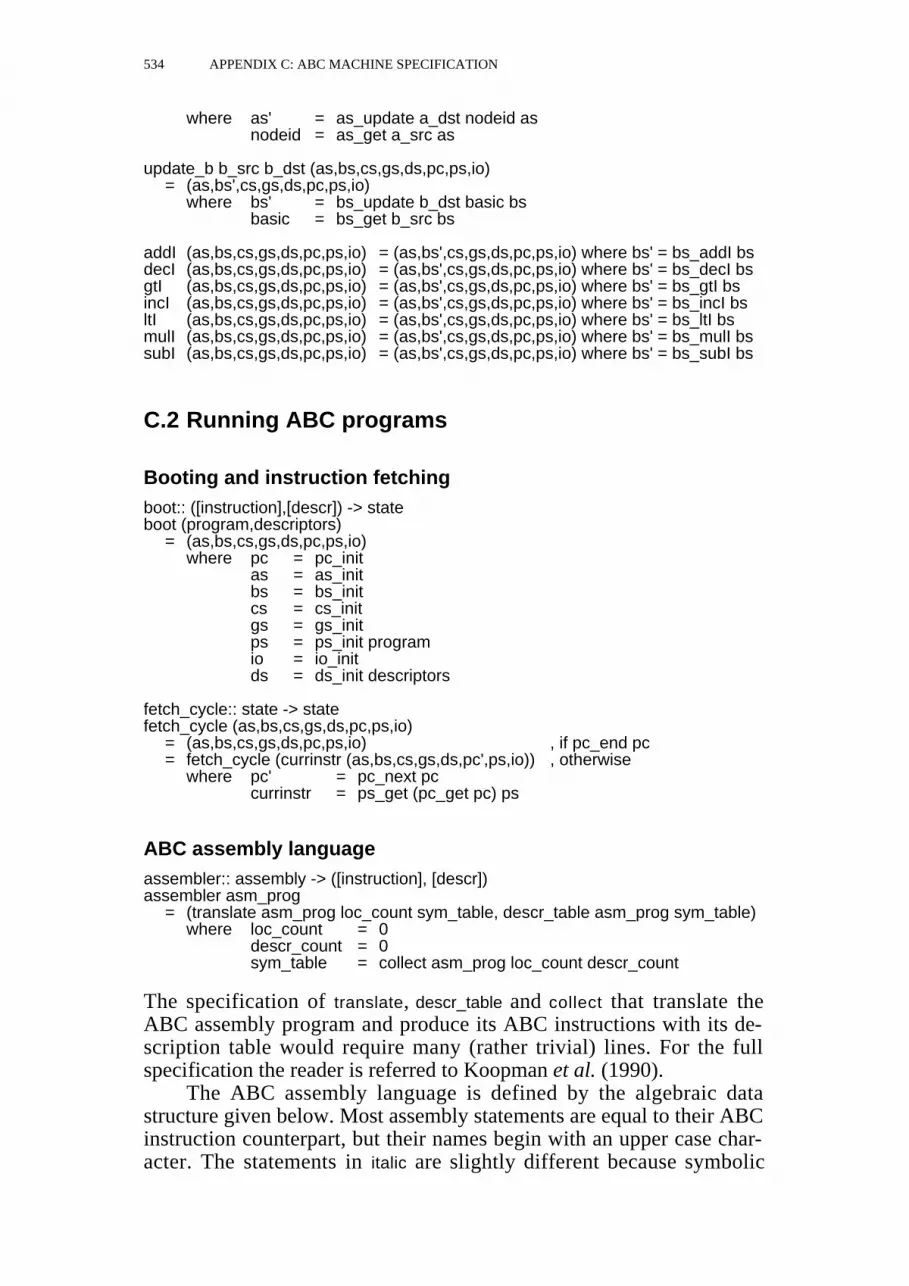
534 APPENDIX C: ABC MACHINE SPECIFICATION
where as' = as_update a_dst nodeid asnodeid = as_get a_src as
update_b b_src b_dst (as,bs,cs,gs,ds,pc,ps,io)= (as,bs',cs,gs,ds,pc,ps,io)
where bs' = bs_update b_dst basic bsbasic = bs_get b_src bs
addI (as,bs,cs,gs,ds,pc,ps,io) = (as,bs',cs,gs,ds,pc,ps,io) where bs' = bs_addI bsdecI (as,bs,cs,gs,ds,pc,ps,io) = (as,bs',cs,gs,ds,pc,ps,io) where bs' = bs_decI bsgtI (as,bs,cs,gs,ds,pc,ps,io) = (as,bs',cs,gs,ds,pc,ps,io) where bs' = bs_gtI bsincI (as,bs,cs,gs,ds,pc,ps,io) = (as,bs',cs,gs,ds,pc,ps,io) where bs' = bs_incI bsltI (as,bs,cs,gs,ds,pc,ps,io) = (as,bs',cs,gs,ds,pc,ps,io) where bs' = bs_ltI bsmulI (as,bs,cs,gs,ds,pc,ps,io) = (as,bs',cs,gs,ds,pc,ps,io) where bs' = bs_mulI bssubI (as,bs,cs,gs,ds,pc,ps,io) = (as,bs',cs,gs,ds,pc,ps,io) where bs' = bs_subI bs
C.2 Running ABC programs
Booting and instruction fetchingboot:: ([instruction],[descr]) -> stateboot (program,descriptors)
= (as,bs,cs,gs,ds,pc,ps,io)where pc = pc_init
as = as_initbs = bs_initcs = cs_initgs = gs_initps = ps_init programio = io_initds = ds_init descriptors
fetch_cycle:: state -> statefetch_cycle (as,bs,cs,gs,ds,pc,ps,io)
= (as,bs,cs,gs,ds,pc,ps,io) , if pc_end pc= fetch_cycle (currinstr (as,bs,cs,gs,ds,pc',ps,io)) , otherwise
where pc' = pc_next pccurrinstr = ps_get (pc_get pc) ps
ABC assembly languageassembler:: assembly -> ([instruction], [descr])assembler asm_prog
= (translate asm_prog loc_count sym_table, descr_table asm_prog sym_table)where loc_count = 0
descr_count = 0sym_table = collect asm_prog loc_count descr_count
The specification of translate, descr_table and collect that translate theABC assembly program and produce its ABC instructions with its de-scription table would require many (rather trivial) lines. For the fullspecification the reader is referred to Koopman et al. (1990).
The ABC assembly language is defined by the algebraic datastructure given below. Most assembly statements are equal to their ABCinstruction counterpart, but their names begin with an upper case char-acter. The statements in italic are slightly different because symbolic

RUNNING ABC PROGRAMS 535
names are used instead of addresses. In addition, the assembler allowsthe definition of labels and descriptors. Furthermore, Branch instructionsare added to allow the specification of relative jumps. The assemblerwill convert them to jump instructions. These extra assembly statementsare also shown in italic.
assembly = = [statement]red_label = = labeldescr_label = = labellabel = = [char]nr_instr = = int
statement:: = Label label | No_op |
Descriptor descr_label red_label arity name | Pop_a nr_args |Br nr_instr | Pop_b nr_args |Br_false nr_instr | Print string |Br_true nr_instr | Print_symbol a_src |Add_args a_src nr_args a_dst | Push_a a_src |Create | Push_ap_entry a_src |Del_args a_src nr_args a_dst | Push_arg a_src arity arg_nr |Eq_descr descr_label a_src | Push_arg_b a_src |Eq_descr_arity descr_label arity a_src | Push_args a_src arity arg_nr |EqB | Push_args_b a_src |EqB_a bool a_src | Push_b b_src |EqB_b bool b_src | PushB bool |EqI | PushB_a a_src |EqI_a int a_src | PushI int |EqI_b int b_src | PushI_a a_src |Fill descr_label nr_args label a_dst | Repl_args arity nr_args |Fill_a a_src a_dst | Repl_args_b |FillB bool a_dst | Rtn |FillB_b b_src a_dst | Set_entry label a_dst |FillI int a_dst | Update_a a_src a_dst |FillI_b b_src a_dst | Update_b b_src b_dst |Get_descr_arity a_src |Get_node_arity a_src |Halt | AddI |Jmp label | DecI |Jmp_eval | GtI |Jmp_false label | IncI |Jmp_true label | LtI |Jsr label | MulI |Jsr_eval | SubI
C.3 The ABC micro-instructionsabstype astack, bstack, cstack, graphstore, descrstore, pc, programstore, io
with
ps_get :: instrid -> programstore -> instructionps_init :: [instruction] -> programstore
pc_end :: pc -> boolpc_get :: pc -> instridpc_halt :: pc -> pcpc_init :: pcpc_next :: pc -> pcpc_update :: instrid -> pc -> pc

536 APPENDIX C: ABC MACHINE SPECIFICATION
gs_get :: nodeid -> graphstore -> nodegs_init :: graphstoregs_newnode :: graphstore -> (graphstore,nodeid)gs_update :: nodeid -> (node -> node) -> graphstore -> graphstore
n_arg :: node -> arg_nr -> arity -> nodeidn_args :: node -> arity -> nodeid_seqn_arity :: node -> arityn_B :: node -> booln_copy :: node -> node -> noden_descrid :: node -> descridn_entry :: node -> instridn_eq_arity :: node -> arity -> booln_eq_B :: node -> bool -> booln_eq_descrid :: node -> descrid -> booln_eq_I :: node -> int -> booln_eq_symbol :: node -> node -> booln_fill :: descrid -> instrid -> nodeid_seq -> node -> noden_fillB :: descrid -> instrid -> bool -> node -> noden_fillI :: descrid -> instrid -> int -> node -> noden_I :: node -> intn_nargs :: node -> nr_args -> arity -> nodeid_seqn_setentry :: instrid -> node -> node
ds_get :: descrid -> descrstore -> descrds_init :: [descr] -> descrstore
d_ap_entry :: descr -> instridd_arity :: descr -> arityd_name :: descr -> string
as_get :: a_src -> astack -> nodeidas_init :: astackas_popn :: nr_args -> astack -> astackas_push :: nodeid -> astack -> astackas_pushn :: nodeid_seq -> astack -> astackas_topn :: nr_args -> astack -> nodeid_seqas_update :: a_dst -> nodeid -> astack -> astack
bs_get :: b_src -> bstack -> basicbs_getB :: b_src -> bstack -> boolbs_getI :: b_src -> bstack -> intbs_init :: bstackbs_popn :: nr_args -> bstack -> bstackbs_push :: basic -> bstack -> bstackbs_pushB :: bool -> bstack -> bstackbs_pushI :: int -> bstack -> bstackbs_update :: b_dst -> basic -> bstack -> bstack
bs_addI :: bstack -> bstackbs_decI :: bstack -> bstackbs_eqB :: bstack -> bstackbs_eqI :: bstack -> bstackbs_eqBi :: bool -> b_src -> bstack -> bstackbs_eqIi :: int -> b_src -> bstack -> bstackbs_gtI :: bstack -> bstackbs_incI :: bstack -> bstackbs_ltI :: bstack -> bstackbs_mulI :: bstack -> bstackbs_subI :: bstack -> bstack
cs_init :: cstackcs_get :: c_src -> cstack -> instrid

THE ABC MICRO-INSTRUCTIONS 537
cs_popn :: nr_args -> cstack -> cstackcs_push :: instrid -> cstack -> cstack
io_init :: ioio_print :: string -> io -> ioio_print_symbol :: node -> descr -> io -> io
Program storeprogramstore = = [location]location :: = I instruction
ps_get target ps = instr where I instr = ps ! target
ps_init (instruction : rest) = I instruction : ps_init restps_init [ ] = [ ]
Program counterpc = = instrid
pc_end instrid = instrid < 0pc_get instrid = instridpc_halt instrid = –1pc_init = 0pc_next instrid = instrid + 1pc_update instrid pc = instrid
Graph storegraphstore = = (graph, nat)
gs_get nodeid (nds,free) = nds ! (nodeid – free – 1)gs_init = ([ ], store_size)
store_size:: natstore_size = 100 || some natural number indicating the size
gs_newnode (nds,0) = error "graph-store is full"gs_newnode (nds,free) = ((Empty : nds, free – 1), free)
gs_update nid f (nodes,free) = (upd (nid – free –1) nodes f, free)where upd 0 (nd : nds) f = f nd : nds
upd n (nd : nds) f = nd : upd (n – 1) nds f
Nodesnode :: = Node descrid instrid nodeid_seq | Basic descrid instrid basic | Emptybasic :: = Int int | Bool bool
n_arg node n arity = args ! (n – 1) where args = n_args node arityn_args (Node descrid entry args) arity = args || arity can be used for optimizations
n_arity (Basic descrid entry basic) = 0n_arity (Node descrid entry args) = # args
n_B (Basic descrid entry (Bool b)) = bn_copy new old = new

538 APPENDIX C: ABC MACHINE SPECIFICATION
n_descrid (Node descrid entry args) = descridn_descrid (Basic descrid entry basic) = descrid
n_entry (Node descrid entry args) = entryn_entry (Basic descrid entry basic) = entry
n_eq_arity node n = n_arity node = nn_eq_B node b = n_B node = bn_eq_descrid node descrid = n_descrid node = descridn_eq_I node i = n_I node = in_eq_symbol (Node descrid1 entry1 args1) (Node descrid2 entry2 args2)
= descrid1 = descrid2n_eq_symbol (Basic descrid1 entry1 basic1) (Basic descrid2 entry2 basic2)
= descrid1 = descrid2 & basic1 = basic2n_eq_symbol node1 node2 = Falsen_fill descr entry args node = Node descr entry argsn_fillB descr entry b node = Basic descr entry (Bool b)n_fillI descr entry i node = Basic descr entry (Int i)n_I (Basic descrid entry (Int i)) = in_nargs node arg_count arity = take arg_count (n_args node arity)
n_setentry newentry (Node descrid entry args) = Node descrid newentry argsn_setentry newentry (Basic descrid entry basic) = Basic descrid newentry basic
Descriptor storedescrstore = = [descr]
ds_get target ds = ds ! targetds_init descriptors = descriptors
Descriptorsdescr :: = Descr ap_entry arity name
d_ap_entry (Descr ap_entry arity name) = ap_entryd_arity (Descr ap_entry arity name) = arityd_name (Descr ap_entry arity name) = name
A-stackastack = = [nodeid]
as_get target as = as ! targetas_init = [ ]as_popn n as = drop n asas_push nodeid as = nodeid : asas_pushn nodeids as = nodeids ++ asas_topn n as = take n as
as_update 0 nodeid (a : x) = nodeid : xas_update n nodeid (a : x) = a : as_update (n – 1) nodeid x
B-stackbstack = = [basic]
bs_get target bs = bs ! targetbs_getB n bs = b where Bool b = bs_get n bs

THE ABC MICRO-INSTRUCTIONS 539
bs_getI n bs = i where Int i = bs_get n bsbs_init = [ ]bs_popn n bs = drop n bsbs_push basic bs = basic : bsbs_pushB b bs = Bool b : bsbs_pushI i bs = Int i : bs
bs_update 0 basic (b : x) = basic : xbs_update n basic (b : x) = b : bs_update (n – 1) basic x
bs_addI (Int i1 : Int i2 : r) = Int (i1 + i2) : rbs_decI (Int i : r) = Int (i – 1) : rbs_eqB (Bool b1 : Bool b2 : r) = Bool (b1 = b2) : rbs_eqBi b n bs = bs_push (Bool (b = bs_getB n bs)) bsbs_eqI (Int i1 : Int i2 : r) = Bool (i1 = i2) : rbs_eqIi i n bs = bs_push (Bool (i = bs_getI n bs)) bsbs_gtI (Int i1 : Int i2 : r) = Bool (i1 > i2) : rbs_incI (Int i : r) = Int (i + 1) : rbs_ltI (Int i1 : Int i2 : r) = Bool (i1 < i2) : rbs_mulI (Int i1 : Int i2 : r) = Int (i1 * i2) : rbs_subI (Int i1 : Int i2 : r) = Int (i1 – i2) : r
C-stackcstack = = [instrid]
cs_init = [ ]cs_get target cs = cs ! targetcs_popn n cs = drop n cscs_push c cs = c : cs
I/O channelio = = [char]
io_init = [ ]io_print string output = output ++ string
io_print_symbol (Basic descrid ap_entry (Int i)) descr output = output ++ show iio_print_symbol (Basic descrid ap_entry (Bool b)) descr output = output ++ show bio_print_symbol (Node descrid entry args) (Descr ap_entry arity name) output
= output ++ name

541
Appendix DPABC machine specification
D.1 The PABC instruction setD.2 Running PABC programs
D.3 The new micro-instructions
The PABC machine is a parallel extension of the ABC machine. Thisextension has some consequences for the sequential ABC instructionspresented in Appendix C. For most instructions only the machine statehas to be extended. Together with the extension of the assembly lan-guage for the new instructions this is left to the reader.
For some sequential instructions a call to the operating systemhas to be included. This is fully specified together with the parallel in-structions that are marked ("•") in the summary below. The instructionsnewP, randomP, currentP, neighbourP and channelP require some ex-tensions of the specification (see Exercise 16.2).
D.1 The PABC instruction set
Sequential and parallel reducer instructionsinstruction = = state -> statestate = = (local_state,global_state,opsys_callqueue)local_state = = (astack,bstack,cstack,nqueue,pc,wlist)global_state = = (admin,graphstore,descrstore,programstore)
• halt :: instruction• jmp :: instrid -> instruction• jsr :: instrid -> instruction• print :: string -> instruction• print_symbol :: a_src -> instruction
channelP :: a_src -> instruction• create_channel :: instruction
currentP :: instruction• get_node :: instruction• getWL :: a_src -> instruction• is_empty_n :: instruction
neighbourP :: instruction

542 APPENDIX D: PABC MACHINE SPECIFICATION
• new_ext_reducer :: instrid -> a_src -> instruction• new_int_reducer :: instrid -> a_src -> instruction• newP :: instruction
randomP :: instruction• release :: instruction• send_graph :: a_src -> a_src -> instruction• send_request :: a_src -> instruction• set_continue :: a_src -> instruction• set_wait :: a_src -> instruction• stop_reducer :: instruction• suspend :: instruction
Operating system instructionsopsys_instruction = = opsys_state -> opsys_stateopsys_state = = (schedule_adm,in_msgs,out_msgs,global_state,opsys_callqueue)
• os_halt :: opsys_instruction• os_new_reducer :: instrid -> nodeid -> opsys_instruction• os_print :: string -> opsys_instruction• os_reducerprio :: opsys_instruction• os_release :: wlist -> opsys_instruction• os_schedule :: opsys_instruction• os_send_graph :: nodeid -> nodeid -> opsys_instruction• os_send_newchannel :: procid -> nodeid -> opsys_instruction• os_send_newreducer :: instrid -> nodeid -> opsys_instruction• os_send_request :: nodeid -> opsys_instruction• os_setwait :: nodeid -> opsys_instruction• os_stop_reducer :: opsys_instruction• os_suspend_reducer :: opsys_instruction
Communication process instructionscomproc_instruction = = comproc_state -> comproc_statecomproc_state = = (in_msgs,out_msgs,global_state,opsys_callqueue)
• cp_accept_msg :: msg_contents -> comproc_instruction
Specification of sequential reducer instructionshalt ((as,bs,cs,nq,pc,wl),glob,cq)
= ((as,bs,cs,nq,pc,wl),glob,cq')where cq' = os_call cq [os_stop_reducer, os_halt]
jmp address ((as,bs,cs,nq,pc,wl),glob,cq)= ((as,bs,cs,nq,pc',wl),glob,cq')
where pc' = pc_update address pccq' = os_call cq [os_schedule]
jsr address ((as,bs,cs,nq,pc,wl),glob,cq)= ((as,bs,cs',nq,pc',wl),glob,cq')
where pc' = pc_update address pccs' = cs_push (pc_get pc) cscq' = os_call cq [os_schedule]
print string (loc,glob,cq)= (loc,glob,cq')
where cq' = os_call cq [os_print string, os_schedule]
print_symbol a_src ((as,bs,cs,nq,pc,wl),(ad,gs,ds,ps),cq)

THE PABC INSTRUCTION SET 543
= ((as,bs,cs,nq,pc,wl),(ad,gs,ds,ps),cq')where cq' = os_call cq [os_print string, os_schedule]
nodeid = as_get a_src asnode = gs_get nodeid gsstring = ds_get_repr node ds
Specification of parallel reducer instructionscreate_channel ((as,bs,cs,nq,pc,wl),(ad,gs,ds,ps),cq)
= ((as',bs',cs,nq,pc,wl),(ad,gs',ds,ps),cq')where bs' = bs_popn 1 bs
pid = bs_getP 0 bs(gs',nid) = gs_newchannel pid gsas' = as_push nid ascq' = os_call cq [os_send_newchannel pid nid,
os_setwait nid, os_suspend_reducer]
get_node ((as,bs,cs,nq,pc,wl),glob,cq)= ((as',bs,cs,nq',pc,wl),glob,cq)
where as' = as_push n asn = nq_first nqnq' = nq_remove nq
getWL a_depth ((as,bs,cs,nq,pc,wl),(ad,gs,ds,ps),cq)= ((as,bs,cs,nq,pc,wl'),(ad,gs,ds,ps),cq)
where wl' = n_wl_get (gs_get nid gs)nid = as_get a_depth as
is_empty_n ((as,bs,cs,nq,pc,wl),glob,cq)= ((as,bs',cs,nq,pc,wl),glob,cq)
where bs' = bs_pushB (nq_empty nq) bs
new_ext_reducer code chan_depth ((as,bs,cs,nq,pc,wl),glob,cq)= ((as,bs,cs,nq,pc,wl),glob,cq')
where chanid = as_get chan_depth ascq' = os_call cq [os_send_newreducer code chanid]
new_int_reducer code a_depth ((as,bs,cs,nq,pc,wl),glob,cq)= ((as,bs,cs,nq,pc,wl),glob,cq')
where nid = as_get a_depth ascq' = os_call cq [os_new_reducer code nid]
newP ((as,bs,cs,nq,pc,wl),(ad,gs,ds,ps),cq)= ((as,bs',cs,nq,pc,wl),(ad',gs,ds,ps),cq)
where bs' = bs_pushP pid bs(ad',pid) = ad_new_procid ad
release ((as,bs,cs,nq,pc,wl),glob,cq)= ((as,bs,cs,nq,pc,wl),glob,cq')
where cq' = os_call cq [os_release wl] , if ~ wl_empty wl= cq , otherwise
send_graph graph_depth chan_depth ((as,bs,cs,nq,pc,wl),glob,cq)= ((as,bs,cs,nq,pc,wl),glob,cq')
where chanid = as_get chan_depth asgraphid = as_get graph_depth ascq' = os_call cq [os_send_graph graphid chanid]
send_request chan_depth ((as,bs,cs,nq,pc,wl),glob,cq)= ((as,bs,cs,nq,pc,wl),glob,cq')
where cq' = os_call cq [os_send_request chanid,os_reducerprio]chanid = as_get chan_depth as

544 APPENDIX D: PABC MACHINE SPECIFICATION
set_continue depth ((as,bs,cs,nq,pc,wl),glob,cq)= ((as,bs,cs,nq',pc,wl),glob,cq)
where n = as_get depth asnq' = nq_add n nq
set_wait a_depth ((as,bs,cs,nq,pc,wl),glob,cq)= ((as,bs,cs,nq,pc,wl),glob,cq')
where nid = as_get a_depth ascq' = os_call cq [os_setwait nid,os_reducerprio]
stop_reducer ((as,bs,cs,nq,pc,wl),glob,cq)= ((as,bs,cs,nq,pc,wl),glob,cq')
where cq' = os_call cq [os_stop_reducer]
suspend ((as,bs,cs,nq,pc,wl),glob,cq)= ((as,bs,cs,nq,pc,wl),glob,cq')
where cq' = os_call cq [os_suspend_reducer]
Specification of operating system instructionsschedule_adm = = ([active], [passive])active = = reducerpassive = = reducerreducer = = (redid, local_state)
os_halt (rs,in,out,(ad,gs,ds,ps),instrs)= (rs,in,out',(ad,gs,ds,ps),instrs)
where out' = out ++ [(my_pid, 0, Msg_Halt)]my_pid = ad_pid ad
os_new_reducer code nid (rs,in,out,(ad,gs,ds,ps),instrs)= (rs',in,out,(ad',gs,ds,ps),instrs)
where rs' = (act_reds ++ [new_red], pass_reds)(act_reds, pass_reds) = rsnew_red = (new_redid,(as,bs,cs,nq,pc,wl))
where as = as_initbs = bs_initcs = cs_initnq = nq_new nidpc = pc_update code pc_initwl = wl_init
(ad', new_redid) = ad_new_redid ad
os_print string (rs,in,out,(ad,gs,ds,ps),instrs)= (rs,in,out',(ad,gs,ds,ps),instrs)
where out' = out ++ [(my_pid, 0, Msg_Print string)]my_pid = ad_pid ad
os_reducerprio (rs,in,out,(ad,gs,ds,ps),instrs)= (rs,in,out,(ad',gs,ds,ps),instrs)
where ad' = ad_new_prio Prio_Reducer ad
os_release wl (rs,in,out,(ad,gs,ds,ps),instrs)= (rs',in,out',(ad,gs,ds,ps),instrs)
where (reds,reqs,nid) = (wl_reds wl, wl_reqs wl, wl_nid wl)(old_acts, old_pass) = rsgraph = gs_copy nid my_pid ds gsrs' = (new_acts, new_pass)new_acts = old_acts ++ rel_redsnew_pass = old_pass – – rel_redsrel_reds = [(rid,loc) | (rid,loc) <- old_pass; rid' <- reds; rid' = rid]

THE PABC INSTRUCTION SET 545
out' = out ++ [(my_pid, n_pid_of_global dst,Msg_Graph graph dst) | dst <- reqs]
my_pid = ad_pid ad
os_schedule ((act_reds,pass_reds),in,out,glob,instrs)= ((act_reds,pass_reds),in,out,glob,instrs) , if act_reds = [ ]= (rs',in,out,glob,instrs) , otherwise
where rs' = (new_act_reds, pass_reds)new_act_reds = rest_act_reds ++ [red]red : rest_act_reds = act_reds
os_send_graph graphid chanid (rs,in,out,(ad,gs,ds,ps),instrs)= (rs,in,out',(ad,gs,ds,ps),instrs)
where out' = out ++ [(my_pid, pid, Msg_Graph graph' dstid)]graph = gs_copy graphid my_pid ds gsgraph' = gs_root_update (n_setdescr defer_descr) graphpid = n_pid_of_global dstiddstid = n_dest (gs_get chanid gs)my_pid = ad_pid ad
os_send_newchannel pid chanid (rs,in,out,(ad,gs,ds,ps),instrs)= (rs,in,out',(ad,gs,ds,ps),instrs)
where out' = out ++ [(my_pid, pid, Msg_CreateChannel chan_eid)]chan_eid = n_global my_pid chanidmy_pid = ad_pid ad
os_send_newreducer code chanid (rs,in,out,(ad,gs,ds,ps),instrs)= (rs,in,out',(ad,gs,ds,ps),instrs)
where chan = n_dest (gs_get chanid gs)out' = out ++ [(my_pid, pid, Msg_NewReducer chan code)]pid = n_pid_of_global chanmy_pid = ad_pid ad
os_send_request chanid (rs,in,out,(ad,gs,ds,ps),instrs)= (rs,in,out',(ad,gs,ds,ps),instrs)
where out' = out ++ [(my_pid, pid, Msg_Request srcid dstid)]srcid = n_global my_pid chanidpid = n_pid_of_global dstiddstid = n_dest (gs_get chanid gs)my_pid = ad_pid ad
os_setwait nid (rs,in,out,(ad,gs,ds,ps),instrs)= (rs,in,out,(ad,gs',ds,ps),instrs)
where gs' = gs_update nid (n_wl_add_red rid) gs(rid, loc) = red(red : reds, pass_reds) = rs
os_stop_reducer (rs,in,out,glob,instrs)= (rs',in,out,glob,instrs)
where rs' = (act_reds, pass_reds)(red : act_reds, pass_reds) = rs
os_suspend_reducer (rs,in,out,glob,instrs)= (rs',in,out,glob,instrs)
where rs' = (act_reds, red : pass_reds)(red : act_reds, pass_reds) = rs
Specification of communication process instructionsin_msgs = = [msg_contents]out_msgs = = [message]message = = (proc_src, proc_dst, msg_contents)

546 APPENDIX D: PABC MACHINE SPECIFICATION
msg_contents :: = Msg_CreateChannel ext_nid | Msg_Channel ext_nid ext_nid
| Msg_Request ext_nid ext_nid | Msg_Graph graph ext_nid| Msg_NewReducer ext_nid instrid | Msg_Print string | Msg_Halt
proc_src = = procidproc_dst = = procidext_nid = = (procid, nodeid)
cp_accept_msg (Msg_CreateChannel src_eid) (in,out,(ad,gs,ds,ps),instrs)= (in,out',(ad,gs',ds,ps),instrs)
where (gs', rqid) = gs_newnode gsout' = out ++ [(my_pid, pid, Msg_Channel rq_eid src_eid)]rq_eid = n_global my_pid rqidpid = n_pid_of_global src_eidmy_pid = ad_pid ad
cp_accept_msg (Msg_Channel rq_eid dst_eid) (in,out,(ad,gs,ds,ps),instrs)= (in,out,(ad,gs',ds,ps),instrs')
where nid = n_local dst_eidgs' = gs_update nid (n_putchannel rq_eid) gswl = n_wl_get (gs_get nid gs)instrs' = os_call instrs [os_release wl]
cp_accept_msg (Msg_NewReducer rq_eid code) (in,out,(ad,gs,ds,ps),instrs)= (in,out,(ad,gs,ds,ps),instrs')
where instrs' = os_call instrs [os_new_reducer code (n_local rq_eid)]cp_accept_msg (Msg_Request chan_eid rq_eid) (in,out,(ad,gs,ds,ps),instrs)
= (in,out',(ad,gs',ds,ps),instrs)where rqid = n_local rq_eid
rnf = n_entry (gs_get rqid gs) = rnf_entryout' = out ++ [(my_pid, pid, Msg_Graph graph chan_eid)] , if rnf
= out , otherwisewhere pid = n_pid_of_global chan_eid
graph = gs_copy rqid my_pid ds gsmy_pid = ad_pid ad
gs' = gs_update rqid (n_wl_add_req chan_eid) gs , if ~ rnf= gs , otherwise
cp_accept_msg (Msg_Graph gr dst_eid) (in,out,(ad,gs,ds,ps),instrs)= (in,out,(ad,gs',ds,ps),instrs')
where gs' = gs_store nid gr gswl = n_wl_get (gs_get nid gs)nid = n_local dst_eidinstrs' = os_call instrs [os_release wl]
D.2 Running PABC programs
Booting and instruction fetchingboot:: nat -> ([instruction],[descr]) -> networkboot nr_proc (program,descriptors) = nw_init nr_proc (program,descriptors)
machine_cycle:: network -> outputmachine_cycle nw
= output , if op_halt output= op_append output (machine_cycle nw') , otherwise
where output = nw_output nwnw' = nw_exec proc_cycle (nw_distribute_msgs nw)
proc_cycle:: processor -> processorproc_cycle = opsys_cycle . red_cycle . opsys_cycle . comproc_cycle
comproc_cycle:: processor -> processor

RUNNING PABC PROGRAMS 547
comproc_cycle (rs,in,out,(ad,gs,ds,ps),cq)= (rs,in,out,(ad',gs,ds,ps),cq) , if ad_prio ad = Prio_Reducer
where ad' = ad_new_prio No_Prio adcomproc_cycle (rs,[ ],out,glob,cq)
= (rs,[ ],out,glob,cq)comproc_cycle (rs,(msg:msgs),out,glob,cq)
= comproc_cycle (rs,in',out',glob',cq')where (in',out',glob',cq') = cp_accept_msg msg (msgs,out,glob,cq)
opsys_cycle:: processor -> processoropsys_cycle (rs,in,out,glob,cq)
= (rs,in,out,glob,cq) , if os_cq_empty cq= opsys_cycle (os_first_call cq (rs,in,out,glob,os_rest_calls cq)), otherwise
red_cycle:: processor -> processorred_cycle ((act_reds,pass_reds),in,out,glob,cq)
= ((act_reds,pass_reds),in,out,glob,cq) , if act_reds = [ ]= (rs',in,out,glob',cq') , otherwise
where rs' = ((rid,loc') : reds, pass_reds)(rid,loc) : reds = act_reds(loc',glob',cq') = fetch_cycle (loc,glob,cq)
fetch_cycle:: state -> statefetch_cycle ((as,bs,cs,nq,pc,wl),(ad,gs,ds,ps),cq)
= ((as,bs,cs,nq,pc,wl),(ad,gs,ds,ps),cq) , if ~ os_cq_empty cq= fetch_cycle (currinstr ((as,bs,cs,nq,pc',wl),(ad,gs,ds,ps),cq)), otherwise
where pc' = pc_next pccurrinstr = ps_get (pc_get pc) ps
D.3 The new micro-instructionsabstype astack, bstack, cstack, nqueue, pc , wlist,
admin, graphstore, descrstore, programstore,opsys_callqueue, network, output
with …gs_copy :: nodeid -> procid -> descrstore -> graphstore -> graphgs_newchannel :: procid -> graphstore -> (graphstore,nodeid)gs_root_update :: (node -> node) -> graph -> graphgs_store :: nodeid -> graph -> graphstore -> graphstore
n_dest :: node -> destn_global :: procid -> nodeid -> ext_nidn_local :: ext_nid -> nodeidn_pid_of_global :: ext_nid -> procidn_putchannel :: ext_nid -> node -> noden_setdescr :: descrid -> node -> noden_wl_add_red :: redid -> node -> noden_wl_add_req :: request -> node -> noden_wl_clear :: node -> noden_wl_get :: node -> wlistn_wl_put :: wlist -> node -> node
ds_get_repr :: node -> descrstore -> string
bs_getP :: b_src -> bstack -> procidbs_pushP :: procid -> bstack -> bstack
nq_add :: nodeid -> nqueue -> nqueuenq_first :: nqueue -> nodeidnq_init :: nqueuenq_empty :: nqueue -> bool

548 APPENDIX D: PABC MACHINE SPECIFICATION
nq_new :: nodeid -> nqueuenq_remove :: nqueue -> nqueue
wl_clear :: wlist -> wlistwl_empty :: wlist -> boolwl_init :: wlistwl_new :: nodeid -> wlistwl_nid :: wlist -> nodeidwl_reds :: wlist -> [redid]wl_reqs :: wlist -> [request]
ad_init :: procid -> procid -> adminad_new_redid :: admin -> (admin,redid)ad_new_procid :: admin -> (admin,procid)ad_new_prio :: schedule_priority -> admin -> adminad_nr_pids :: admin -> procidad_pid :: admin -> procidad_prio :: admin -> schedule_priority
os_call :: opsys_callqueue -> [opsys_instruction] -> opsys_callqueueos_clear :: opsys_callqueueos_first_call :: opsys_callqueue -> opsys_instructionos_init :: procid -> procid -> [instruction] -> [descr] -> opsys_stateos_cq_empty :: opsys_callqueue -> boolos_rest_calls :: opsys_callqueue -> opsys_callqueue
nw_distribute_msgs :: network -> networknw_exec :: (processor -> processor) -> network -> networknw_init :: procid -> ([instruction],[descr]) -> networknw_output :: network -> output
op_append :: output -> output -> outputop_halt :: output -> bool
Graph storegs_copy top pid ds gs
= copywhere (copy,bindings) = copy_nodes [top] pid ds gs 0 empty_bindings
gs_newchannel pid (nds,0)= error "cannot create new channel; graph-store is full"
gs_newchannel pid (nds,free)= ((nds++[new_channel],free-1),nid)
where nid = store_size-freenew_channel = Channel (wl_new nid) new_channel_entry (pid,(-1))
gs_root_update f (n : r) = f n : r
gs_store nodeid graph (old_graph,free)= error "cannot store graph; graph-store is full" , if size_graph > free= (new_graph,free-size_graph+1) , otherwise
where size_graph = # graphsize_old_graph = # old_graphoffset = size_old_graph – 1(top:rest) = graphnew_graph = upd nodeid old_graph (n_copy' top) ++
[adjust_nids node | node<-rest]n_copy' (Node descrid wl entry args) old
= Node descrid (n_wl_get old) entry [arg+offset|arg<-args]n_copy' (Basic descrid wl entry basic) old
= Basic descrid (n_wl_get old) entry basic

THE NEW MICRO-INSTRUCTIONS 549
n_copy' (Channel wl instrid dest) old= Channel (n_wl_get old) instrid dest
upd 0 (nd : nds) f = f nd : ndsupd n (nd : nds) f = nd : upd (n - 1) nds fadjust_nids (Node descrid (rd,rq,nid) entry args)
= Node descrid (wl_new (nid+offset)) entry [arg+offset|arg<-args]adjust_nids (Basic descrid (rd,rq,nid) entry basic)
= Basic descrid (wl_new (nid+offset)) entry basicadjust_nids (Channel (rd,rq,nid) instrid dest)
= Channel (wl_new (nid+offset)) instrid dest
The lazy copying algorithmbindings = = nodeid -> nodeid
copy_nodes:: [nodeid] -> procid -> descrstore -> graphstore -> nodeid -> bindings-> (graph, bindings)
copy_nodes [ ] pid ds gs n bindings= ([ ],bindings)
copy_nodes (nid : rest) pid ds gs n bindings= copy_nodes rest pid ds gs n bindings , if ~ bindings_is_empty bindings nid= (nodes,bindings'') , otherwise
where node = gs_get nid gsnodes = new_node : nodes'(new_node,args) = copy_node pid ds n node bindings''bindings' = bind nid n bindings(nodes',bindings'')
= copy_nodes (args++rest) pid ds gs (n+1) bindings'
copy_node:: procid -> descrstore -> nodeid -> node -> bindings -> (node, args)copy_node pid ds nid (Node descrid wl entry args) bindings
= ((Channel (wl_new nid) new_channel_entry rq_eid),[ ]), if descrid = defer_descr \/ entry = reserved_entry
= ((Node descrid (wl_new nid) new_entry new_args),args) , otherwisewhere new_entry = d_node_entry (ds_get descrid ds)
new_args = map bindings argsrq_eid = (pid,wl_nid wl)
copy_node pid ds nid (Basic descrid wl entry basic) bindings= ((Basic descrid (wl_new nid) entry basic),[ ])
copy_node pid ds nid (Channel wl entry dest) bindings= ((Channel (wl_new nid) entry dest),[ ])
bind:: nodeid -> nodeid -> bindings -> bindingsbind src dst bindings n = dst , if n = src
= bindings n , otherwise
empty_bindings:: bindingsempty_bindings nodeid = –1
bindings_is_empty::bindings -> nodeid -> boolbindings_is_empty b n = b n = –1
Nodesnode :: = Node descrid wlist entry nodeid_seq | Channel wlist entry dest |
Basic descrid wlist entry basic | Emptybasic :: = Int int | Bool bool | Pid procidentry = = instriddest = = (procid,nodeid)
reserved_entry = 3

550 APPENDIX D: PABC MACHINE SPECIFICATION
new_channel_entry = 4defer_descr = 3
n_dest (Channel wl instrid dest) = destn_global pid nid = (pid, nid)n_local (pid, nid) = nidn_pid_of_global (pid, nid) = pidn_putchannel ext_nid (Channel wl entry dest) = Channel (wl_clear wl) entry ext_nidn_setdescr new_descr (Node descr wl entry args) = Node new_descr wl entry args
n_wl_add_red rid (Node descr (rids,reqs,nid) entry args )= Node descr (rid:rids,reqs,nid) entry args
n_wl_add_red rid (Basic descr (rids,reqs,nid) entry basic )= Basic descr (rid:rids,reqs,nid) entry basic
n_wl_add_red rid (Channel (rids,reqs,nid) entry dest)= Channel (rid:rids,reqs,nid) entry dest
n_wl_add_req req (Node descr (rids,reqs,nid) entry args )= Node descr (rids,req:reqs,nid) entry args
n_wl_add_req req (Basic descr (rids,reqs,nid) entry basic )= Basic descr (rids,req:reqs,nid) entry basic
n_wl_add_req req (Channel (rids,reqs,nid) entry dest)= Channel (rids,req:reqs,nid) entry dest
n_wl_clear (Node descr wl entry args ) = Node descr (wl_clear wl) entry argsn_wl_clear (Basic descr wl entry basic) = Basic descr (wl_clear wl) entry basicn_wl_clear (Channel wl entry dest) = Channel (wl_clear wl) entry dest
n_wl_get (Node descr wl entry args) = wln_wl_get (Basic descr wl entry basic) = wln_wl_get (Channel wl entry dest) = wl
n_wl_put (reds,reqs,nid) (Node descr (reds',reqs',nid') entry args )= (Node descr (reds,reqs,nid') entry args )
n_wl_put (reds,reqs,nid) (Basic descr (reds',reqs',nid') entry basic )= (Basic descr (reds,reqs,nid') entry basic )
n_wl_put (reds,reqs,nid) (Channel (reds',reqs',nid') entry dest)= (Channel (reds,reqs,nid') entry dest)
Descriptor storedescr :: = Descr ap_entry node_entry arity namenode_entry = = instrid
d_node_entry (Descr ap_entry node_entry arity name) = node_entryds_get_repr (Basic descrid wl entry (Int i)) ds = show ids_get_repr (Basic descrid wl entry (Bool b)) ds = show bds_get_repr (Node descrid wl entry args) ds = d_name (ds_get descrid ds)
B-stackbs_getP n bs = p where Pid p = bs_get n bsbs_pushP p bs = (Pid p):bs
N-queuenqueue = = [nodeid]
nq_add n nq = nq ++ [ n ]nq_first (n : nq) = n

THE NEW MICRO-INSTRUCTIONS 551
nq_init = [ ]nq_empty (n : q) = Falsenq_empty [ ] = Truenq_new n = [ n ]nq_remove (n : nq) = nq
Waiting listswlist = = ([redid], [request],nodeid)request = = ext_nid
wl_clear (reds,reqs,nid) = ([ ],[ ],nid)wl_empty ([ ],[ ],nid) = Truewl_empty wl = Falsewl_init = ([ ],[ ], –1)wl_new nid = ([ ],[ ],nid)wl_nid (reds,reqs,nid) = nidwl_reds (reds,reqs,nid) = redswl_reqs (reds,reqs,nid) = reqs
Global administrationadmin = = (nr_procids,new_procid,this_procid,redid,schedule_priority)nr_procids = = procidnew_procid = = procidthis_procid = = procidprocid = = numredid = = numschedule_priority :: = No_Prio | Prio_Reducer
ad_init nr_pids pid = (nr_pids, 0, pid, 0, No_Prio)ad_new_redid (nr_pids,new_pid,pid,rid,prio)
= ((nr_pids,new_pid,pid, rid',prio), rid')where rid' = rid + 1
ad_new_procid (nr_pids,new_pid,pid, rid,prio)= ((nr_pids,new_pid',pid, rid,prio),new_pid')
where new_pid' = 1 + (new_pid mod nr_pids)ad_new_prio new_prio (nr_pids,new_pid,pid, rid,prio)
= (nr_pids,new_pid,pid, rid,new_prio)ad_nr_pids (nr_pids,new_pid,pid, rid,prio) = nr_pidsad_pid (nr_pids,new_pid,pid, rid,prio) = pidad_prio (nr_pids,new_pid,pid, rid,prio) = prio
Operating system interfaceopsys_callqueue = = os_cqos_cq :: = OS_cq [opsys_instruction]
os_call (OS_cq instr) new = OS_cq (instr ++ new)os_clear = OS_cq [ ]os_first_call (OS_cq (first : rest)) = firstos_cq_empty (OS_cq (first : rest)) = Falseos_cq_empty (OS_cq [ ]) = Trueos_rest_calls (OS_cq (first : rest)) = OS_cq rest
os_init nr_pids procid program descriptors= (rs,in,out,glob,instrs)
where rs = ([(rid_main, (as,bs,cs,nq,pc,wl))], [ ]) , if procid = 1= ([ ], [ ]) , otherwise
where as = as_init

552 APPENDIX D: PABC MACHINE SPECIFICATION
bs = bs_initcs = cs_initnq = nq_initwl = wl_initpc = pc_init
(ad_main,rid_main) = ad_new_redid (ad_init nr_pids 1)glob = (ad,gs,ds,ps)
where ad = ad_main , if procid = 1= ad_init nr_pids procid , otherwise
gs = gs_initps = ps_init programds = ds_init descriptors
in = [ ]out = [ ]instrs = os_clear
The communication networknetwork = = [network_element]network_element :: = P processorprocessor = = opsys_stateoutput = = [msg_contents]
nw_distribute_msgs processors= [ P (rs,in ++ select_msgs (ad_pid ad) msgs,out,(ad,gs,ds,ps),instrs) |
P (rs,in,out,(ad,gs,ds,ps),instrs) <- new_procs]where msgs = [msg |
P (rs,in,proc_out,glob,instrs)<-processors;msg<-proc_out]new_procs = [ P (rs,in,[ ],glob,instrs) |
P (rs,in,proc_out,glob,instrs) <- processors]select_msgs pid msgs = [cts | (src,dst,cts) <- msgs; dst = pid]
nw_exec proc_cycle processors= [ P (proc_cycle processor) | P processor<-processors]
nw_init nr_procids (program,descriptors)= [ P (os_init nr_procids procid program descriptors) | procid<-[1..nr_procids]]
nw_output processors= [ cts | P (rs,in,proc_out,glob,instrs)<-processors;(src,dst,cts)<-proc_out;dst=0]
op_append o1 o2 = o1 ++ o2op_halt msgs = foldr (\/) False (map (= Msg_Halt) msgs)

553
Bibliography
Abramsky S. (1990). The lazy lambda calculus. In Research Topics inFunctional Programming, Austin Year of Programming Series(Turner D., ed.), Austin TX, pp. 65–117. Reading MA: Addison-Wesley.
Achten P.M., van Groningen J.H.G. and Plasmeijer M.J. (1993). High-level specification of I/O in functional languages. In Proc. 1992International Workshop on Functional Languages, Glasgow.Workshop Notes in Computer Science. Berlin: Springer-Verlag., inpress.
Aho A.V., Sethi R. and Ullman J.D. (1986). Compilers – Principles,Techniques and Tools. Reading MA: Addison-Wesley.
Annot J.K. and Twist R.A.H. van (1987). A novel deadlock free andstarvation free packet switching communication processor. InProc. Parallel Architectures and Languages Europe (PARLE '87),Eindhoven (Bakker J.W. de, Nijman A.J. and Treleaven P.C., eds.),LNCS, 258, pp. 68–85. Berlin: Springer-Verlag.
Augusteijn L. (1985). The Warshall shortest path algorithm in POOL–T. Internal Report Esprit Project 415 A, Doc. 0105. Eindhoven:Philips Research Laboratories.
Augustsson L.A. (1984). A compiler for lazy ML. In Proc. ACM Sym-posium on LISP and Functional Programming, Austin TX, pp.218–227. ACM Press.
Backus J. (1978). Can programming be liberated from the Von Neu-mann style? A functional style and its algebra of programs. CommACM, 21, pp. 613–641.
Baeten J.C.M., Bergstra J.A. and Klop J.W. (1987). Term rewritingsystems with priorities. In Proc. Conference on Rewriting Tech-niques and Applications, Bordeaux (Lescanne P., ed.), LNCS, 256,pp. 83–94. Berlin: Springer-Verlag.
Bakel S.J. van, Brock S. and Smetsers J.E.W. (1992). Partial type as-signment in left-linear term rewriting systems. In Proc. 17th Col-loquium on Trees in Algebra and Programming (CAAP '92),Rennes (Raoult J.C., ed.), LNCS, 581, pp. 300–321. Berlin:Springer-Verlag.
Baker H.G. (1978). List processing in real time on a serial computer.Comm ACM, 4, (21), pp. 280–294.

554 BIBLIOGRAPHY
Barendregt H.P. (1984). The Lambda-Calculus, its Syntax and Seman-tics. Amsterdam: North-Holland.
Barendregt H.P., Eekelen M.C.J.D. van, Glauert J.R.W., KennawayJ.R., Plasmeijer M.J. and Sleep M.R. (1987a). Term graph rewrit-ing. In Proc. Parallel Architectures and Languages Europe(PARLE '87), Eindhoven (Bakker J.W. de, Nijman A.J. and Tre-leaven P.C., eds.), LNCS, 259, II, pp. 141–158. Berlin: Springer-Verlag.
Barendregt H.P., Eekelen M.C.J.D. van, Glauert J.R.W., KennawayJ.R., Plasmeijer M.J. and Sleep M.R. (1987b). Towards an inter-mediate language based on graph rewriting. In Proc. Parallel Ar-chitectures and Languages Europe (PARLE '87), Eindhoven(Bakker J.W. de, Nijman A.J. and Treleaven P.C., eds.), LNCS,259, II, pp. 159–175. Berlin: Springer-Verlag.
Barendregt H.P., Eekelen M.C.J.D. van, Glauert J.R.W., KennawayJ.R., Plasmeijer M.J. and Sleep M.R. (1988). LEAN: An interme-diate language based on graph rewriting. Parallel Computing, 9,pp. 163–177.
Barendsen E. and Smetsers J.E.W. (1992). Graph rewriting and copy-ing. Technical Report 92-20, University of Nijmegen.
Berkling K.J. and Fehr E. (1982). A consistent extension of λ-calculusas a base for functional programming languages. Information andcontrol, 55, (1–3), pp. 89–101.
Bevan D.I. (1987). Distributed garbage collection using referencecounting. In Proc. Parallel Architectures and Languages Europe(PARLE '87), Eindhoven (Bakker J.W. de, Nijman A.J. and Tre-leaven P.C., eds.), LNCS, 259, pp. 176–187. Berlin: Springer-Ver-lag.
Bird R.S. and Wadler P. (1988). Introduction to Functional Program-ming. Englewood Cliffs NY: Prentice-Hall.
Bruijn N.G. de (1972). Lambda calculus notation with nameless dum-mies, a tool for automatic formula manipulation. IndagationesMathematicae, 34, (2), pp. 381–39.
Brus T., Eekelen M.C.J.D. van, Leer M. van, Plasmeijer M.J. andBarendregt H.P. (1987). Clean – a language for functional graphrewriting. In Proc. Conference on Functional Programming Lan-guages and Computer Architecture (FPCA '87), Portland OR(Kahn G., ed.), LNCS, 274, pp. 364–384. Berlin: Springer-Verlag.
Burks A.W., Goldstine H.H. and Neumann J. von (1946). Preliminarydiscussion of the logical design of an electronic computing instru-ment. In John von Neumann, Collected Works, 5, pp. 35–79.
Burn G.L., Hankin C.L. and Abramsky S. (1985). The theory of strict-ness analysis for higher order functions. In Proc. Workshop onPrograms as Data Objects, Copenhagen (Ganzinger H. and JonesN.D., eds.), LNCS, 217, pp. 42–62. Berlin: Springer-Verlag.
Burstall R.M., MacQueen D.B. and Sanella D.T. (1980). Hope: an ex-

BIBLIOGRAPHY 555
perimental applicative language. In Proc. ACM Symposium onLISP and Functional Programming, Stanford CA, pp. 136–143.University of Stanford.
Burton F.W. (1987). Functional programming for concurrent and dis-tributed computing. Computer J, 30, (5), pp. 437–450.
Burton F.W. and Sleep M.R. (1982). Executing functional programs ona virtual tree of processors. In Proc. Conf. Functional Program-ming Languages and Computer Architecture (FPCA '82),Portsmouth, New Hampshire, pp. 187–194.
Church A. (1932). A set of postulates for the foundation of logic. An-nals of Mathematics, 2, (33), pp. 346–366.
Church A. (1933). A set of postulates for the foundation of logic. An-nals of Mathematics, 2, (34), pp. 839–864.
Church A. (1936). An unsolvable problem of elementary number the-ory. American J Mathematics, 58, pp. 354–363.
Church A. and Rosser J.B. (1936). Some properties of conversion.Trans American Mathematical Society, 39, pp. 472–482.
Cohen J. (1981). Garbage collection of linked data structures. Comput-ing Surveys, 13, (3), pp. 341–367.
Curien P.-L. (1986). Categorical Combinators, Sequential Algorithmsand Functional Programming. New York: Pitman/Wiley.
Curry H. B. (1930). Grundlagen der Kombinatorischen Logik. AmericanJ of Mathematics, 52, pp. 509–536, 789–834.
Curry H.B. and Feys R. (1958). Combinatory Logic. 1. Amsterdam:North-Holland.
Darlington J., Field A.J., Harrison P.G., Harpe D., Jouret G.K., KellyP.L., Sephton K.M. and Sharp D.W. (1991). Structured parallelfunctional programming. In Proc. 3rd International Workshop onthe Implementation of Functional Languages on Parallel Architec-tures, Southampton (Glaser H. and Hartel P., eds.). Technical Re-port 91-07, pp. 31–51, University of Southampton.
Dershowitz N. and Jouannaud J.P. (1990). Rewrite systems. In Hand-book of Theoretical Computer Science (van Leeuwen J., ed.), pp.52–66. Amsterdam: North-Holland.
Dijkstra E.W. (1968). GOTO statement considered harmful. CommACM, 11, pp. 341–346.
Dijkstra E. W., Lamport L., Martin A.J., Scholten C.S. and SteffensE.F.M. (1978). On-the-fly garbage collection: an exercise in coop-eration. Comm ACM, 21, (11), pp. 966–975.
Eekelen M.C.J.D. van (1988). Parallel graph rewriting, some contribu-tions to its theory, its implementation and its application. Ph.D.Thesis, University of Nijmegen.
Eekelen M.C.J.D. van, Plasmeijer M.J. and Smetsers J.E.W. (1991).Parallel graph rewriting on loosely coupled machine architectures.In Proc. Conditional and Typed Rewriting Systems (CTRS '90),Montreal (Kaplan S. and Okada M., eds.), LNCS, 516, pp. 354–

556 BIBLIOGRAPHY
369. Berlin: Springer-Verlag.Eekelen M.C.J.D. van, Huitema H., Nöcker E.G.J.M.H., Plasmeijer M.J.
and Smetsers J.E.W. (1992). Concurrent Clean, Language Manual– Version 0.8. Technical Report 92-18, University of Nijmegen.
Ehrig H., Pfender M. and Schneider H.J. (1973). Graph-grammars: analgebraic approach. In Proc. IEEE Conf. on Automata and Switch-ing Theory, pp. 167–180.
Field A.J. and Harrison P.G. (1988). Functional Programming. ReadingMA: Addison-Wesley.
Fraenkel A.A. (1922). Zu den Grundlagen der Cantor-ZermeloschenMengenlehre. Mathematische Annalen, 86, pp. 230–237.
Girard J.-Y. (1987). Linear logic. Theoretical Computer Science, 50, pp.1–102.
Glaser H.W. and Thompson P. (1985). Lazy garbage collection. Soft-ware Practice & Experience, 17, (1), pp. 1–4.
Glauert J.R.W., Kennaway J.R. and Sleep M.R. (1987). DACTL: acomputational model and compiler target language based on graphreduction. ICL Technical J, 5, pp. 509–537.
Goguen J., Kirchner C. and Meseguer J. (1986). Concurrent termrewriting as a model of computation. In Proc. Workshop on GraphReduction, Santa Fe NM (Fasel J.H. and Keller R.M., eds.), LNCS,279, pp. 53–94. Berlin: Springer-Verlag.
Goldsmith R., McBurney D.L. and Sleep M.R. (1993). Parallel execu-tion of Concurrent Clean on ZAPP. In Term Graph Rewriting(Sleep M.R., Plasmeijer M.J. and Eekelen M.C.J.D. van, eds.).New York: John Wiley.
Groningen J.H.G. van (1990). Implementing the ABC-machine onM680x0 based architectures. Master Thesis, University of Nijme-gen.
Groningen J.H.G. van, Nöcker E.G.J.M.H. and Smetsers J.E.W. (1992).Some implementation aspects of Concurrent Clean on distributedmemory architectures. In Proc. 4th International Workshop on theImplementation of Functional Languages on Parallel Architec-tures, Aachen (Kuchen H. and Loogen R., eds.). Aachen: RWTH.
Groot D. de and Lindstrom G (1986). Logic Programming: Functions,Relations, Equations. Englewood Cliff NY: Prentice-Hall.
Harper R., MacQueen D. and Milner R. (1986). Standard ML. InternalReport ECS-LFCS-86-2, Edinburgh University.
Hartel P.H. and Langendoen K.G. (1993). Benchmarking implementa-tions of lazy functional languages. In Proc. Functional Program-ming and Computer Architectures (FPCA '93), Copenhagen. ACMPress, in press.
Hindley J.R. (1969). The principal type scheme of an object in combina-tory logic. Trans American Mathematical Society, 146, pp. 29–60.
Hoare C.A.R. (1978). Communicating sequential processes. CommACM, 21, (8), pp. 666–677.

BIBLIOGRAPHY 557
Hudak P. and Smith L. (1986). Para-functional programming: aparadigm for programming multiprocessor systems. In Proc. 12thACM Symp. on Principles of Programming Languages, pp. 243–254.
Hudak P., Peyton Jones S., Wadler Ph., Boutel B., Fairbairn J., Fasel J.,Hammond K., Hughes J., Johnsson Th., Kieburtz D., Nikhil R.,Partain W. and Peterson J. (1992). Report on the programminglanguage Haskell. ACM SigPlan Notices, 27, (5), pp. 1–164.
Huet G. and Lévy J.-J. (1979). Call-by-need computations in non-ambiguous linear term rewriting systems. Internal Report 359,INRIA.
Huet G. and Oppen D.C. (1980). Equations and rewrite rules: a survey.In Formal Languages: Perspectives and Open Problems (Book R.V., ed.). London: Academic Press.
Hughes R.J.M. (1982). Super-combinators: a new implementationmethod for applicative languages. In Proc. ACM Symposium onLisp and Functional Programming, Pittsburgh, pp. 1–10.
Johnsson Th. (1984). Efficient compilation of lazy evaluation. In Proc.ACM SIGPLAN '84, Symposium on Compiler Construction, Mon-treal, pp. 58–69.
Johnsson Th. (1985). Lambda lifting: transforming programs to recur-sive equations. In Proc. Conference on Functional ProgrammingLanguages and Computer Architecture, Nancy (Jouannaud J.P.,ed.), LNCS, 201, pp. 190–203. Berlin: Springer-Verlag.
Kennaway J.R. (1988). The correctness of an implementation of func-tional Dactl by parallel rewriting. In Proc. UK IT 88 ("Alvey")Conference (I.E.E.), pp. 254–257. British Computer Society.
Kennaway J.R. (1990). Graph rewriting in a category of partial mor-phisms. In Proc. 4th International Workshop on Graph Grammarsand their Applications, Bremen (Ehrig H., Kreowski H.J. andRozenberg G., eds.), LNCS, 532, pp. 490–504. Berlin: Springer-Verlag.
Kennaway J.R., Klop J.W., Sleep M.R. and de Vries F.J. (1993a). Aninfinitary Church–Rosser property for non-collapsing orthogonalterm rewriting systems. In Term Graph Rewriting (Sleep M.R.,Plasmeijer M.J. and Eekelen M.C.J.D. van, eds.). New York: JohnWiley.
Kennaway J.R., Klop J.W., Sleep M.R. and de Vries F.J. (1993b). Theadequacy of term graph rewriting for simulating term rewriting. InTerm Graph Rewriting (Sleep M.R., Plasmeijer M.J. and EekelenM.C.J.D. van, eds.). New York: John Wiley.
Kernighan B., Ritchie W. and Dennis M. (1978). The C ProgrammingLanguage. Englewood Cliff NY: Prentice-Hall.
Kesseler M.H.G. (1991). Implementing the ABC machine on transput-ers. In Proc. 3rd International Workshop on Implementation ofFunctional Languages on Parallel Architectures, Southampton

558 BIBLIOGRAPHY
(Glaser H. and Hartel P., eds.). Technical Report 91-07, pp. 147–192, University of Southampton.
Kesseler M.H.G. (1992). Communication issues regarding parallelfunctional graph rewriting. In Proc. 4th International Workshop onthe Implementation of Functional Languages on Parallel Architec-tures, Aachen (Kuchen H. and Loogen R., eds.). Aachen: RWTH.
Kingdon H., Lester D. and Burn G.L. (1991). The HDG-machine: ahighly distributed graph-reducer for a transputer network. TheComputer J, 34, (4).
Klop J.W. (1992). Term rewriting systems. In Handbook of Logic inComputer Science (Abramsky S., Gabbay D. and Maibaum T.,eds.), 2, pp. 2–108. Oxford: Oxford University Press.
Kluge W.E. (1983). Cooperating reduction machines. IEEE. Transac-tions on Computers, C-32, (11), pp. 1002–1012.
Koopman P.W.M. (1987). Interactive programs in a functional lan-guage: a functional implementation of an editor. Software Practice& Experience, 17, (9), pp. 609–622.
Koopman P.W.M. (1990). Functional programs as executable specifi-cations. Ph.D. Thesis, University of Nijmegen.
Koopman P.W.M. and Nöcker E.G.J.M.H. (1988). Compiling functionallanguages to term graph rewriting systems. Technical Report 88-1,University of Nijmegen.
Koopman P.W.M., Eekelen M.C.J.D. van, Nöcker E.G.J.M.H., Plasmei-jer M.J. and Smetsers J.E.W. (1990). The ABC-machine: a sequen-tial stack-based abstract machine for graph rewriting. TechnicalReport 90-22, University of Nijmegen.
Koopman P.W.M., Eekelen M.C.J.D van and Plasmeijer M.J. (1993).Operational machine specification in a functional programminglanguage. Software Practice & Experience, in press.
Lamping J. (1990). An algorithm for optimal lambda calculus reduction.In Proc. 17th ACM Symp. of Principles of Programming Lan-guages, San Francisco, pp. 16–30.
Landin P.J. (1964). The mechanical evaluation of expressions. Com-puter J, 6, pp. 308–20.
Landin P.J. (1966). The next 700 programming languages. Comm ACM,9, (3), pp. 157–164.
Lévy J.J. (1980). Optimal reductions in the lambda-calculus. In To H.B.Curry: Essays on Combinatory Logic, Lambda-Calculus and For-malism (Seldin J.P. and Hindley J.R., eds.), pp. 159–191. NewYork: Academic Press.
Liebermann H. and Hewitt C. (1983). A real-time garbage collectorbased on the lifetime of objects. Comm ACM, 26, pp. 419–429.
Markovsky G. (1976). Chain-complete p.o.-sets and directed sets withapplications. Algebra Universalis, 6, pp. 53–68.
McCarthy J. (1960). Recursive functions of symbolic expressions andtheir computation by machine. Comm ACM, 4, pp. 184–195.

BIBLIOGRAPHY 559
Meinke K. and Tucker J.V. (1992). Universal algebra. In Handbook ofLogic in Computer Science (Abramsky S., Gabbay D. andMaibaum T., eds.), 1, pp. 189–398. Oxford: Oxford UniversityPress.
Milner R.A. (1978). Theory of type polymorphism in programming. J ofComputer and System Sciences, 17, (3), pp. 348–375.
Minsky M.L. (1963). A Lisp garbage collection algorithm using serialsecondary storage. Project MAC Memo 58 (rev.), MassachusettsInstitute of Technology.
Morris F.L. (1978). A time- and space-efficient garbage compaction al-gorithm. Comm ACM, 21, (8), pp. 662–665.
Motorola (1984–1985). MC68020 32-Bit Microprocessor User's Man-ual. Englewood Cliff NY: Prentice-Hall.
Mycroft A. (1981). Abstract interpretation and optimising transforma-tions for applicative programs. Ph.D. Thesis, University of Edin-burgh.
Mycroft A. (1984). Polymorphic type schemes and recursive defini-tions. In Proc. International Conference on Programming,Toulouse (Paul M. and Robinet B., eds.), LNCS, 167, pp. 217–239.Berlin: Springer-Verlag.
Nöcker E.G.J.M.H. (1988). Strictness analysis based on abstract reduc-tion of term graph rewrite systems. In Proc. Workshop on Imple-mentation of Lazy Functional Languages, University of Göteborg(Johnsson Th., Peyton Jones S. and Karlsson K., eds.). Report 53,pp. 451–462, Chalmers University of Technology, ProgrammingMethodology Group.
Nöcker E.G.J.M.H. (1989). The PABC Simulator, v0.5. ImplementationManual. Technical Report 89-19, University of Nijmegen.
Nöcker E.G.J.M.H. (1990). Strictness analysis using abstract reduction.Technical report 90-14, University of Nijmegen.
Nöcker E.G.J.M.H. (1993). Strictness analysis using abstract reduction.In Proc. Conference on Functional Programming Languages andComputer Architectures (FPCA ‘93), Copenhagen. ACM Press, inpress.
Nöcker E.G.J.M.H. and Smetsers J.E.W. (1993). Partially strict non-recursive data types. J of Functional Programming, in press.
Nöcker E.G.J.M.H., Plasmeijer M.J. and Smetsers J.E.W. (1991a). Theparallel ABC machine. In Proc. 3rd International Workshop onImplementation of Functional Languages on Parallel Architec-tures, Southampton (Glaser H. and Hartel P., eds.), Technical Re-port 91-07, pp. 383–407, University of Southampton.
Nöcker E.G.J.M.H., Smetsers J.E.W., Eekelen M.C.J.D. van and Plas-meijer M.J. (1991b). Concurrent Clean. In Proc. Parallel Architec-tures and Languages Europe (PARLE '91), Eindhoven (AartsE.H.L., Leeuwen J. and Rem M., eds.), LNCS, 506, pp. 202–219.Berlin: Springer-Verlag.

560 BIBLIOGRAPHY
O’Donnell M.J. (1985). Equational Logic as a Programming Language.Foundations of Computing Series. Massachusetts: MIT Press.
Ong C.-H. L. (1988). Lazy lambda calculus: an investigation into thefoundations of functional programming. Ph.D. Thesis, ImperialCollege, London.
Peyton Jones S.L. (1987). The Implementation of Functional Program-ming Languages. Englewood Cliffs NY: Prentice-Hall.
Peyton Jones S.L. and J. Salkild (1989). The spineless tagless G-ma-chine. In Proc. Conference on Functional Programming Lan-guages and Computer Architectures (FPCA '89), pp. 184–201.Reading MA: Addison-Wesley.
Peyton Jones S.L. and Wadler P. (1993). Imperative functional pro-gramming. In Proc. POPL '93, in press.
Plasmeijer M.J., Eekelen M.C.J.D. van, Nöcker E.G.J.M.H. and Smet-sers J.E.W. (1991). The Concurrent Clean System, functional pro-gramming on the Macintosh. In Proc. 7th Internernational Confer-ence of the Apple European University Consortium, Paris, pp. 19–24. Apple Consortium.
Raoult J.C. (1984). On graph rewritings. Theoretical Computer Science,32, pp. 1–24.
Renardel de Lavalette G.R. (1988). Strictness analysis for POLYREC, alanguage with polymorphic and recursive types. Technical Report,University of Utrecht.
Robinson J.A. (1965). A machine-oriented logic based on the resolutionprinciple. J of the ACM, 12, (1), pp. 23–41.
Schönfinkel M. (1924). Über die Bausteine der mathematischen Logik.Mathematische Annalen, 92, pp. 305–316.
Smetsers J.E.W. (1989). Compiling Clean to abstract ABC-machinecode. Technical Report 89-20, University of Nijmegen.
Smetsers J.E.W. (1993). Graph rewriting and functional languages. Ph.D. Thesis, University of Nijmegen.
Smetsers J.E.W., Barendsen E., Eekelen M.C.J.D. van and PlasmeijerM.J. (1993). Guaranteeing safe destructive updates through a typesystem with uniqueness information for graphs. Technical report93-4, University of Nijmegen.
Smetsers J.E.W., Nöcker E.G.J.M.H., Groningen J.H.G. van and Plas-meijer M.J. (1991). Generating efficient code for lazy functionallanguages. In Proc. Conference on Functional Programming Lan-guages and Computer Architecture (FPCA '91), Cambridge MA(Hughes J., ed.), LNCS, 523, pp. 592-617. Berlin: Springer-Verlag.
Staples J. (1980). Computation on graph-like expressions. TheoreticalComputer Science, 10, pp. 171-185.
Stoy J.E. (1977). Denotational Semantics: The Scott–Strachey Ap-proach to Programming Language Theory. Massachusetts: MITPress.
Toyama Y., Smetsers J.E.W., Eekelen M.C.J.D. van and Plasmeijer

BIBLIOGRAPHY 561
M.J. (1993). The functional strategy and transitive term rewritingsystems. In Term Graph Rewriting (Sleep M.R., Plasmeijer M.J.and Eekelen M.C.J.D. van, eds.). New York: John Wiley.
Turing A.M. (1937). Computability and λ-definability. J of SymbolicLogic, 2, pp. 153-163.
Turner D.A. (1979a). A new implementation technique for applicativelanguages. Software Practice & Experience, 9, (1), pp. 31-49.
Turner D.A. (1979b). SASL Language Manual. St. Andrews: Universityof St Andrews.
Turner D.A. (1985). Miranda: a non-strict functional language withpolymorphic types. In Proc. Conference on Functional Program-ming Languages and Computer Architecture, Nancy, France(Jouannaud J.P., ed.), LNCS, 201, pp. 1-16. Berlin: Springer-Verlag.
Vree W.G. and Hartel P.H. (1988). Parallel graph reduction for divide-and-conquer applications; Part I – program transformations. PRMProject Internal Report D-15, University of Amsterdam.
Wadler P. (1987). Strictness analysis on non-flat domains (by abstractinterpretation over finite domains). In Abstract Interpretation ofDeclarative Languages (Abramsky S. and Hankin C., eds.).Chichester: Ellis Horwood.
Wadler P. (1990). Linear types can change the world! In ProgrammingConcepts and Methods (Broy M. and Jones C.B., eds.). Amster-dam: North-Holland.
Wadsworth C.P. (1971). Semantics and pragmatics of the lambda-cal-culus. Ph.D. Thesis, University of Oxford.
Watson P. and Watson I. (1987). An efficient garbage collection schemefor parallel computer architectures. In Proc. Parallel Architecturesand Languages Europe (PARLE '87), Eindhoven (Bakker J.W. de,Nijman A.J. and Treleaven P.C., eds.), LNCS, 259, pp. 432-443.Berlin: Springer-Verlag.
Wirth N. (1982). Programming in Modula-2. Berlin: Springer-Verlag.Zermelo E. (1908). Untersuchungen über die Grundlagen der Men-
gelehre. International Bibliography, Information and Documenta-tion, 65, pp. 261-281.

563
Index
Emboldened terms indicate where a term has been defined in the text.
A
α-conversion 85, 88, 103α-convertible 85ABC assembly 336ABC instruction 323ABC machine 321ABC machine state 323ABC micro-instruction 323ABC program 324, 336abstract data type 55, 57abstract domain 228abstract interpretation 186, 220, 221,
228four-point domain on lists 235safety criterion 225, 229, 230
abstract interpretation function 228abstract ordering 224abstract reduction 186, 221, 242, 269
safety criterion 245abstract signature 56, 57abstract type 263, 283abstract type definition 55, 57abstraction constraint 190active processor component 462active reducer 467actual argument 82additional rule alternative entry 344address register 381administration store 461algebraic data type 55, 56, 262, 281Algol 7alphabetically equivalent 85annotation 265
global 266local 268normal form 428process 429, 447process normal form 430process root normal form 430root normal form 428
step 429strategy 428strict 265{!} 428{!σ} 428{!!} 428{*} 429{I} 444, 447{p!} 430{p!!} 430{P} 444, 447{P AT location} 447, 450{Par} 410, 412, 442{Self} 413, 442
anonymous function 80application constraint 190applicative expression 94applicative language vapplicative order reduction 92, 109applicative style 118apply entry 345apply function 354apply node 354apply rule 354arc 152argument 115
actual 82formal 80needed 220strict 220
argument pointer 370arity 115assembler 336assignment 7A-stack 322, 328, 460, 480, 490
B
β-convertible 91

564 INDEX
β-redex 86β-reduction 86β-reduction step 86β-rewrite step 86basic block 387Berry’s example 132black hole error 173block 40bootstrapper 324, 336bottom symbol 172bound variable 80, 84, 188, 309boundary check 369bracket-abstraction 94B-stack 322, 328, 356, 460, 480, 490burst 454
C
C 7call-by-name 109call-by-need 109call-by-value 109calling convention 343calling mechanism 109canonical form 151, 153cdag 393central processing unit, see CPUchannel 441channel node 472, 484channel process 413child of a node 372Church numerals 100Church–Rosser property 90, 125, 164Church's δ 102Clean 180, 220, 255closed graph 149, 153closed term 115coarse-grain parallelism 406code field 326, 370, 468code generation phase 390code generator 366code pointer 370collector 379combinator 93combinatorial system 131combinatory logic 93comment 14, 256communication channel 441, 448communication network 465communication process 460, 464, 482compaction 373comparing rule 301, 302complete ordering 225complete partial ordering, see cpoConcurrent Clean vi, 9, 447Concurrent Clean software, see
Concurrent Clean system
Concurrent Clean system viiavailability viiicode generator viihow to obtain the software viiinterpreter viiprogramming environment vii
concurrent evaluation 404concurrent program 404condition codes 389conditional rewriting system 137confluency 90confluent GRS 164confluent TRS 125connected dag, see cdagconstant 82constant symbol 151constructor 117, 210, 262constructor definition 301, 303constructor symbol 154contents function 155context switch 466, 482continuous garbage collector 374contractum 156contractum pattern 154conversion phase 390copy node 432copying 168
deferred 435lazy 434
copying garbage collector 375, 493correctness proof 29cpo 225CPU 5C-stack 322, 329, 460, 480, 490current reducer 466curried function type 260Curry type 189Curry type system 188currying 26, 34, 259cycle-in-spine 353cycle-in-spine error 161, 173, 326
D
δ-function 83, 88, 121δ-redex 88, 121δ-reduction step 88, 121δ-rule 83, 88, 121, 160, 230dag 148, 170, 262, 390data constructor 21, 34, 55
arguments of 55data register 381data structure 21, 34deadlock 431, 456, 493declarative programming language vdecomposition property 418defer attribute 434

INDEX 565
deferred indirection node 470deferred node 434defining occurrence 117definition
constant 300, 310constructor 301, 303function 300, 310local constant 300
definition module 271deprocessing 419descr-id 326, 327descriptor 327descriptor pointer 370descriptor store 322, 327, 460, 482, 492desharing 108destructive update 274diamond property 90directed acyclic graph, see dagdirected graph 147, 153discriminating position 134discriminating position strategy 133divide-and-conquer parallelism 410domain
flat 226lifted 226semantic 225
domain theory 225domain type 189dotdot expression 43, 304driver 469driver process 352dynamic loading 480
E
eager copying 432eager evaluation 219, 265entry 326
additional rule alternative 344, 346apply 345, 346_cycle 353_driver 352eval args 344, 345, 356_mismatch 353node 343_rnf 353rule alternative 344, 345, 357
environment 15equal functions 233equation 14error message 19eval args entry 344evaluation 15
eager 109fully lazy 315lazy 109
event I/O 283
explicit import 272export statement 271expression 14expression in PNF 418
F
factorial 30fair rewriting 429fairness 466FGRS 173, 180, 186file I/O 283, 284filter 45, 306fine-grain parallelism 406fixed point
least 227fixed point combinator 99fixed point construction 200, 227fixed point theorem 227flat domain 226forced evaluation 138formal argument 80forwarding address 375forwarding pointer 375, 484FPL 9free-list 372free space 372free variable 84, 310fresh variable 85FTRS 139fully lazy evaluation 315function 9, 11, 117
anonymous 80co-domain 11continuous 226domain 11, 189, 227effectively computable 10equal 233first-order 25formal parameter 14global 39higher order 25image 11infix 15λ-definable 91local 40mathematical 11monotonic 226partial 12, 19polymorphic 199prefix 15range 11, 189strict 220total 12type of 12untypable 53user-defined 15

566 INDEX
function application 14, 81, 188function argument
actual 14formal 14
function body 14, 81function composition 58function computation 13function constructor system 264function definition 14, 33, 188
enumeration 12equations 12
function name 14function on a constructor position 264function result 14function symbol 154function type 189, 281functional graph rewriting system, see
FGRSfunctional languages
advantages 7disadvantages 10eager 18, 25, 33lazy 18, 33pure 9strict 18
functional notation 259functional program 14, 33functional programming 1, 4functional programming style 7functional strategy 139, 174, 348functional style 117functional term rewriting system, see
FTRS
G
garbage 372garbage collection 157, 366, 371
global 486local 486
garbage collector 371, 372continuous 374
mark–scan 377on-the-fly 379
stop-and-collect 374copying 375mark–scan 376
garbage reducer 486generalized graph rewriting system 176generator 44
diagonalizing 46generic type variable 49global garbage collection 486global node 441, 484global register assignment phase 390,
391global strict annotation 266
globally discriminating system 136graph 149, 151, 152
circuit 153closed 149, 153connected 153data graph 153directed 153directed acyclic 262equivalent graphs 153initial 155open 149, 153root 153subgraph of a node-id 153unique 276
graph reduction 107graph rewrite rule 149graph rewriting system, see GRSgraph store 321, 325, 481, 491GRS 147, 149, 151, 153, 169, 176
ambiguous 164comparing 164confluent 164
guard 19, 256overlapping 19
guarded equation 18, 20
H
Haskell 9, 37, 41, 180head normal form 105, 122head redex 105heap 370HOPE 9, 37, 180hot spot 494Huet–Lévy strategy 136hyper-strict 276
I
imperative programming language 5imperative programming style 5implementation module 271import
explicit 272implicit 273
inactive reducer 467indirection node 349indirection table 484induction 30infinite computation 25infinite data structures 23, 24infinite list 25infinite reduction sequence 89infix notation 301initial expression 15, 16, 33, 38

INDEX 567
initial graph 155innermost redex 129innermost strategy 92, 129input/output channel 322, 329, 461instance of a term 119instr-id 324instruction
ABC 323micro 323
instruction entry 325instruction fetch 324, 336interactive program 64, 273interleaved process 405interleaved reducer 429, 448internal polymorphism 206internal reduction step 137I/O
event 285events in 283file 283, 284screen 283
I/O call-back routine 288I/O device 286
dialog 287menu 287timer 287window 286
I/O event handler 288I/O file system 284I/O interaction 287I/O program state 287I/O state 287irrefutable pattern 301, 302
K
Klop’s example 126
L
λ-abstraction 80, 188λ-bar operator 103λ-calculus 9, 78, 80, 131, 186λ-definability 10λ-expression 80
equal 85tree representation 83, 189
λ-lifters 309λ-term 80
consistent 190strongly normalizing 188
lazy context 268lazy copy node 435, 448, 472lazy copying 434, 448lazy evaluation 219, 265
lazy node 268Lean 255least element 225least fixed point 227least upper bound 225left normal TRS 130leftmost redex 92, 129leftmost reduction 92leftmost strategy 92, 129leftmost-innermost redex 92leftmost-innermost reduction 92leftmost-innermost strategy 92leftmost-outermost redex 92leftmost-outermost reduction 92leftmost-outermost strategy 92, 130lifted domain 226lifter
λ 309rule 309
lifting 169LISP 9list 21, 41, 101, 257
comprehension 43dotdot expression 43, 304empty list 21infinite 23length of 23predefined functions on 22recurrent generator 46, 308sorting a list 31ZF-expression 44, 305
list concatenation 23list constructor 22list denotation 22list element 21list subscription 23LML 9, 37, 180load balancing 483local garbage collection 486local register assignment phase 390local strict annotation 268locally discriminating strategy 135locals 490location directive 450locked node 468locked reducer 467locking of processes 430, 448locking of reducers 468loosely connected subgraph 441
M
macro 260macro expansion 386mark phase 377match 119, 155
infinite 244

568 INDEX
partial 122, 160, 244total 244
matching phase 344maximal free expression 316MIMD machine 407Miranda 9, 27, 37, 130, 155, 180ML 9, 37model of computation 13Modula2 7module
definition 271implementation 271pass-through 273start 271system 272
monad 276most general unifier 52mutator 379
N
nameless dummy 104narrowing 137narrowing rewriting system 137natural numbers 100needed redex 128nf annotation 428nfib-number 362node 152, 371
argument of a 152channel 472constant symbol 152copy 432deferred 434deferred indirection 470empty 152, 166, 172global 441lazy 268lazy copy 435, 472locked 468reachable 153reducing a 157reserved 468rewriting a 157strict 268unique 276
node definition 152node entry 343node identifier, see node-idnode-id 149, 151, 152, 325
defining occurrence 152non-deferred subgraph of a 435
node-id constant 149, 152, 153node-id variable 149, 152, 153non-deterministic reducer 127, 168non-deterministic strategy 127non-rule-based strategy 129
normal form 16, 18, 89, 121, 160normal order reduction 92, 109, 219normalizing reduction strategy 91, 127N-queue 461, 469, 481, 491
O
offside rule 40on-the-fly garbage collector 374, 379open graph 149, 153open term 115operating system 460, 461, 463, 482operating system call 463operating system instruction 463order of evaluation 17ordering phase 390, 392ordering relation 227orthogonal TRS 127, 128, 170outermost redex 129outermost strategy 129
P
{Par} annotation 412parallel architecture
MIMD 406distributed memory 407shared memory 407
SIMD 406parallel evaluation 17parallel process 405parallel reducer 127, 168, 448parallel reduction strategy 127, 132,
168, 429parallel-outermost strategy 132parallelism
coarse-grain 406divide-and-conquer 410fine grain 406
parametrized function 28parent of a node 372partial match 160partially ordered set, see posetpartially overlapping rewrite rules 124pass-through module 273path analysis 247path in a graph 153pattern 20, 117
irrefutable 301, 302overlapping 164
pattern match 20, 101, 119picture 286place-holder node 343PNF 417p-nf process annotation 430

INDEX 569
pointerargument 370code 370descriptor 370
polymorphic algebraic type 57, 282polymorphic function 199polymorphism 198poset 225powerset 226, 242predefined functions 15predefined operators 15predefined types 15prefix notation 301priority rewrite system, see PRSp-rnf process annotation 430process 404, 460
channel 413child 412deadlock 431interleaved 405parallel 405parent 412
process allocation 447process annotation 429, 447process normal form, see PNFprocess type 417processor 460processor-id 471product domain 227program counter 322, 325, 381, 460,
480, 490program store 321, 324, 460, 480, 490program transformation 4programming languages
imperative 177logical 137, 177
programming stylebottom-up 67functional 7logical 7object oriented 7step-wise refinement 67top-down 67
projection function 42, 258proof techniques 4proper subterm 115PRS 137, 139pure functions 9
Q
qualifier 44
R
range type 189record 463recursion 12, 14, 98, 198, 200redex 16, 33, 86, 88, 119, 155
self-embedding 165redex pattern 154
instance of 155redirection 150, 154
multiple 177reducer 102, 127, 168, 460, 462
active 465, 467current 466inactive 467interleaved 430, 448locked 467non-deterministic 168parallel 168, 448suspended 467
reducer state 462reduct 89, 121, 160reduction 33, 120, 156
element 236spine 236
reduction order 90, 91reduction rule 80reduction sequence 89, 121, 160reduction step 16, 33, 86, 88, 121, 160reduction strategy 17, 33, 91, 127, 129,
168non-deterministic 168parallel 168, 429
reference count 377reference count garbage collector 374referential transparency 29, 34register 329, 388register node 392representation of a node 491reserved node 468rewrite 120, 156rewrite rule 80, 117, 153rewrite sequence 121, 160rewrite step 121, 160rewriting 33
fair 429rewriting phase 344right-hand side expression 309rightmost redex 129rightmost strategy 129rnf annotation 428root normal form 160root of the cdag 393round robin scheduling 467router 483, 493rule alternative entry 344rule lifting 308rule of signs 221

570 INDEX
rule-based strategy 133run-time system 342, 352, 482, 492
S
SASL 38scan phase 377scheduling 466scope
global 39local 40
screen I/O 283script 38{Self} annotation 413semi-spaces 375sharing 167, 168, 313
common subexpressions 314cycles 314of computation 148partial applications 314
shorthand form 151, 161side-effects 7, 9, 17σ normal form 428signature
abstract 57, 263concrete 57, 263
SIMD machine 406single-threaded 276soft term 122software crisis 4, 7software engineering 4stack frame 342, 343standard interpretation 221start module 271starvation 494state transition system 287static analysis 186static loading 480status register 381step annotation 429stop-and-collect garbage collector 374storage allocator 372store register node 392strategy
hypernormalizing 168innermost 92leftmost 92leftmost-innermost 92leftmost-outermost 92normalizing 168
strategy annotation 428stream 64strict annotation 265strict context 268strict node 268strictness 220strictness analyser 269
strictness analysis 186, 219, 221string reduction 107strong head normal form 123, 174strong reduction 105strong root normal form 161, 174strongly normalizing TRS 130strongly sequential TRS 136subgraph 153
loosely connected 441self-contained 440
subgraph replacement 148subpattern 117subterm 115subterm replacement 148super-combinator 316surrounding λ 103suspended reducer 467suspending of processes 430symbol
defining occurrence 211symbolic substitution 13, 30synonym type 262, 281system module 272
T
tail recursion 348task 404TDRS 170term 115, 149term dag rewriting system, see TDRSterm graph rewriting 169term graph rewriting system, see TGRSterm rewriting system, see TRSterm … rewriting system 169term tree rewriting system, see TTRSTGRS 172top-down design 67totally overlapping rewrite rules 124transputer 488TRS 117, 149, 151, 155, 168, 169, 173,
176, 186ambiguous 123comparing 125confluent 125critical pair 124left-normal 130non-deterministic 123non-left-linear 125orthogonal 127, 172partially ambiguous 123safe 214, 265strongly normalizing 130strongly sequential 136tree representation 116
truly lazy 39TTRS 170

INDEX 571
tuple 41, 257, 300Turing computability 10, 91Turing machine 5type
abstract 263algebraic 56, 210, 262, 281arrow elimination 190arrow introduction 190basis 190constant constraint 211curried function 260Curry types 189domain 188equal 192equivalent 191fresh instance 199function type 188of a function 48generic type 199of a list 48Milner algorithm 202Milner–Mycroft algorithm 206most general unifier 192Mycroft algorithm 205pair 190polymorphic 282polymorphic algebraic 57principal pair 197principal type 197
property 197, 212process 417range 188Robinson’s unification algorithm
192, 215sound operation 191subject reduction property 197, 213,
214synonym 262, 281of a tuple 42, 48unifiable 192unique 277
type abstraction constraint 190type application constraint 190type assignment 210type assignment system 186type assumption 190type checking 48, 54, 206type conclusion 190type constructor 48, 189type conversion 279type deduction 48, 50, 54type environment 199type inferencing 206type instance 191, 262type statement 190
type substitution 191type symbol 262type synonym 55type system
Milner–Mycroft 47polymorphic 49
type tree 188, 189type unification 192type unifier 192type variable 262
U
unification 51unique graph 277unique node 276unique normal form property 164unique propagation
inside-out 281left to right 281
unique propagation rule 280unique type 277unique type attribute 277unique type definition 280unique type specification 277UNQ 277unravelling 169
V
variable 9, 15bound 80, 84, 188, 309free 84, 310fresh 85head 105
Von Neumann architecture 5
W
waiting list 492waiting list register 461, 469, 481, 491weak head normal form 105weak reduction 105weighted reference count 487workspace frame 490
Z
ZF-expression 44, 305

January 11, 2001,10:01
Errata
Rinus Plasmeijer
Marko van Eekelen
Functional Programming
and
Parallel Graph Rewriting

ii ERRATA
Errata
1. page 110:
3.1 ...:(a) (λx.λy. x+y) ((λx. y) 1) ((λy.λz. x z) ((λx. 2*x) z) 5)(b) ...
where FAC is the abbreviation of the λ-expression for the factorialfunction given in Section 3.7.3....
should be:
3.1 ...:(a) (λx.λy.+ x y) ((λx. y) 1) ((λy.λz. x z) ((λx.* 2 x) z) 5)(b) ...
where FAC is the correct translation of the λ-expression for thefactorial function as given in Section 3.7.3. Take in this translationθ (also defined in Section 3.7.3) as the Y combinator.....
2. page 111:
3.3 …(a) ...(b)* (λf.λx. f(f x)) x) ((λf.λx. f(f x)) x)
should be:
3.3 ...

EXERCISES 3
(a) ...(b)* (λf.λx. f (f x)) x ((λf.λx. f (f x)) x)
3. page 273:
:: ...Filter pr [ n | str ] -> ...
-> [ pr | Filter pr str ];
should be:
:: ...Filter pr [ n | str ] -> ...
-> [ n | Filter pr str ];
4. page 183:
5.3
...F (G x y) → G (F x y) y...
should be:5.3
...F (G x y) → G (F y) y...
5. page 183:
5.6 ...(a) ...(b) ... → Cons (g a) (F g b)
... → ...
...should be:5.6 ...
(a) ...(b) ... → Cons (Ap g a) (F g b)
... → ...Ap (+ x) y → + x y...

4 ERRATA


