Embed Size (px)
Citation preview
97
Forecasting global FDI: a panel data approach*
Nina Vujanovića, Bruno Casellab, and Richard Bolwijnc
Abstract
The future patterns of foreign direct investment (FDI) are important inputs for policymakers, even more so during severe economic downturns, such as the one caused by the COVID-19 pandemic. Yet, there is neither empirical consensus nor significant ongoing empirical research on the most appropriate tool for forecasting FDI inflows. This paper aims to fill this gap by proposing an approach to forecasting global FDI inflows based on panel econometric techniques – namely the generalized method of moments – accounting for the heterogeneous nature of FDI across countries and for FDI dependence across time. The empirical comparison with alternative time-series methods confirms the greater predictive power of the proposed approach.
Keywords: FDI, forecast, panel econometrics, time-series econometrics, underlying FDI trend, generalized method of moments
JEL Codes: C23, F23, F47
1234
* Received: 20 December 2020 – Revised: 26 January 2021 – Accepted: 13 February 2021.
The views expressed in this article are solely those of the authors and do not necessary represent the views of the United Nations.
The authors are grateful to Andrija Đurović for programming support. The paper benefits from many comments and suggestions from participants to UNCTAD’s Research Seminar Series.
a Corresponding author. Centre for Macroeconomic and Financial Research and Prognosis, the Central Bank of Montenegro, Podgorica, Montenegro ([email protected]).
b Division of Investment and Enterprises, UNCTAD, Geneva, Switzerland.c Division of Investment and Enterprises, UNCTAD, Geneva, Switzerland.
98 TRANSNATIONAL CORPORATIONS Volume 28, 2021, Number 1
1. Introduction
Foreign direct investment (FDI) is an important contributor to economic growth. The FDI-growth linkage operates through direct and indirect channels. Directly, multinational enterprises (MNEs) expand host countries’ production capacities and employ local workers (Dunning and Lundan, 2008), resulting in higher employment and increased income. Indirectly, MNE activity can produce positive spillovers to domestic economies, improving the productivity of local firms through the transfer of advanced production technologies, managerial knowledge and working practices (Segerstrom, 1991; Grossman and Helpman, 1994). Foreign direct investments have been instrumental in the expansion of global value chains (GVCs), with MNEs coordinating GVCs through their networks of foreign affiliates and non-equity mode partners (UNCTAD,2013; Farole and Winkler, 2014).
Future FDI trends are pivotal information for policymakers, in particular in developing economies, where development prospects are often tied to inflows of foreign productive capital. Sustainable and sustained external financing, including FDI, is key to achieving the United Nations Sustainable Development Goals (SDGs; UNCTAD, 2014). In the midst of an unprecedented health and economic crisis, with potentially dramatic consequences for cross-border capital flows (UNCTAD, 2020), and with less than a decade left to the deadline for the SDGs, it is all the more important to have reliable tools for predicting future trends in FDI.
Yet, although the forecasting of macroeconomic variables such as gross domestic product (GDP) and inflation has a long history, the forecasting of FDI remains empirically relatively unexplored. Some studies perform FDI forecasting for a single country or for a limited set of countries through the application of country-specific univariate time-series, disregarding countries’ heterogeneity and interdependence (Al-Rawashdeh, Nsour and Salameh, 2011; Shi et al., 2012; Perera, 2015; Nyoni, 2018; George and Rupashree, 2019; Sharma and Philli, 2020). To our knowledge, Speller, Thwaites and Wright (2011) is the only effort to simulate future international capital flows at the aggregate level – i.e. including not only FDI. The paper proposes a simulation approach based on simple ordinary least square (OLS), which is potentially prone to problems of endogeneity and reverse causality between the covariates and the dependent variable. UNCTAD has included forward projections of FDI at the global and regional level in its annual World Investment Report for many years, integrating econometric forecasting employing the estimated generalized least square approach (EGLS) with survey data and perspectives based on project announcements. This study formally presents an improvement to UNCTAD long-standing forecasting approach, employing the generalized method of moments (GMM) instead of EGLS to address some key issues related to FDI forecasting.
99Forecasting global FDI: a panel data approach
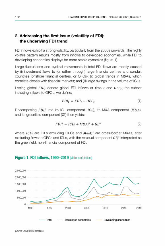
Two issues make FDI forecasting particularly challenging, explaining to some extent the very limited methodological advances in this area: (i) the highly volatile nature of FDI data and (ii) the complexity of properly capturing the many determinants that affect FDI and their interactions.
(i) Although FDI is the most stable source of external financing (World Investment Report, various editions), in the last 20 years its dynamics have exhibited significant variations (figure 1). These are typically generated by one-off transactions such as large cross-border mergers and acquisitions (M&As) and by financial flows, mainly involving developed economies. A useful step for forecasting is to mitigate the strong volatility in the data while retaining the most structural and productive component of FDI.
(ii) Longitudinal and cross-sectional factors interact in complex ways to determine the level of FDI in a country, as investment depends both on the behaviour of past investors (longitudinal dimension) and on the macroeconomic and institutional conditions prevailing across countries (cross-sectional dimension).
The purpose of this paper is to suggest an econometric approach to forecasting FDI that properly addresses these two issues. For the first problem (volatility of FDI) we introduce an underlying FDI trend, smoothing the FDI time series by taking into account the differing nature of the key FDI components, such as greenfield investment, cross-border M&As, financial flows and intracompany loans (ICLs) (section 2).1 For the second problem (heterogeneity across countries and time dependence), we suggest a dynamic panel econometric approach (section 3). The resulting model is a GMM model such as that proposed by Arellano and Bover (1995), accounting for cross-country heterogeneity and time dependence (section 4). The GMM model is then used to forecast FDI (section 5) and the results are compared with alternative time-series methods, confirming the higher predictive power of the proposed approach (section 6). This paper is a step in investigating methods for forecasting global FDI flows within a panel data econometric framework; possible alternative directions for future research, including beyond panel data econometrics, are briefly discussed in the final section (section 7).
1 The UNCTAD underlying trend used in this paper is a composite construct combining different sets of data. For ease of interpretation, we use the term “FDI components” – which in the balance-of-payments construct of FDI denotes equity, reinvested earnings and ICLs (i.e. sources of finance) – in a different sense here to distinguish greenfield projects (i.e. new investments) and M&As (i.e. ownership changes).
100 TRANSNATIONAL CORPORATIONS Volume 28, 2021, Number 1
2. Addressing the first issue (volatility of FDI): the underlying FDI trend
FDI inflows exhibit a strong volatility, particularly from the 2000s onwards. The highly volatile pattern results mostly from inflows to developed economies, while FDI to developing economies displays far more stable dynamics (figure 1).
Large fluctuations and cyclical movements in total FDI flows are mostly caused by (i) investment flows to (or rather through) large financial centres and conduit countries (offshore financial centres, or OFCs); (ii) global trends in M&As, which correlate closely with financial markets; and (iii) large swings in the volume of ICLs.
Letting global denote global FDI inflows at time and , the subset including inflows to OFCs, we define:
(1)
Decomposing into its ICL component ( ), its M&A component ( ), and its greenfield component (GI) then yields:
(2)
where are ICLs excluding OFCs and are cross-border M&As, after excluding flows to OFCs and ICLs, with the residual component interpreted as the greenfield, non-financial component of FDI.
Figure 1. FDI in�ows, 1990–2019 (Millions of dollars)
0
500,000
1,000,000
1,500,000
2,000,000
2,500,000
1990 1995 2000 2005 2010 2015 2019
Source: UNCTAD FDI database.
Total Developed economies Developing economies
101Forecasting global FDI: a panel data approach
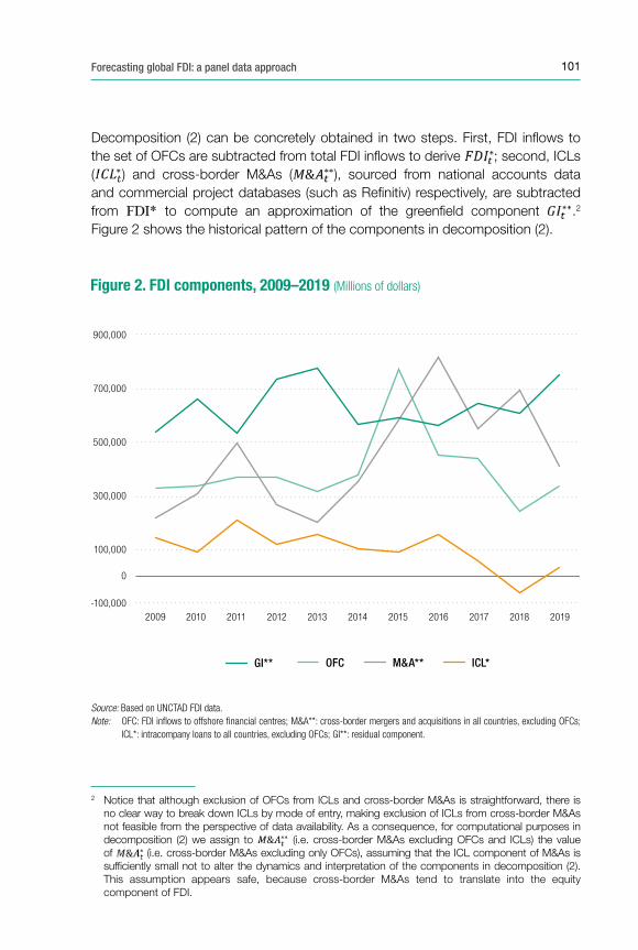
Decomposition (2) can be concretely obtained in two steps. First, FDI inflows to the set of OFCs are subtracted from total FDI inflows to derive ; second, ICLs ( ) and cross-border M&As ( ), sourced from national accounts data and commercial project databases (such as Refinitiv) respectively, are subtracted from to compute an approximation of the greenfield component .2 Figure 2 shows the historical pattern of the components in decomposition (2).
2 Notice that although exclusion of OFCs from ICLs and cross-border M&As is straightforward, there is no clear way to break down ICLs by mode of entry, making exclusion of ICLs from cross-border M&As not feasible from the perspective of data availability. As a consequence, for computational purposes in decomposition (2) we assign to (i.e. cross-border M&As excluding OFCs and ICLs) the value of (i.e. cross-border M&As excluding only OFCs), assuming that the ICL component of M&As is sufficiently small not to alter the dynamics and interpretation of the components in decomposition (2). This assumption appears safe, because cross-border M&As tend to translate into the equity component of FDI.
Figure 2. FDI components, 2009–2019 (Millions of dollars)
0
100,000
-100,000
300,000
500,000
700,000
900,000
2009 2010 2011 2012 2013 2014 2015 2016 2017 2018 2019
GI** OFC M&A** ICL*
Source: Based on UNCTAD FDI data.Note: OFC: FDI in�ows to offshore �nancial centres; M&A**: cross-border mergers and acquisitions in all countries, excluding OFCs; ICL*: intracompany loans to all countries, excluding OFCs; GI**: residual component.
102 TRANSNATIONAL CORPORATIONS Volume 28, 2021, Number 1
The main driver of the large fluctuations in global FDI inflows is the value of cross-border M&As, which in some years of frothy financial markets can account for more than half of global FDI values. For example, the peaks in 2000, 2007 and 2015 (figure 1) were driven to a large extent by M&A booms (compare with figure 2 for 2015). In some years, global FDI statistics are skewed by a very few extremely large transactions, such as the SAB Miller deal in 2016 (6 per cent of global flows in that year), or the Verizon deal in 2014 (10 per cent of total flows). Although the volatility of ICLs is greater, their impact on global FDI flows is significantly less due to their limited absolute size. Nonetheless, they can cause very significant upward or downward swings in individual countries.
All components of FDI are relevant indicators of global investment trends, from the perspectives of both macroeconomics (e.g. the health of a country’s balance of payments) and international production (which expands as much through M&As as through greenfield investments). Yet, it can be hard for policymakers to draw sound conclusions – say, on progress in building a conducive investment climate – on the basis of trends that show wild fluctuations, often driven by exogenous cyclical dynamics in financial markets or by anomalous outliers (such as one-off M&A transactions). It is therefore helpful to study the underlying directional trend, net of the oscillations caused by the most volatile elements in FDI flows. Not only is the construction of an underlying trend a useful descriptive monitoring and analytical tool in itself (UNCTAD, 2019 and 2020), it is also instrumental in addressing the issue of volatility in the forecasting exercise.
The main challenge is to define the underlying trend in such a way as to remove the most disturbing part of the volatility while retaining the fundamental long-term dynamics of FDI. To do so, we rely on decomposition (2), leveraging our prior knowledge of the economic interpretation and statistical behaviour of the elements involved:
• FDI to OFCs is excluded from the calculation of the trend, as it is largely conduit flows and driven by financial and tax motives.
• The moving average technique is applied to smooth the dynamics of M&A** and ICL*, to mitigate large swings generated by one-off transactions.
• The remaining component, GI**, is retained as is to recognize the more productive nature of greenfield investment, which is empirically supported by the evidence of a more stable historical pattern relative to the other components (figure 2).
The underlying FDI trend is then calculated as:
(3)
103Forecasting global FDI: a panel data approach
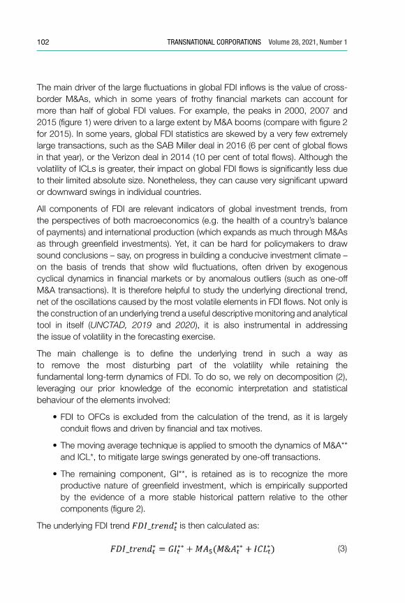
where , and are defined as in (2) and is the five-year moving average function. Consistent with the notation introduced, the asterisk superimposed on the variable indicates the exclusion of flows to OFCs. Figure 3 shows the dynamics of the underlying FDI trend, , relative to total FDI and to total FDI without OFCs ( and , respectively).
The underlying investment trend line does not show the drops in FDI after the dotcom boom and during the global financial crisis. This suggests that FDI is, at its core, quite stable: investment projects have long gestation periods and investment decisions are not easily reversed on the basis of developments in financial markets. Also, a large part of FDI flows is generated by existing FDI stocks, particularly the non-M&A component – including, for example, reinvested earnings. This time-dependent feature makes the underlying FDI trend less prone to external shocks and inherently more stable.
Figure 3. FDI in�ow, with and without OFCs, and underlying FDI trend, 1990–2019 (Millions of dollars)
0
500,000
1,000,000
1,500,000
2,000,000
2,500,000
1990 1995 2000 2005 2010 2015 2019
Source: Based on UNCTAD FDI data.
FDI total FDI excluding OFCs Underlying FDI trend
104 TRANSNATIONAL CORPORATIONS Volume 28, 2021, Number 1
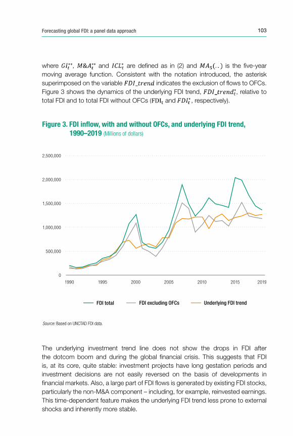
The underlying trend line follows global macroeconomic indicators, such as GDP and trade, more closely than total FDI (figure 4).
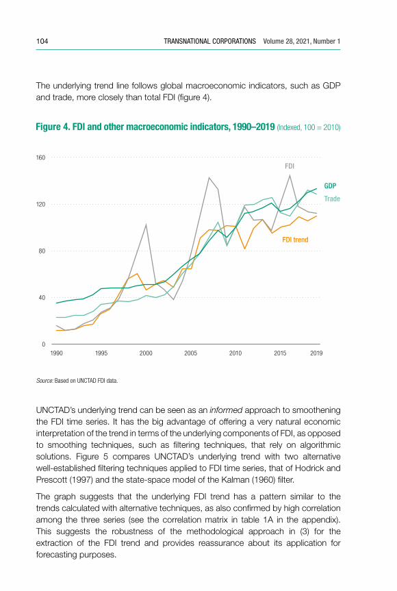
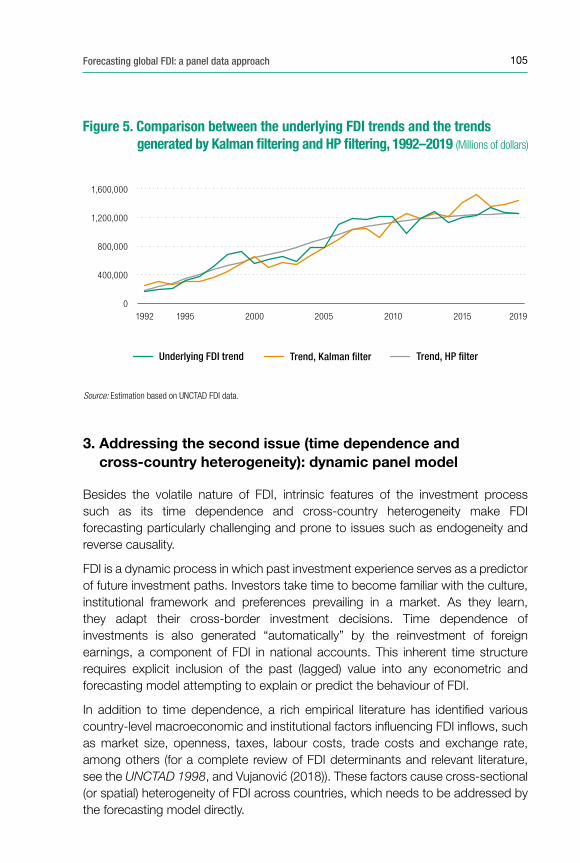
UNCTAD’s underlying trend can be seen as an informed approach to smoothening the FDI time series. It has the big advantage of offering a very natural economic interpretation of the trend in terms of the underlying components of FDI, as opposed to smoothing techniques, such as filtering techniques, that rely on algorithmic solutions. Figure 5 compares UNCTAD’s underlying trend with two alternative well-established filtering techniques applied to FDI time series, that of Hodrick and Prescott (1997) and the state-space model of the Kalman (1960) filter.
The graph suggests that the underlying FDI trend has a pattern similar to the trends calculated with alternative techniques, as also confirmed by high correlation among the three series (see the correlation matrix in table 1A in the appendix). This suggests the robustness of the methodological approach in (3) for the extraction of the FDI trend and provides reassurance about its application for forecasting purposes.
Figure 4. FDI and other macroeconomic indicators, 1990–2019 (Indexed, 100 = 2010)
GDP
Trade
FDI
FDI trend
1990 1995 2000 2005 2010 2015 2019
Source: Based on UNCTAD FDI data.
0
40
80
120
160
105Forecasting global FDI: a panel data approach
3. Addressing the second issue (time dependence and cross-country heterogeneity): dynamic panel model
Besides the volatile nature of FDI, intrinsic features of the investment process such as its time dependence and cross-country heterogeneity make FDI forecasting particularly challenging and prone to issues such as endogeneity and reverse causality.
FDI is a dynamic process in which past investment experience serves as a predictor of future investment paths. Investors take time to become familiar with the culture, institutional framework and preferences prevailing in a market. As they learn, they adapt their cross-border investment decisions. Time dependence of investments is also generated “automatically” by the reinvestment of foreign earnings, a component of FDI in national accounts. This inherent time structure requires explicit inclusion of the past (lagged) value into any econometric and forecasting model attempting to explain or predict the behaviour of FDI.
In addition to time dependence, a rich empirical literature has identified various country-level macroeconomic and institutional factors influencing FDI inflows, such as market size, openness, taxes, labour costs, trade costs and exchange rate, among others (for a complete review of FDI determinants and relevant literature, see the UNCTAD 1998, and Vujanović (2018)). These factors cause cross-sectional (or spatial) heterogeneity of FDI across countries, which needs to be addressed by the forecasting model directly.
Figure 5. Comparison between the underlying FDI trends and the trends generated by Kalman �ltering and HP �ltering, 1992–2019 (Millions of dollars)
1992 1995 2000 2005 2010 2015 20190
400,000
800,000
1,200,000
1,600,000
Source: Estimation based on UNCTAD FDI data.
Trend, Kalman �lterUnderlying FDI trend Trend, HP �lter
106 TRANSNATIONAL CORPORATIONS Volume 28, 2021, Number 1
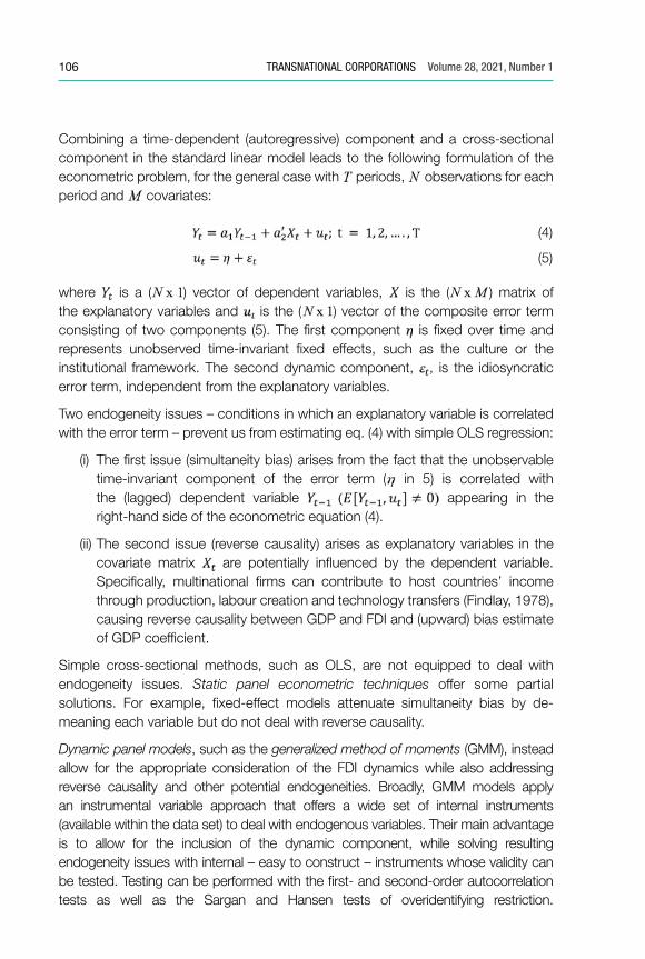
Combining a time-dependent (autoregressive) component and a cross-sectional component in the standard linear model leads to the following formulation of the econometric problem, for the general case with periods, observations for each period and covariates:
(4)
(5)
where is a ( ) vector of dependent variables, is the ( ) matrix of the explanatory variables and is the ( ) vector of the composite error term consisting of two components (5). The first component is fixed over time and represents unobserved time-invariant fixed effects, such as the culture or the institutional framework. The second dynamic component, , is the idiosyncratic error term, independent from the explanatory variables.
Two endogeneity issues – conditions in which an explanatory variable is correlated with the error term – prevent us from estimating eq. (4) with simple OLS regression:
(i) The first issue (simultaneity bias) arises from the fact that the unobservable time-invariant component of the error term ( in 5) is correlated with the (lagged) dependent variable appearing in the right-hand side of the econometric equation (4).
(ii) The second issue (reverse causality) arises as explanatory variables in the covariate matrix are potentially influenced by the dependent variable. Specifically, multinational firms can contribute to host countries’ income through production, labour creation and technology transfers (Findlay, 1978), causing reverse causality between GDP and FDI and (upward) bias estimate of GDP coefficient.
Simple cross-sectional methods, such as OLS, are not equipped to deal with endogeneity issues. Static panel econometric techniques offer some partial solutions. For example, fixed-effect models attenuate simultaneity bias by de-meaning each variable but do not deal with reverse causality.
Dynamic panel models, such as the generalized method of moments (GMM), instead allow for the appropriate consideration of the FDI dynamics while also addressing reverse causality and other potential endogeneities. Broadly, GMM models apply an instrumental variable approach that offers a wide set of internal instruments (available within the data set) to deal with endogenous variables. Their main advantage is to allow for the inclusion of the dynamic component, while solving resulting endogeneity issues with internal – easy to construct – instruments whose validity can be tested. Testing can be performed with the first- and second-order autocorrelation tests as well as the Sargan and Hansen tests of overidentifying restriction.
107Forecasting global FDI: a panel data approach
Finally, adding to their empirical appeal, GMM models do not require distributional assumptions such as the condition of normality and allow for heteroscedasticity (for details on GMM and instrumental variables, see for example Pesaran and Smith (1995) and Greene (2008)).
In the alternative between differenced GMM (Arellano and Bond, 1991) and system GMM (Arellano and Bover, 1995; Blundell and Bond, 1998), the preference here is given to the latter, which offers a wider choice of instruments (exploiting simultaneously levels and differences) and is more suitable when the panel data show some persistence (this is particularly the case for the underlying FDI trend) (Blundell and Bond, 1998; Roodman, 2009).
4. Model selection and results
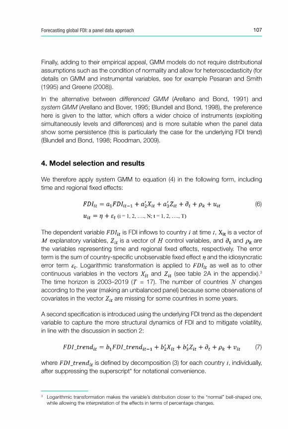
We therefore apply system GMM to equation (4) in the following form, including time and regional fixed effects:
(6)
The dependent variable is FDI inflows to country at time , is a vector of explanatory variables, is a vector of control variables, and and are
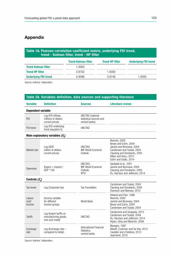
the variables representing time and regional fixed effects, respectively. The error term is the sum of country-specific unobservable fixed effect and the idiosyncratic error term . Logarithmic transformation is applied to as well as to other continuous variables in the vectors and (see table 2A in the appendix).3 The time horizon is 2003–2019 ( = 17). The number of countries changes according to the year (making an unbalanced panel) because some observations of covariates in the vector are missing for some countries in some years.
A second specification is introduced using the underlying FDI trend as the dependent variable to capture the more structural dynamics of FDI and to mitigate volatility, in line with the discussion in section 2:
(7)
where is defined by decomposition (3) for each country , individually, after suppressing the superscript* for notational convenience.
3 Logarithmic transformation makes the variable’s distribution closer to the “normal” bell-shaped one, while allowing the interpretation of the effects in terms of percentage changes.
108 TRANSNATIONAL CORPORATIONS Volume 28, 2021, Number 1
For FDI forecasting purposes, it is critical to select a set of predictors (i) that is significant in explaining the behaviour of FDI and (ii) for which there exist solid forecasts to feed into the forward-looking estimation. The natural choice falls then on the two variables, GDP and trade openness, which are not only the most (theoretically and empirically) established determinants of FDI,4 but are also supported by long-standing forecasting practice by international institutions. The model is then complemented by a vector of controls that includes other relevant variables such as taxation, income group, tariffs and exchange rate – all theoretically important drivers of FDI (Overesch and Wamser, 2010; Bevan and Estrin, 2004; Carstensen and Toubal, 2004; Martínez-San Román, Bengoa and Sánchez-Robles, 2016; Dixit and Pindyck, 1994; Aliber, 1970). Lacking established sources of their future values, the controls do not enter the forecasting exercise, but they are important to test the robustness of the predictors (the autoregressive term and the explanatory variables). Details on the definition, construction and sources of the dependent and independent variables are provided in the appendix (table 2A).
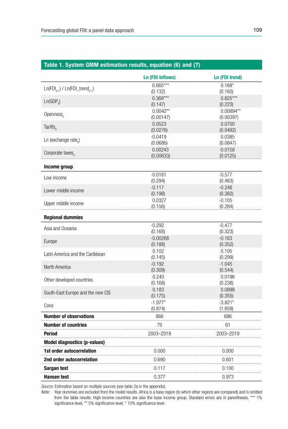
The results of model (6) and (7) are presented in table 1. The diagnostics tests confirm the model’s validity. First- and second-order autocorrelation tests indicate that the instruments are correlated with the endogenous variables but not with the error term. Sargan and Hansen tests also confirm that the instruments, as a group, appear exogenous.
In both models (columns I and II), the lagged dependent variable, GDP and trade openness are significant with the expected positive sign, after controlling for other relevant factors , and for time and regional fixed effects. The coefficient of the lagged dependent variable indicates that the past is a good predictor of the future behaviour of both FDI inflows (column I) and the FDI trend (column II). The positive effect of GDP confirms the importance of market size for FDI inflows. Likewise, trade openness has the expected positive impact on FDI, although much smaller than the impact of GDP. Control variables – taxes, tariffs, exchange rate and the income group – are not statistically significant in either of the models, which is reassuring in regard to the choice – imposed by data constraints – to limit the set of predictors to only GDP and trade.
Comparing the estimates between the two GMM models (column I and column II) provides further insights. The lagged dependent variable affects FDI inflows more strongly than FDI trend. Market size and trade openness, by contrast, have a greater effect on FDI trend, confirming the conceptual intuition (and empirical observation – see figure 4) that the underlying FDI trend can track economic fundamentals more closely.
4 The theoretical and empirical literature on market size (GDP) and trade openness (trade) as FDI determinants is vast. On the theoretical side, see for example Rodrik (1999) and Keller and Yeaple (2013) for GDP; and Caves (2007) for trade. On the empirical side, useful references for GDP include Resmini (2000); Hilber and Voicu (2010); Estrin and Uvalic (2014); and Blonigen and Piger (2014); and for trade include Janicki and Wunnava (2004); Clausing and Dorobantu (2005); and Du et al. (2014).
109Forecasting global FDI: a panel data approach
Table 1. System GMM estimation results, equation (6) and (7)
Ln (FDI inflows) Ln (FDI trend)
Ln(FDIit-1
) / Ln(FDI_trendit-1
)0.665***(0.132)
0.168*(0.160)
Ln(GDPit)
0.369***(0.147)
0.825***(0.223)
Opennessit
0.0042**(0.00147)
0.00894**(0.00397)
Tariffsit
0.0523(0.0276)
0.0700(0.0492)
Ln (exchange rateit)
-0.0419(0.0686)
0.0385(0.0847)
Corporate taxesit
0.00243 (0.00633)
-0.0158(0.0125)
Income group
Low income-0.0181(0.294)
-0.577(0.463)
Lower middle income-0.117(0.198)
-0.246(0.382)
Upper middle income0.0327(0.156)
-0.105(0.284)
Regional dummies
Asia and Oceania-0.292(0.168)
-0.477(0.323)
Europe-0.00268(0.188)
-0.163(0.352)
Latin America and the Caribbean0.102
(0.145)0.105(0.299)
North America-0.192(0.309)
-1.045(0.544)
Other developed countries0.240
(0.168)0.0196(0.238)
South-East Europe and the new CIS0.183
(0.175)0.0898(0.355)
Cons-1.977*(0.874)
-3.821*(1.859)
Number of observations 866 686
Number of countries 70 61
Period 2003–2019 2003–2019
Model diagnostics (p-values)
1st order autocorrelation 0.000 0.000
2nd order autocorrelation 0.690 0.601
Sargan test 0.117 0.100
Hansen test 0.377 0.973
Source: Estimation based on multiple sources (see table 2a in the appendix). Note: Year dummies are excluded from the model results. Africa is a base region (to which other regions are compared) and is omitted
from the table results. High-income countries are also the base income group. Standard errors are in parentheses. *** 1% significance level, ** 5% significance level, * 10% significance level.
110 TRANSNATIONAL CORPORATIONS Volume 28, 2021, Number 1
5. Forecasting FDI with GMM
Panel data econometrics are gaining interest as forecasting tools (Baltagi and Griffin, 1997; Stock and Watson, 2004; Longhi and Nijkamp, 2007; Arkadievich et al., 2008; Girardin and Kholodilin 2011; Wenzel 2013). Yet, their application is still limited relative to time-series econometrics. Their main value added is the ability to control for heterogeneity of FDI across countries (Baltagi, 2013), in addition to the usual dynamic structure. Micro (country) unit contains important information for the dynamics of the aggregate series, and hence, pooling the country data into a panel, can add to the forecasting precision, under the assumption of homogeneity across slope parameters (Fok, Van Dijk and Franses, 2005; Baltagi, 2008; Hsiao, 2014; Dees and Güntner, 2014). The individual countries’ forecast errors can also partially cancel out upon aggregation (Theil, 1957; Baltagi, 2013).
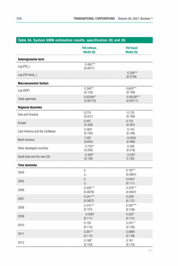
The final GMM specifications used in forecasting are derived from (6) and (7) after excluding the control variables :
(8)
(9)
The GMM regressions results for decompositions (8) and (9) (table 3A in the appendix) are fully consistent with the estimates from equations (6) and (7) reported in table 1.
This model has been used to provide the latest 2020-2021 forecasting of FDI inflows and the FDI trend, reported by UNCTAD 2020 (as of June 2020). UNCTAD forecasting has been relying on the past values of FDI up to 2019 (autoregressive term) and the projections of GDP and trade for 2020 and 2021. GDP and trade projections for 2020 and 2021 are sourced from the International Monetary Fund (IMF) World Economic Outlook of April 2020 and from the World Trade Organization (April 2020),5 respectively.
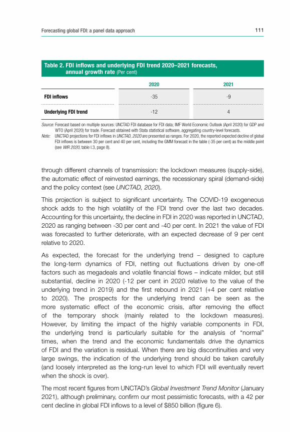
Table 2 reports the forecasted growth rates of global FDI inflows and the FDI trend for 2020 and 2021, on the basis of the GMM estimation of model (8) and (9) (see table 3A in the appendix) and the IMF and WTO projections for GDP and trade.
The projection indicates a sharp decline of global FDI in 2020, to about a third lower than its value in 2019 (-35 per cent) because of the impact of COVID-19 and pre-existing challenging conditions. COVID-19 is exerting a dramatic impact on FDI
5 World Trade Organization (2020). Trade set to plunge as COVID-19 pandemic upends global economy, press release, https://www.wto.org/english/news_e/pres20_e/pr855_e.htm.
111Forecasting global FDI: a panel data approach
through different channels of transmission: the lockdown measures (supply-side), the automatic effect of reinvested earnings, the recessionary spiral (demand-side) and the policy context (see UNCTAD, 2020).
This projection is subject to significant uncertainty. The COVID-19 exogeneous shock adds to the high volatility of the FDI trend over the last two decades. Accounting for this uncertainty, the decline in FDI in 2020 was reported in UNCTAD, 2020 as ranging between -30 per cent and -40 per cent. In 2021 the value of FDI was forecasted to further deteriorate, with an expected decrease of 9 per cent relative to 2020.
As expected, the forecast for the underlying trend – designed to capture the long-term dynamics of FDI, netting out fluctuations driven by one-off factors such as megadeals and volatile financial flows – indicate milder, but still substantial, decline in 2020 (-12 per cent in 2020 relative to the value of the underlying trend in 2019) and the first rebound in 2021 (+4 per cent relative to 2020). The prospects for the underlying trend can be seen as the more systematic effect of the economic crisis, after removing the effect of the temporary shock (mainly related to the lockdown measures). However, by limiting the impact of the highly variable components in FDI, the underlying trend is particularly suitable for the analysis of “normal” times, when the trend and the economic fundamentals drive the dynamics of FDI and the variation is residual. When there are big discontinuities and very large swings, the indication of the underlying trend should be taken carefully (and loosely interpreted as the long-run level to which FDI will eventually revert when the shock is over).
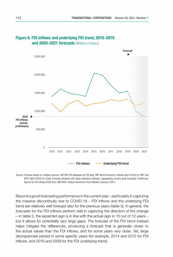
The most recent figures from UNCTAD’s Global Investment Trend Monitor (January 2021), although preliminary, confirm our most pessimistic forecasts, with a 42 per cent decline in global FDI inflows to a level of $850 billion (figure 6).
Table 2. FDI inflows and underlying FDI trend 2020–2021 forecasts, annual growth rate (Per cent)
2020 2021
FDI inflows -35 -9
Underlying FDI trend -12 4
Source: Forecast based on multiple sources: UNCTAD FDI database for FDI data; IMF World Economic Outlook (April 2020) for GDP and WTO (April 2020) for trade. Forecast obtained with Stata statistical software, aggregating country-level forecasts.
Note: UNCTAD projections for FDI inflows in UNCTAD, 2020 are presented as ranges. For 2020, the reported expected decline of global FDI inflows is between 30 per cent and 40 per cent, including the GMM forecast in the table (-35 per cent) as the middle point (see WIR 2020, table I.3, page 8).
112 TRANSNATIONAL CORPORATIONS Volume 28, 2021, Number 1
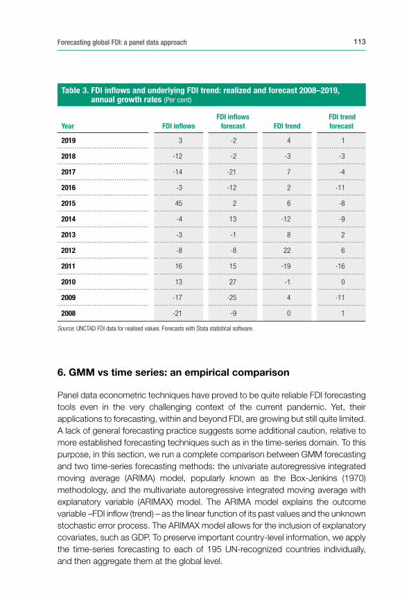
Beyond a good forecasting performance in the current year – particularly in capturing the massive discontinuity due to COVID-19 – FDI inflows and the underlying FDI trend are relatively well forecast also for the previous years (table 3). In general, the forecasts for the FDI inflows perform well in capturing the direction of the change – in table 3, the expected sign is in line with the actual sign in 10 out of 12 years – but it allows for potentially very large gaps. The forecast of the FDI trend instead helps mitigate the differences, producing a forecast that is generally closer to the actual values than the FDI inflows, and for some years very close. Yet, large discrepancies persist in some specific years (for example, 2014 and 2015 for FDI inflows, and 2016 and 2009 for the FDI underlying trend).
Figure 6. FDI in�ows and underlying FDI trend, 2010–2019 and 2020–2021 forecasts (Millions of dollars)
0
500,000
1,000,000
1,500,000
2,000,000
2,500,000
2010 2011 2012 2013 2014 2015 2016 2017 2018 2019 2020 2021
FDI in�ows Underlying FDI trend
2020 FDI in�ows
(actual, preliminary)
Forecast
Source: Forecast based on multiple sources: UNCTAD FDI database for FDI data; IMF World Economic Outlook (April 2020) for GDP and WTO (April 2020) for trade. Forecast obtained with Stata statistical software, aggregating country-level forecasts. Preliminary figures for FDI inflows 2020 from UNCTAD’s Global Investment Trend Monitor (January 2021).
113Forecasting global FDI: a panel data approach
6. GMM vs time series: an empirical comparison
Panel data econometric techniques have proved to be quite reliable FDI forecasting tools even in the very challenging context of the current pandemic. Yet, their applications to forecasting, within and beyond FDI, are growing but still quite limited. A lack of general forecasting practice suggests some additional caution, relative to more established forecasting techniques such as in the time-series domain. To this purpose, in this section, we run a complete comparison between GMM forecasting and two time-series forecasting methods: the univariate autoregressive integrated moving average (ARIMA) model, popularly known as the Box-Jenkins (1970) methodology, and the multivariate autoregressive integrated moving average with explanatory variable (ARIMAX) model. The ARIMA model explains the outcome variable –FDI inflow (trend) – as the linear function of its past values and the unknown stochastic error process. The ARIMAX model allows for the inclusion of explanatory covariates, such as GDP. To preserve important country-level information, we apply the time-series forecasting to each of 195 UN-recognized countries individually, and then aggregate them at the global level.
Table 3. FDI inflows and underlying FDI trend: realized and forecast 2008–2019, annual growth rates (Per cent)
Year FDI inflows FDI inflows
forecast FDI trend FDI trend forecast
2019 3 -2 4 1
2018 -12 -2 -3 -3
2017 -14 -21 7 -4
2016 -3 -12 2 -11
2015 45 2 6 -8
2014 -4 13 -12 -9
2013 -3 -1 8 2
2012 -8 -8 22 6
2011 16 15 -19 -16
2010 13 27 -1 0
2009 -17 -25 4 -11
2008 -21 -9 0 1
Source: UNCTAD FDI data for realised values. Forecasts with Stata statistical software.
114 TRANSNATIONAL CORPORATIONS Volume 28, 2021, Number 1
The country-by-country ARIMA models have the following specification:
(10)
(11)
where ( ) is a function of the autoregressive terms of the order p (s) and the noise is presented as a moving average process of the order q (m), and and are the two constants of equations (10) and (11), respectively. To allow for the inclusion of GDP as an explanatory variable, we also include an ARIMAX model in the comparison:
(12)
(13)
The appropriate number of p and q (s and m) autoregressive terms are assesed with the use of the autocorrelation function and partial autocorrelation function and their corresponding corellograms. The best model choice is decided with the Durbin and Watson test (for serial correlation) as well as the Akaike and Bayesian information criteria of the model fit (Lütkepohl, 1984; Enders, 2008). The appropriate model choice (10-13), parameters estimation and forecasts are automatized with an automatic forecasting algorithm produced in R software (Hyndman and Khandakar, 2007). Once country-level forecasts of FDI inflows and trend are obtained, they are aggregated at the global level.
To summarize the results of the comparison over the 2008–2019 period, two measures of forecast errors are calculated: mean absolute deviation (MAD) and mean square error (MSE) (table 4). MAD is the absolute difference between the actual value and the forecasted values divided by the number of observations forecasted. MSE is the sum of the squared errors divided by the number of observations forecasted.
The GMM forecasting performance is superior to the two time-series techniques based on both MAD and MSE. Time-series techniques, even when applied to each country, produce less precise forecasts than panel econometric techniques, supporting the relevant theory and empirical evidence (Baltagi et al., 2000; Baltagi, Bresson and Pirotte, 2002; Brücker and Siliverstovs, 2006; see discussion in section 3). Applying the FDI trend improves the precision of forecasting for both the GMM and ARIMA techniques, confirming its validity as a tool to mitigate large variations and smooth the forecasting exercise. The poor forecasting performance of ARIMAX may be caused by the inclusion of endogenous GDP (see discussion in section 3), generating biased estimates at the country level and inflating the forecasts. Although the ARIMA model has better forecasting
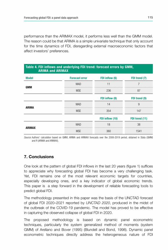
115Forecasting global FDI: a panel data approach
performance than the ARIMAX model, it performs less well than the GMM model. The reason could be that ARIMA is a simple univariate technique that only account for the time dynamics of FDI, disregarding external macroeconomic factors that affect investors’ preferences.
7. Conclusions
One look at the pattern of global FDI inflows in the last 20 years (figure 1) suffices to appreciate why forecasting global FDI has become a very challenging task. Yet, FDI remains one of the most relevant economic targets for countries, especially developing ones, and a key indicator of global economic trends. This paper is a step forward in the development of reliable forecasting tools to predict global FDI.
The methodology presented in this paper was the basis of the UNCTAD forecast of global FDI 2020–2021 reported by UNCTAD 2020, produced in the midst of the outbreak of the COVID-19 pandemic. The model has proved to be effective in capturing the observed collapse of global FDI in 2020.
The proposed methodology is based on dynamic panel econometric techniques, particularly the system generalized method of moments (system GMM) of Arellano and Bover (1995) (Blundell and Bond, 1998). Dynamic panel econometric techniques directly address the heterogeneous nature of FDI
Table 4. FDI inflows and underlying FDI trend: forecast errors by GMM, ARIMA and ARIMAX
Model Forecast error FDI inflow (6) FDI trend (7)
GMMMAD 11 7
MSE 236 87
FDI inflow (8) FDI trend (9)
ARIMAMAD 14 9
MSE 354 147
FDI inflow (10) FDI trend (11)
ARIMAXMAD 18 38
MSE 360 1541
Source: Authors’ calculation based on GMM, ARIMA and ARIMAX forecasts over the 2008-2019 period, obtained in Stata (GMM) and R (ARIMA and ARIMAX).
116 TRANSNATIONAL CORPORATIONS Volume 28, 2021, Number 1
across countries and FDI dynamics across time. System GMM is suited to deal with endogeneity issues caused by the inclusion of lagged FDI and GDP among the regressors.
The forecast is applied not only to the FDI inflows but also to the underlying FDI trend. The underlying FDI trend is an alternative representation of FDI inflows, more in line with the economic fundamentals as it reduces noise in the data caused by one-off transactions and financial flows. The forecast of the underlying trend complements the standard FDI forecast by providing an indication of the long-term future dynamics of FDI.
Compared with two alternative time-series techniques (ARIMA and ARIMAX), the GMM models show better predictive performance, supporting the case for the use of panel data techniques (rather than time-series), pooling countries’ individual information for forecasting FDI at the aggregate level.
Although highly encouraging, the results presented in this paper should not lead to any general claim about the superiority of this approach. This study aims at providing a step forward stimulating more systematic analysis of different methods in forecasting FDI.
Beyond GMM, other econometric tools deserve investigation. The panel vector autoregression (PVAR) accounts well for the static and dynamic interdependence between variables and between countries, as well as the contemporaneous and lagged effects of exogenous variables (Canova and Ciccarelli, 2004). This could be an important aspect in modeling FDI dynamics, where investors usually take time to react to changed macroeconomic circumstances. Spatial econometric techniques is another interesting option (Baltagi, 2013; Baltagi, Fingleton and Pirotte, 2014). In addition to the heterogonous nature of FDI across counties (and possibly across time) spatial econometric tools account for the spatial (geographical) dependence of FDI and its determinants.
* * *
Improving methods to forecast international investment flows, while seemingly an impossible task due to their lumpy and volatile nature, is important for the policy community. At the national level, it is helpful for policymakers to understand the expected direction of investment trends in processes ranging from designing industrial policies to setting performance targets for investment promotion agencies and special economic zones. At the international level, ongoing efforts to boost investment facilitation and to negotiate investment chapters in regional economic cooperation agreements benefit from greater awareness of the tides against which they are rowing and the currents they can exploit.

117Forecasting global FDI: a panel data approach
A huge push for new investment in infrastructure, renewable energy and Industry 4.0 is expected from the recovery stimulus packages that are being adopted in the more affluent regions of the world. It will be interesting to see how this big push affects investment trends going forward and to what extent the model presented in this paper will be able to capture those effects.
118 TRANSNATIONAL CORPORATIONS Volume 28, 2021, Number 1
References
Abbott, A., Cushman, D. O., and De Vita, G. (2012). Exchange rate regimes and FDI flows to developing countries. Review of International Economics, 20(1), 95-107.
Aghion Philippe, and Howitt Peter. (1992). A model of growth through creative destruction. Econometrica, 60(2), 323-351. Retrieved from http://www.jstor.org/stable/2951599.
Aliber, R. Z. (1970). A theory of direct foreign investment. In C. P. Kindleberger (ed.), The International Corporation. Cambridge, MA: MIT Press.
Al-Rawashdeh, S. T., Nsour, J. H., and Salameh, R. S. (2011). Forecasting foreign direct investment in Jordan for the years (2011-2030). International Journal of Business and Management, 6(10), 138.
Arellano, M., and Bover, O. (1995). Another look at the instrumental variable estimation of error-components models. Journal of Econometrics, 68(1), 29-51.
Arellano, M., and Bond, S. (1991). Some tests of specification for panel data: Monte Carlo evidence and an application to employment equations. The Review of Economic Studies, 58(2), 277-297.
Arkadievich Kholodilin, K., Siliverstovs, B., and Kooths, S. (2008). A dynamic panel data approach to the forecasting of the GDP of German Länder. Spatial Economic Analysis, 3(2), 195-207.
Baltagi, B. H., and Griffin, J. M. (1997). Pooled estimators vs. their heterogeneous counterparts in the context of dynamic demand for gasoline. Journal of Econometrics, 77(2), 303-327.
Baltagi, B. H., Griffin, J. M., and Xiong, W. (2000). To pool or not to pool: Homogeneous versus heterogeneous estimators applied to cigarette demand. Review of Economics and Statistics, 82(1), 117-126.
Baltagi, B. H., Bresson, G., and Pirotte, A. (2002). Comparison of forecast performance for homogeneous, heterogeneous and shrinkage estimators: Some empirical evidence from US electricity and natural-gas consumption. Economics Letters, 76(3), 375-382.
Baltagi, B. H., Fingleton, B., and Pirotte, A. (2014). Spatial lag models with nested random effects: An instrumental variable procedure with an application to English house prices. Journal of Urban Economics, 80, 76-86.
Baltagi, B. (2008). Econometric Analysis of Panel Data. Chichester, UK: John Wiley & Sons.
Baltagi, B. H. (2013). Panel data forecasting. Handbook of Economic Forecasting, 2, 995-1024.
Baltagi, B. H., and Li, D. (2006). Prediction in the panel data model with spatial correlation: the case of liquor. Spatial Economic Analysis, 1(2), 175-185.
Bevan, A. A., and Estrin, S. (2004). The determinants of foreign direct investment into European transition economies. Journal of Comparative Economics, 32(4), 775-787. doi:10.1016/j.jce.2004.08.006.
Blundell, R., and Bond, S. (1998). Initial conditions and moment restrictions in dynamic panel data models. Journal of Econometrics, 87(1), 115-143.
Blonigen, B. A. (1997). Firm-specific assets and the link between exchange rates and foreign direct investment. The American Economic Review, 447-465.
119Forecasting global FDI: a panel data approach
Blonigen, B. A., and Piger, J. (2014). Determinants of foreign direct investment. Canadian Journal of Economics/Revue canadienne d’économique, 47(3), 775-812.
Blonigen, B. A., Tomlin, K., and Wilson, W. W. (2004). Tariff-jumping FDI and domestic firms’ profits. The Canadian Journal of Economics, 37(3), 656-677.
Box, G. E., Jenkins, G. M., and Reinsel, G. (1970). Time Series Analysis: Forecasting and Control. San Francisco: Holden Day.
Brücker, H., and Siliverstovs, B. (2006). On the estimation and forecasting of international migration: how relevant is heterogeneity across countries? Empirical Economics, 31(3), 735-754.
Canova, F., and Ciccarelli, M. (2004). Forecasting and turning point predictions in a Bayesian panel VAR model. Journal of Econometrics, 120(2), 327-359.
Cardamone, P., and Scoppola, M. (2012). The impact of EU preferential trade agreements on foreign direct investment. The World Economy, 35(11), 1473-1501.
Carstensen, K., and Toubal, F. (2004). Foreign direct investment in central and eastern European countries: A dynamic panel analysis. Journal of Comparative Economics, 32(1), 3-22. doi:10.1016/j.jce.2003.11.001
Cavallari, L., and d’Addona, S. (2013). Nominal and real volatility as determinants of FDI. Applied Economics, 45(18), 2603-2610. doi:10.1080/00036846.2012.674206
Caves, R. E. (2007). Multinational Enterprise and Economic Analysis (3rd ed.). Cambridge, U.K.: Cambridge University Press.
Clausing, K. A., and Dorobantu, C. L. (2005). Re‐entering Europe: Does European Union candidacy boost foreign direct investment? Economics of Transition, 13(1), 77-103.
Cole, M. T., and Davies, R. B. (2011). Strategic tariffs, tariff jumping, and heterogeneous firms. European Economic Review, 55(4), 480-496. doi:10.1016/j.euroecorev.2010.07.006.
Croissant, Y., and Millo, G. (2019). Panel Data Econometrics with R. Hoboken, NJ: John Wiley and Sons.
Dees, S., and Güntner, J. (2014). Analysing and forecasting price dynamics across euro area countries and sectors: A panel VAR approach. ECB Working Paper No. 1724, European Central Bank, Frankfurt.
Dixit, A. K., Dixit, R. K., and Pindyck, R. S. (1994). Investment under Uncertainty. Princeton, NJ: Princeton University Press.
Du, J., Lu, Y., and Tao, Z. (2008). FDI location choice: Agglomeration vs institutions. International Journal of Finance & Economics, 13(1), 92-107. doi:10.1002/ijfe.348.
Du, L., Harrison, A., and Jefferson, G. (2014). FDI spillovers and industrial policy: The role of tariffs and tax holidays. World Development, 64, 366-383.
Dunning, J., and Lundan, S. (eds.) (2008). Multinational Enterprises and the Global Economy (2nd ed.). Cheltenham, U.K.: Edward Elgar Ltd. Retrieved from http://lib.myilibrary.com?ID=177936.
Elhorst, J. P. (2005). Unconditional maximum likelihood estimation of linear and log‐linear dynamic models for spatial panels. Geographical Analysis, 37(1), 85-106.
Elhorst, J. P. (2012). Dynamic spatial panels: models, methods, and inferences. Journal of Geographical Systems, 14(1), 5-28.
120 TRANSNATIONAL CORPORATIONS Volume 28, 2021, Number 1
Enders, W. (2008). Applied Econometric Time Series. New York: John Wiley & Sons.
Estrin, S., and Uvalic, M. (2014). FDI into transition economies: Are the Balkans different? Economics of Transition, 22(2), 281-312. doi:10.1111/ecot.12040.
Farole, Thomas, and Winkler, Deborah (2014). Does FDI work for Africa? assessing local spillovers in a world of global value chains. Economic Premise, 135.
Fok, D., Van Dijk, D., and Franses, P. H. (2005). Forecasting aggregates using panels of nonlinear time series. International Journal of Forecasting, 21(4), 785-794.
Findlay, R. (1978). Relative backwardness, direct foreign investment, and the transfer of technology: a simple dynamic model. The Quarterly Journal of Economics, 92(1), 1-16.
Garibaldi, Pietro, Mora, Nada, Sahay, Ratna, and Zettelmeyer, Jeromin (2001). What moves capital to transition economies? IMF Staff Papers, 48(4), 109-145.
Girardin, E., and Kholodilin, K. A. (2011). How helpful are spatial effects in forecasting the growth of Chinese provinces? Journal of Forecasting, 30(7), 622-643.
Giroud, A., and Mirza, H. (2015). Refining of FDI motivations by integrating global value chains’ considerations. The Multinational Business Review, 23(1), 67-76.
Greene, W. (2008). Econometric Analysis. 6th ed. New Jersey: Prentice Hall.
George, A., and Rupashree, R. (2019). Forecast of foreign direct investment inflow (2019-2023) with reference to Indian economy. International Journal of Research in Engineering, IT and Social Sciences, 9(4), 22-26.
Grossman, G. M., and Helpman, E. (1994). Endogenous innovation in the theory of growth. The Journal of Economic Perspectives, 8(1), 23-44. doi:10.1257/jep.8.1.23.
Harm, P., and Meon, P. G. (2018). Good and useless FDI: The growth effects of greenfield investment and mergers and acquisition. Review of International Economics, 26 (1), 37-59.
Head, K., and Mayer, T. (2004). Market potential and the location of Japanese investment in the European Union. Review of Economics and Statistics, 86(4), 959-972.
Herzer, D. (2012). How does foreign direct investment really affect developing countries’ growth? Review of International Economics, 20(2), 396-414.
Hilber, C. A., and Voicu, I. (2010). Agglomeration economies and the location of foreign direct investment: Empirical evidence from Romania. Regional Studies, 44(3), 355-371.
Hijzen, A., Görg, H., and Manchin, M. (2008). Cross-border mergers and acquisitions and the role of trade costs. European Economic Review, 52(5), 849-866.
Hodrick, R. J., and Prescott, E. C. (1997). Postwar US business cycles: an empirical investigation. Journal of Money, Credit, and Banking, 1-16.
Holland, D., and Pain, N. (1998). The diffusion of innovations in Central and Eastern Europe: A study of the determinants and impact of foreign direct investment. NIESR Discussion Papers 137, National Institute of Economic and Social Research, London.
Hyndman, R. J., and Khandakar, Y. (2007). Automatic time series for forecasting: the forecast package for R. Monash Econometrics and Business Statistics Working Papers No. 6/07, Monash University, Clayton, VIC, Australia.
Hsiao, C. (2014). Analysis of Panel Data. Econometric Society Monographs No. 54. Cambridge, UK: Cambridge University Press.
121Forecasting global FDI: a panel data approach
IMF (2020). World Economic Outlook, April 2020: The Great Lockdown. Washington, D.C.: International Monetary Fund.
IMF (2019). World Economic Outlook, October 2019: Global Manufacturing Downturn, Rising Trade Barriers. Washington, D.C.: International Monetary Fund.
Janicki, H. P., and Wunnava, P. V. (2004). Determinants of foreign direct investment: empirical evidence from EU accession candidates. Applied Economics, 36(5), 505-509.
Jeanneret, A. (2016). International firm investment under exchange rate uncertainty. Review of Finance, 20(5), 2015-2048.
Kalman, R. (1960) A new approach to linear filtering and prediction problems. Journal of Basic Engineering, 82, pp. 35 – 45.
Keller, W., and Yeaple, S. R. (2009). Multinational enterprises, international trade, and productivity growth: firm-level evidence from the United States. The Review of Economics and Statistics, 91(4), 821-831.
Ledyaeva, S. (2009). Spatial econometric analysis of foreign direct investment determinants in Russian regions. World Economy, 32(4), 643-666. doi:10.1111/j.1467-9701.2008.01145.
Longhi, S., and Nijkamp, P. (2007). Forecasting regional labor market developments under spatial autocorrelation. International regional science review, 30(2), 100-119.
Lütkepohl, H. (1984). Forecasting contemporaneously aggregated vector ARMA processes. Journal of Business and Economic Statistics, 2(3), 201-214.
Martínez-San Román, V., Bengoa, M., and Sánchez-Robles, B. (2016). Foreign direct investment, trade integration and the home bias: evidence from the European Union. Empirical Economics, 50(1), 197-229.
Nyoni, T. (2018). Box-Jenkins ARIMA approach to predicting net FDI inflows in Zimbabwe. Munich Personal RePEc Archive, https://mpra.ub.uni-muenchen.de/87737/.
Overesch, M., and Wamser, G. (2010). The effects of company taxation in EU accession countries on German FDI. Economics of Transition, 18(3), 429-457. doi:10.1111/j.1468- 0351.2009.00385.
Perera, P. (2015). Modeling and forecasting foreign direct investment (FDI) into SAARC for the period of 2013-2037 with ARIMA. International Journal of Business and Social Science, 6(2).
Pesaran, M. H., and Smith, R. (1995). Estimating long-run relationships from dynamic heterogeneous panels. Journal of Econometrics, 68(1), 79-113.
Resmini, L. (2000). The determinants of foreign direct investment in the CEECs: new evidence from sectoral patterns. Economics of Transition, 8(3), 665-689.
Rodrik, D. (1999). The new global economy and developing countries: making openness work. Policy Essay No. 24, Overseas Development Council and Johns Hopkins University Press. accessed on https://sisis.rz.htw-berlin.de/inh2008/12364320.pdf.
Roodman, D. (2009). How to do xtabond2: An introduction to difference and system GMM in Stata. The Stata Journal, 9(1), 86-136.
Saini, N., and Singhania, M. (2018). Determinants of FDI in developed and developing countries: a quantitative analysis using GMM. Journal of Economic Studies, 45(2), 348-382.
122 TRANSNATIONAL CORPORATIONS Volume 28, 2021, Number 1
Segerstrom, P. S. (1991). Innovation, imitation, and economic growth. The Journal of Political Economy, 99(4), 807-827.
Sharma, D., and Philli, K. (2020). Box-Jenkins ARIMA modelling: Forecasting FDI in India. ScienceOpen Posters, doi: 10.14293/S2199-1006.1.SOR-.PPZCKJY.v1.
Shi, H., Zhang, X., Su, X., and Chen, Z. (2012). Trend prediction of FDI based on the intervention model and ARIMA-GARCH-M model. AASRI Procedia, 3, 387-393.
Speller, W., Thwaites, G., and Wright, M. (2011). The future of international capital flows. Bank of England Financial Stability Paper No. 12, Bank of England.
Stock, J. H., and Watson, M. W. (2004). Combination forecasts of output growth in a seven‐country data set. Journal of Forecasting, 23(6), 405-430.
Theil, H. (1957). Linear aggregation in input-output analysis. Econometrica: Journal of the Econometric Society, 111-122.
UNCTAD (2013). World Investment Report 2013: Global Value Chains: Investment and Trade for Development. New York and Geneva: United Nations.
UNCTAD (2014). World Investment Report 2014: Investing in the SDGs: An Action Plan. New York and Geneva: United Nations.
UNCTAD (2019). World Investment Report 2019: Special Economic Zones. New York and Geneva: United Nations.
UNCTAD (2020). World Investment Report 2020: International Production Beyond the Pandemic. New York and Geneva: United Nations.
Vujanović, N. (2018). FDI spillovers in selected SEE countries: sectoral and spatial diversities. Doctoral thesis, Staffordshire University.
Wenzel, L. (2013). Forecasting regional growth in Germany: A panel approach using business survey data. HWWI Research Paper No. 133, Hamburg Institute of International Economics.
123Forecasting global FDI: a panel data approach
Appendix
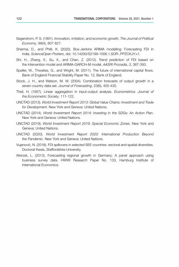
Table 1A. Pearson correlation coefficient matrix, underlying FDI trend, trend - Kalman filter, trend - HP filter
Trend Kalman filter Trend HP filter Underlying FDI trend
Trend Kalman filter 1.0000
Trend HP filter 0.9702 1.0000
Underlying FDI trend 0.9496 0.9746 1.0000
Source: Authors’ elaboration.
Table 2A. Variables definition, data sources and supporting literature
Variable Definition Sources Literature review
Dependent variable
FDILog (FDI inflows, millions of dollars, current prices)
UNCTAD (national statistical sources and central banks)
FDI trend Log (FDI underlying trend (equation1)) UNCTAD
Main explanatory variables (Xit)
Market sizeLog (GDP, million of dollars, current prices)
UNCTAD; IMF World Economic Outlook
Resmini, 2000Bevan and Estrin, 2004Janicki and Wunnava, 2004Carstensen and Toubal, 2004Clausing and Dorobantu, 2005Hilber and Voicu, 2010Estrin and Uvalic, 2014
Openness (Export + Import) / GDP *100
UNCTAD; IMF World Economic Outlook; WTO
Garibaldi et al., 2001Janicki and Wunnava, 2004Clausing and Dorobantu, 2005Du, Harrison and Jefferson, 2014
Controls (Zit)
Tax levels Log (Corporate tax) Tax Foundation Carstensen and Toubal, 2004Clausing and Dorobantu, 2005Overesch and Wamser, 2010
Labour cost/Income
Dummy variable for different income groups
World Bank
Holland and Pain, 1998Resmini, 2000Janicki and Wunnava, 2004Bevan and Estrin, 2004Carstensen and Toubal, 2004
TariffsLog (Import tariffs on manufacturing goods, ores and metal)
UNCTAD
Cardamone and Scoppola, 2012Carstensen and Toubal, 2004Du, Harrison and Jefferson, 2014Hijzen, Görg and Manchin, 2008
Exchange rate
Log (Exchange rate – compared to dollar)
International Financial Statistics, central banks
Blonigen, 1997Abbott, Cushman and De Vita, 2012Cavallari and d’Addona, 2013Jeanneret, 2016
Source: Authors’ elaboration.
124 TRANSNATIONAL CORPORATIONS Volume 28, 2021, Number 1
Table 3A. System GMM estimation results, specification (8) and (9)
FDI inflows Model (8)
FDI trend Model (9)
Autoregressive term
Log (FDIt-1
)0.485***(0.0977)
Log (FDI trendt-1
)0.328***(0.0736)
Macroeconomic factors
Log (GDP)0.340** (0.153)
0.643***(0.109)
Trade openness0.00356**(0.00175)
0.00538***(0.00111)
Regional dummies
Asia and Oceania0.210(0.251)
-0.135(0.166)
Europe0.447(0.328)
0.125(0.281)
Latin America and the Caribbean0.363* (0.195)
0.143(0.166)
North America1.042(0.655)
-0.0263(0.489)
Other developed countires0.735**
(0.293)0.336(0.216)
South East and the new CIS0.308**
(0.130)0.245*0.130)
Time dummies
20040(.)
0.197**(0.0861)
20050(.)
0.0437(0.111)
20060.328***(0.0979)
0.378***(0.0947)
20070.341***(0.0927)
0.248*(0.137)
20080.315***(0.107)
0.287***(0.109)
2009 -0.0287(0.111)
0.222*(0.131)
20100.150(0.115)
0.241**(0.108)
20110.261**(0.113)
0.0890(0.138)
20120.198*(0.103)
0.161(0.133)
.../...
125Forecasting global FDI: a panel data approach
Table 3A. System GMM estimation results, specification (8) and (9) (Concluded)
FDI inflows Model (8)
FDI trend Model (9)
Time dummies
20130.0870(0.107)
0.0870(0.126)
20140.130(0.115)
0.166(0.126)
20150.0252(0.117)
0.0690(0.141)
20160.181(0.115)
0.194(0.125)
20170.141(0.119)
0.123(0.127)
20180.159(0.109)
0.00881(0.127)
20190.0497(0.108)
0.0787(0.133)
_cons-0.554(1.107)
-2.645***(0.721)
Number of observations 1662 1829
Number of countries 111 111
Diagnostics (p-value)
Autocorrelation tests
1st order 0.000 0.000
2nd order 0.106 0.108
Hansen test 0.099 0.732
Source: Estimation based on multiple sources (see table 2a).Note: Africa is a base region (that other regions are compared to) and is omitted. Standard errors in parentheses. *** 1% significance
level, ** 5% significance level, * 10% significance level.


