follow wisdom

EXPLORING PATTERNS OF KNOWLEDGE PRODUCTION

RUFUS POLLOCK

UNIVERSITY OF CAMBRIDGE

MAY 2009

Definition 1 (Knowledge). The term ‘knowledge’ is here used broadly to signify all

forms of information production including those involved in technological innovation,

cultural creativity and academic advance.

1. Introduction

Today, thanks to rapid advances in IT, we have available substantial datasets

pertaining both to the extent and the structure of knowledge production across

disciplines, space and time. Especially recent is the availability of good ‘structural’

data – that is data on the linkages and relationships of different pieces of knowledge,

for example as provided by citation information. This new material allows us to

explore the “patterns of knowledge production” in deeper and richer ways than ever

previously possible and often using entirely new methods.

For example, it has long been accepted that innovation and creativity are cumu-

lative processes, in which new ideas build upon old. However, other than anecdotal

and case-study material provided by historians of ideas and sociologists of science

there has been little data with which to study this issue – and almost none of a

comprehensive kind that would make possible a systematic examination. However,

the recent availability of comprehensive databases containing ’citation’ information

have allowed us to begin really examining the extent to which new work builds upon

Emmanuel College and Faculty of Economics, University of Cambridge. Email: [email protected] [email protected]. First version in this form, March 2007. I’m very grateful to FerminMoscoso-del-Prado-Martin for early discussions which have done much to form the analysis pre-sented here. This paper is licensed under Creative Commons attribution (by) license v3.0 (alljurisdictions).

1

2 RUFUS POLLOCK UNIVERSITY OF CAMBRIDGE MAY 2009

old – be it a new technology as represented by a patent or a new idea in academia

as represented by a paper, builds upon old.

Similar opportunities present themselves in relation to identifying the creation of

new fields of research or technology, and tracing their evolution over time. Here

the existence of extensive ”structural information” as presented, for example, by

citation databases, enables new systematic approaches – for example, can new fields

be identified (or perhaps defined) as points in ‘knowledge space’ far away from the

existing loci of effort; or, alternatively, by the nature of its connections to the existing

body of work.

Structural information of this kind can also be used in charting other changes in

the life-cycle of knowledge creation. For example, to offer a specific conjecture, a

field entering decline, though still exhibiting a similar level of output (papers etc)

and even citations to a field in rude health, may display a citation structure which

is markedly different – for example, more clustered within the field itself. Thus,

by using this additional structural information we may be able to gain insights not

available with simpler approaches.

At the same time, structure must also play a central role in any attempt to

estimate knowledge related ‘output’ measures. This is of course not true for other

forms of ‘output’, for example that of corn of steel, where we have relatively well-

defined objective measures available: tonnes of such-and-such a quality.

But knowledge is different: the most obvious metrics, such as number of patents

or papers produced, seem entirely inadequate: one particular innovation or paper

may be ‘worth’ as much as a hundred or a thousand others. The issue here is that,

compared to corn or steel, knowledge is extremely inhomogeneous, or put slightly

differently, quality (or significance) differs very substantially across the individual

pieces of knowledge (papers, patents etc). Thus, any serious attempt to measure

the progress of knowledge must must find some way to do this quality-adjustment

and structural information seems essential to this.

EXPLORING PATTERNS OF KNOWLEDGE PRODUCTION 3

2. What specific questions might we explore with such datasets?

The following is a (non-exhaustive) list of the kinds of questions one might explore

using these new datasets:

(1) Can we use structure to infer information about quality of individual items?

Clearly the answer is yes, for example by using a citation-based metric where

a work’s value is estimated based on its citation by others.

(2) Can we then use this information together with more global structure of the

production network to gain a better idea of total (quality-adjusted) output.

This would allow one to chart progress, or the lack of it, over time?

(3) Can we use structural information to investigate the life-cycle of fields? For

example, can we see fields ‘dying out’ or the onset of diminishing returns?

Can we see new fields coming into existence and their initial growth patterns?

(4) What about productivity per capita and its variation across the population?

It is likely that one would need to focus here within a discipline as it would

be difficult to directly compare across disciplines, at least when using quality

adjusted productivity.

(5) Do the structures of knowledge production vary over time and across dis-

ciplines and does this have implications for their productivity? Can we

compare the structure of evolution in technology or economics with that in

‘natural’ evolution and, if not, what are the primary differences?

(6) How do other (observable) attributes related to the producers of knowledge

(their collaboration with others, their geographical location) affect the struc-

tures we observe and the associated outcomes (output, productivity) already

discussed above?

(7) Do different policies (for example openness vs. closedness – weak vs. strong

IP) have implications for the structure of production and hence for output

and productivity?


(8) Is knowledge production (in a particular area) ergodic or path-dependent?

Crudely: do we always end up in the same place or do small shocks have

large long-term effects?

3. Framework and Methodology

3.1. Framework. We have a set of standardized ‘items’ of knowledge that we shall

terms ‘works’: patents, papers, books, films etc. For each such ‘item’ we will have

information on some set of attributes, such as:

(1) Classificatory: e.g. keywords, subject classification etc

(2) Temporal: e.g. when it was produced

(3) Relational: e.g. citation data, or, more loosely, the set of other articles

published in that journal

(4) Miscellaneous: number of claims in the patent, length of book, journal in

which article was published

Our aim is to utilize these sorts of information in order to answer our questions.

3.2. Approach. At the general level there are 3 basic methodological approaches

we can take given the data:

3.2.1. Vector Spaces. Define vectors for each work by converting attributes into

dimensions. For example, suppose we have a controlled vocabulary containing N

terms used for classifying works, e.g. subject categories or keywords for patents or

papers. Then, associated to each work i, we can define a length N vector xi as the

vector with 1 in column j if and only if the paper is classified with the jth entry in

the controlled vocabulary.

Alternatively, if relational data is available, we can create a vector for each work

by taking the dimensions to be the other works. That is, if there are N works in

total, then work i is represented by a vector in an N-dimensional space with a 1 in

position j if and only if it links to work j. (This equivalent to the ith row in the


standard adjacency matrix for the directed graph associated to this citation network

– see below).

The beauty of converting works into vectors is that there is a very large existing

literature on how to do classification, clustering and analysis of objects distributed

in vector spaces.

3.2.2. Graphs. Where relational information exists it is natural to convert works into

nodes and define edges between the nodes depending on whether the corresponding

works are linked (where the relation is directed, for example in the case of citation,

this will give a directed graph). The result of this will be a presentation of the set

of works as a Graph. Standard graph-theoretic techniques can then be used.

3.2.3. Temporality and Evolution. If a temporal aspect is present it is natural to

include this in the analysis. In the first case, this may simply involve stratifying

by time when applying either of the two previous approaches (for example, only

considering those works from a particular year). However, temporality is more than

a simple filter, in particular, many of the processes we wish to examine, such as the

birth and development of fields, are temporal in nature. Furthermore, in examining

changes over time there are specific techniques and approaches that can be used.

4. Examples

4.1. Introduction. The data for most of the examples in this section come from

Hall et al. (2001). Associated code can be obtained from the author (written using

Python, SciPy and the NetworkX packages). The NBER dataset contains all patents

issued between 1963 and 1999 (approx 2.3m) and a complete set of citations on all

patents 1975-1999 (over 16m). Thus, we are working with a fairly sizable dataset and

one which therefore poses some significant technical challenges from a computational

and performance perspective.

4.2. Example 1: The Degree Distribution. A huge amount of intellecual en-

ergy has been exerted examining the citation distribution of different knowledge


‘networks’ going back to the pioneering work of Price (1965) and even earlier. In

graph theoretic terms this would be the in-degree distribution – with the out-degree

distribution being the distribution of ‘cites’. This distribution, and its properties, is

considered important because citations are taken to represent, albeit very crudely,

some measure of importance and therefore quality.

More recently the exact form of the degree distribution, both here and in other

areas where graph theoretic models are suitable, has been the subject of renewed

interest because of the possibility that certain features may be common across a set

of diverse areas (itself an indicator that there may be some theoreticabaly modelable

common process).1

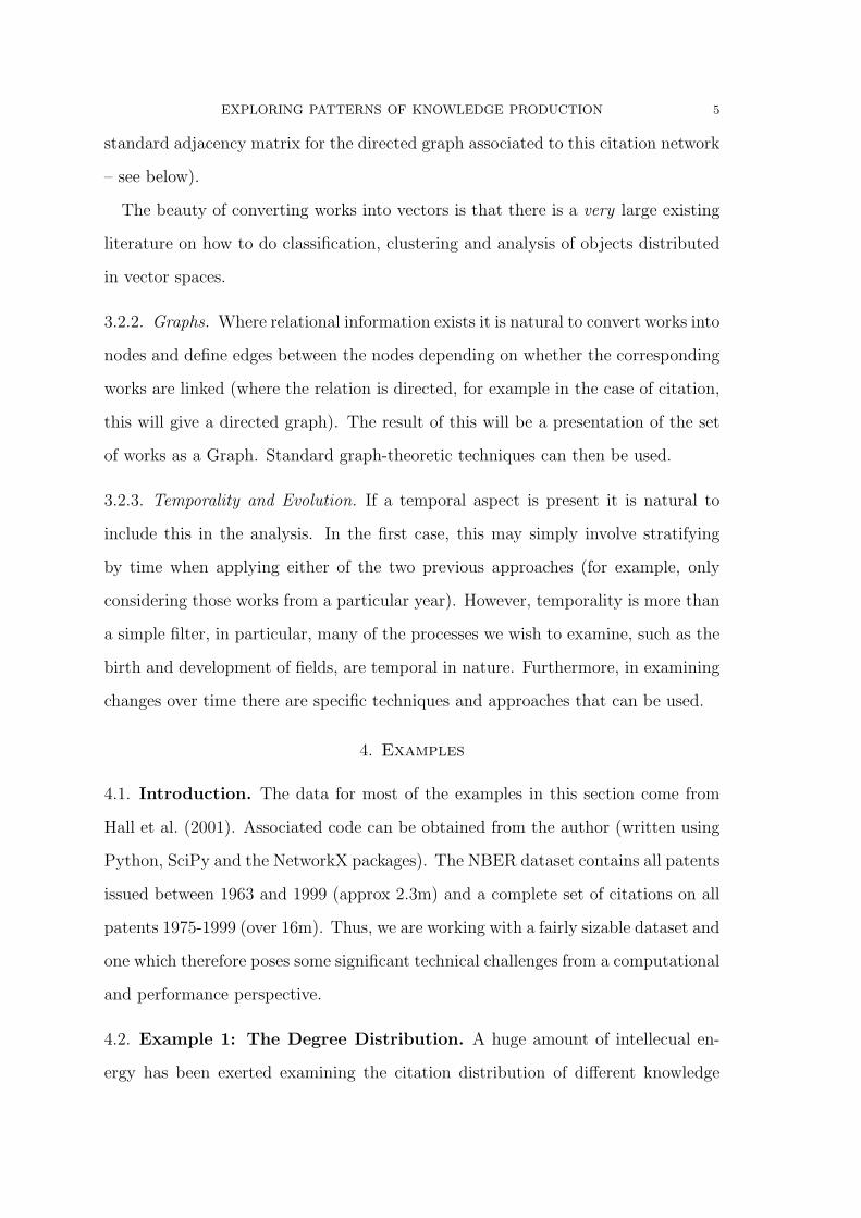
The full citation distribution for the complete NBER dataset is shown in figure 1

in both log-log and semilog forms. On the crude chi-by-eye approach is looks like a

power law is a good fit for the middle portion of the the distribution (papers cited

between 10 and ≈ 300 times) but is less good outside of these regions.2

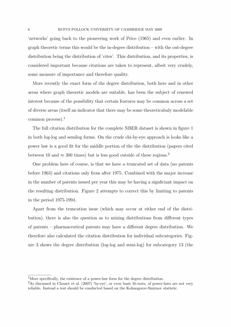
One problem here of course, is that we have a truncated set of data (no patents

before 1963) and citations only from after 1975. Combined with the major increase

in the number of patents issued per year this may be having a signficiant impact on

the resulting distribution. Figure 2 attempts to correct this by limiting to patents

in the period 1975-1994.

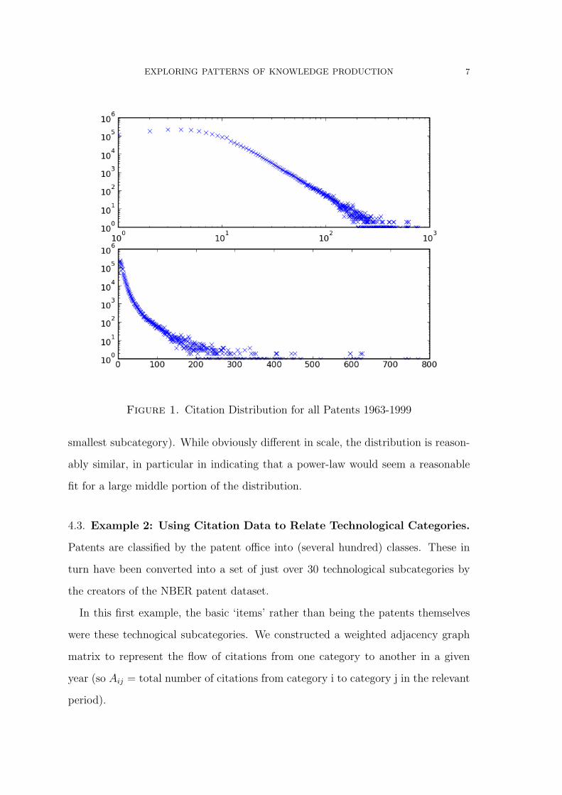
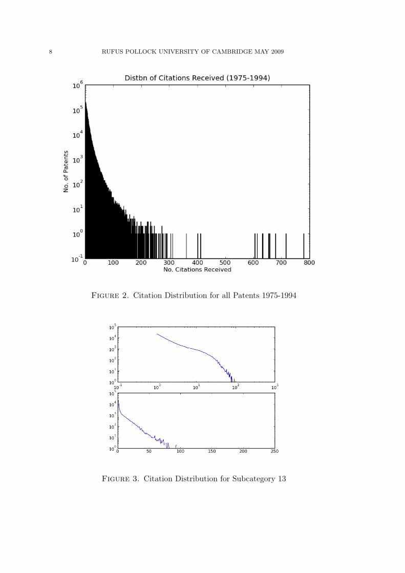
Apart from the truncation issue (which may occur at either end of the distri-

bution), there is also the question as to mixing distributions from different types

of patents – pharmaceutical patents may have a different degree distribution. We

therefore also calculated the citation distribution for individual subcategories. Fig-

ure 3 shows the degree distribution (log-log and semi-log) for subcategory 13 (the

1More specifically, the existence of a power-law form for the degree distribution.2As discussed in Clauset et al. (2007) ‘by-eye’, or even basic fit-tests, of power-laws are not veryreliable. Instead a test should be conducted based on the Kolmogorov-Smirnov statistic.


Figure 1. Citation Distribution for all Patents 1963-1999

smallest subcategory). While obviously different in scale, the distribution is reason-

ably similar, in particular in indicating that a power-law would seem a reasonable

fit for a large middle portion of the distribution.

4.3. Example 2: Using Citation Data to Relate Technological Categories.

Patents are classified by the patent office into (several hundred) classes. These in

turn have been converted into a set of just over 30 technological subcategories by

the creators of the NBER patent dataset.

In this first example, the basic ‘items’ rather than being the patents themselves

were these technogical subcategories. We constructed a weighted adjacency graph

matrix to represent the flow of citations from one category to another in a given

year (so Aij = total number of citations from category i to category j in the relevant

period).


Figure 2. Citation Distribution for all Patents 1975-1994

Figure 3. Citation Distribution for Subcategory 13


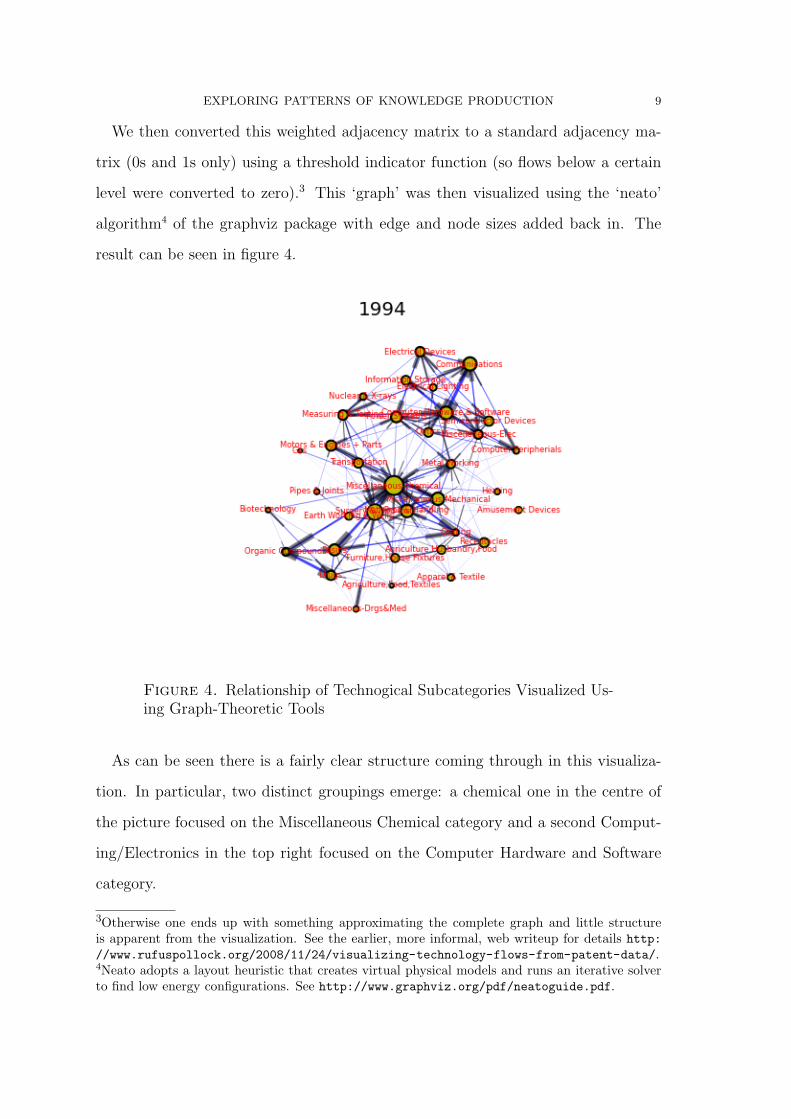
We then converted this weighted adjacency matrix to a standard adjacency ma-

trix (0s and 1s only) using a threshold indicator function (so flows below a certain

level were converted to zero).3 This ‘graph’ was then visualized using the ‘neato’

algorithm4 of the graphviz package with edge and node sizes added back in. The

result can be seen in figure 4.

Figure 4. Relationship of Technogical Subcategories Visualized Us-ing Graph-Theoretic Tools

As can be seen there is a fairly clear structure coming through in this visualiza-

tion. In particular, two distinct groupings emerge: a chemical one in the centre of

the picture focused on the Miscellaneous Chemical category and a second Comput-

ing/Electronics in the top right focused on the Computer Hardware and Software

category.

3Otherwise one ends up with something approximating the complete graph and little structureis apparent from the visualization. See the earlier, more informal, web writeup for details http://www.rufuspollock.org/2008/11/24/visualizing-technology-flows-from-patent-data/.4Neato adopts a layout heuristic that creates virtual physical models and runs an iterative solverto find low energy configurations. See http://www.graphviz.org/pdf/neatoguide.pdf.


One can also see natural bridging groups, for example various (high-tech) me-

chanical and measuring categories in the middle-to-top left which connect to both

the computer group and the chemical group.

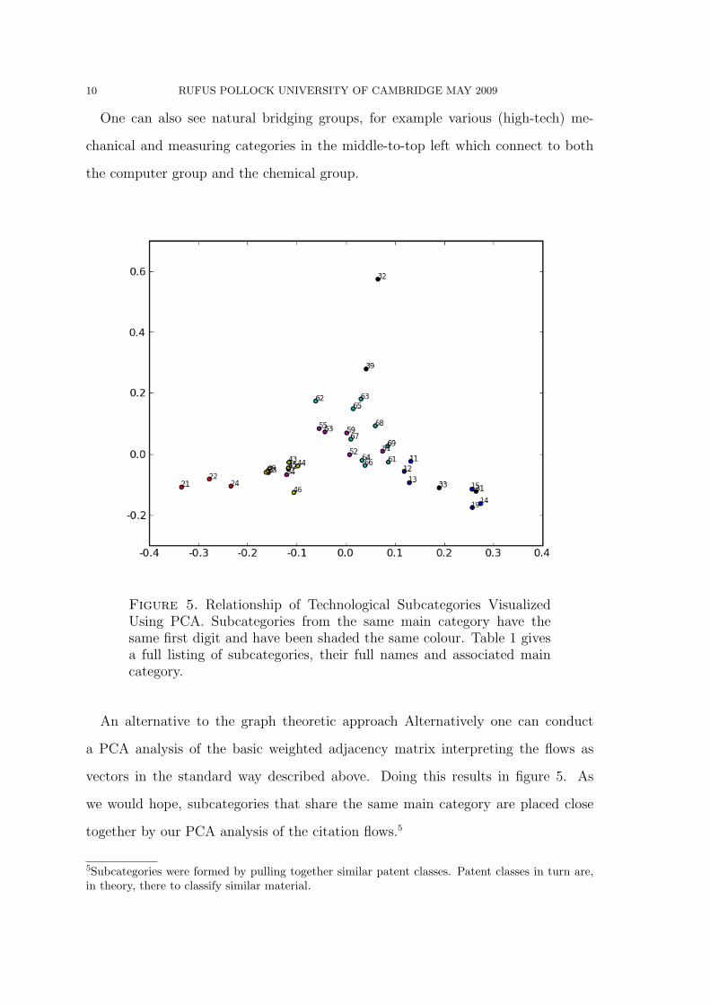
Figure 5. Relationship of Technological Subcategories VisualizedUsing PCA. Subcategories from the same main category have thesame first digit and have been shaded the same colour. Table 1 givesa full listing of subcategories, their full names and associated maincategory.

An alternative to the graph theoretic approach Alternatively one can conduct

a PCA analysis of the basic weighted adjacency matrix interpreting the flows as

vectors in the standard way described above. Doing this results in figure 5. As

we would hope, subcategories that share the same main category are placed close

together by our PCA analysis of the citation flows.5

5Subcategories were formed by pulling together similar patent classes. Patent classes in turn are,in theory, there to classify similar material.


However, there is some notable variation. For example, some categories subcat-

egories are much more tighly grouped than others – compare the 40s with the 30s.

There are also some noticeable outliers: 32 (Surgery and Med. Instr.) and, to a

lesser, extent, 39 (Misc Drugs and Chemicals). Some main categories show a clear

division into two groups, such as the 1x grouping (Chemical) which splits crudely

as ‘applications’ (11,12,13) and ‘pure chemicals’ (14,15,19). There are also some

clear misclassifications, for example Optics (54) is in the Mechanical (5x) category

but looks like it should be in the Electrical and Electronic (4x) category, similarly

Computer Peripherals (23) looks like it should be in Electrial and Electronics (4x)

rather than in Computer and Communications. Overall, the groupings one would

impose via simple proximity via the PCA would look rather different from the actual

category groupings we have: based on a crude by-eye approach, one would create

4-5 categories, one at bottom-left around 2x, one at mid-bottom-left around 4x, one

bottom-right around 1x+31, one at top around 32, and a large amorphous grouping

in the centre (perhaps split into 2).

4.4. Example 3: Patents in Space. This example uses a vector-based approach

in which our ‘items’ are the patents from the NBER patent file and the vectors

are based on the subcategory classifications given to patents. So with N = 36

subcategories each patent is mapped to a vector x in an N = 36 dimensional vector

space. We term these vectors ‘subject’ vectors as they relate to the subject matter

of the patent.

Each patent is classified to a single subcategory so under the simplest mapping

each patent would be represented by a 1 in a single column. This would not be very

interesting! Thus instead, motivated by the implied relationship involved in citatin,

we construct the vector for patent i using the subcategories of the patents that are

cited by i.6 To allow for the fact that patents vary substantially in the number of

cites they make we normalized each vector by dividing by the total number of cites

6We could symmetrically have also used the categories of patents citing i. However, given thegreater inequality in citation than in citing we preferred to focus on citing alone.


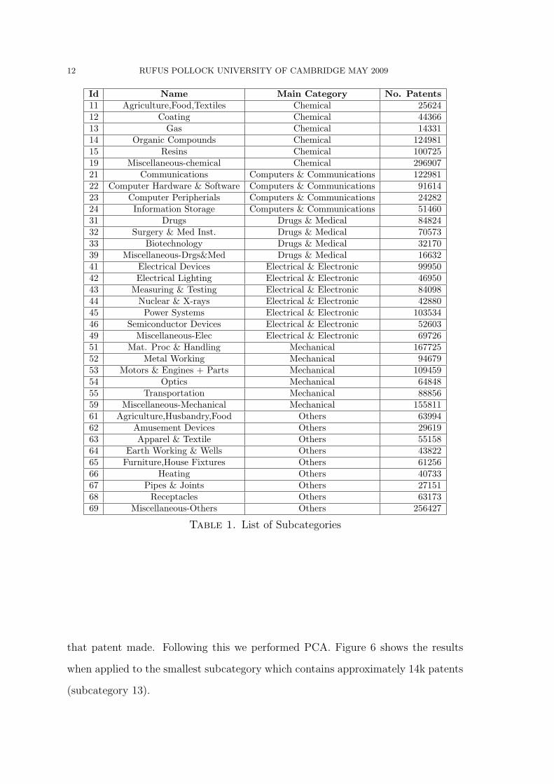
Id Name Main Category No. Patents11 Agriculture,Food,Textiles Chemical 2562412 Coating Chemical 4436613 Gas Chemical 1433114 Organic Compounds Chemical 12498115 Resins Chemical 10072519 Miscellaneous-chemical Chemical 29690721 Communications Computers & Communications 12298122 Computer Hardware & Software Computers & Communications 9161423 Computer Peripherials Computers & Communications 2428224 Information Storage Computers & Communications 5146031 Drugs Drugs & Medical 8482432 Surgery & Med Inst. Drugs & Medical 7057333 Biotechnology Drugs & Medical 3217039 Miscellaneous-Drgs&Med Drugs & Medical 1663241 Electrical Devices Electrical & Electronic 9995042 Electrical Lighting Electrical & Electronic 4695043 Measuring & Testing Electrical & Electronic 8409844 Nuclear & X-rays Electrical & Electronic 4288045 Power Systems Electrical & Electronic 10353446 Semiconductor Devices Electrical & Electronic 5260349 Miscellaneous-Elec Electrical & Electronic 6972651 Mat. Proc & Handling Mechanical 16772552 Metal Working Mechanical 9467953 Motors & Engines + Parts Mechanical 10945954 Optics Mechanical 6484855 Transportation Mechanical 8885659 Miscellaneous-Mechanical Mechanical 15581161 Agriculture,Husbandry,Food Others 6399462 Amusement Devices Others 2961963 Apparel & Textile Others 5515864 Earth Working & Wells Others 4382265 Furniture,House Fixtures Others 6125666 Heating Others 4073367 Pipes & Joints Others 2715168 Receptacles Others 6317369 Miscellaneous-Others Others 256427

Table 1. List of Subcategories

that patent made. Following this we performed PCA. Figure 6 shows the results

when applied to the smallest subcategory which contains approximately 14k patents

(subcategory 13).


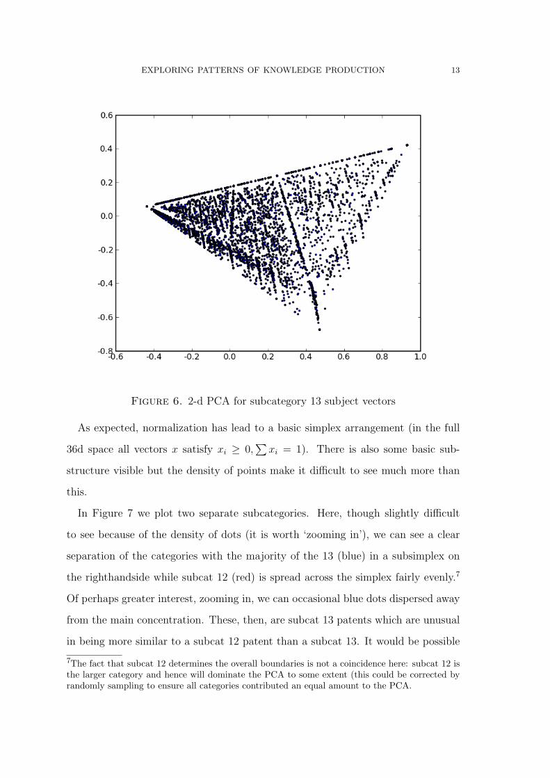
Figure 6. 2-d PCA for subcategory 13 subject vectors

As expected, normalization has lead to a basic simplex arrangement (in the full

36d space all vectors x satisfy xi ≥ 0,∑

xi = 1). There is also some basic sub-

structure visible but the density of points make it difficult to see much more than

this.

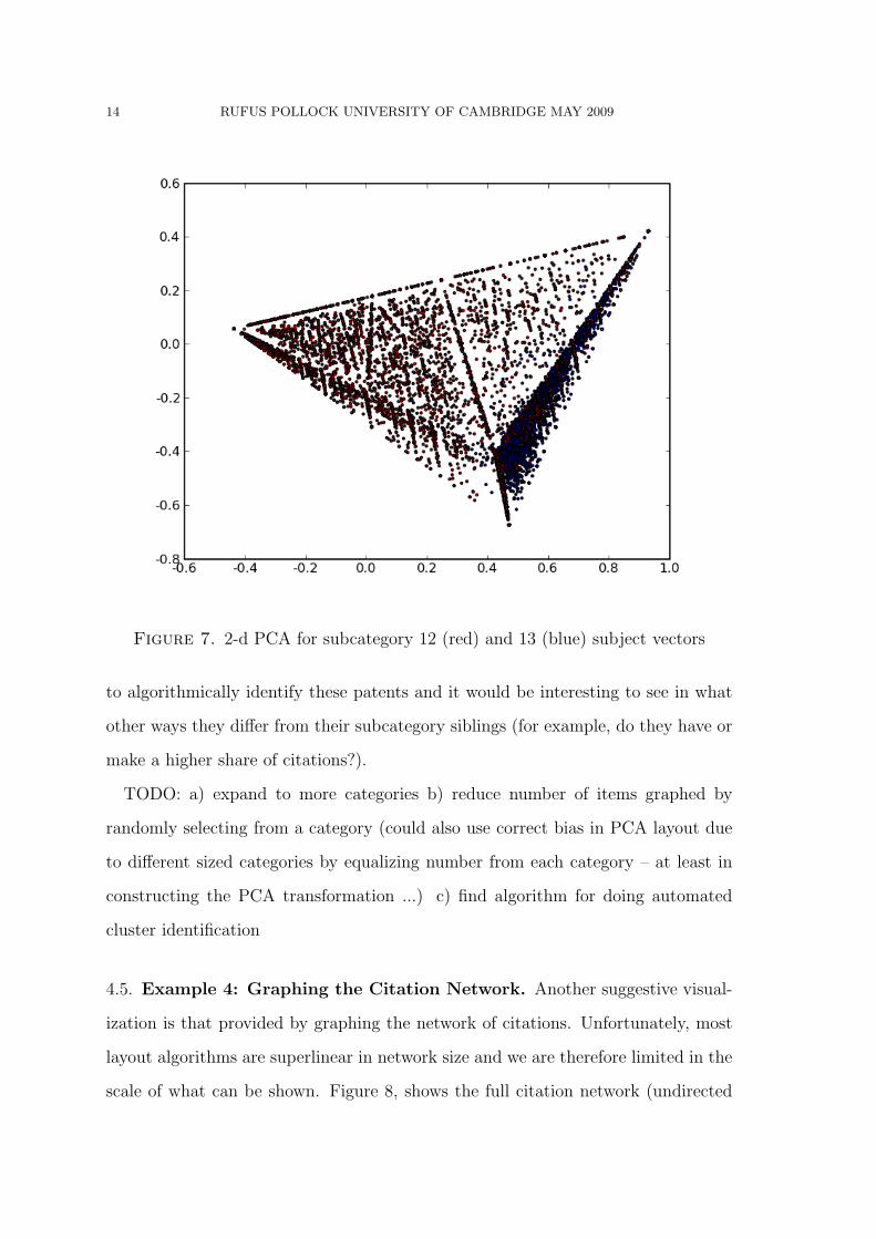
In Figure 7 we plot two separate subcategories. Here, though slightly difficult

to see because of the density of dots (it is worth ‘zooming in’), we can see a clear

separation of the categories with the majority of the 13 (blue) in a subsimplex on

the righthandside while subcat 12 (red) is spread across the simplex fairly evenly.7

Of perhaps greater interest, zooming in, we can occasional blue dots dispersed away

from the main concentration. These, then, are subcat 13 patents which are unusual

in being more similar to a subcat 12 patent than a subcat 13. It would be possible

7The fact that subcat 12 determines the overall boundaries is not a coincidence here: subcat 12 isthe larger category and hence will dominate the PCA to some extent (this could be corrected byrandomly sampling to ensure all categories contributed an equal amount to the PCA.


Figure 7. 2-d PCA for subcategory 12 (red) and 13 (blue) subject vectors

to algorithmically identify these patents and it would be interesting to see in what

other ways they differ from their subcategory siblings (for example, do they have or

make a higher share of citations?).

TODO: a) expand to more categories b) reduce number of items graphed by

randomly selecting from a category (could also use correct bias in PCA layout due

to different sized categories by equalizing number from each category – at least in

constructing the PCA transformation ...) c) find algorithm for doing automated

cluster identification

4.5. Example 4: Graphing the Citation Network. Another suggestive visual-

ization is that provided by graphing the network of citations. Unfortunately, most

layout algorithms are superlinear in network size and we are therefore limited in the

scale of what can be shown. Figure 8, shows the full citation network (undirected


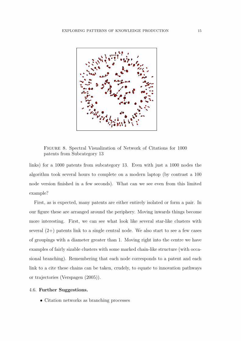
Figure 8. Spectral Visualization of Network of Citations for 1000patents from Subcategory 13

links) for a 1000 patents from subcategory 13. Even with just a 1000 nodes the

algorithm took several hours to complete on a modern laptop (by contrast a 100

node version finished in a few seconds). What can we see even from this limited

example?

First, as is expected, many patents are either entirely isolated or form a pair. In

our figure these are arranged around the periphery. Moving inwards things become

more interesting. First, we can see what look like several star-like clusters with

several (2+) patents link to a single central node. We also start to see a few cases

of groupings with a diameter greater than 1. Moving right into the centre we have

examples of fairly sizable clusters with some marked chain-like structure (with occa-

sional branching). Remembering that each node corresponds to a patent and each

link to a cite these chains can be taken, crudely, to equate to innovation pathways

or trajectories (Verspagen (2005)).

4.6. Further Suggestions.

• Citation networks as branching processes


• Evolution over time using dirichlet diffusion trees

• Classifying outliers and examining their properties

• Computing centrality (e.g. a primary eigenvector) for the citation network

and correlating that with other standard features of item value (in degree,

etc)

• Identifying items (e.g. patents) that fill ‘structural holes’

References

Albert, R. and Barabasi, A.-L. (2002). Statistical mechanics of complex networks.

Reviews of Modern Physics, 74:47.

Albert, R., Jeong, H., and Barabasi, A.-L. (2000). Error and attack tolerance of

complex networks. Nature, 406:378.

Barabasi, A. L., Jeong, H., Neda, Z., Ravasz, E., Schubert, A., and Vicsek, T.

(2002). Evolution of the social network of scientific collaborations. PHYSICA A,

311:3.

Batagelj, V. (2003). Efficient Algorithms for Citation Network Analysis.

Bilke, S. and Peterson, C. (2001). Topological properties of citation and metabolic

networks. Phys. Rev. E, 64(3):036106.

Burda, Z., Jurkiewicz, J., and Nowak, M. A. (2003). Is Econophysics a Solid Science?

ACTA PHYSICA POLONICA B, 34:87.

Callaway, D. S., Hopcroft, J. E., Kleinberg, J. M., Newman, M. E. J., and Strogatz,

S. H. (2001). Are randomly grown graphs really random? Physical Review E,

64:041902.

Callaway, D. S., Newman, M. E. J., Strogatz, S. H., and Watts, D. J. (2000). Network

robustness and fragility: Percolation on random graphs. Physical Review Letters,

85:5468.

Clauset, A., Shalizi, C. R., and Newman, M. E. J. (2007). Power-law distributions

in empirical data.


Csardi, G., Strandburg, K. J., Zalanyi, L., Tobochnik, J., and Erdi, P. (2005).

Modeling innovation by a kinetic description of the patent citation system.

Dorogovtsev, S. N. and Mendes, J. F. F. (2002). Evolution of networks. Advances

in Physics, 51:1079.

Eagly, R. V. (1975). Economics Journals as a Communications Network. Journal

of Economic Literature, 13:878–888.

Eeckhout, J (2004). Gibrat’s Law for (All) Cities. American Economic Review,

(5):1429–1451.

Fleming, L. and Sorenson, O. (2001). Technology as a complex adaptive system:

evidence from patent data. Research Policy, 30(7):1019–1039.

Frenken, K. and Boschma, R. A. (2007). A theoretical framework for evolution-

ary economic geography: industrial dynamics and urban growth as a branching

process. J Econ Geogr, 7(5):635–649.

Gallos, L. K. and Argyrakis, P. (2007). Scale-free networks resistant to intentional

attacks. EPL (Europhysics Letters), 80(5):58002 (5pp).

G.Bianconi and Barabasi, A.-L. (2000). Competition and multiscaling in evolving

networks.

Glnzel, W. and Schubert, A. (1985). Price distribution. an exact formulation of

price’s square root law. Scientometrics, 7(3):211–219.

Hall, B., Jaffe, A., and Trajtenberg, M. (2001). The NBER Patent Citations Data

File: Lessons, Insights and Methodological Tools.

Harhoff, D., von Graevenitz, G., and Wagner, S. (2008). Incidence and Growth of

Patent Thickets - The Impact of Technological Opportunities and Complexity.

CEPR Discussion Papers 6900, C.E.P.R. Discussion Papers.

Hou, Z., Kong, X., Shi, D., and Chen, G. (2008). Degree-distribution stability of

scale-free networks.

Jeong, H., Neda, Z., and Barabasi, A. L. (2003). Measuring preferential attachment

in evolving networks. EPL (Europhysics Letters), 61(4):567–572.


Leskovec, J., Kleinberg, J., and Faloutsos, C. (2005). Graphs over Time: Densifica-

tion Laws, Shrinking Diameters and Possible Explanations.

Li, X., Chen, H., Zhang, Z., and Li, J. (2007). Automatic patent classification using

citation network information: an experimental study in nanotechnology. In JCDL

’07: Proceedings of the 7th ACM/IEEE-CS joint conference on Digital libraries,

pages 419–427, New York, NY, USA. ACM.

Nelson, R. R. and Winter, S. G. (2002). Evolutionary Theorizing in Economics. The

Journal of Economic Perspectives, 16:23–46.

Newman, M. (2001). The structure of scientific collaboration networks. Proceedings

of the National Academy of Sciences, 98:404.

Newman, M. E. J. (2003). The structure and function of complex networks. SIAM

Review, 45:167.

Palacios-Huerta, I. and Volij, O. (2002). The Measurement of Intellectual Influence.

Economic theory and game theory 015, Oscar Volij.

Price, D. D. S. (1965). Networks of Scientific Papers. Science, 149:510–5.

Price, D. D. S. (1976). A general theory of bibliometric and other cumulative advan-

tage processes. Journal of the American Society for Information Science, 27(5-

6):292–306.

Rosvall, M. and Bergstrom, C. (2008). Maps of random walks on complex networks

reveal community structure. Proceedings of the National Academy of Sciences,

105(4):1118.

Simon, H. (1955). On a Class of Skew Distribution Functions. Biometrika, 42(3-

4):425–440.

Small, H. (2003). Paradigms, citations, and maps of science: a personal history. J.

Am. Soc. Inf. Sci. Technol., 54(5):394–399.

Sternitzke, C., Bartkowski, A., and Schramm, R. (2008). Visualizing patent statistics

by means of social network analysis tools. World Patent Information, In Press,

Corrected Proof.


Valverde, S., Sole, R. V., Bedau, M. A., and Packard, N. H. (2006). Topology and

evolution of technology innovation networks.

Vazquez, A. (2000). Knowing a network by walking on it: emergence of scaling.

Vazquez, A. (2001). Statistics of citation networks.

Verspagen, B. (2005). Mapping Technological Trajectories as Patent Citation Net-

works. A Study on the History of Fuel Cell Research. Technical report.

Documents

follow wisdom