Fog forecasting at Cape Town International Airport: A climatological

Fog forecasting at Cape Town International

Airport: A climatological approach

By

Lynette van Schalkwyk

Submitted in partial fulfilment of the requirements for the degree

MASTER OF SCIENCE (METEOROLOGY)

in the

Faculty of Natural & Agricultural Sciences

University of Pretoria

August 2011

©© UUnniivveerrssiittyy ooff PPrreettoorriiaa

ii

DISSERTATION SUMMARY

Fog forecasting at Cape Town International Airport: A

climatological approach

By: L. Van Schalkwyk

Supervisor: Liesl L. Dyson

Department: Geography, Geoinformatics and Meteorology

Faculty: Natural and Agricultural Sciences

University: University of Pretoria

Degree: Master of Science (Meteorology)

Cape Town International Airport (CTIA) is located along the extreme southern portion

of the west coast of South Africa which has the highest frequency of fog in the country.

Fog occurs more frequently at CTIA than at any other of the international airports in

South Africa. Fog forecasting research in South Africa has largely been neglected and

fog forecast verification results show the urgent need for improvement. Accurate fog

forecasts are imperative for the aviation industry to prevent costly flight delays and

diversions. The main aim of this research is to improve the forecasts of fog at CTIA.

The first step towards realising this aim is to provide aviation forecasters with a

comprehensive fog climatology that encompasses all aspects of fog: from the seasonal

characteristics, to detail regarding the types of fog that frequently occur, synoptic

circulations associated with fog and characteristics of the vertical profile of the lower

troposphere and boundary layer in which fog forms.

Fog types at CTIA are classified by means of an objective hierarchical classification

method that takes the formation mechanisms of fog into consideration. Self Organising

Maps (SOMs) are used as a synoptic typing method, to determine the synoptic

circulations that are most frequently associated with fog at CTIA.

iii

Case studies are presented to illustrate the formation mechanisms of 5 different fog

types by means of the synoptic circulation, surface observations, satellite imagery and

atmospheric soundings. Conclusions drawn from these case studies can assist

forecasters with the identification of potential fog events in advance.

It is recommended that climatology and case study results be made available to aviation

forecasters at CTIA and that similar studies be conducted for all international airports in

South Africa that are frequently affected by fog.

iv

ACKNOWLEDGEMENTS

“Praise the Lord from the earth, you great sea creatures and all deeps, fire and hail,

snow and mist, stormy wind fulfilling his word!”-Ps. 148:7-8-

I would like to express thanks to the following people and organisations for their

assistance and contributions to make this dissertation possible:

- My study leader Liesl, who leads by example and who’s passion for the weather

is contagious. Thank you for your friendship and patience and all the help with

programming.

- My wonderful husband for all your help and moral support. From statistical and

programming support to the beautiful flowers that regularly stood on my desk.

- My parents for their support and regular phone calls.

- The staff at the SAWS Cape Town Weather Office, especially the forecasters as

well as Johan Stander, Rian Smit, Gail Linnow and Jan Crous (who saved the

precious digitized hourly data!).

- Retired forecasters Steve Medcalf, Keith Moir and Niek Koegelenberg for your

valuable input from years of fog forecasting experience.

- Anastasia Demertzis and Colleen de Villiers from the SAWS for supplying me

with literature and data needed for this research.

- Christien Engelbrecht, Chantal Greenwood, Candice McKechnie, Prof. Jana

Olivier, Gerry O’Loghlen and Lee-ann Simpson, for providing me with the

necessary background information and programs.

- Prof. Johan van Heerden and Liesl Dyson for financial support to attend the fog

conference in Germany.

- My friend and forecaster partner, Luis Fernandes, for your support and hours of

weather talk.

- Eumetsat for delivering satellite imagery to my doorstep free of charge.

v

TABLE OF CONTENTS

1 INTRODUCTION ............................................................................................................1

1.1 BACKGROUND....................................................................................................1

1.1.1 Climate and location of Cape Town International Airport .............................1

1.1.2 Fog as a resource and risk in South Africa......................................................5

1.1.3 The influence of fog on the aviation industry .................................................8

1.2 AIMS ....................................................................................................................10

1.2.1 Verify the accuracy of fog forecasts at CTIA ...............................................10

1.2.2 Determine the characteristics of fog at Cape Town International Airport

in the Western Cape....................................................................................................10

1.2.3 Facilitate the improvement of fog forecasts at CTIA. ..................................11

1.3 OUTLINE OF THIS DOCUMENT....................................................................11

2 DEFINITIONS, DATA AND METHODOLOGY .....................................................12

2.1 VERIFICATION OF FOG FORECASTS..........................................................12

2.1.1 Data.................................................................................................................12

2.1.2 Methodology ..................................................................................................13

2.1.3 Categorical Statistics......................................................................................15

2.2 FOG CLIMATOLOGY .......................................................................................17

2.2.1 Fog definitions ...............................................................................................18

2.2.2 Fog type definitions .......................................................................................19

2.2.3 Data.................................................................................................................21

2.2.4 Methodology ..................................................................................................23

2.3 SYNOPTIC CLASSIFICATION ........................................................................26

2.3.1 Data.................................................................................................................26

2.3.2 Methodology ..................................................................................................27

2.4 ATMOSPHERIC SOUNDINGS.........................................................................28

2.4.1 Data.................................................................................................................28

2.4.2 Methodology ..................................................................................................28

2.5 SUMMARY .........................................................................................................30

3 VERIFICATION RESULTS ........................................................................................31

3.1 GENERAL VERIFICATION OF FOG FORECASTS AT CTIA.....................31

vi

3.1.1 Percentage Correct .........................................................................................33

3.1.2 Bias .................................................................................................................33

3.1.3 Probability of detection..................................................................................33

3.1.4 Critical Success Index....................................................................................34

3.1.5 False Alarm Ratio ..........................................................................................34

3.2 EVALUATION OF VISIBILITY FORECASTS...............................................36

3.2.1 Forecasts of visibility less than 1000m .........................................................38

3.2.2 Forecasts of visibility less than or equal to 1000m.......................................39

3.2.3 Forecasts of visibility less than or equal to 5000m.......................................39

3.3 DISCUSSION OF VERIFICATION RESULTS................................................39

4 CLIMATOLOGY...........................................................................................................41

4.1 FOG SEASON .....................................................................................................42

4.2 FOG TYPES AT CTIA........................................................................................46

4.2.1 Fog type frequency.........................................................................................47

4.2.2 Fog intensity and duration .............................................................................50

4.2.3 Diurnal variability of fog onset and dissipation............................................52

4.2.4 Flaws in the hierarchical fog type classification method..............................56

4.2.5 Summary ........................................................................................................57

4.3 SYNOPTIC CLASSIFICATION ........................................................................58

4.3.1 Dominant synoptic types ...............................................................................58

4.3.2 Synoptic circulations related to fog occurrence ............................................60

4.3.3 Fog types related to synoptic circulation.......................................................66

4.3.4 Summary ........................................................................................................71

4.4 ATMOSPHERIC SOUNDINGS.........................................................................72

4.4.1 Atmospheric variables on fog days, non-fog days and the long term

average ........................................................................................................................72

4.4.2 Average temperature and relative humidity anomalies on fog days ............77

4.4.3 Characteristics of atmospheric variables in the lower troposphere ..............79

4.4.4 Summary ........................................................................................................83

5 CASE STUDIES .............................................................................................................84

5.1 ADVECTION FOG FROM THE SOUTH: 2 APRIL 2010...............................85

5.1.1 Introduction ....................................................................................................85

5.1.2 Synoptic circulation .......................................................................................86

5.1.3 Synoptic classification ...................................................................................87

vii

5.1.4 Surface observations and atmospheric sounding ..........................................88

5.1.5 Satellite imagery.............................................................................................90

5.1.6 Conclusion......................................................................................................91

5.2 ADVECTION FOG FROM THE NORTHWEST: 5 MARCH 2010................92

5.2.1 Introduction ....................................................................................................92

5.2.2 Synoptic circulation .......................................................................................93

5.2.3 Synoptic classification ...................................................................................94

5.2.4 Surface observations and atmospheric sounding ..........................................95

5.2.5 Satellite imagery.............................................................................................97

5.2.6 Conclusion......................................................................................................99

5.3 CLOUD BASE LOWERING FOG: 19 JUNE 2006 ..........................................99

5.3.1 Introduction ....................................................................................................99

5.3.2 Synoptic circulation .....................................................................................100

5.3.3 Synoptic classification .................................................................................101

5.3.4 Surface observations and atmospheric sounding ........................................102

5.3.5 Satellite imagery...........................................................................................104

5.3.6 Conclusion....................................................................................................105

5.4 RADIATION FOG: 25 AUGUST 2009 ...........................................................106

5.4.1 Introduction ..................................................................................................106




5.4.5 Satellite imagery...........................................................................................110

5.4.6 Conclusion....................................................................................................111

5.5 EVAPORATION FOG: 8 APRIL 2002............................................................112

5.5.1 Introduction ..................................................................................................112




5.5.5 Conclusion....................................................................................................116

5.6 SUMMARY .......................................................................................................116

6 SUMMARY, CONCLUSION AND RECOMMENDATIONS ..............................118

6.1 GENERAL SUMMARY...................................................................................118

6.2 SUMMARY OF MOST SIGNIFICANT RESULTS.......................................119

viii

6.2.1 Verification...................................................................................................119

6.2.2 Climatology..................................................................................................119

6.2.3 Case studies ..................................................................................................124

6.3 CONCLUSIONS................................................................................................124

6.3.1 General .........................................................................................................124

6.3.2 Conclusions of importance in an operational forecast environment ..........126

6.3.3 Practical application of this research...........................................................126

6.4 RECOMMENDATIONS...................................................................................128

REFERENCES....................................................................................................................130

APPENDIX A ......................................................................................................................134

ix

LIST OF FIGURES

Figure 1.1 The location of Cape Town International Airport (CTIA) at 33°58’10”S

and 18°35’50”E. ...........................................................................................................1

Figure 1.2 Average Sea Surface Temperatures (1998-2008) in False Bay

(Muizenberg) and along the southern portion of the West coast of South-Africa

(Kommetjie and Koeberg)............................................................................................2

Figure 1.3 Spatial distribution of fog in South Africa (WB40) (Adapted from: Olivier

and Van Heerden, 1999)...............................................................................................6

Figure 2.1 Fog forecast verification procedure: Step 1. (A, B, C and D refer to each

category represented in Table 2.1.) ............................................................................13

Figure 2.2 Time line illustrating the evaluation process of forecasts and observations.

TAF 1 contains a ‘hit’: fog was forecast and observed (a). TAF 2 contains a

‘miss’: fog was observed during TAF 2’s validity period, but not forecast. ............14

Figure 2.3 Fog forecast verification procedure: Step 2: (A, B, C and D refer to each

category represented in Table 2.1). ............................................................................15

Figure 2.4 Decision tree illustrating the fog type classification method (after Tardif and

Rasmussen, 2007). Different colours represent different fog types..........................23

Figure 2.5 Wind rose for fog days at CTIA at 06:00UTC, March-August, (1978-2008) ....24

Figure 2.6 Spatial domain used for the MSLP SOM domain................................................27

Figure 3.1 Yearly POD, CSI and FAR values for the general verification of fog and

mist days during March-August.................................................................................34

Figure 3.2 Monthly CSI, POD and FAR values for all fog and mist observations (2004-

2007). ..........................................................................................................................35

Figure 3.3 POD, CSI and FAR values for different visibility thresholds (March-August,

2004-2007)..................................................................................................................38

Figure 4.1 Average number of fog and mist days (1978-2008) per month with

visibilities less than or equal to 5000m......................................................................43

Figure 4.2 Same as for Fig. 4.1, but for visibilities below 1000m. .......................................43

Figure 4.3 Average number of fog and mist observations per month with visibilities less

than or equal to 5000 m at 06:00, 12:00 and 18:00UTC (1978-2008). ....................44

Figure 4.4 Same as Fig. 4.3 but for visibilities below 1000m. ..............................................45

x

Figure 4.5 Number of fog days with surface visibility below 1000m (1978-2008).

Linear trend line (purple) shows a decreasing trend in the number of fog days. .....46

Figure 4.6 Overall event frequency of different fog types (March to August, 1997-

2010). ..........................................................................................................................47

Figure 4.7 Pollution on the Cape Flats after sunrise in July 2011. The Location of CTIA

is highlighted by the yellow box. (Photo courtesy: H. van Schalkwyk)...................48

Figure 4.8 Frequencies of different fog types during the fog season. ...................................48

Figure 4.9 Frequency of wind direction at the onset of advection fog events (March to

August, 1997-2010)....................................................................................................49

Figure 4.10 Box and whisker plots illustrating the distribution of minimum visibility

during fog events for each fog type (March to August, 1997-2010). Grey boxes

denote 25th to 75th percentiles, while the solid black bar indicates the median

value. The vertical lines (whiskers) extend to the maximum and minimum

values. .........................................................................................................................51

Figure 4.11 Same as Fig. 4.10, but for event duration of each fog type (March-August,

1997-2010)..................................................................................................................51

Figure 4.12 Frequency of fog formation time (black bars) and fog dissipation time (grey

bars) relative to sunrise time (s). Data are for radiation fog events at CTIA,

March to August, (1997-2010)...................................................................................53

Figure 4.13 Same as Fig. 4.12, but data are for cloud base lowering fog events at CTIA,

March to August, (1997-2010)...................................................................................53

Figure 4.14 Same as Fig. 4.12, but data are for advection fog events at CTIA, March to

August, (1997-2010)...................................................................................................54

Figure 4.15 Same as Fig. 4.10, but for event onset time relative to sunrise (s) for each

fog type (March-August, 1997-2010). .......................................................................54

Figure 4.16 Same as Fig. 4.10, but for event dissipation time relative to sunrise (s) for

each fog type (March-August, 1997-2010). ..............................................................56

Figure 4.17 The 5x7 SOM of sea level pressure (March-August, 1997-2010) centred

about the south-western Cape. ...................................................................................59

Figure 4.18 Frequency (%) of days between 1997 and 2010 mapping to each node (A1

to G5). .........................................................................................................................60

Figure 4.19 Contour plot illustrating the frequency of fog events that occurred per node...61

Figure 4.20 Contour plot illustrating the probability of fog associated with each node.......61

xi

Figure 4.21 I-VI. Contour plot illustrating the number of fog events per synoptic

circulation for the months March (I) to August (VI) (1997-2010). ..........................63

Figure 4.22 Frequency of fog types per node (March-August, 1997-2010). Advection

fog indicated in grey (A), radiation fog: black (R), CBL fog: diagonal lines (C),

‟unknown” events: dark grey (U) and evaporation fog: white (E). ..........................66

Figure 4.23 Node E2 displaying the synoptic circulation associated with most fog

events during the fog season (1997-2010) at CTIA. .................................................67

Figure 4.24 Frequency of radiation fog per node (March-August, 1997-2010). ..................67

Figure 4.25 Nodes F3, E2, D3 and G5 displaying the synoptic circulations associated

with most radiation events during the fog season (1997-2010). ...............................68

Figure 4.26 Frequency of CBL fog per node (March-August, 1997-2010)..........................68

Figure 4.27 Nodes C3, D3 and C2 displaying the synoptic circulations associated with

most CBL events during the fog season (1997-2010)...............................................69

Figure 4.28 Frequency of advection fog per node (March-August, 1997-2010)..................69

Figure 4.29 Nodes F2, E2 and A3 displaying the synoptic circulations associated with

most advection events during the fog season (1997-2010). ......................................70

Figure 4.30 Frequency of unknown fog events per node (March-August, 1997-2010). ......70

Figure 4.31 Nodes A2 and B2 displaying the synoptic circulations associated with most

unknown events during the fog season (1997-2010).................................................71

Figure 4.32 The average temperature and dew point temperature at 00:00UTC for CTIA

(1997-2010) from the surface to 200hPa. ..................................................................73

Figure 4.33 Same as fig.4.a but from the surface to 750hPa.................................................74

Figure 4.34 Average heights of lower and upper levels of a temperature inversion in feet

above ground level per month....................................................................................75

Figure 4.35 Average wind profile during the fog season at 00:00UTC for CTIA (1997-

2010) between 1000 and 700hPa. Long term average (red), non- fog days

(green) and fog days (blue). .......................................................................................76

Figure 4.36 Temperature anomalies (˚C) during the fog season at 00:00UTC for fog

days. ............................................................................................................................78

Figure 4.37 Relative humidity (RH) anomalies during the fog season at 00:00UTC for

fog days.......................................................................................................................79

Figure 4.38 Box and whisker plots illustrating the distribution of average temperature

(°C) between 1000 and 700hPa for fog days and non-fog days (March to

August, 1997-2010). Grey boxes denote 25th to 75th percentiles, while the solid

xii

black bar indicates the median value. The vertical lines (whiskers) extend to the

maximum and minimum values.................................................................................80

Figure 4.39 Same as Fig. 4.38, but for the distribution of average relative humidity

(RH) below the temperature inversion on fog days relative to non-fog days

(March-August, 1997-2010). .....................................................................................81

Figure 4.40 Same as Fig. 4.38, but for the distribution of average relative humidity

(RH) between 925 and 850hPa on fog days relative to non-fog days (March-

August, 1997-2010)....................................................................................................81

Figure 4.41 Same as Fig. 4.38, but for the distribution of surface dewpoint temperatures

(°C) on fog days relative to non-fog days (March-August, 1997-2010). .................82

Figure 4.42 Same as Fig. 4.38, but for the distribution of geopotential thickness (m) on

fog days relative to non-fog days (March-August, 1997-2010)................................83

Figure 5.1 MSG satellite, Natural Colour RGB: 2010-04-02, 06:00UTC. The white area

along the coastal regions is fog. © (2010) Eumetsat.................................................85

Figure 5.2 Sea level pressure (Pa) for 2010-04-01 00:00UTC (A) to 2010-04-02

12:00UTC (F). Location of a cold front indicated in bottom-left corner of “F”. .....87

Figure 5.3 Node C3 of Fig. 4.17 associated with the synoptic circulation at 00:00UTC

during the southerly advection fog event on 2 April 2010........................................88

Figure 5.4 Surface observations from 2011-04-01 till 2011-04-02: Visibility associated

with FG (fog), BR (mist) and BCFG (fog patches): For example 5K=5000m,

2K=2000m, 900=900m. Cloud cover: FEW (1-2 octas), SCT (3-4 octas), BKN

(5-7 octas) and OVC (8 octas). Cloud base in feet for example: 008=800ft,

010=1000ft..................................................................................................................89

Figure 5.5 Skew-T, log p plot of temperature (right) and dew point temperature (left) at

CTIA on 2010-04-02 00:00UTC. The wind speed (knots) and direction are

shown in the extreme right. (Courtesy of SAWS and the University of

Wyoming). ..................................................................................................................90

Figure 5.6 MSG Satellite, Fog RGB from 2010-04-01 22:00UTC (A) till 2010-04-02

03:00UTC (F). CTIA's position indicated with a green circle at "CT". Black

arrow (A) shows fog that developed to the northeast of CTIA before fog was

reported in observations (©, (2010) Eumetsat). ........................................................91

Figure 5.7 As Fig. 5.1 but for 2010-03-05, 07:00UTC..........................................................93

Figure 5.8 Sea level pressure (Pa) for 2010-03-04 12:00UTC (A) to 2010-03-05

06:00UTC (D).............................................................................................................94

xiii

Figure 5.9 Node B2 of Fig. 4.17 associated with the synoptic circulation at 00:00UTC

during a north-westerly advection fog event on 5 March 2010. ...............................95

Figure 5.10 As in Fig. 5.4, but meteogram for CTIA from 10:00UTC 2010-03-04 to

10:00UTC 2010-03-05. ..............................................................................................96

Figure 5.11 Same as Fig. 5.5, but for 2010-03-05, 00:00UTC..............................................97

Figure 5.12 Same as Figure 5.6, but fog RGB at 2-hourly intervals from 2010-03-04

18:00UTC (A) till 2010-03-05 04:00UTC (F). Fog bank and region of clear

skies labelled as such in A. The black arrow in F indicating fog that formed to

the east of Cape Agulhas (© (2010) Eumetsat). ........................................................98

Figure 5.13 As Fig. 5.1 but for 2006-06-18, 14:00UTC......................................................100

Figure 5.14 Sea level pressure (Pa) for 2006-06-18, 18:00UTC (A) to 2006-06-19,

12:00UTC (D)...........................................................................................................101

Figure 5.15 Node F5 of Fig. 4.17 associated with the synoptic circulation during a CBL

fog event on 19 June 2006........................................................................................102


14:00UTC 2006-06-19. ............................................................................................103

Figure 5.17 Same as Fig. 5.5 but for 2006-06-19, 00:00UTC.............................................104

Figure 5.18 Same as Fig. 5.6, but Fog RGB at 2-hourly intervals from 2006-06-18

20:00UTC (A) till 2006-06-19 06:00UTC (F). Black arrow indicates cirrus

cloud..........................................................................................................................105

Figure 5.19 As Fig. 5.1 but for 2009-08-25, 08:00UTC......................................................106

Figure 5.20 Sea level pressure (Pa) for 2009-08-25 00:00UTC (A) and 06:00UTC (B). ..107

Figure 5.21 Node D3 of Fig. 4.17 associated with the synoptic circulation during a

radiation fog event on 25 August 2009....................................................................108


10:00UTC 2009-08-25. ............................................................................................109

Figure 5.23 Same as Fig. 5.5 but for 2009-08-25, 00:00UTC.............................................110

Figure 5.24 Same as Fig. 5.6, but Fog RGB at hourly intervals from 2009-08-25

00:00UTC (A) till 2009-08-25 05:00UTC (F). .......................................................111

Figure 5.25 Same as Fig. 5.2, but sea level pressure fields for 2002-04-07 18:00UTC

(A) till 2002-04-08 06:00UTC (C). .........................................................................113

Figure 5.26 Node A2 of Fig. 4.17 associated with the synoptic circulation during the

evaporation fog event on 8 April 2002. ...................................................................114

xiv


10:00UTC 2002-04-08. ............................................................................................114

Figure 5.28 Same as Fig. 5.5 but for 2002-04-07 12:00UTC (A) and 2002-04-08

00:00UTC (B)...........................................................................................................116

Figure 6.1 Synoptic circulation patterns associated with most radiation events during

the fog season. ..........................................................................................................121

Figure 6.2 Same as Fig. 6.1 but for CBL fog events............................................................122

Figure 6.3 Same as Fig. 6.1 but for advection fog events....................................................123

xv

LIST OF TABLES

Table 1.1 Maximum (Tx) and minimum (Tn) air temperatures for a few interior (*) and

coastal stations along the Southwest Coast..................................................................3

Table 2.1 Schematic contingency table for forecasts of a binary event. The numbers of

observations in each category represented by A, B, C and D and N is the total

(after Jolliffe et al, 2003). ...........................................................................................14

Table 3.1 Categorisation of all fog and mist forecasts and observations in a contingency

table.............................................................................................................................32

Table 3.2 General verification results for all fog or mist forecasts and observations at

CTIA (March to August, 2004-2007). .......................................................................32

Table 3.3 Yearly Percentage Correct and Bias values of general verification......................32

Table 3.4 Monthly Percentage Correct and Bias values of general verification...................33

Table 3.5 Yearly contingency tables of general verification (a. to d.). .................................35

Table 3.6 Monthly contingency tables of general verification (a to f). .................................36

Table 3.7 Contingency table for different visibility thresholds between March and

August (2004-2007)....................................................................................................37

Table 3.8 Percentage correct and bias values for different visibility thresholds...................37

Table 4.1 Nodes with the highest number of fog events for each month of the fog

season (1997-2010). ...................................................................................................65

xvi

LIST OF DEFINITIONS

Fog: When the obstruction to vision consists of water droplets or ice crystals and the

visibility has been reduced to less than 1000m.

Advection fog: When there is a sudden onset of fog with wind speeds of 3ms-1 or more

and the cloud base height is less than 600ft.

Cloud base lowering fog: When fog forms due to the lowering of cloud bases within a

5 hour period prior to fog onset, with an initial cloud base height below 1km.

Evaporation fog: When fog forms within the first hour after sunrise, associated with a

rise in dewpoint temperature that exceeds the rise in temperature.

Precipitation fog: When fog forms due to the evaporation of precipitation that falls

through a cold layer of moist air.

Radiation fog: When fog forms under clear skies or lifting cloud bases after sunset and

before sunrise, accompanied by a cooling trend before fog onset, if wind speeds prior to

onset are less than 3ms-1.

Mist: When the obstruction, due to ice crystals or water droplets, reduces the visibility

to at least 1000m, but not more than 5000m

Fog day: A day when there was one or more observation of fog or mist

Fog event: When fog occurs and lasts 3 or more consecutive hours with an observed

surface visibility less than 5000m, and at least one observation of surface visibility less

than 1000m.

CAVOK: Aviation code word included in METARs and TAFs when the visibility is

10km or more, there is no cloud below 5000ft or below the highest minimum sector

altitude, which ever is the greater, and there is no Cumulonimbus cloud or significant

weather phenomena.

Knots: Unit of speed equal to 0.51m.s-1 or 1.85km.h-1.

xvii

LIST OF ABBREVIATIONS

- AGL: Above ground level

- BOM: Bureau of Meteorology

- CAVOK: Ceiling And Visibility Okay.

- CSI: Critical success index

- CTIA: Cape Town International Airport

- FACT: ICAO location indicator for Cape Town International Airport

- FAR: False alarm rate

- ICAO: International Civil Aviation Organization

- ILS: Instrument landing system

- LIFR: Low instrument flight rules

- METAR: Meteorological Aerodrome Report

- MSG: Meteosat Second Generation

- MSLP: Mean sea level pressure

- NCEP: National Centres for Environmental Prediction

- NWP: Numerical Weather Prediction

- PC: Percent correct

- POD: Probability of detection

- RGB: Red-Green-Blue

xviii

- RVR: Runway visual range

- SAST: South African Standard Time (UTC+2 hours)

- SAWB: South African Weather Bureau

- SAWS: South African Weather Service

- SOMs: Self-organising maps

- SSTs: Sea Surface Temperatures

- SUMO: Software for the Utilisation of Meteosat in Outlook activities

- TAF: Terminal Aerodrome Forecast

- UTC: Coordinated Universal Time (SAST-2 hours)

- VFR: – Visual flight rules

- WMO: World Meteorological Organization

1

CHAPTER 1

INTRODUCTION

1 INTRODUCTION

1.1 BACKGROUND

1.1.1 Climate and location of Cape Town International Airport

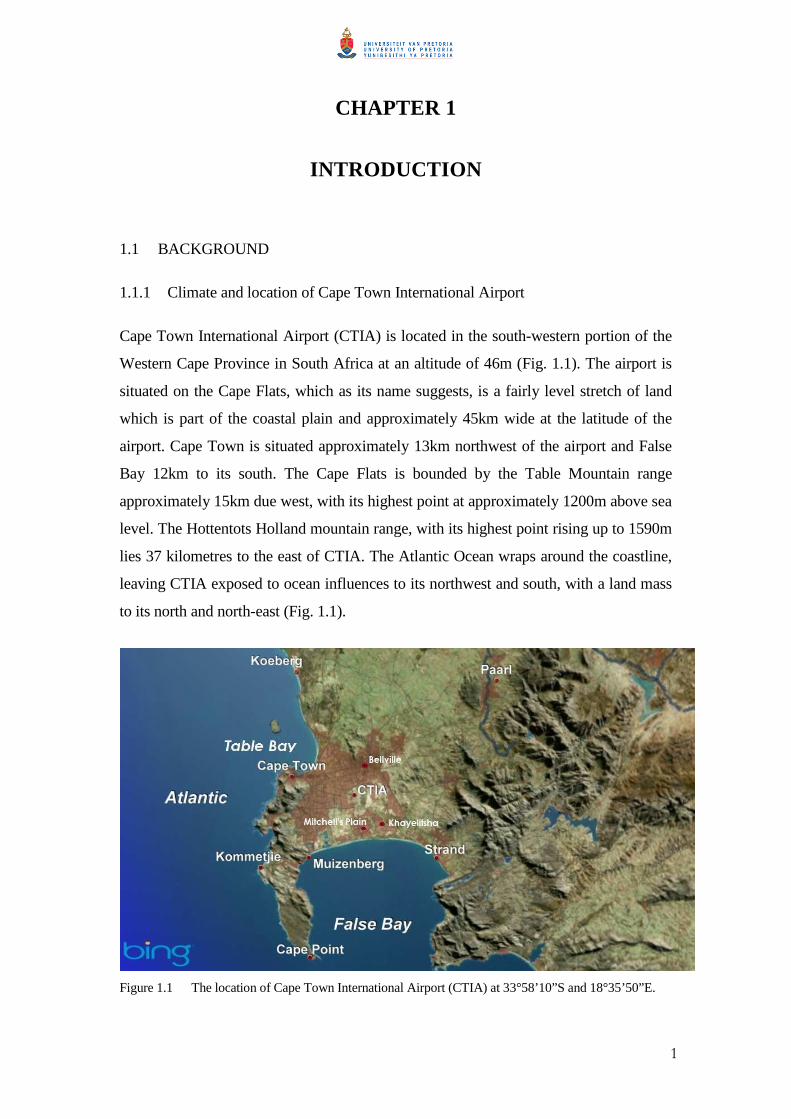
Cape Town International Airport (CTIA) is located in the south-western portion of the

Western Cape Province in South Africa at an altitude of 46m (Fig. 1.1). The airport is

situated on the Cape Flats, which as its name suggests, is a fairly level stretch of land

which is part of the coastal plain and approximately 45km wide at the latitude of the

airport. Cape Town is situated approximately 13km northwest of the airport and False

Bay 12km to its south. The Cape Flats is bounded by the Table Mountain range

approximately 15km due west, with its highest point at approximately 1200m above sea

level. The Hottentots Holland mountain range, with its highest point rising up to 1590m

lies 37 kilometres to the east of CTIA. The Atlantic Ocean wraps around the coastline,

leaving CTIA exposed to ocean influences to its northwest and south, with a land mass

to its north and north-east (Fig. 1.1).

Figure 1.1 The location of Cape Town International Airport (CTIA) at 33°58’10”S and 18°35’50”E.

2

CTIA is affected by a very prominent wind regime that differs greatly from winter to

summer. The prevailing winds are from the southeast to southwest in summer (October

to March) and from the north to northwest in winter (May to August). In summer a high

percentage of wind velocities (at least 30%) are in the range of 7 to 13m.s-1

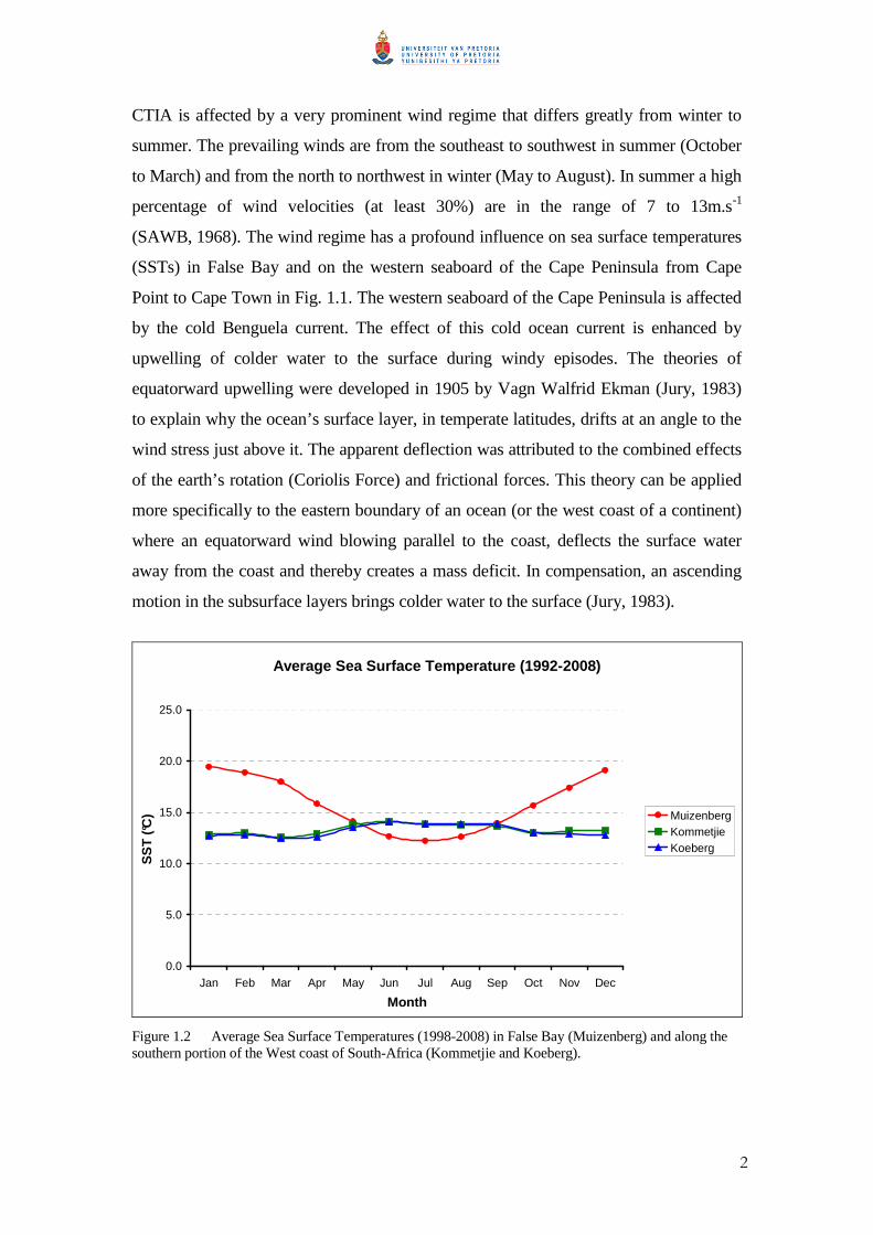
(SAWB, 1968). The wind regime has a profound influence on sea surface temperatures

(SSTs) in False Bay and on the western seaboard of the Cape Peninsula from Cape

Point to Cape Town in Fig. 1.1. The western seaboard of the Cape Peninsula is affected

by the cold Benguela current. The effect of this cold ocean current is enhanced by

upwelling of colder water to the surface during windy episodes. The theories of

equatorward upwelling were developed in 1905 by Vagn Walfrid Ekman (Jury, 1983)

to explain why the ocean’s surface layer, in temperate latitudes, drifts at an angle to the

wind stress just above it. The apparent deflection was attributed to the combined effects

of the earth’s rotation (Coriolis Force) and frictional forces. This theory can be applied

more specifically to the eastern boundary of an ocean (or the west coast of a continent)

where an equatorward wind blowing parallel to the coast, deflects the surface water

away from the coast and thereby creates a mass deficit. In compensation, an ascending

motion in the subsurface layers brings colder water to the surface (Jury, 1983).

Average Sea Surface Temperature (1992-2008)

0.0

5.0

10.0

15.0

20.0

25.0

Jan Feb Mar Apr May Jun Jul Aug Sep Oct Nov Dec

Month

SS

T (

°C) Muizenberg

KommetjieKoeberg

Figure 1.2 Average Sea Surface Temperatures (1998-2008) in False Bay (Muizenberg) and along the southern portion of the West coast of South-Africa (Kommetjie and Koeberg).

3

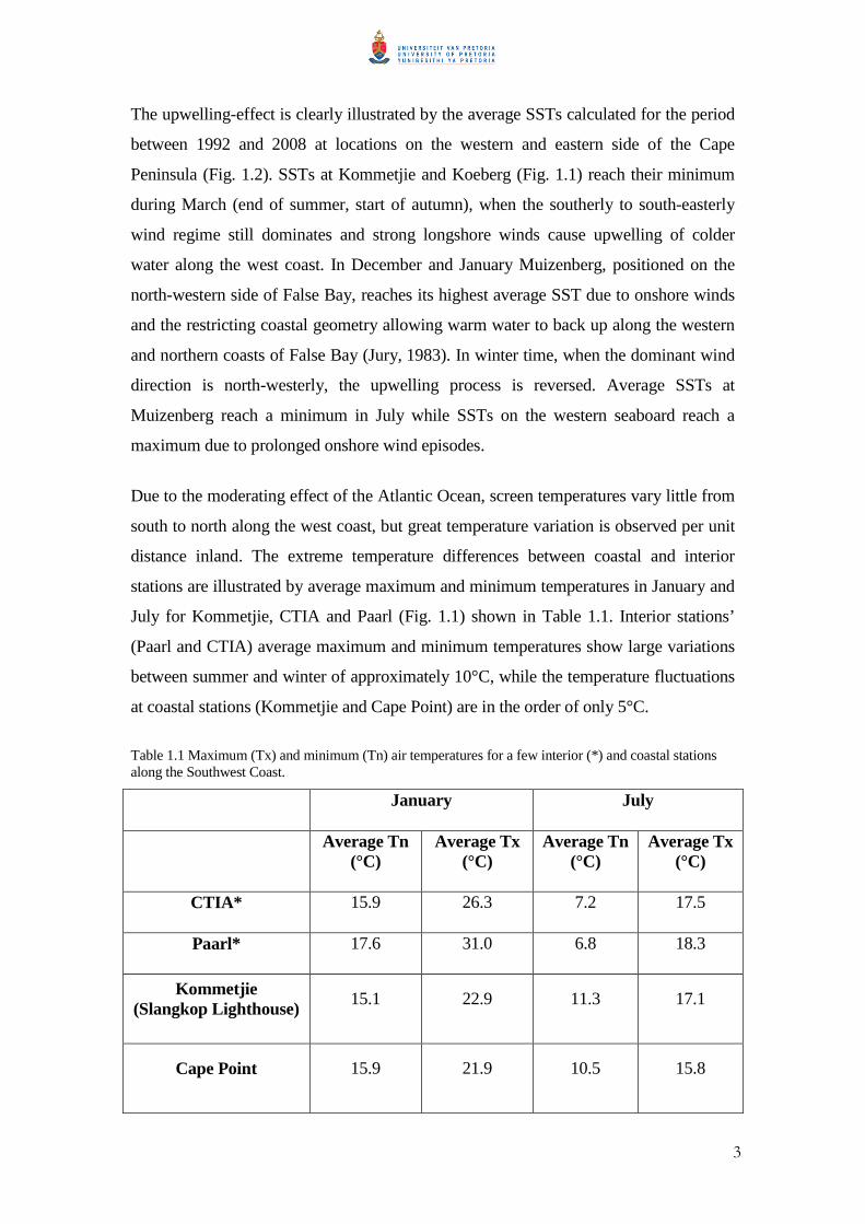
The upwelling-effect is clearly illustrated by the average SSTs calculated for the period

between 1992 and 2008 at locations on the western and eastern side of the Cape

Peninsula (Fig. 1.2). SSTs at Kommetjie and Koeberg (Fig. 1.1) reach their minimum

during March (end of summer, start of autumn), when the southerly to south-easterly

wind regime still dominates and strong longshore winds cause upwelling of colder

water along the west coast. In December and January Muizenberg, positioned on the

north-western side of False Bay, reaches its highest average SST due to onshore winds

and the restricting coastal geometry allowing warm water to back up along the western

and northern coasts of False Bay (Jury, 1983). In winter time, when the dominant wind

direction is north-westerly, the upwelling process is reversed. Average SSTs at

Muizenberg reach a minimum in July while SSTs on the western seaboard reach a

maximum due to prolonged onshore wind episodes.

Due to the moderating effect of the Atlantic Ocean, screen temperatures vary little from

south to north along the west coast, but great temperature variation is observed per unit

distance inland. The extreme temperature differences between coastal and interior

stations are illustrated by average maximum and minimum temperatures in January and

July for Kommetjie, CTIA and Paarl (Fig. 1.1) shown in Table 1.1. Interior stations’

(Paarl and CTIA) average maximum and minimum temperatures show large variations

between summer and winter of approximately 10°C, while the temperature fluctuations

at coastal stations (Kommetjie and Cape Point) are in the order of only 5°C.

Table 1.1 Maximum (Tx) and minimum (Tn) air temperatures for a few interior (*) and coastal stations along the Southwest Coast.

January July

Average Tn (°C)

Average Tx (°C)

Average Tn (°C)

Average Tx (°C)

CTIA* 15.9 26.3 7.2 17.5

Paarl* 17.6 31.0 6.8 18.3

Kommetjie (Slangkop Lighthouse)

15.1 22.9 11.3 17.1

Cape Point 15.9 21.9 10.5 15.8

4

The south-western Cape receives its maximum rainfall in winter from May to August.

Due to the mountainous nature of the region, rainfall averages vary significantly from

place to place. For instance, the rainfall varies from 250mm on the West Coast to

1400mm on the slopes of Table Mountain. CTIA receives approximately 500mm

rainfall annually, while the amount increases to 1300mm in the suburbs of Cape Town

on the eastern slopes of Table Mountain (SAWB, 1996).

Snow does not occur at CTIA but the surrounding mountain ranges, including Table

Mountain on rare occasions, do experience snowfalls in winter. Thunderstorms occur

rarely at CTIA with an annual frequency of approximately 7 days per year, but CTIA is

frequently affected by fog (SAWB, 1968). The occurrence and nature of fog events at

CTIA will be discussed extensively in this dissertation.

A synoptic circulation type frequently associated with fog at CTIA is the coastal low

(SAWB, 1968). The coastal lows that occur along the South African coastal belt are

local shallow systems associated with intense and rapid weather changes. These

changes always occur in the form of a change in wind direction and speed, and a

temperature change from relatively hot, to cool post-low conditions. These weather

changes may be accompanied by low cloud, fog or drizzle (Carter, 2005). Three types

of coastal lows have been identified in South Africa (CLW, 1984 cited in Carter,

2005:28):

- Type 1: The “summer” west coast low, which takes place predominantly in

summer.

- Type 2: The “travelling” coastal low which is associated with a high pressure

system ridging to the south, which leads to the formation of a coastal low along the

west coast. The coastal low moves down the west coast while its associated cold

front approaches from the west, where after the coastal low propagates ahead of the

cold front along the south and southeast coasts.

- Type 3: The “winter” coastal low which takes place predominantly in winter. In this

case the South Atlantic High does not ridge in south of the continent, but is

positioned slightly further north. In such a case a series of cold fronts can pass over

the south of the country in association with a single westerly wave. Prior to the

5

passage of the first cold front, the coastal low will be established along the south

coast where after it will act as a leader low pressure cell along the east coast.

Any of these three synoptic situations or classes of coastal lows can occur at any time of

the year. Furthermore it was found that there is often no link between the coastal low on

the west coast and the one on the south coast, with the west coast low remaining semi-

stationary and the south coast coastal low forming ahead of the approaching cold front

(CLW, 1984 cited in Carter, 2005:28).

1.1.2 Fog as a resource and risk in South Africa

Fog is defined as an obscurity in the surface layers of the atmosphere and is caused by

particles of condensed moisture held in suspension in the air (McIntosh, 1972). By

international definition fog reduces visibility to less than 1km and forms when the

relative humidity of the air approaches 100%. Mist occurs when this very low cloud is

associated with a visibility of a 1000m or more and with relative humidity between 95

and 100%, but generally less than 100% (AMS, 2010).

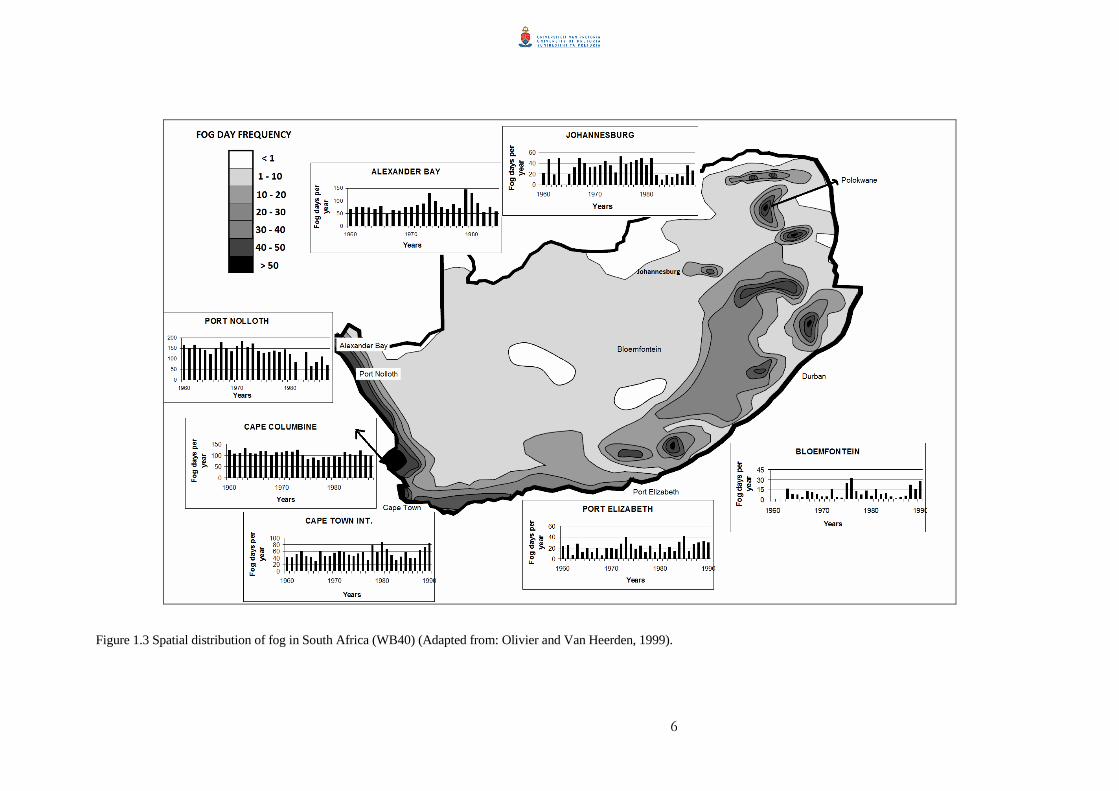
In South Africa the highest fog frequencies occur along the west coast where fog is

observed on more than 50 days per year on average (Fig. 1.3) (Olivier and Van

Heerden, 1999). The sea surface temperature along the west coast varies between

13-15°C and with the arid, hot land surface, advection fog occurs almost exclusively

and throughout the year (Olivier and Van Heerden, 1999). The number of fog days

decrease slightly towards the southwest coast; at CTIA there are on average 44 days

with fog per year with April to July being the months with the most fog days. More than

6 days with fog occur on average during these months. (SAWS, 1998). There is a

general decrease in fog days along the coast from west to east to such an extent that Port

Elizabeth Airport receives only 9 days with fog and Durban International Airport only 2

fog days a year.

6

Figure 1.3 Spatial distribution of fog in South Africa (WB40) (Adapted from: Olivier and Van Heerden, 1999).

7

Southern Africa is characterised by a moderately elevated plateau, for the greater part

rising to over 1000m above sea level and to more than 1500m over extensive areas

(Taljaard, 1994). O.R. Tambo International Airport (Johannesburg), the busiest

international airport in Africa, is situated over this highveld and receives just over

30 days of fog per year. The radiation process is the primary cause of fog at this airport

and the months with the highest frequency of fog days are March-May (approximately

3 fog days per month), (SAWS, 1998). The Southern African plateau rises steeply in

most areas over the first 200-300km from the coast and over south-eastern South Africa

the main escarpment rises to 1500m or more (Taljaard, 1994). Fog occurs along this

escarpment when the flow becomes onshore and moist air is forced to rise resulting in

condensation and fog or cloud formation.

Reduced visibility as a result of fog poses a great risk to road users in fog prone areas

and is regarded as one of the most dangerous environmental road hazards

(Arrive Alive, 2011). During the period 2007 to 2008, a total of 647 fatal crashes,

related to poor visibility and following distances, occurred in South Africa, which

entailed a loss of 947 lives (RTMC, 2008).

Before sails were replaced by steam engines, shipping accidents around the coast of

South Africa, occurred mainly as a result of gales. Thereafter the most common cause

of shipwrecks was fog. Nowadays radar systems are fitted to most vessels and although

there was a noticeable reduction in the number of wrecks since World War II, fog still

remains a factor to be reckoned within the shipping industry (Turner, 1988).

Fog related transport accidents are not limited to road or marine incidents, but also

result in serious safety concerns for the aviation industry. A noteworthy fog related

aircraft accident that made headlines across the globe, involved a Tupolev 154

passenger jet, operated by the Polish Air Force, which crashed upon approach at the

Smolensk Air Base in Russia in poor visibility as a result of thick fog on

April 10th, 2010. This tragic accident claimed the lives of all 96 passengers, including

that of the Polish President, Lech Kaczynski and his wife (AirDisaster.com, 2010).

Fog can play a hazardous role in road, marine and aviation safety, but it is also an

important ecological agent in southern Africa. Considerable amounts of moisture,

which cannot be measured by conventional methods, may be intercepted directly or

8

indirectly by vegetation (Cowling et al., 1997). One instance illustrating the role of fog

as a water source is the Namib Dune Bushman Grass or Stipagrostis sabulicola. This

grass type grows in the central Namib Desert on extremely arid dune fields. In a study

by Roth-Nebelsic et al., (2010), the average amount of fog water collected by a

medium-sized mound of S. sabulicola amounted to 4 litres per fog night. The interaction

of fog with the environment can also be illustrated by the prominent presence of fleshy

seaweeds on the west coast of South Africa which has been linked to the protective

effects of fog banks, which greatly reduce insolation and thereby the dehydration effect

of emersion (Cowling et al., 1997).

In South Africa alone communities in the Soutpansberg Mountains in the Limpopo

Province, the Eastern Cape as well as on the west coast of the Western and Northern

Cape, enjoy the benefits of fog as a water source (Van Heerden et al., 2008). Worldwide

initiatives exist to provide water scarce, but fog rich communities with an alternative

source of drinking water.

1.1.3 The influence of fog on the aviation industry

The cost of fuel is one of the major expenses in the aviation industry. During the

2008/2009 financial year, 35 % of South African Airways’ (SAA) direct aircraft

operating costs consisted of energy expenses. Other expenses included labour, material,

other operating costs and the depreciation and amortisation of aircraft (SAA, 2009).

Aircraft engines are designed to operate most efficiently and economically at high

altitudes (Bristow, 2002). The greater the altitude, the lower the atmospheric air density,

which in turn results in a lower thrust requirement to maintain the engine’s optimal

cruising ‘revolutions per minute’ (rpm). The optimal en route altitude has the best

aerodynamic and engine performance qualities and result in the best fuel economy, if

maintained for a large percentage of the flight (Bristow, 2002). Therefore the converse

is also true: when an approaching aircraft is placed in a holding pattern by air traffic

controllers, after descending to a lower altitude, and forced to delay its landing by

several minutes, the operating cost of the flight increases. When inclement weather is

forecast, flight crews are inclined to load more fuel than the legal minimum required.

This results in extra weight which results in extra fuel consumption and lower profit for

the flight (De Villiers and Van Heerden, 2007). Burger (2006) determined that the

9

estimated cost for diverting a narrow body aircraft in South Africa was R39, 000 per hr

for a Boeing 737-800 carrying 160 passengers. In 2009 the direct aircraft operating

costs for scheduled U.S. passenger airlines due to delays, were estimated at 6.1 billion

US dollars. This estimate does not take the average cost to passengers into

consideration arising from lost productivity, wages and goodwill (Airport Transport

Association, 2010).

CTIA is the second largest airport in South Africa and the third largest in Africa

(World Airports, 2010). In 2009 there were nearly 48 000 aircraft arriving at the airport

and it hosts more than 15 international airlines (ACSA, 2010). According to the

International Civil Aviation Organization (ICAO) takeoff and landing of aircraft under

visual flight rules (VFR) is not allowed when the visibility is less than 5000m and the

cloud base is 1500ft or less. These rules are adjusted according to the experience of the

pilot, the type of aircraft and the instrumentation at an airport. For instance at CTIA,

with a Category IIIB Instrument Landing System (ILS) (World airports, 2008) aircraft

with suitable equipment and qualified pilots can land with a minimum runway visual

range (RVR) between 75-200m and 0m decision height, or a cloud base and vertical

visibility of 0m (Civil Aviation Authority, 2007). However, aircraft diversions and

delays at CTIA as a result of reduced visibility due to fog are not uncommon. During

the autumn and winter months of 2009, 15 weather related aircraft diversions occurred

of which all were as a result of fog (SAWS, 2009). Improved knowledge of the

circumstances under which fog occurs or does not occur, will result in more accurate

forecasts and fewer false alarms. This will result in improved flight planning by airlines,

increased profit and improved preparedness by airport authorities (De Villiers and Van

Heerden, 2007).

Fig. 1.3 shows that CTIA is the airport in South Africa with the greatest number of fog

days per annum. Due to the influence of the cold Benguela current, west coast fog is

often advected inland with a north-westerly wind, affecting CTIA as low based stratus

or in some cases fog (SAWS, 2006). Previous climatological studies at CTIA suggest

that advection fog occurs more frequently than radiation fog and that advection fog

from the northwest occurs twice as often as advection fog from the south

(SAWS, 2006). The Aeronautical summaries, (1968 and 2006) offer a climatological

summary of general weather that influences CTIA. This does not provide sufficient

10

detail of fog characteristics at CTIA as required by aviation forecasters to improve

aerodrome forecasts. An increased understanding of fog characteristics for a given

location, can lead to improved forecast results: Tardif and Rasmussen, (2007)

concluded that the most hopeful approach to the fog forecasting problem consists of an

increased understanding of the various mechanisms involved in its formation,

maintenance and dissipation. Croft et al., (1997) highlights the importance of a

conceptual model approach, of which a fog climatology, numerical guidance and

sounding analyses form part, but none of these techniques in isolation are appropriate

for the mesoscale prediction of fog. De Villiers (2010) compiled a fog forecasting

checklist for aviation forecasters at Abu Dhabi International Airport to establish the

likelihood of fog. This checklist takes the afternoon sounding, forecast minimum

temperature, numerical guidance and synoptic circulation into consideration. Meyer and

Lala, (1990) formulated that an increased understanding of local climatological

parameters associated with a specific fog type appears to carry some benefits while

Hyvärinen et al., (2007) illustrated the importance of a fog climatology in situations

where aviation forecasters are responsible for a large number of aerodrome forecasts in

varying climatological regions.

1.2 AIMS

1.2.1 Verify the accuracy of fog forecasts at CTIA

- Terminal Aerodrome Forecasts (TAFs) will be verified by using categorical

statistics such as False Alarm Rates and Probability of Detection.

1.2.2 Determine the characteristics of fog at Cape Town International Airport in the

Western Cape.

- Compilation of a comprehensive fog climatology for CTIA. Currently available

fog climatologies will be updated and specific information about the time of

onset and duration will be provided.

- Identify the synoptic circulation patterns responsible for the development of fog.

The synoptic patterns will be identified by using objective techniques.

11

1.2.3 Facilitate the improvement of fog forecasts at CTIA.

- Identify a set of atmospheric variables and circulation patterns associated with

fog at CTIA.

1.3 OUTLINE OF THIS DOCUMENT

In order to achieve these aims, results and methods were documented in 6 chapters. The

outline of this dissertation is described below:

In Chapter 2 a description of the data and methods used in this study are described. The

verification process of fog forecasts at CTIA is explained, while several important

concepts are defined. The use of self-organising maps (SOMs) and atmospheric

soundings, which supplement climatological fog information, is described.

Results of the fog forecast verification process are presented in Chapter 3 by means of

categorical statistics, while Chapter 4 provides a detailed description of fog

characteristics at CTIA. This involves an identification of different fog types at CTIA,

synoptic circulations resulting in different fog types and the vertical profile of the lower

atmosphere in which fog forms.

Case studies of each of the different fog types at CTIA are performed in Chapter 5,

relating climatological information with synoptic circulation patterns and atmospheric

soundings.

Chapter 6 contains conclusions and suggestions of further research on this topic.

12

CHAPTER 2

DEFINITIONS, DATA AND METHODOLOGY

2 DEFINITIONS, DATA AND METHODOLOGY

In this chapter important concepts are defined which will be used extensively in

subsequent chapters. Furthermore the methods used to verify the fog forecasts as well

as the procedures to create a detailed fog climatology will be explained. Self-organising

maps (SOMs) and data from aerological soundings will form part of the fog

climatology in Chapter 4 and their methodologies are addressed separately in 2.3 and

2.4.

2.1 VERIFICATION OF FOG FORECASTS

In order to verify the accuracy with which fog is forecast at CTIA, Terminal Aerodrome

Forecasts (TAFs) and hourly meteorological observations for CTIA were compared for

the period 2004-2007.

2.1.1 Data

Datasets of TAF forecasts and hourly MET352 observations were obtained for CTIA

from the Cape Town Weather Office for the period 2004-2007. Both datasets were

virtually complete. However, hourly observations for August 2007 were not complete

and this month was therefore omitted from the dataset. TAFs with a validity period of

24 hours were issued at 03:00, 09:00, 12:00 and 18:00UTC. The TAF issued at

12:00UTC would be valid for 24 hours starting from 18:00UTC and therefore provided

the forecaster with the last and best opportunity to predict the onset of fog for that

evening, since the latest afternoon atmospheric sounding would be available. This TAF

also forms an important part of inbound airlines’ fuelling strategy for the evening in

case of possible diversions (Tilbury, 1978). The verification was therefore performed on

TAFs issued at 12:00UTC with a validity period of 24 hours, valid from 18:00UTC.

13

2.1.2 Methodology

As will be shown in Chapter 4, the fog season at CTIA falls between the months March

and August. The verification of fog forecasts for the airport was therefore performed for

the same months for the years of 2004 till 2007. Fig. 2.1 illustrates the rudimentary

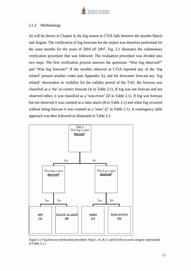
verification procedure that was followed. The evaluation procedure was divided into

two steps: The first verification process answers the questions: “Was fog observed?”

and “Was fog forecast?” If the weather observer at CTIA reported any of the ‘fog

related’ present weather codes (see Appendix A), and the forecaster forecast any ‘fog

related’ obscuration in visibility for the validity period of the TAF, the forecast was

classified as a ‘hit’ or correct forecast (A in Table 2.1). If fog was not forecast and not

observed either, it was classified as a ‘non-event’ (D in Table 2.1). If fog was forecast

but not observed it was counted as a false alarm (B in Table 2.1) and when fog occurred

without being forecast it was counted as a ‘miss’ (C in Table 2.1). A contingency table

approach was then followed as illustrated in Table 2.1.

Figure 2.1 Fog forecast verification procedure: Step 1. (A, B, C and D refer to each category represented in Table 2.1.)

14

Table 2.1 Schematic contingency table for forecasts of a binary event. The numbers of observations in each category represented by A, B, C and D and N is the total (after Jolliffe et al, 2003).

Observed

Yes No Total

Yes A B A + B F

orec

ast

No C D C + D

Total A + C B + D A + B + C + D = N

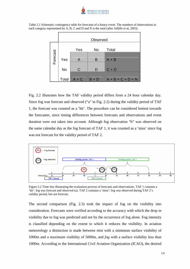
Fig. 2.2 illustrates how the TAF validity period differs from a 24 hour calendar day.

Since fog was forecast and observed (“a” in Fig. 2.2) during the validity period of TAF

1, the forecast was counted as a ‘hit’. The procedure can be considered lenient towards

the forecaster, since timing differences between forecasts and observations and event

duration were not taken into account. Although fog observation “b” was observed on

the same calendar day as the fog forecast of TAF 1, it was counted as a ‘miss’ since fog

was not forecast for the validity period of TAF 2.

Figure 2.2 Time line illustrating the evaluation process of forecasts and observations. TAF 1 contains a ‘hit’: fog was forecast and observed (a). TAF 2 contains a ‘miss’: fog was observed during TAF 2’s validity period, but not forecast.

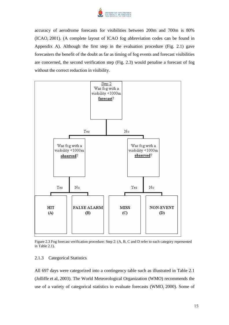
The second comparison (Fig. 2.3) took the impact of fog on the visibility into

consideration. Forecasts were verified according to the accuracy with which the drop in

visibility due to fog was predicted and not by the occurrence of fog alone. Fog intensity

is classified depending on the extent to which it reduces the visibility. In aviation

meteorology a distinction is made between mist with a minimum surface visibility of

1000m and a maximum visibility of 5000m, and fog with a surface visibility less than

1000m. According to the International Civil Aviation Organization (ICAO), the desired

15

accuracy of aerodrome forecasts for visibilities between 200m and 700m is 80%

(ICAO, 2001). (A complete layout of ICAO fog abbreviation codes can be found in

Appendix A). Although the first step in the evaluation procedure (Fig. 2.1) gave

forecasters the benefit of the doubt as far as timing of fog events and forecast visibilities

are concerned, the second verification step (Fig. 2.3) would penalise a forecast of fog

without the correct reduction in visibility.

Figure 2.3 Fog forecast verification procedure: Step 2: (A, B, C and D refer to each category represented in Table 2.1).

2.1.3 Categorical Statistics

All 697 days were categorized into a contingency table such as illustrated in Table 2.1

(Jolliffe et al, 2003). The World Meteorological Organization (WMO) recommends the

use of a variety of categorical statistics to evaluate forecasts (WMO, 2000). Some of

16

these parameters were calculated from elements in the contingency table to describe

particular characteristics of fog forecasts at CTIA.

a. Bias

The simplest bias measure is the ratio of the number of times an event was forecast over

the number of times it was observed (WMO, 2000).

Bias = CA

BA

++

(1)

The range of the bias score is from 0 to infinity and a perfect score is 1. The bias score

indicates whether the forecast system has a tendency to under forecast (bias <1) or over

forecast (bias >1).

b. Percent Correct

The simplest accuracy measure is the percent correct (PC) for all forecasts

(WMO, 2000):

PC =DCBA

DA

++++

(2)

Under circumstances where the forecast event occurs rarely, (A is small and D is large),

or frequently (A is large and D is small), the PC has to be interpreted with care. Since

the forecast of non-events are in many cases trivially easy, a large count of D values can

result in a high PC, even if the number of hits A were comparatively small

(Jolliffe et.al., 2003). Marzban (1998) characterized the rare-event situation as:

D >> B, where A~C (3)

In order to establish whether fog at CTIA can be considered a rare event the procedure

as explained by Marzban (1998) was used where the ratio between the sum of hits and

misses and the sum of the number of non-events and false alarms is calculated:

DB

CA

++

(4)

Marzban’s (1998) indicated that the above ratio would be 1% in the case of a rare event.

The ratio at CTIA was 41%. It is therefore safe to assume that the occurrence of fog at

CTIA during the fog season (March to August) is not a rare event and that the

17

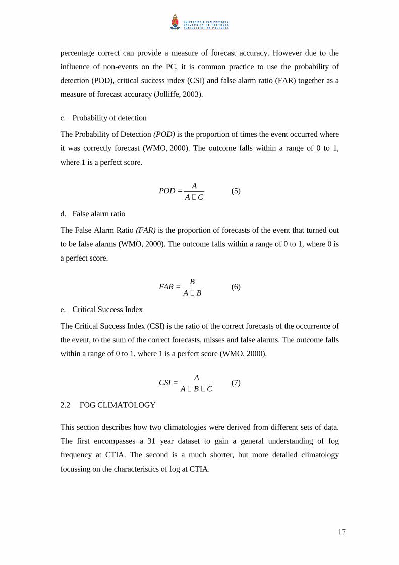
percentage correct can provide a measure of forecast accuracy. However due to the

influence of non-events on the PC, it is common practice to use the probability of

detection (POD), critical success index (CSI) and false alarm ratio (FAR) together as a

measure of forecast accuracy (Jolliffe, 2003).

c. Probability of detection

The Probability of Detection (POD) is the proportion of times the event occurred where

it was correctly forecast (WMO, 2000). The outcome falls within a range of 0 to 1,

where 1 is a perfect score.

POD =CA

A

+ (5)

d. False alarm ratio

The False Alarm Ratio (FAR) is the proportion of forecasts of the event that turned out

to be false alarms (WMO, 2000). The outcome falls within a range of 0 to 1, where 0 is

a perfect score.

FAR =BA

B

+ (6)

e. Critical Success Index

The Critical Success Index (CSI) is the ratio of the correct forecasts of the occurrence of

the event, to the sum of the correct forecasts, misses and false alarms. The outcome falls

within a range of 0 to 1, where 1 is a perfect score (WMO, 2000).

CSI =CBA

A

++ (7)

2.2 FOG CLIMATOLOGY

This section describes how two climatologies were derived from different sets of data.

The first encompasses a 31 year dataset to gain a general understanding of fog

frequency at CTIA. The second is a much shorter, but more detailed climatology

focussing on the characteristics of fog at CTIA.

18

2.2.1 Fog definitions

In South Africa the coding of visibility for aviation purposes is provided in metre or

kilometre. A weather observer is obliged to report fog (FG) when the obstruction to

vision consists of water droplets or ice crystals and the visibility has been reduced to

less than 1000m. Mist (BR) is reported when the obstruction, due to ice crystals or water

droplets, reduces the visibility to at least 1000m, but not more than 5000m (SAWS

Aviation Codes, 2004). The explanation of codes for other fog related present weather

types (shallow fog (MIFG), fog patches (BCFG), vicinity fog (VCFG) or partial fog

(PRFG)) can be found in Appendix A. The aeronautical definitions of fog and mist

correspond to the definition found in the American Meteorological Society’s (AMS)

glossary which states: “a fog observation is usually made when the horizontal visibility

is less than 1000m and the relative humidity approaches 100%” (AMS, 2010). Mist on

the other hand does not reduce the visibility to below 1000m and the relative humidity

is generally below 100%, but above 95% (AMS, 2010). However, some researchers

have adapted this definition depending on the focus of their research. Conforming to the

accepted definition of fog Cho et al., (2000) used a horizontal visibility of less than

1000m while Meyer and Lala (1990) used 400m as the maximum visibility for fog

events. Tardif and Rasmussen (2007) used the visibility threshold corresponding to Low

Instrument Flight Rules (LIFR) for the United States, which comprises a surface

visibility less than 1600m (1 statute mile). In this study fog is considered to have

occurred if the horizontal visibility was less than 1000m.

Distinction is made between a fog day and a fog event. A fog day is defined as a day

when there was one or more observation of fog or mist (Cereceda et al, 1991). In this

research fog days were determined making use of observations available at 6 hourly

intervals: 06:00, 12:00 and 18:00UTC. Tardif and Rasmussen (2007) defines a fog event

when fog occurs and lasts 3 or more consecutive hours with an observed surface

visibility less than 1600m, and at least one observation of surface visibility less than

1000m. The same approach is followed here, however instead of using a maximum

visibility threshold of 1600m as the highest visibility for a fog event, provision was

made for variations in visibility up to 5000m. This exception was made to prevent

separation of a single fog event into two or three shorter events, by temporary

improvements or fluctuations in visibility. Fog events rather than fog days are used in

19

this research since synoptic phenomena are not confined to time boundaries (Meyer and

Lala, 1990).

2.2.2 Fog type definitions

Following Tardif and Rasmussen’s (2007) fog type classification procedure, this

research will consider five different types of fog. They are: radiation fog, advection fog,

fog resulting from the lowering of cloud base, morning evaporation fog and

precipitation fog.

a. Radiation fog

Radiation fog is produced over a land area when radiational cooling reduces the air

temperature to or below its dewpoint. Therefore a strict radiation fog is a night-time

occurrence, but it may begin to form by evening twilight and often does not dissipate

until after sunrise. Factors favouring the formation of radiation fog are a shallow surface

layer of relatively moist air beneath a dry layer and clear skies, and light surface winds

(AMS, 2010). Radiation fog is distinguished from advection fog by investigating wind

speed and cloud cover (Meyer and Lala, 1990). The presence of cloud cover inhibits the

cooling necessary to saturate the air and excessive wind enhances drying of the air and

reduces the cooling rate at the surface. Wind speeds below 1ms-1 were optimum for

radiation fog formation in Albany, New York (Meyer and Lala, 1990). Pilié et al.,

(1975) showed in their study of valley fog near Elmira, New York, that wind speeds

never exceeded 4ms-1 on radiation fog nights, with average speeds substantially less.

Tillbury (1978) commented that surface wind in excess of 5ms-1 at CTIA, with or

without cloud cover, was detrimental to radiation fog formation. Considering these

values but by taking care not to set criteria which will exclude certain radiation fog

events an event was classified as a radiation fog event if wind speeds prior to onset

were less than 3ms-1. Additionally fog onset had to be after sunset and before sunrise.

Clear skies or lifting cloud bases accompanied with a cooling trend before fog onset,

were also prerequisites for an event to be classified as a radiation fog event.

b. Advection Fog

Baars (2003) distinguished between two types of advection or sea fog: the first type

(advection fog) appearing as a “wall” of fog reaching the observation station and is

characterized by a sudden drop in visibility and appearance of a low cloud base. The

20

second type (cloud base lowering fog) accounts for events where fog initially moves in

as low based cloud. Advection or “wall” fog occurred with wind speeds in excess of

1ms-1 (Baars, 2003). For fog which formed over the ocean to be advected inland, Tardif

and Rasmussen (2007) found that a wind speed greater than 2.5ms-1 and a cloud base

less than 600ft was significant. Subsequent to the definition of radiation fog with wind

speeds prior to fog onset less than 3ms-1, the converse was used for the definition of

advection events. In this study advection fog is defined when there is a sudden onset of

fog with wind speeds of 3ms-1 or more and the cloud base height is less than 600ft.

c. Cloud base lowering fog

Cloud base lowering fog was classified by Baars (2003) when cloud base heights were

less than 810 ft and it occurred in association with a wind speed in excess of 1ms-1 over

a period of up to 8 hours prior to the onset of fog. In this study cloud base lowering fog

was defined according to the definition of Tardif and Rasmussen (2007): lowering of

cloud bases within a 5 hour period prior to fog onset, with an initial cloud base height

below 1km.

d. Evaporation Fog

Evaporation fog occurs as isolated fog events which lasts for less than 3 hours and is

often observed within the first hour after sunrise (Tardif and Rasmussen, 2007). On a

clear morning, the cooling of the earth’s surface can continue beyond sunrise for

approximately a half hour, as outgoing longwave radiation exceeds incoming solar

energy (Ahrens, 2000). This happens because incoming solar radiation from the early

morning sun has to pass through a thick section of the atmosphere before striking the

earth’s surface at a low angle, failing to heat the earth’s surface effectively. Surface

heating may be reduced even more when the ground is moist (with dew for example)

and available energy is used for evaporation (Ahrens, 2000). Increasing solar radiation

associated with sunrise can act to promote, enhance and eventually dissipate radiation

fog (Meyer and Lala, 1990). The delayed radiation balance temperature rise, as well as

the evaporation of moisture such as dew, plays an important role in the promotion and

enhancement of this type of fog. Tardif and Rasmussen (2007) classified fog events

with an onset time within the first hour after sunrise, associated with a rise in dewpoint

temperature that exceeded the rise in temperature, as evaporation fog. In this study

similar criteria were used to identify evaporation fog events. Their fog type

21

classification results showed that isolated fog events which did not last 3 hours, were

often observed within the first hour after sunrise. Consequently in this study fog events

with a duration shorter than 3 hours were also considered for classification, provided

that the time of onset was within an hour after sunrise.

e. Precipitation Fog

Precipitation fog forms as a result of the evaporation of precipitation that falls through a

cold layer of moist air. When the air becomes saturated and mixing occurs, fog may

form (Ahrens, 2000). Tardif and Rasmussen (2007) classified fog events associated

with precipitation at the time of onset as precipitation fog. Of the 248 fog events that

were considered for classification, only 2 events were associated with precipitation

during the fog event. In both cases the precipitation did not occur at the start of the

event. Precipitation fog was therefore not considered as a potential fog type at CTIA.

2.2.3 Data

In an attempt to understand more about the characteristics of the seasonality of fog at

CTIA, observation data were analysed for a period of 31 years. These data were

obtained from the South African Weather Service (SAWS) and are only available for

the hours 06:00, 12:00 and 18:00UTC from 1978-2008. The data are compiled from

surface synoptic messages and include information on temperature, dewpoint

temperature, wind strength and direction, clouds (low cloud amount, type and height),

visibility and present weather. The coarse temporal resolution of these data limits their

use in compiling a thorough fog climatology and were used only to determine the

months with the highest incidence of fog at CTIA. Following from its earlier definition

(Section 2.2.2), a day was considered to be a fog day only if fog reducing the visibility

to less than 1000m occurred at 06:00, 12:00 or 18:00UTC. The average number of fog

days was calculated per month and the results are presented in Chapter 4.

Information about the monthly frequency of fog was supplemented by a shorter

climatology of fog events at CTIA. The type of fog occurrence as well as the diurnal

characteristics of fog events was investigated by using hourly Meteorological

Aerodrome Reports (METARs) for CTIA. These data were only available for the

14-year period from 1997-2010 and the SAWS data were obtained from Weather

Underground (2010). These coded hourly observations contain information about wind

22

direction and speed, temperature and dewpoint temperature, visibility, cloud amount

and cloud base height. Quality control had to be performed on the data and the

following types of errors were found: duplications of METARs and AUTO messages

containing no cloud or present weather information. Duplicated METARs were

removed from the dataset. Data for the year 2000 were incomplete and removed

completely from the dataset.

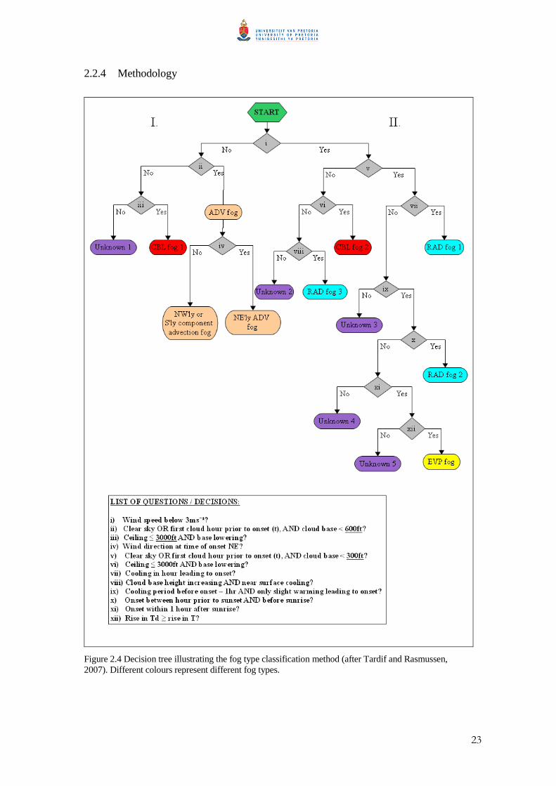
23

2.2.4 Methodology

Figure 2.4 Decision tree illustrating the fog type classification method (after Tardif and Rasmussen, 2007). Different colours represent different fog types.

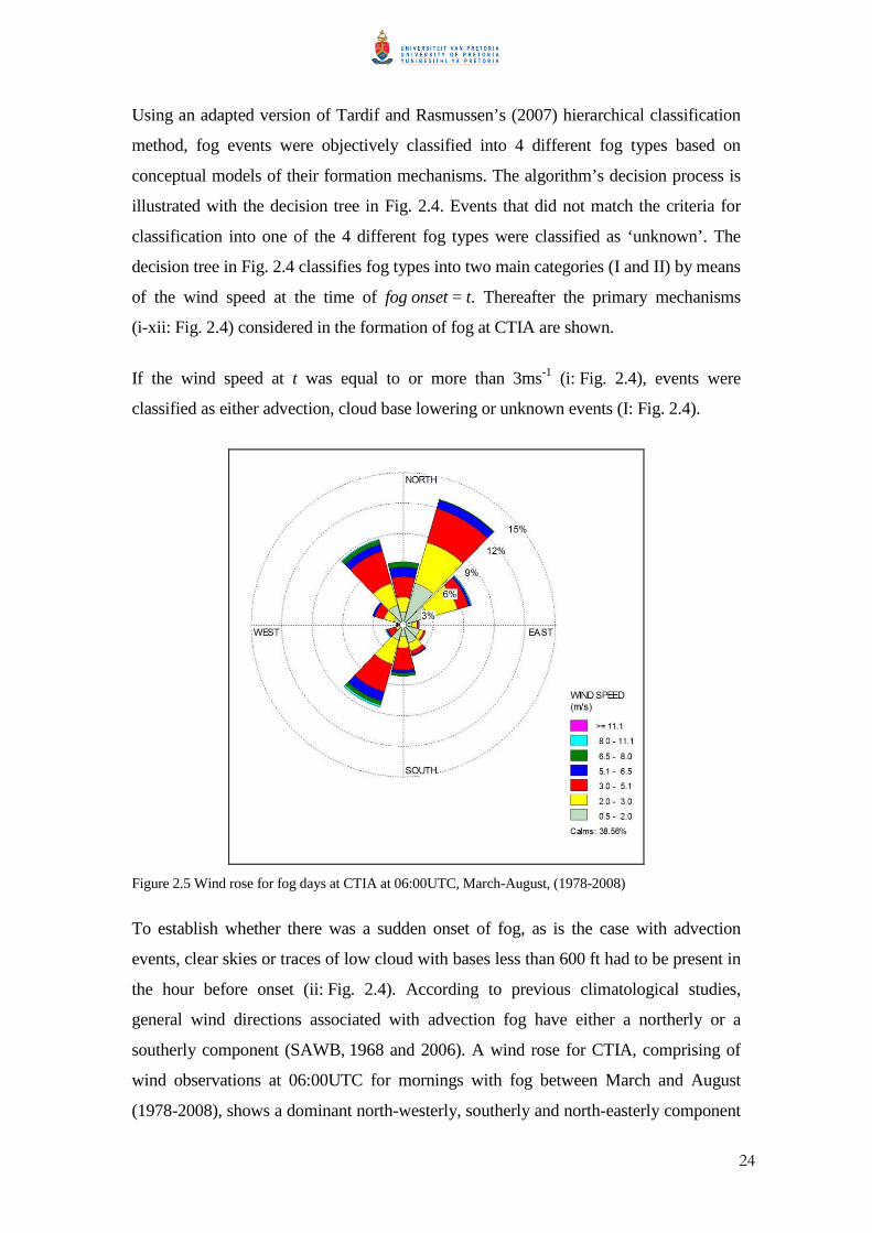
24

Using an adapted version of Tardif and Rasmussen’s (2007) hierarchical classification

method, fog events were objectively classified into 4 different fog types based on

conceptual models of their formation mechanisms. The algorithm’s decision process is

illustrated with the decision tree in Fig. 2.4. Events that did not match the criteria for

classification into one of the 4 different fog types were classified as ‘unknown’. The

decision tree in Fig. 2.4 classifies fog types into two main categories (I and II) by means

of the wind speed at the time of fog onset = t. Thereafter the primary mechanisms

(i-xii: Fig. 2.4) considered in the formation of fog at CTIA are shown.

If the wind speed at t was equal to or more than 3ms-1 (i: Fig. 2.4), events were

classified as either advection, cloud base lowering or unknown events (I: Fig. 2.4).

Figure 2.5 Wind rose for fog days at CTIA at 06:00UTC, March-August, (1978-2008)

To establish whether there was a sudden onset of fog, as is the case with advection

events, clear skies or traces of low cloud with bases less than 600 ft had to be present in

the hour before onset (ii: Fig. 2.4). According to previous climatological studies,

general wind directions associated with advection fog have either a northerly or a

southerly component (SAWB, 1968 and 2006). A wind rose for CTIA, comprising of

wind observations at 06:00UTC for mornings with fog between March and August

(1978-2008), shows a dominant north-westerly, southerly and north-easterly component

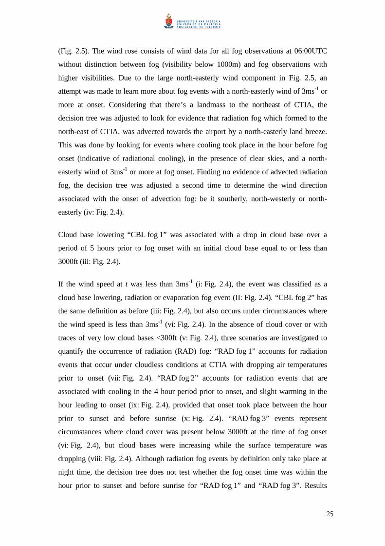
25

(Fig. 2.5). The wind rose consists of wind data for all fog observations at 06:00UTC

without distinction between fog (visibility below 1000m) and fog observations with

higher visibilities. Due to the large north-easterly wind component in Fig. 2.5, an

attempt was made to learn more about fog events with a north-easterly wind of 3ms-1 or

more at onset. Considering that there’s a landmass to the northeast of CTIA, the

decision tree was adjusted to look for evidence that radiation fog which formed to the

north-east of CTIA, was advected towards the airport by a north-easterly land breeze.

This was done by looking for events where cooling took place in the hour before fog

onset (indicative of radiational cooling), in the presence of clear skies, and a north-

easterly wind of 3ms-1 or more at fog onset. Finding no evidence of advected radiation

fog, the decision tree was adjusted a second time to determine the wind direction

associated with the onset of advection fog: be it southerly, north-westerly or north-

easterly (iv: Fig. 2.4).

Cloud base lowering “CBL fog 1” was associated with a drop in cloud base over a

period of 5 hours prior to fog onset with an initial cloud base equal to or less than

3000ft (iii: Fig. 2.4).

If the wind speed at t was less than 3ms-1 (i: Fig. 2.4), the event was classified as a

cloud base lowering, radiation or evaporation fog event (II: Fig. 2.4). “CBL fog 2” has

the same definition as before (iii: Fig. 2.4), but also occurs under circumstances where

the wind speed is less than 3ms-1 (vi: Fig. 2.4). In the absence of cloud cover or with

traces of very low cloud bases <300ft (v: Fig. 2.4), three scenarios are investigated to

quantify the occurrence of radiation (RAD) fog: “RAD fog 1” accounts for radiation

events that occur under cloudless conditions at CTIA with dropping air temperatures

prior to onset (vii: Fig. 2.4). “RAD fog 2” accounts for radiation events that are

associated with cooling in the 4 hour period prior to onset, and slight warming in the

hour leading to onset (ix: Fig. 2.4), provided that onset took place between the hour

prior to sunset and before sunrise (x: Fig. 2.4). “RAD fog 3” events represent

circumstances where cloud cover was present below 3000ft at the time of fog onset

(vi: Fig. 2.4), but cloud bases were increasing while the surface temperature was

dropping (viii: Fig. 2.4). Although radiation fog events by definition only take place at

night time, the decision tree does not test whether the fog onset time was within the

hour prior to sunset and before sunrise for “RAD fog 1” and “RAD fog 3”. Results

26

however show that all events classified as “RAD fog 1” and “RAD fog 3” occurred at

night. Evaporation fog events were similarly defined as “RAD fog 2” apart from the

fact that onset took place within the first hour after sunrise (xi: Fig. 2.4), and was

accompanied with an increase in dewpoint temperature (Td) and air temperature (T)

(xii: Fig. 2.4).

2.3 SYNOPTIC CLASSIFICATION

Synoptic classification or synoptic typing has often been used as a data reduction

technique in process studies that examine interactions or relationships between the

circulation and local environmental parameters (Hewitson and Crane, 2002). Synoptic

classification methods vary from several forms of cluster analyses to labour intensive

manual techniques and also the use of SOMs.

The Australian Bureau of Meteorology (BOM) has developed an automated, objective

synoptic typing system by making use of principal component analysis. After

identifying principal components that incorporates fields of mean sea level pressure, a

K-means unsupervised clustering scheme is used to derive synoptic types. Numerical

weather prediction (NWP) model output is then automatically classified to generate

synoptic type guidance to forecasters in an operational environment (Dahni, 2003).

Synoptic classification is also used in climate change related studies. Hope et al, (2006)

used SOMs to clarify the decrease in rainfall experienced in southwest Western

Australia since 1975, concluding that large scale circulation changes in the region have

been associated with the rainfall decline.

In this study, SOMs will be used to identify synoptic circulation patterns that are

generally associated with fog at CTIA.

2.3.1 Data

Reanalysis II data of mean sea level pressure (MSLP) fields at 00:00UTC were

obtained from the National Centre for Environmental Prediction (NCEP). The data have

a 2.5° grid resolution and spanned a domain centered around the south-western Cape

(20°S-40°S, 10°E-35°E), (Fig. 2.6). Data are for the fog season period (March to

August), from 1997-2010.

27

Figure 2.6 Spatial domain used for the MSLP SOM domain.

2.3.2 Methodology

The artificial neural network system of SOMs is described in detail by Kohonen (2001).

Hewitson and Crane (2002) provide a good platform and explanation of the application

of SOMs to synoptic climatology. Here the SOM was used to reduce multivariate

atmospheric data and produce generalized weather circulation patterns over South

Africa and the adjacent ocean. Daily atmospheric data between the months March to

August were categorized into 35 archetypal synoptic circulation nodes representing

synoptic circulations that occur most frequently during that time of the year. The size of

the SOM array, 5 x 7, was chosen to minimise the degree of generalization that will be

produced by the SOM. The more nodes you choose, the finer the representation of

detail, while the fewer nodes, the broader the level of generalization. Nevertheless the

same broad pattern is revealed at each level of generalization (Hewitson and

Crane, 2002).

Once the SOM produced 35 nodes or synoptic types, the frequency of occurrence of

synoptic systems was determined. This was achieved by accumulating the number of

days mapped to each node and dividing them by the total number of observations in the

dataset.

28

The next step in producing a synoptic climatology was to relate the synoptic circulation

patterns to the number of fog days over the 14 year period. Of the 248 events classified

as fog, 235 fog days were mapped to the 35 SOMs to see which synoptic circulations

were frequently associated with fog. On days where 2 fog events were classified by the

decision tree in Fig. 2.4, only 1 event was manually selected, which accounts for the 13

events that were not mapped to a SOM. A monthly breakdown of the number of fog

events per synoptic circulation was done to observe the change in circulation patterns

associated with fog during the course of the fog season. Finally the different fog types

as presented in section 4.2 were related to each of the 35 synoptic circulations.

2.4 ATMOSPHERIC SOUNDINGS

A study on fog would not be complete without referring to the vertical temperature and

dewpoint temperature profile of the atmosphere. A stable atmosphere is one of the key

requirements for fog formation since it inhibits vertical air motion (Ahrens, 2000) and

the tephigram is an operationally available forecasting tool providing in situ

measurements of the boundary layer and atmosphere above. Croft et al., (1997)

emphasises the importance of including a sounding analysis in their conceptual model

approach to obtain more information on the boundary layer environment in which fog

occurs.

2.4.1 Data

SAWS atmospheric soundings were obtained from the University of Wyoming (2011)

for the months of the fog season between 1997 and 2010. There were no data available

for 61 of the fog days and 533 of the non-fog days. The midnight sounding closest to

each fog event was selected in order to be most representative of the atmosphere in

which fog developed.

2.4.2 Methodology

Anticipating distinct differences, a comparison was made between the average sounding

characteristics of fog days, non-fog days and the overall long term average. Specific

attention was paid to the boundary layer below the temperature inversion where fog

would occur as well as the layer above the temperature inversion up to the 700hPa

level.

29

The average height of the base and top of temperature inversions were calculated for

each month of the fog season. Where possible, the differences observed between the

months of the fog season were related to the dominant fog type (4.2.1) for those

months.

Croft et al., (1997) investigated directional wind shear between the surface and 700hPa

and found that radiation fog occurred under weak backing or neutral wind patterns,

while advection fog occurred under a veering wind pattern for the southern region of

the United States. A similar investigation was done for each month of the fog season to

determine whether significant directional shear occurred on fog days.

A comparison was made between the vertical profile of fog days and non-fog days for

the following variables from 1000hPa up to 700hPa. The non-parametric Mann-

Whitney test, also known as the Wilcoxon Rank Sum test, was used to test the null

hypothesis that these variables have the same median at the 95% confidence level on

fog days and non-fog days (Steyn et al., 1994).

a. Temperature

Difference maps were obtained by subtracting monthly average temperature values

from monthly fog day values. The average temperature between 1000 and 700hPa was

compared between fog days and non-fog days to establish whether there are significant

differences.

b. Relative humidity (RH)

Difference maps were obtained by subtracting monthly average RH values from

monthly fog day values. Fog day values, of the average RH below and above the

temperature inversion, were compared with non-fog day values, to establish if any

significant differences exist and to see if the average RH on fog days is higher or lower

than normal.

c. Surface dewpoint temperature

Surface dewpoint values were compared between fog days and non-fog days to

establish whether dewpoints were higher or lower on fog days than on non-fog days.

d. Geopotential thickness

30

Geopotential thickness values provide another indication of the average temperature

T between 2 pressure surfaces p0 (the lower surface) and p (the higher surface). The

thickness in metres ∆z between p0 and p is expressed in the following equation where

the earth’s gravitational acceleration g = 9.8ms-2 (Tyson et al., 2000).

0

lnp

p

g

TRz =∆

An increase in the average column temperature T between two pressure levels would

result in a higher thickness value. A comparison of thickness values was done between

fog days and non-fog days. Higher thickness values on fog days could be an indication

of subsidence and inherently a stable atmosphere. In this research the geopotential

thickness was calculated by simply subtracting the geopotential height at the 700hPa

pressure level from the geopotential height from the 1000hPa pressure level. These

variables are available in the raw data.

2.5 SUMMARY

In this study several sets of data are used to perform a verification of fog forecasts and a

climatology of fog events at CTIA. An attempt was made to strike a balance between

the use of data with a higher temporal resolution for shorter periods and using the

longest data set available with 6-hourly gaps between observations. The fog forecast

verification data set is small (2004-2007) in comparison with data used for climatology

purposes, but the emphasis of the verification analysis is not to provide a

comprehensive overview of fog forecasts over the years, but to emphasize the need for

improvement of fog forecasting processes in South Africa. General information about

the occurrence of fog at CTIA were obtained from a 31 year dataset (1978-2008) with 6

hourly observations excluding 00:00UTC, but specific fog characteristics at CTIA were

obtained by investigating reanalysis II data, atmospheric soundings and METAR data

between 1997 and 2010.

31

CHAPTER 3

VERIFICATION RESULTS

3 VERIFICATION RESULTS

The results of the verification of TAFs at CTIA between March and August

(2004-2007) are presented here. These results are only for TAFs issued at 12:00UTC

and which were valid for a 24 hour period from 18:00UTC. The 24 hour TAFs issued at

06:00, 09:00 and 18:00UTC were not included, nor were short term TAFs, issued at 3

hourly intervals.

Hourly observation data for August 2007 and 8 TAFs were missing from the dataset.

Apart from this, 697 days between March and August (2004-2007) were categorized as

fog days or non-fog days.

In order to verify the accuracy with which forecasters at CTIA forecast fog, the number

of times fog was forecast was compared to the number of times it actually occurred

during the fog season. The number of times fog occurred without being forecast was

also investigated. The simplest way of evaluating the occurrence or non-occurrence of

fog, is by making use of a contingency table as illustrated in Table 3.1 (WMO, 2000).

Firstly the forecasters’ ability to identify a potential fog event was evaluated. This

involved a general investigation to determine whether an obscuration in visibility due to

fog or mist was expected in the 24 hour TAF issued at 12:00UTC.

Secondly the reduction in visibility was taken into account. ICAO requires an 80%

forecast accuracy of weather events where visibilities drop between 200 and 700m. The

second evaluation investigated how successful forecasters were in forecasting fog

events with minimum visibilities less than 1000m.

3.1 GENERAL VERIFICATION OF FOG FORECASTS AT CTIA

The general verification process answers the questions: “Was fog observed?” and “Was

fog forecast?” Particulars of the verification process are described in section 2.1.2. Once

32

all of the 697 days were categorized into Table 3.1, the overall POD, CSI, PC, FAR and

bias values were calculated (Table 3.2). Contingency tables were used to represent

forecast and observation data yearly (Table 3.5) and monthly (Table 3.6).

Table 3.1 Categorisation of all fog and mist forecasts and observations in a contingency table.

Observed

Yes No Total

Yes 89 82 171

For

ecas

t

No 115 411 526

Total 204 493 697

Bias and percentage correct verification scores were also calculated on a yearly (Table

3.3) and monthly (Table 3.4) basis. Since it is advisable to interpret the POD, CSI and

FAR together (Jolliffe et al., 2003), their values are displayed separately from the PC

and bias values in Fig. 3.1 to Fig. 3.3. The general verification results are discussed

below.

Table 3.2 General verification results for all fog or mist forecasts and observations at CTIA (March to August, 2004-2007).

PC Bias POD FAR CSI

March-August

(2004-2007) 0.72 0.84 0.44 0.48 0.31

Table 3.3 Yearly Percentage Correct and Bias values of general verification.

2004 2005 2006 2007

Percent Correct 0.76 0.69 0.71 0.70

Bias 0.67 1.04 0.74 0.98

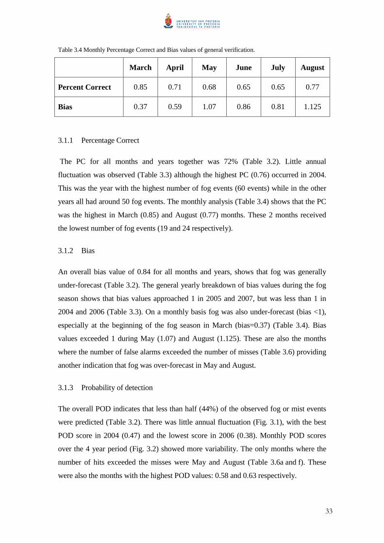
33

Table 3.4 Monthly Percentage Correct and Bias values of general verification.

March April May June July August

Percent Correct 0.85 0.71 0.68 0.65 0.65 0.77

Bias 0.37 0.59 1.07 0.86 0.81 1.125

3.1.1 Percentage Correct

The PC for all months and years together was 72% (Table 3.2). Little annual

fluctuation was observed (Table 3.3) although the highest PC (0.76) occurred in 2004.

This was the year with the highest number of fog events (60 events) while in the other

years all had around 50 fog events. The monthly analysis (Table 3.4) shows that the PC

was the highest in March (0.85) and August (0.77) months. These 2 months received

the lowest number of fog events (19 and 24 respectively).

3.1.2 Bias

An overall bias value of 0.84 for all months and years, shows that fog was generally

under-forecast (Table 3.2). The general yearly breakdown of bias values during the fog

season shows that bias values approached 1 in 2005 and 2007, but was less than 1 in

2004 and 2006 (Table 3.3). On a monthly basis fog was also under-forecast (bias <1),

especially at the beginning of the fog season in March (bias=0.37) (Table 3.4). Bias

values exceeded 1 during May (1.07) and August (1.125). These are also the months

where the number of false alarms exceeded the number of misses (Table 3.6) providing

another indication that fog was over-forecast in May and August.

3.1.3 Probability of detection

The overall POD indicates that less than half (44%) of the observed fog or mist events

were predicted (Table 3.2). There was little annual fluctuation (Fig. 3.1), with the best

POD score in 2004 (0.47) and the lowest score in 2006 (0.38). Monthly POD scores

over the 4 year period (Fig. 3.2) showed more variability. The only months where the

number of hits exceeded the misses were May and August (Table 3.6a and f). These

were also the months with the highest POD values: 0.58 and 0.63 respectively.

34

3.1.4 Critical Success Index

Approximately 30% of all fog or mist events were correctly forecast (Table 3.2).

Following a similar curve to the POD, the highest CSI value (0.39) occurred in 2004,

which was also the year with the lowest number of false alarms (a in Table 3.5).

Thereafter it decreased and remained constant from 2005-2007 (Fig. 3.1). The monthly

CSI values were highest in May (0.39) and August (0.41), but lowest at the beginning

of the fog season in March (0.18) and April (0.15) (Fig. 3.2).

3.1.5 False Alarm Ratio

The overall FAR was 48% (Table 3.2). This means that just under a half of predicted

fog or mist events did not occur. The year 2004 had the lowest FAR (0.3) (Fig. 3.1).

April was the only month where the number of false alarms exceeded the number of

hits (Table 3.6b) and was correspondingly the month with the highest FAR (0.58) (Fig.

3.2).

General Yearly Verification

0

0.1

0.2

0.3

0.4

0.5

0.6

0.7

0.8

0.9

1

2004 2005 2006 2007

Year

PODCSIFAR

Figure 3.1 Yearly POD, CSI and FAR values for the general verification of fog and mist days during March-August.

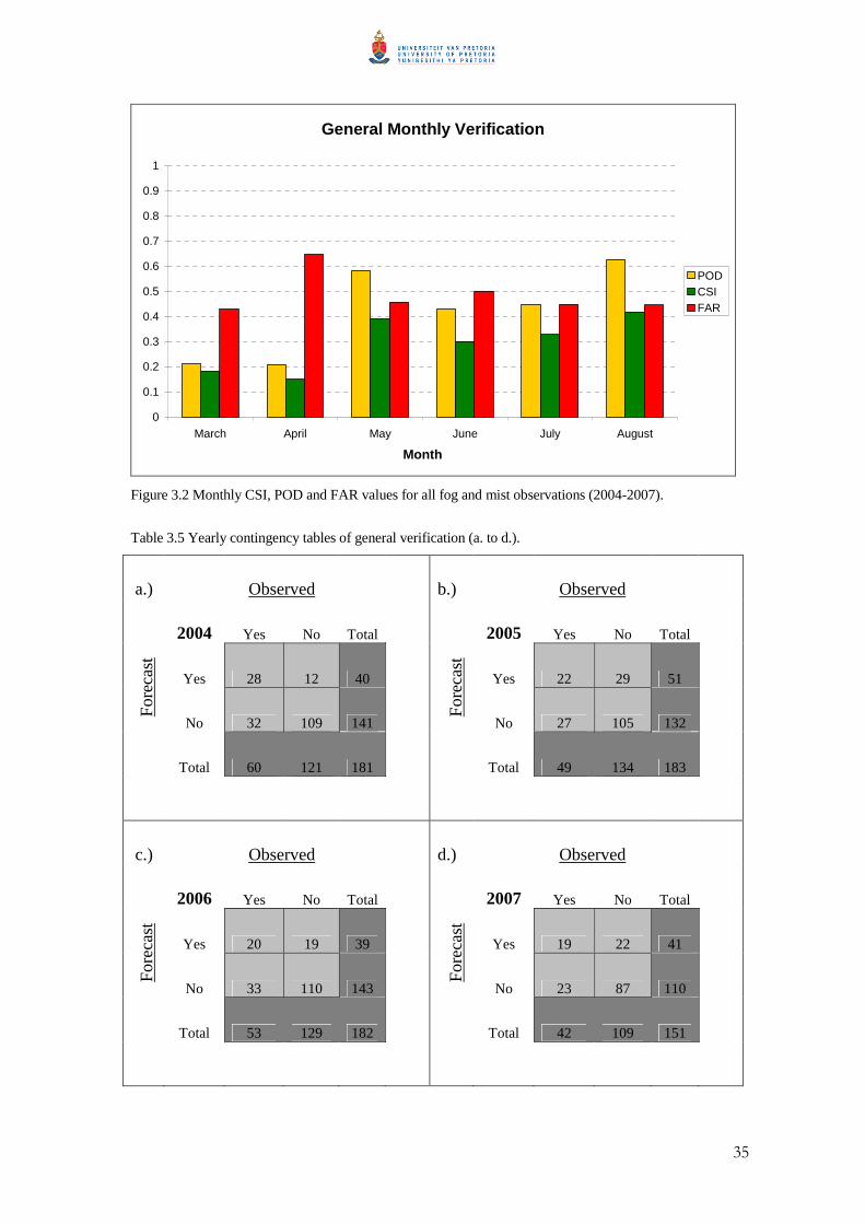
35

General Monthly Verification

0

0.1

0.2

0.3

0.4

0.5

0.6

0.7

0.8

0.9

1


Month

POD CSI FAR

Figure 3.2 Monthly CSI, POD and FAR values for all fog and mist observations (2004-2007).

Table 3.5 Yearly contingency tables of general verification (a. to d.).

a.) Observed b.) Observed

2004 Yes No Total 2005 Yes No Total

Yes 28 12 40 Yes 22 29 51

For

ecas

t

No 32 109 141

For

ecas

t

No 27 105 132

Total 60 121 181 Total 49 134 183

c.) Observed d.) Observed

2006 Yes No Total 2007 Yes No Total

Yes 20 19 39 Yes 19 22 41

For

ecas

t

No 33 110 143

For

ecas

t

No 23 87 110

Total 53 129 182 Total 42 109 151

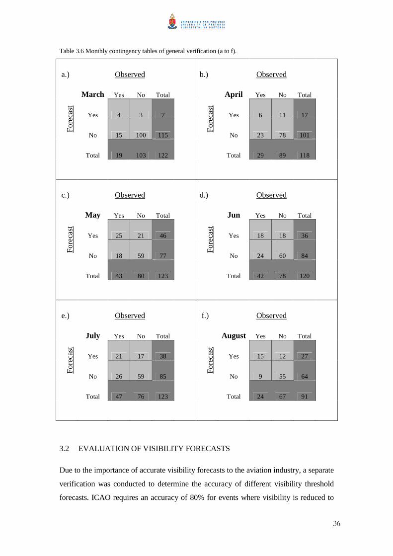
36

Table 3.6 Monthly contingency tables of general verification (a to f).


March Yes No Total April Yes No Total

Yes 4 3 7 Yes 6 11 17

For

ecas

t

No 15 100 115

For

ecas

t

No 23 78 101

Total 19 103 122 Total 29 89 118

c.) Observed d.) Observed

May Yes No Total Jun Yes No Total

Yes 25 21 46 Yes 18 18 36

For

ecas

t

No 18 59 77

For

ecas

t

No 24 60 84

Total 43 80 123 Total 42 78 120

e.) Observed f.) Observed

July Yes No Total August Yes No Total

Yes 21 17 38 Yes 15 12 27

For

ecas

t

No 26 59 85

For

ecas

t

No 9 55 64

Total 47 76 123 Total 24 67 91

3.2 EVALUATION OF VISIBILITY FORECASTS

Due to the importance of accurate visibility forecasts to the aviation industry, a separate

verification was conducted to determine the accuracy of different visibility threshold

forecasts. ICAO requires an accuracy of 80% for events where visibility is reduced to

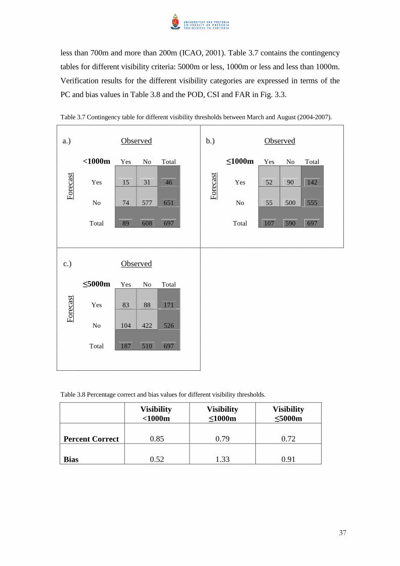
37

less than 700m and more than 200m (ICAO, 2001). Table 3.7 contains the contingency

tables for different visibility criteria: 5000m or less, 1000m or less and less than 1000m.

Verification results for the different visibility categories are expressed in terms of the

PC and bias values in Table 3.8 and the POD, CSI and FAR in Fig. 3.3.

Table 3.7 Contingency table for different visibility thresholds between March and August (2004-2007).


<1000m Yes No Total ≤1000m Yes No Total

Yes 15 31 46 Yes 52 90 142

For

ecas

t

No 74 577 651

For

ecas

t No 55 500 555

Total 89 608 697 Total 107 590 697

c.) Observed

≤5000m Yes No Total

Yes 83 88 171

For

ecas

t

No 104 422 526

Total 187 510 697

Table 3.8 Percentage correct and bias values for different visibility thresholds.

Visibility <1000m

Visibility ≤1000m

Visibility ≤5000m

Percent Correct 0.85 0.79 0.72

Bias 0.52 1.33 0.91

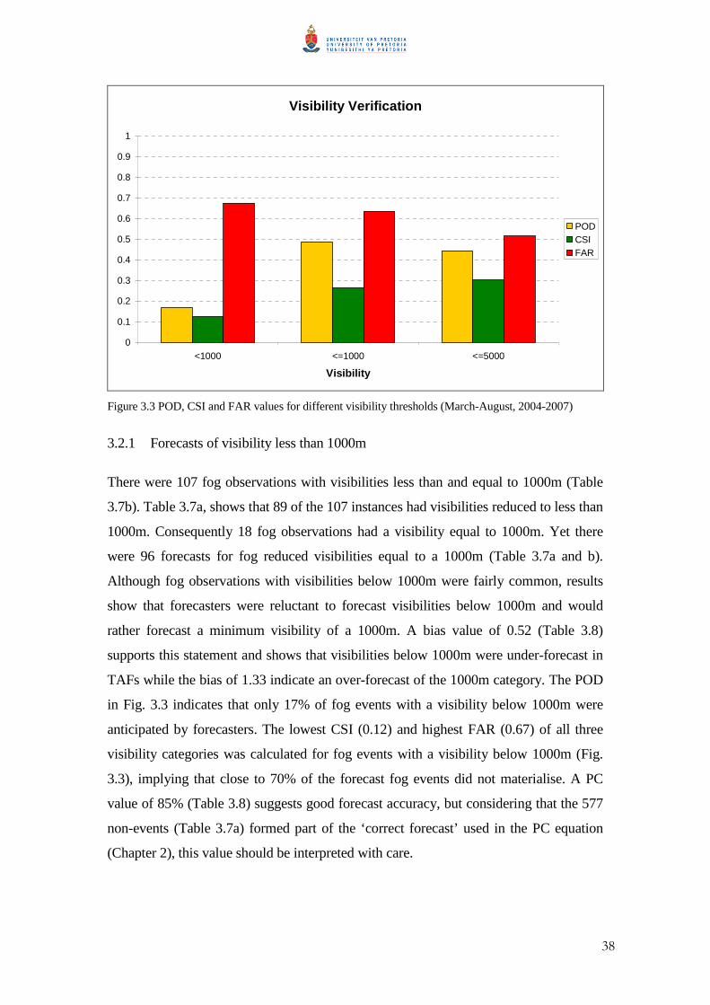
38

Visibility Verification

0

0.1

0.2

0.3

0.4

0.5

0.6

0.7

0.8

0.9

1

<1000 <=1000 <=5000

Visibility

PODCSIFAR

Figure 3.3 POD, CSI and FAR values for different visibility thresholds (March-August, 2004-2007)

3.2.1 Forecasts of visibility less than 1000m

There were 107 fog observations with visibilities less than and equal to 1000m (Table

3.7b). Table 3.7a, shows that 89 of the 107 instances had visibilities reduced to less than

1000m. Consequently 18 fog observations had a visibility equal to 1000m. Yet there

were 96 forecasts for fog reduced visibilities equal to a 1000m (Table 3.7a and b).

Although fog observations with visibilities below 1000m were fairly common, results

show that forecasters were reluctant to forecast visibilities below 1000m and would

rather forecast a minimum visibility of a 1000m. A bias value of 0.52 (Table 3.8)

supports this statement and shows that visibilities below 1000m were under-forecast in

TAFs while the bias of 1.33 indicate an over-forecast of the 1000m category. The POD

in Fig. 3.3 indicates that only 17% of fog events with a visibility below 1000m were

anticipated by forecasters. The lowest CSI (0.12) and highest FAR (0.67) of all three

visibility categories was calculated for fog events with a visibility below 1000m (Fig.

3.3), implying that close to 70% of the forecast fog events did not materialise. A PC

value of 85% (Table 3.8) suggests good forecast accuracy, but considering that the 577

non-events (Table 3.7a) formed part of the ‘correct forecast’ used in the PC equation

(Chapter 2), this value should be interpreted with care.

39

3.2.2 Forecasts of visibility less than or equal to 1000m

By including a visibility of a 1000m in the verification process, CSI and POD values

increased to 0.26 and 0.49 respectively (Fig. 3.3). The bias value of 1.33 (Table 3.8)

indicates that fog was still over-forecast in TAFs, which explains why the FAR is still

as high as 0.63 (Fig. 3.3) At 79% (Table 3.8) the PC is lower than in the previous

section, due to a higher number of false alarms and a lower number of correct negative

forecasts. The overall performance is still better than for visibilities below 1000m.

3.2.3 Forecasts of visibility less than or equal to 5000m

Table 3.7c shows very similar verification results as Table 3.1, although there are more

fog observations in Table 3.1. This difference can be ascribed to 17 fog or mist events

with visibilities greater than 5000m. Aviation forecasters are required to indicate

expected visibility changes in a TAF when the visibility is expected to change to or pass

through 5000m or less, since a significant number of flights are operated in accordance

with Visual Flight Rules (VFR) (SAWS, 2004). Therefore the 17 fog events with

visibilities greater than 5000m that were observed but not forecast are not considered as

misses in Table 3.7c. This table encompasses all 171 fog forecasts during the period

March to August (2004-2007). Although it has the lowest overall PC value of 72%

(Table 3.8), it has the lowest FAR (0.51) and the highest CSI (0.3) (Fig. 3.3). The POD

(Fig. 3.3) indicates that 44% of the observed fog or mist events were predicted, which

agrees with a bias value of 0.91 showing that fog events with visibilities of 5000m or

less went under-forecast.

3.3 DISCUSSION OF VERIFICATION RESULTS

An evaluation of fog forecasts in general showed that fog events between the months

March and August (2004-2007) went under-forecast. The low bias values in March can

be an indication that forecasters do not yet anticipate fog at that time of the year. On the

other hand high bias values at the end of the fog season indicate that forecasters tend to

over-forecast fog as the number of fog events start tapering towards the end of the fog

season. Considering that the timing of events was not evaluated, the fact that only 44%

of fog days were expected in advance indicates the need for the improvement of fog

forecasts at CTIA.

40

The verification of forecast visibility underlines this dilemma by indicating that less

than 20% of fog events with a visibility below 1000m were expected in advance. Close

investigation of visibility forecasts indicates that despite caution on forecaster side to

forecast visibilities below 1000m, the number of false alarms is still high. Forecasters

do however tend to forecast a visibility of 1000m regularly with much better accuracy,

although the number of false alarms remains high. It is the author’s opinion that access

to a detailed fog climatology can raise awareness among forecasters of the regularity

with which fog occurs at CTIA.

The verification results should be interpreted as a whole, and care should be taken not to

isolate certain verification scores. High PC values were misleading in several cases and

did not give a true reflection of fog forecasting accuracy in general. As an example the

month of March had the highest PC value, but simultaneously one of the lowest CSI

and POD values.

41

CHAPTER 4

CLIMATOLOGY

4 CLIMATOLOGY

One of the aims of this dissertation is to improve fog forecasts at CTIA by gaining

knowledge about fog by means of a comprehensive climatology. A fog climatology

used in conjunction with numerical guidance and atmospheric sounding analyses, can

allow mesoscale fog predictions to be made (Croft, 1997). Hyvärinen et al., (2007)

suggested that knowledge of the climatological peculiarities of an area is important

because numerical weather prediction models are not always as useful as forecasters

would like them to be. They specifically determined climatological aspects of fog at

several airports in Finland to assist aviation forecasters.

A literature study of fog strongly suggests that this is the first climatology for CTIA of

its kind. One of the advantages of a climatology is that it serves as a reference to

prevent predictions of fog at a time of year where it doesn’t occur (false alarms), but

also alerts the forecaster to duly predict severe events, preventing under-forecasting

(misses). Verification results in Chapter 3 showed that despite a high number of false

alarms, fog events went under-forecast between March and August (2004-2007).

Chapter 4 provides aviation forecasters with a concise but comprehensive document to

be used as an operational fog forecasting tool. The characteristics of fog as well as

synoptic circulation patterns and lower tropospheric atmospheric variables at CTIA

were derived from the following:

- Instantaneous observations at main synoptic observation times (06:00, 12:00

and 18:00UTC) over a period of 31 years. These data were used to provide an

overview of the frequency of fog at CTIA and its seasonal nature.

- Hourly observations over a period of 13 years from which fog types were

derived and details about duration, time of onset and dissipation and other

characteristics were determined.

- NCEP reanalysis II data over a period of 14 years that were used to classify the

synoptic circulation associated with the occurrence of fog.

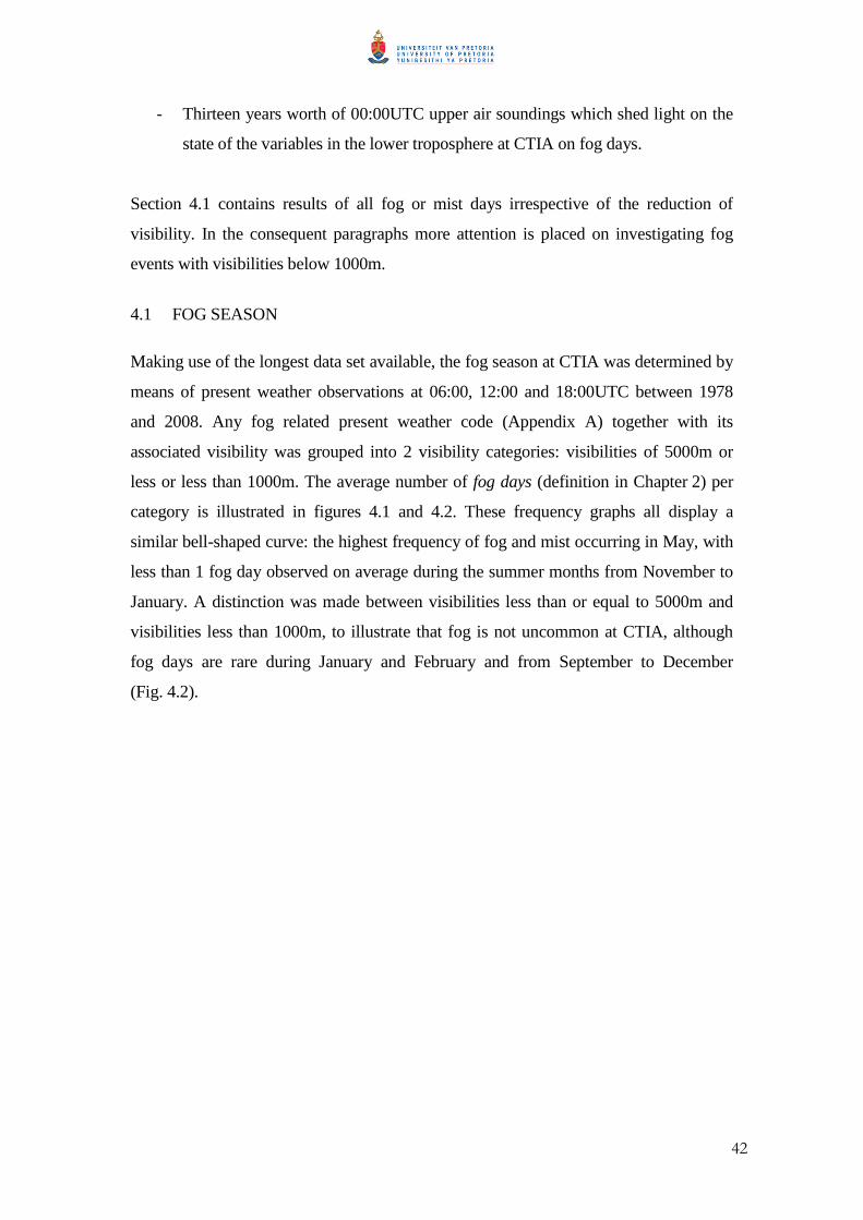
42

- Thirteen years worth of 00:00UTC upper air soundings which shed light on the

state of the variables in the lower troposphere at CTIA on fog days.

Section 4.1 contains results of all fog or mist days irrespective of the reduction of

visibility. In the consequent paragraphs more attention is placed on investigating fog

events with visibilities below 1000m.

4.1 FOG SEASON

Making use of the longest data set available, the fog season at CTIA was determined by

means of present weather observations at 06:00, 12:00 and 18:00UTC between 1978

and 2008. Any fog related present weather code (Appendix A) together with its

associated visibility was grouped into 2 visibility categories: visibilities of 5000m or

less or less than 1000m. The average number of fog days (definition in Chapter 2) per

category is illustrated in figures 4.1 and 4.2. These frequency graphs all display a

similar bell-shaped curve: the highest frequency of fog and mist occurring in May, with

less than 1 fog day observed on average during the summer months from November to

January. A distinction was made between visibilities less than or equal to 5000m and

visibilities less than 1000m, to illustrate that fog is not uncommon at CTIA, although

fog days are rare during January and February and from September to December

(Fig. 4.2).

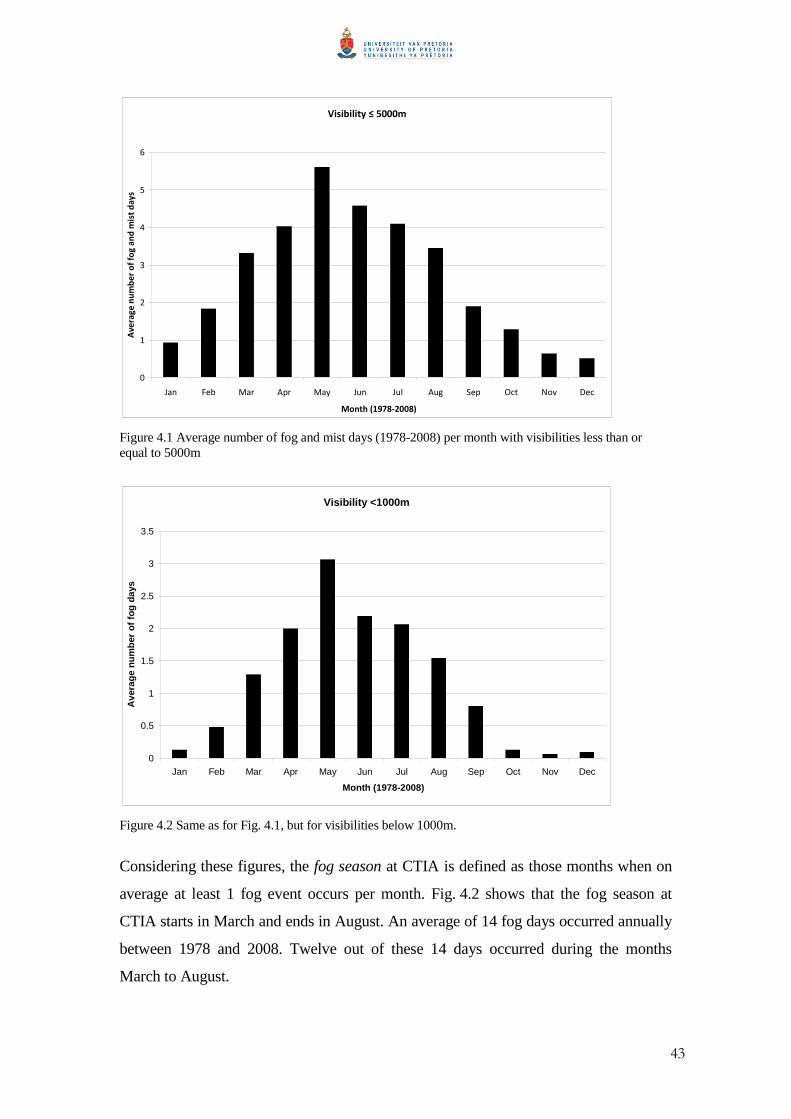
43

Visibility ≤ 5000m

0

1

2

3

4

5

6


Month (1978-2008)

Av

era

ge

nu

mb

er

of

fog

an

d m

ist

da

ys

Figure 4.1 Average number of fog and mist days (1978-2008) per month with visibilities less than or equal to 5000m

Visibility <1000m

0

0.5

1

1.5

2

2.5

3

3.5


Month (1978-2008)

Ave

rage

num

ber

of fo

g da

ys

Figure 4.2 Same as for Fig. 4.1, but for visibilities below 1000m.

Considering these figures, the fog season at CTIA is defined as those months when on

average at least 1 fog event occurs per month. Fig. 4.2 shows that the fog season at

CTIA starts in March and ends in August. An average of 14 fog days occurred annually

between 1978 and 2008. Twelve out of these 14 days occurred during the months

March to August.

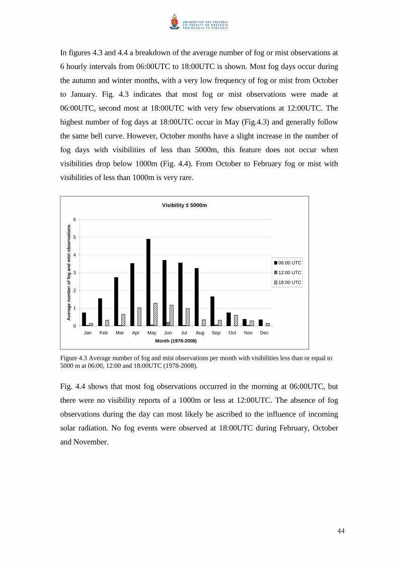
44

In figures 4.3 and 4.4 a breakdown of the average number of fog or mist observations at

6 hourly intervals from 06:00UTC to 18:00UTC is shown. Most fog days occur during

the autumn and winter months, with a very low frequency of fog or mist from October

to January. Fig. 4.3 indicates that most fog or mist observations were made at

06:00UTC, second most at 18:00UTC with very few observations at 12:00UTC. The

highest number of fog days at 18:00UTC occur in May (Fig.4.3) and generally follow

the same bell curve. However, October months have a slight increase in the number of

fog days with visibilities of less than 5000m, this feature does not occur when

visibilities drop below 1000m (Fig. 4.4). From October to February fog or mist with

visibilities of less than 1000m is very rare.

Visibility ≤ 5000m

0

1

2

3

4

5

6


Month (1978-2008)

Ave

rage

num

ber

of fo

g an

d m

ist o

bser

vatio

ns

06:00 UTC

12:00 UTC

18:00 UTC

Figure 4.3 Average number of fog and mist observations per month with visibilities less than or equal to 5000 m at 06:00, 12:00 and 18:00UTC (1978-2008).

Fig. 4.4 shows that most fog observations occurred in the morning at 06:00UTC, but

there were no visibility reports of a 1000m or less at 12:00UTC. The absence of fog

observations during the day can most likely be ascribed to the influence of incoming

solar radiation. No fog events were observed at 18:00UTC during February, October

and November.

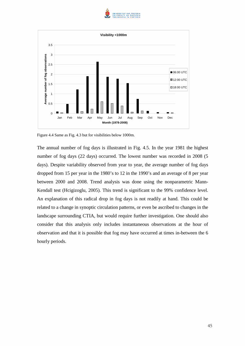
45

Visibility <1000m

0

0.5

1

1.5

2

2.5

3

3.5


Month (1978-2008)

Ave

rage

num

ber

of fo

g ob

serv

atio

ns

06:00 UTC

12:00 UTC

18:00 UTC

Figure 4.4 Same as Fig. 4.3 but for visibilities below 1000m.

The annual number of fog days is illustrated in Fig. 4.5. In the year 1981 the highest

number of fog days (22 days) occurred. The lowest number was recorded in 2008 (5

days). Despite variability observed from year to year, the average number of fog days

dropped from 15 per year in the 1980’s to 12 in the 1990’s and an average of 8 per year

between 2000 and 2008. Trend analysis was done using the nonparametric Mann-

Kendall test (Hcigizoglu, 2005). This trend is significant to the 99% confidence level.

An explanation of this radical drop in fog days is not readily at hand. This could be

related to a change in synoptic circulation patterns, or even be ascribed to changes in the

landscape surrounding CTIA, but would require further investigation. One should also

consider that this analysis only includes instantaneous observations at the hour of

observation and that it is possible that fog may have occurred at times in-between the 6

hourly periods.

46

y = -0.3653x + 18.555

02468

1012141618202224

1978

1980

1982

1984

1986

1988

1990

1992

1994

1996

1998

2000

2002

2004

2006

2008

Year

Den

se F

og D

ays

Dense fog days

Linear (Dense fog days)

Figure 4.5 Number of fog days with surface visibility below 1000m (1978-2008). Linear trend line (purple) shows a decreasing trend in the number of fog days.

Summarising the above mentioned results, the fog season at CTIA starts in March and

ends in August. These months receive at least 1 fog day where the surface visibility

drops below 1000m. During the years 1978 to 2008 most fog events occurred in the

morning at 06:00UTC, while there were no incidents of fog at 12:00UTC. There has

been a distinct drop in the number of fog observations at the hours 06:00, 12:00 and

18:00UTC between 1978 and 2008.

4.2 FOG TYPES AT CTIA

Making use of an adapted version of Tardif and Rasmussen’s (2007) hierarchical fog

type classification method (Fig. 2.4), hourly METAR data from 1997 to 2010 were used

to characterize significant fog events (lasting 3 hours or longer with a minimum

visibility below 1000m), into different types of fog that frequently occur at CTIA. After

application of the hierarchical fog type classification method 213 out of 248 events

were classified as radiation, cloud base lowering (CBL), advection or morning

evaporation fog. Six events were not classified and 14% of the events had an

‘unknown’ fog type classification. This is a higher ratio of unknown events than the 5%

of events that were not successfully classified by Tardif and Rasmussen (2007). A

description of weaknesses in the hierarchical classification process is given in section

4.2.4. Fog type classification results are presented here with characteristic features of

the four fog types that occur most frequently at CTIA during the fog season.

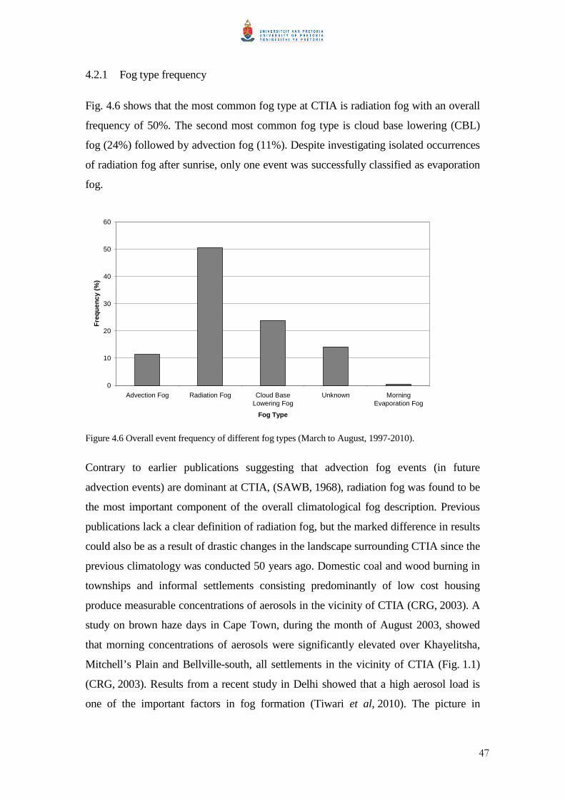
47

4.2.1 Fog type frequency

Fig. 4.6 shows that the most common fog type at CTIA is radiation fog with an overall

frequency of 50%. The second most common fog type is cloud base lowering (CBL)

fog (24%) followed by advection fog (11%). Despite investigating isolated occurrences

of radiation fog after sunrise, only one event was successfully classified as evaporation

fog.

0

10

20

30

40

50

60

Advection Fog Radiation Fog Cloud BaseLowering Fog

Unknown MorningEvaporation Fog

Fog Type

Fre

quen

cy (

%)

Figure 4.6 Overall event frequency of different fog types (March to August, 1997-2010).

Contrary to earlier publications suggesting that advection fog events (in future

advection events) are dominant at CTIA, (SAWB, 1968), radiation fog was found to be

the most important component of the overall climatological fog description. Previous

publications lack a clear definition of radiation fog, but the marked difference in results

could also be as a result of drastic changes in the landscape surrounding CTIA since the

previous climatology was conducted 50 years ago. Domestic coal and wood burning in

townships and informal settlements consisting predominantly of low cost housing

produce measurable concentrations of aerosols in the vicinity of CTIA (CRG, 2003). A

study on brown haze days in Cape Town, during the month of August 2003, showed

that morning concentrations of aerosols were significantly elevated over Khayelitsha,

Mitchell’s Plain and Bellville-south, all settlements in the vicinity of CTIA (Fig. 1.1)

(CRG, 2003). Results from a recent study in Delhi showed that a high aerosol load is

one of the important factors in fog formation (Tiwari et al, 2010). The picture in

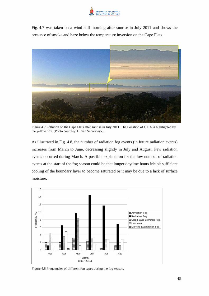
48

Fig. 4.7 was taken on a wind still morning after sunrise in July 2011 and shows the

presence of smoke and haze below the temperature inversion on the Cape Flats.

Figure 4.7 Pollution on the Cape Flats after sunrise in July 2011. The Location of CTIA is highlighted by the yellow box. (Photo courtesy: H. van Schalkwyk).

As illustrated in Fig. 4.8, the number of radiation fog events (in future radiation events)

increases from March to June, decreasing slightly in July and August. Few radiation

events occurred during March. A possible explanation for the low number of radiation

events at the start of the fog season could be that longer daytime hours inhibit sufficient

cooling of the boundary layer to become saturated or it may be due to a lack of surface

moisture.

0

2

4

6

8

10

12

14

16

Mar Apr May Jun Jul Aug

Month (1997-2010)

Fre

quen

cy (

%) Advection Fog

Radiation FogCloud Base Lowering FogUnknownMorning Evaporation Fog

Figure 4.8 Frequencies of different fog types during the fog season.

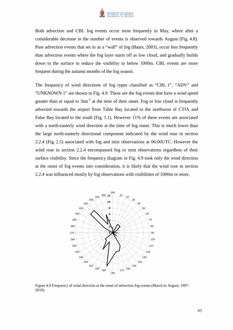
49

Both advection and CBL fog events occur most frequently in May, where after a

considerable decrease in the number of events is observed towards August (Fig. 4.8).

Pure advection events that set in as a “wall” of fog (Baars, 2003), occur less frequently

than advection events where the fog layer starts off as low cloud, and gradually builds

down to the surface to reduce the visibility to below 1000m. CBL events are more

frequent during the autumn months of the fog season.

The frequency of wind directions of fog types classified as “CBL 1”, “ADV” and

“UNKNOWN 1” are shown in Fig. 4.9. These are the fog events that have a wind speed

greater than or equal to 3ms-1 at the time of their onset. Fog or low cloud is frequently

advected towards the airport from Table Bay located to the northwest of CTIA and

False Bay located to the south (Fig. 1.1). However 11% of these events are associated

with a north-easterly wind direction at the time of fog onset. This is much lower than

the large north-easterly directional component indicated by the wind rose in section

2.2.4 (Fig. 2.5) associated with fog and mist observations at 06:00UTC. However the

wind rose in section 2.2.4 encompassed fog or mist observations regardless of their

surface visibility. Since the frequency diagram in Fig. 4.9 took only the wind direction

at the onset of fog events into consideration, it is likely that the wind rose in section

2.2.4 was influenced mostly by fog observations with visibilities of 1000m or more.

0

2

4

6

8

10

12360

1020

30

40

50

60

70

80

90

100

110

120

130

140

150160

170180

190200

210

220

230

240

250

260

270

280

290

300

310

320

330340

350

Figure 4.9 Frequency of wind direction at the onset of advection fog events (March to August, 1997-2010).

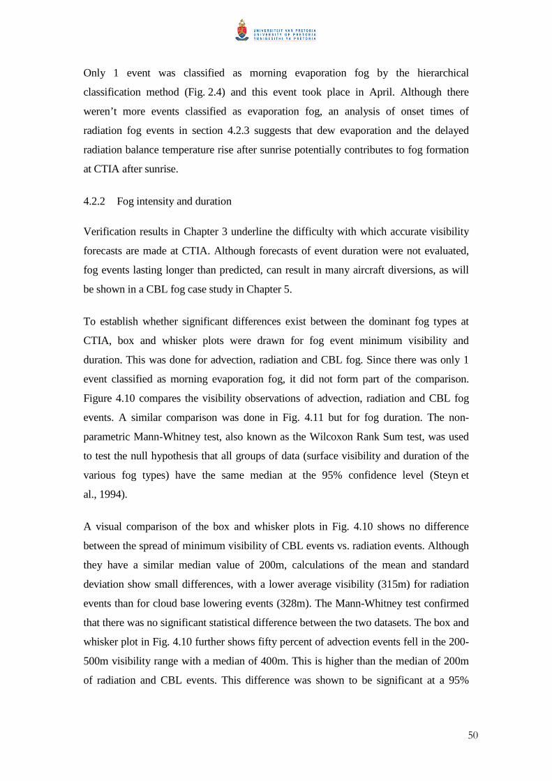
50

Only 1 event was classified as morning evaporation fog by the hierarchical

classification method (Fig. 2.4) and this event took place in April. Although there

weren’t more events classified as evaporation fog, an analysis of onset times of

radiation fog events in section 4.2.3 suggests that dew evaporation and the delayed

radiation balance temperature rise after sunrise potentially contributes to fog formation

at CTIA after sunrise.

4.2.2 Fog intensity and duration

Verification results in Chapter 3 underline the difficulty with which accurate visibility

forecasts are made at CTIA. Although forecasts of event duration were not evaluated,

fog events lasting longer than predicted, can result in many aircraft diversions, as will

be shown in a CBL fog case study in Chapter 5.

To establish whether significant differences exist between the dominant fog types at

CTIA, box and whisker plots were drawn for fog event minimum visibility and

duration. This was done for advection, radiation and CBL fog. Since there was only 1

event classified as morning evaporation fog, it did not form part of the comparison.

Figure 4.10 compares the visibility observations of advection, radiation and CBL fog

events. A similar comparison was done in Fig. 4.11 but for fog duration. The non-

parametric Mann-Whitney test, also known as the Wilcoxon Rank Sum test, was used

to test the null hypothesis that all groups of data (surface visibility and duration of the

various fog types) have the same median at the 95% confidence level (Steyn et

al., 1994).

A visual comparison of the box and whisker plots in Fig. 4.10 shows no difference

between the spread of minimum visibility of CBL events vs. radiation events. Although

they have a similar median value of 200m, calculations of the mean and standard

deviation show small differences, with a lower average visibility (315m) for radiation

events than for cloud base lowering events (328m). The Mann-Whitney test confirmed

that there was no significant statistical difference between the two datasets. The box and

whisker plot in Fig. 4.10 further shows fifty percent of advection events fell in the 200-

500m visibility range with a median of 400m. This is higher than the median of 200m

of radiation and CBL events. This difference was shown to be significant at a 95%

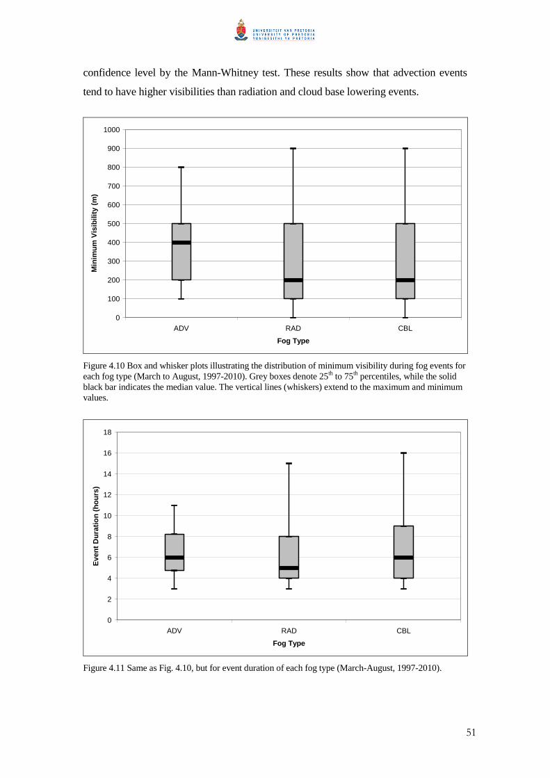
51

confidence level by the Mann-Whitney test. These results show that advection events

tend to have higher visibilities than radiation and cloud base lowering events.

0

100

200

300

400

500

600

700

800

900

1000

ADV RAD CBL

Fog Type

Min

imum

Vis

ibili

ty (

m)

plea

se

Figure 4.10 Box and whisker plots illustrating the distribution of minimum visibility during fog events for each fog type (March to August, 1997-2010). Grey boxes denote 25th to 75th percentiles, while the solid black bar indicates the median value. The vertical lines (whiskers) extend to the maximum and minimum values.

0

2

4

6

8

10

12

14

16

18

ADV RAD CBL

Fog Type

Eve

nt D

urat

ion

(hou

rs)

Figure 4.11 Same as Fig. 4.10, but for event duration of each fog type (March-August, 1997-2010).

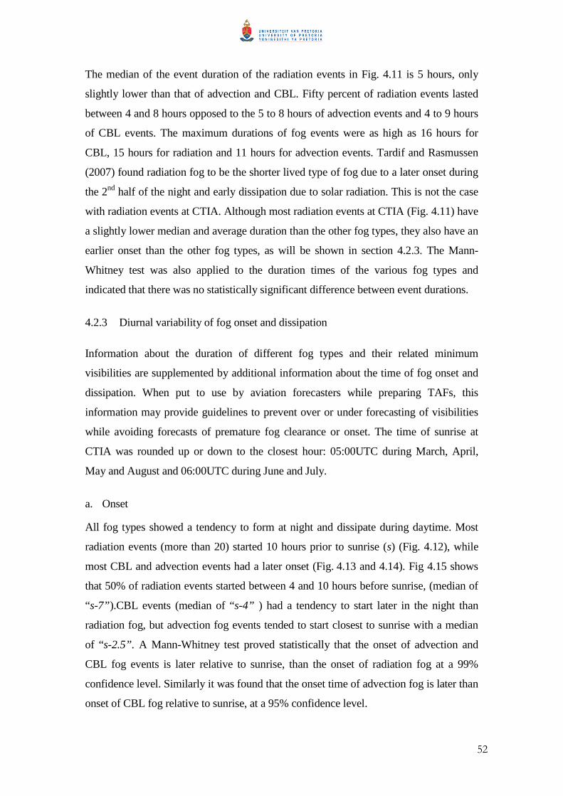
52

The median of the event duration of the radiation events in Fig. 4.11 is 5 hours, only

slightly lower than that of advection and CBL. Fifty percent of radiation events lasted

between 4 and 8 hours opposed to the 5 to 8 hours of advection events and 4 to 9 hours

of CBL events. The maximum durations of fog events were as high as 16 hours for

CBL, 15 hours for radiation and 11 hours for advection events. Tardif and Rasmussen

(2007) found radiation fog to be the shorter lived type of fog due to a later onset during

the 2nd half of the night and early dissipation due to solar radiation. This is not the case

with radiation events at CTIA. Although most radiation events at CTIA (Fig. 4.11) have

a slightly lower median and average duration than the other fog types, they also have an

earlier onset than the other fog types, as will be shown in section 4.2.3. The Mann-

Whitney test was also applied to the duration times of the various fog types and

indicated that there was no statistically significant difference between event durations.

4.2.3 Diurnal variability of fog onset and dissipation

Information about the duration of different fog types and their related minimum

visibilities are supplemented by additional information about the time of fog onset and

dissipation. When put to use by aviation forecasters while preparing TAFs, this

information may provide guidelines to prevent over or under forecasting of visibilities

while avoiding forecasts of premature fog clearance or onset. The time of sunrise at

CTIA was rounded up or down to the closest hour: 05:00UTC during March, April,

May and August and 06:00UTC during June and July.

a. Onset

All fog types showed a tendency to form at night and dissipate during daytime. Most

radiation events (more than 20) started 10 hours prior to sunrise (s) (Fig. 4.12), while

most CBL and advection events had a later onset (Fig. 4.13 and 4.14). Fig 4.15 shows

that 50% of radiation events started between 4 and 10 hours before sunrise, (median of

“s-7”).CBL events (median of “s-4” ) had a tendency to start later in the night than

radiation fog, but advection fog events tended to start closest to sunrise with a median

of “s-2.5”. A Mann-Whitney test proved statistically that the onset of advection and

CBL fog events is later relative to sunrise, than the onset of radiation fog at a 99%

confidence level. Similarly it was found that the onset time of advection fog is later than

onset of CBL fog relative to sunrise, at a 95% confidence level.

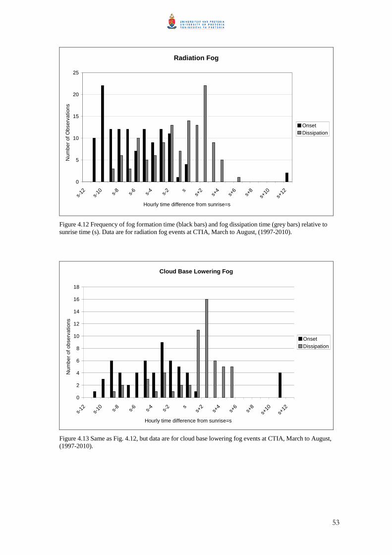
53

Radiation Fog

0

5

10

15

20

25

s-12

s-10 s-

8s-

6s-

4s-

2 ss+

2s+

4s+

6s+

8s+

10s+

12

Hourly time difference from sunrise=s

Num

ber

of O

bser

vatio

ns r

ed

OnsetDissipation

Figure 4.12 Frequency of fog formation time (black bars) and fog dissipation time (grey bars) relative to sunrise time (s). Data are for radiation fog events at CTIA, March to August, (1997-2010).

Cloud Base Lowering Fog

0

2

4

6

8

10

12

14

16

18

s-12

s-10

s-8

s-6

s-4

s-2 s

s+2

s+4

s+6

s+8

s+10

s+12


Num

ber

of o

bser

vatio

ns r

ed

OnsetDissipation

Figure 4.13 Same as Fig. 4.12, but data are for cloud base lowering fog events at CTIA, March to August, (1997-2010).

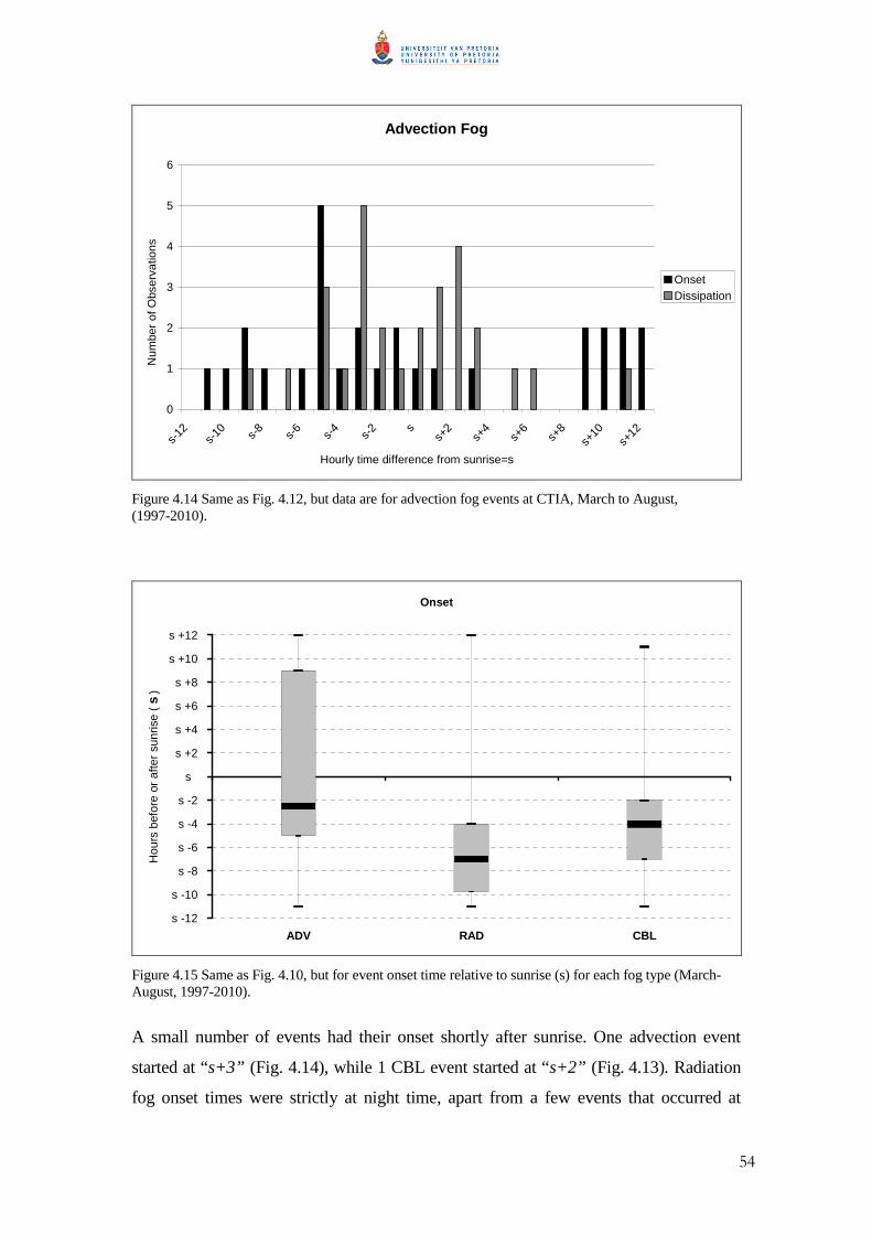
54

Advection Fog

0

1

2

3

4

5

6

s-12

s-10 s-

8s-

6s-

4s-

2 ss+

2s+

4s+

6s+

8s+

10s+

12


Num

ber

of O

bser

vatio

ns R

ED

OnsetDissipation

Figure 4.14 Same as Fig. 4.12, but data are for advection fog events at CTIA, March to August, (1997-2010).

Onset

s -12

s -10

s -8

s -6

s -4

s -2

s

s +2

s +4

s +6

s +8

s +10

s +12

ADV RAD CBL

Hou

rs b

efor

e or

afte

r su

nris

e ( s

)

Figure 4.15 Same as Fig. 4.10, but for event onset time relative to sunrise (s) for each fog type (March-August, 1997-2010).

A small number of events had their onset shortly after sunrise. One advection event

started at “s+3” (Fig. 4.14), while 1 CBL event started at “s+2” (Fig. 4.13). Radiation

fog onset times were strictly at night time, apart from a few events that occurred at

55

sunrise (Fig. 4.12). A dramatic drop in radiation event onset is observed between the

two hours before sunrise “s-2” and “s-1”. Yet a rise in the number of event onsets is

observed at “s” (Fig. 4.12). Similar observations of increased radiation fog onset at

sunrise were made by Meyer and Lala (1990) who commented that increased solar

radiation associated with sunrise can act to promote, enhance and eventually dissipate

radiation fog. The role of dew evaporation resulting from the increase of surface

temperature after sunrise is most important to provide a moist lower boundary for fog

formation or persistence after sunrise (Pilié et al., 1975). Even though only 1 event was

classified as an evaporation event by the hierarchical classification method, the

increased frequency of radiation fog onset times in Fig. 4.12 shows the potential

influence dew evaporation has on fog formation after sunrise.

Advection fog showed the largest variation in onset times (Fig. 4.14 and 4.15). There

were no event onsets during midday and early afternoon (four to eight hours after

sunrise), but 8 events started within 9 to 12 hours after sunrise. The earlier onset of

advection fog events, in comparison with other fog types, is possibly because a marine

fog layer will often remain stationary along the coast during daytime as solar heating of

the land mass causes dissipation of the fog by convective mixing that takes place

between drier, warmer, continental air and the advancing marine layer. But as soon as

temperatures start to decrease towards night time, the cooler and less turbulent

boundary layer allows an inland propagation of the fog layer (Tardif and

Rasmussen, 2007), allowing for fog onset during the late afternoon and early evening as

seen in Fig. 4.14.

b. Dissipation

A striking feature on dissipation histograms in Fig. 4.12 to 4.14 is the number of fog

events that dissipated before sunrise (s). From a fog forecasting point of view an event

that dissipates earlier than expected can lead to forecast errors just as much as an event

that dissipates much later. Forecasting the dissipation time of radiation events that clear

before sunrise is challenging since the reasons behind clearance before sunrise are often

unclear. This does however show that dissipation of fog is not always due to an increase

in solar radiation, but could also be ascribed to a change in the low level horizontal

advection during evolving synoptic conditions (Tardif and Rasmussen, 2007).

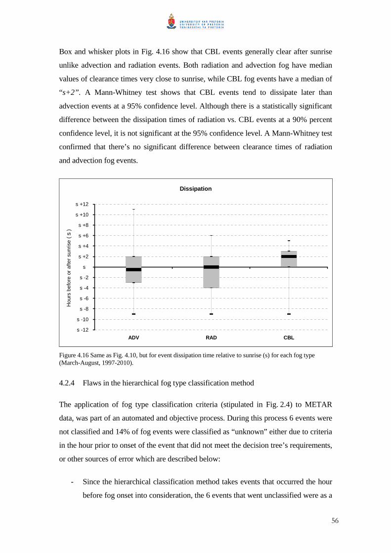
56

Box and whisker plots in Fig. 4.16 show that CBL events generally clear after sunrise

unlike advection and radiation events. Both radiation and advection fog have median

values of clearance times very close to sunrise, while CBL fog events have a median of

“s+2”. A Mann-Whitney test shows that CBL events tend to dissipate later than

advection events at a 95% confidence level. Although there is a statistically significant

difference between the dissipation times of radiation vs. CBL events at a 90% percent

confidence level, it is not significant at the 95% confidence level. A Mann-Whitney test

confirmed that there’s no significant difference between clearance times of radiation

and advection fog events.

Dissipation

s -12

s -10

s -8

s -6

s -4

s -2

s

s +2

s +4

s +6

s +8

s +10

s +12

ADV RAD CBL

Hou

rs b

efor

e or

afte

r su

nris

e ( s

)

Figure 4.16 Same as Fig. 4.10, but for event dissipation time relative to sunrise (s) for each fog type (March-August, 1997-2010).

4.2.4 Flaws in the hierarchical fog type classification method

The application of fog type classification criteria (stipulated in Fig. 2.4) to METAR

data, was part of an automated and objective process. During this process 6 events were

not classified and 14% of fog events were classified as “unknown” either due to criteria

in the hour prior to onset of the event that did not meet the decision tree’s requirements,

or other sources of error which are described below:

- Since the hierarchical classification method takes events that occurred the hour

before fog onset into consideration, the 6 events that went unclassified were as a

57

result of automatically (AUTO) generated METAR reports preceding the onset

of fog. These reports do not contain cloud or visibility information and would

produce an error in the fog type classification.

- Out of the 35 “unknown” fog types, 6 occurred on days where 2 separate fog

events were classified on 1 day. In all these instances a temporary improvement

of visibility resulted in the hierarchical classification method identifying the

second deterioration of visibility as the onset of a “new” event, which was then

classified as “unknown”.

Having accounted for 6 “unknown” events that were erroneously classified as such, the

proportion of “unknown” events drops to 12%.

4.2.5 Summary

Of the 248 events that were classified into different fog types, the 3 types of fog that

occur most frequently at CTIA are: radiation fog (50%), CBL fog (24%) and advection

fog (11%).

The frequency of radiation events increased from March to June and decreased slightly

in July and August. CBL events occurred more frequently during the first 3 months of

the fog season, where after the frequency dropped to its lowest in August, while

advection fog increased from March to May and decreased from June to August.

Most advective events where the wind speed was greater than 3ms-1 at the time of fog

onset were associated with north-westerly, southerly or north-easterly wind directions.

Apart from a land mass to the northeast, CTIA is exposed to the ocean to its northwest

and south, where most advection fog comes from.

Radiation and CBL events were associated with similar minimum visibilities, which

were lower than the minimum visibility of advection events. The different fog types did

not have significantly different event durations, although CBL and advection fog tended

to last slightly longer than radiation fog.

The onset times of advection fog events showed most variation relative to sunrise and

were not strictly confined to the night time. Advection fog events tended to start later in

the night than CBL and radiation events, while radiation fog had the earliest onset

58

relative to sunrise. Radiation and advection fog events tended to dissipate at or before

sunrise, but most CBL events dissipated within 2 to 3 hours after sunrise.

4.3 SYNOPTIC CLASSIFICATION

This section describes the use of SOMs to classify synoptic circulation patterns

associated with fog at CTIA during the fog seasons of 1997-2010. Making the weather

forecaster aware of the synoptic circulation usually associated with fog will be an

important step to aid in the forecasting of fog at CTIA.

4.3.1 Dominant synoptic types

A 5x7-node SOM of daily (00:00UTC) sea level pressure for March-August from 1997

to 2010 (Fig 4.17) was created using National Centres for Environmental Prediction

reanalysis data. All days where fog occurred were considered in the SOM. A relatively

large SOM, analogous in effect to clustering to 35 cluster groups, was chosen to capture

the high level of variability in daily fields and indicates the dominant synoptic

circulation types that occurred during the above mentioned period.

Each node in Fig. 4.17 represents a group of similar synoptic circulations that were

present in the original dataset. Similar synoptic types are located adjacent to one other,

while dissimilar synoptic types are found at opposite ends of the SOM. The synoptic

types representing westerly troughs (most likely associated with the passage of cold

fronts) are in the upper portion of the SOM (Fig. 4.17). Consider the first line in the

SOM and note how the westerly systems gradually move southward with a high

pressure system establishing itself over the western interior at G1. This trend is present

in all the SOMs with lower pressures on the left but with increasing pressures to the

right. Node B3 and C3 look similar but in C3 the central pressure of the low/trough is

slightly higher than in B3. Synoptic types with a dominant high over the interior are

found to the right nodes, while synoptic types with lower pressure over the interior and

a high to the west of the country are found in the bottom left corner. Transition states,

mainly featuring areas of lower pressure along the west coast, are found in the centre

nodes.

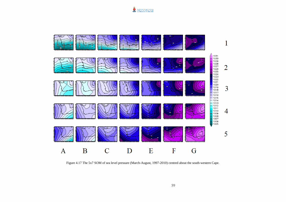
59

Figure 4.17 The 5x7 SOM of sea level pressure (March-August, 1997-2010) centred about the south-western Cape.

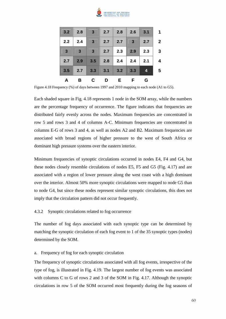
60

3.2 2.8 3 2.7 2.8 2.6 3.1 1

2.2 2.4 3 2.7 2.7 3 2.7 2

3 3 3 2.7 2.3 2.9 2.3 3

2.7 2.9 3.5 2.8 2.4 2.4 2.1 4

3.5 2.7 3.3 3.1 3.2 3.3 4 5

A B C D E F G

Figure 4.18 Frequency (%) of days between 1997 and 2010 mapping to each node (A1 to G5).

Each shaded square in Fig. 4.18 represents 1 node in the SOM array, while the numbers

are the percentage frequency of occurrence. The figure indicates that frequencies are

distributed fairly evenly across the nodes. Maximum frequencies are concentrated in

row 5 and rows 3 and 4 of columns A-C. Minimum frequencies are concentrated in

columns E-G of rows 3 and 4, as well as nodes A2 and B2. Maximum frequencies are

associated with broad regions of higher pressure to the west of South Africa or

dominant high pressure systems over the eastern interior.

Minimum frequencies of synoptic circulations occurred in nodes E4, F4 and G4, but

these nodes closely resemble circulations of nodes E5, F5 and G5 (Fig. 4.17) and are

associated with a region of lower pressure along the west coast with a high dominant

over the interior. Almost 50% more synoptic circulations were mapped to node G5 than

to node G4, but since these nodes represent similar synoptic circulations, this does not

imply that the circulation pattern did not occur frequently.

4.3.2 Synoptic circulations related to fog occurrence

The number of fog days associated with each synoptic type can be determined by

matching the synoptic circulation of each fog event to 1 of the 35 synoptic types (nodes)

determined by the SOM.

a. Frequency of fog for each synoptic circulation

The frequency of synoptic circulations associated with all fog events, irrespective of the

type of fog, is illustrated in Fig. 4.19. The largest number of fog events was associated

with columns C to G of rows 2 and 3 of the SOM in Fig. 4.17. Although the synoptic

circulations in row 5 of the SOM occurred most frequently during the fog seasons of

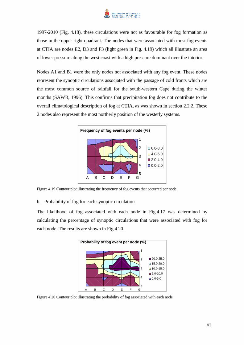
61

1997-2010 (Fig. 4.18), these circulations were not as favourable for fog formation as

those in the upper right quadrant. The nodes that were associated with most fog events

at CTIA are nodes E2, D3 and F3 (light green in Fig. 4.19) which all illustrate an area

of lower pressure along the west coast with a high pressure dominant over the interior.

Nodes A1 and B1 were the only nodes not associated with any fog event. These nodes

represent the synoptic circulations associated with the passage of cold fronts which are

the most common source of rainfall for the south-western Cape during the winter

months (SAWB, 1996). This confirms that precipitation fog does not contribute to the

overall climatological description of fog at CTIA, as was shown in section 2.2.2. These

2 nodes also represent the most northerly position of the westerly systems.

A B C D E F G5

4

3

2

1

Frequency of fog events per node (%)

6.0-8.0

4.0-6.0

2.0-4.0

0.0-2.0

Figure 4.19 Contour plot illustrating the frequency of fog events that occurred per node.

b. Probability of fog for each synoptic circulation

The likelihood of fog associated with each node in Fig.4.17 was determined by

calculating the percentage of synoptic circulations that were associated with fog for

each node. The results are shown in Fig.4.20.

A B C D E F G5

4

3

2

1

Probability of fog event per node (%)

20.0-25.0

15.0-20.0

10.0-15.0

5.0-10.0

0.0-5.0

Figure 4.20 Contour plot illustrating the probability of fog associated with each node.

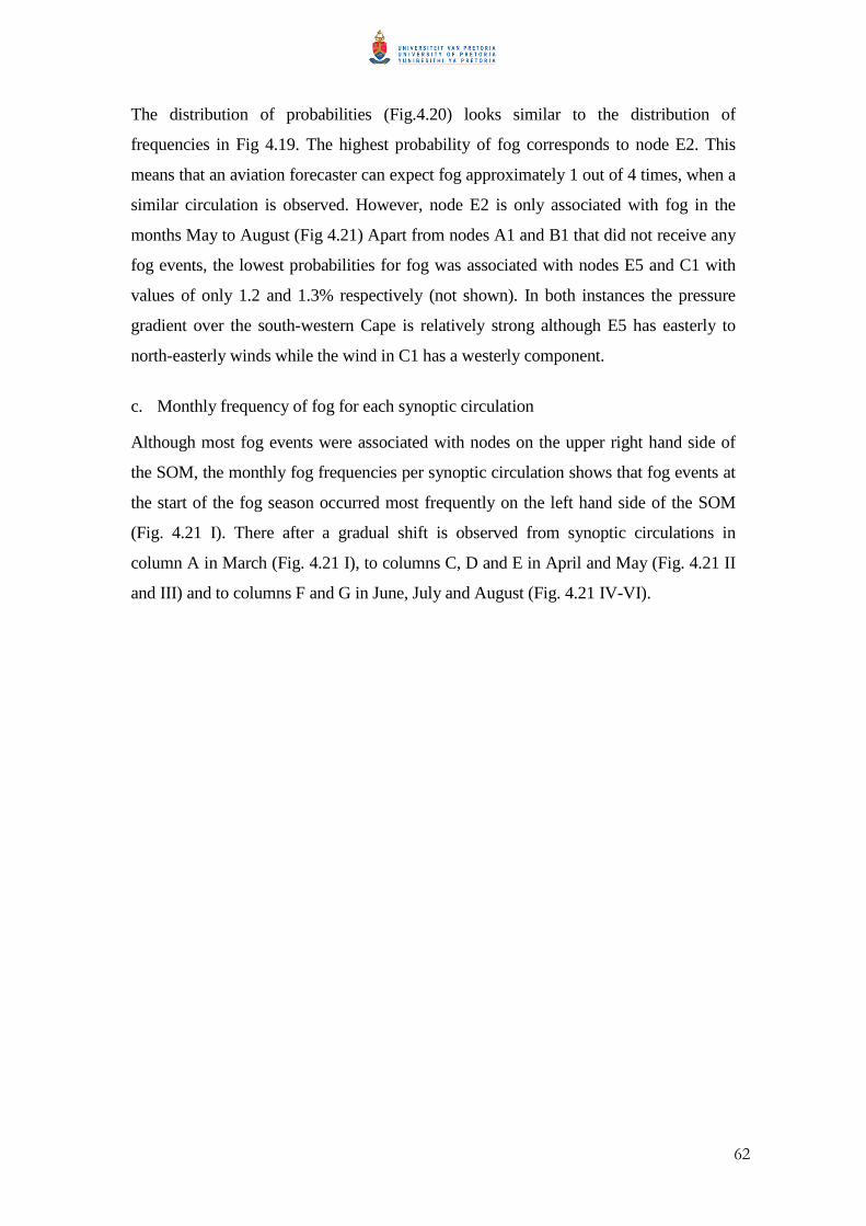
62

The distribution of probabilities (Fig.4.20) looks similar to the distribution of

frequencies in Fig 4.19. The highest probability of fog corresponds to node E2. This

means that an aviation forecaster can expect fog approximately 1 out of 4 times, when a

similar circulation is observed. However, node E2 is only associated with fog in the

months May to August (Fig 4.21) Apart from nodes A1 and B1 that did not receive any

fog events, the lowest probabilities for fog was associated with nodes E5 and C1 with

values of only 1.2 and 1.3% respectively (not shown). In both instances the pressure

gradient over the south-western Cape is relatively strong although E5 has easterly to

north-easterly winds while the wind in C1 has a westerly component.

c. Monthly frequency of fog for each synoptic circulation

Although most fog events were associated with nodes on the upper right hand side of

the SOM, the monthly fog frequencies per synoptic circulation shows that fog events at

the start of the fog season occurred most frequently on the left hand side of the SOM

(Fig. 4.21 I). There after a gradual shift is observed from synoptic circulations in

column A in March (Fig. 4.21 I), to columns C, D and E in April and May (Fig. 4.21 II

and III) and to columns F and G in June, July and August (Fig. 4.21 IV-VI).

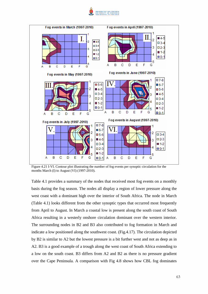
63

Figure 4.21 I-VI. Contour plot illustrating the number of fog events per synoptic circulation for the months March (I) to August (VI) (1997-2010).

Table 4.1 provides a summary of the nodes that received most fog events on a monthly

basis during the fog season. The nodes all display a region of lower pressure along the

west coast with a dominant high over the interior of South Africa. The node in March

(Table 4.1) looks different from the other synoptic types that occurred most frequently

from April to August. In March a coastal low is present along the south coast of South

Africa resulting in a westerly onshore circulation dominant over the western interior.

The surrounding nodes in B2 and B3 also contributed to fog formation in March and

indicate a low positioned along the southwest coast. (Fig.4.17). The circulation depicted

by B2 is similar to A2 but the lowest pressure is a bit further west and not as deep as in

A2. B3 is a good example of a trough along the west coast of South Africa extending to

a low on the south coast. B3 differs from A2 and B2 as there is no pressure gradient

over the Cape Peninsula. A comparison with Fig 4.8 shows how CBL fog dominates

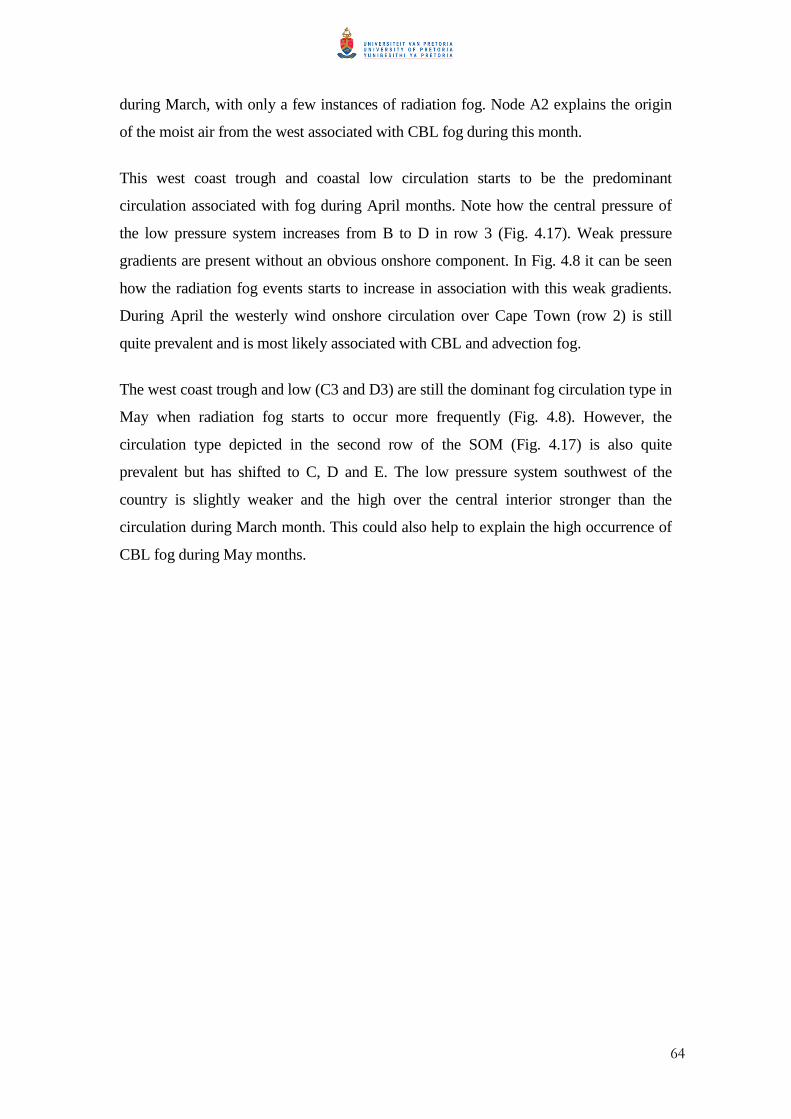
64

during March, with only a few instances of radiation fog. Node A2 explains the origin

of the moist air from the west associated with CBL fog during this month.

This west coast trough and coastal low circulation starts to be the predominant

circulation associated with fog during April months. Note how the central pressure of

the low pressure system increases from B to D in row 3 (Fig. 4.17). Weak pressure

gradients are present without an obvious onshore component. In Fig. 4.8 it can be seen

how the radiation fog events starts to increase in association with this weak gradients.

During April the westerly wind onshore circulation over Cape Town (row 2) is still

quite prevalent and is most likely associated with CBL and advection fog.

The west coast trough and low (C3 and D3) are still the dominant fog circulation type in

May when radiation fog starts to occur more frequently (Fig. 4.8). However, the

circulation type depicted in the second row of the SOM (Fig. 4.17) is also quite

prevalent but has shifted to C, D and E. The low pressure system southwest of the

country is slightly weaker and the high over the central interior stronger than the

circulation during March month. This could also help to explain the high occurrence of

CBL fog during May months.

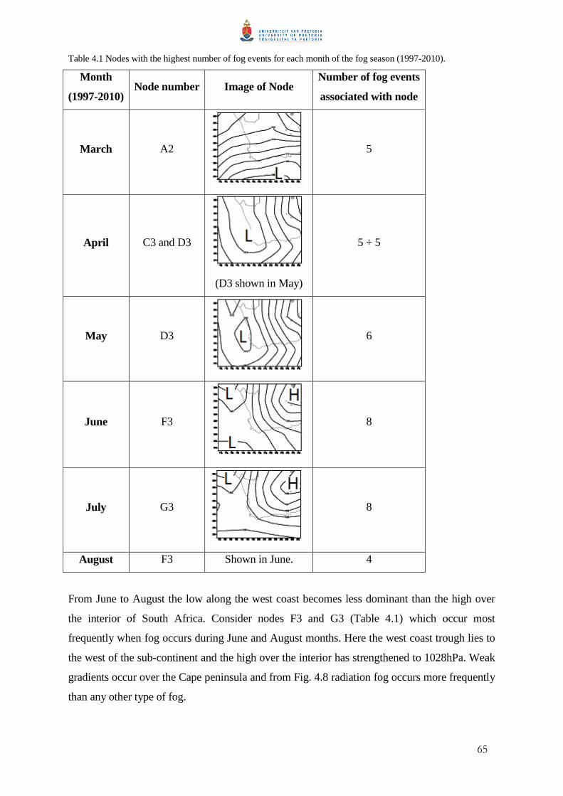
65

Table 4.1 Nodes with the highest number of fog events for each month of the fog season (1997-2010).

Month

(1997-2010) Node number Image of Node

Number of fog events

associated with node

March A2

5

April C3 and D3

(D3 shown in May)

5 + 5

May D3

6

June F3

8

July G3

8

August F3 Shown in June. 4

From June to August the low along the west coast becomes less dominant than the high over

the interior of South Africa. Consider nodes F3 and G3 (Table 4.1) which occur most

frequently when fog occurs during June and August months. Here the west coast trough lies to

the west of the sub-continent and the high over the interior has strengthened to 1028hPa. Weak

gradients occur over the Cape peninsula and from Fig. 4.8 radiation fog occurs more frequently

than any other type of fog.

66

4.3.3 Fog types related to synoptic circulation

The synoptic circulation generally associated with fog, does not remain constant during the fog

season. A monthly fog type frequency chart (Fig. 4.8) indicates how the prevalent fog type

changes from advective events in March, to dominant radiation events from April to August. In

this section the synoptic circulations associated with the different fog types at CTIA will be

explored.

0 2 4 6 8 10 12 14 16 18

A1B1C1D1E1F1G1A2B2C2D2E2F2G2A3B3C3D3E3F3G3A4B4C4D4E4F4G4A5B5C5D5E5F5G5

Freq: AFreq: RFreq: CFreq: UFreq: E

Figure 4.22 Frequency of fog types per node (March-August, 1997-2010). Advection fog indicated in grey (A), radiation fog: black (R), CBL fog: diagonal lines (C), ‟unknown” events: dark grey (U) and evaporation fog: white (E).

Node E2 (Fig. 4.23) was associated with the most fog events at CTIA. Although there were no

fog observations associated with node E2 in March and April (Fig. 4.21); 17 fog events

occurred between May and August. Most of these events were radiation fog events (11), but

there were also 1 CBL, 2 unknown and 3 advection events (Fig. 4.22). The presence of the low

along the southwest coast most likely acts as a source of surface moisture due to onshore winds.

The high over the interior in turn causes subsidence which contributes to atmospheric stability

and the formation of radiation fog. Therefore two fog formation processes eventually result in

the formation of radiation fog with a synoptic circulation like node E2: advection of moisture

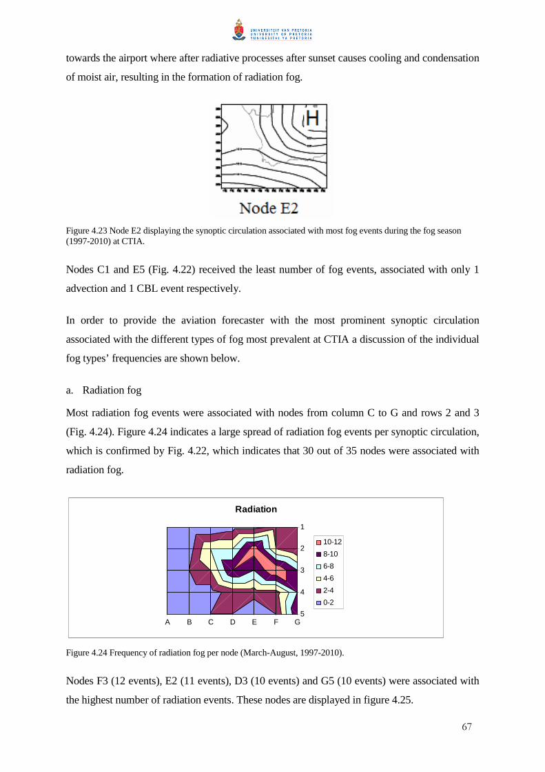
67

towards the airport where after radiative processes after sunset causes cooling and condensation

of moist air, resulting in the formation of radiation fog.

Figure 4.23 Node E2 displaying the synoptic circulation associated with most fog events during the fog season (1997-2010) at CTIA.

Nodes C1 and E5 (Fig. 4.22) received the least number of fog events, associated with only 1

advection and 1 CBL event respectively.

In order to provide the aviation forecaster with the most prominent synoptic circulation

associated with the different types of fog most prevalent at CTIA a discussion of the individual

fog types’ frequencies are shown below.

a. Radiation fog

Most radiation fog events were associated with nodes from column C to G and rows 2 and 3

(Fig. 4.24). Figure 4.24 indicates a large spread of radiation fog events per synoptic circulation,

which is confirmed by Fig. 4.22, which indicates that 30 out of 35 nodes were associated with

radiation fog.

A B C D E F G5

4

3

2

1

Radiation

10-12

8-10

6-8

4-6

2-4

0-2

Figure 4.24 Frequency of radiation fog per node (March-August, 1997-2010).

Nodes F3 (12 events), E2 (11 events), D3 (10 events) and G5 (10 events) were associated with

the highest number of radiation events. These nodes are displayed in figure 4.25.

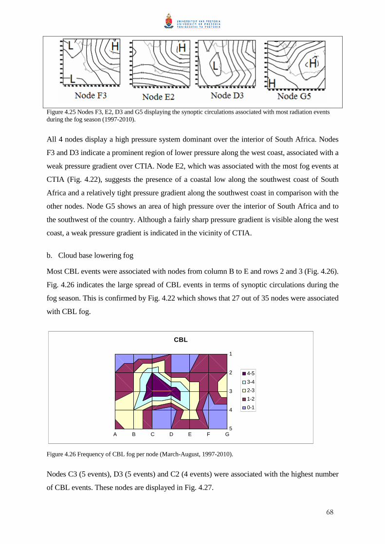
68

Figure 4.25 Nodes F3, E2, D3 and G5 displaying the synoptic circulations associated with most radiation events during the fog season (1997-2010).

All 4 nodes display a high pressure system dominant over the interior of South Africa. Nodes

F3 and D3 indicate a prominent region of lower pressure along the west coast, associated with a

weak pressure gradient over CTIA. Node E2, which was associated with the most fog events at

CTIA (Fig. 4.22), suggests the presence of a coastal low along the southwest coast of South

Africa and a relatively tight pressure gradient along the southwest coast in comparison with the

other nodes. Node G5 shows an area of high pressure over the interior of South Africa and to

the southwest of the country. Although a fairly sharp pressure gradient is visible along the west

coast, a weak pressure gradient is indicated in the vicinity of CTIA.

b. Cloud base lowering fog

Most CBL events were associated with nodes from column B to E and rows 2 and 3 (Fig. 4.26).

Fig. 4.26 indicates the large spread of CBL events in terms of synoptic circulations during the

fog season. This is confirmed by Fig. 4.22 which shows that 27 out of 35 nodes were associated

with CBL fog.

A B C D E F G5

4

3

2

1

CBL

4-5

3-4

2-3

1-2

0-1

Figure 4.26 Frequency of CBL fog per node (March-August, 1997-2010).

Nodes C3 (5 events), D3 (5 events) and C2 (4 events) were associated with the highest number

of CBL events. These nodes are displayed in Fig. 4.27.

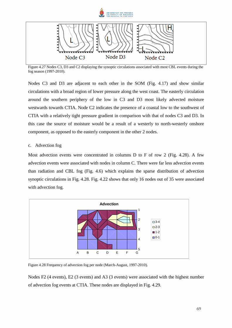
69

Figure 4.27 Nodes C3, D3 and C2 displaying the synoptic circulations associated with most CBL events during the fog season (1997-2010).

Nodes C3 and D3 are adjacent to each other in the SOM (Fig. 4.17) and show similar

circulations with a broad region of lower pressure along the west coast. The easterly circulation

around the southern periphery of the low in C3 and D3 most likely advected moisture

westwards towards CTIA. Node C2 indicates the presence of a coastal low to the southwest of

CTIA with a relatively tight pressure gradient in comparison with that of nodes C3 and D3. In

this case the source of moisture would be a result of a westerly to north-westerly onshore

component, as opposed to the easterly component in the other 2 nodes.

c. Advection fog

Most advection events were concentrated in columns D to F of row 2 (Fig. 4.28). A few

advection events were associated with nodes in column C. There were far less advection events

than radiation and CBL fog (Fig. 4.6) which explains the sparse distribution of advection

synoptic circulations in Fig. 4.28. Fig. 4.22 shows that only 16 nodes out of 35 were associated

with advection fog.

A B C D E F G5

4

3

2

1

Advection

3-4

2-3

1-2

0-1

Figure 4.28 Frequency of advection fog per node (March-August, 1997-2010).

Nodes F2 (4 events), E2 (3 events) and A3 (3 events) were associated with the highest number

of advection fog events at CTIA. These nodes are displayed in Fig. 4.29.

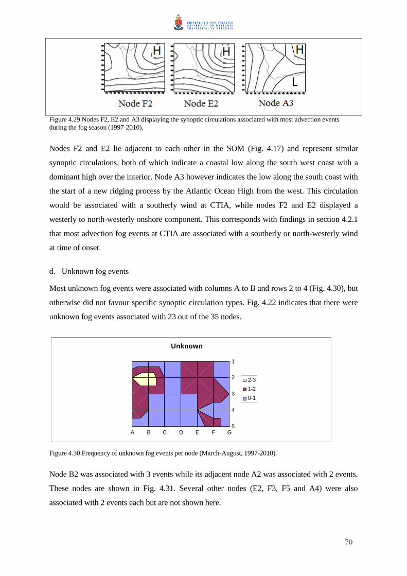
70

Figure 4.29 Nodes F2, E2 and A3 displaying the synoptic circulations associated with most advection events during the fog season (1997-2010).

Nodes F2 and E2 lie adjacent to each other in the SOM (Fig. 4.17) and represent similar

synoptic circulations, both of which indicate a coastal low along the south west coast with a

dominant high over the interior. Node A3 however indicates the low along the south coast with

the start of a new ridging process by the Atlantic Ocean High from the west. This circulation

would be associated with a southerly wind at CTIA, while nodes F2 and E2 displayed a

westerly to north-westerly onshore component. This corresponds with findings in section 4.2.1

that most advection fog events at CTIA are associated with a southerly or north-westerly wind

at time of onset.

d. Unknown fog events

Most unknown fog events were associated with columns A to B and rows 2 to 4 (Fig. 4.30), but

otherwise did not favour specific synoptic circulation types. Fig. 4.22 indicates that there were

unknown fog events associated with 23 out of the 35 nodes.

A B C D E F G5

4

3

2

1

Unknown

2-3

1-2

0-1

Figure 4.30 Frequency of unknown fog events per node (March-August, 1997-2010).

Node B2 was associated with 3 events while its adjacent node A2 was associated with 2 events.

These nodes are shown in Fig. 4.31. Several other nodes (E2, F3, F5 and A4) were also

associated with 2 events each but are not shown here.

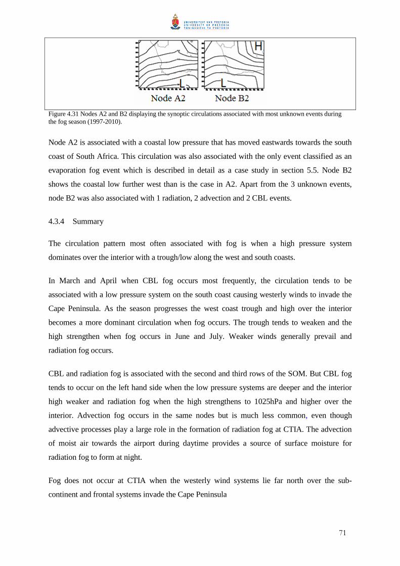
71

Figure 4.31 Nodes A2 and B2 displaying the synoptic circulations associated with most unknown events during the fog season (1997-2010).

Node A2 is associated with a coastal low pressure that has moved eastwards towards the south

coast of South Africa. This circulation was also associated with the only event classified as an

evaporation fog event which is described in detail as a case study in section 5.5. Node B2

shows the coastal low further west than is the case in A2. Apart from the 3 unknown events,

node B2 was also associated with 1 radiation, 2 advection and 2 CBL events.

4.3.4 Summary

The circulation pattern most often associated with fog is when a high pressure system

dominates over the interior with a trough/low along the west and south coasts.

In March and April when CBL fog occurs most frequently, the circulation tends to be

associated with a low pressure system on the south coast causing westerly winds to invade the

Cape Peninsula. As the season progresses the west coast trough and high over the interior

becomes a more dominant circulation when fog occurs. The trough tends to weaken and the

high strengthen when fog occurs in June and July. Weaker winds generally prevail and

radiation fog occurs.

CBL and radiation fog is associated with the second and third rows of the SOM. But CBL fog

tends to occur on the left hand side when the low pressure systems are deeper and the interior

high weaker and radiation fog when the high strengthens to 1025hPa and higher over the

interior. Advection fog occurs in the same nodes but is much less common, even though

advective processes play a large role in the formation of radiation fog at CTIA. The advection

of moist air towards the airport during daytime provides a source of surface moisture for

radiation fog to form at night.

Fog does not occur at CTIA when the westerly wind systems lie far north over the sub-

continent and frontal systems invade the Cape Peninsula

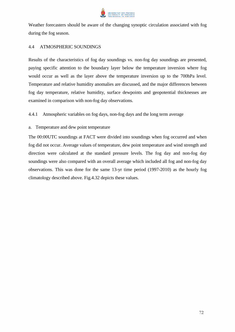
72

Weather forecasters should be aware of the changing synoptic circulation associated with fog

during the fog season.

4.4 ATMOSPHERIC SOUNDINGS

Results of the characteristics of fog day soundings vs. non-fog day soundings are presented,

paying specific attention to the boundary layer below the temperature inversion where fog

would occur as well as the layer above the temperature inversion up to the 700hPa level.

Temperature and relative humidity anomalies are discussed, and the major differences between

fog day temperature, relative humidity, surface dewpoints and geopotential thicknesses are

examined in comparison with non-fog day observations.

4.4.1 Atmospheric variables on fog days, non-fog days and the long term average

a. Temperature and dew point temperature

The 00:00UTC soundings at FACT were divided into soundings when fog occurred and when

fog did not occur. Average values of temperature, dew point temperature and wind strength and

direction were calculated at the standard pressure levels. The fog day and non-fog day

soundings were also compared with an overall average which included all fog and non-fog day

observations. This was done for the same 13-yr time period (1997-2010) as the hourly fog

climatology described above. Fig.4.32 depicts these values.

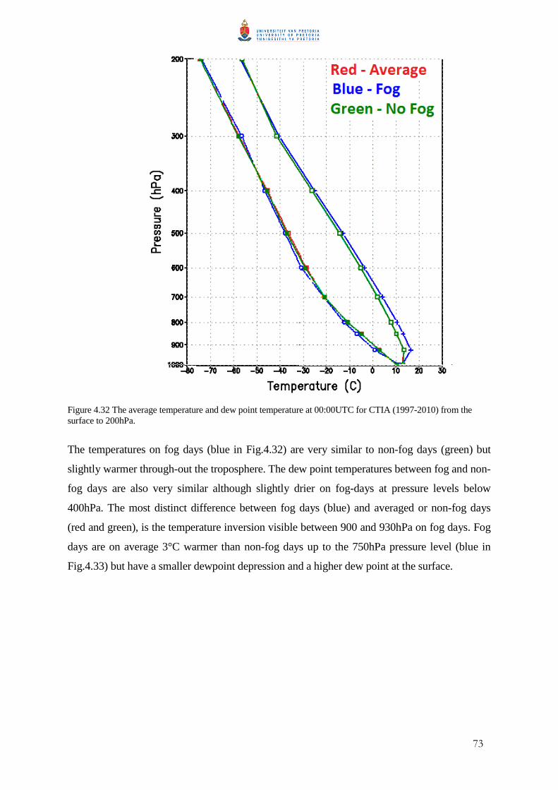
73

Figure 4.32 The average temperature and dew point temperature at 00:00UTC for CTIA (1997-2010) from the surface to 200hPa.

The temperatures on fog days (blue in Fig.4.32) are very similar to non-fog days (green) but

slightly warmer through-out the troposphere. The dew point temperatures between fog and non-

fog days are also very similar although slightly drier on fog-days at pressure levels below

400hPa. The most distinct difference between fog days (blue) and averaged or non-fog days

(red and green), is the temperature inversion visible between 900 and 930hPa on fog days. Fog

days are on average 3°C warmer than non-fog days up to the 750hPa pressure level (blue in

Fig.4.33) but have a smaller dewpoint depression and a higher dew point at the surface.

74

Figure 4.33 Same as fig.4.a but from the surface to 750hPa

b. Temperature inversion height above ground level

The lowest inversion tops on fog days are observed during June and July with heights of

approximately 400 and 300ft respectively (Fig4.34). June has the shallowest inversion layer of

only 136ft. Referring to Fig. 4.8 which indicates the frequencies of different fog types during

the fog season, there seems to be a connection between the low inversion tops in June and July

and the high frequency of radiation fog events. Croft et al. (1997) also found radiative cases to

have a shallower boundary layer than advective fog events. In an examination of the dynamics

of fog and stratus formation, Hauze (1993) associated the most stable of boundary layers with

radiation fog scenarios since radiational cooling allows the boundary layer to drop rapidly to

near the earth’s surface. Conversely radiation fog is least frequent in March, which also has the

highest average fog day temperature inversion base (Fig. 4.34).

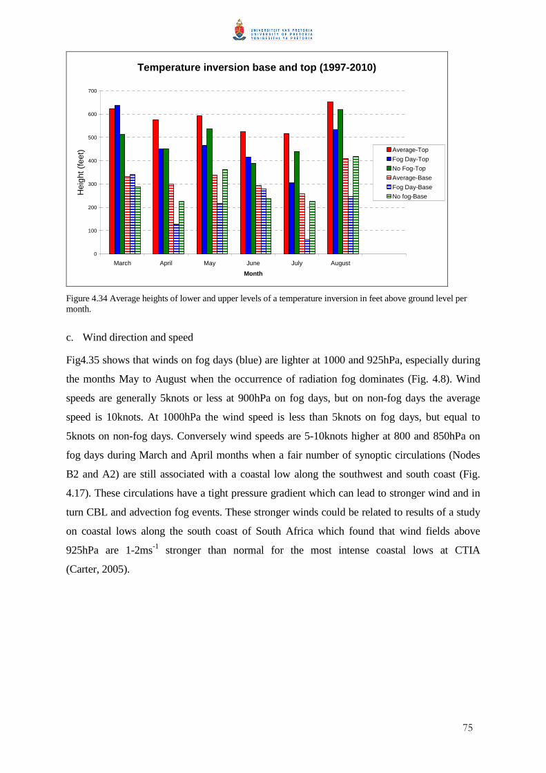
75

Temperature inversion base and top (1997-2010)

0

100

200

300

400

500

600

700


Month

Hei

ght (

feet

) Average-Top

Fog Day-Top

No Fog-Top

Average-Base

Fog Day-Base

No fog-Base

Figure 4.34 Average heights of lower and upper levels of a temperature inversion in feet above ground level per month.

c. Wind direction and speed

Fig4.35 shows that winds on fog days (blue) are lighter at 1000 and 925hPa, especially during

the months May to August when the occurrence of radiation fog dominates (Fig. 4.8). Wind

speeds are generally 5knots or less at 900hPa on fog days, but on non-fog days the average

speed is 10knots. At 1000hPa the wind speed is less than 5knots on fog days, but equal to

5knots on non-fog days. Conversely wind speeds are 5-10knots higher at 800 and 850hPa on

fog days during March and April months when a fair number of synoptic circulations (Nodes

B2 and A2) are still associated with a coastal low along the southwest and south coast (Fig.

4.17). These circulations have a tight pressure gradient which can lead to stronger wind and in

turn CBL and advection fog events. These stronger winds could be related to results of a study

on coastal lows along the south coast of South Africa which found that wind fields above

925hPa are 1-2ms-1 stronger than normal for the most intense coastal lows at CTIA

(Carter, 2005).

76

Figure 4.35 Average wind profile during the fog season at 00:00UTC for CTIA (1997-2010) between 1000 and 700hPa. Long term average (red), non- fog days (green) and fog days (blue).

Croft et al., (1997) used the change of wind directions between the surface and 700hPa to

determine whether the fog event was associated with warm air advection or cold air advection

at the surface. In the southern region of the United States along the gulf coast, a southerly wind

direction is associated with warm air advection as moist air is fed in from the Gulf of Mexico.

A northerly wind direction at the surface signifies a land breeze and is associated with cold air

advection. Winds at CTIA veered with height between 1000 and 700hPa on fog days during

March, April and August (Fig. 4.35), but backed in June and remained neutral (no directional

change with height) during May and July. Croft et al., (1997) found that dense radiation events

occurred under weak backing or neutral wind patterns, while dense advection fog occurred

under a veering wind pattern. Comparing these results with those of the case studies conducted

at CTIA in Chapter 5, it was found that 4 out of the 5 case studies were associated with wind

directions veering with height between the surface and 700hPa. The only case that was not

associated with a veering wind pattern was the north-westerly advection fog event (section 5.2),

where winds remained north-westerly between the surface and 700hPa. In all cases except the

CBL fog event (section 5.3) wind speeds increased significantly above the temperature

inversion.

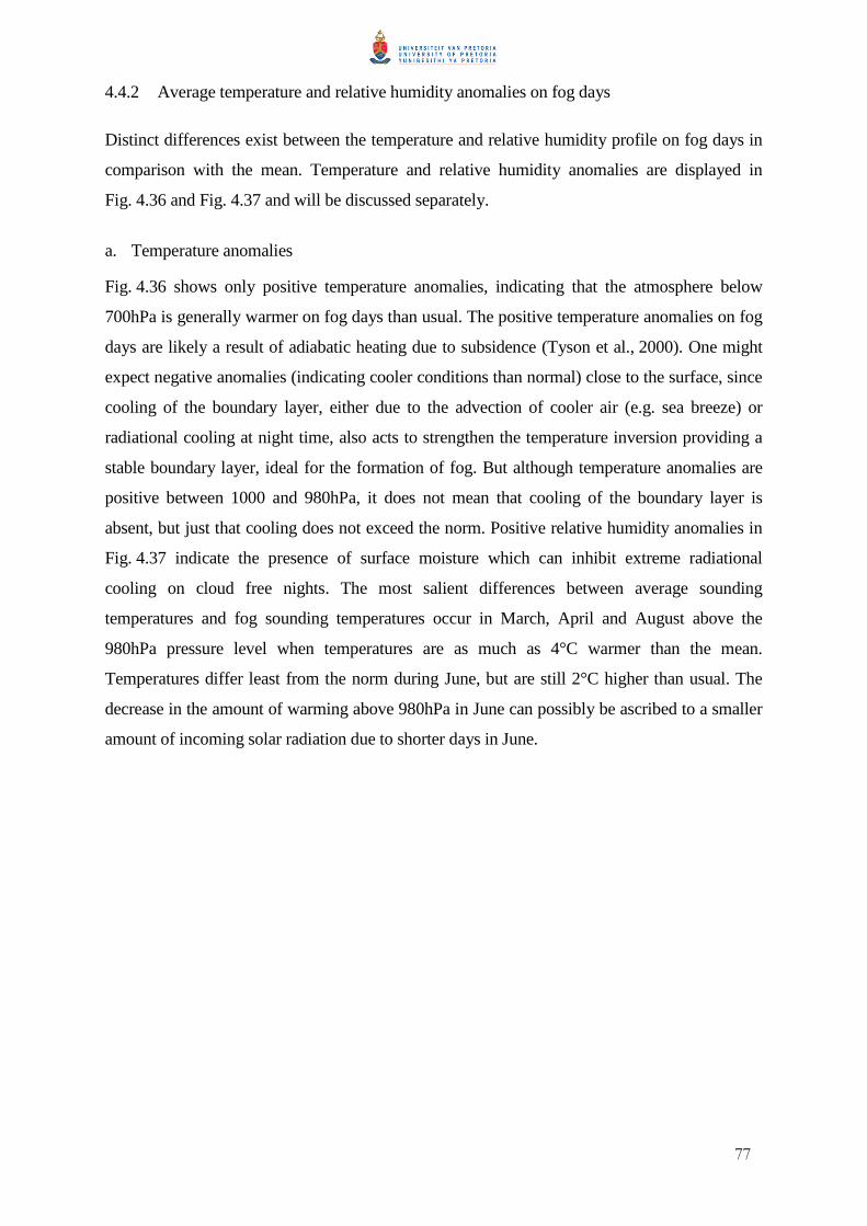
77

4.4.2 Average temperature and relative humidity anomalies on fog days

Distinct differences exist between the temperature and relative humidity profile on fog days in

comparison with the mean. Temperature and relative humidity anomalies are displayed in

Fig. 4.36 and Fig. 4.37 and will be discussed separately.

a. Temperature anomalies

Fig. 4.36 shows only positive temperature anomalies, indicating that the atmosphere below

700hPa is generally warmer on fog days than usual. The positive temperature anomalies on fog

days are likely a result of adiabatic heating due to subsidence (Tyson et al., 2000). One might

expect negative anomalies (indicating cooler conditions than normal) close to the surface, since

cooling of the boundary layer, either due to the advection of cooler air (e.g. sea breeze) or

radiational cooling at night time, also acts to strengthen the temperature inversion providing a

stable boundary layer, ideal for the formation of fog. But although temperature anomalies are

positive between 1000 and 980hPa, it does not mean that cooling of the boundary layer is

absent, but just that cooling does not exceed the norm. Positive relative humidity anomalies in

Fig. 4.37 indicate the presence of surface moisture which can inhibit extreme radiational

cooling on cloud free nights. The most salient differences between average sounding

temperatures and fog sounding temperatures occur in March, April and August above the

980hPa pressure level when temperatures are as much as 4°C warmer than the mean.

Temperatures differ least from the norm during June, but are still 2°C higher than usual. The

decrease in the amount of warming above 980hPa in June can possibly be ascribed to a smaller

amount of incoming solar radiation due to shorter days in June.

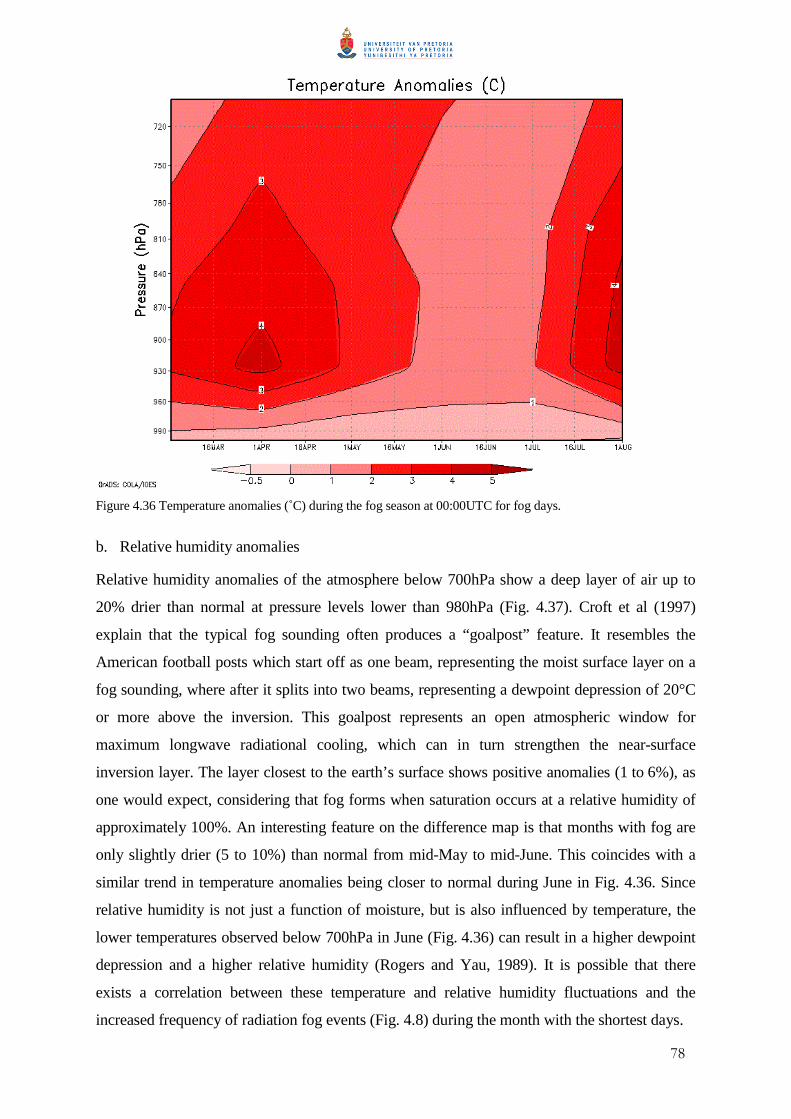
78

Figure 4.36 Temperature anomalies (˚C) during the fog season at 00:00UTC for fog days.

b. Relative humidity anomalies

Relative humidity anomalies of the atmosphere below 700hPa show a deep layer of air up to

20% drier than normal at pressure levels lower than 980hPa (Fig. 4.37). Croft et al (1997)

explain that the typical fog sounding often produces a “goalpost” feature. It resembles the

American football posts which start off as one beam, representing the moist surface layer on a

fog sounding, where after it splits into two beams, representing a dewpoint depression of 20°C

or more above the inversion. This goalpost represents an open atmospheric window for

maximum longwave radiational cooling, which can in turn strengthen the near-surface

inversion layer. The layer closest to the earth’s surface shows positive anomalies (1 to 6%), as

one would expect, considering that fog forms when saturation occurs at a relative humidity of

approximately 100%. An interesting feature on the difference map is that months with fog are

only slightly drier (5 to 10%) than normal from mid-May to mid-June. This coincides with a

similar trend in temperature anomalies being closer to normal during June in Fig. 4.36. Since

relative humidity is not just a function of moisture, but is also influenced by temperature, the

lower temperatures observed below 700hPa in June (Fig. 4.36) can result in a higher dewpoint

depression and a higher relative humidity (Rogers and Yau, 1989). It is possible that there

exists a correlation between these temperature and relative humidity fluctuations and the

increased frequency of radiation fog events (Fig. 4.8) during the month with the shortest days.

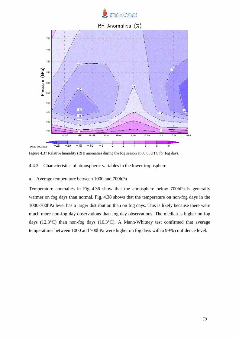
79

Figure 4.37 Relative humidity (RH) anomalies during the fog season at 00:00UTC for fog days.

4.4.3 Characteristics of atmospheric variables in the lower troposphere

a. Average temperature between 1000 and 700hPa

Temperature anomalies in Fig. 4.36 show that the atmosphere below 700hPa is generally

warmer on fog days than normal. Fig. 4.38 shows that the temperature on non-fog days in the

1000-700hPa level has a larger distribution than on fog days. This is likely because there were

much more non-fog day observations than fog day observations. The median is higher on fog

days (12.3°C) than non-fog days (10.3°C). A Mann-Whitney test confirmed that average

temperatures between 1000 and 700hPa were higher on fog days with a 99% confidence level.

80

Average Temperature: 1000-700hPa

-10

-5

0

5

10

15

20

25

30

Fog No fog

Tem

pera

ture

(°C

)

Figure 4.38 Box and whisker plots illustrating the distribution of average temperature (°C) between 1000 and 700hPa for fog days and non-fog days (March to August, 1997-2010). Grey boxes denote 25th to 75th percentiles, while the solid black bar indicates the median value. The vertical lines (whiskers) extend to the maximum and minimum values.

b. Relative humidity below the surface inversion

On fog days the average RH below the temperature inversion is higher than on non-fog days

(Fig4.39). Seventy five percent of average RH values below the inversion on fog days were

between 90 and 100% with a median value of 94%. In comparison non-fog day soundings

showed RH values between 79 and 100% with a median value of 87%. A Mann-Whitney test

confirmed that the average RH below the temperature inversion was higher on fog days with a

99% confidence level.

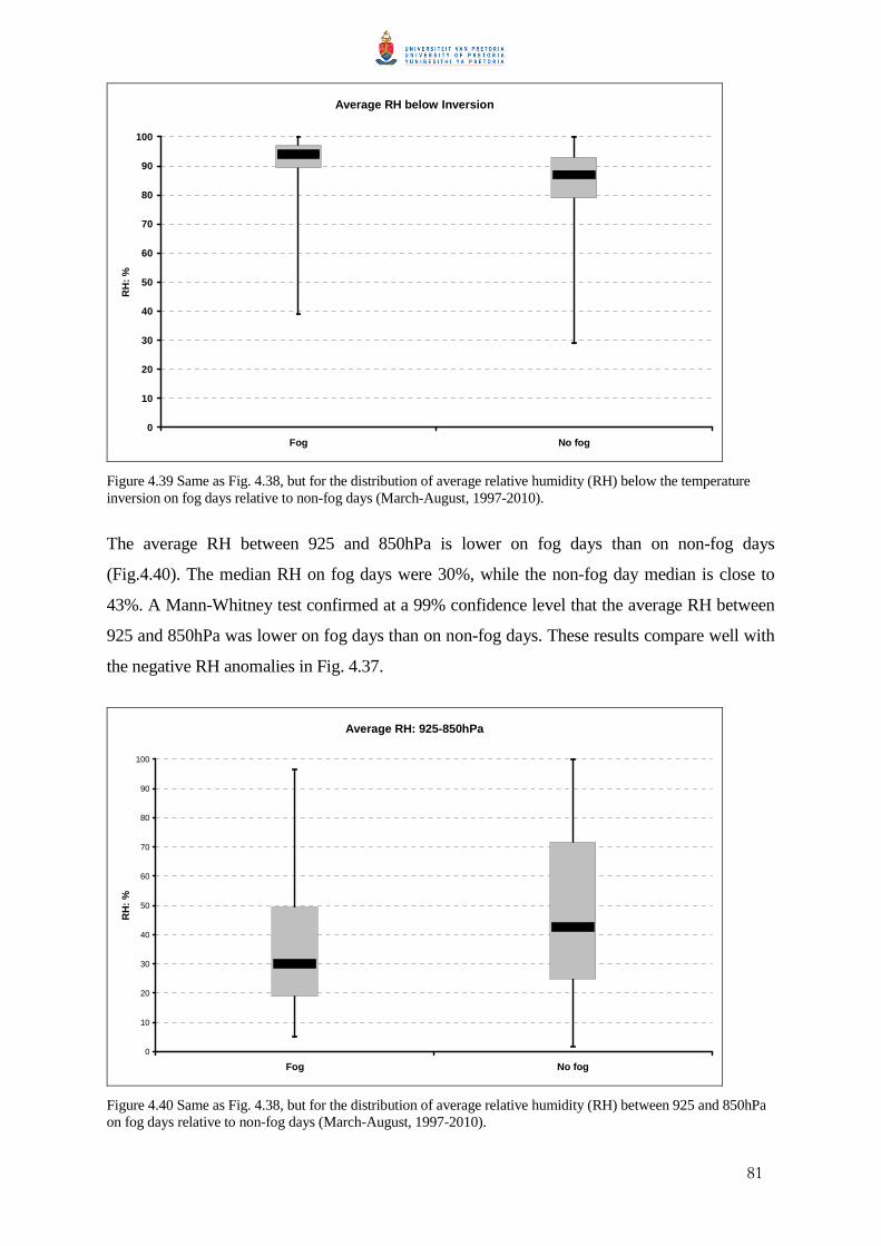
81

Average RH below Inversion

0

10

20

30

40

50

60

70

80

90

100

Fog No fog

RH

: %

Figure 4.39 Same as Fig. 4.38, but for the distribution of average relative humidity (RH) below the temperature inversion on fog days relative to non-fog days (March-August, 1997-2010).

The average RH between 925 and 850hPa is lower on fog days than on non-fog days

(Fig.4.40). The median RH on fog days were 30%, while the non-fog day median is close to

43%. A Mann-Whitney test confirmed at a 99% confidence level that the average RH between

925 and 850hPa was lower on fog days than on non-fog days. These results compare well with

the negative RH anomalies in Fig. 4.37.

Average RH: 925-850hPa

0

10

20

30

40

50

60

70

80

90

100

Fog No fog

RH

: %

Figure 4.40 Same as Fig. 4.38, but for the distribution of average relative humidity (RH) between 925 and 850hPa on fog days relative to non-fog days (March-August, 1997-2010).

82

c. Surface dewpoint temperature

The relative humidity results above compare well with those of surface dewpoint temperature

values. Fig. 4.41 indicates that surface dewpoint values were in general higher during fog days

with a median of 10.5°C, and 9.5° on non-fog days. A Mann-Whitney test confirmed that there

is a statistically significant difference between the surface dewpoint temperature on fog days

and non-fog days at a 95% confidence level.

Surface Dewpoint Temperature

-10

-5

0

5

10

15

20

25

Fog No fog

Td

(°C)

Figure 4.41 Same as Fig. 4.38, but for the distribution of surface dewpoint temperatures (°C) on fog days relative to non-fog days (March-August, 1997-2010).

d. Geopotential thickness between 1000hPa and 700hPa

The median value of geopotential thicknesses on fog days (3104m) were higher than on non-

fog days (3077m) (Fig.4.42). This corresponds well with the average column temperature

between 1000 and 700hPa (Fig. 4.38). The relationship between thickness and temperature

between two pressure levels is explained in section 2.4.2. Consequently higher average

temperatures below 700hPa on fog days lead to higher thickness values. A Mann-Whitney test

confirmed that thicknesses between 1000 and 700hPa were higher on fog days than on non-fog

days at a 99% confidence level.

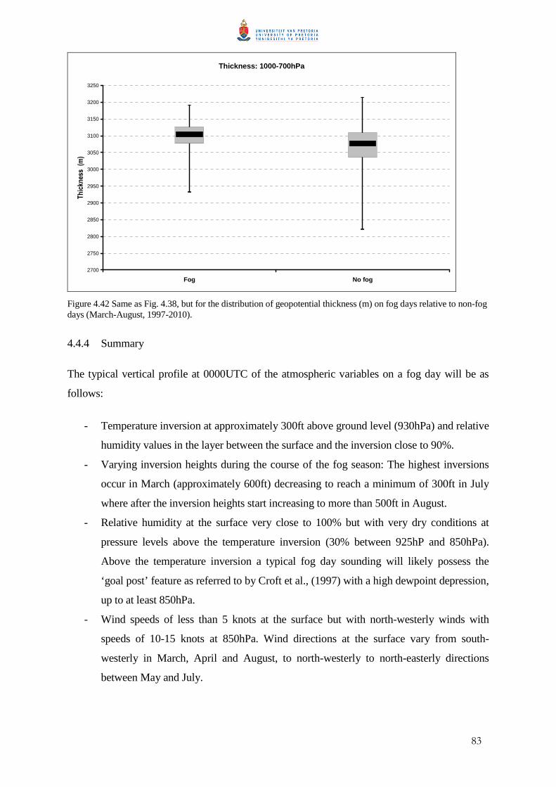
83

Thickness: 1000-700hPa

2700

2750

2800

2850

2900

2950

3000

3050

3100

3150

3200

3250

Fog No fog

Th

ickn

ess

(m

)

Figure 4.42 Same as Fig. 4.38, but for the distribution of geopotential thickness (m) on fog days relative to non-fog days (March-August, 1997-2010).

4.4.4 Summary

The typical vertical profile at 0000UTC of the atmospheric variables on a fog day will be as

follows:

- Temperature inversion at approximately 300ft above ground level (930hPa) and relative

humidity values in the layer between the surface and the inversion close to 90%.

- Varying inversion heights during the course of the fog season: The highest inversions

occur in March (approximately 600ft) decreasing to reach a minimum of 300ft in July

where after the inversion heights start increasing to more than 500ft in August.

- Relative humidity at the surface very close to 100% but with very dry conditions at

pressure levels above the temperature inversion (30% between 925hP and 850hPa).

Above the temperature inversion a typical fog day sounding will likely possess the

‘goal post’ feature as referred to by Croft et al., (1997) with a high dewpoint depression,

up to at least 850hPa.

- Wind speeds of less than 5 knots at the surface but with north-westerly winds with

speeds of 10-15 knots at 850hPa. Wind directions at the surface vary from south-

westerly in March, April and August, to north-westerly to north-easterly directions

between May and July.

84

CHAPTER 5

CASE STUDIES

5 CASE STUDIES

In this chapter, case studies of five different fog events are described. These events were

selected based on their fog type classification, as done by the hierarchical classification method

in section 4.2 and include 2 advection events, 1 CBL, 1 radiation and 1 evaporation event. The

purpose of these case studies is to investigate the formation mechanisms (stated in section

2.2.2) of the different fog types that occur frequently at CTIA and to make conclusions that are

relevant to the forecasting of fog at CTIA.

Eumetsat Meteosat Second Generation (MSG) satellite imagery is included in all case studies,

except for the evaporation fog event which occurred in 2002, before these images were

available. MSG data were examined by means of two Red-Green-Blue (RGB) colour

composites: the “Natural Colour” RGB which makes use of 3 solar channels and the “Fog/Low

clouds” RGB based on infrared channel data, used to monitor night-time fog or low stratus The

“Natural Colour” RGB can only be used at daytime since it contains the following solar

channels: Channel 3 (near infrared 1.6µm), Channel 2 (VIS 0.8µm) and Channel 1 (VIS

0.6µm). To create the Day Natural RGB these channels are used in the following combination:

Red (03) -Green (02) –Blue (01). The Fog RGB is used to detect fog and low clouds at night

time and is based on the principle that the emissivity of water cloud at 3.9µm is less than that at

10.8µm. Subtracting Channel 4 from Channel 9 in the green beam, highlights the presence of

warm water clouds (not in the ice phase). The “Fog/Low clouds” RGB therefore makes use of

Channel 9 (IR10.8µm), Channel 10 (IR12.0µm) and Channel 4 (IR3.9µm) in the following

combination: Red (10-09)-Green (09-04)-Blue (09) (Eumetsat, 2011). All satellite images are

displayed by means of Software for the Utilisation of Meteosat in Outlook activities (SUMO)

(SAWS, 2011).

After a short introduction about the sequence of events, a discussion of the synoptic circulation

will follow making use of NCEP reanalysis mean sea level pressure fields. The synoptic

circulation will be related to the synoptic classification of fog events by means of SOMs in

section 4.3. Surface observations, atmospheric soundings and satellite imagery (where relevant)

will also be used to describe one example of each of the different types of fog that occur

85

frequently at CTIA. A discussion of noteworthy similarities and differences between the

different case studies will follow at the end of each case study.

5.1 ADVECTION FOG FROM THE SOUTH: 2 APRIL 2010

5.1.1 Introduction

Wisps of stratus were reported at CTIA during the early evening of the 1st of April 2010 but the

main fog event occurred on the 2nd when fog rolled in from False Bay. Prior to this radiation

fog formed to the northeast of CTIA. Fog was reported for 5 consecutive hours from 02:00 to

06:00UTC where after an increase in wind speed and solar radiation after sunrise resulted in the

fog lifting and dissipating (see Fig. 5.4). Fog formation was not confined to the Cape Flats, but

extended along the west, southwest and south coast at 06:00UTC (Fig. 5.1). In figure 5.1 the

higher reflectivity of the fog contrasts well against the darker shade of the ocean.

Figure 5.1 MSG satellite, Natural Colour RGB: 2010-04-02, 06:00UTC. The white area along the coastal regions is fog. © (2010) Eumetsat.

86

5.1.2 Synoptic circulation

The synoptic circulation prior, during and after the fog event is depicted in Fig. 5.2. This

sequence of images shows the progressive development of a coastal low. This process already

started on the 1st of April when the anti-cyclonic circulation around the Indian Ocean High in

the east caused an offshore flow along the west coast of South Africa (Fig. 5.2A) resulting in

the deepening of an existing low pressure area along the west coast during the course of the 1st.

The low is visible along the northern section of the South African west coast in A, after which

it deepened over land at 12:00UTC (Fig. 5.2B). The low was still positioned over land at

18:00UTC (Fig. 5.2C), but at 00:00UTC on 2 April 2010 (Fig. 5.2D) a semi-closed low was

positioned along the southwest coast of South Africa. In this case study the low did not move

around the west coast, but formed over land and extended southwards onto the south coast. The

position of the low in Fig. 5.2D caused an easterly to south-easterly circulation around the

periphery of the low along the south coast of the Western Cape. The southerly circulation

behind this low advected moist air and fog from False Bay towards the airport. The low moved

eastwards after 06:00UTC (Fig. 5.2E and F) and the fog at CTIA started to clear.

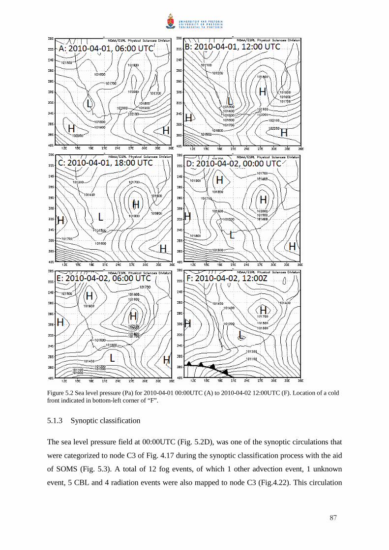
87

Figure 5.2 Sea level pressure (Pa) for 2010-04-01 00:00UTC (A) to 2010-04-02 12:00UTC (F). Location of a cold front indicated in bottom-left corner of “F”.

5.1.3 Synoptic classification

The sea level pressure field at 00:00UTC (Fig. 5.2D), was one of the synoptic circulations that

were categorized to node C3 of Fig. 4.17 during the synoptic classification process with the aid

of SOMS (Fig. 5.3). A total of 12 fog events, of which 1 other advection event, 1 unknown

event, 5 CBL and 4 radiation events were also mapped to node C3 (Fig.4.22). This circulation

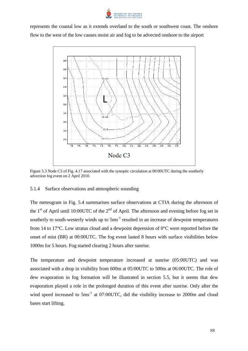
88

represents the coastal low as it extends overland to the south or southwest coast. The onshore

flow to the west of the low causes moist air and fog to be advected onshore to the airport

Figure 5.3 Node C3 of Fig. 4.17 associated with the synoptic circulation at 00:00UTC during the southerly advection fog event on 2 April 2010.

5.1.4 Surface observations and atmospheric sounding

The meteogram in Fig. 5.4 summarises surface observations at CTIA during the afternoon of

the 1st of April until 10:00UTC of the 2nd of April. The afternoon and evening before fog set in

southerly to south-westerly winds up to 5ms-1 resulted in an increase of dewpoint temperatures

from 14 to 17°C. Low stratus cloud and a dewpoint depression of 0°C were reported before the

onset of mist (BR) at 00:00UTC. The fog event lasted 8 hours with surface visibilities below

1000m for 5 hours. Fog started clearing 2 hours after sunrise.

The temperature and dewpoint temperature increased at sunrise (05:00UTC) and was

associated with a drop in visibility from 600m at 05:00UTC to 500m at 06:00UTC. The role of

dew evaporation in fog formation will be illustrated in section 5.5, but it seems that dew

evaporation played a role in the prolonged duration of this event after sunrise. Only after the

wind speed increased to 5ms-1 at 07:00UTC, did the visibility increase to 2000m and cloud

bases start lifting.

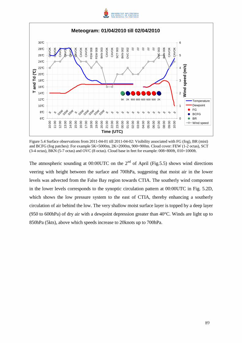
89

Meteogram: 01/04/2010 till 02/04/2010

BK

N 0

03

FE

W 0

08

FE

W 0

08

BK

N 0

02

OV

C 0

02

BK

N 0

06

OV

C 0

03////

////

////

////

////

S S S S S S S S S S S S S S S S SSSW

SSWSSW

SSWSSW

SSWSSW

SSW

5K 2K 2K900 800 500600 600

CA

VO

K

CA

VO

K

CA

VO

K

CA

VO

K

CA

VO

K

CA

VO

K

CA

VO

K

CA

VO

K

CA

VO

K

CA

VO

K

CA

VO

K

SC

T 0

03

CA

VO

K

6°C

8°C

10°C

12°C

14°C

16°C

18°C

20°C

22°C

24°C

26°C

28°C

30°C

10:0

0

11:0

0

12:0

0

13:0

0

14:0

0

15:0

0

16:0

0

17:0

0

18:0

0

19:0

0

20:0

0

21:0

0

22:0

0

23:0

0

00:0

0

01:0

0

02:0

0

03:0

0

04:0

0

05:0

0

06:0

0

07:0

0

08:0

0

09:0

0

10:0

0

Time (UTC)

T a

nd T

d (°C

)

0

1

2

3

4

5

6

Win

d sp

eed

(m/s

)

Temperature

Dewpoint

FG

BCFG

BR

Wind speed

Figure 5.4 Surface observations from 2011-04-01 till 2011-04-02: Visibility associated with FG (fog), BR (mist) and BCFG (fog patches): For example 5K=5000m, 2K=2000m, 900=900m. Cloud cover: FEW (1-2 octas), SCT (3-4 octas), BKN (5-7 octas) and OVC (8 octas). Cloud base in feet for example: 008=800ft, 010=1000ft.

The atmospheric sounding at 00:00UTC on the 2nd of April (Fig.5.5) shows wind directions

veering with height between the surface and 700hPa, suggesting that moist air in the lower

levels was advected from the False Bay region towards CTIA. The southerly wind component

in the lower levels corresponds to the synoptic circulation pattern at 00:00UTC in Fig. 5.2D,

which shows the low pressure system to the east of CTIA, thereby enhancing a southerly

circulation of air behind the low. The very shallow moist surface layer is topped by a deep layer

(950 to 600hPa) of dry air with a dewpoint depression greater than 40°C. Winds are light up to

850hPa (5kts), above which speeds increase to 20knots up to 700hPa.

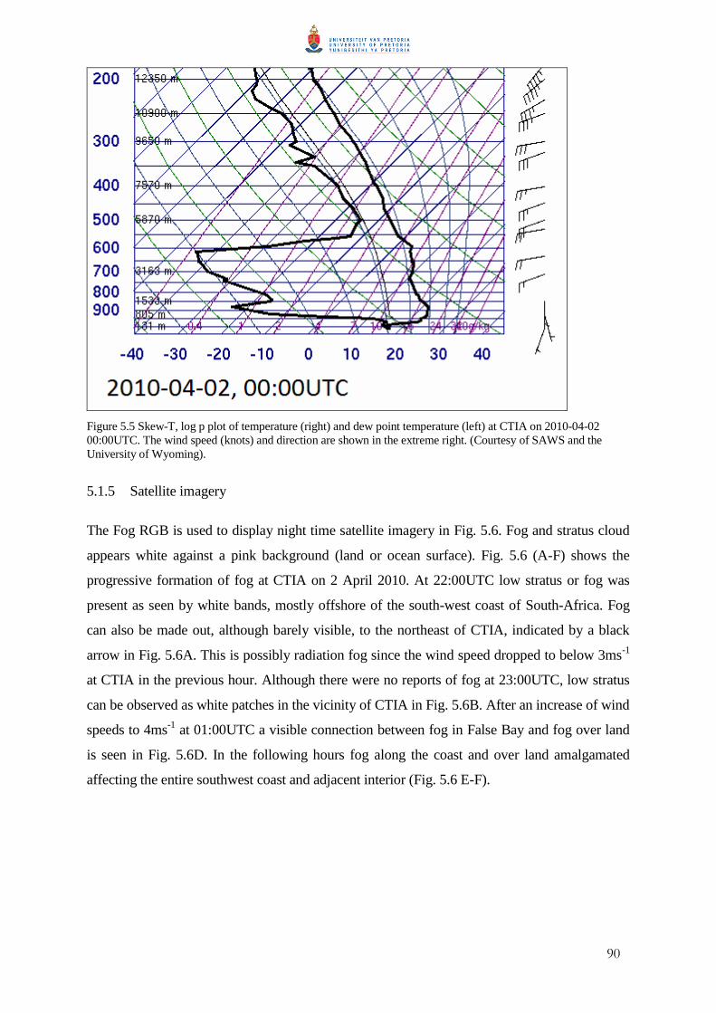
90

Figure 5.5 Skew-T, log p plot of temperature (right) and dew point temperature (left) at CTIA on 2010-04-02 00:00UTC. The wind speed (knots) and direction are shown in the extreme right. (Courtesy of SAWS and the University of Wyoming).

5.1.5 Satellite imagery

The Fog RGB is used to display night time satellite imagery in Fig. 5.6. Fog and stratus cloud

appears white against a pink background (land or ocean surface). Fig. 5.6 (A-F) shows the

progressive formation of fog at CTIA on 2 April 2010. At 22:00UTC low stratus or fog was

present as seen by white bands, mostly offshore of the south-west coast of South-Africa. Fog

can also be made out, although barely visible, to the northeast of CTIA, indicated by a black

arrow in Fig. 5.6A. This is possibly radiation fog since the wind speed dropped to below 3ms-1

at CTIA in the previous hour. Although there were no reports of fog at 23:00UTC, low stratus

can be observed as white patches in the vicinity of CTIA in Fig. 5.6B. After an increase of wind

speeds to 4ms-1 at 01:00UTC a visible connection between fog in False Bay and fog over land

is seen in Fig. 5.6D. In the following hours fog along the coast and over land amalgamated

affecting the entire southwest coast and adjacent interior (Fig. 5.6 E-F).

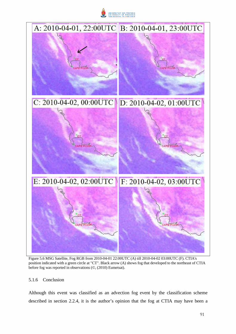
91

Figure 5.6 MSG Satellite, Fog RGB from 2010-04-01 22:00UTC (A) till 2010-04-02 03:00UTC (F). CTIA's position indicated with a green circle at "CT". Black arrow (A) shows fog that developed to the northeast of CTIA before fog was reported in observations (©, (2010) Eumetsat).

5.1.6 Conclusion

Although this event was classified as an advection fog event by the classification scheme

described in section 2.2.4, it is the author’s opinion that the fog at CTIA may have been a

92

combination of advection and radiation processes. The persistent southerly to south-westerly

breeze advected moist air towards the airport during the afternoon of the 1st. A drop in wind

speeds and radiational cooling led to the formation of fog over land to the northeast of CTIA

during the early morning hours (Fig.5.6A). Once the southerly wind picked up again, fog at sea

was blown ashore, connecting with fog over land (Fig. 5.6E). In section 4.2.2 it was shown that

the minimum visibility associated with advection events are often higher than with CBL and

radiation events. In this case study the minimum visibility reported at CTIA was 500m (Fig.

5.4) which is slightly higher than that of most advection events that occurred during 1997-2010.

5.2 ADVECTION FOG FROM THE NORTHWEST: 5 MARCH 2010

5.2.1 Introduction

After a hot afternoon on the 4th of March 2010, clear skies were reported at CTIA throughout

the evening. The wind direction veered to the northwest before midnight and a sudden increase

in wind speed denoted the arrival of a coastal low. Within two hours thereafter low stratus and

reduced visibilities due to fog were reported. This case study describes the classic scenario

where fog that developed behind a coastal low, spread southwards along the west coast,

eventually reaching CTIA. As the coastal low continued traversing the coastline of South

Africa, fog spread eastwards. The Natural Colour RGB in Fig. 5.7 indicates widespread fog in

white against a dark background of the ocean and the brown landmass on the morning of the 5th

of March 2010 along the west and southwest coast.

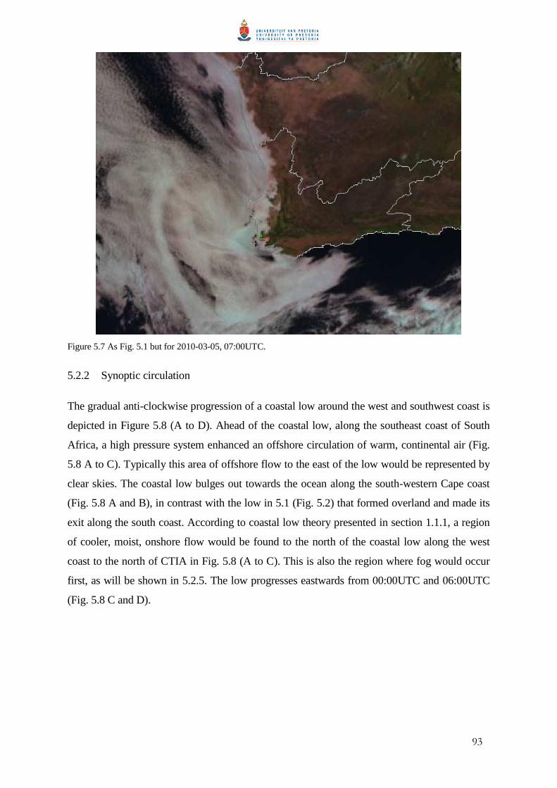
93

Figure 5.7 As Fig. 5.1 but for 2010-03-05, 07:00UTC.


The gradual anti-clockwise progression of a coastal low around the west and southwest coast is

depicted in Figure 5.8 (A to D). Ahead of the coastal low, along the southeast coast of South

Africa, a high pressure system enhanced an offshore circulation of warm, continental air (Fig.

5.8 A to C). Typically this area of offshore flow to the east of the low would be represented by

clear skies. The coastal low bulges out towards the ocean along the south-western Cape coast

(Fig. 5.8 A and B), in contrast with the low in 5.1 (Fig. 5.2) that formed overland and made its

exit along the south coast. According to coastal low theory presented in section 1.1.1, a region

of cooler, moist, onshore flow would be found to the north of the coastal low along the west

coast to the north of CTIA in Fig. 5.8 (A to C). This is also the region where fog would occur

first, as will be shown in 5.2.5. The low progresses eastwards from 00:00UTC and 06:00UTC

(Fig. 5.8 C and D).

94

Figure 5.8 Sea level pressure (Pa) for 2010-03-04 12:00UTC (A) to 2010-03-05 06:00UTC (D).


The sea level pressure field at 00:00UTC (Fig. 5.8C), was one of the synoptic circulations that

were categorized to node B2 of Fig. 4.17 during the synoptic classification process in section

4.3 (duplicated in Fig. 5.9). Eight fog events, of which 1 other advection, 2 CBL, 1 radiation

and 3 unknown events, were also mapped to node B2 (Fig. 4.22). This circulation is very

typical of a low moving southward along the west coast, protruding along the coast southwest

of the continent where after moving eastwards and is referred to as the “travelling” coastal low

in section 1.1.1.

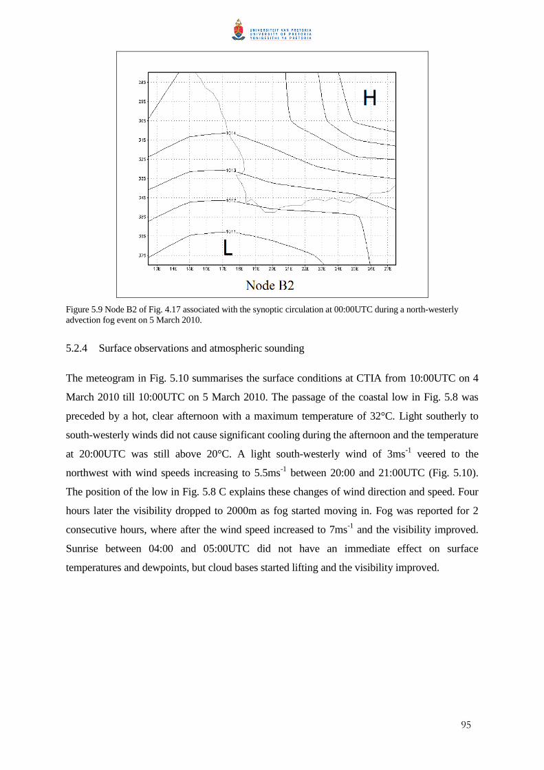
95

Figure 5.9 Node B2 of Fig. 4.17 associated with the synoptic circulation at 00:00UTC during a north-westerly advection fog event on 5 March 2010.


The meteogram in Fig. 5.10 summarises the surface conditions at CTIA from 10:00UTC on 4

March 2010 till 10:00UTC on 5 March 2010. The passage of the coastal low in Fig. 5.8 was

preceded by a hot, clear afternoon with a maximum temperature of 32°C. Light southerly to

south-westerly winds did not cause significant cooling during the afternoon and the temperature

at 20:00UTC was still above 20°C. A light south-westerly wind of 3ms-1 veered to the

northwest with wind speeds increasing to 5.5ms-1 between 20:00 and 21:00UTC (Fig. 5.10).

The position of the low in Fig. 5.8 C explains these changes of wind direction and speed. Four

hours later the visibility dropped to 2000m as fog started moving in. Fog was reported for 2

consecutive hours, where after the wind speed increased to 7ms-1 and the visibility improved.

Sunrise between 04:00 and 05:00UTC did not have an immediate effect on surface

temperatures and dewpoints, but cloud bases started lifting and the visibility improved.

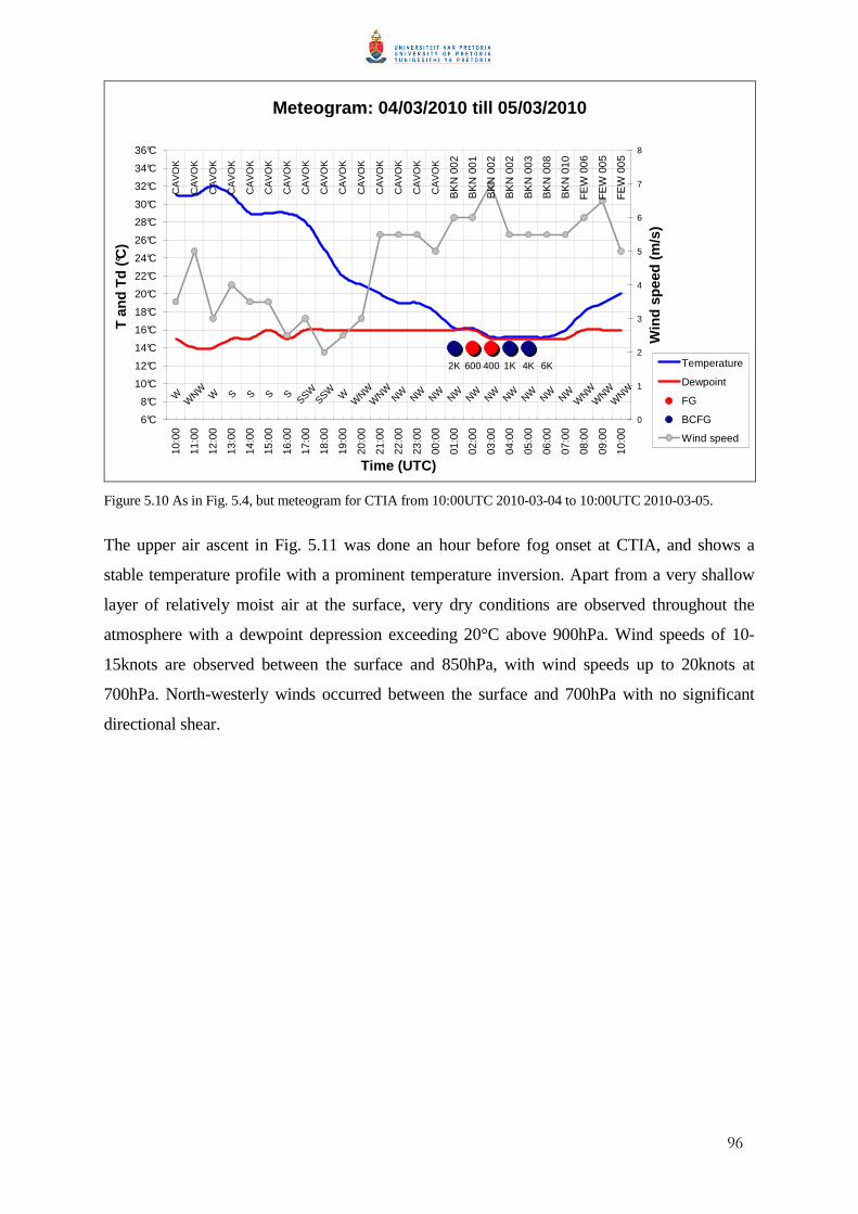
96

Meteogram: 04/03/2010 till 05/03/2010

S S S SSSW

SSW

BK

N 0

02

BK

N 0

02

BK

N 0

02

BK

N 0

03

BK

N 0

10

FE

W 0

06

WNW

WNW

WNW

WNW

WNW

WNW

NW NW NW NW NW NW NW NW NW NWW W W

2K 600 400 4K

CA

VO

K

CA

VO

K

CA

VO

K

CA

VO

K

CA

VO

K

CA

VO

K

CA

VO

K

CA

VO

K

CA

VO

K

CA

VO

K

CA

VO

K

CA

VO

K

CA

VO

K

CA

VO

K

CA

VO

K

BK

N 0

01

BK

N 0

08

FE

W 0

05

FE

W 0

05

1K 6K

6°C

8°C

10°C

12°C

14°C

16°C

18°C

20°C

22°C

24°C

26°C

28°C

30°C

32°C

34°C

36°C

10:0

0

11:0

0

12:0

0

13:0

0

14:0

0

15:0

0

16:0

0

17:0

0

18:0

0

19:0

0

20:0

0

21:0

0

22:0

0

23:0

0

00:0

0

01:0

0

02:0

0

03:0

0

04:0

0

05:0

0

06:0

0

07:0

0

08:0

0

09:0

0

10:0

0

Time (UTC)

T a

nd T

d (°C

)

0

1

2

3

4

5

6

7

8

Win

d sp

eed

(m/s

)

Temperature

Dewpoint

FG

BCFG

Wind speed

Figure 5.10 As in Fig. 5.4, but meteogram for CTIA from 10:00UTC 2010-03-04 to 10:00UTC 2010-03-05.

The upper air ascent in Fig. 5.11 was done an hour before fog onset at CTIA, and shows a

stable temperature profile with a prominent temperature inversion. Apart from a very shallow

layer of relatively moist air at the surface, very dry conditions are observed throughout the

atmosphere with a dewpoint depression exceeding 20°C above 900hPa. Wind speeds of 10-

15knots are observed between the surface and 850hPa, with wind speeds up to 20knots at

700hPa. North-westerly winds occurred between the surface and 700hPa with no significant

directional shear.

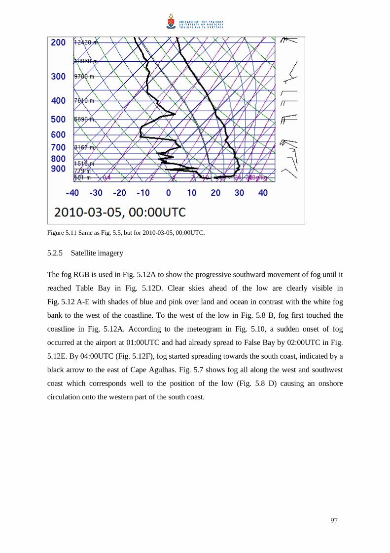
97

Figure 5.11 Same as Fig. 5.5, but for 2010-03-05, 00:00UTC.


The fog RGB is used in Fig. 5.12A to show the progressive southward movement of fog until it

reached Table Bay in Fig. 5.12D. Clear skies ahead of the low are clearly visible in

Fig. 5.12 A-E with shades of blue and pink over land and ocean in contrast with the white fog

bank to the west of the coastline. To the west of the low in Fig. 5.8 B, fog first touched the

coastline in Fig, 5.12A. According to the meteogram in Fig. 5.10, a sudden onset of fog

occurred at the airport at 01:00UTC and had already spread to False Bay by 02:00UTC in Fig.

5.12E. By 04:00UTC (Fig. 5.12F), fog started spreading towards the south coast, indicated by a

black arrow to the east of Cape Agulhas. Fig. 5.7 shows fog all along the west and southwest

coast which corresponds well to the position of the low (Fig. 5.8 D) causing an onshore

circulation onto the western part of the south coast.

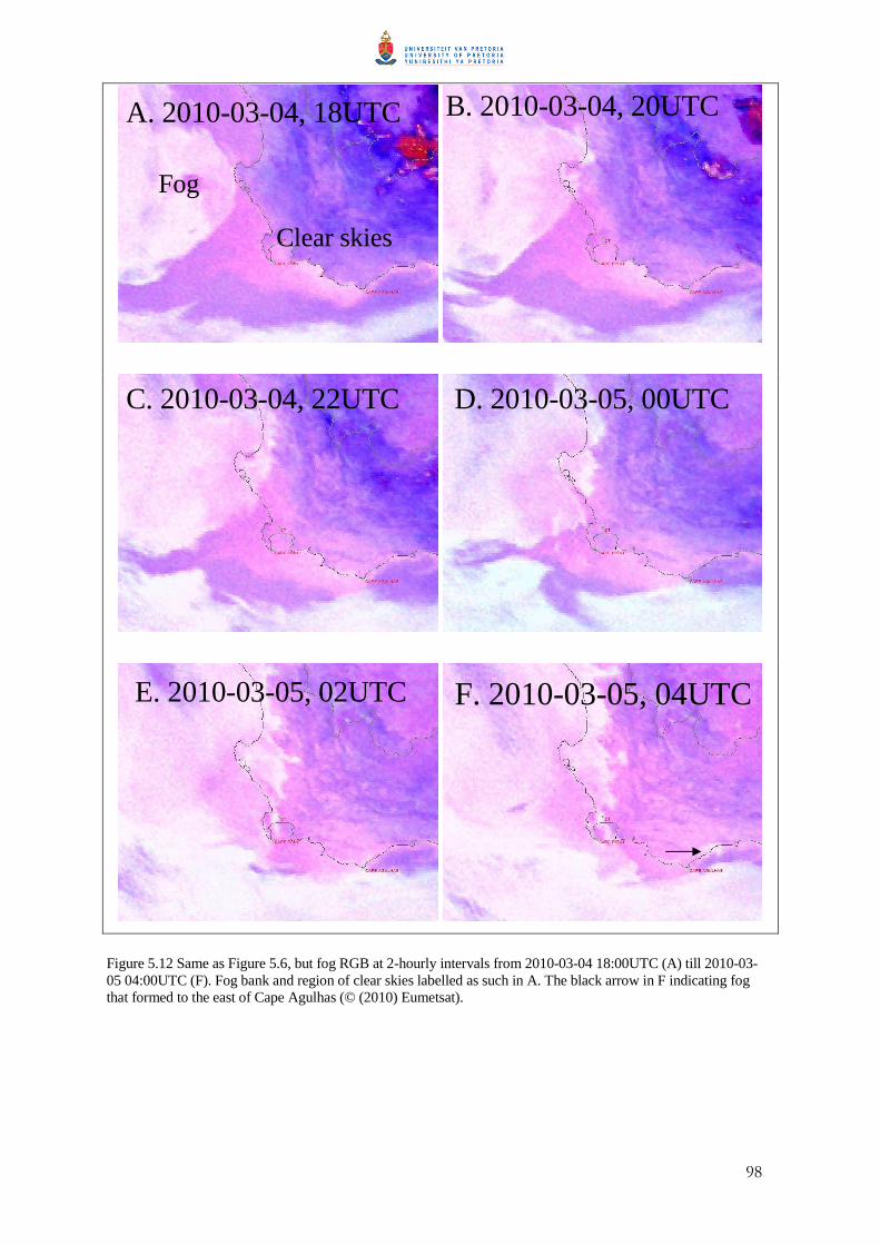
98

Figure 5.12 Same as Figure 5.6, but fog RGB at 2-hourly intervals from 2010-03-04 18:00UTC (A) till 2010-03-05 04:00UTC (F). Fog bank and region of clear skies labelled as such in A. The black arrow in F indicating fog that formed to the east of Cape Agulhas (© (2010) Eumetsat).

A. 2010-03-04, 18UTC B. 2010-03-04, 20UTC

C. 2010-03-04, 22UTC D. 2010-03-05, 00UTC

E. 2010-03-05, 02UTC F. 2010-03-05, 04UTC

Clear skies

Fog

99

5.2.6 Conclusion

North-westerly advection fog affected CTIA during the early hours of 5 March 2010. This was

caused by the anti-clockwise progression of a coastal low around the west and southwest coast

of South Africa.

From a forecasting point of view, north-westerly advection fog is fairly predictable when

making use of satellite imagery and sea level pressure analyses. As was shown in section 4.2.2,

the drop in visibility associated with advection fog events are often less than with CBL and

radiation events. In this case study, the minimum visibility reported at CTIA was 400m

(Fig. 5.10) which is similar to the minimum visibilities of most advection events that occurred

during 1997-2010.

5.3 CLOUD BASE LOWERING FOG: 19 JUNE 2006

5.3.1 Introduction

A deck of low based stratus cloud accompanied by a light southerly breeze at CTIA eventually

saw a gradual lowering of cloud bases through the evening of the 18th of June 2006 and the

early morning of the 19th. The Natural Colour RGB below (Fig. 5.13) displays patches of

stratus or fog in False Bay and the surrounding southwest coast at 14:00UTC on 18 June 2006

(the afternoon prior to fog onset at CTIA). What is unusual about this fog event from the other

selected case studies is the late time of day at which the fog cleared. The event lasted 8 hours,

starting at 02:00UTC with fog only clearing from 09:00UTC. This resulted in 20 aircraft

diversions (SAWS, 2006).

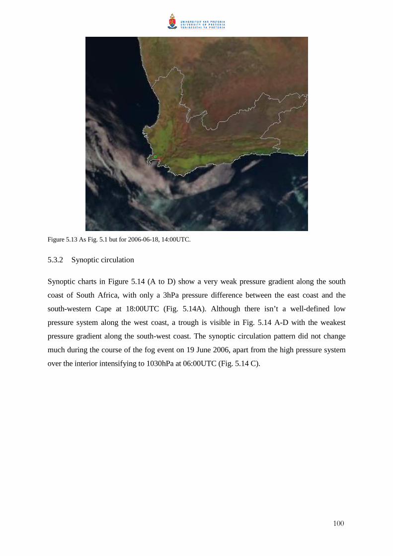
100



Synoptic charts in Figure 5.14 (A to D) show a very weak pressure gradient along the south

coast of South Africa, with only a 3hPa pressure difference between the east coast and the

south-western Cape at 18:00UTC (Fig. 5.14A). Although there isn’t a well-defined low

pressure system along the west coast, a trough is visible in Fig. 5.14 A-D with the weakest

pressure gradient along the south-west coast. The synoptic circulation pattern did not change

much during the course of the fog event on 19 June 2006, apart from the high pressure system

over the interior intensifying to 1030hPa at 06:00UTC (Fig. 5.14 C).

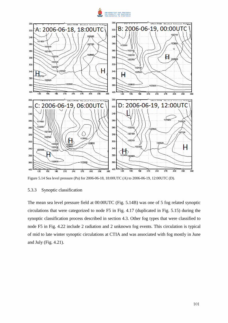
101

Figure 5.14 Sea level pressure (Pa) for 2006-06-18, 18:00UTC (A) to 2006-06-19, 12:00UTC (D).


The mean sea level pressure field at 00:00UTC (Fig. 5.14B) was one of 5 fog related synoptic

circulations that were categorized to node F5 in Fig. 4.17 (duplicated in Fig. 5.15) during the

synoptic classification process described in section 4.3. Other fog types that were classified to

node F5 in Fig. 4.22 include 2 radiation and 2 unknown fog events. This circulation is typical

of mid to late winter synoptic circulations at CTIA and was associated with fog mostly in June

and July (Fig. 4.21).

102

Figure 5.15 Node F5 of Fig. 4.17 associated with the synoptic circulation during a CBL fog event on 19 June 2006.


The meteogram in Fig. 5.16 indicates observations of 5-8 octas of low cloud with bases below

1000ft throughout the afternoon of 18 June 2006. A steady southerly breeze varied in strength

during the course of the afternoon and evening, with a maximum speed of 6ms-1 at 20:00UTC.

As the wind speed dropped to 1ms-1 at 01:00UTC on the 19th, the cloud base lowered to 300ft,

where after fog was reported from 02:00UTC. Sunrise just prior to 06:00UTC did not cause

any increase in temperature or improvement of visibility for another 2 hours. At 09:00UTC the

dewpoint dropped by a degree where after the visibility improved, but remained below 10km

all afternoon, most likely due to haze.

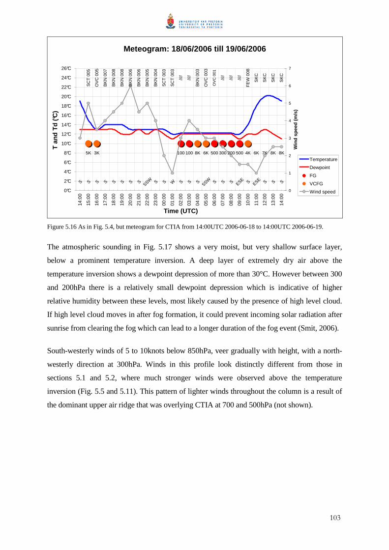
103

Meteogram: 18/06/2006 till 19/06/2006

S S S S S S S S S S S S S S S S S S S SSSW

SSW

500 500

ESEESE

W

3K 7K8K 8K 8K6K 6K300100 100

OV

C 0

05

OV

C 0

03

BK

N 0

07

BK

N 0

08

BK

N 0

08

BK

N 0

06

BK

N 0

06

BK

N 0

04

BK

N 0

03

SC

T 0

03

SC

T 0

03

////

////

////

////

////

SK

C

SK

C

SK

C

SK

C

5K 200 4K

OV

C 0

01

BK

N 0

05

SC

T 0

05

FE

W 0

08

0°C

2°C

4°C

6°C

8°C

10°C

12°C

14°C

16°C

18°C

20°C

22°C

24°C

26°C

14:0

0

15:0

0

16:0

0

17:0

0

18:0

0

19:0

0

20:0

0

21:0

0

22:0

0

23:0

0

00:0

0

01:0

0

02:0

0

03:0

0

04:0

0

05:0

0

06:0

0

07:0

0

08:0

0

09:0

0

10:0

0

11:0

0

12:0

0

13:0

0

14:0

0

Time (UTC)

T a

nd T

d (°C

)

0

1

2

3

4

5

6

7

Win

d sp

eed

(m/s

)

Temperature

Dewpoint

FG

VCFG

Wind speed


The atmospheric sounding in Fig. 5.17 shows a very moist, but very shallow surface layer,

below a prominent temperature inversion. A deep layer of extremely dry air above the

temperature inversion shows a dewpoint depression of more than 30°C. However between 300

and 200hPa there is a relatively small dewpoint depression which is indicative of higher

relative humidity between these levels, most likely caused by the presence of high level cloud.

If high level cloud moves in after fog formation, it could prevent incoming solar radiation after

sunrise from clearing the fog which can lead to a longer duration of the fog event (Smit, 2006).

South-westerly winds of 5 to 10knots below 850hPa, veer gradually with height, with a north-

westerly direction at 300hPa. Winds in this profile look distinctly different from those in

sections 5.1 and 5.2, where much stronger winds were observed above the temperature

inversion (Fig. 5.5 and 5.11). This pattern of lighter winds throughout the column is a result of

the dominant upper air ridge that was overlying CTIA at 700 and 500hPa (not shown).

104

Figure 5.17 Same as Fig. 5.5 but for 2006-06-19, 00:00UTC.


The Fog RGB is used to not only confirm the presence of low stratus prior to fog onset at CTIA

during the evening of the 18th, but also show the extent of low cloud or fog penetration before

00:00UTC (Fig. 5.18A-B). In this case study the west coast and western side of the Cape

Peninsula remained relatively clear till 02:00UTC (areas clear of fog indicated in shades of

pink), while the Cape Agulhas region remained overcast (light blue patches against a pink

background) throughout the night. Fog was reported at CTIA from 02:00UTC (Fig. 5.16)

which is also when fog or low cloud filled up False Bay and the entire south-west coast (Fig.

5.18D-F). Cirrus cloud is visible to the south of CTIA in Fig. 5.18A, B and E (see black arrow)

which explains the higher relative humidity observed between 300 and 200hPa in Fig. 5.17.

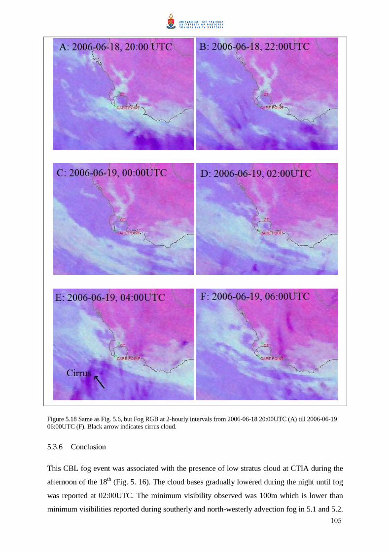
105

Figure 5.18 Same as Fig. 5.6, but Fog RGB at 2-hourly intervals from 2006-06-18 20:00UTC (A) till 2006-06-19 06:00UTC (F). Black arrow indicates cirrus cloud.

5.3.6 Conclusion

This CBL fog event was associated with the presence of low stratus cloud at CTIA during the

afternoon of the 18th (Fig. 5. 16). The cloud bases gradually lowered during the night until fog

was reported at 02:00UTC. The minimum visibility observed was 100m which is lower than

minimum visibilities reported during southerly and north-westerly advection fog in 5.1 and 5.2.

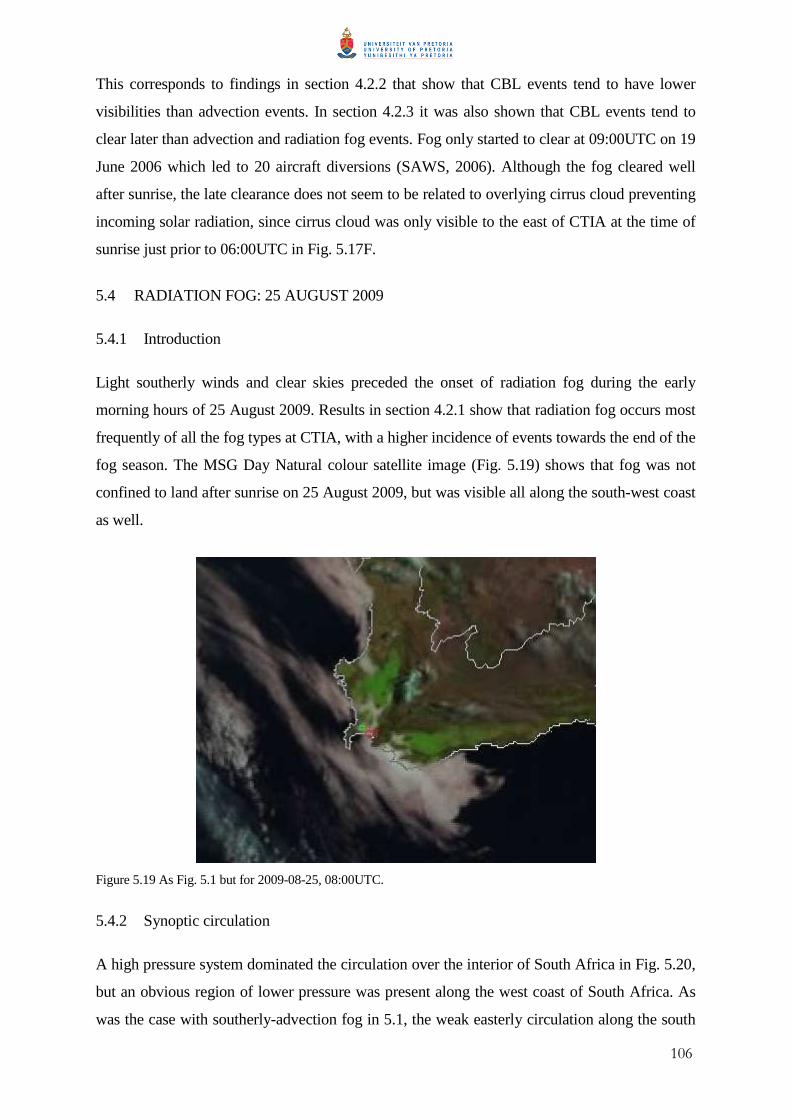
106

This corresponds to findings in section 4.2.2 that show that CBL events tend to have lower

visibilities than advection events. In section 4.2.3 it was also shown that CBL events tend to

clear later than advection and radiation fog events. Fog only started to clear at 09:00UTC on 19

June 2006 which led to 20 aircraft diversions (SAWS, 2006). Although the fog cleared well

after sunrise, the late clearance does not seem to be related to overlying cirrus cloud preventing

incoming solar radiation, since cirrus cloud was only visible to the east of CTIA at the time of

sunrise just prior to 06:00UTC in Fig. 5.17F.

5.4 RADIATION FOG: 25 AUGUST 2009

5.4.1 Introduction

Light southerly winds and clear skies preceded the onset of radiation fog during the early

morning hours of 25 August 2009. Results in section 4.2.1 show that radiation fog occurs most

frequently of all the fog types at CTIA, with a higher incidence of events towards the end of the

fog season. The MSG Day Natural colour satellite image (Fig. 5.19) shows that fog was not

confined to land after sunrise on 25 August 2009, but was visible all along the south-west coast

as well.



A high pressure system dominated the circulation over the interior of South Africa in Fig. 5.20,

but an obvious region of lower pressure was present along the west coast of South Africa. As

was the case with southerly-advection fog in 5.1, the weak easterly circulation along the south

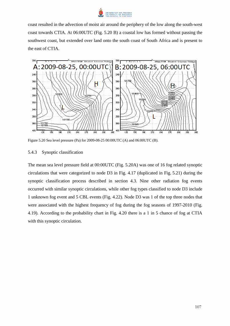
107

coast resulted in the advection of moist air around the periphery of the low along the south-west

coast towards CTIA. At 06:00UTC (Fig. 5.20 B) a coastal low has formed without passing the

southwest coast, but extended over land onto the south coast of South Africa and is present to

the east of CTIA.

Figure 5.20 Sea level pressure (Pa) for 2009-08-25 00:00UTC (A) and 06:00UTC (B).


The mean sea level pressure field at 00:00UTC (Fig. 5.20A) was one of 16 fog related synoptic

circulations that were categorized to node D3 in Fig. 4.17 (duplicated in Fig. 5.21) during the

synoptic classification process described in section 4.3. Nine other radiation fog events

occurred with similar synoptic circulations, while other fog types classified to node D3 include

1 unknown fog event and 5 CBL events (Fig. 4.22). Node D3 was 1 of the top three nodes that

were associated with the highest frequency of fog during the fog seasons of 1997-2010 (Fig.

4.19). According to the probability chart in Fig. 4.20 there is a 1 in 5 chance of fog at CTIA

with this synoptic circulation.

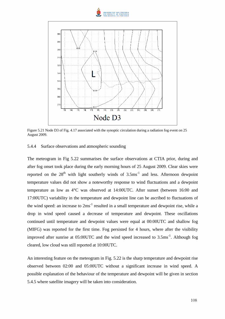
108

Figure 5.21 Node D3 of Fig. 4.17 associated with the synoptic circulation during a radiation fog event on 25 August 2009.


The meteogram in Fig 5.22 summarises the surface observations at CTIA prior, during and

after fog onset took place during the early morning hours of 25 August 2009. Clear skies were

reported on the 28th with light southerly winds of 3.5ms-1 and less. Afternoon dewpoint

temperature values did not show a noteworthy response to wind fluctuations and a dewpoint

temperature as low as 4°C was observed at 14:00UTC. After sunset (between 16:00 and

17:00UTC) variability in the temperature and dewpoint line can be ascribed to fluctuations of

the wind speed: an increase to 2ms-1 resulted in a small temperature and dewpoint rise, while a

drop in wind speed caused a decrease of temperature and dewpoint. These oscillations

continued until temperature and dewpoint values were equal at 00:00UTC and shallow fog

(MIFG) was reported for the first time. Fog persisted for 4 hours, where after the visibility

improved after sunrise at 05:00UTC and the wind speed increased to 3.5ms-1. Although fog

cleared, low cloud was still reported at 10:00UTC.

An interesting feature on the meteogram in Fig. 5.22 is the sharp temperature and dewpoint rise

observed between 02:00 and 05:00UTC without a significant increase in wind speed. A

possible explanation of the behaviour of the temperature and dewpoint will be given in section

5.4.5 where satellite imagery will be taken into consideration.

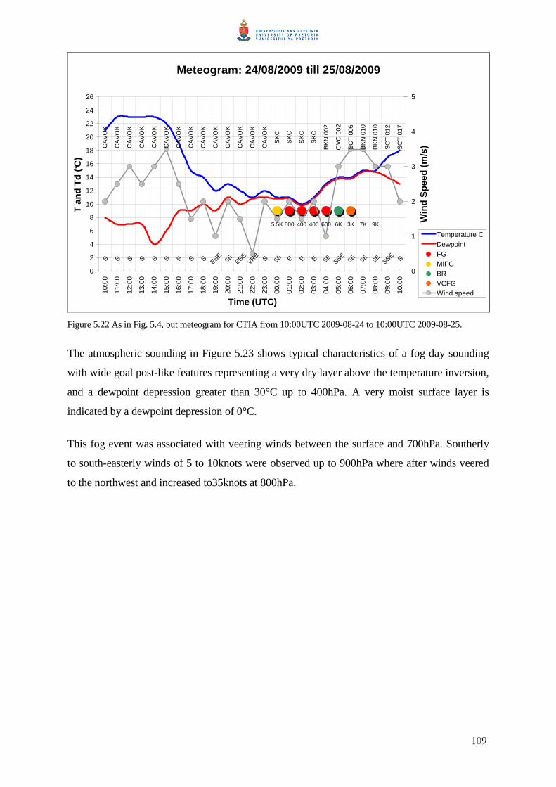
109

Meteogram: 24/08/2009 till 25/08/2009

7K6K 9K5.5K 400800

S S S S S S S S S S SSSESSE

SE SE SE SE SE SEESE

ESE E E EVRB

CA

VO

K

CA

VO

K

CA

VO

K

CA

VO

K

CA

VO

K

CA

VO

K

CA

VO

K

CA

VO

K

CA

VO

K

CA

VO

K

CA

VO

K

CA

VO

K

CA

VO

K

CA

VO

K

SK

C

SK

C

SK

C

SK

C

BK

N 0

02

OV

C 0

02

SC

T 0

06

BK

N 0

10

BK

N 0

10

SC

T 0

12

SC

T 0

17

400 3K600

0

2

4

6

8

10

12

14

16

18

20

22

24

2610

:00

11:0

0

12:0

0

13:0

0

14:0

0

15:0

0

16:0

0

17:0

0

18:0

0

19:0

0

20:0

0

21:0

0

22:0

0

23:0

0

00:0

0

01:0

0

02:0

0

03:0

0

04:0

0

05:0

0

06:0

0

07:0

0

08:0

0

09:0

0

10:0

0

Time (UTC)

T a

nd T

d (°C

)

0

1

2

3

4

5

Win

d S

peed

(m

/s)

Temperature CDewpointFGMIFGBRVCFGWind speed


The atmospheric sounding in Figure 5.23 shows typical characteristics of a fog day sounding

with wide goal post-like features representing a very dry layer above the temperature inversion,

and a dewpoint depression greater than 30°C up to 400hPa. A very moist surface layer is

indicated by a dewpoint depression of 0°C.

This fog event was associated with veering winds between the surface and 700hPa. Southerly

to south-easterly winds of 5 to 10knots were observed up to 900hPa where after winds veered

to the northwest and increased to35knots at 800hPa.

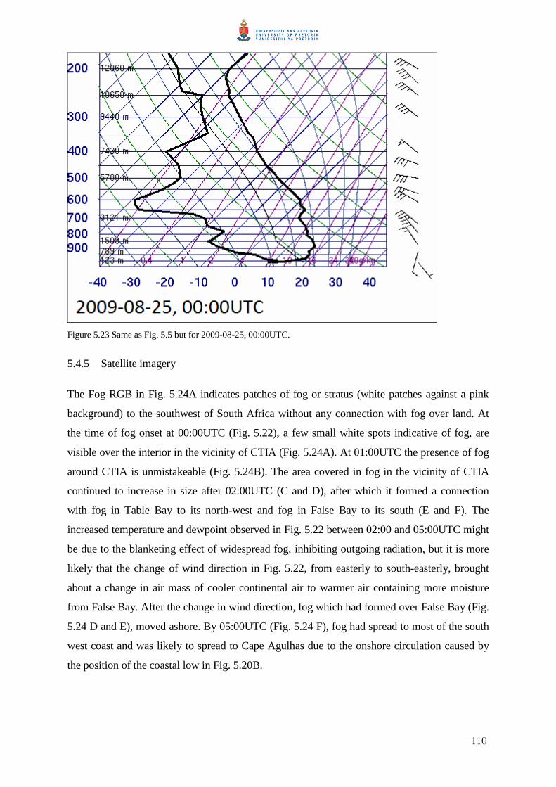
110

Figure 5.23 Same as Fig. 5.5 but for 2009-08-25, 00:00UTC.


The Fog RGB in Fig. 5.24A indicates patches of fog or stratus (white patches against a pink

background) to the southwest of South Africa without any connection with fog over land. At

the time of fog onset at 00:00UTC (Fig. 5.22), a few small white spots indicative of fog, are

visible over the interior in the vicinity of CTIA (Fig. 5.24A). At 01:00UTC the presence of fog

around CTIA is unmistakeable (Fig. 5.24B). The area covered in fog in the vicinity of CTIA

continued to increase in size after 02:00UTC (C and D), after which it formed a connection

with fog in Table Bay to its north-west and fog in False Bay to its south (E and F). The

increased temperature and dewpoint observed in Fig. 5.22 between 02:00 and 05:00UTC might

be due to the blanketing effect of widespread fog, inhibiting outgoing radiation, but it is more

likely that the change of wind direction in Fig. 5.22, from easterly to south-easterly, brought

about a change in air mass of cooler continental air to warmer air containing more moisture

from False Bay. After the change in wind direction, fog which had formed over False Bay (Fig.

5.24 D and E), moved ashore. By 05:00UTC (Fig. 5.24 F), fog had spread to most of the south

west coast and was likely to spread to Cape Agulhas due to the onshore circulation caused by

the position of the coastal low in Fig. 5.20B.

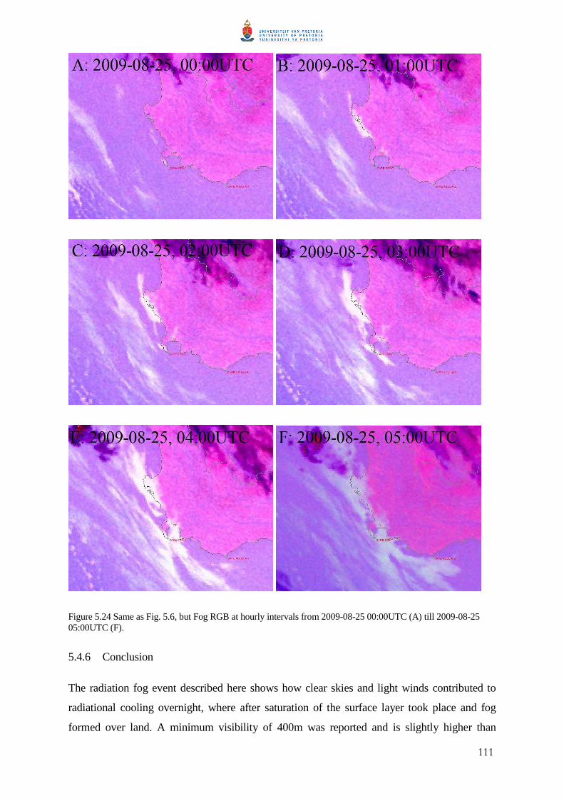
111

Figure 5.24 Same as Fig. 5.6, but Fog RGB at hourly intervals from 2009-08-25 00:00UTC (A) till 2009-08-25 05:00UTC (F).

5.4.6 Conclusion

The radiation fog event described here shows how clear skies and light winds contributed to

radiational cooling overnight, where after saturation of the surface layer took place and fog

formed over land. A minimum visibility of 400m was reported and is slightly higher than

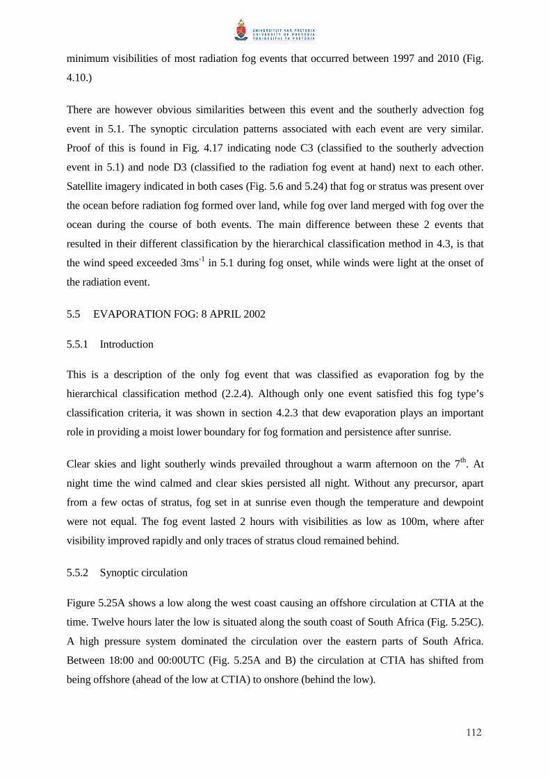
112

minimum visibilities of most radiation fog events that occurred between 1997 and 2010 (Fig.

4.10.)

There are however obvious similarities between this event and the southerly advection fog

event in 5.1. The synoptic circulation patterns associated with each event are very similar.

Proof of this is found in Fig. 4.17 indicating node C3 (classified to the southerly advection

event in 5.1) and node D3 (classified to the radiation fog event at hand) next to each other.

Satellite imagery indicated in both cases (Fig. 5.6 and 5.24) that fog or stratus was present over

the ocean before radiation fog formed over land, while fog over land merged with fog over the

ocean during the course of both events. The main difference between these 2 events that

resulted in their different classification by the hierarchical classification method in 4.3, is that

the wind speed exceeded 3ms-1 in 5.1 during fog onset, while winds were light at the onset of

the radiation event.

5.5 EVAPORATION FOG: 8 APRIL 2002

5.5.1 Introduction

This is a description of the only fog event that was classified as evaporation fog by the

hierarchical classification method (2.2.4). Although only one event satisfied this fog type’s

classification criteria, it was shown in section 4.2.3 that dew evaporation plays an important

role in providing a moist lower boundary for fog formation and persistence after sunrise.

Clear skies and light southerly winds prevailed throughout a warm afternoon on the 7th. At

night time the wind calmed and clear skies persisted all night. Without any precursor, apart

from a few octas of stratus, fog set in at sunrise even though the temperature and dewpoint

were not equal. The fog event lasted 2 hours with visibilities as low as 100m, where after

visibility improved rapidly and only traces of stratus cloud remained behind.


Figure 5.25A shows a low along the west coast causing an offshore circulation at CTIA at the

time. Twelve hours later the low is situated along the south coast of South Africa (Fig. 5.25C).

A high pressure system dominated the circulation over the eastern parts of South Africa.

Between 18:00 and 00:00UTC (Fig. 5.25A and B) the circulation at CTIA has shifted from

being offshore (ahead of the low at CTIA) to onshore (behind the low).

113

Figure 5.25 Same as Fig. 5.2, but sea level pressure fields for 2002-04-07 18:00UTC (A) till 2002-04-08 06:00UTC (C).


The sea level pressure field at 00:00UTC (Fig. 5.25B) was one of the synoptic circulations that

was categorised to node A2 of Fig. 4.17 during the synoptic classification process in section

4.3, duplicated below in Fig. 5.26. Six other fog events of which 2 radiation, 1 CBL, 1

advection and 2 unknown events occurred with a similar synoptic circulation as shown in Fig.

4.22. Similar to the synoptic circulation in Fig. 5.25B, node A2 shows a low pressure system

that has passed CTIA and is now positioned along the south coast of South Africa.

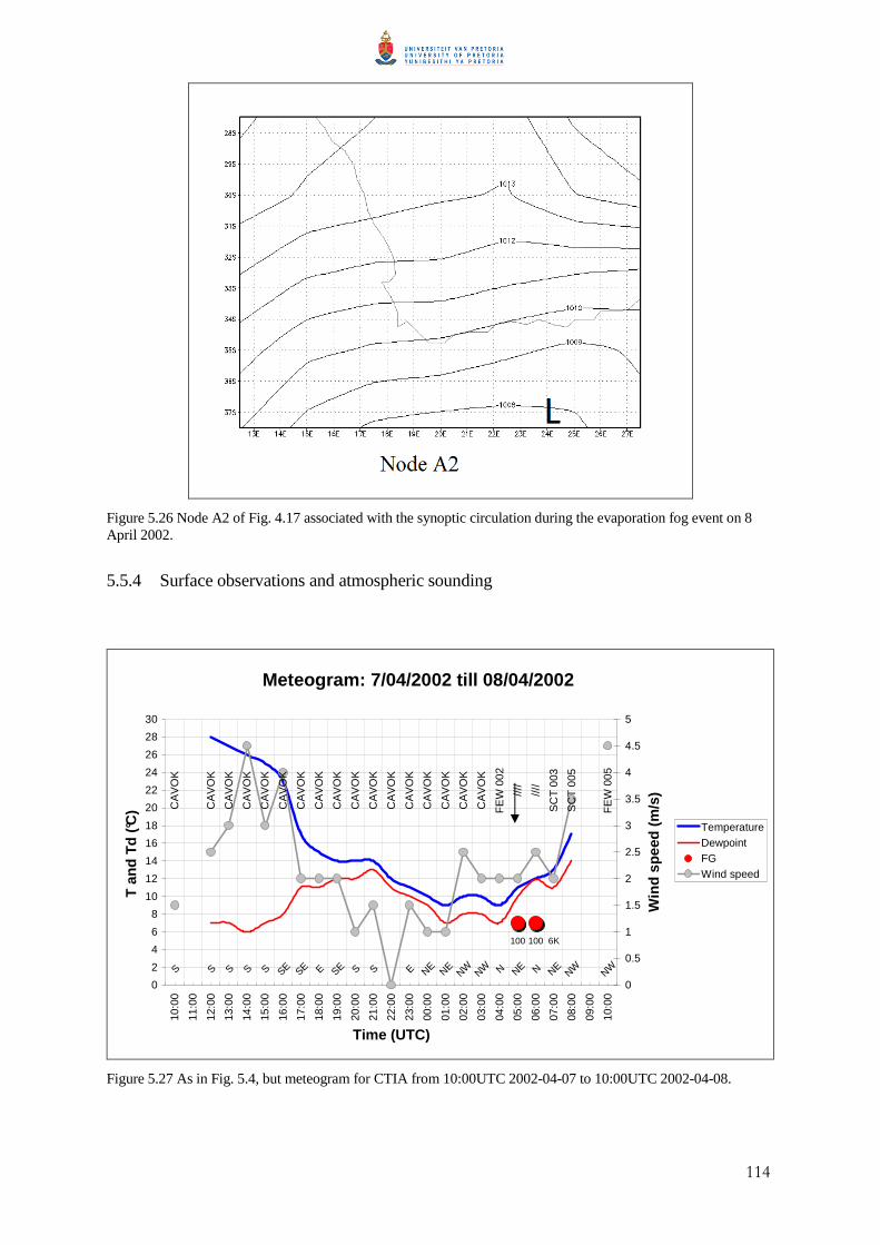
114

Figure 5.26 Node A2 of Fig. 4.17 associated with the synoptic circulation during the evaporation fog event on 8 April 2002.


Meteogram: 7/04/2002 till 08/04/2002

6K100 100

CA

VO

K

CA

VO

K

CA

VO

K

CA

VO

K

CA

VO

K

CA

VO

K

CA

VO

K

CA

VO

K

CA

VO

K

CA

VO

K

CA

VO

K

CA

VO

K

CA

VO

K

CA

VO

K

CA

VO

K

CA

VO

K

CA

VO

K

FE

W 0

02

////

////

SC

T 0

03

SC

T 0

05

FE

W 0

05

S S S S S S SSE SE SEE NE NE NE NENW NW NW NWN NE

0

2

4

6

8

10

12

14

16

18

20

22

24

26

28

30

10:0

0

11:0

0

12:0

0

13:0

0

14:0

0

15:0

0

16:0

0

17:0

0

18:0

0

19:0

0

20:0

0

21:0

0

22:0

0

23:0

0

00:0

0

01:0

0

02:0

0

03:0

0

04:0

0

05:0

0

06:0

0

07:0

0

08:0

0

09:0

0

10:0

0

Time (UTC)

T a

nd T

d (°C

)

0

0.5

1

1.5

2

2.5

3

3.5

4

4.5

5

Win

d sp

eed

(m/s

)

TemperatureDewpointFGWind speed


115

The meteogram in Fig. 5.27 summarises the surface conditions at CTIA from 10:00UTC on 7

April 2002 till 10:00UTC on 8 April 2002. At 18:00UTC (while the low pressure system was

still to the north of CTIA (Fig. 5.25A)) light easterly to south-easterly winds of 2ms-1 were

reported with a 5°C dewpoint depression. Even when the wind speed dropped to 0ms-1 at

22:00UTC, temperature and dewpoint values stayed a degree apart. Considering the synoptic

circulation in Fig. 5.25B, one would expect the wind direction to have a southerly or south-

westerly component as was the case in 5.1. This weak low pressure system did not cause wind

directions to back, instead they varied between north-easterly and north-westerly after

00:00UTC and stayed north-westerly till 10:00UTC when the low was well to the east of

CTIA.

Just before sunrise 1-2 octas of stratus were reported at a very low base of 200ft. With the wind

direction still northerly to north-easterly and the wind speed still below 3ms-1, the temperature

and dewpoint started rising rapidly towards sunrise (black arrow indicating sunrise in Fig. 2.27)

allowing dew to evaporate and contribute to a saturated boundary layer (Pilié et al., 1975). At

05:00UTC the visibility dropped to 100m and stayed like that for another hour till 06:00UTC

which was the only time temperature and dewpoint values were equal. As the temperature

continued to rise the dewpoint started falling and the visibility improved to 6000m at

07:00UTC. After the fog had dissipated there were still reports of low cloud until 10:00UTC.

The 00:00UTC atmospheric sounding in Fig 5.28B shows a very stable temperature profile

with temperatures at the surface more than 10°C lower than at the 950hPa level. Although the

passage of the low did not bring about a wind direction change at the surface (Fig. 5.27),

atmospheric soundings of the afternoon prior to and after the low’s passage (Fig. 5.28A and B)

show that a north-westerly wind of 5knots (2.5ms-1) at 950hPa, backed to the south and

increased to 10knots (5ms-1) 12 hours later at 00:00UTC (Fig. 5.28B).

116

Figure 5.28 Same as Fig. 5.5 but for 2002-04-07 12:00UTC (A) and 2002-04-08 00:00UTC (B).

5.5.5 Conclusion

Despite clear skies, light winds and a stable atmosphere, radiation fog did not form during the

early morning hours at CTIA on 8 April 2002. Fog onset did however take place at sunrise

(05:00UTC) after the temperature and dewpoint increased due to dew evaporation. The fog

event was of short duration, but the visibility dropped to 100m.

5.6 SUMMARY

Case studies of the 5 different types of fog that occur most frequently at CTIA showed that the

hierarchical fog type classification method described in section 2.2.4, classified fog events

according to their formation characteristics successfully. In each case the synoptic classification

method described in section 2.3 associated the 00:00UTC mean sea level pressure field with a

similar synoptic circulation, as shown by the different nodes of Fig. 4.17.

In all of the above case studies, atmospheric soundings indicated an absolutely stable

atmosphere with saturated or nearly saturated conditions at the surface and very dry conditions

directly above the temperature inversion. Four out of the 5 case studies showed wind directions

veering with height between the surface and 700hPa and in all cases except the CBL event (5.3)

wind speeds increased significantly above the temperature inversion.

The coastal low or west coast trough played an important role in all the case studies, except

with the CBL event, where a high pressure system over the interior dominated the circulation.

Some cases such as the southerly advection (5.1), north-westerly advection (5.2) and radiation

(5.4) fog events, showed similar synoptic characteristics, but with the help of satellite imagery

117

and surface observations the different formation mechanisms leading to fog onset could be

distinguished.

118

CHAPTER 6

SUMMARY, CONCLUSION AND RECOMMENDATIONS

6 SUMMARY, CONCLUSION AND RECOMMENDATIONS

6.1 GENERAL SUMMARY

Fog occurs more frequently at CTIA than at any other of the international airports in South

Africa (SAWB, 1968). Extensive fog research in South Africa has been conducted to harvest

fog as a source of water (Van Heerden and Olivier, 1999), but research on the forecasting of

fog has largely been neglected in South Africa. However, there is a great need to improve fog

forecasting as it was shown (Chapter 3) that the quality of the fog forecasts at CTIA does not

meet the required WMO standard. Furthermore, incorrect fog forecasts can lead to unplanned

aircraft diversions and delays which have an astronomical impact on airline expenses.

Therefore the main aim of this research is to improve fog forecasts at CTIA. The first step in

addressing this aim is to provide a comprehensive fog climatology. This climatology is

presented in Chapter 4 and contains information for 31 years at 06:00, 12:00 and 18:00UTC as

well as a 13 year climatology at hourly intervals. The fog climatology also provides the

characteristics of fog such as fog type, time of onset and dissipation and the intensity and

duration of fog events. Fog types that frequently occur were identified by application of a

hierarchical classification method that was first implemented in the United States by Tardif and

Rasmussen (2007) and the synoptic circulation associated with these fog types was determined

by means of SOMs. The upper air characteristics on fog days are also provided.

Once fog types and their characteristics were determined, 5 different fog types that frequently

occur at CTIA were identified. Case studies of these fog types are presented in Chapter 5.

In this chapter an overview of the most significant results of the above mentioned chapters are

provided. Conclusions are made and recommendations are given that could lead to the

improvement of fog forecasts at CTIA and airports across South Africa.

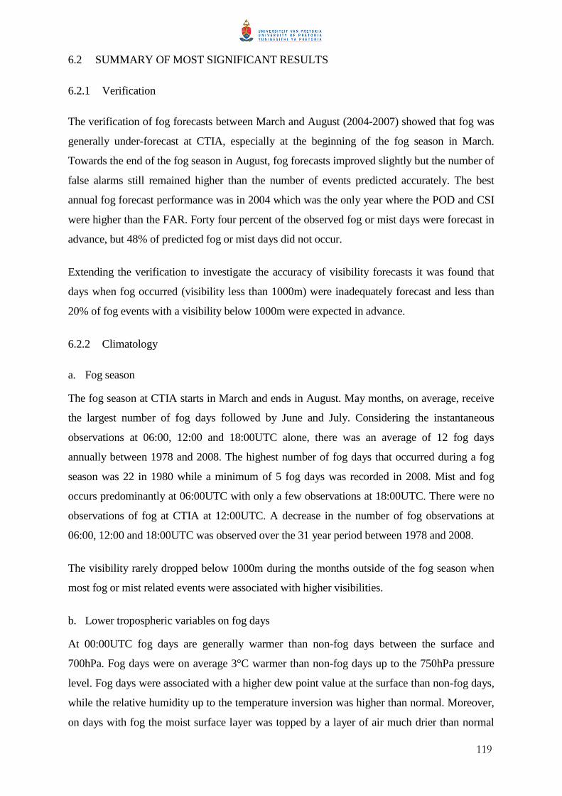
119

6.2 SUMMARY OF MOST SIGNIFICANT RESULTS

6.2.1 Verification

The verification of fog forecasts between March and August (2004-2007) showed that fog was

generally under-forecast at CTIA, especially at the beginning of the fog season in March.

Towards the end of the fog season in August, fog forecasts improved slightly but the number of

false alarms still remained higher than the number of events predicted accurately. The best

annual fog forecast performance was in 2004 which was the only year where the POD and CSI

were higher than the FAR. Forty four percent of the observed fog or mist days were forecast in

advance, but 48% of predicted fog or mist days did not occur.

Extending the verification to investigate the accuracy of visibility forecasts it was found that

days when fog occurred (visibility less than 1000m) were inadequately forecast and less than

20% of fog events with a visibility below 1000m were expected in advance.

6.2.2 Climatology

a. Fog season

The fog season at CTIA starts in March and ends in August. May months, on average, receive

the largest number of fog days followed by June and July. Considering the instantaneous

observations at 06:00, 12:00 and 18:00UTC alone, there was an average of 12 fog days

annually between 1978 and 2008. The highest number of fog days that occurred during a fog

season was 22 in 1980 while a minimum of 5 fog days was recorded in 2008. Mist and fog

occurs predominantly at 06:00UTC with only a few observations at 18:00UTC. There were no

observations of fog at CTIA at 12:00UTC. A decrease in the number of fog observations at

06:00, 12:00 and 18:00UTC was observed over the 31 year period between 1978 and 2008.

The visibility rarely dropped below 1000m during the months outside of the fog season when

most fog or mist related events were associated with higher visibilities.

b. Lower tropospheric variables on fog days

At 00:00UTC fog days are generally warmer than non-fog days between the surface and

700hPa. Fog days were on average 3°C warmer than non-fog days up to the 750hPa pressure

level. Fog days were associated with a higher dew point value at the surface than non-fog days,

while the relative humidity up to the temperature inversion was higher than normal. Moreover,

on days with fog the moist surface layer was topped by a layer of air much drier than normal

120

between 925 and 850hPa. Corresponding to a higher average column temperature between

1000 and 700hPa on fog days, than non-fog days, the geopotential thicknesses are also higher

on fog days.

Temperature inversions occur between 300 and 650ft on fog days. The lowest monthly average

fog day temperature inversion occur in July (300ft AGL) and the highest in March. June had

the shallowest monthly inversion layer (140ft AGL).

From May to August, lower wind speeds than normal (5knots or less), were observed on fog

days at 1000 and 900hPa, but higher wind speeds (10 to 15knots) were observed at 800 and

850hPa in March and April.

c. Fog types

A 13 year climatology of fog events at CTIA showed that there are 3 dominant fog types that

occur commonly at CTIA: Radiation fog occurs most frequently, followed by CBL fog and

then advection fog. Other fog types such as precipitation and evaporation fog were considered

but do not form a significant part of the types of fog that occur frequently at CTIA. Previous

studies (such as Aeronautical Summary, 1968) found that advection fog occurred at CTIA more

than any other type. However, in their research no clear definition of radiation fog is provided

which makes a direct comparison difficult. Moreover land use in the vicinity of the airport has

changed significantly in the past 50 years and it is feasible that an increase in aerosols from

wood and coal burning in the informal settlements affected the dominant fog type at CTIA.

i) Radiation fog

Fifty percent of fog events that occur during the fog season at CTIA are radiation fog

events. Of this 50% only 1% occurs in March, but this frequency increases rapidly to

14% in June. Radiation fog is the most common type of fog in all the months except

March months when CBL fogs are most frequent.

The minimum visibility associated with radiation fog has a median of 200m while 75%

of the events have a minimum visibility of less than 500m. Radiation fog generally has

a duration between 4 and 8 hours which is slightly less than any other fog type. Most

radiation fog events started 10 hours prior to sunrise which equates to an onset time

between 19:00 and 20:00UTC. The onset time of radiation fog is at night. It is quite

interesting to note the decrease in radiation fog onset about 2 hours before sunrise but

with an increase in the onset of radiation fog at sunrise. This suggests that dew

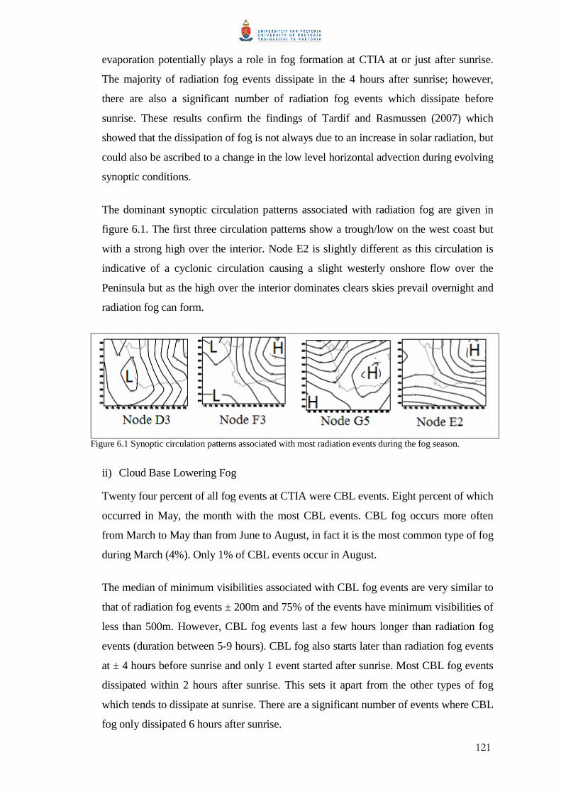
121

evaporation potentially plays a role in fog formation at CTIA at or just after sunrise.

The majority of radiation fog events dissipate in the 4 hours after sunrise; however,

there are also a significant number of radiation fog events which dissipate before

sunrise. These results confirm the findings of Tardif and Rasmussen (2007) which

showed that the dissipation of fog is not always due to an increase in solar radiation, but

could also be ascribed to a change in the low level horizontal advection during evolving

synoptic conditions.

The dominant synoptic circulation patterns associated with radiation fog are given in

figure 6.1. The first three circulation patterns show a trough/low on the west coast but

with a strong high over the interior. Node E2 is slightly different as this circulation is

indicative of a cyclonic circulation causing a slight westerly onshore flow over the

Peninsula but as the high over the interior dominates clears skies prevail overnight and

radiation fog can form.

Figure 6.1 Synoptic circulation patterns associated with most radiation events during the fog season.

ii) Cloud Base Lowering Fog

Twenty four percent of all fog events at CTIA were CBL events. Eight percent of which

occurred in May, the month with the most CBL events. CBL fog occurs more often

from March to May than from June to August, in fact it is the most common type of fog

during March (4%). Only 1% of CBL events occur in August.

The median of minimum visibilities associated with CBL fog events are very similar to

that of radiation fog events ± 200m and 75% of the events have minimum visibilities of

less than 500m. However, CBL fog events last a few hours longer than radiation fog

events (duration between 5-9 hours). CBL fog also starts later than radiation fog events

at ± 4 hours before sunrise and only 1 event started after sunrise. Most CBL fog events

dissipated within 2 hours after sunrise. This sets it apart from the other types of fog

which tends to dissipate at sunrise. There are a significant number of events where CBL

fog only dissipated 6 hours after sunrise.

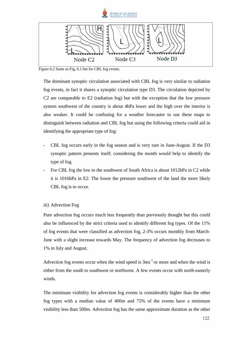
122

Figure 6.2 Same as Fig. 6.1 but for CBL fog events.

The dominant synoptic circulation associated with CBL fog is very similar to radiation

fog events, in fact it shares a synoptic circulation type D3. The circulation depicted by

C2 are comparable to E2 (radiation fog) but with the exception that the low pressure

system southwest of the country is about 4hPa lower and the high over the interior is

also weaker. It could be confusing for a weather forecaster to use these maps to

distinguish between radiation and CBL fog but using the following criteria could aid in

identifying the appropriate type of fog:

- CBL fog occurs early in the fog season and is very rare in June-August. If the D3

synoptic pattern presents itself; considering the month would help to identify the

type of fog.

- For CBL fog the low to the southwest of South Africa is about 1012hPa in C2 while

it is 1016hPa in E2. The lower the pressure southwest of the land the more likely

CBL fog is to occur.

iii) Advection Fog

Pure advection fog occurs much less frequently than previously thought but this could

also be influenced by the strict criteria used to identify different fog types. Of the 11%

of fog events that were classified as advection fog, 2-3% occurs monthly from March-

June with a slight increase towards May. The frequency of advection fog decreases to

1% in July and August.

Advection fog events occur when the wind speed is 3ms-1 or more and when the wind is

either from the south to southwest or northwest. A few events occur with north-easterly

winds.

The minimum visibility for advection fog events is considerably higher than the other

fog types with a median value of 400m and 75% of the events have a minimum

visibility less than 500m. Advection fog has the same approximate duration as the other

123

two fog types (5-8 hours). The onset time of advection fog is about 2 hours before

sunrise and dissipates about 2 hours after sunrise. However, there were some notable

cases of advection fog which started 9 to 12 hours after sunrise. In these cases the

marine fog layer will often remain stationary along the coast during daytime as solar

heating of the land mass causes dissipation of the fog by convective mixing that takes

place between drier, warmer, continental air and the advancing marine layer. But as

soon as temperatures start to decrease towards night time, the cooler and less turbulent

boundary layer allows an inland propagation of the fog layer (Tardif and

Rasmussen, 2007)

Figure 6.3 Same as Fig. 6.1 but for advection fog events.

The synoptic circulation dominant during advection fog days are not dissimilar to the

circulation during the other two types of fog. However, in node A3 the low is clearly

situated along the south coast with south-westerly to southerly onshore flow into False

Bay. Node F2 is very similar to E2 but with a high pressure system over the interior

further west causing a stronger pressure gradient and increased wind speeds over the

south-western Cape. A weather forecaster will be well advised to consider the strength

of the wind when referring to these synoptic patterns to forecast advection fog.

d. Further notes on the synoptic circulation

The synoptic circulation associated with most fog events at CTIA (node E2) was also

associated with the most radiation fog events. Fog rarely occurs when a strong westerly

circulation dominates. However, in many of the other circulation patterns identified, several

types of fog may occur.

A monthly distribution of synoptic circulation types showed that the character of fog related

circulation types change from March to August. In March the dominant synoptic circulation

type resembles a coastal low that is positioned off the south coast of South Africa, causing an

onshore circulation along the west and southwest coast. During April and May the circulation

changes to a broad region of lower pressure along the west coast and adjacent interior with a

124

high dominant over the interior of South Africa. But from June to August, the presence of the

low on the west coast becomes weaker and the high pressure system that was dominant over

the interior during April and May, then dominates the synoptic circulation along the west coast

as well. Together with this seasonal change of synoptic circulation patterns the dominant fog

types also change between the start and the end of the fog season.

6.2.3 Case studies

- Atmospheric soundings of all 5 case studies indicated an absolutely stable atmosphere with

saturated or nearly saturated conditions at the surface and very dry conditions directly

above the temperature inversion.

- Four out of the 5 case studies showed wind directions veering with height from a southerly

direction in the lower levels to a north-westerly wind at 700hPa. Only during the north-

westerly advection fog case study did wind directions remain north-westerly up to 700hPa.

- In all cases except the CBL event, wind speeds increased significantly with height.

- The coastal low or west coast trough was prominent in all five case studies except with the

CBL event, where a high pressure system over the interior dominated the circulation.

- Fog that has formed over the ocean is not often advected towards the airport, but fog

frequently forms later in the night as radiation fog after the advection process has

transported moisture towards the airport during the previous afternoon and evening.

6.3 CONCLUSIONS

6.3.1 General

- Fog related low visibility forecasts at CTIA do not comply with ICAO minimum accuracy

criteria.

- Fog or mist forecasts in general were more often than not incorrect.

- Forecasters rarely forecast fog and rather forecast a visibility of 1000m or more.

- Forecasters at CTIA lack clear guidelines to forecast all aspects of fog accurately: these

aspects include time of onset and dissipation, duration and intensity of the event.

125

- The hierarchical fog type classification method successfully classified fog events into

different fog types at CTIA. The three fog types that were found to occur most frequently

are: radiation fog, cloud base lowering fog and advection fog. Earlier publications (SAWS,

1968) suggested that advection fog dominates at CTIA while pure radiation fog events are

rare.

- The use of SOMs as a synoptic classification method brought new insight into the synoptic

circulation patterns associated with different fog types at CTIA:

o Radiation fog events can also occur during the passage of a coastal low.

o Synoptic circulations conducive to fog at CTIA change during the course of the fog

season. Similar circulation types may cause different types of fog depending on the

month of the season. The results describing the monthly occurrence of the different

types of fog could aid the aviation weather forecaster to determine the type of fog

which occurs with a particular circulation type. Special attention should also be

given to the location and depth of the low and high pressure system in order to

distinguish between different types of fog.

o However, a fog forecast can not be based on the synoptic circulation alone, since

different fog types can be associated with the same circulation pattern and the

presence of a specific circulation pattern is by no means a guarantee that fog will

form.

- Knowledge of the circulation patterns that are most regularly associated with fog at CTIA,

can help forecasters identify potential fog scenarios in advance by making use of NWP

mean sea level pressure forecasts.

- All aspects of fog forecasts can be improved by increased knowledge of the fog season, the

accurate diagnosis of the expected fog type and the application of fog type characteristics to

the forecast or TAF. The same criteria that were used for fog type classification can be

applied to identify whether an event is likely to be advective or radiative. Forecasts of wind

speed, sea level pressure and even temperature and dewpoint profiles can be made with

NWP output. Once the likelihood of fog has been determined, the fog type characteristics

such as minimum visibility, duration, time of onset and clearance can be implemented.

126

- One can expect the typical fog day sounding to have a very moist layer below the

temperature inversion, associated with a very small dewpoint depression. Above the

temperature inversion a typical fog day sounding will likely possess the ‘goal post’ feature

as referred to by Croft et al., (1997) with a high dewpoint depression, up to at least 850hPa.

6.3.2 Conclusions of importance in an operational forecast environment

- Radiative and advective processes often combine to form radiation fog at CTIA. Moist air

is advected towards the airport from False Bay by the southerly sea breeze in the afternoon

or from Table Bay by a north-westerly wind caused by the presence of a low along the

southwest coast. At night the wind drops which allows radiative processes to take over.

- All radiation fog events can be traced back to a source of surface moisture: forecasters

should be on the lookout for a southerly or north-westerly sea breeze in the afternoon, signs

of low stratus or fog along the south-western Cape coastline on satellite imagery, the

presence of stratus or fog earlier in the day or recent rainfall that could fill wetlands in the

vicinity of the airport.

- Dew evaporation should be considered as a secondary fog formation mechanism,

contributing to a moist boundary layer and enhancing fog after sunrise.

- Less daylight hours in June seem to alter the vertical temperature profile of the atmosphere

in the lower levels and potentially contribute to the increased number of radiation fog

events.

- The presence of a coastal low along the south-western Cape coastline and coastal stratus or

fog on satellite imagery, should be considered as a potential fog threat at CTIA.

6.3.3 Practical application of this research

The results of this research could be applied to facilitate the improvement of the forecasting

process of fog events at CTIA. Aviation forecasters are encouraged to use the following steps

to improve the forecasts of fog during the fog season at CTIA:

127

STEP 1: Isolate the most likely fog types for the current month of the fog season.

The aviation forecaster should familiarise him/herself with the month of the fog season at hand.

Provided that there are no limiting factors for fog formation in the forecast (such as rain or

strong winds in which fog is unlikely to form), the forecaster can proceed to:

STEP 2: Investigate the synoptic circulation forecast for 00:00UTC by means of NWP

data.

- Compare the forecast synoptic circulation as well as the central pressures associated with

the highs and lows, with that of the nodes that caused fog at CTIA most frequently (Fig.

6.1, 6.2 and 6.3).

STEP 3: Determine whether a stable boundary layer can be expected at 00:00UTC.

- Make use of a NWP temperature and dewpoint profile valid for 00:00UTC to determine

whether:

o A temperature inversion is present below 650ft.

o Winds are light below the temperature inversion and wind directions veer from

the south to the northwest between the surface and 700hPa.

o A small dewpoint depression is obvious at the surface indicative of a moist

boundary layer.

o A large dewpoint depression (more than 20°C) is present above the temperature

inversion indicative of very dry air above the temperature inversion.

STEP 4: Determine the fog type.

- If steps 2 and 3 indicate favourable conditions for fog formation, determine the expected

fog type by taking the month of the fog season, the synoptic circulation as well as likely

formation mechanisms of fog into consideration:

o Light winds and clear skies (speeds less than 3ms-1) favour the development of

radiation fog if there is a source of surface moisture. A source of moisture can

range from recent rainfall, to a southerly or north-westerly sea breeze in the

afternoon or the evaporation of dew after sunrise.

128

o Light winds with the presence of low stratus on the Cape Flats during the

afternoon or around the southwest coast, can favour CBL fog. CBL fog can also

occur in the presence of winds of 3ms-1 or more which will act to advect low

stratus towards CTIA.

o The presence of fog over the ocean to the south or along the west coast in the

presence of southerly or north-westerly winds with speeds of 3ms-1 or more, are

indicators of potential advection fog.

STEP 5: Apply fog type characteristics in the climatology to the TAF.

Once a decision has been made about the type of fog which will occur, the results in Chapter 4

could aid to predict the minimum visibility, duration and time of onset and dissipation.

- Most of the time the minimum visibility of all fog types during the fog season is 500m or

less.

- All fog types have approximately the same duration (5-8 hours).

- Radiation and advection fog clears around sunrise but CBL fog clears after sunrise.

- The time of onset of most radiation fog events is before 00:00UTC, but CBL fog’s onset

time is mostly 4 hours prior to sunrise. Advection events’ onset times vary from just before

sunrise, to just before sunset. Satellite imagery can provide helpful information to predict

when fog will reach CTIA.

6.4 RECOMMENDATIONS

- The results of this study should be made available to aviation weather forecasters at CTIA

to use in the forecasting of fog at the airport.

- Aviation forecasters should be equipped with climatological knowledge of fog at CTIA.

- The fog type and synoptic classification process should be applied to all airports in South

Africa where fog is a potential hazard.

- The fog type classification process should be repeated with a longer period of hourly data.

129

- The large percentage of events classified as “unknown” should be investigated: strict

classification criteria could have resulted in certain events remaining unclassified which

could be remedied by reclassifying unknown events manually.

- The likelihood of fog should be under constant review by taking satellite imagery and

surface observations into consideration, especially during the fog season.

- Further research of the following is encouraged:

o The role of the coastal low or west coast trough in the formation of fog at CTIA.

o Secondary mechanisms contributing to fog formation: SSTs in False Bay and Table

Bay, dew evaporation after sunrise and the shallow water table on the Cape Flats

that provides moisture to the boundary layer prior to radiation fog events towards

the end of the fog season.

o Decline observed in the annual number of fog days at CTIA: SOMs have been

applied successfully to identify evolving rainfall patterns in Australia (Hope et

al., 2006), the United States (Hewitson et al., 2002) and locally (Lennard, 2009),

and could shed light on changing fog related synoptic patterns as well.

o The influence of aerosols on fog formation over the Cape Flats.

- Development of an operational fog forecast guidance tool which will allow subjective

forecaster input and incorporate the synoptic circulation type, surface observations as well

as NWP data.

130

REFERENCES

- Ahrens C. D., (2000): Meteorology Today, Brooks/Cole, Pacific Grove, California

- AirDisaster.com Accident Database, 2010: http://www.airdisaster.com/cgi-

bin/view_details.cgi?date=04102010&reg=101&airline=Polish+Air+Force

- Airports Company South Africa (ACSA), 2010: Cape Town International Airport, Aircraft

Statistics, www.acsa.co.za.

- Airport Transport Association, 2010: www.airlines.org

- American Meteorological Society (AMS), 2010: Glossary of Meteorology,

http://amsglossary.allenpress.com/glossary

- Arrive Alive Road Safety Awareness, 2011: Safe Driving in the Fog and Mist,

http://www.arrivealive.co.za/pages.aspx?i=2936

- Baars, J. A., Witiw, M. and Al-Habash, A., 2003: Determining fog type in the Los Angeles

basin using historic surface observation data. Proc. 16th Conference on Probability and

Statistics in the Atmospheric Sciences, Long Beach, CA, AMS., CD-ROM, J3.8.

- Bristow G. V., (2002): Ace the Technical Pilot Interview, The McGraw-Hill Companies,

Inc, New York.

- Burger, L., (2006): The Influence and Forecasting of Fog at Cape Town International

Airport, Proc. 22nd SASAS Conference, Maselspoort Conference Centre, Bloemfontein,

South Africa.

- Carter T. J., (2005): The evolution of coastal lows along the south coast of South Africa,

“unpublished MSc dissertation”, University of Zululand, KwaDlangezwa, South Africa.

- Cereceda, P., and Schemenauer, R.S., (1991): The Occurrence of fog in Chile, AMS, Vol.

30, 1097-1105.

- Cho, Y., Kim, M., and Kim, B., (2000): Sea fog around the Korean peninsula, Journal of

Applied Meteorology. 39, 2473-2479.

- Civil Aviation Authority, 2007: CAA, Operations Specifications Template, Form CA ACC-

F-011, www.caa.co.za

- Cowling, R.M., Richardson, D.M. & Pierce, S.M., (1997): Vegetation of Southern Africa,

Cambridge University Press, United Kingdom.

- CRG (Climate Research Group), (2003): Cape Town Brown Haze II Project-Final Report,

University of the Witwatersrand, Johannesburg, South Africa.

- Croft, P.J., Pfost, R.L., Medlin, J.M., Johnson, G.A., (1997): Fog Forecasting for the

Southern Region: A Conceptual Model Approach, Weather and Forecasting. 12, 545-556.

131

- Dahni R.R., (2003): An Automated Synoptic Typing System Using Archived and Real-time

NWP model output, Bureau of Meteorology, Melbourne, Australia.

- De Villiers, M. P. and Van Heerden J., 2007: Fog at Abu Dhabi International Airport,

Weather – August 2007, Vol. 62, No. 8.

- De Villiers, M. P., (2010): Predicting the development of weather phenomena that

influence aviation at Abu Dhabi International Airport, “Unpublished PhD Thesis”,

University of Pretoria, Pretoria.

- Eumetsat (2011): Real-time imagery, RGB Composites, www.eumetsat.int

- Hauze, R.A., (1993): Cloud Dynamics, Academic Press, San Diego.

- Hcigizoglu H. K., Bayazit M., and Önöz B., (2005), Trends in the Maximum, Mean, and

Low Flows of Turkish Rivers. J. of Hydrometeorol. 6 (3) 280–290.

- Hewitson B.C. and Crane R.G., (2002): Self-organizing maps: applications to synoptic

climatology, Clim Res. Vol.22, 13-26.

- Hope P.K., Drosdowsky N.N. and Nicholls N., (2006): Shifts in the synoptic systems

influencing southwest Western Australia, Climate Dynamics 26, 751-764.

- Hyvärinen, O., Julkunen, J. and Nietosvaara, V., (2007): Climatological Tools for Low

Visibility Forecasting, Pure appl. Geophys. 164, 1383-1396.

- ICAO (2001): Annex 3 to the Convention on International Civil Aviation. International

Standards and Recommended Practices, Attachment E, International Civil Aviation

Organization.

- Jolliffe I.T. and Stephenson D.B., (2003): Forecast Verification: A Practitioner’s Guide in

Atmospheric Science, John Wiley & Sons Ltd, England.

- Jury, M. R., (1983): Wind shear & differential upwelling along the SW tip of Africa,

“Unpublished PhD Thesis”, University of Cape Town.

- Kohonen, T., (2001): Self-Organizing Maps, Third Edition, Springer-Verlag Berlin

Heidelberg New York

- Marzban, C., (1998): Scalar Measures of Performance in Rare-Event Situations, Weather

and Forecasting. 13, 753-763.

- McIntosh, D. H., (1972): Meteorological Glossary, Great Britain Meteorological Office,

318pp.

- Meyer, M. B., and Lala G. G., (1990), Climatological Aspects of Radiation Fog Occurrence

at Albany, New York, Journal of Climate. 3, 577-586.

- Olivier, J., and Van Heerden, J., (1999), The South African fog water collection project,

Water Research Commission, Report no. 671/1/99.

132

- Pilié, R.J., Mack, E.J., Kocmond, W.C., Rogers, C.W. and Eadie, W.J., (1975), The Life

Cycle of Valley Fog. Part I: Micrometeorological Characteristics, JAM. 14, 347-373.

- RTMC (Road Traffic Management Corporation) (2008), Road Traffic Report March 2008,

http://www.arrivealive.co.za/documents/March_2008_-_Road_Traffic_Report_-

_March_2008.pdf

- Rogers, R.R., and Yau, M.K., (1989), A Short Course in Cloud Physics, Pergamon Press,

U.K.

- Roth-Nebelsick A., Ebner M., & Miranda T., 2010: Efficient fog harvesting by Stipagrostis

sabulicola (Namib dune bushman grass), Proc. 5th International Conference on Fog, Fog

Collection and Dew, 25-30 July 2010, Münster, Germany, 63.

- SAWB (SOUTH AFRICAN WEATHER BUREAU) (1968): Aeronautical Climatological

Summaries, 1957-1964. WB31, South African Weather Bureau, Pretoria, South Africa.

- SAWB (SOUTH AFRICAN WEATHER BUREAU) (1996): Regional description of the

weather and climate of South Africa: The Weather and Climate of the extreme south-

western Cape, South African Weather Bureau, Pretoria, South Africa, 39.

- SAWS (SOUTH AFRICAN WEATHER SERVICE) (1998): Climate of South Africa.

Climate statistics 1961-1990. WB42, South African Weather Service, Pretoria, South

Africa.

- SAWS (SOUTH AFRICAN WEATHER SERVICE) (2004): Training Manual,

Meteorological Aviation Codes for Weather Observers (METAR/TAF/ADDENDUM 1 TO

3)

- SAWS (SOUTH AFRICAN WEATHER SERVICE) (2006): Aeronautical Climatological

Summaries, 1996-2005. South African Weather Service, Pretoria, South Africa.

- SAWS Monthly Aviation Reports for Cape Town International Airport. (2006): South

African Weather Service, Cape Town, South Africa.

- SAWS Monthly Aviation Reports for Cape Town International Airport. (2009): South

African Weather Service, Cape Town, South Africa.

- SAWS SUMO software (2011): South African Weather Service, Pretoria, South Africa.

- Smit, R. D., 2006: Personal communication, Senior Forecaster, Cape Town, SAWS, P.O.

Box 21, Cape Town Int. Airport, 7525.

- South African Airways, (2009): Financial report,

http://www.flysaa.com/pv_obj_cache/pv_obj_id_764DD0882A0ADB7FDD6F4E5FE9CC

EE89D8BF2700/filename/SAA_2009_Annual_Report.pdf

- Steyn A.G.W., Smit C.F., Du Toit S.H.C, and Strasheim C., (1994): Modern statistics in

practice, J.L Van Schaik , Pretoria, South Africa.

133

- Taljaard J.J., (1994): Atmospheric Circulation Systems, Synoptic Climatology and Weather

Phenomena of South Africa. Part 1: Controls of the weather and climate of South Africa,

South African Weather Bureau, Pretoria, South Africa, 27.

- Tardif, R. and Rasmussen, R.M., (2007): Event-Based Climatology and Typology of Fog in

the New York City Region, Journal of Appl. Meteorology and Climatology. 46, 1141-1168.

- Tilbury, M.R.R., (ed.) (1978): Fog Prediction at the D.F. Malan Airport, Cape Town

- Tiwari, S., Payra, S., and Bisht, D.S., (2010): Visibility Degradation during Foggy Period

due to Anthropogenic Urban Aerosol at Delhi, India. Proc. 5th International Conference on

Fog, Fog Collection and Dew, 25-30 July 2010, Münster, Germany, 92 95.

- Turner, M., (1988): Shipwrecks & Salvage in South Africa – 1505 to the present, Struik

House, Cape Town.

- Tyson, P.D. & Preston-Whyte R.A., (2000): The Weather and Climate of Southern Africa,

Oxford University Press Southern Africa, Cape Town.

- University of Wyoming (UWYO), 2011: Upper air soundings,

http://weather.uwyo.edu/upperair/sounding.html .

- Van Heerden J., Olivier J., Evans D., & Muller H., (2008): A new design cloud water

system for the Cabazana community in the Alfred Nzo Municipality, Eastern Cape

Province, Proc. 24th SASAS Conference, 28 Sep-1 Oct 2008, SANLAM Auditorium,

University of Pretoria, South Africa, 104-105.

- WMO (World Meteorological Organization) 2000: Guidelines on performance assessment

of public Weather Services, WMO, WMO/TD No. 1023.

- World Airports (2010, 2008), Cape Town International Airport, O.R. Tambo International

Airport, www.azworldairports.com.

- Weather Underground (2010), Historic METAR data downloads:

www.wunderground.com.

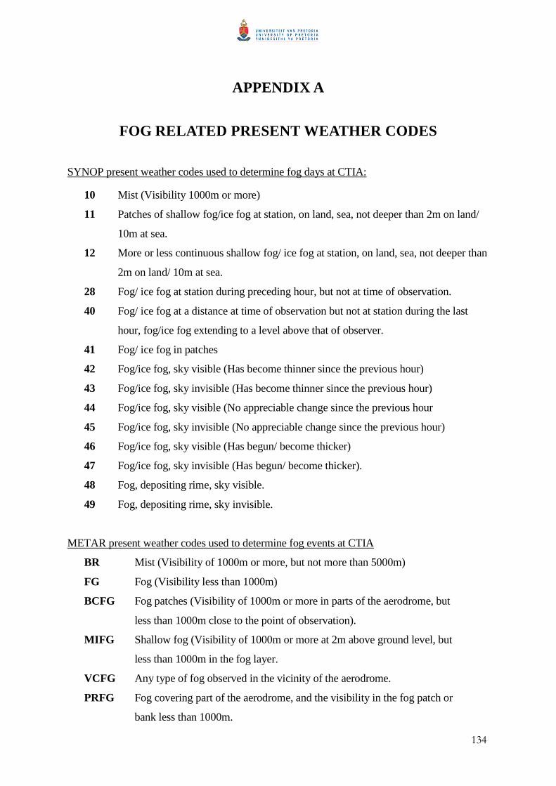
134

APPENDIX A

FOG RELATED PRESENT WEATHER CODES

SYNOP present weather codes used to determine fog days at CTIA:

10 Mist (Visibility 1000m or more)

11 Patches of shallow fog/ice fog at station, on land, sea, not deeper than 2m on land/

10m at sea.

12 More or less continuous shallow fog/ ice fog at station, on land, sea, not deeper than

2m on land/ 10m at sea.

28 Fog/ ice fog at station during preceding hour, but not at time of observation.

40 Fog/ ice fog at a distance at time of observation but not at station during the last

hour, fog/ice fog extending to a level above that of observer.

41 Fog/ ice fog in patches

42 Fog/ice fog, sky visible (Has become thinner since the previous hour)

43 Fog/ice fog, sky invisible (Has become thinner since the previous hour)

44 Fog/ice fog, sky visible (No appreciable change since the previous hour

45 Fog/ice fog, sky invisible (No appreciable change since the previous hour)

46 Fog/ice fog, sky visible (Has begun/ become thicker)

47 Fog/ice fog, sky invisible (Has begun/ become thicker).

48 Fog, depositing rime, sky visible.

49 Fog, depositing rime, sky invisible.

METAR present weather codes used to determine fog events at CTIA

BR Mist (Visibility of 1000m or more, but not more than 5000m)

FG Fog (Visibility less than 1000m)

BCFG Fog patches (Visibility of 1000m or more in parts of the aerodrome, but

less than 1000m close to the point of observation).

MIFG Shallow fog (Visibility of 1000m or more at 2m above ground level, but

less than 1000m in the fog layer.

VCFG Any type of fog observed in the vicinity of the aerodrome.

PRFG Fog covering part of the aerodrome, and the visibility in the fog patch or

bank less than 1000m.

Documents

Fog forecasting at Cape Town International Airport: A climatological