Embed Size (px)
Citation preview
NO9800029
NEI-NO--890
VELAUTHAPILLAI DHAYALAN
FOCUSING OFELECTROMAGNETIC WAVES
DEPARTMENT OF PHYSICSUNIVERSITY OF BERGENNORWAY1996
i l
FOCUSING OF ELECTROMAGNETICWAVES
Thesis submitted for the degree ofDoctor Scientiarum
by
VELAUTHAPILLAI DHAYALAN
Department of PhysicsUniversity of Bergen
Norway
1996
Velauthapillai DhayalanDepartment of PhysicsUniversity of BergenAllegt. 55, N-5007 BergenNorway
Thesis submitted for the degree of Doctor Scientiarum.May 1996
ISBN 82-993933-0-2
Front cover:Time-averaged electric energy density in the focal plane for a convergingelectric-dipole wave (Kirchhoff solution). Fresnel number N — 10 and f—number —0.5.

TO APPA, AMMA, SIVANANTHY, DHANUSHAN AND MAURAN
Preface and Acknowledgement
The thesis consists of one published article and four articles submitted orto be submitted for publishing. The five articles are presented in chapters2-6. Chapters 2-4 deal with focusing of electromagnetic waves in a singlemedium, and chapters 5 and 6 deal with focusing in a layered medium.
The following chapters have appeared or will appear elsewhere:Chapter 2: Pure Appl. Opt. 5, 195-226 (1996)Chapter 3: Pure Appl. Opt., submittedChapter 4: Pure Appl. Opt., submittedChapter 5: J. Opt. Soc. Am. A, submittedChapter 6: To be submitted
Parts of the work covered by these papers are presented or will be presentedat three conferences:Norwegian Electro-Optics Meeting, Norway (1995)Workshop on Diffractive Optics, Prague, Czech Republic (1995)Annual meeting of the Opt. Soc. Am., New York, USA (1996)
Now I want to express my sincere gratitude to number of special persons.First of all, I will characterize myself as the luckiest person on earth tohave Prof. Jakob J. Stamnes as supervisor. He has been there to helpme and guide me whenever I needed his advice. The encouragement andinspiration he rendered me during this study is impossible to express inwords. His comments, revisions and suggestions have been very valuable forthe completion of the thesis. I thank him very much from the bottom of myheart.
This work is carried out at the Department of Physics, University of Bergenunder a grant given by the Research Council of Norway for which I will beallways thankful. All the support and encouragement from my collegues andstaff at the Physics institute of University of Bergen is greatly appreciated.I would like to thank especially my friends in the optics group for all thekind assistance and encouragement.
I thank sincerely for the blessings, support and encouragement from myparents, my wife's parents, brothers, sisters, in-laws and all the relativesand friends. I would like to thank especially my dear wife Sivananthy andmy wonderful children Dhanushan and Mauran for their understanding andtolerance during the course of this study. Finally, but most importantly, Ithank the allmighty god for helping me to complete this thesis.
Bergen, May 1996
Velauthapillai Dhayalan
Contents
Introduction 11.1 Background 11.2 Summary 3
Focusing of electric-dipole waves 91 Introduction 102 Diffraction through an aperture in a plane screen 12
2.1 Exact solution of boundary-value problem 122.2 Kirchhoff solution of diffraction problem 14
3 Focusing through an aperture in a plane screen 163.1 Debye approximation of the focused field 173.2 Kirchhoff approximation of the focused field 18
4 Focusing of converging electric-dipole wave 194.1 Specification of incident field 194.2 Debye approximation of converging electric-dipole wave 204.3 Kirchhoff approximation of converging electric-dipole
wave 235 Comparison with Debye theory for rotationally symmetric op-
tical systems 255.1 Analytical comparisons 265.2 Numerical comparisons 29
6 Concluding remarks 38
Focusing of mixed-dipole waves 413.1 Introduction 423.2 Radiation from a magnetic source 43
3.2.1 Angular-spectrum representations 453.2.2 Field from a magnetic dipole 47
3.3 Focusing of converging electromagnetic waves 483.3.1 Focusing through an aperture in a plane screen . . . . 493.3.2 Focusing of converging magnetic-dipole waves 52
3.4 Focusing of converging mixed-dipole wa ve in the Debye ap-proximation 593.4.1 Polarization vector, strength factor, and energy pro-
jection 603.4.2 Energy densities 64
3.5 Numerical Results 683.5.1 Energy densities 683.5.2 Poynting vector or direction of e nergy flow 723.5.3 Cross polarization 76
3.6 Summary and Conclusions 783.7 Aknowledgments 79
4 Focusing of electric-dipole waves in the Debye and Kirchhoffapproximations 834.1 Introduction 844.2 Evaluation of the angular spectrum in the aperture plane . . 85
4.2.1 Angular spectrum in the Kirchhoff approximation . . 854.2.2 Angular spectrum in the Debye app roximation . . . . 864.2.3 Asymptotic evaluation of the angu lar spectrum in the
Kirchhoff approximation 874.2.4 Numerical evaluation of the angul ar spectrum . . . . 89
4.3 Focusing of electric-dipole waves 924.3.1 Focusing of electric-dipole waves in Debye approxima-
tion 934.3.2 Focusing of electric-dipole waves in Kirchhoff approx-
imation 944.3.3 Numerical results 95
4.4 Aknowledgments 95
5 REFLECTION AND REFRACTION OF AN ARBITRARYELECTROMAGNETIC WAVE IN A LAYERED MEDIUM 1095.1 Introduction 1105.2 The one-layer medium I l l
5.2.1 TE and TM plane-wave represen tations I l l5.2.2 Whittaker potentials 1135.2.3 Solutions for spectral-domain pot entials 1145.2.4 Exact solutions for reflected, tr ansmitted, and slab
fields 1185.3 Matrix theory for a multilayered mediu m 122
5.3.1 Scalar theory 1235.3.2 Electromagnetic theory 132
5.4 Dyadic Green's functions for layered m edium 1385.4.1 Reflected and transmitted fields 1385.4.2 Field inside the j th layer 139
5.5 Summary and Conclusions 1425.6 Aknowledgments 143
A Spectral-domain dyadic Green's functions for a slab 145
B Spectral-domain dyadic Green's functions for a multilayeredmedium 147
in
C Comparison between slab and the multilayered system re-duced to a one-layer system 149
6 Focusing of electromagnetic waves insidea dielectric slab 1536.1 Introduction 1546.2 Problem Definition 155
6.2.1 Exact solutions for reflected, transmitted fields andslab fields 156
6.2.2 Fields inside a slab 1596.3 Focusing of electromagnetic waves inside a slab 1606.4 Numerical Techniques 163
6.4.1 Reduction from double integral to single integral . . . 1636.4.2 Dividing the integration area 1656.4.1 Integration Algorithms 168
6.5 Asymptotic evaluation 1716.6 Comparison between exact and asymptotic solutions 173
6.6.1 Analytical comparison 1736.6.2 Numerical comparisons 176
6.7 Numerical Results 1856.8 Conclusion 1946.9 Aknowledgments 194
D Transmission and reflection coefficients 195
IV
Chapter 1
Introduction
1.1 Background
The first time diffraction phenomena ever were mentioned, was as early as in the 15thcentury. But the real understanding of diffraction phenomena, which are a consequence ofthe wave character of light, came after the work of Grimaldi 150 years later. He was thefirst to mention that light has wave characteristics. Without knowing Grimaldi's work,Huygens proposed a new wave theory, nowadays referred to as Huygens's principle, sug-gesting that every point on a wave front has to be regarded as the center of a secondarywave front which forms at a later instant an envelope of secondary wavefronts. Fresnel(1818) contributed his part to the so called 'Huygens-Fresnel principle' by accounting forthe interference between the secondary wave fronts.
The earliest theoretical studies of the diffraction theory of imaging have to be attributedto the work of Airy (1835). He established that the intensity distribution in the focalplane due to an aberration-free wave front from a circular aperture would have the form of[Ji(v)/v]2, where J\(v) is the first order Bessel function. Lommel (1885) presented boththeoretical and experimental work, thus extending Airy's treatment to account for theintensities at all points in the viscinity of the focus. In 1909 Debye established the generalfeatures of the diffracted field near and far away from the focus [1], and the assumptionson which his work was based, are now commonly referred to as the Debye approximation.
The classical theory of imaging, which the optical community has relied on for manyyears, depends on three approximations [2]: the assumption of a scalar field, the parax-ial approximation, and the Debye approximation. But owing to Maxwell's work on theelectromagnetic theory (1873), it is well known that visible light is merely one form of elec-tromagnetic energy, usually described as electromagnetic waves. The complete spectrum ofelectromagnetic waves extend from radio waves to Gamma radiation. The classical scalartheory of imaging which neglects polarization effects can be applicable only to systems ofmoderate angular apertures. The second and third approximations mentioned above forthe classical theory to be valid, cannot be fulfilled at the same time. The paraxial approx-imation is poor for large apertures, while the Debye approximation is best at large Fresnelnumbers N defined by N = a2f\zi. Here a is the aperture radius, A is the wavelength,and zi is the distance between the aperture and the focal point. The range of validityof the classical theory is thus restricted. Although the vector treatment is complicatedcompared to the scalar treatement one must employ it to obtain a proper description ofthe polarization and the energy flow in the focal region.
Focusing of electromagnetic waves has been of interest in the optical community ever sincethe appearence of first papers published in this area by Ignatowsky [3, 4] in 1919 and 1920.Ignatowsky obtained expressions for the electric and magnetic fields in the image regionof a paraboloid and also of a rotationally symmetric aplanatic optical system based on theDebye approximation. In 1943 and 1945 Hopkins [5, 6] investigated the intensity distribu-tion in the focal plane of a rotationally symmetric optical system by increasing its angularaperture.
A breakthrough in the theoretical development of the vector diffraction theory of focus-ing came in 1959 with the papers of Wolf [7] and Richards and Wolf [8]. The treatmentof Richards and Wolf [8] was based on the Debye approximation. Within this approxi-mation, they formulated a theory for electromagnetic diffraction in optical systems withspecial emphasis on rotationally symmetric, aplanatic systems. Their numerical resultsalong with the numerical results of Boivin and Wolf [9] and of Boivin et al [10] providedextensive information about the electromagnetic field in the image space of a rotationallysymmetric, aplanatic system. Since then many papers have appeared based on the anal-ysis of Richards and Wolf [8], treating topics as annular apertures [11], lens and mirrorsystems [12], high-aperture optical systems [13], computational aspects [14], and aberra-tions [15, 16].
Diffraction problems are amongst the most difficult ones encountered in classical optics.Since rigorous solutions rarely can be obtained, approximative theories are employed.There are two approximations that are frequently used in studies of focusing problems,namely the Kirchhoff and the Debye approximation. In the Kirchhoff approximation, oneassumes that the field inside the aperture is equal to the unpertubed incident field andthat it vanishes outside the aperture. In the Debye approximation, one assumes that theangular spectrum of the incident field is nonzero only for directions inside the cone that isformed by drawing straight lines from the edges of the aperture to the focal point. Out-side this cone the angular spectrum is assumed to vanish. The Kirchhoff and the Debyeassumptions are not equivalent. They lead to different results for the focused field. Whencomparing these two assumptions in the scalar case, one finds that the Debye approxima-tion is valid only for systems with high Fresnel numbers [17, 18]. But in some cases, theDebye approximation can provide a reduction from a double integral to a single integraland thus to give a considerable reduction in computing time[19].
All papers mentioned above were based on the electromagnetic Debye theory of focus-ing, which, as mentioned above, is valid only at high Fresnel numbers. In contrast,Mansuripur [20, 21] used a vectorial Kirchhoff diffraction theory and presented results forthe distribution of light at and near the focus of a high-aperture objective of NA = 0.3.Here the numerical aperture NA is defined as NA = sin a/2, where a is the angle sub-tended by the exit pupil at the focal point. Recently, Visser and Wiersma [22, 23, 24]employed a vectorial Kirchhoff theory based on the formulation by Stratton and Chu[25] to study the effects of aberrations on electromagnetic fields in both low- and high-aperture systems. Comparisons between results obtained in the Kirchhoff and the Debyeapproximation were first made by Stamnes [17] for two-dimensional waves, and similarcomparisons for the three-dimensional vector case are presented in chapter 4 of this work.
Along with the rapid improvements in computer technology, new, efficient numerical meth-ods for evaluating diffraction integrals have been presented in recent years. Stamnes,Spjelkavik, and Pedersen [26, 2] developed a numerical method for evaluating diffrac-
tion integrals whose integrands appear in the form of a product of an amplitude functionand an exponential function containing a purely imaginary phase function. To obtainan efficient numerical algorithm, they applied different parabolic approximations to thephase and amplitude functions. Mansuripur [20] developed a factorization technique andbased his computations of diffraction integrals on the Fast-Fourier-Transform for algoritm.Kant [14, 15, 16] published another simple and accurate method for numerical evaluationof the diffraction integrals associated with the electromagnetic theory of focusing withinthe Debye approximation. Recently his method has also been implemented by Torok etal [27, 28, 29].
The improvements in computer technology also have led to the study of more complicateddiffraction problems. In 1976 Gasper et al [30] derived exact and asymptotic approxima-tions for the reflected and the refracted fields obtained when an arbitrary electromagneticwave is incident at a plane interface. In 1984 Ling and Lee [31] considered for the firsttime focusing of electromagnetic waves through an interface. While Ling and Lee basedtheir study on a vectorial KirchhofF theory of focusing, Torok et al [27, 28, 29] used theelectromagnetic Debye theory to study focusing of electromagnetic waves through a pla-nar interface between materials of mismatched refractive indices. As mentioned above, theDebye approximation is valid only for systems with high Fresnel numbers.
1.2 Summary
As the use of focusing techniques in biological studies and material sciences is increasing,new interesting and important aspects of focusing of electromagnetic waves emerge. Theobjective of this thesis is six-fold. First it is to develop a theoretical basis for diffractionof electromagnetic waves through a plane aperture in both the KirchhofF and the Debyeapproximation. Second it is to adapt this theoretical basis to consider new aspects of fo-cusing of electromagnetic waves, such as focusing of electric- and mixed-dipole waves, andto find the best choice of energy and polarization distribution over the converging wavefront to obtain the best energy concentration in and around the focus. The third objectiveis to define criteria which can be used to determine when to employ the Kirchhoff andDebye approximations in the electromagnetic analysis of focusing problems. The fourthobjective is to develop a new theoretical basis to obtain exact and explicit solutions forthe reflected and transmitted fields, and for the fields inside the layers, when an arbitraryelectromagnetic wave is incident on a multilayered medium with parallell interfaces. Thefifth objective is to use this theoretical basis to provide exact results for special cases ofthe multilayered medium. The sixth objective is to develop computational methods andprograms that can be applied to evaluate complicated diffraction integrals.
The organization of the thesis is as follows: In chapter 2 the theoretical basis for thediffraction of electromagnetic waves through an aperture in a plane screen is thoroughlydiscussed with special emphasis on the focusing properties of converging electric-dipolewaves. A converging electric-dipole wave is defined as the complex conjugate of the di-verging wave radiated by a linearly polarized electric dipole. Explicit results for the field,due to an incident converging electric-dipole wave, in the focal region are given both withinthe Debye and the Kirchhoff approximation. The results for a focused electric-dipole waveobtained within the Debye approximation are compared with the corresponding resultspresented by Richards and Wolf [8] for the field obtained when focusing a linearly polar-ized plane wave by a rotationally symmetric, aplanatic system. Our results show that at
high angular apertures, the converging electric-dipole wave has better energy concentra-tion and less cross-polarization both in the focal plane and along the optical axis.
The motivation for considering the focusing properties of a converging mixed-dipole wavecomes from the desire to search for that amplitude and polarization distribution in theaperture plane which would give the best energy concentration in the focal plane. Shep-pard and Larkins [32] noted that the electromagnetic analog to the so-called 'perfect scalarwave' defined by Stamnes [17, 33, 34] would be the mixed-dipole wave generated by thesum of an electric and an othogonal magnetic dipole. It is not clear how Sheppard andLarkins [32] arrived at this conclusion. Therefore, in chapter 3, we consider the focusing ofa converging mixed-dipole wave. First we derive the radiated field from a magnetic dipole.Then we define a mixed-dipole wave as the sum of a converging electric-dipole wave and aconverging magnetic-dipole wave due to a magnetic dipole which is clockwise-orthogonal tothe electric dipole and has a strength equal to i/w times the strength of the electric dipole.This particular relative strength and orientation of the two dipoles make the mixed-dipolewave have the same polarization over the converging wavefront in the image region as thatobtained when a plane wave, polarized in the direction of the electric dipole, is focused bya rotationally symmetric system. The results of chapter 2 is used in chapter 3 to obtainthe contribution from the electric-dipole wave to the mixed-dipole wave. Within the Debyeapproximation we present analytical and numerical comparisons of the results for a con-verging mixed-dipole wave with corresponding results for a converging electric-dipole waveand also with the results obtained using a rotationally symmetric, aplanatic system. Ourcomparisons of these three types of waves show that the converging electric-dipole wavehas best electric energy concentration and least cross-polarization both in the focal planeand along the optical axis. These facts make it the natural choice as the electromagneticanalog of the 'perfect wave' in the scalar case.
In chapter 4 we compare the Kirchhoff and Debye approximations for the electromagneticcase and determine the conditions under which the Debye approximation is valid. To thatend, we use the results from chapter 2 for the focusing of electric-dipole waves and analyseboth the angular spectrum in the aperture plane and the field around the focus. Ourcomparisons show that for systems with Fresnel numbers higher than 20 and f-numberslower than 0.5, the two approximations give identical results. Here the f-number is definedby z\/2a, where z\ is the distance between the aperture and the focus and a is the radiusof the aperture. As in the scalar case [35, 36, 37], we find that the Debye approximationdoes not account for expected asymmetries and focal-shift phenomena, which are com-mon features in systems with low Fresnel numbers. When comparing the influence of theFresnel number and the f-number on the focal-shift phenomena, we find that focal-shift ismainly dependent on the Fresnel number. But at low Fresnel numbers, we find that thelower the f-number, the higher the ralative focal shift.
In chapters 5 and 6, we consider a different aspect of the focusing of electromagneticwaves, namely focusing inside a layered medium with plane parallel! interfaces. This kindof application is of interest in the modelling of microstrip antennas [38, 39, 40, 41], in hy-perthermia [31, 42], in optical data storage [20], and also in the probing of the subsurfaceof the earth with electromagnetic waves [43]. General descriptions of how one can proceedto solve the multilayer problem are given in [44] and [45], but the procedures and theresults are rather complicated. By using TE and TM plane-wave expansions, we generalizethe matrix formalism used to solve the problem for a single incident plane wave of the TEor TM type so as to obtain exact, explicit solutions for the fields inside each layer and forthe transmitted and reflected fields in terms of the given field or source outside the layers.
Also, explicit expressions for each of the spectral domain dyadic Green's functions aregiven. As a check, we consider the special case in which the multilayered medium reducesto a slab and show that the results obtained by the matrix formalism correctly reducesto those derived by a completely different method. Compared to earlier approaches, oursis much easier to follow, and the results are given explicitly in terms of the field or thesource outside the layers.
In chapter 6 we consider the special case in which the multilayered medium reduces toa slab and apply the results from chapter 5 to analyse the focusing of electromagneticwaves inside a slab. We provide both asymptotic and exact results for the focused fieldsinside the slab and also for the two special cases in which the slab problem reduces to asingle -interface problem or a single medium problem. The numerical approach to calcu-late the exact, focused field inside a slab is very time consuming. First one must carryout a spectral double integration to obtain the contribution due to one particular pointsource in the aperture, and then do a double integration over the aperture plane to obtainthe focused field. The computing time is reduced considerably by expressing the impulseresponse of the problem (i.e. the field produced inside the slab by a point source in theaperture) as a plane-wave expansion and evaluating the corresponding (kx, ky) integral bythe method of stationary phase. We refer to this as the asymptotic method in chapter 6.The asymptotic solution becomes invalid at observation points near the aperture or nearthe interfaces or when the observation angle is near the critical angle. Also, in the case ofa slab, we show that the plane-wave transmission coefficient contains a number of poles,the actual number being proportional to the thickness of the slab. This means that onemust consider the contributions from the associated surface waves. Since the asymptoticsolution described above, does not contain such pole contributions, branch point contri-butions, or contributions from evanascent waves, its validity is questionable under thesecircumstances.
In chapter 6 we also discuss the numerical methods used to compute the exact solutions forthe cases in which the multilayered-medium problem reduces to either a slab-problem ora single-interface problem or a single medium-problem. Our comparisons between asymp-totic and exact solutions show that the difference is small in a single medium, while itcan be considerable in the case of a single interface or a slab. With some modifications,the numerical methods employed in this chapter can be used for determining the fieldsradiated by a microstrip antenna.
The main difficulty in analysing the focusing of electromagnetic waves lies in the adap-tation of suitable computing methods. Even with today's fast computers, evaluating thediffraction integrals is time consuming. In the process of this thesis, much time has beendevoted to develop numerical tools and computer programs which reduce the computingtime considerably. We have utilized both one- and two-dimensional SSP methods [26, 2]along with the Gauss-Legendre [46] method in evaluating the diffractional integrals.
The focusing of electromagnetic waves inside a slab has also been treated by consideringthe incident field in the aperture plane to be the complex conjugate of the field radiatedby a point source located inside the slab. In this manner an optimal concentration of thefocused energy inside the slab can be obtained. However the theory and the results onthis aspect of the problem are not included in this thesis. Finally, it should be mentionedthat the theory developed in chapter 4 for the reflection and transmission of an arbitraryelectromagnetic wave incident on a multilayered- medium should be extended to the casein which the source is located inside any of the layers.
Bibliography
[1] M. Born and E. Wolf. Principles of Optics. Pergamon Press, Oxford, London, andNew York, 1980.
[2] J.J. Stamnes. Waves in Focal Regions. Adam Hilger, Bristol and Boston, 1986.
[3] V.S. Ignatowsky. Trans. Opt. Inst. PetrogradI, paper IV, 1919.
[4] V. S. Ignatowsky. Trans. Opt. Inst. PetrogradI, paper V, 1920.
[5] H. H. Hopkins. Proc. Phys. Soc. 55, 116, 1943.
[6] H. H. Hopkins. Nature, Lond. 155, 277, 1945.
[7] E. Wolf. Electromagnetic diffractions in optical systems I. An integral representationof the image field. Proc. R. Soc. A 253, 349-357, 1959.
[8] B. Richards and E. Wolf. Electromagnetic diffraction in optical systems II. Structureof the image field in an aplanatic system. Proc. R. Soc. A 253,358-379, 1959.
[9] A. Boivin and E. Wolf. Electromagnetic field in the neighborhood of the focus of acoherent beam. Phys. Rev. 1385, 1561-1565, 1965.
[10] A. Boivin, J. Dow, and E. Wolf. Energy flow in the neighborhood of the focus of acoherent beam. J. Opt. Soc. Am. A 57B, 1171-1175, 1967.
[11] A. Yoshida and T. Asakura. Electromagnetic field in the focal plane of a coherentbeam from a wide-angular annular-aperture system. Optik 40, 322-331, 1974.
[12] C. J. R. Sheppard. Electromagnetic field in the focal region of wide-angular annularlens and mirror systems. J. Microwaves, Optics and Acoustics 2, 163-166, 1978.
[13] C. J. R. Sheppard and H. J. Matthews. Imaging in high-aperture optical systems. J.Opt. Soc. Am. 4, 1354-1360, 1987.
[14] R. Kant. An analytical solution of vector diffraction problems for focusing opticalsystems. J. Mod. Opt. 40, 337-347, 1993.
[15] R. Kant. An analytical solution of vector diffraction for focusing optical systems withSeidel aberrations I. Spherical aberration, curvature of field, and distortion. J. Mod.Opt. 40, 2293-2310, 1993.
[16] R. Kant. An analytical solution of vector diffraction for focusing optical systems withSeidel aberrations. II. Astigmatism and coma. J. Mod. Opt. 42, 299-320, 1995.
[17] J. J. Stamnes. Focusing of two-dimensional waves. J. Opt. Soc. Am. 71 , 15-31, 1981.
[18] E. Wolf and Y.Li. Conditions for the validity of the Debye integral representation offocused fields. Opt. Commun. 39, 205-210, 1981.
[19] J.J. Stamnes and V. Dhayalan. Focusing of electric-dipole waves. J. Pure and AppliedOpt. 5, 195-226, 1996.
[20] M. Mansuripur. Certain computational aspects of vector diffraction problems. J. Opt.Soc. Am. A 6, 786-805, 1989.
[21] M. Mansuripur. Distribution of light at and near the focus of high-numerical-apertureobjectives. J. Opt. Soc. Am. A 3, 2086-2093, 1995.
[22] T. D. Visser and S. H. Wiersma. Spherical aberration and the electromagnetic fieldin high aperture systems. J. Opt. Soc. Am. A 8, 1404-1410, 1991.
[23] T. D. Visser and S. H. Wiersma. Diffraction of converging electromagnetic waves. J.Opt. Soc. Am. A 9, 2034-2047, 1992.
[24] T. D. Visser and S. H. Wiersma. Electromagnetic description of the image formationin confocal fluorescence microscopy. J. Opt. Soc. Am. A 11, 599-608, 1994.
[25] J. A. Stratton and L. J. Chu. Diffraction theory of converging electromagnetic waves.Phys. Rev., 56 B 99-107, 1939.
[26] J. J. Stamnes, B. Spjelkavik, and H. M. Pedersen. Evaluation of diffraction integralsusing local phase and amplitude approximations. Optica Ada 30, 207-222, 1983.
[27] P. Torok, P. Varga, Z. Laczic, and G. R. Booker. Electromagnetic diffraction of lightfocused through a planar interface between materials of mismatched refractive indices:an integral reperesentation. J. Opt. Soc. Am. A 12, 325-332, 1995.
[28] P. Torok, P. Varga, and G. R. Booker. Electromagnetic diffraction of light focusedthrough a planar interface between materials of mismatched refractive indices: struc-ture of the electromagnetic field. I. J. Opt. Soc. Am. A 12, 2136-2144, 1995.
[29] P. Torok, P. Varga, and G. Nemeth. Analytical solution of the diffraction integralsand interpretation of wave-front distortion when light is focused through a planarinterface between materials of mismatched refractive indices. J. Opt. Soc. Am. A 12,2660-2671, 1995.
[30] J. Gasper, G. C. Sherman, and J. J. Stamnes. Reflection and refraction of an arbitraryelectromagnetic wave at a plane interface. J. Opt. Soc. Am. 66, 955-61, 1976.
[31] H. Ling and S.W. Lee. Focusing of electromagnetic waves through a dielectric inter-face. J. Opt. Soc. Am. A 1,965-973, 1984.
[32] C. J. R. Sheppard and K. G. Larkin. Optimal concentration of electromagnetic radi-ation. J. Mod. Opt. 41, 1495-1505, 1994.
[33] J. J. Stamnes. Focusing of a perfect wave and the Airy pattern formula. Opt. Commun.37, 311-14, 1981.
[34] J. J. Stamnes. The Luneburg apodization problem in the nonparaxial domain. Opt.Commun. 38, 325-29, 1981.
[35] Y. Li. Dependence of the focal shift on Fresnel number and f-number. J. Opt. Soc.Am. A 72, 770-4, 1982.
[36] Y. Li and E. Wolf. Three-dimensional intensity distribution near the focus in systemsof different Fresnel numbers. J. Opt. Soc. Am. A 1, 801-8, 1984.
[37] Y. Li and E. Wolf. Focal shifts in diffracted converging spherical waves. Opt. Commun.39, 211-215, 1981.
[38] David M. Pozar. A reciprocity method of analysis for printed slot and slot-coupledmicrostrip antennas. IEEE Trans. Antennas Propagat. 34, 1439-46, 1986.
[39] J. R. Mosig and F. E. Gardiol. A dynamical radiation model for microstrip structures.Advances in Electronics and Electron Physics, 59 139-237, 1982.
[40] J. R. James and P. S. Hall. Handbook of Microstrip Antennas, volume 1 and 2. PeterPeregrinus Ltd, London, United Kingdom, 1989.
[41] B. A. Brynjarsson. A study of printed antennas in layered dielectric media. Dr.ing.Thesis, Norwegian Institute of Technology, 1994.
[42] H. Ling, S.W. Lee, and W. Gee. Frequency optimization of focused microwave hy-perthermia applications. Proc. IEEE 72, 224-225, 1984.
[43] J.R. Wait. Electromagnetic waves in Stratified media. Pergamon Press, Oxford, NewYork, Toronto, Sydney and Braunschweig, 1970.
[44] L. B. Felsen and N. Marcuvitz. Radiation and Scattering of Waves. Prentice-HallInternational, Inc., London, 1973.
[45] V. W. Hansen. Numerical Solution of Antennas in Layered Media. John Wiley &Sons, New York, Chichester, Brisbane, Toronto and Singapore, 1989.
[46] M. Abramowitz and LA. Stegun. Handbook of Mathematical Functions,. Dover, NewYork, 5th edition, 1968.
Chapter 2
FOCUSING OF ELECTRIC-DIPOLE WAVES
Chapter 2
Focusing of electric-dipole waves
Jakob J. Stamnes and Velauthapillai Dhayalan
Physics DepartmentUniversity of Bergen, Allegt. 55
N-5007 Bergen, Norway
Published in
Journal of Pure and Applied Optics
Vol. 5 1996, Page 195-225
Pure Appl. Opt. 5 (1996) 195-225. Printed in the UK
Focusing of electric-dipole waves
J J Stamnes and V Dhayalan
Physics Department, University of Bergen, Norway
Received 29 May 1995, in final form 25 September 1995
Abstract. Diffraction of electromagnetic waves through an aperture in a plane screen isdiscussed with particular emphasis on the focusing properties of a converging electric-dipolewave. Explicit results for the field in the focal region are given both within the Debye andthe Kirchhoff approximations. Within the Debye approximation, the results for a focusedelectric-dipole wave are compared analytically and numerically with those obtained earlier forthe focusing of a linearly polarized plane wave by a rotationally symmetric, aplanatic system.It is shown that at high angular apertures, the converging electric-dipole wave has better energyconcentration and less cross-polarization, both in the focal plane and along the optical axis.
1. Introduction
Focusing of electromagnetic waves was first treated by Ignatowsky in 1919, who derivedformulae for the electric and magnetic field vectors in the image region of a rotationallysymmetric, aplanatic system [1] and also of a paraboloid [2]. Forty years later, Richards andWolf [3] rederived the formulae of Ignatowsky for an aplanatic system [1] and employedthem to make important deductions about the polarization, the energy density, and theenergy flow in the focal region. Further numerical results for aplanatic systems were givenby Boivin and Wolf [4] and Boivin et al [5], and energy projections different from theaplanatic one were considered by Innes and Bloom [6]. In recent years, various extensionsof the work in [3] have been reported, such as annular apertures [7], computational aspects[8,9], lens and mirror systems [10], and Seidel aberrations [11,12].
All works mentioned above were based on the electromagnetic Debye theory of focusing[13, sections 15.4.2 and 16.1], which is known to be valid only at high Fresnel numbersTV = a1/kz\, where a is the aperture radius, k is the wavelength, and z\ is the distancefrom the aperture to the geometrical focal plane. In contrast, Visser and Wiersma [14-16] employed an electromagnetic Kirchhoff theory, based on the formulation by Strattonand Chu [17], and obtained the expected asymmetry about the focal plane at low Fresnelnumbers. Another aspect of electromagnetic focusing was considered by Ling and Lee[18], who treated the case in which the aperture and the focal point were in two differentdielectric media. They also based their treatment on a Kirchhoff or physical-optics type ofapproximation and used asymptotic approximations to reduce the computing time.
In this paper, we consider the case in which the aperture and the focal point are inthe same medium. Then, as noted above, the Debye theory is valid provided the Fresnelnumber is sufficiently large. If the Fresnel number is not sufficiently large, one must applythe Kirchhoff theory, which is always superior to the Debye theory. Thus, the questionmay be asked: why use the Debye theory at all? One reason one would like to use theDebye theory, whenever it is applicable, is that it sometimes may give simple formulae
0963-9659/96/020195+3l$19.50 © 1996 IOP Publishing Ltd 195
196 J J Stamnes and V Dhayalan
for the focused field that could not be obtained in the Kirchhoff approximation. In othercases it may provide a reduction from a double integral to a single integral and thus givea significant reduction in the computing time. Also, as noted above, many of the earlierresults obtained for focusing of electromagnetic waves were based on the Debye theory. Inorder to enable us to make a meaningful comparison with these earlier results, we must usethe same approximation. Finally, it should be noted that in many practical applications theFresnel number is indeed sufficiently large for the Debye theory to be valid.
Assume now that the Fresnel number is sufficiently large for the Debye theory to bevalid. Then, as shown by Stamnes [19-21], for the focusing of scalar waves, the best energyconcentration in the focal plane is obtained when the amplitude distribution in the apertureplane corresponds to that of a so-called 'perfect' wave. In the electromagnetic case, notonly the amplitude distribution of the field in the aperture plane is important, but also itspolarization. Both will influence the properties of the focused field. Richards and Wolf[3] considered an amplitude and polarization distribution over the converging wavefrontcorresponding to that which would be obtained by focusing of a linearly polarized wave bya rotationally symmetric, aplanatic optical system. In this paper, we discuss diffraction ofelectromagnetic waves through an aperture in a plane screen with particular emphasis onthe focusing properties of a converging electric-dipole wave, which is given as the complexconjugate of the diverging wave radiated by a linearly polarized electric dipole.
According to Shepphard and Larkin [22], a mixed-dipole wave, generated by the sumof an electric and an orthogonal magnetic dipole, can be considered the electromagneticanalogue of the 'perfect' wave of Stamnes [19-21], which, as noted above, was constructedto give the best possible energy concentration in the focal plane in the scalar case. Herewe consider a converging electric-dipole wave, and within the Debye approximation, wecompare the focusing properties of this wave with those of the focused wave consideredby Richards and Wolf [3]. We show that at high angular apertures, the converging electric-dipole wave has better energy concentration and less cross-polarization, both in the focalplane and along the optical axis. In a forthcoming paper, we will return to the focusingproperties of the mixed-dipole wave.
The organization of the paper is as follows. In section 2.1, we start by consideringthe diffraction of an arbitrary electromagnetic wave through an aperture in a plane screen.First, we present an exact solution to the electromagnetic boundary value problem in whichthe tangential components of the electric field are known across a plane surface. Theseexact solutions are given both as plane-wave or angular-spectrum representations and asequivalent spherical-wave or impulse-response representations. In section 2.2, we discussan approximate solution, based on the Kirchhoff or physical-optics approximation, to thecorresponding diffraction problem in which an electromagnetic wave is incident on anaperture in a plane screen.
In section 3, we use the results in section 2.2 to analyse focusing of electromagneticwaves through an aperture in a plane screen, and we discuss the difference between theKirchhoff and the Debye approximation. We start section 4 by introducing the concept of aconverging electric-dipole wave and derive explicit expressions for the focused field in theDebye and Kirchhoff approximations when such a wave is diffracted through an aperture.As mentioned above, the Debye theory is valid only at high Fresnel numbers, while theKirchhoff theory is valid irrespective of the size of the Fresnel number.
In section 5, we present analytical and numerical comparisons of the results for a focusedelectric-dipole wave within the Debye approximation with corresponding results obtained byRichards and Wolf [3] for the focusing of a linearly polarized plane wave by a rotationallysymmetric, aplanatic system. Finally, in section 6, we summarize the results of the paper.
Focusing of electric-dipole waves 197
2. Diffraction through an aperture in a plane screen
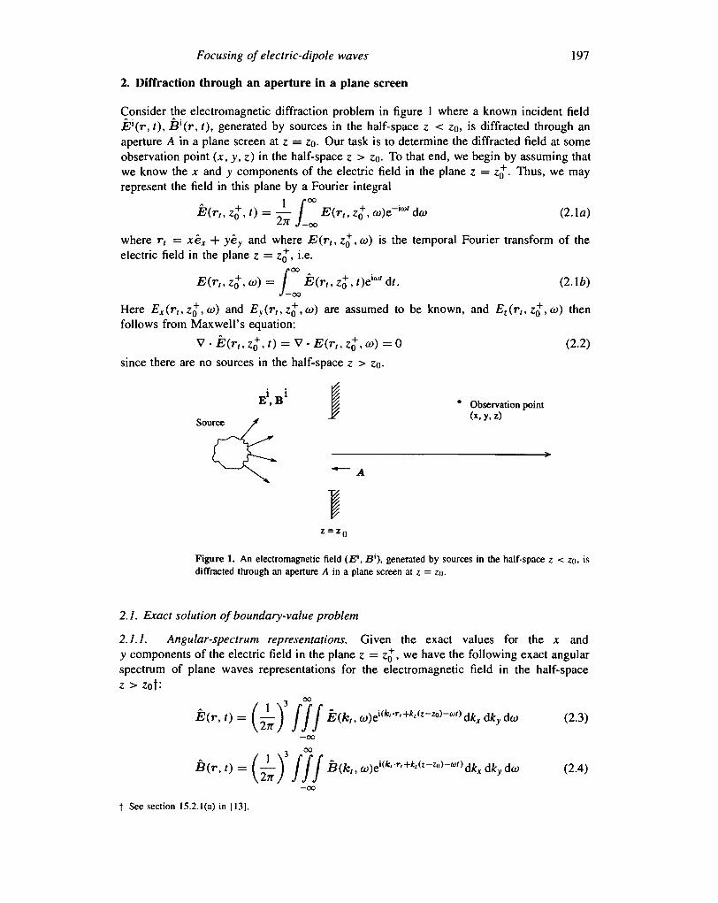
Consider the electromagnetic diffraction problem in figure 1 where a known incident fieldE'(r,t), B\r,t), generated by sources in the half-space z < Zo» is diffracted through anaperture A in a plane screen at z = Zo- Our task is to determine the diffracted field at someobservation point (x, y, z) in the half-space z > Zo- To that end, we begin by assuming thatwe know the x and y components of the electric field in the plane z = z$. Thus, we mayrepresent the field in this plane by a Fourier integral
E(r,, z0+, t) = ±- f E(r,, z+, W)c~ia" dco (2.1a)
2?r ywhere r, = xex + yey and where E(r,, ZQ,CO) is the temporal Fourier transform of theelectric field in the plane z = ZQ, i.e.
/•OO
E(rt, z+, co) = / E(r,, z+, t)elu" dr. (2.1b)J
Here Ex(r,, ZQ,CO) and Ey(r,, ZQ,OO) are assumed to be known, and Ez(r,, ZQ,CO) thenfollows from Maxwell's equation:
V • E(rt, z+, t) = V • E(r,, z+, a>) = 0 (2.2)
since there are no sources in the half-space z > Zo-
Source
p iR i P*!''a V> * Observation point
V (x, y, z)
= z f
Figure 1. An electromagnetic field (E\ Bl), generated by sources in the half-space z < zo, isdiffracted through an aperture A in a plane screen at z = zo.
2.1. Exact solution of boundary-value problem
2.1.1. Angular-spectrum representations. Given the exact values for the x andy components of the electric field in the plane z = ZQ, we have the following exact angularspectrum of plane waves representations for the electromagnetic field in the half-spacez > zot:
E(r,t) = (—) t f I ECk^co^'-r'+^-^-^dk.dkydco (2.3)\27T/ J J J
—oo
B(r, t) = (—) f [ [ B(k<, co)el(krT'+k'u-Zo)-a")dkx dky dco (2.4)\2n J J J J
—OO
t See section 15.2.I(a) in [13].
198 J J Stamnes and V Dhayalan
whereoo
Ej (k, <«>)=[[ Ej(r' • 4 ' ^)e" i f c / ' r ' djc Ay (j = x, y) (2.5)—oo
Ez(kt, to) = --kt- E(k,,co) (2.6)
B(k,,co) = -k x E(k,,co) (2.7)
fc = k, + kzez k, = kxex + kyey k2 = k\ + k) (2.8)
r = r, + zez r, = xex + yey (2.9)
kz = (k2-k?)i/2 lmkz>0 (2.10)
. (2.11)
Here co is the angular frequency, c is the velocity of light in vacuum, \i is the permeability,E{O)) is the permittivity, and a is the conductivity. Henceforth, we assume that the mediumis non-conducting, i.e. that a = 0, so that,
CO ik = -n(co); n(co) = y/fie(a>). (2.12)
c
Note that in general there is no simple relationship between the incident field (E\ B1) andthe field (E(r,, z£, a>), B(r,, z£, CO)) in the plane immediately behind the aperture. Thefield in this plane may be known either from measurements or from exact calculations thatwe do not enter into here.
If the medium between the source and the plane z = ZQ is non-dispersive, the temporalbehaviour of the field must be the same at every point in this plane, so that we may write
(2.13)
which on substitution in (2.1b) gives
E(r,, z£, co) = E(r,,z£)f(co) (2.14)
where f(t) and f(co) constitute the temporal Fourier-transform pair:
f(t) = — / f((o)e~"°' dco f(co)= I f(t)ela"dt. (2.15)* 7 T «/—oo J—oo
In this case (2.5) gives (with j = x, y)
Ej(k,, co) = Ej(k,, z£)f(a>) (2.16)
where the spectral amplitude Ej(kt, ZQ) is given byoo
£,(*„ z+) = /" f Ej(rt, z+Je"*"1' d^ dv (2.17)
—oo
and (2.3) and (2.4) take the form
1 f°°E(r, f) = — / £ ( r , to)/(o>)e-ift" dw (2.18a)
2^ J-oo1 f°°
-,0 = — / B(r,w)/(o;)e-|a"dw (2.186)2?T J - O O
Focusing of electric-dipole waves 199
where
2
E(r, co) = (^-\ f [ E(kl,z^)e'(k'-r-+k^-Zo))dkxdky (2.19a)- 00
2 °°B(r, co) = (^-\ t [ B{kt, z+)e i ( f e ' r '+^ ( z-Z o ) )^ djfc, (2.196)
with
Ez(ku z£) = —-[kxEx(kt, zj) + kyEy(k,, z+)] (2.20a)
B(k,,4) = -kx E(kt, z0). (2.20ft)CO
From now on, we shall mainly be concerned with only one temporal frequency componentof the field. To simplify the notation, we therefore often suppress the co dependence inE(r, co) and B{r, co) and simply write E(r) and B(r).
2.1.2. Impulse-response representations—Huygens' principle. In (2.19a, b), the electro-magnetic field is expressed as a superposition of plane waves. Alternatively, we may usethe convolution theorem to rewrite (2.19a) or (2.196) as a superposition of spherical wavesin accordance with Huygens' principle. Thus, suppressing the co dependence, as notedabove, we havef,
_ jj « , - , y, Zo+)_[kR
where
R = [(x- x')2 + (y- y'f + (z - zo)2]I/2- (2.21c)
2.2. Kirchhoff solution of diffraction problem
The results derived in section 2.1 are exact for an arbitrary incident field provided we haveaccurate knowledge of the field in the plane immediately behind the aperture. In practice, weoften do not know the field in this plane from measurements, and since it is quite involved toobtain exact solutions for Ex(rt, ZQ) and Ey(r,, ZQ), which appear in (2.17) and (2.21a, b),we shall use a Kirchhoff or physical-optics type of approximation:):, according to which theJC and y components of the electric field in the aperture plane are equal to those of the
f See section 15.2.1(b) in [13].| See [13], section 4.3.1 in the scalar case and section 15.4.1 in the electromagnetic case.
200 J J Stamnes and V Dhayalan
incident field inside the aperture A in figure 1 and are equal to zero outside of A. Then thespectral amplitude in (2.17) takes the form
Ef(kt, z0+) = JJ E) (r,, zo
+)e-ifc'-r' dx dy (j=x, y) (2.22a)A
where the superscript K in Ef(k,, ZQ) signifies the use of the Kirchhoff approximation andthe superscript i in £j(r,, z£) denotes the incident field.
The z-component of the spectral amplitude follows from (2.20a). Thus, in the Kirchhoffapproximation, the z-component of the spectral amplitude in the plane z = zj~ is given by
EK/L, _ + \ — ri- JrKft 7~*~\ 4- t P^Otr 7~*~M (7 9 9 M7 V. 11 ^.ft / ~~ * L X *"* r V / » ^ O ) I " V *"• v V / * ^*n / J • \£*.£m4*lJ I
By substituting (2.22a, b) in (2.19a, b), we obtain the electric and magnetic fields in theKirchhoff approximation, each expressed as an angular spectrum of plane waves.
Alternatively, we may use the impulse-response representations in (2.21a, b), accordingto which we have
* 1 / • / - , , , 3 /eikR\EK(r) = - - — / / El(x , y , ZQ)— ) dx dy (2.23a)
2% J J oz \ R J
r(x, y, zZ) x — V dx'dy'. (2.23b)dz \ R )
A
If we assume that only E'x(x', y', z£) and Ey(x', y', ZQ) are given inside the aperture A, thenwe may compute E'z(x\ y', ZQ) at points inside A by substituting (2.22b) in the z-componentof (2.19a) with z = z^. Thus, we have
/ 1 \ 2 f°°f 1E[(r,,z^) = - I — I / / — [kxE?(kt, z£) + kyEf(kt, z£)]exp[ikt -r^d^dky. (2.24)
V. 2?r / J J kz- 0 0
Next, we substitute (2.22a) in (2.24) and interchange the order of the integrations to obtain
E[(rt, z + ) = - ( - i - ) l!{E\(x', y ' , z+)Ix(x -x',y- y')
A
+Ey(x', y', z£)Iy(x -x',y- y')}dx'dy' (2.25a)
whereoo
/, = JJ ^Ax-x'^ly-y')) ^ ^ {225b)—oo
oo
= JJ ^LenkAx-x') ( 2 2 5 c )
To evaluate the integral in (2.256), we note that
where
Ix = lim Ix(z) (2.26a)z->0
<•«-// ^ " - " ' ( 2 2 6 b )
Focusing of electric-dipole waves 201
Using Weyl's plane-wave expansion of a spherical wavef, we have
Ix(z) = -2n — I—— J R(z) = [(x - x')2 + (y - y'f + z2]1/2 (2.27)
so that (2.26a) gives
ikR0\
) 2 2 i < 2 (2.28a)Ix \imIAz) 2 n lz-o dx \ Ro
Similarly, (2.25c) gives
( 2 - 2 8 6 >
Substituting (2.28a, b) in (2.25a), we obtain
i r r /pikRo• i II f _i_ / t
7 v t * ^n / ^~ \ / / " ? V t * ^o ' * ' I
A
where r't = x'ex + y'ey and
v, = ex-—h ev—— •E'A",. z0 ; = £j:V~;» Zo -teJc ' ^ y v ' f zo ^ e y (z.zyo)
ox ' ay
3. Focusing through an aperture in a plane screen
Let the incident field in figure 1 be a non-aberrated, converging electromagnetic wave withgeometrical focus at (x\, y\, z\), as depicted in figure 2. The x and y components of theincident electric field in the aperture plane will now be of the general formj,
E)(r,, z+) = Eojir,)^- (j = x, y) (3.1)
with
*i = [(JC - xx)2 + (y - yi)
2 + (Z, - zof]l/2 (3.2)
so that the Kirchhoff approximation to the spectral amplitude in (2.22a) becomes
Ef(k,, z0+) = II gj(x, y)ei/(x-v) dx dy (j = x, y) (3.3a)
A
where
(3.3c)
t See e.g. equation (4.15) in [13].| See [13], equation (12.10a) in the scalar case and equation (15.67d) in the electromagnetic case.
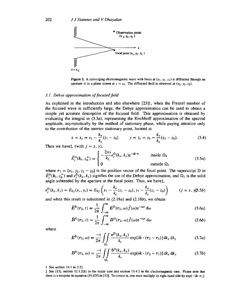
202 J J Stamnes and V Dhayalan
* Observation point
Focal point ( X | , y | ,
Figure 2. A converging electromagnetic wave with focus at (x\, y\,z\) is diffracted through anaperture A in a plane screen at z = z<). The diffracted field is observed at (JC2, V2, zi).
3.1. Debye approximation of focused field
As explained in the introduction and also elsewhere [23]f, when the Fresnel number ofthe focused wave is sufficiently large, the Debye approximation can be used to obtain asimple yet accurate description of the focused field. This approximation is obtained byevaluating the integral in (3.3a), representing the Kirchhoff approximation of the spectralamplitude, asymptotically by the method of stationary phase, while paying attention onlyto the contribution of the interior stationary point, located at
k kx = xs =x\ - -^(zi - z 0 ) y = ys = y\ --r(z\ - zo). (3.4)
kz kz
Then we havet, (with j = x, y),
£ ;D(fc,,z0
+) = '-^P-ef(kx,ky)e-'kri inside £]
kz
0 outside
(3.5a)
where r\ = {xi, V|, Z| — Zo) is the position vector of the focal point. The superscript D inEf(k,, ZQ) and e®(kx, ky) signifies the use of the Debye approximation, and Q] is the solidangle subtended by the aperture at the focal point. Thus, we havef,
ef(kx,ky) = EOj(xs, y,) = EOj lx] - j-(z\ - Zo), >'i - T^(ZI - z\ Kz Kz
and when this result is substituted in (2.18a) and (2.186), we obtain
ED(r2, t) = ~— I ED(r2,co)f(co)e~'a"da) (3.6a)2n J_oo
1 C°°BD(r2,t) = — / B°(r2, u>) f ((o)e~ia>l dco (3.66)
2n y_oo
where—iff eD(k k)
E°(r2, (o) = — / / — *' y exp[ifc • (r2 - r,)] dkx dky (3.7a)
—i f f bD(k k )BD(r2, co) = — *' y> exp[ifc • (r2 - r,)] dkx dky (3.76)
2.TI J J kz
t See section 14.1 in [13].t See [13], section 12.1.2(b) in the scalar case and section 15.4.2 in the electromagnetic case. Please note thatthere is a misprint in equation (15.670 in [13]. To correct it, one must multiply its right-hand side by exp(—ifc-ri).
Focusing of electric-dipole waves 203
with
eD(*,, *v) = {<£, e», ef) bD(kx, ky) = [bDx, 6 ° , bD
z}. (3.7c)
Here r\ = {x\,y\,z\ — ZoJ and r2 = {x2, y2, z2 - Zo) are the position vectors of respectivelythe focal point and the observation point. Note that (3.7a) and {3.1b) are in agreementwith equations (15.67/i) and (15.67/) in [13]. These equations were first derived by Wolf[24], but in a different manner, which obscures the connection between the Debye and theKirchhoff approximations.
The spectral amplitudes e®(kx,ky) and e®(kx,ky) are given in (3.5b), and from (2.6)and (2.7) we have
«?(**, *,) = -T-[kxe°(kx,ky) + kye*(kx, ky)] (3.8)
&D(JfcJt,*y) = - fcxe D (Jfc J t ,*v) . (3.9)CO
We emphasize once again that the results in (3.6)-(3.9) are valid provided the Fresnelnumber of the focused wave is sufficiently large.
3.2. Kirchhoff approximation of focused field
From (2.18) we have in the Kirchhoff approximation
1 f°°EK(r2,t) = — / EK(r2,a))f(a))e-ltt"da) (3.10a)
2n y_TO
BK(r2, t) = ^- I BK(r2, a>) f (ai)^"' da> (3.10&)
where (cf (2.19a, b))
2 °°J5K(r2,10) = (-J- J If EK(k,, z+)e«
k--ri,+kz(z2-z0)) dkx ^ (3.1 la)
-00
2 °°BK(r2,a>) = (^-\ f [ BK(kl,zZ)c'(krri-+k>(Z
To enable us to express the focused field in the Kirchhoff approximation in a similar formas in (3.6)-(3.7), we now write (with j = x, y)
ef(kx,ky) = ^exp[ i fc . r ,]£*(*;,, z+) (3.11c)
with Ef(k,,Zo) given in (3.3a). Substituting (3.11c) in (3.11a,b), we obtain
EK(r2, a>) = ^- Jj e {k^ky) exp[i*:. (r2 - r,)] d*, dA, (3.12a)
i f C b (k k )B\r2, a)) = — JJ Y ' y) exp[ifc . (r2 - r,)]difc, dky (3.126)
—00
00—i f C b (k k )\r2 a)) = JJ Y' y)
204 J J Stamnes and V Dhayalan
with (cf (3.8) and (3.9))
e?(kx, ky) = —r-[kxe*{kx,ky) + kyef(kx, fc,)] (3.13)
bK(kx, ky) = -k x eK(kx, ky). (3.14)
Comparing (3.7) and (3.12), we see that a main difference between the Debye and theKirchhoff approximation is that in the former case, the integration extends only over a finitepart of the (kx, ky) plane, while in the latter case, it extends over the entire (kx,ky) plane.
Note that it remains to specify the incident field amplitude EQj(rt) (j = x, y) in (3.1).This quantity obviously will depend on both the source and the optical system employed togenerate it.
4. Focusing of converging electric-dipole wave
The results in section 3 are valid for a converging incident wave with a general vectoramplitude EOj(rt) (j = x, y) in (3.1). Here we shall consider an idealized case in which theincident field is that of a converging electric-dipole wave. As mentioned in the introduction,this particular choice is motivated by the fact that for focusing of scalar waves, a convergingscalar dipole wave gives a better energy concentration in the focal plane than a convergingspherical wave [20-22].
4.1. Specification of incident field
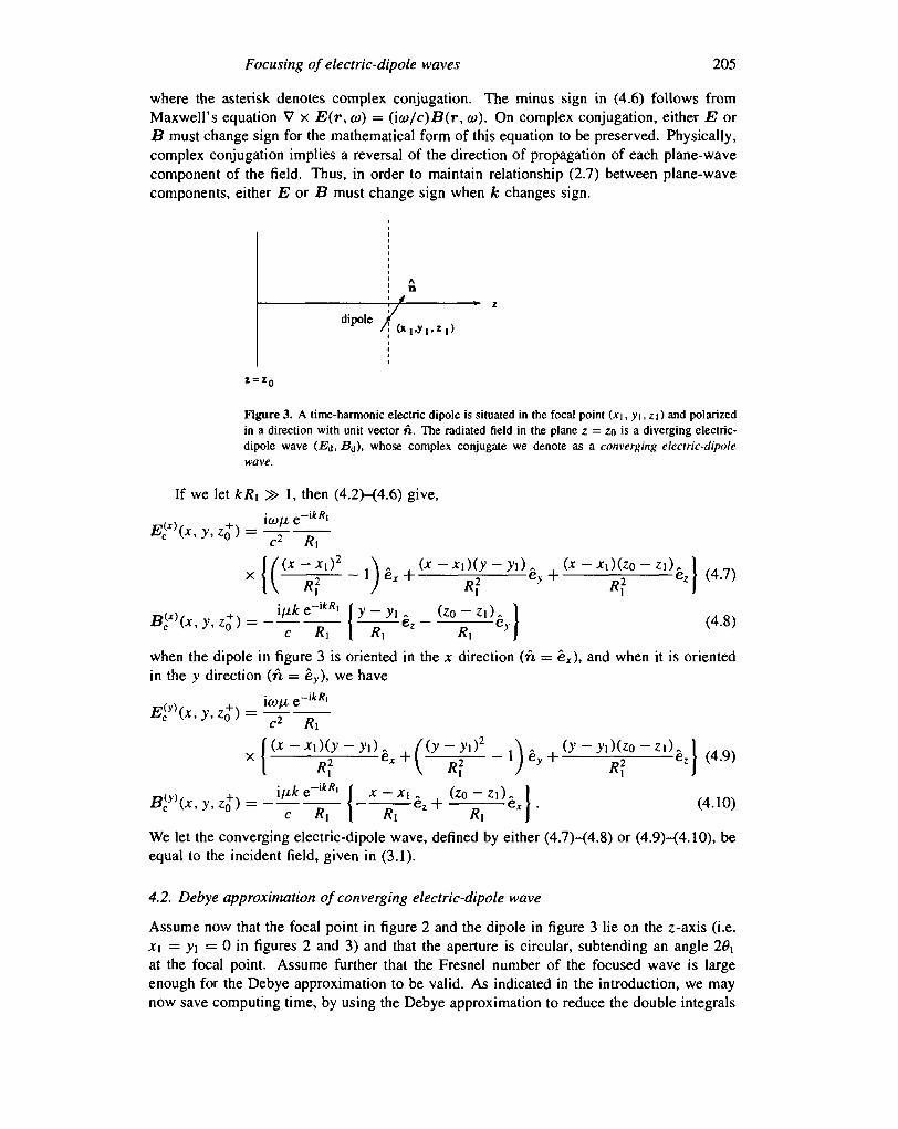
Our converging electric-dipole wave is constructed in the following manner. Let a time-harmonic dipole be situated in the focal point (JCI , >'i, Zi), and let it be polarized in a directionwith unit vector n, as indicated in figure 3. This dipole radiates a diverging electric-dipolewave with spatial electric and magnetic field distributions E& and B^ in the plane z = Zogiven byf,
(4.1)
where R] is given in (3.2). On carrying out the differentiations in (4.1), we have
i \ ATi- )n( ) x e R l (4.3)
wherex - xi y - y} zo - z\ *
e*i = —j^~e* + —^~ey + ~R^~ez- ( 4-4 )
We now define a converging electric-dipole wave whose electric and magnetic fielddistributions Ec and Bc in the plane z = ZQ are given by
Ec(x, y, z+) = [JBd(jc, y, z+)]* (4.5)
Be(x, y, z+) = -[B6(x, y, zj)]• (4.6)
f These results follow readily from equation (15.24) in [13] by setting Jo(fco±, a>) = n and using Weyl's plane-wave expansion of a spherical wave, see equations (4.14) and (4.15) in [13],
Focusing of electric-dipole waves 205
where the asterisk denotes complex conjugation. The minus sign in (4.6) follows fromMaxwell's equation V x E{r, co) = (ico/c)B(r, co). On complex conjugation, either E orB must change sign for the mathematical form of this equation to be preserved. Physically,complex conjugation implies a reversal of the direction of propagation of each plane-wavecomponent of the field. Thus, in order to maintain relationship (2.7) between plane-wavecomponents, either E or B must change sign when k changes sign.
dipole
Figure 3. A time-harmonic electric dipole is situated in the focal point (x\,yi, z\) and polarizedin a direction with unit vector n. The radiated field in the plane z = zn is a diverging electric-dipole wave ( £ J , B J ) , whose complex conjugate we denote as a converging electric-dipolewave.
If we let 1, then (4.2H4.6) give,
icofi e-it/?,
« . C*~ >„ (* - J T I ) ( Z O - Z I ) . , . . _ ,"e> + =5 ez \ (4-7)
(4.8)
when the dipole in figure 3 is oriented in the x direction (n = e*), and when it is orientedin the y direction (n = ey), we have
xx -
We let the converging electric-dipole wave, defined by either (4.7)-(4.8) or (4.9)-{4.10), beequal to the incident field, given in (3.1).
4.2. Debye approximation of converging electric-dipole wave
Assume now that the focal point in figure 2 and the dipole in figure 3 lie on the z-axis (i.e.x\ = yi = 0 in figures 2 and 3) and that the aperture is circular, subtending an angle 26\at the focal point. Assume further that the Fresnel number of the focused wave is largeenough for the Debye approximation to be valid. As indicated in the introduction, we maynow save computing time, by using the Debye approximation to reduce the double integrals
206 J J Stamnes and V Dhayalan
in (3.7a, b) to single integrals. Using (3.1) and (3.5) (with j — x,y,z) and analogousexpressions for the B field in combination with (4.7)-(4.8) or (4.9)-(4.10), we have in theDebye approximation
,_. icou -i -i*>' •x'(k k } — —-((k k \f> 4-kkf>4-kkf>\ (A 111
,w*> ^ iU
b(Dx\kx,ky) = —{-kzey + kyez} (4.12)
e(D'y)(kx, ky) = ^{kxkyex + (*2 - k2)ey + kykzez] (4.13)
b(Dy\kx,ky) = ^{kzex -kxez] (4.14)
where the superscript j = x, y in e(D'7)(fcx, Jfcy) and 6<D~JHkx, ky) signifies the polarizationdirection of the dipole. As a check, one readily confirms that (4.11)—(4.14) are in agreementwith (3.8M3.9).
In order to reduce the double integrals in (3.7a, b) to single integrals, we now introducespherical coordinates r, 0, <j>, centred at the focal point, i.e. we writef,
r = T2 — r\ = xex 4- yey + zez = r[sin 6 cos ij>ex + sin 0 sin <j>ey + cos 0ez] (4.15)
and make the change of variables
kx = -fcsinacos/3; ky =—ksinasinp (4.16)
in (3.7a, b) to obtain
' = TI j s ina{[2- sin2a(l + cos(2/3))]ex - sin2asin(2/3)e>.47TC2 Jo Jo
+2sino!cosacos^ez}exp(ifc • f)dard/J (4.17). . IL2 rlix p9\
£}(D,x) _ I i sina{cosaey + sinorsin^ez}exp(ifc • f)dad/J (4.18)2?rc JO JO
£(D,>) _ / I sina{—sin2asin(26)ex + [2 — sin2a(l — cos(26))]ev4TTC2 JO JO
+2sinarcosasin/Jez}exp(ifc • f )dad^ (4.19)
+• sinacos/3ez}exp(ifc • f) da d/3 (4.20)
where 6\ is the angular half-aperture and
k • r — k - {T2 — r\) = Jtr[cos0cosa — sin 6 sin a cos(^ — <j>)\. (4.21)
The p integrals in (4.17)-(4.20) can be expressed in terms of Bessel functions by means ofthe formulae:):
f2*I cos(nP)exp[—\tcos(P — y)]<ip = 27i(—\)Jn(t)cos(ny) (4.22)
Jor y)]dp = 27r(-i)FI7fl(f)sin(n)/) (4.23)
t See section 16.1 in [13], where the analogous problem of electromagnetic focusing through a rotationallysymmetric optical system is treated.X Equation (16.5a-b) in [13].
Focusing of electric-dipole waves 207
where n is any integer and Jn(t) is the Bessel function of the first kind and order n. Thus,we find
, n * (i(ok i\\ - . . (i)j£(u,x) _ T"{[ O ' ^2c°s(20)]ex + 72sin(2</>)ey — 2i/. cos^>ez) (4.24)
r> — \ / n ey — 1/] sin<pezj (H.AJ)
— 2i/| sin^ez} (4.26)
(4-27)c
where
70(l) = / sin a(2 - sin2 a)70['i (a)] exp[ir2(a)] da (4.28)
Jo(1) 1
If. = I sinacosa7o[^i(a)]exp[ir2(a)]da (4.29)Jo
l\n) = I ' sin2 a cos" a J, [h (a)] exp[if2(a)] da (n = 0, 1) (4.30)Jo
h = I sirJo
(4.31)Jo
with
tl (a) = kf sin 6 sin a; ^(«) = ^ cos 6 cos a. (4.32)
As noted earlier, the superscripts j = x,y in JE7(D-') and B(DJ) in (4.24)-(4.27) signify thepolarization of the incident converging electric-dipole wave.
Finally, we introduce dimensionless optical coordinates u and v given by
« = kf cos 0 sin2 6>i = kz sin2 0i; z = z2 - Zi (4.33)
v - kf sin § sin #i = ^p sin 6t; p = (x2 + >-2)1/2. (4.34)
Then (4.28)-(4.31) take the formre.
/„<>, v) = f sina(2 - sin2a)y0 [ ^ ^ 1 exp [ i ^ ^ l da (4.35a)Jo L s i n ^ i J L sin2^, J
,(2), f6' • r [vsina~\ f.Hcosal ^ ~ , , ^lr'(u,v)= I s i n a c o s a 7 0 ^ ^ - exp I—=— da (4.356)
Jo I s i n^i J L sinz^j J/,(n)(«,u)= r s i n 2 a c o s ' 1 a 7 1 [ ^ ^ l e x p [ i ^ ^ l d a (« = 0, 1) (4.35c)
Jo L s i n^i J L sin20, Jf°' • i fusina"] [.wcosa"!
h(u, v) = / sin3 a J2 . exp l—=— da. (4.35</)Jo L sin ^i J L sin2 6\ J
Compared with (4.17M4.20), the simplicity of (4.24H427) lies in the fact that thef) integration has been eliminated through the use of (4.22) and (4.23). From a practicalpoint of view, this simplification is important, since it gives a significant reduction in thecomputing time.
Note also that formulae (4.24)-(4.27), which follow from (3.1a, b), imply that onedetermines the temporal behaviour of the electromagnetic field at a given observation pointby first integrating over spatial frequencies to obtain the field due to each temporal frequency
208 J J Stamnes and V Dhayalan
component. Then one adds the fields due to all different temporal frequency components,using (3.6a, b), to obtain the temporal behaviour of the field. This approach is convenientfor cases in which the temporal frequency band is narrow, i.e. for nearly time-harmonicfields or quasi-monochromatic fields.
4,3. Kirchhoff approximation of converging electric-dipole wave
When the Fresnel number of the focused wave is not large enough for the Debyeapproximation to be valid, we must use the Kirchhoff approximation. Then the focusedelectric field follows from (2.23a) with r replaced by r2, i.e.
E(K^(r2) = -— / / E%\x, y, $)—( — ) dx dy (4.36a)In J J azi \ R2 )
A
where
Ri = [ t o - x)2 + (>'2 - y)2 + (z2 - zo)2]]/2 (4.36b)
and where the superscript j = x,y denotes the polarization of the converging electric-dipolewave. Substitution of (4.7) and (4.9) in (4.36a) gives
R
3
A
(y-ytf \^?—lr>
RSimilarly, we obtain on substituting (4.8) and (4.10) in (4.36a) with E replaced by B:
1-Hr1*+^-} 4 ( f )In (4.38a, b), we have made use of the fact that we also knew B inside the aperture A.If we had known E only, we could have used (2.236) to obtain B. For the convergingelectric-dipole wave with x polarization, we then would get
\c
where
V2 = — e , H ey + — e z . (4.39*)3^2 3j2 3Z2
From (4.7), we have,
Focusing of electric-dipole waves 209
where e^i is given in (4.4). On substituting this result in (4.39a) and carrying out thegradient operation, we obtain
( iI+IR-
where
eR2 = — — e x + — — e y + — — e z . (4.406)A2 " 2 " 2
For kR2 » 1, the difference between the results in (4.38a) and (4.40a) is
-I]
J JH—— — —^—&Ri x ^Ki) + ex x eR2\ \ dxdy. (4.41)
K2 OZ2 LBut since,
e — \ =\k— ( l + - — ) — • (4-42)
1(4.43)
it follows that for kR2 ^> 1, (4.41) can be written
AB(K-X)(r2) = 1 1 F(x, y) I — — ~ ( e R 2 x eR\) + ex x (eR\ + eR2) J dxdy (4.44)-4
where
When the observation point (Jt2,;y2,Z2) coincides with the focal point (x],y\,z\), eR2 =—eR\, implying that AB^Kx)(r2) = 0. When the observation point is close to the focalpoint, the first term inside the curly bracket in (4.44) is small, because eR2 and eR\ arenearly anti-parallel. Also, integration along any line y = constant in the aperture will tendto give cancellation in the first term of (4.44), since x changes sign. The second term canbe written
ex x (e*. + eR2) = [— + - ^ - j e*- — [l- ^ ^ e,. (4.46)
The first term in (4.46) gives cancellation on integration along any line x = constant inthe aperture, since y changes sign. The second term in (4.46) gives cancellation because(/?i /R2)[(z2—Zo)/(z\ —Zo)] varies around 1 when the integration point explores the aperturef.
From these discussions, we conclude that when kR\ S> 1 and kR2 » 1 and theobservation point is close to the focal point, then (4.38a) and (4.40a) will give essentiallythe same result. Similar considerations apply to the z component of the electric field, which
t See section 12.1(d) in [13].
210 J J Stamnes and V Dhayalan
alternatively can be obtained from (2.29a), and also to the converging electric-dipole wavewith y polarization.
Finally, we note that this comparison between the B fields in (4.38a) and (4.40a)is related to that between the Rayleigh-Sommerfeld and Kirchhoff diffraction theories inthe scalar casef and to the comparisons made by Karczewski and Wolf [25,26] in theelectromagnetic case.
5. Comparison with Debye theory for rotationally symmetric optical systems
Once again we assume that the Fresnel number of the focused wave is large enough forthe Debye approximation to be valid, and we now compare our Debye-theory resultsin section 4.2 for a focused field due to a converging electric-dipole wave with thecorresponding results of Richards and Wolf [3] obtained by focusing of a linearly polarizedplane wave by a rotationally symmetric, aplanatic optical system. Thus, we consider arotationally symmetric optical system, in which all refracting or reflecting surfaces arecentred on a common optical axis, which points along the z axis of our coordinatesystem. We let the incident field be a monochromatic, linearly polarized plane wave,which propagates along the optical axis with its electric field vector directed along thex axis. Provided the system produces an aberration-free image, the spectral amplitude ofthe electric field in image space can be expressed asj,
eD(kx, ky) = A(kx, ky)p(kx, ky) (5.1)
where p(kx,ky) is a unit vector in the direction of polarization of the plane waveexp[ifc • (r2 — r\)] in (3.7a), which propagates in the k direction with a relative strengthof A(kx,ky). Assuming that the angle between the polarization vector p(kx,ky) and themeridional plane (the plane containing fc and the optical axis) does not change on refractionor reflection at any of the surfaces of the system, we can express the polarization vector inimage space as§,
p(kx, ky) = p(a, ft) = [cosa + sin2 /3(1 — cosa)]ex — [(1 — cosa)siny3cos^]eJ.
+(sinacos0)ez (5.2)
where a and fi are given in (4.16).Because of the rotational symmetry, the strength factor A(kx,ky) does not depend on
the azimuth angle jS, and if the system is assumed to be aplanatic, so that it obeys the sinecondition, we have [3]||,
A(kx, ky) = A(a) = cos1/2a. (5.3)
Other strength factors A(a) are discussed in [22] and in section 16.1.2 in [13].If one substitutes (5.1) in (3.7a, b), with bD(kx,ky) in (3.7Z?) given in (3.9) and with
p(kx,ky) and A(kx,ky) in (5.1) given in (5.2) and (5.3), respectively, one obtains on using(4.16), (4.22), and (4.23)1:
2"E = -—{[/o + cos(20)/2)]ejt + sin(20)/2e> - (2icos0)/,ez) (5.4a)
B = -—{sin(20)/2ex + [/„ - cos(20)/2]e, - (2isin^)/,ez} (5.46)
f See section 12.l(d) in [13].| Equation (16.1a) in [13].§ Equation (16.3a) in [13].|| See also section 16.1.2 in [13].1 See [3] or equations (16.6a-b) and (16.8a-c) in [13].
Focusing of electric-dipole waves 211
where
f9* /usina\ /iwcosa\I0(u, v) = I /4(a)sina(l +cosa)7o I ) exp ^— I da
Jo \ sin6»i / r V sin26>, /
/,(«. v) = f *(«)(«„'«)/, (^) exp (Jo \sir\6i ) \
da
f6' /usina\ /i«cosa\I2(u, v) = I A(a)sina(l — cosa)/2 I —: I exp { =— I da
Jo \ sin 0i / V sin2 (9! /
with the optical coordinates u and v defined in (4.33) and (4.34).
(5.5a)
(5.56)
(5.5c)
5./. Analytical comparisons
5.1.1. Polarization vectors. For a converging electric-dipole wave polarized in thex direction, it follows from (4.11) and (4.16) that,
e(D,x) _ £j[j _ s j n2
a c o s2 p]ex _ sin2 a sin cos e v + sin a cos a cos fiez} (5.6a)
where
(5.6b)
(5.7)
On writing (5.6a) in the form
elD-x) = Cp(a, P)A(a, 0)
where p(a, f$) is a unit vector, we obtain,
(D,x)
which gives
i>(a<P) = T,—^{U - sin2 a cos2 0]ex - s in 2 a;
(5.8)
sinacosacos)3ez}
with
= [l - s in 2 acos 2 £] l / 2 .
(5.9a)
(5.96)
We see that the polarization vector in (5.9a) for a converging electric-dipole wave differssignificantly from that for a rotationally symmetric optical system, given in (5.2). In thelatter case, the focused fields are given by (5.4a, b), which are to be compared with thecorresponding expressions in (4.24) and (4.25) for the converging electric-dipole wave. Inboth cases, the focused fields are given in terms of one-dimensional integrals. The dipolecase is slightly more complicated, since it involves five different integrals, given in (4.35a-d), while the focused field for the rotationally symmetric optical system involves only thethree integrals in (5.5a-c).
212 J J Stamnes and V Dhayalan
5.1.2. Symmetries of fields and energy densities. In an aplanatic system, the focused-fieldcomponents, given in (5.4), have symmetries about the geometrical focal plane u = 0[3]. The symmetries of the focused field of a converging electric-dipole polarized in thex direction, follow from (4.24)-(4.25) and (4.28H4.31). From (4.28)-(4.31), we have,
C(-u,v) = [I^\u,v)T (5.10)
I™(-u,v) = [I™ («,«)]* (5.11)
l\n\-u, v) = [l\n\u, v)]* (n = 0, 1) (5.12)
hi-u, v) = [I2(u, v)]* (5.13)
where the asterisk denotes complex conjugation. It follows from (5.10M5.13) that thefocused-field components in (4.24)-(4.25), corresponding to an x polarized convergingelectric-dipole wave, have the same symmetries about the geometrical focal plane as inthe case of an aplanatic system, i.e.
A> ( -« ,u ,0) = [A>(«,u,0)]* j=x,y (5.14)
Az(-u,v,#) = -[Az(u,v,$)]* (5.15)
where A stands for either E or B.In an aplanatic system, the focused E and B fields in any plane u = constant are the
same, except that they are rotated with respect to each other by 90° around the optical axisf.For an x polarized converging electric-dipole wave, however, it follows from (4.24)-(4.25)that there is no such simple relationship between the focused E and B fields.
Note also that the focused B field of an x polarized converging electric-dipole wave,given in (4.25), has no x component, i.e. Bf-x) = 0, while the corresponding focusedB field for an aplanatic system in (5.46) has a non-vanishing x component.
The time-averaged electric and magnetic energy densities in the focal region are givenby
j ^ - E * (5.16)
HH* (5.17)(wm(u,v,$)) HHIO7T
where we have assumed that £ = fi = 1 (focal region in air).For the focused field of an x polarized converging electric-dipole wave, we find by
substituting (4.24H4.25) in (5.16H5.17):
( l ) 2 2 ^ < I ) / 2 * ] } (5.18)
(5.19)] { | / | + | / | s i n < £ } .C J 1D7T
The total time-averaged energy density w = we + wm becomes:
+2cos(20)Re[/o(1)/2*] + 4|/1
(O)|2sin20}. (5.20)
Because of the symmetries in (5.10H5.13), it follows from (5.18H5.20) that,
(W(-u,v,$)) = (W(u,v,$)) (5.21)
t Section 16.1.3 in [13].
Focusing of electric-dipole waves 213
where W stands for either we, wm, or w. Thus, as in the case of an aplanatic system, alltime-averaged focused-energy densities are symmetrical about the geometrical focal plane.
In the focal region of an aplanatic system, the electric and magnetic energy densitiesare the same, except that they are rotated with respect to each other by 90° about the opticalaxis, i.e. [3],
{wm(u, v, 0)) = {we(u, v, 0 - \n)). (5.22)
Also, in this case, the time-averaged total energy density is independent of 4>, i.e. it issymmetrical about the optical axis. In contrast, the time-averaged electric and magneticenergy densities in the focal region of a converging electric-dipole wave satisfy no suchsimple relationship as the one in (5.22), and the total energy density is not independent of
Along the optical axis i; = 0, it follows from (4.28H4.31) that 7,(n) = 0 (n = 0, 1),h = 0, and
7Q!) = / sina(l + cos2a)exp[ifczcosa]da (5.23)Jo
7i2) = I sinacosaexp[ijfczcosa]dar (5.24)Jo
which on letting cos a = x, becomes/ • l
73° = / (1+x2)exp[iifczx]dx (5.25)./cos 0i
/.I7® = / xexp[iitzx]dx. (5.26)
./cos 0i
At the focus z = 0, (5.25) and (5.26) give,
7Q!) = I — cos#i — j cos3#i (5.27)
7® = |sin26», (5.28)
and hence from (5.18H5.20), (with n = 1)
<twe(O,O))= — R-cos0, -{cos^r (5.29)' 167T ' i
~k2l2 1(wm(0, 0)> = | - | — {isin20,}2 (5.30), 0)> = [ - 1L c J
rp-|2 i, 0)) = I —J —(itf(0,0)) = \ - \ - - { [ l - c o s ^ - i c o s ^ ^ ^ + lsin^,]2}. (5.31)
167TAlong the optical axis v = 0 away from the focus z = 0 we get on integrating by parts in(5.25) and (5.26)
7(1° = —r[2exp(iifcz) - (1 +cos20i)exp(iitzcos0i)]kz
2
—j[exp(iA:z) - exp(i^zcos0i)] (5.32)z)
exp(i/:zcos0i)] + ——j[exp(ifcz) - exp(ifczcos^i)]. (5.33)KZ)
214 J J Stamnes and V Dhayalan
The right-hand sides of (5.32) and (5.33) become indeterminate at the focus, where (5.27)-(5.28) are to be used.
5.2. Numerical comparisons
In this section, we present numerical results in order to compare the focusing characteristicsof an aplanatic system with those of a converging electric-dipole wave.
(b)
(d)
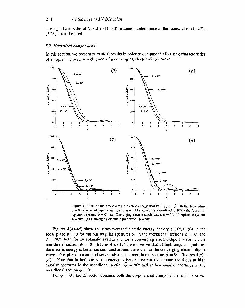
Figure 4. Plots of the time-averaged electric energy density (wc(u, v,(j>)) in the focal planeu = 0 for selected angular half-apertures Q\. The values are normalized to 100 at the focus, (a)Aplanatic system, 0 = 0". (b) Converging electric-dipole wave, 0 = 0°. (c) Aplanatic system,4> = 90°. (d) Converging electric-dipole wave, j> = 90°.
Figures 4{a)-(d) show the time-averaged electric energy density {we(u, v, 0)) in thefocal plane u = 0 for various angular apertures 6\ in the meridional sections 0 = 0° and<p = 90°, both for an aplanatic system and for a converging electric-dipole wave. In themeridional section <j> = 0° (figures 4(a)-(b)), we observe that at high angular apertures,the electric energy is better concentrated around the focus for the converging electric-dipolewave. This phenomenon is observed also in the meridional section (j> = 90° (figures 4(c)-(d)). Note that in both cases, the energy is better concentrated around the focus at highangular apertures in the meridional section <p = 90° and at low angular apertures in themeridional section ^ = 0°.
For <j> = 0°, the E vector contains both the co-polarized component x and the cross-
Focusing of electric-dipole waves 215
polarized component z, while for 0 = 90°, it contains only the co-polarized component x.In both cases, the cross-polarized component y is zero. For a converging electric-dipolewave, this follows from (4.24) and for an aplanatic system, it follows from (5.4a).
(b)1UU~
80-
A
$ . -
1-V
M -
0-
\
9,-so* J\
\
\
9,-30*
e,-»o*
I 1 1
(a)
i i
0 1 20 -
8,-90* (c)
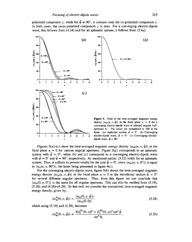
Figure 5. Plots of the time-averaged magnetic energydensity {wm(u, v, 0)) in the focal plane u = 0 for aconverging electric-dipole wave at selected angular half-apertures 9\. The values are normalized to 100 at thefocus, (a) Aplanatic system, 0 = 0°. (b) Convergingelectric-dipole wave, <p = 0°. (c) Converging electric-dipole wave, 4> — 90°.
Figures 5(a)-(c) show the time-averaged magnetic energy density {wm(u, v,<j>)) in thefocal plane u = 0 for various angular apertures. Figure 5(a) corresponds to an aplanaticsystem with <p = 0°, while (b) and (c) correspond to a converging electric-dipole wavewith 4> = 0° and 0 = 90°, respectively. As mentioned earlier, (5.22) holds for an aplanaticsystem. Thus, it suffices to present results for the case </> = 0°, since {wm(u, v, 0°)) is equalto (we(u, v, 90°)), the latter being presented in figure 4(c).
For the converging electric-dipole wave, figure 5(b) shows the time-averaged magneticenergy density {wm(u, v, 0)) in the focal plane u = 0 in the meridional section 0 = 0°for several different angular apertures. Thus, from this figure we can conclude that{wm(0, v, 0°)> is the same for all angular apertures. This can also be verified from (5.19),(5.28), and (4.28)-(4.29). To that end, we consider the normalized, time-averaged magneticenergy density, given by,
(wm(0,v,<f>)}(5.34)
which using (5.19) and (5.30), becomes
sin40,(5.35)
216 J J Stamnes and V Dhayalan
For <p = 0°, we have
( u ; > , t ; , 0 ° ) ) = 4 | / » 2 | ^ ; ) | 2 . (5.36)sin 6\
According to (4.35b), we have
/<2)(0, v) = I sin a cos a Jo ^ ^ da (5.37)Jo L s m ( ? i J
which by the change of variable usinor/sin#i = x and the use of [XJQ{X)\ = xJ\(x)becomes
<?\ ^ (5.38)
Substituting (5.38) into (5.36), we get
. (5.39)
This result shows that for a converging electric-dipole wave, the normalized, time-averagedmagnetic energy density for <$> = 0° does not depend on the angular aperture, as indicatedin figure 5(b).
Figure 5(c) shows (iuJJJ(O, v, #)) at 4> = 90° for a converging electric-dipole wave. Wesee that (u>^(0, v, 90°)) has an unexpected behaviour at large angular apertures. In contrastto the behaviour at 0 = 0°, it now attains a minimum value at the focus, where v = 0,and a maximum value at some other v value. As shown in figure 5(c), in the limit as theangular aperture 6\ tends to 90°, the maximum occurs at i; ^ 1.5.
Figures 6(a)-(c) show the time-averaged total energy density (w{u, u,</>)) in the focalplane « = 0 for different angular apertures. As noted earlier, for an aplanatic system,(ui(0, u, 4>)) is independent of 4>. In contrast, (w(0, v, 4>)) does depend on 0 for a convergingelectric-dipole wave. Also in this case, we observe that the total energy is better concentratedaround the focus for the converging electric-dipole wave.
Figures l{a)-(b) show the time-averaged electric energy density {we(u, v,<ji>)} alongthe optical axis v = 0 at selected angular apertures, both for an aplanatic system and aconverging electric-dipole wave. At low angular apertures, both systems give approximatelythe same energy concentration, while at high angular apertures, the converging electric-dipole wave has better energy concentration around the focus.
Contour plots of the time-averaged electric energy density {we(u, v,4>)} are shown infigures 8(a)-(&), both for an aplanatic system and for a converging electric-dipole wave.In each case, the result reduces to that of the scalar classical theory as the angular aperture0i tends to zero, giving a rotationally symmetric distribution. As the angular apertureincreases, the rotational symmetry disappears. In both cases, the contours near the focusbecome elliptical with major axes in the direction of the polarization of the incident field.But for large values of 6\, we note that the diffraction pattern for the converging electric-dipole wave starts to differ from that of the aplanatic system, especially away from thefocus in the focal plane.
Figures 9(a)-(b) show contours of the time-averaged electric energy density(we(u, v, </>)) in the focal plane M = 0 for an aplanatic system and for a converging electric-dipole wave, respectively. Figures 9{c)-{d) show the corresponding plots in a receivingplane u = 6. In all four figures, the angular half-aperture is 0i = 45°. In both systems,we note that at u = 6, v = 0, the time-averaged electric energy density is nearly 31, when
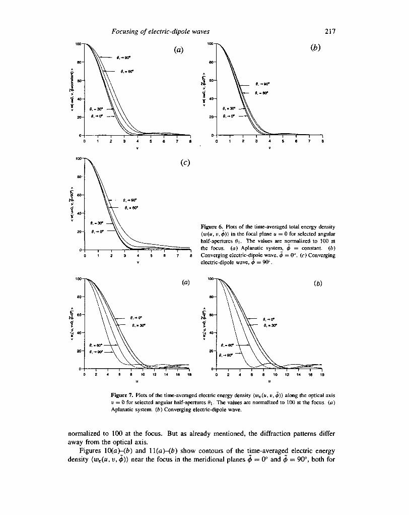
Focusing of electric-dipole waves 217
Figure 6. Plots of the time-averaged total energy density[w(u, v, j>)) in the focal plane « = 0 for selected angularhalf-apertures 0\. The values are normalized to 100 atthe focus, (a) Aplanatic system, 0 = constant, (b)Converging electric-dipole wave, # = 0°. (c) Convergingelectric-dipole wave, <j> = 90°.
Figure 7. Plots of the time-averaged electric energy density {wc(u, v, <j>)) along the optical axisv = 0 for selected angular half-apertures 0\. The values are normalized to 100 at the focus, (a)Aplanatic system, (b) Converging electric-dipole wave.
normalized to 100 at the focus. But as already mentioned, the diffraction patterns differaway from the optical axis.
Figures \0(a)-(b) and ll(a)-(b) show contours of the time-averaged electric energydensity (we(u, v, </>)) near the focus in the meridional planes 0 = 0° and <j> = 90°, both for
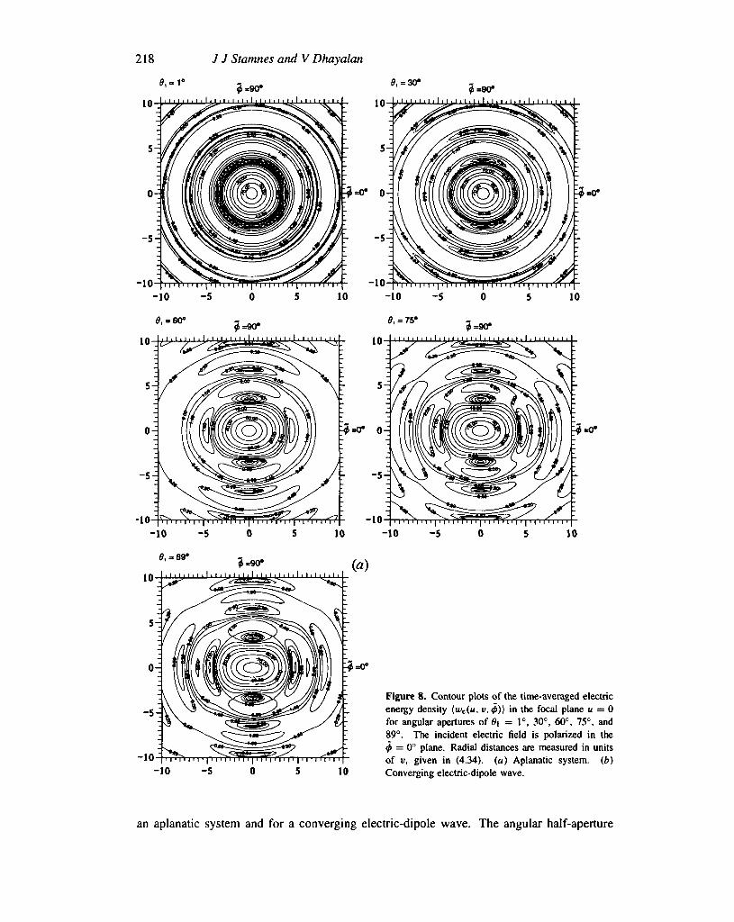
218 J J Stamnes and V Dhayalan
0=90*
| ' I ' I ' I ' I • | ' I ' I • I ' 1 ' | ' I ' I ' I ' I
10 -10 -5 0 5 10
i I i I i I I I • I i I i I t I i I • I i U I i I i I i I i I i I i, I t I i
3=0°
-10-10 -5
Figure 8. Contour plots of the time-averaged electricenergy density (we(u, v,4>)) in the focal plane u = 0for angular apertures of 6\ = 1°, 30°, 60°, 75°, and89°. The incident electric field is polarized in the<j> = 0° plane. Radial distances are measured in unitsof v, given in (4.34). (a) Aplanatic system, (b)Converging electric-dipole wave.
an aplanatic system and for a converging electric-dipole wave. The angular half-aperture
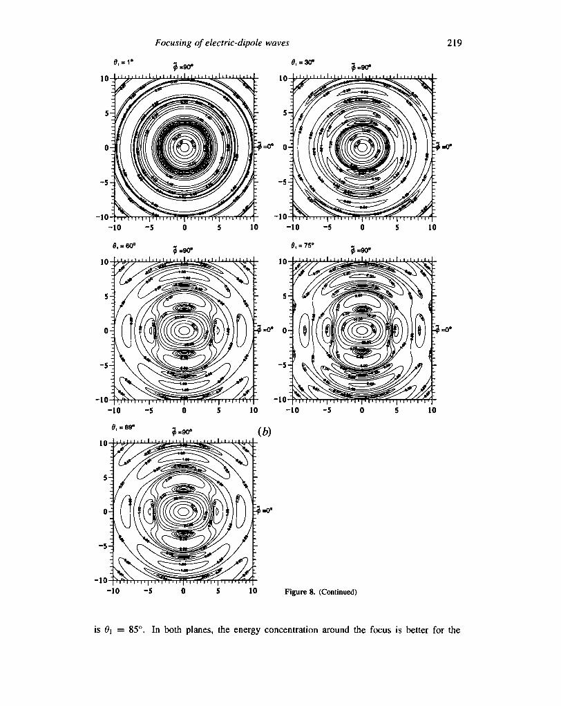
Focusing of electric-dipole waves 219
10
10 Figure 8. (Continued)
is 9\ = 85°. In both planes, the energy concentration around the focus is better for the
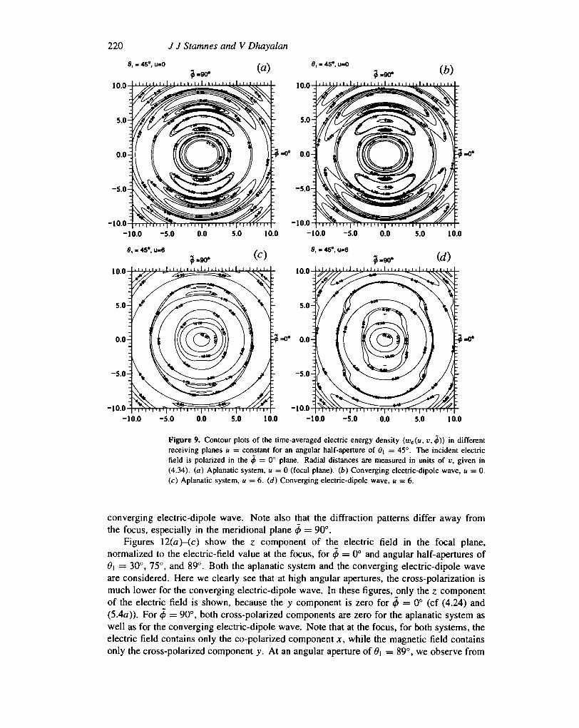
220 J J Stamnes and V Dhayalan
0, = 45*, u-0
10.0
5.0-
0.0-
-5.0-
-10.0
10.0
5.0-
0.0-
-5.0-
-10.0
-10.0 -5.0 0.0 5.0 10.0
8, - 45', u«O
10.0
5.0-
3 -0* 0.0
-5.0-i
-10.0-
10.0
5.0-
•$ =o* o .o-
-5.0-
-10.0-10.0 10.0
-10.0 -5.0 0.0 5.0 10.0
-10.0 5.0 10.0
Figure 9. Contour plots of the time-averaged electric energy density (we(u, v, 0)) in differentreceiving planes u = constant for an angular half-aperture of 6\ = 45°. The incident electricfield is polarized in the 4> = 0° plane. Radial distances are measured in units of i\ given in(4.34). (a) Aplanatic system, « = 0 (focal plane), (b) Converging electric-dipole wave, u = 0.(c) Aplanatic system, u = 6. (d) Converging electric-dipole wave, u = 6.
converging electric-dipole wave. Note also that the diffraction patterns differ away fromthe focus, especially in the meridional plane <p = 90°.
Figures 12(a)-(c) show the z component of the electric field in the focal plane,normalized to the electric-field value at the focus, for 0 = 0° and angular half-apertures of9\ = 30°, 75°, and 89°. Both the aplanatic system and the converging electric-dipole waveare considered. Here we clearly see that at high angular apertures, the cross-polarization ismuch lower for the converging electric-dipole wave. In these figures, only the z componentof the electric field is shown, because the y component is zero for 0 = 0° (cf (4.24) and(5.4a)). For 0 = 90°, both cross-polarized components are zero for the aplanatic system aswell as for the converging electric-dipole wave. Note that at the focus, for both systems, theelectric field contains only the co-polarized component x, while the magnetic field containsonly the cross-polarized component y. At an angular aperture of #i = 89°, we observe from
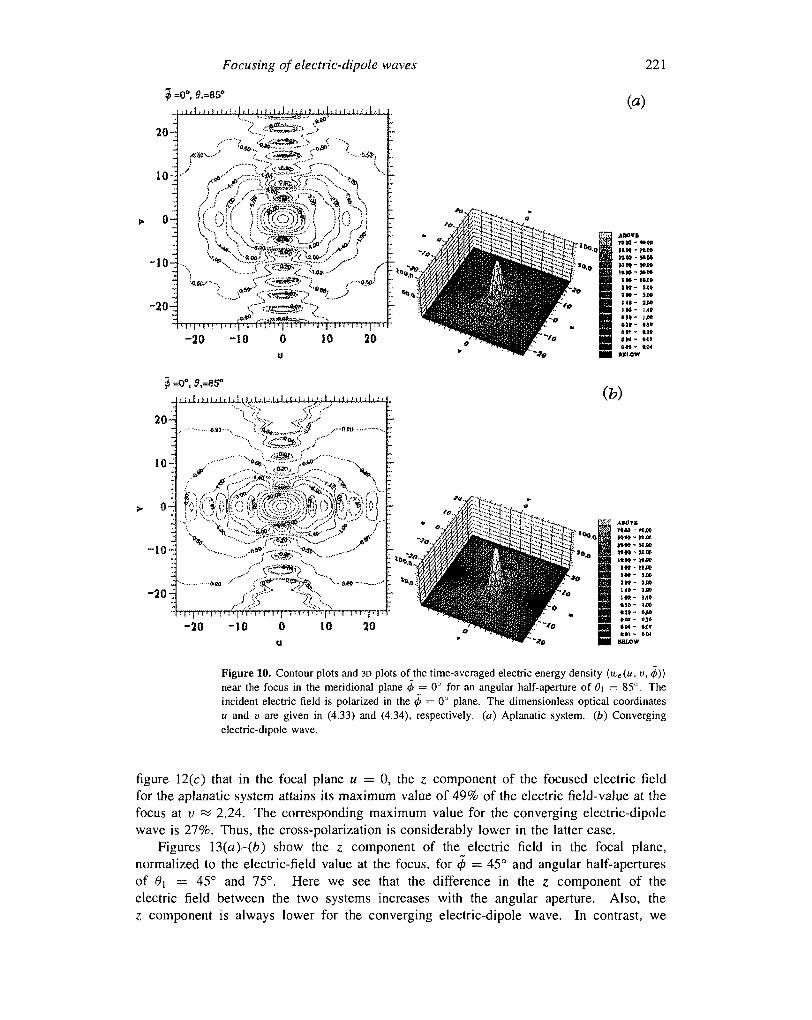
Focusing of electric-dipole waves 221
20-
o-
0", 0,=85°
: I J1 l i i . ' I I I l i p I J.I j . l . ;_ r • | = I I I . I • i : I ' 1: I •• I • .
• I ' l ' i T ' i - i i | ' i ' l H ' ' " ) i i ' " ( ' b / ' J . | i i - i M i l | i ' i i
-20 -10 0 10 20
=0°, 0,=85"
J^ijJjJul.JjJ.Uji.yjj^JU.U.LiLilil ily'.jiU lU
10-
-20 -;
/ • •
-20 -10 0 10 20
(b)
Figure 10. Contour plots and 3D plots of the time-averaged electric energy density (we(u, v, </>)>near the focus in the meridional plane 4> = 0° for an angular half-aperture of 6\ = 85C. Theincident electric field is polarized in the <£> = 0° plane. The dimensionless optical coordinatesK and v are given in (4.33) and (4.34), respectively, (a) Aplanatic system, (b) Convergingelectric-dipole wave.
figure 12(c) that in the focal plane u = 0, the z component of the focused electric fieldfor the aplanatic system attains its maximum value of 49% of the electric field-value at thefocus at v « 2.24. The corresponding maximum value for the converging electric-dipolewave is 27%. Thus, the cross-polarization is considerably lower in the latter case.
Figures \3(a)-(b) show the z component of the electric field in the focal plane,normalized to the electric-field value at the focus, for <f> = 45° and angular half-aperturesof 0\ = 45° and 75°. Here we see that the difference in the z component of theelectric field between the two systems increases with the angular aperture. Also, thez component is always lower for the converging electric-dipole wave. In contrast, we
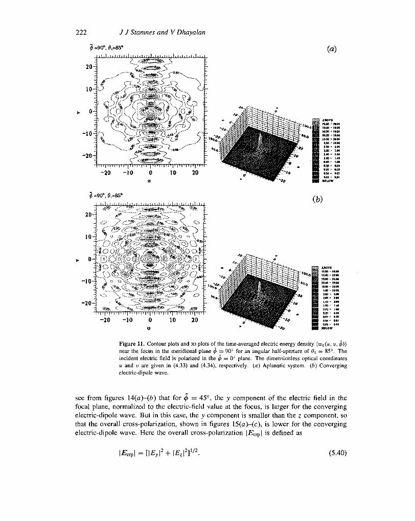
222 J J Stamnes and V Dhayalan
(a)I ! ! I i I i I r I i i i I : I , I • t : -' I I • I < I : '. I i • 1 i I i 1 i ! . I: t i
Figure 11. Contour plots and 3D plots of the time-averaged electric energy density (we(u, v, <j>))near the focus in the meridional plane ij> = 90= for an angular half-aperture of d\ = 85°. Theincident electric field is polarized in the </> = 0= plane. The dimensionless optical coordinatesM and v are given in (4.33) and (4.34), respectively, (a) Aplanatic system, (b) Convergingelectric-dipole wave.
see from figures I4(a)-(b) that for 4> = 45°, the y component of the electric field in thefocal plane, normalized to the electric-field value at the focus, is larger for the convergingelectric-dipole wave. But in this case, the y component is smaller than the z component, sothat the overall cross-polarization, shown in figures I5(a)-(c), is lower for the convergingelectric-dipole wave. Here the overall cross-polarization |-Ecrp| is defined as
(5.40)
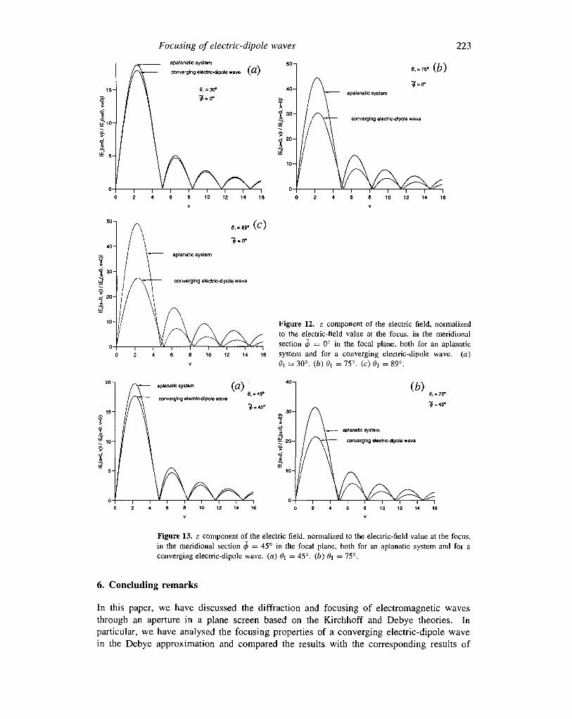
Focusing of electric-dipole waves 223
apalanatic system
converging electriodipole wave Kfl) ...w (b)
apalanatic system
converging electric-dipole wave
10 12 14 16
30H
I20H
6, = 88*
aplanatic Gysiem
converging electric-dipole wave
Figure 12. z component of the electric field, normalizedto the electric-field value at the focus, in the meridionalsection 4> = 0° in the focal plane, both for an aplanatic
4 6 8 10 12 14 16 system and for a converging electric-dipole wave, (a)v 0i = 30=. (b) 6\ = 75=. (c) 6, = 89°.
aplanatic system (&)
converging electric-dipole wave
aplanatic system
converging etectrtc-dlpole wave
8, = 75*
Figure 13. z component of the electric field, normalized to the electric-field value at the focus,in the meridional section </> = 45° in the focal plane, both for an aplanatic system and for aconverging electric-dipole wave, (a) 9\ = 45°. (b) 0\ = 75°.
6. Concluding remarks
In this paper, we have discussed the diffraction and focusing of electromagnetic wavesthrough an aperture in a plane screen based on the Kirchhoff and Debye theories. Inparticular, we have analysed the focusing properties of a converging electric-dipole wavein the Debye approximation and compared the results with the corresponding results of
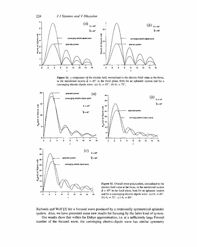
224 J J Stamnes and V Dhayalan
7-
6 -
§ 5 "
I-t3ur 2 .
i-
0-
r\\r\
/
v (a)\ 9,.
T converging electric-dipole wave
r T aplanatic system
\ A\\A
9,« 75*
•55=45°
converging electric-olpote wave
aplanatic system
Figure 14. v component of the electric field, normalized to the electric-field value at the focus,in the meridional section </> = 45° in the focal plane, both for an aplanatic system and for aconverging electric-dipole wave, (a) 8\ = 45°. (b) 9\ = 75°.
20- , aplanatic system (
converging electric-dipole wave9, - 75°
aplanatic system
converging electric-dipota wove
I 1 I I i l "-] 1 1 r2 4 6 8 10 12 14 16 0 2 4 6 6 10 12 14 16
(c)
aplanatic system
converging electric-dipole wave
, -89*
Figure IS. Overall cross-polarization, normalized to theelectric-field value at the focus, in the meridional section4> — 45° in the focal plane, both for an aplanatic systemand for a converging electric-dipole wave, (a) B\ = 4 5 ° .(b) <9, = 75=. (c) 0i = 89°.
Richards and Wolf [3] for a focused wave produced by a rotationally symmetrical aplanaticsystem. Also, we have presented some new results for focusing by the latter kind of system.
Our results show that within the Debye approximation, i.e. at a sufficiently large Fresnelnumber of the focused wave, the converging electric-dipole wave has similar symmetry
Focusing of electric-dipole waves 225
properties as the focused wave considered in [3], but in contrast with the latter case, thereis no simple relationship between the time-averaged electric and magnetic energy densitiesdue to a converging electric-dipole wave. At low angular apertures, the time-averagedelectric energy density in [3] is similar to that of the converging electric-dipole wave, bothin the focal plane and along the optical axis. But at angular half-apertures greater than30°, our numerical results show that the converging electric-dipole wave has better energyconcentration around the geometrical focus.
There are noticeable differences between the time-averaged magnetic energy densitiesin the two cases, mainly because the converging electric-dipole wave gives a vanishingcomponent of the magnetic field in the direction of polarization of the incident field. Also,the converging electric-dipole wave has less electric-field cross polarization, which may beadvantageous in some applications.
In forthcoming papers, we compare the focusing properties of the converging electric-dipole wave with those of a mixed-dipole wave both in the Kirchhoff and the Debyeapproximations. Also, we study the focusing properties of electromagnetic waves in amulti-layered medium.
References
[1] Ignatowsky V S 1919 Trans. Opt. Inst. Petrograd I paper IV[2] Ignatowsky V S 1920 Trans. Opt. Inst. Petrograd I paper V[3] Richards B and Wolf E 1959 Proc. R. Soc. A 253 358-79[4] Boivin A and Wolf E 1965 Phys. Rev. B 138 1561-5[5] Boivin A, Dow J and Wolf E 1967 J. Opt. Soc. Am. 57 1171-5[6] Innes D J and Bloom A L 1966 Spectra-Physics Laser Tech. Bull. 5 1-10[7] Yoshida A and Asakura T 1974 Optik 40 322-31[8] Mansuripur M 1989 /. Opt. Soc. Am. A 6 786-805[9] Kant R 1993 J. Mod. Opt. 40 337^7
[10] Sheppard C J R, Choudhury A and Gannaway J 1977 IEEJ. Microwaves, Opt. Acou.it. 1 129-32[11] Kant R 1993 J. Mod. Opt. 40 2293-310[12] Kant R 1995 J. Mod. Opt. 42 299-320[13] Stamnes J J 1986 Waves in Focal Regions (Bristol: Hilger)[14] Visser T D and Wiersma S H 1991 .A Opt. Soc. Am. A 8 1404-10[15] Visser T D and Wiersma S H 1992 J. Opt. Soc. Am. 9 2034-47[16] Visser T D and Weirsma S H 1994 J. Opt. Soc. Am. 11 599-608[17] Stratton J A and Chu L J 1939 Phys. Rev. 56 99-107[18] Ling H and Lee S W 1984 / Opt. Soc. Am. A 1 965-73[19] Stamnes J J 1981 J. Opt. Soc. Am. 71 15-31. See also section 13.2 in [13][20] Stamnes J J 1981 Opt. Commun. 37 311-4. See also section 12.3 in [13][21] Stamnes J J 1981 Opt. Commun. 38 325-9. See also section 12.3 in [13][22] Sheppard C J R and Larkin K G 1994 J. Mod. Opt. 41 1495-505[23] Wolf E and Li Y 1981 Opt. Commun. 39 205-10[24] Wolf E 1959 Proc. R. Soc. A 253 349-57[25] Karczewski B and Wolf E 1966 J. Opt. Soc. Am. 56 1207-14[26] Karczewski B and Wolf E 1966 J. Opt. Soc. Am. 56 1214-19
Chapter 3
FOCUSING OF MIXED-DIPOLE WAVES
Chapter 3
Focusing of mixed-dipole waves
Submitted to J. Pure and Appl. Opt.
Velauthapillai Dhayalan and Jakob J. Stamnes
Physics Department, University of Bergen, Allegt. 55, N-5007 Bergen, Norway
Abstract
A converging mixed-dipole wave is defined as the sum of a converging electric-dipole waveand a converging magnetic-dipole wave. In this paper we study the focusing properties ofconverging mixed-dipole waves for the case in which the two dipoles are orthogonal. Withinthe Debye approximation, we compare both analytical and numerical results for the convergingmixed-dipole wave with those of the converging electric-dipole wave and also with the resultsobtained when a linearly polarized plane wave is focused by a rotationally symmetric, aplanaticsystem. At large angular apertures, the converging electric-dipole wave is shown to give bestelectric-energy concentration and least cross-polarization, both in the focal plane and alongthe optical axis. At angular half-apertures less than 30°, the three types of converging wavesgive identical electric and total energy distributions around the focus. These facts make theconverging electric-dipole wave the natural choice as the electromagnetic analog of the 'perfectwave' in the scalar case.
41
3.1 Introduction
Many publications on the focusing of electromagnetic waves have appeared since the first pa-pers on this subject by Ignatowsky [1, 2] in 1919. In most of these publications the apertureplane and the focal point were in the same dielectric medium, and the analysis was based onthe electromagnetic Debye theory of focusing [3-12] . The Debye theory, however, is valid onlyat high Fresnel numbers, and other authors [13-15] based their analysis on an electromagneticKirchhoff theory of focusing, thus obtaining more accurate results at low Fresnel numbers.Another aspect of electromagnetic focusing was recently considered, namely that in which theaperture and the focal point are in two different media [16, 17]. The first of these treatementswas based on a Kirchhoff or physical-optics type of approximation [16], while the other wasbased on the Debye theory [17].
In a previous paper [18], we studied the diffraction of an arbitrary electromagnetic wavethrough an aperture in a plane screen, and presented explicit results for the focused fieldboth in the Debye and Kirchhoff approximations. The focusing of a converging electric-dipolewave was studied in depth. Such a wave is defined as the complex conjugate of the divergingwave radiated by a linearly polarized electric dipole. A converging magnetic-dipole wave isdefined in an analogous manner. In [18] the focused field due to a converging electric-dipolewave was compared with the field obtained when a linearly polarized plane wave is focusedby a rotationally symmetric, aplanatic system [3]. These comparisons showed that at highangular apertures, the converging electric-dipole wave gives better energy concentration andless cross-polarization both in the focal plane and along the optical axis.
In a recent paper, Sheppard and Larkin [19] considered a converging mixed-dipole wave,which is the sum of a converging electric- and a converging magnetic-dipole wave. They notedthat when the two dipoles are orthogonal, the converging mixed-dipole wave can be consideredas the electromagnetic analogue of the 'perfect wave' of Stamnes [20, 21]. In this paper westudy the focusing properties of mixed-dipole waves, based on the theory developed in [18].Our objective is two-fold. First it is to obtain analytical and numerical solutions for the fo-cused field due to a converging mixed-dipole wave in the Debye and Kirchhoff approximations.Second it is to compare the fields obtained by focusing of i) a linearly polarized plane waveby a rotationally symmetric, aplanatic system, ii) a converging electric-dipole wave, and iii)a converging mixed-dipole wave.
The paper is organised as follows: In section 3.2 we derive angular-spectrum representa-tions for the electromagnetic field radiated by a general magnetic source in a homogeneousmedium. In section 3.3 we use the results in [18] for the focusing of an arbitrary electro-magnetic wave through an aperture in a plane screen to obtain the focused fields due to aconverging magnetic-dipole wave.
We introduce the concept of a converging mixed-dipole wave in section 3.4, and give explicitanalytical results for the focused fields and the associated electric and magnetic energy densi-ties and the Poynting vector. We also give explicit expressions for the polarisation vector andthe strength factor associated with the incident field. When the Fresnel number is sufficientlylarge, we can use the Debye approximation and thus reduce the computing time significantly.In section 3.5 we present numerical results within the Debye approximation for focused fieldsdue to a converging mixed-dipole wave, and compare these results with those due to a con-verging electric-dipole wave and with those obtained when focusing a linearly polarized planewave by a rotationally symmetric, aplanatic system. We conclude the paper with a summaryand discussion in section 3.6.
42
3.2 Radiation from a magnetic source
The radiation by an electric dipole is thoroughly discussed in [18]. Here we consider theradiation by a localized magnetic source in a linear homogeneous medium. To that end, westart with Maxwell's equations and assume that the current source Jo(r, t) and the magneticsource Mo(r, t) are real and bounded for all r and t, and that also the electric and magneticfields E and H and the charge density p(r, t) are real. For a harmonic problem with timevariation exp(-iwt) , Maxwell's equations in Gaussian units are [22]:
V X E = —^(H + 47rM0), (3.1a)c
- J 0 , (3.1b)c
V H = -471-V-Mo, (3.1c)
withec = e + 4xicr/a>, (3.1e)
where a and e are the conductivity and the permittivity, both of which are assumed to beconstants. Here ( 3.1c) follows by taking the divergence of ( 3.1a) and using the relationV • (V X a) = 0, where a is an arbitrary vector. Similarly, ( 3.Id) follows by taking thedivergence of (3.1b).
We assume that the material equations are given by
B = /xH ; D = eE, (3.2)
where the permeability fi also is a constant.
When there is no magnetic source, so that Mo = 0, the field radiated by the electric currentsource Jo can be expressed in terms of angular-spectrum representations, as shown in [23]1.Here we assume that there is no electric source, so that Jo = 0, and we follow the sameprocedure as that used in [23] to determine the field radiated by Jo when Mo = 0, todetermine the field radiated by Mo when Jo = 0. To that end, we start by defining theFourier-transform pair
oo
i / / / V(k) exP(ik • r)<f3k, (3.3a)
'Section 15.1.2.
43
where V(k) is the Fourier transform of V(r) given by
CO
V(k)= / / /v(r)exp(-ikr)d3r . (3.3b)
—oo
By taking the inverse Fourier transform of (3.1a)-(3.1d), we obtain
k x E = ^ ( H + 47rM0), (3.4a)
kxH=-^E, (3.4b)c
k H = -4xk • Mo, (3.4c)
k • E = 0. (3.4d)
To solve for H we multiply (3.4b) vectorially with k and use (3.4a) to obtain
2
k x (k x H) = k(k • H) - Jfc2H) = - ^ - ^ [ H + 4irM0]. (3.5)c
Finally, we subtitute ( 3.4c) in (3.5) to get
KZ — KZQ
where
By substituting (3.6) in (3.4b), we find that E is given by
k x Mo
(3.7)
Next, we substitute (3.6) and (3.8) in ( 3.3a) with V = E, H to obtain the Fourier represen-tations of E and H given by
44
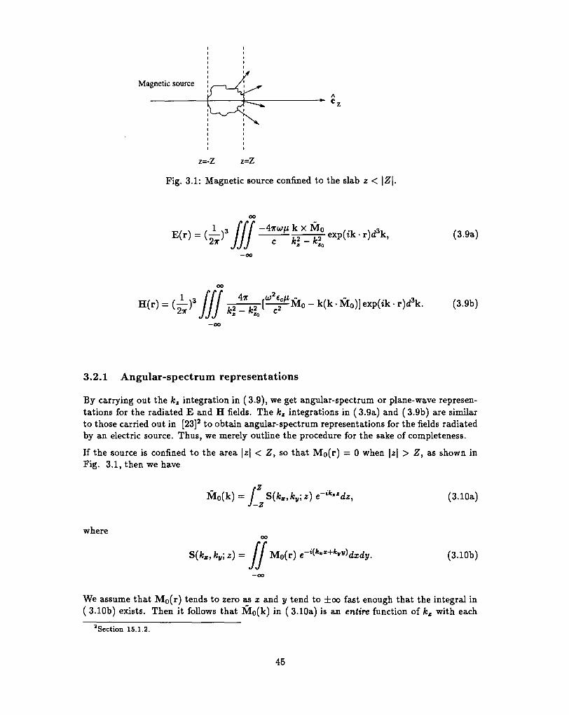
Magnetic source
z=-Z z=Z
Fig. 3.1: Magnetic source confined to the slab z < \Z\.
(3.9a)
H(r) = (^) 3 JJJ ^ ± ^ [ ^ M 0 - k(k • Mo)l exp(ik • r)d\. (3.9b)
3.2.1 Angular-spectrum representations
By carrying out the kz integration in (3.9), we get angular-spectrum or plane-wave represen-tations for the radiated E and H fields. The kz integrations in (3.9a) and (3.9b) are similarto those carried out in [23]2 to obtain angular-spectrum representations for the fields radiatedby an electric source. Thus, we merely outline the procedure for the sake of completeness.
If the source is confined to the area \z\ < Z, so that Mo(r) = 0 when \z\ > Z, as shown inFig. 3.1, then we have
M 0 (k )= / S{kx,ky\z)e-ik"dz,J-z
(3.10a)
where
S(fc«, fcv; z) = i f M0(r) (3.10b)
We assume that M0(r) tends to zero as x and y tend to ±oo fast enough that the integral in( 3.10b) exists. Then it follows that Mo(k) in (3.10a) is an entire function of kz with each
'Section 15.1.2.
45
Cartesian component Moi(k) (i = x,y,z) satisfying the inequality
< Kexp(\k'z\Z), (3.11)
where K is a real constant and k'z is the imaginary part of kx.
As a consequence of these results, we can apply the calculus of residues to perform the kz
integration in ( 3.9a) and ( 3.9b) by completing the contour at infinity in the upper half ofthe kz plane when z > Z and in the lower half of the kz plane when z < -Z. It followsfrom (3.11) that the integral along the portion of the contour at infinity does not contributeover the closed contour. Hence, the kz integrals in (3.9a) and (3.9b) are equal to 2iri timesthe sum of residues of the poles in the upper half plane when z > Z and are equal to — 2xitimes the sum of residues of the poles in the lower half-plane when z < Z. Since Mo(k) is anentire function of complex kz, the integrands in (3.9a) and (3.9b) have only the singularitiesassociated with the poles of [k\ — A^J .
Thus, we obtain
E ^ r ) = / / I5±(k±) e^±Tdkxdky, (3.12a)= / / I5±
— OO
OO
H±(r)= J(3.12b)
where
(3.12c)
with
k± = kt ± fc^e* ; kt = kxex + kyey, (3.13a)
andi _ / . i * * if
(3.13b)
The superscripts + and - in E and H are used to denote the fields in the half-space z > Zand the half-space z < Z, respectively.
46
3.2.2 Field from a magnetic dipole
Now we can specify a magnetic dipole source and obtain the radiated electric and magneticfields from (3.12a) and (3.12b). Let a time-harmonic magnetic dipole be placed at the originand polarized in the direction of the unit vector n. Then
M0(r) = mh6(r), (3.14)
where m is the dipole strength, and the Fourier transform is given by
oo
flfM 0 (k )= / / / M 0 ( r ) e - k r d 3 r = mn. (3.15)
- o o
Substituting (3.15) in (3.12c) and (3.12d), we have from (3.12a) and (3.12b)
e Tdkxdky, (3.16a)= ff -iwfim
JJ 2™
= // pJJ 2*/:
H±(r) = / / pP- k* x (k* x n) e t k ± r dMV (3.16b)JJ 2*/:
Next, we subtitute the relations
V X (n «***) = i(k± X n) e i k ± r , (3.17a)
V X (V X (n e ' k ± r ) ) = - k ± x (k± x n) e ' k ± r , (3.17b)
in ( 3.16a) and ( 3.16b), we obtain
oo
= JJ 2 ^ [ V X (V X (" e*±"'
( 3 - 1 8 a )
H±(r) = JJ 2 ^ [ V X (V X (" e*±"'))]dfc-d*«- (3-18b)
Hereafter we consider the radiated fields only in the half-space z > Z. These fields carry the
47
superscript (+), which we drop hereafter for notational convenience. For the same reason wewrite kt instead of k^ from now on.
Using WeyPs integral [23]3, ( 3.18a) and ( 3.18b) become
^ x ( n ^ ) ] , (3.19a)
H(r) = m[V X (V X ( n — ) ] . (3.19b)
On carrying out the differentiations in (3.19a) and (3.19b), we have
• J L _
E ( r) = _ ^ H ^ ( i + ± )£_(e , x n), (3.20a)C K i t
H(r) = - m l f e ' ^ e , • n)[l + £ - ^ ] - n[l + £ - ^ ] > , (3.20b)
where e,. is a unit vector given by
-ex + e + -ez. (3.20c)r r y r
Assume now that the time-harmonic magnetic dipole is placed at (xi,jh, zi), and consider anobservation point ( i , y, z0) at a sufficiently large distance R\ from the dipole, so that kR\ > 1.From (3.20) it follows that the radiated fields then are given by
= _ ^ ^ L ( i R i „ ft), (3.21a)C Jti
n eikRl2H(r) = - m A : ' — [ ^ ( e , . • n) - n], (3.21b)
where
Ri = \J(x - xO2 + {y - Vl)2 + (z0 - 21)2. (3.22b)
3.3 Focusing of converging electromagnetic waves
Before proceeding with converging magnetic-dipole waves, we summarize some results in [18]pertaining to converging electromagnetic waves having a general polarization and energy dis-tribution over the incident wave front.
48
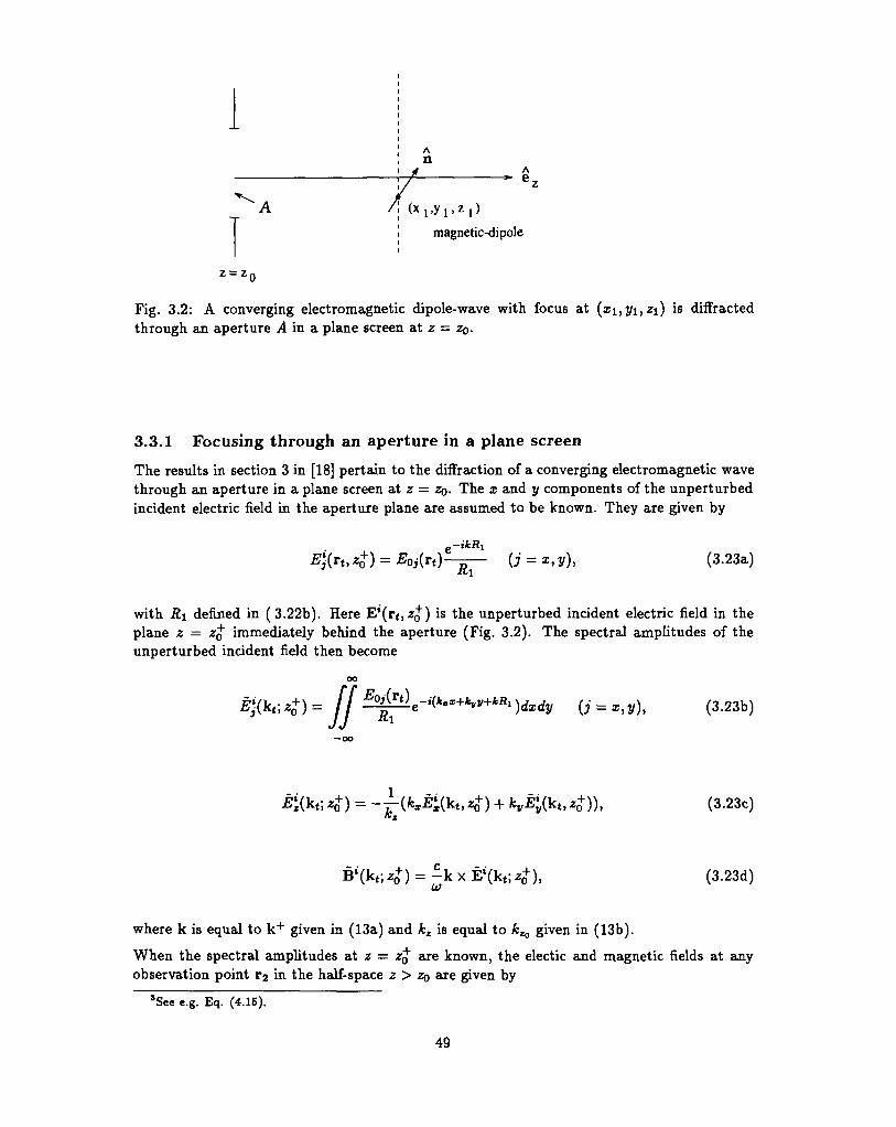
A
n A
e.
magnetic-dipole
z = z,
Fig. 3.2: A converging electromagnetic dipole-wave with focus atthrough an aperture A in a plane screen at z — ZQ.
is diffracted
3.3.1 Focusing through an aperture in a plane screen
The results in section 3 in [18] pertain to the diffraction of a converging electromagnetic wavethrough an aperture in a plane screen at z — ZQ. The x and y components of the unperturbedincident electric field in the aperture plane are assumed to be known. They are given by
E){rt, z+) = £o j( (j = x,y), (3.23a)
with Ri denned in (3.22b). Here E*(rt,.z^) is the unperturbed incident electric field in theplane z = z£ immediately behind the aperture (Fig. 3.2). The spectral amplitudes of theunperturbed incident field then become
)dxdy = x,y), (3.23b)
t. 4) (3.23c)
(3.23d)
where k is equal to k+ given in (13a) and kz is equal to k^ given in (13b).
When the spectral amplitudes at z = z£ are known, the electic and magnetic fields at anyobservation point r2 in the half-space z > ZQ are given by
sSee e.g. Eq. (4.15).
49
1 ff(r2) = {^f II £(kt;z+y^-T*<+k'^-«>»dkxdkv, (3.24a)
B(r2) = (^)2 if B(kt; z+)^^+k^-^dkxdkv, (3.24b)
wherer2 = r2e + z2ez ; r2t = x2ex + y2ey. (3.24c)
KirchhofF approximation of focused field
When the electric field E at z = z£ is known, we can, in accordance with Huygens's principle,express the fields at any observation point r2 in the half-space z > z£ as a superposition ofspherical waves. Thus we have [23]4, [18] 5
1 ff a eikR'E ( r 2 ) = " 2 ^ / / v(*>y>4)dr2(-RT)dxdy' (3-25a)
— oo
oo
ic d eikR*
where- x2y + (y - y2f + {z2 - 0o)2- (3.25c)
Now we use the Kirchhoff or physical-optics approximation according to which the electricfield ~E(x,y,z£) in the plane immediately behind the aperture is equal to the unperturbedincident electric field inside the aperture and is equal to zero outside the aperture, i.e.
inside Aoutside A
where A is the aperture area. Thus using the Kirchhoff approximation, we find that theelectric and magnetic fields at an observation point T2 are given by
h IL^x^zt)-kc:RT)dxdy' (3-27a)•Section 15.2.1(b)."section 2.1.2.
50
where Elj(x,y, z£) (j = x,y) is given by (3.23a). If Ez(x,y,Zo) is not given inside apertureA, it can be found from equation (2.24) in [18]. The superscript K in (3.27a-b) denotes thatthe fields are obtained using the Kirchhoff approximation.
Debye approximation of focused field
The Kirchhoff approximation to the x and y components of the spectral amplitude of theelectric field in the plane z = z£ is obtained from (3.23b) by limiting the integration over theaperture, i.e.
Ef(kt;z+) = I I M*lle-i('"*+k*«+kR^dxdy (j = x,y). (3.28)J J A -*M
When the Presnel number of the focused wave is sufficiently large, we can use the Debye ap-proximation as explained in [18], to obtain an approximate solution for the spectral amplitudein ( 3.28). Thus, we evaluate the integral in (3.28) by the method of stationary phase andpay attention only to the contribution from the interior stationary point, located at
k kx = x, = xi- ~-{zi -ZQ) y = y, = yi- ~{zi - ZQ). (3.29)
Kz Kz
Then the spectral amplitude in (3.23b) is given by [18]
^ l*t, z o ) - \ 0 o u t s i d e fll W - *>Vh (3.30a)
whereef(kx,ky) = Eoj(x.,y,) (j = x,y). (3.30b)
Here (xa,yt) is given by (3.29), and r i = {xi,2/1,21 - ZQ} is the position vector of the focalpoint. The superscript D in Ej3(kt;zo') and e^{kx,kv) signifies the use of the Debye approx-imation, and fii in ( 3.30a) is the solid angle subtended by the aperture at the focal point.Thus the fields in (3.24a) and (3.24b) become
^ (3.31a)
(3.31b)
51
whereeD(kX)ky) = {ef.e^.e?} bD(kx,kv) = {6?, 6°, 6?}. (3.31c)
Here ef (kx,kv) and bD(kx,ky) can be determined from e^(kx,kv) and e^(fcx>&v) using rela-tions analogous to (3.23b) and (3.23c), respectively, i.e.
«?(*-,*») = -^[*-«?(*-,*») + V?(*«.*v)]. (3.31d)
= - k x eD(ifcI, *„). (3.31e)
3.3.2 Focusing of converging magnetic-dipole waves
Consider now the idealized case in which the incident field is that of a converging magnetic-dipole wave. In analogy with the definition of a converging electric-dipole wave (cf. equations(4.5) and (4.6) in [18]), we define a converging magnetic-dipole wave whose electric and mag-netic distributions Ej^ and H£, in the plane z — ZQ are given by
Ecm(x,y,z+) = [Em(x,y,z+)]*, (3.32a)
Bcm(x, y, z+) = -[Bm(x, y, z+)]*, (3.32b)
where Em(x,y, z£) and Bm(x,y,Zo) are the fields radiated by a magnetic dipole situated atthe focal point (i i ,yi,^i). From (3.21a) and (3.21b), we have
p ' (e«i x »). (3.33a)ill
eikRiBc
m(x,y,z+) = mfik2—-—[eRl{eR, • n) - n], (3.33b)
K\
where GRX is defined in (3.22a).
Now we assume that the magnetic-dipole is polarized in the xy plane in a direction makingan angle 7 with the positive y axis, and an angle f +7 with the positive x axis. Thus, we have
n = - sin7ex + cos 7 ^ , (3.34a)
so that (22a) gives
eR l x n = —^-cos7ex —— s in7^ + (* Z l COS7+ V Vx sin7)ef. (3.34b)ttl iC\ K% Ki
52
By subtituting (3.34a) and (3.34b) in (3.33a) and (3.33b), we have
e~lkRt z0 - zx . z0 - zx .[ c o s 7 e s i[ R cos7ex
0 xcos7ex — - s i n 7 ^
(3.35a)
(3.35b)
Here the subscript m signifies that the fields are due to a magnetic-dipole wave and thesuperscript c signifies that the fields are converging.
If 7 = 0, so that the magnetic dipole is polarized in the positive y direction, then (3.35a) and(3.35b) become
(3.36b)
If 7 = 3TT/2, SO that the magnetic dipole is polarized in the positive x direction, then (3.35a)and (3.35b) become,
and
(3.37b)
Here the superscript 1 or j signifies that the polarization of the magnetic dipole is in thepositive x or y direction, respectively.
53
Kirchhoff approximation to focusing of converging magnetic-dipole wave
Let a magnetic dipole of strength m = l /(- iw) be located at the focal point, which weassume to be on the z axis, i.e. [x\,y\yz\) = (0,0, Zi). This particular strength factor ischosen to simplify the relations between the fields radiated by the magnetic dipole and thecorresponding fields radiated by an electric dipole of unit strength. When the incident electricfield E*(x,i/,Zo") is that of a converging magnetic-dipole wave polarised in the positive x or ydirection, ( 3.27a ) gives (with j=x,y)
E(*-')(r2) = --J JAE%(x,y)z+)-£-(—)dxdy. (3.38a)
In section 4.3 in [18], it was shown that when kRi > 1 and kR2 3* 1 a n d the observationpoint is close to the focal point, then instead of using (3.27b), we can write
(3.38b)
whereR2 - [(x2 - x)2 + (y2 - yf + (z2 - zo)
2f'2, (3.38c)
and where the superscript j — x,y denotes the polarization of the magnetic dipole.
By substituting ( 3.36a)-( 3.37b) in ( 3.38a)-( 3.38b), the focused electric and magnetic fieldsbecome
( 3 , 9 b )
( 3 , 9 d )
54
Debye approximation of converging magnetic-dipole wave
Let us assume that the Fresnel number of the converging magnetic-dipole wave is large enoughthat we can use the Debye approximation. From (3.23a), (3.30b), (3.29) with i i = j/i = 0,( 3.36), and ( 3.37) we then have
^ ^ e , - ^ } , (3.40a)
(jS - l)ev + ^ e , } , (3.40b)
(3.40c)
{f2 - l)ex + e y + * £ * , } . (3.40d)
To reduce the double integrals in (3.31a) and (3.31b) to single integrals, we follow the sameprocedure as for the electric dipole wave [18]. Thus, we introduce spherical coordinates r, 6,ij), centered at the focal point, i.e.
f = r2 — i"i = f[sin 6 cos <pex + sin0sin0ex + cos0ez], (3.41a)
and make the change of integration variables
kx = — fcsinacos/3 ; ky = -fcsinasin/3, (3.41b)
to obtain from (3.31a) and (3.31b)
E(D,V) = ztlt. P* f l s i n Q r c o s a ^ x + s i n a c o s p$. u*-*dad/3, (3.42)
2-KC Jo Jo
Bm >w) = -T1— I I s i n « { - s i n 2 a*™2P*x + [2 - sin2 a ( l - cos2/3)]ev47ra; Jo Jo
+ 2 sin a cos a sin f5ez}eiVidad/3, (3.43)
'x) = %— f f 1 sin a[cos aey + sin a sin /3e2]e*kf dad/3, (3.44)2xc JO Jo
55
B(D,x) _ J^_ /" * / ' s i n a{[2 _ Sin2 a ( l + cos 20)]ex - sin2 a sin 2/3e,,4xtL> Jo Jo
+ 2sinacosacos/3eI}e*kfdady(3) (3.45)
where
k • f = A:f[cos0cosa — sin 9 sin a cos (/? - <j>)]. (3.46)
The /3 integrals in (3.43)-( 3.46) can be expressed in terms of Bessel functions by means ofthe formulae [23]
/ cos (n/3) exp[-ii cos(/3 - j)]dp = 2*(-i)nJn(t) cos(n-y), (3.47a)Jo
[ *sin(n/9)exp[-i<cos(/3 --y)]d0 = 2*{-i)nJn{t) mn{ny)t (3.47b)Jo
where n is any integer and Jn(t) is the Bessel function of the first kind and order n. Thus(3.42)-( 3.45) become
ECD.v) =
- I2 cos2^]ev - 2i/1(1)sin ^e z } , (3.48b)
sin fc,}, (3.48c)
cos
where
= / ' sin a(2 - sin2 a) J0[ti{o.)]e^^W, (3.49a)
^2) = / l sin a cos a ^ [ ^ ( a ^ e ^ ^ d a , (3.49b)JO
56
* sin2 acosnaJilhia^e^^da (n = 0,1), (3.49c)
7 2 = [ * an3 aJ2[ti(a)]e&*Wda, (3.49d)Jo
withti(a) = kr sin. 6 sin a ; ^ (a ) = &f cos (? cos a. (3.49e)
Note that the integrals (3.49a)-(3.49e) are the same as those appearing in expressions for theconverging electric-dipole wave in [18]. In terms of the dimensionless optical coordinates uand v, we have [18]
(D, x fBl . ,~ . 5 >, ,»sina, r .ucosa.4 ' ( ) J (2 2 ) M ] [ ](D, x f . ,~ . 5 >, ,»sina, r .ucosa. , .4 '(«.«) - Jo *™ »(2 " sm2 a)M~^-] exP[2^2^-]da' (3-50a)
/"*l . T .usina, . .ucosa. , . , .= s inacosaJ0[^-7-]exp[i . ]da, (3.50b)
Jo sm ui sin c/i
rtn\, . rl . i „ , .Dsma. ..ucosa. , ,„ „„ .l\'(u,v)= sin2acosnaJi — exp i—r—- da. (3.50c)
Jo sin 0i sin1* 0i
r, - fSl • -K t rVsina. r . u c o s a . , /«»«,vI2{u,v)= sin3aJ2[ . ]exp[z . ](fa, (3.50d)
Jo sin &i sin PI
whereu = kf cos 0sin2 Oi = kz sin2 0i ; i = z2 - zx, (3.51a)
v = kf cos 0 sin 6i = kp sin 9i ; p = A / 1 ! + 2 • (3.51b)
Comparison with converging electric-dipole wave
In this section we compare the focused field of a converging electric-dipole wave with that ofa converging magnetic-dipole wave. In the Kirchhoff approximation, the focused fields due toa converging electric-dipole wave are [18]
57
(3,2c)
where the subscript e denotes that the fields are due to a converging electric-dipole wave, andwhere the superscript x or y denotes that the electric-dipole wave is polarized in the positivex or y direction, respectively.
By comparing (3.39a)-(3.39d) with (3.52a)-(3.52d), we see that
( 3 5 3 a )
, (3.53b)
E(K-,y) = B(jr,») | ( 3 5 3 c )
B|K*> = -EjflV). (3.53d)
Prom [18] we have the following expressions for the focused fields of a converging electricdipole wave in the Debye approximation:
7(i) + j2 c o s 2fax + I2 sin 2 ^ , - 2i/{1) cos e 2 } , (3.54a)
s i n ^ e z } , (3.54b)
58
s i n 2 ^ x + [7(i) _ h c o s
)cos fe}. (3.54d)
Here the subscript e denotes that the focused fields are due to a converging electric-dipolewave, whereas the superscript D denotes that the fields are valid in the Debye approximation.
By comparing ( 3.48a)-( 3.48d) with (3.54a)-( 3.54d), we see that the electric and magneticfields due to a converging electric-dipole wave and a converging magnetic-dipole wave aresimilarly related in the Debye and Kirchhoff approximations (cf.( 3.53)).
3.4 Focusing of converging mixed-dipole wave in the Debyeapproximat ion
In this section, we study the focusing properties of a converging mixed-dipole wave, whichSheppard and Larkins [19] referred to as the electromagnetic analogue of Stamnes1 [21] 'per-fect wave'. The term mixed-dipole wave refers to the sum of the fields radiated by an electricdipole and an orthogonal magnetic dipole. The objective in the remaining part of this paperis to compare the focusing charecteristics of mixed-dipole waves with those of electric-dipolewaves [18] and with the field obtained by focusing a linearly polarized plane wave in a rota-tionally symmetric, aplanatic system [3]. Since the numerical results in [18] and [3] are validonly in the Debye approximation, we restrict our attention here to the same approximation.
We consider first the case in which the electric dipole is polarized in the x direction, while andthe magnetic dipole is polarized in the y direction. Next, we let the electric dipole be polarizedin the y direction and the magnetic dipole be polarized in the x direction. In these two cases,the Debye representation of the focused fields due to a converging mixed-dipole wave can beobtained from (3.42)-(3.45) and equations (4.17)-(4.20) in [18]. Thus, by assuming that thefocal region is in air (n = 1 and k = ^ ) , we have with V — E, B
', (3.55a)
where
E(D,xy) _ - ^ I I l s i n a ^ 2 - sin2 a ( l + cos 2/3) + 2 cos a]ex - sin2 a sin 2/9ey
BJm'xv - -r— / / sina{-sin2asin2/3e I-(-[2cosa + 2-s in 2 a( l -cos2 /9) ]e v4xc Jo Jo
59
+ (2 sin a sin/? + 2 sin a cos a sin e j e ' * * dad/3, (3.55c)
' f *f ' f * sin a{-sin 2 a sin 2/3^ + [-2 cos a + 2 - sin2a(l + cos 2/3)]ey
2sinacosasin/3)e.t}e'k'1'da<£/3, (3.55d)
B(D,vx) _ _JL_ I / s i n a{[-2 cos a + 2 - sin2 a( l - cos 20)]ex - sin2 a sin 2/3ev4irc Jo JO
+ [2 sin a cos a cos /3 - 2 sin a cos /3]ez}e*kfdad^, (3.55e)
Here the subscript em denotes that the focused fields are due to a converging mixed-dipolewave. In the superscripts xy and yx the first letter denotes the polarization of the electricdipole and the second letter denotes the polarization of the magnetic dipole.
By expressing the integrals in (3.55b)-(3.55e) in terms of the Bessel functions using (3.47a)-( 3.47b), and then using the integrals in (3.50a)-(3.50d), we obtain
(IQ + I2 cos 24> + 2IQ ')ex + I2 sin 2 ^ , - 2i cos $(!{ ' + l[ )ez}, (3.56a)
cos 2^ - 27^2))eI + I2 sin 20ev + 2icos^(J1(0) - j f ^ e , } . (3.56d)
3.4.1 Polarization vector, strength factor, and energy projection
For the focused electric field in ( 3.55b) due to a converging mixed-dipole wave, the angulardistribution of the electric field over the converging spherical wave front in image space is
eem'xy^ — C{[1 -sin2 a cos2 /?+cos a]e s -sin2 a sin /? cos /3ev+[sin a cos a cos /3+sin a cos @]ez},(3.57)
60
where
C -. £*. ,3,8,
Now we write (3.57) in the form
£) (a)A"»(a,j3), (3.59)
where pxy(a) is a unit vector in the direction of polarization the plane wave exp(ik • r) in( 3.55b), which propagates in the k direction with a relative strength of . /^(a, /?) . Here thesuperscript xy denotes that the electric dipole is polarized in the positive x direction, whilethe magnetic dipole is polarized in the positive y direction.
Thuse£ l X v ) • e&*«>' = C2[A*«(aJ))2. (3.60)
By substituting (3.57) in (3.60) and solving for Axy(a,f3), we obtain
Axv{a, (3) = A^ia) = 2 cos2 a/2. (3.61)
Note that the strength factor Axy for a converging mixed-dipole wave is independent of theazimuth angle /?, whereas the strength factor for a converging electric-dipole wave depends onP [18]. The strength factor Axy(a) obtained here is in agreement with that given by Sheppardand Larkins [19], but is different from that of an aplanatic system [3], Using (3.57), (3.59),and (3.61), we find that the polarization vector of the converging mixed-dipole wave is givenby
px y(a) = 27—7^r{[l-sm2 a c o s 2 /3+cos a]ex—sin2 a sin/3 cosy3ev+[sin a cos a cos/?+sin a cos/3]ez},
(3.62a)
which can be written
2a) = [cosa + sin2/?(l - coso:)]ex - [(1 - cos a) sin /? cos /3}ey + (sinacos/?)^. (3.62b)
The polarization vector p ^ a ) for the converging mixed-dipole wave in ( 3.62b) is the sameas that for the converging electromagnetic wave in image space of the rotationally symmetricsystem analysed by Richards and Wolf [3] with the incident field linearly polarized in the xdirection. Note that this agreement holds only when the mixed-dipole wave is defined as thesum of the waves radiated by an electric dipole polarized in the positive x direction and amagnetic dipole polarized in the positive y direction.
For a converging mixed-dipole wave, the angular distribution of the electric field over theconverging spherical wave front in image space is given in (3.57). Suppose this electric-fielddistribution was obtained by focusing of a linearly polarized plane wave front by a rotationallysymmetric optical system. Then it would be of interest to know how rays, parallell to the
61
optical axis in object space, were projected on the converging spherical wave front in imagespace. Suppose this projection is given by
P = fg(a), (3.63)
where p is the height above the optical axis of a ray in object space, a is the correspondingangular coordinate of the ray in image space, and / is the radius of the converging sphericalwave front.
The projection g(a) is given by [23],
/if/vl n't r*\ i
(3.64)Si l l CL
where A(a) is the strength factor and Ao(p) is the amplitude of the incident wave. For aplane incident wave Ao(p) — 1, so that
For the xy-mixed dipole wave, it follows from (3.61) and (3.65) that
g(a) = 4 sin(a/2)[l - sin2 (a/2) + sm*[aM]k. (3.66)o
Note that this expression for g(a) for the xy-mixed dipole wave does not agree with that givenin [19], where the third term inside the square root in (3.66) is missing.
The expressions for A(a), p(a), and g(a) given in (3.61), (3.62b), and (3.66) are valid onlyfor that particular converging mixed-dipole wave which is due to an electric dipole polarizedin the positive x direction and a magnetic dipole polarized in the positive y direction. Notealso that to obtain these results the complex strength of the magnetic dipole must be a factori/u times the strength of the electric dipole. From symmetry considerations it follows fromthese results that if both dipoles are polarized in the focal plane [xy plane) and the magneticdipole is rotated relative to the electric dipole an angle ir/2 in the counter-clockwise directionas seen from the positive z axis, then A(a) and g(a) will be as gven in ( 3.61) and ( 3.66)respectively, and p(a) will be the same as that obtained when focusing a plane wave withlinear polarization in the direction of the electric dipole by a rotationally symmetric opticalsystem.
To show that the results described above do not hold for a converging mixed-dipole wavedue to any orthogonal pair of electric and magnetic dipoles, we now consider the convergingmixed-dipole wave due to an electric and a magnetic dipole polarized in the positve y and xdirections, respectively. We refer to this as the yx-mixed dipole wave. By proceeding in asimilar manner as described above for the xy-mixed dipole wave, we find
A*"(a) = 2 sin2 a/2, (3.67a)
62
pwx(a) = {-(1 + cosa)cos/?sin/3ex + [1 - (1 + cos a) sin2 @]ey - sinacos/3ez}, (3.67b)
where the superscript yx denotes that the electric dipole is polarized in the positive y direction,while the magnetic dipole is polarized in the positive x direction.
In this case it follows from (3.65) that
5(a) = 4= sin3 (a/2). (3.68)v3
Thus, these expressions for A(a), p(a), and g(a) are quite different from those obtained in thexy case. Assume now that in the focusing of a plane wave by a rotationally symmetric opticalsystem, the electric vector of the incident wave is linearly polarized in the positive y direction.By using the same technique as Richards and Wolf [3] and equations similar to (16.1c-d) in[23], one can show that the polarization vector of the electric field in the object space becomes
p(a) = — cos/3sin/3(l — cosa)ex + [1 - sin2/3(l — cosa)]ey + sinasin/?ez. (3.69)
Next, we assume that the converging mixed-dipole wave is due to an electric dipole polarizedin the positive y direcion and a magnetic dipole polarized in the negative x direction. Byassuming that 7 = TT/2 in (3.35a) and following the same procedure as above, one can showthat the angular distribution of the electric field due to this particular converging mixed-dipoleis given by an expression similar to that in (3.57), i.e.
e=m w'~x) = c i - s i n 2 a c o s P s i n P*x + [(1 - sin2 a sin2 /?) + cos a]ey + sin a ( l + cos a) sin /3ez},(3.70a)
where the superscript y, —x denotes that the electric-dipole is polarized in the positive ydirection, while the magnetic dipole is polarized in the negative x direction. One can showthat the strength factor obtained in this case is the same as in the xy case, i.e.
Av'—(a) = 2 cos2 a/2, (3.70b)
and that the polarization vector is given by
pVl~x(a) = — cos/3sin/3(l — cosa)ex + [1 - sin2/3(l - cosa)]ev + sinasin/3ez. (3.70c)
We see that the polarization vector pVl x(a) of the electric field of a converging mixed-dipolewave, which is due to an electric dipole polarized in the positive y direction and a magneticdipole polarized in the negative x direction, is the same as that given in (3.69) for the electricfield in the image space of a rotationally symmetric system when the incident electric vectoris polarized in the positive y direction. Thus, we can conclude that the polarization of aconverging mixed-dipole wave is the same as that for the electric field in the image space ofa rotationally symmetric system, provided that the electric dipole has the same polarization
63
as the incident field in the object space of the rotationally symmetric system, and providedthat the magnetic dipole has a strength i/u times the strength of the electric dipole and ispolarized in the direction making a positive angle of w/2 with that of the electric dipole.
3.4.2 Energy densities
By assuming that e — fi = n = 1, the time-averaged electric and magnetic energy densitiesare given by
< w,(u,v,4>) >= - ^ - E • E*, (3.71a)
< wm(u,v,j>) >= - | - H • HV (3.71b)
For the focused field of a converging mixed-dipole wave, we find by substituting ( 3.56a)-(3.56b) in (3.71a)-(3.71b)
< wV{u,v,4>) >=
+ 4 cos 24>Re{I2#)*} + 4 cos2 4>[\l[O)\2 + |/|X)|2 + 2Re{l[0)l[1)*}}}, (3.72a)
and
( M l f t >= JL{!j!-r{\$)\* + \I2\* + 4|42V - 2cos2^e{41)j-} + iRe{I^I^}
2 ^ | 0 ) 2 ^ 2 71(0)71
(1)*}]}> (3.72b)
where Re denotes the real part.
From (3.72a) and (3.72b) we see that the time-averaged electric and magnetic energy densitiesare same in the focal region, except that they are rotated with respect to each other by anangle of x/2 about the optical axis, i.e.
< w%(u,v,4>) >=< w?(u,vj- | ) > . (3.73)
The relation is the same for the rotationally symmetric, aplanatic system considered byRichards and Wolf [3]. But no such simple relationship exists for the focused fields dueto a converging electric-dipole or magnetic-dipole wave.
The total time-averaged energy density < ry*v(u, v,<f>) > can be determined from
< •u/sv(u,v,^) >=< vi?(u,v,4t) > + < w%{u,v,j>) >, (3.74a)
64
which using ( 3.72a) and ( 3.72b) gives
*y(,v,}) >= ±-(£-)>{\lU\> + |72|2 + 4|7<2>|2
l[0)l[1>}}. (3.74b)
As in the case of a rotationally symmetric, aplantic system, the total time-averaged energydensity in ( 3.72b) for the converging mixed-dipole wave is independent of <j>, whereas itdependents on <j> both in case of a converging electric-dipole [18] or magnetic-dipole wave.
Along the optical axis T; = 0, it follows from (3.50c) and (3.50d) that /{ n ) = 0 (n = 0,1) andI2 - 0, so that we obtain the following time-averaged energy densities from (3.72)-( 3.74b)
^ ^ ^ 4 2 ) W}], (3.75a)
(3.75b)
(«,0,*) = ^(^)2[l41 } |2 + 4|42)|2 + 4 J t e{ iW}] , (3.75c)
From ( 3.75a)-( 3.75c) we observe that along the optical axis the time-averaged electric andmagnetic energy densities are the same and equal to half the total energy density.
From now on we drop the superscript xy, since all analytical and numerical results to followare due to the converging mixed-dipole wave for which the electric dipole is polarized in thepositive x direction, while the magnetic dipole is polarized in the positive y direction.
Poynting Vector
The Poynting vector < S > is given by
< S >= ^-Re{E X H*}. (3.76a)
By substituting (3.56a)-( 3.56b) with e = jj = n = l i n ( 3.76a), we find for the focused fieldsof the converging mixed-dipole wave
5, >= - I ^ { 0 ^ ( | { ) ^ ( | { ) ( 2 ^(3.76b)
65
Sy >= j ^ - c Im {sinfa$> +7 2 cos 2^ + 27<2)][71(0)* + /j1)*) + sin 2^cos #7a
(0 ) + l[l))I2*},(3.76c)
* >= ^^JRe{(41)+/2cos2<^+242))(41) '-/2*cos2^+242)*)-sin220|/2 |2}. (3.76d)
where Re and 7m denote the real and the imaginary part, respectively. After some algebra(3.76b)-(3.76d) become
>= J^rc^4> Irn {(7<0> + l[\i; - 41)* - 242)*)}, (3.77a)
<SV>= ^ sin4> Im {(/|°> + lM)(i; - #>* - 2I&*)}, (3.77b)
}, (3.77c)
and the magnitude squared of the Poynting vector becomes
l< S > |2 = (J^J'flltfV - |72|2 + 4|42)|2 + ABeifiW}]*
W $) $? ^)})*}. (3.77d)
Note that the magnitude of the Poynting vector is independent of <j>. Thus, it is symmetricabout the optical axis as in the case of the rotationally symmetric, aplanatic system treatedin [3,4].
Along the optical axis v = 0, l[n^ = 0 (n = 0,1) and 72 = 0, so that < Sx > = < Sy >= 0, andthe magnitude of the Poynting vector becomes
4> W}}. (3-78)
Comparing (3.78) with (3.77c), we note that along the optical axis, we have
| < S > | = | < S z > | = c < ' u ; > . (3.79)
Next, we determine the direction of energy flow in the focal plane u = 0. From ( 3.50) it
66

follows that all integrals appearing in (3.77a)-(3.77c), are real when u = 0, so that we get
< Sx{0,v,<j>) >=< Sy{O,v,<j>) >= 0, (3.80a)
so that< 5(0,v,4>)>=< 5,(0,v,4)>. (3.80b)
This means that the energy flow is normal to the focal plane, and its magnitude is determinedby the values of the integrals I^\l^2\ and 72 in (3.77c). Thus, from (3.79) and (3.80b), weconclude that both along the optical axis and in the focal plane the energy flow is parallel tothe optical axis.
67
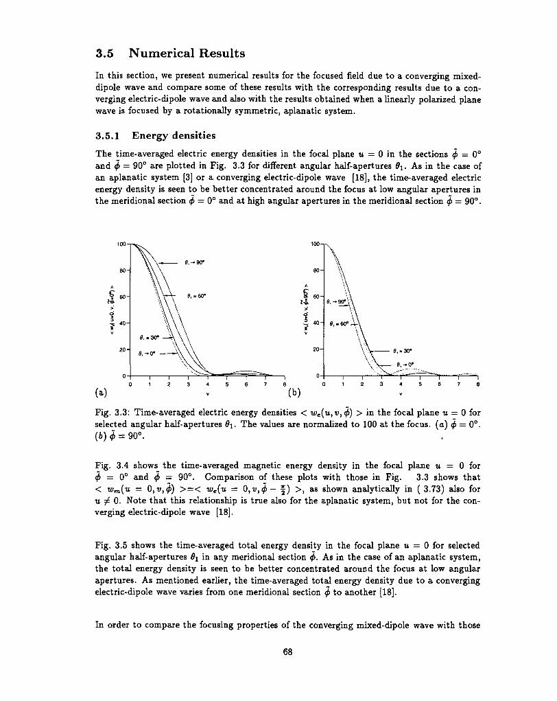
3.5 Numerical Results
In this section, we present numerical results for the focused field due to a converging mixed-dipole wave and compare some of these results with the corresponding results due to a con-verging electric-dipole wave and also with the results obtained when a linearly polarized planewave is focused by a rotationally symmetric, aplanatic system.
3.5.1 Energy densities
The time-averaged electric energy densities in the focal plane u = 0 in the sections <j> = 0°and $ = 90° are plotted in Fig. 3.3 for different angular half-apertures B\. As in the case ofan aplanatic system [3] or a converging electric-dipole wave [18], the time-averaged electricenergy density is seen to be better concentrated around the focus at low angular apertures inthe meridional section 4> — 0° and at high angular apertures in the meridional section (f> = 90°.
8,-»90°
100 -i
6 0 -e, - 9 0 - Y
8 , . 60* - i
i i i i i i i i0 1 2 3 4 5 6 7 8
Fig. 3.3: Time-averaged electric energy densities < we(u,v,<j>) > in the focal plane u = 0 forselected angular half-apertures 0\. The values are normalized to 100 at the focus, (a) <p — 0°.(6) j> = 90°.
Fig. 3.4 shows the time-averaged magnetic energy density in the focal plane u = 0 for0 = 0° and <j> — 90°. Comparison of these plots with those in Fig. 3.3 shows that< wm(u = 0,v,4>) >=< we(u = 0,t;,^— y) >, as shown analytically in (3.73) also foru / 0 . Note that this relationship is true also for the aplanatic system, but not for the con-verging electric-dipole wave [18].
Fig. 3.5 shows the time-averaged total energy density in the focal plane u — 0 for selectedangular half-apertures 6\ in any meridional section 4>. As in the case of an aplanatic system,the total energy density is seen to be better concentrated around the focus at low angularapertures. As mentioned earlier, the time-averaged total energy density due to a convergingelectric-dipole wave varies from one meridional section ^ to another [18].
In order to compare the focusing properties of the converging mixed- dipole wave with those
68
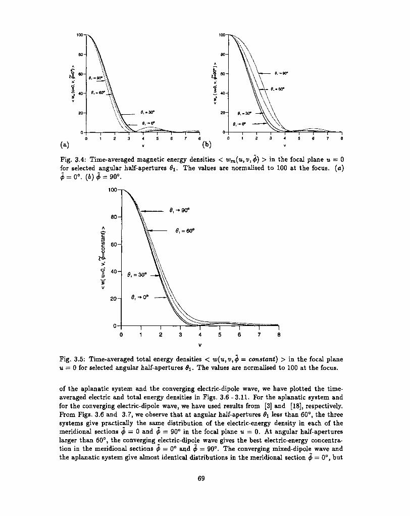
Fig. 3.4: Time-averaged magnetic energy densities < wm(u, v, 4>) > in the focal plane u = 0for selected angular half-apertures 6\. The values are normalised to 100 at the focus, (a)£ = 0°. (6) £ = 90°.
100n
8 0 -
60 -
4 0 -
2 0 -
Fig. 3.5: Time-averaged total energy densities < u;(«,u,^ = constant) > in the focal planeu = 0 for selected angular half-apertures d\. The values are normalised to 100 at the focus.
of the aplanatic system and the converging electric-dipole wave, we have plotted the time-averaged electric and total energy densities in Figs. 3.6 -3.11. For the aplanatic system andfor the converging electric-dipole wave, we have used results from [3] and [18], respectively.From Figs. 3.6 and 3.7, we observe that at angular half-apertures 6\ less than 60°, the threesystems give practically the same distribution of the electric-energy density in each of themeridional sections 4> = 0 and 4> = 90° in the focal plane u = 0. At angular half-apertureslarger than 60°, the converging electric-dipole wave gives the best electric-energy concentra-tion in the meridional sections ^ = 0° and <j> — 90°. The converging mixed-dipole wave andthe aplanatic system give almost identical distributions in the meridional section $ = 0°, but
69
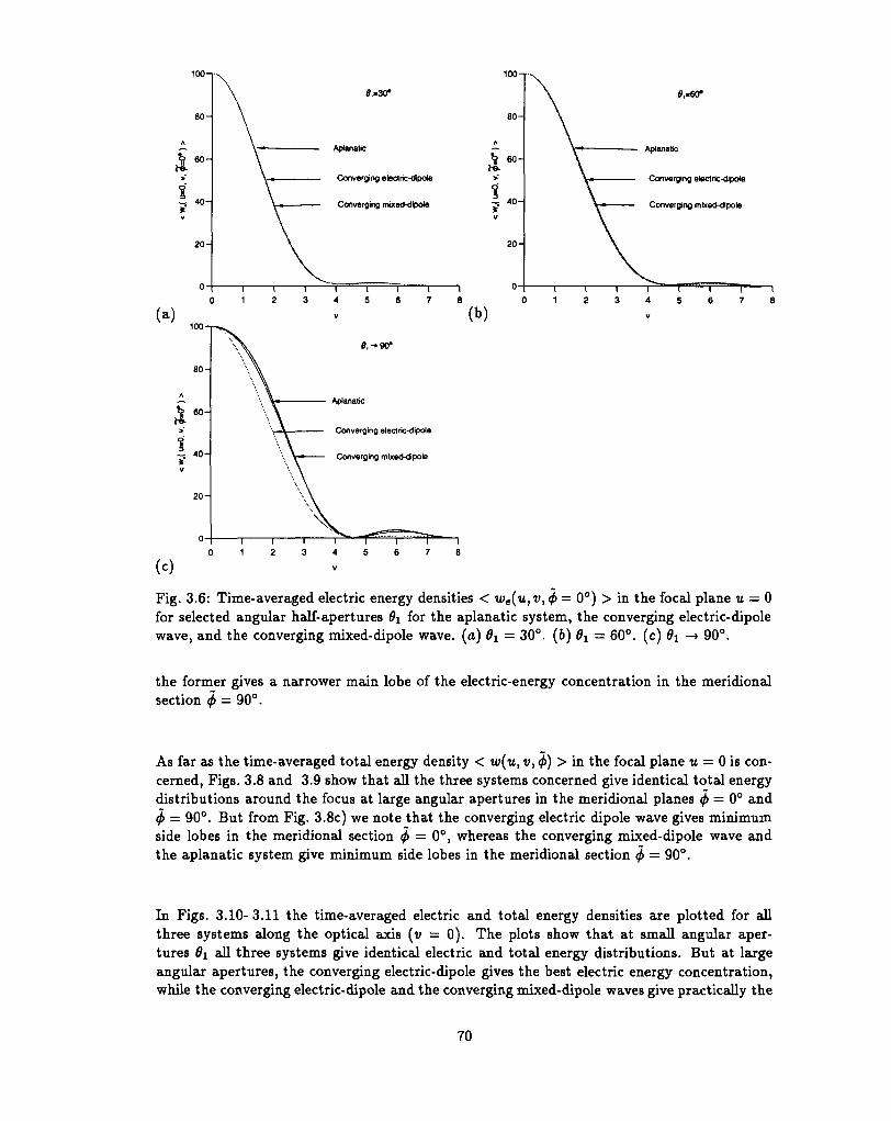
100-r
9,-30*
Aplanatlc
Converging electric-dipole
Converging mixed-dipole
Aplanatic
Converging electric-dipole
Converging mixed-dipole
0 1 2 3 4 S 6 7
100-1
80-
60-
~ 40-
20-
Aplanatic
Converging electric-dipole
Converging mixed-dipole
Fig. 3.6: Time-averaged electric energy densities < we(u, v, <}> = 0°) > in the focal plane u — 0for selected angular half-apertures 9i for the aplanatic system, the converging electric-dipolewave, and the converging mixed-dipole wave, (a) 9X = 30°. (6) 6X = 60°. (c) 8X -> 90°.
the former gives a narrower main lobe of the electric-energy concentration in the meridionalsection <f> - 90°.
As far as the time-averaged total energy density < w(u, v, 4>) > in the focal plane u — 0 is con-cerned, Figs. 3.8 and 3.9 show that all the three systems concerned give identical total energydistributions around the focus at large angular apertures in the meridional planes ^ = 0° and4> = 90°. But from Fig. 3.8c) we note that the converging electric dipole wave gives minimumside lobes in the meridional section ^ = 0°, whereas the converging mixed-dipole wave andthe aplanatic system give minimum side lobes in the meridional section <f> = 90°.
In Figs. 3.10- 3.11 the time-averaged electric and total energy densities are plotted for allthree systems along the optical axis (v = 0). The plots show that at small angular aper-tures 6\ all three systems give identical electric and total energy distributions. But at largeangular apertures, the converging electric-dipole gives the best electric energy concentration,while the converging electric-dipole and the converging mixed-dipole waves give practically the
70
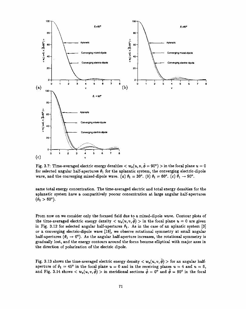
fl,«30*
Aplanatic
Converging mbted-dipole
Converging electric-dipole
100n
80-
60-^s•
40-
20 -
fl,.6O*
Aplanatic
Converging mixed-dipole
Converging electric-dipole
Fig. 3.7: Time-averaged electric energy densities < we{u, v,4> — 90°) > in the focal plane u = 0for selected angular half-apertures #i for the aplanatic system, the converging electric-dipolewave, and the converging mixed-dipole wave, (a) $i - 30°. (b) #i = 60°. (c) 6X -> 90°.
same total energy concentration. The time-averaged electric and total energy densities for theaplanatic system have a comparitively poorer concentration at large angular half-apertures(0i > 60°).
From now on we consider only the focused field due to a mixed-dipole wave. Contour plots ofthe time-averaged electric energy density < we(u,v,<i>) > in the focal plane u = 0 are givenin Fig. 3.12 for selected angular half-apertures &i. As in the case of an aplantic system [3]or a converging electric-dipole wave [18], we observe rotational symmetry at small angularhalf-apertures (0i —> 0°). As the angular half-aperture increases, the rotational symmetry isgradually lost, and the energy contours around the focus become elliptical with major axes inthe direction of polarization of the electric dipole.
Fig. 3.13 shows the time-averaged electric energy density < we(u, v,<f>) > for an angular half-aperture of $i = 45° in the focal plane u = 0 and in the receiving planes u = 4 and u = 6,and Fig. 3.14 shows < we(u,v,<f>) > in meridional sections 0 = 0° and 0 = 90° in the focal
71
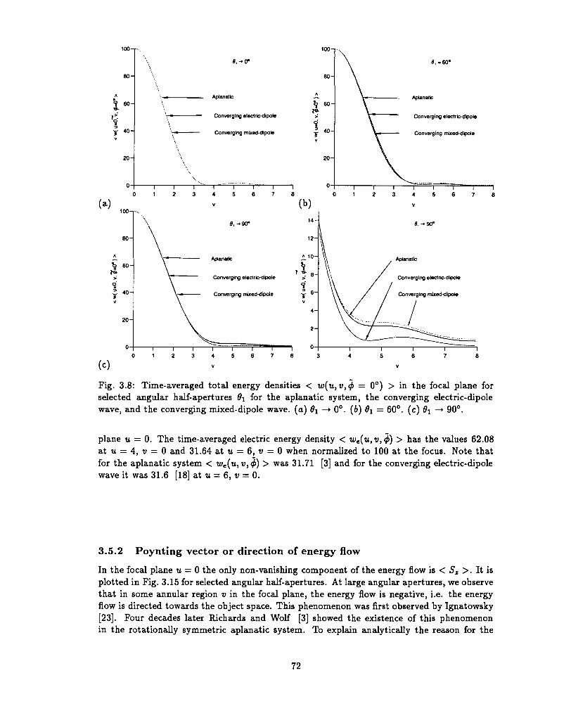
60-
60 -
2 0 -
0 -
\
\
\\\
1 1 1
Aplanatic
Converging electric-dipole
Converging mixed-dipote
I I I I
60-
40-
20 -
6,-60"
Aplanatic
Converging electrtc-dipole
Converging mixed-dipole
V
9 , - > 9 0 *
Aplanatic
Converging electric-dipole
Converging mixed-dipole
(b)
14-
12-
^ 1 0 -
T 6 "
4 -
2 -
0
3 4 5 6v
Aplanatic
Converging electric-dipole
Converging mixed-dipole
Fig. 3.8: Time-averaged total energy densities < w{u,v,4> = 0°) > in the focal plane forselected angular half-apertures 0\ for the aplanatic system, the converging electric-dipolewave, and the converging mixed-dipole wave, (a) 6X -+ 0°. (6) 0\ = 60°. (c) 0a -> 90°.
plane u = 0. The time-averaged electric energy density < we(u, v,<j>) > has the values 62.08at u = 4, v = 0 and 31.64 at u — 6, v — 0 when normalized to 100 at the focus. Note thatfor the aplanatic system < we(u,v,<i)) > was 31.71 [3] and for the converging electric-dipolewave it was 31.6 [18] at u = 6, v = 0.
3.5.2 Poynting vector or direction of energy flow
In the focal plane u = 0 the only non-vanishing component of the energy flow is < Sz >. It isplotted in Fig. 3.15 for selected angular half-apertures. At large angular apertures, we observethat in some annular region v in the focal plane, the energy flow is negative, i.e. the energyflow is directed towards the object space. This phenomenon was first observed by Ignatowsky[23]. Four decades later Richards and Wolf [3] showed the existence of this phenomenonin the rotationally symmetric aplanatic system. To explain analytically the reason for the
72
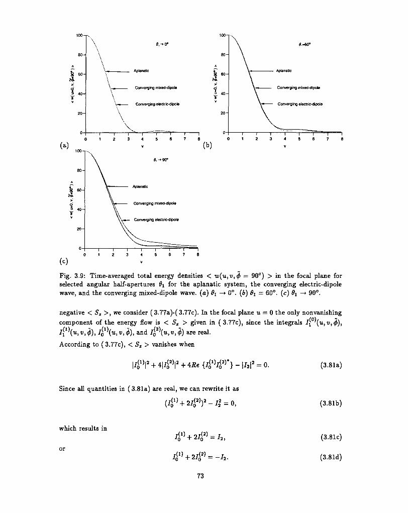
10O n
80 -
60-
40-
AplanaOc
Converging mixed-dlpole
Converging electrc-dipole
9, -»90*
AplanaBc
Converging mixed-dipole
Converging electric-dipole
0,-60°
Aplanatc
Converging mixed-dipole
Converging electric-dipole
Fig. 3.9: Time-averaged total energy densities < w(u, v,<j) — 90°) > in the focal plane forselected angular half-apertures 9\ for the aplanatic system, the converging electric-dipolewave, and the converging mixed-dipole wave, (a) 8i —* 0°. (b) 6i = 60°. (c) Q\ —* 90°.
negative < Sz >, we consider (3.77a)-( 3.77c). In the focal plane u — 0 the only nonvanishingcomponent of the energy flow is < Sz > given in ( 3.77c), since the integrals /} \u, v,4>),I?\u,v,j>), l£\u,v,i>), and I{*\u,v,4>) are real.
According to (3.77c), < Sz> vanishes when
(3.81a)
Since all quantities in (3.81a) are real, we can rewrite it as
(3.81b)
which results in
or
(3.81c)
(3.81d)
73
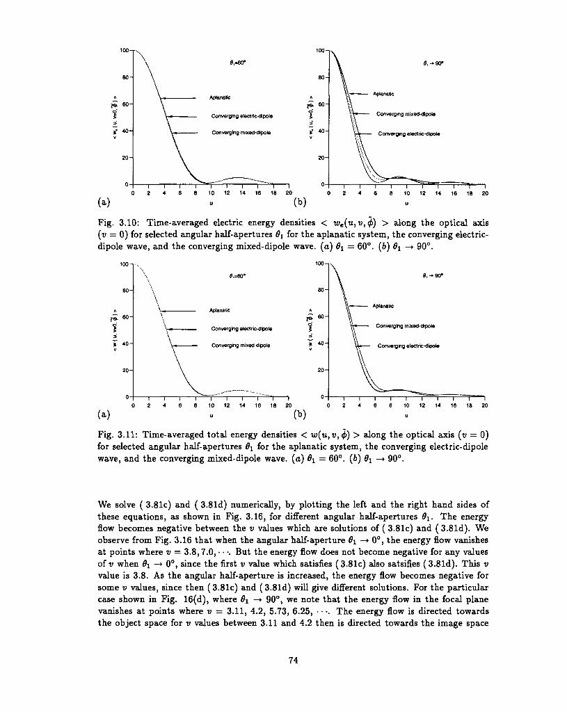
100-r
80-
«H
40H
20-
Aplanatic
Converging electric-dipole
Converging mixed-dipole
(a)6 8 10 12 U 16 18 20
6, - 9 0 "
Aplanatic
Converging mixed-dipole
Converging electric-dipole
Fig. 3.10: Time-averaged electric energy densities < we(u, v,<j>) > along the optical axis(v = 0) for selected angular half-apertures 8\ for the aplanatic system, the converging electric-dipole wave, and the converging mixed-dipole wave, (a) 8i = 60°. (6) 0i —> 90°.
80
6 0 -
20-
100-1
Aplanatic
Converging electric-dipole
Converging mixed-dipole
13
T
20-
Aplanatic
Converging mixed-dipole
Converging electric-dipole
(a)6 8 10 12 14 16 18 20
(b)
~l 1 1 1 1 1 I I6 8 10 12 14 16 18 20
Fig. 3.11: Time-averaged total energy densities < w(u,v,<f>) > along the optical axis (v = 0)for selected angular half-apertures $i for the aplanatic system, the converging electric-dipolewave, and the converging mixed-dipole wave, (a) 6\ — 60°. (6) 9\ —* 90°.
We solve ( 3.81c) and ( 3.81d) numerically, by plotting the left and the right hand sides ofthese equations, as shown in Fig. 3.16, for different angular half-apertures 9\. The energyflow becomes negative between the v values which are solutions of (3.81c) and (3.81d). Weobserve from Fig. 3.16 that when the angular half-aperture $i —> 0°, the energy flow vanishesat points where v = 3.8,7.0, • • •. But the energy flow does not become negative for any valuesoft; when 9\ —> 0°, since the first v value which satisfies (3.81c) also satsifies (3.81d). This vvalue is 3.8. As the angular half-aperture is increased, the energy flow becomes negative forsome v values, since then (3.81c) and (3.81d) will give different solutions. For the particularcase shown in Fig. 16(d), where $i —> 90°, we note that the energy flow in the focal planevanishes at points where v = 3.11, 4.2, 5.73, 6.25, • • •. The energy flow is directed towardsthe object space for v values between 3.11 and 4.2 then is directed towards the image space
74
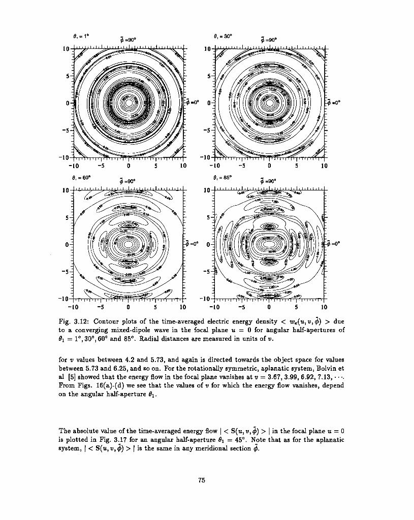
10
•4=0°
0=90°i I i I ( I i I i I | I i I i I i I I I I I I | i I i ) i I i I < I i I i I iI I < I t I I I I I ] I I I I I I I I I ( I I I I I I I I I I I I I I I I I I
-10 -5
Fig. 3.12: Contour plots of the time-averaged electric energy density < we(u, v,<f>) > dueto a converging mixed-dipole wave in the focal plane u = 0 for angular half-apertures of#i — l°,30°,60° and 85°. Radial distances are measured in units oft;.
for v values between 4.2 and 5.73, and again is directed towards the object space for valuesbetween 5.73 and 6.25, and so on. For the rotationally symmetric, aplanatic system, Boivin etal [5] showed that the energy flow in the focal plane vanishes at v = 3.67, 3.99, 6.92, 7.13, • • •.From Figs. 16(a)-(d) we see that the values of v for which the energy flow vanishes, dependon the angular half-aperture 9\.
The absolute value of the time-averaged energy flow | < S(w, v, (j>) > | in the focal plane u = 0is plotted in Fig. 3.17 for an angular half-aperture 6\ = 45°. Note that as for the aplanaticsystem, | < S(u, v, <j>) > \ is the same in any meridional section ^.
75
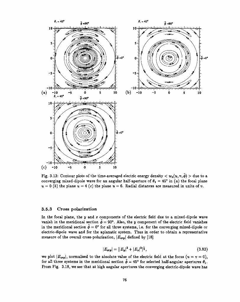
0, = 45° 0, = 45"
-10(a) -10 -5
e, = 45°
-10(b) -10
4=0°
- 5 -
-10(c) -10 -5 10
Fig. 3.13: Contour plots of the time-averaged electric energy density < we(u,v,<f>) > due to aconverging mixed-dipole wave for an angular half-aperture of 0\ = 45° in (a) the focal planeu = 0 (6) the plane u = 4 (c) the plane u = 6. Radial distances are measured in units of v.
3.5.3 Cross polarization
In the focal plane, the y and z components of the electric field due to a mixed-dipole wavevanish in the meridional section ^ = 90°. Also, the y component of the electric field vanishesin the meridional section ^ = 0° for all three systems, i.e. for the converging mixed-dipole orelectric-dipole wave and for the aplanatic system. Thus in order to obtain a representativemeasure of the overall cross-polarization, |l?crp| denned by [18]
\Ecrp\ = [\Ev\2 + \Ez\
2]k, (3.82)
we plot |£crp|, normalised to the absolute value of the electric field at the focus (u = v = 0),for all three systems in the meridional section $ = 45° for selected half-angular apertures 9\.From Fig. 3.18, we see that at high angular apertures the converging electric-dipole wave has
76
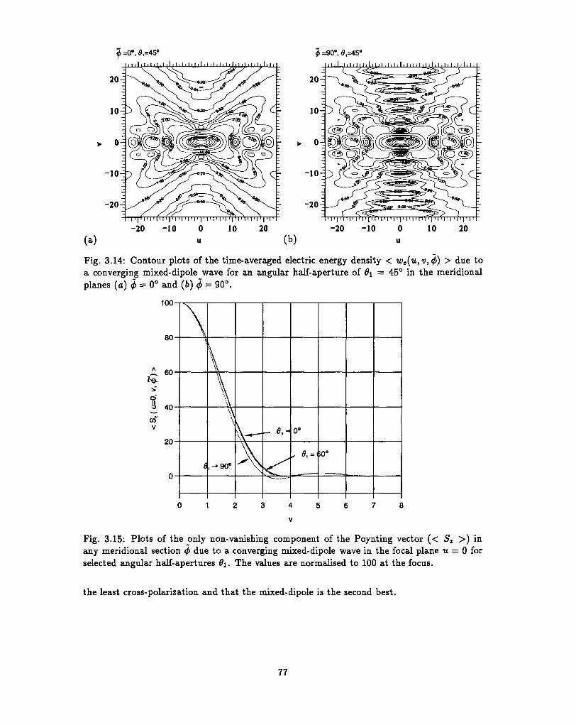
0 =0°, 0,=45°l I 1 I I I > I i I I I i I I I t I I I i I t I I I I I I I I I I I I I I I I I I I I
=90°, 0,=45°1 1 1 1 1 1 1 1 1 1 1 1 1 1 1 1 1 1 1 1 1 1 1 1 1 1 1 1 1 1 1 1 1 1 i 1 1 1 1 1 1 1 , 1 1 1 1
Fig. 3.14: Contour plots of the time-averaged electric energy density < we(u,v, <j>) > due toa converging mixed-dipole wave for an angular half-aperture of $i = 45° in the meridionalplanes (a) </> = 0° and (b) </> = 90°.
100-
80-
1 60-
I 40-
20-
\1
e
\\\
\
1-»90°
V-\
_ fl.H 0°
, s, =>0°
0 1 2 3 4 5 6 7 8
V
Fig. 3.15: Plots of the only non-vanishing component of the Poynting vector (< St >) inany meridional section ^ due to a converging mixed-dipole wave in the focal plane u = 0 forselected angular half-apertures Oi. The values are normalised to 100 at the focus.
the least cross-polarization and that the mixed-dipole is the second best.
77
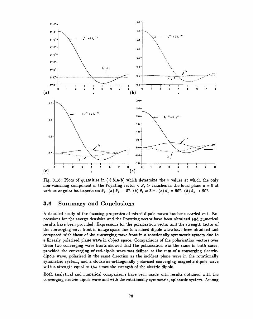
Fig. 3.16: Plots of quantities in ( 3.81a-b) which determine the v values at which the onlynon-vanishing component of the Poynting vector < Sz > vanishes in the focal plane u = 0 atvarious angular half-apertures $i. (a) 9i -> 0°. (6) 0i = 30°. (c) 0x = 60°. (d) 0a -> 90°.
3.6 Summary and Conclusions
A detailed study of the focusing properties of mixed-dipole waves has been carried out. Ex-pressions for the energy densities and the Poynting vector have been obtained and numericalresults have been provided. Expressions for the polarization vector and the strength factor ofthe converging wave front in image space due to a mixed-dipole wave have been obtained andcompared with those of the converging wave front in a rotationally symmetric system due toa linearly polarized plane wave in object space. Comparisons of the polarization vectors overthese two converging wave fronts showed that the polarization was the same in both cases,provided the converging mixed-dipole wave was denned as the sum of a converging electric-dipole wave, polarized in the same direction as the incident plane wave in the rotationallysymmetric system, and a clockwise-orthogonally polarized converging magnetic-dipole wavewith a strength equal to i/cj times the strength of the electric dipole.
Both analytical and numerical comparisons have been made with results obtained with theconverging electric-dipole wave and with the rotationally symmetric, aplanatic system. Among
78
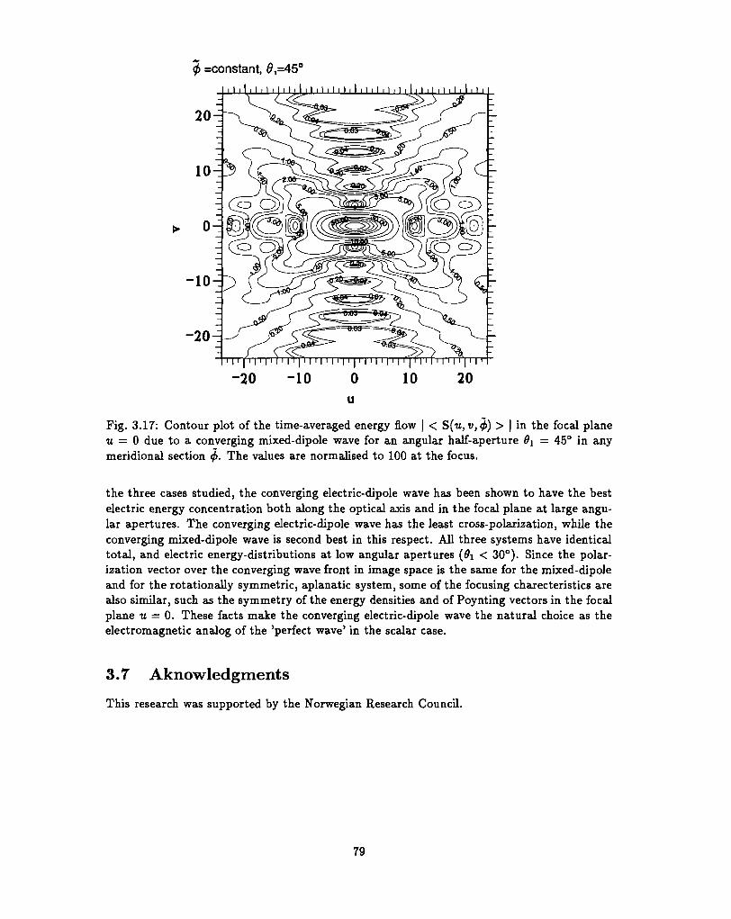
=constant, 0,=45°
1 1 1 1 1 1 1 1 1 1 1 1 1 1 1 1 1 1 1 1 1 1 1 1 1 1 1 1
20-
-20 -
-20 -10 10 20u
Fig. 3.17: Contour plot of the time-averaged energy flow | < S(u, v, <f>) > | in the focal planeu = 0 due to a converging mixed-dipole wave for an angular half-aperture 0^ = 45° in anymeridional section <f>. The values are normalised to 100 at the focus.
the three cases studied, the converging electric-dipole wave has been shown to have the bestelectric energy concentration both along the optical axis and in the focal plane at large angu-lar apertures. The converging electric-dipole wave has the least cross-polarization, while theconverging mixed-dipole wave is second best in this respect. All three systems have identicaltotal, and electric energy-distributions at low angular apertures (0i < 30°). Since the polar-ization vector over the converging wave front in image space is the same for the mixed-dipoleand for the rotationally symmetric, aplanatic system, some of the focusing charecteristics arealso similar, such as the symmetry of the energy densities and of Poynting vectors in the focalplane u = 0. These facts make the converging electric-dipole wave the natural choice as theelectromagnetic analog of the 'perfect wave' in the scalar case.
3.7 Aknowledgments
This research was supported by the Norwegian Research Council.
79
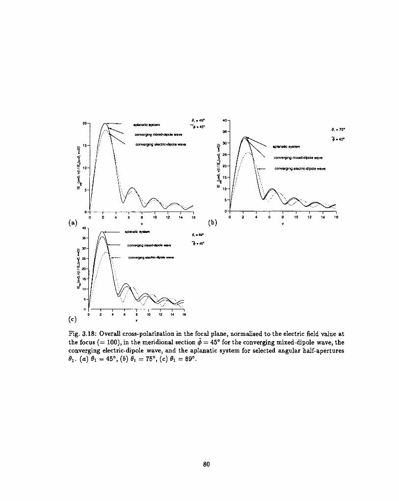
aplanatic system
converging mbced-dipole wave
converging electric-dipole wave
convafging rmxaCKapoM vmva
converging atectric-dipoi* way*
fl, - 7 5 '
aplanatic system
converging mixed-dipole wave
converging electric-dipole wave
10 16
Fig. 3.18: Overall cross-polarization in the focal plane, normalised to the electric field value atthe focus (= 100), in the meridional section $ = 45° for the converging mixed-dipole wave, theconverging electric-dipole wave, and the aplanatic system for selected angular half-apertures0i. (a) 0a = 45°, (b) 0x = 75°, (c) Ox = 89°.
80
Bibliography
[1] V. S. Ignatowsky. Trans. Opt. Inst. Petrograd I, paper IV, 1919.
[2] V. S. Ignatowsky. Trans. Opt. Inst. Petrograd I, paper V, 1920.
[3] B. Richards and E. Wolf. Electromagnetic diffraction in optical systems II. Structure ofthe image field in an aplanatic system. Proc. R. Soc. A 253, 358-379, 1959.
[4] A. Boivin and E. Wolf. Electromagnetic field in the neighborhood of the focus of acoherent beam. Phys. Rev. 1385, 1561-1565, 1965.
[5] A. Boivin, J. Dow, and E. Wolf. Energy flow in the neighborhood of the focus of acoherent beam. J. Opt. Soc. Am. A 57B, 1171-1175, 1967.
[6] D. J. Innes and A. L. Bloom. Design of optical systems for use with laser beams. Spectra-Physics Laser Tech. Bull 5, 1-10, 1966.
[7] A. Yoshida and T. Asakura. Electromagnetic field in the focal plane of a coherent beamfrom a wide-angular annular-aperture system. Optik, 40, 322-331, 1974.
[8] M. Mansuripur. Certain computational aspects of vector diffraction problems. J. Opt.Soc. Am. A 6, 786-805, 1989.
[9] R. Kant. An analytical solution of vector diffraction problems for focusing optical systems.J. Mod. Opt. 40, 337-347, 1993.
[10] C. J. R. Sheppard, A. Choudhury, and J. Gannaway. Electromagnetic field near thefocus of wide-angular annular lens and mirror systems. J. Micro. Optics and Acoustics,1, 129-132, 1977.
[11] R. Kant. An analytical solution of vector diffraction for focusing optical systems withseidel aberrations I. Spherical aberration, curvature of field, and distortion. J. Mod. Opt.40, 2293-2310, 1993.
[12] R. Kant. An analytical solution of vector diffraction for focusing optical systems withSeidel aberrations. II. astigmatism and coma. J. Mod. Opt. 42, 299-320, 1995.
[13] T. D. Visser and S. H. Wiersma. Spherical aberration and the electromagnetic field inhigh aperture systems. J. Opt. Soc. Am. A 8, 1404-1410, 1991.
[14] T. D. Visser and S. H. Wiersma. Diffraction of converging electromagnetic waves. J.Opt. Soc. Am. A 9, 2034-2047, 1992.
[15] T. D. Visser and S. H. Wiersma. Electromagnetic description of the image formation inconfocal fluorescence microscopy. J. Opt. Soc. Am. A 11, 599-608, 1994.
81
[16] H. Ling and S. W. Lee. Focusing of electromagnetic waves through a dielectric interface.J. Opt. Soc. Am. A 1,965-973, 1984.
[17] P. Tdrok, P. Varga, Z. Laczic, and G. R. Booker. Electromagnetic diffraction of lightfocused through a planar interface between materials of mismatched refractive indices:an integral reperesentation. J. Opt. Soc. Am. A 12, 325-332, 1995.
[18] J. J. Stamnes and V. Dhayalan. Focusing of electric-dipole waves. Pure Appl. Opt. 5,195-226, 1996.
[19] C. J. R. Sheppard and K. G. Larkin. Optimal concentration of electromagnetic radiation.J. Mod. Opt. 41, 1495-1505, 1994.
[20] J. J. Stamnes. The Luneburg apodization problem in the nonparaxial domain. Opt.Commun. 38, 325-29, 1981.
[21] J. J. Stamnes. Focusing of a perfect wave and the Airy pattern formula. Opt. Commun.37, 311-14, 1981.
[22] J. D. Jackson. Classical Electrodynamics. John Wiley and Sons,, New York, London andSydney, 1965.
[23] J. J. Stamnes. Waves in Focal Regions. Adam Hilger, Bristol and Boston, 1986.
82
Chapter 4
FOCUSING OF ELECTRIC-DIPOLE WAVES IN
THE DEBYE AND KIRCHHOFF APPROXIMATIONS
Chapter 4
Focusing of electric-dipole waves inthe Debye and Kirchhoffapproximations
Submitted to J. Pure and Appl. Opt.
Velauthapillai Dhayalan and Jakob J. Stamnes
Physics Department, University of Bergen, Allegt. 55, N-5007 Bergen, Norway
Abstract
We compare the Debye and Kirchhoff approximations for focusing of electromagnetic waves,with special emphasis on the focusing of converging electric-dipole waves. Numerical solutionsfor the spectral amplitude of the incident converging wave and for the focused field are providedin both approximations for a variety of Presnel numbers and f-numbers. Comparisons of thenumerical solutions in Kirchhoff and Debye approximations show that for systems of Presnelnumbers larger than 20 and f-numbers less than 0.5, both approximations give identical resultsfor focused electric-dipole waves. At low Presnel numbers, the Kirchhoff approximation givesthe best results irrespective of the f-number, as in the scalar case. The focal shift mainlydepends on the Presnel number, but at low Presnel numbers, a reduction of the f-numbergives an increase of the relative focal shift.
83
4.1 Introduction
In order to obtain the diffracted field in the image region of optical systems approximatetheories are used, since rigorous solutions rarely can be obtained. The most widely used ap-proximate theory is based on the well-known Kirchhoff approximation, according to which thefield is assumed to vanish outside the exit pupil of the system and is assumed to be equal tothe unperturbed incident field inside the exit pupil. In focusing problems the Debye approxi-mation is often used instead of the Kirchhoff approximation because the computing time thencan be significantly reduced in some cases. According to the Debye approximation for focusingthrough an aperture, the angular spectrum of the field vanishes outside the cone formed bydrawing lines from the edges of the aperture through the focus. Inside this cone the angularspectrum of the field is assumed to be equal to the angular spectrum of the incident field.
Wolf [1] considered the focusing of electromagnetic waves through a high-aperture systemin a homogeneous single medium. The fields were represented by integral formulas similarto those of Debye (1909). Richards and Wolf [2] then used these integrals to describe thefocused field in the image space of a rotationally symmetric, aplanatic system. Since then theintegral forms developed by Wolf [1] have been used as the starting point in many articles[3, 4, 5, 6] considering different aspects of the electromagnetic focusing problems.
The Kirchhoff and the Debye approximations were compared for the first time by Stamnes [7]for focusing of two-dimensional waves. In the scalar case of three-dimensional waves, numer-ical results have been provided [8] for focusing of converging spherical waves, both in theDebye and Kirchhoff approximations. In the scalar case it was noted that for a fixed focaldistance, the Debye approximation gets better as the angular aperture increases, and for afixed angular aperture, it gets better as the focal distance increases. However, when usingthe Debye approximation, vital information about asymmetries and focal shifts are lost. Li[9, 10, 11] used the Kirchhoff theory to develop analytical expressions for the focal shift ob-tained when a converging spherical wave is diffracted at a circular aperture. As pointed out byWolf [1], the scalar approach to the electromagnetic focusing problem is highly suspicious insystems of high angular aperture systems. In this regard, Visser [12] showed that the scalarand electromagnetic diffraction theories have significant differences for high apertures withspherical aberrations. Since earlier comparisons of the Kirchhoff and Debye approximationsin the scalar case, not necessarily will be applicable to the focusing of electromagnetic waves.To that end, we compare these approximations in this paper for focusing of electromagneticwaves with special emphasis on the focusing of electric-dipole waves.
In two previous papers [13, 14] we obtained analytical solutions for the focused electromag-netic fields of converging electric-dipole waves [13] and of converging mixed-dipole waves [14],both in the Debye and Kirchhoff approximations. In these papers numerical solutions for thefocused fields were provided only in the Debye approximation. The Debye approximation isused because it some times can give a reduction from double integrals to single integrals, areduction that is not possible in the Kirchhoff approximation. As a result, the computingtime can be reduced significantly by using the Debye approximation. In the scalar case, ithas been shown that when the Presnel number is sufficiently large, the Debye approximationprovides good results [7, 15]. The question is which limitations there are on the use of theDebye approximation in the vector case. In this paper we address this question by comparingnumerical results obtained in the Debye and the Kirchhoff approximations.
The organization of the paper is as follows. In section 4.2 the solutions for the focused fieldsof electric-dipole waves are presented, both in the Kirchhoff and Debye approximations. Nu-
84
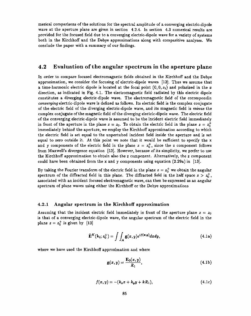
merical comparisons of the solutions for the spectral amplitude of a converging electric-dipolewave at the aperture plane are given in section 4.2.4. In section 4.3 numerical results areprovided for the focused field due to a converging electric-dipole wave for a variety of systemsboth in the Kirchhoff and the Debye approximations along with comparitive analyses. Weconclude the paper with a summary of our findings.
4.2 Evaluation of the angular spectrum in the aperture plane
In order to compare focused electromagnetic fields obtained in the Kirchhoff and the Debyeapproximation, we consider the focusing of electric-dipole waves [13]. Thus we assume thata time-harmonic electric dipole is located at the focal point (0,0, zi) and polarized in the xdirection, as indicated in Fig. 4.1. The electromagnetic field radiated by this electric dipoleconstitutes a diverging electric-dipole wave. The electromagnetic field of the correspondinconverging electric-dipole wave is defined as follows. Its electric field is the complex conjugateof the electric field of the diverging electric-dipole wave, and its magnetic field is minus thecomplex conjugate of the magnetic field of the diverging electric-dipole wave. The electric fieldof the converging electric-dipole wave is assumed to be the incident electric field immediatelyin front of the aperture in the plane z — ZQ. TO obtain the electric field in the plane z = z£immediately behind the aperture, we employ the Kirchhoff approximation according to whichthe electric field is set equal to the unpertubed incident field inside the aperture and is setequal to zero outside it. At this point we note that it would be sufficient to specify the xand y components of the electric field in the plane z — ZQ, since the z component followsfrom Maxwell's divergence equation [13]. However, because of its simplicity, we prefer to usethe Kirchhoff approximation to obtain also the z component. Alternatively, the z componentcould have been obtained from the x and y components using equation (2.29a) in [13].
By taking the Fourier transform of the electric field in the plane z — z£ we obtain the angularspectrum of the diffracted field in this plane. The diffracted field in the half space z > z£,associated with an incident focused electromagnetic wave, can then be expressed as an angularspectrum of plane waves using either the Kirchhoff or the Debye approximations
4.2.1 Angular spectrum in the Kirchhoff approximation
Assuming that the incident electric field immediately in front of the aperture plane z = ZQis that of a converging electric-dipole wave, the angular spectrum of the electric field in theplane z = ZQ is given by [13]
E* (kt; z+) = J JA g(x, yyH*'*)dxdy, (4.1a)
where we have used the Kirchhoff approximation and where
f{x,y)=~(kxx + kvy + kR1), (4.1c)
85
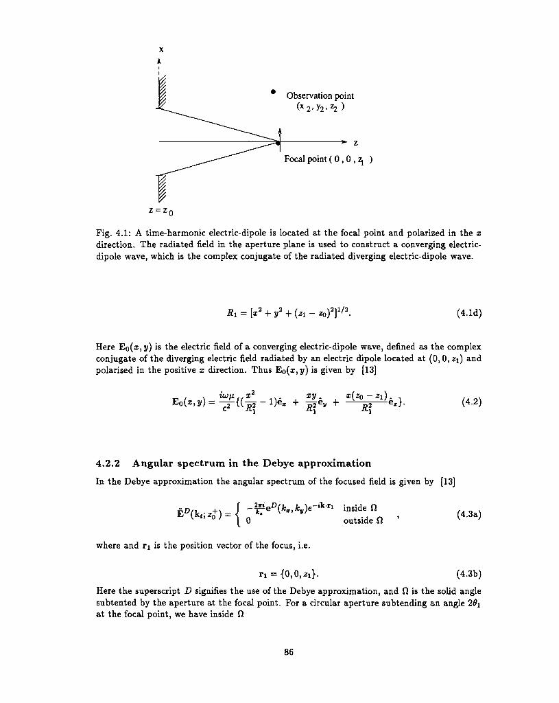
Observation point(x2,y2,z2 )
Focal point ( 0 , 0 , ^ )
= z,
Fig. 4.1: A time-harmonic electric-dipole is located at the focal point and polarized in the xdirection. The radiated field in the aperture plane is used to construct a converging electric-dipole wave, which is the complex conjugate of the radiated diverging electric-dipole wave.
Here E0(x,y) is the electric field of a converging electric-dipole wave, defined as the complexconjugate of the diverging electric field radiated by an electric dipole located at (0,0, zi) andpolarised in the positive x direction. Thus Eo(i,y) is given by [13]
R\(4.2)
4.2.2 Angular spectrum in the Debye approximation
In the Debye approximation the angular spectrum of the focused field is given by [13]
where and ri is the position vector of the focus, i.e.
r-i = {0,0, zi}. (4.3b)
Here the superscript D signifies the use of the Debye approximation, and fi is the solid anglesubtented by the aperture at the focal point. For a circular aperture subtending an angle 2#iat the focal point, we have inside fi
86
k2x + k2
y < k2 s in 2 9X. (4.3c)
Further, we have
e [KX,Ky) — ijQ(xa,y3) — JLtQ\ — -—\z\ — ZQ), —-.—\Z\ — ZQ)), (4.O<1)
which after substitution in (4.2) gives the following result for a converging electric-dipole wave
(k2x-k
2)ex + kxkyey + kxktet}. (4.3e)
Now by introducing the change of variables
kx — k sin a cos f3 , ky = fcsinasin/3, (4-4)
in (4.3e) and using (4.3c), (4.3a) becomes
{(sin2 a cos2/? — l)eT + sin2 a cos/? sin/?ev + cos a sin a cos/3ez}, (4.5){(sin2 a cos2/? l)e + sin2v " 0 / cfccosa
for a < 0X and E^kt; z£) - 0 for a > Bx.
4.2.3 Asymptotic evaluation of the angular spectrum in the Kirchhoff ap-proximation
The Debye approximation to the angular spectrum is obtained by evaluating the Kirchhoff-approximation result in (4.1a) asymptotically using the method of stationary phase, whilepaying attention only to the asymptotic contribution of the interior stationary point of thephase function f(x,y) in (4.1c). Thus, the asymptotic contributions to the integral in (4.1a)due to the boundary of the integration domain are ignored in the Debye approximation. Inorder to use asymptotic methods to evaluate the integral in (4.1a), we assume that the focalpoint lies many wave-lengths away from the aperture, so that k{z\ — ZQ) >> 1.
The asymptotic contribution of the interior stationary point is equal to E°(k t ; ZQ) given in( 4.5). In order to determine the contribution of the boundary, we introduce the change ofvariables
x = t{z,\ — zo)co$(f> ; y — t[z\ — Zo)sin</>, (4-6)
and use (4.4) in (4.1a) to obtain
87
°/(zi~zo)
The integral in ( 4.7) can be written in the following form
1 ^ *°
(4.7)
E*'(kt;z+)= (^ f1 ^ *° G{ty<t,)eik^-^F^^dtd<f>, (4.8a)Jo Jo
where
G(t, <l>) = {Gx(t, 0 ) , Gv(*, < ), G,(f, <f>)}, (4.8b)
(4.8c)
with
Gj(t,<t>) = ^ri*i - zo) * lEojdzi - zo)tcos<j>,(Zl - zo)tsm(j>) {j = x,y,z). (4.8d)
Here EOj- follows from ( 4.2). Numerical integration of integrals of the type in ( 4.8a) istime consuming. Stamnes et al [16] have developed an efficient and accurate method toevaluate this type of diffraction integrals. This particular method is referred to as the SSP(Stamnes-Spjelkavik-Pedersen) method and can be applied to the double integral in (4.8a) forintegreation over one variable along with a Gauss-Legendre integration over the other variable.
Alternatively we could use an asymptotic evaluation of the t integral in (4.7), employing themethods described in [8]1, to obtain the asymptotic contribution of the boundary. To thatend, we integrate (4.7) by parts with respect to the t variable to obtain the following boundarycontribution
E?(kt;z+)= f2'g(<l>)eika^d4> (j = x,y,z), (4.9a)
where
Section 11.2.2.
88
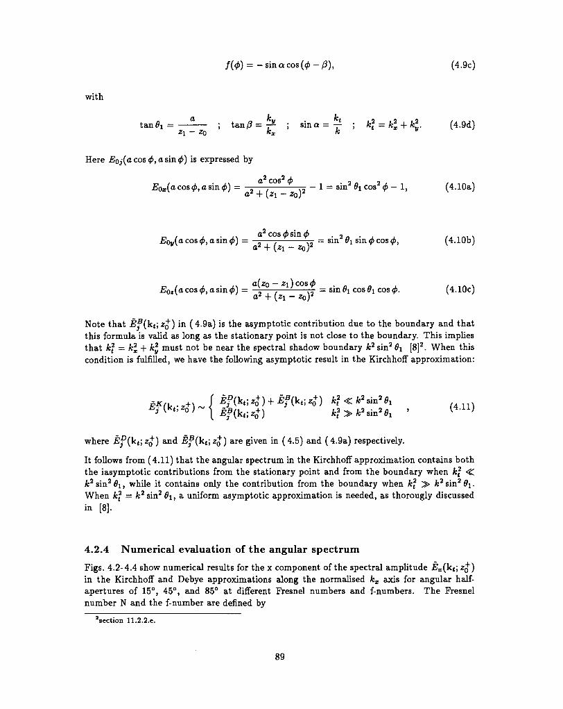
/(</>) = - s in a cos (0 - /3 ) , (4.9c)
with
tan#i = ; tan/3 = -^- ; sina = - ^ ; k2 - k2x + A:2. (4.9d)
Here Eoj(a cos 0, a sin 0) is expressed by
2 2 ii>, a sin 0) = a c o s y _ j _ s m 2 g c o g2 ^ _ i (4.10a)
a2 + (z! - ZQ)2
a2 cos <f> sin d> 2a c o s 0> a s m 0) = ~2—7 \¥ ~ s*n ^ i s i n 0 c o s 0 , (4.10b)
a + (z Z)
€L(ZQ — Z\j COS 0
E O z ( acos0 , a s i n 0 ) = —5 ; rr — sin cos 0i cos 0. (4.10c)fl + (^1 — -zb)
Note that E^(k t; z ") in (4.9a) is the asymptotic contribution due to the boundary and thatthis formula is valid as long as the stationary point is not close to the boundary. This impliesthat fc2 = k2. + fc2 must not be near the spectral shadow boundary k2 sin2 6\ [8]2. When thiscondition is fulfilled, we have the following asymptotic result in the Kirchhoff approximation:
zt) + Ef(kt] 4) k2 « k2 sin2 6,2Q+) k? >> k2 s .n 2 0i , (4.11)
where Ef(kt\z£) and Ef(k.t\z£) are given in (4.5) and (4.9a) respectively.
It follows from (4.11) that the angular spectrum in the Kirchhoff approximation contains boththe iasymptotic contributions from the stationary point and from the boundary when k2 <Ck2 sin2 6\, while it contains only the contribution from the boundary when k2 > k2 sin2 81.When k2 — k2 sin2 81, a uniform asymptotic approximation is needed, as thorougly discussedin [8].
4.2.4 Numerical evaluation of the angular spectrum
Figs. 4.2-4.4 show numerical results for the x component of the spectral amplitude Ex(kt; zj")in the Kirchhoff and Debye approximations along the normalised kx axis for angular half-apertures of 15°, 45°, and 85° at different Fresnel numbers and f-numbers. The Fresnelnumber N and the f-number are defined by
'section 11.2.2.C.
89
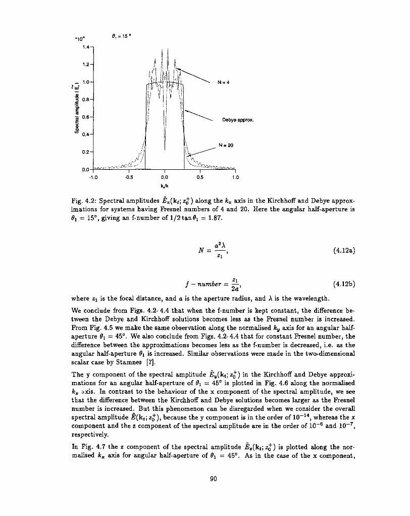
e, = 15°
N = 4
Debye approx.
-1.0 -0.5
Fig. 4.2: Spectral amplitudes Ex(kt; -zjj") along the kx axis in the Kirchhoff and Debye approx-imations for systems having Fresnel numbers of 4 and 20. Here the angular half-aperture is&i = 15°, giving an f-number of l/2tan0i = 1.87.
N =a?\
(4.12a)
/ - number = J-, (4.12b)2a
where z\ is the focal distance, and a is the aperture radius, and A is the wavelength.We conclude from Figs. 4.2- 4.4 that when the f-number is kept constant, the difference be-tween the Debye and Kirchhoff solutions becomes less as the Fresnel number is increased.From Fig. 4.5 we make the same observation along the normalised kv axis for an angular half-aperture 0\ = 45°. We also conclude from Figs. 4.2-4.4 that for constant Fresnel number, thedifference between the approximations becomes less as the f-number is decreased, i.e. as theangular half-aperture 9\ is increased. Similar observations were made in the two-dimensionalscalar case by Stamnes [7].
The y component of the spectral amplitude £y(kt; z§) in the Kirchhoff and Debye approxi-mations for an angular half-aperture of 9\ = 45° is plotted in Fig. 4.6 along the normalisedA;x axis. In contrast to the behaviour of the x component of the spectral amplitude, we seethat the difference between the Kirchhoff and Debye solutions becomes larger as the Fresnelnumber is increased. But this phenomenon can be disregarded when we consider the overallspectral amplitude E(kt; z£), because the y component is in the order of 10~14, whereas the xcomponent and the z component of the spectral amplitude are in the order of 10~6 and 10~7,respectively.
In Fig. 4.7 the z component of the spectral amplitude Ez(kt;zo) is plotted along the nor-malised kx axis for angular half-aperture of 6\ = 45°. As in the case of the x component,
90
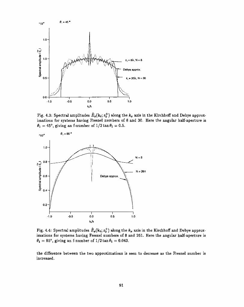
*10" 9, = 45 °
-1.0 1.0
Fig. 4.3: Spectral amplitudes Ex(kt; z£) along the kx axis in the Kirchhoff and Debye approx-imations for systems having Fresnel numbers of 8 and 30. Here the angular half-aperture is0i — 45°, giving an f-number of 1/2 tan6\ = 0.5.
•10- 0, = 85 °
1.0-
- 0.8-lui
0.6-
0.4-
0.2-
N = 8
N = 261
-1.0 -0.5I
0.0I
0.5I
1.0
Fig. 4.4: Spectral amplitudes Ex(kt\ z£) along the kx axis in the Kirchhoff and Debye approx-imations for systems having Fresnel numbers of 8 and 261. Here the angular half-aperture isex = 85°, giving an f-number of 1/2 tan 0x - 0.043.
the difference between the two approximations is seen to decrease as the Fresnel number isincreased.
91
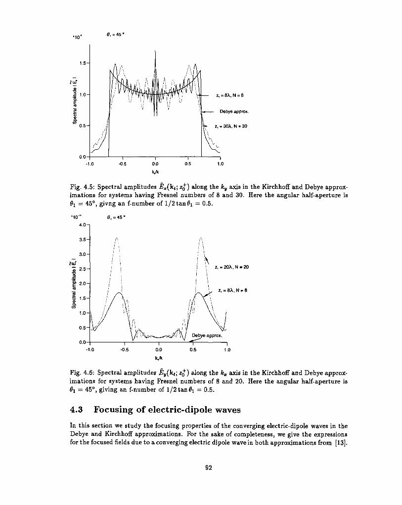
8, = 45 °
0.0
-1.0 -0.5
Fig. 4.5: Spectral amplitudes Ex(kt; z£) along the ky axis in the Kirchhoff and Debye approx-imations for systems having Fresnel numbers of 8 and 30. Here the angular half-aperture is0i = 45°, givng an f-number of 1/2 tan 0i = 0.5.
•10"4.0-1
3.5-
3.0-
2.5-
2.0-
JuT
2t5 1.5-
1.0-
0.5-
0.0
6, = 45°
-1.01
-0.5r
o.o
z, = 20X, N = 20
z, = 8X, N = 8
Debye approx.
0.5i
1.0
Fig. 4.6: Spectral amplitudes ^y(k t ; z£) along the kx axis in the Kirchhoff and Debye approx-imations for systems having Fresnel numbers of 8 and 20. Here the angular half-aperture is6i = 45°, giving an f-number of 1/2 tan 0i = 0.5.
4.3 Focusing of electric-dipole waves
In this section we study the focusing properties of the converging electric-dipole waves in theDebye and Kirchhoff approximations. For the sake of completeness, we give the expressionsfor the focused fields due to a converging electric dipole wave in both approximations from [13].
92
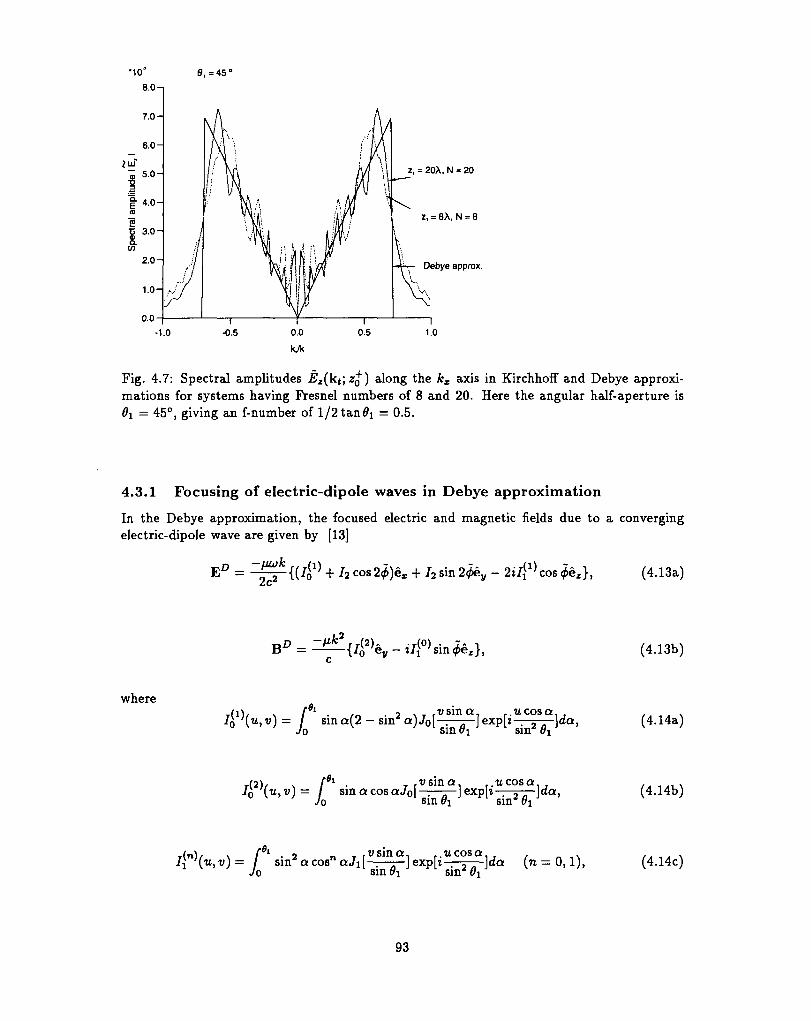
-1.0
z, = 20X, N = 20
z, = 8X, N = 8
Debye apprax.
Fig. 4.7: Spectral amplitudes f?z(kt;zQ") along the kx axis in Kirchhoff and Debye approxi-mations for systems having Fresnel numbers of 8 and 20. Here the angular half-aperture is6\ = 45°, giving an f-number of l/2tan#i = 0.5.
4.3.1 Focusing of electric-dipole waves in Debye approximation
In the Debye approximation, the focused electric and magnetic fields due to a convergingelectric-dipole wave are given by [13]
(4.13a)
(4.13b)
where
sina(2 - sin2 a) (4.14a)
r(2)/ \ fBl • .usina ucosa , , . , , ,iy{u,v)= I sinacosaJol . ]exp[i . - ]da, (4.14b)
Jo sin 0\ sin &i
l[n){u,v)= siJO
sin2 a cosn ucosa,sin 9\
(n = 0,1), . . . . s(4.14c)
93
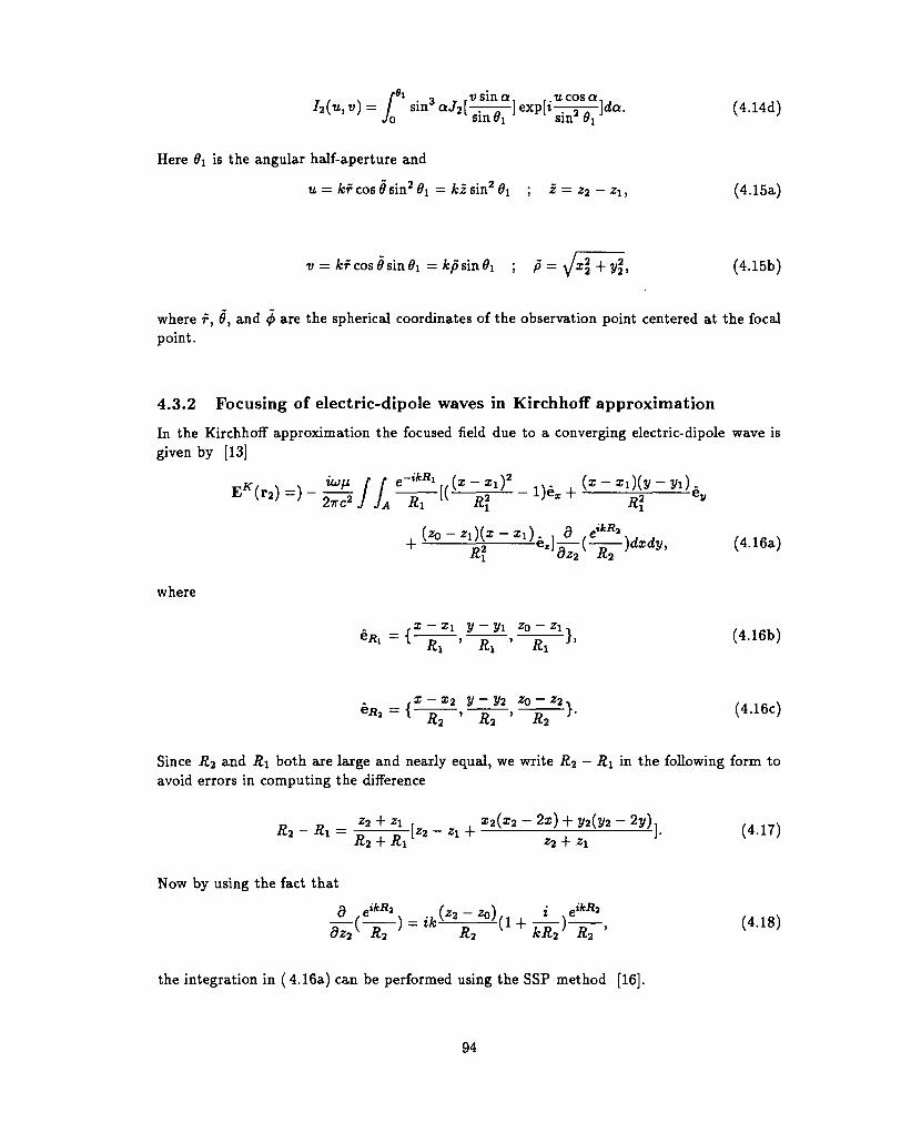
, , . [6x . •> _ rvsina, r.ucosa, ,/,(«, v) = jQ s ^ a J a [ _ ] exP[i-^-]<fa. (4.14d)
Here #i is the angular half-aperture and
u = kf cos 6 sin2 #i = kz sin2 #i ; z = z2 - z\, (4.15a)
v = kf cos 0 sin 6\ = kp sin $i ; P — 'J^i-'ry^ (4.15b)
where f, 0, and # are the spherical coordinates of the observation point centered at the focalpoint.
4.3.2 Focusing of electric-dipole waves in KirchhofF approximation
In the Kirchhoff approximation the focused field due to a converging electric-dipole wave isgiven by [13]
where
tx — x\ y — yi ZQ — z\.(4.16b)
V - V2 ZQ-Z2. , . . . ,—j?—'~p—J- (4.16c)
&2 K2
Since R2 and iZi both are large and nearly equal, we write R2 - R\ in the following form toavoid errors in computing the difference
, x2(x2 - 2x) + y2(y2 - 2y)*2 ~ «1 + — —
*2 + zR2-
Now by using the fact that
i _ ) = iA:-ii_i°-(l + _!-)£__, (4.18)
the integration in (4.16a) can be performed using the SSP method [16].
94
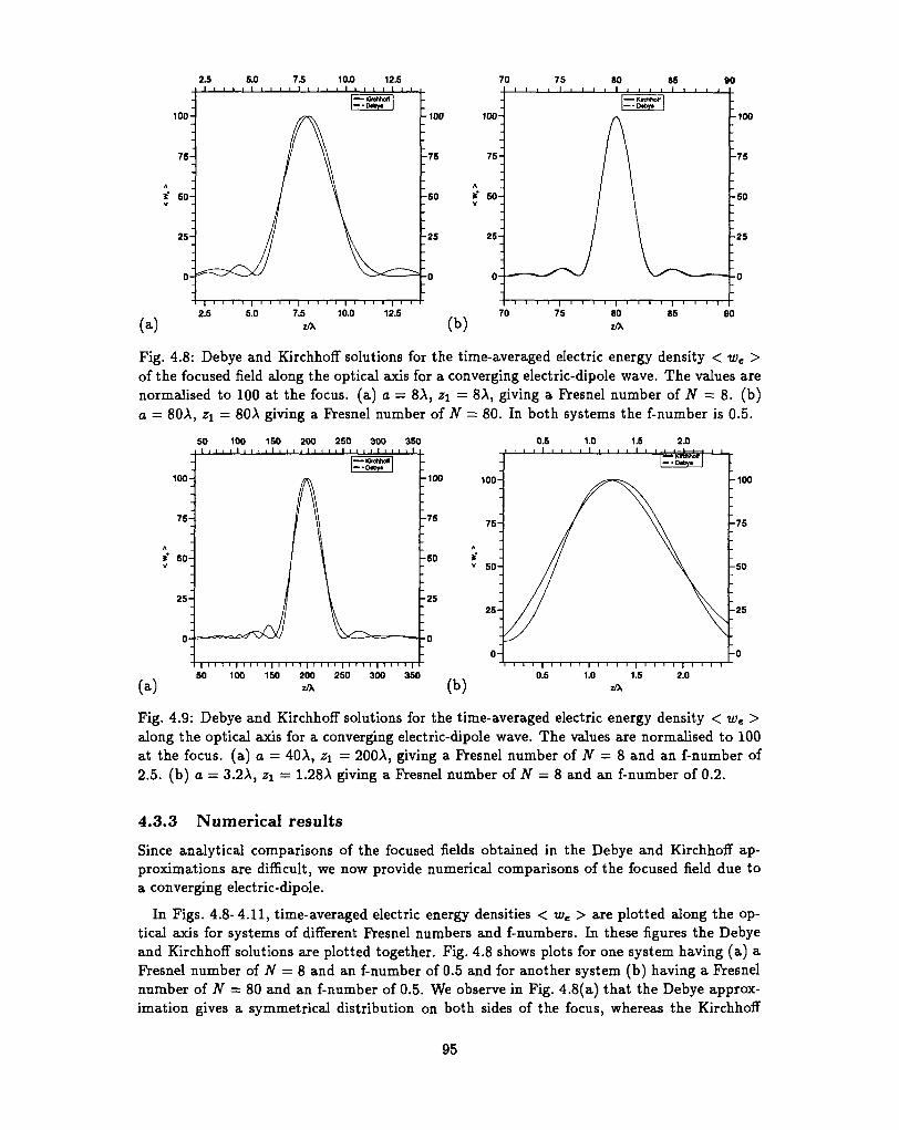
100-
75-
* SO-
(a)
-100 100-
-75
-50 * 50-
25 - -25
12.5(b)
-100
-75
-50
-25
90
Fig. 4.8: Debye and Kirchhoff solutions for the time-averaged electric energy density < we >of the focused field along the optical axis for a converging electric-dipole wave. The values arenormalised to 100 at the focus, (a) a = 8A, z\ — 8A, giving a Presnel number of N = 8. (b)a = 80A, z\ — 80A giving a Fresnel number of N = 80. In both systems the f-number is 0.5.
50 300 350
100- -100
(a)
100- -100
350 0.5 2.0
Fig. 4.9: Debye and Kirchhoff solutions for the time-averaged electric energy density < we >along the optical axis for a converging electric-dipole wave. The values are normalised to 100at the focus, (a) a = 40A, z\ = 200A, giving a Fresnel number of N — 8 and an f-number of2.5. (b) a — 3.2A, z\ = 1.28A giving a Fresnel number of N — 8 and an f-number of 0.2.
4.3.3 Numerical results
Since analytical comparisons of the focused fields obtained in the Debye and Kirchhoff ap-proximations are difficult, we now provide numerical comparisons of the focused field due toa converging electric-dipole.
In Figs. 4.8-4.11, time-averaged electric energy densities < we > are plotted along the op-tical axis for systems of different Fresnel numbers and f-numbers. In these figures the Debyeand Kirchhoff solutions are plotted together. Fig. 4.8 shows plots for one system having (a) aFresnel number of N = 8 and an f-number of 0.5 and for another system (b) having a Fresnelnumber of N = 80 and an f-number of 0.5. We observe in Fig. 4.8(a) that the Debye approx-imation gives a symmetrical distribution on both sides of the focus, whereas the Kirchhoff
95
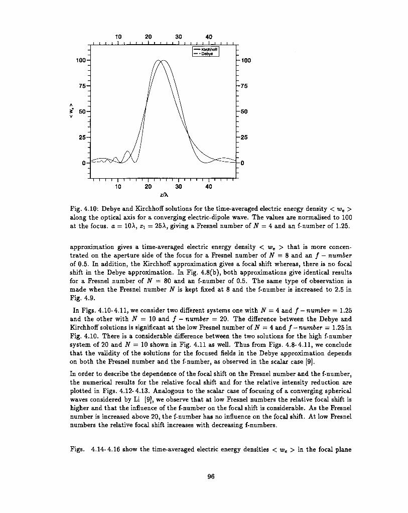
10 20 30 40
100-
75-
I 1 I I I i I I I I I I I I I I I I I I I I I I
-100
-75
-50
-25
I10 20 30
i40
z/X
Fig. 4.10: Debye and Kirchhoff solutions for the time-averaged electric energy density < we >along the optical axis for a converging electric-dipole wave. The values are normalised to 100at the focus, a — 10A, z\ — 25A, giving a Presnel number of N = 4 and an f-number of 1.25.
approximation gives a time-averaged electric energy density < we > that is more concen-trated on the aperture side of the focus for a Fresnel number of N = 8 and an / — numberof 0.5. In addition, the Kirchhoff approximation gives a focal shift whereas, there is no focalshift in the Debye approximation. In Fig. 4.8(b), both approximations give identical resultsfor a Fresnel number of N = 80 and an f-number of 0.5. The same type of observation ismade when the Fresnel number N is kept fixed at 8 and the f-number is increased to 2.5 inFig. 4.9.
In Figs. 4.10-4.11, we consider two different systems one with N = 4 and / - number = 1.25and the other with TV = 10 and / - number = 20. The difference between the Debye andKirchhoff solutions is significant at the low Fresnel number of N = 4 and / - number — 1.25 inFig. 4.10. There is a considerable difference between the two solutions for the high f-numbersystem of 20 and N — 10 shown in Fig. 4.11 as well. Thus from Figs. 4.8-4.11, we concludethat the validity of the solutions for the focused fields in the Debye approximation dependson both the Fresnel number and the f-number, as observed in the scalar case [9].
In order to describe the dependence of the focal shift on the Fresnel number and the f-number,the numerical results for the relative focal shift and for the relative intensity reduction areplotted in Figs. 4.12-4.13. Analogous to the scalar case of focusing of a converging sphericalwaves considered by Li [9], we observe that at low Fresnel numbers the relative focal shift ishigher and that the influence of the f-number on the focal shift is considerable. As the Fresnelnumber is increased above 20, the f-number has no influence on the focal shift. At low Fresnelnumbers the relative focal shift increases with decreasing f-numbers.
Figs. 4.14-4.16 show the time-averaged electric energy densities < we > in the focal plane
96
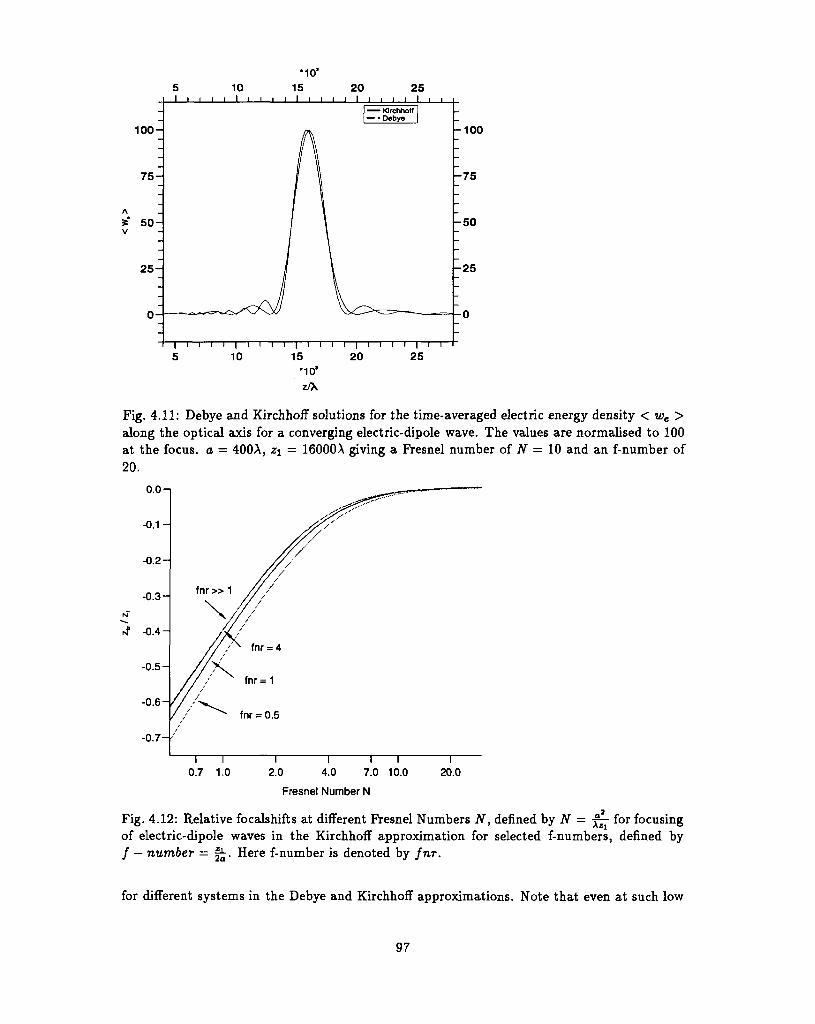
100- -100
- 7 5
- 5 0
- 2 5
10I 1 1 1
15•10s
z/X
201 • i
25
Fig. 4.11: Debye and Kirchhoff solutions for the time-averaged electric energy density < we >along the optical axis for a converging electric-dipole wave. The values are normalised to 100at the focus, a = 400A, z\ = 16000A giving a Presnel number of N = 10 and an f-number of20.
u.u —
- 0 . 1 -
- 0 . 2 -
- 0 . 3 -
- 0 . 4 -
- 0 . 5 -
- 0 . 6 -
- 0 . 7 -
//% fnr
/ / / fnr =
/ / ^ ^ fnr =
/
/
= 4
1
0.5
i r0.7 1.0 2.0
I4.0 7.0 10.0
Fresnel Number N
20.0
Fig. 4.12: Relative focalshifts at different Fresnel Numbers N, defined by N — f^- for focusingof electric-dipole waves in the Kirchhoff approximation for selected f-numbers, defined by/ — number = |£. Here f-number is denoted by fnr.
for different systems in the Debye and Kirchhoff approximations. Note that even at such low
97
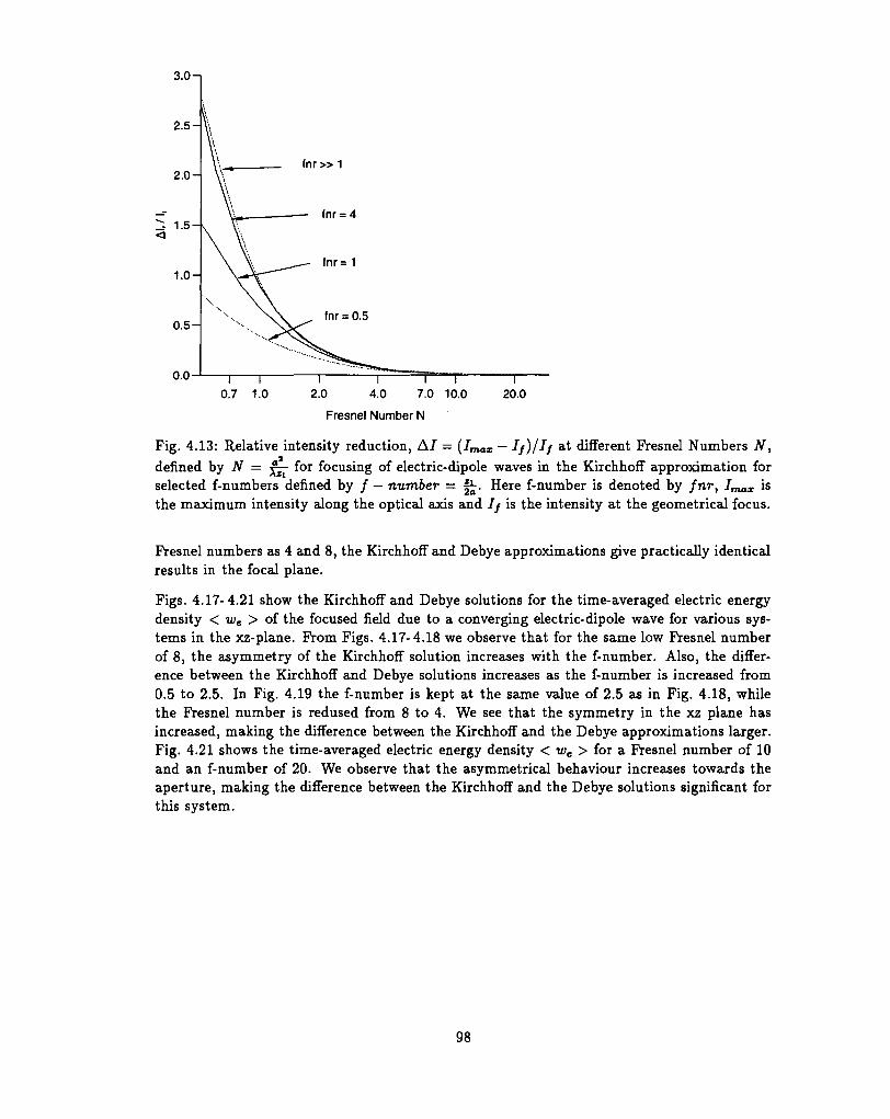
3.0-i
fnr» 1
I I I I0.7 1.0 2.0 4.0 7.0 10.0
Fresnel Number N
Fig. 4.13: Relative intensity reduction, A/ — (Imax — If)llf at different Fresnel Numbers jV,defined by JV = f^- for focusing of electric-dipole waves in the Kiichhoff approximation forselected f-numbers defined by / — number = |£. Here f-number is denoted by fnr, Imax isthe maximum intensity along the optical axis and If is the intensity at the geometrical focus.
Fresnel numbers as 4 and 8, the Kirchhoff and Debye approximations give practically identicalresults in the focal plane.
Figs. 4.17-4.21 show the Kirchhoff and Debye solutions for the time-averaged electric energydensity < we > of the focused field due to a converging electric-dipole wave for various sys-tems in the xz-plane. From Figs. 4.17-4.18 we observe that for the same low Fresnel numberof 8, the asymmetry of the Kirchhoff solution increases with the f-number. Also, the differ-ence between the Kirchhoff and Debye solutions increases as the f-number is increased from0.5 to 2.5. In Fig. 4.19 the f-number is kept at the same value of 2.5 as in Fig. 4.18, whilethe Fresnel number is redused from 8 to 4. We see that the symmetry in the xz plane hasincreased, making the difference between the Kirchhoff and the Debye approximations larger.Fig. 4.21 shows the time-averaged electric energy density < we > for a Fresnel number of 10and an f-number of 20. We observe that the asymmetrical behaviour increases towards theaperture, making the difference between the Kirchhoff and the Debye solutions significant forthis system.
98
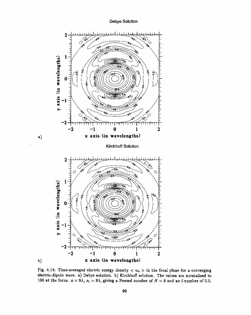
Debye Solution
a)
I I I I I I I I I I I I ! I I I I I I I I I I I I I I I I I I I I I I I I I
-2-1 0 1
x axis (in wavelengths)
Kirchhoff Solution
i 1 1 1 1 1 1 1 1 1 1 1 1 1 1 1 1 1 1 1 1 1 1 1 1 1 1 1 1 1 1 1 1 1 i
i i i i | i i i i i i i i i i | i | i i i | i i i i |
- 1 0 1 2b) x axis (in wavelengths)
Fig. 4.14: Time-averaged electric energy density < we > in the focal plane for a convergingelectric-dipole wave, a) Debye solution, b) Kirchhoff solution. The values are normalised to100 at the focus, a - 8A, zx = 8A, giving a Fresnel number of N = 8 and an f-number of 0.5.
99
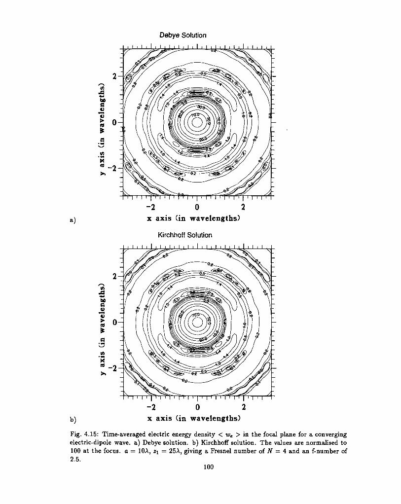
Debye Solution
i i I i i i i i i i i i I i
a)
I i I i I ' I i I i I i I i I i I i I i I ' I i 1 " i ~ T
-2 0 2x axis (in wavelengths)
Kirchhoff Solution
-2 0 2b) x axis (in wavelengths)
Fig. 4.15: Time-averaged electric energy density < we > in the focal plane for a convergingelectric-dipole wave, a) Debye solution, b) Kirchhoff solution. The values are normalised to100 at the focus, a = 10A, z\ = 25A, giving a Fresnel number of N = 4 and an f-number of2.5.
100
4.4 Conclusion
We have presented detailed comparison between the Kirchhoff and Debye solutions for thefocusing of electromagnetic waves, with special emphasis on converging electric-dipol waves.First we presented numerical comparisons of the spectral amplitudes of the electric field inthe aperture plane in the two approximations for various Presnel numbers and f-numbers.Then we presented the numerical comparisons of the Kirchhoff and Debye solutions for thefocused field due to a converging electric-dipole wave. From these comparisons, we concludethat the Debye approximations is valid only for systems with Fresnel numbers larger than20 and f-numbers less than 0.5. As in the scalar case, we have found that the relative focalshift decreases with increasing Fresnel numbers. For Fresnel numbers larger than 20, the focalshift can be neglected, regardless of the size of the f-number. But at low Fresnel numbers, areduction of the f-numbers gives an increase in the relative focal shift.
4.5 Aknowledgments
This research was supported by the Norwegian Research Council.
101
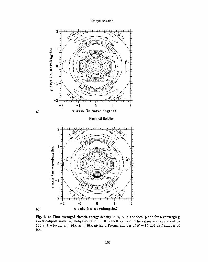
Debye Solution
a)
If)
dv
(0
i j i i i i | I i i i i i i i i i I i i | i i i i i i I | i i i i ( j i
-1 0 1x axis (in wavelengths)
Kirchhoff Solution
I I I I I I I I I I I I I I I I C I I I I I I I I I I I I I I I I I
i > | • i • i > i ' i 11 i i i i i 11 i i | i 11 i i i ' i-2- 2 - 1 0 1 2
b) x axis (in wavelengths)
Fig. 4.16: Time-averaged electric energy density < we > in the focal plane for a convergingelectric-dipole wave, a) Debye solution, b) Kirchhoff solution. The values are normalised to100 at the focus, a = 80A, z\ - 80A, giving a Fresnel number of N = 80 and an f-number of0.5.
102
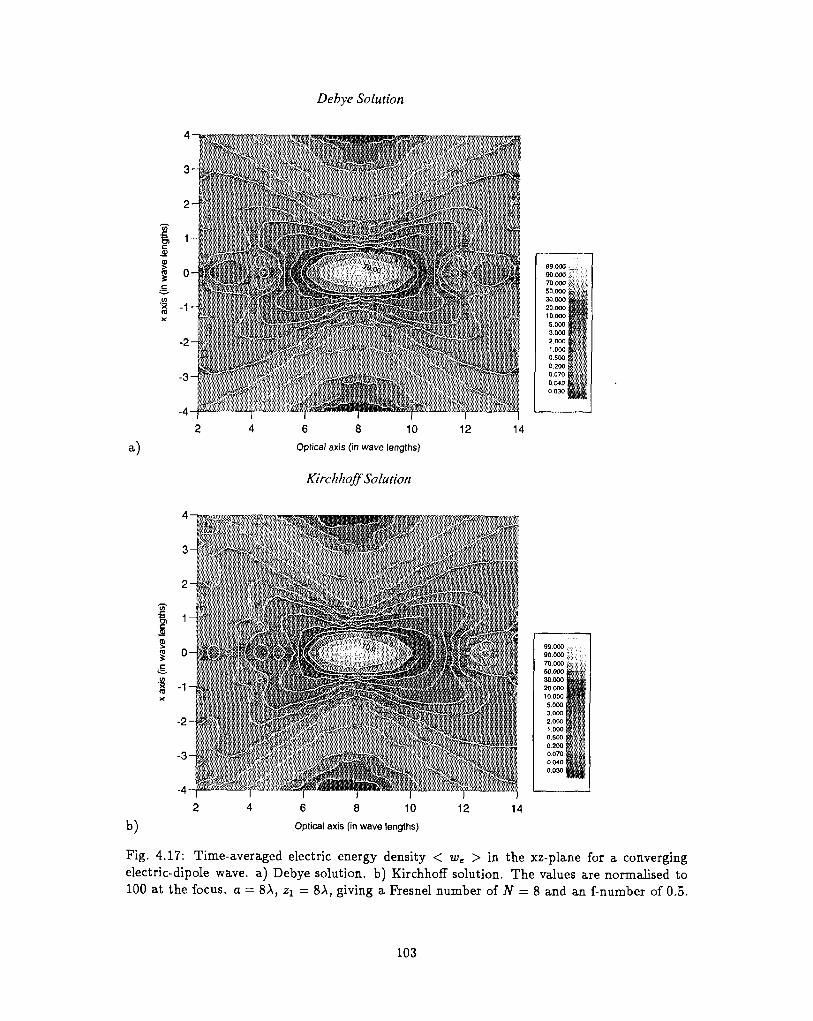
Debye Solution
a)8 10
Optical axis (in wave lengths)
Kirchhoff Solution
3 -
£ 1 -I
I
-2-T-
-4-T2
i -6 8 10
Optical axis (in wave lengths)
- € I _
| "
12
i
**-<-•
14
99.00090.000,70.000 Z-50.000 ^s»»—30000 H im20 000|J|Ji10.000 P S5.000 ft'~rt3.000 p l i f l2.000 » , . . ,1.000 |? v ^ .0.500 g 'Z0.200 || i0.070 |g
OMO t s i0030 fiiil
Fig. 4.17: Time-averaged electric energy density < we > in the xz-plane for a convergingelectric-dipole wave, a) Debye solution, b) Kirchhoff solution. The values are normalised to100 at the focus, a = 8A, zx = 8A, giving a Presnel number of N = 8 and an f-number of 0.5.
103
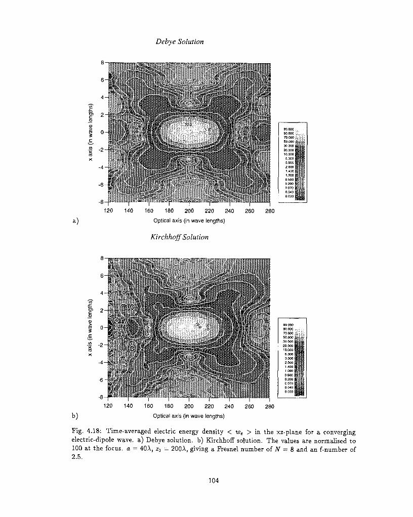
Debye Solution
-4itssiiiw
a) Optical axis (in wave lengths)
Kirchhoff Solution
8-r-
pillNHPii§jijp
1111111118818111iiflllPiiiiiiMHiiilfIBBili-iirtiiiiis^ffliiSiiiiis^11
99.00090.000 >; •:70.000 g | | |
30.ooo l l H i l20 0 0 o | | | |10,000 ffllfll5,000 ffliffl3,ooo H i i i2.000 p l f i1.400 pi lHi.ooo ppiiH0.500 i ! | l l l0.200 ^ l l ^ l i i0.070 M i S | |O.O40 S i i i l0 0 3 0 1 1
120 140 160 180 200 220 240 260 280
b) Optical axis (in wave lengths)
Fig. 4.18: Time-averaged electric energy density < we > in the xz-plane for a convergingelectric-dipole wave, a) Debye solution, b) Kirchhoff solution. The values are normalised to100 at the focus, a = 40A, z\ — 200A, giving a Fresnel number of AT = 8 and an f-number of2.5.
104
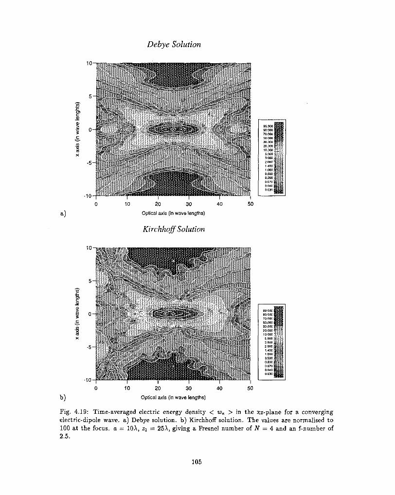
Debye Solution
10-
c
in
. I S
-5-
a)
5 -
- 5 -
-10
-10-r0 10
™ urn ini liiliii|iiiiiililiiiii«i|i«ni»ln«»ii|tiiirlipliiiiilHil
20 30
Optical axis (in wave lengths)
Kirchhoff Solution
I40
I50
10 20 30 40
Optical axis (in wave lengths)
I50
99.00090.00070.00050.00030.00020.00010.0005.000
1*SOOTfe2.0001.4001.0000.5000.2000.07000400.030
W ^S -'*
B
Fig. 4.19: Time-averaged electric energy density < we > in the xz-plane for a convergingelectric-dipole wave, a) Debye solution, b) Kirchhoff solution. The values are normalised to100 at the focus, a = 10A, z\ = 25A, giving a Fresnel number of N = 4 and an f-number of2.5.
105
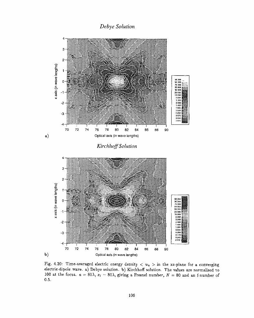
Debye Solution
a.)
I
78 80 82 84
Optical axis (in wave lengths)
Kirchhoff Solution
-4-r70 72 74 76 78 80 82 84 86
Optical axis (in wave lengths)
88 90
Fig. 4.20: Time-averaged electric energy density < we > in the xz-plane for a convergingelectric-dipole wave, a) Debye solution, b) Kirchhoff solution. The values are normalised to100 at the focus, a = 80A, z1 = 80A, giving a Fresnel number, N = 80 and an f-number of0.5.
106
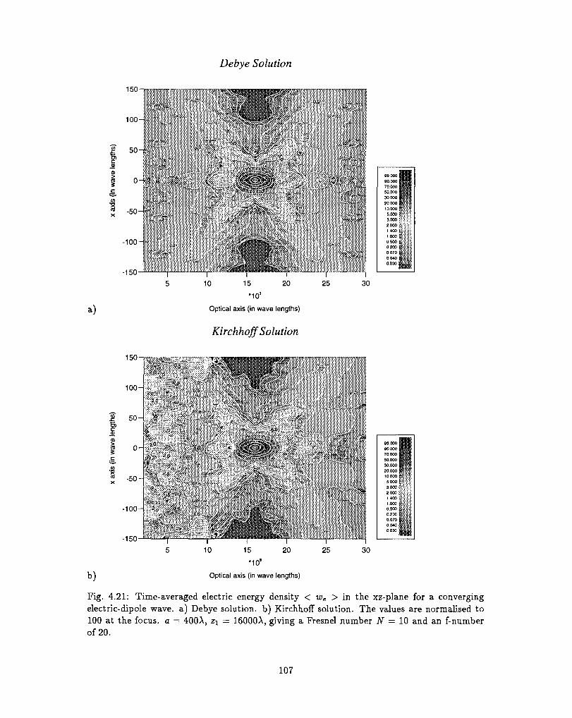
Debye Solution
150 —
100- '*
50-.
a)
0-1 '
-50-
-100-
-150 —
_f"l -- r ^ , " ^ T10 15 20
MO1
Optical axis (in wave lengths)
Kirchhoff Solution
25 30
150-
!
100-
I 5(H
ICO
I o-c
to
-501
-100
-150-
J>.
V
13 "
^ -
I '
* 1 L . / 1 > ^ _
j |
) 15 20
MO3
Optical axis (in wave lengths)
t r
[
25
• j
I30
SSSB8199 000 ^ S90 000 ^ ^ S7Doo° S50.000 | | | | §3 0 . 0 0 0 ^ ^20.000 g - " * 3
10.000 ! f5000 ?"3000"2000 „
1.000 E0.500 i..0 . 2 M ^0 .070^ - - ^0.040 {£,- =- _.0.030 feyg
Fig. 4.21: Time-averaged electric energy density < we > in the xz-plane for a convergingelectric-dipole wave, a) Debye solution, b) KirchhoiT solution. The values are normalised to100 at the focus, a = 400A, zx = 16000A, giving a Fresnel number N = 10 and an f-numberof 20.
107
Bibliography
[1] E. Wolf. Electromagnetic diffractions in optical systems I. An integral representation ofthe image field. Proc. R. Soc. A 253, 349-357, 1959.
[2] B. Richards and E. Wolf. Electromgnetic diffraction in optical systems II, Structure ofthe image field in an aplanatic system. Proc. R. Soc. A 253, 358-379, 1959.
[3] A. Yoshida and T. Asakura. Electromagnetic field in the focal plane of a coherent beamfrom a wide-angular annular-aperture system. Optik, 40, 322-331, 1974.
[4] C. J. R. Sheppard. Electromagnetic field in the focal region of wide-angular annular lensand mirror systems. J. Micro. Optics and Acoustics 2, 163-166, 1978.
[5] R. Kant. An analytical solution of vector diffraction problems for focusing optical systems./ . Mod. Opt. 40, 337-347, 1993.
[6] P. Torok, P. Varga, Z. Laczic, and G. R. Booker. Electromagnetic diffraction of lightfocused through a planar interface between materials of mismatched refractive indices:an integral reperesentation. J. Opt. Soc. Am. A 12, 325-332, 1995.
[7] J. J. Stamnes. Focusing of two-dimensional waves. J. Opt. Soc. Am. 71, 15-31, 1981.
[8] J. J. Stamn.es. Waves in Focal Regions. Adam Hilger, Bristol and Boston, 1986.
[9] Y. Li. Dependence of the focal shift on Fresnel number and f-number. J. Opt. Soc. Am.A 72, N0.6, 1982.
[10] Y. Li and E. Wolf. Three-dimensional intensity distribution near the focus in systems ofdifferent Fresnel numbers. J. Opt. Soc. Am. A 1, No.8, 1984.
[11] Y. Li and E. Wolf. Focal shifts in diffracted converging spherical waves. Opt. Commun.39, N0.4, 211-215, 1981.
[12] T. D. Visser and S. H. Wiersma. Spherical aberration and the electromagnetic field inhigh aperture systems. J. Opt. Soc. Am. A 8, 1404-1410, 1991.
[13] J. J. Stamnes and V. Dhayalan. Focusing of electric-dipole waves. Pure Appl. Opt. 5,195-226, 1996.
[14] V. Dhayalan and J. J. Stamnes. Focusing of mixed-dipole waves. Submitted to J. PureAppl. Opt, 1996.
[15] E. Wolf and Y.Li. Conditions for the validity of the debye integral representation offocused fields. Opt. Commun. 39, 205-210, 1981.
[16] J. J. Stamnes, B. Spjelkavik, and H. M. Pedersen. Evaluation of diffraction integralsusing local phase and amplitude approximations. Optica Ada 30, 207-222, 1983.
108
Chapter 5
REFLECTION AND REFRACTION OF AN ARBITRARY
ELECTROMAGNETIC WAVE IN A LAYERED MEDIUM
Chapter 5
REFLECTION ANDREFRACTION OF ANARBITRARYELECTROMAGNETIC WAVEIN A LAYERED MEDIUM
Submitted to J. Optical Society of America A
Velauthapillai Dhayalan, Jakob J. Stamnes, and Hans M. Pedersen*
Department of Physics, University of Bergen, Allegt. 55, N-5007 Bergen, Norway
* Department of Physics, Norwegian Institute of Technology, Trondheim, Norway
Abstract
In many applications it is important to have an accurate description of the propagationof electromagnetic waves in a layered medium with plane parallel interfaces. To that end,we present in this paper exact solutions for the reflected and transmitted electromagneticfields and for the electromagnetic fields inside each layer in terms of the given field orsource current outside the medium.
109
5.1 Introduction
In many different applications there is a need for an accurate description of wave propa-gation in a layered medium with plane parallel interfaces. As an example, dyadic Green'sfunctions in such media play an important role in the modelling of microstrip antennasto determine characteristics like gain, surface wave losses, and cross-polarisation [1, 2, 3],Also, in the probing of the subsurface of the earth with electromagnetic or seismic waves,the idealized model often used is that of a layered medium [4]. General descriptions ofhow one can proceed to solve the multilayer problem are given in [5] and [6], but theprocedures and the results are rather complicated.
In optics the most important applications of wave propagation in layered media are in thedesign of antireflection coatings and spectral transmission filters based on thin films [7, 8].Matrix methods for computing the TE and TM reflection and transmission coefficients forplane waves in thin films are now being used extensively. However, it is not obvious howthese matrix methods can be generalized so as to apply to a nonplanar incident wave ofarbitrary form.
In this paper, we consider the case in which the source of the field is outside the layers,and we generalize the matrix formalism so as to obtain exact, explicit solutions for thereflected and transmitted fields and for the fields inside each layer in terms of the givenfield or source on the outside. Compared to earlier approaches [5, 6] ours is simplifiedthrough the application of TE and TM plane-wave expansions, which earlier have beenapplied successfully to analogous single-interface problems involving isotropic as well asanisotropic media [9, 10]. Since there is no coupling between TE and TM plane waveson reflection and reflection at plane interfaces, this procedure leads most directly to thedesired results and make them appear in a simple form that is easy to interpretate physi-cally.
The paper is organised as follows. In section 5.2 we consider the simplified case of a slaband derive exact solutions for the reflected and transmitted fields, as well as for the fieldsinside the slab, by first expressing each of these fields by TE and TM angular-spectrumrepresentations. Next, we use the boundary conditions that E and H are required tosatisfy at the two interfaces of the slab to determine the TE and TM spectral amplitudesof the reflected fields and the fields inside the slab in terms of the TE and TM spectralamplitudes of the incident field or its source. Explicit solutions in the form of angular-spectrum and impulse-response representations are given for the reflected and transmittedfields and for the fields inside the slab directly in terms of the incident field or its source.Also, explicit expressions for each of the spectral domain dyadic Green's functions aregiven.
In section 5.3 we consider a multilayered medium consisting of N layers, and we startby developing the matrix theory for the scalar or acoustical problem. Then we considerthe corresponding electromagnetic problem and show how its solution can be obtainedfrom the scalar solution. Explicit solutions in the form of angular-spectrum and impulse-response representations are given for the reflected and transmitted fields and for the fieldsinside each layer directly in terms of the incident field or its source. Also, the associatedspectral domain dyadic Green's functions are given. For the case in which the multilayeredmedium reduce to a slab, we show that the results in section 5.3 correctly reduce to thosederived in section 5.2 by a completely different method.
Finally, in section 5.4 and 5.5 we summarize our findings and discuss how our results can
110
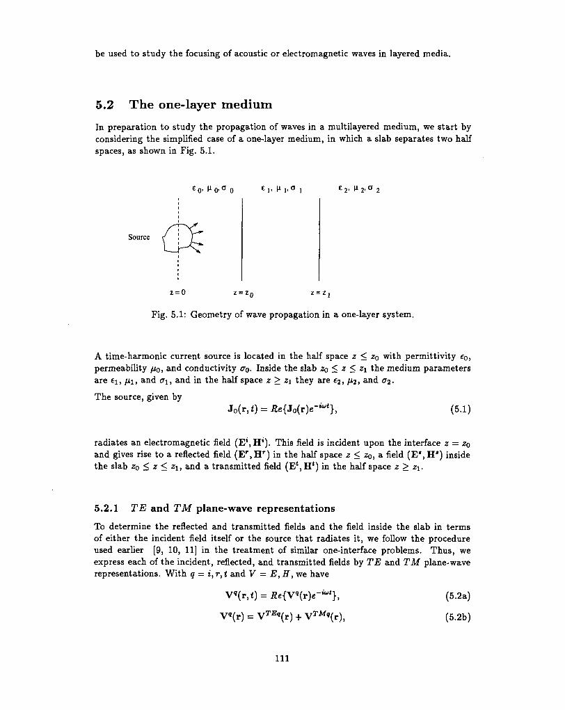
be used to study the focusing of acoustic or electromagnetic waves in layered media.
5.2 The one-layer medium
In preparation to study the propagation of waves in a multilayered medium, we start byconsidering the simplified case of a one-layer medium, in which a slab separates two halfspaces, as shown in Fig. 5.1.
Source
e,, e 2, n 2, a 2
z=0 z = z o z=Zj
Fig. 5.1: Geometry of wave propagation in a one-layer system.
A time-harmonic current source is located in the half space z < ZQ with permittivity eo>permeability fj,o, and conductivity <7o. Inside the slab ZQ < z < z\ the medium parametersare ci, /ii, and o\, and in the half space z > z\ they are C2> A*2> ajid 02 •
The source, given byr)e I w e } , (5.1)
radiates an electromagnetic field (E*, H*). This field is incident upon the interface z = z0
and gives rise to a reflected field (E r ,H r ) in the half space z < ZQ, a field (E*,H*) insidethe slab z0 < z < z\, and a transmitted field (Ef,H£) in the half space z > z\.
5.2.1 TE and TM plane-wave representations
To determine the reflected and transmitted fields and the field inside the slab in termsof either the incident field itself or the source that radiates it, we follow the procedureused earlier [9, 10, 11] in the treatment of similar one-interface problems. Thus, weexpress each of the incident, reflected, and transmitted fields by TE and TM plane-waverepresentations. With q = i,r,t and V = E,H, we have
(5.2a)
I, (5.2b)V«(r) = VTEq{r)
111
M f c y (p = TE,TM), (5.2c)
k* = kt + A;«ez ; kt = fcxex + kyey, (5.2d)
+&*„ if q = i-kZQ ifq = r , (5.2e)+A;Z3 if q = t
= xex + ye,, ; *« H * I f ^ f ' 7 ' (5-2f)
; Jm A,. > 0 (J = 0,1,2), (5.2g)
7 ^ p (J = 0,1,2). (5.2h)
Thus, when Aj < fc^ (j = 0,1,2) the incident and the transmitted fields consist of planewaves having wave vectors k* and k' with positive z—components, while the reflected fieldconsists of plane waves, each having a wave vector kr with negative z—component.
Inside the slab (z0 < z < z{) the field will be the sum of two parts V + and V~, i.e.
r)e-i»t}, (5.3a)
where+ + V-(r), (5.3b)
V±(p) = VTE±(r) + VT M ±(r), (5.3c)
oo
2" JJ(p = TE,TM), (5.3d)
Thus, V p + and V are comprised of plane waves with wave vectors having positive andnegative z-components, respectively.
112
5.2.2 Whittaker potentials
The spectral amplitudes VM(k t; z9) (V = E, H ; q = i, r, t, +, - ) are given by [II]1.
ETi?9(k t; z9) = (2x)2—{k«)2aTE*{kt; z9)kt X e2, (5.4a)
x (kt X ez), (5.4b)
E™«(k f; z9) = -(27r)2a™«(k t; z")k« x (kt X e,), (5.4c)
H™9(kt; z9) = ( 2 x ) 2 - ^ - d ™ 9 ( k t ; z9)kt x ez, (5.4d)
where z9, kq, and pq are given by
, ° ., ,' q I -f '.«i if q=+,- ; p* = < pi nq = +,— .
(5.4e)
Here ^ ( k ^ z 9 ) (p = TE,TM) are spectral forms of the so-called Whittaker potentialsassociated with the incident field. Since
i(kf; z0) + E™'(k t ; z0), (5.4f)
where ETBl(k t; zo) and ETAft(k t; z0) are given by (5.4a) and (5.4c), repectively (withq = i), we can express the potentials aTEl(kt; z0) and &™x(kt; z0) in terms of the spectralamplitude of the incident electric field, by multiplying (5.4f) vectorially by kt X ez andk' x (kt x ez). Thus we obtain [II]2
where
'Eqs. (15.32 b-c) and (15.34 c-d) with s = e,. Note that E^ktizo) equals (2x)2 times the quantity(ki,o;)inEqs. (15.37d-e).
2Eqs. (15.32 d-e) with q = i and s = ex.
113
E t (k t ;z 0 )= Bl{rt,zo)e-lK-tTtdxdy. (5.5c)
Alternatively, d^ktjzo) (p — TE,TM) can be expressed in terms of the source thatradiates the incident field [II]3.
' X (k, X «.)] • M^) < ^ 0 , (5.6a)
aTEl(kt;zo) = ^ fc2(kt x ez) • Jo(k') ell"°«>, (5.6b)
where
oo
Jo(kO= If f Join, z)e-i[*tTt+k'°z]dxdydz. (5.6c)
5.2.3 Solutions for spectral-domain potentials
In order to determine dP9(kt; zq) (p = TE, TM ; q — r, + , - ,<) , we apply the boundary
conditions that E and H have to satisfy at the interfaces z = z0 and z — z\. At eachof these interfaces the tangential components of E and H must be continuous. Thus, atz — ZQ we have
e, x [El + E r - E+ - E~]z=zo = 0, (5.7a)
st x [W + H r - H+ - H- ] J = J 0 = 0. (5.7b)
Next, we substitute the angular-spectrum representations given in (5.2) and (5.3), withspectral amplitudes given in (5.4), in (5.7a) and (5.7b) to obtain (with j = E,H)
oo
/ /
Aj(kt)exp(iktrt)dA;Idfew - 0, (5.8a)
3Eqs. (15.37 c-d) with s = e , and with a factor ^ omitted since we are considering a time-harmonicfield (cf Eqs. (15.5) and (15.7)).
114
where
t) = ez X {- aTMi(kt; ZQ)W X (kt x ez) - -k2aTEi(kt; zo)kt X ez
wr x (kt X ez) - -klaTEr(kt; zo)kt x ez
aTM+(kt;zo)kt X (k, X ez) + -fc?dTS+(k t; 20)kt X ez
X (k« X ez) + -klaTE-{kt; zo)kt x ez}, (5.8b)
= ez x {^ . a T M i (k t ; zo)kt X ez - ( - ) 2 ^ d T E i ( k e ; ^ ) k ' X (k( X ez)
X ez - ( - ) ^ a r B ' ( k i ; zo)k' X (kt X ez)
X ez + (^$-aTE+(kt;z0)kt X (kt x ez)
' $ T E x ( k i x e z ) } . (5.8c)
Since the integral in (5.8a) is a Fourier-transform integral, it follows from the Fourier-uniqueness theorem that
A*(k t) = AH{kt) = 0. (5.9)
Also, since the vectors appearing in (5.8b) and (5.8c), i.e.
ez X [k9 X (kt X ez)] = kq • ez(ez x k t), (5.10a)
ez X (kt X ez) = kt, (5.10b)
are orthogonal, the sum of the coefficients in front of each of them in (5.8b) and (5.8c)must vanish. Hence we obtain the following four equations:
aTMi(kt;z0) - aTMr(kt;zo) = (a™+(kt;z0) - &™-(kt;zo)), (5.11a)
aTMi(kt; MO) + a™'(kt;«,) = |^ (d^+(kt i *) + a™-(kt; *)), (5.11b)
115
aTEi(kt; zo) + aTE'(kt; z0) = ^(aTE+(kt; z0) + aTE-(kt; * ) ) , (5.11c)
aTJK(k (; z0) - aTEr(kt; z0) = ^ ^ - ( d T E + ( k t ; z0) - dTB-(k<; z0)).
Similarly, by applying the boundary conditions at z = zi, which are
e, x [E+ + E" - E 'k = r i = 0, (5.12a)
ez x [H+ + H - - H*],=Jl = 0, (5.12b)
we obtain the following four equations :
d™+(k t ; zo)ei61 + d ™ - ( k t ; zo)e-^ = ^ d T M t ( k t ; za), (5.13b)
aTE+(kt; ab)e* - aTE~(kt; zo)e~^ =
(5.13d)
whereSi = kZl(zi — zo). (5-14)
Note that (5.11a-b) and (5.13a-b) contain TM potentials only, while (5.11c-d) and (5.13c-d) contain TE potentials only. This shows that there is no coupling between TE and TMplane waves, as expected.
We now define the following reflection and transmission coefficients [II]4
rpTE± _ *1
*Eq. (15.40).
116
V J
~ kl a™(kt; Zl) ~ k* fi™(kt;
.'
Solving (5.11a-b) and (5.13a-b) and (5.11c-d) and (5.13c-d), we find {p - TE,TM)
Tp = e^TP+e^-8^ ; 2»" = TP+r^e'2*1 ; iip = Tp~ei0, (5.16a)
whereo = fczo(2i-zo), (5.16b)
V ^
with
- k2 U-k T>™ - 7)™T> 7)
T M
*
TE _
2PmhLnKzm T
117
n 4 v >Vm + Pn(0.
where
P J M = ^ I $* = %• (5.17e)
Here m, rc, and j are integers, all having values 0,1, or 2.
5.2.4 Exact solutions for reflected, transmitted, and slab fields
In section 5.2.3, we have determined the spectral form dM(k t; z*) (p = TE,TM ; q =r, t, +, —) of each potential in terms of the spectral form of the incident potential a 1 " ^ ; zo),where the latter is given explicitly in terms of either the two-dimensional spatial Fouriertransform E'(k t; zo) of the incident electric field (cf. (5.5)) or the three-dimensional spatialFourier transform Jo(k') of the source (cf. (5.6)).
Reflected and transmitted fields
With q — r, t and V = E,H,vfe can now express the exact solutions for the reflected andtransmitted fields by dyadic Green's functions in two alternative ways, either in terms ofthe incident field or directly in terms of the source. In either case, the spatial part of thefield is a sum of a TE and a TM field, i.e. (cf. (5.2b))
V«(r) = VTE\r) + V™' ( r ) . (5.18)
Each of these fields can be expressed in terms of the incident electric field, either in thespectral or spatial domain, i.e. (cf. (5.5))
VM(r) = (^)2 if g ™v(kt) • E'(kt; zo^'dk^dky, (5.19a)
or
VM(r) = ffa^itt - r[) • Ei(r't1zo)dx'dy', (5.19b)
—oo
where
oo
—oo
Here ( 5.19b) follows from ( A.2) by the convolution theorem [II]5. Alternatively, each6Eq. (4.11).
118
field in (5.18) can be expressed in terms of the source, i.e. (cf. (5.6))
V"(r) = / ( ^ ) 2 if g ^(k«; zo - *') • Jo(k«; z^^d^dkydz', (5.20a)-oo
— oo
where
oo
Jo(kt; z') = I J0(rJ, z')e-iktr'<dx'dy'. (5.20b)
— oo
By the convolution theorem, we have from (5.20a)
oo
VM(r) = / / / G_ ( r t -r't,zo- z') • J0(rJ,z')dx'dy'dz', (5.20c)
JJJ—oo
where
G M (pt - r;, zo - z') = (^-)2 / / G " (kt; zo - z')elkt^-T^dkxdkv. (5.20d)O = (^)2 Jfg
Prom (5.5) and (5.6) it follows that the spectral-domain Green's functions in (5.19c) and( 5.20d) are related by
fl 7,(kt; z0 - z>) = - ^ M o e M o ^
From Maxwell's equation V X E = ~\TZ> which gives
k9 x EM, (5.22)
it follows that £| ^H(k t) and £ ^ (k j ) are related by
Q M (k*) = k' xGr" (k*) (5 23)
When using (5.23), it is convenient to note that
k9 x [k« x (kt x e,)] = -(fc')2k( x ez. (5.24)
119
As an example, we now derive the spectral domain Green's functions for the transmittedTE field. Prom (5.2c) with V = E , p = TE, and q = t, we have
oo
rr•'i'-IJETBt(r) = (^)2 II ETm{kt;Zl)et^-Tt+k^*-^dkxdky, (5.25)
where (cf. (5.4a) with q — t)
ET E ' (k f; Zl) = — klaTEt(kt; zi)kt X ez. (5.26)
From (5.15c), we have
where we have used (5.16b). We now substitute (5.5b) in ( 5.27) to obtain from ( 5.25)and (5.26) (cf. (A.2) with V = E, p - TE, and q = t)
CXI
= (^)2 (I gETBt(r) = ( ^ ) 2 (I g TE
EE\kt) • E'(kt; zQ)^^dkxdky, (5.28a)
where the spectral-domain dyadic Green's function associated with the incident electricfield is given by
£ EE
E\kt) = ^ ( k t X ez)(kt X e,)ei[fc'o<*l-«0)+*•»(—01. (5.28b)k
By substituting (5.6b) in ( 5.27), we obtain from ( 5.25) and ( 5.26) (cf. ( 5.20a) withV = E, p - TE, and q = t)
2x 2TC 2< / < / =
(5.29a)
where Q_ EE (k t) is given in (5.28b). From (5.6c) we have
J 0(k i)= j°° J0(kt;z')e-ik*oz'dz', (5.29b)J—oo
where Jo(k t; z') is given in (5.20b). Substitution of (5.29b) in (5.29a) gives
120
= / (±-ETBt(r) = / (±-)* j[g ^ ( k t ; zo - z') • J0(kt; z')^^ dkxdkydz', (5.29c)' —oo
—oo
where the spectral-domain dyadic Green's function associated with the source is given by
QzJE(kt;z0-z')= ™ - QEE(kt), (5.29d)
in agreement with (5.21) with V = E, p = TE, and q = t. Using the convolution theorem,we can write (5.29c) as
G TZ\vt - r't, Z0 - z') • 30(r't, z')dx'dy'dz', (5.29e)
in agreement with (5.20b) with V = E, p = TE, and q = t.
The other spectral-domain dyadic Green's functions can be derived in a similar manner.They are listed in Appendix A.
Fields inside the slab
From (5.3b) it follows that the field inside the slab consists of two parts, V+ ( r ) and V~(r).Each of these can be expressed as a sum of a TE and a TM field, i.e.
+ V-(r) [V = E,H), (5.30a)
V±(r) = V T S ± ( r ) + V T M ± ( r ) , (5.30b)
where (cf. ( A.2) and ( 5.19b)) with p = TE, TM
oo
Vp±(r) = ( i ) 2 / / £ ^ ( k t ) • Ei{kt;z0)eiktItdkxdky, (5.31a)
—oo
or oo
Vp ±(r) = / / fi fyfr - r't) • W(r't, zo)dx'dy', (5.31b)
121
with
- r't) = (5.31c)
Alternatively, each field in (5.30b) can be expressed in terms of the source (cf. ( 5.20a)and (5.20c))
OO
Vp±(r)=/ (— )2 / / g^iktizo-z^-Joikuz'y^'d^dkydz', (5.32a)
or
V±(r) = [[[gfyrt - r't,z0 - z') • J0(r't,z')dx'dy'dz', (5.32b)
where
^ fv(vt - r't,zo - z') = (^) (5.32c)
Relations analogous to (5.21) and (5.23) are
fi (5.33a)
(5.33b)
The spectral-domain dyadic Green's functions £listed in Appendix A.
(p = TE,TM ; V = E,H) are
5.3 Matrix theory for a multilayered medium
In this section we develop a matrix theory that can be used to obtain the field due to anarbitrary incident wave at any observation point in a multilayered medium. We begin byconsidering the scalar case and then generalize to the electromagnetic case.
122
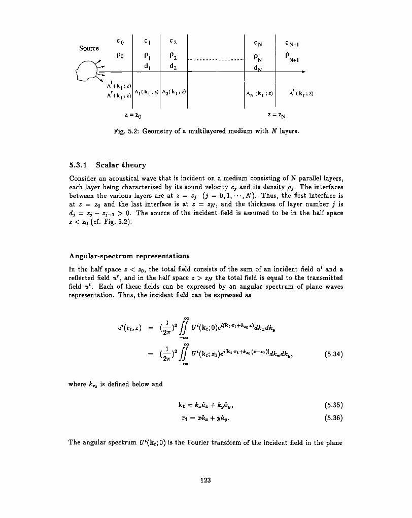
SourcePo
A (k t ;z)
A r(k t;z)A , ( k t ; z ) A2(k,;z)
C N
A N ( k t
CN+1
N+l
A ( k t ; z )
z = z0
Fig. 5.2: Geometry of a multilayered medium with iV layers.
5.3.1 Scalar theory
Consider an acoustical wave that is incident on a medium consisting of N parallel layers,each layer being characterized by its sound velocity Cj and its density pj. The interfacesbetween the various layers are at z = Zj (j = 0,1,- • -,N). Thus, the first interface isat z — ZQ and the last interface is at z = ZN, and the thickness of layer number j isdj = Zj — Zj-.i > 0. The source of the incident field is assumed to be in the half spacez < z0 (cf. Fig. 5.2).
Angular-spectrum representations
In the half space z < zo, the total field consists of the sum of an incident field u1 and areflected field ur, and in the half space z > Zff the total field is equal to the transmittedfield u*. Each of these fields can be expressed by an angular spectrum of plane wavesrepresentation. Thus, the incident field can be expressed as
(I-)2
—oo
oo
(5.34)
where k^ is defined below and
~r
r t = xex + yey.
(5.35)
(5.36)
The angular spectrum Ul(kt; 0) is the Fourier transform of the incident field in the plane
123
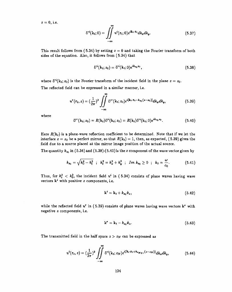
z = 0, i.e.oo
^ i i k T t d k x d k y . (5.37)ui{Tt;0)eiktT
This result follows from (5.34) by setting z = 0 and taking the Fourier transform of bothsides of the equation. Also, it follows from (5.34) that
where ff*(kt; ZQ) is the Fourier transform of the incident field in the plane z = ZQ.
The reflected field can be expressed in a similar manner, i.e.
oo
UT{TUZ) = (-^)2 / / Ur(kt;zo)ei^It-k'o^ (5.39)
whereUT(kt; ZQ) = R{kt)U\ku z0) = fl(kt)tf *(kt; 0)eifc*or°. (5.40)
Here R(kt) is a plane-wave reflection coefficient to be determined. Note that if we let theinterface z = ZQ be a perfect mirror, so that R[kt) — lj then, as expected, (5.39) gives thefield due to a source placed at the mirror image position of the actual source.
The quantity kZo in (5.34) and (5.38)-( 5.40) is the z component of the wave vector given by
L — . IL.2 _ L2 . L2 _ JL2 , L2 . r u > f ) • fc_ — — ^ 4 1 ^Kzo — Y "'0 ""t i t — Kx ' Ky i 11'1 "''o — u i K0 — • \0-^J-y
Thus, for kj < k%, the incident field u* in ( 5.34) consists of plane waves having wavevectors k* with positive z components, i.e.
V* = kt + k^ez, (5.42)
while the reflected field ur in (5.39) consists of plane waves having wave vectors k r withnegative z components, i.e.
kr = kt - k^hz. (5.43)
The transmitted field in the half space z > zjf can be expressed as
ti*(r(,z) = ( ^ ) 2 f[ Ut{kf,zK)eiV**<+k'»+il-"'»dk (5.44)
124
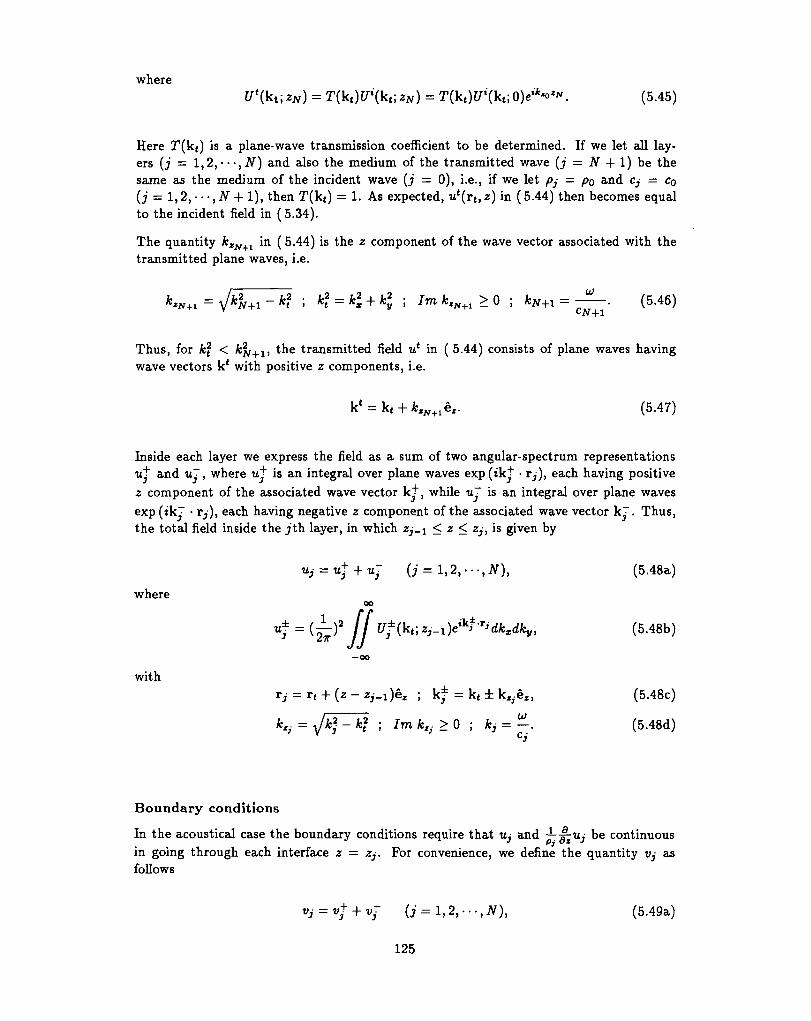
whereU\kt;zN) = T(k t)^(k«;^) = T(kt)^(kt; 0)eik^. (5.45)
Here T(k t) is a plane-wave transmission coefficient to be determined. If we let all lay-ers (j = 1,2,- • -,N) and also the medium of the transmitted wave (j = N + 1) be thesame as the medium of the incident wave (j — 0), i.e., if we let pj — po and Cj = CQ(j = 1,2, • • •, N + 1), then T(kt) = 1. As expected, u'(rt> z) in (5.44) then becomes equalto the incident field in (5.34).
The quantity kZf{+1 in (5.44) is the z component of the wave vector associated with thetransmitted plane waves, i.e.
- kt i *? = k2x + kl ; Im kZN+1 > 0 ; kN+1 = -^—. (5.46)
Thus, for fcj < kff+1, the transmitted field u* in ( 5.44) consists of plane waves havingwave vectors k* with positive z components, i.e.
k' = k t + * w + l e , . (5.47)
Inside each layer we express the field as a sum of two angular-spectrum representationsu t and uj, where u+ is an integral over plane waves exp(ik+ • Tj), each having positivez component of the associated wave vector k+, while u~ is an integral over plane wavesexp (ikj • rj), each having negative z component of the associated wave vector kj. Thus,the total field inside the jth. layer, in which ,Zj_i < z < ZJ, is given by
«,• = «+ + « ; (i = 1,2,...,JV), (5.48a)
whereoo
(^)2 / /f ^ ?kf, z^)^tT'dkxdky, (5.48b)
—oo
withTj = rt + (z- Zj-i)ez ; k* = k t ± k^.e , , (5.48c)
' I m k*i * ° J *> = - • (5.48d)
Boundary conditions
In the acoustical case the boundary conditions require that Uj and —j^Uj be continuousin going through each interface z — Zj. For convenience, we define the quantity Vj asfollows
(j = l,2,--.,N), (5.49a)
125
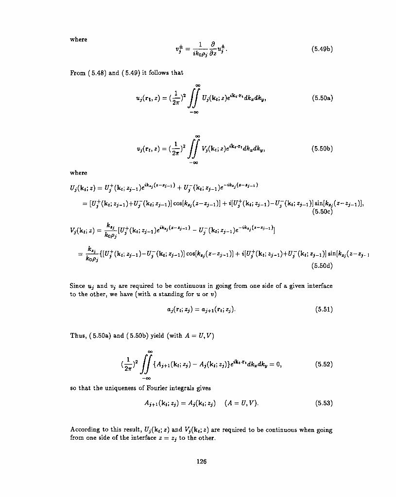
wherevf = T^—^-uf. (5.49b)
3 tkopj az 3
Prom (5.48) and (5.49) it follows that
oo
«*(*. *) = ( ^ ) 2 ff Uj(kt', z)eik^dkxdkv, (5.50a)
(5.50b)
where
^•(k t; z) = D
(5.50c)
^
z,-^)] sin[A:z.(z-z,-.,
(5.50d)
Since Uj and Vj are required to be continuous in going from one side of a given interfaceto the other, we have (with a standing for u or v)
ai(Tf, zi) = aj+i(rt; Zj). (5.51)
Thus, (5.50a) and (5.50b) yield (with A = U,V)
Ai+i(kS> z>) ~ ^ ( k < : Zi))e*tTtdkxdky = 0, (5.52)
so that the uniqueness of Fourier integrals gives
i4,-+i(kt; ZJ) - Aj(kt; ZJ) {A = U, V). (5.53)
According to this result, Uj(kt; z) and y,(k t; z) are required to be continuous when goingfrom one side of the interface z = Zj to the other.
126
Upon setting z = Zj-\ in (5.50c) and (5.50d), we have
Uj(kt;«,-_!) = [U+(kt; ^ i-1) + Ur(kt; *,-_!)], (5.54a)
l £ (5.54b)
from which we can determine Uj~(kt]Zj_i) and {7~(kt;Zj_i) in terms of Uj(kt\ Zj-i) and
[ t r ( k _ 1 ) ± - ^ ( k , ^ ) ] , (5.55)
It follows from (5.54a) and (5.54b) that (5.50c) and (5.50d) can be expressed in terms ofUj(kt; 2j-i) and Vj(kt; ZJ-\) in the following manner (ZJ-I < z < Zj):
Uj{kt; z) = Uj(kt; ZJ_X) cos[kZj(z - Zj-i)] + — Vj(kt; ZJ_I) sm[kZi(z - Zj-i)], (5.56)Pi
Vj(kt; z) = Vjikf, zi-1)coa[kz.[z - z^)} + iPjUj{kt; «,-_i) sin[A;Zj(z - z^)]. (5.57)
These two equations describe the spectral amplitudes in the region 0 < z — Zj-\ < dj or^ j ^ ! < z < 0j = 2j_i + dj. By using (53) and letting z — Zj = Zj-i + dj in (5.56) and(5.57), we get
Ui+I(kt;zj) = Ujiktizj) = Ujikf.Zj^) cosSj + —V;-(k«; *,•_;,) sin*,-, (5.58)
Vj
Vj+i(kt; ZJ) = V -(kt; Zj) = ipjUj(kt; Zj.{) sin*j + Vj(kt; *j_i) cos , (5.59)
where6j = kZidj • di = zj-zi-1. (5.60)
Matrix formalism
Equations (5.58) and (5.59) can be rewritten in matrix form as follows:
7j+i(kt;zj) \ _ f c°sSj ^s'mSj \ ( Uj(kt;Zj^)
Here U and V at z = Zj = Zj^i + dj are given in terms of U and V at z = Zj_j. Inabbreviated notation, (5.61) reads
where/ cos *, — sin Sj \ ,
. .J p> / . (5.63ipjsmOj cosdj J
127
Note that Uj and Vj are the spectral amplitudes at the interface z = Zj_i. Since U andV are continuous in going from one side of a given layer interface to the other, the totalmatrix for a system of N layers becomes
( ^ (5.64a)
where Mj, given in (5.63), is the matrix connecting U and V at the layer interface z = Zj_\with U and V at the layer interface z = Zj, i.e.
v £ ) = M j { v J ) = M'M'-1 ( Vill ) = MjMj-' • • -MaMl ( Uv, ) • (5"64b)
Let us denote the elements of the total matrix by A, B, C, and D, i.e.
M=(* BD J = M W M J V _ 1 M 3 - - - M 2 M 1 . (5.65)
At the first interface z = ZQ, we have (cf. (5.40))
Ui(kf, z0) = U\kt; z0) + Ur(kt; ZQ) = (1 + J2(kt))ff»(k,; zb), (5.66a)
and at the last interface z = z^, we have (cf. (45))
t; zN) = U'ikt; zN) = T(kt)^'(kt; zN). (5.66b)
In analogy with (5.49), we define (q = i,r, t)
^^k"^q)U (5.67a)
where
f +ktQ if q — i-k^ if q = r . (5.67c)
+kZN^ if q = <Then we have
Vi(kt; z0) = po[l - -R(k()]f'(kt; z0), (5.68a)
*; ZN) = PN+iT(kt)Ul(kt; ZN). (5.68b)
128
Substitution of (67) and (69) in (5.64b) with j = 1 yields
^ e ^ ( ) ( A B (PN+lT(kt) ) e -{C D ){ po(l
from which R and T can be determined, i.e.
where
g ("Oc)
With R(kt) and T(k t) given by (5.70a) and (5.70b), the values of U and V at the firstinterface z = ZQ and at the last interface z = zn follow from equations (5.66) and (5.68).Thus, to determine the spectral amplitudes Uj and Vj at the layer interface z = ZJ-I(j = 2,3, • • •, N), we can start from the values at the first interface z — ZQ using ( 5.64a)with N replaced by j — 1. Thus we have
y. I ~ *~J-I.I i TA / ' (5.70d)
where
M,--!,! = M J _ I M J _ 2 - - - M 2 M 1 (jf = 2,3, • • • , # ) , (5.70e)
and
M0,i = [ * ° J . (5.70f)
When f and V have been determined in this manner at the interface z = ZJ - I , then Uand V in the region Zj_x < z < Zj-\ + dj follow from equations (5.56) and (5.57).
Summary of results
We now collect our results. The incident, reflected, and transmitted fields tt*, ur, and u*are given by (q = i,r, t)
oo
129
where; kt = kxex + kyey, (5.71b)
-A; if q - i*« = { -kzo if q = r , (5.71c)
; rt = xex + yey ; (5.71d)
with
z0) if 9 = i^ ( k t ; z0) if 9 = r^ (k t ; Z j v ) if g = *
Po(D - PN+IB) - C + PN+IA '
Po(D — pff+iB) + C — PN+\A
Po{D — pjv+i-fl) — C + ptf+iA
Here A, B, C, and D are the elements of the multilayer system matrix, i.e.
A BM =
where
(5.71e)
(5.72a)
i = -Ti-
(V/ m fc*; > 0 ; fcj = -
(5.72c)
(5.72d)
1). (5.72e)
Inside the j t h layer, where Zj-\ < z < Zj (j - 1,2,- • •, N), the field is given by
oo
Uj{Tt''z) = {h)2 IfUjikt]zy{ktI
130
where
= 0,- coB[fcXJ(* - z,-_i)] + —Vj sin[*,.(z - z,-_i)], (5.73a)Pi
(5.73b)
Here t j and Vy are the values J7 and V at the interface z — Zj-\. They are related to thevalues of U and V at the first interface by
y. I = M-j-1,1 [ Vi ) ' (5 '73C)
whereMj_i t l = Mj_iMj_j • • -MjMi (j = 2,3, • • •, N), (5.73d)
with Mj given in (5.72b), and Mo,i is the unit matrix. The values of U and V at the firstand last layer interfaces are
CTi(k,; zo) = [1 + £(kt)]£T(kt; *>), (5.74a)
i(k(; zo) = po[l - i2(kt)]£T(kt; ^0), (5.74b)
UN+1{kt; zN) = T(k t )^(k t ; ^ ) , (5.74c)
^ ( k t ; zN), (5.74d)
(5.74e)
Here i7*(kt; z0) is assumed to be known, and (k f) and T(k t) are given in (5.71f)-( 5.71g).
131
5.3.2 Electromagnetic theory
From our treatment of the one-layer system in section 5.2.3, we know that each of theincident, reflected, and transmitted fields can be expressed as a sum of a TE and a TMplane-wave expansion. Thus (E'.H*) and (E r ,H r ) follow from (5.2) with q — i and q = r,respectively, while (E'.H*) follows from (5.2) with q = t, kz - kZlf+1, and z* = z^. Thespectral amplitudes VM(k t; z
q) in (5.2) associated with the incident and reflected TE andTM fields follow from (5.4) with q — i and q - r, respectively, and with z* = zr = z0
and kl = kT — k0. Similarly, the spectral amplitudes of the transmitted TE and TM fieldfollows from (5.4) with q = t, zl = Zff and kl =
Fields inside each layer
Inside the jth layer, where Zj-\ < z < Zj, the electromagnetic field (Ej,Hj) can be ex-pressed in a form similar to that in (5.48) in the scalar case and to that in (5.3) in theelectromagnetic case. Thus we have
+ V-(r) (V = E,H; j = 1,2, • • -,N), (5.75a)
VjM ±(r), (5.75b)
= TE,TM), (5.75c)
kf = k t ± kZjez ; Tj = rt + (z- z . , _ i ) e r , (5.75d)
where the spectral amplitudes are given by (cf. (5.4))
ct;zj_i) = —fc|dJE±(k t;z J_i) kt X ez, (5.76a)
( j ^ . , ^ ) k ± x ( k | x &a) f (5.76b)
_!) = -dJM ±(k t ;z,-_ a) k+ X (k, X e2), (5.76c)
132
t;Zj^) kt X e,. (5.76d)
Boundary conditions
The boundary conditions require that the tangential components of E and H be continu-ous in going from one side of a given interface layer to the other. Thus, the quantities
= ez X {EJE+(r) + EjE~(r) + EJM+(r) + E™-(r)}, (5.77a)
AH(r) = e2 X {H™+(r) + H™"(r) + B.JM+(r) + B.™~(r)}, (5.77b)
must be continuous. We now substitute the plane-wave expansions in (5.75c) with V = Eand V = H and with spectral amplitudes given in (5.76), in (5.77). Then by using (5.10)and the uniqueness of Fourier integrals, we find that the following spectral quantities mustbe continuous
; z) = *?[aT*+(kf; z ^ ) ^ ^ ^ + " ( k , ; z^) e^-iC-'i-O], (5.78a)
V?E(\ct;z) = kM.£[&JE+(kt]zj-1)e*'il'-'*-^-aJE-(kt-,zi-1) e-^-C'-i-i)], (5.78b)Mi
U™(kt; z) = %{a™+(kt]z^Oe^it'-'i-O + a™~(kt; z^) e-^-i^-i-O], (5.78c)Pi
V™{kt;z) = kZj[a^(kt]z^)eik^-'^ - aJ^Omz^) «-*«<—'-'>]. (5.78d)
Matrix formalism
We rewrite (5.78) as follows
&J(kt; z) = U?+{kt; zi.l)eik'^-i-^ + Uf(kt; z^x) e-
ifc'i(*-'i-O> (5.79a)
V?{kt; z) = [Uj+(kt; zi_1)eik'il"i-^ - Uf~(kt] *,•_,) e-^(—i-i)] f (5.79b)
133
where the superscript p stands for TE or TM and
it\Zj-i) ; pJE = — , (5.79c)
TTTM±flr . , \ ™7 - T M ± / . \ . TM _ MJ^ZJ /,-
Mi «i
Comparison of (5.79c)-( 5.79d) with (5.50c)-( 5.50d) shows that we get the same result asin the scalar case if we replace Uf by U? and replace pj by p*j, where the superscript pstands for TE or TM.
In analogy with (5.55), we have from (5.79c)-( 5.79d)
Vf^zi-t) = IWiktiZj^) ± ^VfiktiZj.!)], (5.80)
where the superscript p stands for TE or TM.
In analogy with (5.79c)-(5.79d), we write with q = i,r, t
UjE«(kt; z<) = (k*faTE<(kt; z") ; pTE* = £ | , (5.81a)
t; z")^ z") ; / ^ = 0 , (5.81b)
where A;?, 2:«, fc9, and /x« are given in (5.82g), (5.82h), and (5.82j).
Summary of results
We now collect our results. The incident, reflected, and transmitted fields are given by
OO
2* "JJ
oo
; H« = B.TE" + H™«, (5.82a)
X ez e^^dk^ky, (5.82b)
134
( i-)2 i if U™*{kt; z")kt x ez e^ (5.82d)
x (kt X ft.) (5.82e)
= k t + Ar'e, ; k t = kxex + kyeyey, (5.82f)
+kzo if q = ik«z={ - * „ , ifg = r , (5.82g)
p ' = f, + ( « - z«)e, ; (5-82h)
if g = tt; z0) if q = r (5.82i)
, if q = t ? =
_
- C*
_ ^fi . JTM _
135
M " = I £ p p P I =M5rMSr_1.--M5M?> (5.82n)
cos 6j j sin Sj= -«F • * ^ / (J l , 2 , , n (5.82o)
\ itf-sinOj cos Oj /
(5.82p)
fcZj. = ^ - A? ; Jm A,. > 0 ; k) = ^ { t j + p ) (j = 1,2, • • •, N), (5.82q)
t; z0) = A g d ^ k , ; z0) = - ^ ^ X e z ) ] ^ ^ (
- MfiTMwk . _ x _ [k'x(ktxef)]-E'(kt;zp)
W - j [k x (kt x ez)] • Jo(k') eifc^*°. (5.82s)
The subscript U in Ty in (5.821) is to remind us that this transmission coefficient is aratio between spectral amplitudes U, i.e. (cf. (5.15) and (5.79c)-(5.79d)).
aTEt(kt;zN) _ TE
nTM _ U™\kt] zN) _J-TT —u UTMi(kt;zN)
T1M, (5.82u)
where the transmission coefficient Tv is the ratio between spectral amplitudes of the elec-tric field.
Inside the j th layer, where Zj-i < z < Zj (j = 1,2, • • •, N), we have
Ej = Ej* + Ej M ; H ^ H j ^ + H ^ , (5.83a)
^ HP- {p = TE,TM), (5.83b)
136
^?l If UjE±rt) z) = -{^?l If UjE±(kt; z^Jkt X ez^t^dkxdkyi (5.83c)
Hj£±(rt> z) = -(JL)»(£)»-L If UjE±(*f, *i-i)kj x (kt x eje^dkzdky, (5.83d)
HjM±(rt, *) = {^f~ II UjM±{*f, z;-i)kt X e^t^dkxdky, (5.83e)
rt, z) = - ( — ) 2 ^ / / U?M±(kt; 2,-i)k± x (k t x ez)exKi Tidkxdkv, (5.83f)k
2TT k2 11 3 3
j JJ— OO
; p,-= rt + (« -z^ - i j e , , (5.83g)
^[^(kt;*,--!) ± ^/(kfjzj.x)]. (5.83h)
Here J7J and Vl are the values of Up and Vp at the interface z = ZJ-\ . They are relatedto the values of Up and Vp at the first interface by
where
iP
P i - «^_i,i I T/P / ~ I /^P DP M T/P J ' (5.84a)
(5.84b)
with M^ given by (C.I) with pj replaced by p£. For j — 1 we have
( A\ Bp \ ( 1 0
= ( £ J = ( o iThe values of Up and Vp at the first and last layer interfaces are
Up(kt; zo) = [1 + R?(kt)]U*(kt; zo), (5.85a)
137
V?(kt; zo) = pg[l - Rp(kt))U^(kt; zo), (5.85b)
UpN+1(kt; zN) = Tp(kt)U^(kt; zN), (5.85c)
zN) = pw + 17*(k t)C^(k t ; **) , (5.85d)
(5.85e)
5.4 Dyadic Green's functions for layered medium
5.4.1 Reflected and transmitted fields
As an example, we now derive the spectral domain Green's functions for the transmittedTM field. From (5.82e) with q=t, we have
ooJV+1 ff_— / / u™t(kt;zN)elk'^^z~ZN'kt x (kt x ez) e
lk* r''dkxdky,N+l JJ
—oo
(5.86a)
where UTMt(kt;zN) foUows from (5.82i), (5.82s), and (5.82u):
UTMl{kt] zN) = ~ kN+[ r , T [ k * X (k< x e,)] • E'(kt; -zoK*^1™). (5.86b)f*N+1*0 Kt
Substitution of ( 5.86b) and (5.86a) gives
oo
= (^)2 (I g EEE'(k t; zo)dkxdkv, (5.87a)
where
- TMt,, , 1* tk ' X (k* X e,)][k«" X (kt x e,)] (5.87b)
138
with
-zo) + kZN+1{z - zN). (5.87c)
The corresponding dyadic Green's function for the H-field follows from (A.I) with q — t,i.e.
x ^ x ( k < x * • ) ] •
The spectral domain dyadic Green's function for the transmitted TE field and for the re-flected TE and TM fields can be derived in a similar manner. They are listed in AppendixB.
5.4.2 Field inside the jth layer
Inside the j t h layer, where Z J _ I < z < Zj (j = 1,2, •••,N), we have from ( 5.83c) and(5.83f)
OO
f, z,--i)kt X eMe*k'il-'i-^eA***dk.dky, (5.89a)
E™±fr^ - _(_Ly2£z / / uTM±(k,-z- Ok* X (k, X e k* ' 1 ^-* ' - 1 V1
(5.89b)
where (cf. (5.83h))
U^(k*' z-x) — —\U?(kr z _ i ) ± —-V^(k#- Z'_i)l (5 89c)
with (cf. (5.84a)) and (5.85a)-( 5.85b))
'1 "3
(5.89d)
Thus by defining T?U and T?V by
f ^ * ^ - 1 - * 0 ) , (5.90a)
139
(kt; zo)eik^^-^), (5.90b)
we have from ( 5.89d):
Tf = {A*(l + Rp) + fl? i f c ( )
In analogy with (5.15a), we define
^ ^(«i-i-«o). (5.90d)
We now substitute (5.90a) and (5.90b) in (5.89c) to obtain
UfiktiZj-t) = \[Tf ± ^TfY^-^U^kuZo). (5.91a)
which together with the relations (cf. (5.79c)) and (5.82r))
t; z^^ (5.91c)
t;z0), (5.91d)
give
^T£±(kt; zi-x) = TjE±eik^^-^UTE\kt- z*). (5.92)
Similarly, we define in analogy with (5.15b)
~TM±(\, . , \ , ~TM±/\, . „ \TTM±
which together with the relations (cf. (5.79d) and ( 5.82s))
f, *j-i) = ^ d J M ± ( k t ; , , . . 0 , (5.93b)Mi
140
UTMi(kt; zo) = %-aTMi(kt; z0), (5.93c)(Ml
give
jM±UjM±{kt] Zj-X) =
On comparing (5.92) and (5.94) with (5.91a) with p = TE and p = TM, respectively, wehave
= [T ± ^ T j ] t (5.95)
TM±
From (5.92) and (5.82r) we find
UfE±(kt; ZJ-I) = -TjE±eik'°(z>-1-Zo)--2[kt x ez] • E'(k t; ZQ), (5.97)
which on substitution in (5.89a) gives
oo
EjB±(r) = (^-)2 / / Q_ T^(kt) • E^kj; zo)dkxdky, (5.98a)
where the spectral domain Green's function is
rpTE±
with
V»f = &*O(ZJ-I - 20) ± * ^ ( 2 - Z j - i ) . (5.98c)
The corresponding spectral domain dyadic Green's function for the H-field follows from
141
which givesrpTE±
= - - ^ - e * * i -^-[kf X (k, X ez)][k t x e z ] . (5.100)
From (5.94) and (5.82s) we find
UjM±{\it\Zi-i) = - ^ T T M ± e i f c ' o ( ^ - " ' ) ^ - 2 [ k i x (k, x e,)] -E^ktjzb), (5.101)fljKo HoKt
which on substitution in (5.89b) gives
oo
f™* ky, (5.102)
where the spectral domain dyadic Green's function is
The corresponding spectral domain dyadic Green's function for the H-field follows from
t )> ( 5 - 1 0 4 )
which gives
All dyadic Green's functions for the transmitted and the reflected fields and for the fieldsinside the j t h layer are listed in Appendix B.
5.5 Summary and Conclusions
We have considered the reflection, refraction, and transmission of arbitrary scalar or elec-tromagnetic waves in a multilayered medium. For a general source placed outside a mediumwith N parallel layers, we have derived explicit solutions for the reflected and transmittedfields, as well as for the fields inside each of the layers, in terms of the incident field orits source. The solutions have been expressed both in the form of angular-spectrum rep-resentations and equivalent impulse-response representations, and the associated dyadicGreen's functions have also been derived.
As a check of our results, we have derived in a different manner the solution for a one-layermedium or a slab and shown that the general results for a mutilayered medium correctly
142

reduce to those for a slab when the number of layers is set equal to 1 (N = 1).
In forthcoming papers, the results in this paper will be used to study the focusing ofelectromagnetic waves in layered media. In that connection, the computational aspectsassociated with the solutions presented here will also be addressed.
5.6 Aknowledgments
This research was supported by the Norwegian Research Council.
143

Bibliography
[1] David M. Pozar. A Reciprocity Method of Analysis for Printed Slot and Slot-CoupledMicrostrip Antennas. IEEE Trans. Antennas Propagat. 34, 1439-46, 1986.
[2] J.R. Mosig and F.E. Gardiol. A Dynamical Radiation Model for Microstrip Structures.Advances in Electronics and Electron Physics, 59, 1982.
[3] J. R. James and P. S. Hall. Handbook of Microstrip Antennas, volume 1 and 2. PeterPeregrinus Ltd, London, United Kingdom, 1989.
[4] J.R. Wait. Electromagnetic waves in Stratified media. Pergamon Press, Oxford, NewYork, Toronto, Sydney and Braunschweig, 1970.
[5] L. B. Felsen and N. Marcuvitz. Radiation and Scattering of Waves. Prentice-HallInternational, Inc., London, 1973.
[6] V. W. Hansen. Numerical Solution of Antennas in Layered Media. John Wiley &Sons, New York, Chichester, Brisbane, Toronto and Singapore, 1989.
[7] M. Born and E. Wolf. Principles of Optics. Pergamon Press, Oxford, London, andNew York, 1980.
[8] F. Abeles. Ann. d Physique 5, page 611, 1950.
[9] J. Gasper, G. C. Sherman, and J. J. Stamnes. Reflection and refraction of an arbtraryelectromagnetic wave at a plane interface. J. Opt. Soc. Am. 66, 955-61, 1976.
[10] J. J. Stamnes and G. C. Sherman. Radiation of electromagnetic fields in uniaxiallyanisotropic media. J. Opt. Soc. Am. 66, 780-88, 1976.
[11] J.J. Stamnes. Waves in Focal Regions. Adam Hilger, Bristol and Boston, 1986.
144
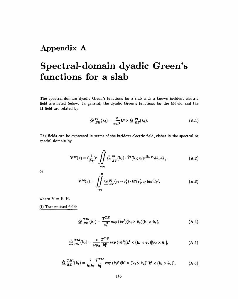
Appendix A
Spectral-domain dyadic Green'sfunctions for a slab
The spectral-domain dyadic Green's functions for a slab with a known incident electricfield are listed below. In general, the dyadic Green's functions for the E-field and theH-field are related by
The fields can be expressed in terms of the incident electric field, either in the spectral orspatial domain by
(A.2)
or oo
V"( r ) = / / g ^ ( r t - r't) • E'(r|, zo)dx'dy', (A.3)
where V = E,H.
(i) Transmitted fields
£«(*<) =
- TEt C TTE
G (kt) = 7j-exp {iip'Vk1 X (kt X ez)][kt X ez], (A.5)
- TMt 1 T™
= EE ( k t ) = k ^ l c f ^ ^ ^ X ( k t X ) ] [ k ' X ( k t
145

TMt -C Jfeo T™
£ ™ (kt) = -~^-^- **P W)[k* X e,][k* x (kt x e.)], (A.7)
iff* = k^zi - z0) + kZ7(z - zi). (A.8)
(ii) Reflected fields
^ EE (
=
X (k« X t*W X (k« X ez)], (A.ll)
iVr)[kt x ea][k* X (kt x e,)],
(iii) Fields inside slab
TJT+ T'TBi
S ») = ^ e ± l f c ' i ( ' - ^ ) ( k t x e,)(kt X e,),
^ ** (kt) = ^ " P ~ c ± ' M ~ ° ) [ k ± x (kt x )][kt x
^ (kt) = T ^
X e , ) ] ^ x (kt X e,)],
x * - ] ^ x ^ k ' x
146
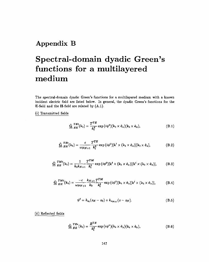
Appendix B
Spectral-domain dyadic Green'sfunctions for a multilayeredmedium
The spectral-domain dyadic Green's functions for a multilayered medium with a knownincident electric field are listed below. In general, the dyadic Green's functions for theE-field and the H-field are related by (A.I).
(i) Transmitted fields
TEt TTE
§L EE (k t) = T2~ e x p ( ^ ' ) ( k ' x e*)(kt X ez), (B.I)
Tfiv r fTE
cz TEtu,A ^-exp(iV»t)[kt x (kt x e,)][k« X ez], (B.2)
TMt 1 T
EE (k ' ) = VZ p - exP W)[k* x (kt X e , ) ] ^ X (kt x e,)], (B.3)KOKN+1 Kt
exp wt)[kt x *^kl x <k*x
(B.5)
(ii) Reflected fields
TET RTE
Q ( k ) ( t^ ) (k t x e,)(k t X ez), (B.6)
147
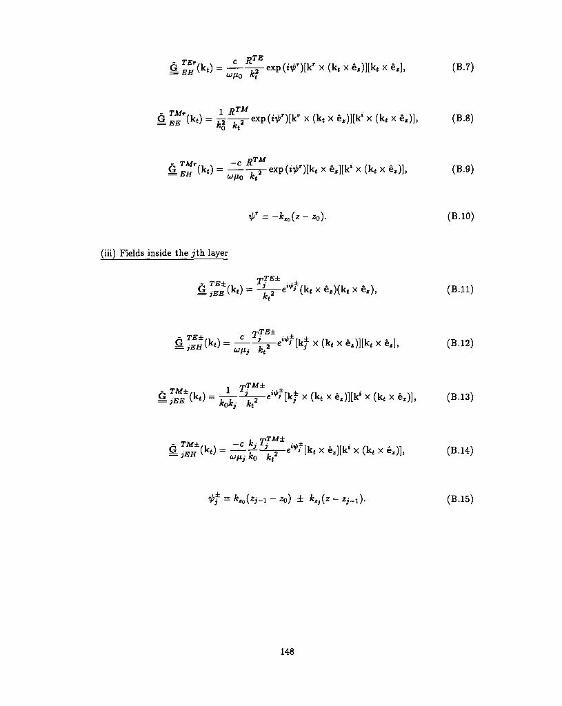
k (kO ^ ^ x p ( z V r ) [ k r X (kt X ez)][kt X ez], (B.7)
1 ff™rexp( i f ) [k f X (k( X e2)][k* X (kt X e,)], (B.8)
[iipT)[kt X ez][k ; X (k t x e , )] , (B.9)
i>r = -A: ^ 0 (^ - zo). (B.10)
(iii) Fields inside the j t h layer
\<A — -A p^j (k, y p Vlf. y p \ fR 1 1 \
)Hk< X
TM±
t) = ~L~ 3U2 e>^J tk ( X 6z][k* X (k t X ez)],
148
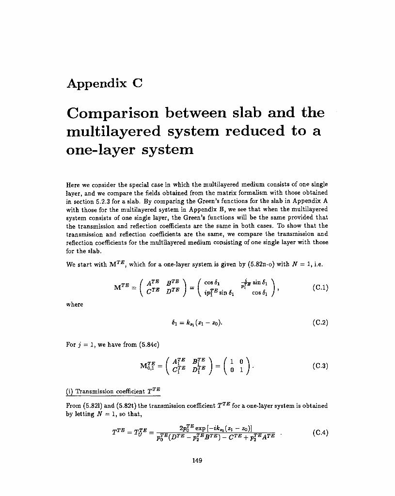
Appendix C
Comparison between slab and themultilayered system reduced to aone-layer system
Here we consider the special case in which the multilayered medium consists of one singlelayer, and we compare the fields obtained from the matrix formalism with those obtainedin section 5.2.3 for a slab. By comparing the Green's functions for the slab in Appendix Awith those for the multilayered system in Appendix B, we see that when the multilayeredsystem consists of one single layer, the Green's functions will be the same provided thatthe transmission and reflection coefficients are the same in both cases. To show that thetransmission and reflection coefficients are the same, we compare the transmission andreflection coefficients for the multilayered medium consisting of one single layer with thosefor the slab.
We start with M.TE, which for a one-layer system is given by (5.82n-o) with N — 1, i.e.
BTE \ (nTE = TE l
where
*i = M * i - * b ) - (C2)
For j — 1, we have from (5.84c)
T E _ ( r f _ ( 0\Oli ~ [ C T E DTE J - ^ „ 1 j • (C3)
(i) Transmission coefficient TTE
Prom (5.821) and (5.82t) the transmission coefficient TTE for a one-layer system is obtainedby letting N — 1, so that,
TTE _ TTE _U ~ p^E
-zp)]
149
Substituting ATE, BTE, CTE, and DTE from ( C.I) in (C.4), we get
TTE _ TTE _ zPo V\ e
~ U ~
where
*o = *»o(*i-«>)- (C6)
Next we consider the transmission coefficient TTE for the slab in section 5.2.3, whichaccording to (5.16a) is given by
TTE = tf
where iff and TTE+ are given by (5.17d) and (5.16c) respectively. By subtituting (5.17d)and (5.16c) in ( C.7), we obtain
mTE 4pTEp™e-«°
) i - isin^(pg-^s + {vTE?) ' (C-8)
which is the same result as in (C.5).
Similarly, we can show that the transmission coemecient T™ obtained from the matrixformalism in the special case of a one-layer system is the same as the transmission co-effiecient T™ obtained in section 5.2.3 for the slab.
(ii) Reflection Coefficient
Prom (5.82k) the reflection coefficient RTE for a one-layer system is obtained by lettingN = 1, so that,
JTEf r,TE nTE T>TE\ , /-tTE nTE ATEnTE _ PO i ^ ~ P2 -P J + I - P2 A
~ PIE{DTE - PIEBTE) - cTE + PIEATE ' [ }
Substituting ATE, BTE,CTE, and DTE from ( C.I) in ( C.9), we get
RTE (PZEPTE ~ P!EPD COS ft + i sin ( ( P P ) 2 - pg" (VF +iETE) h i i ^ ( ( P ) 2 T
Next we consider the reflection coefficient RTB for the slab in section 5.2.3, which accord-ing to (5.16d) is given by,
150
TE_ *•PTE_
where r ^ and T\E are given by (5.17c). By subtituting from (5.17c) in (C. l l ) , we have
?TE _
which after a little algebra can be written
nTB (PToEPTiE -PlEP?E)COSfi + tsintf,((PP)2 -pT0
Ep™)
This result is the same as that in ( C.10). Similarly, we can show that the reflectioncoeffiecient R™ obtained from the matrix formalism in the special case of a one-layersystem is the same as the reflection coeffiecient R™ obtained in section 5.2.3 for the slab.
(ii) Transmission Coefficients TTE± and TTM±
From (5.95), (5.90c), and (5.90d) the transmission coefficient TjE± for a one-layer systemis obtained by letting j — N = 1, so that
= -{A} [l + R ) + B-y p0 [l-R ) + - y ^ ( C 1 (l + R ) + Di p0 [1-R )],
nTE nTE^ ^ T B ] . (C14)Pi Pi
where we have used ( C.3).
By substituting ( C.13) in ( C.14), we obtain
TTE+ _ T g(fE
(P^PP+PPPP+PPPP)cos^ -trin^^-J'+pg-V')' l ^
Next we consider the transmision coefficient TTE+ for the slab in section 5.2.3, whichaccording to (5.16c), is given by
where ^ is given by (5.17d) and r$f and rff are given by (5.17c). Substituting theseresults in ( C.16), we get
151

TE(nTE I TE\ —tiiTTE+ Po_\Vi + P2 ) e , Q 17-v
- t sin
which is the same result as in ( C.15). Similarly, we can show that the transmissioncoefficients TTE~ and TTM± obtained from the matrix formalism in the special case of aone-layer system are the same as the corresponding transmission coefficients obtained insection 5.2.3 for the slab.
152
Chapter 6
FOCUSING OF ELECTROMAGNETIC WAVES
INSIDE A DIELECTRIC SLAB
Chapter 6
Focusing of electromagnetic wavesinside a dielectric slab
To be submitted for publication after revision
Velauthapillai Dhayalan and Jakob J. Stamnes
Physics Department, University of Bergen, Allegt. 55, N-5007 Bergen, Norway
Abst rac t
In many different applications, such as microstrip antennas, optical data storage, and hy-perthermia, it is important to have an accurate description of the propagation and focusingof electromagnetic waves in a layered medium. To that end, we present in this paper bothexact and asymptotic solutions for an electromagnetic wave focused inside a dielectric slabin terms of the given field or source current at a finite aperture in front of the slab. Thefield in the aperture is assumed to be time-harmonic, and its phase is predetermined bygeometrical optics so as to cancel the aberrations introduced by the slab interface.
The asymptotic solution is obtained by expressing the impulse response of the problem(i.e. the field produced inside the slab by a point source in the aperture) as a plane-waveexpansion and evaluating the corresponding (fcx, ky) integral by the method of stationaryphase. As a result, one finds that the main contribution to the impulse response comesfrom one particular plane wave emitted by the aperture point, namely that for which thecorresponding ray on refraction through the interface passes through the given observa-tion point. Since this asymptotic solution gives a big reduction in the computing time,it is important to examine its range of validity. We do so by comparing the asymptoticresults with those obtained from the exact solution. Such comparisons are made also forthe two special cases in which the slab problem reduces to a single-interface problem or asingle-medium problem.
Our numerical computations show that the differences between asymptotic and exact re-sults are small in a single medium, while they can be considerable in the case of a singleinterface or a dielectric slab. The asymptotic results become invalid near the apertureand near the interface. At low Presnel numbers, one observes focal shift phenomena andaxial asymmetries in each of the three cases (single medium, single interface, and slab),irrespective of whether one uses exact or asymptotic solutions.
153
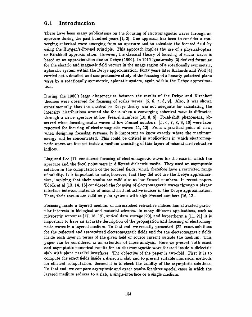
6.1 Introduction
There have been many publications on the focusing of electromagnetic waves through anaperture during the past hundred years [1, 2]. One approach has been to consider a con-verging spherical wave emerging from an aperture and to calculate the focused field byusing the Huygen's-Fresnel principle. This approach implies the use of a physical-opticsor KirchhofF approximation. However, the classical theory of focusing of scalar waves isbased on an approximation due to Debye (1909). In 1919 Ignatowsky [3] derived formulaefor the electric and magnetic field vectors in the image region of a rotationally symmetric,aplanatic system within the Debye approximation. Forty years later Richards and Wolf [4]carried out a detailed and comprehensive study of the focusing of a linearly polarized planewave by a rotationally symmetric, aplanatic system, again within the Debye approxima-tion.
During the 1980's large discrepencies between the results of the Debye and Kirchhofftheories were observed for focusing of scalar waves [5, 6, 7, 8, 9]. Also, it was shownexperimentally that the classical or Debye theory was not adequate for calculating theintensity distributions around the focus when a converging spherical wave is diffractedthrough a circle aperture at low Fresnel numbers [10, 8, 9]. Focal-shift phenomena, ob-served when focusing scalar waves at low Fresnel numbers [5, 6, 7, 8, 9, 10] were laterreported for focusing of electromagnetic waves [11, 12]. From a practical point of view,when designing focusing systems, it is important to know exactly where the maximumenergy will be concentrated. This could be critical in applications in which electromag-netic waves are focused inside a medium consisting of thin layers of mismatched refractiveindices.
Ling and Lee [11] considered focusing of electromagnetic waves for the case in which theaperture and the focal point were in different dielectric media. They used an asymptoticsolution in the computation of the focused fields, which therefore have a restricted rangeof validity. It is important to note, however, that they did not use the Debye approxima-tion, implying that their results are valid also at low Fresnel numbers. In recent papersTorok et al [13, 14, 15] considered the focusing of electromagnetic waves through a planarinterface between materials of mismatched refractive indices in the Debye approximation.Thus, their results are valid only for systems with high Fresnel numbers [16, 12].
Focusing inside a layered medium of mismatched refractive indices has attracted partic-ular interests in biological and material sciences. In many different applications, such asmicrostrip antennas [17, 18, 19], optical data storage [20], and hyperthermia [11, 21], it isimportant to have an accurate description of the propagation and focusing of electromag-netic waves in a layered medium. To that end, we recently presented [22] exact solutionsfor the reflected and transmitted electromagnetic fields and for the electromagnetic fieldsinside each layer in terms of the given field or source current outside the medium. Thispaper can be considered as an extention of those analysis. Here we present both exactand asymptotic numerical results for an electromagnetic wave focused inside a dielectricslab with plane parallel interfaces. The objective of the paper is two-fold. First it is tocompute the exact fields inside a dielectric slab and to present suitable numerical methodsfor efficient computation. Second it is to check the validity of the asymptotic solutions.To that end, we compare asymptotic and exact results for three special cases in which thelayered medium reduces to a slab, a single-interface or a single medium.
154
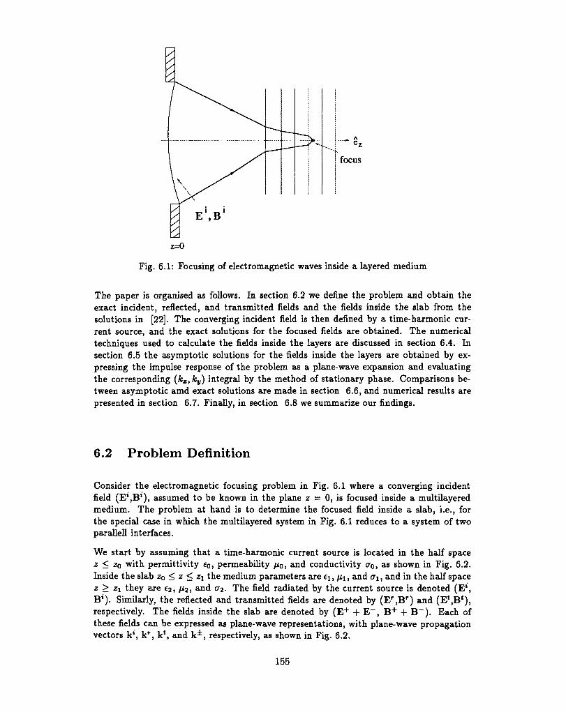
1 \ .
— —— —-—-- — !
!!•
focus
z=0
E , B '
Fig. 6.1: Focusing of electromagnetic waves inside a layered medium
The paper is organised as follows. In section 6.2 we define the problem and obtain theexact incident, reflected, and transmitted fields and the fields inside the slab from thesolutions in [22]. The converging incident field is then defined by a time-harmonic cur-rent source, and the exact solutions for the focused fields are obtained. The numericaltechniques used to calculate the fields inside the layers are discussed in section 6.4. Insection 6.5 the asymptotic solutions for the fields inside the layers are obtained by ex-pressing the impulse response of the problem as a plane-wave expansion and evaluatingthe corresponding (A;x, kv) integral by the method of stationary phase. Comparisons be-tween asymptotic amd exact solutions are made in section 6.6, and numerical results arepresented in section 6.7. Finally, in section 6.8 we summarize our findings.
6.2 Problem Definition
Consider the electromagnetic focusing problem in Fig. 6.1 where a converging incidentfield (E*,B*), assumed to be known in the plane z = 0, is focused inside a multilayeredmedium. The problem at hand is to determine the focused field inside a slab, i.e., forthe special case in which the multilayered system in Fig. 6.1 reduces to a system of twoparallell interfaces.
We start by assuming that a time-harmonic current source is located in the half spacez < ZQ with permittivity eo, permeability /x0, and conductivity <70, as shown in Fig. 6.2.Inside the slab ZQ < z < z\ the medium parameters are ei, /zi, and <j\, and in the half spacez > z\ they are e2, fa, and a2. The field radiated by the current source is denoted (E l,B'). Similarly, the reflected and transmitted fields are denoted by (E r ,B r) and (E'.B*),respectively. The fields inside the slab are denoted by (E+ + E~, B + + B~). Each ofthese fields can be expressed as plane-wave representations, with plane-wave propagationvectors kl, k r , k*, and k*, respectively, as shown in Fig. 6.2.
155
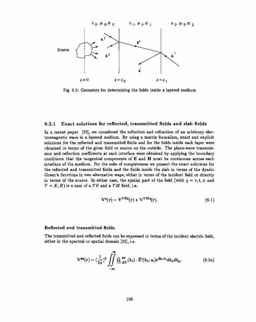
E 0' f0'
Source
E l , e2, \i2>a 2
z = 0 = z. = z,
Fig. 6.2: Geometry for determining the fields inside a layered medium
6.2.1 Exact solutions for reflected, transmitted fields and slab fields
In a recent paper [22], we considered the reflection and refraction of an arbitrary elec-tromagnetic wave in a layered medium. By using a matrix formalism, exact and explicitsolutions for the reflected and transmitted fields and for the fields inside each layer wereobtained in terms of the given field or source on the outside. The plane-wave transmis-sion and reflection coefficients at each interface were obtained by applying the boundaryconditions that the tangential components of E and H must be continuous across eachinterface of the medium. For the sake of completeness we present the exact solutions forthe reflected and transmitted fields and the fields inside the slab in terms of the dyadicGreen's functions in two alternative ways, either in terms of the incident field or directlyin terms of the source. In either case, the spatial part of the field (with q = r, t, ± andV = E, H) is a sum of a TE and a TM field, i.e.
V*(r) = VTEq{r) (6.1)
Reflected and transmitted fields
The transmitted and reflected fields can be expressed in terms of the incident electric field,either in the spectral or spatial domain [22], i.e.
Vw(r) == (^)2 (I g E«(kt; (6.2a)
156
or
V*(r) = ff g «v(rt - r't) • E^rJ, zo)dx'dy', (6.2b)
—oo
whereoo
gSr(r. " r{) = {±? Jjg^(k^^-^ (6.2c)
Here p = TE,TM and the subscript E in the Green's function Q. ** denotes that thisdyadic Green's function is associated with the known incident field E*. Also note that
r t = xex + yey (6.3a)
and that the k vectors in Fig. 6.2 are given by
k* = kt + k^ez ; k r = kt — fc^e* ; kt = kxex -f kyey (6.3b)
KZj - y K ; s t i Kt — Kx + "-y ' J 7 n S»j - U W ~ U> 1 > z j i ^D.Oaj
with fcj being the wave number in medium j , i.e.
Alternatively, each field in (6.1) can be expressed in terms of the electric source current,i.e.
oo[•OO
= / (-^)2 j[ g"v(kt;z0- z')-30(kt;z')e*'r*dkxdkvdz', (6.4a)r —oo
—oo
where
oo
0(k t;z ')= If 30{r't>z')e-AtT<dx'dy', (6.4b)
157
with
oo
- z') = {^f Jjg ^(k,; * - z')e^-**)dkxdky. (6.4c)
Here the subscript J in the Green's function £ |J*, denotes that this Green's function isassociated with the known current source Jo .
The spectral-domain dyadic Green's functions in (6.2c) and (6.4c) are related by
The dyadic Green's functions for the E field and the H field are related by
The spectral-domain dyadic Green's functions for TE and TM fields transmitted througha slab are given by [22]
rpTE« ) = - * * - e x p ( i V > t ) ( k t x ^ ) ( k t x h')> ( 6 - 7 a )
C Tl ^ ) ^ 1 X (kt X e,)][kt X e.], (6.7b)
1 T ™( k t ) = j f c ^ i f c r e x p ( # 4 ) [ k t x (kt x )][k*x (kt x )]> (6Jc)
TMt -C fco T ™i EH (k«) = — F I T exP (^ ' ) [ k t x e,][k« x (k, x &,)], (6.7d)
where^ * = *jO(«i-2b) + * j a ( * - * i ) . (6.7e)
The spectral-domain dyadic Green's functions for TE and TM fields reflected from a slabare given by [22]
QEE (k<) = -fc2-exP(:VO(kt X e,)(k t x e,), (6.8a)
158
£ EHc RT
(k<) = ^ - " T 2 - exP W ) [ k ' x (k« x e,)][kt x BZ), (6.8b)w / 0 K
1 R
(kO = I 5 T 2 - « P W)P<P x (k* x 6«)llkt x (k ' x 6-)l. (6-8c)
r)tkt x ki x ( k ' x *•)]•
wherei>T = -fczjz - zo). (6.8e)
The plane-wave transmission coefficients T™ and TTE and reflection coefficients R™and RTE are listed in Appendix D.
6.2.2 Fields inside the slab
The field inside the slab consists of two parts, V + ( r ) and V"(r) . Each of these can beexpressed as a sum of a TE and a TM field, i.e.
+ V-(r) (V = E,H), (6.9a)
V±(r) = VTE±(r) + VTM±(r), (6.9b)
where (cf. (6.2a) and (6.2b)) with p = TE,TM
—oo
oroo
Vp±(r) = / / £L fyirt - rj) • E'(r'(, zo)dxV- (6.10b)
—oo
The spectral-domain dyadic Green's functions for the fields inside a slab are given by [22]
TTE±__-c±'**i(*-*o)(k t x ez)(kt X ez), (6.11a)
159
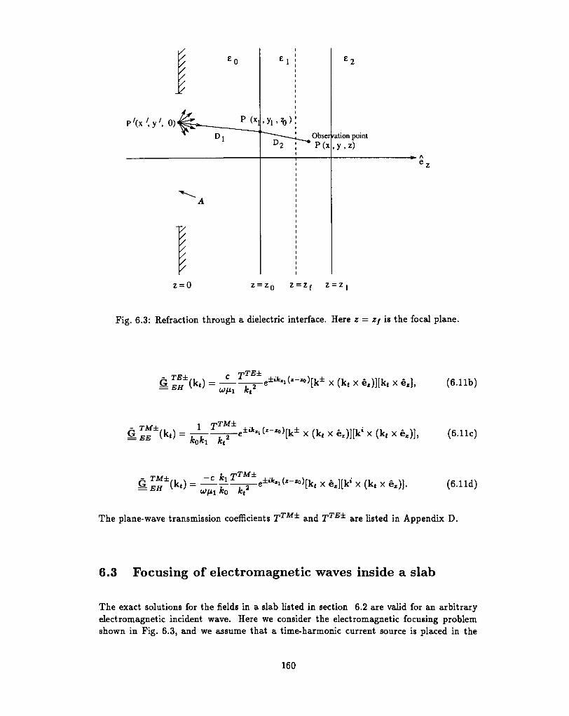
//
^ ^ 7 - — •
A
V/////
e l
, Obser^ P(x
e 2
ration point
z = 0 = Z Z = Z ,
Fig. 6.3: Refraction through a dielectric interface. Here z = Zf is the focal plane.
x < k ' x *>W* x
£-^^e ± i f c ' i ( * -*> [k t X ex][k* X (k, X e,)].
The plane-wave transmission coefficients TTM± and TTE± are listed in Appendix D.
6.3 Focusing of electromagnetic waves inside a slab
The exact solutions for the fields in a slab listed in section 6.2 are valid for an arbitraryelectromagnetic incident wave. Here we consider the electromagnetic focusing problemshown in Fig. 6.3, and we assume that a time-harmonic current source is placed in the
160
aperture plane z = 0. Following Ling and Lee [11], we assume that the source is polarisedin the x direction and is given by
J0(x',y',z') = J0(x',yf,z')ex, (6.12a)
where
Jo(*', y', -0 = -2A(x', y') exp \-i<f>{x', y')]S(z'). (6.12b)
Here A(x', y') and (f>(x't y') are the amplitude and phase distributions of the current source.<j>(x',y') is introduced in order to produce an aberration-free converging wave front afterrefraction through the interface.
Now we apply the physical-optics or Kirchhoff approximation, according to which the am-plitude A(x',y') of the current source vanishes outside the aperture. Thus the Fouriertransform of the current source in the aperture plane z = 0+ is given by
3o(kt;z') = jo(kt)6{z')ex, (6.13a)
where
Jo(k4) = -2Jj^A(x', y') exp {-#(*', y') + kt • r't}}dx'dy'. (6.13b)
Thus[k* x (kt x ez)] • jo(k e ; *') = *«*„ J0(k t), (6.14a)
[kt x ez) • j o (k t ) = kvJ0{kt). (6.14b)
Using (6.13), (6.14) and the Green's functions for the transmitted and reflected fields in(6.5), (6.7) and (6.8) in (6.4a) and carrying out the z' integration, we obtain the followingexact solutions for the TE and TM parts of the transmitted and reflected electric fields :
' X (kt X e.)J0(k t)c i k- Ttdkxdky,
(6.15a)
IT rTBr^jei(*«o'l+fc'»(*-l))klxe,Jo(kt)e<kf-rtdfc«d*v, (6.15b)J J -oo ^zn^t2%c2
161
E™T = ~ ^ T E 2 I T iZ™r|e*fc*o(z-2'°))kr x (kt X ez)7o(kt)e'k'- r*c£Jfcx<iA;v, (6.15c)Z7TC K Q »/ »/ —oo ™|
x e, jo(kt)e i k ' - r « d M V (6.15d)
Similarly, using (6.13) and (6.14) and the Green's functions for the fields inside the slab in(6.11) in (6.4a) and carrying out the z' integration, we obtain the following exact solutionsfor the TE and TM parts of the electric fields inside the slab:
E TM± = ^ IT T™±>£eik^k± x ( k t x ^)e±ifcll(
(6.16a)
r r TTE±_^L_{kt x ^ )J J _oo *zo"-t
(6.16b)
where Jo(kt) is given in (6.13b) and k* is given in (6.3c).
From now on we focus our attention on the electric fields inside the slab. By substituting( 6.13b) in (6.16a) - (6.16b) and interchanging the order of the integrations, we have
ET A f ± = / / / ( * ' > V') exp [-uK*\ 2/')]FTM±(z', y')dx'dy', (6.17a)
= JJAA(x',y')ex?[-i4>(x',y'))FTE±(x',y')dx'dy', (6.17b)
where (with p = TE, TM)
Fp±(x',y') = [f°° ^ ( f c , , *„)exp [ih^k,, kv)]dkxdky, (6.17c)J J —OO
with
^(fcx, ky) = kx(x - x') + ky{y -y') + kzozo± kZl (z - 2b), (6.18a)
f -
162
KZQKt
6.4 Numerical Techniques
6.4.1 Reduction from double integral to single integral
We must first compute the spectral double integral in (6.17c) to obtain the contributiondue to one particular point source in the aperture, and then carry out a double integrationover the aperture plane to obtain the fields inside the slab given by (6.17a) - (6.17b). Sincethis procedure is time consuming, we reduce the double integral in (6.17c) by introducingsuitable variable-shifts.
We first consider the (kx, ky) integral in (6.17c) and by using (6.3c), we can write f± in(6.18) as follows:
( 6 1 9 b )
Now we introduce the change of integration variables
kx = A cos/? ; kv = Asin/3 ; dkxdky = XdXdfi, (6.20a)
and put
x - x' - pcoscf> ; y-y' = psinQ ; p = [(x - x')2 + (y - y')2]», (6.20b)
so that
kx(x - x') + ky(y - y') = Xp cos ((3 - </>), (6.20c)
kt = x* J i f = cos2/9 >" i f = S'312/3. (6.20d)
* i = *o ~ A2 ; ik2, = fc? - A2, (6.20e)
163
^ = \sin2p. (6.20f)
By adding the TE and TM parts of the electric fields we obtain from (6.17a)-(6.17b)
E± = E M ± + E™ ± = / / / ( * ' > *') exP H#*'> »0]F V . •)* '«#, (6.21a)
where
F±(x',y') = FTE±(x',y') + FTM±(x',y') = / / " ^ ( ^ . J f c ^ c ^ ^ * - ^ ) ^ ^ , (6.21b)J J -OO
with(cf. (6.19) and (6.20))
-, *y) + fTM:t(*«, fcy) (6.21c)
(6.21d)
Now on we let the amplitude of the aperture current distribution be uniform, i.e. A(x', y') =1.
When we substitute (6.21d) in (6.21b) and take into account the change of variables in(6.20), we find that the /3 integrals can be expressed in terms of Bessel functions usingthe formulas
/ * eitco<p-*hos0dp = 2Kicos<f>J1(t), (6.22a)
I + ire'«««(^-*)cos2/3<f^ = 7r[J0(t)(l + c o s 2 ^ ) - c o s 2 < / ) ^ ^ ] , (6.22b)
/•*+2ireitco.(/3-*)sin2/gd/3 = x[j0(t)(i - cos 2^) + cos 2 0 ^ ^ ] , (6.22c)
Jd> t
J4,
Thus we obtain
f*+27r eitco,(fi-4>) s i n 2pd/3 = -2-K sin 2 ^ [ 2 ^ ^ - J0(t)]. (6.22d)
Jd> t
(6.23a)
164
where
TTE± L.2sin2 * ± ^ T ™ ± cos2 <f>], (6.23b)
« • 20, (6.23c)
ill ^ rpTE±
= -DUX) = J i - ^ M T ™ * - i p - l r i n l ^ , (6.23d)C KQK K
(6.23e)
(6.23f)
6.4.2 Dividing the integration area
From (6.23a) we observe that along the integration area [0,oo], k^ and kZl can be eitherreal or imaginary. Assuming that ki > ko, in the interval 0 < A < ko both k^ and kZl arereal. In the interval fc0 < A < ki, k^ is imaginary while kZl is real. Finally, in the intervalki < A < oo both ktQ and fctl are imaginary. So one must divide the integration area in(6.23a) to three different parts and use appropriate numerical method. In order to usethe trignometric functions later, we first make the following substitutions:
A = M , (6.24a)
and
kT = ^-. (6.24b)
Thus,
K =k1(k~2-t2)^ (6.25a)
kZl = «i(l - <2)> (6.25b)
165
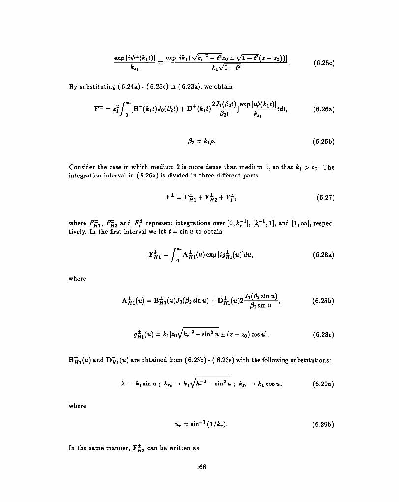
exp exp( 6 - 2 5 c )
By substituting (6.24a) - (6.25c) in (6.23a), we obtain
J 0( 6 . 2 6 a )
= klP. (6.26b)
Consider the case in which medium 2 is more dense than medium 1, so that Arj > A;0- Theintegration interval in (6.26a) is divided in three different parts
(6.27)
where F^, F^2 and Ff represent integrations over [0,fcr *], [kr 1 ,1], and [l,oo], respec-
tively. In the first interval we let t = sin u to obtain
where
^(«)exp[i<fex{?)\du, (6.28a)
(6.28b)
where
9HI(U) - ^lt^ov^r2 - s i n 2 u ± ( z - zo)cosu]. (6.28c)
and D^1(u) are obtained from (6.23b) - ( 6.23e) with the following substitutions:
A —• ki sin u ; k^ —> ki y Av 2 - sin2 u ; kZl -* ki cos u, (6.29a)
(6.29b)
In the same manner, F ^ 2 can be written as
166
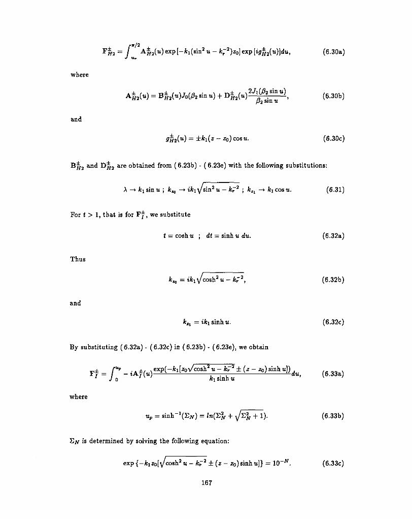
/
•KJ2
A£2(u) exp [-fc^sin2 u - k;2)z0] exp [ig%2(u)]du, (6.30a)
where
Aj? 2 ( u ) = B ^ 2 ( u ) Jo(/32 sin u) + D ^ 2 ( u ) — l i z l £ j (6.30b)
and
= i* i (^ - ^o) c o s u- (6.30c)
and D ^ 2 are obtained from (6.23b) - (6.23e) with the following substitutions:
A -y ki sin u ; k^ -»i&iy sin2 u - A;r 2 ; Ar»l -» fci cos u. (6.31)
For t > 1, that is for Ff, we substitute
t = cosh u ; dt = sinh u du. (6.32a)
Thus
kzo = t'^i y c o s h 2 u - kf2, (6.32b)
and
Ki = iki sinh u. (6.32c)
By substituting (6.32a) - (6.32c) in (6.23b) - (6.23e), we obtain
_+ /"**»> + exp(-A;i [zo\/cosh2 u - kr2 ±{z - ZQ) sinh u]) . nnFf = / - zAf (« )—^—i^ —-— s m ^du, (6.33a)' J o J Jfci sinh u '
where
Up = s inh^Etf ) = ln{Y?N + ^ S ^ + 1). (6.33b)
is determined by solving the following equation:
exp {-kizo[\Jcosh2 u - Ar 2 ±(z- ZQ) sinh tt]} = 10"^. (6.33c)
167
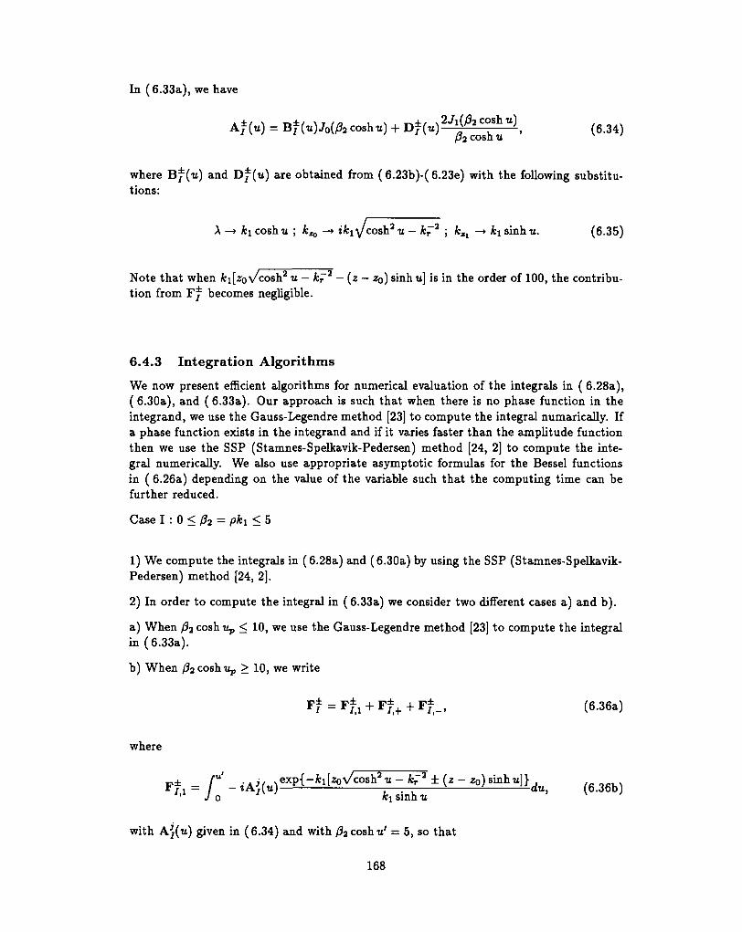
In (6.33a), we have
Af(u) = Bf (U)J0(/32coShu) + »t(»)2Jlfo^lU\ (6-34)
where Bf(u) and T)f(u) are obtained from (6.23b)-(6.23e) with the following substitu-tions:
coshu ; k^ -» i* iy cosh2 u - kr 2 ; kZl -» fci sinhu. (6.35)
Note that when fc1[z0'v/cosh2 u - /cr
2 — (z - zo) sinhu] is in the order of 100, the contribu-tion from F* becomes negligible.
6.4.3 In tegra t ion Algori thms
We now present efficient algorithms for numerical evaluation of the integrals in ( 6.28a),(6.30a), and (6.33a). Our approach is such that when there is no phase function in theintegrand, we use the Gauss-Legendre method [23] to compute the integral numarically. Ifa phase function exists in the integrand and if it varies faster than the amplitude functionthen we use the SSP (Stamnes-Spelkavik-Pedersen) method [24, 2] to compute the inte-gral numerically. We also use appropriate asymptotic formulas for the Bessel functionsin ( 6.26a) depending on the value of the variable such that the computing time can befurther reduced.
Case I : 0 < 02 = ph < 5
1) We compute the integrals in (6.28a) and (6.30a) by using the SSP (Stamnes-Spelkavik-Pedersen) method [24, 2].
2) In order to compute the integral in (6.33a) we consider two different cases a) and b).
a) When /32 cosh tip < 10, we use the Gauss-Legendre method [23] to compute the integralin (6.33a).
b) When fa cosh Up > 10, we write
F ^ F ^ + F^ + F^, (6.36a)
where
1 = f ' - iA^ ) e X p { - f c l [ W c O 5 h 2 : t : f ± <* - *> Sinhtt»rftt, (6.36b)' J o «i sinn u
with Aj(u) given in (6.34) and with fa coshu' = 5, so that
168
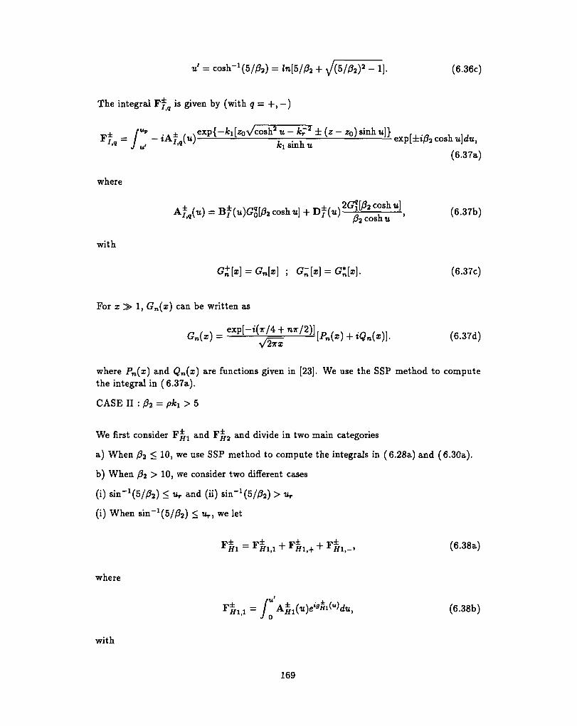
u' = cosh-^S/ft) = ln[5/p2 + ^/(5//32)2 - 1]. (6.36c)
The integral Ffq is given by (with q = +,-)
Nexp{—fci[zo\/cosh2 u — kr 2 ± (z - zo)siiihu]}
(6.37a)
where
Aj (u) = Br (U)GQ[/?2coshu] -\-T)T(U)— , (6.37b)P2coshu
with
(6.37c)
For I > 1 , Gn(a:) can be written as
(^'M r /"1 .M + «J.)|. (MTd)
where Pn(a;) and Qn(i) are functions given in [23]. We use the SSP method to computethe integral in (6.37a).
CASE II : p2 = pki > 5
We first consider F J x and F ^ 2 and divide in two main categories
a) When /?2 < 10, we use SSP method to compute the integrals in (6.28a) and (6.30a).
b) When fa > 10, we consider two different cases
(i) am-1 (5/fa) < tir and (ii) sin"1 (5/&) > tv
(i) When sin'1 (5f/32) < u r, we let
where
*Hi.i = r<A|1(ii)e*«Wdti, (6.38b)j o
with
169
. (6.38c)
and g^^u) are given by (6.28b) and (6.28c). Integral F ^ is given by (with)
x, (6.39a)
where
Ai/i,q(u) = ^%i(u)^'o\fi2 sin u] + D^x(u)—-^—7 . (6.39b)
B ^ a and D ^ are given by (6.23b) - (6.23e) and Gn(i) is given by (6.37d).
The integral in (6.30a) is divided in two parts:
FH2 = FH2,+ + FH2,- (6.40a)
with
FH2 ~ I' AmqiuW9"^6''11*"'™"'1'11'' (6.40b)
where
(u) = BJiJu)Gn\02 sin ul + D%Ju)—^-? -. (6.40c)
Here Gn(x) and g^2 a r e defined in (6.37d) and (6.30c), respectively.
(ii) When sin~1(5//92) > tV, the SSP method is used to calculate the integral in (6.28a),and (6.30a) is divided in three different parts:
F | 2 = J* 3 i l + F±2>+ + F±2>_, (6.41a)
where
/ " %i&Mdu, (6.41b)
(q = + , - ) . (6.41c)
170
u), 9^2{u) a n d &H2,q{
u) a r e defined by (6.30b), (6.30c), and (6.40c), respectively.
2) F^ in (6.33a) can be computed using:
F± = F± + + F±_. (6.42)
Here F * (with q = +, - ) is given by (6.37a) and can be computed using the SSP method.
For the case in which k\ < ko, the integration interval in (6.26a) is divided in three dif-ferent parts [0,1], [ljJfe"1] and [fc"1,^]. When ki = ko the integration interval is dividedin two parts [0,1] and [1, oo]. We adapt numerical techniques similar to those discussedabove for the case in which fcj > ko.
For each observation point (x,y, z) and integration point (x',y'), the spectral integrals in( 6.26a) are computed using the numerical methods discussed above. These results arethen used in (6.17a) - (6.17b), and the corresponding integrals are then carried out usingthe two-dimensional SSP method [24, 2]. The main problem in obtaining exact numericalresults is the very long computing time needed. In order to reduce the computing time,one can evaluate the spectral integrals in (6.26a) asymptotically using the method of sta-tionary phase. This is discussed in the following section.
6.5 Asymptotic evaluation
The asymptotic solution is obtained by assuming that the main contribution to the im-pulse response comes from one particular plane wave emitted by the aperture point, namelythat for which the corresponding ray on refraction through the interface passes throughthe observation point [11, 2]. This contribution is obtained by evaluating the spectralintegrals F p ± ( i ' , y') in (6.17c) asymptotically by using the method of stationary phase.The stationary points (&*, &*) of the phase function h(kx, kv) in (6.18a) are given by [2, 11]
(6.43a)
K = fco^- = fclZJ*. (6.43b)
where D\ is the distance between the integration point in the aperture and the refractionpoint at the interface, and D2 is the distance between the refraction point at the interfaceand the observation point, as shown in Fig. 6.3. Thus, we have
D1 = [(x - x')2 + (y - y'f + zlY'\ (6.43c)
171
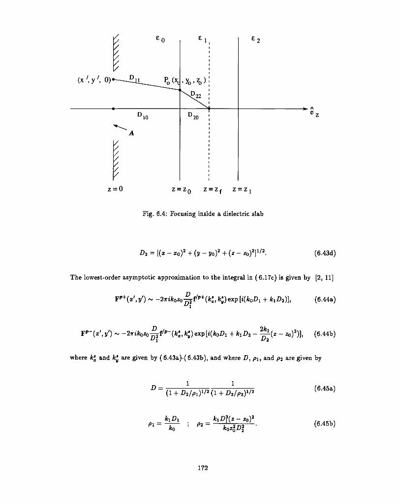
(x ', y', 0)
z = 0 Z — Z rv Z — Z r Z — Z i
Fig. 6.4: Focusing inside a dielectric slab
(V - !/o)2 (6.43d)
The lowest-order asymptotic approximation to the integral in (6.17c) is given by [2, 11]
)-^f/p+(fc*) k'y) exp [i{koDx1
(6.44a)
Tp-(x',y') ~ -27ri^o4f/p-(fci,fc')exp[i(fcoi?1 + kxD2 - ^(z - zo)2)], (6.44b)
where A;* and fc* are given by (6.43a)-( 6.43b), and where D, pit and p2 are given by
D = (6.45a)
(6.45b)
172
The phase <j)(x', y') in (6.16a)-( 6.16b) is determined from geometrical optics so as to can-cel the aberrations introduced by the interface between the aperture and the focal point.From Fig. 6.4 it follows that the requirement of equal phase at the focal point for fieldsalong all geometrical rays is
<p{x', y') = fco-Dn + &il>22 ~ k0Dw - fciAjo, (6.46)
where Du, D22, Dw and D20 are the distances specified in Fig. 6.4 given by
= [(*o - x')2 + (2/0 - y')2 + *02]1/2> (6.47a)
(6.47b)
D10 = z0, (6.47c)
D20 = zf~ zo- (6.47d)
6.6 Comparison between exact and asymptotic solutions
6.6.1 Analytical comparison
We now compare the exact and asymptotic solutions for F p ± given by (6.17c) and (6.44),respectively, for the special case in which the interfaces are removed.
We assume that ^ 2 = Mi = Mo = 1> and e2 = «i = o = i so that fc2 = k\ = fc0 = k ;kZ2 = K = ** = *z i T™+ = TTE+ = 1 ; h(kx,ky) = k.R;R = {x-x',y-y',z}.Then addition of fTAf+ and fTE+ in (6.19a,b) give
which can be combined to give
Substituting equation (6.49) in (6.17c), we obtain
173
which can be rewritten as
Thus, by using Weyl's plane-wave expansion of a spherical wave
ikR ; r foo -ik-RpikR ; r foo -ik-R .
~R~ = 2^JJ oo~kTdkxdky' * = l* l : ^ = l^l = V ( a ; - ^ ) 2 + (3/-y')2 + ^ , (6-52)
we have
J reikR. 1 d
(6.53)/I K* J l . n> ISO/ -il,
The result in (6.53) is exact. The corresponding asymptotic result is readily obtained byapplying the following asymptotic formula:
f foo -tk-R. fi'kfi
/ / f(k)——dkxdky ~ -2™—-f(k'), (6.54)J J - o o "»* -K
where
k* = k{X~X , y ~ y , —}. (6.55)
Thus we have from (6.50)
,ikR' y>) - -2*i-^e—<e fl - {* ~ *?] - e - e
To enable us to compare the asymptotic result in (6.56) with the exact result in (6.53),we carry out the differentiations in the latter equation. By doing so (6.53) can be written
F{xW) = - « £ £ { [ ! + JL3t 3 (x - xQz 3i
Comparison of the exact result in ( 6.57) with the corresponding result in (6.56), shows
174
that when terms of order j ^ and /fcLj are neglected in (6.57), we get agreement with(6.56).
Finally, we show that the asymptotic result in (6.56) follows directly from the asymptoticresult in (6.44) in the limit e2 —• ei. For the single medium (6.44) becomes,
F(x', y') ~ -2*ikz0^ exp [i kD2))t(kx, k'y),
where
F(x', y') = FTE(x', y') + F™(x', y'),
(6.58)
(6.59)
f (k'x, k'y) = iTE{k'x, k'y) + f™(k'x, k'y). (6.60)
When ei = £o, we obtain
+ D2 = R, (6.61a)
ZQ Z — ZQ(6.61b)
D =l+g- R
From (6.60), ( 6.43a - 6.43b) and (6.48) we have
(6.61c)
(6.62a)
Dl (*-O(y-
u . L ^ _K_ Di(x-x')z (6.62c)
Here we have used the fact thatin ( 6.58), we have
= ^ and ^- = ^ . Substituting (6.61) and (6.62)
*.} (663)
175
in agreement with (6.56). Our analysis here shows that for kR > 1 the asymptotic andthe exact solutions agree with each other for a single medium.
6.6.2 Numerical comparisons
In cases of one single interface or a slab, analytical comparisons between exact and asymp-totic results are difficult to carry out. Therefore, we provide numerical comparisons be-tween the two solutions in these two particular cases.
Single interface
In the case of a single interface the asymptotic solutions become invalid when the obser-vation point or the aperture point lies close to the interface. We must also rememberthat the singularities (branch points) of the transmission coefficients T™ and TTE canbe disregarded only when k\ < fco or when Aj > ko and the observation angle is not nearsin"1 (ko/ki). When these conditions are not fulfilled, the asymptotic analysis becomesmore complicated. We will now compare the asymptotic and exact results for the focusedfield through the interface. It is sufficient to compare the x component of F p + in (6.23a)since Fp~ = 0, and since the x component of F p + dominates because of the fact that thecurrent source was assumed to be polarised in the x direction. For convenience we dropthe superscript + because we consider a system of only one interface here. The asymptoticresult for Fx is given by
Fx(x',y') = FxrE + F™, (6.64a)
where FjE and F™ in (6.44) can be obtained from (6.19a)-(6.19b) with the stationarypoints &*, k'y given in (6.43a)-(6.43b). Thus
Fx(X>,y>) = - 2 i ^ * o * b ^ « x p W ^ + ^ ^ ) ] [ ^ ^ ^ + r r * ] ^ ] . (6.64b)
The exact solution for Fx obtained from (6.23a)-(6.23c) is as follows:
Fx(x,y)-2-^-Jo[T — c o s ^ + T — sin <f>] J0(Xp) - [(T —
(6.65a)
where <f>, p, X, (3 are defined in (6.20), and ip(X) is (cf. (6.23f))
4>{X) = k^zo + kZl(z - zo). (6.65b)
176
The asymptotic and exact solutions in ( 6.64b) and ( 6.65a) are plotted in Fig. 6.5 forobservation points along the optical axis. Here we consider Fx due to three different setsof aperture points (x\y').
In Figs. 6.5a-c, the spectral amplitude |Fx(i ' , y')\2 is plotted for various points in the aper-ture plane namely x' = y' = a/10\/2 in Fig. 6.5a and x' = y' — a/2y/2 in Fig. 6.5b andx' = y' = ajy/2 in Fig. 6.5c. From Figs. 6.5a-b we observe that the difference betweenthe asymptotic and the exact results is comparitively small. But as expected, we see inFig. 6.5c that the asymptotic results become invalid near the interface when the aperturepoint is near to the edge of the aperture and the observation angle comes close to thecritical angle.
In Fig. 6.6 we have plotted the relative difference between the exact and asymptotic solu-tions for the spectral amplitude |.Fx(z', y')|2 a* a n aperture point x' = y' = a/2>/2. Herethe relative difference is defined by
Relative Difference = * * " ~ F""y, (6.66)
where the subscripts ex and asy denote that the amplitudes concerned are for the ex-act and asymptotic solutions, respectively. Subscript max denotes that we consider themaximum amplitude of the exact result. From Fig. 6.6 we observe that the relative differ-ence between the exact and the asymptotic solutions is high near the interface as expected.Away from the interface the difference gradually decreases, suggesting that the asymptoticresults are accurate when the observation point lies several wavelengths from the interface.
Slab
We first analyse whether the transmission coefficients TTE+ and T™+ have any singular-ities for the slab case. Assuming that fio = (i\ = fi2 = 1 and e2 = €Q, TP+ (p = TE,TM)becomes
where
Si = kZl{Zl - zo), (6.67b)
and where t^ and r ^ can be obtained from Appendix D. We will consider the TM case,so that
TTM+ ,h_\2 2fc0A;1A:Xo(fegfcJ.1 + frfo^)V (*2* + * 2 * ) 2 " (*2* - A ^ e x p ^ ) ' l }
177
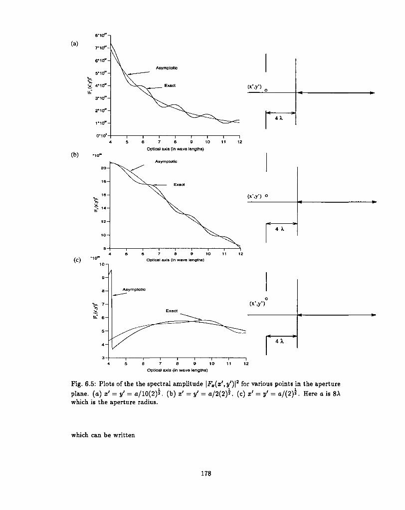
(a)
(b)
(c)
8*10"-i
7*10"-
6*10"-
5*10"-
4*10"-
3*10"-
2*10"-
1*10"-
0*10"
-10"
•10"
8 -
~=. 7 -
it" 6 -
5 -
Asymplotic
6 7 8 9 10
Optical axis (in wave lengths)
Asymptotic
6 7 8 9 10Optical axis (in wave lengths)
Asymptotic
Exact
11 12
(x'.y1) o
4 X
(x'.y1)
6 7 8 9 10Optical axis (in wave lengths)
12
Fig. 6.5: Plots of the the spectral amplitude | F X ( I ' , J / ' ) | 2 for various points in the apertureplane, (a) x' = y' = a/10(2)'. (b) x' = y' = a/2(2)». (c) x' = y' = a/(2)s. Here a is 8Awhich is the aperture radius.
which can be written
178
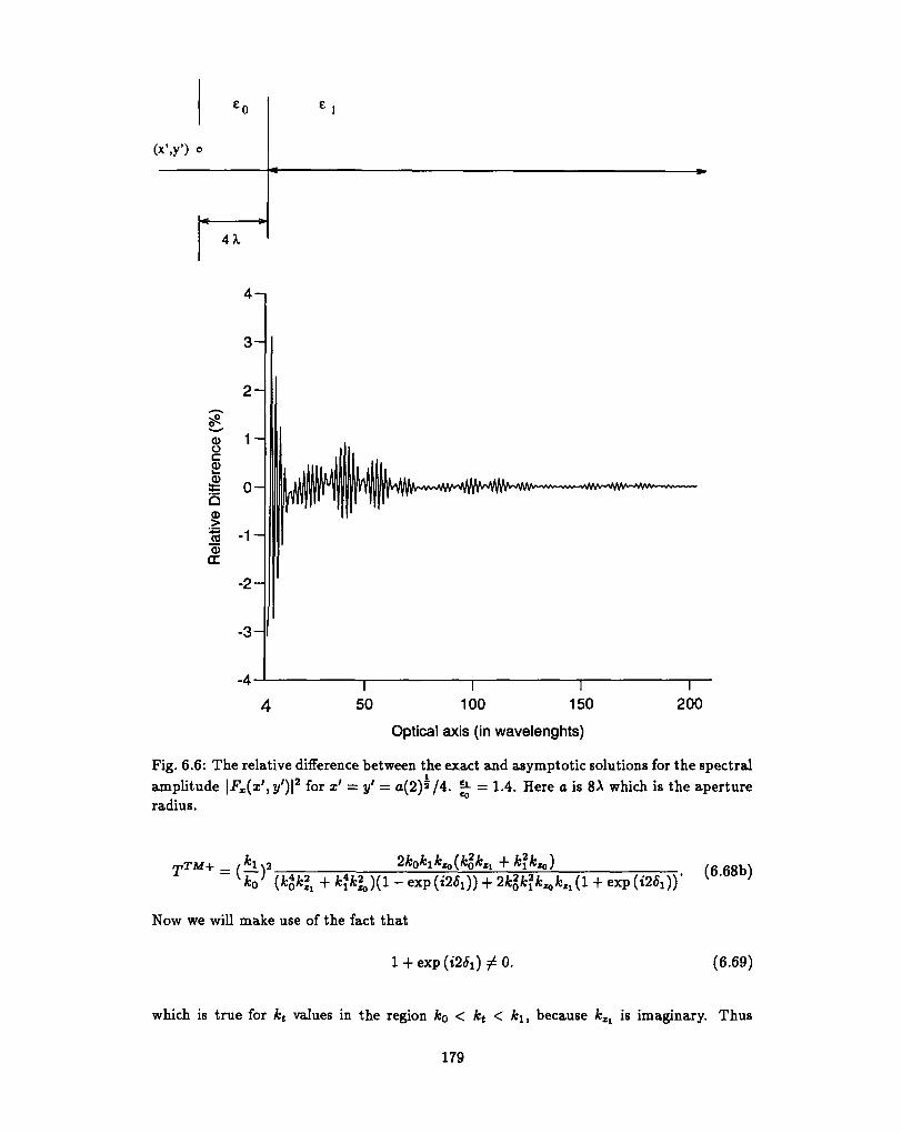
4A.
100 150
Optical axis (in wavelenghts)
200
Fig. 6.6: The relative difference between the exact and asymptotic solutions for the spectralamplitude \Fx(x',y')\2 for x' = y' = o(2)a/4. ^ = 1.4. Here a is 8A which is the apertureradius.
-. (6.68b)
Now we will make use of the fact that
1 + exp (6.69)
which is true for kt values in the region ko < kt < ki, because kZl is imaginary. Thus
179
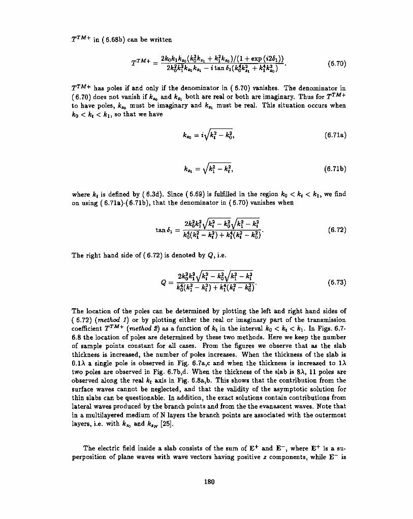
T™+ in (6.68b) can be written
TTM+ _ 2*o
T™+ has poles if and only if the denominator in ( 6.70) vanishes. The denominator in(6.70) does not vanish if k^ and kZl both are real or both are imaginary. Thus for T™+
to have poles, k^ must be imaginary and kXl must be real. This situation occurs whenko < kt < ki, so that we have
K = i Jk* - k2, (6.71a)
fcZl = Jk\ - k2, (6.71b)
where kt is denned by (6.3d). Since (6.69) is fulfilled in the region k0 < kt < ki, we findon using (6.71a)-(6.71b), that the denominator in (6.70) vanishes when
The right hand side of ( 6.72) is denoted by (J, i.e.
lie2 — le2
The location of the poles can be determined by plotting the left and right hand sides of( 6.72) (method 1) or by plotting either the real or imaginary part of the transmissioncoefficient T™+ (method 2) as a function of kt in the interval k0 < kt < Jfei. In Figs. 6.7-6.8 the location of poles are determined by these two methods. Here we keep the numberof sample points constant for all cases. From the figures we observe that as the slabthickness is increased, the number of poles increases. When the thickness of the slab is0.1A a single pole is observed in Fig. 6.7a,c and when the thickness is increased to 1Atwo poles are observed in Fig. 6.7b,d. When the thickness of the slab is 8A, 11 poles areobserved along the real kt axis in Fig. 6.8a,b. This shows that the contribution from thesurface waves cannot be neglected, and that the validity of the asymptotic solution forthin slabs can be questionable. In addition, the exact solutions contain contributions fromlateral waves produced by the branch points and from the the evanascent waves. Note thatin a multilayered medium of N layers the branch points are associated with the outermostlayers, i.e. with A; and kZff [25].
The electric field inside a slab consists of the sum of E + and E , where E + is a su-perposition of plane waves with wave vectors having positive z components, while E~ is
180
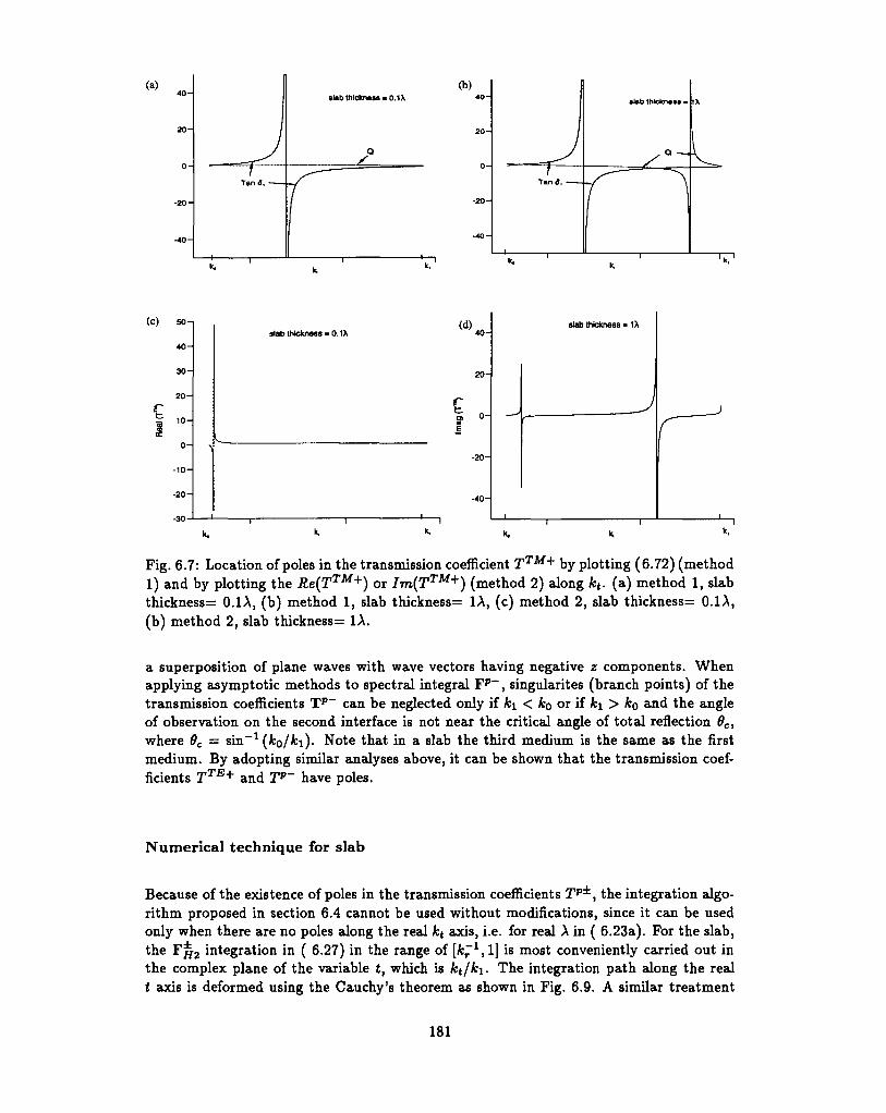
(a)slab thickness - 0 . 1 X
(b)4 0 -
2 0 -
0 -
-20-
-40-
Tan 6, •
slab thicknasa -
Q —
I1
IX
(c)
r
50 -
4 0 -
3 0 -
2 0 -
0 -
-10-
-20-
-30
slab thickness. 0. Hi(d)
E
40-
20-
• 2 0 -
- 4 0 -
slab thickness - 1X
J rFig. 6.7: Location of poles in the transmission coefficient T™+ by plotting (6.72) (method1) and by plotting the Re(T™+) or Im(T™+) (method 2) along Jfct. (a) method 1, slabthickness= 0.1A, (b) method 1, slab thickness= IX, (c) method 2, slab thickness= 0.1A,(b) method 2, slab thickness= IX.
a superposition of plane waves with wave vectors having negative z components. Whenapplying asymptotic methods to spectral integral Fp~, singularites (branch points) of thetransmission coefficients Tp~ can be neglected only if k\ < fco or if hi > k0 and the angleof observation on the second interface is not near the critical angle of total reflection 0C,where 6C = sin"1 (ko/k\). Note that in a slab the third medium is the same as the firstmedium. By adopting similar analyses above, it can be shown that the transmission coef-ficients TTE+ and Tp~ have poles.
Numerical technique for slab
Because of the existence of poles in the transmission coefficients T p ± , the integration algo-rithm proposed in section 6.4 cannot be used without modifications, since it can be usedonly when there are no poles along the real kt axis, i.e. for real X in ( 6.23a). For the slab,the F ^ 2 integration in ( 6.27) in the range of [A"1,1] is most conveniently carried out inthe complex plane of the variable t, which is ktjk\. The integration path along the realt axis is deformed using the Cauchy's theorem as shown in Fig. 6.9. A similar treatment
181
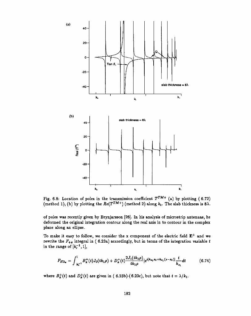
(a)4 0 -
2 0 -
0 -
-20-
-40- slab thickness = 8X
(b)
4 0 -
2 0 -
0 -
- 2 0 -
- 4 0 -
slab thickness = 8A
K> k, k.
Fig. 6.8: Location of poles in the transmission coefficient T™+ (a) by plotting ( 6.72)(method 1), (b) by plotting the Re(T™+) (method 2) along kt. The slab thickness is 8A.
of poles was recently given by Brynjarsson [26]. In his analysis of microstrip antennas, hedeformed the original integration contour along the real axis in to contour in the complexplane along an ellipse.
To make it easy to follow, we consider the x component of the electric field E + and werewrite the F+x integral in ( 6.23a) accordingly, but in terms of the integration variable tin the range of [A:"1,1],
FH2. = -Ldt (6.74)
where B+{t) and D+{t) are given in ( 6.23b)-( 6.23c), but note that t =
182
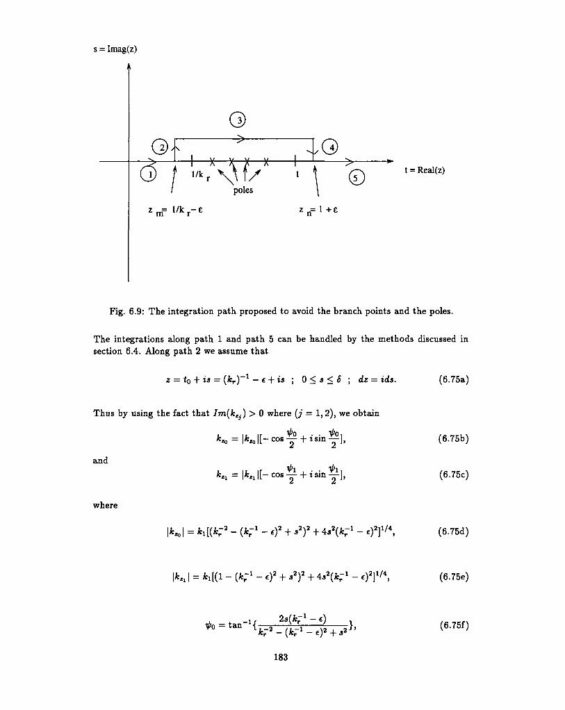
s = Imag(z)
(5zm= l / k r - e
poles
•G>
z n = l + e
t = Real(z)
Fig. 6.9: The integration path proposed to avoid the branch points and the poles.
The integrations along path 1 and path 5 can be handled by the methods discussed insection 6.4. Along path 2 we assume that
z — to + i s = (kT) — e + i s ; 0 < s < 6 ; dz = i d s . (6.75a)
Thus by using the fact that Im(kZi) > 0 where (j = 1,2), we obtain
[ - c o s
and
(6.75b)
(6.75c)
where
(6.75d)
- ef (6.75e)
2s{k~1-e)(6.75f)
183
When selecting the values for S, it has to be noted that the integrand decays to zero asthe exponential part of the integrand in (6.74) is rapidly decreasing. At the same time thepath must not be too near to the real axis of z, as the integrand then might be influencedby the singularities. The selected values for 6 and e are as follows:
£ = 1 * 10~6 ; 6 = 5* 10"7. (6.76)
The integration along path 2 is carried out using the SSP method. A similar approachcan be used for the integration along path 4. Along path 3 the s values are kept constantat s = S and the integration is carried out by means of SSP method.
As mentioned earlier, in thin layers contributions from surface waves, lateral waves, andevanascent waves may be significant and thus the validity of the asymptotic solution isquestionable. In order to check the validity of the asymptotic solutions, we present inthe following section both exact and asymptotic numerical results and compare them forfocused fields inside a slab and for the special case in which the slab reduces to a singleinterface or to a single medium.
184
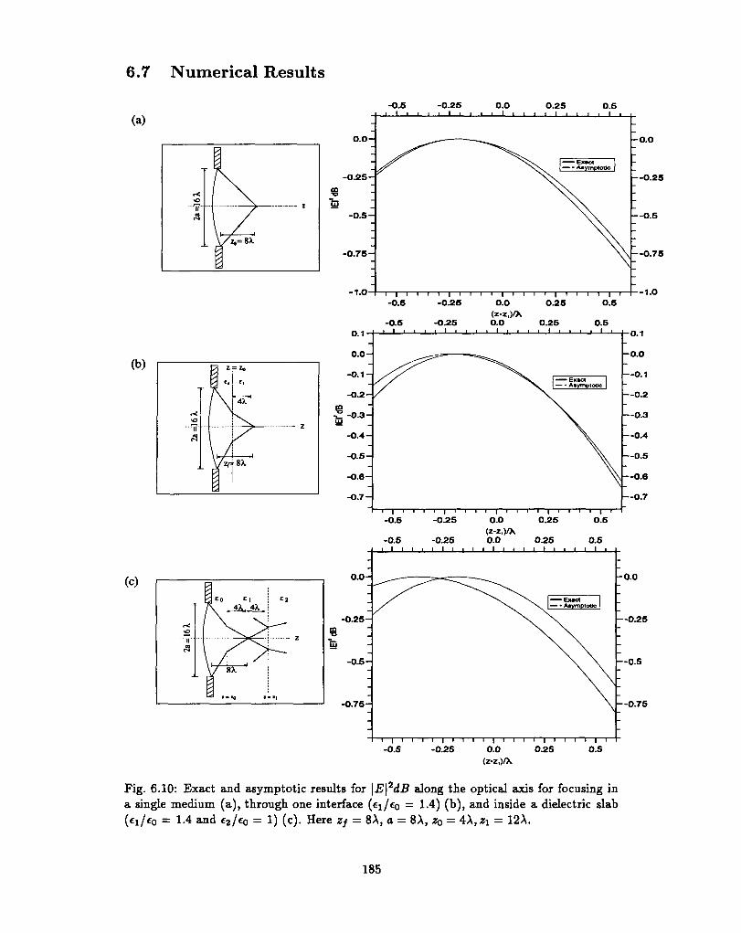
6.7 Numerical Results
-O.5 -0.25 0.0 0.25 0.5
(a)
(b)
(c)
-0.0
—0.25
—0.5
—0.75
-1.0
—0.75
-0.5 -0.25 0.0 0.25(z-z,yx
Fig. 6.10: Exact and asymptotic results for \E\2dB along the optical axis for focusing ina single medium (a), through one interface (ci/to = 1-4) (b), and inside a dielectric slab
= 1-4 and €2/^0 = 1) (c). Here Zf = 8A, o = 8A, ZQ — 4A,zi = 12A.
185
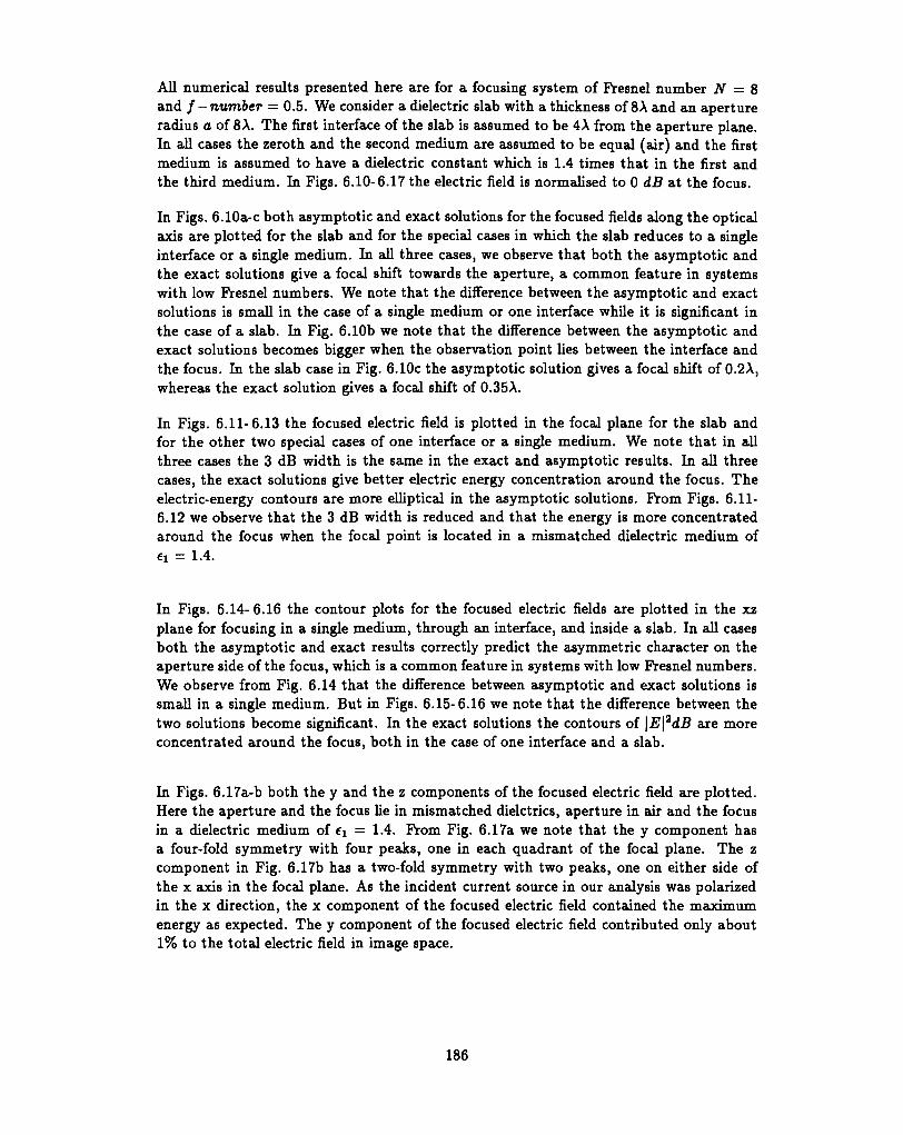
All numerical results presented here are for a focusing system of Fresnel number N = 8and f —number = 0.5. We consider a dielectric slab with a thickness of 8A and an apertureradius a of 8A. The first interface of the slab is assumed to be 4A from the aperture plane.In all cases the zeroth and the second medium are assumed to be equal (air) and the firstmedium is assumed to have a dielectric constant which is 1.4 times that in the first andthe third medium. In Figs. 6.10-6.17 the electric field is normalised to 0 dB at the focus.
In Figs. 6.10a-c both asymptotic and exact solutions for the focused fields along the opticalaxis are plotted for the slab and for the special cases in which the slab reduces to a singleinterface or a single medium. In all three cases, we observe that both the asymptotic andthe exact solutions give a focal shift towards the aperture, a common feature in systemswith low Fresnel numbers. We note that the difference between the asymptotic and exactsolutions is small in the case of a single medium or one interface while it is significant inthe case of a slab. In Fig. 6.10b we note that the difference between the asymptotic andexact solutions becomes bigger when the observation point lies between the interface andthe focus. In the slab case in Fig. 6.10c the asymptotic solution gives a focal shift of 0.2A,whereas the exact solution gives a focal shift of 0.35A.
In Figs. 6.11-6.13 the focused electric field is plotted in the focal plane for the slab andfor the other two special cases of one interface or a single medium. We note that in allthree cases the 3 dB width is the same in the exact and asymptotic results. In all threecases, the exact solutions give better electric energy concentration around the focus. Theelectric-energy contours are more elliptical in the asymptotic solutions. From Figs. 6.11-6.12 we observe that the 3 dB width is reduced and that the energy is more concentratedaround the focus when the focal point is located in a mismatched dielectric medium of«1 = 1.4.
In Figs. 6.14- 6.16 the contour plots for the focused electric fields are plotted in the xzplane for focusing in a single medium, through an interface, and inside a slab. In all casesboth the asymptotic and exact results correctly predict the asymmetric character on theaperture side of the focus, which is a common feature in systems with low Fresnel numbers.We observe from Fig. 6.14 that the difference between asymptotic and exact solutions issmall in a single medium. But in Figs. 6.15-6.16 we note that the difference between thetwo solutions become significant. In the exact solutions the contours of \E\2dB are moreconcentrated around the focus, both in the case of one interface and a slab.
In Figs. 6.17a-b both the y and the z components of the focused electric field are plotted.Here the aperture and the focus lie in mismatched dielctrics, aperture in air and the focusin a dielectric medium of ei = 1.4. From Fig. 6.17a we note that the y component hasa four-fold symmetry with four peaks, one in each quadrant of the focal plane. The zcomponent in Fig. 6.17b has a two-fold symmetry with two peaks, one on either side ofthe x axis in the focal plane. As the incident current source in our analysis was polarizedin the x direction, the x component of the focused electric field contained the maximumenergy as expected. The y component of the focused electric field contributed only about1% to the total electric field in image space.
186
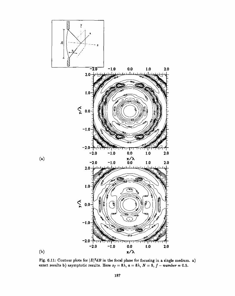
-1.0 0.0 1.0 2.0
(a)
(b)
-2.0-2.0
-2.0
-1.0
-1.0
0.0x/X0.0
1.0
1.0
2.0
2.0
- 1 . 0 -
-2.0-2.0 2.0
Fig. 6.11: Contour plots for \E\2dB in the focal plane for focusing in a single medium, a)exact results b) asymptotic results. Here zj = 8X, a = 8A, N — 8, f — number = 0.5.
187
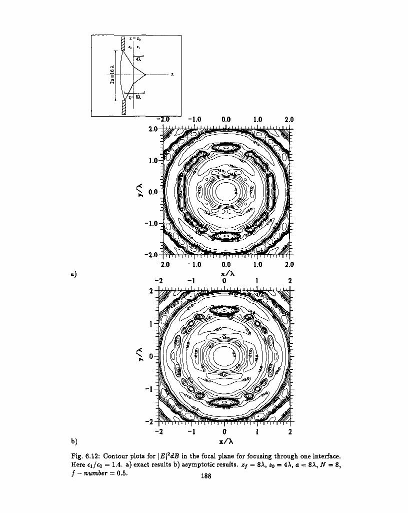
a)
-1.0 0.0 1.0 2.0
-1.0
-2.0
-2.0 -1.0 0.0 1.0 2.0x/X
- 2 - 1 0 1 2
-2
Fig. 6.12: Contour plots for |i?|2d.B in the focal plane for focusing through one interface.Here cj/co = 1-4. a) exact results b) asymptotic results, zj = 8\, ZQ = 4A, a = 8A, N = 8,/ — number = 0.5.
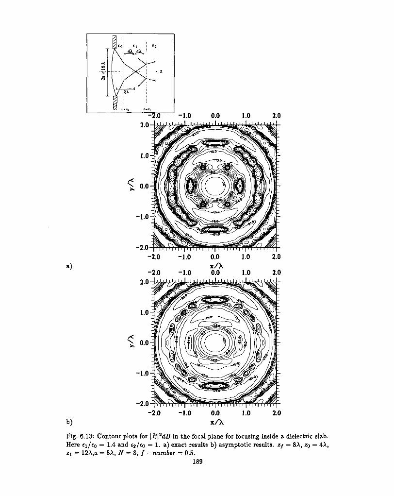
b)
-2.0-2.0 2.0
Fig. 6.13: Contour plots for \B\2dB in the focal plane for focusing inside a dielectric slab.Here ei/eo = 1.4 and 62/ 0 = 1. a) exact results b) asymptotic results, zj = 8A, ZQ = 4A,zi = 12\,a = 8A, N = 8, / - number = 0.5.
189
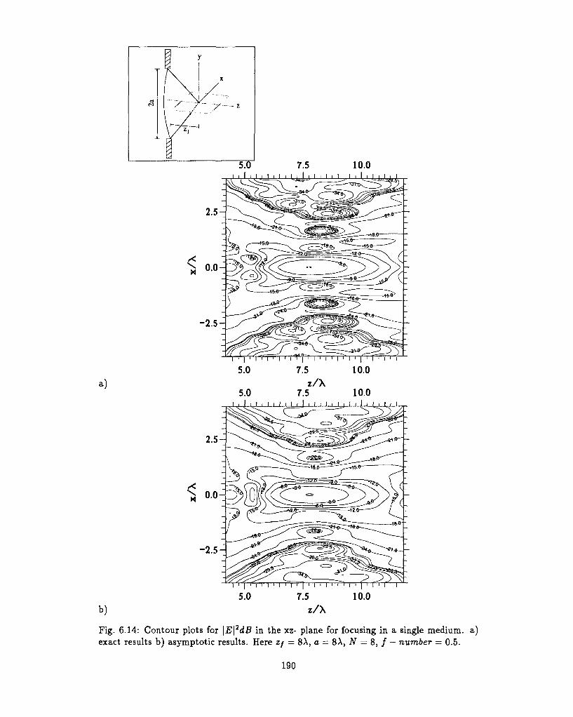
a)
I i i i i i i i i i I i i i i i i i i i I i i i i I i
H"iaii ' i ' \ n M ' i M • i n ' f'
Fig. 6.14: Contour plots for \E\2dB in the xz- plane for focusing in a single medium, a)exact results b) asymptotic results. Here Zf = 8A, a = 8A, N = 8, / — number — 0.5.
190
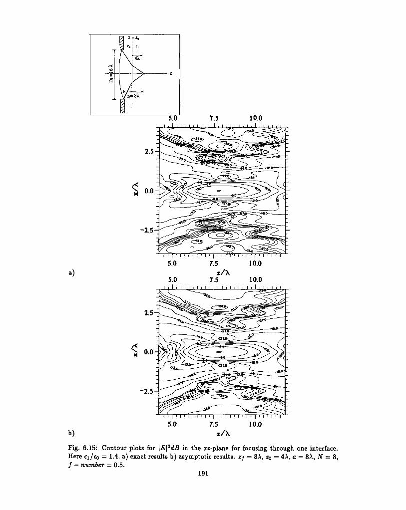
I l l I.I.I I I I I I I I I I I
a)
b)
I ' I ' I ' I ' I I I i I I I i- T" ' I ' I ' | i I i I ' I
5.0 7.5 10.0z/X
5.0 7.5 10.0' MI I
2.5-
0.0-
- 2 . 5 -
7.5 10.0z/X
Fig. 6.15: Contour plots for \E\2dB in the xz-plane for focusing through one interface.Here ei/eo = 1.4. a) exact results b) asymptotic results. Zj — 8X, z0 = 4A, a = 8A, N = 8,/ — number — 0.5.
191

II
A
7 \ :, 4X, 4X,.£2
- z
a)
2.5-
0.0-
- 2 . 5 -
1 I 1 1 1 1 1 1 1 1 1 I 1 1 1 1 1 1 1 1 1 1 f 1 1 1
I ' I ' I ' I ' I ' I ' I T I F [ I I I I I
5.0 7.5 10.0z/X
5.0 7.5 10.01 I 1 1 1 1 1 1 1 1 1 I 1 1 1 1 1 1 1 1 1 I 1 1 1 1 1
2.5-
0.0-
- 2 . 5 -
b)
Fig. 6.16: Contour plots for |E|2d5 in the xz- plane for focusing inside a dielectric slab.Here ei/eo = 1-4 and €2/ 0 = !• a) exact results b) asymptotic results. Zf = 8X, ZQ = 4A,zi = 12A, o = 8A, N = 8, / - number = 0.5.
192
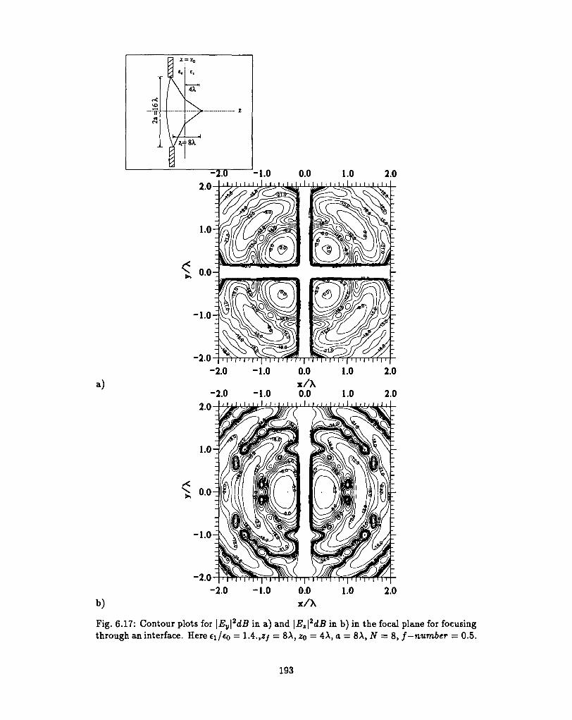
a)
-1.0 0.0 1.0 2.02 Q l l l i l l l l l l l l l l l l l l l i l l l l l i l l l i l i l i l i l . i l
i < i > i > 1 1 1 ' i
-2.0 -1.0
-2.0 -1.0 0.0
-2.0 2.0
Fig. 6.17: Contour plots for \Ev\2dB in a) and \Ez\
2dB in b) in the focal plane for focusingthrough an interface. Here ei/co = 1.4. ,z/ = 8X, ZQ = 4A, a = 8\, N = 8, /—number = 0.5.
193
6.8 Conclusion
We have examined the focusing of electromagnetic waves inside a slab and also consideredthe two special cases in which the slab reduces to a single interface or a single medium.To that end, we have used the exact solutions for the fields inside a layered medium,given in terms of the outside current source [22] to obtain the solutions for the focusedelectric field inside a slab. We have considered both exact and asymptotic solutions of theproblem and discussed the validity of the latter. We have developed a numerical algorithmfor evaluating the diffraction integrals with special emphasis on reducing the computingtime. The numerical techniques in this paper can readily be applied to evaluate similardiffraction integrals occuring e.g. in microstrip antennas.
We have employed both exact and asymptotic methods to obtain the focused field. Theasymptotic solution was obtained by expressing the impulse response of the problem (i.e.the field produced inside the slab by a point source in the aperture) as a plane-waveexpansion and evaluating the corresponding (kx, ky) integral by the method of stationaryphase. As a result, one finds that the main contribution to the impulse response comesfrom one particular plane wave emitted by the aperture point, namely that for which thecorresponding ray on refraction through the interface passes through the given observationpoint. Since this asymptotic solution gives a big reduction in the computing time, we haveexamined its range of validity. Our analysis has shown that the asymptotic solutionsbased on the staionary-phase method give accurate results in a single medium providedthat kR > 1, where k is wave number and R is the distance from the aperture to the focalpoint. In the case of focusing through an interface, we have shown that the asymptoticsolutions become invalid at observation points near the interface, and when the observationangle comes close to the critical angle. We have also found that there will not be any surfacewave contributions to the exact solutions when focusing through an interface, since thetransmission coefficients then contain no poles. In this case the difference between exactand asymptotic solutions comes from contributions of lateral waves due to the branchpoints, and evanascent waves.
In the case of focusing inside a slab, we have shown that the transmission coefficienthas poles which give rise to surface waves. Our numerical results for the focused fieldinside the slab show that the asymptotic solutions cannot be trusted in a thin slab whosethickness is of the order of a wavelength. At low Presnel numbers focal-shift phenomenaand asymmetries are observed in each of the three cases (single medium, single interface,and slab), both in the exact and the asymptotic solutions.
6.9 Aknowledgments
This research was supported by the Research Council of Norway.
194
Appendix D
Transmission and reflectioncoefficients
Transmission and reflection coefficients in a slab with two interfaces z = ZQ and z = z2 aredefined in terms of the Whittaker potentials as follows [22, 2]:
TM± _
TE _ klak* d ^ ( k t ; Zl) - k*
TM _ k2g™\kt;Zl) _ k2
" * d ^ ( k ) - J f c
(D.le)
Tp = ei2T*+e<Sl-6a) ; T"" = Tp+r*2ei2S* ; iZ" = Tp~f10, (D.2a)
where*o = A;zo(z1-zo) ^ 1 = ^ ( ^ 1 - ^ 0 ) , (D.2b)
195
with
TE
P
196
TM _ *&*m*«m - k^k^ _ p™ - p™mn kl^k + A&JXfc ~ P™ + P™ ' l
p™
tTE _
where
pj = ^ r ^ ; PJ = • (D-3e)
Here m, n, and j are integers, all having values 0,1, or 2.
Bibliography
[1] M. Born and E. Wolf. Principles of Optics. Pergamon Press, Oxford, London, andNew York, 1980.
[2] J.J. Stamnes. Waves in Focal Regions. Adam Hilger, Bristol and Boston, 1986.
[3] V.S. Ignatowsky. Trans. Opt. Inst. PetrogradI, paper IV, 1919.
[4] B. Richards and E. Wolf. Electromagnetic diffraction in optical systems II. Structureof the image field in an aplanatic system. Proc. R. Soc. A 253,358-379, 1959.
[5] J. H. Erkkila and M. E. Rogers. Diffracted fields in the focal volume of a convergingwave. J. Opt. Soc. Am. 71, 904-905, 1981.
[6] J. J. Stamnes and B. Spjelkavik. Focusing at small angular apertures in the debyeand kirchhoff approximations. Opt. Commun. 40, 81-85, 1981.
[7] E. Wolf and Y.Li. Conditions for the validity of the Debye integral representation offocused fields. Opt. Commun. 39, 205-210, 1981.
[8] Y. Li. Encircled energy for systems of different Fresnel numbers. Optik 64, 207-218,1983.
[9] Y. Li and H. Platzer. An experimental investigation of diffraction patterns in low-Fresnel-number focusing systems. Opt. Ada 30, 1621-1643, 1983.
[10] Y. Li. Dependence of the focal shift on Fresnel number and f-number. J. Opt. Soc.Am. A 72, 770-4, 1982.
[11] H. Ling and S.W. Lee. Focusing of electromagnetic waves through a dielectric inter-face. J. Opt. Soc. Am. A 1,965-973, 1984.
[12] V. Dhayalan and J.J. Stamnes. Focusing of electric-dipole waves in the Debye andKirchhoff approximations. Submitted to Pure and Appl. Opt, 1996.
[13] P. Torok, P. Varga, Z. Laczic, and G. R. Booker. Electromagnetic diffraction of lightfocused through a planar interface between materials of mismatched refractive indices:an integral reperesentation. J. Opt. Soc. Am. A 12, 325-332, 1995.
[14] P. Torok, P. Varga, and G. R. Booker. Electromagnetic diffraction of light focusedthrough a planar interface between materials of mismatched refractive indices: struc-ture of the electromagnetic field. I. J. Opt. Soc. Am. A 12, 2136-2144, 1995.
[15] P. Torok, P. Varga, and G. Nemeth. Analytical solution of the diffraction integralsand interpretation of wave-front distortion when light is focused through a planarinterface between materials of mismatched refractive indices. J. Opt. Soc. Am. A 12,2660-2671, 1995.
197
[16] J.J. Stamnes and V. Dhayalan. Focusing of electric-dipole waves. Pure Appl. Opt. 5,195-226, 1996.
[17] David M. Pozar. A reciprocity method of analysis for printed slot and slot-coupledmicrostrip antennas. IEEE Trans. Antennas Propagat. 84, 1439-46, 1986.
[18] J. R. Mosig and F. E. Gardiol. A dynamical radiation model for microstrip structures.Advances in Electronics and Electron Physics, 59 159-237, 1982.
[19] J. R. James and P. S. Hall. Handbook of Microstrip Antennas, volume 1 and 2. PeterPeregrinus Ltd, London, United Kingdom, 1989.
[20] M. Mansuripur. Distribution of light at and near the focus of high-numerical-apertureobjectives. J. Opt. Soc. Am. A 3, 2086-2093, 1995.
[21] H. Ling, S.W. Lee, and W. Gee. Frequency optimization of focused microwave hy-perthermia applications. Proc. IEEE 72, 224-225, 1984.
[22] V. Dhayalan, J.J. Stamnes, and H.M. Pedersen. Reflection and refraction of anarbitrary electromagnetic wave in a layered medium. Submitted to J. Opt. Soc. Am.A, 1996.
[23] M. Abramowitz and LA. Stegun. Handbook of Mathematical Functions,. Dover, NewYork, 5th edition, 1968.
[24] J. J. Stamnes, B. Spjelkavik, and H. M. Pedersen. Evaluation of diffraction integralsusing local phase and amplitude approximations. Optica Ada 30, 207-222, 1983.
[25] A. Banos. Dipole Radiation in the Presence of a Conducting Half-space. PergamonPress, Oxford, London, and New York, 1966.
[26] B. A. Brynjarsson. A study of printed antennas in layered dielectric media. Dr.ing.Thesis, Norwegian Institute of Technology, 1994.
198

ISBN 82-993933-0-2
Bergen, Norway 1996


