Flutter Vulnerability Assessment

of Flexible Bridges

Dissertation

submitted to, and approved by,

the Department of Architecture, Civil Engineering and Environmental Sciencesof the Technische Universitat

Carolo-Wilhelminazu Braunschweig

andthe Faculty of Engineering

Department of Civil Engineeringof the University of Florence

in candidacy for the degree of aDoktor-Ingenieur (Dr.-Ing.)/

Dottore di Ricerca in Risk Management on the Built Environment*)

byClaudio Mannini

from Florence, Italy

Submitted on 31 March 2006Oral examination on 19 May 2006Professoral advisor Prof. Udo Peil

Prof. Gianni Bartoli

2006*) Either the German or the Italian form of the title may be used.

The dissertation is published in an electronic form by the Braunschweig universitylibrary at the address

http://www.biblio.tu-bs.de/ediss/data/

TutorsProf. Dr.-Ing. Gianni Bartoli University of FlorenceProf. Dr.-Ing. Udo Peil Technical University of Braunschweig

Doctoral course coordinatorsProf. Dr.-Ing. Claudio Borri University of FlorenceProf. Dr.-Ing. Udo Peil Technical University of Braunschweig

Examining CommitteeProf. Dr.-Ing. Gianni Bartoli University of FlorenceProf. Dr.-Ing. Reinhard Leithner Technical University of BraunschweigProf. Dr. Giorgia Giovannetti University of FlorenceProf. Dr.-Ing. Herald Budelmann Technical University of BraunschweigProf. Dr.-Ing. Claudio Borri University of FlorenceProf. Dr.-Ing. Hocine Oumeraci Technical University of BraunschweigProf. Dr.-Ing. Enrica Caporali University of FlorenceProf. Dr.-Ing. Udo Peil Technical University of BraunschweigProf. Dr.-Ing. Marcello Ciampoli University of Rome “La Sapienza”Prof. Dr. rer. nat. Heinz Antes Technical University of BraunschweigProf. Dr.-Ing. Andrea Vignoli University of FlorenceProf. Dr.-Ing. Jorn Pachl Technical University of BraunschweigProf. Dr.-Ing. Renzo Ciuffi University of FlorenceProf. Dr.-Ing. Joachim Stahlmann Technical University of Braunschweig

This thesis is dedicated to my family

Abstract

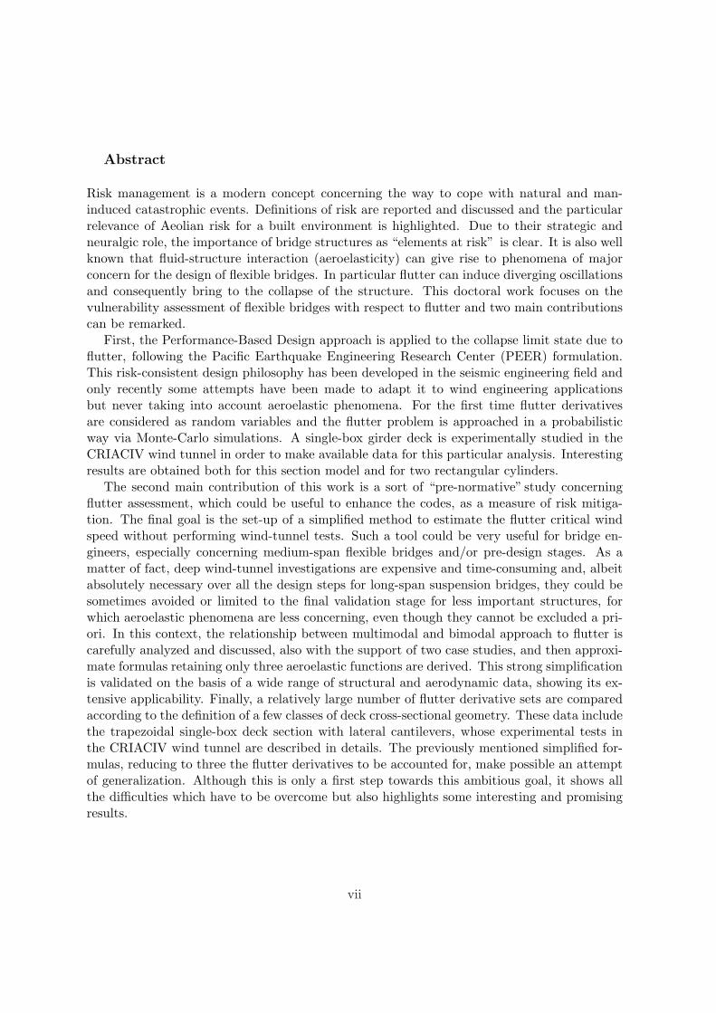
Risk management is a modern concept concerning the way to cope with natural and man-induced catastrophic events. Definitions of risk are reported and discussed and the particularrelevance of Aeolian risk for a built environment is highlighted. Due to their strategic andneuralgic role, the importance of bridge structures as “elements at risk” is clear. It is also wellknown that fluid-structure interaction (aeroelasticity) can give rise to phenomena of majorconcern for the design of flexible bridges. In particular flutter can induce diverging oscillationsand consequently bring to the collapse of the structure. This doctoral work focuses on thevulnerability assessment of flexible bridges with respect to flutter and two main contributionscan be remarked.

First, the Performance-Based Design approach is applied to the collapse limit state due toflutter, following the Pacific Earthquake Engineering Research Center (PEER) formulation.This risk-consistent design philosophy has been developed in the seismic engineering field andonly recently some attempts have been made to adapt it to wind engineering applicationsbut never taking into account aeroelastic phenomena. For the first time flutter derivativesare considered as random variables and the flutter problem is approached in a probabilisticway via Monte-Carlo simulations. A single-box girder deck is experimentally studied in theCRIACIV wind tunnel in order to make available data for this particular analysis. Interestingresults are obtained both for this section model and for two rectangular cylinders.

The second main contribution of this work is a sort of “pre-normative” study concerningflutter assessment, which could be useful to enhance the codes, as a measure of risk mitiga-tion. The final goal is the set-up of a simplified method to estimate the flutter critical windspeed without performing wind-tunnel tests. Such a tool could be very useful for bridge en-gineers, especially concerning medium-span flexible bridges and/or pre-design stages. As amatter of fact, deep wind-tunnel investigations are expensive and time-consuming and, albeitabsolutely necessary over all the design steps for long-span suspension bridges, they could besometimes avoided or limited to the final validation stage for less important structures, forwhich aeroelastic phenomena are less concerning, even though they cannot be excluded a pri-ori. In this context, the relationship between multimodal and bimodal approach to flutter iscarefully analyzed and discussed, also with the support of two case studies, and then approxi-mate formulas retaining only three aeroelastic functions are derived. This strong simplificationis validated on the basis of a wide range of structural and aerodynamic data, showing its ex-tensive applicability. Finally, a relatively large number of flutter derivative sets are comparedaccording to the definition of a few classes of deck cross-sectional geometry. These data includethe trapezoidal single-box deck section with lateral cantilevers, whose experimental tests inthe CRIACIV wind tunnel are described in details. The previously mentioned simplified for-mulas, reducing to three the flutter derivatives to be accounted for, make possible an attemptof generalization. Although this is only a first step towards this ambitious goal, it shows allthe difficulties which have to be overcome but also highlights some interesting and promisingresults.

vii

Acknowledgements

First of all I would like to thank my tutors, Prof. Gianni Bartoli and Prof. Udo Peil, for theirsupport and advice. I feel particularly grateful to Prof. Gianni Bartoli for the enthusiasmfor scientific research that he has always transmitted to me, as well as for the continuoussupervision of the progress of my work. A special thanks to Prof. Claudio Borri for the strongsupport and encouragement he has given me during the entire period of study and to Prof.Francesco Ricciardelli, who extensively reviewed this dissertation, for his useful remarks andsuggestions. All my gratitude to Lorenzo Procino for his constant and indispensable helpduring the long wind-tunnel test campaign and to Serena Cartei who has friendly supportedme in all the bureaucratic issues. I sincerely also have to thank all the colleagues of theInternational Doctoral Course for the help I have often received during these three years andfor their friendly companionship. Then a special thanks to Carlotta Costa, Stefano Pasto andLuca Salvatori for the extremely fruitful scientific discussions and exchange of ideas.

A grateful acknowledgement to CSTB-Nantes, and in particular to Olivier Flamand andGerard Grillaud, for the large quantity of data they made available for this research work. Itis also impossible to forget the warm welcome I received at DLR-Gottingen and the preciousscientific enrichment I got meeting Dr. Gunter Schewe, Dr. Ralph Voß and Ante Soda. FinallyI would like to thank Prof. Masaru Matsumoto and Prof. Partha Sarkar for the data theykindly sent me.

ix

Contents

List of Figures xv

List of Tables xix

1 The risk management framework 11.1 What is risk management? . . . . . . . . . . . . . . . . . . . . . . . . . . . . . . 11.2 Aeolian risk and aeroelastic phenomena . . . . . . . . . . . . . . . . . . . . . . 41.3 Performance-Based Design . . . . . . . . . . . . . . . . . . . . . . . . . . . . . . 71.4 Contribution of the present research work . . . . . . . . . . . . . . . . . . . . . 9

2 Aeroelastic phenomena 132.1 Fluid-structure interaction . . . . . . . . . . . . . . . . . . . . . . . . . . . . . . 132.2 Aeroelastic phenomena . . . . . . . . . . . . . . . . . . . . . . . . . . . . . . . . 13

2.2.1 Torsional divergence . . . . . . . . . . . . . . . . . . . . . . . . . . . . . 132.2.2 Galloping . . . . . . . . . . . . . . . . . . . . . . . . . . . . . . . . . . . 152.2.3 Vortex shedding and lock-in . . . . . . . . . . . . . . . . . . . . . . . . . 172.2.4 Flutter . . . . . . . . . . . . . . . . . . . . . . . . . . . . . . . . . . . . . 222.2.5 Buffeting . . . . . . . . . . . . . . . . . . . . . . . . . . . . . . . . . . . 252.2.6 Rain-wind induced vibrations . . . . . . . . . . . . . . . . . . . . . . . . 26

2.3 Theoretical approach for a thin flat plate . . . . . . . . . . . . . . . . . . . . . 272.3.1 Self-excited forces: Theodorsen and Wagner’s functions . . . . . . . . . 282.3.2 Gust loading: Sears and Kussner’s functions . . . . . . . . . . . . . . . . 31

2.4 Bridge flutter models . . . . . . . . . . . . . . . . . . . . . . . . . . . . . . . . . 332.4.1 Frequency-domain approach . . . . . . . . . . . . . . . . . . . . . . . . . 332.4.2 Time-domain approach . . . . . . . . . . . . . . . . . . . . . . . . . . . 382.4.3 Quasi-steady approach . . . . . . . . . . . . . . . . . . . . . . . . . . . . 39

3 Wind-tunnel tests 453.1 Motivations for these tests . . . . . . . . . . . . . . . . . . . . . . . . . . . . . . 453.2 CRIACIV-DIC Boundary Layer Wind Tunnel . . . . . . . . . . . . . . . . . . . 463.3 Instrumentation . . . . . . . . . . . . . . . . . . . . . . . . . . . . . . . . . . . . 463.4 Static tests . . . . . . . . . . . . . . . . . . . . . . . . . . . . . . . . . . . . . . 49

3.4.1 Experimental set-up . . . . . . . . . . . . . . . . . . . . . . . . . . . . . 493.4.2 Results . . . . . . . . . . . . . . . . . . . . . . . . . . . . . . . . . . . . 53

xi

3.4.3 Comparison with CFD simulations . . . . . . . . . . . . . . . . . . . . . 643.5 Aeroelastic tests . . . . . . . . . . . . . . . . . . . . . . . . . . . . . . . . . . . 72

3.5.1 Experimental set-up . . . . . . . . . . . . . . . . . . . . . . . . . . . . . 723.5.2 Results . . . . . . . . . . . . . . . . . . . . . . . . . . . . . . . . . . . . 76

3.6 Conclusions . . . . . . . . . . . . . . . . . . . . . . . . . . . . . . . . . . . . . . 98

4 Probabilistic flutter approach 1054.1 Flutter derivative measurements and uncertainty . . . . . . . . . . . . . . . . . 1054.2 Model assumptions . . . . . . . . . . . . . . . . . . . . . . . . . . . . . . . . . . 1064.3 Results for two rectangular cylinders . . . . . . . . . . . . . . . . . . . . . . . . 1094.4 Application to the tested bridge section . . . . . . . . . . . . . . . . . . . . . . 1164.5 Conclusions . . . . . . . . . . . . . . . . . . . . . . . . . . . . . . . . . . . . . . 121

5 From multimodal to bimodal approach to flutter 1275.1 Introduction . . . . . . . . . . . . . . . . . . . . . . . . . . . . . . . . . . . . . . 1275.2 Multimodal approach to flutter . . . . . . . . . . . . . . . . . . . . . . . . . . . 1285.3 Model simplification . . . . . . . . . . . . . . . . . . . . . . . . . . . . . . . . . 1315.4 Examples . . . . . . . . . . . . . . . . . . . . . . . . . . . . . . . . . . . . . . . 135

5.4.1 Bosporus I Strait Bridge . . . . . . . . . . . . . . . . . . . . . . . . . . . 1355.4.2 Ponte all’Indiano . . . . . . . . . . . . . . . . . . . . . . . . . . . . . . . 139

5.5 Conclusions . . . . . . . . . . . . . . . . . . . . . . . . . . . . . . . . . . . . . . 143

6 Simplified formulas 1456.1 Introduction . . . . . . . . . . . . . . . . . . . . . . . . . . . . . . . . . . . . . . 1456.2 Flutter problem . . . . . . . . . . . . . . . . . . . . . . . . . . . . . . . . . . . . 1466.3 Simplification procedure . . . . . . . . . . . . . . . . . . . . . . . . . . . . . . . 147

6.3.1 Range of variability of the dynamic parameters . . . . . . . . . . . . . . 1486.3.2 Simplified equation for critical frequency . . . . . . . . . . . . . . . . . . 1496.3.3 Simplified equation for critical reduced wind speed . . . . . . . . . . . . 153

6.4 Further simplification . . . . . . . . . . . . . . . . . . . . . . . . . . . . . . . . 1546.5 Degree of approximation . . . . . . . . . . . . . . . . . . . . . . . . . . . . . . . 1566.6 Case studies . . . . . . . . . . . . . . . . . . . . . . . . . . . . . . . . . . . . . . 1616.7 Torsional flutter . . . . . . . . . . . . . . . . . . . . . . . . . . . . . . . . . . . 1686.8 Nakamura’s formula . . . . . . . . . . . . . . . . . . . . . . . . . . . . . . . . . 1736.9 Conclusions . . . . . . . . . . . . . . . . . . . . . . . . . . . . . . . . . . . . . . 174

7 A first step towards generalization of flutter derivatives 1757.1 Introduction . . . . . . . . . . . . . . . . . . . . . . . . . . . . . . . . . . . . . . 1757.2 Flutter derivatives for classes of deck geometry . . . . . . . . . . . . . . . . . . 177

7.2.1 Trapezoidal single-box girder decks with lateral cantilevers . . . . . . . 1777.2.2 Trapezoidal single-box girder decks . . . . . . . . . . . . . . . . . . . . . 1817.2.3 Bi-girder decks . . . . . . . . . . . . . . . . . . . . . . . . . . . . . . . . 183

7.3 Conclusions . . . . . . . . . . . . . . . . . . . . . . . . . . . . . . . . . . . . . . 186

xii

General conclusions and outlook 189

Bibliography 191

A Other wind-tunnel test results I

xiii

List of Figures

1.1 Operational risk management . . . . . . . . . . . . . . . . . . . . . . . . . . . . 21.2 Risk mitigation diagram . . . . . . . . . . . . . . . . . . . . . . . . . . . . . . . 21.3 The collapse of Tacoma Narrows Bridge . . . . . . . . . . . . . . . . . . . . . . 51.4 Scheme of the simplification procedure for flutter problem . . . . . . . . . . . . 11

2.1 Vertical force coefficient and galloping vibration amplitude for a square cylinder 162.2 Experimental investigation of lock-in . . . . . . . . . . . . . . . . . . . . . . . . 192.3 Resonance curves in bending for an H-shaped cylinder . . . . . . . . . . . . . . 192.4 Lift and moment response diagrams for an H-shaped cylinder . . . . . . . . . . 202.5 Spanwise pressure correlation vs. oscillation amplitude for a circular cylinder . 212.6 Response of a circular model stack for different values of structural damping . . 222.7 Reduced critical flutter wind speed for a theoretical flat plate vs. frequency ratio 242.8 Reference system for oscillating flat plate theory . . . . . . . . . . . . . . . . . 282.9 Real and imaginary parts of Theodorsen’s circulatory function . . . . . . . . . 292.10 Wagner’s function after Garrick’s rational approximation . . . . . . . . . . . . 302.11 Real and imaginary part of Sears’ function . . . . . . . . . . . . . . . . . . . . . 322.12 Kussner’s function in the rational approximation . . . . . . . . . . . . . . . . . 332.13 Scanlan’s reference system for bridge self-excited forces . . . . . . . . . . . . . . 342.14 Flutter derivatives for a theoretical flat plate . . . . . . . . . . . . . . . . . . . 362.15 Reference system for the quasi-steady theory . . . . . . . . . . . . . . . . . . . 392.16 Quasi-steady and unsteady lift; polar plot of the Theodorsen’s function . . . . 44

3.1 View of the CRAICIV-DIC Boundary Layer Wind Tunnel in Prato . . . . . . . 463.2 Schematic view of the wind tunnel . . . . . . . . . . . . . . . . . . . . . . . . . 473.3 View of a strain-gauges load cell; load cell output voltage vs. actual force applied 483.4 View of a laser triangulator transducer; laser output voltage vs. actual distance 493.5 Geometric characteristics of the bridge deck section model . . . . . . . . . . . . 513.6 Sketch of the set-up for the static measurements . . . . . . . . . . . . . . . . . 523.7 Set-up for the static measurements . . . . . . . . . . . . . . . . . . . . . . . . . 533.8 Section model natural frequencies . . . . . . . . . . . . . . . . . . . . . . . . . . 543.9 Reference system for the aerodynamic force coefficients . . . . . . . . . . . . . . 553.10 Aerodynamic force coefficients vs. Reynolds number (α = 0°) . . . . . . . . . . 563.11 Example of power spectral density of load cell signal . . . . . . . . . . . . . . . 573.12 Power spectral density of the hot-wire anemometer signals . . . . . . . . . . . . 58

xv

3.13 Measured and mean values of the Strouhal number . . . . . . . . . . . . . . . . 593.14 Mean aerodynamic force coefficients at different angles of attack . . . . . . . . 613.15 RMS values of the aerodynamic force coefficients at different angles of attack . 623.16 Aerodynamic coefficients in the range -3°. α . 0° for three different wind speeds 633.17 Sunshine Skyway Bridge section model . . . . . . . . . . . . . . . . . . . . . . . 663.18 CRIACIV section model . . . . . . . . . . . . . . . . . . . . . . . . . . . . . . . 663.19 Experim. and numerical aerodynamic coefficients for SSB and CRIACIV section 673.20 Hybrid “Medium” mesh used in the CFD simulations . . . . . . . . . . . . . . . 683.21 Grid-convergence study . . . . . . . . . . . . . . . . . . . . . . . . . . . . . . . 693.22 Computed horizontal velocity field corresponding to the instant of maximum lift 693.23 Pressure coefficient distribution over the bridge deck surface . . . . . . . . . . . 703.24 Set-up for the aeroelastic measurements . . . . . . . . . . . . . . . . . . . . . . 743.25 Sketch of the set-up for the aeroelastic measurements . . . . . . . . . . . . . . . 753.26 Heaving and pitching static stiffness of the elastically suspended section model 763.27 Still-air heaving, pitching and rolling signals and psd . . . . . . . . . . . . . . . 773.28 Still-air free-decay heaving and pitching motions (30 s) . . . . . . . . . . . . . . 783.29 Mass and mass moment of inertia measurements . . . . . . . . . . . . . . . . . 793.30 Ambient vibrations: mean and rms values of heaving and pitching displacements 813.31 Lift and moment coefficients measured via static and aeroelastic tests . . . . . 833.32 Particular behavior at high wind speed of the section model for α0 = −3.72° . . 843.33 ULS reconstruction of the measured signals . . . . . . . . . . . . . . . . . . . . 873.34 Scanlan’s reference system for bridge self-excited forces . . . . . . . . . . . . . . 873.35 Flutter derivatives for three different initial conditions . . . . . . . . . . . . . . 903.36 Repeatability of the flutter derivative measurements . . . . . . . . . . . . . . . 913.37 Flutter derivatives for two different choices of the length of the processed signals 923.38 Frequency and modal damping evolution with the wind speed (α0 = 0°) . . . . 943.39 Power spectral density of heaving and pitching signals at different wind speeds 953.40 First cycles of oscillation of the heaving signal immediately before flutter . . . . 963.41 Mean values of the flutter derivative for different still-air angles of attack α0 . . 1003.42 Rotation center and phase angle relative to the pitching-branch mode . . . . . 1023.43 Frequency and modal damping evolution with the wind speed (α0 = −1.70°) . . 103

4.1 Probability plot and CDF for the flutter derivatives (U = 15 m/s) . . . . . . . 1074.2 Probability distribution of flutter boundaries for R12.5 in smooth flow . . . . . 1104.3 Examples of Monte-Carlo generated A∗2 functions (R12.5 in smooth flow) . . . 1114.4 Deterministic vs. probabilistic flutter (R12.5 in smooth flow) . . . . . . . . . . 1114.5 Probability distribution of flutter boundaries for R12.5 in turbulent flow . . . . 1124.6 Deterministic vs. probabilistic flutter (R12.5 in turbulent flow) . . . . . . . . . 1144.7 Probability distribution of flutter boundaries for R5 in smooth flow . . . . . . . 1154.8 Deterministic vs. probabilistic flutter (R5 in smooth flow) . . . . . . . . . . . . 1164.9 CDF of the flutter critical wind speed for the studied rectangular cylinders . . 1174.10 Bridge deck flutter derivative mean values and confidence intervals . . . . . . . 1194.11 Example of Monte-Carlo simulations of bridge deck flutter derivatives . . . . . 1204.12 Probability distribution of flutter boundaries (bridge section: “test case 0”) . . 122

xvi

4.13 Deterministic vs. probabilistic flutter (“test case 0”) . . . . . . . . . . . . . . . 1234.14 CDF of the critical flutter wind speed for “test case 0” . . . . . . . . . . . . . . 1234.15 Probability distribution of flutter boundaries (bridge section: “test case 2”) . . 1244.16 Deterministic vs. probabilistic flutter (“test case 2”) . . . . . . . . . . . . . . . 1254.17 CDF of the critical flutter wind speed for “test case 2” . . . . . . . . . . . . . . 125

5.1 Reference system for displacements and self-excited forces . . . . . . . . . . . . 1295.2 Bosporus I Strait Bridge and cross section assumed for the aerodynamics . . . 1365.3 Flutter mode shape for Bosporus I Strait Bridge . . . . . . . . . . . . . . . . . 1375.4 Bosporus I Strait Bridge: still-air modes mainly involved in the flutter coupling 1385.5 Ponte all’Indiano and cross section assumed for the aerodynamics . . . . . . . . 1395.6 Flutter mode shape for Ponte all’Indiano . . . . . . . . . . . . . . . . . . . . . . 1415.7 Ponte all’Indiano: still-air modes mainly involved in the flutter coupling . . . . 142

6.1 Comparison between the four terms composing the real flutter equation . . . . 1566.2 Degree of approximation of the formula for A∗3 for three cross sections . . . . . 1576.3 Approximate formulas vs. eigenvalue analysis . . . . . . . . . . . . . . . . . . . 1596.4 Comparison between author’s formula and Selberg and Rocard’s formulas . . . 1606.5 Examples of the graphical solution of the approximate formulas . . . . . . . . . 1636.6 Graphical solutions of the approximate formulas for Tsurumi Fairway Bridge . 1636.7 Degree of approximation of the formula for A∗3 for the tested cross section . . . 1656.8 Graphical solutions of the approximate formulas for the “CRIACIV section” . . 1666.9 Results of the approximate formulas for the wind-tunnel test cases . . . . . . . 1676.10 Weight of the four terms composing the real flutter equation for R5 . . . . . . 1706.11 Degree of approximation of the formula for A∗3 for R5 and Tacoma Bridge . . . 1716.12 2-DoF and 1-DoF flutter problems vs. approximate formulas . . . . . . . . . . 172

7.1 Trapezoidal single-box girder decks with lateral cantilevers . . . . . . . . . . . . 1787.2 Flutter derivatives for the single-box girder decks with lateral cantilevers . . . . 1807.3 Trapezoidal single-box girder decks . . . . . . . . . . . . . . . . . . . . . . . . . 1827.4 Flutter derivatives for the trapezoidal single-box girder decks . . . . . . . . . . 1857.5 Bi-girder decks . . . . . . . . . . . . . . . . . . . . . . . . . . . . . . . . . . . . 1867.6 Flutter derivatives for the bi-girder decks . . . . . . . . . . . . . . . . . . . . . 188

A.1 Aerodynamic coefficients (mean and RMS) vs. Reynolds number (α = −5°) . . IIA.2 Aerodynamic coefficients (mean and RMS) vs. Reynolds number (α = 0°) . . . IIIA.3 Aerodynamic coefficients (mean and RMS) vs. Reynolds number (α = +5°) . . IVA.4 Power spectral density of the hot-wire anemometer signals (α = −5°) . . . . . . VIA.5 Power spectral density of the hot-wire anemometer signals (α = 0°) . . . . . . . VIIIA.6 Power spectral density of the hot-wire anemometer signals (α = +5°) . . . . . . XA.7 Repeatability of the flutter derivative measurements . . . . . . . . . . . . . . . XIIA.8 Flutter derivatives for four different still-air angles of attack α0 . . . . . . . . . XIVA.9 Probability plot and CDF for the flutter derivatives (4 m/s) . . . . . . . . . . . XVA.10 Probability plot and CDF for the flutter derivatives (15 m/s) . . . . . . . . . . XVIA.11 Probability plot and CDF for the flutter derivatives (19.2 m/s) . . . . . . . . . XVII

xvii

List of Tables

2.1 Comparison between unsteady and quasi-steady (QS) results . . . . . . . . . . 44

3.1 Main technical characteristics of the strain-gauges load cells . . . . . . . . . . . 483.2 Micro-epsilon Model OptoNCDT 1605 laser characteristics . . . . . . . . . . . . 503.3 Strouhal number evaluation from hot-wire anemometer measures . . . . . . . . 603.4 Main properties of the meshes used in the grid-convergence study . . . . . . . . 713.5 Grid-convergence study results (α = 0°) . . . . . . . . . . . . . . . . . . . . . . 713.6 Computed and measured Strouhal numbers for the two bridge sections . . . . . 713.7 Main properties of the springs used for the aeroelastic set-up . . . . . . . . . . 723.8 Comparison between measured and theoretical static stiffness . . . . . . . . . . 763.9 Damping ratios in the heaving and pitching modes vs. signal length . . . . . . 783.10 Comparison between static, dynamic and theoretical stiffness . . . . . . . . . . 793.11 Summary of the mechanical parameters of the aeroelastic system . . . . . . . . 803.12 Still-air initial conditions for the identification of the flutter derivatives . . . . . 883.13 Dynamic parameters of the test cases for flutter calculation . . . . . . . . . . . 963.14 Measured and calculated flutter boundaries . . . . . . . . . . . . . . . . . . . . 97

4.1 Dynamic parameters of the two rectangular cylinders . . . . . . . . . . . . . . . 1134.2 Measured and deterministically calculated flutter boundaries for R12.5 and R5 1134.3 Results of the probabilistic flutter calculation for R12.5 and R5 . . . . . . . . . 1134.4 Dynamic parameters for flutter calculation (bridge section) . . . . . . . . . . . 1204.5 Measured and deterministically calculated flutter boundaries (bridge section) . 1204.6 Results of the probabilistic flutter calculation for the bridge section . . . . . . . 120

5.1 Modal analysis results for Bosporus I Strait Bridge . . . . . . . . . . . . . . . . 1365.2 Bosporus I Strait Bridge: multimodal and bimodal flutter analyses . . . . . . . 1375.3 Modal analysis results for Ponte all’Indiano . . . . . . . . . . . . . . . . . . . . 1405.4 Ponte all’Indiano: multimodal and bimodal flutter analyses . . . . . . . . . . . 140

6.1 Main geometric and dynamic properties of the considered bridges . . . . . . . . 1496.2 Weight of the terms appearing in the real flutter equation (first case) . . . . . . 1506.3 Weight of the terms appearing in the real flutter equation (second case) . . . . 1516.4 Weight of the terms appearing in the real flutter equation (third case) . . . . . 1516.5 Weight of the terms appearing in the real flutter equation (fourth case) . . . . 1516.6 Eigenvalue analysis vs. approximate formula for critical frequency . . . . . . . 152

xix

6.7 Case studies (coupled flutter) . . . . . . . . . . . . . . . . . . . . . . . . . . . . 1626.8 Results for the case studies presented in Tab. 6.7 . . . . . . . . . . . . . . . . . 1626.9 Approx. formulas vs. eig. analysis for the tested cross section (approx. sol. I) . 1656.10 Approx. formulas vs. eig. analysis for the tested cross section (approx. sol. II) 1656.11 Case studies (single-degree-of-freedom torsional flutter) . . . . . . . . . . . . . 1716.12 Results for the study cases listed in Tab. 6.11 . . . . . . . . . . . . . . . . . . . 171

7.1 Modal parameters for the flutter calculations . . . . . . . . . . . . . . . . . . . 1817.2 Flutter boundaries calculated with the simplified formulas . . . . . . . . . . . . 1817.3 Further flutter calculations . . . . . . . . . . . . . . . . . . . . . . . . . . . . . 181

xx

Chapter 1

The risk management framework

1.1 What is risk management?

Risk management is a quite modern concept and it refers to the ensemble of “coordinatedactivities to direct and control an organization with respect to risk” (Shortreed et al., 2003).This definition obviously implies the presence of elements at risk, that is of a built environment,where a given catastrophic event can produce human or economic losses.

Risk management can be considered both as an operational process (operational risk man-agement) concerning an existing protection system, and a process of design and implementa-tion (risk mitigation) of a new protection system (Plate, 2000). Operational risk managementincludes concepts such as maintenance, preparedness and disaster response (Fig. 1.1).

It is obvious that an existing protection system has to be continuously maintained in orderto function as planned and improved to respond to the changes in the concept of protection.Risk analysis is the instrument that allows this dynamic update of the system. Neverthelessit must be clear that the presence of a residual risk is unavoidable, that is the probabilitythat the protection system fails or a rare event exceeding the design one occurs, is never zero.For this reason preparedness to catastrophic events is a fundamental ring in the chain of riskmanagement. Early warning systems are nowadays a more and more powerful tool relying onfairly sophisticated forecasting techniques and technologies. The final step of operational riskmanagement is disaster response and relief and it includes all the actions that must be takenwhen disasters occur, such as humanitarian aid to the victims and reconstructions of lifelinesand damaged or destroyed buildings.

As it has already been claimed, the dual concept of operational risk management is riskmitigation, which is related to the planning of a new protection system (Fig. 1.2). When theexisting protection system, if any, does no longer meet the demands of the present society,in other words when the residual risk is larger than the acceptable risk, a new system hasto be planned and implemented. It is worth noting that acceptable risk is determined bysociety perception and attitude toward risk, whereas residual risk depends on human activitiesand natural changes (such as climate changes) which modify the boundary conditions of theproblem. The definition of the acceptable risk level is by itself a very challenging problemsince it concerns the allocation of the limited resources of a nation, that means it should be a

1

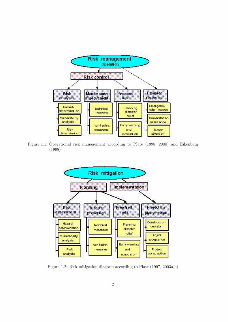
Figure 1.1: Operational risk management according to Plate (1998, 2000) and Eikenberg(1998)

Figure 1.2: Risk mitigation diagram according to Plate (1997, 2003a,b)

2

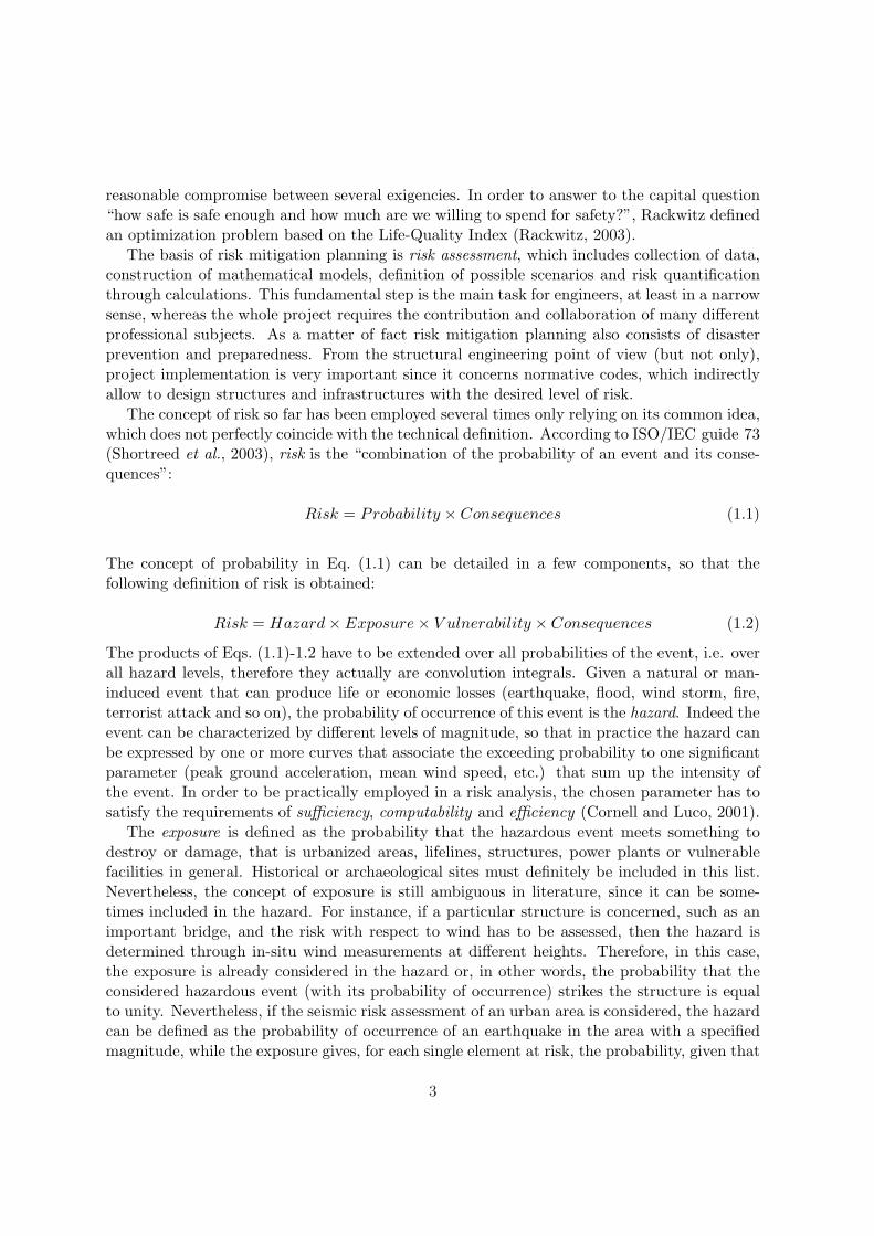
reasonable compromise between several exigencies. In order to answer to the capital question“how safe is safe enough and how much are we willing to spend for safety?”, Rackwitz definedan optimization problem based on the Life-Quality Index (Rackwitz, 2003).

The basis of risk mitigation planning is risk assessment, which includes collection of data,construction of mathematical models, definition of possible scenarios and risk quantificationthrough calculations. This fundamental step is the main task for engineers, at least in a narrowsense, whereas the whole project requires the contribution and collaboration of many differentprofessional subjects. As a matter of fact risk mitigation planning also consists of disasterprevention and preparedness. From the structural engineering point of view (but not only),project implementation is very important since it concerns normative codes, which indirectlyallow to design structures and infrastructures with the desired level of risk.

The concept of risk so far has been employed several times only relying on its common idea,which does not perfectly coincide with the technical definition. According to ISO/IEC guide 73(Shortreed et al., 2003), risk is the “combination of the probability of an event and its conse-quences”:

Risk = Probability × Consequences (1.1)

The concept of probability in Eq. (1.1) can be detailed in a few components, so that thefollowing definition of risk is obtained:

Risk = Hazard×Exposure× V ulnerability × Consequences (1.2)

The products of Eqs. (1.1)-1.2 have to be extended over all probabilities of the event, i.e. overall hazard levels, therefore they actually are convolution integrals. Given a natural or man-induced event that can produce life or economic losses (earthquake, flood, wind storm, fire,terrorist attack and so on), the probability of occurrence of this event is the hazard. Indeed theevent can be characterized by different levels of magnitude, so that in practice the hazard canbe expressed by one or more curves that associate the exceeding probability to one significantparameter (peak ground acceleration, mean wind speed, etc.) that sum up the intensity ofthe event. In order to be practically employed in a risk analysis, the chosen parameter has tosatisfy the requirements of sufficiency, computability and efficiency (Cornell and Luco, 2001).

The exposure is defined as the probability that the hazardous event meets something todestroy or damage, that is urbanized areas, lifelines, structures, power plants or vulnerablefacilities in general. Historical or archaeological sites must definitely be included in this list.Nevertheless, the concept of exposure is still ambiguous in literature, since it can be some-times included in the hazard. For instance, if a particular structure is concerned, such as animportant bridge, and the risk with respect to wind has to be assessed, then the hazard isdetermined through in-situ wind measurements at different heights. Therefore, in this case,the exposure is already considered in the hazard or, in other words, the probability that theconsidered hazardous event (with its probability of occurrence) strikes the structure is equalto unity. Nevertheless, if the seismic risk assessment of an urban area is considered, the hazardcan be defined as the probability of occurrence of an earthquake in the area with a specifiedmagnitude, while the exposure gives, for each single element at risk, the probability, given that

3

earthquake, to have a particular peak ground acceleration (for instance), taking into accountthe distance from the epicenter, soil characteristics, etc.. It is also worth noting that sometimesthe same meaning of consequences is given to the concept of exposure.

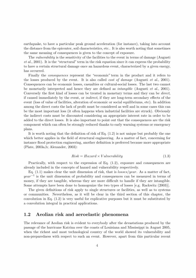
The vulnerability is the sensitivity of the facilities to the event in terms of damage (Augustiet al., 2001). It is the “structural” term in the risk equation since it can express the probabilityto have a certain structural damage once an hazardous event, characterized by a given energy,has occurred.

Finally the consequences represent the “economic” term in the product and it refers tothe losses produced by the event. It is also called cost of damage (Augusti et al., 2001).Consequences can be economic losses, casualties or cultural-social losses. The last two cannotbe monetarily interpreted and hence they are defined as intangible (Augusti et al., 2001).Conversely the first kind of losses can be treated in monetary terms and they can be direct,if caused immediately by the event, or indirect, if they are long-term secondary effects of theevent (loss of value of facilities, alteration of economic or social equilibriums, etc). In additionamong the direct costs the lack of profit must be considered as well and in some cases this canbe the most important loss (it often happens when industrial facilities are struck). Obviouslythe indirect costs must be discounted considering an appropriate interest rate in order to beadded to the direct losses. It is also important to point out that the consequences are the riskcomponent which can often be strongly reduced thanks to early warning systems or emergencyplans.

It is worth noting that the definition of risk of Eq. (1.2) is not unique but probably the onewhich better applies in the field of structural engineering. As a matter of fact, concerning forinstance flood protection engineering, another definition is preferred because more appropriate(Plate, 2003a,b; Alexander, 2003):

Risk = Hazard× V ulnerability (1.3)

Practically, with respect to the expression of Eq. (1.2), exposure and consequences arealready included in the concepts of hazard and vulnerability respectively.

Eq. (1.1) makes clear the unit dimension of risk, that is losses/year. As a matter of fact,year−1 is the unit dimension of probability and consequences can be measured in terms ofmoney, if they are tangible, whereas they are more difficult to handle if they are intangible.Some attempts have been done to homogenize the two types of losses [e.g. Rackwitz (2003)].

The given definitions of risk apply to single structures or facilities, as well as to systemsor communities. Nevertheless, as it will be clear in the third section of this chapter, theconvolution in Eq. (1.2) is very useful for explicative purposes but it must be substituted bya convolution integral in practical applications.

1.2 Aeolian risk and aeroelastic phenomena

The relevance of Aeolian risk is evident to everybody after the devastations produced by thepassage of the hurricane Katrina over the coasts of Louisiana and Mississippi in August 2005,when the richest and most technological country of the world showed its vulnerability andnon-preparedness with respect to such an event. However, apart from this particular recent

4

(a) (b)

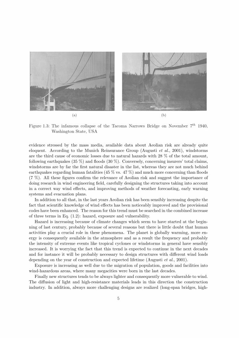
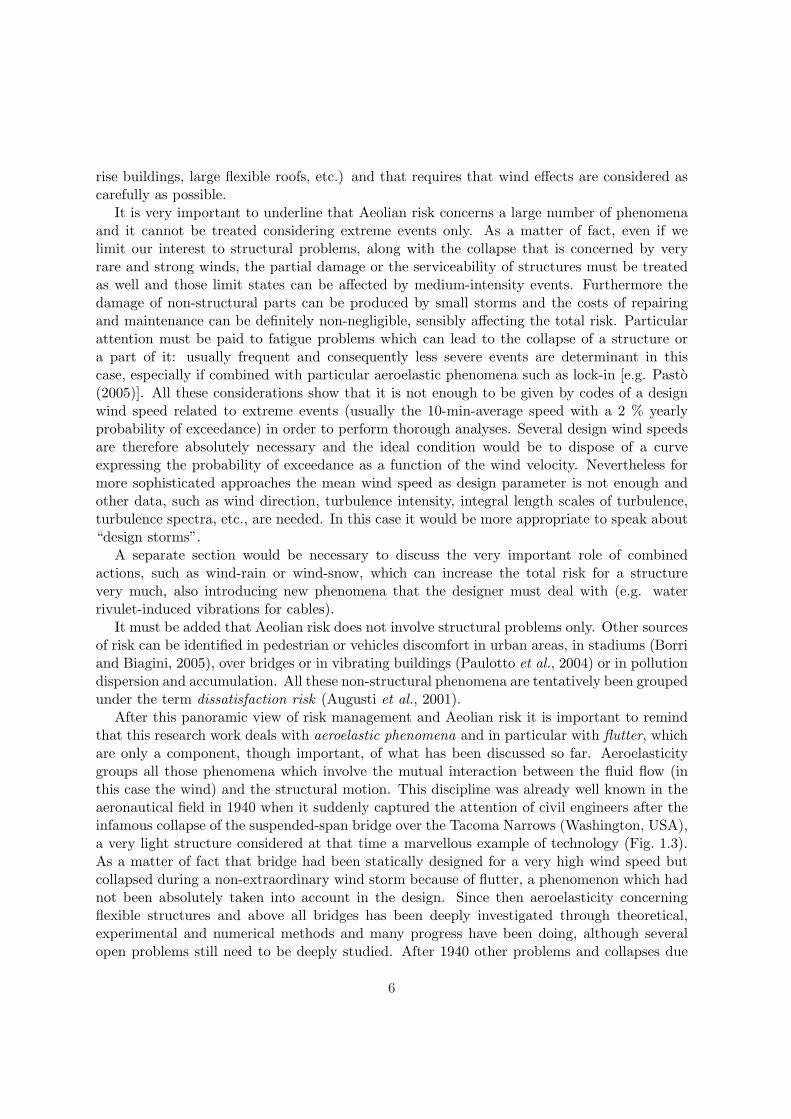
Figure 1.3: The infamous collapse of the Tacoma Narrows Bridge on November 7th 1940,Washington State, USA

evidence stressed by the mass media, available data about Aeolian risk are already quiteeloquent. According to the Munich Reinsurance Group (Augusti et al., 2001), windstormsare the third cause of economic losses due to natural hazards with 28 % of the total amount,following earthquakes (35 %) and floods (30 %). Conversely, concerning insurers’ total claims,windstorms are by far the first natural disaster in the list, whereas they are not much behindearthquakes regarding human fatalities (45 % vs. 47 %) and much more concerning than floods(7 %). All these figures confirm the relevance of Aeolian risk and suggest the importance ofdoing research in wind engineering field, carefully designing the structures taking into accountin a correct way wind effects, and improving methods of weather forecasting, early warningsystems and evacuation plans.

In addition to all that, in the last years Aeolian risk has been sensibly increasing despite thefact that scientific knowledge of wind effects has been noticeably improved and the provisionalcodes have been enhanced. The reason for this trend must be searched in the combined increaseof three terms in Eq. (1.2): hazard, exposure and vulnerability.

Hazard is increasing because of climate changes which seem to have started at the begin-ning of last century, probably because of several reasons but there is little doubt that humanactivities play a crucial role in these phenomena. The planet is globally warming, more en-ergy is consequently available in the atmosphere and as a result the frequency and probablythe intensity of extreme events like tropical cyclones or windstorms in general have sensiblyincreased. It is worrying the fact that this trend is expected to continue in the next decadesand for instance it will be probably necessary to design structures with different wind loadsdepending on the year of construction and expected lifetime (Augusti et al., 2001).

Exposure is increasing as well due to the migration of population, goods and facilities intowind-hazardous areas, where many megacities were born in the last decades.

Finally new structures tends to be always lighter and consequently more vulnerable to wind.The diffusion of light and high-resistance materials leads in this direction the constructionindustry. In addition, always more challenging designs are realized (long-span bridges, high-

5

rise buildings, large flexible roofs, etc.) and that requires that wind effects are considered ascarefully as possible.

It is very important to underline that Aeolian risk concerns a large number of phenomenaand it cannot be treated considering extreme events only. As a matter of fact, even if welimit our interest to structural problems, along with the collapse that is concerned by veryrare and strong winds, the partial damage or the serviceability of structures must be treatedas well and those limit states can be affected by medium-intensity events. Furthermore thedamage of non-structural parts can be produced by small storms and the costs of repairingand maintenance can be definitely non-negligible, sensibly affecting the total risk. Particularattention must be paid to fatigue problems which can lead to the collapse of a structure ora part of it: usually frequent and consequently less severe events are determinant in thiscase, especially if combined with particular aeroelastic phenomena such as lock-in [e.g. Pasto(2005)]. All these considerations show that it is not enough to be given by codes of a designwind speed related to extreme events (usually the 10-min-average speed with a 2 % yearlyprobability of exceedance) in order to perform thorough analyses. Several design wind speedsare therefore absolutely necessary and the ideal condition would be to dispose of a curveexpressing the probability of exceedance as a function of the wind velocity. Nevertheless formore sophisticated approaches the mean wind speed as design parameter is not enough andother data, such as wind direction, turbulence intensity, integral length scales of turbulence,turbulence spectra, etc., are needed. In this case it would be more appropriate to speak about“design storms”.

A separate section would be necessary to discuss the very important role of combinedactions, such as wind-rain or wind-snow, which can increase the total risk for a structurevery much, also introducing new phenomena that the designer must deal with (e.g. waterrivulet-induced vibrations for cables).

It must be added that Aeolian risk does not involve structural problems only. Other sourcesof risk can be identified in pedestrian or vehicles discomfort in urban areas, in stadiums (Borriand Biagini, 2005), over bridges or in vibrating buildings (Paulotto et al., 2004) or in pollutiondispersion and accumulation. All these non-structural phenomena are tentatively been groupedunder the term dissatisfaction risk (Augusti et al., 2001).

After this panoramic view of risk management and Aeolian risk it is important to remindthat this research work deals with aeroelastic phenomena and in particular with flutter, whichare only a component, though important, of what has been discussed so far. Aeroelasticitygroups all those phenomena which involve the mutual interaction between the fluid flow (inthis case the wind) and the structural motion. This discipline was already well known in theaeronautical field in 1940 when it suddenly captured the attention of civil engineers after theinfamous collapse of the suspended-span bridge over the Tacoma Narrows (Washington, USA),a very light structure considered at that time a marvellous example of technology (Fig. 1.3).As a matter of fact that bridge had been statically designed for a very high wind speed butcollapsed during a non-extraordinary wind storm because of flutter, a phenomenon which hadnot been absolutely taken into account in the design. Since then aeroelasticity concerningflexible structures and above all bridges has been deeply investigated through theoretical,experimental and numerical methods and many progress have been doing, although severalopen problems still need to be deeply studied. After 1940 other problems and collapses due

6

to aeroelastic phenomena have been observed, though not so astonishing as Tacoma failure,but nowadays very challenging designs are conceived accounting for aeroelastic stability as oneof the most important requirements. The more eloquent example is surely the proposal ofMessina Strait Bridge but many other light modern structures with very low eigenfrequenciesof oscillation and damping levels are designed all over the world. These structures tend to beless sensitive to seismic action and geotechnical settlements but much more vulnerable to windloads and in particular to aeroelastic effects. Therefore the relevance of aeroelastic phenomenafor a risk analysis is absolutely evident, also given the economic and strategic importance ofthe aforementioned types of structures.

A brief critical review of aeroelastic phenomena, with particular attention to bridges, willbe detailed in Chapter 2.

1.3 Performance-Based Design

Performance-Based Design (PBD) represents the structural design philosophy consistent withrisk management approach, which is aimed directly to the achievement and optimization ofwell specified performance objectives. This modern approach does not exclude prescriptionsand consequently it should not be considered an alternative to provisional codes. In PBD itis not new the idea of fixing some performance objectives but the probabilistic way to achievethem. In fact modern codes, even the most recent such as Eurocode 1 (ENV1991-2-4, 1995;EN1990, 2002), translate these performance objectives in several limit states but the safetypartial coefficients they give are not calibrated in a probabilistic way but just on empiricalbasis.

PDB has been developed mainly in the USA for seismic risk applications and design [e.g.Baker and Cornell (2003)] but it is still at an embryonic stage concerning wind engineering(Paulotto et al., 2004). A very interesting translation of PBD in equation was proposed bythe Pacific Earthquake Research Center (PEER) [e.g. Paulotto et al. (2004)]:

p(DV ) =∫ ∫ ∫

p(DV |DM) · |dp(DM |EDP )| · |dp(EDP |IM)| · dp(IM) (1.4)

where:IM (Intensity Measure) denotes a measure of the magnitude of the action;EDP (Engineering Demand Parameter) denotes a parameter which describes the structuralresponse;DM denotes a measure of the damage (cracking level, spalling, etc.);DV denotes a decision variable, that is a parameter which determines the design decision (forinstance a limit state, the amount of economic or human losses, etc.);p(·) denotes a probability of exceedance;p(·|·) denotes a conditional probability of exceedance.The integrals extend over all the possible Intensity Measures whose probabilities of exceedanceare determined through hazard analysis. The term p(EDP |IM) represents the probabilityof exceedance of a certain level of structural response, given a particular measure of theevent, whereas the term p(DM |EDP ) is the probability of exceedance of a certain structural

7

damage, once the structural response is given. The former is obtained through the structuralanalysis, the latter by means of the damage analysis. Their product can be identified as thevulnerability in Eq. (1.2). Finally the term p(DV |DM) represents a probability measure of thecost of damage, that is of the consequences. It is obtained through the loss analysis. Severalprofessional figures are involved in the outlined risk analysis: hazard analysis usually competesto pure scientists (meteorologists, geophysicists, etc.), vulnerability analysis (structural anddamage analysis) is the main task of engineers, while in loss analysis economists can give themost important contribution.

One of the most difficult terms to treat in the equation is the one that relates the measure ofthe damage DM to the structural response EDP . As a matter of fact, to simulate numericallythe actual damage of a structure is a very hard task. In addition the available experimentaldata are too limited, especially concerning the damage of non-structural components andgoods present inside the buildings. For this reason, in particular in the wind engineering field,attempts have been made to express the damage through the structural response itself [e.g.Paulotto et al. (2004)]. The PEER equation consequently simplifies as follows:

p(DV ) =∫ ∫

p(DV |DM) · |dp(DM |IM)| · dp(IM) (1.5)

Fragility curves are the practical expression of the term p(DM |IM) in the previous equa-tion. They express the probability of exceeding a specific damage state, conditioned on thevalue of the parameter synthesizing the magnitude of the natural or man-induced event. Thereare two types of fragility curves: system fragility and component fragility curves. Systemfragility refers to the damage of the entire structure whereas component fragility curves takeinto account only a specific part of the structure. The fragility of the entire structure can beapproximated assembling the component fragilities. In wind engineering practice the intensitymeasure is usually the mean wind speed so that the fragility curves express a relation betweenthe probability of exceedance of a damage state and the mean wind speed.

In order to make Eq. (1.5) and all the concepts discussed so far easier to apply in practice,it is possible to fix a certain number of limit states as performance objectives. In particular,distinction can be made between low performance levels and high performance levels. Hencecollapse and damage limit states require low structural performance with respect to the haz-ardous event, whereas serviceability and comfort limit states are related to limited losses andconsequently require high performance behavior. The concept of comfort is very general andrefers to pedestrians, vehicles, occupants of buildings or structures and so on. For each limitstate a maximum probability of exceedance in a fixed time period has to be specified in or-der to verify the safety of the design. The way to fix these probabilities, as we have alreadydiscussed in the first section of this chapter, is a very complex problem which should involveeconomic and political considerations through an optimization process [e.g. Rackwitz (2003)].

It is worth noting that fragility curves for high performance levels exist in literature whileit is not possible to find examples for low performance levels (Paulotto et al., 2004), thusconfirming the still primitive state of PBD in wind engineering.

The complete PBD approach is often difficult to apply, especially in those fields where thestate of the art has not reached yet the same level of development as in seismic engineering. Afully probabilistic structural design would often be a significant step forward. This is equivalent

8

to simplify the PEER equation by taking a Limit State as Decision Variable (SL ≡ DV ) andthen relating it directly to a structural response parameter (DV ≡ DM ≡ EDP ):

Pfail ≡ p(SL) =∫

p(SL|IM) · dp(IM) (1.6)

Once a set of relevant limit states have been identified and the acceptable probability of failurehas been fixed on the basis of socioeconomic issues, the safety of the structure can be checkedby comparing the probability of failure Pfail with its acceptable value. This more strictlyengineering formulation of the PEER equation allows to apply the Performance-Based Designin common design practice (national and international recommendations) and it is particularlyconvenient for our purposes.

Aeroelastic phenomena play a key role with respect to all limit states, both for low andhigh performance levels, when flexible structures, such as cable-stayed or suspension bridges,are concerned. Nevertheless the adaptation of Performance-Based Design to aeroelastic phe-nomena is a very challenging task at the present state of the art.

1.4 Contribution of the present research work

Concerning the large sphere of risk management this research work focuses on vulnerability,that is mainly on the step of structural analysis in the process of risk assessment or risk analysis.As we have already pointed out, wind engineering as a modern discipline is fairly young andrisk-consistent approaches in this field are still not very well codified. Then, if we concentrateon aeroelastic phenomena, to perform risk analyses and to conceive risk mitigation planningis even much more difficult, since this phenomena are already quite difficult to treat in atraditional, deterministic way. The ambitious attempt of this work is to include in risk analysisbridge aeroelasticity and specifically flutter stability. Two contributions in this direction aregiven: the first one is a sort of pre-normative study, which is related to risk mitigation throughcode implementation; the second one is a probabilistic approach to flutter problem whichshould allow to treat this phenomenon coherently with Performance-Based Design philosophy.

The importance to perform careful risk analyses concerning bridges is fairly clear. As amatter of fact, these structures are very expensive to build and to maintain, therefore they havea very high intrinsic value. Moreover they usually play important strategic roles for connectionsand traffic circulation. Therefore the closure of a bridge because of a windstorm can producea large amount of economic losses, even though the structure is not at all damaged. Alsowind-induced discomfort is very concerning for bridges since it affects traffic safety. Finally ina catastrophic scenario due to a natural or man-induced hazardous event, the collapse or theserviceability failure of important bridges can make extremely difficult the disaster responseconcerning emergency plans and humanitarian assistance. On the other hand, improvementsin material technology and technical knowledge allow nowadays to build superlong-span orvery light medium-span bridges. Consequently these structures are always more vulnerable towind actions and in particular to aeroelastic phenomena, which have to be carefully accountedfor in any structural analysis.

Aeroelastic phenomena are usually dealt with through wind-tunnel tests, which at thepresent state-of-the-art are the only reliable tool to treat aerodynamics and fluid-structure

9

coupling for bluff-bodies such as bridge decks. Complete extensive experimental investigationscan be very expensive and time-consuming but they are absolutely necessary since the reallyfirst design stages for large-span bridges, for which aerodynamics and aeroelasticity are usuallythe key points of the design. Conversely for medium-span bridges and conventional geometriesthese problems are less concerning even though they cannot be excluded a priori. In additionextensive experimental campaigns are not always possible in these cases, above all for reasonsof budget, and often wind-tunnel tests, if any, are performed only at the last design stageas final validation. Therefore for bridge engineers it could be very useful to dispose of aninstrument able to highlight or to exclude with a certain degree of reliability the possibility ofaeroelastic instabilities or large amplitudes of vibration, without performing wind-tunnel tests,at least at pre-design stages. Unfortunately this instrument is not provided by the nationalor international provisional codes, which always refer to wind tunnel tests when aeroelasticityis concerned. Indeed, empirical formulas for classical flutter, galloping and vortex sheddingwere given in the ECCS recommendations (ECCS, 1987), which was, to the knowledge of thewriter, the most courageous provisional document at this regard, but they were afterwards notreported in the following documents of Eurocode 1 [e.g. ENV1991-2-4 (1995)]. In the presentresearch work we limited our attention to bridge deck flutter instability and we tried to setup a simplified method of calculation which could be used in order to understand if a givenbridge, for a specified level of the hazard, is safe enough (flutter is definitely not a problem) orthe design must be definitely modified (the flutter wind speed is definitely too low) or if windtunnel tests are needed in order to better assess the actual vulnerability of the structure. Thistool could be useful to better design medium-span conventional bridges and in this sense wecan speak about a pre-normative study, which could help to improve the codes, therefore as ameasure of risk mitigation.

The aforementioned simplified approach is based on Scanlan’s definition of linearized self-excited forces via flutter derivative functions (see Chapter 2) and it consists of three mainsteps. In the first one, described in Chapter 5, the possibility to pass from a multimodal witheighteen flutter derivatives to a bimodal approach to flutter with eight aeroelastic functionsis checked. Then in Chapter 6 the flutter equations are analyzed in details, manipulate andsimplified on the basis of a large database of dynamic and aerodynamic data. The resultingformulas depend on three or even two flutter derivatives only, which are recognized to bethe most reliable, the easiest to be identified through wind-tunnel tests and those for whichmore data are available in literature. Apart from the practical interest of the formulas, in thewriter’s opinion this result is also scientifically important for the insight it gives in the fluttermechanism. Finally, thanks also to the contribution of the Centre Scientifique et Techniquedu Batiment (CSTB) of Nantes, France, a relatively large number of data are collected for afew classes of bridge deck geometries and in Chapter 7 a first step towards flutter derivativegeneralization is attempted. A scheme of the explained procedure is shown in Fig. 1.4. It isworth noting that the last step is crucial in order to be able to assess flutter boundaries witha certain degree of reliability without performing wind-tunnel tests and it still needs furtherresearch.

In Chapter 3 an extensive wind tunnel test campaign is described. A bridge deck section-model is tested in the DIC-CRIACIV Boundary Layer Wind Tunnel of Prato in order toinvestigate its static-aerodynamic and in particular its aeroelastic behavior. One of the main

10

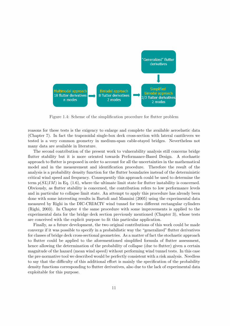
Figure 1.4: Scheme of the simplification procedure for flutter problem

reasons for these tests is the exigency to enlarge and complete the available aeroelastic data(Chapter 7). In fact the trapezoidal single-box deck cross-section with lateral cantilevers wetested is a very common geometry in medium-span cable-stayed bridges. Nevertheless notmany data are available in literature.

The second contribution of the present work to vulnerability analysis still concerns bridgeflutter stability but it is more oriented towards Performance-Based Design. A stochasticapproach to flutter is proposed in order to account for all the uncertainties in the mathematicalmodel and in the measurement and identification procedure. Therefore the result of theanalysis is a probability density function for the flutter boundaries instead of the deterministiccritical wind speed and frequency. Consequently this approach could be used to determine theterm p(SL|IM) in Eq. (1.6), where the ultimate limit state for flutter instability is concerned.Obviously, as flutter stability is concerned, the contribution refers to low performance levelsand in particular to collapse limit state. An attempt to apply this procedure has already beendone with some interesting results in Bartoli and Mannini (2005) using the experimental datameasured by Righi in the DIC-CRIACIV wind tunnel for two different rectangular cylinders(Righi, 2003). In Chapter 4 the same procedure with some improvements is applied to theexperimental data for the bridge deck section previously mentioned (Chapter 3), whose testsare conceived with the explicit purpose to fit this particular application.

Finally, as a future development, the two original contributions of this work could be madeconverge if it was possible to specify in a probabilistic way the “generalized” flutter derivativesfor classes of bridge deck cross-sectional geometries. As a matter of fact the stochastic approachto flutter could be applied to the aforementioned simplified formula of flutter assessment,hence allowing the determination of the probability of collapse (due to flutter) given a certainmagnitude of the hazard (mean wind speed) without performing wind tunnel tests. In this casethe pre-normative tool we described would be perfectly consistent with a risk analysis. Needlessto say that the difficulty of this additional effort is mainly the specification of the probabilitydensity functions corresponding to flutter derivatives, also due to the lack of experimental dataexploitable for this purpose.

11

Chapter 2

Aeroelastic phenomena

2.1 Fluid-structure interaction

The complex interaction between air flow and solid structures has always been a very importantissue. Although not fully understood, it was of great concern for civil engineers already in theXIX century, when several bridges collapsed or were severely damaged because of wind effects.In the first half of the XX century, the fluid-structure interaction phenomena were practicallyforgotten in civil engineering, whereas they were carefully studied in the aeronautical field,where the theory of aeroelasticity was funded. After the Tacoma Bridge failure in 1940 thisdiscipline has got back to the civil engineering sphere as well and nowadays the effects ofthe fluid-structure coupling are more and more important due to the increased flexibility ofmodern constructions.

The basic idea of the fluid-structure interaction is that the flow around a solid structureproduces steady and unsteady loads which tend to elastically deform the structure inducingvibration. If this motion is large enough, it is able to influence the flow field around thebody and consequently to change the aerodynamic loads. This feedback is the actual core ofaeroelasticity. In particular, since bridges and civil structures in general cannot be consideredstreamlined profiles, we are mainly interested in bluff-body aerodynamics and aeroelasticity,where flow separation plays a key role.

The second section of this chapter gives a brief overview of the most common aeroelasticphenomena in the civil engineering field, referring to the design limit states involved. Then,the following sections give deeper details concerning the fundamental theory and models todescribe self-excited forces and calculate flutter instability.

2.2 Aeroelastic phenomena

2.2.1 Torsional divergence

Torsional divergence is a static instability phenomenon produced by the loss of torsional stiff-ness due to steady aerodynamic moment. Considering a cylinder-type structure, the latter can

13

be written as follows:M(α) =

12ρU2B2CM (α) (2.1)

where ρ is the air density, U the mean airflow speed, B the cylinder chord length, CM theaerodynamic moment coefficient around the twist axis (positive clockwise) and α the meanangle of twist (positive clockwise). Considering a single-degree-of-freedom linear structure, theequilibrium position is given by the equation:

Kαα =12ρU2B2CM (α) (2.2)

The aerodynamic moment coefficient can be linearized around the undeformed position (α=0):

CM (α) = CM (0) +dCM

dα(0)α (2.3)

so that Eq. (2.2) can be written as:

Kαα = qB2[CM (0) +dCM

dα(0)α] (2.4)

where q = 12ρU2 is the kinematic pressure. Reorganizing the terms in the previous equation,

static angle of twist can be expressed as follows:

α =qB2CM (0)

Kα − qB2 dCMdα (0)

(2.5)

It is evident from Eq. (2.5) that the mean angle of twist tends to increase indefinitely whenKα − qB2 dCM

dα (0) → 0, that is when the total stiffness (structural + aerodynamic) tends tozero. The corresponding mean wind speed Udiv is called critical divergence wind speed:

Udiv =

√2Kα

ρB2 dCMdα (0)

(2.6)

In case the aerodynamic moment coefficient is not linear with respect to the angle of attack,the same linearization may be applied around a generic static twist angle α = α0 or the moregeneral nonlinear Eq. (2.2) could have been solved numerically. Furthermore it is evident fromEqs. (2.5)-(2.6) that static divergence can occur only if the moment coefficient is characterizedby a positive slope dCM

dα (0) > 0.It is also worth noting that the previous analysis refers to single-degree-of-freedom structures

but it may readily be generalized to three-dimensional structures such as bridge decks [e.g.Simiu and Scanlan (1996)].

Torsional divergence, which refers to the ultimate limit state, is usually not a very con-cerning problem for real bridges as it tends to appear at sensibly higher wind speed than thedynamic instability called flutter (see section 2.2.4). Nevertheless this cannot be trusted incase of bridges with frequency ratio between torsion and bending critical modes close to oneor even lower than unity [e.g. Dyrbye and Hansen (1997)].

14

2.2.2 Galloping

Galloping is a single-degree-of-freedom instability typical of slender structures characterizedby particular cross-sectional geometry, such as rectangular or D-shaped. It can lead to verylarge-amplitude oscillations in the across-wind direction.

The phenomenon is usually approached with the quasi-steady theory, thus meaning thatthe influence of fluid memory on the instability mechanism can be neglected. In order todetermine the galloping critical wind speed Ug for the condition of incipient instability intwo-dimensional cylinders, the aerodynamic lift due to the heaving vibration can be linearizedaround the mean deformed configuration (see section 2.4.3) and the equation of motion canbe written as follows:

m[h + 2ζhωhh + ω2hh] =

12ρU2B[

dCL

dα(α0) + CD(α0)]

h

U(2.7)

where m is the mass per unit length, ζh is the damping ratio for the bending mode and ωh

is the bending circular frequency; CD(α0) and dCLdα (α0) are the drag coefficient and the first

derivative of the lift coefficient evaluated at the mean angle of attack α0. According to theGlauert-Den Hartog criterion [e.g. Blevins (1990); Simiu and Scanlan (1996); Dyrbye andHansen (1997)] galloping occurs when the total damping (structural+aerodynamic) vanishes:

2mζhωh − 12ρUB[

dCL

dα(α0) + CD(α0)] = 0 (2.8)

Therefore one obtains:Ug = − 4mζhωh

ρB[dCLdα (α0) + CD(α0)]

(2.9)

It is evident from Eq. (2.9) that a structure can gallop in a bending mode only if [dCLdα (α0) +

CD(α0)] < 0. That is why circular cylinders, characterized by dCLdα ≡ 0 and CD > 0, are not

prone to this type of instability. Nevertheless, cables too can undergo galloping oscillationswhen their circular shape is altered, for instance by ice coating.

In order to calculate the limit-cycle amplitude of oscillation at a certain post-critical windspeed and not merely the critical wind speed, a nonlinear model for the aerodynamic forces isnecessary. In one of the most famous models, the vertical force coefficient CFz is expressed asa polynomial series retaining the terms up to the third or seventh order (Blevins, 1990; Simiuand Scanlan, 1996; Dyrbye and Hansen, 1997; Thompson and Stewart, 2002):

CFz = A1z

U−A3(

z

U)3 + A5(

z

U)5 −A7(

z

U)7 (2.10)

Parkinson and Smith (1964) determined the coefficients A1 to A7 for a square cylinder applyinga polynomial fit to the static experimental values for CFz(α) and compared with experimentsthe resulting limit-cycle amplitudes, observing a very good agreement (Fig. 2.1). It is clearlyshown in Fig. 2.1 that the seventh order model is able to capture the Hopf bifurcation suggestedby the experiments, while this nonlinear dynamic feature cannot be appreciated adopting thethird order polynomial fit (Blevins, 1990).

15

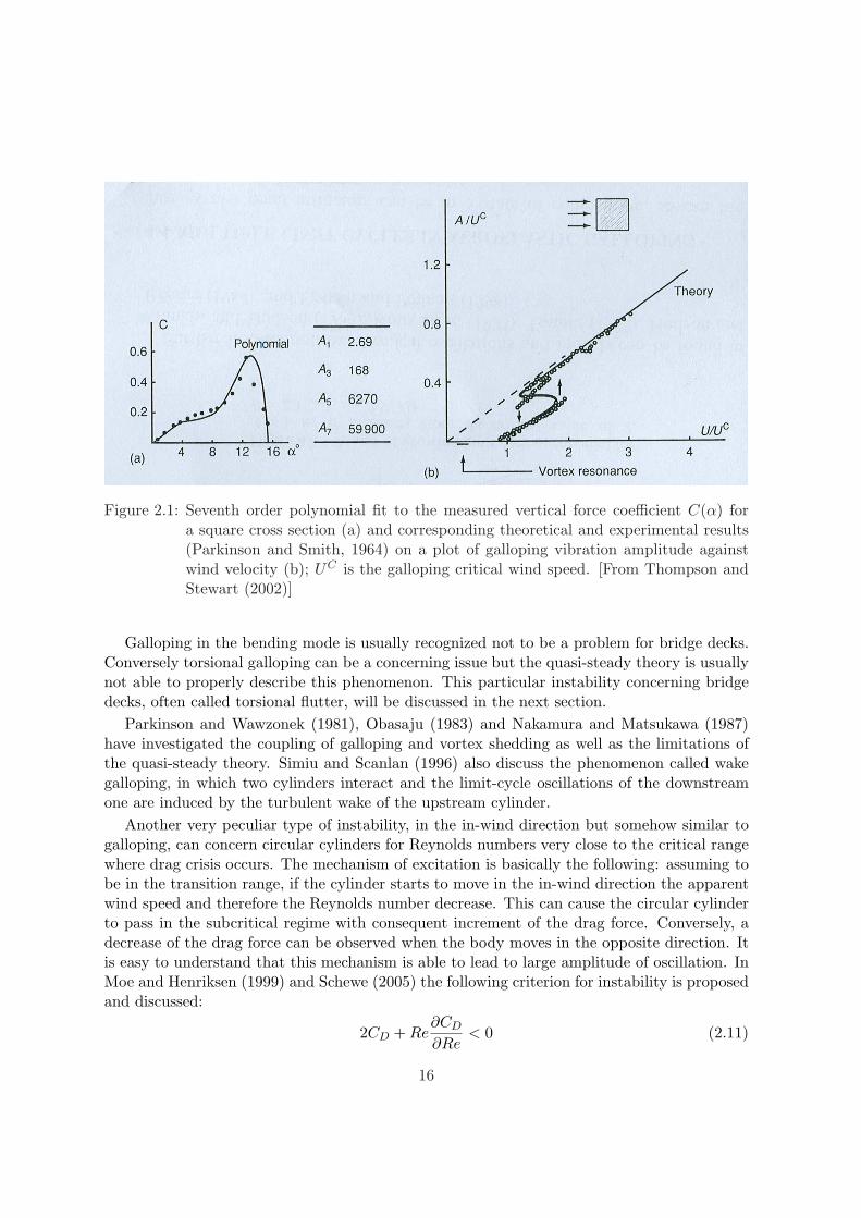
Figure 2.1: Seventh order polynomial fit to the measured vertical force coefficient C(α) fora square cross section (a) and corresponding theoretical and experimental results(Parkinson and Smith, 1964) on a plot of galloping vibration amplitude againstwind velocity (b); UC is the galloping critical wind speed. [From Thompson andStewart (2002)]

Galloping in the bending mode is usually recognized not to be a problem for bridge decks.Conversely torsional galloping can be a concerning issue but the quasi-steady theory is usuallynot able to properly describe this phenomenon. This particular instability concerning bridgedecks, often called torsional flutter, will be discussed in the next section.

Parkinson and Wawzonek (1981), Obasaju (1983) and Nakamura and Matsukawa (1987)have investigated the coupling of galloping and vortex shedding as well as the limitations ofthe quasi-steady theory. Simiu and Scanlan (1996) also discuss the phenomenon called wakegalloping, in which two cylinders interact and the limit-cycle oscillations of the downstreamone are induced by the turbulent wake of the upstream cylinder.

Another very peculiar type of instability, in the in-wind direction but somehow similar togalloping, can concern circular cylinders for Reynolds numbers very close to the critical rangewhere drag crisis occurs. The mechanism of excitation is basically the following: assuming tobe in the transition range, if the cylinder starts to move in the in-wind direction the apparentwind speed and therefore the Reynolds number decrease. This can cause the circular cylinderto pass in the subcritical regime with consequent increment of the drag force. Conversely, adecrease of the drag force can be observed when the body moves in the opposite direction. Itis easy to understand that this mechanism is able to lead to large amplitude of oscillation. InMoe and Henriksen (1999) and Schewe (2005) the following criterion for instability is proposedand discussed:

2CD + Re∂CD

∂Re< 0 (2.11)

16

whereRe =

UB

ν(2.12)

is the Reynolds number based on the chord length and ν is the air kinematic viscosity(ν = 1.5 · 10−5 m2s−1 for the air at 20°C).

Due to the large-amplitude vibrations, galloping in its basic across-wind quasi-steady naturemainly concerns the ultimate limit state for cables and other linelike structures.

2.2.3 Vortex shedding and lock-in

It is well known that a bluff body in a fluid flow develops a turbulent wake, wherein periodicalvortical structures are recognizable. Boundary layers separate and produce unstable shearlayers that tend to roll up and generate alternate eddies that are then convected downstream.

At the end of the nineteenth century an experimental study of Strouhal (Strouhal, 1878)showed that there is a linear relation between the frequency of shedding of vortical structures(fs) and the undisturbed flow velocity (U), which allows the definition of a nondimensionalquantity known as Strouhal number:

St =fsD

U(2.13)

where D is a characteristic body dimension (usually the cross-section thickness). The Strouhalnumber is known to be dependent on the body geometry and Reynolds number.

An analytical study concerning the stability of the vortex patterns in the wake of a station-ary cylindrical body was carried out in 1911 by von Karman and Rubach (von Karman andRubach, 1912). Assuming irrotational flow except in concentrated vortices and adopting thetwo-dimensional potential flow theory, they were able to show that the vortex trail is stableonly if the eddies are organized in alternate double row pattern (Karman’s vortex street).They also calculated the steady drag induced by this vortex trail. More recent studies tried tofind an expression for the fluctuating lift based on the ideal Karman’s vortex street [e.g. Chen(1972); Sallet (1973)].

Flow separation that generates vortex shedding can be geometrically induced, when theseparation point is fixed by the presence of sharp edges, or flow induced, when the boundarylayer physical properties determine where separation occurs. Common examples for the firstcase are the square cylinder [e.g. Lyn et al. (1995); Schewe (1984, 1990)] and the H-shapedcross-section cylinder, similar to Tacoma Narrows Bridge deck (Schewe, 1984, 1989), whereasfor the second case the most studied example is the circular cylinder [e.g. Roshko (1954,1961); van Nunen (1974); Schewe (1983, 1986); Lourenco and Shih (1993); Ong and Wallace(1996); Zdravkovich (1997); Kravchenko and Moin (2000)]. When separation is induced bygeometry the unsteady wake is less sensitive to flow parameters such as Reynolds number, eventhough some significant effects have been sometimes observed (Okajima, 1982; Schewe, 1984,2006). Conversely for smooth bodies the shedding process is extremely sensitive to Mach andReynolds numbers. In the case of the circular cylinder several wake regimes were identifiedaccording to Reynolds number [e.g. Roshko (1954) or Pasto (2005) for an extensive criticalreview] and an abrupt wake transition can be observed around Re ∼= 3÷ 4 · 105, called criticalregion (Roshko, 1961; Wooton and Scruton, 1970; Schewe, 1983).

17

Apart from global Reynolds number (and Mach number for compressible flows) other flowparameters can have a strong influence on the vortex formation process. For instance veryimportant is the role played by local Reynolds numbers associable to the degree of sharpness ofthe corners and to the surface roughness of the body [e.g. Simiu and Scanlan (1996)]. Also theoncoming turbulence can strongly affect the shedding mechanism, usually reducing its overallintensity [e.g. Simiu and Scanlan (1996)].

Moreover the vortex-shedding process is characterized by pronounced three-dimensionalfeatures, also for two dimensional body. As a matter of fact the unstable shear layers rollup with a limited coherence and then the forming eddies stretch in the spanwise direction.A comprehensive discussion of the physics standing behind this phenomenon is reported inBuresti (1998) and the three-dimensional structure of the eddies are clearly shown by theexperiments performed by Schewe on the airfoil of a Growian wind-power plant (Schewe,2001).

It is also worth noting that the vortex shedding mechanism is particularly complicate forquasi-streamlined body, such as modern bridge deck cross sections, whose aerodynamics ischaracterized by separation, reattachment and merging of small eddies structures, so thatoften several Strouhal numbers corresponding to different shedding processes are detectable[e.g. Bruno and Khris (2003)].

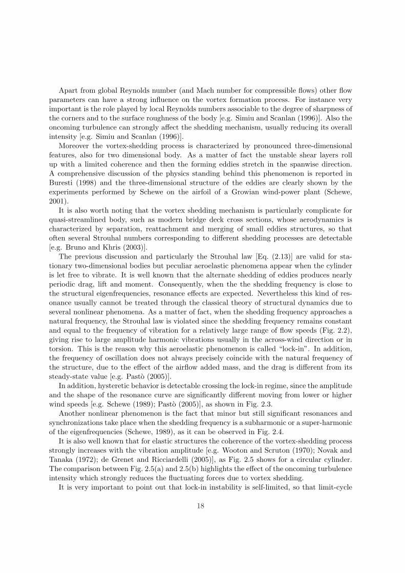
The previous discussion and particularly the Strouhal law [Eq. (2.13)] are valid for sta-tionary two-dimensional bodies but peculiar aeroelastic phenomena appear when the cylinderis let free to vibrate. It is well known that the alternate shedding of eddies produces nearlyperiodic drag, lift and moment. Consequently, when the the shedding frequency is close tothe structural eigenfrequencies, resonance effects are expected. Nevertheless this kind of res-onance usually cannot be treated through the classical theory of structural dynamics due toseveral nonlinear phenomena. As a matter of fact, when the shedding frequency approaches anatural frequency, the Strouhal law is violated since the shedding frequency remains constantand equal to the frequency of vibration for a relatively large range of flow speeds (Fig. 2.2),giving rise to large amplitude harmonic vibrations usually in the across-wind direction or intorsion. This is the reason why this aeroelastic phenomenon is called “lock-in”. In addition,the frequency of oscillation does not always precisely coincide with the natural frequency ofthe structure, due to the effect of the airflow added mass, and the drag is different from itssteady-state value [e.g. Pasto (2005)].

In addition, hysteretic behavior is detectable crossing the lock-in regime, since the amplitudeand the shape of the resonance curve are significantly different moving from lower or higherwind speeds [e.g. Schewe (1989); Pasto (2005)], as shown in Fig. 2.3.

Another nonlinear phenomenon is the fact that minor but still significant resonances andsynchronizations take place when the shedding frequency is a subharmonic or a super-harmonicof the eigenfrequencies (Schewe, 1989), as it can be observed in Fig. 2.4.

It is also well known that for elastic structures the coherence of the vortex-shedding processstrongly increases with the vibration amplitude [e.g. Wooton and Scruton (1970); Novak andTanaka (1972); de Grenet and Ricciardelli (2005)], as Fig. 2.5 shows for a circular cylinder.The comparison between Fig. 2.5(a) and 2.5(b) highlights the effect of the oncoming turbulenceintensity which strongly reduces the fluctuating forces due to vortex shedding.

It is very important to point out that lock-in instability is self-limited, so that limit-cycle

18

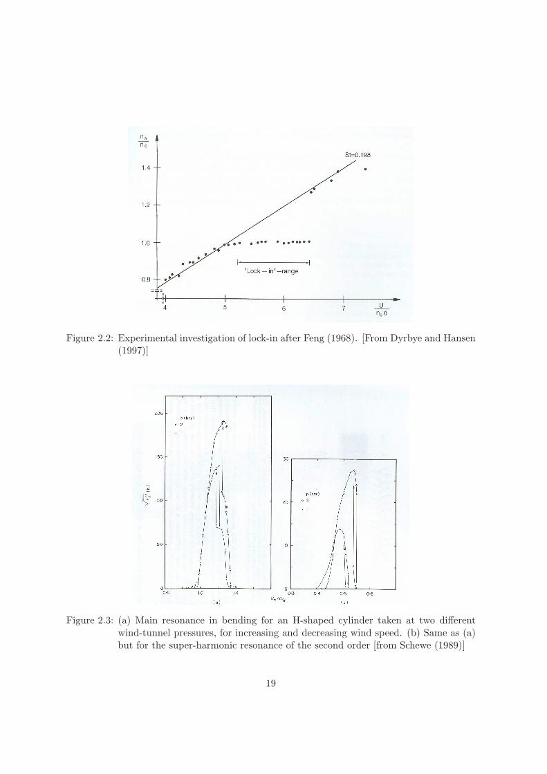
Figure 2.2: Experimental investigation of lock-in after Feng (1968). [From Dyrbye and Hansen(1997)]

Figure 2.3: (a) Main resonance in bending for an H-shaped cylinder taken at two differentwind-tunnel pressures, for increasing and decreasing wind speed. (b) Same as (a)but for the super-harmonic resonance of the second order [from Schewe (1989)]

19

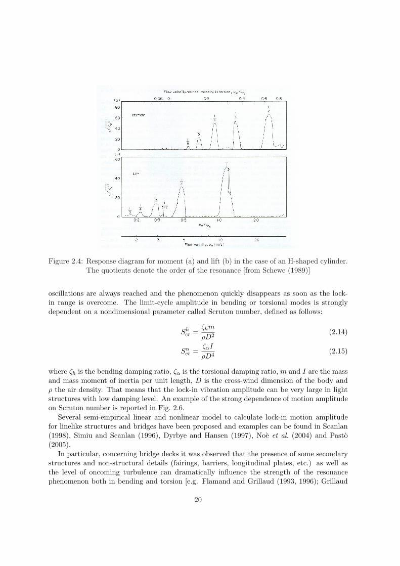
Figure 2.4: Response diagram for moment (a) and lift (b) in the case of an H-shaped cylinder.The quotients denote the order of the resonance [from Schewe (1989)]

oscillations are always reached and the phenomenon quickly disappears as soon as the lock-in range is overcome. The limit-cycle amplitude in bending or torsional modes is stronglydependent on a nondimensional parameter called Scruton number, defined as follows:

Shcr =

ζhm

ρD2(2.14)

Sαcr =

ζαI

ρD4(2.15)

where ζh is the bending damping ratio, ζα is the torsional damping ratio, m and I are the massand mass moment of inertia per unit length, D is the cross-wind dimension of the body andρ the air density. That means that the lock-in vibration amplitude can be very large in lightstructures with low damping level. An example of the strong dependence of motion amplitudeon Scruton number is reported in Fig. 2.6.

Several semi-empirical linear and nonlinear model to calculate lock-in motion amplitudefor linelike structures and bridges have been proposed and examples can be found in Scanlan(1998), Simiu and Scanlan (1996), Dyrbye and Hansen (1997), Noe et al. (2004) and Pasto(2005).

In particular, concerning bridge decks it was observed that the presence of some secondarystructures and non-structural details (fairings, barriers, longitudinal plates, etc.) as well asthe level of oncoming turbulence can dramatically influence the strength of the resonancephenomenon both in bending and torsion [e.g. Flamand and Grillaud (1993, 1996); Grillaud

20

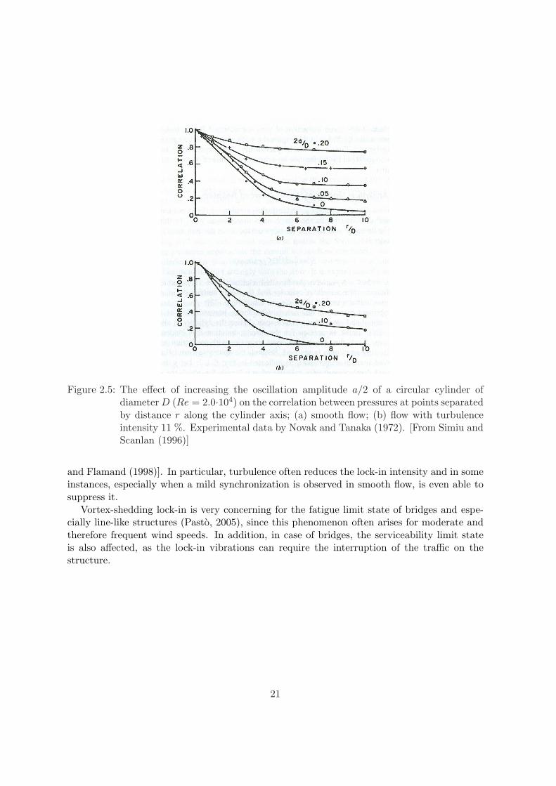
Figure 2.5: The effect of increasing the oscillation amplitude a/2 of a circular cylinder ofdiameter D (Re = 2.0·104) on the correlation between pressures at points separatedby distance r along the cylinder axis; (a) smooth flow; (b) flow with turbulenceintensity 11 %. Experimental data by Novak and Tanaka (1972). [From Simiu andScanlan (1996)]

and Flamand (1998)]. In particular, turbulence often reduces the lock-in intensity and in someinstances, especially when a mild synchronization is observed in smooth flow, is even able tosuppress it.

Vortex-shedding lock-in is very concerning for the fatigue limit state of bridges and espe-cially line-like structures (Pasto, 2005), since this phenomenon often arises for moderate andtherefore frequent wind speeds. In addition, in case of bridges, the serviceability limit stateis also affected, as the lock-in vibrations can require the interruption of the traffic on thestructure.

21

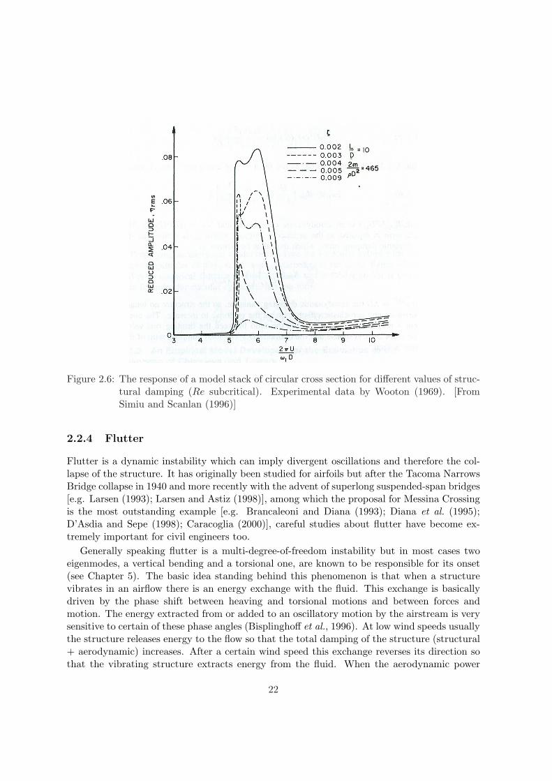
Figure 2.6: The response of a model stack of circular cross section for different values of struc-tural damping (Re subcritical). Experimental data by Wooton (1969). [FromSimiu and Scanlan (1996)]

2.2.4 Flutter

Flutter is a dynamic instability which can imply divergent oscillations and therefore the col-lapse of the structure. It has originally been studied for airfoils but after the Tacoma NarrowsBridge collapse in 1940 and more recently with the advent of superlong suspended-span bridges[e.g. Larsen (1993); Larsen and Astiz (1998)], among which the proposal for Messina Crossingis the most outstanding example [e.g. Brancaleoni and Diana (1993); Diana et al. (1995);D’Asdia and Sepe (1998); Caracoglia (2000)], careful studies about flutter have become ex-tremely important for civil engineers too.

Generally speaking flutter is a multi-degree-of-freedom instability but in most cases twoeigenmodes, a vertical bending and a torsional one, are known to be responsible for its onset(see Chapter 5). The basic idea standing behind this phenomenon is that when a structurevibrates in an airflow there is an energy exchange with the fluid. This exchange is basicallydriven by the phase shift between heaving and torsional motions and between forces andmotion. The energy extracted from or added to an oscillatory motion by the airstream is verysensitive to certain of these phase angles (Bisplinghoff et al., 1996). At low wind speeds usuallythe structure releases energy to the flow so that the total damping of the structure (structural+ aerodynamic) increases. After a certain wind speed this exchange reverses its direction sothat the vibrating structure extracts energy from the fluid. When the aerodynamic power

22

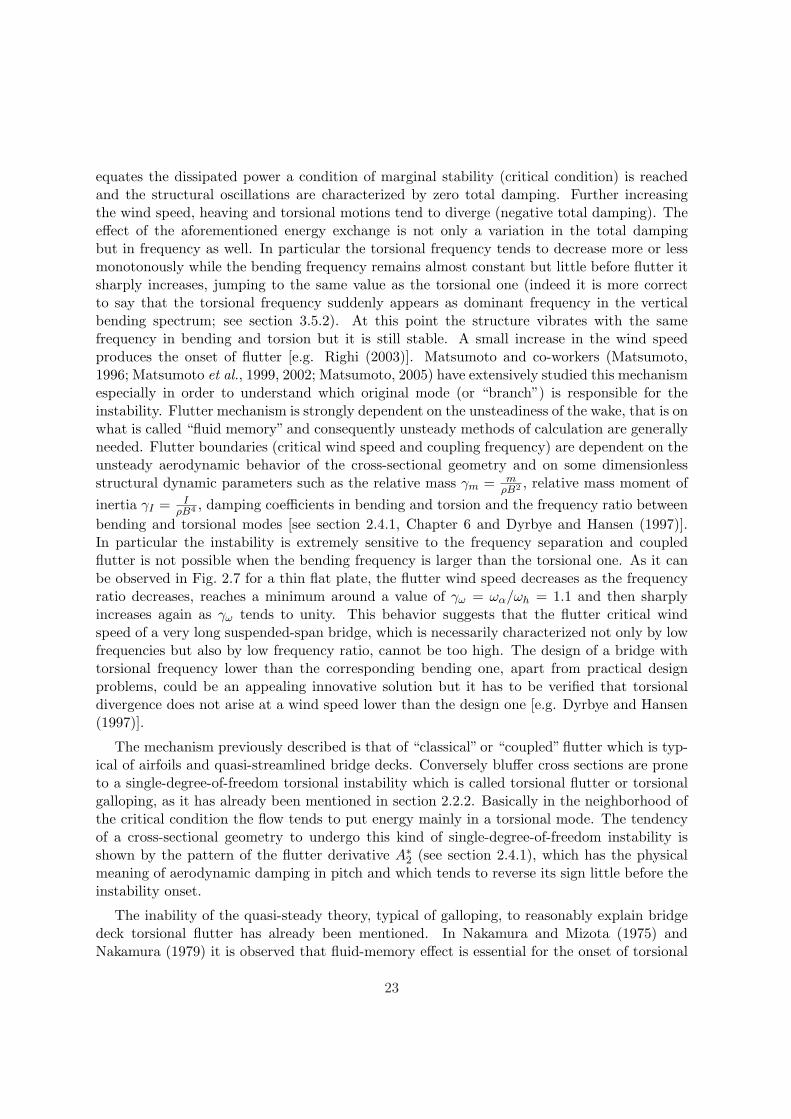
equates the dissipated power a condition of marginal stability (critical condition) is reachedand the structural oscillations are characterized by zero total damping. Further increasingthe wind speed, heaving and torsional motions tend to diverge (negative total damping). Theeffect of the aforementioned energy exchange is not only a variation in the total dampingbut in frequency as well. In particular the torsional frequency tends to decrease more or lessmonotonously while the bending frequency remains almost constant but little before flutter itsharply increases, jumping to the same value as the torsional one (indeed it is more correctto say that the torsional frequency suddenly appears as dominant frequency in the verticalbending spectrum; see section 3.5.2). At this point the structure vibrates with the samefrequency in bending and torsion but it is still stable. A small increase in the wind speedproduces the onset of flutter [e.g. Righi (2003)]. Matsumoto and co-workers (Matsumoto,1996; Matsumoto et al., 1999, 2002; Matsumoto, 2005) have extensively studied this mechanismespecially in order to understand which original mode (or “branch”) is responsible for theinstability. Flutter mechanism is strongly dependent on the unsteadiness of the wake, that is onwhat is called “fluid memory” and consequently unsteady methods of calculation are generallyneeded. Flutter boundaries (critical wind speed and coupling frequency) are dependent on theunsteady aerodynamic behavior of the cross-sectional geometry and on some dimensionlessstructural dynamic parameters such as the relative mass γm = m

ρB2 , relative mass moment ofinertia γI = I

ρB4 , damping coefficients in bending and torsion and the frequency ratio betweenbending and torsional modes [see section 2.4.1, Chapter 6 and Dyrbye and Hansen (1997)].In particular the instability is extremely sensitive to the frequency separation and coupledflutter is not possible when the bending frequency is larger than the torsional one. As it canbe observed in Fig. 2.7 for a thin flat plate, the flutter wind speed decreases as the frequencyratio decreases, reaches a minimum around a value of γω = ωα/ωh = 1.1 and then sharplyincreases again as γω tends to unity. This behavior suggests that the flutter critical windspeed of a very long suspended-span bridge, which is necessarily characterized not only by lowfrequencies but also by low frequency ratio, cannot be too high. The design of a bridge withtorsional frequency lower than the corresponding bending one, apart from practical designproblems, could be an appealing innovative solution but it has to be verified that torsionaldivergence does not arise at a wind speed lower than the design one [e.g. Dyrbye and Hansen(1997)].

The mechanism previously described is that of “classical” or “coupled” flutter which is typ-ical of airfoils and quasi-streamlined bridge decks. Conversely bluffer cross sections are proneto a single-degree-of-freedom torsional instability which is called torsional flutter or torsionalgalloping, as it has already been mentioned in section 2.2.2. Basically in the neighborhood ofthe critical condition the flow tends to put energy mainly in a torsional mode. The tendencyof a cross-sectional geometry to undergo this kind of single-degree-of-freedom instability isshown by the pattern of the flutter derivative A∗2 (see section 2.4.1), which has the physicalmeaning of aerodynamic damping in pitch and which tends to reverse its sign little before theinstability onset.

The inability of the quasi-steady theory, typical of galloping, to reasonably explain bridgedeck torsional flutter has already been mentioned. In Nakamura and Mizota (1975) andNakamura (1979) it is observed that fluid-memory effect is essential for the onset of torsional

23

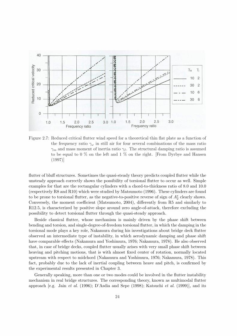
Figure 2.7: Reduced critical flutter wind speed for a theoretical thin flat plate as a function ofthe frequency ratio γω in still air for four several combinations of the mass ratioγm and mass moment of inertia ratio γI . The structural damping ratio is assumedto be equal to 0 % on the left and 1 % on the right. [From Dyrbye and Hansen(1997)]

flutter of bluff structures. Sometimes the quasi-steady theory predicts coupled flutter while theunsteady approach correctly shows the possibility of torsional flutter to occur as well. Simpleexamples for that are the rectangular cylinders with a chord-to-thickness ratio of 8.0 and 10.0(respectively R8 and R10) which were studied by Matsumoto (1996). These cylinders are foundto be prone to torsional flutter, as the negative-to-positive reverse of sign of A∗2 clearly shows.Conversely, the moment coefficient (Matsumoto, 2004), differently from R5 and similarly toR12.5, is characterized by positive slope around zero angle-of-attack, therefore excluding thepossibility to detect torsional flutter through the quasi-steady approach.

Beside classical flutter, whose mechanism is mainly driven by the phase shift betweenbending and torsion, and single-degree-of-freedom torsional flutter, in which the damping in thetorsional mode plays a key role, Nakamura during his investigations about bridge deck flutterobserved an intermediate type of instability, in which aerodynamic damping and phase shifthave comparable effects (Nakamura and Yoshimura, 1976; Nakamura, 1978). He also observedthat, in case of bridge decks, coupled flutter usually arises with very small phase shift betweenheaving and pitching motions, that is with almost fixed center of rotation, normally locatedupstream with respect to midchord (Nakamura and Yoshimura, 1976; Nakamura, 1978). Thisfact, probably due to the lack of inertial coupling between heave and pitch, is confirmed bythe experimental results presented in Chapter 3.

Generally speaking, more than one or two modes could be involved in the flutter instabilitymechanism in real bridge structures. The corresponding theory, known as multimodal flutterapproach [e.g. Jain et al. (1996); D’Asdia and Sepe (1998); Katsuchi et al. (1999)], and its

24

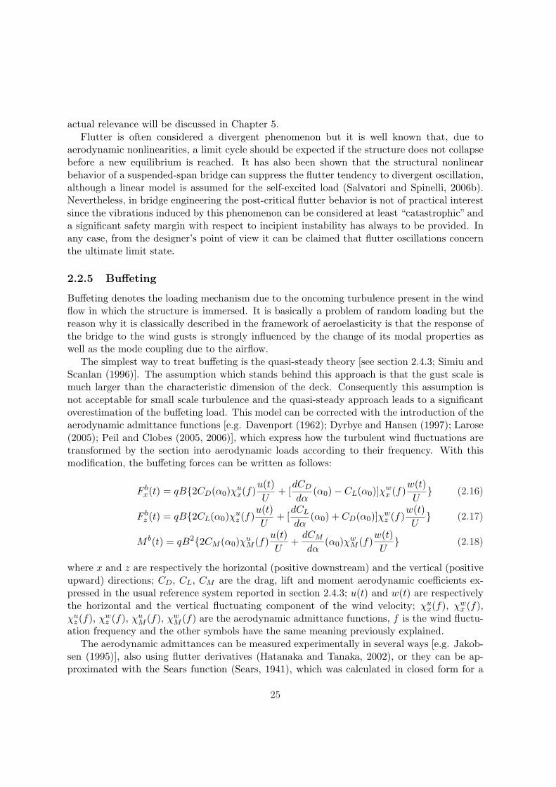
actual relevance will be discussed in Chapter 5.Flutter is often considered a divergent phenomenon but it is well known that, due to

aerodynamic nonlinearities, a limit cycle should be expected if the structure does not collapsebefore a new equilibrium is reached. It has also been shown that the structural nonlinearbehavior of a suspended-span bridge can suppress the flutter tendency to divergent oscillation,although a linear model is assumed for the self-excited load (Salvatori and Spinelli, 2006b).Nevertheless, in bridge engineering the post-critical flutter behavior is not of practical interestsince the vibrations induced by this phenomenon can be considered at least “catastrophic” anda significant safety margin with respect to incipient instability has always to be provided. Inany case, from the designer’s point of view it can be claimed that flutter oscillations concernthe ultimate limit state.

2.2.5 Buffeting

Buffeting denotes the loading mechanism due to the oncoming turbulence present in the windflow in which the structure is immersed. It is basically a problem of random loading but thereason why it is classically described in the framework of aeroelasticity is that the response ofthe bridge to the wind gusts is strongly influenced by the change of its modal properties aswell as the mode coupling due to the airflow.

The simplest way to treat buffeting is the quasi-steady theory [see section 2.4.3; Simiu andScanlan (1996)]. The assumption which stands behind this approach is that the gust scale ismuch larger than the characteristic dimension of the deck. Consequently this assumption isnot acceptable for small scale turbulence and the quasi-steady approach leads to a significantoverestimation of the buffeting load. This model can be corrected with the introduction of theaerodynamic admittance functions [e.g. Davenport (1962); Dyrbye and Hansen (1997); Larose(2005); Peil and Clobes (2005, 2006)], which express how the turbulent wind fluctuations aretransformed by the section into aerodynamic loads according to their frequency. With thismodification, the buffeting forces can be written as follows:

F bx(t) = qB{2CD(α0)χu

x(f)u(t)U

+ [dCD

dα(α0)− CL(α0)]χw

x (f)w(t)U

} (2.16)

F bz (t) = qB{2CL(α0)χu

z (f)u(t)U

+ [dCL

dα(α0) + CD(α0)]χw

z (f)w(t)U

} (2.17)

M b(t) = qB2{2CM (α0)χuM (f)

u(t)U

+dCM

dα(α0)χw

M (f)w(t)U

} (2.18)

where x and z are respectively the horizontal (positive downstream) and the vertical (positiveupward) directions; CD, CL, CM are the drag, lift and moment aerodynamic coefficients ex-pressed in the usual reference system reported in section 2.4.3; u(t) and w(t) are respectivelythe horizontal and the vertical fluctuating component of the wind velocity; χu

x(f), χwx (f),

χuz (f), χw

z (f), χuM (f), χw

M (f) are the aerodynamic admittance functions, f is the wind fluctu-ation frequency and the other symbols have the same meaning previously explained.

The aerodynamic admittances can be measured experimentally in several ways [e.g. Jakob-sen (1995)], also using flutter derivatives (Hatanaka and Tanaka, 2002), or they can be ap-proximated with the Sears function (Sears, 1941), which was calculated in closed form for a

25

thin flat plate (see section 2.3.2). Some authors also explored the possibility to use indicialfunctions as the time-domain counterpart of the aerodynamic admittance functions in timedomain (Scanlan, 1984; Scanlan and Jones, 1999; Borri and Costa, 2004; Costa, 2006).

The aerodynamic admittance functions are expected to tend to unity, like Sears function,as the gust frequency approaches zero and the quasi-steady assumption becomes verified.Nevertheless this is true only for fully correlated gusts which do not exist in the real world.Consequently a coherence function have to be introduced in order to account for the actualcorrelation of the gusts in the spanwise direction (Simiu and Scanlan, 1996; Dyrbye and Hansen,1997). Alternatively the aerodynamic admittances can be defined not only as a function ofthe reduced gust frequency but also of the ratio of the characteristic gust scale to the bridgedeck width (Graham, 1970; Larose, 2005).

As previously mentioned, when a buffeting analysis is performed, either in frequency ortime domain, it is very important to take into account the contribution of self-excited forces(see section 2.4) due to the deck motion. If the strong (and questionable) assumption ofsuperposition of effects holds and self-excited forces are transferred to the left-hand side ofthe equations of motion, their contribution can be read as either aerodynamic damping orstiffness and cannot be neglected if realistic estimations of the bridge deck displacementsdue to buffeting are sought. Even the contribution of cross terms in self-excited forces (seesection 2.4.1) should not be forgotten if the reference wind speed is not much smaller than theflutter critical wind speed (Dyrbye and Hansen, 1997).

Buffeting involves both serviceability and ultimate limit states. As a matter of fact, thevibrations due to turbulent wind can prevent the regular traffic on bridges and at the sametime the maximum stresses induced by buffeting have to be considered in order to verify thatthe limit capacity of the structural elements is not exceeded. In some cases buffeting shouldalso be considered for fatigue risk-assessment.

2.2.6 Rain-wind induced vibrations

Rain-wind induced vibration is a very complex fluid-structure interaction phenomenon whichappears when rain and wind act simultaneously on cables, hangers and ropes and is particularlyconcerning for fatigue problems, since it usually arises at low wind speed. It was first con-sciously observed in 1986 on the cables of Meikonishi Bridge in Japan (Hikami and Shiraishi,1988). The vibrations can reach large amplitude and usually concern both the in-wind andacross-wind degrees of freedom. Important examples of wind-tunnel tests for this phenomenoncan be found in Flamand (1994) or in Matsumoto et al. (1998).

The actual fluid-dynamic mechanism which leads to rain-wind induced vibration is notcompletely clear yet. An interesting discussion about the physics of the phenomenon can befound in Matsumoto et al. (1992). The restriction of the vibrations to a limited wind speedrange suggests resonance phenomena induced by vortex shedding but the large amplitudes, theindependence of the eigenfrequencies and the usually wider velocity range invoke a differentexplanation. Galloping is excluded too for several reasons and especially because the wind-speed range of occurrence is limited, i.e. the phenomenon suddenly stops beyond a certainwind speed. In addition, the very small size of water rivulets with respect to the cable diameterdoes not seem able to induce galloping. The fact that water flows over the cable according to

26

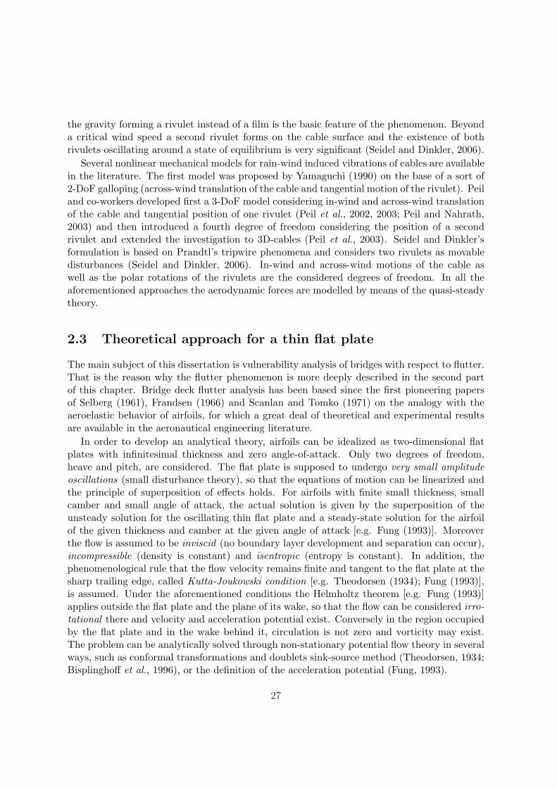
the gravity forming a rivulet instead of a film is the basic feature of the phenomenon. Beyonda critical wind speed a second rivulet forms on the cable surface and the existence of bothrivulets oscillating around a state of equilibrium is very significant (Seidel and Dinkler, 2006).

Several nonlinear mechanical models for rain-wind induced vibrations of cables are availablein the literature. The first model was proposed by Yamaguchi (1990) on the base of a sort of2-DoF galloping (across-wind translation of the cable and tangential motion of the rivulet). Peiland co-workers developed first a 3-DoF model considering in-wind and across-wind translationof the cable and tangential position of one rivulet (Peil et al., 2002, 2003; Peil and Nahrath,2003) and then introduced a fourth degree of freedom considering the position of a secondrivulet and extended the investigation to 3D-cables (Peil et al., 2003). Seidel and Dinkler’sformulation is based on Prandtl’s tripwire phenomena and considers two rivulets as movabledisturbances (Seidel and Dinkler, 2006). In-wind and across-wind motions of the cable aswell as the polar rotations of the rivulets are the considered degrees of freedom. In all theaforementioned approaches the aerodynamic forces are modelled by means of the quasi-steadytheory.

2.3 Theoretical approach for a thin flat plate

The main subject of this dissertation is vulnerability analysis of bridges with respect to flutter.That is the reason why the flutter phenomenon is more deeply described in the second partof this chapter. Bridge deck flutter analysis has been based since the first pioneering papersof Selberg (1961), Frandsen (1966) and Scanlan and Tomko (1971) on the analogy with theaeroelastic behavior of airfoils, for which a great deal of theoretical and experimental resultsare available in the aeronautical engineering literature.

In order to develop an analytical theory, airfoils can be idealized as two-dimensional flatplates with infinitesimal thickness and zero angle-of-attack. Only two degrees of freedom,heave and pitch, are considered. The flat plate is supposed to undergo very small amplitudeoscillations (small disturbance theory), so that the equations of motion can be linearized andthe principle of superposition of effects holds. For airfoils with finite small thickness, smallcamber and small angle of attack, the actual solution is given by the superposition of theunsteady solution for the oscillating thin flat plate and a steady-state solution for the airfoilof the given thickness and camber at the given angle of attack [e.g. Fung (1993)]. Moreoverthe flow is assumed to be inviscid (no boundary layer development and separation can occur),incompressible (density is constant) and isentropic (entropy is constant). In addition, thephenomenological rule that the flow velocity remains finite and tangent to the flat plate at thesharp trailing edge, called Kutta-Joukowski condition [e.g. Theodorsen (1934); Fung (1993)],is assumed. Under the aforementioned conditions the Helmholtz theorem [e.g. Fung (1993)]applies outside the flat plate and the plane of its wake, so that the flow can be considered irro-tational there and velocity and acceleration potential exist. Conversely in the region occupiedby the flat plate and in the wake behind it, circulation is not zero and vorticity may exist.The problem can be analytically solved through non-stationary potential flow theory in severalways, such as conformal transformations and doublets sink-source method (Theodorsen, 1934;Bisplinghoff et al., 1996), or the definition of the acceleration potential (Fung, 1993).

27

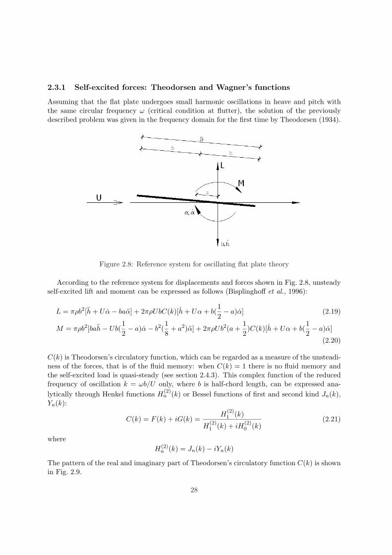
2.3.1 Self-excited forces: Theodorsen and Wagner’s functions

Assuming that the flat plate undergoes small harmonic oscillations in heave and pitch withthe same circular frequency ω (critical condition at flutter), the solution of the previouslydescribed problem was given in the frequency domain for the first time by Theodorsen (1934).

Figure 2.8: Reference system for oscillating flat plate theory

According to the reference system for displacements and forces shown in Fig. 2.8, unsteadyself-excited lift and moment can be expressed as follows (Bisplinghoff et al., 1996):

L = πρb2[h + Uα− baα] + 2πρUbC(k)[h + Uα + b(12− a)α] (2.19)

M = πρb2[bah− Ub(12− a)α− b2(

18

+ a2)α] + 2πρUb2(a +12)C(k)[h + Uα + b(

12− a)α]

(2.20)

C(k) is Theodorsen’s circulatory function, which can be regarded as a measure of the unsteadi-ness of the forces, that is of the fluid memory: when C(k) = 1 there is no fluid memory andthe self-excited load is quasi-steady (see section 2.4.3). This complex function of the reducedfrequency of oscillation k = ωb/U only, where b is half-chord length, can be expressed ana-lytically through Henkel functions H

(2)n (k) or Bessel functions of first and second kind Jn(k),

Yn(k):

C(k) = F (k) + iG(k) =H

(2)1 (k)

H(2)1 (k) + iH

(2)0 (k)

(2.21)

whereH(2)

n (k) = Jn(k)− iYn(k)

The pattern of the real and imaginary part of Theodorsen’s circulatory function C(k) is shownin Fig. 2.9.

28

0 2 4 6 8 10−0.4

−0.2

0

0.2

0.4

0.6

0.8

1

k

FG

(a)

0 20 40 60 80 100

−0.2

0

0.2

0.4

0.6

0.8

1

UR

F

G

(b)

Figure 2.9: Real and imaginary parts of Theodorsen’s circulatory function C(k) = F (k) +iG(k), plotted as a function of the reduced frequency of oscillation k (a) and ofthe reduced wind speed UR = U

Bf = πk , being ω = 2πf (b)

Unsteady lift and moment in that form are considered as applied to the flat plate elasticaxis, whose horizontal distance from mid-chord is indicated with a [for a discussion about therigorous definition of elastic axis and shear center see for instance Fung (1993)]. Obviously nounsteady drag is expected. The terms in h and α in Eqs. (2.19)-(2.20) have noncirculatoryorigin, that means they are not due to the vortex sheets on the flat plate and in the wake,but they are apparent mass forces. The lift term πρb2(h − baα) has its center of pressure atmid-chord and correspond to the apparent mass ρπb2 of an air cylinder with the diameterequal to the flat plate chord. Conversely the pure nose-down couple −1

8ρπb4α corresponds toone fourth of the mass moment of inertia of the same air cylinder. If the relative density isvery large, as usually is, these aerodynamic inertial terms can be neglected without significanterrors (Bisplinghoff et al., 1996). The quasi-steady lift term ρπb2Uα has circulatory natureand corresponds to a centrifugal force with the same magnitude as the apparent mass ρπb2

times Uα, with center of pressure at 3/4-chord point. Neglecting this term may occasionallylead to a marked underestimation of stability (Bisplinghoff et al., 1996). All the other liftterms have circulatory origin and the forward quarter-chord point as center of pressure.

Bridge sections usually are symmetric with respect to the vertical plane so that a = 0 (theelastic axis intersects the cross section at mid-chord) and Eqs. (2.19)-(2.20) can be simplifiedas follows:

L = πρb2[h + Uα] + 2πρUbC(k)[h + Uα +b

2α] (2.22)

M = −12πρb3[Uα +

b

4α] + πρUb2C(k)[h + Uα +

b

2α] (2.23)

29

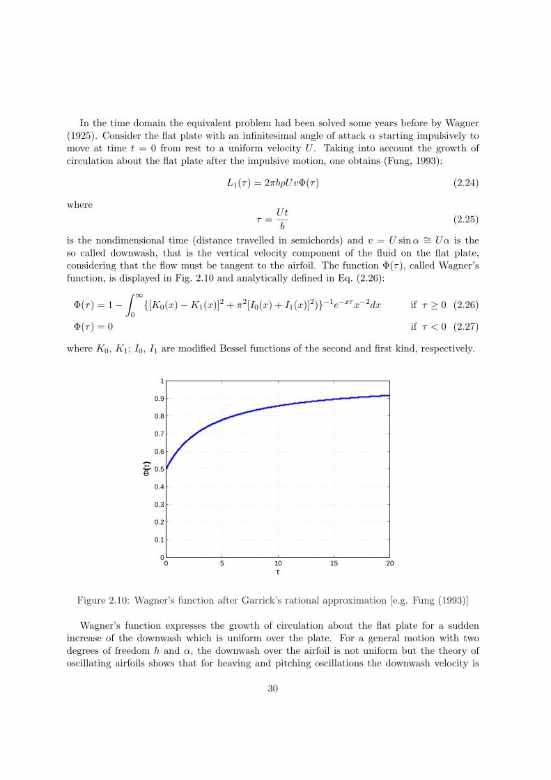
In the time domain the equivalent problem had been solved some years before by Wagner(1925). Consider the flat plate with an infinitesimal angle of attack α starting impulsively tomove at time t = 0 from rest to a uniform velocity U . Taking into account the growth ofcirculation about the flat plate after the impulsive motion, one obtains (Fung, 1993):

L1(τ) = 2πbρUvΦ(τ) (2.24)

whereτ =

Ut

b(2.25)

is the nondimensional time (distance travelled in semichords) and v = U sinα ∼= Uα is theso called downwash, that is the vertical velocity component of the fluid on the flat plate,considering that the flow must be tangent to the airfoil. The function Φ(τ), called Wagner’sfunction, is displayed in Fig. 2.10 and analytically defined in Eq. (2.26):

Φ(τ) = 1−∫ ∞

0{[K0(x)−K1(x)]2 + π2[I0(x) + I1(x)]2)}−1e−xτx−2dx if τ ≥ 0 (2.26)

Φ(τ) = 0 if τ < 0 (2.27)

where K0, K1; I0, I1 are modified Bessel functions of the second and first kind, respectively.

0 5 10 15 200

0.1

0.2

0.3

0.4

0.5

0.6

0.7

0.8

0.9

1

τ

Φ(τ

)

Figure 2.10: Wagner’s function after Garrick’s rational approximation [e.g. Fung (1993)]

Wagner’s function expresses the growth of circulation about the flat plate for a suddenincrease of the downwash which is uniform over the plate. For a general motion with twodegrees of freedom h and α, the downwash over the airfoil is not uniform but the theory ofoscillating airfoils shows that for heaving and pitching oscillations the downwash velocity is

30

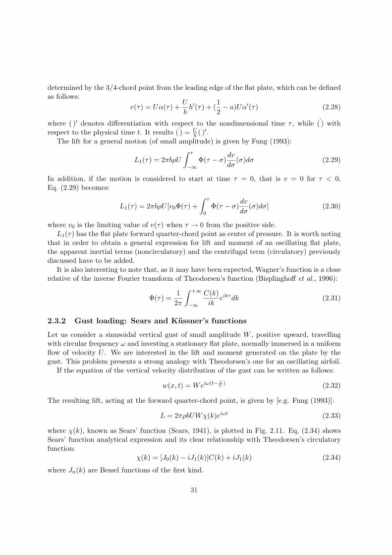
determined by the 3/4-chord point from the leading edge of the flat plate, which can be definedas follows:

v(τ) = Uα(τ) +U

bh′(τ) + (

12− a)Uα′(τ) (2.28)

where ( )′ denotes differentiation with respect to the nondimensional time τ , while ˙( ) withrespect to the physical time t. It results ˙( ) = U

b ( )′.The lift for a general motion (of small amplitude) is given by Fung (1993):

L1(τ) = 2πbρU

∫ τ

−∞Φ(τ − σ)

dv

dσ(σ)dσ (2.29)

In addition, if the motion is considered to start at time τ = 0, that is v = 0 for τ < 0,Eq. (2.29) becomes:

L1(τ) = 2πbρU [v0Φ(τ) +∫ τ

0Φ(τ − σ)

dv

dσ(σ)dσ] (2.30)

where v0 is the limiting value of v(τ) when τ → 0 from the positive side.L1(τ) has the flat plate forward quarter-chord point as center of pressure. It is worth noting

that in order to obtain a general expression for lift and moment of an oscillating flat plate,the apparent inertial terms (noncirculatory) and the centrifugal term (circulatory) previouslydiscussed have to be added.

It is also interesting to note that, as it may have been expected, Wagner’s function is a closerelative of the inverse Fourier transform of Theodorsen’s function (Bisplinghoff et al., 1996):

Φ(τ) =12π

∫ +∞

−∞

C(k)ik

eikτdk (2.31)

2.3.2 Gust loading: Sears and Kussner’s functions

Let us consider a sinusoidal vertical gust of small amplitude W , positive upward, travellingwith circular frequency ω and investing a stationary flat plate, normally immersed in a uniformflow of velocity U . We are interested in the lift and moment generated on the plate by thegust. This problem presents a strong analogy with Theodorsen’s one for an oscillating airfoil.

If the equation of the vertical velocity distribution of the gust can be written as follows:

w(x, t) = Weiω(t− xU

) (2.32)

The resulting lift, acting at the forward quarter-chord point, is given by [e.g. Fung (1993)]:

L = 2πρbUWχ(k)eiωt (2.33)

where χ(k), known as Sears’ function (Sears, 1941), is plotted in Fig. 2.11. Eq. (2.34) showsSears’ function analytical expression and its clear relationship with Theodorsen’s circulatoryfunction:

χ(k) = [J0(k)− iJ1(k)]C(k) + iJ1(k) (2.34)

where Jn(k) are Bessel functions of the first kind.

31

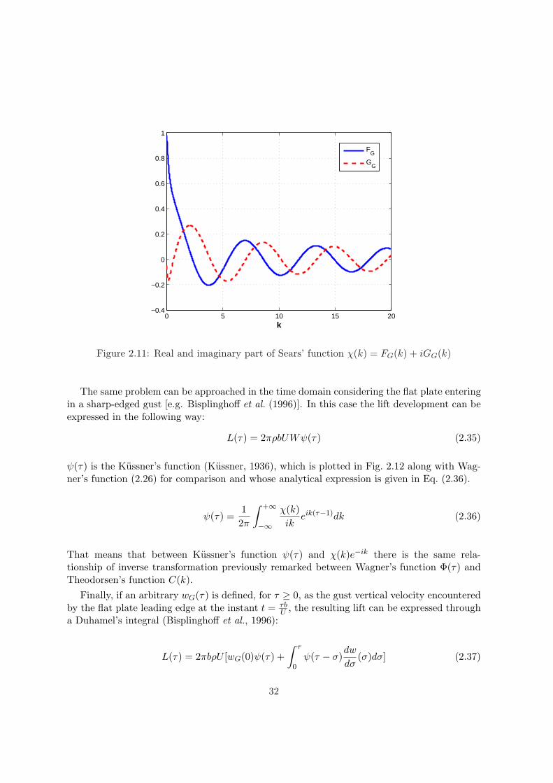
0 5 10 15 20−0.4

−0.2

0

0.2

0.4

0.6

0.8

1

k

FG

GG

Figure 2.11: Real and imaginary part of Sears’ function χ(k) = FG(k) + iGG(k)

The same problem can be approached in the time domain considering the flat plate enteringin a sharp-edged gust [e.g. Bisplinghoff et al. (1996)]. In this case the lift development can beexpressed in the following way:

L(τ) = 2πρbUWψ(τ) (2.35)

ψ(τ) is the Kussner’s function (Kussner, 1936), which is plotted in Fig. 2.12 along with Wag-ner’s function (2.26) for comparison and whose analytical expression is given in Eq. (2.36).

ψ(τ) =12π

∫ +∞

−∞

χ(k)ik

eik(τ−1)dk (2.36)

That means that between Kussner’s function ψ(τ) and χ(k)e−ik there is the same rela-tionship of inverse transformation previously remarked between Wagner’s function Φ(τ) andTheodorsen’s function C(k).

Finally, if an arbitrary wG(τ) is defined, for τ ≥ 0, as the gust vertical velocity encounteredby the flat plate leading edge at the instant t = τb

U , the resulting lift can be expressed througha Duhamel’s integral (Bisplinghoff et al., 1996):

L(τ) = 2πbρU [wG(0)ψ(τ) +∫ τ

0ψ(τ − σ)

dw

dσ(σ)dσ] (2.37)

32

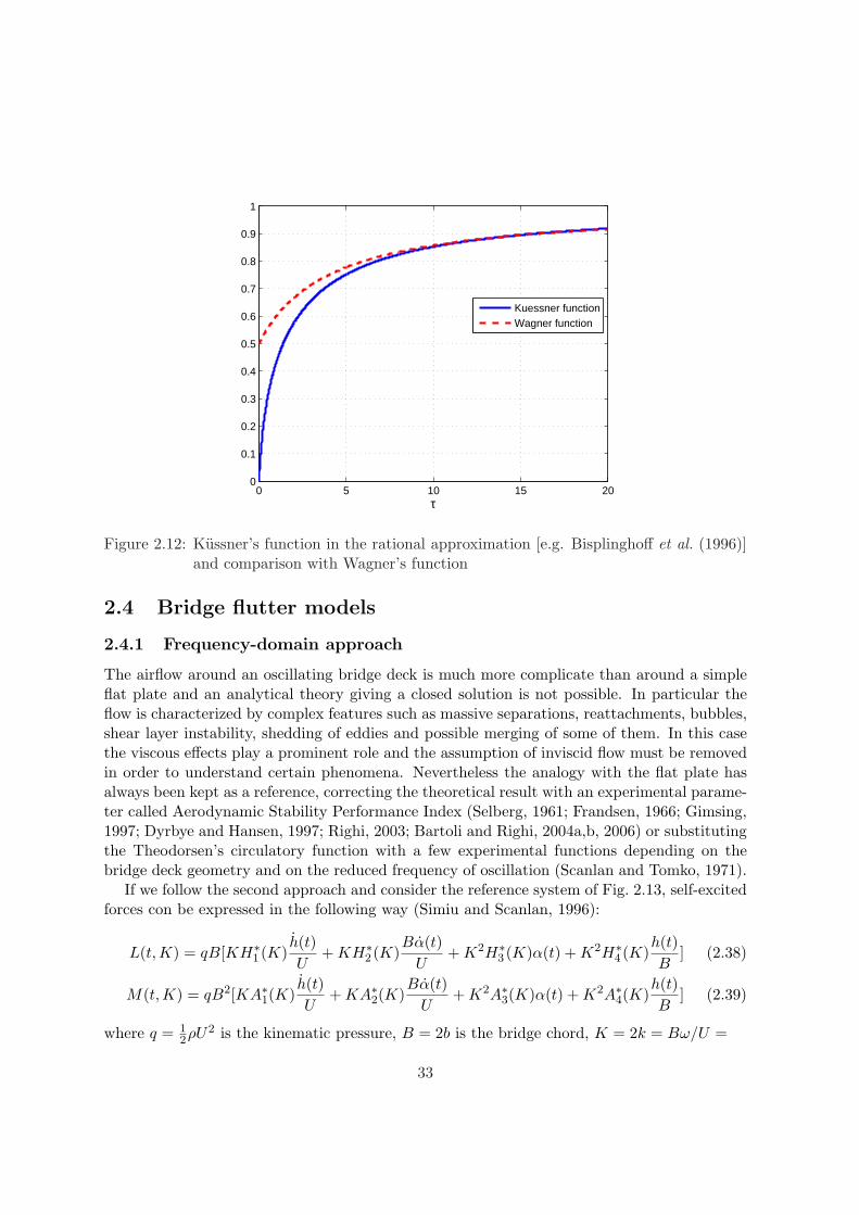
0 5 10 15 200

0.1

0.2

0.3

0.4

0.5

0.6

0.7

0.8

0.9

1

τ

Kuessner functionWagner function

Figure 2.12: Kussner’s function in the rational approximation [e.g. Bisplinghoff et al. (1996)]and comparison with Wagner’s function

2.4 Bridge flutter models

2.4.1 Frequency-domain approach

The airflow around an oscillating bridge deck is much more complicate than around a simpleflat plate and an analytical theory giving a closed solution is not possible. In particular theflow is characterized by complex features such as massive separations, reattachments, bubbles,shear layer instability, shedding of eddies and possible merging of some of them. In this casethe viscous effects play a prominent role and the assumption of inviscid flow must be removedin order to understand certain phenomena. Nevertheless the analogy with the flat plate hasalways been kept as a reference, correcting the theoretical result with an experimental parame-ter called Aerodynamic Stability Performance Index (Selberg, 1961; Frandsen, 1966; Gimsing,1997; Dyrbye and Hansen, 1997; Righi, 2003; Bartoli and Righi, 2004a,b, 2006) or substitutingthe Theodorsen’s circulatory function with a few experimental functions depending on thebridge deck geometry and on the reduced frequency of oscillation (Scanlan and Tomko, 1971).

If we follow the second approach and consider the reference system of Fig. 2.13, self-excitedforces con be expressed in the following way (Simiu and Scanlan, 1996):

L(t,K) = qB[KH∗1 (K)

h(t)U

+ KH∗2 (K)

Bα(t)U

+ K2H∗3 (K)α(t) + K2H∗

4 (K)h(t)B

] (2.38)

M(t,K) = qB2[KA∗1(K)h(t)U

+ KA∗2(K)Bα(t)

U+ K2A∗3(K)α(t) + K2A∗4(K)

h(t)B

] (2.39)

where q = 12ρU2 is the kinematic pressure, B = 2b is the bridge chord, K = 2k = Bω/U =

33

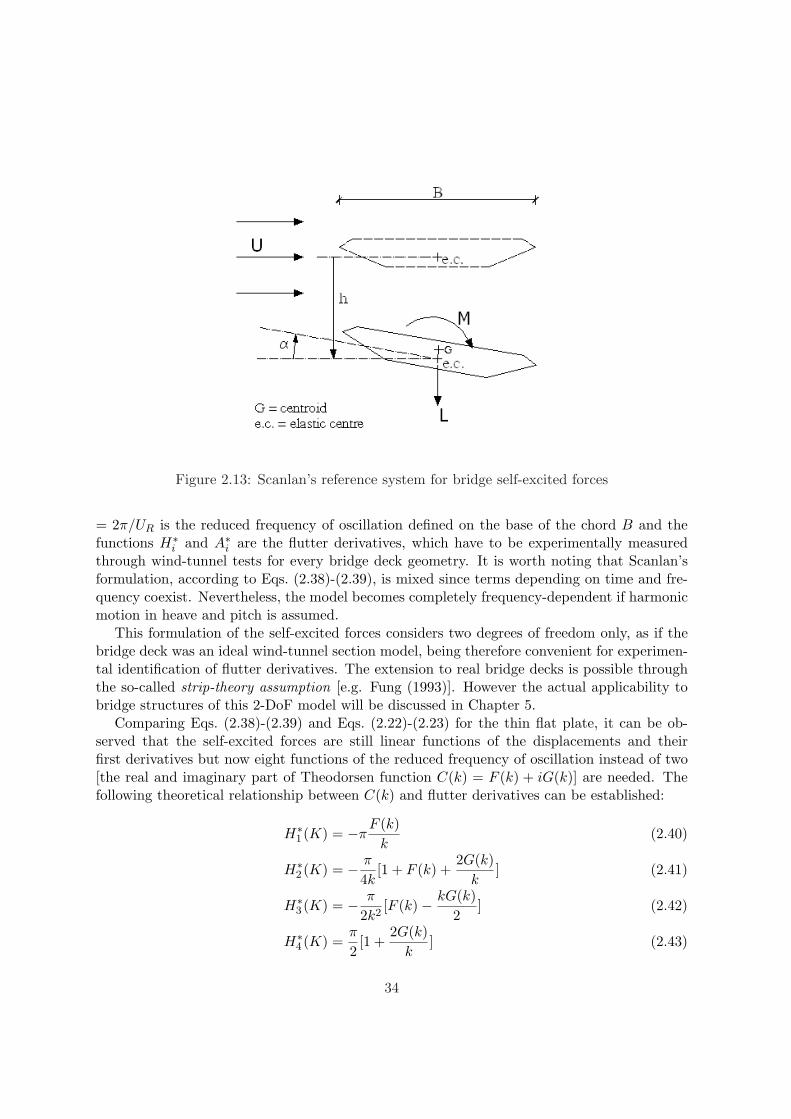
Figure 2.13: Scanlan’s reference system for bridge self-excited forces

= 2π/UR is the reduced frequency of oscillation defined on the base of the chord B and thefunctions H∗

i and A∗i are the flutter derivatives, which have to be experimentally measuredthrough wind-tunnel tests for every bridge deck geometry. It is worth noting that Scanlan’sformulation, according to Eqs. (2.38)-(2.39), is mixed since terms depending on time and fre-quency coexist. Nevertheless, the model becomes completely frequency-dependent if harmonicmotion in heave and pitch is assumed.

This formulation of the self-excited forces considers two degrees of freedom only, as if thebridge deck was an ideal wind-tunnel section model, being therefore convenient for experimen-tal identification of flutter derivatives. The extension to real bridge decks is possible throughthe so-called strip-theory assumption [e.g. Fung (1993)]. However the actual applicability tobridge structures of this 2-DoF model will be discussed in Chapter 5.

Comparing Eqs. (2.38)-(2.39) and Eqs. (2.22)-(2.23) for the thin flat plate, it can be ob-served that the self-excited forces are still linear functions of the displacements and theirfirst derivatives but now eight functions of the reduced frequency of oscillation instead of two[the real and imaginary part of Theodorsen function C(k) = F (k) + iG(k)] are needed. Thefollowing theoretical relationship between C(k) and flutter derivatives can be established:

H∗1 (K) = −π

F (k)k

(2.40)

H∗2 (K) = − π

4k[1 + F (k) +

2G(k)k

] (2.41)

H∗3 (K) = − π

2k2[F (k)− kG(k)

2] (2.42)

H∗4 (K) =

π

2[1 +

2G(k)k

] (2.43)

34

(2.44)

A∗1(K) = πF (k)4k

(2.45)

A∗2(K) = − π

16k[1− F (k)− 2G(k)

k] (2.46)

A∗3(K) =π

8k2[k2

8+ F (k)− kG(k)

2] (2.47)

A∗4(K) = −πG(k)4k

(2.48)

The terms not containing F (k) and G(k) in the previous equations are those with noncircula-tory origin (apparent inertial forces) or with circulatory centrifugal nature (see section 2.3.1).The pattern of the flutter derivatives for the theoretical flat plate are shown in Fig. 2.14.

The terms H∗4 and A∗4 are usually considered as negligible for bridges and as a matter of

fact Scanlan had not introduced them in its first formulation of self-excited forces (Scanlanand Tomko, 1971). A∗2 conversely has the physical meaning of aerodynamic damping in torsionand it is known to play a key role in flutter instability. In particular when it quickly reversesits sign and become positive (that is the aerodynamic damping becomes negative), it meansthat the cross section is prone to single-degree-of-freedom torsional flutter.

As we have already said, flutter derivatives are not universal functions but they stronglydepend on the cross-sectional geometry. They can be identified in wind tunnel on sectionmodels via free-vibration tests [e.g. Scanlan and Tomko (1971); Ibrahim and Mikulcik (1977);Sarkar (1992); Sarkar et al. (1994); Gu et al. (2000); Chowdhury and Sarkar (2003); Contri(2003); Righi (2003)] and forced-vibration tests [e.g. Li (1995); Matsumoto (1996); Dianaet al. (2004)] but some attempts have also been done adopting ambient vibration tests [e.g.Jakobsen (1995); Brownjohn and Jakobsen (2001); Jakobsen et al. (2003); Ricciardelli andde Grenet (2002); Zhang et al. (2003); Zhang and Brownjohn (2004); Fathi (2003)]. In somecases these functions have been tentatively identified on taut-strip models and full aeroelasticmodels as well (Zasso et al., 1996).

Concerning the possible conventions for the flutter derivatives, that proposed in Eqs. (2.38)-(2.39) is for sure the most used but many others can be found in the literature [e.g. Zasso(1996); Jensen and Hoffer (1998); Caracoglia (2000)].

The validity of a linear model for bridge deck self-excited forces is one of the most discussedproblems in bridge aeroelasticity, especially concerning the dependence of flutter derivativeson the amplitude of motion (see Chapter 3). Nevertheless a sure source of nonlinearity is thestrong dependence of these functions on the mean angle of attack [e.g. Flamand (2001); Dianaet al. (2005a,b) and section 3.5.2 in the present dissertation]. The mean angle of attack canbe due to a possible inclination of the flow, to the static deck torsional deformation and tolarge scale turbulence (Diana et al., 2005a,b; Chen and Kareem, 2000). Conversely, small scaleturbulence can influence directly the pattern of flutter derivatives increasing the mixing in theseparated shear layers and therefore changing the flow field around the body (Scanlan andLin, 1978; Nakamura and Ohya, 1984; Lin, 1996; Righi, 2003; Bartoli and Mannini, 2005).

The 2-DoF equations of motion for the flutter problem in the case of a linear structure can

35

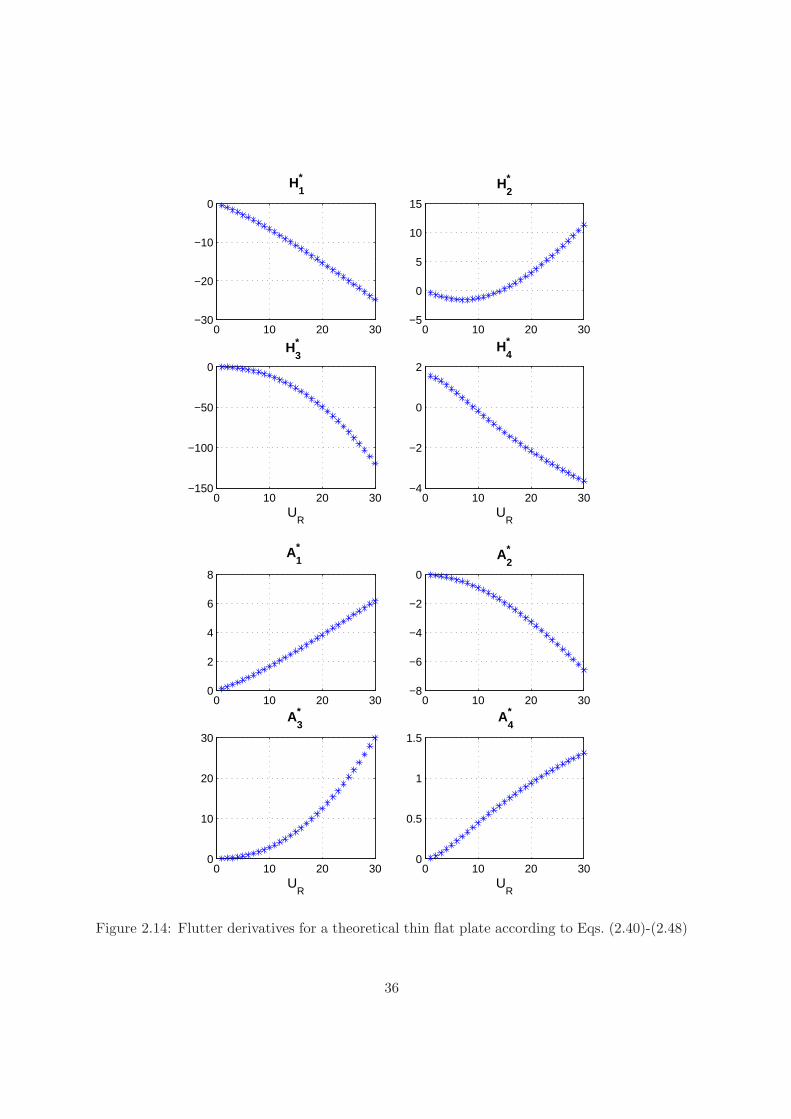
0 10 20 30−30

−20

−10

0

H1*

0 10 20 30−5

0

5

10

15

H2*

0 10 20 30−150

−100

−50

0

H3*

UR

0 10 20 30−4

−2

0

2

H4*

UR

0 10 20 300

2

4

6

8

A1*

0 10 20 30−8

−6

−4

−2

0

A2*

0 10 20 300

10

20

30

A3*

UR

0 10 20 300

0.5

1

1.5

A4*

UR

Figure 2.14: Flutter derivatives for a theoretical thin flat plate according to Eqs. (2.40)-(2.48)

36

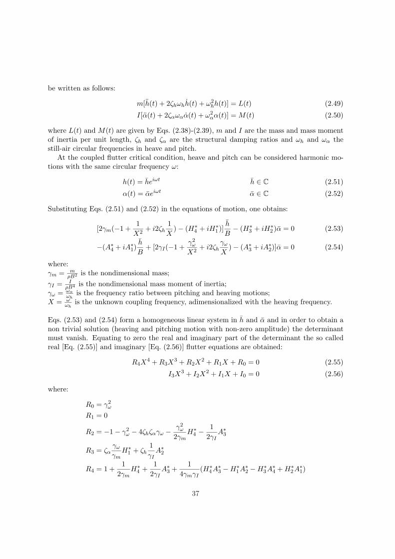
be written as follows:

m[h(t) + 2ζhωhh(t) + ω2hh(t)] = L(t) (2.49)

I[α(t) + 2ζαωαα(t) + ω2αα(t)] = M(t) (2.50)

where L(t) and M(t) are given by Eqs. (2.38)-(2.39), m and I are the mass and mass momentof inertia per unit length, ζh and ζα are the structural damping ratios and ωh and ωα thestill-air circular frequencies in heave and pitch.

At the coupled flutter critical condition, heave and pitch can be considered harmonic mo-tions with the same circular frequency ω:

h(t) = heiωt h ∈ C (2.51)

α(t) = αeiωt α ∈ C (2.52)

Substituting Eqs. (2.51) and (2.52) in the equations of motion, one obtains:

[2γm(−1 +1

X2+ i2ζh

1X

)− (H∗4 + iH∗

1 )]h

B− (H∗

3 + iH∗2 )α = 0 (2.53)

−(A∗4 + iA∗1)h

B+ [2γI(−1 +

γ2ω

X2+ i2ζh

γω

X)− (A∗3 + iA∗2)]α = 0 (2.54)

where:γm = m

ρB2 is the nondimensional mass;γI = I

ρB4 is the nondimensional mass moment of inertia;γω = ωα

ωhis the frequency ratio between pitching and heaving motions;

X = ωωh

is the unknown coupling frequency, adimensionalized with the heaving frequency.

Eqs. (2.53) and (2.54) form a homogeneous linear system in h and α and in order to obtain anon trivial solution (heaving and pitching motion with non-zero amplitude) the determinantmust vanish. Equating to zero the real and imaginary part of the determinant the so calledreal [Eq. (2.55)] and imaginary [Eq. (2.56)] flutter equations are obtained:

R4X4 + R3X

3 + R2X2 + R1X + R0 = 0 (2.55)

I3X3 + I2X

2 + I1X + I0 = 0 (2.56)

where:

R0 = γ2ω

R1 = 0

R2 = −1− γ2ω − 4ζhζαγω − γ2

ω

2γmH∗

4 −1

2γIA∗3

R3 = ζαγω

γmH∗

1 + ζh1γI

A∗2

R4 = 1 +1

2γmH∗

4 +1

2γIA∗3 +

14γmγI

(H∗4A∗3 −H∗

1A∗2 −H∗3A∗4 + H∗

2A∗1)

37

I0 = 2ζhγ2ω + 2ζαγω

I1 = − γ2ω

2γmH∗

1 −1

2γIA∗2

I2 = −2ζh − 2ζαγω − ζαγω

γmH∗

4 − ζh1γI

A∗3

I3 =1

2γmH∗

1 +1

2γIA∗2 +

14γmγI

(H∗4A∗2 + H∗

1A∗3 −H∗3A∗1 −H∗

2A∗4)

The unknowns in Eqs. (2.55)-(2.56) are the coupling flutter frequency, contained in X, and thecritical reduced wind speed UR which is the argument of the flutter derivatives. The two equa-tions can be solved numerically [e.g. Simiu and Scanlan (1996); Dyrbye and Hansen (1997)],plotting the real X solutions of both equations against UR: the actual flutter boundaries aregiven by the intersection of these two curves (or the intersection for the lowest physical windspeed, if it is not unique). The flutter coupling frequency has to be larger than the heavingfrequency and smaller than the pitching frequency. It is worth noting that the flutter equa-tions allow to calculate the flutter critical wind speed and the coupling frequency and then,introducing this solution in Eqs. (2.51) and (2.52), the ratio between the complex amplitudesof pitching and heaving motions α and h can be found as well. Nevertheless their actual valuesare undetermined given the linearity of the model.

2.4.2 Time-domain approach

Self-excited forces can also be expressed in the time domain, following the analogy with the liftformulation for the thin flat plate of Eq. (2.29) or Eq. (2.30). For bridge decks several indicialfunctions are employed instead of Wagner’s function. Again these functions are not universaland they are usually determined from the corresponding flutter derivatives [e.g. Borri andHoffer (2000); Caracoglia and Jones (2003b); Costa (2004); Costa and Borri (2006)], which areeasier to be measured through wind-tunnel tests. In few cases tentatively indicial functionshave been directly identified by experiments (Caracoglia, 2000; Caracoglia and Jones, 2003a).Several formulations, not very different one from the other, are available in the literature [e.g.Scanlan et al. (1974); Borri and Hoffer (2000); Caracoglia and Jones (2003b); Costa (2004);Costa and Borri (2006)]; in Eqs. (2.57)-(2.58) that after Costa (2004) is reported:

L(t) =− qBdCL

dα(0)[ΦLh(0)

h(t)U

+ ΦLα(0)α(t)+

+∫ t

0ΦLh(t− σ)

h(σ)U

dσ +∫ t

0ΦLα(t− σ)α(σ)dσ]

(2.57)

M(t) = qB2 dCM

dα(0)[ΦMh(0)

h(t)U

+ ΦMα(0)α(t)+

+∫ t

0ΦMh(t− σ)

h(σ)U

dσ +∫ t

0ΦMα(t− σ)α(σ)dσ]

(2.58)

38

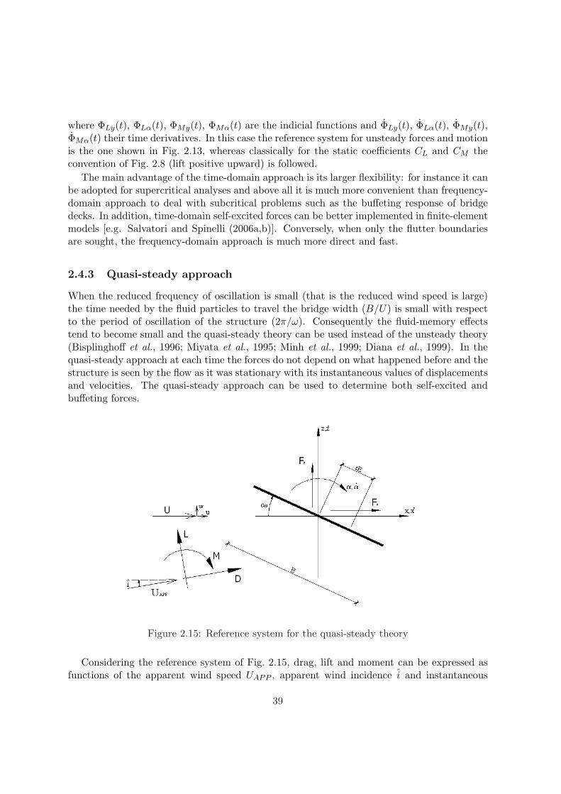
where ΦLy(t), ΦLα(t), ΦMy(t), ΦMα(t) are the indicial functions and ΦLy(t), ΦLα(t), ΦMy(t),ΦMα(t) their time derivatives. In this case the reference system for unsteady forces and motionis the one shown in Fig. 2.13, whereas classically for the static coefficients CL and CM theconvention of Fig. 2.8 (lift positive upward) is followed.

The main advantage of the time-domain approach is its larger flexibility: for instance it canbe adopted for supercritical analyses and above all it is much more convenient than frequency-domain approach to deal with subcritical problems such as the buffeting response of bridgedecks. In addition, time-domain self-excited forces can be better implemented in finite-elementmodels [e.g. Salvatori and Spinelli (2006a,b)]. Conversely, when only the flutter boundariesare sought, the frequency-domain approach is much more direct and fast.

2.4.3 Quasi-steady approach

When the reduced frequency of oscillation is small (that is the reduced wind speed is large)the time needed by the fluid particles to travel the bridge width (B/U) is small with respectto the period of oscillation of the structure (2π/ω). Consequently the fluid-memory effectstend to become small and the quasi-steady theory can be used instead of the unsteady theory(Bisplinghoff et al., 1996; Miyata et al., 1995; Minh et al., 1999; Diana et al., 1999). In thequasi-steady approach at each time the forces do not depend on what happened before and thestructure is seen by the flow as it was stationary with its instantaneous values of displacementsand velocities. The quasi-steady approach can be used to determine both self-excited andbuffeting forces.

Figure 2.15: Reference system for the quasi-steady theory

Considering the reference system of Fig. 2.15, drag, lift and moment can be expressed asfunctions of the apparent wind speed UAPP , apparent wind incidence i and instantaneous

39

pitching angle α with respect to the mean position α0:

D =12ρU2

APP BCD(α0 + i + α) (2.59)

L =12ρU2

APP BCL(α0 + i + α) (2.60)

M =12ρU2

APP B2CM (α0 + i + α) (2.61)

where

U2APP = (U + u− x)2 + (w − z + rBα)2 (2.62)

i = arctanw − z + rBα

U + u− x(2.63)

It is immediately worth noting that with respect to sections 2.3.1, 2.4.1 and 2.4.2, the meaningof L is slightly different here. This is the reason why the notation Fz is introduced to denotethe force in the direction of the vertical displacement. The angle of attack due to the angularmotion of the structure is not constant over the chord but, in analogy with the unsteadyairfoil theory, it is assumed here that there is a point at a distance rB from midchord, which isrepresentative for the whole section. Nevertheless, this point can be different for drag (r = rD),lift (r = rL) and moment (r = rM ). If the wind speed fluctuations are small with respect tothe mean wind speed and the structure undergoes small displacements, Eqs. (2.62)-(2.63) canbe linearized:

U2APP

∼= U2 + 2Uu− 2Ux = U2(1 +2u

U− 2x

U) (2.64)

i ∼= w

U− z

U+

rBα

U(2.65)

If the aerodynamic coefficients are developed in Taylor’s series around the mean angle ofattack α0, retaining the linear terms only and neglecting the products of small quantities ashigher-order infinitesimals, drag, lift and moment can be written as follows:

D ∼=qB(1 +2u

U− 2x

U)[CD(α0) +

dCD

dα(α0)(i + α)]

∼=qBCD(α0)(1 +2u

U− 2x

U) + qB

dCD

dα(α0)(i + α)

(2.66)

L ∼=qB(1 +2u

U− 2x

U)[CL(α0) +

dCL

dα(α0)(i + α)]

∼=qBCL(α0)(1 +2u

U− 2x

U) + qB

dCL

dα(α0)(i + α)

(2.67)

M ∼=qB2(1 +2u

U− 2x

U)[CM (α0) +

dCM

dα(α0)(i + α)]

∼=qB2CM (α0)(1 +2u

U− 2x

U) + qB2 dCM

dα(α0)(i + α)

(2.68)

40

where, as usual, q = 12ρU2 is the kinematic pressure. Drag and Lift can be composed in order

to obtain horizontal and vertical forces:

Fx = D cos i− L sin i ∼= D − Li (2.69)

Fz = D sin i + L cos i ∼= Di + L (2.70)

Discarding again the higher-order terms one obtains:

Fx∼= qBCD(α0)(1 +

2u

U− 2x

U) + qB[

dCD

dα(α0)− CL(α0)]i + qB

dCD

dα(α0)α (2.71)

Fz∼= qBCL(α0)(1 +

2u

U− 2x

U) + qB[

dCL

dα(α0) + CD(α0)]i + qB

dCL

dα(α0)α (2.72)

M ∼= qB2CM (α0)(1 +2u

U− 2x

U) + qB2 dCM

dα(α0)i + qB2 dCM

dα(α0)α (2.73)

It is now possible to split the aerodynamic forces we found in mean, buffeting and self-excitedcontributions:

Fx = Fx + F bx + F se

x (2.74)

Fz = Fz + F bz + F se

z (2.75)

M = M + M b + M se (2.76)

• Mean aerodynamic forces

Fx = qBCD(α0) (2.77)Fz = qBCL(α0) (2.78)

M = qB2CM (α0) (2.79)

• Buffeting forces

F bx = qB{2CD(α0)

u

U+ [

dCD

dα(α0)− CL(α0)]

w

U} (2.80)

F bz = qB{2CL(α0)

u

U+ [

dCL

dα(α0) + CD(α0)]

w

U} (2.81)

M b = qB2{2CM (α0)u

U+

dCM

dα(α0)

w

U} (2.82)

• Self-excited forces

F sex = qB{−2CD(α0)

x

U+ [

dCD

dα(α0)− CL(α0)](− z

U+

rxBα

U) +

dCD

dα(α0)α} (2.83)

F sez = qB{−2CL(α0)

x

U+ [

dCL

dα(α0) + CD(α0)](− z

U+

rzBα

U) +

dCL

dα(α0)α} (2.84)

M se = qB2{−2CM (α0)x

U+

dCM

dα(α0)(− z

U+

rMBα

U+ α)} (2.85)

41

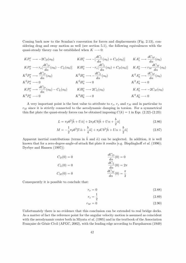
Coming back now to the Scanlan’s convention for forces and displacements (Fig. 2.13), con-sidering drag and sway motion as well (see section 5.1), the following equivalences with thequasi-steady theory can be established when K −→ 0:

KP ∗1 −→ −2CD(α0) KH∗

1 −→ −[dCL

dα(α0) + CD(α0)] KA∗1 −→

dCM

dα(α0)

KP ∗2 −→ rx[

dCD

dα(α0)− CL(α0)] KH∗

2 −→ −rz[dCL

dα(α0) + CD(α0)] KA∗2 −→ rM

dCM

dα(α0)

K2P ∗3 −→

dCD

dα(α0) K2H∗

3 −→ −dCL

dα(α0) K2A∗3 −→

dCM

dα(α0)

K2P ∗4 −→ 0 K2H∗

4 −→ 0 K2A∗4 −→ 0

KP ∗5 −→

dCD

dα(α0)− CL(α0) KH∗

5 −→ 2CL(α0) KA∗5 −→ −2CM (α0)

K2P ∗6 −→ 0 K2H∗

6 −→ 0 K2A∗6 −→ 0

A very important point is the best value to attribute to rx, rz and rM and in particular torM since it is strictly connected to the aerodynamic damping in torsion. For a symmetricalthin flat plate the quasi-steady forces can be obtained imposing C(k) = 1 in Eqs. (2.22)-(2.23):

L = πρb2[h + Uα] + 2πρUb[h + Uα +b

2α] (2.86)

M = −12πρb3[Uα +

b

4α] + πρUb2[h + Uα +

b

2α] (2.87)

Apparent inertial contributions (terms in h and α) can be neglected. In addition, it is wellknown that for a zero-degree-angle-of-attack flat plate it results [e.g. Bisplinghoff et al. (1996);Dyrbye and Hansen (1997)]:

CD(0) = 0dCD

dα(0) = 0

CL(0) = 0dCL

dα(0) = 2π

CM (0) = 0dCM

dα(0) =

π

2

Consequently it is possible to conclude that:

rx = 0 (2.88)

rz =12

(2.89)

rM = 0 (2.90)

Unfortunately there is no evidence that this conclusion can be extended to real bridge decks.As a matter of fact the reference point for the angular velocity motion is assumed as coincidentwith the aerodynamic center both in Miyata et al. (1995) and in the textbook of the AssociationFrancaise de Genie Civil (AFGC, 2002), with the leading edge according to Farquharson (1949)

42

or with a point placed at a chord distance upstream with respect to the midchord in Dianaet al. (2004).

It is also important to understand when the quasi-steady theory can actually be usedinstead of the unsteady theory. To the writer’s knowledge no clear studies are available in theliterature for real bridge decks. Conversely for airfoils in Bisplinghoff et al. (1996) it is saidthat also for reduced frequency values k < 0.1 (that is UR > 30) the fluid-memory effects onthe flutter instability can be remarkable. As a matter of fact C(k) is responsible for a phase lagbetween forces and motions (along with a magnitude reduction of forces), which is extremelyimportant for the flutter mechanism. Fig. 2.16 shows a polar plot of Theodorsen’s functionand it can be easily noted that the maximum phase-shifting effect occurs around k = 0.2 andfor k = 0.1 this is definitely not negligible. A similar conclusion may be drawn observing inFig. 2.9(b) how the real and imaginary part of C(k) slowly approach their asymptotic values.

In order to quantify the actual effect of fluid memory, a particular study case is considered.The modal properties of the proposed design of Messina Strait Bridge (D’Asdia and Sepe,1998) and the flutter derivatives of the theoretical flat plate are combined, while the chordlength B is considered as a free parameter in order to increase as much as possible the flutterreduced critical wind speed. In Tab. 2.1 the comparison between unsteady and quasi-steadyresults [Eqs. (2.86)-(2.87)] is outlined. It is worth noting that also for large reduced wind speed(UR

∼= 100) the difference between the results given by the two theories is not negligible. Inaddition, it is confirmed that the contribution of apparent inertial forces is small.

43

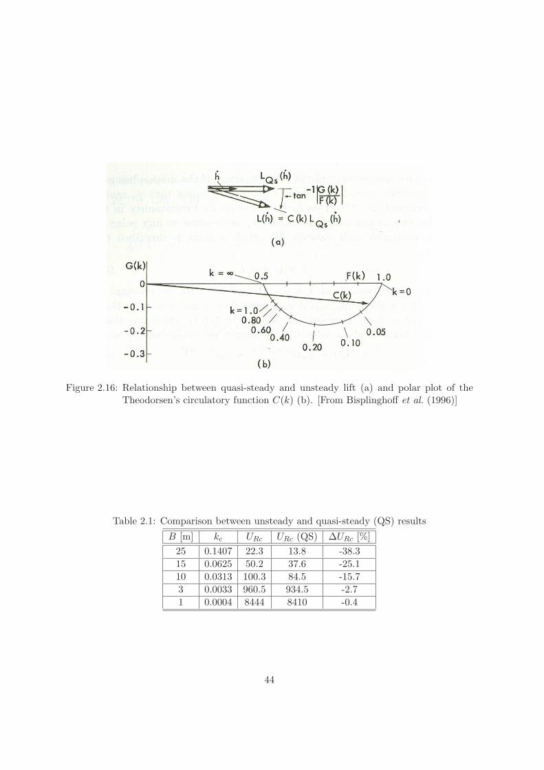
Figure 2.16: Relationship between quasi-steady and unsteady lift (a) and polar plot of theTheodorsen’s circulatory function C(k) (b). [From Bisplinghoff et al. (1996)]

Table 2.1: Comparison between unsteady and quasi-steady (QS) results

B [m] kc URc URc (QS) ∆URc [%]25 0.1407 22.3 13.8 -38.315 0.0625 50.2 37.6 -25.110 0.0313 100.3 84.5 -15.73 0.0033 960.5 934.5 -2.71 0.0004 8444 8410 -0.4

44

Chapter 3

Wind-tunnel tests

3.1 Motivations for these tests

The main purpose of this experimental campaign is to increase the number of available dataconcerning bridge deck flutter derivatives. The choice of the cross-sectional geometry, namelya trapezoidal single-box girder with lateral cantilevers [Fig. 3.5(b)], is due to the fact that itis common for medium-span cable-stayed bridges, for which the simplified method of flutterassessment outlined in this dissertation could be particularly appealing. In addition, for thisgeometry just few sets of data are available in the literature and in some cases only threefunctions are measured (Barre et al., 1996a,b).

Another important motivation for these tests is the need to give a probabilistic descriptionof flutter derivatives, in order to apply the method of probabilistic flutter assessment describedin Chapter 4.

The relevance of this experimental work also concerns several other issues, such as theidentification of flutter derivatives at different angles of attack via free-vibration tests. In factit is well known that the aeroelastic coefficients can be very sensitive to the mean angle offlow incidence [e.g. ONERA (1989); Flamand (2000, 2001); Diana et al. (2005a,b)] and howimportant this effect can be on flutter and buffeting calculations (Diana et al., 2005a,b; Chenand Kareem, 2000). Nevertheless, flutter derivatives are only rarely measured at differentangles of attack and usually via forced-vibration tests.

Another point discussed in the following is the supposed linearity of self-excited forces withrespect to the amplitude of the motion [Eqs. (2.38)-(2.39)], that being still an open issue inbridge aeroelasticity.

Besides aeroelastic tests, static tests are performed in order to measure the aerodynamicforce coefficients. In addition to their direct use (static load, buffeting analysis, quasi-steadyself-excited load), their knowledge is useful to determine indicial functions [Eqs. (2.57)-(2.58)]and their patterns can say much about the aerodynamic behavior of the cross section. More-over, with stationary configurations it is easier than with aeroelastic suspension systems toinvestigate Reynolds number effects.

The results of a few Computational Fluid Dynamics simulations, performed by the writerat the Institute of Aeroelasticity of the German Aerospace Center (DLR) of Gottingen are

45

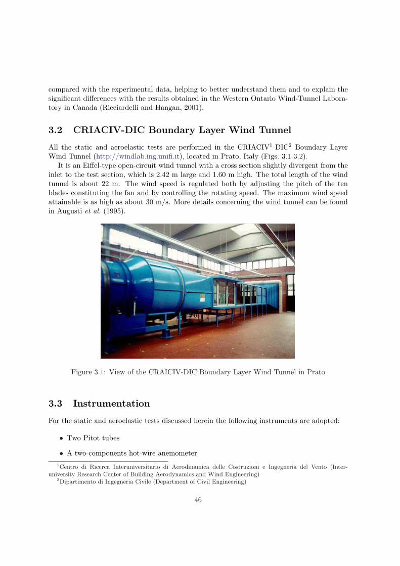
compared with the experimental data, helping to better understand them and to explain thesignificant differences with the results obtained in the Western Ontario Wind-Tunnel Labora-tory in Canada (Ricciardelli and Hangan, 2001).

3.2 CRIACIV-DIC Boundary Layer Wind Tunnel

All the static and aeroelastic tests are performed in the CRIACIV1-DIC2 Boundary LayerWind Tunnel (http://windlab.ing.unifi.it), located in Prato, Italy (Figs. 3.1-3.2).

It is an Eiffel-type open-circuit wind tunnel with a cross section slightly divergent from theinlet to the test section, which is 2.42 m large and 1.60 m high. The total length of the windtunnel is about 22 m. The wind speed is regulated both by adjusting the pitch of the tenblades constituting the fan and by controlling the rotating speed. The maximum wind speedattainable is as high as about 30 m/s. More details concerning the wind tunnel can be foundin Augusti et al. (1995).

Figure 3.1: View of the CRAICIV-DIC Boundary Layer Wind Tunnel in Prato

3.3 Instrumentation

For the static and aeroelastic tests discussed herein the following instruments are adopted:

• Two Pitot tubes

• A two-components hot-wire anemometer1Centro di Ricerca Interuniversitario di Aerodinamica delle Costruzioni e Ingegneria del Vento (Inter-

university Research Center of Building Aerodynamics and Wind Engineering)2Dipartimento di Ingegneria Civile (Department of Civil Engineering)

46

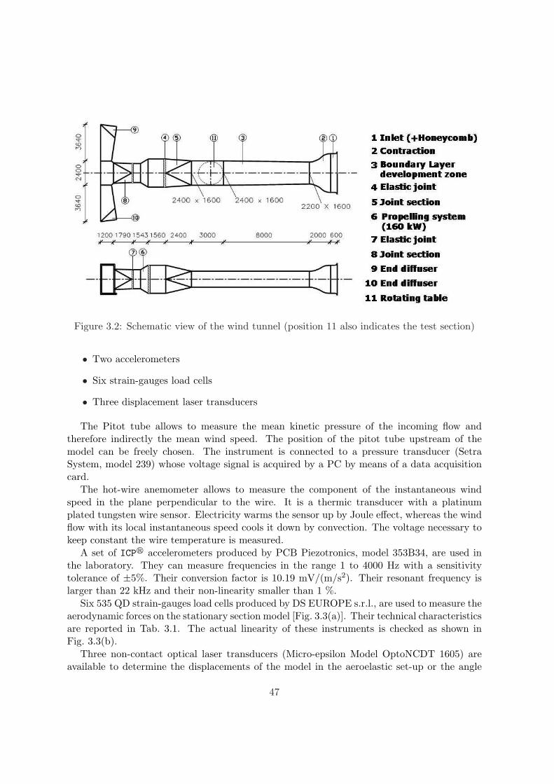
Figure 3.2: Schematic view of the wind tunnel (position 11 also indicates the test section)

• Two accelerometers

• Six strain-gauges load cells

• Three displacement laser transducers

The Pitot tube allows to measure the mean kinetic pressure of the incoming flow andtherefore indirectly the mean wind speed. The position of the pitot tube upstream of themodel can be freely chosen. The instrument is connected to a pressure transducer (SetraSystem, model 239) whose voltage signal is acquired by a PC by means of a data acquisitioncard.

The hot-wire anemometer allows to measure the component of the instantaneous windspeed in the plane perpendicular to the wire. It is a thermic transducer with a platinumplated tungsten wire sensor. Electricity warms the sensor up by Joule effect, whereas the windflow with its local instantaneous speed cools it down by convection. The voltage necessary tokeep constant the wire temperature is measured.

A set of ICPr accelerometers produced by PCB Piezotronics, model 353B34, are used inthe laboratory. They can measure frequencies in the range 1 to 4000 Hz with a sensitivitytolerance of ±5%. Their conversion factor is 10.19 mV/(m/s2). Their resonant frequency islarger than 22 kHz and their non-linearity smaller than 1 %.

Six 535 QD strain-gauges load cells produced by DS EUROPE s.r.l., are used to measure theaerodynamic forces on the stationary section model [Fig. 3.3(a)]. Their technical characteristicsare reported in Tab. 3.1. The actual linearity of these instruments is checked as shown inFig. 3.3(b).

Three non-contact optical laser transducers (Micro-epsilon Model OptoNCDT 1605) areavailable to determine the displacements of the model in the aeroelastic set-up or the angle

47

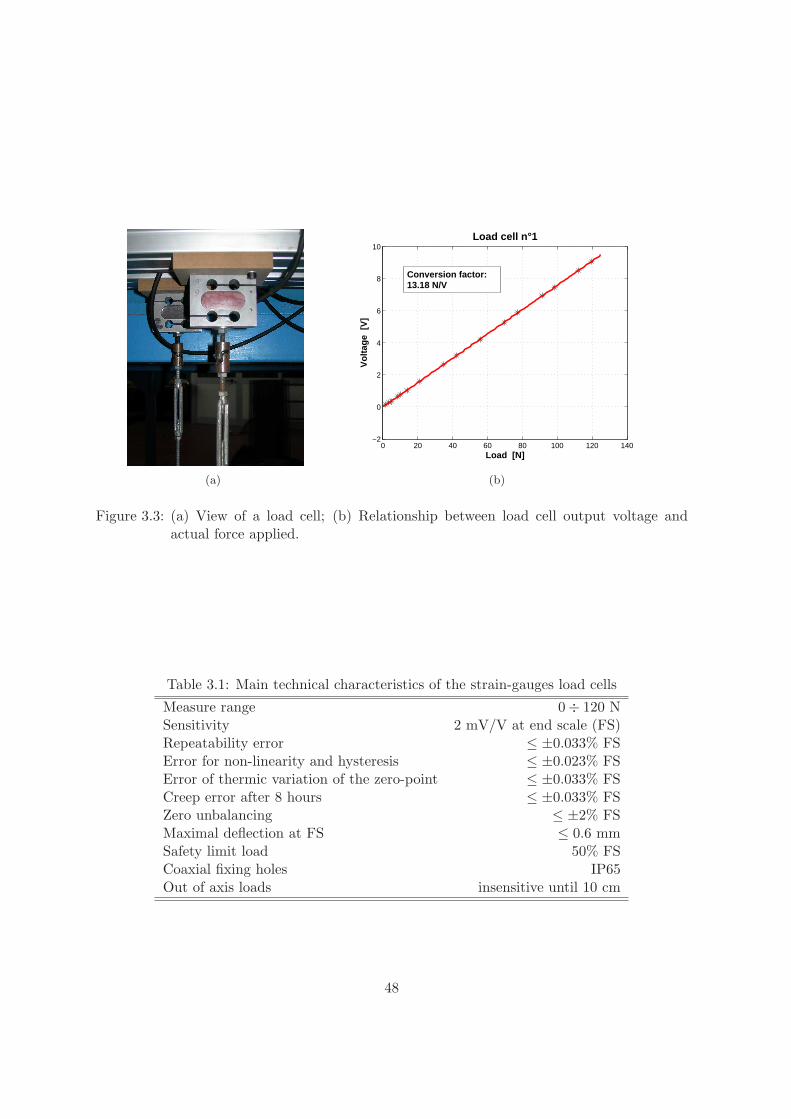
(a)

0 20 40 60 80 100 120 140−2

0

2

4

6

8

10

Load [N]

Vol

tage

[V

]

Load cell n°1

Conversion factor:13.18 N/V

(b)

Figure 3.3: (a) View of a load cell; (b) Relationship between load cell output voltage andactual force applied.

Table 3.1: Main technical characteristics of the strain-gauges load cells

Measure range 0÷ 120 NSensitivity 2 mV/V at end scale (FS)Repeatability error ≤ ±0.033% FSError for non-linearity and hysteresis ≤ ±0.023% FSError of thermic variation of the zero-point ≤ ±0.033% FSCreep error after 8 hours ≤ ±0.033% FSZero unbalancing ≤ ±2% FSMaximal deflection at FS ≤ 0.6 mmSafety limit load 50% FSCoaxial fixing holes IP65Out of axis loads insensitive until 10 cm

48

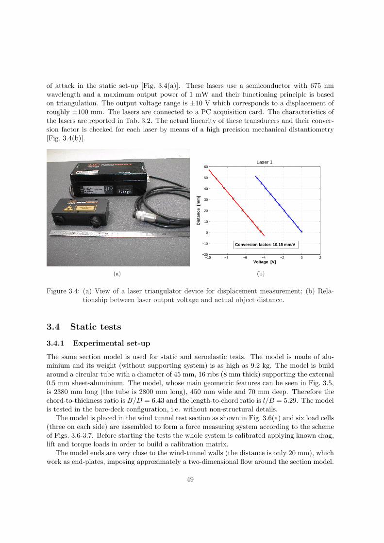
of attack in the static set-up [Fig. 3.4(a)]. These lasers use a semiconductor with 675 nmwavelength and a maximum output power of 1 mW and their functioning principle is basedon triangulation. The output voltage range is ±10 V which corresponds to a displacement ofroughly ±100 mm. The lasers are connected to a PC acquisition card. The characteristics ofthe lasers are reported in Tab. 3.2. The actual linearity of these transducers and their conver-sion factor is checked for each laser by means of a high precision mechanical distantiometry[Fig. 3.4(b)].

(a)

−10 −8 −6 −4 −2 0 2−20

−10

0

10

20

30

40

50

60Laser 1

Voltage [V]

Dis

tan

ce [

mm

]

Conversion factor: 10.15 mm/V

(b)

Figure 3.4: (a) View of a laser triangulator device for displacement measurement; (b) Rela-tionship between laser output voltage and actual object distance.

3.4 Static tests

3.4.1 Experimental set-up

The same section model is used for static and aeroelastic tests. The model is made of alu-minium and its weight (without supporting system) is as high as 9.2 kg. The model is buildaround a circular tube with a diameter of 45 mm, 16 ribs (8 mm thick) supporting the external0.5 mm sheet-aluminium. The model, whose main geometric features can be seen in Fig. 3.5,is 2380 mm long (the tube is 2800 mm long), 450 mm wide and 70 mm deep. Therefore thechord-to-thickness ratio is B/D = 6.43 and the length-to-chord ratio is l/B = 5.29. The modelis tested in the bare-deck configuration, i.e. without non-structural details.

The model is placed in the wind tunnel test section as shown in Fig. 3.6(a) and six load cells(three on each side) are assembled to form a force measuring system according to the schemeof Figs. 3.6-3.7. Before starting the tests the whole system is calibrated applying known drag,lift and torque loads in order to build a calibration matrix.

The model ends are very close to the wind-tunnel walls (the distance is only 20 mm), whichwork as end-plates, imposing approximately a two-dimensional flow around the section model.

49

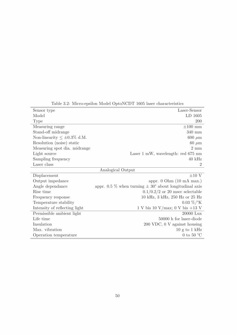
Table 3.2: Micro-epsilon Model OptoNCDT 1605 laser characteristics

Sensor type Laser-SensorModel LD 1605Type 200Measuring range ±100 mmStand-off midrange 340 mmNon-linearity ≤ ±0.3% d.M. 600 µmResolution (noise) static 60 µmMeasuring spot dia. midrange 2 mmLight source Laser 1 mW, wavelength: red 675 nmSampling frequency 40 kHzLaser class 2

Analogical OutputDisplacement ±10 VOutput impedance appr. 0 Ohm (10 mA max.)Angle dependance appr. 0.5 % when turning ± 30° about longitudinal axisRise time 0.1/0.2/2 or 20 msec selectableFrequency response 10 kHz, 3 kHz, 250 Hz or 25 HzTemperature stability 0.03 %/°KIntensity of reflecting light 1 V bis 10 V/max; 0 V bis +13 VPermissible ambient light 20000 LuxLife time 50000 h for laser-diodeInsulation 200 VDC, 0 V against housingMax. vibration 10 g to 1 kHzOperation temperature 0 to 50 °C

50

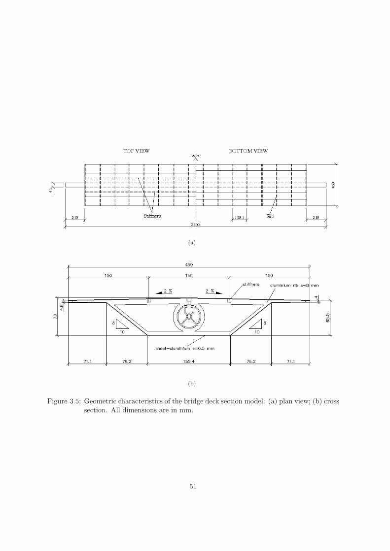
(a)

(b)

Figure 3.5: Geometric characteristics of the bridge deck section model: (a) plan view; (b) crosssection. All dimensions are in mm.

51

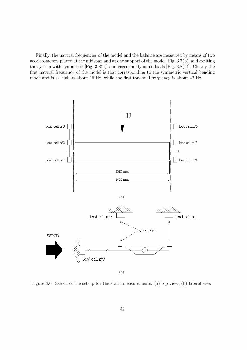
Finally, the natural frequencies of the model and the balance are measured by means of twoaccelerometers placed at the midspan and at one support of the model [Fig. 3.7(b)] and excitingthe system with symmetric [Fig. 3.8(a)] and eccentric dynamic loads [Fig. 3.8(b)]. Clearly thefirst natural frequency of the model is that corresponding to the symmetric vertical bendingmode and is as high as about 16 Hz, while the first torsional frequency is about 42 Hz.

(a)

(b)

Figure 3.6: Sketch of the set-up for the static measurements: (a) top view; (b) lateral view

52

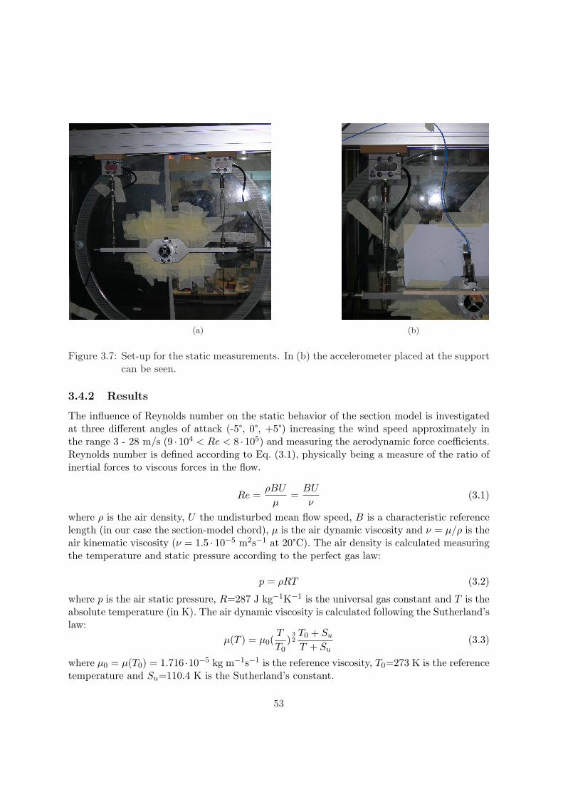
(a) (b)

Figure 3.7: Set-up for the static measurements. In (b) the accelerometer placed at the supportcan be seen.

3.4.2 Results

The influence of Reynolds number on the static behavior of the section model is investigatedat three different angles of attack (-5°, 0°, +5°) increasing the wind speed approximately inthe range 3 - 28 m/s (9 ·104 < Re < 8 ·105) and measuring the aerodynamic force coefficients.Reynolds number is defined according to Eq. (3.1), physically being a measure of the ratio ofinertial forces to viscous forces in the flow.

Re =ρBU

µ=

BU

ν(3.1)

where ρ is the air density, U the undisturbed mean flow speed, B is a characteristic referencelength (in our case the section-model chord), µ is the air dynamic viscosity and ν = µ/ρ is theair kinematic viscosity (ν = 1.5 · 10−5 m2s−1 at 20°C). The air density is calculated measuringthe temperature and static pressure according to the perfect gas law:

p = ρRT (3.2)

where p is the air static pressure, R=287 J kg−1K−1 is the universal gas constant and T is theabsolute temperature (in K). The air dynamic viscosity is calculated following the Sutherland’slaw:

µ(T ) = µ0(T

T0)

32T0 + Su

T + Su(3.3)

where µ0 = µ(T0) = 1.716 ·10−5 kg m−1s−1 is the reference viscosity, T0=273 K is the referencetemperature and Su=110.4 K is the Sutherland’s constant.

53

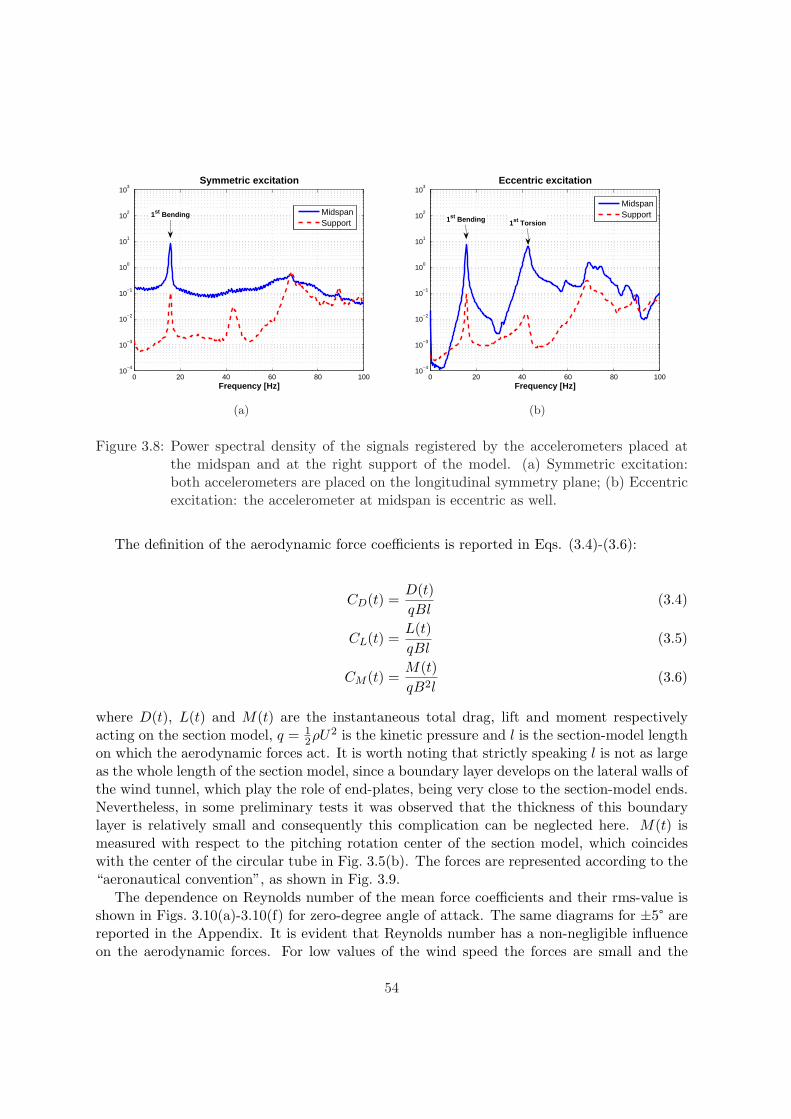
0 20 40 60 80 10010

−4

10−3

10−2

10−1

100

101

102

103

Frequency [Hz]

Symmetric excitation

MidspanSupport

1st Bending

(a)

0 20 40 60 80 10010

−4

10−3

10−2

10−1

100

101

102

103

Frequency [Hz]

Eccentric excitation

MidspanSupport

1st Bending 1st Torsion

(b)

Figure 3.8: Power spectral density of the signals registered by the accelerometers placed atthe midspan and at the right support of the model. (a) Symmetric excitation:both accelerometers are placed on the longitudinal symmetry plane; (b) Eccentricexcitation: the accelerometer at midspan is eccentric as well.

The definition of the aerodynamic force coefficients is reported in Eqs. (3.4)-(3.6):

CD(t) =D(t)qBl

(3.4)

CL(t) =L(t)qBl

(3.5)

CM (t) =M(t)qB2l

(3.6)

where D(t), L(t) and M(t) are the instantaneous total drag, lift and moment respectivelyacting on the section model, q = 1

2ρU2 is the kinetic pressure and l is the section-model lengthon which the aerodynamic forces act. It is worth noting that strictly speaking l is not as largeas the whole length of the section model, since a boundary layer develops on the lateral walls ofthe wind tunnel, which play the role of end-plates, being very close to the section-model ends.Nevertheless, in some preliminary tests it was observed that the thickness of this boundarylayer is relatively small and consequently this complication can be neglected here. M(t) ismeasured with respect to the pitching rotation center of the section model, which coincideswith the center of the circular tube in Fig. 3.5(b). The forces are represented according to the“aeronautical convention”, as shown in Fig. 3.9.

The dependence on Reynolds number of the mean force coefficients and their rms-value isshown in Figs. 3.10(a)-3.10(f) for zero-degree angle of attack. The same diagrams for ±5° arereported in the Appendix. It is evident that Reynolds number has a non-negligible influenceon the aerodynamic forces. For low values of the wind speed the forces are small and the

54

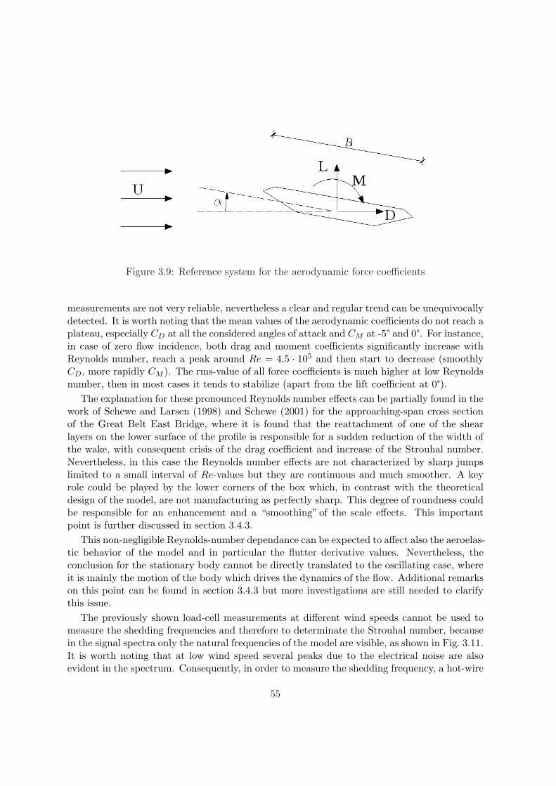
Figure 3.9: Reference system for the aerodynamic force coefficients

measurements are not very reliable, nevertheless a clear and regular trend can be unequivocallydetected. It is worth noting that the mean values of the aerodynamic coefficients do not reach aplateau, especially CD at all the considered angles of attack and CM at -5° and 0°. For instance,in case of zero flow incidence, both drag and moment coefficients significantly increase withReynolds number, reach a peak around Re = 4.5 · 105 and then start to decrease (smoothlyCD, more rapidly CM ). The rms-value of all force coefficients is much higher at low Reynoldsnumber, then in most cases it tends to stabilize (apart from the lift coefficient at 0°).

The explanation for these pronounced Reynolds number effects can be partially found in thework of Schewe and Larsen (1998) and Schewe (2001) for the approaching-span cross sectionof the Great Belt East Bridge, where it is found that the reattachment of one of the shearlayers on the lower surface of the profile is responsible for a sudden reduction of the width ofthe wake, with consequent crisis of the drag coefficient and increase of the Strouhal number.Nevertheless, in this case the Reynolds number effects are not characterized by sharp jumpslimited to a small interval of Re-values but they are continuous and much smoother. A keyrole could be played by the lower corners of the box which, in contrast with the theoreticaldesign of the model, are not manufacturing as perfectly sharp. This degree of roundness couldbe responsible for an enhancement and a “smoothing” of the scale effects. This importantpoint is further discussed in section 3.4.3.

This non-negligible Reynolds-number dependance can be expected to affect also the aeroelas-tic behavior of the model and in particular the flutter derivative values. Nevertheless, theconclusion for the stationary body cannot be directly translated to the oscillating case, whereit is mainly the motion of the body which drives the dynamics of the flow. Additional remarkson this point can be found in section 3.4.3 but more investigations are still needed to clarifythis issue.

The previously shown load-cell measurements at different wind speeds cannot be used tomeasure the shedding frequencies and therefore to determinate the Strouhal number, becausein the signal spectra only the natural frequencies of the model are visible, as shown in Fig. 3.11.It is worth noting that at low wind speed several peaks due to the electrical noise are alsoevident in the spectrum. Consequently, in order to measure the shedding frequency, a hot-wire

55

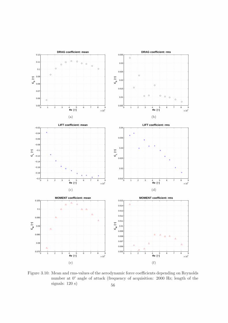
0 1 2 3 4 5 6 7 8 9

x 105

0.05

0.06

0.07

0.08

0.09

0.1

0.11

0.12DRAG coefficient: mean

Re [−]

CD [

−]

(a)

0 1 2 3 4 5 6 7 8 9

x 105

0.005

0.01

0.015

0.02

0.025

0.03

0.035DRAG coefficient: rms

Re [−]

CD [

−](b)

0 1 2 3 4 5 6 7 8 9

x 105

−0.2

−0.18

−0.16

−0.14

−0.12

−0.1

−0.08

−0.06

−0.04

−0.02LIFT coefficient: mean

Re [−]

CL [

−]

(c)

0 1 2 3 4 5 6 7 8 9

x 105

0.015

0.02

0.025

0.03

0.035

0.04LIFT coefficient: rms

Re [−]

CL [

−]

(d)

0 1 2 3 4 5 6 7 8 9

x 105

0.075

0.08

0.085

0.09

0.095

0.1

0.105MOMENT coefficient: mean

Re [−]

CM

[−]

(e)

0 1 2 3 4 5 6 7 8 9

x 105

0.005

0.006

0.007

0.008

0.009

0.01

0.011

0.012

0.013

0.014

0.015MOMENT coefficient: rms

Re [−]

CM

[−]

(f)

Figure 3.10: Mean and rms-values of the aerodynamic force coefficients depending on Reynoldsnumber at 0° angle of attack (frequency of acquisition: 2000 Hz; length of thesignals: 120 s) 56

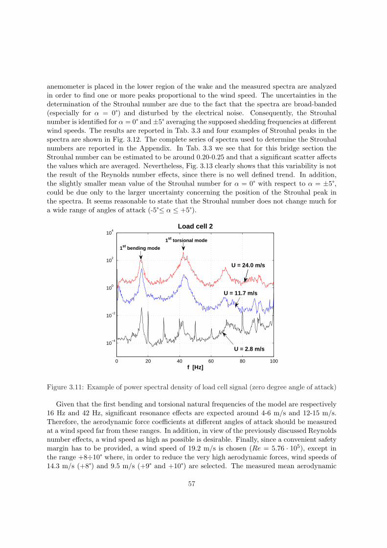
anemometer is placed in the lower region of the wake and the measured spectra are analyzedin order to find one or more peaks proportional to the wind speed. The uncertainties in thedetermination of the Strouhal number are due to the fact that the spectra are broad-banded(especially for α = 0°) and disturbed by the electrical noise. Consequently, the Strouhalnumber is identified for α = 0° and±5° averaging the supposed shedding frequencies at differentwind speeds. The results are reported in Tab. 3.3 and four examples of Strouhal peaks in thespectra are shown in Fig. 3.12. The complete series of spectra used to determine the Strouhalnumbers are reported in the Appendix. In Tab. 3.3 we see that for this bridge section theStrouhal number can be estimated to be around 0.20-0.25 and that a significant scatter affectsthe values which are averaged. Nevertheless, Fig. 3.13 clearly shows that this variability is notthe result of the Reynolds number effects, since there is no well defined trend. In addition,the slightly smaller mean value of the Strouhal number for α = 0° with respect to α = ±5°,could be due only to the larger uncertainty concerning the position of the Strouhal peak inthe spectra. It seems reasonable to state that the Strouhal number does not change much fora wide range of angles of attack (-5°≤ α ≤ +5°).

0 20 40 60 80 100

10−4

10−2

100

102

104

f [Hz]

Load cell 2

1st bending mode

1st torsional mode

U = 15.0 m/sU = 24.0 m/s

U = 11.7 m/s

U = 2.8 m/s

Figure 3.11: Example of power spectral density of load cell signal (zero degree angle of attack)

Given that the first bending and torsional natural frequencies of the model are respectively16 Hz and 42 Hz, significant resonance effects are expected around 4-6 m/s and 12-15 m/s.Therefore, the aerodynamic force coefficients at different angles of attack should be measuredat a wind speed far from these ranges. In addition, in view of the previously discussed Reynoldsnumber effects, a wind speed as high as possible is desirable. Finally, since a convenient safetymargin has to be provided, a wind speed of 19.2 m/s is chosen (Re = 5.76 · 105), except inthe range +8÷10° where, in order to reduce the very high aerodynamic forces, wind speeds of14.3 m/s (+8°) and 9.5 m/s (+9° and +10°) are selected. The measured mean aerodynamic

57

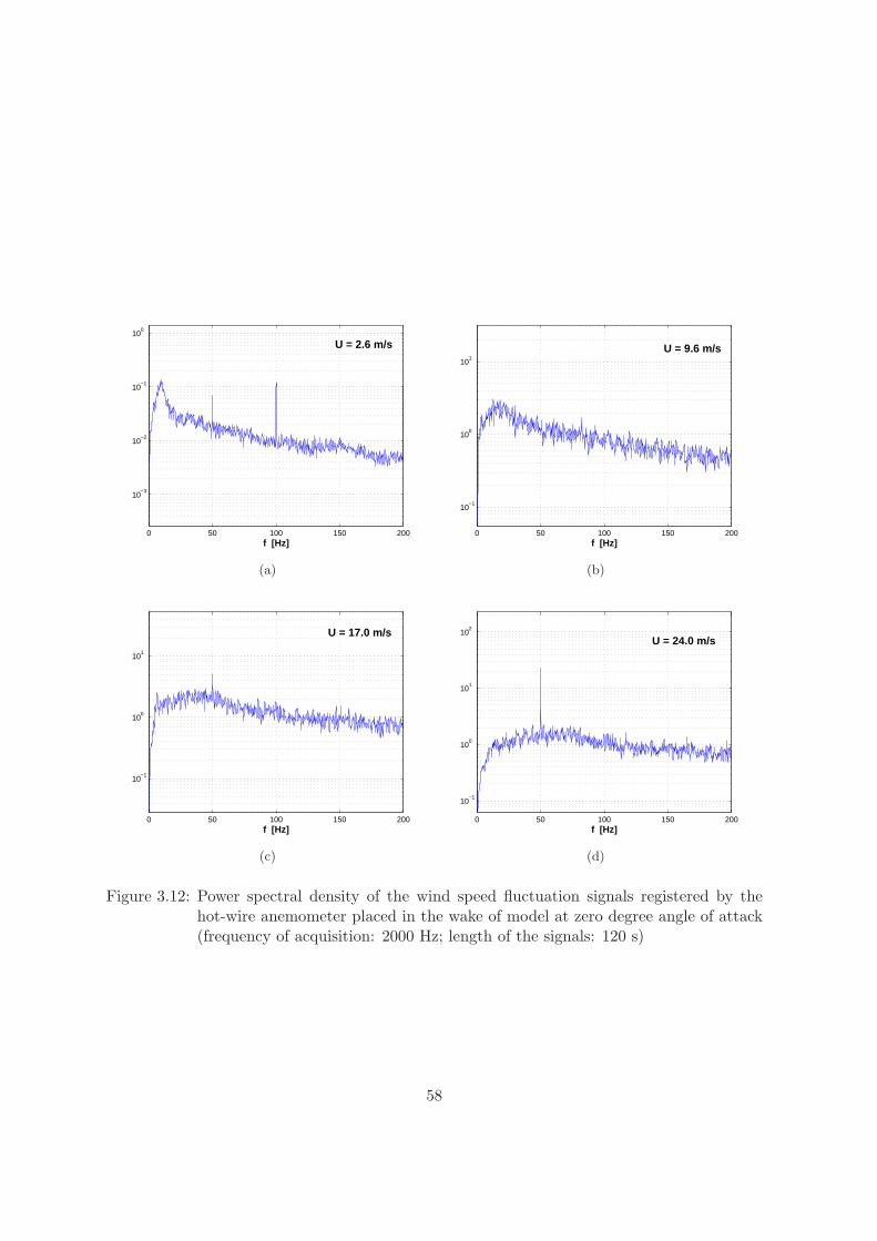
0 50 100 150 200

10−3

10−2

10−1

100

f [Hz]

U = 2.6 m/s

(a)

0 50 100 150 200

10−1

100

101

f [Hz]

U = 9.6 m/s

(b)

0 50 100 150 200

10−1

100

101

f [Hz]

U = 17.0 m/s

(c)

0 50 100 150 200

10−1

100

101

102

f [Hz]

U = 24.0 m/s

(d)

Figure 3.12: Power spectral density of the wind speed fluctuation signals registered by thehot-wire anemometer placed in the wake of model at zero degree angle of attack(frequency of acquisition: 2000 Hz; length of the signals: 120 s)

58

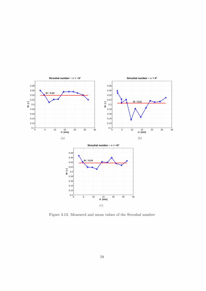
0 5 10 15 20 25 300.1

0.12

0.14

0.16

0.18

0.2

0.22

0.24

0.26

0.28

Strouhal number − α = −5°

U [m/s]

St

[−]

St ≅ 0.24

(a)

0 5 10 15 20 25 300.1

0.12

0.14

0.16

0.18

0.2

0.22

0.24

0.26

0.28

Strouhal number − α = 0°

U [m/s]

St

[−] St ≅ 0.21

(b)

0 5 10 15 20 25 300.1

0.12

0.14

0.16

0.18

0.2

0.22

0.24

0.26

0.28

Strouhal number − α = +5°

U [m/s]

St

[−]

St ≅ 0.24

(c)

Figure 3.13: Measured and mean values of the Strouhal number

59

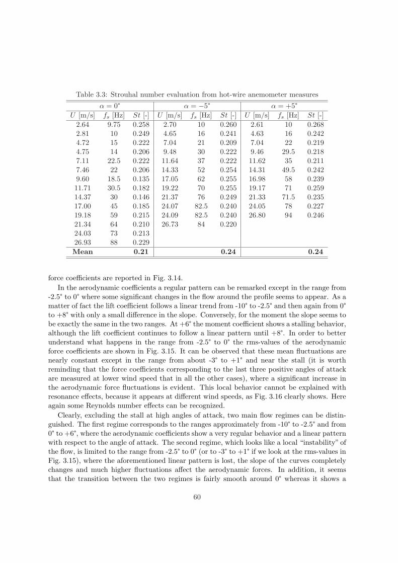
Table 3.3: Strouhal number evaluation from hot-wire anemometer measures

α = 0° α = −5° α = +5°U [m/s] fs [Hz] St [-] U [m/s] fs [Hz] St [-] U [m/s] fs [Hz] St [-]

2.64 9.75 0.258 2.70 10 0.260 2.61 10 0.2682.81 10 0.249 4.65 16 0.241 4.63 16 0.2424.72 15 0.222 7.04 21 0.209 7.04 22 0.2194.75 14 0.206 9.48 30 0.222 9.46 29.5 0.2187.11 22.5 0.222 11.64 37 0.222 11.62 35 0.2117.46 22 0.206 14.33 52 0.254 14.31 49.5 0.2429.60 18.5 0.135 17.05 62 0.255 16.98 58 0.23911.71 30.5 0.182 19.22 70 0.255 19.17 71 0.25914.37 30 0.146 21.37 76 0.249 21.33 71.5 0.23517.00 45 0.185 24.07 82.5 0.240 24.05 78 0.22719.18 59 0.215 24.09 82.5 0.240 26.80 94 0.24621.34 64 0.210 26.73 84 0.22024.03 73 0.21326.93 88 0.229Mean 0.21 0.24 0.24

force coefficients are reported in Fig. 3.14.In the aerodynamic coefficients a regular pattern can be remarked except in the range from

-2.5° to 0° where some significant changes in the flow around the profile seems to appear. As amatter of fact the lift coefficient follows a linear trend from -10° to -2.5° and then again from 0°to +8° with only a small difference in the slope. Conversely, for the moment the slope seems tobe exactly the same in the two ranges. At +6° the moment coefficient shows a stalling behavior,although the lift coefficient continues to follow a linear pattern until +8°. In order to betterunderstand what happens in the range from -2.5° to 0° the rms-values of the aerodynamicforce coefficients are shown in Fig. 3.15. It can be observed that these mean fluctuations arenearly constant except in the range from about -3° to +1° and near the stall (it is worthreminding that the force coefficients corresponding to the last three positive angles of attackare measured at lower wind speed that in all the other cases), where a significant increase inthe aerodynamic force fluctuations is evident. This local behavior cannot be explained withresonance effects, because it appears at different wind speeds, as Fig. 3.16 clearly shows. Hereagain some Reynolds number effects can be recognized.

Clearly, excluding the stall at high angles of attack, two main flow regimes can be distin-guished. The first regime corresponds to the ranges approximately from -10° to -2.5° and from0° to +6°, where the aerodynamic coefficients show a very regular behavior and a linear patternwith respect to the angle of attack. The second regime, which looks like a local “instability” ofthe flow, is limited to the range from -2.5° to 0° (or to -3° to +1° if we look at the rms-values inFig. 3.15), where the aforementioned linear pattern is lost, the slope of the curves completelychanges and much higher fluctuations affect the aerodynamic forces. In addition, it seemsthat the transition between the two regimes is fairly smooth around 0° whereas it shows a

60

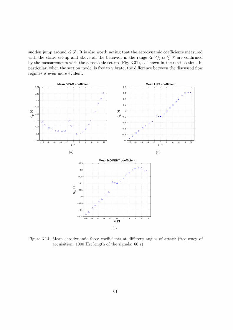
sudden jump around -2.5°. It is also worth noting that the aerodynamic coefficients measuredwith the static set-up and above all the behavior in the range -2.5°. α . 0° are confirmedby the measurements with the aeroelastic set-up (Fig. 3.31), as shown in the next section. Inparticular, when the section model is free to vibrate, the difference between the discussed flowregimes is even more evident.

−10 −8 −6 −4 −2 0 2 4 6 8 100.08

0.1

0.12

0.14

0.16

0.18

0.2

0.22

0.24Mean DRAG coefficient

α [°]

CD [

−]

(a)

−10 −8 −6 −4 −2 0 2 4 6 8 10−1

−0.8

−0.6

−0.4

−0.2

0

0.2

0.4

0.6

0.8Mean LIFT coefficient

α [°]

CL [

−]

(b)

−10 −8 −6 −4 −2 0 2 4 6 8 10−0.15

−0.1

−0.05

0

0.05

0.1

0.15

0.2

0.25Mean MOMENT coefficient

α [°]

CM

[−]

(c)

Figure 3.14: Mean aerodynamic force coefficients at different angles of attack (frequency ofacquisition: 1000 Hz; length of the signals: 60 s)

61

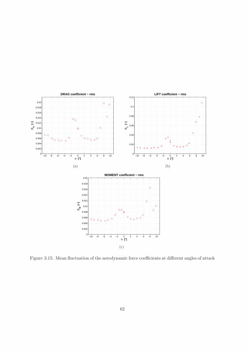
−10 −8 −6 −4 −2 0 2 4 6 8 100

0.002

0.004

0.006

0.008

0.01

0.012

0.014

0.016

0.018

0.02

DRAG coefficient − rms

α [°]

CD [

−]

(a)

−10 −8 −6 −4 −2 0 2 4 6 8 100

0.02

0.04

0.06

0.08

0.1

0.12LIFT coefficient − rms

α [°]

CL [

−]

(b)

−10 −8 −6 −4 −2 0 2 4 6 8 100

0.002

0.004

0.006

0.008

0.01

0.012

0.014

0.016

0.018

0.02MOMENT coefficient − rms

α [°]

CM

[−]

(c)

Figure 3.15: Mean fluctuation of the aerodynamic force coefficients at different angles of attack

62

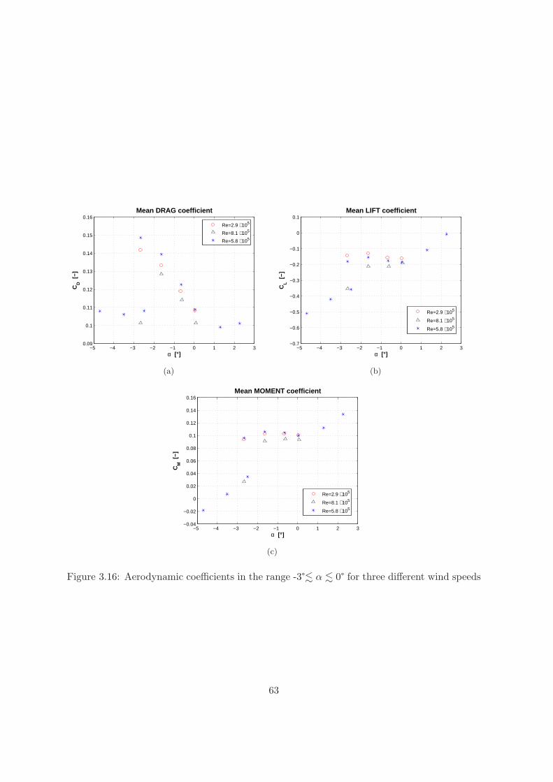
−5 −4 −3 −2 −1 0 1 2 30.09

0.1

0.11

0.12

0.13

0.14

0.15

0.16

α [°]

CD [

−]

Mean DRAG coefficient

Re=2.9 ⋅ 105

Re=8.1 ⋅ 105

Re=5.8 ⋅ 105

(a)

−5 −4 −3 −2 −1 0 1 2 3−0.7

−0.6

−0.5

−0.4

−0.3

−0.2

−0.1

0

0.1

α [°]

CL [

−]

Mean LIFT coefficient

Re=2.9 ⋅ 105

Re=8.1 ⋅ 105

Re=5.8 ⋅ 105

(b)

−5 −4 −3 −2 −1 0 1 2 3−0.04

−0.02

0

0.02

0.04

0.06

0.08

0.1

0.12

0.14

0.16

α [°]

CM

[−]

Mean MOMENT coefficient

Re=2.9 ⋅ 105

Re=8.1 ⋅ 105

Re=5.8 ⋅ 105

(c)

Figure 3.16: Aerodynamic coefficients in the range -3°. α . 0° for three different wind speeds

63

3.4.3 Comparison with CFD simulations

Very similar to the section model tested by the writer (from now on called “CRIACIV section”)is the one of the Sunshine Skyway Bridge (SSB) in Florida, in the bare-deck configuration,tested at Western Ontario Wind-Tunnel Laboratory in Canada (Davenport and King, 1982;Ricciardelli and Hangan, 2001). The two cross sections are compared in Figs. 3.17 and 3.18and at first glance they appear to be very similar, with only minor differences in the geometry(for instance B/D = 6.43 for the CRIACIV section and B/D = 6.80 for the SSB section).Nevertheless, the aerodynamic force coefficients and Strouhal numbers measured for the twoprofiles result to be very different (Fig. 3.19). For instance, the mean lift coefficient at 0°is definitely positive for the Sunshine Skyway Bridge (CL = +0.29), while it is negative forthe CRIACIV section (CL = −0.20), as confirmed by the measurements performed with theaeroelastic set-up (see Fig. 3.31 in the next section). Also in order to shed some light on thesediscrepancies, the CRIACIV section is investigated through Computational Fluid Dynamics(CFD) simulations (Mannini et al., 2006a,b). It is worth noting that in the following noattempt has been made to reproduce the exact geometry of the SSB section.

The flow around the stationary cross section is calculated through the Navier-Stokes codeTau [e.g. Gerhold et al. (1997)], developed at the Deutsches Zentrum fur Luft- und Raumfahrt(DLR), an unstructured solver based on finite volume approach. This code, normally used foraeronautical applications and transonic flows, has been validated for low Mach number flowsaround both streamlined and bluff bodies such as square (B/D=1) and rectangular (B/D=5)cylinders (Mannini et al., 2006a,b). The code solves the compressible governing equationswith second-order accuracy in both space and time. The diffusive terms are approximatedwith the central differencing scheme, while the convective terms can be modelled with centralor upwinding algorithms: in the computations discussed herein the central differencing schemewith classical dissipation is adopted. The flow variables are stored in the nodes of the primarygrid (cell-vertex scheme). For time-accurate simulations the dual-time-stepping technique isused, along with the explicit residual smoothing and a multi-grid technique based on agglom-eration of the dual-grid volumes. All computations are performed on the computer cluster ofthe Institut fur Aeroelastik, DLR-Gottingen.

The two-dimensional Unsteady Reynolds-Averaged Navier-Stokes (URANS) approach isadopted along with the Linearized Explicit Algebraic (LEA) turbulence model (Rung et al.,1999) based on the two-equation k−ω model of Wilcox. The one-equation turbulence model ofSpalart and Allmaras (1992) is also tested but discarded because it gives an unrealistic steadyflow solution and less accurate results.

The spatial domain is discretized with a hybrid grid, composed of body-aligned structuredquadrilateral cells near the body, in order to better capture boundary layer development,separation and reattachment, and unstructured triangular cells in the remaining part of thedomain (Fig. 3.20). A non-reflecting circular farfield is assumed at one-hundred chord distancefrom the solid body. Concerning time discretization, the expected period of vortex sheddingis resolved with 500 time steps (∆s = U∆t/B = 2.8 · 10−3) and 100 inner iterations per timestep.

In order to obtain a flow solution independent of the spatial and temporal discretization,grid- and time-convergence studies are performed for the case α = 0°. In particular, in Fig. 3.21

64

and Tabs. 3.4-3.5 the results of the grid-convergence study are reported. Four meshes withdifferent levels of refinement (Tab. 3.4) are tested. The use of the so-called “Coarsest grid”)implies a steady solution (Fig. 3.21 and Tab. 3.5), while in the case of the “Fine grid”) theobserved high-frequency oscillations with small amplitude (Fig. 3.21) are probably the resultof numerical instabilities due to the lack of numerical dissipation. Finally, it seems possibleto consider the “Medium grid” (Fig. 3.20) solution as a converged result and therefore thiscomputational mesh is used in all the following simulations.

Two angle-of-attack configurations (0° and +5°) are simulated for Re = 6.0 · 105 and theresults are in good agreement with the aerodynamic force coefficients and Strouhal numbermeasured for the bare-deck configuration of the Sunshine Skyway Bridge, as clearly shown inFig. 3.19 and Tab. 3.6. The most significant geometrical difference between the two sectionmodels compared in Figs. 3.17 and 3.18 are the lower corners of the trapezoidal box, which areintentionally made sharp in the SSB case by means of small triangular appendices. Conversely,in the CRIACIV section a small roundness is present, due to the bending of the aluminium-sheet during the manufacturing of the model, and this feature is believed to be responsiblefor such a big difference in the results, since there the separation of the boundary layer occurs(Fig. 3.22). A small radius of curvature can move forward or backward the separation point andthat is critical for the possible shear layer reattachment. In the computations the corners aresimulated as perfectly sharp and this explains the agreement with the Sunshine Skyway Bridgedata, as confirmed by Fig. 3.23(a) where the calculated mean pressure coefficient distributionshows an outstanding agreement with the experimental measures (Ricciardelli and Hangan,2001). Conversely, concerning the mean fluctuations of the pressure coefficient [Fig. 3.23(b)]the agreement is only qualitative, being the measured values significantly underestimated bythe numerical simulation. The reasons for this discrepancy are not clear yet (limits of theURANS approach, difference in the Reynolds number and so forth). In addition, the perfectsharpness of the lower edges could be the cause for the Reynolds number insensitivity suggestedby the results reported in Figs. 3.19 and 3.23 and Tab. 3.6.

In order to prove these speculations, another computation is run modifying the cross-sectional geometry introducing a small radius of curvature (R = 0.05B) in correspondenceof the lower corners. As a result, the flow field around the body dramatically changes, asclearly shown in Fig. 3.22: the lower shear layer, which is fully separated at the intrados of theprofile in case of perfectly sharp edges [Fig. 3.22(a)], now quickly reattaches on the bottomsurface [Fig. 3.22(b)]. Consequently, the width of the wake is reduced and the frequency ofvortex shedding increases. In addition, the aerodynamic coefficients and the Strouhal numberapproach the values measured for the CRIACIV section (Fig. 3.19 and Tab. 3.6): in particularthe lift at 0° becomes negative and the moment coefficient perfectly matches the experimentalvalue. In order to obtain an even better agreement with the experiments, probably it wouldbe necessary to simulate the actual radius of curvature which characterizes the lower edges ofthe section model. Unfortunately, this parameter is very difficult to be measured and perhapseven not constant along the span of the model. Therefore, a parametric study may be thebest way to address the problem. As a future development, it could be also interesting tounderstand if the smooth corners completely change the aerodynamic behavior of the profileor just anticipate a Reynolds-dependent wake transition, like it was observed in Schewe andLarsen (1998) and Schewe (2001) for the Great Belt East Bridge, which would occur anyway

65

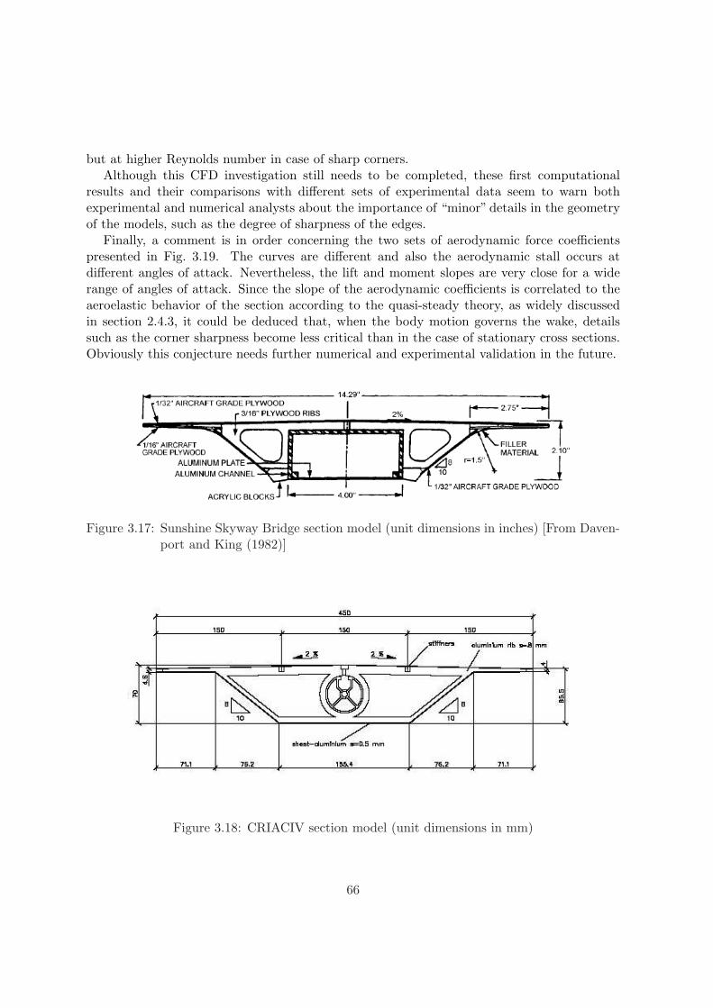
but at higher Reynolds number in case of sharp corners.Although this CFD investigation still needs to be completed, these first computational

results and their comparisons with different sets of experimental data seem to warn bothexperimental and numerical analysts about the importance of “minor” details in the geometryof the models, such as the degree of sharpness of the edges.

Finally, a comment is in order concerning the two sets of aerodynamic force coefficientspresented in Fig. 3.19. The curves are different and also the aerodynamic stall occurs atdifferent angles of attack. Nevertheless, the lift and moment slopes are very close for a widerange of angles of attack. Since the slope of the aerodynamic coefficients is correlated to theaeroelastic behavior of the section according to the quasi-steady theory, as widely discussedin section 2.4.3, it could be deduced that, when the body motion governs the wake, detailssuch as the corner sharpness become less critical than in the case of stationary cross sections.Obviously this conjecture needs further numerical and experimental validation in the future.

Figure 3.17: Sunshine Skyway Bridge section model (unit dimensions in inches) [From Daven-port and King (1982)]

Figure 3.18: CRIACIV section model (unit dimensions in mm)

66

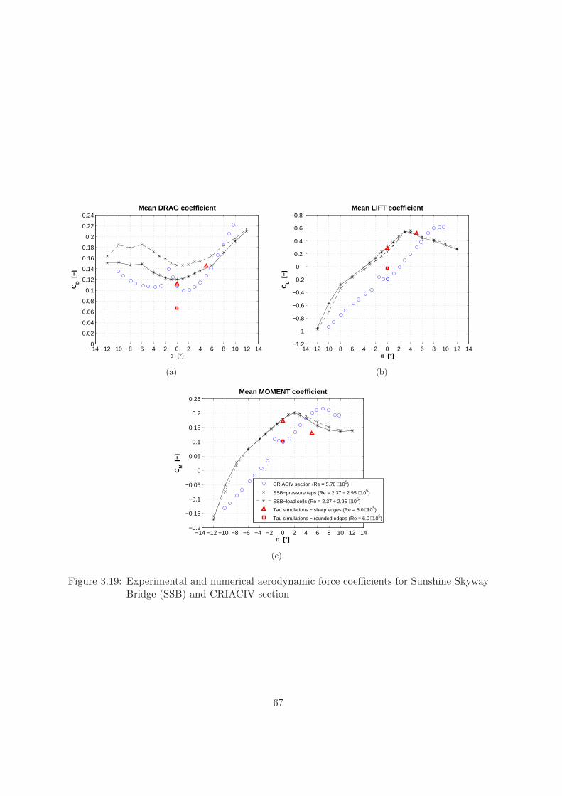
−14 −12 −10 −8 −6 −4 −2 0 2 4 6 8 10 12 140

0.02

0.04

0.06

0.08

0.1

0.12

0.14

0.16

0.18

0.2

0.22

0.24Mean DRAG coefficient

α [°]

CD [

−]

(a)

−14 −12 −10 −8 −6 −4 −2 0 2 4 6 8 10 12 14−1.2

−1

−0.8

−0.6

−0.4

−0.2

0

0.2

0.4

0.6

0.8 Mean LIFT coefficient

α [°]

CL [

−]

(b)

−14 −12 −10 −8 −6 −4 −2 0 2 4 6 8 10 12 14−0.2

−0.15

−0.1

−0.05

0

0.05

0.1

0.15

0.2

0.25

α [°]

CM

[−]

Mean MOMENT coefficient

CRIACIV section (Re = 5.76 ⋅ 105)

SSB−pressure taps (Re = 2.37 ÷ 2.95 ⋅ 105)

SSB−load cells (Re = 2.37 ÷ 2.95 ⋅ 105)

Tau simulations − sharp edges (Re = 6.0 ⋅ 105)

Tau simulations − rounded edges (Re = 6.0 ⋅ 105)

(c)

Figure 3.19: Experimental and numerical aerodynamic force coefficients for Sunshine SkywayBridge (SSB) and CRIACIV section

67

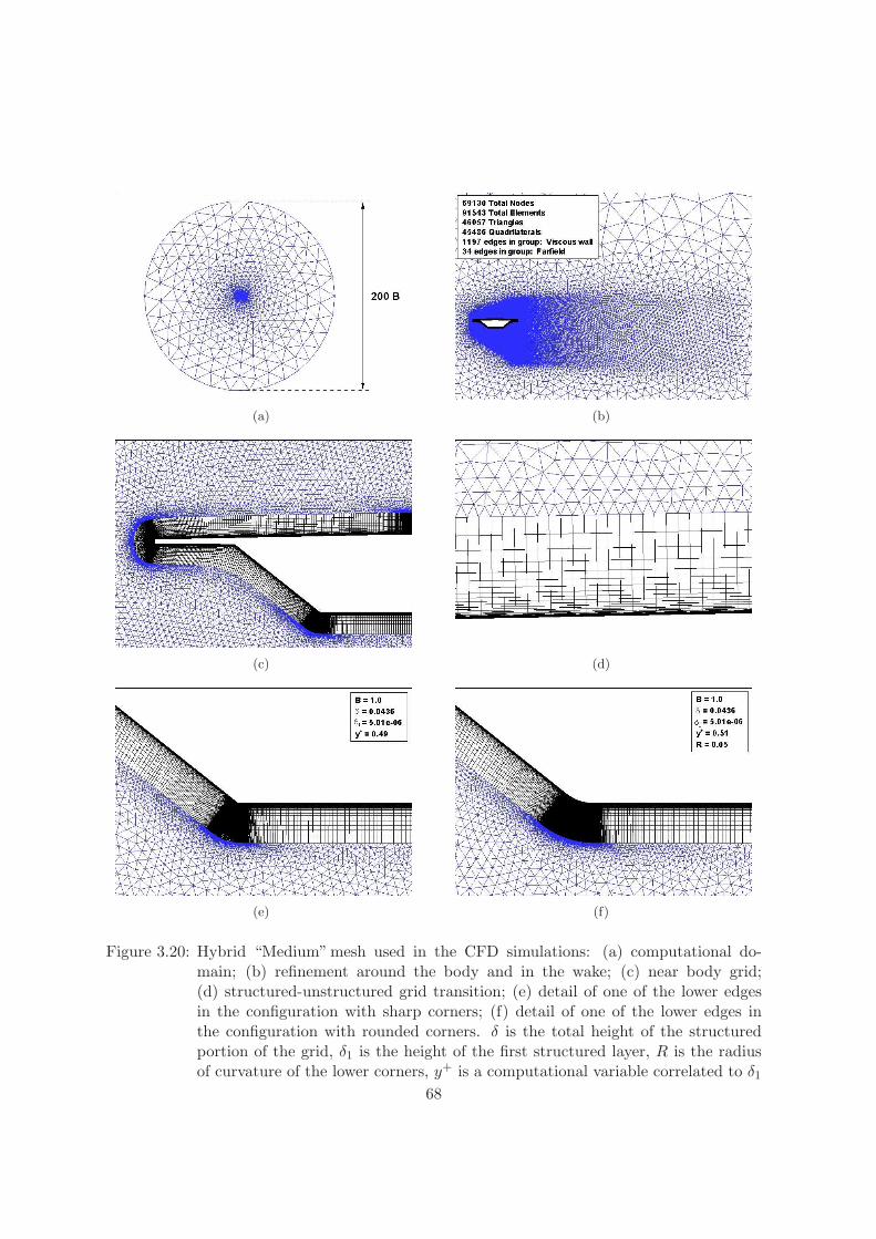
(a) (b)

(c) (d)

(e) (f)

Figure 3.20: Hybrid “Medium” mesh used in the CFD simulations: (a) computational do-main; (b) refinement around the body and in the wake; (c) near body grid;(d) structured-unstructured grid transition; (e) detail of one of the lower edgesin the configuration with sharp corners; (f) detail of one of the lower edges inthe configuration with rounded corners. δ is the total height of the structuredportion of the grid, δ1 is the height of the first structured layer, R is the radiusof curvature of the lower corners, y+ is a computational variable correlated to δ1

68

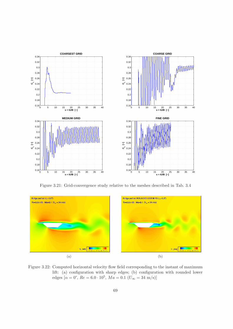
0 5 10 15 20 25 30 35 400.16

0.18

0.2

0.22

0.24

0.26

0.28

0.3

0.32

0.34COARSEST GRID

s = tU/B [−]

CL [

−]

0 5 10 15 20 25 30 35 400.16

0.18

0.2

0.22

0.24

0.26

0.28

0.3

0.32

0.34COARSE GRID

s = tU/B [−]

CL [

−]

0 5 10 15 20 25 30 35 400.16

0.18

0.2

0.22

0.24

0.26

0.28

0.3

0.32

0.34MEDIUM GRID

s = tU/B [−]

CL [

−]

0 5 10 15 20 25 30 35 400.16

0.18

0.2

0.22

0.24

0.26

0.28

0.3

0.32

0.34FINE GRID

s = tU/B [−]

CL [

−]

Figure 3.21: Grid-convergence study relative to the meshes described in Tab. 3.4

(a) (b)

Figure 3.22: Computed horizontal velocity flow field corresponding to the instant of maximumlift: (a) configuration with sharp edges; (b) configuration with rounded loweredges [α = 0°, Re = 6.0 · 105, Ma = 0.1 (U∞ = 34 m/s)]

69

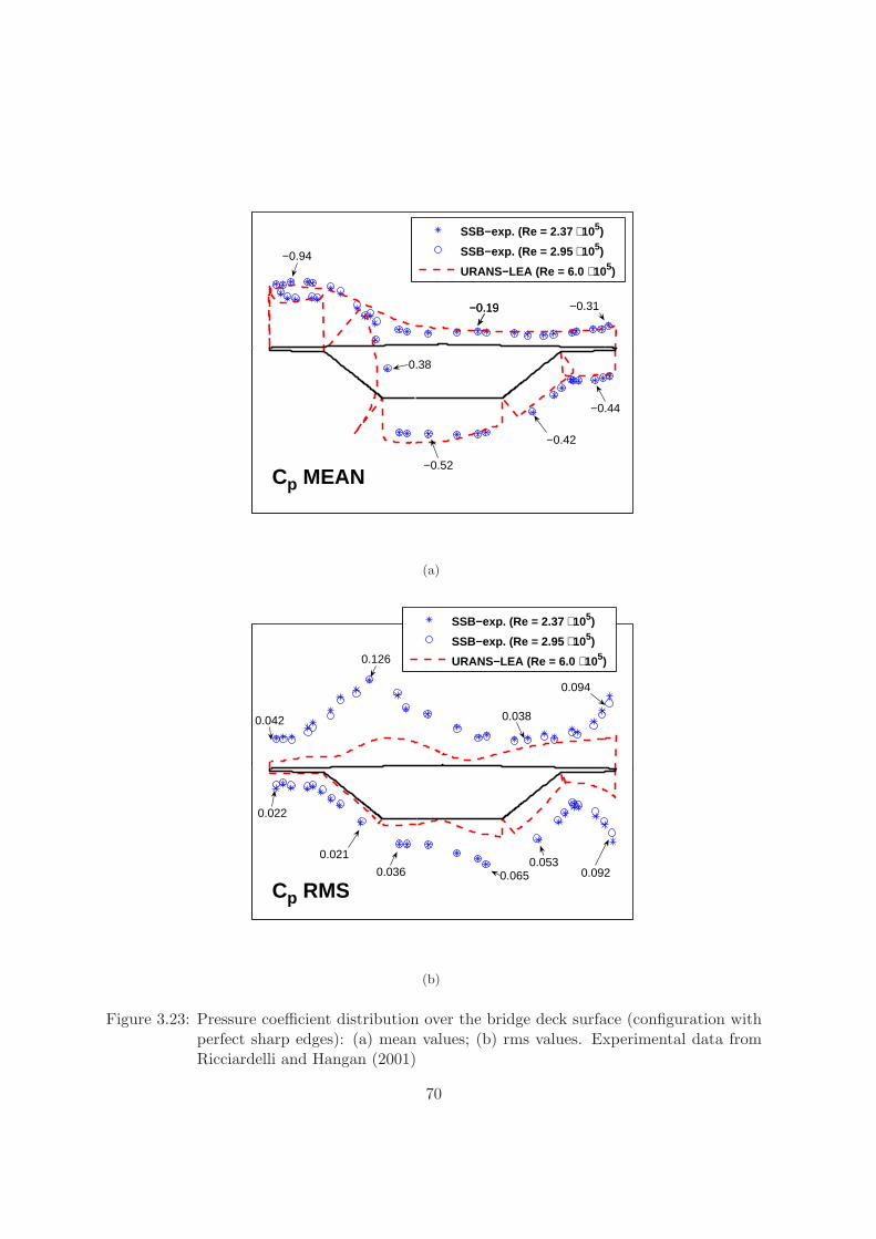
SSB−exp. (Re = 2.37 ⋅ 105)

SSB−exp. (Re = 2.95 ⋅ 105)

URANS−LEA (Re = 6.0 ⋅ 105)−0.94

−0.19−0.19 −0.31

0.38

−0.52

−0.42

−0.44

Cp MEAN

(a)

SSB−exp. (Re = 2.37 ⋅ 105)

SSB−exp. (Re = 2.95 ⋅ 105)

URANS−LEA (Re = 6.0 ⋅ 105)

0.042

0.126

0.094

0.038

0.022

0.021

0.036 0.0650.053

0.092

Cp RMS

(b)

Figure 3.23: Pressure coefficient distribution over the bridge deck surface (configuration withperfect sharp edges): (a) mean values; (b) rms values. Experimental data fromRicciardelli and Hangan (2001)

70

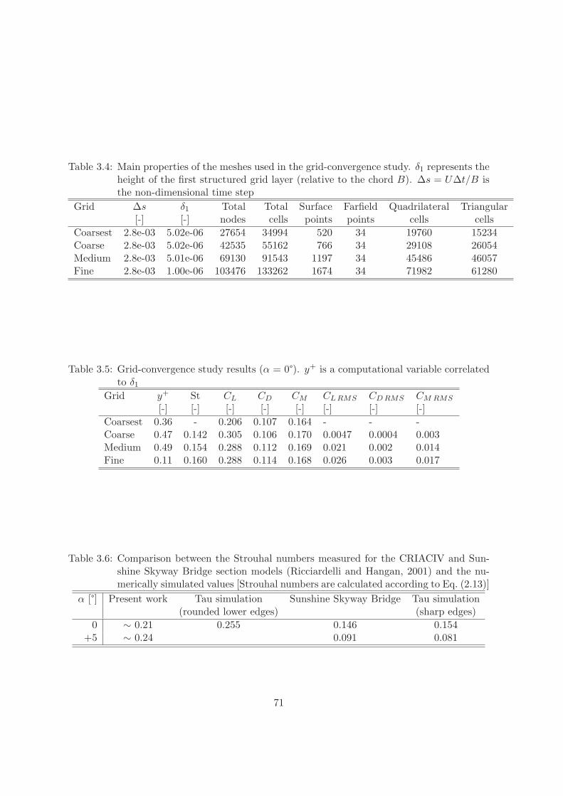
Table 3.4: Main properties of the meshes used in the grid-convergence study. δ1 represents theheight of the first structured grid layer (relative to the chord B). ∆s = U∆t/B isthe non-dimensional time step

Grid ∆s δ1 Total Total Surface Farfield Quadrilateral Triangular[-] [-] nodes cells points points cells cells

Coarsest 2.8e-03 5.02e-06 27654 34994 520 34 19760 15234Coarse 2.8e-03 5.02e-06 42535 55162 766 34 29108 26054Medium 2.8e-03 5.01e-06 69130 91543 1197 34 45486 46057Fine 2.8e-03 1.00e-06 103476 133262 1674 34 71982 61280

Table 3.5: Grid-convergence study results (α = 0°). y+ is a computational variable correlatedto δ1

Grid y+ St CL CD CM CL RMS CD RMS CM RMS

[-] [-] [-] [-] [-] [-] [-] [-]Coarsest 0.36 - 0.206 0.107 0.164 - - -Coarse 0.47 0.142 0.305 0.106 0.170 0.0047 0.0004 0.003Medium 0.49 0.154 0.288 0.112 0.169 0.021 0.002 0.014Fine 0.11 0.160 0.288 0.114 0.168 0.026 0.003 0.017

Table 3.6: Comparison between the Strouhal numbers measured for the CRIACIV and Sun-shine Skyway Bridge section models (Ricciardelli and Hangan, 2001) and the nu-merically simulated values [Strouhal numbers are calculated according to Eq. (2.13)]

α [°] Present work Tau simulation Sunshine Skyway Bridge Tau simulation(rounded lower edges) (sharp edges)

0 ∼ 0.21 0.255 0.146 0.154+5 ∼ 0.24 0.091 0.081

71

3.5 Aeroelastic tests

3.5.1 Experimental set-up

For the aeroelastic tests a set-up in which the section model is elastically suspended and boththe heaving and pitching modes are allowed, is necessary. This is obtained by clamping thecore-tube of the model to rigid suspension arms and then connecting eight springs to them.Each suspension arm consists of two aluminium plates connected together, in order to beas light as possible but very stiff with respect to the bending in the vertical plane. Theconnection between the springs and the suspension arms is realized with thin steel cables,in order to minimize the mechanical friction and allow the springs to work as regularly aspossible. The springs are placed at a transversal distance of 500 mm and prestressed in orderto behave always linearly. Those springs which are mounted above the section model (T42630)are stiffer than those mounted below it (T42150), since they have to bear also the weight ofthe model and the suspension arms. The main properties of the two sets of springs employedin the tests, produced by D.I.M. s.r.l., are reported in Tab. 3.7.

Table 3.7: Main properties of the springs used for the aeroelastic set-up (k = stiffness;L0 = total length at rest; f1 = maximum allowable displacement)

Material k L0 f1

[N/m] [mm] [mm]T42630 stainless steel 800 102.0 139.0T42150 stainless steel 380 87.7 137.0

Since only two degrees of freedom should be allowed, it is necessary to restrain the oscillationof the model in the along wind direction, as well as the rotation about a vertical axis. Thisis obtained by means of four long steel anti-drag cables which are connected to the model bymeans of two low-friction pillow blocks, in order not to interfere with the pitching degree offreedom [Fig. 3.24(d)]. Some pictures and a sketch of the set-up are reported in Figs. 3.24-3.25.

Finally, since the flutter derivatives are identified by measuring the heaving-pitching free-decay motion under wind, a system to impose a controlled and as regular as possible heaving-pitching initial condition is necessary. This consists of two magnets and two iron devicesthat are able to release two steel cables which are connected to the model suspension arms[Fig. 3.24(f)]. In order to limit as much as possible the rolling motion (rotation with respectto a horizontal axis perpendicular to the model longitudinal axis), it is important that the twomagnets release the steel ropes at same time and that the initial vertical displacements arethe same on both sides of the model.

72

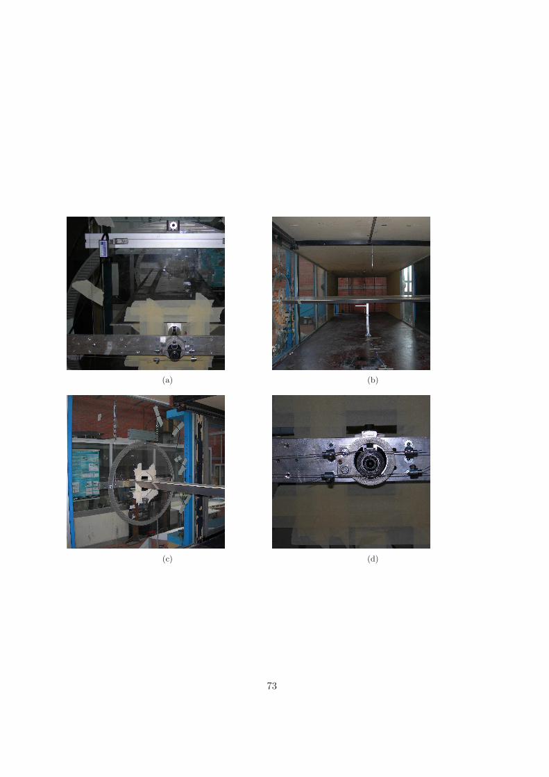
(a) (b)

(c) (d)

73

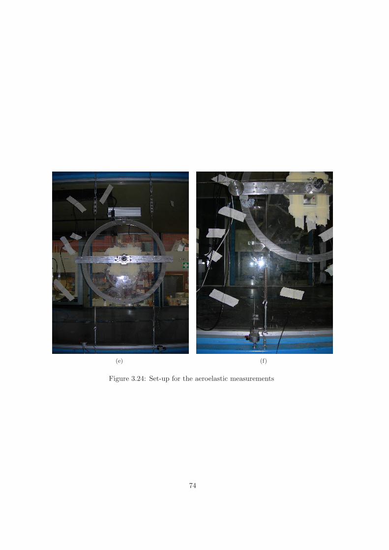
(e) (f)

Figure 3.24: Set-up for the aeroelastic measurements

74

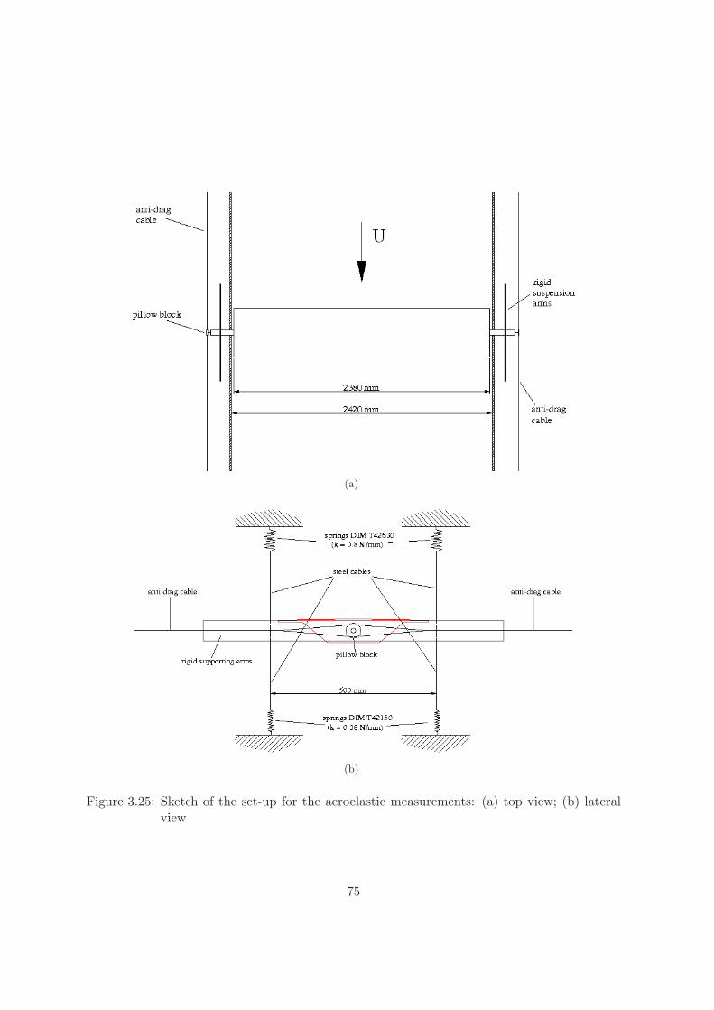
(a)

(b)

Figure 3.25: Sketch of the set-up for the aeroelastic measurements: (a) top view; (b) lateralview

75

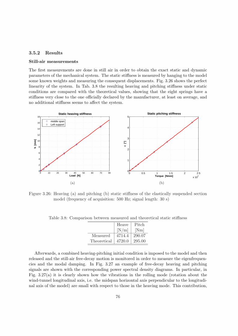
3.5.2 Results

Still-air measurements

The first measurements are done in still air in order to obtain the exact static and dynamicparameters of the mechanical system. The static stiffness is measured by hanging to the modelsome known weights and measuring the consequent displacements. Fig. 3.26 shows the perfectlinearity of the system. In Tab. 3.8 the resulting heaving and pitching stiffness under staticconditions are compared with the theoretical values, showing that the eight springs have astiffness very close to the one officially declared by the manufacturer, at least on average, andno additional stiffness seems to affect the system.

0 10 20 30 40 50 60 70 800

2

4

6

8

10

12

14

16

18

Load [N]

h [

mm

]

Static heaving stiffness

middle spanLeft support

(a)

0 0.5 1 1.5 2 2.5

x 104

0

1

2

3

4

5Static pitching stiffness

Torque [Nmm]

α [°

]

(b)

Figure 3.26: Heaving (a) and pitching (b) static stiffness of the elastically suspended sectionmodel (frequency of acquisition: 500 Hz; signal length: 30 s)

Table 3.8: Comparison between measured and theoretical static stiffness

Heave Pitch[N/m] [Nm]

Measured 4714.4 290.07Theoretical 4720.0 295.00

Afterwards, a combined heaving-pitching initial condition is imposed to the model and thenreleased and the still-air free-decay motion is monitored in order to measure the eigenfrequen-cies and the modal damping. In Fig. 3.27 an example of free-decay heaving and pitchingsignals are shown with the corresponding power spectral density diagrams. In particular, inFig. 3.27(a) it is clearly shown how the vibrations in the rolling mode (rotation about thewind-tunnel longitudinal axis, i.e. the midspan horizontal axis perpendicular to the longitudi-nal axis of the model) are small with respect to those in the heaving mode. This contribution,

76

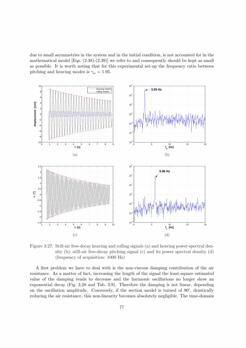
due to small asymmetries in the system and in the initial condition, is not accounted for in themathematical model [Eqs. (2.38)-(2.39)] we refer to and consequently should be kept as smallas possible. It is worth noting that for this experimental set-up the frequency ratio betweenpitching and heaving modes is γω = 1.95.

0 1 2 3 4 5 6 7 8 9−10

−8

−6

−4

−2

0

2

4

6

8

10

t [s]

dis

pla

cem

ent

[m

m]

heaving motionrolling motion

(a)

0 5 10 15 2010

−6

10−4

10−2

100

102

104

106

fh [Hz]

3.05 Hz

(b)

1 2 3 4 5 6 7 8 9 10−2.5

−2

−1.5

−1

−0.5

0

0.5

1

1.5

2

2.5

t [s]

α [°

]

(c)

0 5 10 15 2010

−6

10−4

10−2

100

102

104

106

fα [Hz]

5.96 Hz

(d)

Figure 3.27: Still-air free-decay heaving and rolling signals (a) and heaving power spectral den-sity (b); still-air free-decay pitching signal (c) and its power spectral density (d)(frequency of acquisition: 1000 Hz)

A first problem we have to deal with is the non-viscous damping contribution of the airresistance. As a matter of fact, increasing the length of the signal the least-square estimatedvalue of the damping tends to decrease and the harmonic oscillations no longer show anexponential decay (Fig. 3.28 and Tab. 3.9). Therefore the damping is not linear, dependingon the oscillation amplitude. Conversely, if the section model is turned of 90°, drasticallyreducing the air resistance, this non-linearity becomes absolutely negligible. The time-domain

77

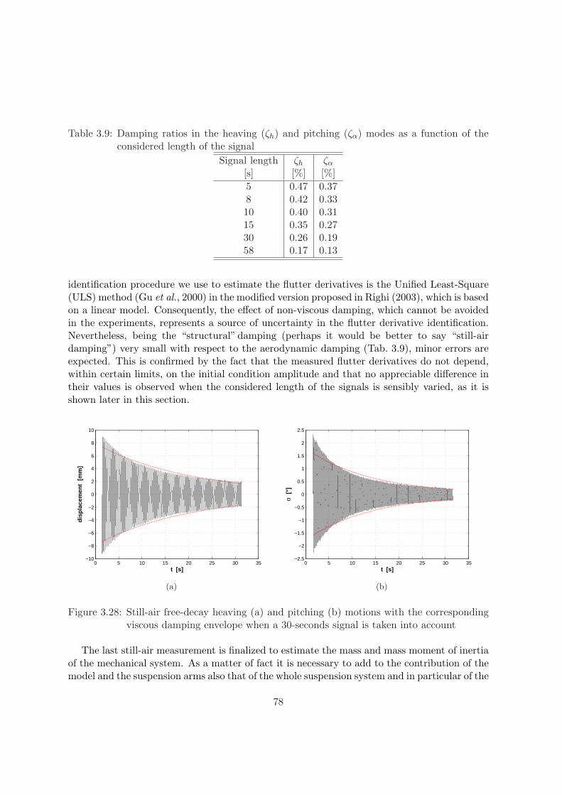
Table 3.9: Damping ratios in the heaving (ζh) and pitching (ζα) modes as a function of theconsidered length of the signal

Signal length ζh ζα

[s] [%] [%]5 0.47 0.378 0.42 0.3310 0.40 0.3115 0.35 0.2730 0.26 0.1958 0.17 0.13

identification procedure we use to estimate the flutter derivatives is the Unified Least-Square(ULS) method (Gu et al., 2000) in the modified version proposed in Righi (2003), which is basedon a linear model. Consequently, the effect of non-viscous damping, which cannot be avoidedin the experiments, represents a source of uncertainty in the flutter derivative identification.Nevertheless, being the “structural” damping (perhaps it would be better to say “still-airdamping”) very small with respect to the aerodynamic damping (Tab. 3.9), minor errors areexpected. This is confirmed by the fact that the measured flutter derivatives do not depend,within certain limits, on the initial condition amplitude and that no appreciable difference intheir values is observed when the considered length of the signals is sensibly varied, as it isshown later in this section.

0 5 10 15 20 25 30 35−10

−8

−6

−4

−2

0

2

4

6

8

10

t [s]

dis

pla

cem

ent

[m

m]

(a)

0 5 10 15 20 25 30 35−2.5

−2

−1.5

−1

−0.5

0

0.5

1

1.5

2

2.5

t [s]

α [°

]

(b)

Figure 3.28: Still-air free-decay heaving (a) and pitching (b) motions with the correspondingviscous damping envelope when a 30-seconds signal is taken into account

The last still-air measurement is finalized to estimate the mass and mass moment of inertiaof the mechanical system. As a matter of fact it is necessary to add to the contribution of themodel and the suspension arms also that of the whole suspension system and in particular of the

78

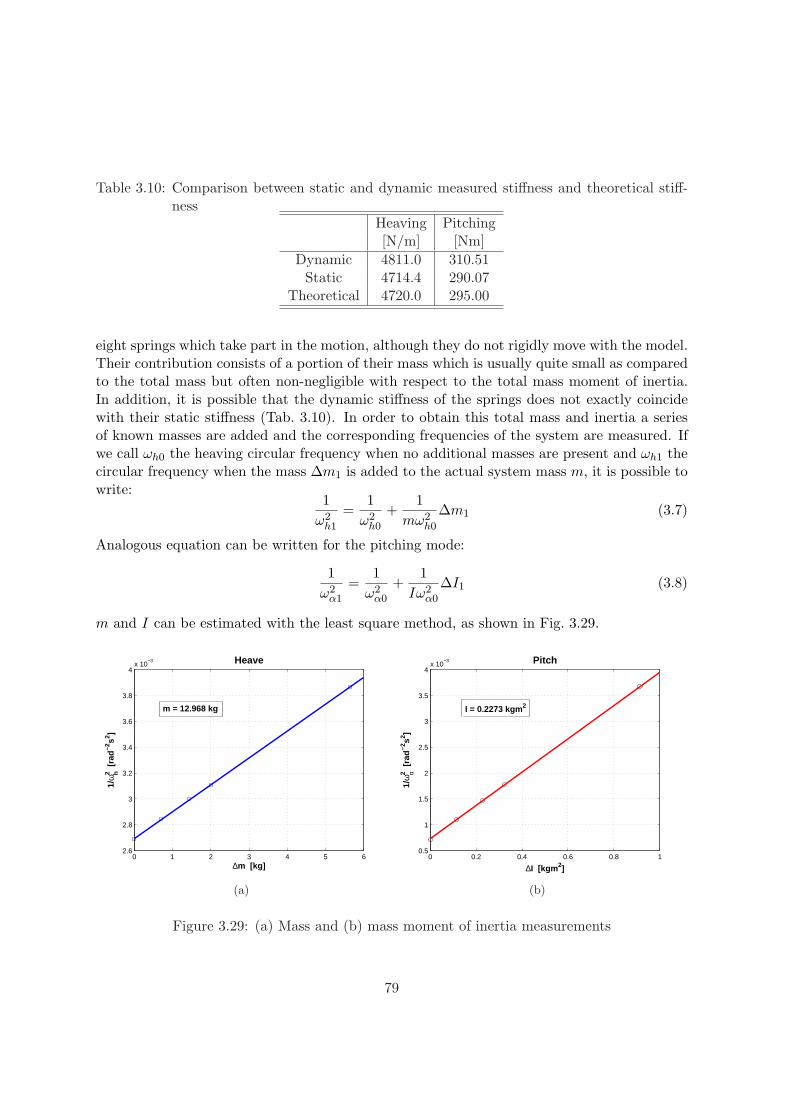
Table 3.10: Comparison between static and dynamic measured stiffness and theoretical stiff-ness

Heaving Pitching[N/m] [Nm]

Dynamic 4811.0 310.51Static 4714.4 290.07

Theoretical 4720.0 295.00

eight springs which take part in the motion, although they do not rigidly move with the model.Their contribution consists of a portion of their mass which is usually quite small as comparedto the total mass but often non-negligible with respect to the total mass moment of inertia.In addition, it is possible that the dynamic stiffness of the springs does not exactly coincidewith their static stiffness (Tab. 3.10). In order to obtain this total mass and inertia a seriesof known masses are added and the corresponding frequencies of the system are measured. Ifwe call ωh0 the heaving circular frequency when no additional masses are present and ωh1 thecircular frequency when the mass ∆m1 is added to the actual system mass m, it is possible towrite:

1ω2

h1

=1

ω2h0

+1

mω2h0

∆m1 (3.7)

Analogous equation can be written for the pitching mode:

1ω2

α1

=1

ω2α0

+1

Iω2α0

∆I1 (3.8)

m and I can be estimated with the least square method, as shown in Fig. 3.29.

0 1 2 3 4 5 62.6

2.8

3

3.2

3.4

3.6

3.8

4x 10

−3

∆m [kg]

1/ω

h2 [

rad

−2s2 ]

Heave

m = 12.968 kg

(a)

0 0.2 0.4 0.6 0.8 10.5

1

1.5

2

2.5

3

3.5

4x 10

−3

∆I [kgm 2]

1/ω

α2 [

rad

−2s2 ]

Pitch

I = 0.2273 kgm 2

(b)

Figure 3.29: (a) Mass and (b) mass moment of inertia measurements

79

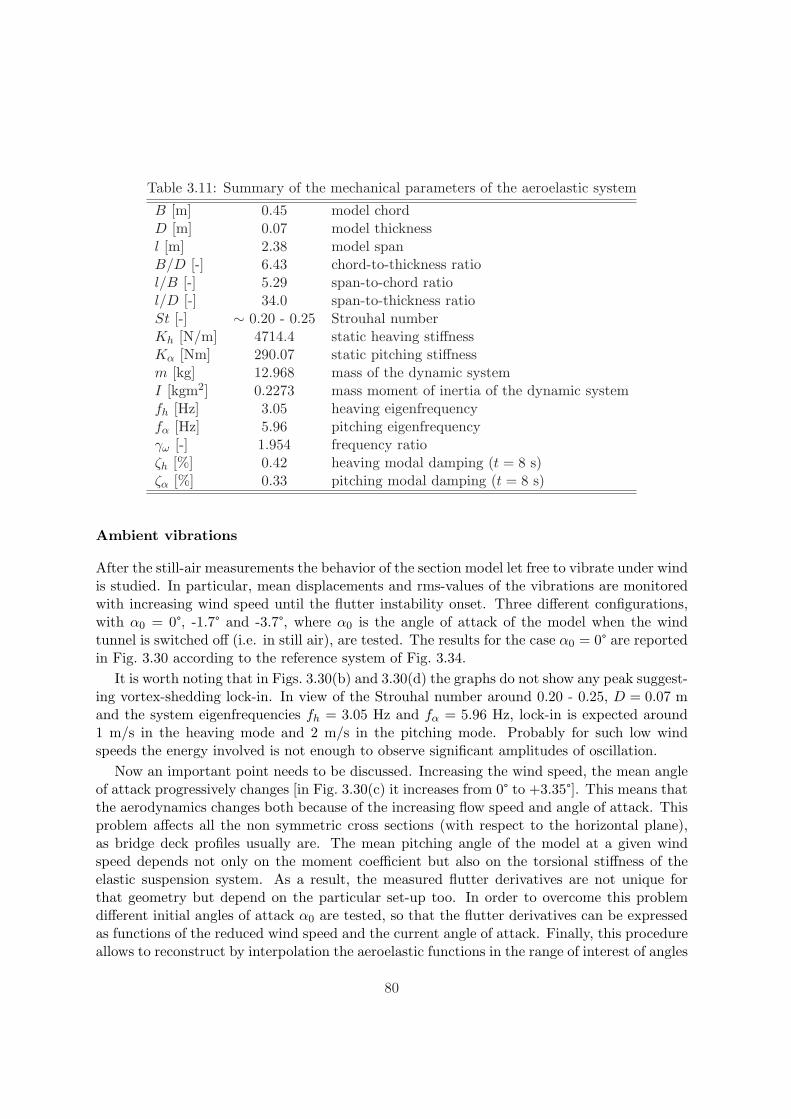
Table 3.11: Summary of the mechanical parameters of the aeroelastic system

B [m] 0.45 model chordD [m] 0.07 model thicknessl [m] 2.38 model spanB/D [-] 6.43 chord-to-thickness ratiol/B [-] 5.29 span-to-chord ratiol/D [-] 34.0 span-to-thickness ratioSt [-] ∼ 0.20 - 0.25 Strouhal numberKh [N/m] 4714.4 static heaving stiffnessKα [Nm] 290.07 static pitching stiffnessm [kg] 12.968 mass of the dynamic systemI [kgm2] 0.2273 mass moment of inertia of the dynamic systemfh [Hz] 3.05 heaving eigenfrequencyfα [Hz] 5.96 pitching eigenfrequencyγω [-] 1.954 frequency ratioζh [%] 0.42 heaving modal damping (t = 8 s)ζα [%] 0.33 pitching modal damping (t = 8 s)

Ambient vibrations

After the still-air measurements the behavior of the section model let free to vibrate under windis studied. In particular, mean displacements and rms-values of the vibrations are monitoredwith increasing wind speed until the flutter instability onset. Three different configurations,with α0 = 0°, -1.7° and -3.7°, where α0 is the angle of attack of the model when the windtunnel is switched off (i.e. in still air), are tested. The results for the case α0 = 0° are reportedin Fig. 3.30 according to the reference system of Fig. 3.34.

It is worth noting that in Figs. 3.30(b) and 3.30(d) the graphs do not show any peak suggest-ing vortex-shedding lock-in. In view of the Strouhal number around 0.20 - 0.25, D = 0.07 mand the system eigenfrequencies fh = 3.05 Hz and fα = 5.96 Hz, lock-in is expected around1 m/s in the heaving mode and 2 m/s in the pitching mode. Probably for such low windspeeds the energy involved is not enough to observe significant amplitudes of oscillation.

Now an important point needs to be discussed. Increasing the wind speed, the mean angleof attack progressively changes [in Fig. 3.30(c) it increases from 0° to +3.35°]. This means thatthe aerodynamics changes both because of the increasing flow speed and angle of attack. Thisproblem affects all the non symmetric cross sections (with respect to the horizontal plane),as bridge deck profiles usually are. The mean pitching angle of the model at a given windspeed depends not only on the moment coefficient but also on the torsional stiffness of theelastic suspension system. As a result, the measured flutter derivatives are not unique forthat geometry but depend on the particular set-up too. In order to overcome this problemdifferent initial angles of attack α0 are tested, so that the flutter derivatives can be expressedas functions of the reduced wind speed and the current angle of attack. Finally, this procedureallows to reconstruct by interpolation the aeroelastic functions in the range of interest of angles

80

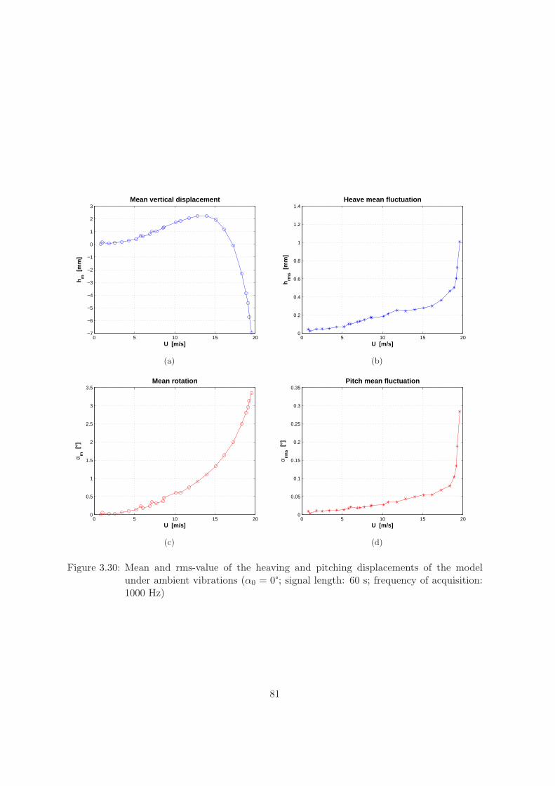
0 5 10 15 20−7

−6

−5

−4

−3

−2

−1

0

1

2

3Mean vertical displacement

U [m/s]

hm

[m

m]

(a)

0 5 10 15 200

0.2

0.4

0.6

0.8

1

1.2

1.4Heave mean fluctuation

U [m/s]

hrm

s [m

m]

(b)

0 5 10 15 200

0.5

1

1.5

2

2.5

3

3.5Mean rotation

U [m/s]

α m [

°]

(c)

0 5 10 15 200

0.05

0.1

0.15

0.2

0.25

0.3

0.35Pitch mean fluctuation

U [m/s]

α rms [

°]

(d)

Figure 3.30: Mean and rms-value of the heaving and pitching displacements of the modelunder ambient vibrations (α0 = 0°; signal length: 60 s; frequency of acquisition:1000 Hz)

81

of attack and reduced wind speeds. Also the initial condition changes with the wind speedas a consequence of the mean pitching angle and mean vertical displacement. However theresults, within certain limits, seem to be insensitive to the amplitude of the initial condition,as it will be shown later on.

In order to check the aerodynamic force coefficients measured via static tests, the same coef-ficients can be calculated on the basis of the mean displacements obtained with the aeroelasticset-up [Figs. 3.30(a)-3.30(c)]:

CL = −Kh · hm

qBl(3.9)

CM =Kα · αm

qB2l(3.10)

where Kh and Kα are the section-model static stiffness in heave and pitch (Tab. 3.10), hm

and αm the mean vertical displacement and pitching rotation, q the kinetic pressure, B and lrespectively the chord and length of the model. The minus in Eq. 3.9 is due to the differentreference system for lift in case of static and aeroelastic tests (see Figs. 3.9-3.34). In Fig. 3.31the lift and moment coefficients obtained in these two different ways are compared. A perfectsuperposition cannot be expected given the non-negligible Reynolds number effects shown inFig. 3.10 and in the Appendix. Nevertheless, except few values affected by some measurementerrors at low wind speed [the points corresponding to small irregularities in the curves ofFigs. 3.30(a)-3.30(c)], the three sets of results are in good agreement and the small distancebetween them seems to follow the previously discussed Reynolds number effects. This resultconfirms the validity of the measures of the aerodynamic force coefficients reported in Fig. 3.14,in particular concerning the irregular behavior observed for small negative angles of attack.

Particular attention must be paid to the configuration with α0 = −3.72° since the systembecomes unstable when the mean angle of attack is in the “critical” range between -2.5° and0°. In this case the instability arises much earlier than expected and two equilibrium states arereached: the first one characterized by large positive (downward) mean vertical displacementand large negative (nose-down) mean angle of attack, which is stable; the second one withsmaller positive mean vertical displacement and smaller negative mean angle of attack, whichis unstable. As shown in Fig. 3.32, the model continuously switches between these two statesso that the oscillations do not diverge for a wide range of wind speeds. Also the heavingfrequency continuously changes, coupling to the pitching frequency when the model undergoesdiverging oscillations. It is quite difficult to determine precisely the mean displacements (andconsequently the mean aerodynamic coefficient values) corresponding to the two different statesbut it seems that, when the model is unstable, the mean angle of attack is around -2° andthe mean aerodynamic coefficients assume a value which belongs to the previously discussedirregular branch. Conversely, when the model is in the stable state, the mean angle of attack isaround -3° and the corresponding mean aerodynamic coefficients fall at the end of the regularstraight branch or in the steep transition zone of the curves.

82

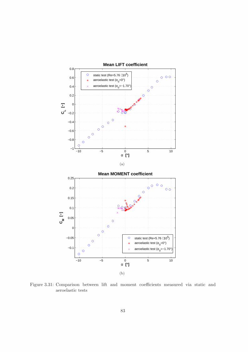
−10 −5 0 5 10−1

−0.8

−0.6

−0.4

−0.2

0

0.2

0.4

0.6

0.8

α [°]

CL [

−]Mean LIFT coefficient

static test (Re=5.76 ⋅ 105)

aeroelastic test (α0=0°)

aeroelastic test (α0=−1.70°)

(a)

−10 −5 0 5 10

−0.1

−0.05

0

0.05

0.1

0.15

0.2

0.25

α [°]

CM

[−]

Mean MOMENT coefficient

static test (Re=5.76 ⋅ 105)

aeroelastic test (α0=0°)

aeroelastic test (α0=−1.70°)

(b)

Figure 3.31: Comparison between lift and moment coefficients measured via static andaeroelastic tests

83

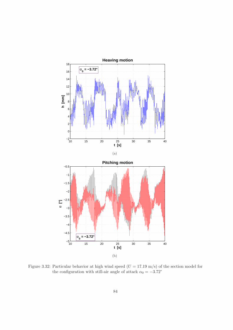
10 15 20 25 30 35 40−2

0

2

4

6

8

10

12

14

16

18Heaving motion

t [s]

h [m

m]

α0 = −3.72°

(a)

10 15 20 25 30 35 40−5

−4.5

−4

−3.5

−3

−2.5

−2

−1.5

−1

−0.5Pitching motion

t [s]

α [°

]

α0 = −3.72°

(b)

Figure 3.32: Particular behavior at high wind speed (U = 17.19 m/s) of the section model forthe configuration with still-air angle of attack α0 = −3.72°

84

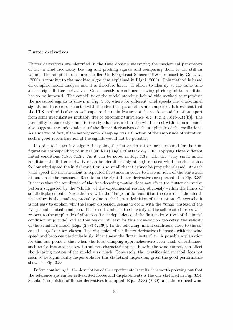
Flutter derivatives

Flutter derivatives are identified in the time domain measuring the mechanical parametersof the in-wind free-decay heaving and pitching signals and comparing them to the still-airvalues. The adopted procedure is called Unifying Least-Square (ULS) proposed by Gu et al.(2000), according to the modified algorithm explained in Righi (2003). This method is basedon complex modal analysis and it is therefore linear. It allows to identify at the same timeall the eight flutter derivatives. Consequently a combined heaving-pitching initial conditionhas to be imposed. The capability of the model standing behind this method to reproducethe measured signals is shown in Fig. 3.33, where for different wind speeds the wind-tunnelsignals and those reconstructed with the identified parameters are compared. It is evident thatthe ULS method is able to well capture the main features of the section-model motion, apartfrom some irregularities probably due to oncoming turbulence [e.g. Fig. 3.33(g)-3.33(h)]. Thepossibility to correctly simulate the signals measured in the wind tunnel with a linear modelalso suggests the independence of the flutter derivatives of the amplitude of the oscillations.As a matter of fact, if the aerodynamic damping was a function of the amplitude of vibration,such a good reconstruction of the signals would not be possible.

In order to better investigate this point, the flutter derivatives are measured for the con-figuration corresponding to initial (still-air) angle of attack α0 = 0°, applying three differentinitial conditions (Tab. 3.12). As it can be noted in Fig. 3.35, with the “very small initialcondition” the flutter derivatives can be identified only at high reduced wind speeds becausefor low wind speed the initial condition is so small that it cannot be properly released. At eachwind speed the measurement is repeated five times in order to have an idea of the statisticaldispersion of the measures. Results for the eight flutter derivatives are presented in Fig. 3.35.It seems that the amplitude of the free-decaying motion does not affect the flutter derivativepattern suggested by the “clouds” of the experimental results, obviously within the limits ofsmall displacements. Nevertheless, with the “large” initial condition the scatter of the identi-fied values is the smallest, probably due to the better definition of the motion. Conversely, itis not easy to explain why the larger dispersion seems to occur with the “small” instead of the“very small” initial condition. This result confirms the linearity of the self-excited forces withrespect to the amplitude of vibration (i.e. independence of the flutter derivatives of the initialcondition amplitude) and at this regard, at least for this cross-section geometry, the validityof the Scanlan’s model [Eqs. (2.38)-(2.39)]. In the following, initial conditions close to the so-called “large” one are chosen. The dispersion of the flutter derivatives increases with the windspeed and becomes particularly significant near the flutter instability. A possible explanationfor this last point is that when the total damping approaches zero even small disturbances,such as for instance the low turbulence characterizing the flow in the wind tunnel, can affectthe decaying motion of the model very much. Conversely, the identification method does notseem to be significantly responsible for this statistical dispersion, given the good performanceshown in Fig. 3.33.

Before continuing in the description of the experimental results, it is worth pointing out thatthe reference system for self-excited forces and displacements is the one sketched in Fig. 3.34,Scanlan’s definition of flutter derivatives is adopted [Eqs. (2.38)-(2.39)] and the reduced wind

85

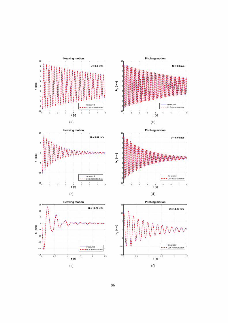
0 1 2 3 4 5 6 7 8−10

−8

−6

−4

−2

0

2

4

6

8

10

t [s]

h [

mm

]

Heaving motion

U = 0.0 m/s

measuredULS reconstruction

(a)

0 1 2 3 4 5 6 7 8−10

−8

−6

−4

−2

0

2

4

6

8

10

t [s]h

α [m

m]

Pitching motion

U = 0.0 m/s

measuredULS reconstruction

(b)

0 1 2 3 4 5 6 7 8−15

−10

−5

0

5

10

t [s]

h [

mm

]

Heaving motion

U = 5.04 m/s

measuredULS reconstruction

(c)

0 1 2 3 4 5 6 7 8−10

−8

−6

−4

−2

0

2

4

6

8

10

t [s]

hα [

mm

]

Pitching motion

U = 5.04 m/s

measuredULS reconstruction

(d)

0 0.5 1 1.5 2 2.5−25

−20

−15

−10

−5

0

5

10

15

t [s]

h [

mm

]

Heaving motion

U = 14.87 m/s

measuredULS reconstruction

(e)

0 0.5 1 1.5 2 2.5−15

−10

−5

0

5

10

15

t [s]

hα [

mm

]

Pitching motion

U = 14.87 m/s

measuredULS reconstruction

(f)

86

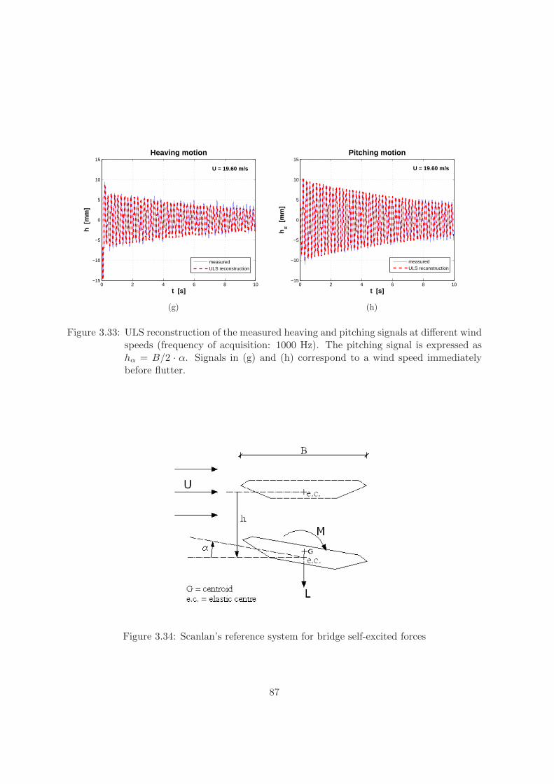
0 2 4 6 8 10−15

−10

−5

0

5

10

15

t [s]

h [

mm

]

Heaving motion

U = 19.60 m/s

measuredULS reconstruction

(g)

0 2 4 6 8 10−15

−10

−5

0

5

10

15

t [s]h

α [m

m]

Pitching motion

U = 19.60 m/s

measuredULS reconstruction

(h)

Figure 3.33: ULS reconstruction of the measured heaving and pitching signals at different windspeeds (frequency of acquisition: 1000 Hz). The pitching signal is expressed ashα = B/2 · α. Signals in (g) and (h) correspond to a wind speed immediatelybefore flutter.

Figure 3.34: Scanlan’s reference system for bridge self-excited forces

87

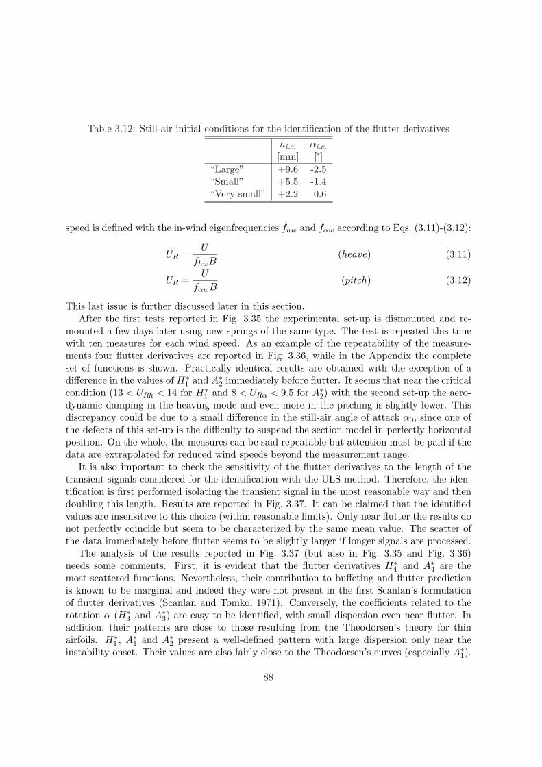
Table 3.12: Still-air initial conditions for the identification of the flutter derivatives

hi.c. αi.c.

[mm] [°]“Large” +9.6 -2.5“Small” +5.5 -1.4“Very small” +2.2 -0.6

speed is defined with the in-wind eigenfrequencies fhw and fαw according to Eqs. (3.11)-(3.12):

UR =U

fhwB(heave) (3.11)

UR =U

fαwB(pitch) (3.12)

This last issue is further discussed later in this section.After the first tests reported in Fig. 3.35 the experimental set-up is dismounted and re-

mounted a few days later using new springs of the same type. The test is repeated this timewith ten measures for each wind speed. As an example of the repeatability of the measure-ments four flutter derivatives are reported in Fig. 3.36, while in the Appendix the completeset of functions is shown. Practically identical results are obtained with the exception of adifference in the values of H∗

1 and A∗2 immediately before flutter. It seems that near the criticalcondition (13 < URh < 14 for H∗

1 and 8 < URα < 9.5 for A∗2) with the second set-up the aero-dynamic damping in the heaving mode and even more in the pitching is slightly lower. Thisdiscrepancy could be due to a small difference in the still-air angle of attack α0, since one ofthe defects of this set-up is the difficulty to suspend the section model in perfectly horizontalposition. On the whole, the measures can be said repeatable but attention must be paid if thedata are extrapolated for reduced wind speeds beyond the measurement range.

It is also important to check the sensitivity of the flutter derivatives to the length of thetransient signals considered for the identification with the ULS-method. Therefore, the iden-tification is first performed isolating the transient signal in the most reasonable way and thendoubling this length. Results are reported in Fig. 3.37. It can be claimed that the identifiedvalues are insensitive to this choice (within reasonable limits). Only near flutter the results donot perfectly coincide but seem to be characterized by the same mean value. The scatter ofthe data immediately before flutter seems to be slightly larger if longer signals are processed.

The analysis of the results reported in Fig. 3.37 (but also in Fig. 3.35 and Fig. 3.36)needs some comments. First, it is evident that the flutter derivatives H∗

4 and A∗4 are themost scattered functions. Nevertheless, their contribution to buffeting and flutter predictionis known to be marginal and indeed they were not present in the first Scanlan’s formulationof flutter derivatives (Scanlan and Tomko, 1971). Conversely, the coefficients related to therotation α (H∗

3 and A∗3) are easy to be identified, with small dispersion even near flutter. Inaddition, their patterns are close to those resulting from the Theodorsen’s theory for thinairfoils. H∗

1 , A∗1 and A∗2 present a well-defined pattern with large dispersion only near theinstability onset. Their values are also fairly close to the Theodorsen’s curves (especially A∗1).

88

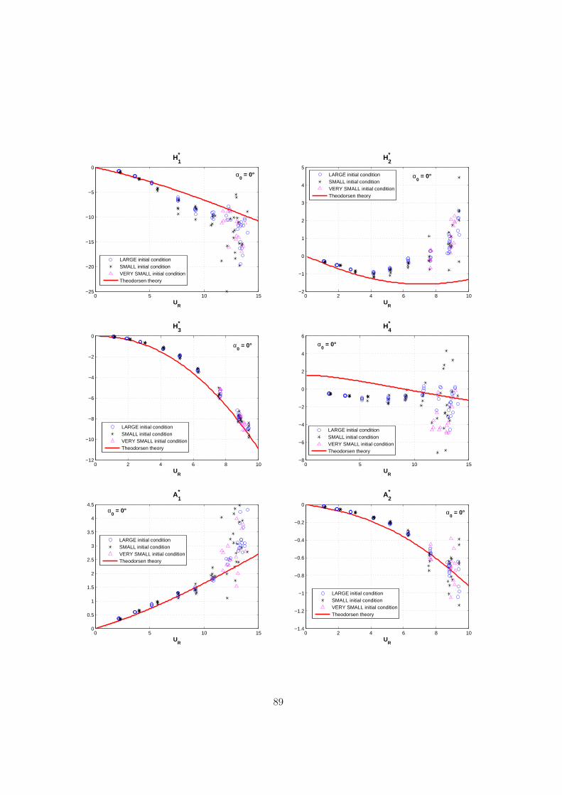
0 5 10 15−25

−20

−15

−10

−5

0

UR

H1*

α0 = 0°

LARGE initial conditionSMALL initial conditionVERY SMALL initial conditionTheodorsen theory

0 2 4 6 8 10−2

−1

0

1

2

3

4

5

UR

H2*

α0 = 0°LARGE initial condition

SMALL initial conditionVERY SMALL initial conditionTheodorsen theory

0 2 4 6 8 10−12

−10

−8

−6

−4

−2

0

UR

H3*

α0 = 0°

LARGE initial conditionSMALL initial conditionVERY SMALL initial conditionTheodorsen theory

0 5 10 15−8

−6

−4

−2

0

2

4

6

UR

H4*

α0 = 0°

LARGE initial conditionSMALL initial conditionVERY SMALL initial conditionTheodorsen theory

0 5 10 150

0.5

1

1.5

2

2.5

3

3.5

4

4.5

UR

A1*

α0 = 0°

LARGE initial conditionSMALL initial conditionVERY SMALL initial conditionTheodorsen theory

0 2 4 6 8 10−1.4

−1.2

−1

−0.8

−0.6

−0.4

−0.2

0

UR

A2*

α0 = 0°

LARGE initial conditionSMALL initial conditionVERY SMALL initial conditionTheodorsen theory

89

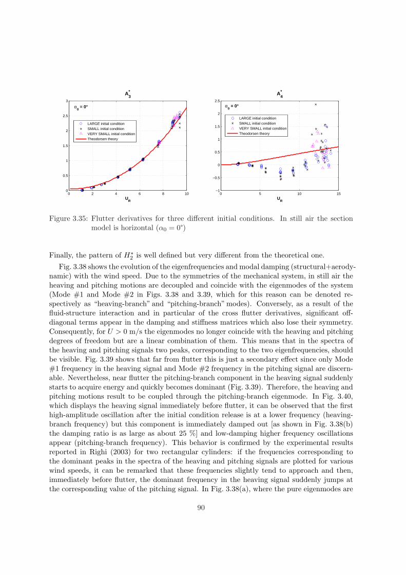
0 2 4 6 8 100

0.5

1

1.5

2

2.5

3

UR

A3*

α0 = 0°

LARGE initial conditionSMALL initial conditionVERY SMALL initial conditionTheodorsen theory

0 5 10 15−1

−0.5

0

0.5

1

1.5

2

2.5

UR

A4*

α0 = 0°

LARGE initial conditionSMALL initial conditionVERY SMALL initial conditionTheodorsen theory

Figure 3.35: Flutter derivatives for three different initial conditions. In still air the sectionmodel is horizontal (α0 = 0°)

Finally, the pattern of H∗2 is well defined but very different from the theoretical one.

Fig. 3.38 shows the evolution of the eigenfrequencies and modal damping (structural+aerody-namic) with the wind speed. Due to the symmetries of the mechanical system, in still air theheaving and pitching motions are decoupled and coincide with the eigenmodes of the system(Mode #1 and Mode #2 in Figs. 3.38 and 3.39, which for this reason can be denoted re-spectively as “heaving-branch” and “pitching-branch”modes). Conversely, as a result of thefluid-structure interaction and in particular of the cross flutter derivatives, significant off-diagonal terms appear in the damping and stiffness matrices which also lose their symmetry.Consequently, for U > 0 m/s the eigenmodes no longer coincide with the heaving and pitchingdegrees of freedom but are a linear combination of them. This means that in the spectra ofthe heaving and pitching signals two peaks, corresponding to the two eigenfrequencies, shouldbe visible. Fig. 3.39 shows that far from flutter this is just a secondary effect since only Mode#1 frequency in the heaving signal and Mode #2 frequency in the pitching signal are discern-able. Nevertheless, near flutter the pitching-branch component in the heaving signal suddenlystarts to acquire energy and quickly becomes dominant (Fig. 3.39). Therefore, the heaving andpitching motions result to be coupled through the pitching-branch eigenmode. In Fig. 3.40,which displays the heaving signal immediately before flutter, it can be observed that the firsthigh-amplitude oscillation after the initial condition release is at a lower frequency (heaving-branch frequency) but this component is immediately damped out [as shown in Fig. 3.38(b)the damping ratio is as large as about 25 %] and low-damping higher frequency oscillationsappear (pitching-branch frequency). This behavior is confirmed by the experimental resultsreported in Righi (2003) for two rectangular cylinders: if the frequencies corresponding tothe dominant peaks in the spectra of the heaving and pitching signals are plotted for variouswind speeds, it can be remarked that these frequencies slightly tend to approach and then,immediately before flutter, the dominant frequency in the heaving signal suddenly jumps atthe corresponding value of the pitching signal. In Fig. 3.38(a), where the pure eigenmodes are

90

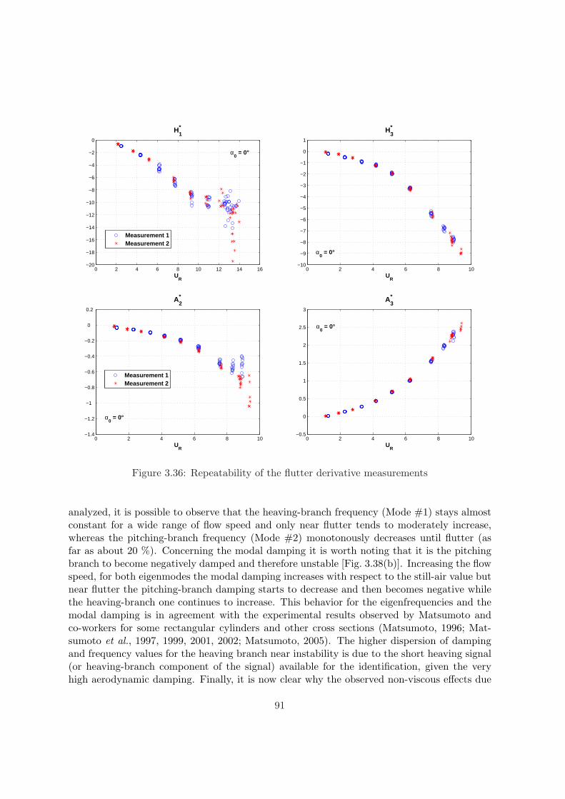
0 2 4 6 8 10 12 14 16−20

−18

−16

−14

−12

−10

−8

−6

−4

−2

0

UR

H1*

α0 = 0°

Measurement 1Measurement 2

0 2 4 6 8 10−10

−9

−8

−7

−6

−5

−4

−3

−2

−1

0

1

H3*

UR

α0 = 0°

0 2 4 6 8 10−1.4

−1.2

−1

−0.8

−0.6

−0.4

−0.2

0

0.2

UR

A2*

α0 = 0°

Measurement 1Measurement 2

0 2 4 6 8 10−0.5

0

0.5

1

1.5

2

2.5

3

A3*

UR

α0 = 0°

Figure 3.36: Repeatability of the flutter derivative measurements

analyzed, it is possible to observe that the heaving-branch frequency (Mode #1) stays almostconstant for a wide range of flow speed and only near flutter tends to moderately increase,whereas the pitching-branch frequency (Mode #2) monotonously decreases until flutter (asfar as about 20 %). Concerning the modal damping it is worth noting that it is the pitchingbranch to become negatively damped and therefore unstable [Fig. 3.38(b)]. Increasing the flowspeed, for both eigenmodes the modal damping increases with respect to the still-air value butnear flutter the pitching-branch damping starts to decrease and then becomes negative whilethe heaving-branch one continues to increase. This behavior for the eigenfrequencies and themodal damping is in agreement with the experimental results observed by Matsumoto andco-workers for some rectangular cylinders and other cross sections (Matsumoto, 1996; Mat-sumoto et al., 1997, 1999, 2001, 2002; Matsumoto, 2005). The higher dispersion of dampingand frequency values for the heaving branch near instability is due to the short heaving signal(or heaving-branch component of the signal) available for the identification, given the veryhigh aerodynamic damping. Finally, it is now clear why the observed non-viscous effects due

91

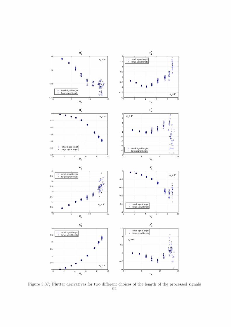
0 5 10 15−15

−10

−5

0

UR

H1*

α0 = 0°

small signal lengthlarge signal length

0 2 4 6 8 10−2

−1.5

−1

−0.5

0

0.5

1

1.5

2

UR

H2*

α0 = 0°

small signal lengthlarge signal length

0 2 4 6 8 10−12

−10

−8

−6

−4

−2

0

UR

H3*

α0 = 0°

small signal lengthlarge signal length

0 5 10 15−6

−5

−4

−3

−2

−1

0

1

2

3

UR

H4*

α0 = 0°

small signal lengthlarge signal length

0 5 10 150

0.5

1

1.5

2

2.5

3

3.5

4

UR

A1*

α0 = 0°

small signal lengthlarge signal length

0 2 4 6 8 10−1

−0.8

−0.6

−0.4

−0.2

0

UR

A2*

α0 = 0°

small signal lengthlarge signal length

0 2 4 6 8 100

0.5

1

1.5

2

2.5

3

UR

A3*

α0 = 0°

small signal lengthlarge signal length

0 5 10 15−1

−0.5

0

0.5

1

1.5

UR

A4*

α0 = 0°

small signal lengthlarge signal length

Figure 3.37: Flutter derivatives for two different choices of the length of the processed signals92

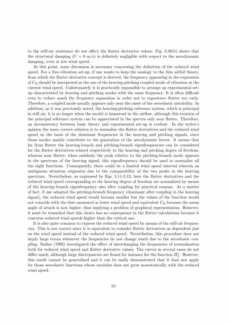
to the still-air resistance do not affect the flutter derivative values: Fig. 3.38(b) shows thatthe structural damping (U = 0 m/s) is definitely negligible with respect to the aerodynamicdamping, even at low wind speed.

At this point, some discussion is necessary concerning the definition of the reduced windspeed. For a free-vibration set-up, if one wants to keep the analogy to the thin airfoil theory,from which the flutter derivative concept is derived, the frequency appearing in the expressionof UR should be interpreted as the one of the heaving-pitching coupled mode of vibration at thecurrent wind speed. Unfortunately it is practically impossible to arrange an experimental set-up characterized by heaving and pitching modes with the same frequency. It is often difficulteven to reduce much the frequency separation in order not to experience flutter too early.Therefore, a coupled mode usually appears only near the onset of the aeroelastic instability. Inaddition, as it was previously noted, the heaving-pitching reference system, which is principalin still air, it is no longer when the model is immersed in the airflow, although this rotation ofthe principal reference system can be appreciated in the spectra only near flutter. Therefore,an inconsistency between basic theory and experimental set-up is evident. In the writer’sopinion the more correct solution is to normalize the flutter derivatives and the reduced windspeed on the basis of the dominant frequencies in the heaving and pitching signals, sincethose modes mainly contribute to the generation of the aerodynamic forces. It means thatfar from flutter the heaving-branch and pitching-branch eigenfrequencies can be consideredfor the flutter derivatives related respectively to the heaving and pitching degree of freedom,whereas near flutter, when suddenly the peak relative to the pitching-branch mode appearsin the spectrum of the heaving signal, this eigenfrequency should be used to normalize allthe eight functions. Consequently, there could be a limited wind speed interval wherein anambiguous situation originates due to the comparability of the two peaks in the heavingspectrum. Nevertheless, as expressed by Eqs. 3.11-3.12, here the flutter derivatives and thereduced wind speed corresponding to the heaving degree of freedom are normalized by meansof the heaving-branch eigenfrequency also after coupling for practical reasons. As a matterof fact, if one adopted the pitching-branch frequency (dominant after coupling in the heavingsignal), the reduced wind speed would become smaller but the values of the function wouldnot coincide with the that measured at lower wind speed and equivalent UR because the meanangle of attack is now higher, thus implying a problem of graphical representation. However,it must be remarked that this choice has no consequence in the flutter calculations because itconcerns reduced wind speeds higher than the critical one.

It is also quite common to express the reduced wind speed by means of the still-air frequen-cies. This is not correct since it is equivalent to consider flutter derivatives as dependent juston the wind speed instead of the reduced wind speed. Nevertheless, this procedure does notimply large errors whenever the frequencies do not change much due to the aeroelastic cou-pling. Sarkar (1992) investigated the effect of interchanging the frequencies of normalizationboth for reduced wind speed and flutter derivative values. The curves in several cases do notdiffer much, although large discrepancies are found for instance for the function H∗

2 . However,this result cannot be generalized and it can be easily demonstrated that it does not applyfor those aeroelastic functions whose modulus does not grow monotonically with the reducedwind speed.

93

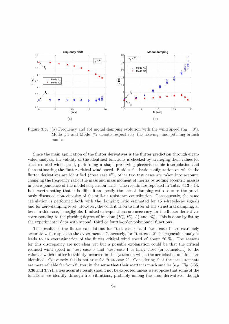
0 5 10 15 202.5

3

3.5

4

4.5

5

5.5

6

6.5

U [m/s]

f [H

z]

Frequency shift

α0 = 0°

fh

fα

Mode #1Mode #2

(a)

0 5 10 15 20−5

0

5

10

15

20

25

30

U [m/s]

ζ [%

]

Modal damping

α0 = 0°

ζh

ζα

Mode #1Mode #2

(b)

Figure 3.38: (a) Frequency and (b) modal damping evolution with the wind speed (α0 = 0°).Mode #1 and Mode #2 denote respectively the heaving- and pitching-branchmodes

Since the main application of the flutter derivatives is the flutter prediction through eigen-value analysis, the validity of the identified functions is checked by averaging their values foreach reduced wind speed, performing a shape-preserving piecewise cubic interpolation andthen estimating the flutter critical wind speed. Besides the basic configuration on which theflutter derivatives are identified (“test case 0”), other two test cases are taken into account,changing the frequency ratio, the mass and mass moment of inertia by adding eccentric massesin correspondence of the model suspension arms. The results are reported in Tabs. 3.13-3.14.It is worth noting that it is difficult to specify the actual damping ratios due to the previ-ously discussed non-viscosity of the still-air resistance contribution. Consequently, the samecalculation is performed both with the damping ratio estimated for 15 s-free-decay signalsand for zero-damping level. However, the contribution to flutter of the structural damping, atleast in this case, is negligible. Limited extrapolations are necessary for the flutter derivativescorresponding to the pitching degree of freedom (H∗

2 , H∗3 , A∗2 and A∗3). This is done by fitting

the experimental data with second, third or fourth-order polynomial functions.

The results of the flutter calculations for “test case 0” and “test case 1” are extremelyaccurate with respect to the experiments. Conversely, for “test case 2” the eigenvalue analysisleads to an overestimation of the flutter critical wind speed of about 20 %. The reasonsfor this discrepancy are not clear yet but a possible explanation could be that the criticalreduced wind speed in “test case 0” and “test case 1” is fairly close (or coincident) to thevalue at which flutter instability occurred in the system on which the aeroelastic functions areidentified. Conversely this is not true for “test case 2”. Considering that the measurementsare more reliable far from flutter, in the sense that their scatter is much smaller (e.g. Fig. 3.35,3.36 and 3.37), a less accurate result should not be expected unless we suppose that some of thefunctions we identify through free-vibrations, probably among the cross-derivatives, though

94

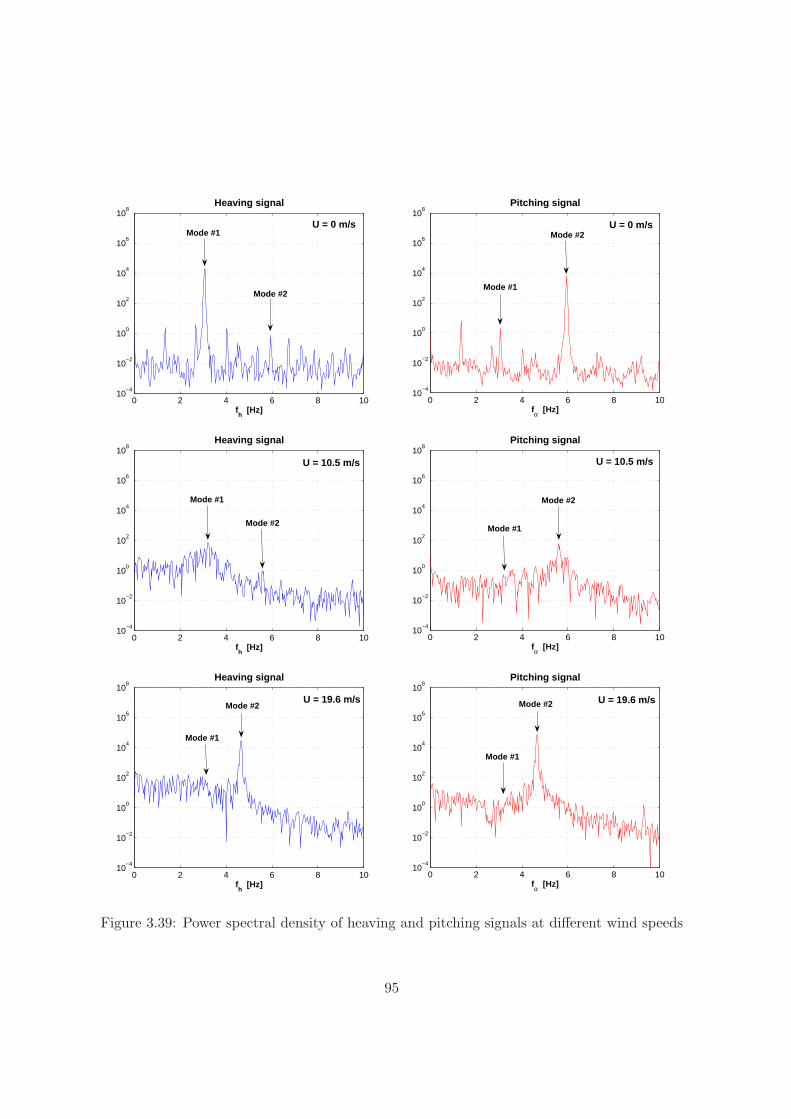
0 2 4 6 8 1010

−4

10−2

100

102

104

106

108

Heaving signal

fh [Hz]

U = 0 m/sMode #1

Mode #2

0 2 4 6 8 1010

−4

10−2

100

102

104

106

108

Pitching signal

fα [Hz]

U = 0 m/s

Mode #1

Mode #2

0 2 4 6 8 1010

−4

10−2

100

102

104

106

108

Heaving signal

fh [Hz]

U = 10.5 m/s

Mode #1

Mode #2

0 2 4 6 8 1010

−4

10−2

100

102

104

106

108

Pitching signal

fα [Hz]

U = 10.5 m/s

Mode #1

Mode #2

0 2 4 6 8 1010

−4

10−2

100

102

104

106

108

Heaving signal

fh [Hz]

U = 19.6 m/s

Mode #1

Mode #2

0 2 4 6 8 1010

−4

10−2

100

102

104

106

108

Pitching signal

fα [Hz]

U = 19.6 m/s

Mode #1

Mode #2

Figure 3.39: Power spectral density of heaving and pitching signals at different wind speeds

95

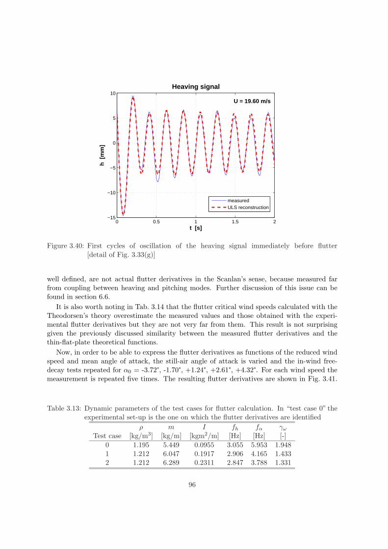
0 0.5 1 1.5 2−15

−10

−5

0

5

10

t [s]

h [

mm

]

Heaving signal

U = 19.60 m/s

measuredULS reconstruction

Figure 3.40: First cycles of oscillation of the heaving signal immediately before flutter[detail of Fig. 3.33(g)]

well defined, are not actual flutter derivatives in the Scanlan’s sense, because measured farfrom coupling between heaving and pitching modes. Further discussion of this issue can befound in section 6.6.

It is also worth noting in Tab. 3.14 that the flutter critical wind speeds calculated with theTheodorsen’s theory overestimate the measured values and those obtained with the experi-mental flutter derivatives but they are not very far from them. This result is not surprisinggiven the previously discussed similarity between the measured flutter derivatives and thethin-flat-plate theoretical functions.

Now, in order to be able to express the flutter derivatives as functions of the reduced windspeed and mean angle of attack, the still-air angle of attack is varied and the in-wind free-decay tests repeated for α0 = -3.72°, -1.70°, +1.24°, +2.61°, +4.32°. For each wind speed themeasurement is repeated five times. The resulting flutter derivatives are shown in Fig. 3.41.

Table 3.13: Dynamic parameters of the test cases for flutter calculation. In “test case 0” theexperimental set-up is the one on which the flutter derivatives are identified

ρ m I fh fα γω

Test case [kg/m3] [kg/m] [kgm2/m] [Hz] [Hz] [-]0 1.195 5.449 0.0955 3.055 5.953 1.9481 1.212 6.047 0.1917 2.906 4.165 1.4332 1.212 6.289 0.2311 2.847 3.788 1.331

96

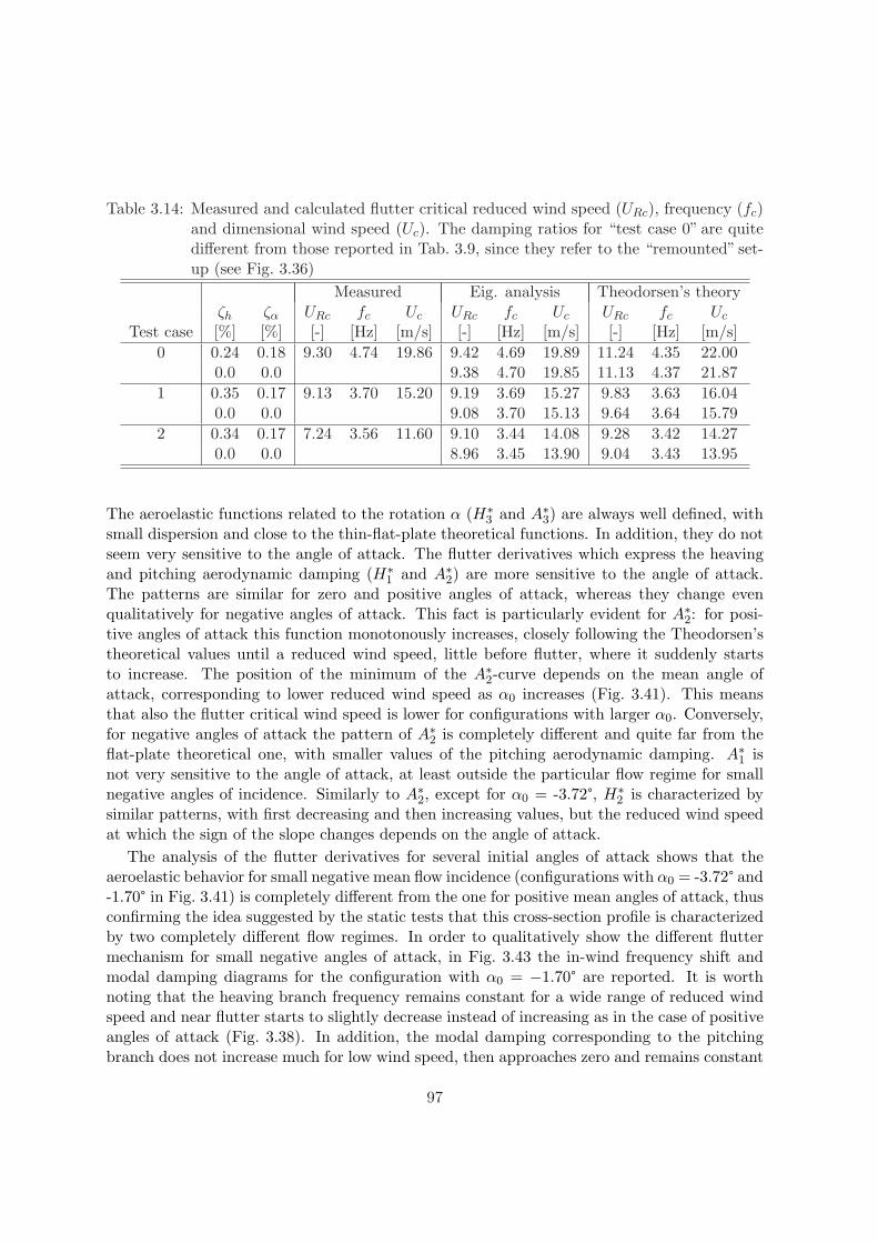
Table 3.14: Measured and calculated flutter critical reduced wind speed (URc), frequency (fc)and dimensional wind speed (Uc). The damping ratios for “test case 0” are quitedifferent from those reported in Tab. 3.9, since they refer to the “remounted” set-up (see Fig. 3.36)

Measured Eig. analysis Theodorsen’s theoryζh ζα URc fc Uc URc fc Uc URc fc Uc

Test case [%] [%] [-] [Hz] [m/s] [-] [Hz] [m/s] [-] [Hz] [m/s]0 0.24 0.18 9.30 4.74 19.86 9.42 4.69 19.89 11.24 4.35 22.00

0.0 0.0 9.38 4.70 19.85 11.13 4.37 21.871 0.35 0.17 9.13 3.70 15.20 9.19 3.69 15.27 9.83 3.63 16.04

0.0 0.0 9.08 3.70 15.13 9.64 3.64 15.792 0.34 0.17 7.24 3.56 11.60 9.10 3.44 14.08 9.28 3.42 14.27

0.0 0.0 8.96 3.45 13.90 9.04 3.43 13.95

The aeroelastic functions related to the rotation α (H∗3 and A∗3) are always well defined, with

small dispersion and close to the thin-flat-plate theoretical functions. In addition, they do notseem very sensitive to the angle of attack. The flutter derivatives which express the heavingand pitching aerodynamic damping (H∗

1 and A∗2) are more sensitive to the angle of attack.The patterns are similar for zero and positive angles of attack, whereas they change evenqualitatively for negative angles of attack. This fact is particularly evident for A∗2: for posi-tive angles of attack this function monotonously increases, closely following the Theodorsen’stheoretical values until a reduced wind speed, little before flutter, where it suddenly startsto increase. The position of the minimum of the A∗2-curve depends on the mean angle ofattack, corresponding to lower reduced wind speed as α0 increases (Fig. 3.41). This meansthat also the flutter critical wind speed is lower for configurations with larger α0. Conversely,for negative angles of attack the pattern of A∗2 is completely different and quite far from theflat-plate theoretical one, with smaller values of the pitching aerodynamic damping. A∗1 isnot very sensitive to the angle of attack, at least outside the particular flow regime for smallnegative angles of incidence. Similarly to A∗2, except for α0 = -3.72°, H∗

2 is characterized bysimilar patterns, with first decreasing and then increasing values, but the reduced wind speedat which the sign of the slope changes depends on the angle of attack.

The analysis of the flutter derivatives for several initial angles of attack shows that theaeroelastic behavior for small negative mean flow incidence (configurations with α0 = -3.72° and-1.70° in Fig. 3.41) is completely different from the one for positive mean angles of attack, thusconfirming the idea suggested by the static tests that this cross-section profile is characterizedby two completely different flow regimes. In order to qualitatively show the different fluttermechanism for small negative angles of attack, in Fig. 3.43 the in-wind frequency shift andmodal damping diagrams for the configuration with α0 = −1.70° are reported. It is worthnoting that the heaving branch frequency remains constant for a wide range of reduced windspeed and near flutter starts to slightly decrease instead of increasing as in the case of positiveangles of attack (Fig. 3.38). In addition, the modal damping corresponding to the pitchingbranch does not increase much for low wind speed, then approaches zero and remains constant

97

(flutter limit cycle oscillations).In addition, the position of the rotation center x0 and the phase angle φ between heaving and

pitching motion are plotted against the wind speed for different angles of attack in Fig. 3.42.Significant coupling is observed only for the pitching-branch mode, which becomes unstableat flutter and is therefore taken into account in the graphs. For the same reason the resultsshown in Fig. 3.42 are particularly relevant for wind speeds near flutter. The position of therotation center, positive downstream, is defined as:

x0 = −h0

α0(3.13)

where h0 and α0 are the amplitudes respectively of the heaving- and pitching-branch modes.It can be remarked that the rotation center is placed always upstream with respect to themidchord, its distance increasing with the wind speed, following roughly the same pattern forall the considered angles of attack. In the case α0 = 0°, at flutter the rotation center is placednearly 14 cm from the midchord. The pitching motion lags behind the heaving motion butthe phase angle is fairly small near flutter for zero and positive angles of attack (for α0 = 0°φ ∼= −10°), thus confirming the assumption discussed by Nakamura (1978). Conversely, fornegative incidence [Figs. 3.42(d) and 3.42(f)] the phase lag is much larger.

Finally, the flutter derivative values we measured could be thought as functions of twovariables, the reduced wind speed and the mean angle of attack [α(U) instead of α0]. Conse-quently, if a two-dimensional interpolation is performed, then it could be possible to extractthe flutter derivatives corresponding to a constant angle of attack in the range of interest.This manipulation would significantly widen the practical applicability of the data presentedin this chapter.

3.6 Conclusions

Static and aeroelastic tests are performed on a bridge deck section model (bare-deck configura-tion) whose cross section is common for medium-span cable-stayed bridges (closed-box girderwith lateral cantilevers).

The static tests allow to measure the aerodynamic force coefficients for several angles ofattack as well as the Strouhal number. These tests show a certain sensitivity to Reynoldsnumber, whereas the comparison with other tests on a similar cross section and with CFDsimulations highlighted the strong dependence of the flow field around the deck on the degreeof sharpness of the lower corners of the trapezoidal box.

The aeroelastic tests confirm the static results concerning the mean lift and moment coeffi-cients and allow the identification of the flutter derivatives for several initial angles of attack.The dependency of these functions on the amplitude of the motion, the repeatability of themeasures as well as the sensitivity with respect to the considered length of the transient sig-nals, showing the robustness of the results. It is also shown the capability of the UnifyingLeast-Square method to properly interpret and reproduce the measured signals. Furthermore,the critical flutter wind speed calculated with the flutter derivatives is compared with thedirectly measured value for three different test cases.

98

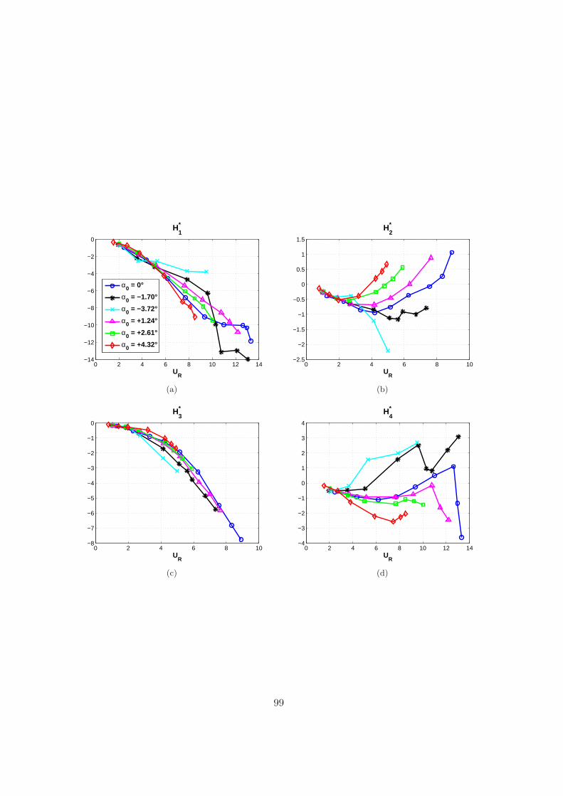
0 2 4 6 8 10 12 14−14

−12

−10

−8

−6

−4

−2

0

UR

H1*

α0 = 0°

α0 = −1.70°

α0 = −3.72°

α0 = +1.24°

α0 = +2.61°

α0 = +4.32°

(a)

0 2 4 6 8 10−2.5

−2

−1.5

−1

−0.5

0

0.5

1

1.5

H2*

UR

(b)

0 2 4 6 8 10−8

−7

−6

−5

−4

−3

−2

−1

0

UR

H3*

(c)

0 2 4 6 8 10 12 14−4

−3

−2

−1

0

1

2

3

4

H4*

UR

(d)

99

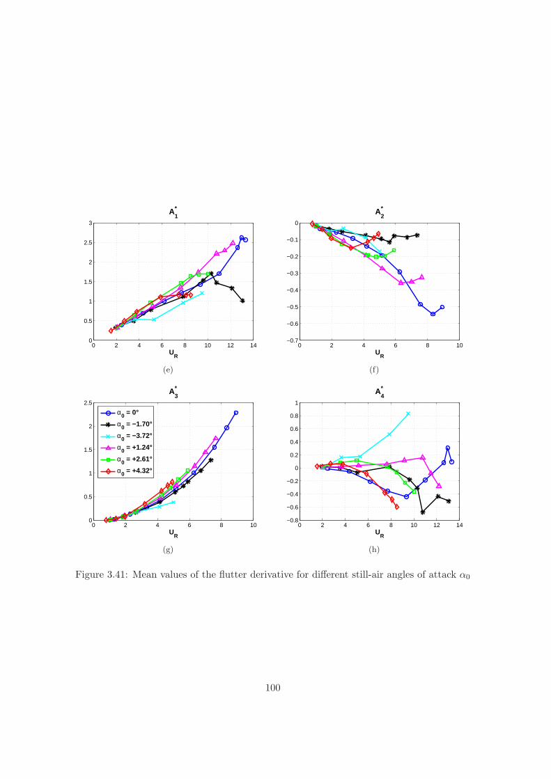
0 2 4 6 8 10 12 140

0.5

1

1.5

2

2.5

3

UR

A1*

(e)

0 2 4 6 8 10−0.7

−0.6

−0.5

−0.4

−0.3

−0.2

−0.1

0

UR

A2*

(f)

0 2 4 6 8 100

0.5

1

1.5

2

2.5

UR

A3*

α0 = 0°

α0 = −1.70°

α0 = −3.72°

α0 = +1.24°

α0 = +2.61°

α0 = +4.32°

(g)

0 2 4 6 8 10 12 14−0.8

−0.6

−0.4

−0.2

0

0.2

0.4

0.6

0.8

1

A4*

UR

(h)

Figure 3.41: Mean values of the flutter derivative for different still-air angles of attack α0

100

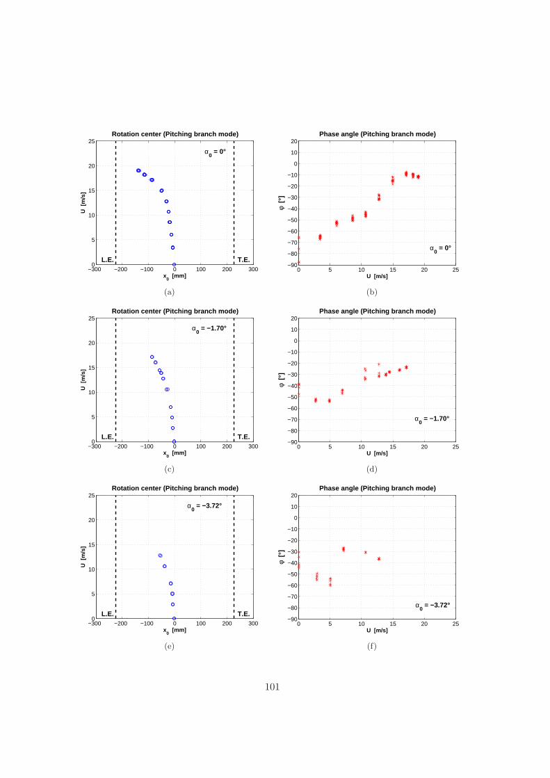
−300 −200 −100 0 100 200 3000

5

10

15

20

25Rotation center (Pitching branch mode)

x0 [mm]

U [

m/s

]

L.E. T.E.

α0 = 0°

(a)

0 5 10 15 20 25−90

−80

−70

−60

−50

−40

−30

−20

−10

0

10

20Phase angle (Pitching branch mode)

U [m/s]φ

[°]

α0 = 0°

(b)

−300 −200 −100 0 100 200 3000

5

10

15

20

25Rotation center (Pitching branch mode)

x0 [mm]

U [

m/s

]

L.E. T.E.

α0 = −1.70°

(c)

0 5 10 15 20 25−90

−80

−70

−60

−50

−40

−30

−20

−10

0

10

20Phase angle (Pitching branch mode)

U [m/s]

φ [°

]

α0 = −1.70°

(d)

−300 −200 −100 0 100 200 3000

5

10

15

20

25Rotation center (Pitching branch mode)

x0 [mm]

U [

m/s

]

L.E. T.E.

α0 = −3.72°

(e)

0 5 10 15 20 25−90

−80

−70

−60

−50

−40

−30

−20

−10

0

10

20Phase angle (Pitching branch mode)

U [m/s]

φ [°

]

α0 = −3.72°

(f)

101

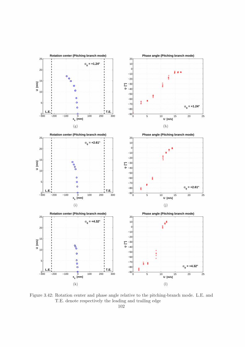
−300 −200 −100 0 100 200 3000

5

10

15

20

25Rotation center (Pitching branch mode)

x0 [mm]

U [

m/s

]

L.E. T.E.

α0 = +1.24°

(g)

0 5 10 15 20 25−90

−80

−70

−60

−50

−40

−30

−20

−10

0

10

20Phase angle (Pitching branch mode)

U [m/s]

φ [°

]

α0 = +1.24°

(h)

−300 −200 −100 0 100 200 3000

5

10

15

20

25Rotation center (Pitching branch mode)

x0 [mm]

U [

m/s

]

L.E. T.E.

α0 = +2.61°

(i)

0 5 10 15 20 25−90

−80

−70

−60

−50

−40

−30

−20

−10

0

10

20Phase angle (Pitching branch mode)

U [m/s]

φ [°

]

α0 = +2.61°

(j)

−300 −200 −100 0 100 200 3000

5

10

15

20

25Rotation center (Pitching branch mode)

x0 [mm]

U [

m/s

]

L.E. T.E.

α0 = +4.32°

(k)

0 5 10 15 20 25−90

−80

−70

−60

−50

−40

−30

−20

−10

0

10

20Phase angle (Pitching branch mode)

U [m/s]

φ [°

]

α0 = +4.32°

(l)

Figure 3.42: Rotation center and phase angle relative to the pitching-branch mode. L.E. andT.E. denote respectively the leading and trailing edge

102

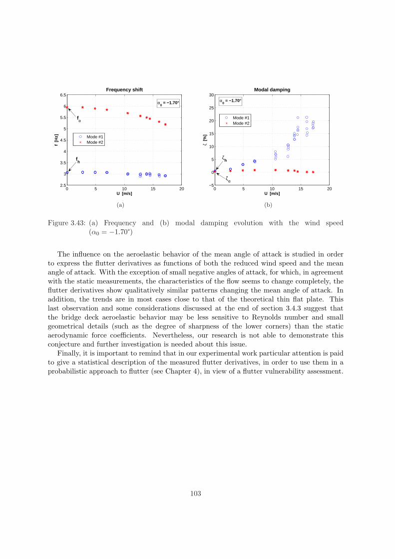
0 5 10 15 202.5

3

3.5

4

4.5

5

5.5

6

6.5

U [m/s]

f [H

z]

Frequency shift

α0 = −1.70°

fh

fα

Mode #1Mode #2

(a)

0 5 10 15 20−5

0

5

10

15

20

25

30

U [m/s]

ζ [%

]

Modal damping

α0 = −1.70°

ζh

ζα

Mode #1Mode #2

(b)

Figure 3.43: (a) Frequency and (b) modal damping evolution with the wind speed(α0 = −1.70°)

The influence on the aeroelastic behavior of the mean angle of attack is studied in orderto express the flutter derivatives as functions of both the reduced wind speed and the meanangle of attack. With the exception of small negative angles of attack, for which, in agreementwith the static measurements, the characteristics of the flow seems to change completely, theflutter derivatives show qualitatively similar patterns changing the mean angle of attack. Inaddition, the trends are in most cases close to that of the theoretical thin flat plate. Thislast observation and some considerations discussed at the end of section 3.4.3 suggest thatthe bridge deck aeroelastic behavior may be less sensitive to Reynolds number and smallgeometrical details (such as the degree of sharpness of the lower corners) than the staticaerodynamic force coefficients. Nevertheless, our research is not able to demonstrate thisconjecture and further investigation is needed about this issue.

Finally, it is important to remind that in our experimental work particular attention is paidto give a statistical description of the measured flutter derivatives, in order to use them in aprobabilistic approach to flutter (see Chapter 4), in view of a flutter vulnerability assessment.

103

Chapter 4

Probabilistic flutter approach

4.1 Flutter derivative measurements and uncertainty

It has been said several times in the previous chapters that flutter derivatives can be consideredas functions of the cross-sectional geometry, reduced wind speed and mean angle of attack.The role played by small scale turbulence is still not clear but it seems to act as if the shapeof the bluff body was slightly different, usually more streamlined (Scanlan and Lin, 1978; Lin,1996; Righi, 2003; Bartoli and Mannini, 2005).

Flutter derivatives are usually considered as deterministic functions but the dispersionwhich always characterizes their values, as shown in the previous chapter for the single-boxgirder deck section or in Righi (2003) for two rectangular cylinders, demonstrates that theyhave to be treated as not deterministic. Many sources of uncertainties can be enumerated:

• experimental measurement errors

• non-perfect capability of the mathematical model to explain the physical phenomenon

• imperfections in the identification procedure

• turbulence

It has already been shown that the identification method ULS is able to reproduce very wellthe measured signals. Therefore its contribution to the scatter of data does not seem verysignificant. Conversely, Righi (2003) highlighted the important contribution to uncertaintygiven by turbulence, which strongly increases the dispersion of the measured values, even atlow wind speeds. It is important to bear in mind that the contribution of turbulence cannot beavoided as natural wind is always turbulent and wind-tunnel flows are never really “smooth”,especially in the case of boundary layer wind tunnels for civil engineering applications wherea minimum turbulence intensity of about 1 % is quite common. It is also worth noting thatin case of forced-vibration set-ups the scatter affecting the aeroelastic coefficients is expectedto be smaller than for free-vibration tests but it cannot be avoided.

Hence flutter derivatives have to be considered probabilistic functions of the reduced windspeed (and mean angle of attack) and the uncertainties which affect their values are necessarily

105

somehow transferred to the calculated flutter critical wind speed and frequency. A modelof probabilistic flutter assessment is then necessary to find the probability distribution ofthe flutter wind speed and consequently to evaluate the reliability of the calculated flutterboundaries and indirectly of the measured flutter derivatives. It is important to understandthat if the dispersion affecting the flutter calculation output is very large, the number one callscritical wind speed is not very meaningful. Practically, in this chapter a method to estimatethe variance of this variable is proposed.

In addition, the probabilistic approach outlined herein is consistent with the vulnerabilityassessment in a Performance-Based Design scheme. As a matter of fact, repeating here thepreviously discussed PEER equation [Eqs. (1.4),(1.6), (4.1) and (4.2)], the proposed approachcan be considered as a method to define the term p(EDP |IM), that is the exceedance proba-bility to have a certain structural response EDP (flutter oscillations) given a certain IntensityMeasure IM (mean wind speed). Even though aerodynamic and structural [e.g. Salvatoriand Spinelli (2006b)] nonlinearities could lead to large-amplitude limit-cycle oscillations, as afirst approximation and in any case to be conservative, flutter can be regarded as a divergentphenomenon and consequently the collapse limit state is concerned. Therefore, with referenceto what is said in section 1.3, also the term p(SL|IM) can be calculated with respect to theultimate limit state for flutter instability.

p(DV ) =∫ ∫ ∫

p(DV |DM) · |dp(DM |EDP )| · |dp(EDP |IM)| · dp(IM) (4.1)

p(SL) =∫

p(SL|IM) · dp(IM) (4.2)

In the following the main assumptions standing behind the proposed probabilistic model arepresented and discussed, the results obtained for two rectangular cylinders are summarized,then the probabilistic method is applied to the bridge deck section analyzed in Chapter 3 andfinally some conclusions are drawn.

4.2 Model assumptions

The probabilistic model is based on the following assumptions:

1. each flutter derivative is a random variable independent from the corresponding variableat a different reduced wind speed;

2. given the reduced wind speed, the eight flutter derivatives are independent betweenthem;

3. these random variables are normally-distributed with the same mean and variance as theexperimental samples.

The first point to discuss is the independency of the random variables. The measurements atdifferent wind speeds absolutely do not depend on each other because, after a measure is done,the initial condition is imposed again and then released, therefore the previous measure has no

106

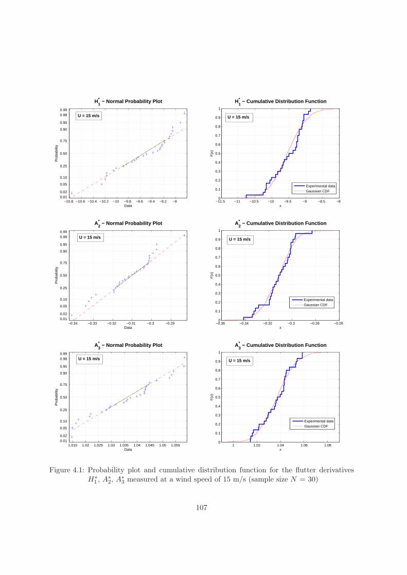
−10.8 −10.6 −10.4 −10.2 −10 −9.8 −9.6 −9.4 −9.2 −90.01 0.02

0.05

0.10

0.25

0.50

0.75

0.90

0.95

0.98 0.99

Data

Pro

babi

lity

H1* − Normal Probability Plot

U = 15 m/s

−11.5 −11 −10.5 −10 −9.5 −9 −8.5 −80

0.1

0.2

0.3

0.4

0.5

0.6

0.7

0.8

0.9

1

xF

(x)

H1* − Cumulative Distribution Function

Experimental dataGaussian CDF

U = 15 m/s

−0.34 −0.33 −0.32 −0.31 −0.3 −0.290.01 0.02

0.05

0.10

0.25

0.50

0.75

0.90

0.95

0.98 0.99

Data

Pro

babi

lity

A2* − Normal Probability Plot

U = 15 m/s

−0.36 −0.34 −0.32 −0.3 −0.28 −0.260

0.1

0.2

0.3

0.4

0.5

0.6

0.7

0.8

0.9

1

x

F(x

)

A2* − Cumulative Distribution Function

Experimental dataGaussian CDF

U = 15 m/s

1.015 1.02 1.025 1.03 1.035 1.04 1.045 1.05 1.0550.01 0.02

0.05

0.10

0.25

0.50

0.75

0.90

0.95

0.98 0.99

Data

Pro

babi

lity

A3* − Normal Probability Plot

U = 15 m/s

1 1.02 1.04 1.06 1.080

0.1

0.2

0.3

0.4

0.5

0.6

0.7

0.8

0.9

1

x

F(x

)

A3* − Cumulative Distribution Function

Experimental dataGaussian CDF

U = 15 m/s

Figure 4.1: Probability plot and cumulative distribution function for the flutter derivativesH∗

1 , A∗2, A∗3 measured at a wind speed of 15 m/s (sample size N = 30)

107

influence at all on the following one. Despite that, due to the physics of the phenomenon, theflutter derivative values at different reduced velocities are supposed to follow a certain pattern.This means that, if one performed just a measurement per wind speed, the current measurewould not be influenced by the previous value, but patterns far from the “physical” one wouldbe less probable than patterns close to the ideal, and a priori unknown, curve. Hence theassumption of independency does not fully hold. To accept that is equivalent to spread outthe “clouds” or random points, which substitute the deterministic curves (see Figs. 4.3 and4.11), consequently increasing the actual variance of the input.

The second assumption states that at the same reduced wind speed the different flutterderivatives are independent random variables. This point is questionable because for instancethe contribution to uncertainty of turbulence is likely to have an effect which is correlated, es-pecially for some aeroelastic coefficients. Nevertheless, first investigations on the experimentaldata seem to show a weaker correlation than it could have been expected. Furthermore, toaccount for that would require the estimation of a large number of joint probability functions,therefore complicating very much the probabilistic model. As further development of thiswork, we would like to better investigate this aspect of the problem and consequently improvethe model.

The fact that the flutter derivative values follow a normal distribution should be proved.A first attempt was done in Bartoli and Mannini (2005) for the flutter derivatives measuredfor two rectangular cylinders in smooth and turbulent flow by Righi (2003). Statistical testsare performed on the hypothesis of Gaussian distribution at the significance level of 5 %and in most cases positive answers are obtained. Nevertheless the samples are too small todraw robust conclusions. During the experimental campaign described in Chapter 3, for threedifferent wind speeds large samples are produced (30 measures for each wind speed), in orderto perform meaningful tests. The first series of measurements is performed at a wind speedof about 4 m/s when the aerodynamic damping is not very high; the second series at 15 m/swhen the aerodynamic damping is very high and the flutter instability limit is still far; finallythe last series of measurements are performed at a wind speed of 19.2 m/s, that is immediatelybefore the flutter onset. The initial angle of attack is always α0 = 0°. Two different tests areperformed to check the goodness of fit to a normal distribution: Lilliefors and Jarque-Beratests. The Lilliefors test is very similar to a Kolmogorov-Smirnov test but it adjusts for thefact that the parameters of the normal distribution are estimated from the sample rather thanspecified in advance. The empirical distribution of the variable is compared with a normaldistribution having the same mean and variance as the sample. Conversely, the Jarque-Beratest determines whether the sample skewness and kurtosis are unusually different than theirexpected values for a normal distribution (0 and 3 respectively), as measured by a chi-squarestatistic. The Jarque-Bera test is an asymptotic test and is not recommended when smallsamples are available, in which cases the Lilliefors test has to be preferred. For the three seriesof measures for all the eight flutter derivatives both tests with significance level of 5 % givepositive answers with the only exception of the Jarque-Bera test for H∗

3 at low wind speed.Therefore it is possible to conclude that the measured flutter derivatives at each reduced windspeed are normally-distributed random variables. As visual examples of the distributions ofthe flutter derivatives and of the corresponding normal distributions, normal probability plotsand cumulate distribution functions for H∗

1 , A∗2, A∗3 at 15 m/s are reported in Fig. 4.1. For

108

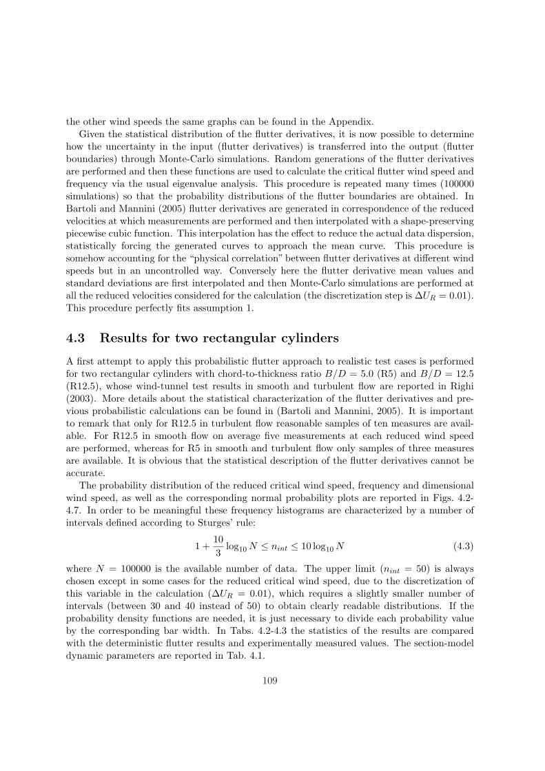
the other wind speeds the same graphs can be found in the Appendix.Given the statistical distribution of the flutter derivatives, it is now possible to determine

how the uncertainty in the input (flutter derivatives) is transferred into the output (flutterboundaries) through Monte-Carlo simulations. Random generations of the flutter derivativesare performed and then these functions are used to calculate the critical flutter wind speed andfrequency via the usual eigenvalue analysis. This procedure is repeated many times (100000simulations) so that the probability distributions of the flutter boundaries are obtained. InBartoli and Mannini (2005) flutter derivatives are generated in correspondence of the reducedvelocities at which measurements are performed and then interpolated with a shape-preservingpiecewise cubic function. This interpolation has the effect to reduce the actual data dispersion,statistically forcing the generated curves to approach the mean curve. This procedure issomehow accounting for the “physical correlation” between flutter derivatives at different windspeeds but in an uncontrolled way. Conversely here the flutter derivative mean values andstandard deviations are first interpolated and then Monte-Carlo simulations are performed atall the reduced velocities considered for the calculation (the discretization step is ∆UR = 0.01).This procedure perfectly fits assumption 1.

4.3 Results for two rectangular cylinders

A first attempt to apply this probabilistic flutter approach to realistic test cases is performedfor two rectangular cylinders with chord-to-thickness ratio B/D = 5.0 (R5) and B/D = 12.5(R12.5), whose wind-tunnel test results in smooth and turbulent flow are reported in Righi(2003). More details about the statistical characterization of the flutter derivatives and pre-vious probabilistic calculations can be found in (Bartoli and Mannini, 2005). It is importantto remark that only for R12.5 in turbulent flow reasonable samples of ten measures are avail-able. For R12.5 in smooth flow on average five measurements at each reduced wind speedare performed, whereas for R5 in smooth and turbulent flow only samples of three measuresare available. It is obvious that the statistical description of the flutter derivatives cannot beaccurate.

The probability distribution of the reduced critical wind speed, frequency and dimensionalwind speed, as well as the corresponding normal probability plots are reported in Figs. 4.2-4.7. In order to be meaningful these frequency histograms are characterized by a number ofintervals defined according to Sturges’ rule:

1 +103

log10 N ≤ nint ≤ 10 log10 N (4.3)

where N = 100000 is the available number of data. The upper limit (nint = 50) is alwayschosen except in some cases for the reduced critical wind speed, due to the discretization ofthis variable in the calculation (∆UR = 0.01), which requires a slightly smaller number ofintervals (between 30 and 40 instead of 50) to obtain clearly readable distributions. If theprobability density functions are needed, it is just necessary to divide each probability valueby the corresponding bar width. In Tabs. 4.2-4.3 the statistics of the results are comparedwith the deterministic flutter results and experimentally measured values. The section-modeldynamic parameters are reported in Tab. 4.1.

109

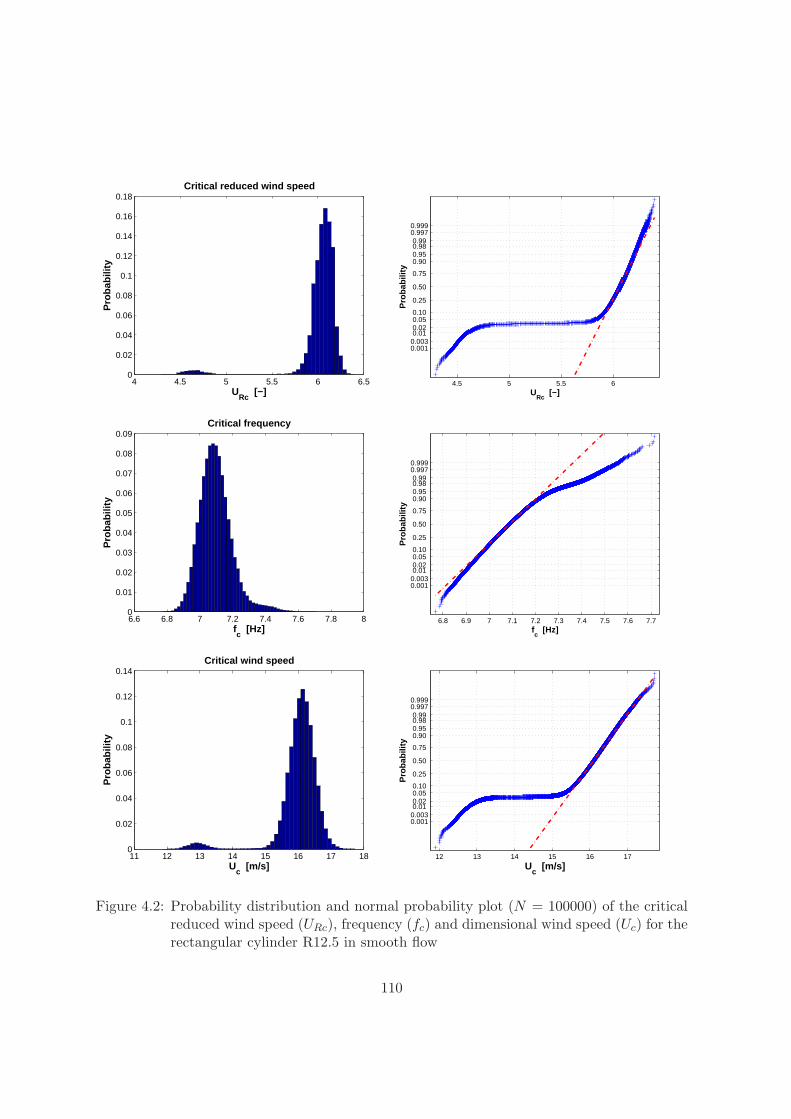
4 4.5 5 5.5 6 6.50

0.02

0.04

0.06

0.08

0.1

0.12

0.14

0.16

0.18Critical reduced wind speed

URc

[−]

Pro

babi

lity

4.5 5 5.5 6

0.0010.0030.01 0.02 0.05 0.10

0.25

0.50

0.75

0.90 0.95 0.98 0.99

0.9970.999

URc

[−]P

roba

bilit

y

6.6 6.8 7 7.2 7.4 7.6 7.8 80

0.01

0.02

0.03

0.04

0.05

0.06

0.07

0.08

0.09Critical frequency

fc [Hz]

Pro

bab

ility

6.8 6.9 7 7.1 7.2 7.3 7.4 7.5 7.6 7.7

0.0010.0030.01 0.02 0.05 0.10

0.25

0.50

0.75

0.90 0.95 0.98 0.99

0.9970.999

fc [Hz]

Pro

bab

ility

11 12 13 14 15 16 17 180

0.02

0.04

0.06

0.08

0.1

0.12

0.14Critical wind speed

Uc [m/s]

Pro

bab

ility

12 13 14 15 16 17

0.0010.0030.01 0.02 0.05 0.10

0.25

0.50

0.75

0.90 0.95 0.98 0.99

0.9970.999

Uc [m/s]

Pro

bab

ility

Figure 4.2: Probability distribution and normal probability plot (N = 100000) of the criticalreduced wind speed (URc), frequency (fc) and dimensional wind speed (Uc) for therectangular cylinder R12.5 in smooth flow

110

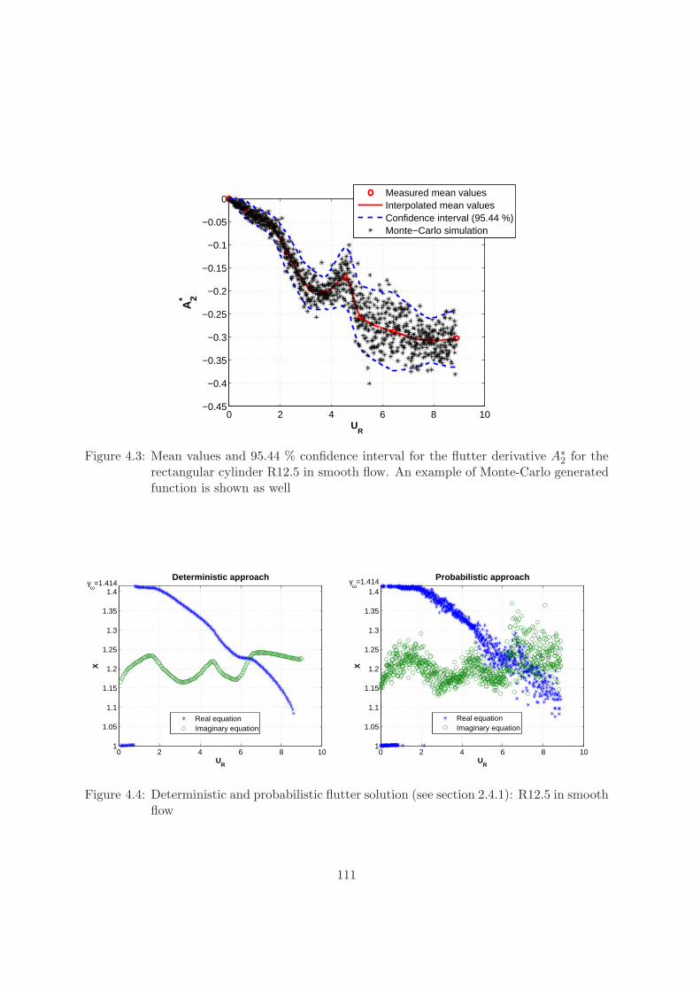
0 2 4 6 8 10−0.45

−0.4

−0.35

−0.3

−0.25

−0.2

−0.15

−0.1

−0.05

0

UR

A2*

Measured mean valuesInterpolated mean valuesConfidence interval (95.44 %)Monte−Carlo simulation

Figure 4.3: Mean values and 95.44 % confidence interval for the flutter derivative A∗2 for therectangular cylinder R12.5 in smooth flow. An example of Monte-Carlo generatedfunction is shown as well

0 2 4 6 8 101

1.05

1.1

1.15

1.2

1.25

1.3

1.35

1.4

UR

X

Deterministic approachγω=1.414

Real equationImaginary equation

0 2 4 6 8 101

1.05

1.1

1.15

1.2

1.25

1.3

1.35

1.4

UR

X

Probabilistic approachγω=1.414

Real equationImaginary equation

Figure 4.4: Deterministic and probabilistic flutter solution (see section 2.4.1): R12.5 in smoothflow

111

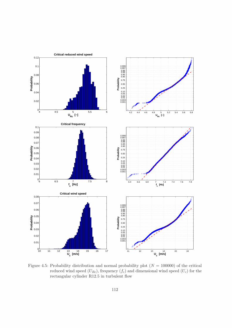
4 4.5 5 5.5 60

0.02

0.04

0.06

0.08

0.1

0.12Critical reduced wind speed

URc

[−]

Pro

babi

lity

4.2 4.4 4.6 4.8 5 5.2 5.4 5.6 5.8

0.0010.0030.01 0.02 0.05 0.10

0.25

0.50

0.75

0.90 0.95 0.98 0.99

0.9970.999

URc

[−]P

roba

bilit

y

6 6.5 7 7.5 80

0.01

0.02

0.03

0.04

0.05

0.06

0.07

0.08

0.09

0.1Critical frequency

fc [Hz]

Pro

bab

ility

6.4 6.6 6.8 7 7.2 7.4 7.6 7.8

0.0010.0030.01 0.02 0.05 0.10

0.25

0.50

0.75

0.90 0.95 0.98 0.99

0.9970.999

fc [Hz]

Pro

bab

ility

10 11 12 13 14 15 16 170

0.01

0.02

0.03

0.04

0.05

0.06

0.07

0.08Critical wind speed

Uc [m/s]

Pro

bab

ility

11 12 13 14 15 16

0.0010.0030.01 0.02 0.05 0.10

0.25

0.50

0.75

0.90 0.95 0.98 0.99

0.9970.999

Uc [m/s]

Pro

bab

ility

Figure 4.5: Probability distribution and normal probability plot (N = 100000) of the criticalreduced wind speed (URc), frequency (fc) and dimensional wind speed (Uc) for therectangular cylinder R12.5 in turbulent flow

112

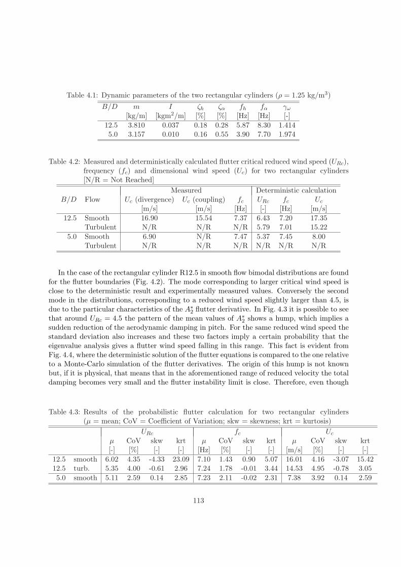
Table 4.1: Dynamic parameters of the two rectangular cylinders (ρ = 1.25 kg/m3)

B/D m I ζh ζα fh fα γω

[kg/m] [kgm2/m] [%] [%] [Hz] [Hz] [-]12.5 3.810 0.037 0.18 0.28 5.87 8.30 1.4145.0 3.157 0.010 0.16 0.55 3.90 7.70 1.974

Table 4.2: Measured and deterministically calculated flutter critical reduced wind speed (URc),frequency (fc) and dimensional wind speed (Uc) for two rectangular cylinders[N/R = Not Reached]

Measured Deterministic calculationB/D Flow Uc (divergence) Uc (coupling) fc URc fc Uc

[m/s] [m/s] [Hz] [-] [Hz] [m/s]12.5 Smooth 16.90 15.54 7.37 6.43 7.20 17.35

Turbulent N/R N/R N/R 5.79 7.01 15.225.0 Smooth 6.90 N/R 7.47 5.37 7.45 8.00

Turbulent N/R N/R N/R N/R N/R N/R

In the case of the rectangular cylinder R12.5 in smooth flow bimodal distributions are foundfor the flutter boundaries (Fig. 4.2). The mode corresponding to larger critical wind speed isclose to the deterministic result and experimentally measured values. Conversely the secondmode in the distributions, corresponding to a reduced wind speed slightly larger than 4.5, isdue to the particular characteristics of the A∗2 flutter derivative. In Fig. 4.3 it is possible to seethat around URc = 4.5 the pattern of the mean values of A∗2 shows a hump, which implies asudden reduction of the aerodynamic damping in pitch. For the same reduced wind speed thestandard deviation also increases and these two factors imply a certain probability that theeigenvalue analysis gives a flutter wind speed falling in this range. This fact is evident fromFig. 4.4, where the deterministic solution of the flutter equations is compared to the one relativeto a Monte-Carlo simulation of the flutter derivatives. The origin of this hump is not knownbut, if it is physical, that means that in the aforementioned range of reduced velocity the totaldamping becomes very small and the flutter instability limit is close. Therefore, even though

Table 4.3: Results of the probabilistic flutter calculation for two rectangular cylinders(µ = mean; CoV = Coefficient of Variation; skw = skewness; krt = kurtosis)

URc fc Uc

µ CoV skw krt µ CoV skw krt µ CoV skw krt[-] [%] [-] [-] [Hz] [%] [-] [-] [m/s] [%] [-] [-]

12.5 smooth 6.02 4.35 -4.33 23.09 7.10 1.43 0.90 5.07 16.01 4.16 -3.07 15.4212.5 turb. 5.35 4.00 -0.61 2.96 7.24 1.78 -0.01 3.44 14.53 4.95 -0.78 3.055.0 smooth 5.11 2.59 0.14 2.85 7.23 2.11 -0.02 2.31 7.38 3.92 0.14 2.59

113

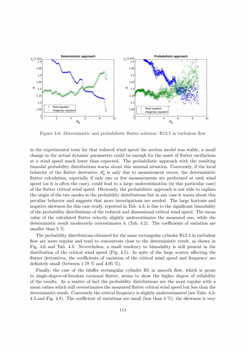
0 2 4 6 8 101

1.05

1.1

1.15

1.2

1.25

1.3

1.35

1.4

UR

X

Deterministic approachγω=1.414

Real equationImaginary equation

0 2 4 6 8 101

1.05

1.1

1.15

1.2

1.25

1.3

1.35

1.4

UR

X

Probabilistic approachγω=1.414

Real equationImaginary equation

Figure 4.6: Deterministic and probabilistic flutter solution: R12.5 in turbulent flow

in the experimental tests for that reduced wind speed the section model was stable, a smallchange in the actual dynamic parameters could be enough for the onset of flutter oscillationsat a wind speed much lower than expected. The probabilistic approach with the resultingbimodal probability distributions warns about this unusual situation. Conversely, if the localbehavior of the flutter derivative A∗2 is only due to measurement errors, the deterministicflutter calculation, especially if only one or few measurements are performed at each windspeed (as it is often the case), could lead to a large underestimation (in this particular case)of the flutter critical wind speed. Obviously, the probabilistic approach is not able to explainthe origin of the two modes in the probability distributions but in any case it warns about thispeculiar behavior and suggests that more investigations are needed. The large kurtosis andnegative skewness for this case study, reported in Tab. 4.3, is due to the significant bimodalityof the probability distributions of the reduced and dimensional critical wind speed. The meanvalue of the calculated flutter velocity slightly underestimates the measured one, while thedeterministic result moderately overestimates it (Tab. 4.2). The coefficients of variation aresmaller than 5 %.

The probability distributions obtained for the same rectangular cylinder R12.5 in turbulentflow are more regular and tend to concentrate close to the deterministic result, as shown inFig. 4.6 and Tab. 4.3. Nevertheless, a small tendency to bimodality is still present in thedistribution of the critical wind speed (Fig. 4.5). In spite of the large scatter affecting theflutter derivatives, the coefficients of variation of the critical wind speed and frequency aredefinitely small (between 1.78 % and 4.95 %).

Finally, the case of the bluffer rectangular cylinder R5 in smooth flow, which is proneto single-degree-of-freedom torsional flutter, seems to show the higher degree of reliabilityof the results. As a matter of fact the probability distributions are the most regular with amean values which still overestimates the measured flutter critical wind speed but less than thedeterministic result. Conversely the critical frequency is slightly underestimated (see Tabs. 4.2-4.3 and Fig. 4.8). The coefficient of variations are small (less than 4 %), the skewness is very

114

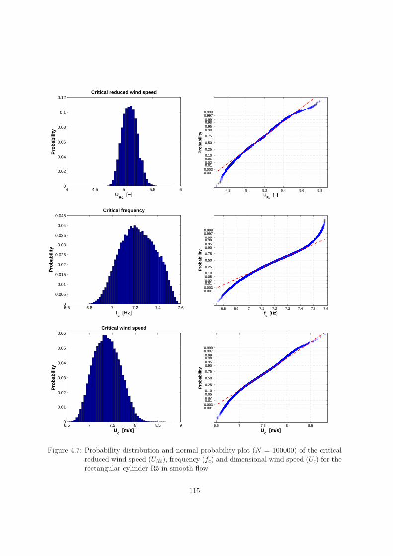
4 4.5 5 5.5 60

0.02

0.04

0.06

0.08

0.1

0.12Critical reduced wind speed

URc

[−]

Pro

babi

lity

4.8 5 5.2 5.4 5.6 5.8

0.0010.0030.01 0.02 0.05 0.10

0.25

0.50

0.75

0.90 0.95 0.98 0.99

0.9970.999

URc

[−]P

roba

bilit

y

6.6 6.8 7 7.2 7.4 7.60

0.005

0.01

0.015

0.02

0.025

0.03

0.035

0.04

0.045Critical frequency

fc [Hz]

Pro

bab

ility

6.8 6.9 7 7.1 7.2 7.3 7.4 7.5 7.6

0.0010.0030.01 0.02 0.05 0.10

0.25

0.50

0.75

0.90 0.95 0.98 0.99

0.9970.999

fc [Hz]

Pro

bab

ility

6.5 7 7.5 8 8.5 90

0.01

0.02

0.03

0.04

0.05

0.06Critical wind speed

Uc [m/s]

Pro

bab

ility

6.5 7 7.5 8 8.5

0.0010.0030.01 0.02 0.05 0.10

0.25

0.50

0.75

0.90 0.95 0.98 0.99

0.9970.999

Uc [m/s]

Pro

bab

ility

Figure 4.7: Probability distribution and normal probability plot (N = 100000) of the criticalreduced wind speed (URc), frequency (fc) and dimensional wind speed (Uc) for therectangular cylinder R5 in smooth flow

115

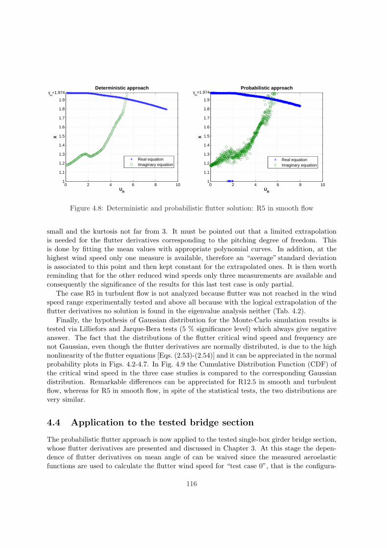
0 2 4 6 8 101

1.1

1.2

1.3

1.4

1.5

1.6

1.7

1.8

1.9

UR

X

Deterministic approachγω=1.974

Real equationImaginary equation

0 2 4 6 8 101

1.1

1.2

1.3

1.4

1.5

1.6

1.7

1.8

1.9

UR

X

Probabilistic approachγω=1.974

Real equationImaginary equation

Figure 4.8: Deterministic and probabilistic flutter solution: R5 in smooth flow

small and the kurtosis not far from 3. It must be pointed out that a limited extrapolationis needed for the flutter derivatives corresponding to the pitching degree of freedom. Thisis done by fitting the mean values with appropriate polynomial curves. In addition, at thehighest wind speed only one measure is available, therefore an “average” standard deviationis associated to this point and then kept constant for the extrapolated ones. It is then worthreminding that for the other reduced wind speeds only three measurements are available andconsequently the significance of the results for this last test case is only partial.

The case R5 in turbulent flow is not analyzed because flutter was not reached in the windspeed range experimentally tested and above all because with the logical extrapolation of theflutter derivatives no solution is found in the eigenvalue analysis neither (Tab. 4.2).

Finally, the hypothesis of Gaussian distribution for the Monte-Carlo simulation results istested via Lilliefors and Jarque-Bera tests (5 % significance level) which always give negativeanswer. The fact that the distributions of the flutter critical wind speed and frequency arenot Gaussian, even though the flutter derivatives are normally distributed, is due to the highnonlinearity of the flutter equations [Eqs. (2.53)-(2.54)] and it can be appreciated in the normalprobability plots in Figs. 4.2-4.7. In Fig. 4.9 the Cumulative Distribution Function (CDF) ofthe critical wind speed in the three case studies is compared to the corresponding Gaussiandistribution. Remarkable differences can be appreciated for R12.5 in smooth and turbulentflow, whereas for R5 in smooth flow, in spite of the statistical tests, the two distributions arevery similar.

4.4 Application to the tested bridge section

The probabilistic flutter approach is now applied to the tested single-box girder bridge section,whose flutter derivatives are presented and discussed in Chapter 3. At this stage the depen-dence of flutter derivatives on mean angle of can be waived since the measured aeroelasticfunctions are used to calculate the flutter wind speed for “test case 0”, that is the configura-

116

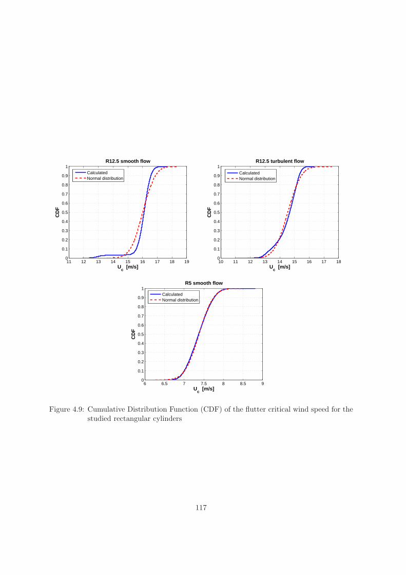
11 12 13 14 15 16 17 18 190

0.1

0.2

0.3

0.4

0.5

0.6

0.7

0.8

0.9

1

Uc [m/s]

CD

F

R12.5 smooth flow

CalculatedNormal distribution

10 11 12 13 14 15 16 17 180

0.1

0.2

0.3

0.4

0.5

0.6

0.7

0.8

0.9

1

Uc [m/s]

CD

F

R12.5 turbulent flow

CalculatedNormal distribution

6 6.5 7 7.5 8 8.5 90

0.1

0.2

0.3

0.4

0.5

0.6

0.7

0.8

0.9

1

Uc [m/s]

CD

F

R5 smooth flow

CalculatedNormal distribution

Figure 4.9: Cumulative Distribution Function (CDF) of the flutter critical wind speed for thestudied rectangular cylinders

117

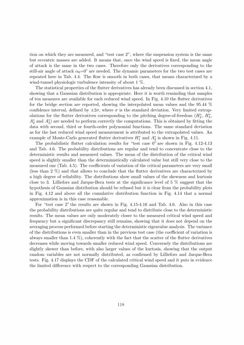
tion on which they are measured, and “test case 2”, where the suspension system is the samebut eccentric masses are added. It means that, once the wind speed is fixed, the mean angleof attack is the same in the two cases. Therefore only the derivatives corresponding to thestill-air angle of attack α0=0° are needed. The dynamic parameters for the two test cases arerepeated here in Tab. 4.4. The flow is smooth in both cases, that means characterized by awind-tunnel physiologic turbulence intensity of about 1 %.

The statistical properties of the flutter derivatives has already been discussed in section 4.1,showing that a Gaussian distribution is appropriate. Here it is worth reminding that samplesof ten measures are available for each reduced wind speed. In Fig. 4.10 the flutter derivativesfor the bridge section are reported, showing the interpolated mean values and the 95.44 %confidence interval, defined by ±2σ, where σ is the standard deviation. Very limited extrap-olations for the flutter derivatives corresponding to the pitching degree-of-freedom (H∗

2 , H∗3 ,

A∗2 and A∗3) are needed to perform correctly the computations. This is obtained by fitting thedata with second, third or fourth-order polynomial functions. The same standard deviationas for the last reduced wind speed measurement is attributed to the extrapolated values. Anexample of Monte-Carlo generated flutter derivatives H∗

1 and A∗2 is shown in Fig. 4.11.The probabilistic flutter calculation results for “test case 0” are shown in Fig. 4.12-4.13

and Tab. 4.6. The probability distributions are regular and tend to concentrate close to thedeterministic results and measured values. The mean of the distribution of the critical windspeed is slightly smaller than the deterministically calculated value but still very close to themeasured one (Tab. 4.5). The coefficients of variation of the critical parameters are very small(less than 2 %) and that allows to conclude that the flutter derivatives are characterized bya high degree of reliability. The distributions show small values of the skewness and kurtosisclose to 3. Lilliefors and Jarque-Bera tests at the significance level of 5 % suggest that thehypothesis of Gaussian distribution should be refused but it is clear from the probability plotsin Fig. 4.12 and above all the cumulative distribution function in Fig. 4.14 that a normalapproximation is in this case reasonable.

For “test case 2” the results are shown in Fig. 4.15-4.16 and Tab. 4.6. Also in this casethe probability distributions are quite regular and tend to distribute close to the deterministicresults. The mean values are only moderately closer to the measured critical wind speed andfrequency but a significant discrepancy still remains, showing that it does not depend on theaveraging process performed before starting the deterministic eigenvalue analysis. The varianceof the distributions is even smaller than in the previous test case (the coefficient of variation isalways smaller than 1.4 %), coherently with the fact that the scatter of the flutter derivativesdecreases while moving towards smaller reduced wind speed. Conversely the distributions areslightly skewer than before, with also larger values of the kurtosis, showing that the outputrandom variables are not normally distributed, as confirmed by Lilliefors and Jarque-Beratests. Fig. 4.17 displays the CDF of the calculated critical wind speed and it puts in evidencethe limited difference with respect to the corresponding Gaussian distribution.

118

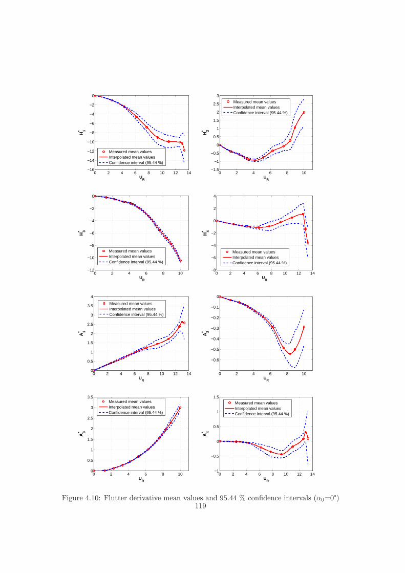
0 2 4 6 8 10 12 14−16

−14

−12

−10

−8

−6

−4

−2

0

UR

H1*

Measured mean valuesInterpolated mean valuesConfidence interval (95.44 %)

0 2 4 6 8 10−1.5

−1

−0.5

0

0.5

1

1.5

2

2.5

3

UR

H2*

Measured mean valuesInterpolated mean valuesConfidence interval (95.44 %)

0 2 4 6 8 10−12

−10

−8

−6

−4

−2

0

UR

H3*

Measured mean valuesInterpolated mean valuesConfidence interval (95.44 %)

0 2 4 6 8 10 12 14−8

−6

−4

−2

0

2

4

UR

H4*

Measured mean valuesInterpolated mean valuesConfidence interval (95.44 %)

0 2 4 6 8 10 12 140

0.5

1

1.5

2

2.5

3

3.5

4

UR

A1*

Measured mean valuesInterpolated mean valuesConfidence interval (95.44 %)

0 2 4 6 8 10

−0.6

−0.5

−0.4

−0.3

−0.2

−0.1

0

UR

A2*

0 2 4 6 8 100

0.5

1

1.5

2

2.5

3

3.5

UR

A3*

Measured mean valuesInterpolated mean valuesConfidence interval (95.44 %)

0 2 4 6 8 10 12 14−1

−0.5

0

0.5

1

1.5

UR

A4*

Measured mean valuesInterpolated mean valuesConfidence interval (95.44 %)

Figure 4.10: Flutter derivative mean values and 95.44 % confidence intervals (α0=0°)119

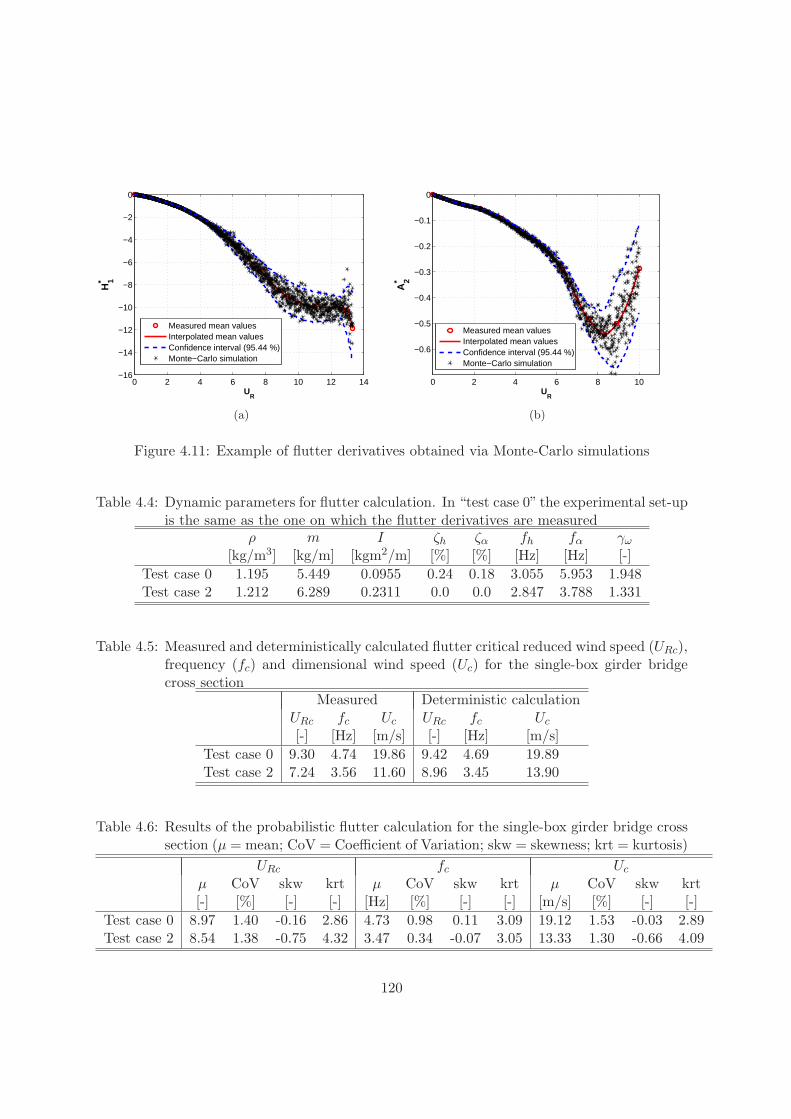
0 2 4 6 8 10 12 14−16

−14

−12

−10

−8

−6

−4

−2

0

UR

H1*

Measured mean valuesInterpolated mean valuesConfidence interval (95.44 %)Monte−Carlo simulation

(a)

0 2 4 6 8 10

−0.6

−0.5

−0.4

−0.3

−0.2

−0.1

0

UR

A2*

Measured mean valuesInterpolated mean valuesConfidence interval (95.44 %)Monte−Carlo simulation

(b)

Figure 4.11: Example of flutter derivatives obtained via Monte-Carlo simulations

Table 4.4: Dynamic parameters for flutter calculation. In “test case 0” the experimental set-upis the same as the one on which the flutter derivatives are measured

ρ m I ζh ζα fh fα γω

[kg/m3] [kg/m] [kgm2/m] [%] [%] [Hz] [Hz] [-]Test case 0 1.195 5.449 0.0955 0.24 0.18 3.055 5.953 1.948Test case 2 1.212 6.289 0.2311 0.0 0.0 2.847 3.788 1.331

Table 4.5: Measured and deterministically calculated flutter critical reduced wind speed (URc),frequency (fc) and dimensional wind speed (Uc) for the single-box girder bridgecross section

Measured Deterministic calculationURc fc Uc URc fc Uc

[-] [Hz] [m/s] [-] [Hz] [m/s]Test case 0 9.30 4.74 19.86 9.42 4.69 19.89Test case 2 7.24 3.56 11.60 8.96 3.45 13.90

Table 4.6: Results of the probabilistic flutter calculation for the single-box girder bridge crosssection (µ = mean; CoV = Coefficient of Variation; skw = skewness; krt = kurtosis)

URc fc Uc

µ CoV skw krt µ CoV skw krt µ CoV skw krt[-] [%] [-] [-] [Hz] [%] [-] [-] [m/s] [%] [-] [-]

Test case 0 8.97 1.40 -0.16 2.86 4.73 0.98 0.11 3.09 19.12 1.53 -0.03 2.89Test case 2 8.54 1.38 -0.75 4.32 3.47 0.34 -0.07 3.05 13.33 1.30 -0.66 4.09

120

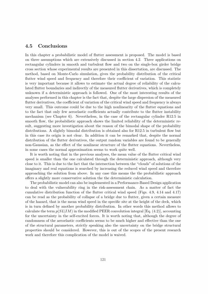
4.5 Conclusions

In this chapter a probabilistic model of flutter assessment is proposed. The model is basedon three assumptions which are extensively discussed in section 4.2. Three applications onrectangular cylinders in smooth and turbulent flow and two on the single-box girder bridgecross section whose experimental results are presented in this dissertation, are discussed. Themethod, based on Monte-Carlo simulation, gives the probability distribution of the criticalflutter wind speed and frequency and therefore their coefficient of variation. This statisticis very important because it allows to estimate the actual degree of reliability of the calcu-lated flutter boundaries and indirectly of the measured flutter derivatives, which is completelyunknown if a deterministic approach is followed. One of the most interesting results of theanalyses performed in this chapter is the fact that, despite the large dispersion of the measuredflutter derivatives, the coefficient of variation of the critical wind speed and frequency is alwaysvery small. This outcome could be due to the high nonlinearity of the flutter equations andto the fact that only few aeroelastic coefficients actually contribute to the flutter instabilitymechanism (see Chapter 6). Nevertheless, in the case of the rectangular cylinder R12.5 insmooth flow, the probabilistic approach shows the limited reliability of the deterministic re-sult, suggesting more investigation about the reason of the bimodal shape of the probabilitydistributions. A slightly bimodal distribution is obtained also for R12.5 in turbulent flow butin this case its origin is not clear. In addition it can be remarked that, despite the normaldistribution of the flutter derivatives, the output random variables are found to be generallynon-Gaussian, as the effect of the nonlinear structure of the flutter equations. Nevertheless,in some cases the normal approximation seems to work quite well.

It is worth noting that in the previous analyses, the mean value of the flutter critical windspeed is smaller than the one calculated through the deterministic approach, although veryclose to it. This is due to the fact that the intersection between the “clouds” of solutions of theimaginary and real equations is searched by increasing the reduced wind speed and thereforeapproaching the solution from above. In any case this means the the probabilistic approachoffers a slightly more conservative solution the the deterministic calculation.

The probabilistic model can also be implemented in a Performance-Based Design applicationto deal with the vulnerability ring in the risk-assessment chain. As a matter of fact thecumulative distribution function of the flutter critical wind speed (Figs. 4.9, 4.14 and 4.17)can be read as the probability of collapse of a bridge due to flutter, given a certain measureof the hazard, that is the mean wind speed in the specific site at the height of the deck, whichis in turn defined by another probability distribution. In other words this method allows tocalculate the term p(SL|IM) in the modified PEER convolution integral [Eq. (4.2)], accountingfor the uncertainty in the self-excited forces. It is worth noting that, although the degree ofrandomness of the aeroelastic coefficients seems to be much higher and effective than the oneof the structural parameters, strictly speaking also the uncertainty on the bridge structuralproperties should be considered. However, this is out of the scopes of the present researchwork and therefore this complication of the model is waived.

121

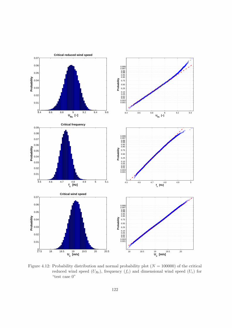
8.4 8.6 8.8 9 9.2 9.4 9.60

0.01

0.02

0.03

0.04

0.05

0.06

0.07Critical reduced wind speed

URc

[−]

Pro

babi

lity

8.4 8.6 8.8 9 9.2 9.4

0.0010.0030.01 0.02 0.05 0.10

0.25

0.50

0.75

0.90 0.95 0.98 0.99

0.9970.999

URc

[−]P

roba

bilit

y

4.5 4.6 4.7 4.8 4.9 5 5.10

0.01

0.02

0.03

0.04

0.05

0.06

0.07

0.08

0.09Critical frequency

fc [Hz]

Pro

bab

ility

4.5 4.6 4.7 4.8 4.9 5

0.0010.0030.01 0.02 0.05 0.10

0.25

0.50

0.75

0.90 0.95 0.98 0.99

0.9970.999

fc [Hz]

Pro

bab

ility

17.5 18 18.5 19 19.5 20 20.50

0.01

0.02

0.03

0.04

0.05

0.06

0.07Critical wind speed

Uc [m/s]

Pro

bab

ility

18 18.5 19 19.5 20

0.0010.0030.01 0.02 0.05 0.10

0.25

0.50

0.75

0.90 0.95 0.98 0.99

0.9970.999

Uc [m/s]

Pro

bab

ility

Figure 4.12: Probability distribution and normal probability plot (N = 100000) of the criticalreduced wind speed (URc), frequency (fc) and dimensional wind speed (Uc) for“test case 0”

122

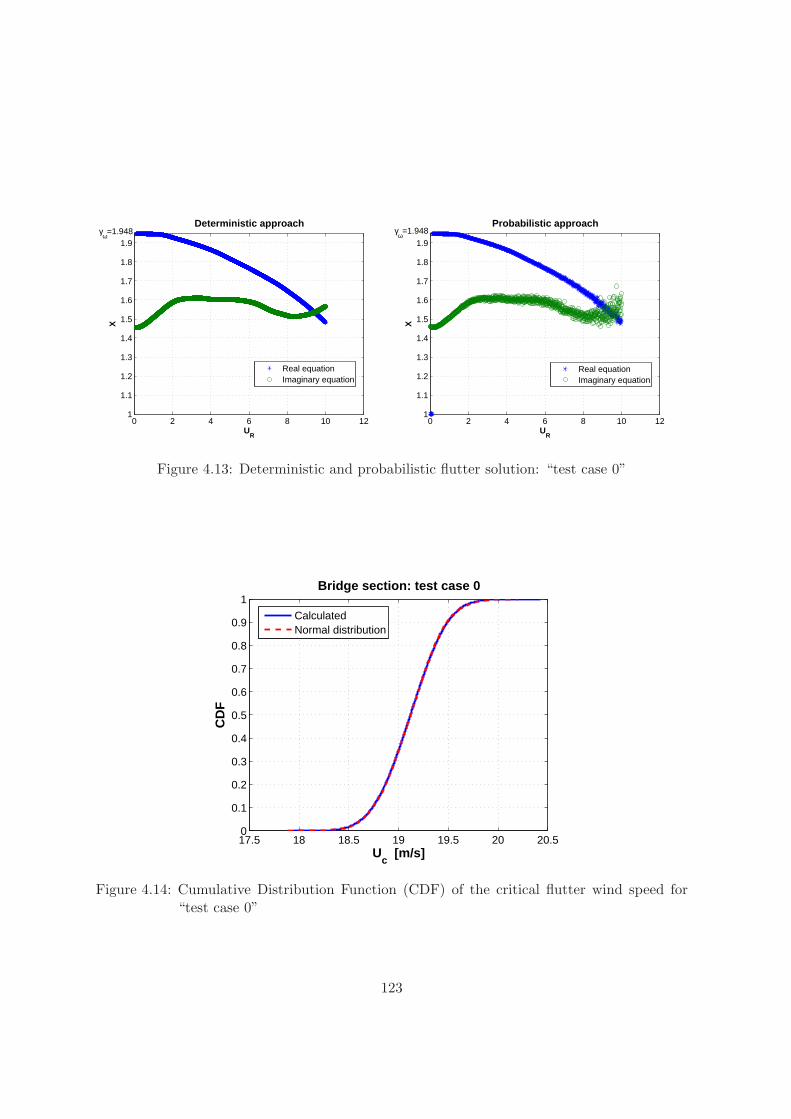
0 2 4 6 8 10 121

1.1

1.2

1.3

1.4

1.5

1.6

1.7

1.8

1.9

UR

X

Deterministic approachγω=1.948

Real equationImaginary equation

0 2 4 6 8 10 121

1.1

1.2

1.3

1.4

1.5

1.6

1.7

1.8

1.9

UR

X

Probabilistic approachγω=1.948

Real equationImaginary equation

Figure 4.13: Deterministic and probabilistic flutter solution: “test case 0”

17.5 18 18.5 19 19.5 20 20.50

0.1

0.2

0.3

0.4

0.5

0.6

0.7

0.8

0.9

1

Uc [m/s]

CD

F

Bridge section: test case 0

CalculatedNormal distribution

Figure 4.14: Cumulative Distribution Function (CDF) of the critical flutter wind speed for“test case 0”

123

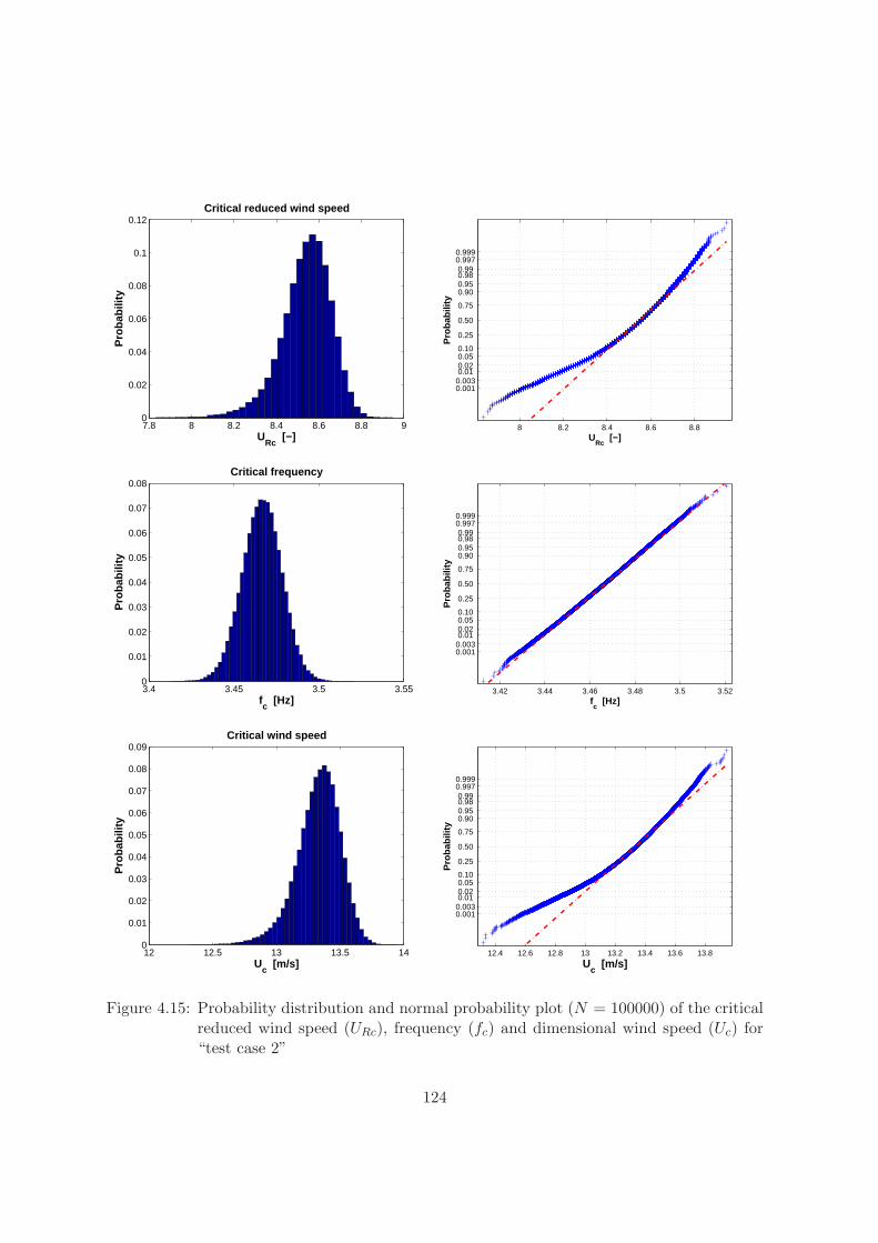
7.8 8 8.2 8.4 8.6 8.8 90

0.02

0.04

0.06

0.08

0.1

0.12Critical reduced wind speed

URc

[−]

Pro

babi

lity

8 8.2 8.4 8.6 8.8

0.0010.0030.01 0.02 0.05 0.10

0.25

0.50

0.75

0.90 0.95 0.98 0.99

0.9970.999

URc

[−]P

roba

bilit

y

3.4 3.45 3.5 3.550

0.01

0.02

0.03

0.04

0.05

0.06

0.07

0.08Critical frequency

fc [Hz]

Pro

bab

ility

3.42 3.44 3.46 3.48 3.5 3.52

0.0010.0030.01 0.02 0.05 0.10

0.25

0.50

0.75

0.90 0.95 0.98 0.99

0.9970.999

fc [Hz]

Pro

bab

ility

12 12.5 13 13.5 140

0.01

0.02

0.03

0.04

0.05

0.06

0.07

0.08

0.09Critical wind speed

Uc [m/s]

Pro

bab

ility

12.4 12.6 12.8 13 13.2 13.4 13.6 13.8

0.0010.0030.01 0.02 0.05 0.10

0.25

0.50

0.75

0.90 0.95 0.98 0.99

0.9970.999

Uc [m/s]

Pro

bab

ility

Figure 4.15: Probability distribution and normal probability plot (N = 100000) of the criticalreduced wind speed (URc), frequency (fc) and dimensional wind speed (Uc) for“test case 2”

124

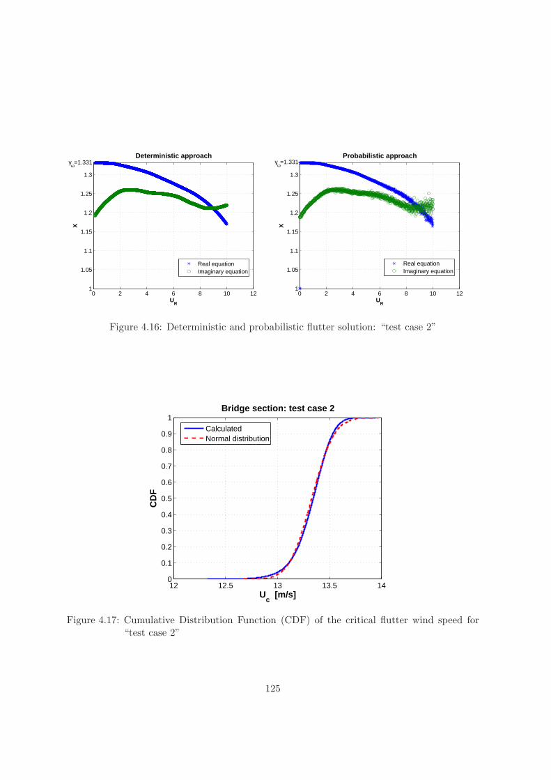
0 2 4 6 8 10 121

1.05

1.1

1.15

1.2

1.25

1.3

UR

X

Deterministic approachγω=1.331

Real equationImaginary equation

0 2 4 6 8 10 121

1.05

1.1

1.15

1.2

1.25

1.3

UR

X

Probabilistic approachγω=1.331

Real equationImaginary equation

Figure 4.16: Deterministic and probabilistic flutter solution: “test case 2”

12 12.5 13 13.5 140

0.1

0.2

0.3

0.4

0.5

0.6

0.7

0.8

0.9

1

Uc [m/s]

CD

F

Bridge section: test case 2

CalculatedNormal distribution

Figure 4.17: Cumulative Distribution Function (CDF) of the critical flutter wind speed for“test case 2”

125

Chapter 5

From multimodal to bimodalapproach to flutter

5.1 Introduction

In the section 1.4 it is stated that code-implementation can be an effective strategy of riskmitigation and in Fig. 1.4 the procedure we are following to set up a simplified method offlutter assessment is schematized. The simplified formulas and the discussion about flutterderivative generalization are treated in the next two chapters. Here only the first box ofthe flow chart is analyzed, that is the simplification from multimodal to bimodal approach toflutter. This step is crucial because it implies a strong simplification of the model, reducing thenumber of experimental functions from 18 to 8 and the number of modes from n to 2. In thisway the flutter calculation becomes much easier to handle, reducing the possibilities of errorand allowing a better understanding of the basic features of the phenomenon. Nevertheless,the most important consequence of this simplification is that the identification of ten flutterderivatives, namely H∗

5 , H∗6 , A∗5, A∗6, P ∗

1 ,...,P ∗6 , which are extremely difficult to be measured

in wind tunnel and whose reliability is known to be poor, is no longer necessary.The bimodal approach to flutter is often adopted instead of the multimodal one in prac-

tical applications but it is not completely clear which is the approximation which it actuallyintroduces. Since the simplified formulas we are proposing in Chapter 6 are directly based onthe assumption of binary flutter, it is crucial to check accurately the validity of this model.

Several investigations about the multimodal approach to flutter seem to suggest that thenature of the phenomenon is less complicated and that generally only a bending and a torsionalmode give rise to the instability. This seems to be true even for such a peculiar structure likeMessina Strait Bridge, where, according to D’Asdia and Sepe (1998) and Caracoglia (2000),only the first antisymmetric vertical bending and torsional modes couple in the neighborhoodof the critical wind speed.

The scope of the present chapter is to discuss and clarify the relationship between multimodeand binary flutter, highlighting the individual steps that lead to the simplified model and thepossible limits in their validity. Finally two examples of bridge structures are analyzed tosupport the theoretical investigations.

127

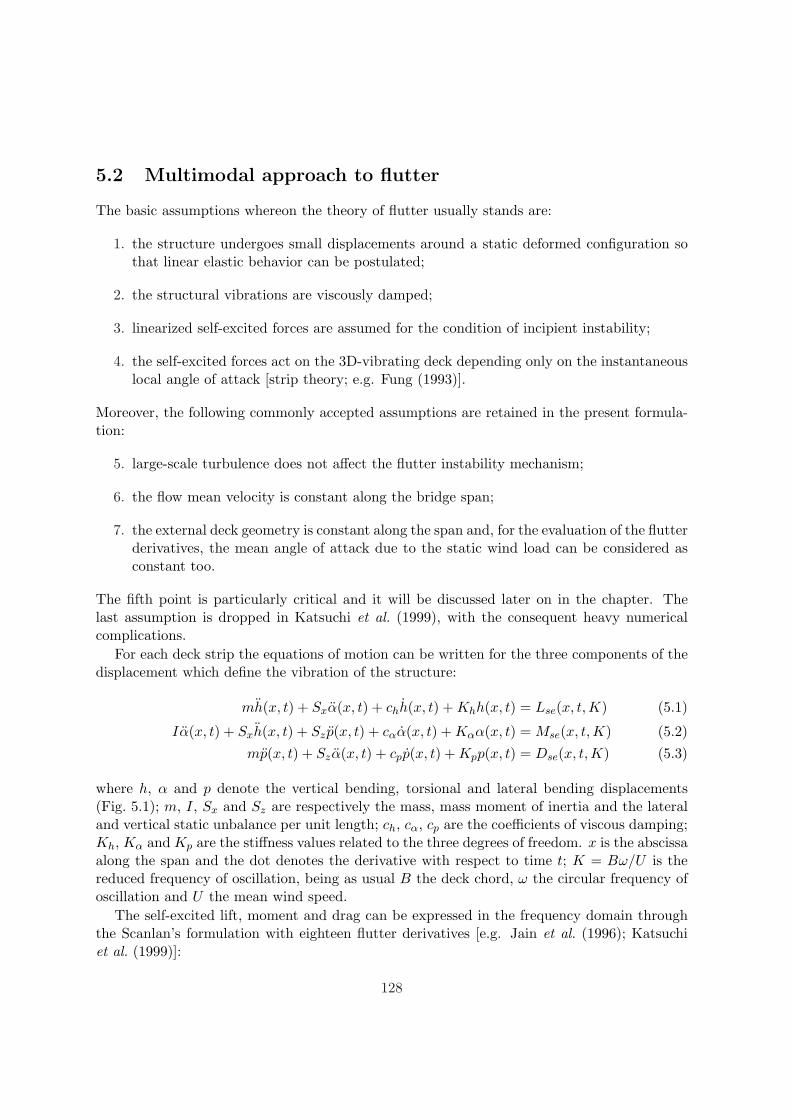
5.2 Multimodal approach to flutter

The basic assumptions whereon the theory of flutter usually stands are:

1. the structure undergoes small displacements around a static deformed configuration sothat linear elastic behavior can be postulated;

2. the structural vibrations are viscously damped;

3. linearized self-excited forces are assumed for the condition of incipient instability;

4. the self-excited forces act on the 3D-vibrating deck depending only on the instantaneouslocal angle of attack [strip theory; e.g. Fung (1993)].

Moreover, the following commonly accepted assumptions are retained in the present formula-tion:

5. large-scale turbulence does not affect the flutter instability mechanism;

6. the flow mean velocity is constant along the bridge span;

7. the external deck geometry is constant along the span and, for the evaluation of the flutterderivatives, the mean angle of attack due to the static wind load can be considered asconstant too.

The fifth point is particularly critical and it will be discussed later on in the chapter. Thelast assumption is dropped in Katsuchi et al. (1999), with the consequent heavy numericalcomplications.

For each deck strip the equations of motion can be written for the three components of thedisplacement which define the vibration of the structure:

mh(x, t) + Sxα(x, t) + chh(x, t) + Khh(x, t) = Lse(x, t,K) (5.1)

Iα(x, t) + Sxh(x, t) + Sz p(x, t) + cαα(x, t) + Kαα(x, t) = Mse(x, t,K) (5.2)mp(x, t) + Szα(x, t) + cpp(x, t) + Kpp(x, t) = Dse(x, t, K) (5.3)

where h, α and p denote the vertical bending, torsional and lateral bending displacements(Fig. 5.1); m, I, Sx and Sz are respectively the mass, mass moment of inertia and the lateraland vertical static unbalance per unit length; ch, cα, cp are the coefficients of viscous damping;Kh, Kα and Kp are the stiffness values related to the three degrees of freedom. x is the abscissaalong the span and the dot denotes the derivative with respect to time t; K = Bω/U is thereduced frequency of oscillation, being as usual B the deck chord, ω the circular frequency ofoscillation and U the mean wind speed.

The self-excited lift, moment and drag can be expressed in the frequency domain throughthe Scanlan’s formulation with eighteen flutter derivatives [e.g. Jain et al. (1996); Katsuchiet al. (1999)]:

128

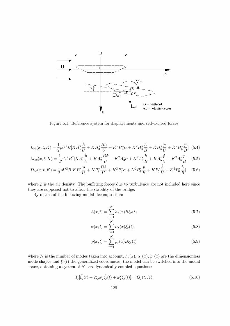
Figure 5.1: Reference system for displacements and self-excited forces

Lse(x, t, K) =12ρU2B[KH∗

1

h

U+ KH∗

2

Bα

U+ K2H∗

3α + K2H∗4

h

B+ KH∗

5

p

U+ K2H∗

6

p

B] (5.4)

Mse(x, t,K) =12ρU2B2[KA∗1

h

U+ KA∗2

Bα

U+ K2A∗3α + K2A∗4

h

B+ KA∗5

p

U+ K2A∗6

p

B] (5.5)

Dse(x, t,K) =12ρU2B[KP ∗

1

p

U+ KP ∗

2

Bα

U+ K2P ∗

3 α + K2P ∗4

p

B+ KP ∗

5

h

U+ K2P ∗

6

h

B] (5.6)

where ρ is the air density. The buffeting forces due to turbulence are not included here sincethey are supposed not to affect the stability of the bridge.

By means of the following modal decomposition:

h(x, t) =N∑

r=1

hr(x)Bξr(t) (5.7)

α(x, t) =N∑

r=1

αr(x)ξr(t) (5.8)

p(x, t) =N∑

r=1

pr(x)Bξr(t) (5.9)

where N is the number of modes taken into account, hr(x), αr(x), pr(x) are the dimensionlessmode shapes and ξr(t) the generalized coordinates, the model can be switched into the modalspace, obtaining a system of N aerodynamically coupled equations:

Ij [ξj(t) + 2ζjωj ξj(t) + ω2j ξj(t)] = Qj(t,K) (5.10)

129

where Ij , ωj and ζj are respectively the generalized mass, the circular frequency and the damp-ing ratio-to-critical associated with the j-th eigenmode of the structure (j=1...N). Qj(t,K)is the frequency-time dependent generalized force given by:

Qj(t,K) =∫

S(LseBhj + Mseαj + DseBpj)ds ∼=

∫

D(LseBhj + Mseαj + DseBpj)dx (5.11)

The subscript S in Eq. (5.11) indicates that the integral is extended to the whole structurewhile D means that it is limited to the deck. In Eq. (5.11) it is assumed that the contributionof the self-excited forces to flutter instability is negligible outside the deck. This seems tobe acceptable for lift and moment but is known to be a rough approximation for drag. Thegeneralized mass is given by:

Ij =∫

Sη2

j (x, y, z) · dm(x, y, z) (5.12)

where ηj(x, y, z) is the full bridge mode shape and dm the infinitesimal mass. Introducing areference length L (usually the main span length), the equations of motion can be written inthe following way (Jain et al., 1996):

Ij(ξj + 2ζjωj ξj + ω2j ξj) =

12ρU2B2L · [KH∗

1

N∑

r=1

Bξr

UGhrhj

+ KH∗2

N∑

r=1

Bξr

UGαrhj

+

K2H∗3

N∑

r=1

ξrGαrhj + K2H∗4

N∑

r=1

ξrGhrhj + KH∗5

N∑

r=1

Bξr

UGprhj + K2H∗

6

N∑

r=1

ξrGprhj+

KA∗1N∑

r=1

Bξr

UGhrαj + KA∗2

N∑

r=1

Bξr

UGαrαj + K2A∗3

N∑

r=1

ξrGαrαj + K2A∗4N∑

r=1

ξrGhrαj+

KA∗5N∑

r=1

Bξr

UGprαj + K2A∗6

N∑

r=1

ξrGprαj + KP ∗1

N∑

r=1

Bξr

UGprpj + KP ∗

2

N∑

r=1

Bξr

UGαrpj+

K2P ∗3

N∑

r=1

ξrGαrpj + K2P ∗4

N∑

r=1

ξrGprpj + KP ∗5

N∑

r=1

Bξr

UGhrpj + K2P ∗

6

N∑

r=1

ξrGhrpj ]

(5.13)

where the coefficients denoted by G are the modal integrals:

Glrnj =∫

Dlr(x) · nj(x)

dx

L(5.14)

and l, n = h, α, p ; r, j = 1...N . It is important to point out that if the deck geometry, themean wind speed and the mean angle of attack are significantly varying along the span, theflutter derivatives are functions of the position x as well and they have to be kept inside theintegral of Eq. (5.14), as shown in Katsuchi et al. (1999).

130

In order to determine the flutter critical condition, harmonic oscillation at the commonfrequency ω is assumed:

ξj(t) = ξ0jeiωt (5.15)

where i =√−1 is the imaginary unit. The following equation in matrix notation is finally

obtained:E(X,K) · ξ0 = [D(X,K) + iF(X,K)] · ξ0 = 0 (5.16)

where it is set:

X = (Xj)j=1...N (5.17)ξ0 = (ξ0j)j=1...N (5.18)

being E(X,K) the matrix of the complex system of equations, whose components are givenby:

Ejr(Xj ,K) =(1− 2iζjXj −X2j ) · δjr + γj · [(iH∗

1 + H∗4 )Ghrhj + (iH∗

2 + H∗3 )Gαrhj+

(iH∗5 + H∗

6 )Gprhj + (iA∗1 + A∗4)Ghrαj + (iA∗2 + A∗3)Gαrαj + (iA∗5 + A∗6)Gprαj+

(iP ∗1 + P ∗

4 )Gprpj + (iP ∗2 + P ∗

3 )Gαrpj + (iP ∗5 + P ∗

6 )Ghrpj ](5.19)

where

γj =ρB4L

2Ij(5.20)

Xj =ωj

ω(5.21)

The flutter critical condition can be determined as the lowest value of U such that it exists areal value of ω for which the matrix E(X,K) becomes singular. The solution of the problem isquite laborious and it requires the computation of the generalized masses and 3N(3N + 1)/2modal integrals, given the symmetry of the G terms.

5.3 Model simplification

Starting from the complete multimode system, we want now to introduce a sequence of as-sumptions in order to finally obtain the binary flutter model. The first generally acceptedsimplification is to neglect the contribution of lateral displacements and drag forces. In mostcases this is not merely an option but is dictated by the difficulty to identify the correspondingflutter derivatives. In addition, it has already been remarked that considering the unsteadydrag forces acting on the deck alone might not be correct to describe the actual self-excited

131

contribution. Despite that, to neglect the drag and the horizontal degree of freedom seems tobe reasonable, at least for non-super-long-span bridges characterized by low-drag profiles.

In the flutter analysis of the Akashi Kaikyo Bridge performed by Katsuchi et al. (1999),it is found that neglecting the P ∗

2 and P ∗3 the critical wind speed increases of about 70 %.

This surprising result is not confirmed by some simple analyses carried out by the writer. Asa matter of fact, for the modified cross-section configuration (Katsuchi et al., 1999; Miyata,1995), practically the same critical wind speed and frequency found by Katsuchi et al. (1999)through a complete multimodal analysis, can be calculated with a simple bimodal approach,considering only the first symmetric vertical bending and first symmetric torsional modes (seeTabs. 6.7-6.8 in Chapter 6). However, given the relevance of this issue, an effort should bedone by the scientific community in order to shed some light on the actual role played by theflutter derivatives relative to drag and sway motion.

The second simplifying assumption that can be made is that the modes are pure verticalbending or pure torsional. This is absolutely true for symmetric decks (with respect to a longi-tudinal vertical plane) as the elastic center and the centroid are vertically aligned. Obviouslythis assumption should be rejected in the very particular case of asymmetric bridge decks. Asa consequence, the N coupled equations (N minus the number of lateral modes) can be dividedinto two groups (Nh relative to the vertical bending modes and Nα to torsional modes). Thennormalizing the generalized inertias and modal integrals as follows:

meq.r =

∫S m(x)h2

r(x)dx∫D h2

r(x)dx(5.22)

Ieq.s =

∫S I(x)α2

s(x)dx∫D α2

s(x)dx(5.23)

Chjhr =Ghjhr

Ghrhr

=

∫D hj(x)hr(x)dx∫

D h2r(x)dx

(5.24)

Cαkhr =Gαkhr

Ghrhr

=

∫D αk(x)hr(x)dx∫

D h2r(x)dx

(5.25)

Cαkαs =Gαkαs

Gαsαs

=

∫D αk(x)αs(x)dx∫

D α2s(x)dx

(5.26)

Chjαs =Ghjαs

Gαsαs

=

∫D hj(x)αs(x)dx∫

D α2s(x)dx

(5.27)

and setting:

pr(t) = Bξh.r(t) r = 1...Nh (5.28)qs(t) = ξα.s(t) s = 1...Nα (5.29)

where ξh.r(t) and ξα.s(t) are the generalized coordinates relative to the r-th vertical bendingmode and the s-th torsional mode respectively, the following equations can be obtained:

132

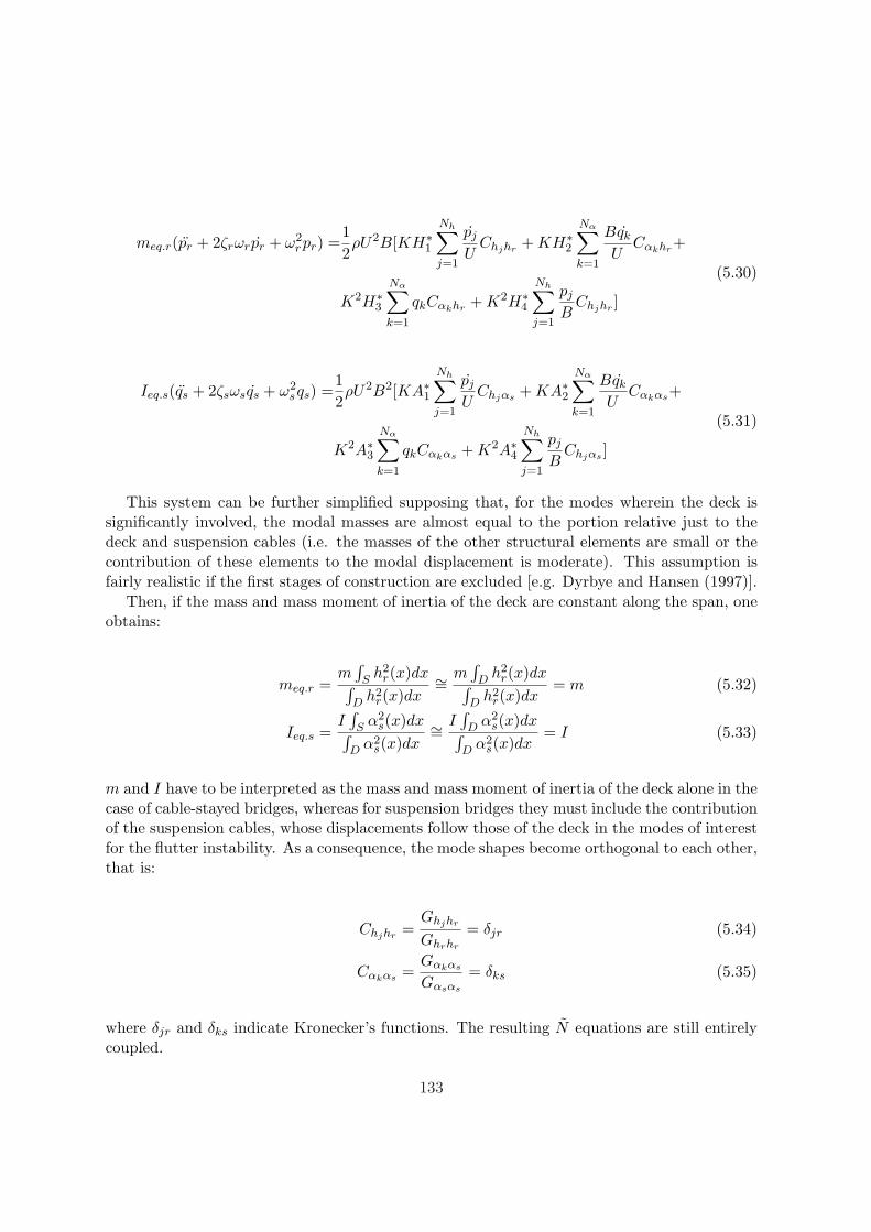
meq.r(pr + 2ζrωrpr + ω2rpr) =

12ρU2B[KH∗

1

Nh∑

j=1

pj

UChjhr + KH∗

2

Nα∑

k=1

Bqk

UCαkhr+

K2H∗3

Nα∑

k=1

qkCαkhr + K2H∗4

Nh∑

j=1

pj

BChjhr ]

(5.30)

Ieq.s(qs + 2ζsωsqs + ω2sqs) =

12ρU2B2[KA∗1

Nh∑

j=1

pj

UChjαs + KA∗2

Nα∑

k=1

Bqk

UCαkαs+

K2A∗3Nα∑

k=1

qkCαkαs + K2A∗4Nh∑

j=1

pj

BChjαs ]

(5.31)

This system can be further simplified supposing that, for the modes wherein the deck issignificantly involved, the modal masses are almost equal to the portion relative just to thedeck and suspension cables (i.e. the masses of the other structural elements are small or thecontribution of these elements to the modal displacement is moderate). This assumption isfairly realistic if the first stages of construction are excluded [e.g. Dyrbye and Hansen (1997)].

Then, if the mass and mass moment of inertia of the deck are constant along the span, oneobtains:

meq.r =m

∫S h2

r(x)dx∫D h2

r(x)dx∼= m

∫D h2

r(x)dx∫D h2

r(x)dx= m (5.32)

Ieq.s =I

∫S α2

s(x)dx∫D α2

s(x)dx∼= I

∫D α2

s(x)dx∫D α2

s(x)dx= I (5.33)

m and I have to be interpreted as the mass and mass moment of inertia of the deck alone in thecase of cable-stayed bridges, whereas for suspension bridges they must include the contributionof the suspension cables, whose displacements follow those of the deck in the modes of interestfor the flutter instability. As a consequence, the mode shapes become orthogonal to each other,that is:

Chjhr =Ghjhr

Ghrhr

= δjr (5.34)

Cαkαs =Gαkαs

Gαsαs

= δks (5.35)

where δjr and δks indicate Kronecker’s functions. The resulting N equations are still entirelycoupled.

133

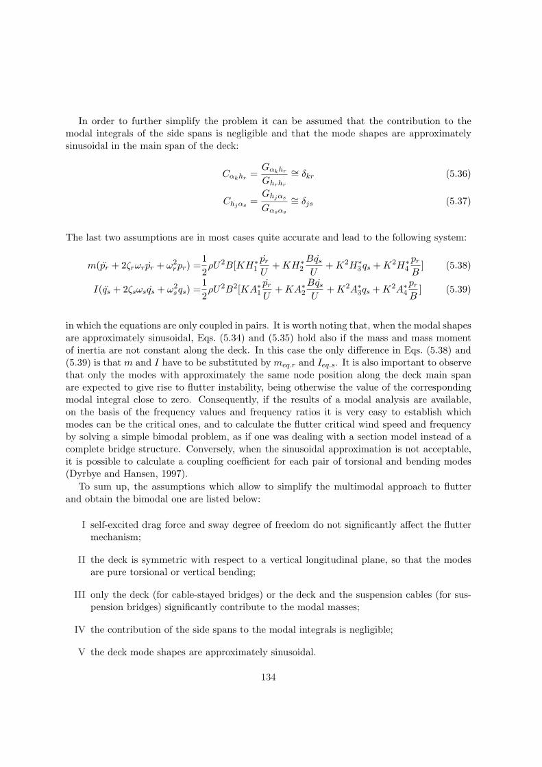
In order to further simplify the problem it can be assumed that the contribution to themodal integrals of the side spans is negligible and that the mode shapes are approximatelysinusoidal in the main span of the deck:

Cαkhr =Gαkhr

Ghrhr

∼= δkr (5.36)

Chjαs =Ghjαs

Gαsαs

∼= δjs (5.37)

The last two assumptions are in most cases quite accurate and lead to the following system:

m(pr + 2ζrωrpr + ω2rpr) =

12ρU2B[KH∗

1

pr

U+ KH∗

2

Bqs

U+ K2H∗

3qs + K2H∗4

pr

B] (5.38)

I(qs + 2ζsωsqs + ω2sqs) =

12ρU2B2[KA∗1

pr

U+ KA∗2

Bqs

U+ K2A∗3qs + K2A∗4

pr

B] (5.39)

in which the equations are only coupled in pairs. It is worth noting that, when the modal shapesare approximately sinusoidal, Eqs. (5.34) and (5.35) hold also if the mass and mass momentof inertia are not constant along the deck. In this case the only difference in Eqs. (5.38) and(5.39) is that m and I have to be substituted by meq.r and Ieq.s. It is also important to observethat only the modes with approximately the same node position along the deck main spanare expected to give rise to flutter instability, being otherwise the value of the correspondingmodal integral close to zero. Consequently, if the results of a modal analysis are available,on the basis of the frequency values and frequency ratios it is very easy to establish whichmodes can be the critical ones, and to calculate the flutter critical wind speed and frequencyby solving a simple bimodal problem, as if one was dealing with a section model instead of acomplete bridge structure. Conversely, when the sinusoidal approximation is not acceptable,it is possible to calculate a coupling coefficient for each pair of torsional and bending modes(Dyrbye and Hansen, 1997).

To sum up, the assumptions which allow to simplify the multimodal approach to flutterand obtain the bimodal one are listed below:

I self-excited drag force and sway degree of freedom do not significantly affect the fluttermechanism;

II the deck is symmetric with respect to a vertical longitudinal plane, so that the modesare pure torsional or vertical bending;

III only the deck (for cable-stayed bridges) or the deck and the suspension cables (for sus-pension bridges) significantly contribute to the modal masses;

IV the contribution of the side spans to the modal integrals is negligible;

V the deck mode shapes are approximately sinusoidal.

134

The validity of the assumptions from II to V can be straightforward checked just lookingat the results of the modal analysis, so that the degree of approximation they introduce iseasily perceived. Conversely, the first assumption cannot be verified unless the whole set ofeighteen flutter derivatives is experimentally measured. That assumption is definitely the mostquestionable point in this analysis and further investigation is needed on this issue.

5.4 Examples

In order to verify the simplifying assumptions discussed in the previous section, through whichthe multimodal problem is transformed into a bimodal one, two existing structures, a quitelarge suspension bridge and a small cable-stayed bridge, are taken into account as studycases. For this analysis sets of eighteen flutter derivatives are needed. Therefore the structuralcharacteristics of the bridges are associated to the aerodynamic properties of two cross-sectionalprofiles for which these aeroelastic data are available. This combination can be done because,as it is remarked in section 2.4.1, flutter derivatives are independent of the modal parametersof the structure on which these functions are measured. Nevertheless, the results of theflutter calculations no longer refer to the considered bridges but to hybrid non-existing (albeitpossible) structures.

5.4.1 Bosporus I Strait Bridge

The first study case is the Bosporus I Strait Bridge (Bogazici Bridge, Istanbul, Turkey, 1973),a suspension bridge with a main span of 1074 m [Figs. 5.2(c) and 5.2(a)]. The data about thestructure can be found in Martini (2004). The aerodynamic behavior of the deck is simulatedconsidering the flutter derivatives of a thin rectangular box girder section with semi-circularfairings and a chord-to-thickness ratio of 14.3 [Fig. 5.2(d)], reported in Chowdhury and Sarkar(2004).

The modal analysis is performed with the software SAP (CSI, 1999) on the finite-elementmodel displayed in Fig. 5.2(b). The results are listed in Tab. 5.1. As modal damping, given thesmall influence of this parameter on the flutter instability, an arbitrary value of 1 % is assumedfor all modes. The results of the rigorous multimodal (Multimodal I) and bimodal flutteranalyses are reported in Tab. 5.2 in terms of critical wind speed and coupling frequency. Othertwo calculations, both neglecting the lateral bending modes (Multimodal II and III) and thesecond one considering only the contributions of the deck to the modal masses (Multimodal III),are also included. It is evident that the difference in the results is negligible. Therefore thesimplifying assumptions discussed in the previous chapter seem to be in this case largelyreasonable, including the one about the negligibility of the flutter derivatives correspondingto drag and sway degree of freedom.

135

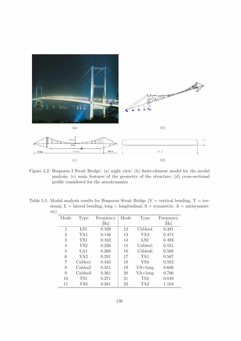
(a) (b)

(c) (d)

Figure 5.2: Bosporus I Strait Bridge: (a) night view; (b) finite-element model for the modalanalysis; (c) main features of the geometry of the structure; (d) cross-sectionalprofile considered for the aerodynamics

Table 5.1: Modal analysis results for Bosporus Strait Bridge (V = vertical bending, T = tor-sional, L = lateral bending, long = longitudinal, S = symmetric, A = antisymmet-ric)

Mode Type Frequency Mode Type Frequency[Hz] [Hz]

1 LS1 0.109 12 Cables4 0.3812 VA1 0.146 13 VA3 0.4743 VS1 0.162 14 LS2 0.4934 VS2 0.226 15 Cables5 0.5515 LA1 0.268 16 Cables6 0.5666 VA2 0.291 17 TA1 0.5677 Cables1 0.343 18 VS4 0.5828 Cables2 0.351 19 VS+long 0.6669 Cables3 0.361 20 VA+long 0.70610 TS1 0.371 21 TS2 0.84911 VS3 0.381 22 TA2 1.104

136

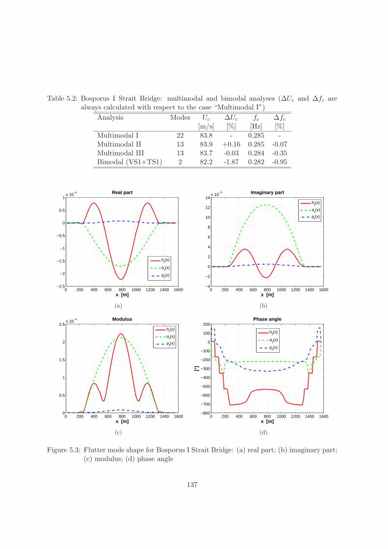
Table 5.2: Bosporus I Strait Bridge: multimodal and bimodal analyses (∆Uc and ∆fc arealways calculated with respect to the case “Multimodal I”)

Analysis Modes Uc ∆Uc fc ∆fc

[m/s] [%] [Hz] [%]Multimodal I 22 83.8 - 0.285 -Multimodal II 13 83.9 +0.16 0.285 -0.07Multimodal III 13 83.7 -0.03 0.284 -0.35Bimodal (VS1+TS1) 2 82.2 -1.87 0.282 -0.95

0 200 400 600 800 1000 1200 1400 1600−2.5

−2

−1.5

−1

−0.5

0

0.5

1x 10

−4

x [m]

Real part

hf(x)

αf(x)

pf(x)

(a)

0 200 400 600 800 1000 1200 1400 1600−4

−2

0

2

4

6

8

10

12

14x 10

−5

x [m]

Imaginary part

hf(x)

αf(x)

pf(x)

(b)

0 200 400 600 800 1000 1200 1400 16000

0.5

1

1.5

2

2.5x 10

−4

x [m]

Modulus

hf(x)

αf(x)

pf(x)

(c)

0 200 400 600 800 1000 1200 1400 1600−800

−700

−600

−500

−400

−300

−200

−100

0

100

200

x [m]

[°]

Phase angle

hf(x)

αf(x)

pf(x)

(d)

Figure 5.3: Flutter mode shape for Bosporus I Strait Bridge: (a) real part; (b) imaginary part;(c) modulus; (d) phase angle

137

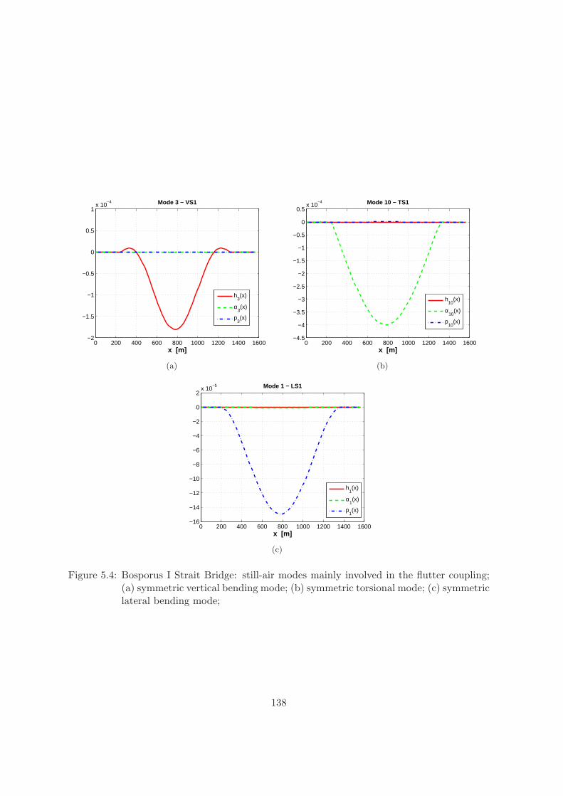
0 200 400 600 800 1000 1200 1400 1600−2

−1.5

−1

−0.5

0

0.5

1x 10

−4

x [m]

Mode 3 − VS1

h3(x)

α3(x)

p3(x)

(a)

0 200 400 600 800 1000 1200 1400 1600−4.5

−4

−3.5

−3

−2.5

−2

−1.5

−1

−0.5

0

0.5x 10

−4

x [m]

Mode 10 − TS1

h10

(x)

α10

(x)

p10

(x)

(b)

0 200 400 600 800 1000 1200 1400 1600−16

−14

−12

−10

−8

−6

−4

−2

0

2x 10

−5

x [m]

Mode 1 − LS1

h1(x)

α1(x)

p1(x)

(c)

Figure 5.4: Bosporus I Strait Bridge: still-air modes mainly involved in the flutter coupling;(a) symmetric vertical bending mode; (b) symmetric torsional mode; (c) symmetriclateral bending mode;

138

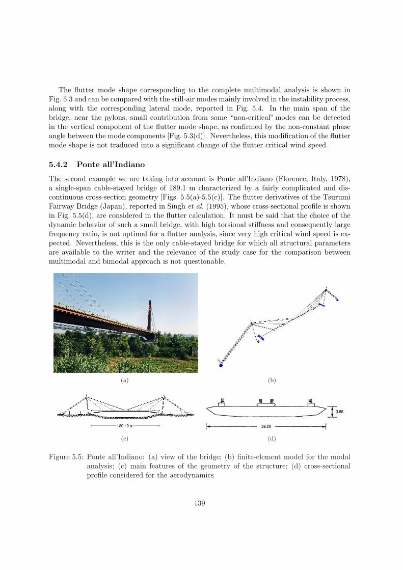
The flutter mode shape corresponding to the complete multimodal analysis is shown inFig. 5.3 and can be compared with the still-air modes mainly involved in the instability process,along with the corresponding lateral mode, reported in Fig. 5.4. In the main span of thebridge, near the pylons, small contribution from some “non-critical”modes can be detectedin the vertical component of the flutter mode shape, as confirmed by the non-constant phaseangle between the mode components [Fig. 5.3(d)]. Nevertheless, this modification of the fluttermode shape is not traduced into a significant change of the flutter critical wind speed.

5.4.2 Ponte all’Indiano

The second example we are taking into account is Ponte all’Indiano (Florence, Italy, 1978),a single-span cable-stayed bridge of 189.1 m characterized by a fairly complicated and dis-continuous cross-section geometry [Figs. 5.5(a)-5.5(c)]. The flutter derivatives of the TsurumiFairway Bridge (Japan), reported in Singh et al. (1995), whose cross-sectional profile is shownin Fig. 5.5(d), are considered in the flutter calculation. It must be said that the choice of thedynamic behavior of such a small bridge, with high torsional stiffness and consequently largefrequency ratio, is not optimal for a flutter analysis, since very high critical wind speed is ex-pected. Nevertheless, this is the only cable-stayed bridge for which all structural parametersare available to the writer and the relevance of the study case for the comparison betweenmultimodal and bimodal approach is not questionable.

(a) (b)

(c) (d)

Figure 5.5: Ponte all’Indiano: (a) view of the bridge; (b) finite-element model for the modalanalysis; (c) main features of the geometry of the structure; (d) cross-sectionalprofile considered for the aerodynamics

139

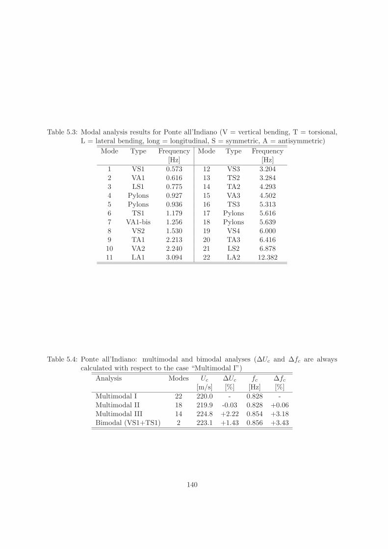
Table 5.3: Modal analysis results for Ponte all’Indiano (V = vertical bending, T = torsional,L = lateral bending, long = longitudinal, S = symmetric, A = antisymmetric)

Mode Type Frequency Mode Type Frequency[Hz] [Hz]

1 VS1 0.573 12 VS3 3.2042 VA1 0.616 13 TS2 3.2843 LS1 0.775 14 TA2 4.2934 Pylons 0.927 15 VA3 4.5025 Pylons 0.936 16 TS3 5.3136 TS1 1.179 17 Pylons 5.6167 VA1-bis 1.256 18 Pylons 5.6398 VS2 1.530 19 VS4 6.0009 TA1 2.213 20 TA3 6.41610 VA2 2.240 21 LS2 6.87811 LA1 3.094 22 LA2 12.382

Table 5.4: Ponte all’Indiano: multimodal and bimodal analyses (∆Uc and ∆fc are alwayscalculated with respect to the case “Multimodal I”)

Analysis Modes Uc ∆Uc fc ∆fc

[m/s] [%] [Hz] [%]Multimodal I 22 220.0 - 0.828 -Multimodal II 18 219.9 -0.03 0.828 +0.06Multimodal III 14 224.8 +2.22 0.854 +3.18Bimodal (VS1+TS1) 2 223.1 +1.43 0.856 +3.43

140

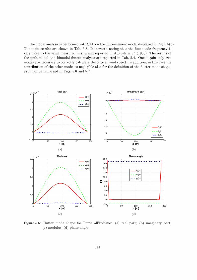
The modal analysis is performed with SAP on the finite-element model displayed in Fig. 5.5(b).The main results are shown in Tab. 5.3. It is worth noting that the first mode frequency isvery close to the value measured in situ and reported in Augusti et al. (1980). The results ofthe multimodal and bimodal flutter analysis are reported in Tab. 5.4. Once again only twomodes are necessary to correctly calculate the critical wind speed. In addition, in this case thecontribution of the other modes is negligible also for the definition of the flutter mode shape,as it can be remarked in Figs. 5.6 and 5.7.

0 50 100 150 200−0.5

0

0.5

1

1.5

2

2.5x 10

−4

x [m]

Real part

hf(x)

αf(x)

pf(x)

(a)

0 50 100 150 200−6

−5

−4

−3

−2

−1

0

1x 10

−5

x [m]

Imaginary part

hf(x)

αf(x)

pf(x)

(b)

0 50 100 150 2000

0.5

1

1.5

2

2.5x 10

−4

x [m]

Modulus

hf(x)

αf(x)

pf(x)

(c)

0 50 100 150 200−20

0

20

40

60

80

100

120

140

160

180

x [m]

[°]

Phase angle

hf(x)

αf(x)

pf(x)

(d)

Figure 5.6: Flutter mode shape for Ponte all’Indiano: (a) real part; (b) imaginary part;(c) modulus; (d) phase angle

141

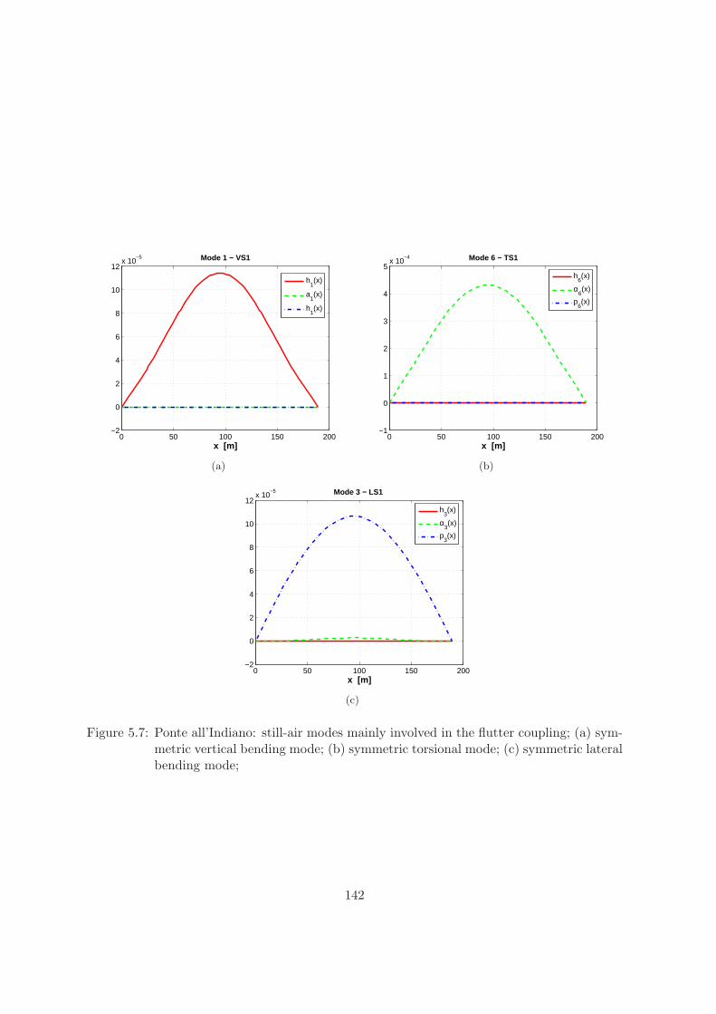
0 50 100 150 200−2

0

2

4

6

8

10

12x 10

−5

x [m]

Mode 1 − VS1

h1(x)

a1(x)

h1(x)

(a)

0 50 100 150 200−1

0

1

2

3

4

5x 10

−4

x [m]

Mode 6 − TS1

h6(x)

α6(x)

p6(x)

(b)

0 50 100 150 200−2

0

2

4

6

8

10

12x 10

−5

x [m]

Mode 3 − LS1

h3(x)

α3(x)

p3(x)

(c)

Figure 5.7: Ponte all’Indiano: still-air modes mainly involved in the flutter coupling; (a) sym-metric vertical bending mode; (b) symmetric torsional mode; (c) symmetric lateralbending mode;

142

5.5 Conclusions

The numerical results reported in the previous section, as well as those showed in D’Asdia andSepe (1998) and Caracoglia (2000) for Messina Strait Bridge (albeit considering the quasi-steady approach to determine the flutter derivatives corresponding to drag and sway motion),seem to confirm the validity of the assumptions listed in the third section of the presentchapter. That means that the contribution of the lateral bending modes to flutter is negligibleand there is no significant transfer of energy between modes with different modal shapes.

Nevertheless, the first conclusion needs further investigation since its validity for long-spanbridges with high drag, like Akashi Kaikyo Bridge, is still doubtful (Katsuchi et al., 1999). Asa matter of fact, the sets of flutter derivatives considered herein for the study cases correspondto deck cross sections with low drag, so that surprising destabilizing effects due to the lateralbending modes are not expected.

Conversely, the second statement, in the case of laminar wind, is based only on some easyassumptions whose validity can be straightforward checked before the calculation. On theother hand, considering non-perfectly correlated turbulent flows and performing a much moresophisticated analysis of stochastic stability, it is known that the energy transfer betweenmodes is enhanced with either stabilizing or destabilizing effects on flutter [e.g. Bucher andLyn (1988a,b, 1989); Bartoli et al. (1995)]. The actual relevance of these effects requires to bebetter understood even in order to define a simplified procedure of flutter assessment.

Finally, it is important to precise that the fact that basically only two modes seem to beresponsible for the flutter instability mechanism does not mean that the same conclusion canbe extended to the pre-critical state. In fact, several modes have to be taken into accountin order to correctly predict the response of a structure to turbulent wind [e.g. Minh et al.(1999); Diana et al. (1999); Salvatori and Spinelli (2006b)].

143

Chapter 6

Simplified formulas

6.1 Introduction

In this chapter we deal with the simplification of the flutter calculation procedure in orderto finally achieve an approximate method of flutter assessment which does not require wind-tunnel tests. The importance for risk-mitigation to dispose of simplified tools to treat bridgeflutter and aeroelastic phenomena in general and the lack of them both in the national andinternational codes have already been discussed in section 1.4.

A common simplified method to investigate flutter is the quasi-steady approach [e.g. Miy-ata et al. (1995); Minh et al. (1999); Diana et al. (1999)], in which the knowledge of staticaerodynamic coefficients is required instead of flutter derivatives. Nevertheless, it has al-ready been discussed in section 2.4.3 that this approach does not seem to be appropriate forthe relatively low reduced wind speeds which characterize bridge deck flutter. In addition,Nakamura (Nakamura and Mizota, 1975; Nakamura, 1979) pointed out that the quasi-steadyresult can be not only quantitatively inaccurate but also qualitatively uncorrect in the case ofsingle-degree-of-freedom torsional flutter (see section 2.2.4).

Another simplified method to assess flutter instability consists in the calculation of the crit-ical wind speed for a dynamically equivalent thin flat plate, which is then reduced (usually) orincreased (rarely) by introducing an empirical coefficient of “aeroelastic performance” dependingon the actual cross-sectional geometry (Frandsen, 1966; Gimsing, 1997; Dyrbye and Hansen,1997; Righi, 2003; Bartoli and Righi, 2004b, 2006). The main limit of this approach is thatthe physics of the phenomenon is lost, condensing in one coefficient the whole aerodynamicsof the deck section.

The proposed approach is based on the eigenvalue stability analysis and is able to followthe actual mechanism of destabilization. The flutter equations are manipulated on the basisof a large number of dynamic and aerodynamic data in order to find simplified analyticalexpressions for the coupling frequency and reduced wind speed, depending only on three (H∗

1 ,A∗2 and A∗3) or even two (H∗

1 and A∗2) aeroelastic functions instead of the usual eight. It is worthnoting that the retained aeroelastic functions are supposed to be the most reliable and easiestto be identified through wind-tunnel tests and those for which more data are available in theliterature. The validity and the limits of this approach are investigated through a wide range

145

of bridge deck flutter derivatives and its applicability comes out to be surprisingly wide, beingthe degree of approximation usually very good. In particular, although the method is mainlythought for classical coupled flutter, it seems to apply in the case of single-degree-of-freedomtorsional instability as well.

It is also worth noting that it is the first time, at least to the knowledge of the writer, thatsuch a wide range of dynamic and aerodynamic data about bridge decks are collected andanalyzed in order to study the flutter mechanism and to check the validity of an approximateformula.

6.2 Flutter problem

For two degree-of-freedom structural systems allowed to undergo heaving and pitching vibra-tions, the equations of motion can be written in the following form, common in the aeronauticalfield (Fung, 1993):

m[h + (1 + igh)ω2hh] = Lh (6.1)

I[α + (1 + igα)ω2αα] = Mα (6.2)

where h and α denote respectively the heaving displacement and the pitching rotation (Fig. 2.13),m and I the mass and mass moment of inertia per unit length, ωh and ωα the circular frequen-cies of the heaving and pitching modes (in still air), Lh and Mα the lift and moment per unitlength, i is the imaginary unit and the dot denotes the derivative with respect to time. gh andgα are the coefficients of rate-independent damping for the heaving and pitching modes and,in the case of a sinusoidal motion with circular frequency ω, they can be related to the morecommon ratio-to-critical damping coefficients ζh and ζα through the simple expressions:

gh = 2ζhω

ωh(6.3)

gα = 2ζαω

ωα(6.4)

The advantage of using rate-independent damping instead of the more familiar notation willresult clear later.

Lift and moment can be expressed as the sum of steady forces due to mean wind, buffetingand self-excited forces but only the latter must be retained when flutter stability is concerned.Self-excited forces can be expressed again in the Scanlan’s form (Simiu and Scanlan, 1996), asfollows:

Lse(t,K) = qB[KH∗1 (K)

h(t)U

+ KH∗2 (K)

Bα(t)U

+ K2H∗3 (K)α(t) + K2H∗

4 (K)h(t)B

] (6.5)

Mse(t,K) = qB2[KA∗1(K)h(t)U

+ KA∗2(K)Bα(t)

U+ K2A∗3(K)α(t) + K2A∗4(K)

h(t)B

] (6.6)

146

where q = 12ρU2 is the kinetic pressure, B is the deck chord, K is the reduced frequency of

oscillation defined on the base of the chord B and the functions H∗i and A∗i are the well known

flutter derivatives.Substituting Eqs. (6.5)-(6.6) in Eqs. (6.1)-(6.2), imposing a sinusoidal motion with coupled

frequency (critical condition) and the singularity of the resulting system, as explained inChapter 2, two flutter equations are then obtained. In particular, following the approachoutlined here, they can be written as follows (Fung, 1993):

(1− ghgα)r2αµ2

γ2ω

X2 − [r2αµ2(1 +

1γ2

ω

) +µ

γ2ω

(A∗3 − ghA∗2) + r2αµ(H∗

4 − gαH∗1 )]X+

r2αµ2 + µA∗3 + r2

αµH∗4 + H∗

4A∗3 −H∗1A∗2 −H∗

3A∗4 + H∗2A∗1 = 0

(6.7)

(gh + gα)r2αµ2

γ2ω

X2 − [r2αµ2(gα +

gh

γ2ω

) +µ

γ2ω

(ghA∗3 + A∗2) + r2αµ(gαH∗

4 + H∗1 )]X+

µA∗2 + r2αµH∗

1 + H∗4A∗2 + H∗

1A∗3 −H∗3A∗1 −H∗

2A∗4 = 0(6.8)

where it is set:

µ =2m

ρB2rα =

√I

mB2γω =

ωα

ωhX =

ω2α

ω2

The parameter µ represents the relative mass of the deck, that is proportional to the ratio ofthe mass of the deck to the mass of the air moved by the deck; rα is the dimensionless radiusof inertia of the deck, γω is the frequency ratio in still air between the torsional and verticalbending modes susceptible to couple and X is the unknown non-dimensional frequency ofoscillation at flutter. It is now evident the advantage of writing in Eqs. (6.1)-(6.2) the dampinglike a complex stiffness, as it allows to deal with flutter equations of second order in X insteadof fourth and third order respectively if usual notation for damping is assumed [Eqs. (2.55)and (2.56)]. It is also worth noting that all the modal properties of the 2-DoF system relevantfor flutter instability are summarized by the parameters µ, rα and γω along with the dampingcoefficients.

Eq. (6.7) is usually called “real equation” as it is obtained imposing the vanishing of thereal part of the determinant of the aforementioned system of equations. For analogous reasonsEq. (6.8) is called “imaginary equation”. It is important to point out that from Eqs. (6.7)-(6.8) it is possible to calculate the critical reduced wind speed (URc = 2π/Kc, where c standsfor “critical”), the coupling frequency and consequently the actual flutter wind speed, whichdepend only on the aerodynamic parameters (flutter derivatives) and the already mentionednon-dimensional modal parameters (µ, rα, γω, gh, gα).

6.3 Simplification procedure

In order to simplify the flutter equations it can immediately be noted that ghgα ¿ 1 inEq. (6.7), since hardly the damping coefficients are higher than 0.02. Isolating then in the lefthand side of both equations the term r2

αµ2X2/γ2ω and consequently equating the right hand

sides, an equation of first order in X is obtained:

147

[r2αµ2

γ2ω

(γ2

ωgh + gα

gh + gα) +

µA∗3γ2

ω

(gα

gh + gα)− µA∗2

γ2ω

(gh +1

gh + gα) + r2

αµH∗4 (

gh

gh + gα)+

− r2αµH∗

1 (gα +1

gh + gα)]X − r2

αµ2 − µA∗3 +µA∗2

gh + gα− r2

αµH∗4 +

r2αµH∗

1

gh + gα+

−H∗4A∗3 + H∗

1A∗2 + H∗3A∗4 −H∗

2A∗1 +H∗

4A∗2 + H∗1A∗3 −H∗

3A∗1 −H∗2A∗4

gh + gα= 0

(6.9)

In Eq. (6.9) the terms which contain a second power of the damping coefficients can be ne-glected, giving:

[r2αµ2

γ2ω

(γ2

ωgh + gα

gh + gα) +

µ

γ2ω

(gαA∗3

gh + gα− A∗2

gh + gα) + r2

αµ(ghH∗

4

gh + gα− H∗

1

gh + gα)]X+

− r2αµ2 − µA∗3 +

µA∗2gh + gα

− r2αµH∗

4 +r2αµH∗

1

gh + gα−H∗

4A∗3 + H∗1A∗2 + H∗

3A∗4 −H∗2A∗1+

H∗4A∗2 + H∗

1A∗3 −H∗3A∗1 −H∗

2A∗4gh + gα

= 0

(6.10)

It is worth noting that Eq. (6.9) relies on the assumption that gh+gα 6= 0. The case gh = gα = 0will be discussed later in section 6.3.2.

6.3.1 Range of variability of the dynamic parameters

Now it is important to understand the range of variability of the non-dimensional modalparameters which appear in the equations above. For this reason they are reported in Tab. 6.1for some bridge decks with various characteristics. Four suspended-span bridges of differentdimensions and cross sections are taken into account: First Tacoma Narrows Bridge, USA(Larsen, 1998), Bosporus Strait Bridge, Turkey (Martini, 2004), Akashi Kaikyo Bridge, Japan(Miyata and Yamaguchi, 1993) and the proposed Messina Strait Bridge, Italy (D’Asdia andSepe, 1998). In the first part of Table 1 the main geometric and modal properties and the non-dimensional parameters appearing in the flutter equations can be found (L = main span length;fh, fα = vertical bending and torsional frequencies susceptible to couple). The same data arereported in the second part of Tab. 6.1 for four cable-stayed bridges: Ponte all’Indiano, Italy(Augusti et al., 1980), Guama Bridge, Brazil (Rocha et al., 2003), Tsurumi Fairway Bridge,Japan (Sarkar, 1992) and Normandy Bridge, France (ONERA, 1989). Finally, in the thirdpart of Tab. 6.1 two footbridges are taken into account: Ruffolo footbridge near Siena (Bartoliand Procino, 2004) and the footbridge of the Olympic Arch in the Olympic Village in Turin(Flamand, 2003b).

Looking at the last four columns of Tab. 6.1, it seems reasonable to consider as oppositelimit cases the Tsurumi Fairway Bridge and the Guama Bridge, whose mass properties will beassumed as reference in the following analyses. In particular, Guama Bridge is characterizedby a concrete deck and consequently by a remarkable mass as compared to the chord B.Tsurumi Fairway Bridge, instead, presents a quite light steel deck with a large chord length.

148

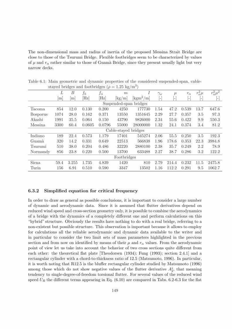
The non-dimensional mass and radius of inertia of the proposed Messina Strait Bridge areclose to those of the Tsurumi Bridge. Flexible footbridges seem to be characterized by valuesof µ and rα rather similar to those of Guama Bridge, since they present usually light but verynarrow decks.

Table 6.1: Main geometric and dynamic properties of the considered suspended-span, cable-stayed bridges and footbridges (ρ = 1.25 kg/m3)

L B fh fα m I γω µ rα r2αµ r2

αµ2

[m] [m] [Hz] [Hz] [kg/m] [kgm2/m] [-] [-] [-] [-] [-]Suspended-span bridges

Tacoma 854 12.0 0.130 0.200 4250 177730 1.54 47.2 0.539 13.7 647.6Bosporus 1074 28.0 0.162 0.371 13550 1351645 2.29 27.7 0.357 3.5 97.3Akashi 1991 35.5 0.064 0.150 43790 9826000 2.34 55.6 0.422 9.9 550.3Messina 3300 60.4 0.0605 0.0796 55000 28000000 1.32 24.1 0.374 3.4 81.2

Cable-stayed bridgesIndiano 189 22.4 0.573 1.179 17401 545274 2.06 55.5 0.250 3.5 192.3Guama 320 14.2 0.331 0.649 22513 566838 1.96 178.6 0.353 22.3 3984.8Tsurumi 510 38.0 0.204 0.486 32220 2880100 2.38 35.7 0.249 2.2 78.9Normandy 856 23.8 0.220 0.500 13700 633488 2.27 38.7 0.286 3.2 122.2

FootbridgesSiena 59.4 3.255 1.735 4.839 1420 810 2.79 214.4 0.232 11.5 2475.8Turin 156 6.91 0.510 0.590 3347 13502 1.16 112.2 0.291 9.5 1062.7

6.3.2 Simplified equation for critical frequency

In order to draw as general as possible conclusions, it is important to consider a large numberof dynamic and aerodynamic data. Since it is assumed that flutter derivatives depend onreduced wind speed and cross-section geometry only, it is possible to combine the aerodynamicsof a bridge with the dynamics of a completely different one and perform calculations on this“hybrid” structure. Obviously the results have nothing to do with a real bridge, referring to anon-existent but possible structure. This observation is important because it allows to employfor calculations all the reliable aerodynamic and dynamic data available to the writer andin particular to consider the two limit sets of mass parameters highlighted in the previoussection and from now on identified by means of their µ and rα values. From the aerodynamicpoint of view let us take into account the behavior of two cross sections quite different fromeach other: the theoretical flat plate [Theodorsen (1934); Fung (1993); section 2.4.1] and arectangular cylinder with a chord-to-thickness ratio of 12.5 (Matsumoto, 1996). In particular,it is worth noting that R12.5 is the bluffer rectangular cylinder studied by Matsumoto (1996)among those which do not show negative values of the flutter derivative A∗2, that meaningtendency to single-degree-of-freedom torsional flutter. For several values of the reduced windspeed UR the different terms appearing in Eq. (6.10) are compared in Tabs. 6.2-6.3 for the flat

149

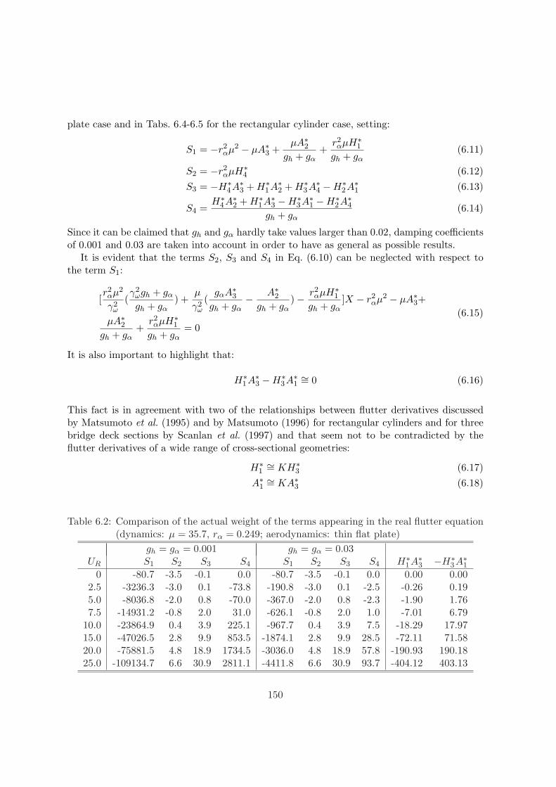
plate case and in Tabs. 6.4-6.5 for the rectangular cylinder case, setting:

S1 = −r2αµ2 − µA∗3 +

µA∗2gh + gα

+r2αµH∗

1

gh + gα(6.11)

S2 = −r2αµH∗

4 (6.12)S3 = −H∗

4A∗3 + H∗1A∗2 + H∗

3A∗4 −H∗2A∗1 (6.13)

S4 =H∗

4A∗2 + H∗1A∗3 −H∗

3A∗1 −H∗2A∗4

gh + gα(6.14)

Since it can be claimed that gh and gα hardly take values larger than 0.02, damping coefficientsof 0.001 and 0.03 are taken into account in order to have as general as possible results.

It is evident that the terms S2, S3 and S4 in Eq. (6.10) can be neglected with respect tothe term S1:

[r2αµ2

γ2ω

(γ2

ωgh + gα

gh + gα) +

µ

γ2ω

(gαA∗3

gh + gα− A∗2

gh + gα)− r2

αµH∗1

gh + gα]X − r2

αµ2 − µA∗3+

µA∗2gh + gα

+r2αµH∗

1

gh + gα= 0

(6.15)

It is also important to highlight that:

H∗1A∗3 −H∗

3A∗1 ∼= 0 (6.16)

This fact is in agreement with two of the relationships between flutter derivatives discussedby Matsumoto et al. (1995) and by Matsumoto (1996) for rectangular cylinders and for threebridge deck sections by Scanlan et al. (1997) and that seem not to be contradicted by theflutter derivatives of a wide range of cross-sectional geometries:

H∗1∼= KH∗

3 (6.17)A∗1 ∼= KA∗3 (6.18)

Table 6.2: Comparison of the actual weight of the terms appearing in the real flutter equation(dynamics: µ = 35.7, rα = 0.249; aerodynamics: thin flat plate)

gh = gα = 0.001 gh = gα = 0.03UR S1 S2 S3 S4 S1 S2 S3 S4 H∗

1A∗3 −H∗3A∗1

0 -80.7 -3.5 -0.1 0.0 -80.7 -3.5 -0.1 0.0 0.00 0.002.5 -3236.3 -3.0 0.1 -73.8 -190.8 -3.0 0.1 -2.5 -0.26 0.195.0 -8036.8 -2.0 0.8 -70.0 -367.0 -2.0 0.8 -2.3 -1.90 1.767.5 -14931.2 -0.8 2.0 31.0 -626.1 -0.8 2.0 1.0 -7.01 6.79

10.0 -23864.9 0.4 3.9 225.1 -967.7 0.4 3.9 7.5 -18.29 17.9715.0 -47026.5 2.8 9.9 853.5 -1874.1 2.8 9.9 28.5 -72.11 71.5820.0 -75881.5 4.8 18.9 1734.5 -3036.0 4.8 18.9 57.8 -190.93 190.1825.0 -109134.7 6.6 30.9 2811.1 -4411.8 6.6 30.9 93.7 -404.12 403.13

150

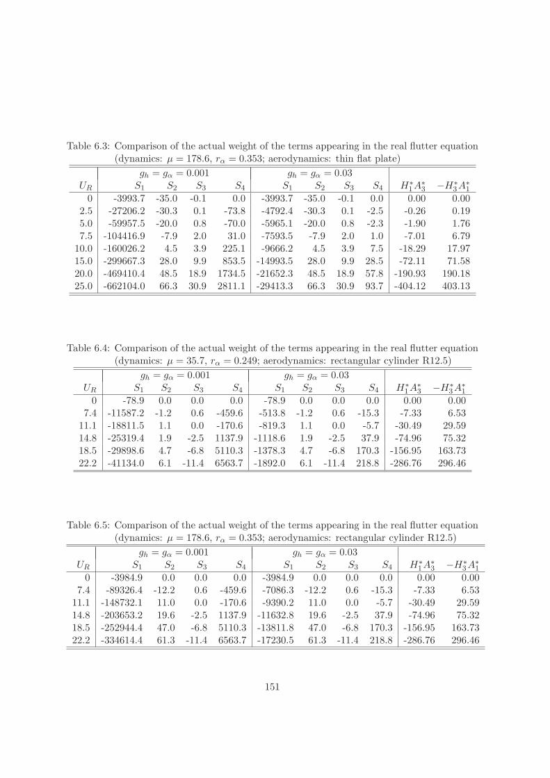
Table 6.3: Comparison of the actual weight of the terms appearing in the real flutter equation(dynamics: µ = 178.6, rα = 0.353; aerodynamics: thin flat plate)

gh = gα = 0.001 gh = gα = 0.03UR S1 S2 S3 S4 S1 S2 S3 S4 H∗

1A∗3 −H∗3A∗1

0 -3993.7 -35.0 -0.1 0.0 -3993.7 -35.0 -0.1 0.0 0.00 0.002.5 -27206.2 -30.3 0.1 -73.8 -4792.4 -30.3 0.1 -2.5 -0.26 0.195.0 -59957.5 -20.0 0.8 -70.0 -5965.1 -20.0 0.8 -2.3 -1.90 1.767.5 -104416.9 -7.9 2.0 31.0 -7593.5 -7.9 2.0 1.0 -7.01 6.79

10.0 -160026.2 4.5 3.9 225.1 -9666.2 4.5 3.9 7.5 -18.29 17.9715.0 -299667.3 28.0 9.9 853.5 -14993.5 28.0 9.9 28.5 -72.11 71.5820.0 -469410.4 48.5 18.9 1734.5 -21652.3 48.5 18.9 57.8 -190.93 190.1825.0 -662104.0 66.3 30.9 2811.1 -29413.3 66.3 30.9 93.7 -404.12 403.13

Table 6.4: Comparison of the actual weight of the terms appearing in the real flutter equation(dynamics: µ = 35.7, rα = 0.249; aerodynamics: rectangular cylinder R12.5)

gh = gα = 0.001 gh = gα = 0.03UR S1 S2 S3 S4 S1 S2 S3 S4 H∗

1A∗3 −H∗3A∗1

0 -78.9 0.0 0.0 0.0 -78.9 0.0 0.0 0.0 0.00 0.007.4 -11587.2 -1.2 0.6 -459.6 -513.8 -1.2 0.6 -15.3 -7.33 6.53

11.1 -18811.5 1.1 0.0 -170.6 -819.3 1.1 0.0 -5.7 -30.49 29.5914.8 -25319.4 1.9 -2.5 1137.9 -1118.6 1.9 -2.5 37.9 -74.96 75.3218.5 -29898.6 4.7 -6.8 5110.3 -1378.3 4.7 -6.8 170.3 -156.95 163.7322.2 -41134.0 6.1 -11.4 6563.7 -1892.0 6.1 -11.4 218.8 -286.76 296.46

Table 6.5: Comparison of the actual weight of the terms appearing in the real flutter equation(dynamics: µ = 178.6, rα = 0.353; aerodynamics: rectangular cylinder R12.5)

gh = gα = 0.001 gh = gα = 0.03UR S1 S2 S3 S4 S1 S2 S3 S4 H∗

1A∗3 −H∗3A∗1

0 -3984.9 0.0 0.0 0.0 -3984.9 0.0 0.0 0.0 0.00 0.007.4 -89326.4 -12.2 0.6 -459.6 -7086.3 -12.2 0.6 -15.3 -7.33 6.53

11.1 -148732.1 11.0 0.0 -170.6 -9390.2 11.0 0.0 -5.7 -30.49 29.5914.8 -203653.2 19.6 -2.5 1137.9 -11632.8 19.6 -2.5 37.9 -74.96 75.3218.5 -252944.4 47.0 -6.8 5110.3 -13811.8 47.0 -6.8 170.3 -156.95 163.7322.2 -334614.4 61.3 -11.4 6563.7 -17230.5 61.3 -11.4 218.8 -286.76 296.46

151

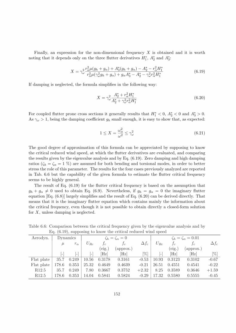
Finally, an expression for the non-dimensional frequency X is obtained and it is worthnoting that it depends only on the three flutter derivatives H∗

1 , A∗2 and A∗3:

X = γ2ω

r2αµ(gh + gα) + A∗3(gh + gα)−A∗2 − r2

αH∗1

r2αµ(γ2

ωgh + gα) + gαA∗3 −A∗2 − γ2ωr2

αH∗1

(6.19)

If damping is neglected, the formula simplifies in the following way:

X = γ2ω

A∗2 + r2αH∗

1

A∗2 + γ2ωr2

αH∗1

(6.20)

For coupled flutter prone cross sections it generally results that H∗1 < 0, A∗2 < 0 and A∗3 > 0.

As γω > 1, being the damping coefficient gh small enough, it is easy to show that, as expected:

1 ≤ X =ω2

α

ω2≤ γ2

ω (6.21)

The good degree of approximation of this formula can be appreciated by supposing to knowthe critical reduced wind speed, at which the flutter derivatives are evaluated, and comparingthe results given by the eigenvalue analysis and by Eq. (6.19). Zero damping and high dampingratios (ζh = ζα = 1 %) are assumed for both bending and torsional modes, in order to betterstress the role of this parameter. The results for the four cases previously analyzed are reportedin Tab. 6.6 but the capability of the given formula to estimate the flutter critical frequencyseems to be highly general.

The result of Eq. (6.19) for the flutter critical frequency is based on the assumption thatgh + gα 6= 0 used to obtain Eq. (6.9). Nevertheless, if gh = gα = 0 the imaginary flutterequation [Eq. (6.8)] largely simplifies and the result of Eq. (6.20) can be derived directly. Thatmeans that it is the imaginary flutter equation which contains mainly the information aboutthe critical frequency, even though it is not possible to obtain directly a closed-form solutionfor X, unless damping is neglected.

Table 6.6: Comparison between the critical frequency given by the eigenvalue analysis and byEq. (6.19), supposing to know the critical reduced wind speed

Aerodyn. Dynamics ζh = ζα = 0 ζh = ζα = 0.01µ rα URc fc fc ∆fc URc fc fc ∆fc

(eig.) (approx.) (eig.) (approx.)[-] [-] [-] [Hz] [Hz] [%] [-] [Hz] [Hz] [%]

Flat plate 35.7 0.249 10.56 0.3178 0.3161 -0.53 10.93 0.3123 0.3102 -0.67Flat plate 178.6 0.353 25.32 0.4649 0.4639 -0.21 26.51 0.4551 0.4541 -0.22

R12.5 35.7 0.249 7.80 0.3667 0.3752 +2.32 8.25 0.3589 0.3646 +1.59R12.5 178.6 0.353 14.04 0.5841 0.5824 -0.29 17.32 0.5580 0.5555 -0.45

152

6.3.3 Simplified equation for critical reduced wind speed

Since we observed that the result of the previous section mainly comes from the imaginaryflutter equation, let us come back now to the real flutter equation [Eq. (6.7)], retaining theonly trivial simplification ghgα ¿ 1 and rearranging it in the following way:

[µA∗3 − r2αµ2(X − 1)] · (1− X

γ2ω

)− r2αµH∗

4 (X − 1) + (ghµA∗2 + gαγ2ωr2

αµH∗1 )

X

γ2ω

+

H∗4A∗3 −H∗

1A∗2 −H∗3A∗4 + H∗

2A∗1 = 0(6.22)

by defining:

T1 = [µA∗3 − r2αµ2(X − 1)] · (1− X

γ2ω

) (6.23)

T2 = −r2αµH∗

4 (X − 1) (6.24)

T3 = (ghµA∗2 + gαγ2ωr2

αµH∗1 )

X

γ2ω

(6.25)

T4 = H∗4A∗3 −H∗

1A∗2 −H∗3A∗4 + H∗

2A∗1 (6.26)

Eq. (6.22) can be written in the following form:

T1 + T2 + T3 + T4 = 0 (6.27)

The term T3 vanishes if zero damping is assumed. It is interesting to understand which isthe actual weight of the four terms in the equation. Therefore each term and their sum areplotted against UR in Fig. 6.1, for different values of X in the interval 1 ≤ X ≤ γ2

ω for thechosen case studies. Unrealistically high damping coefficients are assumed (gh = gα = 0.05) inorder to stress the role of the term T3. The results are shown in the aforementioned graphs.It is possible to observe that the weight of the terms T2, T3 and T4 is definitely negligible withrespect to T1.

0 = T1 + T2 + T3 + T4∼= T1 (6.28)

In addition, it is also expected that X 6= γω, that is ω 6= ωh, so that the critical conditionbecomes:

A∗3 − r2αµ(X − 1) = 0 (6.29)

Finally, the expression for X given by Eq. (6.19) is substituted in this equation, leading to anapproximate formula for the flutter critical reduced wind speed:

153

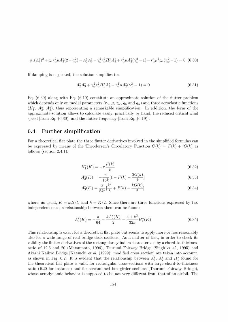
gα(A∗3)2 +gαr2

αµA∗3(2−γ2ω)−A∗2A

∗3−γ2

ωr2αH∗

1A∗3 +r2αµA∗2(γ

2ω−1)−r4

αµ2gα(γ2ω−1) = 0 (6.30)

If damping is neglected, the solution simplifies to:

A∗2A∗3 + γ2

ωr2αH∗

1A∗3 − r2αµA∗2(γ

2ω − 1) = 0 (6.31)

Eq. (6.30) along with Eq. (6.19) constitute an approximate solution of the flutter problemwhich depends only on modal parameters (rα, µ, γω, gh and gα) and three aeroelastic functions(H∗

1 , A∗2, A∗3), thus representing a remarkable simplification. In addition, the form of theapproximate solution allows to calculate easily, practically by hand, the reduced critical windspeed [from Eq. (6.30)] and the flutter frequency [from Eq. (6.19)].

6.4 Further simplification

For a theoretical flat plate the three flutter derivatives involved in the simplified formulas canbe expressed by means of the Theodorsen’s Circulatory Function C(k) = F (k) + iG(k) asfollows (section 2.4.1):

H∗1 (K) = −π

F (k)k

(6.32)

A∗2(K) = − π

16k[1− F (k)− 2G(k)

k] (6.33)

A∗3(K) =π

8k2[k2

8+ F (k)− kG(k)

2] (6.34)

where, as usual, K = ωB/U and k = K/2. Since there are three functions expressed by twoindependent ones, a relationship between them can be found:

A∗3(K) = − π

64− kA∗2(K)

2− 4 + k2

32kH∗

1 (K) (6.35)

This relationship is exact for a theoretical flat plate but seems to apply more or less reasonablyalso for a wide range of real bridge deck sections. As a matter of fact, in order to check itsvalidity the flutter derivatives of the rectangular cylinders characterized by a chord-to-thicknessratio of 12.5 and 20 (Matsumoto, 1996), Tsurumi Fairway Bridge (Singh et al., 1995) andAkashi Kaikyo Bridge [Katsuchi et al. (1999): modified cross section] are taken into account,as shown in Fig. 6.2. It is evident that the relationship between A∗3, A∗2 and H∗

1 found forthe theoretical flat plate is valid for rectangular cross-sections with large chord-to-thicknessratio (R20 for instance) and for streamlined box-girder sections (Tsurumi Fairway Bridge),whose aerodynamic behavior is supposed to be not very different from that of an airfoil. The

154

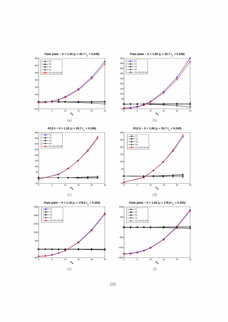
0 5 10 15 20 25−100

0

100

200

300

400

500

600

UR

Flate plate − X = 1.20 ( µ = 35.7 rα = 0.249)

T1T2T3T4T1+T2+T3+T4

(a)

0 5 10 15 20 25−50

0

50

100

150

200

250

300

350

400

450

UR

Flate plate − X = 1.80 ( µ = 35.7 rα = 0.249)

T1T2T3T4T1+T2+T3+T4

(b)

0 5 10 15 20 25−50

0

50

100

150

200

250

300

350

400

UR

R12.5 − X = 1.20 (µ = 35.7 rα = 0.249)

T1T2T3T4T1+T2+T3+T4

(c)

0 5 10 15 20 25−50

0

50

100

150

200

250

300

UR

R12.5 − X = 1.80 (µ = 35.7 rα = 0.249)

T1T2T3T4T1+T2+T3+T4

(d)

0 5 10 15 20 25−500

0

500

1000

1500

2000

2500

UR

Flate plate − X = 1.15 ( µ = 178.6 rα = 0.353)

T1T2T3T4T1+T2+T3+T4

(e)

0 5 10 15 20 25−1500

−1000

−500

0

500

1000

UR

Flate plate − X = 1.55 ( µ = 178.6 rα = 0.353)

T1T2T3T4T1+T2+T3+T4

(f)

155

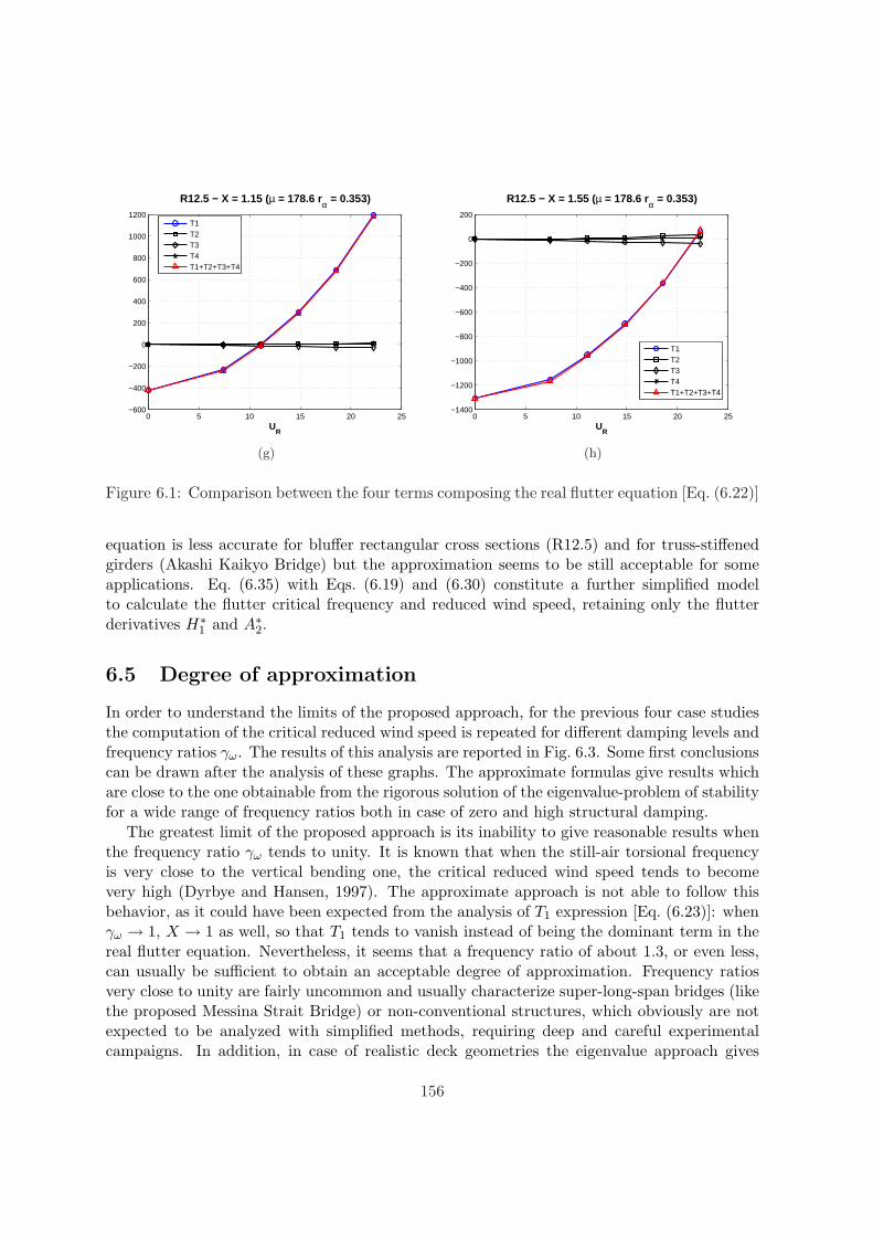
0 5 10 15 20 25−600

−400

−200

0

200

400

600

800

1000

1200

UR

R12.5 − X = 1.15 (µ = 178.6 rα = 0.353)

T1T2T3T4T1+T2+T3+T4

(g)

0 5 10 15 20 25−1400

−1200

−1000

−800

−600

−400

−200

0

200

UR

R12.5 − X = 1.55 (µ = 178.6 rα = 0.353)

T1T2T3T4T1+T2+T3+T4

(h)

Figure 6.1: Comparison between the four terms composing the real flutter equation [Eq. (6.22)]

equation is less accurate for bluffer rectangular cross sections (R12.5) and for truss-stiffenedgirders (Akashi Kaikyo Bridge) but the approximation seems to be still acceptable for someapplications. Eq. (6.35) with Eqs. (6.19) and (6.30) constitute a further simplified modelto calculate the flutter critical frequency and reduced wind speed, retaining only the flutterderivatives H∗

1 and A∗2.

6.5 Degree of approximation

In order to understand the limits of the proposed approach, for the previous four case studiesthe computation of the critical reduced wind speed is repeated for different damping levels andfrequency ratios γω. The results of this analysis are reported in Fig. 6.3. Some first conclusionscan be drawn after the analysis of these graphs. The approximate formulas give results whichare close to the one obtainable from the rigorous solution of the eigenvalue-problem of stabilityfor a wide range of frequency ratios both in case of zero and high structural damping.

The greatest limit of the proposed approach is its inability to give reasonable results whenthe frequency ratio γω tends to unity. It is known that when the still-air torsional frequencyis very close to the vertical bending one, the critical reduced wind speed tends to becomevery high (Dyrbye and Hansen, 1997). The approximate approach is not able to follow thisbehavior, as it could have been expected from the analysis of T1 expression [Eq. (6.23)]: whenγω → 1, X → 1 as well, so that T1 tends to vanish instead of being the dominant term in thereal flutter equation. Nevertheless, it seems that a frequency ratio of about 1.3, or even less,can usually be sufficient to obtain an acceptable degree of approximation. Frequency ratiosvery close to unity are fairly uncommon and usually characterize super-long-span bridges (likethe proposed Messina Strait Bridge) or non-conventional structures, which obviously are notexpected to be analyzed with simplified methods, requiring deep and careful experimentalcampaigns. In addition, in case of realistic deck geometries the eigenvalue approach gives

156

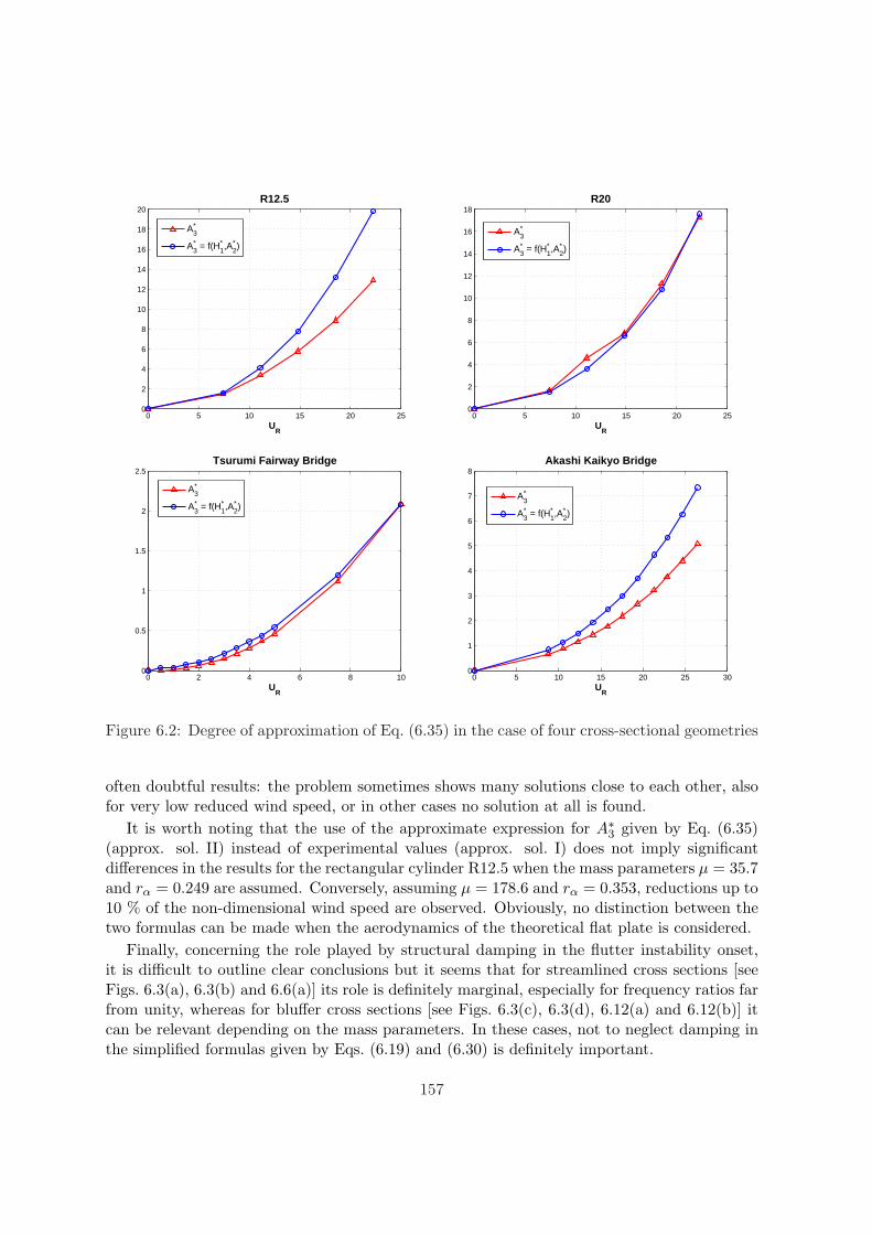
0 5 10 15 20 250

2

4

6

8

10

12

14

16

18

20

UR

R12.5

A3*

A3* = f(H1

* ,A2* )

0 5 10 15 20 250

2

4

6

8

10

12

14

16

18

UR

R20

A3*

A3* = f(H1

* ,A2* )

0 2 4 6 8 100

0.5

1

1.5

2

2.5

UR

Tsurumi Fairway Bridge

A3*

A3* = f(H1

* ,A2* )

0 5 10 15 20 25 300

1

2

3

4

5

6

7

8

UR

Akashi Kaikyo Bridge

A3*

A3* = f(H1

* ,A2* )

Figure 6.2: Degree of approximation of Eq. (6.35) in the case of four cross-sectional geometries

often doubtful results: the problem sometimes shows many solutions close to each other, alsofor very low reduced wind speed, or in other cases no solution at all is found.

It is worth noting that the use of the approximate expression for A∗3 given by Eq. (6.35)(approx. sol. II) instead of experimental values (approx. sol. I) does not imply significantdifferences in the results for the rectangular cylinder R12.5 when the mass parameters µ = 35.7and rα = 0.249 are assumed. Conversely, assuming µ = 178.6 and rα = 0.353, reductions up to10 % of the non-dimensional wind speed are observed. Obviously, no distinction between thetwo formulas can be made when the aerodynamics of the theoretical flat plate is considered.

Finally, concerning the role played by structural damping in the flutter instability onset,it is difficult to outline clear conclusions but it seems that for streamlined cross sections [seeFigs. 6.3(a), 6.3(b) and 6.6(a)] its role is definitely marginal, especially for frequency ratios farfrom unity, whereas for bluffer cross sections [see Figs. 6.3(c), 6.3(d), 6.12(a) and 6.12(b)] itcan be relevant depending on the mass parameters. In these cases, not to neglect damping inthe simplified formulas given by Eqs. (6.19) and (6.30) is definitely important.

157

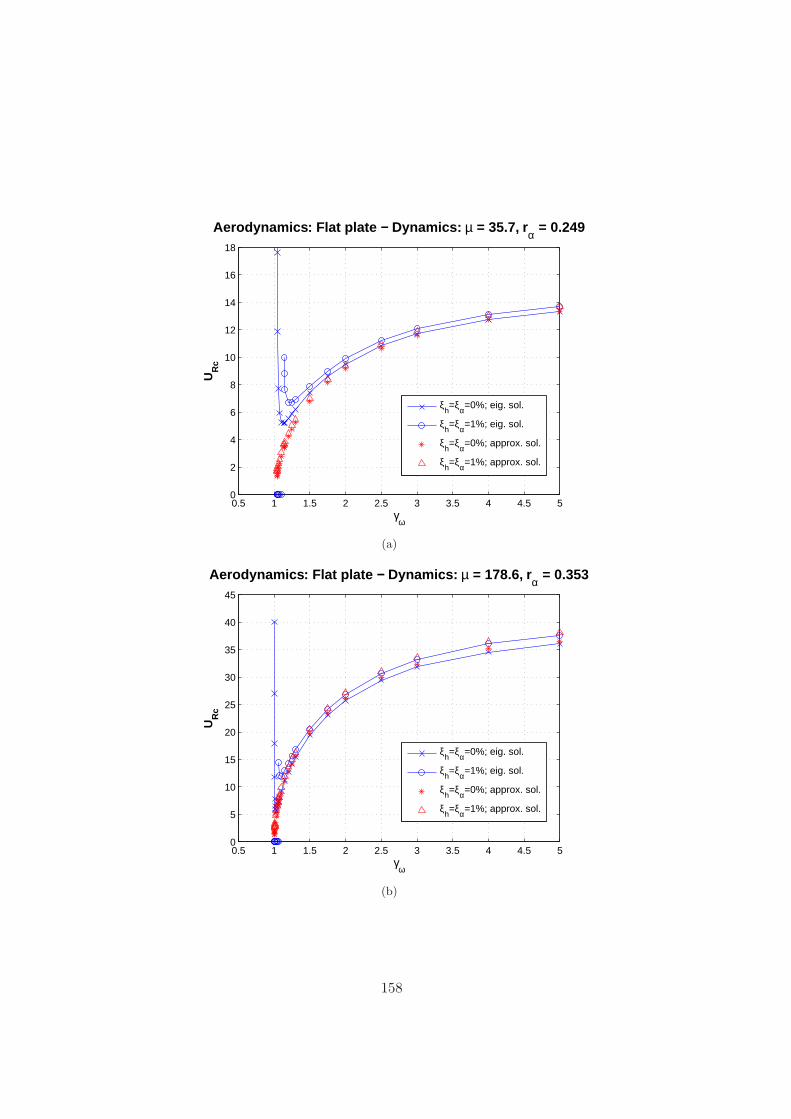
0.5 1 1.5 2 2.5 3 3.5 4 4.5 50

2

4

6

8

10

12

14

16

18

Aerodynamics: Flat plate − Dynamics: µ = 35.7, rα = 0.249

γω

UR

c

ξh=ξα=0%; eig. sol.

ξh=ξα=1%; eig. sol.

ξh=ξα=0%; approx. sol.

ξh=ξα=1%; approx. sol.

(a)

0.5 1 1.5 2 2.5 3 3.5 4 4.5 50

5

10

15

20

25

30

35

40

45

Aerodynamics: Flat plate − Dynamics: µ = 178.6, rα = 0.353

γω

UR

c

ξh=ξα=0%; eig. sol.

ξh=ξα=1%; eig. sol.

ξh=ξα=0%; approx. sol.

ξh=ξα=1%; approx. sol.

(b)

158

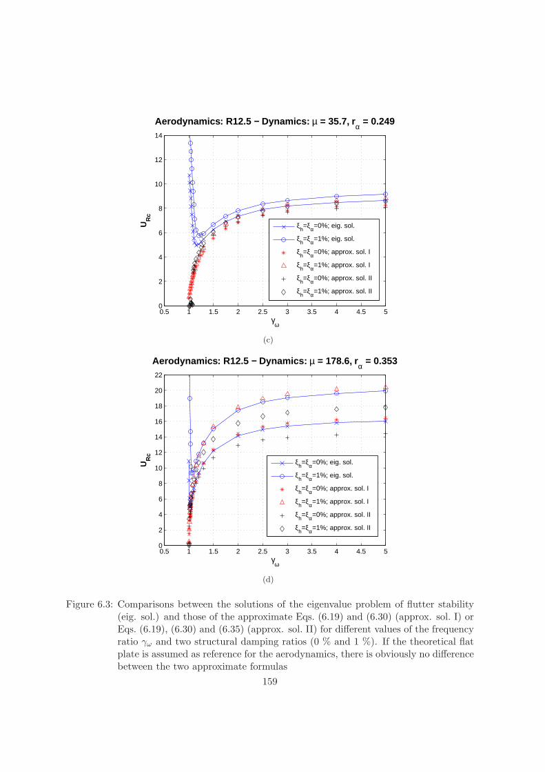
0.5 1 1.5 2 2.5 3 3.5 4 4.5 50

2

4

6

8

10

12

14

Aerodynamics: R12.5 − Dynamics: µ = 35.7, rα = 0.249

γω

UR

c

ξh=ξα=0%; eig. sol.

ξh=ξα=1%; eig. sol.

ξh=ξα=0%; approx. sol. I

ξh=ξα=1%; approx. sol. I

ξh=ξα=0%; approx. sol. II

ξh=ξα=1%; approx. sol. II

(c)

0.5 1 1.5 2 2.5 3 3.5 4 4.5 50

2

4

6

8

10

12

14

16

18

20

22

Aerodynamics: R12.5 − Dynamics: µ = 178.6, rα = 0.353

γω

UR

c

ξh=ξα=0%; eig. sol.

ξh=ξα=1%; eig. sol.

ξh=ξα=0%; approx. sol. I

ξh=ξα=1%; approx. sol. I

ξh=ξα=0%; approx. sol. II

ξh=ξα=1%; approx. sol. II

(d)

Figure 6.3: Comparisons between the solutions of the eigenvalue problem of flutter stability(eig. sol.) and those of the approximate Eqs. (6.19) and (6.30) (approx. sol. I) orEqs. (6.19), (6.30) and (6.35) (approx. sol. II) for different values of the frequencyratio γω and two structural damping ratios (0 % and 1 %). If the theoretical flatplate is assumed as reference for the aerodynamics, there is obviously no differencebetween the two approximate formulas

159

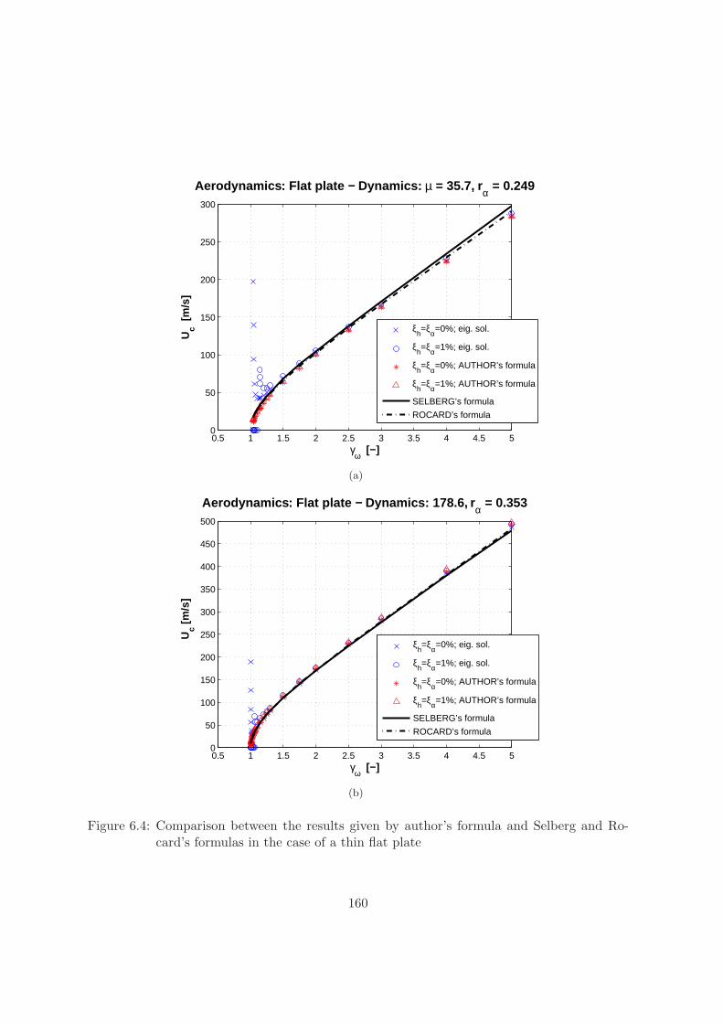
0.5 1 1.5 2 2.5 3 3.5 4 4.5 50

50

100

150

200

250

300

Aerodynamics: Flat plate − Dynamics: µ = 35.7, rα = 0.249

γω [−]

Uc [

m/s

]

ξh=ξα=0%; eig. sol.

ξh=ξα=1%; eig. sol.

ξh=ξα=0%; AUTHOR’s formula

ξh=ξα=1%; AUTHOR’s formula

SELBERG’s formula

ROCARD’s formula

(a)

0.5 1 1.5 2 2.5 3 3.5 4 4.5 50

50

100

150

200

250

300

350

400

450

500

Aerodynamics: Flat plate − Dynamics: 178.6, rα = 0.353

γω [−]

Uc [m

/s]

ξh=ξα=0%; eig. sol.

ξh=ξα=1%; eig. sol.

ξh=ξα=0%; AUTHOR’s formula

ξh=ξα=1%; AUTHOR’s formula

SELBERG’s formula

ROCARD’s formula

(b)

Figure 6.4: Comparison between the results given by author’s formula and Selberg and Ro-card’s formulas in the case of a thin flat plate

160

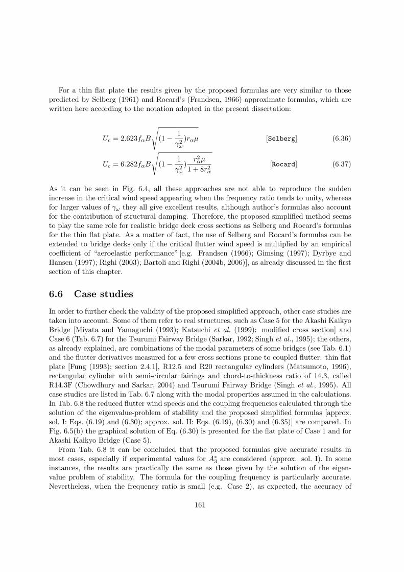
For a thin flat plate the results given by the proposed formulas are very similar to thosepredicted by Selberg (1961) and Rocard’s (Frandsen, 1966) approximate formulas, which arewritten here according to the notation adopted in the present dissertation:

Uc = 2.623fαB

√(1− 1

γ2ω

)rαµ [Selberg] (6.36)

Uc = 6.282fαB

√(1− 1

γ2ω

)r2αµ

1 + 8r2α

[Rocard] (6.37)

As it can be seen in Fig. 6.4, all these approaches are not able to reproduce the suddenincrease in the critical wind speed appearing when the frequency ratio tends to unity, whereasfor larger values of γω they all give excellent results, although author’s formulas also accountfor the contribution of structural damping. Therefore, the proposed simplified method seemsto play the same role for realistic bridge deck cross sections as Selberg and Rocard’s formulasfor the thin flat plate. As a matter of fact, the use of Selberg and Rocard’s formulas can beextended to bridge decks only if the critical flutter wind speed is multiplied by an empiricalcoefficient of “aeroelastic performance” [e.g. Frandsen (1966); Gimsing (1997); Dyrbye andHansen (1997); Righi (2003); Bartoli and Righi (2004b, 2006)], as already discussed in the firstsection of this chapter.

6.6 Case studies

In order to further check the validity of the proposed simplified approach, other case studies aretaken into account. Some of them refer to real structures, such as Case 5 for the Akashi KaikyoBridge [Miyata and Yamaguchi (1993); Katsuchi et al. (1999): modified cross section] andCase 6 (Tab. 6.7) for the Tsurumi Fairway Bridge (Sarkar, 1992; Singh et al., 1995); the others,as already explained, are combinations of the modal parameters of some bridges (see Tab. 6.1)and the flutter derivatives measured for a few cross sections prone to coupled flutter: thin flatplate [Fung (1993); section 2.4.1], R12.5 and R20 rectangular cylinders (Matsumoto, 1996),rectangular cylinder with semi-circular fairings and chord-to-thickness ratio of 14.3, calledR14.3F (Chowdhury and Sarkar, 2004) and Tsurumi Fairway Bridge (Singh et al., 1995). Allcase studies are listed in Tab. 6.7 along with the modal properties assumed in the calculations.In Tab. 6.8 the reduced flutter wind speeds and the coupling frequencies calculated through thesolution of the eigenvalue-problem of stability and the proposed simplified formulas [approx.sol. I: Eqs. (6.19) and (6.30); approx. sol. II: Eqs. (6.19), (6.30) and (6.35)] are compared. InFig. 6.5(b) the graphical solution of Eq. (6.30) is presented for the flat plate of Case 1 and forAkashi Kaikyo Bridge (Case 5).

From Tab. 6.8 it can be concluded that the proposed formulas give accurate results inmost cases, especially if experimental values for A∗3 are considered (approx. sol. I). In someinstances, the results are practically the same as those given by the solution of the eigen-value problem of stability. The formula for the coupling frequency is particularly accurate.Nevertheless, when the frequency ratio is small (e.g. Case 2), as expected, the accuracy of

161

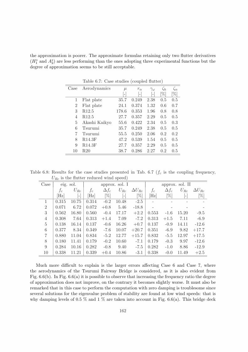
the approximation is poorer. The approximate formulas retaining only two flutter derivatives(H∗

1 and A∗2) are less performing than the ones adopting three experimental functions but thedegree of approximation seems to be still acceptable.

Table 6.7: Case studies (coupled flutter)

Case Aerodynamics µ rα γω ζh ζα

[-] [-] [-] [%] [%]1 Flat plate 35.7 0.249 2.38 0.5 0.52 Flat plate 24.1 0.374 1.32 0.6 0.73 R12.5 178.6 0.353 1.96 0.8 0.84 R12.5 27.7 0.357 2.29 0.5 0.55 Akashi Kaikyo 55.6 0.422 2.34 0.5 0.36 Tsurumi 35.7 0.249 2.38 0.5 0.57 Tsurumi 55.5 0.250 2.06 0.2 0.28 R14.3F 47.2 0.539 1.54 0.5 0.59 R14.3F 27.7 0.357 2.29 0.5 0.5

10 R20 38.7 0.286 2.27 0.2 0.5

Table 6.8: Results for the case studies presented in Tab. 6.7 (fc is the coupling frequency,URc is the flutter reduced wind speed)

Case eig. sol. approx. sol. I approx. sol. IIfc URc fc ∆fc URc ∆URc fc ∆fc URc ∆URc

[Hz] [-] [Hz] [%] [-] [%] [Hz] [%] [-] [%]1 0.315 10.75 0.314 -0.2 10.48 -2.5 - - - -2 0.071 6.72 0.072 +0.8 5.46 -18.8 - - - -3 0.562 16.80 0.560 -0.4 17.17 +2.2 0.553 -1.6 15.20 -9.54 0.308 7.64 0.313 +1.4 7.09 -7.2 0.313 +1.5 7.11 -6.95 0.138 16.14 0.137 -0.6 16.26 +0.7 0.137 -0.9 14.11 -12.66 0.377 8.34 0.349 -7.6 10.07 +20.7 0.351 -6.9 9.82 +17.77 0.880 11.04 0.834 -5.2 12.77 +15.7 0.832 -5.5 12.97 +17.58 0.180 11.41 0.179 -0.2 10.60 -7.1 0.179 -0.3 9.97 -12.69 0.284 10.16 0.282 -0.8 9.40 -7.5 0.282 -1.0 8.86 -12.910 0.338 11.21 0.339 +0.4 10.86 -3.1 0.338 -0.0 11.49 +2.5

Much more difficult to explain is the larger errors affecting Case 6 and Case 7, wherethe aerodynamics of the Tsurumi Fairway Bridge is considered, as it is also evident fromFig. 6.6(b). In Fig. 6.6(a) it is possible to observe that increasing the frequency ratio the degreeof approximation does not improve, on the contrary it becomes slightly worse. It must also beremarked that in this case to perform the computation with zero damping is troublesome sinceseveral solutions for the eigenvalue problem of stability are found at low wind speeds: that iswhy damping levels of 0.5 % and 1 % are taken into account in Fig. 6.6(a). This bridge deck

162

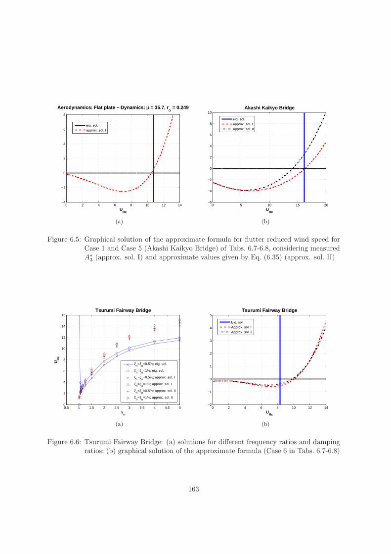
0 2 4 6 8 10 12 14−4

−2

0

2

4

6

8

Aerodynamics: Flat plate − Dynamics: µ = 35.7, rα = 0.249

URc

eig. sol.approx. sol. I

(a)

0 5 10 15 20−6

−4

−2

0

2

4

6

8

10Akashi Kaikyo Bridge

URc

eig. sol.approx. sol. Iapprox. sol. II

(b)

Figure 6.5: Graphical solution of the approximate formula for flutter reduced wind speed forCase 1 and Case 5 (Akashi Kaikyo Bridge) of Tabs. 6.7-6.8, considering measuredA∗3 (approx. sol. I) and approximate values given by Eq. (6.35) (approx. sol. II)

0.5 1 1.5 2 2.5 3 3.5 4 4.5 50

2

4

6

8

10

12

14

16Tsurumi Fairway Bridge

γω

UR

c

ξh=ξα=0.5%; eig. sol.

ξh=ξα=1%; eig. sol.

ξh=ξα=0.5%; approx. sol. I

ξh=ξα=1%; approx. sol. I

ξh=ξα=0.5%; approx. sol. II

ξh=ξα=1%; approx. sol. II

(a)

0 2 4 6 8 10 12 14−2

−1

0

1

2

3

4

5Tsurumi Fairway Bridge

URc

Eig. sol.Approx. sol. IApprox. sol. II

(b)

Figure 6.6: Tsurumi Fairway Bridge: (a) solutions for different frequency ratios and dampingratios; (b) graphical solution of the approximate formula (Case 6 in Tabs. 6.7-6.8)

163

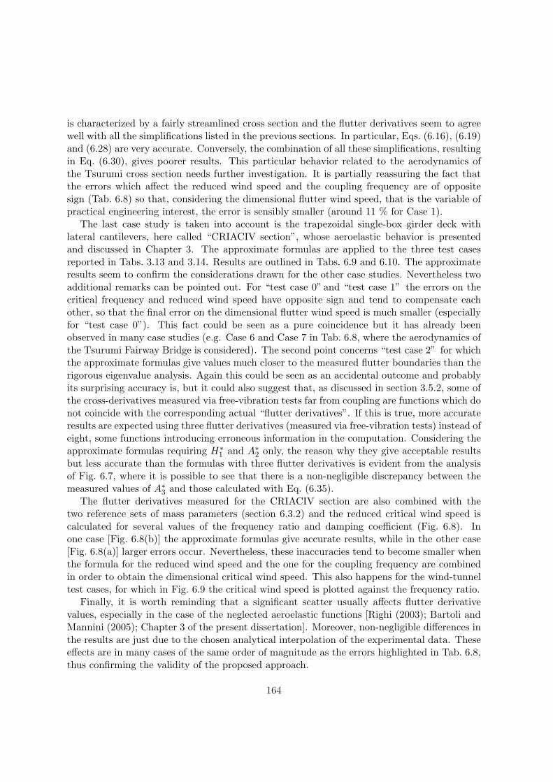
is characterized by a fairly streamlined cross section and the flutter derivatives seem to agreewell with all the simplifications listed in the previous sections. In particular, Eqs. (6.16), (6.19)and (6.28) are very accurate. Conversely, the combination of all these simplifications, resultingin Eq. (6.30), gives poorer results. This particular behavior related to the aerodynamics ofthe Tsurumi cross section needs further investigation. It is partially reassuring the fact thatthe errors which affect the reduced wind speed and the coupling frequency are of oppositesign (Tab. 6.8) so that, considering the dimensional flutter wind speed, that is the variable ofpractical engineering interest, the error is sensibly smaller (around 11 % for Case 1).

The last case study is taken into account is the trapezoidal single-box girder deck withlateral cantilevers, here called “CRIACIV section”, whose aeroelastic behavior is presentedand discussed in Chapter 3. The approximate formulas are applied to the three test casesreported in Tabs. 3.13 and 3.14. Results are outlined in Tabs. 6.9 and 6.10. The approximateresults seem to confirm the considerations drawn for the other case studies. Nevertheless twoadditional remarks can be pointed out. For “test case 0” and “test case 1” the errors on thecritical frequency and reduced wind speed have opposite sign and tend to compensate eachother, so that the final error on the dimensional flutter wind speed is much smaller (especiallyfor “test case 0”). This fact could be seen as a pure coincidence but it has already beenobserved in many case studies (e.g. Case 6 and Case 7 in Tab. 6.8, where the aerodynamics ofthe Tsurumi Fairway Bridge is considered). The second point concerns “test case 2” for whichthe approximate formulas give values much closer to the measured flutter boundaries than therigorous eigenvalue analysis. Again this could be seen as an accidental outcome and probablyits surprising accuracy is, but it could also suggest that, as discussed in section 3.5.2, some ofthe cross-derivatives measured via free-vibration tests far from coupling are functions which donot coincide with the corresponding actual “flutter derivatives”. If this is true, more accurateresults are expected using three flutter derivatives (measured via free-vibration tests) instead ofeight, some functions introducing erroneous information in the computation. Considering theapproximate formulas requiring H∗

1 and A∗2 only, the reason why they give acceptable resultsbut less accurate than the formulas with three flutter derivatives is evident from the analysisof Fig. 6.7, where it is possible to see that there is a non-negligible discrepancy between themeasured values of A∗3 and those calculated with Eq. (6.35).

The flutter derivatives measured for the CRIACIV section are also combined with thetwo reference sets of mass parameters (section 6.3.2) and the reduced critical wind speed iscalculated for several values of the frequency ratio and damping coefficient (Fig. 6.8). Inone case [Fig. 6.8(b)] the approximate formulas give accurate results, while in the other case[Fig. 6.8(a)] larger errors occur. Nevertheless, these inaccuracies tend to become smaller whenthe formula for the reduced wind speed and the one for the coupling frequency are combinedin order to obtain the dimensional critical wind speed. This also happens for the wind-tunneltest cases, for which in Fig. 6.9 the critical wind speed is plotted against the frequency ratio.

Finally, it is worth reminding that a significant scatter usually affects flutter derivativevalues, especially in the case of the neglected aeroelastic functions [Righi (2003); Bartoli andMannini (2005); Chapter 3 of the present dissertation]. Moreover, non-negligible differences inthe results are just due to the chosen analytical interpolation of the experimental data. Theseeffects are in many cases of the same order of magnitude as the errors highlighted in Tab. 6.8,thus confirming the validity of the proposed approach.

164

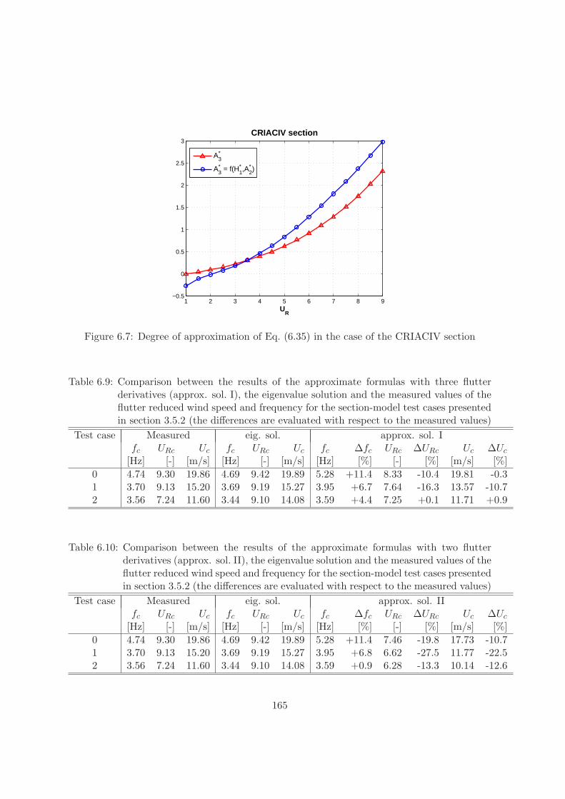
1 2 3 4 5 6 7 8 9−0.5

0

0.5

1

1.5

2

2.5

3

UR

CRIACIV section

A3*

A3* = f(H1

* ,A2* )

Figure 6.7: Degree of approximation of Eq. (6.35) in the case of the CRIACIV section

Table 6.9: Comparison between the results of the approximate formulas with three flutterderivatives (approx. sol. I), the eigenvalue solution and the measured values of theflutter reduced wind speed and frequency for the section-model test cases presentedin section 3.5.2 (the differences are evaluated with respect to the measured values)

Test case Measured eig. sol. approx. sol. Ifc URc Uc fc URc Uc fc ∆fc URc ∆URc Uc ∆Uc

[Hz] [-] [m/s] [Hz] [-] [m/s] [Hz] [%] [-] [%] [m/s] [%]0 4.74 9.30 19.86 4.69 9.42 19.89 5.28 +11.4 8.33 -10.4 19.81 -0.31 3.70 9.13 15.20 3.69 9.19 15.27 3.95 +6.7 7.64 -16.3 13.57 -10.72 3.56 7.24 11.60 3.44 9.10 14.08 3.59 +4.4 7.25 +0.1 11.71 +0.9

Table 6.10: Comparison between the results of the approximate formulas with two flutterderivatives (approx. sol. II), the eigenvalue solution and the measured values of theflutter reduced wind speed and frequency for the section-model test cases presentedin section 3.5.2 (the differences are evaluated with respect to the measured values)

Test case Measured eig. sol. approx. sol. IIfc URc Uc fc URc Uc fc ∆fc URc ∆URc Uc ∆Uc

[Hz] [-] [m/s] [Hz] [-] [m/s] [Hz] [%] [-] [%] [m/s] [%]0 4.74 9.30 19.86 4.69 9.42 19.89 5.28 +11.4 7.46 -19.8 17.73 -10.71 3.70 9.13 15.20 3.69 9.19 15.27 3.95 +6.8 6.62 -27.5 11.77 -22.52 3.56 7.24 11.60 3.44 9.10 14.08 3.59 +0.9 6.28 -13.3 10.14 -12.6

165

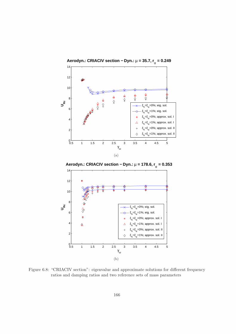
0.5 1 1.5 2 2.5 3 3.5 4 4.5 50

2

4

6

8

10

12

14

Aerodyn.: CRIACIV section − Dyn.: µ = 35.7, rα = 0.249

γω

UR

c

ξh=ξα=0%; eig. sol.

ξh=ξα=1%; eig. sol.

ξh=ξα=0%; approx. sol. I

ξh=ξα=1%; approx. sol. I

ξh=ξα=0%; approx. sol. II

ξh=ξα=1%; approx. sol. II

(a)

0.5 1 1.5 2 2.5 3 3.5 4 4.5 50

2

4

6

8

10

12

14

Aerodyn.: CRIACIV section − Dyn.: µ = 178.6, rα = 0.353

γω

UR

c

ξh=ξα=0%; eig. sol.

ξh=ξα=1%; eig. sol.

ξh=ξα=0%; approx. sol. I

ξh=ξα=1%; approx. sol. I

ξh=ξα=0%; approx. sol. II

ξh=ξα=1%; approx. sol. II

(b)

Figure 6.8: “CRIACIV section”: eigenvalue and approximate solutions for different frequencyratios and damping ratios and two reference sets of mass parameters

166

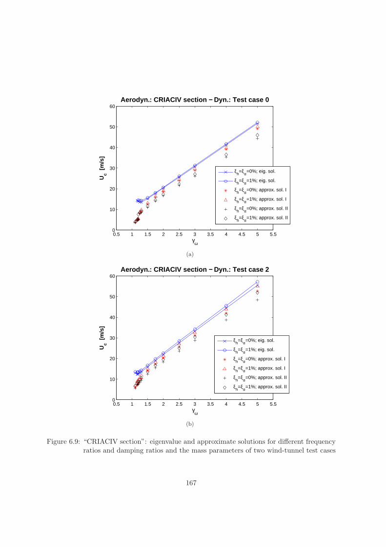
0.5 1 1.5 2 2.5 3 3.5 4 4.5 5 5.50

10

20

30

40

50

60Aerodyn.: CRIACIV section − Dyn.: Test case 0

γω

Uc [

m/s

]

ξh=ξα=0%; eig. sol.

ξh=ξα=1%; eig. sol.

ξh=ξα=0%; approx. sol. I

ξh=ξα=1%; approx. sol. I

ξh=ξα=0%; approx. sol. II

ξh=ξα=1%; approx. sol. II

(a)

0.5 1 1.5 2 2.5 3 3.5 4 4.5 5 5.50

10

20

30

40

50

60Aerodyn.: CRIACIV section − Dyn.: Test case 2

γω

Uc [

m/s

]

ξh=ξα=0%; eig. sol.

ξh=ξα=1%; eig. sol.

ξh=ξα=0%; approx. sol. I

ξh=ξα=1%; approx. sol. I

ξh=ξα=0%; approx. sol. II

ξh=ξα=1%; approx. sol. II

(b)

Figure 6.9: “CRIACIV section”: eigenvalue and approximate solutions for different frequencyratios and damping ratios and the mass parameters of two wind-tunnel test cases

167

6.7 Torsional flutter

The deck cross sections taken into account insofar are all prone to coupled flutter, as confirmedby the monotonic negative trend of H∗

1 and A∗2 shown in the given references. Nevertheless, itis well known that a wide range of real bridges, whose deck cross sections are not streamlined,are prone to single-degree-of-freedom torsional flutter. For these bridge decks the functionA∗2 tends to reverse its sign from negative to positive at relatively low reduced wind speedintroducing negative aerodynamic damping in the torsional modes. In this case, an alternativeway to deal with the flutter phenomenon is to consider just the frequency shift due to A∗3 andthe damping reduction produced by A∗2:

fc = fα[1 +ρB4

2IA∗3(Kc)]−

12 (6.38)

A∗2(Kc) = 4ζαI

ρB4· fα

fc(Kc)(6.39)

where Kc = UcB2πfc

is the critical reduced frequency, Uc is the critical wind speed, fc the critical(torsional) frequency. Eqs. (6.38)-(6.39) constitute a nonlinear system (1-DoF problem) whichhas to be iteratively solved. The 2-DoF and 1-DoF approaches usually give close results, unlessthe frequency ratio is near to unity.

All the steps which, starting from Eqs. (6.7)-(6.8), led to the simplified formulas discussedin the previous sections, can be checked now in the particular case of cross sections proneto torsional flutter. As reference examples two prototypes characterized again by the massproperties of Tsurumi Fairway Bridge (µ = 35.7, rα = 0.249) and Guama Bridge (µ = 178.6,rα = 0.353) and by the aerodynamics of a rectangular cylinder with a chord-to-thickness ratioof 5.0 (Matsumoto, 1996), are considered. The simplifications which led to the approximateformula for critical frequency [Eq. (6.19)], discussed in Tabs. 6.2-6.5 for cross sections proneto coupled flutter, are still valid if the analysis is limited to reduced wind speeds in theneighborhood of the zero-crossing point of A∗2, since it is in that range that the critical flutterspeed must be sought. In Fig. 6.10 the weight of the terms constituting the real flutter equation[Eq. (6.22)] are compared for values of X not far from unity, since the single degree-of-freedomtorsional flutter always arises with frequency close to the still-air torsional one. It can beunderstood from the presented graphs that no solution is found beyond a certain value of X.In Fig. 6.11 the relation between the flutter derivatives H∗

1 , A∗2 and A∗3 [Eq. (6.35)] is checkedfor the aforementioned rectangular cylinder R5 and for the First Tacoma Narrows Bridge(Scanlan and Tomko, 1971). The relation assumed between the three aeroelastic functionsis based upon the theoretical expression of the flutter derivatives for a thin flat plate andtherefore is less effective in the case of a bluff cross section. Nevertheless, it can be observed inFig. 6.11 that this approximation does not seem completely wrong in the range of interestingreduced wind speeds, that is around A∗2 zero-crossing point.

In Fig. 6.12 the critical reduced wind speed is plotted against the frequency ratio for thetwo reference sets of mass parameters. It is possible to remark that the critical reducedwind speed is independent of the frequency separation, unless the ratio γω is quite close tounity. In this region the curves lose the flat trend and the 2-DoF eigenvalue approach gives

168

results that diverge from those obtained through the 1-DoF approach [Eqs. (6.38)-(6.39)].Conversely, the 1-DoF and the 2-DoF approaches give usually very close solutions for frequencyratios far enough from unity. For a structure characterized by µ = 178.6 and rα = 0.353[Fig. 6.12(b)], the agreement between the 2-DoF and 1-DoF solutions is practically perfectprovided that γω is greater than approximately 1.5. It can be also remarked the strongdependence on structural damping, as already shown in Fig. 6.3(d). On the other hand, fora structure characterized by µ = 35.7 and rα = 0.249 [Fig. 6.12(a)], a much lower influenceof damping and a larger discrepancy between 1-DoF and 2-DoF solutions can be observed.A first reason for the difference between the two solutions might be the role played in theinstability mechanism by heaving motion. Another possible explanation could be that, whenthe frequency ratio is small a coupled instability arises before torsional flutter. Neverthelessthis fact, experimentally observed by Nakamura (Nakamura and Yoshimura, 1976), is not ableto explain the discrepancy between 1-DoF and 2-DoF solutions in Fig. 6.12(a), which, althoughdecreasing, is still significant for large frequency separation. Moreover, if it was the case, itis not clear the reason why the flutter critical wind speed does not tend to increase whenγω −→ 1. It is also worth noting in Fig. 6.12 and Table 6.12 that the 2-DoF solution seemsto be conservative with respect to the 1-DoF result (lower URc, almost the same fc). Theresults of the simplified formulas closely follow the 2-DoF eigenvalue solution and the degreeof approximation seems generally very good.

Finally, in Table 6.12 the approximate approach is further validated considering the casestudies presented in Table 6.11, where the aerodynamic behavior of the rectangular cylinderR10, characterized by a chord-to-thickness ratio of 10 (Matsumoto, 1996), is considered alongwith the First Tacoma Narrows Bridge (Scanlan and Tomko, 1971) and the previously men-tioned rectangular cylinder R5 (Matsumoto, 1996). As reference, the solutions of both 2-DoF[Eqs. (6.7)-(6.8)] and 1-DoF approach [Eqs. (6.38)-(6.39)] are reported.

It seems possible to conclude that the proposed method, although less useful, applies wellalso in the case of cross sections prone to torsional flutter. The approximate formulas adoptingjust two flutter derivatives (approx. sol. II) are less accurate for these bluffer cross sections butonly in one case (Case 5 in Tables 6.11-6.12) the error is very large (although the differencebetween 1-DoF and 2-DoF approach is even larger).

Particularly interesting is the case of R10, the most streamlined Matsumoto’s rectangularcylinder showing positive values of the flutter derivative A∗2 reversing its sign from negative topositive (Matsumoto, 1996). As compared to R5, the A∗2 zero-crossing takes place at higherreduced wind speed and, above all, with much smaller slope. The proposed approximation isaccurate, while the discrepancy between the 1-DoF and the 2-DoF solutions is larger in thatcase, probably due to the fact that the coupled instability arises before torsional flutter.

169

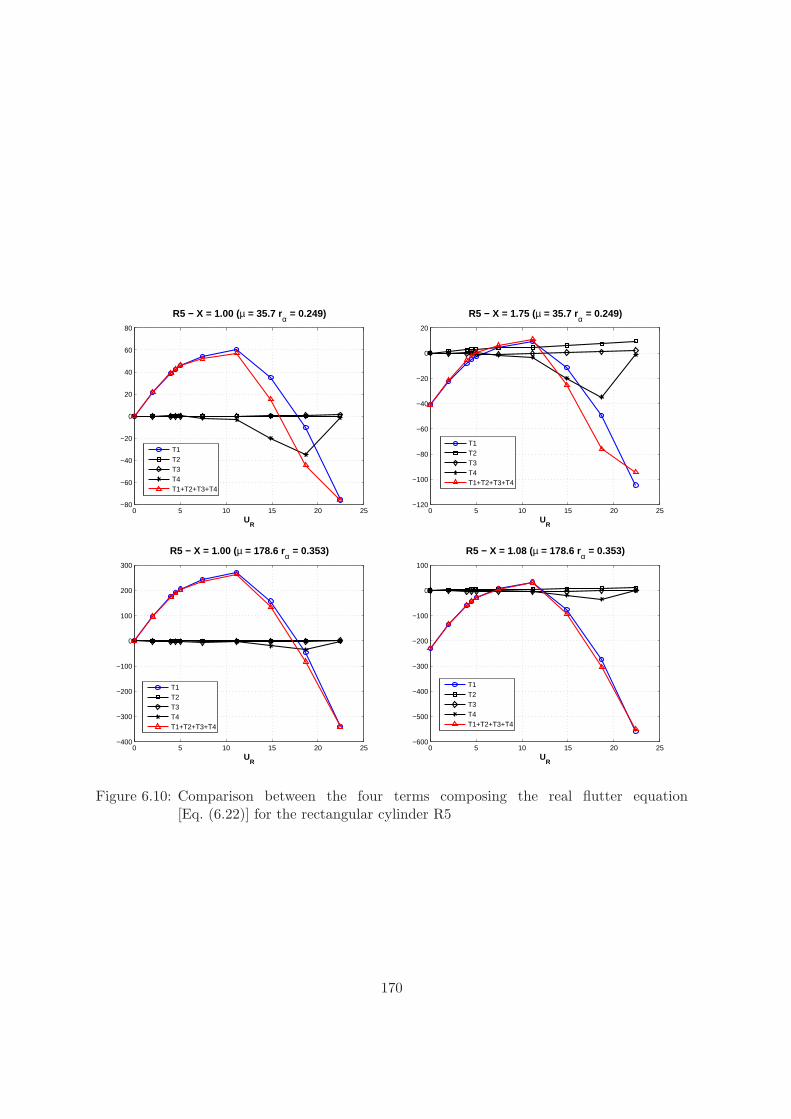
0 5 10 15 20 25−80

−60

−40

−20

0

20

40

60

80

UR

R5 − X = 1.00 (µ = 35.7 rα = 0.249)

T1T2T3T4T1+T2+T3+T4

0 5 10 15 20 25−120

−100

−80

−60

−40

−20

0

20

UR

R5 − X = 1.75 (µ = 35.7 rα = 0.249)

T1T2T3T4T1+T2+T3+T4

0 5 10 15 20 25−400

−300

−200

−100

0

100

200

300

UR

R5 − X = 1.00 (µ = 178.6 rα = 0.353)

T1T2T3T4T1+T2+T3+T4

0 5 10 15 20 25−600

−500

−400

−300

−200

−100

0

100

UR

R5 − X = 1.08 (µ = 178.6 rα = 0.353)

T1T2T3T4T1+T2+T3+T4

Figure 6.10: Comparison between the four terms composing the real flutter equation[Eq. (6.22)] for the rectangular cylinder R5

170

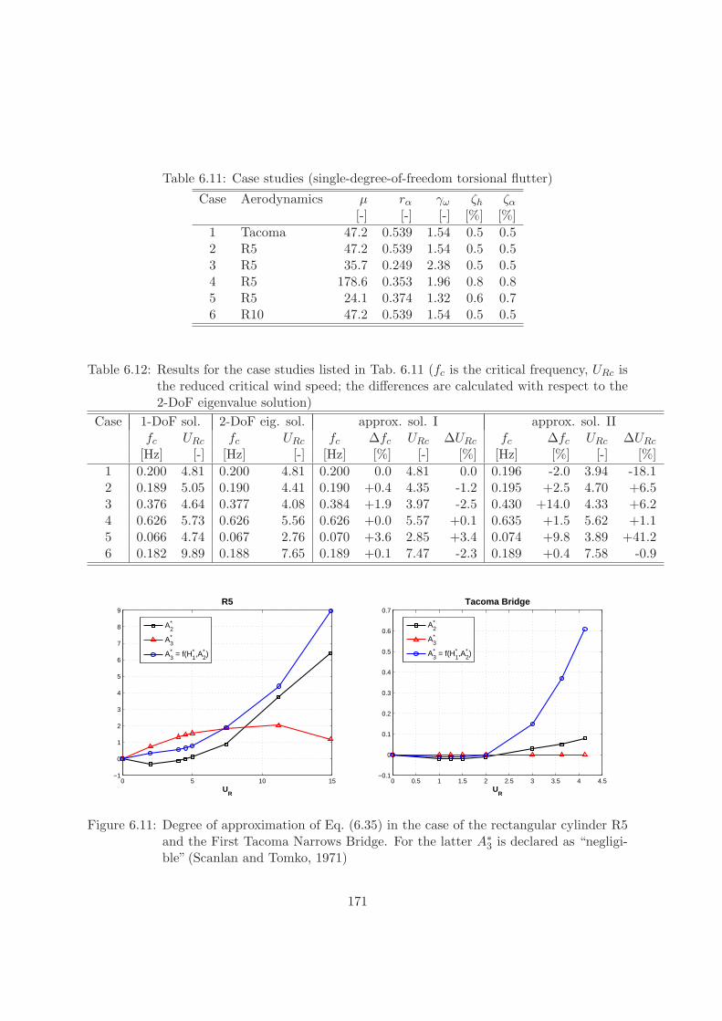
Table 6.11: Case studies (single-degree-of-freedom torsional flutter)

Case Aerodynamics µ rα γω ζh ζα

[-] [-] [-] [%] [%]1 Tacoma 47.2 0.539 1.54 0.5 0.52 R5 47.2 0.539 1.54 0.5 0.53 R5 35.7 0.249 2.38 0.5 0.54 R5 178.6 0.353 1.96 0.8 0.85 R5 24.1 0.374 1.32 0.6 0.76 R10 47.2 0.539 1.54 0.5 0.5

Table 6.12: Results for the case studies listed in Tab. 6.11 (fc is the critical frequency, URc isthe reduced critical wind speed; the differences are calculated with respect to the2-DoF eigenvalue solution)

Case 1-DoF sol. 2-DoF eig. sol. approx. sol. I approx. sol. IIfc URc fc URc fc ∆fc URc ∆URc fc ∆fc URc ∆URc

[Hz] [-] [Hz] [-] [Hz] [%] [-] [%] [Hz] [%] [-] [%]1 0.200 4.81 0.200 4.81 0.200 0.0 4.81 0.0 0.196 -2.0 3.94 -18.12 0.189 5.05 0.190 4.41 0.190 +0.4 4.35 -1.2 0.195 +2.5 4.70 +6.53 0.376 4.64 0.377 4.08 0.384 +1.9 3.97 -2.5 0.430 +14.0 4.33 +6.24 0.626 5.73 0.626 5.56 0.626 +0.0 5.57 +0.1 0.635 +1.5 5.62 +1.15 0.066 4.74 0.067 2.76 0.070 +3.6 2.85 +3.4 0.074 +9.8 3.89 +41.26 0.182 9.89 0.188 7.65 0.189 +0.1 7.47 -2.3 0.189 +0.4 7.58 -0.9

0 5 10 15−1

0

1

2

3

4

5

6

7

8

9

UR

R5

A2*

A3*

A3* = f(H1

* ,A2* )

0 0.5 1 1.5 2 2.5 3 3.5 4 4.5−0.1

0

0.1

0.2

0.3

0.4

0.5

0.6

0.7

UR

Tacoma Bridge

A2*

A3*

A3* = f(H1

* ,A2* )

Figure 6.11: Degree of approximation of Eq. (6.35) in the case of the rectangular cylinder R5and the First Tacoma Narrows Bridge. For the latter A∗3 is declared as “negligi-ble” (Scanlan and Tomko, 1971)

171

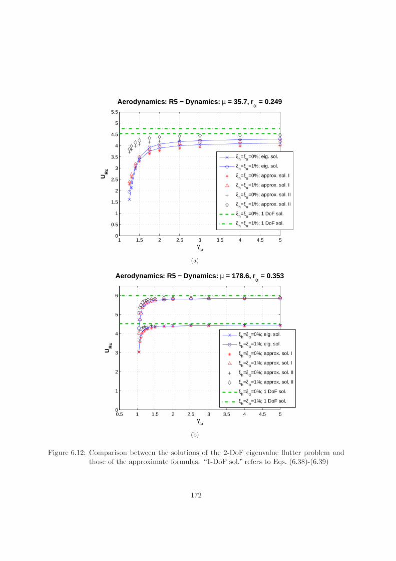
1 1.5 2 2.5 3 3.5 4 4.5 50

0.5

1

1.5

2

2.5

3

3.5

4

4.5

5

5.5

Aerodynamics: R5 − Dynamics: µ = 35.7, rα = 0.249

γω

UR

c

ξh=ξα=0%; eig. sol.

ξh=ξα=1%; eig. sol.

ξh=ξα=0%; approx. sol. I

ξh=ξα=1%; approx. sol. I

ξh=ξα=0%; approx. sol. II

ξh=ξα=1%; approx. sol. II

ξh=ξα=0%; 1 DoF sol.

ξh=ξα=1%; 1 DoF sol.

(a)

0.5 1 1.5 2 2.5 3 3.5 4 4.5 50

1

2

3

4

5

6

Aerodynamics: R5 − Dynamics: µ = 178.6, rα = 0.353

γω

UR

c

ξh=ξα=0%; eig. sol.

ξh=ξα=1%; eig. sol.

ξh=ξα=0%; approx. sol. I

ξh=ξα=1%; approx. sol. I

ξh=ξα=0%; approx. sol. II

ξh=ξα=1%; approx. sol. II

ξh=ξα=0%; 1 DoF sol.

ξh=ξα=1%; 1 DoF sol.

(b)

Figure 6.12: Comparison between the solutions of the 2-DoF eigenvalue flutter problem andthose of the approximate formulas. “1-DoF sol.” refers to Eqs. (6.38)-(6.39)

172

6.8 Nakamura’s formula

Nakamura (1978) proposed a series of approximate equations for bridge deck flutter which canbe easily transformed into the simplified formula proposed herein for the critical reduced windspeed neglecting structural damping [Eq. (6.31)]. For critical frequency a simplified formulaanalogous to Eq. (6.29) is given.

Nakamura’s results are based on the following assumptions about the unsteady aeroelasticbehavior of bridge decks:

1. |H∗2 | ¿ |H∗

3 |;

2. H∗1 = KH∗

3 , A∗1 = KA∗3, H∗4 = −KH∗

2 , A∗4 = −KA∗2;

3. the stability of the pitching branch is considered, whereas the heaving branch is assumedto be stable. The equivalent center of rotation should not be far from the midchord;

4. the phase angle between heaving and pitching motions is assumed to be small.

These conditions seem quite limiting and perhaps too theoretical, but the author himselfclaims that they are not seriously restrictive, being the formulas expected to be applicable to avariety of structures ranging from a flat plate to much bluffer bridge deck sections (Nakamura,1978). Nakamura’s experimental work, the investigation reported herein in Chapter 3, aswell as the data analyzed in this chapter, seem to confirm the validity of the aforementionedassumptions. In particular, Nakamura shows that the small phase angle between heaving andpitching motions as well as the absolute peculiarity of bridge deck flutter with respect toaircraft wing flutter may be attributed to the absence of inertial coupling.

After comparison with the research outlined in Nakamura (1978), some interesting pointsof the present work can be summarized:

• the same result as Nakamura’s is reached in a completely independent way and withoutsetting any theoretical assumption, by means of a much more “empirical” approach,manipulating and simplifying the flutter equations on the basis of a large number ofdata.

• Here the formula proposed for the frequency of oscillation at flutter depends on H∗1 and

A∗2 [Eq. (6.20)]. Conversely, in Nakamura (1978) Eq. (6.29) is obtained for the samepurpose, containing only the flutter derivative A∗3.

• In the proposed formulas damping is not neglected [Eqs. (6.19) and (6.30)] and itsinfluence on flutter onset is investigated, showing sometimes a significant effect [seeFigs. 6.3(d) and 6.12(b)].

• The possibility to take into account two flutter derivatives (H∗1 and A∗2) instead of three

(H∗1 , A∗2 and A∗3) is also considered and discussed.

173

6.9 Conclusions

In this chapter an approximate method to calculate the flutter critical wind speed and fre-quency is presented. The formulas are derived from the manipulation of the flutter equationsand seem to give results close to the rigorous solution of the eigenvalue problem of stability.The significant feature of this method is the fact that only three flutter derivatives (H∗

1 , A∗2and A∗3) or even two (H∗

1 and A∗2) are necessary to perform the calculation. In particular,these functions seem to be the most reliable and the easiest to be identified through wind-tunnel tests. Interestingly, although the formulas are particularly thought for binary coupledflutter, they seem to apply well also in case of cross sections prone to single-degree-of-freedomtorsional flutter.

This work, underlying the key role played by the flutter derivatives H∗1 and A∗2, confirm the

results found by Matsumoto for a wide range of rectangular cylinders. Nevertheless, it alsosuggests the necessity to consider in many instances a third aeroelastic function (A∗3) in orderto obtain accurate estimations of flutter boundaries. Moreover, it is worth noting that theproposed formulas are not directly obtainable either by setting to zero five out of eight flutterderivatives or only applying the inter-dependence relationships suggested by other authors.

The approximate approach proposed herein represents the basis to set up a simplifiedmethod of flutter assessment suitable to be implemented in codes and recommendations. Inorder to do that the generalization of the retained flutter derivatives for classes of deck geometryis still necessary and this step will be discussed in the next chapter. Nevertheless, it is worthnoting that by means of these formulas the calculation of the coupled flutter critical wind speedis possible also without identifying cross-flutter derivatives (H∗

2 , H∗3 , A∗1, A∗4), for instance when

a simpler 1-DoF test set-up is adopted.Another interesting aspect of this work is the theoretical insight it gives in the flutter

equations and in the instability mechanism. It mainly highlights the dominant role of theflutter derivatives H∗

1 and A∗2 and it supports the idea that Scanlan’s model for self-excitedforces, with eight empirical aeroelastic functions is somehow redundant [e.g. Bucher and Lyn(1988a,b); Matsumoto (1996, 2005); Borri et al. (2005)].

Finally, the role played in the flutter instability mechanism by several structural parametersis investigated. In particular, it is shown that, despite what is usually believed, the contributionof structural damping to flutter onset is not always negligible, depending both on the dynamicand aerodynamic properties of the bridge. Consequently, in some particular cases the fluttercritical wind speed can be significantly over- or under-predicted if structural damping is notcorrectly accounted for.

174

Chapter 7

A first step towards generalizationof flutter derivatives

7.1 Introduction

In Chapter 5 it is pointed out that a bimodal approach is usually adequate to predict theflutter critical wind speed and frequency. Then, in Chapter 6 an approximate method toassess them is proposed and discussed. This method is satisfactorily validated with a widerange of test cases, from the thin flat plate and quasi-streamlined decks to bluff cross sectionsprone to torsional flutter. The main feature of the proposed formulas, apart from their simpleform, is the dependency on at most three flutter derivatives only. These functions, H∗

1 , A∗2and A∗3, are direct flutter derivatives and can be measured also with relatively easy set-upsthrough one-degree-of-freedom free-vibration tests. Consequently, a larger number of dataare available in the literature and in the experimental laboratories. In addition, they aregenerally recognized as more reliable than cross-derivatives: for instance it can be observedhow the agreement between the flutter derivatives measured for two rectangular cylinders viafree-vibration (Righi, 2003) and forced-vibration tests (Matsumoto, 1996) is much better forthese three functions than for the other ones.

On these bases an attempt of generalization of flutter derivatives for conventional classesof deck geometries, limiting to the aforementioned three functions, becomes possible. Thatmeans to define “universal” curves or envelops which can be adopted as flutter derivativesin flutter calculations, implying small errors in the resulting critical wind speed. This step,corresponding to the upper box of the flow chart presented in Fig. 1.4, would allow to predictthe flutter wind speed without performing wind-tunnel tests. As it has been repeated severaltimes in this dissertation, this simplified approach cannot substitute wind-tunnel tests, espe-cially for long-span bridges or non-conventional structures, but it could represent an usefulnormative tool to understand whether or not flutter is a problem for a bridge structure: ifthe estimated flutter wind speed is too low, the structural design should be changed from thebeginning; conversely, if it is sufficiently high, wind-tunnel tests can be avoided or postponedto the final design validation; in the less obvious cases further experimental investigations areneeded. This method, if available in the design codes, even as “recommendations”, could be

175

very useful for bridge engineers, especially in case of medium-span conventional bridges and atpre-design stages. Nevertheless, in order to attempt this generalization of flutter derivatives, alarge number of reliable aeroelastic data, measured by different staffs in different laboratorieson several similar geometries are necessary. Probably benchmark and parametric studies onparticular geometries should be also available. In addition, since the dependence on the meanangle of attack cannot be forgotten [e.g. ONERA (1989); Flamand (2000); Flamand (2001);Diana et al. (2004); Fig. 3.41 in the present dissertation], the flutter derivative generalizationshould take care of this aspect, clearly warning about the wind incidence range of validityof the proposed curves and excluding the cross-sectional geometries very sensitive to smallvariations of the angle of attack, as well as to the presence of small non-structural details.Another point that should be clarified is the actual dependence of aeroelastic coefficients onReynolds number, as briefly discussed in sections 3.5.2 and 3.6, in Diana et al. (1999) andin Schewe (2006): needless to say that the geometries which are very sensitive to Reynoldsnumber cannot be considered for any sort of generalization.

In the present research work the collection of data has been one of the most difficult tasks.It is also not obvious to find data for which all test conditions, as well as the identificationprocedure, are known. A wide range of data are kindly made available by the Centre Scien-tifique et Technique du Batiment (CSTB) of Nantes, France, during writer’s visiting periodin February 2005. In most cases only the flutter derivatives H∗

1 , A∗2 and A∗3 are measured viafree-vibration technique on 1-DoF set-ups. The aeroelastic coefficients are identified followingthe simple procedure outlined in Scanlan and Tomko (1971). In most cases only one measure-ment is performed for each reduced wind speed, nevertheless many close points are available,so that the pattern of the functions is fairly clear and well defined.

In the following, three relevant classes of conventional deck sections for cable-stayed and sus-pension bridges are taken into account: trapezoidal single-box girder with lateral cantilevers,trapezoidal single-box girder (without lateral cantilevers) and bi-girder. For each group thegeometries of the concerned bridge decks are compared and then the corresponding flutterderivative patterns are discussed. Truss-stiffened girder decks are not taken into account heredue to the lack of data and also for the difficulty in defining similar geometries from theaeroelastic point of view. Nevertheless, it seems natural to distinguish between “old genera-tion” cross sections, such as Golden Gate Bridge (Simiu and Scanlan, 1996) and TancarvilleBridge (Flamand, 1996), which are prone to single-degree-of-freedom torsional flutter, and“new generation” cross sections, among which Akashi Kaikyo Bridge (Miyata and Yamaguchi,1993; Katsuchi et al., 1999) is the most important example, which are prone to coupled flutter,showing a relatively good aeroelastic behavior.

Here only a preliminary step towards an actual attempt of generalization is performed but,as far as the writer is aware, it is the first time after the pioneering work of Scanlan and Tomko(1971) that such a relatively large number of aeroelastic data are collected and compared onthe basis of geometric similarities.

176

7.2 Flutter derivatives for classes of deck geometry

7.2.1 Trapezoidal single-box girder decks with lateral cantilevers

The first class of geometry we are taking into account includes the bridge section experimentallystudied by the writer. It is worth reminding that this type of cross section has been chosenfor wind-tunnel tests mainly because it is fairly common for medium-span cable-stayed andsuspension bridge decks, although not many aeroelastic data are available in the literature.This geometry, extensively studied in Chapters 3-4 and displayed in Fig. 7.2(a), is calledin the following “CRIACIV section”. As it has already been said, it is very similar to theSunshine Skyway Bridge cross section in the bare-deck configuration (Fig. 3.17) and flutterderivatives are measured via free-vibration techniques and 2-DoF set-up. The other sets offlutter derivatives are measured by the CSTB-Nantes via free-vibration technique and 1-DoFset-up. These refer to Chevanon [Barre et al. (1996b); Fig. 7.2(b)], Aswan [Barre et al. (1996a);Fig. 7.2(c)] and Trois Bassins [Flamand (2003a); Fig. 7.2(d)] bridges. For the latter only theflutter derivative H∗

1 is measured for several positive angles of attack. Conversely, for theother two bridge sections, sets of three flutter derivatives are available both for constructionand service configurations.

It is worth noting that in the case of Chevanon and Trois Bassins decks the lateral cantileversare supported by tubular secondary beams (“bracons” in French), but, not being continuous,these are supposed not to influence much the aerodynamics of the section. The Trois Bassinsbridge deck presents definitely the most bluff geometry, even with opposite slope of the boxlateral walls. Aswan Bridge seems to be characterized by the most “streamlined” cross section,which is also the one closest to the CRIACIV section, although the chord-to-thickness ratioB/D is significantly higher (7.36 instead of 6.43).

In Fig. 7.2 the flutter derivatives of these bridge sections are plotted together for comparison.As usual, all aeroelastic functions are expressed in the Scanlan’s convention, that is accordingto Eqs. (2.38)-(2.39) and Fig. 2.13.

It is clearly shown that all sets of flutter derivatives are similar and very good agreement isfound between the experiments performed in the CSTB-Nantes and CRIACIV wind tunnels.In particular, concerning H∗

1 , all sets of functions belong to a relatively narrow spindle ofcurves, including the much bluffer Trois Bassins Bridge section. The wideness of the envelopof curves increases with the wind speed, according to the physiological dispersion affecting thedata, extensively discussed in Chapters 3-4. It is also worth noting that the flutter derivativegiven by Thodorsen’s theory for a thin flat plate almost represents the mean line of the envelop.

The comment of the graph for A∗2 is even more interesting. The first remark concerns Aswanbridge deck in the construction configuration, whose curve is quite different from all the otherones, showing values always close to zero, that means a limited aerodynamic damping inpitching. This result is quite surprising because Aswan deck seems to be characterized by thethe most “streamlined” section among those we considered. The reasons for this discrepancyhave not been understood yet. All the remaining curves (including the one for Aswan Bridge inthe service configuration) present similar patterns. In particular, for UR < 7.5 these all closelyfollow Theodorsen’s theory. Then, for higher reduced wind speeds the aerodynamic dampingin pitching suddenly starts to decrease. It is worth reminding that Fig. 3.41 showed that the

177

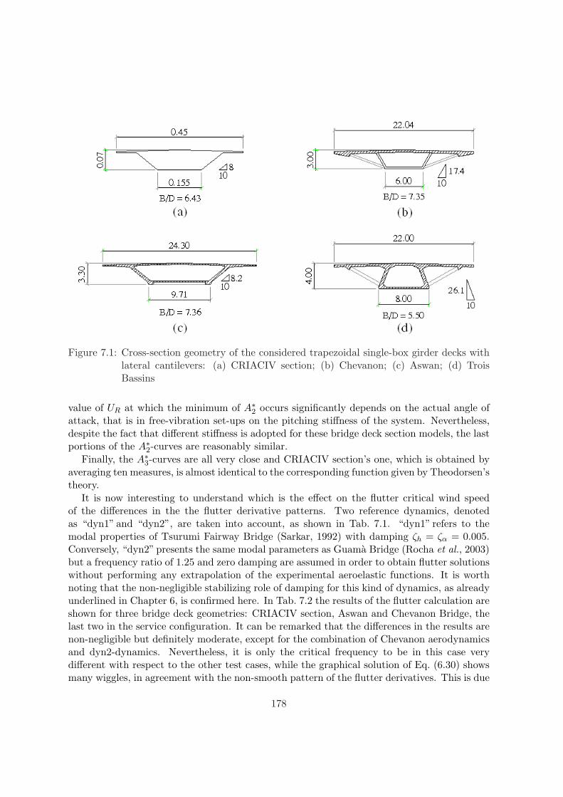
Figure 7.1: Cross-section geometry of the considered trapezoidal single-box girder decks withlateral cantilevers: (a) CRIACIV section; (b) Chevanon; (c) Aswan; (d) TroisBassins

value of UR at which the minimum of A∗2 occurs significantly depends on the actual angle ofattack, that is in free-vibration set-ups on the pitching stiffness of the system. Nevertheless,despite the fact that different stiffness is adopted for these bridge deck section models, the lastportions of the A∗2-curves are reasonably similar.

Finally, the A∗3-curves are all very close and CRIACIV section’s one, which is obtained byaveraging ten measures, is almost identical to the corresponding function given by Theodorsen’stheory.

It is now interesting to understand which is the effect on the flutter critical wind speedof the differences in the the flutter derivative patterns. Two reference dynamics, denotedas “dyn1” and “dyn2”, are taken into account, as shown in Tab. 7.1. “dyn1” refers to themodal properties of Tsurumi Fairway Bridge (Sarkar, 1992) with damping ζh = ζα = 0.005.Conversely, “dyn2” presents the same modal parameters as Guama Bridge (Rocha et al., 2003)but a frequency ratio of 1.25 and zero damping are assumed in order to obtain flutter solutionswithout performing any extrapolation of the experimental aeroelastic functions. It is worthnoting that the non-negligible stabilizing role of damping for this kind of dynamics, as alreadyunderlined in Chapter 6, is confirmed here. In Tab. 7.2 the results of the flutter calculation areshown for three bridge deck geometries: CRIACIV section, Aswan and Chevanon Bridge, thelast two in the service configuration. It can be remarked that the differences in the results arenon-negligible but definitely moderate, except for the combination of Chevanon aerodynamicsand dyn2-dynamics. Nevertheless, it is only the critical frequency to be in this case verydifferent with respect to the other test cases, while the graphical solution of Eq. (6.30) showsmany wiggles, in agreement with the non-smooth pattern of the flutter derivatives. This is due

178

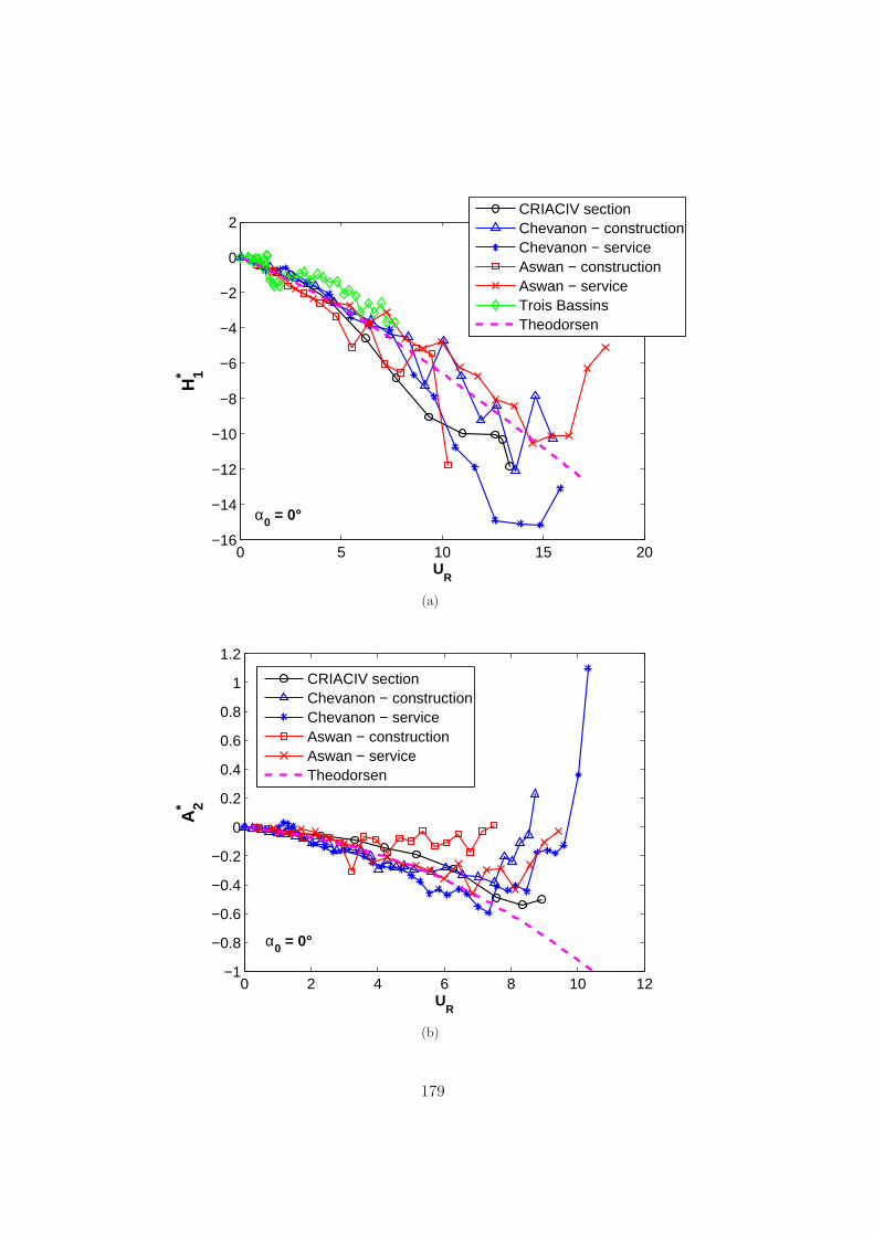
0 5 10 15 20−16

−14

−12

−10

−8

−6

−4

−2

0

2

UR

H1*

α0 = 0°

CRIACIV sectionChevanon − constructionChevanon − serviceAswan − constructionAswan − serviceTrois BassinsTheodorsen

(a)

0 2 4 6 8 10 12−1

−0.8

−0.6

−0.4

−0.2

0

0.2

0.4

0.6

0.8

1

1.2

UR

A2*

α0 = 0°

CRIACIV sectionChevanon − constructionChevanon − serviceAswan − constructionAswan − serviceTheodorsen

(b)

179

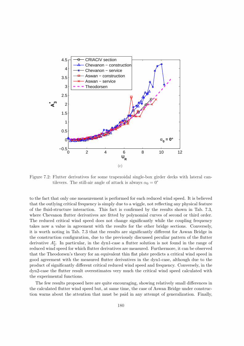
0 2 4 6 8 10 12−0.5

0

0.5

1

1.5

2

2.5

3

3.5

4

4.5

UR

A3*

α0 = 0°

CRIACIV sectionChevanon − constructionChevanon − serviceAswan − constructionAswan − serviceTheodorsen

(c)

Figure 7.2: Flutter derivatives for some trapezoidal single-box girder decks with lateral can-tilevers. The still-air angle of attack is always α0 = 0°

to the fact that only one measurement is performed for each reduced wind speed. It is believedthat the outlying critical frequency is simply due to a wiggle, not reflecting any physical featureof the fluid-structure interaction. This fact is confirmed by the results shown in Tab. 7.3,where Chevanon flutter derivatives are fitted by polynomial curves of second or third order.The reduced critical wind speed does not change significantly while the coupling frequencytakes now a value in agreement with the results for the other bridge sections. Conversely,it is worth noting in Tab. 7.3 that the results are significantly different for Aswan Bridge inthe construction configuration, due to the previously discussed peculiar pattern of the flutterderivative A∗2. In particular, in the dyn1-case a flutter solution is not found in the range ofreduced wind speed for which flutter derivatives are measured. Furthermore, it can be observedthat the Theodorsen’s theory for an equivalent thin flat plate predicts a critical wind speed ingood agreement with the measured flutter derivatives in the dyn1-case, although due to theproduct of significantly different critical reduced wind speed and frequency. Conversely, in thedyn2-case the flutter result overestimates very much the critical wind speed calculated withthe experimental functions.

The few results proposed here are quite encouraging, showing relatively small differences inthe calculated flutter wind speed but, at same time, the case of Aswan Bridge under construc-tion warns about the attention that must be paid in any attempt of generalization. Finally,

180

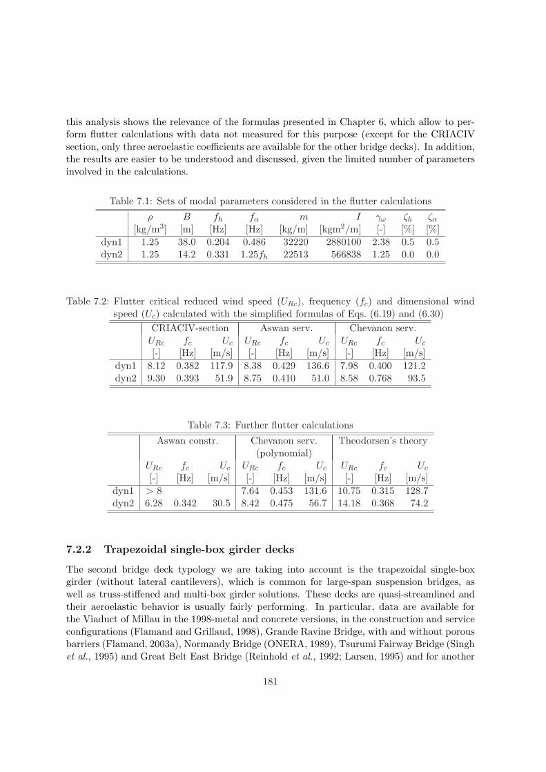
this analysis shows the relevance of the formulas presented in Chapter 6, which allow to per-form flutter calculations with data not measured for this purpose (except for the CRIACIVsection, only three aeroelastic coefficients are available for the other bridge decks). In addition,the results are easier to be understood and discussed, given the limited number of parametersinvolved in the calculations.

Table 7.1: Sets of modal parameters considered in the flutter calculations

ρ B fh fα m I γω ζh ζα

[kg/m3] [m] [Hz] [Hz] [kg/m] [kgm2/m] [-] [%] [%]dyn1 1.25 38.0 0.204 0.486 32220 2880100 2.38 0.5 0.5dyn2 1.25 14.2 0.331 1.25fh 22513 566838 1.25 0.0 0.0

Table 7.2: Flutter critical reduced wind speed (URc), frequency (fc) and dimensional windspeed (Uc) calculated with the simplified formulas of Eqs. (6.19) and (6.30)

CRIACIV-section Aswan serv. Chevanon serv.URc fc Uc URc fc Uc URc fc Uc

[-] [Hz] [m/s] [-] [Hz] [m/s] [-] [Hz] [m/s]dyn1 8.12 0.382 117.9 8.38 0.429 136.6 7.98 0.400 121.2dyn2 9.30 0.393 51.9 8.75 0.410 51.0 8.58 0.768 93.5

Table 7.3: Further flutter calculations

Aswan constr. Chevanon serv. Theodorsen’s theory(polynomial)

URc fc Uc URc fc Uc URc fc Uc

[-] [Hz] [m/s] [-] [Hz] [m/s] [-] [Hz] [m/s]dyn1 > 8 7.64 0.453 131.6 10.75 0.315 128.7dyn2 6.28 0.342 30.5 8.42 0.475 56.7 14.18 0.368 74.2

7.2.2 Trapezoidal single-box girder decks

The second bridge deck typology we are taking into account is the trapezoidal single-boxgirder (without lateral cantilevers), which is common for large-span suspension bridges, aswell as truss-stiffened and multi-box girder solutions. These decks are quasi-streamlined andtheir aeroelastic behavior is usually fairly performing. In particular, data are available forthe Viaduct of Millau in the 1998-metal and concrete versions, in the construction and serviceconfigurations (Flamand and Grillaud, 1998), Grande Ravine Bridge, with and without porousbarriers (Flamand, 2003a), Normandy Bridge (ONERA, 1989), Tsurumi Fairway Bridge (Singhet al., 1995) and Great Belt East Bridge (Reinhold et al., 1992; Larsen, 1995) and for another

181

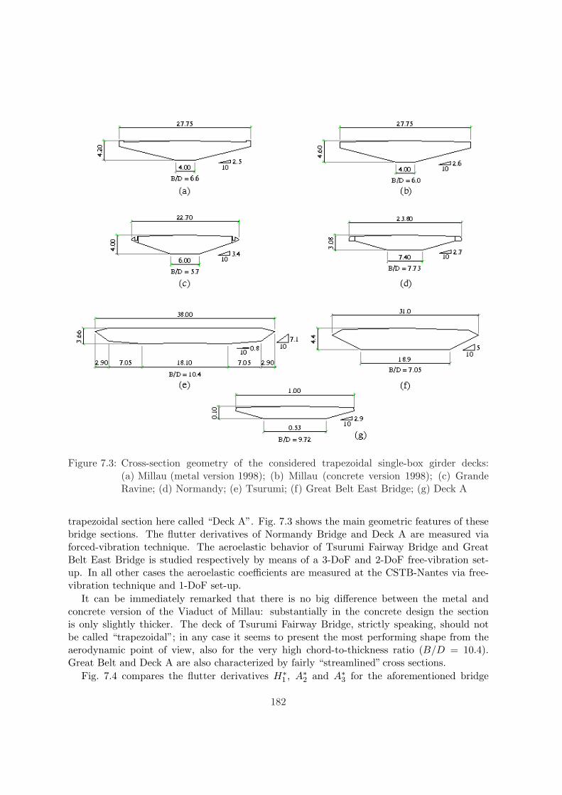
Figure 7.3: Cross-section geometry of the considered trapezoidal single-box girder decks:(a) Millau (metal version 1998); (b) Millau (concrete version 1998); (c) GrandeRavine; (d) Normandy; (e) Tsurumi; (f) Great Belt East Bridge; (g) Deck A

trapezoidal section here called “Deck A”. Fig. 7.3 shows the main geometric features of thesebridge sections. The flutter derivatives of Normandy Bridge and Deck A are measured viaforced-vibration technique. The aeroelastic behavior of Tsurumi Fairway Bridge and GreatBelt East Bridge is studied respectively by means of a 3-DoF and 2-DoF free-vibration set-up. In all other cases the aeroelastic coefficients are measured at the CSTB-Nantes via free-vibration technique and 1-DoF set-up.

It can be immediately remarked that there is no big difference between the metal andconcrete version of the Viaduct of Millau: substantially in the concrete design the sectionis only slightly thicker. The deck of Tsurumi Fairway Bridge, strictly speaking, should notbe called “trapezoidal”; in any case it seems to present the most performing shape from theaerodynamic point of view, also for the very high chord-to-thickness ratio (B/D = 10.4).Great Belt and Deck A are also characterized by fairly “streamlined” cross sections.

Fig. 7.4 compares the flutter derivatives H∗1 , A∗2 and A∗3 for the aforementioned bridge

182

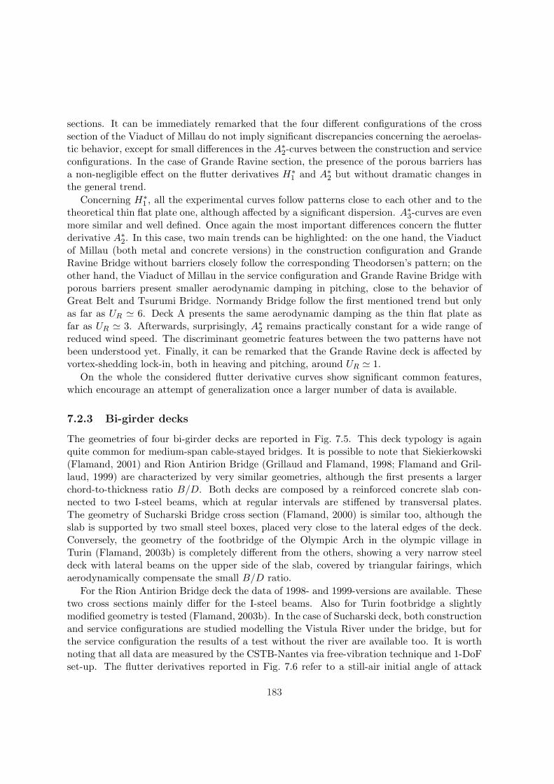
sections. It can be immediately remarked that the four different configurations of the crosssection of the Viaduct of Millau do not imply significant discrepancies concerning the aeroelas-tic behavior, except for small differences in the A∗2-curves between the construction and serviceconfigurations. In the case of Grande Ravine section, the presence of the porous barriers hasa non-negligible effect on the flutter derivatives H∗

1 and A∗2 but without dramatic changes inthe general trend.

Concerning H∗1 , all the experimental curves follow patterns close to each other and to the

theoretical thin flat plate one, although affected by a significant dispersion. A∗3-curves are evenmore similar and well defined. Once again the most important differences concern the flutterderivative A∗2. In this case, two main trends can be highlighted: on the one hand, the Viaductof Millau (both metal and concrete versions) in the construction configuration and GrandeRavine Bridge without barriers closely follow the corresponding Theodorsen’s pattern; on theother hand, the Viaduct of Millau in the service configuration and Grande Ravine Bridge withporous barriers present smaller aerodynamic damping in pitching, close to the behavior ofGreat Belt and Tsurumi Bridge. Normandy Bridge follow the first mentioned trend but onlyas far as UR ' 6. Deck A presents the same aerodynamic damping as the thin flat plate asfar as UR ' 3. Afterwards, surprisingly, A∗2 remains practically constant for a wide range ofreduced wind speed. The discriminant geometric features between the two patterns have notbeen understood yet. Finally, it can be remarked that the Grande Ravine deck is affected byvortex-shedding lock-in, both in heaving and pitching, around UR ' 1.

On the whole the considered flutter derivative curves show significant common features,which encourage an attempt of generalization once a larger number of data is available.

7.2.3 Bi-girder decks

The geometries of four bi-girder decks are reported in Fig. 7.5. This deck typology is againquite common for medium-span cable-stayed bridges. It is possible to note that Siekierkowski(Flamand, 2001) and Rion Antirion Bridge (Grillaud and Flamand, 1998; Flamand and Gril-laud, 1999) are characterized by very similar geometries, although the first presents a largerchord-to-thickness ratio B/D. Both decks are composed by a reinforced concrete slab con-nected to two I-steel beams, which at regular intervals are stiffened by transversal plates.The geometry of Sucharski Bridge cross section (Flamand, 2000) is similar too, although theslab is supported by two small steel boxes, placed very close to the lateral edges of the deck.Conversely, the geometry of the footbridge of the Olympic Arch in the olympic village inTurin (Flamand, 2003b) is completely different from the others, showing a very narrow steeldeck with lateral beams on the upper side of the slab, covered by triangular fairings, whichaerodynamically compensate the small B/D ratio.

For the Rion Antirion Bridge deck the data of 1998- and 1999-versions are available. Thesetwo cross sections mainly differ for the I-steel beams. Also for Turin footbridge a slightlymodified geometry is tested (Flamand, 2003b). In the case of Sucharski deck, both constructionand service configurations are studied modelling the Vistula River under the bridge, but forthe service configuration the results of a test without the river are available too. It is worthnoting that all data are measured by the CSTB-Nantes via free-vibration technique and 1-DoFset-up. The flutter derivatives reported in Fig. 7.6 refer to a still-air initial angle of attack

183

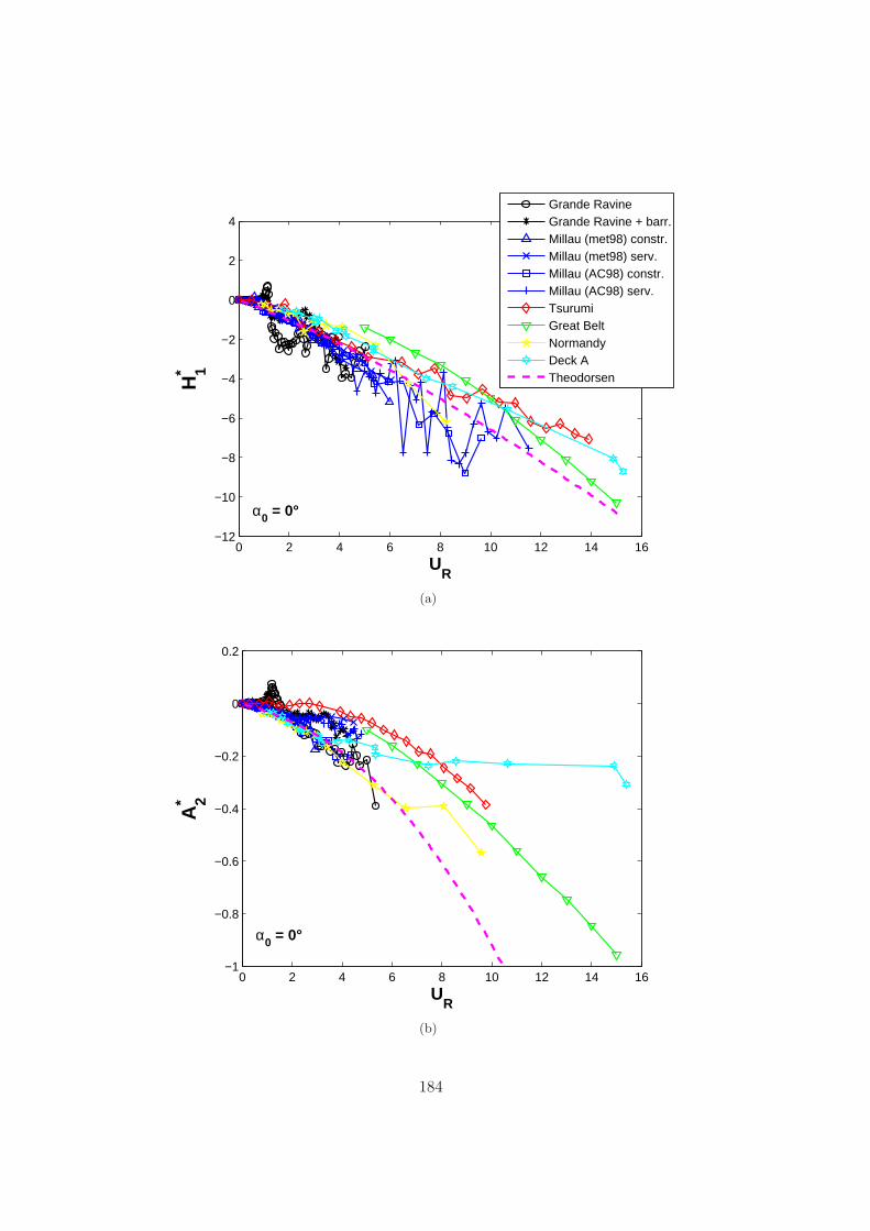
0 2 4 6 8 10 12 14 16−12

−10

−8

−6

−4

−2

0

2

4

UR

H1*

α0 = 0°

Grande RavineGrande Ravine + barr.Millau (met98) constr.Millau (met98) serv.Millau (AC98) constr.Millau (AC98) serv.TsurumiGreat BeltNormandyDeck ATheodorsen

(a)

0 2 4 6 8 10 12 14 16−1

−0.8

−0.6

−0.4

−0.2

0

0.2

UR

A2*

α0 = 0°

(b)

184

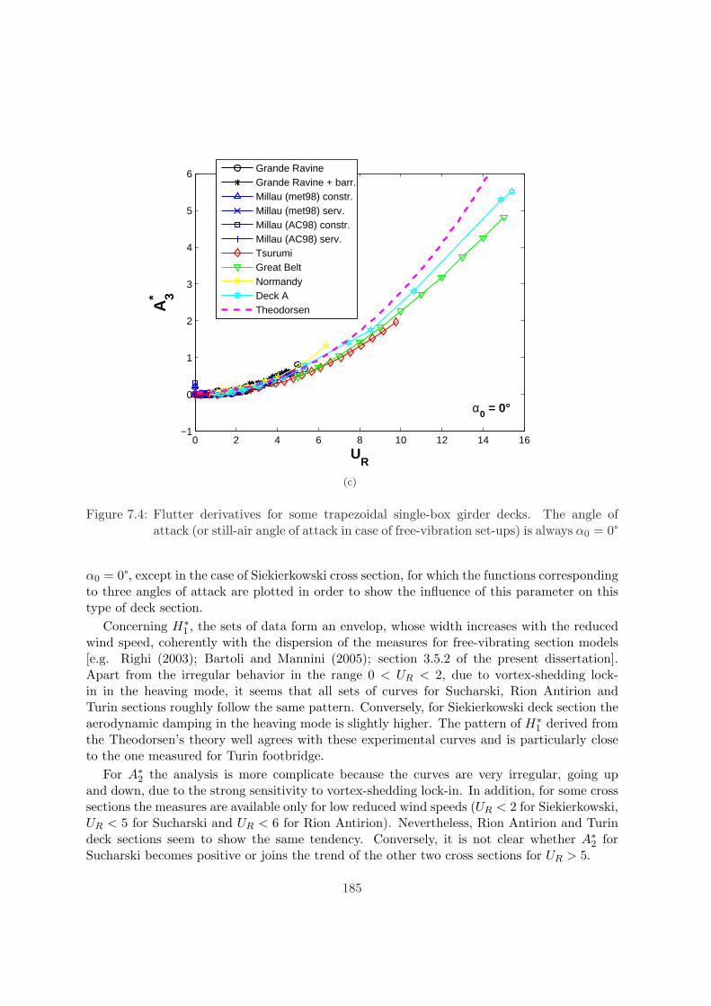
0 2 4 6 8 10 12 14 16−1

0

1

2

3

4

5

6

UR

A3*

α0 = 0°

Grande RavineGrande Ravine + barr.Millau (met98) constr.Millau (met98) serv.Millau (AC98) constr.Millau (AC98) serv.TsurumiGreat BeltNormandyDeck ATheodorsen

(c)

Figure 7.4: Flutter derivatives for some trapezoidal single-box girder decks. The angle ofattack (or still-air angle of attack in case of free-vibration set-ups) is always α0 = 0°

α0 = 0°, except in the case of Siekierkowski cross section, for which the functions correspondingto three angles of attack are plotted in order to show the influence of this parameter on thistype of deck section.

Concerning H∗1 , the sets of data form an envelop, whose width increases with the reduced

wind speed, coherently with the dispersion of the measures for free-vibrating section models[e.g. Righi (2003); Bartoli and Mannini (2005); section 3.5.2 of the present dissertation].Apart from the irregular behavior in the range 0 < UR < 2, due to vortex-shedding lock-in in the heaving mode, it seems that all sets of curves for Sucharski, Rion Antirion andTurin sections roughly follow the same pattern. Conversely, for Siekierkowski deck section theaerodynamic damping in the heaving mode is slightly higher. The pattern of H∗

1 derived fromthe Theodorsen’s theory well agrees with these experimental curves and is particularly closeto the one measured for Turin footbridge.

For A∗2 the analysis is more complicate because the curves are very irregular, going upand down, due to the strong sensitivity to vortex-shedding lock-in. In addition, for some crosssections the measures are available only for low reduced wind speeds (UR < 2 for Siekierkowski,UR < 5 for Sucharski and UR < 6 for Rion Antirion). Nevertheless, Rion Antirion and Turindeck sections seem to show the same tendency. Conversely, it is not clear whether A∗2 forSucharski becomes positive or joins the trend of the other two cross sections for UR > 5.

185

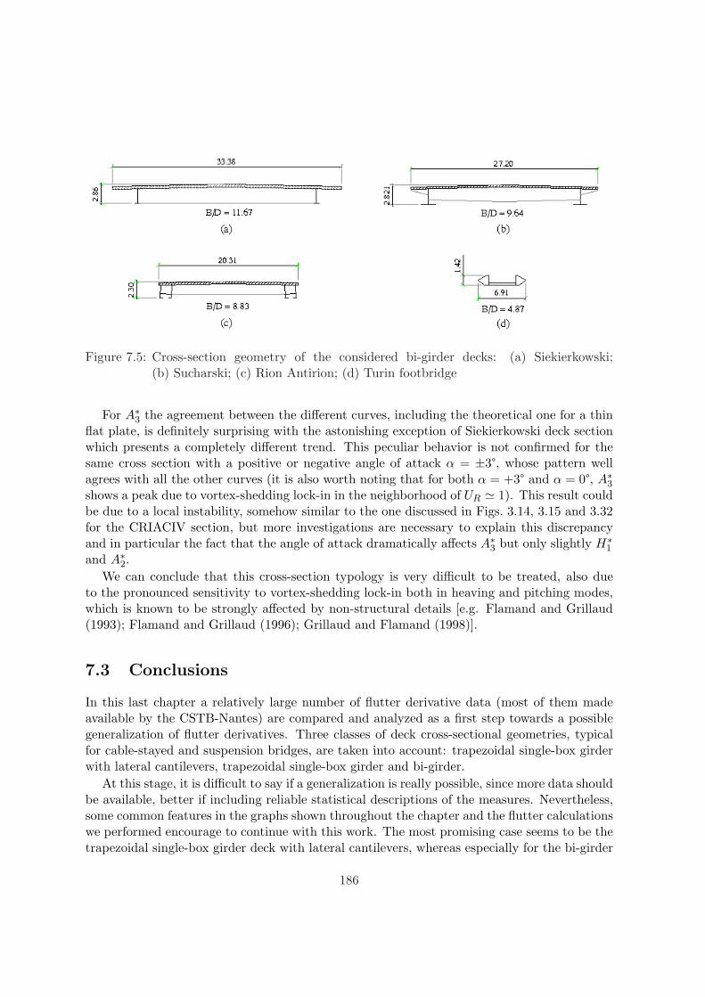
Figure 7.5: Cross-section geometry of the considered bi-girder decks: (a) Siekierkowski;(b) Sucharski; (c) Rion Antirion; (d) Turin footbridge

For A∗3 the agreement between the different curves, including the theoretical one for a thinflat plate, is definitely surprising with the astonishing exception of Siekierkowski deck sectionwhich presents a completely different trend. This peculiar behavior is not confirmed for thesame cross section with a positive or negative angle of attack α = ±3°, whose pattern wellagrees with all the other curves (it is also worth noting that for both α = +3° and α = 0°, A∗3shows a peak due to vortex-shedding lock-in in the neighborhood of UR ' 1). This result couldbe due to a local instability, somehow similar to the one discussed in Figs. 3.14, 3.15 and 3.32for the CRIACIV section, but more investigations are necessary to explain this discrepancyand in particular the fact that the angle of attack dramatically affects A∗3 but only slightly H∗

1

and A∗2.We can conclude that this cross-section typology is very difficult to be treated, also due

to the pronounced sensitivity to vortex-shedding lock-in both in heaving and pitching modes,which is known to be strongly affected by non-structural details [e.g. Flamand and Grillaud(1993); Flamand and Grillaud (1996); Grillaud and Flamand (1998)].

7.3 Conclusions

In this last chapter a relatively large number of flutter derivative data (most of them madeavailable by the CSTB-Nantes) are compared and analyzed as a first step towards a possiblegeneralization of flutter derivatives. Three classes of deck cross-sectional geometries, typicalfor cable-stayed and suspension bridges, are taken into account: trapezoidal single-box girderwith lateral cantilevers, trapezoidal single-box girder and bi-girder.

At this stage, it is difficult to say if a generalization is really possible, since more data shouldbe available, better if including reliable statistical descriptions of the measures. Nevertheless,some common features in the graphs shown throughout the chapter and the flutter calculationswe performed encourage to continue with this work. The most promising case seems to be thetrapezoidal single-box girder deck with lateral cantilevers, whereas especially for the bi-girder

186

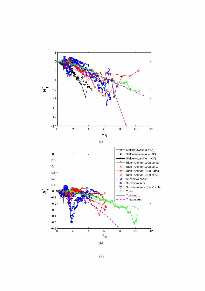
0 2 4 6 8 10 12−14

−12

−10

−8

−6

−4

−2

0

2

UR

H1*

(a)

0 2 4 6 8 10 12−0.6

−0.5

−0.4

−0.3

−0.2

−0.1

0

0.1

0.2

0.3

0.4

0.5

0.6

UR

A2*

Siekierkowski (α = 0°)

Siekierkowski (α = −3°)

Siekierkowski (α = +3°)Rion−Antirion 1998 constr.Rion−Antirion 1998 serv.Rion−Antirion 1998 trafficRion−Antirion 1999 serv.Sucharski constr.Sucharski serv.Sucharski serv. (no Vistula)TurinTurin mod.Theodorsen

(b)

187

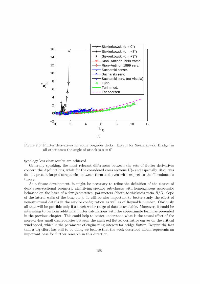
0 2 4 6 8 10 12−2

0

2

4

6

8

10

12

14

16

UR

A3*

Siekierkowski (α = 0°)Siekierkowski (α = −3°)Siekierkowski (α = +3°)Rion−Antirion 1998 trafficRion−Antirion 1999 serv.Sucharski constr.Sucharski serv.Sucharski serv. (no Vistula)TurinTurin mod.Theodorsen

(c)

Figure 7.6: Flutter derivatives for some bi-girder decks. Except for Siekierkowski Bridge, inall other cases the angle of attack is α = 0°

typology less clear results are achieved.Generally speaking, the most relevant differences between the sets of flutter derivatives

concern the A∗2-functions, while for the considered cross sections H∗1 - and especially A∗3-curves

do not present large discrepancies between them and even with respect to the Theodorsen’stheory.

As a future development, it might be necessary to refine the definition of the classes ofdeck cross-sectional geometry, identifying specific sub-classes with homogeneous aeroelasticbehavior on the basis of a few geometrical parameters (chord-to-thickness ratio B/D, slopeof the lateral walls of the box, etc.). It will be also important to better study the effect ofnon-structural details in the service configuration as well as of Reynolds number. Obviouslyall that will be possible only if a much wider range of data is available. Moreover, it could beinteresting to perform additional flutter calculations with the approximate formulas presentedin the previous chapter. This could help to better understand what is the actual effect of themore-or-less small discrepancies between the analyzed flutter derivative curves on the criticalwind speed, which is the parameter of engineering interest for bridge flutter. Despite the factthat a big effort has still to be done, we believe that the work described herein represents animportant base for further research in this direction.

188

General conclusions and outlook

In this doctoral work the vulnerability ring in the chain of risk analysis of flexible bridgeswith respect to flutter is dealt with. The first contribution is the application of Performance-Based Design philosophy to collapse limit state due to flutter, in agreement with the PacificEarthquake Engineering Research Center (PEER) formulation. For the first time, flutterderivatives are considered as random variables and the flutter problem is approached in aprobabilistic way via Monte-Carlo simulations. A single-box deck girder is experimentallystudied in the CRIACIV wind tunnel in order to get data to be used for this particularanalysis. Results are obtained with this approach both for this section model and for tworectangular cylinders. In the future it could be interesting to apply this method to other casestudies in order to better understand its potentialities. In addition, the outlined vulnerabilityanalysis could be included in the larger frame of a complete risk analysis for a real bridgestructure.

The second contribution of this work is a sort of “pre-normative” study concerning flut-ter assessment, which could be useful to enhance the codes, as a measure of risk mitigation.As final goal a simplified method to estimate flutter critical wind speed without performingwind-tunnel tests should be set up. Such a tool could be of great interest for bridge engi-neers, especially concerning medium-span flexible bridges and/or pre-design stages. First, thepassage from multimodal to bimodal approach to flutter is analyzed and discussed and thena simplified formula retaining only three (or even two) aeroelastic functions is derived. Thisstrong simplification is validated on the basis of a wide range of dynamic and aerodynamicdata, showing its extensive applicability. Finally, a relatively large number of aeroelastic data,collected during the three years of the doctoral course, are compared and analyzed accordingto the definition of a few classes of deck cross-sectional geometry. The previously mentionedsimplified formulas allow to take into account three flutter derivatives only, thus making possi-ble an attempt of generalization. Although this is only a first step towards this ambitious goal,it shows all the difficulties which have to be overcome but it also highlights some interestingand encouraging results. As future development, the database should be definitely enlarged,considering data measured in different laboratories and reorganizing them according to morerefined and detailed classes of deck cross-sectional geometry. In addition, both the passagefrom multimodal to bimodal approach and the simplified formulas for flutter should be furtherinvestigated, identifying the cases for which the multimodal analysis is definitely necessary andclarifying few points in the simplified procedure which have not been fully understood yet.

189

Bibliography

AFGC (2002). Comportement au vent des ponts. Presses de l’Ecole Nationale des Ponts etChaussees, Paris, first edition. (Association Francaise de Genie Civil).

Alexander, D. (2003). Lecture in: Pre-warning and monitoring of natural man-induced disas-ters as prevention/reduction measures. Socrates Intensive Program (Borri, C. and Peil, U.Editors), Villa Vigoni, Como.

Augusti, G., Chiarugi, A., and Vignoli, A. (1980). Experimental analysis of a cable-stayedbridge. Inserto Costruzioni Metalliche, 3, 2–16.

Augusti, G., Spinelli, P., Borri, C., Bartoli, G., Giachi, M., and Giordano, S. (1995). TheC.R.I.A.C.I.V. Atmospheric Boundary Layer Wind Tunnel. In Proc. 9th International Con-ference on Wind Engineering, New Delhi. Wiley Eastern Ltd.

Augusti, G., Borri, C., and Niemann, H.-J. (2001). Is Aeolian risk as significant as otherenvironmental risks? Reliability Engineering and System Safety, 74, 227–237.

Baker, J. and Cornell, C. (2003). Uncertainty specification and propagation for loss estimationusing FOSM method. PEER Report 2003/07, Pacific Earthquake Engineering ResearchCenter.

Barre, C., Flamand, O., and Grillaud, G. (1996a). Aerodynamic stability of Aswan cablestayed bridge over the Nile. EN-ECA 96.5 C, CSTB, Nantes.

Barre, C., Flamand, O., and Grillaud, G. (1996b). Proprietes aerodynamiques des viaducs del’Autoroute A89. EN-ECA 96.14 C, CSTB, Nantes.

Bartoli, G. and Mannini, C. (2005). Reliability of bridge deck flutter derivative measurementsin wind tunnel tests. In G. Augusti and M. Ciampoli, editors, Proc. 9th International Con-ference On Structural Safety And Reliability, pages 1193–1200, Rome. Millpress, Rotterdam.

Bartoli, G. and Procino, L. (2004). Prove in galleria del vento su modello sezione di unapasserella pedonale in loc. Ruffolo (Siena). Internal Report, CRIACIV.

Bartoli, G. and Righi, M. (2004a). Analisi del flutter per sezioni rettangolari in flusso laminaree turbolento. In Proc. 8th Italian National Conference on Wind Engineering IN-VENTO ,pages 53–62, Reggio Calabria.

191

Bartoli, G. and Righi, M. (2004b). Flutter optimization of bridge decks: experimental and ana-lytical procedures. In F. Bontempi, editor, Proc. 2nd International Conference on Structuraland Construction Engineering, volume 3, pages 2375–2381, Rome. Balkema.

Bartoli, G. and Righi, M. (2006). Flutter mechanism for rectangular prisms in smooth andturbulent flow. J. Wind Eng. Ind. Aerodyn., 94, 275–291.

Bartoli, G., Borri, C., and Gusella, V. (1995). Aeroelastic behaviour of bridge decks: asensitivity analysis of the turbulent nonlinear response. In Proc. 9th International Conferenceon Wind Engineering , pages 851–862, New Delhi. Wiley Eastern Ltd.

Bisplinghoff, R., Ashley, H., and Halfman, R. (1996). Aeroelasticity . Dover Publications, Inc.,New York, first edition.

Blevins, R. (1990). Flow-induced vibration. Van Nostrand Reinhold, New York, second edition.

Borri, C. and Biagini, P. (2005). Wind response of large roofs of stadions and arena. InJ. Naprstek and C. Fischer, editors, Proc. 4th European and African Conference on WindEngineering , Prague.

Borri, C. and Costa, C. (2004). Numerical simulation of buffeting forces in bridge deck aerody-namics via indicial functions. In Proc. 8th Italian National Conference on Wind EngineeringIN-VENTO , pages 121–130, Reggio Calabria.

Borri, C. and Hoffer, R. (2000). Aeroelastic wind forces on flexible girders. Meccanica, 35(10),1–15.

Borri, C., Costa, C., and Salvatori, L. (2005). Reliability of indicial functions in bridge deckaeroelasticity. In G. Augusti and M. Ciampoli, editors, Proc. 9th International ConferenceOn Structural Safety And Reliability, pages 1217–1224, Rome. Millpress, Rotterdam.

Brancaleoni, F. and Diana, G. (1993). The aerodynamic design of the Messina Straits Bridge.J. Wind Eng. Ind. Aerodyn., 48(2-3), 395–409.

Brownjohn, J. and Jakobsen, J. (2001). Strategies for aeroelastic parameter identification frombridge deck free vibration data. J. Wind Eng. Ind. Aerodyn., 89, 1113–1136.

Bruno, L. and Khris, S. (2003). The validity of 2D numerical simulations of vortical structuresaround a bridge deck. Mathematical and Computer Modelling, 37, 795–828.

Bucher, C. and Lyn, Y. (1988a). Effect of spanwise correlation of turbulence field on themotion stability of long-span bridges. J. Fluids and Structures, 2, 437–451.

Bucher, C. and Lyn, Y. (1988b). Stochastic stability of bridges considering coupled modes I.J. Eng. Mech. ASCE , 114(12), 2055–2071.

Bucher, C. and Lyn, Y. (1989). Stochastic stability of bridges considering coupled modes II.J. Eng. Mech. ASCE , 115(2), 384–400.

192

Buresti, G. (1998). Vortex-shedding from bluff bodies. In Riera and Davenport, editors, Windeffects on buildings and structures. Balkema, Rotterdam.

Caracoglia, L. (2000). Wind-structure oscillations on long-span suspension bridges. Ph.D.thesis, University of Trieste.

Caracoglia, L. and Jones, N. (2003a). A methodology for the experimental extraction ofindicial functions for streamlined and bluff deck sections. J. Wind Eng. Ind. Aerodyn.,91(5), 609–636.

Caracoglia, L. and Jones, N. (2003b). Time domain vs. frequency domain characterization ofaeroelastic forces for bridge deck sections. J. Wind Eng. Ind. Aerodyn., 91(3), 371–402.

Chen, X. and Kareem, A. (2000). Nonlinear response analysis of long-span bridges underturbulent winds. In Proc. 4th International Colloquium on Bluff Body Aerodynamics andApplications, Bochum.

Chen, Y. (1972). Fluctuating lift forces on the Karman vortex streets on single circularcylinders and in tube bundles; part 1: the vortex street geometry of the single circularcylinder; part 2: lift forces of single cylinders. Journal of Engineering for Industry, 94(2),603–612 & 613–622. Transactions of the ASME series B.

Chowdhury, A. and Sarkar, P. (2003). A new technique for identification of eighteen flutterderivatives using a three-degree-of-freedom section model. Engineering Structures, 25, 1763–1772.

Chowdhury, A. and Sarkar, P. (2004). Identification of eighteen flutter derivatives of an airfoiland a bridge deck. Wind and Structures, 7(3), 187–202.

Contri, S. (2003). Il flutter negli impalcati da ponte: identificazione delle derivate aeroelastichein galleria del vento. Master’s thesis, University of Florence.

Cornell, C. and Luco, N. (2001). Ground motion intensity measures for structural performanceassessment at near-fault sites. In Proc. U.S.-Japan Joint Workshop and Third GranteesMeeting, U.S.-Japan Cooperative Research on Urban Earthquake Disaster Mitigation, pages30–38, University of Washington,Seattle.

Costa, C. (2004). Time-domain models in bridge deck aeroelasticity. Ph.D. thesis, Universityof Florence.

Costa, C. (2006). Aerodynamic admittance functions and buffeting forces for bridges viaindicial functions. J. Fluids and Structures, (in press).

Costa, C. and Borri, C. (2006). Application of indicial functions in bridge deck aeroelasticity.J. Wind Eng. Ind. Aerodyn., 94(11), 859–881.

CSI (1999). SAP 2000 Analisi statica, dinamica, lineare e non lineare agli elementi finiti .Computer and Structures, Inc., Barkely, California, USA. Italian translation in September2000 by Brunetta and Perin Engineering Srl.

193

D’Asdia, P. and Sepe, V. (1998). Aeroelastic instability of long-span suspended bridges: amulti-mode approach. J. Wind Eng. Ind. Aerodyn., 74-76, 849–857.

Davenport, A. (1962). Buffeting of a suspension bridge by storm winds. J. Struct. Eng.,88(ST3), 233–268.

Davenport, A. and King, J. (1982). A study of the wind effect for the Sunshine Skyway Bridge,Tampa, Florida, concrete alternate. BLWT-SS24-1982, The Boundary Layer Wind TunnelLaboratory, The University of Western Ontario, London, Canada.

de Grenet, E. and Ricciardelli, F. (2005). The span-wise correlation of aerodynamic forces ona rectangular cylinder for different vibration regimes. In C. Soize and G. Schueller, editors,Proc. 6th European Conference on Structural Dynamics, pages 373–378, Paris. Millpress.

Diana, G., Falco, M., Bruni, S., Cigada, A., Larose, G., Damsgaard, A., and Collina, A. (1995).Comparisons between wind tunnel tests on a full aeroelastic model of the proposed bridgeover Stretto di Messina and numerical results. J. Wind Eng. Ind. Aerodyn., 54-55, 101–113.

Diana, G., Cheli, F., Zasso, A., and Bocciolone, M. (1999). Suspension bridge response toturbulent wind: Comparison of a new numerical simulation method results with full scaledata. In Larsen, Larose, and Livesey, editors, Wind Engineering into the 21st Century, Proc.10th International Conference on Wind Engineering, Copenhagen. Balkema, Rotterdam.

Diana, G., Resta, F., Zasso, A., Belloli, M., and Rocchi, D. (2004). Forced motion andfree motion aeroelastic tests on a new concept dynamometric section model of the Messinasuspension bridge. J. Wind Eng. Ind. Aerodyn., 92(6), 441–462.

Diana, G., Bruni, S., and Rocchi, D. (2005a). A numerical and experimental investigation onaerodynamic nonlinearities in bridge response to turbulent wind. In J. Naprstek and C. Fis-cher, editors, Proc. 4th European and African Conference on Wind Engineering, Prague.

Diana, G., Bruni, S., Rocchi, D., Resta, F., and Belloli, M. (2005b). A numerical and experi-mental investigation on aerodynamic nonlinearities in bridge response to turbulent wind. InC. Soize and G. Schueller, editors, Proc. 6th European Conference on Structural Dynamics,pages 397–402, Paris. Millpress.

Dyrbye, C. and Hansen, S. (1997). Wind Loads on Structures. John Wiley & Sons, firstedition.

ECCS (1987). Recommandations pour le calcul des effets du vent sur les constructions,deuxieme edition. European Convention for Constructional Steelwork (ECCS) - ComiteTechnique 12 “Vent”.

Eikenberg, C. (1998). Journalistenhandbuch zum Katastrophenmanagement . German IDNDRCommittee, Bonn, fifth edition.

EN1990 (2002). Eurocode 1: Basis of design.

194

ENV1991-2-4 (1995). Eurocode 1: Basis of design and actions on structures. Part 2-4: Windactions.

Farquharson, F. (1949). Aerodynamic stability of suspension bridges with special reference tothe Tacoma Narrows Bridge. Bulletin of the University of Washington, Seattle, Washington.

Fathi, S. (2003). Methodes d’identification des coefficients aeroelastiques des tabliers de ponts:application a la technique CBHM. EN-CAPE 04.015 R, CSTB, Nantes.

Feng, C. (1968). The measurement of vortex induced effects in flow past stationary and os-cillating circular and D-section cylinders. Ph.D. thesis, University of British Columbia,Canada.

Flamand, O. (1994). Rain-wind induced vibration of cables. In Proc. International Conferenceon cable-stayed and suspension bridges (AFPC), Deauville.

Flamand, O. (1996). Etude du comportement aerodynamique du Pont de Tancarville. EN-ECA 96.6 C, CSTB, Nantes.

Flamand, O. (2000). Stabilite aerodynamique du tablier du Pont Sucharski a Gdansk. EN-AEC 00.38 C, CSTB, Nantes.

Flamand, O. (2001). Stabilite aerodynamique du tablier du Pont Siekierkowski a Varsovie.EN-AEC 01.55 C, CSTB, Nantes.

Flamand, O. (2003a). Stabilite aerodynamique des ponts de Grande Ravine et de Trois Bassinssur la route des Tamarins a la Reunion. EN-CAPE 03.075 C - V0, CSTB, Nantes.

Flamand, O. (2003b). Validation de la stabilite aerodynamique d’une passerelle a Turin.EN-CAPE 03.210 C - V0, CSTB, Nantes.

Flamand, O. and Grillaud, G. (1993). Stabilite aerodynamique des ponts de Barranca etQuetzalapa: etude complementaire. EN-ECA 93.3 C, CSTB, Nantes.

Flamand, O. and Grillaud, G. (1996). Etude aerodynamique du pont de Beaucaire-Tarascona geometrie modifiee. EN-ECA 96.4 C, CSTB, Nantes.

Flamand, O. and Grillaud, G. (1998). Stabilite aerodynamique du tablier du Pont de Millau.EN-AEC 98.80 C, CSTB, Nantes.

Flamand, O. and Grillaud, G. (1999). Aerodynamic stability of the Rion Antirion bridge deck.Complementary cross-sectional test results. ARD 00015 A, CSTB, Nantes.

Frandsen, A. (1966). Wind stability of suspension bridges. Application of the theory of “thinairfoils”. In Proc. International Symposium on Suspension Bridges, pages 609–627, Lisbon.

Fung, Y. (1993). An introduction to the theory of aeroelasticity. Dover Publications, Inc., NewYork.

195

Gerhold, T., Galle, M., Friedrich, O., and Evans, J. (1997). Calculation of complex three-dimensional configurations employing the DLR-Tau code. In Proc. 35th AIAA AerospaceSciences Meeting and Exhibit, AIAA Paper 97-0167 , Reno, Nevada, USA.

Gimsing, N. (1997). Cable Supported Bridges - Concepts and Design. John Wiley & Sons,Inc., New York, second edition.

Graham, J. (1970). Lifting-surface theory for the problem of an arbitrary yawed sinusoidalgust incident on a thin aerofoil in incompressible flow. Aeronautical Quaterly , 21, 182–198.

Grillaud, G. and Flamand, O. (1998). Aerodynamic stability of the Rion Antirion bridge deck.EN-AEC 98.48 C, CSTB, Nantes.

Gu, M., Zhang, R., and Xiang, H. (2000). Identification of flutter derivatives of bridge decks.J. Wind Eng. Ind. Aerodyn., 84, 151–162.

Hatanaka, A. and Tanaka, H. (2002). New estimation method of aerodynamic admittancefunction. J. Wind Eng. Ind. Aerodyn., 84(2), 151–162.

Hikami, Y. and Shiraishi, N. (1988). Rain-wind induced vibrations of cables stayed bridges.J. Wind Eng. Ind. Aerodyn., 29, 409–418.

Ibrahim, S. and Mikulcik, E. (1977). A method for the direct identification of vibrationparameters from the free response. The Shock and Vibration Bull., 47(Part 4).

Jain, A., Jones, N., and Scanlan, R. (1996). Coupled flutter and buffeting analysis of long-spanbridges. J. Struct. Eng., ASCE , 122(7), 716–725.

Jakobsen, J. (1995). Fluctuating wind load and response of a line-like engineering structurewith emphasis on motion-induced wind forces. Ph.D. thesis, The Norwegian Institute ofTechnology, Trondheim.

Jakobsen, J., Savage, M., and Larose, G. (2003). Aerodynamic derivatives from buffeting re-sponse of a flat plate model with stabilizing winglets. In Proc. 11th International Conferenceon Wind Engineering , pages 673–680, Lubbock, Texas.

Jensen, A. and Hoffer, R. (1998). Flat plate flutter derivatives: an alternative formulation. J.Wind Eng. Ind. Aerodyn., 74-76, 859–869.

Katsuchi, H., Jones, N., and Scanlan, R. (1999). Multimode coupled flutter and buffetinganalysis of the Akashi Kaikyo Bridge. J. Struct. Eng., ASCE , 125(1), 60–70.

Kravchenko, A. and Moin, P. (2000). Numerical studies of flow over a circular cylinder atReD=3900. Physics of Fluids, 12(2).

Kussner, H. (1936). Zusammenfassender Bericht uber den instationaren Auftrieb von Flugeln.Luftfahrtforsch., Bd. 13(11).

196

Larose, G. (2005). Aerodynamic admittance of bridge decks: a proposal. In C. Soize andG. Schueller, editors, Proc. 6th European Conference on Structural Dynamics, pages 391–395, Paris. Millpress.

Larsen, A. (1993). Aerodynamic aspects of the final design of the 1624 m suspension bridgeacross the Great Belt. J. Wind Eng. Ind. Aerodyn., 48, 261–285.

Larsen, A. (1995). Prediction of aeroelastic stability of suspension bridges during erection. InProc. 9th International Conference on Wind Engineering, New Delhi.

Larsen, A. (1998). Advances in aeroelastic analyses of suspension and cable-stayed bridges. J.Wind Eng. Ind. Aerodyn., 74-76, 73–90.

Larsen, A. and Astiz, M. (1998). Aeroelastic considerations for the Gibraltar Bridge feasibilitystudy. In Larsen and Esdahl, editors, Proc. Bridge Aerodynamics, pages 165–173. Balkema,Rotterdam.

Li, Q. (1995). Measuring flutter derivatives for bridge sectional models in water channel. J.Eng. Mech., ASCE , 121(1), 90–101.

Lin, Y. (1996). Stochastic stability of wind-excited long-span bridges. Probab. Eng. Mech.,11, 257–261.

Lourenco, L. and Shih, C. (1993). Characteristics of the plane wake of a circular cylinder.A particle image velocimetry. From Kravchenko & Moin Report TF-73, 1998, StanfordUniversity, California.

Lyn, D., Einav, S., Rodi, W., and Park, J.-H. (1995). A laser-Doppler velocimetry study ofensemble-averaged characteristics of the turbulent near wake of a square cylinder. J. FluidMech., 304, 285–319.

Mannini, C., Soda, A., and Voss, R. (2006a). Computational investigation of flow aroundbridge sections. In J. Radic, editor, Proc. International Conference on Bridges, pages 343–350, Dubrovnik, Croatia.

Mannini, C., Soda, A., Voss, R., and Schewe, G. (2006b). URANS and DES simulation of theflow around bridge sections. In Proc. 9th Italian National Conference on Wind EngineeringIN-VENTO , Pescara.

Martini, S. (2004). Entwurf der Grundung einer Hangebrucke unter Berucksichtigung vonErdbebenbeanspruchungen gemaß EC8-Teil2 . Master’s thesis, Bergische Universitat, Wup-pertal.

Matsumoto, M. (1996). Aerodynamic damping of prisms. J. Wind Eng. Ind. Aerodyn., 59,159–175.

Matsumoto, M. (2004). Personal communication.

197

Matsumoto, M. (2005). Flutter instability of structures. In J. Naprstek and C. Fischer, editors,Proc. 4th European and African Conference on Wind Engineering, Prague.

Matsumoto, M., Shiraishi, N., and Shirato, H. (1992). Rain-wind induced vibration of cablesin cable-stayed bridges. J. Wind Eng. Ind. Aerodyn., 43, 2011–2022.

Matsumoto, M., Kobayashi, K., Niihara, Y., Shiarto, H., and Hamasaki, H. (1995). Fluttermechanism and its stabilisation of bluff bodies. In Proc. 9th International Conference onWind Engineering , pages 827–838, New Delhi. Wiley Eastern Ltd.

Matsumoto, M., Daito, Y., Yoshizumi, F., Ichikawa, Y., and Yabutani, T. (1997). Torsionalflutter of bluff bodies. J. Wind Eng. Ind. Aerodyn., 69-71, 871–882.

Matsumoto, M., Daito, Y., Kanamura, T., Shigemura, Y., Sakuma, S., and Ishizaki, H. (1998).Rain-wind induced vibration of cables in cable-stayed bridges. J. Wind Eng. Ind. Aerodyn.,74-76, 1015–1027.

Matsumoto, M., Yoshizumi, F., Yabutami, T., Abe, K., and Nakajima, N. (1999). Flutterstabilization and heaving-branch flutter. J. Wind Eng. Ind. Aerodyn., 83, 289–299.

Matsumoto, M., Nakajima, N., Taniwaki, Y., and Shijo, R. (2001). Grating effect on flutterinstability. J. Wind Eng. Ind. Aerodyn., 89, 1487–1497.

Matsumoto, M., Taniwaki, Y., and Shijo, R. (2002). Frequency characteristics in various flutterinstabilities of bridge girders. J. Wind Eng. Ind. Aerodyn., 90, 1973–1980.

Minh, N., Miyata, T., Yamada, H., and Sanada, Y. (1999). Numerical simulation of windturbulence and buffeting analysis of long-span bridges. J. Wind Eng. Ind. Aerodyn., 83(1-3), 301–315.

Miyata, T. (1995). Full model testing of large cable-supported bridges. In State of the Artin Wind Engineering; 9th International Conference on Wind Engineering, pages 249–280,New Delhi. Wiley Eastern Ltd.

Miyata, T. and Yamaguchi, K. (1993). Aerodynamics of wind effects on the Akashi KaikyoBridge. J. Wind Eng. Ind. Aerodyn., 48, 287–315.

Miyata, T., Yamada, H., Boonyapinyo, V., and Santos, J. (1995). Analytical investigation onthe response of a very long suspension bridge under gusty wind. In Proc. 9th InternationalConference on Wind Engineering, pages 1006–1017, New Delhi.

Moe, G. and Henriksen, M. (1999). Flow induced vibrations of line-like structures. In Proc.3rd International Cable Dynamics Conference, Trondheim.

Nakamura, Y. (1978). An analysis of binary flutter of bridge deck sections. J. Sound andVibration, 57(4), 471–482.

Nakamura, Y. (1979). On the aerodynamic mechanism of torsional flutter of bluff structures.J. Sound and Vibration, 67(2), 163–177.

198

Nakamura, Y. and Matsukawa, T. (1987). Vortex excitation of rectangular cylinders with along side normal to the flow. J. Fluid Mech., 180, 171–191.

Nakamura, Y. and Mizota, T. (1975). Torsional flutter of rectangular prisms. J. Eng. Mech.Div., 101(EM2), 125–142.

Nakamura, Y. and Ohya, Y. (1984). The effects of turbulence on the mean flow past two-dimensional rectangular cylinders. J. Fluid Mech., 149, 255–273.

Nakamura, Y. and Yoshimura, T. (1976). Binary flutter of suspension bridge deck sections. J.Eng. Mech. Div., 102(EM4), 685–700.

Noe, S., Fathi, S., and D’Asdia, P. (2004). Modello analitico per la stima della ampiezzadi oscillazione per distacco di vortici. In Proc. 8th Italian National Conference on WindEngineering IN-VENTO , pages 397–404, Reggio Calabria.

Novak, M. and Tanaka, H. (1972). Pressure correlations on vertical cylinder. In Proc. 4th

International Conference on Wind Effects on Structures, pages 227–232, Heathrow, U.K.Cambridge University Press.

Obasaju, E. (1983). An investigation of the effects of incidence on the flow around a squaresection cylinder. Aeronautical Quarterly , 34, 243–259.

Okajima, A. (1982). Strouhal numbers of rectangular cylinders. J. Fluid Mech., 123, 379–398.

ONERA (1989). Etude du comportement dans le vent du tablier definitif du pont de Nor-mandie. Rapport Technique n°15/3588 RY 091R-391G.

Ong, L. and Wallace, J. (1996). The velocity field of the turbulent very near wake of a circularcylinder. Exp. Fluids, 20.

Parkinson, G. and Smith, J. (1964). The square cylinder as an aeroelastic non-linear oscillator.J. Mech. Appl. Math., 17, 225–239.

Parkinson, G. and Wawzonek, M. (1981). Some considerations of combined effects of gallopingand vortex resonance. J. Wind Eng. Ind. Aerodyn., 8(1-2), 135–143.

Pasto, S. (2005). Fatigue-risk assessment of slender structures with circular cross-section atlock-in. Ph.D. thesis, University of Florence - TU Braunschweig.

Paulotto, C., Ciampoli, M., and Augusti, G. (2004). Some proposals for a first step towardsa Performance Based Wind Engineering. In Proc. 1st International Forum in EngineeringDecision Making (IFED), Stoos.

Peil, U. and Clobes, M. (2005). Time domain model for buffeting wind loads verified in fullscale measurements. In C. Soize and G. Schueller, editors, Proc. 6th European Conferenceon Structural Dynamics, Paris. Millpress.

Peil, U. and Clobes, M. (2006). Modelle zur instationaren ubertragung der Windturbulenz imZeitbereich. In Proc. VDI-Baudynamik Conference, Kassel.

199

Peil, U. and Nahrath, N. (2003). Modeling of rain-wind induced vibrations. Wind and Struc-tures, 6(1), 41–52.

Peil, U., Behrens, M., and Nahrath, N. (2002). Dynamic response of slender structures underwind load. In Proc. 5th European Conference on Structural Dynamics, Munich.

Peil, U., Nahrath, N., and Dreyer, O. (2003). Modeling of rain-wind induced vibrations. InProc. 11th International Conference on Wind Engineering, Lubbock, Texas.

Plate, E. (1997). Dams and safety management at downstream valleys. In Betamio deAlmeida A. and Viseu T., Dams and safety management at downstream valleys, pages27–43. Balkema, Lisbon.

Plate, E. (1998). Stochastic hydraulic modelling - a way to cope with uncertainty. In Proc.3rd International Conference on Hydro- Science and Engineering, Cottbus.

Plate, E. (2000). Flood risk and flood management. In A. Bronstert, C. Bismuth, and L. Men-zel, editors, Proc. European Conference on Advances in Flood Research, Potsdam.

Plate, E. (2003a). Lecture in: Pre-warning and monitoring of natural man-induced disasters asprevention/reduction measures. Socrates Intensive Program (Borri, C. and Peil, U. Editors),Villa Vigoni, Como.

Plate, E. (2003b). Towards development of a Human Security Index. In Proc. Osiris Workshop,Berlin.

Rackwitz, R. (2003). Lecture in: Pre-warning and monitoring of natural man-induced disas-ters as prevention/reduction measures. Socrates Intensive Program (Borri, C. and Peil, U.Editors), Villa Vigoni, Como.

Reinhold, T., Brinch, M., and Damsgaard, A. (1992). Wind tunnel tests for the Great Beltlink. In A. Larsen, editor, Proc. 1st International Symposium on Aerodynamics of LargeBridges, Copenhagen. Balkema, Rotterdam.

Ricciardelli, F. and de Grenet, E. (2002). Evaluation of bridge flutter derivatives from wind ex-cited vibration of section models. In Proc. 5th European Conference on Structural Dynamics,pages 587–592, Munich.

Ricciardelli, F. and Hangan, H. (2001). Pressure distribution and aerodynamic forces onstationary box bridge sections. Wind and Structures, 4(5), 399–412.

Righi, M. (2003). Aeroelastic stability of long span suspended bridges: flutter mechanism onrectangular cylinders in smooth and turbulent flow . Ph.D. thesis, University of Florence.

Rocha, M., Loredo-Souza, A., Paluch, M., and Nunez, G. (2003). Aspectos aerodinamicosa serem considerados no projeto de pontes estaiadas - Estudo de caso: ponte sobre o RioGuama. In Proc. 5th Simposio EPUSP sobre Estruturas de Concreto, Sao Paulo.

200

Roshko, A. (1954). On the development of turbulent wakes from vortex streets. Report 1191,NACA.

Roshko, A. (1961). Experiments on the flow past a circular cylinder at very high Reynoldsnumber. J. Fluid Mech., 10(3), 345–356.

Rung, T., Lubcke, H., Xue, L., Thiele, F., and Fu, S. (1999). Assessment of Explicit AlgebraicStress Models in transonic flows. In W. Rodi and D. Laurence, editors, Proc. 4th Interna-tional Symposium on Engineering Turbulence Modelling and Experiments, pages 659–668,Ajaccio, France. Elsevier, Amsterdam.

Sallet, D. (1973). The lift and drag due to von Karman vortex wake. Journal of Hydronautics,7(4), 161–165.

Salvatori, L. and Spinelli, P. (2006a). A discrete 3D model for bridge aerodynamics andaeroelasticity: nonlinearities and linearizations. Meccanica, (in press).

Salvatori, L. and Spinelli, P. (2006b). Effects of structural nonlinearity and along-span windcoherence on suspension bridge aerodynamics: some numerical simulation results. J. WindEng. Ind. Aerodyn., 94, 415–430.

Sarkar, P. (1992). New identification methods applied to the response of flexible bridges towind . Ph.D. thesis, John Hopkins University, Baltimore.

Sarkar, P., Jones, N., and Scanlan, R. (1994). Identification of aeroelastic parameters of flexiblebridges. J. Eng. Mech., ASCE , 120(8), 1718–1742.

Scanlan, R. (1984). Role of indicial functions in buffeting analysis of bridges. J. Struct. Eng.,110(7), 1433–1446.

Scanlan, R. (1998). Bridge flutter derivatives at vortex lock-in. J. Struct. Eng., 124(4),450–458.

Scanlan, R. and Jones, N. (1999). A form of aerodynamic admittance for use in bridge aeroelas-tic analysis. J. Fluids Struct., 13, 1017–1027.

Scanlan, R. and Lin, W.-H. (1978). Effects of turbulence on bridge flutter derivatives. J. Eng.Mech. Div., 104(EM4), 719–733.

Scanlan, R. and Tomko, J. (1971). Airfoil and bridge deck flutter derivatives. J. Eng. Mech.Div. Proc. ASCE , 97, 1717–1737.

Scanlan, R., Beliveau, J.-G., and Budlong, K. (1974). Indicial aerodynamic functions forbridge decks. J. Eng. Mech. Div., 100(EM4), 657–672.

Scanlan, R., Jones, N., and Singh, L. (1997). Inter-relations among flutter derivatives. J.Wind Eng. Ind. Aerodyn., 69-71, 829–837.

Schewe, G. (1983). On the force fluctuations acting on a circular cylinder in cross flow fromsubcritical up to transcritical Reynolds numbers. J. Fluid Mech., 133.

201

Schewe, G. (1984). Untersuchung der aerodynamischen Krafte, die auf stumpfe Profile-bei großen Reynolds-Zahalen wirken. DFVLR-Mitt.84-19, DLR, Institut fur Aeroelastik,Gottingen.

Schewe, G. (1986). Sensitivity of transition phenomena to small perturbations in flow rounda circular cylinder. J. Fluid Mech., 172, 33–46.

Schewe, G. (1989). Nonlinear flow-induced resonances of an H-shaped section. J. Fluids andStructures, 3, 327–348.

Schewe, G. (1990). Analyse der Aerodynamischen Kraftschwankungen, die auf Quadratprofilbei Anstellwinkelvariation wirken. In Proc. DGLR-Symp. ”Stromung mit Ablosung”, Achen.

Schewe, G. (2001). Reynolds-number effects in flow around more-or-less bluff bodies. J. WindEng. Ind. Aerodyn., 89, 1267–1289.

Schewe, G. (2005). Reynolds-number effects and their influence on flow induced vibrations.In Proc. 6th European Conference on Structural Dynamics, pages 337–342, Paris. Millpress,Rotterdam.

Schewe, G. (2006). Influence of the reynolds-number on flow-induced vibrations of genericbridge sections. In J. Radic, editor, Proc. International Conference on Bridges, pages 351–358, Dubrovnik, Croatia.

Schewe, G. and Larsen, A. (1998). Reynolds number effects in the flow around a bluff bridgedeck cross section. J. Wind Eng. Ind. Aerodyn., 74-76, 829–838.

Sears, W. (1941). Some aspects of non-stationary airfoil theory and its practical application.J. Aeronaut. Sci., 8, 104–108.

Seidel, C. and Dinkler, D. (2006). Rain-wind induced vibrations: phenomenology, mechanicalmodelling and numerical analysis. Computer and Structures, 84(24-25), 1584–1595.

Selberg, A. (1961). Oscillation and aerodynamic stability of suspension bridges. In ActaPolytechnica Scandinavica, Civ. Eng. and Build. Constr. Series n°13 , Oslo.

Shortreed, J., Hicks, J., and Craig, L. (2003). Basic frameworks for risk management. Finalreport, Prepared for The Ontario Ministry of the Environment, NERAM.

Simiu, E. and Scanlan, R. (1996). Wind effects on structures. John Wiley & Sons, Inc., NewYork, third edition.

Singh, L., Jones, N., Scanlan, R., and Lorendeaux, O. (1995). Simultaneous identification of3-dof aeroelastic parameters. In Proc. 9th International Conference on Wind Engineering,pages 972–981, New Delhi. Wiley Eastern Ltd.

Spalart, P. and Allmaras, S. (1992). A one-equation turbulence model for aerodynamic flows.In Proc. 30th AIAA Aerospace Sciences Meeting and Exhibit, AIAA Paper 92-0439 , Reno,Nevada, USA.

202

Strouhal, V. (1878). Uber eine besondere Art der Tonerregung. Annalen der Physik undChemie, pages 216–251.

Theodorsen, T. (1934). General theory of aerodynamic instability and the mechanism offlutter. NACA Technical Report 496, Aeronautics, Twentieth Annual Report of the NationalAdvisory Committee for Aeronautics, NACA.

Thompson, J. and Stewart, H. (2002). Nonlinear dynamics and chaos. John Wiley & Sons,New York, second edition.

van Nunen, J. (1974). Pressure and forces on a circular cylinder in a cross flow at high reynoldsnumber. In E. Naudascher, editor, Flow Induced Structural Vibrations. Springer-Verlag,Berlin.

von Karman, T. and Rubach, H. (1912). Uber den Mechanismus des Flussigkeits- undLuftwiderstandes. Physikalische Zeitschrift , 15(2), 49–59.

Wagner, H. (1925). Uber die Entstehung des dynamischen Auftriebes von Tagflugeln. Z.Angew. Math. Mech., Bd. 5-Helft 1.

Wooton, L. (1969). The oscillations of large circular stacks in wind. Proc. Inst. Civ. Eng., 43,573–598.

Wooton, L. and Scruton, C. (1970). Aerodynamic stability. In Seminar on Modern Design ofWind-Sensitive Structures, pages 65–81. Construction Industry Research and InformationAssociation (CIRIA), London.

Yamaguchi, H. (1990). Analytical study on growth mechanism of rain vibration of cables. J.Wind Eng. Ind. Aerodyn., 31, 73–80.

Zasso, A. (1996). Flutter derivatives: Advantages of a new representation convention. J. WindEng. Ind. Aerodyn., 60, 35–47.

Zasso, A., Cigada, A., and Negri, S. (1996). Flutter derivatives identification through fullbridge aeroelastic model transfer function analysis. J. Wind Eng. Ind. Aerodyn., 60, 17–33.

Zdravkovich, M. (1997). Flow around circular cylinders. Oxford University Press, Oxford.

Zhang, Y. and Brownjohn, J. (2004). Effect of relative amplitude on bridge deck flutter. J.Wind Eng. Ind. Aerodyn., 92(6), 493–508.

Zhang, Y., Brownjohn, J., and Omenzetter, P. (2003). Time domain formulation of self-excitedforces on bridge deck for wind tunnel experiment. J. Wind Eng. Ind. Aerodyn., 91(6), 723–736.

203

Appendix A

Other wind-tunnel test results

I

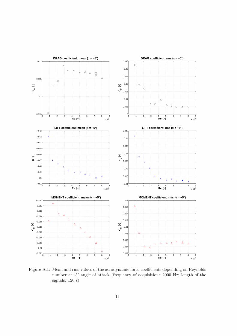
0 1 2 3 4 5 6 7 8 9

x 105

0.095

0.1

0.105

0.11DRAG coefficient: mean ( α = −5°)

Re [−]

CD [

−]

0 1 2 3 4 5 6 7 8 9

x 105

0

0.005

0.01

0.015

0.02

0.025

0.03

0.035DRAG coefficient: rms ( α = −5°)

Re [−]C

D [

−]

0 1 2 3 4 5 6 7 8 9

x 105

−0.51

−0.5

−0.49

−0.48

−0.47

−0.46

−0.45

−0.44

−0.43

−0.42LIFT coefficient: mean ( α = −5°)

Re [−]

CL [

−]

0 1 2 3 4 5 6 7 8 9

x 105

0.01

0.015

0.02

0.025

0.03

0.035

0.04

0.045LIFT coefficient: rms ( α = −5°)

Re [−]

CL [

−]

0 1 2 3 4 5 6 7 8 9

x 105

−0.021

−0.02

−0.019

−0.018

−0.017

−0.016

−0.015

−0.014

−0.013

−0.012

−0.011MOMENT coefficient: mean ( α = −5°)

Re [−]

CM

[−]

0 1 2 3 4 5 6 7 8 9

x 105

0.002

0.004

0.006

0.008

0.01

0.012

0.014

0.016

0.018MOMENT coefficient: rms ( α = −5°)

Re [−]

CM

[−]

Figure A.1: Mean and rms-values of the aerodynamic force coefficients depending on Reynoldsnumber at -5° angle of attack (frequency of acquisition: 2000 Hz; length of thesignals: 120 s)

II

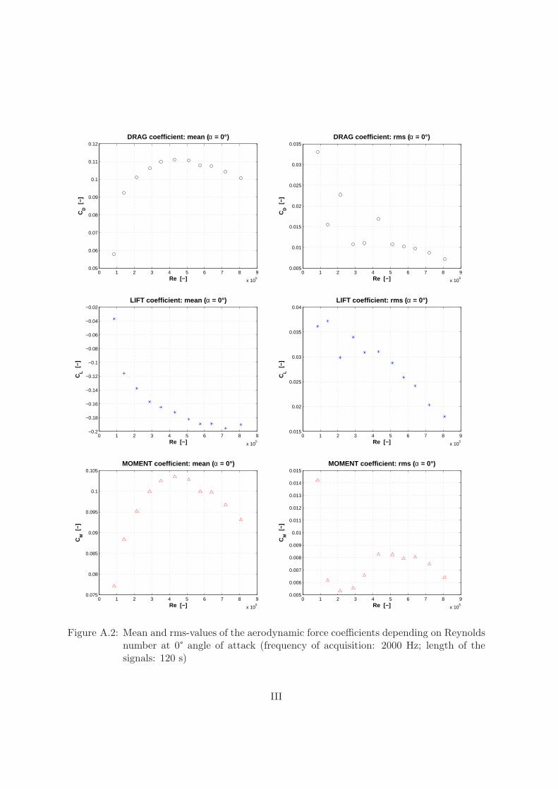
0 1 2 3 4 5 6 7 8 9

x 105

0.05

0.06

0.07

0.08

0.09

0.1

0.11

0.12DRAG coefficient: mean ( α = 0°)

Re [−]

CD [

−]

0 1 2 3 4 5 6 7 8 9

x 105

0.005

0.01

0.015

0.02

0.025

0.03

0.035DRAG coefficient: rms ( α = 0°)

Re [−]C

D [

−]

0 1 2 3 4 5 6 7 8 9

x 105

−0.2

−0.18

−0.16

−0.14

−0.12

−0.1

−0.08

−0.06

−0.04

−0.02LIFT coefficient: mean ( α = 0°)

Re [−]

CL [

−]

0 1 2 3 4 5 6 7 8 9

x 105

0.015

0.02

0.025

0.03

0.035

0.04LIFT coefficient: rms ( α = 0°)

Re [−]

CL [

−]

0 1 2 3 4 5 6 7 8 9

x 105

0.075

0.08

0.085

0.09

0.095

0.1

0.105MOMENT coefficient: mean ( α = 0°)

Re [−]

CM

[−]

0 1 2 3 4 5 6 7 8 9

x 105

0.005

0.006

0.007

0.008

0.009

0.01

0.011

0.012

0.013

0.014

0.015MOMENT coefficient: rms ( α = 0°)

Re [−]

CM

[−]

Figure A.2: Mean and rms-values of the aerodynamic force coefficients depending on Reynoldsnumber at 0° angle of attack (frequency of acquisition: 2000 Hz; length of thesignals: 120 s)

III

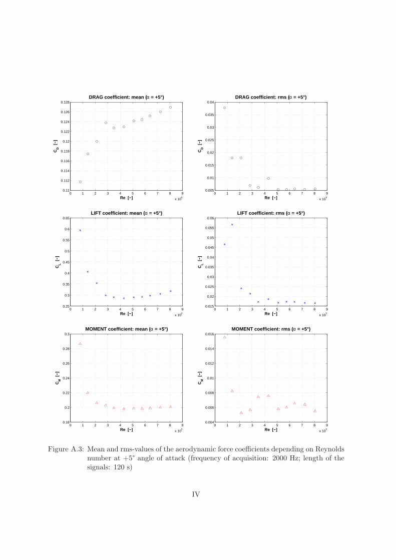
0 1 2 3 4 5 6 7 8 9

x 105

0.11

0.112

0.114

0.116

0.118

0.12

0.122

0.124

0.126

0.128DRAG coefficient: mean ( α = +5°)

Re [−]

CD [

−]

0 1 2 3 4 5 6 7 8 9

x 105

0.005

0.01

0.015

0.02

0.025

0.03

0.035

0.04DRAG coefficient: rms ( α = +5°)

Re [−]C

D [

−]

0 1 2 3 4 5 6 7 8 9

x 105

0.25

0.3

0.35

0.4

0.45

0.5

0.55

0.6

0.65LIFT coefficient: mean ( α = +5°)

Re [−]

CL [

−]

0 1 2 3 4 5 6 7 8 9

x 105

0.015

0.02

0.025

0.03

0.035

0.04

0.045

0.05

0.055

0.06LIFT coefficient: rms ( α = +5°)

Re [−]

CL [

−]

0 1 2 3 4 5 6 7 8 9

x 105

0.18

0.2

0.22

0.24

0.26

0.28

0.3MOMENT coefficient: mean ( α = +5°)

Re [−]

CM

[−]

0 1 2 3 4 5 6 7 8 9

x 105

0.004

0.006

0.008

0.01

0.012

0.014

0.016MOMENT coefficient: rms ( α = +5°)

Re [−]

CM

[−]

Figure A.3: Mean and rms-values of the aerodynamic force coefficients depending on Reynoldsnumber at +5° angle of attack (frequency of acquisition: 2000 Hz; length of thesignals: 120 s)

IV

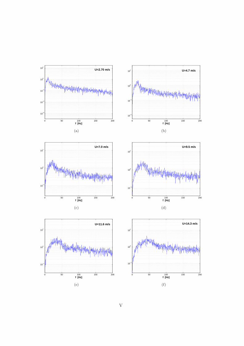
0 50 100 150 200

10−3

10−2

10−1

100

101

f [Hz]

U=2.70 m/s

(a)

0 50 100 150 200

10−2

10−1

100

101

f [Hz]

U=4.7 m/s

(b)

0 50 100 150 200

10−1

100

101

f [Hz]

U=7.0 m/s

(c)

0 50 100 150 200

10−1

100

101

f [Hz]

U=9.5 m/s

(d)

0 50 100 150 200

10−1

100

101

f [Hz]

U=11.6 m/s

(e)

0 50 100 150 200

10−1

100

101

f [Hz]

U=14.3 m/s

(f)

V

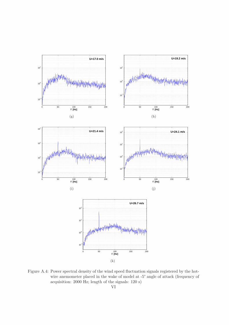
0 50 100 150 200

10−1

100

101

f [Hz]

U=17.0 m/s

(g)

0 50 100 150 200

10−1

100

101

f [Hz]

U=19.2 m/s

(h)

0 50 100 150 200

10−1

100

101

102

f [Hz]

U=21.4 m/s

(i)

0 50 100 150 200

10−1

100

101

102

f [Hz]

U=24.1 m/s

(j)

0 50 100 150 200

10−1

100

101

102

f [Hz]

U=26.7 m/s

(k)

Figure A.4: Power spectral density of the wind speed fluctuation signals registered by the hot-wire anemometer placed in the wake of model at -5° angle of attack (frequency ofacquisition: 2000 Hz; length of the signals: 120 s)

VI

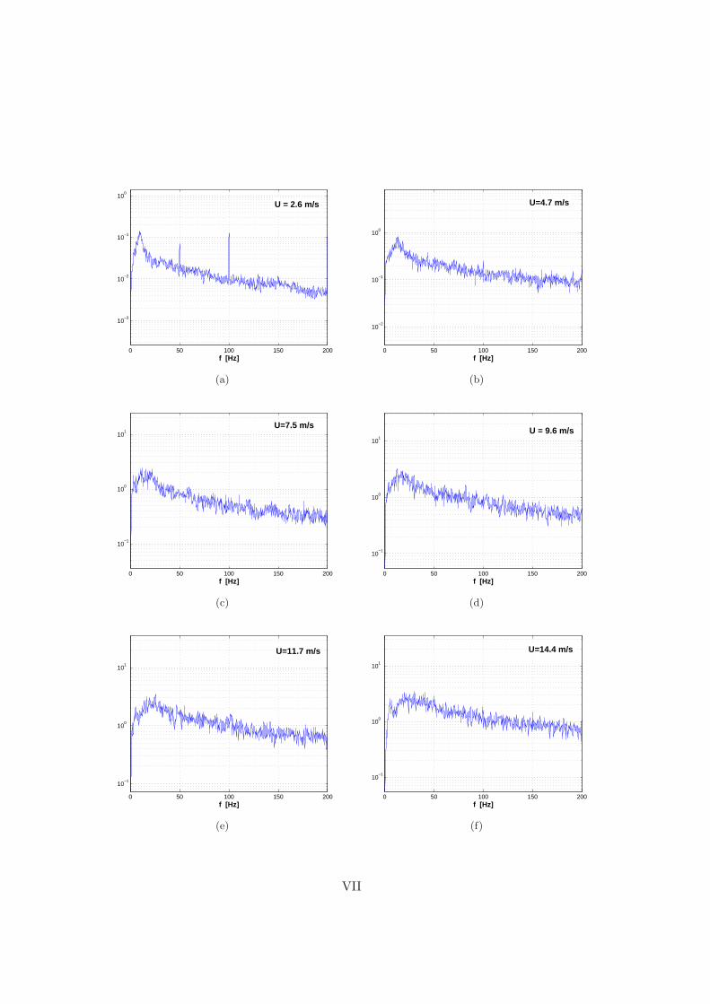
0 50 100 150 200

10−3

10−2

10−1

100

f [Hz]

U = 2.6 m/s

(a)

0 50 100 150 200

10−2

10−1

100

f [Hz]

U=4.7 m/s

(b)

0 50 100 150 200

10−1

100

101

f [Hz]

U=7.5 m/s

(c)

0 50 100 150 200

10−1

100

101

f [Hz]

U = 9.6 m/s

(d)

0 50 100 150 200

10−1

100

101

f [Hz]

U=11.7 m/s

(e)

0 50 100 150 200

10−1

100

101

f [Hz]

U=14.4 m/s

(f)

VII

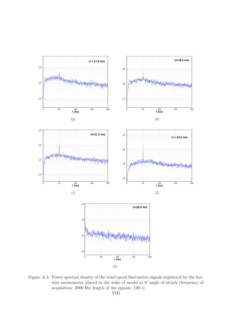
0 50 100 150 200

10−1

100

101

f [Hz]

U = 17.0 m/s

(g)

0 50 100 150 200

10−1

100

101

f [Hz]

U=19.2 m/s

(h)

0 50 100 150 200

10−1

100

101

102

f [Hz]

U=21.3 m/s

(i)

0 50 100 150 200

10−1

100

101

102

f [Hz]

U = 24.0 m/s

(j)

0 50 100 150 200

101

102

103

104

f [Hz]

U=26.9 m/s

(k)

Figure A.5: Power spectral density of the wind speed fluctuation signals registered by the hot-wire anemometer placed in the wake of model at 0° angle of attack (frequency ofacquisition: 2000 Hz; length of the signals: 120 s)

VIII

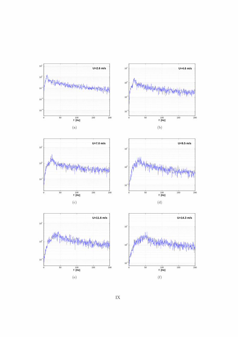
0 50 100 150 200

10−3

10−2

10−1

100

101

f [Hz]

U=2.6 m/s

(a)

0 50 100 150 200

10−2

10−1

100

101

f [Hz]

U=4.6 m/s

(b)

0 50 100 150 200

10−1

100

101

f [Hz]

U=7.0 m/s

(c)

0 50 100 150 200

10−1

100

101

f [Hz]

U=9.5 m/s

(d)

0 50 100 150 200

10−1

100

101

f [Hz]

U=11.6 m/s

(e)

0 50 100 150 200

10−1

100

101

f [Hz]

U=14.3 m/s

(f)

IX

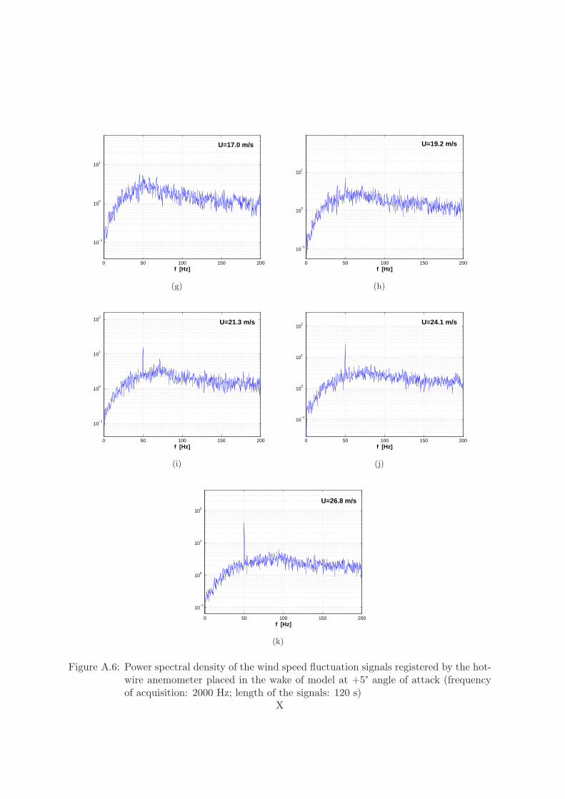
0 50 100 150 200

10−1

100

101

f [Hz]

U=17.0 m/s

(g)

0 50 100 150 200

10−1

100

101

f [Hz]

U=19.2 m/s

(h)

0 50 100 150 200

10−1

100

101

102

f [Hz]

U=21.3 m/s

(i)

0 50 100 150 200

10−1

100

101

102

f [Hz]

U=24.1 m/s

(j)

0 50 100 150 200

10−1

100

101

102

f [Hz]

U=26.8 m/s

(k)

Figure A.6: Power spectral density of the wind speed fluctuation signals registered by the hot-wire anemometer placed in the wake of model at +5° angle of attack (frequencyof acquisition: 2000 Hz; length of the signals: 120 s)

X

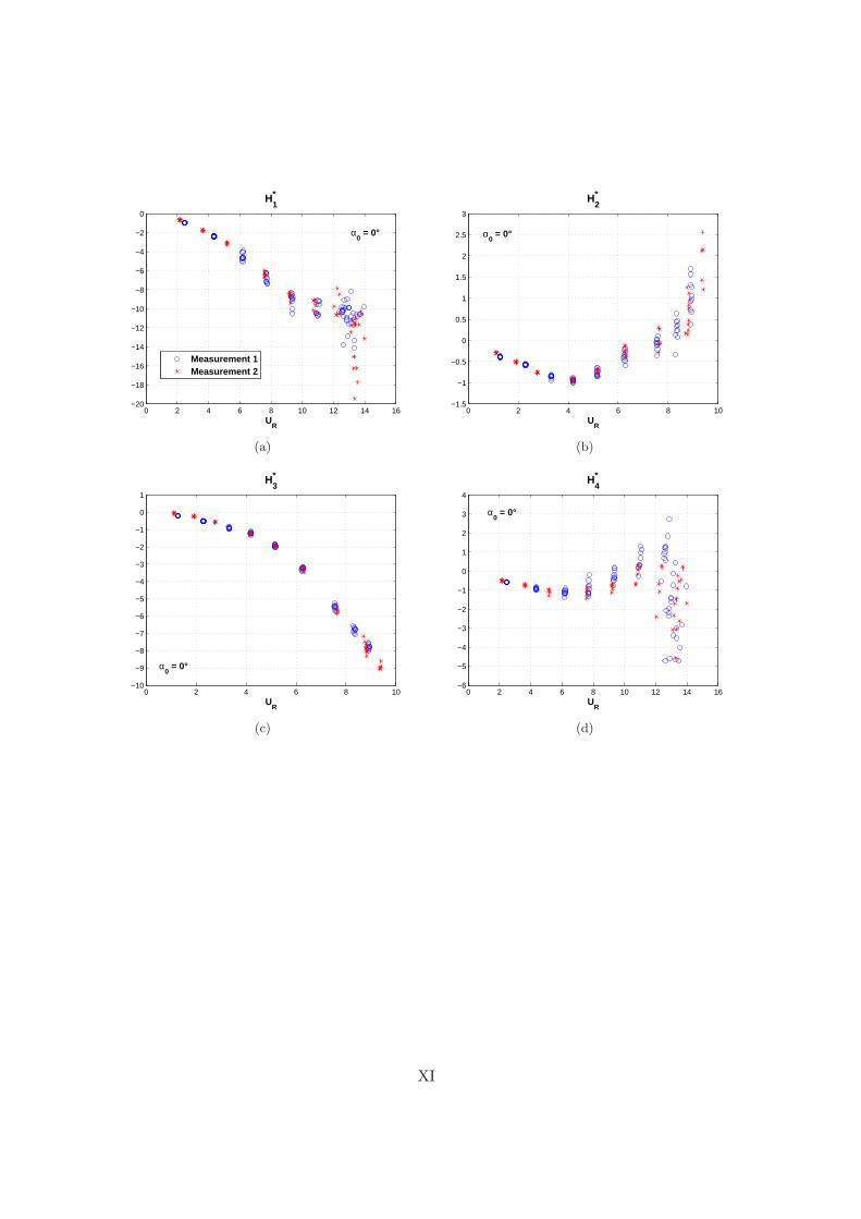
0 2 4 6 8 10 12 14 16−20

−18

−16

−14

−12

−10

−8

−6

−4

−2

0

UR

H1*

α0 = 0°

Measurement 1Measurement 2

(a)

0 2 4 6 8 10−1.5

−1

−0.5

0

0.5

1

1.5

2

2.5

3

H2*

UR

α0 = 0°

(b)

0 2 4 6 8 10−10

−9

−8

−7

−6

−5

−4

−3

−2

−1

0

1

H3*

UR

α0 = 0°

(c)

0 2 4 6 8 10 12 14 16−6

−5

−4

−3

−2

−1

0

1

2

3

4

H4*

UR

α0 = 0°

(d)

XI

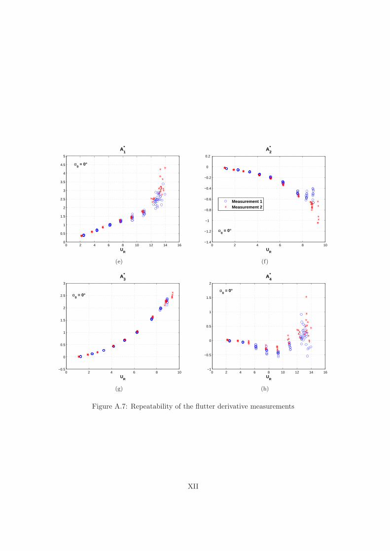
0 2 4 6 8 10 12 14 160

0.5

1

1.5

2

2.5

3

3.5

4

4.5

5

A1*

UR

α0 = 0°

(e)

0 2 4 6 8 10−1.4

−1.2

−1

−0.8

−0.6

−0.4

−0.2

0

0.2

UR

A2*

α0 = 0°

Measurement 1Measurement 2

(f)

0 2 4 6 8 10−0.5

0

0.5

1

1.5

2

2.5

3

A3*

UR

α0 = 0°

(g)

0 2 4 6 8 10 12 14 16−1

−0.5

0

0.5

1

1.5

2

A4*

UR

α0 = 0°

(h)

Figure A.7: Repeatability of the flutter derivative measurements

XII

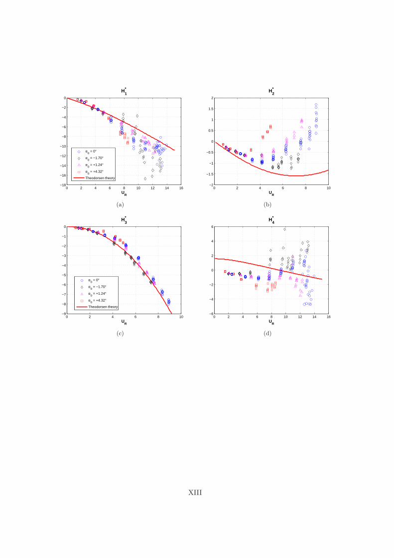
0 2 4 6 8 10 12 14 16−18

−16

−14

−12

−10

−8

−6

−4

−2

0

UR

H1*

α0 = 0°

α0 = −1.70°

α0 = +1.24°

α0 = +4.32°

Theodorsen theory

(a)

0 2 4 6 8 10−2

−1.5

−1

−0.5

0

0.5

1

1.5

2

UR

H2*

(b)

0 2 4 6 8 10−9

−8

−7

−6

−5

−4

−3

−2

−1

0

UR

H3*

α0 = 0°

α0 = −1.70°

α0 = +1.24°

α0 = +4.32°

Theodorsen theory

(c)

0 2 4 6 8 10 12 14 16−6

−4

−2

0

2

4

6

UR

H4*

(d)

XIII

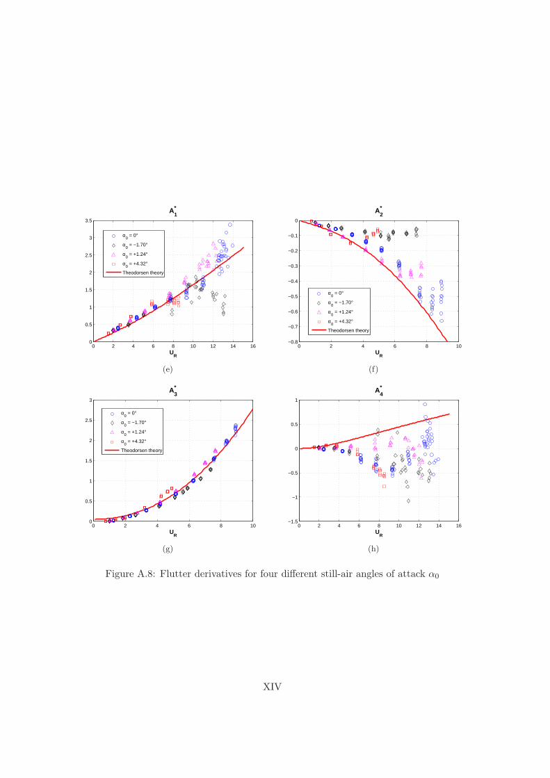
0 2 4 6 8 10 12 14 160

0.5

1

1.5

2

2.5

3

3.5

UR

A1*

α0 = 0°

α0 = −1.70°

α0 = +1.24°

α0 = +4.32°

Theodorsen theory

(e)

0 2 4 6 8 10−0.8

−0.7

−0.6

−0.5

−0.4

−0.3

−0.2

−0.1

0

UR

A2*

α0 = 0°

α0 = −1.70°

α0 = +1.24°

α0 = +4.32°

Theodorsen theory

(f)

0 2 4 6 8 100

0.5

1

1.5

2

2.5

3

UR

A3*

α0 = 0°

α0 = −1.70°

α0 = +1.24°

α0 = +4.32°

Theodorsen theory

(g)

0 2 4 6 8 10 12 14 16−1.5

−1

−0.5

0

0.5

1

UR

A4*

(h)

Figure A.8: Flutter derivatives for four different still-air angles of attack α0

XIV

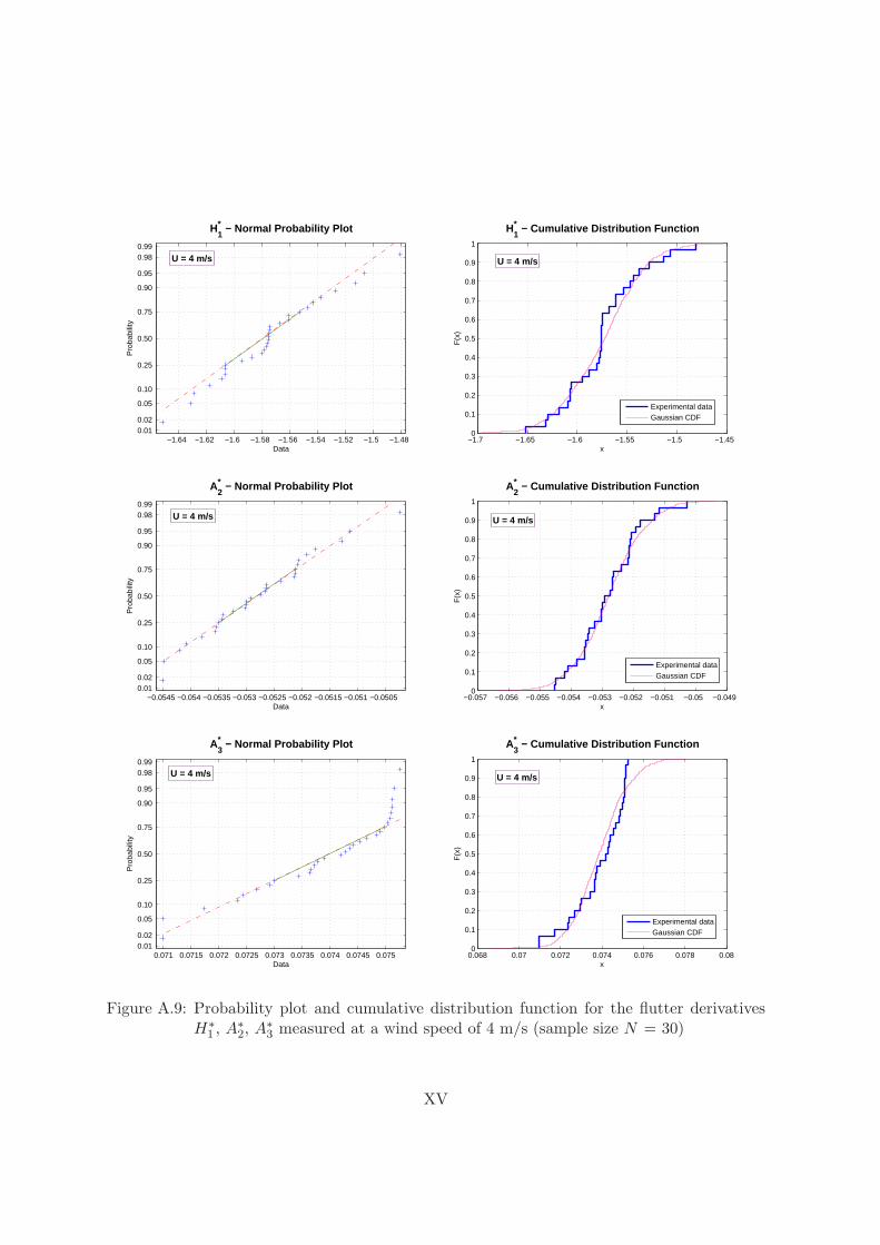
−1.64 −1.62 −1.6 −1.58 −1.56 −1.54 −1.52 −1.5 −1.480.01 0.02

0.05

0.10

0.25

0.50

0.75

0.90

0.95

0.98 0.99

Data

Pro

babi

lity

H1* − Normal Probability Plot

U = 4 m/s

−1.7 −1.65 −1.6 −1.55 −1.5 −1.450

0.1

0.2

0.3

0.4

0.5

0.6

0.7

0.8

0.9

1

xF

(x)

H1* − Cumulative Distribution Function

U = 4 m/s

Experimental dataGaussian CDF

−0.0545 −0.054 −0.0535 −0.053 −0.0525 −0.052 −0.0515 −0.051 −0.05050.01 0.02

0.05

0.10

0.25

0.50

0.75

0.90

0.95

0.98 0.99

Data

Pro

babi

lity

A2* − Normal Probability Plot

U = 4 m/s

−0.057 −0.056 −0.055 −0.054 −0.053 −0.052 −0.051 −0.05 −0.0490

0.1

0.2

0.3

0.4

0.5

0.6

0.7

0.8

0.9

1

x

F(x

)

A2* − Cumulative Distribution Function

U = 4 m/s

Experimental dataGaussian CDF

0.071 0.0715 0.072 0.0725 0.073 0.0735 0.074 0.0745 0.0750.01 0.02

0.05

0.10

0.25

0.50

0.75

0.90

0.95

0.98 0.99

Data

Pro

babi

lity

A3* − Normal Probability Plot

U = 4 m/s

0.068 0.07 0.072 0.074 0.076 0.078 0.080

0.1

0.2

0.3

0.4

0.5

0.6

0.7

0.8

0.9

1

x

F(x

)

A3* − Cumulative Distribution Function

U = 4 m/s

Experimental dataGaussian CDF

Figure A.9: Probability plot and cumulative distribution function for the flutter derivativesH∗

1 , A∗2, A∗3 measured at a wind speed of 4 m/s (sample size N = 30)

XV

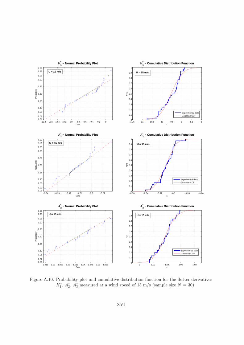
−10.8 −10.6 −10.4 −10.2 −10 −9.8 −9.6 −9.4 −9.2 −90.01 0.02

0.05

0.10

0.25

0.50

0.75

0.90

0.95

0.98 0.99

Data

Pro

babi

lity

H1* − Normal Probability Plot

U = 15 m/s

−11.5 −11 −10.5 −10 −9.5 −9 −8.5 −80

0.1

0.2

0.3

0.4

0.5

0.6

0.7

0.8

0.9

1

xF

(x)

H1* − Cumulative Distribution Function

Experimental dataGaussian CDF

U = 15 m/s

−0.34 −0.33 −0.32 −0.31 −0.3 −0.290.01 0.02

0.05

0.10

0.25

0.50

0.75

0.90

0.95

0.98 0.99

Data

Pro

babi

lity

A2* − Normal Probability Plot

U = 15 m/s

−0.36 −0.34 −0.32 −0.3 −0.28 −0.260

0.1

0.2

0.3

0.4

0.5

0.6

0.7

0.8

0.9

1

x

F(x

)

A2* − Cumulative Distribution Function

Experimental dataGaussian CDF

U = 15 m/s

1.015 1.02 1.025 1.03 1.035 1.04 1.045 1.05 1.0550.01 0.02

0.05

0.10

0.25

0.50

0.75

0.90

0.95

0.98 0.99

Data

Pro

babi

lity

A3* − Normal Probability Plot

U = 15 m/s

1 1.02 1.04 1.06 1.080

0.1

0.2

0.3

0.4

0.5

0.6

0.7

0.8

0.9

1

x

F(x

)

A3* − Cumulative Distribution Function

Experimental dataGaussian CDF

U = 15 m/s

Figure A.10: Probability plot and cumulative distribution function for the flutter derivativesH∗

1 , A∗2, A∗3 measured at a wind speed of 15 m/s (sample size N = 30)

XVI

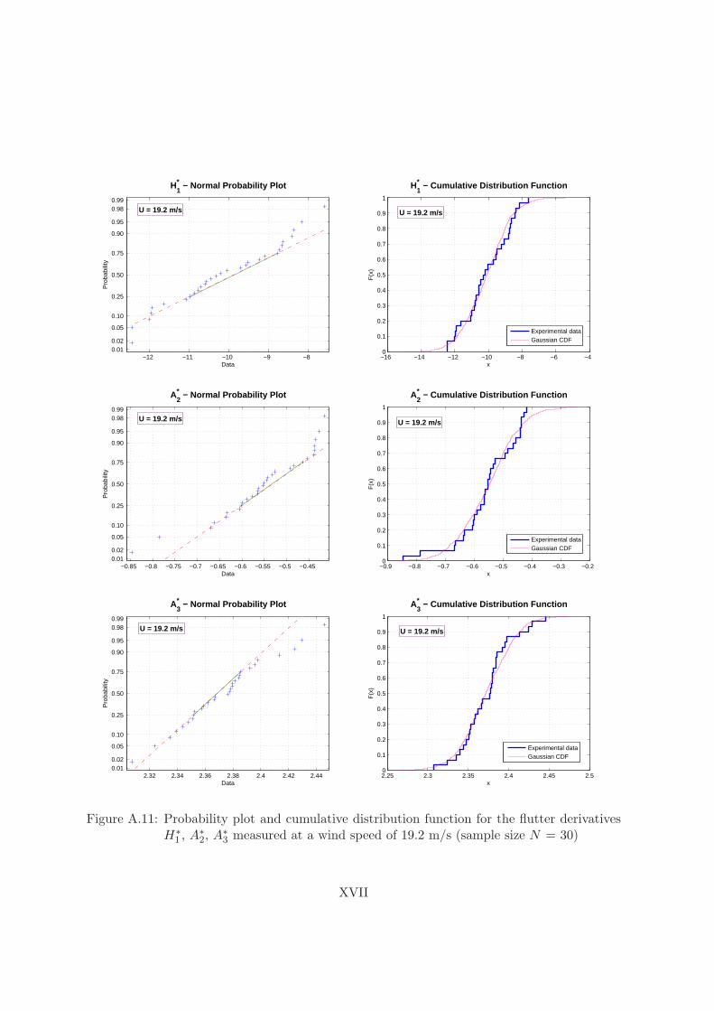
−12 −11 −10 −9 −80.01 0.02

0.05

0.10

0.25

0.50

0.75

0.90

0.95

0.98 0.99

Data

Pro

babi

lity

H1* − Normal Probability Plot

U = 19.2 m/s

−16 −14 −12 −10 −8 −6 −40

0.1

0.2

0.3

0.4

0.5

0.6

0.7

0.8

0.9

1

xF

(x)

H1* − Cumulative Distribution Function

U = 19.2 m/s

Experimental dataGaussian CDF

−0.85 −0.8 −0.75 −0.7 −0.65 −0.6 −0.55 −0.5 −0.450.01 0.02

0.05

0.10

0.25

0.50

0.75

0.90

0.95

0.98 0.99

Data

Pro

babi

lity

A2* − Normal Probability Plot

U = 19.2 m/s

−0.9 −0.8 −0.7 −0.6 −0.5 −0.4 −0.3 −0.20

0.1

0.2

0.3

0.4

0.5

0.6

0.7

0.8

0.9

1

x

F(x

)

A2* − Cumulative Distribution Function

U = 19.2 m/s

Experimental dataGaussian CDF

2.32 2.34 2.36 2.38 2.4 2.42 2.440.01 0.02

0.05

0.10

0.25

0.50

0.75

0.90

0.95

0.98 0.99

Data

Pro

babi

lity

A3* − Normal Probability Plot

U = 19.2 m/s

2.25 2.3 2.35 2.4 2.45 2.50

0.1

0.2

0.3

0.4

0.5

0.6

0.7

0.8

0.9

1

x

F(x

)

A3* − Cumulative Distribution Function

U = 19.2 m/s

Experimental dataGaussian CDF

Figure A.11: Probability plot and cumulative distribution function for the flutter derivativesH∗

1 , A∗2, A∗3 measured at a wind speed of 19.2 m/s (sample size N = 30)

XVII