1

Flexible Routing Architecture Generation for Domain-Specific Reconfigurable Subsystems

Katherine Compton

Northwestern University Evanston, IL USA

kati@ece.northwestern.edu

Akshay Sharma, Shawn Phillips, Scott Hauck

University of Washington Seattle, WA USA

{akshay, phillips, hauck}@ee.washington.edu

Abstract

Reconfigurable hardware is ideal for use in Systems-on-a-Chip, as it provides hardware speeds as well as the benefits of post-fabrication modification. However, not all applications are equally suited to any one reconfigurable architecture. Therefore, the Totem Project focuses on the automatic generation of customized reconfigurable hardware. This paper details our first attempts at the design of algorithms for automatic generation of customized flexible routing architectures. We show that these algorithms provide results with a low area overhead compared to the custom-designed RaPiD routing architecture, as well as the flexibility needed to handle some application modifications.

Introduction

Reconfigurable hardware shows great potential for use in systems-on-a-chip (SoCs), as it provides speeds similar to hardware execution, but maintains a level of flexibility not available with more traditional custom circuitry. This flexibility is the key to allowing for both hardware reuse and post-fabrication modification.

A widely available form of reconfigurable hardware is the field-programmable gate array (FPGA), and the structures within an SoC could be patterned after these designs. However, because of their highly flexible nature, FPGAs can incur significant area and speed penalties. If the SoC itself will be custom-fabricated, this presents the opportunity for customization of the reconfigurable hardware based on characteristics of the target application domain. Domain-specific reconfigurable hardware provides

2

only the amount of reconfigurability needed by the applications, which leads to reduced area and increased performance compared to a generic FPGA-style solution.

Manual design of a new reconfigurable architecture for each new application set would be disadvantageous in terms of design time and expertise required. Instead, we focus on the automatic creation of customized reconfigurable architectures, including high-level design, VLSI layout [1], and custom place and route tools creation [2]. This paper focuses on the Totem Project's work towards the automatic creation of reconfigurable architectures that are flexible enough to handle small changes in the application circuits, such as upgrades or bug-fixes, or perhaps even the addition of different circuits entirely.

Background

Our current architecture generator creates designs in the style of the RaPiD architecture [3][4][5]. The two primary motivations for choosing the RaPiD system as a starting point for our research, apart from its successes in DSP applications, are that it is a one-dimensional architecture, and because a compiler for this system is already in place. The one-dimensional nature of RaPiD simplifies our task significantly, though in future efforts we will extend our techniques to 2D architectures. Also, as is the case for the RaPiD architecture, a 1D design is quite suited to the datapath-style computations that we are initially targeting. The existing compiler is also important because this provides us with a method to generate benchmark application circuits.

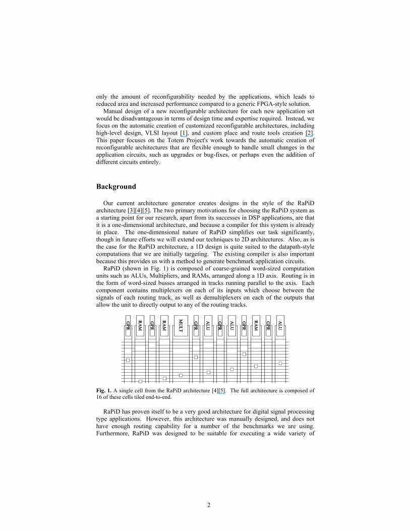
RaPiD (shown in Fig. 1) is composed of coarse-grained word-sized computation units such as ALUs, Multipliers, and RAMs, arranged along a 1D axis. Routing is in the form of word-sized busses arranged in tracks running parallel to the axis. Each component contains multiplexers on each of its inputs which choose between the signals of each routing track, as well as demultiplexers on each of the outputs that allow the unit to directly output to any of the routing tracks.

GPR

RA

M

RA

M

GPR

MU

LT

GPR

ALU

ALU

GPR

GPR

RA

M

ALU

GPR

GPR

RA

M

RA

M

GPR

MU

LT

GPR

ALU

ALU

GPR

GPR

RA

M

ALU

GPR

Fig. 1. A single cell from the RaPiD architecture [4][5]. The full architecture is composed of 16 of these cells tiled end-to-end.

RaPiD has proven itself to be a very good architecture for digital signal processing type applications. However, this architecture was manually designed, and does not have enough routing capability for a number of the benchmarks we are using. Furthermore, RaPiD was designed to be suitable for executing a wide variety of

3

circuits. Our goal is to customize an architecture for a given application set, with some extra resources if desired for future flexibility, and to be able to generate this architecture automatically.

Routing Architecture Generation

For this paper we concentrate primarily on the generation of configurable routing architectures. We use a slightly modified version of our previous algorithms for generating logic structures along a 1D axis [6]. The routing architectures are generated using a number of heuristics to generate solutions targeting different combinations of area and flexibility goals.

Each of our routing generation algorithms shares a couple of key concepts. The first is the difference between local and distance routing tracks. Local tracks are used for short connections. The top five tracks of RaPiD are of this type. The length of a wire in a track can be determined by finding the indices of the furthest units a wire can reach, and subtracting the left index from the right index. A special local track, which is the topmost shown in Fig. 1, is a track containing length 0 “feedback” wires, that only route from a unit's outputs to the unit's inputs. Distance routing tracks include the added flexibility that longer wires can be created from shorter ones through the bus connectors. Each bus connector can be independently programmed. This allows a great deal of routing flexibility, but adds a delay as a signal passes through the bus connector, and adds an area penalty. The lower eight tracks of RaPiD are of this type.

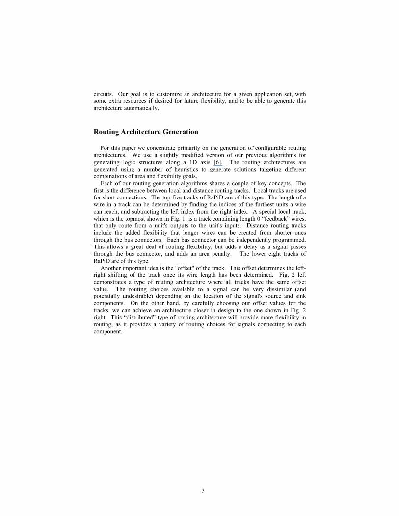
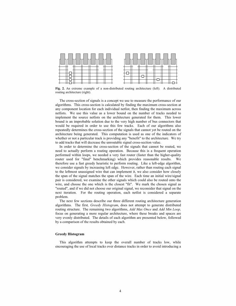
Another important idea is the "offset" of the track. This offset determines the left-right shifting of the track once its wire length has been determined. Fig. 2 left demonstrates a type of routing architecture where all tracks have the same offset value. The routing choices available to a signal can be very dissimilar (and potentially undesirable) depending on the location of the signal's source and sink components. On the other hand, by carefully choosing our offset values for the tracks, we can achieve an architecture closer in design to the one shown in Fig. 2 right. This “distributed” type of routing architecture will provide more flexibility in routing, as it provides a variety of routing choices for signals connecting to each component.

4

Fig. 2. An extreme example of a non-distributed routing architecture (left). A distributed routing architecture (right).

The cross-section of signals is a concept we use to measure the performance of our algorithms. This cross-section is calculated by finding the maximum cross-section at any component location for each individual netlist, then finding the maximum across netlists. We use this value as a lower bound on the number of tracks needed to implement the source netlists on the architecture generated for them. This lower bound is an improbable solution due to the very high number of bus connectors that would be required in order to use this few tracks. Each of our algorithms also repeatedly determines the cross-section of the signals that cannot yet be routed on the architecture being generated. This computation is used as one of the indicators of whether or not a particular track is providing any "benefit" to the architecture. We try to add tracks that will decrease the unroutable signal cross-section value.

In order to determine the cross-section of the signals that cannot be routed, we need to actually perform a routing operation. Because this is a frequent operation performed within loops, we needed a very fast router (faster than the higher-quality router used for "final" benchmarking) which provides reasonable results. We therefore use a fast greedy heuristic to perform routing. Like a left-edge algorithm, we consider signals by increasing left edge. However, rather than routing each signal to the leftmost unassigned wire that can implement it, we also consider how closely the span of the signal matches the span of the wire. Each time an initial wire/signal pair is considered, we examine the other signals which could also be routed onto the wire, and choose the one which is the closest "fit". We mark the chosen signal as "routed", and if we did not choose our original signal, we reconsider that signal on the next iteration. For the routing operation, each netlist is considered a separate problem.

The next few sections describe our three different routing architecture generation algorithms. The first, Greedy Histogram, does not attempt to generate distributed routing structure. The remaining two algorithms, Add Max Once and Add Min Loop, focus on generating a more regular architecture, where these breaks and spaces are very evenly distributed. The details of each algorithm are presented below, followed by a comparison of the results obtained by each.

Greedy Histogram

This algorithm attempts to keep the overall number of tracks low, while encouraging the use of local tracks over distance tracks in order to avoid introducing a

5

large number of bus connectors. Each track has a specific type and wire length used for all segments within that track. However, we make no restrictions as to what offset should be used. This creates a potentially non-distributed routing architecture which may not have uniform connectivity and thus may not be as flexible as a more regular interconnect architecture.

In this algorithm, tracks are added one at a time within an infinite loop. The loop is broken when all of the netlists can be fully routed onto the architecture using the routing algorithm we discussed previously. The algorithm chooses the wire length for a "new" track by looking at largest value in the histogram of the unrouted signal lengths. The actual track creation method depends in part upon the wire length chosen. For lengths smaller than 8, we choose a local routing track to avoid excessive use of bus connectors, and check all possible offsets (from 0 to length-1) to find the best one for that wire length. Otherwise we create a distance track, and we check all wire lengths from 8 to the chosen length, and all offsets for each length to find the track that reduces the histogram the most at the length we chose.

Regular Routing Algorithms

The next two algorithms generate a distributed routing architecture, where not only are the breaks or connectors evenly distributed within a track, but also across tracks. In other words, we choose our track offsets so as to provide a somewhat consistent level of connectivity regardless of location in the architecture. Fig. 2 right shows an example of this type of routing architecture. In order to make the complex task of even break/connector distribution easier to approximate, we have restricted wire lengths to powers of two, where the track possibilities are now local tracks of length 0 (feedback), 2, and 4, and distance tracks of length 8 and 16. Because the Greedy Histogram method infrequently chose wire lengths greater than 16, we did not include options for lengths 32 or higher.

Add Max Once

This algorithm is fairly simple in organization, much more than the Greedy Histogram algorithm. We start from the shortest track length and go to the longest track length, seeing how many tracks of each type we can add while still improving the cross-section of unroutable signals. In other words, we add tracks of the given type until no further cross-section reductions are possible due to the creation additional tracks of the type.

Add Min Loop

The previous algorithm tends to weight towards the use of distance routing tracks because it only considers each wire length and type combination once. It is possible, however, that once a distance track is added, using additional local tracks will in fact once again reduce the unroutable signal cross-section. Therefore, we have created the

6

Add Min Loop algorithm in an effort to more accurately generate tracks with local wires.

This algorithm iteratively adds a small number of tracks to the overall routing architecture, until full routeability can be achieved, with only one type of track added per iteration. Within the loop, we repeatedly attempt to add tracks in the following order: length 0 local tracks, length 2 local tracks, length 4 local tracks, length 16 distance tracks, and length 8 distance tracks. In the case of the local routing tracks, we attempt to add as many tracks as the length of the wires in the track (providing potentially the full range of offsets for that particular track type). For distance routing tracks, which we consider to be much more expensive, we only attempt to add a single track of each type. We only keep the tracks we attempt to add if it causes a reduction in the cross-section of unroutable signals. If we keep any tracks, we immediately remove any track containing longer wires than our new track(s). This is done because that once the shorter wire length track is added, the architecture may not need as many longer-type tracks as was earlier computed. After we modify the counts accordingly, we return to the top of the loop.

Algorithm Comparison

Both area and flexibility are important when comparing reconfigurable architectures, as a very small architecture with little flexibility may not meet the needs of the user. Conversely, an architecture that is overly flexible may be able to implement any circuit required, yet the area cost may be prohibitive. In this paper we compare our three different routing generation algorithms first on an area basis, and second on the flexibility of the resulting architectures.

We are using a number of benchmarks from which we choose our various application "sets". These benchmarks have been compiled using the RaPiD compiler [3] into a coarse netlist format, which our tools then interpret and use. The benchmark sets are:

• Radar – used to observe the atmosphere using FM signals • Digital Camera – a set of three operations needed for a digital camera • OFDM – part of a MC-CDMA receiver application that uses a smart antenna • Image Processing Library – a minimal image processing library • All DCT/FFT – two different 16-point FFTs and a DCT • All FIR –six different FIR filters, two of which time-multiplex use of multipliers • All Matrix Multiply – five different matrix multipliers • All Sort – two 1D sorting netlists and two 2D sorting netlists

Area

In order to determine area numbers, we found the areas of the components as provided by the RaPiD group. All layouts were done in a TSMC .25µm process. To

7

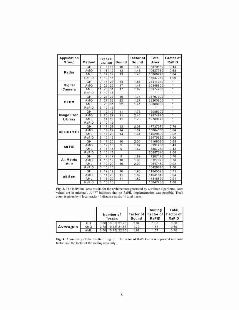
compare to a RaPiD implementation, we assume that RaPiD is easily tileable to any number of cells, but that the routing architecture and logic within each cell is fixed. This represents the obvious hard-macro approach to SoC reconfigurable subsystem design. For each application group, we found the minimum number of RaPiD cells that fit all of the netlists using our initial place and route tool [2]. The individual area results of the comparisons are shown in Fig. 3. If a benchmark set cannot be implemented using tileable RaPiD cells, a “*” appears in the results table. In these cases, the RaPiD routing architecture is simply not large or flexible enough for that particular application set.

For each application set, we show the track count generated by each of the three algorithms, and compare to the lower bound. Note that the lower bound is different for Greedy Histogram, since the logic layout is not constrained to be “distributed”. The chart then indicates how far from the lower bound each algorithm's routing architecture is, where the lower bound is the maximum of the cross-section of all signals in each netlist. As mentioned earlier, we consider this lower bound to be unrealistic. Finally, the total area is given for the architectures, including for the required RaPiD implementation, and each method is compared to the RaPiD implementation for the same application group. These results are summarized in Fig. 4.

The average fraction of the RaPiD solution was .66 for the Greedy Histogram, .69 for Add Max Once, and .70 for Add Min Loop. This is not even taking into account the benchmark sets that could not be implemented on RaPiD as the architecture is now. The majority of this benefit is due to including only the necessary logic for each benchmark set. This is where customization can greatly affect overall area results. As these values indicate, the extra routing area overhead introduced by using automatic routing generation (instead of hand-design as is the case with RaPiD) did not overwhelm the area benefits of removing unnecessary logic. For the cases where we were able to compare to a RaPiD implementation, we averaged a factor of nearly 2.5 in logic area reduction. Meanwhile, we only increased routing area by an average of 1.37 times for Greedy Histogram, 1.53 times for Add Max Once, and 1.57 times for Add Min Loop.

8

Application Group Method Bound

Factor of Bound

Total Area

Factor of RaPiD

GH 7 8 15 10 1.50 6879160 0.44AMO 1 18 19 13 1.46 10637760 0.68AML 5 14 19 13 1.46 10066770 0.64

RaPiD 5 10 15 15647260 1.00GH 9 17 26 14 1.86 26414350 *

AMO 2 23 25 17 1.47 30348850 *AML 11 20 31 17 1.82 33974950 *

RaPiD 5 10 15 * *GH 10 23 33 19 1.74 94797900 *

AMO 1 27 28 22 1.27 88205800 *AML 6 25 31 22 1.41 86888800 *

RaPiD 5 10 15 * *GH 7 12 19 11 1.73 12085300 *

AMO 2 25 27 11 2.45 12974970 *AML 5 14 19 11 1.73 12789070 *

RaPiD 5 10 15 * *GH 8 17 25 12 2.08 17737070 0.76

AMO 3 19 22 14 1.57 15084150 0.64AML 6 17 23 14 1.64 14629560 0.62

RaPiD 5 10 15 23475660 1.00GH 9 11 20 10 2.00 14106060 0.68

AMO 3 12 15 9 1.67 8991460 0.43AML 4 11 15 9 1.67 8857280 0.42

RaPiD 5 10 15 20857340 1.00GH 10 7 17 9 1.89 7287170 0.70

AMO 4 15 19 10 1.90 8127370 0.78AML 8 12 20 10 2.00 9547450 0.92

RaPiD 5 10 15 10426080 1.00GH 7 12 19 10 1.90 11045520 0.71

AMO 6 14 20 11 1.82 14641540 0.94AML 7 13 20 11 1.82 14316820 0.91

RaPiD 5 10 15 15647780 1.00

Tracks (L/D/Tot)

All DCT/FFT

All FIR

All Matrix Mult

All Sort

Radar

Digital Camera

OFDM

Image Proc. Library

Fig. 3. The individual area results for the architectures generated by our three algorithms. Area values are in microns2. A “*” indicates that no RaPiD implementation was possible. Track count is given by # local tracks / # distance tracks / # total tracks

Factor of Bound

Routing Factor of

RaPiD

Total Factor of

RaPiDGH 8.38 13.38 21.75 1.84 1.37 0.66

AMO 2.75 19.13 21.88 1.70 1.53 0.69AML 6.50 15.75 22.25 1.69 1.57 0.70

Number of Tracks

Averages

Fig. 4. A summary of the results of Fig. 3. The factor of RaPiD area is separated into total factor, and the factor of the routing area only.

9

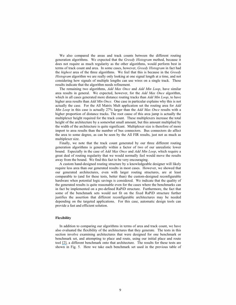
We also compared the areas and track counts between the different routing generation algorithms. We expected that the Greedy Histogram method, because it does not require as much regularity as the other algorithms, would perform best in terms of track count and area. In some cases, however, Greedy Histogram in fact had the highest area of the three algorithms. We feel that this is because in the Greedy Histogram algorithm we are really only looking at one signal length at a time, and not considering how signals of multiple lengths can use wires on a single track. These results indicate that the algorithm needs refinement.

The remaining two algorithms, Add Max Once and Add Min Loop, have similar area results in general. We expected, however, for the Add Max Once algorithm, which in all cases generated more distance routing tracks than Add Min Loop, to have higher area results than Add Min Once. One case in particular explains why this is not actually the case. For the All Matrix Mult application set the routing area for Add Min Loop in this case is actually 27% larger than the Add Max Once results with a higher proportion of distance tracks. The root cause of this area jump is actually the multiplexer height required for the track count. These multiplexers increase the total height of the architecture by a somewhat small amount, but this amount multiplied by the width of the architecture is quite significant. Multiplexer size is therefore of more import to area results than the number of bus connectors. Bus connectors do affect the area to some degree, as can be seen by the All FIR results, just not as much as multiplexer size.

Finally, we note that the track count generated by our three different routing generation algorithms is generally within a factor of two of our unrealistic lower bound. Especially in the case of Add Max Once and Add Min Loop, which require a great deal of routing regularity that we would normally feel would move the results away from the bound. We find this fact to be very encouraging.

A custom hand-designed routing structure by a knowledgeable designer will likely require less area than our generated results in most cases. However, we showed that our generated architectures, even with larger routing structures, are at least comparable to (and for these tests, better than) the custom-designed reconfigurable hardware when potential logic savings is considered. We indicate that the quality of the generated results is quite reasonable even for the cases where the benchmarks can in fact be implemented on a pre-defined RaPiD structure. Furthermore, the fact that some of the benchmark sets would not fit on the fixed RaPiD structure further justifies the assertion that different reconfigurable architectures may be needed depending on the targeted applications. For this case, automatic design tools can provide a fast and efficient solution.

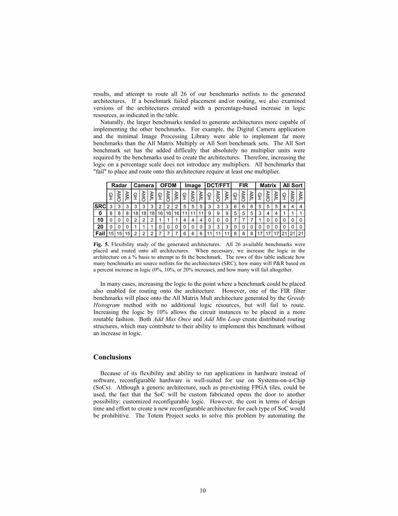
Flexibility

In addition to comparing our algorithms in terms of area and track count, we have also evaluated the flexibility of the architectures that they generate. The tests in this section involve examining architectures that were designed for one benchmark or benchmark set, and attempting to place and route, using our initial place and route tool [2], a different benchmark onto that architecture. The results for these tests are shown in Fig. 5. Here we take each benchmark set used in the previous table of

10

results, and attempt to route all 26 of our benchmarks netlists to the generated architectures. If a benchmark failed placement and/or routing, we also examined versions of the architectures created with a percentage-based increase in logic resources, as indicated in the table.

Naturally, the larger benchmarks tended to generate architectures more capable of implementing the other benchmarks. For example, the Digital Camera application and the minimal Image Processing Library were able to implement far more benchmarks than the All Matrix Multiply or All Sort benchmark sets. The All Sort benchmark set has the added difficulty that absolutely no multiplier units were required by the benchmarks used to create the architectures. Therefore, increasing the logic on a percentage scale does not introduce any multipliers. All benchmarks that "fail" to place and route onto this architecture require at least one multiplier.

GH

AM

O

AM

L

GH

AM

O

AM

L

GH

AM

O

AM

L

GH

AM

O

AM

L

GH

AM

O

AM

L

GH

AM

O

AM

L

GH

AM

O

AM

L

GH

AM

O

AM

L

SRC 3 3 3 3 3 3 2 2 2 5 5 5 3 3 3 6 6 6 5 5 5 4 4 40 8 8 8 18 18 18 16 16 16 11 11 11 9 9 9 5 5 5 3 4 4 1 1 1

10 0 0 0 2 2 2 1 1 1 4 4 4 0 0 0 7 7 7 1 0 0 0 0 020 0 0 0 1 1 1 0 0 0 0 0 0 3 3 3 0 0 0 0 0 0 0 0 0

Fail 15 15 15 2 2 2 7 7 7 6 6 6 11 11 11 8 8 8 17 17 17 21 21 21

DCT/FFT FIR Matrix All SortRadar Camera OFDM Image

Fig. 5. Flexibility study of the generated architectures. All 26 available benchmarks were placed and routed onto all architectures. When necessary, we increase the logic in the architecture on a % basis to attempt to fit the benchmark. The rows of this table indicate how many benchmarks are source netlists for the architectures (SRC), how many will P&R based on a percent increase in logic (0%, 10%, or 20% increase), and how many will fail altogether.

In many cases, increasing the logic to the point where a benchmark could be placed also enabled for routing onto the architecture. However, one of the FIR filter benchmarks will place onto the All Matrix Mult architecture generated by the Greedy Histogram method with no additional logic resources, but will fail to route. Increasing the logic by 10% allows the circuit instances to be placed in a more routable fashion. Both Add Max Once and Add Min Loop create distributed routing structures, which may contribute to their ability to implement this benchmark without an increase in logic.

Conclusions

Because of its flexibility and ability to run applications in hardware instead of software, reconfigurable hardware is well-suited for use on Systems-on-a-Chip (SoCs). Although a generic architecture, such as pre-existing FPGA tiles, could be used, the fact that the SoC will be custom fabricated opens the door to another possibility: customized reconfigurable logic. However, the cost in terms of design time and effort to create a new reconfigurable architecture for each type of SoC would be prohibitive. The Totem Project seeks to solve this problem by automating the

11

process of custom reconfigurable architecture creation in order to quickly and easily provide reconfigurable structures for use in systems-on-a-chip.

Our previous work produced a tool that could generate architectures with the minimum amount of flexibility required for the maximum amount of hardware-reuse across benchmark circuits. This resulted in a very ASIC-like architecture, with no real flexibility for future upgrades or changes. The work presented in this paper shifted the focus to the automatic generation of more flexible architectures, concentrating on routing architectures for RaPiD-style 1D reconfigurable architectures.

Using our architecture generation tool, we can provide a custom reconfigurable architecture targeted to specific netlists that uses just over 2/3 of the area of a RaPiD implementation on average. Despite the fact that RaPiD is an efficient architecture targeted to DSP in general, in some cases our generated architectures are even less than half the required RaPiD area. These improvements are due to the automatic customization of reconfigurable architectures according to the actual needs of the netlists that will be used. We have also shown that even with these area savings, we are able to generate routing architectures flexible enough to handle changes to the application netlists, as well as different netlists entirely. Researchers are only beginning to explore this area of study. Our future work will expand our efforts even further, considering algorithm improvements, additional algorithms, and other issues aimed at producing efficient flexible architectures automatically.

Acknowledgements

Thanks to the members of the RaPiD group who provided tools, layouts and particularly advice. Katherine Compton is supported by a UPR grant from Motorola, Inc. Scott Hauck is supported in part by an NSF CAREER Award and a Sloan Research Fellowship. The overall Totem effort is support by grants from NSF.

References

[1] S. Phillips, S. Hauck, "Automatic Layout of Domain-Specific Reconfigurable Subsystems for System-on-a-Chip", ACM/SIGDA Symposium on Field-Programmable Gate Arrays, 2002.

[2] A. Sharma, "Development of a Place and Route Tool for the RaPiD Architecture", Master's Project, University of Washington, December 2002.

[3] D. C. Cronquist, P. Franklin, S.G. Berg, C. Ebeling, "Specifying and Compiling Applications for RaPiD", IEEE Symposium on FPGAs for Custom Computing Machines, 1998.

[4] D. C. Cronquist, P. Franklin, C. Fisher, M. Figueroa, C. Ebeling, "Architecture Design of Reconfigurable Pipelined Datapaths", Twentieth Anniversary Conference on Advanced Research in VLSI, 1999.

[5] M. Scott, "The RaPiD Cell Structure", Personal Communications, 2001. [6] K. Compton, S. Hauck, “Totem: Custom Reconfigurable Array Generation”, IEEE

Symposium on FPGAs for Custom Computing Machines, 2001.