See discussions, stats, and author profiles for this publication at: https://www.researchgate.net/publication/304571329

FIRST YEAR LABORATORY MANUAL

Raw Data · June 2016

DOI: 10.13140/RG.2.1.3771.0324

CITATIONS

0READS

7,031

1 author:

Some of the authors of this publication are also working on these related projects:

Thin film characterization View project

Thermal Emittance and Solar absorptance of cds Thin Films View project

John Maera

Maasai Mara University

19 PUBLICATIONS   14 CITATIONS   

SEE PROFILE

All content following this page was uploaded by John Maera on 29 June 2016.

The user has requested enhancement of the downloaded file.

Page 1 of 70

MAASAI MARA UNIVERSITY

School of Science

Department of PHYSICS

FIRST YEAR LABORATORY MANUAL

PHY 110 & PHY 111: BASIC PHYSICS 1&II

2015

@Maera John

Page 2 of 70

STUDENT DATA

NAME: __________________________________________REG NO: ________________

GROUP NAME: _____________________________________________________________

GROUP MEMBERS:

SNO NAME REG NO

1.

2.

3.

4.

5.

6.

7.

8.

FILL IN THE TABLE BELOW IN COLUMNS 1,2AND 3. DO NOT SIGN IN COLUMN 5.

EXP

NO:

EXPERIMENT TITLE DATE

DONE

MARKS

/10

Signature

Student’s signature: _________________________________

Page 3 of 70

Table of Contents

NOTE TO LABORORY SUPERVISOR ...................................................................................................................... 5

AIMS OF THE COURSE ......................................................................................................................................... 5

INTRODUCTLON TO THE STUDENT ..................................................................................................................... 6

LABORATORY RULES ........................................................................................................................................... 6

DATA ANALYSIS ................................................................................................................................................... 7

Introductory Experiment: PRECISION MEASUREMENTS ................................................................................... 15

PARTA: MECHANICS ......................................................................................................................................... 17

Experiment I: PARALLELOGRAM AND TRIANGLE OF FORCE THEOREMS........................................................... 17

Experiment 2: THE SIMPLE PENDULUM ............................................................................................................ 18

Experiment 3: PRINCIPLES OF EQUILIBRIUM.................................................................................................... 20

Experiment 4: DETERMINATION OF ‘g’ BY FREE FALL ...................................................................................... 21

Experiment 5: VARIABLE INERTIA BAR ............................................................................................................. 23

B. PROPERTIES OF MATTER .............................................................................................................................. 27

Experiment 6: YOUNG’S MODULUS OF ELASTICITY ......................................................................................... 27

Experiment 7: VISCOSITY ................................................................................................................................ 29

PART C: HEAT .................................................................................................................................................... 31

Experiment 8: LINEAR EXPANSION ................................................................................................................... 31

Experiment 9: SPECIFIC HEAT BY THE METHOD OF MIXTURES ......................................................................... 33

Experiment 10: THERMAL CONDUCTIVITY - SEARLE’S BAR ............................................................................... 35

Experiment 11: NEWTON’S LAW OF COOLING ........................................................................................... 38

Experiment 12: BOYLE’S LAW .......................................................................................................................... 41

PART D: WAVE MOTION ................................................................................................................................. 44

Experiment 13: STANDING WAVES IN A TAUT STRING ..................................................................................... 44

Experiment 14: RESONANCE TUBE................................................................................................................... 46

E. OPTICS .......................................................................................................................................................... 50

Experiment 15: REFLECTION ............................................................................................................................. 50

Experiment 16: LAWS OF REFRACTION AND PROPERTIES OF LENSES .............................................................. 52

Page 4 of 70

Experiment 17: THE SPECTROMETER REFRACIIVE INDEX ................................................................................. 56

F. ELECTRICITY ................................................................................................................................................... 61

Experiment 18: OHM’S LAW ........................................................................................................................... 61

Experiment 19: THE THERMISTOR ................................................................................................................... 63

Experiment 23: THE POTENTIOMETER .............................................................................................................. 65

Experiment 21: THE OSCILLOSCOPE ................................................................................................................. 68

Page 5 of 70

NOTE TO LABORORY SUPERVISOR

This laboratory manual has been designed for first year students taking practical physics course at the

proposed to be Maasai Mara University.

The aim of the laboratory sessions cannot simply be to demonstrate what has been learnt in the lectures.

Most laboratory classes have neither the time, nor sufficient equipment to do this instead, the emphasis

is on laboratory techniques, data analysis and the interpretation of results. This will then provide a

solid basis for laboratory work in subsequent years.

AIMS OF THE COURSE 1. How to use various measuring instruments and to estimate their reading errors.

2. How to reduce/eliminate errors. 3. How to calculate errors.

4. How to use various common instruments.

5. Methods of analysis and how to draw and interpret linear and curved graphs.

6. To discuss results and draw intelligent COC1US1OflS.

7. Laboratory techniques and laboratory safety.

Each experiment is designed so that it can be completed within a three hour session, including

written work. Students will be expected to fill in during the course of the experiments. The

worksheets include blank data tables, spaces for data manipulation and error calculation,

questions on the experiments and spaces for discussion and conclusion. All written work,

including rough graphs, is to be handed in at the end of each practical session. Late work is not

acceptable under any circumstances.

Cooperation from the students is required. Students will be told in advance which experiment

they will be doing. They must read the script before coming to the class. They should be able to

plan their own time order to set up the apparatus, do the experiment do the analysis, and discuss it.

The format will make marking easier and faster. It is regretted that the students will not get much

practice in report writing, but these skills will be taught in the second and later years.

Before students are admitted to the laboratory, it would be helpful to conduct perhaps two tutorial

Sessions in the lecture theater:

1. Laboratory conduct, safety, units, significant figures, how to draw graphs, how to

interpret graphs - students to do examples in class.

2. Errors - different types, how to estimate reading error how to reduce or eliminate errors,

calculation of errors. Again, students to do examples in class.

First laboratory session every student will do a Common experiment designed to introduce

them to various types of common measuring instruments, simple error analysis, etc.

Subsequent laboratory sessions- a series of experiments designed to introduce the students

to laboratory techniques, analysis, different types of equipment, .

Page 6 of 70

INTRODUCTLON TO THE STUDENT

This manual contains all the experimental scripts and worksheets that you will need for the

first year practical course in physics. You will also find information on graphical analysis and

error analysis which form an important part of the course.

The aim of the course is not simply to demonstrate practically the physics principles learnt in

the lectures. It is just not possible to provide the equipment for all of you, for example, to

experiment with lenses in the laboratory class after learning about lenses in a lecture. There

may be only one or two sets of apparatus, or the experiment may be too difficult or too

dangerous to be performed by a student in class.

Instead, the major objective of the course is to enable you to lean laboratory technique and

discipline. You will learn how to take measurements and estimate reading errors; how to

analyze and interpret data; how to discuss your results and draw intelligent conclusions from

them. There will be exposure to different types of equipment, illustrating different laboratory

and analytic techniques. And of course you will also be learning some physics!

Remember that “Without Observations and Experiments our natural Philosophy [Physics]

could only be a Science of Terms and a unintelligible jargon” (J.T Desaguliers, 1683-1744).

LABORATORY RULES

Students are required to attend all laboratory sessions and to hand completed work at the

end of each session. This means that you should plan your time so that all experimental

work and all written work is finish within the three hours of the laboratory class. Work

handed in late will not be marked.

Students who come to the laboratory late may not be admitted. Students who are absent

because of illness must provide satisfactory evidence if this is be taken into consideration.

Students should come to the laboratory class prepared. You will need:

a pad of graph paper,

Calculator, pen, pencil etc.

You will be told in advance which experiments you will be doing, and this should be read

before coming to the class.

For each experiment, fill in the data sheet (s) provided with the actual observations made

during the experiment. The data sheets must be fill using ink - data sheets and reports written

in pencil are not acceptable.

Plot rough graphs during the experiment itself. That way you will be able spot any

measurements that may have to be repeated. These rough graphs must be handed in at the end

of the class. Do all calculations, including error calculations, and draw any graphs required.

Answer any questions posed.

After experiments have been marked and returned, keep this manual safe. It must all be handed

in at the end of the year.

Page 7 of 70

Note on completing worksheets

1. Discussion- discuss the sources of error in the experiment and whether they are

acceptable. How does your final answer compare with theory or with accepted values?

What is the significance of your results? Can you explain any unexpected findings? Are

there ways of improving the experiment?

Writing a satisfactory discussion requires you to think about the experiment in all its

aspects. Be brief

2. Conclusion - this is where you sum up and justify your results. The conclusion should

always relate to the original objectives of the experiment.

DATA ANALYSIS Units Where relevant, units should always be quoted, e.g. in headings of tables, axes of graphs and in

the statement of results. All units must be S.I. or derived SI units.

Significant Figures

Since you will be using calculators, the calculation of quantities usually yields more figures in the

results than are warranted by the precision of the measurements made. Care should be taken not to

include these figures in further calculations or in the statement of results. For example:

g =9.7937126 m/s2 would not represent the accuracy with which laboratory measurements are

made. The correct figure would be g = 9.8 m/s2.

Graphs

Graphs must be drawn on graph paper, and they must have a title. Use crosses or circles to mark

points on the graphs. Choose sensible scales, drawing the graph as large as possible, preferably.

filling the page..

(i) A graph can disclose information not apparent from looking at a table of observations. For

example, in Boyle’s law experiment, the intercept on the vertical negative axis gives the

atmospheric pressure. One could not deduce this from a table of figures easily.

(ii) You can deduce the relation between two physical quantities, e.g. in Boyle’s law

experiment, that P and 1/V are linearly related,

(iii) You can interpolate (reading between observed points) or extrapolate (producing the

graph beyond the region of. observation). However, care is needed in extrapolating curves as it is

difficult to judge. ‘how the curve will continue.

(iv) You can deduce important data from discontinuities maxima and minima, or gradients.

In all cases, plot a rough graph while the experiment is running. Then it is easy to see if there

are any erroneous measurements and to redo them if necessary..

In plotting graphs

Important - use a sharp pencil for plotting graphs, making crosses or circles for marking the points.

The graph should be headed with a brief title, for example, in the experiment about the simple

pendulum, the title could read:

period, T2 versus length L. Horizontal axis - plot the physical quantity which is varied in

Page 8 of 70

consciously controlled steps (e.g. pendulum length), Vertical axis - plot the physical quantity

which is then measured (e.g. period of the pendulum).

For a linear graph of the form y = ax + b, y is the measured variable and is plotted on the vertical

axis. x is the controlled variable and is plotted on the horizontal axis.

Drawing curved graphs Consider the experiment on Newton’s law of cooling. When plotted, the data points indicate a

curve. Draw a smooth curve through the points. It does not matter if some points lie outside the

curve. Never join up the dots to give a linked line.

Slopes Always choose the largest possible triangle from which to calculate the slopes. The larger the

values of the sides of the triangle, the smaller the percentage error in them. Remember - the

vertical and horizontal values must be measured in the units of the scales of the graph, NOT in

cm or ‘squares’.

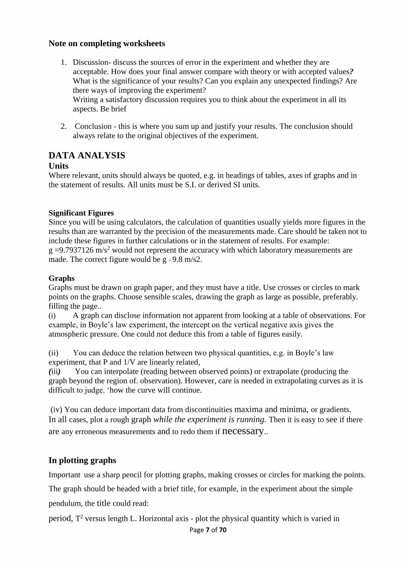
For an equation of the form y = mx + c, a straight line graph on an x-y Coordinate frame can be

drawn, as shown below:

When a straight line graph is used as a source of information, the slope or the intercept or both

are usually measured. To measure the slope of a line, select two points, A and B, on the line

drawn - observational points - which are well separated. Record from the graph thevalues of YA

and XA(at A),and of YB andX3 (at B).The

the slope is: B A

B A

Y Y

X X

N.B: BD and AD represent measurements along the scales of the Y and x axes.

This form of graphical analysis for straight line graphs is not the best way of obtaining

information from your data. It is not objective because you cannot be certain that the line

you have drawn truly gives the best fit to the data points. In fact learn how to analyze

graph objectively using the least squares method.

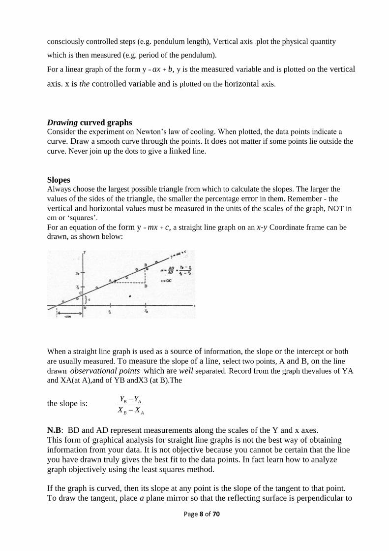
If the graph is curved, then its slope at any point is the slope of the tangent to that point.

To draw the tangent, place a plane mirror so that the reflecting surface is perpendicular to

Page 9 of 70

the curve (see Fig. 2). Turn the mirror about until the curve and their reflections appear as

one Continuous curve, The reflecting surface of the mirror is then normal to the Curve.

Rule a line along its base. The tangent will then be at right angles to the line.

Fig 2.

NB: Graphical analysis is the roost accurate method of obtaining your final result. It is

more accurate than doing a calculation for each individual pair of results and then

averaging, However, the accuracy of the graph can be destroyed by two easily avoidable

mistakes:

(1) Choosing the scales so that the slope is either close to infinity or close to zero. Either

way, measurement of the shorter side of the triangle will have a large percentage error

compared to the measurement of the longer side. The most accurate slope measurement is

made from a line inclined approximately 450 to the axis.

(ii) Assuming that the origin is the most accurate point on the graph. The origin is frequently

not a very reliable point due to, for example, instrument error or inaccurate zero adjustment.

Errors The term error, when used in physics, has a meaning different from its everyday meaning. In

layman’s terms an error is a mistake. In physics, an error in an observational reading is a way of

indicating the range of uncertainty of the reading. Mistakes of course do occur in physics, so it is

important when writing reports to distinguish clearly between the mistake you might make and

the error that can occur in a reading. There are a number of different types of error, which are

discussed below.

(a) Random errors

If a measurement is repeated a number of times, the values obtained do not always agree. This

variation is due to random errors which arise from a number of factors.

(i) Errors of judgment - estimates of a fraction of the smallest division of a scale on an instrument

may vary in a series of measurements.

(ii) Fluctuating conditions - important factors in a given experiment, such as temperature,

pressure or voltage, may vary during the measurements, affecting the results.

(iii) Small disturbances - for example, small mechanical vibrations, the pick-up of spurious

electrical signals.

(iv) Lack of definition in the quantity measured for example, measurements of the thickness of a

steel plate having non-uniform surfaces using a micrometer will in general not be reproducible.

Page 10 of 70

(v) Randomness in the quantity measured - for example, repeated measurements of the number

of disintegrations per second in a radioactive source will give different values because radioactive

disintegrations occur randomly in time.

Thus when random errors are present, deviations of measured values from the true value will vary

in a series of repeated measurement

(b) Systematic errors

If Systematic errors are present in a measurement the deviations of the measurement values from

the true value will be constant in a series of repeated measurement For example, a systematic

error will be present in a set of measurements if the measuring instrument is not correctly

calibrated or is improperly used, This could be a Stop-watch running fast or slowly, or a

micrometer screw gauge with an undetected zero error, This type of error cannot, in general, be

determined except by checking out the apparatus against other standards.

Precision and accuracy A measurement is said to be accurate if the measured values cluster closely about the true value.

An experiment with little or no systematic errors as well as small random errors is regarded as

having high accuracy.

A measurement is said to be precise if the spread of measured values is small, a precise

measurement can be very precise but not accurate if the systematic error(s) are large. Precision

and accuracy are both limited by the sensitivity of the measuring devices. For example, the

sensitivity of a meter rule subdivided in mm is I mm.

Reading error

In general, the reading error is plus or minus the smallest division on the measuring scale. For a meter rule

subdivided into mm, the reading error L ± 1 mm. However if the division is large, then one may estimate

to the nearest half-division. For example, the thermometer in common use in the laboratory has a scale

subdivided into degrees, but as the divisions are large, one can estimate to the nearest half-degree, and the

reading error is ± 0.5 degrees.

Progation of errors

In most experiments, the initial readings are used to calculate out some quantity. To calculate the error in

this quantity, the reading errors of the individual measurements must be combined. The final error may be

quoted in a number of different ways:

(a) As the actual error dx of the quantity x. This will have the same units as the quantity itself.

(b) As the fractional error, dx/x. This will have no units.

(c) As the percentage error, = fractional error x 100%

The combination of the original reading errors is quite simple if a number of simple rules are followed:

(1) Addition or subtraction

x = a + b + c ; then dx =da +db + dc

x = a – b then dx=da + db

Page 11 of 70

In both cases the reading errors are added together.

Length L (4.5 ±0.l) cm + (3.6±O1) cm

Error in length is then 0.1+0.1= O.2 crn

Thus ‘we write for the length, L = (8.1± O.2) cm

or

Length L= (5.4 ±0 1) - (3 2 ±) cm

The error will again be (0.1 + 0.1) = 0.2cm

Therefore the length will be L = (2.2 ± 0.2) cm

In both cases, the error is added.

(ii) Quotient or product

abx orb

a

In both cases divide the reading error by the actual value of that measurement for each value in

the equation. Then the fractional error in the final quantity is equal to the sum of the individual

fractional errors:

b

db

a

da

x

dx

The mass per unit length of a wire is given by (5.6±0.1) divided by (50.0 ± 0.1) cm. The fractional

error is given by:

0198.0002.0....0178.050

1.0

6.5

1.0

The actual error is then obtained by multiplying the fractional error by the result, i.e

11.2 g/m x 0.0198 = 0.2 gm

Note that the error has the same number of decimal places as the actual value.

(iii) Powers

Errors in square or higher powers magnify rapidlya

dan

x

dxax n for example, if

T2 = (1.2 ± 0.2) seccds, then

. error in T2 is T

dT2; ondsTeiei sec)33.044.1(..;33.0

2.1

2.02..

(iv) Error in logarithmic functions

If x=e2 then dzx

dx ; if x = logeZ then dx = dzlz

Least squares analysis for linear graphs

Calculating the error on a quantity derived from a formula involves applying the error calculation

rules correctly. But what do you do if some of the information in that formula has been derived

from a graph?

Consider a linear graph of variable x versus variable y. x and y represent measurements you have

taken so there will be a reading error associated with each x value and each y value.

Page 12 of 70

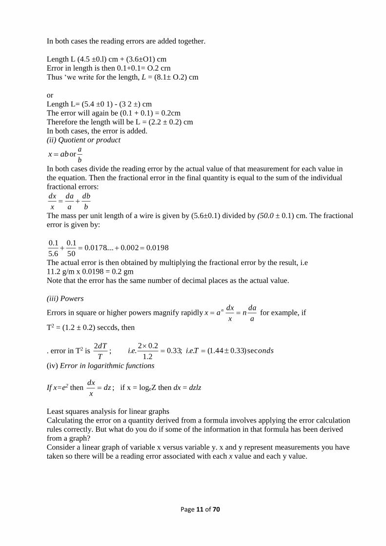
Fig. 3

The points are plotted on the graph represented by the crosses. The reading errors may be marked

with error bars, the length of the bar being the size of the error according to your scales. A

horizontal bar denotes the reading error in x, a vertical bar, that in y. The crosses are positioned in

the diagram above such that they seem to form a straight line. However, given the errors on each

point, it is difficult to draw the actual graph. If you wish to obtain the value of the slope or

intercept, you will see that a big error may be introduced. Where do you draw the line to minimize

the error?

Fortunately, there is a way of finding the slope and intercept with minimum error. It is called least

squares analysis.

The equation of a straight line is: y = a + bx

x and y represent the horizontal and vertical axes respectively. a is the intercepted on the y axis

and b is the slope of the line. The slope, b, may be calculated according to the formula:

n

xx

n

yxxy

b2

2 )(

; where n is the total number of points.

[If you wish to know where the formula came from, consult any text book on experimental

errors.]

The intercept is then: xbya

The bars over x and y denote the averages of all the x values and all the y values.

If you have a scientific calculator, you should be able to calculate the sum and averages easily.

You can then use the calculated values of a and b to draw the line on the graph if you wish.

Note that the slope and intercept thus calculated, plus the resulting line on the graph, are objective

solutions in graphical analysis. A line drawn by estimating it by eye is not objective. Also, note

that you will not be tempted to draw the line through the origin if you think it is meant to go there.

Why should the origin be the most accurate place on the graph if you haven’t even made a

measurement at that point?

Calculating the line will force you to find reasons as to why the graph does not behave as you

expect (e.g does not go through the origin) instead of fudging the results to obtain what you want.

Example of an experiment

In the Ohm’s law experiment, the value of an unknown resistance may be found by measuring

different values of the current flowing through the resistor as the voltage across it is changed.

Page 13 of 70

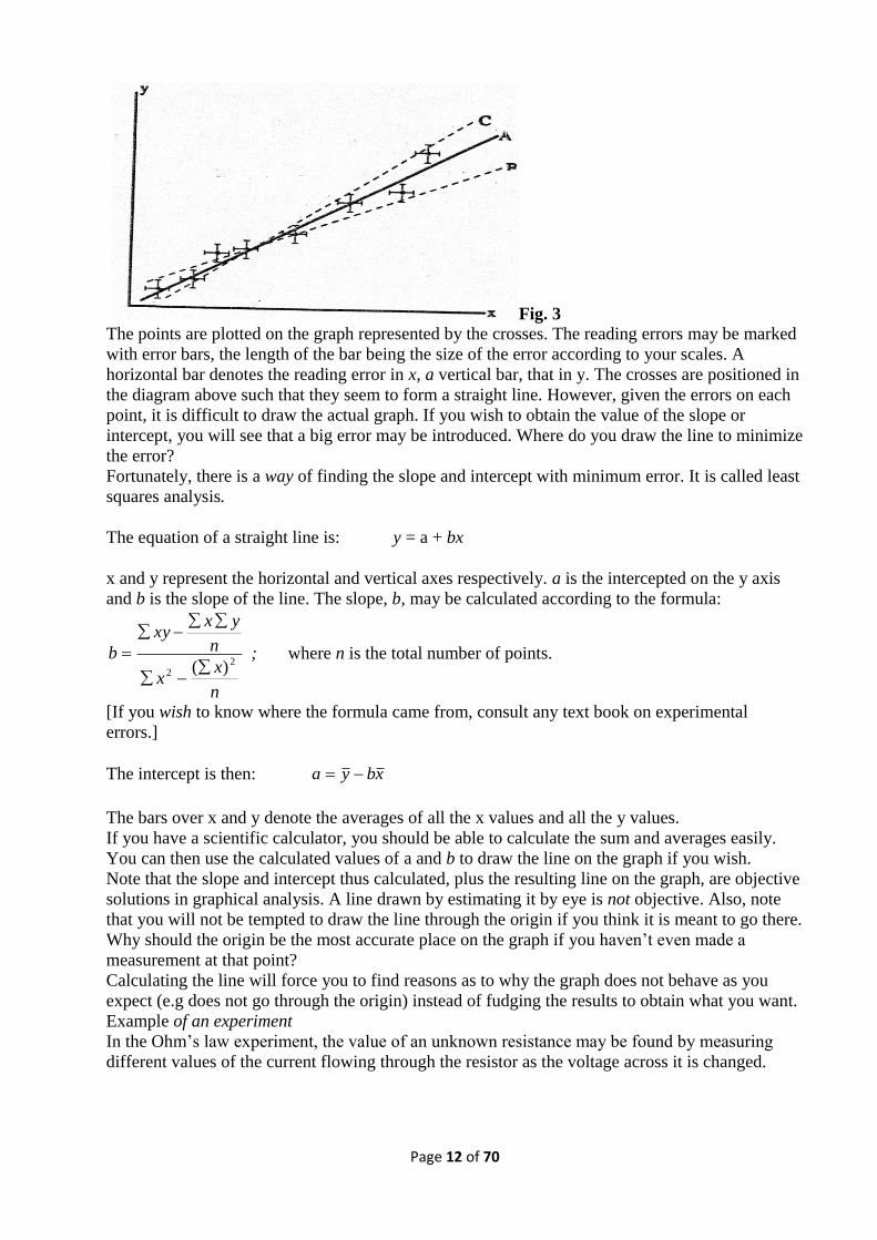
V, volts I x 10-3, amps

0.5 1.1

1.0 1.9

1.5 3.2

2.0 3.9

2.5 4.9

3.0 6.2

3.5 6.7

4.0 8.1

4.5 9.3

5.0 10.0

Calculate the slope and the intercept from these values letting V form the y Coordinates and I form the x

coordinates. You should find that the slope, b, is 494.4, i.e the resistance is 494.4 Ohms, The intercept, a,

turns out to be a value other than zero, i.e 0.13. Find a reason for this,

We can find the error in the slope and intercept by calculating the standard errors in the slope and intercept

using the appropriate formulae,

Let Sy be the standard error in y

Sa be the standard error in the intercept, a

Sb be the standard error in the slope, b

2/122

2/1

22

22/1

2

/)(

1,

/)(,

2:

nxxSS

nxxn

xSS

n

xycyaySThen ybyay

Calculate the standard errors in the slope and intercept using the Ohm’s law data.

Note: (important) - the standard errors you have calculated arise, from the statistical analysis; they do not

include the reading errors. Strictly speaking for accuracy, these errors should be included, i.e weighted

measurement should be used. However, since the number of readings in your experiment is usually small

(10 readings ‘or less), the standard error will partly) compensate for the neglect of reading errors. In any

case, the use of weighted measurements complicates and lengthens the analysis to an extend unnecessary at

this juncture.

If the slope and/or intercept is subsequently used in a formula to calculate some value, then the standard

errors are used in the error calculations in the same way as you would use a reading error.

Note that this procedure is only useful for linear graphs. It cannot be applied to curved graphs such as the

cooling curve drawn in the Newton’s Law of cooling experiment.

Reference: A more detailed discussion of least squares analysis using a scientific calculator is given in

“Introduction to First Year Experiments Physics at Kenyatta University by Father P. ‘Gouin, July 1983.

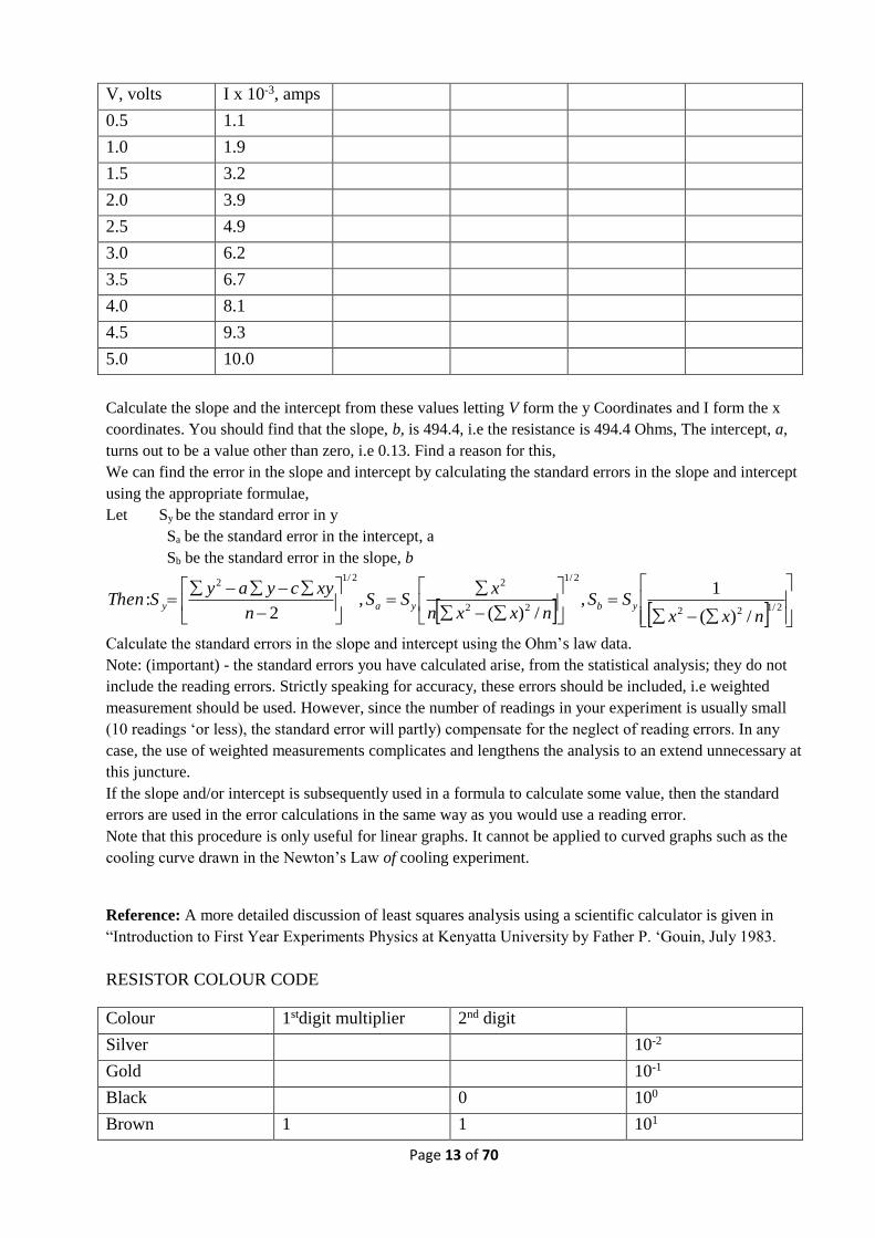
RESISTOR COLOUR CODE

Colour 1stdigit multiplier 2nd digit

Silver 10-2

Gold 10-1

Black 0 100

Brown 1 1 101

Page 14 of 70

Red 2 2 102

Orange 3 3 103

Yellow 4 4 104

Green 5 5 105

Blue 6 6 106

Violet 7 7 107

Grey 8 8 108

White 9 9 109

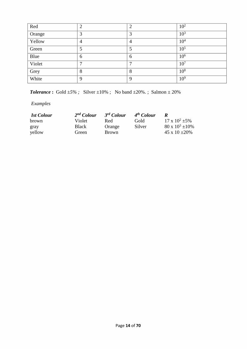
Tolerance : Gold ±5% ; Silver ±10% ; No band ±20%. ; Salmon ± 20%

Examples

Ist Colour 2nd Colour 3rd Colour 4th Colour R

brown Violet Red Gold 17 x 102 ±5%

gray Black Orange Silver 80 x 103 ±10%

yellow Green Brown 45 x 10 ±20%

Page 15 of 70

Introductory Experiment: PRECISION MEASUREMENTS

Objectives

To study some of the instruments and methods used in precision measurements, and to compute

the volume and density of various items.

Apparatus

Metre rule, vernier calipers, micrometer screw gauge, electronic balance and travelling

microscope. Such items as a copper cylinder, steel ball and glass capillary tube are also supplied.

Method

The experiment comprises the measurement of the various objects supplied with the appropriate

instruments. Where feasible, at least two instruments should be used for each measurement and

the precision obtained in each case compared. In this way, the volume and density of at least two

metal object should be deduced and the capacity of the capillary tube determined. All weighing

should be done on the electronic balance.

in the second part of the experiment, some electrical circuits have been set up for you to measure

the current. Measure the current using an ammeter, milliammeter and a microammeter,and

estimate the reading errors in each case.

N.B. In all cases an estimate of the precision obtained should be given, i.e note the reading errors

on all measurements. Where appropriate, note the zero error.

Record the data in Worksheet 1, working out any calculations asked for Answer the questions

posed on the sheet.

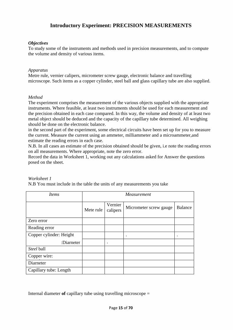
Worksheet 1

N.B You must include in the table the units of any measurements you take

Items Measurement

Mete rule

Vernier

calipers Micrometer screw gauge Balance

Zero error

Reading error

Copper cylinder: Height

:Diarneter

. .

.

Steel ball

Copper wire:

Length Diarneter

Capillary tube: Length

Internal diameter of capillary tube using travelling microscope =

Page 16 of 70

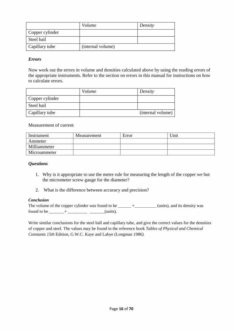
Volume Density

Copper cylinder

Steel bail

Capillary tube (internal volume)

Errors

Now work out the errors in volume and densities calculated above by using the reading errors of

the appropriate instruments. Refer to the section on errors in this manual for instructions on how

to calculate errors.

Volume Density

Copper cylinder

Steel bail

Capillary tube (internal volume)

Measurement of current

Instrument Measurement Error Unit

Ammeter

Milliammeter

Microammeter

Questions

1. Why is it appropriate to use the metre rule for measuring the length of the copper we but

the micrometer screw gauge for the diameter?

2. What is the difference between accuracy and precision?

Conclusion

The volume of the copper cylinder was found to be ______ +__________ (units), and its density was

found to be _______+ _________ _______(units).

Write similar conclusions for the steel ball and capillary tube, and give the correct values for the densities

of copper and steel. The values may be found in the reference book Tables of Physical and Chemical

Constants 15th Edition, G.W.C. Kaye and Labye (Longman 1986).

Page 17 of 70

PARTA: MECHANICS

Experiment I: PARALLELOGRAM AND TRIANGLE OF FORCE

THEOREMS Objective

To verify the Parallelogram and Triangle Theorems.

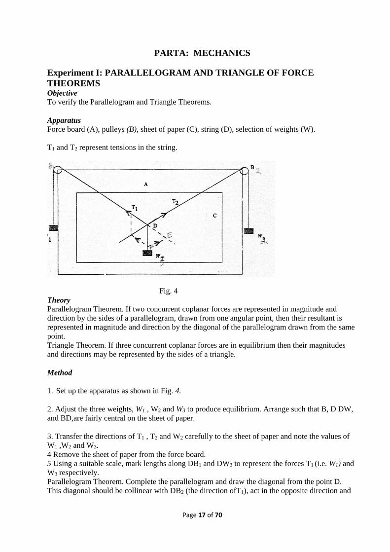
Apparatus

Force board (A), pulleys (B), sheet of paper (C), string (D), selection of weights (W).

T1 and T2 represent tensions in the string.

Fig. 4

Theory

Parallelogram Theorem. If two concurrent coplanar forces are represented in magnitude and

direction by the sides of a parallelogram, drawn from one angular point, then their resultant is

represented in magnitude and direction by the diagonal of the parallelogram drawn from the same

point.

Triangle Theorem. If three concurrent coplanar forces are in equilibrium then their magnitudes

and directions may be represented by the sides of a triangle.

Method

1. Set up the apparatus as shown in Fig. 4.

2. Adjust the three weights, W1 , W2 and W3 to produce equilibrium. Arrange such that B, D DW,

and BD,are fairly central on the sheet of paper.

3. Transfer the directions of T1 , T2 and W2 carefully to the sheet of paper and note the values of

W1 ,W2 and W3.

4 Remove the sheet of paper from the force board.

5 Using a suitable scale, mark lengths along DB1 and DW3 to represent the forces T1 (i.e. W1) and

W3 respectively.

Parallelogram Theorem. Complete the parallelogram and draw the diagonal from the point D.

This diagonal should be collinear with DB2 (the direction ofT1), act in the opposite direction and

Page 18 of 70

be equal in magnitude to T2 sinceT2 is the equilibrant of T1 and W3. This verifies the

parallelogram theorem.

Triangle Theorem. Produce BD towards E Using a suitable scale mark off lengths along DE and

DF to represent the forceT1 (i.e. W1 ) and W3

Join the ends of these lengths with FE The line FE should bepara1lel to DB2 , and have a length

which represents T2 (i.e. W2 according to the scale used. This verifies the triangle theorem.

Complete the data table given below and answer the questions that follow.

Worksheet 2

Units Mass (Kg) Mass (N)

W1

W2

W3

Questions

1. How do you convert kilograrns to newtons?

2. Comment on your drawings and state whether or not you have verified the theorems.

3. What are the sources of error in this experiment?

Conclusion

Experiment 2: THE SIMPLE PENDULUM

Objective

To determine acceleration due to gravity using a simple pendulum.

Apparatus

Pendulum bob, thread, clarnp and stand, stopwatch.

Theory

The time period, T, of a simple pendulum oscillating with amplitudes

(less than 10̊ ) is given by the expression: g

LT 2

where L= length of pendulum thread and g = acceleration due to gravity.

Method

1. Set the pendulum d 50 cm and set the pendulum swinging with small oscillations.

2. Time 50 oscillations

Page 19 of 70

3. Repeat for a number of different pendulum between 50 and 100cm.

4. Note the reading errors in time and length.

5. Draw a graph and deduce the acceleration due to gravity from the graph. Indicate error bar on

the

graph. Estimate the error in g.

6. Answer the questions in the worksheet.

Worksheet 3

Length Time ? (You decide)

Units: Length: Time:

Reading error: Length: Time:

(i) Plot a suitable graph.

(ii) Indicate the error bars.

(iii)From the graph, deduce the value of g.

(iv) Estimate the error in g.

Questions

1. Why are 50 oscillations timed instead of only one?

2. Why must the size of amplitude be small?

3. Compare the value of g obtained with the standard value for Narok.

Conclusion

Page 20 of 70

Experiment 3: PRINCIPLES OF EQUILIBRIUM

Objective

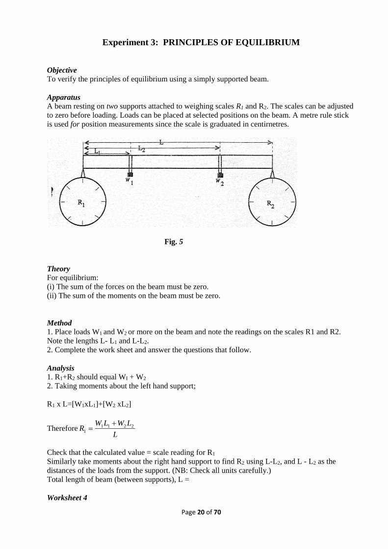
To verify the principles of equilibrium using a simply supported beam.

Apparatus

A beam resting on two supports attached to weighing scales R1 and R2. The scales can be adjusted

to zero before loading. Loads can be placed at selected positions on the beam. A metre rule stick

is used for position measurements since the scale is graduated in centirnetres.

Fig. 5

Theory

For equilibrium:

(i) The sum of the forces on the beam must be zero.

(ii) The sum of the moments on the beam must be zero.

Method

1. Place loads W1 and W2 or more on the beam and note the readings on the scales R1 and R2.

Note the lengths L- L1 and L-L2.

2. Complete the work sheet and answer the questions that follow.

Analysis

1. R1+R2 should equal WI + W2

2. Taking moments about the left hand support;

R1 x L=[W1xL1]+[W2 xL2]

ThereforeL

LWLWR 2211

1

Check that the calculated value = scale reading for R1

Similarly take moments about the right hand support to find R2 using L-L2, and L - L2 as the

distances of the loads from the support. (NB: Check all units carefully.)

Total length of beam (between supports), L =

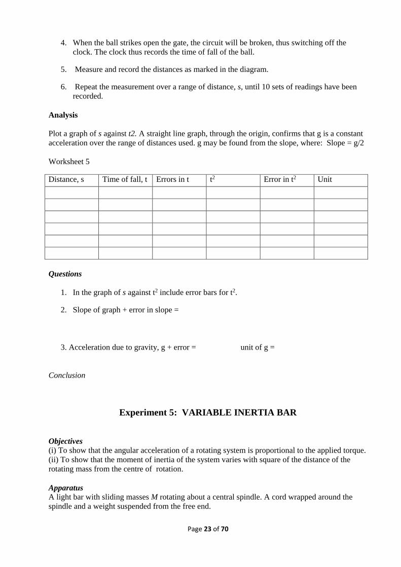
Worksheet 4

Page 21 of 70

First try Second try

Value Units Value Units

W

W

L

L

R

R

First try Second try

R1 +R2

W1+W2

R1 scale:

R2 calculation:

R2 scale:

R3 calculation:

Questions

1. State the reading errors in:

(i) mass =

(ii) length=

(iii) scale reading of R=

What is the error in R1 + R2?

What is the error in W1+W2?

What other sources of error are there in this experiment?

2. What would you expect if one of the loads was directly over the support?

3. What would happen if W acted upwards?

Conclusion

Make a statement as to whether or not the principles of equilibrium were verified in your

experiment.

Experiment 4: DETERMINATION OF ‘g’ BY FREE FALL

Objective

To determine the value of the acceleration of a falling body.

Page 22 of 70

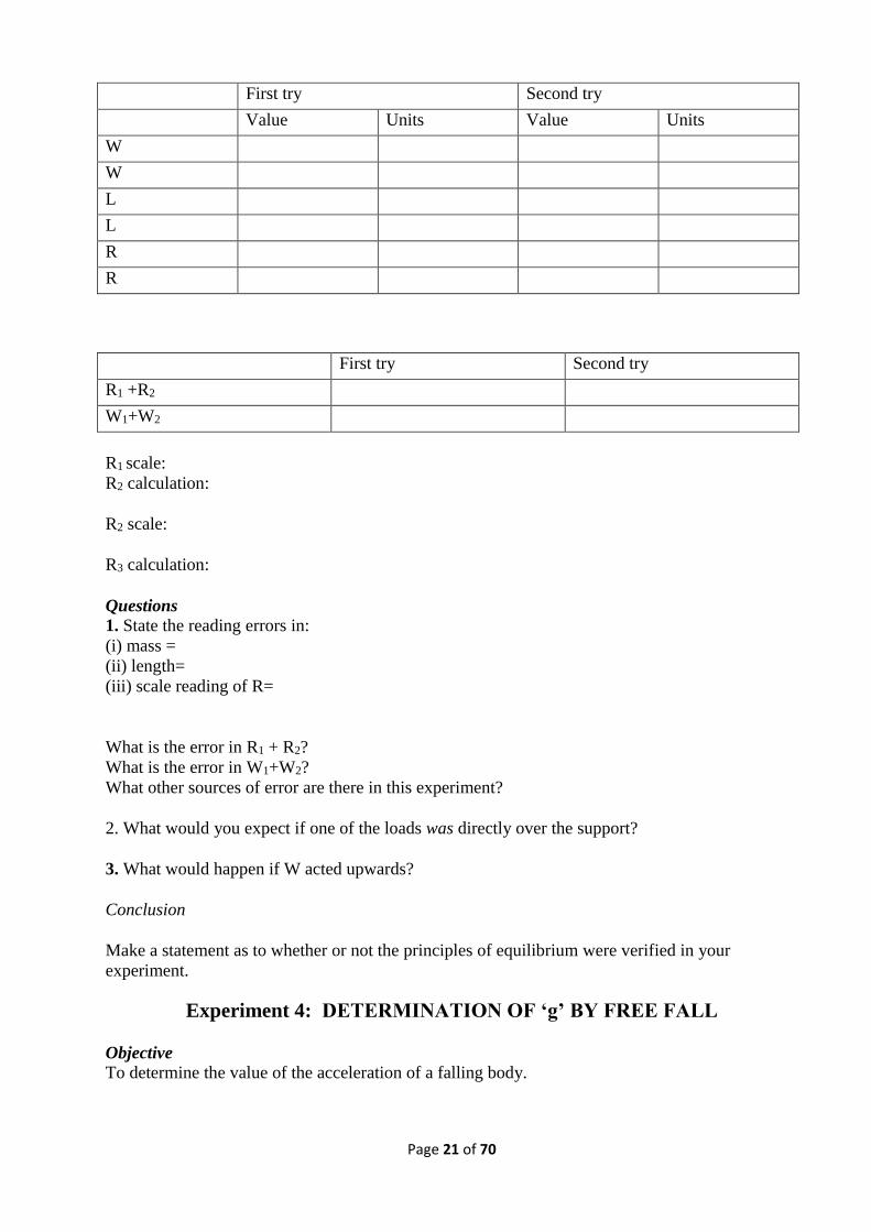
Apparatus

A steel ball suspended from a solenoid magnet powered via a clack timer.

(When the sweep hand of the clock passes zero the solenoid is de-energised

2nd the ball starts top)

A gate switch connected to the timer is positioned some distance below.

(When the ball strikes the flap, the circuit is broken and the timer stops.)

Theory

The distance traavelled by the fall is measured and the time elapsed noted.

Then:

2

2 2

2

1

t

SgandgtS

Method

1. Adjust the plug at the open end of the gate switch so that the hinged steel plate is just held

in the closed position by the small inset permanent magnet. Place the steel ball in the

lower end of the core of the e1ecomagnet and then adjust the core position by means of the

threaded ring at its upper end so that the ball is just held by the magnetized core. This is to

ensure the prompt release of the ball when the clock is switched on.

2. Now adjust the positions of the electromagnet and gate switch so that when the ball is

released, it falls on the steel plate near its free end and opens the gate.

3. Set the clock in the timer to zero, Then switch it on. At that instant the steel ball will be

released.

Page 23 of 70

4. When the ball strikes open the gate, the circuit will be broken, thus switching off the

clock. The clock thus records the time of fall of the ball.

5. Measure and record the distances as marked in the diagram.

6. Repeat the measurement over a range of distance, s, until 10 sets of readings have been

recorded.

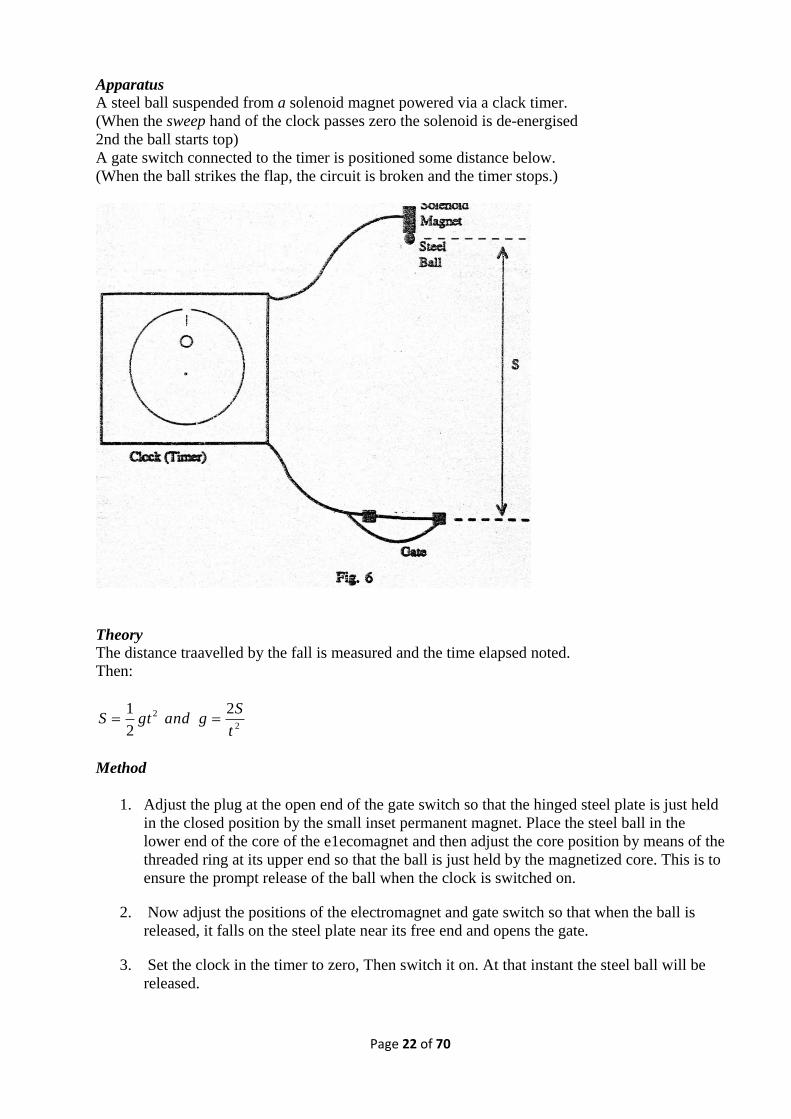
Analysis

Plot a graph of s against t2. A straight line graph, through the origin, confirms that g is a constant

acceleration over the range of distances used. g may be found from the slope, where: Slope = g/2

Worksheet 5

Distance, s Time of fall, t Errors in t t2 Error in t2 Unit

Questions

1. In the graph of s against t2 include error bars for t2.

2. Slope of graph + error in slope =

3. Acceleration due to gravity, g + error = unit of g =

Conclusion

Experiment 5: VARIABLE INERTIA BAR

Objectives

(i) To show that the angular acceleration of a rotating system is proportional to the applied torque.

(ii) To show that the moment of inertia of the system varies with square of the distance of the

rotating mass from the centre of rotation.

Apparatus

A light bar with sliding masses M rotating about a central spindle. A cord wrapped around the

spindle and a weight suspended from the free end.

Page 24 of 70

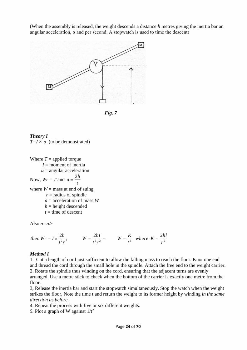
(When the assembly is released, the weight descends a distance h metres giving the inertia bar an

angular acceleration, α and per second. A stopwatch is used to time the descent)

Fig. 7

Theory I

T=I × α (to be demonstrated)

Where T = applied torque

I = moment of inertia

α = angular acceleration

Now, Wr = T and t

ha

2

where W = mass at end of suing

r = radius of spindle

a = acceleration of mass W

h = height descended

t = time of descent

Also α=a/r

22222

22;

2

r

hlKwhere

t

KW

rt

hIW

rt

hIWrthen

Method I

1. Cut a length of cord just sufficient to allow the falling mass to reach the floor. Knot one end

and thread the cord through the small hole in the spindle. Attach the free end to the weight carrier.

2. Rotate the spindle thus winding on the cord, ensuring that the adjacent turns are evenly

arranged. Use a metre stick to check when the bottom of the carrier is exactly one metre from the

floor.

3, Release the inertia bar and start the stopwatch simultaneously. Stop the watch when the weight

strikes the floor, Note the time t and return the weight to its former height by winding in the same

direction as before.

4. Repeat the process with five or six different weights.

5. Plot a graph of W against 1/t2

Page 25 of 70

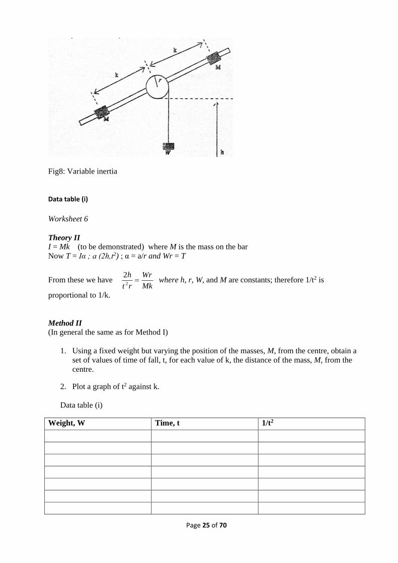
Fig8: Variable inertia

Data table (i)

Worksheet 6

Theory II

I = Mk (to be demonstrated) where M is the mass on the bar

Now T = Iα ; a (2h,t2) ; α = a/r and Wr = T

From these we have Mk

Wr

rt

h

2

2 where h, r, W, and M are constants; therefore 1/t2 is

proportional to 1/k.

Method II

(In general the same as for Method I)

1. Using a fixed weight but varying the position of the masses, M, from the centre, obtain a

set of values of time of fall, t, for each value of k, the distance of the mass, M, from the

centre.

2. Plot a graph of t2 against k.

Data table (i)

Weight, W Time, t 1/t2

Page 26 of 70

Plot a graph of W against 1/t2 inc1uding error bars on 1/t2

Time, t t2 Distance, k

Plot a graph of t2 against k including error bars on t2.

Comment on your two graphs and state whether or not the objectives of the experiments have

been achieved.

Reading error in t2 =

Reading error in k =

Assume no error in W. What other errors are found in this experiment?

Conclusion

Page 27 of 70

B. PROPERTIES OF MATTER

Experiment 6: YOUNG’S MODULUS OF ELASTICITY

Objective

To determine Young’s Modulus (E) for a wire.

Apparatus

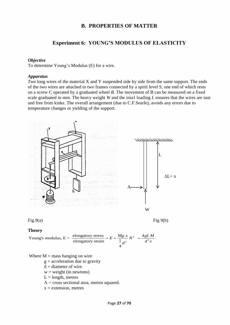
Two long wires of the material X and Y suspended side by side from the same support. The ends

of the two wires are attached to two frames connected by a spirit level S, one end of which rests

on a screw C operated by a graduated wheel B. The movement of B can be measured on a fixed

scale graduated in mm. The heavy weight W and the inia1 loading L ensures that the wires are taut

and free from kinks. The overall arrangement (due to C.F.Searle), avoids any errors due to

temperature changes or yielding of the support.

L

∆L= x

A

W

Fig.9(a) Fig 9(b)

Theory

2

22

elongatory stress . 4Young's modulus, E =

1 elongatory strain

4

Mg x gL ME N

d xd

Where M = mass hanging on wire

g = acceleration due to gravity

d = diameter of wire

w = weight (in newtons)

L = length, metres

A = cross sectional area, metres squared.

x = extension, metres

Page 28 of 70

This equation applies only within the elastic region upto the limit of proportionality.

Method

1. The original length of the test wire Y is measured using a metre rule

2. The diameter of the wire is measured using a micrometer screw gauge. Readings are

taken at several points along the length of the wire and a mean value calculated.

3. With the initial load in place, the spirit level is adjusted by means of the wheel so that it is

horizontal. The initial reading on the scale is noted.

4. The extending load is added to the pan in steps up to a maximum total load of 3.5kg. After each

step the spirit level is adjusted so that it is horizontal and the reading on the scale is noted. 5. The load is then removed step by step, and a note is made of the scale readings at each step as

before.

Analysis

A graph of extending load (in newtons) versus extension (in metres) should

d2 x be a straight line through the origin. The slope of the graph is w/x.

Calculate the slope of the graph and the cross sectional area of the wire.

Determine the value of Young’s modulus and the error in your value.

Errors

Original length of the wire L = ±m

Diameter of the wire = , , ±m

Mean diameter = ±m

Initial reading of scale A = ±

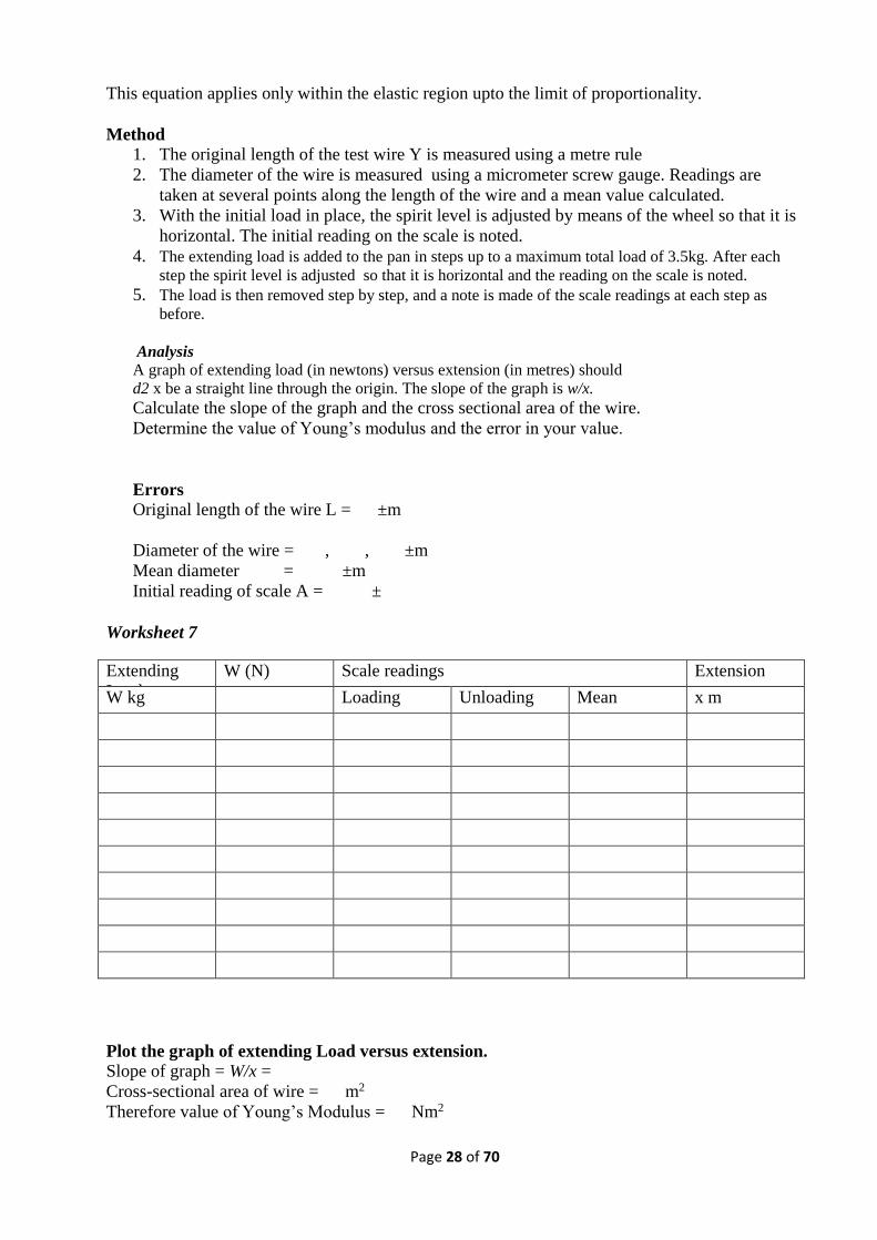
Worksheet 7

Extending

Load

W (N) Scale readings Extension

W kg Loading Unloading Mean x m

Plot the graph of extending Load versus extension.

Slope of graph = W/x =

Cross-sectional area of wire = m2

Therefore value of Young’s Modulus = Nm2

Page 29 of 70

Error in calculation (i.e. error in E = (% error in L) + 2(% error in d) + (% error in slope)

Comment on your answer value and the error.

Questions

1. Why is it acceptable to use a metre rule to measure L, while a micrometer screw is used to

measure d?

2. What is the yield strength?

3. Compare the calculated value of E with the accepted value for the material of the wire.

Conclusion

Experiment 7: VISCOSITY

Objective

To measure the coefficient of viscosity of water.

Apparatus

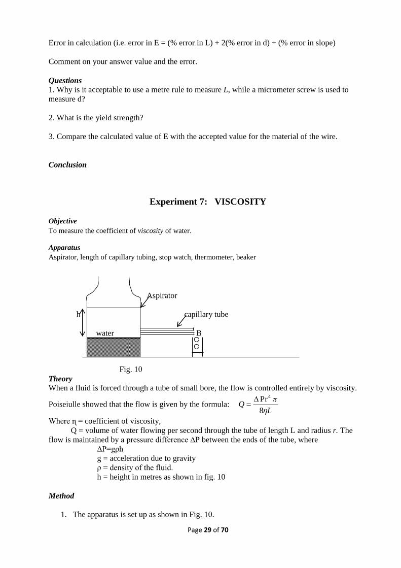
Aspirator, length of capillary tubing, stop watch, thermometer, beaker

Aspirator

h capillary tube

water B

Fig. 10

Theory

When a fluid is forced through a tube of small bore, the flow is controlled entirely by viscosity.

Poiseiulle showed that the flow is given by the formula: L

Q

8

Pr4

Where ɳ = coefficient of viscosity,

Q = volume of water flowing per second through the tube of length L and radius r. The

flow is maintained by a pressure difference ∆P between the ends of the tube, where

∆P=gρh

g = acceleration due to gravity

ρ = density of the fluid.

h = height in metres as shown in fig. 10

Method

1. The apparatus is set up as shown in Fig. 10.

Page 30 of 70

2. Adjust the rate of flow through the capillary tube so that water emerges slowly in drops

from B. Smear a little vaseline under end B to prevent water running along the outside of

the tube.

3. Weigh a clean dry beaker and record its mass.

4. Time the collection of about 50 ml of water and reweigh the beaker plus water.

5. Repeat the water collection several times, and note the room temperature at intervals.

6. Measure the length of the capillary tube. Measure the diameter of the capillary tube using

the travelling microscope. Remember to level the microscope before use.

7. Fill the data into the tables provided and calculate the coefficient of viscosity of water.

Worksheet 8

Length of capillary tube, L = m

Travelling microscope measurements: ‘(To find internal radius of capillary tube).

First scale reading (m) Second scale reading (m) Difference (m)

Average diameter = m; Radius = m; Error in scale of microscope = m;

Error in radius = m; Density of liquid (water) = kg/m3; Height, h = m

Mass of beaker = kg

Mass of beaker plus

water (Kg)

Mass of water (Kg) Time (s) Volume flow per

second, Q (kg/m3.s)

Page 31 of 70

From the data given above calculate the coefficient of viscosity for each volume of water timed.

The average coefficient of viscosity was found to be:

The unit of viscosity is: -

Now calculate the error in your value of viscosity using one set of data: -

What is the accepted value for the coefficient of viscosity?

Is your value within experimental error of this accepted value?

How does the coefficient of viscosity vary with temperature? Why

Conclusion

PART C: HEAT

Experiment 8: LINEAR EXPANSION

Objective

To measure the coefficient of linear expansion of copper.

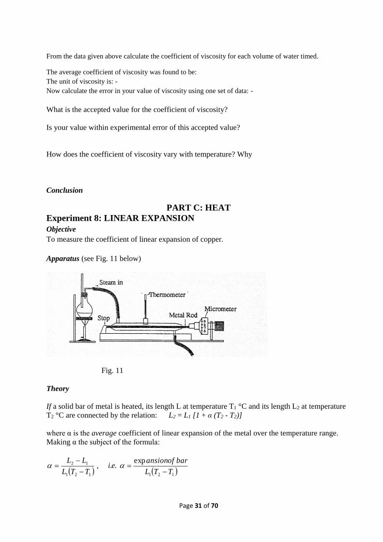
Apparatus (see Fig. 11 below)

Fig. 11

Theory

If a solid bar of metal is heated, its length L at temperature T1 °C and its length L2 at temperature

T2 °C are connected by the relation: L2 = L1 [1 + α (T2 - T2)]

where α is the average coefficient of linear expansion of the metal over the temperature range.

Making α the subject of the formula:

121121

12 exp..,

TTL

barofansionei

TTL

LL

Page 32 of 70

Method

1. Remove the bar of metal from the steam jacket and measure its length L1, and temperature

T1.

2. Replace the bar in its steam jacket and adjust the micrometer until j just tips the end of the

bar. Record the micrometer reading.

3. Reset the micrometer back from the end of the bar to allow room for expansion of the bar.

4. Heat the water in the flask and allow steam to flow around the bar until the expansion is

complete. This will take 10 to 15 minutes.

5. With steam still passing through the jacket record the new reading on the micrometer and

the temperature of the steam.

Analysis

Calculate the coefficient of linear expansion of the copper and the error in this value.

Answer the questions in Worksheet 9 below.

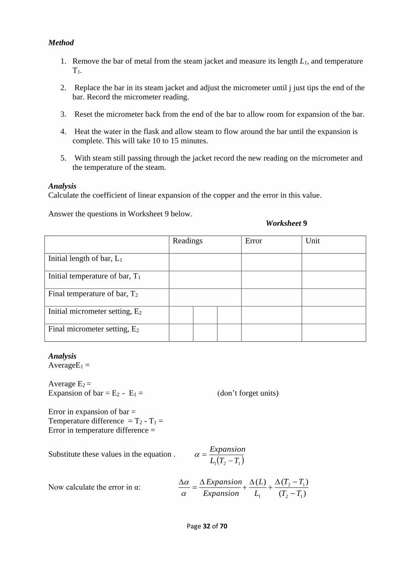
Worksheet 9

Readings Error Unit

Initial length of bar, L1

Initial temperature of bar, T1

Final temperature of bar, T2

Initial micrometer setting, E2

Final micrometer setting, E2

Analysis

AverageE1 =

Average E2 =

Expansion of bar = E2 - E1 = (don’t forget units)

Error in expansion of bar =

Temperature difference = T2 - T1 =

Error in temperature difference =

Substitute these values in the equation . 121 TTL

Expansion

Now calculate the error in α: )(

)()(

12

12

1 TT

TT

L

L

Expansion

Expansion

Page 33 of 70

This gives the fractional error. Multiply through by 100 to find the percentage error.

Questions

1. What would happen if the micrometer screw gauge was not reset back from the end of the bar?

3. Why is it necessary to measure the expansion with a micrometer screw gauge, whereas the

initial length of the bar can be measured with a meter rule?

Conclusion

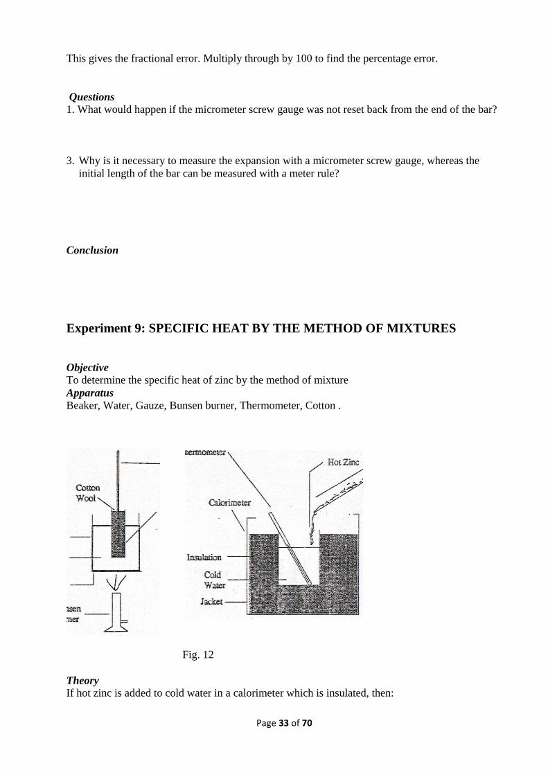
Experiment 9: SPECIFIC HEAT BY THE METHOD OF MIXTURES

Objective

To determine the specific heat of zinc by the method of mixture

Apparatus

Beaker, Water, Gauze, Bunsen burner, Thermometer, Cotton .

Fig. 12

Theory If hot zinc is added to cold water in a calorimeter which is insulated, then:

Page 34 of 70

Heat gained by water + calorimeter = Heat lost by zinc

(Mw Cw + Mc Cc) (T2 – T1) = Mzn Czn (T3-T2)

Where Mw = mass of water

Cw= specific heat of water

Mw= mass of calorimeter

Cc = specific heat of calorimeter

T2 = final temperature of mixture

T1 = initial temperature of water and calorimeter

Mzn = mass of zinc

Czn = specific heat of zinc

T3 = temperature of hot zinc

Method

1. Put the thermometer into the boiling tube and put as much zinc as possible around the

thermometer. Place some cotton wool on top.

2. Place the boiling tube in a beaker of water and heat to boiling. Keep the water boiling for at

least five minutes.

3. Meanwhile, weigh the calorimeter empty and then add about 113 full of water.

4. Replace the calorimeter in its jacket. Record the temperature of the water.

5. Record the temperature of the hot zinc.

6. Remove the cotton wool and thermometer from the boiling tube, and immediately pour the

zinc into the calorimeter.

7. Stir the contents of the calorimeter

8. Record the highest temperature reached, and then remove the thermometer.

9. Weigh the calorimeter and its contents.

10. Record the data on Worksheet 10 and evaluate the specific heat of the zinc.

Worksheet 10

Reading Error in reading units

Mass of calorimeter Mo

Mass of calorimeter + cold water M1

Temperature of cold water T1

Temperature of hot zinc T2

Temperature of mixture T3

Mass of calorimeter, water + zinc M2

Analysis

Page 35 of 70

Value Error in value Unit

Mass of cold water Mw=M1-Mc

Mass of zinc Mzn=M2-M1

Increase in temperature of water +

calorimeter, (T2-T1)

Decrease in temperature of

zinc(T3-T2)

Specific heat capacity of water = 4186 J/g deg C

Specific heat capacity of copper = 380 J/kg deg C

From these values, substitute into the equation given above and calculate a value for the specific

heat of zinc.

Calculate a value for the error in the specific heat of zinc

Questions

1. What are the sources of error in this experiment?

2. Why is water the medium used in so many heat exchange processes?

3. Compare and contrast the specific heat for zinc obtained in this experiment with the standard

value.

Conclusion

Experiment 10: THERMAL CONDUCTIVITY - SEARLE’S BAR

Objective

To measure the thermal conductivity coefficient of copper using Searle’s apparatus.

Apparatus

AB is a solid copper bar which is heated at end A by steam. At end B, a coil carrying water is

wrapped around the bar. Thermometers T1, T2, T3 andT4

are inserted as shown. The apparatus is well lagged and is enclosed in a wooden box.

Page 36 of 70

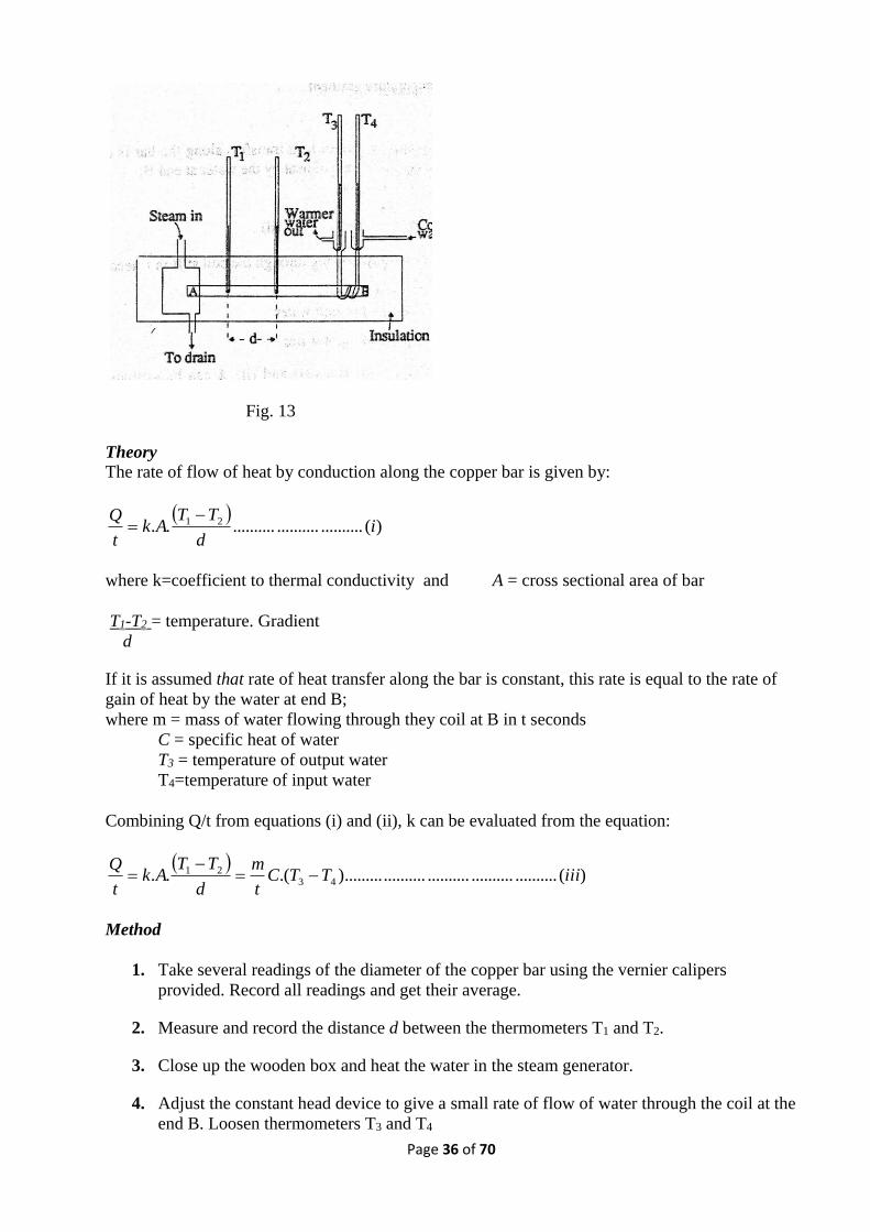
Fig. 13

Theory

The rate of flow of heat by conduction along the copper bar is given by:

)(................................ 21 i

d

TTAk

t

Q

where k=coefficient to thermal conductivity and A = cross sectional area of bar

T1-T2 = temperature. Gradient

d

If it is assumed that rate of heat transfer along the bar is constant, this rate is equal to the rate of

gain of heat by the water at end B;

where m = mass of water flowing through they coil at B in t seconds

C = specific heat of water

T3 = temperature of output water

T4=temperature of input water

Combining Q/t from equations (i) and (ii), k can be evaluated from the equation:

)(........................................)..........(.. 43

21 iiiTTCt

m

d

TTAk

t

Q

Method

1. Take several readings of the diameter of the copper bar using the vernier calipers

provided. Record all readings and get their average.

2. Measure and record the distance d between the thermometers T1 and T2.

3. Close up the wooden box and heat the water in the steam generator.

4. Adjust the constant head device to give a small rate of flow of water through the coil at the

end B. Loosen thermometers T3 and T4

Page 37 of 70

momentarily to eliminate air pockets in the water jacket, then insert the stoppers securely

so that there are no leaks.

5. While the steam is circulating around end A, record temperatures T1, T2, T3 and T4 every

five minutes. The purpose of these readings is to enable you to ascertain easily when the

steady state has been reached, i.e. that none of the temperatures is changing with time.

6. When this state has been reached, the temperature difference between thermometers T3

and T4 should be about 10°C. Adjust the water

flow if necessary.

7. Then record the mass of water collected from exit B in a beaker during a time of five

minutes. If marked fluctuations appear in any of the temperatures during water collection,

repeat this reading and take an average.

8. Record all data in Worksheet 11. Calculate the value for k and estimate its error.

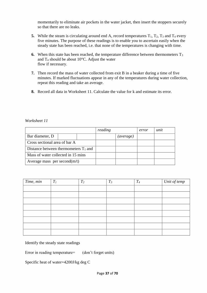
Worksheet 11

reading error unit

Bar diameter, D (average)

Cross sectional area of bar A

Distance between thermometers T1 and

T2, d

Mass of water collected in 15 mins

Average mass per second(m/t)

Time, min T1 T2 T3 T4 Unit of temp

Identify the steady state readings

Error in reading temperature= (don’t forget units)

Specific heat of water=4200J/kg deg C

Page 38 of 70

Substitute values into the equation:

).(.. 43

21 TTCt

m

d

TTAk

t

Q

Therefore, error-in (T1 - T2) =

Error in (T3 - T4) =

Calculate a value for k.

Calculate the error in your value of k. State the error arising from errors in measurement of

temperatures.

The thermal conductivity of copper

Questions

1. Explain why this method is not a good one for poor thermal conductors.

2. Do you think that the accuracy of the experiment would be improved if a bar of a larger

diameter was used?

3. By what percentage does your value of k deviate from the standard value of k for copper?

Conclusion

Experiment 11: NEWTON’S LAW OF COOLING

Objective

To investigate Newton’s law of cooling.

Apparatus

Bunsen burner, tripod stand, gauze, beakers, thermometer, stopwatch

Page 39 of 70

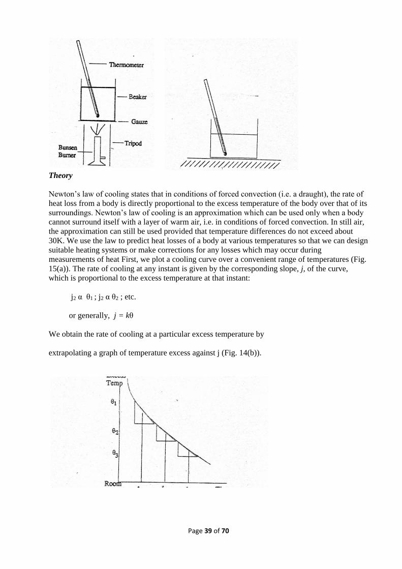
Theory

Newton’s law of cooling states that in conditions of forced convection (i.e. a draught), the rate of

heat loss from a body is directly proportional to the excess temperature of the body over that of its

surroundings. Newton’s law of cooling is an approximation which can be used only when a body

cannot surround itself with a layer of warm air, i.e. in conditions of forced convection. In still air,

the approximation can still be used provided that temperature differences do not exceed about

30K. We use the law to predict heat losses of a body at various temperatures so that we can design

suitable heating systems or make corrections for any losses which may occur during

measurements of heat First, we plot a cooling curve over a convenient range of temperatures (Fig.

15(a)). The rate of cooling at any instant is given by the corresponding slope, j, of the curve,

which is proportional to the excess temperature at that instant:

j2 α θ1 ; j2 α θ2 ; etc.

or generally, j = kθ

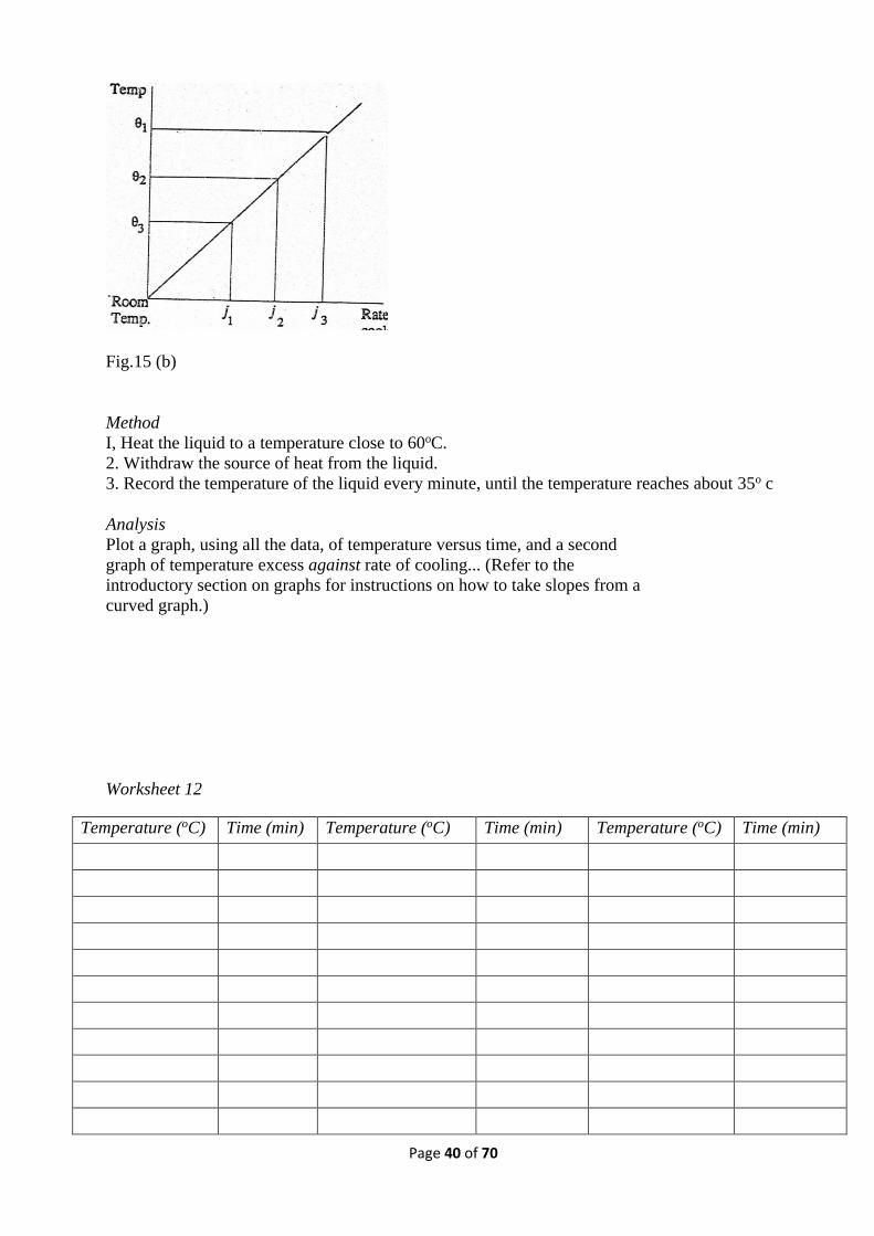
We obtain the rate of cooling at a particular excess temperature by

extrapolating a graph of temperature excess against j (Fig. 14(b)).

Page 40 of 70

Fig.15 (b)

Method

I, Heat the liquid to a temperature close to 60oC.

2. Withdraw the source of heat from the liquid.

3. Record the temperature of the liquid every minute, until the temperature reaches about 35o c

Analysis

Plot a graph, using all the data, of temperature versus time, and a second

graph of temperature excess against rate of cooling... (Refer to the

introductory section on graphs for instructions on how to take slopes from a

curved graph.)

Worksheet 12

Temperature (oC) Time (min) Temperature (oC) Time (min) Temperature (oC) Time (min)

Page 41 of 70

Plot a graph of temperature against time.

Room temperature=

Temperature (oC) Temperature excess (oC) Slope, j C/min

Plot a graph of temperature excess against slope, j.

Comments

Conclusion

Experiment 12: BOYLE’S LAW

Objectives

(i) To verify Boyle’s law

(ii) To determine atmospheric pressure graphically

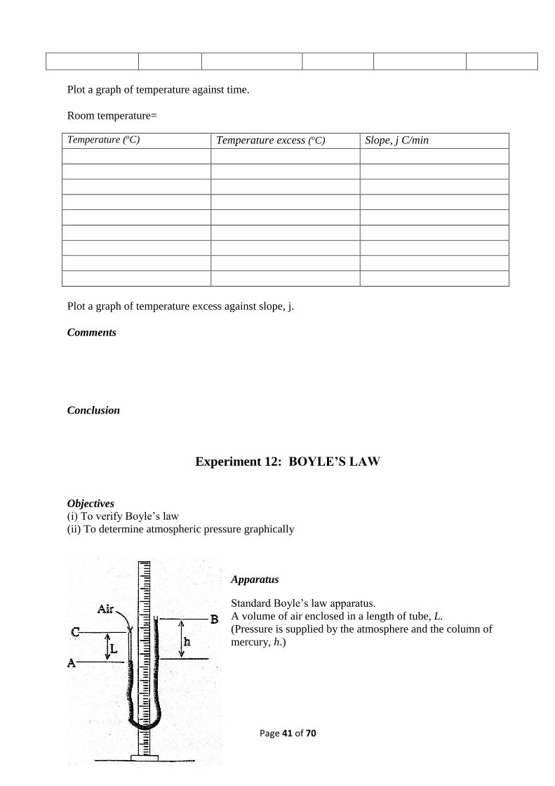
Apparatus

Standard Boyle’s law apparatus.

A volume of air enclosed in a length of tube, L.

(Pressure is supplied by the atmosphere and the column of

mercury, h.)

Page 42 of 70

Fig. 16

Theory Boyle’s law states that, at constant, temperature, the volume of a definite mass of gas is inversely

proportional to its pressure.

PV = k (at constant temperature)

Assuming that the tube AC is of uniform cross-section, the volume of air in AC will be V units.

Pressure is proportional to (H + h) cm of mercury (Hg), where H is atmospheric pressure. Thus,

in terms of these quantities,

Boyle’s law becomes: (H + h) L = k (at constant temperature).

Method

1. Adjust the apparatus so that the mercury level in tube B is at the highest feasible level and

that in tube A it is at the lowest feasible level. Note these levels and also the level of C.

NB Make these changes slowly in order to prevent temperature changes which might result

due to compression.

2. Take these measurements for four settings with the mercury level in B above that in A, and

four settings with A above B.

3. Tabulate your observations.

4. Read off the room temperature and atmospheric pressure from the barometer.

Analysis

The equation for Boyles law, (H + h) L = k can be written in the form:

HL

khandl

khH

1;

which is of the form y=mx+c, with y=h and x= 1/L. Hence if a graph of h against 1/L is plotted, a

straight line should result.

This would verify Boyle’s law and also yield a value for H as the negative intercept on the y axis.

Worksheet 13

Level of A(cm) Level of B (cm) Level of C (cm) h(cm) L (cm) 1/L (cm)

Page 43 of 70

Reading error in measuring the levels = cm

Room temperature = ° C

Pressure from barometer = mm Hg

Plot a graph of h versus 1/L.

Intercept on y-axis = cm

Comment on your graph.

Compare the two values of atmospheric pressure (from barometer and from the graph).

What would be the effect on your results if the temperature was to charge during the course of the

course of the experiment?

Conclusion

Page 44 of 70

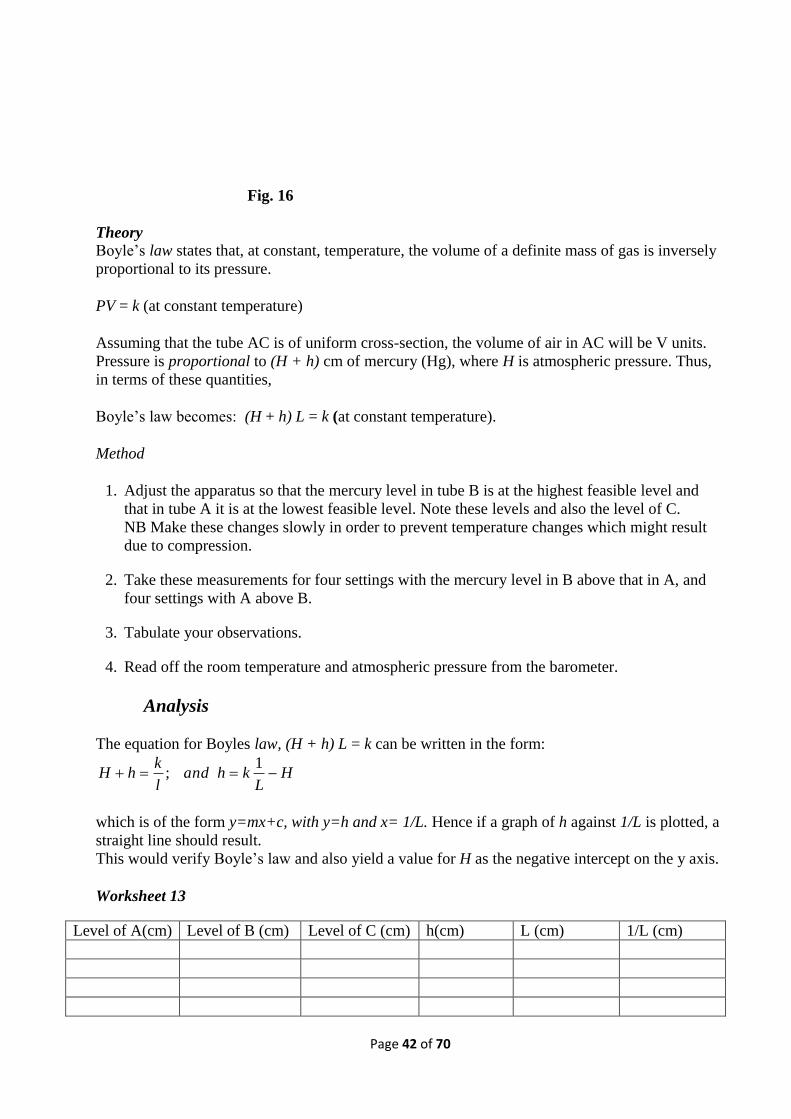
PART D: WAVE MOTION

Experiment 13: STANDING WAVES IN A TAUT STRING

Objective

To study the relationship between resonant frequency and the tension in a taut string.

Apparatus

A string of mass per unit length m, set up as shown, with an electrically driven vibrator and a set

of weights.

Fig. 17

Theory

When the applied frequency is equal to a natural frequency of the string it will resonate in one of

its modes of vibration.

The frequency of the fundamental mode or first harmonic, m

T

Lf

2

11

The frequency of the first overtone or 2nd harmonic, m

T

Lf

2

22

The frequency of the nth harmonic, m

T

L

nf n

2

mgT ; Hzm

Mg

L

nf n

2

Method

1. The apparatus is set up as shown in Fig. 17 above. L should be between I and 1.5 metres.

2. A sample of string is used to measure m.

3. A mass of l50g is attached at M.

4. The signal generator is switched on and the frequency (f) varied slowly from zero Hz. When

the string vibrates clear1y in its first harmonic, the corresponding value off is noted (f1).

Page 45 of 70

5. With the same mass, increase f to roughly twice this value and observe the second harmonic.

Note the new value of f (f2).

6. Where possible, observe and record the frequencies of higher harmonics, fn.

7. Repeat 4-6 for a range of values of M and tabulate the results as shown on Worksheet 14.

NB. Unwanted resonances originating in the vibrator itself may be observed. Be careful that the

frequency readings refer to a consistent set of harmonics.

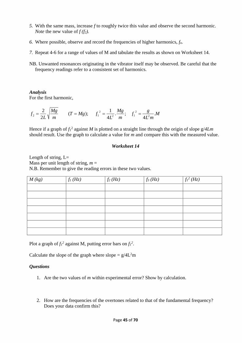
Analysis For the first harmonic,

MmL

gf

m

Mg

LfMgT

m

Mg

Lf .

4;.

4

1);(

2

22

2

12

2

12

Hence if a graph of f12 against M is plotted on a straight line through the origin of slope g/4Lm

should result. Use the graph to calculate a value for m and compare this with the measured value.

Worksheet 14

Length of string, L=

Mass per unit length of string, m =

N.B. Remember to give the reading errors in these two values.

M (kg) f1 (Hz) f2 (Hz) f3 (Hz) f12 (Hz)

Plot a graph of f12 against M, putting error bars on f1

2.

Calculate the slope of the graph where slope = g/4L2m

Questions

1. Are the two values of m within experimental error? Show by calculation.

2. How are the frequencies of the overtones related to that of the fundamental frequency?

Does your data confirm this?

Page 46 of 70

3. Give two examples of resonance which are of practical importance.

Conclusion

Experiment 14: RESONANCE TUBE

Objective To determine the velocity of sound using a resonance tube.

Apparatus

Set of resonance tubes of varying lengths

Large tube nearly full of water

Retort stand and clamp to hold

Resonance tube

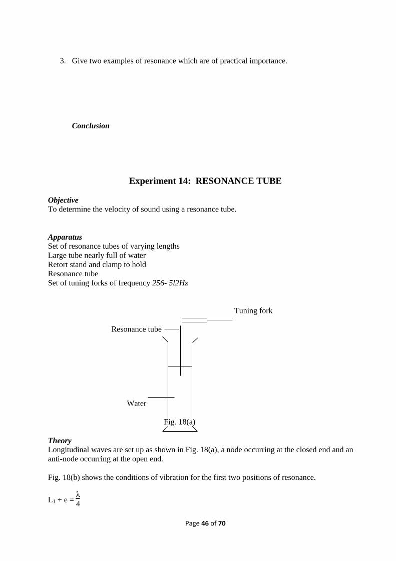
Set of tuning forks of frequency 256- 5l2Hz

Tuning fork

Resonance tube

Water

Fig. 18(a)

Theory

Longitudinal waves are set up as shown in Fig. 18(a), a node occurring at the closed end and an

anti-node occurring at the open end.

Fig. 18(b) shows the conditions of vibration for the first two positions of resonance.

L1 + e = λ

4

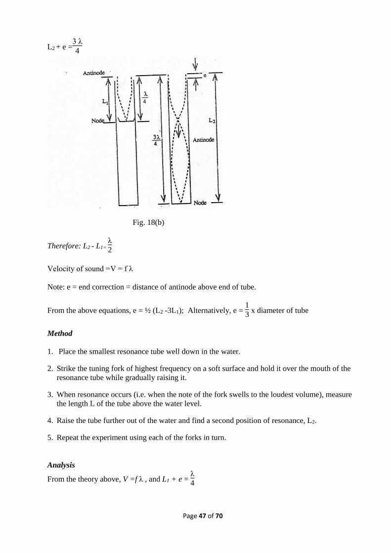
Page 47 of 70

L2 + e =3 λ

4

Fig. 18(b)

Therefore: L2 - L1=

λ

2

Velocity of sound =V = f λ

Note: e = end correction = distance of antinode above end of tube.

From the above equations, e = ½ (L2 -3L1); Alternatively, e = 1

3 x diameter of tube

Method

1. Place the smallest resonance tube well down in the water.

2. Strike the tuning fork of highest frequency on a soft surface and hold it over the mouth of the

resonance tube while gradually raising it.

3. When resonance occurs (i.e. when the note of the fork swells to the loudest volume), measure

the length L of the tube above the water level.

4. Raise the tube further out of the water and find a second position of resonance, L2.

5. Repeat the experiment using each of the forks in turn.

Analysis

From the theory above, V =f λ , and L1 + e = λ

4

Page 48 of 70

Combining these two equations: λ. = v

f = 4 (L1 + e)

Rearranging, we have L1 = v

4 .

1

f – e

A graph of L against I

f should be a straight line with a gradient of

v

4 . The negative intercept on

the vertical axis will yield a value for e.

Worksheet 15

Tuning fork frequency HZ l/

f

Length,L1 m Length,L2 m

Plot a graph of L1 against I

f

Slope of graph = v

4 =

Velocity of sound =

End correction

Diameter of resonance tube =

1. e =1

3 x diameter of tube =

2. Negative intercept on graph =

3. e = ½ (L2 - 3L1) =

Comment on, and compare, the three values you obtained for the end correction.

Reading error in length =

Page 49 of 70

What are the other sources of error in this experiment?

Conclusion

Page 50 of 70

E. OPTICS

Experiment 15: REFLECTION

Objectives

(i) To verify the laws of reflection.

(ii) To investigate some properties of spherical mirrors.

Laws of Reflection

A. Plane Mirror

Apparatus

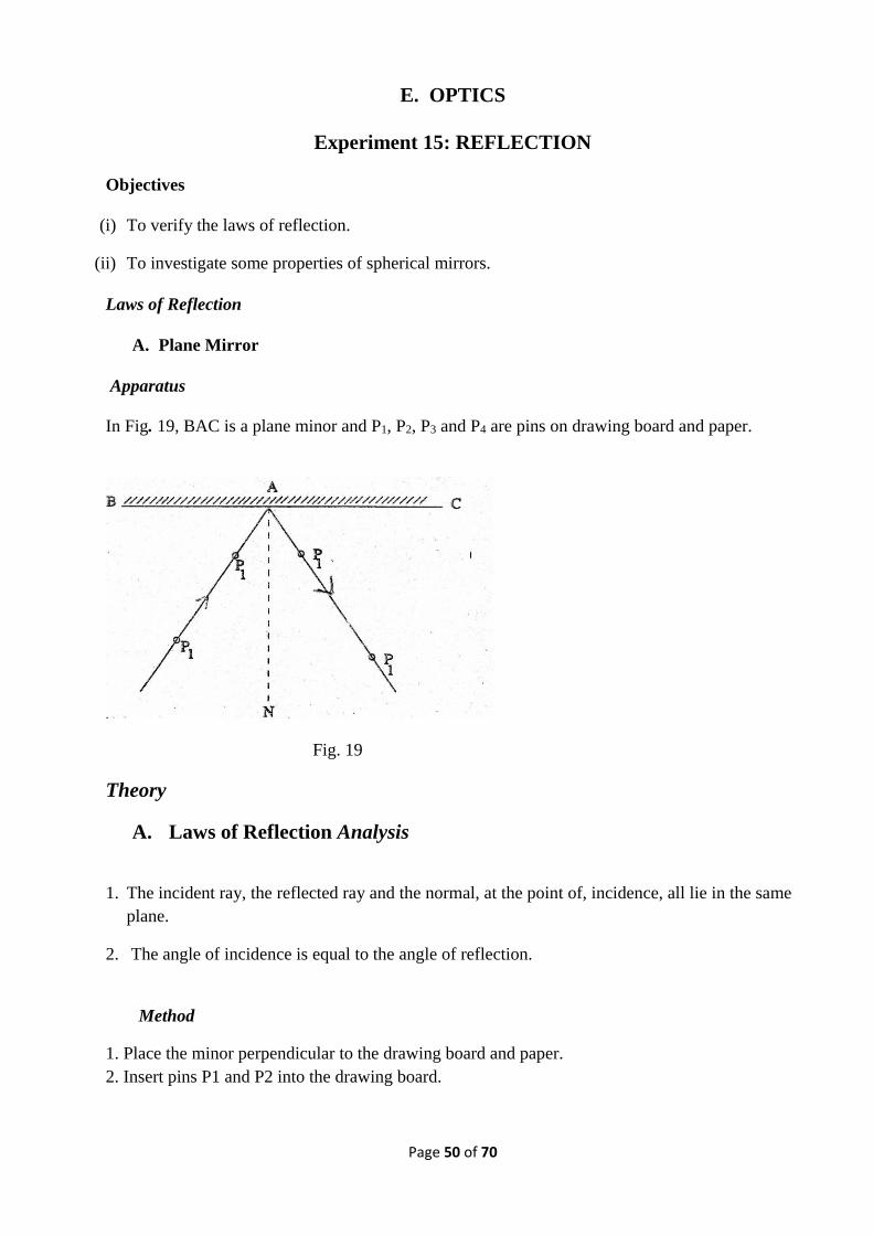
In Fig. 19, BAC is a plane minor and P1, P2, P3 and P4 are pins on drawing board and paper.

Fig. 19

Theory

A. Laws of Reflection Analysis

1. The incident ray, the reflected ray and the normal, at the point of, incidence, all lie in the same

plane.

2. The angle of incidence is equal to the angle of reflection.

Method

1. Place the minor perpendicular to the drawing board and paper.

2. Insert pins P1 and P2 into the drawing board.

Page 51 of 70

3. Look in along the direction P3 and P4 until pins P1 and P2 are seen the same line.

4. Insert pins P3 and P4 into the drawing board in line with the images P1 and P2,such that when

looking into the mirror all the four pins appear to lie in line.

5. Draw a line on the drawing board to mark the reflecting surface of the mirror.

6. Remove the mirror and pins from the paper.

7. Draw AN (the normal) perpendicular to BAC.

8. Measure the angles of incidence and reflection.

Analysis

The data should show that the first and the second laws are verified.

B. Spherical Mirrors

Apparatus

Illuminated object, pins screen, concave and convex mirrors.

Theory

The distance of the object and the image from a spherical mirror are related to the focal length of

the mirror by the formula:

1

u +

1

v =1f

Where , u = object distance; v = image distance; f = focal length

A ray of light from the object which enters the mirror parallel to the principal axis will be

reflected back through the focus. The ray of light which enters the mirror through the center of

curvature will be reflected back along the same path.

Method

1. Switch on the illuminated object.

2. Move the concave mirror slowly away from the illuminated object until it projects an image of

the illuminated object onto itself. Move the mirror such that a good clear focus is obtained.

3. Measure the distance between the mirror and the object/image. Half this distance is the focal

length.

4. Set the mirror at a distance greater than 2f away from the object.

5 Use the screen to locate the image and measure v (2f> u <f and u = f). (image distance).

6. Repeat this for 2f > u >f and u =f.

7. Use the method of no parallax to locate the virtual images in the concave and convex mirrors

using the search pins provided.

Analysis

Calculate the focal length,f, in each case, thereby verifying the formula:

Page 52 of 70

1/u + 1/v =1/f for the concave mirror.

Worksheet 16

A. Plane mirror

Angle Error

Angle of incidence, i

Angle of reflection, r

N.B. Hand in original ray diagrams

Are the two laws of reflecrion verified?

What sort of image is seen in a plane mirror?

What sort of image does the convex mirror produce?

Conclusion

Experiment 16: LAWS OF REFRACTION AND PROPERTIES OF LENSES

Objectives

(1) To verify the law of refraction

(ii) To investigate properties of lenses

A. The Laws of Refraction

Apparatus

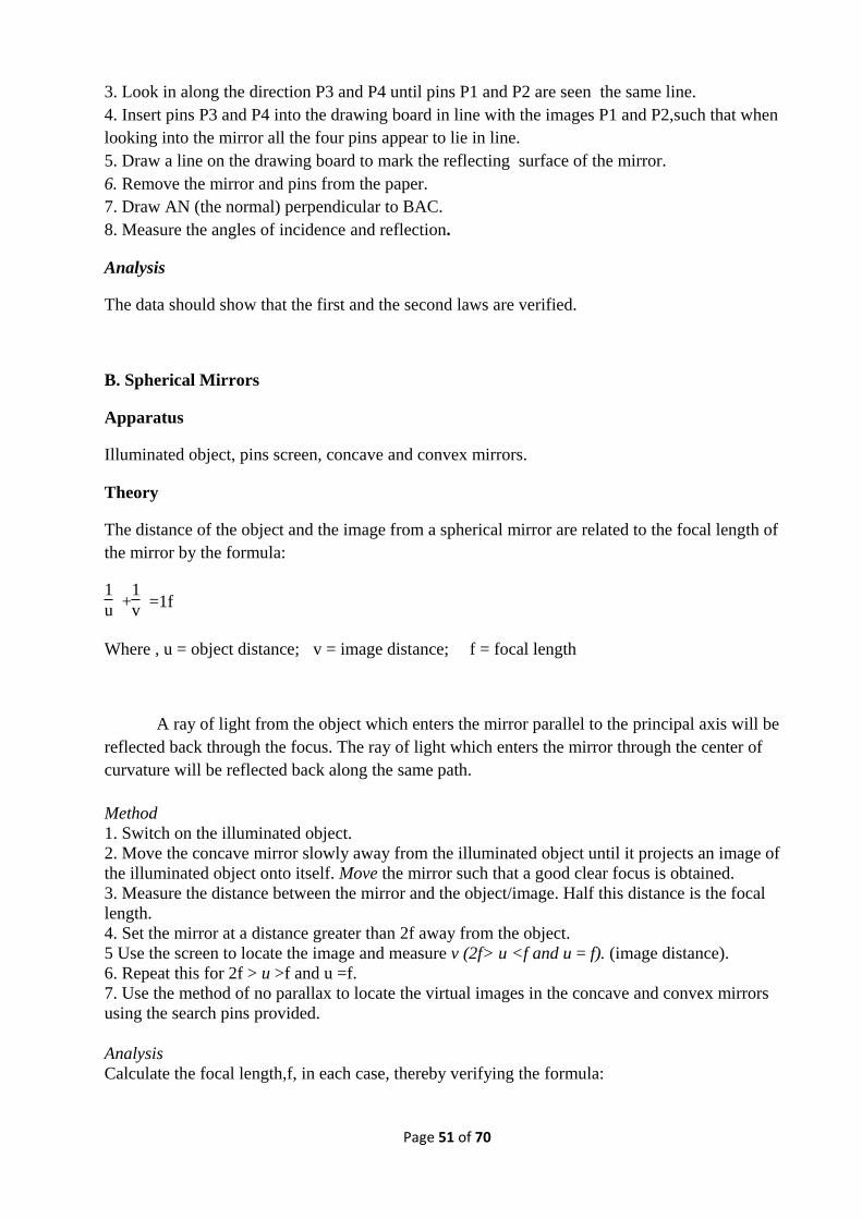
ABCD is a rectangular glass block. P1,P2,P3 and P4 are pins on a drawing board and paper.

Fig. 20

Theory

Laws of refraction

Page 53 of 70

1. The incident ray, the refracted ray and the normal,at the point of incidence, all lie in the

same plane.

2. The sine of the angle of incidence divided by the sine of the angle of refraction is equal to

a constant called the refractive index for the two media involved

Method 1. Place a rectangular glass block on a paper on the drawing board.

2. Insert pins P1 and P2 into the drawing board.

3. Look in along the direction P3 and P4 until the pins P1 and P2 are seen in line.

4. Insert pins P3 and P4 in the drawing board in line with the images of P1 and P2 such that when

looking into the glass block all the four pins appear in line.

5. Draw the outline of the glass block on the drawing paper.

6. Remove the glass block and pins from the paper.

7. Draw the normal at point E and F and join EF

8. Measure the angles i and r with a protractor and calculate the refractive index.

Analysis The data should show that the first and second laws of refraction have been verified.

Additional note

Device an experiment to show that: real depth

apparent depth = n

by using a glass block and a microscope. (Consult the lecturer in charge.)

B. Lenses

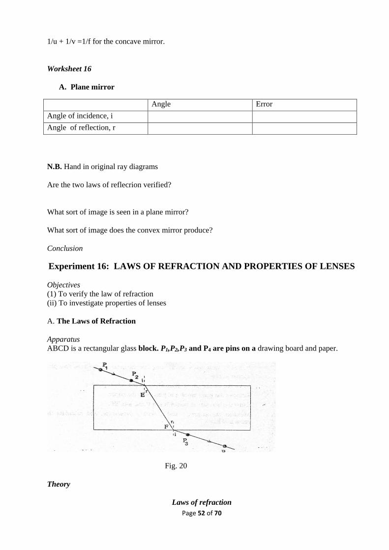
Apparatus An illuminated object, pins, screen, concave and convex lenses,

Fig. 21

Theory

The location and type of image formed in a lens can be ascertained by drawing a ray

diagram. The ray of light from the object which enters the lens parallel to the principal axis will

Page 54 of 70

be refracted through the focus. The ray of light which goes through the center of the lens will

emerge undeviated. It can be shown that:

1

f =

1

u +

1

v

Where f = focal length from lens

u=distance of image from lens

v=distance of image from lens

Method

1.Establish a rough value for the focal length of the convex lens by focusing on a distant object

(eg. window of laboratory) on the screen.

2. Switch on the illuminated object and place it at a position greater than

2f from the lens. Move the screen until a clear image is in focus on it.

3. Measure the distance from the object to the lens (u) and from the lens to the screen (v).

4. Calculate f using the above values of u and v.

5. Repeat the above steps for positions of the object:

u=2f ; 2f>u>f ; u=f

6. Use the method of no parallax to locate virtual images in both the

convex and the concave lenses using search pins provided.

Additional notes

The focal length of the concave lens can also be determined by combining the lens with a convex

lens of shorter focal length than itself. The focal length of the combining (F) is given by:

1

F =

1

f1 +

1

f2

where f1 = focal length of convex lens

f2= focal lenth of concave lens

F is determined by using the combination lens to form a real image on a screen, whence:

1

F =

1

u +

1

v

f1 is known and hence F can be calculated.

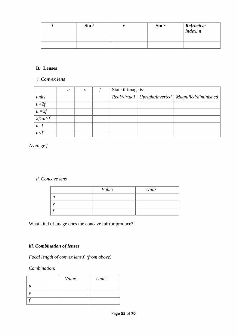
Worksheet 17

A. Laws of Refraction

Page 55 of 70

i Sin i r Sin r Refractive

index, n

B. Lenses

i. Convex lens

u v f State if image is:

units Real/virtual Upright/inverted Magnified/diminished

u>2f

u =2f

2f>u>f

u=f

u<f

Average f

ii. Concave lens

Value Units

u

v

f

What kind of image does the concave mirror produce?

iii. Combination of lenses

Focal length of convex lens,f1 (from above)

Combination:

Value Units

u

v

f

Page 56 of 70

1

F =

1

f1 +

1

f2

Calculate f2

How does this answer correspond to that obtained in (ii) above?

Conclusion

Experiment 17: THE SPECTROMETER REFRACIIVE INDEX

Objective To measure the refractive index of the glass of a prism using monochromatic

light from a sodium lamp

Apparatus

Spectrometer, glass prism, sodium lamp.

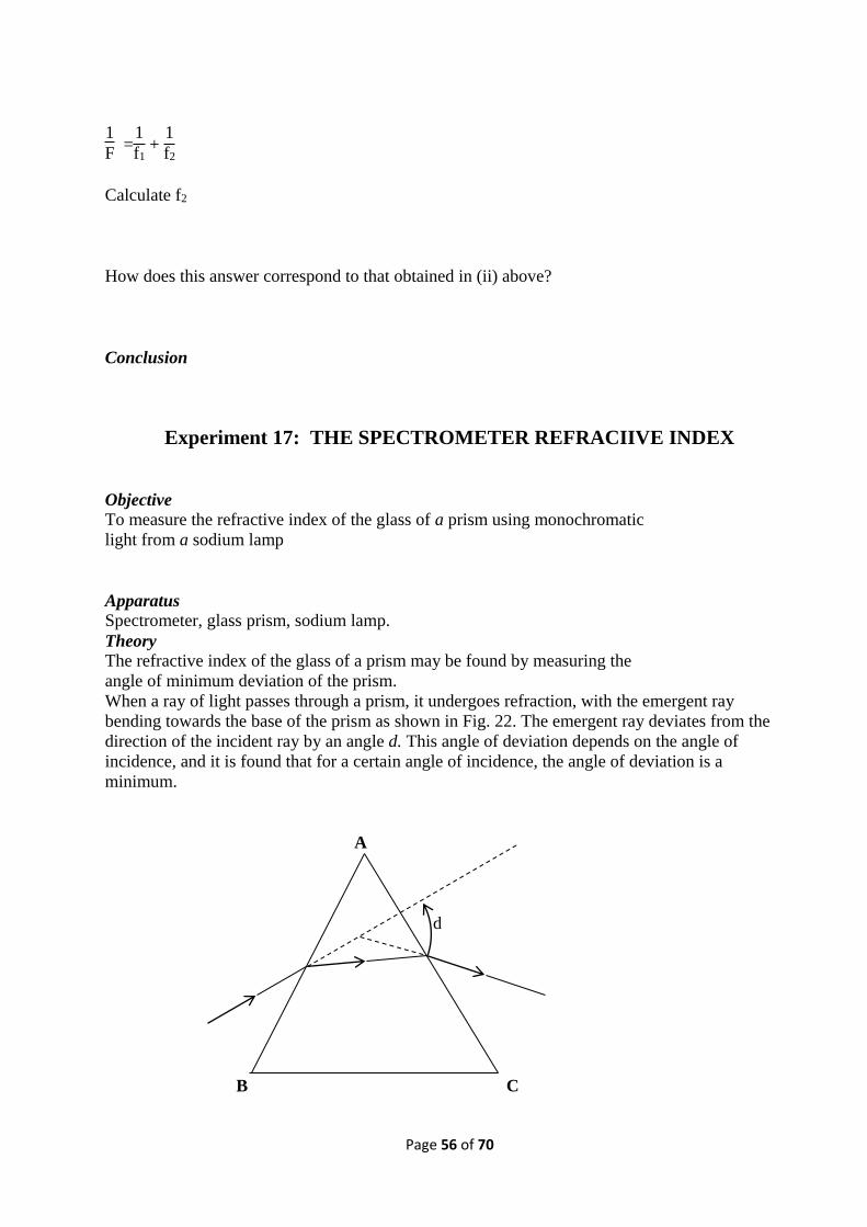
Theory

The refractive index of the glass of a prism may be found by measuring the

angle of minimum deviation of the prism.

When a ray of light passes through a prism, it undergoes refraction, with the emergent ray

bending towards the base of the prism as shown in Fig. 22. The emergent ray deviates from the

direction of the incident ray by an angle d. This angle of deviation depends on the angle of

incidence, and it is found that for a certain angle of incidence, the angle of deviation is a

minimum.

A

d

B C

Page 57 of 70

Let D= angle of minimum deviation, and A= refracting angle of prism

Then the refractive angle of the glass of the prism is given by: n=

sin(A+D

2 )

sinA

2

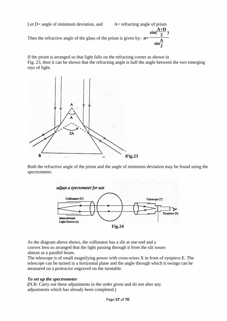
If the prism is arranged so that light falls on the refracting corner as shown in

Fig. 23, then it can be shown that the refracting angle is half the angle between the two emerging

rays of light.

Fig.23

Both the refractive angle of the prism and the angle of minimum deviation may be found using the

spectrometer.

Fig.24

As the diagram above shows, the collimator has a slit at one end and a

convex lens so arranged that the light passing through it from the slit issues

almost as a parallel beam.

The telescope is of small magnifying power with cross-wires X in front of eyepiece E. The

telescope can be turned in a horizontal plane and the angle through which it swings can be

measured on a protractor engraved on the turntable.

To set up the spectrometer (N.B: Carry out these adjustments in the order given and do not alter any

adjustments which has already been completed.)

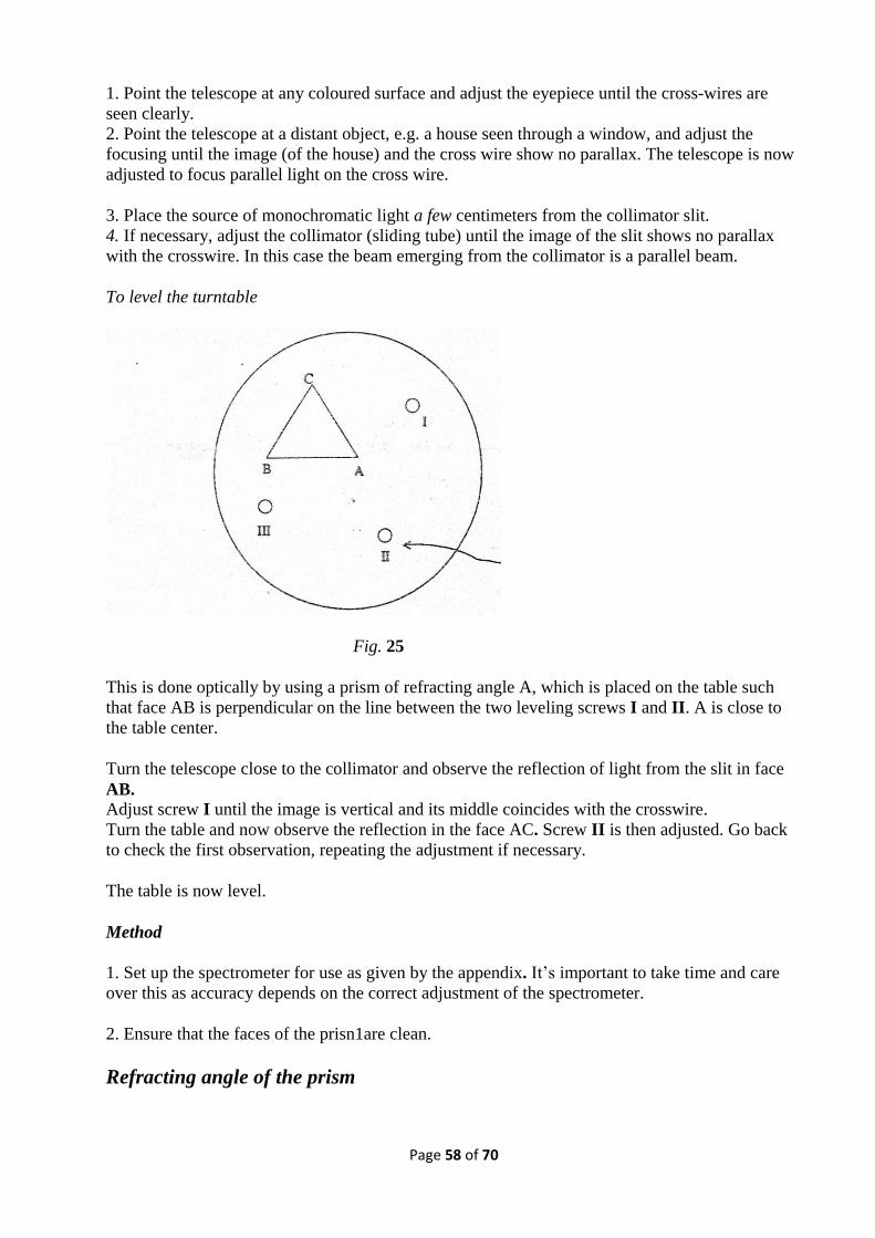
Page 58 of 70

1. Point the telescope at any coloured surface and adjust the eyepiece until the cross-wires are

seen clearly.

2. Point the telescope at a distant object, e.g. a house seen through a window, and adjust the

focusing until the image (of the house) and the cross wire show no parallax. The telescope is now

adjusted to focus parallel light on the cross wire.

3. Place the source of monochromatic light a few centimeters from the collimator slit.

4. If necessary, adjust the collimator (sliding tube) until the image of the slit shows no parallax

with the crosswire. In this case the beam emerging from the collimator is a parallel beam.

To level the turntable

Fig. 25

This is done optically by using a prism of refracting angle A, which is placed on the table such

that face AB is perpendicular on the line between the two leveling screws I and II. A is close to

the table center.

Turn the telescope close to the collimator and observe the reflection of light from the slit in face

AB.

Adjust screw I until the image is vertical and its middle coincides with the crosswire.

Turn the table and now observe the reflection in the face AC. Screw II is then adjusted. Go back

to check the first observation, repeating the adjustment if necessary.

The table is now level.

Method

1. Set up the spectrometer for use as given by the appendix. It’s important to take time and care

over this as accuracy depends on the correct adjustment of the spectrometer.

2. Ensure that the faces of the prisn1are clean.

Refracting angle of the prism

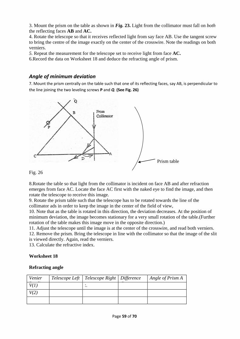
Page 59 of 70

3. Mount the prism on the table as shown in Fig. 23. Light from the collimator must fall on both

the reflecting faces AB and AC.

4. Rotate the telescope so that it receives reflected light from say face AB. Use the tangent screw

to bring the centre of the image exactly on the center of the crosswire. Note the readings on both

verniers.

5. Repeat the measurement for the telescope set to receive light from face AC.

6.Record the data on Worksheet 18 and deduce the refracting angle of prism.

Angle of minimum deviation

7. Mount the prism centrally on the table such that one of its reflecting faces, say AB, is perpendicular to

the line joining the two leveling screws P and Q. (See Fig. 26)

Prism table

Fig. 26

8.Rotate the table so that light from the collimator is incident on face AB and after refraction

emerges from face AC. Locate the face AC first with the naked eye to find the image, and then

rotate the telescope to receive this image.

9. Rotate the prism table such that the telescope has to be rotated towards the line of the

collimator ads in order to keep the image in the center of the field of view,

10. Note that as the table is rotated in this direction, the deviation decreases. At the position of

minimum deviation, the image becomes stationary for a very small rotation of the table.(Further

rotation of the table makes this image move in the opposite direction.)

11. Adjust the telescope until the image is at the center of the crosswire, and read both verniers.

12. Remove the prism. Bring the telescope in line with the collimator so that the image of the slit

is viewed directly. Again, read the verniers.

13. Calculate the refractive index.

Worksheet 18

Refracting angle

Venier

Readings

Telescope Left Telescope Right Difference

Ө

Angle of Prism A

V(1)

:.

V(2)

Page 60 of 70

Mean A= ; Error in A=

N.B. When taking the difference angle, Ө, pay attention to what happens when the telescope is

rotated through the 360 degree mark!

Angle of Minimum Deviation

Vernier

Readings Prism in minimum deviation position Ө1 Straight through reading Ө2

Difference Ө

Ө2 - Ө1= D

V(1)

V (2)

Mean D = ; Error in D: ; Refractive index:

N.B: Quote the value of n (and its error) to three decimal places since this is the minimum

accuracy expected with the spectrometer. Error in Refractive Index:

Questions

1. Show how 2/sin

2/)sin(

A

BAn

is derived

2. Why is the telescope adjusted for a distant object?

3. When will the maximum deviation occur in this experiment?

Conclusion

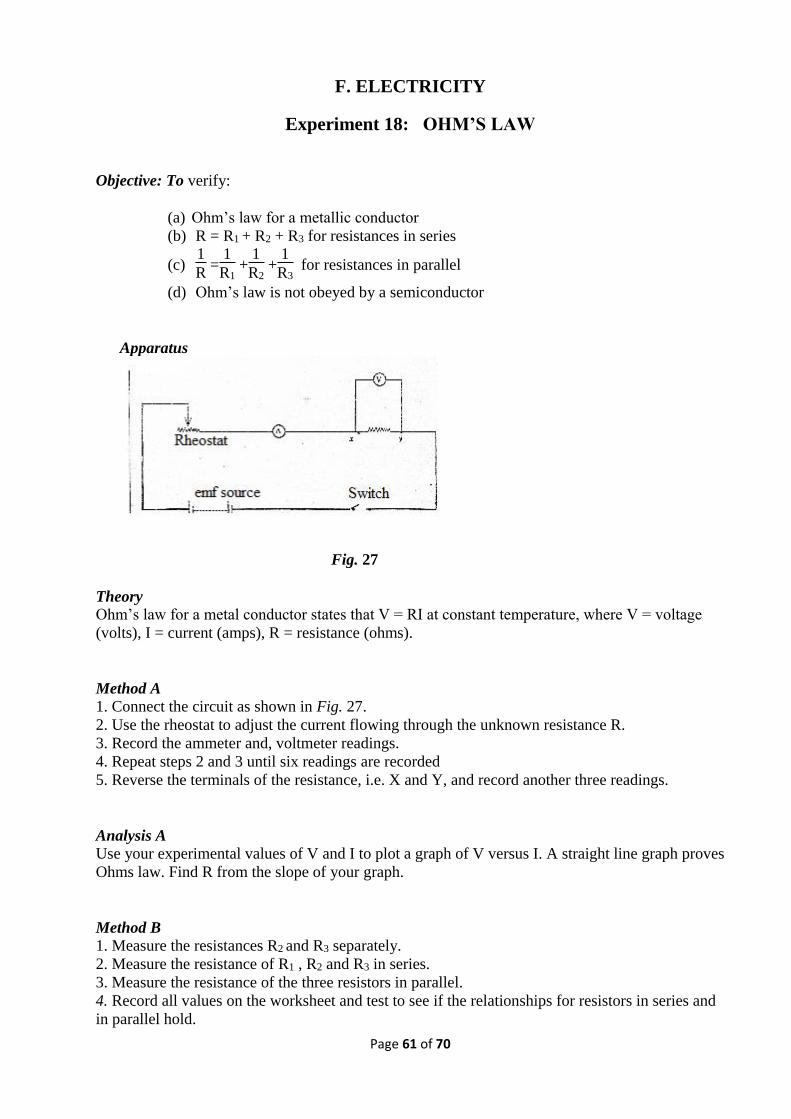
Page 61 of 70

F. ELECTRICITY

Experiment 18: OHM’S LAW

Objective: To verify:

(a) Ohm’s law for a metallic conductor

(b) R = R1 + R2 + R3 for resistances in series

(c) 1

R =

1

R1 +

1

R2 +

1

R3 for resistances in parallel

(d) Ohm’s law is not obeyed by a semiconductor

Apparatus

Fig. 27

Theory Ohm’s law for a metal conductor states that V = RI at constant temperature, where V = voltage

(volts), I = current (amps), R = resistance (ohms).

Method A 1. Connect the circuit as shown in Fig. 27.

2. Use the rheostat to adjust the current flowing through the unknown resistance R.

3. Record the ammeter and, voltmeter readings.

4. Repeat steps 2 and 3 until six readings are recorded

5. Reverse the terminals of the resistance, i.e. X and Y, and record another three readings.

Analysis A Use your experimental values of V and I to plot a graph of V versus I. A straight line graph proves

Ohms law. Find R from the slope of your graph.

Method B 1. Measure the resistances R2 and R3 separately.

2. Measure the resistance of R1 , R2 and R3 in series.

3. Measure the resistance of the three resistors in parallel.

4. Record all values on the worksheet and test to see if the relationships for resistors in series and

in parallel hold.

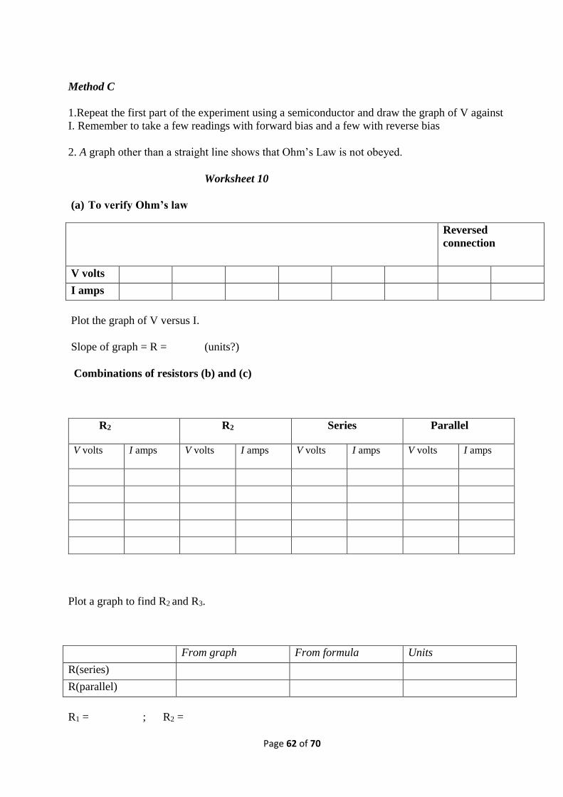
Page 62 of 70

Method C

1.Repeat the first part of the experiment using a semiconductor and draw the graph of V against

I. Remember to take a few readings with forward bias and a few with reverse bias

2. A graph other than a straight line shows that Ohm’s Law is not obeyed.

Worksheet 10

(a) To verify Ohm’s law

Reversed

connection

V volts

I amps

Plot the graph of V versus I.

Slope of graph = R = (units?)

Combinations of resistors (b) and (c)

R2 R2 Series Parallel

V volts I amps V volts I amps V volts I amps V volts I amps

Plot a graph to find R2 and R3.

From graph From formula Units

R(series)

R(parallel)

R1 = ; R2 =

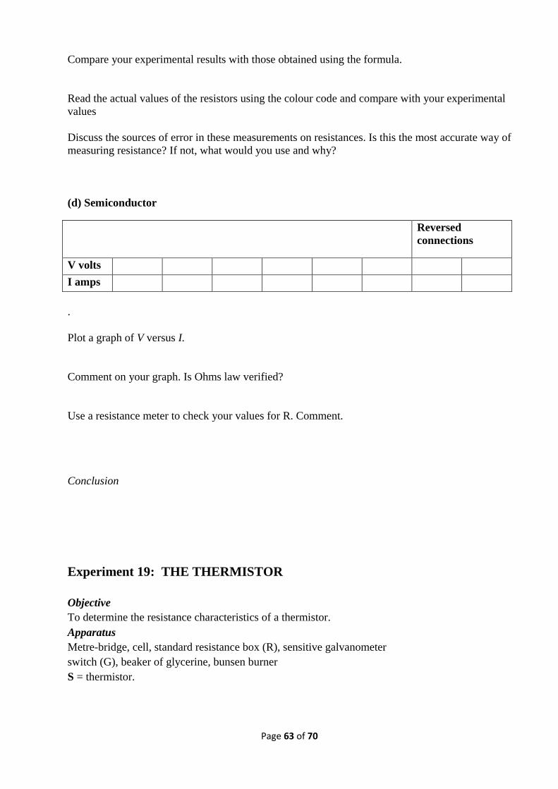
Page 63 of 70

Compare your experimental results with those obtained using the formula.

Read the actual values of the resistors using the colour code and compare with your experimental

values

Discuss the sources of error in these measurements on resistances. Is this the most accurate way of

measuring resistance? If not, what would you use and why?

(d) Semiconductor

Reversed

connections

V volts

I amps

.

Plot a graph of V versus I.

Comment on your graph. Is Ohms law verified?

Use a resistance meter to check your values for R. Comment.

Conclusion

Experiment 19: THE THERMISTOR

Objective

To determine the resistance characteristics of a thermistor.

Apparatus

Metre-bridge, cell, standard resistance box (R), sensitive galvanometer

switch (G), beaker of glycerine, bunsen burner

S = thermistor.

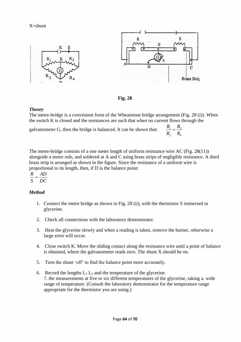
Page 64 of 70

X=shunt

Fig. 28

Theory

The metre-bridge is a convenient form of the Wheatstone bridge arrangement (Fig. 28 (i)). When

the switch K is closed and the resistances are such that when no current flows through the

galvanometer G, then the bridge is balanced. It can be shown that: 31

2 4

RR

R R

The metre-bridge consists of a one meter length of uniform resistance wire AC (Fig. 28(11))

alongside a metre rule, and soldered at A and C using brass strips of negligible resistance. A third

brass strip is arranged as shown in the figure. Since the resistance of a uniform wire is

proportional to its length, then, if D is the balance point:

DC

AD

S

R

Method

1. Connect the metre bridge as shown in Fig. 28 (ii), with the thermistor S immersed in

glycerine.

2. Check all connections with the laboratory demonstrator.

3. Heat the glycerine slowly and when a reading is taken, remove the burner, otherwise a

large error will occur.

4. Close switch K. Move the sliding contact along the resistance wire until a point of balance

is obtained, where the galvanometer reads zero. The shunt X should be on.

5. Turn the shunt ‘off’ to find the balance point more accurately.

6. Record the lengths L1 L2 and the temperature of the glycerine.

7. the measurements at five or six different temperatures of the glycerine, taking a. wide

range of temperature. (Consult the laboratory demonstrator for the temperature range

appropriate for the thermistor you are using.)

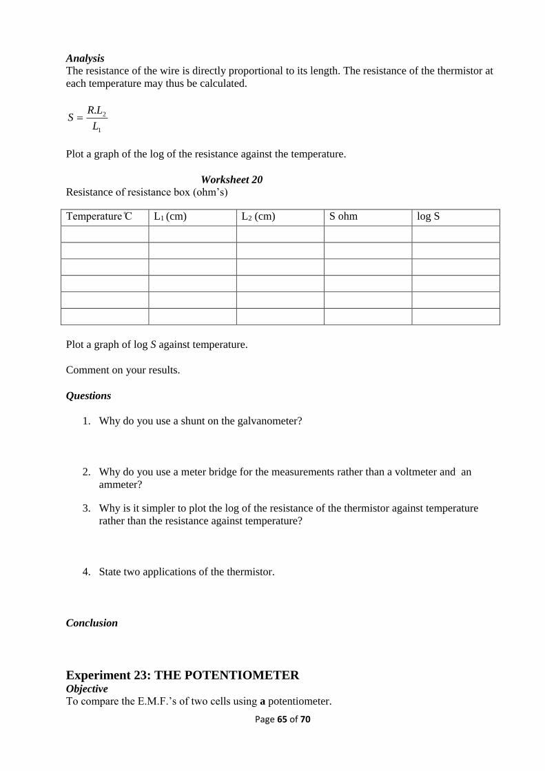
Page 65 of 70

Analysis

The resistance of the wire is directly proportional to its length. The resistance of the thermistor at

each temperature may thus be calculated.

1

2.

L

LRS

Plot a graph of the log of the resistance against the temperature.

Worksheet 20

Resistance of resistance box (ohm’s)

Temperature ̊C L1 (cm) L2 (cm) S ohm log S

Plot a graph of log S against temperature.

Comment on your results.

Questions

1. Why do you use a shunt on the galvanometer?

2. Why do you use a meter bridge for the measurements rather than a voltmeter and an

ammeter?

3. Why is it simpler to plot the log of the resistance of the thermistor against temperature

rather than the resistance against temperature?

4. State two applications of the thermistor.

Conclusion

Experiment 23: THE POTENTIOMETER Objective

To compare the E.M.F.’s of two cells using a potentiometer.

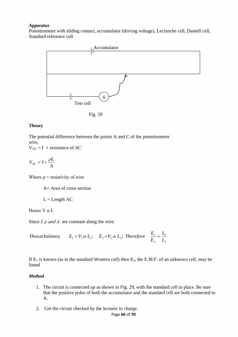
Page 66 of 70

Apparatus

Potentiometer with sliding contact, accumulator (driving voltage), Leclanche cell, Daniell cell,

Standard reference cell

Accumulator

Test cell

Fig. 29

Theory

The potential difference between the points A and C of the potentiometer

wire,

VAC = I × resistance of AC

A

LIVAC

Where ρ = resistivity of wire

A= Area of cross section

L = Length AC

Hence V α L

Since I, ρ and A are constant along the wire.

2

1

2

1222111 ;;,

L

L

E

EThereforeLVELVEbalanceatThus

If E1 is known (as in the standard Western cell) then E2, the E.M.F. of an unknown cell, may be

found

Method

1. The circuit is connected up as shown in Fig. 29, with the standard cell in place. Be sure

that the positive poles of both the accumulator and the standard cell are both connected to

A.

2. Get the circuit checked by the lecturer in charge.

G

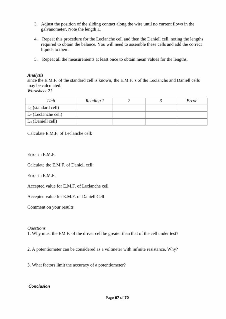
Page 67 of 70

3. Adjust the position of the sliding contact along the wire until no current flows in the

galvanometer. Note the length L.

4. Repeat this procedure for the Leclanche cell and then the Daniell cell, noting the lengths

required to obtain the balance. You will need to assemble these cells and add the correct

liquids to them.

5. Repeat all the measurements at least once to obtain mean values for the lengths.

Analysis

since the E.M.F. of the standard cell is known; the E.M.F.’s of the Leclanche and Daniell cells

may be calculated.

Worksheet 21

Unit Reading 1 2 3 Error

L1 (standard cell)

L2 (Leclanche cell)

L3 (Daniell cell)

Calculate E.M.F. of Leclanche cell:

Error in E.M.F.

Calculate the E.M.F. of Daniell cell:

Error in E.M.F.

Accepted value for E.M.F. of Leclanche cell

Accepted value for E.M.F. of Daniell Cell

Comment on your results

Questions

1. Why must the EM.F. of the driver cell be greater than that of the cell under test?

2. A potentiometer can be considered as a voltmeter with infinite resistance. Why?

3. What factors limit the accuracy of a potentiometer?

Conclusion

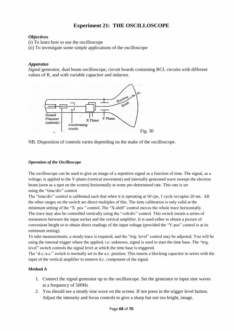
Page 68 of 70

Experiment 21: THE OSCILLOSCOPE

Objectives

(i) To learn how to use the oscilloscope

(ii) To investigate some simple applications of the oscilloscope

Apparatus

Signal generator, dual beam oscilloscope, circuit boards containing RCL circuits with different

values of R, and with variable capacitor and inductor.

Fig. 30

NB. Disposition of controls varies depending on the make of the oscilloscope.

Operation of the Oscilloscope

The oscilloscope can be used to give an image of a repetitive signal as a function of time. The signal, as a

voltage, is applied to the Y-plates (vertical movement) and internally generated wave sweeps the electron

beam (seen as a spot on the screen) horizontally at some pre-determined rate. This rate is set

using the “time/div” control.

The “time/div” control is calibrated such that when it is operating at 50 cps, 1 cycle occupies 20 ms. All

the other ranges on the switch are direct multiples of this. The time calibration is only valid at the

minimum setting of the “X pos ” control. The “X-shift” control moves the whole trace horizontally.

The trace may also be controlled vertically using the “volt/div” control. This switch inserts a series of

resistances between the input socket and the vertical amplifier. It is used either to obtain a picture of

convenient height or to obtain direct readings of the input voltage (provided the “Y-pos” control is at its

minimum setting).

To take measurements, a steady trace is required, and the “trig. level” control may be adjusted. You will be

using the internal trigger where the applied, i.e. unknown, signal is used to start the time base. The “trig.

level” switch controls the signal level at which the time base is triggered.

The “d.c./a.c.” switch is normally set to the a.c. position. This inserts a blocking capacitor in series with the

input of the vertical amplifier to remove d.c. component of the signal.

Method A

1. Connect the signal generator up to the oscilloscope. Set the generator to input sine waves

at a frequency of 500Hz

2. You should see a steady sine wave on the screen. If not press in the trigger level button.

Adjust the intensity and focus controls to give a sharp but not too bright, image.

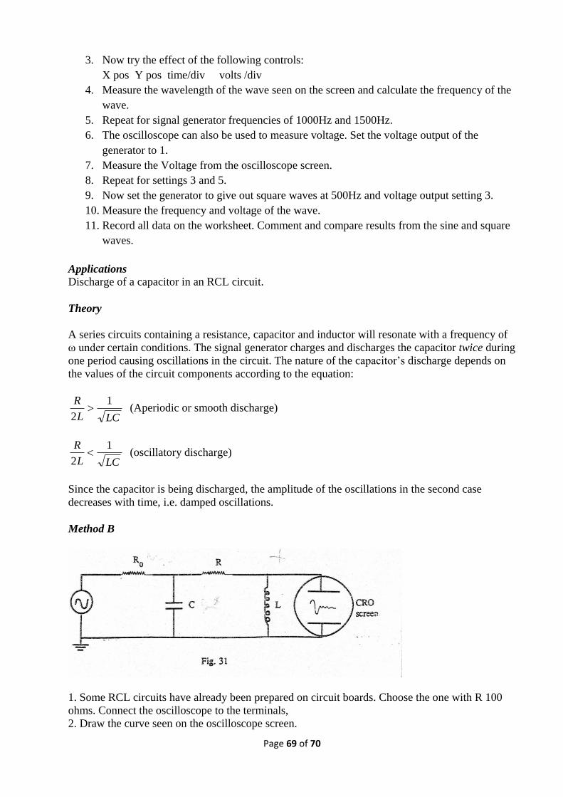
Page 69 of 70

3. Now try the effect of the following controls:

X pos Y pos time/div volts /div

4. Measure the wavelength of the wave seen on the screen and calculate the frequency of the

wave.

5. Repeat for signal generator frequencies of 1000Hz and 1500Hz.

6. The oscilloscope can also be used to measure voltage. Set the voltage output of the

generator to 1.

7. Measure the Voltage from the oscilloscope screen.

8. Repeat for settings 3 and 5.

9. Now set the generator to give out square waves at 500Hz and voltage output setting 3.

10. Measure the frequency and voltage of the wave.

11. Record all data on the worksheet. Comment and compare results from the sine and square

waves.

Applications

Discharge of a capacitor in an RCL circuit.

Theory

A series circuits containing a resistance, capacitor and inductor will resonate with a frequency of

ω under certain conditions. The signal generator charges and discharges the capacitor twice during

one period causing oscillations in the circuit. The nature of the capacitor’s discharge depends on

the values of the circuit components according to the equation:

LCL

R 1

2 (Aperiodic or smooth discharge)

LCL

R 1

2 (oscillatory discharge)

Since the capacitor is being discharged, the amplitude of the oscillations in the second case

decreases with time, i.e. damped oscillations.

Method B

1. Some RCL circuits have already been prepared on circuit boards. Choose the one with R 100

ohms. Connect the oscilloscope to the terminals,

2. Draw the curve seen on the oscilloscope screen.

Page 70 of 70

3. Repeat for R = 1000 ohm and 10,000 ohm (or 100,000 ohm). (Use appropriate circuit boards).

4. Investigate what happens to the curve on the oscilloscope screen when C and L are changed.

5. Fill in the data sheets.

Worksheet 22

A. Oscilloscope controls

Sine Wave

Generator

reqzeiwy Hz)

Length on

screen (cm)

Time/div

(secs) Time (secs Osilloscope freqency(Hz)

500

:

1000

1500

Voltage setting Height on screen (cm) Volts/div (volts) Voltage (volts)

1

3

5

Square wave

Generator

frequency (Hz)

Length on screen

(cm)

Time/div (secs) Time (sec) Oscilloscope

frequency (Hz)

500

Voltage setting Height on screen (cm) Volt/div (volts) Voltage (volts)

3

Comment on your results, comparing the two types of waves.

Discharge of a capacitor in an RCL circuit.

R= 10 ohms, C=4700pF, L=0.4H

Draw a diagram of what you see on the oscilloscope screen.

On a separate sheet of paper (to be handed in) draw the diagrams for R = 1000 ohms and R

=10,000 ohms. Also draw the diagrams obtained when C and L are varied. In each case say

whether the discharge is oscillatory or aperiodic. Is this borne out by theory? If not, why not?

The End

View publication statsView publication stats