Finite element modelling of electromagnetic waves in doubly and triply periodic structures

C. Mias, J. P. Webb and R. L. Ferrari

Abstract: A weighted residual finite element method (FEM) is employed to obtain the dispersion curves of two-dimensional (2D) doubly periodic and three-dimensional (3D) triply periodic structures (such as those employed in photonic band gap devices). The scalar and vector finite element formulations used in the computations are given. FEM results of 2D and 3D models are presented in a structured manner, which confirms the correct functioning of the finite element codes.

1 Introduction

Electromagnetic wave guidance by a spatially periodic structure is utilised by a wide variety of microwave and optical devices, the simplest of these being a closed corrugated waveguide. Such structures have the following properties: their eigenmodes (Floquet modes) (a) represent waves which have phase velocities varying from zero to infinity, (b) may exhibit photonic band-gaps (PBG), frequency bands in which the waves do not propagate. Because of (a) closed periodic structures are used as slow wave devices [ l ] allowing the interaction of the electro- magnetic field with an electron beam. The property (b) allows closed periodic structures to be used as filters or as reflectors of electromagnetic energy [2-61.

Present microfabrication technology allows optical frequency doubly periodic PBG structures to be made [7-121. Considerable effort is currently spent in fabricating triply periodic structures exhibiting PBG at optical frequencies [ 131. Photonic bandgap triply periodic struc- tures at microwave frequencies have already been fabri- cated [2, 141.

The fabrication of PBG structures is a time-consuming and costly process. Thus considerable attention has been devoted to the numerical modelling of candidate structures. Initially, all the numerical techniques were borrowed from the area of electronic band theory, applying the Korringa- Kohn-Rostoker method (essentially an integral equation method) [ 151, plane wave expansion methods [ 16, 171 and on shell methodologies [18, 191.

In 1994, the first research report on the electromagnetic modelling of doubly periodic structures by the transmis- sion line method (TLM), was published [20]. Reports followed applying the finite difference method [2 11, the finite difference time domain method [6, 221 and the

0 IEE, 1998 IEE Proceedings online no. 19990603 DOI: 10.1049/ip-opt: 19990603 Paper first received 28th July 1998, and in revised form 18th November 1998 C. Mias is with the Department of Electronic and Electrical Engineering, The Nottingham Trent University, Nottingham, NGl 4BU, UK J.P. Webb is with the Department of Electrical Engineering, McGill University, Montreal, H3A 2A7, Canada R.L. Ferrari is with the Engineering Department, Cambridge University, Trumpington Street, Cambridge CB2 lPZ, UK

IEE Proc.-Optoelectron.. Vol. 146, No. 2, April 1999

integral equation method [23]. Here, an alternative technique, the finite element method

(FEM) is employed to model both doubly and triply periodic structures. The FE programs described herein are based on 2D- and 3D-weighted residual formulations [24] employing scalar or vector finite elements. The FEM produces an eigenvalue matrix equation which is solved using a subspace iteration program [25] in conjunction with the Harwell subroutine library (ME27, ME28 Harwell subroutines). In all of the FE programs, the Floquet propagation vector p was specified and an appropriate number of corresponding normalised frequency eigenva- lues ko were computed. A time harmonic dependence e@* is assumed and for the purpose of verifying the codes the structures considered were lossless. A main advantage of the FEM is that it can easily model inhomogeneous materials bounded by curved surfaces and it avoids the staircasing error introduced in standard finite difference methods. The FE formulation for doubly periodic 2D and triply periodic 3D structures are presented in Sections 2 and 3, respectively. Section 4 contains the numerical results.

2 Two-dimensional doubly periodic structures

The FEM has already been used to model 2D closed singly periodic structures in electromagnetics [26], and for the dispersion analysis of doubly periodic structures in quan- tum mechanics [27] and acoustics [28]. An example of a 2D-closed doubly-periodic structure is illustrated in Fig. 6. The governing differential equation is the scalar Helmholtz equation:

(1) 1

P V. -V& + kiq4 = 0

where k, = o m . For the TE polarisation, 4 = Ey and the relative constituent parameters are p = p,., q = E,. For TM polarisation, 4 = Hy, p = E,, q = pr . The weighted residual formulation of the Helmholtz equation is given by:

111

k 5 6

1 Lx -Dx-

a

b

Fig. 1 3 0 structure a 2D structure b 3D structure

Unit cell of a doubly periodic 2 0 structure and a triply periodic

where A is the area of the periodic unit cell (Fig. la), and W is some arbitrary weighting function. From Green's theorem, eqn. 2 becomes:

(3)

where I' represents the perimeter of A. The axes of periodicity here are assumed to be orthogonal; there is no fundamental difficulty in treating the more general nonorthogonal case [29]. The application of eqn. 3 to 2D FEM nonperiodic configurations is standard [30] and, with suitable W, corresponds to a Rayleigh-Ritz variational treatment. However, with periodic boundaries the weighted residual route is not so straightforward. In nonperiodic cases the line integral in eqn. 3 is eliminated by constrain- ing the FEM trial functions 4 and weight functions W to vanish wherever the essential boundary condition 4 = 0 on r applies, while the natural condition a 4/ an = 0 requires no further action. Such steps are also taken here but do not account for the portions of r corresponding to the unit cell periodic closures. The latter are taken into account by employing Floquet's theorem. Thus, the degrees of free- dom (d.0.f.) of 4 associated with the nonoverlapping geometric parts (1-9) of the unit cell in Fig. l a are related as follows:

42 = 4 1 < x , 4 4 = 43ty, 4 6 = 455x3 47 = $ 5 4 ~ 9 48 = 4 5 t x t y (4)

where tx = e - J A D x , ty = e-Jp Y y and p = (Px, 0,) is the Floquet propagation vector. Cpgraining the weight func- tions with reciprocal factors (tx, ty) = (t; ', t; ') so that:

w' = w1&, w4 = w 3 t y > w6 = w55x3

w7 = w55,, w, = w5txzy ( 5 )

it follows that the line integral around r cancels because the normal derivative operator a l a n acts in opposite

112

directions on the first and second boundary of each periodic boundary pair. Thus, instead of eqn. 3, a residual:

applies to the whole region A . On an element-by-element basis one may write:

R = ~ R , = O e

(7)

Provided 4 and W are continuous across interelement boundaries, the line integrals due to such interfaces cancel and need not be included in eqn. 8. The fimction 4 is expanded within an element as:

where j ( e ) signifies nodes relating to the element e but counted on a global basis, while N," represents appropriate Lagrangian interpolation (shape) functions. The constant gje is introduced in order to impose the periodic constraints of eqn. 4, as shown later. In the preferred weighted residual option, the weight functions are selected from the inter- polation functions:

W f = ceNF (10)

where the C: are arbitrary constants. In this case the element residuals eqn. 8 may be represented in matrix form by:

Re = Seme - kiTe@, (1 1) where the column vectors Re and ae correspond to w,", 4jjce,, respectively. Assuming that p and q are constant within an element and given c:, gj", the local matrix elements:

(12) s cege se. = VNf - VN7dA I/

p A,

are readily evaluated. The constants C: and gje are specified so as to be consistent with the boundary and interface rules:

(a) If node l (e ) lies on an internal element boundary, cz, gee are chosen such that for any element e' sharing the node l , c; = cz, gg =gee, otherwise the continuity of Wand 4 is violated. A value of c;= 1, gg= 1 may conveniently be chosen for such nodes and also for nodes not shared by any other element.

(b) If l ( e ) is a node for which 4 is prescribed (4 = 0 here), c;=O is chosen to satisfy the requirement W=O at that node.

(c) If l(eo) = lo represents a node at ( X O , yo) on a periodic boundary (corresponding to geometric parts 1,3,5 in Fig. la), there is a node l ( e , ) = e l at (xo +Ox, yo), (xo, yo +Dy) or (xo + Dx, yo + D,), as appropriate, on the corresponding periodic cell closure (geometric parts 2,4,6,7,8 in Fig. la) . In that case, eqns. 5, 6 and 10 show th_at_choosing ce",o = 1, then either cg; = tx, or cgll = tY or cg; = tXty must be used in eqns. 12 and 13 relating to the second node. In a similar way, from eqn. 4, gg:= 1 and g;l' is set to t,, ty or t,tY,, respectively. Finally, the unknown variable $el is set equal to 4eo thereby eliminating it from the system of equations.

IEE Proc.-Optoelechon., Vol. 146, No. 2. March 1999

Note that it is a requirement in the above discussion that the finite element mesh at periodic boundary pairs is identical.

Summing the individual element residuals (eqn. 11) as in eqn. 7 now amounts to a procedure which, element by element and node by node, assembles the global matrix equation:

R = scf, - k , 2 ~ c f , = o (14)

where Q, is the column vector of the unknown nodal &- values, ready for treatment as an eigenequation to solve for ko and Q, given @ = (bx , by): In the formulation here we use 6: itself as the working variable whereas in [26] and [27] there is a slightly different but exactly equivalent approach employing the Floquet (or Bloch) periodic variable &p (r):

4 = 4p(r)e-'p.r (15)

In eqn. 14, the given propagation vector @ is built into S and T, whereas using the &p variable, extra arrays, them- selves independent of @, arise as coefficients in the corresponding matrix equation, which is now overtly quadratic in @.

3 Three-dimensional triply periodic structures

Triply periodic 3D structures in acoustics have been modelled using the scalar FEM method [28]. Here, vector finite elements, both hexahedral covariant projection elements [30-321 and tetrahedral vector elements [33], are employed to obtain the dispersion curves of triply periodic structures. Using vector elements, spurious solutions at nonzero frequencies are avoided (see, for example, [34-371 where some examples of the convergence of the FEM are also presented).

Note that singly periodic 3D structures have previously been analysed by the FEM [38] using a penalty function method or the transverse magnetic-field component method. Edge element results were also obtained [39] (after the application of Floquet's theorem was introduced in a FEM analysis of propagation in a circularly symmetric periodic waveguide [40]). Here, the vector wave equation:

V x -V x F - kiqF = 0

is employed, where p = p,, q = E, for F = E and p = e,, q = p, for F = H. Taking the scalar product of eqn. 16 with an arbitrary vector weight function W, integrating over the 3D periodic unit-cell problem region l2 and applying the vector form of Green's theorem gives the weighted resi- dual:

(16) 1

P

R = IQ[(V x W ) - c V x F) - k b W y F ] d R (17)

The Floquet propagation vector is now @ = ( f i x , by, Bz). Its three components correspond to the three periodicities Dx, D,,, D, , for simplicity assumed orthogonal, respectively. The FE mesh at periodic boundary pairs must be made identical so that the tangential field components there can be linked via Floquet's theorem. The unit cell is divided into 27 nonoverlapping geometric parts (Fig. 1 b). The 27th part represents the unit cell's inner volume region. The

IEE Proc.-Optoelectron., Vol. 146, No. 2, April 1999

d.0.f. associated with such parts are related (by Floquet's theorem) as follows:

Ft ,2 = F t , l t x $ Ft.4 = Ft ,35y1 ' t , 6 = ' t , 5 t z , Ft.10 = F t , 7 1 x l y

(18)

and so on. Furthermore, (,= e-JprDr, Cy = e -JpvDJ , 5, = e-JpZDz. Once again, in order to give a useful expression for the weighted residual, the second integral term in the weak- form residual (eqn. 17) now a surface integral needs to be eliminated. The action required for surfaces representing electric/magnetic walls is standard [4 11. Such action still leaves the parts of the periodic planes not constrained in the standard fashion unaccounted for. The procedure adopted mirrors that used in the 2D doubly periodic scalar variable case (Section 2); the vector weight functions W on the periodic c losges are chosen with reciprocal exponential factors (tx, tY, tZ) = (5, I , 5; I , 5, ') such that, corresponding to eqn. 18:

and so on. Then, because of the equal and opposite normal vectors n, as appearing in eqn. 17, the parts of the surface integral, corresponding to a pair of unit-cell periodic closures, cancel. Thus, the surface integral in eqn. 17 is eliminated and the final weighted residual equation becomes:

R = IQ[(. x w ) - c V x F) - k;W-qF]dQ = 0 (20)

The setting up of a finite element matrix eigenequation follows the same pattern as for the 2D scalar case in Section 2. The vector variable F is expanded within a finite element e as:

where r is the position vector, zj" are the vector interpola- tion functions (written out explicitly, in the case of tetra- hedral edge elements, in [42]) and Fj are the associated scalar degrees of freedom. The weight functions for any given element e become:

Wr(r) = crz; (22)

Here, c:, gi" are constants as in Section 2. If z: corresponds to an element edge or face in an F x n = 0 constrained surface, cf must be set to zero. Otherwise, if e has no edge or face lying in one of the periodic unit-cell boundaries, all c:, gj" are chosen to be unity, so as to maintain tangential continuity of W and F between finite elements. When z: does correspond to a periodic boundary, for each member of a periodic pair, say, the geometric parts 1 and 2 in Fig. 1 b, the cf, g: of part 1, say CO", g& are set to unity and cf, ge correponding to part 2 are set to tX, tx, respectively, and so on. Now corresponding to eqn. 11, there is:

It, = S,F, - kiT,F, (23)

where Fe is the column vector of the element degrees of freedom and:

113

where p and q are constant within an element. Eqn. 7 remains valid for the vector element residuals (eqn. 23), thus a global matrix equation:

R = SF - ~ ; T F = o (26)

may be assembled, using eqns. 23-25, by choosing the values of the coefficients c:, g: based on the degrees of freedom within elements then summing Re in a procedure similar to that in Section 2. As in the scalar case, the Floquet periodic vector variable Fp , where:

p = F ,-jP.r

may be used as an alternative working variable, avoiding building f3 into the assembled matrices, but at the expense of introducing further matrices into the equivalent of eqn. 26.

P (27)

4 Numerical results

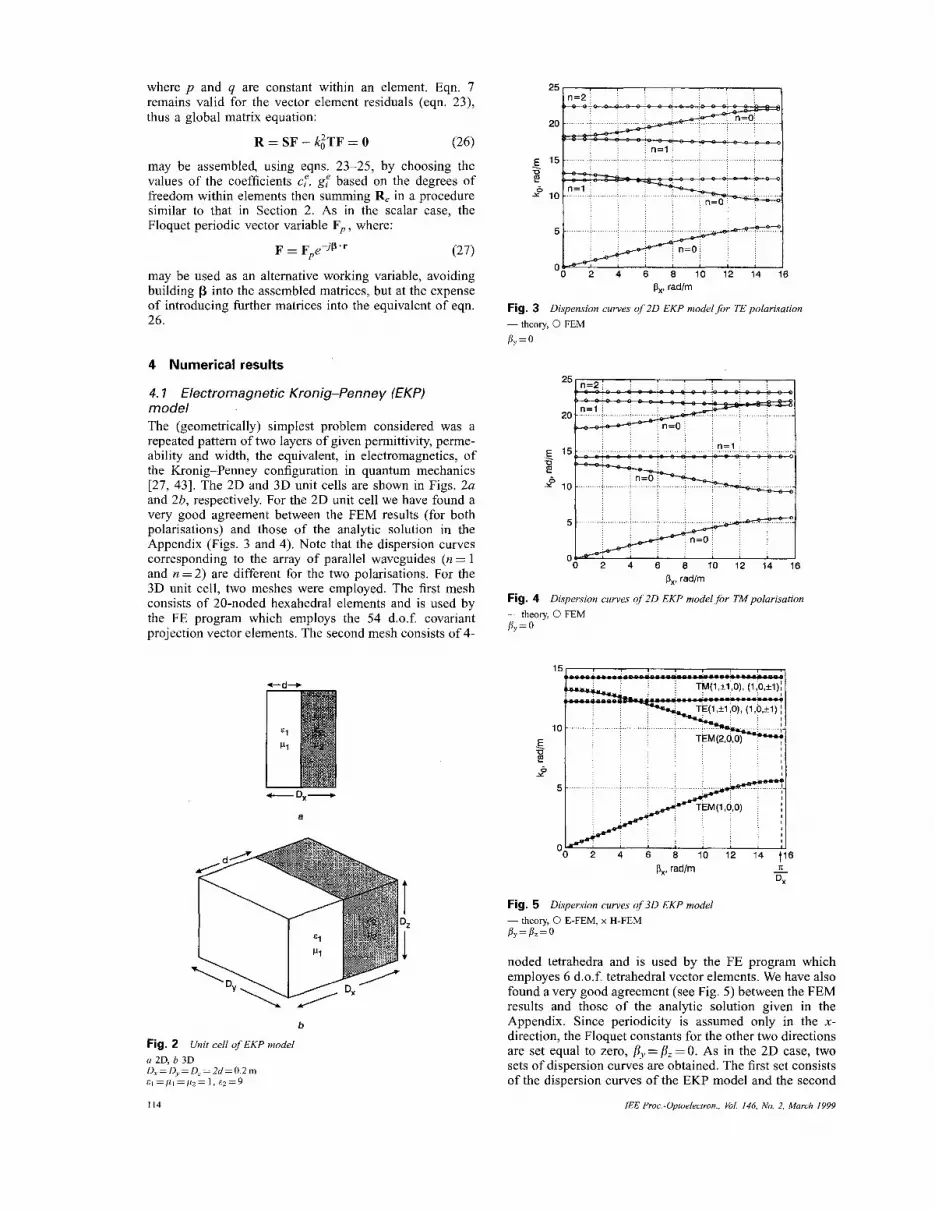
4. I Electromagnetic Kronig-Penney (EKP) model The (geometrically) simplest problem considered was a repeated pattern of two layers of given permittivity, perme- ability and width, the equivalent, in electromagnetics, of the Kronig-Penney configuration in quantum mechanics [27, 431. The 2D and 3D unit cells are shown in Figs. 2a and 2b, respectively. For the 2D unit cell we have found a very good agreement between the FEM results (for both polarisations) and those of the analytic solution in the Appendix (Figs. 3 and 4). Note that the dispersion curves corresponding to the array of parallel waveguides (n = 1 and n = 2) are different for the two polarisations. For the 3D unit cell, two meshes were employed. The first mesh consists of 20-noded hexahedral elements and is used by the FE program which employs the 54 d.0.f. covariant projection vector elements. The second mesh consists of 4-

b

Fig. 2 a 2D, b 3D 0, = Dy = 0, = 2d = 0.2 m

Unit cell of EKP model

E , = p , = pz = 1, 62 = 9

1 I4

25 n=2 I

20

E 15 3 c!

ro 10

5

'0 2 4 6 8 10 12 14 16 px, radlm

Fig. 3 - theory, 0 FEM

Dispension curves of 2 0 EKP model for TE polarisation

B,=O

25

20

a c!

y 10 0

5

0 0 2 4 6 8 10 12 14 16

U c!

y 10 0

5

0 0 2 4 6 8 10 12 14 16

Px, radlm

Fig. 4 - theory, 0 FEM

Dispersion curves of 2D EKP modelfor TMpolarisation

P,=O

15

10 E a c! 9

5

. . . . . . .. , .. .. ,, .. . . .. . . ,. . . . .. . . . . . . .

set consists of the dispersion curves of an array of parallel plane waveguides (a detailed explanation is given in the Appendix). Note that the second set of curves contains both, the TE and TM dispersion curves. This result could not have been obtained using a deficient 3D code. The incremental step between succeeding calculation points was Abx = 0.025nJDx (radm.)

4.2 Doubly periodic array of metal rods Subsequently, a doubly periodic array of infinitely long and perfectly conducting metal rods was considered. The 2D and 3D geometry of the structure's unit cell is presented in Fig. 6. The 3D FE mesh consisted of 6 d.0.f. tetrahedral vector elements. The period along the z-direction can be of any length. The Floquet constant pz was set to zero. Although one can solve separately for the TE and the TM polarisation in the 2D models, in 3D all three Cartesian components of either E or H, which contain both polarisa- tions, must be solved for simultaneously. The dispersion

Fig. 6 Doubly periodic array of infinitely long (in z-direction) and pefectly conducting metal rods showing the unit cells of the 2 0 and 3D model --_ unit cells D,=1.6m, Dy=1.4m, w=0.7m,D2=0.1m

Y

'0 0.1 0.2 03 0.4 0.5 0.6 0.7 08 0.9 1.0 q, r a d h

Fig. 7 Dispersion curves for TE and TM modes of doubly periodic array of metal rods obtained from both 2 0 and 3 0 models - TE (2D-FEM) - -TM (2D-FEM) 0 (3D-FEM using E-vanable) (A2 by) = 4 @IDx. 0 5 xIDy). /r, = 0

IEE Proc -0ptoelectron , El 146, No 2, April 1999

Y

-

0.167 0.333 0.500 0.667 0.833

Fig. 8 Relative magnitude o f fe ld distribution JEJ o f f r s t TE Floquet mode of doubly periodic array of pefectly conducting rods for (px, &) = 0.4 (xJDx, 0.5 n/DJ radJm Results from FE program of 2D doubly periodic model using 8-noded isopara- metric quadrilateral elements (upper), and from FE program of 3D triply periodic model using 6 d.0.f. tetrahedral vector elements (lower) (8, = 0)

curves obtained by the FE program of the triply periodic 3D model agree well with the dispersion curves obtained by the FE program of the 2D model, Fi . 7. Some disagreement between the two results (for k j > 35 (rad/ m)2) is most probably due to an insufficient number of tetrahedral vector elements per wavelength. Other disper- sion curves, arising from setting pz=O, have not been encountered within the normalised frequency range shown in Fig. 7. Furthermore, Fig. 8 shows the magnitude of the component of the electric field for the first Floquet mode at (fix, p,) = 0.4 (z/Dx, 0.5n/D,). It was computed using both the 2D and the 3D FE programs. The results from the two programs are in very good agreement.

4.3 Doubly periodic array of holes The next model considered was a doubly periodic array of air holes of infinite depth drilled in a dielectric material. The dielectric material is lossless. The geometries of the 2D and the 3D unit cells are illustrated in Fig. 9. For the 3D unit cell, the period along the z-direction can be of any

115

b12 b12

Fig. 9 drilled in dielectric material ___ unit cell in 2D model and in 3D model DX=D," = 1 m, a = b= 0.25 m, E~ = p1 = p2 = 1, E~ = 13 (D.= 0.05 m)

Doubly periodic array of air holes of injnite depth (in z-direction)

9

8

7

6 N-

E

s! - 4 *o

3

2

1

' 0 1 2 3 4 5 6 7

a 5

Y

A B px+B,, rad/m

Fig. 10 Dispersion curves for TE and TM modes of doubly periodic array of air holes (drilled in dielectric material). obtained for both 2 0 and 3 0 models - TE (2D-FEM) -- TM(2D-FEM) 0 3D-FEM using E-vanable A -t B . 0 5 br 5 n/Dx, by = 0, pz= 0 B - t T bx=n/D,, O ~ / 3 y ~ ~ / D y bz=O

length and pz = 0. There is a very good agreement between the dispersion curves obtained by the FE program of the 3D model and those obtained by the FE program of the 2D model (Fig. 10). Other dispersion curves, arising from setting pz = 0, have not been encountered within the normalised frequency range shown in Fig. 10. It was found that, when two dispersion curves cross, as in Fig. 7, the program can still trace each individual curve, provided the starting vector for the subspace iterations is the previously computed eigenvector.

4.4 Having verified in a systematic approach that the triply periodic 3D FE program developed functions correctly, the triply periodic array of perfectly conducting metal cubes in Fig. 11 is considered. Also shown is its 3D unit cell. The dispersion curves are shown in Fig. 12. They were obtained

Triply periodic array of metal cubes

116

Fig. 11

kx Triply periodic array of perfectly conducting

unit cell D,=D,=Dz= lm w=OSm E l = p , = I

6

5

4 E a s ! 3 0 1

2

1

0

metal cubes and

1 2 3 4 5 6 7 8 9 10 t t t I n 2n 3x

px+py+pz, rad/m

Fig. 12 ing metal cubes (illustrated in Fig. I I )

~ E (covariant projection) ~~ H (covariant projection) 0 E (6 d.0.f. tetrahedra) x H (6 d.o.f. tetrahedra)

For A + B : 0 5 /i;i x/D,, & = O , bz=O For B - t r : px= n/Dx, 0 5 By 5 n/D,, bz = 0 For l- -t A : Pr=n/D,, by= n/Dy, 0 5 bz 5 n/D,

using either the electric E or the magnetic H field as the working variable. Two meshes were employed. The first mesh consisted of 448 hexahedral elements resulting in 10344 d.0.f. for E and 11112 d.0.f. for H. The second mesh consisted of 17920 tetrahedra sesulting in 20904 d.0.f. for E and 22056 d.0.f. for H. The incremental step between successive calculation points was n/ 10 raam for the 6 d.0.f. tetrahedra and n/20 radlm for the covariant projection elements. The accuracy of these results was recently confirmed by other authors [44] who compared their independently derived finite element results with those of Fig. 12, communicated to them privately. For most of their graphs, the two results are identical. Towards

Dispersion curves of triply periodic array of perfectly conduct-

IEE Proc.-Optoelecfron., Vol. 146, No. 2, March 1999

the higher values of ko the two results start to deviate, and they reach no more than 10% difference in value. Finally, note that the use of solvers (which fully exploit the sparsity of FE matrices) to solve the system of linear equations, arising during the solution of eqn. 26, results in low memory requirements (as was demonstrated in [36], for the case of inhomogeneously loaded cavity resonators).

5 Conclusions

We have reported the application of the FE method in calculat- ing the dispersion curves of 2D doubly periodic and 3D triply periodic structures. The scalar and vector FE formulations used in our programs have been described and, through numerical simulations, the correct functioning of the devel- oped FE programs in a systematic way has been demonstrated.

6 Acknowledgments

We thank Dr F. A. Fernandez and his team at University College London for providing the subspace iteration program. We also acknowledge the use of the Hanvell subroutine librarv. Hanvell Laboratorv. Oxfordshire, UK.

7

1

2

3 4

5

6

7

8

9

10

11

12

13

References

BEVENSEE, R. M.: ‘Electromagnetic slow wave systems’ (John Wiley, 1964) YABLONOVITCH, E.: ‘Photonic crystals’, Mod. Opt., 1994,41, (2), pp. 173-194 RUSSELL, P. St. J.: ‘Photonic band gaps’, Phys. World, 1992, pp. 3 7 4 2 CARROLL, J. E., ZHANG, L. M., and BRAY, M. E.: ‘A Bragg about lasers’, IEE Electron. Commun. 1, 1993, pp. 325-337 JOANNOPOULOS, J. D., MEADE, R. A., and WINN, J. N.,‘Photonic Crystals’ (Princeton University Press, 1995) MEKIS, A., CHEN, J. C., KURLAND, I., FAN, S., VILLENEUVE, I? R., and JOANNOPOULOS, J. D.: ‘High transmission through sharp bends in photonic crystal waveguides’, Phys. Rev. Lett., 1996, 77, (18), pp. 3787-3790 KRAUSS, T., SONG, Y. P., THOMS, S., WLLKINSON, C. D. W., and DE LA RUE, R. M.: ‘Fabrication of 2-D photonic bandgap structures GaAdAIGaAs’, Electron. Lett., 1994, 30, (17), pp. 1444-1446 KRAUSS, T., DE LA RUE, R. M., and BRAND, S.: Two dimensional photonic-bandgap structures operating at near infrared wavelengths’, Nature, 1996,383, pp. 699-702 HAMANO, T., HIRAYAMA, H., and AOYAGT, Y.: ‘New technique for fabrication of two-dimensional photonic bandgap crystals by selective epitaxy’, Jpn. 1 Appl. Phys., Pt. Il, 1997, 36, (3A), pp. 286-288 BABA, T., and MATSUZAKI, T.: ‘Fabrication and photoluminescence studies of GalnAsP/InP 2-dimensional photonic crystals’, Jpn. 1 Appl. Phys., Pt. I, 1996, 35, (2B), pp. 1348-1352 BIRNER, A., GRUNING, U,, OTTOW, S., SCHNEIDER, A., MULLER, F., LEHMANN, V, FOLL, H., GOSELE, U,: ‘Macrophorous silicon: a two-dimensional photonic bandgap material suitable for the near-infrared spectral range’, P h j ~ Stat. Solidi A: Appl. Res., 1998,165, (I), pp. 11 1-1 17 BERGER, V., GAUTHIER-LAFAYE, O., and COSTARD, E.: ‘Fabrica- tion of a 2D photonic bandgap by a holographic method’, Electron. Lett., 1997, 33, (5), pp. 425426 McINTOSH, K. A., MAHONEY, L. J., MOLVAR, K. M., McMAHON, 0. B., VERGHESE, S., ROTHSCHILD, M., and BROWN, E. R.: Three-dimensional metallodielectric photonic crystals exhibiting reso-

nant infrared stop bands’, Appl. Phys. Lett., 1997, 70, (22), pp. 2937- 2939

14 SHEPHERD, T. J., BREWITT-TAYLOR, C. R., DIMOND, P., FIXTER, G., LAIGHT, A., LEDERER, P., ROBERTS, P. J., TAPSTER, P. R., and YOUNGS, I. J.: ‘3D microwave photonic crystals: novel fabrication and structures’, Electron. Lett., 1998, 34, (8), pp. 787-789

15 WANG, X., ZHANG, X. G., YU, Q., and HARMON, B. N.: ‘Multiple- ‘ scattering theory for electromagnetic waves’, Phys. Rev. B, 1993,47, (8),

pp. 41614167 16 MEADE, R. D., RAPPE, A. M., BROMMER, K. D., and JOANNO-

POULOS, J. D.: ‘Accurate theoretical analysis of photonic band-gap materials’, Phys. Review B, 1993,48, (1 I), pp. 8434-8437

17 HAUS, J. W.: ‘A brief review of theoretical results for photonic band structures’, Mod. Opt., 1994, 41, (2), pp. 195-207

18 PENDRY, J. B.: ‘Photonic band structures’, 1 Mod. Opt., 1994, 41, (2), pp. 209-229

19 SIGALAS, M. M., SOUKOULIS, C. M., CHAN, C. T., and HO, K. M.: Electromagnetic-wave propagation through dispersive and absorptive

photonic-bandgap materials, Phys. Rev. B, 1994, 49, (16), pp. 11080- 11087

.lEE ~Proc.-Optoelectron., ‘Vol. 146, No. 2, April 1999

20 ROBERTSON, W. M., BOOTHROYD, S. A., and CHAN, L.: ‘Photonic band structure calculations using a two-dimensional electromagnetic simulator’, Mod. Opt., 1994, 41, (2), pp. 285-293

21 YANG, H. Y. D.: ‘Photonic band structures for a class of 2D periodic dielectric materials’, IEEE MTT international symposium 1996 , San Francisco, USA, pp. 883-886

22 CHAN, C. T., YU, Q. L., and HO, K. M.: ‘Order-n spectral method for electromagnetic waves’, Phys. Rev. B, 1995, 51, (23), pp. 16635-16642

23 YANG, H. Y. D.: ‘3-D integral equation analysis of guided and leaky waves on a thin-film structure with 2-D material gratings’, IEEE MTT international symposium 1996 , San Francisco, USA, pp. 723-726

24 MIAS, C.: ‘Finite element modelling of the electromagnetic behaviour of spatially periodic structures’. 1995 PhD dissertation, Engineering Department, Cambridge University

25 FERNANDEZ, F. A., DAVIES, J. B., ZHU, S., and LU, Y.: ‘Sparse matrix eigenvalue solver for finite element solution of dielectric wave- guides’, Electron. Lett., 1991, 27, (20), pp. 1824-1826

26 FERRARI, R. L.: ‘Finite element solution oftime-harmonic modal fields in periodic structures’, Electron. Lett., 1991, 27, (I), pp. 33-34

27 FERRARI, R. L.: ‘Electronic band-structure for 2-dimensional periodic lattice quantum configurations by the finite element method’, Int. 1 Numer: Model. Electron. Netw.. Devices, Fields, 1993, 6, (4), pp. 283- 297

28 LANGLET, P., HENNION, A. C. H., and DECARPIGNY, J. N.: ‘Analysis of the propagation of plane acoustic waves in passive periodic materials using the finite element method’, 1 Acoust. Soc. Am., 1995,98, (S), Pt. 11, pp. 2792-2800

29 MIAS, C., WEBB, J. I?, and FERRARI, R. L.: ‘Finite element analysis of electromagnetic plane wave scattering from an infinite doubly periodic structure’, COMPEL, 1994, 13, (A), pp. 393-398

30 SILVESTER, P. P., and FERRARI, R. L.: , ‘Finite elements for electrical engineers’ (Cambridge University Press, 1996) 3rd. edn.

31 CROWLEY, C. W., SILVESTER, P. P., and HURWITZ, H.: ‘Covariant projection elements for 3D vector field problems’, IEEE Trans. Magn., 1988, M-24, (I), pp. 397400

32 WEBB, J. P., and MINIOWITZ, R.: ‘Analysis of 3-D microwave resonators usinn covariant oroiection elements’. IEEE Trans. Microw.

33

34

35

36

37

38

39

40

41

42

43

44

45

~~~~~

Theory Tech:, 1591, MTT-i9,”(1 l), pp. 1895-1899 WEBB, J. P., and FORGHANI, B.: ‘Hierarchal Scalar and Vector Tetrahedra’, IEEE Trans. Magn., 1993, M-29, (2), pp. 1495-1498 ZHU, Z. L., DAVIES, J. B., and FERNANDEZ, F. A.: ‘3-D edge element analysis of dielectric loaded resonant cavities’, Int. 1 Numer: Model: Electron. Netw., Devices, Fields, 1994, 7, (I), pp. 3 5 4 1 WANG, S. J., and IDA, N.: ‘Curvilinear and higher order ‘edge’ finite elements in electromagnetic field computation’, IEEE Trans. Magn., 1993, M29, (2), pp. 1491-1494 GOLIAS, N., PAPAGIANNAKIS, A. G., and TSIBOUKIS, T.: ‘Efficient mode analysis with edge elements and 3 - 0 adaptive refinement, IEEE Trans. Microw. Theory Tech., 1994, MTT-42, (I), pp. 99-106 DILLON, B. M., LIU, P. T. S., and WEBB, J. P.: ‘Spurious modes in quadrilateral and triangular edge elements’, COMPEL, 1994, 13, (A), pp. 311-316 INOUE, K., HAYATA, K., and KOSHIBA, M.: ‘Finite-element solution of three-dimensional periodic waveguide problems’, Electron. Conzmun. Japan, 1989, 72, (8), Pt. 11, pp. 68-77 MIAS, C., and FERRARI, R. L.: ‘Closed singly periodic three dimen- sional waveguide analysis using vector finite elements’, Electron. Lett.,

DAVIES, B. J., FERNANDEZ, F. A., and PHILIPPOU, G. Y.: ‘Finite element analysis of all modes in cavities with circular symmetry’, IEEE Trans. Microw. Theory Tech., 1982, MTT-30, (1 I), pp. 1975-1980 FERRARI, R. L., and NAIDU, R. L.: ‘Finite element modelling of high- frequency electromagnetic problems with material discontinuities’, IEE Proc. A , 1990, 137, (6), pp. 313-320 WEBB, J. P.: ‘Edge elements and what they can do for you’, IEEE Trans. Magn., 1993, M-29, (2), pp. 1460-1465 NUSSBAUM, A.: ‘The Kronig-Penney approximation: may it rest in peace, IEEE Trans. Educ., 1986, E-29, (l), pp. 12-15 COCCIOLI, R., ITOH, T., and PELOSI, G.: ‘Electromagnetic character- ization of photonic crystals by fem’, XI RiNEm (1 Ith Italian National Meeting on Electromagnetism), 1996, Florence, Italy pp. 32 1-324 YEH, P., YAM\! A., and HONG, C. S.: ‘Electromagnetic propagation in periodic stratified media. I. General theory’, 1 Opt. Soc. Am., 1977, 67, (4), pp. 423438

1994,30, (22), pp. 1863-1865

8 Appendix

8.1 Analytic solution of eigenmodes in a stratified periodic medium The analytic solution of modes in a stratified periodic medium worked out here follows that given by Yeh et al. [45] but here a 3D periodic unit cell which is finite in all Dimensions (Fig. 2b) is considered. The governing equa- tion is eqn. 16 subject to Floquet constraint over the cell periodic faces. Since p and q are piecewise constant, the

117

vector P is required to be nondivergent while eqn. 16 reduces to:

Suppose p = (D.x, 0,O) is given; consider cases where F has no x-component, similar to TE and TM modes in a slab waveguide, however, noting that the other of the electro- magnetic vector pair, G say, may nevertheless possess an x-component. From eqn. 28 the remaining components Fy and F, decouple so that, from V . F = 0 , Fy must be independent of y and F, of z. Thus are obtained:

where the subscripts i = 1,2 signify variables representing the two piecewise uniform regions of the unit cell (Fig. 2b) and k:=piqiko2. Eqn. 29 is examined here subject to Floquet periodicity in D, and D, the treatment for eqn. 30 being similar. Applying a classical separation of the vari- ables gives:

FZi = (Ai exp(-jk~$)x) + Bi exp( jkz’x)) exp(-jkyy), i = 1 , 2

(31) (32) k$l2 + k,” = k,?

Because of the finite periodic unit cell assumed and in order to meet the Floquet periodicity condition in y:

(33)

where rn is a positive or negative integer (or zero) [Note: I]. To allow continuity across the 1,2 interface, the integer m has to be the same for both material regions. If the periodic cell extends over - d 5 x 5 0 (material 1) and

Note 1: In the independent treatment of eqn. 30 we should choose k, = 2nn/D,, in which case eqns. 3 1-33 have to be rewritten in terms of a corresponding kxl,z(z). Here we consider only cases m # 0, n = 0 or vice versa. The case m # 0, n # 0 did not arise within the range of the results presented here.

0 5 x 5 D, - d (material 2), the transverse field and Floquet periodicity conditions in x give equations:

which are sufficient to eliminate the arbitrary constants A 1,

B, , A2, B2 from eqn. 31 to yield, after some algebra, the dispersion relation;

cos p,D, = - +’& sin k,, d sin kx2(D, - d) 2 L,, P 2 k J

+ COS k,, d COS k,2(Dx - d ) (3 8)

The (ko , p,) eigensolutions represented by eqn. 38 are now examined, noting that the numerical eigensolver models dual E- and H-fields. Following practice for the numerical solver, px is considered as specified and ko eigenvalues sought, even though numerically eqn. 38 will inevitably be tackled the other way round. Cases m = 0, n = 0 corre- spond to purely transverse field vectors both F and G, however at ko values corresponding to some number 1 of periodic variations in x. These solutions are the transverse electromagnetic Kronig-Penney (EKP) modes, analogues of the one-dimensional quantum modes for electrons in a periodic potential, and may be labelled TEMloo. Because here the numerical solver returns identical eigenvalues for both Fy (x) and F, (x) (irrespective of the values Dy, 0,) each ko has a multiplicity of 2. If one or other of m and n (but not both) are nonzero, the parallel slab array modes returned by eqn. 38 may be identified with waves which would have arisen in the model extending infinitely in y and z however specifying either p =( f ix , f iy , 0) or (p,, 0, p,), with = kv = 2nm/Dy, (or pz = k, = 2nn/Dz as appro- priate). Evidently, considering finite periodicities in y and z , starting with (p,, 0, 0) can simulate propagation in the transversely infinite periodic sandwich which is oblique to the principal axis, the actual obliquity being determined by m and Dy (or n and 0,). Such modes, relating to a dual problem pair, may be labelled either TFLmo or TFlon, depending upon whether the solution refers to F, or Fy. The solver returns identical ko-values for each of the y-polarisation m = f Iml options, similarly for z- polarisation n = f In[; if Dy and D, are identical, these values are all the same and there is a fourfold multiplicity of ko-eigenvalues.

118 IEE Proc.-Optoelectron., Vol. 146, No. 2, March 1999