1

Finite element model of primary recrystallization in

polycrystalline aggregates using a level set framework

M Bernacki, H Resk, T Coupez and R E Logé

Centre de mise en forme des matériaux (CEMEF), Mines-Paristech, UMR CNRS

7635, BP 207, 06904 Sophia Antipolis Cedex, France

E-mail : Marc.Bernacki@mines-paristech.fr

Abstract

The paper describes a robust finite element model of interface motion in media with

multiple domains and junctions, as the case in polycrystalline materials. The adopted

level set framework describes each domain (grain) with a single level set function,

while avoiding the creation of overlap or vacuum between these domains. The finite

element mesh provides information on stored energies, calculated from a previous

deformation step. Nucleation and growth of new grains are modelled by inserting

additional level set functions around chosen nodes of the mesh. The kinetics and

topological evolutions induced by primary recrystallization are discussed from simple

test cases to more complex configurations and compared with the Johnson-Mehl-

Avrami-Kolmogorov (JMAK) theory.

1.Introduction

Recrystallization phenomena inevitably occur during thermal and mechanical processes and have a

major impact on the final in-use properties of metallic materials. Theories for recrystallization that

provide quantitatively correct predictions of crystallographic orientation and grain size distributions

have long been sought to fill a critical link in our ability to model material processing from start to

finish. To date, no such theory exists. The phenomena of recrystallization seem simple but their

mechanisms are not very well understood. Various features of the microstructure contribute to strain

energy, particularly defect populations and mismatches in lattice orientation at grain boundaries. On

the other hand, kinetics of grain or subgrain boundary motion is controlled not only by the boundary

features, but also by the interactions with other defect populations, like dislocations, cells walls,

particles or solute atoms. And this kinetics will itself affect the strain energy distribution. In summary,

the strain energy distribution factors heavily into the progression of change from old to new grain

arrangement, and itself is directly affected by that progression. This dynamic interplay underscores

why multiscale models are in principle needed to fully describe recrystallization phenomena in a

generic way [1-5].

Historical approaches of recrystallization were based on the Johnson-Mehl-Avrami-

Kolmogorov (JMAK) analytical model where equation (1) is used for the description of

recrystallization kinetics [6]:

),exp(1)( nbttX −−= (1)

where X is the recrystallized volume fraction, b a constant which depends on nucleation and growth

and n the Avrami exponent. If this equation is accurate for very simple loading histories and for some

materials, it is no longer the case for complex thermomechanical paths and/or complex

microstructures. Heterogeneous nucleation, non-homogeneous stored energy or anisotropic mobility of

grain boundaries are only a few of the phenomena to be considered in those cases, especially when the

prediction of grain size or crystallographic textures is of concern [1].

hal-0

0508

362,

ver

sion

1 -

30 M

ar 2

011

Author manuscript, published in "Modelling and Simulation in Materials Science and Engineering 17, 6 (2009) 22 pages - ArticleNumber: 064006"

DOI : 10.1088/0965-0393/17/6/064006

2

Considerable progress has been made in the numerical simulation of recrystallization

phenomena since the JMAK approach [7]. In the Microstructural Path Method (MPM) [8], the

microstructure was not only characterized by the volume fraction transformed but also by the

interfacial area between the recrystallized and unrecrystallized material. This allowed the analysis of

more complex grain geometries. Based on the work of Mahin [9], several groups have employed so-

called "geometric models" which have extended the analytical methods of the JMAK approach and the

MPM to incorporate computer simulation of grain structure evolution. The major disadvantage of

these approaches, however, is that they are "blind" approaches: grain growth without regard to the

stored energy field into which they intrude.

Monte Carlo (MC) and Cellular Automaton (CA) methods [10] are both probabilistic

techniques which deliver grain structures with kinetics: they are associated with 2D or 3D geometric

representations of the microstructure, discretized on a regular grid made of "cells" which are allocated

to the grains. Both methods have been successfully applied to recrystallization. The standard MC

method as derived from the Potts model (multistate Ising model) applies probabilistic rules at each cell

in each time step of the simulation. In this model, contrary to the vertex approach, the interfaces

between the grains are implicitly defined thanks to the membership of the cells to the various grains.

In this context, kinks or steps on the boundaries can execute random walks along the boundaries,

which allow changes in curvature to be communicated along the boundaries. The energy of the system

is defined by a Hamiltonian which sums the interfacial energy and the topological events appear in a

natural way by minimization of this energy, which represents an important advantage of this approach.

Moreover, the use of this model in 3D is relatively easy and efficient [11] and can be extended to the

recrystallization modelling [10]. However the comparison between MC results and experiments is not

straightforward [1]. Furthermore, the standard form of the model does not result in a linear

relationship between migration rate and stored energy and the absence of length and time scales can

complicate the comparison with the experimental results.

The CA method uses physically based rules to determine the propagation rate of a

transformation from one cell to a neighbouring cell [6], and can therefore be readily applied to the

microstructure change kinetics of a real system. In the case of recrystallization the switch rule is

simple: an unrecrystallized cell will switch to being recrystallized if one of its neighbours is

recrystallized. In the standard CA method, the state of all cells are simultaneously updated, which

provides efficiency but does not enable the curvature to be a driving force for grain boundary

migration [10]. Another major problem of the CA method to model recrystallization is the absence of

effective methods for the treatment of nucleation phenomena [1].

Several workers have preferred to define microstructures in terms of vertices. Historically, the

vertex models (also called "front tracking" models) described only the grain growth stage and not

primary recrystallization [12]. In these models the grain boundaries are considered as continuous

interfaces transported by a velocity defined thanks to the local curvature of the grains boundaries. The

main idea is to model the interfaces by a set of points and to move these points at each time increment

by using the velocity and the normal to the interfaces, which explains the term "front tracking".

Complex topological events such as the disappearance of grains or node dissociations are treated

thanks to a set of rules which is completed by a repositioning of the nodes. More recently, the vertex

model was extended in order to take into account both recrystallization and grain growth [13].

However, even if 2D results for isotropic grain growth seem to show a good agreement with the theory

[14], the difficulty remains the non-natural treatment of the topological events, mainly in 3D, where

the set of rules becomes very complex and numerically expensive [15]. Moreover, the nucleation

modelling remains an open problem.

Other methods suitable for the recrystallization modelling include the phase field model, as in

[16], and the level-set method, as in [4,5,17]. These two methods have many common points. They

have both the advantage of avoiding the difficult problem of tracking interfaces. More precisely, in

both approaches, artificial fields are introduced for the sole purpose of avoiding this difficulty. The

initial concept of the phase-field model was to describe the location of two phases by introducing an

order parameter (the phase field) which varies smoothly from one to zero (or minus one to one)

through a diffuse interface [18]. This concept has been extended to deal with more complex problems

involving more than two phases and for modelling microstructure evolution [19,20]. In the case of

polycrystalline microstructures, each grain orientation is used as a non-conserved order parameter

hal-0

0508

362,

ver

sion

1 -

30 M

ar 2

011

3

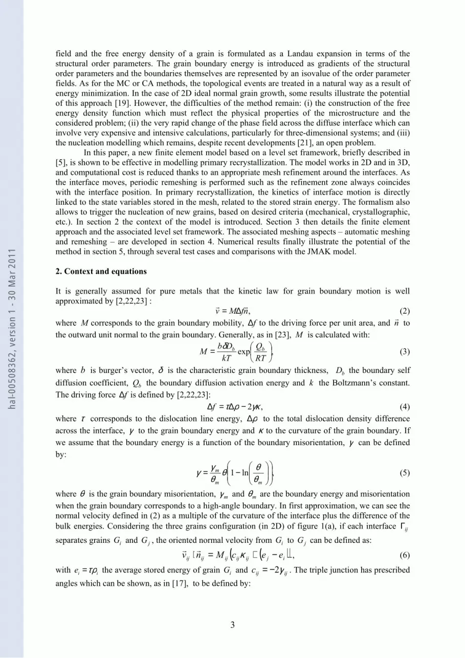
field and the free energy density of a grain is formulated as a Landau expansion in terms of the

structural order parameters. The grain boundary energy is introduced as gradients of the structural

order parameters and the boundaries themselves are represented by an isovalue of the order parameter

fields. As for the MC or CA methods, the topological events are treated in a natural way as a result of

energy minimization. In the case of 2D ideal normal grain growth, some results illustrate the potential

of this approach [19]. However, the difficulties of the method remain: (i) the construction of the free

energy density function which must reflect the physical properties of the microstructure and the

considered problem; (ii) the very rapid change of the phase field across the diffuse interface which can

involve very expensive and intensive calculations, particularly for three-dimensional systems; and (iii)

the nucleation modelling which remains, despite recent developments [21], an open problem.

In this paper, a new finite element model based on a level set framework, briefly described in

[5], is shown to be effective in modelling primary recrystallization. The model works in 2D and in 3D,

and computational cost is reduced thanks to an appropriate mesh refinement around the interfaces. As

the interface moves, periodic remeshing is performed such as the refinement zone always coincides

with the interface position. In primary recrystallization, the kinetics of interface motion is directly

linked to the state variables stored in the mesh, related to the stored strain energy. The formalism also

allows to trigger the nucleation of new grains, based on desired criteria (mechanical, crystallographic,

etc.). In section 2 the context of the model is introduced. Section 3 then details the finite element

approach and the associated level set framework. The associated meshing aspects – automatic meshing

and remeshing – are developed in section 4. Numerical results finally illustrate the potential of the

method in section 5, through several test cases and comparisons with the JMAK model.

2. Context and equations

It is generally assumed for pure metals that the kinetic law for grain boundary motion is well

approximated by [2,22,23] :

,nfMvrr

∆= (2)

where M corresponds to the grain boundary mobility, f∆ to the driving force per unit area, and nr to

the outward unit normal to the grain boundary. Generally, as in [23], M is calculated with:

,exp

=RT

Q

kT

DbM bbδ

(3)

where b is burger’s vector, δ is the characteristic grain boundary thickness, bD the boundary self

diffusion coefficient, bQ the boundary diffusion activation energy and k the Boltzmann’s constant.

The driving force f∆ is defined by [2,22,23]:

,2γκρτ −∆=∆f (4)

where τ corresponds to the dislocation line energy, ρ∆ to the total dislocation density difference

across the interface, γ to the grain boundary energy and κ to the curvature of the grain boundary. If

we assume that the boundary energy is a function of the boundary misorientation, γ can be defined

by:

,ln1

−=

mm

m

θθθ

θγγ (5)

where θ is the grain boundary misorientation, mγ and mθ are the boundary energy and misorientation

when the grain boundary corresponds to a high-angle boundary. In first approximation, we can see the

normal velocity defined in (2) as a multiple of the curvature of the interface plus the difference of the

bulk energies. Considering the three grains configuration (in 2D) of figure 1(a), if each interface ijΓ

separates grains iG and jG , the oriented normal velocity from iG to jG can be defined as:

( )( )ijijijijijij eecMnv −+=⋅ κrr, (6)

with ii

e τρ= the average stored energy of grain iG and ijijc γ2−= . The triple junction has prescribed

angles which can be shown, as in [17], to be defined by:

hal-0

0508

362,

ver

sion

1 -

30 M

ar 2

011

4

12

3

13

2

23

1 sinsinsin

ccc

ααα == , (7)

with iα the angle at the triple junction inside grain iG . The problem is complex, principally for the

treatment of the triple junction where, initially, the curvature is not defined. Moreover, even in the

simplified case where only bulk energies are considered, it has been shown that if no further

conditions on the motion are imposed, the solution is not unique [24-26]. In [26] it is proved, by

considering a particular energy functional, that if the energy of the interfaces are not null

( ( )ji, 0 ∀≠ijc ), the time decrease of this functional is equivalent to the condition defined by equation

(7). However if we consider only the bulk energy term of the velocity expression, the results are more

complex: uniqueness of the solution is not guaranteed. For example, figure 1(a) describes an initial

three grains configuration and figure 1(b) and figure 1(c) correspond to two solutions at t=1 for the

problem described by equation (6) and this particular geometry. In [26] the authors developed the

concept of "vanishing surface tension" solution (called VST solution) by considering the limit problem

defined by:

( ) ( ) 0. with ,ji, →∀−+=⋅ εκεijijijijijijij

eeMcMnvrr

(8)

Using various 2D tests cases and a perturbation analysis, they strongly suggest that the VST solution

corresponds to one of the solutions of the considered problem for 0=ε , while it corresponds to the

unique solution of the problem for .0→ε

(a)

(b) (c)

Figure 1. (a) Example of a triple junction configuration; two solutions at t=1 of this

configuration for the problem defined by equation (6): (b) the VST solution and (c)

another solution.

hal-0

0508

362,

ver

sion

1 -

30 M

ar 2

011

5

In this paper, a new algorithm is proposed to model the problem defined by equation (6), in

2D or in 3D, and for any polycrystalline microstructure configuration. The numerical approach is

detailed but the treatment of the curvature term at the multiple junction and the simulations with this

term will be discussed in a forthcoming publication. The presented approach is based on a level set

method [5,25,26], now commonly used to follow propagating fronts in various numerical models [27-

29]. In Ref. [25], the authors have extended the standard level set method to model the motion of

multiple junctions; the method is appropriate for the case of grain growth, i.e. with zero bulk energies.

Each region has its own private level set function, and this function moves each level set with a

normal velocity defined by the conditions at the nearest interface. A reassignment step is used to avoid

kinematic incompatibilities, i.e. the development of vacuum and overlapping regions. The present

model proposes a new formulation accounting for bulk stored energies as well as nucleation events,

and still avoiding the development of vacuum and overlapping regions.

3. Finite element model and level set framework

3.1. Introduction

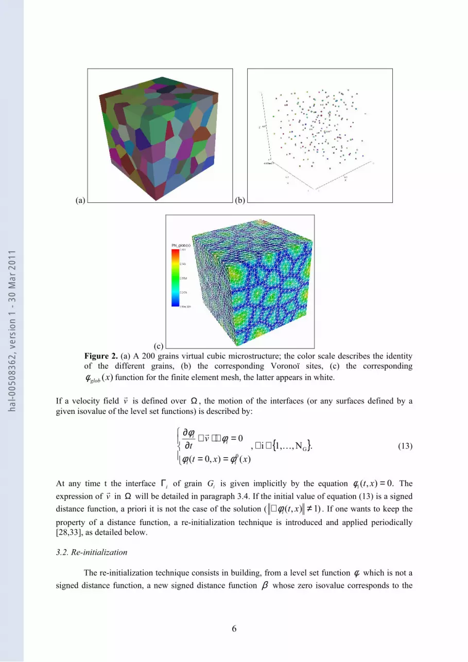
Figure 2 illustrates the procedure of creating a virtual microstructure, and the associated finite element

mesh. Figure 2(a) shows a two hundred grains digital sample [3,30-32], made of Voronoï cells, The

Voronoï tessellation is fully described by N seeds or Voronoï sites shown in Figure 2(b). Each site is

defines a Voronoï cell or grain Gi, which consists of all points closer to is than to any other site. The

conversion of the Voronoï tessellation into a finite element mesh is illustrated in Figure 2(c). The

location of the interfaces (grain boundaries) is defined implicitly using a level set framework. For each

individual cell or grain, a signed distance function ,φ defined over a domain Ω , gives at any point x

the distance to the grain boundary Γ . In turn, the interface Γ is then given by the level 0 of the

functionφ :

=Ω∈=ΓΩ∈Γ=0)( ,

),,()(

xx

xxdx

φφ

(9)

Assuming that the domain Ω contains GN grains, we have G

Ni1 , ≤≤i

φ with the sign convention

0≥iφ inside grain iG , and 0≤iφ outside grain iG . The procedure to evaluate these functions at all

nodes x of the finite element mesh goes through evaluating the functions

,ij ,Nji,1 ,2

1)( G ≠≤≤

⋅−= →

→→→

ji

iji

jiij

ss

xsssssxα (10)

which correspond to the signed distance of x to the bisector of the segment [ ]ji ss , . )(xiφ is then

defined as:

( ))(min)(

1

xx ij

ijNj

iG

αφ≠≤≤

= . (11)

One can also define a global unsigned distance function as:

.1),(max)( Giglob Nixx ≤≤= φφ

(12)

This function is positive everywhere and the zero value corresponds to the grain boundary network.

Figure 2(c) displays the function )(xglobφ corresponding to the microstructure of Figure 2(a) and

calculated at the nodal points of the finite element mesh (in white).

hal-0

0508

362,

ver

sion

1 -

30 M

ar 2

011

6

(a) (b)

(c)

Figure 2. (a) A 200 grains virtual cubic microstructure; the color scale describes the identity

of the different grains, (b) the corresponding Voronoï sites, (c) the corresponding

)(xglobφ function for the finite element mesh, the latter appears in white.

If a velocity field vr is defined over Ω , the motion of the interfaces (or any surfaces defined by a

given isovalue of the level set functions) is described by:

.N,1,i ,

)(),0(

0G

0

K

r

∈∀

==

=∇⋅+∂∂

xxt

vt

ii

ii

φφ

φφ (13)

At any time t the interface iΓ of grain i

G is given implicitly by the equation .0),( =xtiφ The

expression of vr in Ω will be detailed in paragraph 3.4. If the initial value of equation (13) is a signed

distance function, a priori it is not the case of the solution ( )1),( ≠∇ xtiφ . If one wants to keep the

property of a distance function, a re-initialization technique is introduced and applied periodically

[28,33], as detailed below.

3.2. Re-initialization

The re-initialization technique consists in building, from a level set function φ which is not a

signed distance function, a new signed distance function β whose zero isovalue corresponds to the

hal-0

0508

362,

ver

sion

1 -

30 M

ar 2

011

7

zero isovalue of φ . The most common method to re-initialize level set functions is to solve the

following Hamilton-Jacobi equation [28]:

==

=−∇+∂∂

),(),0(

0)1(

xtx

s

ii

iii

φτβ

βτβ

, with ).( ii signs β= (14)

In practice, equation (14) is solved periodically, typically every few time steps. Equation (14) can be

seen as a pure convective equation. Indeed, if we write i

iii sU

ββ

∇∇

=r

, it becomes:

==

=∇+∂∂

),(),0(

.

xtx

sU

ii

iiii

φτβ

βτβ r

(15)

To define the fictitious time τ , a stability condition is used: hU i =∆=∆ ττr

, where h corresponds

to the mesh size. Hence the fictitious time step is usually chosen as h .

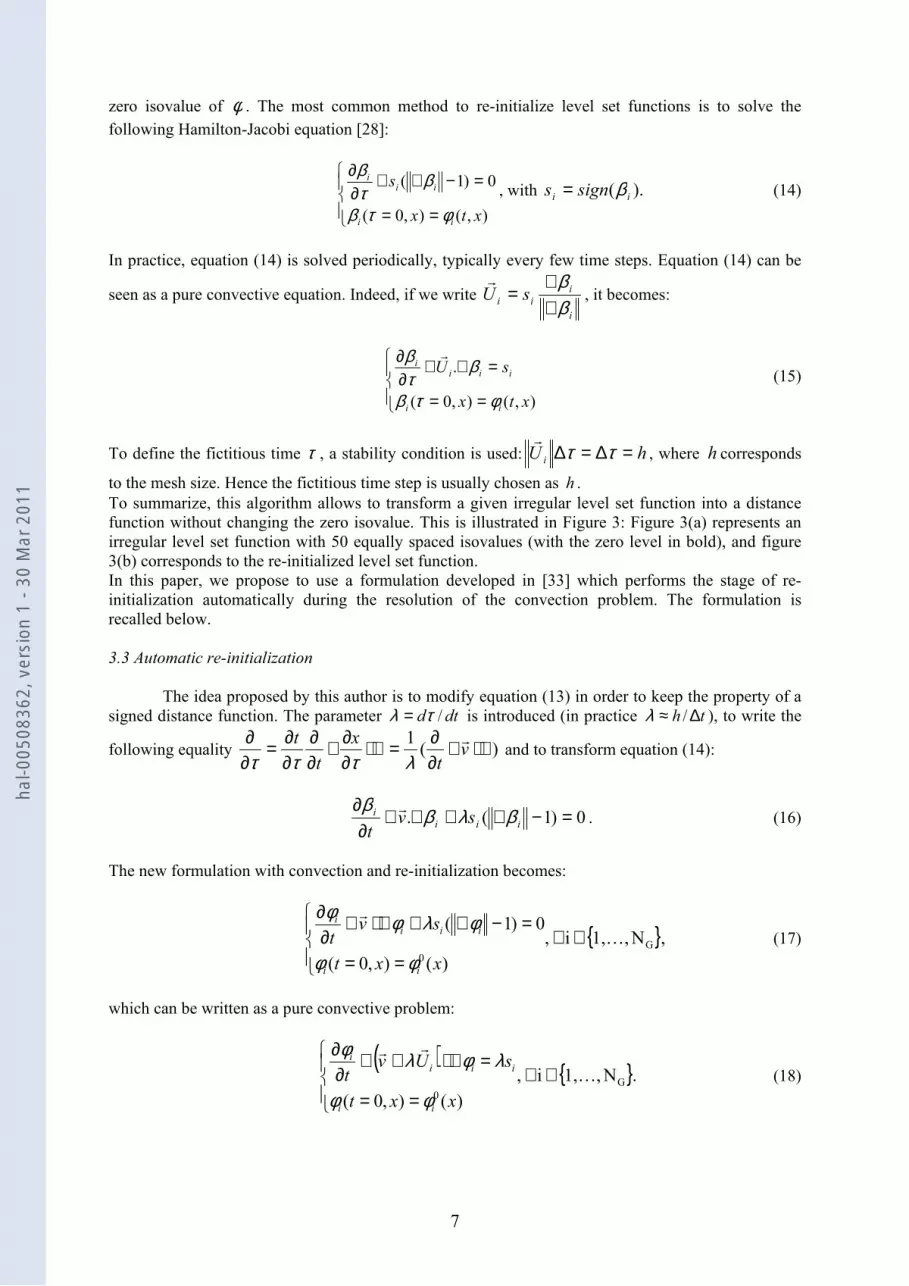
To summarize, this algorithm allows to transform a given irregular level set function into a distance

function without changing the zero isovalue. This is illustrated in Figure 3: Figure 3(a) represents an

irregular level set function with 50 equally spaced isovalues (with the zero level in bold), and figure

3(b) corresponds to the re-initialized level set function.

In this paper, we propose to use a formulation developed in [33] which performs the stage of re-

initialization automatically during the resolution of the convection problem. The formulation is

recalled below.

3.3 Automatic re-initialization

The idea proposed by this author is to modify equation (13) in order to keep the property of a

signed distance function. The parameter dtd /τλ = is introduced (in practice th ∆≈ /λ ), to write the

following equality )(1 ∇⋅+

∂∂=∇⋅

∂∂+

∂∂

∂∂=

∂∂

vt

x

t

t r

λτττ and to transform equation (14):

0)1(. =−∇+∇+∂

∂iii

i svt

βλββ r. (16)

The new formulation with convection and re-initialization becomes:

,N,1,i ,

)(),0(

0)1(G

0

K

r

∈∀

==

=−∇+∇⋅+∂∂

xxt

svt

ii

iiii

φφ

φλφφ (17)

which can be written as a pure convective problem:

( ) .N,1,i ,

)(),0(

G

0

K

rr

∈∀

==

=∇⋅++∂∂

xxt

sUvt

ii

iiii

φφ

λφλφ (18)

hal-0

0508

362,

ver

sion

1 -

30 M

ar 2

011

8

Remark 3.1: the function ( )ii ss φ= can take the values 1, -1 or 0 if .0=iφ To force equation (18) to

be conservative near the interface, the following expression is used:

. , if 0 , if i hss ii

i

ii ≈≤=>= εεφεφ

φφ

(19)

Remark 3.2: we refer the reader to [33] for a complete description of the method and its possible

extension (regular truncation of the level set functions).

(a)

(b)

Figure 3. (a) An irregular level set function with 50 equally spaced

isovalues and the zero level in bold, (b) the same representation after re-

initialization.

3.4 Expression of the velocity field

In the considered problem, the expression of the velocity field is of prime importance.

Several comments should be made:

• In order to avoid kinematic incompatibilities (overlapping or vacuum regions), it is necessary

to work with the same velocity field for all the level set functions. However the kinetic law

defined by equation (6) is built according to parameters which are specific to a single level set

function (grain): bulk stored energy difference across the boundary and unit normal

(neglecting the curvature term).

• The construction of the velocity field around multiple junctions is critical for a good

description of microstructure evolution. On a numerical point of view, it must be as regular as

possible.

• The expression (6) of the kinetic law implies a very accurate calculation of the normal to each

interface.

The proposed level set framework gives an answer to each of these comments. Concerning the

geometric parameters of the interface, it is well known that the level set method is perfectly adapted to

their accurate calculation [25]. Indeed, keeping in mind the sign convention described previously, if

the function iφ corresponds to the signed distance function of grain iG :

- The outward unit normal to any isovalue of iφ is defined by:

i

i

i

ii

n φφφ

φ∇−=

∇∇−=

=∇ 1

r. (20)

hal-0

0508

362,

ver

sion

1 -

30 M

ar 2

011

9

- The curvature of any isovalue of iφ is defined by:

iiii

n φκφ

∆=⋅−∇==∇ 1

r. (21)

Concerning the definition of the velocity field, it is useful to divide it in two parts: evvvrrr

+= κ . The

first part is related to the curvature of the boundary, while the second part refers to the bulk energy

term. First of all, some general remarks apply:

• At any time t a given point Ω∈M of coordinates x , is easily located, i.e. the grain to which

it belongs is easily identified. Indeed, as the set Gi Ni1 ,\ ≤≤ΓiG corresponds to a

partition of the domain Ω and with the sign convention described previously, the following

results are verified:

( ) ,0,i =⇔Γ∈ xtM iφ (22)

( ) ( ) .0, 0,\ ji ≤≠∀⇔>⇔∉⇔Γ∈≠

xtijxtGMGM ijij

i φφU (23)

• The description of an interface by a level set function remains a « fuzzy » description, which

means that the zero level of the level set function (the interface) does not inevitably

correspond to nodes of the mesh. The point M is located using the following relationship:

( ) ( )( ).,max,1

xtxtGM kNk

iiG

φφ≤≤

=⇔∈ (24)

A classical way to build the velocity field vr, for any node of the mesh, is as follows:

• Find i with ( ) ( )( )xtxt kNk

iG

,max,1

φφ≤≤

= .

• Compare ( )xti ,φ with a positive fixed parameter l which defines a length scale related to the

proximity of the node to the interface:

( ) ( )( ) ( )( ) ( ) ( ) ( )

−=⇒==⇒>

≠≤≤

xtneextfMxtvxtxtj

xtvxt

iijiijek

ikNk

j

i

G

,))(,,(,,max, with find

else 0,, If

1

rl

v

rvl

φφφφ

, (25)

with f a decreasing continuous function varying from 1 to 0 when ( )xti ,φ varies from 0 to l , and

ijM the mobility at the interface between grain i and grain j . The main disadvantage of this

approach lies in the management of multiple junctions: discontinuous velocity fields are generated,

which then lead to convergence problems in the resolution of the convection equation (18). We

propose another algorithm which considers, at any point x , all GN level set functions:

Find i with,

( ) ( )( ) ( ) ( ),,)(),(exp),(,max,1

1∑

≠=≤≤

−−=⇒=G

ij

G

N

j

jjijijekNk

i xtneextMxtvxtxtrr φαφφ (26)

with α a positive fixed parameter [5]. Expression (26) leads to a smoother velocity field and avoids

topological considerations, i.e. there is no need to identify neighbouring grains at point x . The difference between these two approaches (25) and (26) is illustrated in [5] for the triple junction case

of Figure 2, where the smoothing effect of (26) appears clearly when compared to (25). As stated

earlier, we do not detail here the method used to estimate the curvatures of the interfaces (defined by

the functions φ∆− ), in particular at multiple junctions where these curvatures are not defined. All

hal-0

0508

362,

ver

sion

1 -

30 M

ar 2

011

10

simulations described in section 5 will therefore involve only the stored energy part of the velocity, in

the context of primary recrystallization phenomena.

To summarize, the velocity field for primary recrystallization could be defined as follows:

( ) ( ) ( ) ( )∑∑= =

≠

∇−−==G G

ij

i

N

i

N

j

jijjijGe xteextMxtxtvxtv1 1

,)(),(exp,),(, φφαχrr, (27)

with ( )xtiG ,χ the characteristic function of the grain iG . To solve the problem defined by equations

(18) and (27), a finite element method based on the C++ library ‘Cimlib’ [33] is used, with

unstructured meshes and a stabilized P1 solver as SUPG or RFB method. The quality of the described

approach is strongly related to the accuracy of level set function calculations around the interfaces.

Indeed, a little disturbance of the levels around an interface leads to an error in the velocity estimation

and consequently in their own evolution. For a given computational cost, optimal accuracy is obtained

by using anisotropic meshes, with refinement close to the boundaries [3-5]. The technique to generate

anisotropic meshes adapted to a polycrystalline aggregate is presented in section 4.

3.5 Nucleation modelling and disappearance of grains

One of the prominent advantages in using front capturing methods for describing interface

motion is that there is no need for specific treatment when some regions (grains) disappear. Complex

topological evolutions are handled automatically. In a similar way, it is possible to introduce new

regions (grains), based on given criteria. For example, new grains can nucleate during primary

recrystallization, with an assumed low (often zero) stored energy.

A very simple method to create a nucleation site is to build a new signed distance function at a

desired time increment and at a given spatial position. For example, the new distance function can be

such that the boundary of the nucleus is spherical (3D) or circular (2D), centred around one node of

the mesh. Each nucleus, described by a new signed distance function, evolves subsequently according

to the principles described by equation (27). In particular, spontaneous growth occurs if a zero stored

energy is assumed inside the new region. Different rules have been developed for the time and space

nucleation laws. For example, at each time step of the simulation, a probabilistic or deterministic law

of nucleation can be used considering a set of possible nucleation sites. This set can be chosen in

different ways: (i) randomly in the domain Ω, (ii) only at grain boundaries, or (iii) according to

specific criteria based on crystallographic or mechanical variables calculated from a previous

deformation step of the polycrystal. This last method can be implemented for example when the

deformation step is modelled using crystal plasticity based constitutive laws [34].

Instead of nucleating new grains, topological evolutions can also lead to the disappearance of

grains. Level set methods automatically manage this type of event, but the numerical cost of the

simulation needs to be considered. It is clearly optimized by not taking into account the signed

distance functions which correspond to grains which have disappeared. Each level set function indeed

leads to a computational effort related to the evaluation of the velocity field according to the kinetic

law (27), the resolution of the convection equation together with the re-initialization (18), and the

remeshing operations around the interface every few increments. Hence, the problem solved evolves

dynamically during the calculation: for each time step, the signed distance functions which become

negative on the whole domain (disappearance of the corresponding grain) are excluded from the

calculation as well as the corresponding solvers.

Finally, at each time step, the following simplified algorithm concerning the nucleation and

the disappearance of grains is used:

- Evaluations of the maximum of each signed distance function and decision to exclude or not the

corresponding grain.

- Probabilistic or deterministic rule to choose the new nucleation sites (in agreement with the set

of possible sites, and ignoring the part of the domain which is already recrystallized).

- If at least one nucleation site is activated, the corresponding new signed distance functions are

built and the signed distance functions of the existing grains, which have an intersection with these

new grains, are accordingly modified.

hal-0

0508

362,

ver

sion

1 -

30 M

ar 2

011

11

- If at least one site is activated, an anisotropic remeshing operation is performed to obtain an

adapted anisotropic mesh around the new grain(s).

- Velocity field re-evaluated in the new topological configuration.

Tests cases illustrating this algorithm will be described in section 5.

4. Generation of finite element meshes

Figure 4(a) and figure 4(b) illustrate an adapted anisotropic mesh to the microstructure

detailed in Figure 2. The mesh is made of tetrahedral elements, whose size and shape are not

homogeneous. Anisotropic meshing is used along the interfaces of the grains, with a smaller size in the

direction perpendicular to the boundary.

(a) (b)

Figure 4. (a) An adapted anisotropic mesh to the microstructure detailed in Figure 2, (b) A

zoom on the surface of a triple junction

The technique used to generate such meshes lies in the definition of a metric. A metric is a symmetric

positive defined tensor which represents a local base modifying the way to compute a distance, such

that:

uuu t rrrM

M= , vuvu t rrrr

MM=>< , . (28)

If M is the identity tensor, the distance corresponds to the usual one in the Euclidian space. As M is a

symmetric positive defined tensor, it is diagonalizable in an orthonormal basis of eigenvectors and all

the eigenvalues are strictly positive. The metric M can be interpreted as a tensor whose eigenvalues

are linked to the mesh sizes, and whose eigenvectors define the direction in which these mesh sizes are

applied. Let us consider the simple case of figure 5 with only two grains (hence, one interface). The

direction of mesh refinement is the unit normal to the interface (vector φ∇ in figure 5). To specify the

mesh size in that direction, and its evolution in space, a characteristic thickness E is introduced (see

figure 5):

><

interface thefromfar 2/)(

interface near the2/)(

Ex

Ex

φφ

(29)

The mesh size takes a default value far from the interface, and is reduced in the direction

perpendicular to the interface when φ is reduced. A simple example is given by the following choice

of h :

+−

=⇒<

=⇒≥

m

hx

mE

mhhEx

hhEx

dd

d

)()1(2

2/)(

2/)(

φφ

φ (30)

hal-0

0508

362,

ver

sion

1 -

30 M

ar 2

011

12

At the interface the mesh size is reduced by a factor m with respect to the default value dh . This mesh

size increases with the distance φ to the default value dh at the distance 2/E . The unit normal to the

interface φ∇ , and the mesh size h defined by equation (30), lead to the following metric:

( )2

dhC

IdM +∇⊗∇= φφ with

<−

≥

=

2

11

20

22

Eif

hh

Eif

C

d

φ

φ (31)

with Id the identity tensor. This metric corresponds to an isotropic metric far from the interface (with

a mesh size equal to dh for all directions) and an anisotropic metric near the interface (with a mesh size

equal to h in the direction φ∇ and equal to dh for the other directions, i.e. in the plane normal to

φ∇ ).

When dealing with polycrystalline aggregates and multiple interfaces, the above strategy is

repeated for each grain. Combining all information, the number of refinement directions is then

evaluated at each node of the mesh. For the nodes at which:

( ) Gi NEx ≤≤≥ i1 ,2/φ , (32)

there is no direction of refinement, and the mesh size is isotropic with d

hh = . As the number of

directions of refinement increases, the mesh size is reduced in one or several directions. This happens

when there is more than one level set function for which 2/)( Exi

<φ , and when the corresponding

normal directions inr

calculated from equation (20) are not co-linear. A vector base is then

constructed from these normals, and refinement is performed along these independent vectors, which

are the eigenvectors of the metric. For each vector direction the mesh size is calculated from equation

(30), with )(xiφ being the signed distance function associated to the considered normal. At triple or

multiple junctions, the refinement may therefore become isotropic [35].

Anisotropic meshes are built using the MTC mesher-remesher developed by T. Coupez [36], it is

based on local mesh topology optimizations and works for all meshing applications from adaptive

remeshing to mesh generation by using a minimal volume principle. MTC improves a mesh topology

by considering the quality of the elements. The quality of an element is defined through a shape factor

that gives to equilateral triangles the highest quality, while the worst quality corresponds to a triangle

which degenerates into a segment (2D). In 3D, degeneration corresponds to a tetrahedron becoming a

surface. The element quality is normalised within an interval [0,1], and the shape factor is given by :

del

ecec

)()( 0= , (33)

where 0c is a normalised coefficient, e the volume of the element, ( )el the average length of the

element edges and d the space dimension. The shape factor takes into account the metric by

calculating volume and lengths according to equation (28). More details and illustrations of the

robustness and capability of this meshing technique for microstructure are described in [35].

hal-0

0508

362,

ver

sion

1 -

30 M

ar 2

011

13

Figure 5. A 2D grain boundary

5. Numerical results

As explained in section 3, the investigated applications study the motion of interfaces under

evr caused by the spatial distribution of bulk stored energy, in the context of primary recrystallization.

For the sake of simplicity, the mobility is assumed to be a constant equal to one, independent from the

crystallographic nature of the interfaces.

5.1 A three grains academic test case

The first test case, which is very classical and instructive [5,26], corresponds to the

configuration detailed in figure 1: three straight lines meeting at 120° in an unit square domain. We set

231 == ee and 12 =e , the challenge is to check the growth of grain 2 at the expense of grains 1 and

3. The time step considered is equal to 1.4e-3 s. Figure 6 shows the comparison, after 20 time steps, of

isovalues of 1φ using an adapted anisotropic mesh, with and without re-initialization. This comparison

illustrates the need for re-initialization steps of the level set functions to avoid the appearance of

discontinuities and associated numerical instabilities. Figure 7 shows the influence of the mesh on the

evolution of the distance functions. Lines indicate the 3105 −⋅± isovalues of the three distance

functions as a function of time, with an isotropic constant mesh size equal to 0.01 and with an adapted

anisotropic mesh close to the interfaces. In the latter case, automatic operations of anisotropic

remeshing are performed every five time steps in order to track the interfaces and the anisotropic

metric was built thanks to equation (31) with 015.0=E , 01.0=dh and 31 −= eh . The bad quality

of the results with an isotropic constant mesh underlines the need to work with very fine meshes near

the interfaces. Working with anisotropic meshes avoids the use of too fine elements far from the

interfaces. At the same time, it is seen in figure 7 that the non uniform anisotropic meshing procedure

leads to results which are in very good agreement with one of the exact solutions of this configuration

(see [26] or Figure 1), although this solution does not correspond to the VST solution. In terms of

accuracy, the 2L error between the exact and calculated function defined by ( )( )

≤≤≤≤xtk

NkTt Gend

,maxmax10

φ

is less than 3%. At the triple junction, the numerical treatment smoothes out the geometrical

discontinuity and, as underlined in the introduction, it is a way of imposing the uniqueness of the

solution, i.e. the configuration now evolves in a deterministic way. The numerical result is coherent

with the construction method of the velocity field, which allows (i) the accurate account of stored

energy differences across boundaries, and (ii) regularizing the discontinuous nature of the problem,

incompatible with the resolution of the convection equations given by (18). Obviously, the proposed

numerical strategy has a cost. On average, there is an approximate 10% difference in terms of number

of nodes or elements between the constant isotropic mesh and the non uniform anisotropic mesh.

Besides, the cost of successive remeshing operations (typically every 5 time steps) must be added to

hal-0

0508

362,

ver

sion

1 -

30 M

ar 2

011

14

this 10% difference. The simulation of Figure 7 was performed on 4 processors of an Opteron 2,4GHz

linux cluster in 7min20s with no remeshing, and in 18min32s with automatic anisotropic remeshing. It

is therefore important to find a good compromise between numerical cost and desired accuracy.

(a) (b)

Figure 6. Function 1φ after 20 time steps: (a) without re-initialization and (b) with re-initialization

5.2 A simple nucleation case

Figure 8 describes primary recrystallization in a unit square domain, starting from a 25 grains

aggregate. A uniform stored energy field is assumed initially, such that the recrystallization front is

convected everywhere with a velocity of the same magnitude. A random set of 1000 potential

nucleation sites is considered, and a probability of activation of 410.2 − is used at each time step of the

simulation. A new activated site is effectively taken into account if it does not belong to the existing

recrystallized volume fraction of the domain. Figure 10 illustrates the evolution of the recrystallized

volume fraction in white. The computation time is 30 minutes, performed on 8 processors of the

cluster described previously. Two hundred time steps were necessary to achieve 100% of

recrystallization with an automatic remeshing operation every five time steps and a time step equal to

8.6e-3 s. The anisotropic metric was calculated thanks to equation (31) with 04.0=E , 01.0=dh and

366.2 −= eh . The adopted level set framework, associated with the smoothed definition of the

interface velocities, and automatic adapted remeshing operations, is shown here to systematically

avoid kinematic incompatibilities (no development of vacuum or overlapping regions [23]).

Furthermore, the approach is very effective and natural in the modelling of nucleation events.

Comparison can be made with the JMAK theory [6,37,38] predicting the recrystallized volume

fraction X as a function of the annealing time t using equation (1). Assuming a two-dimensional

growth, the JMAK theory predicts n=3 for a low and constant nucleation rate. A linear kinetics refers

to a constant value of n; i.e. a linear JMAK plot displaying ln[-ln(1-X)] as a function of ln(t). A least-

square regression analysis on the numerical results of Figure 8 was performed, providing n=2.95.

Figure 9 describes the comparison between the numerical results and the curve obtained by the least-

square regression. This result is considered as a validation of our model in 2D.

hal-0

0508

362,

ver

sion

1 -

30 M

ar 2

011

15

(a) (e)

(b) (f)

(c) (g)

(d) (h)

Figure 7. 3105 −⋅± isovalues of the three distance functions with isotropic mesh after

(a) 0, (b) 120, (c) 300 and (d) 395 time steps and with adapted anisotropic mesh at the

grain boundaries (darker orange) after (e) 0, (f) 120, (g) 300 and (h) 395 time steps

hal-0

0508

362,

ver

sion

1 -

30 M

ar 2

011

16

(a) (b)

(c) (d)

(e) (f)

Figure 8. 2D simulation of primary recrystallization with an initial uniform stored energy.

Recrystallized part in white corresponding to volume fractions of (a) 1%, (b) 10%, (c) 40%, (d)

60%, (e) 90% and (f) 100%

hal-0

0508

362,

ver

sion

1 -

30 M

ar 2

011

17

Figure 9. JMAK approximation of the numerical recrystallization kinetics extracted

from Figure 8.

5.3 A case with stored energy

A ten grains microstructure in a unit cubic domain is considered, and mechanical testing is performed

using finite element simulations where each integration point of the mesh behaves as a single crystal

subjected to finite strain increments. The finite element approach is based on a mixed velocity–

pressure formulation with an enhanced (P1+/P1) four-node tetrahedral element [39]. Classical theory

of crystal plasticity [40,41] is considered, using a slightly modified version of the time integration

algorithm developed by Delannay et al. [34,42]. For computational efficiency, one computes rates of

lattice rotation and rates of dislocation slip in a decoupled way. The objective of the test case is to

analyze the spatial distribution of stored strain energy in a digital aggregate, subjected to large

deformations. A channel die test has been chosen. Slip is assumed to operate on the 12 111<110>

slip systems as is typically considered in fcc crystals at room temperature. For more details, see

[34,35]. A 20% reduction in height is applied, and the stored energy is computed from:

∫ ∇= dtvEn :rσδ . (34)

with δ the fraction of the strain energy which is stored in the material, considered constant in a first

approximation. The stored energy corresponds to defects (dislocations essentially), which represent

the driving force for subsequent static recrystallization when performing a heat treatment. Figure 10

illustrates the final stored energy distribution and the corresponding norm of the stored energy gradient

En∇ , together with the adaptive and anisotropic meshing used to model subsequent recrystallization

(see section 4 for the meshing strategy). More accurate measures of stored energy could be

implemented in the future, by directly relying on dislocation densities computed within the crystal

plasticity approach [43].

hal-0

0508

362,

ver

sion

1 -

30 M

ar 2

011

18

(a) (b)

(c) (d)

Figure 10. A 3D ten grains microstructure after plastic deformation: (a) external surface view of

stored energy, (b) corresponding norm of the stored energy gradient ( En∇ ), (c) volumetric view

of the stored energy with grain boundaries in black and (d) adaptive and anisotropic meshing in

white, grain boundaries in black.

The calculated stored energy field is used as an input to model recrystallization. A normalized average

of the stored energy is computed for each grain iG , and the distribution of En∇ is used to define the

set of potential nucleation sites. The selection of 1000 potential sites is done by choosing the nodes of

the mesh for which En∇ is the highest, while considering a safe distance between two neighbouring

nuclei equal to 3 times the average element size. As for the previous test case, a probability of

activation of 410.2 − is used at each time step, and 1200 time steps were simulated to achieve 100% of

recrystallization with a time step equal to 3e-3 s. Figure 11 illustrates the increasing recrystallized

volume fractions and the corresponding recrystallized front in blue. The simulation was performed in

6 hours on 16 processors of the cluster described previously and the final microstructure is made of 27

grains. The anisotropic metric was calculated thanks to equation (31) with 1.0=E for the anisotropic

thickness, 05.0=dh and 366.6 −= eh .

Comparisons with the JMAK theory were performed again, and are described in Figure 12. A first

simple comparison was done with no consideration of the stored energy field, with a random choice of

nucleation sites. A least-square regression analysis on the numerical results provided a JMAK

exponent n=3.91 (Figure 12(a)), while the theoretical value is n=4 in 3D. This result validates our

method in 3D. The second case, illustrated by Figure 12(b), corresponds to the numerical

recrystallization kinetics of the numerical simulation described by Figure 11. Interestingly, in this

case, a single value of n does not allow fitting the numerical results with sufficient accuracy. This

result must be placed in the context of repeated discussions in the literature on the reasons of

deviations from the standard JMAK theory. Heterogeneous distribution of stored energy [44], and,

spatial and time distribution of nuclei [45] can explained these deviations. These can be studied in

details with the present level-set model.

hal-0

0508

362,

ver

sion

1 -

30 M

ar 2

011

19

(a) (f)

(b) (g)

(c) (h)

(d) (i)

(e) (j)

Figure 11. 3D recrystallization with a non uniform initial stored energy field: external

surface view of the stored energy for recrystallized volume fractions of (a) 1%, (b) 15%,

(c) 58%, (d) 80%, (e) 95%, and corresponding recrystallized front in blue (f-j).

hal-0

0508

362,

ver

sion

1 -

30 M

ar 2

011

20

(a)

(b) Figure 12. JMAK approximations of the numerical recrystallization kinetics

extracted from Figure 11: (a) random choice of nucleation sites, low and

constant nucleation rate of 410.2 − ; (b) considering the non uniform stored

energy field and choosing nucleation sites at highest values of En∇ .

6. Conclusion It has been shown that a finite element model associated to a level set framework, using

adaptive anisotropic automatic remeshing, is a promising tool to describe primary recrystallization in a

polycrystalline material. A special smoothing algorithm is applied to the calculated velocity field,

which allows avoiding the appearance of vacuum or overlapping regions. The method allows efficient

and natural modelling of nucleation phenomena. On going work is currently addressing:

• The modelling of primary recrystallization with stored energy due to prior deformation steps,

modelled with crystal plasticity and 3D aggregates composed of a statistical number of grains.

• Comparisons with experiments and other models, like the Monte-Carlo or phase field

methods.

hal-0

0508

362,

ver

sion

1 -

30 M

ar 2

011

21

• The respective influences of initial microstructure topology, stored energy field, and local

crystallographic orientations, on the nucleation and growth kinetics involved in static

recrystallization.

• The extension of the method to model grain growth and discontinuous dynamic

recrystallization.

Acknowledgments

This work was supported by the European Communities under the contract no. NMP3-CT-2006-

017105 (DIGIMAT project).

The authors would like to thank the Professor J.-L. Chenot for his precious advice.

References

[1] Rollett A D 1997 Overview of modeling and simulation of recrystallization Progress in Mat. Sci. 42 79-

99

[2] Kugler G and Turk R 2006 Study of the influence of initial microstructure topology on the kinetics of

static recrystallization using a cellular automata model Comp. Mat. Sc. 37 284-291

[3] Bernacki M Chastel Y Digonnet H Resk H Coupez T and Logé R E 2007 Development of numerical

tools for the multiscale modelling of recrystallization in metals, based on a digital material framework

Comp. Met. in Mat. Sc. 7 142-149

[4] Logé R E Bernacki M Resk H Digonnet H and Coupez T 2007 Numerical modelling of plastic

deformation and subsequent recrystallization in polycristalline materials, based on a digital material

framework Recrystallization and Grain Growth III proceedings Korea 1133-1138

[5] Bernacki M Chastel Y Coupez T and Logé R E 2008 Level set method for the numerical modelling of

primary recrystallization in the polycrystalline materials Scripta. Mater. 58 1129-1132

[6] Raabe D 1999 Introduction of a scaleable 3D cellular automaton with a probabilistic switching rule for

the discrete mesoscale simulation of recrystallization phenomena Phil. Mag. A 79 2339-2358

[7] Miodownik M A 2002 A review of microstructural computer models used to simulate grain growth and

recrystallisation in aluminium alloys J. Light Metals 2 125-135

[8] Vandermeer R A and Rath B B 1989 Modeling recystallization kinetics in a deformed iron single

crystal Metall.Trans. 20A 391-401

[9] Mahin K W Hanson K and Morris J W 1980 Comparative analysis of the cellular and Johnson-Mehl

microstructures through computer simulation Acta Metall. 28 443-453

[10] Rollett A D and Raabe D 2001 A hybrid model for mesoscopic simulation of recrystallization Comp.

Mat. Sc. 21 69-78

[11] Hassold G N and Holm E A 1993 A fast serial algorithm for the finite temperature quenched Potts

model J. Comput. Phys. 7 97-107

[12] Nagai T Ohta S Kawasaki K and Okuzono T 1990 Computer simulation of cellular pattern growth in

two and three dimensions Phase Trans. 28 177-211

[13] Piekos K Tarasiuk J Wierzbanowski K and Bacroix B 2007 Generalized vertex model-Study of

Recrystallization in copper Recrystallization and grain growth III proceedings Korea 1157-1162

[14] Maurice C 2001 2- and 3-d curvature driven vertex simulations of grain growth Recrystallization and

grain growth proceedings Berlin 123-134

[15] Weygand D Brechet Y and Lepinoux J 2001 A vertex simulation of grain growth in 2D and 3D Adv.

Engng. Mater. 3 67-71

[16] Chen L Q 1995 A novel computer simulation technique for modeling grain growth Scripta Metall.

Mater. 32 115-120

[17] Zhao H K Chan T Merriman B and Osher S 1996 A variational level set approach to multiphase motion

J. Comp. Phys. 127 179-195

[18] Collins J B and Levine H 1985 Diffuse interface model of diffusion-limited crystal growth Phys. Rev.

B31 6119-6122

hal-0

0508

362,

ver

sion

1 -

30 M

ar 2

011

22

[19] Chen L Q 2002 Phase-field models for microstructure evolution Ann. Rev. Mater. Res. 32 113-140

[20] Karma A 2001 Phase-field formulation for quantitative modelling of alloy solidification Phys. Rev.

Letters 8711 115701

[21] Takaki T Yamanaka A Higa Y and Tomita Y 2008 Phase-field model during static recrystallization

based on crystal-plasticity theory J. Comp.-Aided Mater. Des. 14 75-84

[22] Humphreys F J and Haterly M 1995 Recrystallization and related annealing phenomena Oxford:

Pergamon Press

[23] Kugler G and Turk R 2004 Modeling the dynamic recrystallization under multi-stage hot deformation,

Acta Mat. 52 4659-4668

[24] Taylor J E 1995 The motion of multiple-phase junctions under prescribed phase-boundary velocities J.

Differ. Eq. 119 109-136

[25] Merriman B Bence J and Osher S J 1994 Motion of Multiple Junctions: A Level Set Approach J. Comp.

Phys. 112 334-363

[26] Reitich F and Soner H M 1996 Three-phase boundary motions under constant velocities. I: The

vanishing surface tension limit Proc. of the Roy. Soc. of Edinburgh 126A 837-865

[27] Sethian J A 1996 Level Set methods Cambridge University Press

[28] Osher S and Sethian J A 1988 Fronts propagating with curvature-dependent speed: Algorithms based on

Hamilton-Jacobi formulations J. Comp. Phys. 79 12-49

[29] Sussman M Smereka P and Osher S 1994 A Level Set Approach for Computing Solutions to

Incompressible Two-Phase Flow J. Comp. Phys. 114 146-159

[30] Dawson P R 2000 Computational crystal plasticity Int. J. Solids Struct. 37 115-130

[31] Dawson P R Miller M P Han T S and Bernier J 2005 An Accelerated Methodology for the Evaluation

of Critical Properties in Polyphase Alloys Metall. Mater. Trans. A 36 1627-1641

[32] Logé R E and Chastel Y 2006 Coupling the thermal and mechanical fields to metallurgical evolutions

within a finite element description of a forming process Comp. Meth. in Appl. Mech. and Eng. 195

6843-6857

[33] Coupez T 2007 Convection of local level set function for moving surfaces and interfaces in moving

flow NUNIFORM'07 proceedings Plenary lecture 61-66

[34] Logé R Bernacki M Resk H Delannay L Digonnet H Chastel Y and Coupez T 2008 Linking plastic

deformation to recrystallization in metals using digital microstructures Phil. Mag. 88 3691-3712

[35] Resk H Delannay L Bernacki M Coupez T and Logé R Adaptive mesh refinement and automatic

remeshing in crystal plasticity finite element simulations to appear in Modelling and Simulation in

Materials Science and Engineering

[36] Coupez T Digonnet H and Ducloux R 2000 Parallel meshing and remeshing by repartitioning Appl.

Math. Modeling 25 153-175

[37] Johnson W A and Mehl R F 1939 Reaction kinetics in processes of nucleation and growth Trans. Am.

Inst. Miner. Eng. 135 416-458

[38] Avrami M 1939 Kinetics of Phase Change. I. General Theory J. Chem. Phys. 7 1103-1112

[39] Mocellin K Fourment L Coupez T and Chenot J-L 2001 Toward large scale F.E. computation of hot

forging process using iterative solvers, parallel computation and multigrid algorithms Int. J. Num.

Methods. Eng. 2 473-488

[40] Kalidindi S R Bronkhorst C A and Anand L 1992 Crystallographic evolution in bulk deformation

processing of FCC metals J. Mech. Phys. Solids 40 537-569

[41] Marin E B and Dawson P R 1998 Elastoplastic finite element analyses of metal deformations using

polycrystal constitutive models Comput. Meth. Appl. Mech. Eng. 165 23-41

[42] Delannay L Jacques P J and Kalidindi S R 2006 Finite element modeling of crystal plasticity with

grains shaped as truncated octahedrons Int. J. Plast. 22 1879-1898

hal-0

0508

362,

ver

sion

1 -

30 M

ar 2

011

23

[43] Baudin T Etter A L Gerber P Samet A Penelle R and Rey C 2005 Influence of thermo-mechanical

treatments on the stored energy simulated by FEM for two low carbon steels Mater. Sci. Forum

495/497 1291-1296

[44] Oyarzabal M Matrinez-de-Guerenu A and Gutierrez I 2008 Effect of stored energy and recovery on the

overall recrystallization kinetics of a cold rolled low carbon steel Mater. Sci. Eng. A 485 200-209

[45] Liu F and Yang G 2007 Effects of anisotropic growth on the deviations from Johnson–Mehl–Avrami

kinetics Acta Mater. 55 1629-1639

hal-0

0508

362,

ver

sion

1 -

30 M

ar 2

011