Embed Size (px)
Citation preview

This electronic thesis or dissertation has beendownloaded from Explore Bristol Research,http://research-information.bristol.ac.uk
Author:Mckee, Jessica G
Title:Volumetric Imaging Using 2D Phased Arrays
General rightsAccess to the thesis is subject to the Creative Commons Attribution - NonCommercial-No Derivatives 4.0 International Public License. Acopy of this may be found at https://creativecommons.org/licenses/by-nc-nd/4.0/legalcode This license sets out your rights and therestrictions that apply to your access to the thesis so it is important you read this before proceeding.
Take down policySome pages of this thesis may have been removed for copyright restrictions prior to having it been deposited in Explore Bristol Research.However, if you have discovered material within the thesis that you consider to be unlawful e.g. breaches of copyright (either yours or that ofa third party) or any other law, including but not limited to those relating to patent, trademark, confidentiality, data protection, obscenity,defamation, libel, then please contact [email protected] and include the following information in your message:
•Your contact details•Bibliographic details for the item, including a URL•An outline nature of the complaint
Your claim will be investigated and, where appropriate, the item in question will be removed from public view as soon as possible.

Volumetric Imaging Using2D Phased Arrays
JESSICA G. MCKEE
Department of Mechanical Engineering
A dissertation submitted to the University of Bristolin accordance with the requirements for award of thedegree of DOCTOR OF PHILOSOPHY in the Faculty ofEngineering.
FEBRUARY 2021
Word count: 26,609


Author’s Declaration
I declare that the work in this dissertation was carried out in accordancewith the requirements of the University’s Regulations and Code of Practicefor Research Degree Programmes and that it has not been submitted for anyother academic award. Except where indicated by specific reference in thetext, the work is the candidate’s own work. Work done in collaboration with,or with the assistance of, others, is indicated as such. Any views expressed inthe dissertation are those of the author.
SIGNED: .................................................... DATE: ..........................................
i

Abstract
Phased arrays are commonly employed in the ultrasonic non-destructive testing ofindustrial components. Their use allows the full-matrix capture (FMC) acquisitiontechnique to be used; this contains all possible information of an inspection for a specificarray location, and therefore allows a number of imaging algorithms to be applied in post-processing. One such algorithm, termed the total focusing method (TFM), produces fullyfocused images of inspection regions and outperforms conventional imaging techniques.
Having access to three-dimensional (3D) volumetric knowledge of a specimen’sinterior is imperative for accurate inspections, as it enables any defects present to beaccurately characterised so their severity can be evaluated. The type of array used alsohas an impact on the resulting TFM images. As two-dimensional (2D) phased arrays havethe ability to focus in multiple directions, more information regarding a defect is able tobe obtained from a single array location when compared to a linear one-dimensional (1D)array. Furthermore, the use of a 2D array can speed up inspections and reduce data size,as volumetric inspections with a linear array requires multiple data sets to be capturedas the array is scanned over a given area. This thesis aims to demonstrate the benefitsof using a 2D array over a linear array when obtaining accurate volumetric knowledge ofdefects.
A 2D array is also used to investigate 3D volumetric imaging of defects withina complex-shaped specimen, which is a current challenge in industry. This is achieved byextracting an estimate of the surface profile using a novel TFM image-based method. Theextracted surface is then used to produce another 3D TFM image of the interior of thespecimen to enable defect detection and characterisation to be investigated. Scanned ar-ray inspections using a 2D array are also explored to investigate the 3D characterisationof machined defects within a large specimen.
The response of a defect varies with inspection setup, which can result in oneregion of the specimen being viewed well from one array position and poorly from another.This effect is investigated by generating a 3D ultrasonic model of the predicted defectresponse and using it to improve the detection of defects within simple and complexspecimens.
iii


Acknowledgements
Firstly, I would like to express my deepest gratitude to my supervisors, Professor PaulWilcox and Dr. Rob Malkin, for their guidance, encouragement and dedication of timeover the course of this work. Their insights have been invaluable and I would not havebeen able to do any of this without them.
This work was made possible by Frazer-Nash Consultancy and the Ministryof Defence (MOD), and I wish to thank Dr. Brian Gribben and Mr. Mike Anderson inparticular for their support and eagerness to help in any way they could over the pastfour years.
My appreciation extends to the Ultrasonics and Non-Destructive Testing groupin Bristol and my colleagues. It has been exciting to be part of such a dynamic andintelligent group of people who helped keep my spirits high and were always up for agood chat. Special thanks go to Dr. Rhodri Bevan and Dr. Nicolas Budyn for sharing theirideas and code with me; I am extremely grateful for their patience and good humourduring times when I thought all hope was lost.
The Research Centre in NDE (RCNDE) also deserves some praise; I am grate-ful for the opportunities and courses that were made available to me, along with theexperiences I had and people I met along the way.
I would also like to thank my close friends for keeping me humble and pretend-ing to be interested in my research. They always made time when the pressure got toointense and never let me give up.
Finally, I am eternally indebted to my parents, Andrew and Kerry, my sisterHolly and the rest of my family members for their unwavering belief in my abilities andsupport throughout my studies.
v


Author’s publications
1. J. G. MCKEE, P. D. WILCOX, & R. E. MALKIN, Effect of surface compensation
for imaging through doubly-curved surfaces using a 2D phased array, in AIP
Conference Proceedings, 38 (2019). https://doi.org/10.1063/1.5099836
2. J. G. MCKEE, R. L. T. BEVAN, P. D. WILCOX & R. E. MALKIN Volumetric imaging
through a doubly-curved surface using a 2D phased array, NDT and E International,
113 (2020). https://doi.org/10.1016/j.ndteint.2020.102260
vii


Table of Contents
Author’s Declaration i
Abstract iii
Acknowledgements v
Author’s publications vii
List of Figures xiii
List of Tables xvii
Abbreviations xix
Symbols xxi
1 Introduction 11.1 Ultrasonic phased arrays . . . . . . . . . . . . . . . . . . . . . . . . . . . . . . 2
1.1.1 1D arrays . . . . . . . . . . . . . . . . . . . . . . . . . . . . . . . . . . . 3
1.1.2 2D arrays . . . . . . . . . . . . . . . . . . . . . . . . . . . . . . . . . . . 5
1.1.3 Array parameters . . . . . . . . . . . . . . . . . . . . . . . . . . . . . . 6
1.2 Ultrasonic imaging techniques . . . . . . . . . . . . . . . . . . . . . . . . . . 8
1.3 Motivation . . . . . . . . . . . . . . . . . . . . . . . . . . . . . . . . . . . . . . 9
1.4 Aims & objectives . . . . . . . . . . . . . . . . . . . . . . . . . . . . . . . . . . 10
1.4.1 Thesis outline . . . . . . . . . . . . . . . . . . . . . . . . . . . . . . . . 10
2 Imaging through a planar surface 132.1 Inspection in contact . . . . . . . . . . . . . . . . . . . . . . . . . . . . . . . . 14
2.1.1 Linear array . . . . . . . . . . . . . . . . . . . . . . . . . . . . . . . . . 15
ix
TABLE OF CONTENTS
2.1.2 Matrix 2D array . . . . . . . . . . . . . . . . . . . . . . . . . . . . . . . 18
2.1.3 Sparse 2D array . . . . . . . . . . . . . . . . . . . . . . . . . . . . . . . 19
2.1.4 Discussion . . . . . . . . . . . . . . . . . . . . . . . . . . . . . . . . . . 21
2.2 Inspection in immersion . . . . . . . . . . . . . . . . . . . . . . . . . . . . . . 26
2.2.1 Surface measurement and compensation . . . . . . . . . . . . . . . . 28
2.2.2 Linear array . . . . . . . . . . . . . . . . . . . . . . . . . . . . . . . . . 31
2.2.3 Matrix 2D array . . . . . . . . . . . . . . . . . . . . . . . . . . . . . . . 31
2.2.4 Sparse 2D array . . . . . . . . . . . . . . . . . . . . . . . . . . . . . . . 32
2.2.5 Discussion . . . . . . . . . . . . . . . . . . . . . . . . . . . . . . . . . . 34
2.3 Summary . . . . . . . . . . . . . . . . . . . . . . . . . . . . . . . . . . . . . . . 38
3 Imaging through a non-planar surface 393.1 Non-planar surface compensation methods . . . . . . . . . . . . . . . . . . . 39
3.2 Singly and doubly curved surfaces . . . . . . . . . . . . . . . . . . . . . . . . 41
3.3 GPU parallel computing . . . . . . . . . . . . . . . . . . . . . . . . . . . . . . 41
3.4 Surface extraction . . . . . . . . . . . . . . . . . . . . . . . . . . . . . . . . . . 44
3.5 Inspection in immersion . . . . . . . . . . . . . . . . . . . . . . . . . . . . . . 50
3.5.1 Doubly curved specimen #1 . . . . . . . . . . . . . . . . . . . . . . . . 52
3.5.2 Results . . . . . . . . . . . . . . . . . . . . . . . . . . . . . . . . . . . . 54
3.5.3 Discussion . . . . . . . . . . . . . . . . . . . . . . . . . . . . . . . . . . 59
3.6 Summary . . . . . . . . . . . . . . . . . . . . . . . . . . . . . . . . . . . . . . . 62
4 Large, complex specimen inspection 634.1 Data acquisition . . . . . . . . . . . . . . . . . . . . . . . . . . . . . . . . . . . 64
4.2 Post-processing analysis . . . . . . . . . . . . . . . . . . . . . . . . . . . . . . 65
4.2.1 Stitching TFM images . . . . . . . . . . . . . . . . . . . . . . . . . . . 66
4.2.2 Surface validation . . . . . . . . . . . . . . . . . . . . . . . . . . . . . 68
4.3 Surface imaging and extraction . . . . . . . . . . . . . . . . . . . . . . . . . . 71
4.4 Interior imaging . . . . . . . . . . . . . . . . . . . . . . . . . . . . . . . . . . . 74
4.5 Summary . . . . . . . . . . . . . . . . . . . . . . . . . . . . . . . . . . . . . . . 85
5 3D sensitivity images 875.1 Sensitivity image generation . . . . . . . . . . . . . . . . . . . . . . . . . . . 88
5.1.1 Ray tracing . . . . . . . . . . . . . . . . . . . . . . . . . . . . . . . . . . 89
5.1.2 Beamspread coefficient . . . . . . . . . . . . . . . . . . . . . . . . . . 91
5.1.3 Element directivity . . . . . . . . . . . . . . . . . . . . . . . . . . . . . 92
x

TABLE OF CONTENTS
5.1.4 Transmission coefficient . . . . . . . . . . . . . . . . . . . . . . . . . . 92
5.1.5 Scattering amplitude . . . . . . . . . . . . . . . . . . . . . . . . . . . . 93
5.2 Single-frame application . . . . . . . . . . . . . . . . . . . . . . . . . . . . . . 93
5.3 Multi-frame application to doubly curved specimen #1 . . . . . . . . . . . . 98
5.3.1 Results . . . . . . . . . . . . . . . . . . . . . . . . . . . . . . . . . . . . 99
5.4 Summary . . . . . . . . . . . . . . . . . . . . . . . . . . . . . . . . . . . . . . . 107
6 Defect characterisation 1096.1 Defect sizing . . . . . . . . . . . . . . . . . . . . . . . . . . . . . . . . . . . . . 110
6.2 Defect orientation . . . . . . . . . . . . . . . . . . . . . . . . . . . . . . . . . . 112
6.3 Processing method . . . . . . . . . . . . . . . . . . . . . . . . . . . . . . . . . . 114
6.4 Case #1 – Planar surface . . . . . . . . . . . . . . . . . . . . . . . . . . . . . . 114
6.4.1 Specimen description . . . . . . . . . . . . . . . . . . . . . . . . . . . . 114
6.4.2 Results and discussion . . . . . . . . . . . . . . . . . . . . . . . . . . . 115
6.5 Case #2 – Doubly curved specimen #2 . . . . . . . . . . . . . . . . . . . . . . 121
6.5.1 Specimen description . . . . . . . . . . . . . . . . . . . . . . . . . . . . 122
6.5.2 Results and discussion . . . . . . . . . . . . . . . . . . . . . . . . . . . 124
6.6 Summary . . . . . . . . . . . . . . . . . . . . . . . . . . . . . . . . . . . . . . . 128
7 Conclusions 1317.1 Review of thesis . . . . . . . . . . . . . . . . . . . . . . . . . . . . . . . . . . . 131
7.2 Future work . . . . . . . . . . . . . . . . . . . . . . . . . . . . . . . . . . . . . 132
A Differential evolution (DE) 135
Bibliography 139
xi

List of Figures
FIGURE Page
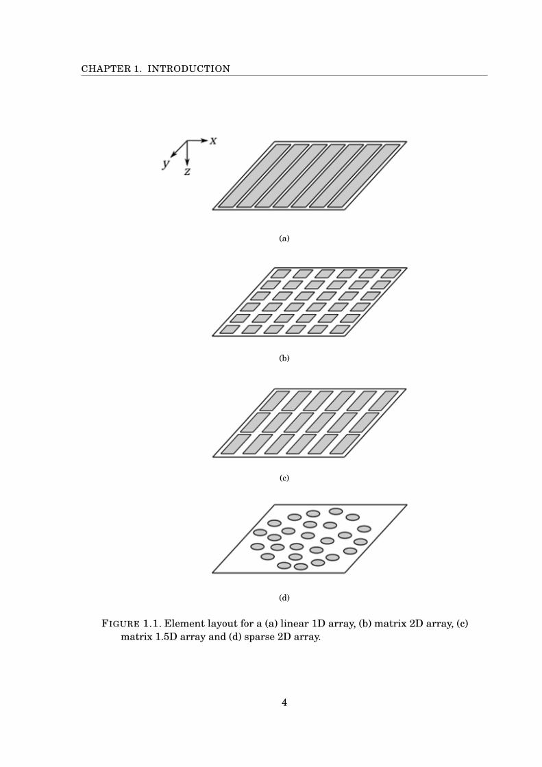
1.1 Element layouts for linear 1D, matrix 2D, matrix 1.5D and sparse 2D arrays 4
2.1 2D illustration of the ray paths required for contact TFM imaging . . . . . . . 15
2.2 Contact inspection setup for imaging through a planar surface . . . . . . . . . 16
2.3 Example of 5 individual 2D TFM images taken at different y locations using
a linear array . . . . . . . . . . . . . . . . . . . . . . . . . . . . . . . . . . . . . . . 17
2.4 Contact pseudo-3D volumetric TFM image of the A block using a linear array
translated in the y direction . . . . . . . . . . . . . . . . . . . . . . . . . . . . . . 18
2.5 Contact 3D TFM image of the A block using a matrix 2D array . . . . . . . . . 19
2.6 Contact 3D TFM image of the A block using a sparse 2D array . . . . . . . . . 20
2.7 (x− z) elevation views of the contact 3D TFM images of the A block . . . . . . 22
2.8 V-6 dB values obtained from 3D TFM images generated using different arrays
in contact . . . . . . . . . . . . . . . . . . . . . . . . . . . . . . . . . . . . . . . . . 23
2.9 Zoomed in windows around FBH 13 using the linear array and the sparse array 24
2.10 Signal-to-noise ratio (SNR) of flat bottom holes for each type of array . . . . . 25
2.11 Average SNR of FBHs for each type of array at increasing depth . . . . . . . . 26
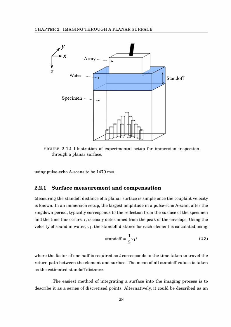
2.12 Illustration of experimental setup for immersion inspection through a planar
surface . . . . . . . . . . . . . . . . . . . . . . . . . . . . . . . . . . . . . . . . . . . 28
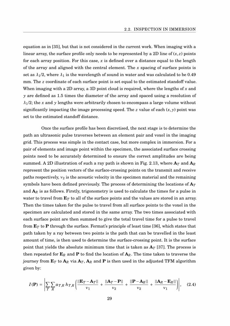
2.13 Illustration of a ray path in an immersion setup . . . . . . . . . . . . . . . . . . 30
2.14 Immersion pseudo-3D TFM image of the A block using a linear array trans-
lated in the y direction . . . . . . . . . . . . . . . . . . . . . . . . . . . . . . . . . 31
2.15 Immersion 3D TFM image of the A block using a matrix 2D array . . . . . . . 32
2.16 Immersion 3D TFM image of the A block using a sparse 2D array . . . . . . . 33
2.17 (x− z) elevation views of the immersion 3D TFM images of the A block . . . . 35
xiii
LIST OF FIGURES
2.18 Comparison of V-6 dB obtained from 3D TFM images generated using different
arrays in immersion . . . . . . . . . . . . . . . . . . . . . . . . . . . . . . . . . . . 36
2.19 Signal-to-noise ratio (SNR) of flat bottom holes for each type of array in
immersion . . . . . . . . . . . . . . . . . . . . . . . . . . . . . . . . . . . . . . . . . 36
2.20 Average SNR of FBHs for each type of array at increasing depth in immersion 37
3.1 Surface results for a single array position over a non-planar surface . . . . . . 42
3.2 Single-medium TFM processing time against number of voxels using MATLAB
(CPU) and CUDA (GPU) . . . . . . . . . . . . . . . . . . . . . . . . . . . . . . . . 43
3.3 2D illustration of a non-planar specimen immersed in water, highlighting the
region that single-medium TFM is to be generated in to allow image-based
surface extraction . . . . . . . . . . . . . . . . . . . . . . . . . . . . . . . . . . . . 44
3.4 3D illustration of a ray path in a single medium that yields the global mini-
mum ToF between ET , P1, and ER using a 2D phased array . . . . . . . . . . . 45
3.5 Illustration of the surface extraction method for a doubly curved surface . . . 48
3.6 Illustration of a top view of the extraction process . . . . . . . . . . . . . . . . . 49
3.7 3D illustration of a ray path in immersion that yields the global minimum
ToF between ET , P2, and ER using a 2D array . . . . . . . . . . . . . . . . . . . 50
3.8 The flow diagram for TFM imaging in immersion through a non-planar surface
using a single array position . . . . . . . . . . . . . . . . . . . . . . . . . . . . . . 51
3.9 Illustration of doubly curved specimen #1 with machined defects . . . . . . . . 53
3.10 Reduced region of doubly curved specimen #1 that is used to investigate 3D
TFM imaging through a non-planar surface . . . . . . . . . . . . . . . . . . . . 55
3.11 Schematic showing the reflection of a sound pulse from a non-planar surface 56
3.12 Illustration showing the experimental setup used to image a non-planar
surface in immersion . . . . . . . . . . . . . . . . . . . . . . . . . . . . . . . . . . 56
3.13 Surface results for a single array position over a non-planar surface . . . . . . 57
3.14 Interior 3D TFM results for a single array position over a non-planar surface 58
3.15 The difference between z values at each (x, y) location of the extracted surface
profile with the values obtained from the equation of the surface . . . . . . . . 59
3.16 Unequal alignment of the reference frames for the equation of the surface and
the experimental setup . . . . . . . . . . . . . . . . . . . . . . . . . . . . . . . . . 60
3.17 Machined surface profile with the locations of defects K and L and the array
location overlaid . . . . . . . . . . . . . . . . . . . . . . . . . . . . . . . . . . . . . 61
4.1 Scanned array positions with 50% overlap relative to the specimen location . 65
xiv
LIST OF FIGURES
4.2 The flow diagram showing the methodology for generating a TFM image using
a scanned array . . . . . . . . . . . . . . . . . . . . . . . . . . . . . . . . . . . . . 67
4.3 2D schematic of overlapping imaging regions for two array positions using
50% array overlap. . . . . . . . . . . . . . . . . . . . . . . . . . . . . . . . . . . . . 68
4.4 Associated position errors in z between the equation of the surface and a laser
scan of doubly curved specimen #1 . . . . . . . . . . . . . . . . . . . . . . . . . . 70
4.5 Stitched 3D surface TFM image of doubly curved specimen #1 . . . . . . . . . 72
4.6 Comparison of the ultrasonically-extracted surface of doubly curved specimen
#1 with the equation of the surface . . . . . . . . . . . . . . . . . . . . . . . . . . 73
4.7 Illustration of a subsection of the extracted surface points used for imaging
directly beneath the array . . . . . . . . . . . . . . . . . . . . . . . . . . . . . . . 75
4.8 Stitched interior 3D TFM image of doubly curved specimen #1 . . . . . . . . . 77
4.9 Zoomed in snapshots of BDHs K, L and M plotted at nominal positions . . . . 78
4.10 Zoomed in snapshots of EDM notches 4, 3 and 2 plotted at nominal positions 79
4.11 Comparison of measured and true defect positions . . . . . . . . . . . . . . . . 81
4.12 Surface inclination with the locations of the EDM notches and BDHs marked 82
4.13 Illustration of reflection of sound energy when incident on a plane greater
than the critical angle . . . . . . . . . . . . . . . . . . . . . . . . . . . . . . . . . . 83
4.14 The directivity of a 1.7 mm diameter circular element radiating into water at
3 MHz as a function of angle relative to the element normal direction . . . . . 84
5.1 Illustration of an incident and transmitted angle on a non-planar surface
between element ET and image point P. . . . . . . . . . . . . . . . . . . . . . . . 90
5.2 Calculating surface normal in 3D . . . . . . . . . . . . . . . . . . . . . . . . . . . 91
5.3 Normalised 3D sensitivity image using the data from section 2.2 for the sparse
array . . . . . . . . . . . . . . . . . . . . . . . . . . . . . . . . . . . . . . . . . . . . 94
5.4 2D (x− z) slices of 3D sensitivity image in Fig. 5.3 at increasing steps along y 95
5.5 Weighted immersion 3D TFM image of the A block described in chapter 2 . . 96
5.6 Comparison of maximum amplitude of defects in the standard and normalised
3D TFM images . . . . . . . . . . . . . . . . . . . . . . . . . . . . . . . . . . . . . 97
5.7 Stitched 3D interior TFM image of doubly curved specimen #1 obtained using
sensitivity images . . . . . . . . . . . . . . . . . . . . . . . . . . . . . . . . . . . . 100
5.8 Zoomed in snapshots of BDHs K, L and M plotted at nominal positions . . . . 102
5.9 Zoomed in snapshots of EDM notches 4, 3 and 2 plotted at nominal positions 103
xv

LIST OF FIGURES
5.10 Comparison of measured and true defect positions using the stitched surface
obtained by sensitivity images . . . . . . . . . . . . . . . . . . . . . . . . . . . . . 104
5.11 Comparison of maximum amplitude of defects in the standard stitched and
weighed stitched 3D TFM images using sensitivity images . . . . . . . . . . . 106
6.1 Illustration of the 6 dB drop method for defect sizing in 2D . . . . . . . . . . . 111
6.2 Illustration of the 6 dB drop method for slot sizing and orientation in 2D . . . 113
6.3 Flow diagram showing the key steps of two methods used for stitching multiple
TFM images into a single, larger TFM image . . . . . . . . . . . . . . . . . . . . 115
6.4 Diagram of the test piece used in case #1 for defect characterisation . . . . . . 116
6.5 Stitched 3D interior TFM images through a planar surface using both stitch-
ing method 1 . . . . . . . . . . . . . . . . . . . . . . . . . . . . . . . . . . . . . . . 118
6.6 Stitched 3D interior TFM images through a planar surface using both stitch-
ing method 2 . . . . . . . . . . . . . . . . . . . . . . . . . . . . . . . . . . . . . . . 119
6.7 2D TFM image of angled slot 4 . . . . . . . . . . . . . . . . . . . . . . . . . . . . 121
6.8 Illustration of doubly curved specimen #2 . . . . . . . . . . . . . . . . . . . . . . 123
6.9 Stitched 3D TFM images of the defects in doubly curved specimen #2 using
both stitching methods . . . . . . . . . . . . . . . . . . . . . . . . . . . . . . . . . 125
6.10 Comparison of measured defect diameters in doubly curved specimen #2
compared to true value . . . . . . . . . . . . . . . . . . . . . . . . . . . . . . . . . 126
6.11 Tip geometries of a RBH and FBH . . . . . . . . . . . . . . . . . . . . . . . . . . 127
xvi

List of Tables
TABLE Page
1.1 Parameters of the linear 1D, matrix 2D and sparse 2D arrays used in the
current work . . . . . . . . . . . . . . . . . . . . . . . . . . . . . . . . . . . . . . . 7
2.1 Processing times for contact 3D TFM using different arrays . . . . . . . . . . . 27
2.2 Processing times for immersion 3D TFM using different arrays . . . . . . . . . 37
3.1 Comparison of measured and machined defect locations using a non-planar
surface . . . . . . . . . . . . . . . . . . . . . . . . . . . . . . . . . . . . . . . . . . . 60
3.2 API values for imaged defects K and L through a non-planar surface profile . 61
6.1 Characterisation parameters of defects in specimen used for case #1 . . . . . 117
6.2 Measured defect parameters for case #1 using both stitching methods . . . . . 120
6.3 Type and diameter of defects in doubly curved specimen #2 . . . . . . . . . . . 122
6.4 Summary of mean and standard deviation errors of measured FBHs and
RBHs in doubly curved specimen #2 using both stitching methods . . . . . . . 128
xvii


Abbreviations
NDT Non-destructive testing
NDE Non-destructive evaluation
UT Ultrasonic testing
1D One-dimensional
1.5D One-and-a-half dimensional
2D Two-dimensional
3D Three-dimensional
dB Decibel
TFM Total Focusing Method
FMC Full-matrix capture
HMC Half-matrix capture
PWI Plane Wave Imaging
ToF Time-of-flight
FBH Flat bottom hole
SNR Signal-to-noise ratio
MB Megabyte
CPU Central processing unit
GPU Graphics processing unit
BDH Bottom drilled hole
EDM Electrical discharge machining
xix

ABBREVIATIONS
RMSE Root-mean square error
DE Differential evolution
S-matrix Scattering matrix
RBH Round bottom hole
xx

Symbols
fc Array centre frequency
x Primary/secondary imaging axis
y Primary/secondary imaging axis
z Depth imaging axis
T Transmitting element index
R Receiving element index
E Position vector of element (with transmission (T) and reception (R) components)
P Position vector of image point (with various components defined in text)
ν Velocity of sound (with various components defined in text)
I Image intensity (2D or 3D)
τ Time
h Complex analytic signal of an A-scan
V Volume (with component defined in text)
λ Wavelength (with various components defined in text)
A Position vector of surface-crossing location (with transmission (T) and reception
(R) components)
ε Size of single-medium TFM window in z
Z Locations of extracted 3D surface points in z
σ Standard deviation
θ Angle (various components defined in text)
xxi

SYMBOLS
D Directivity coefficient
φ Beam elevation angle
E Sensitivity image intensity
B Beamspread coefficient
Γ Transmission coefficient
S Scattering matrix
ρ Material density (various components defined in text)
d Hole diameter
l Slot length
xxii

Chapter 1
Introduction
Non-destructive testing (NDT), also known as non-destructive evaluation (NDE), refers to
the collection of techniques that can be used to test and analyse industrial components for
defects, flaws or weaknesses to evaluate the useability of a component or system without
causing permanent damage. This is an essential process in industries such as power
generation [1, 2], aerospace [3] and transport [4], where failure of a component could
lead to catastrophic damage. Developments in NDT over the last few decades have made
it possible to obtain accurate internal images of solid structures within the engineering
design process, after part manufacture is completed and during service. Frequently used
NDT techniques include ultrasonic testing (UT), electromagnetic testing (ET), magnetic
particle testing (MPI), radiography, dye penetrant inspection (DPI) and visual inspection.
It is common for multiple inspection techniques to be used in conjunction with others,
but the geometry of the component or type of defect being imaged can have an impact
on the chosen method. For example, radiography is preferred when inspecting small-
bore and thin-walled tubing welds, while UT is desirable when collecting thickness
measurements over time in the case of pipe corrosion. UT in particular is a highly
desirable technique to use in industry due to the flexibility of inspections, ability to
obtain high resolution internal images, lack of harm to the operator and potential for
real-time imaging. This introductory chapter introduces the principles of phased arrays
and their use in volumetric UT, along with the motivation for this work.
1
CHAPTER 1. INTRODUCTION
1.1 Ultrasonic phased arrays
UT involves transmitting a high-frequency sound pulse into a component and processing
the reflected signals to generate an image. If the pulse encounters a change in material
property or density, such as a boundary or crack, the signal is reflected and can be
picked up by the transducer at a registered time. Traditionally this pulse was generated
from a single-element transducer and yielded a time-amplitude trace, termed an A-
scan, which could be presented graphically. Single-element transducers consist of a
single crystal element in a casing which vibrates when exposed to electrical signals;
the crystal both transmits and receives sound energy and is therefore the foundation
of all ultrasonic imaging methods. Any density or material property changes that a
sound pulse encounters can be identified by the timing of peaks in the A-scan, which
correspond to positions that can easily be calculated using the time the peak occurs
and the acoustic velocity of the sound wave in the component. While A-scans are an
effective tool for thickness measurements, they are not effective at characterising the
interior of a specimen beyond identifying large defects. Therefore, key limitations of
using single-element probes in UT inspections include the inability to vary focal depth,
a restricted number of fixed directions available from which to detect defects, and the
consequent potential for missing defects that are in unexpected positions or orientations.
It is for these reasons that research groups began to focus on ultrasonic phased arrays
and their ability to improve inspections.
Ultrasonic phased arrays, more commonly referred to as just ‘arrays’, are com-
posed of many single-element transducers, and therefore have the benefits of electronic
beam steering, focusing and scanning by applying delay laws to individually addressable
elements [5]. As a direct result of these properties, phased arrays can be applied to a
wider range of imaging scenarios and have the ability to speed up ultrasonic inspections
significantly, along with improving defect image resolution [6]. Arrays typically contain
between 64–128 individual elements, with the maximum number limited by the number
of channels available in the array controller. Array controllers exist that can accommo-
date arrays with up to 512 elements, however arrays of this type are relatively rare due
to electrical complexity and cost.
Arrays are typically designed to be either one-dimensional (1D), one-and-a-half-
dimensional (1.5D) or two-dimensional (2D). Descriptions of these types of arrays are
given in the following sections.
2
1.1. ULTRASONIC PHASED ARRAYS
1.1.1 1D arrays
Linear 1D arrays, or simply just linear arrays, are composed of a row of single-element
transducers arranged in a straight line, as shown in Fig. 1.1(a). The elements are spaced
along the x direction and are comparatively long in the y direction, so therefore are
assumed to behave as infinitely long strip sources. Traditional imaging methods involved
transmitting a sub-aperture of elements in the array; this was most commonly achieved
by pulsing all elements in a sub-aperture simultaneously to behave as a monolithic
transducer. Upon capturing an A-scan, the aperture is moved one element along and
the process is repeated until the last element is included in the aperture; advancing the
aperture beyond this limit results in an aperture with fewer elements than it initially
contained. When the A-scans are stacked side-by-side they represent a 2D B-scan image,
displaying depth below the array and lateral distance. As the area insonified by a linear
array is substantially larger when compared to a single-element transducer, physical
movement of the array is not required between A-scan capture when imaging the same
size of area. By manipulating the delay laws to a selection of elements, focused and
sector B-scans can be obtained to provide more information of a region [7]. B-scans are
commonly used in medical imaging for a wide range of applications due to their ease
of implementation and ability to image in real-time [8]. The interactions of different
pairs of elements can also be investigated depending on the data capture method, so
inspections with a linear array are not limited to pulse-echo.
Despite the many benefits linear arrays have over single-element transducers,
they still do not demonstrate the true potential of phased array technology. A substantial
limitation of using linear arrays is that the steering is confined to a single plane and
therefore there is no ability to control focusing in the plane perpendicular to the image
plane, or the out-of-plane direction [9]. This means that inspections with this type of array
are limited to 2D slices, which is of particular concern when building up a volumetric
image of the interior of a component, or imaging through surfaces that are curved in
multiple directions. Three-dimensional (3D) volumetric inspections using a linear array
have previously been achieved by translating the array in the out-of-plane direction and
combining the resulting images together to reconstruct a ‘pseudo-3D’ volume from a
series of 2D slices [10]. As there is the possibility of missing scattering effects in the
out-of-plane direction, there is the subsequent chance of completely missing defects that
are in unexpected positions or orientations.
3
CHAPTER 1. INTRODUCTION
(a)
(b)
(c)
(d)
FIGURE 1.1. Element layout for a (a) linear 1D array, (b) matrix 2D array, (c)matrix 1.5D array and (d) sparse 2D array.
4
1.1. ULTRASONIC PHASED ARRAYS
1.1.2 2D arrays
A 2D array is characterised by having its elements distributed across a 2D aperture.
By distributing elements in this way, it is possible to better characterise defects within
components as beam manipulation can occur throughout a 3D volume without requiring
movement of the array, along with the ability to probed a defect over a larger range of
solid angles [11]. This ability significantly increases coverage of the imaging region, as
long as the array and surface orientations are favourable, and allows a more detailed
inspection through volumetric beam steering and focusing. Due to the layout of elements
in this type of array, the ultrasonic beam can be focused in both lateral directions. As a
result, components with complex surfaces can be inspected and defects in unexpected
orientations have a higher likelihood of being detected.
When considering the design of 2D arrays, there are infinite possibilities of
element layouts. Researching the optimal element layout has been the focus of research
over the past couple of decades [6, 12–15] and two common types of 2D arrays are
considered in the current work.
Matrix 2D
The most intuitive 2D array design consists of elements arranged in a grid layout, termed
a matrix array, as illustrated in Fig. 1.1(b). This type of array is essentially an extension
of a linear array, where the long elements have been divided into smaller, independent
square elements arranged in a regular grid orientation across the x and y directions. A
major problem with matrix arrays is the requirement of the inter-element spacing, or
pitch, to be less than half the wavelength of emitted waves. This limit is derived from the
Nyquist spatial sampling critera and is needed to avoid aliasing effects in the form of
unwanted grating lobes, which can minimise energy in the main lobe and hence reduce
overall imaging capabilities in periodic arrays [16, 17]. At the same time, a wide spatial
extension is necessary for high resolution imaging, as the lateral resolution is directly
dependent on aperture size. To enhance array performance the number of elements
can be increased while maintaining the pitch constraint, but this quickly increases
the number of elements required, and therefore complexity and cost. Furthermore, the
periodic spacing of elements in a matrix array also results in the appearance of grating
lobes [11, 18].
An alternative matrix element layout has been presented in the form of a 1.5D
5
CHAPTER 1. INTRODUCTION
array, whereby the linear elements are coarsely divided into rectangles in the y direction,
as shown in Fig. 1.1(c). As a result, the number of elements in a row does not equal
the number of elements in a column, as is typical in a matrix 2D array. The number of
elements has been reduced, while still enabling focusing in the out-of-plane direction
for enhanced detection capability [19, 20]. However, finer resolution of elements in the y
direction is necessary for beam steering and only 2D images are formed using this type
of array. It is for this reason that 1.5D arrays are unused in the current work.
Sparse 2D
Research has demonstrated that a sparse 2D array with elements arranged in a Poisson
disk distribution outperforms a matrix 2D array with the same number of elements
[5, 11]. This is a result of the non-periodic element layout preventing the formation
of grating effects while still maintaining a high level of imaging resolution. In this
configuration, circular elements are randomly distributed across the aperture with a
constraint applied to the minimum separation distance. Although the presence of grating
lobes has been removed, a consequence of the sparseness of the array is that the overall
background noise in the image increases, and hence lowers the signal-to-noise ratio
(SNR). This is a result of the psuedorandom spacing of elements dispersing the energy of
would-be grating lobes into the surrounding environment. An illustration of the element
layout for an array of this type is shown in Fig. 1.1(d).
1.1.3 Array parameters
Descriptions of the Immasonic (Besançon, France) arrays used in the current work are
given in Table 1.1; to collect data throughout this thesis, the commercial array controller
device MicroPulse FMC (Peak NDT Ltd., Derby, UK) was used.
The dimensions, shape and pitch of an element all contribute towards the
nature of the ultrasonic field produced. In both the linear 1D and matrix 2D arrays,
the element pitch is determined by the Nyquist criterion, which states that the pitch
in a periodic array should be less than half the wavelength of emitted sound waves.
Both arrays were manufactured for anticipated use in metals, as both pitches satisfy
the half-wavelength criterion when travelling with velocities greater than ∼3000 m/s
and ∼6000 m/s respectively. As it is not necessary to satisfy the Nyquist criterion when
considering an irregular distribution of elements, the pitch of the sparse 2D array can
6

1.1. ULTRASONIC PHASED ARRAYS
be larger than λ/2 while still avoiding grating lobes. However, the pitch must be large
enough to avoid cross-coupling between neighbouring elements, but small enough to
allow high resolution imaging. This results in the ability to create a sparse 2D array
with a larger aperture than would be possible using a matrix 2D array using the same
number of elements. The sparse 2D array was designed to operate at 3 MHz in order
to be comparable with the matrix 2D array. Although the classic Nyquist rule for the
element pitch of a periodic array design is well known, a study in [18] shows that the
pitch can be increased without significant degradation of image quality, providing angle
limits are applied to the aperture. This means that future arrays of a certain size could
be populated with larger pitches and fewer elements to reduce data sizes, and ultimately
speed up inspections.
The length and width values associated with a circular element in the sparse
2D array are equal and represent the element diameter. Matrix 2D arrays typically have
square-shaped elements, while the sparse 2D array contains circular elements; elements
of this shape complement the Poisson disk shape and produce symmetrical ultrasonic
beams. The bandwidth is defined here as the magnitude of the spread of frequencies
corresponding to 6 dB below the maximum signal amplitude (defined to be 0 decibels, or
dB), or the full width at half maximum (FWHM).
TABLE 1.1. Parameters of the linear 1D, matrix 2D and sparse 2D arrays usedin the current work.
Array type Linear 1D Matrix 2D Sparse 2DElement properties
Count 128 121 (11x11) 128Shape Rectangular Square CircularLength (mm) 15.0 0.8 1.7Width (mm) 0.2 0.8 1.7Pitch (mm) 0.3 1.0 ≥ 1.9Spacing (mm) 0.1 0.2 ≥ 0.2
Array propertiesActive area (mm) 38.5 x 15.0 10.8 x 10.8 ≈152π
Centre frequency (MHz) 5 3 3Bandwidth (–6 dB) ≥ 2.5 > 1.5 ≥ 1.5
7
CHAPTER 1. INTRODUCTION
1.2 Ultrasonic imaging techniques
Ultrasonic imaging is generally conducted in three main stages: acquisition, reconstruc-
tion and visualisation. Acquisition refers to the collection of time-domain data from an
experimental setup, reconstruction aims to process the information contained in the
collected data set by applying an imaging algorithm, and visualisation is the method of
displaying the final image result.
Up to this point, the reconstruction of data has only been discussed in terms
of B-scans. While arrays have the ability to produce focused B-scans, this is limited to
a predefined depth in a component. This is a problem when the location of a defect is
unknown and an accurate image of a region within a component is to be obtained. It
therefore follows that a fully-focused image would be optimal. Within recent decades,
computer power has enabled improvements in post-processing techniques that allow data
sets to be processed offline instead of physical beam forming at the time of inspection.
This enabled an imaging algorithm, termed the Total Focusing Method (TFM), to be
implemented, which focuses the full array in both transmission and reception at every
point in a defined imaging grid [7]. TFM imaging requires the full-matrix capture (FMC)
data set containing the A-scans of all transmit-receive element pair combinations and
results in n2 scans, where n is the number of elements in a given array. Time-domain
data acquired in this format contains the maximum possible amount of information of a
setup, and therefore can result in large data files and slow scanning speeds. A practice
for reducing the amount of data collected can be used, whereby reciprocities can be
eliminated by assuming that the A-scan obtained from transmitting from element T and
receiving on element R is identical to the A-scan obtained by transmitting from R and
receiving on T. This results in the half-matrix data set being captured, termed the HMC
[5], which reduces the number of A-scans to n(n+1)/2. Inspection is therefore sped up
without a significant loss of data, and hence HMC is used throughout the current work.
While TFM offers clear imaging advantages, obtaining the FMC data set re-
quires at least n separate transmissions and processing can be computationally intensive.
An alternative imaging approach known as Plane Wave Imaging (PWI) has been shown
to produce images with equivalent quality to those obtained using TFM, but with fewer
transmissions [21–23]. The basic premise of capturing data for PWI is to emit m plane
waves at m different angles into a component and receive the backscattered signals on
all n elements in parallel, resulting in a m×n matrix. The higher power input into the
8
1.3. MOTIVATION
component, along with significantly fewer acquisition cycles makes PWI an appealing
alternative imaging method. However, 3D imaging using plane waves has yet to be fully
explored and not investigated in the current work.
Volumetric images of processed data can be challenging to visualise, but are
typically displayed by (i) 2D slices through a chosen image point, or (ii) showing the
location of 3D amplitude values above a specified threshold. The type of images produced
depends on the properties of the transducer that was used. Real-time imaging is possible
with present technology, however significant optimisations are required during post-
processing due to the large number of calculations.
1.3 Motivation
When a component contains a flaw or defect hidden beneath the surface, the structural
integrity can be compromised depending on the nature of the defect. Distinguishing
between defect types is crucial for thorough and accurate inspections, as the severity
of defects depends on their size, orientation and shape; for instance, it is well known
that planar discontinuities (e.g. cracks) are usually more dangerous than volumetric
defects (e.g. voids) due to their sharp edges that have the potential to grow and cause
breaks. To enable precise defect characterisation, it is therefore necessary to obtain
volumetric information about defects. 2D arrays have the ability to obtain volumetric
defect information from a single location, and their use is therefore desirable for UT
inspections.
A cross sector problem in the NDT industry is the inspection of defects within
regions where the surface geometry of a component curves in multiple directions, also
known as doubly curved surfaces, such as those found in turbine blades, pipework
branches and nozzles. Current inspection procedures through these surfaces involve
using either (i) a single-element transducer that probes the region from a range of
locations, or (ii) radiography. The use of a single-element transducer means that a highly-
skilled operator needs to interpret the data and it is extremely challenging to build up
a volumetric image of the region, while radiography is not very effective for detecting
and sizing planar defects without prior knowledge of their likely location and orientation
[24]. Developments over the past few decades have introduced phased array transducers
to the UT process and the choice of transducer plays an integral role in the imaging
9
CHAPTER 1. INTRODUCTION
capability of the inspection. Due to the double curvature of the surface, linear arrays
are not ideal for inspections of this type. However, the ability of 2D arrays to focus
through doubly curved surfaces presents an opportunity for improving the detection and
characterisation of defects within complex-shaped components.
1.4 Aims & objectives
The aim of the current work is to improve FMC-based inspections for volumetric defect
imaging through complex surfaces using 2D phased arrays. A sparse 2D array is used
due to its ability to suppress prominent grating lobes while maintaining a high imaging
resolution when compared to a matrix 2D array of a similar number of elements; this
is a result of the larger aperture of a sparse 2D array which is made possible as the
pitch is not constrained by the Nyquist criterion. The captured time-domain data is
processed using TFM imaging to produce fully focused images of the interior of specimens.
Initially, imaging is conducted on a simple, planar surface in contact and immersion
setups to quantitatively illustrate the benefits of using a sparse 2D array. A test specimen
with a doubly curved surface is then imaged, whereby the surface profile is assumed
unknown and a surface compensation method is required. A scanned array system is
then considered, whereby a large specimen is imaged using multiple data sets collected
at different locations. Two methods will be introduced to combine the data sets and
ultimately 3D defects will be detected and characterised through a large, complex surface.
The current work provides the groundwork for 3D TFM imaging of specimens without
prior surface knowledge using a 2D array, and demonstrates the benefits for their uptake
in industry for improved UT inspections.
1.4.1 Thesis outline
Chapter 2 introduces 3D TFM imaging through a planar surface utilising linear, matrix
2D and sparse 2D arrays. Imaging methods in both contact and immersion are compared
and the imaging capabilities of each type of array are compared using experimental data.
In chapter 3, a method of imaging through a complex, non-planar surface from a
single array position is introduced. A novel 3D surface extraction algorithm is introduced
and validated against the true surface before the positioning of defects is investigated.
Computational processing speed is also examined here and a method for increasing 3D
TFM imaging speeds is described.
10

1.4. AIMS & OBJECTIVES
Chapter 4 expands on the previous chapter and introduces a scanned array
system for volumetric imaging through a doubly curved surface. The surface profile is
extracted and subsequently used for the positioning of defects at a range of depths and
positions.
Chapter 5 furthers the results of chapter 4 by proposing a new technique for
combining individual TFM images obtained from a scanned array inspection. This is
achieved through the generation of sensitivity images, which are used to normalise TFM
images depending on the array imaging performance for specific array locations.
Chapter 6 considers the challenge of characterising defects using volumetric
defect information. A range of defects are imaged using a scanned array inspection and
their orientations determined before being compared to their true values.
Chapter 7 summarises the key findings of the current work and discusses
potential avenues for future work.
11

Chapter 2
Imaging through a planar surface
Specimens with a planar surface profile are the simplest to image through due to the
continuity of the surface. When considering a direct contact inspection setup using
an array with a flat footprint, i.e. all of the elements are in a single plane, the active
region of the array and the surface of the specimen are complementary and imaging is
straightforward using a thin layer of couplant. In this case, the complexity of calculations
required to produce an internal image is low due to all of the ultrasonic rays travelling
in a single medium. In cases where contact inspection is not possible, for example in
corrosive or hostile environments [25], or if elevated temperatures prevent the array from
being close to the surface [26], a waveguide could be used to facilitate the transmission of
ultrasonic energy into the specimen. The inclusion of this intermediate layer adds a level
of complexity to the imaging process as the pulse no longer travels at a constant speed
and refraction effects must be accounted for. Additionally, non-contact systems involving
laser ultrasonics [27] and electromagnetic acoustic transducers (EMATs) [28] could be
implemented. Direct coupling with the surface is not necessary using these methods,
where transduction is achieved using light and magnetic fields respectively.
Linear arrays are commonly used in industry for ultrasonic inspections, while
2D arrays have not yet been fully implemented. 2D imaging using a linear array is a
relatively simple process and can give inspectors an estimation of artefact positions
within a specimen, along with allowing post-processing defect characterisation and
model validation. 2D images are routinely used in academia and industry because
of their ease of implementation, however a more detailed picture can be obtained by
employing 2D arrays. This chapter investigates the 3D volumetric imaging capabilities
13
CHAPTER 2. IMAGING THROUGH A PLANAR SURFACE
of the three types of ultrasonic arrays described in the introduction: linear 1D, matrix
2D and sparse 2D. The imaging performance of each array is investigated and compared
by imaging machined defects in a test specimen with a planar surface. The imaging
process is described for contact and immersion setups using the TFM algorithm. A
linear array is used as a comparison of the imaging capabilities of 1D and 2D arrays,
while the matrix and sparse 2D arrays are used to compare the effect of element layout
on imaging performance. It is worth noting that all array types used here have flat
footprints, however arrays with curved footprints are commonly found in industry to
perform inspections of pipes.
2.1 Inspection in contact
When conducting a contact inspection, the active region of the array is placed directly on
the surface of the specimen. This setup maximises the transmission of energy as the flat
footprint of the array and the planar surface are in close contact, while an added layer of
gel couplant on the interface eliminates the presence of any trapped air. As the couplant
layer is very thin, any effect it has on ray refraction is assumed negligible and so only the
properties of a single medium need to be considered. This simplifies the imaging process
as a relatively small number of calculations are required when compared to imaging in
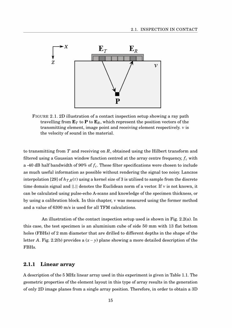
immersion. An 2D illustration of the ray path an ultrasonic pulse takes while travelling
from a transmitting element, T, at ET to an image point at P to a receiving element,
R, at ER in a contact setup is shown in Fig. 2.1, where bold letters represent position
vectors. A 2D system is illustrated for clarity, however it is representative of a 3D system.
When considering 3D space, the image point is referred to as a voxel.
When performing TFM imaging, the time taken, τ, for sound, travelling at
velocity ν, to traverse the journey from ET to P to ER , termed the time-of-flight (ToF), is
required to obtain the amplitude of the signal at P. The amplitude of each element-pair
contribution at P is summed to obtain the final intensity, I(P), and it follows that the
process is repeated for each voxel and element-pair. This is described mathematically as:
I (P) =∣∣∣∣∣∑T
∑R
aT,R hT,R
( ||ET −P|| + ||ER −P||ν
)∣∣∣∣∣ , (2.1)
where aT,R denotes an optional apodisation term which is unused in this work, hence
aT,R = 1, and hT,R(τ) represents the complex analytic signal of the A-scan corresponding
14
2.1. INSPECTION IN CONTACT
FIGURE 2.1. 2D illustration of a contact inspection setup showing a ray pathtravelling from ET to P to ER , which represent the position vectors of thetransmitting element, image point and receiving element respectively. ν isthe velocity of sound in the material.
to transmitting from T and receiving on R, obtained using the Hilbert transform and
filtered using a Gaussian window function centred at the array centre frequency, fc with
a -40 dB half bandwidth of 90% of fc. These filter specifications were chosen to include
as much useful information as possible without rendering the signal too noisy. Lanczos
interpolation [29] of hT,R(τ) using a kernel size of 3 is utilised to sample from the discrete
time domain signal and ||.|| denotes the Euclidean norm of a vector. If ν is not known, it
can be calculated using pulse-echo A-scans and knowledge of the specimen thickness, or
by using a calibration block. In this chapter, ν was measured using the former method
and a value of 6300 m/s is used for all TFM calculations.
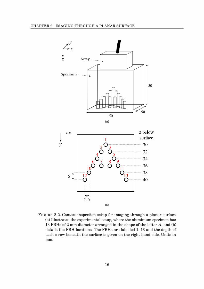
An illustration of the contact inspection setup used is shown in Fig. 2.2(a). In
this case, the test specimen is an aluminium cube of side 50 mm with 13 flat bottom
holes (FBHs) of 2 mm diameter that are drilled to different depths in the shape of the
letter A. Fig. 2.2(b) provides a (x− y) plane showing a more detailed description of the
FBHs.
2.1.1 Linear array
A description of the 5 MHz linear array used in this experiment is given in Table 1.1. The
geometric properties of the element layout in this type of array results in the generation
of only 2D image planes from a single array position. Therefore, in order to obtain a 3D
15
CHAPTER 2. IMAGING THROUGH A PLANAR SURFACE
(a)
(b)
FIGURE 2.2. Contact inspection setup for imaging through a planar surface.(a) Illustrates the experimental setup, where the aluminium specimen has13 FBHs of 2 mm diameter arranged in the shape of the letter A, and (b)details the FBH locations. The FBHs are labelled 1–13 and the depth ofeach x row beneath the surface is given on the right hand side. Units inmm.
16
2.1. INSPECTION IN CONTACT
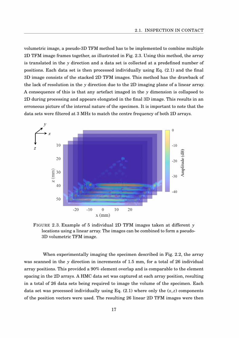
volumetric image, a pseudo-3D TFM method has to be implemented to combine multiple
2D TFM image frames together, as illustrated in Fig. 2.3. Using this method, the array
is translated in the y direction and a data set is collected at a predefined number of
positions. Each data set is then processed individually using Eq. (2.1) and the final
3D image consists of the stacked 2D TFM images. This method has the drawback of
the lack of resolution in the y direction due to the 2D imaging plane of a linear array.
A consequence of this is that any artefact imaged in the y dimension is collapsed to
2D during processing and appears elongated in the final 3D image. This results in an
erroneous picture of the internal nature of the specimen. It is important to note that the
data sets were filtered at 3 MHz to match the centre frequency of both 2D arrays.
FIGURE 2.3. Example of 5 individual 2D TFM images taken at different ylocations using a linear array. The images can be combined to form a pseudo-3D volumetric TFM image.
When experimentally imaging the specimen described in Fig. 2.2, the array
was scanned in the y direction in increments of 1.5 mm, for a total of 26 individual
array positions. This provided a 90% element overlap and is comparable to the element
spacing in the 2D arrays. A HMC data set was captured at each array position, resulting
in a total of 26 data sets being required to image the volume of the specimen. Each
data set was processed individually using Eq. (2.1) where only the (x, z) components
of the position vectors were used. The resulting 26 linear 2D TFM images were then
17
CHAPTER 2. IMAGING THROUGH A PLANAR SURFACE
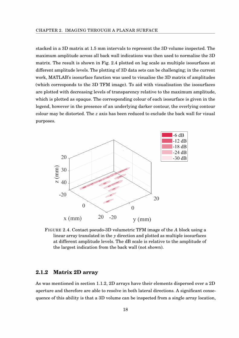
stacked in a 3D matrix at 1.5 mm intervals to represent the 3D volume inspected. The
maximum amplitude across all back wall indications was then used to normalise the 3D
matrix. The result is shown in Fig. 2.4 plotted on log scale as multiple isosurfaces at
different amplitude levels. The plotting of 3D data sets can be challenging; in the current
work, MATLAB’s isosurface function was used to visualise the 3D matrix of amplitudes
(which corresponds to the 3D TFM image). To aid with visualisation the isosurfaces
are plotted with decreasing levels of transparency relative to the maximum amplitude,
which is plotted as opaque. The corresponding colour of each isosurface is given in the
legend, however in the presence of an underlying darker contour, the overlying contour
colour may be distorted. The z axis has been reduced to exclude the back wall for visual
purposes.
FIGURE 2.4. Contact pseudo-3D volumetric TFM image of the A block using alinear array translated in the y direction and plotted as multiple isosurfacesat different amplitude levels. The dB scale is relative to the amplitude ofthe largest indication from the back wall (not shown).
2.1.2 Matrix 2D array
As was mentioned in section 1.1.2, 2D arrays have their elements dispersed over a 2D
aperture and therefore are able to resolve in both lateral directions. A significant conse-
quence of this ability is that a 3D volume can be inspected from a single array location,
18
2.1. INSPECTION IN CONTACT
eliminating the need to combine multiple 2D TFM images. The 3D TFM algorithm can
be directly applied to generate the final image using a single data set.
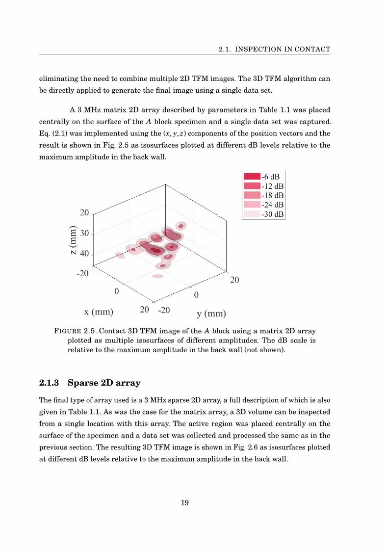
A 3 MHz matrix 2D array described by parameters in Table 1.1 was placed
centrally on the surface of the A block specimen and a single data set was captured.
Eq. (2.1) was implemented using the (x, y, z) components of the position vectors and the
result is shown in Fig. 2.5 as isosurfaces plotted at different dB levels relative to the
maximum amplitude in the back wall.
FIGURE 2.5. Contact 3D TFM image of the A block using a matrix 2D arrayplotted as multiple isosurfaces of different amplitudes. The dB scale isrelative to the maximum amplitude in the back wall (not shown).
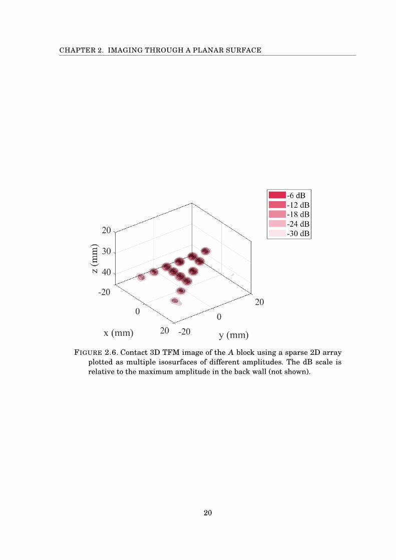
2.1.3 Sparse 2D array
The final type of array used is a 3 MHz sparse 2D array, a full description of which is also
given in Table 1.1. As was the case for the matrix array, a 3D volume can be inspected
from a single location with this array. The active region was placed centrally on the
surface of the specimen and a data set was collected and processed the same as in the
previous section. The resulting 3D TFM image is shown in Fig. 2.6 as isosurfaces plotted
at different dB levels relative to the maximum amplitude in the back wall.
19
CHAPTER 2. IMAGING THROUGH A PLANAR SURFACE
FIGURE 2.6. Contact 3D TFM image of the A block using a sparse 2D arrayplotted as multiple isosurfaces of different amplitudes. The dB scale isrelative to the maximum amplitude in the back wall (not shown).
20
2.1. INSPECTION IN CONTACT
2.1.4 Discussion
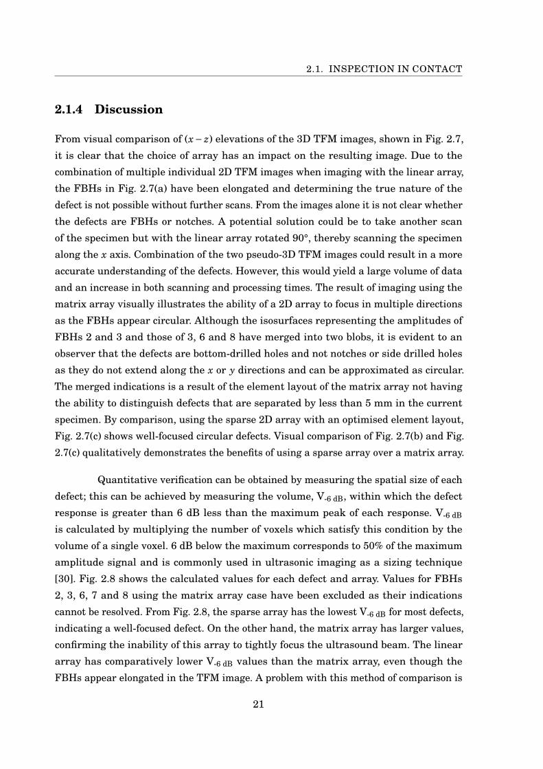
From visual comparison of (x− z) elevations of the 3D TFM images, shown in Fig. 2.7,
it is clear that the choice of array has an impact on the resulting image. Due to the
combination of multiple individual 2D TFM images when imaging with the linear array,
the FBHs in Fig. 2.7(a) have been elongated and determining the true nature of the
defect is not possible without further scans. From the images alone it is not clear whether
the defects are FBHs or notches. A potential solution could be to take another scan
of the specimen but with the linear array rotated 90°, thereby scanning the specimen
along the x axis. Combination of the two pseudo-3D TFM images could result in a more
accurate understanding of the defects. However, this would yield a large volume of data
and an increase in both scanning and processing times. The result of imaging using the
matrix array visually illustrates the ability of a 2D array to focus in multiple directions
as the FBHs appear circular. Although the isosurfaces representing the amplitudes of
FBHs 2 and 3 and those of 3, 6 and 8 have merged into two blobs, it is evident to an
observer that the defects are bottom-drilled holes and not notches or side drilled holes
as they do not extend along the x or y directions and can be approximated as circular.
The merged indications is a result of the element layout of the matrix array not having
the ability to distinguish defects that are separated by less than 5 mm in the current
specimen. By comparison, using the sparse 2D array with an optimised element layout,
Fig. 2.7(c) shows well-focused circular defects. Visual comparison of Fig. 2.7(b) and Fig.
2.7(c) qualitatively demonstrates the benefits of using a sparse array over a matrix array.
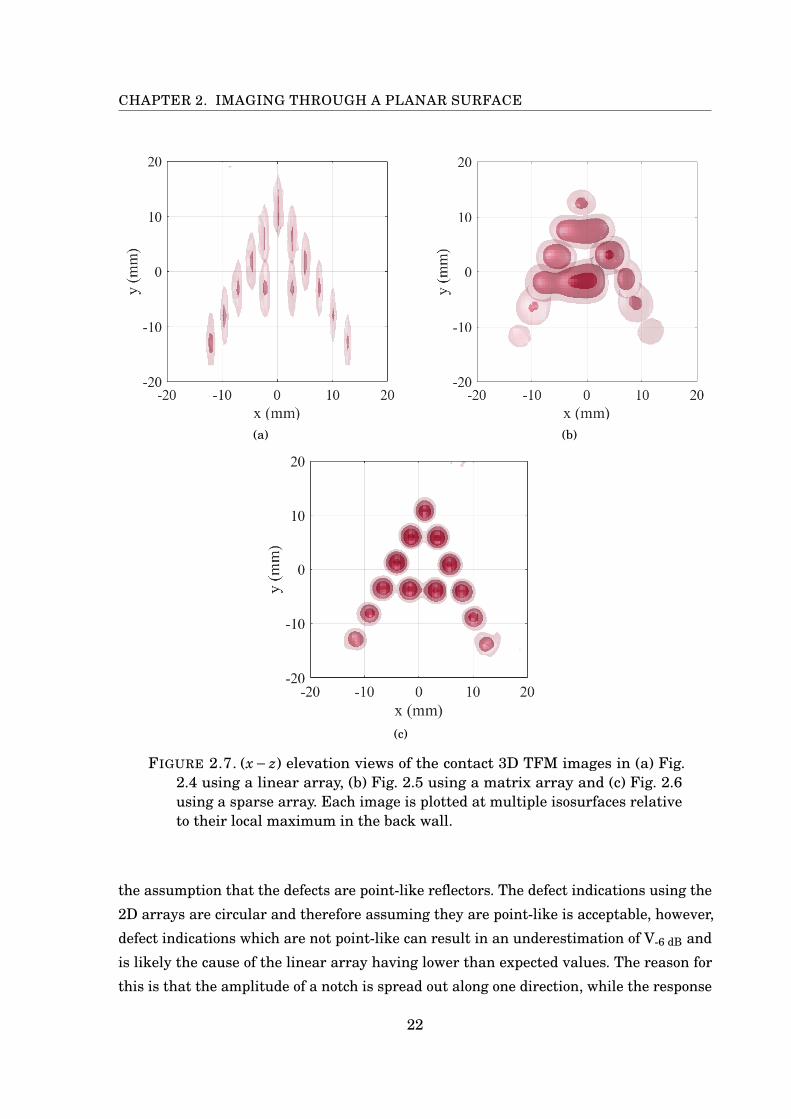
Quantitative verification can be obtained by measuring the spatial size of each
defect; this can be achieved by measuring the volume, V-6 dB, within which the defect
response is greater than 6 dB less than the maximum peak of each response. V-6 dB
is calculated by multiplying the number of voxels which satisfy this condition by the
volume of a single voxel. 6 dB below the maximum corresponds to 50% of the maximum
amplitude signal and is commonly used in ultrasonic imaging as a sizing technique
[30]. Fig. 2.8 shows the calculated values for each defect and array. Values for FBHs
2, 3, 6, 7 and 8 using the matrix array case have been excluded as their indications
cannot be resolved. From Fig. 2.8, the sparse array has the lowest V-6 dB for most defects,
indicating a well-focused defect. On the other hand, the matrix array has larger values,
confirming the inability of this array to tightly focus the ultrasound beam. The linear
array has comparatively lower V-6 dB values than the matrix array, even though the
FBHs appear elongated in the TFM image. A problem with this method of comparison is
21
CHAPTER 2. IMAGING THROUGH A PLANAR SURFACE
(a) (b)
(c)
FIGURE 2.7. (x− z) elevation views of the contact 3D TFM images in (a) Fig.2.4 using a linear array, (b) Fig. 2.5 using a matrix array and (c) Fig. 2.6using a sparse array. Each image is plotted at multiple isosurfaces relativeto their local maximum in the back wall.
the assumption that the defects are point-like reflectors. The defect indications using the
2D arrays are circular and therefore assuming they are point-like is acceptable, however,
defect indications which are not point-like can result in an underestimation of V-6 dB and
is likely the cause of the linear array having lower than expected values. The reason for
this is that the amplitude of a notch is spread out along one direction, while the response
22
2.1. INSPECTION IN CONTACT
from a point has a narrow amplitude spread, as illustrated in the zoomed in regions
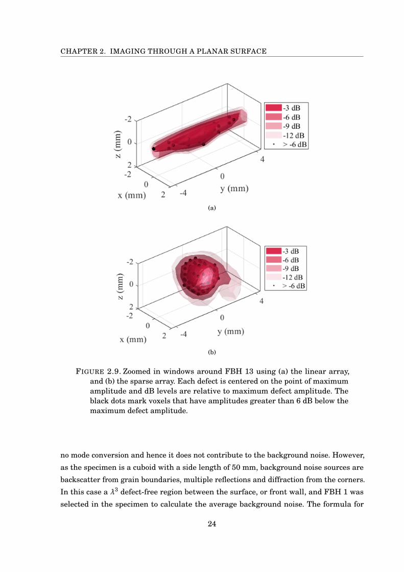
around FBH 13 in Fig. 2.9. Additionally, the resolution in the y direction using the linear
array is limited by the translation of the array between scans, which in this case was
1.5 mm, leading to 21 voxels in Fig. 2.9(a) exceeding the amplitude threshold, while 73
voxels satisfy the condition in Fig. 2.9(b) when imaged using the sparse array with a
grid spacing of λ/4= 0.53 mm in all x, y, z directions, where λ is the wavelength of sound
in the specimen. It is for this reason that V-6 dB is not an accurate measure parameter
for the results using the linear array, however the results do illustrate the benefits of
imaging with a sparse array over a matrix or linear array.
FIGURE 2.8. V-6 dB values obtained from 3D TFM images generated usingdifferent arrays in contact.
The signal-to-noise ratio (SNR) was also used as an additional comparison
measure. The SNR reflects the overall image quality by looking at the relationship
between the defect signal strength and the amplitude level in a defect-free region of
the image. There are two main categories of noise that negatively affect ultrasonic
imaging: coherent and incoherent [31]. An incoherent noise source in this setup is
random electrical noise from the array controller; the effect of this is minimised by
averaging the signals on collection. Coherent noise sources are intrinsic to the inspection
and their effect can not be reduced by averaging. Common causes include backscatter
from grain boundaries in the microstructure and artefacts due to multiple reflections,
mode conversion or diffraction from sharp corners. When imaging with the sparse array,
an additional source of coherent noise is a direct result of the non-periodic element
spacing; as was mentioned in section 1.1, the non-periodic spacing of elements disperses
the energy of would-be grating lobes into specimen. In this contact setup, there has been
23
CHAPTER 2. IMAGING THROUGH A PLANAR SURFACE
(a)
(b)
FIGURE 2.9. Zoomed in windows around FBH 13 using (a) the linear array,and (b) the sparse array. Each defect is centered on the point of maximumamplitude and dB levels are relative to maximum defect amplitude. Theblack dots mark voxels that have amplitudes greater than 6 dB below themaximum defect amplitude.
no mode conversion and hence it does not contribute to the background noise. However,
as the specimen is a cuboid with a side length of 50 mm, background noise sources are
backscatter from grain boundaries, multiple reflections and diffraction from the corners.
In this case a λ3 defect-free region between the surface, or front wall, and FBH 1 was
selected in the specimen to calculate the average background noise. The formula for
24
2.1. INSPECTION IN CONTACT
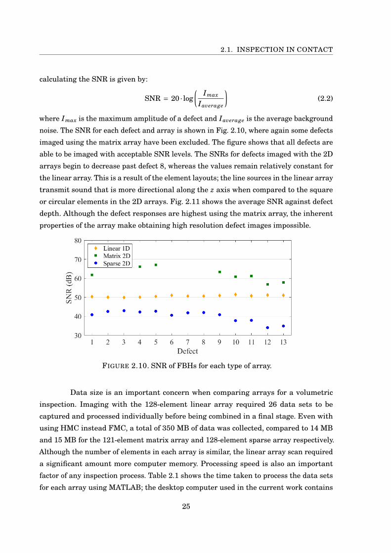
calculating the SNR is given by:
SNR = 20 · log(
Imax
Iaverage
)(2.2)
where Imax is the maximum amplitude of a defect and Iaverage is the average background
noise. The SNR for each defect and array is shown in Fig. 2.10, where again some defects
imaged using the matrix array have been excluded. The figure shows that all defects are
able to be imaged with acceptable SNR levels. The SNRs for defects imaged with the 2D
arrays begin to decrease past defect 8, whereas the values remain relatively constant for
the linear array. This is a result of the element layouts; the line sources in the linear array
transmit sound that is more directional along the z axis when compared to the square
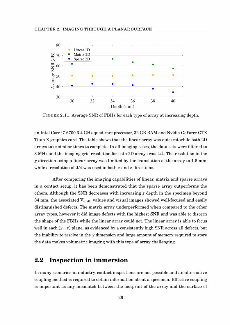
or circular elements in the 2D arrays. Fig. 2.11 shows the average SNR against defect
depth. Although the defect responses are highest using the matrix array, the inherent
properties of the array make obtaining high resolution defect images impossible.
FIGURE 2.10. SNR of FBHs for each type of array.
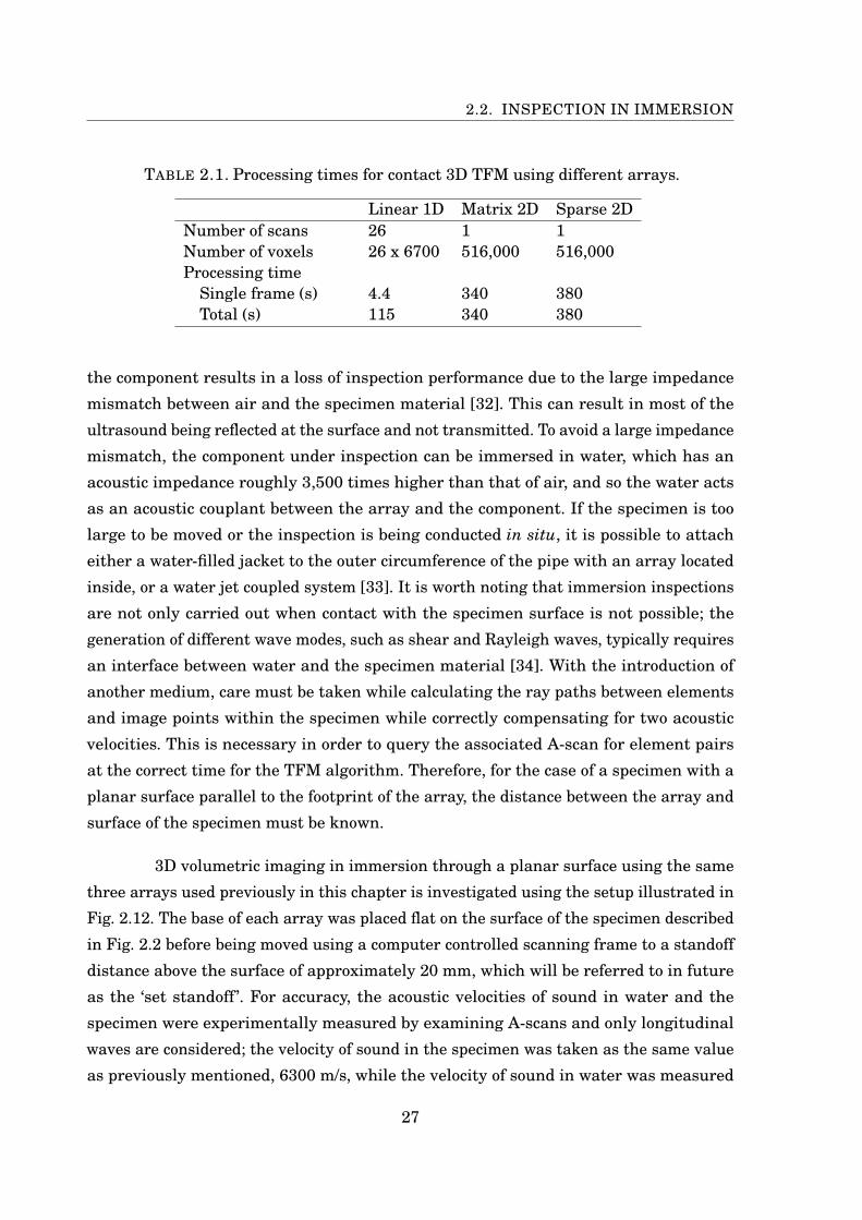
Data size is an important concern when comparing arrays for a volumetric
inspection. Imaging with the 128-element linear array required 26 data sets to be
captured and processed individually before being combined in a final stage. Even with
using HMC instead FMC, a total of 350 MB of data was collected, compared to 14 MB
and 15 MB for the 121-element matrix array and 128-element sparse array respectively.
Although the number of elements in each array is similar, the linear array scan required
a significant amount more computer memory. Processing speed is also an important
factor of any inspection process. Table 2.1 shows the time taken to process the data sets
for each array using MATLAB; the desktop computer used in the current work contains
25
CHAPTER 2. IMAGING THROUGH A PLANAR SURFACE
FIGURE 2.11. Average SNR of FBHs for each type of array at increasing depth.
an Intel Core i7-6700 3.4 GHz quad-core processor, 32 GB RAM and Nvidia GeForce GTX
Titan X graphics card. The table shows that the linear array was quickest while both 2D
arrays take similar times to complete. In all imaging cases, the data sets were filtered to
3 MHz and the imaging grid resolution for both 2D arrays was λ/4. The resolution in the
y direction using a linear array was limited by the translation of the array to 1.5 mm,
while a resolution of λ/4 was used in both x and z directions.
After comparing the imaging capabilities of linear, matrix and sparse arrays
in a contact setup, it has been demonstrated that the sparse array outperforms the
others. Although the SNR decreases with increasing z depth in the specimen beyond
34 mm, the associated V-6 dB values and visual images showed well-focused and easily
distinguished defects. The matrix array underperformed when compared to the other
array types, however it did image defects with the highest SNR and was able to discern
the shape of the FBHs while the linear array could not. The linear array is able to focus
well in each (x− z) plane, as evidenced by a consistently high SNR across all defects, but
the inability to resolve in the y dimension and large amount of memory required to store
the data makes volumetric imaging with this type of array challenging.
2.2 Inspection in immersion
In many scenarios in industry, contact inspections are not possible and an alternative
coupling method is required to obtain information about a specimen. Effective coupling
is important as any mismatch between the footprint of the array and the surface of
26
2.2. INSPECTION IN IMMERSION
TABLE 2.1. Processing times for contact 3D TFM using different arrays.
Linear 1D Matrix 2D Sparse 2DNumber of scans 26 1 1Number of voxels 26 x 6700 516,000 516,000Processing time
Single frame (s) 4.4 340 380Total (s) 115 340 380
the component results in a loss of inspection performance due to the large impedance
mismatch between air and the specimen material [32]. This can result in most of the
ultrasound being reflected at the surface and not transmitted. To avoid a large impedance
mismatch, the component under inspection can be immersed in water, which has an
acoustic impedance roughly 3,500 times higher than that of air, and so the water acts
as an acoustic couplant between the array and the component. If the specimen is too
large to be moved or the inspection is being conducted in situ, it is possible to attach
either a water-filled jacket to the outer circumference of the pipe with an array located
inside, or a water jet coupled system [33]. It is worth noting that immersion inspections
are not only carried out when contact with the specimen surface is not possible; the
generation of different wave modes, such as shear and Rayleigh waves, typically requires
an interface between water and the specimen material [34]. With the introduction of
another medium, care must be taken while calculating the ray paths between elements
and image points within the specimen while correctly compensating for two acoustic
velocities. This is necessary in order to query the associated A-scan for element pairs
at the correct time for the TFM algorithm. Therefore, for the case of a specimen with a
planar surface parallel to the footprint of the array, the distance between the array and
surface of the specimen must be known.
3D volumetric imaging in immersion through a planar surface using the same
three arrays used previously in this chapter is investigated using the setup illustrated in
Fig. 2.12. The base of each array was placed flat on the surface of the specimen described
in Fig. 2.2 before being moved using a computer controlled scanning frame to a standoff
distance above the surface of approximately 20 mm, which will be referred to in future
as the ‘set standoff ’. For accuracy, the acoustic velocities of sound in water and the
specimen were experimentally measured by examining A-scans and only longitudinal
waves are considered; the velocity of sound in the specimen was taken as the same value
as previously mentioned, 6300 m/s, while the velocity of sound in water was measured
27
CHAPTER 2. IMAGING THROUGH A PLANAR SURFACE
FIGURE 2.12. Illustration of experimental setup for immersion inspectionthrough a planar surface.
using pulse-echo A-scans to be 1470 m/s.
2.2.1 Surface measurement and compensation
Measuring the standoff distance of a planar surface is simple once the couplant velocity
is known. In an immersion setup, the largest amplitude in a pulse-echo A-scan, after the
ringdown period, typically corresponds to the reflection from the surface of the specimen
and the time this occurs, t, is easily determined from the peak of the envelope. Using the
velocity of sound in water, ν1, the standoff distance for each element is calculated using:
standoff = 12ν1t (2.3)
where the factor of one half is required as t corresponds to the time taken to travel the
return path between the element and surface. The mean of all standoff values is taken
as the estimated standoff distance.
The easiest method of integrating a surface into the imaging process is to
describe it as a series of discretised points. Alternatively, it could be described as an
28
2.2. INSPECTION IN IMMERSION
equation as in [35], but that is not considered in the current work. When imaging with a
linear array, the surface profile only needs to be represented by a 2D line of (x, z) points
for each array position. For this case, x is defined over a distance equal to the length
of the array and aligned with the central element. The x spacing of surface points is
set as λ1/2, where λ1 is the wavelength of sound in water and was calculated to be 0.49
mm. The z coordinate of each surface point is set equal to the estimated standoff value.
When imaging with a 2D array, a 3D point cloud is required, where the lengths of x and
y are defined as 1.5 times the diameter of the array and spaced using a resolution of
λ1/2; the x and y lengths were arbitrarily chosen to encompass a large volume without
significantly impacting the image processing speed. The z value of each (x, y) point was
set to the estimated standoff distance.
Once the surface profile has been discretised, the next stage is to determine the
path an ultrasonic pulse traverses between an element pair and voxel in the imaging
grid. This process was simple in the contact case, but more complex in immersion. For a
pair of elements and image point within the specimen, the associated surface crossing
points need to be accurately determined to ensure the correct amplitudes are being
summed. A 2D illustration of such a ray path is shown in Fig. 2.13, where AT and AR
represent the position vectors of the surface-crossing points on the transmit and receive
paths respectively, ν2 is the acoustic velocity in the specimen material and the remaining
symbols have been defined previously. The process of determining the locations of AT
and AR is as follows. Firstly, trigonometry is used to calculate the times for a pulse in
water to travel from ET to all of the surface points and the values are stored in an array.
Then the times taken for the pulse to travel from all surface points to the voxel in the
specimen are calculated and stored in the same array. The two times associated with
each surface point are then summed to give the total travel time for a pulse to travel
from ET to P through the surface. Fermat’s principle of least time [36], which states that
path taken by a ray between two points is the path that can be travelled in the least
amount of time, is then used to determine the surface-crossing point. It is the surface
point that yields the absolute minimum time that is taken as AT [37]. The process is
then repeated for ER and P to find the location of AR . The time taken to traverse the
journey from ET to AR via AT , AR and P is then used in the adjusted TFM algorithm
given by:
I (P) =∣∣∣∣∣∑T
∑R
aT,R hT,R
( ||ET −AT ||ν1
+ ||AT −P||ν2
+ ||P−AR ||ν2
+ ||AR −ER ||ν1
)∣∣∣∣∣ , (2.4)
29
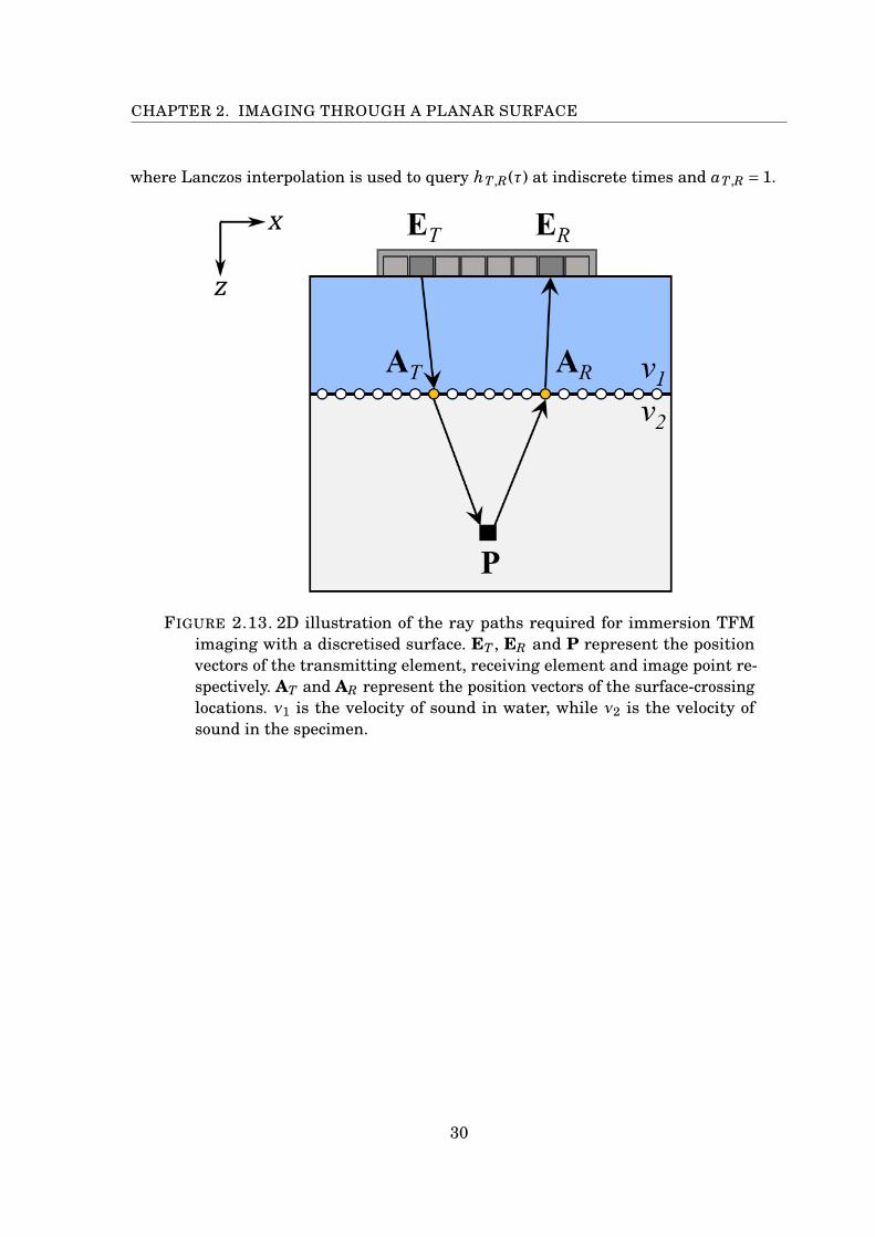
CHAPTER 2. IMAGING THROUGH A PLANAR SURFACE
where Lanczos interpolation is used to query hT,R(τ) at indiscrete times and aT,R = 1.
FIGURE 2.13. 2D illustration of the ray paths required for immersion TFMimaging with a discretised surface. ET , ER and P represent the positionvectors of the transmitting element, receiving element and image point re-spectively. AT and AR represent the position vectors of the surface-crossinglocations. ν1 is the velocity of sound in water, while ν2 is the velocity ofsound in the specimen.
30
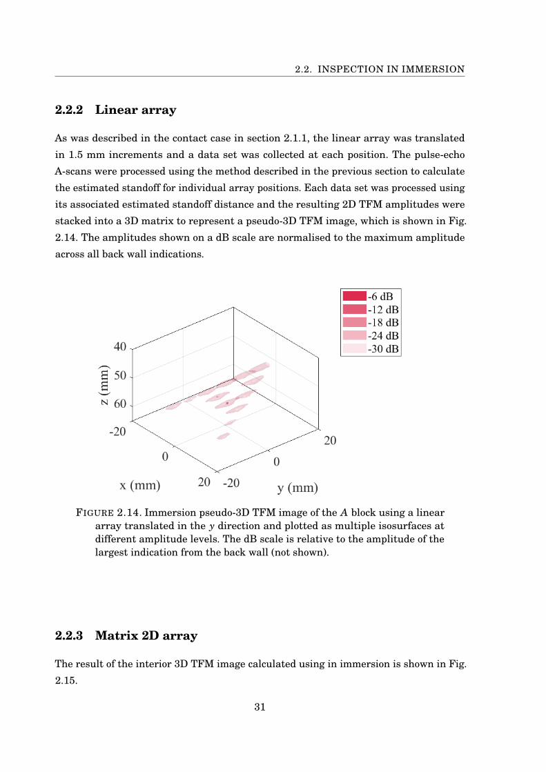
2.2. INSPECTION IN IMMERSION
2.2.2 Linear array
As was described in the contact case in section 2.1.1, the linear array was translated
in 1.5 mm increments and a data set was collected at each position. The pulse-echo
A-scans were processed using the method described in the previous section to calculate
the estimated standoff for individual array positions. Each data set was processed using
its associated estimated standoff distance and the resulting 2D TFM amplitudes were
stacked into a 3D matrix to represent a pseudo-3D TFM image, which is shown in Fig.
2.14. The amplitudes shown on a dB scale are normalised to the maximum amplitude
across all back wall indications.
FIGURE 2.14. Immersion pseudo-3D TFM image of the A block using a lineararray translated in the y direction and plotted as multiple isosurfaces atdifferent amplitude levels. The dB scale is relative to the amplitude of thelargest indication from the back wall (not shown).
2.2.3 Matrix 2D array
The result of the interior 3D TFM image calculated using in immersion is shown in Fig.
2.15.
31
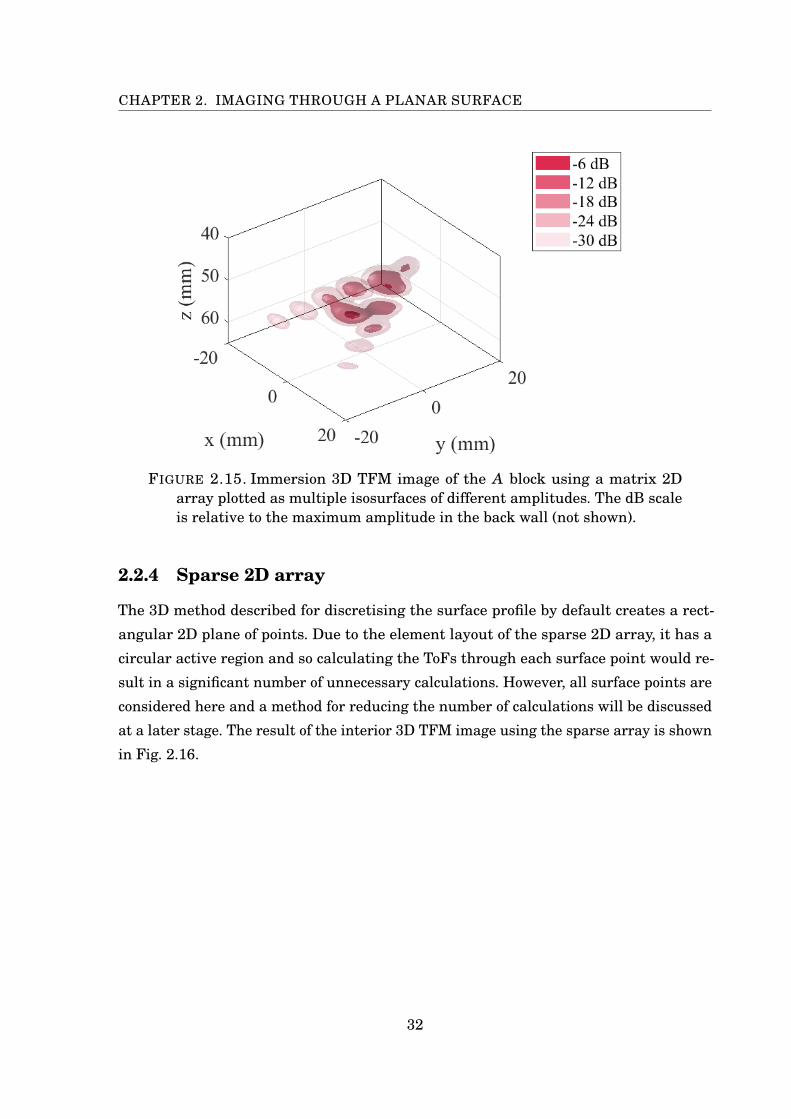
CHAPTER 2. IMAGING THROUGH A PLANAR SURFACE
FIGURE 2.15. Immersion 3D TFM image of the A block using a matrix 2Darray plotted as multiple isosurfaces of different amplitudes. The dB scaleis relative to the maximum amplitude in the back wall (not shown).
2.2.4 Sparse 2D array
The 3D method described for discretising the surface profile by default creates a rect-
angular 2D plane of points. Due to the element layout of the sparse 2D array, it has a
circular active region and so calculating the ToFs through each surface point would re-
sult in a significant number of unnecessary calculations. However, all surface points are
considered here and a method for reducing the number of calculations will be discussed
at a later stage. The result of the interior 3D TFM image using the sparse array is shown
in Fig. 2.16.
32

2.2. INSPECTION IN IMMERSION
FIGURE 2.16. Immersion 3D TFM image of the A block using a sparse 2Darray plotted as multiple isosurfaces of different amplitudes. The dB scaleis relative to the maximum amplitude in the back wall (not shown).
33
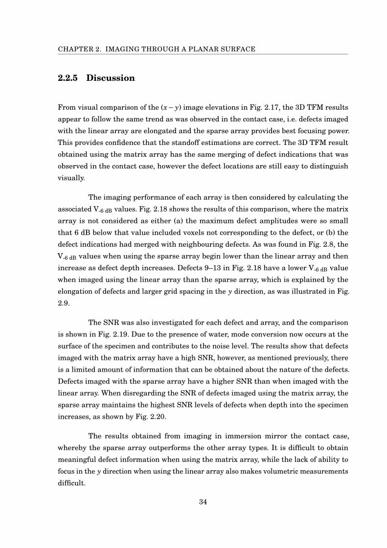
CHAPTER 2. IMAGING THROUGH A PLANAR SURFACE
2.2.5 Discussion
From visual comparison of the (x− y) image elevations in Fig. 2.17, the 3D TFM results
appear to follow the same trend as was observed in the contact case, i.e. defects imaged
with the linear array are elongated and the sparse array provides best focusing power.
This provides confidence that the standoff estimations are correct. The 3D TFM result
obtained using the matrix array has the same merging of defect indications that was
observed in the contact case, however the defect locations are still easy to distinguish
visually.
The imaging performance of each array is then considered by calculating the
associated V-6 dB values. Fig. 2.18 shows the results of this comparison, where the matrix
array is not considered as either (a) the maximum defect amplitudes were so small
that 6 dB below that value included voxels not corresponding to the defect, or (b) the
defect indications had merged with neighbouring defects. As was found in Fig. 2.8, the
V-6 dB values when using the sparse array begin lower than the linear array and then
increase as defect depth increases. Defects 9–13 in Fig. 2.18 have a lower V-6 dB value
when imaged using the linear array than the sparse array, which is explained by the
elongation of defects and larger grid spacing in the y direction, as was illustrated in Fig.
2.9.
The SNR was also investigated for each defect and array, and the comparison
is shown in Fig. 2.19. Due to the presence of water, mode conversion now occurs at the
surface of the specimen and contributes to the noise level. The results show that defects
imaged with the matrix array have a high SNR, however, as mentioned previously, there
is a limited amount of information that can be obtained about the nature of the defects.
Defects imaged with the sparse array have a higher SNR than when imaged with the
linear array. When disregarding the SNR of defects imaged using the matrix array, the
sparse array maintains the highest SNR levels of defects when depth into the specimen
increases, as shown by Fig. 2.20.
The results obtained from imaging in immersion mirror the contact case,
whereby the sparse array outperforms the other array types. It is difficult to obtain
meaningful defect information when using the matrix array, while the lack of ability to
focus in the y direction when using the linear array also makes volumetric measurements
difficult.
34

2.2. INSPECTION IN IMMERSION
(a) (b)
(c)
FIGURE 2.17. (x−z) elevation views of the immersion 3D TFM images in (a) Fig.2.4 using a linear array, (b) Fig. 2.5 using a matrix array and (c) Fig. 2.6using a sparse array. Each image is plotted at multiple isosurfaces relativeto their local maximum in their respective back wall.
With the inclusion of a layer of surface points the total time for the imaging
process increases. This is not as noticeable when imaging with the linear array, however
processing times using a 2D array drastically increases. A comparison of imaging speeds
is given in Table 2.2 where it can be seen that using the same interior grid resolutions as
the contact case, the addition of the layer of surface points has a significant impact on
35
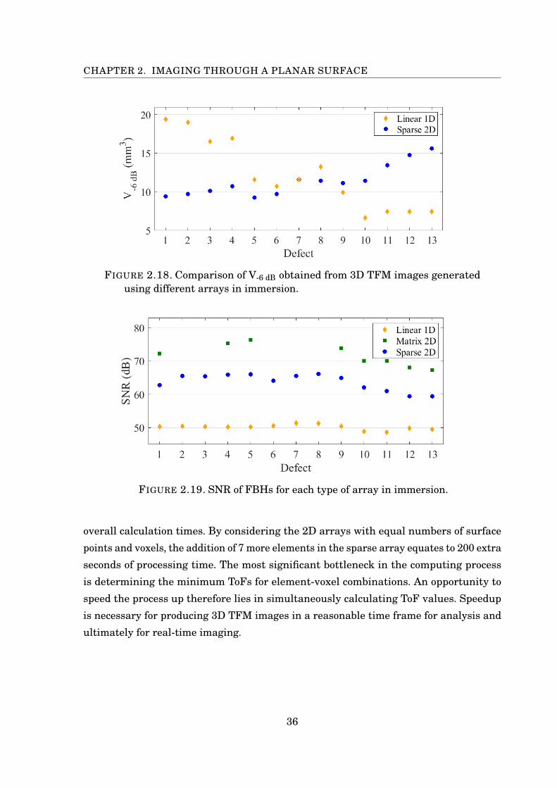
CHAPTER 2. IMAGING THROUGH A PLANAR SURFACE
FIGURE 2.18. Comparison of V-6 dB obtained from 3D TFM images generatedusing different arrays in immersion.
FIGURE 2.19. SNR of FBHs for each type of array in immersion.
overall calculation times. By considering the 2D arrays with equal numbers of surface
points and voxels, the addition of 7 more elements in the sparse array equates to 200 extra
seconds of processing time. The most significant bottleneck in the computing process
is determining the minimum ToFs for element-voxel combinations. An opportunity to
speed the process up therefore lies in simultaneously calculating ToF values. Speedup
is necessary for producing 3D TFM images in a reasonable time frame for analysis and
ultimately for real-time imaging.
36
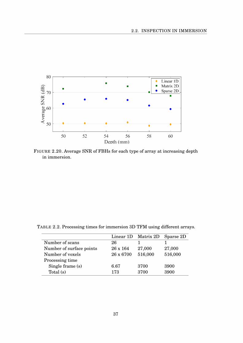
2.2. INSPECTION IN IMMERSION
FIGURE 2.20. Average SNR of FBHs for each type of array at increasing depthin immersion.
TABLE 2.2. Processing times for immersion 3D TFM using different arrays.
Linear 1D Matrix 2D Sparse 2DNumber of scans 26 1 1Number of surface points 26 x 164 27,000 27,000Number of voxels 26 x 6700 516,000 516,000Processing time
Single frame (s) 6.67 3700 3900Total (s) 173 3700 3900
37
CHAPTER 2. IMAGING THROUGH A PLANAR SURFACE
2.3 Summary
An investigative comparison of using linear and 2D arrays for 3D volumetric imaging
has been investigated in this chapter. The results have shown that in order to obtain
high quality, accurate images of the inside of a specimen, using a 2D array is optimal due
to its ability to focus across two axes. The effect that the element layout in a 2D array
has on imaging ability was also investigated; the results confirmed that the sparse array
with elements arranged in a Poisson disk formation outperforms the matrix array with
elements arranged in a grid. In both contact and immersion setups, the sparse array
imaged defects with high SNR and low V-6 dB values, and will therefore be the only type
of array used in the following chapters. Processing speed is a concern when generating
3D images, as ultimately real-time imaging is desirable for inspections. The results have
shown that imaging in contact can be conducted in reasonable time frames, but imaging
in immersion is significantly slower when using 2D arrays. Linear arrays in immersion
provide faster imaging speeds, but at the cost of lower defect resolution and larger data
files. When considering 3D imaging with a 2D array it is therefore necessary to optimise
the calculations to complete in a reasonable time and a method used to improve imaging
speeds will be discussed in the following chapter. Additionally, the surface considered
here was planar and parallel to the array, so pulse-echo signals were used to determine
the standoff distance. The ability of 2D arrays to focus accurately through non-planar
surfaces is highly relevant to industry and is therefore also investigated in the following
chapter.
38
Chapter 3
Imaging through a non-planarsurface
In many industrial inspection scenarios, ultrasonic imaging needs to be conducted
through surfaces which are non-planar. Components with non-planar geometries are
commonly found in modern structures, particularly in the power generation sector where
thousands of pipes are interconnected. Pipework branches and pressure vessel nozzles
are of particular interest due to the high stress and risk of failure in these regions. If
corrections are not made for varying surface profiles, loss of the original focus point can
occur and inaccurate TFM images will be obtained [32]. Even minor surface errors can
result in a significant loss of final image quality, so it is extremely important that an
accurate depiction of the surface profile is obtained.
This chapter introduces a method for extracting a 3D surface profile from a
non-planar specimen using a TFM-based imaging method. The discretised surface is then
used to generate an internal 3D TFM image. The computational challenges associated
with 3D imaging and the use of GPU programming is also discussed.
3.1 Non-planar surface compensation methods
Many factors need to be taken into account when designing the inspection setup for
complex surfaces. Firstly, to maximise the transmission of sound energy, close to normal
incidence of the sound wave to the surface is desirable. However, for non-planar surfaces
this is not always possible and the array may need to be moved or rotated during
39
CHAPTER 3. IMAGING THROUGH A NON-PLANAR SURFACE
inspections and multiple sets of data collected. As was discussed in the previous chapter,
coupling between the array and surface profile is crucial for transmission of ultrasonic
energy. There are currently three main approaches to tackle this coupling problem.
The first of these involves using a liquid, such as water, to couple a rigid array
to the surface of the component under inspection. The liquid acts as an acoustic couplant
between the array and the component and the surface profile can be extracted from the
ultrasonic data using an imaging algorithm. This is an effective method when there is no
previous knowledge of the surface [5, 38, 39]. In a previous study, a 2D array was used
to generate 3D images in immersion [40]; however, in this case the test specimen had a
planar surface and determining the surface position from the data is straightforward. A
similar method to this was used for immersion imaging in the previous chapter.
A second approach involves fitting the array with a wedge that complements
the surface geometry [41], however, each wedge is only suited to a single, known surface
profile and so multiple wedges may need to be constructed for the inspection of a complex
component. Wedges are commonly used in industry but are unable to be applied to a
wide range of imaging setups and are therefore not considered in the current work. A
lesser-used hybrid method of these two previous approaches has also been considered,
which involves the use of a membrane-coupled phased array device. The membrane can
either be a water-filled, low-loss membrane attached to a standard linear 1D phased
array which then conforms to the surface profile [42, 43], or a silicone-based coupling
pad [44].
The final approach involves the use of a flexible contact array, of which there are
two types: the first is a linear array where each element is able to move perpendicularly
as the array is translated across the surface [45–47], while the second is constructed
using flexible composite material that moulds to the surface [48]. As the first type of
flexible array can only adapt in one dimension, it can not be applied to elbows and nozzles
and is therefore unable to be applied to this research. Like wedges, the composite arrays
are designed with a specific application in mind and are not suitable for all applications.
Throughout this thesis all non-contact inspections use the setup described in
the first method, whereby water is used as the acoustic couplant.
40
3.2. SINGLY AND DOUBLY CURVED SURFACES
3.2 Singly and doubly curved surfaces
The types of non-planar surfaces focused on in this thesis are smooth and curved, of which
there are two categories: singly curved and doubly curved. Both represent geometries
that are routinely inspected in industry and hence their relevance to the current work.
Singly curved, or developable, surfaces have zero Gaussian curvature every-
where and can be created by transforming a plane without causing stretching, cutting
or wrinkling. The tangential plane touches surfaces of this type by a line. Pipes are
examples of this surface as they can be ‘unrolled’ into a plane. As there is curvature in
only one principal axis, the use of linear arrays is sufficient to obtain well-focused planar
images. However, using this type of array means that resolution in the out-of-plane
direction is limited. An illustration of a singly curved surface and a tangenial plane is
shown in Fig. 3.1(a).
Doubly curved, or non-developable, surfaces describe the majority of smooth
surfaces and have non-zero Gaussian curvature across their surface; every point on
the surface has an associated tangential plane. As mentioned in the project motivation,
pipework branches and pressure vessel nozzles are relevant examples of this type of
surface. Linear arrays are unable to focus efficiently through surfaces of this nature due
to the curvature in both principal axis, and a 2D array becomes necessary for imaging.
An illustration of a pipework branch is illustrated in Fig. 3.1(b), where a surface normal
point is shown on the doubly curved region.
3.3 GPU parallel computing
When considering 2D TFM imaging, the central processing unit (CPU) of a desktop PC
can process data at adequate speeds; however with the inclusion of a third dimension,
as is the case in 3D TFM imaging, the number of voxels in the final image increases
drastically. The calculations and images in the previous chapter were processed using
the MATLAB computing software, with image processing times in excess of an hour
using a 2D array in immersion. This process is slow in MATLAB as the ToF calculation
for each element and voxel pair is calculated in series, which is a serious limitation
when 3D imaging is considered. As each calculation is independent of the others, i.e. the
distance between an element and voxel does not depend on other elements or voxels, a
huge opportunity to speed up the process lies in parallelisation [49].
41
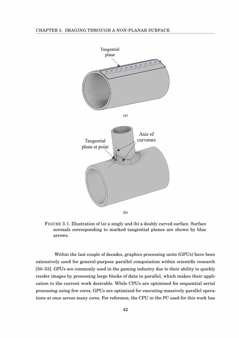
CHAPTER 3. IMAGING THROUGH A NON-PLANAR SURFACE
(a)
(b)
FIGURE 3.1. Illustration of (a) a singly and (b) a doubly curved surface. Surfacenormals corresponding to marked tangential planes are shown by bluearrows.
Within the last couple of decades, graphics processing units (GPUs) have been
extensively used for general-purpose parallel computation within scientific research
[50–53]. GPUs are commonly used in the gaming industry due to their ability to quickly
render images by processing large blocks of data in parallel, which makes their appli-
cation to the current work desirable. While CPUs are optimised for sequential serial
processing using few cores, GPUs are optimised for executing massively parallel opera-
tions at once across many cores. For reference, the CPU in the PC used for this work has
42
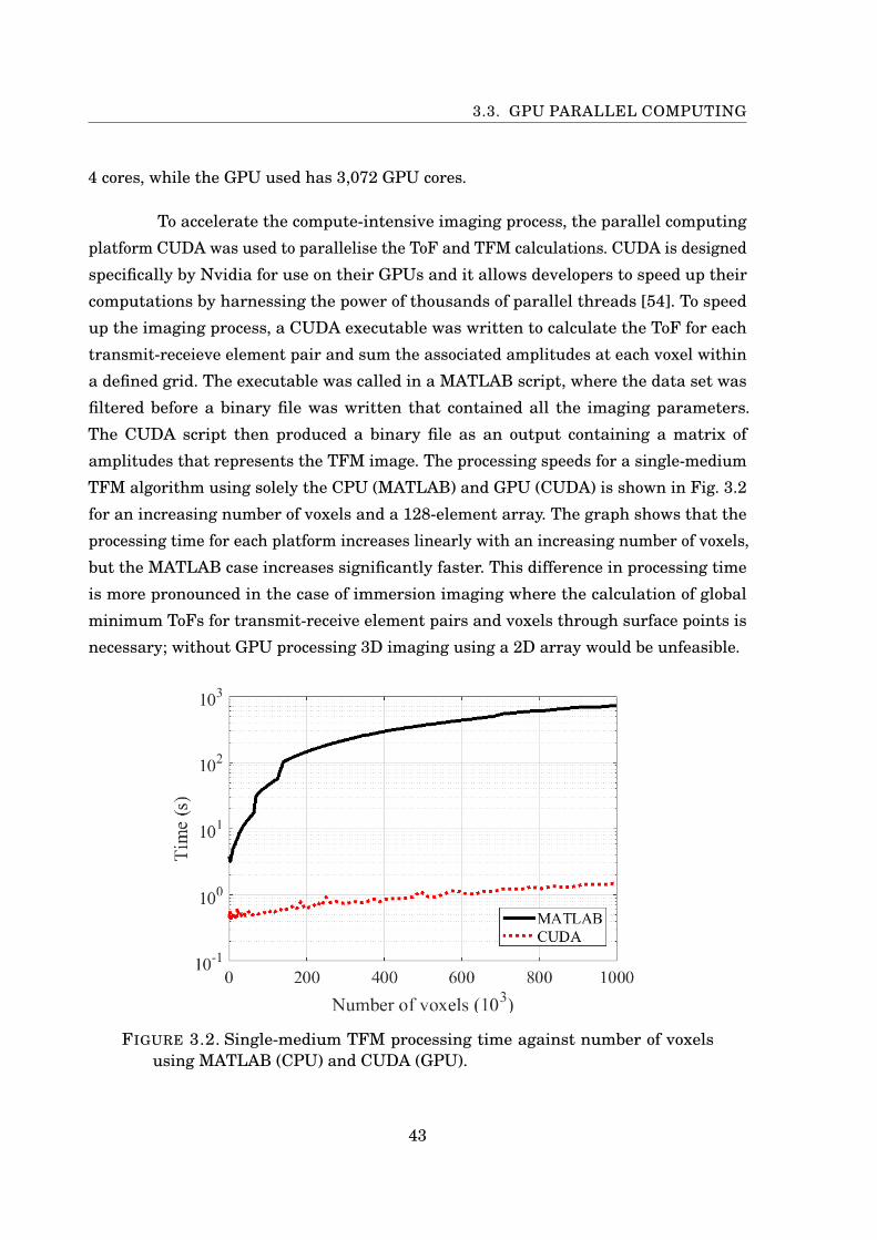
3.3. GPU PARALLEL COMPUTING
4 cores, while the GPU used has 3,072 GPU cores.
To accelerate the compute-intensive imaging process, the parallel computing
platform CUDA was used to parallelise the ToF and TFM calculations. CUDA is designed
specifically by Nvidia for use on their GPUs and it allows developers to speed up their
computations by harnessing the power of thousands of parallel threads [54]. To speed
up the imaging process, a CUDA executable was written to calculate the ToF for each
transmit-receieve element pair and sum the associated amplitudes at each voxel within
a defined grid. The executable was called in a MATLAB script, where the data set was
filtered before a binary file was written that contained all the imaging parameters.
The CUDA script then produced a binary file as an output containing a matrix of
amplitudes that represents the TFM image. The processing speeds for a single-medium
TFM algorithm using solely the CPU (MATLAB) and GPU (CUDA) is shown in Fig. 3.2
for an increasing number of voxels and a 128-element array. The graph shows that the
processing time for each platform increases linearly with an increasing number of voxels,
but the MATLAB case increases significantly faster. This difference in processing time
is more pronounced in the case of immersion imaging where the calculation of global
minimum ToFs for transmit-receive element pairs and voxels through surface points is
necessary; without GPU processing 3D imaging using a 2D array would be unfeasible.
FIGURE 3.2. Single-medium TFM processing time against number of voxelsusing MATLAB (CPU) and CUDA (GPU).
43
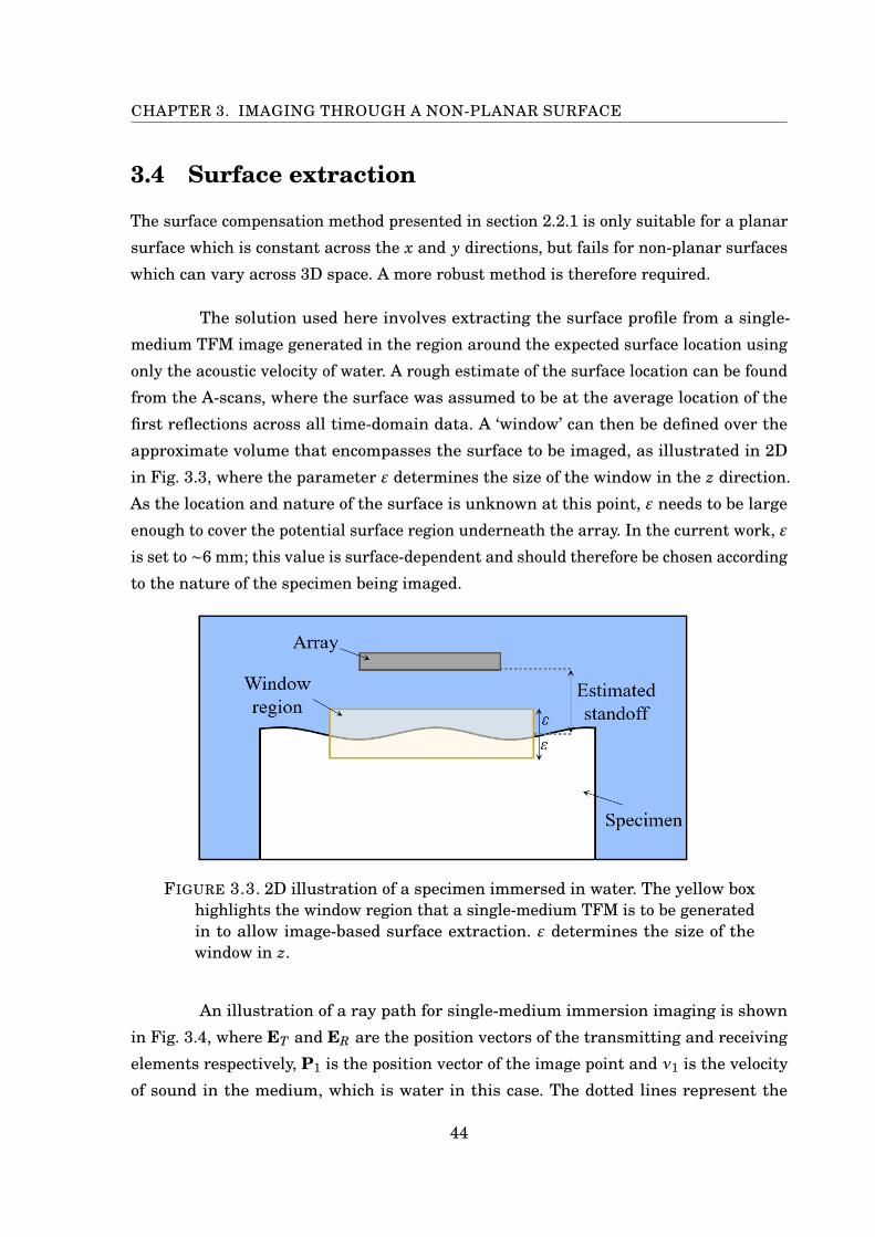
CHAPTER 3. IMAGING THROUGH A NON-PLANAR SURFACE
3.4 Surface extraction
The surface compensation method presented in section 2.2.1 is only suitable for a planar
surface which is constant across the x and y directions, but fails for non-planar surfaces
which can vary across 3D space. A more robust method is therefore required.
The solution used here involves extracting the surface profile from a single-
medium TFM image generated in the region around the expected surface location using
only the acoustic velocity of water. A rough estimate of the surface location can be found
from the A-scans, where the surface was assumed to be at the average location of the
first reflections across all time-domain data. A ‘window’ can then be defined over the
approximate volume that encompasses the surface to be imaged, as illustrated in 2D
in Fig. 3.3, where the parameter ε determines the size of the window in the z direction.
As the location and nature of the surface is unknown at this point, ε needs to be large
enough to cover the potential surface region underneath the array. In the current work, ε
is set to ∼6 mm; this value is surface-dependent and should therefore be chosen according
to the nature of the specimen being imaged.
FIGURE 3.3. 2D illustration of a specimen immersed in water. The yellow boxhighlights the window region that a single-medium TFM is to be generatedin to allow image-based surface extraction. ε determines the size of thewindow in z.
An illustration of a ray path for single-medium immersion imaging is shown
in Fig. 3.4, where ET and ER are the position vectors of the transmitting and receiving
elements respectively, P1 is the position vector of the image point and ν1 is the velocity
of sound in the medium, which is water in this case. The dotted lines represent the
44
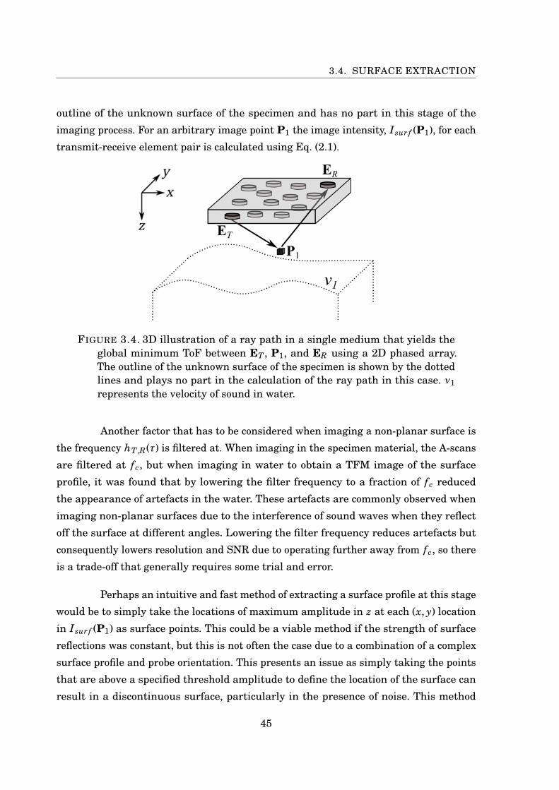
3.4. SURFACE EXTRACTION
outline of the unknown surface of the specimen and has no part in this stage of the
imaging process. For an arbitrary image point P1 the image intensity, Isur f (P1), for each
transmit-receive element pair is calculated using Eq. (2.1).
FIGURE 3.4. 3D illustration of a ray path in a single medium that yields theglobal minimum ToF between ET , P1, and ER using a 2D phased array.The outline of the unknown surface of the specimen is shown by the dottedlines and plays no part in the calculation of the ray path in this case. ν1represents the velocity of sound in water.
Another factor that has to be considered when imaging a non-planar surface is
the frequency hT,R(τ) is filtered at. When imaging in the specimen material, the A-scans
are filtered at fc, but when imaging in water to obtain a TFM image of the surface
profile, it was found that by lowering the filter frequency to a fraction of fc reduced
the appearance of artefacts in the water. These artefacts are commonly observed when
imaging non-planar surfaces due to the interference of sound waves when they reflect
off the surface at different angles. Lowering the filter frequency reduces artefacts but
consequently lowers resolution and SNR due to operating further away from fc, so there
is a trade-off that generally requires some trial and error.
Perhaps an intuitive and fast method of extracting a surface profile at this stage
would be to simply take the locations of maximum amplitude in z at each (x, y) location
in Isur f (P1) as surface points. This could be a viable method if the strength of surface
reflections was constant, but this is not often the case due to a combination of a complex
surface profile and probe orientation. This presents an issue as simply taking the points
that are above a specified threshold amplitude to define the location of the surface can
result in a discontinuous surface, particularly in the presence of noise. This method
45

CHAPTER 3. IMAGING THROUGH A NON-PLANAR SURFACE
of extracting a surface was used in a previous study [38], where linear interpolation
was used to bridge gaps between locations of surface image points above a threshold.
However, in that work a linear array and 2D TFM image was considered, and it would be
difficult to apply to the current work as the surface curves throughout 3D space. A more
sophisticated, two-pass surface extraction process is therefore required. This process is
outlined as follows.
A discrete point in the imaging grid is defined as Pi jk = (xi, yj, zk
), where xi
denotes equally spaced points in x, and similarly for yj and zk. The image amplitude at
this point is then obtained by I i jk =∣∣Isur f
(Pi jk
)∣∣. The first step of the extraction process
is to find the indices (i, j,k)= (I, J,K) of the location of the maximum amplitude in the
TFM image using:
(I, J,K) = argmax(i, j,k)
I i jk (3.1)
and therefore PIJK = (xI , yJ , zK ) is taken as the first point of the extraction process.
Let Z(1)i j denote the 3D surface points that are to be determined. The first surface point
obtained in Z(1)i j is the value of the z coordinate at the position of the global maximum
found above:
Z(1)IJ = zK . (3.2)
In the first pass, the primary and secondary directions are x and y respectively.
The 2D (x− z) plane through yJ is examined first by working out from (i, j) = (I, J) in
the primary direction. The next surface point in the x direction, i.e. Z(1)(I+1)J , is found by
fitting a spline, ξ(z), to the image amplitudes I(I+1)JK , at k-indices that satisfy
Z(1)IJ − δz ≤ zk ≤ Z(1)
IJ + δz, (3.3)
where δz is a predefined tolerance parameter, in this case set to approximately 1.2λ1,
where λ1 is the wavelength of sound in water that was calculated to be approximately
0.49 mm. If the maximum of ξ(z) exceeds a predefined threshold, defined as 10 dB below
I IJK , then the z coordinate of the next surface point is defined as:
Z(1)(I+1)J = argmax
zξ(z), (3.4)
with the procedure shown in Fig. 3.5. If no value is found in the range of Eq. (3.3) that
satisfies the amplitude threshold, the surface point at Z(1)(I+1)J is defined as absent and
46
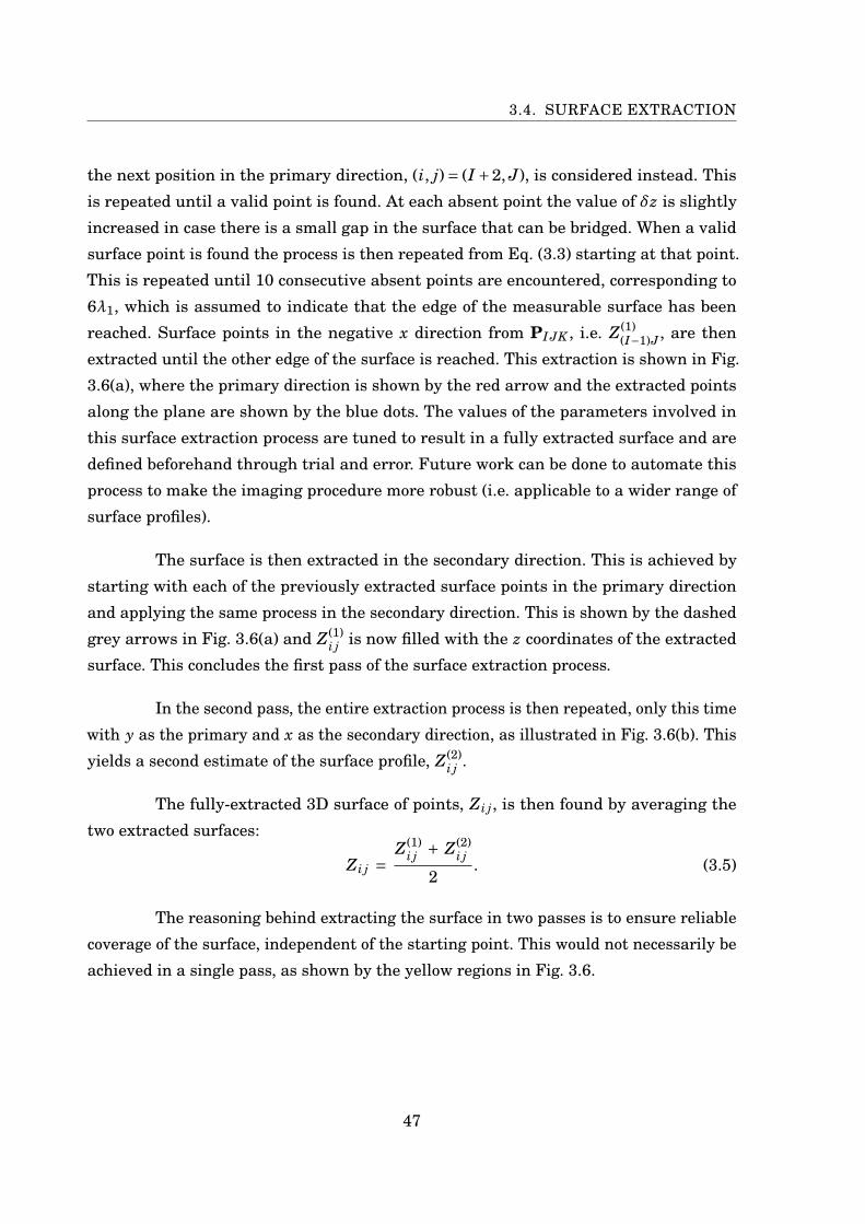
3.4. SURFACE EXTRACTION
the next position in the primary direction, (i, j)= (I +2, J), is considered instead. This
is repeated until a valid point is found. At each absent point the value of δz is slightly
increased in case there is a small gap in the surface that can be bridged. When a valid
surface point is found the process is then repeated from Eq. (3.3) starting at that point.
This is repeated until 10 consecutive absent points are encountered, corresponding to
6λ1, which is assumed to indicate that the edge of the measurable surface has been
reached. Surface points in the negative x direction from PIJK , i.e. Z(1)(I−1)J , are then
extracted until the other edge of the surface is reached. This extraction is shown in Fig.
3.6(a), where the primary direction is shown by the red arrow and the extracted points
along the plane are shown by the blue dots. The values of the parameters involved in
this surface extraction process are tuned to result in a fully extracted surface and are
defined beforehand through trial and error. Future work can be done to automate this
process to make the imaging procedure more robust (i.e. applicable to a wider range of
surface profiles).
The surface is then extracted in the secondary direction. This is achieved by
starting with each of the previously extracted surface points in the primary direction
and applying the same process in the secondary direction. This is shown by the dashed
grey arrows in Fig. 3.6(a) and Z(1)i j is now filled with the z coordinates of the extracted
surface. This concludes the first pass of the surface extraction process.
In the second pass, the entire extraction process is then repeated, only this time
with y as the primary and x as the secondary direction, as illustrated in Fig. 3.6(b). This
yields a second estimate of the surface profile, Z(2)i j .
The fully-extracted 3D surface of points, Zi j, is then found by averaging the
two extracted surfaces:
Zi j =Z(1)
i j + Z(2)i j
2. (3.5)
The reasoning behind extracting the surface in two passes is to ensure reliable
coverage of the surface, independent of the starting point. This would not necessarily be
achieved in a single pass, as shown by the yellow regions in Fig. 3.6.
47
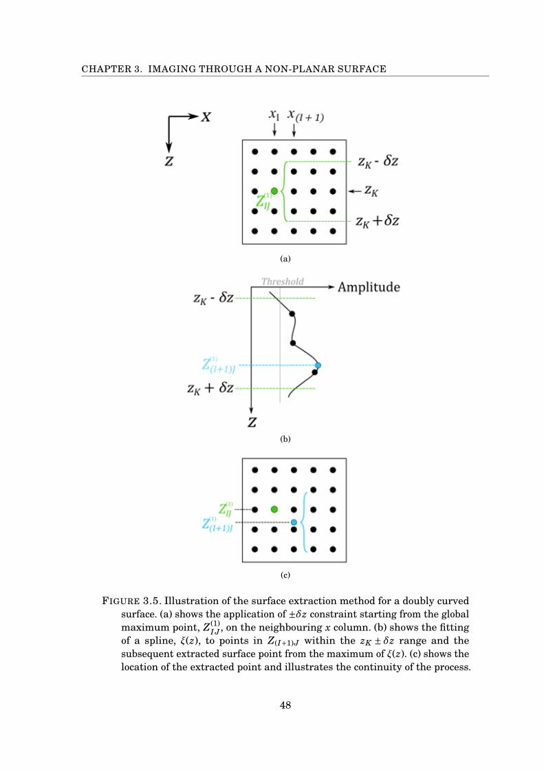
CHAPTER 3. IMAGING THROUGH A NON-PLANAR SURFACE
(a)
(b)
(c)
FIGURE 3.5. Illustration of the surface extraction method for a doubly curvedsurface. (a) shows the application of ±δz constraint starting from the globalmaximum point, Z(1)
IJ , on the neighbouring x column. (b) shows the fittingof a spline, ξ(z), to points in Z(I+1)J within the zK ± δz range and thesubsequent extracted surface point from the maximum of ξ(z). (c) shows thelocation of the extracted point and illustrates the continuity of the process.
48
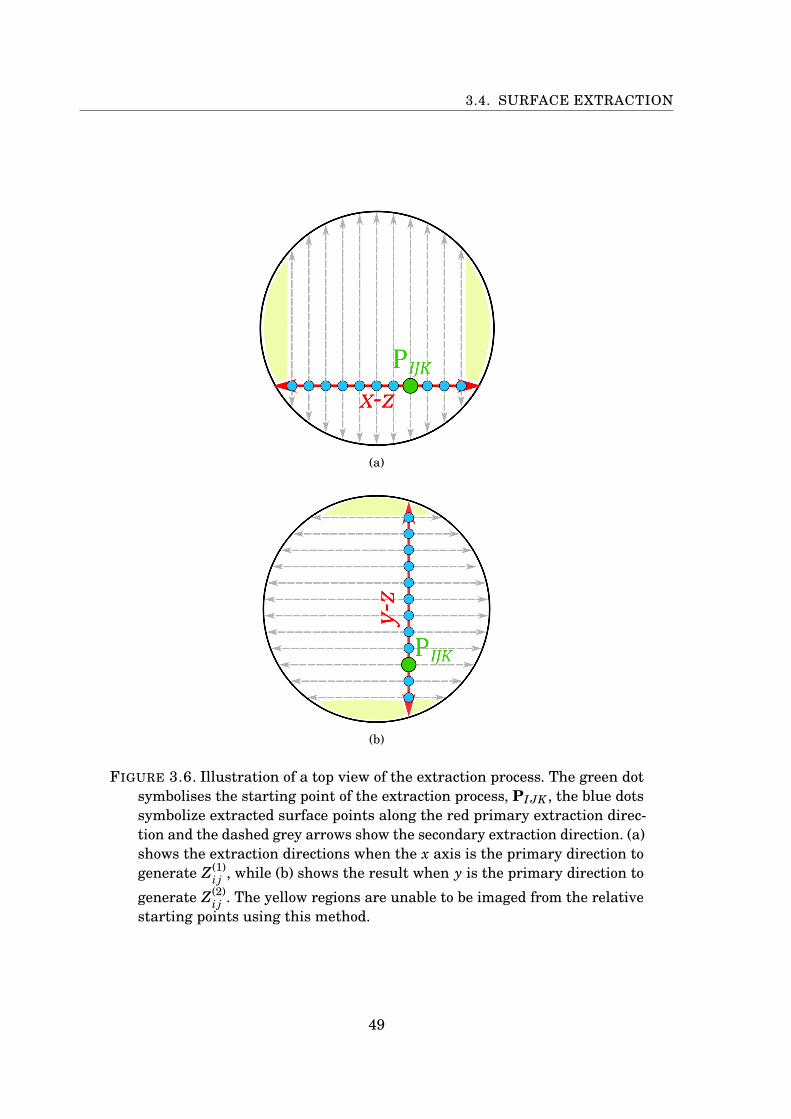
3.4. SURFACE EXTRACTION
(a)
(b)
FIGURE 3.6. Illustration of a top view of the extraction process. The green dotsymbolises the starting point of the extraction process, PIJK , the blue dotssymbolize extracted surface points along the red primary extraction direc-tion and the dashed grey arrows show the secondary extraction direction. (a)shows the extraction directions when the x axis is the primary direction togenerate Z(1)
i j , while (b) shows the result when y is the primary direction to
generate Z(2)i j . The yellow regions are unable to be imaged from the relative
starting points using this method.
49
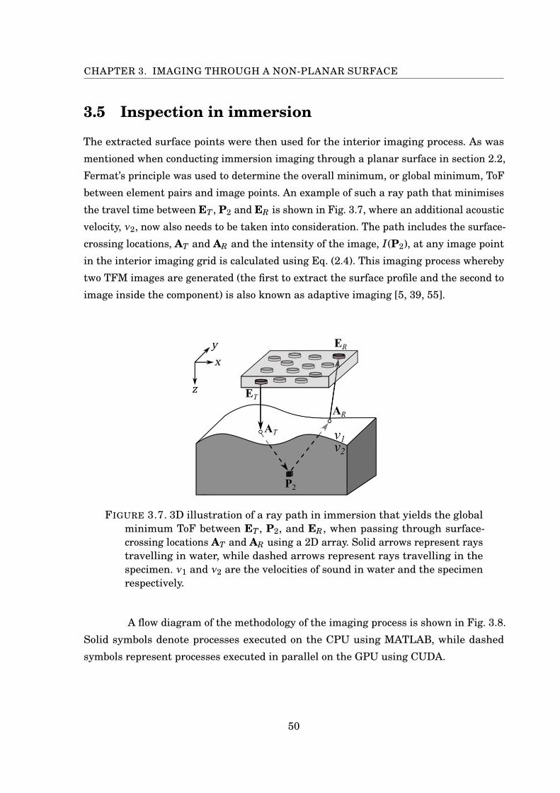
CHAPTER 3. IMAGING THROUGH A NON-PLANAR SURFACE
3.5 Inspection in immersion
The extracted surface points were then used for the interior imaging process. As was
mentioned when conducting immersion imaging through a planar surface in section 2.2,
Fermat’s principle was used to determine the overall minimum, or global minimum, ToF
between element pairs and image points. An example of such a ray path that minimises
the travel time between ET , P2 and ER is shown in Fig. 3.7, where an additional acoustic
velocity, ν2, now also needs to be taken into consideration. The path includes the surface-
crossing locations, AT and AR and the intensity of the image, I(P2), at any image point
in the interior imaging grid is calculated using Eq. (2.4). This imaging process whereby
two TFM images are generated (the first to extract the surface profile and the second to
image inside the component) is also known as adaptive imaging [5, 39, 55].
FIGURE 3.7. 3D illustration of a ray path in immersion that yields the globalminimum ToF between ET , P2, and ER, when passing through surface-crossing locations AT and AR using a 2D array. Solid arrows represent raystravelling in water, while dashed arrows represent rays travelling in thespecimen. ν1 and ν2 are the velocities of sound in water and the specimenrespectively.
A flow diagram of the methodology of the imaging process is shown in Fig. 3.8.
Solid symbols denote processes executed on the CPU using MATLAB, while dashed
symbols represent processes executed in parallel on the GPU using CUDA.
50
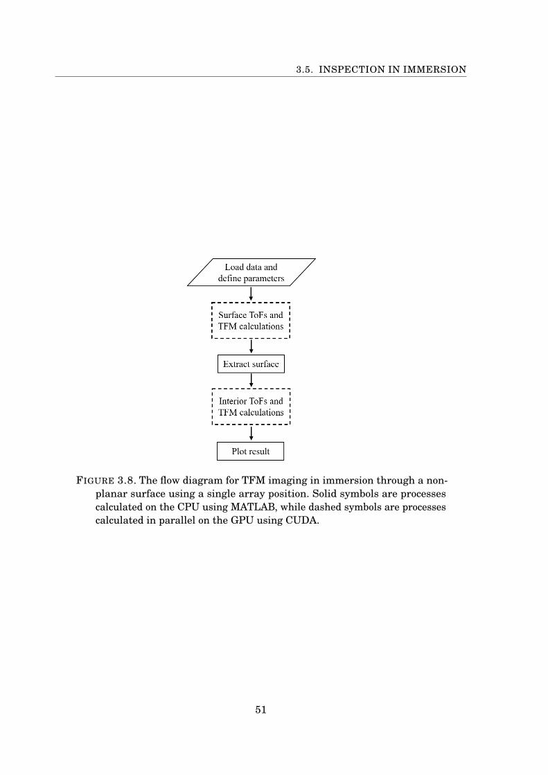
3.5. INSPECTION IN IMMERSION
FIGURE 3.8. The flow diagram for TFM imaging in immersion through a non-planar surface using a single array position. Solid symbols are processescalculated on the CPU using MATLAB, while dashed symbols are processescalculated in parallel on the GPU using CUDA.
51
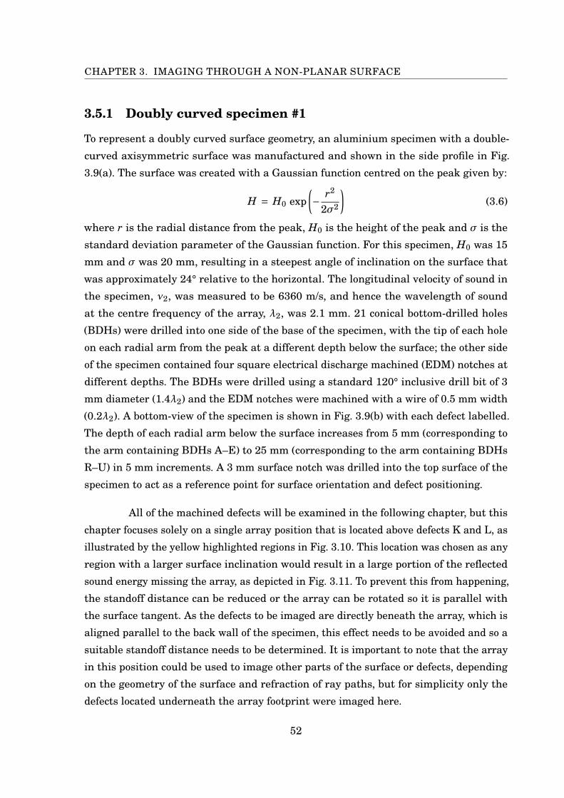
CHAPTER 3. IMAGING THROUGH A NON-PLANAR SURFACE
3.5.1 Doubly curved specimen #1
To represent a doubly curved surface geometry, an aluminium specimen with a double-
curved axisymmetric surface was manufactured and shown in the side profile in Fig.
3.9(a). The surface was created with a Gaussian function centred on the peak given by:
H = H0 exp(− r2
2σ2
)(3.6)
where r is the radial distance from the peak, H0 is the height of the peak and σ is the
standard deviation parameter of the Gaussian function. For this specimen, H0 was 15
mm and σ was 20 mm, resulting in a steepest angle of inclination on the surface that
was approximately 24° relative to the horizontal. The longitudinal velocity of sound in
the specimen, ν2, was measured to be 6360 m/s, and hence the wavelength of sound
at the centre frequency of the array, λ2, was 2.1 mm. 21 conical bottom-drilled holes
(BDHs) were drilled into one side of the base of the specimen, with the tip of each hole
on each radial arm from the peak at a different depth below the surface; the other side
of the specimen contained four square electrical discharge machined (EDM) notches at
different depths. The BDHs were drilled using a standard 120° inclusive drill bit of 3
mm diameter (1.4λ2) and the EDM notches were machined with a wire of 0.5 mm width
(0.2λ2). A bottom-view of the specimen is shown in Fig. 3.9(b) with each defect labelled.
The depth of each radial arm below the surface increases from 5 mm (corresponding to
the arm containing BDHs A–E) to 25 mm (corresponding to the arm containing BDHs
R–U) in 5 mm increments. A 3 mm surface notch was drilled into the top surface of the
specimen to act as a reference point for surface orientation and defect positioning.
All of the machined defects will be examined in the following chapter, but this
chapter focuses solely on a single array position that is located above defects K and L, as
illustrated by the yellow highlighted regions in Fig. 3.10. This location was chosen as any
region with a larger surface inclination would result in a large portion of the reflected
sound energy missing the array, as depicted in Fig. 3.11. To prevent this from happening,
the standoff distance can be reduced or the array can be rotated so it is parallel with
the surface tangent. As the defects to be imaged are directly beneath the array, which is
aligned parallel to the back wall of the specimen, this effect needs to be avoided and so a
suitable standoff distance needs to be determined. It is important to note that the array
in this position could be used to image other parts of the surface or defects, depending
on the geometry of the surface and refraction of ray paths, but for simplicity only the
defects located underneath the array footprint were imaged here.
52
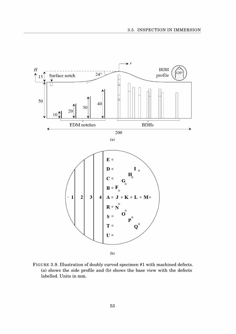
3.5. INSPECTION IN IMMERSION
(a)
(b)
FIGURE 3.9. Illustration of doubly curved specimen #1 with machined defects.(a) shows the side profile and (b) shows the base view with the defectslabelled. Units in mm.
53
CHAPTER 3. IMAGING THROUGH A NON-PLANAR SURFACE
A schematic diagram of the experimental setup is shown in Fig. 3.12, where
the array mounting has three degrees of freedom and is connected to a motor. Firstly,
the velocity of sound in water, ν1, was measured to be 1470 m/s which corresponded to
a wavelength, λ1, of 0.49 mm. To initialise the scan, the specimen was submerged in
water and the array was mounted and aligned parallel to the back wall of the specimen
using a B-scan image obtained over the flat region of the surface. The array was then
set to a standoff distance of 13 mm above the peak of the specimen, before being moved
to the correct location for imaging defects K and L. A HMC data set was captured with
10 averages, then filtered and Hilbert transformed using a Gaussian window function
centred at fc/3 with a -40 dB half bandwidth of 90% of fc/3.
3.5.2 Results
The result of applying the single-medium 3D TFM algorithm to the captured data set is
shown in Fig. 3.13(a) as multiple isosurfaces plotted relative to the maximum surface
amplitude, where the array is located at z = 0 mm. The method described in section 3.4 is
then applied to extract a discretised estimate of the surface profile, shown in Fig. 3.13(b)
as a surface plot.
The interior 3D TFM image obtained by using Eq. (2.4) is shown in Fig. 3.14.
Fig. 3.14(a) shows defects K and L and the back wall of the specimen, while Fig. 3.14(b)
shows a zoomed in region around the defects. Defect K is located in positive y and defect
L is in negative y.
54
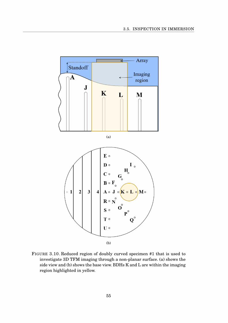
3.5. INSPECTION IN IMMERSION
(a)
(b)
FIGURE 3.10. Reduced region of doubly curved specimen #1 that is used toinvestigate 3D TFM imaging through a non-planar surface. (a) shows theside view and (b) shows the base view. BDHs K and L are within the imagingregion highlighted in yellow.
55
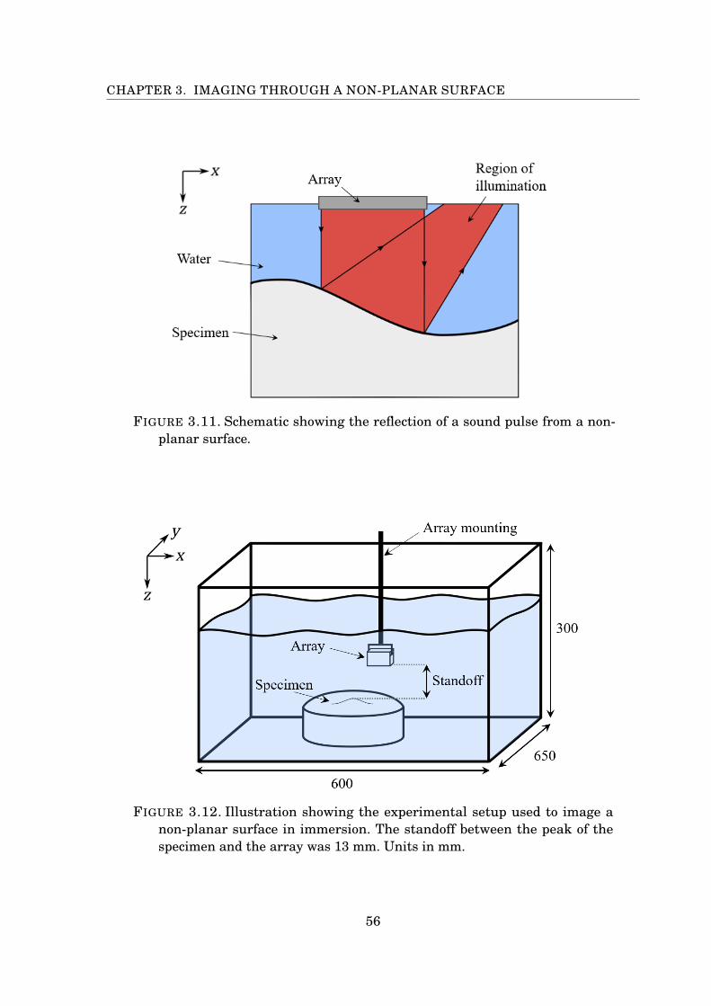
CHAPTER 3. IMAGING THROUGH A NON-PLANAR SURFACE
FIGURE 3.11. Schematic showing the reflection of a sound pulse from a non-planar surface.
FIGURE 3.12. Illustration showing the experimental setup used to image anon-planar surface in immersion. The standoff between the peak of thespecimen and the array was 13 mm. Units in mm.
56
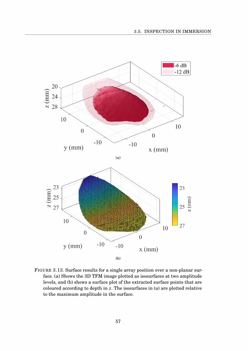
3.5. INSPECTION IN IMMERSION
(a)
(b)
FIGURE 3.13. Surface results for a single array position over a non-planar sur-face. (a) Shows the 3D TFM image plotted as isosurfaces at two amplitudelevels, and (b) shows a surface plot of the extracted surface points that arecoloured according to depth in z. The isosurfaces in (a) are plotted relativeto the maximum amplitude in the surface.
57
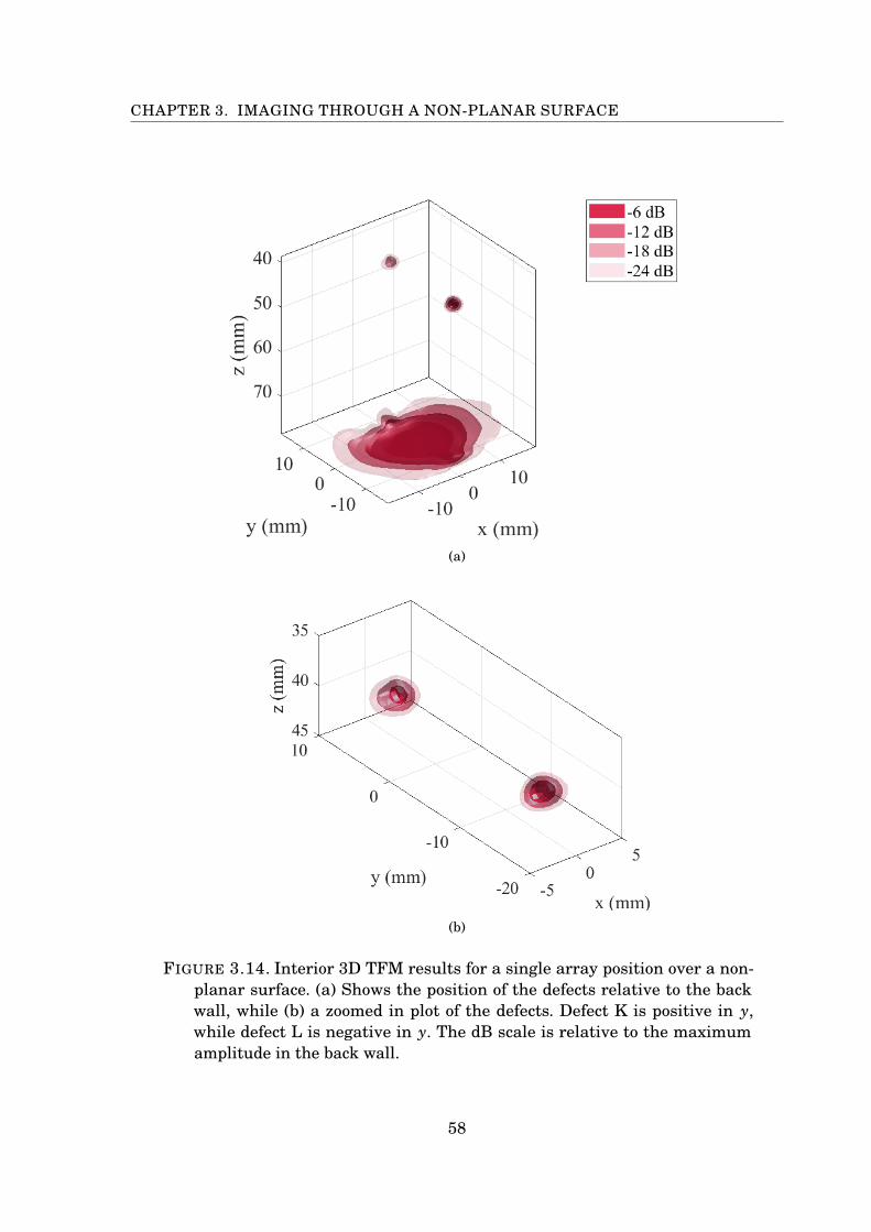
CHAPTER 3. IMAGING THROUGH A NON-PLANAR SURFACE
(a)
(b)
FIGURE 3.14. Interior 3D TFM results for a single array position over a non-planar surface. (a) Shows the position of the defects relative to the backwall, while (b) a zoomed in plot of the defects. Defect K is positive in y,while defect L is negative in y. The dB scale is relative to the maximumamplitude in the back wall.
58
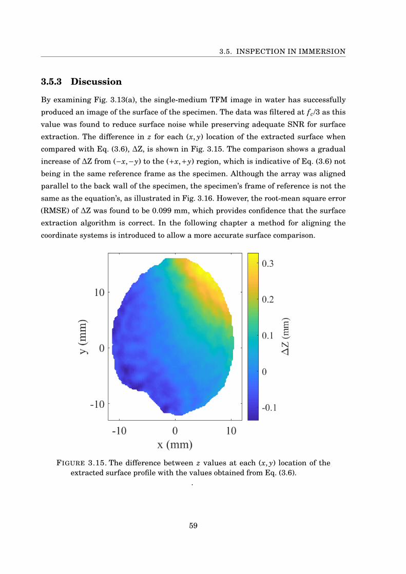
3.5. INSPECTION IN IMMERSION
3.5.3 Discussion
By examining Fig. 3.13(a), the single-medium TFM image in water has successfully
produced an image of the surface of the specimen. The data was filtered at fc/3 as this
value was found to reduce surface noise while preserving adequate SNR for surface
extraction. The difference in z for each (x, y) location of the extracted surface when
compared with Eq. (3.6), ∆Z, is shown in Fig. 3.15. The comparison shows a gradual
increase of ∆Z from (−x,−y) to the (+x,+y) region, which is indicative of Eq. (3.6) not
being in the same reference frame as the specimen. Although the array was aligned
parallel to the back wall of the specimen, the specimen’s frame of reference is not the
same as the equation’s, as illustrated in Fig. 3.16. However, the root-mean square error
(RMSE) of ∆Z was found to be 0.099 mm, which provides confidence that the surface
extraction algorithm is correct. In the following chapter a method for aligning the
coordinate systems is introduced to allow a more accurate surface comparison.
FIGURE 3.15. The difference between z values at each (x, y) location of theextracted surface profile with the values obtained from Eq. (3.6).
.
59
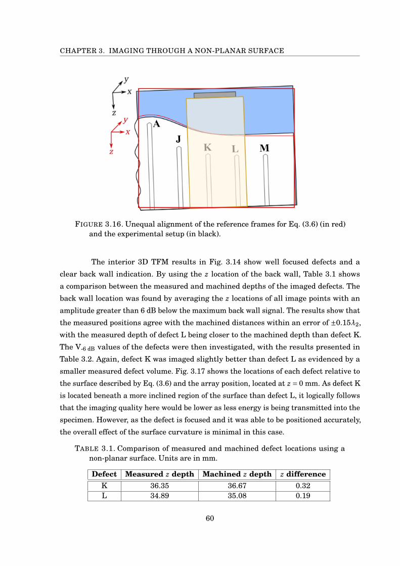
CHAPTER 3. IMAGING THROUGH A NON-PLANAR SURFACE
FIGURE 3.16. Unequal alignment of the reference frames for Eq. (3.6) (in red)and the experimental setup (in black).
The interior 3D TFM results in Fig. 3.14 show well focused defects and a
clear back wall indication. By using the z location of the back wall, Table 3.1 shows
a comparison between the measured and machined depths of the imaged defects. The
back wall location was found by averaging the z locations of all image points with an
amplitude greater than 6 dB below the maximum back wall signal. The results show that
the measured positions agree with the machined distances within an error of ±0.15λ2,
with the measured depth of defect L being closer to the machined depth than defect K.
The V-6 dB values of the defects were then investigated, with the results presented in
Table 3.2. Again, defect K was imaged slightly better than defect L as evidenced by a
smaller measured defect volume. Fig. 3.17 shows the locations of each defect relative to
the surface described by Eq. (3.6) and the array position, located at z = 0 mm. As defect K
is located beneath a more inclined region of the surface than defect L, it logically follows
that the imaging quality here would be lower as less energy is being transmitted into the
specimen. However, as the defect is focused and it was able to be positioned accurately,
the overall effect of the surface curvature is minimal in this case.
TABLE 3.1. Comparison of measured and machined defect locations using anon-planar surface. Units are in mm.
Defect Measured z depth Machined z depth z differenceK 36.35 36.67 0.32L 34.89 35.08 0.19
60
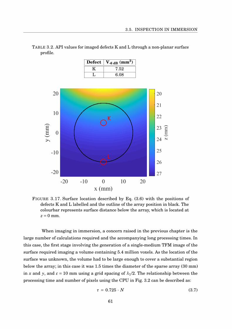
3.5. INSPECTION IN IMMERSION
TABLE 3.2. API values for imaged defects K and L through a non-planar surfaceprofile.
Defect V-6 dB (mm3)K 7.52L 6.08
FIGURE 3.17. Surface location described by Eq. (3.6) with the positions ofdefects K and L labelled and the outline of the array position in black. Thecolourbar represents surface distance below the array, which is located atz = 0 mm.
When imaging in immersion, a concern raised in the previous chapter is the
large number of calculations required and the accompanying long processing times. In
this case, the first stage involving the generation of a single-medium TFM image of the
surface required imaging a volume containing 5.4 million voxels. As the location of the
surface was unknown, the volume had to be large enough to cover a substantial region
below the array; in this case it was 1.5 times the diameter of the sparse array (30 mm)
in x and y, and ε= 10 mm using a grid spacing of λ1/2. The relationship between the
processing time and number of pixels using the CPU in Fig. 3.2 can be described as:
τ = 0.725 · N (3.7)
61

CHAPTER 3. IMAGING THROUGH A NON-PLANAR SURFACE
where τ is time in seconds and N is the number of voxels in units of a thousand. Using this
equation, a volume containing 5.4 million voxels would take ≈ 3900 s to process, whereas
the measured time to compute this using CUDA was found to be 7.2 s. With CUDA
completing the calculations at a speed of more than 500 times faster than MATLAB for a
single-medium scenario, it is clear that parallel programming is essential for immersion
imaging as the number of calculations only increases with the inclusion of a layer of
surface points. For completeness, imaging 700,000 voxels at a λ2/4 grid spacing within
the specimen using 7300 surface points took 17.1 s, yielding a total imaging time of
approximately 24 s.
3.6 Summary
This chapter has discussed 3D imaging of defects through an unknown, doubly curved
surface and presented a method for extracting a discretised 3D surface using an image-
based approach. The inspection of doubly curved surfaces in industry is usually conducted
using single-crystal transducers, which is time consuming and difficult, or potential
hazardous radiographic methods. By demonstrating that 2D phased arrays have the
ability to quickly and safely image through surfaces of this nature, inspections can be
conducted faster, easier and with higher accuracy. The extracted surface was validated
by comparing it with the equation of the surface and the defects were focused and
accurately positioned. As the number of calculations increases drastically when imaging
a 3D volume, the parallel computing platform CUDA was implemented to speed up the
imaging process. The following chapter expands on these results to a scan of the entire
specimen to further highlight the benefits of 2D phased arrays.
62

Chapter 4
Large, complex specimen inspection
All modern-day industrial structures contain large components that require regular
inspection, such as large diameter pipes and turbine blades. Due to the size of these
components and their integral role in a larger structure, inspections must occur in situ
and therefore require a shutdown of the immediate area while an operator collects data;
the motivations for this can include to reduce temperature, internal access to the pipe
is required or the requirement to inspect turbine blades while they are stationary. Any
inspection design therefore needs to consider how to collect the data as quickly and safely
as possible in order to minimise costs. This is of particular importance in nuclear power
plants where security access is strictly controlled and exposure to radiation is a huge
concern. It is worth noting that continuous monitoring of thickness measurements by
permanently installed sensors have become popular in recent years, particularly in plant
regions where corrosion and fatigue cracking is of concern [56]. However, beam steering
is not yet possible with these sensors and inspections are limited to pulse-echo.
Scanned arrays have become more popular within the last decade as a solution
to not only speed up the data collection process, but also to conduct inspections in
environments which pose a safety threat to humans [57–59]. The process involves fixing
an array to a jig or motor-controlled system which can mechanically translate the array
along a desired axis at a predetermined scan pitch. Data is collected at each position and
can then be processed offline. Further benefits of using a scanned array include increased
coverage, resolution and defect characterisation performance [60]. By scanning the
array over the surface, the effective aperture and range of probing angles are increased
which makes its use relevant to specimens with complex surfaces. Currently in industry
63
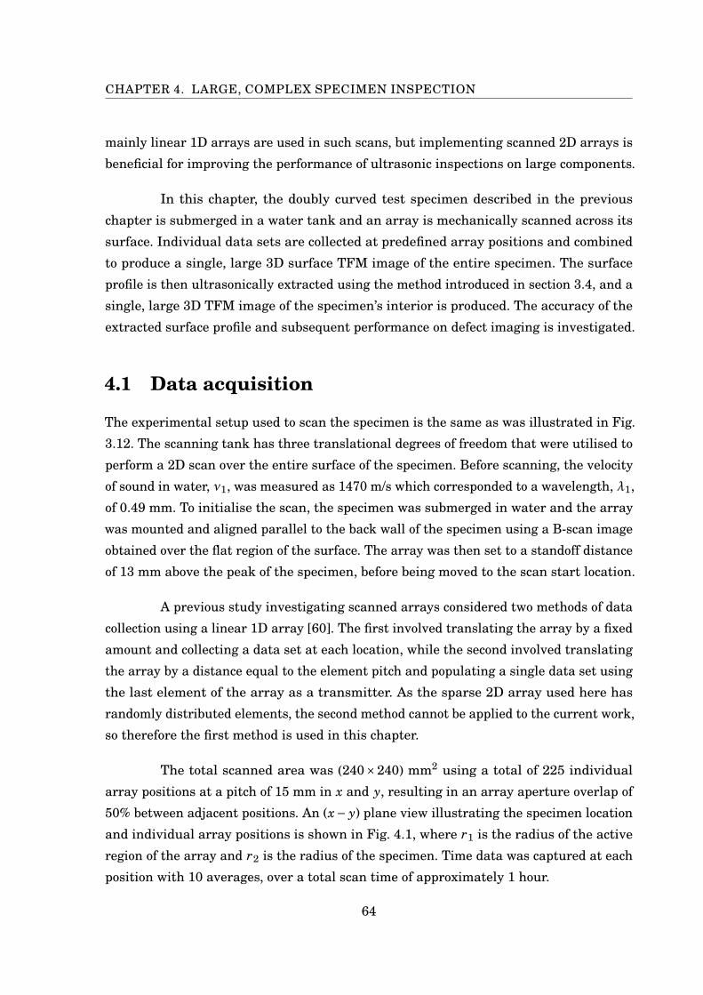
CHAPTER 4. LARGE, COMPLEX SPECIMEN INSPECTION
mainly linear 1D arrays are used in such scans, but implementing scanned 2D arrays is
beneficial for improving the performance of ultrasonic inspections on large components.
In this chapter, the doubly curved test specimen described in the previous
chapter is submerged in a water tank and an array is mechanically scanned across its
surface. Individual data sets are collected at predefined array positions and combined
to produce a single, large 3D surface TFM image of the entire specimen. The surface
profile is then ultrasonically extracted using the method introduced in section 3.4, and a
single, large 3D TFM image of the specimen’s interior is produced. The accuracy of the
extracted surface profile and subsequent performance on defect imaging is investigated.
4.1 Data acquisition
The experimental setup used to scan the specimen is the same as was illustrated in Fig.
3.12. The scanning tank has three translational degrees of freedom that were utilised to
perform a 2D scan over the entire surface of the specimen. Before scanning, the velocity
of sound in water, ν1, was measured as 1470 m/s which corresponded to a wavelength, λ1,
of 0.49 mm. To initialise the scan, the specimen was submerged in water and the array
was mounted and aligned parallel to the back wall of the specimen using a B-scan image
obtained over the flat region of the surface. The array was then set to a standoff distance
of 13 mm above the peak of the specimen, before being moved to the scan start location.
A previous study investigating scanned arrays considered two methods of data
collection using a linear 1D array [60]. The first involved translating the array by a fixed
amount and collecting a data set at each location, while the second involved translating
the array by a distance equal to the element pitch and populating a single data set using
the last element of the array as a transmitter. As the sparse 2D array used here has
randomly distributed elements, the second method cannot be applied to the current work,
so therefore the first method is used in this chapter.
The total scanned area was (240×240) mm2 using a total of 225 individual
array positions at a pitch of 15 mm in x and y, resulting in an array aperture overlap of
50% between adjacent positions. An (x− y) plane view illustrating the specimen location
and individual array positions is shown in Fig. 4.1, where r1 is the radius of the active
region of the array and r2 is the radius of the specimen. Time data was captured at each
position with 10 averages, over a total scan time of approximately 1 hour.
64
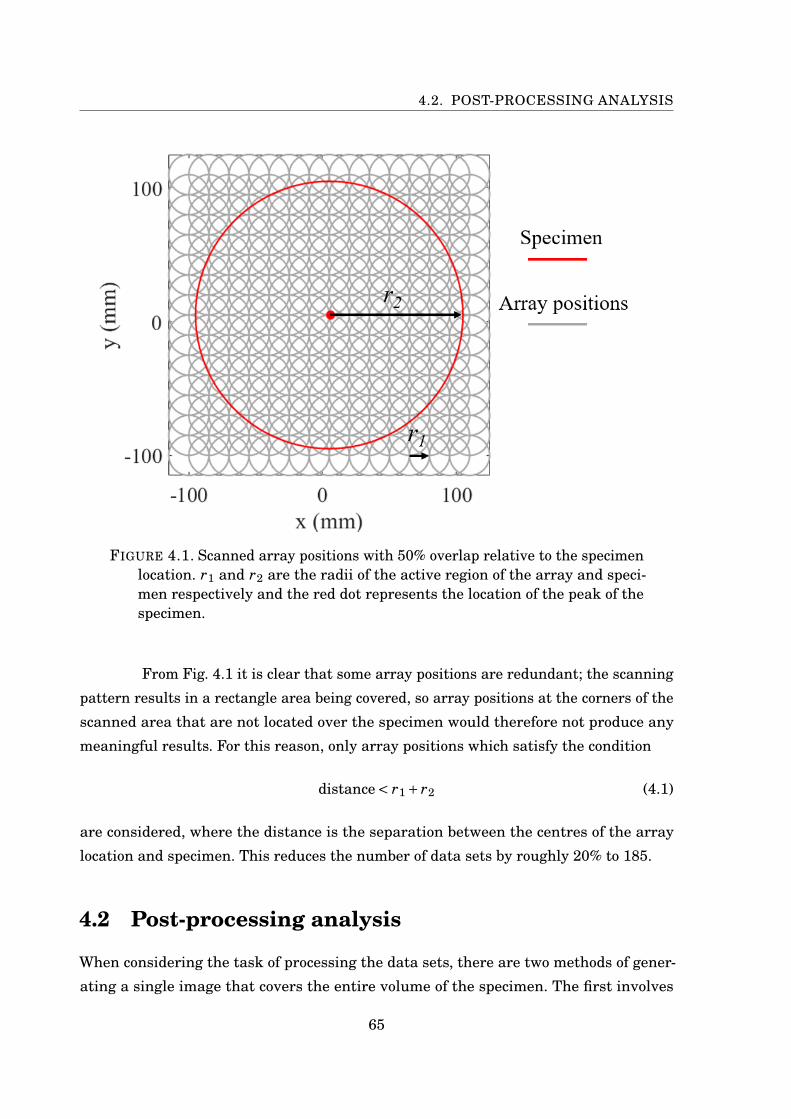
4.2. POST-PROCESSING ANALYSIS
FIGURE 4.1. Scanned array positions with 50% overlap relative to the specimenlocation. r1 and r2 are the radii of the active region of the array and speci-men respectively and the red dot represents the location of the peak of thespecimen.
From Fig. 4.1 it is clear that some array positions are redundant; the scanning
pattern results in a rectangle area being covered, so array positions at the corners of the
scanned area that are not located over the specimen would therefore not produce any
meaningful results. For this reason, only array positions which satisfy the condition
distance< r1 + r2 (4.1)
are considered, where the distance is the separation between the centres of the array
location and specimen. This reduces the number of data sets by roughly 20% to 185.
4.2 Post-processing analysis
When considering the task of processing the data sets, there are two methods of gener-
ating a single image that covers the entire volume of the specimen. The first involves
65
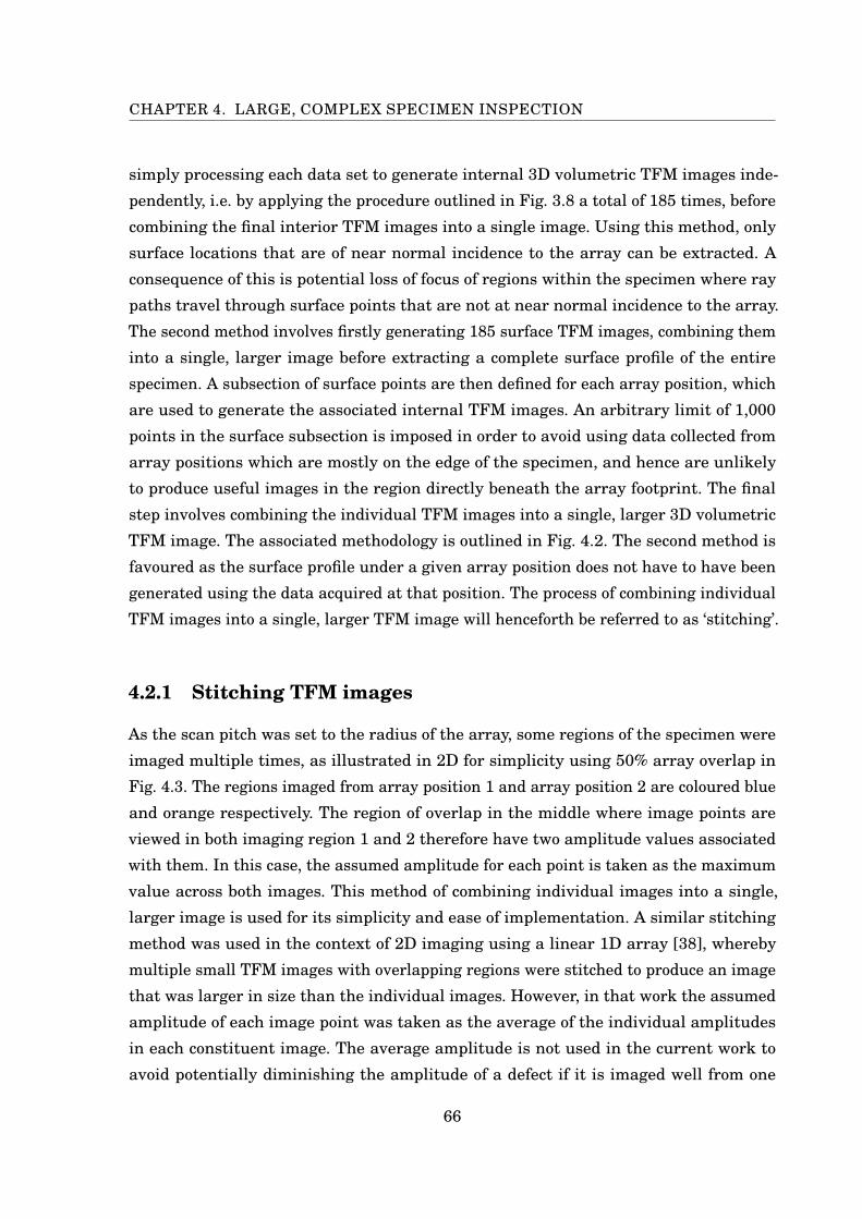
CHAPTER 4. LARGE, COMPLEX SPECIMEN INSPECTION
simply processing each data set to generate internal 3D volumetric TFM images inde-
pendently, i.e. by applying the procedure outlined in Fig. 3.8 a total of 185 times, before
combining the final interior TFM images into a single image. Using this method, only
surface locations that are of near normal incidence to the array can be extracted. A
consequence of this is potential loss of focus of regions within the specimen where ray
paths travel through surface points that are not at near normal incidence to the array.
The second method involves firstly generating 185 surface TFM images, combining them
into a single, larger image before extracting a complete surface profile of the entire
specimen. A subsection of surface points are then defined for each array position, which
are used to generate the associated internal TFM images. An arbitrary limit of 1,000
points in the surface subsection is imposed in order to avoid using data collected from
array positions which are mostly on the edge of the specimen, and hence are unlikely
to produce useful images in the region directly beneath the array footprint. The final
step involves combining the individual TFM images into a single, larger 3D volumetric
TFM image. The associated methodology is outlined in Fig. 4.2. The second method is
favoured as the surface profile under a given array position does not have to have been
generated using the data acquired at that position. The process of combining individual
TFM images into a single, larger TFM image will henceforth be referred to as ‘stitching’.
4.2.1 Stitching TFM images
As the scan pitch was set to the radius of the array, some regions of the specimen were
imaged multiple times, as illustrated in 2D for simplicity using 50% array overlap in
Fig. 4.3. The regions imaged from array position 1 and array position 2 are coloured blue
and orange respectively. The region of overlap in the middle where image points are
viewed in both imaging region 1 and 2 therefore have two amplitude values associated
with them. In this case, the assumed amplitude for each point is taken as the maximum
value across both images. This method of combining individual images into a single,
larger image is used for its simplicity and ease of implementation. A similar stitching
method was used in the context of 2D imaging using a linear 1D array [38], whereby
multiple small TFM images with overlapping regions were stitched to produce an image
that was larger in size than the individual images. However, in that work the assumed
amplitude of each image point was taken as the average of the individual amplitudes
in each constituent image. The average amplitude is not used in the current work to
avoid potentially diminishing the amplitude of a defect if it is imaged well from one
66
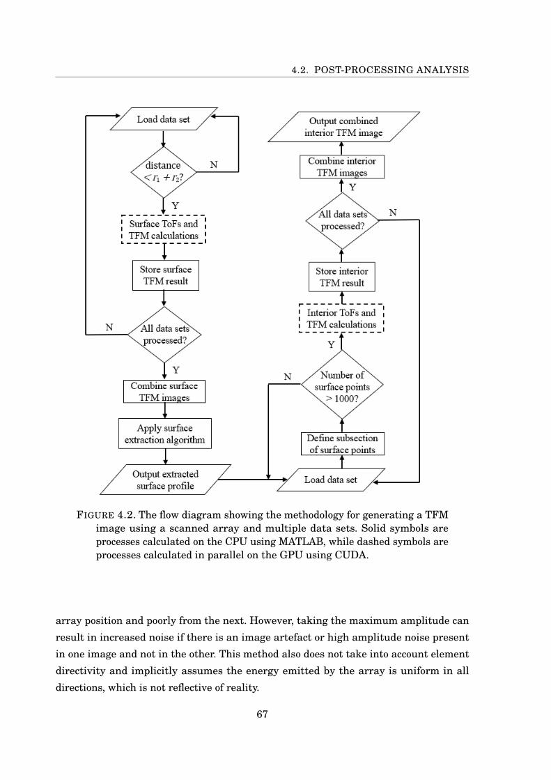
4.2. POST-PROCESSING ANALYSIS
FIGURE 4.2. The flow diagram showing the methodology for generating a TFMimage using a scanned array and multiple data sets. Solid symbols areprocesses calculated on the CPU using MATLAB, while dashed symbols areprocesses calculated in parallel on the GPU using CUDA.
array position and poorly from the next. However, taking the maximum amplitude can
result in increased noise if there is an image artefact or high amplitude noise present
in one image and not in the other. This method also does not take into account element
directivity and implicitly assumes the energy emitted by the array is uniform in all
directions, which is not reflective of reality.
67
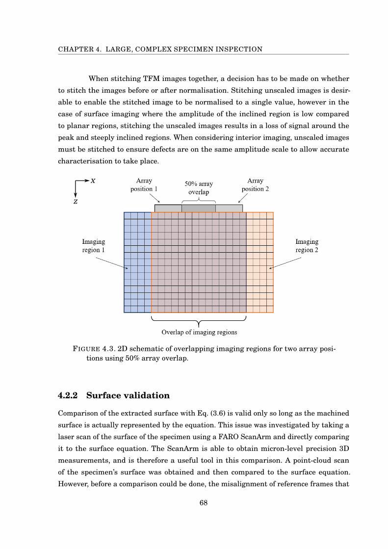
CHAPTER 4. LARGE, COMPLEX SPECIMEN INSPECTION
When stitching TFM images together, a decision has to be made on whether
to stitch the images before or after normalisation. Stitching unscaled images is desir-
able to enable the stitched image to be normalised to a single value, however in the
case of surface imaging where the amplitude of the inclined region is low compared
to planar regions, stitching the unscaled images results in a loss of signal around the
peak and steeply inclined regions. When considering interior imaging, unscaled images
must be stitched to ensure defects are on the same amplitude scale to allow accurate
characterisation to take place.
FIGURE 4.3. 2D schematic of overlapping imaging regions for two array posi-tions using 50% array overlap.
4.2.2 Surface validation
Comparison of the extracted surface with Eq. (3.6) is valid only so long as the machined
surface is actually represented by the equation. This issue was investigated by taking a
laser scan of the surface of the specimen using a FARO ScanArm and directly comparing
it to the surface equation. The ScanArm is able to obtain micron-level precision 3D
measurements, and is therefore a useful tool in this comparison. A point-cloud scan
of the specimen’s surface was obtained and then compared to the surface equation.
However, before a comparison could be done, the misalignment of reference frames that
68
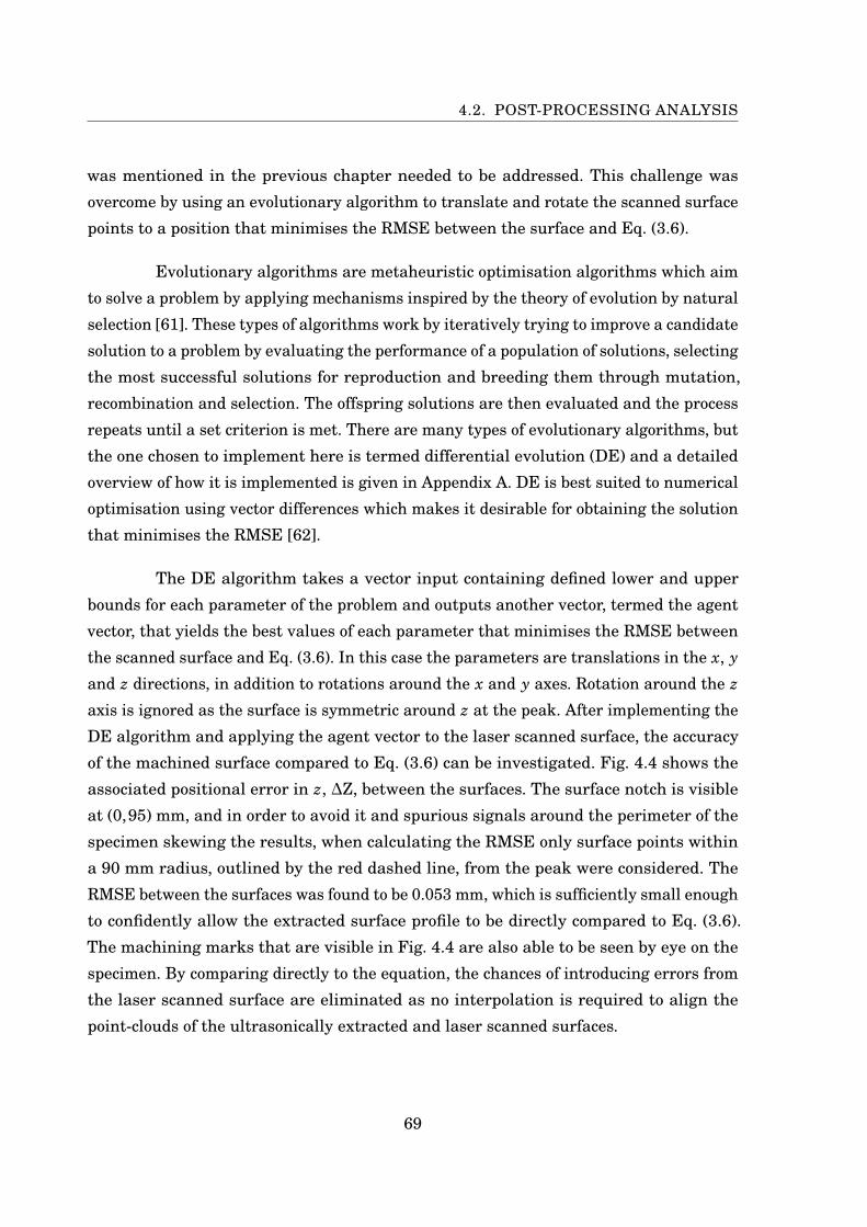
4.2. POST-PROCESSING ANALYSIS
was mentioned in the previous chapter needed to be addressed. This challenge was
overcome by using an evolutionary algorithm to translate and rotate the scanned surface
points to a position that minimises the RMSE between the surface and Eq. (3.6).
Evolutionary algorithms are metaheuristic optimisation algorithms which aim
to solve a problem by applying mechanisms inspired by the theory of evolution by natural
selection [61]. These types of algorithms work by iteratively trying to improve a candidate
solution to a problem by evaluating the performance of a population of solutions, selecting
the most successful solutions for reproduction and breeding them through mutation,
recombination and selection. The offspring solutions are then evaluated and the process
repeats until a set criterion is met. There are many types of evolutionary algorithms, but
the one chosen to implement here is termed differential evolution (DE) and a detailed
overview of how it is implemented is given in Appendix A. DE is best suited to numerical
optimisation using vector differences which makes it desirable for obtaining the solution
that minimises the RMSE [62].
The DE algorithm takes a vector input containing defined lower and upper
bounds for each parameter of the problem and outputs another vector, termed the agent
vector, that yields the best values of each parameter that minimises the RMSE between
the scanned surface and Eq. (3.6). In this case the parameters are translations in the x, y
and z directions, in addition to rotations around the x and y axes. Rotation around the z
axis is ignored as the surface is symmetric around z at the peak. After implementing the
DE algorithm and applying the agent vector to the laser scanned surface, the accuracy
of the machined surface compared to Eq. (3.6) can be investigated. Fig. 4.4 shows the
associated positional error in z, ∆Z, between the surfaces. The surface notch is visible
at (0,95) mm, and in order to avoid it and spurious signals around the perimeter of the
specimen skewing the results, when calculating the RMSE only surface points within
a 90 mm radius, outlined by the red dashed line, from the peak were considered. The
RMSE between the surfaces was found to be 0.053 mm, which is sufficiently small enough
to confidently allow the extracted surface profile to be directly compared to Eq. (3.6).
The machining marks that are visible in Fig. 4.4 are also able to be seen by eye on the
specimen. By comparing directly to the equation, the chances of introducing errors from
the laser scanned surface are eliminated as no interpolation is required to align the
point-clouds of the ultrasonically extracted and laser scanned surfaces.
69
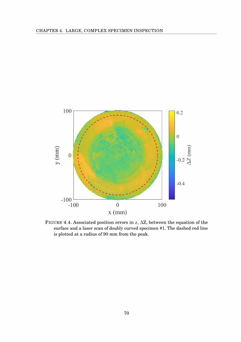
CHAPTER 4. LARGE, COMPLEX SPECIMEN INSPECTION
FIGURE 4.4. Associated position errors in z, ∆Z, between the equation of thesurface and a laser scan of doubly curved specimen #1. The dashed red lineis plotted at a radius of 90 mm from the peak.
70
4.3. SURFACE IMAGING AND EXTRACTION
4.3 Surface imaging and extraction
After each data set was processed for surface imaging using Eq. (2.1) and normalised
using localised maxima in the front wall signals, the next step involved stitching the 3D
TFM images together using the method outlined in section 4.2.1. The result is plotted
in Fig. 4.5 as an isosurface at –10 dB and coloured according to z depth beneath the
array, which was located at z = 0 mm. The visible gridded appearance in the plot is due
to the stitching algorithm, whereby the maximum amplitudes of image points in the
overlapped regions are taken as the true amplitudes. The x and y lengths of the imaging
region for each array position were twice the diameter of the array, and so the presence
of imaging artefacts in overlapped regions results in a slightly distorted image. Each
data set was filtered at fc/3, and a small amount of surface noise is shown in the (x− z)
image of the stitched surface that is viewed along y=−100 mm in Fig. 4.5(b). This filter
frequency was chosen through trial and error to reduce the appearance of artefacts in
the water, while maintaining a strong front wall response in the TFM image to allow
surface extraction.
The surface extraction method implemented on the stitched 3D TFM image is
the same as was described in section 3.4 for a single array position. As the resolution
of surface points is λ1/2 = 0.25 mm, the extracted surface looks almost identical to Fig.
4.5(a) and is therefore not shown. The accuracy of the surface extraction algorithm was
then compared using Eq. (3.6) after applying the DE algorithm to align the reference
frames by minimising the RMSE. The result of this comparison for each surface location
is shown in Fig. 4.6(a) where ∆Z is the difference in z locations between Eq. (3.6) and
Zi j for each (x, y) surface point. The gridded appearance is visible but has not affected
surface extraction. The RMSE within the 90 mm radius of the peak was found to be
0.042 mm and a histogram of ∆Z values is given in Fig. 4.6(b). This shows a normal
distribution of ∆Z values around a mean of 0.89 µm with a standard deviation, σ, of
0.042 mm, which implies the surface has been accurately extracted.
Using a surface resolution of λ1/2, the time to process all data sets was 1520 s,
or approximately 8 s per data set including transfer time with 4.8 million voxels in each
TFM image.
71
CHAPTER 4. LARGE, COMPLEX SPECIMEN INSPECTION
(a)
(b)
FIGURE 4.5. Stitched 3D surface TFM image of doubly curved specimen #1plotted as an isosurface at -10 dB realtive to the maximum amplitude inthe surface. (a) shows a 3D view while (b) shows the (x− z) plane viewedalong y=−100 mm.
72
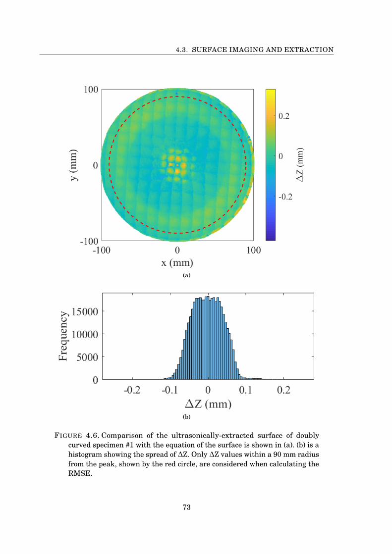
4.3. SURFACE IMAGING AND EXTRACTION
(a)
(b)
FIGURE 4.6. Comparison of the ultrasonically-extracted surface of doublycurved specimen #1 with the equation of the surface is shown in (a). (b) is ahistogram showing the spread of ∆Z. Only ∆Z values within a 90 mm radiusfrom the peak, shown by the red circle, are considered when calculating theRMSE.
73
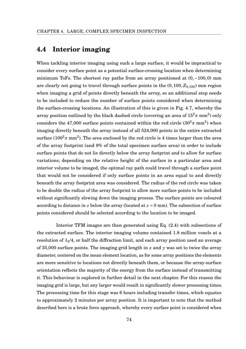
CHAPTER 4. LARGE, COMPLEX SPECIMEN INSPECTION
4.4 Interior imaging
When tackling interior imaging using such a large surface, it would be impractical to
consider every surface point as a potential surface-crossing location when determining
minimum ToFs. The shortest ray paths from an array positioned at (0,−100,0) mm
are clearly not going to travel through surface points in the (0,100, Z0,100) mm region
when imaging a grid of points directly beneath the array, so an additional step needs
to be included to reduce the number of surface points considered when determining
the surface-crossing locations. An illustration of this is given in Fig. 4.7, whereby the
array position outlined by the black dashed circle (covering an area of 152π mm2) only
considers the 47,000 surface points contained within the red circle (302π mm2) when
imaging directly beneath the array instead of all 524,000 points in the entire extracted
surface (1002π mm2). The area enclosed by the red circle is 4 times larger than the area
of the array footprint (and 9% of the total specimen surface area) in order to include
surface points that do not lie directly below the array footprint and to allow for surface
variations; depending on the relative height of the surface in a particular area and
interior volume to be imaged, the optimal ray path could travel through a surface point
that would not be considered if only surface points in an area equal to and directly
beneath the array footprint area was considered. The radius of the red circle was taken
to be double the radius of the array footprint to allow more surface points to be included
without significantly slowing down the imaging process. The surface points are coloured
according to distance in z below the array (located at z = 0 mm). The subsection of surface
points considered should be selected according to the location to be imaged.
Interior TFM images are then generated using Eq. (2.4) with subsections of
the extracted surface. The interior imaging volume contained 1.8 million voxels at a
resolution of λ2/4, or half the diffraction limit, and each array position used an average
of 35,000 surface points. The imaging grid length in x and y was set to twice the array
diameter, centered on the mean element location, as for some array positions the elements
are more sensitive to locations not directly beneath them, or because the array-surface
orientation reflects the majority of the energy from the surface instead of transmitting
it. This behaviour is explored in further detail in the next chapter. For this reason the
imaging grid is large, but any larger would result in significantly slower processing times.
The processing time for this stage was 6 hours including transfer times, which equates
to approximately 2 minutes per array position. It is important to note that the method
described here is a brute force approach, whereby every surface point is considered when
74
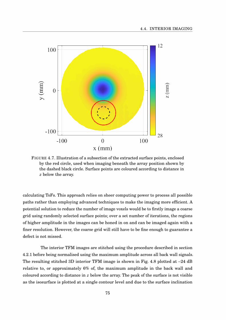
4.4. INTERIOR IMAGING
FIGURE 4.7. Illustration of a subsection of the extracted surface points, enclosedby the red circle, used when imaging beneath the array position shown bythe dashed black circle. Surface points are coloured according to distance inz below the array.
calculating ToFs. This approach relies on sheer computing power to process all possible
paths rather than employing advanced techniques to make the imaging more efficient. A
potential solution to reduce the number of image voxels would be to firstly image a coarse
grid using randomly selected surface points; over a set number of iterations, the regions
of higher amplitude in the images can be honed in on and can be imaged again with a
finer resolution. However, the coarse grid will still have to be fine enough to guarantee a
defect is not missed.
The interior TFM images are stitched using the procedure described in section
4.2.1 before being normalised using the maximum amplitude across all back wall signals.
The resulting stitched 3D interior TFM image is shown in Fig. 4.8 plotted at –24 dB
relative to, or approximately 6% of, the maximum amplitude in the back wall and
coloured according to distance in z below the array. The peak of the surface is not visible
as the isosurface is plotted at a single contour level and due to the surface inclination
75

CHAPTER 4. LARGE, COMPLEX SPECIMEN INSPECTION
angle and the orientation of the array, the amplitude of the inclined surface regions are
much lower than that of the flat regions. Snapshots of individual defects can also be
obtained by creating a window around volumes in the TFM image. Snapshots of BDHs
K, L and M are shown in Fig. 4.9 and EDM notches 4, 3 and 2 are shown in Fig. 4.10. It
was found that the defects located under the region of steep inclination are unable to be
imaged at any reasonable amplitude level, as is evident by the gap in the isosurface plots
of EDM notches 3 and 4. For this reason, BDHs B, F, J, N and R are excluded from the
results. BDHs A and C are also excluded as their SNR is too low for imaging. The central
location of each BDH and EDM notch was found by taking the mean location of points
whose amplitudes were greater than 6 dB below the local maximum amplitude. Each
defect is plotted at its central location using isosurfaces at different amplitude levels
relative to the maximum amplitude in the back wall.
76
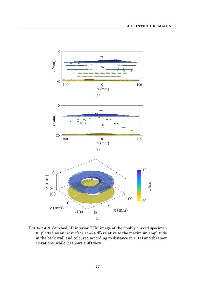
4.4. INTERIOR IMAGING
(a)
(b)
(c)
FIGURE 4.8. Stitched 3D interior TFM image of the doubly curved specimen#1 plotted as an isosurface at –24 dB relative to the maximum amplitudein the back wall and coloured according to distance in z. (a) and (b) showelevations, while (c) shows a 3D view.
77
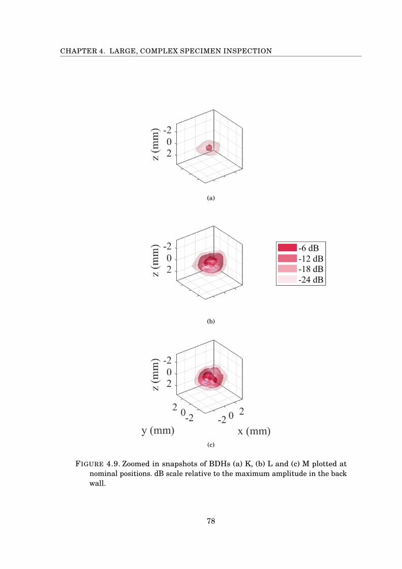
CHAPTER 4. LARGE, COMPLEX SPECIMEN INSPECTION
(a)
(b)
(c)
FIGURE 4.9. Zoomed in snapshots of BDHs (a) K, (b) L and (c) M plotted atnominal positions. dB scale relative to the maximum amplitude in the backwall.
78
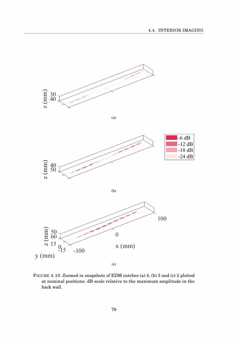
4.4. INTERIOR IMAGING
(a)
(b)
(c)
FIGURE 4.10. Zoomed in snapshots of EDM notches (a) 4, (b) 3 and (c) 2 plottedat nominal positions. dB scale relative to the maximum amplitude in theback wall.
79

CHAPTER 4. LARGE, COMPLEX SPECIMEN INSPECTION
Of the defects that were able to be imaged, their positions were investigated
and compared to the machined locations using their centre points. This was achieved
using two metrics: the first is the depth above the back wall and the second is the lateral
distance from the surface notch. These distances are then compared to the true values
from the specimen design file, with the results shown in Fig. 4.11. It was found that σ of
the depth and lateral distance comparisons were 0.571 mm and 1.01 mm respectively.
Both values are comparable to λ2/2 = 1.05 mm and so the measured defect locations are
in good agreement with the true positions.
From observing the result in Fig. 4.8, it is evident that some defects are visible,
while others are not; Fig. 4.11 shows that the defects that are able to be imaged appear
in their intended locations and the surface is being accounted for correctly. Further
investigation into why some defects were unable to be imaged is as follows. Fig. 4.12
shows the surface inclination across all surface points along with the machined positions
of defects; the visible defects are coloured red, while the defects that were unable to be
imaged are shown in white. The figure shows defects under the region of the surface
with an approximate inclination larger than the longitudinal critical angle for a wave
travelling from water to aluminium, θc = 13.4°, proved impossible to image using this
setup orientation. EDM notch 4, shown in Fig. 4.10(a), illustrates this as there is a gap
in the isosurface as part of the notch is underneath the region of highest inclination. The
BDHs that were unable to be imaged include BDHs B, F, J, N and R, along with BDHs
A and C due to their low SNR and are coloured white in the figure. BDH A is excluded
as it is 5 mm directly under the peak and interior reflections in this area have buried
the defect response in noise. The reason for low SNR on BDH C is due to it lying on the
radial arm that was drilled at the smallest depth below the surface. The reason for the
other defects not being imaged is due to several factors.
Firstly, consider the surface to be an inclined plane with a steepest angle of
24° and the array positioned directly above it, as depicted in Fig. 4.13. In the region
of the sample directly under the array, the majority of the incident energy is reflected
due to the surface angle being larger than θc. To the side of the array further up the
plane, there is a region where rays from the array are incident on the surface below
θc, shown in red in Fig. 4.13 where θi < θc. However, the directivity amplitude of the
elements in the array means that there is low transmission and reception sensitivity in
these directions as they are at relatively large angles relative to the array normal. Fig.
4.14 shows the directivity, D(φ), of a 1.7 mm diameter circular element radiating into
80
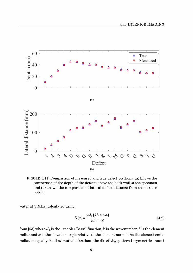
4.4. INTERIOR IMAGING
(a)
(b)
FIGURE 4.11. Comparison of measured and true defect positions. (a) Shows thecomparison of the depth of the defects above the back wall of the specimenand (b) shows the comparison of lateral defect distance from the surfacenotch.
water at 3 MHz, calculated using
D(φ)= 2J1(kb sinφ
)kb sinφ
(4.2)
from [63] where J1 is the 1st order Bessel function, k is the wavenumber, b is the element
radius and φ is the elevation angle relative to the element normal. As the element emits
radiation equally in all azimuthal directions, the directivity pattern is symmetric around
81

CHAPTER 4. LARGE, COMPLEX SPECIMEN INSPECTION
FIGURE 4.12. Surface inclination with the locations of the EDM notches andBDHs marked. White circles represent defects that were unable to imagedand white lines represent portions of EDM notches that were unable to beimaged.
the element normal. D(φ) represents the directivity on transmission and reception,
so to obtain the total directivity for a transmit-receive element pair their individual
directivities at the respective angles are calculated and multiplied together. The array
elements’ highest sensitivity is at 0°, which corresponds to the direction directly beneath
the element. For a planar surface parallel to the base of the array, the directivity of the
elements is therefore the highest, as shown in the ± θc range by the solid blue line in
Fig. 4.14. However, for a surface inclination of 24°, as shown by the dashed red region
of the graph, the directivity within the 24° ± θc range is much lower. For this surface
inclination the elements have reduced sensitivity to any signals entering or leaving the
specimen. The ratio of the average directivity in the parallel surface case when compared
to the inclined surface case is approximately 20:1. By examining BDHs K, L and M in
Fig. 5.8(a), 5.8(b) and 5.8(c) respectively, this effect is evident as the average amplitude
in BDH K is approximately 10 dB, or 33%, lower than that in BDHs L and M, illustrating
that defects located under the inclined region have lower amplitudes when compared to
defects located under a planar surface parallel to the array.
82
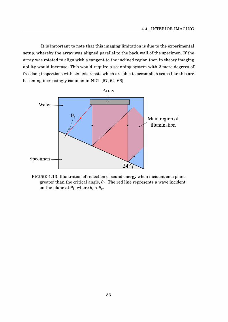
4.4. INTERIOR IMAGING
It is important to note that this imaging limitation is due to the experimental
setup, whereby the array was aligned parallel to the back wall of the specimen. If the
array was rotated to align with a tangent to the inclined region then in theory imaging
ability would increase. This would require a scanning system with 2 more degrees of
freedom; inspections with six-axis robots which are able to accomplish scans like this are
becoming increasingly common in NDT [57, 64–66].
FIGURE 4.13. Illustration of reflection of sound energy when incident on a planegreater than the critical angle, θc. The red line represents a wave incidenton the plane at θi, where θi < θc.
83
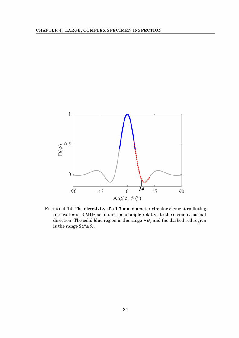
CHAPTER 4. LARGE, COMPLEX SPECIMEN INSPECTION
FIGURE 4.14. The directivity of a 1.7 mm diameter circular element radiatinginto water at 3 MHz as a function of angle relative to the element normaldirection. The solid blue region is the range ± θc and the dashed red regionis the range 24°± θc.
84
4.5. SUMMARY
4.5 Summary
Scanned arrays are becoming more popular in industry due to their ability to quickly
scan large components and potentially improve the characterisation of defects by probing
from an increased number of angles. In this chapter, a sparse 2D array was scanned
over the surface of a specimen with a doubly curved surface profile that was unknown a
priori. A stitching method was implemented to combine the surface images generated
from each array position into a single, larger 3D TFM image before a surface extraction
algorithm was applied. By comparing the ultrasonically-extracted surface with the true
equation of the surface, it was found that the surface extraction algorithm produced
a surface that was in excellent agreement with the machined surface. Subsections of
the extracted surface points were then used to generate interior TFM images to avoid
excessive processing times. The positioning of machined defects within the specimen was
then investigated; defects that were able to be imaged appeared in the correct locations,
while defects located under relatively steep inclined surface regions proved impossible to
image with the current setup. Up to this point the elements in the sparse 2D array have
be assumed to act as ideal point sources, which is not representative of their true nature.
The energy of the ultrasonic beam excited by the array transducer at different angles
is not uniform, so as the relative geometrical position between a defect and the array
aperture is different, different amplitude results will be obtained for identical defects.
This effect was pronounced when defects beneath steep surface angles were unable to
be imaged, even though some ray paths were able to pass through the surface at larger
angles relative to the element normals. This will be the focus of the following chapter.
85

Chapter 5
3D sensitivity images
When a sound wave is incident on the surface of a specimen, the nature of the interaction
is complex due to surface geometry, incident angle, and relative material impedance.
This means that the amplitude and angle of energy transmitted into a specimen differs
as an array is scanned across a non-planar surface. Consequently, a region of the interior
of the specimen may be viewed well from one array position, and poorly from the next.
This effect is termed the sensitivity of the region of interest to an array position and can
be displayed in a sensitivity image [67]. Sensitivity images can quantitatively determine
which array positions yield a strong amplitude for a given setup and are therefore a useful
tool when processing data from a scanned array. They have been used in multi-view
array inspection, whereby each combination of wave modes have different sensitivities
depending on angle and amplitude [68], and data fusion, which aims to combine valuable
information from numerous multi-view images into a single image [69].
In the previous chapter, the true amplitudes of voxels imaged from more than
one array position were obtained by taking the maximum amplitude values across all
images. The method assumes uniform sensitivity throughout the TFM images, and so
if there is an artefact in a region of low sensitivity, the signal from the artefact can be
misidentified as a defect signal and result in an inaccurate final image. An alternative
stitching method is proposed in this chapter, whereby the amplitude of a voxel is the
sum of the individual weighted TFM amplitudes obtained from each array position. This
chapter focuses on the generation of sensitivity images and their implementation in an
alternative stitching algorithm.
87
CHAPTER 5. 3D SENSITIVITY IMAGES
5.1 Sensitivity image generation
A 2D model developed in [68] provides an estimate of the TFM intensity a particular
defect would yield for a specific setup. By assuming the sound energy is incident at a
single frequency, ω0, and the amplitude at the defect centre is representative of the
true peak amplitude (as is the case for small defects), a time efficient method was
introduced when compared to a multi-frequency model or a finite element analysis
implementation. The contributions to the model can be separated into three main
sections for an immersion setup: the first considers the transmit path from the element
to the scatterer through the surface, the second is the calculation of the scattering and
the final section is the receive path from the scatterer to the receiving element through
the surface. The incident pulse amplitude on the scatterer is always less than the initial
amplitude emitted from the source element due to amplitude loss through geometrical
attenuation effects and transmission across an interface. Additional amplitude is lost
during the scattering stage, where the scattering is dependent on the nature of the defect
and the incident angle. Furthermore, the amplitude of the reflected signal is decreased
by returning across the specimen’s surface to the receiving element. The model accounts
for these losses of signal amplitude, along with the contribution of the element directivity.
Effects from material attenuation are assumed here to be negligible, although they
can easily be included in the same framework if they are significant. The equation to
generate a sensitivity image intensity, E (P), is defined for small defects located at vector
positions P by:
E (P) =∣∣∣∣∣∑T
∑R
aT,R (P)CT,R (ω0,P)
∣∣∣∣∣ , (5.1)
where T and R are the transmitting and receiving element indices respectively, aT,R is
the optional weighting factor that is used in the TFM imaging algorithm in Eq. (2.4)
(unused in the current work, so therefore set equal to 1) and
CT,R (ω0,P) = BT (P)B′R (P)DT (ω0,P)D′
R (ω0,P)ΓT (P)Γ′R (P)ST,R (ω0,P) , (5.2)
where
• BT and B′R represent the geometrical attenuation, or beamspread, for the transmit
and receive paths;
88
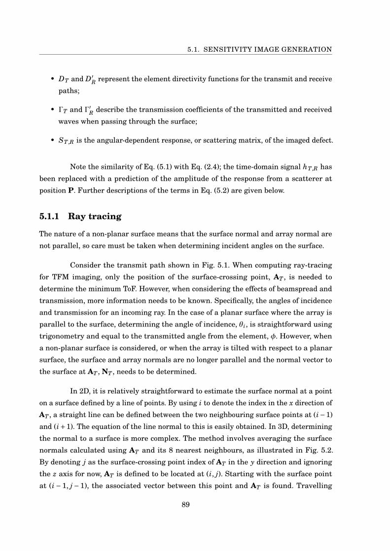
5.1. SENSITIVITY IMAGE GENERATION
• DT and D′R represent the element directivity functions for the transmit and receive
paths;
• ΓT and Γ′R describe the transmission coefficients of the transmitted and received
waves when passing through the surface;
• ST,R is the angular-dependent response, or scattering matrix, of the imaged defect.
Note the similarity of Eq. (5.1) with Eq. (2.4); the time-domain signal hT,R has
been replaced with a prediction of the amplitude of the response from a scatterer at
position P. Further descriptions of the terms in Eq. (5.2) are given below.
5.1.1 Ray tracing
The nature of a non-planar surface means that the surface normal and array normal are
not parallel, so care must be taken when determining incident angles on the surface.
Consider the transmit path shown in Fig. 5.1. When computing ray-tracing
for TFM imaging, only the position of the surface-crossing point, AT , is needed to
determine the minimum ToF. However, when considering the effects of beamspread and
transmission, more information needs to be known. Specifically, the angles of incidence
and transmission for an incoming ray. In the case of a planar surface where the array is
parallel to the surface, determining the angle of incidence, θi, is straightforward using
trigonometry and equal to the transmitted angle from the element, φ. However, when
a non-planar surface is considered, or when the array is tilted with respect to a planar
surface, the surface and array normals are no longer parallel and the normal vector to
the surface at AT , NT , needs to be determined.
In 2D, it is relatively straightforward to estimate the surface normal at a point
on a surface defined by a line of points. By using i to denote the index in the x direction of
AT , a straight line can be defined between the two neighbouring surface points at (i−1)
and (i+1). The equation of the line normal to this is easily obtained. In 3D, determining
the normal to a surface is more complex. The method involves averaging the surface
normals calculated using AT and its 8 nearest neighbours, as illustrated in Fig. 5.2.
By denoting j as the surface-crossing point index of AT in the y direction and ignoring
the z axis for now, AT is defined to be located at (i, j). Starting with the surface point
at (i −1, j −1), the associated vector between this point and AT is found. Travelling
89
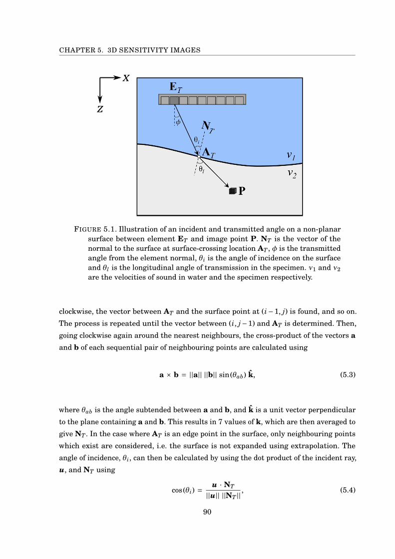
CHAPTER 5. 3D SENSITIVITY IMAGES
FIGURE 5.1. Illustration of an incident and transmitted angle on a non-planarsurface between element ET and image point P. NT is the vector of thenormal to the surface at surface-crossing location AT , φ is the transmittedangle from the element normal, θi is the angle of incidence on the surfaceand θl is the longitudinal angle of transmission in the specimen. ν1 and ν2are the velocities of sound in water and the specimen respectively.
clockwise, the vector between AT and the surface point at (i−1, j) is found, and so on.
The process is repeated until the vector between (i, j−1) and AT is determined. Then,
going clockwise again around the nearest neighbours, the cross-product of the vectors aand b of each sequential pair of neighbouring points are calculated using
a × b = ||a|| ||b|| sin(θab) k, (5.3)
where θab is the angle subtended between a and b, and k is a unit vector perpendicular
to the plane containing a and b. This results in 7 values of k, which are then averaged to
give NT . In the case where AT is an edge point in the surface, only neighbouring points
which exist are considered, i.e. the surface is not expanded using extrapolation. The
angle of incidence, θi, can then be calculated by using the dot product of the incident ray,
u, and NT using
cos(θi) = u · NT
||u|| ||NT ||, (5.4)
90
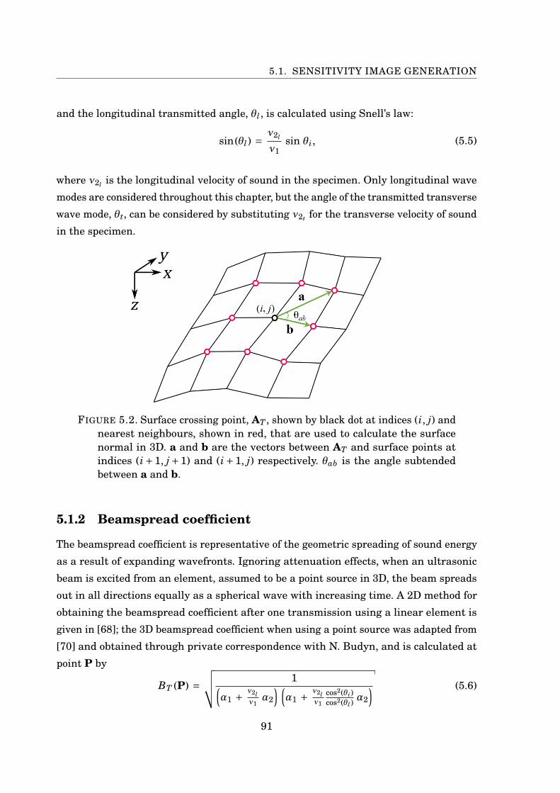
5.1. SENSITIVITY IMAGE GENERATION
and the longitudinal transmitted angle, θl , is calculated using Snell’s law:
sin(θl) = ν2l
ν1sin θi, (5.5)
where ν2l is the longitudinal velocity of sound in the specimen. Only longitudinal wave
modes are considered throughout this chapter, but the angle of the transmitted transverse
wave mode, θt, can be considered by substituting ν2t for the transverse velocity of sound
in the specimen.
FIGURE 5.2. Surface crossing point, AT , shown by black dot at indices (i, j) andnearest neighbours, shown in red, that are used to calculate the surfacenormal in 3D. a and b are the vectors between AT and surface points atindices (i +1, j +1) and (i +1, j) respectively. θab is the angle subtendedbetween a and b.
5.1.2 Beamspread coefficient
The beamspread coefficient is representative of the geometric spreading of sound energy
as a result of expanding wavefronts. Ignoring attenuation effects, when an ultrasonic
beam is excited from an element, assumed to be a point source in 3D, the beam spreads
out in all directions equally as a spherical wave with increasing time. A 2D method for
obtaining the beamspread coefficient after one transmission using a linear element is
given in [68]; the 3D beamspread coefficient when using a point source was adapted from
[70] and obtained through private correspondence with N. Budyn, and is calculated at
point P by
BT (P) =√√√√ 1(
α1 + ν2lν1α2
) (α1 + ν2l
ν1
cos2(θi)cos2(θl )
α2
) (5.6)
91

CHAPTER 5. 3D SENSITIVITY IMAGES
with
α1 = ||ET − AT || and α2 = ||AT − P|| .The beamspread coefficient for the return path to element R, B′
R (P), can be obtained by
making the following substitutions in Eq. (5.6):
α1 −→α2
ν1 −→ ν2l
ν2l −→ ν1
θi −→ θl
θl −→ θi.
5.1.3 Element directivity
The directivity of a circular element in 3D can be modelled as a plane circular piston
emitting radiation. In the far field approximation, the directional factor is represented
by Eq. (4.2).
5.1.4 Transmission coefficient
When a ray is incident on a boundary between two media, a fraction of the energy is
reflected back in the same medium as the incident wave travelled, while the rest of it gets
transmitted into the other medium. Depending on the incident angle, some energy can
travel on the surface of the specimen as a Rayleigh wave. The transmission coefficient,
Γ, describes the amplitude of the transmitted wave with respect to the incident wave;
similarly, the reflection coefficient describes the amplitude of the reflected wave in
relation to the incident wave. Derivations of the transmission coefficient calculations
for different conditions can be found in [71] and the key equations are given here. For a
water–specimen boundary with an incident longitudinal wave in water, the transmission
coefficient of the acoustic pressure is calculated using:
ΓT = 2M
cos(2θt) (5.7)
with the abbreviation
M =(ν2t
ν2l
)2sin(2θl) sin(2θt) + cos2 (2θt) + ρ1ν1
ρ2ν2l
cos(θl)cos(θi)
, (5.8)
where ρ1 and ρ2 are the densities of water and the specimen respectively, and all other
symbols have been previously defined.
92
5.2. SINGLE-FRAME APPLICATION
In the case of a specimen-water boundary, as is encountered on the return path
from the scatterer to the receiving element, the transmission coefficient using an incident
longitudinal wave is found using:
Γ′R = 2M
ρ1ν1
ρ2ν2l
cos(2θt) cos(θl)cos(θi)
(5.9)
where all symbols have the same meanings as before and M is from Eq. (5.8).
5.1.5 Scattering amplitude
The scattering of an ultrasonic wave by a defect is influenced by a number of factors in-
cluding wave frequency, incident angle and defect size, shape, orientation and roughness.
The scattering amplitude can be measured over a range of angles in what is termed a
scattering matrix, or S-matrix, which is dependent upon wave frequency, incident angle
and reflected angle [72]. S-matrices can be used to accurately determine the size and
orientation of small, crack-like defects in 2D [73], but have yet to be fully explored in 3D.
S-matrices will be discussed further in the following chapter.
With no prior knowledge about the nature of the defects expected, the most
appropriate assumption is that the scatterer is assumed to behave as a point reflector
with ST,R = 1 and so only beamspread, directivity and transmission coefficients need to
be considered when modelling the sensitivity image.
5.2 Single-frame application
Consider the inspection scenario described in section 2.2, where an array is used to
image a specimen with a planar surface in immersion. By using the parameters of this
setup (i.e. array and surface locations) and combining the contribution of B, D, Γ and S
at each voxel in a defined imaging grid, Eq. (5.1) can be used to generate a sensitivity
image, E(P). Fig. 5.3 shows the 3D sensitivity image obtained of the interior of the
specimen, where the amplitudes have been normalised between 0 and 1. The array is
positioned at z = 0 mm. Individual (x− z) 2D planes of E(P) at increasing steps along
the y axis are also shown in Fig. 5.4. The figures show that sensitivity is not uniform
throughout the imaging region; the array is most sensitive to the the region directly
beneath it. For all z distances, as the x and y distances increase or decrease, the expected
amplitude from a point target is minimised. If the dominant source of noise is uniform
93
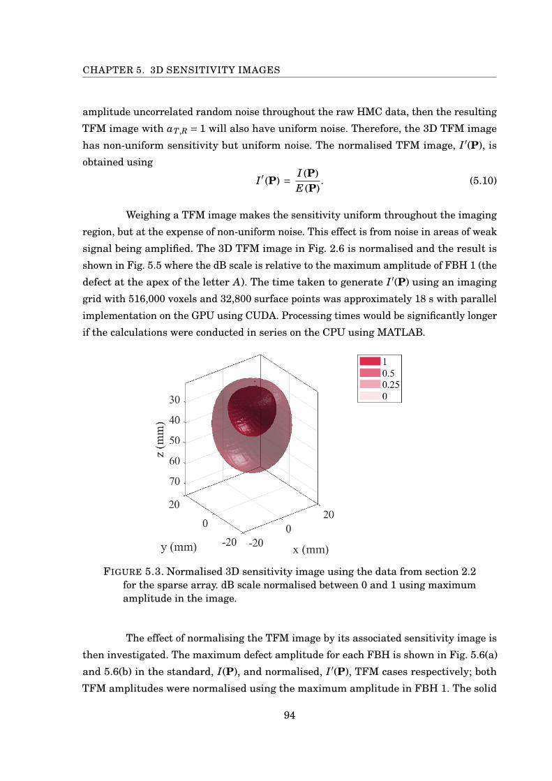
CHAPTER 5. 3D SENSITIVITY IMAGES
amplitude uncorrelated random noise throughout the raw HMC data, then the resulting
TFM image with aT,R = 1 will also have uniform noise. Therefore, the 3D TFM image
has non-uniform sensitivity but uniform noise. The normalised TFM image, I ′(P), is
obtained using
I ′ (P) = I (P)E (P)
. (5.10)
Weighing a TFM image makes the sensitivity uniform throughout the imaging
region, but at the expense of non-uniform noise. This effect is from noise in areas of weak
signal being amplified. The 3D TFM image in Fig. 2.6 is normalised and the result is
shown in Fig. 5.5 where the dB scale is relative to the maximum amplitude of FBH 1 (the
defect at the apex of the letter A). The time taken to generate I ′(P) using an imaging
grid with 516,000 voxels and 32,800 surface points was approximately 18 s with parallel
implementation on the GPU using CUDA. Processing times would be significantly longer
if the calculations were conducted in series on the CPU using MATLAB.
FIGURE 5.3. Normalised 3D sensitivity image using the data from section 2.2for the sparse array. dB scale normalised between 0 and 1 using maximumamplitude in the image.
The effect of normalising the TFM image by its associated sensitivity image is
then investigated. The maximum defect amplitude for each FBH is shown in Fig. 5.6(a)
and 5.6(b) in the standard, I(P), and normalised, I ′(P), TFM cases respectively; both
TFM amplitudes were normalised using the maximum amplitude in FBH 1. The solid
94
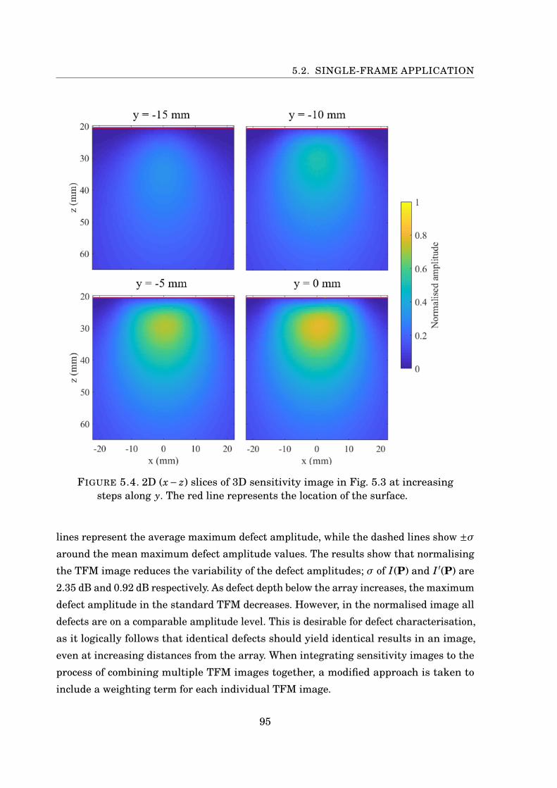
5.2. SINGLE-FRAME APPLICATION
FIGURE 5.4. 2D (x− z) slices of 3D sensitivity image in Fig. 5.3 at increasingsteps along y. The red line represents the location of the surface.
lines represent the average maximum defect amplitude, while the dashed lines show ±σaround the mean maximum defect amplitude values. The results show that normalising
the TFM image reduces the variability of the defect amplitudes; σ of I(P) and I ′(P) are
2.35 dB and 0.92 dB respectively. As defect depth below the array increases, the maximum
defect amplitude in the standard TFM decreases. However, in the normalised image all
defects are on a comparable amplitude level. This is desirable for defect characterisation,
as it logically follows that identical defects should yield identical results in an image,
even at increasing distances from the array. When integrating sensitivity images to the
process of combining multiple TFM images together, a modified approach is taken to
include a weighting term for each individual TFM image.
95
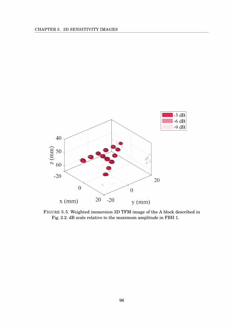
CHAPTER 5. 3D SENSITIVITY IMAGES
FIGURE 5.5. Weighted immersion 3D TFM image of the A block described inFig. 2.2. dB scale relative to the maximum amplitude in FBH 1.
96
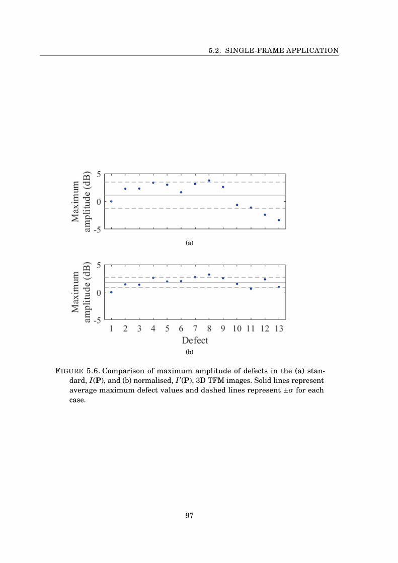
5.2. SINGLE-FRAME APPLICATION
(a)
(b)
FIGURE 5.6. Comparison of maximum amplitude of defects in the (a) stan-dard, I(P), and (b) normalised, I ′(P), 3D TFM images. Solid lines representaverage maximum defect values and dashed lines represent ±σ for eachcase.
97
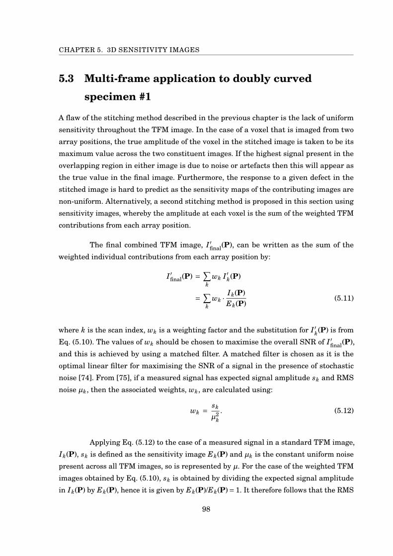
CHAPTER 5. 3D SENSITIVITY IMAGES
5.3 Multi-frame application to doubly curvedspecimen #1
A flaw of the stitching method described in the previous chapter is the lack of uniform
sensitivity throughout the TFM image. In the case of a voxel that is imaged from two
array positions, the true amplitude of the voxel in the stitched image is taken to be its
maximum value across the two constituent images. If the highest signal present in the
overlapping region in either image is due to noise or artefacts then this will appear as
the true value in the final image. Furthermore, the response to a given defect in the
stitched image is hard to predict as the sensitivity maps of the contributing images are
non-uniform. Alternatively, a second stitching method is proposed in this section using
sensitivity images, whereby the amplitude at each voxel is the sum of the weighted TFM
contributions from each array position.
The final combined TFM image, I ′final(P), can be written as the sum of the
weighted individual contributions from each array position by:
I ′final(P) = ∑k
wk I ′k(P)
= ∑k
wk ·Ik(P)Ek(P)
(5.11)
where k is the scan index, wk is a weighting factor and the substitution for I ′k(P) is from
Eq. (5.10). The values of wk should be chosen to maximise the overall SNR of I ′final(P),
and this is achieved by using a matched filter. A matched filter is chosen as it is the
optimal linear filter for maximising the SNR of a signal in the presence of stochastic
noise [74]. From [75], if a measured signal has expected signal amplitude sk and RMS
noise µk, then the associated weights, wk, are calculated using:
wk = sk
µ2k
. (5.12)
Applying Eq. (5.12) to the case of a measured signal in a standard TFM image,
Ik(P), sk is defined as the sensitivity image Ek(P) and µk is the constant uniform noise
present across all TFM images, so is represented by µ. For the case of the weighted TFM
images obtained by Eq. (5.10), sk is obtained by dividing the expected signal amplitude
in Ik(P) by Ek(P), hence it is given by Ek(P)/Ek(P)= 1. It therefore follows that the RMS
98

5.3. MULTI-FRAME APPLICATION TO DOUBLY CURVED SPECIMEN #1
noise in I ′k(P) is µ/Ek(P). Combining these results with the associated weights in Eq.
(5.12), the optimal weighting is defined by:
wk = 1µ2 / E2
k(P)
= E2k(P)
µ2 (5.13)
Combining Eqs. (5.11) and (5.13) therefore yields:
∑k
wk ·Ik(P)Ek(P)
= ∑k
E2k(P)
µ2 · Ik(P)Ek(P)
= 1µ2
∑k
Ek(P) Ik(P) (5.14)
which in theory gives optimal SNR at every point, but the sensitivity to defects will not
be spatially uniform. To obtain uniform sensitivity with an ideal reflector at every point,
Ik(P) = Ek(P) and hence each scan should be normalised by E2k (P) to give the final
expression:
I ′final (P) =∑k
Ik (P)Ek (P)∑k
E2k (P)
, (5.15)
where the scaling factor 1/µ2 is ignored.
5.3.1 Results
To investigate stitching using sensitivity images, the same data set that was used in
the previous chapter is used here. Again, the surface is assumed to be unknown and
therefore needs to be extracted. As the method of stitching TFM images that was used
in the previous chapter allowed an accurate surface to be extracted, it is used in the
surface extraction stage here for speed. Using subsections of the extracted surface as
before, the internal 3D TFM image is then generated using Eq. (5.15) and normalised to
the maximum amplitude within a patch of the back wall unobstructed by the presence
of defects. The interior 3D TFM image is shown in Fig. 5.7 as an isosurface at –24 dB
relative to the maximum amplitude in the back wall patch. The defect positions are
easily identified, along with large amplitude noise signals around the perimeter of the
specimen caused by normalisation using sensitivity images.
99
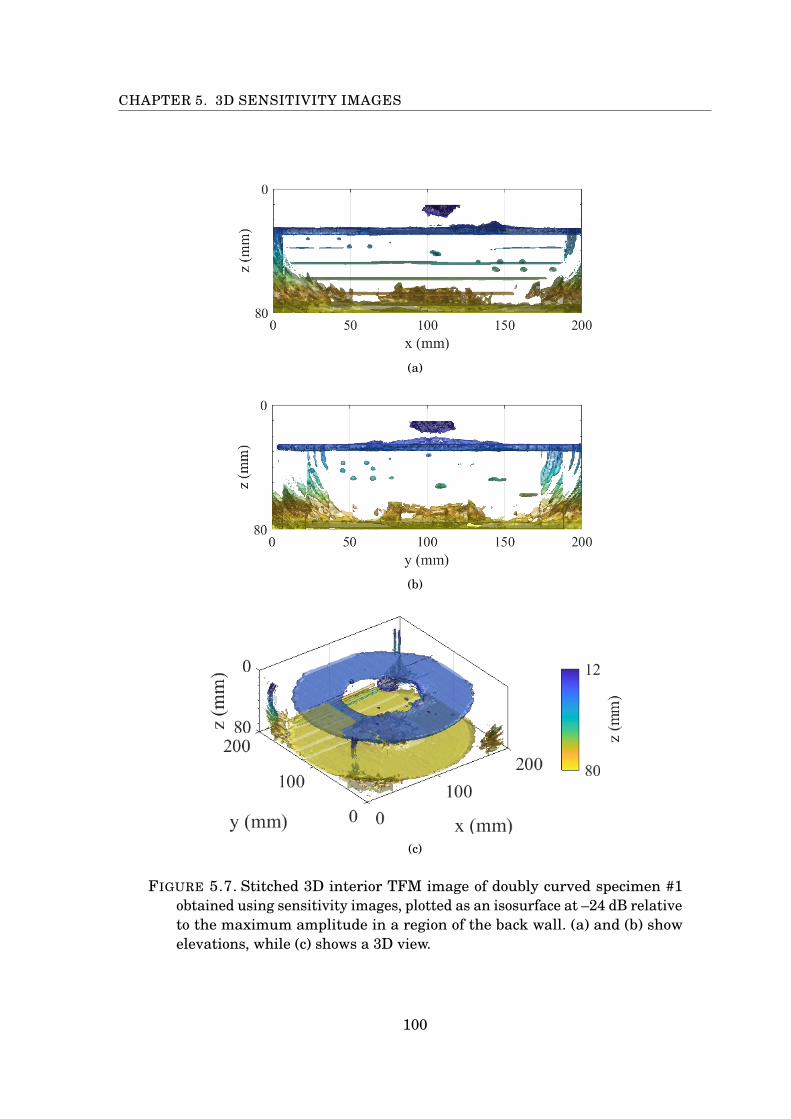
CHAPTER 5. 3D SENSITIVITY IMAGES
(a)
(b)
(c)
FIGURE 5.7. Stitched 3D interior TFM image of doubly curved specimen #1obtained using sensitivity images, plotted as an isosurface at –24 dB relativeto the maximum amplitude in a region of the back wall. (a) and (b) showelevations, while (c) shows a 3D view.
100

5.3. MULTI-FRAME APPLICATION TO DOUBLY CURVED SPECIMEN #1
As was examined in chapter 4, zoomed in windows around BDHs K, L and M
are shown in Fig. 5.8, where the defects are circular and well-focused. Snapshots of EDM
notches 4, 3 and 2 are also shown in Fig. 5.9; EDM notch 4 has low amplitude as a result
of normalisation using the maximum amplitude in the back wall patch, however in all
EDM notches the variation of amplitude that was visible in Fig. 4.10 along each notch is
not apparent due to the summing of weighted amplitudes at each image point.
One noticeable difference between stitching methods is the ability to view BDH
C; this defect was buried in noise in the previous chapter, but is able to be distinguished
through weighing, although it has an amplitude approximately 10 dB lower than the
second smallest defect signal. BDHs A, B, F, J, N, and R still remain unable to be imaged
using the current setup for the reasons described in section 4.4. Of the defects that
were able to be imaged, their positions were investigated and compared to the machined
locations using their centre points. This was achieved using the same two metrics as
in section 4.4: the first is the depth above the back wall and the second is the lateral
distance from the surface notch. These distances are then compared to the true values
from the specimen design file, with the comparison shown in Fig. 5.10. It was found
that σ for the depth comparison was 0.66 mm and 0.92 mm for the lateral distance
comparison. Both values are comparable to λ2/2 and are also in close agreement with
the values obtained using the other stitching method.
101
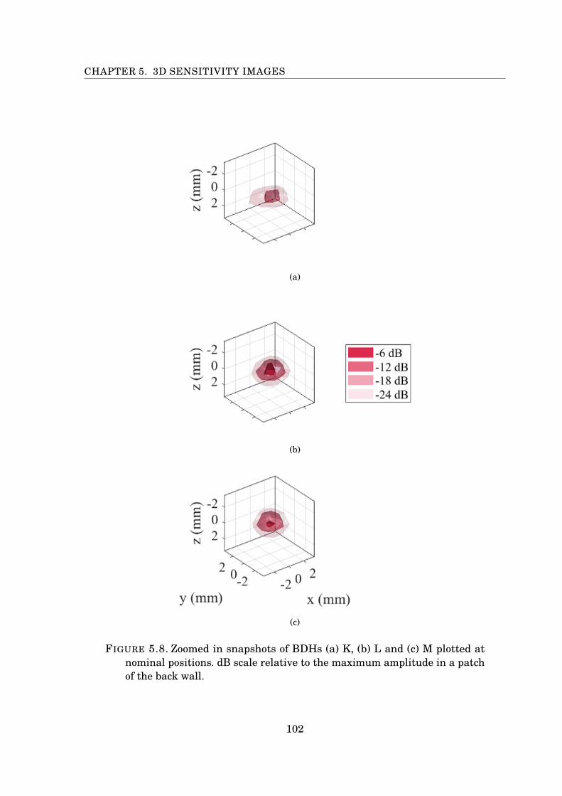
CHAPTER 5. 3D SENSITIVITY IMAGES
(a)
(b)
(c)
FIGURE 5.8. Zoomed in snapshots of BDHs (a) K, (b) L and (c) M plotted atnominal positions. dB scale relative to the maximum amplitude in a patchof the back wall.
102
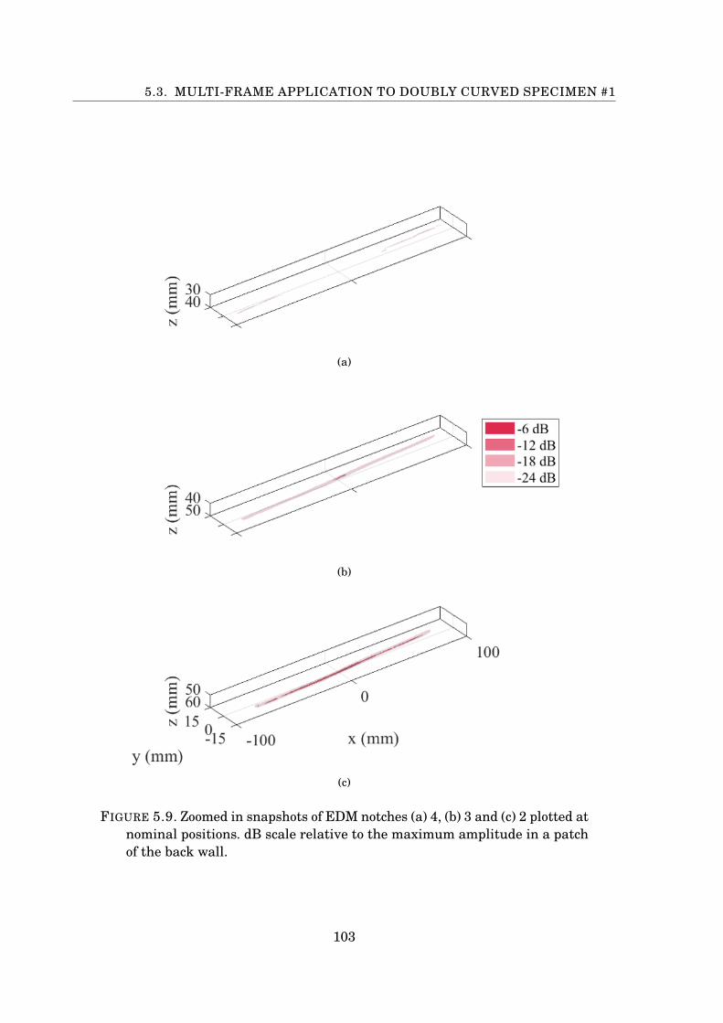
5.3. MULTI-FRAME APPLICATION TO DOUBLY CURVED SPECIMEN #1
(a)
(b)
(c)
FIGURE 5.9. Zoomed in snapshots of EDM notches (a) 4, (b) 3 and (c) 2 plotted atnominal positions. dB scale relative to the maximum amplitude in a patchof the back wall.
103
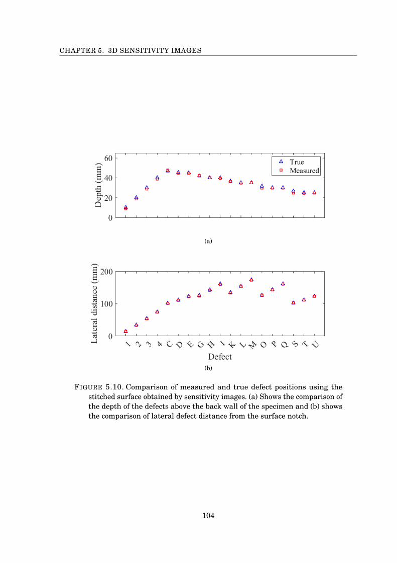
CHAPTER 5. 3D SENSITIVITY IMAGES
(a)
(b)
FIGURE 5.10. Comparison of measured and true defect positions using thestitched surface obtained by sensitivity images. (a) Shows the comparison ofthe depth of the defects above the back wall of the specimen and (b) showsthe comparison of lateral defect distance from the surface notch.
104
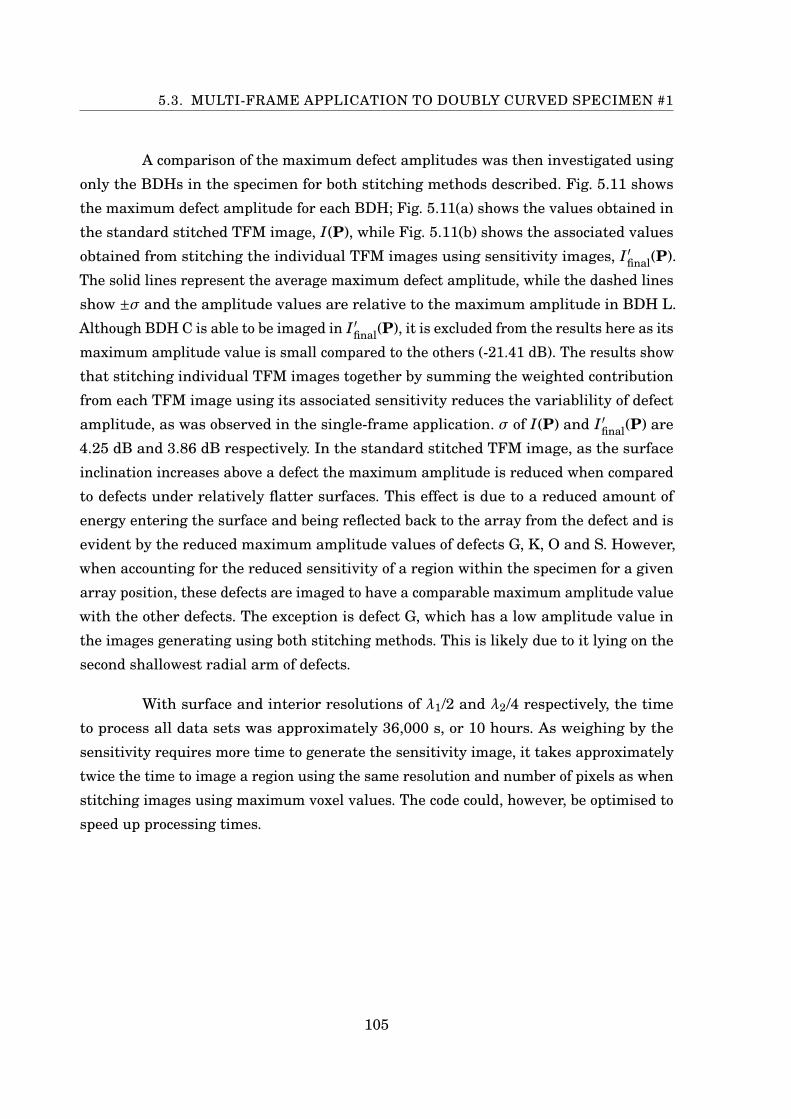
5.3. MULTI-FRAME APPLICATION TO DOUBLY CURVED SPECIMEN #1
A comparison of the maximum defect amplitudes was then investigated using
only the BDHs in the specimen for both stitching methods described. Fig. 5.11 shows
the maximum defect amplitude for each BDH; Fig. 5.11(a) shows the values obtained in
the standard stitched TFM image, I(P), while Fig. 5.11(b) shows the associated values
obtained from stitching the individual TFM images using sensitivity images, I ′final(P).
The solid lines represent the average maximum defect amplitude, while the dashed lines
show ±σ and the amplitude values are relative to the maximum amplitude in BDH L.
Although BDH C is able to be imaged in I ′final(P), it is excluded from the results here as its
maximum amplitude value is small compared to the others (-21.41 dB). The results show
that stitching individual TFM images together by summing the weighted contribution
from each TFM image using its associated sensitivity reduces the variablility of defect
amplitude, as was observed in the single-frame application. σ of I(P) and I ′final(P) are
4.25 dB and 3.86 dB respectively. In the standard stitched TFM image, as the surface
inclination increases above a defect the maximum amplitude is reduced when compared
to defects under relatively flatter surfaces. This effect is due to a reduced amount of
energy entering the surface and being reflected back to the array from the defect and is
evident by the reduced maximum amplitude values of defects G, K, O and S. However,
when accounting for the reduced sensitivity of a region within the specimen for a given
array position, these defects are imaged to have a comparable maximum amplitude value
with the other defects. The exception is defect G, which has a low amplitude value in
the images generating using both stitching methods. This is likely due to it lying on the
second shallowest radial arm of defects.
With surface and interior resolutions of λ1/2 and λ2/4 respectively, the time
to process all data sets was approximately 36,000 s, or 10 hours. As weighing by the
sensitivity requires more time to generate the sensitivity image, it takes approximately
twice the time to image a region using the same resolution and number of pixels as when
stitching images using maximum voxel values. The code could, however, be optimised to
speed up processing times.
105
CHAPTER 5. 3D SENSITIVITY IMAGES
(a)
(b)
FIGURE 5.11. Comparison of maximum amplitude of BDH defects in the (a)standard stitched TFM image, I(P), and (b) stitched 3D TFM images usingsensitivity images, I ′final(P). Solid lines represent average maximum defectvalues and dashed lines represent ±σ for each case.
106
5.4. SUMMARY
5.4 Summary
3D sensitivity images have been introduced in this chapter for optimising TFM imaging
using a single frame and multiple data sets captured from a scanned array. The sensitivity
image represents an estimate of the TFM intensity that would be measured from a defect
at a specific location, and is a useful tool for determining regions in a specimen that can
be optimally imaged using a particular inspection setup. Using a single frame application,
a TFM image that was normalised by its sensitivity image has resulted in less variability
of maximum defect amplitudes of identical defects at increasing depths, as the sensitivity
has become uniform in the image. However, normalising a TFM image by its associated
sensitivity image produces non-uniform noise in the resulting image. In a standard TFM
image, sensitivity is non-uniform and so defects located further away from the array have
lower amplitude responses compared to an identical defect located closer to the array. An
alternative method for stitching multiple TFM images has also been introduced, whereby
the true amplitude of a voxel is the sum of weighted contributions from normalised TFM
images at each array position. Defects in the stitched 3D TFM image obtained using
sensitivity images were able to be accurately positioned, however defects located under a
relatively steep inclined surface region remain impossible to image in the current setup.
To assess the stitching methods, the following chapter focuses on the characterisation of
defects.
107


Chapter 6
Defect characterisation
After a defect has been successfully detected, the next step of a thorough inspection
involves characterisation whereby defect parameters such as size, shape and orientation
can be determined. Knowledge of these parameters allows the defect type to be identified,
which is crucial for determining the integrity of a system as planar defects with sharp
edges (e.g. cracks and lack of fusion) are more likely to grow and cause failure when
compared to volumetric defects (e.g. voids and inclusions). Engineering specifications for
a component normally have a requirement that any detected defect must be below an
allowable size for continued operation; considering the high-cost structures in which NDT
is routinely implemented, accurate characterisation of defects can be the difference be-
tween safe operation and failure. Additionally, characterisation on end-of-life components
can influence the decision between remanufacturing or scrapping. Remanufacturing is
viewed as an advantageous solution when deciding what to do with used components
as it is environmentally friendly and cost efficient [76]. The component must, however,
meet certain standards before it is reused, which are determined using NDE methods.
3D characterisation of a defect is important for determining its nature. As de-
fects can appear in arbitrary orientations in 3D, it is desirable to insonify the defect from
as many directions as possible to obtain the maximum amount of information. Inspection
with a linear array means insonifying the defect in a single plane; 3D information about
the defect therefore cannot be obtained without translation or rotation of the array. As
was mentioned in earlier chapters, a consequence of this means that resolution is limited
in the out-of-plane direction, thus making accurate characterisation challenging. As a
2D array can probe a defect over a larger range of solid angles from a single position, its
109
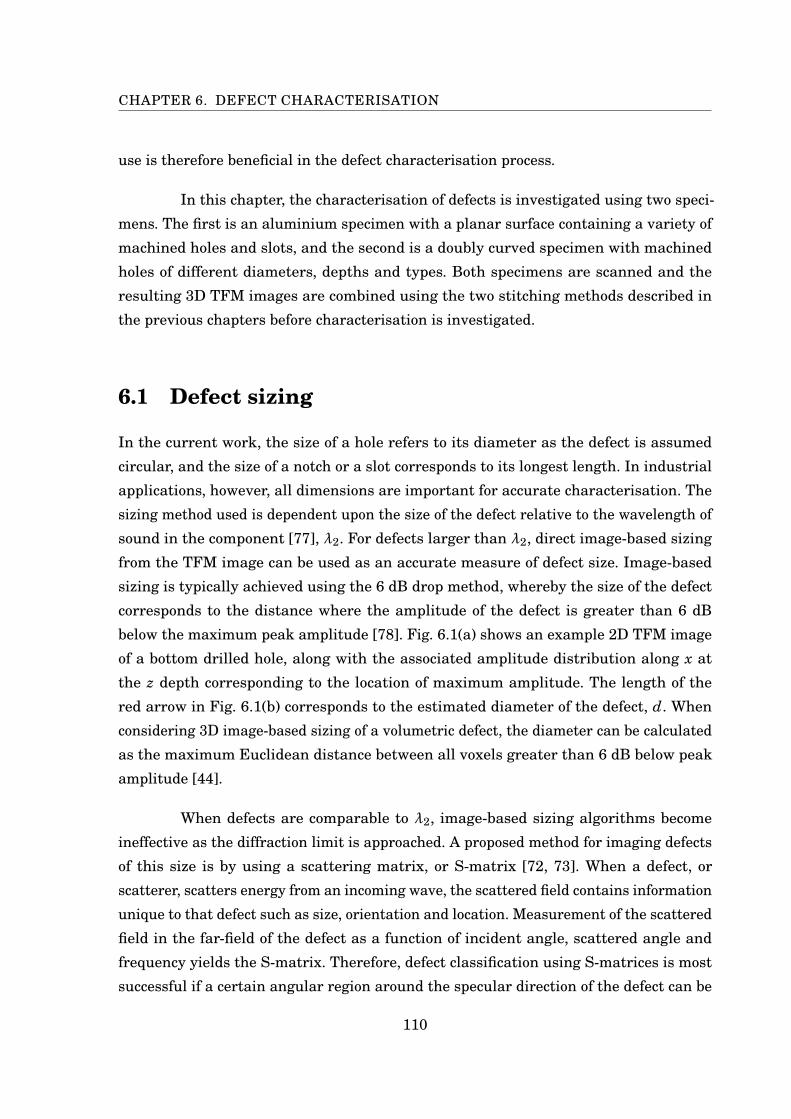
CHAPTER 6. DEFECT CHARACTERISATION
use is therefore beneficial in the defect characterisation process.
In this chapter, the characterisation of defects is investigated using two speci-
mens. The first is an aluminium specimen with a planar surface containing a variety of
machined holes and slots, and the second is a doubly curved specimen with machined
holes of different diameters, depths and types. Both specimens are scanned and the
resulting 3D TFM images are combined using the two stitching methods described in
the previous chapters before characterisation is investigated.
6.1 Defect sizing
In the current work, the size of a hole refers to its diameter as the defect is assumed
circular, and the size of a notch or a slot corresponds to its longest length. In industrial
applications, however, all dimensions are important for accurate characterisation. The
sizing method used is dependent upon the size of the defect relative to the wavelength of
sound in the component [77], λ2. For defects larger than λ2, direct image-based sizing
from the TFM image can be used as an accurate measure of defect size. Image-based
sizing is typically achieved using the 6 dB drop method, whereby the size of the defect
corresponds to the distance where the amplitude of the defect is greater than 6 dB
below the maximum peak amplitude [78]. Fig. 6.1(a) shows an example 2D TFM image
of a bottom drilled hole, along with the associated amplitude distribution along x at
the z depth corresponding to the location of maximum amplitude. The length of the
red arrow in Fig. 6.1(b) corresponds to the estimated diameter of the defect, d. When
considering 3D image-based sizing of a volumetric defect, the diameter can be calculated
as the maximum Euclidean distance between all voxels greater than 6 dB below peak
amplitude [44].
When defects are comparable to λ2, image-based sizing algorithms become
ineffective as the diffraction limit is approached. A proposed method for imaging defects
of this size is by using a scattering matrix, or S-matrix [72, 73]. When a defect, or
scatterer, scatters energy from an incoming wave, the scattered field contains information
unique to that defect such as size, orientation and location. Measurement of the scattered
field in the far-field of the defect as a function of incident angle, scattered angle and
frequency yields the S-matrix. Therefore, defect classification using S-matrices is most
successful if a certain angular region around the specular direction of the defect can be
110
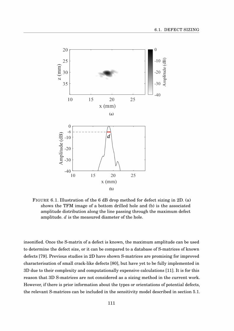
6.1. DEFECT SIZING
(a)
(b)
FIGURE 6.1. Illustration of the 6 dB drop method for defect sizing in 2D. (a)shows the TFM image of a bottom drilled hole and (b) is the associatedamplitude distribution along the line passing through the maximum defectamplitude. d is the measured diameter of the hole.
insonified. Once the S-matrix of a defect is known, the maximum amplitude can be used
to determine the defect size, or it can be compared to a database of S-matrices of known
defects [79]. Previous studies in 2D have shown S-matrices are promising for improved
characterisation of small crack-like defects [80], but have yet to be fully implemented in
3D due to their complexity and computationally expensive calculations [11]. It is for this
reason that 3D S-matrices are not considered as a sizing method in the current work.
However, if there is prior information about the types or orientations of potential defects,
the relevant S-matrices can be included in the sensitivity model described in section 5.1.
111
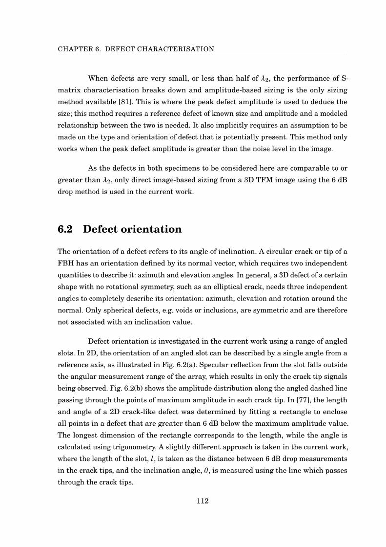
CHAPTER 6. DEFECT CHARACTERISATION
When defects are very small, or less than half of λ2, the performance of S-
matrix characterisation breaks down and amplitude-based sizing is the only sizing
method available [81]. This is where the peak defect amplitude is used to deduce the
size; this method requires a reference defect of known size and amplitude and a modeled
relationship between the two is needed. It also implicitly requires an assumption to be
made on the type and orientation of defect that is potentially present. This method only
works when the peak defect amplitude is greater than the noise level in the image.
As the defects in both specimens to be considered here are comparable to or
greater than λ2, only direct image-based sizing from a 3D TFM image using the 6 dB
drop method is used in the current work.
6.2 Defect orientation
The orientation of a defect refers to its angle of inclination. A circular crack or tip of a
FBH has an orientation defined by its normal vector, which requires two independent
quantities to describe it: azimuth and elevation angles. In general, a 3D defect of a certain
shape with no rotational symmetry, such as an elliptical crack, needs three independent
angles to completely describe its orientation: azimuth, elevation and rotation around the
normal. Only spherical defects, e.g. voids or inclusions, are symmetric and are therefore
not associated with an inclination value.
Defect orientation is investigated in the current work using a range of angled
slots. In 2D, the orientation of an angled slot can be described by a single angle from a
reference axis, as illustrated in Fig. 6.2(a). Specular reflection from the slot falls outside
the angular measurement range of the array, which results in only the crack tip signals
being observed. Fig. 6.2(b) shows the amplitude distribution along the angled dashed line
passing through the points of maximum amplitude in each crack tip. In [77], the length
and angle of a 2D crack-like defect was determined by fitting a rectangle to enclose
all points in a defect that are greater than 6 dB below the maximum amplitude value.
The longest dimension of the rectangle corresponds to the length, while the angle is
calculated using trigonometry. A slightly different approach is taken in the current work,
where the length of the slot, l, is taken as the distance between 6 dB drop measurements
in the crack tips, and the inclination angle, θ, is measured using the line which passes
through the crack tips.
112
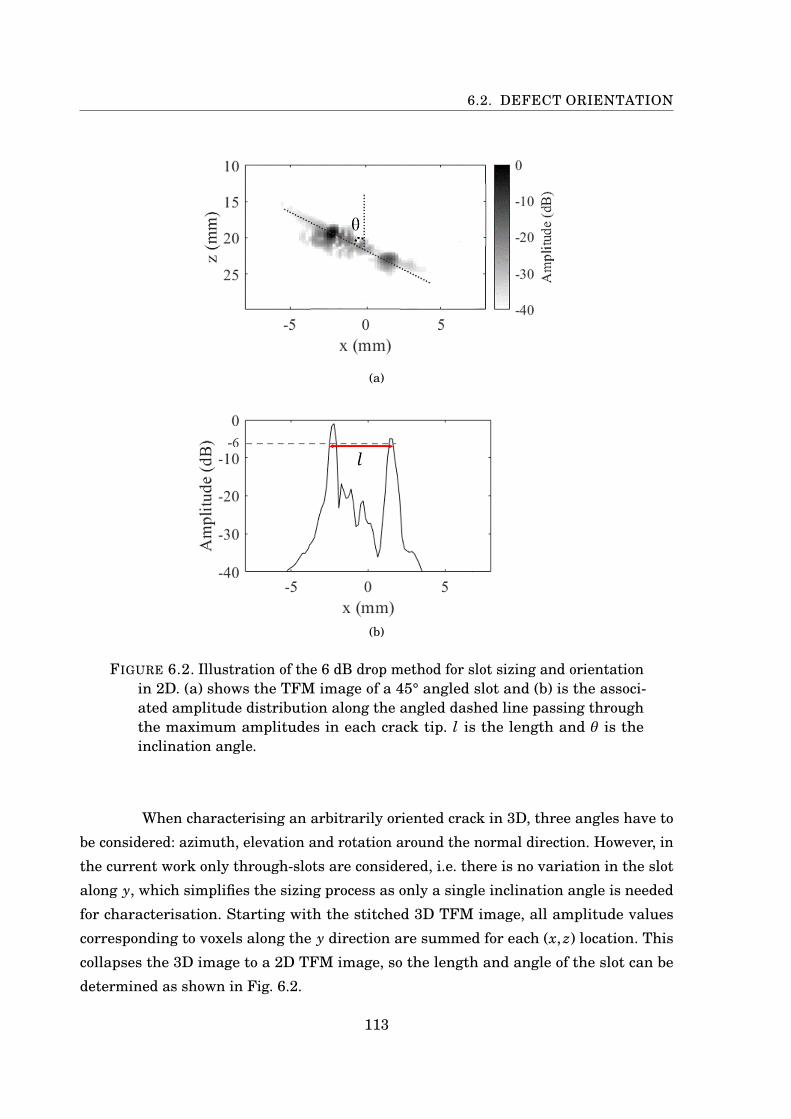
6.2. DEFECT ORIENTATION
(a)
(b)
FIGURE 6.2. Illustration of the 6 dB drop method for slot sizing and orientationin 2D. (a) shows the TFM image of a 45° angled slot and (b) is the associ-ated amplitude distribution along the angled dashed line passing throughthe maximum amplitudes in each crack tip. l is the length and θ is theinclination angle.
When characterising an arbitrarily oriented crack in 3D, three angles have to
be considered: azimuth, elevation and rotation around the normal direction. However, in
the current work only through-slots are considered, i.e. there is no variation in the slot
along y, which simplifies the sizing process as only a single inclination angle is needed
for characterisation. Starting with the stitched 3D TFM image, all amplitude values
corresponding to voxels along the y direction are summed for each (x, z) location. This
collapses the 3D image to a 2D TFM image, so the length and angle of the slot can be
determined as shown in Fig. 6.2.
113
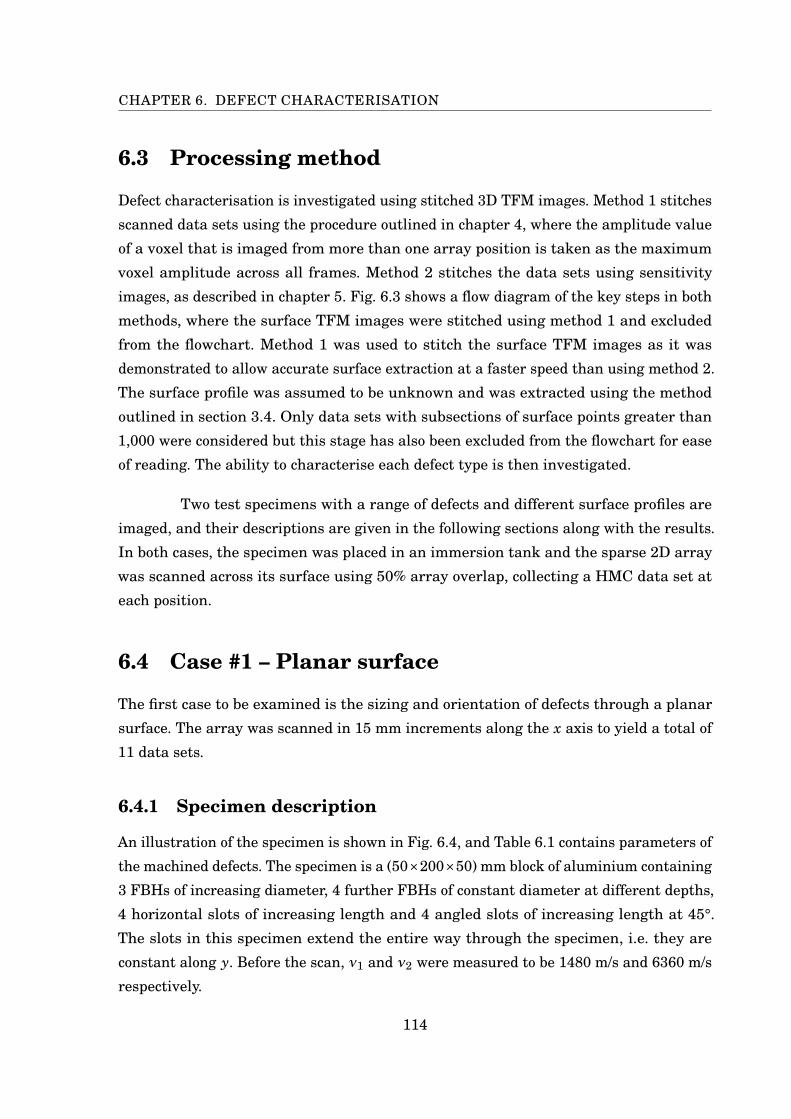
CHAPTER 6. DEFECT CHARACTERISATION
6.3 Processing method
Defect characterisation is investigated using stitched 3D TFM images. Method 1 stitches
scanned data sets using the procedure outlined in chapter 4, where the amplitude value
of a voxel that is imaged from more than one array position is taken as the maximum
voxel amplitude across all frames. Method 2 stitches the data sets using sensitivity
images, as described in chapter 5. Fig. 6.3 shows a flow diagram of the key steps in both
methods, where the surface TFM images were stitched using method 1 and excluded
from the flowchart. Method 1 was used to stitch the surface TFM images as it was
demonstrated to allow accurate surface extraction at a faster speed than using method 2.
The surface profile was assumed to be unknown and was extracted using the method
outlined in section 3.4. Only data sets with subsections of surface points greater than
1,000 were considered but this stage has also been excluded from the flowchart for ease
of reading. The ability to characterise each defect type is then investigated.
Two test specimens with a range of defects and different surface profiles are
imaged, and their descriptions are given in the following sections along with the results.
In both cases, the specimen was placed in an immersion tank and the sparse 2D array
was scanned across its surface using 50% array overlap, collecting a HMC data set at
each position.
6.4 Case #1 – Planar surface
The first case to be examined is the sizing and orientation of defects through a planar
surface. The array was scanned in 15 mm increments along the x axis to yield a total of
11 data sets.
6.4.1 Specimen description
An illustration of the specimen is shown in Fig. 6.4, and Table 6.1 contains parameters of
the machined defects. The specimen is a (50×200×50) mm block of aluminium containing
3 FBHs of increasing diameter, 4 further FBHs of constant diameter at different depths,
4 horizontal slots of increasing length and 4 angled slots of increasing length at 45°.
The slots in this specimen extend the entire way through the specimen, i.e. they are
constant along y. Before the scan, ν1 and ν2 were measured to be 1480 m/s and 6360 m/s
respectively.
114
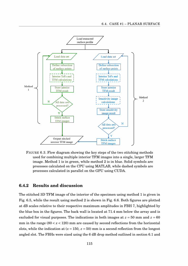
6.4. CASE #1 – PLANAR SURFACE
FIGURE 6.3. Flow diagram showing the key steps of the two stitching methodsused for combining multiple interior TFM images into a single, larger TFMimage. Method 1 is in green, while method 2 is in blue. Solid symbols areprocesses calculated on the CPU using MATLAB, while dashed symbols areprocesses calculated in parallel on the GPU using CUDA.
6.4.2 Results and discussion
The stitched 3D TFM image of the interior of the specimen using method 1 is given in
Fig. 6.5, while the result using method 2 is shown in Fig. 6.6. Both figures are plotted
at dB scales relative to their respective maximum amplitudes in FBH 7, highlighted by
the blue box in the figures. The back wall is located at 71.4 mm below the array and is
excluded for visual purposes. The indications in both images at z = 50 mm and z = 60
mm in the range (80< x < 120) mm are caused by second reflections from the horizontal
slots, while the indication at (x = 150, z = 50) mm is a second reflection from the longest
angled slot. The FBHs were sized using the 6 dB drop method outlined in section 6.1 and
115
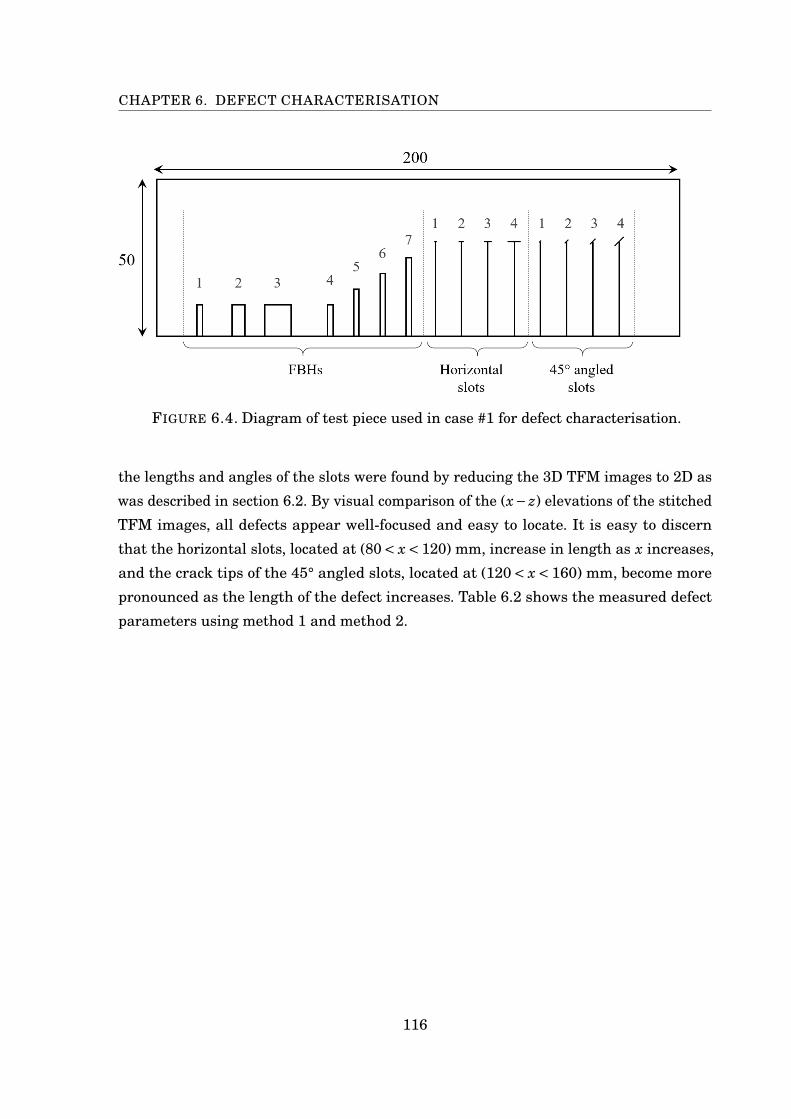
CHAPTER 6. DEFECT CHARACTERISATION
FIGURE 6.4. Diagram of test piece used in case #1 for defect characterisation.
the lengths and angles of the slots were found by reducing the 3D TFM images to 2D as
was described in section 6.2. By visual comparison of the (x− z) elevations of the stitched
TFM images, all defects appear well-focused and easy to locate. It is easy to discern
that the horizontal slots, located at (80< x < 120) mm, increase in length as x increases,
and the crack tips of the 45° angled slots, located at (120< x < 160) mm, become more
pronounced as the length of the defect increases. Table 6.2 shows the measured defect
parameters using method 1 and method 2.
116
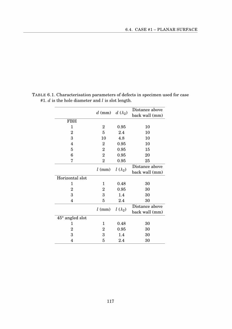
6.4. CASE #1 – PLANAR SURFACE
TABLE 6.1. Characterisation parameters of defects in specimen used for case#1. d is the hole diameter and l is slot length.
d (mm) d (λ2)Distance aboveback wall (mm)
FBH1 2 0.95 102 5 2.4 103 10 4.8 104 2 0.95 105 2 0.95 156 2 0.95 207 2 0.95 25
l (mm) l (λ2)Distance aboveback wall (mm)
Horizontal slot1 1 0.48 302 2 0.95 303 3 1.4 304 5 2.4 30
l (mm) l (λ2)Distance aboveback wall (mm)
45° angled slot1 1 0.48 302 2 0.95 303 3 1.4 304 5 2.4 30
117
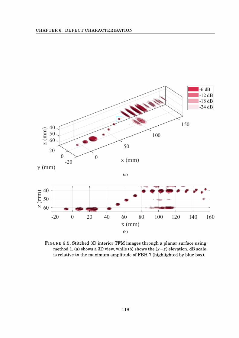
CHAPTER 6. DEFECT CHARACTERISATION
(a)
(b)
FIGURE 6.5. Stitched 3D interior TFM images through a planar surface usingmethod 1. (a) shows a 3D view, while (b) shows the (x−z) elevation. dB scaleis relative to the maximum amplitude of FBH 7 (highlighted by blue box).
118
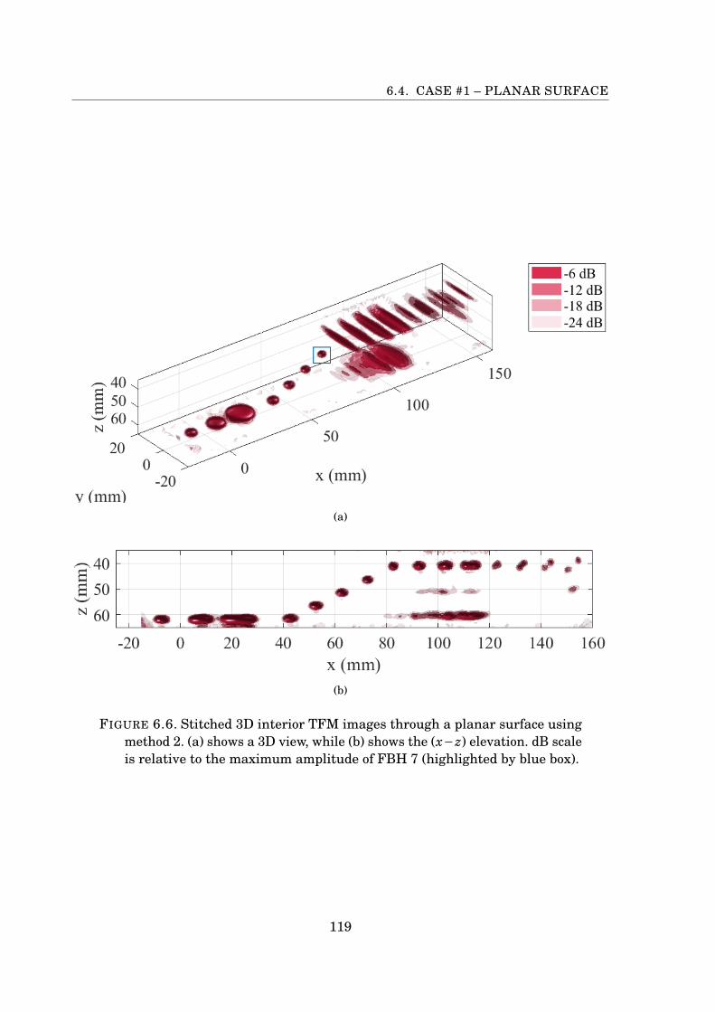
6.4. CASE #1 – PLANAR SURFACE
(a)
(b)
FIGURE 6.6. Stitched 3D interior TFM images through a planar surface usingmethod 2. (a) shows a 3D view, while (b) shows the (x−z) elevation. dB scaleis relative to the maximum amplitude of FBH 7 (highlighted by blue box).
119
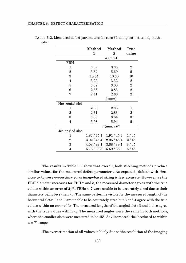
CHAPTER 6. DEFECT CHARACTERISATION
TABLE 6.2. Measured defect parameters for case #1 using both stitching meth-ods.
Method1
Method2
Truevalue
d (mm)FBH
1 3.39 3.35 22 5.32 5.60 53 10.54 10.36 104 3.20 3.32 25 3.39 3.08 26 2.68 2.83 27 2.41 2.66 2
l (mm)Horizontal slot
1 2.59 2.35 12 2.61 2.83 23 3.35 3.64 34 5.98 5.94 5
l (mm) / θ°45° angled slot
1 1.87 / 45.4 1.91 / 45.4 1 / 452 3.02 / 45.4 2.96 / 45.4 2 / 453 4.03 / 39.1 3.88 / 39.1 3 / 454 5.76 / 38.3 5.69 / 38.3 5 / 45
The results in Table 6.2 show that overall, both stitching methods produce
similar values for the measured defect parameters. As expected, defects with sizes
close to λ2 were overestimated as image-based sizing is less accurate. However, as the
FBH diameter increases for FBH 2 and 3, the measured diameter agrees with the true
values within an error of λ2/3. FBHs 4–7 were unable to be accurately sized due to their
diameters being less than λ2. The same pattern is visible for the measured length of the
horizontal slots: 1 and 2 are unable to be accurately sized but 3 and 4 agree with the true
values within an error of λ2. The measured lengths of the angled slots 3 and 4 also agree
with the true values within λ2. The measured angles were the same in both methods,
where the smaller slots were measured to be 45°. As l increased, the θ reduced to within
a ± 7° range.
The overestimation of all values is likely due to the resolution of the imaging
120
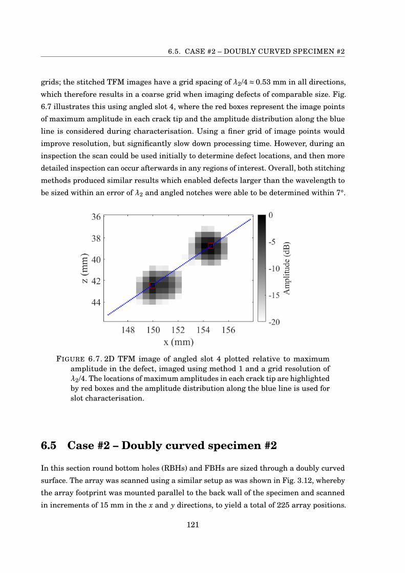
6.5. CASE #2 – DOUBLY CURVED SPECIMEN #2
grids; the stitched TFM images have a grid spacing of λ2/4≈ 0.53 mm in all directions,
which therefore results in a coarse grid when imaging defects of comparable size. Fig.
6.7 illustrates this using angled slot 4, where the red boxes represent the image points
of maximum amplitude in each crack tip and the amplitude distribution along the blue
line is considered during characterisation. Using a finer grid of image points would
improve resolution, but significantly slow down processing time. However, during an
inspection the scan could be used initially to determine defect locations, and then more
detailed inspection can occur afterwards in any regions of interest. Overall, both stitching
methods produced similar results which enabled defects larger than the wavelength to
be sized within an error of λ2 and angled notches were able to be determined within 7°.
FIGURE 6.7. 2D TFM image of angled slot 4 plotted relative to maximumamplitude in the defect, imaged using method 1 and a grid resolution ofλ2/4. The locations of maximum amplitudes in each crack tip are highlightedby red boxes and the amplitude distribution along the blue line is used forslot characterisation.
6.5 Case #2 – Doubly curved specimen #2
In this section round bottom holes (RBHs) and FBHs are sized through a doubly curved
surface. The array was scanned using a similar setup as was shown in Fig. 3.12, whereby
the array footprint was mounted parallel to the back wall of the specimen and scanned
in increments of 15 mm in the x and y directions, to yield a total of 225 array positions.
121

CHAPTER 6. DEFECT CHARACTERISATION
TABLE 6.3. Type and diameter of defects in doubly curved specimen #2.
DefectFBH RBH d (mm)
A - 6B1 B2 8C1 C2 8D1 D2 8E1 E2 8F1 F2 4G1 G2 4H1 H2 4I1 I2 4J1 J2 6K1 K2 6L1 L2 6M1 M2 6N1 N2 2O1 O2 2P1 P2 2Q1 Q2 2
Array positions that were not directly over the specimen were discounted. Before the
scan, ν1 and ν2 were measured to be 1480 m/s and 6470 m/s respectively.
6.5.1 Specimen description
The specimen used to investigate defect sizing through a doubly curved surface has
an identical surface profile to doubly curved specimen #1 from section 3.5.1, i.e. it is
described by Eq. (3.6), but the height of the base was reduced to allow defects to be
machined. The specimen contains FBHs and RBHs of different diameters located 20 mm
below the surface; FBHs were chosen because the flat tip appears like a circular crack
when ultrasonically imaged from above, while the tip of RBHs resemble a spherical void.
An illustration of the specimen design is shown in Fig. 6.8, with the defects labelled in
the base view in Fig. 6.8(b). The diameters, d, and types of machined defects are given in
Table 6.3.
122
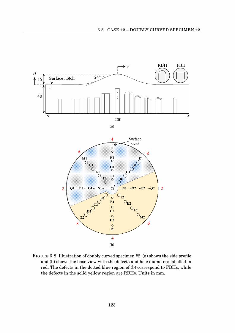
6.5. CASE #2 – DOUBLY CURVED SPECIMEN #2
(a)
(b)
FIGURE 6.8. Illustration of doubly curved specimen #2. (a) shows the side profileand (b) shows the base view with the defects and hole diameters labelled inred. The defects in the dotted blue region of (b) correspond to FBHs, whilethe defects in the solid yellow region are RBHs. Units in mm.
123
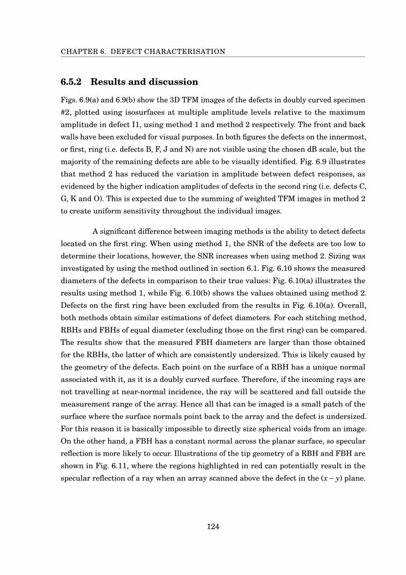
CHAPTER 6. DEFECT CHARACTERISATION
6.5.2 Results and discussion
Figs. 6.9(a) and 6.9(b) show the 3D TFM images of the defects in doubly curved specimen
#2, plotted using isosurfaces at multiple amplitude levels relative to the maximum
amplitude in defect I1, using method 1 and method 2 respectively. The front and back
walls have been excluded for visual purposes. In both figures the defects on the innermost,
or first, ring (i.e. defects B, F, J and N) are not visible using the chosen dB scale, but the
majority of the remaining defects are able to be visually identified. Fig. 6.9 illustrates
that method 2 has reduced the variation in amplitude between defect responses, as
evidenced by the higher indication amplitudes of defects in the second ring (i.e. defects C,
G, K and O). This is expected due to the summing of weighted TFM images in method 2
to create uniform sensitivity throughout the individual images.
A significant difference between imaging methods is the ability to detect defects
located on the first ring. When using method 1, the SNR of the defects are too low to
determine their locations, however, the SNR increases when using method 2. Sizing was
investigated by using the method outlined in section 6.1. Fig. 6.10 shows the measured
diameters of the defects in comparison to their true values: Fig. 6.10(a) illustrates the
results using method 1, while Fig. 6.10(b) shows the values obtained using method 2.
Defects on the first ring have been excluded from the results in Fig. 6.10(a). Overall,
both methods obtain similar estimations of defect diameters. For each stitching method,
RBHs and FBHs of equal diameter (excluding those on the first ring) can be compared.
The results show that the measured FBH diameters are larger than those obtained
for the RBHs, the latter of which are consistently undersized. This is likely caused by
the geometry of the defects. Each point on the surface of a RBH has a unique normal
associated with it, as it is a doubly curved surface. Therefore, if the incoming rays are
not travelling at near-normal incidence, the ray will be scattered and fall outside the
measurement range of the array. Hence all that can be imaged is a small patch of the
surface where the surface normals point back to the array and the defect is undersized.
For this reason it is basically impossible to directly size spherical voids from an image.
On the other hand, a FBH has a constant normal across the planar surface, so specular
reflection is more likely to occur. Illustrations of the tip geometry of a RBH and FBH are
shown in Fig. 6.11, where the regions highlighted in red can potentially result in the
specular reflection of a ray when an array scanned above the defect in the (x− y) plane.
124
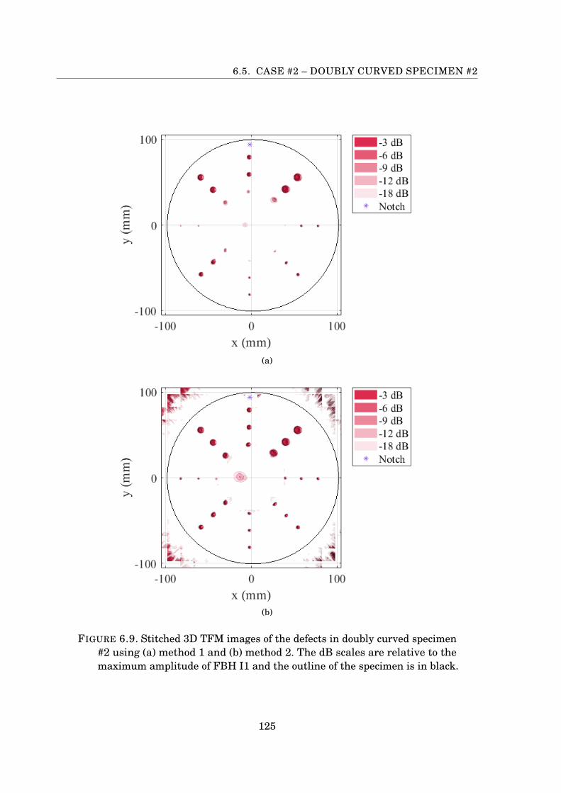
6.5. CASE #2 – DOUBLY CURVED SPECIMEN #2
(a)
(b)
FIGURE 6.9. Stitched 3D TFM images of the defects in doubly curved specimen#2 using (a) method 1 and (b) method 2. The dB scales are relative to themaximum amplitude of FBH I1 and the outline of the specimen is in black.
125
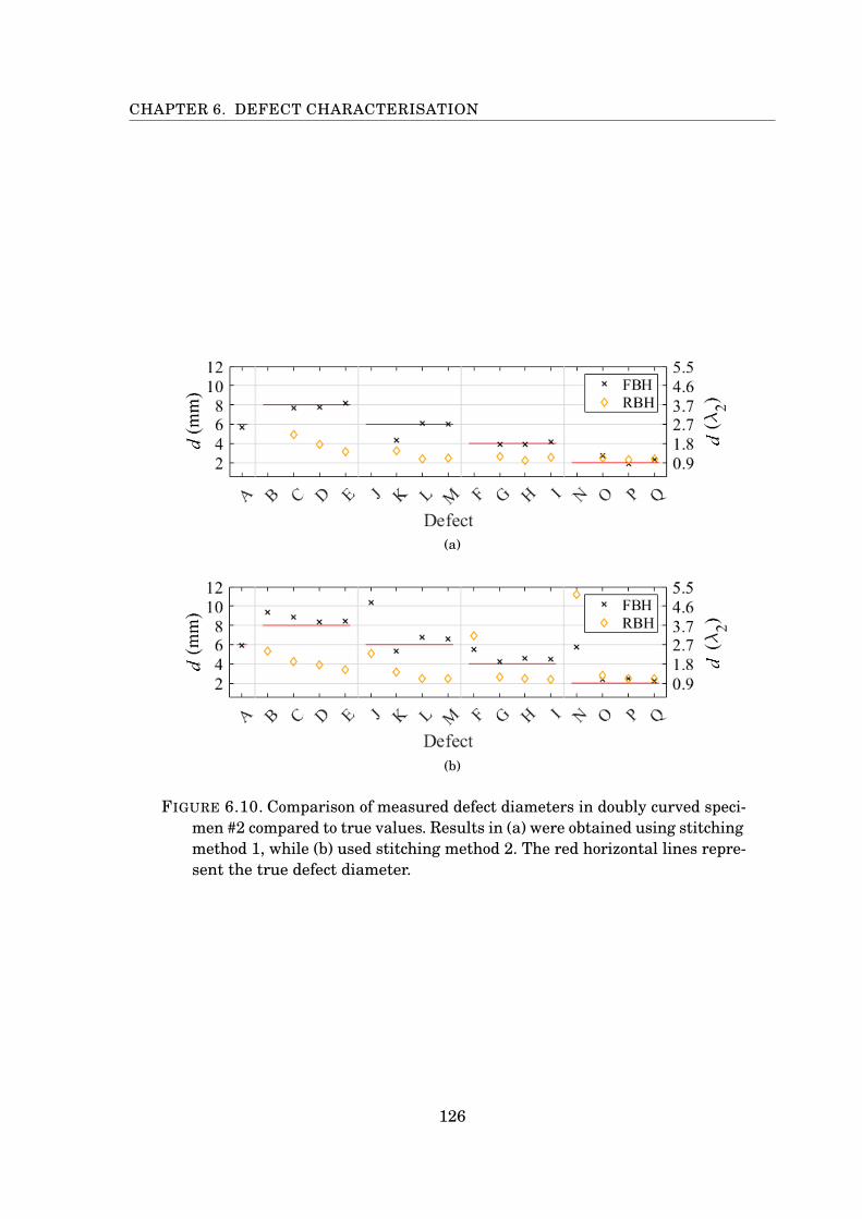
CHAPTER 6. DEFECT CHARACTERISATION
(a)
(b)
FIGURE 6.10. Comparison of measured defect diameters in doubly curved speci-men #2 compared to true values. Results in (a) were obtained using stitchingmethod 1, while (b) used stitching method 2. The red horizontal lines repre-sent the true defect diameter.
126
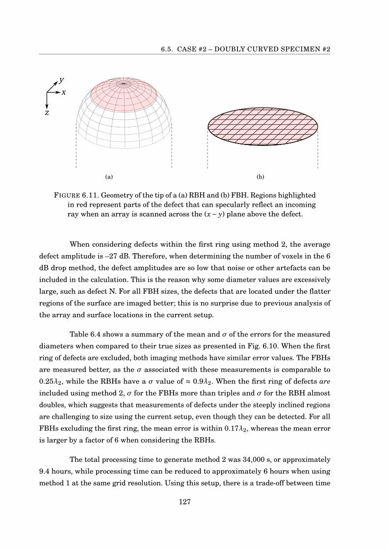
6.5. CASE #2 – DOUBLY CURVED SPECIMEN #2
(a) (b)
FIGURE 6.11. Geometry of the tip of a (a) RBH and (b) FBH. Regions highlightedin red represent parts of the defect that can specularly reflect an incomingray when an array is scanned across the (x− y) plane above the defect.
When considering defects within the first ring using method 2, the average
defect amplitude is –27 dB. Therefore, when determining the number of voxels in the 6
dB drop method, the defect amplitudes are so low that noise or other artefacts can be
included in the calculation. This is the reason why some diameter values are excessively
large, such as defect N. For all FBH sizes, the defects that are located under the flatter
regions of the surface are imaged better; this is no surprise due to previous analysis of
the array and surface locations in the current setup.
Table 6.4 shows a summary of the mean and σ of the errors for the measured
diameters when compared to their true sizes as presented in Fig. 6.10. When the first
ring of defects are excluded, both imaging methods have similar error values. The FBHs
are measured better, as the σ associated with these measurements is comparable to
0.25λ2, while the RBHs have a σ value of ≈ 0.9λ2. When the first ring of defects are
included using method 2, σ for the FBHs more than triples and σ for the RBH almost
doubles, which suggests that measurements of defects under the steeply inclined regions
are challenging to size using the current setup, even though they can be detected. For all
FBHs excluding the first ring, the mean error is within 0.17λ2, whereas the mean error
is larger by a factor of 6 when considering the RBHs.
The total processing time to generate method 2 was 34,000 s, or approximately
9.4 hours, while processing time can be reduced to approximately 6 hours when using
method 1 at the same grid resolution. Using this setup, there is a trade-off between time
127
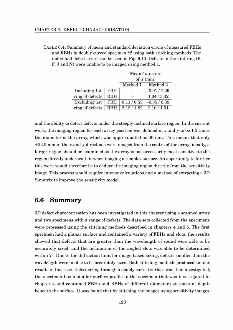
CHAPTER 6. DEFECT CHARACTERISATION
TABLE 6.4. Summary of mean and standard deviation errors of measured FBHsand RBHs in doubly curved specimen #2 using both stitching methods. Theindividual defect errors can be seen in Fig. 6.10. Defects in the first ring (B,F, J and N) were unable to be imaged using method 1.
Mean / σ errorsof d (mm)
Method 1 Method 2Including 1string of defects
FBH - -0.91 / 1.29RBH - 1.04 / 3.42
Excluding 1string of defects
FBH 0.11 / 0.55 -0.35 / 0.39RBH 2.12 / 1.82 2.10 / 1.91
and the ability to detect defects under the steeply inclined surface region. In the current
work, the imaging region for each array position was defined in x and y to be 1.5 times
the diameter of the array, which was approximated as 30 mm. This means that only
±22.5 mm in the x and y directions were imaged from the centre of the array; ideally, a
larger region should be examined as the array is not necessarily most sensitive to the
region directly underneath it when imaging a complex surface. An opportunity to further
this work would therefore be to deduce the imaging region directly from the sensitivity
image. This process would require intense calculations and a method of extracting a 3D
S-matrix to improve the sensitivity model.
6.6 Summary
3D defect characterisation has been investigated in this chapter using a scanned array
and two specimens with a range of defects. The data sets collected from the specimens
were processed using the stitching methods described in chapters 4 and 5. The first
specimen had a planar surface and contained a variety of FBHs and slots; the results
showed that defects that are greater than the wavelength of sound were able to be
accurately sized, and the inclination of the angled slots was able to be determined
within 7°. Due to the diffraction limit for image-based sizing, defects smaller than the
wavelength were unable to be accurately sized. Both stitching methods produced similar
results in this case. Defect sizing through a doubly curved surface was then investigated;
the specimen has a similar surface profile to the specimen that was investigated in
chapter 4 and contained FBHs and RBHs of different diameters at constant depth
beneath the surface. It was found that by stitching the images using sensitivity images,
128

6.6. SUMMARY
defects that were unable to be imaged using the other method were now able to be
detected. However, the amplitude signals of these defects were too low to allow accurate
sizing. As was observed in the first specimen, both stitching methods produced similar
results and the standard deviation of defect sizing was less than a quarter of the
wavelength. Stitching images using sensitivity maps took on average 4 hours longer to
process than the method of taking the maximum defect amplitude across multiple image
frames, so there is a trade-off between processing time and the ability to detect defects.
129

Chapter 7
Conclusions
7.1 Review of thesis
This thesis has investigated 3D volumetric TFM imaging using a sparse 2D phased array
and the subsequent ability to detect and characterise defects through complex surfaces.
First, in chapter 2, the imaging abilities of linear, matrix and sparse arrays were
compared through a planar surface in contact and immersion setups using HMC and
TFM. It was shown that the sparse array outperformed the other arrays as it produced
well focused defects, made possible by the spread of elements across a 2D aperture
allowing focusing throughout a 3D volume. Although a matrix array also has the ability
to focus throughout a volume, the geometry of the element layout resulted in reduced
focusing power.
The challenge of imaging through a non-planar surface that is doubly curved
was considered in chapter 3. This highlights another benefit of 2D arrays: the ability to
accurately focus through surfaces that are curved in multiple directions. This chapter
introduced a novel image-based surface extraction algorithm, whereby a point cloud
is extracted from an initial starting location within the limits of defined constraints.
The surface extraction method resulted in a surface estimation that was shown to be in
very good agreement with the equation of the surface. Defects within the specimen were
then imaged and able to be accurately positioned, further confirming the accuracy of the
surface extraction. A parallel computing implementation process was also described as a
solution for overcoming the slow processing times that is associated with generating 3D
TFM images.
131
CHAPTER 7. CONCLUSIONS
A scanned array system was introduced in chapter 4, whereby the doubly curved
specimen that was introduced in chapter 3 was imaged by translating the array over
the surface at defined intervals and collecting a data set at position. An algorithm was
introduced to combine the individually generated surface TFM images to create a single,
large image of surface of the specimen in a process that is termed as ‘stitching’. The
surface extraction method described in the previous chapter was then applied and used
for generating internal TFM images. However, only subsections of the extracted surface
points were used for interior imaging due to speed. Individual interior TFM images were
then stitched to generate a single image of the interior of the specimen. The stitching
method used here involved taking the maximum amplitude of voxels that were imaged
from more than one array location. Defects at different depths within the specimen were
then able to be accurately detected and positioned using the stitched 3D TFM image.
Chapter 5 introduces 3D sensitivity images, which are used to predict the
TFM amplitude of a given scatterer at a specific location. An individual TFM image
can be weighed by its associated sensitivity image at the same location to yield a
normalised TFM image with uniform sensitivity. This was demonstrated to reduce the
variation of maximum amplitudes of identical defects at increasing depths in a specimen.
An alternative stitching method for a scanned array inspection is introduced using
sensitivity images, whereby the amplitude at each voxel is the weighted sum of the
individual contributions from each array position in a scan. This method is applied to
the same FMC data set that was used in chapter 4.
Finally, chapter 6 then assessed both stitching methods by characterising 3D
defects through planar and doubly curved surfaces. A range of machined defects were
sized and their orientations determined. The results show that both stitching methods
produce defects that are easily identified and sized, but using the sensitivity image
method allows defects to be detected that would otherwise not be visible using the
standard stitching TFM method. However, stitching using sensitivity images was found
to take a significantly longer time to process.
7.2 Future work
The work presented in this thesis has laid the foundations for 3D volumetric TFM
imaging using 2D phased arrays. There are numerous potential avenues which can
132
7.2. FUTURE WORK
therefore be explored. As only longitudinal wave modes were considered throughout this
work, multi-view 3D TFM imaging could be investigated as a way to increase knowledge
of a defect to allow for accurate detection and characterisation. As this is an active area
of research using 2D images, expanding to 3D could lead to more accurate inspections.
Data fusion in 2D is also currently being investigated, so using data obtained from a 2D
array could enable the generation of a single image with maximum defect information.
Another highly relevant area of further work relates to the measurement of 3D
S-matrices as this is a topic that has yet to be fully explored. 3D S-matrices can be used
in the sizing of small defects and could also allow a more accurate sensitivity model to be
generated. In the current work a simplification was used and the defects were assumed
to behave as point reflectors. However, by including the S-matrix for a particular defect
in the sensitivity image, the design of multi-view TFM inspections could be improved.
The entire process of generating 3D volumetric TFM images is highly computa-
tionally intense and processing times can be on the order of tens of minutes for a single
data set. Therefore, in order to allow substantial progress in 3D TFM imaging, optimi-
sation of the processing method is necessary. A significant bottleneck in the imaging
process is the determination of surface-crossing points for an immersion setup between
array elements and image voxels. Accelerating these calculations through creating an
initial coarse grid and numerous iterations of refining it could be a potential way to speed
things up, however this method could be subject to the nature of the surface. Similarly,
generating sensitivity images for larger regions can be beneficial when imaging complex
surfaces. In the current work only a relatively small region around the array footprint
was imaged, but the detection of defects that are not located directly under the array
could be improved. Consequently, the sensitivity map could then be used to determine
which regions to apply an imaging algorithm to, thereby potentially reducing the number
of voxels in the imaging region.
When considering a scanned array inspection, in the current work 50% was
chosen as the array overlap between scans. It would be interesting to investigate the rela-
tionship between defect detectability and characterisation with array overlap percentage.
As it is desirable to complete an inspection as efficiently as possible, determining the min-
imum array overlap that maintains the ability to accurately characterise defects would
be desirable. Additionally, as TFM imaging requires data stored in FMC format, the
amount of data captured can quickly become large. Therefore, PWI could be investigated
133

CHAPTER 7. CONCLUSIONS
as another method for generating 3D volumetric images. As this technique requires
fewer transmissions and reduced data sizes, imaging using this method could speed up
the long processing times associated with TFM imaging.
134

Appendix A
Differential evolution (DE)
First presented in [82], DE is a parallel direct search method which seeks to minimise
non-linear and non-differentiable objective functions. With more than 24,000 citations at
the time of writing the current work, it is one of the most popular algorithms for solving
complex optimisation problems. An outline of the procedure is as follows.
First, NP D-dimensional parameter vectors, or agent vectors, act as the initial
population of candidate solutions for each generation, G:
Xi,G =
x1i,G , x2
i,G , . . . , xDi,G
i = 1,2, . . . , NP (A.1)
NP is constant throughout the process and commonly taken as 10D. The initial agent
population covers the entire search space by randomising the individuals within the
search space by minimum and maximum parameter bounds:
xmin =
x1min, x2
min, . . . , xDmin
and xmax =
x1
max, x2max, . . . , xD
max
, (A.2)
and is chosen randomly. Considering the ith agent vector in the first generation, the jth
parameter is calculated using:
x ji,0 = x j
min + rand (0, 1) ·(x j
max − x jmin
)j = 1,2, . . . ,D (A.3)
where rand(0,1) represents a uniformly distributed random variable within the range [0,
1]. Once all agent vectors are initialised, a mutation operation is employed to generate a
mutant vector, Vi,G , with respect to each agent vector, Xi,G , in the current population. For
135
APPENDIX A. DIFFERENTIAL EVOLUTION (DE)
each agent vector, its associated mutant vector, Vi,G =v1
i,G , v2i,G , . . . , vD
i,G
, in generation
G is created according to:
Vi,G = xr1,G + F · (xr2,G − xr3,G)
(A.4)
with random indexes (r1, r2, r3 ∈ i) where r1 6= r2 6= r3 6= i and F is a real, constant scale
factor within the range [0, 1].
To increase the diversity of the parameter vectors, a crossover operation is then
applied to each corresponding pair of agent and mutant vectors to generate a trial vector:
Ui,G =u1
i,G , u2i,G , . . . , uD
i,G
. By employing a binomial crossover defined as:
u ji,G =
v ji,G if rand j(0,1)≤ CR or j = jrand
x ji,G otherwise j = 1,2, . . . ,D
(A.5)
where the crossover rate, CR, controls the fraction of parameter values copied from the
mutant vector and is within the range [0,1]. jrand is a randomly chosen integer in the
range [0, D] which ensures the trial vector gets at least one parameter from the mutant
vector. The binomial crossover copies the jth parameter of the mutant vector to the
corresponding element in the trial vector if rand j(0,1)< CR or j = jrand. Otherwise, it
is copied from the corresponding agent vector.
Once the trial vectors have been generated, the selection operation is performed.
The objective function value is calculated for each trial vector, f(Ui,G
), and compared
to that of the corresponding agent vector, f(Xi,G
)in the current population. If the trial
vector yields a value less than or equal to the objective function value (for minimisation),
the trial vector replaces the agent vector and enters the population of the following
generation. Otherwise, the agent vector enters the next generation and the trial vector
is discarded:
Xi,G+1 =U j
i,G if f(Ui,G
) ≤ f(Xi,G
)X j
i,G otherwise(A.6)
where f (·) is the objective function to be minimised. The entire process is repeated until
a criterion is reached or all generations are completed. The agent vector that yields the
minimum cost function is then returned as the best candidate solution. The larger the
population size, the higher the probability of finding a global optimum. However, a larger
136

population size results in slower convergence rate and therefore a longer processing
speed.
To apply this to the current work, 5 dimensional parameter vectors were used
to correspond to 3 translations (x, y, z) and 2 rotations (around x and y axes). An initial
population size, NP, was chosen as 10D = 50. The DE algorithm ran with 1,000 genera-
tions using F = 0.4 and CR = 0.3. The trial vectors are applied to the extracted surface
points to create an updated surface location. The RMSE value between the equation
of the surface given in Eq. (3.6) and the updated extracted surface points is calculated
and compared to the current minimum RMSE value. The minimum RMSE value is
constantly updated with each generation until a stopping criterion reached to end the
algorithm. This halted the DE algorithm when the number of consecutive generations
which resulted in no change of minimum RMSE value reached 50, which for this example
was after 14.5 minutes. The best agent vector returned contained the translation/rotation
values that should be applied to the extracted surface points in order to minimise the
RMSE between the surface and Eq. (3.6).
137


Bibliography
[1] Sung-Jin Song, Hyeon Jae Shin, and You Hyun Jang. Development of an ultra sonic
phased array system for nondestructive tests of nuclear power plant components.
Nuclear Engineering and Design, 214(1-2):151–161, may 2002.
[2] M A Drewry and G A Georgiou. A review of NDT techniques for wind turbines.
Insight - Non-Destructive Testing and Condition Monitoring, 49(3):137–141, mar
2007.
[3] R A Smith, J M Bending, L D Jones, T R C Jarman, and D I A Lines. Rapid
ultrasonic inspection of ageing aircraft. Insight - Non-Destructive Testing and
Condition Monitoring, 45(3):174–177, mar 2003.
[4] Robin Clark. Rail flaw detection: overview and needs for future developments. NDT
& E International, 37(2):111–118, mar 2004.
[5] Paul D. Wilcox. Ultrasonic arrays in NDE: Beyond the B-scan. Review of Progress
in Quantitative Nondestructive Evaluation, 1511:33–50, 2013.
[6] Bruce W. Drinkwater and Paul D. Wilcox. Ultrasonic arrays for non-destructive
evaluation: A review. NDT & E International, 39(7):525–541, oct 2006.
[7] Caroline Holmes, Bruce W. Drinkwater, and Paul D. Wilcox. Post-processing of the
full matrix of ultrasonic transmit–receive array data for non-destructive evaluation.
NDT & E International, 38(8):701–711, dec 2005.
[8] Aladin Carovac, Fahrudin Smajlovic, and Dzelaludin Junuzovic. Application of
ultrasound in medicine. Acta Informatica Medica, 19(3):168, 2011.
[9] Bjørn A.J. Angelsen, Hans Torp, Sverre Holm, Kjell Kristoffersen, and T.A. Whitting-
ham. Which transducer array is best? European Journal of Ultrasound, 2(2):151–
164, apr 1995.
139
BIBLIOGRAPHY
[10] William Kerr, Philip Rowe, and Stephen Gareth Pierce. Accurate 3D reconstruction
of bony surfaces using ultrasonic synthetic aperture techniques for robotic knee
arthroplasty. Computerized Medical Imaging and Graphics, 58:23–32, jun 2017.
[11] A. Velichko, P. D. Wilcox, Donald O. Thompson, and Dale E. Chimenti. Defect
characterization using two-dimensional arrays. In Review of progress in quantitative
nondestructive evaluation, pages 835–842, 2011.
[12] Shyamal C. Mondal, Paul D. Wilcox, and Bruce W. Drinkwater. Design of two-
dimensional ultrasonic phased array transducers. Journal of Pressure Vessel Tech-
nology, 127(3):336, 2005.
[13] Y. Mendelsohn and E. Wiener-Avnear. Simulations of circular 2D phase-array
ultrasonic imaging transducers. Ultrasonics, 39(9):657–666, aug 2002.
[14] A. Tweedie, V. Murray, and G. Hayward. Aperiodic and deterministic 2D phased
array structures for ultrasonic imaging. In 2009 IEEE International Ultrasonics
Symposium, pages 406–409. IEEE, sep 2009.
[15] O Martínez. A small 2D ultrasonic array for NDT applications. NDT & E Interna-
tional, 36(1):57–63, jan 2003.
[16] Sivaram N. Ramadas, Joseph C. Jackson, Jerzy Dziewierz, Richard O’Leary, and
Anthony Gachagan. Application of conformal map theory for design of 2-D ultrasonic
array structure for ndt imaging application: a feasibility study. IEEE Transactions
on Ultrasonics, Ferroelectrics, and Frequency Control, 61(3):496–504, mar 2014.
[17] F. Joseph Pompei and Shi-Chang Wooh. Phased array element shapes for suppress-
ing grating lobes. The Journal of the Acoustical Society of America, 111(5):2040,
2002.
[18] Paul D. Wilcox and Jie Zhang. Quantification of the effect of array element pitch
on imaging performance. IEEE Transactions on Ultrasonics, Ferroelectrics, and
Frequency Control, 65(4):600–616, apr 2018.
[19] T. S. Barber, P. D. Wilcox, and A. D. Nixon. A comparison of 1D and 1.5D arrays for
imaging volumetric flaws in small bore pipework. In AIP Conference Proceedings,
pages 962–969, 2015.
140
BIBLIOGRAPHY
[20] E. D. Light, R. E. Davidsen, J.O. Fiering, T. A. Hruschka, and S. W. Smith. Progress
in two-dimensional arrays for real-time volumetric imaging. Ultrasonic Imaging,
20(1):1–15, jan 1998.
[21] Léonard Le Jeune, Sébastien Robert, Eduardo Lopez Villaverde, and Claire Prada.
Multimodal plane wave imaging for non-destructive testing. Physics Procedia,
70:570–573, 2015.
[22] Rosen K. Rachev, Paul D. Wilcox, Alexander Velichko, and Kevin L. McAughey.
Plane wave imaging techniques for immersion testing of components with nonplanar
surfaces. IEEE Transactions on Ultrasonics, Ferroelectrics, and Frequency Control,
67(7):1303–1316, jul 2020.
[23] A. Velichko and A. J. Croxford. Strategies for data acquisition using ultrasonic
phased arrays. Proceedings of the Royal Society A: Mathematical, Physical and
Engineering Sciences, 474(2218):20180451, oct 2018.
[24] R.J. Ditchburn, S.K. Burke, and C.M. Scala. NDT of welds: state of the art. NDT &
E International, 29(2):111–117, apr 1996.
[25] A.N. Sinclair and A.M. Chertov. Radiation endurance of piezoelectric ultrasonic
transducers – A review. Ultrasonics, 57:1–10, mar 2015.
[26] Mohammad Hossein Amini, Anthony N. Sinclair, and Thomas W. Coyle. A new high-
temperature ultrasonic transducer for continuous inspection. IEEE Transactions
on Ultrasonics, Ferroelectrics, and Frequency Control, 63(3):448–455, mar 2016.
[27] Jean-Pierre Monchalin. Laser-ultrasonics: Principles and industrial applications.
e-Journal of Nondestructive Testing, 25(3), 2020.
[28] S.E. Burrows, Y. Fan, and S. Dixon. High temperature thickness measurements
of stainless steel and low carbon steel using electromagnetic acoustic transducers.
NDT & E International, 68:73–77, dec 2014.
[29] K. Turkowski. Filters for common resampling tasks. Graphics Gems, pages 147–165,
1990.
[30] R. V. Murphy. Ultrasonic defect-sizing using decibel drop methods volume I: Text.
Technical report, N.B. Research & Productivity Council, 1987.
141
BIBLIOGRAPHY
[31] Harry A. Bloxham, Alexander Velichko, and Paul David Wilcox. Combining sim-
ulated and experimental data to simulate ultrasonic array data from defects in
materials with high structural noise. IEEE Transactions on Ultrasonics, Ferro-
electrics, and Frequency Control, 63(12):2198–2206, dec 2016.
[32] Alan J. Hunter, Bruce W. Drinkwater, and Paul D. Wilcox. Autofocusing ultrasonic
imagery for non-destructive testing and evaluation of specimens with complicated
geometries. NDT & E International, 43(2):78–85, mar 2010.
[33] W. Deutsch, M. Joswig, Klaus Maxam, S. Nitsche, Tubes Düsseldorf, A. Noël, Patrick
Pichard, and S. Deutsch. Phased array ultrasonic testing of heavy-wall seamless
tubes by means of a testing portal authors:. 2010.
[34] Joseph L. Rose. Surface and subsurface waves. In Ultrasonic Guided Waves in
Solid Media, pages 107–119. Cambridge University Press, New York, 2014.
[35] Miles Weston, Peter Mudge, Claire Davis, and Anthony Peyton. Time efficient
auto-focussing algorithms for ultrasonic inspection of dual-layered media using Full
Matrix Capture. NDT & E International, 47:43–50, apr 2012.
[36] Arthur Schuster. An introduction to the theory of optics. Edward Arnold, London,
1909.
[37] R. Long, J. Russell, P. Cawley, N. Habgood, Donald O. Thompson, and Dale E.
Chimenti. Ultrasonic phased array inspection of flaws on weld fusion faces using
full matrix capture. In AIP Conference Proceedings, pages 848–855. AIP, 2009.
[38] Robert E. Malkin, Amanda C. Franklin, Rhodri L.T. Bevan, Hiroshige Kikura, and
Bruce W. Drinkwater. Surface reconstruction accuracy using ultrasonic arrays:
Application to non-destructive testing. NDT & E International, 96:26–34, 2018.
[39] L. Le Jeune, S. Robert, P. Dumas, A. Membre, and C. Prada. Adaptive ultrasonic
imaging with the total focusing method for inspection of complex components im-
mersed in water. In Review of Progress in Quantitative Nondestructive Evaluation,
pages 1037–1046, Boise, Idaho, 2015.
[40] A. Tweedie, R.L. O’Leary, G. Harvey, A. Gachagan, C. Holmes, P.D. Wilcox, and
B.W. Drinkwater. Total focussing method for volumetric imaging in immersion non
destructive evaluation. In 2007 IEEE Ultrasonics Symposium Proceedings, pages
1017–1020. IEEE, oct 2007.
142
BIBLIOGRAPHY
[41] B W Drinkwater and A I Bowler. Ultrasonic array inspection of the Clifton Suspen-
sion Bridge chain-links. Insight - Non-Destructive Testing and Condition Monitoring,
51(9):491–498, sep 2009.
[42] J. Russell, R. Long, and P. Cawley. Development of a twin crystal membrane coupled
conformable phased array for the inspection of austenitic welds. Review of Progress
in Quantitative Nondestructive Evaluation, 30:811–818, 2011.
[43] R. Long, P. Cawley, Donald O. Thompson, and Dale E. Chimenti. Further develop-
ment of a conformable phased array device for inspection over irregular surfaces.
In AIP Conference Proceedings, volume 975, pages 754–761. AIP, 2008.
[44] James P. Kirkpatrick, Paul D. Wilcox, and Robert A. Smith. Row–column addressed
arrays for nondestructive evaluation applications. IEEE Transactions on Ultrason-
ics, Ferroelectrics, and Frequency Control, 66(6):1119–1128, jun 2019.
[45] Olivier Roy, Steve Mahaut, and Olivier Casula. Control of the ultrasonic beam trans-
mitted through an irregular profile using a smart flexible transducer: modelling
and application. Ultrasonics, 40:243–246, 2002.
[46] O Casula, C Poidevin, G Cattiaux, and G Fleury. A flexible phased array transducer
for contact examination of components with complex geometry. In Proceedings of
the 16th World Conference on NDT, 2004.
[47] Frédéric Lasserre, David Roue, Juergen Laube, Philippe Dumas, Bruno Kingler,
François Cartier, and Olivier Roy. Industrialization of a large advanced ultrasonic
flexible probe for non-destructive testing of austenitic steel pieces with irregular
surface. Journal of Civil Engineering and Architecture, 11(10), oct 2017.
[48] Blair Rocks, Fabrizio Gaudenzi, Daniel Irving, and David Allan Hughes. Fully-
flexible thin-film ultrasonic array for use in industrial NDE applications. In 2019
IEEE International Ultrasonics Symposium (IUS), pages 2493–2495. IEEE, oct
2019.
[49] J. Dziewierz and A. Gachagan. Computationally efficient solution of snell’s law of
refraction. IEEE Transactions on Ultrasonics, Ferroelectrics, and Frequency Control,
60(6):1256–1259, jun 2013.
143

BIBLIOGRAPHY
[50] Grand Roman Joldes, Adam Wittek, and Karol Miller. Real-time nonlinear finite
element computations on GPU – Application to neurosurgical simulation. Computer
Methods in Applied Mechanics and Engineering, 199(49-52):3305–3314, dec 2010.
[51] Joshua A. Anderson, Chris D. Lorenz, and A. Travesset. General purpose molecular
dynamics simulations fully implemented on graphics processing units. Journal of
Computational Physics, 227(10):5342–5359, may 2008.
[52] Cris Cecka, Adrian J. Lew, and E. Darve. Assembly of finite element methods on
graphics processors. International Journal for Numerical Methods in Engineering,
85(5):640–669, feb 2011.
[53] Peter Huthwaite. Accelerated finite element elastodynamic simulations using the
GPU. Journal of Computational Physics, 257:687–707, jan 2014.
[54] CUDA C++ programming guide https://docs.nvidia.com/cuda/
cuda-c-programming-guide/index.html.
[55] Hossein Taheri, Lucas Koester, Timothy Bigelow, Leonard J. Bond, Dominique Bra-
connier, Ewen Carcreff, Gavin Dao, Alan Caulder, and Ahmed Arabi Hassen. Fast
ultrasonic imaging with total focusing method (TFM) for inspection of additively
manufactured polymer composite component. In ASNT 27th Annual Research
Symposium Proceedings, pages 212–220. ASNT, oct 2018.
[56] Frederic Cegla. High temperature ultrasonic monitoring with permanently installed
sensors. In Proceedings of the National Seminar & Exhibition on Non-Destructive
Evaluation, pages 360–363, 2011.
[57] C. Mineo, Douglas Herbert, S. Pierce, M. Morozov, I. Nicholson, and I. Cooper.
Robotic non-destructive inspection. 2013.
[58] B.L. Luk, A.A. Collie, D. S. Cooke, and S. Chen. Walking and climbing service robots
for safety inspection of nuclear reactor pressure vessels. Measurement and Control,
39(2):43–47, mar 2006.
[59] Robert Bogue. Robots in the nuclear industry: a review of technologies and applica-
tions. Industrial Robot: An International Journal, 38(2):113–118, mar 2011.
[60] Caroline Holmes, Bruce W. Drinkwater, and Paul D. Wilcox. Advanced post-
processing for scanned ultrasonic arrays: Application to defect detection and classi-
fication in non-destructive evaluation. Ultrasonics, 48(6-7):636–642, nov 2008.
144
BIBLIOGRAPHY
[61] Kalyanmoy Deb and Deb Kalyanmoy. Multi-objective optimization using evolution-
ary algorithms. John Wiley Sons, Inc., USA, 2001.
[62] Swagatam Das and Ponnuthurai Nagaratnam Suganthan. Differential evolution:
A survey of the state-of-the-art. IEEE Transactions on Evolutionary Computation,
15(1):4–31, feb 2011.
[63] Lawrence E. Kinsler, Austin R. Frey, Alan B. Coppens, and James V. Sanders.
Fundamentals of acoustics. John Wiley & Sons, 4th edition, 2000.
[64] Jeffrey T. Stetson and Walter De Odorico. Robotic inspection of fiber reinforced
composites using phased array UT. pages 1889–1895, 2014.
[65] E. Cuevas, M. López, and M García. Ultrasonic techniques and industrial robots:
natural evolution of inspection systems. In 4th International Symposium on NDT
in Aerospace, Ausburg, Germany, 2012.
[66] C Mineo, S G Pierce, B Wright, I Cooper, and P I Nicholson. PAUT inspection
of complex-shaped composite materials through six DOFs robotic manipulators.
Insight - Non-Destructive Testing and Condition Monitoring, 57(3):161–166, mar
2015.
[67] Nicolas Budyn, Rhodri Bevan, Anthony J. Croxford, Jie Zhang, Paul D. Wilcox,
Artem Kashubin, and Peter Cawley. Sensitivity images for multi-view ultrasonic
array inspection. In AIP Conference Proceedings, page 080001, 2018.
[68] Nicolas Budyn, Rhodri L. T. Bevan, Jie Zhang, Anthony J. Croxford, and Paul D.
Wilcox. A model for multiview ultrasonic array inspection of small two-dimensional
defects. IEEE Transactions on Ultrasonics, Ferroelectrics, and Frequency Control,
66(6):1129–1139, jun 2019.
[69] Rhodri L. T. Bevan, Nicolas Budyn, Jie Zhang, Anthony J. Croxford, So Kitazawa,
and Paul D. Wilcox. Data fusion of multiview ultrasonic imaging for characterization
of large defects. IEEE Transactions on Ultrasonics, Ferroelectrics, and Frequency
Control, 67(11):2387–2401, nov 2020.
[70] Lester W. Schmerr. Fundamentals of ultrasonic phased arrays, volume 215 of Solid
Mechanics and Its Applications. Springer International Publishing, 2015.
145
BIBLIOGRAPHY
[71] Josef Krautkrämer and Herbert Krautkrämer. Ultrasonic testing of materials.
Springer Berlin Heidelberg, Berlin, Heidelberg, 4th edition, 1990.
[72] Jie Zhang, B. Drinkwater, and P. Wilcox. Defect characterization using an ultra-
sonic array to measure the scattering coefficient matrix. IEEE Transactions on
Ultrasonics, Ferroelectrics and Frequency Control, 55(10):2254–2265, oct 2008.
[73] Long Bai, Alexander Velichko, and Bruce Drinkwater. Ultrasonic characterization
of crack-like defects using scattering matrix similarity metrics. IEEE Transactions
on Ultrasonics, Ferroelectrics, and Frequency Control, 62(3):545–559, 2015.
[74] Minghui Li and Gordon Hayward. Optimal matched filter design for ultrasonic
NDE of coarse grain materials. In AIP Conference Proceedings, page 020011, 2016.
[75] A. V. Oppenheim and G. C. Verghese. Signals, systems and in-
ference — class notes for 6.011: Introduction to communication,
control and signal processing spring 2010 (MIT) https://ocw.
mit.edu/courses/electrical-engineering-and-computer-science/
6-011-introduction-to-communication-control-and-signal-processing-spring-2010/
readings/MIT6_011S10_chap14.pdf , 2010.
[76] Fatma Doga Ocal and Yuchun Xu. Using ndt techniques to detect and characterise
the damage of end-of-life components in remanufacturing. InImpact: The Journal
of Innovation Impact, 7:136, 2016.
[77] Jie Zhang, Bruce W. Drinkwater, and Paul D. Wilcox. The use of ultrasonic arrays
to characterize crack-like defects. Journal of Nondestructive Evaluation, 29(4):222–
232, dec 2010.
[78] Maria V. Felice, Alexander Velichko, and Paul D. Wilcox. Accurate depth measure-
ment of small surface-breaking cracks using an ultrasonic array post-processing
technique. NDT & E International, 68:105–112, dec 2014.
[79] Long Bai, Alexander Velichko, and Bruce W. Drinkwater. Ultrasonic defect charac-
terisation—Use of amplitude, phase, and frequency information. The Journal of the
Acoustical Society of America, 143(1):349–360, 2018.
[80] Chaoyong Peng, Long Bai, Jie Zhang, and Bruce W. Drinkwater. The sizing of small
surface-breaking fatigue cracks using ultrasonic arrays. NDT & E International,
99:64–71, 2018.
146

BIBLIOGRAPHY
[81] Ichiro Komura, Taiji Hirasawa, Satoshi Nagai, Jun-ichi Takabayashi, and Katsuhiko
Naruse. Crack detection and sizing technique by ultrasonic and electromagnetic
methods. Nuclear Engineering and Design, 206(2-3):351–362, jun 2001.
[82] Rainer Storn and Kenneth Price. Differential evolution – a simple and efficient
heuristic for global optimization over continuous spaces. Journal of Global Opti-
mization, 11(4):341–359, 1997.
147


