Embed Size (px)
Citation preview

Film Thickness Measurements in
Falling Annular Films
A Thesis
Submitted to the College of Graduate Studies and Research in
Partial Fulfilment of the Requirements
for the degree of
Master of Science
in the
Department of Mechanical Engineering
University of Saskatchewan
Saskatoon
By
Anand Padmanaban
Copyright © Anand Padmanaban, October 2006. All rights reserved
i
Permission to use
In presenting this thesis in partial fulfilment of the requirements for a post-graduate
degree from the University of Saskatchewan, I agree that the libraries of this
University may make it freely available for inspection. I further agree that permission
for copying of the thesis in any manner, in whole or in part, for scholarly purposes
may be granted by Professor J.D. Bugg or, in his absence, by the Head of the
Department of Mechanical Engineering or the Dean of the College of Engineering. It
is understood that any copying or publication or use of this thesis or parts thereof for
financial gain shall not be allowed without my permission. It is also understood that
due recognition shall be given to me and to the University of Saskatchewan in any
scholarly use which may be made of any material in my thesis.
Requests for permission to copy or make any other use of material in this thesis in
whole or in part should be addressed to:
Head of Department of Mechanical Engineering
57 Campus Drive
University of Saskatchewan
Saskatoon, Saskatchewan, Canada
S7N 5A9
ii
Acknowledgements
I would like to express my sincere thanks and appreciation to my supervisor, Dr. J. D.
Bugg. I would like to thank him for his thoughtful insights, guidance, support, and
understanding throughout my Master’s program and thesis preparation. I would like
to thank my advisory committee members, Dr. D. Sumner and Dr. D. Torvi, for their
useful suggestions. My special thanks to Mr. Dave Deutscher for his technical
support and assistance in the Experimental Fluid Mechanics laboratory. My
appreciation also goes to Mr. Henry Berg and Mr. Keith Palibroda of the Engineering
Shops for their design support.
It is my pleasure to acknowledge the encouragement and constant support received
from my parents and my brother who helped me in many ways to make this program
a success. I would also like to thank my fellow colleagues and friends at the
University for their motivation and moral support.
Finally, this acknowledgement would be incomplete without thanking God for his
abundant grace in my life.
iii
Abstract
Liquid films falling under the influence of gravity are widely encountered in a variety
of industrial two-phase flow applications (distillation columns, nuclear reactor cores,
etc.). In addition, the falling annular film represents a fundamental limiting case of
the annular flow regime of two-phase gas-liquid flows. The literature on annular
falling films is dominated by studies concerning the average film thickness.
Information on more detailed characteristics of the film thickness variations and
information on the velocity profile within the film and wall shear stress are much less
common. The statistical description of the film thickness is complicated by the fact
that practically all flows of interest occur in the turbulent regime. Due to the complex
and unsteady nature of the turbulent annular falling film, no complete theories or
models have yet been developed on the subject. Experimental studies are needed to
gain insight into the basic mechanisms that govern this complex flow.
The primary purpose of this thesis research was to characterise the film thickness of
falling annular films at high and very high Reynolds numbers using non-intrusive
imaging techniques. Another objective was to develop ray-tracing techniques to
reduce optical distortion and obtain high-quality experimental data.
Instantaneous film thickness measurements of falling annular films were extracted at
five different Reynolds numbers in the range Re = 1000 ~ 6000 for the fully
developed turbulent regime using an automated optical measurement technique.
From visual observation of the images obtained it was found that waves were not
axisymmetric, i.e., there was substantial azimuthal variation in film thickness. The
turbulent waves appeared to be similar in appearance to very large breaking ocean
waves driven by strong winds. The random nature of these falling annular films was
subjected to statistical analysis.
Statistical characteristics of film thickness were studied at Reynolds numbers in the
range Re = 1000 ~ 6000. A correlation for dimensionless mean film thickness +δ was

iv
obtained in the turbulent flow regime. The dimensionless mean film thickness +δ
obtained here was found to be in reasonable agreement with the other established
experimental and theoretical studies. It was shown that the Reynolds number Re
influences the statistical characteristics of film thickness such as standard deviation s
and coefficient of variation δs . The additional data obtained here shows that the
standard deviation continues to increase in proportion to the mean film thickness in
the turbulent regime. In other words, in the lower turbulent zones the films are thin
and less wavy, whereas in the higher turbulent zones the films are thicker and
extremely wavy in nature.
The probability density distributions ( )δP were also obtained. It was found that the
measured probability density distributions ( )δP were asymmetric. They all had a
maximum peak and were skewed to the right hand side with a long tail that stretched
to over six times the peak value. The maximum peak could be considered to
represent the modal value of the film thickness or the substrate film thickness. The
increase in skewness and the decrease in the height of the peak with liquid Reynolds
number could be attributed to the presence of large disturbance waves which ride on
the substrate film. This enhances the waviness of the film.
A common problem in imaging flows in cylindrical tubes is the optical distortion
caused by the wall curvature. To minimise this problem the cylindrical tube was
surrounded by an optical correction box with flat walls filled with water. In addition,
an advanced ray tracing model was employed to reduce optical distortion effects in
the cylindrical tube. This technique increased the accuracy of the imaging technique
and enabled quantitative measurements of film thickness to be made.

v
Table of Contents
Permission to Use i
Acknowledgements ii
Abstract iii
Table of Contents v
List of Figures vii
List of Tables ix
Nomenclature x
Chapter 1 Introduction 1.1 General 1 1.2 Description of film flow 1
1.2.1 Flow patterns in vertical gas-liquid two-phase flows 2 1.3 Motivation and objectives 5
1.3.1 Motivation 5 1.3.2 Objectives 6 1.3.3 Scope 6
1.4 General outline of thesis 6
Chapter 2 Literature Review 2.1 Introduction 8 2.2 Theoretical considerations 8
2.2.1 General equations for a smooth laminar film flow 8 2.2.2 Film thickness variation for a smooth laminar liquid film 11
2.3 Characteristic film thickness parameters 12 2.3.1 Mean film thickness 12 2.3.2 Standard deviation 13 2.3.3 Probability density function 13
2.4 Literature review 13 2.4.1 Classical theories and modelling studies 14 2.4.2 Experimental studies 17
2.5. Summary 26
Chapter 3 Apparatus and Measurement Techniques 3.1 Introduction 28 3.2 Flow loop 28 3.3 Instrumentation 30
3.3.1 Important features of a Nikon D70 digital SLR camera 31 3.3.2 Spatial resolution and image quality 32 3.3.3 Shooting and focus modes 33
3.4. Procedure for determination of the wall location 33
vi
3.5. Image processing 34 3.5.1 Image enhancement and measurement operations 35 3.5.2 Flow chart representation of sequence of operations 36 3.5.3 Description of image processing operations 37
3.6 Correction for visual distortion 42 3.6.1 Arrangement of the test section and optical correction box 43 3.6.2 Properties of test section and correction box materials 43 3.6.3 Properties of matching fluids 44
3.7 Optical correction using ray tracing 46 3.7.1 Ray tracing 47 3.7.2 Ray tracing equations and calculations 48 3.7.3 Computer-generated ray tracing diagrams 53
3.8 Experimental confirmation of ray tracing procedure 57 3.8.1 Description of the stylus and stylus holder 57 3.8.2 Comparison of experimental results to ray-tracing model 59
Chapter 4 Results and discussion 4.1 Introduction 62 4.2 Qualitative observations of falling films 62 4.3 Instantaneous film thickness measurements 68
4.3.1 Mean film thickness 71 4.3.2 Standard deviation 73 4.3.3 Coefficient of variation 76 4.3.4 Probability density distribution 77 4.3.5 Sensitivity analysis 78
4.4 Summary 82
Chapter 5 Conclusions and Recommendations 5.1 Conclusions 84 5.2 Recommendations for future work 85
References 87
Appendix A: The script for measurement of film thickness 92

vii
List of Figures Figure 1.1 Flow patterns observed in vertical downward two phase flow regimes 2
Figure 2.1 Velocity profile for a fully developed, laminar falling annular film 9
Figure 2.2 Parabolic profile of a smooth laminar falling liquid film 11
Figure 2.3 Sample of earlier film thickness data near the critical Reynolds number plotted in terms of the dimensionless mean film thickness parameter ( +δ ) and the Reynolds number (Re), for the case of zero gas flow
22
Figure 3.1 Experimental apparatus for the falling annular film studies 29
Figure 3.2 Calibration curve for the turbine flow meter 30
Figure 3.3 Components of a Nikon D70 digital SLR camera 31
Figure 3.4 Static image of the water meniscus with the tube wall shown by a thin
vertical line
34
Figure 3.5 Flow chart of steps to be followed in digital image processing using
Inspector®
36
Figure 3.6 Falling annular film at Q = 4.68 L/min and Re = 974 40
Figure 3.7 Cross-section view of a falling annular film 40
Figure 3.8 Falling annular film at Q = 21.86 L/min and Re = 4552 41
Figure 3.9 (a) Left side portion of the falling annular film with measurements, (b)
Right side portion of the falling annular film with measurements
41
Figure 3.10 Arrangement of test section and optical correction box 46
Figure 3.11 Ray tracing geometry for a straight cylindrical tube with an optical correction box and a pin hole camera
48
Figure 3.12 Ray-tracing through the optical correction box wall 49
Figure 3.13 Intersection between a ray and the outer surface of the tube 50
Figure 3.14 Snell’s law for the outer surface of the tube 51
Figure 3.15 Intersection of a ray with the inner surface of the tube 52
Figure 3.16 Ray refracted inside the inner surface of the tube 52
Figure 3.17 (a) Ray traced very close to the tube wall, (b) ray traced mid-way between the tube wall and the centre of the tube, (c) Ray traced close to the tube centre
54
Figure 3.18 The effect of using water in the optical correction box as determined by the ray tracing model
56
Figure 3.19 Picture of the stylus flush with the vertical tube wall 57
Figure 3.20 Front view of the in-situ calibration setup 58
viii
Figure 3.21 Enlarged view of the Stylus 58
Figure 3.22 Comparison of experimental and theoretical results for ray tracing 60
Figure 3.23 Percentage error versus apparent film thickness 60
Figure 4.1 Falling annular film at Q = 10.68 L/min and Re = 2111 63
Figure 4.2 Falling annular film at Q = 16.03 L/min and Re = 3337 64
Figure 4.3 Falling annular film at Q = 21.86 L/min and Re = 4552 65
Figure 4.4 Falling annular film at Q = 21.86 L/min and Re = 4552 65
Figure 4.5 Falling annular film at Q = 28.45 L/min and Re = 5924 66
Figure 4.6 Falling annular film at Q = 28.45 L/min and Re = 5924 67
Figure 4.7 The influence of Reynolds number on the dimensionless mean film thickness +δ for turbulent flow regime
72
Figure 4.8 The influence of Reynolds number on the standard deviation s of film thickness fluctuations
74
Figure 4.9 The influence of Reynolds number on the coefficient of variation, δs 76
Figure 4.10 The influence of Reynolds number on the Probability density P 77
Figure 4.11 Sensitivity plot for Re = 974 79
Figure 4.12 Sensitivity plot for Re = 2111 79
Figure 4.13 Sensitivity plot for Re = 3337 80
Figure 4.14 Sensitivity plot for Re = 4552 80
Figure 4.15 Sensitivity plot for Re = 5924 81
ix
List of Tables
Table 2.1 Summary of experimental, theoretical and modelling methods used in the past for a vertical downward annular flow without air flow
26
Table 3.1 Properties of tube and correction box materials 44
Table 3.2 Properties of some fluids 45
Table 3.3 Some fixed parameters involved in ray-tracing calculations 53
Table 4.1 t-test results for raw mean film thickness data 70
Table 4.2 Summary of experimental results for film thickness 70
x
Nomenclature
English symbols:
D diameter of the vertical tube (m)
f f-stop
g acceleration due to gravity (m/s 2 )
iH height of object in the image plane (pixels)
aL distance between optical correction box and pin hole (mm)
iL distance between pinhole and image plane (mm)
wL distance between outside of tube and optical correction box (mm)
m slope of a line
lm& liquid film mass flow rate (kg/s)
N total the number of measurements
n refractive index of a medium
P probability density function
p pressure (Pa)
Q volume flow rate (m 3 /s)
0R outer tube radius (mm)
wR internal tube or wall radius (mm)
Re Reynolds number
ir radius of the gas-liquid interface (mm)
θ,r , z cylindrical coordinates
s standard deviation in film thickness (mm) 2s variance in film thickness (mm 2 )
T time (s)
ct calculated t for t-test
tt tabulated t from t-chart
lu superficial liquid velocity (m/s)
zu liquid film velocity (m/s)

xi
*u friction velocity (m/s)
W thickness of the optical correction box wall (mm)
z longitudinal distance from liquid inlet (m)
Greek symbols:
α angle between a ray and normal to a surface (degrees)
β contact angle (degrees)
( )Tδ instantaneous film thickness at observation time T (mm)
δ mean film thickness (mm)
υδ=δ+ iu* dimensionless mean film thickness
δ′ substrate film thickness (mm)
μ dynamic viscosity (kg/ms)
ν kinematic viscosity (cS)
ρ density (kg/m 3 )
σ surface tension (N/m)
wτ wall shear stress (kg/ms 2 )
Abbreviations:
A air
Ac acrylic
LCD Liquid Crystal Display
LDA laser Doppler anemometer
LDV laser Doppler velocimetry
r.m.s root-mean-square
S point source
SLR Single Lens Reflex
TTL through-the-lens
W water

1
CHAPTER 1
INTRODUCTION
1.1 General
Thin liquid films falling under the influence of gravity are widely encountered in a
variety of industrial applications that involve gas-liquid two-phase flow. Flow in
nuclear reactor cores, steam condensers, water tube boilers, cooling towers,
distillation columns, and vertical tube evaporators are some of the practical examples
of this flow configuration. In order to design these systems with greater efficiency
and lower cost, a basic understanding of the physical processes occurring in falling
films is needed.
1.2 Background
In this section, the basic flow patterns observed in vertical gas-liquid two-phase flows
will be briefly discussed. Following this, the special case of falling annular films will
be introduced. Also, the significance of Reynolds number in film flow will be
considered here.
1.2.1 Flow patterns in vertical gas-liquid two phase flows
A flow regime is a geometrical configuration taken up by the gas and liquid in a two-
phase flow. For conditions of technological interest, there are a few major types of
flow regimes observed for gas-liquid flow in pipes. Characteristics of these flow
regimes, and the conditions under which these flow patterns exist, depend on (among
other things) the orientation of the pipe with respect to gravity. Usually the
transitions between regimes are not distinct and this leads to variability in the
2
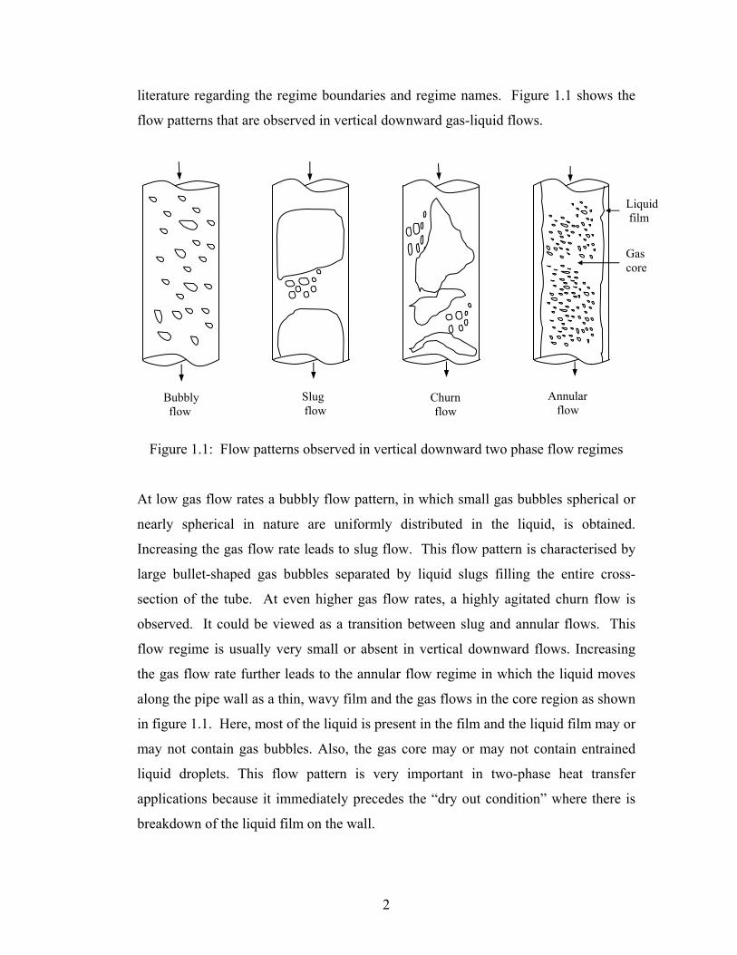
literature regarding the regime boundaries and regime names. Figure 1.1 shows the
flow patterns that are observed in vertical downward gas-liquid flows.
Figure 1.1: Flow patterns observed in vertical downward two phase flow regimes
At low gas flow rates a bubbly flow pattern, in which small gas bubbles spherical or
nearly spherical in nature are uniformly distributed in the liquid, is obtained.
Increasing the gas flow rate leads to slug flow. This flow pattern is characterised by
large bullet-shaped gas bubbles separated by liquid slugs filling the entire cross-
section of the tube. At even higher gas flow rates, a highly agitated churn flow is
observed. It could be viewed as a transition between slug and annular flows. This
flow regime is usually very small or absent in vertical downward flows. Increasing
the gas flow rate further leads to the annular flow regime in which the liquid moves
along the pipe wall as a thin, wavy film and the gas flows in the core region as shown
in figure 1.1. Here, most of the liquid is present in the film and the liquid film may or
may not contain gas bubbles. Also, the gas core may or may not contain entrained
liquid droplets. This flow pattern is very important in two-phase heat transfer
applications because it immediately precedes the “dry out condition” where there is
breakdown of the liquid film on the wall.
Bubbly flow
Slug flow
Churn flow
Annular flow
Liquid film
Gas core
3
The falling annular film represents a fundamental limiting case of the annular flow
regime of two-phase gas-liquid flows. The liquid film descends on the walls and
there is no net flow of gas in the pipe. This means that the gas core is a constant
pressure region. As for other flows, falling films can be broadly classified into
laminar and turbulent film flows. The most important flow, which is of greater
practical interest, is the turbulent film flow where there are random fluctuations in the
velocity field. The flow is more complicated due to the presence of waves on the
gas-liquid interface and is considered to be unsteady and non-uniform. The presence
of waves enhances the macroscopic transport properties of the system. As a
consequence, simple energy transfer rate equations fail to describe the flow process
accurately.
A dimensional analysis of film flow has shown the Reynolds number to be important.
The Reynolds number (Re) used in this thesis is defined as follows (note that in the
present case, the superficial gas velocity is zero),
μπ
=μ
ρ=
DmDuRe ll
4&
. ( )1.1
where ρ is the density (kg/m 3 ), μ is the liquid dynamic viscosity (kg/ms), lu is the
superficial liquid velocity (m/s), D is the diameter of the vertical tube (m), and lm& is
the liquid mass flow rate (kg/s). The superficial liquid velocity is the velocity that the
liquid would have if it flowed through the total cross-sectional area available for the
flow. Sometimes, a Reynolds number used by previous researchers in their studies
was defined as follows
Re =μ
ρ Du l
μπ=
Dml&4
. ( )2.1
All Reynolds numbers used in this thesis have been converted to be consistent with
equation 1.1.
It is well known that below a certain critical value of Reynolds number the flow will
be mainly laminar in nature, while above this value, turbulence plays an important
role. The same is true for falling annular films. At all but the smallest of Reynolds

4
numbers (Re = 5), a liquid falling under the influence of gravity contains waves or
ripples on the interface (Kapitza, 1965). Even at very low Reynolds numbers, the
film is not smooth but the wave motion is periodic in character. The waves are
widely spaced with long troughs between each large wave and with small waves of
capillary size following the peaks. At somewhat higher flow rates, periodic motion
exists only near the entry region of a vertical film. However, farther downstream the
periodic motion is replaced with a greater frequency of large waves. The wave fronts
of these large waves are steep followed by smaller waves which are no longer of
capillary size. At the highest flow rates, the flow becomes very complex and random
in nature. There are several reports in the literature of the critical Reynolds number at
which turbulence commences in falling liquid films. These values are usually
determined from discontinuities which appear in plots of film thickness, heat or mass
transfer coefficients, etc., as the Reynolds number is increased. Several investigators
have quoted a lower and upper critical value enclosing a transition region. Dukler
and Bergelin (1952) and Zhivaikin and Volgin (1961) have pointed out that the
transition to turbulence in a thin film is likely to be a gradual process, so that it is not
reasonable to expect a single, sharply defined critical Reynolds number.
Nevertheless, it is of value to subdivide film flow into laminar and turbulent regimes
depending on whether the Reynolds number is greater or less than a critical Reynolds
number. The bulk of the evidence seems to support a lower value of critical
Reynolds number in the region 250-400, at which turbulence could be detected, and a
less well-marked upper value of about 800, at which the flow became “fully
turbulent” (Fulford, 1964). The turbulent regime is characterised by flows above a
Reynolds number of 250 (Bird et al., 1960). Photographs presented by Dukler and
Bergelin (1952) for the turbulent regime clearly show that no two waves are alike. On
the basis of Dukler and Bergelin (1952) experimental data, the transition from
laminar to turbulent film flow occurs at a Reynolds number of 270.

5
1.3 Motivation and objectives
1.3.1 Motivation
Falling liquid films are generally used due to their relatively high energy and mass
transfer potentials at low liquid flow rates. A significant amount of research work
both experimental and theoretical carried out over the last few decades suggests that
the rates of momentum, heat and mass transfer are strongly influenced by the film
thickness characteristics and especially the waviness of the gas-liquid interface.
Although many attempts have been made in the past to describe the statistical
characteristics of the film thickness in falling liquid films, and some of these results
have been in good agreement with the available experimental observations, their
applicability is restricted to small Reynolds numbers. A numerical simulation of the
wavy film flow requires both the solution of the Navier-Stokes equations and the film
shape, and is usually limited by the numerical instabilities arising from factors related
to modelling the moving interface. As a result, convergence is difficult to obtain
except at very low flow rates.
So, experimental investigations of the characteristics of falling annular films play a
vital role in gaining a profound understanding of the nature of falling annular films.
The major difficulty in measuring film thickness within falling liquid films is that the
liquid films normally encountered are of the order of one millimetre thick. Some of
the common film thickness measurement techniques used in the past, such as pressure
probes, Pitot tubes, and hot-wire anemometers inevitably obstruct or disturb the films
or suffer from limited spatial resolution, yielding somewhat inaccurate data. Most of
the literature on annular falling films is dominated by studies concerning the average
film thickness. Information on more detailed characteristics of the film thickness
variations is much less common. The statistical description of the film thickness is
complicated by the fact that practically all flows of interest occur in the turbulent
flow regime.
6
1.3.2 Objectives
The objectives of this research are:
1. To use non-intrusive imaging techniques to extract quantitative instantaneous
film thickness measurements in falling annular films. The measurement of
instantaneous film thickness of the falling liquid film through flow visualisation
studies might yield some information regarding the structure of turbulence which
forms the basis for analysing the phenomena of heat and mass transfer in falling
liquid films.
2. To employ a ray-tracing technique to reduce optical distortion effects in
cylindrical tubes. Thus, quantitative measurements of film thickness will be
made possible.
3. To characterise the film thickness of falling annular films at high and very high
Reynolds numbers.
1.3.3 Scope
This research focuses on an experimental study of the characteristics of falling
annular films using a non-intrusive imaging technique. The work was undertaken in
a 4 m long vertical tube with an internal diameter of 25.48 mm at a Reynolds number
( μρ= 4lDuRe ) in the range of 1000 to 6000 (where the characteristic velocity is the
superficial liquid velocity, and the characteristic length is the diameter of the tube) for
the fully-developed turbulent flow regime. The present research shows the highly
localised film thickness measurements and also reveals some of the statistical and
random characteristics of falling annular film flows at high and very high Reynolds
numbers. Thus, the once formidable task of measuring the qualitative and
quantitative instantaneous film thickness in falling liquid films at high and very high
Reynolds numbers is no longer insurmountable.
1.4 General outline of thesis
The theoretical considerations for a smooth laminar film flow and a detailed literature
review of falling liquid films are presented in Chapter 2. The apparatus,
7
instrumentation and measurement techniques employed in the present study are
described in Chapter 3. The development of the ray tracing concepts along with
image processing and extraction of quantitative measurements from two-dimensional
images are also explained in more detail in the same chapter. In Chapter 4, some
general qualitative observations and the results of the quantitative measurements of
film thickness on falling annular films are presented. Also, a discussion of the
statistical characteristics of the film thickness such as mean film thickness, standard
deviation, coefficient of variation, and the probability density distribution is found in
the same chapter. In Chapter 5, the conclusions and recommendations for future
work are outlined. The Inspector® code written for the extraction of raw film
thickness from the images is presented in Appendix A.

8
CHAPTER 2
LITERATURE REVIEW
2.1 Introduction
In this chapter, the Navier-Stokes equations are solved for a smooth laminar falling
annular film flow. Also, the definitions of some of the important statistical
characteristics such as the mean film thickness, standard deviation, and probability
density distribution of film thickness are discussed briefly. The theoretical, modelling
and experimental falling annular film literature are then reviewed in more detail.
Finally, the turbulent film thickness correlations of previous researchers and some of
the conditions used to obtain them are summarised briefly.
2.2 Theoretical considerations
2.2.1 General equations for smooth laminar film flow
Consider a liquid film of thickness δ flowing inside a vertical tube of internal
radius wR . The flow is assumed to be a steady, incompressible, fully developed, and
laminar and flows in the z direction as shown in figure 2.1. It is driven by gravity and
the pressure is assumed to be constant. The axial component of the Navier-Stokes
equations in cylindrical coordinates is as follows:
⎥⎥⎦
⎤
⎢⎢⎣
⎡
∂∂
+θ∂
∂+⎟
⎠⎞
⎜⎝⎛
∂∂
∂∂
μ+ρ+∂∂
−=⎥⎦
⎤⎢⎣
⎡∂∂
+θ∂
∂+
∂∂
+∂∂
ρ θ2
2
2
2
2
11zuu
rrur
rrg
zp
zuuu
ru
ruu
tu zzz
zz
zzz
rz
( )1.2
In addition, the continuity equation is:

9
( ) ( ) ( ) 011=
∂∂
+∂∂
+∂∂
zr uz
ur
rurr θθ
. ( )2.2
By assuming axisymmetric flow in the pipe ( 0,0 =∂∂= θθu ), equation 2.1
reduces to the following:
ρ ⎥⎥⎦
⎤
⎢⎢⎣
⎡
∂∂
+⎟⎠⎞
⎜⎝⎛
∂∂
∂∂
μ+ρ+∂∂
−=⎥⎦
⎤⎢⎣
⎡∂∂
+∂∂
+∂∂
2
21zu
rur
rrg
zp
zuu
ruu
tu zz
zz
zz
rz . ( )3.2
where zu is the axial velocity, θ,r and z are the cylindrical coordinates, t is the time,
ρ and µ are the density and dynamic viscosity, p is the pressure, and g is the
acceleration due to gravity.
Assume that the flow is fully developed and has a constant pressure, so
0=∂∂z
and 0=∂∂
zp .
With these assumptions the continuity equation demands that 0=ru . The boundary
conditions are
0=zu at wRr = (no slip at tube wall)
0=∂∂
ruz at irr = (no shear at gas-liquid interface)
Figure 2.1: Velocity profile for a fully developed, laminar falling annular film
z
zu
δ
wτ
w2R
Vertical tube wall
Thin liquid film
Gas core
Gas-liquid Interface
ir
10
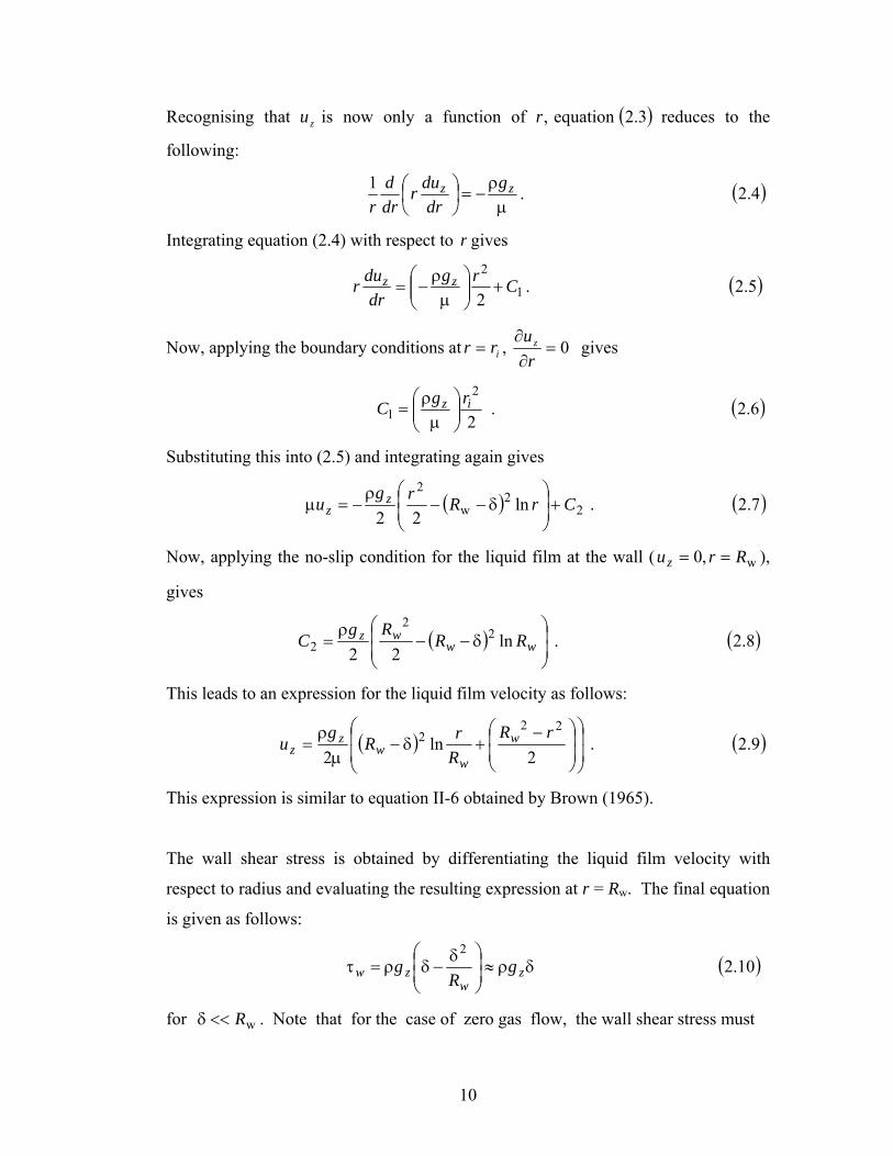
Recognising that zu is now only a function of ,r equation ( )3.2 reduces to the
following:
μρ
−=⎟⎠⎞
⎜⎝⎛ zz g
drdur
drd
r1 . ( )4.2
Integrating equation (2.4) with respect to r gives
1
2
2Crg
drdur zz +⎟⎟
⎠
⎞⎜⎜⎝
⎛μρ
−= . ( )5.2
Now, applying the boundary conditions at irr = , 0=∂∂
ruz gives
.2
2
1iz rgC ⎟⎟
⎠
⎞⎜⎜⎝
⎛μρ
= ( )6.2
Substituting this into (2.5) and integrating again gives
( ) 22
w
2ln
22CrRrgu z
z +⎟⎟⎠
⎞⎜⎜⎝
⎛δ−−
ρ−=μ . ( )7.2
Now, applying the no-slip condition for the liquid film at the wall ( w,0 Rruz == ),
gives
( ) ⎟⎟⎠
⎞⎜⎜⎝
⎛δ−−
ρ= ww
wz RRRgC ln
222
2
2 . ( )8.2
This leads to an expression for the liquid film velocity as follows:
( )⎟⎟
⎠
⎞
⎜⎜
⎝
⎛
⎟⎟⎠
⎞⎜⎜⎝
⎛ −+δ−
μρ
=2
ln2
222 rR
RrR
gu w
ww
zz . ( )9.2
This expression is similar to equation II-6 obtained by Brown (1965).
The wall shear stress is obtained by differentiating the liquid film velocity with
respect to radius and evaluating the resulting expression at r = Rw. The final equation
is given as follows:
δρ≈⎟⎟⎠
⎞⎜⎜⎝
⎛ δ−δρ=τ z
wzw g
Rg
2 ( )10.2
for wR<<δ . Note that for the case of zero gas flow, the wall shear stress must

11
support the total weight of the film.
The mass flow rate of the liquid film can be obtained by integrating the liquid film
velocity profile over the film cross section. Thus,
drrumw
i
R
rZ∫= πρ2l& . ( )11.2
Substituting equation (2.9) into (2.11) and integrating leads to,
( ) ( ) ( ) ⎟⎟⎠
⎞⎜⎜⎝
⎛δ−+⎟⎟
⎠
⎞⎜⎜⎝
⎛ δ−δ−−+δ−−
μπρ
= 444222
l 3ln448 w
w
wwwww
z RR
RRRRR
gm& . ( )12.2
for given fluid physical properties ρ andμ , given pipe diameter (2 wR ), and film
thickness ( iw rR −=δ ). Using this equation, the liquid film mass flow rate ( lm& ) can
be determined. By expanding the terms above in powers of ( )wRδ , it can be shown
that the liquid film mass flow rate increases as a cubic power of film thickness.
2.2.2: Film thickness variation for a smooth laminar liquid film
A graph was plotted between flow rate and film thickness as shown in figure 2.2.
0
0.001
0.002
0.003
0.004
0.005
0.006
0 0.01 0.02 0.03 0.04 0.05 0.06
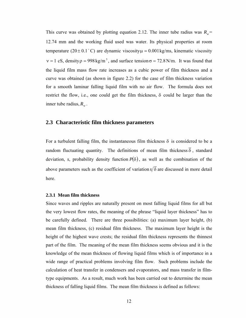
Figure 2.2: Parabolic profile of a smooth laminar falling liquid film Flow rate, m 3 /s
Film
thic
knes
s, m
12
This curve was obtained by plotting equation 2.12. The inner tube radius was wR =
12.74 mm and the working fluid used was water. Its physical properties at room
temperature (20± 0.1 o C) are dynamic viscosity 001.0=μ kg/ms, kinematic viscosity
=ν 1 cS, density 998=ρ kg/m 3 , and surface tension 8.72=σ N/m. It was found that
the liquid film mass flow rate increases as a cubic power of film thickness and a
curve was obtained (as shown in figure 2.2) for the case of film thickness variation
for a smooth laminar falling liquid film with no air flow. The formula does not
restrict the flow, i.e., one could get the film thickness, δ could be larger than the
inner tube radius, wR .
2.3 Characteristic film thickness parameters
For a turbulent falling film, the instantaneous film thickness δ is considered to be a
random fluctuating quantity. The definitions of mean film thickness δ , standard
deviation, s, probability density function ( )δP , as well as the combination of the
above parameters such as the coefficient of variation δs are discussed in more detail
here.
2.3.1 Mean film thickness
Since waves and ripples are naturally present on most falling liquid films for all but
the very lowest flow rates, the meaning of the phrase “liquid layer thickness” has to
be carefully defined. There are three possibilities: (a) maximum layer height, (b)
mean film thickness, (c) residual film thickness. The maximum layer height is the
height of the highest wave crests; the residual film thickness represents the thinnest
part of the film. The meaning of the mean film thickness seems obvious and it is the
knowledge of the mean thickness of flowing liquid films which is of importance in a
wide range of practical problems involving film flow. Such problems include the
calculation of heat transfer in condensers and evaporators, and mass transfer in film-
type equipments. As a result, much work has been carried out to determine the mean
thickness of falling liquid films. The mean film thickness is defined as follows:
13
( )dTTT
T
T ∫ δ=δ∞→
0
1lim . ( )13.2
where T is the time and ( )Tδ is the instantaneous film thickness in an observation
time T.
2.3.2 Standard deviation
The root-mean-square (r.m.s.) of the fluctuations or standard deviation s, of a data
sample is the positive square root of the second central moment, as defined below,
and provides a measure of the “dispersion” of data about their mean value. The
variance 2s is defined as follows:
( )( )∫ δ−δ=∞→
T
TdTT
Ts
0
22 1lim . ( )14.2
The ratio of the standard deviation of film thickness fluctuations to the mean film
thickness is the coefficient of variation δs . It is a very common indicator of wave
growth.
2.3.3 Probability density function
The probability density function of the time series describes the probability that the
data will assume a value within some defined range at any instant of time. Chu and
Dukler (1974) defined “substrate film thickness” based on the characteristics of the
probability density function of film thickness. Substrate film thickness was defined
as the most probable film thickness and is indicated by a peak in the probability
density function. The probability that ( )Tδ assumes a value within the range between
δ and ( )δΔ+δ during an observation time T may be defined as follows (Bendat and
Piersol 1971):
( ) ( ){ }δΔ
δΔ+δ<δ<δ=δ
→δΔ
TPP0
lim . ( )15.2
14
2.4 Literature Review
2.4.1 Classical theories and modelling studies
According to Fulford (1964), Nusselt proposed a theory for a smooth, laminar
uniform, and two-dimensional flow on an infinitely wide plate in 1916. According to
the theory, “the liquid film mass flow rate increases as a cubic power of film
thickness and even a small difference in the film thickness results in a large
difference in the liquid flow rate; especially for thick films obtained at high Reynolds
numbers” (Refer to figure 2.2 in section 2.2). The equations, derivable from force
balances on an element in the liquid film, were developed with the assumptions of
viscous flow where no shear or wave motion existed at the liquid surface. This
theory is very simple as it does not take into account the effects of even small waves
on the falling liquid film. Nusselt’s theory for a smooth laminar flow is as follows:
( ) 3123 gReυ=δ . ( )16.2
Experimental observations of laminar falling liquid films indicated that the gas-liquid
interface was not a constant flat surface, but exhibited a wavy structure at Reynolds
number as low as Re = 5. Numerous theoretical attempts have been made to study
the waves formed on free-falling liquid films. The research can be divided into three
general groups with respect to Reynolds numbers. The first group refers to the wave
evolution over laminar films flowing at low Reynolds numbers and it involves a
number of different approaches. For smooth wavy laminar flow, the mean film
thickness was given by Kapitza’s (1965) theory which accounts for the effects of
regular periodic waves and surface tension in a falling laminar film as follows:
( ) 3124.2 gReυ=δ . ( )17.2
A parameter that had been identified to be important for characterising wavy laminar
falling films besides Reynolds number was the Kapitza number,
,3/13/4 gρνσ=γ where σ is the surface tension and ν is the kinematic viscosity.
Kapitza’s (1965) theory appeared to account for the wavy nature of falling films only
if the wavelength was less than 13.7 times the film thickness, which corresponds to a
Reynolds number of Re = 12 for falling liquid films.

15
The second group of theoretical studies deals with films at higher Reynolds numbers.
This is in a transition zone where fast-moving, large waves tend to overtake the small
(capillary) waves resulting in a complicated wave structure. Numerical simulations
of laminar wavy films at relatively high Reynolds numbers were conducted by
several investigators (e.g., Wasden and Dukler (1989), Chang (1994), Yu et al.
(1995) and Stuhltrager et al. (1995)), to predict the spatial variations in film thickness
along with the velocity field inside the interacting waves. Wasden and Dukler (1989)
examined wave structures of interacting waves in regions where the Navier-Stokes
equations could be solved. Their model, based on flows with a Reynolds number of
220, predicted the existence of recirculation cells within large disturbance waves. In
addition, the computational simulation depicted regions of acceleration in the wave
fronts, and deceleration zones at the wave backs. This work was continued by Yu et
al. (1995), examining the stability of the two-dimensional Navier-Stokes equations
using non-linear wave evolution assumptions.
The third group of studies deals with even higher Reynolds numbers of Re > 270,
which produce a turbulent film. The problem of turbulent flow in thin films is very
complex and there are no theoretical treatments for wavy turbulent flow. A common
approach is to neglect the surface waves and obtain solutions for the case of smooth
turbulent flow. Nikuradse in 1933 developed the universal velocity distribution for
circular tubes, which provided a means by which flows could be examined in terms
of boundary layer analysis based on dimensionless parameters (Bird et al. (1960)).
This theory was derived for fully-developed, single-phase, turbulent pipe flow. From
the universal velocity profile equations developed by Nikuradse in 1933, Dukler and
Bergelin (1952) derived a theoretical expression for dimensionless film thickness in
the turbulent regime as follows:
( ) 64ln5.20.3 +=δδ+ ++ Re . ( )18.2
Equation 2.18 was obtained with the aid of the friction velocity ∗u , evaluated from a
force balance of wall friction and the gravity force as follows:
dzRdzRg ww πτ=δπρ 22 w . ( )19.2
δ=ρτ=∗ gu w . ( )20.2

16
The non–dimensional film thickness, +δ , in equation 2.18 is defined as follows:
υδ=δ ∗+ u . ( )21.2
The falling film may become turbulent if the dimensionless film thickness +δ ,
obtained from local film thickness δ , reaches a value of 30. Dukler and Bergelin
(1952) also carried out an analysis in the laminar and transition zones and found that
the transition from laminar to turbulent film flow occurs at a Reynolds number of
270.
A numerical study of turbulent wavy films for the fully developed region was carried
out by prescribing a geometric shape for large waves by Brauner (1987). The
proposed model could yield some useful information regarding the velocity
distribution within large waves, including the effects of turbulence. Brauner (1987)
showed that there are two basic characteristics of the wavy flow, namely the wave
celerity and the average wavy film thickness. Wave celerity is the speed of
propagation of the wave crest or trough. It is worth emphasising that these two
parameters are the usual measured quantities that are of importance in modelling the
momentum, heat and mass transfer, associated with wavy flow. Yet, the model was
rather complex with different physical mechanisms controlling various zones along a
large wave. Moreover, the employed shape of large waves – assumed to have a linear
slope at both the front and the back of the waves – was oversimplified compared to
experimental observations. An expression for the average film thickness was derived
from energy and mass balances in stationary and moving coordinate systems. The
average wavy film thicknesses for laminar and turbulent flows were obtained as
follows:
31
2
83
⎟⎠⎞
⎜⎝⎛ υ=δ gRe for laminar flow; ( )22.2
( ) 127312104.0 Regυ=δ for turbulent flow. ( )23.2
The other available literature on theoretical developments range from classical works
dealing with the stability of the film surface (e.g., Kapitza (1947); Benjamin (1957);
Yih (1963); Bankoff (1971); Spindler (1981); Kokamustafaogullari (1985) to a
17
rigorous mathematical study of the behaviour of falling films (Alekseenko et al.,
1994). A few studies used finite element solutions of the full Navier stokes equations
(e.g., Bach and Villadsen (1984); Kheshgi and Scriven (1987); Salamon et al. (1994)
assuming waves with finite amplitude or a stationary profile. Other efforts were
based on simplified Navier - Stokes equations under various approximations or order-
of-magnitude assumptions (e.g., Alekseenko et al. (1985); Nguyen and Balakotaiah
(2000)). On the whole, these studies found waveforms that are only in fair agreement
with experimental observations and only for small Reynolds numbers – usually below
75 – which are much lower than those encountered in many practical applications.
2.4.2 Experimental studies
Many techniques have been used for the measurement of mean film thickness and to
study the statistical characteristics of film thickness. It is worth mentioning here that
the mean film thickness obviously depends to a certain extent on the measurement
being adopted. The results of the experimental studies and the details of the proposed
experiments are reviewed in more detail in this section.
According to Fulford (1964), Brotz studied films of water and refrigerating oil inside
tubes of various diameters with kinematic viscosities of 1.0-8.48 cS and
Re 4300100 −= using a drainage technique in 1954. In this technique, the feed of
liquid to the channel is shut off and the liquid film flowing from the channel is
collected and measured. Knowing the wetted area of the channel, the mean film
thickness can be determined from the volume of the liquid collected. Later it was
realised by Portalski (1963) in his experiments with water films in vertical tubes that
this type of apparatus suffers from certain disadvantages which preclude a thorough
examination of the many phenomena relating to the hydrodynamics of film flow. In
his experience, it is very unlikely to produce highly accurate and reproducible results
unless the apparatus has an automatic device for stopping the feed and simultaneously
collecting the drainage from a fairly large wetted area. This cannot be achieved
easily, if at all, using small-bore tubes of moderate length and for high liquid flow
rates. The main difficulty is to ensure fully instantaneous isolation of the section.

18
The critical Reynolds number at which turbulence was found to commence was 590.
From dimensional considerations, Brotz showed that, in the turbulent regime, the
mean film thickness is given as follows:
( ) 323123112.0 Regυ=δ . ( )24.2
Jackson (1955) used a radio active emission technique to determine the film thickness
in falling liquid films. In this technique, a radio active substance is dissolved in the
flowing liquid. If a radioactive detector is brought up to the film, the amount of
radiation detected depends on the film thickness. The radiation is, of course, partially
attenuated by absorption in the liquid film. Jackson (1955) came up with the
following expression for laminar liquid films:
cAC=δ . ( )25.2
where C is a constant and cA is described as the corrected absorption activity of the
liquid film (counts/sec). The constant C in the equation was evaluated by operating
the vertical tube apparatus under conditions where the film thickness could be
calculated from the flow rate using Nusselt’s equation. That is, the value of the
constant was determined by plotting corrected absorption activity cA against the
calculated film thickness δ . The problem with this technique is the fact that, even if
this could be done for the region where the flow is truly viscous and waves are
absent, this method automatically shifts the experimental film thickness results at low
flow rates and pins them down on the theoretical line proposed by Nusselt in 1916.
But Nusselt’s theory fails to predict the film thickness correctly, even for steady
laminar conditions of flow, that is, before the onset of wave motion (Portalski 1963).
On examination of his results, Jackson (1955) states that “the data permits few
conclusions concerning the inception of turbulence” and that “for water and the
lighter liquids no significant departure from viscous behaviour is indicated up to
Reynolds numbers of 1250 although scattering of the data is observed above Re =
500”. In view of the above criticism, Jackson’s (1955) results are not entirely
surprising.

19
According to Fulford (1964), Brauer in 1956 carried out extensive experimental
studies of film flow outside tubes of diameter 4.3 cm and length 130 cm for kinematic
viscosities of 0.9-12.7 cS and at Re = 20-1800. He used the feeler-probe method
which is a refined modification of the micrometer screw method. Here, a very fine
needle is mounted on a micrometer and is adjusted to touch the liquid film, the
contact being registered normally by an electronic counter. The objection to this
method is quite obvious: by touching the surface of the film by a probe, or even
worse, by introducing the probe into the film, however fine the probe may be, one
interferes with the natural flow of the film. One measures, therefore, a disturbed
condition which may not be closely related to the original undisturbed flow. The
lower limit of critical Reynolds number was found to be equal to 400. For turbulent
flow, the mean film thickness was well described by the following empirical formula:
( ) 1583123302.0 Regυ=δ . ( )26.2
Belkin et al. (1959) carried out photographic techniques at zero gas flow and at
different Reynolds numbers in the lower and higher turbulent regimes. A direct
lighting technique was used for water flowing down the outer surface of a vertical
glass rod of diameter 25.48 mm for Reynolds numbers above 1258. High-speed
photographs of the rod with water flow were compared with photographs of the dry
rod, using a planimeter on enlarged photographs. There was evidence of discrete
turbulent eddies at Re = 1258 which indicates the persistence of transitional flow. It
was apparent that the data did not make it possible to fix the exact Reynolds number
at which the advent of turbulence begins to affect the thickness parameter. The
photographs presented at even higher Reynolds number showed that full turbulence
had been obtained. Additional photographs indicated more intense turbulence but the
same over-all type of flow at Reynolds numbers between 4000 and 7500. It showed
the random distribution of shallow troughs and crests in the fully turbulent region and
the turbulent waves took nearly a trochoidal form. A trochoid is the curve generated
by a point on a circle which rolls along the underside of a straight line. Their pictures
made it easy to visualise that a profile cutting across the indentation between adjacent
crests might closely resemble such a form. According to Portalski (1963), it is
extremely difficult to enlarge photographs to exactly the same length – especially if

20
two cameras are used for the purpose – unless the photographed portions are marked
beforehand. In any case, the three-dimensional effect of the waves was quite obvious
in the photographs submitted.
According to Fulford (1964), Fiend in 1960 used a drainage technique and measured
the thickness of various films for kinematic viscosities from 1 to 19.7 cS flowing in
vertical tubes ( 0.50.2 − cm diameter). At low Reynolds numbers, the values of film
thickness agreed well with Nusselt’s predictions. Once the wavy flow commenced,
the values deviated towards the Kapitza line (equation 2.17). At larger Reynolds
numbers, there was a gradual transition back towards the Nusselt line (equation 2.16)
which was finally crossed at Re = 350. In the turbulent zone, the experimental values
fell above the Nusselt line. The lower and upper value of critical Reynolds number
was found to be 400 and 800, respectively. For the turbulent regime, it was found that
( ) 213123369.0 Regυ=δ . ( )27.2
According to Fulford (1964), Zhivaikin and Volgin in 1961 used an analogy with
pipe flow and measured mean film thickness in a tube 2 cm in diameter and 98 cm
long at Re 3500150 −= with water as the working fluid. The lower limit of critical
Reynolds number was found to be 400, at which turbulence commenced, and an
upper value of 1000, at which the flow became fully turbulent. For the turbulent
regime, the mean film thickness was obtained as follows:
( ) ( ) 127312 4141.0 Regυ=δ . ( )28.2
Neal and Bankoff (1963) and numerous other researchers measured liquid film
thickness using a needle-contact probe. In principle, the point of the needle is
brought upon the film and when the needle makes contact, the distance between the
needle point and the solid boundary is noted. If the film is of uniform thickness with
no waves, the first point of contact represents the film thickness. When there are
waves on the film, however, contact is first made with the tips of the waves and a
continuous contact does not occur until the troughs of the waves are being touched.
The point of contact is determined by electric capacity methods. It gives results for
contact frequency and relative contact time. This probe is accurate and easy to
handle, but suffers from limited spatial resolution. Telles and Dukler (1970)

21
conducted electrical conductivity measurements in a 5.4 m long rectangular conduit
made of Plexiglas. In this technique, it is necessary for the film to be conducting
(e.g., by adding electrolytes) and for it to flow over the electrodes. Electrical
connections to the selected length of film are then made by insertion of electrodes in
the wall. Statistical characteristics of thin, vertical, wavy, liquid films were
determined at Reynolds numbers in the range 225 to 1500 and showed the random
nature of waves and their behaviour as a two wave system; large waves which carry
the bulk of the liquid and the small waves which cover the substrate. The probability
density distribution had a maximum peak and a long tail stretching from 5 to 12 times
the minimum film thickness. A comparison of their mean experimental film
thickness with the values predicted by Dukler and Bergelin (1952) theory showed
significant deviations. It seems clear that the original development of Dukler and
Bergelin (1952) does not produce the correct mean film thickness for a film with
large waves. Webb and Hewitt (1975) carried out measurements in downward
annular two phase flows in tubes of 3.18 and 3.28 cm bore. The film thickness data
showed reasonable agreement with Telles and Dukler (1970) although there were
slight discrepancies which could be attributed to the effect of wall curvature.
Later Chu and Dukler (1975) used conductivity probes to determine the statistical
characteristics of thin wavy turbulent liquid films inside Plexiglas pipes of diameter
50 mm and length 4.27 m. In this technique, the probes are placed in close proximity
to one another in the surface over which the film is flowing and flush with the wall.
The conductance between the probes depends on the liquid film thickness and the
specific conductivity of the liquid. Two classes of random waves were found to exist
on falling films at flow rates of practical interest (Re > 175). In order to characterise
the random large waves, it was necessary to measure their mean film thickness,
standard deviation, and probability density distribution. The probability density
distribution curve obtained was highly asymmetrical around the modal value. The
maximum peak values decreased sharply with increasing liquid flow rate and the long
tail existed which stretches to over six times the modal value. Such measurements
confirm, in general, certain statistical characteristics of large waves as suggested by
22
Telles and Dukler (1970). Salazar and Marschall (1978) measured the interfacial
characteristics using light scattering and hot-film probes, but these did not easily
yield the absolute film height. Blass (1979) did an extensive study of falling liquid
films in vertical tubes for Reynolds numbers up to 2000 and found that the mean film
thickness appeared to be the same for vertical flat plates and for flow outside or
inside a vertical tube, provided the ratio of film thickness to tube radius is small (i.e.,
less than 0.2). The effect of the film curvature cannot be neglected for falling annular
films on and in narrow tubes, or on wires or fibres, when the ratio of the film
thickness to tube radius is greater than 0.2.
Figure 2.3 shows a sample of the earlier non-dimensional film thickness data plotted
against the Reynolds number (Refer to Fulford, G.D., 1964). Takahama and Kato
(1980) carried out flow measurements using needle contact and electric capacity
methods along the outer wall of a circular tube (44.92± 0.02 mm in diameter and 2
Figure 2.3: Sample of earlier film thickness data near the critical Reynolds number plotted in terms of the dimensionless mean film thickness parameter ( +δ ) and the Reynolds number (Re), for the case of zero gas flow (“Reprinted from In: Advances in Chemical Engineering, Vol. 5, Fulford, G.D., The flow of liquids in thin films, 151-235, 1964, with permission from Elsevier”)
+δ
Re

23
m long) with and without concurrent gas flow. The test channel used was a brass
cylinder with water as the working fluid. The mean film thickness data obtained
were statistically processed. First, the probability distribution function was obtained
by the needle contact method at different positions along the circumference of the
tube. Then, the mean film thickness was evaluated from graphical integration of the
probability distribution. It was found that at small Reynolds numbers of Re = 200
and longitudinal distance of z = 100 mm, δ decreases only by 3% from its initial
value at the inlet. On the other hand, at large Re = 997 and z < 500mm, δ increases
rapidly, but at larger longitudinal distances becomes constant. For intermediate
Reynolds numbers between 200 and 997, δ increases, decreases to a minimum level
and then increases again. This peculiar behaviour may be due to transition from
laminar to turbulent flow. The experimental results obtained were compared with the
theories for laminar and turbulent flow (equation 2.16 and 2.18) and also with
Brauner’s (1956) empirical formula (equation 2.23). At 400<Re the experimental
results agree with those of Nusselt’s theory (equation 2.16) and at 400>Re the
experimental results tend to coincide with Brauner’s equation (equation 2.23) for
turbulent flow. The lower value of critical Reynolds number Re is obtained at the
intersection of the laminar and turbulent lines. Evaluation of critical Reynolds
number leads to Re = 368 which agreed closely with the theory of smooth turbulent
flow (equation 2.18). Although it provided useful statistical information about the
distribution of film thickness; it could not give information about the continuous
change of film thickness since only one depth is investigated at each needle setting.
The other difficulty with the method is the problem of contact hysteresis; the film
may tend to stick to the needle and the break of contact with the film may therefore
be delayed. A further disadvantage of the method is that the flow must necessarily be
disturbed in other parts of the channel in order to introduce the contact needle (Hewitt
and Hall-Taylor, 1970). The mean film thickness in the turbulent regime was given
by the following empirical formula:
( ) 526.0312473.0 Regυ=δ . ( )29.2

24
Zabaras (1985) carried out measurements of the film thickness in falling annular
films using a flush-mounted probe. The method is based on the fact that the electrical
conductance between two probes, placed flush on wall over which a liquid film is
flowing, depends on the thickness of the film. The vertical test section was made of
several segments of Plexiglas pipe with an inside diameter equal to 50 mm ± 20mm
and the overall length was 6.5 m. The film thickness obtained at low Reynolds
number and at short distances from the entry was found to be in good agreement with
Nusselt’s film thickness equation. At larger distances from the liquid entry (1.94 m
and 4.0 m) the waves were developed. In particular, the waves at the 4.0 m location
could be considered to be fully developed. At these distances, the values deviated
from the Nusselt line indicating a transition to turbulence. The standard deviation of
the film thickness was also found to increase with increasing liquid Reynolds number
and longitudinal distance from the liquid inlet. This implies that at larger distances
the waves have higher amplitudes. The probability density distribution curves also
suggested the existence of high wave amplitudes at this location. The possible
objections to the use of flush-mounted probes come from the perturbation induced in
the flowing film of liquid and from a meniscus effect due to the wetting of the wires.
Koskie et al. (1989) used parallel-wire probes and determined film thickness in
falling liquid films at Reynolds numbers in the range 250 to 18,750. The measuring
technique consists of two parallel fine wires placed side by side in the pipe
perpendicular to the direction of the flow. By using the liquid as a conductor it is
possible to measure the resistance between the two wires and convert the resistance to
a measure of the immersion of the wires. It is based on the fact that the resistance is
inversely proportional to the length of the wires immersed in the liquid. They
obtained continuous measurements of film thickness for thick films (> 1 mm), but the
resulting probe yielded some error for thin liquid films (< 1 mm). Karapantsios et al.
(1989) also studied characteristics of free falling films at Re = 126-3275 using a
parallel wire conductance technique. In their experiments, water was used as the
working fluid. It was found that at Re > 375, the random character of the film flow
becomes more pronounced. The Reynolds number was found to correlate well with
the characteristic film thickness parameters such as standard deviation, s and
25
coefficient of variation, δs . Information obtained on the film thickness fluctuations
showed that they exhibit a stochastic character. The mean film thickness was given
by the following empirical formula:
( ) 538.0312451.0 Regυ=δ . ( )30.2
Since spatial resolution and calibration have been typical problems in the practical
use of traditional conductance probes such as flush-mounted probes and parallel-wire
probes, Kang and Kim (1992) developed a flush-wire probe. It consists of an
electrode which is flush with the wall and a wire electrode which is vertically inserted
from the top side. This technique enhanced the spatial resolution and enabled
continuous measurement of liquid film thickness up to a Reynolds number of 1500.
Their measured mean film thickness was found to be 0.1 mm lower than those of
Takahama and Kato (1980) and Karapantsios et al. (1989), but slightly larger than
Salazar and Marschall (1978). Karimi and Kawaji (1998) carried out film thickness
measurements in falling annular films at Re = 352 - 1637 with deodorised kerosene as
the working fluid using the photochromic dye tracer technique. In this technique, the
dye trace appears as a deep blue straight line along the path of the laser beam. The
dye trace formed follows the motion of the liquid and thereby tracks the movements
of the liquid elements. Large scatter in film thickness measurements were reported
especially at high Reynolds numbers in the turbulent flow regime. Recently,
Ambrosini et al. (2002) determined the statistical characteristics of freely falling
films down a vertical plane (2 m long, 0.6 m wide and 0.022 m thick). Capacitance
probes, consisting of two parallel conducting plates mounted vertically were used to
collect discrete film thickness time series and to extract relevant statistical data. One
of these plates was fixed in position while the second plate could be moved to vary
the distance between the plates. The capacitance of this sensor was directly
proportional to the dielectric constant of the fluid between the plates and the area of
the plates. The mean film thickness data were in reasonable agreement with
Nusselt’s theory for low Reynolds numbers after which larger deviations appeared,
possibly due to transition to turbulent flow. The standard deviation was also found to

26
be in good agreement with Karapantsios et al. (1989) in the range of Reynolds
number, Re = 100-400.
2.3 Summary
The experimental, theoretical, and modelling methods along with conditions such as
test geometry, measuring location relative to the inlet and the correlation for the film
thickness obtained for the turbulent regime are summarised in Table 2.1.
Table 2.1: Summary of experimental, theoretical, and modelling methods used in the past for a vertical downward annular flow without air flow.
Researchers
Geometry
Reynolds number
Experimental/Model/
Theoretical
Film thickness correlation
Dukler and Bergelin (1952)
Flat plate/ Pipe inside
> 270
Theory
( ) 64ln5.20.3 +=δδ+ ++ Re
Brotz (1954)
Pipe inside 100 - 4300 Drainage technique ( ) 323123112.0 Regυ=δ
Brauer (1956)
Pipe outside 20 - 1800 Feeler probe method ( ) 1583123302.0 Regυ=δ
Belkin et al. (1959)
Pipe outside 1200 - 7500 Photographic technique
Not available
Fiend (1960)
Pipe inside - Drainage technique ( ) 213123369.0 Regυ=δ
Zhivaikin and Volgin (1961)
Pipe inside 150 - 3500 Not available ( ) ( ) 127312 4141.0 Regυ=δ
Chu and Dukler (1975)
Pipe inside 150 -1500 Flush-mounted probe
Not available
Webb and Hewitt (1975)
Pipe inside - Conductance probe method
Not available
Salazar et al. (1978 )
Flat plate - Laser scattering Not available
Takahama and Kato (1980)
Pipe inside 150 - 2000 Needle contact and capacitance probe
( ) 526.0312473.0 Regυ=δ
Zabaras (1985) Pipe inside - Wire conductance probe
Not available
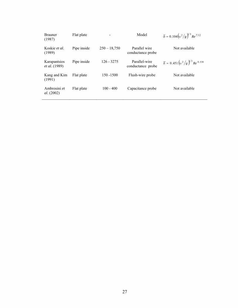
27
Brauner (1987)
Flat plate - Model ( ) 127312104.0 Regυ=δ
Koskie et al. (1989)
Pipe inside 250 – 18,750 Parallel wire conductance probe
Not available
Karapantsios et al. (1989)
Pipe inside 126 - 3275 Parallel-wire conductance probe
( ) 538.0312451.0 Regυ=δ
Kang and Kim (1991)
Flat plate 150 -1500 Flush-wire probe Not available
Ambrosini et al. (2002)
Flat plate 100 - 400 Capacitance probe Not available

28
CHAPTER 3
APPARATUS AND MEASUREMENT TECHNIQUES
3.1 Introduction
The experimental and measurement procedures described in this chapter were
undertaken to produce instantaneous measurements of film thickness in falling
annular liquid films. The experiments were conducted in a 4 m long vertical tube of
25.48 mm (1 inch) inside diameter. Water was used as the working fluid. The tube
was long enough to establish a fully developed flow in the test section. Flow
visualisation studies in falling annular films were carried out using a non-intrusive
digital photographic technique. The main instruments used were a digital camera and
a pair of remote flash units to capture instantaneous images of a falling annular film.
The flow loop, calibration procedures, image analysis techniques, and optical
distortion correction techniques used in the experiments will be discussed in detail in
this chapter.
3.2 Flow Loop
A schematic of the experimental apparatus is shown in figure 3.1. The flow loop was
designed to produce a fully developed, gravity-driven liquid film in the test section.
The test section consists of a 4 m long transparent vertical tube with an inside
diameter of 25.48 mm suspended from the upper reservoir. In order to produce a
uniform film, a bell-mouth entrance was fitted to the upper end of the tube. Marbles
of diameter 19 mm (3/4 inch) were placed in the upper reservoir to break down the
jets of water at the liquid inlet into the upper reservoir. This ensured a smooth entry
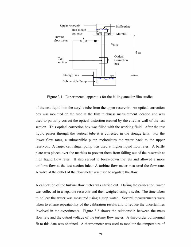
29
Figure 3.1: Experimental apparatus for the falling annular film studies
of the test liquid into the acrylic tube from the upper reservoir. An optical correction
box was mounted on the tube at the film thickness measurement location and was
used to partially correct the optical distortion created by the circular wall of the test
section. This optical correction box was filled with the working fluid. After the test
liquid passes through the vertical tube it is collected in the storage tank. For the
lower flow rates, a submersible pump recirculates the water back to the upper
reservoir. A larger centrifugal pump was used at higher liquid flow rates. A baffle
plate was placed over the marbles to prevent them from falling out of the reservoir at
high liquid flow rates. It also served to break-down the jets and allowed a more
uniform flow at the test section inlet. A turbine flow meter measured the flow rate.
A valve at the outlet of the flow meter was used to regulate the flow.
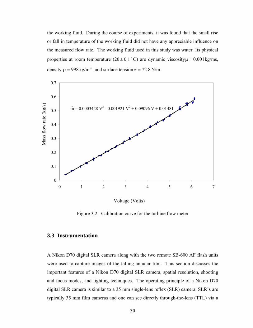
A calibration of the turbine flow meter was carried out. During the calibration, water
was collected in a separate reservoir and then weighed using a scale. The time taken
to collect the water was measured using a stop watch. Several measurements were
taken to ensure repeatability of the calibration results and to reduce the uncertainties
involved in the experiments. Figure 3.2 shows the relationship between the mass
flow rate and the output voltage of the turbine flow meter. A third-order polynomial
fit to this data was obtained. A thermometer was used to monitor the temperature of
Storage tank
Submersible Pump
Turbine flow meter
Upper reservoir Bell-mouth entrance
Valve
Optical Correction box
Test section
Marbles
4 m
Baffle plate
30
the working fluid. During the course of experiments, it was found that the small rise
or fall in temperature of the working fluid did not have any appreciable influence on
the measured flow rate. The working fluid used in this study was water. Its physical
properties at room temperature (20± 0.1 o C) are dynamic viscosity 001.0=μ kg/ms,
density 998=ρ kg/m 3 , and surface tension 8.72=σ N/m.
m = 0.0003428 V3 - 0.001921 V2 + 0.09096 V + 0.01481
0
0.1
0.2
0.3
0.4
0.5
0.6
0.7
0 1 2 3 4 5 6 7
Figure 3.2: Calibration curve for the turbine flow meter
3.3 Instrumentation
A Nikon D70 digital SLR camera along with the two remote SB-600 AF flash units
were used to capture images of the falling annular film. This section discusses the
important features of a Nikon D70 digital SLR camera, spatial resolution, shooting
and focus modes, and lighting techniques. The operating principle of a Nikon D70
digital SLR camera is similar to a 35 mm single-lens reflex (SLR) camera. SLR’s are
typically 35 mm film cameras and one can see directly through-the-lens (TTL) via a
Mas
s flo
w ra
te (k
g/s)
Voltage (Volts)
.
31
mirror that reflects the image to the viewfinder. The mirror moves out of the way
when the shot is taken.
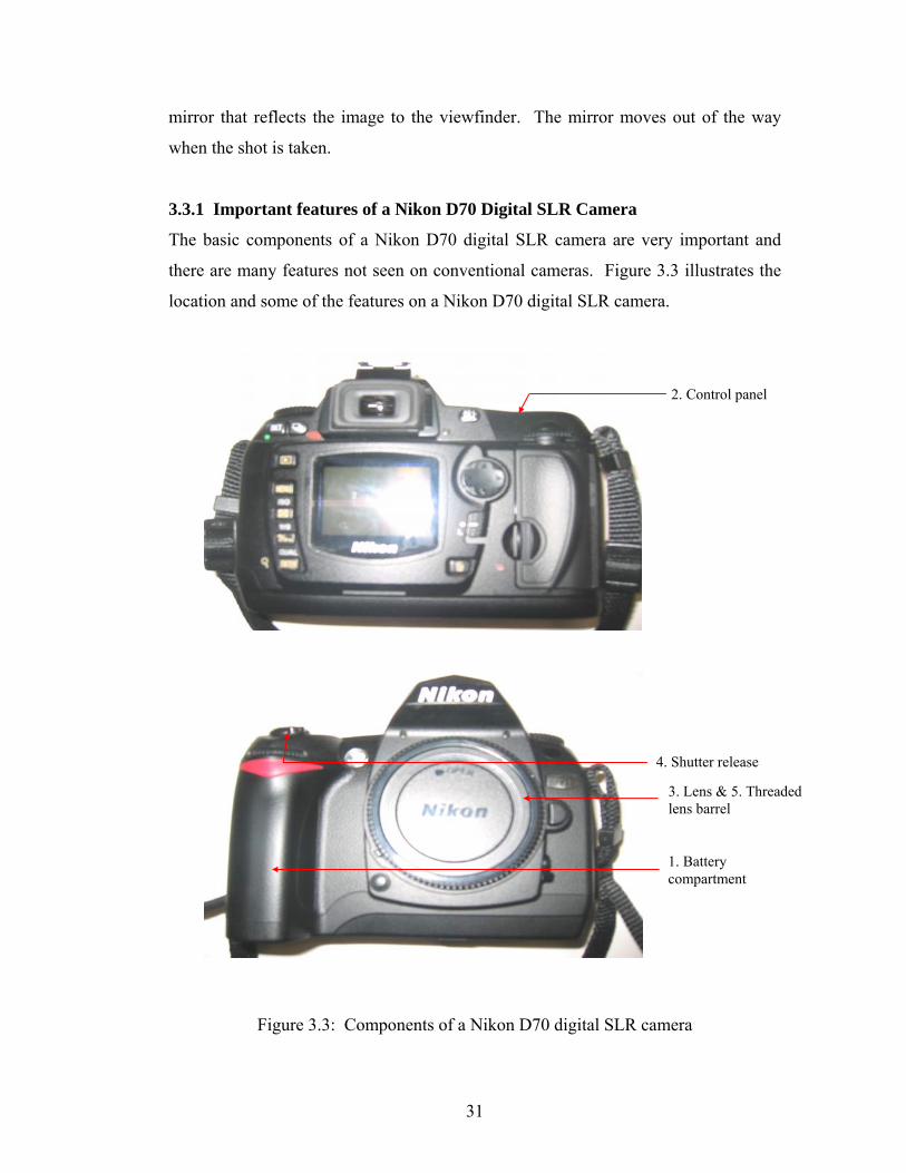
3.3.1 Important features of a Nikon D70 Digital SLR Camera
The basic components of a Nikon D70 digital SLR camera are very important and
there are many features not seen on conventional cameras. Figure 3.3 illustrates the
location and some of the features on a Nikon D70 digital SLR camera.
Figure 3.3: Components of a Nikon D70 digital SLR camera
3. Lens & 5. Threaded lens barrel
2. Control panel
1. Battery compartment
4. Shutter release

32
1. Battery Compartment: This is the slot for installing the camera’s batteries. The
batteries are rechargeable. It can hold multiple batteries.
2. Control Panel: The control panel is a small liquid crystal display (LCD) that
displays the current settings, battery life, number of images remaining to be
taken, and mode operation of the camera.
3. Lens: The lens is a piece of ground glass or plastic that focuses the light on the
sensors. It is mounted in a cylindrical housing, which is attached to the front of
the camera. The lens moves within the housing closer or nearer to the image
sensors, which allows focussing of the image. The lenses are detachable and
interchangeable.
4. Shutter Release: The shutter release is a multifunction button, found on the top
right part of the camera. It is used in its half-pressed mode to set metering and
focus. In its fully pressed mode, it releases the shutter to expose the electronic
image sensors and capture the image.
5. Threaded Lens Barrel: The lens barrel is threaded and it can accept a wide
variety of special-effects, and close-up filters. It can also adapt to wide-angle
lenses. It can be spotted by looking at the screw threads at the inside rim of the
metal that surrounds the front lens element.
3.3.2 Spatial resolution and image quality
The spatial resolution is the distance in the object plane represented by one pixel in
the image plane. The factors affecting the spatial resolution are sensor pixel count,
sensor size, lens and extension ring combination, and object distance. The Nikon
D70 digital SLR camera has a sensor pixel count of 3008×2000. The lens of the
camera focuses the light collected from the object on to the image plane. A 200 mm
camera lens was used for this purpose. An extension ring attached to the camera lens
served to allow closer object distances and thereby increase the resolution of the
images. The object distance was then adjusted so that the tube diameter almost filled
the image area.
33
3.3.3 Shooting and focus modes
The Nikon D70 digital SLR camera was operated in the manual shooting mode. The
manual mode of operation allows for a higher degree of control over the exposure,
giving options that automatic mode cannot offer in many situations. Exposure is
controlled by the size of the aperture, the duration and intensity of the flash, the
sensitivity of the CCD, the placement of the flash units, and the scene being
photographed. To maximise the overall sharpness of the image from as close to the
camera as possible, the smallest f-stop (largest number, f-22) was used to narrow the
aperture as much as possible. This counterbalancing of aperture and flash settings
allowed choosing between controlling depth-of-field (aperture) or stop action
(external flash) while maintaining a level of exposure. Focus is the ability of the
camera lens to bring to clarity the most important parts of an image’s detail. Focus
was achieved by manually adjusting the focus ring on the lens. Two remote SB-600
AF flash units were used to increase the level of exposure in the images. The SB-600
AF speedlights were connected to the camera via a hot shoe and a synchronous cord.
The external flash has a zoom in the range 24-85 mm and an output power of M1-
1/64. The external flash has a rotating head which made it possible to direct the
illumination evenly over the object. The duration of the electronic flash unit was
approximately 1/25,000 seconds at M1/64 output, which is faster than any shutter.
This enabled freezing the rapid movements of the liquid film. Also, using a second
flash dramatically increased the ability to control the contrast of the light in several
areas of a photo at once.
3.4 Procedure for determination of the wall location The correct position of the vertical tube wall was determined by taking pictures of the
air-water meniscus with stagnant water in the tube. A spirit level was used to ensure
that the tube was vertical. The wall position is shown by a thin vertical yellow line in
figure 3.4. Among the most critical parameters needed was the pixel scale factor
which relates a physical dimension to the pixel size. The pixel positions for the wall
on both sides were recorded. This combined with the known inside diameter was
used to determine the pixel scale factor (pixel to millimetre conversion). It was found

34
to be equal to 108.7 pixels/mm. The pixel scale factor needs to be determined only
once for a given camera setup. The factor has been found to be very consistent, even
after moving and remounting the camera apparatus several times. It is important,
however, that the Nikon D70 digital SLR camera be mounted quite rigidly on the
tripod stand with respect to the wall location of the test section to maintain a constant
pixel scale factor and to reduce any noise due to movement of the camera. Possible
movement of the camera is a potential source of a large systematic uncertainty.
Measurements of the wall location were carried out before and after the film
thickness measurements to eliminate this possibility. The difference was at most one
pixel in magnitude. This corresponds to about 0.0091 mm.
Figure 3.4: Static image of the water meniscus with the tube wall shown by a thin
vertical line
3.5 Image processing
Images are two-dimensional representations of the visual world. Images are
important sources of information for data interpretation and analysis. Image
processing is a term used to describe operations carried out on images; the objective
Air
Water
25.48 mm
Meniscus
Contact line
Tube wall
35
might be to reduce noise or to extract information of particular interest to the observer
(Pearson, 1991). The visual inspection process is time-consuming and is subject to
inconsistency. Computers, on the other hand, are ideal for performing these tasks.
For computers to process images, the images must be numerically represented. This
process is known as image digitisation. Once images are represented digitally,
computers can reliably automate the extraction of useful information using digital
image processing. Digital image processing performs various types of image
enhancements and measurements. Inspector® is a hardware-independent application
designed for image capture, storage, and processing applications. Inspector®
provides a comprehensive set of image processing operations. There are two main
types of processing operations:
1. Those that enhance or transform an image;
2. Those that take measurements in an image, i.e., generate a numeric or graphical
report that relates to specific image information.
3.5.1 Image enhancement and measurement operations
Inspector’s® image enhancement and transformation operations improve the quality
of the image and / or transform the image. Only the techniques used in this thesis
will be discussed here. These include:
1. Point-to-point operations: These operations include brightness and contrast
adjustment, and thresholding. Point-to-point operations compute each pixel
result as a function of the pixel value at the corresponding location in the
original image.
2. Spatial filtering operations: These operations are also known as convolution
operations. They include operations that can enhance and smooth images,
accentuate image edges, and remove noise from an image. Most of these
operations compute results based on an underlying neighbourhood process:
the weighted sum of a pixel value and its neighbour’s values.

36
3. Morphological operations: These operations include opening, closing,
erosion and dilation of images. These operations compute new pixel values
according to geometric relationships and matches to known patterns in the
input image.
4. Measurement operations: These operations include distance and angle
measurements, as well as measurements using selected spatial positions
(known as markers).
3.5.2 Flowchart representation of sequence of operations
Digital image processing operations such as image enhancements, transformations
and extraction of measurements was performed using Inspector®. The typical
application steps that were followed for the extraction of instantaneous film thickness
measurements are represented as a flowchart in figure 3.5. The images were pre-
processed to improve their quality before extracting information from them.
Figure 3.5: Flow chart of steps followed in digital image processing using Inspector®
Load an image from memory
Create a greyscale image from a colour image
Convert a greyscale into a binary image
Set the threshold for an image
Apply a spatial filter (Median filter)
Perform Opening and Closing operations
Use Erosion and Dilation (in extreme cases with more blobs)
Create markers
Allocate markers based on edges
Extract measurements using markers
Write measurements to file
Perform uniform histogram equalisation
37
3.5.3 Description of image processing operations
• First, the image was loaded from memory.
• All colour images were converted into grey scale images. A greyscale image
was created because certain image processing operations such as
measurement operations can be performed only on 8-bit unsigned greyscale
images (pixel value 0 to 255).
• Then, the intensity distribution of the image was adjusted by performing a
histogram equalisation operation. The process is spatially adaptive as
histogram modification is applied to each pixel based upon the histogram of
pixels within a moving window neighbourhood. This process resulted in a
more uniform distribution of the image’s pixel values.
• The thresholding operation was carried out to define a range of brightness
values in the original image, selecting the pixels within this range as
belonging to the foreground, and rejecting all other pixels to the background.
Such an image was then displayed as a binarised or two-level image, using
black and white colours to distinguish the regions (Russ, 1995). Since a
thresholded image contains fewer pixel values than the original image, some
operations can be performed more efficiently.
• The Gaussian random noise and systematic noise with small scale variations
were reduced by applying a median filter to the image. The Gaussian random
noise may be caused, for example, by the camera or digitiser because, in
general, electronic devices tend to generate noise. This type of noise
introduces pixels of arbitrary values that are generally noticeable because they
are completely unrelated to the neighbouring pixels. Systematic noise can be
predicted, appearing as a group of pixels that are not part of the actual image.
It may be caused, for example, by the camera or digitiser, or by uneven
lighting. If the image was magnified, microscopic dust particles, on either the
object or a camera lens, may appear to be part of the image. Median filter
operations were more suitable for removing such noise, since they replaced
each pixel with a value from its neighbourhood rather than with a weighted
sum of its neighbourhood. A median filter is a type of spatial filter that
38
replaces each pixel with the median of its operating neighbourhood.
Inspector® provides a pre-defined median filter which operates on each pixel’s
3×3 neighbourhood. It performs a non-linear filtering operation where a
window moves over a signal and at each point the median value of the data
within the window was taken as the output. Median filtering has some
desirable properties that cannot be achieved with other filtering operations.
The impulse response of the median filter is zero. This property makes it
attractive in suppressing impulsive noise. Median filters are robust and are
well suited for data smoothing when the noise characteristics are unknown. A
stepwise change in a signal passes the median filter unaltered. This property
is used in application such as image filtering, where data need to be smoothed,
but blurring of the signal edges is not acceptable (Refer to Astola et al., 1990).
• A morphological opening operation was performed to remove small particles
(e.g., bubbles in liquid films) or to break isthmuses or connections between
touching objects. Inspector® provides the opening function to operate on 3×3
neighbourhoods taking all neighbourhood pixels into account. The closing
operation is useful in filling holes in objects; however, in doing so, they also
connect objects that are close to each other. The closing function also
performs a standard 3×3 closing operation taking all neighbourhood pixels
into account. Erosion and dilation operations were also used in some extreme
cases with more blobs. Erosion peels layers from objects or particles,
removing extraneous pixels and small particles from the image. On grey scale
images, Inspector’s® pre-defined erosion operation replaces each pixel with
the minimum value in its 3×3 neighbourhood (if operating on bright objects)
or with the maximum value (if operating on dark objects). Dilation adds
layers to objects or particles, enlarging particles. On grey scale images,
Inspector’s® pre-defined dilation operation replaces each pixel with the
maximum value in its 3×3 neighbourhood (if operating on bright objects) or
with a minimum value (if operating on dark objects).
• Once the image had been pre-processed, film thickness measurements could
be extracted by positioning markers at the gas-liquid interface using

39
Inspector’s® edge detection features. The process of positioning these
markers begins by specifying a search box. The size and position of the
search box specifies the search area. Also the orientation of the search box
has to be specified to ensure the proper search direction as shown in figure
3.8. The search box is positioned using the already-known wall location from
the water meniscus pictures. The search takes place in the same direction as
the search direction line. To obtain valid results, the box must include a
portion of the edge and be completely inside the image. In addition, the edge
should enter and leave by opposite sides of the box (occupy the entire box
width). The box’s location line can also be adjusted to indicate the expected
position of the edge. To ensure the fastest possible search operation, the
smallest possible search box is used; search time is roughly proportional to the
area searched. In reality, the search box is just 1 pixel high. It is shown larger
in figure 3.8 for more clarity. In addition to locating the edge and to measure
its true width, the location line of the search box is set at approximately the
same angle as the edge. This allows Inspector® to find the edges of the same
orientation as the location line. However, the most accurate results are
obtained when searching for an edge at 0° or 90°. The Inspector® finds the
required edge using certain specified characteristics such as angle, polarity,
strip width, reference position, edge strength, and contrast, etc.
• Figure 3.6 was taken at a flow rate Q = 4.678 L/min and Re = 974. Here, the
liquid film is very thin and is characterised by small waves. The tube wall
determined from the air-water meniscus pictures as discussed earlier is shown
by a thin vertical yellow line on the extreme right- and left-hand sides. The
features present in the falling annular film images are shown in figure 3.6.
The object plane with the surface waves (viewed from the liquid side) is also
depicted in figure 3.7. Figure 3.8 was taken at an even higher Reynolds
number of Re = 4552. The search box, box width, search direction, and

40
Figure 3.6: Falling annular film at Q = 4.68 L/min and Re = 974
Figure 3.7: Cross-section view of a falling annular film
Wavy gas-liquid interface
Liquid film
Tube outer diameter
Tube inner diameter
Nikon D70 digital camera
SB-600 Speed-light
Object plane
Optical correction box
Tube wall
Liquid film
Gas- liquid interface
Waves
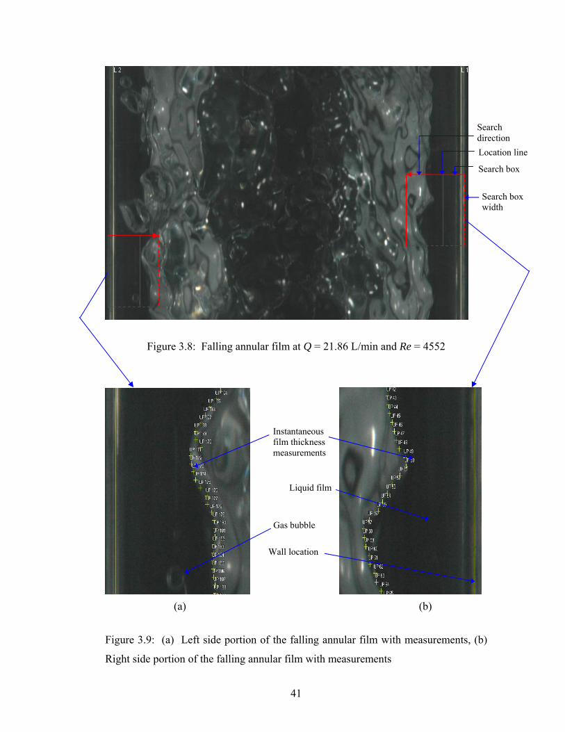
41
Figure 3.8: Falling annular film at Q = 21.86 L/min and Re = 4552
(a) (b)
Figure 3.9: (a) Left side portion of the falling annular film with measurements, (b)
Right side portion of the falling annular film with measurements
Instantaneous film thickness measurements
Gas bubble
Liquid film
Wall location
Search box width
Location line
Search direction
Search box

42
location line are also shown in figure 3.8. Figure 3.9a and 3.9b show a small
portion of figure 3.8 with the measurements on the right- and left-hand sides
extracted after carrying out all the image processing and analysis operations
described. The vertical distance between each instantaneous film thickness
measurement was equal to 20 pixels. Using edge detection techniques,
Inspector® identifies the gas- liquid interface in these two-dimensional
pictures as a characteristic of an edge. About 200 edge measurements were
extracted from the left- and right-hand sides of each image.
• Finally, all of the operations just described were automated using the
Inspector® scripting feature, allowing many instantaneous film thickness
measurements to be made in a very short period of time. The script is
recorded in Inspector® by performing the operations manually with the script
recorder activated. Once the recording started, the sequence of operations
was added to the script as a user-defined script function. A user-defined script
function is simply a named group of script statements, which is referred to as
a macro. To run the code autonomously, the script function was edited. A
script can have several user-defined functions, as well as statements outside of
these functions. Inspector® displays the script in a script window. The
required modifications were typed directly in the script window, or the script
was saved in a file and edited using a text editor. Later, powerful scripting
constructs such as looping, comments, and macros were also manually added.
These functions added more flexibility to the code during execution and
enabled many quantitative instantaneous film thickness measurements to be
extracted in a short period of time. The code for the measurement of
instantaneous film thickness in annular falling liquid films was written using
Inspector® (Refer to Appendix A.)
3.6 Correction of visual distortion
One of the most common problems in imaging flows in cylindrical tubes is the optical
distortion caused by the wall curvature. To produce quantitative results using

43
photographic techniques, these optical distortions need to be minimised. This
distortion occurs because of the combined effects of the curvature of the surfaces and
differences in refractive indices of the interacting media. To minimise this problem
the cylindrical tube must be surrounded by an optical correction box with flat walls
filled with a matching fluid.
3.6.1 Arrangement of test section and optical correction box
For the case of internal flow through a tube, it is necessary to construct a box with flat
walls (optical correction box) around the model. If the flowing liquid also has the
same refractive index, the flow can now be viewed without refraction errors from
directions perpendicular to each face of the view box. Bhatia et al. (1982) and Durst
et al. (1988) used this method to conduct near-wall measurements in a turbulent pipe
flow. In their experiments, the entire test section was submerged in a fluid with
matched refractive index in a container with flat walls. Durst et al. (1988) also
discussed methods for determining the laser Doppler velocimetry (LDV) measuring
position relative to the wall when refractive index matching is employed. Duncan et
al. (1988) used the optical-correction box method to study flow through elastic wall
casts of aortic bifurcations where wall motions were present. Budwig et al. (1993)
conducted flow studies through axisymmetric bulges in tubes using this method. The
bulge models were machined from rectangular blocks of acrylic plastic. For external
flows around solids with curved surfaces the view box becomes a fluid channel
through which the matching fluid is pumped. Chen and Fan (1992) have used this
method to investigate the flow structure in fluidised beds. Agrawal et al. (1978) and
Bovendeerd et al. (1987) dealt with the refractive index problem by machining the
circular tubes with rectangular outer walls and filling the tube with a fluid that
matches the refractive index of the surrounding walls.
3.6.2 Properties of test section and correction box materials
Table 3.1 shows some of the common materials that are used to construct optical
correction boxes and test sections. The important issues with regard to these
materials are ease of model and test section construction, index of refraction, optical

44
clarity, scratch resistance, and price. Some projects might have special requirements
such as models with flexible or porous walls. For this thesis, acrylic was chosen as
the tube and correction box material due to its availability, price, and transparency.
Table 3.1: Properties of tube and correction box materials
Material Model Construction methods
Index of Refraction
Scratch resistance
Comments
Glass Pyrex glass
glassblowing fusing
1.47 to 1.49
+ + +
Available in sheets, tubes, rods and special fittings
Optical glasses Plexiglas
grinding polishing moulding and extrusion
1.45 to 1.96
1.51
+ to + + + Available in flats and lenses-expensive to purchase and to work with, Durst et al. (1988) Exceptional optical clarity, chemical resistance, Gupta and Kaplan (1942)
Plastic Pre-cast or extruded
machining, bonding, bending, and polishing
Available in sheet, tubes, and rods
Acrylic 1.49 + Less expensive, transparent and easy to fabricate
Polycarbonate (Lexan)
1.58 + +
Casting resins can be machined after casting (except silicon)
Silicon elastometer
1.43 +
Elastic walls, Duncan et al. (1990)
Urethane based 1.49 + + Cure at 65 o C Acrylic based 1.49-1.53 +
3.6.3 Properties of matching fluids
Some of the considerations for successful use of matching fluids include index of
refraction, optical clarity, density, viscosity, material compatibility, chemical
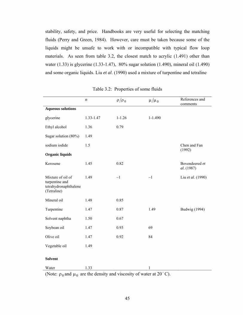
45
stability, safety, and price. Handbooks are very useful for selecting the matching
fluids (Perry and Green, 1984). However, care must be taken because some of the
liquids might be unsafe to work with or incompatible with typical flow loop
materials. As seen from table 3.2, the closest match to acrylic (1.491) other than
water (1.33) is glycerine (1.33-1.47), 80% sugar solution (1.490), mineral oil (1.490)
and some organic liquids. Liu et al. (1990) used a mixture of turpentine and tetraline
Table 3.2: Properties of some fluids
n 0ρρ 0μμ References and comments
Aqueous solutions
glycerine
1.33-1.47 1-1.26 1-1.490
Ethyl alcohol
1.36 0.79
Sugar solution (80%)
1.49
sodium iodide
1.5 Chen and Fan (1992)
Organic liquids
Kerosene 1.45 0.82 Bovendeered et al. (1987)
Mixture of oil of turpentine and tetrahydronaphthalene (Tetraline)
1.49
~1
~1
Liu et al. (1990)
Mineral oil
1.48
0.85
Turpentine
1.47 0.87 1.49 Budwig (1994)
Solvent naphtha
1.50 0.67
Soybean oil
1.47 0.93 69
Olive oil
1.47 0.92 84
Vegetable oil
1.49
Solvent Water
1.33
1
(Note: 0ρ and 0μ are the density and viscosity of water at 20 o C).

46
(1.490) whose density and viscosity were similar to those of water and that matched
the refractive index of acrylic used in fabrication of the test section. Flows with
variable refractive index have similar problems. While these methods may simplify
the image analysis by reducing distortion, they also restrict the range of experimental
exploration. For this thesis, water was chosen to be the working fluid because of its
availability and other physical and chemical characteristics. Once the index of
refraction problem was fixed, there was a need to eliminate the visual distortions.
Figure 3.10: Arrangement of test section and optical correction box
After the test section material, correction box material, and the matching fluid were
chosen, the test section and optical correction box were arranged as shown in figure
3.10. In this research, an optical correction box was placed around the tube and was
made of the same material as the tube (acrylic). It was filled with the same liquid
(water) as the test liquid. Since the index of refraction of the test liquid did not match
the tube material exactly, further correction was required. A ray tracing model was
developed for this purpose and will be discussed in detail in the next section.
3.7 Optical correction using ray tracing In this section, the general purpose of the ray tracing diagram will be explained.
Then a brief review of the work done by past researchers in this field will be
discussed. Finally, the technique will be discussed in detail using ray tracing
Nikon D70 SLR Digital camera
(Top View)
200 mm lens
Image processing computer
Water
105 mm f /2.8 extension ring
Tube (acrylic)
Wavy falling Annular film
Optical correction Box (acrylic)
Remote flash unit
35 cm Gas core
Flash units at 45°

47
diagrams and detailing all equations involved in the calculations. The experimental
validation of the ray tracing procedure will be explained in detail later in section 3.8.
3.7.1 Ray tracing
An accurate determination of the shapes and positions of objects within a cylindrical
tube requires an analysis of the bending of light rays at various interfaces. This
process is governed by Snell’s law of refraction which is as follows:
2211 sinsin α=α nn . ( )1.3
where, n is the index of refraction of the medium and α is the angle between a ray
and the surface normal. The subscripts 1 and 2 refer to the two substances. Since it
was difficult to track the rays close to the tube wall, a ray tracing approach had to be
adopted. The specifics are given in detail in the next section. The ray tracing
problem has been studied by Boadway and Karahan (1981) and Bicen (1982) in fluid
flow investigations using laser-Doppler anemometry (LDA). Their analysis was
limited to determining the intersection of two laser beams entering the tube from
various angles. Durret et al. (1985) used ray tracing techniques to reduce the optical
distortion and design corrective lenses to facilitate alignment of the laser beams.
Later, Lowe and Kutt (1992) reconstructed the three-dimensional trajectories of
particles in fluid flows and developed a method for measuring the co-ordinates of
particles located inside a straight cylindrical tube by viewing it from two directions
using cameras and digital imaging techniques. They showed that refraction through a
cylindrical tube wall can generate phenomena such as hidden regions and multiple
images.
In this thesis, both a theoretical and experimental approach to correct for the visual
distortion was used. The imaging system was modelled as a simple pinhole camera
for this purpose. The main objective was to map points on the image plane to points
on the object plane. A backward ray-tracing method was adopted in which the rays
were traced from the image plane to the object plane. The details of all the ray
tracing equations and calculations will be described in the next section.
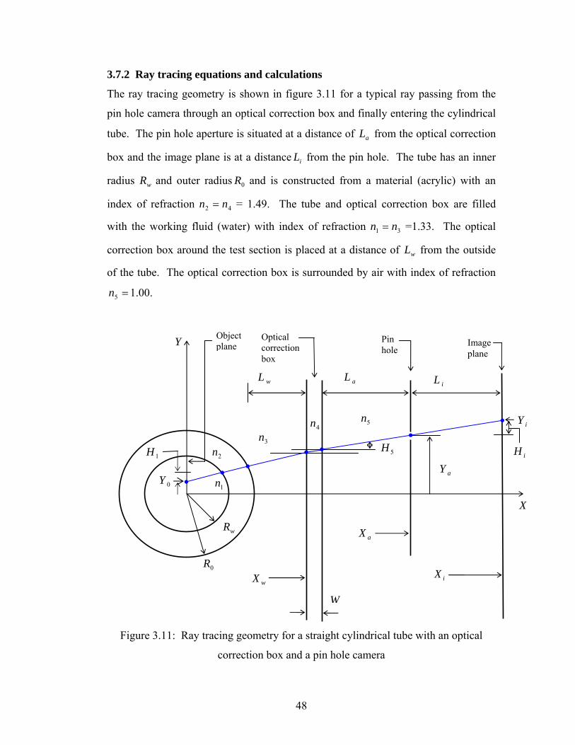
48
3.7.2 Ray tracing equations and calculations
The ray tracing geometry is shown in figure 3.11 for a typical ray passing from the
pin hole camera through an optical correction box and finally entering the cylindrical
tube. The pin hole aperture is situated at a distance of aL from the optical correction
box and the image plane is at a distance iL from the pin hole. The tube has an inner
radius wR and outer radius 0R and is constructed from a material (acrylic) with an
index of refraction 42 nn = = 1.49. The tube and optical correction box are filled
with the working fluid (water) with index of refraction 31 nn = =1.33. The optical
correction box around the test section is placed at a distance of wL from the outside
of the tube. The optical correction box is surrounded by air with index of refraction
.00.15 =n
Figure 3.11: Ray tracing geometry for a straight cylindrical tube with an optical
correction box and a pin hole camera
Y
L w L a L i
Pin hole
Image plane
W
X i
X a
X w
Y a
Y i
H i
0R
wR
X
Y 0 1n
2n 3n
4n 5n
5H H 1
Optical correction box
Object plane
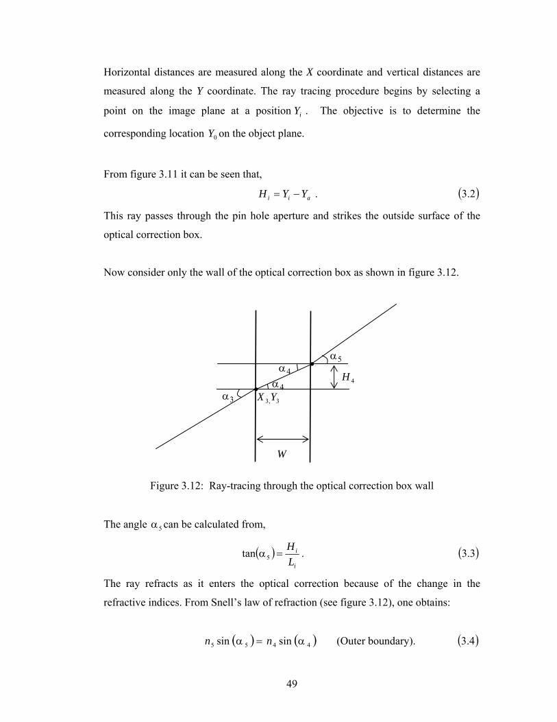
49
Horizontal distances are measured along the X coordinate and vertical distances are
measured along the Y coordinate. The ray tracing procedure begins by selecting a
point on the image plane at a position iY . The objective is to determine the
corresponding location 0Y on the object plane.
From figure 3.11 it can be seen that,
aii YYH −= . ( )2.3
This ray passes through the pin hole aperture and strikes the outside surface of the
optical correction box.
Now consider only the wall of the optical correction box as shown in figure 3.12.
Figure 3.12: Ray-tracing through the optical correction box wall
The angle 5α can be calculated from,
( )i
i
LH
=α5tan . ( )3.3
The ray refracts as it enters the optical correction because of the change in the
refractive indices. From Snell’s law of refraction (see figure 3.12), one obtains:
( ) ( )4455 sinsin α=α nn (Outer boundary). ( )4.3
5α 4α
4α 3α
W
4H
3,3 YX

50
( ) ⎟⎟⎠
⎞⎜⎜⎝
⎛⎟⎟⎠
⎞⎜⎜⎝
⎛α=α
4
554 sinarcsin
nn
( )5.3
As the thickness W of the optical correction box is known, 4H is calculated as follows:
( )44 tan α=WH . ( )6.3
Then, applying Snell’s law for the outer surface of the tube, the following result is
obtained:
( ) ( )4433 sinsin α=α nn (Inner boundary). ( )7.3
Knowing the values of the refractive indices 3n and 4n and the angle of
refraction 4α , the value of 3α can be determined.
Now, knowing the slope 3m and the point on the left surface of the optical correction
box ( )33 Y,X , the intersection point with the outer tube ( )22 Y,X can be determined.
The intersection between the ray and the outer surface of the tube (point 2) is as
shown in figure 3.13.
Figure 3.13: Intersection between a ray and the outer surface of the tube
The equation for the intersection point between a straight line and a circle can be
found from,
( )3,3 YX
2β
0R X
33 bXmY +=
20
22
22 RYX =+
22
202 XRY −=
22 ,YX
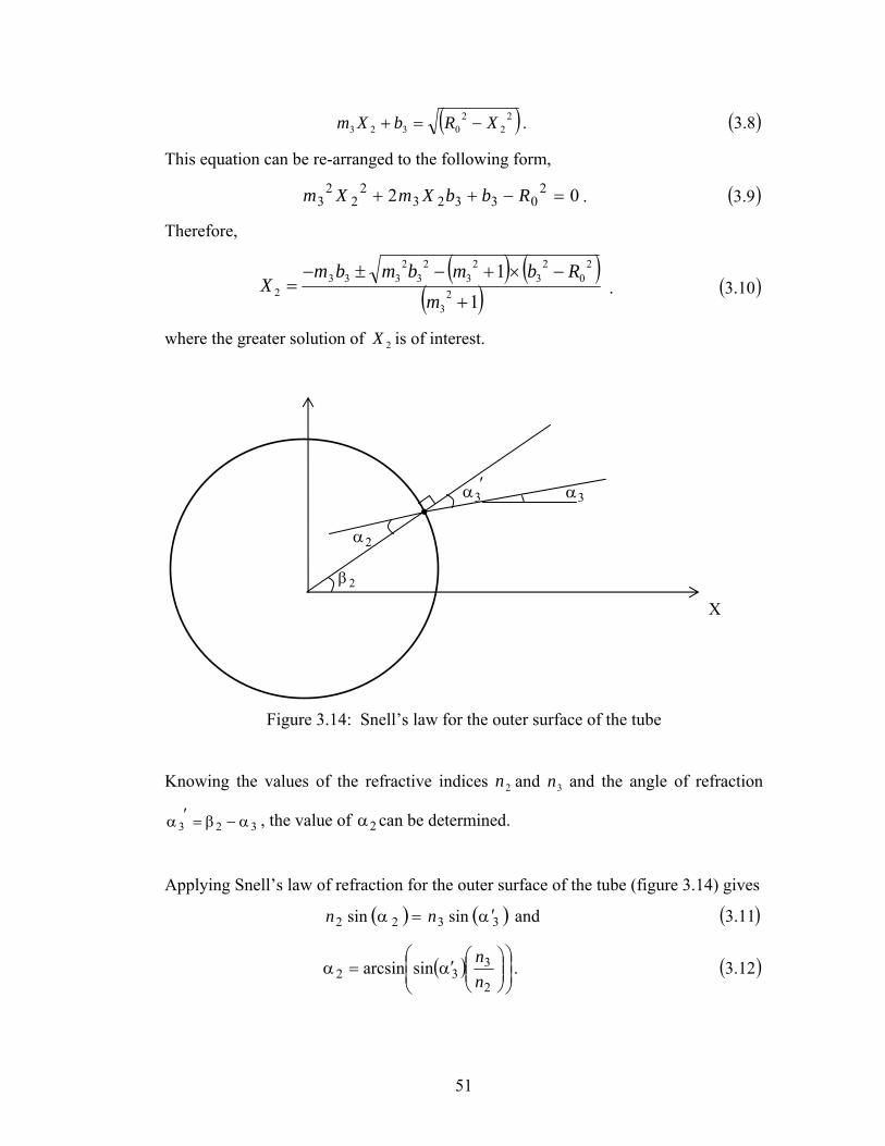
51
( )22
20323 XRbXm −=+ . ( )8.3
This equation can be re-arranged to the following form,
02 203323
22
23 =−++ RbbXmXm . ( )9.3
Therefore,
( ) ( )
( )11
23
20
23
23
23
2333
2+
−×+−±−=
mRbmbmbm
X . ( )10.3
where the greater solution of 2X is of interest.
Figure 3.14: Snell’s law for the outer surface of the tube
Knowing the values of the refractive indices 2n and 3n and the angle of refraction
323 α−β=′α , the value of 2α can be determined.
Applying Snell’s law of refraction for the outer surface of the tube (figure 3.14) gives
( ) ( )3322 sinsin α′=α nn and ( )11.3
( ) ⎟⎟⎠
⎞⎜⎜⎝
⎛⎟⎟⎠
⎞⎜⎜⎝
⎛α′=α
2
332 sinarcsin
nn
. ( )12.3
3α ′α3
X
2α
2β

52
The same procedure is repeated for the inner radius of the tube as shown in figure
3.15. Knowing the slope 2m and the intersection point with the outer tube ( )22 ,YX ,
the intersection point with the inner tube ( )11 ,YX can be determined. Then, applying
Snell’s law again for the inner surface of the tube, the following result is obtained:
( ) ( )2211 sinsin α′=α nn . ( )13.3
Figure 3.15: Intersection of a ray with the inner surface of the tube
Figure 3.16: Ray refracted inside the inner surface of the tube
1β
1α
11 α−β
1H
X
Y
Y 0
2β
X
Y
iR
2α
′α2
1β
( )22 ,YX ( )11 ,YX
bXmY += 2

53
Knowing the values of the refractive indices 1n and 2n and the angle of refraction
′α 2 , the value of 1α can be determined.
Finally from figure 3.16, 1H is calculated as follows,
( )1111 tan α−β= XH . ( )14.3
Using the value of 1H , the object distances 0Y can be calculated. This process is
repeated for many points on the image plane.
3.7.3 Computer-generated ray tracing diagrams
The ray tracing equations were programmed and solved using Microsoft® Excel.
Computer-generated ray tracing diagrams are shown in figure 3.17a, 3.17b and 3.17c
for three cases at different locations from the edge of the tube towards the tube centre.
For simplicity, only a portion of the vertical tube and the optical correction box is
shown. The geometry and refractive indices correspond to the experimental
conditions of this thesis. Some of the fixed parameters involved in the calculations
are given below in Table 3.3. The ray was automatically traced from the image plane
back to the object plane from where it originated. It is seen that the refractive angles
become larger near the edges of the tube (figure 3.17a). In practice, points near the
edge become difficult to observe partly because of distortion but also because of
irregularities in the surface of the acrylic tube. Towards the centre, the refractive
angles become smaller (figure 3.17b).
Table 3.3: Some fixed parameters involved in ray-tracing calculations
Parameter
Distance (mm)
aY 15
0R 15.82
wR 12.74
wL 15.93
aL 1000
iL 100 W 3.175

54
0
5
10
15
20
25
30
0 5 10 15 20 25 30 35 40 45 50
X (mm)
y (m
m)
Figure 3.17 (a): Ray traced very close to the tube wall
0
5
10
15
20
25
30
0 5 10 15 20 25 30 35 40 45 50
X (mm)
y (m
m)
Figure 3.17 (b): Ray traced mid-way between the tube wall and the centre of the tube
Ac = Acrylic (n =1.491)
Vertical tube wall
Optical correction box
Ac A
Ac
W
S
(a)
(b)
W
A = Air (n =1.00) S = Point sourceW = Water (n=1.33)
Y (m
m)
X (mm)
X (mm)
Y (m
m)
Object plane
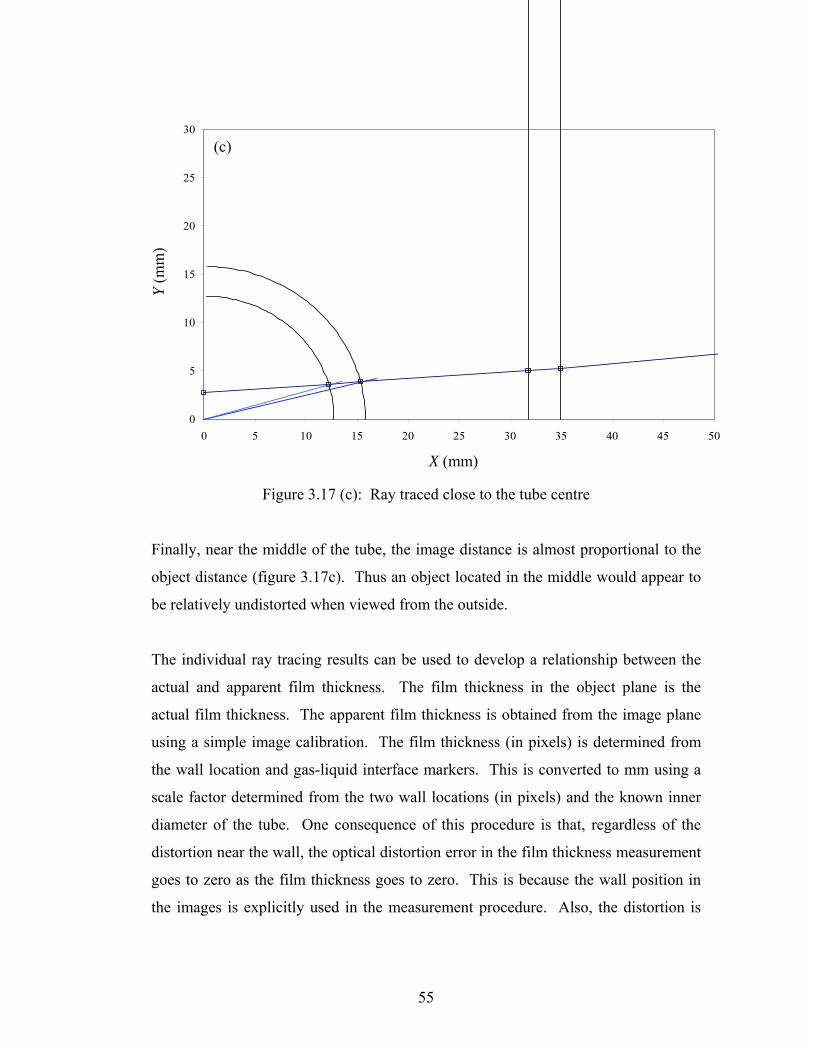
55
0
5
10
15
20
25
30
0 5 10 15 20 25 30 35 40 45 50
X (mm)
y (m
m)
Figure 3.17 (c): Ray traced close to the tube centre
Finally, near the middle of the tube, the image distance is almost proportional to the
object distance (figure 3.17c). Thus an object located in the middle would appear to
be relatively undistorted when viewed from the outside.
The individual ray tracing results can be used to develop a relationship between the
actual and apparent film thickness. The film thickness in the object plane is the
actual film thickness. The apparent film thickness is obtained from the image plane
using a simple image calibration. The film thickness (in pixels) is determined from
the wall location and gas-liquid interface markers. This is converted to mm using a
scale factor determined from the two wall locations (in pixels) and the known inner
diameter of the tube. One consequence of this procedure is that, regardless of the
distortion near the wall, the optical distortion error in the film thickness measurement
goes to zero as the film thickness goes to zero. This is because the wall position in
the images is explicitly used in the measurement procedure. Also, the distortion is
(c)
X (mm)
Y (m
m)

56
zero at the tube centreline because the rays are normal to all surfaces. This case,
however, is of no practical importance since the films are never that thick.
Figure 3.18 shows the distortion error as a function of the apparent film thickness.
Without the optical correction box, there is substantial distortion near the edge of the
tube. The distortion reaches a maximum of 0.6 mm for 3 mm thick films. However,
when liquid (water in this case) is put in the optical correction box; the distortion
greatly reduces. The distortion near the edge of the tube means that film thicknesses
appear smaller than they actually are. The distortion is reduced even though the
index of refraction of water is much different than acrylic. Experimental data is
required to validate that this method could effectively correct for distortion.
0.0
0.1
0.2
0.3
0.4
0.5
0.6
0.7
0.0 2.0 4.0 6.0 8.0 10.0 12.0 14.0
Without correction box
With water incorrection box
Figure 3.18: The effect of using water in the optical correction box as determined by the ray tracing model
Apparent Film thickness (mm)
Act
ual –
App
aren
t film
thic
knes
s (m
m)

57
3.8 Experimental confirmation of ray tracing procedure The experimental investigations of optical distortion carried out in the test section are
presented here. The in-situ calibration procedures that were carried out to determine
the effect of distortion caused by the tube wall when light rays get refracted near the
edges are explained. Finally, the experimental results obtained were compared with
the ray tracing model.
3.8.1 Description of the calibration stylus and holder
A picture with the calibration stylus and the stylus holder flushed with the tube wall
can be seen in figure 3.19. The tube wall is shown by a thin vertical line on right side
of the picture. The calibration stylus and stylus holder were designed to position a
calibration target in the object plane inside the water-filled tube (see figure 3.20). An
enlarged view of the stylus used in the calibration is also shown in figure 3.21. The
Figure 3.19: Picture of the stylus flush with the vertical tube wall
Lead screw Stylus holder Water
Stylus (Each graduation = 0.127 mm)
Air vent
Tube wall
Feed water inlet

58
Figure 3.20: Front view of the in-situ calibration setup
Figure 3.21: Enlarged view of the stylus
Stylus
Stylus holder
Feed water
Lead screw
Turning knob
O- Rings
Tube wall
Air vent
45° R =10.16 mm
45°0.127 mm
59
stylus was made of brass with fine grooves cut in it. The distance between the crest
and the trough of each groove is 0.127 mm. The stylus holder was made of acrylic
and it contains the stylus, the lead screw, turning knob, and the feed water circuit. As
the lead screw is advanced in the slot, it moves the stylus to contact the inner tube
wall. The small region containing the stylus is flooded with water. The region
around the stylus was flooded to mimic the actual conditions during testing. Air was
vented through the top to remove any unwanted bubbles in the region.
3.8.2 Comparison of experimental results to ray tracing model
The pixel number corresponding to each graduation (i.e., the crest and the trough of
each groove) in the stylus was recorded. As per the ray tracing theory, the distances
between graduations near the centre of the tube should not be deformed when viewed
through the correction box filled with water. Therefore, if there was no visual
distortion, the pixel to stylus graduation ratio was constant throughout the whole
picture, meaning that the near wall graduations were not deformed. But very near to
the wall, it was found that the stylus graduations seemed to be deformed or closer to
one another. This observation near the wall was consistent with the ray tracing
theory.
Figure 3.22 shows the (Actual - Apparent film thickness) as a function of apparent
film thickness. The experimental results appear to be in reasonable agreement with
the theoretical results near the tube wall and up to a film thickness of about ~ 6 mm.
This value of film thickness is thicker than the expected films of 1 ~ 2 mm. The
reason for the slight deviation from the theoretical curve beyond these points could
not be determined. Small variations in the wall thickness of the acrylic tube may
have contributed to this error. Figure 3.23 shows the relationship between the
percentage error and the apparent film thickness. As predicted by the theory, there is
distortion as the light rays get refracted near the tube wall. But the percentage error
goes to zero as apparent film thickness goes to zero. This is because the deviation
between the actual film thickness and the apparent film thickness approaches zero
near the tube centre. The experimental results for film thickness agree closely to
60
0.00
0.05
0.10
0.15
0.20
0.25
0.0 2.0 4.0 6.0 8.0 10.0 12.0 14.0
Ray-tracing modelExperimental
Figure 3.22: Comparison of experimental and theoretical results for ray-tracing
0.0
0.1
0.2
0.3
0.4
0.5
0.6
0.0 2.0 4.0 6.0 8.0 10.0 12.0 14.0
Ray-tracing modelExperimental
Figure 3.23: Percentage error versus apparent film thickness
Apparent Film thickness (mm)
% E
rror
Apparent Film thickness (mm)
Act
ual –
App
aren
t film
thic
knes
s (m
m)
61
within ~ ±1% with theoretical results for thinner and thicker films. Thus, it was
concluded that ray tracing techniques and the calibration procedures employed here
would increase the accuracy of the non-intrusive imaging technique and yield
quantitative film thickness measurements inside the cylindrical tube. This method
can be applied to any optical apparatus involving containers with cylindrical walls.

62
CHAPTER 4
RESULTS AND DISCUSSION
4.1 Introduction
In this chapter, qualitative observations on falling annular films are made. The
instantaneous film thickness data and the dependence of statistical properties of the
film thickness on liquid Reynolds number will be presented. The statistical
parameters will be compared with other investigators’ work.
The non-intrusive imaging technique described in Chapter 3 was successfully
implemented to make localised film thickness measurements in a falling annular film
at high Reynolds numbers. Some of the digital images will be presented here. These
images provide quantitative film thickness measurements and also a qualitative
picture of the turbulent characteristics of the falling annular film. The main
advantages of this technique are that it leaves the flow undisturbed and is independent
of elusive factors such as liquid hold-up and contact hysteresis which influence other
techniques. The instantaneous film thickness data used the ray tracing technique
described in the previous chapter to reduce the optical distortion. This technique
improved the accuracy of the film thickness measurements.
4.2 Qualitative observations of falling films
In this section, some very interesting qualitative observations of turbulent wavy film
flow are presented. Perhaps, one of the most interesting features of film flow is the
wavy patterns which appear at free surface of the flowing film.

63
The flow cannot be continuously examined because the framing rate is not high
enough. Many features of the flow may be present in one image, but not in the
subsequent image. However, the images did provide a general indication of the gas-
liquid interface structure. The images presented here are typical for the flow rates
indicated. Figure 4.1 and 4.2 are examples of images taken at Reynolds numbers of
Re = 2111 and Re = 3337. These figures clearly indicate the general trends in liquid
film thickness variations with Reynolds number. The degree of waviness in the
falling liquid film increases as the Reynolds number is increased. The random nature
of falling liquid films evident in these images is a result of the three-dimensional gas-
liquid interface characterised by waves of different sizes. Some observations on
waves were also made by Taylor et al. (1963) for the case of upward co-current
annular two-phase flow of air-water mixtures. Coincidentally, they also used a
photographic technique to study the motion and frequency of the large disturbance
waves. The wave crests slowly showed a tendency to split or overtake each other.
Figure 4.1: Falling annular film at Q = 10.68 L/min and Re = 2111
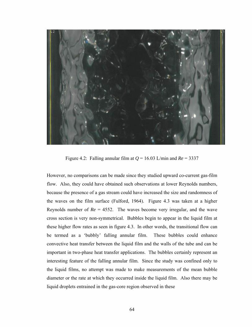
64
Figure 4.2: Falling annular film at Q = 16.03 L/min and Re = 3337
However, no comparisons can be made since they studied upward co-current gas-film
flow. Also, they could have obtained such observations at lower Reynolds numbers,
because the presence of a gas stream could have increased the size and randomness of
the waves on the film surface (Fulford, 1964). Figure 4.3 was taken at a higher
Reynolds number of Re = 4552. The waves become very irregular, and the wave
cross section is very non-symmetrical. Bubbles begin to appear in the liquid film at
these higher flow rates as seen in figure 4.3. In other words, the transitional flow can
be termed as a ‘bubbly’ falling annular film. These bubbles could enhance
convective heat transfer between the liquid film and the walls of the tube and can be
important in two-phase heat transfer applications. The bubbles certainly represent an
interesting feature of the falling annular film. Since the study was confined only to
the liquid films, no attempt was made to make measurements of the mean bubble
diameter or the rate at which they occurred inside the liquid film. Also there may be
liquid droplets entrained in the gas-core region observed in these
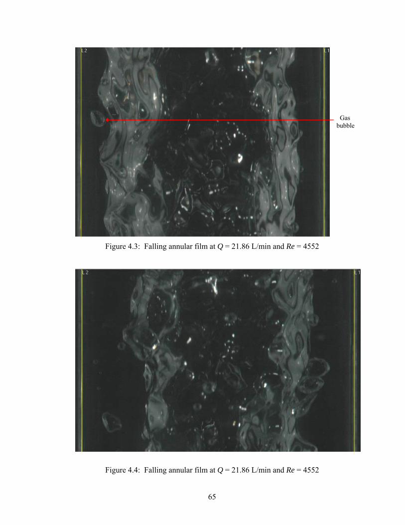
65
Figure 4.3: Falling annular film at Q = 21.86 L/min and Re = 4552
Figure 4.4: Falling annular film at Q = 21.86 L/min and Re = 4552
Gas bubble
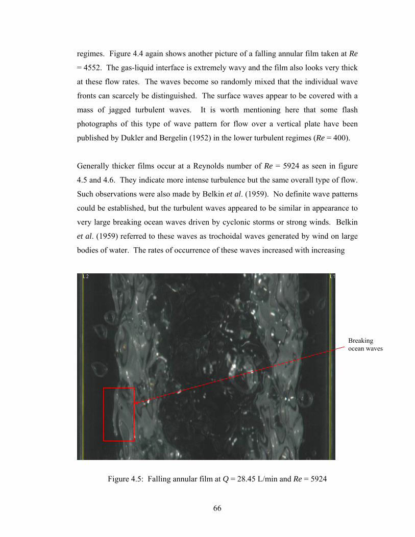
66
regimes. Figure 4.4 again shows another picture of a falling annular film taken at Re
= 4552. The gas-liquid interface is extremely wavy and the film also looks very thick
at these flow rates. The waves become so randomly mixed that the individual wave
fronts can scarcely be distinguished. The surface waves appear to be covered with a
mass of jagged turbulent waves. It is worth mentioning here that some flash
photographs of this type of wave pattern for flow over a vertical plate have been
published by Dukler and Bergelin (1952) in the lower turbulent regimes (Re = 400).
Generally thicker films occur at a Reynolds number of Re = 5924 as seen in figure
4.5 and 4.6. They indicate more intense turbulence but the same overall type of flow.
Such observations were also made by Belkin et al. (1959). No definite wave patterns
could be established, but the turbulent waves appeared to be similar in appearance to
very large breaking ocean waves driven by cyclonic storms or strong winds. Belkin
et al. (1959) referred to these waves as trochoidal waves generated by wind on large
bodies of water. The rates of occurrence of these waves increased with increasing
Figure 4.5: Falling annular film at Q = 28.45 L/min and Re = 5924
Breaking ocean waves

67
Figure 4.6: Falling annular film at Q = 28.45 L/min and Re = 5924
Reynolds numbers. Large numbers of bubbles with varying sizes were also present in
the liquid film. Sometimes the bubbles were large enough that they seemed to
occupy a major portion of the liquid film thickness. There is clear evidence that the
effects of these bubbles on the walls and on the large waves can no longer be
neglected at these Reynolds numbers. The shearing action or the tearing away of the
waves can also be clearly seen in figure 4.6. This tearing away of the gas-liquid
interface is due to very large disturbance waves that occasionally occurred at Re =
4552 and Re = 5924. From visual observation, the rates of occurrence of this
shearing action or tearing away of gas-liquid interface were observed on an average
in 10 ~ 20 pictures for each of the 200 pictures analysed at these higher flow rates.
Due to this shearing effect and the extremely chaotic nature of the waves, the gas-
liquid interface was not clearly discernible. The troughs of the surface waves were
sometimes masked by the crests of waves closer to the camera. Also the bubbles
occupying a major portion of the liquid film tried to form bridges or isthmuses
between tube walls and the gas core. This led to some difficulties in the image
Shearing action or tearing away of the gas-liquid interface
Large number of bubbles of varying sizes

68
processing and determining the exact liquid film thickness in some of these high
Reynolds number pictures.
4.3 Instantaneous film thickness measurements The Nikon D70 digital SLR camera was located 35 cm from the test section (see
Figure 3.10). The camera was operated in the manual focus mode and two remote
flash units provided illumination. Measurements of the wall location were carried out
before and after taking images at each flow rate (as discussed in the Chapter 3). Both
sides of the tube were in the field of view so data could be obtained from both sides.
Two hundred high-resolution images were obtained at each of five different flow
rates. The images captured were analysed using the image processing techniques
discussed in Chapter 3. About 40,000 instantaneous film thickness measurements
were extracted at each Reynolds number at longitudinal distances of z = 3.80 m to
3.90 m from the liquid inlet. All the experimental runs were conducted in the facility
described in Chapter 3. The present experiments used water at 27ºC and covered a
range of liquid Reynolds numbers from 1000 to 6000 in the fully developed turbulent
regime. Due to the automated nature of the measurement technique, several hundred
instantaneous film thickness measurements may be taken in a few minutes.
In general, the film thickness measurements at the right- and left-hand sides of the
tube showed good agreement with each other. A t-test was performed to determine
whether there is any significant difference between the mean film thicknesses at the
right- and left-hand sides. The t-test assesses whether the means of two groups are
statistically different from each other. The test is applied to the null hypothesis which
states that “if the two mean film thicknesses (right-and left-hand sides) being
compared belong to the same population, their variance estimates must not be
significantly different”. The significance of the difference is measured by the ratio of
the difference in the means to its standard deviation, and is denoted by ct , so that
d
lrc s
tδ−δ
= ( )1.4

69
where rδ and lδ are the mean film thicknesses on the right-and left-hand sides, and
ds is the standard deviation of the difference of the two means. The standard
deviation of the difference of the two means ds is obtained from the estimated
variance 2cs . The estimated variance is weighted by the number of degrees of
freedom available for its calculation. The estimated variance is calculated as follows:
( ) ( )( ) ( )11
11 2l
2r2
c −+−−+−
=lr
lr
nnnsnss ( )2.4
where 2
cs is the estimated variance
n is the number of sample image sets (Here, lr nnn += )
subscript r denotes a parameter measured for the right side of the tube
subscript l denotes a parameter measured for the left side of the tube
The standard deviation of the difference of means is:
lr
lr
nnnnss +
= cd ( )3.4
The level of significance at which the null hypothesis is rejected is usually 5% or 1%.
For this thesis, a 1% level of significance was used. If the calculated ct is greater than
the tabulated tt value (from t-chart) at the specified level of significance, the null
hypothesis is rejected, and the conclusion is that the difference is significant. If the
calculated ct is not greater than the tabulated tt at 1% level of significance, the null
hypothesis is accepted and the conclusion is that the difference is insignificant. Table
4.1 shows the t-test results obtained for mean film thicknesses obtained on both sides.
As seen from Table 4.1, the calculated ct values were always found to be less than the
tabulated tt (from t-chart) which was equal to 1.645 for ( ) ∞≈−+ 2lr nn degrees of
freedom. Thus, it can be concluded that the differences in the mean film thicknesses
between the right- and left-hand sides of the tube are insignificant.

70
Table 4.1: t-test results for raw (uncorrected) mean film thickness data
n Re rδ (mm) lδ (mm) rs (mm) ls (mm) ct
200
974
0.748
0.730
0.451
0.475
0.382
200
2111 1.168 1.142 0.640 0.675 0.394
200
3337 1.540 1.511 0.788 0.820 0.369
200
4552 1.920 1.877 0.908 0.913 0.477
200
5924 2.318 2.263 1.024 1.050 0.526
Note: Here n represents only the number of sample image sets at each Re
Later, the ray tracing model described in Chapter 3 was used to correct for the visual
distortion near the tube wall. Thus, the optical distortions were minimised and
qualitative film thicknesses measurements were obtained. The details of the
experimental results are summarised in Table 4.2. The data for the corrected mean
film thickness and standard deviation presented in Table 4.2 for the first three flow
rates had an image resolution of 108.7 pixels/mm. The last two flow rates had a
Table 4.2: Summary of experimental results for film thickness
N Q (L/min) Re δ (mm) s(mm) +δ
40000
4.679
974
0.891
0.531
19.078
40000 10.139 2111 1.321 0.736 28.287
40000
40000
40000
16.026
21.860
28.453
3337
4552
5924
1.695
2.068
2.457
0.892
1.059
1.273
36.295
44.276
52.599
Note: Here N represents the total number of instantaneous film thickness
measurements at each Reynolds number.
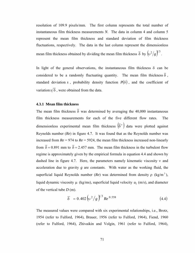
71
resolution of 109.9 pixels/mm. The first column represents the total number of
instantaneous film thickness measurements N. The data in column 4 and column 5
represent the mean film thickness and standard deviation of film thickness
fluctuations, respectively. The data in the last column represent the dimensionless
mean film thickness obtained by dividing the mean film thickness δ by ( ) 312 gυ .
In light of the general observations, the instantaneous film thickness δ can be
considered to be a randomly fluctuating quantity. The mean film thickness δ ,
standard deviation s , probability density function ( )δP , and the coefficient of
variation δs , were obtained from the data.
4.3.1 Mean film thickness
The mean film thickness δ was determined by averaging the 40,000 instantaneous
film thickness measurements for each of the five different flow rates. The
dimensionless experimental mean film thickness ( )+δ data were plotted against
Reynolds number (Re) in figure 4.7. It was found that as the Reynolds number was
increased from Re = 974 to Re = 5924, the mean film thickness increased non-linearly
from =δ 0.891 mm to =δ 2.457 mm. The mean film thickness in the turbulent flow
regime is approximately given by the empirical formula in equation 4.4 and shown by
dashed line in figure 4.7. Here, the parameters namely kinematic viscosity ν and
acceleration due to gravity g are constants. With water as the working fluid, the
superficial liquid Reynolds number (Re) was determined from density ρ (kg/m 3 ),
liquid dynamic viscosity μ (kg/ms), superficial liquid velocity lu (m/s), and diameter
of the vertical tube D (m).
( ) 558.0312402.0 Regυ=δ ( )4.4
The measured values were compared with six experimental relationships, i.e., Brotz,
1954 (refer to Fulford, 1964), Brauer, 1956 (refer to Fulford, 1964), Fiend, 1960
(refer to Fulford, 1964), Zhivaikin and Volgin, 1961 (refer to Fulford, 1964),
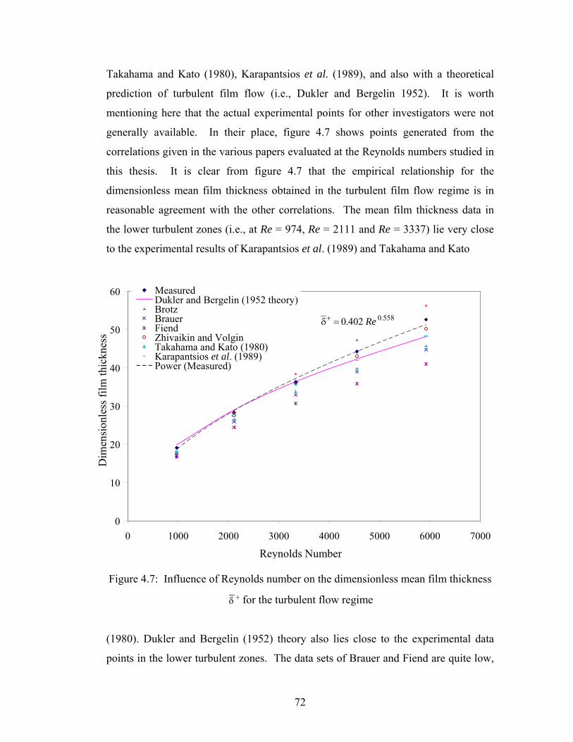
72
Takahama and Kato (1980), Karapantsios et al. (1989), and also with a theoretical
prediction of turbulent film flow (i.e., Dukler and Bergelin 1952). It is worth
mentioning here that the actual experimental points for other investigators were not
generally available. In their place, figure 4.7 shows points generated from the
correlations given in the various papers evaluated at the Reynolds numbers studied in
this thesis. It is clear from figure 4.7 that the empirical relationship for the
dimensionless mean film thickness obtained in the turbulent film flow regime is in
reasonable agreement with the other correlations. The mean film thickness data in
the lower turbulent zones (i.e., at Re = 974, Re = 2111 and Re = 3337) lie very close
to the experimental results of Karapantsios et al. (1989) and Takahama and Kato
Figure 4.7: Influence of Reynolds number on the dimensionless mean film thickness +δ for the turbulent flow regime
(1980). Dukler and Bergelin (1952) theory also lies close to the experimental data
points in the lower turbulent zones. The data sets of Brauer and Fiend are quite low,
0
10
20
30
40
50
60
0 1000 2000 3000 4000 5000 6000 7000
Measured Dukler and Bergelin (1952 theory)BrotzBrauer FiendZhivaikin and VolginTakahama and Kato (1980)Karapantsios et al. (1989)Power (Measured)
Dim
ensi
onle
ss fi
lm th
ickn
ess
Reynolds Number
558.0402.0 Re=δ+
73
especially above Re = 2000 where the flow starts to be become more turbulent. At
higher Reynolds numbers, there is more scatter in the mean film thicknesses reported
in the published data. At Re = 4552, the mean film thickness of this work is about
0.08 mm ~ 0.1 mm larger than those of Karapantsios et al. (1989) and Dukler and
Bergelin (1952), but slightly lower than the data obtained by Zhivaikin and Volgin.
At an even higher Reynolds number of Re = 5924, the mean film thickness is close to
0.2 mm larger than Karapantsios et al. (1989) and Dukler and Bergelin (1952).
Karapantsios et al. (1989) did not carry out experiments at the higher Reynolds
numbers. The deviation of mean film thickness from Dukler and Bergelin (1952)
theory could be attributed to the fact that the underlying theory was developed by
Nikuradse in 1933 for a full pipe flow. It could be open to discussion as to whether
Dukler and Bergelin (1952) theory would still be applicable to the liquid layer in two-
phase film flow at these high Reynolds numbers. Telles and Dukler (1970) compared
their experimental film thickness measurements (not available here) with the values
predicted from Dukler and Bergelin (1952) theory and their analysis showed
significant deviations. At high interfacial shear, the agreement was satisfactory, but
the discrepancy between Telles’s (1970) experiments and Dukler and Bergelin (1952)
theory increased at lower gas flow rates. Telles and Dukler (1970) pointed out that the
original development of Dukler and Bergelin (1952) does not produce the correct
average film thickness for a film with large interfacial waves.
4.3.2 Standard deviation
Waves are observed on falling annular films (see figure 4.8) even when the gas flow
rate is zero. A visual observation suggests that the waviness of the film flow increases
with increasing Reynolds number in the turbulent flow regime. Post processing of the
digital images showed random fluctuations in the instantaneous film thickness δ .
Further analysis was carried out to determine the standard deviation s .
The data obtained support this observation, showing an increase in the standard
deviation s as the Reynolds number, Re is increased. As the Reynolds number was

74
Figure 4.8: The influence of Reynolds number on the standard deviation s of film thickness fluctuations
increased from Re= 974 to 3337, the standard deviation s increased from 0.531 mm
to 0.892 mm. The data obtained here clearly show that at a distance z = 3.80 m to
3.90 m from the liquid entry, the standard deviation values are very large which
implies that at a large distance from the liquid inlet, the waves have higher
amplitudes. The results obtained were compared with two sets of experimental data
(Set A, Set B) obtained by Karapantsios et al. (1989) at a longitudinal distance of z =
2.5 m as shown in figure 4.8. It is worth mentioning that Karapantsios et al. (1989)
also observed a similar trend in his experiments showing an increase in standard
deviation as the Reynolds number is increased and at a large distance from the liquid
entry. The data compared reasonably well, although Karapantsios et al. (1989)
reported slightly higher standard deviation values in the lower turbulent zones. The
standard deviation results obtained in this thesis were also compared with two other
experimental sets of data obtained by Karapantsios and Karabelas (1995) for z = 2.19
m and z = 2.46 m in the lower turbulent zones. In general, the data agreed well with
0.2
0.4
0.6
0.8
1.0
1.2
1.4
0 1000 2000 3000 4000 5000 6000 7000
Measured at z =3.80 m to 3.90 mKarapantsios et al. (1989) for z =2.5 m, Set AKarapantsios et al. (1989) for z =2.5 m, Set BKarapantsios and Karabelas (1995) for z =2.19 mKarapantsios and Karabelas (1995) for z =2.46 mTakahama and Kato (1980) for z =1.7 mZabaras (1985) at z =1.94 mChu and Dukler (1975)
Reynolds number
Stan
dard
dev
iatio
n (m
m)

75
the standard deviation values of both Karapantsios and Karabelas (1995) and
Karapantsios et al. (1989). Takahama and Kato’s (1980) data on standard deviation s
also displayed an increasing trend up to Re = 2000. Relatively large standard
deviation values, such as those obtained in this thesis, were also reported by
Takahama and Kato (1980) for z = 1.7 m. From the standard deviation values
obtained here and their comparison with other established experimental results, the
liquid film can be considered to be fully developed at a longitudinal distance of z =
3.80 m to 3.90 m from liquid inlet. However, the standard deviation values presented
by Zabaras (1985) were small, e.g., s ~ 0.25 mm at 1.94 m from the inlet and Re =
1125. He reported that, above Re = 1250, there is little increase in the standard
deviation. The reasons for such a large deviation might be due to the fact that
Zabaras (1985) employed a different technique for measuring the film thickness and
also used different test fluids in most of the runs. Chu and Dukler (1975) also
reported standard deviation values for falling liquid films with and without gas flow.
For the case of zero gas flow, the standard deviation values were s ~ 0.3093 mm at Re
= 1125 and s ~ 0.3398 mm at Re = 1500. Again the values reported by Chu and
Dukler (1975) were small compared to the present study. The reasons could be
because Chu and Dukler’s (1975) experiments were limited only to transition and
lower turbulent regimes up to a Reynolds number of Re .1500≤
New values of standard deviation have been reported here at Reynolds numbers of Re
= 4552 and Re = 5924 in the higher turbulent zones. There is no indication that the
standard deviation values have reached an upper limit or an asymptotic value. The
waviness of the falling annular films continues to increase with increasing mean film
thickness δ and increasing Reynolds numbers. The standard deviation s reaches a
value of s ~ 1.273 mm at Reynolds number Re = 5924 and mean film thickness
=δ 2.457 mm. The falling films become very thick and the gas-liquid interface tends
to be extremely wavy at these very high Reynolds numbers. Thus, it can be
concluded that thin films are characterised by small waves that are less wavy and the
thicker films are characterised by large disturbance waves that are wavier in nature.
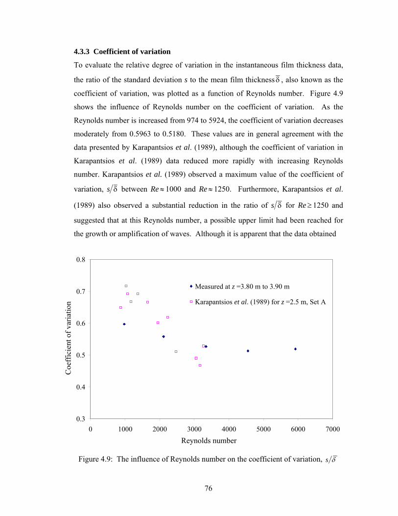
76
4.3.3 Coefficient of variation
To evaluate the relative degree of variation in the instantaneous film thickness data,
the ratio of the standard deviation s to the mean film thickness δ , also known as the
coefficient of variation, was plotted as a function of Reynolds number. Figure 4.9
shows the influence of Reynolds number on the coefficient of variation. As the
Reynolds number is increased from 974 to 5924, the coefficient of variation decreases
moderately from 0.5963 to 0.5180. These values are in general agreement with the
data presented by Karapantsios et al. (1989), although the coefficient of variation in
Karapantsios et al. (1989) data reduced more rapidly with increasing Reynolds
number. Karapantsios et al. (1989) observed a maximum value of the coefficient of
variation, δs between Re≈ 1000 and Re≈ 1250. Furthermore, Karapantsios et al.
(1989) also observed a substantial reduction in the ratio of δs for Re≥ 1250 and
suggested that at this Reynolds number, a possible upper limit had been reached for
the growth or amplification of waves. Although it is apparent that the data obtained
Figure 4.9: The influence of Reynolds number on the coefficient of variation, δs
0.3
0.4
0.5
0.6
0.7
0.8
0 1000 2000 3000 4000 5000 6000 7000
Measured at z =3.80 m to 3.90 m
Karapantsios et al. (1989) for z =2.5 m, Set A
Coe
ffic
ient
of v
aria
tion
Reynolds number

77
in the present study do not make it possible to fix the exact Reynolds number at
which the maximum upper limit for amplification of waves has been reached, a
similar decreasing trend to those obtained by Karapantsios et al. (1989) had been
observed in the data at Re ≥ 1000. Karapantsios and Karabelas (1995), Karapantsios
et al. (1989) and Takahama and Kato (1980), all observed a limiting value of the
coefficient of variation, ≈δs 0.3 to 0.7 in their experimental range. The values
obtained here are in general agreement with those results.
4.3.4 Probability density function
The probability density function was introduced to illustrate the detailed statistical
distribution of the instantaneous film thickness. The mean film thickness and
standard deviation discussed earlier are properties of the probability density function.
The probability density functions for the five different Reynolds numbers are shown
in Figure 4.10.
Figure 4.10: The influence of Reynolds number on the probability density function, P
0.00
0.05
0.15
0.20
0.25
0.30
0.35
0 1 2 3 4 5 6 7 8 9 10
Re = 5924Re = 4552Re = 3337Re = 2111Re = 974
mm695.1=δ mm068.2=δ mm457.2=δ
mm321.1=δ
Prob
abili
ty
Film thickness (mm)
0.10
mm891.0=δ mm70.0~δ′ mm25.0~δ′
mm85.0~δ′ mm05.1~δ′ mm45.1~δ′
78
Points on this figure were produced by binning the film thickness measurements into
intervals of =δΔ 0.3 mm for each of the Reynolds numbers. The probability density
function of the film thickness describes the likelihood of the film assuming a value
within a given interval. As has already been observed by other investigators, the
probability density function is highly asymmetrical and the height of the peak
decreases with increasing liquid Reynolds number. The maximum peak or the main
peak can be considered to represent the modal value of film thickness or the substrate
film thickness. It is very interesting to note that the deviation between the mean film
thickness δ and the substrate film thickness δ′ increases as the Reynolds number is
increased, but the substrate film thickness δ′ is always below the mean film
thickness δ . This suggests that the liquid film may assume a defined film thickness
and the waves ride on top of the substrate. All the probability distributions obtained
here have a maximum peak and are skewed to the right hand side with a long tail that
stretches to over 6 times the peak or modal value of film thickness. The increase in
skewness and the decrease in the height of the peak with liquid Reynolds number can
be attributed to presence of large disturbance waves which ride on the substrate film.
This enhances the waviness of the film. As the waviness is increased, the probability
that the film thickness will fall within a particular interval is decreased and the
skewness is increased. Thus, it is very clear that the probability density distributions
that describe the statistical characteristics of film thickness are non-Gaussian in
nature. It is worth mentioning here that similar observations were also made by Telles
and Dukler (1970), Chu and Dukler (1975), Zabaras (1985) and Karapantsios et al.
(1989).
4.3.5 Sensitivity analysis
To determine whether 200 images are sufficient to get accurate measurements of
mean film thickness and standard deviation, a sensitivity analysis was performed.
Sensitivity plots check for the convergence of statistical parameters such as the film
thickness and standard deviation. Figures 4.11 to 4.15 show the sensitivity plots
obtained at different Reynolds numbers. At first, the 40,000 instantaneous film
thickness measurements were grouped into eight independant sets of 5000

79
0.4
0.5
0.6
0.7
0.8
0.9
0 10000 20000 30000 40000 50000
Film thicknessStandard deviation
Figure 4.11: Sensitivity plot for Re = 974
0.4
0.6
0.8
1
1.2
1.4
0 10000 20000 30000 40000 50000
Film thicknessStandard deviation
Figure 4.12: Sensitivity plot for Re = 2111
Number of measurements
Film
thic
knes
s (m
m),
Stan
dard
dev
iatio
n (m
m)
Number of measurements
Film
thic
knes
s (m
m),
Stan
dard
dev
iatio
n (m
m)

80
0.4
0.6
0.8
1
1.2
1.4
1.6
1.8
0 10000 20000 30000 40000 50000
Film thicknessStandard deviation
Figure 4.13: Sensitivity plot for Re = 3337
0.4
0.6
0.8
1
1.2
1.4
1.6
1.8
2
2.2
0 10000 20000 30000 40000 50000
Film thicknessStandard deviation
Figure 4.14: Sensitivity plot for Re = 4552
Number of measurements
Film
thic
knes
s (m
m),
Stan
dard
dev
iatio
n (m
m)
Number of measurements
Film
thic
knes
s (m
m),
Stan
dard
dev
iatio
n (m
m)
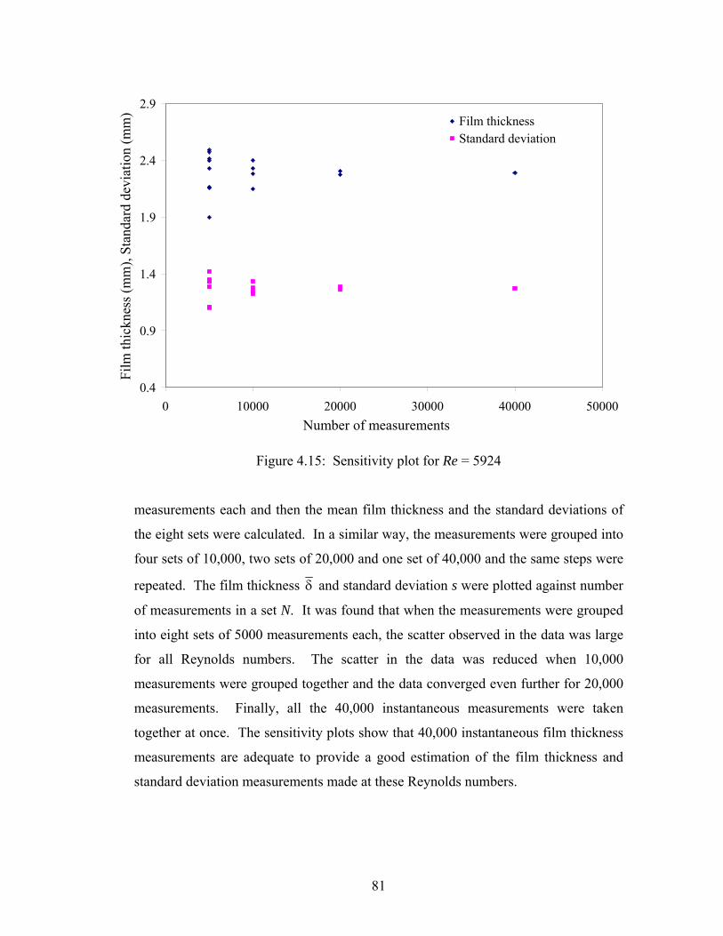
81
0.4
0.9
1.4
1.9
2.4
2.9
0 10000 20000 30000 40000 50000
Film thicknessStandard deviation
Figure 4.15: Sensitivity plot for Re = 5924
measurements each and then the mean film thickness and the standard deviations of
the eight sets were calculated. In a similar way, the measurements were grouped into
four sets of 10,000, two sets of 20,000 and one set of 40,000 and the same steps were
repeated. The film thickness δ and standard deviation s were plotted against number
of measurements in a set N. It was found that when the measurements were grouped
into eight sets of 5000 measurements each, the scatter observed in the data was large
for all Reynolds numbers. The scatter in the data was reduced when 10,000
measurements were grouped together and the data converged even further for 20,000
measurements. Finally, all the 40,000 instantaneous measurements were taken
together at once. The sensitivity plots show that 40,000 instantaneous film thickness
measurements are adequate to provide a good estimation of the film thickness and
standard deviation measurements made at these Reynolds numbers.
Number of measurements
Film
thic
knes
s (m
m),
Stan
dard
dev
iatio
n (m
m)

82
4.4 Summary
An experimental study of falling annular films was conducted at five different
Reynolds numbers in the turbulent regime. Film thickness measurements were
obtained at a longitudinal distance of z = 3.80 m to 3.90 m from the liquid inlet. One
of the main objectives of the study was to characterise the film thickness at high
Reynolds numbers. The experiments involved the use of flow visualisation
techniques that yield information regarding the turbulent characteristics in falling
liquid films. 40,000 instantaneous film thickness measurements of falling annular
films at Reynolds numbers in the range Re = 1000 ~ 6000 were extracted using a non-
intrusive imaging technique. A ray tracing model was employed to reduce optical
distortion effects in cylindrical tubes. This technique increased the accuracy of the
imaging technique and enabled quantitative measurements of film thickness to be
made. From visual observation of the images obtained, no definite wave patterns
could be established at these Reynolds numbers. However, the turbulent waves
appeared to be similar in appearance to very large breaking ocean waves driven by
strong winds. The random nature of these falling annular films was subjected to
statistical analysis and qualitative observations were made at these Reynolds
numbers.
The experiments conducted here enabled the determination of the some statistical
characteristics of falling annular films. A correlation for dimensionless mean film
thickness +δ , obtained in the turbulent flow regime was found to be in reasonable
agreement with the other established experimental and theoretical studies. It was
shown that the Reynolds number influences the statistical characteristics of film
thickness such as standard deviation s and coefficient of variation δs . Results
obtained at higher Reynolds numbers show that the standard deviation continues to
increase in proportion to the mean film thickness in the turbulent regime. In other
words, in the lower turbulent zones the films are thin and less wavy, whereas in the
higher turbulent zones the films are thicker and extremely wavy. In addition, the
83
measured probability density distributions ( )δP were also studied. The probability
distributions obtained were asymmetric. All the measured probability distributions
had a maximum peak and were skewed to the right hand side with a long tail that
stretches to over six times the peak value. The maximum peak represents the modal
value of the film thickness or the substrate film thickness. The increase in skewness
and the decrease in the height of the peak with liquid Reynolds number could be
attributed to presence of large disturbance waves which ride on the substrate film that
tends to enhance the waviness of the film.

84
CHAPTER 5
CONCLUSIONS AND RECOMMENDATIONS
5.1 Conclusions
A non-intrusive imaging technique was used to extract 40,000 instantaneous film
thickness measurements of falling annular films at each of five different Reynolds
numbers in the range Re = 1000 ~ 6000 for the fully developed turbulent regime. The
conclusions drawn from this study are outlined below.
1. Digital images of the falling annular films obtained with a spatial resolution of
20003008× pixels have been presented here. In general, the waves are not
axisymmetric, i.e., there is a lot of azimuthal variation in the film thickness.
The turbulent waves appeared to be similar in appearance to very large
breaking ocean waves driven by strong winds.
2. A correlation for dimensionless mean film thickness +δ was obtained in the
turbulent flow regime. The dimensionless mean film thickness +δ obtained
here was found to be in reasonable agreement with the other established
experimental and theoretical studies. It was shown that the Reynolds number
influences the statistical characteristics of film thickness such as standard
deviation s and coefficient of variation δs . Results obtained at higher
Reynolds numbers show that the standard deviation continues to increase in
proportion to the mean film thickness in the turbulent regime. In other words,
in the lower turbulent zones the films are thin and less wavy, whereas in the
higher turbulent zones the films are thicker and extremely wavy in nature.

85
3. The probability density distributions ( )δP were also obtained. It was found
that the measured probability density distributions were asymmetric. They all
had a maximum peak and were skewed to the right hand side with a long tail
that stretches to over six times the peak value. The maximum peak could be
considered to represent the modal value of the film thickness or the substrate
film thickness. The increase in skewness and the decrease in the height of the
peak with liquid Reynolds number could be attributed to the presence of large
disturbance waves which ride on the substrate film that tends to enhance the
waviness of the film.
4. In addition, an advanced ray tracing model was employed to reduce the
optical distortions caused by the tube wall curvature. Experimental studies
and calibration procedures were also conducted in the laboratory to confirm
the validity of the ray tracing model. The ray tracing model and the calibration
procedures employed here increased the accuracy of this imaging technique.
5.2 Recommendations for future work
A more detailed study of the statistical characteristics of waves is required. The
measurement of probability distributions makes it possible to make accurate
determination of the moments. The second and the third moments will reveal more
information regarding the structure of these large waves and their contribution to the
gas-liquid interface. Moreover the frequency of large waves occurring at these high
flow rates can also be measured from their spectral density functions. It is a measure
of how much of the motion is assignable to wavelengths around a certain value. This
can be achieved by using an accurately timed camera shutter with higher framing
rates. By using a combination of different parameters such as the frequency of the
surface waves, the influence of other dimensionless numbers such as the Strouhal
number can also considered. The Strouhal number is formed from the frequency of
the surface waves, and various geometrical ratios.
86
Further experimental work is also required to determine the hydrodynamic
characteristics of falling annular films such as instantaneous velocity fields and wall
shear stress. This is very challenging since the thickness of falling annular films are
usually of the order of one millimetre. To enable these quantitative measurements, a
refractive index matching fluid should be used in the optical correction box and in the
test section. Particle image velocimetry (PIV) can be used to accurately measure the
complex instantaneous velocity field in falling annular films. It involves the use of
whole field techniques based on imaging the light scattered by small particles in the
flow illuminated by a laser. The two-dimensional or three-dimensional time
dependant velocity fields might yield more information regarding the structure of
large waves in the turbulent region. Studies can also be undertaken to investigate the
mechanisms governing wave growth and wave-to-wave interactions at the gas-liquid
interface. It may be of interest to examine the velocity profiles to generate
streamlines to describe the flow field completely in falling annular films in the
turbulent regime. The local wall shear stress can also be estimated by measuring the
velocity gradient near the wall.
87
References Agrawal, Y., Talbot, L., Gong, K., 1978. Laser anemometer study of flow development in curved circular pipes. Journal of Fluid Mechanics. 85, 497-518.
Alekseenko, S.V., Nakoryakov, V.E., and Pokusaev, B.G., 1985. Wave formation on vertical falling liquid films. International Journal of Multiphase Flow. 11, 607-627.
Alekseenko, S.V., Nakoryakov, V.E., Pokusaev, B.G., 1994. In: Fukano, T. (Ed.), Wave flow of liquid films. Begell House, New York.
Ambrosini, W., Forgione, N., Oriolo, F., 2002. Statistical characteristics of a water film falling down a flat plate at different inclinations and temperatures. International Journal of Multiphase Flow. 28, 1521-1540.
Astola, J., Haavisto, P., and Neuvo, Y., 1990. Vector median filters. Proceedings of the Institute of Electrical and Electronic Engineers. 78, 678-689
Bach, P., and Villadsen, J., 1984. Simulation of the vertical flow of a thin, wavy film using a finite element method. International Journal of Heat and Mass Transfer. 27, 815-827.
Bankoff, S.G., 1971. Stability of liquid flow down a heated inclined plate. International Journal of Heat Transfer. 14, 377-385.
Bathia, J.C., Durst, F., Jovanovic, J. 1982. Correction of hot-wire measurements. Journal of Fluid Mechanics. 122, 411-431.
Belkin, H.H., McLeod, A.A., Monrad, C.C., and Rothfus, R.R., 1959. Turbulent liquid flow down vertical walls. American Institute of Chemical Engineers Journal. 5, 245-248.
Bendat, J.S., and Piersol, A.G., 1971. Random Data: Analysis and Measurement Procedures. Wiley, New York.
Bicen, A.F. 1982: Refraction correction for LDA measurements in flows with curved optical boundaries. TSI Quarterly. 8, 10-12.
Bird, R.B., Stewart, W.E., and Lightfoot, E.N. 1960. Transport Phenomena. Wiley, New York. 3-179.
Blass, E., 1979. Gas/film flow in tubes. International Chemical Engineering. 19, 183-195.
Boadway, J.D.; Karahan, E. 1981. Correction of laser Doppler anemometer readings for refraction at cylindrical interfaces. DISA Information. 26, 4-6.

88
Bovendeerd, P.H.M.; Van Steenhoven, A.A.; Van de Vosse, F.N.; Vossers, G. 1987. Steady entry flow in a curved pipe. Journal of Fluid Mechanics. 177, 233-246.
Brauner, N., 1987. Roll wave celerity and average film thickness in turbulent wavy film, flow. Chemical Engineering Science. 42, 265-273.
Brown, R. A. S., 1965. The mechanics of large gas bubbles in tubes. Canadian Journal of Chemical Engineering. 43, 217-223.
Budwig, R. 1994. Refractive index matching methods for liquid flow investigations. Experiments in Fluids. 17, 350-355.
Chang, H.C., 1994. Wave evolution on a falling film. Annual Review of Fluid Mechanics. 26, 103-136.
Chen, R.C.; Fan, L.S. 1992. Particle image velocimetry for characterizing the flow structure in three-dimensional gas-liquid-solid fluidized beds. Chemical Engineering Science. 47, 3615-3622.
Chu, K.J., and Dukler, A.E., 1974. Statistical characteristics of thin, wavy films: part II. Studies of the substrate and its wave structure. American Institute of Chemical Engineers Journal. 20, 695-705.
Chu, K.J., and Dukler, A.E., 1975. Statistical characteristics of thin, wavy films: part III. Structure of the large waves and their resistance to gas flow. American Institute of Chemical Engineers Journal. 21, 583-593.
Dukler, A.E., Bergelin, O.P., 1952. Characteristics of flow in falling films. Chemical Engineering Progress. 48, 557-563.
Duncan, D.D.; Bargeron, G.B.; Borchardt, S.E.; Deters, O.J.; Gearhart, S.A.; Mark F.F. 1990. The effect of compliance on wall shear in casts of a human aortic bifurcation. ASME Journal of Biomechanical Engineering. 112, 183-188.
Durret, R.P.; Gould, R.D.; Stevenson, W.H.; Thompson, H.D. 1985. A correction lens for laser Doppler velocimeter measurements in a cylindrical tube. American Institute of Aeronautics and Astronautics Journal. 23, 1387-1391.
Durst, F.; Muller, R; Jovanovic, J. 1988. Determination of the measuring positioning laser-Doppler anemometry. Experiments in Fluids. 6, 105-110.
Fulford, G.D., 1964. The flow of liquids in thin films. In: Advances in Chemical Engineering, edited by Drew, T.B., Hoopes, J.W., and Vermeulen, T., 5, Academic Press, 151-235.
Gupta, A.K. and Kaplan, R.E. 1972. Statistical characteristics of Reynolds stress in turbulent boundary layer. Physics of Fluids. 15, 981-985.
89
Hewitt, G.F., and Hall-Taylor, N.S., 1970. Annular two-phase flow. Pergamon Press, Oxford.
Jackson, M.L. 1955. Liquid films in viscous flow. American Institute of Chemical Engineers Journal. 1, 231-240.
Kang, H.C., Kim M.H., 1992. The development of a flush-wire probe and calibration method for measuring liquid film thickness. International Journal of Multiphase Flow. 18, 423-437.
Kapitza, P.L., 1947. Wave flow of thin layers of a viscous fluid, English translation in collected papers of P.L. Kapitza, II, Macmillan, New York.
Kapitza, P.L., 1965. In: Ter-Haar, D. (Ed), Collected papers of Kapitza 1938-1964,. Pergamon Press, New York. 2, 662-709.
Karapantsios, T.D., Paras, S.V., and Karabelas, A.J., 1989. Statistical characteristics of free falling films at high Reynolds numbers. International Journal of Multiphase Flow. 15, 1-21.
Karapantsios, T.D., and Karabelas, A.J, 1995. Longitudinal characteristics of wavy falling films. International Journal of Multiphase flow. 21, 119-127.
Karimi, G., and Kawaji, M., 1998. An experimental study of freely falling films in vertical tube. Chemical Engineering Science. 53, 3501-3512.
Kheshgi, H.S., and Scriven, L.E., 1987. Distributed film flow on a vertical plate. Physics of Fluids. 30, 990-997.
Kokamustafaougullari, G., 1985. Two- fluid modelling in analyzing the interfacial stability of liquid film flows. International Journal of Multiphase flow. 15, 1-21.
Koskie, J.E., Mudawar, I., and Tiederman, W.G., 1989. Parallel – wire probes for measurement of thick liquid films. International Journal of Multiphase flow. 15, 521-530.
Liu, C.H.; Vafidis, C.; Whitelaw, J.H. 1990. Flow in the coolant passages of an internal combustion engine cylinder head. Experiments in Fluids. 10, 50-54.
Lowe M.L.; Kutt, P.H. 1992. Refraction through cylindrical tubes. Experiments in Fluids. 13, 315-320.
Neal, L.G., and Bankoff, S.G., 1963. A high resolution resistivity probe for determination of local void properties in gas-liquid flow. American Institute of Chemical Engineers Journal. 9, 490.
Nguyen, L.T., Balakotaiah, V., 2000. Modelling and experimental studies of wave evolution on free falling liquid films. Physics of Fluids. 12, 2236-2256.

90
Pearson, D.E., 1991 Image Processing, McGraw-Hill, New York.
Perry, R.H.; Green, D.W. 1973. Perry’s Chemical Engineering Handbook (ISBN 0-0704-9578-9). 6th edition, New York, McGraw-Hill.
Portalski, S., 1963. Studies of falling liquid film flow: film thickness on a smooth vertical plate. Chemical Engineering Science. 18, 787-804.
Russ, J.C., 1995 The image processing Handbook, CRC Press.
Salamon, T.R., Armstrong, R.C., Brown, R.A., 1994. Travelling waves on inclined films: numerical analysis by the finite-element method. Physics of Fluids. 6, 2202-2220.
Salazar, R.P. and Marschall, E., 1978. Time average local thickness measurement in falling liquid film flow. International Journal of Multiphase flow. 4, 408-412.
Spindler, B., 1981. Linear stability of liquid films with interfacial phase change. International Journal of Heat and Mass Transfer. 25, 161-173.
Stuhltrager, E., Miyara, A., Uehara, H.., 1995. Flow dynamics and heat transfer of a condensate film on a vertical wall-part II. Flow dynamics and heat transfer. International Journal of Heat and Mass Transfer. 38, 2715-2722.
Takahama, H. and Kato, S., 1980. Longitudinal flow characteristics of vertically falling liquid films without concurrent gas flow. International Journal of Multiphase Flow. 6, 203-215.
Taylor, N.H., Hewitt, G.F., and Lacey, P.M.C., 1963. The motion and frequency of large disturbance waves in annular two-phase flow of air-water mixtures. Chemical Engineering Science. 18, 537-552
Telles, A.S., Dukler, A.E., 1970. Statistical characteristics of thin, vertical, wavy, liquid films. Industrial and Engineering Chemistry Fundamentals. 9, 412-421.
Wasden, F.K. and Dukler, A.E., 1989. Insights into hydrodynamics of free falling liquid films. American Institute of Chemical Engineers Journal. 35, 187-195.
Webb, D.R., and Hewitt, G. 1975. Downwards co-current annular flow. International Journal of Multiphase Flow. 2, 35-49.
Yih, C.S., 1963. Stability of liquid flow down an inclined plane. Physics of Fluids 6, 321-334.
Yu, L.Q., Wasden, F.K., Dukler, A.E., Balakotaiah, V., 1995. Nonlinear evolution of waves on falling films at high Reynolds number. Physics of Fluids. 7, 1886-1902.

91
Zabaras, G.J., 1985. Studies of vertical annular gas-liquid flows. Ph.D Thesis in Chemical Engineering, University of Houston, Texas, U.S.A.
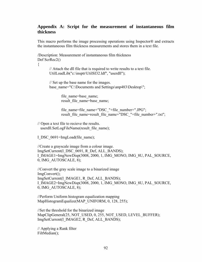
92
Appendix A: Script for the measurement of instantaneous film thickness This macro performs the image processing operations using Inspector® and extracts the instantaneous film thickness measurements and stores them in a text file. /Description: Measurement of instantaneous film thickness Def ScrRec2() { // Attach the dll file that is required to write results to a text file. UtilLoadLib("c:\insptr\UtilSI32.ldf", "userdll"); // Set up the base name for the images. base_name="C:\Documents and Settings\anp483\Desktop\"; file_name=base_name; result_file_name=base_name; file_name=file_name+"DSC_"+file_number+".JPG"; result_file_name=result_file_name+"DSC_"+file_number+".txt"; // Open a text file to recieve the results. userdll.SetLogFileName(result_file_name); I_DSC_0691=ImgLoad(file_name); //Create a grayscale image from a colour image. ImgSetCurrent(I_DSC_0691, R_Def, ALL_BANDS); I_IMAGE1=ImgNewDisp(3008, 2000, 1, IMG_MONO, IMG_8U, PAL_SOURCE, 0, IMG_AUTOSCALE, 8); //Convert the gray scale image to a binarized image ImgConvert(); ImgSetCurrent(I_IMAGE1, R_Def, ALL_BANDS); I_IMAGE2=ImgNewDisp(3008, 2000, 1, IMG_MONO, IMG_8U, PAL_SOURCE, 0, IMG_AUTOSCALE, 8); //Perform Uniform histogram equalization mapping MapHistogramEqualize(MAP_UNIFORM, 0, 128, 255); //Set the threshold for the binarized image MapClipGeneral(25, NOT_USED, 0, 255, NOT_USED, LEVEL_BUFFER); ImgSetCurrent(I_IMAGE2, R_Def, ALL_BANDS); // Applying a Rank filter FiltMedian();

93
//To perform open and a close operation MorphCloseEx(2, 1); MorphOpenEx(15, 1); //To perform erosion and dilation operation/ Morphological operation MorphErodeEx(1, 1); MorphDilateEx(1, 1); //Initialize the constants right_wall_position=2875; left_wall_position=105; search_box_height=2000; x1_position=right_wall_position-30; ImgSetCurrent(I_DSC_0691, R_Def, ALL_BANDS); MeasNewRefLine(right_wall_position, 0, right_wall_position, 2000); ImgSetCurrent(I_IMAGE2, R_Def, ALL_BANDS); //To loop through every 20 j positions on the righthand side of the binarized image for(j=1;j<=2000;j=j+20) { // to find an edge on the right right hand side and allocate a point and/or line marker based on this edge (note:set width of search box to 1 pixel) MeasSetEdgeStripeAngle(MEAS_NEAREST_NEIGHBOR, 360, 360, 5, 5); MeasNewEdgeEx(270, MEAS_POL_AUTO, right_wall_position-70, j, 1,search_box_height, right_wall_position-50,j+0.5, MEAS_MARKER_POS, MEAS_ANY, MEAS_ANY); x1_position=MeasGetResult(MeasGetLastID(),MEAS_X1); userdll.LogInteger(j,0); // Write the j position to a file. userdll.LogString(" ",0); // Write a space between j and x1 positions userdll.LogFloat(x1_position,1); // Write the x1 position to a file. ImgSetCurrent(I_DSC_0691, R_Def, ALL_BANDS); MeasNewRefPoint(x1_position,j); ImgSetCurrent(I_IMAGE2, R_Def, ALL_BANDS); } //To loop through every 20 j positions on the left hand side of the binarized image

94
x2_position=left_wall_position+30; ImgSetCurrent(I_DSC_0691, R_Def, ALL_BANDS); MeasNewRefLine(left_wall_position, 0, left_wall_position, 2000); ImgSetCurrent(I_IMAGE2, R_Def, ALL_BANDS); for(j=2;j<=2000;j=j+20) { // to find an edge on the left hand side and allocate a point and/or line marker based on this edge (note:set width of search box to 1 pixel) MeasSetEdgeStripeAngle(MEAS_NEAREST_NEIGHBOR, 360, 360, 5, 5); MeasNewEdgeEx(90, MEAS_POL_AUTO, left_wall_position+40, j, 1, search_box_height, left_wall_position+50, j+0.5, MEAS_MARKER_POS, MEAS_ANY, MEAS_ANY); x2_position=MeasGetResult(MeasGetLastID(),MEAS_X1); userdll.LogInteger(j,0); // Write the j position to a file. userdll.LogString(" ",0); // Write a space between j and x2 positions userdll.LogFloat(x2_position,1); // Write the x2 position to a file. ImgSetCurrent(I_DSC_0691, R_Def, ALL_BANDS); MeasNewRefPoint(x2_position,j); ImgSetCurrent(I_IMAGE2, R_Def, ALL_BANDS); }
Note: The threshold values used to create a binarized image at five different Reynolds
numbers are given below.
Table A.1: Threshold values at different Reynolds numbers
Reynolds number Threshold 974 50 2111 50 3337 50 4552 30 5924 25


