applied sciences

Article

Fiducial Lower Confidence Limit of Reliability for a PowerDistribution System

Xia Cai 1, Liang Yan 2,*, Yan Li 1 and Yutong Wu 1

�����������������

Citation: Cai, X.; Yan, L.; Li, Y.; Wu,

Y. Fiducial Lower Confidence Limit of

Reliability for a Power Distribution

System. Appl. Sci. 2021, 11, 11317.

https://doi.org/10.3390/

app112311317

Academic Editors: Cheng-Wei Fei,

Zhixin Zhan, Behrooz Keshtegar and

Yunwen Feng

Received: 13 October 2021

Accepted: 25 November 2021

Published: 29 November 2021

Publisher’s Note: MDPI stays neutral

with regard to jurisdictional claims in

published maps and institutional affil-

iations.

Copyright: © 2021 by the authors.

Licensee MDPI, Basel, Switzerland.

This article is an open access article

distributed under the terms and

conditions of the Creative Commons

Attribution (CC BY) license (https://

creativecommons.org/licenses/by/

4.0/).

1 School of Science, Hebei University of Science and Technology, Shijiazhuang 050018, China;caixia@hebust.edu.cn (X.C.); liyan@hebust.edu.cn (Y.L.); hbkjwuyutong@163.com (Y.W.)

2 School of Mathematics and Statistics, Hebei University of Economics and Business,Shijiazhuang 050061, China

* Correspondence: yanliang@heuet.edu.cn

Abstract: Reliability performance, especially the lower confidence limit of reliability, plays an im-portant role in system risk and safety assessment. A good estimator of the lower confidence limitof system reliability can help engineers to make the right decisions. Based on the lifetime of thekey component in a typical satellite intelligent power distribution system, the generalized fiducialmethod is adopted to estimate the lower confidence limit of the system reliability in this paper. First,the generalized pivotal quantity and the lower confidence limit of reliability for the key componentare derived for the lifetimes of the exponential-type and Weibull-type components. Simulationsshow that the sample median is more appropriate than the sample mean when the lower confidencelimit of reliability is estimated. Moreover, the lower confidence limit of reliability is obtained for thetypical satellite intelligent power distribution system through the pseudo-lifetime data of the metallicoxide semiconductor field effect transistor. The lower confidence limit of reliability for this powerdistribution system at 15 years is 0.998, which meets the factory’s reliability requirement. Finally,through the comparison, a hot standby subsystem can be substituted with a cold standby subsystemto increase the lower confidence limit of the system reliability.

Keywords: reliability assessment; lower confidence limit; power distribution system; fiducial method;Monte Carlo simulation

1. Introduction

A power distribution system (PDS) is a power network system consisting of a varietyof power distribution equipment (or components), and it carries electricity from the trans-mission system to individual consumers. The basic function of a PDS is to supply customerswith electrical energy as reliably as possible [1]. The reliability and maintainability of aPDS have attracted some scholars’ interests. For example, the authors of [2] discussed theprotection devices for the aircraft power distribution system. The authors in [3] evaluatedthe reliability of a PDS subjected to hurricanes. A framework for the optimal maintenanceof a PDS subjected to non-stationary hurricane hazard and decay is presented in [4]. Theauthors of [5] reviewed the technological perspective of cyber secure smart inverters usedin PDS. The authors of [6] analyzed the reliability of a 20-KV electric PDS, while those in [7]and [8] calculated the reliability of two Nigeria PDSs, one of which was aging. The authorsin [9] evaluated an Indian PDS and gave some suggestions to minimize the outages whichcan improve reliability. The authors of [10] presented an inverse reliability evaluationwhere some components’ reliability parameters were unknown in a specific PDS.

In general, there is a key subsystem named the solid state power controller (SSPC)in a PDS. The SSPC is a system protection device which provides protections for theelectric installations from short circuits and overloads [11]. Based on the importanceof SSPC, several researchers studied the structure and applications of the SSPC. Theauthors of [12] summarized the advantages of an SSPC, such as high reliability, small

Appl. Sci. 2021, 11, 11317. https://doi.org/10.3390/app112311317 https://www.mdpi.com/journal/applsci

Appl. Sci. 2021, 11, 11317 2 of 16

size and accessible remote control. The authors in [13] presented an optimizing schemefor behavioral modeling of an SSPC, while those in [14] proposed some models for somespecial SSPCs. The authors in [15] analyzed the reliability of a kind of SSPC from anengineering standpoint, and those in [16] proposed two fault detection methods with theanalysis of only the half cycle data.

Due to the characteristics of a long lifetime and high reliability, it is particularlyimportant to analyze the reliability of the PDS and SSPC. Technically, the reliability isoften defined as the probability that a system will perform its intended function underoperating conditions for a specified period of time [17]. In system reliability assessment,the estimator of reliability is a major concern. The authors of [18] estimated the reliabilityof the multicomponent stress–strength based on a two-parameter exponentiated Weibulldistribution. The authors in [19] compared different least squares methods for reliabilityof the Weibull distribution based on the right censored data, and those in [20] and [21]analyzed the reliability of Weibull distribution with zero-failure data and very little failuredata, respectively. However, a point estimator makes little sense if the variance of theestimator is too high. Consequently, it is necessary to give the lower confidence limit(LCL) of reliability [22]. How to get the LCL of system reliability through the lifetimes ofcomponents is an important issue. Many scholars have conducted a lot of research on this.An effective reliability confidence bound for a multi-state system with binary-capacitatedcomponents is suggested in [23]. This is only applied for a series or parallel system. Inaddition, the authors of [24] considered the LCL of reliability under a nonparametricassumption, but the parametric method is often more accurate than the nonparametricmethod when the distribution type is known. The authors in [25] provided the maximumlikelihood estimate (MLE) and a more accurate lower confidence limit for the SoS reliability,but the MLE method is more appropriate for a large sample size. Based on the smallsample size, the authors of [26] applied the WCF approach to analyze the reliability of aspecial complicated system based on accelerated degradation data, but the WCF method iscomplicated for mathematical formula derivation. Based on records data, the authors of [27]calculated the interval estimation of quantiles and reliability in a two-parameter exponentialdistribution. In practice, some electronic components, such as the key components of aPDS, have a long lifetime and high reliability [28,29]. The sample size of these lifetime datais usually very small. To overcome the shortcoming of a large sample, some referencesadopted the Bayesian method to estimate the LCL of reliability. For example, the authorsof [30] and [31] used the Bayesian method to study the reliability for binomial systems,while those in [32] used Bayesian networks to present developments for traditional seriesand parallel systems. The authors in [33] and [34] applied the Bayesian approach to analyzethe reliability of the degradation data. Although the Bayesian approach is suitable for asmall sample of lifetime data, the selection of the prior distribution is difficult.

To avoid the difficulty of choosing a proper prior distribution, the fiducial methodis adopted to estimate the LCL of reliability for a PDS in this paper. The fiducial methodconsiders the parameter as a random variable whose distribution is decided by the observa-tion instead of the prior distribution. The authors of [35] developed the fiducial method bydefining a functional model, and those in [36] proved that the LCL derived by the fiducialmethod is the same as the LCL obtained by the traditional method under some conditions.Recently, some optimal inferences [37] and generalizations of the fiducial method [38] havebeen developed based on [38–40], giving the generalized fiducial inference for generalizedexponential and Lomax distribution.

It can be seen that the generalized fiducial method is an effective method to estimatethe reliability of a long-life product. Based on the high reliability of the PDS, this paperestimates the LCLs of the reliability of the PDS by using the generalized fiducial method.For a typical satellite intelligent PDS, the lifetime distribution of the key components inthe satellite intelligent PDS are assumed to follow an exponential distribution and Weibulldistribution according to the experience of the engineers. In this situation, two algorithmprocedures are presented to estimate the LCL of the reliability for an exponential-type

Appl. Sci. 2021, 11, 11317 3 of 16

component and a Weibull-type component. Then, the LCLs of reliability for the satelliteintelligent PDS are established by the relationship between the key components and thesystem. Compared with the Bayesian method, the generalized fiducial method of thispaper is more flexible to avoid the selection of the prior distribution.

2. Materials and Methods2.1. Power Distribution System Reliability Model

In the design of the satellite intelligent PDS, the Beijing Satellites Casting Factorydivided the PDS into three subsystems according to different functions of the components.These three subsystems were the direct current to direct current power supply (DC/DC),solid state power controller (SSPC) and telemetry and telecontrol unit (TM/TC). TheDC/DC is responsible for converting the bus bar voltage into the voltage which is requiredby the analog circuit and digital circuit in the system. The SSPC can play a protective role,including limiting the current protection and short circuit protection and collecting currentvoltage. The TM/TC can not only save current voltage data but also check the variousSSPCs and monitor the historical data.

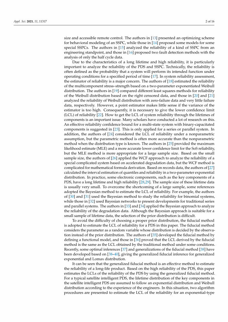
In order to improve the reliability of the PDS, standby systems are often adoptedin system design. There are two traditional types of standby redundancy: hot standbyand cold standby. In hot standby redundancy, components which are in standby modeoperate in synchrony with the main unit and are ready to take over at any time, whilein cold standby redundancy, components in standby mode are unpowered and thus donot operate until needed to replace a faulty main unit [41,42]. In the satellite intelligentPDS, the hot standby systems are used for the DC/DC and SSPC, and the cold standbysystems are used for the TM/TC. These three subsystems are in arranged in a series way.The reliability block diagram of this PDS is shown in Figure 1.

Figure 1. The reliability block diagram of a typical PDS.

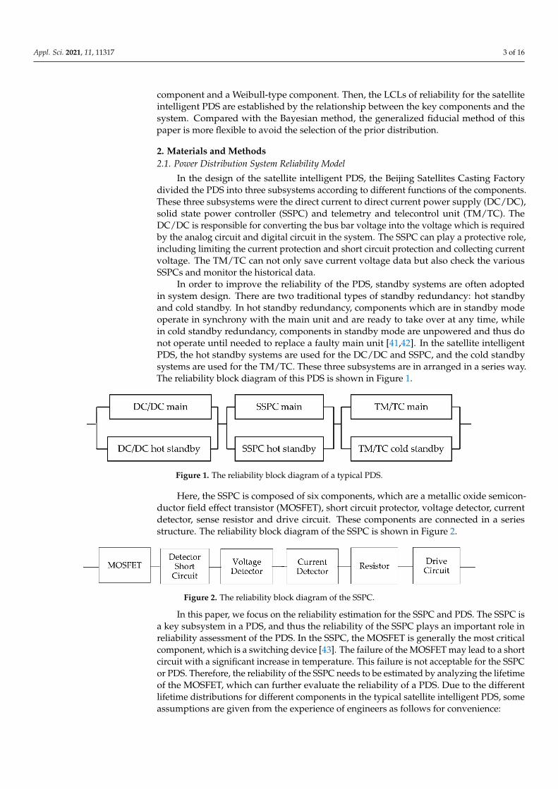
Here, the SSPC is composed of six components, which are a metallic oxide semicon-ductor field effect transistor (MOSFET), short circuit protector, voltage detector, currentdetector, sense resistor and drive circuit. These components are connected in a seriesstructure. The reliability block diagram of the SSPC is shown in Figure 2.

Figure 2. The reliability block diagram of the SSPC.

In this paper, we focus on the reliability estimation for the SSPC and PDS. The SSPC isa key subsystem in a PDS, and thus the reliability of the SSPC plays an important role inreliability assessment of the PDS. In the SSPC, the MOSFET is generally the most criticalcomponent, which is a switching device [43]. The failure of the MOSFET may lead to a shortcircuit with a significant increase in temperature. This failure is not acceptable for the SSPCor PDS. Therefore, the reliability of the SSPC needs to be estimated by analyzing the lifetimeof the MOSFET, which can further evaluate the reliability of a PDS. Due to the differentlifetime distributions for different components in the typical satellite intelligent PDS, someassumptions are given from the experience of engineers as follows for convenience:

Appl. Sci. 2021, 11, 11317 4 of 16

Assumption 1. A PDS has independent components, and the switching mechanism from the mainsubsystem to the standby subsystem is considered to be completely reliable.

Assumption 2. In an SSPC, the lifetime of the MOSFET follows a Weibull distribution, and thelifetimes of the others follow exponential distributions with different failure rates.

Assumption 3. The failure rates of the voltage detector, current detector, sense resistor and drivecircuit are known from experience, but the short circuit protector’s is unknown.

Assumption 4. The lifetimes of the DC/DC and TM/TC follow exponential distributions withknown failure rates.

Based on these assumptions, in the following subsections, the fiducial method wasadopted to derive the LCLs of reliability for a single component: an SSPC and a PDS.

2.2. Fiducial LCL of Reliability for an Exponential-Type Component

In this subsection, we discuss the LCL of reliability based on a typical componentwhose lifetime follows the exponential distribution commonly used in a PDS.

Except for the MOSFET, the lifetimes of the other components in an SSPC wereassumed to be exponentially distributed. Thus, we derived the LCL of reliability for anexponential-type component first.

Let T be a random variable which follows an exponential distribution with an un-known parameter λ. The cumulative distribution function of T is

F(t) = 1− e−λt, t > 0. (1)

Suppose T1, T2, · · · , Tn is a random sample from the population T, where n is thesample size. Then, the total test time Tsum = T1 + T2 + · · · + Tn follows a Gamma distributionwith parameters n and λ. Therefore, 2λTsum follows an χ2 distribution with 2n degrees offreedom. Then, parameter λ can be represented as

λ =E

2Tsum, E ∼ χ2(2n), (2)

where E is the pivotal quantity which follows a completely known distribution.We can derive the estimator and the confidence interval (CI) of parameter λ by solving

the expectation and the quantile of χ2 distribution, respectively, or by generating a randomnumber. The CI for λ with the confidence level is given by[

χ2α/2(2n)/2Tsum, χ2

1−α/2(2n)/2Tsum

], (3)

where χ2α/2(2n) is the α/2 quantile of a Chi-square distribution with 2n degrees of freedom.

Equation (3) is the same as the result of the traditional method.However, the quantity of interest is the reliability, which is a function of parameter λ.

The reliability of the component whose lifetime follows an exponential distribution at timet can be expressed as

R(t) = exp{− t

2TsumE}

, E ∼ χ2(2n). (4)

Then, the LCL of reliability with the confidence level 1 − α is

RL(t) = exp{− t

2Tsumχ2

1−α(2n)}

. (5)

The fiducial algorithm for the CI of parameter λ and the LCL of reliability based onan exponential distribution is shown in Algorithm 1.

Appl. Sci. 2021, 11, 11317 5 of 16

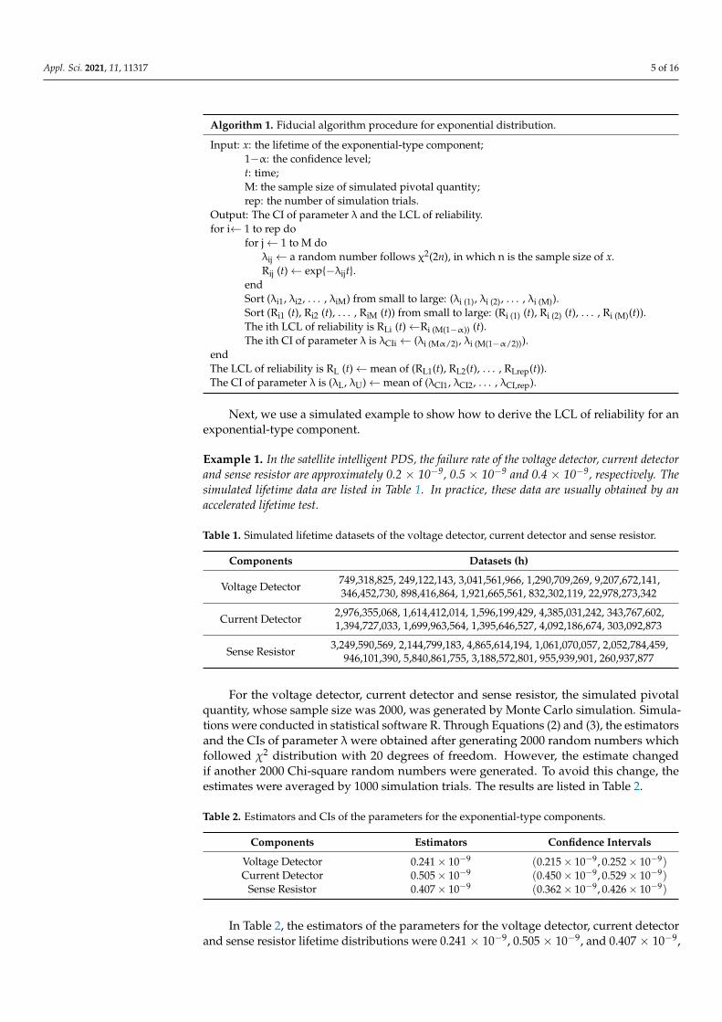
Algorithm 1. Fiducial algorithm procedure for exponential distribution.

Input: x: the lifetime of the exponential-type component;1−α: the confidence level;t: time;M: the sample size of simulated pivotal quantity;rep: the number of simulation trials.

Output: The CI of parameter λ and the LCL of reliability.for i← 1 to rep do

for j← 1 to M doλij ← a random number follows χ2(2n), in which n is the sample size of x.Rij (t)← exp{−λijt}.

endSort (λi1, λi2, . . . , λiM) from small to large: (λi (1), λi (2), . . . , λi (M)).Sort (Ri1 (t), Ri2 (t), . . . , RiM (t)) from small to large: (Ri (1) (t), Ri (2) (t), . . . , Ri (M)(t)).The ith LCL of reliability is RLi (t)←Ri (M(1−α)) (t).The ith CI of parameter λ is λCIi ← (λi (Mα/2), λi (M(1−α/2))).

endThe LCL of reliability is RL (t)←mean of (RL1(t), RL2(t), . . . , RLrep(t)).The CI of parameter λ is (λL, λU)←mean of (λCI1, λCI2, . . . , λCI,rep).

Next, we use a simulated example to show how to derive the LCL of reliability for anexponential-type component.

Example 1. In the satellite intelligent PDS, the failure rate of the voltage detector, current detectorand sense resistor are approximately 0.2 × 10−9, 0.5 × 10−9 and 0.4 × 10−9, respectively. Thesimulated lifetime data are listed in Table 1. In practice, these data are usually obtained by anaccelerated lifetime test.

Table 1. Simulated lifetime datasets of the voltage detector, current detector and sense resistor.

Components Datasets (h)

Voltage Detector 749,318,825, 249,122,143, 3,041,561,966, 1,290,709,269, 9,207,672,141,346,452,730, 898,416,864, 1,921,665,561, 832,302,119, 22,978,273,342

Current Detector 2,976,355,068, 1,614,412,014, 1,596,199,429, 4,385,031,242, 343,767,602,1,394,727,033, 1,699,963,564, 1,395,646,527, 4,092,186,674, 303,092,873

Sense Resistor 3,249,590,569, 2,144,799,183, 4,865,614,194, 1,061,070,057, 2,052,784,459,946,101,390, 5,840,861,755, 3,188,572,801, 955,939,901, 260,937,877

For the voltage detector, current detector and sense resistor, the simulated pivotalquantity, whose sample size was 2000, was generated by Monte Carlo simulation. Simula-tions were conducted in statistical software R. Through Equations (2) and (3), the estimatorsand the CIs of parameter λ were obtained after generating 2000 random numbers whichfollowed χ2 distribution with 20 degrees of freedom. However, the estimate changedif another 2000 Chi-square random numbers were generated. To avoid this change, theestimates were averaged by 1000 simulation trials. The results are listed in Table 2.

Table 2. Estimators and CIs of the parameters for the exponential-type components.

Components Estimators Confidence Intervals

Voltage Detector 0.241× 10−9 (0.215× 10−9, 0.252× 10−9)Current Detector 0.505× 10−9 (0.450× 10−9, 0.529× 10−9)

Sense Resistor 0.407× 10−9 (0.362× 10−9, 0.426× 10−9)

In Table 2, the estimators of the parameters for the voltage detector, current detectorand sense resistor lifetime distributions were 0.241 × 10−9, 0.505 × 10−9, and 0.407 × 10−9,

Appl. Sci. 2021, 11, 11317 6 of 16

respectively. It is shown that the fiducial estimators were close to the true value. In the sameway, with Equations (4) and (5), the estimators and the LCLs of reliability at t0 = 87,600 h(10 years) with a confidence level 0.8 are listed in Table 3.

Table 3. Estimators and LCLs of reliability for the exponential-type components (t0 = 87,600 h).

Components Estimators Lower Confidence Limits

Voltage Detector 0.9999789 0.9999736

Current Detector 0.9999558 0.9999446

Sense Resistor 0.9999644 0.9999553

From Table 3, we find that the estimator and the LCL of reliability for the voltagedetector were 0.9999789 and 0.9999736 at 10 years, respectively. These two numbers wereboth very close to one since the failure rate was very small. In fact, if t0 is taken as8.76 × 107 h, the reliability is approximately 0.97, which is still very high. The analysesof the current detector and sense resistor were similar. We could treat them as “non-failed” components.

2.3. Fiducial LCL of Reliability for a Weibull-Type Component

In this subsection, we use the fiducial method to derive the LCL of reliability for aWeibull-type component.

Let T1, T2, · · · , Tn be a random sample from the Weibull distribution. The cumulativedistribution function of the Weibull distribution is

FT(t) = 1− exp{−(t/η)m}, t > 0, (6)

where η > 0 and m > 0 are called the scale parameter and shape parameter, respectively. Itis difficult to derive the estimators of η and m directly.

In general, Tj is transformed to Xj by Xj = ln Tj, and then Xj follows an extreme valuedistribution with σ = 1/m and µ = ln η, j = 1, 2, · · · , n. The common cumulative distributionfunction of Xj, j = 1, 2, · · · , n is

FXj(xj) = 1− exp{−e

xj−µ

σ

}. (7)

Let the following be true:

Wj =Xj − µ

σ= m

(ln Tj − ln η

), j = 1, 2, · · · , n. (8)

Then, Wj follows a common standard extreme value distribution which is completelyknown, and the distribution of their function is also completely known. Thus, we treat thefunction of Wj as the pivotal quantity.

Denote the following:

X =1n

n

∑i=1

Xi, S2 =1n

n

∑i=1

(Xi − X)2, W =

1n

n

∑i=1

Wi, V2 =1n

n

∑i=1

(Wi −W)2. (9)

These statistics have relations as follows:

µ = X− WV

S, σ =SV

, η = exp

{X− W

VS

}, m =

VS

. (10)

Appl. Sci. 2021, 11, 11317 7 of 16

Then, parameters η and m can be expressed as

η = exp{

X− E1

E2S}

, m =E2

S, (11)

where E1 and E2 are pivotal quantities which have the same distributions as W and V,respectively. However, it is difficult to derive the explicit formula of the probability densityfor these two distributions. Instead, the random numbers which follow a standard extremevalue distribution are easily generated by Monte Carlo simulation. Then, we treated thesample mean and the sample standard deviation as E1 and E2. The simulated values ofparameters η and m were derived by Equation (11). By repeating this sampling method,we could get many pairs of η and m. By averaging the sample, the estimators of theparameters were derived. The CIs were obtained by finding the sample quantiles of thesimulated parameters.

Here, the quantity of interest is the reliability, which can be expressed as

R(t) = exp{−(t/η)m} = exp

−(

t exp{

E1

E2S− X

}) E2S

. (12)

Then, the estimator and the LCL of reliability with a confidence level could be derived.The fiducial algorithm for the CIs of parameters η and m and the LCL of reliability

based on a Weibull distribution is shown in Algorithm 2.

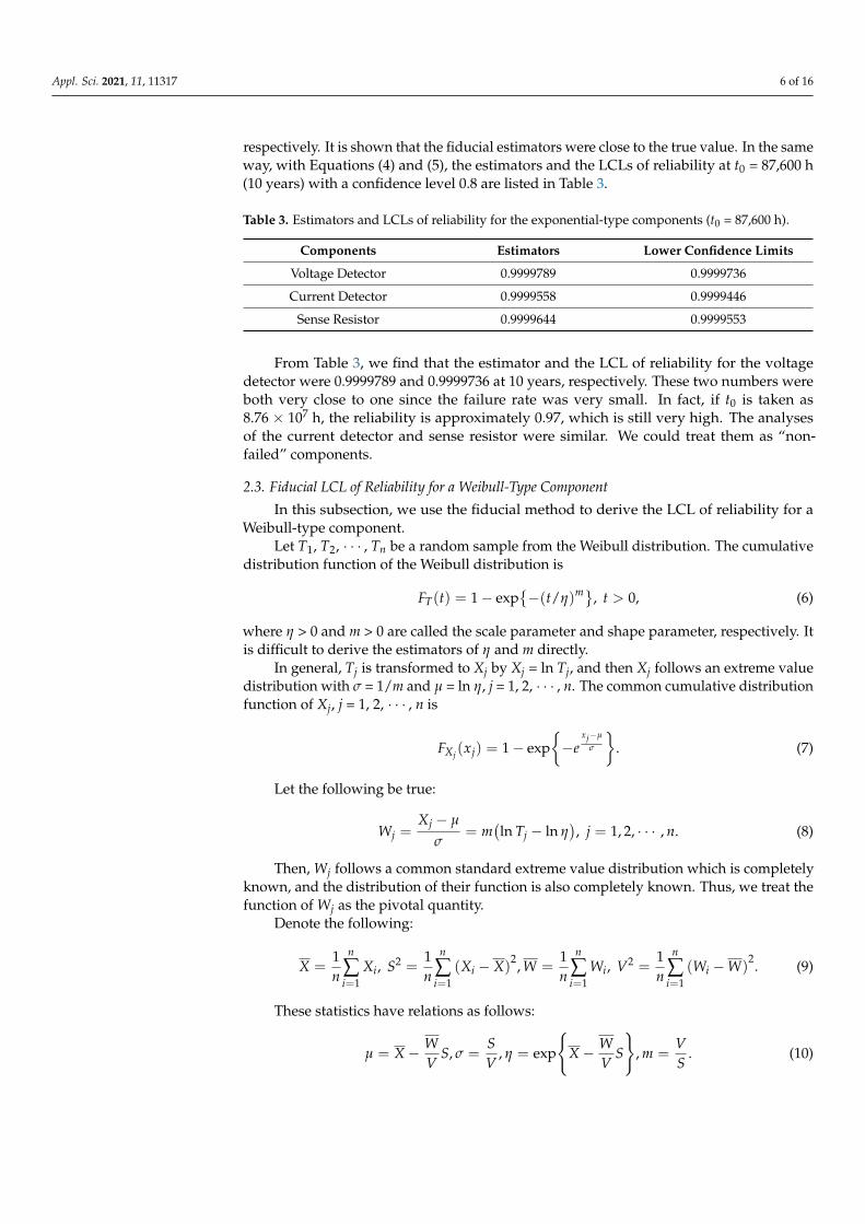
Algorithm 2. Fiducial algorithm procedure for Weibull distribution.

Input: tw: the lifetime of the Weibull-type component;1−α: the confidence level;t: time;M: the sample size of simulated pivotal quantity;rep: the number of simulation trials.

Output: The CIs of parameters η and m and the LCL of reliability.n← sample size of tw.x←logarithm of tw.xbar←mean of x.s← standard deviation of x.for i← 1 to rep do

for j← 1 to M dofor k← 1 to n do

wijk ← a random number which follows standard extreme value distribution.endwbarij ←mean of (wij1, wij2, . . . , wijn).vij ← standard deviation of (wij1, wij2, . . . , wijn).ηij ← exp(xbar − wbarij/vij*s).mij ← vij/s.R ij (t)← exp(−(tij/η)mij)

endSort (ηi1, ηi2, . . . , ηiM) from small to large: (ηi (1), ηi (2), . . . , ηi (M)).Sort (mi1, mi2, . . . , miM) from small to large: (mi (1), mi (2), . . . , mi (M)).Sort (Ri1 (t), Ri2 (t), . . . , RiM (t)) from small to large: (Ri (1) (t), Ri (2) (t), . . . , Ri (M)(t)).The ith LCL of reliability is RLi (t)←Ri (M(1-α))(t).The ith CI of parameter η is ηCIi← (ηi (Mα/2),ηi (M(1−α/2))).The ith CI of parameter m is mCIi← (mi (Mα/2),mi (M(1−α/2))).

endThe LCL of reliability is RL (t)←mean of (RL1(t), RL2(t), . . . , RLrep(t)).The CI of parameter η is (ηL,ηU)←mean of (ηCI1,ηCI2, . . . , ηCI,rep).The CI of parameter m is (mL,mU)←mean of (mCI1,mCI2, . . . , mCI,rep).

Appl. Sci. 2021, 11, 11317 8 of 16

Next, we also used a simulated example to show how to derive the LCL of reliabilityfor a Weibull-type component.

Example 2. Consider a MOSFET in an SSPC whose lifetime is assumed to be Weibull-distributedwith the scale parameter η = 950,000 and the shape parameter m = 5. The simulated and logarithmictransformed data are listed in Table 4.

Table 4. Simulated lifetime dataset of the MOSFET.

MOSFET Datasets (h)

Original Data 1,168,880.9, 1,048,819.6, 1,094,062.7, 995,454.8, 951,788.8,923,084.9,427,006.4, 812,771.7, 619,423.7, 862,760.0

LogarithmicTransformed Data

13.97156, 13.86318, 13.90541, 13.81095, 13.76610,13.73548, 12.96455, 13.60821, 13.33654, 13.66789

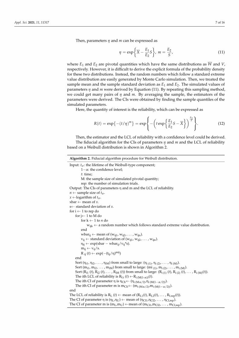
The simulated pivotal dataset, whose sample size was 2000, was generated by MonteCarlo simulation. The estimates were averaged by 1000 simulation trials. The estimatorsand CIs of the parameters are shown in Figure 3.

Figure 3. Estimators and CIs of the parameters for the MOSFET.

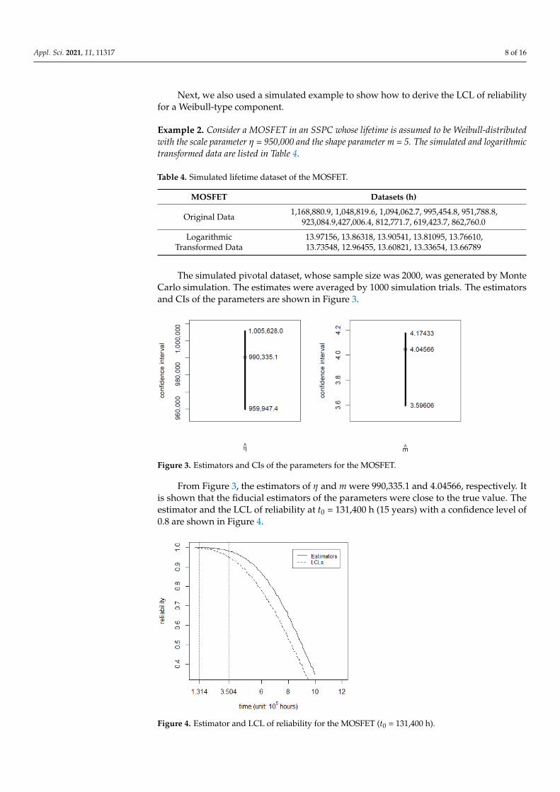
From Figure 3, the estimators of η and m were 990,335.1 and 4.04566, respectively. Itis shown that the fiducial estimators of the parameters were close to the true value. Theestimator and the LCL of reliability at t0 = 131,400 h (15 years) with a confidence level of0.8 are shown in Figure 4.

Figure 4. Estimator and LCL of reliability for the MOSFET (t0 = 131,400 h).

Appl. Sci. 2021, 11, 11317 9 of 16

From Figure 4, we found that the estimator and the LCL of reliability at 15 years were0.9995892 and 0.9975223, respectively. Here, we used the median to estimate the reliabilityinstead of the mean. In fact, the LCL was sometimes larger than the mean, because thereliability was close to 1 at 15 years. In the Monte Carlo simulations, several simulatedvalues may have been much smaller than the others, and these small values could betreated as the outliers. The outliers made the mean smaller than the LCL. In this case, themedian was better than the mean. In other words, the sample median was more robustthan the sample mean. Therefore, we used the sample median and the sample mean toestimate the reliability in the subsequent analysis.

2.4. LCL Analysis of Reliability for a Typical PDS

In Section 2.2 and Section 2.3, the pivotal quantities were derived for the lifetime ofan exponential-type component and a Weibull-type component. In this subsection, weanalyze the LCL of reliability for a typical satellite intelligent PDS. The structure of thisPDS is shown in Figure 1. The SSPC is a key subsystem in this PDS. Thus, we analyzed theLCL of reliability for the SSPC first.

The lifetime of the MOSFET was assumed to be Weibull-distributed with unknownparameters η and m, and the lifetime of the short circuit protector was assumed to beexponentially distributed with an unknown failure rate λS2. The lifetimes of the voltagedetector, current detector, sense resistor and drive circuit in the SSPC were assumed to beexponentially distributed with known failure rates λS3, λS4, λS5 and λS6, respectively.

Let RS(t) be the reliability of the SSPC at time t. RS1(t), RS2(t), RS3(t), RS4(t), RS5(t)and RS6(t) represent the reliability of the MOSFET, short circuit protector, voltage detector,current detector, sense resistor and drive circuit, respectively. Thus, RS(t) can be expressedas follows:

RS(t) = RS1(t)RS2(t)RS3(t)RS4(t)RS5(t)RS6(t)= exp

{−(t/η)m − λS2t− λS3t− λS4t− λS5t− λS6t

}= exp

{−(

t exp{

E1E2

S− X}) E2

S − t2T E−

6∑

i=3λSit

}, ...

(13)

where X and S are the logarithm mean and the logarithm standard deviation of the samplelifetime for the MOSFET, respectively. E, E1 and E2 are independent random variables.E follows an χ2 distribution with 2n2 (n2 is the sample size of the short circuit protector)degrees of freedom. E1 and E2 have the same distribution as the sample mean and standarddeviation of W1, · · · , Wn1 (W1, · · · , Wn1 follow the standard extreme value distribution,and n1 is the sample size of the MOSFET). By simulating χ2 random numbers and standardextreme value random numbers, the simulations of the pivotal quantities E, E1 and E2 werederived. Then, the simulated RS(t) was computed by Equation (13). The estimator and theLCL of RS(t) for a single SSPC were taken as the sample mean (or sample median) and thesample quantile of the simulations.

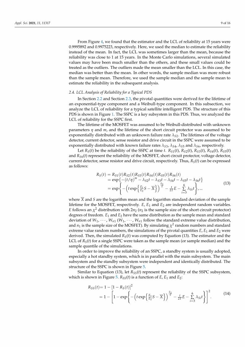
In order to improve the reliability of an SSPC, a standby system is usually adopted,especially a hot standby system, which is in parallel with the main subsystem. The mainsubsystem and the standby subsystem were independent and identically distributed. Thestructure of the SSPC is shown in Figure 5.

Similar to Equation (13), let RSS(t) represent the reliability of the SSPC subsystem,which is shown in Figure 5. RSS(t) is a function of E, E1 and E2:

RSS(t)= 1− [1− RS(t)]2

= 1−[

1− exp

{−(

t exp{

E1E2

S− X}) E2

S − t2T E−

6∑

i=3λSit

}]2

.(14)

Appl. Sci. 2021, 11, 11317 10 of 16

Figure 5. The reliability block diagram of the SSPC.

Then, we analyzed the LCL of reliability for a satellite intelligent PDS, which is shownin Figure 1. The cold standby subsystem was adopted for the TM/TC, whose lifetimewas assumed to be exponentially distributed with a failure rate λT = 338.58 × 10−9. Thisconstant could be used directly when the reliability was calculated. Then the reliability ofthe TM/TC subsystem with one cold standby subsystem at time t can be expressed as

RTT(t) = e−λT t0(1 + λTt). (15)

For the DC/DC, a hot standby system was adopted. The lifetime of the DC/DC wasassumed to follow an exponential distribution with a failure rate λD = 96.3 × 10−9. Thereliability of this subsystem with a hot standby subsystem at time t is

RDD(t) = 1−(

1− e−λDt)2

. (16)

In general, there are a DC/DC, TM/TC and at least one SSPC in an intelligent PDS.First, one SSPC was considered for simplicity. Therefore, the reliability of the PDS with oneSSPC subsystem at time t is

R(t) = RDD(t)RTT(t)RSS(t)=[1−

(1− e−λDt)2

]e−λT t(1 + λTt)

·

1−[

1− exp

{−(

t exp{

E1E2

S− X}) E2

S − t2T E−

6∑

i=3λSit

}]2.

(17)

The reliability of the entire PDS with N SSPC subsystems at time t is

RN(t) = RDD(t)RTT(t)[RSS(t)]N

=[1−

(1− e−λDt)2

]e−λT t(1 + λTt)

·

1−[

1− exp

{−(

t exp{

E1E2

S− X}) E2

S − t2T E−

6∑

i=3λSit

}]2

N

.

(18)

In this subsection, the LCLs of reliability for the SSPC and PDS were formulized. Thedetailed calculation process is given in the next section.

Appl. Sci. 2021, 11, 11317 11 of 16

3. Results

This section uses the datasets of the MOSFET and short circuit protector, which arethe key components in a typical satellite intelligent PDS made by the Beijing SatellitesCasting Factory, to illustrate the proposed method. The lifetimes of the MOSFET camefrom the accelerated lifetime test, and the lifetimes of the short circuit protector came fromthe simulated data. The datasets of the MOSFET and short circuit protector are shown inTable 5. The failure rates of the voltage detector, current detector, sense resistor and drivecircuit were 0.2 × 10−9, 0.5 × 10−9, 0.4 × 10−9 and 0.6 × 10−9, respectively, which wereknown from experience.

Table 5. Datasets of the MOSFET and short circuit protector.

Components Datasets (h)

MOSFET 913,440.6, 919,580.9, 415,447.5, 754,872.8, 592,204.5,1,101,658.4, 993,999.6, 1,006,450.1, 570,526.9, 993,583.7

Short Circuit Protector 5,871,090,193, 5,989,641,035, 1,108,022,425, 182,198,277,191,327,415, 1,037,844,580, 23,220,248,016, 2,069,706,535

From Equation (13), the simulated reliability with 2000 repetitions was obtained. Theestimates were averaged by 1000 simulation trials. The estimator of reliability at 131,400 h(15 years) was taken as the sample mean or the sample median of simulations. Then, weranked the reliability values in order from small to large. The LCL of reliability at 15 yearswas the reliability of the ordered simulations. The results are shown in Table 6.

Table 6. Estimators and LCL of reliability for the SSPC (t0 = 131,400 h).

Reliability Estimator (Mean) Estimator (Median) Lower Confidence Limit

R(t0) 0.9960092 0.9989452 0.9952635

From Table 6, we found that the mean of simulated reliability was 0.9960092, whichwas close to the LCL (0.9952635). Therefore, it was more appropriate to take the median(0.9989452) as the estimator of reliability. It is illustrated that the LCL of reliability at15 years with a confidence level of 0.8 was 0.9952635.

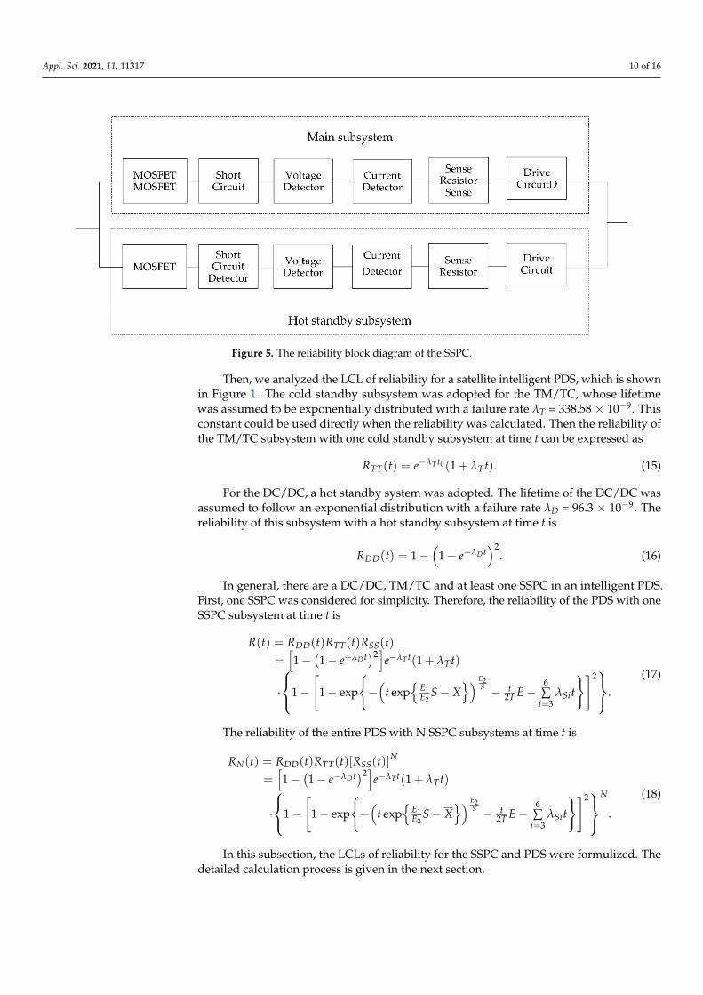
Figure 6 gives a plot of the estimator and the LCL of reliability for the SSPC. Thereal line represents the estimator of reliability for the SSPC. We took the median of thesimulated sample as the estimator instead of the mean. The dashed line represents the LCLof reliability for the SSPC.

Figure 6. Curves of the estimator and the LCL of reliability for the SSPC.

Appl. Sci. 2021, 11, 11317 12 of 16

From Figure 6, we can see the rate of decline was slow when t ranged from 131,400 h(15 years) to 350,400 h (40 years). The LCLs of reliability for the SSPC at 15 years and40 years with a confidence level of 0.8 were 0.995 and 0.930, respectively. Both the estimatorand the LCL of reliability for the SSPC were very high, which could meet the factory’srequirement for reliability.

Next, the reliability for the SSPC with hot standby equipment was calculated. Thestructure is shown in Figure 5. The estimators and the LCL of reliability for the SSPCwith hot standby equipment could also be obtained by Monte Carlo simulation fromEquation (14). The results are shown in Table 7.

Table 7. Estimators and LCL of reliability for an SSPC with hot standby equipment (t0 = 131,400 h).

Reliability Estimator (Mean) Estimator (Median) Lower Confidence Limit

R(t0) 0.9998993 0.9999989 0.9999775

Table 7 illustrates that the estimator and the LCL of reliability at 15 years were0.9999989 and 0.9999775, respectively. When comparing Table 6 with Table 7, it is shownthat the reliability and the LCL were improved when the hot standby systems were adopted.In fact, if the cold or warm standby systems were adopted, the reliability was also im-proved similarly.

Next, the reliability of the whole PDS with at least one SSPC was calculated. Theestimators and the LCL of the whole PDS reliability with one SSPC subsystem wereobtained by Equation (17) and are shown in Table 8.

Table 8. Estimators and LCL of reliability for the PDS with one SSPC (t0 = 131,400 h).

Reliability Estimator (Mean) Estimator (Median) Lower Confidence Limit

R(t0) 0.9987806 0.9988801 0.9988588

From Table 8, it is shown that the estimators and the LCL of reliability were 0.9988801and 0.9988588, respectively. In the same way, we could calculate the LCL of reliability for aPDS with more than one SSPC. For example, Table 9 calculates the estimators and the LCLof PDS reliability at 15 years with 20 SSPCs.

Table 9. Estimators and LCL of reliability for a PDS with 20 SSPCs (t0 = 131,400 h).

Reliability Estimator (Mean) Estimator (Median) Lower Confidence Limit

R(t0) 0.9970009 0.998859 0.9984319

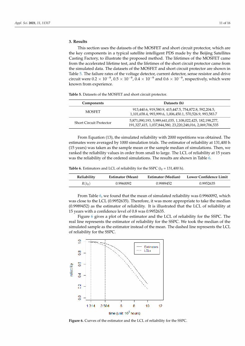
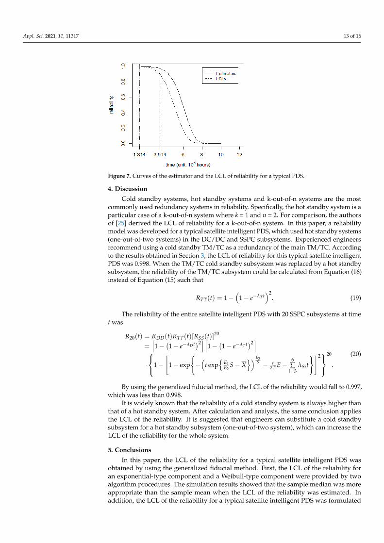
Figure 7 gives two curves of the estimator and the LCL of reliability for the PDS.The real line and dashed line represent the estimator and the LCL of reliability for thePDS, respectively.

As shown in Figure 7, the rate of decline was slow when t ranged from 131,400 h(15 years) to 350,400 h (40 years). The LCL of reliability for the PDS at 15 years and 40 yearswith a confidence level of 0.8 were 0.998 and 0.899, respectively. Compared with Figure 6,the decline rate of reliability for the PDS was faster than that for the SSPC when t rangedfrom 350,400 h (40 years) to 788,400 h (90 years). The reason for this was that there were 20SSPCs in the PDS. When the reliability of the SSPC was reduced, the reliability of the PDSdecreased faster.

According to the factory’s requirement, the LCL of the reliability for this typicalsatellite intelligent PDS at 15 years should be greater than 0.980 with a confidence level of0.8. From Table 9, the LCL of reliability at 15 years was 0.998, which was greater than 0.980(i.e., the reliability met the factory’s requirement).

Appl. Sci. 2021, 11, 11317 13 of 16

Figure 7. Curves of the estimator and the LCL of reliability for a typical PDS.

4. Discussion

Cold standby systems, hot standby systems and k-out-of-n systems are the mostcommonly used redundancy systems in reliability. Specifically, the hot standby system is aparticular case of a k-out-of-n system where k = 1 and n = 2. For comparison, the authorsof [25] derived the LCL of reliability for a k-out-of-n system. In this paper, a reliabilitymodel was developed for a typical satellite intelligent PDS, which used hot standby systems(one-out-of-two systems) in the DC/DC and SSPC subsystems. Experienced engineersrecommend using a cold standby TM/TC as a redundancy of the main TM/TC. Accordingto the results obtained in Section 3, the LCL of reliability for this typical satellite intelligentPDS was 0.998. When the TM/TC cold standby subsystem was replaced by a hot standbysubsystem, the reliability of the TM/TC subsystem could be calculated from Equation (16)instead of Equation (15) such that

RTT(t) = 1−(

1− e−λT t)2

. (19)

The reliability of the entire satellite intelligent PDS with 20 SSPC subsystems at timet was

R20(t) = RDD(t)RTT(t)[RSS(t)]20

=[1−

(1− e−λDt)2

][1−

(1− e−λT t)2

]·

1−[

1− exp

{−(

t exp{

E1E2

S− X}) E2

S − t2T E−

6∑

i=3λSit

}]2

20

.

(20)

By using the generalized fiducial method, the LCL of the reliability would fall to 0.997,which was less than 0.998.

It is widely known that the reliability of a cold standby system is always higher thanthat of a hot standby system. After calculation and analysis, the same conclusion appliesthe LCL of the reliability. It is suggested that engineers can substitute a cold standbysubsystem for a hot standby subsystem (one-out-of-two system), which can increase theLCL of the reliability for the whole system.

5. Conclusions

In this paper, the LCL of the reliability for a typical satellite intelligent PDS wasobtained by using the generalized fiducial method. First, the LCL of the reliability foran exponential-type component and a Weibull-type component were provided by twoalgorithm procedures. The simulation results showed that the sample median was moreappropriate than the sample mean when the LCL of the reliability was estimated. Inaddition, the LCL of the reliability for a typical satellite intelligent PDS was formulated

Appl. Sci. 2021, 11, 11317 14 of 16

based on the structure of the complicated system. The results showed that the LCL of thereliability for the typical satellite intelligent PDS at 15 years was 0.998, which was greaterthan 0.980. The obtained reliability of the system met the factory’s requirement. Finally, theLCLs of the reliability for a cold standby system and a hot standby system were calculated.Analysis showed that a cold standby system outperformed a hot standby system when wewere interested in the LCL of the system reliability. The research results of this paper willprovide a theoretical basis to make the right decisions for reliability engineers.

6. Future Works

Some questions warrant further study. The first question is whether the generalizedfiducial method of the reliability can be used not only for the reliability of the componentsbut also for some other reliability characteristic quantities which are functions of the sampleand pivotal quantities, such as the availability and failure rate of the component. Thenext question concerns the reliability structure of the typical satellite intelligent PDS. Theevaluation method proposed in this paper can be also applied to the LCLs of some othercomplicated reliability structures of a PDS. Finally, because the PDS has the characteristicsof a long lifetime and high reliability, the validation experiment is very difficult. How toconduct the validation experiment is our future work.

Author Contributions: Conceptualization, X.C. and Y.L.; methodology, X.C. and L.Y.; software,X.C.; validation, X.C.; formal analysis, Y.W.; investigation, X.C.; resources, X.C.; data curation, X.C.;writing—original draft preparation, X.C. and Y.L.; writing—review and editing, Y.W.; visualization,X.C.; supervision, L.Y.; project administration, L.Y.; funding acquisition, X.C. All authors have readand agreed to the published version of the manuscript.

Funding: This research was funded by the National Natural Science Foundation of China, grantnumbers NSFC 12001155, 72001070 and 72071071, the Natural Science Foundation of Hebei Province,grant number A2020207006, and the Foundation of Hebei Educational Committee, grant num-ber QN2019062.

Institutional Review Board Statement: Not applicable.

Informed Consent Statement: Not applicable.

Conflicts of Interest: The authors declare no conflict of interest.

References1. Chowdhury, A.A.; Koval, D.O. Power Distribution System Reliability: Practical Methods and Applications; Wiley: New York, NY,

USA, 2009. [CrossRef]2. Izquierdo, D.; Barrado, A.; Raga, C.; Sanz, M.; Zumel, P.; Lázaro, A. Protection devices for aircraft electrical power distribution

systems: A survey. In Proceedings of the 2008 34th Annual Conference of IEEE Industrial Electronics, Orlando, FL, USA, 10–13November 2008; pp. 903–908.

3. Salman, A.; Li, Y.; Stewart, M.G. Evaluating system reliability and targeted hardening strategies of power distribution systemssubjected to hurricanes. Reliab. Eng. Syst. Saf. 2015, 144, 319–333. [CrossRef]

4. Salman, A.; Li, Y.; Bastidas-Arteaga, E. Maintenance optimization for power distribution systems subjected to hurricane hazard,timber decay and climate change. Reliab. Eng. Syst. Saf. 2017, 168, 136–149. [CrossRef]

5. Surya, S.; Srinivasan, M.K.; Williamson, S. Technological Perspective of Cyber Secure Smart Inverters Used in Power DistributionSystem: State of the Art Review. Appl. Sci. 2021, 11, 8780. [CrossRef]

6. Nazaruddin, M.; Fauzi Maimun Subhan Abubakar, S.; Aiyub, S. Reliability Analysis of 20 KV Electric Power Distribution System.IOP Conf. Ser. Mater. Sci. Eng. 2020, 854, 12007. [CrossRef]

7. Obu, U.; Uzoechi, O.L. Reliability Evaluation of Aging Nigeria Power Distribution System Using Monte Carlo Simulation. Int. J.Electr. Electron. Eng. 2020, 7, 7–13. [CrossRef]

8. Ayamolowo, O.J.; Mmonyi, C.A.; Adigun, S.O.; Onifade, O.A.; Adeniji, K.A.; Adebanjo, A.S. Reliability Analysis of PowerDistribution System: A Case Study of Mofor Injection Substation, Delta State, Nigeria. In Proceedings of the IEEE Africon, Accra,Ghana, 25–27 September 2019; pp. 1–6.

9. Prakash, T.; Thippeswamy, K. Reliability Analysis of Power Distribution System: A Case Study. Int. J. Eng. Res. 2017, V6, 6.[CrossRef]

10. Sharifinia, S.; Rastegar, M.; Allahbakhshi, M.; Fotuhi-Firuzabad, M. Inverse Reliability Evaluation in Power Distribution Systems.IEEE Trans. Power Syst. 2019, 35, 818–820. [CrossRef]

Appl. Sci. 2021, 11, 11317 15 of 16

11. Izquierdo, D.; Barrado, A.; Fernandez, C.; Sanz, M.; Zumel, P. Behavioral model for solid-state power controller. IEEE Aerosp.Electron. Syst. Mag. 2013, 28, 4–11. [CrossRef]

12. Guo, Y.-B.; Bhat, K.P.; Aravamudhan, A.; Hopkins, D.C.; Hazelmyer, D.R. High current and thermal transient design of a SiCSSPC for aircraft application. In Proceedings of the 2011 Twenty-Sixth Annual IEEE Applied Power Electronics Conference andExposition (APEC), Fort Worth, TX, USA, 6–11 March 2011; pp. 1290–1297.

13. Dong, Y.; Deng, D.; Zhang, X. An optimizing scheme for behavioral modeling of solid-state power controller. In Proceedingsof the 2015 International Conference on Electrical Systems for Aircraft, Railway, Ship Propulsion and Road Vehicles (ESARS),Aachen, Germany, 3–5 March 2015; pp. 1–5.

14. Grumm, F.; Meyer, M.F.; Waldhaim, E.; Terörde, M.; Schulz, D. Self-testing Solid-State Power Controller for High-Voltage-DCAircraft Applications. In Proceedings of the NEIS Conference 2016, Hamburg, Germany, 15–16 September 2016; pp. 26–31.

15. Sun, X.; Zhang, J.; Zhang, B.; Li, S.; Zhang, B.; He, Z. The reliability study of a kind of solid state power controller (SSPC). InProceedings of the 2017 18th International Conference on Electronic Packaging Technology (ICEPT), Harbin, China, 6–19 August2017; pp. 1216–1218.

16. Li, W.; He, K.; Liu, W.; Zhang, X.; Dong, Y. A fast arc fault detection method for AC solid state power controllers in MEA. Chin. J.Aeronaut. 2018, 31, 1119–1129. [CrossRef]

17. Meeker, W.Q.; Escobar, L.A. Statistical Method for Reliability Data; Wiley: New York, NY, USA, 1998. [CrossRef]18. Rao, G.S.; Aslam, M.; Arif, O. Estimation of reliability in multicomponent stress–strength based on two parameter exponentiated

Weibull Distribution. Commun. Stat. Theory Methods 2017, 46, 7495–7502. [CrossRef]19. Jia, X. A comparison of different least-squares methods for reliability of Weibull distribution based on right censored data. J. Stat.

Comput. Simul. 2021, 91, 976–999. [CrossRef]20. Zhang, C.W. Weibull parameter estimation and reliability analysis with zero-failure data from high-quality products. Reliab. Eng.

Syst. Saf. 2021, 207, 107321. [CrossRef]21. Zhang, L.; Jin, G.; You, Y. Reliability Assessment for Very Few Failure Data and Weibull Distribution. Math. Probl. Eng. 2019,

2019, 8947905. [CrossRef]22. Zhang, M.; Hu, Q.; Xie, M.; Yu, D. Lower confidence limit for reliability based on grouped data using a quantile-filling algorithm.

Comput. Stat. Data Anal. 2014, 75, 96–111. [CrossRef]23. Emmanuel, J.; Marquez, R.; Levitin, G. Algorithm for estimating reliability confidence bounds of multi-state systems. Reliab. Eng.

Syst. Saf. 2008, 93, 1231–1243. [CrossRef]24. Pavlov, I.V. Confidence limits for system reliability indices with increasing function of failure intensity. J. Mach. Manuf. Reliab.

2017, 46, 149–153. [CrossRef]25. Nelson, W.B.; Hall, J.B. Better Confidence Limits for System Reliability. In Proceedings of the 2019 Annual Reliability and

Maintainability Symposium (RAMS), Orlando, FL, USA, 28–31 January 2019; pp. 1–6.26. Cai, X.; Tian, Y.; Xu, H.; Wang, J. WCF approach of reliability assessment for solid state power controller with accelerate

degradation data. Commun. Stat. Simul. Comput. 2014, 46, 458–468. [CrossRef]27. Baklizi, A. Interval estimation of quantiles and reliability in the two—Parameter exponential distribution based on records. Math.

Popul. Stud. 2020, 27, 175–183. [CrossRef]28. Han, L.; Wang, Y.; Zhang, Y.; Lu, C.; Fei, C.; Zhao, Y. Competitive cracking behavior and microscopic mechanism of Ni-based

superalloy blade respecting accelerated CCF failure. Int. J. Fatigue 2021, 150, 106306. [CrossRef]29. Han, L.; Li, P.; Yu, S.; Chen, C.; Fei, C.; Lu, C. Creep/fatigue accelerated failure of Ni-based superalloy turbine blade: Microscopic

characteristics and void migration mechanism. Int. J. Fatigue 2022, 154, 106558. [CrossRef]30. Martz, H.F.; Waller, R.A.; Fickas, E.T. Bayesian Reliability Analysis of Series Systems of Binomial Subsystems and Components.

Technometrics 1988, 30, 143. [CrossRef]31. Martz, H.F.; Waller, R.A. Bayesian Reliability Analysis of Complex Series/Parallel Systems of Binomial Subsystems and Compo-

nents. Technometrics 1990, 32, 407. [CrossRef]32. Wilson, A.; Graves, T.L.; Hamada, M.S.; Reese, C.S. Advances in Data Combination, Analysis and Collection for System Reliability

Assessment. Stat. Sci. 2006, 21, 514–531. [CrossRef]33. Peng, W.; Huang, H.-Z.; Xie, M.; Yang, Y.; Liu, Y. A Bayesian Approach for System Reliability Analysis With Multilevel Pass-Fail,

Lifetime and Degradation Data Sets. IEEE Trans. Reliab. 2013, 62, 689–699. [CrossRef]34. Yuan, R.; Tang, M.; Wang, H.; Li, H. A Reliability Analysis Method of Accelerated Performance Degradation Based on Bayesian

Strategy. IEEE Access 2019, 7, 169047–169054. [CrossRef]35. Dawid, P.; Stone, M. The Functional-Model Basis of Fiducial Inference. Ann. Stat. 1982, 10, 1054–1067. [CrossRef]36. Xu, X.; Li, G. Fiducial inference in the pivotal family of distributions. Sci. China Ser. A Math. 2006, 49, 410–432. [CrossRef]37. Taraldsen, G.; Lindqvist, B.H. Fiducial theory and optimal inference. Ann. Stat. 2013, 41, 323–341. [CrossRef]38. Hannig, J.; Iyer, H.; Lai, R.C.S.; Lee, T.C.M. Generalized Fiducial Inference: A Review and New Results. J. Am. Stat. Assoc. 2016,

111, 1346–1361. [CrossRef]39. Yan, L.; Liu, X. Generalized fiducial inference for generalized exponential distribution. J. Stat. Comput. Simul. 2018, 88, 1369–1381.

[CrossRef]40. Yan, L.; Geng, J.; Wang, L.; He, D. Generalized fiducial inference for the Lomax distribution. J. Stat. Comput. Simul. 2021, 91, 1–12.

[CrossRef]

Appl. Sci. 2021, 11, 11317 16 of 16

41. Levitin, G.; Xing, L.; Dai, Y. Cold vs. hot standby mission operation cost minimization for 1-out-of-N systems. Eur. J. Oper. Res.2014, 234, 155–162. [CrossRef]

42. Eryilmaz, S. The effectiveness of adding cold standby redundancy to a coherent system at system and component levels. Reliab.Eng. Syst. Saf. 2017, 165, 331–335. [CrossRef]

43. Sow, A.; Somaya, S.; Ousten, Y.; Vinassa, J.-M.; Patoureaux, F. Power MOSFET active power cycling for medical system reliabilityassessment. Microelectron. Reliab. 2013, 53, 1697–1702. [CrossRef]