Embed Size (px)
Citation preview
Fiducial and ObjectiveBayesian InferenceHistory, Theory, and Comparisons
Leiv Tore Salte RønnebergMaster’s Thesis, Autumn 2017
This master’s thesis is submitted under the master’s programme Modellingand Data Analysis, with programme option Statistics and Data Analysis, atthe Department of Mathematics, University of Oslo. The scope of the thesisis 60 credits.
The front page depicts a section of the root system of the exceptionalLie group E8, projected into the plane. Lie groups were invented by theNorwegian mathematician Sophus Lie (1842–1899) to express symmetries indifferential equations and today they play a central role in various parts ofmathematics.
Abstract
In 1930, Fisher presented his fiducial argument as a solution to the "fundamen-tally false and devoid of foundation" practice of using Bayes’ theorem with uniformpriors to represent ignorance about a parameter. His solution resulted in an “objec-tive” posterior distribution on the parameter space, but was the subject of a longcontroversy in the statistical community. The theory was never fully accepted byhis contemporaries, notably the Neyman-Wald school of thought, and after Fisher’sdeath in 1962 the theory was largely forgotten, and widely considered his "biggestblunder".
In the past 20 years or so, his idea has received renewed attention, from numer-ous authors, yielding several more modern approaches. The common goal of theseapproaches is to obtain an objective distribution on the parameter space, summa-rizing what might be reasonably learned from the data – without invoking Bayes’theorem.
Similarly, from the Bayesian paradigm, approaches have been made to createprior distributions that are in a sense objective, based either on invariance arguments,or on entropy arguments – yielding an “objective” posterior distribution, given thedata.
This thesis traces the origins of these two approaches to objective statisticalinference, examining the underlying logic, and investigates when they give equal,similar or vastly different answers, given the same data.
I

Preface
First, and foremost, I owe thanks to my supervisor Nils Lid Hjort, for turning myattention towards such an exciting topic. What started as a simple idea, comparingconfidence distributions to Bayesian posteriors, grew into a much more philosophicalthesis than initially planned. It has been tremendously interesting to read these oldfoundational papers, and tracing the history of the fiducial and objective Bayesianarguments from their inception in the early 20th century, through to the beginningsof the 21st. Learning statistics first from an applied background, where the focus ison how and when to apply which test, it has been illuminating to learn more aboutthe underlying logic that went in to the design of frequentist theory as we know ittoday.
I am also grateful for my employer, Statistics Norway, for providing me withan office to work in, after the study hall at the mathematics department closedfor renovations, and for letting me use their servers for computations – though Inever asked for permission. Particularly I would like to thank my boss, RandiJohannessen, for making it possible to pursue a masters degree while keeping a fulltime job, and my coworkers for providing new energy during long days. In addition,gratitude is owed to the people at study hall 802 for making Blindern a fun andinteresting place to be. A special thanks goes to Jonas for proofreading.
I would like to thank my mother, for her endless support and for always beingavailable on the phone after a long day of writing.
Lastly, thank you Stine, for always cheering me on, for listening to my musingsabout statistical inference, for grammatical suggestions, and for simply being whoyou are.
Leiv Tore Salte RønnebergOslo 15.11.17
III


Contents
Contents V
1 Introduction 11.1 Probability . . . . . . . . . . . . . . . . . . . . . . . . . . . . . . . . 3
1.1.1 Paradigms of statistical inference . . . . . . . . . . . . . . . . 51.2 Outline of the thesis . . . . . . . . . . . . . . . . . . . . . . . . . . . 71.3 A note on notation . . . . . . . . . . . . . . . . . . . . . . . . . . . . 8
2 Frequentist distribution estimators 92.1 Fiducial probability and the Bayesian omelette . . . . . . . . . . . . . 9
2.1.1 Interpretation of fiducial distributions . . . . . . . . . . . . . . 122.1.2 Simultaneous fiducial distributions . . . . . . . . . . . . . . . 13
2.2 Generalized Fiducial Inference and fiducial revival . . . . . . . . . . . 162.3 The Confidence Distribution . . . . . . . . . . . . . . . . . . . . . . . 19
2.3.1 Constructing CDs . . . . . . . . . . . . . . . . . . . . . . . . . 202.3.2 Inference with CDs . . . . . . . . . . . . . . . . . . . . . . . . 212.3.3 Optimality . . . . . . . . . . . . . . . . . . . . . . . . . . . . . 232.3.4 Uniform Optimality in the exponential family . . . . . . . . . 27
3 Objective Bayesian Inference 293.1 The case for objectivity . . . . . . . . . . . . . . . . . . . . . . . . . . 293.2 The principle of indifference . . . . . . . . . . . . . . . . . . . . . . . 303.3 Jeffreys’ Prior – the invariance path . . . . . . . . . . . . . . . . . . . 323.4 E. T. Jaynes – the entropy path . . . . . . . . . . . . . . . . . . . . . 353.5 Reference Priors . . . . . . . . . . . . . . . . . . . . . . . . . . . . . . 37
3.5.1 Motivation and Definition . . . . . . . . . . . . . . . . . . . . 373.5.2 Explicit Forms of the Reference Prior . . . . . . . . . . . . . . 413.5.3 Shortcuts to a reference prior . . . . . . . . . . . . . . . . . . 453.5.4 On compact subsets and uniqueness . . . . . . . . . . . . . . . 46
3.6 Frequentist properties of the Bayesian posterior . . . . . . . . . . . . 473.6.1 Probability matching priors . . . . . . . . . . . . . . . . . . . 48
4 Comparisons and Examples 494.1 Difference of exponential parameters . . . . . . . . . . . . . . . . . . 49
4.1.1 An optimal confidence distribution . . . . . . . . . . . . . . . 494.1.2 Objective Bayesian analysis . . . . . . . . . . . . . . . . . . . 504.1.3 Comparisons . . . . . . . . . . . . . . . . . . . . . . . . . . . 544.1.4 Boundary parameters . . . . . . . . . . . . . . . . . . . . . . . 63
4.2 Unbalanced Poisson pairs . . . . . . . . . . . . . . . . . . . . . . . . . 64
V

VI CONTENTS
4.2.1 Exact Matching . . . . . . . . . . . . . . . . . . . . . . . . . . 674.3 Linear combination of Normal means . . . . . . . . . . . . . . . . . . 69
4.3.1 Unknown variance . . . . . . . . . . . . . . . . . . . . . . . . 714.3.2 Behrens-Fisher . . . . . . . . . . . . . . . . . . . . . . . . . . 73
4.4 The Fieller-Creasy problem . . . . . . . . . . . . . . . . . . . . . . . 78
5 Concluding remarks 835.1 Exact matching and uniformly optimal CDs . . . . . . . . . . . . . . 835.2 Approximate matching and PMPs . . . . . . . . . . . . . . . . . . . . 845.3 Paired Exponentials . . . . . . . . . . . . . . . . . . . . . . . . . . . . 855.4 Behrens-Fisher . . . . . . . . . . . . . . . . . . . . . . . . . . . . . . 875.5 Epistemic probability . . . . . . . . . . . . . . . . . . . . . . . . . . . 87
Bibliography 89
A Proofs 93A.1 Proof of Lemma 4.1 . . . . . . . . . . . . . . . . . . . . . . . . . . . . 93A.2 Proof of Lemma 4.2 . . . . . . . . . . . . . . . . . . . . . . . . . . . . 96A.3 The error in the normalizing constant . . . . . . . . . . . . . . . . . . 100
B Selected R code 101B.1 Algorithm from remark 4.2 . . . . . . . . . . . . . . . . . . . . . . . . 101B.2 Marginal posterior from section 4.3.1 . . . . . . . . . . . . . . . . . . 102


Chapter 1
Introduction
Since this thesis concerns itself with some unfamiliar concepts, it is natural to startit off by giving some historical context.
Around the start of the 20th century, the statistician’s toolbox consisted of aseries of ad-hoc mechanisms for statistical inference. These included “Bayes theorem,least squares, the normal distribution and the central limit theorem, binomial andPoisson methods for count data, Galton’s correlation and regression, multivariatedistributions, Pearson’s χ2 and Student’s t” (Efron 1998, p. 96). What was missing,says Efron, was a central core for these ideas. “There were two obvious candidates toprovide a statistical core: ’objective’ Bayesian statistics in the Laplace tradition ofusing uniform priors for unknown parameters, and a rough frequentism exemplifiedby Pearson’s χ2 test. (Efron 1998, p. 97)
The core was to be supplied by Fisher in several landmark papers during the1920s, which gave us many of the tools and concepts in modern estimation theory;sufficiency, maximum likelihood, Fisher information and more. There is no doubtthat Fisher is the father of modern mathematical statistics, and the paradigm he laidout is in the same spirit as that of Pearson – crucially, it involves a complete rejectionof the ’objective’ Bayesianism of Laplace. Fisher’s initial core was built upon bythe works of Neyman and Wald over the next decades to provide the framework forfrequentism as we know it today. With frequentist theory, the logic of statisticalinference were put on a solid, perhaps narrow, mathematical framework – but onethat did not depend on Bayesian reasoning.
While modern statistics is inherently a mathematical subject, it is also in essencean epistemological subject. The nature of statistical inference is to reason under un-certainty, about quantities that are often intrinsically unobservable, on the basis ofsmaller pieces of evidence, confirming or contradicting some hypothesis or prior be-liefs. It was on a philosophical basis that Laplacian Bayesianism, with its ’uniform’priors, was rejected in the first place, which led to the development of the frequen-tist school of thought. The goal was to be able to make inferences about unknownquantities, without appealing to Bayes theorem – especially in cases where a goodprior distribution could not be given. The theory of Neyman and Fisher deliveredwhat Zabell (1989, p. 247) deems; “a nearly lethal blow to Bayesian statistics”.
Of course, the Bayesian paradigm is alive and kicking, for several reasons. Firstand foremost, it works. Without worrying too much about philosophical foun-dations, the Bayesian estimation method provides good results, even in complexsituations. Secondly, simulation methods have been created, that make calcula-tions feasible even when the number of parameters are large, and the models highly
1
2 CHAPTER 1. INTRODUCTION
complex. Third, when framed correctly1, the posterior distributions have a clearinterpretation, more akin to the everyday interpretation of probability, and arecompletely coherent, i.e. marginal distributions can be obtained simply by integra-tion, and regular probability calculus holds. Lastly, the Bayesian method provides adistribution of uncertainty over the entire parameter space, summarizing what maybe reasonably inferred about the underlying parameters.
This last point is an appealing property of the Bayesian paradigm. A posteriordistribution provides a quick and visual summary of the uncertainties present in themodel, given the data. A sharp, localized posterior indicates that we can be quitecertain about the location of our parameter, while a wide, diffuse posterior shouldlead us to be more careful in our judgements. Similarly, the frequentist confidenceintervals provide a measure of our uncertainty, where by fixing a level of confidenceα, we can derive intervals that will cover the true parameter in an α proportionof experiments. A narrow interval at a high level of confidence means we can befairly certain about the location of our parameter. The confidence intervals was aNeymanian construction, one which Fisher disapproved of. Instead, Fisher wantedto have a full distribution of his uncertainty, in the same fashion as the Bayesianparadigm. But he wanted it without using unwarranted prior information.
For this purpose, Fisher created his fiducial distribution, which aims to do pre-cisely this – obtain a posterior distribution without unwarranted prior distributions.The fiducial argument isn’t found in modern textbooks, and it has been largely for-gotten by the statistical mainstream. The reason being that it was surrounded bycontroversies, most of which had to do with how the resulting distributions shouldbe interpreted, or how they should be constructed. In addition, Fisher kept insistingthat he was in the right, even when most of his statistical colleagues thought he wasin the wrong. Recently though, Fisher’s original ideas has received some renewedinterest, spawned by heavy hitters in the field;
... there are practical reasons why it would be very convenient to havegood approximate fiducial distributions, reasons connected with out pro-fession’s 250-year search for a dependable objective Bayes theory. [...]By “objective Bayes” I mean a Bayesian theory in which the subjectiveelement is removed from the choice of prior distribution; in practicalterms a universal recipe for applying Bayes theorem in the absence ofprior information. A widely accepted objective theory, which fiducialinference was intended to be, would be of immense theoretical and prac-tical importance. (Efron 1998, p. 106)
Now then, the goal of the thesis is to follow up the developments over the pastyears, both within the framework of modern fiducial inference, and that of objectiveBayesian inference. The goal isn’t to solve any new problems, but to outline thetheories, their developments and underlying logic. In addition, the two paradigmsof objective inference are compared over a few examples, examining when they giveequal, similar or vastly different conclusions from the same data.
Before giving an outline, and some more details on the thesis; there is a large ele-phant in the room that needs to be addressed; namely the widely different conceptsof probability employed in frequentist and Bayesian reasoning.
1see the next section

1.1. PROBABILITY 3
1.1 ProbabilityThe modus operandi of many statisticians is not to think to hard about what prob-ability really is. Often though, this can lead to misunderstandings, especially whencommunicating results to the public. During the 2016 US presidential election, NateSilver’s blog, FiveThirtyEight ran a daily updated forecast of the election and eachcandidate’s probability of winning.2 On the election day, the probabilities where71.4% in favour of Hillary Clinton winning the election, with Donald Trump esti-mated only at a 28.6% chance of winning. Several other media channels had similarresults in favour of Hillary Clinton. We all know that Donald Trump won the elec-tion, but what followed, was an interesting debate from a statistical point of view.“How could the statisticians be so wrong?” was a commonly asked question. Howcould hundreds of polls, and people whose job it is to predict the outcome, be soutterly wrong?
I think the big question to ask here is; “Were they wrong, or is there a gap betweenthe technicalities of mathematical probability and the common-sense interpretationof it?”
The modern mathematical construction of probability is set within measure the-ory. We start by defining a set, Ω, a σ-algebra, A, of measurable subsets of Ω, anda measure P that assigns a numerical value to elements E ∈ A. We call the tripleΩ,A, P a probability space, if the measure P adheres to the axioms laid down byKolmogorov;
1. Non-negativity: For all subsets E ∈ A, P (E) ≥ 0.
2. Unitarity: P (Ω) = 1.
3. Countable additivity: If E1, E2, . . . are mutually disjoint, thenP (∪∞i=1Ei) =
∑∞i=1 P (Ei).
As an example, consider rolling two dice. The set Ω is our sample space, thevalues our dice can take, we can denote this as pairs 1, 1, 1, 2, 1, 3, . . . , 6, 6,representing the dice faces. The σ-algebra of measurable subsets, A, denotes allevents we may want to know the probability of. One event could be “the sum ofthe two faces equals 3”, another could be “the product of the two faces equals 9”.These seems like natural things to want to know the probability of, but the axiomsfrom above gives no clear answer as to how these values should be assigned by themeasure P . It may seem natural to assign probabilities according to the relativefrequency of which they would occur in the space of all possible outcomes. Take theevent “the sum of the two faces equals 3”. If we were to evaluate all the sums thatwe can possibly attain by rolling two dice, we can see that of all 36 combinationsof die faces possible, only in two cases will the sum be three. If the first die rolls aone, and the second a two; or the first die rolls a two, and the second a one. Wemay then want to assign the probability 2/36 ≈ 0.0556 to this event. This is therelative frequency interpretation of probability, and one may check that it behavesaccording to the axioms above.
As the name indicates, this kind of probability is at the heart of the frequentistparadigm of statistics. It is sometimes also called aleatory probability, from the latinnoun alea, translating roughly to “A game with dice, and in gen., a game of hazard
2https://projects.fivethirtyeight.com/2016-election-forecast/

4 CHAPTER 1. INTRODUCTION
or chance”3. This kind of probability is intrinsically linked with that of games ofchance, naturally occuring random variations and the like. It describes what wouldhappen in the long run, if a process was repeated several times, and we took noteof how often our event happened.
If we were to roll our dice N times, and take note of how many times, n, thesum of their faces equals three, in the long run we would have
n
N→ PF (sum of faces equals three) =
2
36as N →∞,
where the subscript F indicates that the probability in question is one of frequency.Going back to the example of the US election, employing this kind of probability
interpretation, we would have PF (Trump wins election) = 28.6%. Following theinterpretations given above, this should mean that if the election was repeated onethousand times, we should expect Trump to win 286 of these repeated elections –which doesn’t seem so improbable. It’s more probable than rolling a die and havingit come up as one, 1/6 ≈ 16.6%, which seems to happen way too often. But electionsaren’t dice rolls, and they certainly cannot be repeated a thousand times under equalsettings. Furthermore, I don’t think this is the interpretation most people had inmind when viewing the number 28.6%.
I expect most people interpret the above probability as a measure of certainty,or at least that it should say something related to how certain one can be of theoutcome. In everyday conversation, it is not uncommon to use expressions such as“it is likely that ...”, or “I will probably ...”. Clearly, these aren’t statements of long-run frequency. If I’m asked whether or not I’ll attend a party, and my response is “Iwill probably swing by”, the thought process behind this statement isn’t consideringwhat would happen if the evening of the party was repeated numerous times. It isa qualification as to how certain my attendance is.
There seems to be some kind of duality in our notions of probability. On the onehand, we have our frequency interpretation of probability, connected to games ofchance and random variations, but on the other hand, the way we use the languagein daily life seem to represent degrees of certainty. This interpretation of probabilityis often called epistemic probability, after the philosophical term episteme, meaningknowledge, or understanding. The statement PE(Trump wins election) = 28.6%,where the subscript E denotes epistemic probability, is a statement much closer towhat the average person has in mind when using probability in his or her daily life.Namely a statement of how certain we can be, given all the evidence, that Trumpwould win the 2016 US presidential election.
Hacking (2006) traces the origins of probability theory back to its earliest in-ception in Europe in the 17th century, and finds that this duality has always beenpresent. Probability as a concept started emerging through the works of Pascal,Fermat, Huygens and Leibniz in the decade around 1660. Many problems consid-ered by these authors were aleatory in nature, concerning outcomes and strategiesof certain games of chance, others were epistemic, concerning what could reasonablybe learned from evidence – Leibniz, for example, wanted to apply probability in law,to measure degrees of proof.
What about the epistemic interpretation of probability, does it conform to theaxioms from above? Well, we haven’t been given an instruction manual for how to
3Charlton T. Lewis, Charles Short, A Latin Dictionary,http://www.perseus.tufts.edu/hopper/text?doc=Perseus:text:1999.04.0059:entry=alea
1.1. PROBABILITY 5
assign numerical values for a given outcome, so it is difficult to check – without amathematical recipe for how to assign these numerical values, how can we checkthat the recipe conforms to the axioms?
We don’t yet have a rule for constructing the numerical values in the first place,like we did in the relative frequency interpretation with dice. – simply counting theoutcomes. But there is a rule that tells us how to update our values, given newinformation. And crucially, this rule will conform to the axioms of Kolmogorov, infact, it is a pretty direct consequence.
Theorem 1.1 (Bayes’ Theorem). Let A and B be events, and P (B) 6= 0. Then
P (A|B) =P (B|A)P (A)
P (B), (1.1)
where P (A|B) denotes the conditional probability of A, given the event B. Or inwords, the probability of A given B.
The important part now, is to always do our calculations within the system, usingBayes’ theorem to update our prior beliefs in light of new information. In this way,we can ensure that our epistemic probabilities always conform to the Kolmogorovaxioms, and are in fact valid probabilities in the technical sense. Note that there areno subscript on the probabilities in the theorem. The reason is that Bayes’ theoremwill hold in any interpretation of probability, as long as it conforms to the axioms –of course the interpretations will be different though.
Returning a last time, to the example of the US election. I think that most peoplehave an epistemic notion of probability in mind when presented with these quanti-tative measures, and I do believe that Nate Silver, who is a well-known Bayesian,also has this interpretation in mind. The question then remains; Were the pollswrong?
To flip the question; at what numerical value would people feel assured that thepolls were right? Surely if the predictions where 90% in favour of Donald Trump,and he won – they would be assured that the underlying techniques were good. At50%, people might still find it reasonable, chalking it up to a “close-call” situation.What about 40%, or 35%, or 28.6%? My point is that probability is hard, and toreason under uncertainty is not always intuitive. The truth is probably somewhere inbetween the two extremes, the polls might have been a bit off, but so is the generalpublic’s notion of how to reason about probability.
1.1.1 Paradigms of statistical inferenceThe two interpretations of probability has given rise to two distinct schools ofthought in the subject of statistical inference; commonly referred to as frequentism,and Bayesianism – the names indicating which probabilities are underlying.
Modern statistical inference typically start with defining a statistical model forthe underlying phenomena we want to discuss. This model if often contingent onthe value of some underlying parameter θ, that tweaks some aspect of the the data-generating process, f(x|θ). Interest is typically on making inferences about thisparameter, based on observations x = (x1, . . . , xn) from the model in question.
In the frequentist paradigm of statistics, as outlined by Fisher, Neyman andWaldduring the first half of the 20th century, the probabilities are aleatory4, representing
4We will see later that Fisher wasn’t clear on the distinction
6 CHAPTER 1. INTRODUCTION
long-run frequencies. The underlying parameters in the model are considered fixed,unknown quantities, to be discovered from the data.
The way inference often proceeds in the frequentist paradigm is to find a statis-tic of the parameter, say S(X), whose sampling distribution, under repeated repli-cations, can be derived. Ideally, the sampling distribution is independent of theparameter in the model, and we can use it to formulate a test concerning some hy-pothesis H0 we might have about θ. Typically, the statistic is formed in such a waythat, assuming H0 is true, we should expect smaller values of the observed statisticS(x). A larger value of the observed statistic should give us some evidence that H0
may in fact be false. That is, given an outcome, we can calculate the probability,under H0, that this, or something more extreme, happened simply by chance, and ifthis probability is small, our assumption that H0 is true, should come into question.
This is a very strong and cogent logical argument, and one that resonates wellwith Karl Popper’s empirical falsification principle. Another strong point of the ar-gument is that it is completely “objective”, there is no notions of “degree of certainty”,or prior beliefs, the discrediting of H0 is a matter of how probable an outcome is.A weakness is that new techniques, test statistics, and sampling distributions, mustbe derived in each new case of consideration, making it a less cohesive theory.
In the Bayesian paradigm of statistics, the probability in question is epistemic– where it represents degrees of certainty about the parameter. The question ofinference is still one of estimating the value of some true underlying parameter, butbefore we collect data, there is uncertainty about its value. Since probabilities noware epistemic, we can represent our knowledge, or uncertainty, about the parameter,prior to data collection, by a probability distribution. This is what is known as theprior probability distribution, and it is also what is typically meant when people saythat the parameters are ’random’ in the Bayesian paradigm. Once we have this, wecan collect data, and update our prior beliefs in light of new information, to obtain aposterior distribution on the parameter space using Bayes’ theorem. The resultingposterior distribution will also be one of epistemic probability, representing ourdegree of certainty about the location of the parameter, in light of the new evidencewe just observed.
The scheme is simpler than the frequentist paradigm, and it is a more coherentone. The same technique can be applied in each and every case, and the resultis an (epistemic) probability distribution on the parameter space. It is also easy(theoretically) to include any preceding knowledge one might have about θ, into theanalysis – simply by changing the prior distribution to represent this.
If it is so simple and coherent, why was it rejected by the frequentists, whodelivered “a nearly lethal blow” as Zabell put it? There is a question we haven’ttackled yet. I stated that we didn’t have a recipe for assigning numerical valuesfor epistemic probability, but that we had a rule to update them, in light of newevidence. And that this rule, when used correctly, would provide probabilities thatobeyed the Kolmogorov axioms. What came under attack by the frequentists wasthe question of how exactly the prior distribution should be assigned in the firstplace. Especially in cases where one might not have much prior knowledge to buildupon.
Laplace suggested using uniform prior distributions for parameters that one hadlittle or no knowledge about, and had in such an ’objective’ Bayesian theory. Thereare some troubling consequences of the uncritical use of such priors, which waspointed out by many authors in the late 19th and early 20th century, and it even-

1.2. OUTLINE OF THE THESIS 7
tually lead to a departure of the objective Bayesian theory during the 1930s and40s.
The theory was eventually put back on a philosophically sound frameworkthrough the works of deFinetti and Savage5, amongst others – building on a moresubjective notion of epistemic probability. In essence, a version where the probabil-ity distributions utilized are meant to represent a certain individual’s representationof knowledge. These distributions may vary significantly from individual to individ-ual, even in light of the same data, depending on each individual prior knowledgeex-ante. While philosophically sound, it has no intentions of being an objective mea-sure of uncertainty, in the sense of Laplace. The theory of objective Bayesianismwas also put on a more solid footing, notably through the works of Harold Jeffreyswhom we will get back to. The notion of (epistemic) probability here is one ofimpersonal degree of belief, as Cox (2006, p. 73) calls it, where the resulting dis-tributions are to be interpreted as how a rational agent would assign probabilities,given the available information, or lack thereof.
Between these two large paradigms of statistical inference, Bayesian and fre-quentist – Fisher suggested his fiducial distribution as somewhat of a compromise,yielding what he felt was an “objective” epistemic probability distribution on theparameter space, on the basis of aleatory sampling distributions in the sample space,a sort of frequentist-Bayesian fusion. Alas, largely forgotten and in ill repute.
1.2 Outline of the thesisAs previously mentioned, the subject of the thesis is to study the interplay betweenFisher’s fiducial argument (and modern variations of it), and the more “objective”forms of Bayesian inference. The focus is more on the history, and the underlyinglogic rather than on practical applications. Though statistics is a mathematicalsubject, its concern is an epistemological one. It is of interest to think twice aboutwhy we reason as we do, and what underlies our techniques and methods.
Chapter two gives an outline of Fisher’s original fiducial argument, as it waspresented in Fisher (1930, 1935). Further, it gives an outline to its history, and thecontroversies surrounding it. A notable reference in this regard is Zabell (1992). Thefiducial argument has been revived in the last few years, with modern approachescoming into play. The main focus here will be on confidence distributions (CDs), apurely frequentist take on the problem as exemplified by Schweder & Hjort (2016),Schweder & Hjort (2017), and Xie & Singh (2013), where certain optimality resultsin the spirit of Neyman-Pearson theory can be reached. I will also touch upon thegeneralized fiducial inference of for example Hannig (2009) and Hannig et al. (2016),and highlight a first connection to Bayesian theory.
In chapter three, the theory of objective Bayesian inference is studied. Laplaceused uniform priors to represent ignorance, a principle known as the principle ofinsufficient reason, or the principle of indifference, which can go very wrong if notused carefully. I examine the history of objective Bayes, and proceed in a semi-chronological fashion, looking at proposed solutions for objective prior distribution,and examine how, when and why they go wrong. The focus is on the uniform priorsof Laplace, Jeffreys’ invariant prior distribution, and the natural extension to thereference prior theory outlined in for example Bernardo (1979), Berger & Bernardo
5cf. for example de Finetti (1937) and Savage (1954).

8 CHAPTER 1. INTRODUCTION
(1989). The underlying logic of these is founded on the information theoreticalconcept of entropy, which is introduced and discussed through the works of E. T.Jaynes, summarized in his book from 2003.
In chapter four, the two methods of obtaining a distribution on the parameterspace, fiducial and objective Bayes, are compares across some examples. All theseexamples are focused, meaning that there is a single, scalar, parameter ψ of interest.We wish our inference to be as good as possible for this single parameter, treating allother parameters in the model as nuisance parameters. In the context of the naturalexponential family, there are optimal solutions available from the CD approach, andit is of interest to see whether or not these correspond to some Bayesian solutions,and for which prior distributions. Some classical problems are revisited, such as theBehrens-Fisher problem, and the Fieller-Creasy problem.
While the question of numerical agreement between fiducial and Bayesian pos-teriors is an old one, it hasn’t to my knowledge been studied in connection withuniformly optimal confidence distributions.
In the fifth, and final chapter, I give some concluding remarks and outline a fewnatural extensions to the topics covered.
1.3 A note on notationInstead of including a full glossary, I will simply outline some rules of thumb forthe notation in the thesis – most will be familiar. Sample spaces are denoted bycalligraphic letters, X Y , while parameter spaces by large greek letters, Θ Λ, etc.,a notable exception being Φ which denotes the cumulative density of a standardnormal distribution. Large letters X, Y and Z denote random variables, whilelower-case letters denote actual fixed observed values, sometimes with the subscript“obs”, like xobs. Parameters are denoted by greek letters, α β, and a subscript zero,α0 β0 denote the actual true, underlying value of parameters used to generate thedata at hand. Bold versions of the above indicates vectors, i.e. X = (X1, . . . , Xn) isan n-dimensional vector of random variables. For prior distributions, πJ will denoteJeffreys’ prior, while πR denotes a reference prior. The function 1A(x) denotes theset function for the set A.

Chapter 2
Frequentist distribution estimators
2.1 Fiducial probability and the Bayesianomelette
The concept of fiducial probability was first introduced by Fisher in a 1930 papertitled “Inverse Probability”. In it he criticizes the use of inverse probability methods,commonly known as Bayesian methods, when one has insufficient prior knowledge.Especially, he criticizes the use of flat priors to represent ignorance about a param-eter; a practice he deems “fundamentally false and devoid of foundation” (Fisher1930, p. 528). As an alternative he proposes what has come to be known as the"fiducial argument" to obtain a distribution function on the parameter space, likethe Bayesian posterior distribution, but without the specification of a prior distribu-tion. In the words of Savage (1961); Fisher attempts to “make the Bayesian omeletwithout breaking the Bayesian egg”. Below follows a short introduction to the initialfiducial argument as it was presented in Fisher’s 1930 paper1, for a more thoroughexposition of the rise (and fall) of fiducial inference see Zabell (1992).
The argument in the 1930 paper goes something like this: If T is a continuousstatistic and p is the probability that T ≤ t, for some value t, there is a relationshipof the form:
p = F (t, θ) =: Pθ (T ≤ t) . (2.1)
If the exact value of θ is known, then for a fixed p ∈ [0, 1], say 0.95, the equationabove states that t = t0.95(θ) is the 95th percentile of the sampling distribution ofT . Fisher (1930, p. 533) writes:
this relationship implies the perfectly objective fact that in 5 per cent.of samples T will exceed the 95 per cent. value corresponding to theactual value of θ in the population from which it is drawn.
What Fisher now realized was that, instead of viewing the parameter as fixedand finding percentiles of the sampling distribution of T for each p; he could considerthe observed value of the statistic T = tobs as fixed, and look for the values of θsolving (2.1) for each p. In the case where tp(θ) is increasing in θ, Fisher calledthis the fiducial 100(1 − p) percent value of θ corresponding to tobs. He gives thefollowing interpretation:
1Fisher kept making changes to his initial argument over the years as the theory’s shortcomingswere pointed out.
9
10 CHAPTER 2. FREQUENTIST DISTRIBUTION ESTIMATORS
the true value of θ will be less than the fiducial 5 per cent. value corre-sponding to the observed value of T in exactly 5 trials in 100.
This process of transferring the uncertainty from the statistic T to the parameter θis what constitutes Fisher’s fiducial argument. Note the purely frequentist interpre-tation Fisher gives; under repeated sampling, the true value of θ will be less thanthe (data dependent) fiducial 5% value in exactly 5% per cent. of the samples.
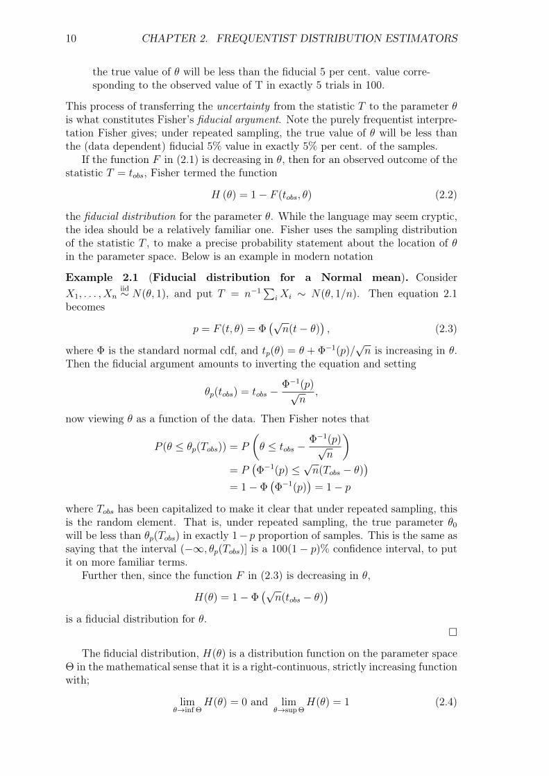
If the function F in (2.1) is decreasing in θ, then for an observed outcome of thestatistic T = tobs, Fisher termed the function
H (θ) = 1− F (tobs, θ) (2.2)
the fiducial distribution for the parameter θ. While the language may seem cryptic,the idea should be a relatively familiar one. Fisher uses the sampling distributionof the statistic T , to make a precise probability statement about the location of θin the parameter space. Below is an example in modern notation
Example 2.1 (Fiducial distribution for a Normal mean). ConsiderX1, . . . , Xn
iid∼ N(θ, 1), and put T = n−1∑
iXi ∼ N(θ, 1/n). Then equation 2.1becomes
p = F (t, θ) = Φ(√
n(t− θ)), (2.3)
where Φ is the standard normal cdf, and tp(θ) = θ + Φ−1(p)/√n is increasing in θ.
Then the fiducial argument amounts to inverting the equation and setting
θp(tobs) = tobs −Φ−1(p)√
n,
now viewing θ as a function of the data. Then Fisher notes that
P (θ ≤ θp(Tobs)) = P
(θ ≤ tobs −
Φ−1(p)√n
)= P
(Φ−1(p) ≤
√n(Tobs − θ)
)= 1− Φ
(Φ−1(p)
)= 1− p
where Tobs has been capitalized to make it clear that under repeated sampling, thisis the random element. That is, under repeated sampling, the true parameter θ0
will be less than θp(Tobs) in exactly 1− p proportion of samples. This is the same assaying that the interval (−∞, θp(Tobs)] is a 100(1− p)% confidence interval, to putit on more familiar terms.
Further then, since the function F in (2.3) is decreasing in θ,
H(θ) = 1− Φ(√
n(tobs − θ))
is a fiducial distribution for θ.
The fiducial distribution, H(θ) is a distribution function on the parameter spaceΘ in the mathematical sense that it is a right-continuous, strictly increasing functionwith;
limθ→inf Θ
H(θ) = 0 and limθ→sup Θ
H(θ) = 1 (2.4)
2.1. FIDUCIAL PROBABILITY AND THE BAYESIAN OMELETTE 11
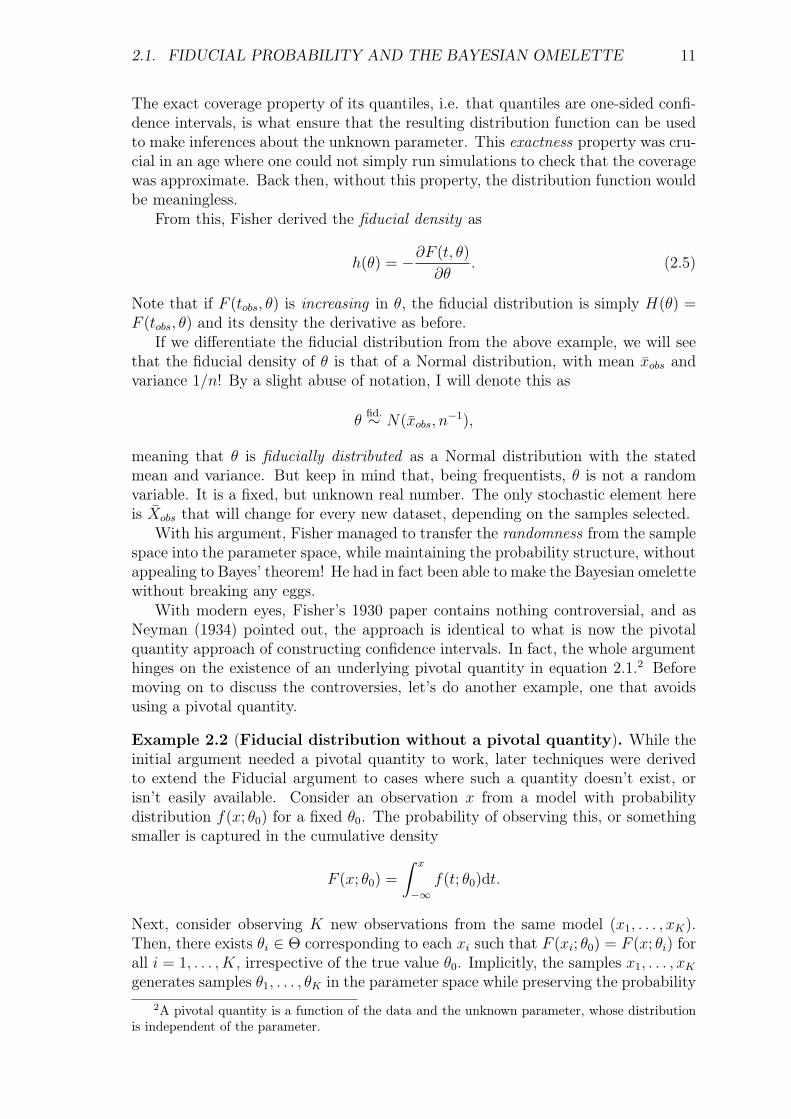
The exact coverage property of its quantiles, i.e. that quantiles are one-sided confi-dence intervals, is what ensure that the resulting distribution function can be usedto make inferences about the unknown parameter. This exactness property was cru-cial in an age where one could not simply run simulations to check that the coveragewas approximate. Back then, without this property, the distribution function wouldbe meaningless.
From this, Fisher derived the fiducial density as
h(θ) = −∂F (t, θ)
∂θ. (2.5)
Note that if F (tobs, θ) is increasing in θ, the fiducial distribution is simply H(θ) =F (tobs, θ) and its density the derivative as before.
If we differentiate the fiducial distribution from the above example, we will seethat the fiducial density of θ is that of a Normal distribution, with mean xobs andvariance 1/n! By a slight abuse of notation, I will denote this as
θfid.∼ N(xobs, n
−1),
meaning that θ is fiducially distributed as a Normal distribution with the statedmean and variance. But keep in mind that, being frequentists, θ is not a randomvariable. It is a fixed, but unknown real number. The only stochastic element hereis Xobs that will change for every new dataset, depending on the samples selected.
With his argument, Fisher managed to transfer the randomness from the samplespace into the parameter space, while maintaining the probability structure, withoutappealing to Bayes’ theorem! He had in fact been able to make the Bayesian omelettewithout breaking any eggs.
With modern eyes, Fisher’s 1930 paper contains nothing controversial, and asNeyman (1934) pointed out, the approach is identical to what is now the pivotalquantity approach of constructing confidence intervals. In fact, the whole argumenthinges on the existence of an underlying pivotal quantity in equation 2.1.2 Beforemoving on to discuss the controversies, let’s do another example, one that avoidsusing a pivotal quantity.
Example 2.2 (Fiducial distribution without a pivotal quantity). While theinitial argument needed a pivotal quantity to work, later techniques were derivedto extend the Fiducial argument to cases where such a quantity doesn’t exist, orisn’t easily available. Consider an observation x from a model with probabilitydistribution f(x; θ0) for a fixed θ0. The probability of observing this, or somethingsmaller is captured in the cumulative density
F (x; θ0) =
∫ x
−∞f(t; θ0)dt.
Next, consider observing K new observations from the same model (x1, . . . , xK).Then, there exists θi ∈ Θ corresponding to each xi such that F (xi; θ0) = F (x; θi) forall i = 1, . . . , K, irrespective of the true value θ0. Implicitly, the samples x1, . . . , xKgenerates samples θ1, . . . , θK in the parameter space while preserving the probability
2A pivotal quantity is a function of the data and the unknown parameter, whose distributionis independent of the parameter.

12 CHAPTER 2. FREQUENTIST DISTRIBUTION ESTIMATORS
structure of the sample space. Then, if we take infinitely many samples x1, x2, . . .we implicitly define a distribution on Θ through the above relationship.
The technique is due to Sprott (1963), and the idea is very much in sync withFisher’s original idea, utilizing the sampling distribution of our data and transferringthe randomness to the parameter space through a function F (x; θ0).
Consider observing xobs from the binomial distribution, Bin(n, p). The cumula-tive density function can be written as
P (X ≤ xobs|p) =
xobs∑x=0
(n
x
)px(1− p)n−x,
or, in terms of the regularized incomplete beta function;
P (X ≤ xobs|p) = (n− xobs)(n
xobs
)∫ 1−p
0
un−xobs−1(1− u)xobsdu.
But, when xobs is considered fixed and p random, this expression is also the cu-mulative distribution function of a Beta distribution with parameters n− xobs andxobs + 1. Thus the fiducial distribution for p given the observation xobs is simply;
pfid.∼ Beta(xobs + 1, n− xobs).
Fisher would not have approved of this distribution, as he did not like the idea ofapplying his Fiducial argument on discrete distributions. The reason is that exactmatching can only be obtained at certain levels of significance. We will return tothis problem in section 4.2
The controversies associated with Fisher’s fiducial inference started in the yearsfollowing the 1930 publication, and was either related to how the fiducial distri-bution should be interpreted, or issues in connection with multiparameter fiducialdistributions.
2.1.1 Interpretation of fiducial distributionsIn his 1930 paper, Fisher stressed that the logical context for fiducial inference wasone of repeated sampling from hypothetical population with a fixed underlying pa-rameter. He was careful to interpret the resulting quantiles and intervals in terms ofwhat we may now recognize as coverage probability. At the same time though, evenin his 1930 paper, he did regard the resulting distribution as a "definite probabil-ity statement about the unknown parameter" (Fisher 1930, p. 533, emhasis added),which surely is problematic given that it is a fixed real number, unless he is invokingan epistemic notion of probability. The reason behind this duality has to do withFisher’s interpretation of probability, which on the one hand was purely aleatory –representing frequencies in a hypothetical infinite population, but at the same timeepistemic – summarizing a rational agent’s degree of belief. He did not make a cleardistinction between these, cf. Zabell (1992).
One of the problems we face when using fiducial inference (as well as confidenceintervals) is that of utilizing two interpretations of probability at once. We areutilizing frequency argumentation and repeated sampling (aleatory probabilities) toestablish what we might deem frequentist properties of fiducial quantiles and inter-vals. That is, by knowing something about the sampling distribution of X we can

2.1. FIDUCIAL PROBABILITY AND THE BAYESIAN OMELETTE 13
construct statements such as P (θ ≤ Tα(X)) = α. Now then, once data is collectedand we have a xobs available for analysis, it is tempting to interpret the interval(−∞, Tα(xobs)] as having probability α of containing the true parameter. But inthe frequentist paradigm, the parameter is considered fixed, so the interval eithercontains θ, or it doesn’t.3 Instead, by careful phrasing, we say that there is a 100α%chance that the interval contains the true parameter. An orthodox frequentist willbe satisfied by this formulation, and not spend too much time worrying if a particu-lar interval calculated from a single sample, actually contains the parameter or not,or how certain he can be that it does. Worrying about these things is closer to anepistemic interpretation of probability, something that isn’t present in frequentisttheory. The problem, stated more generally, is to infer something from the outcomeof a single case, when we only know what happens in the long run – philosophersrefer to this problem as the problem of the single case.
For fiducial inference, it is clear that the distributions themselves can be under-stood in an aleatory sense, but that inferences made from a single distribution mustbe given an epistemic interpretation. In his early writings, Fisher did not spendmuch time on these issues, and he did not find it troublesome to start the analysisby considering θ as a fixed parameter under repeated sampling (aleatory), and thenswitch to an epistemic probability interpretation by the end – now regarding θ asrandom in the epistemic sense, with a fiducial distribution on the parameter space.In addition, he was clear that the resulting epistemic distributions were subject toordinary probability calculus – that a fiducial distribution for θ2 could be foundfrom that of θ by the usual rules. This is not in general true, and fails even in thesimplest cases – Pedersen (1978) proves that the coverage of α-level sets is strictlylarger than α for all θ in a setup similar to that of example 2.1.
2.1.2 Simultaneous fiducial distributions
In Fisher (1935), the fiducial argument is extended to the multiparameter settingby an example. In the paper, the simultaneous fiducial distribution for (µ, σ) ina normal distribution is found from the jointly sufficient statistics (x, s2) using aclever argument via the Student t-distribution.
In the paper, Fisher first derives the fiducial distribution of an additional obser-vation x from the same model, after first having observed (xobs, s
2obs) from an original
sample of size n1.4 He then considers the more general case of observing n2 newobservations from the same model, and deriving a fiducial distribution for (xn2 , s
2n2
)based off of this new sample. Fisher has in mind the two pivotal quantities,
t =xobs − xn2
√n1n2(n1 + n2 − 2)
√n1 + n2
√(n1 − 1)s2
obs + (n2 − 1)s2n2
and z = log(sobs)− log(sn2),
that are functions of the two samples, of which he knows the joint distribution.He then simply substitutes in the expressions of t and z to obtain a joint fiducialdistribution for xn2 and s2
n2. Then, letting n2 →∞, the statistics (xn2 , s
2n2
) convergeto (µ, σ2) and he obtains the joint fiducial distribution for (µ, σ2) given the observedstatistics (xobs, s
2obs).
3This is the source of much confusion.4A predictive fiducial distribution of sorts – analogous to the frequentist predictive intervals.

14 CHAPTER 2. FREQUENTIST DISTRIBUTION ESTIMATORS
Furthermore, he shows that the marginal fiducial distributions of µ and σ, foundsimply by integrating out σ or µ from the joint fiducial, are the fiducial distributionswe would have arrived at by starting from the familiar pivotal quantities:
√n1(µ− xobs)
sobs∼ tn1−1 and
(n1 − 1)s2obs
σ2∼ χ2
n1−1.
From this nicely behaved example he concludes boldly that
. . . it appears that if statistics T1, T2, T3, . . . contain jointly the wholeof the information available respecting parameters θ1, θ2, θ3, . . . and iffunctions t1, t2, t3, . . . of the T ’s and θ’s can be found, the simultaneousdistribution of which is independent of θ1, θ2, θ3, . . . then the fiducial dis-tribution of θ1, θ2, θ3, . . . simultaneously may be found by substitution.(Fisher 1935, p. 395)
. . . an extrapolation that in general isn’t true.Again, Fisher regards the joint fiducial distribution as a regular probability distri-
bution for the unknown parameters. This would entail that the distribution could bereparametrized into a parameter of interest ψ(µ, σ) and a nuisance parameter λ(µ, σ)to obtain the joint fiducial distribution for (ψ, λ). Then λ could be integrated out toobtain the marginal fiducial distribution for ψ. It turns out that this is not true ingeneral, as there is no guarantee that the resulting marginal distributions will havethe correct coverage. Even in this simple case, Pedersen (1978) proved that exactcoverage is only obtained for interest parameters of the form ψ = aµ+ bσ, where aand b are constants.
Another example due to Stein (1959) illustrates that, when treating fiducialdistributions as regular probability distributions, the exact coverage property couldbe lost.
Example 2.3 (The length problem). This slightly artificial example clearly il-lustrates that the fiducial distributions cannot be treated as general probability dis-tributions, obeying standard probability calculus. Let X1, . . . , Xn be independentrandom variables distributed as N(µi, 1) for i = 1, . . . , n. Let the quantity of interestbe∑n
i=1 µ2i , that we wish to obtain a fiducial distribution for. The fiducial distri-
bution of µi from a single observation Xi is simply N(Xi, 1) as µi −Xi ∼ N(0, 1).From standard probability calculus we then have that µ2
ifid.∼ χ2
1(X2i ) where X2
i is anon-centrality parameter. Further, by independence of the observations we have,
n∑i=1
µ2ifid.∼ χ2
n
(n∑i=1
X2i
).
Now then, letting Γn(·, λ) denote the cdf of a non-central chi-squared distributionwith n degrees of freedom and non-centrality parameter λ, and Γ−1
n (·, λ) its inverse,a natural one-sided α-level fiducial interval is simply[
Γ−1n (1− α,
n∑i=1
X2i ),∞
).
Stein (1959) proved that the coverage probability of this interval, for any value ofα can be made smaller than any ε > 0 simply by choosing a sufficiently large n.
2.1. FIDUCIAL PROBABILITY AND THE BAYESIAN OMELETTE 15
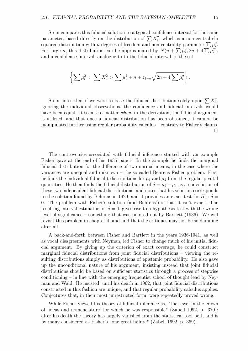
Stein compares this fiducial solution to a typical confidence interval for the sameparameter, based directly on the distribution of
∑X2i , which is a non-central chi
squared distribution with n degrees of freedom and non-centrality parameter∑µ2i .
For large n, this distribution can be approximated by N(n +∑µ2i , 2n + 4
∑µ2i ),
and a confidence interval, analogue to to the fiducial interval, is the set
∑µ2i :
∑X2i >
∑µ2i + n+ z1−α
√2n+ 4
∑µ2i
.
Stein notes that if we were to base the fiducial distribution solely upon∑X2i ,
ignoring the individual observations, the confidence and fiducial intervals wouldhave been equal. It seems to matter when, in the derivation, the fiducial argumentis utilized, and that once a fiducial distribution has been obtained, it cannot bemanipulated further using regular probability calculus – contrary to Fisher’s claims.
The controversies associated with fiducial inference started with an exampleFisher gave at the end of his 1935 paper. In the example he finds the marginalfiducial distribution for the difference of two normal means, in the case where thevariances are unequal and unknown – the so-called Behrens-Fisher problem. Firsthe finds the individual fiducial t-distributions for µ1 and µ2 from the regular pivotalquantities. He then finds the fiducial distribution of δ = µ2−µ1 as a convolution ofthese two independent fiducial distributions, and notes that his solution correspondsto the solution found by Behrens in 1929, and it provides an exact test for H0 : δ =0. The problem with Fisher’s solution (and Behrens’) is that it isn’t exact. Theresulting interval estimator for δ = 0, gives rise to a hypothesis test with the wronglevel of significance – something that was pointed out by Bartlett (1936). We willrevisit this problem in chapter 4, and find that the critiques may not be so damningafter all.
A back-and-forth between Fisher and Bartlett in the years 1936-1941, as wellas vocal disagreements with Neyman, led Fisher to change much of his initial fidu-cial argument. By giving up the criterion of exact coverage, he could constructmarginal fiducial distributions from joint fiducial distributions – viewing the re-sulting distributions simply as distributions of epistemic probability. He also gaveup the unconditional nature of his argument, insisting instead that joint fiducialdistributions should be based on sufficient statistics through a process of stepwiseconditioning – in line with the emerging frequentist school of thought lead by Ney-man and Wald. He insisted, until his death in 1962, that joint fiducial distributionsconstructed in this fashion are unique, and that regular probability calculus applies.Conjectures that, in their most unrestricted form, were repeatedly proved wrong.
While Fisher viewed his theory of fiducial inference as, "the jewel in the crownof ’ideas and nomenclature’ for which he was responsible" (Zabell 1992, p. 370);after his death the theory has largely vanished from the statistical tool belt, and isby many considered as Fisher’s "one great failure" (Zabell 1992, p. 369).

16 CHAPTER 2. FREQUENTIST DISTRIBUTION ESTIMATORS
2.2 Generalized Fiducial Inference and fiducialrevival
In recent years, there has been a resurgence of ideas in the spirit of Fisher’s fiducialargument. The defining feature of these approaches is in line with Fisher’s goal;obtaining inferentially meaningful probability statements on the parameter space,often in the shape of a distribution, without introducing subjective prior infor-mation. These approaches include the Dempster–Shafer theory of belief-functions,confidence distributions (that will be introduced later), and the inferential modelapproach by Martin & Liu (2015).
A particularly well-developed approach is that of generalized fiducial inference(GFI) (Hannig 2009, Hannig et al. 2016), which in the one-parameter case is iden-tical to Fisher’s initial argument, but extends and generalizes to multi-parameterproblems.
The starting point of the GFI approach is to define a data-generating equation,say
X = G(U ,θ), (2.6)
where θ is the unknown parameter and U is a random element with a completelyknown distribution which is independent of θ. We imagine that the data at hand iscreated by drawing U at random from its distribution, and plugging it into the datagenerating equation. In the easiest example, where X is iid. normally distributedwith mean µ and variance σ2, we can write X = G(U ,θ) = µ + σU where U is avector of iid. N(0, 1) random variables, and θT = (µ σ).
Now, assuming the data-generating equation has an inverse Qy(u) = θ for anyobserved y and any arbitrary u – Fisher’s initial fiducial argument simply amountsto finding the distribution of Qy(U ∗) for an independent copy U ∗ of the original Uused to generate the data. Samples from the fiducial distribution can be obtained bysimulating u∗1, . . . ,u∗n and plugging them into the equation. Notice the similaritiesto example 2.2 here. The existence of this inverse means that transferring therandomness from the sample space, into the parameter space can be done in a niceway, which was always the case in Fisher’s examples. But in order to generalize andextend Fisher’s initial argument, one needs to consider the case where this mightnot be as easy.
To obtain a more general solution, there are some technical difficulties one needsto sort out. First off, there is no guarantee that the inverse function Qy(u) = θeven exists. The point being that the set, θ : y = G(u,θ), for a given y and u,could be either empty or contain more than one value of θ. If the set is empty, thesuggested solution is to restrict the distribution of U to a subset where solutionsdo exist, and renormalize the distribution of U on this set. The rationale behindthis method is that, the data must have come from some value of U for a given,but unknown, θ0. However, as Hannig et al. (2016) notes, the set where solutionsdo exist, will typically have measure zero, and conditioning on a set of measure zerocan lead to strange results.5 In any case, care must be taken.
In the case where there are more than one value of the parameter that solvesequation 2.6 for given values of u and y, Hannig et al. (2016) suggests choosing
5Due to the Borel-Kolmogorov paradox, see e.g. Jaynes (2003, sec. 15.7)
2.2. GENERALIZED FIDUCIAL INFERENCE AND FIDUCIAL REVIVAL 17
one of the values, possibly with some sort of random mechanism. They give someexamples that show that the extra uncertainty introduced by this mechanism doesn’tdisturb the final inference much.
Delving too far into these technical details is beyond the scope of this subsection,but it’s worth noting that extending Fisher’s initially simple argument, is far fromeasy. It turns out though, that under fairly mild regularity assumptions, a simpleexpression can be found for the generalized fiducial density.
Definition 2.1 (Generalized Fiducial Density (GFD)). If θ ∈ Θ ⊂ Rp andx ∈ Rn, then under mild regularity assumptions, cf. Hannig et al. (2016, AppendixA), the generalized fiducial density for θ is of the form
r(θ|x) =f(x,θ)J(x,θ)∫
Θf(x,θ′)J(x,θ′)dθ′
, (2.7)
where f(x,θ) is the likelihood, and
J(x,θ) = D
(∂
∂θG(u,θ)
∣∣∣∣u=G−1(x,θ)
).
If (i) n = p then D(A) = |detA|, otherwise the function will depend on the whichnorm is used; (ii) the L∞-norm yields D(A) =
∑i=(i1,...,ip) |detAi|; (iii) under the
L2-norm, if the entries, ∂∂θG(u,θ), all have continuous partial derivatives for all θ
and all u, then D(A) =(detATA
)1/2.
The statement in equation 2.7 is, in a way a normalized likelihood, but withan added Jacobian to make sure that the resulting distribution function is properover the parameter space – it has a certain Bayesian flavour, as illustrated in thefollowing example from Hannig et al. (2016, p. 1350)
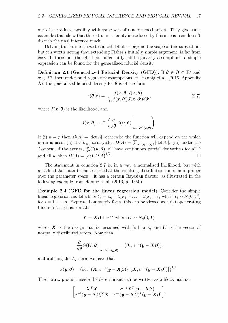
Example 2.4 (GFD for the linear regression model). Consider the simplelinear regression model where Yi = β0 + β1x1 + . . . + βpxp + εi where εi ∼ N(0, σ2)for i = 1, . . . , n. Expressed on matrix form, this can be viewed as a data-generatingfunction á la equation 2.6,
Y = Xβ + σU where U ∼ Nn(0, I),
where X is the design matrix, assumed with full rank, and U is the vector ofnormally distributed errors. Now then,
∂
∂θG(U ,θ)
∣∣∣∣u=G−1(y,θ)
= (X, σ−1(y −Xβ)),
and utilizing the L2 norm we have that
J(y,θ) =(det[(X, σ−1(y −Xβ))T (X, σ−1(y −Xβ))
])1/2.
The matrix product inside the determinant can be written as a block matrix,[XTX σ−1XT (y −Xβ)
σ−1(y −Xβ)TX σ−2(y −Xβ)T (y −Xβ)
],
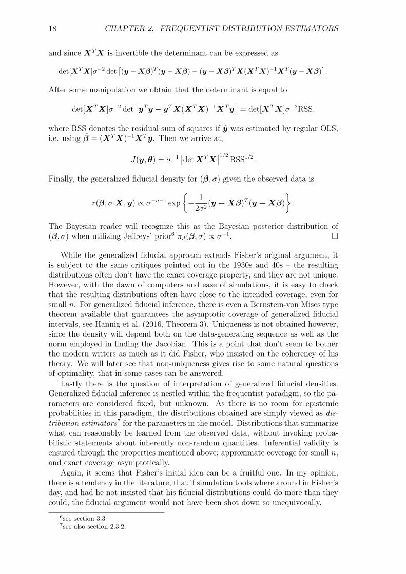
18 CHAPTER 2. FREQUENTIST DISTRIBUTION ESTIMATORS
and since XTX is invertible the determinant can be expressed as
det[XTX]σ−2 det[(y −Xβ)T (y −Xβ)− (y −Xβ)TX(XTX)−1XT (y −Xβ)
].
After some manipulation we obtain that the determinant is equal to
det[XTX]σ−2 det[yTy − yTX(XTX)−1XTy
]= det[XTX]σ−2RSS,
where RSS denotes the residual sum of squares if y was estimated by regular OLS,i.e. using β = (XTX)−1XTy. Then we arrive at,
J(y,θ) = σ−1∣∣detXTX
∣∣1/2 RSS1/2.
Finally, the generalized fiducial density for (β, σ) given the observed data is
r(β, σ|X,y) ∝ σ−n−1 exp
− 1
2σ2(y−Xβ)T (y−Xβ)
.
The Bayesian reader will recognize this as the Bayesian posterior distribution of(β, σ) when utilizing Jeffreys’ prior6 πJ(β, σ) ∝ σ−1.
While the generalized fiducial approach extends Fisher’s original argument, itis subject to the same critiques pointed out in the 1930s and 40s – the resultingdistributions often don’t have the exact coverage property, and they are not unique.However, with the dawn of computers and ease of simulations, it is easy to checkthat the resulting distributions often have close to the intended coverage, even forsmall n. For generalized fiducial inference, there is even a Bernstein-von Mises typetheorem available that guarantees the asymptotic coverage of generalized fiducialintervals, see Hannig et al. (2016, Theorem 3). Uniqueness is not obtained however,since the density will depend both on the data-generating sequence as well as thenorm employed in finding the Jacobian. This is a point that don’t seem to botherthe modern writers as much as it did Fisher, who insisted on the coherency of histheory. We will later see that non-uniqueness gives rise to some natural questionsof optimality, that in some cases can be answered.
Lastly there is the question of interpretation of generalized fiducial densities.Generalized fiducial inference is nestled within the frequentist paradigm, so the pa-rameters are considered fixed, but unknown. As there is no room for epistemicprobabilities in this paradigm, the distributions obtained are simply viewed as dis-tribution estimators7 for the parameters in the model. Distributions that summarizewhat can reasonably be learned from the observed data, without invoking proba-bilistic statements about inherently non-random quantities. Inferential validity isensured through the properties mentioned above; approximate coverage for small n,and exact coverage asymptotically.
Again, it seems that Fisher’s initial idea can be a fruitful one. In my opinion,there is a tendency in the literature, that if simulation tools where around in Fisher’sday, and had he not insisted that his fiducial distributions could do more than theycould, the fiducial argument would not have been shot down so unequivocally.
6see section 3.37see also section 2.3.2.
2.3. THE CONFIDENCE DISTRIBUTION 19
2.3 The Confidence DistributionAnother approach to modern fiducial inference is that of confidence distributions(CDs), as laid out in the review paper by Xie & Singh (2013), the book by Schweder& Hjort (2016), or Schweder & Hjort (2017). This approach follows the strictlyNeymanian interpretation of the fiducial argument; as a method for constructingconfidence intervals, and the resulting distributions are interpreted as distributionsof coverage probability. That is, if C(θ) is a CD for θ, any data-dependent setKα(x) ⊂ Θ satisfying
P (θ ∈ Kα(x)) =
∫Θ
1Kα(x) dC(θ) = α, (2.8)
carries the interpretation that, under repeated sampling, the set Kα(x) will containthe true parameter value in approximately 100α% of samples. The probability inthis statement is over the sample space, and so far we are in line with Fisher’sfiducial argument. The difference between CDs and fiducial distributions is mostlyin their interpretation.
As previously discussed, Fisher would start his analysis by treating the parameteras a fixed, unknown quantity – his probability was frequentist, and the stochasticitywas in the sample space. Once the data was collected, and the fiducial distribution inplace, he would now consider the parameter as being random in the epistemic sense,and regard his distribution as an epistemic probability distribution of the parameter.Through this argumentation he obtained a proper probability distribution on theparameter space, without needing to invoke subjective prior information. We’veseen that this does not always work as intended. The CDs, on the other hand, doesnot have this final interpretation. They are instead considered simply as a collectionof confidence statements about the unknown parameter, given the collected data –not as a distribution of the parameter itself. A useful distinction is made by Xie &Singh (2013, p. 7):
a confidence distribution is viewed as an estimator for the parameter ofinterest, instead of an inherent distribution of the parameter.
This places some restrictions on the theory, notably that CDs are one-dimensional.A general theory for defining multi-parameter confidence sets with exact coverage,is as far as I know still an open problem in the world of statistics.
Cox (1958) was the first to invoke the term confidence distribution when compar-ing Fisher’s fiducial distribution to the Neymanian confidence intervals. He notedthat the difference between the two is mostly due to presentation, and there is noreason to limit the Neymanian approach to only intervals on the parameter space.Instead he suggested constructing the set of all confidence intervals at each level ofprobability α to obtain a distribution on the parameter space, and he called this aconfidence distribution.
One method of creating a confidence distribution is by inverting the upper limitsof one-sided confidence intervals. That is, given the outcome of an experiment x,if (−∞, K(α,x)] is a valid one-sided α-level confidence interval for θ, and K(α,x)is strictly increasing in α for any sample x, one could invert the upper endpointsto obtain the confidence distribution F (θ) = K−1(θ) keeping x fixed. The resultingfunction is in fact a distribution function on the parameter space, obtained by care-fully shifting the uncertainty from the sample space to the parameter space in the
20 CHAPTER 2. FREQUENTIST DISTRIBUTION ESTIMATORS
same fashion as Fisher’s initial fiducial argument. In addition, since it is constructedfrom exact confidence intervals, all subsets will have the specified coverage probabil-ity — again exactly like Fisher’s 1930 argument. But there is no fiducial reasoninginvolved; Cox stressed that the resulting distribution is inherently frequentist. Andwhile it is tempting to interpret statements such as P (θ ≤ K(α,x)) = α as a defi-nite probability statement about the parameter, this is logically wrong because thestatement θ ≤ c for a given constant c, is either true or false.
A more modern definition of confidence distributions, and one not relying oninverting upper endpoints of confidence intervals is found in Xie & Singh (2013).
Definition 2.2 (Confidence Distribution). A function Cn(·) = Cn(x, ·) onX ×Θ→ [0, 1] is called a confidence distribution (CD) for a parameter θ if
i. For each x ∈ X , Cn(·) is a cumulative distribution function on Θ.
ii. At the true parameter value θ = θ0, Cn(θ0) := Cn(x, θ0), as a function of thesample x, follows the uniform distribution U(0, 1).
If the uniformity requirement only holds asymptotically, C(·) is an asymptotic con-fidence distribution (aCD).
The crux in the definition is requirement (ii.) that ensure exact coverage of thespecified subsets. Analogue to Fisher in his 1930 paper, we will call the derivative(when it exists) the confidence density and denote it in lower-case: cn(θ) = C ′n(θ).Sometimes the CDs will have the subscript n to indicate their dependence on thenumber of observations, sometimes it is omitted.
As noted before, one of the reasons why fiducial inference was considered a failurein its time was due to the non-uniqueness of the distributions and marginalizationissues, but also because Fisher insisted that the theory could do more than it actuallycould. The CD theory does not fix any of these issues, but the goal isn’t to "derive anew fiducial theory that is paradox free" (Xie & Singh 2013, p. 4), but instead workwithin the limitations of the theory. It is easy to check that the fiducial distributionin example 2.1 is an exact confidence distribution, most one-dimensional fiducialdistributions are. As for marginalization issues, the marginal distributions foundfrom joint fiducial distributions are often approximate confidence distributions, seefor example the Behrens-Fisher problem in chapter 4. Non-uniqueness isn’t reallya concern either, but leads instead to some natural optimality considerations, seesection 2.3.3.
2.3.1 Constructing CDs
The re-framing of Fisher’s fiducial argument strictly in terms of confidence opensup a bunch of tools for the theory, allowing it to become a natural part of thefrequentist inferential toolbox, and to draw on techniques developed in the last 100years of frequentist theory. In this section I will outline two ways to a confidencedistribution.
By way of a pivotal quantity :The typical, and somewhat canonical way of constructing a CD, is by a pivotalquantity. That is, a function of the data and parameter of interest ψ = a(θ) whosedistribution is independent of the underlying parameters in the model, θ. We’ve

2.3. THE CONFIDENCE DISTRIBUTION 21
already done this in example 2.1, without being explicit about where the pivotalquantity came into play. The technique goes as follows:
Let piv(ψ,X) be a pivotal quantity that is increasing in ψ, and let G(·) de-note the cumulative density function of the pivotal quantity’s sampling distribution.Then, a natural CD for ψ is simply C(ψ) = G(piv(ψ,X)). Analogous, if the pivotis decreasing in ψ, the natural CD is C(ψ) = 1−G(piv(ψ,X)). It is quite easy tocheck that the resulting distribution has a uniform distribution when evaluated atthe true value ψ0 – due to the probability transform.
Example 2.5 (Example 2.1 cont.). Consider again the setup from example 2.1,where T = n−1
∑Xi ∼ N(θ, 1/n). Then a pivotal quantity that is increasing in θ is
Z =√n(θ − X),
which has a standard normal distribution. This means that a confidence distributionfor θ, given observed data xobs is available as
C(θ) = Φ(√
n(θ − xobs)).
Which is also the fiducial distribution we would have arrived at.
By way of ML-theory :Via maximum likelihood theory, there is often an easy way to find an approximateconfidence distribution for a parameter of interest.
Example 2.6 (Approximate CD using ML-theory). Let X1, . . . , Xn be iid.Bernoulli distributed variables, i.e. Bin(1, p). The maximum likelihood estimatorfor p is p = x, which, by the nice properties of ML-estimators, is asymptoticallynormally distributed with mean p and variance p(1−p)/n. By consistency of p (andSlutsky’s Theorem), this means that
Z =
√n(p− p)√p(1− p)
→ N(0, 1),
i.e. Z is asymptotically a pivotal quantity, increasing in p, and thus an approximateCD is directly available as
C(p) = Φ
(√n(p− p)√p(1− p)
).
This technique opens up a wide spectre of possibilities for the CD theory. It isfor example of interest to study how fast the convergence to normality is, and if firstorder approximations can be improved upon. Endeavors in this direction is outlinedin Schweder & Hjort (2016, ch. 7).
2.3.2 Inference with CDs
As discussed in the introduction, having the uncertainties fully represented by adistribution is quite nice. Distributions contain a wealth of information about the
22 CHAPTER 2. FREQUENTIST DISTRIBUTION ESTIMATORS
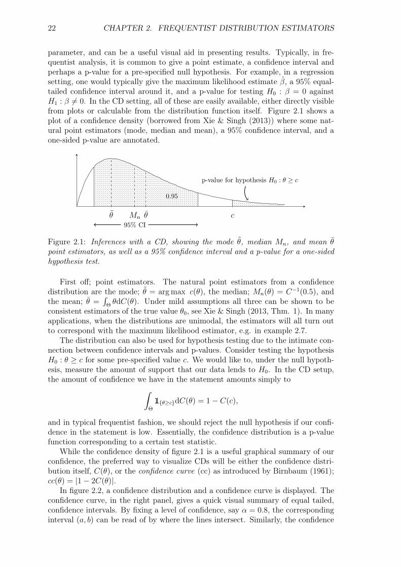
parameter, and can be a useful visual aid in presenting results. Typically, in fre-quentist analysis, it is common to give a point estimate, a confidence interval andperhaps a p-value for a pre-specified null hypothesis. For example, in a regressionsetting, one would typically give the maximum likelihood estimate β, a 95% equal-tailed confidence interval around it, and a p-value for testing H0 : β = 0 againstH1 : β 6= 0. In the CD setting, all of these are easily available, either directly visiblefrom plots or calculable from the distribution function itself. Figure 2.1 shows aplot of a confidence density (borrowed from Xie & Singh (2013)) where some nat-ural point estimators (mode, median and mean), a 95% confidence interval, and aone-sided p-value are annotated.
θ Mn θ c
p-value for hypothesis H0 : θ ≥ c
95% CI
0.95
Figure 2.1: Inferences with a CD, showing the mode θ, median Mn, and mean θpoint estimators, as well as a 95% confidence interval and a p-value for a one-sidedhypothesis test.
First off; point estimators. The natural point estimators from a confidencedistribution are the mode; θ = arg max c(θ), the median; Mn(θ) = C−1(0.5), andthe mean; θ =
∫ΘθdC(θ). Under mild assumptions all three can be shown to be
consistent estimators of the true value θ0, see Xie & Singh (2013, Thm. 1). In manyapplications, when the distributions are unimodal, the estimators will all turn outto correspond with the maximum likelihood estimator, e.g. in example 2.7.
The distribution can also be used for hypothesis testing due to the intimate con-nection between confidence intervals and p-values. Consider testing the hypothesisH0 : θ ≥ c for some pre-specified value c. We would like to, under the null hypoth-esis, measure the amount of support that our data lends to H0. In the CD setup,the amount of confidence we have in the statement amounts simply to∫
Θ
1θ≥cdC(θ) = 1− C(c),
and in typical frequentist fashion, we should reject the null hypothesis if our confi-dence in the statement is low. Essentially, the confidence distribution is a p-valuefunction corresponding to a certain test statistic.
While the confidence density of figure 2.1 is a useful graphical summary of ourconfidence, the preferred way to visualize CDs will be either the confidence distri-bution itself, C(θ), or the confidence curve (cc) as introduced by Birnbaum (1961);cc(θ) = |1− 2C(θ)|.
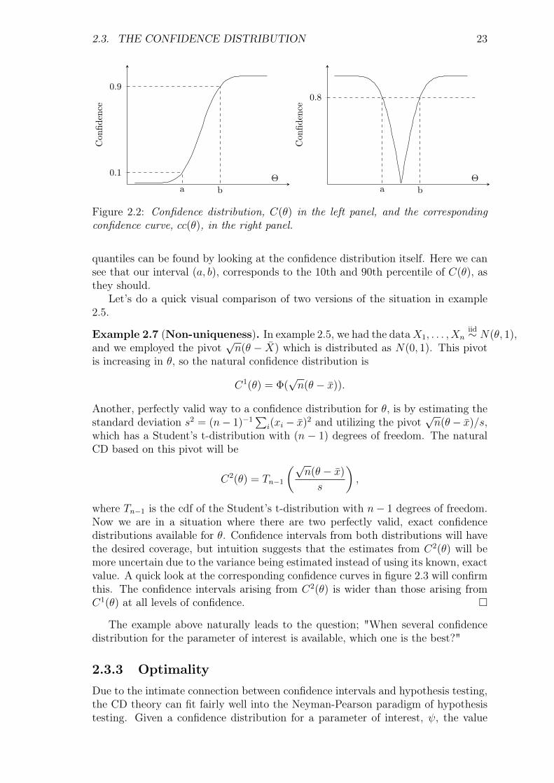
In figure 2.2, a confidence distribution and a confidence curve is displayed. Theconfidence curve, in the right panel, gives a quick visual summary of equal tailed,confidence intervals. By fixing a level of confidence, say α = 0.8, the correspondinginterval (a, b) can be read of by where the lines intersect. Similarly, the confidence
2.3. THE CONFIDENCE DISTRIBUTION 23
0.1
0.9
Θa b
Con
fidence
0.8
Θa b
Con
fidence
Figure 2.2: Confidence distribution, C(θ) in the left panel, and the correspondingconfidence curve, cc(θ), in the right panel.
quantiles can be found by looking at the confidence distribution itself. Here we cansee that our interval (a, b), corresponds to the 10th and 90th percentile of C(θ), asthey should.
Let’s do a quick visual comparison of two versions of the situation in example2.5.
Example 2.7 (Non-uniqueness). In example 2.5, we had the dataX1, . . . , Xniid∼ N(θ, 1),
and we employed the pivot√n(θ − X) which is distributed as N(0, 1). This pivot
is increasing in θ, so the natural confidence distribution is
C1(θ) = Φ(√n(θ − x)).
Another, perfectly valid way to a confidence distribution for θ, is by estimating thestandard deviation s2 = (n− 1)−1
∑i(xi − x)2 and utilizing the pivot
√n(θ− x)/s,
which has a Student’s t-distribution with (n − 1) degrees of freedom. The naturalCD based on this pivot will be
C2(θ) = Tn−1
(√n(θ − x)
s
),
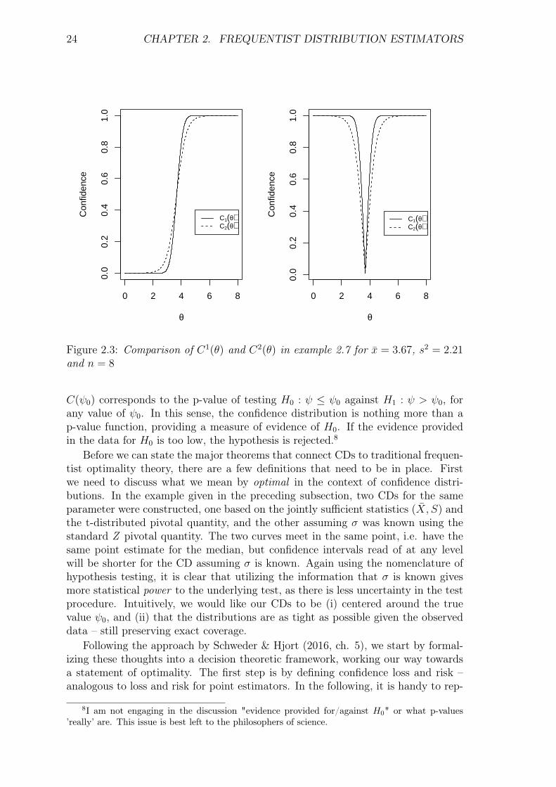
where Tn−1 is the cdf of the Student’s t-distribution with n− 1 degrees of freedom.Now we are in a situation where there are two perfectly valid, exact confidencedistributions available for θ. Confidence intervals from both distributions will havethe desired coverage, but intuition suggests that the estimates from C2(θ) will bemore uncertain due to the variance being estimated instead of using its known, exactvalue. A quick look at the corresponding confidence curves in figure 2.3 will confirmthis. The confidence intervals arising from C2(θ) is wider than those arising fromC1(θ) at all levels of confidence.
The example above naturally leads to the question; "When several confidencedistribution for the parameter of interest is available, which one is the best?"
2.3.3 OptimalityDue to the intimate connection between confidence intervals and hypothesis testing,the CD theory can fit fairly well into the Neyman-Pearson paradigm of hypothesistesting. Given a confidence distribution for a parameter of interest, ψ, the value
24 CHAPTER 2. FREQUENTIST DISTRIBUTION ESTIMATORS
0 2 4 6 8
0.0
0.2
0.4
0.6
0.8
1.0
θ
Con
fiden
ce
C1(θ)C2(θ)
0 2 4 6 80.
00.
20.
40.
60.
81.
0
θ
Con
fiden
ce
C1(θ)C2(θ)
Figure 2.3: Comparison of C1(θ) and C2(θ) in example 2.7 for x = 3.67, s2 = 2.21and n = 8
C(ψ0) corresponds to the p-value of testing H0 : ψ ≤ ψ0 against H1 : ψ > ψ0, forany value of ψ0. In this sense, the confidence distribution is nothing more than ap-value function, providing a measure of evidence of H0. If the evidence providedin the data for H0 is too low, the hypothesis is rejected.8
Before we can state the major theorems that connect CDs to traditional frequen-tist optimality theory, there are a few definitions that need to be in place. Firstwe need to discuss what we mean by optimal in the context of confidence distri-butions. In the example given in the preceding subsection, two CDs for the sameparameter were constructed, one based on the jointly sufficient statistics (X, S) andthe t-distributed pivotal quantity, and the other assuming σ was known using thestandard Z pivotal quantity. The two curves meet in the same point, i.e. have thesame point estimate for the median, but confidence intervals read of at any levelwill be shorter for the CD assuming σ is known. Again using the nomenclature ofhypothesis testing, it is clear that utilizing the information that σ is known givesmore statistical power to the underlying test, as there is less uncertainty in the testprocedure. Intuitively, we would like our CDs to be (i) centered around the truevalue ψ0, and (ii) that the distributions are as tight as possible given the observeddata – still preserving exact coverage.
Following the approach by Schweder & Hjort (2016, ch. 5), we start by formal-izing these thoughts into a decision theoretic framework, working our way towardsa statement of optimality. The first step is by defining confidence loss and risk –analogous to loss and risk for point estimators. In the following, it is handy to rep-
8I am not engaging in the discussion "evidence provided for/against H0" or what p-values’really’ are. This issue is best left to the philosophers of science.
2.3. THE CONFIDENCE DISTRIBUTION 25
resent the confidence distribution by a random variable ψCD, that might be viewedas a random draw from the CD after data has been collected – analogous to a drawfrom the Bayesian posterior distribution.
Definition 2.3 (Confidence loss and risk). Let Γ be a, non-negative functionover R, with Γ(0) = 0. The confidence loss at θ of the CD C(ψ,y), with respect tothe penalty function Γ, where ψ = a(θ) is a focus parameter, is
lo(θ, C) =
∫Γ(ψ′ − ψ)dC(ψ′,y) = EΓ(ψCD − ψ).
The risk is then the expectation of this taken over the data Y under parametervalue θ
R(θ, C) = Eθ lo(θ, C) = EθEΓ(ψCD − ψ).
That is, we extend the notion of ’loss’ for a single point by taking its expectationwith regards to the confidence distribution. Then, we define risk by taking theexpectation again, this time with respect to the data.
Under squared error loss, i.e. Γ(z) = z2, the confidence loss become
lo(θ, C) = Var ψCD + (EψCD − ψ)2
i.e the sum of the variance of C(ψ) and the squared estimation error. We recognizenow that minimizing confidence loss is connected to our two wishes for an optimalCD – that it be tight (variance term small), and centered near, or at, the true valueof ψ (estimation error small, preferably zero).
Now consider two confidence distributions for the same interest parameter, basedon two different statistics S and T , denote these CDs by C(ψ, S) = CS andC(ψ, T ) = CT respectively. By comparing loss and risks of the two CDs, we areable to answer the question of which distribution is best – and also extend someoptimality theorems from the uniformly most powerful (UMP) testing theory. Weneed two more definitions before the main theorems can be stated.
The first definition concerns itself with a notion of uniform optimality, i.e. thatone confidence distribution is better than another, at all values of the true parameter.
Definition 2.4 (Uniform optimality). A confidence distribution CS is uniformlyoptimal if for each penalty function Γ, non-increasing on the negative half-axisand non-decreasing on the positive, with Γ(0) = 0, and for any other confidencedistribution CT ,
lo(ψ0, CS) ≤ lo(ψ0, C
T )
almost surely, for every value of ψ0. If, on the other hand, we only have
R(ψ0, CS) ≤ R(ψ0, C
T ),
for every value of ψ0, we say that CS is uniformly optimal in the mean.

26 CHAPTER 2. FREQUENTIST DISTRIBUTION ESTIMATORS
Note that the confidence loss is stochastic, as it will depend on the specific datapoint, yobs, we are constructing the CD on – hence the almost surely statement inthe definition.
We also need the notion of monotone likelihood ratio (MLR) in order for our CDsto be connected to regular UMP theory, see for example Casella & Berger (2002,ch. 8).
Definition 2.5 (Monotone Likelihood Ratio (MLR)). Let T be a statistic witha distribution indexed by a real-valued parameter θ, e.g. p(t|θ). This distributionhas a monotone likelihood ratio (MLR) of, for every θ2 > θ1, g(t|θ2)/g(t|θ1) is anon-decreasing function of t on the set t : g(t|θ1) > 0 or g(t|θ2) > 0.
We are now ready to state the first of two theorems, this one concerning theuse of sufficient statistics and confidence distributions. The theorem confirms ourintuition from UMP testing theory, that CDs constructed on the basis of a sufficientstatistic will perform better than CDs based on any other statistic.
Theorem 2.1 (Rao-Blackwell for confidence distributions). If the pivotalquantity has the same functional form in a statistic T , as in a sufficient statisticS, and if both the pivot and confidence quantile are convex in the statistic, theconfidence distribution based on S is uniformly as good in the mean.
As it stands, the theorem is somewhat limited, needing convexity and only com-paring pivotal quantities of the same functional form. Intuition tells us that thisshould hold in wider generality9, but the theory is complicated by the fact that CDsdo not obey regular probability calculus.
Finally, the main optimality theorem will be stated, which is a Neyman-Pearsontype theorem for confidence distributions.
Theorem 2.2 (Neyman-Pearson for confidence distributions). A confidencedistribution based on a sufficient statistic in which the likelihood ratio is everywhereincreasing, is uniformly optimal.
This statement is far more powerful than theorem 2.1, since it is a statement ofuniform optimality, not simply optimality in the mean – in addition it is stated infull generality. The proof of this theorem, as well as the proof for Rao-Blackwell isfound in Schweder & Hjort (2016, ch. 5), and I will not go into the details of them,but a heuristic explanation can be done for the Neyman-Pearson result.
Recall that the Neyman-Pearson lemma for composite hypothesis10 states that,if we are using a sufficient statistic S, whose distribution has an MLR, to test thehypothesis H0 : ψ ≤ ψ0 versus H1 : ψ > ψ0. Then, any test that rejects H0 if, andonly if, S > s0, is a UMP level α test, where α = Pψ0(S > s0), i.e. the probabilityof this happening under the null. The p-value function of this test, is precisely theconfidence distribution created on the basis of the same sufficient statistic, usingthe observed value of sobs.
9cf. Schweder & Hjort (2016, exercise 5.9)10Sometimes called the Karlin-Rubin theorem, see for example Casella & Berger (2002, ch. 8)
2.3. THE CONFIDENCE DISTRIBUTION 27
2.3.4 Uniform Optimality in the exponential familyThe exponential family of distributions has certain properties that make it especiallyamenable to the optimality theorem in the past section. Proofs of the statementsin the following paragraph can be found in for example Lehmann & Romano (2005,ch. 2-4).
A distribution is a member of the exponential family if its density can be writtenas,
f(x|θ) = h(x)c(θ) exp
k∑i=1
wi(θ)ti(x)
. (2.9)
The set of parameters (η1, . . . , ηk) = (w1(θ), . . . , wk(θ)) are called the natural pa-rameters of the family, and a characterization of the exponential family in termsof these yield the same structure as above, except for a change in the c(θ) term.If X1, . . . , Xn is a sample from a distribution with density (2.9), the joint distri-bution of the Xi’s is also a member of the exponential family, and the statistics(∑n
i=1 t1(Xi), . . . ,∑n
i=1 tk(Xi)) are jointly sufficient for the natural parameters.If we have an exponential family of the form
f(S,A|ψ,λ) = h(S,A)c(ψ,λ) exp
ψS(X) +
p∑i=1
λiAi(X)
, (2.10)
then the conditional distribution of S given A, is also an exponential family –whose distribution is independent of λ. The statistics (S,A) are jointly sufficientfor (ψ,λ), and S is sufficient for ψ for any fixed value of A, i.e. A is ancillary.Lastly, all members of the exponential family has the MLR property, cf. definition2.5.
Then, there exists UMP tests for testing hypothesis of the form H0 : ψ ≤ ψ0
vs. H1 : ψ > ψ0, and by the theory from the last section, there also exists anoptimal confidence distribution. We have the following theorem from Schweder &Hjort (2016, Thm. 5.11)
Theorem 2.3 (Optimal CDs for exponential families). Let ψ be a scalarparameter of interest, and λ a p-dimensional vector of nuisance parameters in acontinuous exponential model, with density
f(x, ψ,λ) = h(x) exp
ψS(x) +
p∑i=1
λiAi(x)− k(ψ, λ1, . . . , λp)
,
for data vector x in a sample space independent of the parameters. Assume (ψ,λ)is contained in an open (p+ 1)-dimensional parameter set. Then
CS|A(ψ) = Pψ (S > sobs|A = aobs)
is the uniformly most powerful confidence distribution for ψ.
This theorem provides a quick and easy recipe for finding optimal CDs for aparameter of interest, and an effective way of dealing with nuisance parameters – ina large family of distributions.
Sometimes, the conditional distribution of S given A is available in closed form,but often it will need to be simulated by an MCMC type algorithm.
Let’s do two quick examples to illustrate the theorem.

28 CHAPTER 2. FREQUENTIST DISTRIBUTION ESTIMATORS
Example 2.8 (Normal distribution). Let’s first check that the example that hasfollowed us through this chapter is optimal. We had data X1, . . . , Xn
iid∼ N(θ, 1),which makes the joint distribution
f(x|θ) ∝ exp
−1
2
n∑i=1
(Xi − θ)2
∝ exp
θ
n∑i=1
Xi − nθ2/2
,
which is of the form from Theorem 2.3 – with S(x) =∑Xi. Hence, an optimal
confidence distribution is by
P (∑
Xi >∑
xi,obs) =P (X > xobs),
which is course is the same distribution we based our original CD on – since X ∼N(θ, 1/n).
Of course, the power in this theorem first becomes visible when there are nuisanceparameters present in the model.
Example 2.9 (Normal with nuisance parameter). Let X ∼ N(µ, 1) and Y ∼N(µ+ ψ, 1), where X and Y are independent. The joint distribution is of the form
f(x, y|µ, ψ) ∝ exp
−1
2
[(x− µ)2 + (y − (µ+ ψ))2
]∝ exp yψ + (x+ y)µ− k(µ, ψ) ,
which is of the form of the theorem. A uniformly optimal CD for ψ is simply by
C(ψ) = P (Y > yobs|X + Y = xobs + yobs)
= P (Y −X > yobs − xobs|X + Y = xobs + yobs)
= P (Y −X > yobs − xobs) ,
since Y −X is independent of X + Y – this is a well-known property of the normaldistribution. Then Y − X ∼ N(ψ, 2) and a confidence distribution is directlyavailable from the standard pivotal quantity approach.
We will see other examples as well of the theorem in chapter 4, where we look atconnections between optimal confidence distributions and Bayes’ procedures usingobjective prior distributions – which is the topic of the next chapter.
Chapter 3
Objective Bayesian Inference
In this section, the theory of objective Bayesian inference is reviewed. With ’ob-jective’, I mean theories developed within the Bayesian framework that attempt todevelop prior distributions, not on the basis of subjective pre-existing knowledge,but by some formal set of rules. The use of such rules has a long history, dating backto the works of Bayes himself, and of Laplace in the early 1800s. We’ve seen that theuse of flat priors to represent ignorance was an idea Fisher felt was "fundamentallyfalse", and many other influential figures in the early 1900s agreed. Keynes (1921),for example, devotes an entire chapter to the subject in his treatise on probability.
There are many approaches one can take at this point, but they all try to answerthe same question in some sense. Namely, if a state of complete ignorance can berepresented by a function on the parameter space, what should it look like? Howdoes one parametrize ignorance? This is more of an epistemological question thana mathematical one, and it forces us to think hard about questions concerning thelogic of inference. Also, from a mathematical point of view, the implementationonce a prior is found, is often straight forward. Care must be taken to ensure thatthe posterior distribution is proper, but other than that, the concerns have mainlybeen of a philosophical nature.
Due to the large amount of possible approaches one can take, and the limitationsof a thesis, only a few theories are reviewed in the following – for a fuller reviewsee for example Kass & Wasserman (1996). The goal is to compare some of theobjective Bayesian theories with the fiducial inference approaches outlined in theprevious chapter. The main focus will be on Jeffreys’ prior and the reference priorapproach, as developed by Bernardo (1979) and many others.
But first, why should we even care about objectivity?
3.1 The case for objectivity
It has been argued that the Bayesian paradigm of statistics is a subjective one.The probability in question is an epistemic, representing various states of individ-ual knowledge, and the prior distribution is meant to capture any initial state ofknowledge before new data is collected. Once new data is obtained, the prior stateof knowledge is updated to a posterior state of knowledge, in light of the new ev-idence. While this subjectivist view of Bayesian inference is logically appealing, anatural question to ask is whose knowledge is being represented, and on an evendeeper level, how is knowledge represented in a prior distribution?
29
30 CHAPTER 3. OBJECTIVE BAYESIAN INFERENCE
Not including pre-existing prior information into the analysis could be regardedas a mortal sin of plausible reasoning, but there are several reasons why a more ob-jective version of Bayesian inference should be desired. The first, and most obviousreason, is in the situation where no prior knowledge really exists. One could arguethat some prior information always exist, as there often are physical constraintson the underlying parameters in question. But in more complex models, such ashierarchical models often encountered in modern applications, the parameters canlose a physical interpretation, or at least be hard to interpret. We still need tospecify a prior distribution on the parameter, hopefully one that doesn’t disturbfinal inferences too much.
Another main reason is that the "appearance of objectivity", as Berger (2006)calls it, is often required of our results. Researchers in a wide range of fields look tostatistics to provide them with an objective verification of their findings – letting thenumbers speak for themselves.1 Very often this involves frequentist methods such ashypothesis testing and confidence intervals, where the analysis depends exclusivelyon the data, and the methods properly calibrated. For many, the specification ofa prior distribution based on previous knowledge seems shady, making inferenceunreliable.
Even when a suitable prior distribution is available, such as a clinical drug trialswhere expert opinions can be incorporated, one often choose to use frequentistmethods instead. The reason being as stated earlier, the results can feel somewhattampered with by the ambiguity of how the prior was selected.
Based on these reasons, we should want a more objective version of the Bayesianparadigm. We should also hope that such a theory is coherent, logically consistentand easy to use for researchers also outside of mathematical community. As we willsee in this chapter, and in examples later, the theory of objective Bayesian inferenceis none of these things.
3.2 The principle of indifferenceWe will start from the earliest application of what we would call objective Bayesianmethods. Suppose we have a model with a parameter of interest, of which nothingis previously known. How do we represent our complete ignorance in this setup?
The tradition, going back to Bayes and Laplace, was to appeal to the principleof insufficient reason as a general recipe for creating a prior, Keynes called it theprinciple of indifference. The principle states that when there is no a priori evidenceavailable to the researcher to indicate that some values of θ are more likely thanothers, one must assume that they are all equally likely, i.e utilizing a ’flat’ prior:π(θ) ∝ 1. In the case of a discrete and finite parameter space, θ ∈ u1, . . . , uN, theprinciple leads to the appropriately normalized prior π(θ) = 1/N . Which intuitivelyseems correct; if one has absolutely no reason to believe that heads are more probablethan tails when flipping a coin, the only way to quantify ones prior beliefs is togive the two outcomes equal probability. Deviating from this simple situation theprinciple quickly runs into trouble. If the parameter space is infinite, like (−∞,∞)or (0,∞), the principle will lead to an improper prior, i.e. one that cannot benormalized. Philosophically this entails that it is not a proper representation of
1Whatever that is supposed to mean... I find the notion that “numbers are objective” to benonsensical.
3.2. THE PRINCIPLE OF INDIFFERENCE 31
knowledge, and it is not obvious that Bayes theorem even applies in this case.Even more worrying, what are we applying the principle of indifference to? Can wealways pick elements from an infinite set? And if so, if they receive equal weight,the probability of each one will be zero so that only intervals of the parameter spacewill have a non-zero probability. Pragmatically, let’s not worry about the axiomof choice, and simply deem an improper prior as permissible if it leads to a properBayesian posterior distribution.
Another logical flaw, and more worrying, that appears in continuous parameterspaces, is that the flat prior isn’t invariant under monotone transformations. If theresearcher is truly ignorant about the parameter θ, and uniformity really representsthis ignorance, he should be equally ignorant about a one-to-one transformation ofit, φ = a(θ), and the transformed prior
πφ(φ) = πθ(θ(φ))
∣∣∣∣ dθdφ∣∣∣∣ (3.1)
should carry the same information, or lack thereof.
Example 3.1 (The two indifferent statisticians). As an example, consider thecase where we have data, X, from a binomial distribution with parameters n andp, and we wish to estimate the probability of success, p. Let’s assume that the dataat hand is given to two different statisticians for analysis. One of the statisticians isinterested the quantity, p directly, while the other is more interested in estimatingthe odds, R(p) = p/(1−p). There is no prior knowledge available for the probabilityp, so each statistician chooses to appeal to the principle of indifference.
For the first statistician, the prior distribution is π1(p) ∝ 1 on the interval (0, 1)which leads directly to the posterior distribution
π1(p|x) ∝ px(1− p)n−x ∼ Beta(x+ 1, n− x+ 1).
The second statistician, who is more interested in estimating the odds, rewrites thelikelihood of the distribution as
L(R) ∝(
R
1 +R
)x(1
1 +R
)n−x,
and then appeals to the principle of insufficient reason to obtain a prior π2(R) ∝1 over the interval (0,∞). The posterior distribution he obtains is thus directlyproportional to the likelihood above.
Later, the two statisticians meet to compare their analysis, and in order to do so,the second statistician transforms his posterior distribution back to the parameterp. Since, in the posterior distribution, the parameter p is considered random, hemultiplies by the Jacobian dR/dp = (1− p)−2 and obtain the posterior distribution
π2(p|x) ∝ px(1− p)n−x−2 ∼ Beta(x+ 1, n− x− 1).
Thus, starting from the same data, and applying the same logical principle forrepresenting ignorance, the two statisticians have obtained different posterior dis-tributions.
The example above should lead us to believe that the principle of indifference isbadly flawed, and it is for this reason that it has been scrapped as a general rule
32 CHAPTER 3. OBJECTIVE BAYESIAN INFERENCE
for objective priors. Over the years, several new principles have been developed forfinding objective prior distributions. These efforts can mainly be divided into twobroad camps, one which aims at fixing invariance issues like the one above, and theother using information theoretic approaches to best describe states of ignorance.
3.3 Jeffreys’ Prior – the invariance pathBased mainly on invariance arguments, Jeffreys (1946) proposed a general rule forthe construction of a non-informative prior. Letting I(θ) denote the Fisher infor-mation matrix, with elements
I(θ)ij = E
(− ∂2`
∂θi∂θj,
)the prior proposed is;
πJ(θ) ∝ det (I(θ))1/2. (3.2)
In the one-dimensional case, checking that this prior has the invariance property of(3.1) is straight-forward. Let X be distributed according to some model f(x|θ) andlet φ(θ) be a monotone transformation, and denote its inverse by θ(φ). Then
π(φ) ∝√Iφ(φ) =
√√√√E
[(∂f(x|φ)
∂φ
)2]
=
√√√√E
[(∂f(x|θ(φ))
∂φ
∂θ
∂φ
)2]
=
√√√√E
[(∂f(x|θ)∂θ
)2](
∂θ
∂φ
)2
= π(θ)
∣∣∣∣∂θ∂φ∣∣∣∣ ,
by the chain-rule of differentiation and the definition of the Fisher information.Let’s revisit the binomial example from the last section, and check that this prior
really is invariant.
Example 3.2 (The two invariant statisticians). Assume now, that the twostatisticians from the previous example had used Jeffreys’ prior to parametrize theirignorance. Again, let X ∼ Bin(n, p) with interest on the probability of success, p.The log-likelihood of this model can be written as
`(p) = const. + x log p+ (n− x) log (1− p),
from which the Fisher information is easily derived
I(p) = −E(∂2
∂p2`(p)
)=
1
p(1− p).
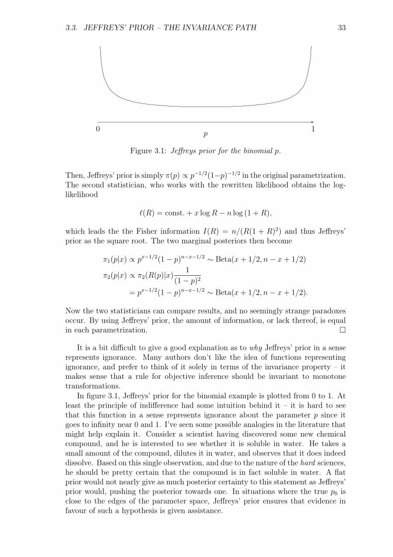
3.3. JEFFREYS’ PRIOR – THE INVARIANCE PATH 33
0 1p
Figure 3.1: Jeffreys prior for the binomial p.
Then, Jeffreys’ prior is simply π(p) ∝ p−1/2(1−p)−1/2 in the original parametrization.The second statistician, who works with the rewritten likelihood obtains the log-likelihood
`(R) = const. + x logR− n log (1 +R),
which leads the the Fisher information I(R) = n/(R(1 + R)2) and thus Jeffreys’prior as the square root. The two marginal posteriors then become
π1(p|x) ∝ px−1/2(1− p)n−x−1/2 ∼ Beta(x+ 1/2, n− x+ 1/2)
π2(p|x) ∝ π2(R(p)|x)1
(1− p)2
= px−1/2(1− p)n−x−1/2 ∼ Beta(x+ 1/2, n− x+ 1/2).
Now the two statisticians can compare results, and no seemingly strange paradoxesoccur. By using Jeffreys’ prior, the amount of information, or lack thereof, is equalin each parametrization.
It is a bit difficult to give a good explanation as to why Jeffreys’ prior in a senserepresents ignorance. Many authors don’t like the idea of functions representingignorance, and prefer to think of it solely in terms of the invariance property – itmakes sense that a rule for objective inference should be invariant to monotonetransformations.
In figure 3.1, Jeffreys’ prior for the binomial example is plotted from 0 to 1. Atleast the principle of indifference had some intuition behind it – it is hard to seethat this function in a sense represents ignorance about the parameter p since itgoes to infinity near 0 and 1. I’ve seen some possible analogies in the literature thatmight help explain it. Consider a scientist having discovered some new chemicalcompound, and he is interested to see whether it is soluble in water. He takes asmall amount of the compound, dilutes it in water, and observes that it does indeeddissolve. Based on this single observation, and due to the nature of the hard sciences,he should be pretty certain that the compound is in fact soluble in water. A flatprior would not nearly give as much posterior certainty to this statement as Jeffreys’prior would, pushing the posterior towards one. In situations where the true p0 isclose to the edges of the parameter space, Jeffreys’ prior ensures that evidence infavour of such a hypothesis is given assistance.
34 CHAPTER 3. OBJECTIVE BAYESIAN INFERENCE
Jeffreys’ prior is not used in multi-parameter settings, as it can have some prettystrong inconsistencies. Consider the following example, which is of the same flavouras example 2.3.
Example 3.3 (Neyman-Scott example). Consider data Xij ∼ N(µj, σ2) for
i = 1, 2 and j = 1, . . . ,m. That is, we have pairs of data (X1j, X2j) from m differentpopulations with common variance, but different means. Suppose we are interestedin estimating the common variance in the data, σ2, and we wish to use Jeffreys’prior to aid us.
The likelihood of a single pair from the model can be written as
L(σ2, µj) ∝1
σ2exp
− 1
σ2
[S2j
4+ (x·j − µj)2
],
where S2j = (x1j − x2j)
2 and x·j is the within-group mean. Since µj only crops upin the full likelihood through the above expression, the contribution to the Fisherinformation matrix in the µj term is by
−E[∂2
∂µ2j
`(µj, σ2)
]=
2
σ2,
and the cross terms are zero. The full likelihood can be written as
L(µ1, . . . , µm, σ2) ∝ 1
σ2m
m∏j=1
exp
− 1
σ2
[Sj4
+ (x·j − µj)2
],
and it is easy enough to derive the Fisher information matrix as
I(µ1, . . . , µm, σ2) =
2/σ2 0 · · · 0 0
0 2/σ2 · · · 0 0...
... . . . ......
0 0 · · · 2/σ2 00 0 · · · 0 m/σ4
,which makes Jeffreys’ prior πJ(µ1, . . . , µm, σ
2) ∝ σ−(m+2).Now, the marginal posterior distribution of σ2, found by integrating out all the
µj from the posterior can be found to be;2
π(σ2|x) ∝ (σ2)−(m+1) exp
− 1
σ2
S2
4
,
where S2 =∑m
j=1 S2j . This distribution is in fact an inverse-gamma distribution
with parameters (m,S2/4), with expectation S2/(4(m − 1)). The problem now isthat, while σ2 = S2/(2(m−1)) is a consistent estimator of the true σ2
0, the marginalposterior distribution for σ2 will concentrate around σ0/2! Even more so for largem.
Since Jeffreys’ prior can lead to some very inconsistent results in higher dimen-sions, it is rarely used in these situations. The underlying issue is that the nuisanceparameters in the model was not dealt with properly. We will see later that thereference prior approach by Berger and Bernardo is a nice extension of Jeffreys’prior when nuisance parameters are present in the model, but to understand theirfoundations, we need a little detour.
2see for example Kim et al. (2006).

3.4. E. T. JAYNES – THE ENTROPY PATH 35
3.4 E. T. Jaynes – the entropy pathThe second line of argument in attempts to parametrize ignorance, is connectedto the information theoretical concept of entropy. The leading figure behind thisapproach is E.T. Jaynes, who had a fascinating take on statistical inference. Thefollowing section is based on the exposition in Jaynes (2003, ch. 2,11,12) and is keptrelatively loose. The main point is to provide some kind of information-theoreticalfoundation for the reference priors.
Jaynes was a proponent of the "probability as extended logic" school of thought.What this means is that he viewed the modern concept of probability as a directextension of formal logic, thinking of statistical inference abstractly, as reasoning un-der incomplete information. He is interested in the underlying logic of this process,and how it can be made quantitative.
The classical way of deductive reasoning is to first state a causal connectionbetween two propositions A and B. We could say that if A is true, then B mustalso be true – or that A implies B. From this statement, we can draw the followingconclusions; If we observe A to be true, then B must also be true. Or, if we observeB to be false, then surely A too must be false.3 These kinds of deductions areusually too strong in practical science, where the causal relationships are not sostraightforward. Instead, we use what may be deemed plausible reasoning.
Plausible reasoning abstractly takes the form of a much weaker syllogism;
If A is true, then B becomes more plausible.B is true, therefore, A becomes more plausible.
In practical applications of statistics, we are often interested in proving that A istrue, on the basis of something that is easier to observe, B. Consider a doctor tryingto figure out whether or not his patient has some kind of disease. The disease itselfis not directly observable, but the anti-bodies that the immune system produces areobservable in the patient’s blood. The presence of anti-bodies in the blood shouldmake the doctor more certain that the patient has the disease, and the amountof anti-bodies in the blood should be directly connected to how certain the doctorshould be. A tiny, almost undetectable, amount of antibodies could be ascribed to ameasurement error, and the doctor should maybe run an extra test in a few days forverification. While, on the other hand, a large amount of anti-bodies in the bloodshould make the doctor quite confident that the patient has the disease in question.
Jaynes is interested in how these things should best be quantified, and find aunifying framework of how to do it. The reason why this is interesting for findingnon-informative priors distributions, is that we need a measure of certainty beforewe can know how to be least certain.
Jaynes outlines three basic desiderata of a theory for representing certainty.First off, one needs to assume that degrees of plausibility can be represented by realnumbers, in some way. Further, one would need that this representation is somehowin sync with ’common sense’, i.e. that strong evidence leads to a stronger degree ofcertainty, as represented in real numbers. Lastly, we should like our theory to beconsistent. By this, it is meant that if a conclusion can be worked out from differentangles, every possible angle should lead to the same result.
3The statement "B is true, therefore A must be true", is a false one – famously demonstratedby Erasmus Montanus.
36 CHAPTER 3. OBJECTIVE BAYESIAN INFERENCE
Working from the simplest case of a finite and discrete parameter spaceθ1, . . . , θn, Jaynes (2003, p. 347) constructs a measure of uncertainty usingthe above principles. First off, we need to assume that some numerical measureHn(p1, . . . , pn) exists that can assign degrees of certainty pi to each possibility θi. Italso seems natural to demand that such a measure is continuous in its arguments,pi, such that a small increase in pi does not lead to a large leap in the overall un-certainty. Next, the measure should be in sync with ’common sense’, which Jaynesbases on the principle of insufficient reason. He argues that we should be moreuncertain when there are many possibilities to choose from, than when there arefew, i.e. that the function
h(n) = Hn
(1
n, · · · , 1
n
)is monotonically increasing in n. Lastly, we should demand consistency of themeasure. If there are many ways to compute the measure in a given situation, eachway should yield the name answer.
After some technicalities, Jaynes finds that the only function Hn satisfying hisconditions imposed on a reasonable measure of uncertainty, is the function
Hn(p1, . . . , pn) = −n∑i=1
pi log pi, (3.3)
which is the Shannon entropy.The Shannon entropy dates back to Shannon (1948), and his works on informa-
tion theory. Originally, it was meant as a measure of the information content inEnglish text, useful for data compression schemes. It has many interpretations, butthe one that is most useful for our purpose is that it can be considered as a measureof unpredictability. Assume a data sequence is generated from some stochastic pro-cess, f taking values in the set θ1, . . . , θn. If the corresponding probabilities arehighly skewed, say that p1 = 0.9 while p2, . . . , pn = 0.1/(n − 1), this is a sequencethat is highly predictable. Constantly guessing that the next value will be θ1, is onaverage a very good guess – this sequence has a low entropy, or high predictability.If instead the probabilities assigned where according to the principle of insufficientreason, guessing the next value in the sequence would be hard, since they are allequally probable – this sequence will have high entropy. In cryptography, one ofthe main desiderata is that the cipher utilized has a uniform distribution over thelanguage, i.e. the alphabet A-Z, for English text – making it difficult to predict.
Jaynes thus argues that the only non-informative prior distribution we shouldassign in the case of a finite and discrete parameter space, is the one that maximizesthe entropy – namely the principle of insufficient reason.
In the case where the parameter space is continuous, there are some difficultiesthat must be overcome. A natural extension of the discrete entropy in (3.3) wouldbe to simply move from summation to integration and define
H ′ = −∫
Θ
p(θ) log p(θ)dθ (3.4)
which is the so-called differential entropy. The problem with this is that it is notinvariant under monotone transformation, so that the measure of uncertainty will
3.5. REFERENCE PRIORS 37
be different depending on the parametrization. A property that we’ve seen shouldreally be demanded of a good prior distribution. Another, slightly more worryingaspect of this definition, is that it is not the result of some well defined limitingprocess.
Jaynes argues that passing from discrete parameter spaces to continuous shouldonly be done in cases where the continuous spaces can be derived through a naturallimiting process. Starting from a finite discrete set of points θ1, . . . , θn, and thecorresponding Shannon entropy Hn, letting n → ∞ such that the parameter spacebecomes denser, he finds that the continuous measure of uncertainty becomes
Hc = −∫
Θ
p(θ) logp(θ)
m(θ)dθ, (3.5)
for some unknown reference measure m(θ). Keeping with the technique in thediscrete case, we should choose our prior distribution p(θ) in such a way that itmaximizes the quantity (3.5), which will turn out to be when p(θ) ∝ m(θ). But theproblem still remains, which reference measure m should we choose in the aboveexpression?
3.5 Reference Priors
3.5.1 Motivation and DefinitionReference priors were first introduced in 1979 by Bernardo and uses information-theoretical arguments to derive a prior that in some sense is least-informative, to beused as a reference, or baseline, when doing Bayesian inference. This is very muchin line with the thoughts of E.T. Jaynes from the past section, and we will see thatthe two positions are highly connected.
Since the posterior distribution is a compromise between prior information andthe observed data, the main idea is that we should choose a prior distribution thatinfluence the posterior as little as possible, while still facilitating a proper posterior.One measure of this influence is the Kullback-Leibler divergence.
Definition 3.1 (Kullback-Leibler divergence). The Kullback-Leibler divergencefrom the prior distribution π(θ) to the posterior p(θ|x) is defined by:
κ(p|π) =
∫Θ
p(θ|x) logp(θ|x)
π(θ)dθ,
where log is the natural logarithm. In the discrete case, integrals are summations.
Loosely stated, the KL-divergence from q to p can be viewed as the distancebetween the two distributions, but there are several interpretations. In this section,we will view it as the information gain from prior to posterior distribution. Itgives a measure of how much information is obtained when updating our beliefsfrom the prior distribution to the posterior distribution. A sharp, localized priordistribution will give less weight to the data, resulting in a smaller information gainfrom observing the data. Intuitively we should want a prior distribution that, whenupdated with information, moves as much as possible – one that gains as muchinformation as possible from the data.
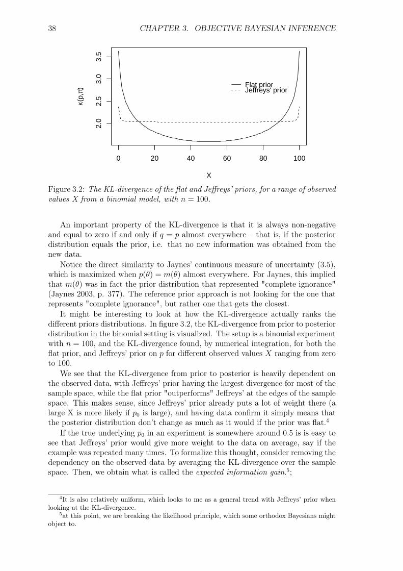
38 CHAPTER 3. OBJECTIVE BAYESIAN INFERENCE
0 20 40 60 80 100
2.0
2.5
3.0
3.5
X
κ(p,
π)Flat priorJeffreys' prior
Figure 3.2: The KL-divergence of the flat and Jeffreys’ priors, for a range of observedvalues X from a binomial model, with n = 100.
An important property of the KL-divergence is that it is always non-negativeand equal to zero if and only if q = p almost everywhere – that is, if the posteriordistribution equals the prior, i.e. that no new information was obtained from thenew data.
Notice the direct similarity to Jaynes’ continuous measure of uncertainty (3.5),which is maximized when p(θ) = m(θ) almost everywhere. For Jaynes, this impliedthat m(θ) was in fact the prior distribution that represented "complete ignorance"(Jaynes 2003, p. 377). The reference prior approach is not looking for the one thatrepresents "complete ignorance", but rather one that gets the closest.
It might be interesting to look at how the KL-divergence actually ranks thedifferent priors distributions. In figure 3.2, the KL-divergence from prior to posteriordistribution in the binomial setting is visualized. The setup is a binomial experimentwith n = 100, and the KL-divergence found, by numerical integration, for both theflat prior, and Jeffreys’ prior on p for different observed values X ranging from zeroto 100.
We see that the KL-divergence from prior to posterior is heavily dependent onthe observed data, with Jeffreys’ prior having the largest divergence for most of thesample space, while the flat prior "outperforms" Jeffreys’ at the edges of the samplespace. This makes sense, since Jeffreys’ prior already puts a lot of weight there (alarge X is more likely if p0 is large), and having data confirm it simply means thatthe posterior distribution don’t change as much as it would if the prior was flat.4
If the true underlying p0 in an experiment is somewhere around 0.5 is is easy tosee that Jeffreys’ prior would give more weight to the data on average, say if theexample was repeated many times. To formalize this thought, consider removing thedependency on the observed data by averaging the KL-divergence over the samplespace. Then, we obtain what is called the expected information gain.5;
4It is also relatively uniform, which looks to me as a general trend with Jeffreys’ prior whenlooking at the KL-divergence.
5at this point, we are breaking the likelihood principle, which some orthodox Bayesians mightobject to.
3.5. REFERENCE PRIORS 39
Definition 3.2 (Expected information gain). Let x be an observation from themodel M := p(x|θ),x ∈ X ,θ ∈ Θ. When the prior distribution is π(θ), theexpected information gain from one observation is
I(π|x) =
∫Xp(x)κ(p|π) dx
=
∫X
∫Θ
p(x|θ)π(θ) logp(θ|x)
π(θ)dθdx,
since p(θ|x) = p(x|θ)π(θ)/p(x). In the discrete case, integrals are summations.
Choosing the prior that will maximize the expected information gain from asingle experiment intuitively seems like a good idea, but we should want somethingmuch stronger. A reference prior should be a baseline for the entire modelM, notjust on the basis of what we can expect to learn about θ from a single experiment.We should aim for a setting where the reference prior maximize the information gainfrom the prior to what is theoretically possible to learn from the model, perhaps byrepeating the experiment many times.
Consider k independent hypothetical replications of the experiment at hand,leading to a sequence of realizations xk = (x1, . . . ,xk) and a measure of informationgain based on this entire vector, I(π|xk). As the number of replications increase,the experiment will eventually provide the all missing information about θ, until itis completely known. The quantity I(π|xk) then, will, as k →∞, begin to representthe amount of missing information about θ contained in the prior, π.
This requires some clarification. Say that we are comparing two prior distribu-tions π1 and π2. Suppose also that the two quantities I(π1|xk) and I(π2|xk) bothconverge to some real numbers, N andM respectively, as k →∞. Then, if N > M ,this means that the expected amount of information needed to know the value of θwith certainty, is larger when starting with π1 than compared to when starting fromπ2. This then means that π1 is less informative about θ than what π2 is, and thequantities N and M in a sense also represents the amount of missing informationassociated with each prior.
Now then, a reference prior is, loosely stated, a permissible prior distribution thatmaximizes the missing information within a class of candidate priors, P . This classof candidate priors is one that agrees with any a priori knowledge the researchermight have, such as natural parameter boundaries, continuity or non-negativity.
This is all incredibly abstract, and there are several concerns that should cometo mind when reading it. The biggest concern should be if the missing informationeven exists, I mean, is the limit limk→∞ I(π|xk) even defined? Or what about theexpected information gain, what is stopping the integrals in definition 3.2 from beinginfinite? Nothing we’ve done so far has put any restrictions in place that makes theabove equations and definitions hold.
Let’s start with the one-parameter case, for which the theory is on a pretty solidmathematical foundation, and follow the way it is laid out in Berger et al. (2009).For the definitions to work, we actually need a stricter notion of permissible priordistributions – it is not enough to demand that they lead to a proper posteriordistribution, we need the reference prior to be the result of a well-defined limitingprocess, again in line with Jaynes. Consider the following definition;
40 CHAPTER 3. OBJECTIVE BAYESIAN INFERENCE
Definition 3.3 (Expected logarithmic convergence of posteriors). LetΘi∞i=1 be an increasing sequence of compact subsets of Θ such that
⋃∞i=1 Θi = Θ.
Let πi(θ|x)∞i=1 denote the corresponding sequence of posteriors, i.e
πi(θ|x) ∝∫
Θi
p(x|θ)πi(θ)dθ
where πi(θ) is the natural restriction of the prior to the subset Θi. Then the sequenceof posteriors is expected logarithmically convergent to the formal posterior π(θ|x)if
limi→∞
∫Xκ (π(·|x)|πi(·|x)) pi(x)dx = 0,
where pi(x) =∫
Θip(x|θ)πi(θ)dθ.
A stronger notion of permissible is then that, (i) the prior should yield a properposterior distribution, and that (ii), for some approximating compact sequence, thecorresponding posterior distributions are expected logarithmically convergent. Thatis, the prior distribution itself is derived implicitly, through a limiting sequence ofposteriors.
Next, we need to tackle the question raised earlier, about the existence of theexpected information gain, and if it really converges to anything. Berger et al.(2009) notes that a bounded parameter space is typically enough to ensure existenceof I(π|xk) for a given k, but if the parameter space is continuous, it will typicallydiverge as k → ∞ – would it not take an infinite amount of information to knowthe value of a real number with certainty? The following definition deals with theseissues,
Definition 3.4 (Maximizing missing information (MMI) property). LetM be a model with one continuous parameter, and let P be the class of priordistributions yielding a proper posterior. The function π(θ) is said to have the MMIproperty for modelM and prior class P if, for any compact subset Θ0 ⊂ Θ and anyp ∈ P ,
limk→∞
I(π0|xk)− I(p0|xk)
≥ 0, (3.6)
where π0 and p0 are renormalized restrictions of π and p to Θ0.
The fact that I(π|xk) can diverge as k →∞ is taken care of, simply by insistingthat it will be larger than the missing information of any other qualified prior p(which also diverges).
Then the formal definition of a reference prior in the one-dimensional case is thefollowing;
Definition 3.5 (Reference Prior). A function πR(θ) = π(θ|M,P) is a referenceprior for model M, given a class of potential priors P , if it is permissible, in thestronger sense, and has the MMI property.
This definition gives no real clue as to how the problem at hand should be solved,i.e. finding the function π(θ) that maximizes the missing information about θ. Butthere are explicit forms or algorithms available for finding them.
3.5. REFERENCE PRIORS 41
3.5.2 Explicit Forms of the Reference Prior
Finding the explicit form of the reference prior in a given model is not always aneasy task, and the definition does not offer many hints on how to go about theproblem. To motivate the formal solution to this problem consider the followingreformulation of the expected information gain under conditions regular enough toallow the operations6:
I(π|xk) =
∫Xk
∫Θ
p(xk|θ)π(θ) logp(θ|xk)π(θ)
dθdxk
=
∫Θ
π(θ)
∫Xkp(xk|θ) log
p(θ|xk)π(θ)
dxkdθ
=
∫Θ
π(θ) logfk(θ)
π(θ)dθ
= −∫
Θ
π(θ) logπ(θ)
fk(θ)dθ, (3.7)
where
fk(θ) = exp
∫Xkp(xk|θ) log p(θ|xk)dxk
. (3.8)
Equation 3.7 is in fact −κ(π|fk), the (negative) KL-divergence from fk(θ) to π(θ).7And since the KL-divergence is always greater than or equal to zero, with equalityif and only if π(θ) = fk(θ) almost everywhere, this equation is maximized whenπ(θ) ∝ fk(θ). Typically though, as we’ve discussed, in continuous parameter cases,or with an unbounded parameter space, the expected information gain either isn’tdefined, or it diverges as k →∞. The following theorem, which is proved in Bergeret al. (2009) circumvents these issues for the one-parameter case.
Theorem 3.1 (Explicit form of the reference prior). Assume a standard modelM := p(x|θ),x ∈ X , θ ∈ Θ ⊂ R and a class P of continuous priors on Θ thatlead to a proper posterior distribution. Let π∗(θ) be a strictly positive continuousprior such that the corresponding posterior, π∗(θ|xk), is proper and asymptoticallyconsistent, i.e. concentrating around the true value θ as k → ∞. Define, for anyinterior point θ0 of Θ,
fk(θ) = exp
∫Xkp(xk|θ) log[π∗(θ|xk)]dxk
and (3.9)
f(θ) = limk→∞
fk(θ)
fk(θ0). (3.10)
If (i) each fk(θ) is continuous and, for any fixed θ and sufficiently large k,[fk(θ)/fk(θ0)] is either monotonic in k or bounded above by some h(θ) integrableon any compact set, and (ii) f(θ) is a permissible prior function, then πR(θ) ∝ f(θ)is a reference prior for modelM and prior class P .
6A bounded parameter space will ensure the existence of I(π|x) and further conditions areneeded to apply Fubini’s theorem.
7It also provides an answer to Jaynes question of which reference measure m(θ) to use inequation 3.5.
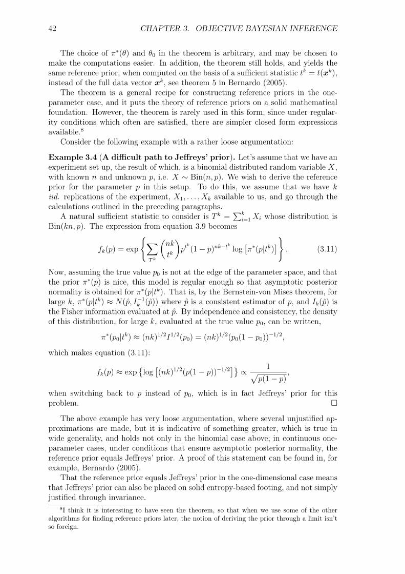
42 CHAPTER 3. OBJECTIVE BAYESIAN INFERENCE
The choice of π∗(θ) and θ0 in the theorem is arbitrary, and may be chosen tomake the computations easier. In addition, the theorem still holds, and yields thesame reference prior, when computed on the basis of a sufficient statistic tk = t(xk),instead of the full data vector xk, see theorem 5 in Bernardo (2005).
The theorem is a general recipe for constructing reference priors in the one-parameter case, and it puts the theory of reference priors on a solid mathematicalfoundation. However, the theorem is rarely used in this form, since under regular-ity conditions which often are satisfied, there are simpler closed form expressionsavailable.8
Consider the following example with a rather loose argumentation:
Example 3.4 (A difficult path to Jeffreys’ prior). Let’s assume that we have anexperiment set up, the result of which, is a binomial distributed random variable X,with known n and unknown p, i.e. X ∼ Bin(n, p). We wish to derive the referenceprior for the parameter p in this setup. To do this, we assume that we have kiid. replications of the experiment, X1, . . . , Xk available to us, and go through thecalculations outlined in the preceding paragraphs.
A natural sufficient statistic to consider is T k =∑k
i=1Xi whose distribution isBin(kn, p). The expression from equation 3.9 becomes
fk(p) = exp
∑T k
(nk
tk
)ptk
(1− p)nk−tk log[π∗(p|tk)
]. (3.11)
Now, assuming the true value p0 is not at the edge of the parameter space, and thatthe prior π∗(p) is nice, this model is regular enough so that asymptotic posteriornormality is obtained for π∗(p|tk). That is, by the Bernstein-von Mises theorem, forlarge k, π∗(p|tk) ≈ N(p, I−1
k (p)) where p is a consistent estimator of p, and Ik(p) isthe Fisher information evaluated at p. By independence and consistency, the densityof this distribution, for large k, evaluated at the true value p0, can be written,
π∗(p0|tk) ≈ (nk)1/2I1/2(p0) = (nk)1/2(p0(1− p0))−1/2,
which makes equation (3.11):
fk(p) ≈ exp
log[(nk)1/2(p(1− p))−1/2
]∝ 1√
p(1− p),
when switching back to p instead of p0, which is in fact Jeffreys’ prior for thisproblem.
The above example has very loose argumentation, where several unjustified ap-proximations are made, but it is indicative of something greater, which is true inwide generality, and holds not only in the binomial case above; in continuous one-parameter cases, under conditions that ensure asymptotic posterior normality, thereference prior equals Jeffreys’ prior. A proof of this statement can be found in, forexample, Bernardo (2005).
That the reference prior equals Jeffreys’ prior in the one-dimensional case meansthat Jeffreys’ prior can also be placed on solid entropy-based footing, and not simplyjustified through invariance.
8I think it is interesting to have seen the theorem, so that when we use some of the otheralgorithms for finding reference priors later, the notion of deriving the prior through a limit isn’tso foreign.

3.5. REFERENCE PRIORS 43
Properties
The reference prior has many desirable properties that one should hope a non-informative prior has. Most desirably, since it agrees with Jeffreys’ prior, it isinvariant under monotone transformations in the one-dimensional case. In the mul-tiparameter case, the reference prior no longer equal Jeffreys’, which we will seelater, and this property is lost. For multi-parameter models, the reference prioris invariant only under certain transformations, see Datta & Ghosh (1996). Thisalso entails that the reference prior will depend on the parameter of interest! Thereference prior for (µ, σ2) may be completely different from the reference prior for(σ/µ, σ).
The reference prior is independent of the sample size in the model. From a Fisher-information viewpoint this is because In(θ) = nI(θ), but note that it may dependon the sampling design in cases where n cannot be pulled out of the informationmatrix – we will see an example of this situation later. From a Bayesian viewpoint,the dependence on sampling design might seem strange, but it stems from the"averaging over the sample space" we did in definition 3.2. Again, we are violatingthe likelihood principle here.
A last important property of the reference priors is that, since it is often a partof the construction to approximate the full parameter space Θ with an expandingsequence of compact subsets Θi∞i=1; the reference prior of the full space Θ, re-stricted to a subset Θi will also be the reference prior found by only working on Θi
from the beginning.
Nuisance parameters
When there are nuisance parameters present in our model, we’ve seen that Jeffreys’prior can provide less than optimal inference. The reference prior paradigm providesa scheme for dealing with nuisance parameters by ordering parameters by theirinferential importance, and using a stepwise-conditioning argument. When thereis only a single nuisance parameter present in the model, the algorithm takes on asimple form.
Consider the problem whereM := x ∈ X , ψ ∈ Ψ ⊂ R, λ ∈ Λ ⊂ R where ψ isthe parameter of interest, and λ is a nuisance parameter. In this case, one would needa joint reference prior for the set of parameters (ψ, λ), to obtain a joint posterior forthe pair, and then a marginal posterior for the parameter of interest, ψ. Bernardo(1979) suggested the following scheme to produce the joint prior distribution for(ψ, λ).
Step 1 Consider ψ fixed and derive the one-dimensional conditional reference priorπR(λ|ψ). In regular cases, this amounts to computing Jeffreys’ prior.
Step 2 If the the conditional prior πR(λ|ψ) is proper, i.e.∫
ΛπR(λ|ψ)dλ < ∞, the
nuisance parameter may be integrated out to find the one-parameter integratedmodel p(x|ψ) =
∫Λp(x|ψ, λ)π(λ|ψ)dλ.
Step 3 Now, derive the one-dimensional reference prior based on p(x|ψ), πR(ψ).In regular cases this again amounts to Jeffreys’ prior.
Step 4 Finally, the joint reference prior is by πR(ψ, λ) = πR(ψ)πR(λ|ψ)

44 CHAPTER 3. OBJECTIVE BAYESIAN INFERENCE
This is a nice scheme, but often it does not work out as intended, the soft spot isin step 2, where the conditional Jeffreys’ prior often isn’t proper. Berger & Bernardo(1989) produce a more general scheme for the one-dimensional nuisance parametersetup. Let I(ψ, λ) denote the Fisher information matrix of this model, and denotethe parameter space by Θ = Ψ × Λ. Step 1 is exactly as before, and typicallyamounts to finding Jeffreys’ prior for λ, while keeping ψ fixed. The rest of theprocedure continues as
Step 2∗ Choose an expanding sequence of compact subsets of Θ, Θi∞i=1 such that⋃i Θi = Θ and π(λ|ψ) is integrable on the slice Ωi,ψ = λ : (ψ, λ) ∈ Θi for
all ψ. Then normalize on each slice to obtain
πi(λ|ψ) = Ki(ψ)π(λ|ψ)1Ωi,ψ(λ) (3.12)
where
K−1i (ψ) =
∫Ωi,ψ
π(λ|ψ)dλ (3.13)
Step 3∗ Compute
πi(ψ) = exp
1
2
∫Ωi,ψ
πi(λ|ψ) log [|I(ψ, λ)| / |I(ψ, λ)22|] dλ
, (3.14)
where I denotes the full Fisher information matrix, and I22 denotes the seconddiagonal element.
Step 4∗ Obtain the joint reference prior as:
π(ψ, λ) = limi→∞
Ki(ψ)πi(ψ)
Ki(ψ0)πi(ψ0)π(λ|ψ) (3.15)
where ψ0 is any fixed, interior point of Ψ.
We will use this algorithm later to derive a reference prior in a relatively simplesetup.
This algorithm is complex, and the integrals one needs to solve often take someugly forms. Luckily, since the nuisance parameter is integrated out before findingthe reference prior for ψ, the choice of nuisance parameter won’t affect πR(ψ). Thismeans that we can often reparametrize the problem into one that is easier to workwith.
If we have multiple nuisance parameters in our model, we must order the parame-ters in the model after inferential importance, and apply the above algorithm sequen-tially. Say the model has parameters ψ,λ where ψ is a parameter of interest, whileλ is a vector of nuisance parameters, an ordering might be ψ, λ1, . . . , λn where ψand λn are most and least important, respectively. Then, we hold ψ, λ1, . . . , λn−1fixed and derive the reference prior for λn, πR(λn|ψ, λ1, . . . , λn−1). We then integratethis parameter out of the model and continue, now holding ψ, λ1, . . . , λn−2 fixedand finding the reference prior πR(λn−1|ψ, λ1, . . . , λn−2). Doing this sequentially, weconstruct the final reference prior as
πR(ψ, λ1, . . . , λn) ∝ πR(ψ)πR(λ1|ψ) · · · πR(λn|ψ, λ1, . . . , λn−1)
Luckily, several shortcuts have been developed for dealing with nuisance param-eters in the models so that we don’t actually have to solve the reference prior in thismanner every time.
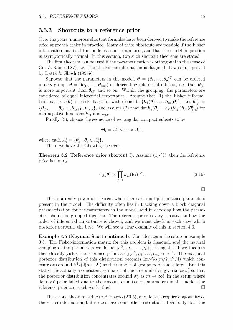
3.5. REFERENCE PRIORS 45
3.5.3 Shortcuts to a reference priorOver the years, numerous shortcut formulas have been derived to make the referenceprior approach easier in practice. Many of these shortcuts are possible if the Fisherinformation matrix of the model is on a certain form, and that the model in questionis asymptotically normal. In this section, two such shortcut theorems are stated.
The first theorem can be used if the parametrization is orthogonal in the sense ofCox & Reid (1987), i.e. that the Fisher information is diagonal. It was first provedby Datta & Ghosh (1995b).
Suppose that the parameters in the model, θ = (θ1, . . . , θp)T can be ordered
into m groups θ = (θ(1), . . . ,θ(m)) of descending inferential interest, i.e. that θ(1)
is more important than θ(2) and so on. Within the grouping, the parameters areconsidered of equal inferential importance. Assume that (1) the Fisher informa-tion matrix I(θ) is block diagonal, with elements h1(θ), . . . ,hm(θ). Let θC(j) =
θ(1), . . . ,θ(j−1),θ(j+1),θ(m), and assume (2) that dethj(θ) = hj1(θ(j))hj2(θC(j)) fornon-negative functions hj1 and hj2.
Finally (3), choose the sequence of rectangular compact subsets to be
Θi = Ai1 × · · · × Aim,
where each Aij = θj : θj ∈ Aij.Then, we have the following theorem.
Theorem 3.2 (Reference prior shortcut I). Assume (1)-(3), then the referenceprior is simply
πR(θ) ∝m∏j=1
hj1(θj)1/2. (3.16)
This is a really powerful theorem when there are multiple nuisance parameterspresent in the model. The difficulty often lies in tracking down a block diagonalparametrization for the parameters in the model, and in choosing how the param-eters should be grouped together. The reference prior is very sensitive to how theorder of inferential importance is chosen, and we must check in each case whichposterior performs the best. We will see a clear example of this in section 4.3.
Example 3.5 (Neyman-Scott continued). Consider again the setup in example3.3. The Fisher-information matrix for this problem is diagonal, and the naturalgrouping of the parameters would be σ2, µ1, . . . , µn, using the above theoremthen directly yields the reference prior as πR(σ2, µ1, . . . , µn) ∝ σ−2. The marginalposterior distribution of this distribution becomes Inv-Ga(m/2, S2/4) which con-centrates around S2/(2(m− 2)) as the number of groups m becomes large. But thisstatistic is actually a consistent estimator of the true underlying variance σ2
0 so thatthe posterior distribution concentrates around σ2
0 as m → ∞! In the setup whereJeffreys’ prior failed due to the amount of nuisance parameters in the model, thereference prior approach works fine!
The second theorem is due to Bernardo (2005), and doesn’t require diagonality ofthe Fisher information, but it does have some other restrictions. I will only state the
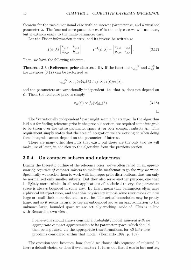
46 CHAPTER 3. OBJECTIVE BAYESIAN INFERENCE
theorem for the two-dimensional case with an interest parameter ψ, and a nuisanceparameter λ. The ’one-nuisance parameter case’ is the only case we will use later,but it extends easily to the multi-parameter case.
Let the Fisher information matrix, and its inverse be written as
I(ψ, λ)
[hψ,ψ, hψ,λhλ,ψ hλ,λ
]I−1(ψ, λ) =
[vψ,ψ vψ,λvλ,ψ vλ,λ
]. (3.17)
Then, we have the following theorem;
Theorem 3.3 (Reference prior shortcut II). If the functions v−1/2ψ,ψ and h1/2
λ,λ inthe matrices (3.17) can be factorized as
v−1/2ψ,ψ ∝ fψ(ψ)gψ(λ) hλ,λ ∝ fλ(ψ)gλ(λ),
and the parameters are variationally independent, i.e. that Λi does not depend onψ. Then, the reference prior is simply
πR(ψ) ∝ fψ(ψ)gλ(λ). (3.18)
The "variationally independent" part might seem a bit strange. In the algorithmlaid out for finding reference prior in the previous section, we required some integralsto be taken over the entire parameter space Λ, or over compact subsets Λi. Thisrequirement simply states that the area of integration we are working on when doingthese integrals cannot depend on the parameter of interest.
There are many other shortcuts that exist, but these are the only two we willmake use of later, in addition to the algorithm from the previous section.
3.5.4 On compact subsets and uniquenessDuring the theoretic outline of the reference prior, we’ve often relied on an approx-imating sequence of compact subsets to make the mathematics go the way we want.Specifically we needed them to work with improper prior distributions, that can onlybe normalized only smaller subsets. But they also serve another purpose, one thatis slightly more subtle. In all real applications of statistical theory, the parameterspace is always bounded in some way. By this I mean that parameters often havea physical interpretation, and that this physicality impose some restrictions on howlarge or small their numerical values can be. The actual boundaries may be prettylarge, and so it seems natural to use an unbounded set as an approximation to theunknown large, bounded space we are actually working inside of. This is in linewith Bernardo’s own views
I believe one should always consider a probability model endowed with anappropriate compact approximation to its parameter space, which shouldthen be kept fixed, via the appropriate transformations, for all inferenceproblems considered within that model. (Bernardo 1997, p. 187)
The question then becomes, how should we choose this sequence of subsets? Isthere a default choice, or does it even matter? It turns out that it can in fact matter,

3.6. FREQUENTIST PROPERTIES OF THE BAYESIAN POSTERIOR 47
and that the reference prior might actually depend on how the sequence was chosen.This is demonstrated in for example Berger & Bernardo (1989) and Sun & Ye (1995)when deriving the reference prior for the product of normal means. Depending onhow the sequence is chosen, the reference prior can change quite a bit, which isslightly unsettling. Berger and Bernardo provide the following pragmatic view:
Choosing the Θi to be natural sets in the original parametrization hasalways worked well in our experience. Indeed, the way we think ofthe Θi is that there is some large compact set on which we are reallynoninformative, but we are unable to specify the size of this set. Wemight, however, be able to specify a shape, Ω, for this set, and wouldthen choose Θi = iΩ∩Θ, where iΩ consists of all points in Ω multipliedby i. (Bernardo & Berger 1992, p. 42)
Taking this literally, it means we need to think about which shapes in our param-eter space it is more natural to be non-informative over. Being pragmatic, in caseswhere multiple reference priors are available, we should evaluate their performance,perhaps by some frequentist criteria.
3.6 Frequentist properties of the Bayesianposterior
When Bayes theorem is employed with a subjective prior distribution, the resultingposterior distribution has a clear, tangible meaning. Your prior knowledge, as it isexpressed in the prior distribution is updated through Bayes theorem, to yield Yourcurrent state of knowledge. And the resulting posterior distributions can be used tomake definite (epistemic) probability statements about the value of the parameters.But when the prior distribution is not chosen to represent the researchers state ofknowledge before the experiment, what should we make of the posterior distribution?Does it even make sense to do inference in this way?
As the clear logic of subjective Bayesian analysis is unavailable for us, one mightwant to consider some more frequentist properties of the posterior distributions –though most objective Bayesians still interpret their posterior distributions the sameway as subjective Bayesians. Sound frequentist properties would also ensure thatthe Bayesian procedure does well on average, something that can be valuable toboth subjective and objective Bayesians.
One way to analyze the frequentist properties of the Bayesian posterior is to lookat the coverage of posterior sets. If Kα ⊂ Θ is a region with posterior probabilityα, i.e.
∫Kαp(θ|X)dθ = α then what is P (θ0 ∈ Kα) in the frequentist sense?
In a few select cases, we can get exact matching, i.e. that any α level credible setshave exactly α-level coverage probability. This amounts to the (marginal) Bayesianposterior distribution being an exact confidence distribution. Situations where thishappens is studied in section 4.2.1.
Outside of the limited frame where Bayesian posterior distributions are alsoconfidence distributions, one might ask how close to the intended coverage can weget? Keeping with the terminology from higher order asymptotics, we will say thata prior distribution is kth-order matching if
P (θ0 ∈ Kα) = α +O(n−k/2
),
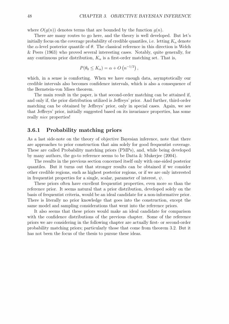
48 CHAPTER 3. OBJECTIVE BAYESIAN INFERENCE
where O(g(n)) denotes terms that are bounded by the function g(n).There are many routes to go here, and the theory is well developed. But let’s
initially focus on the coverage probability of credible quantiles, i.e. lettingKα denotethe α-level posterior quantile of θ. The classical reference in this direction is Welch& Peers (1963) who proved several interesting cases. Notably, quite generally, forany continuous prior distribution, Kα is a first-order matching set. That is,
P (θ0 ≤ Kα) = α +O(n−1/2
),
which, in a sense is comforting. When we have enough data, asymptotically ourcredible intervals also becomes confidence intervals, which is also a consequence ofthe Bernstein-von Mises theorem.
The main result in the paper, is that second-order matching can be attained if,and only if, the prior distribution utilized is Jeffreys’ prior. And further, third-ordermatching can be obtained by Jeffreys’ prior, only in special cases. Again, we seethat Jeffreys’ prior, initially suggested based on its invariance properties, has somereally nice properties!
3.6.1 Probability matching priorsAs a last side-note on the theory of objective Bayesian inference, note that thereare approaches to prior construction that aim solely for good frequentist coverage.These are called Probability matching priors (PMPs), and, while being developedby many authors, the go-to reference seems to be Datta & Mukerjee (2004).
The results in the previous section concerned itself only with one-sided posteriorquantiles. But it turns out that stronger results can be obtained if we considerother credible regions, such as highest posterior regions, or if we are only interestedin frequentist properties for a single, scalar, parameter of interest, ψ.
These priors often have excellent frequentist properties, even more so than thereference prior. It seems natural that a prior distribution, developed solely on thebasis of frequentist criteria, would be an ideal candidate for a non-informative prior.There is literally no prior knowledge that goes into the construction, except thesame model and sampling considerations that went into the reference priors.
It also seems that these priors would make an ideal candidate for comparisonwith the confidence distributions of the previous chapter. Some of the referencepriors we are considering in the following chapter are actually first- or second-orderprobability matching priors; particularly those that come from theorem 3.2. But ithas not been the focus of the thesis to pursue these ideas.
Chapter 4
Comparisons and Examples
In this chapter, some examples are worked through using the theory in the previ-ous chapters. The examples are not intended to be interesting simply on their ownmerit, but are used to highlight various practical and theoretical aspects of the var-ious theories. Furthermore, as a objective goal, to compare the optimal confidencedistributions, viewed somewhat as a gold standard of what can be learned fromdata, to the objective Bayesian theories.
4.1 Difference of exponential parametersThe purpose of this example is to perform a pretty standard objective Bayesiananalysis, deriving objective priors and analyzing their frequentist properties. Inaddition we compare posterior distributions to the optimal CDs, trying to shedsome light on how ’objective’ our posteriors really are. The example illustrates thedifficulties that one encounters trying to derive a reference prior, and contrasts itto the quick and easy CD approach. Lastly, we look at boundary cases where thefrequentists have it easy, but the Bayesians might have it hard.
Let Expo(θ) denote the exponential distribution with density
f(x) = θ exp −θx , x > 0, θ > 0
and consider independent exponentially distributed random variables Xi, Yi whereXi ∼ Expo(θ) and Yi ∼ Expo(θ + δ). Suppose the parameter of interest is δ, thedifference between the exponential rates, and that we observe n independent pairs(Xi, Yi).
4.1.1 An optimal confidence distribution
Starting from the simplest case, with a single pair being observed, the joint densityof X and Y can be written as
p(x, y|θ, δ) = θ(θ + δ) exp −θ(x+ y)− δy , (4.1)
which we can recognize as being on the form of Theorem 2.3. Then an optimalconfidence distribution for δ is available by
C∗1(δ) = P (Y < yobs| (X + Y ) = (xobs + yobs))) . (4.2)
49
50 CHAPTER 4. COMPARISONS AND EXAMPLES
Putting Z = X +Y , the joint density of (Y, Z) is easily available, and from this onefinds the conditional distribution of Y given Z = zobs as
pY |Z(y|z) =δ exp−δy
1− exp−δzfor 0 < y < z, (4.3)
which can be viewed as a truncated exponential distribution. This immediatelyyields the optimal CD for δ as
C∗1(δ) =1− exp−δyobs1− exp−δzobs
. (4.4)
Note that, in the case where δ = 0 this expression is not defined, but the limit atthis point exists and equals yobs/zobs, so we just put C∗1(0) = yobs/zobs in this case.
For the case where n > 1, the joint distribution will again be of the form inTheorem 2.3, and the optimal CD is available as a direct analogue of equation 4.2,
C∗n(δ) = P (S < sobs |A = aobs ) , (4.5)
where S =∑n
i=1 Yi, A =∑n
i=1 (Xi + Yi) and (sobs, aobs) the actual values of thesestatistics observed in the data. This distribution has no easily available closed formparametrization, but can be simulated from using a simple MCMC scheme.
For a single value of our interest parameter, δi, we can simulate N observationsof S from the distribution of S given A = aobs. Then
1
N
N∑j=1
I (Sj < sobs)→ Cn(δi) as N →∞. (4.6)
To obtain the samples Si from the conditional distribution, a Metropolis style algo-rithm can be employed – keeping in mind that the MCMC chains are in the samplespace, and not the parameter space like in the typical Bayesian procedures. Typi-cally we perform the MCMC for a range of fixed δi ∈ ∆, and then use a smoothingmechanism to derive the full confidence distribution. See also remark 4.2 later inthe section.
4.1.2 Objective Bayesian analysisTrying to be an objective Bayesian in this problem poses some difficulty. From thejoint distribution (4.1) one finds the Fisher information matrix as
I(δ, θ) =
1
(θ + δ)2
1
(θ + δ)2
1
(θ + δ)2
1
θ2+
1
(θ + δ)2
, (4.7)
which makes Jeffreys’ overall prior:
πJ(δ, θ) =1
θ(θ + δ). (4.8)
As discussed in section 3.3, and illustrated in example 3.3 Jeffreys’ overall priorcould have some issues, and we would much rather like to utilize a reference prior
4.1. DIFFERENCE OF EXPONENTIAL PARAMETERS 51
approach to deal with our nuisance parameter θ. Following the recipe for referencepriors regarding θ as a nuisance parameter, we get:
Step 1 :Jeffreys’ conditional prior, when keeping δ fixed, is available directly from the Fisherinformation matrix in equation 4.7, as:
π(θ|δ) =
(1
θ2+
1
(θ + δ)2
)1/2
. (4.9)
Step 2 :Next, we need to obtain the marginal distribution p(x|δ) =
∫Θp(x|θ, δ)π(θ|δ)dθ.
This integral becomes
p(x|δ) = exp−δy∫ ∞
0
√(θ + δ)2 + θ2 exp−θ(x+ y)dθ,
which doesn’t really have a closed form solution – or at least it is difficult to solve.One might then try the second algorithm given in section 3.5.2, and normalize theexpression over an expanding sequence of compact subsets. This entails computingthe integral from equation 3.12:
K−1i (δ) =
∫Ai
(1
θ2+
1
(θ + δ)2
)1/2
dθ
for some compact set Ai. Now the difficulty lies in first choosing the sequence ofcompact sets in a good way since for a fixed δ0, this integral will blow up near θ = 0,and assuming δ0 < 0 (which one should allow for), it will blow up near θ = −δ0 aswell. The second, and larger issue is again that there aren’t really any closed formsolutions available for this integral. We can however go further in the problem if weenforce a restriction on the parameter space.
Enforcing a restrictionIf the restriction δ > 0 is enforced, a reparametrization to a nicer nuisance parametermight help. Consider the transformation
ψ = δ and λ = (θ + δ)/θ (4.10)
which is 1-1 as long as δ 6= 0. The parameter space now becomes Ψ×Λ = (0,∞)×(1,∞) and the Jacobian of this transformation is
J =
1 01
λ− 1− ψ
(λ− 1)2
,which leads to the reparametrized information matrix:
I(ψ, λ) = JT I(δ(ψ, λ), θ(ψ, λ))J =
(λ− 1)2
λ2ψ20
01 + λ2
(λ− 1)2λ2
. (4.11)

52 CHAPTER 4. COMPARISONS AND EXAMPLES
This turns out to be an orthogonal parametrization. From this point we couldaim directly for Theorem 3.2 using rectangles in (ψ, λ)-space, but will choose ourrectangles in (δ, θ)-space instead. We will come back to this issue later in theexample.
The conditional Jeffreys prior becomes
π(λ|ψ) =
√(1 + λ2)
(λ− 1)λ.
A natural sequence of compact sets to consider in the original parametrization arethe rectangles (δ, θ) ∈ [li, ki] × [li, ki], where li → 0 and ki → ∞. This leads to theslices Ωi,ψ = (1 + ψ/ki, 1 + ψ/li) in Λ.
Step 3 (restricted case)Working further with the restricted case, equation 3.14 becomes
πi(ψ) = exp
1
2
∫Ωi,ψ
Ki(ψ)π(λ|ψ) log
[1
ψ2
(λ− 1)2
λ2
]dλ
= exp
−Ki log(ψ)
∫Ωi,ψ
π(λ|ψ)dλ
+
∫Ωi,ψ
Ki(ψ)π(λ|ψ) log
[(λ− 1)
λ
]dλ
=1
ψexp
∫Ωi,ψ
Ki(ψ)π(λ|ψ) log
[(λ− 1)
λ
]dλ
=
1
ψexp
Ki(ψ)I i1(ψ)
,
where
I i1(ψ) =
∫Ωi,ψ
√1 + λ2
λ(λ− 1)log
[λ− 1
λ
]dλ.
Now, we’ve narrowed the problem down to computing the integral I i1(ψ), andthe normalizing constant from equation 3.13, i.e.:
K−1i (ψ) =
∫ 1+ψ/li
1+ψ/ki
√1 + λ2
λ(λ− 1)dλ.
The following Lemma is proved in appendix A.
Lemma 4.1. Let
I i1(ψ) =
∫ 1+ψ/li
1+ψ/ki
√1 + λ2
λ(λ− 1)log
[λ− 1
λ
]dλ (4.12)
and,
K−1i (ψ) =
∫ 1+ψ/li
1+ψ/ki
√1 + λ2
λ(λ− 1)dλ. (4.13)
4.1. DIFFERENCE OF EXPONENTIAL PARAMETERS 53
These integrals equals,
I i1(ψ) =1√2
(ψ
kilog
(ψ
ki
)+ψ
ki− log2
(ψ
ki
))+B7, (4.14)
K−1i (ψ) =
1√2
(ψ
ki− 2 log
(ψ
ki
)+√
2 log (1 + ψ/li)
)+B10, (4.15)
where B7 and B10 are bounded functions of ki and li.
Then we have the following expression for πi(ψ);
πi(ψ) =1
ψexp
Ki(ψ)I i1(ψ)
=
1
ψexp
1√2
(ψki
log(ψki
)+ ψ
ki− log2
(ψki
))+B7
1√2
(ψki− 2 log
(ψki
)+√
2 log (1 + ψ/li))
+B10
. (4.16)
Step 4 (restricted case)Now we have the expression for πi(ψ), and we need to take the limit as in equation3.15, i.e
limi→∞
Ki(ψ)πi(ψ)
Ki(ψ0)πi(ψ0).
To make the calculations easier, we choose li = 1/ki leading to the limit being takenover compact sets [k−1
i , ki] × [k−1i , ki] in the original parametrization, and we set
ψ0 = 1. The following lemma is proved in appendix A
Lemma 4.2. Let Ki(ψ) and πi(ψ) be as defined above. Let ki∞i=1 be a sequencediverging to infinity and put li = k−1
i . Then, putting ψ0 = 1 we have that
limi→∞
Ki(ψ)πi(ψ)
Ki(1)πi(1)= ψ
−4+ 5√2 (4.17)
Then, the reference prior for (ψ, λ) becomes:
πR(ψ, λ) ∝ ψ−4+ 5√
2
√(1 + λ2)
(λ− 1)λ,
or, transformed back into (δ, θ) space,
πR(δ, θ) ∝ δ−4+ 5√
2
(1
θ2+
1
(θ + δ)2
)1/2
. (4.18)
So now we have an expression for the reference prior in this problem under therestriction that δ > 0. It would of course be nice to have a reference prior withoutthis restriction, but I have not been able to find it. There are several complicatingfactors that make utilizing the algorithms outlined in section 3.5.2 difficult.
First and foremost, look at the parametrization that was chosen in expression4.10. It might seem arbitrary, but it is chosen to yield a diagonal Fisher information
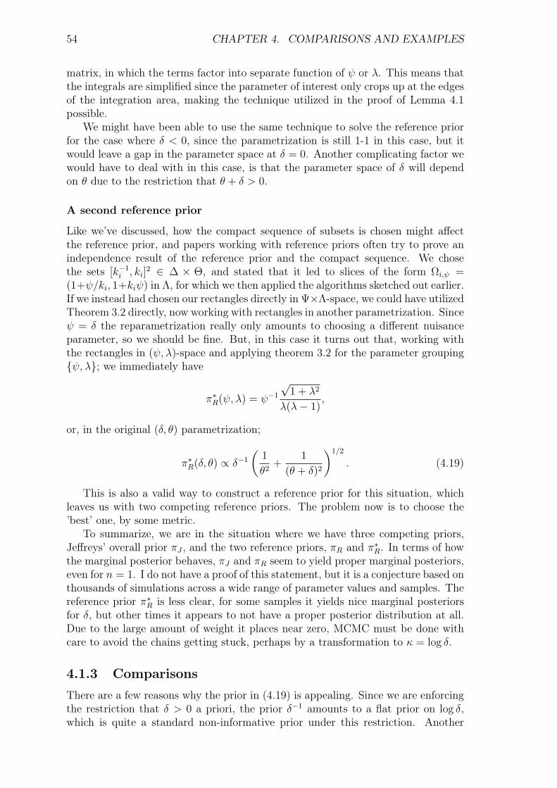
54 CHAPTER 4. COMPARISONS AND EXAMPLES
matrix, in which the terms factor into separate function of ψ or λ. This means thatthe integrals are simplified since the parameter of interest only crops up at the edgesof the integration area, making the technique utilized in the proof of Lemma 4.1possible.
We might have been able to use the same technique to solve the reference priorfor the case where δ < 0, since the parametrization is still 1-1 in this case, but itwould leave a gap in the parameter space at δ = 0. Another complicating factor wewould have to deal with in this case, is that the parameter space of δ will dependon θ due to the restriction that θ + δ > 0.
A second reference prior
Like we’ve discussed, how the compact sequence of subsets is chosen might affectthe reference prior, and papers working with reference priors often try to prove anindependence result of the reference prior and the compact sequence. We chosethe sets [k−1
i , ki]2 ∈ ∆ × Θ, and stated that it led to slices of the form Ωi,ψ =
(1+ψ/ki, 1+kiψ) in Λ, for which we then applied the algorithms sketched out earlier.If we instead had chosen our rectangles directly in Ψ×Λ-space, we could have utilizedTheorem 3.2 directly, now working with rectangles in another parametrization. Sinceψ = δ the reparametrization really only amounts to choosing a different nuisanceparameter, so we should be fine. But, in this case it turns out that, working withthe rectangles in (ψ, λ)-space and applying theorem 3.2 for the parameter groupingψ, λ; we immediately have
π∗R(ψ, λ) = ψ−1
√1 + λ2
λ(λ− 1),
or, in the original (δ, θ) parametrization;
π∗R(δ, θ) ∝ δ−1
(1
θ2+
1
(θ + δ)2
)1/2
. (4.19)
This is also a valid way to construct a reference prior for this situation, whichleaves us with two competing reference priors. The problem now is to choose the’best’ one, by some metric.
To summarize, we are in the situation where we have three competing priors,Jeffreys’ overall prior πJ , and the two reference priors, πR and π∗R. In terms of howthe marginal posterior behaves, πJ and πR seem to yield proper marginal posteriors,even for n = 1. I do not have a proof of this statement, but it is a conjecture based onthousands of simulations across a wide range of parameter values and samples. Thereference prior π∗R is less clear, for some samples it yields nice marginal posteriorsfor δ, but other times it appears to not have a proper posterior distribution at all.Due to the large amount of weight it places near zero, MCMC must be done withcare to avoid the chains getting stuck, perhaps by a transformation to κ = log δ.
4.1.3 ComparisonsThere are a few reasons why the prior in (4.19) is appealing. Since we are enforcingthe restriction that δ > 0 a priori, the prior δ−1 amounts to a flat prior on log δ,which is quite a standard non-informative prior under this restriction. Another

4.1. DIFFERENCE OF EXPONENTIAL PARAMETERS 55
(∆,Θ)
***************************************************************************
(Ψ,Λ)
********
**************
**************
**********
*****************************
Figure 4.1: Compact rectangles in (∆ × Θ)-space transform to wedges in (Ψ × Λ)-space
reason is that of symmetry; it looks nice. There is a sense that when something thissimple tumbles out of the theory – there must be something to it. Especially whenthe other candidate contains the strange looking δ−4+5/
√2.
A third reason has to do with the underlying logic of the construction procedure.Recall the heuristic explanation for the compact sets from section 3.5.4; their shapesare meant to represent shapes in the parameter space one might be indifferent over.In this case, where the parameters are orthogonal – it seems natural to work withrectangles in (Ψ×Λ) space, since the value of one will not affect the parameter spaceof the other. On the one hand, considering rectangles in ∆×Θ space, like we did forthe prior in (4.18), leads to oddly shaped ’wedges’ in the (ψ, λ) parametrization, seefigure 4.1. It is difficult to give a justification to why we should be indifferent overthese shapes, instead of rectangles.1 On the other hand, since λ = (θ+δ)/θ = 1+δ/θ,as θ becomes arbitrarily small, λ becomes arbitrarily large, no matter the value ofδ. This squeezes the parameter space into a point near θ = 0, which might also beunnatural in a sense.
It turns out though, when we look at the marginal posteriors, the reference priorπ∗R(δ, θ) often performs poorly compared to the one derived earlier. The reason beingthat δ−1 places too much weight near zero, much more so than δ−4+5/
√2 ≈ δ−0.47.
This is especially undesirable for low n, where the likelihood is not powerful enoughto pull weight away from zero. In figure 4.2, the marginal posterior distributionsfor δ, based on Jeffreys’ overall prior and the two reference priors, are displayed fortwo different samples at n = 3. In both samples, it is easy to see that the marginalposterior for δ, obtained by using π∗R(δ, θ), is pulled far to the left compared to boththe overall Jeffreys’ prior and the reference prior in 4.18.
This problem, where different sequences lead to different reference priors wasfirst encountered and studied in Berger & Bernardo (1989). In this paper, a naturalreference prior comes from choosing sequences of subsets in the original parameterspace, and going through the same proofs as I did the for lemmas 4.1 and 4.2. Theyare able to prove that, for general choices of sets in the original parametrization(rectangles, circles etc.), the reference prior is unchanged. But, following the sameargumentation we did, where it might be more natural to consider rectangles in(ψ, λ)-space, they derive a second reference prior based on this sequence. Aftersome comparisons, considering the logic of the underlying procedure and lookingat the marginal posteriors, they choose the reference prior based on subsets in the
1One might argue that an even more intuitive way to construct the sequence is on the basisthe parameters φ1 = θ and φ2 = (θ + δ), and consider rectangles in this parametrization.
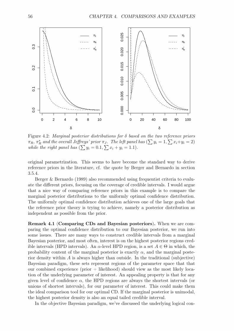
56 CHAPTER 4. COMPARISONS AND EXAMPLES
0 2 4 6 8 10
0.0
0.1
0.2
0.3
δ
πJ
πR
πR*
0 20 40 60 80 1000.
000
0.00
50.
010
0.01
50.
020
0.02
5
δ
πJ
πR
πR*
Figure 4.2: Marginal posterior distributions for δ based on the two reference priorsπR, π∗R and the overall Jeffreys’ prior πJ . The left panel has (
∑yi = 1,
∑xi+yi = 2)
while the right panel has (∑yi = 0.1,
∑xi + yi = 1.1).
original parametrization. This seems to have become the standard way to derivereference priors in the literature, cf. the quote by Berger and Bernardo in section3.5.4.
Berger & Bernardo (1989) also recommended using frequentist criteria to evalu-ate the different priors, focusing on the coverage of credible intervals. I would arguethat a nice way of comparing reference priors in this example is to compare themarginal posterior distributions to the uniformly optimal confidence distribution.The uniformly optimal confidence distribution achieves one of the large goals thatthe reference prior theory is trying to achieve, namely a posterior distribution asindependent as possible from the prior.
Remark 4.1 (Comparing CDs and Bayesian posteriors). When we are com-paring the optimal confidence distribution to our Bayesian posterior, we run intosome issues. There are many ways to construct credible intervals from a marginalBayesian posterior, and most often, interest is on the highest posterior regions cred-ible intervals (HPD intervals). An α-level HPD region, is a set A ∈ Θ in which, theprobability content of the marginal posterior is exactly α, and the marginal poste-rior density within A is always higher than outside. In the traditional (subjective)Bayesian paradigm, these sets represent regions of the parameter space that thatour combined experience (prior + likelihood) should view as the most likely loca-tion of the underlying parameter of interest. An appealing property is that for anygiven level of confidence α, the HPD regions are always the shortest intervals (orunions of shortest intervals), for our parameter of interest. This could make themthe ideal comparison tool for our optimal CD. If the marginal posterior is unimodal,the highest posterior density is also an equal tailed credible interval.
In the objective Bayesian paradigm, we’ve discussed the underlying logical con-
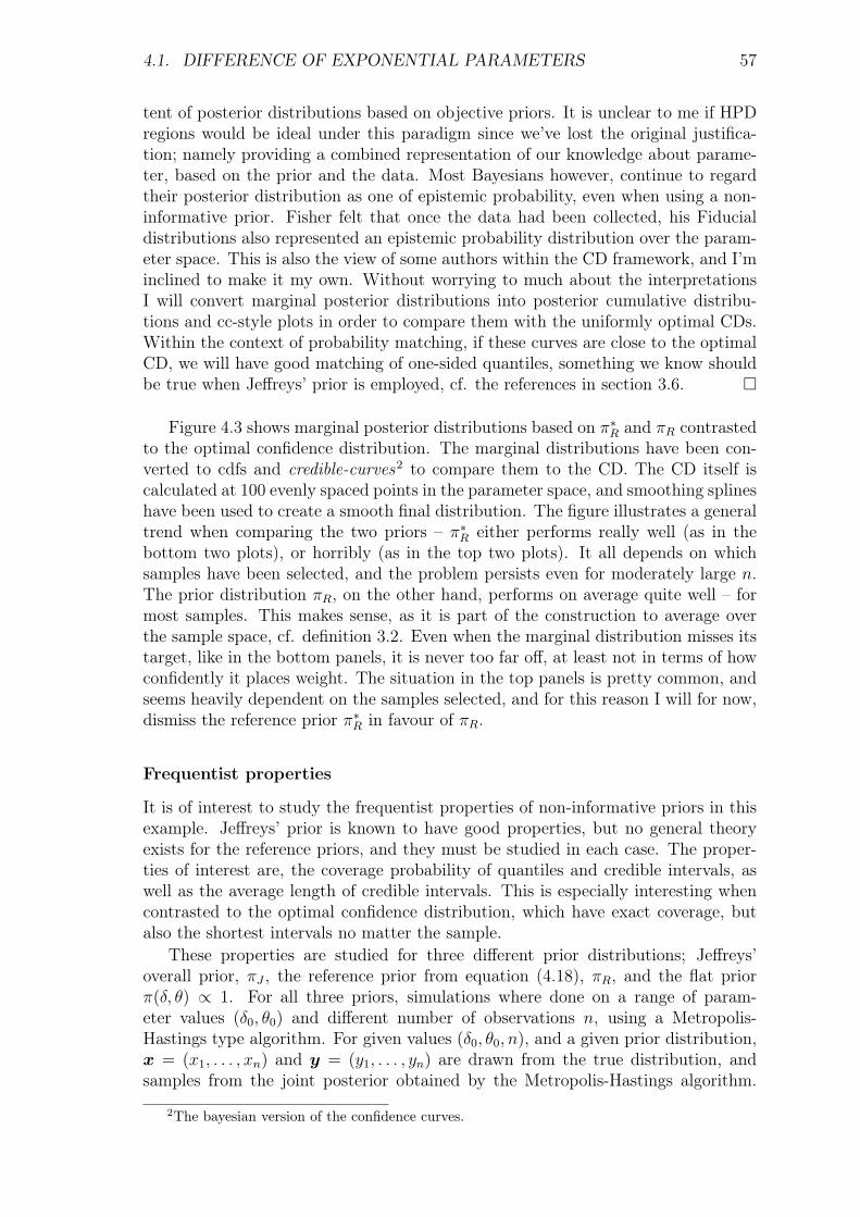
4.1. DIFFERENCE OF EXPONENTIAL PARAMETERS 57
tent of posterior distributions based on objective priors. It is unclear to me if HPDregions would be ideal under this paradigm since we’ve lost the original justifica-tion; namely providing a combined representation of our knowledge about parame-ter, based on the prior and the data. Most Bayesians however, continue to regardtheir posterior distribution as one of epistemic probability, even when using a non-informative prior. Fisher felt that once the data had been collected, his Fiducialdistributions also represented an epistemic probability distribution over the param-eter space. This is also the view of some authors within the CD framework, and I’minclined to make it my own. Without worrying to much about the interpretationsI will convert marginal posterior distributions into posterior cumulative distribu-tions and cc-style plots in order to compare them with the uniformly optimal CDs.Within the context of probability matching, if these curves are close to the optimalCD, we will have good matching of one-sided quantiles, something we know shouldbe true when Jeffreys’ prior is employed, cf. the references in section 3.6.
Figure 4.3 shows marginal posterior distributions based on π∗R and πR contrastedto the optimal confidence distribution. The marginal distributions have been con-verted to cdfs and credible-curves2 to compare them to the CD. The CD itself iscalculated at 100 evenly spaced points in the parameter space, and smoothing splineshave been used to create a smooth final distribution. The figure illustrates a generaltrend when comparing the two priors – π∗R either performs really well (as in thebottom two plots), or horribly (as in the top two plots). It all depends on whichsamples have been selected, and the problem persists even for moderately large n.The prior distribution πR, on the other hand, performs on average quite well – formost samples. This makes sense, as it is part of the construction to average overthe sample space, cf. definition 3.2. Even when the marginal distribution misses itstarget, like in the bottom panels, it is never too far off, at least not in terms of howconfidently it places weight. The situation in the top panels is pretty common, andseems heavily dependent on the samples selected, and for this reason I will for now,dismiss the reference prior π∗R in favour of πR.
Frequentist properties
It is of interest to study the frequentist properties of non-informative priors in thisexample. Jeffreys’ prior is known to have good properties, but no general theoryexists for the reference priors, and they must be studied in each case. The proper-ties of interest are, the coverage probability of quantiles and credible intervals, aswell as the average length of credible intervals. This is especially interesting whencontrasted to the optimal confidence distribution, which have exact coverage, butalso the shortest intervals no matter the sample.
These properties are studied for three different prior distributions; Jeffreys’overall prior, πJ , the reference prior from equation (4.18), πR, and the flat priorπ(δ, θ) ∝ 1. For all three priors, simulations where done on a range of param-eter values (δ0, θ0) and different number of observations n, using a Metropolis-Hastings type algorithm. For given values (δ0, θ0, n), and a given prior distribution,x = (x1, . . . , xn) and y = (y1, . . . , yn) are drawn from the true distribution, andsamples from the joint posterior obtained by the Metropolis-Hastings algorithm.
2The bayesian version of the confidence curves.

58 CHAPTER 4. COMPARISONS AND EXAMPLES
0 10 20 30 40 50 60
0.0
0.2
0.4
0.6
0.8
1.0
δ
Con
fiden
ce
C3(δ)
πR
πR*
0 10 20 30 40 50 60
0.0
0.2
0.4
0.6
0.8
1.0
δ
Con
fiden
ce
C3(δ)
πR
πR*
0 20 40 60 80 100
0.0
0.2
0.4
0.6
0.8
1.0
δ
Con
fiden
ce
C3(δ)
πR
πR*
0 20 40 60 80 100
0.0
0.2
0.4
0.6
0.8
1.0
δ
Con
fiden
ce
C3(δ)
πR
πR*
Figure 4.3: Marginal posterior distributions based on π∗R and πR compared to theoptimal confidence distribution for two different samples.
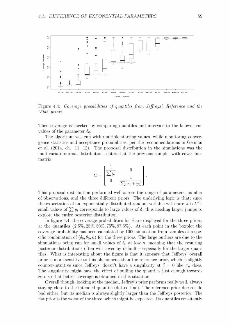
4.1. DIFFERENCE OF EXPONENTIAL PARAMETERS 59
Je2.5% Re2.5% Fl2.5% Je25% Re25% Fl25% Je50% Re50% Fl50% Je75% Re75% Fl75% Je97.5% Re97.5% Fl97.5%
0.0
0.2
0.4
0.6
0.8
1.0
Priors x Quantiles
Cov
erag
e P
roba
bilit
y
Figure 4.4: Coverage probabilities of quantiles from Jeffreys’, Reference and the’Flat’ priors.
Then coverage is checked by comparing quantiles and intervals to the known truevalues of the parameter δ0.
The algorithm was run with multiple starting values, while monitoring conver-gence statistics and acceptance probabilities, per the recommendations in Gelmanet al. (2014, ch. 11, 12). The proposal distribution in the simulations was themultivariate normal distribution centered at the previous sample, with covariancematrix
Σ =
1∑yi
0
01∑
(xi + yi)
.This proposal distribution performed well across the range of parameters, numberof observations, and the three different priors. The underlying logic is that; sincethe expectation of an exponentially distributed random variable with rate λ is λ−1,small values of
∑yi corresponds to large values of δ, thus needing larger jumps to
explore the entire posterior distribution.In figure 4.4, the coverage probabilities for δ are displayed for the three priors,
at the quantiles 2.5%, 25%, 50%, 75%, 97.5%. At each point in the boxplot thecoverage probability has been calculated by 1000 simulation from samples at a spe-cific combination of (δ0, θ0, n) for the three priors. The large outliers are due to thesimulations being run for small values of δ0 at low n, meaning that the resultingposterior distributions often will cover by default – especially for the larger quan-tiles. What is interesting about the figure is that it appears that Jeffreys’ overallprior is more sensitive to this phenomena than the reference prior, which is slightlycounter-intuitive since Jeffreys’ doesn’t have a singularity at δ = 0 like πR does.The singularity might have the effect of pulling the quantiles just enough towardszero so that better coverage is obtained in this situation.
Overall though, looking at the median, Jeffrey’s prior performs really well, alwaysstaying close to the intended quantile (dotted line). The reference prior doesn’t dobad either, but its median is always slightly larger than the Jeffreys posterior. Theflat prior is the worst of the three, which might be expected. Its quantiles consitently

60 CHAPTER 4. COMPARISONS AND EXAMPLES
Je5 Re5 Fl5 Je10 Re10 Fl10 Je50 Re50 Fl50
0.5
0.6
0.7
0.8
0.9
1.0
95% credible intervals
Priors x No. observations
Cov
erag
e P
roba
bilit
y
Figure 4.5: Coverage probability of 95% equal-tailed credible intervals for the threepriors at n = 5, 10, 50.
overshoot its target due to the fact that there is no mechanism that pulls posteriorweight towards zero.
In figure 4.5, the coverage probabilities for equal-tailed 95% credible intervalsare displayed for the three priors at different samples sizes. Again we see that forlow n, Jeffreys’ and the flat prior are sensitive to outliers, while the reference priorperforms better. Interestingly, as n increases to 50, Jeffreys’ and the flat priors seemto outperform the reference prior, which has a larger spread around the intendedcoverage. This might also be coincidental, and more simulations might erase thisdiscrepancy.
The average length of credible intervals is also of interest. A good procedureshould have the correct coverage, as well as a tight distribution around the truevalue – like the optimal CDs.
Remark 4.2 (Simulations from the optimal CD). There is a problem thatneed to be dealt with in order to have consistent simulation results from the optimalconfidence distribution. Unlike the Bayesian MCMC, where the Markov chains aredefined directly on the parameter space, the optimal CDs are defined in terms ofa probability statement (equation 4.5) on the sample space, for a fixed parametervalue. The simulations must be repeated across a range of parameter values in theparameter space in order to approximate the full confidence distribution. What isimportant then, is that the range is defined in such a way that it covers all theinteresting parts of the parameter space, for example so that it contains at leastthe 1st and 99th percentiles of C(δ). One of the issues that then arises, is thatthis range will be data dependent, so that defining one range to fit all samples willlead to a computationally inefficient simulation procedure. In the following, I willdescribe an algorithm for solving this issue.
First off, we need to find the ranges of interest for the n individual CDs based ona single observation, C1(δ). This can be done by applying a root-finding algorithmon the function
C1(δ)− α = 0
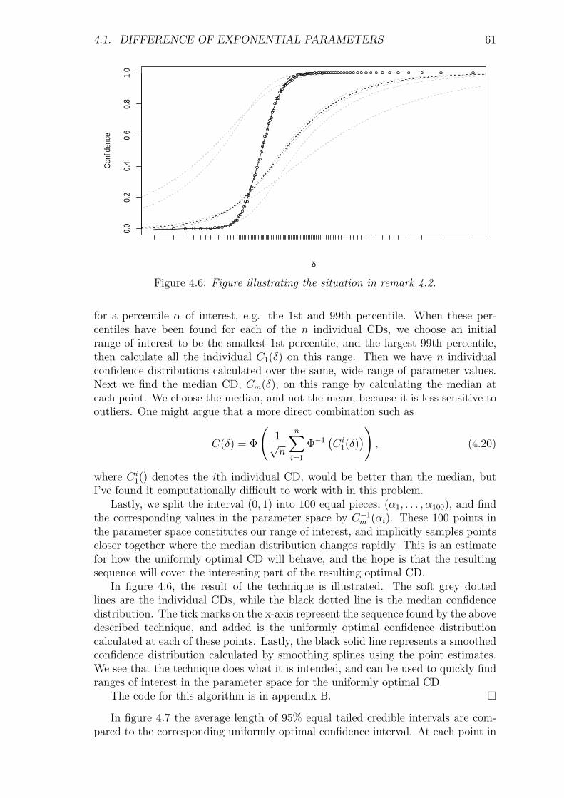
4.1. DIFFERENCE OF EXPONENTIAL PARAMETERS 61
0.0
0.2
0.4
0.6
0.8
1.0
δ
Con
fiden
ce
Figure 4.6: Figure illustrating the situation in remark 4.2.
for a percentile α of interest, e.g. the 1st and 99th percentile. When these per-centiles have been found for each of the n individual CDs, we choose an initialrange of interest to be the smallest 1st percentile, and the largest 99th percentile,then calculate all the individual C1(δ) on this range. Then we have n individualconfidence distributions calculated over the same, wide range of parameter values.Next we find the median CD, Cm(δ), on this range by calculating the median ateach point. We choose the median, and not the mean, because it is less sensitive tooutliers. One might argue that a more direct combination such as
C(δ) = Φ
(1√n
n∑i=1
Φ−1(Ci
1(δ)))
, (4.20)
where Ci1() denotes the ith individual CD, would be better than the median, but
I’ve found it computationally difficult to work with in this problem.Lastly, we split the interval (0, 1) into 100 equal pieces, (α1, . . . , α100), and find
the corresponding values in the parameter space by C−1m (αi). These 100 points in
the parameter space constitutes our range of interest, and implicitly samples pointscloser together where the median distribution changes rapidly. This is an estimatefor how the uniformly optimal CD will behave, and the hope is that the resultingsequence will cover the interesting part of the resulting optimal CD.
In figure 4.6, the result of the technique is illustrated. The soft grey dottedlines are the individual CDs, while the black dotted line is the median confidencedistribution. The tick marks on the x-axis represent the sequence found by the abovedescribed technique, and added is the uniformly optimal confidence distributioncalculated at each of these points. Lastly, the black solid line represents a smoothedconfidence distribution calculated by smoothing splines using the point estimates.We see that the technique does what it is intended, and can be used to quickly findranges of interest in the parameter space for the uniformly optimal CD.
The code for this algorithm is in appendix B.
In figure 4.7 the average length of 95% equal tailed credible intervals are com-pared to the corresponding uniformly optimal confidence interval. At each point in
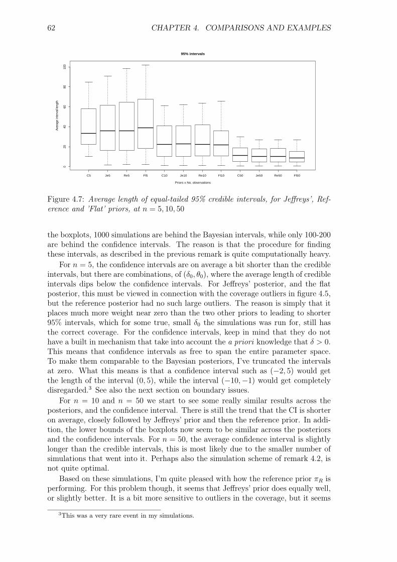
62 CHAPTER 4. COMPARISONS AND EXAMPLES
C5 Je5 Re5 Fl5 C10 Je10 Re10 Fl10 C50 Je50 Re50 Fl50
020
4060
8010
0
95% intervals
Priors x No. observations
Aver
age
inte
rval
leng
th
Figure 4.7: Average length of equal-tailed 95% credible intervals, for Jeffreys’, Ref-erence and ’Flat’ priors, at n = 5, 10, 50
the boxplots, 1000 simulations are behind the Bayesian intervals, while only 100-200are behind the confidence intervals. The reason is that the procedure for findingthese intervals, as described in the previous remark is quite computationally heavy.
For n = 5, the confidence intervals are on average a bit shorter than the credibleintervals, but there are combinations, of (δ0, θ0), where the average length of credibleintervals dips below the confidence intervals. For Jeffreys’ posterior, and the flatposterior, this must be viewed in connection with the coverage outliers in figure 4.5,but the reference posterior had no such large outliers. The reason is simply that itplaces much more weight near zero than the two other priors to leading to shorter95% intervals, which for some true, small δ0 the simulations was run for, still hasthe correct coverage. For the confidence intervals, keep in mind that they do nothave a built in mechanism that take into account the a priori knowledge that δ > 0.This means that confidence intervals as free to span the entire parameter space.To make them comparable to the Bayesian posteriors, I’ve truncated the intervalsat zero. What this means is that a confidence interval such as (−2, 5) would getthe length of the interval (0, 5), while the interval (−10,−1) would get completelydisregarded.3 See also the next section on boundary issues.
For n = 10 and n = 50 we start to see some really similar results across theposteriors, and the confidence interval. There is still the trend that the CI is shorteron average, closely followed by Jeffreys’ prior and then the reference prior. In addi-tion, the lower bounds of the boxplots now seem to be similar across the posteriorsand the confidence intervals. For n = 50, the average confidence interval is slightlylonger than the credible intervals, this is most likely due to the smaller number ofsimulations that went into it. Perhaps also the simulation scheme of remark 4.2, isnot quite optimal.
Based on these simulations, I’m quite pleased with how the reference prior πR isperforming. For this problem though, it seems that Jeffreys’ prior does equally well,or slightly better. It is a bit more sensitive to outliers in the coverage, but it seems
3This was a very rare event in my simulations.
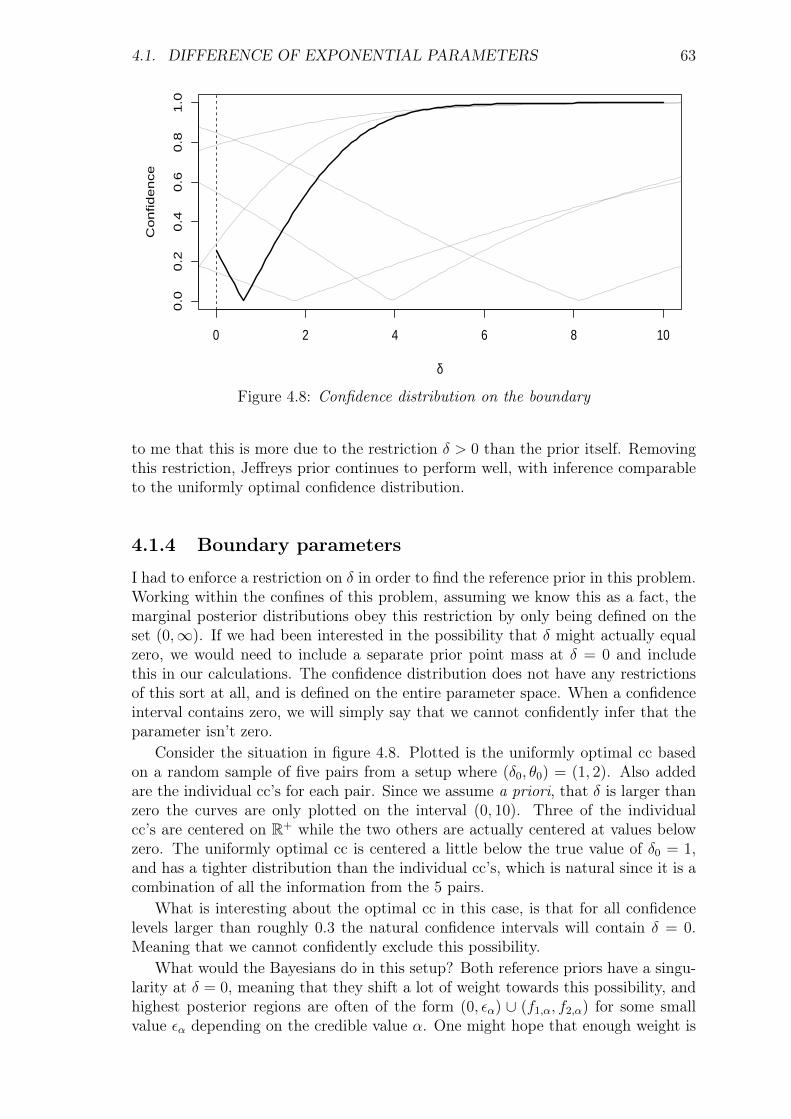
4.1. DIFFERENCE OF EXPONENTIAL PARAMETERS 63
0 2 4 6 8 10
0.0
0.2
0.4
0.6
0.8
1.0
δ
Co
nfid
en
ce
Figure 4.8: Confidence distribution on the boundary
to me that this is more due to the restriction δ > 0 than the prior itself. Removingthis restriction, Jeffreys prior continues to perform well, with inference comparableto the uniformly optimal confidence distribution.
4.1.4 Boundary parameters
I had to enforce a restriction on δ in order to find the reference prior in this problem.Working within the confines of this problem, assuming we know this as a fact, themarginal posterior distributions obey this restriction by only being defined on theset (0,∞). If we had been interested in the possibility that δ might actually equalzero, we would need to include a separate prior point mass at δ = 0 and includethis in our calculations. The confidence distribution does not have any restrictionsof this sort at all, and is defined on the entire parameter space. When a confidenceinterval contains zero, we will simply say that we cannot confidently infer that theparameter isn’t zero.
Consider the situation in figure 4.8. Plotted is the uniformly optimal cc basedon a random sample of five pairs from a setup where (δ0, θ0) = (1, 2). Also addedare the individual cc’s for each pair. Since we assume a priori, that δ is larger thanzero the curves are only plotted on the interval (0, 10). Three of the individualcc’s are centered on R+ while the two others are actually centered at values belowzero. The uniformly optimal cc is centered a little below the true value of δ0 = 1,and has a tighter distribution than the individual cc’s, which is natural since it is acombination of all the information from the 5 pairs.
What is interesting about the optimal cc in this case, is that for all confidencelevels larger than roughly 0.3 the natural confidence intervals will contain δ = 0.Meaning that we cannot confidently exclude this possibility.
What would the Bayesians do in this setup? Both reference priors have a singu-larity at δ = 0, meaning that they shift a lot of weight towards this possibility, andhighest posterior regions are often of the form (0, εα) ∪ (f1,α, f2,α) for some smallvalue εα depending on the credible value α. One might hope that enough weight is

64 CHAPTER 4. COMPARISONS AND EXAMPLES
0 2 4 6 8
0.0
0.2
0.4
0.6
0.8
1.0
δ
Co
nfid
en
ce
C5πRπJ
Figure 4.9: Confidence distribution on the boundary with marginal posterior distri-butions from using Jeffreys’ prior, πJ and the reference prior πR.
shifted so that credible curves from the marginal posteriors will resemble the optimalcc in this case.
The results, based on the same sample as before, are displayed in figure 4.9,where the uniformly optimal cc is compared to credible curves from two differentmarginal posteriors; the reference posterior based on πR, and Jeffreys’ posteriorbased on πJ . Numerical integration of the reference posterior based on π∗R seems toyield an improper posterior distribution in this case, as it does quite often, see alsothe concluding remarks.
We see that the reference prior does a good job at pulling weight towards zero,staying closer to C5(δ) near the boundary than Jeffreys’. It also has a median thatis centered closer to the median CD point estimator. Of course Jeffreys’ prior withno restriction would stay pretty close to the CD here, but the point is to study acase where such a restriction occurs, and how the Bayesian paradigm handles it. Imean, if we know, a priori, that ψ ≥ ψ0 for some value ψ0, then the Bayesians seemsto have some extra difficulties that the frequentists don’t – the natural confidenceintervals will simply contain ψ0 for some level of confidence α > α0.
4.2 Unbalanced Poisson pairs
This example allows us to tackle confidence distributions based on a discrete samplespace with appropriate continuity corrections. I find that a continuity correctedfiducial distribution coincides exactly with the Bayesian posterior based on Jeffreys’or the reference prior, and discuss exact matching in the context of fiducial inferenceand confidence distributions.
Consider the situation where we have Poisson distributed random variables,Xi, . . . , Xn
iid∼ Po(λ) and Y1, . . . , Ymiid∼ Po(λψ). The parameter of interest is the
ratio between the two Poisson means, i.e. ψ, while λ is considered a nuisanceparameter. The data can be considered as coming from two different counting pro-cesses of length n andm, during which the rate is constant at λ and ψλ, respectively.
4.2. UNBALANCED POISSON PAIRS 65
These types of models have wide application in a variety of fields, and have beenstudied from both the frequentist and Bayesian paradigms.
The joint density of this model can be written
p(x,y|λ, ψ) ∝ λ∑i xi+
∑j yjψ
∑j yj exp −nλ−mλψ
= exp log (λ)A+ log (ψ)S − nλ−mλψ) ,
where A =∑n
i=1 xi +∑m
j=1 yj and S =∑m
j=1 yj. This is immediately recognized asbeing on the form of Theorem 2.3, and an optimal confidence distribution for ψ isdirectly available through
Cn(ψ) = P (S > sobs|A = aobs) . (4.21)
This distribution can be worked out exactly by some well known facts about thePoisson distribution. First, the sums of independent Poisson distributed variablesare themselves Poisson distributed, this yields
S =∑
yj ∼ Po(mψλ), A =∑
xi +∑
yj ∼ Po(nλ+mψλ). (4.22)
Also, the conditional distribution of S given A is binomial;
S|A ∼ Bin(A,
mψ
n+mψ
). (4.23)
We haven’t touched much upon discrete data in the material so far, but it has itsown quirks that needs to be sorted out. For discrete data, exact confidence intervalscannot be obtained at every level of significance without some sort of randomizationmechanism. The reason is of course that the equality P (X < x) = P (X ≤ x) doesnot hold. One way to deal with this is through some sort of continuity correction.Let C1(ψ) denote the CD based on a strict inequality in 4.21, and C2(ψ) be basedon the non-strict version. A typical way to apply a continuity correction is thetake the (arithmetic) average of these two distributions, this leads to the typical’half-corrected’ confidence distribution;
CA(ψ) =1
2
(C1(ψ) + C2(ψ)
)= P (S > sobs|A = aobs) +
1
2P (S = sobs|A = aobs) .
(4.24)
Since this expression is a linear combination of confidence distribution, we mighthave lost the exact coverage property, but the resulting distribution is an approxi-mate confidence distribution. There is a strong line of argument within the contextof hypothesis testing that leads to this type of continuity correction, see Stone (1969,Appendix 5).
Another continuity correction to consider is taking the geometric mean of thetwo confidence densities,
cG(ψ) ∝(c1(ψ)c2(ψ)
)1/2, (4.25)
and constructing the confidence distribution CG(ψ) on the basis of this. Again, theexact coverage property might be lost, so the distribution is only an approximateCD. The reason one might consider this expression instead of CA(ψ) is because,when combining distributions p1 and p2 with the same support, the distribution,
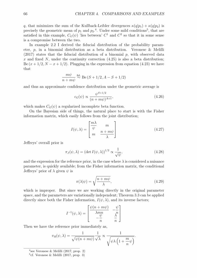
66 CHAPTER 4. COMPARISONS AND EXAMPLES
q, that minimizes the sum of the Kullback-Leibler divergences κ(q|p1) + κ(q|p2) isprecisely the geometric mean of p1 and p2.4. Under some mild conditions5, that aresatisfied in this example, CG(ψ) ’lies between’ C1 and C2 so that it in some senseis a compromise between the two.
In example 2.2 I derived the fiducial distribution of the probability param-eter, p, in a binomial distribution as a beta distribution. Veronese & Melilli(2017) states that the fiducial distribution of a binomial p, with observed datax and fixed N , under the continuity correction (4.25) is also a beta distribution;Be (x+ 1/2, N − x+ 1/2). Plugging in the expression from equation (4.23) we havethat
mψ
n+mψ
fid.∼ Be (S + 1/2, A− S + 1/2)
and thus an approximate confidence distribution under the geometric average is
cG(ψ) ∝ ψS+1/2
(n+mψ)A+1, (4.26)
which makes CG(ψ) a regularized incomplete beta function.On the Bayesian side of things, the natural place to start is with the Fisher
information matrix, which easily follows from the joint distribution;
I(ψ, λ) =
mλψ m
mn+mψ
λ
(4.27)
Jeffreys’ overall prior is
πJ(ψ, λ) = (det I(ψ, λ))1/2 ∝ 1√ψ, (4.28)
and the expression for the reference prior, in the case where λ is considered a nuisanceparameter, is quickly available; from the Fisher information matrix, the conditionalJeffreys’ prior of λ given ψ is
π(λ|ψ) =
√n+mψ
λ, (4.29)
which is improper. But since we are working directly in the original parameterspace, and the parameters are variationally independent; Theorem 3.3 can be applieddirectly since both the Fisher information, I(ψ, λ), and its inverse factors;
I−1(ψ, λ) =
ψ(n+mψ)
λmn−ψn
−ψn
λ
n
Then we have the reference prior immediately as,
πR(ψ, λ) =1√
ψ(n+mψ)
1√λ∝ 1√
ψλ(
1 +m
nψ) .
4see Veronese & Melilli (2017, prop. 2)5cf. Veronese & Melilli (2017, prop. 3)

4.2. UNBALANCED POISSON PAIRS 67
The particularly interesting thing here is that the reference prior acknowledges theunbalanced sampling design through the ratio m/n, controlling the level of imbal-ance. Jeffreys’ overall prior does not have this type of built-in balancing mechanism,but it turns out that the reference prior and Jeffreys’ overall prior leads to the samemarginal posterior in this specific example.
p(ψ|x,y) ∝ ψS+1/2
(n+mψ)A+1, (4.30)
which is of course the same distribution as the confidence distribution in expression(4.26). That is, we have an exact match between the optimal confidence distribution,based on a certain continuity correction, and a posterior distribution based eitheron Jeffreys’ prior, or a reference prior. This isn’t the first time we’ve seen anequality between an, inherently fiducial distribution, and Jeffreys’ prior. We’vealready studied the ordinary linear model in example 2.4. It is, however, the firsttime we’ve seen equality connected to the reference priors.
4.2.1 Exact Matching
The question of exact matching between fiducial and Bayesian inference has a longhistory, and it is an appealing question; when does the Bayesian posterior coincidewith the fiducial distribution? Can we always find a prior distribution such thatthis happens? In the simplest setup, where we have a one-dimensional continuousmodel, and a fiducial distribution constructed on the basis of a pivot, Lindley (1958)was the first to answer.
Letting F (x|θ) denote the cumulative distribution function of such a model,under some restrictions discussed in 2.1, the fiducial density of θ is simply−∂/∂θF (x|θ). The Bayesian posterior distribution is given by
p(θ|x) =π(θ)p(x|θ)
p(x),
where p(x) =∫π(θ)p(x|θ)dθ and p(x|θ) = ∂/∂xF (x|θ). Our question now boils
down to solving the differential equation:
− ∂
∂θF (x|θ) =
∂
∂xF (x|θ)π(θ)
p(x)(4.31)
for the prior distribution π(θ). Finding the solution to this equation, Lindley answersthe question; The fiducial distribution corresponds to a Bayesian posterior withuniform prior, if and only if, the parameter is a location parameter, or can bemade into a location parameter by reparametrization. For a scale parameter, φ,this amounts to a uniform prior on log φ, i.e. π(φ) ∝ φ−1. In the context ofthe exponential family, Lindley noted that his criteria was only fulfilled within theGamma and Normal family of distributions (or distributions that can be transformedinto these).
The result by Lindley was later generalized by authors working within the frame-work of generalized fiducial inference, and answered also in the case of discrete dis-tributions in the natural exponential family. Veronese & Melilli (2015) proved thatequality between Bayesian posteriors and fiducial distributions can be obtained,
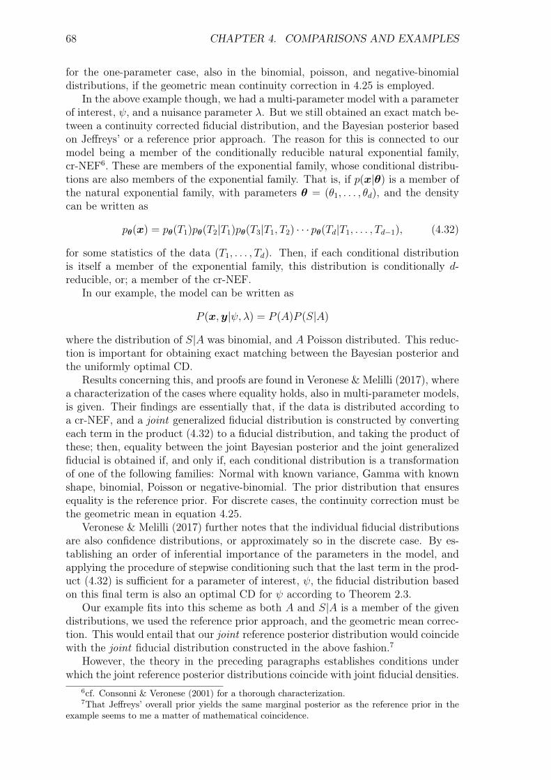
68 CHAPTER 4. COMPARISONS AND EXAMPLES
for the one-parameter case, also in the binomial, poisson, and negative-binomialdistributions, if the geometric mean continuity correction in 4.25 is employed.
In the above example though, we had a multi-parameter model with a parameterof interest, ψ, and a nuisance parameter λ. But we still obtained an exact match be-tween a continuity corrected fiducial distribution, and the Bayesian posterior basedon Jeffreys’ or a reference prior approach. The reason for this is connected to ourmodel being a member of the conditionally reducible natural exponential family,cr-NEF6. These are members of the exponential family, whose conditional distribu-tions are also members of the exponential family. That is, if p(x|θ) is a member ofthe natural exponential family, with parameters θ = (θ1, . . . , θd), and the densitycan be written as
pθ(x) = pθ(T1)pθ(T2|T1)pθ(T3|T1, T2) · · · pθ(Td|T1, . . . , Td−1), (4.32)
for some statistics of the data (T1, . . . , Td). Then, if each conditional distributionis itself a member of the exponential family, this distribution is conditionally d-reducible, or; a member of the cr-NEF.
In our example, the model can be written as
P (x,y|ψ, λ) = P (A)P (S|A)
where the distribution of S|A was binomial, and A Poisson distributed. This reduc-tion is important for obtaining exact matching between the Bayesian posterior andthe uniformly optimal CD.
Results concerning this, and proofs are found in Veronese & Melilli (2017), wherea characterization of the cases where equality holds, also in multi-parameter models,is given. Their findings are essentially that, if the data is distributed according toa cr-NEF, and a joint generalized fiducial distribution is constructed by convertingeach term in the product (4.32) to a fiducial distribution, and taking the product ofthese; then, equality between the joint Bayesian posterior and the joint generalizedfiducial is obtained if, and only if, each conditional distribution is a transformationof one of the following families: Normal with known variance, Gamma with knownshape, binomial, Poisson or negative-binomial. The prior distribution that ensuresequality is the reference prior. For discrete cases, the continuity correction must bethe geometric mean in equation 4.25.
Veronese & Melilli (2017) further notes that the individual fiducial distributionsare also confidence distributions, or approximately so in the discrete case. By es-tablishing an order of inferential importance of the parameters in the model, andapplying the procedure of stepwise conditioning such that the last term in the prod-uct (4.32) is sufficient for a parameter of interest, ψ, the fiducial distribution basedon this final term is also an optimal CD for ψ according to Theorem 2.3.
Our example fits into this scheme as both A and S|A is a member of the givendistributions, we used the reference prior approach, and the geometric mean correc-tion. This would entail that our joint reference posterior distribution would coincidewith the joint fiducial distribution constructed in the above fashion.7
However, the theory in the preceding paragraphs establishes conditions underwhich the joint reference posterior distributions coincide with joint fiducial densities.
6cf. Consonni & Veronese (2001) for a thorough characterization.7That Jeffreys’ overall prior yields the same marginal posterior as the reference prior in the
example seems to me a matter of mathematical coincidence.
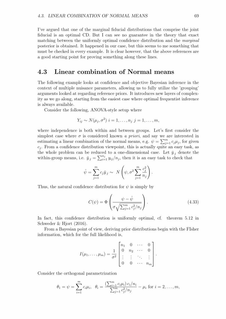
4.3. LINEAR COMBINATION OF NORMAL MEANS 69
I’ve argued that one of the marginal fiducial distributions that comprise the jointfiducial is an optimal CD. But I can see no guarantee in the theory that exactmatching between the uniformly optimal confidence distribution and the marginalposterior is obtained. It happened in our case, but this seems to me something thatmust be checked in every example. It is clear however, that the above references area good starting point for proving something along these lines.
4.3 Linear combination of Normal meansThe following example looks at confidence and objective Bayesian inference in thecontext of multiple nuisance parameters, allowing us to fully utilize the ’grouping’arguments looked at regarding reference priors. It introduces new layers of complex-ity as we go along, starting from the easiest case where optimal frequentist inferenceis always available.
Consider the following, ANOVA-style setup where
Yij ∼ N(µj, σ2) i = 1, . . . , nj j = 1, . . . ,m,
where independence is both within and between groups. Let’s first consider thesimplest case where σ is considered known a priori, and say we are interested inestimating a linear combination of the normal means, e.g. ψ =
∑mj=1 cjµj, for given
cj. From a confidence distribution viewpoint, this is actually quite an easy task, asthe whole problem can be reduced to a one-dimensional case. Let y·j denote thewithin-group means, i.e. y·j =
∑nji=1 yij/nj, then it is an easy task to check that
ψ =m∑j=1
cj y·j ∼ N
(ψ, σ2
m∑j=1
c2j
nj
).
Thus, the natural confidence distribution for ψ is simply by
C(ψ) = Φ
ψ − ψ
σ√∑m
j=1 c2j/nj
. (4.33)
In fact, this confidence distribution is uniformly optimal, cf. theorem 5.12 inSchweder & Hjort (2016).
From a Bayesian point of view, deriving prior distributions begin with the FIsherinformation, which for the full likelihood is,
I(µ1, . . . , µm) =1
σ2
n1 0 · · · 00 n2 · · · 0...
... . . . ...0 0 · · · nm
.Consider the orthogonal parametrization
θ1 = ψ =m∑i=1
ciµi, θi =(∑m
i=1 ciµi) ci/ni∑mj=1 c
2j/nj
− µi for i = 2, . . . ,m,

70 CHAPTER 4. COMPARISONS AND EXAMPLES
or, in terms of the original parameters;
µ1 =c1/n1∑mj=1 c
2j/nj
θ1 +m∑i=2
(ci/c1)θi
µi =ci/ni∑mj=1 c
2j/nj
θ1 − θi for i = 2, . . . ,m.
which yields the reparametrized Fisher information matrix
I(ψ, θ2, . . . , θm) =1
σ2
c21/n1∑m
j=1 c2j/nj
0T
0 A
,where A is a diagonal (m−1)×(m−1) matrix with elements n2, . . . , nm. By work-ing with compact sets in the orthogonal parametrization, the reference prior maybe found by applying theorem 3.2 for the parameter grouping ψ1, θ2, . . . , θm.Then we immediately get
πR(ψ, θ2, . . . , θm) ∝ 1.
which is also Jeffreys’ overall prior for this problem. Notice also that this referenceprior is independent of how the parameters are grouped. Kim et al. (2006) inadver-tently gives the marginal posterior distribution of ψ under the flat reference prior,while deriving the marginal posterior for the case where σ2 is unknown;8
π(ψ|y) ∝ exp
− 1
2σ2 [∑m
i=1 c2i /ni]
2
m∑j=1
c2j
nj
(ψ − y·j
∑mi=1 c
2i /ni
cj/nj
)2. (4.34)
This expression can be viewed as the product of m normal density functions, withmean and variance
µj = y·j
∑mi=1 c
2i /ni
cj/nj, σ2
j =σ2 [∑m
i=1 c2i /ni]
2
c2j/nj
j = 1, . . . ,m. (4.35)
The product of m such densities is itself a normal density9, with mean, µ, andvariance κ2;
µ =
(m∑j=1
µ2
σ2j
)κ2 1
κ2=
m∑j=1
1
σ2j
.
Plugging in the means and variances from 4.35, we find that the posterior in 4.34 isproportional to a normal distribution with mean µ = ψ =
∑mj=1 cj y·j and variance
κ2 = σ2∑m
i=1 c2i /ni. But this is precisely the same distribution as what the uniformly
optimal CD (4.33) is based on! So in this case, the objective Bayesian approachbased on Jeffreys’ or the reference prior, and the uniformly optimal CD approachyield the same result.
8See the proof of Theorem 5 in Kim et al. (2006).9see for example Bromiley (2003).
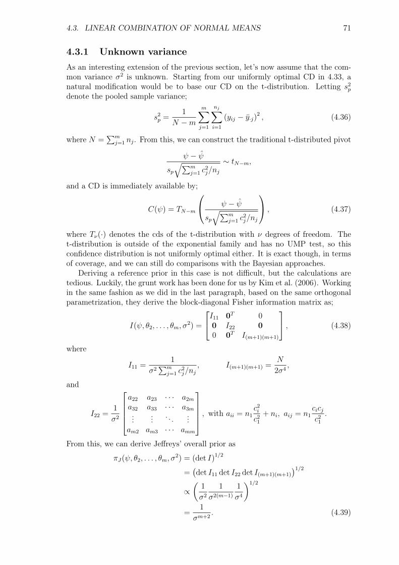
4.3. LINEAR COMBINATION OF NORMAL MEANS 71
4.3.1 Unknown varianceAs an interesting extension of the previous section, let’s now assume that the com-mon variance σ2 is unknown. Starting from our uniformly optimal CD in 4.33, anatural modification would be to base our CD on the t-distribution. Letting s2
p
denote the pooled sample variance;
s2p =
1
N −m
m∑j=1
nj∑i=1
(yij − y·j)2 , (4.36)
where N =∑m
j=1 nj. From this, we can construct the traditional t-distributed pivot
ψ − ψ
sp√∑m
j=1 c2j/nj
∼ tN−m,
and a CD is immediately available by;
C(ψ) = TN−m
ψ − ψ
sp√∑m
j=1 c2j/nj
, (4.37)
where Tν(·) denotes the cds of the t-distribution with ν degrees of freedom. Thet-distribution is outside of the exponential family and has no UMP test, so thisconfidence distribution is not uniformly optimal either. It is exact though, in termsof coverage, and we can still do comparisons with the Bayesian approaches.
Deriving a reference prior in this case is not difficult, but the calculations aretedious. Luckily, the grunt work has been done for us by Kim et al. (2006). Workingin the same fashion as we did in the last paragraph, based on the same orthogonalparametrization, they derive the block-diagonal Fisher information matrix as;
I(ψ, θ2, . . . , θm, σ2) =
I11 0T 00 I22 00 0T I(m+1)(m+1)
, (4.38)
where
I11 =1
σ2∑m
j=1 c2j/nj
, I(m+1)(m+1) =N
2σ4,
and
I22 =1
σ2
a22 a23 · · · a2m
a32 a33 · · · a3m...
... . . . ...am2 am3 · · · amm
, with aii = n1c2i
c21
+ ni, aij = n1cicjc2
1
.
From this, we can derive Jeffreys’ overall prior as
πJ(ψ, θ2, . . . , θm, σ2) = (det I)1/2
=(det I11 det I22 det I(m+1)(m+1)
)1/2
∝(
1
σ2
1
σ2(m−1)
1
σ4
)1/2
=1
σm+2. (4.39)

72 CHAPTER 4. COMPARISONS AND EXAMPLES
For the reference priors, using theorem 3.2 will yield different priors dependingon the parameter grouping. Keeping with the focused theme we’ve been pursuing,where our parameter of interest is most important; two groupings seem natural toconsider:
ψ, θ2, . . . , θm, σ2 and ψ, θ2, . . . , θm, σ2.
Both grouping consider ψ to be the most important parameter, but they differ inhow important the variance is. In the first grouping, the variance is consideredof equal inferential importance as the other mean parameters; (θ2, . . . , θm). Thesecond grouping considers the variance of least importance, less so than the otherθ2, . . . , θm.
For the first grouping, Theorem 3.2 yields
πR1(ψ, θ2, . . . , θm, σ2) =
2∏i=j
hj1(θj)1/2
= 11/2(det I22 det I(m+1)(m+1)
)1/2
∝ 1
σm+1,
while the reference prior based on the second grouping is
πR2(ψ, θ2, . . . , θm, σ2) ∝ 1
σ2.
We see that the reference prior changes quite a bit depending on how the parametersare grouped together. The last prior is interesting because, in the grouping where thevariance is considered least important, it is independent of the number of populationsm. Kim et al. (2006) proves many properties for priors on the form π(·) ∝ σ−2a
for a > 0 in this problem. They prove that the posterior distribution is proper ifN + 2a − m − 2 > 0, and give a formula for the marginal posterior distributionof ψ under any such a-prior. They also prove that this marginal distribution issymmetric and unimodal around ψ – just like the CD in 4.37.
The marginal posterior distribution of ψ, resulting from an a-prior is of the form;
π(ψ|y) ∝
m∑j=1
[Sj + nj
(y·j − ψ
cj/nj∑mi=1 c
2i /ni
)2]−B (y,n, c)
−(N+2a−m−1)/2
,
(4.40)
where Sj is the within-group sum of squares, and B(·) is a function depending onthe constants cj, the samples sizes nj and the data y. R code for computing thismarginal posterior is included in appendix B.
In figure 4.10, the confidence curve based on (4.37) and credible curves basedon marginal posteriors from Jeffreys’ overall prior and the two reference prior isshown. The true underlying variance is σ0 = 2, the number of groups m = 5 andthe linear combination is c = (1, 1, 1, 1, 1). Inference is not particularly sensitive tothese choices, but will vary with n = (n1, . . . , n5). In the left panels, computationsare made with a random sample from a balanced design with n = (3, . . . , 3). Wesee that all four curves are close together, indicating good frequentist properties

4.3. LINEAR COMBINATION OF NORMAL MEANS 73
4 6 8 10 12
0.0
0.4
0.8
ψ
Con
fiden
ceC(δ)πJπR1πR2
4 6 8 10 12
−20
−15
−10
−5
ψ
Log
abso
lute
−di
ffere
nce
πJπR1πR2
2 4 6 8 10
0.0
0.4
0.8
ψ
Con
fiden
ce
C(δ)πJπR1πR2
2 4 6 8 10
−40
−20
ψLo
g ab
solu
te−
diffe
renc
e
πJπR1πR2
Figure 4.10: Confidence curves and log absolute difference between marginal poste-riors and the CD.
of all three posteriors. Inspecting the log absolute difference between the marginalposteriors and the CD, we see that Jeffreys’ overall prior yields the biggest deviation,πR1 is close to Jeffreys, while πR2 has the lowest deviance. In the right panels,computations are done a second time, this time from an unbalanced design withn = (10, 10, 10, 3, 3) – the same trend is apparent here. Overall it seems that πR2
yields the best frequentist performance, being very close to C(ψ) even for low nj.This is also the findings of the simulation study in Kim et al. (2006).
To summarize, we have lost exact matching by assuming the variance is unknown,but even for small sample sizes, the reference prior approach yields inference quiteclose to the exact CD based on the standard t-distributed pivot, close than Jeffreys’prior.
4.3.2 Behrens-Fisher
As a final note on the problem at hand, let’s look at the Behrens-Fisher problemthat we briefly touched upon while discussing simultaneous fiducial inference. LetX1, . . . , Xn
iid∼ N(µ1, σ21) and Y1, . . . , Ym
iid∼ N(µ2, σ22), where all Xi are independent
of all Yi, and consider the two variances unknown and (possibly) unequal. The goalis to obtain inference for the parameter of interest ψ = µ2 − µ1 – simple enough.
This problem is notoriously hard, and no perfect solution really exists, at leastnot one that can be universally agreed upon. This is troubling, especially since it issuch a common situation in statistics to compare two normal means in this fashion.
Let’s first consider Fisher’s solution to the problem, ignoring the discrepancypointed out by Bartlett. Fisher works from the familiar pivotal quantities
t1 =
√n(µ1 − x)
s1
t2 =
√m(µ2 − y)
s2
74 CHAPTER 4. COMPARISONS AND EXAMPLES
which are independent t-distributed random variables with degrees of freedom (n−1)and (m− 1), respectively. This means that µ1 and µ2 can be written as
µ1 = x+s1√nT1
µ2 = y +s2√mT2,
where T1 and T2 are t-distributed random variables with (n−1) and (m−1) degreesof freedom, respectively. This means that µ1 and µ2 are independently fiducially dis-tributed as non-standard t-distributions with location-scale parameters (x, s1/
√n)
and (y, s2/√m), respectively.
Interest now is on the parameter ψ = µ2 − µ1, which yields
ψ = µ2 − µ1 = y − x+s2√mT2 −
s1√nT1.
Leting ψ = y− x, and considering (s1/√nT1, s2/
√mT2) as a point in 2-dimensional
Euclidean space, we can rewrite it in polar coordinates to obtain the statistic;
ψ − ψ√s2
1/n+ s22/m
= T2 cos θ − T1 sin θ, (4.41)
where tan θ = (s1/√n)/(s2/
√m).
We see that the statistic on the left side of the equation is distributed as theconvolution of two t-distributions. Such convolutions are hard to express in closedform, in fact closed form expressions only exist when both degrees of freedom are odd(Nadarajah & Dey 2005). Rahman & Saleh (1974) gives a power-series expressionfor this distribution, and there are R-packages available that will compute it, usuallyby numerical integration.10 Fittingly, this distribution is called the Behrens-Fisherdistribution.
If we let Bn,m,θ(·) denote the cumulative distribution function of the Behrens-Fisher distribution with parameters n, m and the angle θ, we could hope that aconstruction of the kind
C(ψ) = Bn,m,θ
(ψ − ψ√
s21/n+ s2
2/m
), (4.42)
might be an approximate confidence distribution. To test this hypothesis, rememberthe crux in the definition a CD given back in chapter 2. Under the true param-eter, C(ψ0) should be uniformly distributed. By drawing samples from differentcombinations of (n,m, ψ, σ1, σ2) and evaluating the CD at the true value, we canobtain samples from C(ψ0). We can then estimate a kernel density and determineits uniformity.
The result of such a simulation is displayed in figure 4.11, where density estimatesfrom N = 100 000 samples are displayed, based on the beta-kernel density estimatorof Chen (1999) on the bounded interval [0, 1]. This simulation was repeated fordifferent values of parameters (columns), and different samples sizes (rows), yieldingthe array in the figure. We immediately recognize a problem; for low (n,m) this
10for example, the package asht available at https://CRAN.R-project.org/package=asht

4.3. LINEAR COMBINATION OF NORMAL MEANS 75
0.0 0.2 0.4 0.6 0.8 1.0 0.0 0.2 0.4 0.6 0.8 1.0 0.0 0.2 0.4 0.6 0.8 1.0 0.0 0.2 0.4 0.6 0.8 1.0
0.0 0.2 0.4 0.6 0.8 1.0 0.0 0.2 0.4 0.6 0.8 1.0 0.0 0.2 0.4 0.6 0.8 1.0 0.0 0.2 0.4 0.6 0.8 1.0
0.0 0.2 0.4 0.6 0.8 1.0 0.0 0.2 0.4 0.6 0.8 1.0 0.0 0.2 0.4 0.6 0.8 1.0 0.0 0.2 0.4 0.6 0.8 1.0
ψ0=0,σ1=1σ2=1 ψ0=9,σ1=1σ2=1 ψ0=0,σ1=1σ2=10 ψ0=9,σ1=10σ2=1
n=2,
m=
2n=
2,m
=20
n=20
,m=
20
Figure 4.11: Density estimates of samples from C(ψ0) based on the Behrens-Fisherdistribution.
confidence distribution is not uniform, meaning that any α-level interval will nothave α coverage probability. Interestingly, uniformity also seems to depend on thevariances (σ2
1, σ22), where even for low sample sizes uniformity can be somewhat
achieved, if the variances are large and unbalanced.For larger sample sizes, such as (20, 20) we see that uniformity is achieved,
and thus the confidence distribution in (4.42) is a decent approximation to correctcoverage for moderate sample sizes. It would seem that the damning evidenceprovided against Fisher’s fiducial solution to this problem is not so damning afterall.
The critique levied against Fisher’s above solution and argumentation, concerneditself with testing the hypothesis H0 : ψ = 0, for which an α-level test won’t havetype-I error probability at the specified level. With this in mind, Welch (1938)proposed a solution based on the same statistic as Fisher, but using a t-distributioninstead of the Behrens-Fisher distribution. Welch suggested that the statistic in(4.41) approximately has a t-distribution with ν degrees of freedom, where
ν =(S2
1/n+ S22/m)
2
S41/(n
3 − n2) + S42/(m
3 −m2).
This distribution has excellent properties for testing the hypothesis H0, no matterthe true underlying parameters, and does a decent job even at low sample sizes, seefor example Best & Rayner (1987) for a simulation study.
While the confidence distribution can be viewed as a collection of p-values, ofwhich the one from testing this particular H0 is only one in many, one might con-jecture that a CD based on Welch’s proposal would do quite well as an approximate

76 CHAPTER 4. COMPARISONS AND EXAMPLES
0.0 0.2 0.4 0.6 0.8 1.0 0.0 0.2 0.4 0.6 0.8 1.0 0.0 0.2 0.4 0.6 0.8 1.0 0.0 0.2 0.4 0.6 0.8 1.0
0.0 0.2 0.4 0.6 0.8 1.0 0.0 0.2 0.4 0.6 0.8 1.0 0.0 0.2 0.4 0.6 0.8 1.0 0.0 0.2 0.4 0.6 0.8 1.0
0.0 0.2 0.4 0.6 0.8 1.0 0.0 0.2 0.4 0.6 0.8 1.0 0.0 0.2 0.4 0.6 0.8 1.0 0.0 0.2 0.4 0.6 0.8 1.0
ψ0=0,σ1=1σ2=1 ψ0=9,σ1=1σ2=1 ψ0=0,σ1=1σ2=10 ψ0=9,σ1=10σ2=1
n=2,
m=
2n=
2,m
=20
n=20
,m=
20
Figure 4.12: Density estimates of samples from C(ψ0) based on Welch’s solution.
confidence distribution for low samples. As a test, I redid the simulations with thist-distribution instead of the Behrens-Fisher distribution and checked for uniformity.The results are displayed in figure 4.12, and we see that, even for small sample sizes,C(ψ0) is relatively uniform, more so than the fiducial solution.
While this is interesting, I feel the results of the two small simulations speaksmore to the fiducial solution, which achieves approximately uniformity, and hope-fully this the correct coverage probability, even for moderately small sample sizes.Both confidence distributions are approximately uniform at equal sample sizes of 20,but the Welch approximation seems to have some peaks in its density at the edgesfor the unbalanced samples n = 2 and m = 20. This is not a fluke of simulation,as I’ve redone them several times and gotten similar results, for other sample sizesand parameters as well. It would seem that the convergence towards uniformity isnot as smooth as with the fiducial distribution, though I’m not sure what this couldmean for inference.
Fisher provided an approach to epistemic inference, in which his results oftenagree approximately with the strict frequentist criteria of his day. Simulation stud-ies by for example Robinson (1976) indicates that approximate coverage is obtainedquickly, and that at least conservative coverage is achieved, i.e that an α-level inter-val has at least α-level coverage. In addition, the construction is much more generalthan the one of Welch. Again, I feel that his argument would not have been shotdown so quickly if these simulation tools were available in his time.
As a final take, consider the Bayesian solutions to the problem at hand. Thelikelihood can be written as
L(µ1, µ2, σ21, σ
22) ∝ 1
σn1σm2
exp
−1
2
[S2
1 + n(x− µ1)2
σ21
+S2
2 +m(y − µ2)2
σ22
],

4.3. LINEAR COMBINATION OF NORMAL MEANS 77
−15 −10 −5 0 5 10 15
0.0
0.2
0.4
0.6
0.8
1.0
ψ
Cf
Cw
πR
πJ
−15 −10 −5 0 5 10 15
0.0
0.2
0.4
0.6
0.8
1.0
ψ
Cf
Cw
πR
πJ
Figure 4.13: Bayesian credible curves compared to ccs based on Fisher’s fiducialdistribution, and Welch’s approximation.
where S2i denotes the sum-of-squares in each sample. Making the reparametrization
to ψ = µ2 − µ1 and λ = µ1 + µ2, the Fisher information can be written as
I(ψ, λ, σ21, σ
22) =
1
2
n/2σ2
1 0 0 00 m/2σ2
2 0 00 0 n/σ4
1 00 0 0 m/σ4
2
.Now then, Jeffreys’ overall prior can be seen to be πJ(ψ, λ, σ2
1, σ22) ∝ (σ1σ2)−3.
Using theorem 3.2, we have the reference prior, under any other grouping than thatwhich yields Jeffreys’, that πR(ψ, λ, σ2
1, σ22) ∝ (σ1σ2)−2. As an interesting side note,
Jeffreys (1961) proved that the prior π∗J(ψ, λ, σ21, σ
22) ∝ (σ1σ2)−1, which one might
consider to be a quite natural prior since both are scale-parameters, will actuallylead to the fiducial solution.
In figure 4.13, results from two samples are displayed as credible-/confidencecurves based on Fisher’s fiducial solution, Cf , Welch’s approximate solution, Cw,and marginal posterior distributions based on πJ and πR. In the left panel, 5 samplesare drawn from X and Y , with (µ1, µ2, σ1, σ2) = (2, 4, 2, 4), while the right panelhas 10 samples from each distribution with the same means, but more unbalancedstandard deviations (σ1, σ2) = (1, 9).
For the left panel, Jeffreys’ prior leads to the shortest intervals, followed by theReference prior, then Welch’s approximation, and finally Fisher’s fiducial solution.This corroborates the results by Robinson that the fiducial solution is conservative.That being said, the curves are quite close close together, and one would need ahigh degree of confidence to obtain large discrepancies between the lengths of theintervals.
In the right panel, the fiducial solution and Welchs’ approximation is virtuallyindistinguishable from each other, indicating that the fiducial solution works well inobtaining close to the correct coverage. The two posterior distributions also seemcloser together in this plot, but are both narrower than the frequentist solutions,with maybe Jeffreys’ posterior being a little narrower than the one based on thereference prior – indicating approximately the correct coverage.
78 CHAPTER 4. COMPARISONS AND EXAMPLES
The goal of this example was simply to highlight how the frequentist and fiducialapproaches performed, and compare the solutions with some objective Bayesiansolutions. From a Bayesian point of view, it has been studied quite detailed byGhosh & Kim (2001), who also explore the use of probability matching priors forthis problem, and find excellent coverage even for low n.
While Fisher may not have cared to much about the coverage probabilities of hissolution, considering the resulting distribution simply as one of epistemic probability,it could be interesting to pursue the idea of the Behrens-Fisher solution being anapproximate confidence distribution further, as it is a rather open question on theliterature. Simulations pointed to earlier seem to indicate that the Behrens-Fisherintervals are conservative, which should be deemed an admissible form of inference.I mean, as long as a 90% interval has coverage probability larger than, or equal to.9, it seems safe to use in practice. It would be much worse if the interval in questiononly had a 30% chance of covering the true parameter.
4.4 The Fieller-Creasy problem
The Fieller-Creasy problem is a famous problem in statistical inference, and it isincluded here as an example where frequentist and Bayesian inference give twodistinctly different answers, and comparisons are hard, or impossible.
The problem can be stated in the following manner. Let X1, . . . , Xniid∼ N(µ1, σ
2)
and Y1, . . . , Yniid∼ N(µ2, σ
2), where all Xi and Yj are independent, and the varianceunknown. The problem at hand then, in this relatively simple setup, is to estimatethe ratio ψ = µ2/µ1.
This problem has a long history in statistical inference, starting from the originalsolution by Fieller (1940), and further analysis by Creasy (1954).
Given the data as above, the statistics X and Y are distributed as(XY
)∼ N2
((µ1
µ2
),σ2
nI2
)where I2 denotes the 2×2 identity matrix. There is a nice geometry to this problem;the pair (X, Y ) can be considered a point in 2-dimensional euclidean space, and wecan make the transformation into polar coordinates by
X = R cos θ Y = R sin θ
for random variables R ∈ R and θ ∈ [−π/2, π/2). The expectations (µ1, µ2) trans-forms to (r0 cos θ0, r0 sin θ0) for underlying true parameters r0 and θ0. Then since
ψ =µ2
µ1
=r0 sin θ0
r0 cos θ0
= tan θ0,
questions concerning ψ amounts to questions concerning the angle θ0.Next, make the following transformation of the statistics(
Z1
Z2
)=
(cos θ0 sin θ0
− sin θ0 cos θ0
)(XY
).
4.4. THE FIELLER-CREASY PROBLEM 79
This transformation amounts to a clockwise rotation in 2-dimensional space, and itis easy to check that (
Z1
Z2
)∼ N2
((r0
0
),σ2
nI2
),
and that the corresponding polar coordinates for Z1 and Z2 are by R cos (θ − θ0)and R sin (θ − θ0) respectively. Letting S2
p denote the pooled variance as in (4.36),and putting R =
√nR/Sp, the following quantity is a familiar pivot;
R2 sin2 (θ − θ0) =
(Z2
Sp/√n
)2
=
(√nZ2/σ
Sp/σ
)2
∼ F1,n−1, (4.43)
namely F -distributed with (1, n− 1) degrees of freedom.This invites the construction of α-level confidence sets by
Cα =θ0 : R2 sin2 (θ − θ0) ≤ F 2
1,n−1
, (4.44)
where Fα1,n−1 is α quantile of the F distribution. A confidence distribution is not
available though, since this pivot is not monotone in θ0, and it has some strangeproperties. Noticeably, if R2 ≤ Fα
1,n−1 then Cα = R!Consider, after an experiment has been done, that the statistics
(x, y, sp) = (1.6014, 2.7514, 1.721) are obtained from 4 observations. The corre-sponding statistics R and θ is by
R =√x2 + y2 = 3.1835 θ = arctan
y
x= 1.0437,
which makes R2 = 13.69. This implies that all confidence intervals at level α =F−1
1,n−1(13.69) = 0.9657 or higher will be the entire real line. Other possibilities arethat the confidence set is an interval, or the complement of an interval, the situationis illustrated in figure 4.14.
In the figure, the pivot (4.43) is plotted from ψ ∈ (−10, 10) corresponding toθ0 ∈ (−1.47, 1.47), the confidence sets consists of the parts of the parameter spacewhere the pivot dips under the required F -quantiles. We see that the 50% confidenceset is in fact an interval, while the 90% is the complement of an interval. All setswith larger confidence than 96.57% consists of the entire real line, as stated. Alsoadded to the plot, at its lowest point, is a tick mark at the natural point estimatorfor ψ, namely y/x.
This example is sometimes cited as a setup where frequentist inference is non-sensical. What are we to make of the (exact) confidence intervals obtained fromthis setup? Surely a confidence interval consisting of the entire real line must have100% confidence? Are there then levels of confidence, between 1 and for example0.9657 for which we really can’t say anything, where the data doesn’t allow confi-dence statements? This is the view of Schweder & Hjort (2016) and Cox (2006),and is also my own. There are simply situations, where the data obtained from anexperiment does not carry enough information about ψ to make precise confidencestatements at all levels of confidence, there is nothing inherently wrong with this,although it might seem strange at first glance.

80 CHAPTER 4. COMPARISONS AND EXAMPLES
ψ
F−
quan
tiles
−10 −5 0 5 10
F0.5
F0.9
F0.9657
Figure 4.14: The Fieller-Creasy pivot with added F -quantiles.
From the Bayesian point of view, a reference prior is available, with a propermarginal posterior distribution. Yang & Berger (1998) give the reference prior forthis problem as
π(ψ, µ1, σ2) ∝ σ−2(1 + ψ2)−1/2,
and the marginal posterior by
π(ψ|x,y) ∝ (1 + ψ2)−1
(S2 +
n(y − ψx)2
1 + ψ2
)−(2n−1)/2
,
where S2 =∑
(xi − x)2 +∑
(yi − y)2.Plugging in our data from previous, we obtain the marginal posterior distribution
in figure 4.15, where the dotted vertical line represents the estimated ψ = y/x asbefore. The distribution in this case is unimodal, centered a little to the right ofthe frequentist point estimate.
It is difficult to compare the two plots in figures 4.14 and 4.15, as they differboth in form and in logical content, the pivot simply giving rise to confidence re-gions in the parameter space, while the marginal posterior distribution a bona fideprobability distribution – albeit based on an ’objective prior’. The reference pos-terior distribution gives rise to highest posterior credible intervals that are nicelydefined, for all α ∈ (0, 1), in sharp contrast to the frequentist situation. Liseo (1990)studied the coverage probabilities of posterior quantiles based on this distribution,and found that they often are pretty close to the frequentist coverage probability.
Both methods depend heavily on the location of (µ1, µ2) in the parameter space.A µ1 close to zero is likely to make the ratio y/x unstable, resulting in poor perfor-mance of both the Bayesian and frequentist solutions. There seems to be no quickfix from the Bayesian point of view either, with inferences being crucially dependenton the samples obtained.
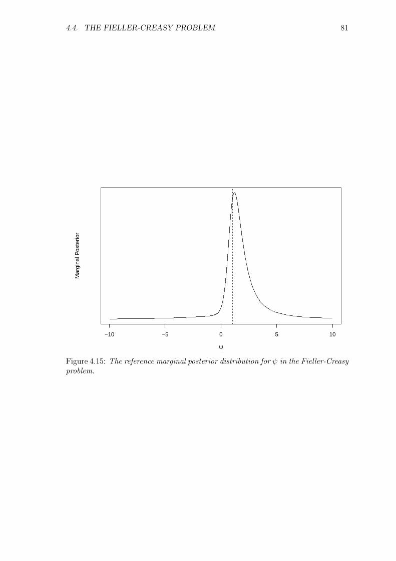
4.4. THE FIELLER-CREASY PROBLEM 81
−10 −5 0 5 10
ψ
Mar
gina
l Pos
terio
r
Figure 4.15: The reference marginal posterior distribution for ψ in the Fieller-Creasyproblem.

Chapter 5
Concluding remarks
In this thesis, I have looked at two vastly different approaches to statistical inference;Fisher’s fiducial argument, specifically focusing on the modern version in termsof confidence distributions, and the theory of objective Bayesianism. Though thetheories are different in approaches and underlying logic, they are trying to achievethe same goal, and they often give quite similar results. In the examples looked at,sometimes we were able to achieve an exact match between the marginal Bayesianposteriors, and an optimal confidence distribution, i.e. one that is uniformly mostpowerful while still admitting the correct coverage. In all cases considered, exactmatching was achieved with Jeffreys’ prior, and typically the reference prior wouldeither equal Jeffreys’, or they would yield the same posterior distributions. Outsidethe context of exactly matching an optimal CD, the reference prior approach seemsto outperform Jeffreys’, when they give different posteriors. Looking at linear-combinations of normal means, the reference prior approach is superior to Jeffreys’when comparing with the CD based on either the t-distributed pivot, or the Behrens-Fisher distribution, this is most likely due to a better approach to handling nuisanceparameters.
The goal of the thesis was not to solve any new problems of fiducial inference,but to highlight connections between fiducial inference and the ’objective’ Bayesianinference. Fisher intended his fiducial distribution to be an objective epistemic prob-ability distribution on the parameter space, allowing definite probability statementsabout the parameter – without appealing to Bayes’ theorem. Comparing the distri-butions from fiducial inference, represented by the confidence distribution approach,to the most compelling Bayesian solution for objective inference, this thesis providesa few answers, but leaves many left to solve.
There are themes in the thesis that one might want to pursue further, eitherbuilding directly upon the work done here, or completely new directions. In thefollowing I will indicate some of these.
5.1 Exact matching and uniformly optimal CDs
We’ve seen that exact matching between Bayesian posterior distributions and jointfiducial distributions, is only possible in a few limited cases. Within the exponentialfamily, this problem seems to be relatively closed due to the findings by (Veronese& Melilli 2017), reviewed in section 4.2.1. While their results establishes conditionsfor exact matching of joint distributions, there is no guarantee that the marginal
83
84 CHAPTER 5. CONCLUDING REMARKS
distribution for a parameter of interest ψ, matches the uniformly optimal CD. Itwould be of interest to close this problem as well, perhaps by putting some furtherconditions on the prior distribution π(·).
Veronese & Melilli (2017) worked within the cr-NEF, i.e. members of the naturalexponential family whose density can be written on the form
pθ(x) = pθ(T1)pθ(T2|T1)pθ(T3|T1, T2) · · · pθ(Td|T1, . . . , Td−1),
where each conditional density is also a member of the NEF. Constructing a jointfiducial distribution from this, by converting each term into a fiducial distribu-tion, and taking the product, this joint distribution will coincide with the Bayesianposterior distribution based on the reference prior. Now then, since each fiducialdistribution in the product above, is also a confidence distribution, the fiducial dis-tribution constructed from pθ(Td|T1, . . . , Td−1) will also be uniformly optimal by thetheory in chapter 2.
Let θ1, . . . , θd denote the natural parameters corresponding to the jointlysufficient statistics T1, . . . , Td from above, so that a CD constructed frompθ(Td|T1, . . . , Td−1) is uniformly optimal for θd. The marginal posterior distribu-tion for θd is
p(θd|x) ∝∫
Θd−1
· · ·∫
Θ1
πR(θ1, . . . , θd)pθ(x)dθ1 · · · dθd−1
= pθ(Td|T1, . . . , Td−1)M(θd, T1, . . . , Td−1),
where the functionM is meant to capture what’s left over from integrating away theparameters θ1, . . . , θd−1. The point now is that this marginal posterior distributionwill only correspond to the uniformly optimal confidence distribution, if the distri-bution of Td|T1, . . . , Td−1 is a member of the correct families and the function M isin fact proportional to the prior ensuring exact coverage. For a natural exponentialfamily with density proportional to
exp θT (x)−K(θ) ,
the only distributions who admit such a prior distribution is again; Normal withknown variance, Gamma with known shape, binomial, Poisson and negative-binomial. In addition, the prior π that ensures exact coverage is the flat priorfor the normal location parameter, and π ∝ K ′(θ) for the others, where K ′ denotesthe derivative of K, see Veronese & Melilli (2015) for a proof of this statement.
To summarize then, we would need pθ(Td|T1, . . . , Td−1) and the functionM(θd, T1, . . . , Td−1) to satisfy some rather strong conditions in order to have exactmatching between uniformly optimal confidence distributions and marginal poste-riors.
It would be of interest to investigate in which cases this happens, and whatrestrictions must be in place to ensure it.
5.2 Approximate matching and PMPsIn section 3.6, I briefly covered some of the basic results on posterior matching.That is, to what order does the quantiles of a Bayesian posterior distribution match
5.3. PAIRED EXPONENTIALS 85
the frequentist coverage probability. The classical result is by Welch & Peers (1963),who proved that all continuous priors will yield first-order matching posteriors, whileJeffreys’ prior will yield second-order matching posteriors. In some special cases,with further restrictions on the likelihood, Jeffreys’ prior will result in a third-ordermatching posterior, but that is pretty much it besides the exact cases mentioned inthe preceding section.
One major topic in this direction, that there simply wasn’t room to explore,is probability matching priors. Prior distributions that are specifically tailored toachieve posterior matching up to some intended order. I briefly mentioned them insection 3.6.1, but it would have been interesting to explore this topic as well. Someof the examples considered already have a great deal of theory in this direction laidout, such as the Behrens-Fisher problem, and the more general linear combinationsof normal means. Quite often, the reference prior approach will actually yield first-or second-order PMPs. Notably, when the parameters are orthogonal, as whenutilizing theorem 3.2, reference priors often are PMPs.
If ψ is some scalar, parameter of interest, and (λ1, . . . , λp) is a vector of nui-sance parameters, and iij is the (i, j)-th element of a diagonal information matrixI(ψ, λ1, . . . , λp)
−1. Then, any prior distribution satisfying
π(ψ, λ1, . . . , λp) ∝ i−1/211 h(λ1, . . . , λp), (5.1)
where h(·) is an arbitrary function, is a second-order PMP for ψ (Datta & Ghosh1995a). With a third-order PMP sometimes within reach by how the function h(·)is chosen.
It could be interesting to compare PMPs to the uniformly optimal CDs, as theyaim more directly for optimal frequentist properties.
5.3 Paired ExponentialsIn section 4.1, I considered the problem of estimating δ, in a setup where we observeexponential pairs (Xi, Yi) with Xi ∼ Expo(θ) and Yi ∼ Expo(θ + δ). The optimalconfidence distribution for this parameter is readily found without much trouble,but the Bayesian approach is difficult. I derived two different reference priors
πR(δ, θ) ∝ δ−4+ 5√
2
(1
θ2+
1
(θ + δ)2
)1/2
π∗R(δ, θ) ∝ δ−1
(1
θ2+
1
(θ + δ)2
)1/2
,
based on how the sequence of compact sets were chosen. πR is based on com-pact rectangles in the original parametrization, using the algorithm sketched out byBerger & Bernardo (1989). The reference prior π∗R is based on compact rectangles inthe orthogonal parametrization of (ψ, λ), and used the theorem of Datta & Ghosh(1995b).
The performance of the posterior distribution based on these two different priorsis puzzling. πR will yield posterior distributions that seemingly always are proper,with performance comparable, or slightly below, that of Jeffreys’ prior in this prob-lem. π∗R seems to sometimes yield posterior distributions on par with Jeffreys’ prior,but other times the posterior distributions do not appear to be proper, even for

86 CHAPTER 5. CONCLUDING REMARKS
0 2 4 6 8 10
0.0
0.1
0.2
0.3
δ
πJ
πR
πR*
0 5 10 15
0.00
0.04
0.08
0.12
δ
πJ
πR
πR*
0 5 10 15 20 25 30 35
0.00
0.02
0.04
0.06
δ
πJ
πR
πR*
0 10 20 30 40 50 60 700.
000
0.01
50.
030
δ
πJ
πR
πR*
Figure 5.1: Marginal posteriors based on Jeffreys’ prior, and the two reference priors,πR and π∗R, for A = 4, and S = 2, 1, 0.5, 0.25.
moderately large n. Consider the statistics A =∑
(xi + yi) and S =∑yi, from n
observations. This makes the posterior distribution
p(δ, θ|A, S) ∝ δa(
1
θ2+
1
(θ + δ)2
)1/2
θn (θ + δ)n exp −δA− θS ,
with a = −1 for π∗R and a = −4 + 5/√
2 for πR.Depending on the sampled values of (A, S), π∗R can yield results on par with
Jeffreys’ prior, or results that are non-sensical, perhaps improper. In figure 5.1,the marginal posterior distributions are displayed, computed for the two referencepriors, and Jeffreys’ prior – at 4 different values of the sampled statistics. The valueof A is kept fixed at 4, while S changes from 2 in the top left, 1 in the top right, 0.5in bottom left and 0.25 in the bottom right, all at n = 10.
As S becomes smaller, the posterior distribution based on π∗R creeps closer andcloser to Jeffreys’, which we’ve seen has good properties in this example. The samehappens for πR, but it seems to be shifted to the right compared to the two others.Comfortingly, the posterior based on πR doesn’t keep traveling right for even lowervalues of S, and at larger values of n, all three posterior distributions look the same.
This behaviour is quite strange, and I have not been able to find a good ex-planation. The reparametrization I did in order to find the reference prior usingthe algorithm of Berger & Bernardo (1989), leaves a gap in the parameter space atδ = 0 where the parametrization is not one-to-one – this is most likely the sourceof the discrepancy, and it might make the theorem by Datta & Ghosh (1995b) in-valid, though I haven’t found anything in the paper to indicate that this is so. The1989 paper by Berger and Bernardo finds the reference prior for the product of twonormal means, under the restriction that both means are strictly larger than zero– similar to the restriction I enforced. And my proofs and techniques are following
5.4. BEHRENS-FISHER 87
their approach. A conjecture might be that the value −4+5/√
2 ≈ −0.46 is as closeto −1 as one can get, while still maintaining a proper distribution on average. Itbecomes a question of choosing between a prior that on average performs well, πR,or a prior that sometimes performs well, and sometimes quite horribly.
The problem was included in the thesis, as an example of how difficult the theoryof ’objective’ Bayes can be, this is particularly interesting when contrasted to theCD solution, which is so simple. It would be of interest to derive the reference priorin this problem without restriction in place, hopefully we should see similar resultscompared to the other problems, where the reference prior seemed to be slightlybetter than Jeffreys’ prior on average over the sample space.
5.4 Behrens-Fisher
In section 4.3.2, the Behrens-Fisher problem was touched upon briefly. This isa problem of immense historical, and practical importance, and could probablywarrant an entire thesis of its own; exploring suggested solutions from differentangles and generalizations. The main question I tried to indicate is whether ornot Fisher’s fiducial solution is a confidence distribution, exactly, approximately, orconservatively – i.e. α-level quantiles have at least α-level coverage. Some initialsimulations seem to indicate that Fisher’s solution is an approximate confidencedistribution, close to uniformity even for moderately small sample sizes, such as n =10. To answer this question more fully would require either a large simulation study,with some measure of closeness to pure uniformity, perhaps the KL-divergence, ormaybe some asymptotic expansions for a more analytic proof. The studies that havebeen done seem to suggest that Fisher’s solution is at least a conservative confidencedistribution, though it remains an open question.
5.5 Epistemic probability
The fiducial argument rests on transferring aleatory probability from the samplespace, into the parameter space. Once we are in the parameter space, the goodold rules for probability calculus no longer seem to apply, at least not under thedesideratum that exact coverage should be conserved. Clearly, once the randomnesshas been transferred, it no longer adheres to the axioms laid down by Kolmogorov– which is troublesome. First, and foremost, it means we need to be clear in ourthought process when working fiducially, paying attention to the underlying logic,and checking resulting distributions as we go along.
Fisher regarded his fiducial distribution as a proper epistemic posterior distribu-tion on the parameter space, regarding the previously fixed parameter of interest,now as a random variable. I will agree with most of the critics that this is in factincorrect, and continue to regard my parameters as fixed unknown quantities. Ifthe fiducial distribution is also a confidence distribution, I am more willing to callthe resulting distribution epistemic in a sense, but not go so far as to consider theparameter as a random variable. I do feel that the confidence distribution in a sensecaptures something more akin to this interpretation of probability. This seems alsoto be the view of Schweder (2017), who argues that confidence is in fact epistemicprobability!
88 CHAPTER 5. CONCLUDING REMARKS
Hampel (2003) regards the confidence distributions as the only proper fiducialargument, as it was laid out in Fisher’s early papers – before he started regardingthe parameters as random. Hampel thinks that “... one of the reasons why we stillhave problems with fiducial probabilities, is that we lack an adequate formalismfor frequentist epistemic probabilities.” (Hampel 2003, p. 8, my emphasis) PerhapsFisher’s fiducial argument is a new type of probability, with it’s own set of rules –we simply need to find out what they are. Perhaps we need a new set of axioms,tailored to this specific system of logic. In this regard, see also Schweder & Hjort(2016, ch. 15.4) and Schweder & Hjort (2017).

Bibliography
Bartlett, M. S. (1936), ‘The information available in small samples’, MathematicalProceedings of the Cambridge Philosophical Society 32(4), 560–566.
Berger, J. (2006), ‘The case for objective Bayesian analysis’, Bayesian Anal.1(3), 385–402.
Berger, J. O. & Bernardo, J. M. (1989), ‘Estimating a product of means: Bayesiananalysis with reference priors’, Journal of the American Statistical Association84(405), 200–207.
Berger, J. O., Bernardo, J. M. & Sun, D. (2009), ‘The formal definition of referencepriors’, Ann. Statist. 37(2), 905–938.
Bernardo, J. (1997), ‘Rejoinder’, Journal of Statistical Planning and Inference65(1), 185 – 189.
Bernardo, J. M. (1979), ‘Reference posterior distributions for Bayesian inference’,Journal of the Royal Statistical Society. Series B (Methodological) 41(2), 113–147.
Bernardo, J. M. (2005), ‘Reference analysis’, Handbook of statistics 25, 17–90.
Bernardo, J. M. & Berger, J. O. (1992), Bayesian statistics 4 : Proceedings of thefourth valencia international meeting, april 15-20, 1991, Clarendon Press ; OxfordUniversity Press, Oxford; New York.
Best, D. J. & Rayner, J. C. W. (1987), ‘Welch’s approximate solution for thebehrens-fisher problem’, Technometrics 29(2), 205–210.
Birnbaum, A. (1961), ‘Confidence curves: An omnibus technique for estimation andtesting statistical hypotheses’, Journal of the American Statistical Association56(294), 246–249.
Bromiley, P. (2003), Products and convolutions of gaussian probability density func-tions, Technical Report 2003-003, Imaging Sciences Research Group, Institute ofPopulation Health, School of Medicine, University of Manchester.
Casella, G. & Berger, R. (2002), Statistical Inference, Duxbury advanced series instatistics and decision sciences, Thomson Learning.
Chen, S. X. (1999), ‘Beta kernel estimators for density functions’, Comput. Stat.Data Anal. 31(2), 131–145.
Consonni, G. & Veronese, P. (2001), ‘Conditionally reducible natural exponen-tial families and enriched conjugate priors’, Scandinavian Journal of Statistics28(2), 377–406.
89
90 BIBLIOGRAPHY
Cox, D. R. (1958), ‘Some problems connected with statistical inference’, The Annalsof Mathematical Statistics 29(2), 357–372.
Cox, D. R. (2006), Principles of Statistical Inference.
Cox, D. R. & Reid, N. (1987), ‘Parameter orthogonality and approximate condi-tional inference’, Journal of the Royal Statistical Society. Series B (Methodologi-cal) 49(1), 1–39.
Creasy, M. A. (1954), ‘Limits for the ratio of means’, Journal of the Royal StatisticalSociety. Series B (Methodological) 16(2), 186–194.
Datta, G. S. & Ghosh, J. K. (1995a), ‘On priors providing frequentist validity forBayesian inference’, Biometrika 82(1), 37–45.
Datta, G. S. & Ghosh, M. (1995b), ‘Some remarks on noninformative priors’, Journalof the American Statistical Association 90(432), 1357–1363.
Datta, G. S. & Ghosh, M. (1996), ‘On the invariance of noninformative priors’, Ann.Statist. 24(1), 141–159.
Datta, G. S. & Mukerjee, R. (2004), ‘Probability matching priors: Higher orderasymptotics’.
de Finetti, B. (1937), ‘La prévision : ses lois logiques, ses sources subjectives’,Annales de l’institut Henri Poincaré 7(1), 1–68.
Efron, B. (1998), ‘R. A. Fisher in the 21st century’, Statistical Science 13(2), 95–114.
Fieller, E. C. (1940), ‘The biological standardization of insulin’, Supplement to theJournal of the Royal Statistical Society 7(1), 1–64.
Fisher, R. A. (1930), ‘Inverse probability’, Mathematical Proceedings of the Cam-bridge Philosophical Society 26(4), 528–535.
Fisher, R. A. (1935), ‘The fiducial argument in statistical inference’, Annals ofEugenics 6(4), 391–398.
Gelman, A., Carlin, J., Stern, H., Dunson, D., Vehtari, A. & Rubin, D. (2014),Bayesian Data Analysis, Third Edition (Chapman & Hall/CRC Texts in Statis-tical Science), third edn, Chapman and Hall/CRC.
Ghosh, M. & Kim, Y.-H. (2001), ‘The Behrens-Fisher problem revisited: A Bayes-frequentist synthesis’, The Canadian Journal of Statistics / La Revue Canadiennede Statistique 29(1), 5–17.
Hacking, I. (2006), The Emergence of Probability; A philosophical study of the earlyideas about probability induction and statistical infernce, second edn, CambridgeUniversity Press.
Hampel, F. (2003), The proper fiducial argument, Technical Report 114, Eidgenös-sische Technische Hochschule.
Hannig, J. (2009), ‘On generalized fiducial inference’, Statistica Sinica 19(2), 491–544.

BIBLIOGRAPHY 91
Hannig, J., Iyer, H., Lai, R. C. S. & Lee, T. C. M. (2016), ‘Generalized fiducial infer-ence: A review and new results’, Journal of the American Statistical Association111(515), 1346–1361.
Jaynes, E. (2003), Probability Theory: The Logic of Science, Cambridge UniversityPress Cambridge.
Jeffreys, H. (1946), ‘An invariant form for the prior probability in estimation prob-lems’, Proceedings of the Royal Society of London A: Mathematical, Physical andEngineering Sciences 186(1007), 453–461.
Jeffreys, H. (1961), Theory of Probability, Oxford University Press.
Kass, R. E. & Wasserman, L. (1996), ‘The selection of prior distributions by formalrules’, Journal of the American Statistical Association 91(435), 1343–1370.
Keynes, J. M. (1921), A treatise on probability, Cambridge University Press.
Kim, D. H., Kang, S. G. & Lee, W. D. (2006), ‘Noninformative priors for linearcombinations of the normal means’, Statistical Papers 47(2), 249–262.
Lehmann, E. L. & Romano, J. P. (2005), Testing statistical hypotheses, SpringerTexts in Statistics, third edn, Springer, New York.
Lindley, D. V. (1958), ‘Fiducial distributions and Bayes’ theorem’, Journal of theRoyal Statistical Society. Series B (Methodological) 20(1), 102–107.
Liseo, B. (1990), Elimination of nuisance parameters with reference non informativepriors, Technical Report 90-58C, Purdue University.
Martin, R. & Liu, C. (2015), Inferential Models: Reasoning with Uncertainty, Chap-man and Hall.
Nadarajah, S. & Dey, D. (2005), ‘Convolutions of the t distribution’, Computers &Mathematics with Applications 49(5), 715 – 721.
Neyman, J. (1934), ‘On the two different aspects of the representative method: Themethod of stratified sampling and the method of purposive selection’, Journal ofthe Royal Statistical Society 97(4), 558–625.
Pedersen, J. G. (1978), ‘Fiducial inference’, International Statistical Review / RevueInternationale de Statistique 46(2), 147–170.
Rahman, M. & Saleh, A. K. M. E. (1974), ‘Explicit form of the distribution ofthe Behrens-Fisher d-statistic’, Journal of the Royal Statistical Society. Series B(Methodological) 36(1), 54–60.
Robinson, G. K. (1976), ‘Properties of Students t and of the Behrens-Fisher solutionto the two means problem’, The Annals of Statistics 4(5), 963–971.
Savage, L. (1954), The Foundations of Statistics, Dover Publications.
Savage, L. J. (1961), The foundations of statistics reconsidered, in ‘Proceedingsof the Fourth Berkeley Symposium on Mathematical Statistics and Probability,Volume 1: Contributions to the Theory of Statistics’, University of CaliforniaPress, Berkeley, Calif., pp. 575–586.
92 BIBLIOGRAPHY
Schweder, T. (2017), ‘Confidence is epistemic probability for empirical science’,Journal of Statistical Planning and Inference . Forthcoming.
Schweder, T. & Hjort, N. L. (2016), Confidence, Likelihood, Probability. StatisticalInference with Confidence Distributions.
Schweder, T. & Hjort, N. L. (2017), ‘Confidence distributions and related themes’,Journal of Statistical Planning and Inference . Forthcoming.
Shannon, C. E. (1948), ‘A mathematical theory of communication’, The Bell SystemTechnical Journal 27(3), 379–423.
Sprott, D. (1963), ‘A transformation model for the investigation of fiducial distri-butions’, Bull. int. statist. Inst. 40, 856–869.
Stein, C. (1959), ‘An example of wide discrepancy between fiducial and confidenceintervals’, Ann. Math. Statist. 30(4), 877–880.
Stone, M. (1969), ‘The role of significance testing: Some data with a message’,Biometrika 56(3), 485–493.
Sun, D. & Ye, K. (1995), ‘Reference prior Bayesian analysis for normal mean prod-ucts’, Journal of the American Statistical Association 90(430), 589–597.
Veronese, P. & Melilli, E. (2015), ‘Fiducial and confidence distributions for realexponential families’, Scandinavian Journal of Statistics 42(2), 471–484.
Veronese, P. & Melilli, E. (2017), ‘Fiducial, confidence and objective Bayesian pos-terior distributions for a multidimensional parameter’, Journal of Statistical Plan-ning and Inference . Forthcoming.
Welch, B. L. (1938), ‘The significance of the difference between two means when thepopulation variances are unequal’, Biometrika 29(3/4), 350–362.
Welch, B. L. & Peers, H. W. (1963), ‘On formulae for confidence points based onintegrals of weighted likelihoods’, Journal of the Royal Statistical Society. SeriesB (Methodological) 25(2), 318–329.
Xie, M.-g. & Singh, K. (2013), ‘Confidence distribution, the frequentist distributionestimator of a parameter: A review’, International Statistical Review 81(1), 3–39.
Yang, R. & Berger, J. O. (1998), A catalog of non-informative priors, Technicalreport.
Zabell, S. (1989), ‘R. A. Fisher on the history of inverse probability’, Statist. Sci.4(3), 247–256.
Zabell, S. L. (1992), ‘R. A. Fisher and fiducial argument’, Statist. Sci. 7(3), 369–387.
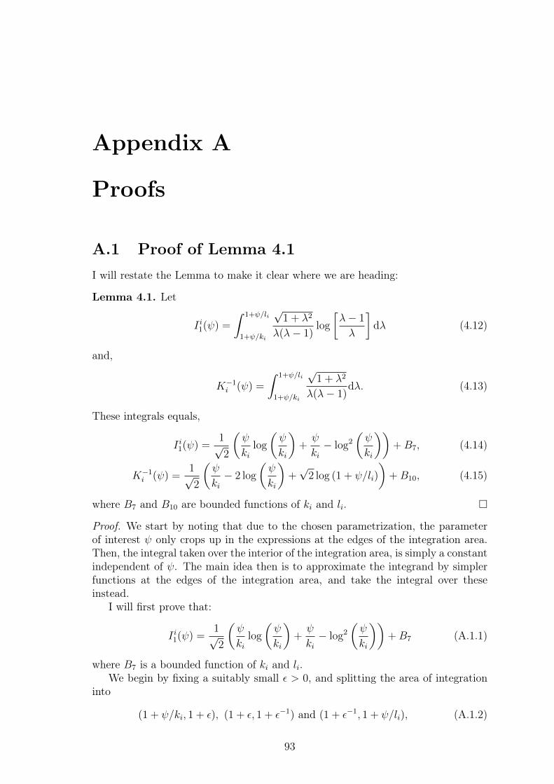
Appendix A
Proofs
A.1 Proof of Lemma 4.1I will restate the Lemma to make it clear where we are heading:
Lemma 4.1. Let
I i1(ψ) =
∫ 1+ψ/li
1+ψ/ki
√1 + λ2
λ(λ− 1)log
[λ− 1
λ
]dλ (4.12)
and,
K−1i (ψ) =
∫ 1+ψ/li
1+ψ/ki
√1 + λ2
λ(λ− 1)dλ. (4.13)
These integrals equals,
I i1(ψ) =1√2
(ψ
kilog
(ψ
ki
)+ψ
ki− log2
(ψ
ki
))+B7, (4.14)
K−1i (ψ) =
1√2
(ψ
ki− 2 log
(ψ
ki
)+√
2 log (1 + ψ/li)
)+B10, (4.15)
where B7 and B10 are bounded functions of ki and li.
Proof. We start by noting that due to the chosen parametrization, the parameterof interest ψ only crops up in the expressions at the edges of the integration area.Then, the integral taken over the interior of the integration area, is simply a constantindependent of ψ. The main idea then is to approximate the integrand by simplerfunctions at the edges of the integration area, and take the integral over theseinstead.
I will first prove that:
I i1(ψ) =1√2
(ψ
kilog
(ψ
ki
)+ψ
ki− log2
(ψ
ki
))+B7 (A.1.1)
where B7 is a bounded function of ki and li.We begin by fixing a suitably small ε > 0, and splitting the area of integration
into
(1 + ψ/ki, 1 + ε), (1 + ε, 1 + ε−1) and (1 + ε−1, 1 + ψ/li), (A.1.2)
93
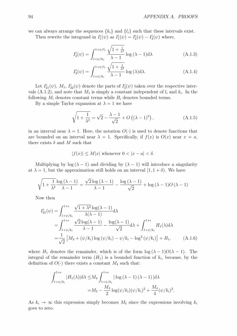
94 APPENDIX A. PROOFS
we can always arrange the sequences ki and li such that these intervals exist.Then rewrite the integrand in I i1(ψ) as I i1(ψ) = I i2(ψ)− I i3(ψ) where,
I i2(ψ) =
∫ 1+ψ/li
1+ψ/ki
√1 + 1
λ2
λ− 1log (λ− 1)dλ (A.1.3)
I i3(ψ) =
∫ 1+ψ/li
1+ψ/ki
√1 + 1
λ2
λ− 1log (λ)dλ. (A.1.4)
Let I i21(ψ), M1, I i22(ψ) denote the parts of I i2(ψ) taken over the respective inter-vals (A.1.2), and note that M1 is simply a constant independent of li and ki. In thefollowing Mi denotes constant terms while Bi denotes bounded terms.
By a simple Taylor expansion at λ = 1 we have√1 +
1
λ2=√
2− λ− 1√2
+O((λ− 1)2
), (A.1.5)
in an interval near λ = 1. Here, the notation O(·) is used to denote functions thatare bounded on an interval near λ = 1. Specifically, if f(x) is O(x) near x = a,there exists δ and M such that
|f(x)| ≤M |x| whenever 0 < |x− a| < δ.
Multiplying by log (λ− 1) and dividing by (λ − 1) will introduce a singularityat λ = 1, but the approximation still holds on an interval [1, 1 + δ). We have√
1 +1
λ2
log (λ− 1)
λ− 1=
√2 log (λ− 1)
λ− 1− log (λ− 1)√
2+ log (λ− 1)O (λ− 1)
Now then
I i21(ψ) =
∫ 1+ε
1+ψ/ki
√1 + λ2 log(λ− 1)
λ(λ− 1)dλ
=
∫ 1+ε
1+ψ/ki
√2 log(λ− 1)
λ− 1− log(λ− 1)√
2dλ+
∫ 1+ε
1+ψ/ki
H1(λ)dλ
=1√2
[M3 + (ψ/ki) log (ψ/ki)− ψ/ki − log2 (ψ/ki)
]+B1, (A.1.6)
where H1 denotes the remainder, which is of the form log (λ− 1)O(λ − 1). Theintegral of the remainder term (H1) is a bounded function of ki, because, by thedefinition of O(·) there exists a constant M4 such that:∫ 1+ε
1+ψ/ki
|H1(λ)|dλ ≤M4
∫ 1+ε
1+ψ/ki
| log (λ− 1) (λ− 1) |dλ
=M5 −M4
2log(ψ/ki)(ψ/ki)
2 +M4
4(ψ/ki)
2.
As ki → ∞ this expression simply becomes M5 since the expressions involving kigoes to zero.
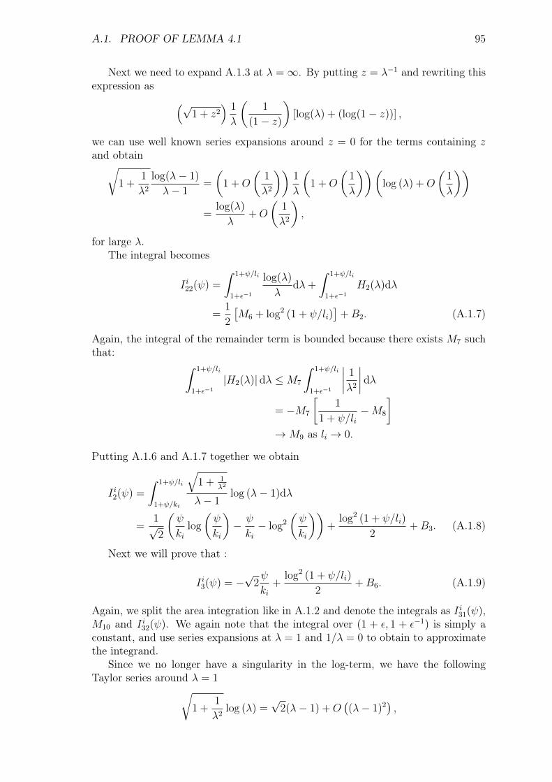
A.1. PROOF OF LEMMA 4.1 95
Next we need to expand A.1.3 at λ =∞. By putting z = λ−1 and rewriting thisexpression as (√
1 + z2) 1
λ
(1
(1− z)
)[log(λ) + (log(1− z))] ,
we can use well known series expansions around z = 0 for the terms containing zand obtain√
1 +1
λ2
log(λ− 1)
λ− 1=
(1 +O
(1
λ2
))1
λ
(1 +O
(1
λ
))(log (λ) +O
(1
λ
))=
log(λ)
λ+O
(1
λ2
),
for large λ.The integral becomes
I i22(ψ) =
∫ 1+ψ/li
1+ε−1
log(λ)
λdλ+
∫ 1+ψ/li
1+ε−1
H2(λ)dλ
=1
2
[M6 + log2 (1 + ψ/li)
]+B2. (A.1.7)
Again, the integral of the remainder term is bounded because there exists M7 suchthat: ∫ 1+ψ/li
1+ε−1
|H2(λ)| dλ ≤M7
∫ 1+ψ/li
1+ε−1
∣∣∣∣ 1
λ2
∣∣∣∣ dλ= −M7
[1
1 + ψ/li−M8
]→M9 as li → 0.
Putting A.1.6 and A.1.7 together we obtain
I i2(ψ) =
∫ 1+ψ/li
1+ψ/ki
√1 + 1
λ2
λ− 1log (λ− 1)dλ
=1√2
(ψ
kilog
(ψ
ki
)− ψ
ki− log2
(ψ
ki
))+
log2 (1 + ψ/li)
2+B3. (A.1.8)
Next we will prove that :
I i3(ψ) = −√
2ψ
ki+
log2 (1 + ψ/li)
2+B6. (A.1.9)
Again, we split the area integration like in A.1.2 and denote the integrals as I i31(ψ),M10 and I i32(ψ). We again note that the integral over (1 + ε, 1 + ε−1) is simply aconstant, and use series expansions at λ = 1 and 1/λ = 0 to obtain to approximatethe integrand.
Since we no longer have a singularity in the log-term, we have the followingTaylor series around λ = 1√
1 +1
λ2log (λ) =
√2(λ− 1) +O
((λ− 1)2
),
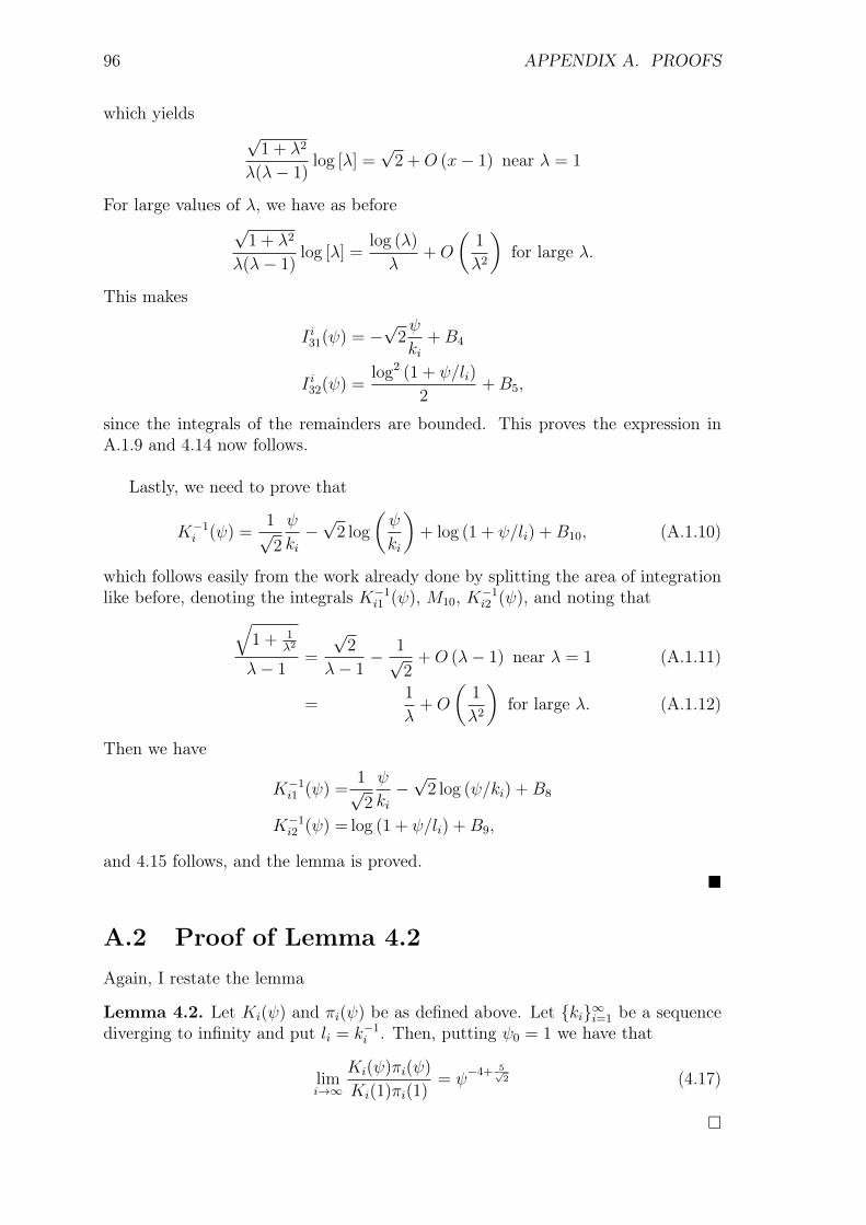
96 APPENDIX A. PROOFS
which yields√
1 + λ2
λ(λ− 1)log [λ] =
√2 +O (x− 1) near λ = 1
For large values of λ, we have as before√
1 + λ2
λ(λ− 1)log [λ] =
log (λ)
λ+O
(1
λ2
)for large λ.
This makes
I i31(ψ) = −√
2ψ
ki+B4
I i32(ψ) =log2 (1 + ψ/li)
2+B5,
since the integrals of the remainders are bounded. This proves the expression inA.1.9 and 4.14 now follows.
Lastly, we need to prove that
K−1i (ψ) =
1√2
ψ
ki−√
2 log
(ψ
ki
)+ log (1 + ψ/li) +B10, (A.1.10)
which follows easily from the work already done by splitting the area of integrationlike before, denoting the integrals K−1
i1 (ψ), M10, K−1i2 (ψ), and noting that√
1 + 1λ2
λ− 1=
√2
λ− 1− 1√
2+O (λ− 1) near λ = 1 (A.1.11)
=1
λ+O
(1
λ2
)for large λ. (A.1.12)
Then we have
K−1i1 (ψ) =
1√2
ψ
ki−√
2 log (ψ/ki) +B8
K−1i2 (ψ) = log (1 + ψ/li) +B9,
and 4.15 follows, and the lemma is proved.
A.2 Proof of Lemma 4.2Again, I restate the lemma
Lemma 4.2. Let Ki(ψ) and πi(ψ) be as defined above. Let ki∞i=1 be a sequencediverging to infinity and put li = k−1
i . Then, putting ψ0 = 1 we have that
limi→∞
Ki(ψ)πi(ψ)
Ki(1)πi(1)= ψ
−4+ 5√2 (4.17)
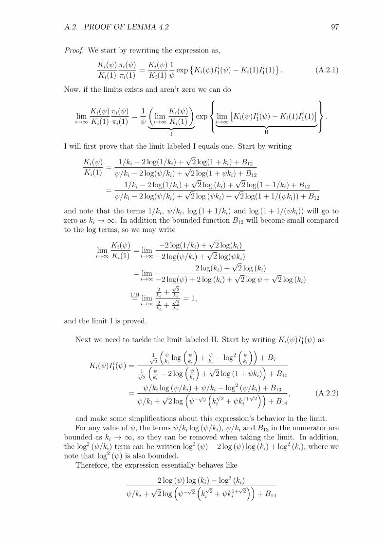
A.2. PROOF OF LEMMA 4.2 97
Proof. We start by rewriting the expression as,
Ki(ψ)
Ki(1)
πi(ψ)
πi(1)=Ki(ψ)
Ki(1)
1
ψexp
Ki(ψ)I i1(ψ)−Ki(1)I i1(1)
. (A.2.1)
Now, if the limits exists and aren’t zero we can do
limi→∞
Ki(ψ)
Ki(1)
πi(ψ)
πi(1)=
1
ψ
(limi→∞
Ki(ψ)
Ki(1)
)︸ ︷︷ ︸
I
exp
limi→∞
[Ki(ψ)I i1(ψ)−Ki(1)I i1(1)
]︸ ︷︷ ︸
II
.
I will first prove that the limit labeled I equals one. Start by writing
Ki(ψ)
Ki(1)=
1/ki − 2 log(1/ki) +√
2 log(1 + ki) +B12
ψ/ki − 2 log(ψ/ki) +√
2 log(1 + ψki) +B12
=1/ki − 2 log(1/ki) +
√2 log (ki) +
√2 log(1 + 1/ki) +B12
ψ/ki − 2 log(ψ/ki) +√
2 log (ψki) +√
2 log(1 + 1/(ψki)) +B12
and note that the terms 1/ki, ψ/ki, log (1 + 1/ki) and log (1 + 1/(ψki)) will go tozero as ki →∞. In addition the bounded function B12 will become small comparedto the log terms, so we may write
limi→∞
Ki(ψ)
Ki(1)= lim
i→∞
−2 log(1/ki) +√
2 log(ki)
−2 log(ψ/ki) +√
2 log(ψki)
= limi→∞
2 log(ki) +√
2 log (ki)
−2 log(ψ) + 2 log (ki) +√
2 logψ +√
2 log (ki)
L’H= lim
i→∞
2ki
+√
2ki
2ki
+√
2ki
= 1,
and the limit I is proved.
Next we need to tackle the limit labeled II. Start by writing Ki(ψ)I i1(ψ) as
Ki(ψ)I i1(ψ) =
1√2
(ψki
log(ψki
)+ ψ
ki− log2
(ψki
))+B7
1√2
(ψki− 2 log
(ψki
)+√
2 log (1 + ψki))
+B10
=ψ/ki log (ψ/ki) + ψ/ki − log2 (ψ/ki) +B13
ψ/ki +√
2 log(ψ−√
2(k√
2i + ψk1+
√2
i
))+B14
, (A.2.2)
and make some simplifications about this expression’s behavior in the limit.For any value of ψ, the terms ψ/ki log (ψ/ki), ψ/ki and B13 in the numerator are
bounded as ki → ∞, so they can be removed when taking the limit. In addition,the log2 (ψ/ki) term can be written log2 (ψ)− 2 log (ψ) log (ki) + log2 (ki), where wenote that log2 (ψ) is also bounded.
Therefore, the expression essentially behaves like
2 log (ψ) log (ki)− log2 (ki)
ψ/ki +√
2 log(ψ−√
2(k√
2i + ψk1+
√2
i
))+B14
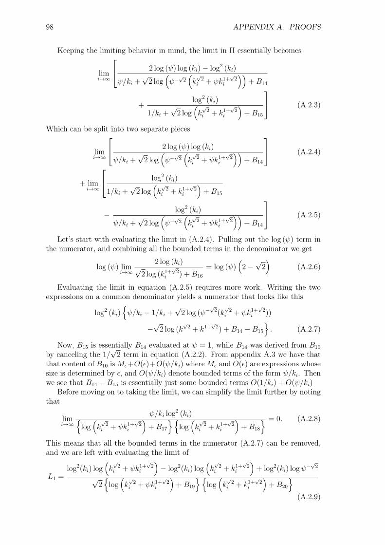
98 APPENDIX A. PROOFS
Keeping the limiting behavior in mind, the limit in II essentially becomes
limi→∞
2 log (ψ) log (ki)− log2 (ki)
ψ/ki +√
2 log(ψ−√
2(k√
2i + ψk1+
√2
i
))+B14
+log2 (ki)
1/ki +√
2 log(k√
2i + k1+
√2
i
)+B15
(A.2.3)
Which can be split into two separate pieces
limi→∞
2 log (ψ) log (ki)
ψ/ki +√
2 log(ψ−√
2(k√
2i + ψk1+
√2
i
))+B14
(A.2.4)
+ limi→∞
log2 (ki)
1/ki +√
2 log(k√
2i + k1+
√2
i
)+B15
− log2 (ki)
ψ/ki +√
2 log(ψ−√
2(k√
2i + ψk1+
√2
i
))+B14
(A.2.5)
Let’s start with evaluating the limit in (A.2.4). Pulling out the log (ψ) term inthe numerator, and combining all the bounded terms in the denominator we get
log (ψ) limi→∞
2 log (ki)√2 log (k1+
√2
i ) +B16
= log (ψ)(
2−√
2)
(A.2.6)
Evaluating the limit in equation (A.2.5) requires more work. Writing the twoexpressions on a common denominator yields a numerator that looks like this
log2 (ki)ψ/ki − 1/ki +
√2 log (ψ−
√2(k√
2i + ψk1+
√2
i ))
−√
2 log (k√
2 + k1+√
2) +B14 −B15
. (A.2.7)
Now, B15 is essentially B14 evaluated at ψ = 1, while B14 was derived from B10
by canceling the 1/√
2 term in equation (A.2.2). From appendix A.3 we have thatthat content of B10 isMε+O(ε)+O(ψ/ki) whereMε and O(ε) are expressions whosesize is determined by ε, and O(ψ/ki) denote bounded terms of the form ψ/ki. Thenwe see that B14 −B15 is essentially just some bounded terms O(1/ki) +O(ψ/ki)
Before moving on to taking the limit, we can simplify the limit further by notingthat
limi→∞
ψ/ki log2 (ki)log(k√
2i + ψk1+
√2
i
)+B17
log(k√
2i + k1+
√2
i
)+B18
= 0. (A.2.8)
This means that all the bounded terms in the numerator (A.2.7) can be removed,and we are left with evaluating the limit of
L1 =log2(ki) log
(k√
2i + ψk1+
√2
i
)− log2(ki) log
(k√
2i + k1+
√2
i
)+ log2(ki) logψ−
√2
√2
log(k√
2i + ψk1+
√2
i
)+B19
log(k√
2i + k1+
√2
i
)+B20
(A.2.9)

A.2. PROOF OF LEMMA 4.2 99
which can be factorized as L1 = 1√2
(L11L12 + L13L14) where,
L11 =log(ki)
log(k√
2i + ψk1+
√2
i
)+B17
L12 =log(ki) log
(k√
2i + ψk1+
√2
i
)− log(ki) log
(k√
2i + k1+
√2
i
)log(k√
2i + k1+
√2
i
)+B18
L13 =log(ki) logψ−
√2
log(k√
2i + ψk1+
√2
i
)+B17
L14 =log(ki)
log(k√
2i + k1+
√2
i
)+B18
and the limit taken over each piece separately. By the same rewrite as in A.2.6, wehave
limi→∞
L11 = limi→∞
L14 = (1 +√
2)−1.
For L13 we get
limi→∞
L13 = (1 +√
2)−1 log (ψ−√
2)
.Lastly we need to tackle L12. Start by rewriting the expression as
L12 =
log(ki)
log(k√
2i + k1+
√2
i
)+B18
log
(1 + ψki1 + ki
).
Taking the limit of the first term, we get (1 +√
2)−1, while the limit of the secondterm can be found by moving the limit inside the logarithm and applying L’Hôpital’srule to obtain log(ψ). In total this yields:
limi→∞
L12 =log(ψ)
1 +√
2.
Putting this all together we get
limi→∞
L1 =1√2
[1
1 +√
2
log(ψ)
1 +√
2−√
2 log(ψ)
1 +√
2
1
1 +√
2
]
= log(ψ)
(−5 +
7√2
), (A.2.10)
and combining it with the limit from (A.2.6) we get
limi→∞
[Ki(ψ)I i1(ψ)−Ki(1)I i1(1)
]=(2−
√2) log (ψ) + log(ψ)
(−5 +
7√2
)=
(5√2− 3
)log(ψ) (A.2.11)
and finally:
limi→∞
Ki(ψ)πi(ψ)
Ki(1)πi(1)= ψ
−4+ 5√2 . (A.2.12)

100 APPENDIX A. PROOFS
A.3 The error in the normalizing constantFor Lemma 4.2, we need to control the bounded error term, B10, in equation A.1.10.In the followingMε andmε will denote constants that are, respectively large or small,and is controlled by how ε is chosen. h(ki) will denote terms of the form aψ/(b+ψkci ),which are bounded terms that tend to zero as ki →∞.
From integrating A.1.11 and A.1.12 over the intervals (1 + ψ/ki, 1 + ε) and(1 + ε−1, 1 + ψki) the remainder terms, H3(λ) and H4(λ) are of the form O(λ − 1)and O(λ−2), and thus by the definition of O(·):∫ 1+ε
1+ψ/ki
|H3(λ)| dλ ≤M1
∫ 1+ε
1+ψ/ki
|(λ− 1)| dλ for some constant M1
= M1 (mε − h(ki)) ,∫ 1+ψki
1+ε−1
|H3(λ)| dλ ≤M2
∫ 1+ψki
1+ε−1
∣∣∣∣ 1
λ2
∣∣∣∣ dλ for some constant M2
= M2 (mε − h(ki)) .
Combining this with the large constant Mε one gets from integrating over(1 + ε, 1 + ε−1) the error term B10 is essentially
B10 = Mε +O(ε) +O(ψ/ki) (A.3.1)
where O(ε) denotes terms bounded by ε (and thus can be made as small as weplease), and O(ψ/ki) denotes bounded terms that tend to zero as ki →∞.
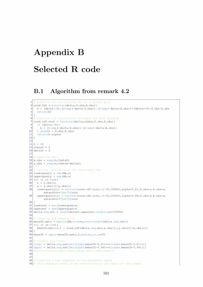
Appendix B
Selected R code
B.1 Algorithm from remark 4.2
1 # Function for calculating CD for a single pair2 cond.cdf = function(delta,S.obs,A.obs)3 k = (delta!=0)*(1-exp(-delta*S.obs))/(1-exp(-delta*A.obs))+(delta==0)*S.obs/A.obs4 return(k)5 6 # Function for calculating CD-alpha for root finding7 cond.cdf.root = function(delta,alpha,S.obs,A.obs)8 if (delta!=0)9 k = (1-exp(-delta*S.obs))/(1-exp(-delta*A.obs))
10 elsek = S.obs/A.obs11 return(k-alpha)12 1314 n = 1015 theta0 = 216 delta0 = 21718 # Sampling data19 x.obs = rexp(n,theta0)20 y.obs = rexp(n,theta0+delta0)2122 # Initial root finding for individual CDs23 lowerquants = rep(NA,n)24 upperquants = rep(NA,n)25 for (i in 1:n)26 s = y.obs[i]27 a = x.obs[i]+y.obs[i]28 lowerquants[i] = uniroot(cond.cdf.root,c(-10,10000),alpha=0.01,S.obs=s,A.obs=a,
extendInt="yes")$root29 upperquants[i] = uniroot(cond.cdf.root,c(-10,10000),alpha=0.99,S.obs=s,A.obs=a,
extendInt="yes")$root30 31 lowerest = min(lowerquants)32 upperest = max(upperquants)33 delta.seq.est = seq(lowerest,upperest,length.out=10000)3435 # Creating the average CD36 meanCD.matr = matrix(NA,nrow=n,ncol=length(delta.seq.est))37 for (i in 1:n)38 meanCD.matr[i,] = cond.cdf(delta.seq.est,y.obs[i],y.obs[i]+x.obs[i])39 40 meanCD = apply(meanCD.matr,2,median,na.rm=T)4142 # Finding the roots43 lower = delta.seq.est[which(abs(meanCD-0.01)==min(abs(meanCD-0.01)))]44 upper = delta.seq.est[which(abs(meanCD-0.99)==min(abs(meanCD-0.99)))]45 #print(c(sum(x.obs+y.obs),sum(y.obs),lower,upper))464748 # Creating a new sequence in the parameter space49 # This sequence needs to be constructed on the basis of the y-axis
101
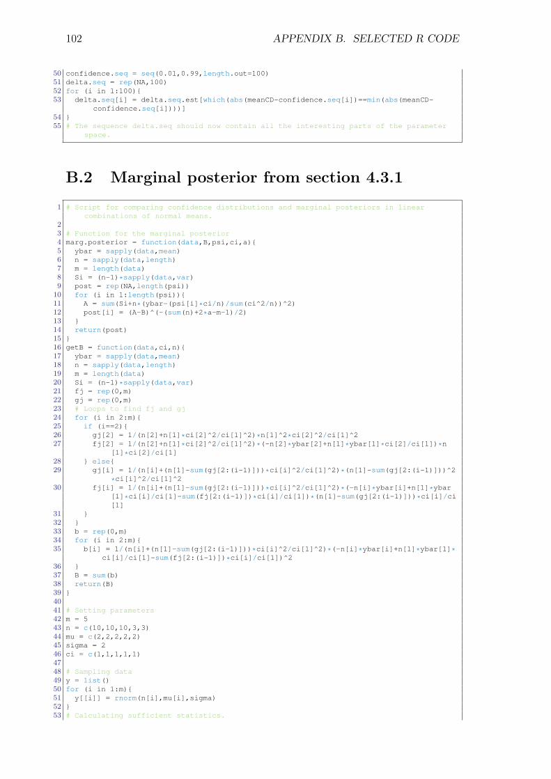
102 APPENDIX B. SELECTED R CODE
50 confidence.seq = seq(0.01,0.99,length.out=100)51 delta.seq = rep(NA,100)52 for (i in 1:100)53 delta.seq[i] = delta.seq.est[which(abs(meanCD-confidence.seq[i])==min(abs(meanCD-
confidence.seq[i])))]54 55 # The sequence delta.seq should now contain all the interesting parts of the parameter
space.
B.2 Marginal posterior from section 4.3.1
1 # Script for comparing confidence distributions and marginal posteriors in linearcombinations of normal means.
23 # Function for the marginal posterior4 marg.posterior = function(data,B,psi,ci,a)5 ybar = sapply(data,mean)6 n = sapply(data,length)7 m = length(data)8 Si = (n-1)*sapply(data,var)9 post = rep(NA,length(psi))
10 for (i in 1:length(psi))11 A = sum(Si+n*(ybar-(psi[i]*ci/n)/sum(ci^2/n))^2)12 post[i] = (A-B)^(-(sum(n)+2*a-m-1)/2)13 14 return(post)15 16 getB = function(data,ci,n)17 ybar = sapply(data,mean)18 n = sapply(data,length)19 m = length(data)20 Si = (n-1)*sapply(data,var)21 fj = rep(0,m)22 gj = rep(0,m)23 # Loops to find fj and gj24 for (i in 2:m)25 if (i==2)26 gj[2] = 1/(n[2]+n[1]*ci[2]^2/ci[1]^2)*n[1]^2*ci[2]^2/ci[1]^227 fj[2] = 1/(n[2]+n[1]*ci[2]^2/ci[1]^2)*(-n[2]*ybar[2]+n[1]*ybar[1]*ci[2]/ci[1])*n
[1]*ci[2]/ci[1]28 else29 gj[i] = 1/(n[i]+(n[1]-sum(gj[2:(i-1)]))*ci[i]^2/ci[1]^2)*(n[1]-sum(gj[2:(i-1)]))^2
*ci[i]^2/ci[1]^230 fj[i] = 1/(n[i]+(n[1]-sum(gj[2:(i-1)]))*ci[i]^2/ci[1]^2)*(-n[i]*ybar[i]+n[1]*ybar
[1]*ci[i]/ci[1]-sum(fj[2:(i-1)])*ci[i]/ci[1])*(n[1]-sum(gj[2:(i-1)]))*ci[i]/ci[1]
31 32 33 b = rep(0,m)34 for (i in 2:m)35 b[i] = 1/(n[i]+(n[1]-sum(gj[2:(i-1)]))*ci[i]^2/ci[1]^2)*(-n[i]*ybar[i]+n[1]*ybar[1]*
ci[i]/ci[1]-sum(fj[2:(i-1)])*ci[i]/ci[1])^236 37 B = sum(b)38 return(B)39 4041 # Setting parameters42 m = 543 n = c(10,10,10,3,3)44 mu = c(2,2,2,2,2)45 sigma = 246 ci = c(1,1,1,1,1)4748 # Sampling data49 y = list()50 for (i in 1:m)51 y[[i]] = rnorm(n[i],mu[i],sigma)52 53 # Calculating sufficient statistics.
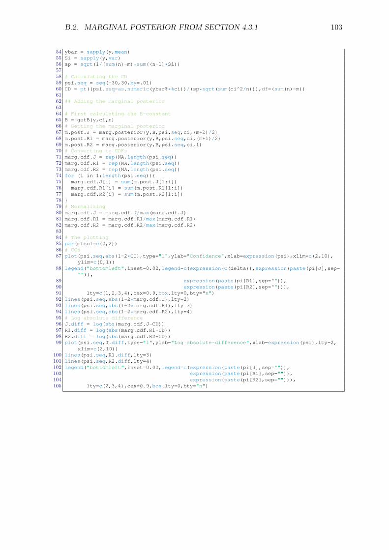
B.2. MARGINAL POSTERIOR FROM SECTION 4.3.1 103
54 ybar = sapply(y,mean)55 Si = sapply(y,var)56 sp = sqrt(1/(sum(n)-m)*sum((n-1)*Si))5758 # Calculating the CD59 psi.seq = seq(-30,30,by=.01)60 CD = pt((psi.seq-as.numeric(ybar%*%ci))/(sp*sqrt(sum(ci^2/n))),df=(sum(n)-m))6162 ## Adding the marginal posterior6364 # First calculating the B-constant65 B = getB(y,ci,n)66 # Getting the marginal posterior67 m.post.J = marg.posterior(y,B,psi.seq,ci,(m+2)/2)68 m.post.R1 = marg.posterior(y,B,psi.seq,ci,(m+1)/2)69 m.post.R2 = marg.posterior(y,B,psi.seq,ci,1)70 # Converting to CDFs71 marg.cdf.J = rep(NA,length(psi.seq))72 marg.cdf.R1 = rep(NA,length(psi.seq))73 marg.cdf.R2 = rep(NA,length(psi.seq))74 for (i in 1:length(psi.seq))75 marg.cdf.J[i] = sum(m.post.J[1:i])76 marg.cdf.R1[i] = sum(m.post.R1[1:i])77 marg.cdf.R2[i] = sum(m.post.R2[1:i])78 79 # Normalizing80 marg.cdf.J = marg.cdf.J/max(marg.cdf.J)81 marg.cdf.R1 = marg.cdf.R1/max(marg.cdf.R1)82 marg.cdf.R2 = marg.cdf.R2/max(marg.cdf.R2)8384 # The plotting85 par(mfcol=c(2,2))86 # CCs87 plot(psi.seq,abs(1-2*CD),type="l",ylab="Confidence",xlab=expression(psi),xlim=c(2,10),
ylim=c(0,1))88 legend("bottomleft",inset=0.02,legend=c(expression(C(delta)),expression(paste(pi[J],sep=
"")),89 expression(paste(pi[R1],sep="")),90 expression(paste(pi[R2],sep=""))),91 lty=c(1,2,3,4),cex=0.9,box.lty=0,bty="n")92 lines(psi.seq,abs(1-2*marg.cdf.J),lty=2)93 lines(psi.seq,abs(1-2*marg.cdf.R1),lty=3)94 lines(psi.seq,abs(1-2*marg.cdf.R2),lty=4)95 # Log absolute difference96 J.diff = log(abs(marg.cdf.J-CD))97 R1.diff = log(abs(marg.cdf.R1-CD))98 R2.diff = log(abs(marg.cdf.R2-CD))99 plot(psi.seq,J.diff,type="l",ylab="Log absolute-difference",xlab=expression(psi),lty=2,
xlim=c(2,10))100 lines(psi.seq,R1.diff,lty=3)101 lines(psi.seq,R2.diff,lty=4)102 legend("bottomleft",inset=0.02,legend=c(expression(paste(pi[J],sep="")),103 expression(paste(pi[R1],sep="")),104 expression(paste(pi[R2],sep=""))),105 lty=c(2,3,4),cex=0.9,box.lty=0,bty="n")


