Female headship, poverty and child welfare: A study of rural orissa, India

1

This is a revised version of a paper presented at the Eleventh WorldCongress of the International Economic Association in Tunis, Tunisia,December 18-22, 1995. I am most grateful to Bina Agarwal, NancyFolbre and Siddiq Osmani for their helpful comments and suggestions. Ialso wish to express my gratitude to International Economic Associationand Indian Council of Social Science Research for providing financialassistance to participate at the World Congress.

FEMALE HEADSHIP, POVERTY AND CHILD WELFARE:

A STUDY OF RURAL ORISSA, INDIA

Pradeep Kumar Panda

Centre for Development Studies

Thiruvananthapuram

August 1997

2

ABSTRACT

First, on the basis of primary data collected in a rural setting in theState of Orissa, an attempt has been made in this paper to compare thesocioeconomic status of male- and female- headed households.Subsequently the differences in the use of resources (time and money)between male-headed and female-headed households have been analysed.Finally, the paper explores the relative well-being of the children betweenthe two groups, i.e., to what extent female headship influences children’saccess to social services, and children’s actual welfare outcomes,measured in terms of health and education indicators.

The results suggest that poverty and female headship are stronglylinked in rural Orissa, India. For eample, if we draw a poverty line thatcorresponds to 15 per cent of the population who are poor, 12 per cent ofpeople living in male-headed househols are poor as compared with 33per cent of people living in female-headed households. This result isbased on per capita consumption as the welfare indicator. When 40 percent poverty line is used, the differences are still large in economic termsand are statistically significant. Moreover, when we use adjustedconsumption as the welfare indicator, the comparisons show a muchhigher incidence of poverty among female-headed households. This istrue for both masures of poverty line, i.e., 15 per cent and 40 per cent.Thus, we conclude that female headship can be a better targetting indicatorfor poverty alleviation in rural Orissa.

The results further suggest that the use of resources are significantlydifferent between the two types of households. Labour force participationdata indicate that female heads are more likely to work in the marketplace than women who are spouses of male heads of household. Thedifferences are large: on average 74 per cent verus 54 per cent.

The comparison of household expenditures indicates that, female-headed households spend relatively less on higher quality food itemssuch as meat, vegetables, milk and other dairy products. However, thereis some evidence that they spend less on personal consumption such asalcoholic beverages. Overall, the differences are pronounced betweenthese households.

Finally, the findings show that children in female-headedhouseholds are disadvantaged both in terms of access to social servicesand actual welfare outcomes.JEL Classification : I12, I32, J12, J13, J16Key words: female headship, poverty, child welfare, gender,

differential resource use, social services, household

3

1. The idea of feminisation of poverty is by no means widely accepted among

scholars, and some recent assessments argue that women are not generally over-

represented in poor households (Lipton and Ravillion, 1995). Moreover, there

is little "robust evidence" to support such assumption (Quisumbing, Haddad and

Pena, 1995).

2. See the evidence reviewed in Buvinic and Gupta (1997).

Introduction

It is estimated that nearly 1300 million persons are poor in the

world (UNDP, 1996; ICQL, 1996), and nearly 70 percent of the world’s

poor are women. Therefore, it is often argued that women, especially in

developing countries, bear an unequal share of the burden of poverty

(UNDP, 1995; United Nations, 1996). 1 Most of the literature on gender

and welfare in developing countries suggest that female-headed

households are one of the key target groups deserving special attention

for any strategy attempting to reduce poverty. 2 However, the extent to

which female-headed households influence child welfare is not clear

and therefore, the ultimate outcome in the welfare of female-headed

household is an empirical question (Kossoudji and Mueller, 1983; Folbre,

1991a; Kennedy, 1992; DeGraff and Bilsborrow, 1992). We expect

female-headed households to be less well off than male-headed

households, mainly because of women’s lower income and more severe

time constraints on non-market activities as compared with those of men

4

(Commonwealth Secretariat, 1989; IDB, 1990). These constraints could

lower the access to social services important to child welfare, and lower

child welfare outcomes.

The recent literature, however, does not support this reasoning

from female-headship to poverty to poor child welfare outcomes. It shows

that since female heads of households presumably have full control over

their resources and they use resources more efficiently than when a man

heads the household, it may produce relatively better welfare outcomes

of children in female-headed households (Dwyer and Bruce, 1988; Bruce;

1989; Blumberg, 1991). In other words, even if female-headed

households are relatively poor and time constrained, their children may

or may not be deprived depending on whether female-headed households’

use of resources is sufficiently child-focused to offset the time and income

constraints that may be tighter in female-headed households (Louat,

Grosh and van der Gaag, 1995; Lloyd and Gage-Brandon, 1993).

Though gender-related differences in the distribution of resources

and resources for survival within poor rural households, and intra-

household dynamics are much discussed (Agarwal, 1986, 1988a, 1992;

Jain and Banerjee, 1985; Singh and Kelles-Vitanen, 1987; Krishnaraj

and Chanana, 1989; Dube and Palriwala, 1990), very little is currently

known about the relationships between female-headedness, poverty, and

child welfare in India. However, there exists some evidence of the

linkages between poverty and female-headedness in India (Visaria, 1980;

Visaria and Visaria, 1985; Parthasarathy, 1982). The existing literature

suggests that female-headed households relative to male-headed

households have poorer survival chances, given their lower control over

land resources and their greater dependency on wage income, their higher

rate of involuntary unemployment, and lower levels of education and

literacy of the household heads (Agarwal, 1986; 1988b; 1995; Kumari,

5

1989; Verghese, 1990; Shanti, 1992; Lingam, 1994; Krishnaraj and

Ranadive, Undated).3 Since the relationship between female-headedness

and poverty is a relatively unexplored area in India, these work still

provide a useful beginning in spite of insufficient statistical rigor and

poor data quality. Much more in-depth study from micro-data is necessary

for a more definitive understanding of such relationship. Moreover, no

study in India examines the relationships between female-headedness,

poverty, and child welfare with a systematic empirical analysis of primary

data.4

This study investigates the links between female-headship,

poverty, and welfare in a rural setting in Orissa, India. It asks three

questions. First, are female-headed households poorer than male-headed

households? Second, do female-headed households spend their resources

differently than male-headed households? And third, do children in

female-headed households have different access to social services and

have different welfare outcomes than their counterparts in male-headed

households?

Background

Orissa is one of the poorest states of India, lying in its eastern

region. It is characterised, inter alia, by low agricultural productivity

and the highest incidence of rural poverty in India. Agricultural

3 In sharp contrast with extensive indications of high levels of deprivation among

female-headed households from these studies, some recent assessments found no

evidence of female-headed households being significantly poorer than male-

headed households in India (Dreze, 1990; Dreze and Srinivasan, 1995).

4. For some of the recent useful studies linking female-headship, poverty, and child

welfare in other countries, see Kennedy and Peters (1992); Kennedy and Haddad

(1994); Rogers (1996); Appleton (1996); Barros, Fox and Mendonca (1997).

6

modernisation and rural infrastructural development lag behind most of

India (World Bank, 1991). Rainfed rice cultivation predominates, leading

to sharp fluctuations in employment availability: seasonal fluctuations

have been reported of up to 40 per cent for female employment and 15

per cent for males (Bardhan, 1979). Although wages are not so low as in

other regions and male/female wage gap is actually among the lowest in

the country, person-day unemployment is high overall and especially

high for women (World Bank, 1991).

Both literacy rates and income levels in Orissa, though increasing,

remain well below the average for India. Female literacy rate, for

example, has reached 34.7 per cent in 1991 compared to 39.3 per cent

for India as a whole; labour force participation of women is now 20.8

per cent, compared to 22.3 per cent in India as a whole (Census of India,

1991). On the economic front, 48.3 per cent of Orissa’s rural population

compared to 33.4 per cent nationally lived below the poverty line in

1987-88, according to the officially released Planning Commission

estimates. According to the Expert Group on Poverty (1993), the

incidence of poverty in rural Orissa was even higher than rural India

(61.5 per cent and 37.6 per cent respectively). Regardless of the debate

on the methodology of poverty estimation, it is clear that rural poverty

in Orissa is the highest in the country. In 1990-91, Orissa’s real annual

per capita income was Rs. 1615 compared to Rs. 2239 for India as a

whole (Centre for Monitoring Indian Economy, 1993).

With regard to the status of women, Orissa portrays a bleak picture.

The status of women is low and is associated with a patriarchal and

patrilineal social structure. The general pattern of social life is derived

from the ideologies of dependence and the notions of social inferiority

of the female - sanctified by scriptures and supported by the folklore

(Jetley, 1984). Arranged marriages, physical and social segregation and

7

extensive restrictions on women are some of the characteristic features

of the rural society.5

Poverty plays a conditioning role on the relationship of women’s

autonomy to their reproductive behaviour. On the one hand, among

middle and high income women in rural Orissa, autonomy does in fact

play a major role, even independent of household economic

characteristics on fertility behaviour. On the other hand, among the

poorest women, women’s autonomy remains virtually unrelated to their

reproductive behaviour, suggesting that among these women, even

women with a certain amount of autonomy require large numbers of

children for their very survival (Panda, 1994). However, these results

are mainly confined to male-headed households in rural Orissa.

The female-headed households constitute nearly 10 per cent of all

rural households in Orissa. However, this figure might be an

underestimation of female-headships because of the range of biases in

actual data collection in the Indian census. These biases would stem

from a variety of factors such as the enumerators and respondents being

typically male (they are predisposed to identify a man rather than a woman

as the household head), the definitions used (the head of household is a

person on whom falls the chief responsibility for the maintenance of the

household), and the instructions given to the enumerators not to make

further enquiry (Agarwal, 1986; Visaria and Visaria, 1985). In fact, a

recent study suggests that in rural India 30 to 35 per cent of all households

are headed by women (World Bank, 1991).

Data Collection and Methodology

Data for this study pertain to 1107 households comprising 6033

individuals. These data come from a field survey conducted in five

5. These social structures are partly responsible for the relative deprivation and

insecurity of elderly women, especially widows, in rural Orissa (Panda, 1997a).

8

villages in the Bolangir district of Orissa. Bolangir district lies in the

hinterland of the state which is predominantly agricultural. The farmers

are entirely dependent on rainfall in the absence of artificial irrigation

facilities. There is little occupational diversification because of the social

structure of rural society and the limited opportunities for mobility. Hence,

Bolangir district is characterised by rural poverty.

The five study villages are located within a distance of 15

kilometres from the district headquarters, Bolangir, and about 300

kilometres from the state capital, Bhubaneshwar. The villages are

typically agricultural in nature, though one village has both agrarian and

industrial features (i.e., a rice mill). The male literacy rate in the study

area is 57.3 per cent while the female literacy rate is 31.9 per cent. Work

participation rates comprise of 65.1 per cent and 38.3 per cent for males

and females respectively.

The survey utilised a household questionnaire that elicited

information from the head of the household on the demographic details

of each resident as well as the household’s social and economic

characteristics. Detailed information on food and non-food expenditures

of each household was also collected for use as general welfare measure

for the family. The children’s access to social services such as education

and health, and their welfare outcomes was a separate module in the

questionnaire for which information was sought.

All households were covered from the five villages with similar

socio-cultural milieu but different levels of development, measured in

terms of use of electricity, extent of non-agricultural work and agricultural

modernization. Villages were selected so as to be representative of

different development pattern found in rural Orissa. Access to

infrastructural facilities was standardized by selecting villages which

were similar to such criteria as transport facilities, availability of school

9

and health services and distance from the nearest town. The survey was

conducted during the months of September 1989 and February 1990.

Interviews took place at the convenience of the respondent, usually at a

time when privacy could be maximal.

The concept of headship used in this paper is not rigorously defined

in terms of relative ‘bargaining’ position of the various members of the

households to uncover the intricacies of gender, intra-household

bargaining, and welfare. The importance of ‘bargaining power’ of women

in the context of ‘gender gap’ was emphasised by many scholars (Folbre,

1983; Sen, 1990; Folbre et al. 1991b). However, utmost care was taken

while collecting information on headship in the survey. Initially, we asked

a male member in the household regarding the head of the household, in

terms of the usual definition of the headship (the household member on

whom falls the chief responsibility for the economic maintenance of the

family). To cross-check the reported headship by the male respondent,

we asked the same question to the female respondents in those households

where both spouses were present. We found that male respondents

reported a male head in 93 per cent of cases, whereas female respondents

reported male heads in 88 per cent of cases. Hence the assignment of

headship was not much dependent upon the gender of the respondent.

Moreover, de facto female heads of household where male partner is

absent temporarily because of migration are limited to only one per cent

of all households in the study area.

Since welfare levels of households are raised by the goods and

services they consume, not by income available for consumption, and

income data are more prone to errors than consumption data, consumption

is used as the measure of welfare rather than income in this paper. In

fact, the consumption-based measures of welfare are commonly used by

the researchers in making poverty assessments (Demery, 1993). The

consumption measure used in this paper is comprehensive which includes

10

food consumption (32 items), daily expenditure (23 items) and

consumption expenditures (27 items). Wedding expenditure (the only

non-consumption expenditure in the study area) and use value of durable

goods could not be included in the aggregation of consumption

expenditures because of non-availability of data. The values for all food

and non-food items were annualized by referring to different recall

periods for different items and the aggregation of total expenditures was

reached. Finally the household’s total consumption is divided by the

number of household members to obtain per capita consumption, which

is used as the main indicator of welfare for this paper.

Since children are less ‘costly’, per capita consumption after

adjusting for age-distribution could be a better measure of welfare than

per capita consumption. Therefore, we estimated adjusted per capita

consumption using adult equivalence scales (assigned a weight of 0.2 to

children 0-6 years, 0.3 to children 7-12 years, 0.5 to children 13-17 years

and 1 to persons more than 18 years) as suggested by Deaton and

Muellbauer (1980, 1986), and Glewwe (1987a , 1987b). This exercise

could help us to test whether some of the results in the paper are robust

to the definition of welfare. Visaria (1980), for instance, has shown for

several Asian countries the sensitivity of the link between poverty and

female headship to definitions and methods used.

In order to measure the differential use of resources between male

and female-headed households, two factors i.e., time and money have

been used. To measure time factor we analyse

(i) the difference in labour force participation among women

of working age (15-59) between women who are heads

and who are spouses of heads, and

11

(ii) the difference in the proportion of households employing

servants for household’s maintenance in male and female-

headed households.

Similarly, in order to examine the money factor, we analysed to

what extent male and female-headed households show different

consumption patterns.

For this, four types of expenditure patterns have been analysed :

(i) share of food and non-food expenditure to total

expenditure,

(ii) share of expenditure for high quality food and alcoholic

beverages to total food expenditure,

(iii) share of expenditure for children to total non-food

expenditure, and

(iv) share of expenditure for domestic help to total non-food

expenditure.

The children’s access to social services such as health services

(preventive and curative care) and education (enrolment rates in primary,

middle and secondary schools) have been examined between the two

groups of households. Finally, child welfare outcomes in terms of health

(diarrhoea in last two weeks and illness in last 4 weeks) and education

(repetition, daily attendance and drop-out rate of children 5-18) indicators

have been analysed.

Characteristics of Female-headship in Rural Orissa

Identifying female-headed households

Nearly 20 per cent of households in the selected rural setting in

Orissa are headed by women. Of these, two-thirds (or 12.6 per cent of

12

all households) are headed by women who are in the oldest generation

present in the household and who do not have a spouse in the household.

These conform to the most common perception of female headship. In

nearly all of the other one-third of female headed households, the woman

who heads the household belongs to the oldest generation in the household

but does have a spouse present. In only one per cent of all households

are there members of a generation older than that of the head. Even

within that group, the portion of female heads with and without spouses

is similar (Figure I).

Figu

re I

: Id

entif

ying

Fem

ale-

head

ed H

ouse

hold

s

13

In male-headed households, 70 per cent of male heads of

households have a spouse present in the household as compared to only

one-third of female heads of households have spouses present.

In one-third of the female-headed households, the females with

spouses were declared to be the head. This is in contrast to the common

perception of female-headship where the male will be considered the

head of the household if the female is married. Figure II presents the

income, age and education in female-headed households with spouses.

It suggests that in these households, the woman had a higher income in

72 per cent of cases. In three per cent of cases she had a lower income

but was older. In 9 per cent of cases, she had a lower income and was

younger, and had a higher education. In 16 per cent of cases, in spite of

earning less, being younger and being less well-educated, she declares

herself as head. On the whole, in 92 per cent of cases of female-headship

there is an easily apparent reason why the woman might be declared as

head (either she has no spouse, or she has a higher income, is older, or

better educated than her counterpart). In the remaining 8 per cent of

cases of female heads (just one per cent of all households), the reason is

less clear.

14

How are female-headed households different ?

Table 1 shows the household size and household composition by

gender of head. It suggests the following results:

1. Female-headed households are smaller than male-headed

households. Their household size is 3.6 members, as

compared to 5.6. The smaller average size of female-

headed households stems partly from the lesser tendency

15

of women to live in large size households. Of all the large

size households (more than 6 members), only 5 per cent

are headed by women. These account for 14 per cent of

female-headed households. On the other extreme, of all

single person households, one half are women and they

account for 28 per cent of female-headed households as

opposed to only 7 per cent of male-headed households.

2. Female-headed households have relatively fewer children,

both in terms of the average number of children per

household and in terms of the per cent of household

members who are children. There is an average of only

0.3 children aged 0-4 years in female-headed households,

Table 1. Household Size and Household Composition by Genderof Head

Gender of the Head

Male Female

% %

Household size

Single person 7.3 28.3Medium : 2-5 28.6 58.0

Large : 6 and above 64.1 13.7Household structure

Mean size 5.9 3.6

Number of children 0-4 0.7 0.3

Number of children 0-9 1.5 0.6

Number of children 0-14 2.2 0.9 % of members 0-4 12.6 8.4

% of members 0-9 24.9 17.0

% of members 0-14 37.0 25.8

Household Size and Structure

16

but 0.7 in male-headed households. Extending the range

of children aged 0-9 and 0-14,doubles and triples the

numbers respectively, but nevertheless, maintaining the

patterns.

Table 2 presents the characteristics of households heads by gender

of head. Some of the most striking findings of table 2 are given below :

Table 2. Characteristics of Household Heads by Gender of Head

Characteristics Gender of the Head

Male % Female %Marital StatusMarried 71.4 34.7Widowed 15.5 52.1Divorced/separated 4.8 9.6Never married 8.3 3.7

Age of the Head15-29 13.3 7.730-39 22.2 15.540-49 19.8 12.850-59 20.8 23.760 and above 23.9 40.2

Education of the HeadNone 56.3 78.1Primary 16.8 10.0Middle 14.3 5.5Secondary and above 12.6 6.4

Occupation of the HeadNot working 15.0 20.5Agricultural self-employed 38.3 19.6Agricultural wage labourer 20.5 49.8Non-Agricultural self- employed 15.0 4.6Non-Agricultural wage labourer 11.3 5.5

Number of days worked during last year3 months or less 20.3 42.53-6 months 12.1 17.86-9 months 28.7 29.39 months and more 38.9 10.3

Caste of the HeadLower caste (SC\ST) 29.5 58.9Upper caste (Others) 70.5 41.1

17

1. The marital status of the heads of the female-headed

households is quite different from that of the heads of male-

headed households. Female-headed households are less

than half as likely as male-headed households to be married

-- 35 per cent as opposed to 71 per cent. They are also

three and half times as likely to be widowed -- 52.1 per

cent as opposed to 15.5 per cent. They are also twice as

likely to be divorced or separated. They are also less than

half as likely to be single.

2. Female heads of households are more than one and half

times as likely as male heads of households to be over age

60 -- 40 per cent as opposed to 24 per cent. They are

correspondingly one and half times less likely to be under

age 40 -- 23 per cent as opposed to 36 per cent. They are

slightly less likely to be in the prime earning range of 40-

60.

3. There are systematic differences in the education status

of male and female heads of households. Female heads

of households are half as likely as male heads of

households to be literate -- 22 per cent as opposed to 44

per cent. They are also less than half as likely to be above

the level of primary education. Thus, differential earnings

are likely to be due to inferior levels of formal education

on the part of the female heads.

4. Female heads of households are somewhat less likely to

work than are male heads of household -- 75 per cent as

opposed to 80 per cent. However, occupational structure

of heads of household differs markedly by the sex of the

18

head of the household. For instance, female heads of

household are half as likely as male heads of household to

be self-employed in agriculture -- 20 per cent as opposed

to 38 per cent. They are also two and half times as likely

to be agricultural wage labourers -- 50 per cent as opposed

to 21 per cent. Finally, they are less than one third as likely

to be self-employed in non-agricultural activity and half

as likely to be non-agricultural wage labourer.

5. When working, female heads of household work fewer

days in the last year prior to survey. While 43 per cent of

female heads work for less than 3 months in a year, only

20 per cent of male heads work for such a less period. On

the contrary, at the upper end, while only 10 per cent of

female heads work for more than 9 months as high as 40

per cent male heads work for such a lengthy period. This

implies lower earnings of female heads of households

partly because of more time devoted to domestic work

and partly because of non-availability of work as a result

of seasonal employment in agriculture. As noted earlier,

half of the female heads work for agricultural wages, and

all of them work for a lesser period (less than six months).

Moreover, earnings from agricultural wages for females

are less than males. All these factors imply a markedly

different levels of earnings between male and female heads

of households.

6. As regards caste status of male and female heads of

household, female heads of household are two times as

likely as male heads of household to be in lower caste, i.e.

scheduled castes and scheduled tribes.

19

Table 3 presents the profile of socioeconomic status of households

and their members by gender of household head. It reveals the following

findings:

Note : hh indicates household and hhs indicates households.

Table 3: Profile of Socioeconomic Status of Households byGender of Household Head

Socioeconomic Status Gender of the Head

Male % Female %

Ownership of land

% of landless hhs 24.3 49.8

Size of landholdings/hh (acres) 4.9 2.0

Size of landholdings per capita (acres) 0.83 0.56

Living conditions

% of hhs with electricity 36.9 14.2

% of hhs residing in a built-up structure 37.3 12.8

Number of rooms per hh 3.1 1.5

Number of rooms per person 0.53 0.42

% of hhs with toilet facility 18.1 5.5

Ownership of modern consumer durable goods

% of hhs owning tables/chairs 41.0 14.2

% of hhs owning watch/cycle 44.4 11.0

% of hhs owning a radio 42.5 12.3

% of hhs owning a motor cycle/scooter 6.4 0.9

% of hhs owning a television set 14.9 4.6

Education of hh members

% of literate (total) 62.7 33.6

% literate (male) 59.3 40.1

% literate (female) 37.2 29.1

Caste of hh members

% of SC/ST 31.9 62.2

20

1. The difference in land ownership is substantial between

the male-headed households and female-headed

households. While three - fourths of the male-headed

households own land, only one-fourth of the female-

headed households own land. Moreover, mean size of

land holdings per household is two and half times higher

in male-headed households as compared to female-headed

households (5 acres and 2 acres respectively). Even size

of land holdings per capita is relatively higher in male-

headed households.

2. There are systematic differences in living conditions

between male and female-headed households. When living

conditions of the households are measured in terms of

household electrification, housing type, number of rooms

per household and per capita, and toilet facilities, in all

cases male-headed households show a substantially higher

living standards than that of female-headed households.

3. The ownership of modern consumer goods such as tables/

chairs, watch/cycle, radio, motorcycle/scooter and

television sets are much higher in male-headed households

as compared to female-headed households.

4. As regards education status of male and female members,

the difference is marked in male and female-headed

households. Both male and female literacy are relatively

higher in male-headed households.

5. The members of the female-headed households are about

two times as likely as members of the male-headed

households to be in lower caste (SCs and STs)---62 per

cent as opposed to 32 per cent.

21

As regards occupational structure of all members of the household,

the pattern is almost similar to household heads i.e., 72 per cent of the

working age members in female-headed households work, while 80 per

cent of working age members of male-headed households work (Table

4). The working age members of female-headed households are twice as

likely to be wage labourers in agriculture --46 per cent as opposed to 23

per cent. They are also one-third as likely to be non-agricultural self-

employed, and one-fourth as likely to be wage-labourers in non-

agricultural activity.

The dependent-to-worker ratio in the household is similar in both

male and female-headed households (1.0). This is the result of the

combination of differences in age structure in the household and in labour

force status of working age members (Table 5).

The results so far indicate that female-headed households are over-

represented by widows, divorced or separated women, are smaller, have

less children and have both heads and other members who are less likely

Table 4. Distribution of Individuals 15-59 by OccupationalStructure and Gender of Head

Gender of the Head

Occupational Structure Male Female

% %

Not working 20.3 27.9

Agricultural self-employed 26.7 17.2

Agricultural wage labour 23.2 46.0

Non-agricultural self-employed 13.5 4.7

Non-agricultural wage labour 16.3 4.1

22

to be working. When working, they work for a lesser period in a year

and in lower category of occupation. Both heads and other members of

female-headed households are less likely to be literate. They are more

likely to be in lower castes. Moreover, female-headed households are

less likely to own land and modern consumer goods and are more

likely to be in poor living conditions. All these factors may lead us to

believe that female-headed households would be poorer than male-headed

households. This issue is discussed in the next section.

Poverty and Female-headship

A growing body of literature stresses that rural female-headed

households are disproportionately represented among the poor (Youssef

and Hetler, 1981; 1984). In order to test this proposition, the relationship

between poverty and female headship is examined in some detail in the

following section.

Note : hh indicates household.

Table 5. Total Number of Household Members for each LabourForce Status by Gender of Head

Labour Force Status Gender of the Head

Male Female

Total number of employed persons in the hh 2.9 1.8

Number of hh members out of labour force 0.8 0.7

Number of hh members too young to work 2.2 0.9

Number of hh members too old to work 0.1 0.2

Number of dependents per worker 1.0 1.0

23Ta

ble

6. C

ompa

riso

n be

twee

n M

ale-

head

ed H

ouse

hold

s an

d F

emal

e-H

eade

d H

ouse

hold

s: P

er C

apit

a an

d P

er A

dult

(A

djus

ted)

Con

sum

ptio

n, A

ccor

ding

to

Var

ious

Hou

seho

ld C

ateg

orie

s

No.

of

pers

ons

Mea

n hh

siz

eM

ean

per

capi

taR

atio

T te

stM

ean

Rat

io T

test

cons

umpt

ion

of h

yp.

adju

sted

of h

yp.

Hou

seho

ld C

ateg

ory

PCm/

PCm

=co

nsum

ptio

nA

Cm/

AC

m =

PCf

PCf

AC

fA

C f

MH

HFH

HM

HH

FHH

MH

HFH

HM

HH

FHH

(PC

m)

(PC

f)(A

Cm)

(AC

f)

All

hous

ehol

ds52

4578

85.

913.

6014

9798

01.

5314

.64

2137

1288

1.67

16.2

7Si

ngle

-pe

rson

6562

1.00

1.00

2662

2133

1.25

1.49

*26

6221

331.

251.

49*

One

pot

entia

l wor

ker

excl

udin

g si

ngle

-per

son

hous

ehol

ds16

9923

04.

922.

9912

8792

11.

403.

2315

7610

241.

545.

96O

ne p

oten

tial w

orke

r w

ith c

hild

(ch

ildre

n)14

4814

85.

463.

4497

888

61.

101.

06**

1608

1228

1.31

1.92

*O

ne p

oten

tial w

orke

r w

ith c

hild

, (0-

4 ye

ars

old)

1028

102

5.81

3.92

834

801

1.04

0.91

**12

1910

971.

111.

36**

One

pot

entia

l wor

ker

with

chi

ld, (

5-9

year

s ol

d)11

1210

85.

733.

4889

575

21.

191.

3212

3512

021.

030.

29**

One

pot

entia

l wor

ker

with

chi

ld, (

10-1

7 ye

ars

old)

1122

113

5.75

3.32

972

843

1.15

1.82

**13

9014

030.

99-0

.63*

*Tw

o po

tent

ial w

orke

rs w

ith c

hild

(C

hild

ren)

1988

178

6.48

4.45

1376

920

1.50

11.2

722

4413

721.

6413

.37

* di

ffer

ence

is n

ot s

igni

fica

nt a

t the

1%

lev

el.

** d

iffe

renc

e is

not

sig

nifi

cant

at t

he 5

% le

vel.

Not

es:

1. M

ean

cons

umpt

ions

are

in R

s./ y

ear

2. A

djus

ted

cons

umpt

ions

is th

e co

nsum

ptio

n pe

r ad

ult e

quiv

alen

t com

pute

d fr

om th

e fo

llow

ing

scal

e. 0

-6 y

ears

old

: 0.2

; 7-1

2 ye

ars

old:

0.3;

13-

17 y

ears

old

: 0.5

; > th

an 1

8:1.

0.3.

The

T-t

est o

f th

e hy

poth

esis

of

equa

l con

sum

ptio

n be

twee

n m

ale

and

fem

ale-

head

ed h

ouse

hold

s is

com

pute

d un

der

the

assu

mpt

ion

ofun

equa

l var

ianc

e of

the

dist

ribu

tions

.4.

'Pot

entia

l wor

ker'

mea

ns a

per

son

betw

een

18 a

nd 5

9 ye

ars

old.

5.M

HH

indi

cate

s M

ale-

head

ed h

ouse

hold

, FH

H in

dica

tes

Fem

ale-

head

ed h

ouse

hold

, hh

indi

cate

s ho

useh

old

and

hyp.

indi

cate

s hy

poth

esis

24

Consumption Measures and Female-headed Households

Table 6 presents the comparison of per capita and per adult

equivalent (adjusted) consumption between male-headed households and

female-headed households, according to various household categories.

The mean per capita consumption level in female-headed households is

Rs.980 per year as compared to Rs.1497 in male-headed households. In

other words, male-headed households have per capita consumption levels

which are about a half higher than those of female-headed households.

This leads to a strong conclusion that female-headed households are

poorer than male-headed households. The differences are large in

economic terms and statistically significant.

When mean adjusted consumption is used, it shows that male-

headed households are wealthier than the female-headed households by

about 66 per cent (Table 6, right-hand panel). The differences are more

when using unadjusted mean per capita consumption because male-

headed households are more likely to have more children. However, the

differences are still large in economic terms and statistically significant.

The comparison of households with only one potential worker and

children of various ages reveals that the average welfare differences are

not significant statistically. It means, the difficulty of single-handedly

raising and providing for children is apparently as great for male

households as for female households in similar circumstances. On the

contrary, when there are no children or when two potential workers are

present in the households, the welfare differences are substantial. The

results suggest that part of the difference in mean per capita consumption

is accounted for by the differences in age-structure between male-headed

and female-headed households. Therefore, household structure is a crucial

indicator in understanding the levels of household welfare. However, in

25

addition to household structure, other variables that tend to be correlated

with headship can also influence the welfare level of the household.

Therefore, to examine the individual influence of each of the included

variables, holding all other variables constant, a multivariate regression

analysis is used.

Table 7. Determinants of Households’ Welfare as Defined byPer Capita Consumption

Variable Coefficient

Dummy variables

Gender of the head –.14*

(Female head=1)(Male head=0)

Marital status of the head –.05

(widowed, divorced or separated=1, else=0)

Occupation of the head .10*

(non-agricultural activity=1, else=0)

Caste of the head((SC/ST=1, else=0) –.03

Continuous variables

Age of the head .00

Education of the head(years of education) .14*

Number of children, 0-4 –.16*

Number of children, 5-9 –.11*

Number of children, 10-18 –.01

Size of landholdings per capita .22*

Adjusted R2 0.5137

* significant at the 5 % level or better.

Notes: 1. Dependent variable is measured as ln(per capita consumption).

2. Universe is all households.

26

As shown in Table 7, female headship has an independent and

negative influence on the welfare level of the household. Other factors

included in the multivariate analysis are standard and the results are as

expected. The education and non-agricultural occupation of the household

head, and per capita land ownership have significant and positive

influence on the welfare level of the household. Household structure has

a significant and negative effect on per capita consumption. In other

words, the more the children and the younger they are (below 10), the

lower is the household welfare. These results are confined to the overall

mean levels of the household welfare. Therefore, let us turn to examine

the relationship between poverty and female-headedness by concentrating

on the low end of the distribution of welfare.

Poverty Measures and Female-headed Households

In this paper, two poverty lines have been used - Rs.972 per capita

household consumption, and Rs. 1224 per capita household consumption.

These correspond to the poorest 15 and 40 per cent of the population

respectively. These two poverty lines are considered here on the basis of

Kakwani and Subbarao’s (1993) estimation of poverty line in rural India

during 1973-87. According to 1986-87 prices, in rural Orissa, Rs 972

per capita household consumption is treated as ultrapoor and Rs.1224

per capita household consumption is treated as poor (Kakwani and

Subbarao, 1993).

A comparison of mean per capita consumption for female and male-

headed households leads to the strong conclusion that female-headed

households are poorer than male-headed households. This is true for

both 15 per cent poverty line and 40 per cent poverty line. Using mean

adjusted consumption shows that female-headed households are much

poorer than male-headed households, because male-headed households

27

are more likely to have more numbers of children (Table 8). This is also

true for both measures of poverty line.

Using the lower poverty line and per capita consumption, we

find that head count index differ significantly by headship. The results

show that 12 per cent of people living in male-headed households are

poor, compared with 33 per cent in female-headed households. The

difference is statistically significant. When adjusted consumption is used

as the welfare indicator, it shows that 11 per cent of people living in

male-headed households are poor, compared to 37 per cent in female-

headed households. The difference is statistically significant for the 15

per cent poverty line. For the more generous poverty line (Rs.1224) and

for both unadjusted and adjusted per capita consumption, the comparisons

Table 8. Poverty and Female Headship †

Welfare Measure 15% poverty line 40% poverty line

Male Female Male Female

Head Head Head Head

Per capita consumption

Mean per capita consumption 1497 980 1497 980

Mean per capita consumption of the poor 748 662 996 862

Head count index 12.3 32.7 34.5 73.8

Adjusted per capita consumption

Mean adjusted per capita

consumption 2137 1288 2137 1288

Mean adjusted per capita consumption of the poor 1178 749 1535 1030

Head count index 11.2 36.5 32.0 78.0

† The tests are for differences by gender of the household head.

* Significant at the 5% level or better.

Note : Mean unadjusted and adjusted consumptions are in Rs./year.

28

show a higher incidence of poverty among female-headed households.

Hence, the results show a systematic difference in welfare level of the

household between male-and female-headed households regardless of

any measures of poverty line. Thus, the results clearly are consistent

with the notion that female-headship is correlated with poverty

irrespective of the poverty measures and the welfare measures used.

Differential Resource Use

The analysis in this section concentrates on whether the resources

(time and money) available to female-headed households differ from

those in male-headed households.

Time use

It has already been noted that female heads of households are

somewhat less likely to be employed than those of male heads (75 per

cent versus 80 per cent). Moreover, female heads work for lesser period

and in low category of occupation. Hence, their income-generating

activities are lessened. In order to examine whether female-headed

households would be constrained in their welfare-generating household

non-market activities more than male-headed households, we examine

the difference in labour force participation among women of working

age (15-59) between women who are heads and who are partners of

heads.

It is found that while 74 per cent of female heads of working age

are in labour force, only 54 per cent of the spouses of the male heads are

in labour force. Hence the spouses of the male heads are considerably

less likely to be employed than the female heads. Thus the data supports

the typical characteristics of male-headed household i.e., the male head

works for income and the female partner spends more time on non-market

household activities that produce welfare for the family and for the

29

children. In contrast, the typical female head fulfils both the roles, i.e.,

she earns income for the family and spends time for welfare-enhancing

activities of the household. Thus the female head would be constrained

for time and money because of this double burden. To further explore

the constraints that female heads of household face, we analyzed the

difference in employing servants who provide domestic help in male

and female-headed households. Surprisingly, while one-fourth of male-

headed households employed servants, only 5 per cent of female-headed

households employed servants. Thus, there is a systematic difference in

the use of time resource between male and female-headed households.

In the next section, we examine the difference in other resource,

i.e., money between male and female-headed households. Specifically,

the difference in consumption patterns is analyzed between the two groups

of households.

Consumption Patterns

Table 9 shows the consumption patterns by levels of per capita

consumption and gender of household head. It reveals the following

conclusions :

1. There is significant difference in percentage share of food

and non-food expenditure to total expenditure by gender

of the head of the household. In female-headed households

share of food-expenditure (58 per cent) is much larger than

the share of non-food expenditure (42 per cent), using the

more generous poverty line (Rs.1224.). However, the

reverse is true in case of male-headed households.

Therefore, consumption difference might have the most

marked impact on child welfare in female-headed

households.

30

2. There is also marked difference in the combination of foods

purchased. Expenditure on such higher quality food items

as meat, vegetables, milk and other dairy products tend to

Table 9. Consumption Shares by Gender of Household Head

Per capita consumption All

Consumption Shares Less than More than Gender of

Rs. 1224 Ra. 1224 the Head

Gender of Gender of

the Head the Head

Male Female Male Female Male Female

% share to total expenditure

Food expenditure 52.7 58.2 46.1 50.2 47.6 55.4Non-food expenditure 47.3 41.8 53.8 49.8 52.4 44.6

% share to total food

expenditure

Expenditure for high qualityfood (items such as meat,vegetables, milk and otherdairy products) 15.2 11.4 34.1 31.2 29.3 17.7

Expenditure for alcoholicbeverages 8.9 4.6 10.4 3.8 10.0 4.3

% share to total

non-food expenditureExpenditure for childgoods such as clothing andeducational expenditure(among households withchildren) 14.8 4.8 27.5 15.3 25.4 10.6

Mean household expenditurefor child goods (Rs.) 482 69 1799 590 1427 235

Expenditure for domestic help 2.3 0.3 8.1 3.6 6.9 1.6Mean household expenditurefor domestic help (Rs.) 75 4 421 67 319 25

31

be higher in male-headed households, irrespective of the

levels of per capita consumption. However, expenditure

on alcoholic beverages are much larger in male-headed

households irrespective of the levels of per capita

consumption and this supports the findings of Horton and

Miller (1989).

3. The share of expenditures for child goods to total non-

food expenditures for household with children shows that

the percentage share as well as mean levels of household

expenditures vary significantly by gender of household

head, irrespective of the level of per capita consumption.

For instance, in female-headed households, the mean levels

of household expenditure for child goods is only Rs.69

compared to Rs. 482 in male-headed households, using

per capita consumption below Rs. 1224.

4. It has been seen that one-fourth of male-headed households

employ servants as compared to only 5 per cent female-

headed households. Obviously, therefore, expenditure for

domestic help is expected to be high for male-headed

households. The results presented in Table 9 suggest that

both share of expenditures for domestic help to total non-

food expenditure as well as average expenditure levels

are higher in male-headed household, regardless of the

levels of per capita consumption. For instance, using 40

per cent poverty line, the mean levels of household

expenditure for domestic help vary significantly by gender

from Rs. 4/- in female-headed households to Rs.75/- in

male-headed households.

32

On the whole, the evidence so far suggests that female heads use

their time differently than other women and that consumption patterns

differ between male and female-headed households. The differences are

also substantial. In other words, female heads of household have faced

tighter constraints on non-market activities. They are also pressed for

money. As a result they may not be able to translate their priority for

children’s welfare. The implications for children’s welfare of the

difference in time and money use are examined in the next section.

Children’s Access to Social Services

In this section, children’s access to social services by gender of

head of the household is measured by way of two factors, i.e. health care

and education.

Health Care

Table 10 shows children’s access to health care by gender of

household head and gender of the child. It shows that both preventive

care and curative care of children are significantly different by gender

of household head. The results also hold true when the analysis is

performed separately for girls or boys.

The children for whom clinic visits for preventive care were

reported in the six months preceding the survey, 12 per cent of them in

male-headed households received preventive care as compared to only

6 per cent in female-headed households. The difference is statistically

significant. The same is true when the analysis is performed separately

for girls or boys. A similar significant difference is found for full

immunization coverage.

For those children who are reported to be ill in the four weeks

prior to the survey period, 35 per cent of them in male-headed households

33

received medical care (curative), compared to 24 per cent of such children

in male-headed households. The difference is statistically significant.

The results hold true when the analysis is performed separately for girls

or boys (Table 10).

One of the most striking findings of Table 10 is that, both

preventive and curative care for boys are much more prevalent as

compared to such care for girls, both in male as well as female-headed

households. Hence, the gender inequality in health care is observed,

regardless of gender of household head.

Education

As shown in Table 11, while 85 per cent of children from age 5-10

in male-headed households are enrolled in school, only 68 per cent of



Table 10. Children’s Access to Health Care†

Access to Health Care Both sexes Boys Girls


Head Head Head Head Head Head

% of children 0-5 years

old for whom clinicvisits for preventivecare were reported inthe last six monthspreceding the survey 11.6 6.3* 15.0 10.8* 8.0 2.3*

% of children 1-4 yearsold with full immuni-zation coverage againstBCG, measles and DPT. 39.6 23.5* 49.1 33.3* 28.8 14.8*

% of children 0-17 years

old who were reportedto be ill in the last fourweeks preceding the survey and had receivedmedical care 35.1 24.5* 49.8 39.5* 18.4 9.1*

34

such children in female-headed households are enrolled in school. The

difference is statistically significant. When we concentrate on the

enrolment of middle (11-13 years) and secondary (14-18 years) age

children, the difference in the enrolment of children is pronounced by

gender of the head. When the analysis is performed separately for girls

or boys, the difference in the enrolment of children by gender of the

head is statistically significant for all the age groups of children.

As in the case of health care, the most striking finding of table 11

is that boys are more likely to be in school than girls regardless of the

gender of the head of the household.

On the whole, the results suggest that the differences in children’s

access to preventive and curative health services, and primary, middle

and secondary education were found to be statistically significant by

gender of the head of household. Moreover, boys access to health

services and education exceed those of girls, regardless of the gender of

the head of the household. Thus we found that children in female-headed

households of rural Orissa are disadvantaged in terms of access to social

services compared to children in male-headed households. Since female-

Table 11. Enrolment Rates by Gender of Child and HouseholdHead †

Age of Both sexes Boys Girls

child


Head Head Head Head Head Head

5-10 yrs 84.9 68.2* 92.1 72.7* 76.5 63.4*

11-13 yrs 72.2 54.1* 79.4 57.9* 64.6 50.0*

14-18 yrs 44.3 29.4* 54.1 34.1* 34.5 24.4*



35

headship and poverty are strongly linked and since female-headed

households face more time and money constraints, the results are much

as expected. The next section looks into the actual welfare outcomes of

children.

Child Welfare Outcomes

In this section, we explore the children’s welfare outcomes by

looking for differences by gender of the household head. The analysis is

also performed separately for boys and girls.

Health Outcome

The incidence of diarrhoea is a good indicator of how effectively

the household produces health.6 As shown in Table 12, nearly 27 per

cent of children under five years of age in female-headed households

have an episode of diarrhoea in the two weeks prior to the survey, as

compared to only 14 per cent of such children in male-headed households.

The difference is statistically significant. Moreover, the differences in

the episode of diarrhoea among boys as well as girls in the two weeks

prior to the survey are also significant by gender of the household head.

Another important finding is that girls are more likely to be affected by

diarrhoea than boys, regardless of the gender of the head.

6. See Panda (1997b) for theoretical and empirical evidence.



Table 12. Health Status of Children Aged 0-4 †

% Reporting Both sexes Boys Girls

Male Female Male Female Male FemaleHead Head Head Head Head Head

Diarrhoea inlast 2 weeks 13.6 27.3* 9.3 20.6* 18.6 34.4*

Illness in last4 weeks 34.2 33.3 36.2 35.3 32.2 31.3

36

As regards illness of children in the month prior to survey, the

differences are not significant by gender of the head of household,

whether all children are considered together, or the analysis is performed

separately for boys or girls (Table 12).

Education Outcome

In order to measure education outcome, we consider three measures

-- repetition, daily attendance and drop-out rate. Repetition, drop-out

rate and low daily attendance are signs of poor educational performance.

Moreover, these features are common in rural India and hence, in rural

Orissa.

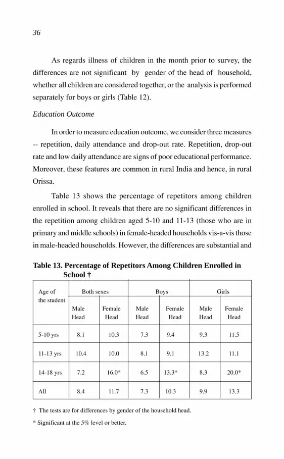
Table 13 shows the percentage of repetitors among children

enrolled in school. It reveals that there are no significant differences in

the repetition among children aged 5-10 and 11-13 (those who are in

primary and middle schools) in female-headed households vis-a-vis those

in male-headed households. However, the differences are substantial and

Table 13. Percentage of Repetitors Among Children Enrolled inSchool †

Age of Both sexes Boys Girlsthe student


5-10 yrs 8.1 10.3 7.3 9.4 9.3 11.5

11-13 yrs 10.4 10.0 8.1 9.1 13.2 11.1

14-18 yrs 7.2 16.0* 6.5 13.3* 8.3 20.0*

All 8.4 11.7 7.3 10.3 9.9 13.3



37

statistically significant among children aged 14-18 (those in secondary

school) between male and female-headed households. The same is true

when the analysis is performed separately for boys or girls. The repetition

of girls 14-18 as compared to boys is much higher in female-headed

households --20 per cent as opposed to 13 per cent.

As shown in Table 14, for the sample of enrolled students in

primary, middle, and secondary schools, nearly three-fourths of them

reported having attended all official school days in the week preceding

the survey. The difference in full attendance of enrolled children during

the previous week is not significant in primary and middle schools

between male and female-headed households. This is true for boys as

well as girls in these households. But, boys are more likely to be attending

the school regularly than girls regardless of the gender of the head for all

levels of schooling. Among the enrolled students aged 14-18 who are in

secondary school, the difference is significant by gender of the head of

the household. The results hold true for either of the sexes of enrolled

students aged 14-18.

Table 14. Percentage of Children with Full Attendance During thePrevious Week, Among Children Enrolled in School †

Age of the Both sexes Boys Girlsstudent


5-10 yrs 76.2 77.6 83.1 84.4 66.4 69.2

11-13 yrs 78.8 75.0 84.4 81.8 71.7 66.7

14-18 yrs 70.1 52.0* 85.3 66.7* 46.3 30.0*

All 75.3 70.9 83.9 79.3 63.2 60.0



38

When we consider all the enrolled students together, or separately

for boys or girls there are no significant differences in full attendance in

the previous week between the gender of the household head and between

boys and girls in these households. However, overall, while 80 per cent

of the enrolled boys attended school for all the days of the previous

week, only 61 per cent of enrolled girls reported full attendance.

Therefore, girls are irregular in attending school, compared to boys

irrespective of the gender of the household head.

Table 15 shows the drop-outs among children and mean age at

drop-out by gender of the household head and gender of the child. The

results suggest that there are systematic differences in drop-outs among

all children, boys and girls, in female-headed households vis-a-vis those

in male-headed households. Moreover, children in female-headed

households drop out of school two years earlier than the children in male-

headed households. Boys in female-headed households drop out 1.8 years

earlier than their counterparts in male-headed households. Girls in

female-headed households drop out 2.7 years earlier than their

counterparts in male-headed households. The mean age of boys who

drop out is nearly 11 years, as contrast to 8 years for girls.

Table 15. Drop-outs Among Children by Gender of HouseholdHead †

Both sexes Boys Girls


% of childrenwho dropped out 32.0 50.0* 23.3 45.8* 41.4 55.0*

Mean age atdrop-out 10.2 8.1* 11.4 9.6* 9.5 6.8*



Particulars ofDrop-outs

39

The analysis so far indicates that children in female-headed

households are disadvantaged in terms of a variety of measures used

like children’s health status, and education performance. The present

unfavourable welfare outcomes would be undesirable both for present

welfare loss and future formation of human capital on which the children

will rely in their adult lives. The strong support for the hypothesis that

children in female-headed households are disadvantaged compared to

those in male-headed households is consistent with the evidence presented

in previous sections of the paper - that poverty and headship are strongly

linked, that female-headed households face more time and money

constraints and are not able to offset these constraints because their use

of resources are less child-oriented, and that their children fare worse in

terms of access to social services than children in male-headed

households.

Conclusions

The results clearly suggest that poverty and female-headship are

strongly linked. Thus, female-headship may be a useful targeting indicator

for poverty alleviation in rural Orissa. In other words, targeting social

programmes to female-headed households will be a successful way of

reaching the poor.7 Moreover, results suggest that female heads face

more time and income constraints - they use their time differently than

other women and consumption patterns differ between the two types of

households. The consumption expenditures of female-headed households

are so low that even though they spend less on personal consumption

like alcoholic beverages, they also spend less on child-oriented goods.

The evidence further suggests that children’s access to preventive and

7 In this context, education, or the control of productive assets, remain real issues;

and they are critical for strategies aiming at acceleratng development as well as

rendering it more equitable (Lipton, 1988; Quibria, 1993; Agarwal, 1994; ILO,

1995).

40

curative health care, and primary, middle and secondary education in

female-headed households are much lower than their counterparts in

male-headed households. Finally, the study supports the hypothesis that

children in female-headed households are disadvantaged in terms of

actual welfare outcomes (education and health outcome). The evidence

of lower welfare outcomes of children in female-headed households is

consistent with the findings that (i) female-headed households are

burdened by tighter income and time constraints, (ii) that their children

are disadvantaged in terms of access to social services and finally, (iii)

that female-headship and poverty are strongly linked regardless of the

welfare measure used, and the poverty measure used.

One of the most striking findings of this study is that, on the whole,

regardless of gender of the head of household, girls are relatively

disadvantaged compared to boys both in terms of access to social services

and actual welfare outcomes.

Since Orissa, like other north Indian states, has a long history of

gender inequities in access to resources (such as education and health)

and crucial means of production (such as land and associated production

technology), our results are in the expected direction and are consistent

with the main body of female-headship literature.

41

REFERENCES

Agarwal, Bina (1986).‘Women, Poverty and Agricultural Growth inIndia’, The Journal of Peasant Studies, Vol.13, No.4, July.

Agarwal, Bina (1988a). Structures of Patriarchy : State Community andHousehold in Modernising Asia, Kali for Women. New Delhi.

Agarwal, Bina (1988b). ‘Who Sows? Who Reaps? Women and LandRights in India’, The Journal of Peasant Studies, Vol.15, No.4,July.

Agarwal, Bina (1992). ‘Rural Women, Poverty and Natural Resources :Sustenance, Sustainability and Struggle for Change’, in BarbaraHarris, S. Guhan and R.H. Cassen (eds.) Poverty in India :Research and Policy, Oxford University Press, Bombay.

Agarwal, Bina (1994). A Field of One’s Own: Gender and Land Rightsin South Asia, Cambridge University Press, Cambridge.

Agarwal, Bina (1995). ‘Gender and Legal Rights in Agricultural Landin India’, Economic and Political Weekly (Review of Agriculture),Vol. 30, No. 13, 25 March.

Appleton, S. (1996). ‘Women-Headed Households and HouseholdWelfare : An Empirical Deconstruction for Uganda’, WorldDevelopment, Vol. 24, No. 12, pp. 1811-1827.

Bardhan, Kalpana (1979). ‘Work as a Medium of Earning and SocialDifferentiation : Rural Women of West Bengal’, Paper presentedat ADC-ICRISAT Conference in Adjustment Mechanisms ofRural Labour Markets in Development Areas, Hyderabad, India.

Barros, R., L. Fox and R. Mendonca (1997). ‘Female-HeadedHouseholds, Poverty, and the Welfare of Children in UrbanBrazil’, Economic Development and Cultural Change, Vol. 45,No. 2, pp. 231-257.

Blumberg, Rae (1991). ‘Income Under Female Versus Male Control’,in Rae Blumberg (ed) Gender, Family and Economy: The TripleOverlap, Sage Press, Newbury Park, pp. 97-127.

Bruce, Judith (1989). ‘Home Divided’, World Development, Vol. 17,No. 7, pp. 979-992.

42

Buvinic, M. and G. Gupta (1997).‘Female-Headed Households andFemale-Maintained Families: Are They Worth Targetting toReduce Poverty in Developing Countries?’, EconomicDevelopment and Cultural Change, Vol. 45, No. 2, pp. 259-280.

Census of India (1991). Final Population Totals - Brief Analysis ofPrimary Census Abstract, Series 1, Paper 2 of 1992, Governmentof India, New Delhi.

Centre for Monitoring Indian Economy (1993). Basic Statistics Relatingto Indian Economy, Vol.2 : States, Economic Intelligence Service,Bombay.

Commonwealth Secretariat (1989). Engendering Adjustment for the1990s, Commonwealth Secretariat, London.

Deaton, Angus and John Muellbauer (1980). Economics and ConsumerBehaviour, Cambridge University Press, Cambridge.

Deaton, Angus and John Muellbauer (1986). ‘On Measuring Child Costs: With Applications to Poor Countries’, Journal of PoliticalEconomy, Vol. 94, No. 4, pp. 720-744.

DeGraff, Deborah S. and Richard E. Bilsborrow (1992). ‘Female-HeadedHouseholds and Family Welfare in Rural Ecuador’, Paperpresented at the Annual Meeting of the Population Associationof America, Denver.

Demery, L. (1993). ‘The Poverty Profile’, in L. Demery, M. Ferroni andC. Grootaert (eds.) Understanding the Social Dimension ofAdjustment, The World Bank, Washington DC.

Dreze, Jean (1990). ‘Widows in Rural India’, Discussion Paper No. 26,Development Economics Research Programme, STICERD,London School of Economics.

Dreze, Jean and P.V. Srinivasan(1995). ‘Widowhood and Poverty in RuralIndia: Some Inferences from Household Survery Data’,Discussion Paper No. 62, Development Economics ResearchProgramme, STICERD, London School of Economics.

Dube, Leela and Rajni Palriwala (eds.) (1990). Structure and Strategies: Women, Work and Family, Sage Publications, New Delhi.

Dwyer, Daisy and Judith Bruce (eds.) (1988). A Home Divided : Womenand Income in the Third World, Stanford University Press,Stanford.

43

Folbre, Nancy (Undated). ‘Mothers on Their Own : Policy Issues forDeveloping Countries’, processed, International Centre forResearch on Women, Washington D C.

Folbre, Nancy (1983). ‘Household Production in The Philippines : ANon-Neoclassical Approach’, WID Working Paper No. 26,Michigan State University, East Lansing,. MI.

Folbre, Nancy (1991a). ‘Women on Their Own : Global Patterns ofFemale Headship’, in Rita S. Gallin and Ann Ferguson (eds.) TheWomen and International Development Annual, Vol. 2, WestviewPress, Boulder.

Folbre, Nancy, B. Bergmann, B. Agarwal and M. Floro (eds.) (1991b).Women’s Work in the World Economy, Macmillan, London .

Glewwe, Paul (1987a). ‘The Distribution of Welfare in Cote d’ Ivoire1985’, Living Standards Measurement Study, Working PaperNo. 29, The World Bank, Washington DC.

Glewwe, Paul (1987b). ‘The Distribution of Welfare in Peru 1985-86’,Living Standards Measurement Study, Working Paper No. 42,The World Bank, Washington DC.

Horton, Susan and Barbara Diane Miller (1989). ‘The Effect of Genderof Household Head on Food Expenditure: Evidence from Low-Income Households in Jamaica’, Paper presented at theConference on Family Gender Difference and Development,Economic Growth Center, Yale University, September 4-6, NewHaven.

ICQL (Independent Commission on the Quality of Life) (1996). TheState of Rural Poverty: An Enquiry into Its Causes andConsequences, Oxford University Press, Oxford.

International Development Bank (1990). ‘Working Women in LatinAmerica’, Economic and Social Progress in Latin America, 1990,International Development Bank, Washington DC.

International Labour Office (1995). Gender, Poverty and Employment:Turning Capabilities into Entitlements, ILO, Geneva.

Jain, Devaki and Nirmala Banerjee (eds.) (1985). Tyranny of theHousehold, Vikas Publishing House, Shakti Book Series, Delhi.

Jetley, Surinder (1984). ‘India : Eternal Waiting’, in Women in theVillages, Men in the Towns, UNESCO, Paris.

44

Kakwani, N . and K. Subbarao (1993). ‘Rural Poverty in India, 1973-87’, in Michael Lipton and Jacques van der Gaag (eds.) Includingthe Poor, The World Bank, Washington DC.

Kennedy, Eileen (1992). ‘Effects of Gender of Head of the Householdon Women’s and Children’s Nutritional Status’, Paper presentedat the Workshop on Effects of Policies and Programs on Women,International Food Policy Research Institute, 16th January,Washington DC.

Kennedy, E. and P. Peters (1992). ‘Household Food Security and ChildNutrition: The Interaction of Income and Gender of the HouseholdHead’, World Development, Vol. 20, No. 8, pp. 1077-1087.

Kennedy, E., and L. Haddad (1994).‘Are Pre-Schoolers from Female-Headed Households Less Malnourished? Evidence from Ghanaand Kenya’, Journal of Development Studies, Vol. 30, No. 3, pp.680-695.

Krishnaraj, Maithreyi and Jyoti Ranadive (Undated). ‘The Rural FemaleHeads of Households: Hidden from View’, SNDT Women'sUniversity, Bombay.

Krishnaraj, Maithreyi and Karuna Chanana (eds.) (1989). Gender andthe Household Domain, Sage Publications, New Delhi .

Kossoudji, Sherrie and Eva Mueller (1983). ‘The Economic andDemographic Status of Female-Headed Households in RuralBotswana’, Economic Development and Cultural Change, Vol.31, No. 4, pp. 831-859.

Kumari, Ranjana (1989). Women-Headed Households in Rural India,Radiant Publishers, New Delhi.

Lingam, Lakshmi (1994). ‘Women-Headed Households: Coping withCaste, Class and Gender Hierarchies’, Economic and PoliticalWeekly, Vol. 29, No. 12, pp. 699-704.

Lipton, Michael (1988). ‘The Poor and the Poorest: Some InterimFindings’, World Bank Discussion Paper No. 25, The World Bank,Washington DC.

Lipton, Michael and M. Ravallion (1995). ‘Poverty and Policy’, in J.Behrman and T. N. Srinivasan (eds) Handbook of DevelopmentEconomics , Vol. 3, North Holand, Amsterdam.

45

Louat, Frederic, Margaret E. Grosh and Jacques van der Gaag (1995).Welfare Implications of Female Headship in JamaicanHouseholds, in L. Haddad, J. Hodinott, H. Alderman and R. Slade(eds.) Intra-Household Resource Allocation: Policy Issues andResearch Methods, Johns Hopkins University Press, Baltimore.

Lloyd, Cynthia and A. Gage-Brandon (1993). ‘Women’s Role inMaintaining Households : Family Welfare and Sexual Inequalityin Ghana’, Population Studies, Vol. 47, No. 1, pp. 115-131.

Panda, Pradeep Kumar (1994). ‘Household Poverty, Women’s Autonomyand Reproductive Behaviour : Linkages in a Rural Setting inOrissa, India’, Paper presented at the IUSSP Seminar on Women,Poverty and Demographic Change, 25-28 October, Oaxaca,Mexico.

Panda, Pradeep Kumar (1997a). ‘Living Arrangements of the Elderly inRural Orissa’, Economic and Political Weekly, (forthcoming).

Panda, Pradeep Kumar (1997b). ‘The Effects of Safe Drinking Waterand Sanitation on Diarrhoel Diseases among Children in RuralOrissa’, Working Paper No. 278, Centre for Development Studies,Thiruvananthapuram, Kerala.

Parthasarathy, G. (1982). ‘Rural Poverty and Female Heads ofHouseholds : Need for Quantitative Analysis’, Paper presentedat a Seminar on Women’s Work and Employment, Institute ofSocial Studies Trust, 9-11 April.

Planning Commission (1993). Report of the Expert Group on Estimationof Proportion and Number of the Poor, Government of India,New Delhi.

Quibria, M.G. (1993). ‘The Gender and Poverty Nexus: Issues andPolicies’, Economics Staff Paper No. 51, Asian DevelopmentBank, Manila.

Quisumbing, Anges, R., Lawrence Haddad and Christine Pena (1995).‘Gender and Poverty: New Eidence from 10 DevelopingCountries’, Food Consumption and Nutrition Division DiscussionPaper No. 9, International Food Policy Research Institute,Washington DC.

Rogers, B. L. (1996). ‘The Implications of Female Household HeadshipFor Food Consumption and Nutritional Status in The DominicanRepublic’, World Development, Vol. 24, No. 1, pp. 113-128.

46

Sen, Amartya K. (1990). ‘Gender and Cooperative Conflict’, in IreneTinker (ed) Persistent Inequalities, Oxford University Press,New York.

Shanti, K. (1992). ‘Economics of Female Headed Households: Incidence,Characteristics and Level of Living in Kerala and Tamil Nadu’,Project report submitted to Department of Women and ChildDevelopment, Government of India, New Delhi.

Singh, A.M. and A. Kelles-Vitanen (eds.) (1987). Invisible Hands :Women in Home-based Production, Sage Publications, NewDelhi.

Visaria, P. (1980). ‘Poverty and Living Standards in Asia’, Populationand Development Review, Vol. 6, No. 2, pp. 189-223.

Visaria, P. and L.Visaria (1985). ‘Indian Households with Female Heads: Their Incidence, Characteristics and Levels of Living’, in DevakiJain and Nirmala Banerjee (eds.) Tyranny of the Household, VikasPublishing House, Shakti Book Series, Delhi.

United Nations (1996). Food Security for All, Food Security for RuralWomen, International Steering Committee on the Advancementof Rural Women, Geneva.

United Nations Development Programme (1995). Human DevelopmentReport, Oxford University Press, New York.

United Nations Development Programme (1996). Human DevelopmentReport, Oxford University Press, New York.

Verghese, Sheela (1990). ‘Female Headed Households in Kerala: A CaseStudy’, M. Phil. Dissertation submitted to University of Kerala,Thiruvananthapuram, Kerala.

World Bank (1991). Gender and Poverty in India, A World Bank CountryStudy, The World Bank, Washington DC.

Youssef, Nadia and Carol Hetler (1981). Women-headed Household andRural Poverty : What Do We Know ? International Labour Office,Geneva.

Youssef, Nadia and Carol Hetler (1984). ‘Rural Households Headed byWomen : A Priority Concern for Development’, Women and RuralDevelopment Paper No. 31, International Labour Office, Geneva.

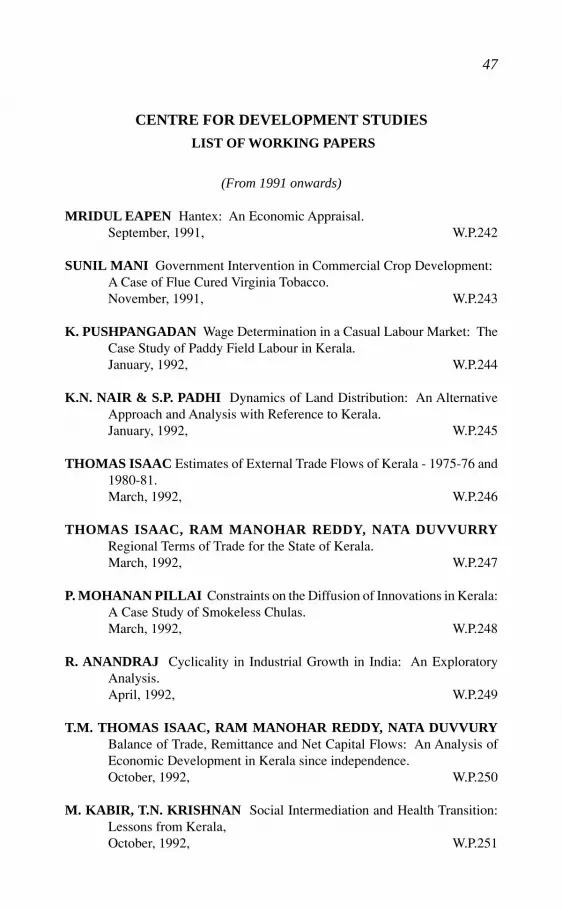
47

CENTRE FOR DEVELOPMENT STUDIES

LIST OF WORKING PAPERS

(From 1991 onwards)

MRIDUL EAPEN Hantex: An Economic Appraisal.September, 1991, W.P.242

SUNIL MANI Government Intervention in Commercial Crop Development:A Case of Flue Cured Virginia Tobacco.November, 1991, W.P.243

K. PUSHPANGADAN Wage Determination in a Casual Labour Market: TheCase Study of Paddy Field Labour in Kerala.January, 1992, W.P.244

K.N. NAIR & S.P. PADHI Dynamics of Land Distribution: An AlternativeApproach and Analysis with Reference to Kerala.January, 1992, W.P.245

THOMAS ISAAC Estimates of External Trade Flows of Kerala - 1975-76 and1980-81.March, 1992, W.P.246

THOMAS ISAAC, RAM MANOHAR REDDY, NATA DUVVURRYRegional Terms of Trade for the State of Kerala.March, 1992, W.P.247

P. MOHANAN PILLAI Constraints on the Diffusion of Innovations in Kerala:A Case Study of Smokeless Chulas.March, 1992, W.P.248

R. ANANDRAJ Cyclicality in Industrial Growth in India: An ExploratoryAnalysis.April, 1992, W.P.249

T.M. THOMAS ISAAC, RAM MANOHAR REDDY, NATA DUVVURYBalance of Trade, Remittance and Net Capital Flows: An Analysis ofEconomic Development in Kerala since independence.October, 1992, W.P.250

M. KABIR, T.N. KRISHNAN Social Intermediation and Health Transition:Lessons from Kerala,October, 1992, W.P.251

48

SUNIL MANI, P. NANDAKUMAR Aggregate Net Financial Flows to India:The Relative Importance of Private Loan vis-a-vis Foreign DirectInvestments.August, 1993, W.P.252

PULAPRE BALAKRISHNAN Rationale and the Result of the CurrentStabilisation Programme.November, 1993, W.P.253

K.K. SUBRAHMANIAN, P. MOHANAN PILLAI Modern Small Industryin Kerala: A Review of Structural Change and Growth Performance.January, 1994, W.P.254

DILIP M.MENON Becoming Hindu and Muslim : Identity and Conflict inMalabar 1900-1936.January, 1994 W.P.255

D. NARAYANA Government Intervention in Commodity Trade: An Analysisof the Coffee Trade in India.January, 1994 W.P.256

K.J. JOSEPH, P. NANDAKUMAR On the Determinants of Current AccountDeficits: A Comparative Analysis of India, China and South Korea.January, 1994 W.P.257

K.K. SUBRAHMANIAN, K.J. JOSEPH Foreign Control and Export Intensityof Firms in Indian Industry.February, 1994 W.P.258

PULAPRE BALAKRISHNAN, K. PUSHPANGADAN Total FactorProductivity Growth in Indian Manufacturing - A Fresh Look.April 1994, W.P.259

D. NARAYANA, K.N. NAIR Role of the Leading Input in Shaping Institutions:Tendency in the Context of Irrigation Uncertainty.May, 1994, W.P.260

G. MURUGAN, K. PUSHPANGADAN Pricing of Drinking Water: AnApplication of Coase Two-part Tariff.December, 1994 W.P.261

MOHANAN PILLAI On the Mexican Crisis.December, 1995, W.P.262

SUNIL MANI Financing Domestic Technology Development through theVenture Capital Route.December, 1995, W.P.263

49

T.T. SREEKUMAR Peasants and Formal Credit in Thiruvithamcore: TheState Institutions and Social Structure 1914-1940.December, 1995 W.P.264

AMITABH Estimation of the Affordability of Land for Housing Purposes inLucknow City, Uttar Pradesh (India): 1970-1990.March, 1996. W.P.265

K. PUSHPANGADAN, G. MURUGAN, K. NAVANEETHAM Travel Time,User Rate & Cost of Supply: Drinking Water in Kerala, India:June 1996. W.P.266

K.J. JOSEPH Structural Adjustment in India: A Survey of Recent Studies &Issues for Further Research,June 1996 W.P.267

D. NARAYANA Asian Fertility Transition: Is Gender Equity in FormalOccupations an Explanatory Factor?October, 1996 W.P.268

D. NARAYANA, SAIKAT SINHAROY Import and Domestic Production ofCapital Goods from Substitution to Complementarity,October 1996. W.P.269

NEW SERIES

W.P. 270 ACHIN CHAKRABORTY On the Possibility of a WeightingSystem for Functionings December 1996

W.P. 271 SRIJIT MISHRA Production and Grain Drain in two inlandRegions of Orissa December 1996

W.P. 272 SUNIL MANI Divestment and Public Sector Enterprise Reforms,Indian Experience Since 1991 February 1997

W.P. 273 ROBERT E. EVENSON, K.J. JOSEPH Foreign TechnologyLicensing in Indian Industry : An econometric analysis of the choiceof partners, terms of contract and the effect on licensees’ performanceMarch 1997

W.P. 274 K. PUSHPANGADAN, G. MURUGAN User Financing &Collective action: Relevance sustainable Rural water supply in India.March 1997.

W.P. 275 G. OMKARNATH Capabilities and the process of DevelopmentMarch 1997

50

W. P. 276 V. SANTHAKUMAR Institutional Lock-in inNatural ResourceManagement: The Case of Water Resources in Kerala, April 1997.

W. P. 277 PRADEEP KUMAR PANDA Living Arrangements of the Elderlyin Rural Orissa, May 1997.

W. P. 278 PRADEEP KUMAR PANDA The Effects of Safe Drinking Waterand Sanitation on Diarrhoeal Diseases Among Children in RuralOrissa, May 1997.

W. P. 279 U. S. MISRA, MALA RAMANATHAN, S. IRUDAYA RAJAN Induced Abortion Potential Among Indian Women, August 1997.

Documents

Female headship, poverty and child welfare: A study of rural orissa, India