Embed Size (px)
Citation preview

Fast Aeroelastic Analysis and Optimisation ofLarge Mixed Materials Wind Turbine Blades

Fast Aeroelastic Analysis and Optimisation ofLarge Mixed Materials Wind Turbine Blades
Proefschrift
ter verkrijging van de graad van doctoraan de Technische Universiteit Delft,
op gezag van de Rector Magnificus prof. dr. ir. T.H.J.J. van der Hagen,voorzitter van het College voor Promoties,
in het openbaar te verdedigen op dinsdag 15 januari 2019 te 12.30 uur
door
Terry HEGBERGIngenieur Luchtvaart- en Ruimtevaarttechniek, Technische Universiteit Delft,
Nederlandgeboren te Zaandam, Nederland.
Dit proefschrift is goedgekeurd door de promotoren:Prof. dr. G.J.W van BusselDr. ir. R. De Breuker
Samenstelling promotiecommissie:
Rector Magnificus, voorzitterProf. dr. G.J.W. van Bussel, Technische Universiteit Delft, promotorDr. ir. R. De Breuker, Technische Universiteit Delft, promotor
Onafhankelijke leden:
Prof. dr. ir. G.A.M. van Kuik, Technische Universiteit DelftProf. dr. C.L. Botasso, Technical University MunichProf. dr. M.H. Hansen, University of Southern DenmarkDr. J.K.S. Dillinger, German Aerospace CenterDr. ir. H.E.N. Bersee, SuzlonProf. dr. S.J. Watson, Technische Universiteit Delft, reservelid
Keywords: Wind Energy, Aeroelasticity, Optimisation, Structural design.
Printed by: Gildeprint
ISBN
Copyright ©2018 by T. Hegberg
Cover picture by Printed in The Netherlands

Voor Sioe Wen, Gohan en Jadzia...

VI
SUMMARY
In this dissertation, structural wind turbine blade lay-outs are presented that aresuitable for 10MW and 20MW wind turbine blades. This has been accomplishedby using a medium fidelity static aeroelastic model embedded in an optimisationframework. The structural solutions are the result of a stiffness optimisation wherethe blade mass is minimised. To accomplish the structurally optimised blade, anaeroelastic analysis model is set up. This model consists of a nonlinear structuralanalysis module and an aerodynamic module. Both models are comparable interms of level of physical modelling and as such, it can be said that both modelsare of equal fidelity. This equal fidelity is favourable for the aeroelastic couplingbetween both models, which generates an aeroelastic solution that is accurate upto the level of physics present in the aerodynamic and the structural models.
The structural modelling starts with defining the lay-up and the thickness dis-tribution of all structural parts within the wind turbine blade. Then, a cross-sectional modeller reduces the degrees of freedom from the full 3D blade to cross-sectional properties in the prescribed 1D beam nodes. During this process, theorthotropic behaviour and the cross-sectional properties of the blade are pre-served. The cross-sectional information is used for defining the Timoshenko beamelements within the finite element structural analysis of the blade. The externalloads resulting from gravity act at the beam nodes and the centrifugal effect isimplemented by putting the distributed centrifugal forces on the beam nodes aswell. This analysis is embedded in a corotational framework, which means thatgeometrically nonlinear behaviour is included as well. As such, large blade tipdeflections are also taken into account within this model.
The aerodynamic loads are determined using a vortex lattice method. The blade,being the bound surface, is divided in spanwise and chordwise vortex panels whichare influenced by each other and vortex panels that form the rotating wake. Forthe wake, a cylindrical shape is assumed, which is sufficient for determining staticaeroelastic blade loads. The induced drag results from the vortex lattice methodand to account for parasite drag, aerodynamic drag coefficient tables are alsoincluded in the analysis.
The aeroelastic coupling is accomplished by using close coupling of the aerody-namic and structural model. For both the aerodynamic and the structural loads,sensitivities are determined with respect to the structural degrees of freedom.
VII
This yields the aerodynamic and structural stiffness. A Newton-Raphson rootfinding algorithm is used to determine the converged aeroelastic solution for theblade deformation and the corresponding blade loads.
For the structural optimisation, the variable stiffness concept is used. The ob-jective function calculates the blade mass, which is minimised, as a function of avector of design variables that contains eight lamination parameters and a thick-ness parameters per laminate used. The thickness parameters depend on using apure fibre laminate or using a sandwich laminate. For pure fibre laminates onlyone thickness parameter is required, for sandwich laminates two are required: onefor the equal thickness facing sheets and one for the core. The optimiser used forthis problem is the globally convergent method of moving asymptotes, which is agradient based method. Two load cases are selected for the optimisation proced-ure, namely, the normal wind profile and the extreme wind shear. The load casesmentioned are most suitable for static aeroelastic analyses and the extreme windshear case covers a significant part of the load envelope. The selected constraintsare strain, buckling, tip deflection and, aerodynamic power loss. Because of thegradient based optimisation, the sensitivities of the objective function and theconstraints with respect to the design variables are determined as well.
The optimisations are carried out for 5MW, 10MW, and 20MW blades containingsandwich composites and blades only consisting of pure fibre laminates. In caseof the sandwich composites, the blade structure consists of suction skin, pressureskin, spar caps, a front spar and a rear spar. Ribs and longitudinal stiffeners arenot necessary in that case. In addition, the sandwich blade optimisation includesthe possibility of using sandwich composites in the spar caps. For the pure fibrelaminate blades, the suction skin, pressure skin, spar caps and the front and rearspars are present as well. The difference with sandwich skins is, that ribs andlongitudinal stiffeners must be added to take care of the skin buckling resistance.For both the sandwich blade and the stiffened skin blade, the optimisation can becarried out for a hybrid composite material blade. The hybrid blade consists ofeglass composites where parts of the spar caps are replaced by carbon composites.
The results show that all sandwich structural lay-outs arrive at a lower blade massthan the baselines. For the sandwich lay-out, it appeared that applying sandwichcomposites in the spar caps, a significant mass saving can be achieved, varyingbetween 14% and 26% with respect to full fibre spar caps. Also the stiffened skinblade structural lay-out shows lower masses compared to the baselines. However,more significant mass savings are observed for the sandwich blades, resulting inapproximately 5% lower masses than the stiffened skin blades. Furthermore, is isobserved that aeroelastic tailoring has some effect on the year power production,a production loss of 4.5% is calculated based on the optimised blades.The blade mass as a function of wind turbine power can be compared to scalinglaws from previous studies where the increase in nominal power estimates theblade mass. It is observed that the optimised results do not follow the scaling
VIII
laws. This can be an indication that the scaling laws cannot be used to scaletowards a 20MW turbine and should be updated. Furthermore, from analyseswhere the blade mass is plotted against the percentage carbon fibre in the sparcaps, it can be said that replacing glass fibres by carbon fibres in the spar capsonly, is an efficient way to implement carbon fibre.
It is concluded that replacing full eglass fibre spar caps by eglass sandwich lam-inate spar caps for the sandwich lay-out is more favourable than eglass stiffenedskin structural solutions. Both the sandwich and the stiffened skin concepts dohave significant lower mass than the baseline designs, however, the eglass sand-wich design is in favour. Replacing the eglass fibres by carbon fibres within apredefined part of the spar caps, gives another significant mass reduction. Espe-cially, for the 20MW blade the replacement of eglass fibres by carbon fibres withinthe spar caps proves to be efficient. The high internal spar cap loads shows thelimits of glass fibre sandwich laminates in terms of thick facing sheets and a van-ishing core thickness at approximately 50% of the blade span. Using carbon fibresandwich laminates, the facing sheet thickness reduces significantly and a thickercore remains. This results in significant mass reductions, while the blade partsare still able to resist buckling which is the critical constraint.As a final remark, it can be said that the aeroelastic model makes it possible toperform a complete blade optimisation for different wind turbine blades. From theoptimised blade results, it is possible to extract new design rules or adapt previousones. From the present research, for tailored blades, it seems that the classicalpower laws used for upscaling of the blades are not consistent in estimating blademasses for the 10MW and 20MW blades.
IX

X
SAMENVATTING
In dit proefschrift worden constructieve lay-outs van windturbinebladen gepres-enteerd die geschikt zijn voor 10MW en 20MW windturbinebladen. Dit wordtbereikt door een statisch aero-elastisch model van middelhoge betrouwbaarheidte gebruiken, geımplementeerd in een optimalisatieroutine. De constructieveoplossingen volgen uit een stijfheidsoptimalisatie waarin de bladmassa wordt gem-inimaliseerd. Voor de geoptimaliseerde bladconstructie wordt een aero-elastischmodel opgebouwd. Dit model bestaat uit een niet-lineaire constructieve moduleen een een aerodynamische module. Beide modellen zijn vergelijkbaar betref-fende de details van de fysische modellering, dat betekent dat beide modellen eenvergelijkbare betrouwbaarheid hebben betreffende de fysica. Deze vergelijkbarebetrouwbaarheid is gunstig voor de aero-elastisch koppeling tussen beide model-len wat zich vertaald in een aeroelastische oplossing die zo nauwkeurig is als defysica aanwezig in zowel het aerodynamisch model als het constructieve model.
De constructieve modellering begint met de initiele opbouw van de vezelrichtingenen de dikteverdelingen van de constructieve elementen van het blad. Vervolgenswordt de 3-dimensionale representatie van het blad gereduceerd naar oppervlaktesen oppervlaktetraagheidsgrootheden van de voorgeschreven knooppunten van het1-dimensionale balkmodel door gebruik te maken van een reductiealgorithme voordoorsnede-oppervlaktes. Gedurende dit reductieproces, blijven het orthotropischekarakter en de oppervlaktetraagheidsgrootheden van het blad behouden. Deze op-pervlaktetraagheidsgrootheden worden gebruikt om de Timoshenko balkelemen-ten te definieren in de eindige elementen analyse van het blad. De uitwendigebelastingen die volgen uit zwaartekracht worden als equivalente knooppuntbe-lastingen op de voorgeschreven balkknooppunten gezet en de centrifugaaleffectenworden gemodelleerd door de verdeelde centrifugaalkrachten ook op de voorges-chreven balkknooppunten te betrekken. Deze analyse is ingebed in een co-roterendassenstelsel wat betekent dat geometrische niet-lineair gedrag ook meegemod-elleerd is. Grote tipverplaatsingen kunnen dus ook worden beschouwd in ditmodel.
De aero-elastische koppeling wordt bereikt door sterke koppeling tussen het aero-dynamisch model en het constructieve model. Voor zowel het aerodynamischmodel als het constructieve model worden gevoeligheden naar de constructievegraden van vrijheid bepaald. Dit resulteert in de aerodynamische stijfheid en
XI
constructieve stijfheid. Een Newton-Raphson nulpuntsbepaling wordt gebruiktom de geconvergeerde aero-elastische oplossing te bepalen voor de bladvervorm-ing en de bijbehorende bladbelastingen.
Voor de optimalisatie van de bladconstructie, wordt het variabel stijfheidsconceptgebruikt. De doelfunctie berekent de bladmassa, die wordt geminimaliseerd, alseen functie van de ontwerpvariabelen die bestaan uit acht laminatieparameters eneen aantal dikteparameters per laminaat. De dikteparameters varieren per lam-inaattype: voor een puur vezellaminaat volstaat een dikteparameter, terwijl eensandwichlaminaat er minimaal twee nodig heeft, namelijk een voor de kerndikteen een voor de laminaatdikte als de laminaten gelijke dikte hebben. Het optimal-isatiealgorithme dat is gebruikt, is de globaal convergente methode van meebewe-gende asymptoten. Deze methode is een op gradienten gebaseerde optimalisatie.Voor de optimalisatie zijn twee load cases gekozen: het normale wind profiel ende extreme windgradient. De genoemde loadcases zijn het meest geschikt voor dequasi-statische optimalisatie en de extreme windgradient situatie dekt een belan-grijk deel van het belastingsspectrum. De gekozen beperkende voorwaarden zijnrek, knik, tipuitwijking en aerodynamisch vermogensverlies. Door de gekozen op-timalisatiemethode, zijn de gevoeligheden van de beperkende voorwaarden naarde ontwerpvariabelen ook nodig voor de gehele optimalisatieprocedure.
De optimalisaties zijn uitgevoerd voor 5MW, 10MW en 20MW bladen opgebouwduit sandwichlaminaten maar ook voor bladen bestaande uit pure vezellaminaten.Voor de sandwichlaminaten, bestaat het blad uit onder- en overdrukhuid en eendoosligger met 2 lijfplaten en 2 liggerflenzen. Ribben en langsverstijvers zijn nietnodig voor sandwich huiden. Bovendien is in de optimalisatie de mogelijkheidgecreeerd om de horizontale delen van de doosligger ook uit sandwichlaminatente laten bestaan. Voor puur vezellaminaat bladen, de over- en onderdrukhuidenzijn verstijfd met ribben en langsverstijvers en de doosligger maakt ook deel uitvan deze constructieve oplossing. De huiden dienen nu echter verstijfd te wordenom huidknik tegen te gaan. Voor zowel de het sandwich blad als wel het puur vezelblad, worden de optimalisaties ook uitgevoerd met hybride composietmaterialen.Dit hybride blad bestaat dan uit huiden van glasvezel composiet maar een deelvan de ligger, en dan slechts delen van de liggerflenzen, wordt vervangen doorkoolstofvezel composiet.
De resultaten laten zien dat alle sandwich bladen uitkomen op lagere bladmassa’svergeleken met de baseline bladen. Voor de sandwich lay-out blijkt dat, wanneersandwich composieten ook in de liggerflenzen wordt gebruikt, een significantemassabesparing wordt bereikt. Deze besparing ligt tussen de 14% en 26% tenopzichte van de puur vezellaminaat liggerflenzen. Ook de bladen met verstijfdehuiden laten een lagere massa zien ten opzichte van de baseline. Echter, de bl-admassa’s komen lager uit met sandwich liggerflenzen, resulterend in 5% lageremassa’s vergeleken met de bladen met het verstijfde huid concept. Verder blijktuit de aero-elastiche optimalisatie dat een aerodynamisch vermogensverlies van
XII
4.5% optreedt.De bladmassa, als functie van het windturbinevermogen, kan worden vergelekenmet schaalwetten van oudere studies waar uit de toename van het nominaal ver-mogen de bladmassa wordt geschat. Het blijkt dat de geoptimaliseerde bladenuit dit proefschrift de schaalwetten niet volgen. Dit kan een aanwijzing zijn datde schaalwetten niet direct kunnen worden gebruikt om een schatting te makenvoor een 20MW windtubine. Een update van de schaalwetten zou dan op zijnplaats zijn. Verder blijkt uit analyses gedaan door de bladmassa uit te zetten te-gen het percentage koolstofvezel in de liggerflenzen, dat vervangen van glasvezelmaterialen door koolstofmaterialen efficient is.
Er kan worden geconcludeerd dat het vervangen van puur glasvezellaminaten doorglasvezel sandwichlaminaten in de liggerflenzen van de bladen met de sandwichlay-out gunstiger is dan het toepassen van het hele blad uit te voeren met het ver-stijfde huid concept. Zowel het verstijfde huid concept als het sandwich conceptgeeft als oplossing bladen met lagere massa’s dan die van de baseline ontwerpen,echter, de glasvezel sandwich combinatie geeft lichtere bladen. Vervangen vanglasvezel door koolstofvezel in een voorgeschreven deel van de liggerflenzen geeftnog eens een extra massabesparing. Voornamelijk het 20MW blad ondervindtvoordelen van koolstofvezel in de flenzen. De hoge interne flensbelastingen latenzien dat op ongeveer 50% van de bladradius, de glasvezels de limiet bereiken voordit 20MW bladontwerp door laminaten die de het kernmateriaal verdringen voorde sandwich lay-out. Gebruik van koolstofvezel reduceert de laminaatdikte weeren de kern krijgt dan ook weer dikte. Dit resulteert in een significante afnamevan de bladmassa terwijl huidknik, welke beperking kritiek blijkt te zijn, geenprobleem meer is.Als een laatste opmerking, kan worden gezegd dat het aero-elastisch model hetmogelijk maakt complete bladoptimalisaties te doen voor verschillende windtur-binebladen. Uit de optimalisatieresultaten van de bladen, kunnen nieuwe ont-werpregels worden opgesteld of kunnen oude worden bijgesteld. Uit deze studieblijkt bijvoorbeeld dat, voor geoptimaliseerde bladen, de klassieke opschaling-swetten voor bladen niet consistent zijn voor het inschatten van de bladmassa’svan 10MW en 20MW bladen.
XIII

XIV
NOMENCLATURE
ROMAN SYMBOLS
A Cross-sectional area m2
A Aerodynamic influence coefficient matrix
A Laminate in-plane stiffness matrix N/m
B Laminate coupling stiffness matrix N
c Chord m
cd Section drag coefficient -
C Cross-sectional property term in cross-sectional tensor C
c Chord vector m
C Cross-sectional tensor
D Laminate out-of-plane stiffness matrix N m
D Drag vector N
E Young’s modulus N/m2
e Unit vector
f Force vector N
F Force vector N
g Gravitational acceleration m/s2
G Shear stiffness N/m2
h Single layer thickness of a laminate m
H Buckling stiffness properties
I Second moment of area m4
J Polar area moment of inertia m4
J Jacobi matrix
K Stiffness matrix
L Lift vector N
m Mass kg
M Stress resultant moments per unit length Nm/m
N Stress resultant forces per unit length N/m
n Unit normal vector for vortex panels -
XV
p Structural degree of freedom vector
Q Stiffness matrix from constitutive equation N/m2
R Rotor radius m
r Vector between two points m
R Residual vector
R Rotation matrix
R Radius of curvature of cylindrical buckling panel m
S Material strength in shear N/m2
S Surface area m2
t Total laminate thickness m
t Sandwich laminate thickness vector m
T Coordinate system
T Rotation matrix used within lamination theory
u flow velocity in eb1 direction m/s
U Material invariant terms for Γ matrices N/m2
v flow velocity in eb2 direction m/s
V Lamination parameter
V Volume m3
V Velocity vector m/s
w flow velocity in eb3 direction m/s
x x-Coordinate m
X Material strength in 0-direction N/m2
x Position vector m
X Inertial position coordinate m
y y-Coordinate m
Y Material strength in 90-direction N/m2
z z-Coordinate m
GREEK SYMBOLS
α Angle of attack rad
γ Shear strain -
Γ Circulation m2/s
Γ Material invariant matrix
ǫ Membrane strain -
ǫ Strain vector -
η Number of half waves in lateral direction
θ Rotational deformation rad
XVI
κ Bending strain -
λ Number of half waves in longitudinal direction
λ Load variation parameter for nonlinear load analysis
ξ Design variable vector
ρ Density kg/m2
σ Stress vector -
φ Two dimensional displacement function -
φ Local inflow angle
φ Perturbation velocity potential m2/s
Ψ Blade azimuth deg
SUB/SUPERSCRIPTS
0 Rotating body axis frame fixed at blade root
∞ Freestream conditions
0 Undeformed
a Aerodynamic load
B Body axis frame attached to tower
b Non-rotating body axis frame fixed at blade root
c Compressive
c Core of a sandwich composite laminate
e External load
f Facing sheet of a sandwich composite laminate
g Geometric
g Global reference frame
I Inertial
k The kthlayerwithinacompositelaminate
l Local reference frame
r Rigid reference frame
s Structural load
t Tangential
t Tensile
w Wake surface
ABBREVIATIONS
BECAS Beam Cross-sectional analysis software
BEM Blade element momentum theory
XVII
CFD Computational fluid dynamics
EWS Extreme wind shear
FEM Finite element method
GCMMA Globally convergent method of moving asymptotes
GDW General dynamic wake
IEC International electrotechnical commission
MBS Multi-body system
NREL National renewable energy laboratory
NWP Normal wind profile
XVIII

XIX

XX
CONTENTS
SUMMARY VII
SAMENVATTING XI
NOMENCLATURE XV
1 INTRODUCTION 1
1.1 STATE-OF-THE-ART OF AEROELASTIC MODELLING AND STRUCTURAL
DESIGN . . . . . . . . . . . . . . . . . . . . . . . . . . . . . . . . . 3
1.2 MINIMISING BLADE MASS AND BLADE OPTIMISATION . . . . . . . . 6
1.3 AEROELASTIC TAILORING . . . . . . . . . . . . . . . . . . . . . . . 7
1.4 UP-SCALING OF WIND TURBINE BLADES . . . . . . . . . . . . . . 8
1.5 RESEARCH GOAL . . . . . . . . . . . . . . . . . . . . . . . . . . . . 9
1.6 CHOICES WITHIN THIS RESEARCH . . . . . . . . . . . . . . . . . . 10
1.7 THESIS OUTLINE . . . . . . . . . . . . . . . . . . . . . . . . . . . . 11
2 EQUAL FIDELITY STATIC AEROELASTIC MODELLING OF LARGEBLADES 15
2.1 WIND TURBINE BLADE REFERENCE FRAMES . . . . . . . . . . . . . 16
2.2 STRUCTURAL MODELLING . . . . . . . . . . . . . . . . . . . . . . . 19
2.3 AERODYNAMIC MODELLING . . . . . . . . . . . . . . . . . . . . . . 35
2.4 AEROELASTIC BLADE MODELLING . . . . . . . . . . . . . . . . . . 44
2.5 AEROELASTIC VALIDATION OF THE 5MW NREL BASELINE ROTOR
BLADE . . . . . . . . . . . . . . . . . . . . . . . . . . . . . . . . . . 46
2.6 CONCLUDING REMARKS . . . . . . . . . . . . . . . . . . . . . . . . 50
XXI
3 OPTIMISATION PROCEDURE 53
3.1 AEROELASTIC OPTIMISATION . . . . . . . . . . . . . . . . . . . . . 53
3.2 DESIGN FORMULATION . . . . . . . . . . . . . . . . . . . . . . . . . 57
3.3 THE WIND TURBINE BLADES CONSIDERED . . . . . . . . . . . . . . 66
3.4 CONCLUDING REMARKS . . . . . . . . . . . . . . . . . . . . . . . . 70
4 AEROELASTIC OPTIMISATION RESULTS OF 5, 10 AND 20MWBLADES 71
4.1 SANDWICH STRUCTURAL CONFIGURATION . . . . . . . . . . . . . . 72
4.2 STIFFENED SKIN BLADE LAY-OUT . . . . . . . . . . . . . . . . . . . 100
4.3 IMPACT OF AEROELASTIC OPTIMISATION ON YEARLY POWER PRO-DUCTION . . . . . . . . . . . . . . . . . . . . . . . . . . . . . . . . 112
4.4 DISCUSSION . . . . . . . . . . . . . . . . . . . . . . . . . . . . . . 117
4.5 CONCLUDING REMARKS . . . . . . . . . . . . . . . . . . . . . . . . 125
5 CONCLUSIONS AND RECOMMENDATIONS 127
5.1 CONCLUSIONS . . . . . . . . . . . . . . . . . . . . . . . . . . . . . 127
5.2 RECOMMENDATIONS . . . . . . . . . . . . . . . . . . . . . . . . . . 131
A CLASSICAL LAMINATE THEORY FORMULAE 133
B STRAIN AND BUCKLING OF OPTIMISED DESIGNS 135
C AERODYNAMIC POWER CONSTRAINTS 145
BIBLIOGRAPHY 149
ACKNOWLEDGEMENTS 155
BIOGRAPHICAL NOTE 157
XXII
1INTRODUCTION
The world energy demand increases due to the modern society. Because of pop-ulation growth together with the use of modern equipment, energy consumptionkeeps growing. In the future, mining fossile fuels requires technologically moreadvanced and expensive solutions. Furthermore, the use of these sources of energyloses public support due to, for instance, strong signals indicating climate changeand pollution. As such, the focus on optimising renewable energy sources shouldincrease.
This research focuses on wind energy in particular. Wind energy becomes moreand more accepted as a cost-effective renewable energy source for the generationof electricity. With increasing demand of this resource, efficiency is improved byincreasing the power or by reducing the cost of a single wind turbine. For moreefficient wind turbines, one could choose for increased hub height, which increasesthe average aerodynamic power because of increased average wind velocity. Thevelocity increase gives a significant amount of aerodynamic power increase sincethe relation between aerodynamic power and wind velocity is cubic. Even moreimportant is the rotor area of the turbine. The power and the area relate linearly,as a consequence, rotor radius relates in a quadratic way to energy yield. Thisexplains the very large dimensions of modern multi-MegaWatt wind turbines.Large wind turbines in large wind farms seem a cost-effective choice for competingwith other ways of electricity generation. Recent tender procedures demonstratethe cost effectiveness of large off-shore windfarms. Those farms are located fairlyclose to the shore at limited water depth.
1
1
1. INTRODUCTION
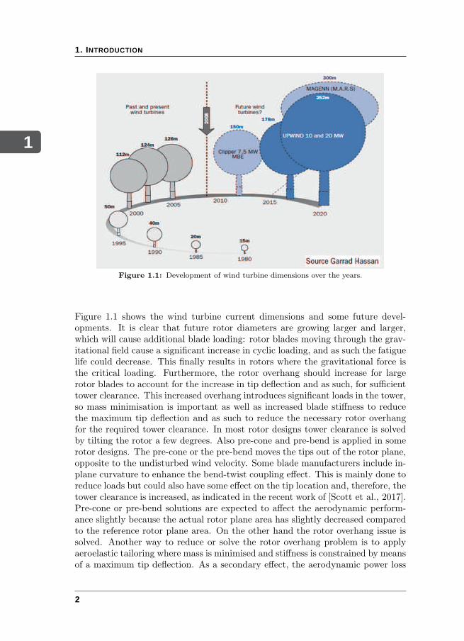
Figure 1.1: Development of wind turbine dimensions over the years.
Figure 1.1 shows the wind turbine current dimensions and some future devel-opments. It is clear that future rotor diameters are growing larger and larger,which will cause additional blade loading: rotor blades moving through the grav-itational field cause a significant increase in cyclic loading, and as such the fatiguelife could decrease. This finally results in rotors where the gravitational force isthe critical loading. Furthermore, the rotor overhang should increase for largerotor blades to account for the increase in tip deflection and as such, for sufficienttower clearance. This increased overhang introduces significant loads in the tower,so mass minimisation is important as well as increased blade stiffness to reducethe maximum tip deflection and as such to reduce the necessary rotor overhangfor the required tower clearance. In most rotor designs tower clearance is solvedby tilting the rotor a few degrees. Also pre-cone and pre-bend is applied in somerotor designs. The pre-cone or the pre-bend moves the tips out of the rotor plane,opposite to the undisturbed wind velocity. Some blade manufacturers include in-plane curvature to enhance the bend-twist coupling effect. This is mainly done toreduce loads but could also have some effect on the tip location and, therefore, thetower clearance is increased, as indicated in the recent work of [Scott et al., 2017].Pre-cone or pre-bend solutions are expected to affect the aerodynamic perform-ance slightly because the actual rotor plane area has slightly decreased comparedto the reference rotor plane area. On the other hand the rotor overhang issue issolved. Another way to reduce or solve the rotor overhang problem is to applyaeroelastic tailoring where mass is minimised and stiffness is constrained by meansof a maximum tip deflection. As a secondary effect, the aerodynamic power loss
2
1
1.1. STATE-OF-THE-ART OF AEROELASTIC MODELLING ANDSTRUCTURAL DESIGN
can be restricted while only optimising the blade structural design: the externalblade shape is not changed.
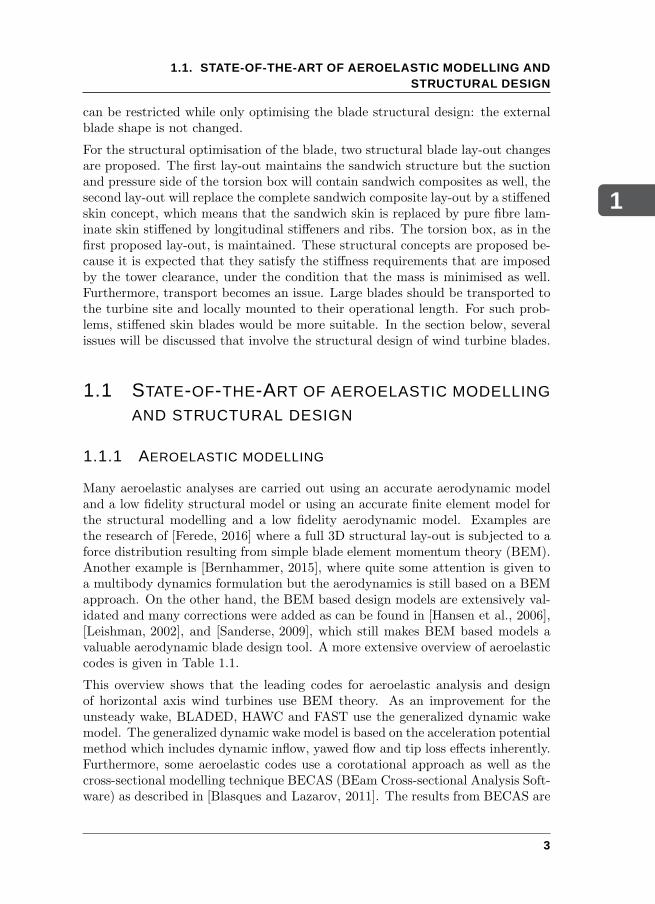
For the structural optimisation of the blade, two structural blade lay-out changesare proposed. The first lay-out maintains the sandwich structure but the suctionand pressure side of the torsion box will contain sandwich composites as well, thesecond lay-out will replace the complete sandwich composite lay-out by a stiffenedskin concept, which means that the sandwich skin is replaced by pure fibre lam-inate skin stiffened by longitudinal stiffeners and ribs. The torsion box, as in thefirst proposed lay-out, is maintained. These structural concepts are proposed be-cause it is expected that they satisfy the stiffness requirements that are imposedby the tower clearance, under the condition that the mass is minimised as well.Furthermore, transport becomes an issue. Large blades should be transported tothe turbine site and locally mounted to their operational length. For such prob-lems, stiffened skin blades would be more suitable. In the section below, severalissues will be discussed that involve the structural design of wind turbine blades.
1.1 STATE-OF-THE-ART OF AEROELASTIC MODELLING
AND STRUCTURAL DESIGN
1.1.1 AEROELASTIC MODELLING
Many aeroelastic analyses are carried out using an accurate aerodynamic modeland a low fidelity structural model or using an accurate finite element model forthe structural modelling and a low fidelity aerodynamic model. Examples arethe research of [Ferede, 2016] where a full 3D structural lay-out is subjected to aforce distribution resulting from simple blade element momentum theory (BEM).Another example is [Bernhammer, 2015], where quite some attention is given toa multibody dynamics formulation but the aerodynamics is still based on a BEMapproach. On the other hand, the BEM based design models are extensively val-idated and many corrections were added as can be found in [Hansen et al., 2006],[Leishman, 2002], and [Sanderse, 2009], which still makes BEM based models avaluable aerodynamic blade design tool. A more extensive overview of aeroelasticcodes is given in Table 1.1.
This overview shows that the leading codes for aeroelastic analysis and designof horizontal axis wind turbines use BEM theory. As an improvement for theunsteady wake, BLADED, HAWC and FAST use the generalized dynamic wakemodel. The generalized dynamic wake model is based on the acceleration potentialmethod which includes dynamic inflow, yawed flow and tip loss effects inherently.Furthermore, some aeroelastic codes use a corotational approach as well as thecross-sectional modelling technique BECAS (BEam Cross-sectional Analysis Soft-ware) as described in [Blasques and Lazarov, 2011]. The results from BECAS are
3
1
1. INTRODUCTION
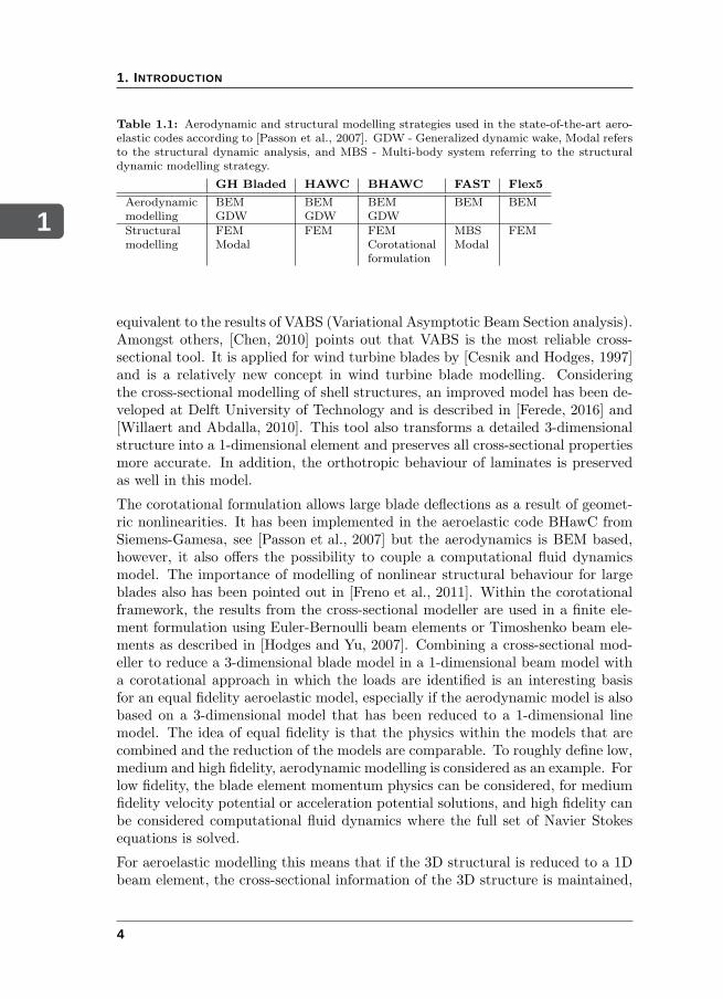
Table 1.1: Aerodynamic and structural modelling strategies used in the state-of-the-art aero-elastic codes according to [Passon et al., 2007]. GDW - Generalized dynamic wake, Modal refersto the structural dynamic analysis, and MBS - Multi-body system referring to the structuraldynamic modelling strategy.
GH Bladed HAWC BHAWC FAST Flex5
Aerodynamic BEM BEM BEM BEM BEMmodelling GDW GDW GDWStructural FEM FEM FEM MBS FEMmodelling Modal Corotational Modal
formulation
equivalent to the results of VABS (Variational Asymptotic Beam Section analysis).Amongst others, [Chen, 2010] points out that VABS is the most reliable cross-sectional tool. It is applied for wind turbine blades by [Cesnik and Hodges, 1997]and is a relatively new concept in wind turbine blade modelling. Consideringthe cross-sectional modelling of shell structures, an improved model has been de-veloped at Delft University of Technology and is described in [Ferede, 2016] and[Willaert and Abdalla, 2010]. This tool also transforms a detailed 3-dimensionalstructure into a 1-dimensional element and preserves all cross-sectional propertiesmore accurate. In addition, the orthotropic behaviour of laminates is preservedas well in this model.
The corotational formulation allows large blade deflections as a result of geomet-ric nonlinearities. It has been implemented in the aeroelastic code BHawC fromSiemens-Gamesa, see [Passon et al., 2007] but the aerodynamics is BEM based,however, it also offers the possibility to couple a computational fluid dynamicsmodel. The importance of modelling of nonlinear structural behaviour for largeblades also has been pointed out in [Freno et al., 2011]. Within the corotationalframework, the results from the cross-sectional modeller are used in a finite ele-ment formulation using Euler-Bernoulli beam elements or Timoshenko beam ele-ments as described in [Hodges and Yu, 2007]. Combining a cross-sectional mod-eller to reduce a 3-dimensional blade model in a 1-dimensional beam model witha corotational approach in which the loads are identified is an interesting basisfor an equal fidelity aeroelastic model, especially if the aerodynamic model is alsobased on a 3-dimensional model that has been reduced to a 1-dimensional linemodel. The idea of equal fidelity is that the physics within the models that arecombined and the reduction of the models are comparable. To roughly define low,medium and high fidelity, aerodynamic modelling is considered as an example. Forlow fidelity, the blade element momentum physics can be considered, for mediumfidelity velocity potential or acceleration potential solutions, and high fidelity canbe considered computational fluid dynamics where the full set of Navier Stokesequations is solved.
For aeroelastic modelling this means that if the 3D structural is reduced to a 1Dbeam element, the cross-sectional information of the 3D structure is maintained,
4
1
1.1. STATE-OF-THE-ART OF AEROELASTIC MODELLING ANDSTRUCTURAL DESIGN
and can be referred to as a medium fidelity structural model. Combining thiswith a multi-panel aerodynamic vortex model, which is also of medium fidelity,this equal fidelity of both the structural model and the aerodynamic model givesthe aeroelastic solution comparable accuracy. This equal fidelity of both modelsis important for optimisations where aeroelastic behaviour is a key issue.
1.1.2 STRUCTURAL DESIGN
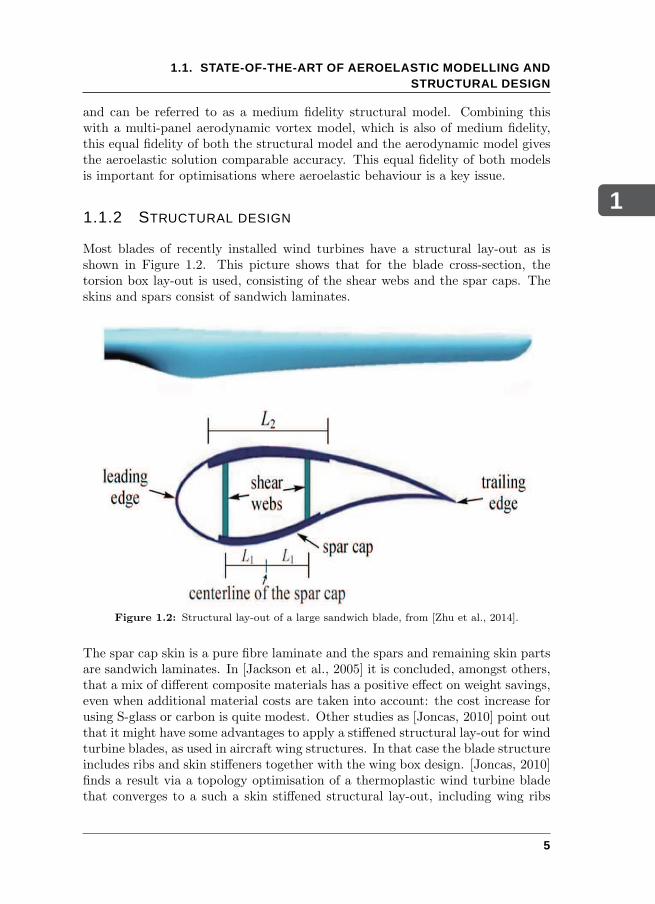
Most blades of recently installed wind turbines have a structural lay-out as isshown in Figure 1.2. This picture shows that for the blade cross-section, thetorsion box lay-out is used, consisting of the shear webs and the spar caps. Theskins and spars consist of sandwich laminates.
Figure 1.2: Structural lay-out of a large sandwich blade, from [Zhu et al., 2014].
The spar cap skin is a pure fibre laminate and the spars and remaining skin partsare sandwich laminates. In [Jackson et al., 2005] it is concluded, amongst others,that a mix of different composite materials has a positive effect on weight savings,even when additional material costs are taken into account: the cost increase forusing S-glass or carbon is quite modest. Other studies as [Joncas, 2010] point outthat it might have some advantages to apply a stiffened structural lay-out for windturbine blades, as used in aircraft wing structures. In that case the blade structureincludes ribs and skin stiffeners together with the wing box design. [Joncas, 2010]finds a result via a topology optimisation of a thermoplastic wind turbine bladethat converges to a such a skin stiffened structural lay-out, including wing ribs
5
1
1. INTRODUCTION
that determine the dimensions of the skin and spar buckling panels. Longitudinalskin reinforcing stiffeners, however, are not a result of this optimisation. For largewind turbine blades it will be obvious that the skin strains, and therefore thestresses, increase because of blade stiffness that should restrict the tip deflectionfor sufficient tower clearance. As a consequence, it is worth to think of redesigningthe structural lay-out of a wind turbine blade and propose a different lay-up butmaintaining the sandwich composite lay-out, or propose a fully stiffened skin set-up. It should be noted, however, that wind turbine blade tailoring is not new, see[Goeij, 1999], but the issues mentioned above might provide some new insights.
1.2 MINIMISING BLADE MASS AND BLADE OPTIMISA-TION
For wind energy, it is important that electricity from wind arrives at the same costlevel as conventional generation of electricity. The blade shape should be such thatit extracts as much power from the wind as possible over a large range of wind ve-locities. This requires an optimum aerodynamic design of the blade: a well-knownmethod is using the BEM approach and design the airfoil distribution, blade chorddistribution and the blade built-in twist distribution to find an optimum valuefor the average annual energy yield. A procedure for such a shape optimisation isexplained in [Hansen, 2003]. However, due to structural deformations, the aero-dynamic loads change and to account for that, an aeroelastic blade design methodshould be used for finding an optimum blade result. In such a way, the struc-tural design determines the blade deformations to have minimum negative effecton the aerodynamic power. The aerodynamic loads, the blade gravitational andthe centrifugal forces in combination with the blade deflections can be used for astiffness optimization where the mass of the blade could be chosen as an objective.An extensive review on optimization within the field of wind turbines is given in[Chehouri et al., 2015]. This gives a clear picture on the state-of-art of the use ofobjective functions, constraints, design variables and the optimisation strategiesused. Few studies assume that, instead of minimizing cost of energy, blade masscould be chosen as objective. [Liao et al., 2012] and [Zhu et al., 2012] only choseto optimise spar caps, [Jureczko et al., 2005] performs a shape optimisation usingcommercial codes. A more recent study performed by [Scott et al., 2017] men-tions that large blades might require a different design philosophy. For instance,aeroelastic tailoring was proposed to reduce blade loads by bend-twist couplingand let this mechanism control the local pitch angle of the blade. The bend-twist mechanism is implemented by pure material behaviour or a combined bladeshape-material bend-twist coupling mechanism. Of course, the objective is toimprove the aerodynamic power and a blade that maintains, approximately, itsbaseline design mass and stiffness. The results showed a decreased root bendingmoments but slightly increased blade masses using some variable stiffness concept.
6
1
1.3. AEROELASTIC TAILORING
In this research bend-twist coupling could be a result of the optimisations, butit is not a separate research goal. The IEA annex, task 37, takes optimisationsof the complete wind energy converter into account, see [IEA, 2015]. Anotherrecent work optimises for the structure and the aerodynamics of rotor blades. In[Bottasso et al., 2016], an aerodynamic shape optimisation is carried out togetherwith aeroelastic tailoring of the spar caps. The final objective is chosen to be costof energy. Minimised blade mass is a significant objective as well, especially forincreasing blade radii crossing the gravitational field: fatigue due to deterministiccyclic gravity loads becomes more of an issue. Also extreme load cases have astronger effect on the structural design of large blades. Furthermore, manufac-turers need less material which can lead to reduction of manufacturing costs. Inthis research, it is proposed therefore, to use aeroelastic tailoring and the variablestiffness concept to optimise for the blade mass.
1.3 AEROELASTIC TAILORING
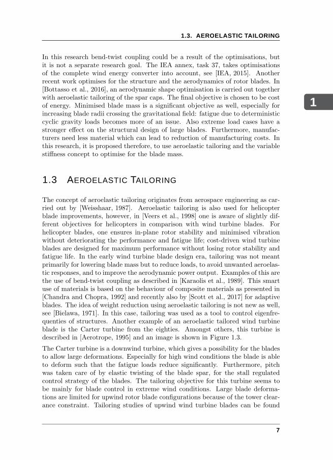
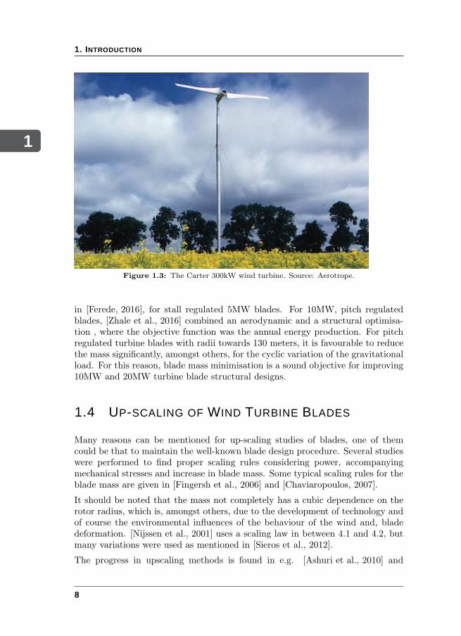
The concept of aeroelastic tailoring originates from aerospace engineering as car-ried out by [Weisshaar, 1987]. Aeroelastic tailoring is also used for helicopterblade improvements, however, in [Veers et al., 1998] one is aware of slightly dif-ferent objectives for helicopters in comparison with wind turbine blades. Forhelicopter blades, one ensures in-plane rotor stability and minimised vibrationwithout deteriorating the performance and fatigue life; cost-driven wind turbineblades are designed for maximum performance without losing rotor stability andfatigue life. In the early wind turbine blade design era, tailoring was not meantprimarily for lowering blade mass but to reduce loads, to avoid unwanted aeroelas-tic responses, and to improve the aerodynamic power output. Examples of this arethe use of bend-twist coupling as described in [Karaolis et al., 1989]. This smartuse of materials is based on the behaviour of composite materials as presented in[Chandra and Chopra, 1992] and recently also by [Scott et al., 2017] for adaptiveblades. The idea of weight reduction using aeroelastic tailoring is not new as well,see [Bielawa, 1971]. In this case, tailoring was used as a tool to control eigenfre-quenties of structures. Another example of an aeroelastic tailored wind turbineblade is the Carter turbine from the eighties. Amongst others, this turbine isdescribed in [Aerotrope, 1995] and an image is shown in Figure 1.3.
The Carter turbine is a downwind turbine, which gives a possibility for the bladesto allow large deformations. Especially for high wind conditions the blade is ableto deform such that the fatigue loads reduce significantly. Furthermore, pitchwas taken care of by elastic twisting of the blade spar, for the stall regulatedcontrol strategy of the blades. The tailoring objective for this turbine seems tobe mainly for blade control in extreme wind conditions. Large blade deforma-tions are limited for upwind rotor blade configurations because of the tower clear-ance constraint. Tailoring studies of upwind wind turbine blades can be found
7
1
1. INTRODUCTION
Figure 1.3: The Carter 300kW wind turbine. Source: Aerotrope.
in [Ferede, 2016], for stall regulated 5MW blades. For 10MW, pitch regulatedblades, [Zhale et al., 2016] combined an aerodynamic and a structural optimisa-tion , where the objective function was the annual energy production. For pitchregulated turbine blades with radii towards 130 meters, it is favourable to reducethe mass significantly, amongst others, for the cyclic variation of the gravitationalload. For this reason, blade mass minimisation is a sound objective for improving10MW and 20MW turbine blade structural designs.
1.4 UP-SCALING OF WIND TURBINE BLADES
Many reasons can be mentioned for up-scaling studies of blades, one of themcould be that to maintain the well-known blade design procedure. Several studieswere performed to find proper scaling rules considering power, accompanyingmechanical stresses and increase in blade mass. Some typical scaling rules for theblade mass are given in [Fingersh et al., 2006] and [Chaviaropoulos, 2007].
It should be noted that the mass not completely has a cubic dependence on therotor radius, which is, amongst others, due to the development of technology andof course the environmental influences of the behaviour of the wind and, bladedeformation. [Nijssen et al., 2001] uses a scaling law in between 4.1 and 4.2, butmany variations were used as mentioned in [Sieros et al., 2012].
The progress in upscaling methods is found in e.g. [Ashuri et al., 2010] and
8
1
1.5. RESEARCH GOAL
[Castillo Capponi et al., 2011]. The progress in rotor blade technology is not aconstant factor in time and technology is generally improving. Due to this, thescaling laws are not always up to date and should be adapted now and then.Furthermore an improved, nonlinear up-scaling method is being developed where,basically the internal blade loads are kept to the level of the NREL 5MW baseline.This has a complication: the scaled blade mass is significantly higher for the non-linear method than for the linear method. For either method, the result is aninfeasible design, especially for the 20MW turbine configuration. This complica-tion can be solved using aeroelastic tailoring to reduce the blade mass and as aresult, the stress levels stay below the allowed stresses for the materials used.
1.5 RESEARCH GOAL
Considering the overview of the previous sections, it is observed that:
• equal fidelity aeroelastic modelling for optimisations purposes can be im-proved,
• most research is carried out on blade optimisation, but mainly by means ofreducing loads and as a secondary effect, reducing mass. With increasingblade dimensions, mass minimisation is chosen to be an objective, with loadreduction as a logical consequence,
• to satisfy stiffness constraints, the current blade structural lay-out may notbe not sufficient for large blades. A different, novel structural lay-out cansolve the stiffness constraint problem,
• traditional upscaling laws might not produce convenient results for designinglarge wind turbine blades, stiffness optimisations using mass as objectivefunction can be used to update the existing scaling laws.
To address the issues mentioned above, the research goals are formulated bydefining the main research question:
Find an optimum structural and material lay-out for large wind turbine blades
using an equal fidelity aeroelastic analysis code suitable for optimisation purposes.
This main research question can be answered by defining the following sub ques-tions:
• How can a computationally fast equal fidelity aeroelastic model be formu-lated for large wind turbine blades, suitable for optimisation purposes?
• What is a suitable optimisation procedure?
• What structurally optimised blade and material lay-outs will appear?
9
1
1. INTRODUCTION
The equal fidelity modelling part includes matching the level of physical modellingof the structural model and the aerodynamic model. The question then is whataerodynamic modelling strategy has a comparable fidelity regarding a Timoshenkobeam finite element model, originating from an advanced cross-sectional model?
Furthermore, the structural lay-out of state-of-the-art wind turbine blades, mainlyexisting of sandwich panels to resist buckling, is changed in the stiffened skinadopted from aeronautics by means of longitudinal stiffeners and ribs, followingthe research of Joncas [Joncas, 2010], where a topology optimization convergedtowards the conventional aircraft wing design. It will also be investigated whetherthe use of different fibre orientations is of advantage for the structural designbesides the fact that costs will be probably higher. The new structural lay-outwill first be compared with the NREL 5MW baseline. The same procedure isfollowed for a single 10MW rotor blade from DTU [Bak et al., 2013], and forthe 20MW preliminary design of ECN, see [Peeringa et al., 2011]. The alteredstructural lay-out is obtained by optimising for minimum blade mass using thelaminate thickness and the fibre orientation of the skin and spars by means of thevariable stiffness concept.
1.6 CHOICES WITHIN THIS RESEARCH
During this research, possible trends are investigated concerning the relationbetween structural and material lay-out of a large wind turbine blade and theblade mass for increasing nominal aerodynamic power. The NREL 5MW turbineis considered as the baseline and the future trends are represented by blades from10MW and 20MW wind turbines. Furthermore, only the aeroelastic behaviourup to rated power is considered, which allows the assumption that the flow ofa single blade stays attached. Near the blade root, not much lift is generatedand since the distance with respect to the blade root is small, the contributionof the aerodynamic loading to the total aerodynamic power is considered to benegligible. As a consequence of this assumption, typical aeroelastic phenomenathat occur in the above rated region are not taken into account in this research.
Furthermore, the optimisations are only performed assuming balanced, symmet-ric laminates to show whether significant mass savings are obtained. Symmetriclaminates do not posses coupling effects as in-plane loadings resulting in out-of-plane deformations and out-of-plane loadings resulting in in-plane deformations.Balanced and unbalanced laminates are symmetric laminates, where symmetriclaminates are defined as laminates where the fibre orientation of a single layer ismirrored with respect to the mid plane. For unbalanced laminates, the orientationof a layer is maintained with respect to the mid plane, after mirroring. The layerthickness is mirrored with respect to the mid plane as well, due to the definitionof a symmetric laminate. One could propose using unbalanced, symmetric lam-
10
1
1.7. THESIS OUTLINE
inates for this research as well. For instance, [Ferede, 2016] used both balancedand unbalanced laminates. The unbalanced laminates were particularly used toincrease the effect of the bend-twist coupling for the stall regulated turbines. Healso used balanced laminates and his research showed significant mass savings.With this knowledge, it is decided to use balanced laminates only, to get a good,yet indicative idea of the mass saving potential.
Another important choice is that only steady aerodynamics is considered. It isrealised that wind turbine rotors are quite dynamic structures and also the aero-dynamics is unsteady, yet it is chosen to consider the blade structural lay-outchanges for steady cases. For steady cases, wind shear and yaw are allowed sincesuch cases show only slow changes in wind velocity, and as such, they can bereferred to as steady. Changes in blade pitch however, cause quick changes inaerodynamic loading, and are referred to as unsteady cases. Both steady andunsteady cases are inherently present within a vortex model as used in this work,however, the unsteady aerodynamics is not a subject within this research. Toaccount for a feasible structural lay-out, it has been decided to consider a severesteady load case for the optimisation: extreme wind shear. This load case is theheaviest case within the steady aerodynamics range, according to [IEC, 2005].For a more refined design of an optimised blade, it should be subjected to severalunsteady loadcases. It could be that the resulting optimised blade does not fitthe complete envelope, which means that the design should be adapted. Duringthis work the goal is to search for trends in structural lay-out to realise reducedblade mass but to maintain an appropriate blade stiffness distribution. All bladesare optimised using the same optimisation procedure, such that the relative com-parison is still objective.
1.7 THESIS OUTLINE
This section describes the main steps during the research, finally leading to theproject results and conclusions. In short, using an equal fidelity aeroelastic ana-lysis method embedded within a gradient based optimiser, two different types ofstructural lay-out of large wind turbine blades were optimised for minimisation ofthe blade mass. The set-up of the models and the optimisation results followingfrom the main research steps are structured by separate chapters.
In chapter 2, the equal fidelity aeroelastic model is explained. The basic conceptsconsidered are axis transformation for describing aerodynamic loads and struc-tural deformations. Also, some specific external loads acting on wind turbineblades are introduced and it is clarified how they are implemented in the struc-tural model. That is, the external loads such as gravity and centrifugal loads arenon-follower forces but must still be transformed to the local beam coordinatesystem where the deformations are determined. Furthermore, a simple repres-
11
1
1. INTRODUCTION
entation of sandwich laminates using lamination parameters is discussed as wellas the advanced cross-sectional modelling of airfoil cross-sectional shapes existingof the sandwich laminates. Also, because some locations within a wind turbineblade are buckling sensitive, a buckling model is used and is described as well.The aerodynamic blade element representation of the wind turbine blade is com-bined with a vortex panel method which gives the aerodynamic model higherfidelity than the blade element momentum formulation. Next, it is described howthe aerodynamic loads are coupled to a 1-dimensional Timoshenko beam elementwithin the corotational framework and why the linear stress-strain assumptionis valid within the corotational formulation. After elaborating on the structuraland the aerodynamic models, the models are coupled using close coupling whichmeans that the necessary sensitivities of the aerodynamic model with respect tothe structural degrees of freedom have to be determined. To finish the chapter, thevalidation of the aeroelastic model for the 5MW NREL rotor blade is performedsuch that it can be used with confidence for the optimisation.
In chapter 3, the optimisation procedure is explained by means of a flow chart.Then, the objective function is described as well as the sensitivities, especiallythe inclusion of the sandwich composite within the objective mass and the designvariable vector is pointed out. Furthermore, some constraint functions or variablesand their sensitivities with respect to design variables are defined if not alreadydone in chapter 2. Next, the design formulation is presented in terms of loadcases and design variables required for the optimisation. Lastly, the wind turbineblades considered are shortly described.
Chapter 4 is dedicated to the optimisation of large wind turbine blades. First, theblade structural elements are all composed of sandwich skins and spars. Also thespar caps are modelled as sandwich composites. Since the state-of-the-art turbineblades have full-fibre composites spar caps, some optimisations are performed forthis case as well. The optimisations for the full sandwich blade are performedfor the 5MW to compare with the baseline, and for the 10MW and 20MW tur-bines to find differences between optimised blade designs and the blades generatedfrom up-scaling laws. Next, the sandwich composite will be replaced by a skinstiffened lay-out for the spars and the skin, without altering the wing box andthe aerodynamic blade shape. This structural lay-out is applied for the 5MW,10MW, and the 20MW turbine blades as well. The chapter continues with ananalysis of the behaviour of the sandwich spar caps in comparison with the full-fibre composite spar caps. Also, due to stiffness and strength problems for 10MWor 20MW blades, some spar cap e-glass composite material has been replaced bycarbon composite material to observe the effect on blade mass and accompanyingstiffness and strength. Then, as a final step, trends are presented consideringblade masses against percentage carbon fibre in the spar caps and the blade massagainst nominal aerodynamic power.
The thesis finishes with conclusions and recommendations about the optimisation
12
1
1.7. THESIS OUTLINE
results and a short outlook concerning the future of tailoring of wind turbineblades.
13

1
1. INTRODUCTION
14
2EQUAL FIDELITY STATIC
AEROELASTIC MODELLING OF LARGE
BLADES
In this chapter, the structure of the aeroelastic model for a wind turbine bladeis presented. The model exists of a structural model and an aerodynamic modelwhere the aerodynamics is suitable for wind turbine blades operating in attachedflow conditions. Both models interact by means of close aeroelastic coupling.Since the blades are built of composite materials, appropriate stress and strainrelations due to external loading are used to model the internal loads. The spe-cific case of sandwich laminates is described and is coupled to the concept oflamination parameters: the relation between the ABD matrix and the lamina-tion parameters is explained. The lamination parameters are used for reducingthe computational effort during the optimisation procedure in which the aeroelas-tic model is implemented, and to facilitate continuous optimisation.The structural model uses linear Timoshenko beam elements embedded in a coro-tational framework. In this manner, large blade deflections can be analysed. Thecross-sectional properties for the beam elements are provided by a cross-sectionalmodeller that preserves the orthotropic behaviour of the composite materials usingthe strain energy concept. The aerodynamic model is of a different nature com-pared to the models used in the state-of-the-art wind turbine aeroelastic codes.Those common aerodynamic models are based on blade element momentum the-
15
2
2. EQUAL FIDELITY STATIC AEROELASTIC MODELLING OF LARGE BLADES
ory including the necessary engineering correction models. Examples of engin-eering correction models are: Prandtl’s finite blade correction, Glauert’s highloading correction, blade-blade interaction, and the dynamic inflow correctionmodel. During this research, vortex panels are used for modelling the deformedblade and the wake. As such, these blade element momentum correction modelsdo not need to be implemented.For the closely coupled aeroelastic solutions, the sensitivities of the structuralforces and the aerodynamic forces with respect to the structural degrees of free-dom are required. The obtained sensitivities represent the structural stiffnessmatrix and the aerodynamic stiffness matrix; these are required for the staticaeroelastic equilibrium equation. For the nonlinear solution of the equation, theNewton-Raphson root finding algorithm is used.The aeroelastic model, implemented in PROTEUS being the computer code, isapplied for the NREL 5MW reference rotor blade for validation, where the nor-mal and tangential force distribution, aerodynamic power per blade as a functionof wind velocity, and the tip displacement as a function of the wind velocity areconsidered as validation cases.
2.1 WIND TURBINE BLADE REFERENCE FRAMES
For the load calculation on wind turbine blades, a number of coordinate trans-formations are necessary. The wind velocity is expressed in an inertial axis frameand the blade loads are calculated in the local, rotating axis system. The trans-formations to be done are:
• From tower body axis frame TB =[eB1 eB2 eB3
]to the non-rotating body
axis system fixed at the blade root, Tb =[eb1 eb2 eb3
]. The origin of the
non-rotating blade system is located at the blade root, i.e. xb = 0;
• From the non-rotating blade root system to the rotating axis system at theblade root T0 =
[e01 e02 e03
]. The origin is also located at the blade root,
with the rotation center at the blade root.
The transformation matrices look as follows:
RB =
0 1 00 0 −11 0 0
, R0 =
cosΨ sinΨ 0− sinΨ cosΨ 0
0 0 1
. (2.1)
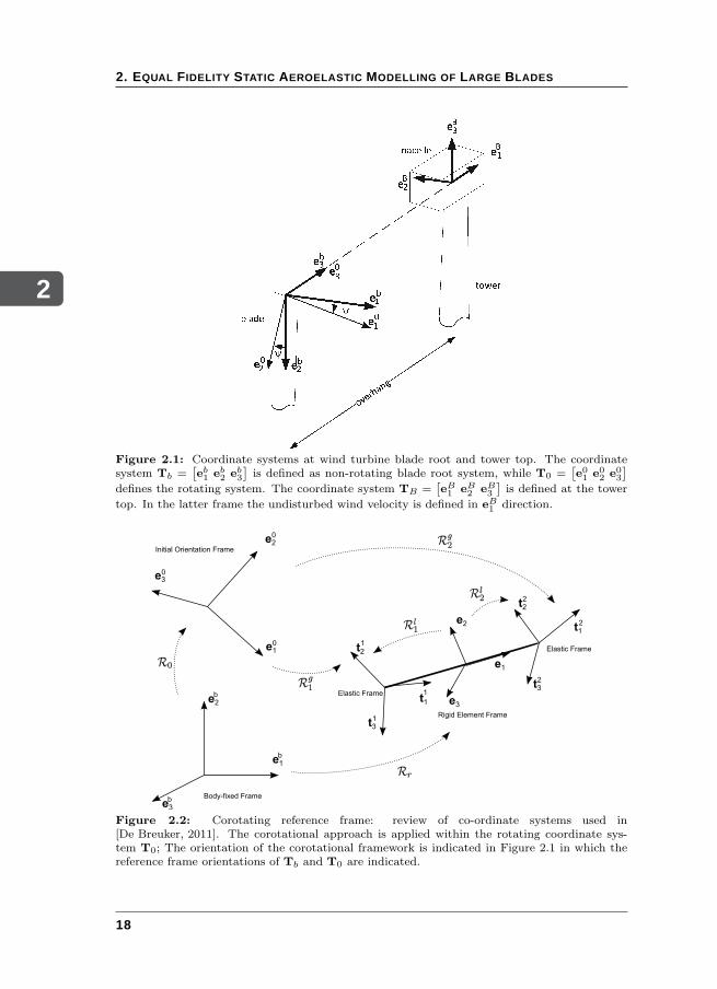
To account for large blade deflections, geometric nonlinearities are introduced byusing a corotational framework. This corotational formulation is applied withinthe local rotating axis system T0 which is indicated in Figure 2.1. The advantage
16
2
2.1. WIND TURBINE BLADE REFERENCE FRAMES
of such a formulation is that the stiffness matrix for the linear material behaviourremains valid since the small displacements are defined in a local coordinate sys-tem connected to each beam element. As such, geometrically large deflections areallowed because the local systems rotate along with the local beam element. Dueto the deflection of the previous element a new local rigid body axis system isdefined in which the new elastic deformations are determined.
The corotational formulation is visually summarised in Figure 2.2. For an unam-biguous formulation of the framework, the sequence if transformations starts ina fixed axis frame. Next, the rotational transformation is performed. Within therotated coordinates of the rigid rotor blade, the deformed blade shape is describedby means of the corotational formulation. Following the symbols in Figure 2.2,the axis frames are presented using the notation Tand the rotational transform-ations with R. This matrix is described in [De Breuker, 2011] and is determinedas follows:
R =
∞∑
k=0
θk
k!= exp (θ) , (2.2)
where θ is the skew-symmetric representation of the pseudo-vector θ = θx, θy, θzt.
The axis frame defined as the body axis fixed frame, Tb, can be identified witha non-rotating system attached to the rotor hub. The rotated blade system isdefined using the initial orientation frame, T0, and indicates the rotated or azi-muthal position of the undeformed blade. In such a way the blade azimuth can betaken into account. Next, the actual corotational formulation is used: the rigidelement frame, Tr, is based on the rigid rotation of the element considered, or theinitial orientation frame if the first element is considered, and is expressed withrespect to the body axis frame. Finally, with respect to the rigid element frame,the beam node orientatiens are calculated. Each beam node has its own triad,ti, indicating the cross-sectional orientation at each node, which means that thelocal deformations of both nodes are determined and the beam strains can becalculated.
Now that the axis frames are defined, the rotation transformations can be clari-fied. The R0 indicates the rotation between the body fixed frame and the initial,undeformed beam orientation. Then, the transformation from the rotating axisframe T0 to the rigid element frame Tr is accomplished usingRr. For the relationbetween the local triads and the initial beam orientation frame two transform-ations can be defined: R
g1from initial to node 1, or R
g2from initial to node
2. Rg is expressed in T0 and Rl is expressed in Tr. Finally, the local element
transformations involve the relations between the rigid element axis frame and thenodal triads that represent the cross-sectional orientation: R
l1 from rigid frame
to node 1 and Rl2 from rigid frame to node 2.
17
2
2. EQUAL FIDELITY STATIC AEROELASTIC MODELLING OF LARGE BLADES
Figure 2.1: Coordinate systems at wind turbine blade root and tower top. The coordinatesystem Tb =
[
eb1eb2eb3
]
is defined as non-rotating blade root system, while T0 =[
e01e02e03
]
defines the rotating system. The coordinate system TB =[
eB1
eB2
eB3
]
is defined at the tower
top. In the latter frame the undisturbed wind velocity is defined in eB1
direction.
Figure 2.2: Corotating reference frame: review of co-ordinate systems used in[De Breuker, 2011]. The corotational approach is applied within the rotating coordinate sys-tem T0; The orientation of the corotational framework is indicated in Figure 2.1 in which thereference frame orientations of Tb and T0 are indicated.
18
2
2.2. STRUCTURAL MODELLING
2.2 STRUCTURAL MODELLING
The state-of-the-art wind turbine blades are manufactured using sandwich lamin-ates for the leading and trailing edge parts of the blades as well as the front andrear spar. The spar caps are pure laminates to resist the highest compressive andtensile stresses. The blade cross-section consists of three cells: a narrow box beamwith spar caps and to the left and right of the spars the cells that resist torsionaldeformation. For large wind turbines in the 20MW region, sometimes one addsan extra spar at approximately 70% of the chord to prevent skin buckling. In thiswork, two novel structural configurations are introduced:
• application of sandwich composite to the spar caps rather than solid sparcaps;
• a stiffened skin by means of longitudinal stiffeners supported by ribs.
To analyse the different structural configurations, the following structural con-cepts are proposed that will be used to determine the internal loads and strainsdue to the external loads acting on the blade.
STRESS AND STRAIN FORMULATION FOR SANDWICH LAMINATES
The state-of-the-art wind turbine blades consist mainly of sandwich laminates.For the sake of an optimal calculation effort for sandwich laminates, a simplifiedstructural model is applied: the stresses are carried by the facing sheets and thecore is added to improve bending stiffness and face sheet buckling behaviour.This has some consequences for the ABD matrix and the lamination parametersfor such laminates, which will be focused on later in this chapter. The ABD
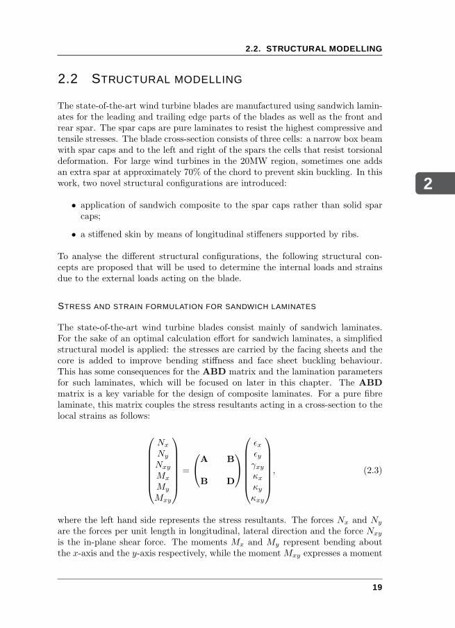
matrix is a key variable for the design of composite laminates. For a pure fibrelaminate, this matrix couples the stress resultants acting in a cross-section to thelocal strains as follows:
Nx
Ny
Nxy
Mx
My
Mxy
=
A B
B D
ǫxǫyγxyκxκyκxy
, (2.3)
where the left hand side represents the stress resultants. The forces Nx and Ny
are the forces per unit length in longitudinal, lateral direction and the force Nxy
is the in-plane shear force. The moments Mx and My represent bending aboutthe x-axis and the y-axis respectively, while the momentMxy expresses a moment
19
2
2. EQUAL FIDELITY STATIC AEROELASTIC MODELLING OF LARGE BLADES
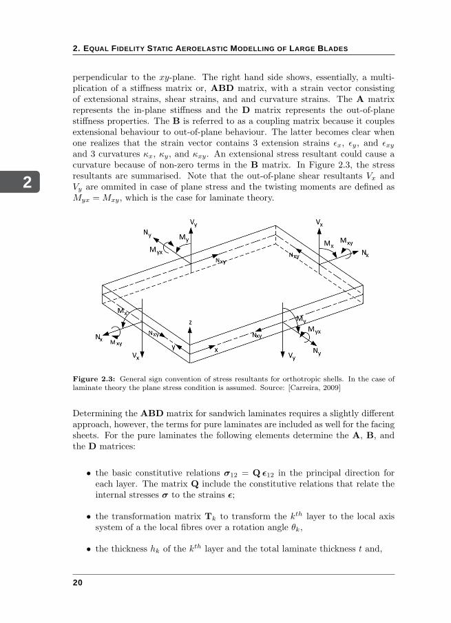
perpendicular to the xy-plane. The right hand side shows, essentially, a multi-plication of a stiffness matrix or, ABD matrix, with a strain vector consistingof extensional strains, shear strains, and and curvature strains. The A matrixrepresents the in-plane stiffness and the D matrix represents the out-of-planestiffness properties. The B is referred to as a coupling matrix because it couplesextensional behaviour to out-of-plane behaviour. The latter becomes clear whenone realizes that the strain vector contains 3 extension strains ǫx, ǫy, and ǫxyand 3 curvatures κx, κy, and κxy. An extensional stress resultant could cause acurvature because of non-zero terms in the B matrix. In Figure 2.3, the stressresultants are summarised. Note that the out-of-plane shear resultants Vx andVy are ommited in case of plane stress and the twisting moments are defined asMyx =Mxy, which is the case for laminate theory.
Figure 2.3: General sign convention of stress resultants for orthotropic shells. In the case oflaminate theory the plane stress condition is assumed. Source: [Carreira, 2009]
Determining the ABD matrix for sandwich laminates requires a slightly differentapproach, however, the terms for pure laminates are included as well for the facingsheets. For the pure laminates the following elements determine the A, B, andthe D matrices:
• the basic constitutive relations σ12 = Q ǫ12 in the principal direction foreach layer. The matrix Q include the constitutive relations that relate theinternal stresses σ to the strains ǫ;
• the transformation matrix Tk to transform the kth layer to the local axissystem of a the local fibres over a rotation angle θk,
• the thickness hk of the kth layer and the total laminate thickness t and,
20
2
2.2. STRUCTURAL MODELLING
• the transformed constitutive relation for the kth layer after rotation per-formed by the matrix Tk, which is written as σxy = Qk ǫxy.
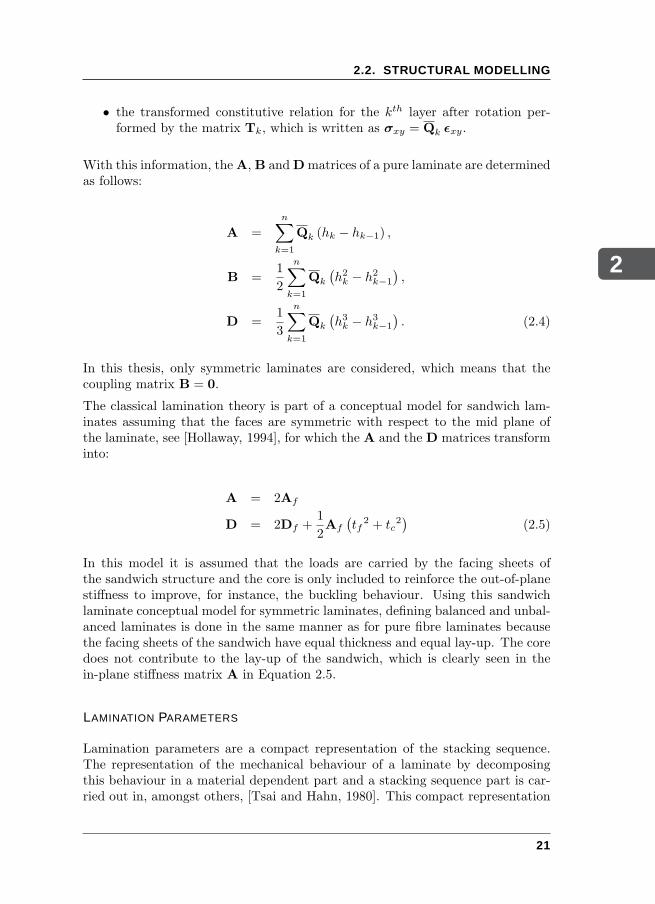
With this information, theA, B andDmatrices of a pure laminate are determinedas follows:
A =n∑
k=1
Qk (hk − hk−1) ,
B =1
2
n∑
k=1
Qk
(h2k − h2k−1
),
D =1
3
n∑
k=1
Qk
(h3k − h3k−1
). (2.4)
In this thesis, only symmetric laminates are considered, which means that thecoupling matrix B = 0.
The classical lamination theory is part of a conceptual model for sandwich lam-inates assuming that the faces are symmetric with respect to the mid plane ofthe laminate, see [Hollaway, 1994], for which the A and the D matrices transforminto:
A = 2Af
D = 2Df +1
2Af
(tf
2 + tc2)
(2.5)
In this model it is assumed that the loads are carried by the facing sheets ofthe sandwich structure and the core is only included to reinforce the out-of-planestiffness to improve, for instance, the buckling behaviour. Using this sandwichlaminate conceptual model for symmetric laminates, defining balanced and unbal-anced laminates is done in the same manner as for pure fibre laminates becausethe facing sheets of the sandwich have equal thickness and equal lay-up. The coredoes not contribute to the lay-up of the sandwich, which is clearly seen in thein-plane stiffness matrix A in Equation 2.5.
LAMINATION PARAMETERS
Lamination parameters are a compact representation of the stacking sequence.The representation of the mechanical behaviour of a laminate by decomposingthis behaviour in a material dependent part and a stacking sequence part is car-ried out in, amongst others, [Tsai and Hahn, 1980]. This compact representation
21
2
2. EQUAL FIDELITY STATIC AEROELASTIC MODELLING OF LARGE BLADES
of stacking sequence is suitable for optimisation purposes since it reduces calcu-lation effort in comparison with the ABD representation of laminates. Thereforethe design variables of the optimisations within this research are expressed inlamination parameters, which are expressed as follows:
(V1A, V2A, V3A, V4A) =1
h
ˆ h/2
−h/2
(cos 2θ, sin 2θ, cos 4θ, sin 4θ) dz,
(V1B, V2B, V3B, V4B) =4
h2
ˆ h/2
−h/2
z (cos 2θ, sin 2θ, cos 4θ, sin 4θ) dz,
(V1D, V2D, V3D, V4D) =12
h3
ˆ h/2
−h/2
z2 (cos 2θ, sin 2θ, cos 4θ, sin 4θ) dz. (2.6)
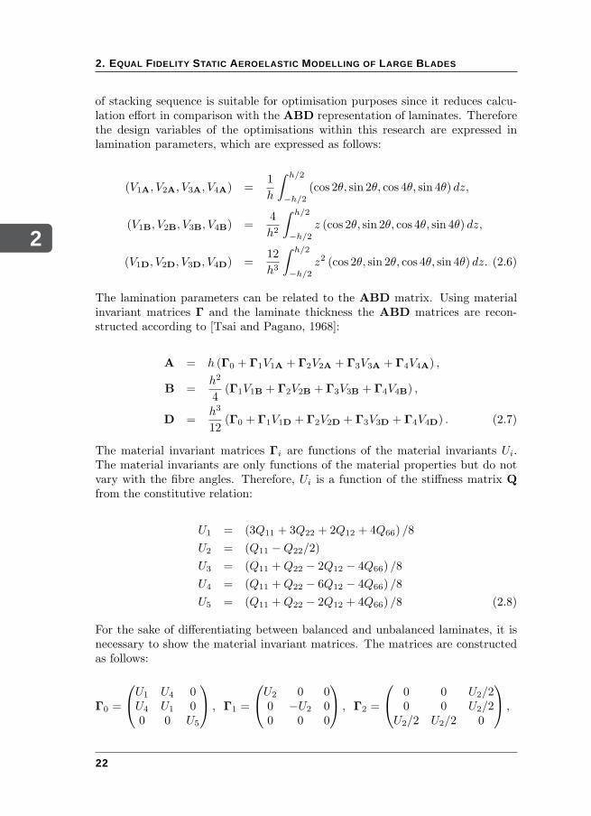
The lamination parameters can be related to the ABD matrix. Using materialinvariant matrices Γ and the laminate thickness the ABD matrices are recon-structed according to [Tsai and Pagano, 1968]:
A = h (Γ0 + Γ1V1A + Γ2V2A + Γ3V3A + Γ4V4A) ,
B =h2
4(Γ1V1B + Γ2V2B + Γ3V3B + Γ4V4B) ,
D =h3
12(Γ0 + Γ1V1D + Γ2V2D + Γ3V3D + Γ4V4D) . (2.7)
The material invariant matrices Γi are functions of the material invariants Ui.The material invariants are only functions of the material properties but do notvary with the fibre angles. Therefore, Ui is a function of the stiffness matrix Q
from the constitutive relation:
U1 = (3Q11 + 3Q22 + 2Q12 + 4Q66) /8
U2 = (Q11 −Q22/2)
U3 = (Q11 +Q22 − 2Q12 − 4Q66) /8
U4 = (Q11 +Q22 − 6Q12 − 4Q66) /8
U5 = (Q11 +Q22 − 2Q12 + 4Q66) /8 (2.8)
For the sake of differentiating between balanced and unbalanced laminates, it isnecessary to show the material invariant matrices. The matrices are constructedas follows:
Γ0 =
U1 U4 0U4 U1 00 0 U5
, Γ1 =
U2 0 00 −U2 00 0 0
, Γ2 =
0 0 U2/20 0 U2/2
U2/2 U2/2 0
,
22
2
2.2. STRUCTURAL MODELLING
Γ3 =
U3 −U3 0−U3 U3 00 0 U3
, Γ4 =
0 0 U3
0 0 −U3
U3 −U3 0
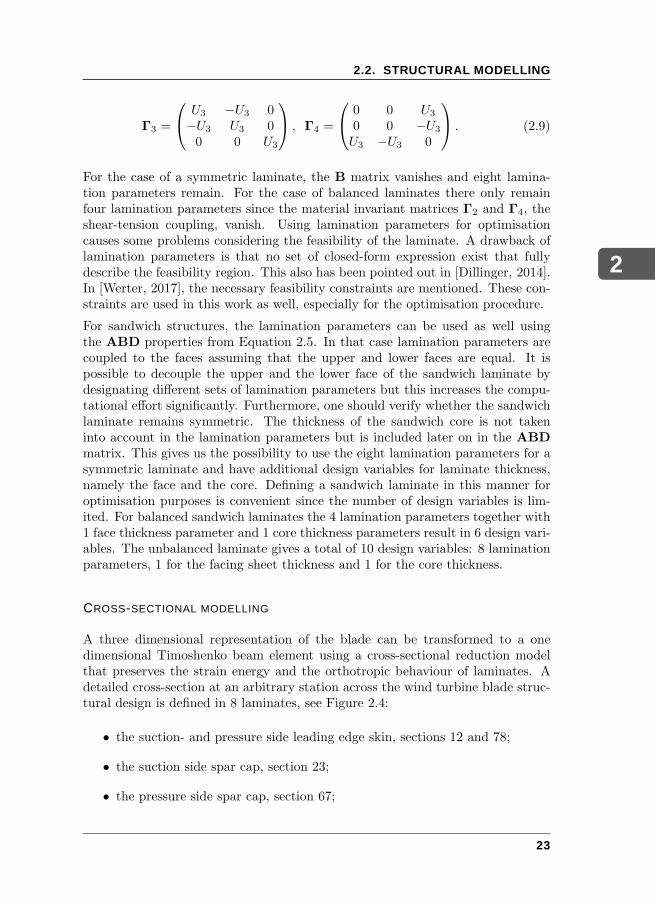
. (2.9)
For the case of a symmetric laminate, the B matrix vanishes and eight lamina-tion parameters remain. For the case of balanced laminates there only remainfour lamination parameters since the material invariant matrices Γ2 and Γ4, theshear-tension coupling, vanish. Using lamination parameters for optimisationcauses some problems considering the feasibility of the laminate. A drawback oflamination parameters is that no set of closed-form expression exist that fullydescribe the feasibility region. This also has been pointed out in [Dillinger, 2014].In [Werter, 2017], the necessary feasibility constraints are mentioned. These con-straints are used in this work as well, especially for the optimisation procedure.
For sandwich structures, the lamination parameters can be used as well usingthe ABD properties from Equation 2.5. In that case lamination parameters arecoupled to the faces assuming that the upper and lower faces are equal. It ispossible to decouple the upper and the lower face of the sandwich laminate bydesignating different sets of lamination parameters but this increases the compu-tational effort significantly. Furthermore, one should verify whether the sandwichlaminate remains symmetric. The thickness of the sandwich core is not takeninto account in the lamination parameters but is included later on in the ABD
matrix. This gives us the possibility to use the eight lamination parameters for asymmetric laminate and have additional design variables for laminate thickness,namely the face and the core. Defining a sandwich laminate in this manner foroptimisation purposes is convenient since the number of design variables is lim-ited. For balanced sandwich laminates the 4 lamination parameters together with1 face thickness parameter and 1 core thickness parameters result in 6 design vari-ables. The unbalanced laminate gives a total of 10 design variables: 8 laminationparameters, 1 for the facing sheet thickness and 1 for the core thickness.
CROSS-SECTIONAL MODELLING
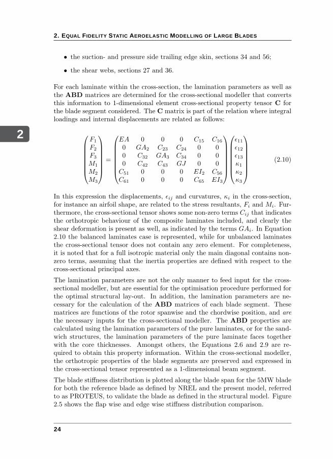
A three dimensional representation of the blade can be transformed to a onedimensional Timoshenko beam element using a cross-sectional reduction modelthat preserves the strain energy and the orthotropic behaviour of laminates. Adetailed cross-section at an arbitrary station across the wind turbine blade struc-tural design is defined in 8 laminates, see Figure 2.4:
• the suction- and pressure side leading edge skin, sections 12 and 78;
• the suction side spar cap, section 23;
• the pressure side spar cap, section 67;
23
2
2. EQUAL FIDELITY STATIC AEROELASTIC MODELLING OF LARGE BLADES
• the suction- and pressure side trailing edge skin, sections 34 and 56;
• the shear webs, sections 27 and 36.
For each laminate within the cross-section, the lamination parameters as well asthe ABD matrices are determined for the cross-sectional modeller that convertsthis information to 1-dimensional element cross-sectional property tensor C forthe blade segment considered. The C matrix is part of the relation where integralloadings and internal displacements are related as follows:
F1
F2
F3
M1
M2
M3
=
EA 0 0 0 C15 C16
0 GA2 C23 C24 0 00 C32 GA3 C34 0 00 C42 C43 GJ 0 0C51 0 0 0 EI2 C56
C61 0 0 0 C65 EI3
ǫ11ǫ12ǫ13κ1κ2κ3
(2.10)
In this expression the displacements, ǫij and curvatures, κi in the cross-section,for instance an airfoil shape, are related to the stress resultants, Fi and Mi. Fur-thermore, the cross-sectional tensor shows some non-zero terms Cij that indicatesthe orthotropic behaviour of the composite laminates included, and clearly theshear deformation is present as well, as indicated by the terms GAi. In Equation2.10 the balanced laminates case is represented, while for unbalanced laminatesthe cross-sectional tensor does not contain any zero element. For completeness,it is noted that for a full isotropic material only the main diagonal contains non-zero terms, assuming that the inertia properties are defined with respect to thecross-sectional principal axes.
The lamination parameters are not the only manner to feed input for the cross-sectional modeller, but are essential for the optimisation procedure performed forthe optimal structural lay-out. In addition, the lamination parameters are ne-cessary for the calculation of the ABD matrices of each blade segment. Thesematrices are functions of the rotor spanwise and the chordwise position, and are
the necessary inputs for the cross-sectional modeller. The ABD properties arecalculated using the lamination parameters of the pure laminates, or for the sand-wich structures, the lamination parameters of the pure laminate faces togetherwith the core thicknesses. Amongst others, the Equations 2.6 and 2.9 are re-quired to obtain this property information. Within the cross-sectional modeller,the orthotropic properties of the blade segments are preserved and expressed inthe cross-sectional tensor represented as a 1-dimensional beam segment.
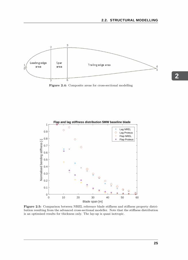
The blade stiffness distribution is plotted along the blade span for the 5MW bladefor both the reference blade as defined by NREL and the present model, referredto as PROTEUS, to validate the blade as defined in the structural model. Figure2.5 shows the flap wise and edge wise stiffness distribution comparison.
24
2
2.2. STRUCTURAL MODELLING
Figure 2.4: Composite areas for cross-sectional modelling
0 10 20 30 40 50 60
Blade span [m]
0
0.1
0.2
0.3
0.4
0.5
0.6
0.7
0.8
0.9
1
Nor
mal
ised
ben
ding
stif
fnes
s [-
]
Flap and lag stiffness distribution 5MW baseline blade
Lag NRELLag ProteusFlap NRELFlap Proteus
Figure 2.5: Comparison between NREL reference blade stiffness and stiffness property distri-bution resulting from the advanced cross-sectional modeller. Note that the stiffness distributionis an optimised results for thickness only. The lay-up is quasi isotropic.
25
2
2. EQUAL FIDELITY STATIC AEROELASTIC MODELLING OF LARGE BLADES
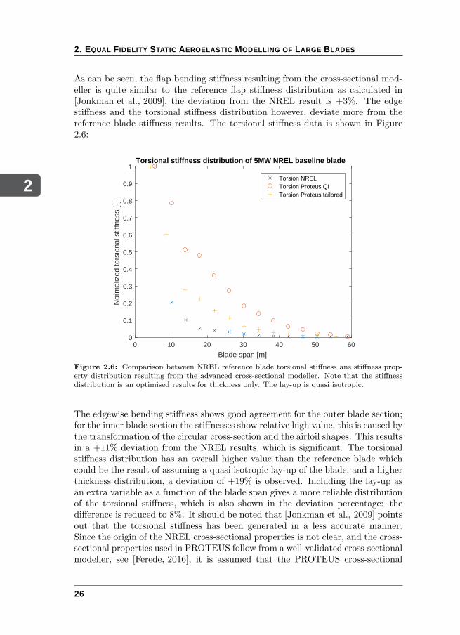
As can be seen, the flap bending stiffness resulting from the cross-sectional mod-eller is quite similar to the reference flap stiffness distribution as calculated in[Jonkman et al., 2009], the deviation from the NREL result is +3%. The edgestiffness and the torsional stiffness distribution however, deviate more from thereference blade stiffness results. The torsional stiffness data is shown in Figure2.6:
0 10 20 30 40 50 60
Blade span [m]
0
0.1
0.2
0.3
0.4
0.5
0.6
0.7
0.8
0.9
1
Nor
mal
ized
tors
iona
l stif
fnes
s [-
]
Torsional stiffness distribution of 5MW NREL baseline blade
Torsion NRELTorsion Proteus QITorsion Proteus tailored
Figure 2.6: Comparison between NREL reference blade torsional stiffness ans stiffness prop-erty distribution resulting from the advanced cross-sectional modeller. Note that the stiffnessdistribution is an optimised results for thickness only. The lay-up is quasi isotropic.
The edgewise bending stiffness shows good agreement for the outer blade section;for the inner blade section the stiffnesses show relative high value, this is caused bythe transformation of the circular cross-section and the airfoil shapes. This resultsin a +11% deviation from the NREL results, which is significant. The torsionalstiffness distribution has an overall higher value than the reference blade whichcould be the result of assuming a quasi isotropic lay-up of the blade, and a higherthickness distribution, a deviation of +19% is observed. Including the lay-up asan extra variable as a function of the blade span gives a more reliable distributionof the torsional stiffness, which is also shown in the deviation percentage: thedifference is reduced to 8%. It should be noted that [Jonkman et al., 2009] pointsout that the torsional stiffness has been generated in a less accurate manner.Since the origin of the NREL cross-sectional properties is not clear, and the cross-sectional properties used in PROTEUS follow from a well-validated cross-sectionalmodeller, see [Ferede, 2016], it is assumed that the PROTEUS cross-sectional
26
2
2.2. STRUCTURAL MODELLING
results are adequate for optimisation purposes.
BUCKLING
The adopted buckling model is taken from [Werter, 2017], previously used by[Dillinger, 2014], from which it is concluded that the wing or blade should atleast exist of spars and ribs. This is the case for large wind turbine blades,however, curvature of the cross-sectional airfoil shape is not included within theproposed model. Furthermore, ribs are not yet used in wind turbine blades whichmeans that buckling panels become fairly large, which has its influence on thebuckling behaviour. Still, the proposed model can be used, which is explainednext. Since the proposed model is a theoretical model, it can be compared toa study carried out by [Gaudern and Symons, 2010]. In this study, such a the-oretical model has been compared to a finite element study for wind turbineswhere curvature of the cross-sectional airfoil shape has been taken into accountand also the simply supported boundary condition results were compared to theclamped results. From this work it is concluded that simply supported boundaryconditions are conservative, which means that the buckling load is estimated tobe lower than the actual value caused by boundary conditions between simplysupported and clamped. Furthermore, it is mentioned that curvature causes thecompression load to be higher than for a flat plate. To clarify this, the work of[Gaudern and Symons, 2010] is used as well. The following equations are used forthe calculation of theoretical buckling loads of cylindrical panels:
Nx = −1
λ2
[(H2
12
H11
)
+H22 +Nyη2
]
, (2.11)
where:
H11 = λ4S22 + 2
(
S12 +1
2S33
)
λ2η2 + S11η4,
H12 =λ2
R,
H22 = λ4D11 + 2 (D12 + 2D33)λ2η2 +D22η
4,
S = A−1. (2.12)
Where Nx and Ny are the compressive loadings in longitudinal and lateral dir-ection respectively. Furthermore, the quantities λ and η indicate the number ofhalf waves in longitudinal and lateral direction respectively. Lastly, A indicatesthe in-plane stiffness matrix, D is the out-of-plane stiffness matrix, and S is theinverse of the in-plane stiffness matrix resulting from the ABD matrix of a lam-inate. The Equations 2.11 and 2.12 are used to explain that for increasing radius
27
2
2. EQUAL FIDELITY STATIC AEROELASTIC MODELLING OF LARGE BLADES
of curvature R the buckling load decreases. This means that the critical bucklingload is lower for a flat plate than for a cylindrical shell. Assuming flat panels forthe leading edge and realising that they underestimate the actual buckling loadfor a curved panel, this assumption is conservative as well as imposing simply sup-ported boundary conditions at the edges of the panels. As a consequence, skinthicknesses will be overestimated during, for instance, an optimisation procedure.
According to [Werter, 2017], the buckling panels should be rectangular and thestresses are assumed to be constant across the panels. The constant stress as-sumption is easily met because the buckling panels are smaller than or equal tothe dimensions of composite panels as defined in Figure 2.4. To accomplish thatfor the blades considered during the research, it is assumed to give the bucklingpanels such dimensions that the blade thickness distribution of the baseline isapproximated. Contrary to pure fibre laminate skins, ribs are not required forsandwich skins. Since sandwich skins are subject to local buckling as well andfor valid data resulting from the adopted buckling model, the buckling panels aredetermined by placing artificial ribs at fixed distances. Using artificial ribs givesthe possibility to control the buckling modes of the sandwich skin and define ap-propriate dimensions of the buckling panels suitable for the model. Therefore, theartificial ribs do not influence the total blade mass and simply supported bound-ary conditions are imposed. Note that for pure fibre laminate skins, the rib massmust be taken into account considering the total blade mass.
Since the panels are already limited in chordwise direction by means of the sparwebs, the panel dimensions are defined. It should be noted that the leading edgepart of the blade is curved and for the structural lay-out of the blade this is acurved buckling panel bounded by two ribs and the spar and the leading edge.The curvature of this cross-sectional part can be approximated by assuming acylindrical curvature, but is modelled as a flat buckling panel to be conservative.Considering the simply supported boundary conditions applied, the artificial ribsin spanwise direction are only placed in such a way that buckling behaviour of thebaseline is approximated, based on [Ferede, 2016]. A quick sensitivity study wasperformed to check the model. The length of the buckling panels was chosen tobe 1, 2, and 4 meters. Starting from the 2 meters as present in the simulations,an decrease in blade mass was observed for the 1 meter panels, while for the4 meter panels an increase in blade mass was observed. In addition, the panellength variations showed appropriate blade mass variations. This means, that thebuckling model behaves as expected. To be conservative for the optimised blademass, the rib masses are included in the total blade mass. From the above, it canbe concluded that the buckling behaviour is modelled in a conservative manner.
The buckling calculation within this research is, just like the cross-sectional mod-eller, based on strain energy from which the stiffness matrices are derived thatare required for the buckling analysis. The governing equation is formulated asan eigenvalue problem from which the inverse buckling value r is calculated for
28
2
2.2. STRUCTURAL MODELLING
each panel. A value r ≤ 1 means a buckling free panel:
(Kg − rK)a = 0, (2.13)
where Kg is the geometric stiffness matrix, K the actual stiffness matrix, and a
contains the coefficients from the assumed displacement functions. The geometricstiffness matrix Kg is containing the information of the local buckling elementloading:
Kg = −NxKxx −NyK
yy −NxyKxy, (2.14)
where is assumed that the local loadings are constant across the buckling panel.The actual stiffness matrix K is given as:
K =∑
i=1,2,6
∑
i=1,2,6
DijKij , (2.15)
where Dij are the out-of-plane components from the local ABD matrix and theKij terms are based on the integral over a product of the second derivativesof the assumed displacement functions across the buckling element. The two-dimensional assumed displacement functions are written as:
w(ξ, η) =∑
p
∑
q
apqφp (ξ)φq (η) , (2.16)
where the the φ represent bubble functions expressed in two perpendicular, non-dimensional directions ξ and η and apq represents the coefficients of the polyno-mials. Since the displacement function is defined, the term Kij is calculated as,for example:
K11
pq =
¨
A
∂2φp
∂x2∂2φq
∂x2dA. (2.17)
The geometrical stiffness matrix terms Kxx, Kyy, and Kxy are based on the in-tegral over the product of the first derivative of the product of the aforementioneddisplacements functions, which gives:
Kxxpq =
¨
A
∂φp∂x
∂φq∂x
dA, (2.18)
Kyypq =
¨
A
∂φp∂y
∂φq∂y
dA, (2.19)
29
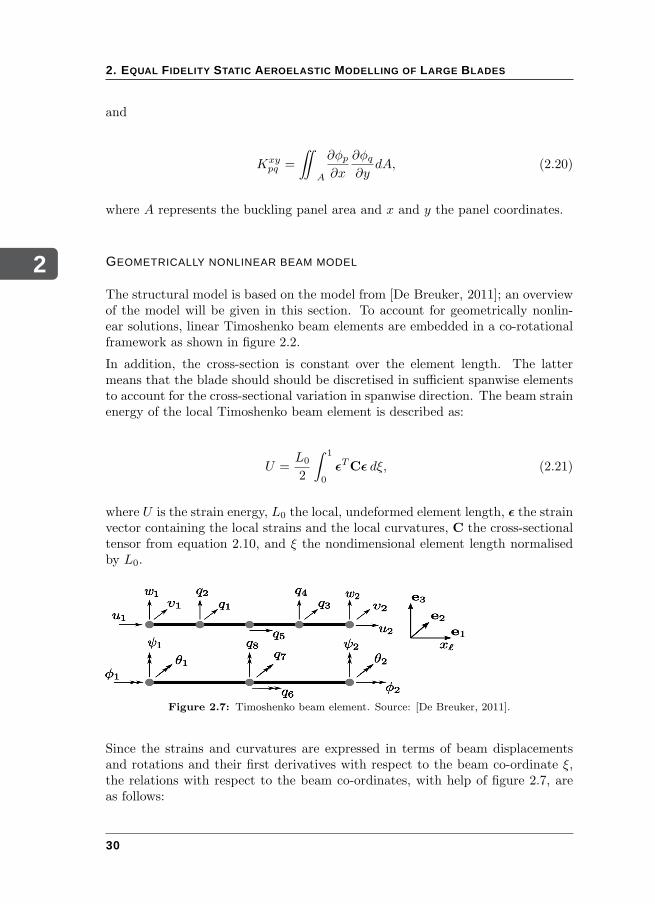
2
2. EQUAL FIDELITY STATIC AEROELASTIC MODELLING OF LARGE BLADES
and
Kxypq =
¨
A
∂φp∂x
∂φq∂y
dA, (2.20)
where A represents the buckling panel area and x and y the panel coordinates.
GEOMETRICALLY NONLINEAR BEAM MODEL
The structural model is based on the model from [De Breuker, 2011]; an overviewof the model will be given in this section. To account for geometrically nonlin-ear solutions, linear Timoshenko beam elements are embedded in a co-rotationalframework as shown in figure 2.2.
In addition, the cross-section is constant over the element length. The lattermeans that the blade should should be discretised in sufficient spanwise elementsto account for the cross-sectional variation in spanwise direction. The beam strainenergy of the local Timoshenko beam element is described as:
U =L0
2
ˆ 1
0
ǫTCǫ dξ, (2.21)
where U is the strain energy, L0 the local, undeformed element length, ǫ the strainvector containing the local strains and the local curvatures, C the cross-sectionaltensor from equation 2.10, and ξ the nondimensional element length normalisedby L0.
Figure 2.7: Timoshenko beam element. Source: [De Breuker, 2011].
Since the strains and curvatures are expressed in terms of beam displacementsand rotations and their first derivatives with respect to the beam co-ordinate ξ,the relations with respect to the beam co-ordinates, with help of figure 2.7, areas follows:
30
2
2.2. STRUCTURAL MODELLING
u = u1 (1− ξ) + u2ξ + q5ξ (1− ξ)
v = v1 (1− ξ) + v2ξ + q1ξ (1− ξ) + q3 (1− ξ) (1/2− ξ)
w = w1 (1− ξ) + w2ξ + q2ξ (1− ξ) + q4 (1− ξ) (1/2− ξ)
φ = φ1 (1− ξ) + φ2ξ + q6ξ (1− ξ) (2.22)
θ = θ1 (1− ξ) + θ2ξ + q7ξ (1− ξ)
ψ = ψ1 (1− xi) + ψ2ξ + q8ξ (1− ξ) .
The extra nodes were introduced to include anisotropic effects as well, such asbend-twist coupling of blades or wings. An other advantage of using extra nodesis that shear locking is avoided, [Crisfield, 1986]. Using the above definition ofthe beam degrees of freedom, the strain vector is set up following [Luo, 2008]:
ǫ =
(1
l0uξ,−ψ +
1
l0vξ, θ +
1
l0wξ,
1
l0φξ,−
1
l0θξ,
1
l0ψξ
)T
, (2.23)
where the subscript ξ indicates the first derivative with respect to the nondimen-sional beam co-ordinate ξ. The second derivative of the strain energy U withrespect to the degrees of freedom p determines the beam stiffness matrix. Avector containing all local element degrees of freedom is defined as follows:
p = (u1, v1, w1, φ1, θ1, ψ1, u2, v2, w2, φ2, θ2, ψ2, q1, q2, q3, q4, q5, q6, q7, q8)T. (2.24)
The information of only the end nodes is required in the aeroelastic analysis. Assuch, the static condensation method is used to reduce the degrees of freedom,[Guyan, 1965], to eliminate the internal nodes qi. Splitting the vector p into pi
and pl to indicate internal nodes and external nodes respectively, the partitionedequation is obtained:
(Kl,l | Kl,i
Ki,l | Ki,i
)(pl
pi
)
=
(fl0
)
(2.25)
The reduction is accomplished by solving the second equation for pi and substi-tuting in the first equation. The resulting equilibrium equation reads as:
Klpl = fl, (2.26)
where:
Kl = Kl,l −Kl,iKi,i−1Ki,l, (2.27)
31
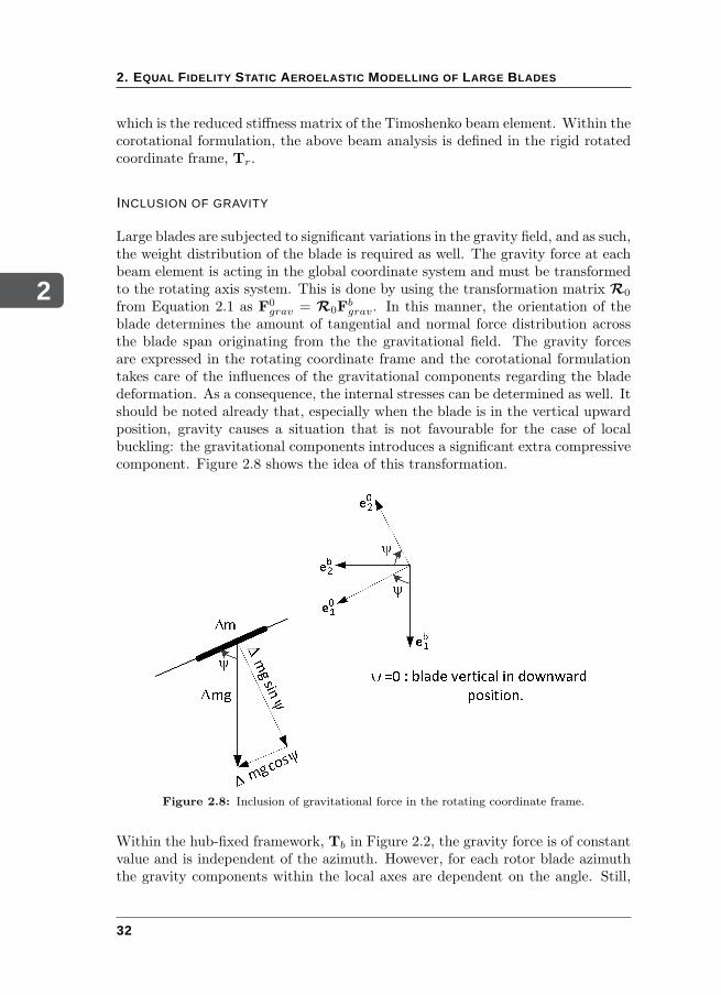
2
2. EQUAL FIDELITY STATIC AEROELASTIC MODELLING OF LARGE BLADES
which is the reduced stiffness matrix of the Timoshenko beam element. Within thecorotational formulation, the above beam analysis is defined in the rigid rotatedcoordinate frame, Tr.
INCLUSION OF GRAVITY
Large blades are subjected to significant variations in the gravity field, and as such,the weight distribution of the blade is required as well. The gravity force at eachbeam element is acting in the global coordinate system and must be transformedto the rotating axis system. This is done by using the transformation matrix R0
from Equation 2.1 as F0grav = R0F
bgrav. In this manner, the orientation of the
blade determines the amount of tangential and normal force distribution acrossthe blade span originating from the the gravitational field. The gravity forcesare expressed in the rotating coordinate frame and the corotational formulationtakes care of the influences of the gravitational components regarding the bladedeformation. As a consequence, the internal stresses can be determined as well. Itshould be noted already that, especially when the blade is in the vertical upwardposition, gravity causes a situation that is not favourable for the case of localbuckling: the gravitational components introduces a significant extra compressivecomponent. Figure 2.8 shows the idea of this transformation.
Figure 2.8: Inclusion of gravitational force in the rotating coordinate frame.
Within the hub-fixed framework, Tb in Figure 2.2, the gravity force is of constantvalue and is independent of the azimuth. However, for each rotor blade azimuththe gravity components within the local axes are dependent on the angle. Still,
32
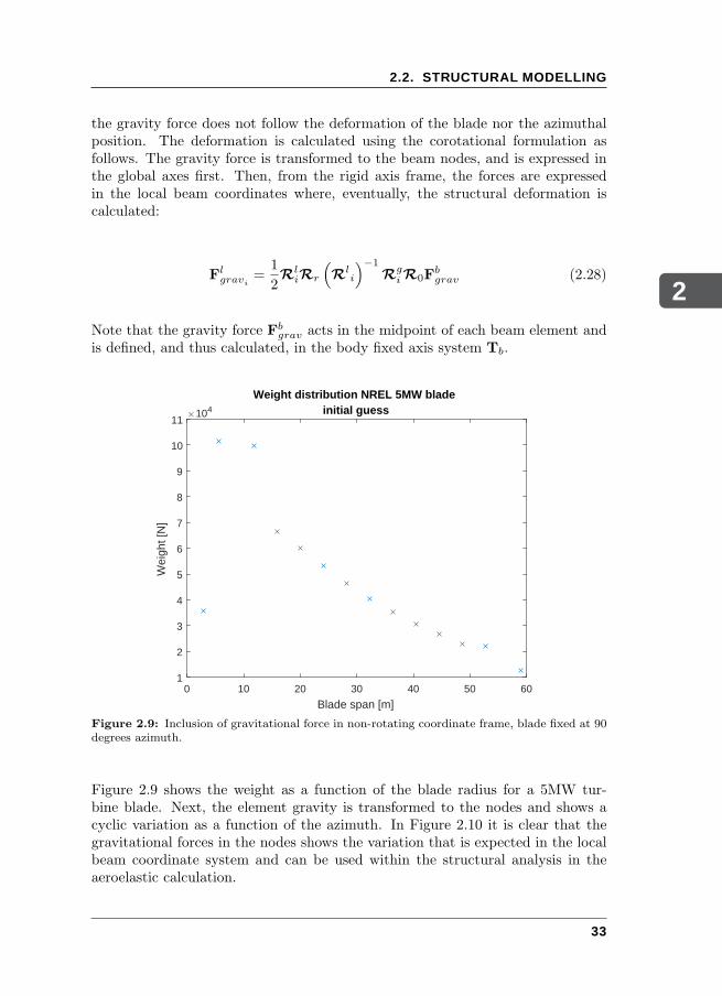
2
2.2. STRUCTURAL MODELLING
the gravity force does not follow the deformation of the blade nor the azimuthalposition. The deformation is calculated using the corotational formulation asfollows. The gravity force is transformed to the beam nodes, and is expressed inthe global axes first. Then, from the rigid axis frame, the forces are expressedin the local beam coordinates where, eventually, the structural deformation iscalculated:
Flgravi
=1
2R
liRr
(
Rli
)−1
RgiR0F
bgrav (2.28)
Note that the gravity force Fbgrav acts in the midpoint of each beam element and
is defined, and thus calculated, in the body fixed axis system Tb.
0 10 20 30 40 50 60
Blade span [m]
1
2
3
4
5
6
7
8
9
10
11
Wei
ght [
N]
104
Weight distribution NREL 5MW bladeinitial guess
Figure 2.9: Inclusion of gravitational force in non-rotating coordinate frame, blade fixed at 90degrees azimuth.
Figure 2.9 shows the weight as a function of the blade radius for a 5MW tur-bine blade. Next, the element gravity is transformed to the nodes and shows acyclic variation as a function of the azimuth. In Figure 2.10 it is clear that thegravitational forces in the nodes shows the variation that is expected in the localbeam coordinate system and can be used within the structural analysis in theaeroelastic calculation.
33
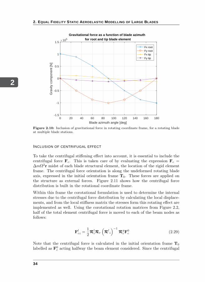
2
2. EQUAL FIDELITY STATIC AEROELASTIC MODELLING OF LARGE BLADES
0 20 40 60 80 100 120 140 160 180
Blade azimuth angle [deg]
-1.5
-1
-0.5
0
0.5
1
1.5
Gra
vity
com
pone
nt [N
]
105
Gravitational force as a function of blade azimuth for root and tip blade element
Fx rootFy rootFx tipFy tip
Figure 2.10: Inclusion of gravitational force in rotating coordinate frame, for a rotating bladeat multiple blade stations.
INCLUSION OF CENTRIFUGAL EFFECT
To take the centrifugal stiffening effect into account, it is essential to include thecentrifugal force Fc. This is taken care of by evaluating the expression Fc =∆mΩ2r midst of each blade structural element, the location of the rigid elementframe. The centrifugal force orientation is along the undeformed rotating bladeaxis, expressed in the initial orientation frame T0. These forces are applied onthe structure as external forces. Figure 2.11 shows how the centrifugal forcedistribution is built in the rotational coordinate frame.
Within this frame the corotational formulation is used to determine the internalstresses due to the centrifugal force distribution by calculating the local displace-ments, and from the local stiffness matrix the stresses form this rotating effect areimplemented as well. Using the corotational rotation matrices from Figure 2.2,half of the total element centrifugal force is moved to each of the beam nodes asfollows:
Flci =
1
2R
liRr
(
Rli
)−1
RgiF
0
c (2.29)
Note that the centrifugal force is calculated in the initial orientation frame T0
labelled as F0c acting halfway the beam element considered. Since the centrifugal
34
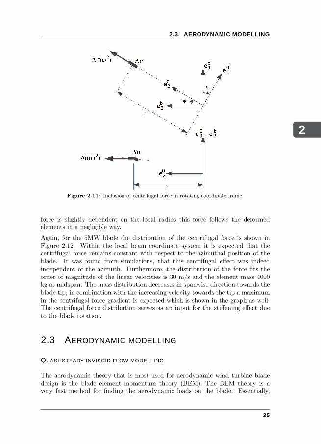
2
2.3. AERODYNAMIC MODELLING
Figure 2.11: Inclusion of centrifugal force in rotating coordinate frame.
force is slightly dependent on the local radius this force follows the deformedelements in a negligible way.
Again, for the 5MW blade the distribution of the centrifugal force is shown inFigure 2.12. Within the local beam coordinate system it is expected that thecentrifugal force remains constant with respect to the azimuthal position of theblade. It was found from simulations, that this centrifugal effect was indeedindependent of the azimuth. Furthermore, the distribution of the force fits theorder of magnitude of the linear velocities is 30 m/s and the element mass 4000kg at midspan. The mass distribution decreases in spanwise direction towards theblade tip; in combination with the increasing velocity towards the tip a maximumin the centrifugal force gradient is expected which is shown in the graph as well.The centrifugal force distribution serves as an input for the stiffening effect dueto the blade rotation.
2.3 AERODYNAMIC MODELLING
QUASI-STEADY INVISCID FLOW MODELLING
The aerodynamic theory that is most used for aerodynamic wind turbine bladedesign is the blade element momentum theory (BEM). The BEM theory is avery fast method for finding the aerodynamic loads on the blade. Essentially,
35
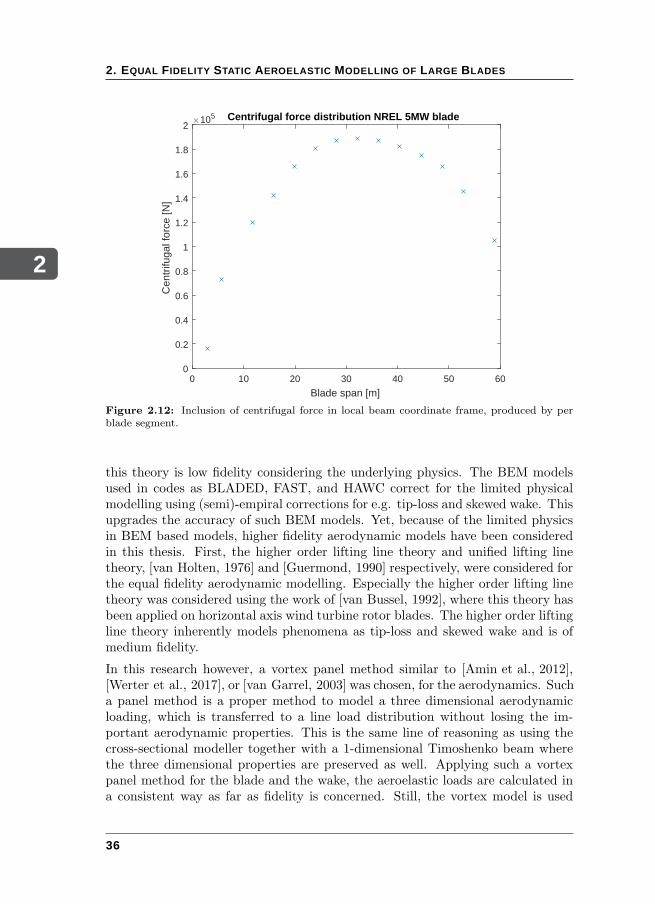
2
2. EQUAL FIDELITY STATIC AEROELASTIC MODELLING OF LARGE BLADES
0 10 20 30 40 50 60
Blade span [m]
0
0.2
0.4
0.6
0.8
1
1.2
1.4
1.6
1.8
2
Cen
trifu
gal f
orce
[N]
105 Centrifugal force distribution NREL 5MW blade
Figure 2.12: Inclusion of centrifugal force in local beam coordinate frame, produced by perblade segment.
this theory is low fidelity considering the underlying physics. The BEM modelsused in codes as BLADED, FAST, and HAWC correct for the limited physicalmodelling using (semi)-empiral corrections for e.g. tip-loss and skewed wake. Thisupgrades the accuracy of such BEM models. Yet, because of the limited physicsin BEM based models, higher fidelity aerodynamic models have been consideredin this thesis. First, the higher order lifting line theory and unified lifting linetheory, [van Holten, 1976] and [Guermond, 1990] respectively, were considered forthe equal fidelity aerodynamic modelling. Especially the higher order lifting linetheory was considered using the work of [van Bussel, 1992], where this theory hasbeen applied on horizontal axis wind turbine rotor blades. The higher order liftingline theory inherently models phenomena as tip-loss and skewed wake and is ofmedium fidelity.
In this research however, a vortex panel method similar to [Amin et al., 2012],[Werter et al., 2017], or [van Garrel, 2003] was chosen, for the aerodynamics. Sucha panel method is a proper method to model a three dimensional aerodynamicloading, which is transferred to a line load distribution without losing the im-portant aerodynamic properties. This is the same line of reasoning as using thecross-sectional modeller together with a 1-dimensional Timoshenko beam wherethe three dimensional properties are preserved as well. Applying such a vortexpanel method for the blade and the wake, the aeroelastic loads are calculated ina consistent way as far as fidelity is concerned. Still, the vortex model is used
36
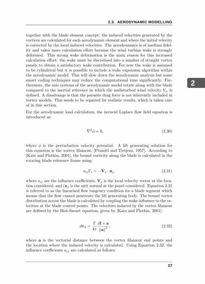
2
2.3. AERODYNAMIC MODELLING
together with the blade element concept: the induced velocities generated by thevortices are calculated for each aerodynamic element and where the initial velocityis corrected by the local induced velocities. The aerodynamics is of medium fidel-ity and takes more calculation effort because the wind turbine wake is stronglydeformed. This strong wake deformation is the main reason for this increasedcalculation effort: the wake must be discretised into a number of straight vortexpanels to obtain a satisfactory wake contribution. For now the wake is assumedto be cylindrical but it is possible to include a wake expansion algorithm withinthe aerodynamic model. This will slow down the aerodynamic analysis but somesmart coding techniques may reduce the computational time significantly. Fur-thermore, the axis systems of the aerodynamic model rotate along with the bladecompared to the inertial reference in which the undisturbed wind velocity Vw isdefined. A disadvange is that the parasite drag force is not inherently included invortex models. This needs to be repaired for realistic results, which is taken careof in this section.
For the aerodynamic load calculation, the inviscid Laplace flow field equation isintroduced as:
∇2φ = 0, (2.30)
where φ is the perturbation velocity potential. A lift generating solution forthis equation is the vortex filament, [Prandtl and Tietjens, 1957]. According to[Katz and Plotkin, 2001], the bound vorticity along the blade is calculated in therotating blade reference frame using:
aijΓi = −Vj · nj , (2.31)
where aij are the influence coefficients, Vj is the local velocity vector at the loca-tion considered, and (nj is the unit normal at the panel considered. Equation 2.31is referred to as the linearised flow tangency condition for a blade segment whichmeans that the flow cannot penetrate the lift generating body. The bound vortexdistribution across the blade is calculated by coupling the wake influence to the ve-locities at the blade control points. The velocities induced by the vortex filamentare defined by the Biot-Savart equation, given by [Katz and Plotkin, 2001]:
dvd =Γ
4π
dl× a
‖a‖3, (2.32)
where a is the vectorial distance between the vortex filament end points andthe location where the induced velocity is calculated. Using Equation 2.32, theinfluence coefficients aij are calculated as follows:
37
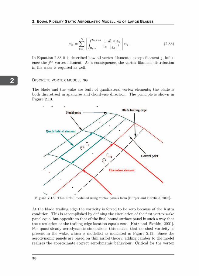
2
2. EQUAL FIDELITY STATIC AEROELASTIC MODELLING OF LARGE BLADES
aij =
N∑
k=1
[ˆ xp,k+1
xp,k
1
4π
dl× ak
‖ak‖3
]
nj . (2.33)
In Equation 2.33 it is described how all vortex filaments, except filament j, influ-ence the jth vortex filament. As a consequence, the vortex filament distributionin the wake is required as well.
DISCRETE VORTEX MODELLING
The blade and the wake are built of quadilateral vortex elements; the blade isboth discretised in spanwise and chordwise direction. The principle is shown inFigure 2.13.
Figure 2.13: Thin airfoil modelled using vortex panels from [Burger and Hartfield, 2006].
At the blade trailing edge the vorticity is forced to be zero because of the Kuttacondition. This is accomplished by defining the circulation of the first vortex wakepanel equal but opposite to that of the final bound surface panel in such a way thatthe circulation at the trailing edge location equals zero, [Katz and Plotkin, 2001].For quasi-steady aerodynamic simulations this means that no shed vorticity ispresent in the wake, which is modelled as indicated in Figure 2.13. Since theaerodynamic panels are based on thin airfoil theory, adding camber to the modelrealizes the approximate correct aerodynamic behaviour. Critical for the vortex
38
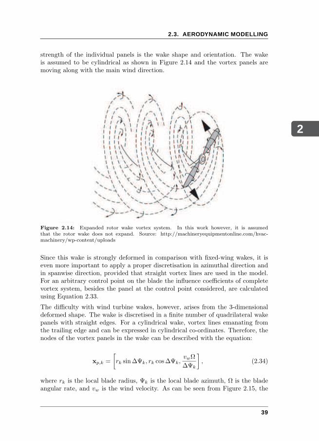
2
2.3. AERODYNAMIC MODELLING
strength of the individual panels is the wake shape and orientation. The wakeis assumed to be cylindrical as shown in Figure 2.14 and the vortex panels aremoving along with the main wind direction.
Figure 2.14: Expanded rotor wake vortex system. In this work however, it is assumedthat the rotor wake does not expand. Source: http://machineryequipmentonline.com/hvac-machinery/wp-content/uploads
Since this wake is strongly deformed in comparison with fixed-wing wakes, it iseven more important to apply a proper discretisation in azimuthal direction andin spanwise direction, provided that straight vortex lines are used in the model.For an arbitrary control point on the blade the influence coefficients of completevortex system, besides the panel at the control point considered, are calculatedusing Equation 2.33.
The difficulty with wind turbine wakes, however, arises from the 3-dimensionaldeformed shape. The wake is discretised in a finite number of quadrilateral wakepanels with straight edges. For a cylindrical wake, vortex lines emanating fromthe trailing edge and can be expressed in cylindrical co-ordinates. Therefore, thenodes of the vortex panels in the wake can be described with the equation:
xp,k =
[
rk sin∆Ψk, rk cos∆Ψk,vwΩ
∆Ψk
]
, (2.34)
where rk is the local blade radius, Ψk is the local blade azimuth, Ω is the bladeangular rate, and vw is the wind velocity. As can be seen from Figure 2.15, the
39
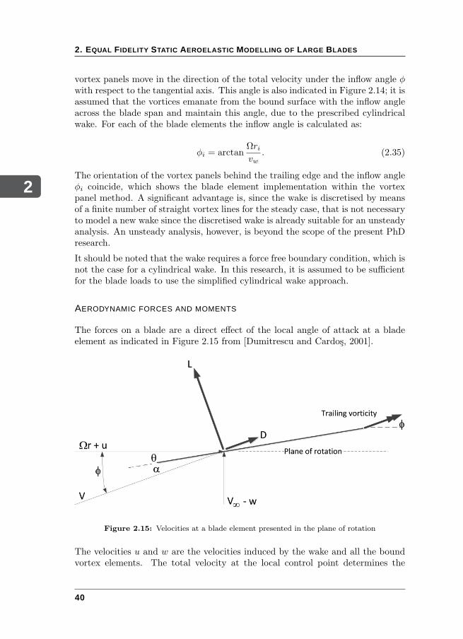
2
2. EQUAL FIDELITY STATIC AEROELASTIC MODELLING OF LARGE BLADES
vortex panels move in the direction of the total velocity under the inflow angle φwith respect to the tangential axis. This angle is also indicated in Figure 2.14; it isassumed that the vortices emanate from the bound surface with the inflow angleacross the blade span and maintain this angle, due to the prescribed cylindricalwake. For each of the blade elements the inflow angle is calculated as:
φi = arctanΩrivw
. (2.35)
The orientation of the vortex panels behind the trailing edge and the inflow angleφi coincide, which shows the blade element implementation within the vortexpanel method. A significant advantage is, since the wake is discretised by meansof a finite number of straight vortex lines for the steady case, that is not necessaryto model a new wake since the discretised wake is already suitable for an unsteadyanalysis. An unsteady analysis, however, is beyond the scope of the present PhDresearch.
It should be noted that the wake requires a force free boundary condition, which isnot the case for a cylindrical wake. In this research, it is assumed to be sufficientfor the blade loads to use the simplified cylindrical wake approach.
AERODYNAMIC FORCES AND MOMENTS
The forces on a blade are a direct effect of the local angle of attack at a bladeelement as indicated in Figure 2.15 from [Dumitrescu and Cardos, 2001].
Figure 2.15: Velocities at a blade element presented in the plane of rotation
The velocities u and w are the velocities induced by the wake and all the boundvortex elements. The total velocity at the local control point determines the
40

2
2.3. AERODYNAMIC MODELLING
vortex strength at the blade element considered because of the flow tangencycondition. This approach implies that all elements do influence each other, whichis not the case in the blade element momentum theory. From the blade bound vor-ticity distribution the lift force per segment is calculated by the Kutta-Joukowskirelation:
L = ρV × Γ, (2.36)
where Γ = Γ∆l. From Equation 2.36 the aerodynamic moment is generated bythe lift as follows:
M = ∆c× L. (2.37)
The velocity vector V is composed of the tangential and the local wind velocity,(Ωr, 0, V∞). Γ is designated the magnitude of the circulation, and ∆l indicatesthe direction of the vortex line considered. The vector ∆c in the moment relationindicates the distance between the quarter chord of the segment airfoil and thelocation of the beam element.
For a reliable estimate of the aerodynamic wind turbine power, an estimation ofthe aerodynamic drag should be included as well. Two types of drag are takeninto account; the induced drag and the parasitic drag. The induced drag is calcu-lated by carrying out the cross product between the induced velocity of the wakepanels on the bound vortex panels and the local circulation vector as proposed by[Katz and Plotkin, 2001]. The induced velocity at the control points is calculatedusing the aerodynamic wake panels that are used for the lift calculation as well:
Di = ρvi × Γ, (2.38)
where vi is the induced velocity vector and, again, Γ = Γ∆l.
The parasitic drag is determined by using the airfoil tables as given by [Timmer, 2017].From the tables, the given drag coefficient is transformed to a drag force at thebound vortex panel, using:
Dpar =
(1
2ρV 2
totalScd
)
eφ, (2.39)
where the unit vector eφ is aligned with the resultant velocity vector, cd is thelocal drag coefficent, and S represents the panel area considered. Decomposingthe unit vector in the plane of rotation by means of tangential component anda normal component, the unit vector eφ is expressed as (cosφ, 0, sinφ). In thismanner, parasite drag components give the correct contributions in the plane of
41
2
2. EQUAL FIDELITY STATIC AEROELASTIC MODELLING OF LARGE BLADES
rotation as drawn in Figure 2.15. For the parasitic drag coefficient, the local angleof attack required for the aerodynamic look-up tables is determined as:
αi = φi − (θi + θc) , (2.40)
where αi is the local angle of attack, φi the local inflow angle, θi the local struc-tural twist angle, and θc the collective pitch angle for power control. Assumingthat the airfoil as a function of the blade span are given, the appropriate dragcoefficient can be searched using the local angle of attack.
The lift, drag, and moment vectors are expressed in the normal and tangentialcomponents with respect to the plane of rotation, which means that the normaland tangential contributions of the aerodynamic loads are immediately suitablefor the aerodynamic power calculation. Subsequently, the aerodynamic power iscalculated as:
P = Ω∑
(Li +Di) ·R0ri, (2.41)
with R0 the transformation shown in Equation 2.1. From the above equation itis observed that the aerodynamic power is based on the tangential force, parallelto the x-axis in the plane of rotation as indicated in Figure 2.15.
BLADE PITCH CONTROL
Wind turbine blades use two types of control: stall regulated or pitch regulated.The control mechanism in this work is pitch control, for recent stall regulatedstudies it is referred to [Ferede, 2016]. The pitch type of control gives a bladepitch command when the generated power of the complete rotor from the windexceeds rated power. The blade is pitched towards lower angles of attack so thatthe aerodynamic blade loads decrease and the power available is rated power.The necessary information for the blades to stay within the wind turbine normaloperation envelope is obtained from controller design used in the NREL 5MWreport, [Jonkman et al., 2009]. In this research the control is such that the ratedpower per blade is not exceeded. This means that the difference between theactual power and the rated power for the blade considered is compared and apitch action is carried out such that the power stays within the power limits ofthe turbine considered. The convergence criterion for this algorithm is chosen tobe the ratio between the power difference and the rated power:
∣∣∣∣
∆P
Prated
∣∣∣∣≤ ǫ. (2.42)
The implementation of the aerodynamic power calculation, including a simplecollective pitch control mechanism, is shown in figure 2.16.
42
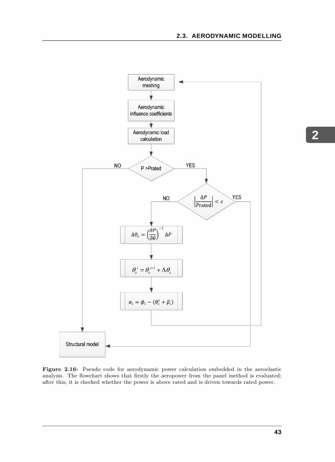
2
2.3. AERODYNAMIC MODELLING
Figure 2.16: Pseudo code for aerodynamic power calculation embedded in the aeroelasticanalysis. The flowchart shows that firstly the aeropower from the panel method is evaluated;after this, it is checked whether the power is above rated and is driven towards rated power.
43
2
2. EQUAL FIDELITY STATIC AEROELASTIC MODELLING OF LARGE BLADES
2.4 AEROELASTIC BLADE MODELLING
The idea of equal fidelity modelling is that the models that interact during theaeroelastic iteration procedure are based on physics that is of comparable fidelity.That means that the aerodynamic vortex panel model should have a similar set-up as the structural model. The aerodynamic model exists of quadrilateral vortexpanels which are meshed on the blade and in the wake. The panels generate thevorticity at the bound surface at which the aerodynamic load per bound surfaceelement is calculated. Those elements give a contribution to the aerodynamicloads with respect to the quarter chord point of the local aerofoil resulting inthe spanwise aerodynamic load distribution at the total quarter chord line ofthe blade. Concluding: a vortex panel model determines the aerodynamic loaddistribution across the wind turbine quarter chord line, which is input for theaeroelastic analysis. The structure is first reduced from a full 3D shape to a1D beam model, so the structural 1D beam model was also constructed from amore refined structural model. This can be compared to the line model resultingfrom the vortex panel code. Both lines serve as input for the aeroelastic analysisand give proper results and is not limited to the accuracy of the model with thelowest fidelity. The aeroelastic analysis couples the aerodynamic and structuralmodel using the sensitivities of the structural loads with respect to the structuraldegrees of freedom as well as the aerodynamic loads with respect to the structuraldegrees of freedom, which is known as a close coupled solution strategy. Theaeroelastic solution is found from a non-linear analysis that is shown in Figure2.17. Following this procedure, first the difference between the aerodynamic forcesand the structural forces are compared:
fs (p)− fa (α,p, q)− fext (p) = R, (2.43)
where the residual R should be equal to zero for the equilibrium situation. Fur-thermore, it should be noted that the vector fext contains the gravity forces andthe centrifugal forces. Then, for the first load estimation this equation is linear-ised around the structural deformation p0 with a perturbation ∆p. The dynamicpressure q, within the aerodynamic force, is only dependent on the air densityand the local velocity. The aeroelastic equation is written as:
∂fs∂p
∣∣∣∣p0
∆p+ fs (p0)−∂fa∂p
∣∣∣∣p0
∆p− fa (α,p0, q)−∂fext∂p
∣∣∣∣p0
∆p− fext (p0) = 0,
(2.44)
where the residual at the equilibrium position is defined as:
R0 = fs (p0)− fa (α,p0, q)− fext (p0) = 0. (2.45)
44
2
2.4. AEROELASTIC BLADE MODELLING
The equation could also be expressed in terms of stiffness matrices:
(Ks −Ka −Kext)︸ ︷︷ ︸
J
∆p = −R0 (2.46)
The difference between the structural stiffness matrix, the aerodynamic stiffnessmatrix, and the stiffness matrix due to the external forces as shown in Equation2.46, is defined as the Jacobi matrix J. The system has a physically correctsolution when the residualR in Equation 2.43 becomes zero, the system is in staticequilibrium. This is accomplished by using the Newton-Raphson root findingalgorithm.
SENSITIVITIES FOR AEROELASTIC ANALYSIS
For an optimum convergence of the iterative solution procedure it is essential thatthe sensitivities with respect to the structural degrees of freedom are correct. Thesensitivities of the aerodynamic forces are determined analytically, by differenti-ating the necessary variables with respect to structural degrees of freedom. Theaerodynamic forces fa on the blade are to be differentiated with respect to thestructural degrees of freedom p analytically. By means of example, the sensitivityanalysis for the lift force looks as follows. Since the aerodynamic loads are de-termined by a vortex lattice method followed by the aerodynamic load calculationas shown in equations 2.36, 2.37, 2.38, and 2.39, the sensitivities of the lift forceat a segment of length ∆l are obtained by differentiating 2.36 with respect to thestructural degrees of freedom:
∂L
∂p= ρV ×
(∂Γ
∂p∆l+ Γ
∂l
∂p
)
(2.47)
From equation 2.47 it is clear that an analytical expressions is required for thederivatives of both the vortex strength and the resulting direction vector of thevortex line with respect to the structural degrees of freedom. Realising that thevortex strength and the direction of the vortex line of the aerodynamic panelconsidered both originate in the definition of the aerodynamic mesh of the bladeand the wake, it is essential to determine the sensitivity of the blade aerody-namic mesh nodes with respect to structural deformations of those nodes. Asa consequence, the wind turbine blade wake will change with the structural de-formation as well. This means that the derivatives of the wake panel nodes withrespect to the structural deformations are also required.
With the structural deformations in mind, the sensitivities of the aerodynamicpanel nodes with respect to the structural degrees of freedom can be determinedby differentiating expression 2.34:
45
2
2. EQUAL FIDELITY STATIC AEROELASTIC MODELLING OF LARGE BLADES
∂xp,k
∂p=
[∂rk∂p
sin∆Ψk,∂rk∂p
cos∆Ψk, 0
]
(2.48)
Note that this wake is described in the fixed blade root co-ordinate system, seeEquation 2.34. In Equation 2.48 the vector x represents aerodynamic mesh co-ordinates, rk the local blade radius position, ∆Ψ the azimuthal increase. Theundisturbed wind velocity vw has vanished form the wake sensitivity analysis,considering the sensitivities with respect to the structural degrees of freedom p.From this information the sensitivities of the influence coefficients with respect tothe structural co-ordinates can be derived which leads to the information requiredfor the aerodynamic stiffness matrix Ka. A sensitivity check has been done bycomparing the analytical derivatives with the central finite differences; the dif-ference was less than 10−4 %. For the close coupling of the aerodynamic modeland the structural model, the required sensitivities can be used with confidencewithin the aeroelastic model. The nonlinear load calculation is summarised inFigure 2.17.
In this pseudo code is shown that the outer loop takes care of the increase inloading. In the case of the static aeroelastic analysis, the wind speed is increasedform zero towards the rated wind speed and is indicated as non-dimensional incre-mental load variable λ that varies between 0 and 1. Furthermore, the inner looprepresents the Newton Raphson iterative root finding algorithm that is searchingfor a static equilibrium. The residual force R and the combined aerodynamicand structural stiffness matrix J meant are the variables from equation 2.46. Theconvergence has been reached when:
∣∣∣∣
∆p
p
∣∣∣∣≤ 10−5 (2.49)
2.5 AEROELASTIC VALIDATION OF THE 5MW NRELBASELINE ROTOR BLADE
For the aerodynamic validation of the blade, a normal wind profile atmosphericwind shear function, see [IEC, 2005], has been adopted and the blade geometryhas been sketched in Figure 2.18.
The exact data for the blade twist angle, the chord distribution, and the aerofoildistribution as a function of the blade span are presented in Table 2.1.
The aerodynamic loading results from Proteus are compared with the thoroughlyvalidated BEM aerodynamic model. It is shown that the normal force distri-bution follows the BEM results very closely, see Figure 2.19. In addition, the
46
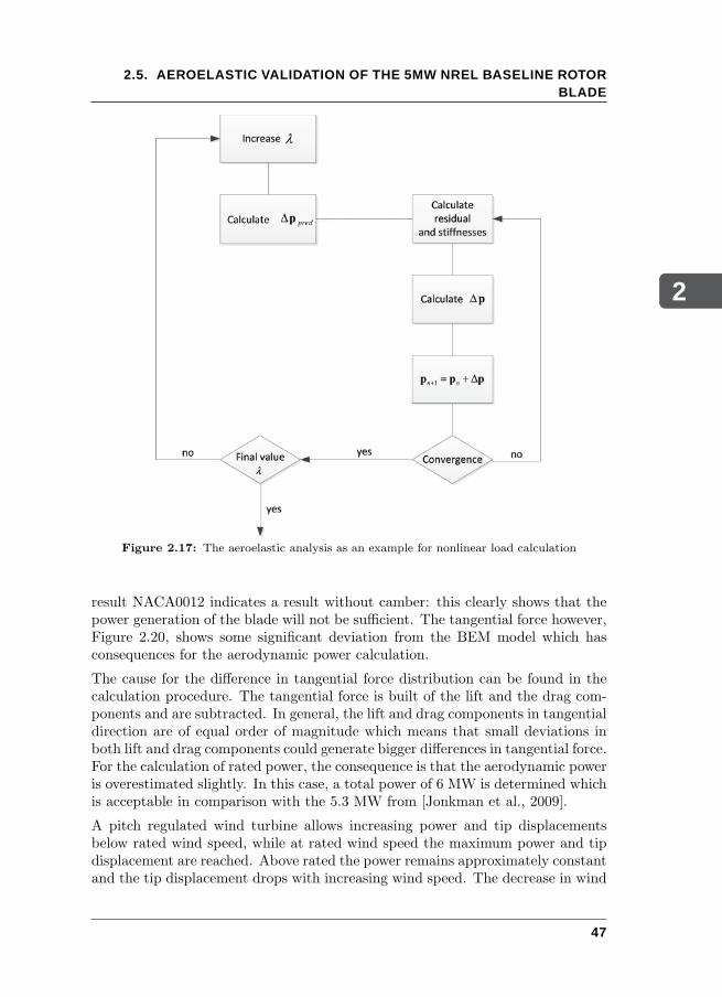
2
2.5. AEROELASTIC VALIDATION OF THE 5MW NREL BASELINE ROTORBLADE
Figure 2.17: The aeroelastic analysis as an example for nonlinear load calculation
result NACA0012 indicates a result without camber: this clearly shows that thepower generation of the blade will not be sufficient. The tangential force however,Figure 2.20, shows some significant deviation from the BEM model which hasconsequences for the aerodynamic power calculation.
The cause for the difference in tangential force distribution can be found in thecalculation procedure. The tangential force is built of the lift and the drag com-ponents and are subtracted. In general, the lift and drag components in tangentialdirection are of equal order of magnitude which means that small deviations inboth lift and drag components could generate bigger differences in tangential force.For the calculation of rated power, the consequence is that the aerodynamic poweris overestimated slightly. In this case, a total power of 6 MW is determined whichis acceptable in comparison with the 5.3 MW from [Jonkman et al., 2009].
A pitch regulated wind turbine allows increasing power and tip displacementsbelow rated wind speed, while at rated wind speed the maximum power and tipdisplacement are reached. Above rated the power remains approximately constantand the tip displacement drops with increasing wind speed. The decrease in wind
47
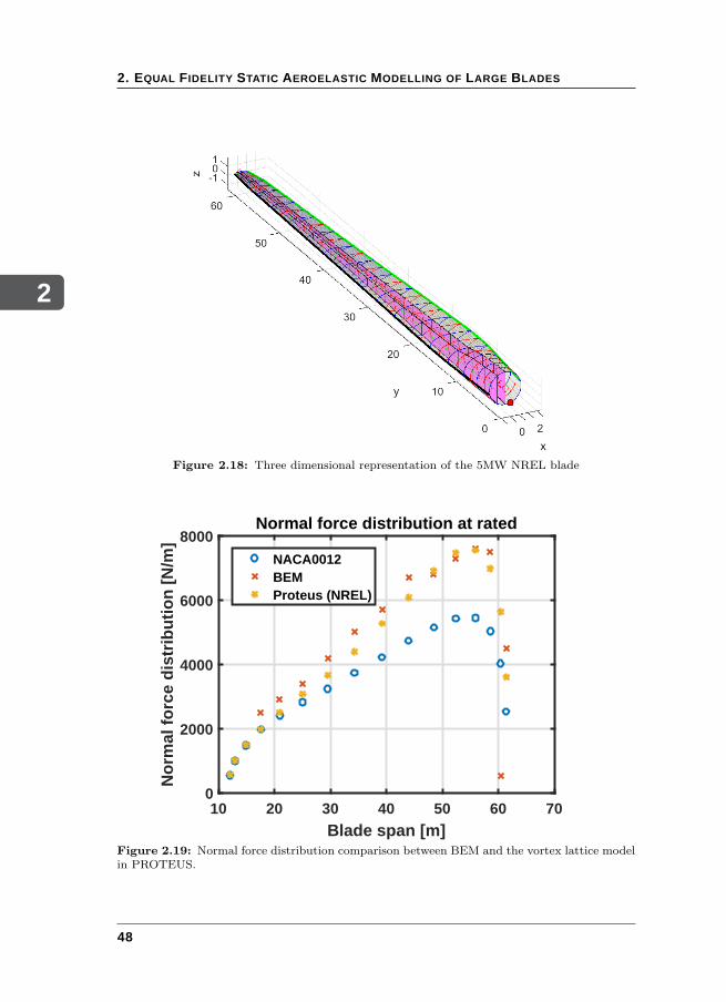
2
2. EQUAL FIDELITY STATIC AEROELASTIC MODELLING OF LARGE BLADES
Figure 2.18: Three dimensional representation of the 5MW NREL blade
10 20 30 40 50 60 70
Blade span [m]
0
2000
4000
6000
8000
No
rmal
fo
rce
dis
trib
uti
on
[N
/m]
Normal force distribution at rated
NACA0012BEMProteus (NREL)
Figure 2.19: Normal force distribution comparison between BEM and the vortex lattice modelin PROTEUS.
48
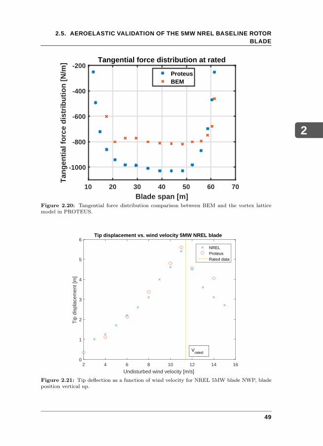
2
2.5. AEROELASTIC VALIDATION OF THE 5MW NREL BASELINE ROTORBLADE
10 20 30 40 50 60 70
Blade span [m]
-1000
-800
-600
-400
-200T
ang
enti
al f
orc
e d
istr
ibu
tio
n [
N/m
] Tangential force distribution at rated
ProteusBEM
Figure 2.20: Tangential force distribution comparison between BEM and the vortex latticemodel in PROTEUS.
2 4 6 8 10 12 14 16
Undisturbed wind velocity [m/s]
0
1
2
3
4
5
6
Tip
dis
plac
emen
t [m
]
Tip displacement vs. wind velocity 5MW NREL blade
NRELProteusRated data
Vrated
Figure 2.21: Tip deflection as a function of wind velocity for NREL 5MW blade NWP, bladeposition vertical up.
49
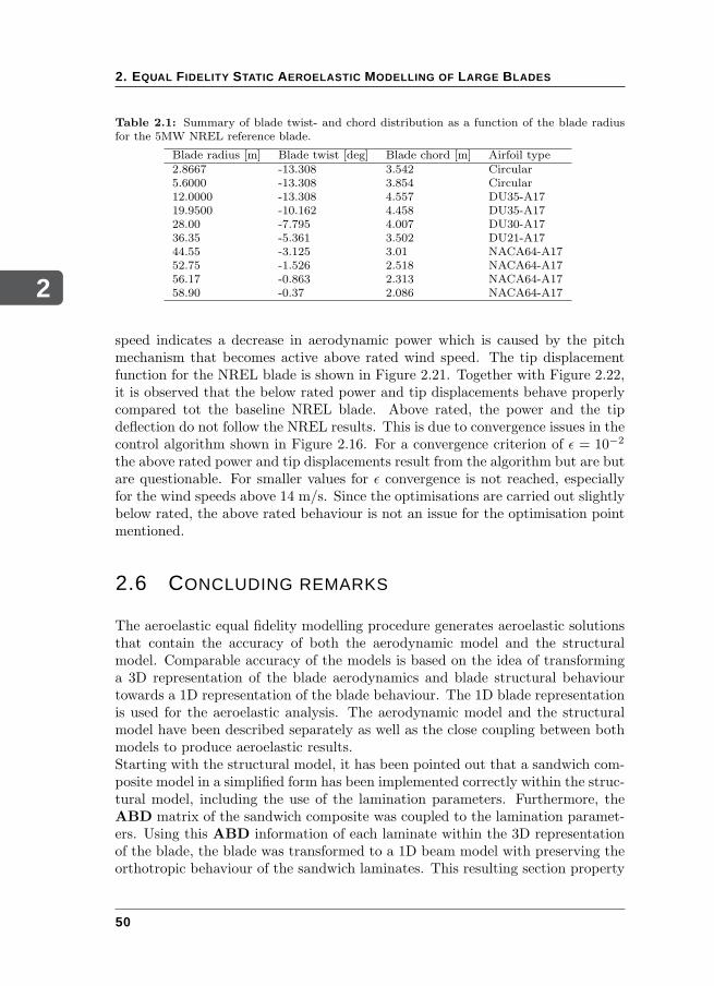
2
2. EQUAL FIDELITY STATIC AEROELASTIC MODELLING OF LARGE BLADES
Table 2.1: Summary of blade twist- and chord distribution as a function of the blade radiusfor the 5MW NREL reference blade.
Blade radius [m] Blade twist [deg] Blade chord [m] Airfoil type2.8667 -13.308 3.542 Circular5.6000 -13.308 3.854 Circular12.0000 -13.308 4.557 DU35-A1719.9500 -10.162 4.458 DU35-A1728.00 -7.795 4.007 DU30-A1736.35 -5.361 3.502 DU21-A1744.55 -3.125 3.01 NACA64-A1752.75 -1.526 2.518 NACA64-A1756.17 -0.863 2.313 NACA64-A1758.90 -0.37 2.086 NACA64-A17
speed indicates a decrease in aerodynamic power which is caused by the pitchmechanism that becomes active above rated wind speed. The tip displacementfunction for the NREL blade is shown in Figure 2.21. Together with Figure 2.22,it is observed that the below rated power and tip displacements behave properlycompared tot the baseline NREL blade. Above rated, the power and the tipdeflection do not follow the NREL results. This is due to convergence issues in thecontrol algorithm shown in Figure 2.16. For a convergence criterion of ǫ = 10−2
the above rated power and tip displacements result from the algorithm but are butare questionable. For smaller values for ǫ convergence is not reached, especiallyfor the wind speeds above 14 m/s. Since the optimisations are carried out slightlybelow rated, the above rated behaviour is not an issue for the optimisation pointmentioned.
2.6 CONCLUDING REMARKS
The aeroelastic equal fidelity modelling procedure generates aeroelastic solutionsthat contain the accuracy of both the aerodynamic model and the structuralmodel. Comparable accuracy of the models is based on the idea of transforminga 3D representation of the blade aerodynamics and blade structural behaviourtowards a 1D representation of the blade behaviour. The 1D blade representationis used for the aeroelastic analysis. The aerodynamic model and the structuralmodel have been described separately as well as the close coupling between bothmodels to produce aeroelastic results.Starting with the structural model, it has been pointed out that a sandwich com-posite model in a simplified form has been implemented correctly within the struc-tural model, including the use of the lamination parameters. Furthermore, theABD matrix of the sandwich composite was coupled to the lamination paramet-ers. Using this ABD information of each laminate within the 3D representationof the blade, the blade was transformed to a 1D beam model with preserving theorthotropic behaviour of the sandwich laminates. This resulting section property
50
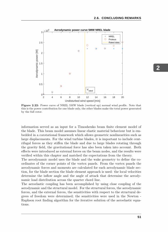
2
2.6. CONCLUDING REMARKS
2 4 6 8 10 12 14 16 18 20
Undisturbed wind speed [m/s]
0
0.5
1
1.5
2
2.5
3
Aer
odyn
amic
pow
er [W
]
106 Aerodynamic power curve 5MW NREL blade
NRELProteusRated data
Vrated
Figure 2.22: Power curve of NREL 5MW blade (vertical up) normal wind profile. Note thatthis is the power contribution for one blade only, the other blades make the total power generatedby the full rotor.
information served as an input for a Timoshenko beam finite element model ofthe blade. This beam model assumes linear elastic material behaviour but is em-bedded in a corotational framework which allows geometric nonlinearities such aslarge displacements. For the wind turbine blades, it is important to include cent-rifugal forces as they stiffen the blade and due to large blades rotating throughthe gravity field, the gravitational force has also been taken into account. Botheffects were introduced as external forces on the beam nodes, and the results wereverified within this chapter and matched the expectations from the theory.The aerodynamic model uses the blade and the wake geometry to define the co-ordinates of the corner points of the vortex panels. From the vortex panels theaerodynamic forces and moments are calculated for each aerodynamic blade sec-tion, for the blade section the blade element approach is used: the local velocitiesdetermine the inflow angle and the angle of attack that determine the aerody-namic load distribution across the quarter chord line.The aeroelastic coupling has been accomplished by using close coupling of theaerodynamic and the structural model. For the structural forces, the aerodynamicforces, and the external forces, the sensitivities with respect to the structural de-grees of freedom were determined; the sensitivities were used in the Newton -Raphson root finding algorithm for the iterative solution of the aeroelastic equa-tions.
51
2
2. EQUAL FIDELITY STATIC AEROELASTIC MODELLING OF LARGE BLADES
It can be concluded that the aeroelastic model behaves as expected, below and atrated wind speed. The above rated results are questionable due to convergenceissues of the pitch control algorithm. This has been concluded from the aerody-namic tangential force, the normal force, the tip displacement as a function ofthe undisturbed wind velocity and power curve. since they are only carried outslightly below rated. However, the questionable behaviour of the pitch controllerdoes not have consequences for the proposed optimisations in this work.
52
3OPTIMISATION PROCEDURE
In this chapter, the optimisation framework is explained as well as the positionof the cross-sectional modeller and the aeroelastic model within this framework.For the optimisation, the objective function has to be chosen, as well as the ap-propriate design variables and the constraints. Besides the design variable vector,the sensitivities of the objective and the constraints with respect to the designvariables are required. As such, the relation between the objective function andthe design variables is described as well as the relation between the constraintsand the design variables. While the work of [Werter, 2017] mentions an objectivefunction that considers mass minimisation of pure fibre composite materials, theemphasis in this research is on objective functions considering sandwich compositestructural models as mentioned in chapter 2. Furthermore, appropriate loadcasesare proposed for a static aeroelastic optimisation and the atmospheric wind velo-city behaviour significant for the blade loading is discussed. Finally, the impactof a stiffness optimisation on the year power production is discussed.
3.1 AEROELASTIC OPTIMISATION
As explained in [Liao et al., 2012], the cost of energy is a significant objective.However, this objective has many variables each possessing a different level ofsignificance with respect to the cost of energy objective. To avoid the difficultiesmentioned when using cost of energy as objective, it was decided to perform a
53
3
3. OPTIMISATION PROCEDURE
stiffness optimisation where the blade mass will be minimised. Blade mass is animportant indicator for blade costs, especially for increasing blade dimensions. Inaddition, as an objective function, it contains clearly defined variables, and thenumber of variables is inherently limited due to the definition of mass. As such, theobjective function mass must be formulated with structural parameters availablein the model, such as laminate thickness and material density. For a structuraloptimisation as performed during this research, the most significant constraintsare the Tsai-Wu strain factor, the lamination parameters feasibility constraints,panel buckling, tip displacements and a predefined aerodynamic power loss. Ithas been realised that the tip deflection is dependent on the blade azimuth, how-ever, tip deflection is only an issue for blade - tower passage. As such, the towerclearance case and the highest aerodynamic blade loading do not coincide. Thehighest blade loading occurs when the blade is in the vertical upward position:the wind velocity is higher in this region. In the vertical downward position towerpassage is an issue, however, the wind velocity in this region is lower and theblade loads are lower as well. To be sure that tower clearance is safe, the max-imum deflection has been applied together with the case where the aerodynamicloads are highest. Considering the constraints and the objective mentioned above,the stiffness of the blade is controlled such that the constraint functions are notviolated during the mass minimisation procedure. The aeroelastic optimisationframework is summarised in Figure 3.1.
Next, the gradient based optimisation problem is formulated as
minξ
m (ξ) (3.1)
subject to gi (ξ) ≤ 0,
also including the derivatives of the objective function, the mass m, and theconstraint functions gi with respect to the design variables ξ:
∂m
∂ξand
∂gi∂ξ
. (3.2)
This means that the mass m, dependent on the design variables ξ subject to theconstraints gi that are functions of the design variables ξ, is minimised. Thegradients take care for the convergence speed of the optimisation, which also de-pend on the chosen method for handling the gradient. Per sandwich laminate,the design variable vector consists of 8 lamination parameters and 2 thicknessparameters for sandwich laminates, tf and tc, the face and the core respectively.It is assumed that the upper and the lower face sheets are identical in lay-up andthickness. For the mass optimisation of a sandwich laminate the mass objectivefunction m depends only on the laminate thickness, width, heigth, and laminatedensity. In Table 3.1 the difference is shown between the number of design vari-
54
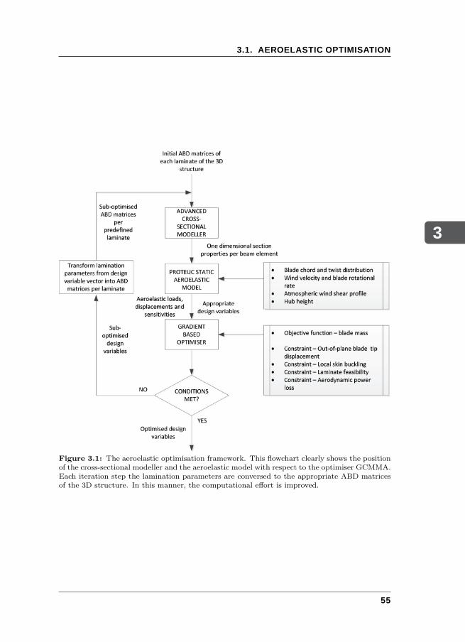
3
3.1. AEROELASTIC OPTIMISATION
Figure 3.1: The aeroelastic optimisation framework. This flowchart clearly shows the positionof the cross-sectional modeller and the aeroelastic model with respect to the optimiser GCMMA.Each iteration step the lamination parameters are conversed to the appropriate ABD matricesof the 3D structure. In this manner, the computational effort is improved.
55
3
3. OPTIMISATION PROCEDURE
Table 3.1: Number of design variables per laminate and per cross-section.
Sandwich laminate Pure fibre laminatebalanced unbalanced balanced unbalanced
# design variables per laminate 6 10 5 9# laminates per cross-section 8 8 8 8# design variables per section 48 80 40 72
ables for pure fibre laminates and sandwich laminates per cross-sectional panelfor balanced, symmetric laminates and for unbalanced but symmetric laminates.
The sensitivity of the mass is determined by defining a derivative with respect tothe thickness of the laminate multiplied by the sensitivity of the thickness withrespect to the design variables. For a single blade segment for a pure laminatethe mass sensitivity with respect to the design variables is written as:
∂mi
∂ξ=∂mi
∂ti
∂ti∂ξ
, (3.3)
and gives the direction change of the elemental mass as:
∆mi =∂mi
∂ξ∆ξ. (3.4)
For the case of a sandwich laminate the thickness of the laminate consists of twofaces and a core. From chapter 2 it can be concluded that if the facing sheetsconsist of symmetric laminates and the sandwich laminate is symmetric as well,the facing sheets are equal in thickness and lay-up. As such, defining the thicknessand lamination parameters of only one facing sheet is sufficient, which results inthe following thickness vector per laminate:
ti = (tf tc)i , (3.5)
and the sensitivity with respect to the design variable vector:
∂ti∂ξ
=
(∂tf∂ξ
∂tc∂ξ
)
i
, (3.6)
which, for the i-th sandwich laminate, results in a sensitivity vector [(0 1 0) (0 0 1)].For the sandwich laminate case, the sensitivity of the elemental mass is definedwith respect to the elemental thickness vector and multiplication with this sensit-ivity matrix ∂mi/∂ti gives the elemental mass with respect to the design variablevector as shown in expression 3.3. For the gradient based optimisation, the glob-ally convergent method of moving asymptotes (GCMMA), see [Svanberg, 2002],
56
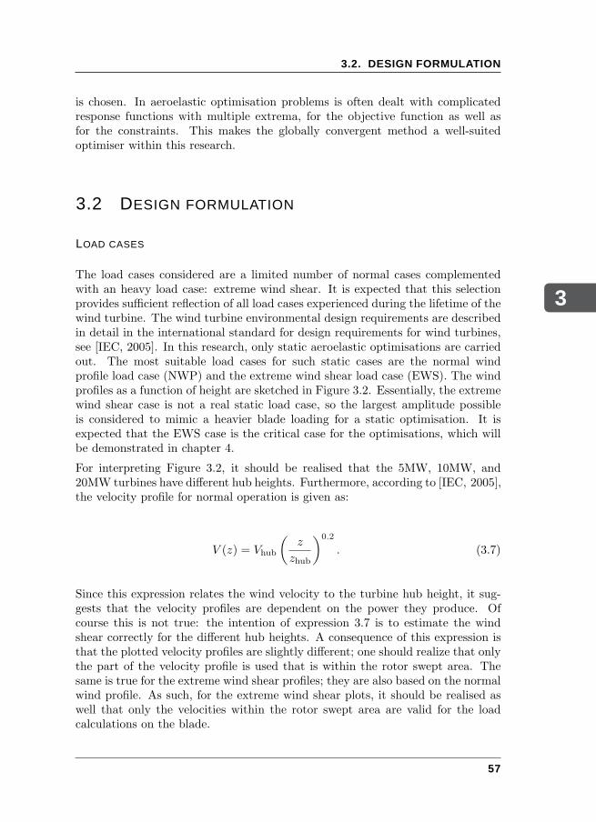
3
3.2. DESIGN FORMULATION
is chosen. In aeroelastic optimisation problems is often dealt with complicatedresponse functions with multiple extrema, for the objective function as well asfor the constraints. This makes the globally convergent method a well-suitedoptimiser within this research.
3.2 DESIGN FORMULATION
LOAD CASES
The load cases considered are a limited number of normal cases complementedwith an heavy load case: extreme wind shear. It is expected that this selectionprovides sufficient reflection of all load cases experienced during the lifetime of thewind turbine. The wind turbine environmental design requirements are describedin detail in the international standard for design requirements for wind turbines,see [IEC, 2005]. In this research, only static aeroelastic optimisations are carriedout. The most suitable load cases for such static cases are the normal windprofile load case (NWP) and the extreme wind shear load case (EWS). The windprofiles as a function of height are sketched in Figure 3.2. Essentially, the extremewind shear case is not a real static load case, so the largest amplitude possibleis considered to mimic a heavier blade loading for a static optimisation. It isexpected that the EWS case is the critical case for the optimisations, which willbe demonstrated in chapter 4.
For interpreting Figure 3.2, it should be realised that the 5MW, 10MW, and20MW turbines have different hub heights. Furthermore, according to [IEC, 2005],the velocity profile for normal operation is given as:
V (z) = Vhub
(z
zhub
)0.2
. (3.7)
Since this expression relates the wind velocity to the turbine hub height, it sug-gests that the velocity profiles are dependent on the power they produce. Ofcourse this is not true: the intention of expression 3.7 is to estimate the windshear correctly for the different hub heights. A consequence of this expression isthat the plotted velocity profiles are slightly different; one should realize that onlythe part of the velocity profile is used that is within the rotor swept area. Thesame is true for the extreme wind shear profiles; they are also based on the normalwind profile. As such, for the extreme wind shear plots, it should be realised aswell that only the velocities within the rotor swept area are valid for the loadcalculations on the blade.
57
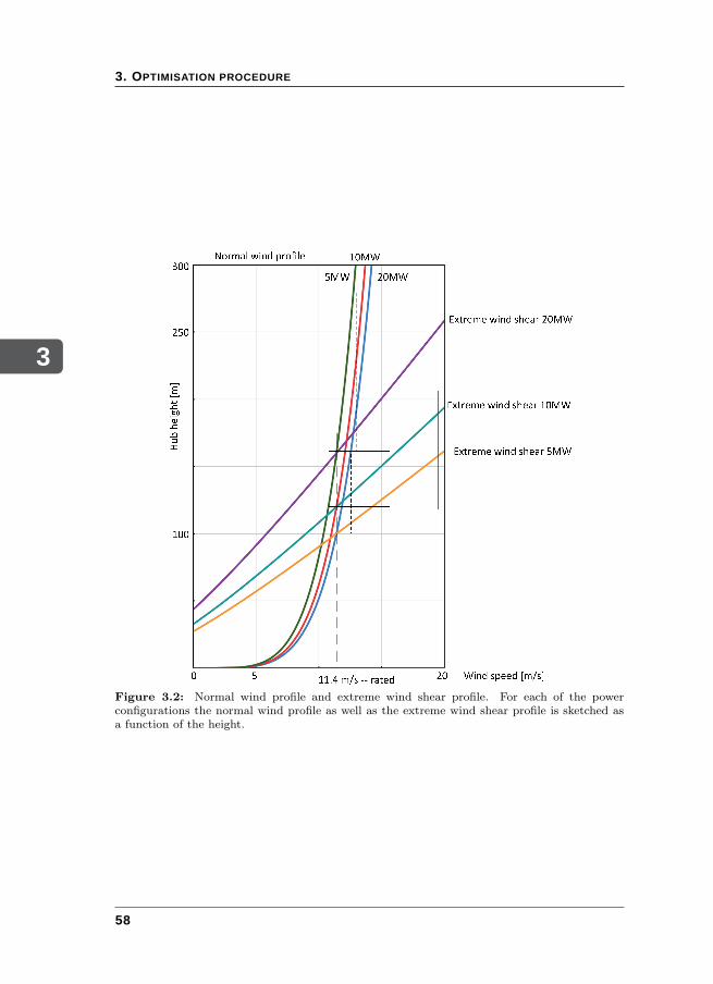
3
3. OPTIMISATION PROCEDURE
Figure 3.2: Normal wind profile and extreme wind shear profile. For each of the powerconfigurations the normal wind profile as well as the extreme wind shear profile is sketched asa function of the height.
58
3
3.2. DESIGN FORMULATION
OBJECTIVE
This study searches for a minimum blade mass using the variable stiffness concept.The blade mass is calculated as follows:
m =∑
i
(2ρf itf i + ρcitci
)lihi, (3.8)
where ρf is the facing sheet material density, ρc the core material density, tf thefacing sheet thickness, tc the core thickness, li the length of the cross-sectionalpanel, and the hi the average height of the cross-sectional panel. From Equation3.8 it is evident that the mass only contains the thickness variation of the skinand the spars assuming that the segments are constant during the optimisationloop. The objective function constains only the facing sheet thickness and the corethickness as design variables for sadndwich blades, while for full fibre laminatesthe only design variable is the laminate thickness. The stiffness variation resultingfrom the stacking sequence originates from the constraints.
DESIGN VARIABLES
The blades are structurally optimised using the sandwich laminate propertiesor the pure fibre laminate properties, depending on the desired structural bladedesign. For the sandwich laminate, this is done by using the lamination para-meters of the faces, the thickness of the faces, and the thickness of the core asseparate design variables. For pure fibre laminates the lamination parameters ofthe laminate together with the thickness of the the laminate are the necessaryvariables for the optimisation procedure. The design variables per laminate aresummarised in the vector:
ξ = [V1A, V2A, V3A, V4A, V1D, V2D, V3D, V4D, tf , tc] (3.9)
for a symmetric, unbalanced sandwich laminate. For balanced laminates, thelamination parameters V2A, V4A, V2D, V4D are omitted, which reduces the com-putational effort significantly. The optimisations will be carried out for a quasi-isotropic case and the symmetric, balanced laminate case. For the quasi-isotropiclay-up all lamination parameters remain unchanged during the optimisation andonly the thickness of laminate is a variable. For pure fibre laminates, the thick-ness tc vanishes from Equation 3.9 because of the absence of a core and the onlythickness remaining is tf , in that case the laminate thickness.
59
3
3. OPTIMISATION PROCEDURE
CONSTRAINTS
As mentioned in [Chehouri et al., 2015], the choice of constraints is somewhatarbitrary. Within this review, the constraints are roughly divided in geometric,aerodynamic and structural constraints. For the stiffness optimisation, as an aero-dynamic constraint, the aerodynamic power loss is considered; furthermore thegeometric and structural constraints determine the stiffness of the laminates. Tobe more specific, for the wind turbine blades in this research, the most significantconstraints are:
• minimum and maximum strain of the skins and the spars;
• skin and spar buckling;
• tip deflection;
• the aerodynamic power loss.
In a gradient based optimisation not only the gradient of the objective function isimportant, the gradients of the constraint functions do matter as well. Since thedesign variable vector is defined as ξ, the gradients of the constraints functionsare determined with respect to this design variable vector. As such, the responsesensitivities are found by differentiating the constraint functions with respect tothe design variable vector ξ. Clearly, for this optimisation problem, the number ofconstraints are larger than the number of design variables, see Table 3.1, thereforedirect sensitivities are used. The differentiation is carried out analytically to bemore numerically efficient within the optimisation loop.
STRAIN: For the strain constraints the procedure from [Werter, 2017] is used.The strain constraints are determined by evaluating the strain responses per struc-tural element. The most critical strain responses for each laminate within thecross-sections are identified by determining the four most critical Tsai-Wu strainfactors. Subsequently, those critical strain factors are introduced as constraints.Next, the gradient of the strains with respect to the design variables is considered.The beam strains as mentioned in Equation 2.23 originate from the local com-posite sectional elements from the 3D blade representation; the cross-sectionalmodelling technique mentioned in chapter 2 transforms the local strains into 1Dbeam strains including the sensitivities with respect to the localA andDmatrices.For the extension strains, as an example for all strains, the response sensitivity isdetermined as follows:
∂ǫ
∂ξ=
∂ǫ
∂A
∂A
∂ξ+
∂ǫ
∂D
∂D
∂ξ+∂ǫ
∂t
∂t
∂ξ(3.10)
60
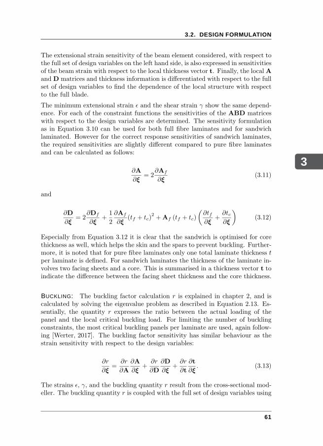
3
3.2. DESIGN FORMULATION
The extensional strain sensitivity of the beam element considered, with respect tothe full set of design variables on the left hand side, is also expressed in sensitivitiesof the beam strain with respect to the local thickness vector t. Finally, the local Aand D matrices and thickness information is differentiated with respect to the fullset of design variables to find the dependence of the local structure with respectto the full blade.
The minimum extensional strain ǫ and the shear strain γ show the same depend-ence. For each of the constraint functions the sensitivities of the ABD matriceswith respect to the design variables are determined. The sensitivity formulationas in Equation 3.10 can be used for both full fibre laminates and for sandwichlaminated. However for the correct response sensitivities of sandwich laminates,the required sensitivities are slightly different compared to pure fibre laminatesand can be calculated as follows:
∂A
∂ξ= 2
∂Af
∂ξ(3.11)
and
∂D
∂ξ= 2
∂Df
∂ξ+
1
2
∂Af
∂ξ(tf + tc)
2+Af (tf + tc)
(∂tf∂ξ
+∂tc∂ξ
)
(3.12)
Especially from Equation 3.12 it is clear that the sandwich is optimised for corethickness as well, which helps the skin and the spars to prevent buckling. Further-more, it is noted that for pure fibre laminates only one total laminate thickness tper laminate is defined. For sandwich laminates the thickness of the laminate in-volves two facing sheets and a core. This is summarised in a thickness vector t toindicate the difference between the facing sheet thickness and the core thickness.
BUCKLING: The buckling factor calculation r is explained in chapter 2, and iscalculated by solving the eigenvalue problem as described in Equation 2.13. Es-sentially, the quantity r expresses the ratio between the actual loading of thepanel and the local critical buckling load. For limiting the number of bucklingconstraints, the most critical buckling panels per laminate are used, again follow-ing [Werter, 2017]. The buckling factor sensitivity has similar behaviour as thestrain sensitivity with respect to the design variables:
∂r
∂ξ=
∂r
∂A
∂A
∂ξ+
∂r
∂D
∂D
∂ξ+∂r
∂t
∂t
∂ξ. (3.13)
The strains ǫ, γ, and the buckling quantity r result from the cross-sectional mod-eller. The buckling quantity r is coupled with the full set of design variables using
61
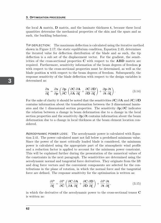
3
3. OPTIMISATION PROCEDURE
the local A matrix, D matrix, and the laminate thickness t, because these localquantities determine the mechanical properties of the skin and the spars and assuch, the buckling behaviour.
TIP DEFLECTION: The maximum deflection is calculated using the iterative methodshown in Figure 2.17; the static equilibrium condition, Equation 2.43, determinesthe iterated value for deflection distribution of the blade and as such, the tipdeflection is a sub set of the displacement vector. For the gradient, the sensit-ivities of the cross-sectional properties C with respect to the ABD matrix arerequired. Furthermore, sensitivity information of the beam degrees of freedom p
with respect to the cross-sectional properties must be determined, as well as theblade position x with respect to the beam degrees of freedom. Subsequently, theresponse sensitivity of the blade deflection with respect to the design variables isdetermined as:
∂x
∂ξ=∂x
∂p
(∂p
∂C
(∂C
∂A
∂A
∂ξ+∂C
∂D
∂D
∂ξ
)
+∂p
∂t
∂t
∂ξ
)
. (3.14)
For the sake of clarity it should be noted that the sensitivities ∂C/∂A and ∂C/∂Dcontains information about the transformation between the 3 dimensional lamin-ates and the 1 dimensional section properties. The sensitivity ∂p/∂C indicatesthe relation between a change in beam deformation due to a change in the localsection properties and the sensitivity ∂p/∂t contains information about the beamdeformation due to a change in local thickness at the beam element location con-sidered.
AERODYNAMIC POWER LOSS: The aerodynamic power is calculated with Equa-tion 2.41. The power calculated must not fall below a predefined minimum value.Since the power of the most critically loaded blade is considered, the minimumpower is calculated using the appropriate part of the atmospheric wind profileand a reduction factor is applied to account for the minimum power constraint.This will be explained further during the presentation of the numerical values ofthe constraints in the next paragraph. The sensitivities are determined using theaerodynamic normal and tangential force derivatives. They originate from the liftand drag force vectors and the convenient components are selected for the con-tributions in the plane of rotation, in which the normal force and the tangentialforce are defined. The response sensitivity for the optimisation is written as:
∂P
∂ξ=∂P
∂C
(∂C
∂A
∂A
∂ξ+∂C
∂D
∂D
∂ξ
)
+∂P
∂t
∂t
∂ξ, (3.15)
in which the derivative of the aerodynamic power to the cross-sectional tensor Cis written as:
62
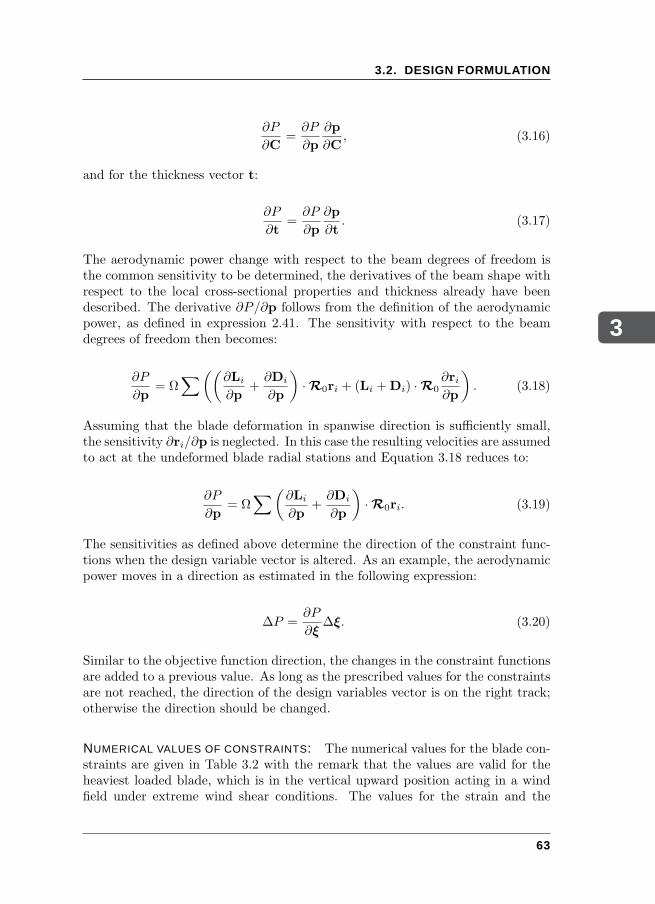
3
3.2. DESIGN FORMULATION
∂P
∂C=∂P
∂p
∂p
∂C, (3.16)
and for the thickness vector t:
∂P
∂t=∂P
∂p
∂p
∂t. (3.17)
The aerodynamic power change with respect to the beam degrees of freedom isthe common sensitivity to be determined, the derivatives of the beam shape withrespect to the local cross-sectional properties and thickness already have beendescribed. The derivative ∂P/∂p follows from the definition of the aerodynamicpower, as defined in expression 2.41. The sensitivity with respect to the beamdegrees of freedom then becomes:
∂P
∂p= Ω
∑((
∂Li
∂p+∂Di
∂p
)
·R0ri + (Li +Di) ·R0
∂ri∂p
)
. (3.18)
Assuming that the blade deformation in spanwise direction is sufficiently small,the sensitivity ∂ri/∂p is neglected. In this case the resulting velocities are assumedto act at the undeformed blade radial stations and Equation 3.18 reduces to:
∂P
∂p= Ω
∑(∂Li
∂p+∂Di
∂p
)
·R0ri. (3.19)
The sensitivities as defined above determine the direction of the constraint func-tions when the design variable vector is altered. As an example, the aerodynamicpower moves in a direction as estimated in the following expression:
∆P =∂P
∂ξ∆ξ. (3.20)
Similar to the objective function direction, the changes in the constraint functionsare added to a previous value. As long as the prescribed values for the constraintsare not reached, the direction of the design variables vector is on the right track;otherwise the direction should be changed.
NUMERICAL VALUES OF CONSTRAINTS: The numerical values for the blade con-straints are given in Table 3.2 with the remark that the values are valid for theheaviest loaded blade, which is in the vertical upward position acting in a windfield under extreme wind shear conditions. The values for the strain and the
63
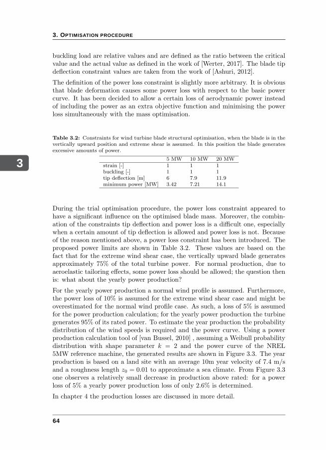
3
3. OPTIMISATION PROCEDURE
buckling load are relative values and are defined as the ratio between the criticalvalue and the actual value as defined in the work of [Werter, 2017]. The blade tipdeflection constraint values are taken from the work of [Ashuri, 2012].
The definition of the power loss constraint is slightly more arbitrary. It is obviousthat blade deformation causes some power loss with respect to the basic powercurve. It has been decided to allow a certain loss of aerodynamic power insteadof including the power as an extra objective function and minimising the powerloss simultaneously with the mass optimisation.
Table 3.2: Constraints for wind turbine blade structural optimisation, when the blade is in thevertically upward position and extreme shear is assumed. In this position the blade generatesexcessive amounts of power.
5 MW 10 MW 20 MWstrain [-] 1 1 1buckling [-] 1 1 1tip deflection [m] 6 7.9 11.9minimum power [MW] 3.42 7.21 14.1
During the trial optimisation procedure, the power loss constraint appeared tohave a significant influence on the optimised blade mass. Moreover, the combin-ation of the constraints tip deflection and power loss is a difficult one, especiallywhen a certain amount of tip deflection is allowed and power loss is not. Becauseof the reason mentioned above, a power loss constraint has been introduced. Theproposed power limits are shown in Table 3.2. These values are based on thefact that for the extreme wind shear case, the vertically upward blade generatesapproximately 75% of the total turbine power. For normal production, due toaeroelastic tailoring effects, some power loss should be allowed; the question thenis: what about the yearly power production?
For the yearly power production a normal wind profile is assumed. Furthermore,the power loss of 10% is assumed for the extreme wind shear case and might beoverestimated for the normal wind profile case. As such, a loss of 5% is assumedfor the power production calculation; for the yearly power production the turbinegenerates 95% of its rated power. To estimate the year production the probabilitydistribution of the wind speeds is required and the power curve. Using a powerproduction calculation tool of [van Bussel, 2010] , assuming a Weibull probabilitydistribution with shape parameter k = 2 and the power curve of the NREL5MW reference machine, the generated results are shown in Figure 3.3. The yearproduction is based on a land site with an average 10m year velocity of 7.4 m/sand a roughness length z0 = 0.01 to approximate a sea climate. From Figure 3.3one observes a relatively small decrease in production above rated: for a powerloss of 5% a yearly power production loss of only 2.6% is determined.
In chapter 4 the production losses are discussed in more detail.
64
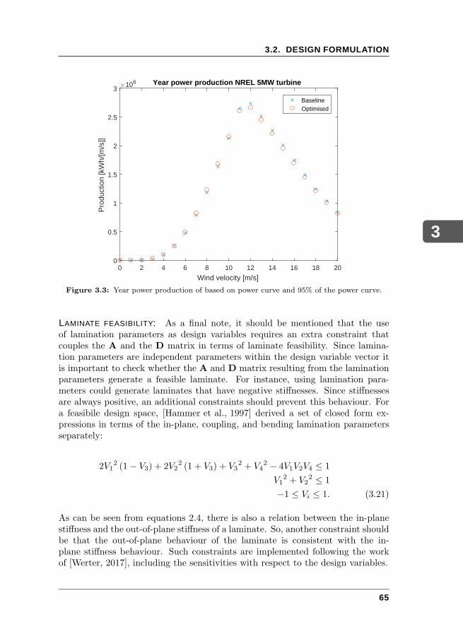
3
3.2. DESIGN FORMULATION
0 2 4 6 8 10 12 14 16 18 20
Wind velocity [m/s]
0
0.5
1
1.5
2
2.5
3
Pro
duct
ion
[kW
h/[m
/s]]
106 Year power production NREL 5MW turbine
BaselineOptimised
Figure 3.3: Year power production of based on power curve and 95% of the power curve.
LAMINATE FEASIBILITY: As a final note, it should be mentioned that the useof lamination parameters as design variables requires an extra constraint thatcouples the A and the D matrix in terms of laminate feasibility. Since lamina-tion parameters are independent parameters within the design variable vector itis important to check whether the A and D matrix resulting from the laminationparameters generate a feasible laminate. For instance, using lamination para-meters could generate laminates that have negative stiffnesses. Since stiffnessesare always positive, an additional constraints should prevent this behaviour. Fora feasibile design space, [Hammer et al., 1997] derived a set of closed form ex-pressions in terms of the in-plane, coupling, and bending lamination parametersseparately:
2V12 (1− V3) + 2V2
2 (1 + V3) + V32 + V4
2 − 4V1V2V4 ≤ 1
V12 + V2
2 ≤ 1
−1 ≤ Vi ≤ 1. (3.21)
As can be seen from equations 2.4, there is also a relation between the in-planestiffness and the out-of-plane stiffness of a laminate. So, another constraint shouldbe that the out-of-plane behaviour of the laminate is consistent with the in-plane stiffness behaviour. Such constraints are implemented following the workof [Werter, 2017], including the sensitivities with respect to the design variables.
65
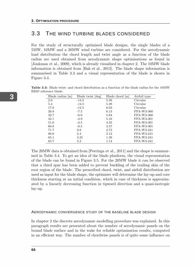
3
3. OPTIMISATION PROCEDURE
3.3 THE WIND TURBINE BLADES CONSIDERED
For the study of structurally optimised blade designs, the single blades of a5MW, 10MW and a 20MW wind turbine are considered. For the aerodynamicload distribution the chord length and twist angle as a function of the bladeradius are used obtained from aerodynamic shape optimisations as found in[Jonkman et al., 2009], which is already visualised in chapter 2. The 10MW bladeinformation is obtained from [Bak et al., 2013]. The blade shape information issummarised in Table 3.3 and a visual representation of the blade is shown inFigure 3.4.
Table 3.3: Blade twist- and chord distribution as a function of the blade radius for the 10MWRISØ reference blade.
Blade radius [m] Blade twist [deg] Blade chord [m] Airfoil type2.0 -14.5 5.38 Circular5.4 -14.5 5.38 Circular17.0 -12.5 6.03 Circular26.8 -7.5 6.13 FFA-W3-36032.7 -6.0 5.84 FFA-W3-36042.1 -4.9 5.16 FFA-W3-30151.6 -2.5 4.35 FFA-W3-30160.8 -0.5 3.57 FFA-W3-30171.7 0.9 2.73 FFA-W3-24180.0 2.4 2.12 FFA-W3-24185.1 3.25 1.39 FFA-W3-24185.7 3.3 1.14 FFA-W3-241
The 20MW data is obtained from [Peeringa et al., 2011] and the shape is summar-ised in Table 3.4. To get an idea of the blade planform, the visual representationof the blade can be found in Figure 3.5. For the 20MW blade it can be observedthat a third spar has been added to prevent buckling of the trailing skin of theroot region of the blade. The prescribed chord, twist, and airfoil distribution areused as input for the blade shape, the optimiser will determine the lay-up and corethickness starting at an initial condition, which in case of thickness is approxim-ated by a linearly decreasing function in tipward direction and a quasi-isotropiclay-up.
AERODYNAMIC CONVERGENCE STUDY OF THE BASELINE BLADE DESIGN
In chapter 2 the discrete aerodynamic modelling procedure was explained. In thisparagraph results are presented about the number of aerodynamic panels on thebound blade surface and in the wake for reliable optimisation results, computedin an efficient way. The number of chordwise panels is of quite some influence on
66
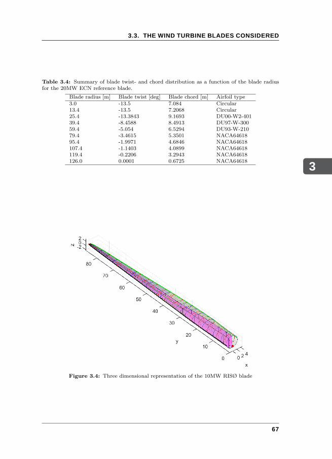
3
3.3. THE WIND TURBINE BLADES CONSIDERED
Table 3.4: Summary of blade twist- and chord distribution as a function of the blade radiusfor the 20MW ECN reference blade.
Blade radius [m] Blade twist [deg] Blade chord [m] Airfoil type3.0 -13.5 7.084 Circular13.4 -13.5 7.2068 Circular25.4 -13.3843 9.1693 DU00-W2-40139.4 -8.4588 8.4913 DU97-W-30059.4 -5.054 6.5294 DU93-W-21079.4 -3.4615 5.3501 NACA6461895.4 -1.9971 4.6846 NACA64618107.4 -1.1403 4.0899 NACA64618119.4 -0.2206 3.2943 NACA64618126.0 0.0001 0.6725 NACA64618
Figure 3.4: Three dimensional representation of the 10MW RISØ blade
67
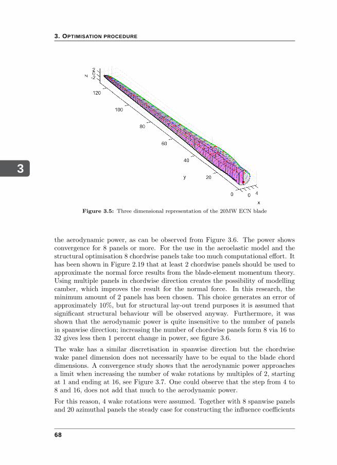
3
3. OPTIMISATION PROCEDURE
Figure 3.5: Three dimensional representation of the 20MW ECN blade
the aerodynamic power, as can be observed from Figure 3.6. The power showsconvergence for 8 panels or more. For the use in the aeroelastic model and thestructural optimisation 8 chordwise panels take too much computational effort. Ithas been shown in Figure 2.19 that at least 2 chordwise panels should be used toapproximate the normal force results from the blade-element momentum theory.Using multiple panels in chordwise direction creates the possibility of modellingcamber, which improves the result for the normal force. In this research, theminimum amount of 2 panels has been chosen. This choice generates an error ofapproximately 10%, but for structural lay-out trend purposes it is assumed thatsignificant structural behaviour will be observed anyway. Furthermore, it wasshown that the aerodynamic power is quite insensitive to the number of panelsin spanwise direction; increasing the number of chordwise panels form 8 via 16 to32 gives less then 1 percent change in power, see figure 3.6.
The wake has a similar discretisation in spanwise direction but the chordwisewake panel dimension does not necessarily have to be equal to the blade chorddimensions. A convergence study shows that the aerodynamic power approachesa limit when increasing the number of wake rotations by multiples of 2, startingat 1 and ending at 16, see Figure 3.7. One could observe that the step from 4 to8 and 16, does not add that much to the aerodynamic power.
For this reason, 4 wake rotations were assumed. Together with 8 spanwise panelsand 20 azimuthal panels the steady case for constructing the influence coefficients
68
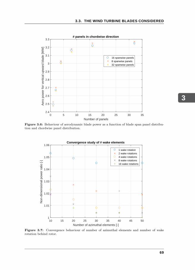
3
3.3. THE WIND TURBINE BLADES CONSIDERED
0 5 10 15 20 25 30 35
Number of panels
2.4
2.5
2.6
2.7
2.8
2.9
3
3.1
3.2
3.3A
ero
pow
er fo
r ve
rtic
al u
pwar
d bl
ade
[MW
]
# panels in chordwise direction
16 spanwise panels8 spanwise panels32 spanwise panels
Figure 3.6: Behaviour of aerodynamic blade power as a function of blade span panel distribu-tion and chordwise panel distribution.
10 15 20 25 30 35 40 45 50
Number of azimuthal elements [-]
1
1.01
1.02
1.03
1.04
1.05
1.06
Non
-dim
ensi
onal
pow
er r
atio
[-]
Convergence study of # wake elements
1 wake rotation2 wake rotations4 wake rotations8 wake rotations16 wake rotations
Figure 3.7: Convergence behaviour of number of azimuthal elements and number of wakerotation behind rotor.
69
3
3. OPTIMISATION PROCEDURE
matrix A is defined.
3.4 CONCLUDING REMARKS
As preparation for the optimisations, the load cases NWP and EWS are selectedas well as the baseline blades. Since the aeroelastic model is designed for thesteady aerodynamic case, the selected loadcases are chosen to be the normal windprofile and, to account for a more severe load case, the extreme wind shear case.Both cases are considered up to rated power or rated wind speed. The bladeswere chosen to be the 5MW NREL reference blade as a baseline, the 10MW pre-liminary design of RISØ, and the preliminary design of the 20MW from ECN.The preliminary designs or reference blades, were considered to be the baselinesfor the 10MW and 20MW respectively.Then, the optimisation framework was explained. For the stiffness optimisation,where the objective is chosen to be the minimum blade mass, it is essential todefine the objective function as a function of the design variables. The design vari-ables are the lamination parameters and laminate thickness for a pure fibre-epoxylaminate. The sandwich laminate design variables are defined by the laminationparameters of the face sheet, the thickness of the face sheet, and the thicknessof the core. For the gradient based optimisation, the GCMMA procedure is se-lected. As a consequence, the response sensitivity of the objective mass must bedefined with respect to the design variables. The selected constraints are strain,skin and spar buckling, laminate feasibility, and aerodynamic power loss of whichthe numerical values are selected as well. In addition, the response sensitivitiesof the constraints with respect to the design variables must be found as well, inorder to relate the constraints to the design variable vector. Finally, an aerody-namic convergence study on the number of blade and wake panels for the baselineblade design was performed. For finding structural lay-out trends using a gradi-ent based optimisation, 2 chordwise blade panels, 8 spanwise blade panels, 20azimuthal wake panels, and 4 wake rotations were assumed.
70
4AEROELASTIC OPTIMISATION
RESULTS OF 5, 10 AND 20MWBLADES
In this chapter, the static aeroelastic optimisations of several wind turbine bladesare performed. First it is shown that the extreme wind shear load case generatesheavier blades compared to the normal wind profile case. Then, using the blademass as objective function, the selected constraint variables and the design vari-ables under the extreme wind shear static load case for 5MW, 10MW and 20MWrotor blades are considered for three different structural configurations:
• a full sandwich composite blade;
• a sandwich composite blade except the spar caps - state-of-the-art designstandard;
• a stiffened skin wing box design - besides the spars also inclusion of ribs anda stiffened, pure fibre-epoxy laminate skin.
In Figure 4.1 the structural configurations for the optimisations are summarised.
The optimisations are performed for a quasi-isotropic lay-up for model verificationand tailoring is applied using the variable stiffness concept for mass minimisation.Furthermore, the effect of mixed materials in a blade is taken into account. Since
71
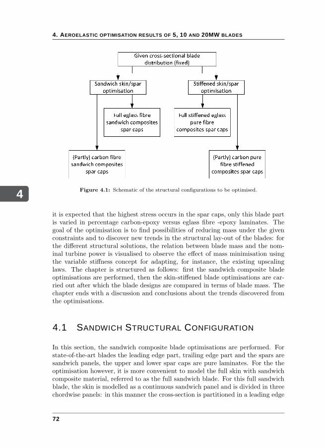
4
4. AEROELASTIC OPTIMISATION RESULTS OF 5, 10 AND 20MW BLADES
Figure 4.1: Schematic of the structural configurations to be optimised.
it is expected that the highest stress occurs in the spar caps, only this blade partis varied in percentage carbon-epoxy versus eglass fibre -epoxy laminates. Thegoal of the optimisation is to find possibilities of reducing mass under the givenconstraints and to discover new trends in the structural lay-out of the blades: forthe different structural solutions, the relation between blade mass and the nom-inal turbine power is visualised to observe the effect of mass minimisation usingthe variable stiffness concept for adapting, for instance, the existing upscalinglaws. The chapter is structured as follows: first the sandwich composite bladeoptimisations are performed, then the skin-stiffened blade optimisations are car-ried out after which the blade designs are compared in terms of blade mass. Thechapter ends with a discussion and conclusions about the trends discovered fromthe optimisations.
4.1 SANDWICH STRUCTURAL CONFIGURATION
In this section, the sandwich composite blade optimisations are performed. Forstate-of-the-art blades the leading edge part, trailing edge part and the spars aresandwich panels, the upper and lower spar caps are pure laminates. For the theoptimisation however, it is more convenient to model the full skin with sandwichcomposite material, referred to as the full sandwich blade. For this full sandwichblade, the skin is modelled as a continuous sandwich panel and is divided in threechordwise panels: in this manner the cross-section is partitioned in a leading edge
72
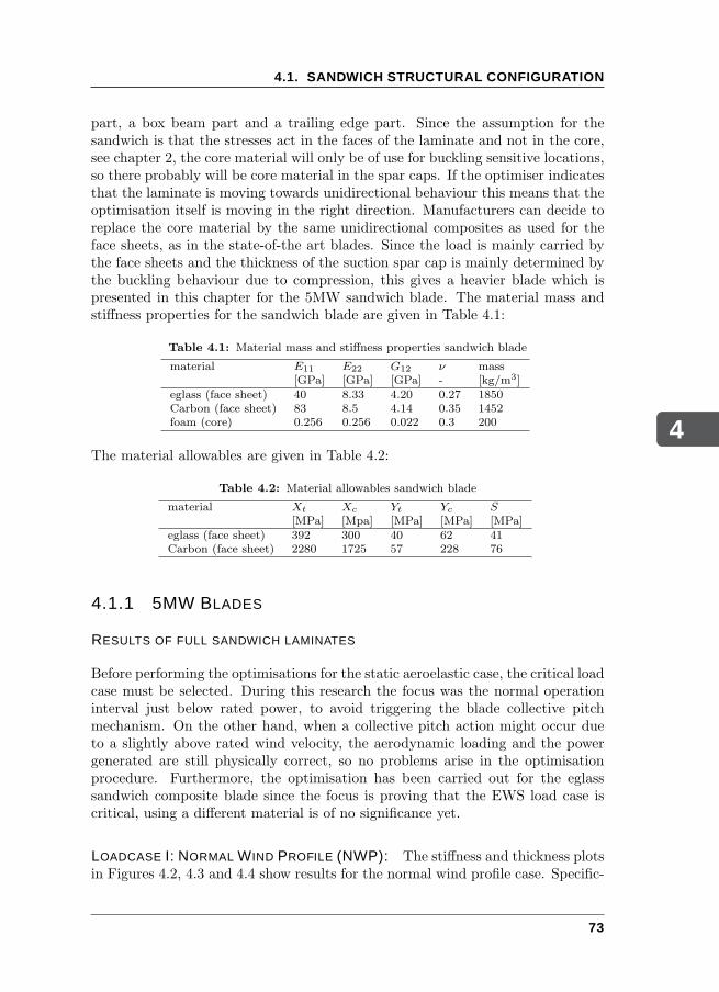
4
4.1. SANDWICH STRUCTURAL CONFIGURATION
part, a box beam part and a trailing edge part. Since the assumption for thesandwich is that the stresses act in the faces of the laminate and not in the core,see chapter 2, the core material will only be of use for buckling sensitive locations,so there probably will be core material in the spar caps. If the optimiser indicatesthat the laminate is moving towards unidirectional behaviour this means that theoptimisation itself is moving in the right direction. Manufacturers can decide toreplace the core material by the same unidirectional composites as used for theface sheets, as in the state-of-the art blades. Since the load is mainly carried bythe face sheets and the thickness of the suction spar cap is mainly determined bythe buckling behaviour due to compression, this gives a heavier blade which ispresented in this chapter for the 5MW sandwich blade. The material mass andstiffness properties for the sandwich blade are given in Table 4.1:
Table 4.1: Material mass and stiffness properties sandwich blade
material E11 E22 G12 ν mass[GPa] [GPa] [GPa] - [kg/m3]
eglass (face sheet) 40 8.33 4.20 0.27 1850Carbon (face sheet) 83 8.5 4.14 0.35 1452foam (core) 0.256 0.256 0.022 0.3 200
The material allowables are given in Table 4.2:
Table 4.2: Material allowables sandwich blade
material Xt Xc Yt Yc S[MPa] [Mpa] [MPa] [MPa] [MPa]
eglass (face sheet) 392 300 40 62 41Carbon (face sheet) 2280 1725 57 228 76
4.1.1 5MW BLADES
RESULTS OF FULL SANDWICH LAMINATES
Before performing the optimisations for the static aeroelastic case, the critical loadcase must be selected. During this research the focus was the normal operationinterval just below rated power, to avoid triggering the blade collective pitchmechanism. On the other hand, when a collective pitch action might occur dueto a slightly above rated wind velocity, the aerodynamic loading and the powergenerated are still physically correct, so no problems arise in the optimisationprocedure. Furthermore, the optimisation has been carried out for the eglasssandwich composite blade since the focus is proving that the EWS load case iscritical, using a different material is of no significance yet.
LOADCASE I: NORMAL WIND PROFILE (NWP): The stiffness and thickness plotsin Figures 4.2, 4.3 and 4.4 show results for the normal wind profile case. Specific-
73
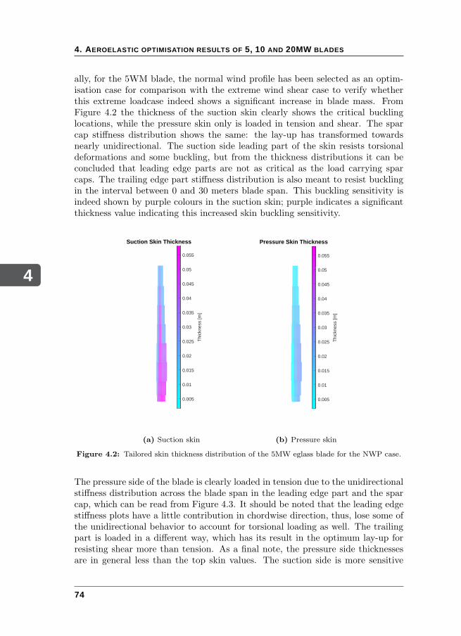
4
4. AEROELASTIC OPTIMISATION RESULTS OF 5, 10 AND 20MW BLADES
ally, for the 5WM blade, the normal wind profile has been selected as an optim-isation case for comparison with the extreme wind shear case to verify whetherthis extreme loadcase indeed shows a significant increase in blade mass. FromFigure 4.2 the thickness of the suction skin clearly shows the critical bucklinglocations, while the pressure skin only is loaded in tension and shear. The sparcap stiffness distribution shows the same: the lay-up has transformed towardsnearly unidirectional. The suction side leading part of the skin resists torsionaldeformations and some buckling, but from the thickness distributions it can beconcluded that leading edge parts are not as critical as the load carrying sparcaps. The trailing edge part stiffness distribution is also meant to resist bucklingin the interval between 0 and 30 meters blade span. This buckling sensitivity isindeed shown by purple colours in the suction skin; purple indicates a significantthickness value indicating this increased skin buckling sensitivity.
Suction Skin Thickness
0.005
0.01
0.015
0.02
0.025
0.03
0.035
0.04
0.045
0.05
0.055
Thi
ckne
ss [m
]
(a) Suction skin
Pressure Skin Thickness
0.005
0.01
0.015
0.02
0.025
0.03
0.035
0.04
0.045
0.05
0.055
Thi
ckne
ss [m
]
(b) Pressure skin
Figure 4.2: Tailored skin thickness distribution of the 5MW eglass blade for the NWP case.
The pressure side of the blade is clearly loaded in tension due to the unidirectionalstiffness distribution across the blade span in the leading edge part and the sparcap, which can be read from Figure 4.3. It should be noted that the leading edgestiffness plots have a little contribution in chordwise direction, thus, lose some ofthe unidirectional behavior to account for torsional loading as well. The trailingpart is loaded in a different way, which has its result in the optimum lay-up forresisting shear more than tension. As a final note, the pressure side thicknessesare in general less than the top skin values. The suction side is more sensitive
74
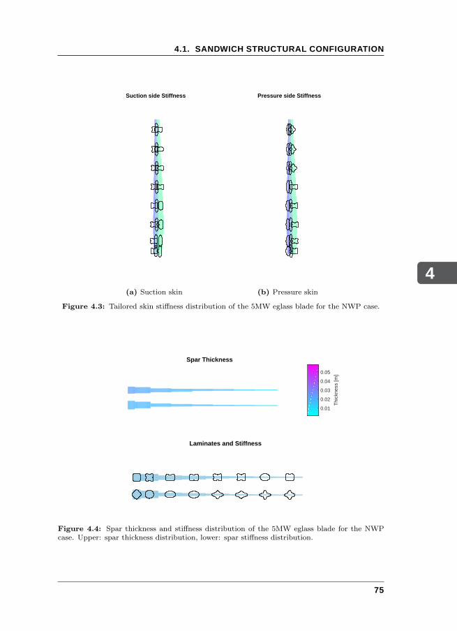
4
4.1. SANDWICH STRUCTURAL CONFIGURATION
Suction side Stiffness
(a) Suction skin
Pressure side Stiffness
(b) Pressure skin
Figure 4.3: Tailored skin stiffness distribution of the 5MW eglass blade for the NWP case.
Spar Thickness
0.01
0.02
0.03
0.04
0.05
Thi
ckne
ss [m
]
Laminates and Stiffness
Figure 4.4: Spar thickness and stiffness distribution of the 5MW eglass blade for the NWPcase. Upper: spar thickness distribution, lower: spar stiffness distribution.
75
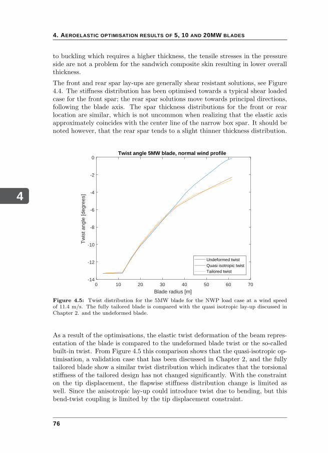
4
4. AEROELASTIC OPTIMISATION RESULTS OF 5, 10 AND 20MW BLADES
to buckling which requires a higher thickness, the tensile stresses in the pressureside are not a problem for the sandwich composite skin resulting in lower overallthickness.
The front and rear spar lay-ups are generally shear resistant solutions, see Figure4.4. The stiffness distribution has been optimised towards a typical shear loadedcase for the front spar; the rear spar solutions move towards principal directions,following the blade axis. The spar thickness distributions for the front or rearlocation are similar, which is not uncommon when realizing that the elastic axisapproximately coincides with the center line of the narrow box spar. It should benoted however, that the rear spar tends to a slight thinner thickness distribution.
0 10 20 30 40 50 60 70
Blade radius [m]
-14
-12
-10
-8
-6
-4
-2
0
Tw
ist a
ngle
[deg
rees
]
Twist angle 5MW blade, normal wind profile
Undeformed twistQuasi isotropic twistTailored twist
Figure 4.5: Twist distribution for the 5MW blade for the NWP load case at a wind speedof 11.4 m/s. The fully tailored blade is compared with the quasi isotropic lay-up discussed inChapter 2. and the undeformed blade.
As a result of the optimisations, the elastic twist deformation of the beam repres-entation of the blade is compared to the undeformed blade twist or the so-calledbuilt-in twist. From Figure 4.5 this comparison shows that the quasi-isotropic op-timisation, a validation case that has been discussed in Chapter 2, and the fullytailored blade show a similar twist distribution which indicates that the torsionalstiffness of the tailored design has not changed significantly. With the constrainton the tip displacement, the flapwise stiffness distribution change is limited aswell. Since the anisotropic lay-up could introduce twist due to bending, but thisbend-twist coupling is limited by the tip displacement constraint.
76
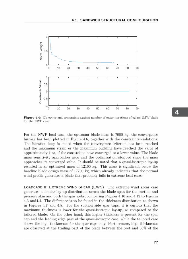
4
4.1. SANDWICH STRUCTURAL CONFIGURATION
0 10 20 30 40 50 60 70 80 900
0.5
1
Nor
m. W
eigh
t
0 10 20 30 40 50 60 70 80 90-1
-0.5
0
0.5
1
Con
stra
ints
Vio
lat.
Figure 4.6: Objective and constraints against number of outer iterations of eglass 5MW bladefor the NWP case.
For the NWP load case, the optimum blade mass is 7900 kg, the convergencehistory has been plotted in Figure 4.6, together with the constraints violations.The iteration loop is ended when the convergence criterion has been reachedand the maximum strain or the maximum buckling have reached the value ofapproximately 1 or, if the constraints have converged to a lower value. The blademass sensitivity approaches zero and the optimization stopped since the massapproaches its converged value. It should be noted that a quasi-isotropic lay-upresulted in an optimised mass of 12100 kg. This mass is significant below thebaseline blade design mass of 17700 kg, which already indicates that the normalwind profile generates a blade that probably fails in extreme load cases.
LOADCASE II: EXTREME WIND SHEAR (EWS) The extreme wind shear casegenerates a similar lay-up distribution across the blade span for the suction andpressure skin and both the spar webs, comparing Figures 4.10 and 4.12 to Figures4.3 and4.4. The difference is to be found in the thickness distribution as shownin Figures 4.7 and 4.8. For the suction side spar caps, it is curious that themaximum thickness is lower for the quasi-isotropic lay-up, as compared to thetailored blade. On the other hand, this higher thickness is present for the sparcap and the leading edge part of the quasi-isotropic case, while the tailored caseshows the high thicknesses for the spar caps only. Furthermore, high thicknessesare observed at the trailing part of the blade between the root and 33% of the
77
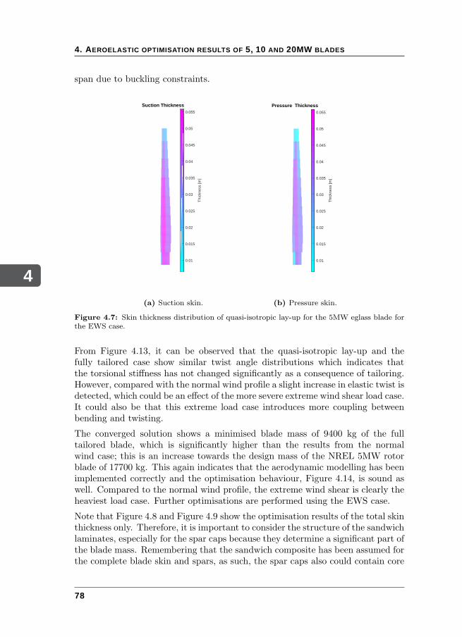
4
4. AEROELASTIC OPTIMISATION RESULTS OF 5, 10 AND 20MW BLADES
span due to buckling constraints.
Suction Thickness
0.01
0.015
0.02
0.025
0.03
0.035
0.04
0.045
0.05
0.055
Thi
ckne
ss [m
]
(a) Suction skin.
Pressure Thickness
0.01
0.015
0.02
0.025
0.03
0.035
0.04
0.045
0.05
0.055
Thi
ckne
ss [m
]
(b) Pressure skin.
Figure 4.7: Skin thickness distribution of quasi-isotropic lay-up for the 5MW eglass blade forthe EWS case.
From Figure 4.13, it can be observed that the quasi-isotropic lay-up and thefully tailored case show similar twist angle distributions which indicates thatthe torsional stiffness has not changed significantly as a consequence of tailoring.However, compared with the normal wind profile a slight increase in elastic twist isdetected, which could be an effect of the more severe extreme wind shear load case.It could also be that this extreme load case introduces more coupling betweenbending and twisting.
The converged solution shows a minimised blade mass of 9400 kg of the fulltailored blade, which is significantly higher than the results from the normalwind case; this is an increase towards the design mass of the NREL 5MW rotorblade of 17700 kg. This again indicates that the aerodynamic modelling has beenimplemented correctly and the optimisation behaviour, Figure 4.14, is sound aswell. Compared to the normal wind profile, the extreme wind shear is clearly theheaviest load case. Further optimisations are performed using the EWS case.
Note that Figure 4.8 and Figure 4.9 show the optimisation results of the total skinthickness only. Therefore, it is important to consider the structure of the sandwichlaminates, especially for the spar caps because they determine a significant part ofthe blade mass. Remembering that the sandwich composite has been assumed forthe complete blade skin and spars, as such, the spar caps also could contain core
78
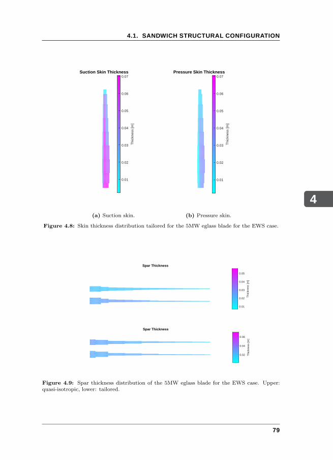
4
4.1. SANDWICH STRUCTURAL CONFIGURATION
Suction Skin Thickness
0.01
0.02
0.03
0.04
0.05
0.06
0.07
Thi
ckne
ss [m
]
(a) Suction skin.
Pressure Skin Thickness
0.01
0.02
0.03
0.04
0.05
0.06
0.07
Thi
ckne
ss [m
]
(b) Pressure skin.
Figure 4.8: Skin thickness distribution tailored for the 5MW eglass blade for the EWS case.
Spar Thickness
0.01
0.02
0.03
0.04
0.05
Thi
ckne
ss [m
]
Spar Thickness
0.02
0.04
0.06
Thi
ckne
ss [m
]
Figure 4.9: Spar thickness distribution of the 5MW eglass blade for the EWS case. Upper:quasi-isotropic, lower: tailored.
79
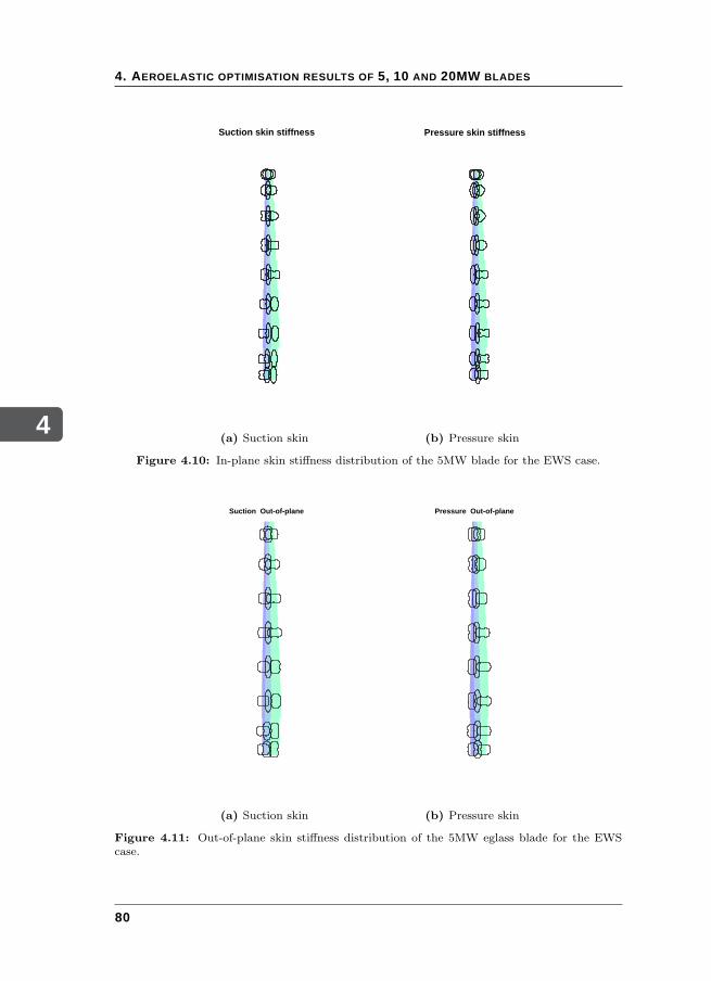
4
4. AEROELASTIC OPTIMISATION RESULTS OF 5, 10 AND 20MW BLADES
Suction skin stiffness
(a) Suction skin
Pressure skin stiffness
(b) Pressure skin
Figure 4.10: In-plane skin stiffness distribution of the 5MW blade for the EWS case.
Suction Out-of-plane
(a) Suction skin
Pressure Out-of-plane
(b) Pressure skin
Figure 4.11: Out-of-plane skin stiffness distribution of the 5MW eglass blade for the EWScase.
80
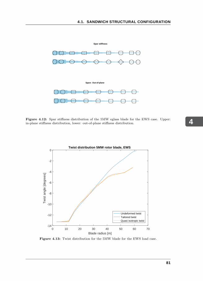
4
4.1. SANDWICH STRUCTURAL CONFIGURATION
Spar stiffness
Spars Out-of-plane
Figure 4.12: Spar stiffness distribution of the 5MW eglass blade for the EWS case. Upper:in-plane stiffness distribution, lower: out-of-plane stiffness distribution.
0 10 20 30 40 50 60 70
Blade radius [m]
-14
-12
-10
-8
-6
-4
-2
0
Tw
ist a
ngle
[deg
rees
]
Twist distribution 5MW rotor blade, EWS
Undeformed twistTailored twistQuasi isotropic twist
Figure 4.13: Twist distribution for the 5MW blade for the EWS load case.
81
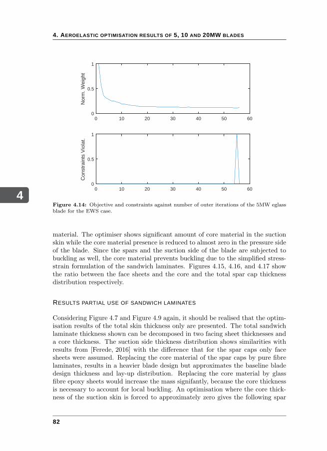
4
4. AEROELASTIC OPTIMISATION RESULTS OF 5, 10 AND 20MW BLADES
0 10 20 30 40 50 600
0.5
1
Nor
m. W
eigh
t
0 10 20 30 40 50 600
0.5
1
Con
stra
ints
Vio
lat.
Figure 4.14: Objective and constraints against number of outer iterations of the 5MW eglassblade for the EWS case.
material. The optimiser shows significant amount of core material in the suctionskin while the core material presence is reduced to almost zero in the pressure sideof the blade. Since the spars and the suction side of the blade are subjected tobuckling as well, the core material prevents buckling due to the simplified stress-strain formulation of the sandwich laminates. Figures 4.15, 4.16, and 4.17 showthe ratio between the face sheets and the core and the total spar cap thicknessdistribution respectively.
RESULTS PARTIAL USE OF SANDWICH LAMINATES
Considering Figure 4.7 and Figure 4.9 again, it should be realised that the optim-isation results of the total skin thickness only are presented. The total sandwichlaminate thickness shown can be decomposed in two facing sheet thicknesses anda core thickness. The suction side thickness distribution shows similarities withresults from [Ferede, 2016] with the difference that for the spar caps only facesheets were assumed. Replacing the core material of the spar caps by pure fibrelaminates, results in a heavier blade design but approximates the baseline bladedesign thickness and lay-up distribution. Replacing the core material by glassfibre epoxy sheets would increase the mass signifantly, because the core thicknessis necessary to account for local buckling. An optimisation where the core thick-ness of the suction skin is forced to approximately zero gives the following spar
82
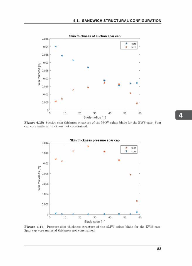
4
4.1. SANDWICH STRUCTURAL CONFIGURATION
0 10 20 30 40 50 60
Blade radius [m]
0
0.005
0.01
0.015
0.02
0.025
0.03
0.035
0.04
0.045S
kin
thik
ness
[m]
Skin thickness of suction spar cap
coreface
Figure 4.15: Suction skin thickness structure of the 5MW eglass blade for the EWS case. Sparcap core material thickness not constrained.
0 10 20 30 40 50 60
Blade span [m]
0
0.002
0.004
0.006
0.008
0.01
0.012
0.014
Ski
n th
ickn
ess
[m]
Skin thickness pressure spar cap
facecore
Figure 4.16: Pressure skin thickness structure of the 5MW eglass blade for the EWS case.Spar cap core material thickness not constrained.
83
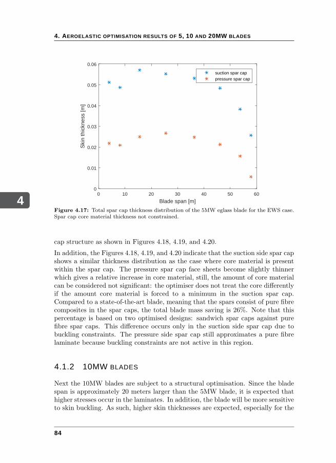
4
4. AEROELASTIC OPTIMISATION RESULTS OF 5, 10 AND 20MW BLADES
0 10 20 30 40 50 60
Blade span [m]
0
0.01
0.02
0.03
0.04
0.05
0.06
Ski
n th
ickn
ess
[m]
suction spar cappressure spar cap
Figure 4.17: Total spar cap thickness distribution of the 5MW eglass blade for the EWS case.Spar cap core material thickness not constrained.
cap structure as shown in Figures 4.18, 4.19, and 4.20.
In addition, the Figures 4.18, 4.19, and 4.20 indicate that the suction side spar capshows a similar thickness distribution as the case where core material is presentwithin the spar cap. The pressure spar cap face sheets become slightly thinnerwhich gives a relative increase in core material, still, the amount of core materialcan be considered not significant: the optimiser does not treat the core differentlyif the amount core material is forced to a minimum in the suction spar cap.Compared to a state-of-the-art blade, meaning that the spars consist of pure fibrecomposites in the spar caps, the total blade mass saving is 26%. Note that thispercentage is based on two optimised designs: sandwich spar caps against purefibre spar caps. This difference occurs only in the suction side spar cap due tobuckling constraints. The pressure side spar cap still approximates a pure fibrelaminate because buckling constraints are not active in this region.
4.1.2 10MW BLADES
Next the 10MW blades are subject to a structural optimisation. Since the bladespan is approximately 20 meters larger than the 5MW blade, it is expected thathigher stresses occur in the laminates. In addition, the blade will be more sensitiveto skin buckling. As such, higher skin thicknesses are expected, especially for the
84
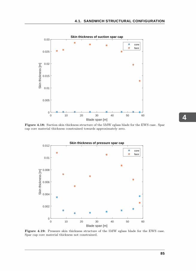
4
4.1. SANDWICH STRUCTURAL CONFIGURATION
0 10 20 30 40 50 60
Blade span [m]
0
0.005
0.01
0.015
0.02
0.025
0.03S
kin
thic
knes
s [m
]Skin thickness of suction spar cap
coreface
Figure 4.18: Suction skin thickness structure of the 5MW eglass blade for the EWS case. Sparcap core material thickness constrained towards approximately zero.
0 10 20 30 40 50 60
Blade span [m]
0
0.002
0.004
0.006
0.008
0.01
0.012
Ski
n th
ickn
ess
[m]
Skin thickness of pressure spar cap
coreface
Figure 4.19: Pressure skin thickness structure of the 5MW eglass blade for the EWS case.Spar cap core material thickness not constrained.
85
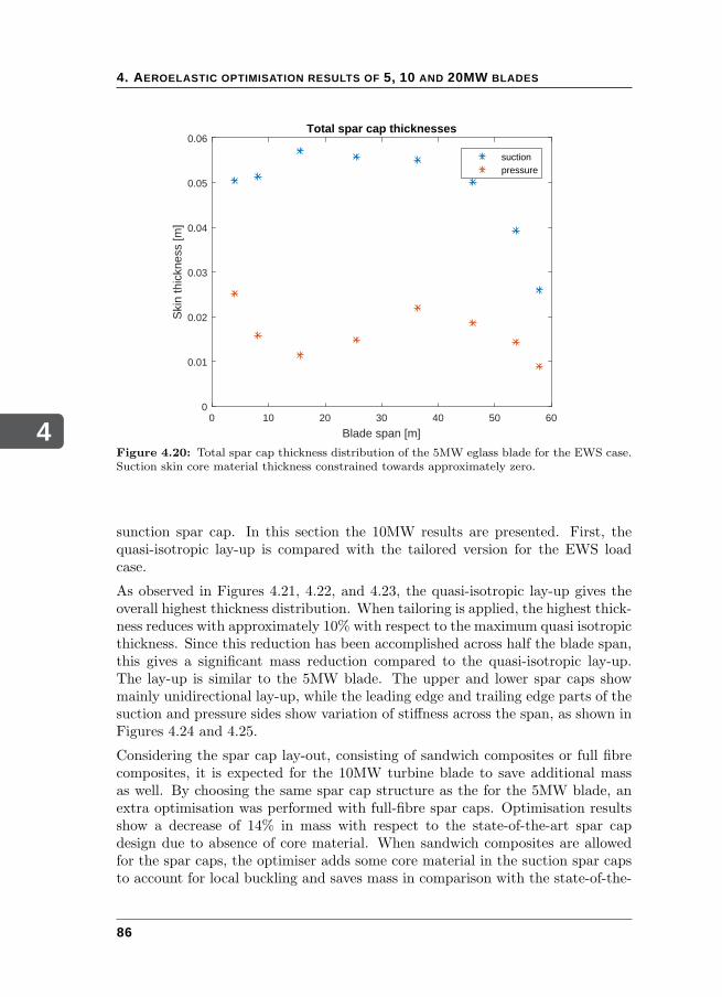
4
4. AEROELASTIC OPTIMISATION RESULTS OF 5, 10 AND 20MW BLADES
0 10 20 30 40 50 60
Blade span [m]
0
0.01
0.02
0.03
0.04
0.05
0.06
Ski
n th
ickn
ess
[m]
Total spar cap thicknesses
suctionpressure
Figure 4.20: Total spar cap thickness distribution of the 5MW eglass blade for the EWS case.Suction skin core material thickness constrained towards approximately zero.
sunction spar cap. In this section the 10MW results are presented. First, thequasi-isotropic lay-up is compared with the tailored version for the EWS loadcase.
As observed in Figures 4.21, 4.22, and 4.23, the quasi-isotropic lay-up gives theoverall highest thickness distribution. When tailoring is applied, the highest thick-ness reduces with approximately 10% with respect to the maximum quasi isotropicthickness. Since this reduction has been accomplished across half the blade span,this gives a significant mass reduction compared to the quasi-isotropic lay-up.The lay-up is similar to the 5MW blade. The upper and lower spar caps showmainly unidirectional lay-up, while the leading edge and trailing edge parts of thesuction and pressure sides show variation of stiffness across the span, as shown inFigures 4.24 and 4.25.
Considering the spar cap lay-out, consisting of sandwich composites or full fibrecomposites, it is expected for the 10MW turbine blade to save additional massas well. By choosing the same spar cap structure as the for the 5MW blade, anextra optimisation was performed with full-fibre spar caps. Optimisation resultsshow a decrease of 14% in mass with respect to the state-of-the-art spar capdesign due to absence of core material. When sandwich composites are allowedfor the spar caps, the optimiser adds some core material in the suction spar capsto account for local buckling and saves mass in comparison with the state-of-the-
86
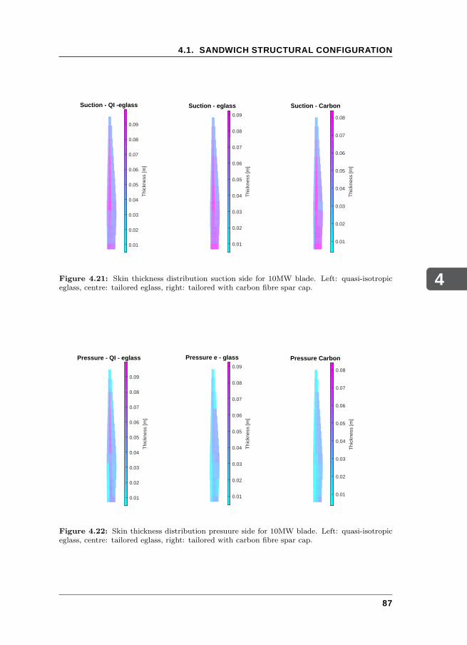
4
4.1. SANDWICH STRUCTURAL CONFIGURATION
Suction - QI -eglass
0.01
0.02
0.03
0.04
0.05
0.06
0.07
0.08
0.09
Thi
ckne
ss [m
]
Suction - eglass
0.01
0.02
0.03
0.04
0.05
0.06
0.07
0.08
0.09
Thi
ckne
ss [m
]
Suction - Carbon
0.01
0.02
0.03
0.04
0.05
0.06
0.07
0.08
Thi
ckne
ss [m
]
Figure 4.21: Skin thickness distribution suction side for 10MW blade. Left: quasi-isotropiceglass, centre: tailored eglass, right: tailored with carbon fibre spar cap.
Pressure - QI - eglass
0.01
0.02
0.03
0.04
0.05
0.06
0.07
0.08
0.09
Thi
ckne
ss [m
]
Pressure e - glass
0.01
0.02
0.03
0.04
0.05
0.06
0.07
0.08
0.09
Thi
ckne
ss [m
]
Pressure Carbon
0.01
0.02
0.03
0.04
0.05
0.06
0.07
0.08
Thi
ckne
ss [m
]
Figure 4.22: Skin thickness distribution presuure side for 10MW blade. Left: quasi-isotropiceglass, centre: tailored eglass, right: tailored with carbon fibre spar cap.
87
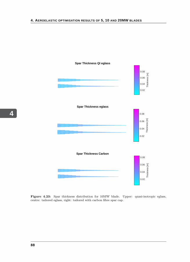
4
4. AEROELASTIC OPTIMISATION RESULTS OF 5, 10 AND 20MW BLADES
Spar Thickness QI eglass
0.02
0.04
0.06
0.08
Thi
ckne
ss [m
]
Spar Thickness eglass
0.02
0.04
0.06
0.08
Thi
ckne
ss [m
]
Spar Thickness Carbon
0.02
0.04
0.06
0.08
Thi
ckne
ss [m
]
Figure 4.23: Spar thickness distribution for 10MW blade. Upper: quasi-isotropic eglass,centre: tailored eglass, right: tailored with carbon fibre spar cap.
88
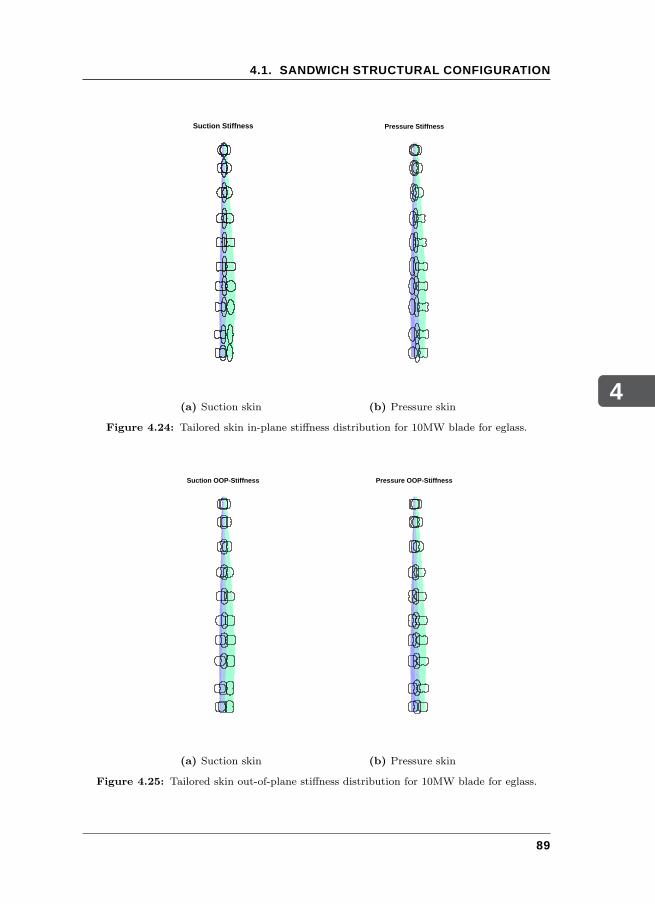
4
4.1. SANDWICH STRUCTURAL CONFIGURATION
Suction Stiffness
(a) Suction skin
Pressure Stiffness
(b) Pressure skin
Figure 4.24: Tailored skin in-plane stiffness distribution for 10MW blade for eglass.
Suction OOP-Stiffness
(a) Suction skin
Pressure OOP-Stiffness
(b) Pressure skin
Figure 4.25: Tailored skin out-of-plane stiffness distribution for 10MW blade for eglass.
89
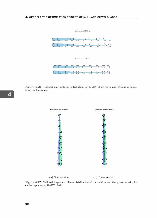
4
4. AEROELASTIC OPTIMISATION RESULTS OF 5, 10 AND 20MW BLADES
Laminates and Stiffness
Laminates and Stiffness
Figure 4.26: Tailored spar stiffness distribution for 10MW blade for eglass. Upper: in-plane,lower: out-of-plane.
(a) Suction skin (b) Pressure skin
Figure 4.27: Tailored in-plane stiffness distribution of the suction and the pressure skin, forcarbon spar caps, 10MW blade.
90
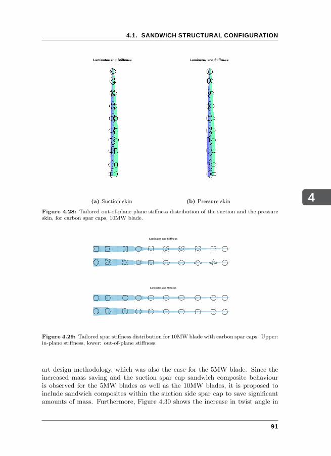
4
4.1. SANDWICH STRUCTURAL CONFIGURATION
(a) Suction skin (b) Pressure skin
Figure 4.28: Tailored out-of-plane plane stiffness distribution of the suction and the pressureskin, for carbon spar caps, 10MW blade.
Laminates and Stiffness
Laminates and Stiffness
Figure 4.29: Tailored spar stiffness distribution for 10MW blade with carbon spar caps. Upper:in-plane stiffness, lower: out-of-plane stiffness.
art design methodology, which was also the case for the 5MW blade. Since theincreased mass saving and the suction spar cap sandwich composite behaviouris observed for the 5MW blades as well as the 10MW blades, it is proposed toinclude sandwich composites within the suction side spar cap to save significantamounts of mass. Furthermore, Figure 4.30 shows the increase in twist angle in
91
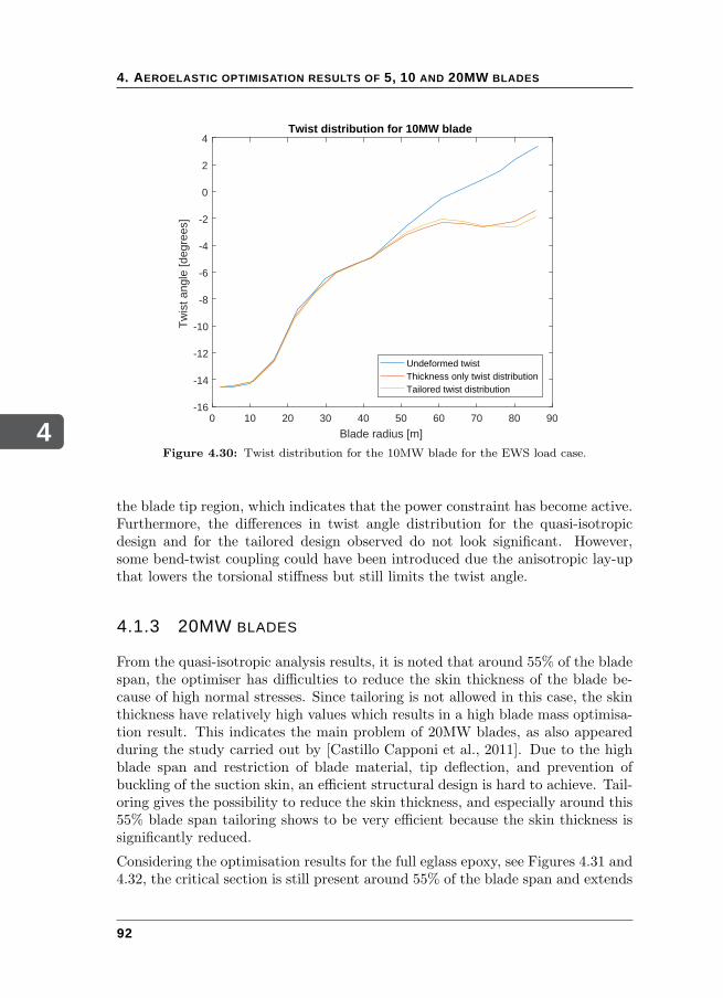
4
4. AEROELASTIC OPTIMISATION RESULTS OF 5, 10 AND 20MW BLADES
0 10 20 30 40 50 60 70 80 90
Blade radius [m]
-16
-14
-12
-10
-8
-6
-4
-2
0
2
4
Tw
ist a
ngle
[deg
rees
]
Twist distribution for 10MW blade
Undeformed twistThickness only twist distributionTailored twist distribution
Figure 4.30: Twist distribution for the 10MW blade for the EWS load case.
the blade tip region, which indicates that the power constraint has become active.Furthermore, the differences in twist angle distribution for the quasi-isotropicdesign and for the tailored design observed do not look significant. However,some bend-twist coupling could have been introduced due the anisotropic lay-upthat lowers the torsional stiffness but still limits the twist angle.
4.1.3 20MW BLADES
From the quasi-isotropic analysis results, it is noted that around 55% of the bladespan, the optimiser has difficulties to reduce the skin thickness of the blade be-cause of high normal stresses. Since tailoring is not allowed in this case, the skinthickness have relatively high values which results in a high blade mass optimisa-tion result. This indicates the main problem of 20MW blades, as also appearedduring the study carried out by [Castillo Capponi et al., 2011]. Due to the highblade span and restriction of blade material, tip deflection, and prevention ofbuckling of the suction skin, an efficient structural design is hard to achieve. Tail-oring gives the possibility to reduce the skin thickness, and especially around this55% blade span tailoring shows to be very efficient because the skin thickness issignificantly reduced.
Considering the optimisation results for the full eglass epoxy, see Figures 4.31 and4.32, the critical section is still present around 55% of the blade span and extends
92
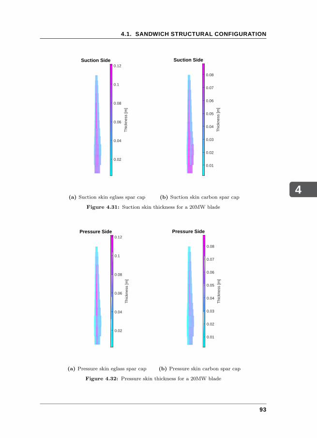
4
4.1. SANDWICH STRUCTURAL CONFIGURATION
Suction Side
0.02
0.04
0.06
0.08
0.1
0.12
Thi
ckne
ss [m
]
(a) Suction skin eglass spar cap
Suction Side
0.01
0.02
0.03
0.04
0.05
0.06
0.07
0.08
Thi
ckne
ss [m
]
(b) Suction skin carbon spar cap
Figure 4.31: Suction skin thickness for a 20MW blade
Pressure Side
0.02
0.04
0.06
0.08
0.1
0.12
Thi
ckne
ss [m
]
(a) Pressure skin eglass spar cap
Pressure Side
0.01
0.02
0.03
0.04
0.05
0.06
0.07
0.08
Thi
ckne
ss [m
]
(b) Pressure skin carbon spar cap
Figure 4.32: Pressure skin thickness for a 20MW blade
93
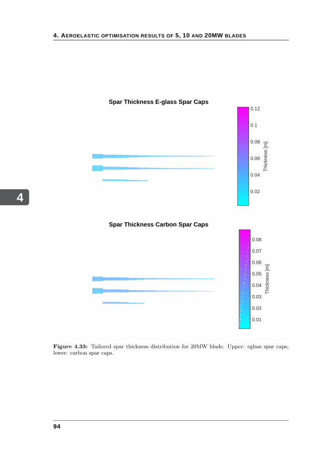
4
4. AEROELASTIC OPTIMISATION RESULTS OF 5, 10 AND 20MW BLADES
Spar Thickness E-glass Spar Caps
0.02
0.04
0.06
0.08
0.1
0.12
Thi
ckne
ss [m
]
Spar Thickness Carbon Spar Caps
0.01
0.02
0.03
0.04
0.05
0.06
0.07
0.08
Thi
ckne
ss [m
]
Figure 4.33: Tailored spar thickness distribution for 20MW blade. Upper: eglass spar caps,lower: carbon spar caps.
94
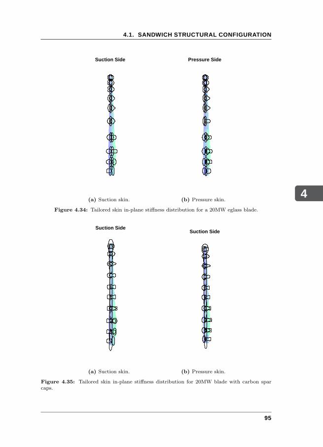
4
4.1. SANDWICH STRUCTURAL CONFIGURATION
Suction Side
(a) Suction skin.
Pressure Side
(b) Pressure skin.
Figure 4.34: Tailored skin in-plane stiffness distribution for a 20MW eglass blade.
Suction Side
(a) Suction skin.
Suction Side
(b) Pressure skin.
Figure 4.35: Tailored skin in-plane stiffness distribution for 20MW blade with carbon sparcaps.
95
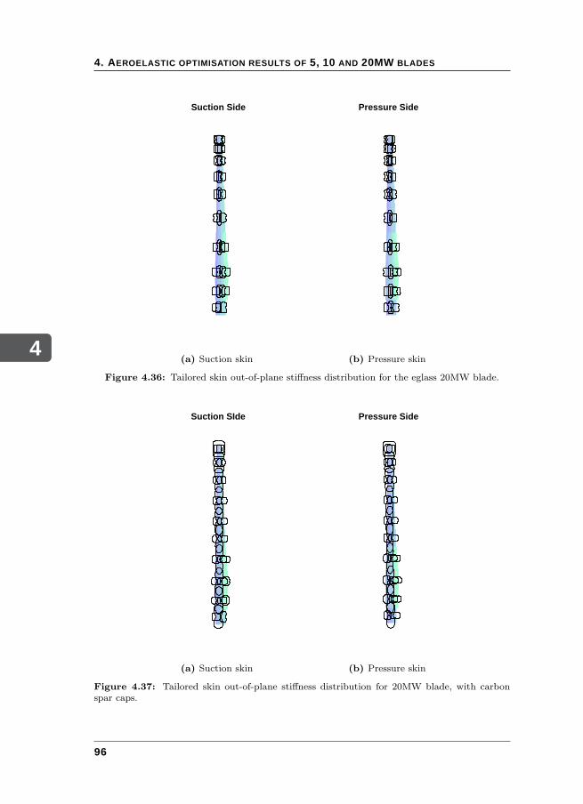
4
4. AEROELASTIC OPTIMISATION RESULTS OF 5, 10 AND 20MW BLADES
Suction Side
(a) Suction skin
Pressure Side
(b) Pressure skin
Figure 4.36: Tailored skin out-of-plane stiffness distribution for the eglass 20MW blade.
Suction SIde
(a) Suction skin
Pressure Side
(b) Pressure skin
Figure 4.37: Tailored skin out-of-plane stiffness distribution for 20MW blade, with carbonspar caps.
96
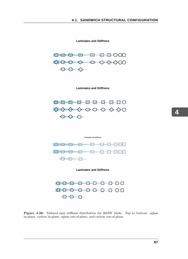
4
4.1. SANDWICH STRUCTURAL CONFIGURATION
Laminates and Stiffness
Laminates and Stiffness
Laminates and Stiffness
Laminates and Stiffness
Figure 4.38: Tailored spar stiffness distribution for 20MW blade. Top to bottom: eglassin-plane, carbon in-plane, eglass out-of-plane, and carbon out-of-plane.
97
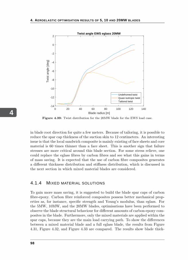
4
4. AEROELASTIC OPTIMISATION RESULTS OF 5, 10 AND 20MW BLADES
0 20 40 60 80 100 120 140
Blade radius [m]
-14
-12
-10
-8
-6
-4
-2
0
2
Tw
ist a
ngle
[deg
]
Twist angle EWS eglass 20MW
Undefromed twistQuasi isotropic twistTailored twist
Figure 4.39: Twist distribution for the 20MW blade for the EWS load case.
in blade root direction for quite a few meters. Because of tailoring, it is possible toreduce the spar cap thickness of the suction skin to 12 centimeters. An interestingissue is that the local sandwich composite is mainly existing of face sheets and corematerial is 60 times thinner than a face sheet. This is another sign that failurestresses are more critical around this blade section. For some stress relieve, onecould replace the eglass fibres by carbon fibres and see what this gains in termsof mass saving. It is expected that the use of carbon fibre composites generatesa different thickness distribution and stiffness distribution, which is discussed inthe next section in which mixed material blades are considered.
4.1.4 MIXED MATERIAL SOLUTIONS
To gain more mass saving, it is suggested to build the blade spar caps of carbonfibre-epoxy. Carbon fibre reinforced composites possess better mechanical prop-erties as, for instance, specific strength and Young’s modulus, than eglass. Forthe 5MW, 10MW, and the 20MW blades, optimisations have been performed toobserve the blade structural behaviour for different amounts of carbon-epoxy com-posites in the blade. Furthermore, only the mixed materials are applied within thespar caps, because they are the main load carrying path. To show the differencesbetween a mixed material blade and a full eglass blade, the results from Figure4.31, Figure 4.32, and Figure 4.33 are compared. The results show blade thick-
98
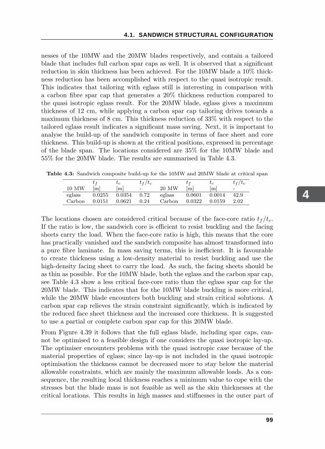
4
4.1. SANDWICH STRUCTURAL CONFIGURATION
nesses of the 10MW and the 20MW blades respectively, and contain a tailoredblade that includes full carbon spar caps as well. It is observed that a significantreduction in skin thickness has been achieved. For the 10MW blade a 10% thick-ness reduction has been accomplished with respect to the quasi isotropic result.This indicates that tailoring with eglass still is interesting in comparison witha carbon fibre spar cap that generates a 20% thickness reduction compared tothe quasi isotropic eglass result. For the 20MW blade, eglass gives a maximumthickness of 12 cm, while applying a carbon spar cap tailoring drives towards amaximum thickness of 8 cm. This thickness reduction of 33% with respect to thetailored eglass result indicates a significant mass saving. Next, it is important toanalyse the build-up of the sandwich composite in terms of face sheet and corethickness. This build-up is shown at the critical positions, expressed in percentageof the blade span. The locations considered are 35% for the 10MW blade and55% for the 20MW blade. The results are summarised in Table 4.3.
Table 4.3: Sandwich composite build-up for the 10MW and 20MW blade at critical span
tf tc tf/tc tf tc tf/tc10 MW [m] [m] - 20 MW [m] [m] -eglass 0.0255 0.0354 0.72 eglass 0.0601 0.0014 42.9Carbon 0.0151 0.0621 0.24 Carbon 0.0322 0.0159 2.02
The locations chosen are considered critical because of the face-core ratio tf/tc.If the ratio is low, the sandwich core is efficient to resist buckling and the facingsheets carry the load. When the face-core ratio is high, this means that the corehas practically vanished and the sandwich composite has almost transformed intoa pure fibre laminate. In mass saving terms, this is inefficient. It is favourableto create thickness using a low-density material to resist buckling and use thehigh-density facing sheet to carry the load. As such, the facing sheets should beas thin as possible. For the 10MW blade, both the eglass and the carbon spar cap,see Table 4.3 show a less critical face-core ratio than the eglass spar cap for the20MW blade. This indicates that for the 10MW blade buckling is more critical,while the 20MW blade encounters both buckling and strain critical solutions. Acarbon spar cap relieves the strain constraint significantly, which is indicated bythe reduced face sheet thickness and the increased core thickness. It is suggestedto use a partial or complete carbon spar cap for this 20MW blade.
From Figure 4.39 it follows that the full eglass blade, including spar caps, can-not be optimised to a feasible design if one considers the quasi isotropic lay-up.The optimiser encounters problems with the quasi isotropic case because of thematerial properties of eglass; since lay-up is not included in the quasi isotropicoptimisation the thickness cannot be decreased more to stay below the materialallowable constraints, which are mainly the maximum allowable loads. As a con-sequence, the resulting local thickness reaches a minimum value to cope with thestresses but the blade mass is not feasible as well as the skin thicknesses at thecritical locations. This results in high masses and stiffnesses in the outer part of
99
4
4. AEROELASTIC OPTIMISATION RESULTS OF 5, 10 AND 20MW BLADES
the blade, which is pointed out in Figure 4.39. The twist distribution in the outerpart is only 1 degree lower and follows the undeformed twist distribution. Thisindicates a very high torsional stiffness in this region which gives the infeasibleblade design. Furthermore, still for the quasi isotropic case, using the carbonmaterial for only 60% of the spar caps this gives a clear picture of the effect onthe total blade. From root to approximately 60% of the blade span the powerconstraint becomes active, which can be seen from the change in elastic twistangle. For spar cap locations consisting of eglass, the thickness is a problem andcauses high stiffnesses again, as can be concluded from the twist angle distribu-tion. However, allowing tailoring, one observes a significant increase in twist anglein the outer blade section, resulting from decreasing thickness due to tailoring.Again, this twist angle distribution is a combination of reduced torsional stiffnessand bend-twist coupling terms that limit the twist angles due to the decreasedtorsional stiffness.
From the stiffness plots, see Figures 4.35, 4.37, and 4.38 together with the twistdistribution plots, it can be deducted that the carbon spar caps give significantimprovements in the mass optimisation results. Because of the favourable stiffnessand the stress allowables of the carbon epoxy laminate, the torsional stiffness ofthe outer blade section decreases due to the aerodynamic power constraint thathas been triggered. In conclusion: the main problem occurs beyond 35% of theblade span for the 10MW and 20MW eglass blades. The mixed material solutionsare mainly suggested for those cases. Especially for the 20MW blade, the criticalstress location is around 55% of the blade span but the favourable mechanicalproperties of the carbon composite allow more tailoring, which delivers a thicknessreduction in the critical area as well. A tailored blade, including full carbon sparcaps, gives the highest mass and thickness reduction. However, from cost pointof view, a mixed spar cap with partial carbon and partial eglass will also givesignificant mass savings as will be elaborated in section 4.4.
4.2 STIFFENED SKIN BLADE LAY-OUT
In the previous section, the sandwich skin blade optimisation results were shown.The results showed quite some potential for blade mass reduction by alteringthe spar cap lay-out. In this section, a different structural lay-out is proposed:the stiffened skin lay-out used in aircraft wings is applied to a wind turbineblade. These aircraft wing designs include ribs, spars and skin stiffeners insteadof core material used in sandwich laminates. This means that the skin existsof pure laminates and the skin stiffeners as well. The dimensions of the sparbuckling panels are determined by the rib spacing while the skin buckling panelsare determined by the rib spacing and the stringer pitch together. Furthermore,different composite materials are used for the same structural lay-out; the bladesare optimised for eglass-epoxy and carbon-epoxy unidirectional laminates, similar
100
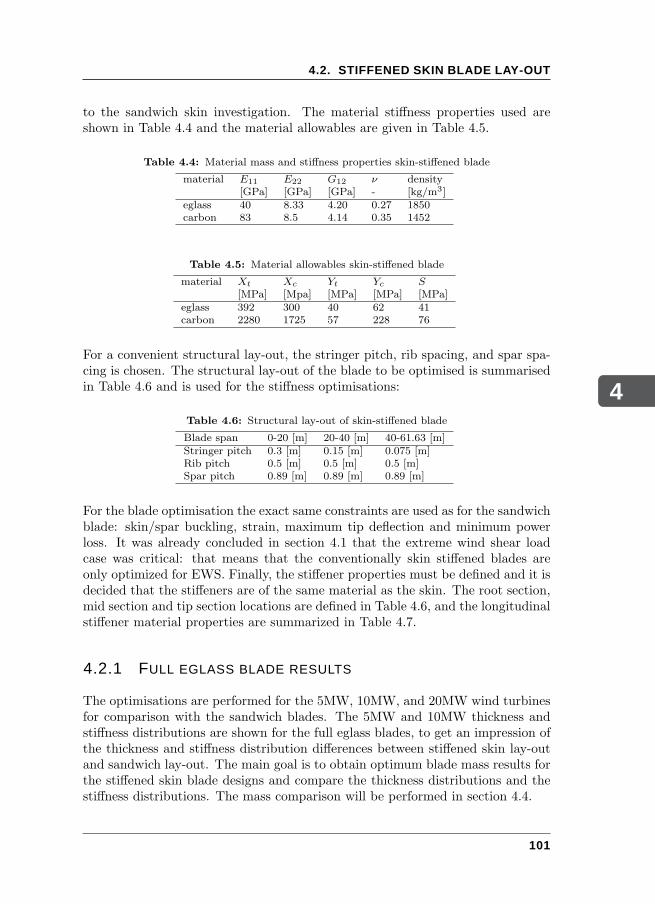
4
4.2. STIFFENED SKIN BLADE LAY-OUT
to the sandwich skin investigation. The material stiffness properties used areshown in Table 4.4 and the material allowables are given in Table 4.5.
Table 4.4: Material mass and stiffness properties skin-stiffened blade
material E11 E22 G12 ν density[GPa] [GPa] [GPa] - [kg/m3]
eglass 40 8.33 4.20 0.27 1850carbon 83 8.5 4.14 0.35 1452
Table 4.5: Material allowables skin-stiffened blade
material Xt Xc Yt Yc S[MPa] [Mpa] [MPa] [MPa] [MPa]
eglass 392 300 40 62 41carbon 2280 1725 57 228 76
For a convenient structural lay-out, the stringer pitch, rib spacing, and spar spa-cing is chosen. The structural lay-out of the blade to be optimised is summarisedin Table 4.6 and is used for the stiffness optimisations:
Table 4.6: Structural lay-out of skin-stiffened blade
Blade span 0-20 [m] 20-40 [m] 40-61.63 [m]Stringer pitch 0.3 [m] 0.15 [m] 0.075 [m]Rib pitch 0.5 [m] 0.5 [m] 0.5 [m]Spar pitch 0.89 [m] 0.89 [m] 0.89 [m]
For the blade optimisation the exact same constraints are used as for the sandwichblade: skin/spar buckling, strain, maximum tip deflection and minimum powerloss. It was already concluded in section 4.1 that the extreme wind shear loadcase was critical: that means that the conventionally skin stiffened blades areonly optimized for EWS. Finally, the stiffener properties must be defined and it isdecided that the stiffeners are of the same material as the skin. The root section,mid section and tip section locations are defined in Table 4.6, and the longitudinalstiffener material properties are summarized in Table 4.7.
4.2.1 FULL EGLASS BLADE RESULTS
The optimisations are performed for the 5MW, 10MW, and 20MW wind turbinesfor comparison with the sandwich blades. The 5MW and 10MW thickness andstiffness distributions are shown for the full eglass blades, to get an impression ofthe thickness and stiffness distribution differences between stiffened skin lay-outand sandwich lay-out. The main goal is to obtain optimum blade mass results forthe stiffened skin blade designs and compare the thickness distributions and thestiffness distributions. The mass comparison will be performed in section 4.4.
101
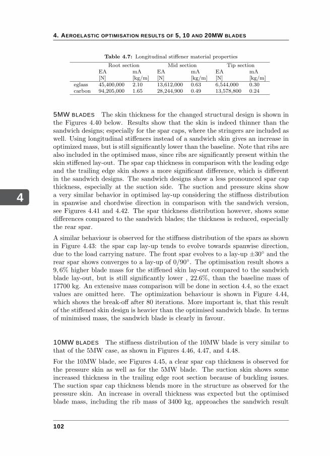
4
4. AEROELASTIC OPTIMISATION RESULTS OF 5, 10 AND 20MW BLADES
Table 4.7: Longitudinal stiffener material properties
Root section Mid section Tip sectionEA mA EA mA EA mA[N] [kg/m] [N] [kg/m] [N] [kg/m]
eglass 45,400,000 2.10 13,612,000 0.63 6,544,000 0.30carbon 94,205,000 1.65 28,244,900 0.49 13,578,800 0.24
5MW BLADES The skin thickness for the changed structural design is shown inthe Figures 4.40 below. Results show that the skin is indeed thinner than thesandwich designs; especially for the spar caps, where the stringers are included aswell. Using longitudinal stiffeners instead of a sandwich skin gives an increase inoptimized mass, but is still significantly lower than the baseline. Note that ribs arealso included in the optimised mass, since ribs are significantly present within theskin stiffened lay-out. The spar cap thickness in comparison with the leading edgeand the trailing edge skin shows a more significant difference, which is differentin the sandwich designs. The sandwich designs show a less pronounced spar capthickness, especially at the suction side. The suction and pressure skins showa very similar behavior in optimised lay-up considering the stiffness distributionin spanwise and chordwise direction in comparison with the sandwich version,see Figures 4.41 and 4.42. The spar thickness distribution however, shows somedifferences compared to the sandwich blades; the thickness is reduced, especiallythe rear spar.
A similar behaviour is observed for the stiffness distribution of the spars as shownin Figure 4.43: the spar cap lay-up tends to evolve towards spanwise direction,due to the load carrying nature. The front spar evolves to a lay-up ±30 and therear spar shows converges to a lay-up of 0/90. The optimisation result shows a9, 6% higher blade mass for the stiffened skin lay-out compared to the sandwichblade lay-out, but is still significantly lower , 22.6%, than the baseline mass of17700 kg. An extensive mass comparison will be done in section 4.4, so the exactvalues are omitted here. The optimization behaviour is shown in Figure 4.44,which shows the break-off after 80 iterations. More important is, that this resultof the stiffened skin design is heavier than the optimised sandwich blade. In termsof minimised mass, the sandwich blade is clearly in favour.
10MW BLADES The stiffness distribution of the 10MW blade is very similar tothat of the 5MW case, as shown in Figures 4.46, 4.47, and 4.48.
For the 10MW blade, see Figures 4.45, a clear spar cap thickness is observed forthe pressure skin as well as for the 5MW blade. The suction skin shows someincreased thickness in the trailing edge root section because of buckling issues.The suction spar cap thickness blends more in the structure as observed for thepressure skin. An increase in overall thickness was expected but the optimisedblade mass, including the rib mass of 3400 kg, approaches the sandwich result
102
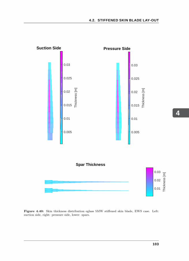
4
4.2. STIFFENED SKIN BLADE LAY-OUT
Suction Side
0.005
0.01
0.015
0.02
0.025
0.03
Thi
ckne
ss [m
]
Pressure Side
0.005
0.01
0.015
0.02
0.025
0.03
Thi
ckne
ss [m
]
Spar Thickness
0.01
0.02
0.03
Thi
ckne
ss [m
]
Figure 4.40: Skin thickness distribution eglass 5MW stiffened skin blade, EWS case. Left:suction side, right: pressure side, lower: spars.
103
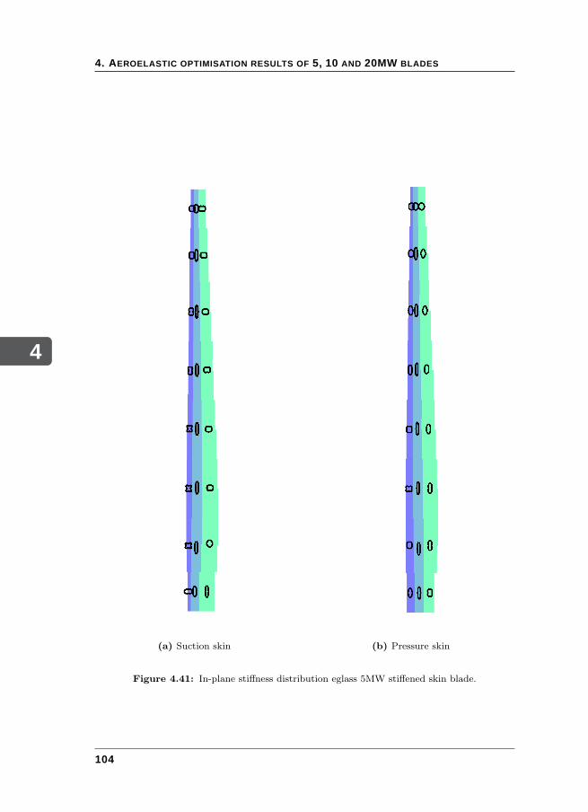
4
4. AEROELASTIC OPTIMISATION RESULTS OF 5, 10 AND 20MW BLADES
(a) Suction skin (b) Pressure skin
Figure 4.41: In-plane stiffness distribution eglass 5MW stiffened skin blade.
104
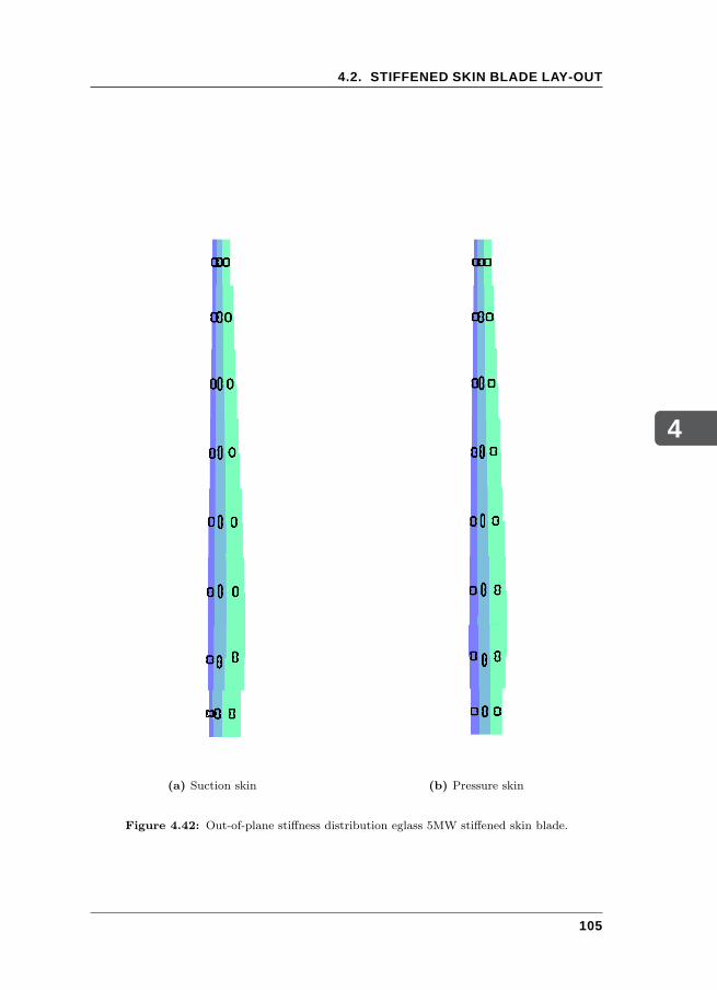
4
4.2. STIFFENED SKIN BLADE LAY-OUT
(a) Suction skin (b) Pressure skin
Figure 4.42: Out-of-plane stiffness distribution eglass 5MW stiffened skin blade.
105
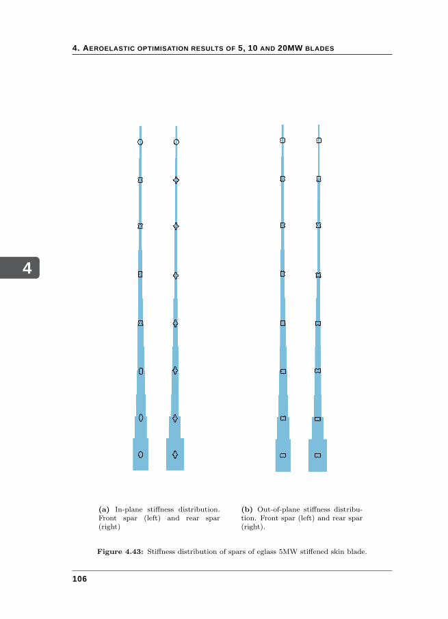
4
4. AEROELASTIC OPTIMISATION RESULTS OF 5, 10 AND 20MW BLADES
(a) In-plane stiffness distribution.Front spar (left) and rear spar(right)
(b) Out-of-plane stiffness distribu-tion. Front spar (left) and rear spar(right).
Figure 4.43: Stiffness distribution of spars of eglass 5MW stiffened skin blade.
106
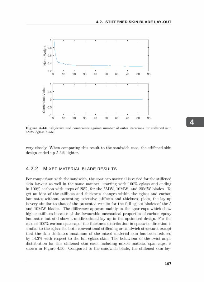
4
4.2. STIFFENED SKIN BLADE LAY-OUT
0 10 20 30 40 50 60 70 80 900.2
0.4
0.6
0.8
1
Nor
m. W
eigh
t
0 10 20 30 40 50 60 70 80 90-1
-0.5
0
0.5
1
Con
stra
ints
Vio
lat.
Figure 4.44: Objective and constraints against number of outer iterations for stiffened skin5MW eglass blade
very closely. When comparing this result to the sandwich case, the stiffened skindesign ended up 5.3% lighter.
4.2.2 MIXED MATERIAL BLADE RESULTS
For comparison with the sandwich, the spar cap material is varied for the stiffenedskin lay-out as well in the same manner: starting with 100% eglass and endingin 100% carbon with steps of 25%, for the 5MW, 10MW, and 20MW blades. Toget an idea of the stiffness and thickness changes within the eglass and carbonlaminates without presenting extensive stiffness and thickness plots, the lay-upis very similar to that of the presented results for the full eglass blades of the 5and 10MW blades. The difference appears mainly in the spar caps which showhigher stiffness because of the favourable mechanical properties of carbon-epoxylaminates but still show a unidirectional lay-up in the optimised design. For thecase of 100% carbon spar caps, the thickness distribution in spanwise direction issimilar to the eglass for both conventional stiffening or sandwich structure, exceptthat the skin thickness maximum of the mixed material skin has been reducedby 14.3% with respect to the full eglass skin. The behaviour of the twist angledistribution for this stiffened skin case, including mixed material spar caps, isshown in Figure 4.50. Compared to the sandwich blade, the stiffened skin lay-
107
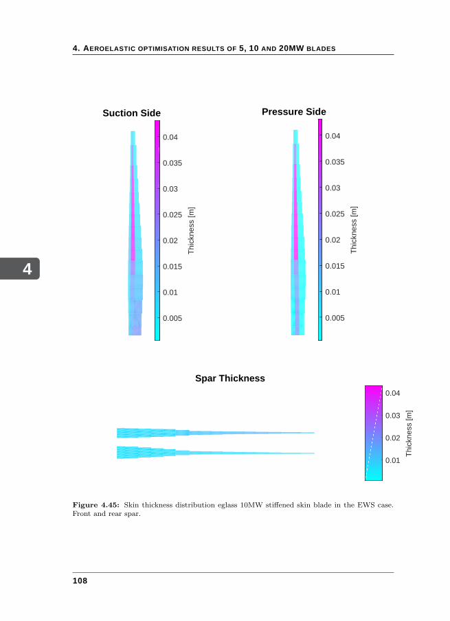
4
4. AEROELASTIC OPTIMISATION RESULTS OF 5, 10 AND 20MW BLADES
Suction Side
0.005
0.01
0.015
0.02
0.025
0.03
0.035
0.04
Thi
ckne
ss [m
]
Pressure Side
0.005
0.01
0.015
0.02
0.025
0.03
0.035
0.04
Thi
ckne
ss [m
]
Spar Thickness
0.01
0.02
0.03
0.04
Thi
ckne
ss [m
]
Figure 4.45: Skin thickness distribution eglass 10MW stiffened skin blade in the EWS case.Front and rear spar.
108
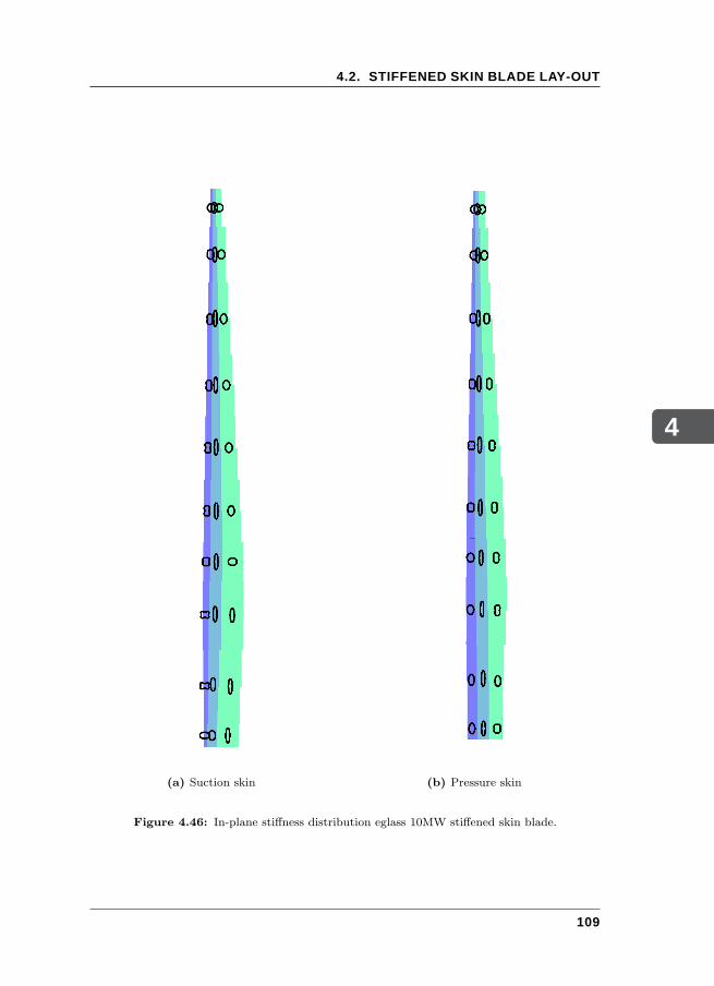
4
4.2. STIFFENED SKIN BLADE LAY-OUT
(a) Suction skin (b) Pressure skin
Figure 4.46: In-plane stiffness distribution eglass 10MW stiffened skin blade.
109
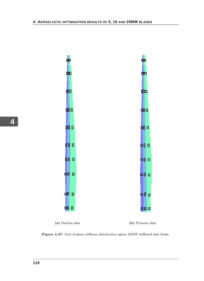
4
4. AEROELASTIC OPTIMISATION RESULTS OF 5, 10 AND 20MW BLADES
(a) Suction skin (b) Pressure skin
Figure 4.47: Out-of-plane stiffness distribution eglass 10MW stiffened skin blade.
110
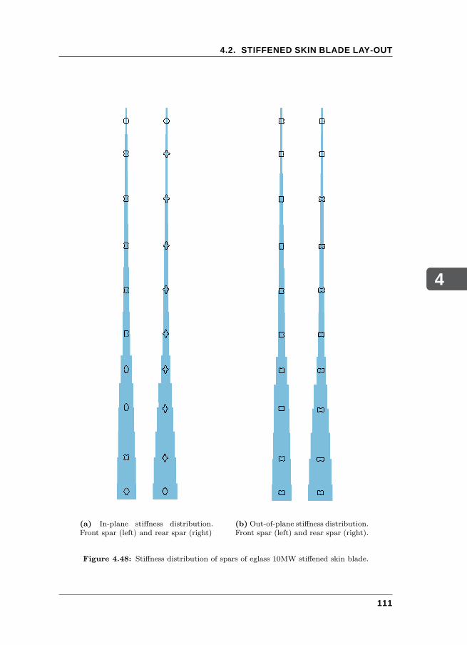
4
4.2. STIFFENED SKIN BLADE LAY-OUT
(a) In-plane stiffness distribution.Front spar (left) and rear spar (right)
(b) Out-of-plane stiffness distribution.Front spar (left) and rear spar (right).
Figure 4.48: Stiffness distribution of spars of eglass 10MW stiffened skin blade.
111
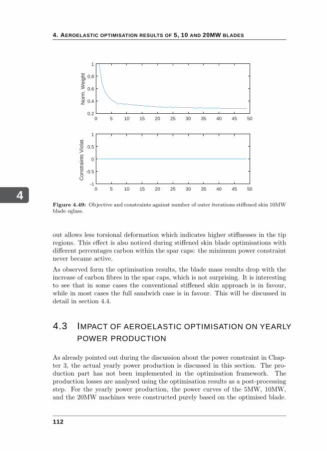
4
4. AEROELASTIC OPTIMISATION RESULTS OF 5, 10 AND 20MW BLADES
0 5 10 15 20 25 30 35 40 45 500.2
0.4
0.6
0.8
1
Nor
m. W
eigh
t
0 5 10 15 20 25 30 35 40 45 50-1
-0.5
0
0.5
1
Con
stra
ints
Vio
lat.
Figure 4.49: Objective and constraints against number of outer iterations stiffened skin 10MWblade eglass.
out allows less torsional deformation which indicates higher stiffnesses in the tipregions. This effect is also noticed during stiffened skin blade optimisations withdifferent percentages carbon within the spar caps: the minimum power constraintnever became active.
As observed form the optimisation results, the blade mass results drop with theincrease of carbon fibres in the spar caps, which is not surprising. It is interestingto see that in some cases the conventional stiffened skin approach is in favour,while in most cases the full sandwich case is in favour. This will be discussed indetail in section 4.4.
4.3 IMPACT OF AEROELASTIC OPTIMISATION ON YEARLY
POWER PRODUCTION
As already pointed out during the discussion about the power constraint in Chap-ter 3, the actual yearly power production is discussed in this section. The pro-duction part has not been implemented in the optimisation framework. Theproduction losses are analysed using the optimisation results as a post-processingstep. For the yearly power production, the power curves of the 5MW, 10MW,and the 20MW machines were constructed purely based on the optimised blade.
112
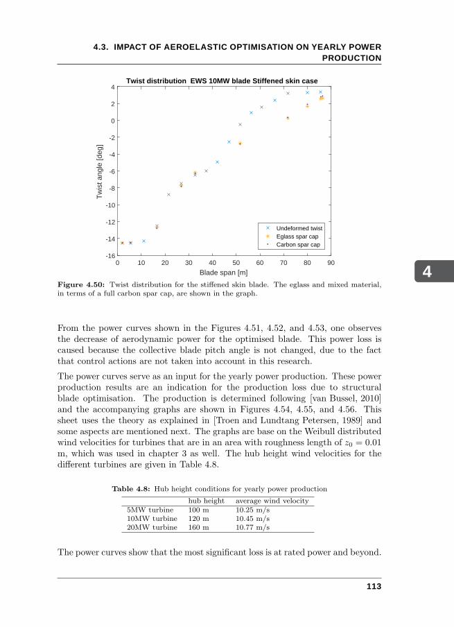
4
4.3. IMPACT OF AEROELASTIC OPTIMISATION ON YEARLY POWERPRODUCTION
0 10 20 30 40 50 60 70 80 90
Blade span [m]
-16
-14
-12
-10
-8
-6
-4
-2
0
2
4
Tw
ist a
ngle
[deg
]
Twist distribution EWS 10MW blade Stiffened skin case
Undeformed twistEglass spar capCarbon spar cap
Figure 4.50: Twist distribution for the stiffened skin blade. The eglass and mixed material,in terms of a full carbon spar cap, are shown in the graph.
From the power curves shown in the Figures 4.51, 4.52, and 4.53, one observesthe decrease of aerodynamic power for the optimised blade. This power loss iscaused because the collective blade pitch angle is not changed, due to the factthat control actions are not taken into account in this research.
The power curves serve as an input for the yearly power production. These powerproduction results are an indication for the production loss due to structuralblade optimisation. The production is determined following [van Bussel, 2010]and the accompanying graphs are shown in Figures 4.54, 4.55, and 4.56. Thissheet uses the theory as explained in [Troen and Lundtang Petersen, 1989] andsome aspects are mentioned next. The graphs are base on the Weibull distributedwind velocities for turbines that are in an area with roughness length of z0 = 0.01m, which was used in chapter 3 as well. The hub height wind velocities for thedifferent turbines are given in Table 4.8.
Table 4.8: Hub height conditions for yearly power production
hub height average wind velocity5MW turbine 100 m 10.25 m/s10MW turbine 120 m 10.45 m/s20MW turbine 160 m 10.77 m/s
The power curves show that the most significant loss is at rated power and beyond.
113
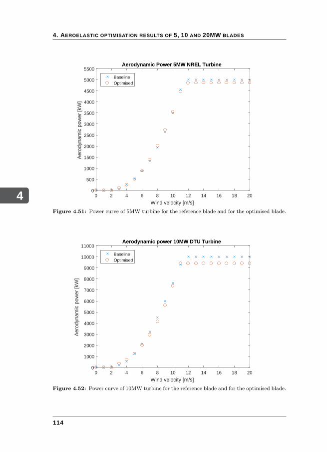
4
4. AEROELASTIC OPTIMISATION RESULTS OF 5, 10 AND 20MW BLADES
0 2 4 6 8 10 12 14 16 18 20
Wind velocity [m/s]
0
500
1000
1500
2000
2500
3000
3500
4000
4500
5000
5500
Aer
odyn
amic
pow
er [k
W]
Aerodynamic Power 5MW NREL Turbine
BaselineOptimised
Figure 4.51: Power curve of 5MW turbine for the reference blade and for the optimised blade.
0 2 4 6 8 10 12 14 16 18 20
Wind velocity [m/s]
0
1000
2000
3000
4000
5000
6000
7000
8000
9000
10000
11000
Aer
odyn
amic
pow
er [k
W]
Aerodynamic power 10MW DTU Turbine
BaselineOptimised
Figure 4.52: Power curve of 10MW turbine for the reference blade and for the optimised blade.
114
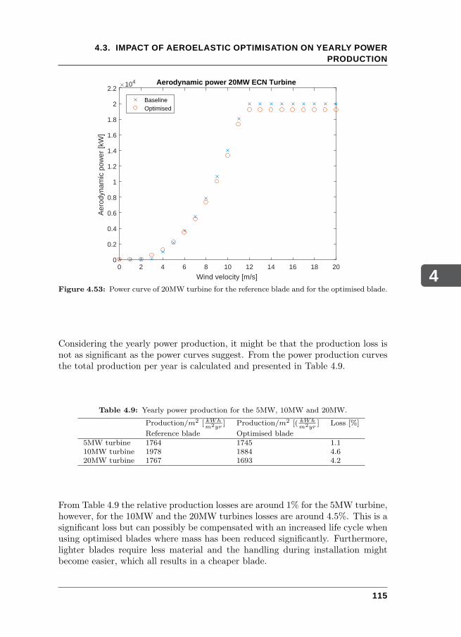
4
4.3. IMPACT OF AEROELASTIC OPTIMISATION ON YEARLY POWERPRODUCTION
0 2 4 6 8 10 12 14 16 18 20
Wind velocity [m/s]
0
0.2
0.4
0.6
0.8
1
1.2
1.4
1.6
1.8
2
2.2
Aer
odyn
amic
pow
er [k
W]
104 Aerodynamic power 20MW ECN Turbine
BaselineOptimised
Figure 4.53: Power curve of 20MW turbine for the reference blade and for the optimised blade.
Considering the yearly power production, it might be that the production loss isnot as significant as the power curves suggest. From the power production curvesthe total production per year is calculated and presented in Table 4.9.
Table 4.9: Yearly power production for the 5MW, 10MW and 20MW.
Production/m2 [ kWhm2yr
] Production/m2 [( kWhm2yr
] Loss [%]
Reference blade Optimised blade5MW turbine 1764 1745 1.110MW turbine 1978 1884 4.620MW turbine 1767 1693 4.2
From Table 4.9 the relative production losses are around 1% for the 5MW turbine,however, for the 10MW and the 20MW turbines losses are around 4.5%. This is asignificant loss but can possibly be compensated with an increased life cycle whenusing optimised blades where mass has been reduced significantly. Furthermore,lighter blades require less material and the handling during installation mightbecome easier, which all results in a cheaper blade.
115
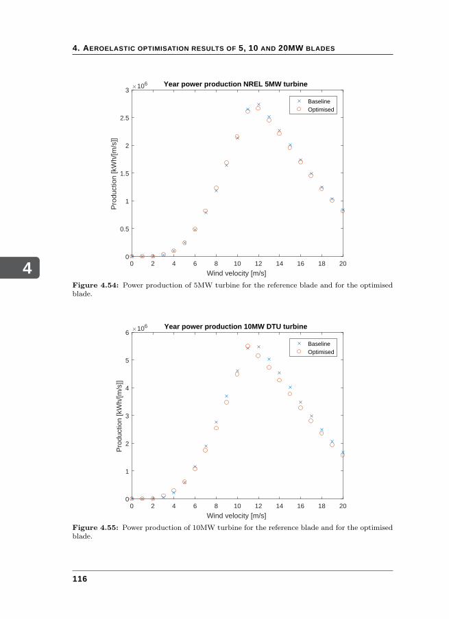
4
4. AEROELASTIC OPTIMISATION RESULTS OF 5, 10 AND 20MW BLADES
0 2 4 6 8 10 12 14 16 18 20
Wind velocity [m/s]
0
0.5
1
1.5
2
2.5
3
Pro
duct
ion
[kW
h/[m
/s]]
106 Year power production NREL 5MW turbine
BaselineOptimised
Figure 4.54: Power production of 5MW turbine for the reference blade and for the optimisedblade.
0 2 4 6 8 10 12 14 16 18 20
Wind velocity [m/s]
0
1
2
3
4
5
6
Pro
duct
ion
[kW
h/[m
/s]]
106 Year power production 10MW DTU turbine
BaselineOptimised
Figure 4.55: Power production of 10MW turbine for the reference blade and for the optimisedblade.
116
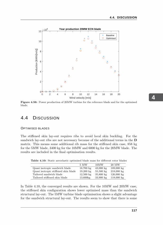
4
4.4. DISCUSSION
0 2 4 6 8 10 12 14 16 18 20
Wind velocity [m/s]
0
2
4
6
8
10
12
Pro
duct
ion
[kW
h/[m
/s]]
106 Year production 20MW ECN blade
BaselineOptimised
Figure 4.56: Power production of 20MW turbine for the reference blade and for the optimisedblade.
4.4 DISCUSSION
OPTIMISED BLADES
The stiffened skin lay-out requires ribs to avoid local skin buckling. For thesandwich lay-out ribs are not necessary because of the additional terms in the D
matrix. This means some additional rib mass for the stiffened skin case, 858 kgfor the 5MW blade, 3400 kg for the 10MW and 6000 kg for the 20MW blade. Theresults are included in the final optimisation results.
Table 4.10: Static aeroelastic optimised blade mass for different rotor blades
5 MW 10MW 20 MWQuasi isotropic sandwich blade 18,700 kg 43,000 kg 189,000 kgQuasi isotropic stiffened skin blade 19,200 kg 55,500 kg 218,000 kgTailored sandwich blade 12,500 kg 35,800 kg 126,000 kgTailored stiffened skin blade 13,600kg 33,900 kg 118,000 kg
In Table 4.10, the converged results are shown. For the 10MW and 20MW case,the stiffened skin configuration shows lower optimised mass than the sandwichstructural lay-out. The 5MW turbine blade optimisation shows a slight advantagefor the sandwich structural lay-out. The results seem to show that there is some
117
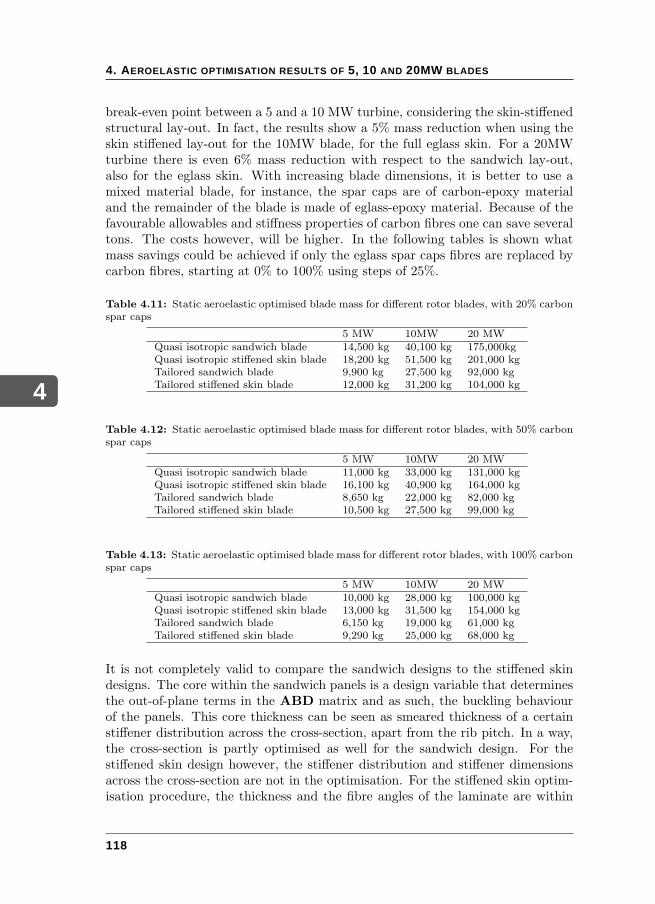
4
4. AEROELASTIC OPTIMISATION RESULTS OF 5, 10 AND 20MW BLADES
break-even point between a 5 and a 10 MW turbine, considering the skin-stiffenedstructural lay-out. In fact, the results show a 5% mass reduction when using theskin stiffened lay-out for the 10MW blade, for the full eglass skin. For a 20MWturbine there is even 6% mass reduction with respect to the sandwich lay-out,also for the eglass skin. With increasing blade dimensions, it is better to use amixed material blade, for instance, the spar caps are of carbon-epoxy materialand the remainder of the blade is made of eglass-epoxy material. Because of thefavourable allowables and stiffness properties of carbon fibres one can save severaltons. The costs however, will be higher. In the following tables is shown whatmass savings could be achieved if only the eglass spar caps fibres are replaced bycarbon fibres, starting at 0% to 100% using steps of 25%.
Table 4.11: Static aeroelastic optimised blade mass for different rotor blades, with 20% carbonspar caps
5 MW 10MW 20 MWQuasi isotropic sandwich blade 14,500 kg 40,100 kg 175,000kgQuasi isotropic stiffened skin blade 18,200 kg 51,500 kg 201,000 kgTailored sandwich blade 9,900 kg 27,500 kg 92,000 kgTailored stiffened skin blade 12,000 kg 31,200 kg 104,000 kg
Table 4.12: Static aeroelastic optimised blade mass for different rotor blades, with 50% carbonspar caps
5 MW 10MW 20 MWQuasi isotropic sandwich blade 11,000 kg 33,000 kg 131,000 kgQuasi isotropic stiffened skin blade 16,100 kg 40,900 kg 164,000 kgTailored sandwich blade 8,650 kg 22,000 kg 82,000 kgTailored stiffened skin blade 10,500 kg 27,500 kg 99,000 kg
Table 4.13: Static aeroelastic optimised blade mass for different rotor blades, with 100% carbonspar caps
5 MW 10MW 20 MWQuasi isotropic sandwich blade 10,000 kg 28,000 kg 100,000 kgQuasi isotropic stiffened skin blade 13,000 kg 31,500 kg 154,000 kgTailored sandwich blade 6,150 kg 19,000 kg 61,000 kgTailored stiffened skin blade 9,290 kg 25,000 kg 68,000 kg
It is not completely valid to compare the sandwich designs to the stiffened skindesigns. The core within the sandwich panels is a design variable that determinesthe out-of-plane terms in the ABD matrix and as such, the buckling behaviourof the panels. This core thickness can be seen as smeared thickness of a certainstiffener distribution across the cross-section, apart from the rib pitch. In a way,the cross-section is partly optimised as well for the sandwich design. For thestiffened skin design however, the stiffener distribution and stiffener dimensionsacross the cross-section are not in the optimisation. For the stiffened skin optim-isation procedure, the thickness and the fibre angles of the laminate are within
118
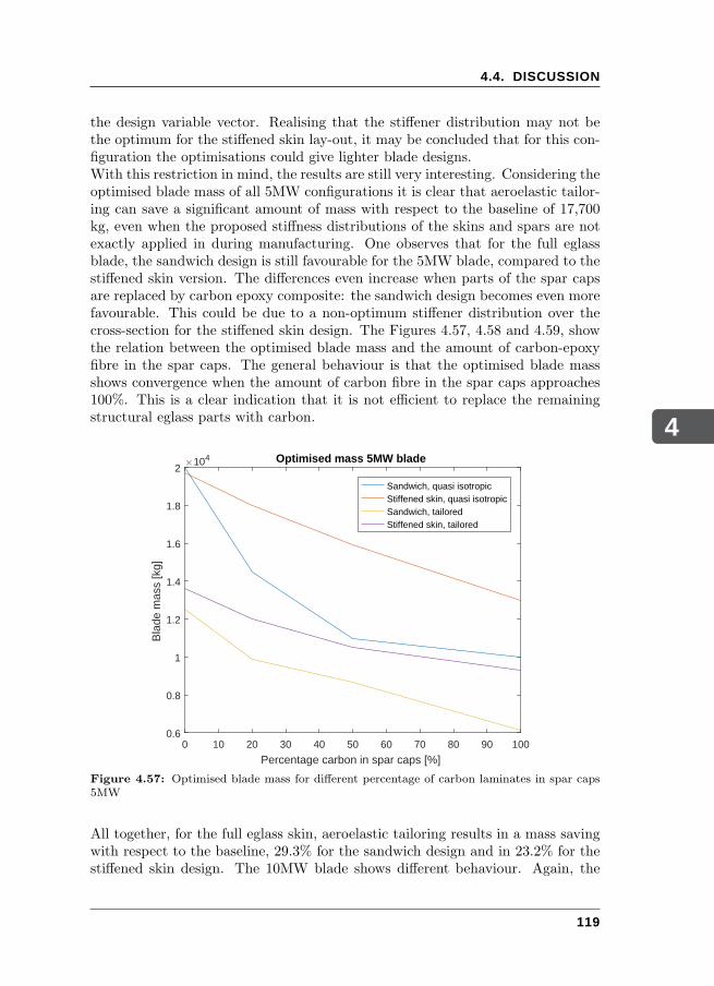
4
4.4. DISCUSSION
the design variable vector. Realising that the stiffener distribution may not bethe optimum for the stiffened skin lay-out, it may be concluded that for this con-figuration the optimisations could give lighter blade designs.With this restriction in mind, the results are still very interesting. Considering theoptimised blade mass of all 5MW configurations it is clear that aeroelastic tailor-ing can save a significant amount of mass with respect to the baseline of 17,700kg, even when the proposed stiffness distributions of the skins and spars are notexactly applied in during manufacturing. One observes that for the full eglassblade, the sandwich design is still favourable for the 5MW blade, compared to thestiffened skin version. The differences even increase when parts of the spar capsare replaced by carbon epoxy composite: the sandwich design becomes even morefavourable. This could be due to a non-optimum stiffener distribution over thecross-section for the stiffened skin design. The Figures 4.57, 4.58 and 4.59, showthe relation between the optimised blade mass and the amount of carbon-epoxyfibre in the spar caps. The general behaviour is that the optimised blade massshows convergence when the amount of carbon fibre in the spar caps approaches100%. This is a clear indication that it is not efficient to replace the remainingstructural eglass parts with carbon.
0 10 20 30 40 50 60 70 80 90 100
Percentage carbon in spar caps [%]
0.6
0.8
1
1.2
1.4
1.6
1.8
2
Bla
de m
ass
[kg]
104 Optimised mass 5MW blade
Sandwich, quasi isotropicStiffened skin, quasi isotropicSandwich, tailoredStiffened skin, tailored
Figure 4.57: Optimised blade mass for different percentage of carbon laminates in spar caps5MW
All together, for the full eglass skin, aeroelastic tailoring results in a mass savingwith respect to the baseline, 29.3% for the sandwich design and in 23.2% for thestiffened skin design. The 10MW blade shows different behaviour. Again, the
119
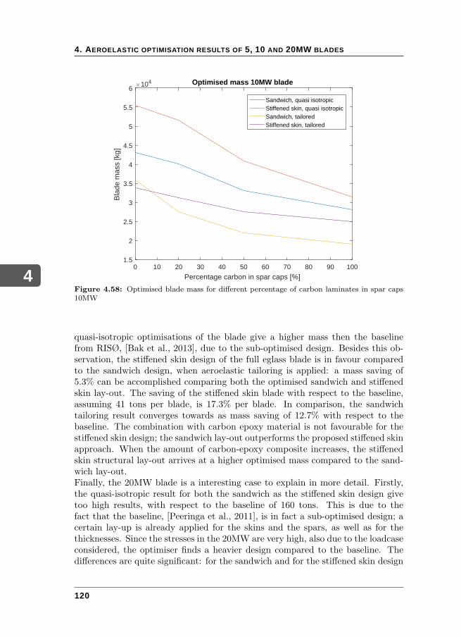
4
4. AEROELASTIC OPTIMISATION RESULTS OF 5, 10 AND 20MW BLADES
0 10 20 30 40 50 60 70 80 90 100
Percentage carbon in spar caps [%]
1.5
2
2.5
3
3.5
4
4.5
5
5.5
6
Bla
de m
ass
[kg]
104 Optimised mass 10MW blade
Sandwich, quasi isotropicStiffened skin, quasi isotropicSandwich, tailoredStiffened skin, tailored
Figure 4.58: Optimised blade mass for different percentage of carbon laminates in spar caps10MW
quasi-isotropic optimisations of the blade give a higher mass then the baselinefrom RISØ, [Bak et al., 2013], due to the sub-optimised design. Besides this ob-servation, the stiffened skin design of the full eglass blade is in favour comparedto the sandwich design, when aeroelastic tailoring is applied: a mass saving of5.3% can be accomplished comparing both the optimised sandwich and stiffenedskin lay-out. The saving of the stiffened skin blade with respect to the baseline,assuming 41 tons per blade, is 17.3% per blade. In comparison, the sandwichtailoring result converges towards as mass saving of 12.7% with respect to thebaseline. The combination with carbon epoxy material is not favourable for thestiffened skin design; the sandwich lay-out outperforms the proposed stiffened skinapproach. When the amount of carbon-epoxy composite increases, the stiffenedskin structural lay-out arrives at a higher optimised mass compared to the sand-wich lay-out.Finally, the 20MW blade is a interesting case to explain in more detail. Firstly,the quasi-isotropic result for both the sandwich as the stiffened skin design givetoo high results, with respect to the baseline of 160 tons. This is due to thefact that the baseline, [Peeringa et al., 2011], is in fact a sub-optimised design; acertain lay-up is already applied for the skins and the spars, as well as for thethicknesses. Since the stresses in the 20MW are very high, also due to the loadcaseconsidered, the optimiser finds a heavier design compared to the baseline. Thedifferences are quite significant: for the sandwich and for the stiffened skin design
120
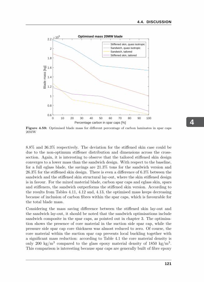
4
4.4. DISCUSSION
0 10 20 30 40 50 60 70 80 90 100
Percentage carbon in spar caps [%]
0.6
0.8
1
1.2
1.4
1.6
1.8
2
2.2
Bla
de m
ass
[kg]
105 Optimised mass 20MW blade
Stiffened skin, quasi isotropicSandwich, quasi isotropicSandwich, tailoredStiffened skin, tailored
Figure 4.59: Optimised blade mass for different percentage of carbon laminates in spar caps20MW
8.8% and 36.3% respectively. The deviation for the stiffened skin case could bedue to the non-optimum stiffener distribution and dimensions across the cross-section. Again, it is interesting to observe that the tailored stiffened skin designconverges to a lower mass than the sandwich design. With respect to the baseline,for a full eglass blade, the savings are 21.3% tons for the sandwich version and26.3% for the stiffened skin design. There is even a difference of 6.3% between thesandwich and the stiffened skin structural lay-out, where the skin stiffened designis in favour. For the mixed material blade, carbon spar caps and eglass skin, sparsand stiffeners, the sandwich outperforms the stiffened skin version. According tothe results from Tables 4.11, 4.12 and, 4.13, the optimised mass keeps decreasingbecause of inclusion of carbon fibres within the spar caps, which is favourable forthe total blade mass.
Considering the mass saving difference between the stiffened skin lay-out andthe sandwich lay-out, it should be noted that the sandwich optimisations includesandwich composite in the spar caps, as pointed out in chapter 3. The optimisa-tion shows the presence of core material in the suction side spar cap, while thepressure side spar cap core thickness was almost reduced to zero. Of course, thecore material within the suction spar cap prevents local buckling together witha significant mass reduction: according to Table 4.1 the core material density isonly 200 kg/m3 compared to the glass epoxy material density of 1850 kg/m3.This comparison is interesting because spar caps are generally built of fibre epoxy
121
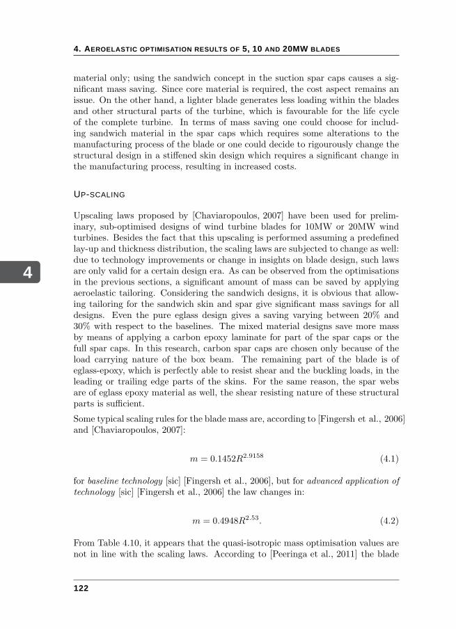
4
4. AEROELASTIC OPTIMISATION RESULTS OF 5, 10 AND 20MW BLADES
material only; using the sandwich concept in the suction spar caps causes a sig-nificant mass saving. Since core material is required, the cost aspect remains anissue. On the other hand, a lighter blade generates less loading within the bladesand other structural parts of the turbine, which is favourable for the life cycleof the complete turbine. In terms of mass saving one could choose for includ-ing sandwich material in the spar caps which requires some alterations to themanufacturing process of the blade or one could decide to rigourously change thestructural design in a stiffened skin design which requires a significant change inthe manufacturing process, resulting in increased costs.
UP-SCALING
Upscaling laws proposed by [Chaviaropoulos, 2007] have been used for prelim-inary, sub-optimised designs of wind turbine blades for 10MW or 20MW windturbines. Besides the fact that this upscaling is performed assuming a predefinedlay-up and thickness distribution, the scaling laws are subjected to change as well:due to technology improvements or change in insights on blade design, such lawsare only valid for a certain design era. As can be observed from the optimisationsin the previous sections, a significant amount of mass can be saved by applyingaeroelastic tailoring. Considering the sandwich designs, it is obvious that allow-ing tailoring for the sandwich skin and spar give significant mass savings for alldesigns. Even the pure eglass design gives a saving varying between 20% and30% with respect to the baselines. The mixed material designs save more massby means of applying a carbon epoxy laminate for part of the spar caps or thefull spar caps. In this research, carbon spar caps are chosen only because of theload carrying nature of the box beam. The remaining part of the blade is ofeglass-epoxy, which is perfectly able to resist shear and the buckling loads, in theleading or trailing edge parts of the skins. For the same reason, the spar websare of eglass epoxy material as well, the shear resisting nature of these structuralparts is sufficient.
Some typical scaling rules for the blade mass are, according to [Fingersh et al., 2006]and [Chaviaropoulos, 2007]:
m = 0.1452R2.9158 (4.1)
for baseline technology [sic] [Fingersh et al., 2006], but for advanced application of
technology [sic] [Fingersh et al., 2006] the law changes in:
m = 0.4948R2.53. (4.2)
From Table 4.10, it appears that the quasi-isotropic mass optimisation values arenot in line with the scaling laws. According to [Peeringa et al., 2011] the blade
122
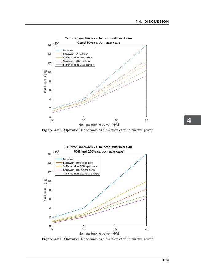
4
4.4. DISCUSSION
5 10 15 20
Nominal turbine power [MW]
0
2
4
6
8
10
12
14
16B
lade
mas
s [k
g]104
Tailored sandwich vs. tailored stiffened skin0 and 20% carbon spar caps
BaselineSandwich, 0% carbonStiffened skin, 0% carbonSandwich, 20% carbonStiffened skin, 20% carbon
Figure 4.60: Optimised blade mass as a function of wind turbine power
5 10 15 20
Nominal turbine power [MW]
0
2
4
6
8
10
12
14
16
Bla
de m
ass
[kg]
104
Tailored sandwich vs. tailored stiffened skin50% and 100% carbon spar caps
BaselineSandwich, 50% spar capsStiffened skin, 50% spar capsSandwich, 100% spar capsStiffened skin, 100% spar caps
Figure 4.61: Optimised blade mass as a function of wind turbine power
123
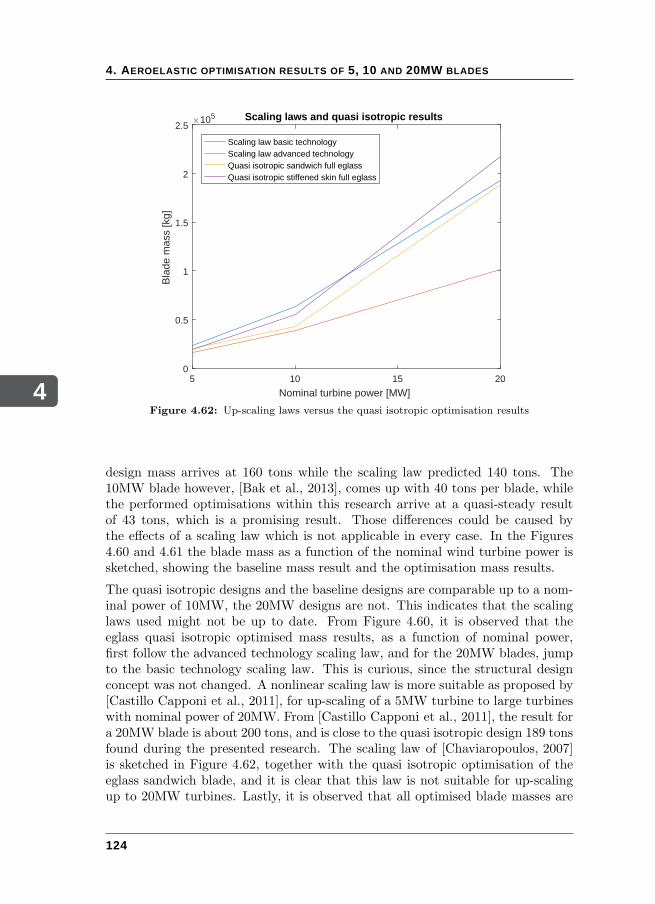
4
4. AEROELASTIC OPTIMISATION RESULTS OF 5, 10 AND 20MW BLADES
5 10 15 20
Nominal turbine power [MW]
0
0.5
1
1.5
2
2.5
Bla
de m
ass
[kg]
105 Scaling laws and quasi isotropic results
Scaling law basic technologyScaling law advanced technologyQuasi isotropic sandwich full eglassQuasi isotropic stiffened skin full eglass
Figure 4.62: Up-scaling laws versus the quasi isotropic optimisation results
design mass arrives at 160 tons while the scaling law predicted 140 tons. The10MW blade however, [Bak et al., 2013], comes up with 40 tons per blade, whilethe performed optimisations within this research arrive at a quasi-steady resultof 43 tons, which is a promising result. Those differences could be caused bythe effects of a scaling law which is not applicable in every case. In the Figures4.60 and 4.61 the blade mass as a function of the nominal wind turbine power issketched, showing the baseline mass result and the optimisation mass results.
The quasi isotropic designs and the baseline designs are comparable up to a nom-inal power of 10MW, the 20MW designs are not. This indicates that the scalinglaws used might not be up to date. From Figure 4.60, it is observed that theeglass quasi isotropic optimised mass results, as a function of nominal power,first follow the advanced technology scaling law, and for the 20MW blades, jumpto the basic technology scaling law. This is curious, since the structural designconcept was not changed. A nonlinear scaling law is more suitable as proposed by[Castillo Capponi et al., 2011], for up-scaling of a 5MW turbine to large turbineswith nominal power of 20MW. From [Castillo Capponi et al., 2011], the result fora 20MW blade is about 200 tons, and is close to the quasi isotropic design 189 tonsfound during the presented research. The scaling law of [Chaviaropoulos, 2007]is sketched in Figure 4.62, together with the quasi isotropic optimisation of theeglass sandwich blade, and it is clear that this law is not suitable for up-scalingup to 20MW turbines. Lastly, it is observed that all optimised blade masses are
124
4
4.5. CONCLUDING REMARKS
lower than the masses resulting from the basic technology law, and that inclu-sion of carbon in the spar caps drives the optimised masses towards the advancedtechnology results.
4.5 CONCLUDING REMARKS
The quasi isotropic optimisation results of the 5MW eglass blade approximatethe baseline blade mass very closely. This indicates a correct critical loadcaseselection and a further proof of correct aerodynamic and structural blade model-ling. A significant result from the quasi isotropic optimisations is that the 20MWrotor blade does not meet the blade mass of the baseline design. This is causedby the material properties of the eglass composite material: the material proper-ties are not sufficient for a feasible 20MW design. It was also found that with aquasi isotropic optimisation, where the spar cap material was replaced by carbonepoxy composite material, this material property problem of eglass became lesssignificant because of the more favourable mechanical properties of carbon. Forthe 10MW blade no problems were detected during the optimisations. The quasiisotropic results of the full eglass blade was comparable to the mass of the 10MWbaseline from RISØ.The tailored 5MW NREL rotor blade mass for the critical load case EWS, con-verges to a value of 12,500 kg. The NWP loadcase had been considered as wellbut resulted in a significantly lower mass, 7900 kg. For further optimisations,the EWS loadcase was used as a critical load case. The optimised blade massresults for the 10MW blade is about 35,000 kg, and 118,000 kg for the 20MWblade for both full eglass blades. For the full carbon sandwich composite spar capversions of the 10MW and 20MW blades the optimised masses become 19,000 kgand 61,000 kg, respectively. One observes a significant drop in blade mass for the20MW blade, compared to the quasi-isotropic case.For both the NWP and the EWS load cases, the stiffness distribution is similar.The spar webs show a shear resisting lay-up, while the suction and pressure sidespar caps are optimised towards a unidirectional lay-up. The skin parts that formthe remainder of the torsion box exhibit different behaviour. Especially the suc-tion skin is critical for the buckling constraints. The lower skin leading edge showssome unidirectional behaviour, which indicates that the leading edge and sparsare the load carrying part while the remaining leading edge and the trailing edgeloading are significantly different, mainly shear resisting. The twist distributionsshow that the twist deformation becomes effective at the outer blade section dueto higher aerodynamic loading and lower torsional stiffness. For the sandwichblades, the aerodynamic power constraint is active in all tailoring sessions whichmeans that the twist angles for the quasi isotropic case and the full tailored caseare approximately equal. The tip deflection constraint assures that the out-of-plane bending stiffness is kept within range.
125
4
4. AEROELASTIC OPTIMISATION RESULTS OF 5, 10 AND 20MW BLADES
A further analysis of the results shows that it is favourable to apply sandwichspar caps in the suction spar caps of the sandwich blade and that this structurallay-out is a better choice than constructing the skin with a longitudinal stiffenersattached to a full fibre skin where the buckling panels are limited by the spars, theribs and, the longerons. Still, this structural lay-out of a skin-stiffened blade isin favour of the state-of-the-art sandwich blades, because of applying the variablestiffness concept.As a last important finding, the optimised blade mass as a function of the aero-dynamic wind turbine power does not follow the scaling laws that were used todesign the reference 10MW and 20MW blades.
126
5CONCLUSIONS AND
RECOMMENDATIONS
Within this research, a stiffness optimisation was performed which has as ob-jective the minimisation of blade mass. For this purpose, an equal fidelity staticaeroelastic analysis code was developed and integrated within an optimisationframework. Using this optimisation framework, optimum structural blade resultswere generated. This chapter summarizes the conclusions drawn throughout thethesis that answer to the main research goal as formulated in chapter 1:
Find an optimum structural and material lay-out for large wind turbine blades
using an equal fidelity aeroelastic analysis code suitable for optimisation purposes.
5.1 CONCLUSIONS
EQUAL FIDELITY AEROELASTIC MODELLING
The aeroelastic model developed in this research was developed for efficient optim-isation purposes. The computational effort within the model was, amongst others,improved by using a cross-sectional modeller that converts a full 3D blade modelto a 1D Timoshenko beam element embedded in a corotational framework whilepreserving the orthotropic behaviour of the composite skin and spar parts. Before
127
5
5. CONCLUSIONS AND RECOMMENDATIONS
this tranformation, a check from a comparison of ABD matrices of pure lamin-ates and sandwich laminates showed the expected behaviour, i.e. the elements inthe A and D matrices for the sandwich laminates have increased with approxim-ately a factor 2 with respect to the pure fibre laminates. This indicates that thesandwich laminates are properly modelled. Furthermore, the aerodynamic modelchosen is a non-planar vortex panel model which may cause computational effortproblems because of the cylindrical wake. To describe the cylindrical wake prop-erly, the number of wake panels is significantly higher compared to a flat fixedwing wake. However, supported by efficient coding techniques, the helical wakedid not cause time problems for the chordwise integrated aerodynamic force andmoment calculations that follow from multiple vortex panels. The aerodynamicloads were obtained from a multi-panel vortex method on the blade and in thewake and is transformed to an aerodynamic load distribution across the bladespan in the local quarter chord position. According to the definition of modelfidelity in chapter 1, this model can be referred to as a medium fidelity aerody-namic model.Eventually, both the structural loads and the aerodynamic loads were defined overa single line of equal fidelity and served as an input to the aeroelastic analysis. Forthe aerodynamic loads and structural loads, the sensitivities with respect to theblade structural degrees of freedom were obtained analytically. This accomplishedthe close coupling within the aeroelastic analysis. The structural solution found isgeometrically nonlinear because beam elements are embedded in a co-rotationalframework.For the validation of the aeroelastic code, the normal force distribution and thetangential force distribution was used to check the aerodynamic part; the aero-elastic behaviour was checked by considering the tip displacement and the aerody-namic power. From the validation results presented in chapter 2 it followed thatthe normal force distribution is almost equal to the results from the validatedFAST code, which means that, up to rated, the aerodynamics was implementedin a sufficient way. For the aeroelastic results, the tip displacement as a functionof the velocity follows the behaviour of the NREL reference blade very close up toa wind velocity of 12 m/s the difference beyond 12 m/s is due to a different, notso accurate, pitch control algorithm. This did not generate problems because theoptimisations were performed 3% below rated. Yet, the blade power curve wasshown, and it was observed that some variation above rated due to aeroelasticsand the unaccurate modelling of the pitch controller is present. However, theaeroelastic code proved to behave such that it can be used for optimisation pur-poses up to rated. The optimisation results were to be used for blade designpurposes.
128
5
5.1. CONCLUSIONS
STRUCTURAL OPTIMISATION PROCEDURE
The optimisations were performed for a sandwich skin but also for a stiffenedskin configuration where the blade consists of ribs and longitudinal stiffeners onthe suction and pressure skin. Next, the structural optimisations required thefollowing design variables. For the sandwich structural lay-out the laminationparameters were coupled to a sandwich laminate by defining only the laminationparameters for the faces that actually contain the fibres. It was also assumed thatboth faces have the same lay-up and thickness such that the lamination paramet-ers of only one face sheet have to be defined. Furthermore, the thickness of thesandwich core was added to the design variable vector to fully define the sandwichlaminate.The optimisation was carried out using the Extreme Wind Shear load case to ar-rive at results that produce useable results for an actual blade structural design.To verify whether the extreme wind shear is a heavier load case than the normalwind profile, a comparison between those load case was done. Thickness plotsand stiffness plots showed that extreme wind shear is indeed a more severe loadcase, especially the maximum thickness is increased by 27% while the thicknessdistribution shows similar behaviour compared to the normal wind profile case.As a reference for the optimiser and also an extra check, quasi-isotropic optimisa-tion cases were carried out. For instance, the quasi isotropic results generated a3% higher flap stiffness distribution than the actual chosen baseline. Because thebaselines already are sub-optimised using the fibre orientation, the stiffness distri-butions and the blade masses will differ. Still, a 3% higher out-of-plane bendingstiffness distribution and a 11% higher in-plane bending distribution are prom-ising results. For the thickness distribution it was found that the 5MW blade (8%higher than baseline mass) and 10MW blade (7.5% higher than baseline mass)were comparable to the actual baseline designs masses but the 20MW blade (18% higher than baseline mass) was not able to converge to a feasible thickness dis-tribution due to high stresses around 55% of the blade span. To solve this issuefor the 20MW blade, a mixed material solution was introduced. Within this solu-tion, the eglass-epoxy laminates of the spar caps were replaced by carbon-epoxylaminates such that the laminate can handle the stresses in a 20MW blade.
TAILORED BLADE RESULTS
The tailored blade results, sandwich as well as stiffened skin configuration, showeda significant mass reduction compared to the baseline designs using the variablestiffness concept. On the other hand, it was observed that the stiffened skinconfiguration did not show significant advantages compared to the sandwich skinconfiguration; this became even more distinct when the mixed-material, wherethe eglass material of some structural parts is replaced by carbon material, wasintroduced within the spar caps. This behaviour was due to the fact that the
129
5
5. CONCLUSIONS AND RECOMMENDATIONS
stiffener pitch has not been optimised; the stiffener pitch was kept constant duringthe optimisation procedure.Both configurations showed significant mass savings compared to the baselinedesigns. And the savings increase with increasing aerodynamic power. For the10MW and 20MW blades, up-scaling based on the 5MW machines is applied. Itappeared that, especially in the 20MW case, the blade design became infeasible.Furthermore, a relation between blade mass and amount of carbon fibre in thedesign showed that using carbon for other parts than spar caps will not give afurther significant reduction of the mass.The graphs of optimised mass against aerodynamic power are kind of upscalinggraphs as well. From those graphs it can be concluded that the baseline designsshow a steeper gradient than the optimised designs; the amount of carbon in thedesigns reduces the gradient even further. It was observed that switching materialsfrom eglass to carbon for a approximately 30% of the baseline structure, in thiscase the full spar caps, saved about 50% blade mass with respect to the baseline.
The stiffened skin designs showed higher masses than the sandwich designs. Thedifferences between the two configurations were most prominent for the 5MWturbine. For the 10MW and 20MW blades, the differences were less because theskin stiffening was not varied for the stiffened skin configuration. Since the sand-wich core thickness was part of the optimisation procedure, the comparison is notcompletely fair. The sandwich core thickness can be seen as some smeared thick-ness of stiffeners and influences skin buckling, which is controlled with stiffenerpitch and dimension in the stiffened skin designs. Since the stiffened skin lay-outwas not optimised for stiffener pitch, it can be assumed that the conventionaldesigns can become lighter. An additional explanation for the mass differencebetween the sandwich design and the conventional design originates in assumingsandwich composite in the spar caps. Especially in the suction spar cap, theoptimiser assumed significant amounts of core material to prevent the skin frombuckling locally, resulting in mass savings of 26% for 5MW blades and 14% for10MW blades with respect to pure fibre laminate spar caps. The state-of-the-art blades do not use sandwich laminates in the spar caps. Allowing sandwichcomposites in the spar caps is a significant cause of the substantial mass sav-ings. The stiffened skin design and the sandwich design, including suction sparcap and eglass only, gave significant mass savings with respect to the baselinedesigns, varying between 23% and 29% for the 5MW blade, where the sandwichwas favourable. For the 10MW blade, a saving between 12% and 17% was accom-plished, where the stiffened skin lay-out is favourable, and, mass savings between21% and 26% were found for the 20MW blade, where the stiffened skin lay-outwas in favour as well. For the mixed material cases, the sandwich lay-out becamefavourable in all cases, and the mass savings with respect to the baseline are evenbetter: for full carbon spar caps, mass savings of 50% with respect to the baselinewere observed.
From this research, it can be concluded that the aeroelastic model makes it pos-
130
5
5.2. RECOMMENDATIONS
sible to perform a complete blade optimisation for different wind turbine bladesfrom which it is possible to extract new design rules or adapt previous ones. Itseems that the classical power laws used for upscaling of the blades are not con-sistent in estimating blade masses for the 10MW and 20MW blades. This wasobserved for the quasi isotropic blade as well as for the tailored blade. Further-more, significant mass savings can be achieved provided that the variable stiffnessconcept is used. Both the sandwich or the stiffened skin configuration give blademass values that stay significantly below the baseline designs.
5.2 RECOMMENDATIONS
EQUAL FIDELITY AEROELASTIC MODEL
Since the present research only considers static aeroelastic results, it is of im-portance to consider dynamic aeroelastic results as well to be sure that the staticdesign is also resisting dynamic loads. Optimisations including dynamic and fa-tigue loads should be performed, however, the turbine blade still must be subjec-ted to some extreme gusts to see whether the blade is resisting those loads. Thismeans that an unsteady aerodynamic model should be implemented. For a fulldynamic aeroelastic analysis, a structural dynamics model must be implementedas well.An other issue considering the aerodynamics is the cylindrical wake. Physic-ally, the wake behind the wind turbine rotor shows expansion which causes somereduction of the aerodynamic loading. It is suggested to implement an iterative al-gorithm that runs together with the aeroelastic iteration. This means that duringeach load iteration the aerodynamic influence coefficients are not only evaluateddue to the blade deformation but also due to the change in shape of the wake.The underlying mechanism is to alter the wake vorticity untill the wake is forcefree, which is not the case for the cylindrical wake assumption.During this research, the blade is assumed to remain in aerodynamic conditionsin which the flow over the blade stays attached. For a more practical vortex dis-tribution in the blade root section, a static stall model has to be implemented,and the vortex model exchanges information with the airfoil tables by means ofanother Newton-Raphson root finding algorithm for quick convergence, to assurethe efficient computational effort of the aeroelastic model.
OPTIMISATION
As concluded in this research, the stiffened skin blade structural configurationgives higher mass results than the sandwich blades. Due to the fixed skin stiffen-ing properties as stringer pitch and stringer shape, the skin is not fully optimisedfor buckling. The stringer pitch has to be included in the optimisation as well, just
131
5
5. CONCLUSIONS AND RECOMMENDATIONS
as the sandwich core is a design variable for the sandwich blade. A problem couldarise here, namely that the computational effort might not be an advantage evenconsidering the aeroelastic model. Due to the differences between the sandwichlay-out and the stiffened skin lay-out, it is suggested to redo the optimisationschoosing a different objective function that includes the cost aspect to see whichstructural lay-out is most favourable.All optimisations are performed by assuming balanced laminates. To find outwhether increased mass saving can be accomplished, an investigation with unbal-anced laminates has to be carried out. Also, unsymmetric laminates have to bea subject of future studies on structural blade mass minimisation when out ofautoclave curing happens.
OUTLOOK
The main conclusion of this work is, that variable stiffness multi-material compos-ite blades with sandwich spar caps are promising for future large wind turbines.One of the challenges is to get the variable stiffness blade concept within the cer-tification procedures of wind turbines. This means that a lot of research has tobe done on building and testing such blades and to formulate valid certificationrules for safe use of such blades.
132
ACLASSICAL LAMINATE THEORY
FORMULAE
A short overview is given on stacking sequence, constructing the ABD matricesand the relation with lamination parameters, since lamination parameters aredefined as the design variables in the optimisations during this thesis. The axissystem used for the laminae is is shown in A.1.
The stress-strain relation of a rotated single composite layer can be written as:
σxσyτxy
k
= Qk
ǫxǫyγxy
k
(A.1)
The rotated stiffness matrix Qk exists of the original stiffness matrix Qk thatis altered by a co-ordinate transformation matrix T and a transformation mat-rix R to compensate the difference between the tensorial shear strain and theengineering shear strain. The matrices T and R are written as:
T =
cos2 θ sin2 θ 2 cos θ sin θsin2 θ cos2 θ −2 cos θ sin θ
− cos θ sin θ cos θ sin θ cos2 θ − sin2 θ
(A.2)
133
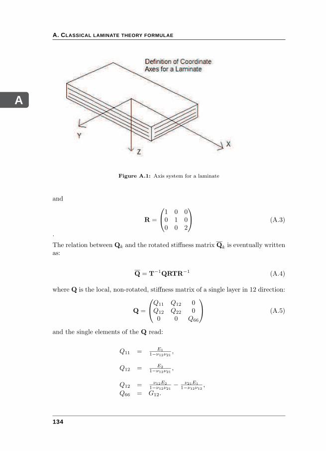
A
A. CLASSICAL LAMINATE THEORY FORMULAE
Figure A.1: Axis system for a laminate
and
R =
1 0 00 1 00 0 2
(A.3)
.
The relation between Qk and the rotated stiffness matrix Qk is eventually writtenas:
Q = T−1QRTR−1 (A.4)
where Q is the local, non-rotated, stiffness matrix of a single layer in 12 direction:
Q =
Q11 Q12 0Q12 Q22 00 0 Q66
(A.5)
and the single elements of the Q read:
Q11 = E1
1−ν12ν21,
Q12 = E2
1−ν12ν21,
Q12 = ν12E2
1−ν12ν21− ν21E1
1−ν12ν12,
Q66 = G12.
134

BSTRAIN AND BUCKLING OF
OPTIMISED DESIGNS
135
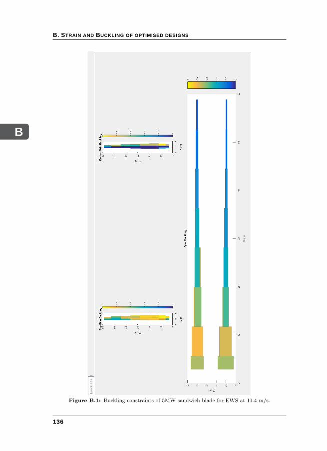
B
B. STRAIN AND BUCKLING OF OPTIMISED DESIGNS
Figure B.1: Buckling constraints of 5MW sandwich blade for EWS at 11.4 m/s.
136
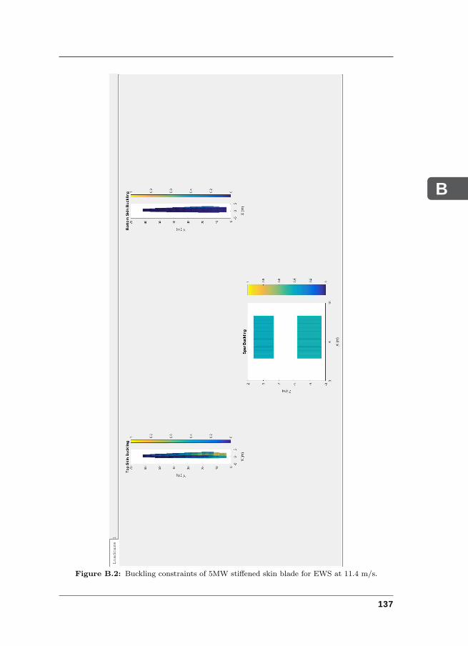
B
Figure B.2: Buckling constraints of 5MW stiffened skin blade for EWS at 11.4 m/s.
137
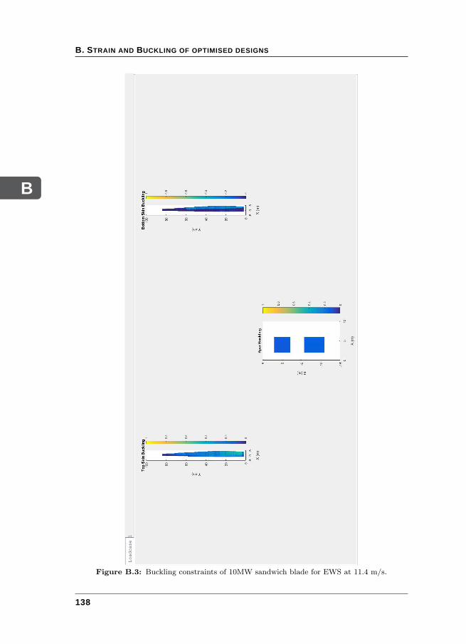
B
B. STRAIN AND BUCKLING OF OPTIMISED DESIGNS
Figure B.3: Buckling constraints of 10MW sandwich blade for EWS at 11.4 m/s.
138
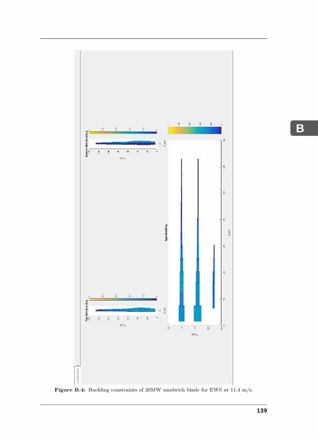
B
Figure B.4: Buckling constraints of 20MW sandwich blade for EWS at 11.4 m/s.
139
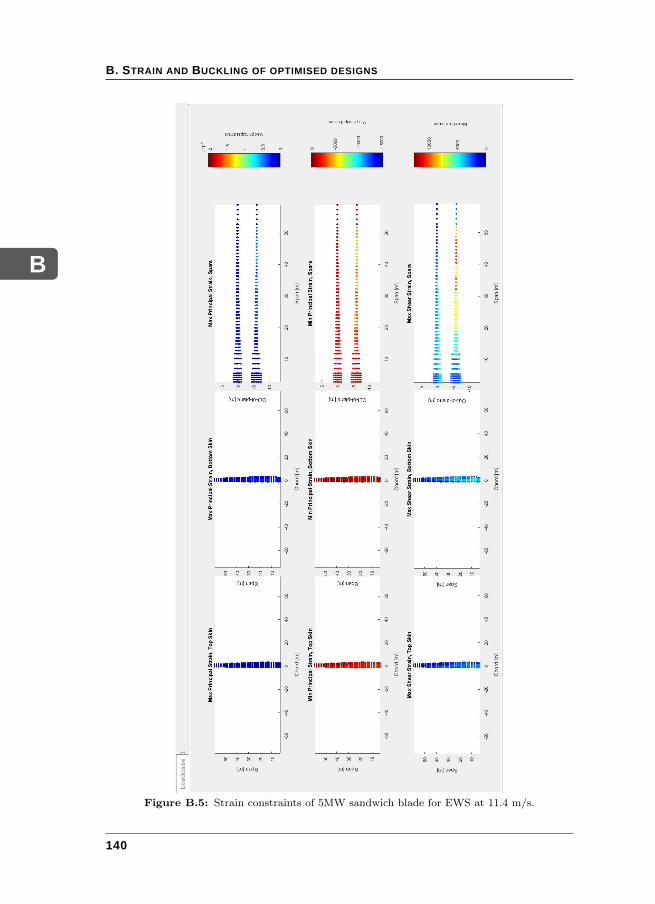
B
B. STRAIN AND BUCKLING OF OPTIMISED DESIGNS
Figure B.5: Strain constraints of 5MW sandwich blade for EWS at 11.4 m/s.
140
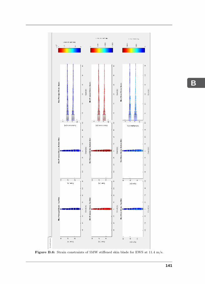
B
Figure B.6: Strain constraints of 5MW stiffened skin blade for EWS at 11.4 m/s.
141
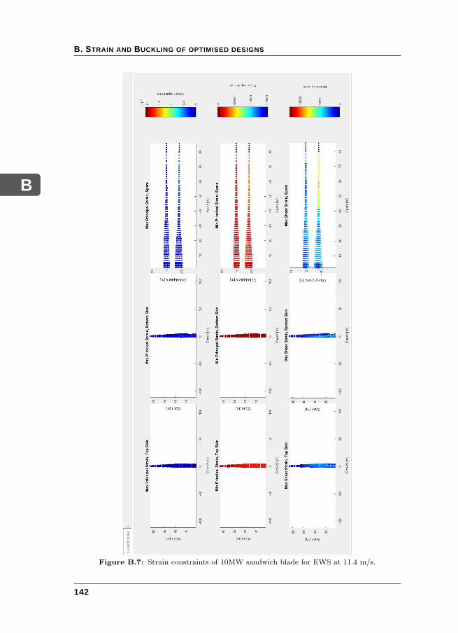
B
B. STRAIN AND BUCKLING OF OPTIMISED DESIGNS
Figure B.7: Strain constraints of 10MW sandwich blade for EWS at 11.4 m/s.
142
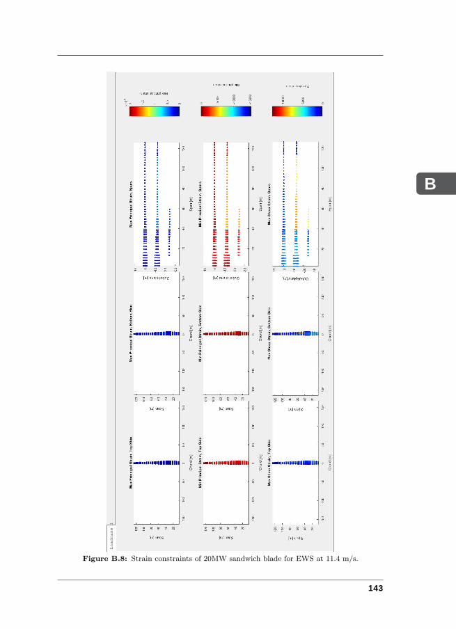
B
Figure B.8: Strain constraints of 20MW sandwich blade for EWS at 11.4 m/s.
143
B
B. STRAIN AND BUCKLING OF OPTIMISED DESIGNS
144
CAERODYNAMIC POWER CONSTRAINTS
145
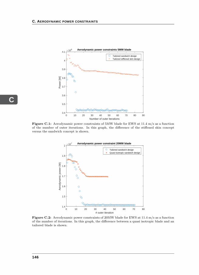
C
C. AERODYNAMIC POWER CONSTRAINTS
0 10 20 30 40 50 60 70 80 90
Number of outer iterations
3.4
3.5
3.6
3.7
3.8
3.9
4
4.1
Pow
er [W
]
106 Aerodynamic power constraints 5MW blade
Tailored sandwich designTailored stiffened skin design
Figure C.1: Aerodynamic power constraints of 5MW blade for EWS at 11.4 m/s as a functionof the number of outer iterations. In this graph, the difference of the stiffened skin conceptversus the sandwich concept is shown.
0 10 20 30 40 50 60 70 80
# outer iteration
1.4
1.5
1.6
1.7
1.8
1.9
2
Aer
odyn
amic
pow
er (
W)
107 Aerodynamic power constraint 20MW blade
Tailored sandwich designQuasi-isotropic sandwich design
Figure C.2: Aerodynamic power constraints of 20MW blade for EWS at 11.4 m/s as a functionof the number of iterations. In this graph, the difference between a quasi isotropic blade and antailored blade is shown.
146
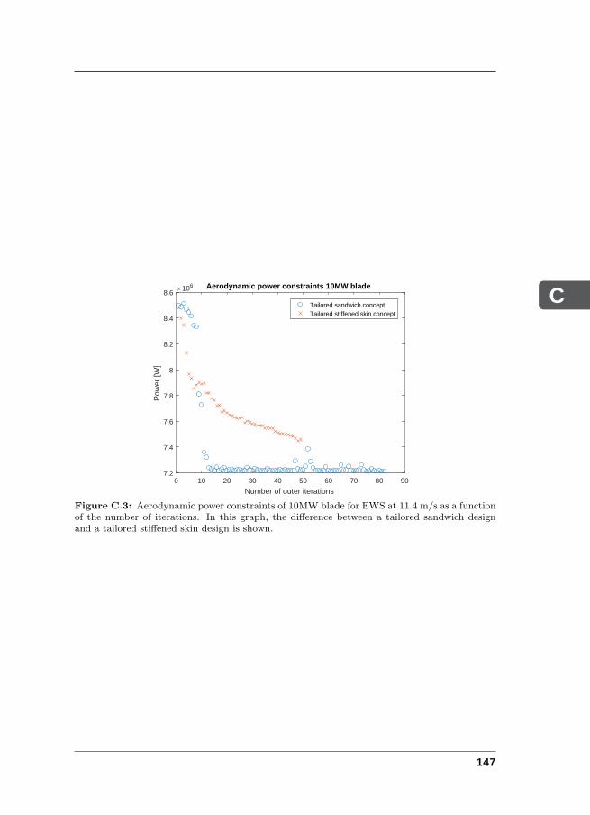
C
0 10 20 30 40 50 60 70 80 90
Number of outer iterations
7.2
7.4
7.6
7.8
8
8.2
8.4
8.6
Pow
er [W
]
106 Aerodynamic power constraints 10MW blade
Tailored sandwich conceptTailored stiffened skin concept
Figure C.3: Aerodynamic power constraints of 10MW blade for EWS at 11.4 m/s as a functionof the number of iterations. In this graph, the difference between a tailored sandwich designand a tailored stiffened skin design is shown.
147
C
C. AERODYNAMIC POWER CONSTRAINTS
148
BIBLIOGRAPHY
[Aerotrope, 1995] Aerotrope (1995). Carter 300 kW Two-Bladed Wind Turbine.
[Amin et al., 2012] Amin, M. M., Ghadiri, B., Abdalla, M. M., Haddadpour, H.,and De Breuker, R. (2012). Continuous-time state-space unsteady aerody-namic modeling based on boundary element method. Engineering Analysis
with Boundary Elements, 36:789–798.
[Ashuri, 2012] Ashuri, T. (2012). Beyond Classical Upscaling: Integrated Aer-
oservoelastic Design and Optimization of Large Offshore Wind Turbines. PhDthesis, Delft University of Technology.
[Ashuri et al., 2010] Ashuri, T., Bussel, v. G., Zaaijer, M., and Kuik, v. G. (2010).An analytical model to extract blade structural properties for optimisation andup-scaling studies. In The Science of Making Torque form Wind, Heraklion,
Crete, Greece, 28-30 June, 2010.
[Bak et al., 2013] Bak, C., Zahle, F., Kim, T., Yde, A., Henriksen, L., Natarajan,A., and Hansen, M. (2013). Description of the DTU 10MW reference 5 windturbine. Technical Report DTU Wind Energy-I-0092.
[Bernhammer, 2015] Bernhammer, L. (2015). Smart Wind Turbine: Analysis and
Autonomous Flap. PhD thesis, Delft University of Technology.
[Bielawa, 1971] Bielawa, R. (1971). Techniques for stability analysis and designoptimization with dynamic constraints of nonconservative linear systems. InAIAA paper 71 - 388, 1971.
[Blasques and Lazarov, 2011] Blasques, J. and Lazarov, B. (2011). BECAS - abeam cross-section analysis tool for anisotropic and inhomogeneous sections ofarbitrary geometry. Technical Report RISO R 1785 Technical Report.
[Bottasso et al., 2016] Bottasso, C. L., Bortolotti, P., Croce, A., and Gualdoni,F. (2016). Integrated aero-structural optimization of wind turbines. Multibody
System Dynamics, 38(4):317–344.
149
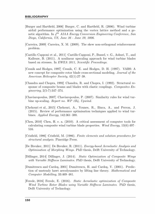
BIBLIOGRAPHY
[Burger and Hartfield, 2006] Burger, C. and Hartfield, R. (2006). Wind turbineairfoil performance optimization using the vortex lattice method and a ge-netic algorithm. In 4th AIAA Energy Conversion Engineering Conference, San
Diego, California, US, June 26 - June 29, 2006.
[Carreira, 2009] Carreira, X. M. (2009). The skew non-orthogonal reinforcementproblem.
[Castillo Capponi et al., 2011] Castillo Capponi, P., Bussel, v. G., Ashuri, T., andKallesøe, B. (2011). A nonlinear upscaling approach for wind turbine bladesbased on stresses. In EWEA 2011, Scientific Proceedings.
[Cesnik and Hodges, 1997] Cesnik, C. E. and Hodges, D. H. (1997). VABS: Anew concept for composite rotor blade cross-sectional modeling. Journal of theAmerican Helicopter Society, 42(1):27–38.
[Chandra and Chopra, 1992] Chandra, R. and Chopra, I. (1992). Structural re-sponse of composite beams and blades with elastic couplings. Composites En-
gineering, 2(5-7):347–374.
[Chaviaropoulos, 2007] Chaviaropoulos, P. (2007). Similarity rules for wind tur-bine up-scaling. Report no. WP 1B4, Upwind.
[Chehouri et al., 2015] Chehouri, A., Younes, R., Ilinca, A., and Perron, J.(2015). Review of performance optimisation techniques applied to wind tur-bines. Applied Energy, 142:361–388.
[Chen, 2010] Chen, H. e. a. (2010). A critical assessment of computer tools forcalculating composite wind turbine blade properties. Wind Energy, 13(6):497–516.
[Crisfield, 1986] Crisfield, M. (1986). Finite elements and solution procedures for
structural analysis. Pineridge Press.
[De Breuker, 2011] De Breuker, R. (2011). Energy-based Aeroelastic Analysis and
Optimisation of Morphing Wings. PhD thesis, Delft University of Technology.
[Dillinger, 2014] Dillinger, J. (2014). Static Optimization of Composite Wings
with Variable Stiffness Laminates. PhD thesis, Delft University of Technology.
[Dumitrescu and Cardos, 2001] Dumitrescu, H. and Cardos, V. (2001). Predic-tion of unsteady hawt aerodynamics by lifting line theory. Mathematical and
Computer Modelling, 33:469–481.
[Ferede, 2016] Ferede, E. (2016). Static Aeroelastic optimization of Composite
Wind Turbine Rotor Blades using Variable Stiffness Laminates. PhD thesis,Delft University of Technology.
150
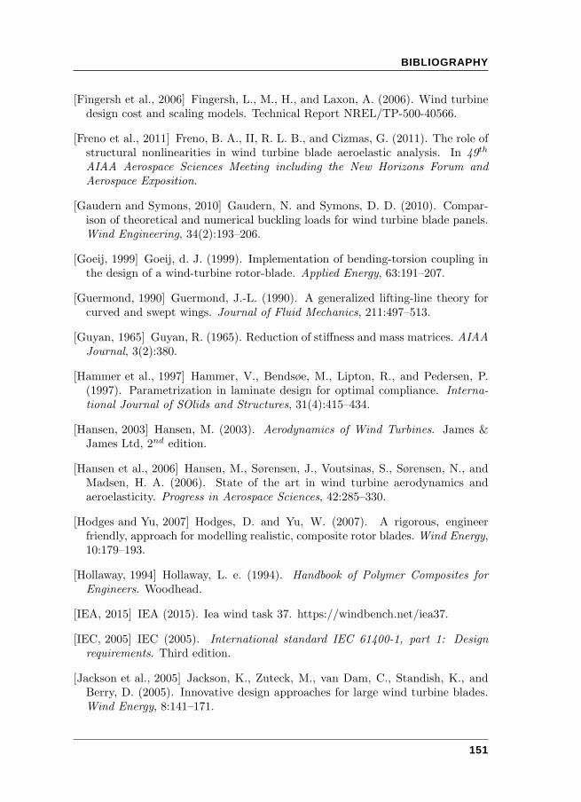
BIBLIOGRAPHY
[Fingersh et al., 2006] Fingersh, L., M., H., and Laxon, A. (2006). Wind turbinedesign cost and scaling models. Technical Report NREL/TP-500-40566.
[Freno et al., 2011] Freno, B. A., II, R. L. B., and Cizmas, G. (2011). The role ofstructural nonlinearities in wind turbine blade aeroelastic analysis. In 49th
AIAA Aerospace Sciences Meeting including the New Horizons Forum and
Aerospace Exposition.
[Gaudern and Symons, 2010] Gaudern, N. and Symons, D. D. (2010). Compar-ison of theoretical and numerical buckling loads for wind turbine blade panels.Wind Engineering, 34(2):193–206.
[Goeij, 1999] Goeij, d. J. (1999). Implementation of bending-torsion coupling inthe design of a wind-turbine rotor-blade. Applied Energy, 63:191–207.
[Guermond, 1990] Guermond, J.-L. (1990). A generalized lifting-line theory forcurved and swept wings. Journal of Fluid Mechanics, 211:497–513.
[Guyan, 1965] Guyan, R. (1965). Reduction of stiffness and mass matrices. AIAAJournal, 3(2):380.
[Hammer et al., 1997] Hammer, V., Bendsøe, M., Lipton, R., and Pedersen, P.(1997). Parametrization in laminate design for optimal compliance. Interna-
tional Journal of SOlids and Structures, 31(4):415–434.
[Hansen, 2003] Hansen, M. (2003). Aerodynamics of Wind Turbines. James &James Ltd, 2nd edition.
[Hansen et al., 2006] Hansen, M., Sørensen, J., Voutsinas, S., Sørensen, N., andMadsen, H. A. (2006). State of the art in wind turbine aerodynamics andaeroelasticity. Progress in Aerospace Sciences, 42:285–330.
[Hodges and Yu, 2007] Hodges, D. and Yu, W. (2007). A rigorous, engineerfriendly, approach for modelling realistic, composite rotor blades. Wind Energy,10:179–193.
[Hollaway, 1994] Hollaway, L. e. (1994). Handbook of Polymer Composites for
Engineers. Woodhead.
[IEA, 2015] IEA (2015). Iea wind task 37. https://windbench.net/iea37.
[IEC, 2005] IEC (2005). International standard IEC 61400-1, part 1: Design
requirements. Third edition.
[Jackson et al., 2005] Jackson, K., Zuteck, M., van Dam, C., Standish, K., andBerry, D. (2005). Innovative design approaches for large wind turbine blades.Wind Energy, 8:141–171.
151
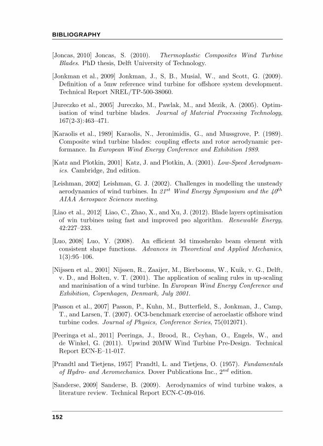
BIBLIOGRAPHY
[Joncas, 2010] Joncas, S. (2010). Thermoplastic Composites Wind Turbine
Blades. PhD thesis, Delft University of Technology.
[Jonkman et al., 2009] Jonkman, J., S, B., Musial, W., and Scott, G. (2009).Definition of a 5mw reference wind turbine for offshore system development.Technical Report NREL/TP-500-38060.
[Jureczko et al., 2005] Jureczko, M., Pawlak, M., and Mezik, A. (2005). Optim-isation of wind turbine blades. Journal of Material Processing Technology,167(2-3):463–471.
[Karaolis et al., 1989] Karaolis, N., Jeronimidis, G., and Mussgrove, P. (1989).Composite wind turbine blades: coupling effects and rotor aerodynamic per-formance. In European Wind Energy Conference and Exhibition 1989.
[Katz and Plotkin, 2001] Katz, J. and Plotkin, A. (2001). Low-Speed Aerodynam-
ics. Cambridge, 2nd edition.
[Leishman, 2002] Leishman, G. J. (2002). Challenges in modelling the unsteadyaerodynamics of wind turbines. In 21st Wind Energy Symposium and the 40th
AIAA Aerospace Sciences meeting.
[Liao et al., 2012] Liao, C., Zhao, X., and Xu, J. (2012). Blade layers optimisationof win turbines using fast and improved pso algorithm. Renewable Energy,42:227–233.
[Luo, 2008] Luo, Y. (2008). An efficient 3d timoshenko beam element withconsistent shape functions. Advances in Theoretical and Applied Mechanics,1(3):95–106.
[Nijssen et al., 2001] Nijssen, R., Zaaijer, M., Bierbooms, W., Kuik, v. G., Delft,v. D., and Holten, v. T. (2001). The application of scaling rules in up-scalingand marinisation of a wind turbine. In European Wind Energy Conference and
Exhibition, Copenhagen, Denmark, July 2001.
[Passon et al., 2007] Passon, P., Kuhn, M., Butterfield, S., Jonkman, J., Camp,T., and Larsen, T. (2007). OC3-benchmark exercise of aeroelastic offshore windturbine codes. Journal of Physics, Conference Series, 75(012071).
[Peeringa et al., 2011] Peeringa, J., Brood, R., Ceyhan, O., Engels, W., andde Winkel, G. (2011). Upwind 20MW Wind Turbine Pre-Design. TechnicalReport ECN-E–11-017.
[Prandtl and Tietjens, 1957] Prandtl, L. and Tietjens, O. (1957). Fundamentals
of Hydro- and Aeromechanics. Dover Publications Inc., 2nd edition.
[Sanderse, 2009] Sanderse, B. (2009). Aerodynamics of wind turbine wakes, aliterature review. Technical Report ECN-C-09-016.
152
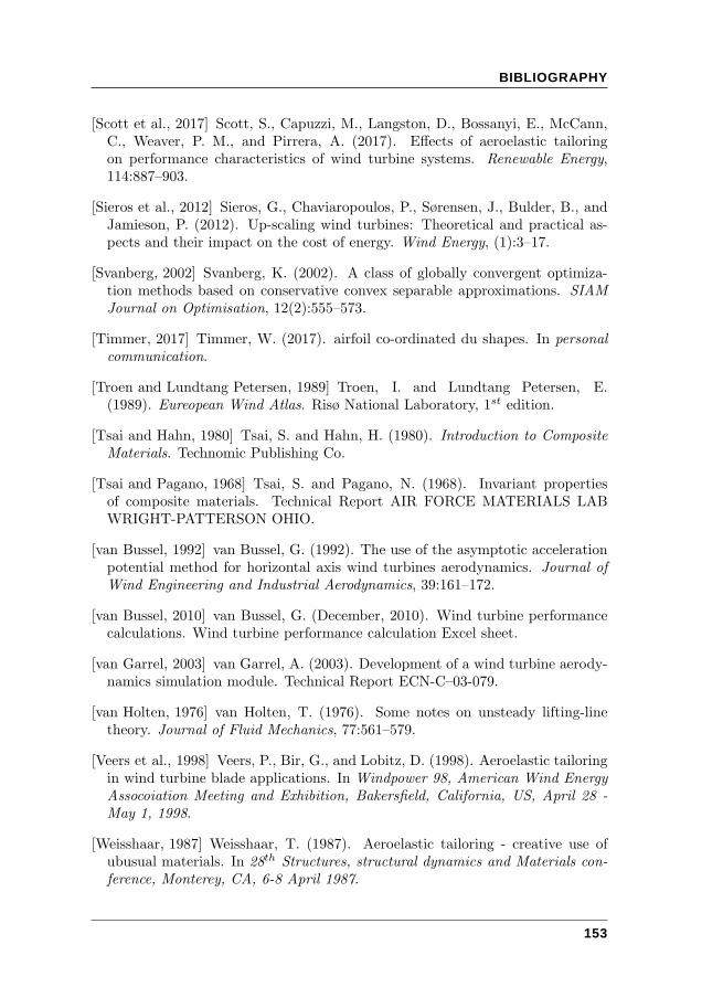
BIBLIOGRAPHY
[Scott et al., 2017] Scott, S., Capuzzi, M., Langston, D., Bossanyi, E., McCann,C., Weaver, P. M., and Pirrera, A. (2017). Effects of aeroelastic tailoringon performance characteristics of wind turbine systems. Renewable Energy,114:887–903.
[Sieros et al., 2012] Sieros, G., Chaviaropoulos, P., Sørensen, J., Bulder, B., andJamieson, P. (2012). Up-scaling wind turbines: Theoretical and practical as-pects and their impact on the cost of energy. Wind Energy, (1):3–17.
[Svanberg, 2002] Svanberg, K. (2002). A class of globally convergent optimiza-tion methods based on conservative convex separable approximations. SIAM
Journal on Optimisation, 12(2):555–573.
[Timmer, 2017] Timmer, W. (2017). airfoil co-ordinated du shapes. In personal
communication.
[Troen and Lundtang Petersen, 1989] Troen, I. and Lundtang Petersen, E.(1989). Eureopean Wind Atlas. Risø National Laboratory, 1st edition.
[Tsai and Hahn, 1980] Tsai, S. and Hahn, H. (1980). Introduction to Composite
Materials. Technomic Publishing Co.
[Tsai and Pagano, 1968] Tsai, S. and Pagano, N. (1968). Invariant propertiesof composite materials. Technical Report AIR FORCE MATERIALS LABWRIGHT-PATTERSON OHIO.
[van Bussel, 1992] van Bussel, G. (1992). The use of the asymptotic accelerationpotential method for horizontal axis wind turbines aerodynamics. Journal of
Wind Engineering and Industrial Aerodynamics, 39:161–172.
[van Bussel, 2010] van Bussel, G. (December, 2010). Wind turbine performancecalculations. Wind turbine performance calculation Excel sheet.
[van Garrel, 2003] van Garrel, A. (2003). Development of a wind turbine aerody-namics simulation module. Technical Report ECN-C–03-079.
[van Holten, 1976] van Holten, T. (1976). Some notes on unsteady lifting-linetheory. Journal of Fluid Mechanics, 77:561–579.
[Veers et al., 1998] Veers, P., Bir, G., and Lobitz, D. (1998). Aeroelastic tailoringin wind turbine blade applications. In Windpower 98, American Wind Energy
Assocoiation Meeting and Exhibition, Bakersfield, California, US, April 28 -
May 1, 1998.
[Weisshaar, 1987] Weisshaar, T. (1987). Aeroelastic tailoring - creative use ofubusual materials. In 28th Structures, structural dynamics and Materials con-
ference, Monterey, CA, 6-8 April 1987.
153
BIBLIOGRAPHY
[Werter, 2017] Werter, N. (2017). Aeroelastic Modelling and Design of Aeroelasti-
cally Tailored and Morphing Wings. PhD thesis, Delft University of Technology.
[Werter et al., 2017] Werter, N. P. M., De Breuker, R., and Abdalla, M. M.(2017). Continuous-time state-space unsteady aerodynamic modeling for ef-ficient loads analysis. AIAA Journal, 56(2):1–12.
[Willaert and Abdalla, 2010] Willaert, M. and Abdalla, M. (2010). A simple finiteelement cross-sectional modelling of thin-walled beams. In Proceedings of the
2nd Aircraft Structural Design Conference.
[Zhale et al., 2016] Zhale, F., TIbaldi, C., Pavese, C., McWilliam, M. K.,Blasques, J. P., and Hansen, M. H. (2016). Design of an aeroelastically tailored10 mw wind turbine rotor. In Journal of Physycs: Conference series 753,
062008.
[Zhu et al., 2012] Zhu, J., Cai, X., Pan, P., and Gu, R. (2012). Optimizationdesign of spar cap layup of wind turbine. Frontiers of Structural and Civil
Engineering, 6(1):53–56.
[Zhu et al., 2014] Zhu, J., Cai, X., Pan, P., and Gu, R. (2014). Multi-objectivestructural optimization design of horizontal-axis wind turbine blades using thenon-dominated sorting genetic algorithm ii and finite element method. Energies,7:988–1002.
154

ACKNOWLEDGEMENTS
Finally! It is done! Nine years of work, combined with a growing family (Gohanwas born in 2014 and Jadzia in 2016), and the teaching job at Inholland Universityof Applied Sciences. I don’t know how I did it, but I succeeded! Of course, I couldnot have succeeded without the help of many people. First of all, I have to thankmy beloved wife, who took care of my children while I worked at some part of theMatlab code, writing a paper, or something like that. Secondly, Inholland madeit possible to do this research during the passed nine years. Many thanks to myemployer. Then, of course, I have to thank both promotors Roeland De Breukerand Gerard van Bussel for their valuable suggestions and sometimes they providedme of new and necessary motivation to continue the research and finishing it.
Next, I should apologise to my colleagues, for the complains they had to listento, after they asked the question: ”How are things with your PhD research?”.Few colleagues were willing to listen more closely to the problems I encountered,which helped me a lot for continuing the research: thank you Arjan, Jan, Pieterand John! One colleague I must mention as well: Marjoke Cornelissen. Shepassed away in december 2017. I miss her very much and I regret that she cannotcelebrate the final steps in my PhD adventure.
During the nine years, I shared my room with several Fellow PhDs. I want tothank you guys, for all good times we had during this nine years. Especiallyin the early days of the adventure, I shared the room with Glenn, Mathieu andMohammed. We had a lot of fun back then, thank you all guys.
Last but not least, I want to thank my parents and parents in law for the relaxingmoments that are very necessary during a PhD!
TerryDen Hoorn, January 2019.
155

ACKNOWLEDGEMENTS
156
BIOGRAPHICAL NOTE
Terry Hegberg was born on April 29, 1970 in Zaandam, The Netherlands where hegrew up. He followed his High-school education at the Zaanlands Lyceum, whichhe completed in 1990. In 1990 he started the study of Aeronautical Engineeringat the University of Applied Sciences in Haarlem. After graduating in 1994, hefollowed a master in Delft, University of Technology at the faculty AerospaceEngineering. He graduated in 1998 in the field of aeroelasticity and helicopterrotor blades. In the same year he started a job at the Energy research centre of theNetherlands at the wind energy department where he did research on aeroelasticbehaviour of wind turbines, wind power meteorology and wind farm design. In2005 he switched jobs and became a teacher at Inholland University of AppliedSciences, Aeronautical Engineering. In 2009 he started a part time PhD researchtrack in collaboration with the Delft University of Technology, which he finishedin 2019.
157


