arX

iv:n

lin/0

1050

39v1

[nl

in.P

S] 1

6 M

ay 2

001

Families of Bragg-grating solitons in a cubic-quintic

medium

Javid Atai1 and Boris A. Malomed2

(1)School of Electrical and Information Engineering, The University of Sydney, Sydney, NSW

2006, Australia

(2)Department of Interdisciplinary Studies, Faculty of Engineering, Tel Aviv University, Tel

Aviv 69978, Israel

Abstract

We investigate the existence and stability of solitons in an optical waveguide equipped with

a Bragg grating (BG) in which nonlinearity contains both cubic and quintic terms. The model

has straightforward realizations in both temporal and spatial domains, the latter being most

realistic. Two different families of zero-velocity solitons, which are separated by a border at

which solitons do not exist, are found in an exact analytical form. One family may be regarded

as a generalization of the usual BG solitons supported by the cubic nonlinearity, while the

other family, dominated by the quintic nonlinearity, includes novel “two-tier” solitons with a

sharp (but nonsingular) peak. These soliton families also differ in the parities of their real and

imaginary parts. A stability region is identified within each family by means of direct numerical

simulations. The addition of the quintic term to the model makes the solitons very robust:

simulating evolution of a strongly deformed pulse, we find that a larger part of its energy is

retained in the process of its evolution into a soliton shape, only a small share of the energy

being lost into radiation, which is opposite to what occurs in the usual BG model with cubic

nonlinearity.

PACS: 42.81.Dp, 42.65.Tg, 42.81.Qb

1

INTRODUCTION

It is commonly known that solitons in various physical media are supported by balance

between nonlinearity and dispersion. In particular, in the case of the nonlinear Schrodinger

(NLS) equation, the cubic self-focusing nonlinearity, which is most typical in dielectric optical

media [1], should be balanced by diffraction or anomalous chromatic dispersion, in order to

provide for the existence of spatial or temporal solitons, respectively. If the relative sign of the

diffraction/dispersion and nonlinearity is opposite, solitons (bright ones) cannot exist.

The above arguments apply to intrinsic diffraction and dispersion in any optical material. In

some media, however, the intrinsic chromatic dispersion is too weak to support solitons in the

temporal or spatiotemporal domain; then, much stronger artificial dispersion can be induced

by means of a Bragg grating (BG) written on the sample. Notable examples are temporal [2]

and spatiotemporal [3] solitons that were created in second-harmonic-generating crystals. In this

case, the size of available samples is a few cm, hence the corresponding soliton’s dispersion length

must be very small, . 1 cm, which cannot be provided for by the material’s intrinsic dispersion,

even if the soliton is very narrow, with the temporal width ∼ 100 fs. As was experimentally

demonstrated in the above-mentioned works [2] and [3] (and proposed in the theoretical work

[4]), the necessary strong dispersion can be generated by BG. A similar situation takes place

in BG-carrying silica fibers, where very strong dispersion induced by BG makes it possible to

generate solitons (supported by the usual Kerr nonlinearity) in a very short piece of fiber [5].

The presence of BG gives rise to a dispersion relation between the frequency ω and prop-

agation constant (wavenumber) k, ω2 = ω20 + k2, with the spectral gap 0 < |ω| < ω0, inside

which families of gap solitons may exist [6]. It can be readily seen that the expansion of the

dispersion relation near k = 0 yields ω∓ω0 = ± k2/ (2ω0)+ ..., i.e., it contains two branches with

opposite signs of the dispersion. This simple argument implies that, unlike media dominated

by the intrinsic material dispersion, there should be no essential difference between self-focusing

(SF) and self-defocusing (SDF) nonlinearity when the dispersion is induced by BG. Note that

a similar situation takes place for spatial solitons in a nonlinear planar waveguide, if strong

artificial diffraction is induced by BG in the form of a system of parallel scores on a surface of

the waveguide: in that case, the same dispersion relation is valid, with ω and k realized as the

longitudinal and transverse wavenumbers (see, e.g., Ref. [7]).

The lack of principal difference between the SF and SDF nonlinearities in BG systems suggests

a possibility to introduce a model in which the dispersion (or diffraction) is induced by BG,

2

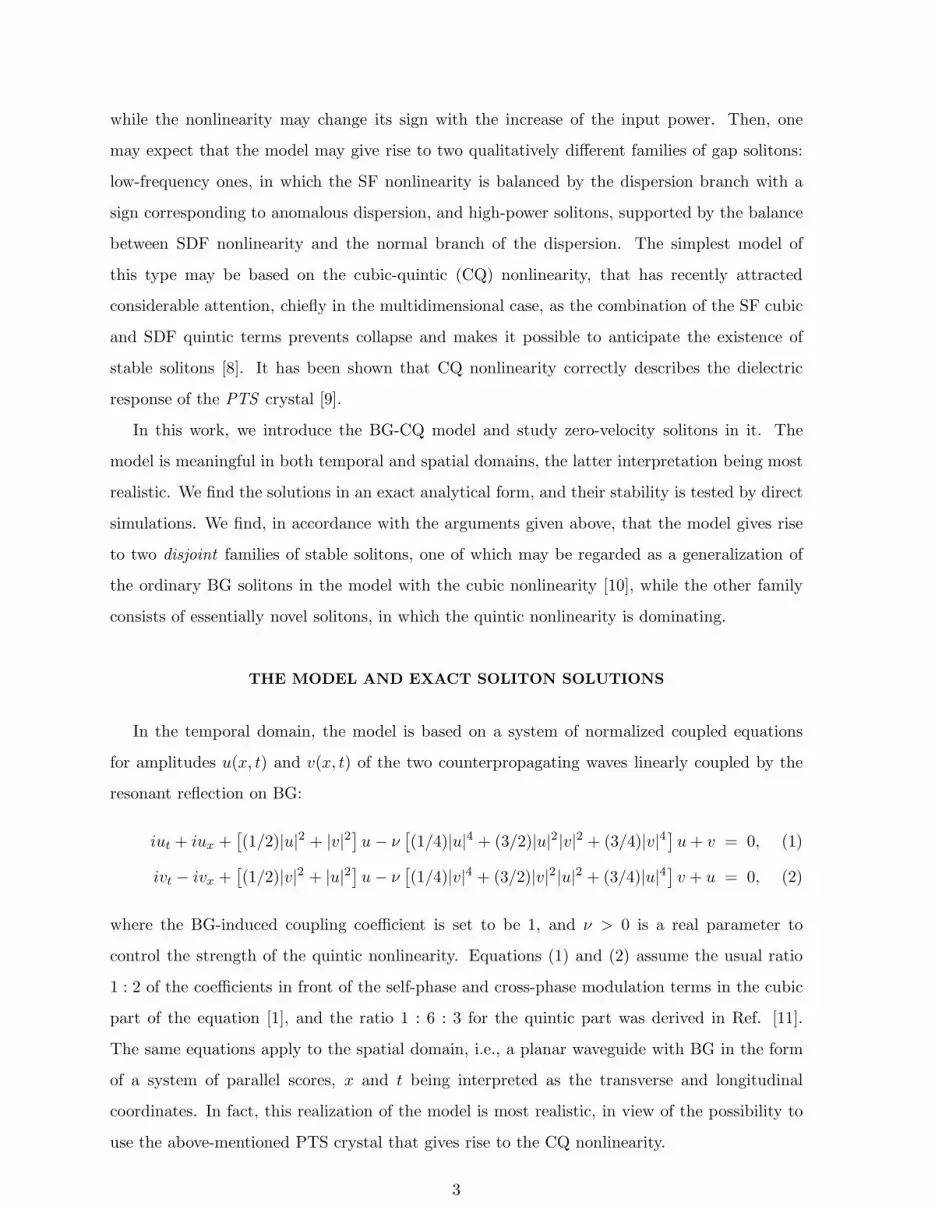
while the nonlinearity may change its sign with the increase of the input power. Then, one

may expect that the model may give rise to two qualitatively different families of gap solitons:

low-frequency ones, in which the SF nonlinearity is balanced by the dispersion branch with a

sign corresponding to anomalous dispersion, and high-power solitons, supported by the balance

between SDF nonlinearity and the normal branch of the dispersion. The simplest model of

this type may be based on the cubic-quintic (CQ) nonlinearity, that has recently attracted

considerable attention, chiefly in the multidimensional case, as the combination of the SF cubic

and SDF quintic terms prevents collapse and makes it possible to anticipate the existence of

stable solitons [8]. It has been shown that CQ nonlinearity correctly describes the dielectric

response of the PTS crystal [9].

In this work, we introduce the BG-CQ model and study zero-velocity solitons in it. The

model is meaningful in both temporal and spatial domains, the latter interpretation being most

realistic. We find the solutions in an exact analytical form, and their stability is tested by direct

simulations. We find, in accordance with the arguments given above, that the model gives rise

to two disjoint families of stable solitons, one of which may be regarded as a generalization of

the ordinary BG solitons in the model with the cubic nonlinearity [10], while the other family

consists of essentially novel solitons, in which the quintic nonlinearity is dominating.

THE MODEL AND EXACT SOLITON SOLUTIONS

In the temporal domain, the model is based on a system of normalized coupled equations

for amplitudes u(x, t) and v(x, t) of the two counterpropagating waves linearly coupled by the

resonant reflection on BG:

iut + iux +[

(1/2)|u|2 + |v|2]

u− ν[

(1/4)|u|4 + (3/2)|u|2|v|2 + (3/4)|v|4]

u+ v = 0, (1)

ivt − ivx +[

(1/2)|v|2 + |u|2]

u− ν[

(1/4)|v|4 + (3/2)|v|2 |u|2 + (3/4)|u|4]

v + u = 0, (2)

where the BG-induced coupling coefficient is set to be 1, and ν > 0 is a real parameter to

control the strength of the quintic nonlinearity. Equations (1) and (2) assume the usual ratio

1 : 2 of the coefficients in front of the self-phase and cross-phase modulation terms in the cubic

part of the equation [1], and the ratio 1 : 6 : 3 for the quintic part was derived in Ref. [11].

The same equations apply to the spatial domain, i.e., a planar waveguide with BG in the form

of a system of parallel scores, x and t being interpreted as the transverse and longitudinal

coordinates. In fact, this realization of the model is most realistic, in view of the possibility to

use the above-mentioned PTS crystal that gives rise to the CQ nonlinearity.

3

In this work, we confine ourselves to the study of zero-velocity solitons, which are sought for

as

u(x, t) = A(x) exp(iφ(x) − iωt), v(x, t) = B(x) exp(iψ(x) − iωt), (3)

where ω belongs to the above-mentioned gap,

− 1 < ω < +1, (4)

and the real amplitudes A,B and phases φ,ψ satisfy equations obtained by the substitution of

(3) into Eqs. (1) and (2). After straightforward manipulations, two simple relations follow from

those equations,

d

dx

(

A2 −B2)

= 0,d

dx(φ+ ψ) = 0, (5)

For the soliton solutions, the fields A and B must vanish at x = ±∞, hence Eq. (5) yields

B(x) = A(x). A constant value of φ+ψ can be set equal to zero by means of an obvious phase

shift, hence we also have ψ(x) = −φ(x). Obviously, these relations between the amplitudes and

phases imply that the two fields are subject to the relation u∗ = v.

The remaining equations for the single amplitude A and single phase φ take the following

form:

da

dx= 2a sin(2φ), a ≡ A2, (6)

dφ

dx= ω +

3

2a−

5

2νa2 + cos(2φ), (7)

A quotient of Eqs. (7) and (6) yields an equation for φ regarded as a function as a,

dc

da+c

a= −

3

2+

5ν

2a, c ≡ ω + cos(2φ), (8)

which can be immediately solved to yield c(a) = c0/a − (3/4)a + (5ν/6)a2, where c0 is an

arbitrary constant. Only the solution with c0 = 0 is not singular, hence we finally have

cos(2φ) = −ω − (3/4)a + (5ν/6)a2. (9)

The next step is to eliminate sinφ from Eq. (6) by means of the expression (9), arriving at an

equation

da

dx= 2a

√

1 −

(

ω +3

4a−

5ν

6a2

)2

. (10)

An integral of Eq. (10) can be written in an implicit form,

x(a) =

∫

a0

a

db

2b

√

1 −(

ω + 34b−

56νb

2)2, (11)

4

which describes soliton solutions in the interval 0 < x < ∞ (for x < 0, the solution can be

obtained trivially, as the function a(x) is even). Indeed, letting a → 0 in Eq. (11), one has

x→ ∞, in compliance with the boundary condition that a(x) must vanish at |x| → ∞. On the

other hand, it also follows from Eq. (11) that a(x) attains its maximum value a0 (which is the

soliton’s peak power) at x = 0.

The integral in (11) can be expressed in terms of incomplete elliptic integrals, but this formal

representation is useless. It is more essential to find the soliton’s peak power a0 in terms of ν

and ω. Because da/dx = 0 at soliton’s center, a0 must be a root of the right hand side of Eq.

(10), i.e., ω + (3/4)a− (5ν/6)a2 = ±1. This pair of quadratic equations have four roots; after a

simple consideration, one can find that only two of them may be relevant, namely

(a0)1 =3

5ν

[

3

4−

√

9

16−

10ν

3(1 − ω)

]

, (12)

(a0)2 =3

5ν

[

3

4+

√

9

16+

10ν

3(1 + ω)

]

. (13)

Note that, in the limit ν → 0, the root (12) yields the peak power (4/3)(1 − ω) of the Bragg-

grating soliton in the usual model with the cubic nonlinearity [10], while the root (13) goes to

infinity in the same limit.

Further straightforward consideration of the structure of the exact solution (11) leads to a

conclusion that, if the root (12) exists as a physical (real) one, i.e., in the region

1 − ω < 27/(160ν), (14)

this root determines the amplitude of the soliton, while the root (13) is then irrelevant. Exactly

at the border of the region (14), 1 − ω = 27/ (160ν), no soliton exists, and in the region

1 − ω > 27/(160ν) (15)

the root (12) does not exist. Nevertheless, Eq. (11) yields a soliton in the region (15) too, but

it takes a principally different shape, with the amplitude given by the expression (13).

Note that the solitons may exist only in the spectral gap (4), or 0 < 1 − ω < 2, therefore

the region (15) is actually present only if ν > 27/320 ≈ 0.0844. Thus, in this case there exist

two different families of the exact soliton solutions separated by the border 1− ω = 27/ (160ν).

Typical examples of solitons of the two types are displayed in Fig. 1. In the region (14), the

solitons may be regarded as obtained by a smooth deformation of the usual gap solitons known in

the model with the cubic nonlinearity [10], while novel solitons existing in the region (15), where

5

the quintic nonlinearity plays a dominant role, may have a characteristic “two-tier” structure,

with a sharp (but nevertheless nonsingular) peak, as it is seen in Fig. 1. Another qualitative

difference between the solutions of the two types pertains to their phase structure and parity: if

the soliton’s amplitude takes the value (12), it follows from Eq. (9) that cos(2φ(x = 0)) = −1,

and the value (13) of the amplitude corresponds to cos(2φ(x = 0)) = +1. It is easy to understand

(with regard to the above normalization setting the constant value of φ(x)+ψ(x) equal to zero)

that a consequence of this is that, in the solutions of the first type, Reu(x) and Re v(x) are

odd, and Imu(x) and Im v(x) are even functions of x. In the solutions of the second type, the

parities of the real and imaginary parts of the solutions are opposite.

STABILITY OF THE SOLITONS

It is known that, even in the model with the cubic nonlinearity, the soliton stability is a

difficult issue. For the first time, a possibility of instability of a part of the gap solitons was

predicted in Ref. [12] on the basis of the variational approximation (VA). In that work, three

(quasi)modes of internal oscillations of a soliton were identified and each of which could become

unstable, depending on the soliton’s frequency ω: one mode generated weak nonoscillatory

instability below a critical frequency, ω < ω(1)cr , and the others gave rise to essentially stronger

oscillatory instability in an interval −1 < ω < ω(2)cr , with ω

(2)cr < ω

(1)cr . Later, the stability of

the gap solitons in the cubic BG model was studied rigorously by means of numerical methods

applied to equations for small perturbations linearized about the soliton [13]. As a result, it was

found that a part of the solitons are unstable indeed. Comparison with the predictions of VA

shows that, while the above-mentioned weak nonoscillatory instability appears to be an artifact

of the approximation (which can probably be explained by a general theory considering possible

false instabilities predicted by VA for solitons [14]), the stronger oscillatory instability sets in

indeed if the frequency ω is smaller than a critical value, which is very close to that predicted

by VA.

By means of systematic simulations of Eqs. (1) and (2) we have tested the stability of both

families of the solitons given by the exact implicit form (11) against small initial perturbations.

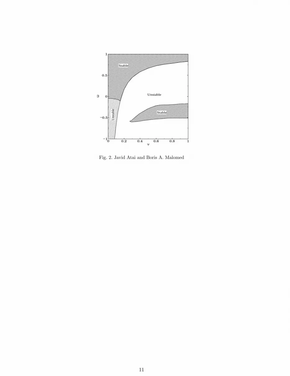
The resultant stability diagram in the (ν, ω) plane is displayed in Fig. 2. The most important

conclusion suggested by the diagram is that as nu increases the stability region for the usual

solitons (corresponding to solitons in region (14)) shrinks but the opposite occurs for the solitons

of the novel type.

The simulations also demonstrate that far from the stability border the unstable solitons

6

decay into radiation. However, in the vicinity of the stability border, after shedding some

radiation, they rearrange themselves into stable solitons. Thus, with regard to the possibility of

radiative losses, the stable solitons play the role of attractors in the present conservative model,

i.e., the stable solitons are really robust objects. A typical example is shown in Fig. 3, where

an unstable soliton evolves into a stable one.

The model presents essential differences against the one with pure cubic nonlinearity not only

concerning the existence of solitons and their stability against small perturbations, but also in

dynamics of strongly perturbed solitons. The simplest and most important example of a strong

perturbation is sudden uniform multiplication of the soliton’s profile by an amplification factor

α essentially exceeding 1, which is a result of the action of an optical amplifier. In the usual

models with the cubic nonlinearity, it is well known that the amplified pulse separates into a new

soliton and considerable amount of radiation. However, in the present model it is feasible that

the quintic term, which has the sign opposite to that in front of the cubic one, may help to shape

the amplified pulse into a new soliton, thus reducing the share of energy emitted with radiation.

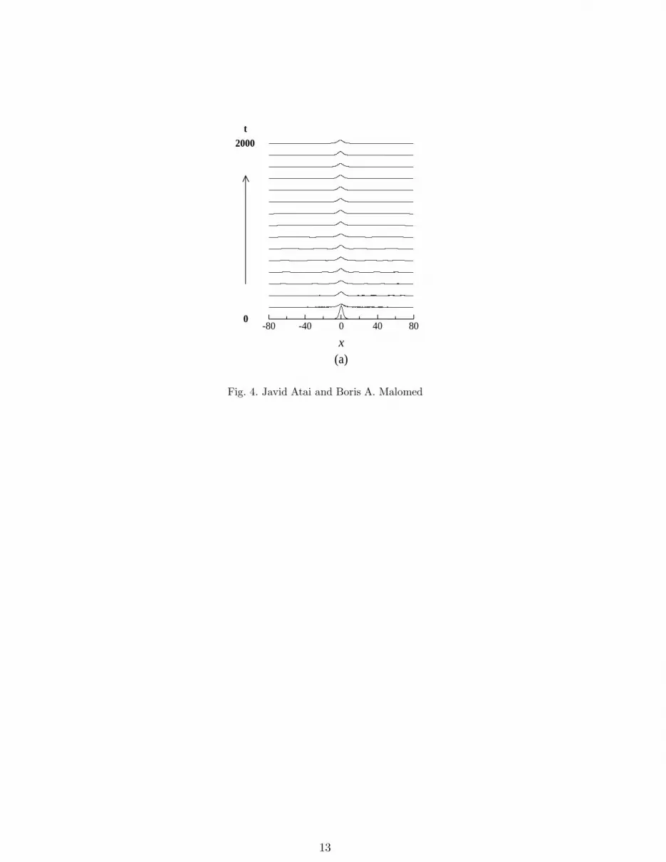
Figure 4, which displays typical examples of the relaxation of the strongly amplified (by the

factor α = 2) pulses in the cubic model proper and cubic-quintic one, demonstrates that this is

indeed the case. In fact, the effect of the quintic term (with ν = 1/2) is very significant: in the

cubic model, the final soliton retains only 11.6% of the initial energy, while the energy-retention

share in the cubic-quintic model is 92.4%.

CONCLUSION

We have introduced a model whose linear part includes two counterpropagating waves coupled

by the resonant reflection on a Bragg grating, and the nonlinear part includes cubic and quintic

terms with opposite signs. The model gives rise to two different families of solitons (provided

that the coefficient in front of the quintic term exceeds a minimum value, ν = 27/320), which

are found in an exact analytical form. One family may be regarded as a generalization of

the usual Bragg-grating solitons supported by the cubic nonlinearity, while the other family,

in which the quintic nonlinearity is dominant, includes “two-tier” solitons with a sharp (but

nonsingular) peak. Also, the soliton families differ in the parities of their real and imaginary

parts. In the plane (ω, ν), the two soliton families are separated by a curve on which solitons do

not exist. Stability regions have been identified within each family by means of direct numerical

simulations. It was also shown that in the vicinity of the stability border the unstable solitons

do not decay. Rather, after losing some energy in the form of radiation, they evolve into stable

7

ones. In the present model, almost all the energy of a strongly perturbed soliton is retained in

the process of its evolution, a fairly small share being lost with radiation, which is opposite to

what occurs in the usual cubic model.

8

[1] G.P. Agrawal, Nonlinear Fiber Optics (Academic Press: San Diego, 1995).

[2] P. Di Trapani, D. Caironi, G. Valiulis, A. Dubielis, R. Dalielius, and A. Piskarskas, Phys. Rev. Lett.

81, 570 (1998).

[3] X. Liu, L.J. Qian and F.W. Wise, Phys. Rev. Lett. 82, 4631 (1999); X. Liu, X., K. Beckwitt, and

F. Wise, Phys. Rev. E 62, 1328 (2000).

[4] H. He and P.D. Drummond, Phys. Rev. Lett. 78, 4311 (1997).

[5] B.J. Eggleton, R.E. Slusher, C.M. de Sterke, P.A. Krug, and J.E. Sipe, Phys. Rev. Lett. 76, 1627

(1996); B.J. Eggleton, C.M. de Sterke and R.E. Slusher, J. Opt. Soc. Am B 14, 2980 (1997).

[6] C.M. de Sterke and J.E. Sipe, Progr. Optics 33, 203 (1994).

[7] W.C.K. Mak, B.A. Malomed, and P.L. Chu, Phys. Rev. E 58, 6708 (1998).

[8] M. Quiroga-Teixeiro and H. Michinel, J. Opt. Soc. Am. B 14, 2004 (1997); A. Berntson, M. Quiroga-

Teixeiro, and H. Michinel, J. Opt. Soc. Am. B 16, 1697 (1999); A. Desyatnikov, A. Maimistov, and B.

Malomed, Phys. Rev. E 61, 3107 (2000); D. Mihalache, D. Mazilu, L.-C. Crasovan, B. A. Malomed,

and F. Lederer, Phys. Rev. E 61, 7142 (2000).

[9] B.L. Lawrence, M. Cha, J.U. Kang, W. Torruellas, G. Stegeman, G. Baker, J. Meth, and S. Etemad,

Electr. Lett. 30, 889 (1994).

[10] D.N. Christodoulides and R.I. Joseph, Phys. Rev. Lett. 62, 1746 (1989); A.B. Aceves and S. Wabnitz,

Phys. Lett. A 141, 116 (1989).

[11] A.I. Maimistov, B.A. Malomed, and A. Desyatnikov, Phys. Lett. A 254, 179 (1999).

[12] B.A. Malomed and R.S. Tasgal, Phys. Rev. E 49, 5787 (1994).

[13] I.V. Barashenkov, D.E. Pelinovsky, and E.V. Zemlyanaya, Phys. Rev. Lett. 80, 5117 (1998); A. De

Rossi, C. Conti, and S. Trillo, Phys. Rev. Lett. 81, 85 (1998).

[14] D.J. Kaup and T.I. Lakoba, J. Math. Phys. 37, 3442 (1996).

9

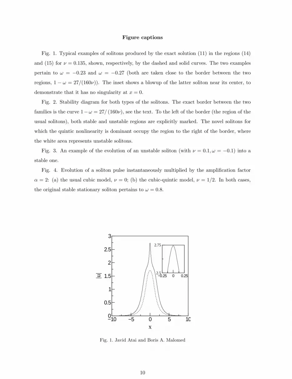
Figure captions

Fig. 1. Typical examples of solitons produced by the exact solution (11) in the regions (14)

and (15) for ν = 0.135, shown, respectively, by the dashed and solid curves. The two examples

pertain to ω = −0.23 and ω = −0.27 (both are taken close to the border between the two

regions, 1 − ω = 27/(160ν)). The inset shows a blowup of the latter soliton near its center, to

demonstrate that it has no singularity at x = 0.

Fig. 2. Stability diagram for both types of the solitons. The exact border between the two

families is the curve 1−ω = 27/ (160ν), see the text. To the left of the border (the region of the

usual solitons), both stable and unstable regions are explicitly marked. The novel solitons for

which the quintic nonlinearity is dominant occupy the region to the right of the border, where

the white area represents unstable solitons.

Fig. 3. An example of the evolution of an unstable soliton (with ν = 0.1,ω = −0.1) into a

stable one.

Fig. 4. Evolution of a soliton pulse instantaneously multiplied by the amplification factor

α = 2: (a) the usual cubic model, ν = 0; (b) the cubic-quintic model, ν = 1/2. In both cases,

the original stable stationary soliton pertains to ω = 0.8.

−10 −5 0 5 10x

0

0.5

1

1.5

2

2.5

3

|u|

−0.25 0 0.252.5

2.75

Fig. 1. Javid Atai and Boris A. Malomed

10

ω

Stable

Uns

tabl

e0.5−

1−

0.5

0

1

0 0.80.60.40.2 1

ν

Stable

Unstable

Fig. 2. Javid Atai and Boris A. Malomed

11

-20 0 20

x

2000t

0

Fig. 3. Javid Atai and Boris A. Malomed

12

-80 -40 0 40 80

x

2000t

0

(a)

Fig. 4. Javid Atai and Boris A. Malomed

13

-80 -40 0 40 80

x

2000t

0

(b)

Fig. 4. Javid Atai and Boris A. Malomed

14