Marine Micropaleontology 72 (2009) 146–156

Contents lists available at ScienceDirect

Marine Micropaleontology

j ourna l homepage: www.e lsev ie r.com/ locate /marmicro

Factors controlling the distribution of planktonic foraminifera in the Red Sea andimplications for the development of transfer functions

Michael Siccha ⁎, Gabriele Trommer, Hartmut Schulz, Christoph Hemleben, Michal KuceraInstitute of Geosciences, Eberhard-Karls University of Tuebingen, Sigwartstr.10, 72076 Tuebingen, Germany

⁎ Corresponding author.E-mail address: michael.siccha@uni-tuebingen.de (M

0377-8398/$ – see front matter © 2009 Elsevier B.V. Adoi:10.1016/j.marmicro.2009.04.002

a b s t r a c t

a r t i c l e i n f o

Article history:Received 20 November 2008Received in revised form 7 April 2009Accepted 14 April 2009

Keywords:Planktonic foraminiferaTransfer functionsProductivityRed Sea

The Red Sea is an extreme marine environment, with conditions limiting the application of standardgeochemical proxies for the reconstruction of paleoclimate. In order to develop paleoenvironmentalreconstruction methods which are not dependent on chemical signals, we investigated the distribution ofplanktonic foraminifera in the surface sediments and assessed the viability of constructing foraminiferaltransfer functions in this basin. We find a distinct gradient in the faunal assemblage along the basin's axis,which is reflected in a high correlation between faunal composition and all considered environmentalparameters (temperature, salinity, chlorophyll a concentration, stratification, and oxycline depth). As aresult, transfer functions constructed by different methods (ANN, MAT, IKM, WA-PLS) appear to be able toestimate all of these parameters with a high average accuracy (15% of the parameter's range in the Red Sea).However, redundancy analysis of the distribution of foraminiferal assemblages in surface sediments alone didnot yield unambiguous results in terms of which of the considered factors exerts a primary control on theforaminifera distribution and which of the observed relationships are the result of the mutual correlationamong the environmental factors. To disentangle the effect of individual environmental parameters, weapplied the obtained transfer functions on a newly generated Holocene record from the central Red Sea. Theintegration of published paleoclimate reconstructions with our data allowed us to identify productivity as themost likely primary control of the planktonic foraminifera distribution in the Red Sea. The generated transferfunctions can estimate paleoproductivity with acceptable accuracy (RMSEP chlorophyll a=0.1 mg/m3; ~8%of recent range), but only under such conditions in the past when circulation patterns and salinity levels inthe basin were fundamentally comparable to the present day. Since productivity in the central and southernRed Sea is closely linked with the Monsoon-driven water exchange across the Strait of Bab al Mandab, theresulting reconstructions can provide indirect information on the mode and intensity of the monsoonalsystem in the past.

© 2009 Elsevier B.V. All rights reserved.

1. Introduction

Reconstructions of past environmental conditions in the Red Seahave so far been limited to two distinct aspects. The first one includesqualitative reconstructions of water-column properties, climate andcirculation patterns by analyses of fossil assemblages of pteropods(Almogi-Labin et al., 1998, 1991), benthic foraminifera (Badawi et al.,2005), planktonic foraminifera (Edelman-Fürstenberg et al., 2009;Fenton et al., 2000; Halicz and Reiss, 1981; Ivanova, 1985) andcoccolithophorida (Legge et al., 2006, 2008). The second aspectconcerns reconstructions of salinity bymeans of stable oxygen isotopeanalysis in shells of planktonic foraminifera (Hemleben et al., 1996)combined with oceanographic modelling (Rohling, 1994; Siddall et al.,2004). The stable isotopic signals in the Red Sea are dependent on the

. Siccha).

ll rights reserved.

water exchange with the open ocean and employed in modelstranslating isotopic records to variations in salinity and indirectly tosea level changes (Siddall et al., 2004). The special characteristics ofthe Red Sea basin (low productivity and extreme salinities) compli-cate the use and interpretation of most standard geochemical proxies.Until now, only one quantitative paleotemperature record has beenobtained by analysis of alkenones from a core in the very north of theRed Sea (Arz et al., 2003). Attempts to use Mg/Ca in planktonicforaminifera have been confrontedwith unusually highMg values andpossible inorganic precipitation (Rohling et al., 2008). In this study wepresent the first planktonic foraminifera transfer function approachfor paleoclimate reconstruction in the Red Sea. Auras-Schudnagieset al. (1989) has shown that the distribution of planktonic foramini-fera in Red Sea sediments is characterised by a distinct gradient, whichreflect the circulation pattern in the basin. This work has shown thatplanktonic foraminifera assemblages in the Red Sea are distinct fromthose in the open ocean, precluding the use of calibration data fromoutside the basin. The aim of this study was to develop a well

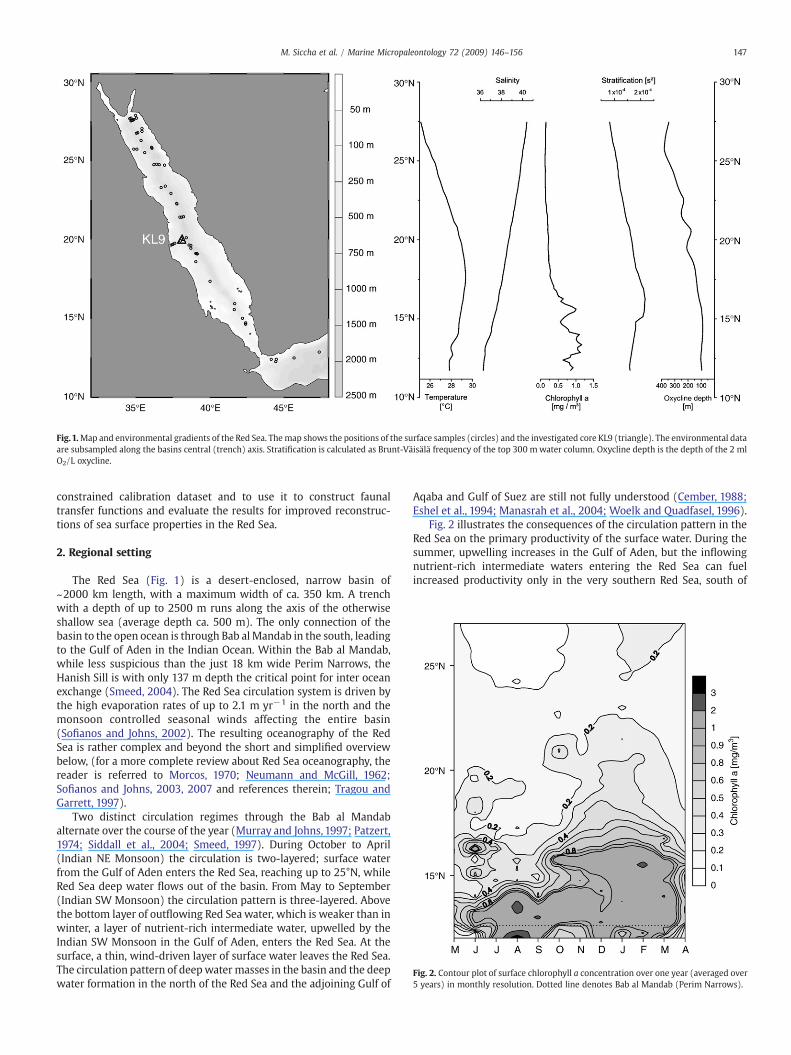
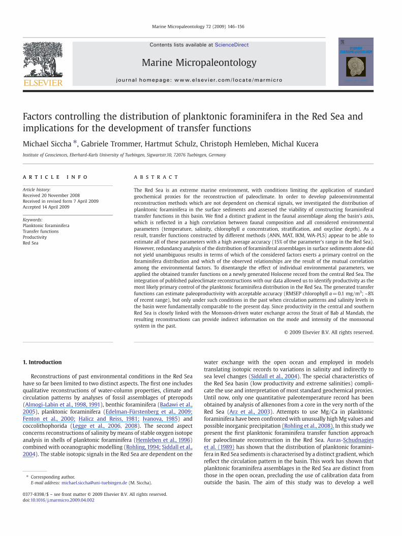
Fig.1.Map and environmental gradients of the Red Sea. Themap shows the positions of the surface samples (circles) and the investigated core KL9 (triangle). The environmental dataare subsampled along the basins central (trench) axis. Stratification is calculated as Brunt-Väisälä frequency of the top 300 mwater column. Oxycline depth is the depth of the 2 mlO2/L oxycline.

Fig. 2. Contour plot of surface chlorophyll a concentration over one year (averaged over5 years) in monthly resolution. Dotted line denotes Bab al Mandab (Perim Narrows).

147M. Siccha et al. / Marine Micropaleontology 72 (2009) 146–156

constrained calibration dataset and to use it to construct faunaltransfer functions and evaluate the results for improved reconstruc-tions of sea surface properties in the Red Sea.

2. Regional setting

The Red Sea (Fig. 1) is a desert-enclosed, narrow basin of~2000 km length, with a maximum width of ca. 350 km. A trenchwith a depth of up to 2500 m runs along the axis of the otherwiseshallow sea (average depth ca. 500 m). The only connection of thebasin to the open ocean is through Bab al Mandab in the south, leadingto the Gulf of Aden in the Indian Ocean. Within the Bab al Mandab,while less suspicious than the just 18 km wide Perim Narrows, theHanish Sill is with only 137 m depth the critical point for inter oceanexchange (Smeed, 2004). The Red Sea circulation system is driven bythe high evaporation rates of up to 2.1 m yr−1 in the north and themonsoon controlled seasonal winds affecting the entire basin(Sofianos and Johns, 2002). The resulting oceanography of the RedSea is rather complex and beyond the short and simplified overviewbelow, (for a more complete review about Red Sea oceanography, thereader is referred to Morcos, 1970; Neumann and McGill, 1962;Sofianos and Johns, 2003, 2007 and references therein; Tragou andGarrett, 1997).

Two distinct circulation regimes through the Bab al Mandabalternate over the course of the year (Murray and Johns, 1997; Patzert,1974; Siddall et al., 2004; Smeed, 1997). During October to April(Indian NE Monsoon) the circulation is two-layered; surface waterfrom the Gulf of Aden enters the Red Sea, reaching up to 25°N, whileRed Sea deep water flows out of the basin. From May to September(Indian SW Monsoon) the circulation pattern is three-layered. Abovethe bottom layer of outflowing Red Sea water, which is weaker than inwinter, a layer of nutrient-rich intermediate water, upwelled by theIndian SW Monsoon in the Gulf of Aden, enters the Red Sea. At thesurface, a thin, wind-driven layer of surface water leaves the Red Sea.The circulation pattern of deepwater masses in the basin and the deepwater formation in the north of the Red Sea and the adjoining Gulf of

Aqaba and Gulf of Suez are still not fully understood (Cember, 1988;Eshel et al., 1994; Manasrah et al., 2004; Woelk and Quadfasel, 1996).

Fig. 2 illustrates the consequences of the circulation pattern in theRed Sea on the primary productivity of the surface water. During thesummer, upwelling increases in the Gulf of Aden, but the inflowingnutrient-rich intermediate waters entering the Red Sea can fuelincreased productivity only in the very southern Red Sea, south of

148 M. Siccha et al. / Marine Micropaleontology 72 (2009) 146–156

14°N, and the resulting chlorophyll concentrations there are markedlyhigher than those of the winter season. The central and northernregions of the Red Sea show their productivity maximum, still withvery low chlorophyll concentrations, during the winter, apparentlypowered by the inflow of Gulf of Aden surface waters (rather thanintermediate waters as in summer). This is consistent with theobservation of high plankton biomass in the Gulf of Aden in winter byvan Couwelaar (1997). In contrast to the monsoon-related summerproductivity in the Red Sea, which is high but patchy, the surfaceinflow during the winter is more homogenous and also morevoluminous than the summer inflow (to compensate evaporativeloss in the north, (e. g. Siddall et al., 2002).

Therefore, the inflowing surface water in winter stimulates ahigher primary productivity in the Red Sea much further to the norththan the Gulf of Aden water entering the basin during the summer.The origin of the weak but distinct productivity maximum in the verynorth of the Red Sea (north of 25°N, Fig. 2) during the winter remainsunclear, but is most probably connected to mixing processes in thewater column during deep water formation.

Directly connected to the pattern of primary productivity is thedevelopment of an oxygen minimum zone (OMZ), more prominent inthe southern part of the Red Sea, with oxygen concentrations as low as0.5 ml/l in its core. The 2.0 ml/l oxycline lies at 75 m depth in thesouth (b16°N) and deepens continuously till it reaches depths ofaround 300m north of 25°N (World Ocean Atlas 2001, Conkright et al.,2001; Neumann andMcGill, 1962). The north–south orientation of theRed Sea in combination with restricted water exchange only at itssouthern end, result in strong and mutually correlated gradients ofmost oceanographic parameters along the basins axis (see Table 1).This strong correlation among virtually all oceanographic parametersposes a challenge to the identification of individual factors whichcontrol the distribution of planktonic organisms in the Red Sea(Auras-Schudnagies et al., 1989).

3. Materials and methods

3.1. Surface samples

The distribution pattern of planktonic foraminifera species wasdetermined by analysing 60 surface sediment samples from the RedSea and the Gulf of Aden, collected during three cruises (see onlinesupporting material). None of these samples showed any signs ofmodification of the assemblages due to carbonate dissolution. This isimportant to note because samples from the Gulf of Aden couldpotentially be affected by dissolution (Almogi-Labin et al., 2000),whereas carbonate dissolution is know to be minimal throughout theRed Sea (Almogi-Labin et al., 1998). Indeed, we have initiallyconsidered seven surface sediment samples from the Gulf of Aden,but rejected two of them because of signs of dissolution. The sampleswere washed over a 63 μm sieve, dry-sieved over 150 μm mesh andsplit with an ASC Scientific microsplitter. For each sample an aliquotcontaining at least 300 individual planktonic foraminifera wascounted under the binocular and the relative abundances ofplanktonic foraminifera species were determined, following thetaxonomy of Hemleben et al. (1989). The resulting database contains

Table 1Correlation of environmental variables in the surface sample dataset.

Tem

Temperature [annual mean at 10 m; WOA 2001] 1.Salinity [annual mean at 10 m ; WOA 2001] −0.Chlorophyll a [annual mean of 5 year period; Merged AquaMODIS-SEAWIFS] 0.Distance to Bab al Mandab [Perim Narrows at 12.36′ °N, 43.22′ °E] −0.Stratification [mean BVF of the top 300 m annual mean water column; WOA 2001] 0.Oxycline depth [depth of annual mean 2 ml O2/l oxycline; WOA 2001] −0.

All values are significant at pb0.05.

more than twice as many samples as the previous study by Auras-Schudnagies et al. (1989). Apart from eight counts of samples thatwere also included in that study, all the additional samples were takenfrom multicorer tubes from the top 1 cm or the top 0.5 cm. In order toachieve the highest possible level of taxonomic consistency in thecounts, all of the 60 samples in this study have been counted by theauthors, and the counts were checked repeatedly for taxonomicconsistency. Multicorer hauls are ideal to recover undisturbed surfacesediment and the recent age of multicorer coretops from the centralRed Sea is supported by radiocarbon dates in Edelman-Furstenberget al. (2009). The count data are available in the online supportingmaterial.

The resulting database of species abundances was compared witha series of environmental parameters describing the most pertinentproperties of the surface waters. The analysis of open-oceanplanktonic foraminifera faunas by Morey et al. (2005) suggeststemperature as the dominant factor controlling the distribution ofplanktonic foraminifera. However, in the restricted environment ofthe Red Sea, many oceanographic parameters (e.g., salinity) showmuch greater gradients than in the open ocean and we have thereforeconsidered the effect of not only temperature but also salinity,chlorophyll a concentration, oxycline depth and stratification (Fig. 1).The latter two variables are rarely considered when analysing thedistribution of planktonic foraminifera, but they are very closelycoupled to the circulation pattern in the Red Sea, which on the basis ofearlier studies (Almogi-Labin et al., 1991; Auras-Schudnagies et al.,1989) seems to represent the most important factor affectingplankton distribution in the basin.

Temperature, salinity and oxygen concentration data used in allfollowing analyses represent annual average values from the 10 mdepth level of the World Ocean Atlas 2001 (WOA; Conkright et al.,2001) interpolated to the position of the samples by area weighting.Investigation of vertical temperature and density gradients in the RedSea leads to the estimation of a very shallow mixed layer depth,ranging from 30 m in the south to around 70 m in the north of thebasin (Monterey and Levitus, 1997). These values reflect the layeringof the circulation system but most probably not the vertical extent ofthe habitat of planktonic foraminifera. Therefore the Brunt-Väisäläfrequency (BVF) was calculated from WOA data for each depthinterval and the average of the top 300 m of the water column wasthen used as a measure of stratification. The BVF is the frequency withwhich a packet of water will oscillate when it is vertically displacedfrom its position in the water column. High frequencies correspond tolarge density differences found typically in a stratified water column,whereas low frequencies will be found in a more homogenous watercolumn. Though the employed average of BVF is highly correlatedwithmixed layer depth, it does not hold any depth-related information perse but is a measure of water column stability and/or the intensity ofthe pycnocline. Surface water chlorophyll a concentrations wereobtained from the Ocean ColorWeb (Feldman andMcClain, 2006).Wenote that the surface chlorophyll a data might not necessarilyrepresent the primary productivity or the biomass of all phytoplank-ton groups throughout the water column, but in the absence ofvertically resolved data at appropriate resolution, the satellite datarepresent the best proxy for productivity available. The annual average

perature Salinity Chlorophyll a Distance Stratification Oxycline depth

00 −0.69 0.34 −0.73 −0.95 −0.8269 1.00 −0.80 1.00 −0.82 0.9534 −0.80 1.00 −0.76 0.57 −0.7373 1.00 −0.76 1.00 −0.84 0.9695 −0.82 0.57 −0.84 1.00 −0.9182 0.95 −0.73 0.96 −0.91 1.00

Table 214C ages obtained by accelerator mass spectrometry dating of monospecific samples(Globigerinoides sacculifer) in the 250–315 μm fraction in core KL9, performed at theLeibniz-Labor AMS facility in Kiel, Germany.

Lab.-ID depth[cm]

Conventional age[yr BP]

±Error[yr]

Calibrated age[cal. yr BP]

KIA33786 2 1315 25 732KIA33785 24 3260 30 2922KIA33130 60 6595 35 6976KIA33131 84 8955 40 9495

Table 3Taxonomic units used for faunal data analysis.

Globigerina bulloidesGlobigerinita glutinataNeogloboquadrina pachyderma merged with Neogloboquadrina incomptaGlobigerinoides ruberGlobigerinoides sacculiferGlobigerinella siphonifera merged with Globigerinella calidaGloboturborotalita tenellaGulf of Aden species incl. Globorotalia menardii Neogloboquadrina dutertrei

149M. Siccha et al. / Marine Micropaleontology 72 (2009) 146–156

values of all variables were used in all analyses. Summer (JJA) andwinter (DJF) averages were considered in the distribution analyses aswell.

3.2. Downcore samples

In order to test the environmental relationships recovered from thesurface sediment dataset by means of transfer functions, new faunaldata were produced for the Holocene of core M5/2-143 GeoTÜ KL(referred to as KL9, 19°57.6′N, 38°8.3′E, 814 m; Nellen et al., 1996). Atotal of 45 samples were taken at 2-cm intervals from the top 90 cm ofthe core. These samples were processed and counted in exactly thesame way as described for the surface samples earlier. These data areavailable in the online supporting material. The age model of theHolocene section of core KL9 is based on linear interpolation betweenfour 14C AMS dates (Table 2). The resulting sedimentation rates andthe implied correlation of faunal patterns are in good agreement withpublished data from the 14C AMS dated core M5/2-174 GeoTÜ KL(referred to as KL11, 18°44.5′N, 39°20.6′E, 825 m) (Schmelzer, 1998)and multi-cores from the central Red Sea (Edelman-Fürstenberg et al.,2009). The transfer functions have been tested on Holocene material,since on glacial–interglacial timescales the planktonic faunas of RedSea are affected by extreme variations in salinity (Fenton et al., 2000).Such variations are not captured by any of the surface samples and it isa-priori obvious that applications of any transfer function beyond theinterglacial sea-level high stands will be confronted with non-analogue faunas.

3.3. Analysis of faunal data and transfer function design

In order to determine the impact of an environmental factor on theplanktonic foraminifera assemblage we first employed gradientanalysis using the Canoco 4.5 software package. An initial detrendedcanonical correspondence analysis showed a gradient length of 1.89,suggesting a direct gradient analysis with a linear response model asthe most appropriate method to analyse the foraminifera data (Lepsand Smilauer, 2003). The redundancy analysis was conducted withuntransformed percentage data and scaling focussed on species-correlations. For counts of 300 individuals, the 95% confidence levelfor a detection limit of a species corresponds to observed abundanceof 1% (Dryden, 1931; Revets, 2004). Therefore the faunal data of eachsample was purged of species not reaching 1% relative abundance inorder to avoid the influence of rare species which might or might nothave been recorded by chance. The purged data were thenrecalculated to 100%.

The results of the redundancy analysis were used to identifyenvironmental factors strongly affecting the foraminifera distribution.The relationship between the faunal distribution and these environ-mental factors was then characterised quantitatively with the aim todevelop transfer functions that will allow us to reconstruct pastenvironmental conditions in the Red Sea from fossil foraminiferaassemblages. For the identification of non-analogue samples, down-core and core–top faunal counts were analysed in a joint principalcomponent analysis. This analysis was based on logratio-transformeddata following the recommendations of Pollard and Blockley (2006).

Our calibration dataset of 60 samples is relatively small for thedevelopment of transfer functions and could lead to method-specificbias (Kucera et al., 2005). In addition, the foraminifera distributiondata in the Red Sea can be expected to show a high autocorrelation(Auras-Schudnagies et al., 1989), which is known to lead to under-estimation of error rates in certain methods (Telford et al., 2004).Therefore, we employed four different approaches with differentsensitivity to the potential sources of error mentioned above: themodern analogue technique (MAT; Hutson, 1980), the method afterImbrie and Kipp (IKM; Imbrie and Kipp,1971), theweighted averagingpartial least square regression (WA-PLS; ter Braak and Juggins, 1993)and the artificial neural networks approach (ANN) introduced byMalmgren and Nordlund (1997).

For the first three approaches we used the C2 software package(Juggins, 2003). For the ANN approach we used the NeuroGeneticOp-timizer© 2.6.142 to develop back propagation networks consisting of amaximum of four neurons in one hidden layer. A genetic algorithmwas applied to optimise the network structure (number of neuronsand type of transfer function) by training a population of 75 networksover 25 generations, with a maximum of 1000 learning epochs. Ineach case, the best networks included four neurons in the hiddenlayer. Network fitness was based solely on the test set, consisting of50% of the surface dataset. The test set samples were randomly chosenby the software and each partition was manually checked forconsistency in the coverage of the environmental gradient. The ANNresults are reported as the mean of the five best networks obtainedfrom five different training set partitions for any single factor. In caseof the MAT approach, we calculated the Bray-Curtis-dissimilarity andused the weighted average of the three most similar samples. Inthe WA-PLS we used the number (usually just one) of components,which yielded the lowest RMSEP (root mean squared error ofprediction). For the IKM we used the simple Kaiser-Guttman criterion(eigenvalueN1.0) to limit the number of factors to three and includedthe quadratic terms in the regression.

For all methods except ANN, the validation of the transferfunctions was performed by bootstrapping the calibration dataset(1000 cycles). The limited number of recent surface samples and theiruneven distribution made the random selection of a validation subsetunsuitable; instead we relied on the bootstrap approach for cross-validation. The prediction error was expressed as RMSEP andestimated as the average RMSE (root mean square error) of thebootstrapping cycles. Due to the high time-demand for the training ofartificial networks, we did not attempt to validate the results by acomparable bootstrapping, but presented only the average RMSE andR2 values for the test sets of the five partitions.

4. Results

4.1. Faunal distribution of planktonic foraminifera

A total of 30 different species (see Appendix A) of planktonicforaminifera in the size fraction N150 μmwere identified in the surfacesamples, of which the three most abundant species, G. sacculifer,G. ruber and G. glutinata contributed 73.3% of all individuals. Since

150 M. Siccha et al. / Marine Micropaleontology 72 (2009) 146–156

most of the species occurred only at very low relative abundances, themathematical analyses of the data were based on a reduced dataset ofthe species, which were considered most important. A distinct pair ofspecies occurring only in the Gulf of Aden samples and only found inthe southernmost of the Red Sea samples, make up less than 1% of theassemblage and were lumped together into one category. In order toachieve maximum consistency in the data, the species G. siphonifera

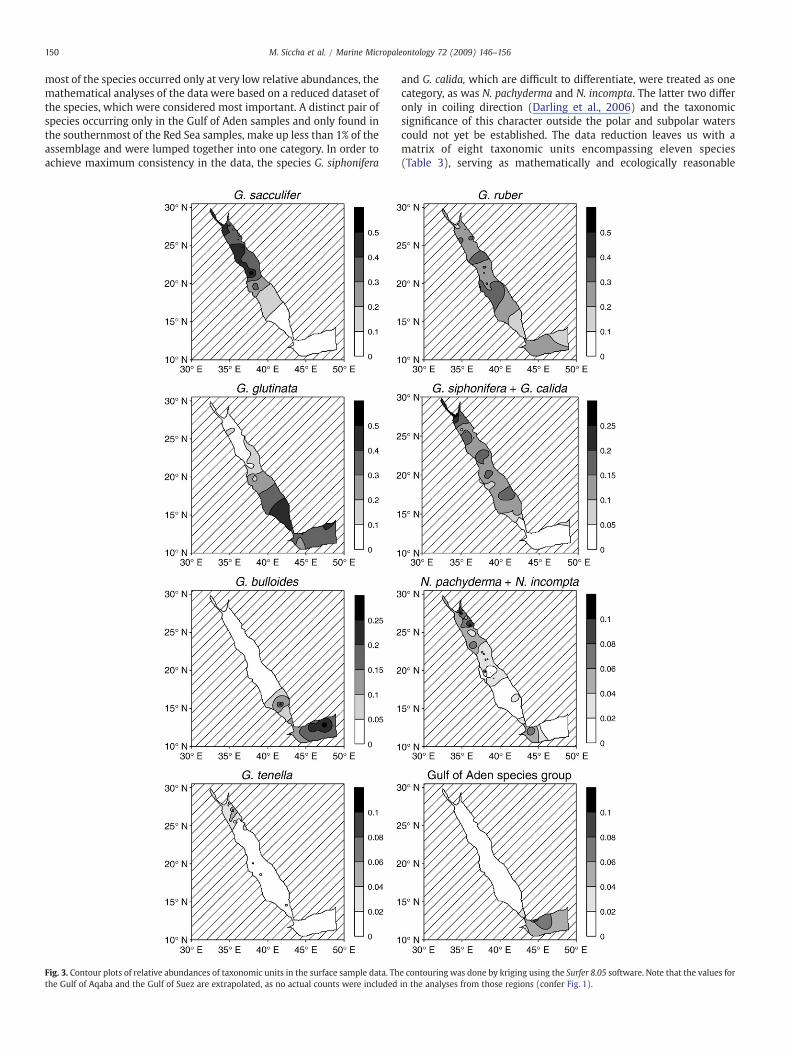
Fig. 3. Contour plots of relative abundances of taxonomic units in the surface sample data. Ththe Gulf of Aqaba and the Gulf of Suez are extrapolated, as no actual counts were included

and G. calida, which are difficult to differentiate, were treated as onecategory, as was N. pachyderma and N. incompta. The latter two differonly in coiling direction (Darling et al., 2006) and the taxonomicsignificance of this character outside the polar and subpolar waterscould not yet be established. The data reduction leaves us with amatrix of eight taxonomic units encompassing eleven species(Table 3), serving as mathematically and ecologically reasonable

e contouring was done by kriging using the Surfer 8.05 software. Note that the values forin the analyses from those regions (confer Fig. 1).

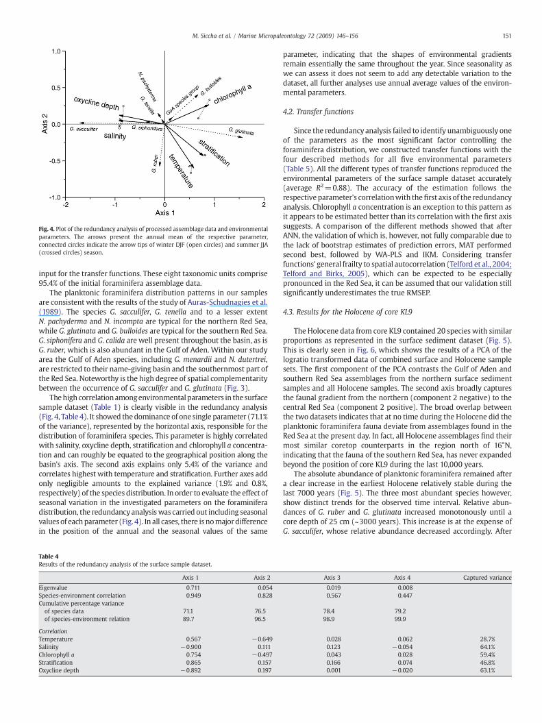
Fig. 4. Plot of the redundancy analysis of processed assemblage data and environmentalparameters. The arrows present the annual mean of the respective parameter,connected circles indicate the arrow tips of winter DJF (open circles) and summer JJA(crossed circles) season.

151M. Siccha et al. / Marine Micropaleontology 72 (2009) 146–156

input for the transfer functions. These eight taxonomic units comprise95.4% of the initial foraminifera assemblage data.

The planktonic foraminifera distribution patterns in our samplesare consistent with the results of the study of Auras-Schudnagies et al.(1989). The species G. sacculifer, G. tenella and to a lesser extentN. pachyderma and N. incompta are typical for the northern Red Sea,while G. glutinata and G. bulloides are typical for the southern Red Sea.G. siphonifera and G. calida are well present throughout the basin, as isG. ruber, which is also abundant in the Gulf of Aden. Within our studyarea the Gulf of Aden species, including G. menardii and N. dutertrei,are restricted to their name-giving basin and the southernmost part ofthe Red Sea. Noteworthy is the high degree of spatial complementaritybetween the occurrence of G. sacculifer and G. glutinata (Fig. 3).

Thehigh correlationamongenvironmentalparameters in the surfacesample dataset (Table 1) is clearly visible in the redundancy analysis(Fig. 4, Table 4). It showed thedominance of one single parameter (71.1%of the variance), represented by the horizontal axis, responsible for thedistribution of foraminifera species. This parameter is highly correlatedwith salinity, oxycline depth, stratification and chlorophyll a concentra-tion and can roughly be equated to the geographical position along thebasin's axis. The second axis explains only 5.4% of the variance andcorrelates highest with temperature and stratification. Further axes addonly negligible amounts to the explained variance (1.9% and 0.8%,respectively) of the species distribution. In order to evaluate the effect ofseasonal variation in the investigated parameters on the foraminiferadistribution, the redundancyanalysiswas carried out including seasonalvalues of each parameter (Fig. 4). In all cases, there is nomajordifferencein the position of the annual and the seasonal values of the same

Table 4Results of the redundancy analysis of the surface sample dataset.

Axis 1 Axis 2

Eigenvalue 0.711 0.054Species-environment correlation 0.949 0.828Cumulative percentage varianceof species data 71.1 76.5of species-environment relation 89.7 96.5

CorrelationTemperature 0.567 −0.649Salinity −0.900 0.111Chlorophyll a 0.754 −0.497Stratification 0.865 0.157Oxycline depth −0.892 0.197

parameter, indicating that the shapes of environmental gradientsremain essentially the same throughout the year. Since seasonality aswe can assess it does not seem to add any detectable variation to thedataset, all further analyses use annual average values of the environ-mental parameters.

4.2. Transfer functions

Since the redundancy analysis failed to identify unambiguously oneof the parameters as the most significant factor controlling theforaminifera distribution, we constructed transfer functions with thefour described methods for all five environmental parameters(Table 5). All the different types of transfer functions reproduced theenvironmental parameters of the surface sample dataset accurately(average R2=0.88). The accuracy of the estimation follows therespective parameter's correlationwith thefirst axis of the redundancyanalysis. Chlorophyll a concentration is an exception to this pattern asit appears to be estimated better than its correlationwith the first axissuggests. A comparison of the different methods showed that afterANN, the validation of which is, however, not fully comparable due tothe lack of bootstrap estimates of prediction errors, MAT performedsecond best, followed by WA-PLS and IKM. Considering transferfunctions' general frailty to spatial autocorrelation (Telford et al., 2004;Telford and Birks, 2005), which can be expected to be especiallypronounced in the Red Sea, it can be assumed that our validation stillsignificantly underestimates the true RMSEP.

4.3. Results for the Holocene of core KL9

The Holocene data from core KL9 contained 20 species with similarproportions as represented in the surface sediment dataset (Fig. 5).This is clearly seen in Fig. 6, which shows the results of a PCA of thelogratio transformed data of combined surface and Holocene samplesets. The first component of the PCA contrasts the Gulf of Aden andsouthern Red Sea assemblages from the northern surface sedimentsamples and all Holocene samples. The second axis broadly capturesthe faunal gradient from the northern (component 2 negative) to thecentral Red Sea (component 2 positive). The broad overlap betweenthe two datasets indicates that at no time during the Holocene did theplanktonic foraminifera fauna deviate from assemblages found in theRed Sea at the present day. In fact, all Holocene assemblages find theirmost similar coretop counterparts in the region north of 16°N,indicating that the fauna of the southern Red Sea, has never expandedbeyond the position of core KL9 during the last 10,000 years.

The absolute abundance of planktonic foraminifera remained aftera clear increase in the earliest Holocene relatively stable during thelast 7000 years (Fig. 5). The three most abundant species however,show distinct trends for the observed time interval. Relative abun-dances of G. ruber and G. glutinata increased monotonously until acore depth of 25 cm (~3000 years). This increase is at the expense ofG. sacculifer, whose relative abundance decreased accordingly. After

Axis 3 Axis 4 Captured variance

0.019 0.0080.567 0.447

78.4 79.298.9 99.9

0.028 0.062 28.7%0.123 −0.054 64.1%0.043 0.028 59.4%0.166 0.074 46.8%0.001 −0.020 63.1%

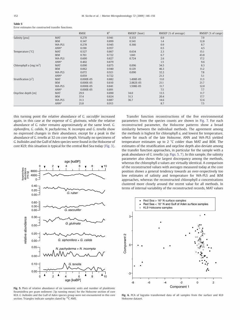
Table 5Error estimates for constructed transfer functions.

RMSE R2 RMSEP (boot) RMSEP (% of average) RMSEP (% of range)

Salinity [psu] MAT 0.270 0.941 0.333 0.9 7.9IKM 0.347 0.899 0.541 1.4 12.8WA-PLS 0.278 0.945 0.366 0.9 8.7ANN⁎ 0.190 0.957 0.5 4.5

Temperature [°C] MAT 0.527 0.867 0.634 2.3 15.1IKM 0.761 0.722 1.841 6.7 43.8WA-PLS 0.600 0.827 0.724 2.6 17.2ANN⁎ 0.402 0.879 1.5 9.6

Chlorophyll a [mg/m3] MAT 0.090 0.875 0.096 34.5 8.3IKM 0.062 0.940 0.129 46.3 11.2WA-PLS 0.072 0.921 0.090 32.2 7.8ANN⁎ 0.059 0.722 21.3 5.1

Stratification [s2] MAT 0.000E-05 0.882 1.498E-05 11.0 11.3IKM 0.000E-05 0.810 2.882E-05 21.1 21.7WA-PLS 0.000E-05 0.841 1.598E-05 11.7 12.0ANN⁎ 0.000E-05 0.891 7.5 7.7

Oxycline depth [m] MAT 29.9 0.890 34.0 13.5 11.7IKM 37.4 0.824 51.3 20.4 17.7WA-PLS 31.3 0.887 36.7 14.6 12.6ANN⁎ 21.8 0.913 8.7 7.5

152 M. Siccha et al. / Marine Micropaleontology 72 (2009) 146–156

this turning point the relative abundance of G. sacculifer increasedagain, in this case at the expense of G. glutinata, while the relativeabundance of G. ruber remains approximately at the same level. G.siphonifera, G. calida, N. pachyderma, N. incompta and G. tenella showno expressed changes in their abundance, except for a peak in theabundance of G. tenella at 32 cm core depth. Virtually no specimens ofG. bulloides and the Gulf of Aden species were found in the Holocene ofcore KL9; this situation is typical for the central Red Sea today (Fig. 3).

Fig. 5. Plots of relative abundance of six taxonomic units and number of planktonicforaminifera per gram sediment (3p running mean) for the Holocene section of coreKL9. G. bulloides and the Gulf of Aden species group were not encountered in this coresection. Triangles indicate samples dated by 14C AMS.

Transfer function reconstructions of the five environmentalparameters from the species counts are shown in Fig. 7. For eachreconstructed parameter, the Holocene patterns show a broadsimilarity between the individual methods. The agreement amongthe methods is highest for chlorophyll a, and lowest for temperature,where for much of the late Holocene, ANN and WA-PLS yieldedtemperature estimates up to 2 °C colder than MAT and IKM. Theestimates of the stratification and oxycline depth also deviate amongthe transfer function approaches, in particular for the sample with apeak abundance of G. tenella (cp. Figs. 5, 7). In this sample, the salinityparameter also shows the largest discrepancy among the methods,whereas the chlorophyll a values are virtually identical. A comparisonof the reconstructed values with averages measured today at the coreposition shows a general tendency towards an over-respectively toolow estimates of salinity and temperature for WA-PLS and IKMapproaches, whereas the reconstructed chlorophyll a concentrationsclustered more closely around the recent value for all methods. Interms of internal variability of the reconstructed records, MAT values

Fig. 6. PCA of logratio transformed data of all samples from the surface and KL9Holocene dataset.

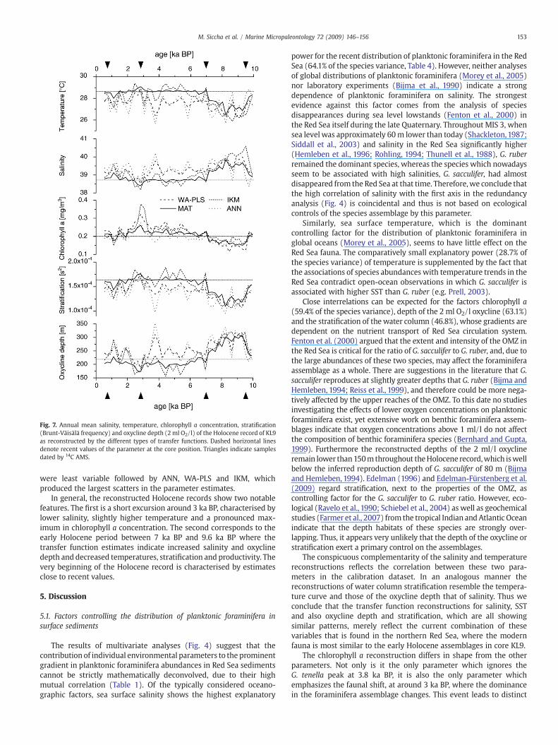
Fig. 7. Annual mean salinity, temperature, chlorophyll a concentration, stratification(Brunt-Väisälä frequency) and oxycline depth (2ml O2/l) of the Holocene record of KL9as reconstructed by the different types of transfer functions. Dashed horizontal linesdenote recent values of the parameter at the core position. Triangles indicate samplesdated by 14C AMS.

153M. Siccha et al. / Marine Micropaleontology 72 (2009) 146–156

were least variable followed by ANN, WA-PLS and IKM, whichproduced the largest scatters in the parameter estimates.

In general, the reconstructed Holocene records show two notablefeatures. The first is a short excursion around 3 ka BP, characterised bylower salinity, slightly higher temperature and a pronounced max-imum in chlorophyll a concentration. The second corresponds to theearly Holocene period between 7 ka BP and 9.6 ka BP where thetransfer function estimates indicate increased salinity and oxyclinedepth and decreased temperatures, stratification and productivity. Thevery beginning of the Holocene record is characterised by estimatesclose to recent values.

5. Discussion

5.1. Factors controlling the distribution of planktonic foraminifera insurface sediments

The results of multivariate analyses (Fig. 4) suggest that thecontribution of individual environmental parameters to the prominentgradient in planktonic foraminifera abundances in Red Sea sedimentscannot be strictly mathematically deconvolved, due to their highmutual correlation (Table 1). Of the typically considered oceano-graphic factors, sea surface salinity shows the highest explanatory

power for the recent distribution of planktonic foraminifera in the RedSea (64.1% of the species variance, Table 4). However, neither analysesof global distributions of planktonic foraminifera (Morey et al., 2005)nor laboratory experiments (Bijma et al., 1990) indicate a strongdependence of planktonic foraminifera on salinity. The strongestevidence against this factor comes from the analysis of speciesdisappearances during sea level lowstands (Fenton et al., 2000) inthe Red Sea itself during the late Quaternary. Throughout MIS 3, whensea level was approximately 60m lower than today (Shackleton,1987;Siddall et al., 2003) and salinity in the Red Sea significantly higher(Hemleben et al., 1996; Rohling, 1994; Thunell et al., 1988), G. ruberremained the dominant species, whereas the species which nowadaysseem to be associated with high salinities, G. sacculifer, had almostdisappeared from the Red Sea at that time. Therefore,we conclude thatthe high correlation of salinity with the first axis in the redundancyanalysis (Fig. 4) is coincidental and thus is not based on ecologicalcontrols of the species assemblage by this parameter.

Similarly, sea surface temperature, which is the dominantcontrolling factor for the distribution of planktonic foraminifera inglobal oceans (Morey et al., 2005), seems to have little effect on theRed Sea fauna. The comparatively small explanatory power (28.7% ofthe species variance) of temperature is supplemented by the fact thatthe associations of species abundances with temperature trends in theRed Sea contradict open-ocean observations in which G. sacculifer isassociated with higher SST than G. ruber (e.g. Prell, 2003).

Close interrelations can be expected for the factors chlorophyll a(59.4% of the species variance), depth of the 2 ml O2/l oxycline (63.1%)and the stratification of the water column (46.8%), whose gradients aredependent on the nutrient transport of Red Sea circulation system.Fenton et al. (2000) argued that the extent and intensity of the OMZ inthe Red Sea is critical for the ratio of G. sacculifer to G. ruber, and, due tothe large abundances of these two species, may affect the foraminiferaassemblage as a whole. There are suggestions in the literature that G.sacculifer reproduces at slightly greater depths that G. ruber (Bijma andHemleben, 1994; Reiss et al., 1999), and therefore could be more nega-tively affected by the upper reaches of the OMZ. To this date no studiesinvestigating the effects of lower oxygen concentrations on planktonicforaminifera exist, yet extensive work on benthic foraminifera assem-blages indicate that oxygen concentrations above 1 ml/l do not affectthe composition of benthic foraminifera species (Bernhard and Gupta,1999). Furthermore the reconstructed depths of the 2 ml/l oxyclineremain lower than150mthroughout theHolocene record,which iswellbelow the inferred reproduction depth of G. sacculifer of 80 m (Bijmaand Hemleben, 1994). Edelman (1996) and Edelman-Fürstenberg et al.(2009) regard stratification, next to the properties of the OMZ, ascontrolling factor for the G. sacculifer to G. ruber ratio. However, eco-logical (Ravelo et al., 1990; Schiebel et al., 2004) as well as geochemicalstudies (Farmer et al., 2007) from the tropical Indian andAtlantic Oceanindicate that the depth habitats of these species are strongly over-lapping. Thus, it appears very unlikely that the depth of the oxycline orstratification exert a primary control on the assemblages.

The conspicuous complementarity of the salinity and temperaturereconstructions reflects the correlation between these two para-meters in the calibration dataset. In an analogous manner thereconstructions of water column stratification resemble the tempera-ture curve and those of the oxycline depth that of salinity. Thus weconclude that the transfer function reconstructions for salinity, SSTand also oxycline depth and stratification, which are all showingsimilar patterns, merely reflect the current combination of thesevariables that is found in the northern Red Sea, where the modernfauna is most similar to the early Holocene assemblages in core KL9.

The chlorophyll a reconstruction differs in shape from the otherparameters. Not only is it the only parameter which ignores theG. tenella peak at 3.8 ka BP, it is also the only parameter whichemphasizes the faunal shift, at around 3 ka BP, where the dominancein the foraminifera assemblage changes. This event leads to distinct

154 M. Siccha et al. / Marine Micropaleontology 72 (2009) 146–156

peak in the chlorophyll a reconstructionwhich clearly stands out fromthe rest of the record. The assumption that productivity (approxi-mated by chlorophyll a concentration) controls the planktonicforaminifera assemblage (Watkins et al., 1996) in the Red Seaintroduces no contradictions with open-ocean observations. Specieslike G. glutinata and G. bulloides, which are typical for regions ofincreased coastal productivity including in the Arabian Sea and theeastern equatorial Atlantic (Schiebel et al., 2001; Thiede, 1975), areassociated with this factor in the redundancy analysis of the Red Seaassemblages (Fig. 4). Under normal oceanic conditions, stratificationwould be expected to be negatively correlated with productivity, as amore stratified water column is less conducive to vertical mixing andtransport of nutrients from deeper waters to the photic zone.However, in the Red Sea basin highest productivity is found in thesouthern area where stratification is also strongest (Fig. 1), because ofthe layered water exchange across the Strait of Bab al Mandab. Wehypothesize that productivity is affecting the planktonic foraminiferaassemblages in the Red Sea independent from local stratification (cf.Table 1, Fig. 4). Since the observed productivity gradient results fromthe same processes that also control the remaining variables(circulation pattern), all variables are highly correlated and cannotbe deconvolved by analysis of recent data. A way to corroborate thishypothesis would be the analysis of fossil assemblages showing theresponse of the Red Sea plankton to oceanographic conditionsdifferent from the present day.

5.2. Interpretation of Holocene paleoenvironmental reconstructionresults in the Red Sea

The two consistent features in our Holocene transfer functionreconstructions in core KL9 (Fig. 7) are linked to changes in theG. sacculifer/G. ruber ratio, which shifted towardsG. ruber at 3 ka BP andtowards G. sacculifer between 7 and 9.6 ka BP. If the increasedabundances of G. sacculifer in the early Holocene reflected increasedsalinity, as suggested by the transfer function reconstructions, then thispattern would be the result of the post-glacial sea level rise that lasteduntil 7 ka BP (Fleming et al., 1998). In this case, G. sacculifer abundances(and salinity reconstructions) should have been the highest in theearliest part of our record. Yet, the abundance of G. sacculifer is atapproximately recent level in the oldest two samples. The lowerabundance of planktonic foraminifera suggests unfavourable livingconditions in general and salinity was probably closer to the tolerancelevel of G. sacculifer. Therefore, the analysis of the Holocene recordfurther support the hypothesis, that salinity itself does not control theassemblage composition of planktonic foraminifera in the Red Sea.

The transfer-function results of decreased productivity in the earliestHolocene are supported by two issues affecting the circulation regime.Firstly the lower sea level had decreased the water exchange throughBab al Mandab and thus the import of nutrients. Secondly there is goodevidence that during the early Holocene (Holocene insolation/thermalmaximum) the Indian SW monsoon was amplified and the ITCZextended further north than at present (Fleitmann et al., 2007; Hauget al., 2001). This fuelled the upwelling in the Arabian Sea (Gupta et al.,2003) and the Gulf of Aden. Under the conditions of a pronounced and/or prolonged Indian SW monsoon, the present day Red Sea circulationwould be expected to importmore nutrient-richwaters from the Gulf ofAden leading to more fertile conditions in the very south of the basinwhile nutrient levels in the central and northern Red Sea would bediminished due to decreased winter circulation (cf. Fig. 2). Theestimation of a reasonableweighting for these two influences is difficult.Sea level reached recent values at about 7 ka BP, while the translation ofthe ITCZ is a continuous process. An examination of the absoluteabundance data of planktonic foraminifera (Fig. 5) yields furthersupport to the transfer function results of a lower productivity.Compared to the period after 7 ka BP, early Holocene planktonicforaminifera abundances per gram sediment are on average about two-

thirds, indicating lower foraminifera productivity in the central Red Sea.The apparent discrepancy between low absolute abundance ofplanktonic foraminifera and higher productivity reconstructed for theoldest two samples could be explained by unsteady conditions duringthe establishment of planktonic foraminifera populations after theaplanktonic period of the last glacial. A shift in size distribution towardssmaller species like G. glutinata and the general frailty of samples withlow total abundances (b1000 ind. g/sed.) towards bias in sampleprocessing could have affected these samples.

Although all of the Holocene samples contain assemblages whichfind good analogues in the present-day Red Sea, the two oldestHolocene samples are apparently the product of non-analogousconditions of a recolonization period. This leads to incorrect inter-pretation of the assemblage by transfer functions. The work of Fentonet al. (2000) showed that the prerequisite of an analogous planktonicforaminifera fauna is not given for large parts of the analysed record,especially during glacials. In summary, we can expect our developedtransfer functions to yield realistic reconstructions of productivity onlyin interglacials, when sea-level and thus salinity was not significantlydifferent from the present day state.

6. Conclusions

In this study we analysed the planktonic foraminifera distributionin recent surface sediments of the Red Sea. The strong environmentalgradient along the basin's axis is mirrored in the faunal assemblages,leading to a significant correlation of assemblage compositionwith allinvestigated surface water parameters. Redundancy analysis showsthat salinity could explain the largest amount of variance in the faunaldataset followed byproductivity in formof chlorophyll a concentrationand the related parameter oxycline depth. Stratification and tempera-ture could explain the least amount of variance. The transfer functionsreproduce the recent distributionwith good to excellent accuracy. Theapplication of these transfer functions on a newly generated Holocenerecord from the central Red Sea also showed a strong interdependencyamong the reconstructed variables, except of productivity, whichshowed a distinct pattern and the highest degree of consistencybetween the different transfer function methods tested. A comparisonwith published ecological and paleoclimate data allowed us to dismisssalinity as the forcing factor and gave support to the concept of aproductivity-controlled foraminifera assemblages. Quantitative recon-structions of this parameter are only viable under the assumption ofsimilarity of foraminifera fauna and climatic conditions between therecent calibration set and the time period to be investigated. It hasbeen shown that this prerequisite is often (i.e. during glacials) notgiven, due the Red Sea's sensibility to climatic changes, notably sea-level variations. During the interglacials, when sea-level was similar tothe present, planktonic foraminifera faunas in the Red Sea can be usedto reconstruct past productivity regimes. Due to the connectionbetween the Red Sea's circulation and the Indian monsoon, recon-structions of productivity in the central parts of the basin can thus yieldindirect information on the intensity andmode of the IndianMonsoonin the past.

Acknowledgements

This work was funded by the Deutsche Forschungsgemeinschaft(DFG grants KU 2259/3-1 “RedSTAR” and HE 697/7, 17, 27). AlexanderFloria and Sofie Jehle helped in preparation of the samples. We thankA. Almogi-Labin and an anonymous referee for helpful comments onthe manuscript.

Appendix A

List of planktonic foraminifera species encountered in modernsurface sediments in the Red Sea.

155M. Siccha et al. / Marine Micropaleontology 72 (2009) 146–156

Species included in transfer functions

Globigerina bulloides (d'Orbigny), 1826abundant in the southernRed Sea and theGulf of Aden, associatedwith productivity in the Red Sea, which is consistent with thebehaviour of this species in the open ocean (Thiede, 1975)

Globigerinella calida (Parker), 1962common in small numbers throughout the area of investigation.The counts of this species weremergedwith those ofG. siphoniferadue the difficulty and subjectivity in their differentiation

Globigerinita glutinata (Egger), 1893abundant, strong increasing gradient of occurrence from north tosouth in the Red Sea, linked to productivity, consistent with theresults of Watkins et al. (1996)

Globorotalia menardii (Parker, Jones and Brady), 1865rare, occurring only in the southern Red Sea and Gulf of Aden;Auras-Schudnagies et al. (1989) showed that this and otherspecies reflect the advection of water masses from the Gulf ofAden. Its abundance is higher when larger size fractions areinvestigated, but in the 150 μm size fraction it is extremely rare inthe Red Sea.

Neogloboquadrina incompta (Cifelli), 1961common in small numbers throughout the area of investigationwith higher numbers in the northern Red Sea

Neogloboquadrina pachyderma (Ehrenberg), 1861common in small numbers throughout the area of investigationwith higher numbers in the northern Red Sea. It could possiblyreflect advection and small population of the unusualN. pachydermaform that thrives in the upwelling cells of the western Arabian Sea(Schiebel et al., 2004), as the abundance of sinistral Neogloboqua-drina individuals ismuchhigher thanwhatwouldbeexpectedof theknown anomalously sinistral specimens of N. incompta (Darlinget al., 2006).

Globigerinoides ruber (d'Orbigny), 1839second most abundant species in this study, occurring abun-dantly throughout the area of investigation, no differentiationbetweenmorphotypes was made, no pink specimens were found

Globigerinoides sacculifer (Brady), 1877most abundant species in this study, strong declining gradient ofoccurrence from north to south in the Red Sea, also occurring insmall numbers in the Gulf of Aden, no differentiation betweenmorphotypes (sacculifer vs. trilobus) was made

Globogerinella siphonifera (d'Orbigny), 1839abundant throughout the area of investigation

Globoturborotalita tenella (Parker), 1958common in small numbers throughout the area of investigationwith higher numbers in the northern Red Sea

Neogloboquadrina dutertrei (d'Orbigny), 1839rare, occurring only in the southern Red Sea and Gulf of Aden, seeG. menardii

Species excluded from transfer functions

Globorotalia anfracta (Parker), 1967rare, mostly in the southern Red Sea and Gulf of Aden

Globigerinoides conglobatus (Brady), 1879very rare, seven individuals (out of 23,818 counted individuals inthe surface dataset; see online supporting material)

Globoquadrina conglomerata (Schwager), 1866very rare, one individual

Beella digitata (Brady), 1879very rare, eight individuals, of which seven come from the Gulf ofAden

Globigerina falconensis Blow, 1959very rare, twelve individuals, of which eight come from the Gulfof Aden

Globorotalia inflata (d'Orbigny), 1839very rare, one individual

Globorotaloides hexagonus (Natland), 1938very rare, five individuals from the Gulf of Aden

Globigerinita minuta (Natland), 1938rare, occurring throughout the area of investigation

Globoturborotalita rubescens (Hofker), 1956common in small numbers throughout the area of investigation,the majority showed the typical pink colouration

Globorotalia scitula (Brady), 1882rare, mostly in the southern Red Sea and Gulf of Aden

Globorotalia truncatulinoides (d'Orbigny), 1839very rare, one individual

Globigerinita uvula (Ehrenberg), 1861very rare, eight individuals

Gallitellia vivans (Cushman), 1934very rare, thirteen individuals, of which eleven come from onesample in the southern Red Sea

Hastigerina digitata (Rhumbler), 1911very rare, fourteen individuals

Hastigerina pelagica (d'Orbigny), 1839common in small numbers throughout the area of investigation

Orbulina universa (d'Orbigny), 1839common in small numbers throughout the area of investigation

Pulleniatina obliquiloculata (Parker and Jones), 1865very rare, three individuals from the Gulf of Aden

Turborotalita humilis (Brady), 1884very rare, three individuals from the Gulf of Aden

Turborotalita quinqueloba (Natland), 1938Appearing sporadically in a quarter of the samples, regularly onlyin the very southern Red Sea and the Gulf of Aden. Disregardedfor transfer functions, because most individuals found in oursamples were below 150 μm in size. They appeared in theN150 μm size fraction as attachments to larger particles and otherforaminifera, preventing a representative count. In samples werequantification was attempted, the abundance of this speciesnever exceeded 12%, the average abundance was 1.3%.

Appendix B. Supplementary data

Supplementary data associated with this article can be found, inthe online version, at doi:10.1016/j.marmicro.2009.04.002.

References

Almogi-Labin, A., Hemleben, C., Meischner, D., Erlenkeuser, H., 1991. Paleoenviron-mental events during the last 13,000 years in the central Red Sea as recorded bypteropoda. Paleoceanography 6 (1), 83–98.

Almogi-Labin, A., Hemleben, C., Meischner, D., 1998. Carbonate preservation andclimatic changes in the central Red Sea during the last 380 kyr as recorded bypteropods. Marine Micropaleontology 33, 87–107.

Almogi-Labin, A., Schmiedl, G., Hemleben, C., Siman-Tov, R., Segl, M., Meischner, D.,2000. The influence of the NE winter monsoon on productivity changes in the Gulfof Aden, NWArabian Sea, during the last 530 ka as recorded by foraminifera. MarineMicropaleontology 40, 295–319.

Arz, H.W., Lamy, F., Pätzold, J., Müller, P.J., Prins, M., 2003. Mediterranean moisturesource for an early-Holocene humid period in the Northern Red Sea. Science 300,118–121.

Auras-Schudnagies, A., Kroon, D., Ganssen, G., Hemleben, C., Van Hinte, J.E., 1989.Distributional pattern of planktonic foraminifers and pteropods in surface watersand top core sediments of the Red Sea, and adjacent areas controlled by themonsoonal regime and other ecological factors. Deep-Sea Research 36 (10),1515–1533.

Badawi, A., Schmiedl, G., Hemleben, C., 2005. Impact of late Quaternary environmentalchanges on deep-sea benthic foraminiferal faunas of the Red Sea. MarineMicropaleontology 58 (1), 13–30.

Bernhard, J.M., Gupta, B.K.S., 1999. Foraminifera of oxygen-depleted environments. In:Gupta, B.K.S. (Ed.), Modern Foraminifera. Kluwer Academic Publishers, Dordrecht,pp. 201–216.

Bijma, J., Hemleben, C., 1994. Population dynamics of the planktic foraminifer Globi-gerinoides sacculifer (Brady) from the central Red Sea. Deep-Sea Research I 41 (3),485–510.

156 M. Siccha et al. / Marine Micropaleontology 72 (2009) 146–156

Bijma, J., Faber Jr., W.W., Hemleben, C., 1990. Temperature and salinity limits for growthand survival of some planktonic foraminifers in laboratory cultures. Journal ofForaminiferal Research 20 (2), 95–116.

Cember, R.P., 1988. On the sources, formation and circulation of Red Sea deep water.Journal of Geophysical Research 93 (C7), 8175–8191.

Conkright, M.E., et al., 2001. World Ocean Atlas 2001.Darling, K.F., Kucera, M., Kroon, D., Wade, C.M., 2006. A resolution for the coiling direction

paradox in Neogloboquadrina pachyderma. Paleoceanography 21 (2), PA2011.Dryden, A.L.J., 1931. Accuracy in percentage representation of heavy mineral

frequencies. Proceedings of the National Academy of Sciences, USA 17 (5), 233–238.Edelman-Fürstenberg, Y., Almogi-Labin, A., Hemleben, C., 2009. Palaeoceanographic

evolution of the central Red Sea during the late Holocene. The Holocene 19 (1),117–127.

Edelman, Y., 1996. Reconstruction of Paleocenaographic Settings During the lateHolocene in the central Red Sea. Hebrew University, Jerusalem, Israel. 172 pp.

Eshel, G., Cane, M.A., Blumenthal, M.B., 1994. Modes of subsurface, intermediate, and deepwater renewal in the Red Sea. Journal of Geophysical Research 99, 15,941–15,952.

Farmer, E.C., Kaplan, A., de Menocal, P.B., Lynch-Stieglitz, J., 2007. Corroborating ecologicaldepth preferences of planktonic foraminifera in the tropical Atlantic with the stableoxygen isotope ratios of core top specimens. Paleoceanography 22 (3), PA3205.

Feldman, G.C. and McClain, C.R., 2006. Ocean Color Web, SeaWIFS/Chlorophyll aconcentration, 07/2002–06/2006. In: N. Eds. Kuring and S.W. Bailey (Editors),http://oceancolor.gsfc.nasa.gov/. NASA Goddard Space Flight Center, Washington,USA.

Fenton, M., Geiselhart, S., Rohling, E.J., Hemleben, C., 2000. Aplanktonic zones in the RedSea. Marine Micropaleontology 40, 277–294.

Fleitmann, D., et al., 2007. Holocene ITCZ and Indian monsoon dynamics recorded instalagmites from Oman and Yemen (Socotra). Quaternary Science Reviews 26,170–188.

Fleming, K., et al., 1998. Refining the eustatic sea-level curve since the Last GlacialMaximum using far- and intermediate-field sites. Earth and Planetary ScienceLetters 163, 327–342.

Gupta, A.K., Anderson, D.M., Overpeck, J.T., 2003. Abrupt changes in the Asiansouthwest monsoon during the Holocene and their links to the North AlanticOcean. Nature 421 (6921), 354–357.

Halicz, E., Reiss, Z., 1981. Paleoecological relations of foraminifera in a desert-enclosedsea — The Gulf of Aqaba (Elat), Red Sea. Marine Ecology 2 (1), 15–34.

Haug, G.H., Hughen, K.A., Sigman, D.M., Peterson, L.C., Röhl, U., 2001. Southwardmigration of the intertropical convergence zone through the Holocene. Science 293,1304–1308.

Hemleben, C., et al., 1996. Three hundred eighty thousand year long stable isotope andfaunal records from the Red Sea: influence of global sea level change onhydrography. Paleoceanography 11 (2), 147–156.

Hemleben, C., Spindler, M., Anderson, O.R., 1989. Modern Planktonic Foraminifera.Springer-Verlag, New York. 363 pp.

Hutson, W.H., 1980. The Agulhas current during the late Pleistocene: analysis of modernfaunal analogs. Science 207, 64–66.

Imbrie, J., Kipp, N.G., 1971. A new micropaleontological method for quantitativepaleoclimatology: application to a late Pleistocene Caribbean core. In: Turekian, K.K.(Ed.), Late Cenozoic Glacial Ages. Yale University Press, New Haven, pp. 71–181.

Ivanova, E.V., 1985. Late Quaternary biostratigraphy and paleotemperatures of the RedSea and the Gulf of Aden based on planktonic foraminifera and pteropods. MarineMicropaleontology 9 (4), 335–364.

Juggins, S., 2003. C2 Data Analysis. University of Newcastle, Newcastle, UK.Kucera, M., et al., 2005. Reconstruction of sea-surface temperatures from assemblages

of planktonic foraminifera: multi-technique approach based on geographicallyconstrained calibration data sets and its application to glacial Atlantic and PacificOceans. Quaternary Science Reviews 24, 951–998.

Legge, H.L., Mutterlose, J., Arz, H.W., 2006. Climatic changes in the northern Red Seaduring the last 22,000 years as recorded by calcareous nannofossils. Paleoceano-graphy 21 (1), PA1003.

Legge, H.L., Mutterlose, J., Arz, H.W., Pätzold, J., 2008. Nannoplankton successions in thenorthern Red Sea during the last glaciation (60 to 14.5 ka BP): reactions to climatechange. Earth and Planetary Science Letters 270 (3–4), 271–279.

Leps, J., Smilauer, P., 2003. Multivariate Analysis of Ecological Data using CANOCO.Cambridge University Press, Cambridge. 269 pp.

Malmgren, B.A., Nordlund, U., 1997. Application of artificial neural networks topaleoceanographic data. Palaeogeography, Palaeoclimatology, Palaeoecology 136,359–373.

Manasrah, R., Badran, M., Lass, H.U., Fennel, W., 2004. Circulation and winter deep-water formation in the northern Red Sea. Oceanologia 46 (1), 5–23.

Monterey, G.I., Levitus, S., 1997. Climatological Cycle of Mixed Layer Depth in the Worldocean. U.S. Gov. Printing Office. NOAA NESDIS.

Morcos, S.A., 1970. Physical and chemical oceanography of the Red Sea. Oceanographyand Marine Biology: An Annual Review 8, 73–202.

Morey, A.E., Mix, A.C., Pisias, N.G., 2005. Planktonic foraminiferal assemblagespreserved in surface sediments correspond to multiple environment variables.Quaternary Science Reviews 24, 925–950.

Murray, S.P., Johns, W., 1997. Direct observations of seasonal exchange through the Babel Mandab Strait. Geophysical Research Letters 24 (21), 2557–2560.

Nellen, W., et al., 1996. MINDIK (Band II), Reise Nr. 5, 2.Januar–24.September 1987.Universität Hamburg.

Neumann, A.C., McGill, D.A., 1962. Circulation of the Red Sea in early summer. Deep-SeaResearch 8, 223–235.

Patzert,W.C., 1974.Wind-induced reversal in Red Sea circulation. Deep-Sea Research 21,109–121.

Pollard, A.M., Blockley, S.P.E., 2006. Some numerical considerations on the geochemicalanalysis of distal microtephra. Applied Geochemistry 21, 1692–1714.

Prell, W.L., 2003. The Brown University Foraminiferal Database (BFD). PANGAEA.Ravelo, A.C., Fairbanks, R.G., Philander, S.G.H., 1990. Reconstructing tropical atlantic

hydrography using planktonic foraminifera and an ocean model. Paleoceanography5 (3), 409–431.

Reiss, Z., Halicz, E., Luz, B., 1999. Late-Holocene foraminifera from the SE LevantineBasin. Israel Journal of Earth Sciences 48, 1–27.

Revets, S.A., 2004. On confidence intervals from micropalaeontological counts. Journalof Micropalaeontology 23 (1), 61–65.

Rohling, E.J., 1994. Glacial conditions in the Red Sea. Paleoceanography 9 (5), 653–660.Rohling, E.J., et al., 2008. High rates of sea-level rise during the last interglacial period.

Nature Geoscience 1 (1), 38–42.Schiebel, R., Waniek, J.J., Bork, M., Hemleben, C., 2001. Planktic foraminiferal production

stimulated by chlorophyll redistribution and entrainment of nutrients. Deep-SeaResearch I 48, 721–740.

Schiebel, R., et al., 2004. Distribution of diatoms, coccolithophores and plankticforaminifers along a trophic gradient during SW monsoon in the Arabian Sea.Marine Micropaleontology 51, 345–371.

Schmelzer, I., 1998. High-frequency event-stratigraphy and paleoceanography of theRed Sea. Ph.D. Thesis, University of Tuebingen, Tuebingen, Germany, 124 pp.

Shackleton, N.J., 1987. Oxygen isotopes, ice volume and sea level. Quaternary ScienceReviews 6, 183–190.

Siddall, M., et al., 2003. Sea-level fluctuations during the last glacial cycle. Nature 423,853–858.

Siddall, M., et al., 2004. Understanding the Red Sea response to sea level. Earth andPlanetary Science Letters 225, 421–434.

Siddall, M., Smeed, D.A., Matthiesen, S., Rohling, E.J., 2002. Modelling the seasonal cycleof the exchange flow in Bab El Mandab (Red Sea). Deep-Sea Research I 49,1551–1569.

Smeed, D.A., 1997. Seasonal variation of the flow in the strait of Bab al Mandab.Oceanologica Acta 20 (6), 773–781.

Smeed, D.A., 2004. Exchange through the Bab el Mandab. Deep-Sea Research II 51,455–474.

Sofianos, S.S., Johns, W.E., 2002. An Oceanic General Circulation Model (OGCM)investigation of the Red Sea circulation: 1. Exchange between the Red Sea and theIndian Ocean. Journal of Geophysical Research 3196.

Sofianos, S.S., Johns, W.E., 2003. An Oceanic General Circulation Model (OGCM)investigation of the Red Sea circulation: 2. Three-dimensional circulation in the RedSea. Journal of Geophysical Research 3066.

Sofianos, S.S., Johns,W.E., 2007. Observations of the summer Red Sea circulation. Journalof Geophysical Research 112 (C6), C06025.

Telford, R.J., Birks, H.J.B., 2005. The secret assumption of transfer functions: problemswith spatial autocorrelation in evaluating model performance. Quaternary ScienceReviews 24 (20–21), 2173–2179.

Telford, R.J., Andersson, C., Birks, H.J.B., Juggins, S., 2004. Biases in the estimation oftransfer function prediction errors. Paleoceanography 19 (4), PA4014.

ter Braak, C.J.F., Juggins, S., 1993. Weighted averaging partial least squares regression(WA-PLS): an improved method for reconstructing environmental variables fromspecies assemblages. Hydrobiologia 269/270, 485–502.

Thiede, J., 1975. Distribution of foraminifera in coastal waters of an upwelling area.Nature 253, 712–714.

Thunell, R.C., Locke, S.M., Williams, D.F., 1988. Glacio-eustatic sea-level control on RedSea salinity. Nature 334, 601–604.

Tragou, E., Garrett, C., 1997. The shallow thermohaline circulation of the Red Sea. Deep-Sea Research I 44, 1355–1376.

van Couwelaar, M., 1997. Zooplankton and micronekton biomass off Somalia and in thesouthern Red Sea during the SW monsoon of 1992 and the NE monsoon of 1993.Deep-Sea Research II 44 (6–7), 1213–1234.

Watkins, J.M., Mix, A.C., Wilson, J., 1996. Living planktic foraminifera: tracers ofcirculation and productivity regimes in the central equatorial Pacific. Deep-SeaResearch II 43 (4–6), 1257–1282.

Woelk, S., Quadfasel, D., 1996. Renewal of deep water in the Red Sea during 1982–1987.Journal of Geophysical Research 101 (C8), 18155–18165.