Exploitation of the Mesosphere (MesosphEO)

Validation Report (VR)

Validation of generated mesospheric data products ITT ESA/AO/1-7759/14/SB-NC Date: 12-23-2017

Version: VR 1.2 WP Manager: Christian von Savigny

WP Manager Organization: Ernst-Moritz-Arndt-University of Greifswald (EMAU)

Document Change Record

Issue Revision Date Modified Items

1 0 02/24/2017 First draft of the document

1 1 11/17/2017 All sections except Mg and NO added

1 2 12/23/2017 Mg section added and NO section updated

Contributors Manuel López-Puertas, Bernd Funke and Maia Garcia-Comas

Instituto de Astrofisica de Andalucia, Granada, Spain Stefan Lossow, Gabrielle Stiller, Stefan Bender and Miriam Sinnhuber

Karlsruhe Institute of Technology, Karlsruhe, Germany Alexei Rozanov

Institute of Enviromental Physics, University of Bremen, Bremen, Germany Kristell Pérot

Chalmers Technical University, Gothenburg, Sweden Christian von Savigny

Institute of Physics, Ernst-Moritz-Arndt-University of Greifswald, Greifswald, Germany

Contents 1. Introduction ..................................................................................................................................... 4

2. Validation reports for all MesosphEO data products ...................................................................... 5

2.1 O3 ............................................................................................................................................. 5

2.2 CH4 ........................................................................................................................................... 5

2.3 CO ............................................................................................................................................ 9

2.4 NO .......................................................................................................................................... 12

2.5 N2O ........................................................................................................................................ 21

2.6 NO2 ........................................................................................................................................ 28

2.7 OH .......................................................................................................................................... 31

2.8 H2O......................................................................................................................................... 33

2.9 CO2 ......................................................................................................................................... 38

2.10 Magnesium ............................................................................................................................ 38

2.11 Sodium ................................................................................................................................... 40

2.12 Noctilucent clouds ................................................................................................................. 49

2.13 Temperature .......................................................................................................................... 52

3 References ..................................................................................................................................... 53

1. Introduction

This document summarizes the validation results for the mesospheric data products generated

within the MesosphEO project. If multiple data products of the same species/parameters are

generated within this project, they are compared to each other. Apart from that, other available data

sets are for the validation. A list of available validation data sets is included in the Validation Survey

Document (VSD, D2). Validation may include validation of the single instrument time series (Level 2)

generated within the MesosphEO project, the validation of single instrument climatologies (Level 3)

as well as validation of the merged (Level 3) data sets with all available independent data sets.

Table 1 provides an overview of the data products to be considered and the institutions responsible

for the validation of the individual data products.

Parameter ACE-FTS GOMOS MIPAS OSIRIS SCIAMACHY SMR Lead

O3 X X X X X X N/A

CO X X X KIT

NO X X X X Chalmers

N2O X X Chalmers

NO2 X X KIT

OH X EMAU/LATMOS

H2O X X X Chalmers

CH4 X X KIT

CO2 X X KIT

Mg/Mg+ X UB

Na X X UB/EMAU

NLC X X X EMAU

Temperature X X KIT

Table 1: Overview of data products.

2. Validation reports for all MesosphEO data products

2.1 O3

The validation and intercomparison of O3 data products was already carried out within ESA’s ozone

CCI (Climate Change Initiative) project and we refer to the corresponding documents.

2.2 CH4

2.2.1 Approach To assess the quality of the CH4 data sets within MesosphEO we employ profile-to-profile comparisons. Only the MIPAS observations yield CH4 data in the mesosphere. External data for comparison are available from HALOE and SOFIE measurements. Both instruments utilize the solar occultation technique. While the HALOE observations provide a global coverage within a few months, the focus of the SOFIE observations is entirely on the polar regions. In a first step prior to the comparisons we sort the individual observations of a given data set chronologically. Then we screen the data sets according to the recommendations provided by the individual data set teams. We consider observations from two data sets as coincident when the following criteria are satisfied:

• a maximum temporal separation of 24 h

• a maximum spatial separation of 1000 km

• a maximum latitude separation of 5 The temporal separation might appear relatively large. However, the chemical life time of CH4 is in the order of months to years in the lower part of the mesosphere and decreases to several days at 100 km, justifying our approach (Brasseur and Solomon, 2005). To determine the coincidences we go through the individual observations of the first data set and then determine the observations of the second data set that fulfil the coincidence criteria. If multiple coincidences are found we choose the coincidence closest in distance, given the life time description above. Once an observation of the second data set is determined as coincidence it is not considered any further as a possible coincidence for other observations of the first data set. Once the set of coincident observations from two data sets is determined we derive the bias. For that we follow essentially the approach outlined by Dupuy et al. (2009), which compared various ozone data sets. The mean bias Bmean(z) between two coincident data sets is calculated as:

where n(z) denotes the altitude-dependent number of coincident measurements and bi(z) the individual differences between those. These differences were considered both in absolute

and relative terms

where x1;i(z) are the methane abundances of the first data set and x2;i(z) correspondingly the abundances of the second data set. As denominator for the relative bias we use the mean of the two data sets. One common argument for this approach has been convenience as satellite observations can have larger uncertainties (Randall et al., 2003) and we do not want to prefer any data set over the other. Before the mean bias Bmean is derived we perform an additional screening on the individual biases bi(z) using the median and median absolute deviation (MAD, e.g., Jones et al., 2012). This is an attempt to ensure meaningful bias estimates. At every altitude level we discarded individual biases

outside the interval {median[b(z)] 10MAD[b(z)]} where b(z) = [b1(z), …, bn(z)]. For a normally

distributed set of data 10MAD correspond roughly to 7.5 standard deviations. Hence this is not a very strict screening, aiming to remove the most prominent outliers of the individual biases bi(z). In the bias calculation we do not consider any differences in the vertical resolution among the individual data sets, since the vertical distribution of methane does not exhibit any pronounced structures that would require this. We derive the bias for different combinations of latitude bands and seasons. In the following section we focus primarily on global results that consider all latitudes and seasons to get a general picture.

2.2.2 Results The comparison results for CH4 are shown in Figure 1 and Figure 2 considering the absolute and relative biases, respectively. The ACE-FTS data set exhibits in general slight positive biases compared to the MIPAS, HALOE and SOFIE data sets. In absolute terms the biases are typically within 0.02 ppmv except around 70km where the comparisons with various MIPAS data sets yield larger biases. Below 60 km the relative biases are generally smaller than 10%. At 70 km the relative biases vary between 10% and 80%, depending on the data set compared with.

The MIPAS V5H data set indicates relative biases within 20% compared to the ACE-FTS and HALOE data sets. The biases for the MIPAS V5R data sets share some common characteristics. Below 60 – 65

km the absolute biases are typically within 0.02 ppmv. Higher up, there is some preference towards negative biases in absolute terms, in particular in the comparisons with the ACE-FTS, HALOE and SOFIE data sets. The MIPAS MA data set shows distinct low biases compared to the MIPAS UA data set, while the latter is relatively consistent in comparison to the MIPAS NLC data set. In relative terms the biases at 70 km can be as large as 100%, both positive and negative.

Figure 1: Absolute biases among the different methane data sets. Every panel represents a different reference data set, as indicated in the title, and the biases are given as reference (first data set) minus the color-coded comparison data sets (second data sets). The comparisons consider all latitudes and seasons.

Figure 2: As Figure 1 but here the relative biases are shown.

2.3 CO

2.3.1 Approach The comparisons follow the approach outlined in Sect. 1.1. Additional CO data outside the MesosphEO project is provided by observations of the MLS instrument aboard the Aura satellite (Waters et al., 2006). Results from the retrieval version 4.2 are considered (Livesey et al., 2015). The primary vertical coordinate of MLS data is pressure. For the conversion to geometric altitude we use the temperature information retrieved from the same observations and a start height taken from a climatology.

2.3.2 Results The ACE-FTS data set exhibits generally very small absolute biases compared to other data sets below 70km (see Figure 3). The only exception is the comparison with the MIPAS V5H data set, where the biases range from about -0.5 ppmv to 0.5 ppmv. Between 70 km and 90 km the ACE-FTS data set shows consistently negative biases, higher up the biases change the sign. In relative terms (see Figure

4) the biases are typically within 20%, except for the comparison with the MLS data set which indicates relative biases between -50% and -10%. However, a similar pattern is also observed in all comparisons with the MLS data set, which might be interpreted as an issue with the MLS data or with the conversion of the vertical coordinate. The MIPAS V5R data sets typically show very small absolute biases below 70 km. Higher up, the biases to the ACE-FTS data set, already described above, are prominent. Towards 100 km the MIPAS V5R data sets indicate some divergences among each in the absolute biases. The MA and NLC data sets indicate low biases compared to the UA data set. In relative terms the biases of the MIPAS data sets are rather favorable, in many cases they are within

10%. For the polar winter, as a region of special interest, a number of the characteristics remain the same (not shown here). Overall, the agreement is a little bit worse than observed for global

comparisons, i.e. the relative biases are typically within 20%.

Figure 3: Absolute biases among the different carbon monoxide data sets. As in Figure 1 the comparisons consider all latitudes and seasons.

Figure 4: As Figure 3, but here the relative biases are shown.

2.4 NO

2.4.1 Approach

In this section, we compare height resolved Nitric Oxide (NO) products from five different satellite

instruments, in an altitude range covering the whole mesosphere as well as the upper stratosphere

and the lower thermosphere. Table 2 presents the considered data sets and their basic

specifications. NO is a chemical species that exhibits important diurnal variations in the altitude

range in consideration. In most cases, it is measured using special modes of the instruments,

dedicated to the observation of the middle atmosphere, that are characterized by a limited temporal

sampling. For these reasons, it is not possible to perform a standard validation study for NO, based

on the comparison of collocated profiles. The number of coincidences would be insufficient to obtain

statistically significant results. This is why our study is based on the comparison of zonal daily

averages, performed separately for day-time and night-time measurements.

The individual NO measurements from each instrument have been filtered according to the

instructions given in the product specification documents provided on the MesosphEO data service

web page. They were then interpolated onto a common 2 km vertical grid from 40 to 118 km, and

were averaged to zonal daily median vmr values binned into 10° latitude bins. These daily zonal

averages constitute the NO data which is used for all subsequent comparisons.

Instrument Measurement period Altitude range (km) Version

SMR 2004 – 2016 40 – 115 3.0

ACE-FTS 2004 – 2013 40 – 110 3.5

MIPAS MA 2005 – 2012 15 – 100 5R - 521

MIPAS UA 2005 – 2012 40 – 100 5R - 622

MIPAS UA (NOw T) 2005 – 2012 40 – 170 5R - 622

OSIRIS 2009 – 2011 86 – 100 N/A

SCIAMACHY 2008 – 2012 65 – 150 6.2

SOFIE 2007 – 2015 40 – 140 1.3

Table 2: Overview of the NO products included in this comparison study.

2.4.2 Results

In a first step, we compare the NO vmr time series in three different latitude bands (90 – 50°S, 50°S –

50°N, 50 – 90°N) at night-time (Figure 5) and day-time (not shown). This gives an overview of how

the data sets are distributed over time and how they compare to each other. A seasonal variation

pattern characterized by strong increases in vmr in winter at high latitudes, in both hemispheres,

corresponding to the downward transport of NO produced at higher altitudes into the polar vortex, is

clearly visible in all data sets (top and bottom panels). At lower latitudes, the signature of the 11 year

solar cycle is visible in measured NO vmr values, especially in ACE-FTS and SMR data sets. At all

latitudes and at the altitudes under consideration, the measurements from MIPAS show significantly

higher variability than the measurements from the other instruments.

In a second step, we perform a more direct comparison of the individual results by comparing the

vertical vmr profiles with each other. As previously explained (Sect. 2.4.1), we focus here on zonally

averaged data, measured at day-time or night-time, on the same day and in the same 10° latitude

bin. Each instrument involved in the MesosphEO project has been compared with all the other

instruments. SOFIE, aboard the AIM satellite, has been used as an external validation instrument. The

figures show the median relative difference (where the mean between the two instruments

compared to each other has been used as the denominator) in three different latitude bands (90 –

50°S, 50°S – 50°N, 50 – 90°N). The local solar times of the measurements, made from instruments

onboard different satellites, can differ substantially. Moreover, the geographical distribution of the

measurements can also be substantially different from one instrument to another. For these reasons,

the comparison of NO vertical profiles is particularly difficult.

Figure 5: NO time series comparison for night-time measurements at high southern latitudes (top panel), at middle and low latitudes (middle panel), and high northern latitudes (bottom panel).

Figure 6 shows the relative differences between NO measured by SMR and by the other instruments.

SMR measures significantly lower NO vmr than MIPAS (all modes), except in the lower mesosphere

by day, and around 75 and 85 km at low and middle latitudes, both by day and by night. SMR NO vmr

values are approximately 150% higher than SOFIE measurements in the lower mesosphere, but they

are consistent within 25% at higher altitude at high latitudes, both in the northern and southern

hemisphere. SMR measurements are relatively close to ACE measurements over the whole altitude

range at high latitudes. However, SMR NO (both day-time and night-time) is significantly higher than

ACE NO between 80 and 95 km at low and middle latitudes, with a maximum of about 150% around

85km. SMR night-time NO vmr is approximately 50% lower than NO vmr measured by OSIRIS. By day,

SMR gives ~30% higher NO vmr than SCIAMACHY at high southern latitudes, and the relative

differences between these two instruments are fluctuating within 150% in other regions.

Figure 7 and Figure 8 show the comparison results for MIPAS (middle and upper atmosphere modes,

version 521 and 622, respectively). All MIPAS NO measurements are higher than the measurements

from the other instruments in the lower thermosphere and in the altitude range 55 – 70 km, at all

latitudes, expect for OSIRIS which measures twice to three times higher NO vmr at night-time. The

relative differences between MIPAS and the other instruments in these regions are on the order of

200%. A low bias is observed in MIPAS day-time measurements in the lower mesosphere and upper

stratosphere. Between 55 and 95 km, MIPAS has a high bias compared to SOFIE at high latitudes, and

the differences between MIPAS and ACE or SMR are fluctuating. Day-time NO measurements from

MIPAS are significantly lower than SCIAMACHY NO vmr from ~70 to ~85km at low and middle

latitudes and at high northern latitudes.

The results of the comparison for ACE-FTS NO day-time and night-time measurements are plotted in

Figure 9. The measured vmr values are consistent with SMR within 70% at high latitudes, with ACE on

the low side. The relative differences between ACE and SCIAMACHY day-time measurements are very

variable, with a minimum value of -5 at 62 km at low latitudes. ACE NO vmr are lower than MIPAS NO

vmr in all regions, except for the lower mesosphere during day-time. NO measured by ACE is

generally higher than NO measured by SOFIE in the lower mesosphere, but lower at high altitudes.

To calculate the relative differences shown in Figure 10, SCIAMACHY has been used as the reference

instrument. Only day-time measurements are considered, because this instrument measures NO in

Sun illuminated conditions only. SCIAMACHY is consistent with SMR within 50% at low southern

latitudes above 65 km, and at all latitudes above 90 km. It has a low bias compared to MIPAS (all

three data sets) over the whole altitude range in the polar regions, and below 68km and above 88 km

at low and middle latitudes. Between 68 and 88 km in the latitude range -50° to +50°, NO vmr

measured by SCIAMACHY is higher than MIPAS measurements, with a maximum relative difference

of about 150% between 75 and 80 km.

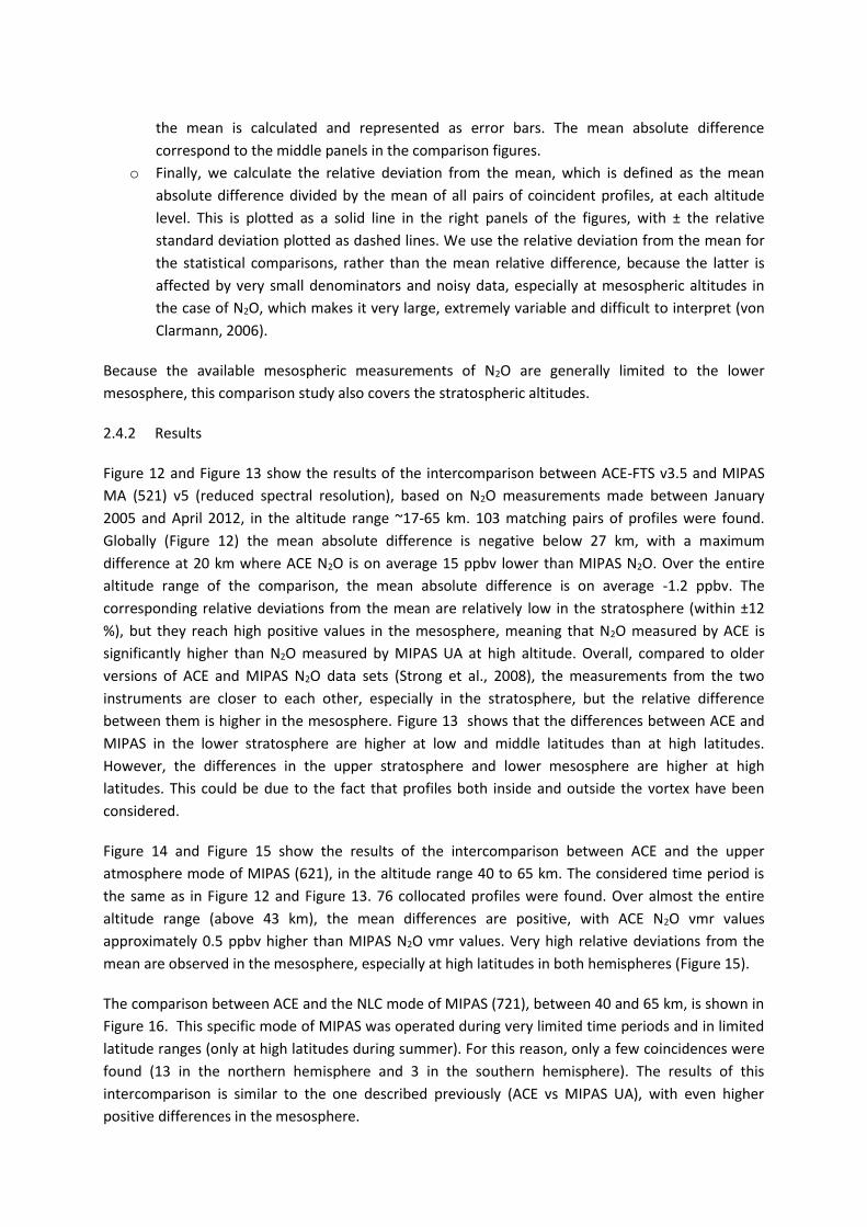
As shown in Figure 11, OSIRIS night-time NO measurements are characterized by a high bias

compared to all the other instruments and in all regions. The most significant relative differences, in

the order of 200%, result from the comparison with SOFIE, ACE and SMR.

Figure 6: Vertical profile comparison of the SMR NO vmr with the other data sets, in three different latitude bands and for day-time (top panel) and night-time (bottom panel) measurements. The median of the relative differences, averaged over coincident days, is shown. The error bars represent the standard error of the mean.

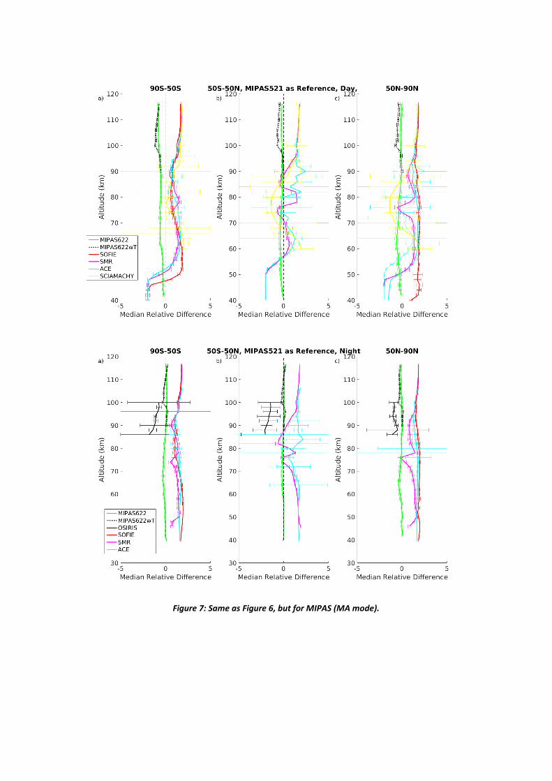
Figure 7: Same as Figure 6, but for MIPAS (MA mode).

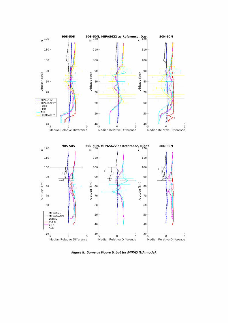
Figure 8: Same as Figure 6, but for MIPAS (UA mode).

Figure 9: Same as Figure 6, but for ACE-FTS.

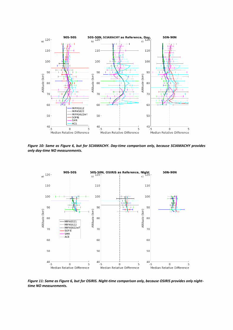
Figure 10: Same as Figure 6, but for SCIAMACHY. Day-time comparison only, because SCIAMACHY provides only day-time NO measurements.

Figure 11: Same as Figure 6, but for OSIRIS. Night-time comparison only, because OSIRIS provides only night-time NO measurements.

2.5 N2O

2.4.1 Approach

The comparisons shown in this section include four N2O products created within the MesosphEO

project: MIPAS v5R (middle atmosphere - 521, upper atmosphere – 621 and NLC -721 modes) and

ACE-FTS v3.5. Aura-MLS N2O v4.2 product is also used as an external independent data set.

This study is based on the comparison of collocated pairs of vertical volume mixing ratio profiles.

Because N2O is a long-lived (no diurnal cycle in the stratosphere and lower mesosphere) and well-

mixed constituent, it is possible to use relatively relaxed temporal and spatial coincidence criteria,

providing good statistics. They were defined as ±9 h and 800km. However, N2O measurements in the

stratosphere can be affected by the subsidence inside the polar vortex. It is in principle possible to

use the associated value of potential vorticity in order to separate the observations made inside and

outside the vortex. However, this has not been taken into account in this study. The comparison

results at high latitudes can therefore be affected by the wintertime downward transport of N2O.

Multiple counting of profiles was allowed. In other words, if n validation measurements met the

criteria with respect to a single observation of the instrument taken as the reference, these were

counted as n coincidences. No smoothing was applied to account for the differences in vertical

resolution. All profiles were linearly interpolated onto a common 1-km altitude grid. MLS profiles are

reported on pressure levels. Their vertical coordinate was converted to altitude by interpolating each

MLS profile onto the retrieved pressure profile of the coincident ACE or MIPAS observation.

Unreliable data has been screened out from all data sets, following the recommendations specific to

each instrument. ACE profiles associated with a flag value in the range of 4 to 9 have been excluded.

Regarding MIPAS, data points with a visibility flag of 0 have been excluded, as well as data points

associated with an averaging kernel diagonal element lower than 0.03. Regarding MLS, only data

points characterised by a positive precision, and only profiles associated with an even status flag, a

quality greater than 1.3 and a convergence lower than 2 were used.

The comparison study has been performed using the following procedure, for each pair of

instruments under consideration:

o The mean profiles of all co-located observations are calculated for the two instruments

separately, along with their standard deviations. These mean profiles are plotted as solid

lines, with ± one standard deviation as dashed lines in the figures discussed below. The

standard error of the mean is included as error bars. It is calculated as σ(z)/√(N(z)), where

N(z) is the number of coincidences at each altitude level. In some cases, these error bars are

so small that they are not visible. These mean profiles correspond to the left panels in the

following figures.

o The mean absolute difference between the instrument used as the reference and the

validation instrument is then calculated, along with the standard deviation of the individual

differences of all coincident pairs. In other words, the differences are first calculated for each

pair of profiles at each altitude, and then averaged to obtain the mean absolute difference at

the given altitude level, which is plotted as a solid line with ±1σ as dashed lines. The error of

the mean is calculated and represented as error bars. The mean absolute difference

correspond to the middle panels in the comparison figures.

o Finally, we calculate the relative deviation from the mean, which is defined as the mean

absolute difference divided by the mean of all pairs of coincident profiles, at each altitude

level. This is plotted as a solid line in the right panels of the figures, with ± the relative

standard deviation plotted as dashed lines. We use the relative deviation from the mean for

the statistical comparisons, rather than the mean relative difference, because the latter is

affected by very small denominators and noisy data, especially at mesospheric altitudes in

the case of N2O, which makes it very large, extremely variable and difficult to interpret (von

Clarmann, 2006).

Because the available mesospheric measurements of N2O are generally limited to the lower

mesosphere, this comparison study also covers the stratospheric altitudes.

2.4.2 Results

Figure 12 and Figure 13 show the results of the intercomparison between ACE-FTS v3.5 and MIPAS

MA (521) v5 (reduced spectral resolution), based on N2O measurements made between January

2005 and April 2012, in the altitude range ~17-65 km. 103 matching pairs of profiles were found.

Globally (Figure 12) the mean absolute difference is negative below 27 km, with a maximum

difference at 20 km where ACE N2O is on average 15 ppbv lower than MIPAS N2O. Over the entire

altitude range of the comparison, the mean absolute difference is on average -1.2 ppbv. The

corresponding relative deviations from the mean are relatively low in the stratosphere (within ±12

%), but they reach high positive values in the mesosphere, meaning that N2O measured by ACE is

significantly higher than N2O measured by MIPAS UA at high altitude. Overall, compared to older

versions of ACE and MIPAS N2O data sets (Strong et al., 2008), the measurements from the two

instruments are closer to each other, especially in the stratosphere, but the relative difference

between them is higher in the mesosphere. Figure 13 shows that the differences between ACE and

MIPAS in the lower stratosphere are higher at low and middle latitudes than at high latitudes.

However, the differences in the upper stratosphere and lower mesosphere are higher at high

latitudes. This could be due to the fact that profiles both inside and outside the vortex have been

considered.

Figure 14 and Figure 15 show the results of the intercomparison between ACE and the upper

atmosphere mode of MIPAS (621), in the altitude range 40 to 65 km. The considered time period is

the same as in Figure 12 and Figure 13. 76 collocated profiles were found. Over almost the entire

altitude range (above 43 km), the mean differences are positive, with ACE N2O vmr values

approximately 0.5 ppbv higher than MIPAS N2O vmr values. Very high relative deviations from the

mean are observed in the mesosphere, especially at high latitudes in both hemispheres (Figure 15).

The comparison between ACE and the NLC mode of MIPAS (721), between 40 and 65 km, is shown in

Figure 16. This specific mode of MIPAS was operated during very limited time periods and in limited

latitude ranges (only at high latitudes during summer). For this reason, only a few coincidences were

found (13 in the northern hemisphere and 3 in the southern hemisphere). The results of this

intercomparison is similar to the one described previously (ACE vs MIPAS UA), with even higher

positive differences in the mesosphere.

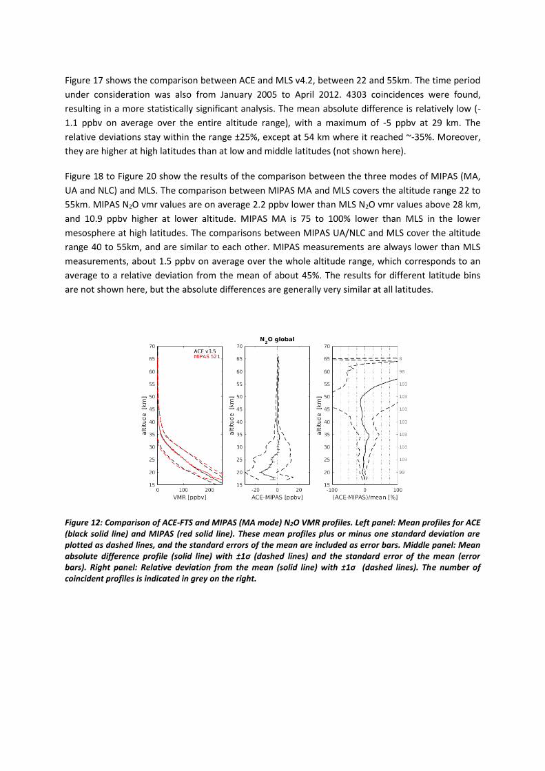
Figure 17 shows the comparison between ACE and MLS v4.2, between 22 and 55km. The time period

under consideration was also from January 2005 to April 2012. 4303 coincidences were found,

resulting in a more statistically significant analysis. The mean absolute difference is relatively low (-

1.1 ppbv on average over the entire altitude range), with a maximum of -5 ppbv at 29 km. The

relative deviations stay within the range ±25%, except at 54 km where it reached ~-35%. Moreover,

they are higher at high latitudes than at low and middle latitudes (not shown here).

Figure 18 to Figure 20 show the results of the comparison between the three modes of MIPAS (MA,

UA and NLC) and MLS. The comparison between MIPAS MA and MLS covers the altitude range 22 to

55km. MIPAS N2O vmr values are on average 2.2 ppbv lower than MLS N2O vmr values above 28 km,

and 10.9 ppbv higher at lower altitude. MIPAS MA is 75 to 100% lower than MLS in the lower

mesosphere at high latitudes. The comparisons between MIPAS UA/NLC and MLS cover the altitude

range 40 to 55km, and are similar to each other. MIPAS measurements are always lower than MLS

measurements, about 1.5 ppbv on average over the whole altitude range, which corresponds to an

average to a relative deviation from the mean of about 45%. The results for different latitude bins

are not shown here, but the absolute differences are generally very similar at all latitudes.

Figure 12: Comparison of ACE-FTS and MIPAS (MA mode) N2O VMR profiles. Left panel: Mean profiles for ACE (black solid line) and MIPAS (red solid line). These mean profiles plus or minus one standard deviation are plotted as dashed lines, and the standard errors of the mean are included as error bars. Middle panel: Mean absolute difference profile (solid line) with ±1σ (dashed lines) and the standard error of the mean (error bars). Right panel: Relative deviation from the mean (solid line) with ±1σ (dashed lines). The number of coincident profiles is indicated in grey on the right.

Figure 13: Comparison of ACE-FTS and MIPAS (MA mode) N2O VMR profiles in three latitude bands. Top row:

60-90°S, middle row: 60°S-60°N, bottom row: 60-90°N.

Figure 14: Same as Figure 12, for ACE-FTS compared to MIPAS (UA mode).

Figure 15: Same as Figure 13, for ACE-FTS compared to MIPAS (UA mode).

Figure 16: Same as Figure 12, for ACE-FTS compared to MIPAS (NLC mode).

Figure 17: Same as Figure 12, for ACE-FTS compared to MLS.

Figure 18: Same as Figure 12, for MIPAS (MA mode) compared to MLS.

Figure 19: Same as Figure 12, for MIPAS (UA mode) compared to MLS.

Figure 20: Same as Figure 12, for MIPAS (NLC mode) compared to MLS.

2.6 NO2

2.6.1 Approach Here, the same approach as for CH4 and CO is used. However, only nighttime observations provide any reasonable mesospheric coverage. Thus, the data sets include only observations with solar zenith

angles of 97 and larger. This limits the number of available data sets to those obtained by GOMOS and MIPAS. Data sets based on the solar occultation or solar scattering technique, as from ACE-FTS, HALOE, MAESTRO, OSIRIS, POAM III, SAGE II, SAGE III or SCIAMACHY, which yield at least stratospheric results (Sheese et al., 2016) are correspondingly not included here. The comparisons for NO2 we perform not in volume mixing ratios, as done for CH4 and CO, but in number density which is the natural retrieval space for the GOMOS data. The temperature and pressure data supplied with the GOMOS data are not observed simultaneously but taken from the MSIS90 (Mass Spectrometer and Incoherent Scatter radar; Hedin, 1991) model. For the MIPAS data a conversion to number density is trivial using the temperature and pressure information retrieved from the same set of observations.

2.6.2 Results The comparison of the GOMOS data set with MIPAS indicates absolute biases within 2 1013 m-3 (see Figure 21). Below 60 km the biases are primarily positive and above primarily negative. The relative biases (see Figure 22) vary typically between -20% and 40%. For the MIPAS V5H data set quantitatively the same absolute bias range is found as for the GOMOS data set. The MIPAS V5R NOM and MA data sets indicate small absolute biases in comparisons with the remaining MIPAS data sets. The comparisons with the GOMOS data set clearly yield larger biases. In relative terms this behavior is not as obvious. For the MIPAS V5R MA data set the relative biases are typically within

20%. For the MIPAS V5R NOM data set this interval is larger, in particular towards the upper limits of the comparisons. The comparison between the MIPAS UA and NLC data sets exhibit differences

above 65 km. In absolute terms the biases amount up to 3 1013 m-3, in relative terms up to 60%.

Figure 21: Absolute biases among the different nitrogen dioxide data sets.

Figure 22: As Figure 21, but here the relative biases are shown.

2.7 OH

As part of the MesosphEO project, OH Meinel-band nightglow emissions in the hydroxyl (8 – 4) band

were extracted from GOMOS observations. The OH(8 – 4) band covers the spectral range from about

930 nm to about 955 nm. Note that these GOMOS OH measurements (provided by LATMOS) are

available as monthly and zonally averaged and latitudinally binned data and the peak limb emission

altitude is provided. It is important to mention that these peak altitudes correspond to uninverted

limb emission rate profiles. Here the GOMOS OH(8 – 4) peak emission altitudes were compared to

centroid altitudes of the OH(3 – 1) (around 1530 nm) and OH(6 – 2) (around 840 nm) Meinel bands

retrieved from SCIAMACHY nightglow observations for the entire duration of the Envisat mission. The

SCIAMACHY OH data (provided by EMAU) were daily and zonally binned and were in addition

monthly averaged for the comparisons shown here. Figure 23 shows comparisons of GOMOS and

SCIAMACHY OH emission altitudes for the years 2003 to 2011 for different latitude bins. Apparently,

there are differences of up to several kilometers between the different data sets. These differences

are due to different reasons:

(a) The GOMOS OH peak altitudes refer to peak altitudes of uninverted limb measurements, i.e.

they will be systematically lower than the peak altitudes of inverted volume emission rate

profiles. The SCIAMACHY OH emission altitudes are centroid altitudes (i.e., altitude weighted

by the vertical OH volume emission rate profile) and are, hence, based on inverted volume

emission rate profiles.

(b) OH emissions from higher vibrational states v’ peak at slightly higher altitudes (about 0.5 km

per vibrational state; von Savigny et al., 2012), which explains the differences between the

SCIAMACHY OH(3 – 1) and OH(6 – 2) data. It is expected that the centroid altitudes of

inverted GOMOS OH(8 – 4) profiles lie above the OH(6 – 2) peak altitudes and a future

inversion of the GOMOS data would be of interest.

Figure 23 shows that the relative and seasonal variations in GOMOS and SCIAMACHY OH emission

altitude are often in quite good agreement. Both data sets show data gaps of different lengths and at

different times of the year. For SCIAMACHY, nighttime limb measurements are only available

between about 10S and 30N. At higher latitudes, measurements are only available in the winter

hemisphere. For the southern hemisphere, SCIAMACHY does not provide any observations at

latitudes poleward of about 40S. This is the reason, why no results are shown for latitudes south of

40S. The OH emission altitude is characterized by an annual variation at mid and high latitudes with

a winter minimum and a summer maximum. At low latitudes a semi-annual variation dominates –

with amplitudes of up to 1 km and equinox minima, solstice maxima, respectively. This can be clearly

seen in, e.g., the OH(3 – 1) emission altitude for the 10N – 20N latitude range.

In summary, a quantitative comparison of GOMOS and SCIAMACHY measurements of OH emission

altitudes is not possible, because of the reasons described above. There is, however, consistency in

terms of the seasonal variations in OH emission altitudes. A future inversion of the GOMOS data

would allow studying the behavior of OH emissions from the ninth vibrational level, in comparison to

SCIAMACHY observations of OH bands from lower vibrational states.

Figure 23: Comparison of monthly and zonally averaged GOMOS OH(8 – 4) (black circles) and SCIAMACHY OH(3 – 1) (red circles) and OH(6 – 2) (blue circles) emission height measurements for different latitude bins. Note that the GOMOS emission heights correspond to the peak height of the uninverted limb emission rate profiles, whereas the SCIAMACHY emission heights are centroid altitudes based on inverted volume emission rate profiles.

2.8 H2O

2.7.1 Approach

The comparisons shown in this section include four H2O products created within the MesosphEO

project: MIPAS v5R (middle atmosphere - 522, upper atmosphere – 622 and NLC -722 modes) and

ACE-FTS v3.5. Aura-MLS H2O v4.2 product is used as an external independent data set. SMR H2O v3.0

could not be included because this newly reprocessed version was not ready to be delivered yet, at

the time this report was written.

This study is based on the comparison of collocated pairs of vertical volume mixing ratio profiles,

using the approach described in 2.4.1. Only the mesospheric altitudes are covered here. Water

vapour is a relatively long-lived constituent at these altitudes, so relaxed temporal and spatial

coincidence criteria were used. They were defined as ±9 h and 800km.

Unreliable data has been screened out from all data sets, following the recommendations specific to

each instrument. ACE profiles associated with a flag value in the range of 4 to 9 have been excluded.

Regarding MIPAS, data points with a visibility flag of 0 have been excluded. Regarding MLS, only data

points characterised by a positive precision, and only profiles associated with an even status flag, a

quality greater than 1.45 and a convergence lower than 2 were used.

Each figure discussed below shows the mean profiles of all co-located observations (left panel), the

mean absolute difference between the instrument used as the reference and the validation

instrument (middle panel), and the relative deviation from the mean (right panel). We refer the

reader to Sect. 2.4.1 for more details.

2.7.2 Results

V3.5 ACE-FTS H2O is compared to three MIPAS modes (v5R MA, UA and NLC), based on

measurements made from 2005 to 2012, in Figure 24 to Figure 27, and to v4.2 MLS, based on

measurements made between 2004 and 2013, in Figure 28. The water vapour measurements from

ACE and MLS are remarkably close to each other, with an absolute difference of only -0.04 ppmv on

average below 85km, corresponding to an average relative deviation from the mean of -1.7 %. The

differences between ACE and MLS are higher between 60 and 70 km, at low and middle latitudes

(not shown here), but still within ±5 % (ACE is approximately 4% lower than MLS at 65 km). ACE is

characterised by a wet bias compared to MIPAS from 55 to 90 km, with a maximum of about 1 ppmv

(2 ppmv compared to MIPAS 722) around 75 km. As shown in Figure 25, this bias is more pronounced

at low and middle latitudes than at polar latitudes. We observe a dry bias in the lowermost part

(below 55 km) and in the uppermost part of the mesosphere, both in the comparisons with MIPAS

and MLS. This is consistent with what had already been shown by previous studies.

MIPAS v5R water vapour measurements (MA, UA and NLC modes) made from 2005 to 2012 are

compared to ACE-FTS v3.5 H2O data set in Figure 24 to Figure 27 and to MLS in Figure 29 to Figure 31.

All comparisons exhibit a marked dry bias above 55 km (approximately -0.5 ppmv, -19%, compared to

ACE, and -0.7 ppmv, -21% compared to MLS). This dry bias is observed at all latitudes (see Figure 25

for example). As shown in the figures, the bias is generally lower in MIPAS MA than in the two other

modes (UA and NLC). In the lowermost part of the mesosphere, MIPAS is in agreement within 5%

with the other instruments. H2O volume mixing ratios measured by MIPAS are higher than vmr

measured by ACE in the uppermost part of the mesosphere (above 92 km), with a maximum relative

deviation of about 75% at 100km.

Figure 24: Comparison of ACE-FTS and MIPAS (MA mode) H2O VMR profiles. Left panel: Mean profiles for ACE (black solid line) and MIPAS (red solid line). These mean profiles plus or minus one standard deviation are plotted as dashed lines, and the standard errors of the mean are included as error bars. Middle panel: Mean absolute difference profile (solid line) with ±1σ (dashed lines) and the standard error of the mean (error bars). Right panel: Relative deviation from the mean (solid line) with ±1σ (dashed lines). The number of coincident profiles is indicated in grey on the right.

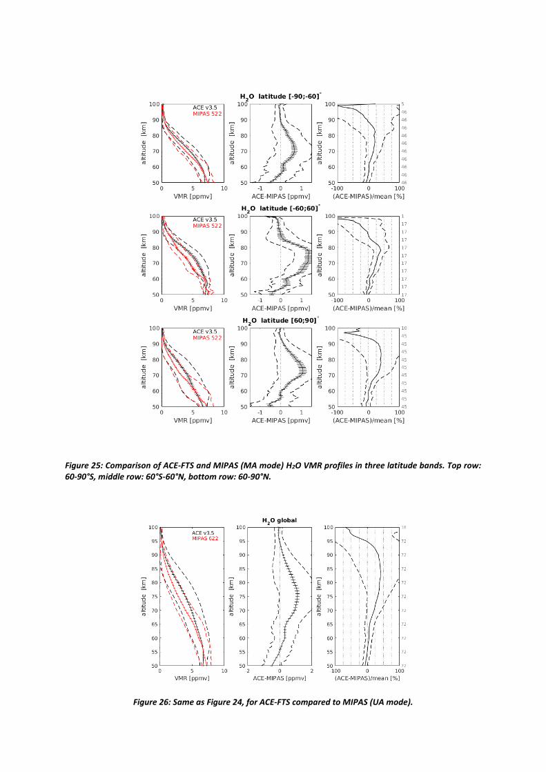
Figure 25: Comparison of ACE-FTS and MIPAS (MA mode) H2O VMR profiles in three latitude bands. Top row: 60-90°S, middle row: 60°S-60°N, bottom row: 60-90°N.

Figure 26: Same as Figure 24, for ACE-FTS compared to MIPAS (UA mode).

Figure 27: Same as Figure 24, for ACE-FTS compared to MIPAS (NLC mode).

Figure 28: Same asFigure 24, for ACE-FTS compared to MLS

.

Figure 29: Same as Figure 24, for MIPAS (MA mode) compared to MLS.

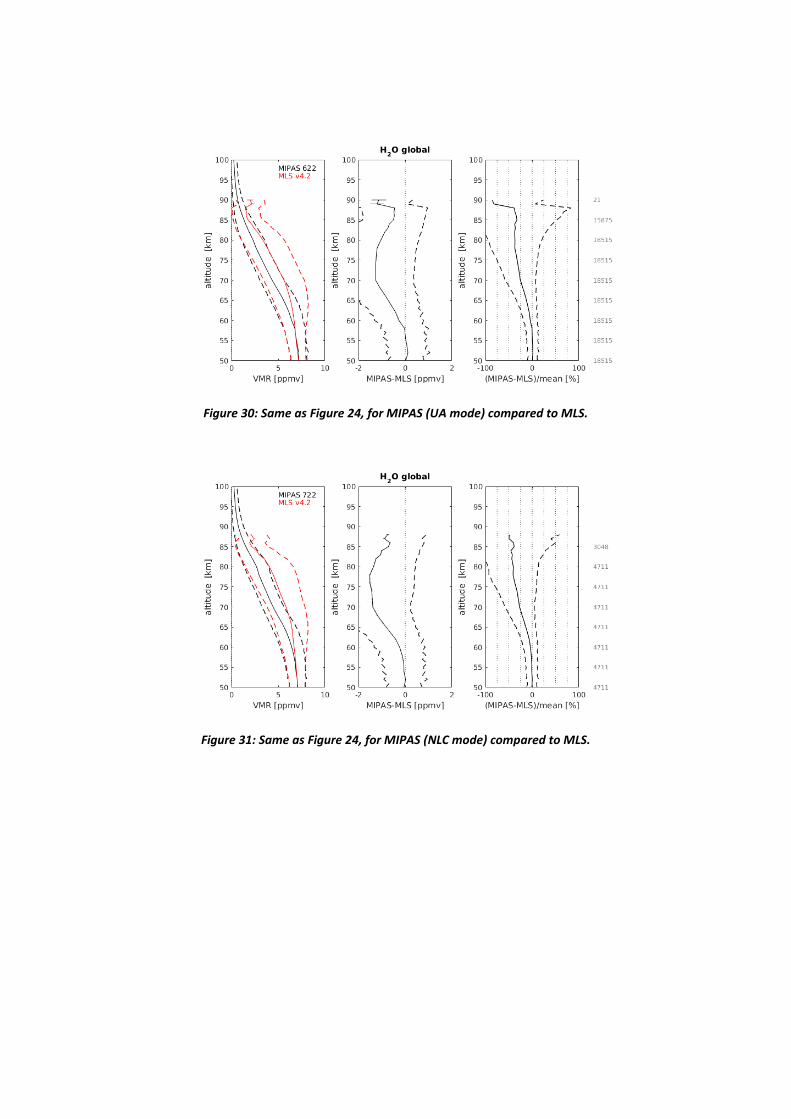
Figure 30: Same as Figure 24, for MIPAS (UA mode) compared to MLS.

Figure 31: Same as Figure 24, for MIPAS (NLC mode) compared to MLS.

2.9 CO2

The inversion of MIPAS CO2 volume mixing ratio (version v5r CO2 622) and the characterization, errors and quality of the retrieved CO2 are described in Jurado-Navarro et al. (2015, 2016). More recently the MIPAS CO2 have been compared to SABER (v2.0) and ACE-FTS (v3.6) CO2; and also with the WACCM simulations “specified dynamics” version (SD-WACCM) (Garcia et al., 2014), as described by Lopez-Puertas et al. (2017). The major differences found with those satellite datasets are described in the latter reference. Here we include an extract of the abstract of that reference summarizing the most salient results. MIPAS shows a very good agreement with ACE-FTS below 100

km with differences of 5%. Above 100 km, MIPAS CO2 is generally lower than ACE-FTS with

differences growing from 5% at 100 km to 20 – 40 % near 110 – 120 km. Part of this disagreement can be explained by the lack of a non-local thermodynamic equilibrium correction in ACE. MIPAS also

agrees very well (5%) with SABER below 100 km. At 90 – 105 km, MIPAS is generally smaller than

SABER by 10 – 30% in the polar summers. At 100 – 120 km, MIPAS and SABER CO2 agree within 10% during equinox but, for solstice, MIPAS is larger by 10 – 25%, except near the polar summer. Whole Atmosphere Community Climate Model (WACCM) CO2 shows the major MIPAS features. At 75 – 100

km, the agreement is very good (5%), with maximum differences of 10%. At 95 – 115km MIPAS CO2 is larger than WACCM by 20 – 30% in the winter hemisphere but smaller (20 – 40%) in the summer. Above 95 – 100km WACCM generally overestimates MIPAS CO2 by about 20 – 80% except in the polar summer where it underestimates it by 20 – 40%. MIPAS CO2 favors a large eddy diffusion below 100km and suggests that the meridional circulation of the lower thermosphere is stronger than in WACCM. The three instruments and WACCM show a clear increase of CO2 with time, more markedly at 90 – 100 km.

2.10 Magnesium

Figure 32 presents a comparison between climatological Mg for January retrieved from MLT

measurements (averaged over all measurements between 2009 and 2012) shown in the upper left

panel and Mg climatologies retrieved from nominal limb measurements for 2003, 2004 and 2008

shown in the upper right, lower left and lower right panels, respectively. As seen from the plot, both

data sets show similar magnitudes of the Mg number densities, however, the results from the

nominal limb measurements are much more noisy. This can be caused by higher noise levels in the

single measurements resulting from a different detector exposure time (4 times shorter in nominal

limb measurements compared to MLT measurements) as well as by a usage of latitudinal smoothing

in MLT retrievals. It is also seen, that the data gets more noisy with time, which is most probably

associated with a degradation of the detector in the UV channel of SCIAMACHY. The data from

nominal limb measurements for January averaged over several years of SCIAMACHY (2003, 2004,

2006 – 2009) are shown in the right panel of Figure 33 in comparison with MLT data set (same as in

the upper left panel of Figure 32. The plot reveals that the noise became reduced but is still clearly

present in the nominal limb data set. While the altitude and latitude behavior of the two data sets is

similar, the absolute values in the nominal limb data set are about 20% smaller than those from the

MLT data. The year 2005 was excluded from the averaging because of identified issues at high

tangent heights (too high values) and the data from 2010 could not be averaged because of a change

in the tangent height sampling of the SCIAMACHY instrument.

The results for other months are very similar to those for January and therefore are not shown here.

Figure 32: Distribution of magnesium atom number density in January retrieved from SCIAMACHY MLT (upper left panel) and nominal limb measurements (upper right, lower left and lower right panels for 2003, 2004 and 2008, respectively).

Figure 33: Distribution of magnesium atom number density in January retrieved from SCIAMACHY MLT (left panel) and nominal limb measurements (right panel).

2.11 Sodium

Different Na data products for the MLT region were developed and validated within the MesosphEO

project. At IUP Bremen, the nominal (or standard) limb measurements (which are available from

August 2002 until April 2012) were used to retrieve Na concentration profiles from daytime

resonance scattering observations with SCIAMACHY. The earlier retrievals (Langowski et al., 2016)

were only based on the special MLT limb observations with SCIAMACHY, which were available since

2008 for two full days every month. In addition, Na profiles were retrieved from SCIAMACHY Na D-

line nightglow observations with an entirely new retrieval (von Savigny et al., 2016).

2.11.1 Comparison of Na retrievals from nominal limb states with other data sets

Figure 34 presents a comparison between a January Na climatology retrieved from MLT

measurements (averaged over all measurements between 2009 and 2012) shown in the upper left

panel and climatologies retrieved from nominal limb measurements for 2003, 2007 and 2011 shown

in the upper right, lower left and lower right panels, respectively. The plot reveals that both

latitudinal and vertical distributions of the sodium values as well as their magnitude are in a good

agreement between the both types of measurements. One observes very low sodium values at the

high latitudes in the summer hemisphere and a strong increase toward the high latitudes of the

winter hemisphere with a local minimum in the tropics. Similar climatologies but for June are

presented in Figure 35. Here, however, MLT measurements were averaged from 2008 to 2011 for the

reason of data availability. It is clearly seen that similarly to the January results both latitude/altitude

dependencies and absolute values are very similar between the results from SCIAMACHY MLT and

nominal limb measurements. The overall behavior of the sodium distribution is the same as in

January with minimum values at high latitudes of the summer hemisphere and maximum values in

the winter hemisphere. A latitude distribution of the retrieved sodium number densities at different

altitudes for January is presented in Figure 36. The plot shows the results from the SCIAMACHY MLT

observations averaged over 2008 – 2012 period (blue), SCIAMACHY standard limb observations

averaged over 2003 – 2012 period (red) and a climatology created from GOMOS measurements for

the 2002 – 2008 period as described by Fussen et al. (2010). It should be noted here, that the latter is

a parameterization of the GOMOS observation data set rather than averaged data as in the case of

both SCIAMACHY data sets. The plot reveals that both SCIAMACHY data sets agree very well both in

latitudinal behavior and absolute values for all considered altitudes. The GOMOS climatology agrees

well with both SCIAMACHY data sets at 90 km altitude but shows a weaker gradient between

southern and northern latitudes. The observed differences increase with decreased altitude. A good

agreement in terms of the absolute values is observed at high southern latitudes and the tropics,

while a strong disagreement is observed at high northern latitudes downwards from 87 km. A similar

comparison between the three data sets but for June is shown in Figure 37. Here a mirrored behavior

as compared to that for January is observed. The agreement is best at high northern latitudes getting

worse towards the southern latitudes.

Furthermore, the agreement decreases with decreasing altitude. Figure 38 depicts the seasonal cycle

of the SCAMACHY MLT, SCIAMACHY standard limb and GOMOS climatologies at four different

altitudes in the tropics. The same color code and same averaging periods as in Figure 36 are used. In

all three data sets one observes a clear semi-annual oscillation; for the GOMOS climatology it is,

however, out of phase as compared with both SCIAMACHY data sets. For mid-latitudes of both

northern and southern hemispheres, shown in Figure 39 and Figure 40, respectively, the annual cycle

for all three data sets is in phase, however, the amplitude of the seasonal cycle for GOMOS is smaller

than that for both SCIAMACHY climatologies downwards from 87 km. In contrast, both SCIAMACHY

data sets show very similar altitude and phase of the seasonal cycle for all considered latitude bands.

Figure 34: Distribution of Sodium in January retrieved from SCIAMACHY MLT (upper left panel) and nominal limb measurements (upper right, lower left and lower right panels for 2003, 2007 and 2011, respectively)

Figure 35: Same as Figure 34 but for June.

Figure 36: Latitude distribution of sodium at different altitudes in January resulting from SCIAMACHY MLT observations averaged over 2009 – 2012 period (blue), SCIAMACHY standard limb observations averaged over 2003 – 2012 period (red) and a climatology created from GOMOS measurements for 2002 – 2008 period (cyan). Upper left panel: 90 km, upper right panel: 87 km, lower left panel: 84 km, lower right panel: 81 km.

Figure 37: Same as Figure 36 but for June

Figure 38: Seasonal of sodium at different altitudes in tropics resulting from SCIAMACHY MLT observations averaged over 2009 – 2012 period (blue), SCIAMACHY standard limb observations averaged over 2003 – 2012 period (red) and a climatology created from GOMOS measurements for 2002 – 2008 period (cyan). Upper left panel: 90 km, upper right panel: 87 km, lower left panel: 84 km, lower right panel: 81 km.

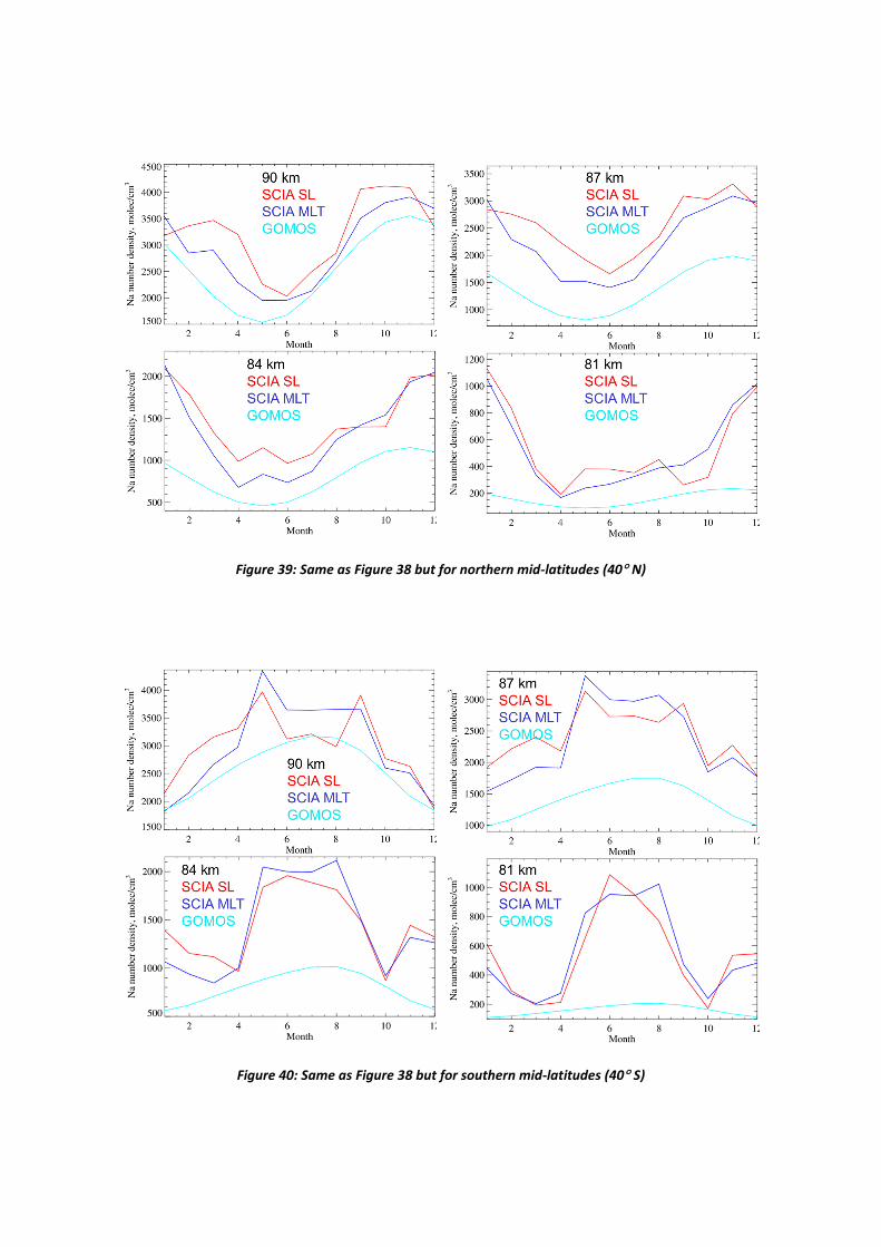
Figure 39: Same as Figure 38 but for northern mid-latitudes (40 N)

Figure 40: Same as Figure 38 but for southern mid-latitudes (40 S)

2.11.2 Comparison of SCIAMACHY MLT state Na retrievals with independent satellite

measurements and WACCM model simulations

In a recent study, Langowski et al. (2017) performed a comprehensive comparison of MLT Na profiles

retrieved from SCIAMACHY limb MLT measurements using the approach described by Langowski et

al. (2016) with OSIRIS Na retrievals (provided by the group of John Plane, University of Leeds), with a

Na climatology based on GOMOS stellar occultation observations (described by Fussen et al., 2010)

and with model simulations with the WACCM-Na model provided by the University of Leeds. Only

the most important findings of Langowski et al. (2017) are summarized here. Investigating the

WACCM model results showed that diurnal variations of the Na vertical column density (VCD) can

reach up to 50% at specific latitudes and times, which complicates comparing satellite observations

performed at different – and potentially changing – local solar times. Figure 41 shows as a sample

result the comparison of the time and latitude variation of Na vertical columns densities based on

the GOMOS, OSIRIS and SCIAMACHY measurements as well as corresponding WACCM model

simulations for the local solar times of the respective satellite data. Note that apparent data gaps in

the OSIRIS data sets are a consequence of Odin’s near terminator orbit. Overall, the agreement has

to be considered quite good and is typically on the order of 25% (results on relative differences not

shown here; see Langowski et al. (2017) for more details). Note that the large values occurring near

the terminator in the OSIRIS data sets are connected to small numbers of individual measurements.

Other sample result is shown in Figure 42. The top panels show the average seasonal variation in Na

vertical column density from the different data sources. The middle panels correspond to the

centroid altitude (i.e. altitude weighted by the density profile) of the Na density profile and the

bottom panels display the seasonal variation of the full width at half maximum (FWHM) of the Na

density profiles. Panels in the left column are for 67N and the right panels are for 67S. The top

panels indicate good overall agreement between model results and observations in terms of the Na

vertical column density. The middle panels indicate, however, that the Na layer altitude is

systematically underestimated by up to 3 km by the WACCM simulations. This is known feature in

the simulations and is also visible in other atmospheric parameters. In terms of the layer FWHM,

WACCM reproduces the OSIRIS and SCIAMACHY observations quite well. Note that the GOMOS

climatology does not provide a realistic seasonal variation on the Na layer FWHM, which also is a

known feature. It is expected that the original GOMOS Na profiles exhibit a realistic seasonal

variation of the layer FWHM. This should be tested in the future. The SCIAMACHY nightglow

retrievals are overall significantly noisier than the other data sets, which mainly is a consequence of

the weakness of the Na D-line nightglow emissions with typical peak emission rates of 40 photons

cm-3 s-1.

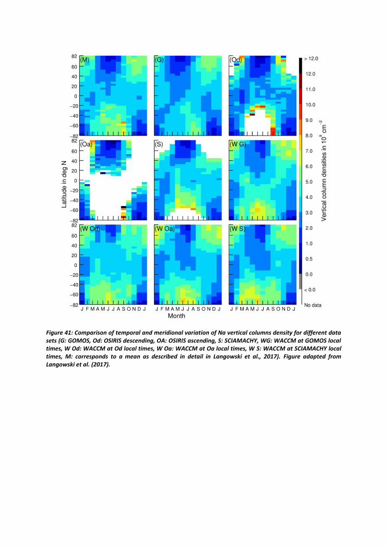
Figure 41: Comparison of temporal and meridional variation of Na vertical columns density for different data sets (G: GOMOS, Od: OSIRIS descending, OA: OSIRIS ascending, S: SCIAMACHY, WG: WACCM at GOMOS local times, W Od: WACCM at Od local times, W Oa: WACCM at Oa local times, W S: WACCM at SCIAMACHY local times, M: corresponds to a mean as described in detail in Langowski et al., 2017). Figure adapted from Langowski et al. (2017).

Figure 42: Top panels: multi-annual mean seasonal variation of Na vertical column density. Middle panels: Similar plot for Na centroid altitude. Bottom panels: similar plots for Na layer full width at half maximum.

Left column: results at 67N. Right column: results at 67S. Figure adapted from Langowski et al. (2017).

2.11.3 Comparison of nightglow Na retrievals

The Na profile retrievals from SCIAMACHY nightglow observations were compared by von Savigny et

al. (2016) to SCIAMACHY daytime measurements as well as the GOMOS climatology by Fussen et al.

(2010). As discussed in the MesosphEO ATBD in detail, the photochemical model used to retrieve Na

concentrations from observations of the Na D-line nightglow emission requires choosing a suitable

value of the branching ratio for the formation of the 2D state of Na. The branching ratio was

empirically chosen to obtain good agreement between the SCIAMACHY nightglow Na retrievals and

SCIAMACHY dayglow retrievals (Langowski et al., 2016) as well as the GOMOS Na climatology.

Therefore, an additional comparison of the SCIAMACHY nightglow retrievals with, e.g., SCIAMACHY

dayglow or GOMOS measurements is not meaningful. With the currently chosen value of the

branching ratio of f = 0.09 the annually averaged Na vertical column densities obtained from

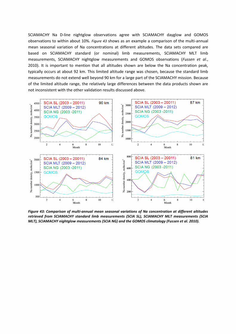
SCIAMACHY Na D-line nightglow observations agree with SCIAMACHY dayglow and GOMOS

observations to within about 10%. Figure 43 shows as an example a comparison of the multi-annual

mean seasonal variation of Na concentrations at different altitudes. The data sets compared are

based on SCIAMACHY standard (or nominal) limb measurements, SCIAMACHY MLT limb

measurements, SCIAMACHY nightglow measurements and GOMOS observations (Fussen et al.,

2010). It is important to mention that all altitudes shown are below the Na concentration peak,

typically occurs at about 92 km. This limited altitude range was chosen, because the standard limb

measurements do not extend well beyond 90 km for a large part of the SCIAMACHY mission. Because

of the limited altitude range, the relatively large differences between the data products shown are

not inconsistent with the other validation results discussed above.

Figure 43: Comparison of multi-annual mean seasonal variations of Na concentration at different altitudes retrieved from SCIAMACHY standard limb measurements (SCIA SL), SCIAMACHY MLT measurements (SCIA MLT), SCIAMACHY nightglow measurements (SCIA NG) and the GOMOS climatology (Fussen et al. 2010).

2.12 Noctilucent clouds

2.12.1 Comparison of NLC (Noctilucent cloud) occurrence frequency

Here we compare time series of NLC occurrence frequency retrieved from GOMOS and from

SCIAMACHY limb observations. The GOMOS data set was provided by LATMOS and the SCIAMACHY

data set by EMAU. The GOMOS data set consists of biweekly (and zonally) averaged and latitudinally

binned data, whereas the SCIAMACHY NLC data is daily and zonally averaged. Figure 44 shows a

comparison of NLC occurrence frequency for the northern hemisphere NLC seasons 2003 to 2011

and for different 5 degree latitude bins. The biweekly averaged GOMOS data are shown as blue solid

circles. The thin grey line shows the daily averaged SCIAMACHY NLC occurrence frequencies and the

red line corresponds to the SCIAMACHY data smoothed with a 5-day running mean filter. The overall

agreement between the GOMOS and SCIAMACHY NLC occurrence rates is remarkably good. NLC

occurrence rate are only enhanced during the NLC seasons, which last from about mid-May until

mid-August in the northern hemisphere. Figure 44 also clearly shows that during the NLC season, NLC

occurrence frequency increases with increasing latitude. At the highest latitudes shown (80N –

85N) the occurrence frequency is nearly 100% for several weeks during the core seasons – in both

the GOMOS and the SCIAMACHY data sets. Note that the good apparent agreement must not be

over interpreted, because occurrence frequency is not a truly objective quantity. It depends in a non-

trivial way on the cloud detection sensitivity, which differs between different instruments and

viewing geometry.

Figure 45 shows a similar comparison between GOMOS and SCIAMACHY NLC occurrence frequency

for the southern hemisphere NLC seasons 2002 – 2003 to 2011 – 2012. For the highest latitude bin

no GOMOS data is available. The overall agreement is not as good as in the northern hemisphere and

the SCIAMACHY cloud occurrence rates are generally lower than for GOMOS. This is likely related to

differences in viewing geometries between the two hemispheres and the two instruments. The

SCIAMACHY limb scatter observations in the northern hemisphere are associated with relatively

small scattering angles (25 – 60), whereas the southern hemisphere observations have scattering

angles of about 130 – 150. As the NLC particles are larger than Rayleigh scatterers in the UV

spectral range, the scattering phase function has a forward peak, implying that the same particle

population will produce a larger scatter signal for forward scattering conditions, i.e. in the northern

hemisphere for SCIAMACHY.

Figure 44: Comparison of GOMOS and SCIAMACHY NLC occurrence frequency for the northern hemisphere

NLC seasons 2003 to 2011 for different latitude bins, from 55N – 60N to 80N to 85N.

Figure 45: Similar to Figure 44 , but for NLC seasons in the southern hemisphere.

2.13 Temperature

MIPAS temperatures (version vM21) have been retrieved from the CO2 emission near 15 m, recorded in the band A accounting for the non-LTE effects. The detailed description of the method and the characterization of the inverted pressure-temperatures profiles are described in Garcia-Comas et al. (2012). The upgrades in the retrieval of the temperature of this version (vM21) and a validation of the results are reported by Garcia-Comas et al. (2014). Briefly, (1) they include an

updated version of the calibrated L1b spectra in the 15 m region (versions 5.02/5.06); (2) the HITRAN 2008 database for CO2 spectroscopic data; (3) the use of a different climatology of atomic oxygen and carbon dioxide concentrations; (4) the improvement of important aspects of the retrieval setup (temperature gradient along the line of sight, offset regularization, and apodization accuracy); and (5) some minor corrections to the CO2 non-LTE modelling (Funke et al., 2012). This current version (vM21) of MIPAS temperatures corrects the main systematic errors of the previous version and has, in general, a remarkable agreement with the measurements taken by ACE-FTS (version 3.0), MLS (v3.3), OSIRIS (Sheese et al., 2012), SABER (v2.0), SOFIE (v1.2) and the Rayleigh lidars at Mauna Loa and Table Mountain. We quote here the major conclusions about the validation of MIPAS temperatures as found by Garcia-Comas et al. (2014). In general, the MIPAS vM21 temperatures are in very good agreement with ACE-FTS, MLS, OSIRIS, SABER, SOFIE and the two Rayleigh lidars at Mauna Loa and Table Mountain. With a few specific exceptions, they typically exhibit differences smaller than 1K below 50 km and smaller than 2K at 50 – 80km in spring, autumn and winter at all latitudes, and summer at low to mid-latitudes. Differences in the high-latitude summers are typically smaller than 1K below 50 km, smaller than 2K at 50 – 65km and 5K at 65 – 80 km. Differences between MIPAS and the other instruments in the mid-mesosphere are generally negative. MIPAS mesopause is within 4K of the other instruments measurements, except in the high-latitude summers, when it is within 5 – 10 K, being warmer there than SABER, MLS and OSIRIS and colder than ACE-FTS and SOFIE. The agreement in the lower thermosphere is typically better than 5 K, except for high latitudes during spring and summer, when MIPAS usually exhibits larger vertical gradients.

3 References

Bailey S. M., G. E. Thomas, M. E. Hervig, J.D. Lumpe, C. E. Randall, J. N. Carstens, B. Thurairajah, D. W.

Rusch, J. M. Russell, and L.L. Gordley, Comparing nadir and limb viewing observations of polar

mesospheric clouds: The effect of the assumed particle size distribution, J. Atmos. Solar-Terr. Phys.,

doi:10.1016/j.jastp.2015.02.007, 2015.

Barret, B., P. Ricaud, M. L. Santee, J.-L. Attié, J. Urban, E. Le Flochmoën, G. Berthet, D. Murtagh, P.

Eriksson, A. Jones, J. de La Noë, E. Dupuy, L. Froidevaux, N. J. Livesey, J. W. Waters and M. J. Filipiak,

Intercomparisons of trace gases profiles from the Odin/SMR and Aura/MLS limb sounders, J.

Geophys. Res., 111, D21302, doi:10.1029/2006JD007305, 2006.

Barth, C. A., Nitric oxide in the lower thermosphere, Planet. Space Sci., 40, 315–336, 1992.

Barth, C. A., K. D. Mankoff, S. M. Bailey, and S. C. Solomon, Global observations of nitric oxide in the

thermosphere, J. Geophys. Res., 108, 1027, doi:10.1029/2002JA009458, A1, 2003.

Baumgarten, G., Fiedler, J., and von Cossart, G., The size of noctilucent cloud particles above Alomar

(69 N, 16 E): optical modeling and method description, Adv. Space Res., 40(6), 772–784,

doi:10.1016/j.asr.2007.01.018, 2007.

Baumgarten, G., Fiedler, J., Lübken, F.-J., and von Cossart, G., Particle properties and water content

of noctilucent clouds and their interannual variation, J. Geophys. Res., 113, D06203,

doi:10.1029/2007JD008884, 2008.

Beagley, S. R., Boone, C., Fomichev, V. I., Jin, J., Semeniuk, K., McConnell, J. C. and Bernath, P. F., First

multi-year occultation observations of CO2 in the MLT by ACE satellite: observations and analysis

using the extended CMAM, Atmos. Chem. Phys., 10(3), 1133–1153, 2010.

Beig, G., S. Fadnavis, H. Schmidt, and G. P. Brasseur, Inter-comparison of 11-year solar cycle response

in mesospheric ozone and temperature obtained by HALOE satellite data and HAMMONIA model, J.

Geophys. Res., 117, D00P10, doi:10.1029/2011JD015697, 2012.

Bellisario, C., P. Keckhut, L. Blanot, A. Hauchecorne, and P. Simoneau, O2 and OH night airglow

emission derived from GOMOS-ENVISAT instrument, J. Atmos. Ocean. Tech., 1301 – 1311, 2014.

Bender, S., Sinnhuber, M., Burrows, J. P., Langowski, M., Funke, B., and López-Puertas, M., Retrieval

of nitric oxide in the mesosphere and lower thermosphere from SCIAMACHY limb spectra, Atmos.

Meas. Tech., 6, 2521–2531, doi:10.5194/amt-6-2521-2013, 2013.

Bender, S., Sinnhuber, M., von Clarmann, T., Stiller, G., Funke, B., López-Puertas, M., Urban, J., Pérot,

K., Walker, K. A., and Burrows, J. P., Comparison of nitric oxide measurements in the mesosphere and

lower thermosphere from ACE-FTS, MIPAS, SCIAMACHY, and SMR, Atmos. Meas. Tech. Discuss., 7,

12735-12794, doi:10.5194/amtd-7-12735-2014, 2014.

Bermejo-Pantaleón, D., Funke, B., López-Puertas, M., García-Comas, M., Stiller, G. P., Clarmann, von,

T., Linden, A., Grabowski, U., Höpfner, M., Kiefer, M., Glatthor, N., Kellmann, S. and Lu, G., Global

observations of thermospheric temperature and nitric oxide from MIPAS spectra at 5.3 μm, J.

Geophys. Res., 116(A10), A10313, 2011.

Boone, C. D., Nassar, R., Walker, K. A., Rochon, Y., McLeod, S. D., Rinsland, C. P., and Bernath, P. F.,

Retrievals for the atmospheric chemistry experiment Fourier-transform spectrometer, Applied

Optics, 44(33), 7218 – 7231, 2005.

Boone, Chris D., Kaley A. Walker, and Peter F. Bernath, Version 3 Retrievals for the Atmospheric

Chemistry Experiment Fourier Transform Spectrometer (ACE-FTS), The Atmospheric Chemistry

Experiment ACE at 10: A Solar Occultation Anthology (Peter F. Bernath, editor, A. Deepak Publishing,

Hampton, Virginia, U.S.A., 103 – 127, 2013.

Bracher, A., H. Bovensmann, K. Bramstedt, J. P. Burrows, T. von Clarmann, K.-U. Eichmann, H. Fischer,

B. Funke, S. Gil-Lopez, N. Glatthor, U. Grabowski, M. Höpfner, M. Kaufmann, S. Kellmann, M. Kiefer,

M. E. Koukouli, A. Linden, M. Lopez-Puertas, G. Mengistu Tsidu, M. Milz, S. Noel, G. Rohen, A.

Rozanov, V. V. Rozanov, C. von Savigny, M. Sinnhuber, J. Skupin, T. Steck, G. P. Stiller, D.-Y. Wang, M.

Weber, and M. W. Wuttke, Cross Validation of O3 and NO2 measured by the atmospheric ENVISAT

instruments GOMOS, MIPAS, and SCIAMACHY, Adv. Space Res., 36(5), 855 – 867, 2005.

Brasseur, G., and S. Solomon, Aeronomy of the middle atmosphere, Springer, ISBN-10 1-4020-3284-

6, P.O. Box 17, 3300 AA Dordrecht, The Netherlands, 2005.

Brinksma, E. J., Bracher, A., Lolkema, D. E., Segers, A. J., Boyd, I. S., Bramstedt, K., Claude, H., Godin-

Beekmann, S., Hansen, G., Kopp, G., Leblanc, T., McDermid, I. S., Meijer, Y. J., Nakane, H., Parrish, A.,

von Savigny, C., Stebel, K., Swart, D. P. J., Taha, G., and Piters, A. J. M., Geophysical validation of

SCIAMACHY Limb Ozone Profiles, Atmos. Chem. Phys., 6, 197 – 209, doi:10.5194/acp-6-197-2006,

2006.

Carleer, M. R., Boone, C. D., Walker, K. A., Bernath, P. F., Strong, K., Sica, R. J., Randall, C. E., Vömel,

H., Kar, J., Höpfner, M., Milz, M., von Clarmann, T., Kivi, R., Valverde-Canossa, J., Sioris, C. E., Izawa,

M. R. M., Dupuy, E., McElroy, C. T., Drummond, J. R., Nowlan, C. R., Zou, J., Nichitiu, F., Lossow, S.,

Urban, J., Murtagh, D. P., and Dufour, D. G., Validation of water vapour profiles from the

Atmospheric Chemistry Experiment (ACE), Atmos. Chem. Phys. Disc., 8, 4499 – 4559, 2008.

Casadio, S., Retscher, C., Lang, R., di Sarra, A., Clemesha, B., and Zehner, C., Retrieval of mesospheric

sodium densities from SCIAMACHY daytime limb spectra, Proc. Envisat Symposium, Montreux,

Switzerland, 23 – 27 April, 2007.

Carleer, M. R., C. D. Boone, K. A. Walker, P. F. Bernath, K. Strong, R. J. Sica, C. E. Randall, H. Vömel, J.

Kar, M. Höpfner, M. Milz, T. von Clarmann, R. Kivi, J. Valverde-Canossa, C. E. Sioris, M. R. M. Izawa, E.

Dupuy, C. T. McElroy, J. R. Drummond, C. R. Nowlan, J. Zou, F. Nichitiu, S. Lossow, J. Urban, D.

Murtagh, and D. G. Dufour, Validation of water vapour profiles from the Atmospheric Chemistry

Experiment (ACE), Atmos. Chem. Phys. Discuss., 8, 4499 – 4559, doi:10.5194/acpd-8-4499-2008,

2008.

Chandra, S., C. H. Jackman, E. L. Fleming, and J. M. Russell III, The seasonal and long term changes in

mesospheric water vapor, Geophys. Res. Lett., 24, 639 – 642, doi: 10.1029/97GL00546, 1997.

von Clarmann, E., N. Glatthor, U. Grabowski, M. Höpfner, S. Kellmann, M. Kiefer, A. Linden, G.

Mengistu Tsidu, M. Milz, T. Steck, G. P. Stiller, D. Y. Wang, H. Fischer, B. Funke, S. Gil-Lopez, and M.

Lopez-Puertas, Retrieval of temperature and tangent altitude pointing from limb emission spectra

recorded from space by the Michelson Interferometer for Passive Atmospheric Sounding (MIPAS), J.

Geophys. Res., 108(D23), 2003.

von Clarmann, T., Höpfner, M., Kellmann, S., Linden, A., Chauhan, S., Funke, B., Grabowski, U.,

Glatthor, N., Kiefer, M., Schieferdecker, T., Stiller, G. P., and Versick, S., Retrieval of temperature,

H2O, O3, HNO3, CH4, N2O, ClONO2 and ClO from MIPAS reduced resolution nominal mode limb

emission measurements, Atmos. Meas. Tech., 2, 159–175, doi:10.5194/amt-2-159-2009, 2009.

Clerbaux, C., P.-F. Coheur, D. Hurtmans, B. Barret, M. Carleer, R. Colin, K. Semeniuk, J. C. McConnell,

C. Boone, and P. Bernath, Carbon monoxide distribution from the ACE-FTS solar occultation

measurements, Geophys. Res. Lett., 32, L16S01, doi:10.1029/2005GL022394.2005, 2005.

Clerbaux, C., M. George, S. Turquety, K.A. Walker, B. Barret, P. Bernath, C. Boone, T. Borsdorff,J.P.

Cammas, V. Catoire, M. Coffey, P.-F. Coheur, M. Deeter, M. De Mazière, J. Drummond, P. Duchatelet,

E. Dupuy, R. de Zafra, F. Eddounia, D.P. Edwards, L. Emmons, B. Funke, J. Gille, D.W.T. Grifïth, J.

Hannigan, F. Hase, M. Höpfner, N. Jones, A. Kagawa, Y. Kasai, I. Kramer, E. Le Flochmoën, N.J. Livesey,

M. López-Puertas, M. Luo, E. Mahieu, D. Murtagh, P. Nédélec, A. Pazmino, H. Pumphrey, P. Ricaud,

C.P. Rinsland, C. Robert, M. Schneider, C. Senten, G. Stiller, A. Strandberg, K. Strong, R. Sussmann, V.

Thouret, J. Urban, A. Wiacek, CO measurements from the ACE-FTS satellite instrument: data analysis

and validation using ground-based, airborne and spaceborne observations, Atmos. Chem. Phys. 8,

2569 – 2594, 2008.

Correira, J., A. C. Aikin, J. M. Grebowsky, W. D. Pesnell, and J. P. Burrows, Seasonal variations of

magnesium atoms in the mesosphere-thermosphere, Geophys. Res. Lett., 35, L06103,

doi:10.1029/2007GL033047, 2008.

Damiani, A., M. Storini, M. L. Santee, and S. Wang, Variability of the nighttime OH layer and

mesospheric ozone at high latitudes during northern winter: influence of meteorology, Atmos. Chem.

Phys., 10(21), 10291 – 10303, doi:10.5194/acp-10-10291-2010, 2010.

Degenstein, D. A., R. L. Gattinger, N. D. Lloyd, A. E. Bourassa, J. T. Wiensz, and E. J. Llewellyn,

Observations of an extended mesospheric tertiary ozone peak, J. Atmos. Sol.-Terr. Phys, 67(15), 1395

– 1402, doi:10.1016/j.jastp.2005.06.019, 2005.

DeLand, M. T., E. P. Shettle, G. E. Thomas, and J. J. Olivero, Solar backscattered ultraviolet (SBUV)

observations of polar mesospheric clouds (PMCs) over two solar cycles, J. Geophys. Res., 108, 8445,

doi:10.1029/2002JD002398, D8, 2003.

DeLand, M.T., E.P. Shettle, G.E. Thomas, and J.J. Olivero, A quarter-century of satellite polar

mesospheric cloud observations, J. Atmos. Solar-Terr. Phys., 68, 9 – 29, 2006.

DeLand, M.T., E.P. Shettle, G.E. Thomas, and J.J. Olivero, Latitude-dependent long-term variations in

polar mesospheric clouds from SBUV version 3 PMC data, J. Geophys. Res., 112, D10315, doi:

10.1029/2006JD007857, 2007.

DeLand M. T., and G. E. Thomas, Updated PMC trends derived from SBUV data, J. Geophys. Res.

Atmos., in press, 2015.

De Mazière, M., Vigouroux, C., Bernath, P. F., Baron, P., Blumenstock, T., Boone, C., Brogniez, C.,

Catoire, V., Coffey, M., Duchatelet, P., Griffith, D., Hannigan, J., Kasai, Y., Kramer, I., Jones, N.,

Mahieu, E., Manney, G. L., Piccolo, C., Randall, C., Robert, C., Senten, C., Strong, K., Taylor, J., Tétard,

C., Walker, K. A., and Wood, S., Validation of ACE-FTS v2.2 methane profiles from the upper

troposphere to the lower mesosphere, Atmos. Chem. Phys., 8, 2421 – 2435, doi:10.5194/acp-8-2421-

2008, 2008.

Dikty, S., H. Schmidt, M. Weber, C. von Savigny, and M.G. Mlynczak, Daytime ozone and temperature

variations in the mesosphere: a comparison between SABER observations and HAMMONIA model,

Atmos. Chem. Phys., 10, 8331 – 8339, doi: 10.5194/acp-10-8331-2010, 2010.

Dunker, T., Hoppe, U.-P., Stober, G., and Rapp, M., Development of the mesospheric Na layer at 69 N

during the Geminids meteor shower 2010, Ann. Geophys., 31, 61 – 73, doi:10.5194/angeo-31-61-

2013, 2013.

Dunker, T., Hoppe, U.-P., Feng, W., Plane, J., and Marsh, D., Mesospheric temperatures and sodium

properties measured with the ALOMAR Na lidar compared with WACCM, J. Atmos. Sol.-Terr. Phys,

127, 111 – 119, doi:10.1016/j.jastp.2015.01.003, 2015a.

Dunker, T., Hoppe, U.-P., Stober, G., and Rapp, M., Corrigendum to ”Development of the

mesospheric Na layer at 69 N during the Geminids meteor shower 2010”, published in Ann.

Geophys., 31, 6173, 2013, Ann. Geophys., 33, 197 – 197, doi:10.5194/angeo-33-197-2015, 2015b.

Dupuy, E., et al., Strato-mesospheric measurements of carbon monoxide with the Odin Sub-

Millimetre Radiometer: Retrieval and first results, Geophys. Res. Lett., 31, L20101,

doi:10.1029/2004GL020558, 2004.

Dupuy, E., K. A. Walker, J. Kar, C. D. Boone, C. T. McElroy, P. F. Bernath, J. R. Drummond, R. Skelton, S.

D. McLeod, R. C. Hughes, C. R. Nowlan, D. G. Dufour, J. Zou, F. Nichitiu, K. Strong, P. Baron, R. M.

Bevilacqua, T. Blumenstock, G. E. Bodeker, T. Borsdorff, A. E. Bourassa, H. Bovensmann, I. S. Boyd, A.

Bracher, C. Brogniez, J. P. Burrows, V. Catoire, S. Ceccherini, S. Chabrillat, T. Christensen, M. T. Coffey,

U. Cortesi, J. Davies, C. De Clercq, D. A. Degenstein, M. De Mazière, P. Demoulin, J. Dodion, B.

Firanski, H. Fischer, G. Forbes, L. Froidevaux, D. Fussen, P. Gerard, S. Godin-Beekmann, F. Goutail, J.

Granville, D. Griffith, C. S. Haley, J.W. Hannigan, M. Höpfner, J. J. Jin, A. Jones, N. B. Jones, K. Jucks, A.

Kagawa, Y. Kasai, T. E. Kerzenmacher, A. Kleinböhl, A. R. Klekociuk, I. Kramer, H. Küllmann, J.

Kuttippurath, E. Kyrölä, J.-C. Lambert, N. J. Livesey, E. J. Llewellyn, N. D. Lloyd, E. Mahieu, G. L.

Manney, B. T. Marshall, J. C. McConnell, M. P. McCormick, I. S. McDermid, M. McHugh, C. A.

McLinden, J. Mellqvist, K. Mizutani, Y. Murayama, D.P. Murtagh, H. Oelhaf, A. Parrish, S. V. Petelina,

C. Piccolo, J.-P. Pommereau, C. E. Randall, C. Robert, C. Roth, M. Schneider, C. Senten, T. Steck, A.

Strandberg, K. B. Strawbridge, R. Sussmann, D. P. J. Swart, D. W. Tarasick, J. R. Taylor, C. Tétard, L. W.

Thomason, A. M. Thompson, M. B. Tully, J. Urban, F. Vanhellemont, C. Vigouroux, T. von Clarmann, P.

von der Gathen, C. von Savigny, J. W. Waters, J. C. Witte, M. Wolff, J. M. Zawodny, Validation of

ozone measurements from the Atmospheric Chemistry Experiment (ACE), Atmos. Chem. Phys. 9, 287

– 343, 2009.

Fan, Z. Y., Plane, J. M. C., Gumbel, J., Stegman, J., and Llewellyn, E. J., Satellite measurements of the

global mesospheric sodium layer, Atmos. Chem. Phys., 7, 4107 – 4115, doi:10.5194/acp-7-4107-2007,

2007.

Fischer, H., Birk, M., Blom, C. E., Carli, B., Carlotti, M., Clarmann, von, T., Delbouille, L., Dudhia, A.,

Ehhalt, D., Endemann, M., Flaud, J. M., Gessner, R., Kleinert, A., Koopmann, R., Langen, J., López-

Puertas, M., Mosner, P., Nett, H., Oelhaf, H., Perron, G., Remedios, J. J., Ridolfi, M., Stiller, G. P. and

Zander, R., MIPAS: an instrument for atmospheric and climate research, Atmos. Chem. Phys., 8, 2151

– 2188, 2008.

Forkman P., O. M. Christensen, P. Eriksson, J. Urban and B. Funke, Six years of mesospheric CO

estimated from ground-based frequency-switched microwave radiometry at 57°N compared with

satellite instruments, Atmos. Meas. Tech., 5, 2827 – 2841, doi: 10.5194/amt-5-2827-2012, 2012.

Froidevaux, L., Livesey, N. J., Read, W. G., Jiang, Y. B., Jimenez, C., Filipiak, M. J., Schwartz, M. J.,

Santee, M. L., Pumphrey, H. C., Jiang, J. H., Wu, D. L., Manney, G. L., Drouin, B. J., Waters, J. W.,

Fetzer, E. J., Bernath, P. F., Boone, C. D., Walker, K. A., Jucks, K. W., Toon, G. C., Margitan, J. J., Sen, B.,

Webster, C. R., Christensen, L. E., Elkins, J. W., Atlas, E., Lueb, R. A., and Hendershot, R., Early

validation analyses of atmospheric profiles from EOS MLS on the Aura satellite. IEEE Trans. Geosci.

Rem. Sens., 44, 1106 – 1121, 2006.

Funke B., M. López-Puertas, T. von Clarmann, G. P. Stiller, H. Fischer, N. Glatthor, U. Grabowski, M.

Höpfner, S. Kellmann, M. Kiefer, A. Linden, G. Mengistu Tsidu, M. Milz, T. Steck and D. Y. Wang,

Retrieval of stratospheric NOx from 5.3 and 6.2 μm nonlocal thermodynamic equilibrium emissions

measured by Michelson Interferometer for Passive Atmospheric Sounding (MIPAS) on Envisat, J.

Geophys. Res., 110, D09302, doi: 10.1029/2004JD005225, 2005.

Funke, B., López-Puertas, M., Garcia-Comas, M., Stiller, G. P., von Clarmann, T., and Glatthor, N.,

Mesospheric N2O enhancements as observed by MIPAS on Envisat during the polar winters in 2002–

2004, Atmos. Chem. Phys., 8, 5787 – 5800, doi:10.5194/acp-8-5787-2008, 2008.

Funke, B., López-Puertas, M., García-Comas, M., Stiller, G. P., von Clarmann, T., Höpfner, M.,

Glatthor, N., Grabowski, U., Kellmann, S., and Linden, A., Carbon monoxide distributions from the

upper troposphere to the mesosphere inferred from 4.7 μm non-local thermal equilibrium emissions

measured by MIPAS on Envisat, Atmos. Chem. Phys., 9, 2387 – 2411, doi:10.5194/acp-9-2387-2009,

2009.

Funke, B., M. Lopez-Puertas, M. Garcia-Comas, M. Kaufmann, M. Höpfner, and G. P. Stiller, GRANADA: A Generic RAdiative traNsfer AnD non-LTE population algorithm, J. Quant. Spec. Rad. Trans., 113, 1771 – 1817, doi:10.1016/j.jqsrt.2012.05.001, 2012.

Fussen, D., Vanhellemont, F., Bingen, C., Kyrölä, E., Tamminen, J., Sofieva, V., Hassinen, S., Seppälä,

A., Verronen, P., Bertaux, J.-L., Hauchecorne, A., Dalaudier, F., Renard, J.-B., Fraisse, R., Fanton

d’Andon, O., Barrot, G., Mangin, A., Theodore, B., Guirlet, M., Koopman, R., Snoeij, P., and Saavedra,

L., Global measurement of the mesospheric sodium layer by the star occultation instrument GOMOS,

Geophys. Res. Lett., 31, L24 110, doi:10.1029/2004GL021618, 2004.

Fussen, D., Vanhellemont, F., Tetard, C., Mateshvili, N., Dekemper, E., Loodts, N., Bingen, C., Kyrölä,

E., Tamminen, J., Sofieva, V., Hauchecorne, A., Dalaudier, F., Bertaux, J.-L., Barrot, G., Blanot, L.,

Fanton d’Andon, O., Fehr, T., Saavedra, L., Yuan, T., and She, C.-Y., A global climatology of the

mesospheric sodium layer from GOMOS data during the 2002–2008 period, Atmos. Chem. Phys., 10,

9225 – 9236, doi:10.5194/acp-10-9225-2010, 2010.

Gao, H., Xu, J., Wu, Q., Seasonal and QBO variations in the OH nightglow emission observed by

TIMED/SABER, J. Geophys. Res., 115, A06313, 2010.

Garcia, R. R., López-Puertas, M., Funke, B., Marsh, D. R., Kinnison, D. E., Smith, A. K. and González-

Galindo, F., On the distribution of CO2 and CO in the mesosphere and lower thermosphere, J.

Geophys. Res., 2013JD021208, doi:10.1002/2013JD021208, 2014.

García-Comas, M., Funke, B., López-Puertas, M., Bermejo-Pantaleón, D., Glatthor, N., Clarmann, von,

T., Stiller, G. P., Grabowski, U., Boone, C. D., French, W. J. R., Leblanc, T., López-Gonzalez, M. J. and

Schwartz, M. J., On the quality of MIPAS kinetic temperature in the middle atmosphere, Atmos.

Chem. Phys., 12(13), 6009 – 6039, doi:10.5194/acp-12-6009-2012, 2012.

García-Comas, M., Funke, B., Gardini, A., López-Puertas, M., Jurado-Navarro, A., Clarmann, von, T.,

Stiller, G. P., Kiefer, M., Boone, C. D., Leblanc, T., Marshall, B. T., Schwartz, M. J. and Sheese, P. E.,

MIPAS temperature from the stratosphere to the lower thermosphere: Comparison of vM21 with

ACE-FTS, MLS, OSIRIS, SABER, SOFIE and lidar measurements, Atmos. Meas. Tech., 7(11), 3633 –

3651, 2014.

Gardner, C. S., J. M. C. Plane, W. Pan, T. Vondra, B. J. Murray, and X. Chu, Seasonal variations of the

Na and Fe layers at the South Pole and their implications for the chemistry and general circulation of

the polar mesosphere, J. Geophys. Res., 110, D10302, doi:10.1029/2004JD005670, 2005.

Glatthor, N., T. von Clarmann, H. Fischer, B. Funke, U. Grabowski, M. Höpfner, S. Kellmann, M. Kiefer,

A. Linden, M. Milz, T. Steck, G. P. Stiller, G. Mengistu Tsidu, and D.-Y. Wang, Mixing processes during

the Antarctic vortex split in September-October 2002 as inferred from source gas and ozone

distributions from ENVISAT-MIPAS, J. Atmos. Sci., 62, 787 – 800, 2005.

van Gijsel, J. A. E., D. P. J. Swart, J.-L. Baray, H. Bencherif, H. Claude, T. Fehr, S. Godin-Beekmann, G.

H. Hansen, P. Keckhut, T. Leblanc, I. S. McDermid, Y. J. Meijer, H. Nakane, E. J. Quel, K. Stebel, W.

Steinbrecht, K. B. Strawbridge, B. I. Tatarov, and E. A. Wolfram, GOMOS ozone profile validation

using ground-based and balloon sonde measurements, Atmos. Chem. Phys., 10, 10473 – 10488,

2010.

Gomez-Ramirez, D., McNabb, J. W. C., Russell III, J. M., Hervig, M. E., Deaver, L. E., Paxton, G., and

Bernath, P. F., Empirical correction of thermal responses in the SOFIE nitric oxide measurements and

initial data validation results, Appl. Optics, 52, 2950 – 2959, 2013.

Gordley, L. L., et al., Validation of nitric oxide and nitrogen dioxide measurements made by the

Halogen Occultation Experiment for UARS platform, J. Geophys. Res., 101(D6), 10241 – 10266,

doi:10.1029/95JD02143, 1996.

Grebowsky, J. M., Goldberg, R. A., and Pesnell, W. D., Do meteor showers significantly perturb the

ionosphere?, J. Atmos. Sol. Terr. Phys., 60, 607 – 615, 1998.

Gumbel, J., J. Stegman, D. P. Murtagh, and G. Witt, Scattering phase functions and particle sizes in

noctilucent clouds, Geophys. Res. Lett., 28(8), 1415 – 1418, 2001.

Gumbel, J., Fan, Z. Y., Waldemarsson, T., Stegman, J., Witt, G., Llewellyn, E., She, C.-Y., and Plane, J.

M. C., Retrieval of global mesospheric sodium densities from the Odin satellite, Geophys. Res. Lett.,

34, L04813, doi:10.1029/2006GL028687, 2007.

Haefele, A., Hocke, K., Kämpfer, N., Keckhut, P., Marchand, M., Bekki, S., Morel, B., Egorova, T., and

Rozanov, E., Diurnal changes in middle atmospheric H2O and O3: Observations in the Alpine region

and climate models, J. Geophys. Res., 113(D12), D17303, 2008.

Hallgren, K., Mesospheric water vapor: Variability at different timescales observed by ground-based

microwave spectroscopy. PhD thesis, Max-Planck-Institut für Sonnensystemforschung, Katlenburg-

Lindau/Universiät Rostock, Germany, 2010.

Harries, J. E., J. M. Russell III, A. F. Tuck, L. L. Gordley, P. Purcell, K. Stone, R. M. Bevilacqua, M.

Gunson, G. Nedoluha, and W. A. Traub, Validation of measurements of water vapor from the

Halogen Occultation Experiment (HALOE), J. Geophys. Res., 101(D6), 10205 – 10216,

doi:10.1029/95JD02933, 1996.

Hauchecorne, A., Bertaux, J.-L., Dalaudier, F., Cot, C., Lebrun, J.-C., Bekki, S., Marchand, M., Kyrölä, E.,

Tamminen, J., Sofieva, V., Fussen, D., Vanhellemont, F., Fanton d’Andon, O., Barrot, G., Mangin, A.,

Theodore, B., Guirlet, M., Snoeij, P., Koopman, R., Saavedra de Miguel, L., Fraisse, R., and Renard, J.-

B., First simultaneous global measurements of nighttime stratospheric NO2 and NO3 observed by

Global Ozone Monitoring by Occultation of Stars (GOMOS)/Envisat in 2003, J. Geophys. Res., 110,

D18301, doi:10.1029/2004JD005711, 2005.

Hedin, A., Extension of the MSIS thermosphere model into the middle and lower atmosphere, J. Geophys. Res., 96, 1159 – 1172, 1991.

Hedin, J. and Gumbel, J., The global mesospheric sodium layer observed by Odin/OSIRIS in 2004–

2009, J. Atmos. Sol. Terr. Phys., 73, 2221 – 2227, doi:10.1016/j.jastp.2010.10.008, 2011.

Hedin, J., M. Rapp, M. Khaplanov, J. Stegman, and G. Witt, Observations of NO in the upper

mesosphere and lower thermosphere during ECOMA 2010, Ann. Geophys., 30, 1611 – 1621, 2012.

Hegglin, M. I., Tegtmeier, S., Anderson, J., Froidevaux, L., Fuller, R., Funke, B., Jones, A., Lingenfelser,

G., Lumpe, J., Pendlebury, D., Remsberg, E., Rozanov, A., Toohey, M., Urban, J., Clarmann, T., Walker,

K. A., Wang, R., and Weigel, K., SPARC Data Initiative: Comparison of water vapor climatologies from

international satellite limb sounders, J. Geophys. Res., 118(D17), 11824, 2013.

Hervig, M. E., L. L. Gordley, M. Stevens, J. M. Russell, and S. Bailey, Interpretation of SOFIE PMC

measurements: Cloud identification and derivation of mass density, particle shape, and particle size,

J. Atmos. Sol.-Terr. Phys., 71, 2009.

Hoffmann, C. G., Raffalski, U., Palm, M., Funke, B., Golchert, S. H. W., Hochschild, G. and Notholt, J.,

Observation of strato-mesospheric CO above Kiruna with ground-based microwave radiometry –

retrieval and satellite comparison, Atmos. Meas. Tech., 4(11), 2389 – 2408, doi:10.5194/amt-4-2389-

2011, 2011.

Huang, F. T., H. G. Mayr, J. M. Russell III, and M. G. Mlynczak, Ozone diurnal variations in the

stratosphere and lower mesosphere, based on measurements from SABER on TIMED, J. Geophys.

Res., 115, D24308, doi: 10.1029/2010JD014484, 2010.

Hultgren, K., and J. Gumbel, Tomographic and spectral views on the lifecycle of polar mesospheric

clouds from Odin/OSIRIS, J. Geophys. Res. Atmos., 119, 14,129 – 14,143, doi:10.1002/2014JD022435,

2014.

Hurst, D. F., S. J. Oltmans, H. Vömel, K. H. Rosenlof, S. M. Davis, E. A. Ray, E. G. Hall, and A. F. Jordan,

Stratospheric water vapor trends over Boulder, Colorado: Analysis of the 30 year Boulder record, J.

Geophys. Res., 116, D02306, doi: 10.1029/2010JD015065, 2011.

Jégou, F., et al., Technical Note: Validation of Odin/SMR limb observations of ozone, comparisons

with OSIRIS, POAM III, ground-based and balloon-borne instruments, Atmos. Chem. Phys., 8(13) 3385

– 3409, 2008.

Jones, A., et al., Technical Note: A trace gas climatology derived from the Atmospheric Chemistry Experiment Fourier Transform Spectrometer (ACE-FTS) data set, Atmos. Chem. Phys., 12, 5207 – 5220, doi:10.5194/acp-12-5207-2012, 2012.

Jurado-Navarro, A. A., M. Lopez-Puertas, B. Funke, M. Garcia-Comas, A. Gardini, G. P. Stiller, and T. v.

Clarmann, Vibrational-vibrational and vibrational-thermal energy transfers of CO2 with N2 from

MIPAS high-resolution limb spectra, J. Geophys. Res., 120, 8002 – 8022, doi:10.1002/2015JD023429,

2015.

Jurado-Navarro, A. A., et al., Global distributions of CO2 volume mixing ratio in the middle and upper

atmosphere from daytime MIPAS high-resolution spectra, Atmos. Meas. Techn., 9, 6081 – 6100,

doi:10.5194/amt-9-6081-2016, 2016.

Karlsson, B. and Rapp, M., Latitudinal Dependence of Noctilucent Cloud Growth, Geophys. Res. Lett.,

33, L11812, doi:10.1029/2006GL025805, 2006.

Kerzenmacher, T., M. A. Wolff, K. Strong, E. Dupuy, K. A. Walker, L. K. Amekudzi, R. L. Batchelor, P. F.

Bernath, G. Berthet, T. Blumenstock, C. D. Boone, K. Bramstedt, C. Brogniez, S. Brohede, J. P.

Burrows, V. Catoire, J. Dodion, J. R. Drummond, D. G. Dufour, B. Funke, D. Fussen, F. Goutail, D. W. T.

Griffith, C. S. Haley, F. Hendrick, M. Höpfner, N. Huret, N. Jones, J. Kar, I. Kramer, E. J. Llewellyn, M.

López-Puertas, G. Manney, C. T. McElroy, C. A. McLinden, S. Melo, S. Mikuteit, D. Murtagh, F.

Nichitiu, J. Notholt, C. Nowlan, C. Piccolo, J.-P. Pommereau, C. Randall, P. Raspollini, M. Ridolfi, A.

Richter, M. Schneider, O. Schrems, M. Silicani, G.P. Stiller, J. Taylor, C. Tétard, M. Toohey, F.

Vanhellemont, T. Warneke, J. M. Zawodny, J. Zou, Validation of NO2 and NO from the Atmospheric

Chemistry Experiment (ACE), Atmos. Chem. Phys., 8, 5801 – 5841, 2008.

Kowalewski, S., von Savigny, C., Palm, M., McDade, I. C., and Notholt, J., On the impact of the

temporal variability of the collisional quenching process on the mesospheric OH emission layer: a

study based on SD-WACCM4 and SABER, Atmos. Chem. Phys., 14, 10193 – 10210, doi:10.5194/acp-

14-10193-2014, 2014.

Kyrölä, E., J. Tamminen, G. W. Leppelmeier, V. Sofieva, S. Hassinen, A. Seppälä, P. T. Verronen, J. L.

Bertaux, A. Hauchecorne, F. Dalaudier, D. Fussen, F. Vanhellemont, O. Fanton d'Andon, G. Barrot, A.

Mangin, B. Theodore, M. Guirlet, R. Koopman, L. Saavedra de Miguel, P. Snoeij, T. Fehr, Y. Meijer and

R. Fraisse, Nighttime ozone profiles in the stratosphere and mesosphere by the Global Ozone

Monitoring by Occultation of Stars on Envisat, J. Geophys. Res., doi: 10.1029/2006JD007193, 2006.

Kyrölä, E., Tamminen, J., Sofieva, V., Bertaux, J. L., Hauchecorne, A., Dalaudier, F., Fussen, D.,

Vanhellemont, F., Fanton d'Andon, O., Barrot, G., Guirlet, M., Fehr, T., and Saavedra de Miguel, L.,

GOMOS O3, NO2, and NO3 observations in 2002–2008, Atmos. Chem. Phys., 10, 7723 – 7738,

doi:10.5194/acp-10-7723-2010, 2010.

Laeng, A., Grabowski, U., von Clarmann, T., Stiller, G., Glatthor, N., Höpfner, M., Kellmann, S., Kiefer,

M., Linden, A., Lossow, S., Sofieva, V., Petropavlovskikh, I., Hubert, D., Bathgate, T., Bernath P.,

Boone, C. D., Clerbaux, C., Coheur P., Damadeo R., Degenstein D., Frith S., Froidevaux L., Gille J.,

Hoppel K., McHugh M., Kasai Y., Lumpe J., Rahpoe N., Toon G., Sano T., Suzuki M., Tamminen J.,

Urban J., Walker K., Weber M., and Zawodny J., Validation of MIPAS IMK/IAA V5R_O3_224 ozone

profiles, Atmos. Meas. Tech., 7, 3971 – 3987, doi:10.5194/amt-7-3971-2014, 2014.

Laeng, A., Plieninger, J., von Clarmann, T., Grabowski, U., Stiller, G., Eckert, E., Glatthor, N., Haenel, F.,

Kellmann, S., Kiefer, M., Linden, A., Lossow, S., Deaver, L., Engel, A., Hervig, M., Levin, I., McHugh, M.,

Noël, S., Toon, G., and Walker, K., Validation of MIPAS IMK/IAA methane profiles, Atmos. Meas. Tech.

Discuss., 8, 5565-5590, doi:10.5194/amtd-8-5565-2015, 2015a.

Laeng, A., D. Hubert, T. Verhoelst, T. von Clarmann, B.M. Dinelli, A. Dudhia, P. Raspollini, G. Stiller, U.

Grabowski, A. Keppens, M. Kiefer, V. Sofieva, L. Froidevaux, K.A. Walker, J.-C. Lambert, C. Zehner, The

ozone climate change initiative: Comparison of four Level-2 processors for the Michelson

Interferometer for Passive Atmospheric Sounding (MIPAS), Rem. Sens. Env., 162, 316 – 343, 2015b.

Lambert, A., et al., Validation of the Aura Microwave Limb Sounder middle atmosphere water vapor

and nitrous oxide measurements, J. Geophys. Res., 112(D11), D24S36, 2007.

Langowski, M., Sinnhuber, M., Aikin, A. C., von Savigny, C., and Burrows, J. P., Retrieval algorithm for

densities of mesospheric and lower thermospheric metal atom and ion species from satellite-borne

limb emission signals, Atmos. Meas. Tech., 7, 29 – 48, doi:10.5194/amt-7-29-2014, 2014.

Langowski, M., C. von Savigny, J. P. Burrows, W. Feng, J. M. C. Plane, D. R. Marsh, D. Janches, M.

Sinnhuber, and A. C. Aikin, Global investigation of the Mg atom and ion layers using

SCIAMACHY/Envisat observations between 70 km and 150 km altitude and WACCM-Mg model

results, Atmos. Chem. Phys., 15, 273 – 295, 2015a.

Langowski, M. P., C von Savigny, J. P. Burrows, V. V. Rozanov, T. Dunker, U.-P. Hoppe, M. Sinnhuber,

and A. C. Aikin, Retrieval of sodium profiles in the mesosphere and lower thermosphere from

SCIAMACHY limb emission, Atmos. Meas. Tech., 9, 295 – 311, 2016

Langowski, M. P., C. von Savigny, J. P. Burrows, D. Fussen, E. C. M. Dawkins, W. Feng, J. M. C. Plane,

and D. Marsh, Comparison of Global Datasets of Sodium Densities in the Mesosphere and Lower

Thermosphere from GOMOS, SCIAMACHY and OSIRIS Measurements and WACCM Model Simulations

from 2008 to 2012, Atmos. Meas. Tech., 10, 2989 – 3006, 2017.

Leblanc, T., Walsh, T. D., McDermid, I. S., Toon, G. C., Blavier, J.-F., Haines, B., Read, W. G., Herman,

B., Fetzer, E., Sander, S., Pongetti, T., Whiteman, D. N., McGee, T. G., Twigg, L., Sumnicht, G.,

Venable, D., Calhoun, M., Dirisu, A., Hurst, D., Jordan, A., Hall, E., Miloshevich, L., Vömel, H., Straub,

C., Kampfer, N., Nedoluha, G. E., Gomez, R. M., Holub, K., Gutman, S., Braun, J., Vanhove, T., Stiller,

G., and Hauchecorne, A., Measurements of Humidity in the Atmosphere and Validation Experiments

(MOHAVE)-2009: overview of campaign operations and results, Atmos. Meas. Tech., 4, 2579 – 2605,

2011.

Livesey, N. J., et al., Validation of Aura Microwave Limb Sounder O3 and CO observations in the

upper troposphere and lower stratosphere, J. Geophys. Res., 113, D15S02,

doi:10.1029/2007JD008805, 2008.

Livesey, N. J., Read, W. J., Froidevaux, L., Lambert, A., Manney, G. L., Pumphrey, H. C., Santee, M. L.,

Schwartz, M. J., Wang, S., Co_eld, R. E., Cuddy, D. T., Fuller, R. A., Jarnot, R. F., Jiang, J. H., Knosp, B.

W., Stek, P. C., Wagner, P. A., and Wu, D. L., Aura/MLS version 3.3 and 3.4 level 2 data quality and

description document, http://mls.jpl.nasa.gov/data/v3 data quality document.pdf, last access: 2 July

2015, 2013.

Livesey, N. J., et al., Aura/MLS version 4.2x level 2 data quality and description document,

http://mls.jpl.nasa.gov/data/v4-2_data_quality_document.pdf, last access: 18 August 2017, 2015.

López-Puertas, M., López-Valverde, M. A., Garcia, R. and Roble, R. G., A Review of CO2 and CO

Abundances in the Middle Atmosphere, Atmospheric Science Across the Stratopause, 123, 83 – 100,

2000.

López-Puertas, M., B. Funke, S. Gil-López, T. von Clarmann, G. P. Stiller, M. Höpfner, S. Kellmann, H.

Fischer, and C. H. Jackman, Observation of NOx enhancement and ozone depletion in the Northern

and Southern Hemispheres after the October–November 2003 solar proton events, J. Geophys. Res.,

110, A09S43, doi:10.1029/2005JA011050, 2005.

López-Puertas, M., M. García-Comas, B. Funke, D. Bermejo-Pantaleón, M. Höpfner, U. Grabowski, G.

P. Stiller, T. von Clarmann, and C. von Savigny, Measurements of polar mesospheric clouds in infrared

emission by MIPAS/ENVISAT, J. Geophys. Res., 114, D00I07, doi:10.1029/2009JD012548, 2009.

Lopez-Puertas, M., B. Funke, A. A. Jurado-Navarro, M. Garcia-Comas, A. Gardini, C. D. Boone, L. Rezac, and R. R. Garcia, Validation of the MIPAS CO2 volume mixing ratio in the mesosphere and lower thermosphere and comparison with WACCM simulations, J. Geophys. Res., 122, 8345 – 8366, doi:10.1002/2017JD026805, 2017.

Lossow, S., Urban, J., Eriksson, P., Murtagh, D. P., and Gumbel, J. (2007), Critical parameters for the

retrieval of mesospheric water vapour and temperature from Odin/SMR limb measurements at 557

GHz, Adv. Space Res., 40, 835 – 845, 2007.

Lossow, S., Urban, J., Gumbel, J., Eriksson, P., and Murtagh, D. P., Observations of the mesospheric

semi-annual oscillation (MSAO) in water vapour by Odin/SMR, Atmos. Chem. Phys., 8, 6527 – 6540,

2008.

Lossow, S., J. Urban, H. Schmidt, D.R. Marsh, J. Gumbel, P. Eriksson, and D. Murtagh, Wintertime

water vapor in the polar upper mesosphere and lower thermosphere: First satellite observations by

Odin submillimeter radiometer, J. Geophys. Res., 114, D10304, doi: 10.1029/2008JD011462, 2009.

Manney, G., C. Piccolo, C. Randall, C. Robert, C. Senten, K. Strong, J. Taylor, C. Tétard, K.A. Walker, S.

Wood, Validation of ACE-FTS v2.2 methane profiles from the upper troposphere to lower

mesosphere, Atmos. Chem. Phys., 8, 2421 – 2435, 2008.

Marsh, D. R., W. R. Skinner, A. R. Marshall, P. B. Hays, D. A. Ortland, and J.‐H. Yee, High Resolution

Doppler Imager observations of ozone in the mesosphere and lower thermosphere, J. Geophys. Res.,

107(D19), 4390, doi: 10.1029/2001JD001505, 2002.

Marsh, D. R., Mills, M. J., Kinnison., D. E., Lamarque, J. F., Calvo, N., and Polvani, L. M., Climate

Change from 1850 to 2005 Simulated in CESM1(WACCM), J. Climate, 26, 7372 – 7391,

doi:10.1175/JCLI-D-12-00558.1, 2013.

Marsh, D. R., Janches, D., Feng, W., and Plane, J. M. C., A global model of meteoric sodium, J.

Geophys. Res. Atmos., 118, 11442 – 11452, doi:10.1002/jgrd.50870, 2013.

Marshall, B. T., Deaver, L. E., Thompson, R. E., Gordley, L. L., McHugh, M. J., Hervig, M. E., and Russell

III, J. M., Retrieval of temperature and pressure using broadband solar occultation: SOFIE approach

and results, Atmos. Meas. Tech., 4, 893-907, doi:10.5194/amt-4-893-2011, 2011.

McClintock, W. E., et al., The cloud imaging and particle size experiment on the aeronomy of ice in

the mesosphere mission: Instrument concept, design, calibration and on‐orbit performance, J.

Atmos. Sol.‐Terr. Phys., 71(3–4), 340 – 355, doi:10.1016/j.jastp.2008.10.011, 2009.

Mertens, C. J., et al., Retrieval of mesospheric and lower thermospheric kinetic temperature from

measurements of CO2 15 μm Earth Limb Emission under non‐LTE conditions, Geophys. Res. Lett,

28(7), 1391 – 1394, 2001.

Mertens, C. J., et al., SABER observations of mesospheric temperatures and comparisons with falling

sphere measurements taken during the 2002 summer MaCWAVE campaign, Geophys. Res. Lett., 31,

L03105, doi:10.1029/2003GL018605, 2004.

Mertens, C. J., James M. Russell III, Martin G. Mlynczak, Chiao-Yao She, Francis J. Schmidlin, Richard

A. Goldberg, Manuel López-Puertas, Peter P. Wintersteiner, Richard H. Picard, Jeremy R. Winick,

Xiaojing Xu, Kinetic temperature and carbon dioxide from broadband infrared limb emission

measurements taken from the TIMED/SABER instrument, Adv. Space Res., 43(1), 15 – 27,

doi:10.1016/j.asr.2008.04.017, 2009.

Mieruch, S., Weber, M., von Savigny, C., Rozanov, A., Bovensmann, H., Burrows, J. P., Bernath, P. F.,

Boone, C. D., Froidevaux, L., Gordley, L. L., Mlynczak, M. G., Russell III, J. M., Thomason, L. W.,

Walker, K. A., and Zawodny, J. M., Global and long-term comparison of SCIAMACHY limb ozone

profiles with correlative satellite data (2002–2008), Atmos. Meas. Tech., 5, 771 – 788,

doi:10.5194/amt-5-771-2012, 2012.

Milz, M., et al., Water vapor distributions measured with the Michelson Interferometer for Passive

Atmospheric Sounding on board Envisat (MIPAS/Envisat), J. Geophys. Res., 110, D24307,

doi:10.1029/2005JD005973, 2005.

Milz, M., Clarmann, T. V., Bernath, P., Boone, C., Buehler, S. A., Chauhan, S., Deuber, B., Feist, D. G.,

Funke, B., Glatthor, N., Grabowski, U., Griesfeller, A., Haefele, A., Höpfner, M., Kämpfer, N.,

Kellmann, S., Linden, A., Müller, S., Nakajima, H., Oelhaf, H., Remsberg, E., Rohs, S., Russell, III, J. M.,

Schiller, C., Stiller, G. P., Sugita, T., Tanaka, T., Vömel, H., Walker, K., Wetzel, G., Yokota, T., Yushkov,

V., and Zhang, G., Validation of water vapour profiles (version 13) retrieved by the IMK/IAA scientific

retrieval processor based on full resolution spectra measured by MIPAS on board Envisat, Atmos.

Meas. Techn., 2, 379 – 399, 2009.

Nedoluha, G. E., Gomez, R. M., Hicks, B. C., Wrotny, J. E., Boone, C., and Lambert, A., Water vapor

measurements in the mesosphere from Mauna Loa over solar cycle 23, J. Geophys. Res., 114(D13),

D23303, 2009.

Nedoluha, G. E., Gomez, R. M., Hicks, B. C., Helmboldt, J., Bevilacqua, R. M., and Lambert, A., Ground-

based microwave measurements of water vapor from the midstratosphere to the mesosphere, J.

Geophys. Res., 116, D02309, 2011.

Nedoluha, G. E., R. M. Gomez, H. Neal, A. Lambert, D. Hurst, C. Boone and G. Stiller, Validation of

long-term measurements of water vapor from the midstratosphere to the mesosphere at two

Network for the Detection of Atmospheric Composition Change sites, J. Geophys. Res., doi:

10.1029/2012JD018900, 2013.

Payan, S., et al., Validation of version-4.61 methane and nitrous oxide observed by MIPAS.

Atmospheric Chemistry and Physics, 9(2), 413 – 442, http://doi.org/10.5194/acp-9-413-20092009.

Pérot, K., Hauchecorne, A., Montmessin, F., Bertaux, J. L., Blanot, L., Dalaudier, F., Fussen, D. and

Kyrölä, E., First climatology of polar mesospheric clouds from GOMOS/ENVISAT stellar occultation

instrument, Atmos. Chem. Phys., 10(6), 2723 – 2735, 2010.

Pérot, K., Hauchecorne, A., Montmessin, F., Noctilucent cloud observations and particle size retrieval

from GOMOS/Enisat, Proceedings of the ESA Conference on Advances in Atmospheric Science and

Applications held in Brugge, Belgium, ESA special publication SP-708, 2012

Pérot, K., Urban, J., and Murtagh, D. P., Unusually strong nitric oxide descent in the Arctic middle

atmosphere in early 2013 as observed by Odin/SMR, Atmos. Chem. Phys., 14, 8009 – 8015,

doi:10.5194/acp-14-8009-2014, 2014.

Petelina, S. V., E. J. Llewellyn, K. A. Walker, D. A. Degenstein, C. D. Boone, P. F. Bernath, C. S. Haley, C.

von Savigny, N. D. Lloyd, and R. L. Gattinger, Validation of ACE-FTS stratospheric ozone profiles

against Odin/OSIRIS measurements, Geophys. Res. Lett., 32, L15S06, doi:10.1029/2005GL022377,

2005.

Petelina, S. V., E. J. Llewellyn, D. A. Degenstein, Properties of Polar Mesospheric Clouds measured by

Odin/OSIRIS in the Northern Hemisphere in 2002-2005, Can. J. Phys., 85, 1143 – 1158, 2007.

Plane, J. M. C., Atmospheric Chemistry of Meteroric Metals, Chem. Rev., 103, 4963 – 4984, 2003.

Plane, J. M. C. and Whalley, C. L., A new model for magnesium chemistry in the upper atmosphere, J.

Phys. Chem. A, 116, 6240 – 6252, 2012.

Plane, J. M. C., Feng, W., and Dawkins, E. C. M., The Mesosphere and Metals: Chemistry and Changes,

Chem. Rev., 115, 4497 – 4541, doi:10.1021/cr500501m, 2015.

Pumphrey, H. C., et al., Validation of middle-atmosphere carbon monoxide retrievals from the

Microwave Limb Sounder on Aura, J. Geophys. Res., 112, D24S38, doi:10.1029/2007JD008723, 2007.

Rahpoe, N., von Savigny, C., Weber, M., Rozanov, A. V., Bovensmann, H., and Burrows, J. P., Error

budget analysis of SCIAMACHY limb ozone profile retrievals using the SCIATRAN model, Atmos. Meas.

Tech., 6, 2825 – 2837, doi:10.5194/amt-6-2825-2013, 2013.

Randall, C. E., et al., Validation of POAM III ozone: Comparisons with ozonesonde and satellite data, J. Geophys. Res., 108, 4367, doi:10.1029/2002JD002944, 2003.

Rapp, M. and Thomas, G. E., Modeling the microphysics of mesospheric ice particles: assessment of

current capabilities and basic sensitivities, J. Atmos. Sol. Terr. Phys., 68, 715 – 744, 2006.

Remsberg, E. E., B. T. Marshall, M. Garcia-Comas, D. Krueger, G. S. Lingenfelser, J. Martin-Torres5, M.

G. Mlynczak, J. M. Russell III, A. K. Smith, Y. Zhao, C. Brown, L. L. Gordley, M. J. Lopez-Gonzalez, M.

Lopez-Puertas, C.-Y. She, M. J. Taylor and R. E. Thompson, Assessment of the quality of the Version

1.07 temperature-versus-pressure profiles of the middle atmosphere from TIMED/SABER, J.

Geophys. Res., 113, D17101, doi: 10.1029/2008JD010013, 2008.

Raspollini, P., Arnone, E., Barbara, F., Carli, B., Castelli, E., Ceccherini, D., Dinelli, B. M., Dudhia, A.,

Kiefer, M., Papandrea, E., and Ridolfi, M., Comparison of the MIPAS products obtained by four

different level 2 processors, Ann. Geophys., 56, Fast Track-1, doi:10.4401/ag-6338, 2014.

Rezac, L., A. Kutepov, J. M. Russell III, A. G. Feofilov, and J. Yue, Simultaneous retrieval of T(p) and

CO2 VMR for non-LTE limb radiance measured by the SABER/TIMED instrument, J. Atmos. Sol. Terr.

Phys., accepted, 2015a.

Rezac L., Y. Jian, J. Yue, J. M. Russell III, A. Kutepov, R. Garcia, K. Walker, P. Bernath, Global

distribution of CO2 volume mixing ratio in the mesosphere and lower thermosphere from SABER, J.

Geophys. Res., submitted, 2015b.

Robert, C. E., C. von Savigny, J. P. Burrows, and G. Baumgarten, Climatology of noctilucent cloud radii

and occurrence frequency using SCIAMACHY, J. Atmos. Sol. Terr. Phys., 71(3–4), 408 – 423, 2009.

Robert, C. E., C. von Savigny, N. Rahpoe, H. Bovensmann, J. P. Burrows, M. T. DeLand, and M. J.

Schwartz, First evidence of a 27 day solar signature in noctilucent cloud occurrence frequency, J.

Geophys. Res., 115, D00I12, doi:10.1029/2009JD012359, [printed 116(D1), 2011], 2010.

Rohen, G., von Savigny, C., Sinnhuber, M., Llewellyn, E. J., Kaiser, J. W., Jackman, C. H., Kallenrode,

M.-B., Schröter, J., Eichmann, K.-U., Bovensmann, H., and Burrows, J. P., Ozone depletion during the

solar proton events of October/November 2003 as seen by SCIAMACHY, J. Geophys. Res., 110,

A09S39, doi:10.1029/2004JA010984, 2005.

Rohen G. J., C. v. Savigny, J. W. Kaiser, E. J. Llewellyn, L. Froidevaux, M. López-Puertas, T. Steck, M.

Palm, H. Winkler, M. Sinnhuber, H. Bovensmann, and J. P. Burrows, Ozone profile retrieval from limb

scatter measurements in the HARTLEY bands: further retrieval details and profile comparisons,

Atmos. Chem. Phys., 8, 2509 – 2517, doi:10.5194/acp-8-2509-2008, 2008.

Rong, P., Russell, J. M., Gordley, L. L., Hervig, M. E., Deaver, L., Bernath, P. F., and Walker, K. A.,

Validation of v1.022 mesospheric water vapor observed by the SOFIE instrument on the AIM

Satellite. J. Geophys. Res., 115(D14), D16209, 2010.

Russell, J. M., III, et al., The Aeronomy of Ice in the Mesosphere (AIM) mission: Overview and early

science results, J. Atmos. Sol.‐Terr. Phys., 71(3–4), 289 – 299, doi:10.1016/j.jastp.2008.08.011, 2009.

von Savigny, C., A. Kokhanovsky, H. Bovensmann, K.-U. Eichmann, J. Kaiser, S. Noël, A.V. Rozanov, J.

Skupin, J.P. Burrows, NLC detection and particle size determination: first results from SCIAMACHY on

ENVISAT, Adv. Space Res., 34(4), 851 – 856, doi:10.1016/j.asr.2003.05.050, 2004.

von Savigny, C., K.-U. Eichmann, E. J. Llewellyn, H. Bovensmann, J. P. Burrows, M. Bittner, K. Höppner,

D. Offermann, W. Steinbrecht, P. Winkler, M. J. Taylor, and Y. Cheng, First near-global retrieval of OH

rotational temperatures from satellite-based Meinel band emission measurements, Geophys. Res.

Lett., 31(15), L15111, doi:10.1029/2004GL, 2004b.

von Savigny, C., S. V. Petelina, B. Karlsson, E. J. Llewellyn, D. A. Degenstein, N. D. Lloyd, and J. P.

Burrows, Vertical variation of NLC particle sizes retrieved from Odin/OSIRIS limb scattering

observations, Geophys. Res. Lett., 32(7), L07806, doi:10.1029/2004GL021982, 2005.

von Savigny, C., I. C. McDade, E. Griffioen, C. S. Haley, C. E. Sioris, and E. J. Llewellyn, Sensitivity

studies and first validation of stratospheric ozone profile retrievals from Odin/OSIRIS observations of

limb scattered solar radiations, Can. J. Phys., 83(9), 957 – 972, 2005.

von Savigny, C., and J. P. Burrows, Latitudinal variation of NLC particle radii derived from northern

hemisphere SCIAMACHY/Envisat limb measrurements, Adv. Space Res., 40(6), 765 – 771,

doi:10.1016/j.asr.2007.12.032, 2007.

von Savigny, C., Robert, C. E., Baumgarten, G., Bovensmann, H., and Burrows, J. P., Comparison of

NLC particle sizes derived from SCIAMACHY/Envisat observations with ground-based LIDAR

measurements at ALOMAR (69° N), Atmos. Meas. Tech., 2, 523 – 531, doi:10.5194/amt-2-523-2009,

2009.

von Savigny, C., McDade, I. C., Eichmann, K.-U., and Burrows, J. P., On the dependence of the OH*

Meinel emission altitude on vibrational level: SCIAMACHY observations and model simulations,

Atmos. Chem. Phys., 12, 8813 – 8828, doi:10.5194/acp-12-8813-2012, 2012.

von Savigny, C., O. Lednyts'kyy, On the relationship between atomic oxygen and vertical shifts

between OH Meinel bands originating from different vibrational levels, Geophys. Res. Lett., 40(21),

5821 – 5825, 2013.

von Savigny, C., Variability of OH(3-1) emission altitude from 2003 to 2011: Long-term stability and

universality of the emission rate - altitude relationship, J. Atmos. Sol.-Terr. Physics, 127, 120 – 128,

2015.

von Savigny, C., O. Lednyts'kyy, J. Forbes, and X. Zhang, Lunar semidiurnal tide in the terrestrial

airglow, Geophys. Res. Lett., 42(9), 3553 – 3559, 2015.

Scharringhausen, M., Aikin, A. C., Burrows, J.P., and Sinnhuber, M., Global column density retrievals

of mesospheric and thermospheric MgI and MgII from SCIAMACHY limb and nadir radiance data, J.

Geophys. Res., 113, doi: 10.1029/2007JD009043, 2008a.

Scharringhausen, M., Aikin, A. C., Burrows, J. P., and Sinnhuber, M., Space-borne measurements of

mesospheric magnesium species – a retrieval algorithm and preliminary profiles, Atmos. Chem.

Phys., 8, 1963 – 1983, doi:10.5194/acp-8-1963-2008, 2008b.

Scheiben, D., Tschanz, B., Hocke, K., Kämpfer, N., Ka, S., and Oh, J. J., The quasi 16-day wave in

mesospheric water vapor during boreal winter 2011/2012, Atmos. Chem. Phys., 14, 6511 – 6522,

2014.

Schwartz, M. J., A. Lambert, G. L. Manney, W. G. Read, N. J. Livesey, L. Froidevaux, C. O. Ao, P. F.

Bernath, C. D. Boone, R. E. Cofield, W. H. Daffer, B. J. Drouin, E. J. Fetzer, R. A. Fuller, R. F. Jarnot, J. H.

Jiang, Y. B. Jiang, B. W. Knosp, K. Krüger, J.-L. F. Li, M. G. Mlynczak, S. Pawson, J. M. Russell III, M. L.

Santee, W. V. Snyder, P. C. Stek, R. P. Thurstans, A. M. Tompkins, P. A. Wagner, K. A. Walker, J. W.

Waters and D. L. Wu, Validation of the Aura Microwave Limb Sounder temperature and geopotential

height measurements, J. Geophys. Res., 113, D15S11, doi: 10.1029/2007JD008783, 2008.

She, C. Y., Chen, S., Hu, Z., Sherman, J., Vance, J. D., Vasoli, V., White, M. A., Yu, J., and Krueger, D. A.,

Eight-year climatology of nocturnal temperature and sodium density in the mesopause region (80 to

105 km) over Fort Collins, CO (41N,105W), Geophys. Res. Lett, 27, 3289 – 3292, 2000.

Sheese, P. E., R. L. Gattinger, E. J. Llewellyn, C. D. Boone and K. Strong, Nighttime nitric oxide

densities in the Southern Hemisphere mesosphere–lower thermosphere, Geophys. Res. Lett., 38(15),

L15812, doi: 10.1029/2011GL048054, 2011.

Sheese, P. E., Strong, K., Llewellyn, E. J., Gattinger, R. L., Russell III, J. M., Boone, C. D., Hervig, M. E.,

Sica, R. J., and Bandoro, J., Assessment of the quality of OSIRIS mesospheric temperatures using

satellite and ground-based measurements, Atmos. Meas. Tech., 5, 2993 – 3006, doi:10.5194/amt-5-

2993 – 2012, 2012.

Sheese, P. E., Strong, K., Gattinger, R. L., Llewellyn, E. J., Urban, J., Boone, C. D., and Smith, A. K., Odin

observations of Antarctic nighttime NO densities in the mesosphere-lower thermosphere and

observations of a lower NO layer, J. Geophys. Res., 118, 7414 – 7425, doi:10.1002/jgrd.50563, 2013.

Sheese, P. E., E. J. Llewellyn, R. L. Gattinger, and K. Strong, OH Meinel band nightglow profiles from

OSIRIS observations, J. Geophys. Res. Atmos., 119, 11,417 – 11,428, doi:10.1002/2014JD021617,

2014.

Sheese, P. E., et al., Validation of ACE-FTS version 3.5 NOy species profiles using correlative satellite measurements, Atmos. Meas. Tech., 9, 5781 – 5810, doi:10.5194/amt-9-5781-2016, 2016.

Shettle, E. P., M. T. DeLand, G. E. Thomas, and J. J. Olivero, Long term variations in the frequency of

polar mesospheric clouds in the Northern Hemisphere from SBUV, Geophys. Res. Lett., 36, L02803,

2009.

Sica, R. J., M. R. M. Izawa, K. A. Walker, C. Boone, S. V. Petelina, P. S. Argall, P. Bernath, G. B. Burns, V.

Catoire, R. L. Collins, W. H. Daffer, C. De Clercq, Z. Y. Fan, B. J. Firanski, W. J. R. French, P. Gerard, M.

Gerding, J. Granville, J. L. Innis, P. Keckhut, T. Kerzenmacher, A. R. Klekociuk, E. Kyrö, J. C. Lambert, E.

J. Llewellyn, G. L. Manney, I. S. McDermid, K. Mizutani, Y. Murayama, C. Piccolo, P. Raspollini, M.

Ridolfi, C. Robert, W. Steinbrecht, K.B. Strawbridge, K. Strong, R. Stübi, B. Thurairajah, Validation of

the Atmospheric Chemistry Experiment (ACE) version 2.2 temperature using ground based and

space-borne measurements, Atmos. Chem. Phys. 8, 35 – 62, 2008.

Siskind, D. E. and J. M. Russell III, Coupling Between Middle and Upper Atmospheric NO: Constraints

from HALOE Observations, Geophys. Res. Lett., Vol. 23, No. 2, 137 – 140, 1996.

Smith, A. K., et al., Satellite observations of ozone in the upper mesosphere, J. Geophys. Res. Atmos.,

118, 5803 – 5821, doi: 10.1002/jgrd.50445, 2013.

Sofieva, V. F., et al., Validation of GOMOS ozone precision estimates in the stratosphere. Atmos.

Meas. Techn., 7(7), 2147 – 2158, http://doi.org/10.5194/amt-7-2147-20142014.

Sonnemann, G. R., Hartogh, P., Grygalashvyly, M., Li, S., and Berger, U., The quasi 5-day signal in the

mesospheric water vapor concentration at high latitudes in 2003 – A comparison between

observations at ALOMAR and calculations, J. Geophys. Res., 113(D12), D04101, 2008

Stevens, M. H., C. R. Englert, M. T. DeLand, and S. M. Bailey, Polar mesospheric cloud mass and the

ice budget: 2. Application to satellite data sets, J. Geophys. Res., 112, D08205,

doi:10.1029/2006JD007532, 2007.

Stiller, G. P., Kiefer, M., Eckert, E., von Clarmann, T., Kellmann, S., Garcia-Comas, M., Funke, B.,

Leblanc, T., Fetzer, E., Froidevaux, L., Gomez, M., Hall, E., Hurst, D., Jordan, A., Kämpfer, N., Lambert,

A., McDermid, I. S., McGee, T., Miloshevich, L., Nedoluha, G., Read, W., Schneider, M., Schwartz, M.,

Straub, C., Toon, G., Twigg, L. W., Walker, K., and Whiteman, D. N., Validation of MIPAS IMK/IAA

temperature, water vapor, and ozone profiles with MOHAVE-2009 campaign measurements. Atmos.

Meas. Techn., 5, 289 – 320, 2012.

Straub, C., Murk, A., Kämpfer, N., Golchert, S. H. W., Hochschild, G., Hallgren, K., and Hartogh, P.,

ARIS-Campaign: intercomparison of three ground based 22 GHz radiometers for middle atmospheric

water vapor at the Zugspitze in winter 2009, Atmos. Meas. Techn., 4, 1979 – 1994, 2011.

Straub, C., Tschanz, B., Hocke, K., Kämpfer, N., and Smith, A. K., Transport of mesospheric H2O during

and after the stratospheric sudden warming of January 2010: observation and simulation, Atmos.

Chem. Phys., 12, 5413 – 5427, 2012.

Strong, K. et al., Validation of ACE-FTS N2O measurements, Atmos. Chem. Phys., 8, 4759 – 4786,

2008.

Thomas, G. E. and McKay, C. P., On the mean particle size and water content of polar mesospheric

clouds, Planet. Space Sci., 33(10), 1209 – 1224, 1985.

Thomason, L. W., S. P. Burton, N. Iyer, J. M. Zawodny, and J. Anderson, A revised water vapor product

for the Stratospheric Aerosol and Gas Experiment (SAGE) II version 6.2 data set, J. Geophys. Res.,

109, D06312, doi: 10.1029/2003JD004465, 2004.

Tschanz, B. and Kämpfer, N., Signatures of the 2-day wave and sudden stratospheric warmings in

Arctic water vapour observed by ground-based microwave radiometry, Atmos. Chem. Phys., 15, 5099

– 5108, 2015.

Urban, J., et al., Odin/SMR limb observations of stratospheric trace gases: Level 2 processing of ClO,

N2O, HNO3, and O3, J. Geophys. Res., 110, D14307, doi:10.1029/2004JD005741, 2005a.

Urban, J., et al., Odin/SMR limb observations of stratospheric trace gases: Validation of N2O, J.

Geophys. Res., 110, D09301, doi:10.1029/2004JD005394, 2005b.

Urban, J., Lautie, N., Murtagh, D., Eriksson, P., Kasai, Y., Lossow, S., Dupuy, E., de la Noe, J., Frisk, U.,

Olberg, M., Le Flochmoen, E., and Ricaud, P., Global observations of middle atmospheric water

vapour by the Odin satellite: an overview, Planet. Space Sci., 55, 1093 – 1102,

doi:10.1016/j.pss.2006.11.021, 2007.

Verronen, P. T., E. Kyrölä, J. Tamminen, B. Funke, S. Gil-López, M. Kaufmann, M. López-Puertas, T.v.

Clarmann, G. Stiller, U. Grabowski, M. Höpfner, A comparison of night-time GOMOS and MIPAS

ozone profiles in the stratosphere and mesosphere, Adv. Space Res., 36(5), 958 – 966,

doi:10.1016/j.asr.2005.04.073, 2005.

Verronen, P. T., Ceccherini, S., Cortesi, U., Kyrölä, E., and Tamminen, J., Statistical comparison of

night-time NO2 observations in 2003 – 2006 from GOMOS and MIPAS instruments, Adv. Space Res.,

43, 1918 – 1925, doi:10.1016/j.asr.2009.01.027, 2009.

Wang, H. J., D. M. Cunnold, L. W. Thomason, J. M. Zawodny, G. E. Bodeker, Assessment of SAGE

version 6.1 ozone data quality, J. Geophys. Res. 107, doi: 10.1029/2002JD002418, 2002.

Waters, J. W., et al., The Earth Observing System Microwave Limb Sounder (EOS MLS) on the Aura Satellite, IEEE Trans. Geosci. Remote Sens., 44, 1075 – 1092, doi:10.1109/TGRS.2006.873771, 2006.

Waymark, C., Walker, K. A., Boone, C. D., and Bernath, P. F., ACE-FTS version 3.0 data set: Validation

and data processing update, Ann. Geophys., 56, 2013.