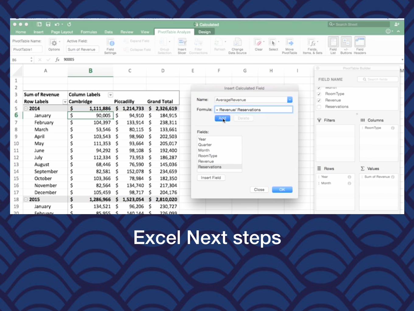
Excel Next steps

Using ZoomPlease mute your device. Click on the microphone icon to turn it on and off.

If you are using a tablet or phone, tap the screen to get the toolbar

Give a reaction

Share your screen

Open Excel document before doing a screen share

Change from Gallery view to active speaker view

• In the top right corner, there is a button that allows you to switch between Gallery view and Active speaker view

On a phone• Swipe left from the active speaker view to switch to

gallery view.

• Swipe right to the first screen to switch back to active speaker view.

Pinning a screen

To pin a video, hover over the video that you want to pin. The dots on a blue box will appear. Click this and select pin video.

(On a phone, change to Gallery view, then Double-tap the video of the participant you want to pin.)

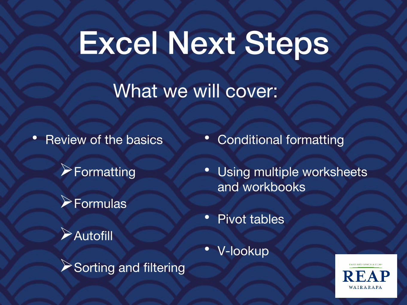
Excel Next Steps

• Review of the basics

ØFormatting

ØFormulas

ØAutofill

ØSorting and filtering

• Conditional formatting

• Using multiple worksheets and workbooks

• Pivot tables

• V-lookup

What we will cover:

What can spreadsheets be used for?

• Calculating financial information, e.g. budget, cashbook, payroll, sales.

• Basic database which can be sorted, searched or filtered.

• Record of results, e.g. sports, schools, elections.

• Changes over time, e.g. weight loss/gain, temperature etc.

• Recording and analysing statistics.

• Other:

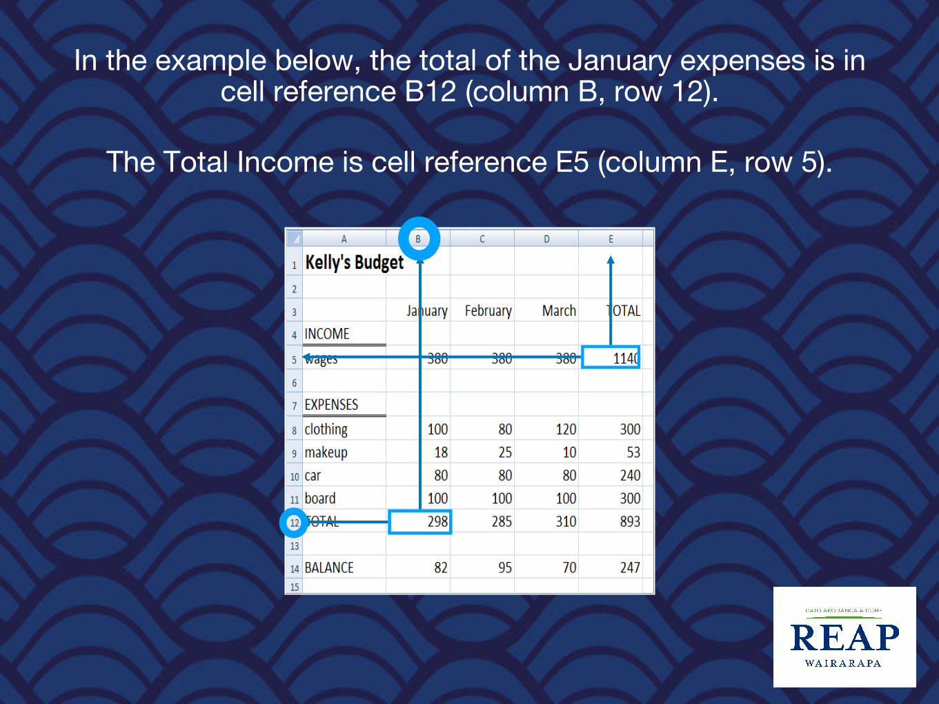
In the example below, the total of the January expenses is in cell reference B12 (column B, row 12).

The Total Income is cell reference E5 (column E, row 5).

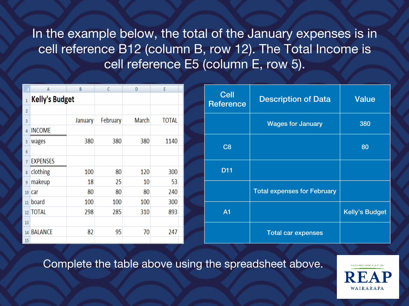
In the example below, the total of the January expenses is in cell reference B12 (column B, row 12). The Total Income is

cell reference E5 (column E, row 5).

Cell Reference Description of Data Value

Wages for January 380

C8 80

D11

Total expenses for February

A1 Kelly’s Budget

Total car expenses

Complete the table above using the spreadsheet above.

Excel basics review

• Household Budget tutorial

1. In cell A1 type Household Budget

2. In cell B2, type January, hold down Ctrl key and press Enter. Ctrl Enter lets you remain in the same cell. (Use Command instead of Ctrl if you are using a Macbook)

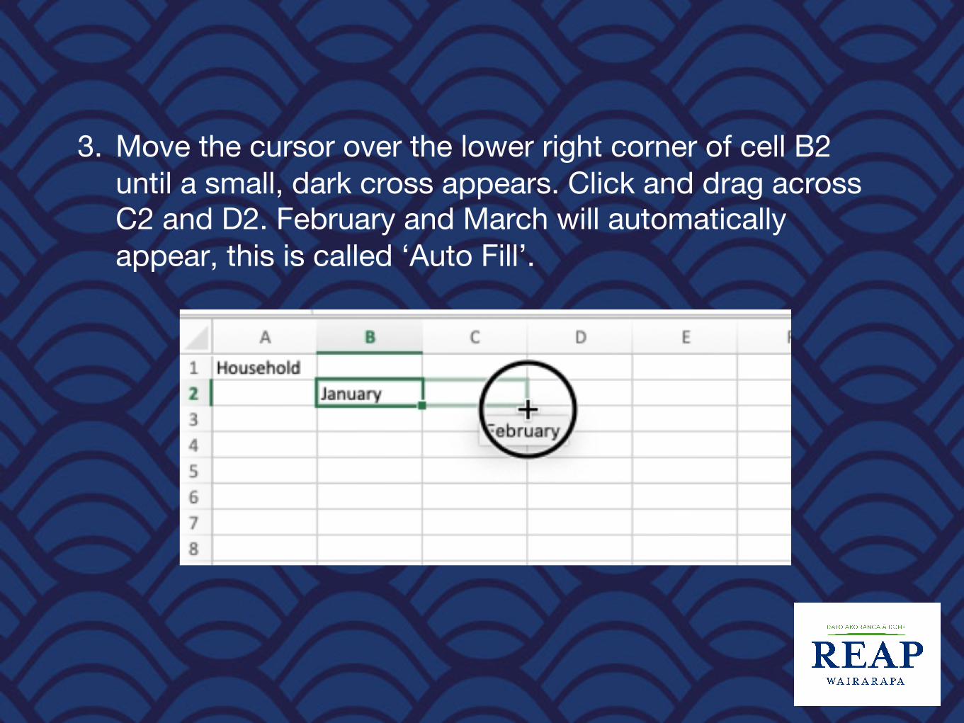
3. Move the cursor over the lower right corner of cell B2 until a small, dark cross appears. Click and drag across C2 and D2. February and March will automatically appear, this is called ‘Auto Fill’.

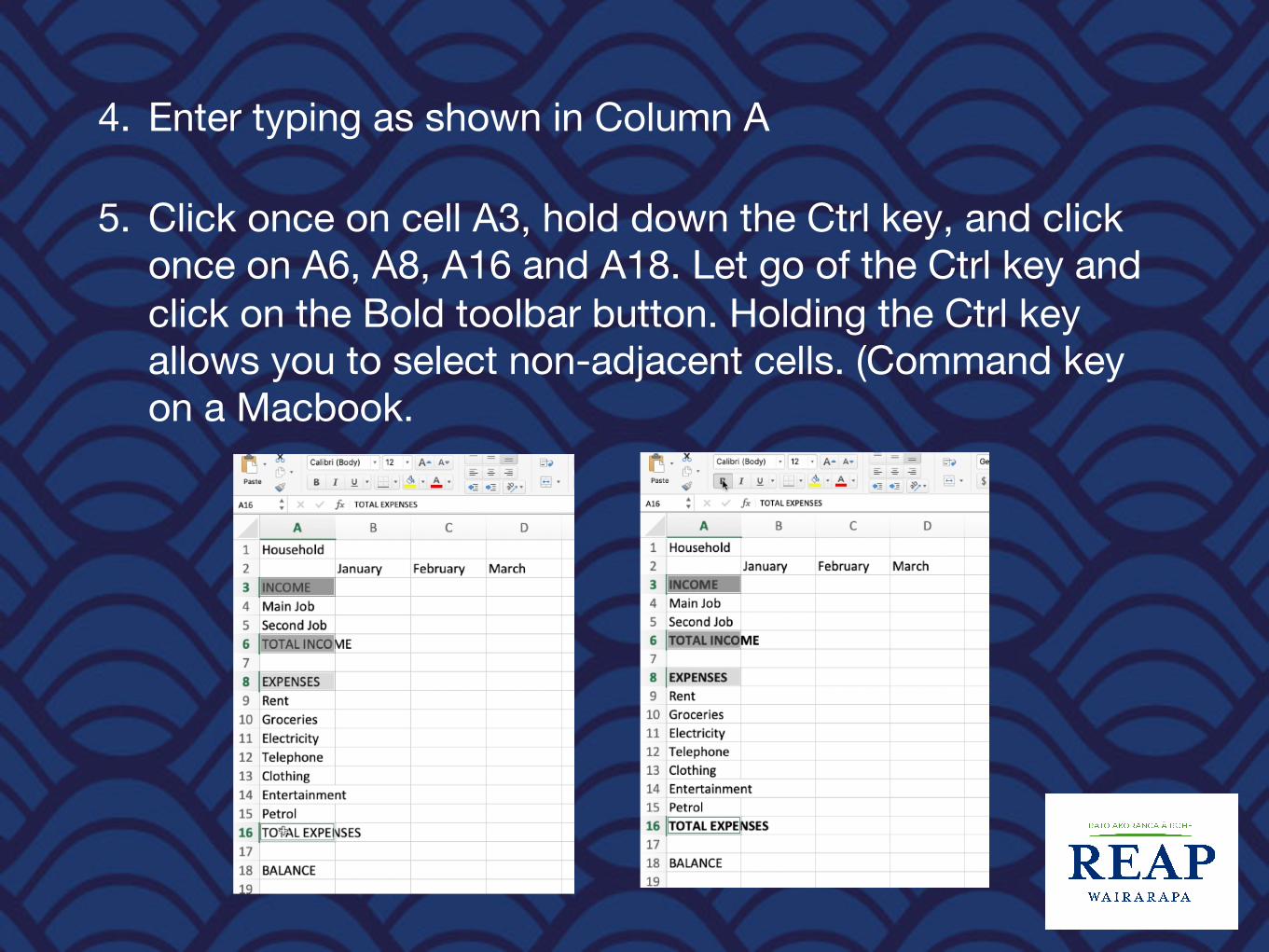
4. Enter typing as shown in Column A

5. Click once on cell A3, hold down the Ctrl key, and click once on A6, A8, A16 and A18. Let go of the Ctrl key and click on the Bold toolbar button. Holding the Ctrl key allows you to select non-adjacent cells. (Command key on a Macbook.

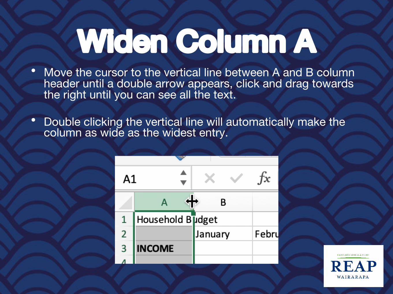
Widen Column A• Move the cursor to the vertical line between A and B column

header until a double arrow appears, click and drag towards the right until you can see all the text.

• Double clicking the vertical line will automatically make the column as wide as the widest entry.

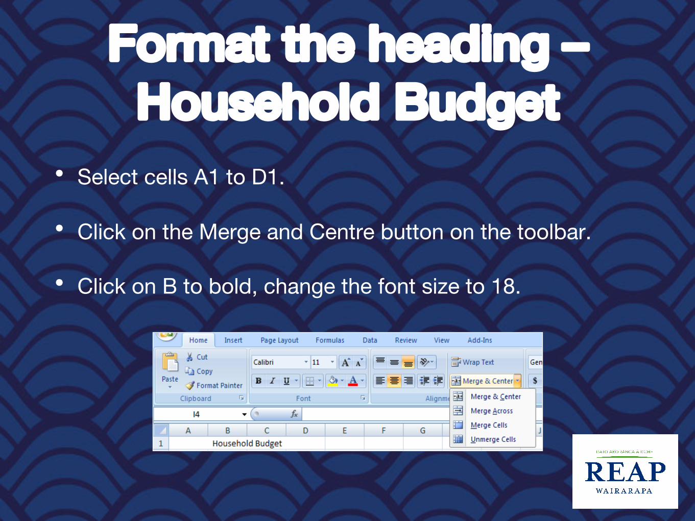
Format the heading –Household Budget

• Select cells A1 to D1.

• Click on the Merge and Centre button on the toolbar.

• Click on B to bold, change the font size to 18.

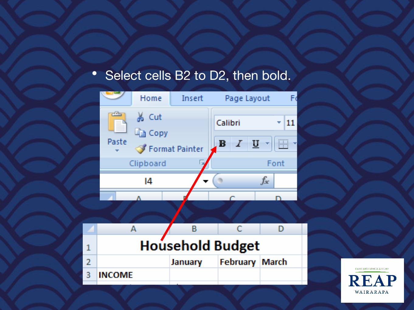
• Select cells B2 to D2, then bold.

FormulasAdd, Divide, Multiply and Subtract

Type an = sign, use ‘math’ operators (signs)

• + (plus sign) to add

• - (minus sign or hyphen) to subtract

• * (multiplication sign or asterisk) to multiply

• / (division sign or forward slash) to divide

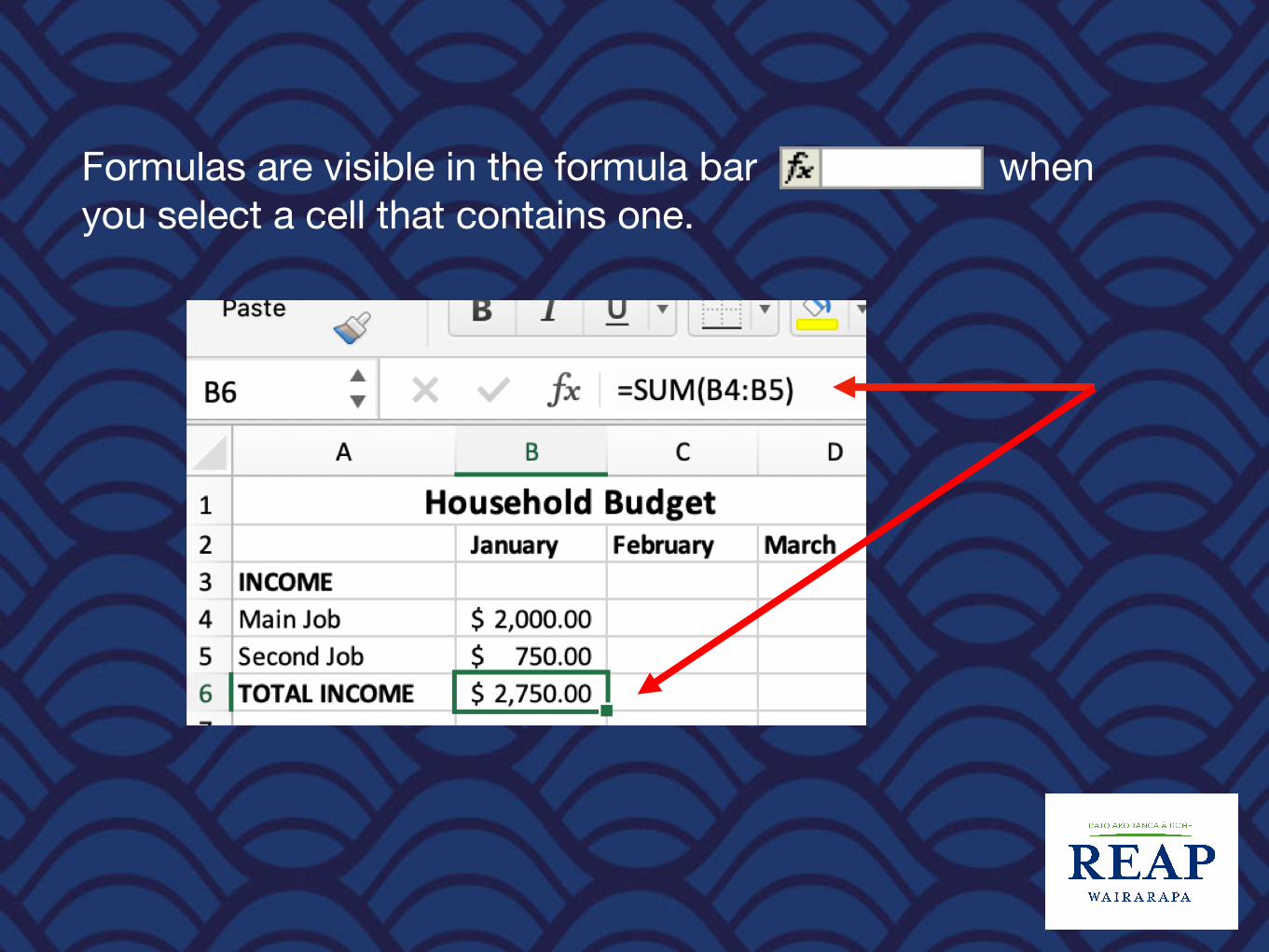
Formulas are visible in the formula bar when you select a cell that contains one.

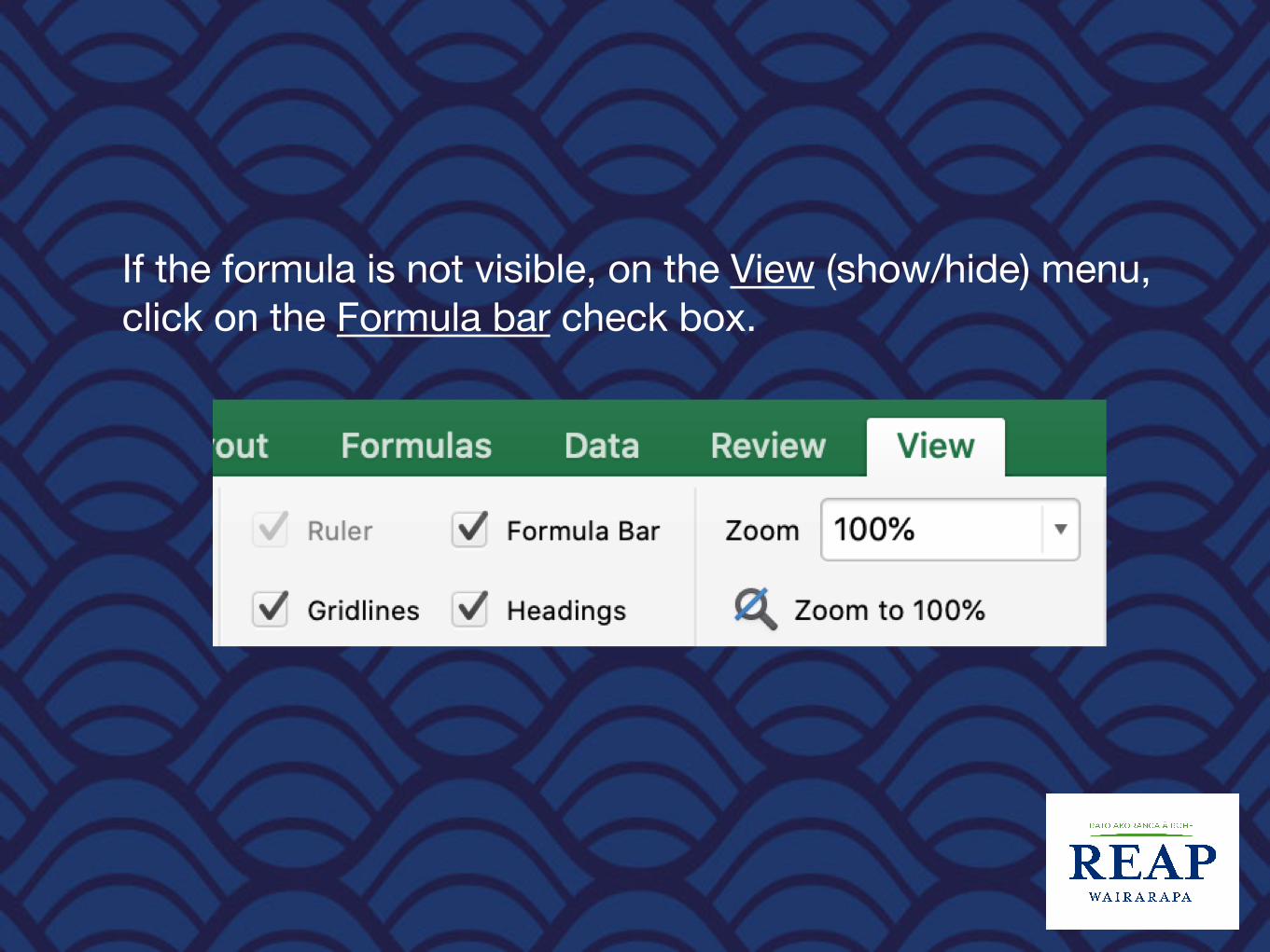
If the formula is not visible, on the View (show/hide) menu, click on the Formula bar check box.

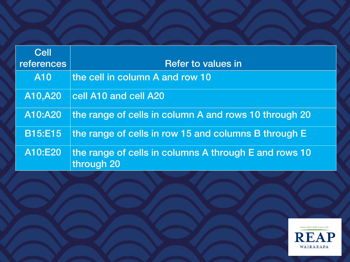
Cell references Refer to values in

A10 the cell in column A and row 10

A10,A20 cell A10 and cell A20

A10:A20 the range of cells in column A and rows 10 through 20

B15:E15 the range of cells in row 15 and columns B through E

A10:E20 the range of cells in columns A through E and rows 10 through 20

Add the values in a row or column

• Use the SUM function, which is a prewritten formula, to add all the values in a row or column:

• Click a cell below the column of values or to the right of the row of values.

• Click the AutoSum button

Find the average, maximum, or minimum

Use the AVERAGE, MAX, or MIN functions.

• Click a cell below or to the right of values for which you want to find the average, the maximum, or the minimum

• Click the arrow next to AutoSum

• Click Average, Max, or Min

To see more functions, click More Functions on the AutoSum list to open the Insert Function dialog box.

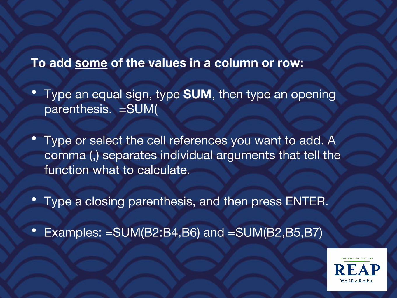
To add some of the values in a column or row:

• Type an equal sign, type SUM, then type an opening parenthesis. =SUM(

• Type or select the cell references you want to add. A comma (,) separates individual arguments that tell the function what to calculate.

• Type a closing parenthesis, and then press ENTER.

• Examples: =SUM(B2:B4,B6) and =SUM(B2,B5,B7)

Household BudgetEnter Formulas

• To total the Income, in B6, type =B4+B5, then press Enter. The number shown should be $2,750.00.

• To total the Expenses, in B16, click on the AutoSum button on the toolbar.

• Make sure the dotted line is around cells B9 to B15, then press Enter. (If not, reselect the correct cells to be added). The correct answer should be $1,670.00. When you click in cell B16, you will now see =SUM(B9:B15) in the formula bar (just above the column headers).

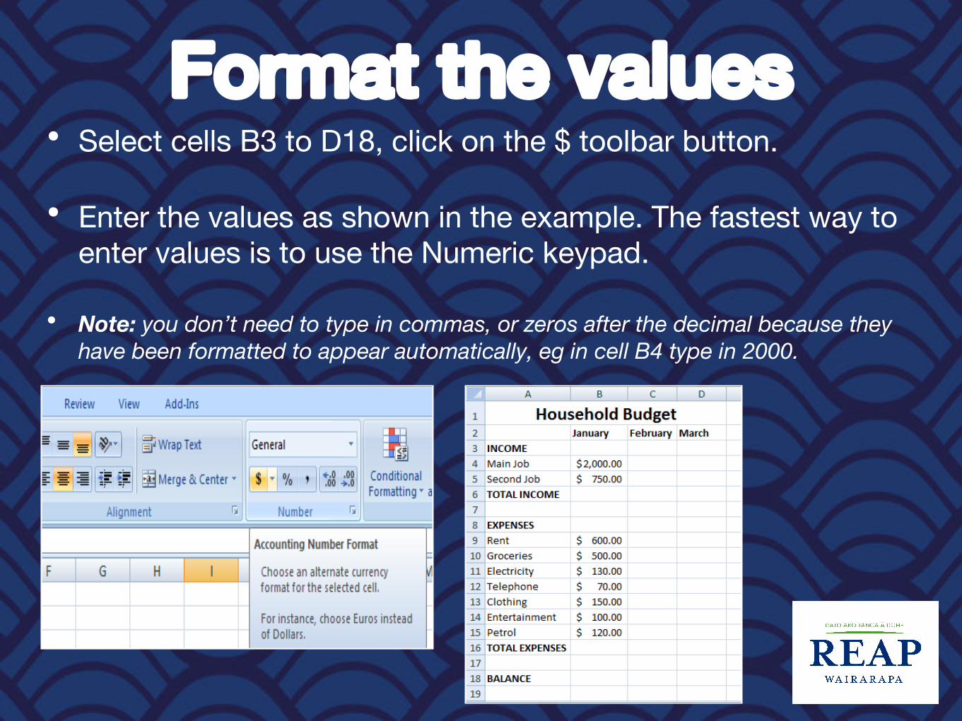
Format the values• Select cells B3 to D18, click on the $ toolbar button.

• Enter the values as shown in the example. The fastest way to enter values is to use the Numeric keypad.

• Note: you don’t need to type in commas, or zeros after the decimal because they have been formatted to appear automatically, eg in cell B4 type in 2000.

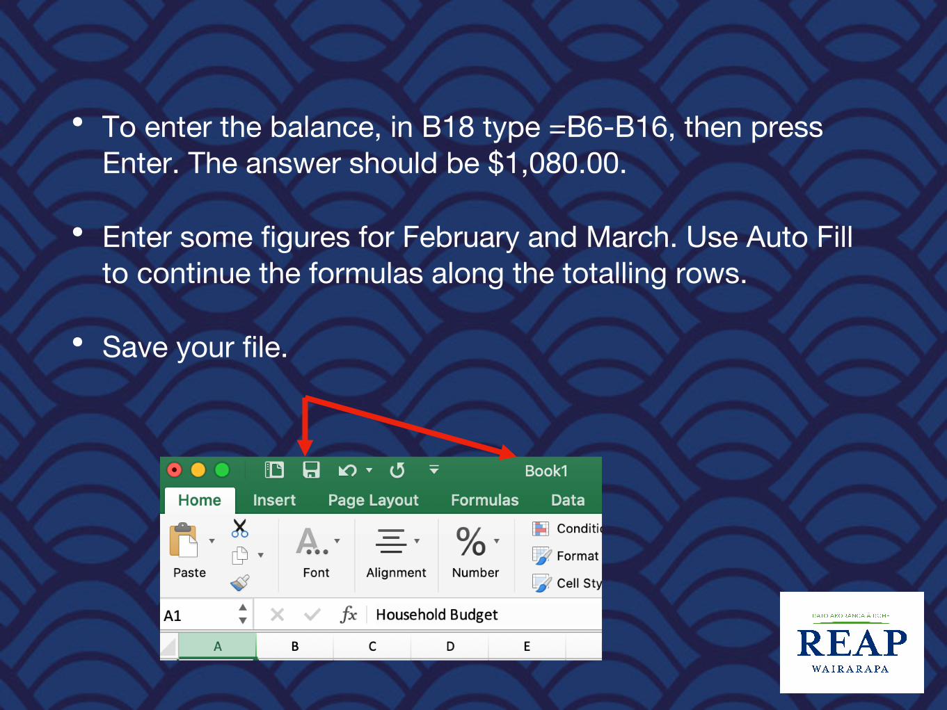
• To enter the balance, in B18 type =B6-B16, then press Enter. The answer should be $1,080.00.

• Enter some figures for February and March. Use Auto Fill to continue the formulas along the totalling rows.

• Save your file.

• Add borders and colour formatting to the table

• Change the direction of the Months

Household Budget -Charts

• By the end of this tutorial you will have:

• created a column chart,

• created a pie chart

• formatted charts

• added and edited chart labels

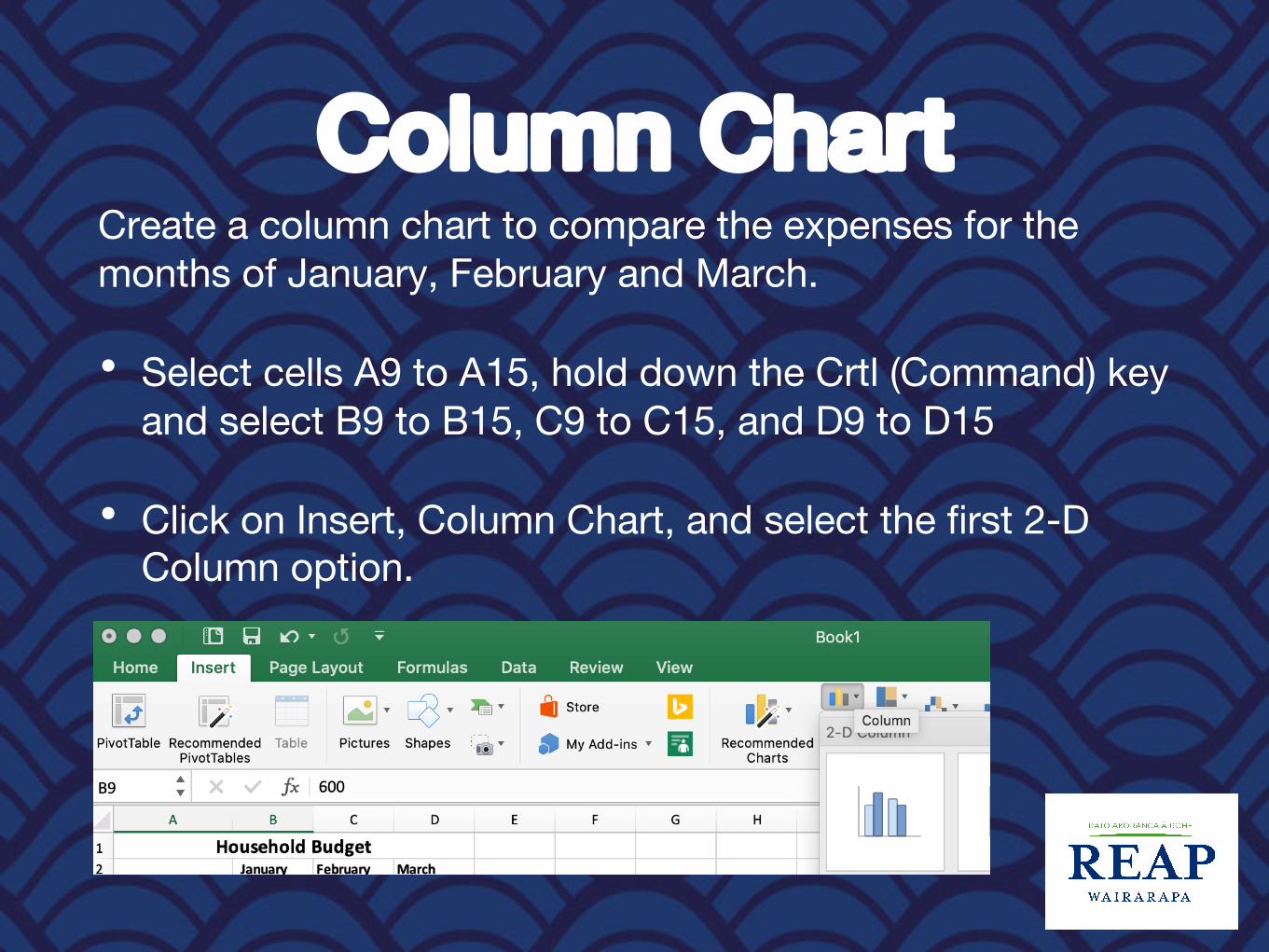
Column ChartCreate a column chart to compare the expenses for the months of January, February and March.

• Select cells A9 to A15, hold down the Crtl (Command) key and select B9 to B15, C9 to C15, and D9 to D15

• Click on Insert, Column Chart, and select the first 2-D Column option.

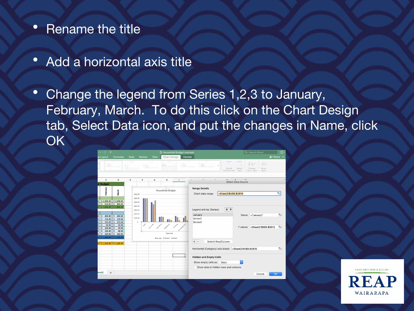
• Rename the title

• Add a horizontal axis title

• Change the legend from Series 1,2,3 to January, February, March. To do this click on the Chart Design tab, Select Data icon, and put the changes in Name, click OK

Pie ChartCreate a pie chart to compare the income for the month of March.

• Select cells A4 to A5, hold down the Crtl key and select D4 to D5.

• Click on Insert, Pie Chart, and select the first 2-D Pie option.

• Your chart will appear on your spreadsheet. Click and drag it to reposition it.

• Add a title and format it.

Printing

• Use Print Preview to see if your spreadsheet and charts will fit on one page.

• When you close the Print Preview, you will see your spreadsheet now has dotted lines to show the edge of the page. You can resize and move your charts around so they fit within the dotted lines.

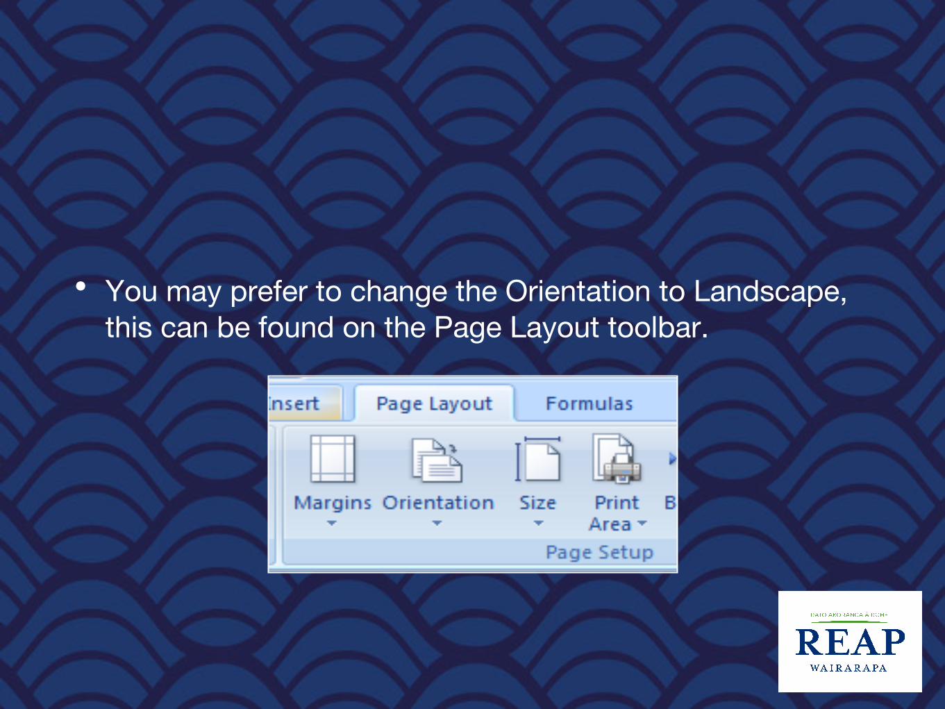
• You may prefer to change the Orientation to Landscape, this can be found on the Page Layout toolbar.

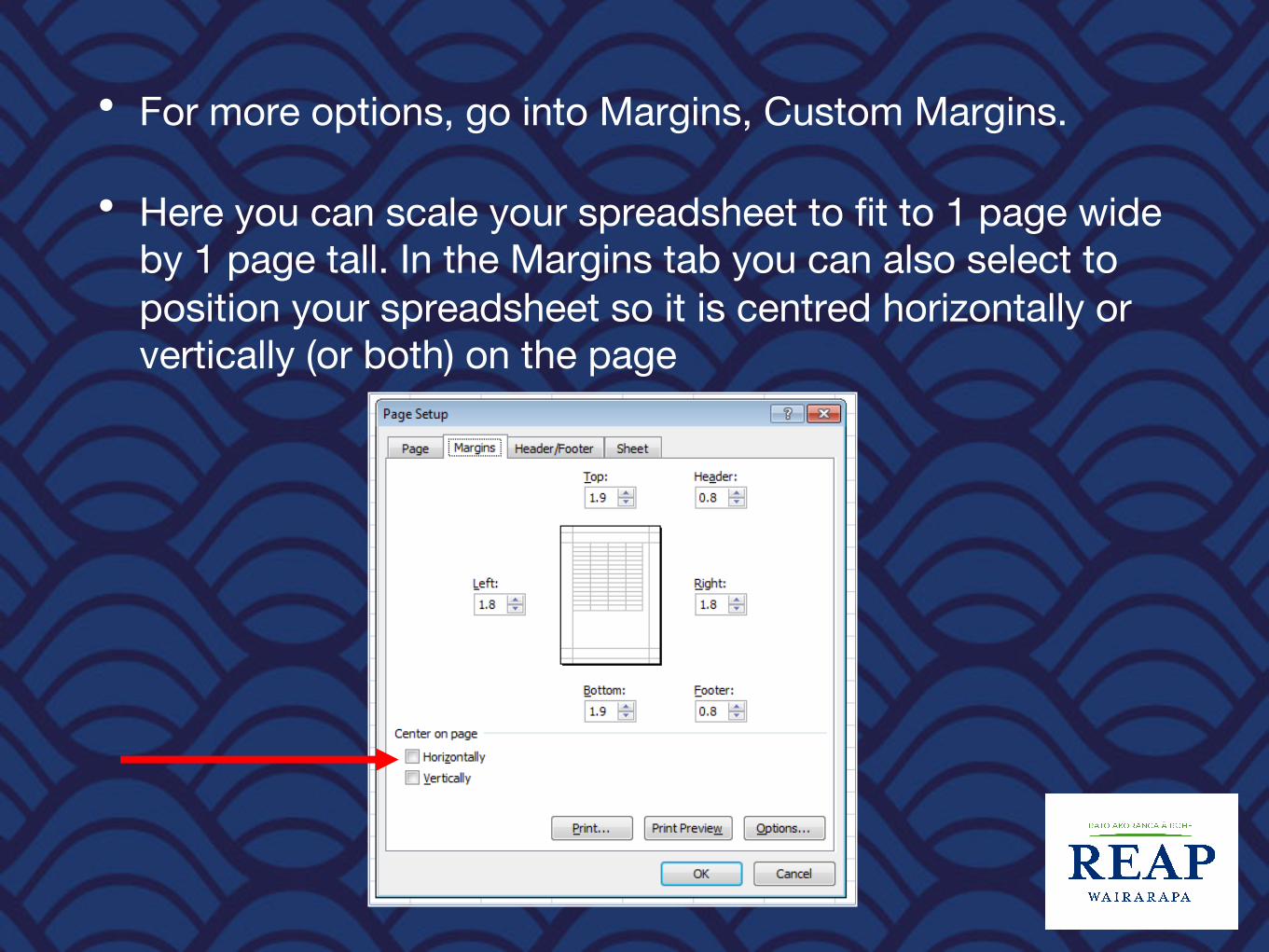
• For more options, go into Margins, Custom Margins.

• Here you can scale your spreadsheet to fit to 1 page wide by 1 page tall. In the Margins tab you can also select to position your spreadsheet so it is centred horizontally or vertically (or both) on the page

Understand error values• ##### The column is not wide enough to display the

content. Increase column width, shrink contents to fit the column, or apply a different number format.

• #REF! A cell reference is not valid. Cells may have been deleted or pasted over.

• #NAME? You may have misspelled a function name.

Cells with errors such as #NAME? may display a color triangle. If you click the cell, an error button appears to give you some error correction options

Use more than one math operator in a formula

• If a formula has more than one operator, Excel follows the rules of operator precedence instead of just calculating from left to right. Multiplication is done before addition: =11.97+3.99*2 is 19.95. Excel multiplies 3.99 by 2, and then adds the result to 11.97.

• Operations inside parentheses take place first: =(11.97+3.99)*2 is 31.92. Excel adds first and then multiplies the result by 2.

• Excel does use operators from left to right if they have the same level of precedence. Multiplication and division are on the same level. Lower than multiplication and division, addition and subtraction are on the same level.

Absolute Reference

• When you copy formulas across or down using autofill, the cell references in the formula will change accordingly.

• An absolute cell reference is used when you want a cell reference to stay fixed on a specific cell. Use a $ sign in front of each letter and number e.g. $A$1.