w o r k i n g

p a p e r

F E D E R A L R E S E R V E B A N K O F C L E V E L A N D

9 8 1 6

Evolutionary Programming as a Solution Technique for the Bellman Equationby Paul Gomme

EvolutionaryProgrammingasa SolutionTechniquefortheBellmanEquation

�Paul Gomme

FederalReserveBankof Clevelandand

CREFE/UQAMpaul.a.gomme@clev.frb.org

October1997

Abstract: Evolutionary programmingis a stochasticoptimizationprocedurewhich hasprovedusefulin optimizing difficult functions. It is shown thatevolutionaryprogramingcanbe usedtosolvetheBellmanequationproblemwith ahighdegreeof accuracy andsubstantiallylessCPUtimethanBellmanequationiteration. Futureapplicationswill focuson sometimesbindingconstraints– aclassof problemfor which standardsolutionstechniquesarenot applicable.

Keywords: evolutionary programming,bellmanequation,value function, computationaltech-niques,stochasticoptimization

�The financialsupportof the SocialSciencesandHumanitiesResearchCouncil (Canada)is gratefullyacknowl-

edged.Theviews statedhereinarethoseof theauthorandarenot necessarilythoseof theFederalReserve BankofClevelandor of theBoardof Governorsof theFederalReserveSystem.

1 Intr oduction

Stochasticoptimizationalgorithms,like evolutionaryprogramming,geneticalgorithmsandsimu-latedannealing,have provedusefulin solving difficult optimizationproblems.In this context, adifficult optimizationproblemmight mean:(1) a non-differentiableobjective function, (2) manylocal optima,(3) a largenumberof parameters,or (4) a largenumberof configurationsof param-eters.1 Thusfar, therearefew economicapplicationsof suchprocedures,with mostattentionhasfocusedon geneticalgorithms;see,for example,Arifovic (1995)andArifovic (1996).This paperexploresthe potentialof evolutionaryprogrammingasa solutionprocedurefor solving Bellmanequation(valuefunction)problems.

Whereasgeneticalgorithmsincludea varietyof operators(for example,mutation,cross-overandreproduction),evolutionaryprogramsuseonly mutation. As such,an evolutionaryprogramcanbeviewedasa specialcaseof a geneticalgorithm. Thebasicsof evolutionaryprogrammingcanbedescribedasfollows. Let

�������betheparameterspaceandlet � ���

denotecandidatesolution � �� ���� � � ��� ���

. If theobjective function is ��� �����, then ��� � � is theevaluationfor

element� . Givensomeinitial population, � ! "�# , proceedasfollows:

1. Sortthepopulationfrom bestto worstaccordingto thefunction � .

2. For theworsthalf of thepopulation,replaceeachmemberwith a correspondingmemberinthetophalf of thepopulation,addingin some‘randomnoise.’

3. Re-evaluateeachmemberaccordingto � .

4. Repeatuntil someconvergencecriterionis satisfied.

The‘noise’ addedin step2 helpstheevolutionaryprogramto escapelocal minimaandat thesametimeexploretheparameterspace.As theamountof noisein step2 is reduced,theevolution-ary programwill typically converge to a solutionarbitrarily closeto the optimum. Propertiesofevolutionaryprogramshavebeenexploredby anumberof authorsincludingFogel(1992).

Therearea numberof complicationswhich arisein applyinganevolutionaryprogramto theBellmanproblem.Themostimportantcomplicationis thatthealgorithmmustsolvefor theobjec-tive function. That is, for thetypical evolutionaryprogram,thefunction � above is known. Here,the valuefunction, which dependson the state,is unknown a priori andthe solutionalgorithmmustsolve for thevaluefunction—whichis alsothe ‘fitness’ criterionusedto evaluatecandidatesolutions.

The basicsof the algorithmarediscussedin Section2. The specificapplicationis the neo-classicalgrowth model. In themostbasicversionof themodel,theparametersto choosearenextperiod’s capitalstock(asa functionof this period’s capitalstock). Thesearerestrictedto lie in adiscreteset.For problemswith a largenumberof capitalstockgrid points,it is shown thattheevo-lutionaryprogramdeliversdecisionrulesarbitrarilycloseto theknown solution,anddoessomuchfasterthanBellmanequationiteration;seeSection3. Also in Section3, the performanceof theevolutionaryprogramis evaluatedwhena labor-leisurechoiceis introduced.For largeproblems,theevolutionaryprogramis againsubstantiallyfasterthanBellmanequationiteration. Section4concludes.

1A classicexampleis thetraveling salesman problem in whichasalesmanwishesto minimizethedistancetraveledin visiting a setof $ cities.

1

2 The Problemand Algorithm

Thespecificapplicationis theneoclassicalgrowth model:

%'& () * + , - + .�/ 0 1+ 2�3 E4 5768 9 : 4<;9�= >@? 9 ACBEDGF

;FIH

(1)

subjectto ? 9�JLK�9 MON<PRQ 9 KTS9 JRU H�VXW�Y K�9 BZDGF�W B [\FIH�B^] P D B H�B _ _ _(2)

where

? 9is consumption,

K 9is capital,

Q 9a technologyshock, ` a well-behaved utility function,

and a a well-behavedproductionfunction.TheassociatedBellmanequation(valuefunction)is:b U K�9 B Q 9 Ydc %'&�() * + , - + .�/ 0 e= >@? 9�J

; E

9 b U K 9 M�N B Q 9 MON Y f(3)

subjectto (2). Oneway to solve this problemis via Bellmanequationiteration:givensomeinitialguess

b 4 U K�9 B Q 9 Y , iterateon (3) asbTg MON U K 9 B Q 9 Y<c %'& () * + , - + .�/ 0 e= >@? 9 J

; E

9 b�g U K 9 MON B Q 9 MON Y fsubjectto (2) (4)

until eitherthedecisionrulesconverge,or thevaluefunctionconverges.To implementthis proce-durecomputationally, thecapitalstockis restrictedto a grid, h P e K

N B KTi B _ _ _�B KTj�k f. The tech-

nologyshockis likewiserestrictedto l P e QN B Q�i B _ _ _OB Q�j�m f

.

Q 9is assumedto follow a Markov

chain:

probe Q 9 M�NnPRQ g�o Q 9�PRQ p f PIq p g _(5)

Whenthereis 100%depreciation(

W P H), aclosed-formsolutioncanbeobtained:K 9 M�NnP [

;Q 9 K S9

(6)? 9 PrU H@VX[;Y Q 9 KTS9 _

(7)

Theseknown solutionswill beusefulin evaluatingtheperformanceof theevolutionaryprogram.The biggestproblemwith Bellman equationiteration is the curse of dimensionality: large

capitalstockgridsor additionalendogenousstatevariablesmake themaximizationin (4) compu-tationallyexpensive. In many ways,theproblemassetout in (4) looks like a naturalapplicationfor anevolutionaryprogram:for eachof the s�t�u\swv grid pointsin thestatespace,thereares�t potentialvaluesfor

K�9 MON. While

b g U K�9 B Q 9 Yis known at iteration x , thelimiting valuefunction,b U K 9 B Q 9 Y<c = y %g z 6 b g U K�9 B Q 9 Y

(8)

is generallyunknown. Ifb U K 9 B Q 9 Y

wereknown, this would bea straightforwardevolutionarypro-gramapplication.However, thealgorithmmustalsoiterateon

bTg U K 9 B Q 9 Yto obtainanapproximation

2

to {'| }�~ � � ~ � . It is this iterationwhich distinguishestheneoclassicalgrowth modelfrom thetypicalevolutionaryprogramapplication.

At eachiterationin (4), thereis asolutionfor next period’scapitalstock,} ~ �O�<�R�G� | } ~ � � ~ �n�w�'� (9)

Ratherthanobtainthis by maximization,supposeonewereto ‘guess’asetof solutions,} ~ ���n�R��� | } ~ � � ~ �n�w�G�Z�<�\����� �T� � � �O� ����� (10)

For each�<�\����� �T� � � �O� �w� canbecomputed{�� | } ~ � � ~ � �R� �@� ~��X� E~ {T� | � � | }�~ � � ~ � � � ~ ��� � (11)

where � ~ � � ~ }T�~ �R| ���\��� } ~O� � � | }�~ � � ~ � � (12)

For each� , this resultsin � ��� �w� numbers(onefor eachof thegrid pointsfor thestatespace).Sothateachguesshasasscalarvalueassociatedwith it, compute{ � � �� ��� �w����   ¡ ¢ �£   ¡ ¤ {�� | } ~ � � ~ � � (13)

Next, sorttheguessessuchthat { �n¥ {§¦ ¥R¨ ¨ ¨ ¥ {�©�� (14)

At thenext iteration,elements�<�\� © ¦ ����� � � ��� �w� will bereplacedasfollows:��� | } ~ � � ~ � � }�ª��w� (15)

where « �R¬'­ ®�¯ ¬'° ��¯ ± � INT | ²O� � � ��³ � � ³ � (16)± is theindex to thecapitalstockgrid point correspondingto � � ´dµ ¶ | } ~ � � ~ � , INT takesthe integerportion of of a real number, and ² is a randomnumberdrawn from �\| · � ¸ ¦ � . The procedurein(15) is repeatedfor each}�~d�\� andfor each� ~<�\¹ . A new randomnumber² is drawn for eachgrid point. Theupshotof this procedureis to replacetheworsthalf of thepopulationof guesseswith thebesthalf, plussomenoise.

How should { � | } ~ � � ~ � be updatedfor the next iteration? In the spirit of the maximizationin(4), let {�� ��� | }�~ � � ~ � �º¬'­�®� ¡�» � ¼ ½ ½ ½ ¼ ©<¾ ¯ {§� | } ~ � � ~ � ³ � for each}�~��w� and � ~d�w¹�� (17)

Anotheralternative would have beento have set {T� �O� | }�~ � � ~ � � { � | } ~ � � ~ � (thevaluefunction forthebestguess).As apracticalmatter, themaximizationin (17) speedsconvergence.

3

In experimentingwith thealgorithm,it wasprudentto replaceguess¿�À Á�Â Ã Ä Å Æ Ä Ç with therulewhich implementsthe maximumin (17). Sincethis replacesthe worst guessin the top half ofthe population,it doesnot overwrite a particularlygoodguess.Further, if the replacementis abad thing to do, the valueassociatedwith this rule will presumablyplaceit in the bottomhalfof the populationnext iteration,andit will be discarded.Intuitively, this is like performingthemaximizationassociatedwith Bellmanequationiteration,but checkingonly a smallsubsetof thepossiblevaluesfor next period’scapitalstock.Again,asapracticalmatter, thisreplacementgreatlyspeedsconvergence.

To finish this section,theevolutionaryprogramwill besummarized.

1. Generatean initial guessfor the valuefunction, È�É Â Ã Ä Å Æ Ä Ç , anda populationof candidatesolutions, Ê ¿�Ë Â Ã�Ä Å Æ Ä Ç Ì ÍË Î�Ï for à ÄGÐrÑ and Æ ÄGÐ7Ò . Also, setan initial valuefor Ó whichgovernstheamountof ‘noise’ introducedto decisionruleswhenthey arecopied.

2. For eachrule Ô<Ð\Ê�Õ�Å ÖTÅ × × ×OÅ ØwÌ , computeÈ�Ë Â Ã�Ä Å Æ Ä Ç via (11)and(12),andcomputeÈ Ë using(13).

3. Sortthepopulationasin (14).

4. ComputeÈTÙ Ú Ï Â Ã�Ä Å Æ Ä Ç using(17). Replacerule Í Û with thatwhich would achieve this maxi-mum.

5. Replacethe bottomhalf of the populationwith perturbedmembersof the top half of thepopulationasdescribedin (15).

6. Repeat2–5until convergeis achieved,or aprespecifiednumberof iterationsarecompleted.

7. ReduceÓ (theamountof experimentation).

8. Repeat2–7until Ó is sufficiently small.

3 Calibration and Results

In this section,theevolutionaryprogramis comparedto Bellmanequationiterationbothin termsof accuracy andcomputationalrequirements.Two majorcasesareconsidered:with andwithouta labor-leisurechoice.Subcasesarepresentedfor closed-formvs. nonclosed-form,andstochasticvs. nonstochastictechnologyshocks( Æ Ä ).3.1 No Labor–LeisureChoice

Table1 presentsparametervaluescommonto all experimentsin this section.For themostpart,theseare valuestypically usedin the real businesscycle literature; see,for example,Prescott(1986).Thecapitalstockgrid wasspecifiedasa setof evenly spacedpointson theinterval Ü Ã Å Ã�Ý ;theupperandlower boundson thecapitalstockwerechosensuchthat theergodicsetfor capitalwas strictly containedin Ü Ã Å Ã�Ý . The set for the technologyshockwas specifiedas having twopoints: ÒßÞ7Ê Æ Å Æ Ì�× (18)

4

Thetechnologyshockevolvesas:

probà á â ãOänå�á æ á â�åRá çOå probà á â ãOänå áOæ á â�å á�çOå�è<é (19)

Thetransitionprobability, è , andvaluesfor á and á werechosento matchthepropertiesof Solowresidualsasreportedin Prescott(1986).

Table1: Parametervaluesusedin computationalexercises.

Parameter Description Valueê capital’sshareof income 0.36ëdiscountfactor 0.99ìlowerboundfor capitalgrid

äí�î steadystateìupperboundfor capitalgrid 2 î steadystateá lowerboundfor technologyshock ï ð ñ ò ñ ñ ó ô õá upperboundfor technologyshock ï ñ ò ñ ñ ó ô õè persistenceof technologyshock 0.975

In termsof initial conditions, öñ ÷ ì â ø á â ù åRúüû ì â ø û�á â ø (20)

and ý�þ÷ ì â ø á â ù å ì û ì â ø û�á â ø ûOÿ é (21)

(21) ensuresthat consumptionis alwayspositive for the initial guesses.2 � , which governstheamountof experimentationin the evolutionaryprogram,startsat

� ý ��� ú . Its valueis halved ateachstep7 (seethe endof Section2) until its valueis lessthan0.1. Iterationsleadingto step7continueuntil therehasbeenno changein the decisionrule generatingthe bestsolution for 20iterations,or until a total of 50 iterationshavebeencompleted.

Resultsfor thecasein which a closed-formsolutionis availablearereportedin Table2; theseresultsaresummarizedin Figure1. Both theevolutionaryprogramandBellmanequationiterationsuccessfullysolved this casein that the final solutionswerewithin onegrid point of the knownsolution. For moderatesizedgrids (up to 200grid pointsfor capital),Bellmanequationiterationis actually fasterthan the evolutionary program. This ranking is reversedfor large grids. Forexample,with 10,000grid points, the evolutionary programis more than 20 times fasterthanBellmanequationiteration. Thesedifferencesmatter: whenthe technologyshockis stochastic,theevolutionaryprogramsolvesin under16 minuteswhile Bellmanequationiterationtakesover6 hours.

Also of interestis the casefor which a closed-formsolutionis not availablesincethis is thesituationwhich typically confrontsthe researcher. Table3 summarizesthe resultsfor this case(seeFigure2 for a graphicalpresentation).Qualitatively, thesamemessageemerges: for a large

2For theevolutionaryprogram,positiveconsumptioncannotbeguaranteedat futurestages.Whena rule specifiesnonpositiveconsumption,thevaluefunctionat thatgrid pointevaluatesto ��� � .

5

Table2: Resultsfor theclosed-formcase:� ��� .Nonstochastic Stochastic

Grid Evolutionary Bellman Evolutionary BellmanPoints Program Iteration Program Iteration� ��� ��� � ��� � ��� � ��� ������ ��� � ��� � ��� � ��� ������ ��� � � ��� � � ��� � ����� ���� ����� ����� � � ��� ��� � ����� � � ������� ���� ����� ����� � ����� ��� � � ������� � ��� ������� ���� ����� � ������� � ��� ��� ��� � ����� ��� � � ������������� �� ��� ����� ��������� � ������� ������� � � � ������� � ��������������� �

Note: In all cases,the solutionswerewithin onegrid point of the known solutionsgivenin (6) and(7). ReportedCPUtimeis theuser timereportedby theUnix timecommandonaSPARCstation20 with a100MHz HyperSPARC chip.

Figure1: CPUtime for closed-formcase.

00:0000:2000:4001:0001:2001:4002:0002:20

0 2000 4000 6000 8000 10000

HH

:MM!

Grid Points

Nonstochastic

EP Bellman

00:0001:0002:0003:0004:0005:0006:0007:00

0 2000 4000 6000 8000 10000

HH

:MM!

Grid Points

Stochastic

EP Bellman

Figure2: CPUtime for � �"��� ����� (noclosedform solution).

00:0002:0004:0006:0008:0010:0012:00

0 2000 4000 6000 8000 10000

HH

:MM!Grid Points

Nonstochastic

EP Bellman

00:0006:0012:0018:0024:0030:0036:00

0 2000 4000 6000 8000 10000

HH

:MM!

Grid Points

Stochastic

EP Bellman

6

Table3: Resultsfor # $"%�& %�'�( (no closedform solution).

Nonstochastic StochasticGrid Evolutionary Error Bellman Evolutionary Error Bellman

Points Program Iteration Program Iteration) %�% ) & * ) ) & + ,�& ( ' (�& )'�%�% ,�& % ' +�& ) +�& - . '�%�& ,(�%�% )�) & * ' ) / %�'�& ) .�%�& . 0 ' / .�(�& .)�1 %�%�% '�+�& + . , / ,�'�& * ) / %�,�& ' % ) . / . ) & ,' 1 %�%�% ) / %�*�& . ' ' ) / %�(�& % ' / .�%�& 0 ' (�0 / ,�*�& (( 1 %�%�% . / '�.�& ) . ' / ,�* / ,�+�& , * / ( %�& * % * / .�+ / .�%�& *) % 1 %�%�% * / ,�,�& 0 . )�) / . ) / .�.�& - ) * / ' 0�& * ) .�% / ( ) / ,�*�& (Note: ReportedCPUtime is theuser time reportedby theUnix time commandonaSPARCstation20 with a100MHz HyperSPARC chip. ‘Error’ is thenumberof gridpointsat which theevolutionaryprogramandBellmanequationiterationdiffer.

numberof grid points,theevolutionaryprogramclearlydominatesin termsof CPUtime. Quan-titatively, the differencesareeven larger thanbefore. In the stochasticcasewith 10,000capitalstockgrid points,theevolutionaryprogramfinishesin lessthan18 minuteswhile Bellmanequa-tion iterationtakesover 30 hours– over 100 timeslonger. Both algorithmsgive nearlythesamedecisionrules for capital accumulation:the maximumnumberof grid points which differ is 6(for the stochasticcasewith 500 capitalstockgrid points). For a particulargrid point, the twoalgorithmsneverdifferedby morethanonegrid point.

3.2 Labor–LeisureChoice

Therearetwo reasonsto be interestedin this case.First, endogenouslaborsupplydecisionsareimportantfor generatingbusinesscycle momentsin therealbusinesscycle literature.Second,theevolutionaryprogramcanbegivena furtherworkoutby requiringthatit solve for laboraswell.3

Therepresentativeagent’sproblemin this caseis:243�56 7 8 9 : 8 9 ; 8 <�= > E? @�AB C DFE�G C H I4J KML CON"P )MQ IMR�J K P )SQUT C R V W 1 %�X G 1 I X ) (22)

subjectto L C NZY C [OE $]\ C Y�^C T E _ ^C N"P )MQ # R Y C 1 %�X]# 1 ` X )�1ba $"% 1 )�1 & & & (23)

where,in additionto theearliervariables,T C

is the fractionof time spentworking. When #c$ ) ,thedecisionrulesare: Y�C [FE $ ` G \ C Y ^C T E _ ^C 1

(24)

3An alternative,usedin Bellmanequationiteration,is to useanEulerequationto solve for laborsupply.

7

d egfih jMkml�npo q e r�se�tgu v sexw (25)

and t e fzy h jSkUl{o h jMkmlpn�oy h jMkml�o h jMkml�npog|]jMk y�} (26)

Theparametervaluesarethesameasbefore,with theadditionthat y fi~ } ��� . In implement-ing Bellmanequationiteration,thesolutionfor time spentworking, t e , is computedusinga onedimensionalnonlinearequationsolverwhichworkson theEulerequation,h jSkUl{o q e r�se�tgv se�� yd e � f jSk yjSk t e w (27)

where d e is computedfrom (23). This stepis computationallycostly, but needonly beperformedoncefor eachof the �����U��������� possibleconfigurations(next period’s capitalstock,thisperiod’scapitalstockandthis period’s technologyshock).

Ratherthanuse(27) to solve for labor, theevolutionaryprogramis requiredto solve not onlyfor thecapitalaccumulationdecisionbut alsolabordecisionsupply. This shouldserve to biastheresultsagainstthe evolutionaryprogram. ��� will now be usedto control the amountof experi-mentationover thecapitalgrid while �O� will controltheexperimentationwith respectto thelabordecision.As above, the initial valuefor � � is ����� j ~ while ��� startsat 0.1. Thesameconver-gencecriteriaareusedasabove. FORTRAN codeto solve this modelis reproducedin AppendixA.

Table4: Resultsfor theclosed-formcasewith endogenouslaborsupply.

Nonstochastic StochasticGrid Evolutionary Bellman Evolutionary Bellman

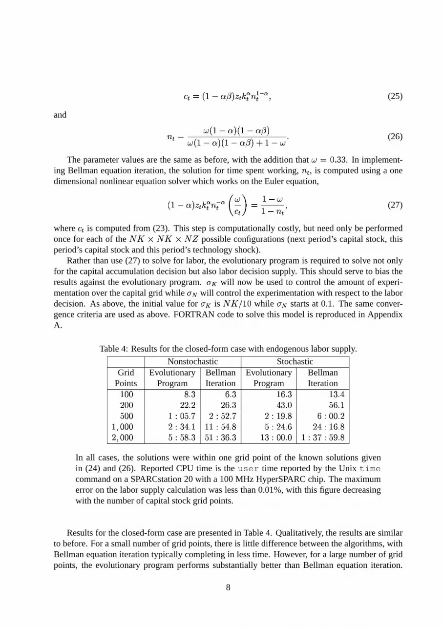
Points Program Iteration Program Iterationj ~�~ � } � ��} � j ��} � j ��} �� ~�~ ��� } � � ��} � ����} ~ � ��} j� ~�~ j ��~�� } � � ��� � } � � �Oj � } � � ��~�~ } �j w ~�~�~ � � ����} j j�j ��� ��} � � � � ��} � � � ��j ��} �� w ~�~�~ � ��� � } � ��j � ����} � j � ��~�~ } ~ j � ��� ����� } �In all cases,the solutionswere within onegrid point of the known solutionsgivenin (24) and(26). ReportedCPU time is theuser time reportedby the Unix timecommandon a SPARCstation20 with a 100MHz HyperSPARC chip. Themaximumerroron thelaborsupplycalculationwaslessthan0.01%,with this figuredecreasingwith thenumberof capitalstockgrid points.

Resultsfor theclosed-formcasearepresentedin Table4. Qualitatively, theresultsaresimilarto before.For asmallnumberof grid points,thereis little differencebetweenthealgorithms,withBellmanequationiterationtypically completingin lesstime. However, for a largenumberof gridpoints, the evolutionary programperformssubstantiallybetterthan Bellman equationiteration.

8

Figure3: CPUtime for closedform casewith endogenouslaborsupply.

00:0000:1000:2000:3000:4000:5001:00

0 500 1000 1500 2000

HH

:MM�

Grid Points

Nonstochastic

EP Bellman

00:0000:1000:2000:3000:4000:5001:0001:1001:2001:3001:40

0 500 1000 1500 2000

HH

:MM�

Grid Points

Stochastic

EP Bellman

With no labor–leisurechoice,the evolutionary programwas about5 times fasterthanBellmanequationiterationfor 2,000grid points(seeTable2). With a labor–leisurechoice,theevolutionaryprogramis over 8 timesfaster. Thesearenot differencesof seconds,but ratherof hours. Largercapitalstockgridswerenot attemptedin this casedueto theCPUandmemoryrequirementsforBellmanequationiteration.4 Theearlierresultssuggestthat for larger grid points,theCPUtimeadvantageof theevolutionaryprogramwouldbesubstantial.

Table5: Resultsfor � �"��� ����� (no closedform solution).Nonstochastic Stochastic

Grid Evolutionary Error Bellman Evolutionary Error BellmanPoints Program Iteration Program Iteration� ���  �� � ¡ � ��� ¢ � £ � � ¤ ¥ ��� ������ �  �� � � � ¦ ����� � ¥  �� ¥ ¤ � ¦ � £ � ������ � ¦ � � � � � � £�¦�¥ ¢�� � � ¦ � ¥ � � � � � £�¦O��� � ���§ ����� � ¦�� ¢�� £ � ¢ ¥�� ¦ � � � � ¡ ¦ ����� � � £ � ¦ � ¤�¦ � ¤ � ¡� § ����� � ¦ ����� ¤ ��  � ¦O� ¤�¦ � ¥ �   ��� ¦�� ��� £ � � ¡ ¦ � £�¦ ����� £

Note: ReportedCPU time is theuser time reportedby the Unix time commandon a SPARCstation20 with a 100MHz HyperSPARC chip. ‘Error’ is thenumberofgrid pointsatwhich thecapitaldecisionrulesdiffer for thetwo algorithms.Excludingthesegrid points,themaximumpercentagedifferenceof the laborsupplydecisionislessthan0.01%,with this differencedecliningwith thenumberof grid points.

Finally, Table5 summarizestheresultsfor thecasein which no closedform solutionis avail-able. Comparedto the casewith inelasticlabor supply, thereis now a greatertendency for thetwo algorithmsto differ with respectto thecapitaldecisionrule. However, thetwo algorithmsarealwayswithin onegrid pointof eachother. Comparedto Table4, Bellmanequationiterationtakes

4Memory requirementsincreasesincethe labor supplydecisionis storedin memoryto speedBellmanequationiteration.

9

Figure4: CPUtime for ¨ ©"ª�« ª�¬�­ (noclosedform solution).

00:0000:2000:4001:0001:2001:4002:0002:20

0 500 1000 1500 2000

HH

:MM�

Grid Points

Nonstochastic

EP Bellman

00:0000:00

01:0001:00

02:0002:00

03:0003:00

04:0004:00

0 500 1000 1500 2000

HH

:MM�

Grid Points

Stochastic

EP Bellman

overtwiceasmuchCPUtimewhile theevolutionaryprogramactuallytakesslightly less.At 2,000capitalstockgrid points,Bellmanequationiterationtakesover 20 timesmoreCPUtime. Again,thedifferencesareminutesversushours.

4 Conclusion

This paperdescribedhow to implementan evolutionaryprogramto solve the Bellmanequationproblemfor the neoclassicalgrowth model. A total of eight caseswere considered:with andwithoutendogenouslaborsupply, constantversusstochastictechnologyshocks,andwhenaclosedform is or is notavailable.Whenclosedformsolutionsareavailable,boththeevolutionaryprogramandBellmanequationiterationdeliverdecisionrulesfor capitalwhicharewithin onegrid pointoftheknown solution. Whenclosedform solutionsarenot available. theevolutionaryprogramandBellmanequationiterationproducedecisionruleswhich arequitecloseto eachother. Themoststrikingdifferenceis in CPUrequirements:wheretheevolutionaryprogramtakestensof minutes,Bellmanequationiterationtakeshours.A stochastictechnologyshocksubstantiallyincreasesCPUtime for Bellmanequationiterationbut haslittle effect on the time requiredfor the evolutionaryprogram.Thereis nothingin theevolutionaryprogramalgorithmwhichtakesadvantageof thefactthatthelargestatespaceis dueto anincreasein thenumberof grid pointsfor theendogenousstatevariable(capital). Thus,theresultsfor, 10,000grid pointsfor capitalshouldcloselyapproximatethosewhich would be obtainedwith two endogenousstatevariables,eachwith 100 grid points.This would be prohibitively expensive in termsof CPU time for Bellmanequationiteration,butcanbesolvedin a relatively shorttimeusingtheevolutionaryprogram

The neoclassicalgrowth modelwasnot the ultimate target for this exercise;therearemanysolutionalgorithmsfor thismodelwhichareevenfaster.5 Theneoclassicalgrowth modelprovidesabenchmarkto evaluatetheaccuracy of thealgorithm.Usefulapplicationswill beonesfor whichtheseotheralgorithmscannotbeused.Onesuchclassof problemis whenconstraintsarenot nec-essarilybinding.For example,in theneoclassicalgrowth modelonemight imposeanonnegativity

5See,for example,King, Plosser, andRebelo(1987)andHansenandPrescott(1995).

10

constrainton investment.6 This canbe handledabove by makingthe currentreturnto violatingthis constraintanarbitrarily largenegativenumber. Anotherexamplewould bea cash-in-advanceeconomyin which money growth is at timessufficiently low that householdswish to hold moremoney thanis necessaryto satisfytheir cash-in-advanceconstraint.

6SeeChristianoandFisher(1994).

11

References

Arifovic, J., 1995,Geneticalgorithmsandinflationaryeconomies,Journalof MonetaryEco-nomics36,219–243.

Arifovic, J.,1996,Thebehavior of theexchangeratein thegeneticalgorithmandexperimentaleconomics,Journalof Political Economy104,510–541.

Christiano,L. J., Fisher, J. D., 1994,Algorithms for solving dynamicmodelswith occasion-ally bindingconstraints,ResearchDepartmentStaff Report171,FederalReserve Bank ofMinneapolis.

Fogel, D., 1992,Evolving Artificial Intelligence,Ph.D. thesis,University of California, SanDiego.

Hansen,G. D., Prescott,E. C., 1995,Recursive methodsfor computingequilibriaof businesscycle models,in: Cooley, T. F. (ed.),Frontiers of Business Cycle Research, 39–54,Prince-ton,New Jersey: PrincetonUniversityPress.

King, R. G., Plosser, C. I., Rebelo,S. T., 1987,Production,growth andbusinesscycles: Tech-nical appendix,mimeo,Universityof Rochester.

Prescott,E. C., 1986,Theoryaheadof businesscycle measurement,FederalReserve BankofMinneapolisQuarterlyReview 10,9–22.

12

Appendix A: FORTRAN SourceCode

program EP4integer NPOP, NK, NPOP2, NZparameter (NPOP=20, NK=10000, NZ=2)integer ktemp(NK,NZ,NPOP), ik, ipop, converge, count,$ idx(NPOP), kold(NK,NZ), cc, krule(NK,NZ,NPOP), iz, iizdouble precision alpha, beta, kstock(NK),$ vstar(NK,NZ), ktrue(NK,NZ), temp, cons, util, delta, sdk,$ v(NK,NZ,NPOP), ev(NPOP), z(NZ), rho(NZ,NZ), Evstar(NK,NZ),$ sdn, ntrue, nrule(NK,NZ,NPOP), omega, ntemp(NK,NZ,NPOP),$ RANMAR, GASDEVexternal RANMAR, GASDEV

CC Initialize random number generator and parameters.C

call RMARIN(28460,12031)

alpha = 0.36d0beta = 0.99d0delta = 1d0omega = 0.33d0

NPOP2=NPOP/2

temp = omega*(1d0-alpha)/(1d0-alpha*beta)ntrue = temp / (temp + 1d0 - omega)

CC Set up grids for the technology shock and capital stock.C

z(1)=-0.00763d0z(2)=-z(1)z(1) = EXP(z(1))z(2) = EXP(z(2))temp = ((1d0/beta - 1d0 + delta)/(alpha*ntrue**(1d0-alpha)))$ **(1d0/(alpha-1d0))call LINSPACE(NK,kstock,0.25d0*temp,2d0*temp)

CC Set up rho which governs the persistence in the technology shock.C

rho(1,1) = 0.975d0rho(1,2) = 1d0-rho(1,1)rho(2,2) = rho(1,1)rho(2,1) = rho(1,2)

CC Initialize the decision rules.C

13

do 1000 ik=1,NKdo 1000 iz=1,NZ

ktrue(ik,iz) = alpha*beta*z(iz)*kstock(ik)**alpha$ *ntrue**(1d0-alpha)

vstar(ik,iz) = 0d0Evstar(ik,iz) = 0d0kold(ik,iz) = 0do 1100 ipop=1,NPOP

krule(ik,iz,ipop) = 1nrule(ik,iz,ipop) = 0.24d0

1100 continue1000 continue

do 1500 ipop=1,NPOPidx(ipop) = ipop

1500 continue

sdn = 0.05d0sdk = DBLE(NK)*0.1d0

do 2000 while (sdk .gt. 0.1d0)count = 0converge = 1

CC Two convergence criteria: Have the decision rules for capitalC changed recently (converge)? Has the algorithm spent "longC enough" with this degree of experimentation?C

do 2999 while ((converge .lt. 20) .and. (count .lt. 50))count = count+1do 2100 ipop=1,NPOP

ev(ipop) = 0d0do 2110 ik=1,NKdo 2110 iz=1,NZ

CC Copy decision rules.C

ktemp(ik,iz,ipop) = krule(ik,iz,ipop)ntemp(ik,iz,ipop) = nrule(ik,iz,ipop)

CC For the worst half of the population, replace with a correspondingC member of the best half, then peturb. There is a 50-50 chanceC of peturbing the capital decision rule, and so a 50-50 chance ofC peturbing the labour supply rule.CC The capital decision rule is, in fact, only changed withC probability p. When changed, the rule can either go up or

14

C down by some random amount which is linear in the increment.CC The labour decision rule is peturbed using a Normal randomC number generator with the standard deviation being adjustedC downward over time.C

if (ipop .le. NPOP2) thenktemp(ik,iz,ipop) = MAX(MIN(krule(ik,iz,ipop+NPOP2)

$ + INT(GASDEV()*sdk),NK),1)ntemp(ik,iz,ipop) =

$ MAX(MIN(nrule(ik,iz,ipop+NPOP2)$ + GASDEV()*sdn,1d0),0d0)

endif2110 continue2100 continue

do 2200 ipop=1,NPOPdo 2210 ik=1,NKdo 2210 iz=1,NZ

CC Compute consumption, current period utility, the value of theC current member at each grid point, and the "average" valueC of the current member.C

cons = z(iz)*kstock(ik)**alpha*ntemp(ik,iz,ipop)$ **(1d0-alpha) - kstock(ktemp(ik,iz,ipop))$ + (1d0-delta)*kstock(ik)

if ((cons .gt. 0d0) .and.$ (ntemp(ik,iz,ipop) .lt. 1d0)) then

util = omega*log(cons)$ + (1d0-omega)*log(1d0-ntemp(ik,iz,ipop))

elseutil = -1d10

endif

v(ik,iz,ipop) = util + Evstar(ktemp(ik,iz,ipop),iz)ev(ipop) = ev(ipop) + v(ik,iz,ipop)

2210 continue2200 continue

CC Do a bubble sort of the "average" value of each member. Actually,C keep track of an index to the "average" values rather than copyC the decision rules back and forth; this step is performed (once)C in the loop which follows.C

call BSORT(ev, idx, NPOP)

15

do 2300 ipop=1,NPOPdo 2310 ik=1,NKdo 2310 iz=1,NZ

krule(ik,iz,ipop) = ktemp(ik,iz,idx(ipop))nrule(ik,iz,ipop) = ntemp(ik,iz,idx(ipop))

2310 continue2300 continue

CC vstar is the BEST v across members of the population. It speedsC the algorithm to keep track of the decision rule which implementC vstar at each grid point (point in the state space). This ruleC is stored in the place of the worst member in the top half ofC the population (i.e., the part which is kept).CC Two notes.CC (1) The computation of vstar is in the spirit of value functionC iteration except that rather than take a maximum over all possibleC values of next period capital, the maximum is over all members ofC the population.CC (2) There seems to be little harm in saving the decision ruleC which attains the maximum over members of the population at eachC grid point since it will be discarded in the next round if thisC turns out to be a bad decision rule.C

do 2400 ik=1,NKdo 2400 iz=1,NZ

vstar(ik,iz) = v(ik,iz,1)krule(ik,iz,NPOP2+1) = ktemp(ik,iz,1)nrule(ik,iz,NPOP2+1) = ntemp(ik,iz,1)do 2410 ipop=2,NPOP

if (v(ik,iz,ipop) .gt. vstar(ik,iz)) thenvstar(ik,iz) = v(ik,iz,ipop)krule(ik,iz,NPOP2+1) = ktemp(ik,iz,ipop)nrule(ik,iz,NPOP2+1) = ntemp(ik,iz,ipop)

endif2410 continue2400 continue

CC Do some calculations to check for convergence.C

cc = 0

do 2500 ik=1,NKdo 2500 iz=1,NZ

16

cc = cc + abs(kold(ik,iz)-krule(ik,iz,NPOP))kold(ik,iz) = krule(ik,iz,NPOP)Evstar(ik,iz) = 0d0do 2510 iiz=1,NZ

Evstar(ik,iz) = Evstar(ik,iz) +$ beta*rho(iz,iiz)*vstar(ik,iiz)

2510 continue2500 continue

if (cc .eq. 0) thenconverge = converge + 1

elseconverge = 0

endif2999 continue

write(6,*) count, sdk, sdn, convergesdn = sdn / 2d0sdk = sdk / 2d0

2000 continue

open(unit=55, file=’ep4-10000.dat’, status=’unknown’)temp = -1d0

do 9000 ik=1,NKwrite(55,10) kstock(ik), ktrue(ik,1), kstock(krule(ik,1,NPOP)),

$ ktrue(ik,2), kstock(krule(ik,2,NPOP)),$ ntrue, nrule(ik,1,NPOP), nrule(ik,2,NPOP)

temp = MAX(temp,ktrue(ik,1)-kstock(krule(ik,1,NPOP)))temp = MAX(temp,ktrue(ik,2)-kstock(krule(ik,2,NPOP)))

9000 continue

close(55)

write(6,*) temp/(kstock(2)-kstock(1))

10 format(8(1x,f20.10))

stopend

C=======================================================================C A bubble sort routine. This sorts the "average" value of membersC of the population, but does so on an index to these membersC rather than copying decision rules back and forth several times.

subroutine BSORT(value, index, NN)integer NN, index(NN), p, swap, tempdouble precision value(NN)

17

1 swap = 0

do 1000 p=1,NN-1if (value(index(p)) .gt. value(index(p+1))) then

swap = 1temp = index(p+1)index(p+1) = index(p)index(p) = temp

endif1000 continue

if (swap .gt. 0) goto 1

returnend

C=======================================================================C Used to initialize various grids. Generates a series of evenlyC spaced grid points between start and end.

subroutine LINSPACE(N, series, start, end)integer N, idouble precision series(N), start, end

do 1000 i=1,Nseries(i) = start + (end-start)*DBLE(i-1)/DBLE(N-1)

1000 continue

returnend

C=======================================================================C Generator of Normally distributed random numbers which mean 0C and standard deviation of 1.

double precision function GASDEV()implicit complex (a-z)integer isetdouble precision v1, v2, r, fac, gset, RANMARexternal RANMARdata iset /0/

if (iset .eq. 0) then1 v1 = 2d0 * RANMAR() - 1d0

v2 = 2d0 * RANMAR() - 1d0r = v1**2 + v2**2if (r .ge. 1d0) goto 1fac = sqrt(-2d0*log(r)/r)gset = v1*facGASDEV = v2*faciset = 1

18

elseGASDEV = gsetiset = 0

endif

returnend

19