http://www.cambridge.org/9780521827003

This page intentionally left blank

Evolutionary Conservation Biology

As anthropogenic environmental changes spread and intensify across the planet, conservationbiologists have to analyze dynamics at large spatial and temporal scales. Ecological and evolu-tionary processes are then closely intertwined. In particular, evolutionary responses to anthro-pogenic environmental change can be so fast and pronounced that conservation biology can nolonger afford to ignore them. To tackle this challenge, currently disparate areas of conservationbiology ought to be integrated into a unified framework. Bringing together conservation genetics,demography, and ecology, this book introduces evolutionary conservation biology as an integra-tive approach to managing species in conjunction with ecological interactions and evolutionaryprocesses. Which characteristics of species and which features of environmental change foster orhinder evolutionary responses in ecological systems? How do such responses affect populationviability, community dynamics, and ecosystem functioning? Under which conditions will evo-lutionary responses ameliorate, rather than worsen, the impact of environmental change? Thisbook shows that the grand challenge for evolutionary conservation biology is to identify strate-gies for managing genetic and ecological conditions such as to ensure the continued operation offavorable evolutionary processes in natural systems embedded in a rapidly changing world.

RÉGIS FERRIÈRE is Professor of Mathematical Ecology in the Department of Ecology at theÉcole Normale Supérieure, Paris, France, and Associate Professor of Evolutionary Ecology inthe Department of Ecology and Evolutionary Biology at the University of Arizona, Tucson, USA.

ULF DIECKMANN is Project Leader of the Adaptive Dynamics Network at the International In-stitute for Applied Systems Analysis (IIASA) in Laxenburg, Austria. He is coeditor of TheGeometry of Ecological Interactions: Simplifying Spatial Complexity, of Adaptive Dynamics ofInfectious Diseases: In Pursuit of Virulence Management, and of Adaptive Speciation.

DENIS COUVET is Professor at the Muséum National d’Histoire Naturelle, Paris, France, andAssociate Professor at the École Polytechnique, Paris, France.

Cambridge Studies in Adaptive DynamicsSeries Editors

ULF DIECKMANNAdaptive Dynamics Network

International Institute forApplied Systems AnalysisA-2361 Laxenburg, Austria

JOHAN A.J. METZInstitute of BiologyLeiden University

NL-2311 GP LeidenThe Netherlands

The modern synthesis of the first half of the twentieth century reconciled Darwinian selectionwith Mendelian genetics. However, it largely failed to incorporate ecology and hence did notdevelop into a predictive theory of long-term evolution. It was only in the 1970s that evolutionarygame theory put the consequences of frequency-dependent ecological interactions into properperspective. Adaptive Dynamics extends evolutionary game theory by describing the dynamics ofadaptive trait substitutions and by analyzing the evolutionary implications of complex ecologicalsettings.

The Cambridge Studies in Adaptive Dynamics highlight these novel concepts and techniquesfor ecological and evolutionary research. The series is designed to help graduate students andresearchers to use the new methods for their own studies. Volumes in the series provide coverageof both empirical observations and theoretical insights, offering natural points of departure forvarious groups of readers. If you would like to contribute a book to the series, please contactCambridge University Press or the series editors.

1. The Geometry of Ecological Interactions: Simplifying Spatial ComplexityEdited by Ulf Dieckmann, Richard Law, and Johan A.J. Metz

2. Adaptive Dynamics of Infectious Diseases: In Pursuit of Virulence ManagementEdited by Ulf Dieckmann, Johan A.J. Metz, Maurice W. Sabelis, and Karl Sigmund

3. Adaptive SpeciationEdited by Ulf Dieckmann, Michael Doebeli, Johan A.J. Metz, and Diethard Tautz

4. Evolutionary Conservation BiologyEdited by Régis Ferrière, Ulf Dieckmann, and Denis Couvet

In preparation:

Branching Processes: Variation, Growth, and Extinction of PopulationsEdited by Patsy Haccou, Peter Jagers, and Vladimir A. Vatutin

Fisheries-induced Adaptive ChangeEdited by Ulf Dieckmann, Olav Rune Godø, Mikko Heino, and Jarle Mork

Elements of Adaptive DynamicsEdited by Ulf Dieckmann and Johan A.J. Metz

Evolutionary Conservation Biology

Edited by

Régis Ferrière, Ulf Dieckmann, and Denis Couvet

cambridge university pressCambridge, New York, Melbourne, Madrid, Cape Town, Singapore, São Paulo

Cambridge University PressThe Edinburgh Building, Cambridge cb2 2ru, UK

First published in print format

isbn-13 978-0-521-82700-3

isbn-13 978-0-511-21065-5

© International Institute for Applied Systems Analysis 2004

2004

Information on this title: www.cambridge.org/9780521827003

This publication is in copyright. Subject to statutory exception and to the provision ofrelevant collective licensing agreements, no reproduction of any part may take placewithout the written permission of Cambridge University Press.

isbn-10 0-511-21242-9

isbn-10 0-521-82700-0

Cambridge University Press has no responsibility for the persistence or accuracy of urlsfor external or third-party internet websites referred to in this publication, and does notguarantee that any content on such websites is, or will remain, accurate or appropriate.

Published in the United States of America by Cambridge University Press, New York

www.cambridge.org

hardback

eBook (EBL)

eBook (EBL)

hardback

Contents

Contributing Authors xii

Acknowledgments xiv

Notational Standards xv

1 Introduction 1Régis Ferrière, Ulf Dieckmann, and Denis Couvet1.1 Demography, Genetics, and Ecology in Conservation Biology . . 11.2 Toward an Evolutionary Conservation Biology . . . . . . . . . . 31.3 Environmental Challenges and Evolutionary Responses . . . . . . 61.4 Evolutionary Conservation Biology in Practice . . . . . . . . . . 101.5 Structure of this Book . . . . . . . . . . . . . . . . . . . . . . . 12

A Theory of Extinction 15Introduction to Part A . . . . . . . . . . . . . . . . . . . . . . . . . . . 16

2 From Individual Interactions to Population Viability 19Wilfried Gabriel and Régis Ferrière2.1 Introduction . . . . . . . . . . . . . . . . . . . . . . . . . . . . . 192.2 From Individual Interactions to Density Dependence . . . . . . . 192.3 Demographic and Interaction Stochasticities . . . . . . . . . . . . 272.4 Environmental Stochasticity . . . . . . . . . . . . . . . . . . . . 342.5 Density Dependence and the Measure of Extinction Risk . . . . . 372.6 Concluding Comments . . . . . . . . . . . . . . . . . . . . . . . 38

3 Age Structure, Mating System, and Population Viability 41Stéphane Legendre3.1 Introduction . . . . . . . . . . . . . . . . . . . . . . . . . . . . . 413.2 Extinction Risk in Age-structured Populations . . . . . . . . . . 413.3 Effect of Sexual Structure on Population Viability . . . . . . . . . 453.4 Interfacing Demography and Genetics . . . . . . . . . . . . . . . 533.5 Concluding Comments . . . . . . . . . . . . . . . . . . . . . . . 57

4 Spatial Dimensions of Population Viability 59Mats Gyllenberg, Ilkka Hanski, and Johan A.J. Metz4.1 Introduction . . . . . . . . . . . . . . . . . . . . . . . . . . . . . 594.2 Deterministic versus Stochastic Metapopulation Models . . . . . 604.3 Threshold Phenomena and Basic Reproduction Ratios . . . . . . 624.4 Modeling Structured Metapopulations . . . . . . . . . . . . . . . 654.5 Metapopulation Structured by Local Population Density . . . . . 684.6 Persistence of Finite Metapopulations: Stochastic Models . . . . 724.7 Concluding Comments . . . . . . . . . . . . . . . . . . . . . . . 78

vii

viii

B The Pace of Adaptive Responses to Environmental Change 81Introduction to Part B . . . . . . . . . . . . . . . . . . . . . . . . . . . 82

5 Responses to Environmental Change: Adaptation or Extinction 85Richard Frankham and Joel Kingsolver5.1 Introduction . . . . . . . . . . . . . . . . . . . . . . . . . . . . . 855.2 Types of Abiotic Environmental Change . . . . . . . . . . . . . . 855.3 Adaptive Responses to Climate Change . . . . . . . . . . . . . . 885.4 Adaptive Responses to Thermal Stress . . . . . . . . . . . . . . . 915.5 Adaptive Responses to Pollution . . . . . . . . . . . . . . . . . . 935.6 Adaptive Responses in Endangered Species . . . . . . . . . . . . 965.7 Concluding Comments . . . . . . . . . . . . . . . . . . . . . . . 99

6 Empirical Evidence for Rapid Evolution 101David Reznick, Helen Rodd, and Leonard Nunney6.1 Introduction . . . . . . . . . . . . . . . . . . . . . . . . . . . . . 1016.2 Guppy Life-history Evolution . . . . . . . . . . . . . . . . . . . 1016.3 Selection Experiments . . . . . . . . . . . . . . . . . . . . . . . 1056.4 Limits to Adaptation . . . . . . . . . . . . . . . . . . . . . . . . 1096.5 Conditions that Favor Rapid Evolution . . . . . . . . . . . . . . . 1166.6 Concluding Comments . . . . . . . . . . . . . . . . . . . . . . . 117

7 Genetic Variability and Life-history Evolution 119Kimberly A. Hughes and Ryan Sawby7.1 Introduction . . . . . . . . . . . . . . . . . . . . . . . . . . . . . 1197.2 Genetic Variation and Life Histories . . . . . . . . . . . . . . . . 1197.3 Forces that Maintain Genetic Variation in Life-history Traits . . . 1207.4 How Much Variation is There? . . . . . . . . . . . . . . . . . . . 1267.5 Inbreeding Depression in Life-history Traits . . . . . . . . . . . . 1317.6 Concluding Comments . . . . . . . . . . . . . . . . . . . . . . . 134

8 Environmental Stress and Quantitative Genetic Variation 136Alexandra G. Imasheva and Volker Loeschcke8.1 Introduction . . . . . . . . . . . . . . . . . . . . . . . . . . . . . 1368.2 Hypotheses and Predictions . . . . . . . . . . . . . . . . . . . . 1388.3 Stress and Phenotypic Variation . . . . . . . . . . . . . . . . . . 1418.4 Stress and Genetic Variation . . . . . . . . . . . . . . . . . . . . 1448.5 Experimental Selection under Stress . . . . . . . . . . . . . . . . 1488.6 Concluding Comments . . . . . . . . . . . . . . . . . . . . . . . 150

C Genetic and Ecological Bases of Adaptive Responses 151Introduction to Part C . . . . . . . . . . . . . . . . . . . . . . . . . . . 152

9 Fixation of New Mutations in Small Populations 155Michael C. Whitlock and Reinhard Bürger9.1 Introduction . . . . . . . . . . . . . . . . . . . . . . . . . . . . . 1559.2 Purging and Fitness Changes in Declining Populations . . . . . . 1559.3 Fixation of Deleterious Mutations: Mutational Meltdown . . . . . 1579.4 Factors Affecting Fixation of Deleterious Mutations . . . . . . . 161

ix

9.5 Fixation of Beneficial Mutations . . . . . . . . . . . . . . . . . . 1659.6 Time Scales for Extinction, Evolution, and Conservation . . . . . 1679.7 Concluding Comments . . . . . . . . . . . . . . . . . . . . . . . 169

10 Quantitative-Genetic Models and Changing Environments 171Reinhard Bürger and Christoph Krall10.1 Introduction . . . . . . . . . . . . . . . . . . . . . . . . . . . . . 17110.2 Quantitative Genetics and Response to Selection . . . . . . . . . 17310.3 Adaptation and Extinction in Changing Environments . . . . . . 17610.4 Concluding Comments . . . . . . . . . . . . . . . . . . . . . . . 186

11 Adaptive Dynamics and Evolving Biodiversity 188Ulf Dieckmann and Régis Ferrière11.1 Introduction . . . . . . . . . . . . . . . . . . . . . . . . . . . . . 18811.2 Adaptation versus Optimization . . . . . . . . . . . . . . . . . . 18911.3 Adaptive Dynamics Theory . . . . . . . . . . . . . . . . . . . . 19811.4 Adaptive Evolution and the Origin of Diversity . . . . . . . . . . 20111.5 Adaptive Evolution and the Loss of Diversity . . . . . . . . . . . 20711.6 Adaptive Responses to Environmental Change . . . . . . . . . . 21711.7 Concluding Comments . . . . . . . . . . . . . . . . . . . . . . . 224

D Spatial Structure 225Introduction to Part D . . . . . . . . . . . . . . . . . . . . . . . . . . . 226

12 Genetic Structure in Heterogeneous Environments 229Oscar E. Gaggiotti and Denis Couvet12.1 Introduction . . . . . . . . . . . . . . . . . . . . . . . . . . . . . 22912.2 Basic Models of Population Genetic Structure . . . . . . . . . . . 23112.3 Adding Geography: The Stepping-stone Model . . . . . . . . . . 23412.4 Metapopulation Processes and Population Differentiation . . . . . 23512.5 Metapopulation Processes and Effective Population Size . . . . . 23812.6 The Effect of Selection on Differentiation: The Island Model . . . 23912.7 Structure and Selection in Source–Sink Metapopulations . . . . . 24112.8 Concluding Comments . . . . . . . . . . . . . . . . . . . . . . . 243

13 Conservation Implications of Niche Conservatism andEvolution in Heterogeneous Environments 244Robert D. Holt and Richard Gomulkiewicz13.1 Introduction . . . . . . . . . . . . . . . . . . . . . . . . . . . . . 24413.2 Adaptations to Temporal Environmental Change . . . . . . . . . 24513.3 Adaptations in Population Sources and Sinks . . . . . . . . . . . 25113.4 Adaptations along Environmental Gradients . . . . . . . . . . . . 25813.5 Conservation Implications . . . . . . . . . . . . . . . . . . . . . 26213.6 Concluding Comments . . . . . . . . . . . . . . . . . . . . . . . 263

x

14 Adaptive Responses to Landscape Disturbances: Theory 265Kalle Parvinen14.1 Introduction . . . . . . . . . . . . . . . . . . . . . . . . . . . . . 26514.2 Selection for Low Dispersal . . . . . . . . . . . . . . . . . . . . 26614.3 Dispersal Evolution and Metapopulation Viability . . . . . . . . . 27514.4 Metapopulation Viability in Changing Environments . . . . . . . 27814.5 Concluding Comments . . . . . . . . . . . . . . . . . . . . . . . 281

15 Adaptive Responses to Landscape Disturbances: Empirical Evidence 284Bruno Colas, Chris D. Thomas, and Ilkka Hanski15.1 Introduction . . . . . . . . . . . . . . . . . . . . . . . . . . . . . 28415.2 Responses of Migration to Landscape Fragmentation . . . . . . . 28615.3 Fragmentation, Migration, and Local Adaptation . . . . . . . . . 29215.4 The Example of Centaurea Species . . . . . . . . . . . . . . . . 29515.5 Concluding Comments . . . . . . . . . . . . . . . . . . . . . . . 298

E Community Structure 301Introduction to Part E . . . . . . . . . . . . . . . . . . . . . . . . . . . 302

16 Coevolutionary Dynamics and the Conservation of Mutualisms 305Judith L. Bronstein, Ulf Dieckmann, and Régis Ferrière16.1 Introduction . . . . . . . . . . . . . . . . . . . . . . . . . . . . . 30516.2 Factors that Influence the Persistence of Mutualisms . . . . . . . 30716.3 Anthropogenic Threats to Mutualisms . . . . . . . . . . . . . . . 31216.4 Responses of Specialized Mutualisms to Threats . . . . . . . . . 31516.5 Responses of Generalized Mutualisms to Threats . . . . . . . . . 32016.6 Concluding Comments . . . . . . . . . . . . . . . . . . . . . . . 325

17 Ecosystem Evolution and Conservation 327Michel Loreau, Claire de Mazancourt, and Robert D. Holt17.1 Introduction . . . . . . . . . . . . . . . . . . . . . . . . . . . . . 32717.2 Evolution under Organism–Environment Feedback . . . . . . . . 32917.3 Evolution in an Ecosystem Context . . . . . . . . . . . . . . . . 33317.4 Coevolution in Other Exploiter–Victim Interactions . . . . . . . . 33917.5 Local Evolution versus Biological Invasions . . . . . . . . . . . . 34117.6 Concluding Comments . . . . . . . . . . . . . . . . . . . . . . . 342

18 The Congener as an Agent of Extermination and Rescue ofRare Species 344Donald A. Levin18.1 Introduction . . . . . . . . . . . . . . . . . . . . . . . . . . . . . 34418.2 Habitat Change and Species Contact . . . . . . . . . . . . . . . . 34418.3 Interactions between Rare Species and Congeners . . . . . . . . . 34618.4 Species Threatened by Hybridization . . . . . . . . . . . . . . . 34818.5 Stabilization of Hybrid Derivatives . . . . . . . . . . . . . . . . . 35118.6 Rescue of Rare Species through Gene Flow . . . . . . . . . . . . 35318.7 Concluding Comments . . . . . . . . . . . . . . . . . . . . . . . 355

xi

19 Epilogue 356Régis Ferrière, Ulf Dieckmann, and Denis Couvet19.1 Introduction . . . . . . . . . . . . . . . . . . . . . . . . . . . . . 35619.2 Humans as the World’s Greatest Evolutionary Force . . . . . . . 35619.3 Evolutionary Conservation in Anthropogenic Landscapes . . . . . 35819.4 Culture’s Role in the Eco-evolutionary Feedback Loop . . . . . . 36119.5 Concluding Comments . . . . . . . . . . . . . . . . . . . . . . . 363

References 365

Index 411

Contributing Authors

Judith Bronstein (judieb@u.arizona.edu) Department of Ecology and Evolutionary Biology,University of Arizona, Tucson, AZ 85712, USA

Reinhard Bürger (Reinhard.Buerger@univie.ac.at) Department of Mathematics, University ofVienna, Strudlhofgasse 4, A-1090 Vienna, Austria

Bruno Colas (bcolas@snv.jussieu.fr) Laboratoire d’Écologie, UMR-CNRS 7625, CC 237,Université de Paris 6, 7 Quai Saint-Bernard, F-75252 Paris Cedex 05, France

Denis Couvet (couvet@mnhn.fr) Muséum National d’Histoire Naturelle, Centre de Recherchesen Biologie des Populations d’Oiseaux, 55 rue Buffon, F-75005 Paris, France

Ulf Dieckmann (dieckman@iiasa.ac.at) Adaptive Dynamics Network, International Institute forApplied Systems Analysis, A-2361 Laxenburg, Austria

Régis Ferrière (Regis.Ferriere@biologie.ens.fr) Laboratoire d’Écologie, École NormaleSupérieure, CNRS-URA 258, 46 rue d’Ulm, F-75230 Paris Cedex 05, France; AdaptiveDynamics Network, International Institute for Applied Systems Analysis, A-2361 Laxenburg,Austria; and Department of Ecology and Evolutionary Biology, University of Arizona, Tucson,AZ 85721, USA

Richard Frankham (rfrankha@rna.bio.mq.edu.au) Department of Biological Sciences,Macquarie University, New South Wales 2109, Australia

Wilfried Gabriel (wilfried.gabriel@LMU.de) Biologie II, Evolutionsökologie, ZoologicalInstitute of LMU, Karlstraße 23–25, D-80333 Munich, Germany

Oscar E. Gaggiotti (Oscar.Gaggiotti@helsinki.fi) Department of Ecology and Systematics,University of Helsinki, FIN-00014 Helsinki, Finland

Richard Gomulkiewicz (gomulki@wsu.edu) Department of Mathematics, Washington StateUniversity, Pullman, WA 99164, USA

Mats Gyllenberg (Mats.Gyllenberg@utu.fi) Department of Mathematics, University of Turku,FIN-20014 Turku, Finland

Ilkka Hanski (ilkka.hanski@helsinki.fi) Metapopulation Research Group, Department ofEcology and Systematics, University of Helsinki, PO Box 17, FIN-00014 Helsinki, Finland

Robert D. Holt (rdholt@zoo.ufl.edu) Department of Zoology, 223 Bartram Hall, PO Box 118525,University of Florida, Gainesville, FL 326ll, USA

Kimberly A. Hughes (kahughes@life.uiuc.edu) Department of Animal Biology, School ofIntegrative Biology, 505 S. Goodwin Avenue, University of Illinois, Urbana, IL 61801, USA

Alexandra G. Imasheva (imasheva@vigg.ru) N.I. Vavilov Institute of General Genetics, RussianAcademy of Sciences, Gubkin Street 3, GSP-1, Moscow-333, 117809, Russia

Joel Kingsolver (jgking@bio.unc.edu) University of North Carolina, CB# 3280, Coker Hall,Chapel Hill, NC 27599, USA

Christoph Krall (christoph.krall@univie.ac.at) Department of Mathematics, University ofVienna, Strudlhofgasse 4, A-1090 Vienna, Austria

Stéphane Legendre (legendre@ens.fr) Laboratoire d’Écologie, École Normale Supérieure, 46rue d’Ulm, F-75230 Paris Cedex 05, France

Donald A. Levin (dlevin@uts.cc.utexas.edu) Section of Integrative Biology, University of Texas,Austin, TX 78713, USA

Volker Loeschcke (volker.loeschcke@biology.au.dk) Department of Ecology and Genetics,Aarhus University, Ny Munkegade, Building 540, DK-8000 Aarhus C, Denmark

Michel Loreau (loreau@ens.fr) Laboratoire d’Écologie, École Normale Supérieure, 46 rued’Ulm, F-75230 Paris Cedex 05, France

Claire de Mazancourt (c.mazancourt@ic.ac.uk) Department of Biology, Imperial College atSilwood Park, Ascot, Berkshire, SL5 7PY, United Kingdom

Johan A.J. Metz (metz@rulsfb.leidenuniv.nl) Institute of Biology, Leiden University, Van der

xii

Contributing Authors xiii

Klaauw Laboratory, P.O.Box 9516, NL-2300 RA Leiden, The Netherlands; and AdaptiveDynamics Network, International Institute for Applied Systems Analysis, A-2361 Laxenburg,Austria

Leonard Nunney (leonard.nunney@ucr.edu) Department of Biology, University of California,Riverside, CA 92521, USA

Kalle Parvinen (kalparvi@utu.fi) Department of Mathematics, University of Turku, FIN-20014Turku, Finland

David Reznick (david.reznick@ucr.edu) Department of Biology, University of California,Riverside, CA 92521, USA

Helen Rodd (hrodd@zoo.utoronto.ca) Department of Zoology, University of Toronto, Toronto,Ontario M5S 3G5, Canada

Ryan J. Sawby (ryan.sawby@gcmail.maricopa.edu) Department of Biology, GlendaleCommunity College, 6000 W. Olive Ave, Glendale, AZ 85302, USA

Chris D. Thomas (c.d.thomas@leeds.ac.uk) Centre for Biodiversity and Conservation, School ofBiology, University of Leeds, Leeds, LS2 9JT, United Kingdom

Michael C. Whitlock (whitlock@zoology.ubc.ca) Department of Zoology, University of BritishColumbia, Vancouver, BC V6T 1Z4, Canada

Acknowledgments

Development of this book took place at the International Institute of Applied Sys-tems Analysis (IIASA), Laxenburg, Austria, at which IIASA’s former directorsGordon J. MacDonald and Arne B. Jernelöv, and current director Leen Hordijk,have provided critical support. Two workshops at IIASA brought together all theauthors to discuss their contributions and thus served as an important element inthe strategy to achieve as much continuity across the subject areas as possible.

Financial support toward these workshops given by the European Science Foun-dation’s Theoretical Biology of Adaptation Programme is gratefully acknowl-edged. Régis Ferrière and Ulf Dieckmann received support from the EuropeanResearch Training Network ModLife (Modern Life-History Theory and its Ap-plication to the Management of Natural Resources), funded through the HumanPotential Programme of the European Commission.

The success of any edited volume aspiring to textbook standards very much de-pends on the cooperation of the contributors in dealing with the many points theeditors are bound to raise. We are indebted to all our authors for their coopera-tiveness and patience throughout the resultant rounds of revision. The book hasbenefited greatly from the support of the Publications Department at IIASA; weare especially grateful to Ewa Delpos, Anka James, Martina Jöstl, Eryl Maedel,John Ormiston, and Lieselotte Roggenland for the excellent work they have putinto preparing the camera-ready copy of this volume. Any mistakes that remainare, however, our responsibility.

Régis FerrièreUlf DieckmannDenis Couvet

xiv

Notational Standards

To allow for a better focus on the content of chapters and to highlight their inter-connections, we have encouraged all the authors of this volume to adhere to thefollowing notational standards:

α Ecological interaction coefficientb Per capita birth rated Per capita death rater Per capita growth rateR0 Per capita growth ratio per generationK Carrying capacityN Population sizeNe Effective population size

x, y, z Phenotypic or allelic trait valuesG Genetic contribution to phenotypeE Environmental contribution to phenotypeP PhenotypeVG Genetic variance(–covariance)VE Environmental variance(–covariance)VP Phenotypic variance(–covariance)VA Additive genetic variance(–covariance)VD Dominance genetic variance(–covariance)VI Epistatic genetic variance(–covariance)VG×E Genotype–environment variance(–covariance)h2 HeritabilityS Selection coefficient/differentialR Response to selectionu Per locus mutation rateU Genomic mutation rateL Mutation loadF Inbreeding coefficientH Level of heterozygosity

f Fitness in continuous time ( f = 0 is neutral)W Fitness in discrete time (W = 1 is neutral)

t TimeT Durationτ Delay time

xv

xvi Notational Standards

n Number of entities other than individualsp, q Probability or (dimensionless) frequencyi, j, k IndicesIE(...) Mathematical expectation�... Difference¯... Averageˆ... Equilibrium value

1Introduction

Régis Ferrière, Ulf Dieckmann, and Denis Couvet

Evolution has molded the past and paves the future of biodiversity. As anthro-pogenic damage to the Earth’s biota spans unprecedented temporal and spatialscales, it has become urgent to tear down the traditional scientific barriers betweenconservation studies of populations, communities, and ecosystems from an evolu-tionary perspective. Acknowledgment that ecological and evolutionary processesclosely interact is now mandatory for the development of management strategiesaimed at the long-term conservation of biodiversity. The purpose of this book isto set the stage for an integrative approach to conservation biology that aims tomanage species as well as ecological and evolutionary processes.

Human activities have brought the Earth to the brink of biotic crisis. Overthe past decades, habitat destruction and fragmentation has been a major causeof population declines and extinctions. Famous examples include the destruc-tion and serious degradation that have swept away over 75% of primary forestsworldwide, about the same proportion of the mangrove forests of southern Asia,98% or more of the dry forests of western Central America, and native grasslandsand savannas across the USA. As human impact spreads and intensifies over thewhole planet, conservation concerns evolve. Large-scale climatic changes havebegun to endanger entire animal communities (Box 1.1). Amphibian populations,for example, have suffered widespread declines and extinctions in many parts ofthe world as a result of atmospheric change mediated through complex local eco-logical interactions. The time scale over which such biological consequences ofglobal change unfolds is measured in decades to centuries. The resultant chal-lenge to conservation biologists is to investigate large spatial and temporal scalesover which ecological and evolutionary processes become closely intertwined. Totackle this challenge, it has become urgent to integrate currently disparate areas ofconservation biology into a unified framework.

1.1 Demography, Genetics, and Ecology in Conservation BiologyFor more than 20 years, conservation biology has developed along three ratherdisconnected lines of fundamental research and practical applications: conserva-tion demography, conservation genetics, and conservation ecology. Conservationdemography focuses on the likely fate of threatened populations and on identifyingthe factors that determine or alter that fate, with the aim of maintaining endangeredspecies in the short term. To this end, stochastic models of population dynamics arecombined with field data to predict how long a given population of an endangered

1

2 1 · Introduction

Box 1.1 Global warming and biological responses

Increasing greenhouse gas concentrations are expected to have significant impactson the world’s climate on a time scale of decades to centuries. Evidence from long-term monitoring suggests that climatic conditions over the past few decades havebeen anomalous compared with past climate variations. Recent climatic and atmo-spheric trends are already affecting the physiologies, life histories, and abundancesof many species and have impacted entire communities (Hughes 2000).

Rapid and sometimes dramatic changes in the composition of communities ofmarine organisms provide evidence of recent climate-induced transformations. A20-year (1974 to 1993) survey of a Californian reef fish assemblage shows that theproportion of northern, cold-affinity species declined from approximately 50% toabout 33%, and the proportion of warm-affinity southern species increased fromabout 25% to 35%. These changes in species composition were accompanied bysubstantial (up to 92%) declines in the abundance of most species (Holbrook et al.1997).

Ocean warming, especially in the tropics, may also affect terrestrial species. In-creased evaporation levels generate large amounts of water vapor, which acceleratesatmospheric warming through the release of latent heat as the moisture condenses.In tropical regions, such as the cloud forests of Monteverde, Costa Rica, this processresults in an elevated cloud base and a decline in the frequency of mist days, a trendthat has been associated strongly with synchronous declines in the populations ofbirds, reptiles, and amphibians (Pounds et al. 1999).

Since the mid-1980s, dramatic declines in amphibian populations have occurredin many parts of the world, including a number of apparent extinctions. Kieseckeret al. (2001) presented evidence that climate change may be the underlying causeof this global deterioration. In extremely dry years, reductions in the water depth ofsites used by amphibians for egg laying increase the exposure of their embryos todamaging ultraviolet B radiation, which allows lethal skin infection by pathogens.Kiesecker et al. (2001) link the dry conditions in their study sites in western NorthAmerica to sea-surface warming in the Pacific, and so identify a chain of eventsthrough which large-scale climate change causes wholesale mortality in an am-phibian population.

species is likely to persist under given circumstances. Conservation demographycan advertise some notable achievements, such as devising measures to boost em-blematic species like the grizzly bear in Yellowstone National Park, planning therescue of Californian condors, or recommending legal action to protect tigers inIndia and China.

A different stance is taken by conservation genetics, which focuses on the issueof preserving genetic diversity. Although the practical relevance of population ge-netics in conservation planning has been heatedly disputed over the past 15 years,empirical studies have lent much weight to the view that the loss of genetic di-versity can have short-term effects, like inbreeding depression, that account for asignificant fraction of a population’s risk of extinction (Saccheri et al. 1998). There

1 · Introduction 3

Ecologicalinteractions

Demographictraits

Geneticstructure

Environmentalchange

Ecologicalinteractions

Demographictraits

Geneticstructure

BiodiversityBiodiversity

(a) (b)

Figure 1.1 The integrative scope of evolutionary conservation biology (b) reconciles thethree traditional approaches to the management of biodiversity (a).

is even experimental support for the contention that restoring genetic variation (toreduce inbreeding depression) can reverse population trajectories that would oth-erwise have headed toward extinction (Madsen et al. 1999).

The third branch of conservation biology, conservation ecology, relies on utiliz-ing, for ecosystem management, the extensive knowledge developed by commu-nity ecologists and ecosystem theorists, in particular of the complicated webs ofbiotic and abiotic interactions that shape patterns of biodiversity and productivity.All the species in a given ecosystem are linked together, and when disturbances –such as biological invasions, disease outbreaks, or human overexploitation – causeone species to rise or fall in numbers, the effects may cascade throughout thesewebs. From a conservation perspective, one of the central questions for commu-nity and ecosystem ecologists is how the diversity and complexity of ecologicalinteractions influence the resilience of ecosystems to disturbances.

All ecologists and population geneticists agree that evolutionary processes areof paramount importance to understand the genetic composition, community struc-ture, and ecological functioning of natural ecosystems. However, relatively littleintegration of demographic, genetic, and ecological processes into a unified ap-proach has actually been achieved to enable a better understanding of patterns ofbiodiversity and their response to environmental change (Figure 1.1). This bookdemonstrates why such an integrative stance is increasingly necessary, and offerstheoretical and empirical avenues for progress in this direction.

1.2 Toward an Evolutionary Conservation BiologyAll patterns of biodiversity that we observe in nature reflect a long evolutionaryhistory, molded by a variety of evolutionary processes that have unfolded since lifeappeared on our planet. In this context, should we be content with safeguarding asmuch as we can of the current planetary stock of species? Or should we pay equal,if not greater, attention to fostering ecological and evolutionary processes that areresponsible for the generation and maintenance of biodiversity?

4 1 · Introduction

Evolutionary responses to environmental changes can, indeed, be so fast and sostrong that researchers are able to witness them, both in the laboratory and in thewild. Some striking instances (Box 1.2) include:

� Laboratory experiments on fruit flies that illuminate the role of intraspecificcompetition in driving fast, adaptive responses to pollution;

� Experiments on Caribbean lizards under natural conditions that demonstraterapid morphological differentiation in response to their introduction into a newhabitat; and

� Statistical analysis of extensive data on harvested fish stocks, from which welearn that the overexploitation of these natural resources can induce a rapidlife-history evolution that must not be ignored when the status of harvestedpopulations is assessed.

From their review of the studies of microevolutionary rates, Hendry and Kinnison(1999) concluded that rapid microevolution perhaps represents the norm in con-temporary populations confronted with environmental change.

Looking much further back, analysis of macroevolutionary patterns suggestsfurther evidence that the interplay of ecological and evolutionary processes is es-sential in securing the diversity and stability of entire communities challengedby environmental disturbances. Striking patterns of ecological and morphologi-cal stability observed in some paleontological records (e.g., from the PaleozoicAppalachian basin) are now explained in terms of “ecological locking”: in thisview, selection enables populations to respond swiftly to high-frequency distur-bances, but is constrained by ecological conditions that change on an altogetherslower time scale (Morris et al. 1995). Rapid microevolutionary processes drivenand constrained by ecological interactions are therefore believed to be critical forthe resilience of ecosystems challenged by environmental disturbances on a widerange of temporal and spatial scales.

Such empirical evidence for a close interaction of ecological and evolution-ary processes in shaping patterns of biodiversity prompts a series of importantquestions that should feature prominently on the research agenda of evolutionaryconservation biologists:

� How do adaptive responses to environmental threats affect population persis-tence?

� What are the key demographic, genetic, and ecological determinants of aspecies’ evolutionary potential for adaptation to environmental challenges?

� Which characteristics of environmental change foster or hinder the adaptationof populations?

� How should the evolutionary past of ecological communities influence contem-porary decisions about their management?

� How should we prioritize conservation measures to account for the immedi-ate, local effects of anthropogenic threats and for the long-term, large-scaleresponses of ecosystems?

1 · Introduction 5

Box 1.2 Fast evolutionary responses to environmental change

Pollution raises threats that permeate entire food webs.Ecological and evolutionary mechanisms can interactto determine the response of a particular population tothe pollution of its environment. This has been shownby Bolnick (2001), who conducted a series of experi-ments on fruit flies (Drosophila melanogaster). By in-troducing cadmium-intolerant populations to environ-ments that contained both cadmium-free and cadmium-

laced resources, he showed that populations experiencing high competition adaptedto cadmium more rapidly, in no more than four generations, than low-competitionpopulations. The ecological process of intraspecific competitive interaction cantherefore act as a potent evolutionary force to drive rapid niche expansion.

Reintroduction of locally extinct species andreinforcement of threatened populations are im-portant tools for conservation managers. A studyby Losos et al. (1997) investigated, through areplicated experiment, how the characteristics ofisolated habitats and the sizes of founder popu-lations affected the ecological success and evo-lutionary differentiation of morphological char-acters. To this end, founder populations of 5–10lizards (Anolis sagrei) from a large island wereintroduced into 14 much smaller islands that didnot contain lizards naturally, probably because of periodic hurricanes. The studyindicates that founding populations of lizards, despite their small initial size, cansurvive and rapidly adapt over a 10–14 year period (about 15 generations) to thenew environmental conditions they encounter.

Overexploitation of natural ecosystems is a major concern to conservation biol-ogists. Heavy exploitation can exert strong selective pressures on harvested pop-ulations, as in the case of the Northeast Arctic cod (Gadus morhua). The ex-ploitation pattern of this stock was changed drastically in the early 20th centurywith the widespread introduction of motor trawling in the Barents Sea. Over the

past 50 years, a period that corresponds to5–7 generations, the life history of NortheastArctic cod has exhibited a dramatic evolution-ary shift toward earlier maturation (Jørgensen1990; Godø 2000; Heino et al. 2000, 2002).The viability of a fish stock is therefore notjust a matter of how many fish are removed

each year; to predict the stock’s fate, the concomitant evolutionary changes in thefish life-history induced by exploitation must also be accounted for. These adaptiveresponses are even likely to cascade, both ecologically and evolutionarily, to otherspecies in the food chain and have the potential to impact the whole marine Arcticecosystem.

6 1 · Introduction

Tackling these questions will require a variety of complementary approaches thatare based on a solid theoretical framework. In Box 1.3, we outline the conceptof the “environment feedback loop” that has been proposed as a suitable tool tolink the joint operation of ecological and evolutionary processes to the dynamicsof populations.

1.3 Environmental Challenges and Evolutionary ResponsesComplex selective pressures on phenotypic traits arise from the interaction of in-dividuals with their local environment, which consists of abiotic factors as well asconspecifics, preys and predators, mutualists, and parasites. Phenotypic traits re-spond to these pressures under the constraints imposed by the organism’s geneticarchitecture, and this response in turn affects how individuals shape their environ-ment. This two-way causal relationship – from the environment to the individuals,and back – defines the environment feedback loop that intimately links ecologicaland evolutionary processes.

The structure of this feedback loop is decisive in determining how ecologicaland evolutionary processes jointly mediate the effects of biotic and abiotic environ-mental changes on species’ persistence and community structure (Box 1.4). Threekinds of phenomena may ensue:

� Genetic constraints and environmental feedback can result in “evolutionarytrapping”, a situation in which a population is incapable of escaping to an al-ternative fitness peak that would ensure its persistence in the face of mountingenvironmental stress.

� Frequency-dependent selection may sometimes hasten extinction by promot-ing adaptations that are beneficial from the perspective of individuals and yetdetrimental to the population as a whole, leading to processes of “evolutionarysuicide”.

� By contrast, “evolutionary rescue” may occur when a population’s persistenceis critically improved by adaptive changes in response to environmental degra-dation.

The relevance of evolutionary trapping, suicide, and rescue was first pointed outin the realm of verbal or mathematically simplified models (Wright 1931, Haldane1932, Simpson 1944). Now, however, these concepts help to explain a wide rangeof evolutionary patterns in realistic models and, even more importantly, have alsobeen documented in natural systems (Box 1.5). Among the most remarkable exam-ples, the study of a narrow endemic plant species, Centaurea corymbosa, providesa clear-cut illustration of evolutionary trapping. The collection and analysis of richdemographic and genetic data sets led to the conclusion that C. corymbosa is stuckby its limited dispersal strategy in an evolutionary dead-end toward extinction:while variant dispersal strategies could promote persistence of the plant, they turnout to be adaptively unreachable from the population’s current phenotypic state.In general, the possibility of evolutionary suicide should not come as a surprisein species that evolve lower basal metabolic rates to cope with the stress imposed

1 · Introduction 7

Box 1.3 The environmental feedback loop

Populations alter the environments they inhabit. The environmental feedbackloop characterizes these interactions of populations with their environments andthus plays a key role in describing their demographic, ecological, and adaptivedynamics.

Environmentalfeedback loop

Density regulationand selection pressures

Modifyingimpacts

Environment

Population

The environmental feedback loop goes beyond the self-evident interaction betweena population and its environment. In fact, the concept aims to capture the pathwaysalong which the characteristics of a resident population affect the variables that de-scribe the state of its environment and how these, in turn, influence the demographicproperties of resident or variant phenotypes in the population (Metz et al. 1996a;Heino et al. 1998). Some illustrative examples of variables that belong to thesethree fundamental sets are given below.

� Population characteristics: mean phenotype, abundance, or biomass, number ofnewborns, spatial clumping index, sex ratio, temporal variance in populationsize, etc. All these variables may be measured, either for the population as awhole or for stage- or age-specific subpopulations.

� Environmental variables: resource density, frequency of intraspecific fights,density of predators, helpers, or heterospecific competitors, etc.

� Demographic properties: rate of growth, fecundity, mortality, probability ofmaturation, dispersal propensity, etc.

The resultant loop structure involves precisely those environmental variables thatare both affected by population characteristics and also impact relevant demo-graphic properties. Specifying the environmental feedback loop therefore enablesa description of all density- and/or frequency-dependent demographic mechanismsand selection pressures that operate in a considered population.

The minimal number of environmental variables or population characteristicsthat are sufficient to determine the demographic properties of resident and variantphenotypes is known as the dimension of the environmental feedback loop (Metzet al. 1996a; Heino et al. 1998; see also Chapter 11). This dimension has twoimportant implications. First, it acts as an upper bound for the number of pheno-types that can stably coexist in the population (Meszéna and Metz 1999). Second,adaptive evolution can operate as an optimizing process and maximize populationviability, under the constraints imposed by the underlying genetic system, only ifthe environmental feedback loop is one-dimensional (Metz et al. 1996a).

8 1 · Introduction

Box 1.4 Evolutionary rescue, trapping, and suicide

Populations that evolve under frequency-dependent selection have a rich repertoireof responses to environmental change. In general, such change affects, on the onehand, the range of phenotypes for which a population is not viable (gray regions inthe panels below) and, on the other hand, the selection pressures (arrows) that, inturn, influence the actual phenotypic state of the population (thick curves).

Rescue Trapping Suicide

Time

Phen

otyp

e

Population not viable Population not viable Population not viable

Three prototypical response patterns can be distinguished:

� Evolutionary rescue (left panel) occurs when environmental deterioration re-duces the viability range of a population to such an extent that, in the absenceof evolution, the population would go extinct, but simultaneously induces direc-tional selection pressures that allow the population to escape extinction throughevolutionary adaptation.

� Evolutionary trapping (middle panel) happens when stabilizing selection pres-sures prevent a population from responding evolutionarily to environmental de-terioration. A particularly intriguing case of evolutionary trapping results fromthe existence of a second evolutionary attractor on which the population couldpersist: unable to attain this safe haven through gradual evolutionary change,the population maintains its phenotypic state until it ceases to be viable.

� Evolutionary suicide (right panel) amounts to a gradual decline, driven by di-rectional selection, of a population’s phenotypic state toward extinction. Sucha tendency can be triggered and/or exacerbated by environmental change and isthe clearest illustration that evolution cannot always be expected to act in the“interest” of threatened populations.

by an extreme environment, as exemplified by many animals living in deserts. Aspecies that undergoes a reduction in metabolic rates must often divert resourcesaway from growth and reproduction to invest in maintenance and survival. Inconsequence, reproductive rates fall and population densities decline, while thespecies’ range may shrink. These adaptations confer a selective advantage to par-ticular individuals, but run against the best interest of the species as a whole (Dob-son 1996). Evolutionary rescue, on the other hand, is thought to be ubiquitous tomaintain the diversity of communities. One example has recently been worked outin detail: the persistence of metapopulations of checkerspot butterflies (Melitaeacinxia) in degrading landscapes has been shown to depend critically on the poten-tial for dispersal strategies to respond adaptively to environmental change.

1 · Introduction 9

Box 1.5 Evolutionary trapping, suicide, and rescue in the wild

Centaurea corymbosa (Asteraceae) is endemicto a small geographic area (less than 3 km2) insoutheastern France. Combining demographicand genetic analysis, Colas et al. (1997) con-cluded that the scarcity of long-range disper-sal events associated with the particular life-history of this species precludes establishmentof new populations and thus evolution towardcolonization ability, even though nearby unoc-cupied sites would offer suitable habitats forthe species. Thus, C. corymbosa seems to betrapped in a life-history pattern that will lead toits ultimate extinction.

Evolution of lower basal metabolic rates in response to environmental stressseems to pave the way for evolutionary suicide. Exposing Drosophila to dry con-ditions in the laboratory for several generations leads to the evolution of a strain

of fruit fly with lowered metabolic rates and anincreased resistance to dessication; incidentally,this also leads to a greater tolerance to a rangeof other stresses (starvation, heat shock, organicpollutants). These individuals, however, exhibit areduction in their average birth rate, and therebyplace their whole population at a high risk of ex-tinction.

Evolutionary rescue can occur in a realisticmetapopulation model of checkerspot butterflies(Melitaea cinxia) subject to habitat deterioration(Heino and Hanski 2001). In these simulations,which have been calibrated to an outstandingwealth of field data, habitat quality deterioratesgradually. In the absence of metapopulationevolution, habitat change leads to extinction ashabitat occupation falls to zero. By contrast, theadaptive response of migration propensity resultsin evolutionary rescue.

Evidently, current communities must have gone through a series of environmen-tal challenges throughout their history. Evolutionary trapping and suicide mustthus have eliminated many species that lacked the ecological and genetic abilitiesto adapt successfully, and current species assemblages are expected to comprisethose species that are endowed with a relatively high potential for evolutionaryrescue (Balmford 1996). This cannot but strengthen the view that to maintain theecological and genetic conditions required for the operation of evolutionary pro-cesses should rank among the top priorities of conservation programs.

10 1 · Introduction

1.4 Evolutionary Conservation Biology in PracticeIn a few remarkable instances, management actions have already been undertakenwith the primary aim of maintaining the potential for evolutionary responses toenvironmental change.

One such example is provided by the conservation plan devised for the Floridapanther (Felis concolor coryi). Management of such an apex predator could be crit-ical for the ecological and evolutionary functions of the whole web of interactionsto which it is connected. After inbreeding depression was identified as a majorthreat to the panther population, a conservation scheme was implemented to man-age genetic diversity. The aim was to reduce the short-term effects of inbreedingdepression, but at the same time preserve those genetic combinations that renderthe Florida panther adapted to its local environment. Reinforcement with indi-viduals that originated from a different subspecies, the Texas panther F. concolorstanleyana, was recognized as the only way to alleviate the deleterious effects ofinbreeding in the remnant population of Florida panthers. The two taxa, however,are neither genetically nor ecologically “exchangeable”, in the sense of Crandallet al. (2000), which implies that they are genetically isolated and adapted to differ-ent ecological conditions. A particular challenge for this evolutionary conservationplan was, therefore, to avoid loss of the genetic identity and local adaptation at-tained by the Florida panther. To address this problem, a mathematical model wasconstructed to evaluate the proportion of introduced individuals that would elimi-nate the genes responsible for inbreeding depression and maintain both the genesresponsible for local adaptations and the neutral genes expressed by typical char-acters that distinguish the two subspecies morphologically (Hedrick 1995). Actionwas then undertaken according to these predictions.

Another characteristic example of a conservation program devised from anevolutionary perspective targets the Cape Floristic Region (CFR), a biodiversityhotspot of global significance located in southwestern Africa. To conserve eco-logical processes that maintain evolutionary potential, and thus may generate bio-logical diversity, is of central concern to managers of the CFR. Over the past fewdecades, considerable insights have been gained regarding evolutionary processesin the CFR, especially for those that involve plants. Now the goal has been setto design a conservation system for the CFR that will preserve large numbers ofspecies and their ecological interactions, as well as their evolutionary potential forfast adaptation and lineage turnover (Box 1.6). The currently proposed plan recog-nizes that extant CFR nature reserves are not located in a manner that will sustaineco-evolutionary processes. The plan also highlights difficult trade-offs betweenthe conservation of either pattern or process, as well as between the requirementsfor biodiversity conservation and other socioeconomic factors.

The ultimate goal of conservation planning should be to foster systems thatenable biodiversity to persist in the face of anthropogenic changes. The two ex-amples mentioned above illustrate the grand challenges that evolutionary conser-vation biology ought to tackle by identifying ways to preserve or restore geneticand ecological conditions that will ensure the continued operation of favorable

1 · Introduction 11

Box 1.6 Evolutionary conservation biology in practice: the Cape Floristic Region

There are very few ecosystems in the world for which an attempt has been madeto develop conservation schemes aimed to preserve biodiversity patterns and eco-evolutionary processes in the context of a rapidly changing environment. One suchis a conservation scheme suggested for the Cape Floristic Region (CFR) of SouthAfrica, a species-rich region that is recognized as a global priority target for con-servation action (Cowling and Pressey 2001). A distinctive evolutionary featureof the CFR is the recent (post-Pliocene) and massive diversification of many plantlineages. Over an area of 90 000 km2, the CFR includes some 9000 plant species,69% of which are endemic – one of the highest concentrations of endemic plantspecies in the world. This diversity is concentrated in relatively few lineages thathave radiated spectacularly. There is evidence for a strong ecological component ofthe diversification processes, which involves meso- and macroscale environmentalgradients and coevolutionary dynamics in plant–pollinator systems.

Site irreplaceability>0.8-1.0>0.4-<0.8>0.2-0.40

Mandatory reserve

Port Elizabeth

Cape Town

100 km

Conservation planning for the CFR aims to identify and conserve key evolutionaryprocesses. For example, gradients from uplands to coastal lowlands and interiorbasins are assumed to form the ecological substrate for the radiation of plant andanimal lineages. Suggested conservation targets amount to preserving at least oneinstance of a gradient within each of the major climate zones that are represented inthe region. In addition, recognized predator–prey coevolutionary processes are mo-tivating recommendations for the strict protection of three “mega wilderness areas”.Altogether, seven types of evolutionary processes have been listed for conservationmanagement, and by selecting from areas in which one or more of these seven pro-cesses are operating, a system of conservation areas has been designed, based on amap of “irreplaceability” (shown above). Units at the highest irreplaceability level(dark gray) include areas of habitat that are all essential to meet conservation goals,whereas units with lowest irreplaceability (white) comprise patches of habitat ina largely pristine state for which conservation goals can be achieved through theimplementation of alternative measures. Black indicates units in which existing re-serves cover more than 50% of the area. Each planning unit is sufficiently large toensure the continual operation of critical ecological and environmental processes(in particular through plant–insect pollinator interactions) and a regular regime ofnatural fire disturbances.

12 1 · Introduction

eco-evolutionary processes in a rapidly changing world. In fact, while protect-ing species may be hard, there is widespread agreement that the conservation ofecological interactions and evolutionary processes will be more efficient and cost-effective than a species-by-species approach (Noss 1996; Thompson 1998, 1999b;Myers and Knoll 2001). This does not rule out management measures directed atparticular species (based on traditional tools such as population viability analysis),but suggests that we reconsider the motivation for doing so. Species-oriented con-servation efforts are expected to be more rewarding when they target endangeredspecies that have passed through the extinction sieve of a long history of naturaland anthropogenic disturbances, and therefore should possess a higher potentialfor evolutionary rescue. Management must also prioritize species that are likelyto play a crucial role in mediating the effect of global change on the integrity ofentire networks of ecological interactions.

1.5 Structure of this BookThis volume is divided into five parts. In Part A, the basic determinants of pop-ulation extinction risks are reviewed, after which Part B surveys the empiricalevidence for rapid adaptive responses to environmental change. Unfolding theresearch program of evolutionary conservation biology, Part C shows how to in-tegrate demographic, genetic, and ecological factors in models of population via-bility. Part D explains how these treatments can be extended to describe spatiallyheterogeneous populations, and Part E discusses embedment into the overarchingcontext of community dynamics.

This structure leads to a development of ideas as follows:

� Part A explains how to devise population models that integrate interactions be-tween individuals (sharing resources, finding mates) with sources of randomfluctuations (demographic and environmental stochasticity). Such models arethe basis for extinction-risk assessment. Different forms of dependence – whichlie at the heart of population regulation and the environmental feedback loop –are shown to differ dramatically in their impact on population viability. In par-ticular, the life cycles and spatial structure of populations must be considered ifextinction risks are to be evaluated accurately.

� One motivation behind denial of a role for adaptive evolution in the dynamicsof threatened populations might come from a belief that evolutionary changealways occurs so slowly (e.g., at the geological time scale of paleontology) thatit does not interact significantly with ecological processes and rapid environ-mental changes. To help overcome this widespread conception, Part B reviewsrecent observational and experimental studies that provide striking demonstra-tions of fast adaptive responses of morphological and life-history traits to envi-ronmental change. Convincing evidence is available for the existence of sub-stantial genetic variation in life-history traits, and a current exciting line of re-search investigates whether genetic variability can sometimes even be enhancedby stressful environmental conditions.

1 · Introduction 13

� The challenge to assess the quantitative impact of life-history adaptation onextinction risk has nourished new developments in evolutionary theory. Threedifferent stances are presented in Part C. A first option is to capitalize on awell-established modeling tradition in population genetics to investigate howmutations affect the extinction risks of small or declining populations in con-stant environments. Quantitative genetics offers an elegant alternative approachand allows the study of the conditions under which selection enables a popu-lation to track a changing environmental optimum. Integration of all the com-ponents of the environmental feedback loop requires the effects of density- andfrequency-dependent ecological interactions to be respected, and the frameworkof adaptive dynamics has been devised to enable this.

� Issues that arise from the spatial dimensions of population dynamics and envi-ronmental change are tackled in Part D. Spatial heterogeneity – be it intrinsic toa habitat’s structure (given, for instance, by an uneven distribution of resources)or resulting from a population’s dynamics (leading to self-organized patterns ofabundance) – modifies existing selection pressures and creates new ones. Inparticular, the option of individual dispersal as an evolutionary alternative tolocal adaptation exists only in spatially structured settings. In this context, theecological and evolutionary role of peripheral populations must be analyzedcarefully. Empirical studies suggest that processes of evolutionary rescue andevolutionary suicide may have occurred through adaptive responses of dispersalstrategies to environmental degradation.

� Today, a scarcity of biological information still tends to confine the scope of via-bility analyses to single populations. Nevertheless, it is clear that the network ofbiotic interactions in which endangered species are embedded can strongly af-fect their viability. Environmental change may impact the focal species directly,or indirectly through its effects on other interacting species. Specific environ-mental changes that directly act on a single population only may be echoed byfeedback responses from interacting species. To elevate our exploration of theadaptive responses to environmental change to the community level providesthe motivation for the final Part E.

In addition to pursuing the main agenda of ideas outlined above, this volume alsooffers coverage of a broad scope of transversal themes. Chapters written in thestyle of an advanced textbook can be used to access up-to-date and self-containedreviews of key topics in population and conservation biology and evolutionaryecology. Crosscutting topics include:

� Extinction dynamics of unstructured and physiologically structured populations(Chapters 2 and 3);

� Dynamics of metapopulations and evolution of dispersal (Chapters 4, 14, and15);

� Adaptive responses of natural systems to climate change, pollution, and habitatfragmentation (Chapters 5, 12, and 15);

14 1 · Introduction

� Empirical studies of life-history evolution in response to environmental threats(Chapters 6, 7, and 8);

� Population genetics and quantitative genetics of small or declining populationsand of metapopulations (Chapters 9, 10, 12, 13, and 15);

� Adaptive dynamics theory and its applications (Chapters 11, 14, 16, and 17);� Explorations of the demographic and genetic causes and consequences of rarity

(Chapters 5, 9, 14, 15, and 18); and� Community dynamics through evolutionary change in interspecific relations

(Chapters 16, 17, and 18).

Merging these approaches will make it possible to acquire new insights into theresponses of ecological and evolutionary processes to environmental change, aswell as into the implications of these responses for population persistence andecosystem diversity. The chapters herein are intended to pave the way for suchintegration.

The aim of this volume is to convince readers of the urgent need for systematicresearch into eco-evolutionary responses to anthropogenic threats. This researchneeds to account for, as accurately as is practically feasible, the type of environ-mental change, the species’ life cycle, its habitat structure, and the network ofecological interactions in which it is embedded. This is a call for innovative ex-perimental work on laboratory organisms, for a more integrative assessment of theliving conditions of threatened populations in the wild, and for an extension of ourtheoretical grasp of processes involved in extinction and rescue. We hope that thebook will entice students and researchers in ecology, genetics, and evolutionarytheory to step into this open arena.

Part A

Theory of Extinction

Introduction to Part A

Local changes in biodiversity happen through migration or speciation and throughextinctions. The latter have been at the focus of conservation biology since thefield’s inception, and the purpose of this opening part is to review the rich theoret-ical foundations for our understanding of population extinction.

Specifically, we aim to understand how mechanisms that operate at the level ofindividuals scale up to the dynamics of populations and thus determine extinctionrisks. In the context of evolutionary conservation biology, this step is necessary toidentify potential targets that impact on population viability. Such targets includeclassic life-history traits (e.g., demographic parameters such as survival probabili-ties, fecundity, or age at maturity) and behavioral traits that determine the effectiveinteractions between individuals (e.g., propensities to move or migrate, competi-tive ability, or mate choice).

Connecting individual characteristics to population properties is also necessaryto understand the origin of the selective pressures by which populations exert afeedback to individuals. Adaptive evolution usually proceeds by small steps: newphenotypes arise from mutation or recombination, and the individuals thus affectedmust compete with their conspecifics. Questions of viability and extinction aretherefore important to address in assessing whether evolutionary innovations areretained through the persistence of their carriers or, instead, are eliminated throughtheir extinction.

The theoretical material in this part should also be relevant to investigatorswith a primary interest in population viability analysis (PVA). For more than twodecades, PVA has provided a fruitful approach to the quantitative assessment ofendangered species; it is used to facilitate the design of management programsand to compare the relative merits of alternative conservation measures prior totheir implementation. The species-oriented and short-term perspective of PVAsis not necessarily at odds with the ecosystem-oriented and long-term perspectivesuggested in this book: there are at least two important reasons for emphasizingthe role of PVAs in the context of evolutionary conservation biology.

First, PVAs often target large vertebrates that are the ecological and evolution-ary cornerstones of their ecosystems. Major ecological and evolutionary knock-onand ripple effects are expected for smaller species (and, indeed, for biotas as awhole) from the decline or extinction of such keystone species. An example isthe current decline of elephants in African savannas. This species and many otherlarge mammals have little hope of innovation in their evolutionary future, but theirrole in the ecosystem is so central that their extinction could alter the ecologicalinteractions and evolutionary paths of many other species in a disastrous manner.Thus, PVAs are very useful to help maintain keystone species, especially if theseare perched on the brink of extinction. This may sometimes win sufficient time

16

Introduction to Part A 17

to design and implement management measures at the broader level of communi-ties and ecosystems. In a similar vein, the implementation of reserve systems toconserve ecological and evolutionary processes, like the ambitious conservationplan for the Cape Floristic Region, can only be gradual. It is therefore criticalthat actions be undertaken to minimize the extent to which conservation targetsare compromised before measures of evolutionary conservation can take effect.

Second, the endangerment of species targeted by PVAs may often have an evo-lutionary basis. We now understand that small population size and a resultant highvulnerability to environmental stress can arise as a by-product of behavioral andlife-history evolution toward large body size and competitive superiority, both ofwhich have to be traded against low reproductive output. Species that have evolvedsuch attributes are likely to have low abundance; such species must have passedthrough highly selective extinction sieves during their evolutionary history, andonly those endowed with particular demographic and genetic features that enabledthem to buffer environmental disturbances have been retained. Thus, rare speciesstill extant today presumably are properly “equipped” by the evolutionary and co-evolutionary processes to cope with perturbations. Conservation managers shouldtherefore be aware of how and to what extent current and forthcoming challengesposed by human activities (often unprecedented in their scope and interaction) dif-fer from the evolutionary history and context of a threatened species.

The three chapters in this part introduce the theoretical tools needed to evaluatethe risk of extinction for a given population. This issue is addressed, in turn,for unstructured populations (Chapter 2), populations with structured life cycles(Chapter 3), and spatially structured populations (Chapter 4).

How do interactions between individuals influence a population’s risk of ex-tinction? In Chapter 2, Gabriel and Ferrière address this question by investigatingthe properties of unstructured population models in which populations are regu-lated through density dependence. These models are appropriate for organismswith simple life cycles. Extinction risks, which are inversely proportional to av-erage times to extinction, respond differently to changes in different demographicparameters. Important scaling relationships depend upon the types of stochasticfluctuations to which populations are exposed. Demographic stochasticity origi-nates from the random timing of birth and death events, from individual variationin birth and death rates, and from random fluctuations in the sex ratio. By contrast,external stochastic influences on population dynamics include environmental noiseand rare catastrophes. Chapter 2 shows how the type and “color” of stochastic fluc-tuations interfere with the nonlinear mechanisms of population regulation to shapepatterns of population viability and extinction.

As few life-history traits are required to parametrize unstructured populationmodels, these models are particularly amenable to mathematical analysis. Suchsimplification, however, carries the cost of ignoring those life-history traits thatgovern transitions in a species’ life cycle. This is problematic since developmen-tal transitions, as well as intraspecific interactions that occur in different ways be-tween particular developmental stages, often critically affect population dynamics.

18 Introduction to Part A

Chapter 3 by Legendre introduces, in a didactical manner, the concepts and toolsneeded to relate population dynamics to the structure and parameters of life cyclesthat involve discrete stages. The chapter first focuses on age-dependent stages andtransitions. After a review of the basic theory, it is explained how to extend classicmodels to account for the influence of sexual reproduction on population viability.Traits and interactions involved in mating processes can have a dramatic impacton the extinction risks of populations. As a genetic factor of demographic changeinduced by sexual reproduction, the consequences of inbreeding depression arediscussed.

Space introduces an extra dimension of population structure and presents newchallenges for the modeling of extinction dynamics. In Chapter 4, Gyllenberg,Hanski, and Metz describe a general framework for modeling spatially fragmentedpopulations. This enables evaluation of the effects on population viability and per-sistence of traits that determine spatial population structure (such as offspring dis-persal). Although the general treatment is mathematically rather sophisticated, theauthors demonstrate the utility of their approach for particular examples, whichallows the essentials to be grasped easily. The question of metapopulation growthor decline is addressed by deriving the metapopulation’s basic reproduction ratiofrom life-history traits and environmental characteristics. Relating these parame-ters to metapopulation viability requires the effects of finite population size to betaken into account, which naturally leads to a discussion of stochastic metapopu-lation models. The resultant analysis disentangles the relative importance of localresource dynamics, regional habitat structure, and life-history traits on the extinc-tion risk of metapopulations.

2From Individual Interactions to Population Viability

Wilfried Gabriel and Régis Ferrière

2.1 IntroductionEarly life in temporary ponds may be tough for many larval anurans. At extremelyhigh densities, all the tadpoles develop slowly enough, in effect because of foodlimitation, for them to be driven to extinction. At intermediate tadpole densities,predators like salamanders can have a significant impact on small tadpoles andexert strong selective pressures for faster individual growth. At very low tadpoledensities yet another aspect comes into play: predatory salamanders have no ap-preciable impact because tadpole growth rates are high (resources are plentiful)and encounter rates are low because of both contact probabilities and the availabil-ity of refuges.

This classic example of density-dependent selection, demonstrated by Wilbur(1984) and Travis (1984), is instructive in several respects. First, it shows that therisk of extinction of these amphibians depends on their density in a nontrivial way.At high density, regulatory mechanisms become so strong that they may result inpopulation extinction. At very low density, the predation risk is relaxed, whichfacilitates persistence. At intermediate density, the population undergoes strongselective pressures on those traits for which the adaptive changes feed back ontopopulation density, and thereby influence the risk of extinction. This fascinatingcase makes it plain that regulatory mechanisms that emanate from individual inter-actions need to be understood to anticipate the impact of environmental change andevolutionary responses on population persistence. In this chapter we examine howdifferent types of density-dependent mechanisms influence the risk of extinctionof unstructured populations subject to three types of chance fluctuations in individ-ual traits: demographic stochasticity, interaction stochasticity, and environmentalstochasticity (Box 2.1). Chapters 3 and 4 address the cases of physiologically andspatially structured populations, respectively. These chapters provide the theoret-ical background necessary to investigate how the risk of extinction is affected byevolutionary processes that impact life-history traits and behavioral interactions.

2.2 From Individual Interactions to Density DependenceDensity dependence is defined as the phenomenon by which the values of vitalrates, such as survivorship and fecundity, depend on the density of the population.The underlying mechanisms involve interactions between individuals, which haveeither negative (e.g., in the case of competition for resources) or positive effects

19

20 A · Theory of Extinction

Box 2.1 Stochastic factors of extinction

Shaffer (1981, 1987) discussed three stochastic demographic factors of extinction:

� Demographic stochasticity is caused by chance realizations of individual proba-bilities of death and reproduction in a finite population. Since independent indi-viduals tend to be averaged out in large populations, demographic stochasticityis most important in small populations.

� Environmental stochasticity arises from a nearly continuous series of small ormoderate perturbations that similarly affect the birth and death rates of all indi-viduals (within each age or stage class) in a population (May 1974). In contrastto demographic stochasticity, environmental stochasticity is important in bothlarge and small populations.

� Catastrophes are large environmental perturbations that act directly upon pop-ulation size and cause reductions in abundance. Usually seen as rare events,catastrophes in a broader sense may also involve recurrent external perturba-tions, such as harvesting.

We introduce the notion of interaction stochasticity (mating, social interactions) asa further stochastic factor of extinction in closed populations. Interaction stochas-ticity does not operate at the level of individuals, but at the level of pairs or groups.It involves the stochasticity of encounters between individuals that may arise in therandom formation of mating pairs or of social groups.

In spatially structured populations, migration stochasticity, that is the chancerealization of dispersal probabilities, also influences the local population dynam-ics, whereas the stochasticity of extinction–recolonization processes operate atthe regional scale. Extinction–recolonization stochasticity can be regarded asa form of demographic stochasticity that affects patches instead of individuals(see Chapter 4).

(e.g., as in cooperative behavior). Although each individual’s vital rates are influ-enced by local interactions, primarily with neighbors, the aim of a wide range ofdensity-dependent models is to describe mean demographic parameters (i.e., theaverage over all the individuals present) as functions of total population size ormean population density (the mean being taken across space). Such models arebest used for the mathematical exploration of qualitative phenomena. On the em-pirical side, the unambiguous identification of density dependence in vital rates isnotoriously difficult, and the choice and fit of particular density-dependent modelsturns out to require massive amounts of data and an in-depth understanding of thedemographic processes at work in the population (Box 2.2).

The simplest density-dependent modelsThe notion of population limitation was first reconciled with density-independentmodels of exponential growth by defining the population carrying capacity as aceiling at which exponential growth ceases. The population size N has a constant

2 · From Individual Interactions to Population Viability 21

Box 2.2 The empirical assessment of density dependence

Existing statistical tests developed to an-alyze trends in population densities oftenyield conflicting results and in general lackthe power to detect even moderate den-sity dependence. In fact, the natural hetero-geneity of population parameters that in-fluence density serve to mask the effectsof density dependence within a population.

Shenk et al. (1998) recently reemphasized that to detect density dependence re-quires investigation of the response of individual life-history traits to changes inpopulation density. This has been achieved in very few studies as yet. By usingindividual histories of capture–recapture, Lebreton et al. (1992) found limited ev-idence for density dependence of survival probabilities in the roe deer (Capreoluscapreolus). In contrast, Leirs et al. (1997) found that the population dynamics ofa murid rodent pest (Mastomys natalensis) are driven by both density-independent(stochastic) and density-dependent factors, the latter affecting several demographictraits in different ways. Massot et al. (1992) applied the same methodology to dataobtained from density manipulation of the common lizard (Lacerta vivipara); den-sity was shown to have little effect on the survival parameters, whereas reproductiveand dispersal traits responded strongly.

A different approach is to calibrate a structured pop-ulation model that incorporates hypothesized density-dependent factors to a time series of class-specific pop-ulation censuses. Dennis et al. (1995) used this ap-proach to demonstrate the action of nonlinear densitydependence in experimental Tribolium populations andto obtain a quantitative assessment of the strength ofthe density-dependent effects on each parameter of themodel.

per capita growth rate r , except at the carrying capacity (ceiling) K where growthstops,

dN

dt=

{r N for 1 < N < K0 for N = K

. (2.1)

For an initial population size N0 between 1 and K , the population grows exponen-tially with time t as N (t) = N0ert . If r is positive, population growth continuesuntil K is reached. This simple model of exponential growth to a carrying capac-ity was analyzed by MacArthur and Wilson (1967), Leigh (1981), and Goodman(1987a, 1987b) in their investigations of demographic and environmental stochas-ticity. If r is negative, the population declines to extinction, which is defined tooccur at a population size of N = 1 individual. For a population with an initialpopulation size of N0 = K , the time until extinction −(ln K )/r then depends

22 A · Theory of Extinction

on the natural logarithm of the initial size. In the following sections we examinewhether a logarithmic dependence of extinction time on the initial population sizealso holds for stochastic models.

The ceiling-growth model, Equation (2.1), yields important insights into theeffect of stochastic factors on extinction risk. Yet it is a very crude representationof population regulation. Instead of piecewise constant growth, that is, at rate rif N < K and at rate 0 if N = K , the celebrated Verhulst–Pearl logistic modelassumes that the growth rate of the population decreases linearly with increasingpopulation density,

dN

dt= r N

(1 − N

K

). (2.2)

The logistic model makes several assumptions about the population:

� It has a stable age distribution;� The response to a change in population density is instantaneous;� The intrinsic rate of increase is reduced by a constant amount for every individ-

ual added to those already present;� Crowding affects all individuals and life stages of a population equally;� The environment is constant; stochastic and genetic effects are unimportant.

An interesting feature of the logistic model is that it enables interpretation of theeffects of density dependence of birth and death rates at the individual level. Forexample, density dependence may affect the death rate d linearly while the birthrate b remains constant, which leads to logistic growth if b = r and d = r N/K .Notice, however, that the same logistic growth term can be obtained by expressingthe birth and death rates in many different ways. This confers a broader scope tothe logistic model, but also raises difficulties when defining a stochastic counter-part to Equation (2.2) (Dennis 1989).

The models above approximate birth and death events as processes that arecontinuous in time. When life-history schedules are markedly seasonal, differenceequations formulated in discrete time are more appropriate. The life cycle of manyspecies of plants and animals may often be separated into a few discrete classeswith transitions between them over discrete units of time (e.g., a few weeks forbeetle cultures, or one year for many birds in temperate regions). By using suchunits, we give the system time to homogenize, so the critical assumption of a globaleffect of density on vital rates may be less problematic in this framework.

Density-dependent models in discrete timeDensity-dependent models in discrete time take on the generic form Nt+1 =φ(Nt ), where Nt denotes population size at the time t , and φ is a nonlinear func-tion. Beyond the straightforward time-discrete version of the ceiling model, inwhich

φ(Nt ) ={

er Nt for 0 ≤ er Nt < KK otherwise

, (2.3)

2 · From Individual Interactions to Population Viability 23

there exists a wide variety of unstructured time-discrete, density-dependent mod-els, reviewed in May and Oster (1976), Hassell et al. (1976), and Caswell andCohen (1995). Equation (2.4a) has been used widely ever since it was introducedby Hassell (1975),

φ(Nt ) = er Nt

(1 + aNt )η, (2.4a)

where a = (er/η − 1)/K and η is a competition parameter. The neat feature ofEquation (2.4a) is that it defines a continuum of simple models that range from theso-called Beverton–Holt model, in which η = 1 (which is equivalent to logisticgrowth), to the so-called Ricker model, in which η goes to infinity.

Beverton–Holt model. The Beverton–Holt model is relevant when there is a nat-ural limitation to the recruitment of new individuals. If the survival of young islimited by the number of territories or the number of nesting sites, a fairly con-stant number of young will be recruited, irrespective of the number of offspringproduced. This is illustrative of the notion of contest competition that gives rise tocompensatory density-dependence: individuals are either fully successful, or theyare not successful.

Ricker model. In contrast, the Ricker model, well-known in the form

φ(Nt ) = Nter(1−Nt /K ) , (2.4b)

involves an overcompensatory response to population density, which results fromscramble competition: all individuals are affected evenly by the competition(Lomnicki 1988). As explained in Box 2.3, the merit of this model is that it relateswell-defined properties of individuals that should be accessible to empirical mea-surement – the size of the home range, the effect of competition per competitor,reproductive success in the absence of competition – to the population behavior.Also, the underlying assumptions (e.g., that of random dispersal) are made explicitin the mathematical derivation of the model.

Other models. Another useful equation was developed by Maynard Smith andSlatkin (1973),

φ(Nt ) = er Nt

1 + (aNt )η. (2.4c)

It is only superficially similar to Equation (2.4a). Here, a is inversely proportionalto the amount of habitat or resource available (approximately 1/K ) and η controlsthe strength of the dependence of population growth on available resources. Afurther possibility reads

φ(Nt ) = er Nt

[1 + (aNt )η]1/η

, (2.4d)

24 A · Theory of Extinction

Box 2.3 Scaling up from individual interactions to population dynamics

Many population dynamic equations in discrete time have been used in the liter-ature. Yet, like the ceiling and logistic continuous-time equations, most of themlack the explicit underpinning of a rigorous derivation that would show them to bemathematically neat derivations from stochastic “first principles” that operate at thelevel of individuals.

One remarkable exception is provided by the celebrated Ricker model, whichassumes discrete generations and a simple life cycle (Royama 1992). Within eachtime interval (e.g., one year), an offspring may grow to maturity with probability s0,and then produce offspring and die. Offspring disperse randomly and establish fixedhome ranges; this means that individuals are spread across homogeneous space in aPoisson distribution. Population density is measured at the onset of the reproductionperiod. Mature individuals compete for resources, and the effect of competition isto reduce fecundity. Competition occurs between “neighbors” only, and the effectof competition is captured by reducing the intrinsic (i.e., maximum, in the absenceof competition) fecundity b0 by a constant factor κ < 1. Any individual is countedas a neighbor to another if their home ranges overlap.

For mathematical tractability, assume that all home ranges are circular with areaσ ; as a consequence of the random (i.e., Poisson) distribution of individuals inspace, given that the population density is N , the probability that an individual hasi neighbors (i ≥ 0) is equal to (4σ N )i e−4σ N/ i !. Hence the expected per capitafecundity is b0e−4σ(1−κ)N . The recursion for the expected population density givenby Equation (2.4b) readily follows, with r = ln(s0b0) and K = ln(s0b0)/[4σ(1−κ)].

which was used, for instance, by Halley and Iwasa (1998) in their analysis of theeffect of environmental and demographic stochasticity on the extinction risk (seeSection 2.4).

Allee effectsIn the study of the preservation of biodiversity, it seems natural to consider thefollowing question posed by Allee (1938, p. 107): “What minimal numbers arenecessary if a species is to maintain itself in nature?” The question arises whenthe per capita growth rate of a species is initially (i.e., at low population den-sity) an increasing function of population density. A potentially important causefor this phenomenon, commonly termed the “Allee effect” [see recent reviews byStephens and Sutherland (1999) and by Courchamp et al. (1999)], is a shortage ofmating encounters in sparse populations (Allee 1931; Haldane 1953; Watt 1968;Wells et al. 1998). That to find mates might be difficult to achieve at low densityhas long been hypothesized, such as for sea urchins (Allee 1931), flour beetles(Park 1933), muskrats (Errington 1940), condors (Mertz 1971), and zooplankton(Gerritsen 1980). Three categories of empirical studies have brought relevant in-sights into mating rates and Allee effects, as reviewed in Dennis (1989), Stephensand Sutherland (1999), and Courchamp et al. (1999):

2 · From Individual Interactions to Population Viability 25

� Experiments that have detected Allee effects possibly due to mating frequency;� Experiments (with assorted insects in mating chambers) that have shown posi-

tive dependence of mating rates on population density;� Correlative studies for a few species in the field that have demonstrated positive

relationships between mating rates and density.

Few data are available on the mating rates and population growth of rare species.Occasionally, rare organisms proved so adept at finding each other that no effectson the mating rates were detected (Teesdale 1940; Surtees and Wright 1960; Burns1968). In contrast, a more recent study (Madsen et al. 1992) on a small, isolatedpopulation of adders (Vipera berus) suggests that an important determinant of pop-ulation growth, litter success, correlates positively with mating frequency. Lande(1988) emphasized that such Allee effects in endangered species could have drasticimplications for the theory and practice of conservation biology. Yet mathematicalmodels that relate mating rates to population growth remain scarce. To date oneof the most comprehensive studies remains that of Dennis (1989), who developeddeterministic and stochastic models to describe the growth, critical density, and ex-tinction probability in sparse populations that experience Allee effects. McCarthy(1997) and Poggiale (1998) have developed more recent advances. The construc-tion of these models involves two steps:

� Starting from behavioral rules that apply to individuals, stochastic models areproposed that predict the probability of mating encounters as a function of pop-ulation density;

� The mating encounter function is then incorporated into a model of populationgrowth.

In the first step, Dennis (1989) recovered a negative exponential function under thefollowing biological assumptions:

� Constant sex ratio;� The probability that a female encounters a male after searching a small area is

proportional to that area and to the density, and it decreases with the number ofprevious encounters (i.e., there is a saturation effect);

� The probability of encountering two partners in a small area is negligible.

The negative exponential function is parametrized by the effective mating area of afemale, that is, the size of the area over which encounters may occur for any givenindividual times the proportion of males in the population (sex ratio), and by otherparameters related to the presumed aggregation structure of the population. Het-erogeneity between individuals in effective mating area can be taken into account,as a consequence of individual differences in, for example, mobility, size of homerange, signaling, or attractiveness. From the negative exponential function arisesa rectangular hyperbola function, which is mathematically similar to the so-calledtype II functional response heretofore used in ecological modeling to describe theresponse of predator feeding rate to prey density.

26 A · Theory of Extinction

The mating encounter function may be incorporated ad hoc into the logisticEquation (2.2): a term proportional to the probability of not mating is subtractedfrom the per capita growth rate, to represent the reduction of reproduction becauseof mating shortage. Let N denote the population density at any given time. Usingthe rectangular hyperbola function, the probability of mating can be shown to beN/(θ + N ); parameter θ can be seen as a behavioral trait with a value equal to thepopulation density at which the probability of mating is 0.5. Then 1−N/(θ+N ) =θ/(θ + N ) is the probability of not mating. Thus, the logistic model adjusted formating encounters is

dN

dt= r N

(1 − N

K

)− δθ

θ + NN , (2.5a)

where the coefficient δ scales the negative effect of not mating. Kostitzin (1940)was the first to publish this growth model, and Jacobs (1984) examined its be-havior. Similar equations arose in the context of populations that experiencedharvesting or predation (May 1977; Huberman 1978; Ludwig et al. 1978; Brauer1979).

From the individual perspective, one possible interpretation of this phenomeno-logic model is to assume that r measures the per capita density-independent birthrate, r N/K the per capita density-dependent death rate, and δθ/(θ + N ) the rateat which individuals are removed from the population through not finding a mate.The assumption that not mating leads to permanent removal looks rather artifi-cial. An alternative, and perhaps more natural, way of accounting for the shortageof mating encounters at low density is to condition reproduction upon finding amate. Assuming negative linear density-dependence of the birth rate and densityindependence of the death rate yields

dN

dt= b

(1 − N

K

)N 2

θ + N− Nd , (2.5b)

where b denotes the intrinsic (i.e., in the absence of negative density-dependenteffects) per capita birth rate, and d the density-independent per capita death rate.Swapping the influence of negative density dependence between birth and deathprocesses leads to the following third model

dN

dt= b

N 2

θ + N− N 2d . (2.5c)

A feature common to Equations (2.5a) and (2.5b) is that they predict either extinc-tion or bistability, that is, an outcome – extinction versus persistence at an equilib-rium density – contingent upon the initial population density. For persistence, thepopulation can reach its viable equilibrium only if the initial density is larger thana critical threshold identified as an unstable equilibrium of the model. This criticalthreshold is germane to the notion of a minimum viable population (Soulé 1987).As we show later (Section 2.3), the existence of such a critical density has impor-tant consequences when the effect of chance factors of extinction on populationviability is assessed. In contrast, Equation (2.5c) describes a kind of degenerate

2 · From Individual Interactions to Population Viability 27

Allee effect: the population growth rate increases with density at low density, butthe existence of a viable equilibrium always implies that the extinction equilibriumis unstable.

2.3 Demographic and Interaction StochasticitiesIn this section a constant environment is assumed. We concentrate on the mostbasic extinction risks that result from random fluctuations in the birth and deathprocesses and in the proportion of females in a population (the sex ratio).

Time to extinction under demographic stochasticityIn a finite population, the per capita growth rate r is subject to random variationthrough the independent chances of individual mortality and reproduction. Thus,for a population of size N , r is a random variable with mean r and variance V/N(assuming no autocorrelation). The parameter V is the variance in individual re-production rate (which comprises birth events and death chance) per unit time(Leigh 1981; Goodman 1987a, 1987b). The growth rate r of a population at a par-ticular time is the mean reproduction rate of individuals in the population, and itsvariance is equal to the sampling variance of this mean, that is, individual variancedivided by population size. The long-run growth rate of a population subject todemographic stochasticity is simply r = r .

First, we review Lande’s (1993) results on the effect of demographic stochas-ticity on the mean persistence time in the ceiling Equation (2.1). Lande (1993)strongly relies on diffusion theory to approximate the dynamics of stochastic pro-cesses; the mathematical basics are introduced in Box 2.4. In Box 2.5, we presentthe results of Lande’s calculations in some detail. These results enable investiga-tion of how the mean extinction time varies with carrying capacity for populationsthat are initially at the carrying capacity, but that have different mean growth rates.Under the appropriate conditions (made explicit in Box 2.5), there is a nearly ex-ponential scaling of average extinction time with carrying capacity when the meanper capita growth rate r is positive (also see Gabriel and Bürger 1992). For r = 0,a nearly linear dependence is found. For negative r , the scaling is dominated bya term proportional to the logarithm of the carrying capacity, as in a populationundergoing a deterministic decline.

The simplest approach to incorporating demographic stochasticity in the moresophisticated time-discrete density-dependent models described above is to as-sume that, given the current population size Nt , the number of individuals actuallypresent at time t+1 is drawn from a Poisson distribution the mean of which is equalto the deterministic projection φ(Nt ) obtained from the corresponding recursionequation, that is,

Nt+1 = Poisson[φ(Nt )] . (2.6)

Mathematically, this leads to a Markov chain model that is not a branching process(Gabriel and Bürger 1992). (In the following subsection, we describe a modelingalternative based on branching processes.) Monte Carlo simulations can be used

28 A · Theory of Extinction

Box 2.4 Diffusion theory for stochastic models

Small or moderate perturbations of the population numbers can be modeled accu-rately as a diffusion process, provided the mean absolute growth rate per unit timeis small (i.e., |r | � 1). Diffusion theory (see Chapter 15 in Karlin and Taylor 1981)can be applied to calculate the mean time of extinction of the population. A diffu-sion process is described fully by its infinitesimal moments and by the behavior ofsample paths at the boundaries. For a population of size N , the infinitesimal meanand variance, denoted by µ(N ) and v(N ), give, respectively, the expected changeand the variance of the change in population size per unit time. Starting from agiven initial size N0, the mean time to extinction T is the solution of the differentialequation

12v(N0)

d2T

dN 20

+ µ(N0)dT

dN0= −1 (a)

with the boundary condition T (1) = 0 and a reflecting boundary at carrying capac-ity K . The general solution to this equation is (Karlin and Taylor 1981)

T (N0) = 2∫ N0

1e−G(z)

∫ K

z

eG(y)

v(y)dy dz , (b)

where

G(y) = 2∫ y

1

µ(N )

v(N )dN . (c)

This formula has been used by Lande (1993) to evaluate the influence of demo-graphic and environmental stochasticity on the persistence of populations that startat carrying capacity.

Typically, catastrophes, which are defined as large and infrequent environmentalperturbations, cannot be described by diffusion approximations and need a differ-ent mathematical treatment. One approach traces back to Hanson and Tuckwell(1978), who used differential-difference equations for which Lande (1993) foundan analytical solution under the assumption of the simple ceiling model. The re-sults confirm the intuitive expectation that, for large populations, catastrophes posea much greater threat than demographic stochasticity.

to explore the extent to which the risk of extinction depends upon the nature ofdensity dependence. It turns out that the mean extinction time predicted by thismodel is highly sensitive to assumptions about the mode of density dependence(Figure 2.1).

For undercompensatory density dependence [φ given by Equation (2.3), or byEquation (2.4a) with η ≤ 1], the time to extinction increases monotonically withthe intrinsic growth rate r . For overcompensatory density dependence [φ givenby Equation (2.4a) with η > 1, or by Equation (2.4b)], the mean time to extinc-tion is maximum at intermediate values of r and declines as r increases further:strong oscillations in population numbers are detrimental to long-term persistence.In the Hassell model of density dependence given by Equation (2.4a), it is found

2 · From Individual Interactions to Population Viability 29

Box 2.5 Scaling laws of time to extinction in the ceiling model

The influence of demographic and environmental stochasticity on the persistence ofpopulations that start at carrying capacity was evaluated by Lande (1993) with thetools of diffusion theory sketched in Box 2.4.

Demographic stochasticity. In a finite population of size N , the per capitagrowth rate r is a random variable with mean r and variance V/N (assuming noautocorrelation). The long-term growth rate of a population subject to demographicstochasticity is simply r = r . Asymptotic scaling relationships can be derived incases for which r is positive, 0, or negative. To this end, it is useful to set ε = 2r/V .With positive r and εK � 1,

T (K ) ≈ eε(K−1) − 1

rεK

(1 + 1

εK

), (a)

where the dominant term is proportional to eεK /K . With r = 0,

T (K ) = 2(K − 1 − ln K )/V . (b)

With negative r and −εK � 1,

T (K ) ≈ ln K + ζ(ε)

−r, (c)

where ζ(ε) is a function of ε only.Environmental stochasticity. The infinitesimal mean and variance of the diffu-

sion process that approximate the actual dynamics when r is small are µ(N ) = r Nand v(N ) = VEN 2, respectively. Transformation of the diffusion process to a loga-rithmic scale yields the transformed infinitesimal mean and variance as r−VE/2 andVE, respectively, in the domain 0 < ln N < ln K . The quantity r = r − VE/2 canbe considered as a stochastic analog of r in the deterministic model. Discountingthe mean growth rate because of random environmental fluctuations is explainedby Lewontin and Cohen (1969) in terms of the finite rate of increase er , the arith-metic mean of which determines the expected population size, whereas the smallergeometric mean determines the dynamics of extinction.

With positive r and c ln K � 1,

T (K ) ≈ 2K c/(VEc2) , (d)

where c = 2r/VE − 1. With r = 0,

T (K ) = (ln K )2/VE . (e)

With negative r and −c ln K � 1,

T (K ) ≈ ln K + 1/c

−r. (f)

Therefore, under environmental stochasticity the average time to extinction scalesfaster or slower than linearly with K , depending on whether r/VE is greater than orless than 1.

30 A · Theory of Extinction

100

101

102

106

103

104

107

a

b

c

0 3 41 2

Mea

n ex

tinct

ion

time,

T(K

)

105

Growth rate, r

—

Figure 2.1 Dependence of the mean time to extinction under demographic stochasticity onthe intrinsic growth rate r for three modes of density dependence: (a) ceiling model givenby Equation (2.3), (b) undercompensatory regulation given by Equation (2.4a) with η = 1,and (c) overcompensatory regulation given by Equation (2.4b). The carrying capacity isK = 16.

that for any positive intrinsic growth rate, the average time to extinction scalesapproximately exponentially with the carrying capacity K ; its maximum value isequal to eK and is approached as r becomes very large and η = 1. Thus, the an-alytical asymptotic scaling of mean extinction time with carrying capacity carriesover to more realistic models of density-dependent population dynamics. How-ever, a strong density dependence associated with a high intrinsic rate of increasecan cause significant fluctuations in the deterministic system, which translate inthe stochastic counterpart into a larger risk of extinction.

Effect of interaction stochasticityAn important form of interaction stochasticity involves the chance formation ofmating pairs. The probability of mating may decrease as population size decreases,resulting in the Allee-type of density dependence described in Section 2.2. Dennis(1989) derived extinction probabilities for various discrete birth–death processesthat account for demographic stochasticity and integrated birth rates limited bymating encounters. The critical density predicted by the logistic model with mat-ing encounter limits, Equation (2.5a), manifests itself as an inflection point in theprobability of extinction plotted as a function of the initial size. The probabilitiesfor a population size at any given time tend to cluster at low values when the initialsize is less than this critical size, and they disperse toward higher values when theinitial size is larger than the critical threshold.

Dennis’ (1989) model assumes a constant sex ratio. However, stochastic vari-ation in the sex ratio is an obvious cause of random fluctuations in the number ofmating pairs, which in turn may generate an Allee effect (Lande 1998a). Therefore,sex can influence extinction through chance fluctuations in the sex ratio in smallpopulations. A striking example is provided by the dusky seaside sparrow (Ammo-spiza maritima nigrescens), which was a subspecies once found in a small area ofFlorida coastal marshes. Habitat destruction, pesticide use, and wildfire reduced

2 · From Individual Interactions to Population Viability 31

Dusky seaside sparrowAmmospiza maritima nigrescens

its population from a high of perhaps 2000pairs until, by 1980, only six birds re-mained. Unfortunately, they were all males.Five of the six were captured, and unsuc-cessful attempts were made to cross themwith females of other subspecies. The lastmale died in 1987 (Ehrlich et al. 1988). Thedusky seaside sparrow succumbed to sex ra-tio stochasticity.

The impact of mating stochasticity(caused by chance variations in the sexratio) on extinction risk was first demon-strated by Gabriel et al. (1991) and Gabrieland Bürger (1992). In the absence of en-vironmental determination or density-dependent regulation of the sex ratio, thedistribution of female offspring can be assumed to follow a binomial distribution.Even for an equal probability of male and female production, the expected pro-portion of females in a population may deviate from 0.5 because of sex-dependentmortality. If both genders are produced and survive with equal probability, theprobability that the population consists only of males, or only of females, is2(1/2)N for a given population size N . Such a population cannot produce off-spring and dies out at the next generation. The expected extinction time for this“pure sex-ratio” model is 2N−1 + 1. If r is small, the risk of extinction throughsex-ratio stochasticity is negligible compared to the risk induced by demographicstochasticity. In contrast, as r increases beyond 1, the mean extinction time be-cause of sex-ratio stochasticity becomes smaller than the mean extinction timeestimated under demographic stochasticity (e.g., with b = 1 in the Hassell model,the extinction time approaches eN with increasing r).

We now address the combined effect of demographic and mating (sex-ratio)stochasticity. A measure of the minimum risk of extinction can be obtained bymaking the extreme assumption that the total offspring production is independentof the actual number of females in the population; that is, all expected offspringwill be produced even if there is only one female in the population. For large intrin-sic growth rates r , the mean extinction time is approximately equal to (1/2)eN/2

(Gabriel and Bürger 1992). If the maximum fecundity of each female is muchsmaller than the carrying capacity and if there are only a few females in the pop-ulation, the total number of offspring produced becomes strongly dependent onthe number of females. The resultant time to extinction drops by several orders ofmagnitude.

Figure 2.2 displays the expected extinction time predicted for the ceiling typeof density dependence [Equation (2.3)], under the various scenarios described inthe previous two paragraphs, as a function of the intrinsic growth rate r . Even atvalues of r so high that a population can recover from a stochastic decline withina single time step, the risk of extinction is underestimated by several orders of

32 A · Theory of Extinction

100

101

102

103

104

0 3 41 2

105

Growth rate, r

Mea

n ex

tinct

ion

time,

T(K

)— a b

Figure 2.2 Mean time to extinction as a function of the intrinsic growth rate r for thedensity-dependent relation given by Equation (2.3) under two stochastic scenarios: (a) de-mographic stochasticity alone, and (b) combined effects of demographic and sex-ratiostochasticities. The carrying capacity is K = 20.

magnitude if the stochasticity in sex ratio is neglected. These models suggest that,in sexual populations, the extinction risk at intermediate or high values of r isdetermined mainly by sex-ratio stochasticity, whereas in species with low r theeffect of demographic stochasticity dominates the extinction risk.

Branching processes and quasi-stationarityAs useful as simulations are, they only scratch the surface of the information fromdemographic and interaction stochasticities in a population model. Approxima-tions based on diffusion methods can yield important analytical results, yet theyface serious limitations (see Box 2.4). Further insights into the analysis of de-mographic and interaction stochasticity can be earned within the framework ofstochastic models called branching processes. A branching process describes acollection of entities (individuals, in this case) that produce random numbers ofnew entities according to some probabilistic rule. These offspring produce fur-ther offspring in their turn. The descendants of each individual form a familytree; hence the name of the process. Introductions to branching processes can befound in most textbooks on stochastic processes; for detailed treatments, see Harris(1963) and Athreya and Ney (1972). Caswell (2001) pointed out that, in spite oftheir long mathematical history, their origin in the problem of extinction, and theirnatural connection with demographic data, ecologists in general, and conservationbiologists in particular, have largely ignored branching processes (but see Lebreton1981; Mode and Pickens 1986; Gosselin and Lebreton 2000).

Hereafter, we give a brief introduction to branching process models for unstruc-tured populations (Chapter 3 introduces multitype processes for age-structuredpopulations). Consider a population that consists of Nt identical individuals. Att+1 each individual is replaced by a random number of “offspring”, including pos-sibly the individual at time t surviving to time t + 1, or new individuals producedby reproduction. We denote the probability distribution of this random variable bypi , i = 0, 1, 2... (i.e., pi is the probability of having i offspring), and λ denotes

2 · From Individual Interactions to Population Viability 33

the mean offspring number. Notice that for extinction to be possible p0 > 0 andpopulation growth requires p0 + p1 < 1. It can be shown that the growth rateof the mean population size is equal to λ, that is, IE(Nt ) = IE(N0) λt , where IEdenotes mathematical expectation. Populations with λ < 1, λ = 1, and λ > 1 arecalled subcritical, critical, and supercritical, respectively. Critical and subcriticalprocesses eventually go extinct with probability 1. The probability of extinctionfor a supercritical process is greater than 0, but less than 1. An important propertyof subcritical processes is that, although they are doomed to extinction, the size ofthe population at time t , given that it has yet to go extinct, converges to a fixed,quasi-stationary distribution [QSD; see Joffe and Spitzer (1967) for a detailed ac-count on this result, originally derived by Yaglom]. It is possible to calculate theexpectation of population size at time t , conditional on nonextinction,

IE(Nt |Nt > 0) = λt

1 − qt, (2.7)

where qt = Pr (extinction by time t). Both the numerator and the denominatordecrease with time, but as t becomes large, their ratio converges to a constant,which is the QSD mean.

Gosselin and Lebreton (2000) have shown that the qualitative properties ofdensity-independent subcritical branching processes carry over to the case of neg-ative density dependence. Assuming that the probability distribution of offspringnumber at time t depends upon the population size Nt , such that the mean offspringnumber decreases as density increases, population extinction must eventually oc-cur with a probability of 1. Conditional on nonextinction, the process convergestoward a fixed QSD. Remarkably, as t goes to infinity, the probability that a tra-jectory that is nonextinct at time t becomes extinct at time t + 1 converges to afixed value q, and the distribution of extinction times approaches a geometric dis-tribution with mean 1/q. How this key parameter q is influenced by the mode ofdensity dependence is currently unknown.

Mating stochasticity can also be approached in the context of branching pro-cess modeling. Unfortunately, simple analyses based on probability-generatingfunctions do not work when the model is nonlinear, which ought to be the casehere since reproduction depends on the relative abundance of the sexes. Thefew results available are mainly from Daley et al. (1986), but also see Gonza-lez and Molina (1996) and Hull (1998). In these models, a “marriage, or mat-ing, function” M of the number of males Nm and females Nf gives the num-ber of mating pairs. The i th pair then gives a number of male offspring anda number of female offspring, independently and identically distributed accord-ing to a bivariate offspring distribution. For example, “mating fidelity” may bemodeled by taking M(Nm, Nf ) = min(Nm, Nf ); “promiscuous mating” withM(Nm, Nf ) = Nf min(1, Nm); and “female dominance” with M(Nm , Nf ) = Nf .Daley et al. (1986) explored how extinction probability scales with the initial num-ber of pairs. Figure 2.3 shows the results: mating fidelity and promiscuous matingboth greatly increase the extinction probability compared to mating under female

34 A · Theory of Extinction

10–10

10–8

10–6

10–4

1

0 30 4010 20

Extin

ctio

n pr

obab

ility

10–2

Initial number of pairs50 60

Female dominancePromiscuityFidelity

Figure 2.3 Probability of eventual extinction predicted by a two-sex branching process, asa function of the initial number of pairs, for three different mating systems: fidelity (contin-uous curve), promiscuity (dashed curve), and female-dominance (dotted curve). Male andfemale offspring numbers are independent Poisson random variables with a mean of 1.2.Source: Caswell (2001), after Daley et al. (1986).

dominance. Chapter 3 extends this investigation to the case of structured popula-tions, and also addresses the further genetic effects of sexual reproduction in smallpopulations (e.g., inbreeding depression).

2.4 Environmental StochasticityIn Section 2.3, we assumed a constant environment to study the extinction risksthat resulted from demographic and interaction processes only. We now assess therelative effect of environmental stochasticity on the extinction risk. The startingpoint is again the ceiling Equation (2.1), for the analysis of which we continueto employ the method of diffusion approximations. Environmental stochasticityis modeled by allowing the population growth rate to fluctuate with time as a sta-tionary time series with mean growth rate r , environmental variance Ve, and noautocorrelation. The scaling of average time to extinction depends qualitativelyon the quantity r = r − Ve/2, which can be considered as a stochastic analog ofr in the deterministic model (Lewontin and Cohen 1969). Under the appropriateconditions (see Box 2.5) with a positive r , the average time to extinction scalesasymptotically and algebraically with the carrying capacity. For r = 0, the aver-age time to extinction depends on the square of the logarithm of carrying capacity.If the long-run growth rate r is negative, the dependence of the average time toextinction on carrying capacity is dominated by a logarithmic term.

Accounting for individual interactions and demographic stochasticityThe diffusion approximation is valid only for small intrinsic growth rates r [see thecomparisons of diffusion approximations and Monte Carlo simulations in Bürgerand Lynch (1997)]. What happens at larger growth rates r? If the carrying ca-pacity K is small, Bürger and Lynch (1997) showed (by means of numerical sim-ulations) that environmental stochasticity poses a weaker threat compared to the

2 · From Individual Interactions to Population Viability 35

risk of extinction caused by sex-ratio stochasticity and demographic stochastic-ity combined together. Unlike the case for small growth rates dealt with throughdiffusion approximations, environmental stochasticity adds little to the extinctionrisk at large values of r . As the carrying capacity K increases, the expected extinc-tion time through environmental stochasticity increases less than exponentially, incontrast with the exponential increase predicted under demographic and sex-ratiostochasticity. Thus, at large carrying capacities, environmental stochasticity ap-pears to be the dominant factor of extinction. These conclusions are underpinnedby the ceiling model, which leads to underestimates of the extinction risk. Howdifferent modes of interactions between individuals, and hence different forms ofdensity dependence, alter the conclusion remains an open question.

Analyses of the extinction risk in unstructured populations based on the ceilingmodel are limited in at least three ways. First, it is assumed that environmen-tal stochasticity impacts population dynamics only through the intrinsic rate ofincrease. Fluctuations of environmental conditions are, indeed, known to have po-tentially severe effects on birth and death rates. Yet variations often impact thehabitat rather than the vital rates directly (e.g., the availability of nesting sites forbirds), which might be more appropriately accounted for by incorporating randomfluctuations in the carrying capacity. A first important step was taken in this di-rection by Gyllenberg et al. (1994) in the analysis of a stochastic version of theRicker model, but their study emphasized more the issue of population regulationthan that of population extinction.

Second, the disjoint study of the effects of demographic, sex-ratio, and en-vironmental stochasticities is artificial: demographic stochasticity is inherent toany birth-and-death process, and sex-ratio stochasticity stems unavoidably fromsexual reproduction; it is not possible to treat environmental stochasticity in isola-tion from these other factors. Halley and Iwasa (1998) developed an unstructuredMarkov chain model for an organism, such as an insect, with two stages (larvaeand adults) and discrete generations. The model incorporates individual compet-itive interactions and environmental stochasticity, which affect reproduction, anddemographic stochasticity, which impacts larvae survival to adulthood. Their anal-ysis is based on a decoupling trick: they compute the QSD Q(N ) of nonextinctpopulation size N , neglecting demographic stochasticity, which is thus set pri-marily by environmental stochasticity and density-dependent processes; next, theyderive the mean time to extinction through direct transitions to zero caused bydemographic stochasticity. More precisely, they show that the asymptotic proba-bility of extinction can be approximated by

∫ +∞0 e−x Q(x) dx . Under the density-

dependent Equation (2.4d), the probability distribution Q can be approximatedanalytically. The results ultimately show that for a given type of individual inter-action [fixed η in Equation (2.4d)] and an increase in the intrinsic growth rate r ,the asymptotic probability of extinction decreases more if η is larger; furthermore,for a given r , increasing η reduces the probability of extinction, and this effect ismore pronounced in species that grow faster (larger r).

36 A · Theory of Extinction

Third, and finally, environmental stochasticity is most often handled as “whitenoise”, that is, uncorrelated stationary fluctuations of external variables. How en-vironmental autocorrelations affect the risk of extinction is examined in the nextsubsection.

The effect of environmental autocorrelationThe limited scope of uncorrelated environmental variations has begun to bewidened (Foley 1994; Ripa and Lundberg 1996; Petchey et al. 1997; Cuddingtonand Yodzis 1999). Following the same line of reasoning that led to Equation (2.6),environmental stochasticity and demographic stochasticity are incorporated in anextended version of the Ricker model

Nt+1 = Poisson[Nt exp(r(1 − Nt/Kt+1)

γ )]

. (2.8)

The exponent γ is an intraspecific competition parameter that measures the degreeof over- or undercompensation (0 < γ < 1, γ = 1 indicates overcompensation).Here, environmental noise is included in the carrying capacity, Kt = K0 + φt ,where φt is drawn from a so-called 1/ f β noise function. It has been suggestedthat 1/ f β-type noises, in which variance at each frequency scales according to apower law, describe a wide range of natural phenomena well (Halley 1996). Thevalue of the spectral exponent β indicates the “noise color”. Red noise, β = 1, hasbeen recommended as a better null model of environmental variation than whitenoise, β = 0 (Halley 1996). Ecological environmental fluctuations often havea reddened noise spectrum (Pimm and Redfearn 1988; Ariño and Pimm 1995).Geophysical variables are described by a range of spectral exponents from red tobrown (β = 2, such as river height fluctuations) to black noise (β = 3, suchas marine temperature fluctuations; see Schroeder 1991). Cuddington and Yodzis(1999) argue that the 1/ f β-paradigm of autocorrelated environmental stochasticityis superior to autoregressive linear models for predicting the effect of noise coloron population dynamics.

In Cuddington and Yodzis’ (1999) simulations, 1/ f β-noises with spectral expo-nents that ranged from 0 to 3.2 were generated using a so-called spectral synthesisapproximation, based on Fourier numerical analysis [see Peitgen and Saupe (1988)for the detailed algorithms]. The results indicate that darker noise increases meantime to extinction (Figure 2.4). This effect interacts significantly with the mode ofinteraction between individuals around red noise (mean extinction time increasesmore dramatically with overcompensatory population regulation), whereas there isno effect of under- or overcompensatory regulation in the range of brown-to-blacknoise. The coefficient of variation (CV) of the extinction time indicates how reli-able the mean is as an estimate of extinction risk. The CVs are functions mostlyof noise color. They are very high around red noise, which indicates that red envi-ronmental variations make population persistence quite unpredictable; this effectis even more pronounced for an overcompensatory regime of density dependence.This can be understood because red noise has a balanced influence of low and highfrequencies in the total signal; consequently, long-term trends may reinforce a fast

2 · From Individual Interactions to Population Viability 37

106

105

104

103

102

101

100

Mea

n ex

tinct

ion

time,

�

Spectral exponent, β

CV o

f pe

rsis

tenc

e tim

e

0.0 0.5 1.0 1.5 2.0 2.5 3.0

2.5

2.0

1.5

1.0

0.5

0.0

0.0 0.5 1.0 1.5 2.0 2.5 3.0

ICP, γ

0.0

0.8

0.4

ICP, γ

0.0

0.8

0.4

_

Figure 2.4 The effect of environmental noise color (spectral exponent β) and mode ofinteraction between individuals (ICP, intraspecific competition parameter γ ) on log meanextinction times and the coefficient of variation (CV) of persistence times. In all simulationsreported hereafter, the initial population size is set at the initial carrying capacity, withN0 = K0 = 100. A low intrinsic growth rate (r = 1.5) was used to generate deterministicdynamics with a stable point attractor. Population extinction occurs when Nt < 1. When anegative value of the carrying capacity was generated, Kt was reset to 5. When extinctiondid not occur, the persistence time was set to the maximum length of the simulation (200 000generations). Source: Cuddington and Yodzis (1999).

oscillation or ameliorate its effects, with a complex ultimate effect on populationdynamics. The conclusion is that individuals who interact in an overcompensatorymode and are exposed to red environmental noise form populations that shouldbe considered much more “at risk” than populations exposed to black noise, andthat more conservative management strategies should be adopted. This raises theinteresting question of whether ecosystems under conservation concerns could bedistinguished by the color of prevailing environmental noise that impacts their ma-jor components.

2.5 Density Dependence and the Measure of Extinction RiskIn this chapter, we use the average time to extinction as a relevant measure to as-sess the influence of the mode of interactions between individuals on the risk ofextinction of a population. This is certainly appropriate for declining or regulatedpopulations that have reached their QSD, since the theory of subcritical or density-dependent branching processes shows that the distribution of extinction times ap-proaches a geometric distribution for a population that has survived long enough

38 A · Theory of Extinction

to “forget” its initial state. However, during the transient phase of convergence tothe QSD, the distribution of extinction times may deviate significantly from thegeometric distribution, and the density-dependence mode will, in general, influ-ence this discrepancy [see Leigh (1981), Goodman (1987b), Gabriel and Bürger(1992), and Ludwig (1996) for numerical examples]. In other words, whether ornot the average time to extinction is an appropriate measure of extinction risk maydepend on the very nature of individual interactions.

Gabriel and Bürger (1992) give a verbal argument to explain the observed de-viations of extinction time from geometric distribution. For a pure demographicmodel without sex the conditional probability that a population of size Nt goesextinct within the next generation is e−Nt at any generation number t . Therefore,the extinction probability depends on the probability distribution of populationsizes Nt . For a population with carrying capacity K and mean time to extinctionT (K ), the extinction time follows a geometric distribution if the instantaneous ex-tinction probability is 1/T (K ), irrespective of the generation number. For largepopulations (e.g., Nt = K ), it can easily be shown that e−K < 1/T (K ); for Nt

sufficiently small, e−Nt > 1/T (K ). If a population starts with a given populationsize N0, the probability distribution of population sizes in the following generationis not independent of N0 and it may take several generations before the extinctionprobability becomes nearly independent of the starting condition. How long theinitial population size will be reflected in the extinction probability distribution de-pends dramatically on the kind of population regulation in effect. One importantfactor can be the time needed to recover from low population sizes, after randomfluctuations, to approach the carrying capacity. For example, in the Hassell Equa-tion (2.4a), with η = 1 this takes much longer for smaller r . Consequently, theobserved deviation from the exponential distribution is more pronounced for low r .

2.6 Concluding CommentsAs already suggested by Boyce (1992), Burgman et al. (1993), Middleton andNisbet (1997), and Pascual et al. (1997), mechanisms of population regulationthat result from individual interactions are critical to predictions of the fate ofpopulations subject to chance factors of extinction. Five main conclusions emergefrom this review:

� In asexual populations with density-independent growth and an upper limit onpopulation size (carrying capacity), the average time to extinction of a popu-lation, starting from the carrying capacity, follows different scaling laws withcarrying capacity in response to demographic stochasticity and environmentalstochasticity.

� In sexual populations, sex-ratio stochasticity may result in an Allee effect thatdramatically alters these relationships. In populations with moderate or largeintrinsic growth rates, the mean time to extinction can be reduced by several or-ders of magnitude compared to the predicted value under demographic stochas-ticity only. Other forms of interaction stochasticity that are conducive to Alleeeffects are likely to have similar consequences on population viability.

2 · From Individual Interactions to Population Viability 39

� Models that explicitly describe the effect of density on vital rates indicate thatthe scaling of mean extinction time with the population’s intrinsic growth ratecritically depends on the mode of interaction between individuals. A muchanalyzed case is that of scramble competition that leads to overcompensatorypopulation regulation; then, for a fixed carrying capacity the mean extinctiontime may decrease as the intrinsic growth rate increases, as a result of the non-linear oscillations in population size caused by the overcompensation.

� Whether or not the mean extinction time is an appropriate quantification ofthe extinction risk of a population also depends on the nature of the densitydependence, at least in populations that have not yet reached their QSD.

� Autocorrelations in environmental fluctuations interfere with the mode of op-eration of density dependence. Reddened environmental noise tends to makethe extinction time quite unpredictable, an effect that is even more pronouncedwith overcompensatory density dependence.

Using brine shrimp (Artemia franciscana) as a model organism, Belovsky et al.(1999) carried out a set of experimental studies of extinction dynamics that shedsome light on the relevance of these conclusions to real populations. Two of their

Brine shrimpArtemia franciscana

results are of particular interest here. First,they show that population variability throughenvironmental stochasticity is less impor-tant to extinction than inherent oscillationsthrough overcompensatory population regula-tion. Environmental stochasticity can evenintensify the density-dependent effects whenoccasional beneficial conditions increase thepopulation size and temporarily produce over-crowding in subsequent less favorable times.Second, they suggest that the nonlinear dy-namics caused by density dependence furtherexplain a substantial departure of the distribu-tion of extinction times from a negative ex-ponential. Overcompensatory dynamics combined with demographic stochastic-ity and uncorrelated environmental noise yield a narrower probability distributionaround the mean extinction time. Altogether, these experimental insights into ex-tinction dynamics emphasize that the inherent nonlinear dynamics caused by indi-vidual interactions can be an important influence on the extinction risk. In general,they show the feasibility and fruitfulness of coupling extinction theories with ex-perimental validation.

How the risk of extinction of a population is influenced by individual life-history traits very much depends on the density-dependent mechanisms involvedin the population’s regulation. The pattern of density dependence also determineswhich selective pressures are exerted on the traits. Behavioral traits involved in thedensity-dependent mechanisms may themselves change in response to selectionthat acts on their genetically based variation. Thus, density dependence interlinks

40 A · Theory of Extinction

individual traits, natural selection, and population viability in a complex interplay.The need to integrate density dependence into models of population viability andextinction has long been acknowledged (Boyce 1992; White 2000). We hope thatthis chapter will foster this fundamental part of the agenda of evolutionary conser-vation biology.

3Age Structure, Mating System,

and Population ViabilityStéphane Legendre

3.1 IntroductionThe fate of populations depends on the life-history traits of the species and possibleadaptive changes in these traits in response to selective pressure. In unstructuredpopulation models, life-history traits are compounded into few parameters, likethe intrinsic growth rate r and the carrying capacity K (see Chapter 2). Struc-tured population models, based on life-cycle graphs, allow the effects of specificlife-history traits (survival rates, fecundities, generation time, age at maturity) onpopulation dynamics to be investigated. For example, sensitivities of the growthrate to changes in life-cycle transitions can be computed. Individual life-historytraits are important determinants of a population’s extinction risk, and are also bothfactors in and targets of a population’s adaptive response to environmental change.

When population size is small – always a concern in conservation biology –both individual life-history traits and the structure of interactions between individ-uals and the genetic system are expected to influence viability. The mating system,for example, may be conducive to an Allee effect (see Chapter 2), and inbreedingdepression is a potentially important factor of the extinction process of small pop-ulations. In this chapter, we study the interplay between population structure, interms of age and sex, and population persistence. Two-sex structured models thatincorporate specific features of the social mating system and possible differencesin male and female life cycles are analyzed. Also, attempts to merge genetic fac-tors and demography into integrated models are presented. Size-structured models,more appropriate to plants and some animal species, are not considered here, butlead to similar developments.

3.2 Extinction Risk in Age-structured PopulationsA life-cycle graph is a macroscopic description of an average organism within apopulation, describing the effects of the life-history traits. A population is con-sidered as a set of individuals that share the same life cycle, and is structured inage classes. The life-history trait and resultant demographic parameters (survival,fecundity) quantify the flows of individuals between age classes. Iterating the lifecycle in discrete time realizes the dynamics of the average life-history phenotypein a given environment.

41

42 A · Theory of Extinction

Essentials about structured deterministic modelsThe life cycle translates into matrix form, which enables several demographicquantities to be computed, among which is the long-term growth rate λ (Caswell1989, 2001; Stearns 1992). A matrix A = (ai j ) can be assembled, with ai j beingthe contribution of an individual in age class i to age class j , from one time step tothe next. The nonzero entries of the matrix are the demographic parameters. Thepopulation trajectory is obtained by iterating over time according to the recursionequation

�N (t + 1) = A �N (t) , (3.1a)

where �N (t) = (N1(t), ..., Nn(t))T denotes the population vector at time t , andNi (t) the number of individuals in age class i ; there are n age classes. The pop-ulation size at time t is N (t), the sum of the entries of the population vector. Anexample of a general female-based matrix A is

A =

σφ0b1 ... σφ0bn−1 σφ0bn

φ1 ... 0 0...

. . ....

...

0 ... φn−1 φ

, (3.1b)

with φ0 being the juvenile survival rate, φ1, ..., φn−1 subadult survival rates, φ

the adult survival rate, and b1, ..., bn fecundities. The primary female sex ratio σ

(proportion of females at birth) is emphasized here as a parameter, the usual valuebeing σ = 0.5. When φ = 0, A takes the form of the so-called Leslie matrix. Aprebreeding census is assumed, since juvenile survival rate φ0 appears in matrix Aas a multiplicative factor of fecundities in the first row.

The main demographic result is that, after transitory damped oscillations, thepopulation enters a stable regime of exponential growth with rate λ, whatever theinitial population vector �N (0), where λ is the dominant eigenvalue of the matrixA. The dynamics of the population depend entirely on the algebraic propertiesof the matrix. Asymptotically, the population size N (t) is such that N (t + 1) ≈λN (t). The celebrated Perron–Frobenius theorem of linear algebra ensures thatλ is real and positive. The population either increases exponentially (λ > 1),which results in demographic explosion, or declines exponentially (λ < 1), whichresults in population extinction. The degenerate case λ = 1 leads to equilibrium.Convergence toward the asymptotic regime is geometric with rate 1/ξ , where ξ =λ/|λ2| is the damping ratio, λ2 being the second eigenvalue of the matrix. Theperiod of the transient oscillations depends mostly on the angle formed by λ2 andthe real axis in the complex plane.

The population structure at time t ,

�W (t) =(

N1(t)

N (t), ...,

Nn(t)

N (t)

)T

, (3.2)

3 · Age Structure, Mating System, and Population Viability 43

is the vector of the proportions of individuals in the various age classes. Exceptfor matrixes A with special structure [see Chapter 4 in Caswell (2001) for moredetails], this vector converges toward a stable population structure �W , known asthe stable age distribution. The vector �W is the right eigenvector of matrix A cor-responding to λ. The left eigenvector �V of the matrix corresponding to λ gives theseries of reproductive values indexed by age. These reproductive values describewhich age classes contribute most to population size when the asymptotic regimeis reached. More precisely, a population’s size is asymptotically given by

N (t) ≈ λt〈 �V , �W (0)〉N (0) , (3.3)

where the angular brackets denote the scalar product of vectors. Equation (3.4)yields an estimator of the actual average growth rate until time t

λ = exp

(ln(N (t)) − ln(N (0))

t

). (3.4)

Another important quantity defined at the population level from individual life-history traits is the generation time. There are various measures of generation time,one being the mean generation length T , a weighted sum of the contribution ofeach age class to offspring once the population has reached its asymptotic regime.For the Leslie matrix, this gives

T =n∑

i=1

i�(i)λ−i , (3.5)

with �(i) = σφ0φ1 ... φi−1bi .

Factors of population regulation and extinctionThe model described above, based on a constant matrix A, can be viewed as adeterministic skeleton upon which density-dependent factors and stochastic pro-cesses will operate. Stochastic processes may be endogenous or exogenous:demographic stochasticity and interaction stochasticity pertain to the first kind,whereas environmental stochasticity and catastrophes are of the second kind (seeBox 2.1). For small populations, demographic stochasticity, which is unavoidableand strictly dependent on population size, can become the main factor of extinc-tion. The long-term growth rate λ of the deterministic skeleton model can alwaysbe defined, but stochastic processes generate variation in the instantaneous growthrate and population size. Predictors of the extinction risk, best described by thedistribution of time to extinction, typically involve measures of this variation. Usu-ally, to obtain such measures requires intensive computer simulations, but a gooddeal of mathematical theory is available to guide the simulations and interpret theresults (e.g., Ferrière et al. 1996; Mills et al. 1996; Fieberg and Ellner 2001).

Density dependence and stochastic factors that affect the population dynamicscan be considered, as a first approximation, to be perturbations of the above model,and their respective influences can be assessed from the sensitivities of the growthrate λ to changes in various parameters (Caswell 1989; Tuljapurkar 1990). When

44 A · Theory of Extinction

a parameter x is varied by an amount ε, the growth rate λ changes by an amountεsλ(x), where sλ(x) = ∂λ/∂x is the sensitivity of λ to changes in x . When aparameter x of the model is varied by η%, the growth rate λ changes by ηeλ(x)%,where eλ(x) = (x/λ)sλ(x) is the elasticity of λ to changes in x . Thus, elasticityis similar to sensitivity, but it takes the relative magnitude of the parameter changeinto account. Sensitivities and elasticities enable us to determine those parametersthat have the greatest impact on population growth. However, sensitivities onlyquantify the impact of small independent perturbations (see Mills et al. 1999).

With Var(ai j ) denoting the variance of temporal fluctuations of the correspond-ing demographic parameter around its average value ai j , the variance in populationgrowth can be approximated by

Var(λ) ≈∑i, j

(∂λ

∂ai j

)2

Var(ai j ) . (3.6)

Thus, the sensitivities to the demographic parameters act as weights to determinethe growth-rate variance from these parameters’ variance. The sensitivities aretherefore important determinants of the extinction risk. A powerful result fromHoullier and Lebreton (1986), which has been little appreciated to date, is thefollowing. With c denoting a common parameter that multiplies the fertilities inthe first row of A [for example, σ or φ0 in Equation (3.1b)], the elasticity withrespect to c is inversely proportional to generation time T , that is

eλ(c) = c

λ

∂λ

∂c= 1

T. (3.7)

This implies that short-lived species are more sensitive to fluctuations in fertilityparameters than long-lived ones. Conversely, long-lived species are, comparativelyspeaking, more sensitive to fluctuations in the adult survival rate.

Density dependence arises from resource limitation (exogenous, such as foodor space, or endogenous, such as partners for reproduction), and results in demo-graphic parameters being functions of the number of individuals in age classes. Ascompetition may involve different resources (food, territory, breeding sites), den-sity dependence may differentially affect the various stages of a life cycle. Nega-tive density dependence leads to extinction or regulation. In the latter case, com-plex dynamics (quasi-periodicity, chaos) may occur (May and Oster 1976; Ruelle1989). Notice that a longstanding common wisdom has been that large and unpre-dictable fluctuations associated with chaotic dynamics should increase a popula-tion’s vulnerability to extinction. In fact, chaotic population dynamics can resultfrom the operation of natural selection on life-history traits (Ferrière and Gatto1993), and chaos may create enough asynchrony between local populations con-nected by migration to promote long-term persistence at the regional scale (Allenet al. 1993). Thus, no simple relationship exists between nonlinear dynamics, theextinction risk, and adaptation (see Chapter 11).

Demographic stochasticity, which stems from the random realization of the lifecycle by each individual in the population, is modeled by specifying a multitype

3 · Age Structure, Mating System, and Population Viability 45

branching process based on the above matrix model (see Section 3.3). Under de-mographic stochasticity, a population either goes extinct or grows at an averagerate λ. For λ ≤ 1 extinction occurs with certainty. For λ > 1 the probability of ex-tinction is strictly larger than 0 and strictly smaller than 1; it depends on the initialpopulation size and structure, and decreases exponentially with initial populationsize. More precisely, the probability of extinction at time t is

qe(t) = q1(t)N1(0) ... qn(t)

Nn (0) , (3.8)

where qi (t) is the probability of extinction at time t when the initial populationconsists of a single individual in age class i . The average population structure isunaffected by demographic stochasticity. For λ < 1, conditional on being nonex-tinct, the probability distribution of population size converges toward a constantdistribution, known as the population’s quasi-stationary distribution. As a conse-quence, from one time step to the next, the population goes extinct with probabil-ity 1 − λ, thus behaving like a single individual with survival probability λ. Thequasi-stationary distribution also exists when the population is regulated by den-sity dependence, or is subject to uncorrelated environmental stochasticity: there isa constant parameter β < 1 such that the population behaves as a single individualwith survival rate β (Gosselin and Lebreton 2000).

Under environmental stochasticity, demographic parameters may vary indepen-dently of each other, or co-vary (e.g., a decrease in survival co-occurs with a de-crease in fecundity), with or without temporal autocorrelations (Shaffer 1987; Tul-japurkar 1990; Lande 1993; Chapter 2). The usual effect is to reduce the expectedgrowth rate, compared to the value that the growth rate would assume if all pa-rameters were fixed at their average value. A stationary population structure isnot guaranteed. The ultimate probability of extinction is independent of the ini-tial population size, but the average time to extinction increases with the initialpopulation size.

All of the above factors contribute to various extents to the risk of extinction.For example, in their survey on translocations, Griffith et al. (1989) find that theinitial population size is a strong predictor of the extinction risk. The probabilityof extinction decreases as the initial population size increases, and remains con-stant above some population-size threshold. This is what is expected under thecombined effects of demographic and environmental stochasticity. Also, an ap-preciation of how environmental stochasticity and density dependence combine iscrucial to forecasting the dynamics of natural populations accurately (e.g., Leirset al. 1997).

3.3 Effect of Sexual Structure on Population ViabilityDemographic models usually describe the dynamics of the female population only.However, for small populations, random fluctuations in sex ratio and pair forma-tion may affect persistence (see Chapter 2). To account for the impact of sexualreproduction on population viability, two-sex life cycles with interactions between

46 A · Theory of Extinction

sexes must be constructed. The pattern of pair formation (the social mating sys-tem), appears to play an important role in extinction processes: for small pop-ulations, the shortage of mates can generate an Allee effect because the femalepopulation forms a limiting resource (Chapter 2; Courchamp et al. 1999; Legen-dre et al. 1999; Stephens and Sutherland 1999; Stephens et al. 1999; Møller andLegendre 2001).

Deterministic two-sex modelsModels of two-sex life cycles can be constructed by duplicating the life-cyclegraph for males and females. Reproductive transitions from the female part of thegraph connect to both male and female parts; the relative contribution to each partis measured by the primary female sex ratio σ , which means that female offspringare produced in proportion σ and males in proportion 1 − σ .

In two-sex models, reproduction parameters become dependent upon the num-ber of mating pairs that can form. Therefore, the mating system ought to be speci-fied (Box 3.1) in terms of a “marriage function” or “mating function” (Caswell andWeeks 1986; see also Heino et al. 1998). This mating function gives the numberM(Nm, Nf ) of matings as a function of the numbers Nm and Nf of reproductivemales and females. Mating models can be designed to account for fidelity, prob-ability of encounter, and asymmetric preferences in males and females dependingon social status or age (Gerritsen 1980; Gimelfarb 1988; Castillo-Chavez and HsuSchmitz 1997). Considering only matings that yield offspring, we assume herethat the number of matings is less than the number of sexually mature females,i.e., M(Nm, Nf ) ≤ Nf .

The mathematical properties of the mating function reflect the structure of en-counters between sexes (Caswell and Weeks 1986; Martcheva 1999). One im-portant property is homogeneity, which is the fact that, for any c ≥ 0, one hasM(cNm, cNf ) = c M(Nm, Nf ). If we define the breeding sex ratio ρ as the pro-portion of reproductive females in the reproductive population, by virtue of theprevious homogeneity property, we have

M(Nm, Nf )

Nf + Nm= M

(Nm

Nf + Nm,

Nf

Nf + Nm

)= M(1 − ρ, ρ) . (3.9a)

Investigating the dynamics of two-sex models is greatly facilitated by consideringthe following limit function µM , which is associated with the mating function Mfor each value of σ in [0,1], and is given by

µM(σ ) = limρ→σ

M(Nm, Nf )

Nf + Nm= M(1 − σ, σ ) . (3.9b)

The limit function µM captures the main features of the mating system. It is 0 forσ = 0 and σ = 1, and is usually concave with a single maximum (Figure 3.1).Furthermore, for M(Nm, Nf ) ≤ Nf , Equation (3.9b) leads to µM(σ ) ≤ σ , whichentails that the graph of the limit function µM lies entirely below the main diago-nal. Notice that the main diagonal coincides with the graph of the limit functionµM recovered when the number of mating paris is merely equal to the number of

3 · Age Structure, Mating System, and Population Viability 47

Box 3.1 Social mating systems

Several aspects of sexual selection are determined by the social mating system,that is, the way males and females pair for reproduction (Orians 1969; Wade andArnold 1980; Arnold and Duvall 1994). There are four important mating systemsin animals:

Monogamy. A single male and a single female form a strong pair bond, usuallyinvolving parental care by both partners. The monogamous mating system is verycommon in birds (90% of all bird species). However, extra-pair copulations arefrequent and can lead to strong sexual selection (Møller and Birkhead 1994).

Polygyny. A single male mates with several females, who mate only with him.Often, males provide nothing but gametes (e.g., lekking species), or they providelittle parental care, but rather territory or protection. Sexual dimorphism is oftencorrelated with the degree of polygyny (pinnipeds,ungulates), an extreme example being that of ele-phant seals, where males outweigh females by morethan five times. Harem sizes are typically 50 indi-viduals, and a large proportion of males never re-produce. Nevertheless, several monogamous speciesare highly dimorphic. There are also examples ofspecies that switch between monogamy and polyg-yny according to environment (e.g., Höglund 1996).Monogamy and polygyny could coexist as alterna-tive tactics (Pinxten and Eens 1990).

Polyandry. A single female mates with several males, who mate only with her.This rare mating system occurs, for example, in the Dunnock Prunella modularis,but polygyny and monogamy are also found in this species, depending on foodresources (Davies and Lundberg 1984).

Polygynandry. In this, the most common breeding system, each sex mates withmore than one member of the opposite sex. Polygynandry is frequent in mammals.While the offspring require intensive parental care (e.g., female mammals producemilk), the males provide no parental care in 95% of mammal species (Clutton-Brock 1989).

females present in the population, M(Nm, Nf ) = Nf . In this case, the two-sexmodel collapses to its one-sex, female counterpart. Figure 3.1 shows the shape ofthe limit function µM for more complex maing systems:

� For the monogamous mating system, males and females pair one-to-one andunpaired individuals do not reproduce. The mating function is M(Nm, Nf ) =min(Nm, Nf ), and the corresponding limit function is µM(σ ) = min(1−σ, σ ).This function has a tent shape with a single maximum at σ = 0.5 (Figure 3.1a).

� For the polygynous mating system with harem size θ , a single male mates onaverage with θ females, giving M(Nm , Nf ) = min(θ Nm, Nf ). The limit func-tion is given by µM(σ ) = min(θ(1 − σ), σ ); it has a maximum, as expected atσ = θ/(θ +1), corresponding to one male mating with θ females (Figure 3.1b).

48 A · Theory of Extinction

(b)

Lim

it fu

nctio

n, µ

M

(a)

(c)

0.0

0.5

0.5

1.0

0.0

0.5

1.0

0.0

0.5

1.0

0.0

0.5

1.0

1.0

Primary female sex ratio, σ

0.0 0.5 1.00.0

0.5 1.00.0 0.5 1.00.0

(d)

Figure 3.1 Limit functions for alternative mating systems. (a) Monogamy, (b) polygynywith harem size θ = 2, (c) polygyny with unrestricted harem size (the filled circle indicatesthat µM is discontinuous at σ = 1, with µM(1) = 0), (d) harmonic-mean mating function.

� For the polygynous mating system with unrestricted harem size, a single malecan mate with as many females as he is willing to. The number of matings isequal to the number of females, except when there are no males, in which casethe number of matings is 0. The graph of the limit function coincides with themain diagonal except for σ = 1, where µM is 0 (Figure 3.1c).

� The harmonic-mean mating function M(Nm,Nf )=min(2Nf Nm/(Nf+Nm),Nf )

can be seen as an intermediate pattern between monogamy and polygyny witha harem size of 2. Indeed, each male mates on average with 2ρ females, withρ being the breeding sex ratio. The graph of the limit function consists of asegment line and half of a parabola (Figure 3.1d).

Under rather general assumptions (the homogeneity property mentioned abovebeing crucial), the two-sex model behaves as the one-sex model, with an asymp-totic exponential growth and a stable population structure (Caswell and Weeks1986; Martcheva 1999). As a result, the realized sex ratio (the proportion of fe-males in the population) stabilizes, as does the breeding sex ratio. As with one-sexdynamics, two-sex dynamics can be decomposed into a transient regime followedby an asymptotic regime of exponential growth. However, convergence toward theequilibrium of the realized sex ratio interferes with convergence toward the sta-ble age distribution, resulting in more complex transient dynamics than in one-sexmodels. Incorporating density dependence or competition between mates can gen-erate even more complex population dynamics (Caswell and Weeks 1986; Chung1994; Lindström and Kokko 1998).

3 · Age Structure, Mating System, and Population Viability 49

0.0

0.5

1.5

1.0

0.5 1.0

One-sex modelTwo-sex model

0.0Primary female sex ratio, σ

Gro

wth

rat

e, λ

Figure 3.2 Growth rate as a function of the primary female sex ratio for the one-sex modeland the two-sex model with monogamous mating function. The two curves coincide forσ ≤ 0.5.

The two-sex expected growth rate, denoted by λM , depends on the mating func-tion M and on the male and female parts of the age-specific life cycle. Assumingthat:

1. Males and females have identical survival rates,2. Matings occur with equal probability among reproductive age classes,3. A limit function µM can be associated to the mating function M [Equa-

tion (3.10b)],

the growth rate λM of the two-sex model with mating function M satisfies (Legen-dre et al. 1999)

λM(σ ) = λ(µM(σ )) . (3.10a)

Thus, the two-sex growth rate is obtained by replacing the primary sex ratio σ inthe one-sex model with µM(σ ). Since the one-sex growth rate λ(σ ) is a continu-ously increasing function of σ , Equation (3.10a) implies that the two-sex growthrate is always less than, or at most equal to, the one-sex growth rate, that is

λM(σ ) ≤ λ(σ ) . (3.10b)

Thus, the maximum of the two-sex growth rate corresponds to the maximum ofthe limit function µM (compare Figure 3.1a with Figure 3.2).

For life cycles that are sex-symmetric, i.e., satisfying assumptions 1 and 2above, the breeding sex ratio ρ is equal to the primary sex ratio σ . However,sex-asymmetric life cycles exist in many species, often in relation to polygamy. Inthe polygynous mating system with harem size θ , the optimal breeding sex ratiothat maximizes the two-sex growth rate is ρopt = θ/(θ + 1), that is, θ femalesper male. Assuming a balanced primary sex ratio, σ = 0.5, the optimal breedingsex ratio can be achieved by reducing the number of reproductive males in severalnonexclusive ways:

� Males have lower (adult) survival rates,� Males have delayed access to reproduction,

50 A · Theory of Extinction

� Only a fraction of mature males have access to reproduction.

All three cases are known to occur in polygynous species.

Influence of sexual reproduction on the extinction riskThe effect of demographic stochasticity on the viability of a sexual, age-structuredpopulation can be investigated by constructing a branching process model basedon the two-sex life cycle and the mating function (Harris 1963; Athreya and Ney1972; Asmussen and Hering 1983; Gabriel and Bürger 1992; Kokko and Ebenhard1996; Hull 1998; see also Chapter 2). Numbers of individuals that result from life-cycle transitions are drawn according to integer-valued probability distributions,depending on the number of individuals in age classes. For “all-or-nothing” tran-sitions – such as surviving or not, being born as male or female, being reproductiveor not – the number of individuals in the next age class is computed by summingBernoulli trials (one trial per individual) or, equivalently, by sampling binomialdistributions. For fecundity transitions, the number of offspring is computed as asum of trials according to, for example, a Poisson distribution with a mean equalto the expected fecundity. For example, the two age-class matrix

A =(

0 σ Bφ1 φ

)(3.11)

leads to recursion Equations (3.12a) and (3.12b) from one time step to the next,

N1(t + 1) = Poisson(σ B) ∗ N2(t) , (3.12a)

N2(t + 1) = Binom(N1(t), φ1) + Binom(N2(t), φ) , (3.12b)

where Poisson(x) ∗ N denotes the sum of N samples of the Poisson distributionwith mean x , and Binom(N , p) denotes the sum of N Bernoulli trials of probabil-ity p. The corresponding two-sex model is specified by the equations

J (t) = Poisson(B) ∗ M(Nm2(t), Nf 2(t)) , (3.13a)

Nf 1(t + 1) = Binom(J (t), σ ) , (3.13b)

Nm1(t + 1) = J (t) − Nf 1(t + 1) , (3.13c)

Nf 2(t + 1) = Binom(Nf 1(t), φ f 1) + Binom(Nf 2(t), φ f ) , (3.13d)

Nm2(t + 1) = Binom(Nm1(t), φm1) + Binom(Nm2(t), φm) . (3.13e)

Equation (3.13a) gives the number J of newborns produced according to the mat-ing function M; Equations (3.13b) and (3.13c) split this number into males and fe-males according to the primary female sex ratio σ ; Equations (3.13d) and (3.13e)give the number of adult males and females that result from the survival of eithersubadult males and subadult females, or adult males and adult females.

3 · Age Structure, Mating System, and Population Viability 51

Under the assumptions 1 to 3 above, the two-sex population under demographicstochasticity either becomes extinct or grows on average at a rate λM , as in theone-sex case. This behavior seems general, but theoretical results are still lack-ing. Incorporation of both sexes and the mating system complicates the structureof the transient dynamics, and possibly reduces the long-term growth rate as aconsequence. Thus, the two-sex branching process has a larger probability of ex-tinction than the corresponding one-sex process, even when the two-sex growthrate is equal to the one-sex growth rate.

Extinction probabilities and the distribution of extinction time turn out to behighly dependent on the mating system. Real data – for passerines introduced toNew Zealand (Legendre et al. 1999), and bighorn sheep in North America (seeSection 3.4) – suggest that demographic stochasticity interacts with the matingsystem to determine the extinction risk of small populations. Long-lived and short-lived sexual species behave differently with regard to extinction because of thestochasticity of the mating process, one reason being that the elasticity of λ tochanges in the primary sex ratio σ is inversely related to the generation time T[see Equation (3.5)]. Differentiating Equation (3.10a) with respect to σ by thechain rule,

∂λM/∂σ = (∂λ/∂µM)(∂µM/∂σ ) , (3.14)

shows that the sensitivity ∂λM/∂σ of the two-sex growth rate to changes in σ ,and hence the probability of extinction, depends on the slope ∂µM/∂σ of the limitfunction. As a result, the same growth rate can lead to different probabilities ofextinction depending on the mating system. For example, the monogamous mat-ing function and the harmonic-mean mating function produce the same two-sexgrowth rate when the primary sex ratio σ is balanced, but the smoothness of theharmonic mean dramatically reduces the probability of extinction, as shown in Fig-ure 3.3a. Furthermore, the value of σ that maximizes the growth rate and the valueof σ that minimizes the probability of extinction usually differ. For the polygynousmating system with unrestricted harem size, the growth rate is maximized whenthe primary sex ratio σ is close to 1 (Figure 3.1c), but the probability of extinc-tion shows a different pattern. If the proportion of females is low, few offspringare produced, and therefore the growth rate is less than 1 and extinction is cer-tain. If the proportion of females is high, then the growth rate is large, but malescan go extinct. The extinction risk turns out to be minimum for an intermediatevalue of σ , as shown in Figure 3.3b. Such contrasting effects of mating structureon a population’s growth rate and extinction risk suggest that the adaptive evolu-tion of sex-related life-history traits may have complex and unexpected effects onpopulation viability.

Sexual selection and extinctionMales and females have conflicting interests in reproduction, and as a consequencenatural selection operates differentially on each sex. This gives rise to sexual se-lection (Darwin 1871; Fisher 1958; Andersson 1994). A general pattern is that

52 A · Theory of Extinction

0.0

0.5

1.0

0.0

0.5

1.0

0.5 1.00.0 0.5 1.00.0Primary female sex ratio, σ

Prob

abili

ty o

f ex

tinct

ion

(b)(a)

Figure 3.3 Probability of extinction as a function of the primary female sex ratio σ , forthe two-sex model as specified in Section 3.3. (a) Monogamous mating system versusharmonic-mean mating function: the smoothness of the harmonic mean reduces the prob-ability of extinction (dotted curve). The initial population comprised 20 adult males and20 adult females. Monte Carlo simulations involved 1000 trials run over 100 time steps.(b) Polygynous mating system with unrestricted harem size: growth rate is maximal forσ ≈ 1, while the probability of extinction is minimal for σ ≈ 0.66. The initial popula-tion comprised five adult males and five adult females. Monte Carlo simulations involved1000 trials run over 50 time steps. Parameters: φ1 = 0.3, φ = 0.5, B = 4.0; growth rateλM(σ ) = 1.064 for σ = 0.5.

females (with a small number of large gametes) are under selection to increasetheir reproductive success by searching for “good” males, while males can increasetheir fitness by copulating with many females (as males have a huge number of tinymotile gametes). This generally induces a larger variance in male reproductive suc-cess (Bateman 1948; Wade and Arnold 1980), and promotes sexual dimorphism,with the development of exaggerated ornaments, weapons, signals, or behaviorsfar beyond the expected optimal under the action of individual selection. In ef-fect, sexually selected species seem more prone to extinction (McLain et al. 1995;Sorci et al. 1998). However, little theory deals with the impact of sexual selectionon demography, as most models pertain to the field of population genetics (Lande1980a; Kirkpatrick 1982; Pomiankowski et al. 1991; Iwasa et al. 1991) or to gametheory (e.g., Maynard Smith 1982; Iwasa and Harada 1998), where, in both cases,demographic structure is usually ignored.

Under sexual selection, the evolution of male and female life-history traits maycause them to diverge, leading to sexual dimorphism. Sexual dimorphism on ageat maturity (bimaturism) or survival can result in a strongly skewed breeding sexratio. For example, in polygynous ungulates, adult males usually have lower sur-vival rates than females; in the bighorn sheep, this difference yields a breedingsex ratio ρ ≈ 0.80 (see Section 3.4). Results in this section suggest that sexualstructure could have a significant impact on persistence. Could the individual be-havior that determines the structure of a mating system evolve concomitantly witha reduced risk of extinction for the population? Evolutionary changes in sexual

3 · Age Structure, Mating System, and Population Viability 53

behavior may be tightly constrained, especially in species undergoing strong sex-ual selection. While the evolution of life histories has been studied in detail, verylittle is known of the effect of sexual reproduction and its evolution on populationdynamics and viability.

3.4 Interfacing Demography and GeneticsIn small populations, genetic drift (the genetic equivalent of demographic stochas-ticity) may beget the fixation of deleterious mutations (see Chapters 5 and 9).

American bighorn sheepOvis canadensis

Assessing the impact of genetic drift on vi-tal rates and population viability requiresthe development of integrated models thatinterface demography and genetics (Lande1994, 1995; Mills and Smouse 1994; Lynchet al. 1995a). To this end, the approachfollowed by Thévenon and Couvet (2002),aims at tracking the population vector ofage-class frequencies and the genetic vec-tor of allelic frequencies simultaneously,while explicitly modeling interactions be-tween the two. The so-called mutation loadthat results from deleterious mutations (seeChapter 9) affects the demographic param-eters and therefore the population size andstructure, which in turn modify the geneticcomposition of the population (Box 3.2). Inthis approach, the effect of selection against deleterious mutation is accounted for(see Chapter 10). In their seminal work, Mills and Smouse (1994) also describethe combined effects of demography and genetics on the risk of population extinc-tion, but selection was not part of their framework. Mildly deleterious mutationsappear to be the most harmful, because, unlike strongly deleterious ones, they arenot eliminated. Below, we illustrate these general considerations with a specificexample, that of the dynamics of the American bighorn sheep, Ovis canadensis.

The American bighorn sheep of the Rocky mountains is a polygynous speciesthat exhibits a strong sexual dimorphism. Females generally start to reproducewhen 2–3 years old. Males mature when 3.5 years old on average, but competitionbetween males usually means that they do not participate in reproduction until at anolder age. Adult male survival rates are lower than those of females. Senescencestarts after 7–8 years, and is more pronounced for males, but animals can live upto 20 years. The bighorn sheep model is summarized in Table 3.1.

Demographic parameters used in the model come from the literature (Geist1971; Monson and Sumner 1981; Festa-Bianchet et al. 1995; Jorgenson et al.1997). Females and males start to reproduce at 3 and 5 years of age, respectively.A polygynous mating system with harem size θ = 4 is used, matings being dis-patched evenly between reproductive female age classes. The two-sex matrix is a

54 A · Theory of Extinction

Box 3.2 Inbreeding depression in structured population models

In a population, the fate of mutations depends on the initial allelic frequencies, themutation rate u (and reverse mutation rate u rev), the selective pressures that elim-inate deleterious genes, and genetic drift. For a given gene with wild and mutantalleles, we denote by h the dominance of the deleterious allele, and by srepr and ssurv

the selection coefficients associated with reproduction and annual survival (juvenilesurvival or adult survival), respectively. For given frequencies p and q = 1 − p ofthe wild and mutant alleles, the expected frequency q ′

repr of the mutant allele afterreproduction is

q ′repr = pq(1 − hsrepr) + q2(1 − srepr)

p2 + 2pq(1 − hsrepr) + q2(1 − srepr)+ (up − urevq) . (a)

After one time step, the expected frequency q ′surv of the mutant allele among surviv-

ing individuals is

q ′surv = pq(1 − hssurv) + q2(1 − ssurv)

p2 + 2pq(1 − hssurv) + q2(1 − ssurv). (b)

The genetic composition of a population of N individuals is described by a geneticvector � with 2N + 1 entries, in which the kth entry gives the probability of arandomly chosen individual to have k mutated genes. Through reproduction N in-dividuals produce N ′ offspring, among which the number of mutants is drawn fromthe binomial distribution Binom(2N ′, q ′

repr), with q ′repr given by Equation (a). The

resultant genetic vector � ′ = Grepr(�, N ′, srepr) has 2N ′ + 1 entries. For survival, ahypergeometric distribution is used with expectation q ′

repr, as given by Equation (b).The mutation load G load(�, s) that affects survival and fecundity parameters is com-puted according to

G load(�, s) =2N∏k=0

[(1 − hs)2pq(1 − s)q2 ]nL�k , (c)

where nL denotes the number of loci, �k is the kth entry of the genetic vector, ands = srepr or ssurv depending on whether the affected trait is a fecundity parameter ora survival parameter. The genetic vectors �(1) and �(2) of two sets of individualscan be combined into a genetic vector � = Gcomp(�

(1), �(2)), where the operatorGcomp is such that the kth entry of � is given by

�k =∑k1,k2

k1 + k2=k

�(1)

k1�

(2)

k2. (d)

This associative composition can be extended to any number of genetic vectors.For each age class i containing Ni individuals, there is a corresponding genetic

vector �(i) with 2Ni +1 entries. Likewise, for each life-cycle transition (i, j), thereis an associated intermediate population size N (i, j) and an intermediate genetic vec-tor �(i, j) with 2N (i, j) + 1 entries. From one time step to the next, the interactionsof genetics and demography are incorporated in the one-sex two-age class matrix(

0 σ Bφ1 φ2

)according to the following scheme:

continued

3 · Age Structure, Mating System, and Population Viability 55

Box 3.2 continued

� Influence of genetics on demography. Compute the intermediate populationsizes N (i, j), taking into account demographic stochasticity and mutational load,

N ′(2,1) = Poisson(G load(�

(2), srepr) × σ B) × N2 ,

N ′(1,2) = Binom(N1, G load(�

(1), ssurv) × φ1

),

N ′(2,2) = Binom(N2, G load(�

(2), ssurv) × φ2

),

N ′1 = N ′(2,1) ,

N ′2 = N ′(1,2) + N ′(2,2) .

� Influence of demography on genetics. Update the intermediate genetic vectors�(i, j), taking the intermediate population sizes N ′(i, j) into account, and computethe resultant genetic vectors � ′( j),

�′(1,2) = Gsurv(�(1), N ′(1,2), ssurv)

�′(2,2) = Gsurv(�(2), N ′(2,2), ssurv)

�′(2,1) = Grepr(�(2), N ′(2,1), srepr)

�′(1) = �′(2,1)

�′(2) = Gcomp(�′(1,2), �′(2,2)) .

14 × 14 block matrix with the upper diagonal block standing for the male life cy-cle, the lower diagonal block for the female life cycle, and the upper nondiagonalblock for the production of male offspring by females.

The two-sex growth rate is λM = 1.03. All female age classes have about thesame reproductive value. The differences in male and female life cycles meanthat the proportion of females in the population is 63%. The breeding sex ratio isρ = 0.81, close to the optimum value ρopt = 4/5 = 0.80 (see Section 3.3). In fact,harem size has a significant impact on the growth rate, which underscores the im-portance of the mating system on population persistence. The effective populationsize, given by

Ne = 4Nm Nf

Nf + Nm= 4Nmρ , (3.15)

is equal to 36% of the total population size, close to the estimated value of 33%for bighorn populations in Wyoming (Fitzsimmons et al. 1997).

Demographic stochasticity is incorporated by treating by randomizing life-cycle transitions and matings as stochastic processes, as explained in Section 3.3.For simplicity, the initial populations are assumed to include individuals that be-long to the oldest age class only, with 80% females and 20% males, close to thestable proportion given by the deterministic model. Probabilities of extinction are

56 A · Theory of Extinction

Table 3.1 Parameters used in the bighorn sheep population model.

Demographic parametersMales Females

Survival probabilitiesJuvenile φm0 0.57 φ f 0 0.57Yearlings φm1 0.86 φ f 1 0.83Prime age φm2 0.86 φ f 2 0.94

φm3, φm4, φm5, φm6 0.78 φ f 3, φ f 4, φ f 5, φ f 6 0.94Older φm 0.63 φ f 0.85Fecundities b3, b4, b5, b6, b7 0.70

Population matrix

0 · · · 0 0 0 Bm3 Bm4 Bm5 Bm6 Bm7

φm1 0 · · · 0 0 · · · 00 φm2 0... φm3 0

..

....

..

.

φm4 0φm5 0 0

0 · · · 0 φm6 φm 0 · · · 00 · · · 0 0 0 Bf 3 Bf 4 Bf 5 Bf 6 Bf 7

φ f 1 0 · · · 00 φ f 2 0

......

... φ f 3 0...

φ f 4 0φ f 5 0 0

0 · · · 0 0 · · · 0 φ f 6 φ f

Mating systemNumber of reproducing females: Nf = Nf 3 + Nf 4 + Nf 5 + Nf 6 + Nf 7

Number of reproducing males: Nm = Nm5 + Nm6 + Nm7

Number of polygynous matings with harem size 4: M = min(4Nm, Nf )

Number of matings involving i-year-old females: Mi = M Nf i/Nf

Primary sex ratio: σ = 0.5Number of 1-year-old males produced by i-year-old females: Bmi Nf i = (1 − σ)φm0bi Mi

Number of 1-year-old females produced by i-year-old females: Bf i Nf i = σφ f 0bi Mi

Genetic parametersDominance h = 0.2Selection coefficient (reproduction) srepr = 0.01Selection coefficient (annual survival) ssurv = 0.0017Mutation rate u = 5 10−6

Reverse mutation rate urev = 5 10−7

Number of loci nL = 10 000

3 · Age Structure, Mating System, and Population Viability 57

0.0

0.5

1.0

50 100

Demographic stochasticityDemographic stochasticity and inbreeding depressionDemographic stochasticity,inbreeding depression, and environmental noise

0

Time, t (years)

Prob

abili

ty o

f ex

tinct

ion

Figure 3.4 Probability of extinction, cumulated over time, as predicted by the bighornsheep model. The initial population comprised 40 individuals; Monte Carlo simulationsinvolved 1000 trials.

0.0

0.5

1.0

0.0

0.5

1.0

40 60200 40 60

1–1516 –3031– 5051–100101+

Initialpopulation:

200

Time, t (years)

Prob

abili

ty o

f ex

tinct

ion (b)(a)

10204070120

Initialpopulation:

Figure 3.5 Probability of extinction, cumulated over time, for the bighorn sheep pop-ulation. (a) Model results under the joint effects of demographic stochasticity, inbreedingdepression, and environmental noise. Monte Carlo simulations involved 1000 trials. (b) Ob-served rates of extinction. Source: Berger (1990).

computed using Monte Carlo simulations that involve 1000 trials (Figures 3.4 and3.5). Inbreeding depression was incorporated in the model as described in Box 3.2,with the parameters given in Table 3.1. Accounting for the genetic load inducesa marked increase of extinction probability, as shown in Figure 3.4. Finally, envi-ronmental noise is incorporated in the model: demographic parameters vary fromyear to year according to probability beta distributions with means equal to es-timated parameter values, and standard deviation fixed to 0.2. This extra noisefurther increases the probability of extinction (Figure 3.4). Demographic stochas-ticity, inbreeding depression, and environmental noise all have to be considered forthe estimated probabilities of extinction to match the real data shown in Figure 3.5.

3.5 Concluding CommentsSelective pressures that affect phenotypes and the viability of a population both de-pend upon the structure of the individual life cycle. We have shown in this chapterthat both the age structure and the mating system – two important characteristics

58 A · Theory of Extinction

of a species’ life cycle – can have a dramatic impact on population viability. In aconservation perspective, population structure and sexual structure correspond tosocial bonds that management should take into account. For example, introducingadults is, in many cases, a better strategy than introducing young, immature indi-viduals (Sarrazin and Legendre 2000), and sustainable hunting pressures dependon the breeding system (Greene et al. 1998; Wielgus et al. 2001).

Sensitivity analysis provides a powerful tool for estimating selection gradientsthat act on life-history traits (Lande 1982; Benton and Grant 1999). Parametersassociated with higher sensitivities are under stronger selective pressures. In pop-ulations subject to environmental stochasticity, the resulting adaptive changes areexpected to increase the deterministic growth rate and reduce the discount factorthat accounts for environmental variation [see Equation (3.7)]. This is expectedto reduce the extinction risk (Lande and Orzack 1988). The underlying theory,however, does not account for density-dependent mechanisms that result from in-teractions between individuals (see Chapters 2 and 11). Models that consider si-multaneously the evolution of complex life cycles and population’s extinction riskin a density-dependent context still need to be developed. One reason for the cur-rent lack of such models is that, traditionally, evolution has been conceived as anoptimizing process, with the growth rate being maximized and the extinction riskbeing minimized as a putative consequence. Chapters in Part C point to alternativeways of thinking about the effect of life-history evolution on population dynamics.

Another aspect of individual responses to environmental change that must beexpected to impact population viability is phenotypic plasticity. Very little at-tention has been paid so far to the effect of phenotypic plasticity on populationdynamics. The analysis of an age-structured model of a population of Drosophilamelanogaster contaminated by the C virus showed that the shortening of devel-opmental time increases the growth rate, but could also increase the extinctionrisk (Thomas-Orillard and Legendre 1996). This example suggests that the plas-tic response of life histories to environmental threats may have contrasting andintricate effects on population dynamics and viability. Phenotypic plasticity mayitself be adaptive, and study of the combined effects of plasticity and its evolutionon population dynamics in changing environments offers a further challenge toeco-evolutionary theorists.

4Spatial Dimensions of Population Viability

Mats Gyllenberg, Ilkka Hanski, and Johan A.J. Metz

4.1 IntroductionIn most parts of the world, habitat loss is the number one threat to endangeredspecies. For instance, in Finland the primary cause of threat is some form ofhabitat loss or alteration in 73% of the red-listed species (Rassi et al. 2001). Typ-ically, a reduced total area of habitat is accompanied by habitat fragmentation,such that the remaining habitat occurs in smaller fragments with reduced con-nectivity. Many landscapes for many species have become highly fragmented (thehabitat fragments are small or relatively small and physically completely isolated),while other landscapes have always been highly fragmented naturally. Species thatlive in such landscapes necessarily have fragmented populations, which more orless closely approach the metapopulation structure originally envisioned by Levins(1969). Levins’ metapopulation is a system of local populations that inhabit in-dividual habitat patches connected, to some extent, by migration. The classicmetapopulation concept assumes that local populations may go extinct, and soleave the respective habitat patch temporarily unoccupied, while the metapopu-lation as a whole may persist in a balance between extinctions and colonizations(Levins 1969; Hanski and Gilpin 1997; Hanski 1999). In a broader sense, anyassemblage of local populations connected by migration can be called a metapop-ulation, regardless of the occurrence of local extinctions (Hanski and Gilpin 1997).What is important is the spatially localized interactions of individuals, which maysignificantly change the dynamics of the metapopulation as a whole in comparisonwith a single panmictic population (Hanski 1999).

The metapopulation concept has received much attention from conservationbiologists during the past 15 years (Soulé 1987; Western and Pearl 1989; Falkand Holsinger 1991; McCullough 1996; Young and Clarke 2000), ever since it

Collared pikaOchotona collaris

replaced the dynamic theory of island biogeogra-phy as the main population ecological paradigmin conservation biology (Hanski and Simberloff1997). The number of well-studied examples ofspecies with a distinctive metapopulation structureand frequent local extinctions is increasing rapidly;these include butterflies, mammals (like the Amer-ican pika), plants, and plant–herbivore–parasitoidcommunities (reviews in Hanski 1999, 2001). ForEuropean butterflies, many of which have suffered

59

60 A · Theory of Extinction

10 km

Figure 4.1 Metapopulation of the Glanville fritillary in the Åland Islands (Finland). Themap shows occupied (filled circles) and empty (open circles) suitable habitat patches inautumn 2000.

greatly from habitat loss and fragmentation (Pullin 1995), tens of studies havedemonstrated the critical role of metapopulation processes in setting the con-dition for their regional persistence, or extinction (Thomas and Hanski 1997;

Glanville fritillary butterflyMelitaea cinxia

Hanski 1999). One example is the Glanville frit-illary butterfly in the Åland Islands in southwestFinland, which lives in a landscape that is highlyfragmented, and probably has been so through-out the period the species has inhabited this area(Hanski 1999). Figure 4.1 illustrates the pat-tern of habitat patch occupancy in one year, andshows that only some 20% of the suitable habitatis occupied at any one time. Nonetheless, there ismuch population turnover, extinctions, and colo-

nizations in this metapopulation, and which particular patches are occupied andwhich are empty changes continuously in time (Hanski 1999). Research on theGlanville fritillary demonstrates conclusively one of the key messages from themetapopulation theory, namely that the currently empty habitat is as important forlong-term persistence as the currently occupied habitat.

4.2 Deterministic versus Stochastic Metapopulation ModelsAs in other branches of ecology, mathematical modeling has proved an indispens-able tool for understanding the dynamics of metapopulations. The choice of themodel depends very much on the real-world situation to be modeled. The num-ber, sizes, and locations of the patches and the sizes of the local populations allinfluence the choice of model.

4 · Spatial Dimensions of Population Viability 61

Metapopulations with few patches

If both the number of patches and the number of individuals in each patchare small, then the metapopulation must be modeled using stochastic processes(Gyllenberg and Silvestrov 1994, 1999, 2000; Etienne and Heesterbeek 2001; Gyl-lenberg, in press). In this case the metapopulation becomes extinct on an ecolog-ical time scale with the probability of 1. Therefore, if evolution is to be studiedat least one of these numbers must be large. Furthermore, in the limiting case, inwhich one of these numbers is infinite, the long-term viability and persistence ofmetapopulations can be dealt with in simple qualitative terms. If all the patcheshave a large carrying capacity, then a deterministic model describes the local dy-namics. If the number of patches is small and there are no local extinctions, thenthe dynamics at the metapopulation level is described by either a system of finitelymany ordinary differential equations (in the continuous-time case) or by a set offinitely many coupled maps (in the case of discrete time). In the continuous-timecase the analysis of persistence and viability thus reduces to well-known resultsfrom the theory of ordinary differential equations (see, e.g., Hofbauer and Sigmund1988). The discrete time case still presents some technical difficulties (Gyllenberget al. 1993) and even some surprising phenomena; for instance, it is possible thatthe replacement of a good-quality patch by a poor-quality patch may salvage themetapopulation from extinction (Gyllenberg et al. 1996).

Metapopulations with many patches

Another possibility is to assume an infinite number of equally coupled patches.This also allows catastrophes to be incorporated in a relatively simple manner.The price to be paid is that it is no longer possible to model explicitly the spatialconfiguration of the patches. The deterministic metapopulation models treated inthis chapter are therefore based on the assumptions that the local populations areinternally homogeneously mixed and that the patches are equally coupled. Theseassumptions may seem unrealistic, but for many purposes, including the calcu-lations in this chapter, a rule of thumb is that these simplifying assumptions canbe used with impunity if, in a spatial configuration, each patch is reached easilyfrom more than 20 neighbors. In Section 4.5 we delve a little deeper into the con-nection between stochastic reality and our deterministic idealizations of it, and inSection 4.6 we discuss a stochastic metapopulation model in which the simplifyingassumptions mentioned above are not made.

A question of utmost importance is, of course, under what conditions will ametapopulation persist. For instance, what is the minimum amount of habitat thatwill guarantee metapopulation persistence? How does habitat deterioration affectmetapopulation persistence? What is the minimum viable metapopulation size? Instochastic models of metapopulations with a finite number of patches with finitelocal populations, these questions are replaced by questions about the distributionof the extinction time and, in particular, the expected time to extinction.

62 A · Theory of Extinction

4.3 Threshold Phenomena and Basic Reproduction RatiosIt is well-known that persistence of metapopulations is linked to threshold phe-nomena. We illustrate this with the following slightly modified Levins model,which was first used by Lande (1987) to investigate the effect of the amount ofhabitat upon metapopulation persistence,

dp

dt= cp(h − p) − µp , (4.1)

where p is the fraction of occupied patches, c is the colonization parameter, µ isthe extinction rate per local population, and h is the fraction of suitable patches.This model is based on the assumption that the colonization rate is proportional tothe fraction of occupied patches (from where the potential colonizers come) andthe fraction h− p of empty but suitable patches (the patches that can potentially becolonized). A simple calculation shows that the trivial solution that correspondsto metapopulation extinction, that is p = 0, is the only steady state and is stable ifch < µ. If ch > µ, the extinction equilibrium is unstable and there exists a uniquenontrivial steady state. Thus, the dimensionless parameter R0, defined by

R0 = c

µh , (4.2)

sets a threshold on metapopulation persistence: the metapopulation persists if andonly if R0 > 1.

Basic reproduction ratios and persistenceThe quantity R0 has a clear-cut and important biological interpretation. It is the ex-pected number of new local populations produced by one local population placedin an otherwise virgin environment, that is in an environment with all other patchesempty. The parameter R0 is a direct analog of the R0 used in epidemic models(Diekmann et al. 1990; Diekmann and Heesterbeek 1999); indeed, Equation (4.1)is nothing but the celebrated “susceptible–infected–susceptible” (SIS) model, inwhich the empty patches are the susceptible individuals and the occupied patchesare the infected individuals.

When R0 > 1, the nontrivial steady state is immediately obtained in the usualway by putting dp/dt = 0 in Equation (4.1) and solving for p. However, to setthe stage for the coming sections we proceed in a slightly more cumbersome, butat the same time more instructive, way. To this end we rewrite the Levins model,Equation (4.1), as

dp

dt= [c(h − I ) − µ]p , (4.3)

where we have simply replaced one p in Equation (4.1) with the symbol I . Thepoint of this seemingly meaningless trick is that, assuming I is given, Equa-tion (4.3) takes the form of a linear differential equation. For the nontrivial steadystate I = p is a constant different from 0. However, according to Equation (4.3),

4 · Spatial Dimensions of Population Viability 63

Equi

libriu

m f

ract

ion

ofoc

cupi

ed p

atch

es, p

µ/h

Colonization parameter, c

Figure 4.2 Bifurcation diagram of Levins’ model [Equations (4.1) and (4.3)], in which thestable and unstable equilibria of I = p are plotted (continous and dashed lines, respectively)against the colonization parameter c, while the other parameters µ and h are kept constant.

this is the case when c(h − I ) − µ = 0, or, equivalently, when the quantity de-fined by

RI = c

µ(h − I ) (4.4)

is equal to 1. Then the equilibrium fraction of occupied patches obtained is p =h − (µ/c).

The introduction of an auxiliary variable (usually called the environmental in-teraction variable, denoted by I ) that cuts the feedback loop and makes the modellinear, assuming that the variable is a known function of time, is the leitmotif ofmodeling structured (meta)populations (Metz and de Roos 1992; Gyllenberg et al.1997; Diekmann et al. 2001). An extra advantage is that the steady state conditionis formulated in terms of the quantity RI , which has a biological interpretationsimilar to that of R0. It is the expected number of new local populations producedby one local population during its entire life, given that the fraction of occupiedpatches is I . The steady state criterion RI = 1 thus formalizes the intuitively ob-vious requirement that a local population on average exactly replaces itself. Notethe consistency in the notation: RI goes to R0 as I goes to zero.

The results presented above can be summarized and illustrated conveniently bya bifurcation diagram (Figure 4.2). In Figure 4.2 c is (quite arbitrarily) chosenas the bifurcation parameter. If the expected lifetime 1/µ of a local populationor the fraction h of habitable patches were chosen as the bifurcation parameter,qualitatively similar diagrams would be obtained.

Persistence and viabilityWe have introduced the general notion of metapopulation persistence. This, bydefinition, means that the metapopulation extinction equilibrium is unstable. Wehave shown that a metapopulation governed by the Levins model is persistent ifand only if R0 > 1. Also, whenever the Levins metapopulation is not persis-tent, the metapopulation inevitably becomes extinct. Therefore, in the case of the

64 A · Theory of Extinction

Equi

libriu

mim

mig

ratio

n ra

te, I

c0 c1

Bifurcation parameter, c

Figure 4.3 Bifurcation diagram of a hypothetical metapopulation model (solid curve, stableequilibria; dashed curve, unstable equilibria). The metapopulation is persistent for all cvalues larger than c1, and viable for all c values larger than c0.

Levins model, persistence coincides with another important notion, namely that ofviability, which we define in general by the existence of a nontrivial attractor. By“nontrivial” we simply mean “other than the extinction equilibrium”; the “attrac-tor” can be a steady state, a periodic orbit, or even a chaotic attractor, but in thischapter we restrict ourselves to steady states.

We emphasize that the coincidence of persistence and viability is a peculiarityof the Levins model and need not be true for more complicated metapopulationmodels. To see this, suppose that a model has a bifurcation diagram as that de-picted in Figure 4.3; an interval of parameter (e.g., c) values occurs in which themetapopulation is viable, but not persistent. In Section 4.5 we give an explicitexample of a metapopulation model in which this situation occurs.

The Levins model, Equation (4.1), is simplified in the extreme. In particular,the dynamics is modeled directly at the level of the metapopulation, ignoring localdynamics altogether. This is manifested in the interpretation of the basic ingre-dients or parameters: µ is the extinction rate per local population and c is thecolonization rate per local population and empty patch. Thus, the persistence cri-terion R0 > 1, with R0 given by Equation (4.2), yields a necessary and sufficientcondition for persistence in terms of these parameters (and the parameter h) at themetapopulation level. There is no obvious relation between c, µ, and the behav-ior of individuals. However, one of the main goals of evolutionary conservationbiology is to understand how population persistence and viability are influencedby individual traits that may be adaptive. To investigate this question we have toturn to more complicated models that explicitly prescribe local dynamics in termsof parameters that describe individual behavior. Such models are called struc-tured metapopulation models and have been treated by, among others, Gyllenbergand Hanski (1992, 1997), Hanski and Gyllenberg (1993), Gyllenberg et al. (1997,2002), Gyllenberg and Metz (2001), Metz and Gyllenberg (2001), and Parvinen(2001a, 2001b). In Section 4.4 the persistence and viability of metapopulationsis investigated within the context of structured models. The key technique is todefine the basic reproduction ratios R0 and RI for these models.

4 · Spatial Dimensions of Population Viability 65

4.4 Modeling Structured MetapopulationsSimple, unstructured metapopulation models face severe limitations. The aim tomake predictions that relate to real data raises the need to include an explicit de-scription of migration in terms of the numbers of individuals moving, rather thana description restricted to the colonization rate of empty habitat, as in the Levinsmodel and other patch-occupancy models. It is now widely recognized that bothemigration and immigration often have important consequences for the dynamicsof especially small local populations (Stacey et al. 1997; Thomas and Hanski 1997;Hanski 1998, 1999), and hence also for the dynamics of metapopulations that con-sist of such small populations. The rescue effect (Brown and Kodric-Brown 1977)– the reduced risk of extinction in a local population because of immigration – isthe best-known example of such effects (Hanski 1985), which can be accounted forin a mechanistic manner within the framework of structured models (Gyllenbergand Hanski 1992).

When modeling and analyzing the temporal dynamics of structured popula-tions, the starting point is to describe mechanisms at the individual level, then liftthe model to the population level, and finally study phenomena at the populationlevel. As pointed out already by Metz and Diekmann (1986) (see also Diekmannet al. 1988, 1989), and later by Gyllenberg and Hanski (1992) (see also Gyllenberget al. 1997), the theory of structured populations can be applied to metapopulationsin a rather straightforward manner if an analogy is made between local populationsand individuals and between metapopulation and population. We have seen an in-stance of this already in our brief discussion of the classic Levins model. However,in some cases a more general analog of an individual is needed, examples of whichare given later. The entity of a metapopulation that corresponds to an individual inordinary populations is called the basic entity.

As a practical aside, note that below we concentrate on the limiting case ofinfinite, which in practice means large, local populations. These may becomeextinct as a consequence of a local catastrophe. The deterministic nature of themodel means that a patch which becomes empty as a result of a local disaster isimmediately recolonized. Therefore, according to the model there are no emptypatches (except in the case of metapopulation extinction). Yet in reality emptypatches do exist. When fitting the model to data this dichotomy can be overcomeof by introducing a detection threshold, by which a patch of local population sizeless than this threshold is empty.

Defining the environmental interaction variableA basic entity develops (i.e., its state changes with time) as a consequence of,for instance, patch-quality dynamics, that is the local population growth throughbirths, deaths, and migration. It gives rise to new local entities (e.g., local popu-lations produce dispersers, which colonize empty patches), and some vanish (e.g.,when a local population becomes extinct or a disperser dies). To model mecha-nisms at the local level, two ingredients are needed, one to describe the production

66 A · Theory of Extinction

of new local entities and one to describe the development and survival of local en-tities. These ingredients depend on the environmental interaction variable I , whichmust be chosen such that for a given I the model becomes linear. The value of I ,in turn, depends on the metapopulation state and therefore the full model at thelevel of the metapopulation becomes nonlinear. We refer to articles by Gyllenberget al. (1997), Diekmann et al. (2001), Gyllenberg and Metz (2001), and Gyllen-berg and Jagers (in press) for accounts of how the modeling task can be carried outin general.

One of the salient features of structured metapopulation models is that theymake it possible to model and hence analyze how migration affects local dynam-ics. Emigration is as easy to model as death is; from the point of view of a localpopulation, it does not make any difference whether an individual is lost throughdeath or emigration. Immigration is more complicated, unless it is assumed thatthe immigration rate I is known, in which case the modeling task is easy, since I isjust an additional contribution to the growth rate of the local population. The im-migration rate I depends, of course, on the overall density of dispersers, which inturn depends on the emigration rate and mortality during dispersal. The nonlinearfeedback thus takes place through migration, and the immigration rate I quali-fies as an environmental interaction variable. Assuming I to be known, a linearproblem is obtained, but the true value of I is found by closing the feedback loop.

Defining the basic entityThe goal of this chapter is to understand the determinants of metapopulation per-sistence and viability. We had seen already, in connection with the Levins model,that this issue can be investigated using the basic reproduction ratios R0 and RI .We therefore generalize these quantities to structured metapopulation models. TheLevins model, however, is so simple that it is not immediately clear how this shouldbe done. There is a general abstract framework for defining the basic reproductionratios (Gyllenberg et al. 1997; Diekmann et al. 1998; Gyllenberg and Metz 2001;Metz and Gyllenberg 2001), but here we are content with a more intuitive approachthat takes advantage of biological interpretation. Let us first examine how the ba-sic reproduction ratio is interpreted for “ordinary” structured populations, that is,for populations without the metastructure. For such models the basic reproductionratio is the expected number of offspring born to a typical individual during itsentire life. Here, part of the problem is to define what the word “typical” means.

For a given individual with a known state at birth, the expected lifetime produc-tion of offspring can be calculated from the basic model ingredients, and findingR0 and RI then amounts to averaging (in the right way!). To translate the ideasof ordinary populations into metapopulations, we must first define the basic en-tity. The local population may, at first sight, seem the obvious choice. However,in terms of an evolutionary approach to metapopulation viability, it is importantto understand the invasion and fixation of rare mutants that have life-history traitsthat are different from those of a wild type formerly established in the metapopula-tion. One therefore has to investigate the competition between different types that

4 · Spatial Dimensions of Population Viability 67

inhabit the same local population, and therefore the local population itself does notcontain sufficient information to qualify as a basic entity.

We restrict our attention to models with two types of local entities: dispersersand resident clans. A resident clan consists of an individual that arrives at a patch(the “ancestor”) and all its descendants (children, grandchildren, great grandchil-dren, etc.), as long as they stay in the patch. When a resident emigrates we saythat the clan gives birth to a disperser. It is convenient to think of the arrival ofa disperser to a patch as the simultaneous death of the disperser and the birth ofa new resident clan. [Note that “resident”, as used in this chapter, means simplyan individual who lives in a patch, as opposed to a migrant, and should not beconfused with the notion of a resident phenotype as opposed to that of a mutantphenotype in the context of adaptive dynamics theory (see Chapters 11, 14, 16,and 17).]

Note that in the metapopulation context one cannot base the persistence crite-rion on an individual-based reproduction ratio. An individual may be very prolificlocally, but if the dispersal rate is not large enough almost all of its descendantsmay be lost at a local disaster. It is therefore necessary to take the resident clan asdefined above, and not the individual, as the basic unit of the metapopulation.

Defining basic reproduction ratiosTo calculate the basic reproduction ratio of a structured metapopulation we firsthave to find an expression for the expected (cumulative) number and local-statedistribution of “offspring” produced by a “newborn” basic entity. At this stage weassume that such an expression is well-defined, given the model. Later we dis-cuss how this expression can be obtained from more detailed models of individualbehavior.

We make three important assumptions about individual behavior:

� All dispersers behave in the same way, that is, dispersers are unstructured;� Dispersers choose their new patch at random;� The behavior of residents may depend on the state X of their local population.

More complicated models could be treated in the same spirit and formally, usingthe same abstract method (Gyllenberg et al. 1997; Diekmann et al. 2001). Thefollowing ingredients can now specify the model:

� EI (X), the expected number of dispersers produced by a clan that was initiatedby a disperser immigrating into a local population of state X , given that theimmigration rate is I ;

� φ, the probability that a disperser survives migration and starts a new clan.

With these model specifications, the expected number of new clans produced by aclan initiated by a disperser that arrives at a local population of state X is φEI (X).We assume dispersers choose their new patch at random and therefore the state-at-birth of new clans equals the steady population size distribution pI that corre-sponds to the immigration rate I . A “typical” clan is therefore one sampled from

68 A · Theory of Extinction

the steady population size distribution pI and we obtain Equation (4.5a) for thereproduction ratio of basic entities,

RI = φ

∫EI (X)pI (X) dX , (4.5a)

where the integral is taken over all possible local population states X .The steady population size distribution pI depends on the local dynamics,

which are not yet specified. It can be shown (Gyllenberg et al., unpublished) thatat equilibrium the basic reproduction ratio becomes

RI = φEI

I�I, (4.5b)

where EI is the expected number of offspring produced by a local populationduring its entire life and �I is the expected lifetime of a local population, given theimmigration rate I . This formula has a very intuitive interpretation. Note that thedenominator on the right-hand side is the expected number of arrivals at a patch.The whole right-hand side is therefore the expected number of arriving (anywherein the metapopulation) offspring of a local population divided by the mean numberof arrivals at a patch. At equilibrium, this quantity should equal 1, hence RI . Itcan also be shown that the equilibrium value of RI given by Equation (4.5b) tendsto R0 as the immigration rate I tends to zero (Gyllenberg et al. 2002).

4.5 Metapopulation Structured by Local Population DensityIn this section we illustrate our theory by a simple example which has the pop-ulation density, denoted as N , as the local state. Our model is specified by thefollowing ingredients:

� h, the fraction of habitable patches;� r(N ), the density-dependent per capita growth rate from local births and deaths;� m(N ), the density-dependent per capita emigration rate;� φ, the probability that a disperser survives migration and establishes a new clan;� µ(N ), the density-dependent local catastrophe rate.

This enables persistence and viability to be expressed using the expected numberEI of dispersers produced by a local population during its entire life, the expectedlifetime �I of a population, and Equation (4.5b) to obtain RI at equilibrium, takingthe limit as I tends to zero to obtain R0. This was carried out by Gyllenberg et al.(2002). However, to calculate R0 there is a shortcut, which we shall follow.

Metapopulation persistenceConsider a newly founded resident clan in an otherwise virgin environment. Thismeans that all other patches are empty and that the local population of the clanis size zero; as a consequence, so long as the metapopulation remains small wecan neglect the effects of density dependence. Thus, the local per capita growthrate, per capita emigration rate, and catastrophe rate are constant and equal to r(0),

4 · Spatial Dimensions of Population Viability 69

Box 4.1 Deriving a criterion for structured metapopulation persistence

Here we use the model assumptions and notations of Section 4.5 to present a deriva-tion of the persistence criterion based on R0. We consider a newly founded residentclan in an otherwise virgin environment. The probability that this clan is still extantt time units later is exp[−µ(0)t], and if it is extant its size is exp(−[r(0)−m(0)]t).Each of the individuals in the clan has a probability m(0) dt of migrating in the in-finitesimal time interval [t, t+dt]. Summing over all times, we obtain the expectednumber of migrants produced by a clan, denoted by E0(0),

E0(0) =∫ ∞

0m(0) exp([r(0)−m(0)−µ(0)]t) dt = m(0)

µ(0)+m(0)−r(0). (a)

Note that the symbol E0(0) is consistent with the notations used so far: the subscript0 indicates zero immigration and the argument 0 means that the clan starts from anempty patch, all in accordance with the notion of a virgin environment.

The equality in Equation (a) is, of course, valid if and only if r(0) < m(0) +µ(0), otherwise the integral is infinite [unless m(0) = 0, in which case E0 assumesthe value 0]. We accept the possibility that E0 will take on infinite values and adoptthe usual arithmetic on [0, ∞], including the convention 0 × ∞ = 0.

From the interpretation of the quantities involved it is clear that R0 = φE0(0)h,but we emphasize that this can be rigorously deduced from Equation (4.5a) sincethe steady population size distribution pI that corresponds to the population-freecase is the point mass of size h concentrated at the origin.

Persistence, then, is found to be determined by the relative values r(0) andm(0) + µ(0):

� If r(0) < m(0) + µ(0), the persistence criterion given by Equation (4.6) isobtained.

� If r(0) > m(0) + µ(0) and m(0) > 0, then R0 = ∞ if h > 0, and R0 = 0 ifh = 0. Thus, in this case R0 > 1 if and only if h > 0.

m(0), and µ(0), respectively. Necessary and sufficient conditions of persistenceare derived in Box 4.1. Results can be summarized as follows:

� If local growth at zero density is slow enough, namely if r(0) is less than thesum m(0) + µ(0), then the persistence criterion is

R0 = hφm(0)

m(0) − [r(0) − µ(0)] > 1 . (4.6)

This persistence criterion is very similar to the corresponding criterion for theLevins model. There is an important difference, though. Whereas the latterwas formulated in terms of the parameters c and µ, which measure attributesat the local population level, Equation (4.6) contains the per capita growth andemigration rates r(0) and m(0), which are properties of individuals.

� If local growth at zero density is fast enough, namely if r(0) is larger thanm(0)+µ(0), and if the emigration rate at low density m(0) is not null, then the

70 A · Theory of Extinction

Box 4.2 Deriving a criterion for structured metapopulation viability

Here we provide the analysis of metapopulation viability in the context of the struc-tured model introduced in Section 4.5. To this end, we have to calculate RI atequilibrium by using Equation (4.5a). First, observe that our specification of indi-vidual behavior implies that local population growth is governed by the differentialequation

dN

dt=r(N ) N −e(N ) N + I . (a)

Now, consider a local population at the time of a local disaster and simultaneousrecolonization. The probability that it is still extant when it has density N is equal toexp

(− ∫ N

0µ(x)

r(x)x−m(x)x+I dx), and given that it is extant with density N the expected

number of dispersers produced in the infinitesimal density interval [N , N + dN ] ism(N )N

r(N )N−m(N )N+I dN . The factor 1/r(N )N −m(N )N + I that occurs in these formulassimply reflects a conversion from quantities per unit of time to quantities per unitof population density. Adding up over all sizes gives

EI =∫

m(N )N

r(N )N −m(N )N + Iexp

(−

∫ N

0

µ(x)

r(x)x−m(x)x+ Idx

)dN . (b)

Similarly, one obtains

�I =∫

1

r(N )N −m(N )N + Iexp

(−

∫ N

0

µ(x)

r(x)x−m(x)x+ Idx

)dN . (c)

The expression for RI at equilibrium follows readily from Equation (4.5a).

persistence criterion R0 > 1 is equivalent to h > 0. This entails that fast localgrowth can compensate for arbitrary loss of habitat and keep the metapopulationalive – any positive amount of suitable habitat is enough to ensure persistence.Notice that in Levins’ model, which neglects local dynamics, nothing of thissort is feasible.

Focusing on the specific effect of the emigration rate on metapopulation persis-tence, two further cases may be distinguished when local growth is slow [r(0) <

m(0) + µ(0)]:� If local growth is too slow the metapopulation is not persistent regardless of the

emigration rate, namely, if r(0) ≤ µ(0);� For intermediate rates of local growth, i.e., µ(0) ≤ r(0) < m(0) + µ(0),

the metapopulation persistence requires that emigration be less than an upperthreshold, denoted by m1 [obtained by rearranging terms in Equation (4.6)].This threshold m1 increases with the difference between the rates of localgrowth and catastrophe at low density, the probability of survival and estab-lishment for dispersers, and the amount of suitable habitat.

4 · Spatial Dimensions of Population Viability 71

0.8

Equi

libriu

mim

mig

ratio

n ra

te, I

m1m1 m2 m1 m2Migration rate, m

(b)(a)

0.1

0.0

0.3

0.4 0.8 1.2 1.4

0.2

0.00.4 0.8 1.2

0.050

0.075

0.025

0.00.000

(c)

0.1

0.00.2 0.4 0.60.0

0.2

Figure 4.4 Bifurcation diagrams for the structured metapopulation model described inSection 4.5. The stable and unstable equilibria values of I are plotted against the per capitamigration rate m, which is density independent and acts as bifurcation parameter. (a) Con-stant rate of catastrophe: µ = 0.4. (b) The catastrophe rate µ(N ) decreases with increasinglocal population density N , and µ(0) = 0.4. (c) The catastrophe rate µ(N ) is as in (b), butwith µ(0) = 1.2. In all cases the local population growth is logistic, with r(N ) = 1 − N ,φ = 0.55, and h = 1.

Metapopulation viabilityAt the metapopulation steady state the condition RI = 1 holds (see Box 4.2), andFigure 4.4 shows plots of the equilibrium fraction of occupied patches determinedby this condition as a function of the emigration rate (from Gyllenberg et al. 2002).It may be a surprise that, even for r(0) ≤ µ(0), in which case the metapopulationis not persistent, there might very well exist a range of emigration rates m(0) overwhich the metapopulation is viable. This is possible even in the case of density-independent migration (i.e., with constant m), and can be seen in Figures 4.4b and4.4c: in the range m1 < m < m2 there exists a stable nontrivial equilibrium andhence the metapopulation is viable for migration rates in this range. In Figures 4.4aand 4.4b the condition µ(0) < r(0) is satisfied, and we know from the previoussubsection that there is a range 0 < m < m1 above which the metapopulation ispersistent. If the catastrophe rate is constant (Figure 4.4a), then persistence and vi-ability coincide. If, on the other hand, the catastrophe rate is a decreasing functionof local population density (Figures 4.4b and 4.4c), there is a range m1 < m < m2

of emigration rates for which the metapopulation is viable but not persistent.These results illustrate the possibility of alternative locally stable equilibria in

metapopulation dynamics (see also Hanski 1985; Hanski and Gyllenberg 1993;Gyllenberg et al. 1997). The size of the metapopulation may move from the do-main of one stable equilibrium to the domain of the alternative equilibrium follow-ing a large environmental perturbation, and at the bifurcation point the metapopu-lation is predicted to show a deterministic “jump” from the nontrivial equilibriumto metapopulation extinction. The lesson here is that it should not be assumedthat slight changes in parameter values will necessarily be reflected in only slightchanges in metapopulation size, and it is possible that large long-lasting changes inmetapopulation size will occur in response to small environmental perturbations.The feedback between migration and local dynamics, on the one hand, and the

72 A · Theory of Extinction

dynamics of the entire metapopulation, on the other, may generate discontinuouschanges in the abundance and distribution of species.

Toward more realistic modelsThe structured metapopulation models analyzed in this section omit a descriptionof the spatial population structure in that they assume the habitat patches are iden-tical (though see Gyllenberg and Hanski 1997) and equally connected. This isnot a great restriction for systems that consist of large networks of well-connectedhabitat patches without a strongly aggregated spatial distribution; yet to relate themodeling results to empirical studies it is often useful to account explicitly forthe spatial structure in metapopulations. The spatially structured metapopulationmodels developed by Hanski (1994, 1999) have recently been analyzed mathemat-ically by Hanski and Ovaskainen (2000) and Ovaskainen and Hanski (2001, 2002,unpublished). This line of modeling retains the present or absent description of dy-namics in local populations, as in the original Levins model, but allows for finitepatch networks with differences in the areas, qualities, and degree of connectivityof the patches. An advantage of these models is that they can be given rigorousparameters for real metapopulations (ter Braak et al. 1998; Moilanen 1999, 2000),and therefore establish a firmer link between theory and empirical studies (Hanski1999).

However, once again, because individuals are not modeled explicitly, the spa-tially structured models cannot be extended easily to evolutionary studies withoutresorting to individual-based simulations. [For an example see Heino and Hanski(2001), who combined individual-based simulations with a spatially structuredpatch occupancy model to constrain the model-predicted long-term dynamics andused a statistical model of individual movement behavior to model migration ofindividuals among multiple populations.] One challenge for further research is todevelop metapopulation models that include both the spatial structure and the localpopulation size structure.

4.6 Persistence of Finite Metapopulations: Stochastic ModelsSo far we have considered metapopulations that consist of infinitely many patches,which, moreover, in the structured case contain infinitely many individuals. Thereason for doing so is that the results for such models can be stated in simple in-tuitive terms, that we have good tools for studying them, and that we may expectthe results to hold to a good approximation when we replace “infinite” with “suf-ficiently large”. Of course, real populations are not infinite. In this section, dedi-cated to predict relationships between individual traits and metapopulation viabil-ity on the basis of stochastic models, we first treat a particular example of a finitemetapopulation model and clearly illustrate the concepts involved in a nontrivialmanner. We follow this up with a heuristic overview of how the mathematicallyidealized infinite cases connect to the more realistic finite cases.

4 · Spatial Dimensions of Population Viability 73

Predictions from a spatially explicit stochastic modelTo exemplify the main concepts that occur in population models of a more finitekind, we concentrate on a stochastic metapopulation model with a finite number ofpatches. The spatial arrangements of patches is modeled explicitly. The basic ideasand results are most easily described when time is taken as a discrete variable, andtherefore from here onward we switch to discrete-time models. Our model is basedon Gyllenberg (in press), but also see Etienne and Heesterbeek (2001). Analogous,but technically more difficult, results for a continuous-time stochastic metapopula-tion model were derived by Gyllenberg and Silvestrov [1999, 2000; see also Frankand Wissel (1994, 1998, 2002) for practically useful heuristics]. We choose thismodel structure, which is rather different from those considered previously, be-cause it allows us to show some overarching ideas and to elucidate some of theinterpretational problems that occur when comparing models of different origin.

We consider a collection of n patches that can be either occupied or empty atthe discrete time instants t = 0, 1, 2, .... Metapopulation extinction correspondsto all patches being empty. The local dynamics are modeled by preassigning aninteraction matrix Q = [qji ] in which:

� qii (i = 1, 2, ..., n) is the probability that, in the absence of migration, thepopulation inhabiting patch i will become extinct in one time-step;

� qji (i = 1, 2, ..., n, j = 1, 2, ..., n, and j �= i) is the probability that patch iwill not be colonized in one time-step by a migrant originating from patch j .

Typically, qji depends on at least the distance between the patches i and j andthe area of patch j . This model incorporates the notion of a rescue effect, that is,the decreasing extinction rate with increasing fraction of occupied patches. Theoverall extinction probability of the local population that inhabits patch i may beconsiderably less than the “internal” extinction probability qii if there are manylarge occupied patches in the vicinity (many small qji ).

The analysis of this model (see Box 4.3) requires three conditions:

� No local population is able to colonize another patch in one time-step withprobability 1;

� Even in the absence of migration (rescue effect), no local population has ex-tinction probability 1 and no local population is protected from extinction;

� Every local population is able to colonize any other patch either directly orthrough a chain of patches (stepping-stone dispersal).

These conditions together imply that we are, indeed, dealing with a true metapop-ulation and not, for instance, with a mainland–island model, in which only migra-tion from the mainland to the islands is allowed, or with a collection of severaldisconnected metapopulations.

Since there is a finite number of patches, sooner or later all extant populationswill simultaneously become extinct and the whole metapopulation will be wipedout. Mathematically speaking, the metapopulation will become extinct with prob-ability 1. In such cases of certain extinction, there is no stationary distribution

74 A · Theory of Extinction

Box 4.3 A spatially explicit stochastic model

We consider a collection of n patches that can be either occupied or empty atthe discrete time instants t = 0, 1, 2, ..., and make use of the notations in-troduced in Section 4.6 to analyze the metapopulation dynamics. The state ofpatch i at time t is given by the random indicator variable ηi (t), which takes onthe value 1 if patch i is occupied and 0 if patch i is empty at time t . The stateof the metapopulation is described by the vector random process in discrete timeη(t) = (η1(t), η2(t), ..., ηn(t)), with t = 0, 1, 2.... The state space of theprocess η(t) is � = {ξ = (x1, ..., xn) : xi ∈ {0, 1}}. It has 2n states. The stateO = (0, ..., 0) corresponds to metapopulation extinction.

We assume that the local extinction processes and the colonization attempts fromdifferent local populations are all independent. As a consequence of this indepen-dence the conditional probabilities qi (ξ) for patch i to be empty at time t +1, giventhat at time t the metapopulation was in state ξ = (x1, ..., xn), are given by theproduct

qi (ξ) =n∏

j=1

qxjj i , i = 1, 2, ..., n , (a)

where we use the convention 00 = 1.Having described the local patch dynamics, we can deduce the law that governs

the time evolution of the process η(t) and gives the state of the metapopulation.This process is a homogeneous Markov chain with state space � and transitionprobabilities

n∏i=1

qi (ξ)1−yi [1 − qi (ξ)]yi , ξ, ζ ∈ � . (b)

The process η(t) is determined completely by the interaction matrix Q, which is as-sumed to satisfy the following conditions (stated verbally in the text of Section 4.6):

� qji > 0, j �= i ;� 0 < qii < 1, i ∈ {1, ..., n};� For each pair ( j, i) of patches, j, i ∈ {1, ..., n}, there exists an integer l and a

chain of indices j = i0, i1, ..., il = i such that∏l

k=1(1 − qik−1ik ) > 0.

The process can be described in terms of its quasi-stationary distribution, which isgiven by the left eigenvector (normalized to a probability distribution) that corre-sponds to the dominant eigenvalue of the transition matrix Q restricted to the tran-sient class �\O. The dominant eigenvalue measures the probability that a metapop-ulation sampled from the quasi-stationary distribution will not become extinct inone time step.

except the trivial one that corresponds to metapopulation extinction. However, wecan define the so-called quasi-stationary distribution (Darroch and Seneta 1965;see also Chapter 2), which is the stationary distribution on the condition that themetapopulation has not become extinct.

4 · Spatial Dimensions of Population Viability 75

If we consider a metapopulation that has been extant for a considerable time,we may use the quasi-stationary distribution as the starting point from which toconsider the time to its future extinction; we refer to the corresponding time toextinction as the quasi-stationary extinction time. This solves the problem that, ingeneral, the time to future extinction is highly dependent on the state in which themetapopulation is at present. In particular, we have to distinguish situations suchas a reintroduction from situations in which the metapopulation has been presentfor a long time. Subject to some natural monotonicity conditions, if a metapop-ulation has known more favorable conditions in the past, the time to extinctionunder a constant continuation of the current regime will be larger (but usually notmuch) than the quasi-stationary one. Conversely, if a metapopulation has just beenstarted from a few individuals, the time to extinction will be less than the quasi-stationary extinction time. (For the mathematically inclined reader, here “below”and “above” should be interpreted as inequalities on the corresponding survivalfunctions.)

Conditional on nonextinction, the state distribution will approach the quasi-stationary distribution. It therefore makes sense to view the dynamics of themetapopulation as a two-state Markov process, the states being metapopulationextinction and the quasi-stationary distribution. If q denotes the probability thata metapopulation sampled from the quasi-stationary distribution will become ex-tinct in one time step, the expected extinction time is equal to 1/q. This is an exactexpression for the expected time to extinction, provided that the metapopulationis initially at the quasi-stationary distribution. However, the exact calculation of q(which is obtained as the eigenvalue of a 2n −1 by 2n −1 matrix) becomes compu-tationally prohibitive as the number of patches n grows. For the continuous-timecase, a good approximation can be found in Frank and Wissel (2002). We refer toEtienne and Heesterbeek (2001) for examples of how this result can be applied toreach practical conclusions about, for instance, how changing the connectivity ofpatches, that is changing the qji values, affects the viability of the metapopulation.

New introductionsAs a second consideration, we look at new introductions. In this case the proba-bility of becoming extinct in the next time step is, in general, larger than q, andonly decreases to q in the long run. The general rule-of-thumb is that in systemswith more or less global coupling, q increases to 1 with increasing system size(see below for a further elaboration), while the time needed for the stepwise ex-tinction probability to converge to q increases much more slowly than 1/q, themean extinction time after reaching quasistationarity. This means that for largersystem sizes we may consider the probability distribution of the time to extinctionas consisting of a discrete mass at zero followed by an exponential tail. In thosecases that have global coupling, it is in general possible to calculate the initialmass from a branching process approximation. For example, if each patch maycontain at most one individual, then under the assumptions of the Levins model(see Section 4.3) the initial mass equals approximately [µ/(ch)]� if µ < ch, and

76 A · Theory of Extinction

1 (so that there is no tail left) if µ > ch, where � is the number of individuals thatstart the metapopulation. More generally, for the deterministic models consideredin Sections 4.3 to 4.5, the initial mass can be written as θ�, where θ equals 1 whenR0 ≤ 1, and θ < 1 when R0 > 1. However, these results have the caveat that itis assumed implicitly that females may always reproduce. Many real populationsof conservation interest contain two sexes. This means that, even though there aremany individuals, if they all happen to be of one sex a population may have nofuture. Whether such considerations really matter greatly depends on the detailedreproductive biology of the species (see Chapters 2 and 3 for a discussion of thisissue in the context of nonspatial models). Further research into this area shouldbe both a mathematical and a biological priority.

Between stochastic and deterministic modelsThe main difference between population models with finite total numbers of in-dividuals and those in which these number are thought of as infinite is that in theformer the population, in the long run, becomes extinct whatever the value of theparameters. However, the time for this to happen is generally very long when thenumber of “close-to-independent” entities involved is large. This latter number isreferred generally to as the system size. In metapopulation models, as consideredhere, there are actually two system sizes, the number of patches n and the patchsize ω (the latter is expressed in units roughly equal to the amount of space neededto support a single individual). We have to consider their interplay to determinewhat sort of limit is obtained and to establish the scaling relations between theextinction time and system sizes, when either or both of them become large.

By the argument of the above subsection, when system sizes become large,the mean extinction time of a population starting from a nonvanishing populationdiffers from the mean quasi-stationary extinction time only by a relatively smallamount. It is these quasistationary mean extinction times that we discuss below.For brevity, we refer to them simply as extinction times.

To establish a feel for the problem, we first consider how the transition to thedeterministic model is made for a single local population, without considering im-migration from other patches and catastrophes. Let N be the number of individualsin the patch and the rates at which these individuals die, give birth, or emigrate as,respectively, b(N/ω), d(N/ω), and m(N/ω), where the unit of the patch size ω

and functions b, d, and m be such that b(1) − d(1) − m(1) = 0, that is, theequilibrium density of a deterministic population model based on those functionsequals 1. With this scaling we can identify the local system size with ω. We obtaina deterministic limit model for the temporal development of the local populationdensity N/ω by letting ω become large. (The limit holds good over any finite timeinterval, but not over the full time axis, except for those cases in which the de-terministic model predicts certain extinction, since for all finite ω the populationbecomes extinct if we wait long enough.) In addition, according to accepted wis-dom, “in viable systems the extinction time of an established local population isroughly exponential in the system size”. More precisely, the extinction time, Tp,

4 · Spatial Dimensions of Population Viability 77

scales exponentially with ω, written as Tp ≈ eθω, to be interpreted as 1ω

ln Tp → θ

for ω → ∞, in which θ is the so-called scaling constant. This result has beenshown to hold good in the simplest possible models (MacArthur 1972; see alsothe figures in Goodman 1987b), is shored up by arguments from statistical physics[see, e.g., Gardiner (1983); also, Schuss (1980), Grasman and HilleRisLambers(1997), Freidlin and Wentzell (1998), and Grasman and Van Herwaarden (1999),who specifically consider metapopulation problems], and is backed up by simula-tions for some other models. With catastrophes, for large ω the local populationsize develops deterministically until the first catastrophe, while the extinction time,Tp, is set by the catastrophe rate.

Next, assume that we have n similar patches equally coupled through migration,and that we let the local system size ω become large. We can then make more thanone biologically meaningful assumption about the immigration rate.

One such assumption is that the migration parameters are constants, so that atlarger patch sizes the number of immigrants grows directly in proportion to ω.Translated into observable quantities, this assumption implies that at least somepatches should contain reasonable numbers of individuals and that the average in-terarrival time of immigrants is small relative to the mean lifetime of individuals.If the local population growth rates decrease with density, and there are no catas-trophes, we have a fully deterministic model in which all patches in the long runcontain an equal population density; this is positive if the quantity R0, calculatedaccording to the analysis in the previous section, is larger than 1. If there are catas-trophes, the metapopulation may die out even in the limit for large ω, but it maycontinue forever. The former definitely happens when R0 ≤ 1, or the parame-ter domain that leads to extinction is always larger, with its size shrinking withincreasing n, than that given by the deterministic criterion R0 ≤ 1 (unpublishedresults by ourselves).

Another possibility is to change the migration parameters such that the meaninterarrival time of immigrants is of the same order of magnitude as the meanlifetime of a local population, Tp. This limit regime applies when the probabil-ity of surviving migration and reaching some other patch is of the order of ω−1,or when emigration is relatively rare on a patch basis, or a combination of boththese factors. At the same time, we assume that the catastrophes occur at a ratethat is slow compared to the speed at which quasistationarity would be reachedby immigrationless local populations. Moreover, we consider the metapopulationon the time scale set by Tp. (Despite the somewhat artificial look of the math-ematical procedure, the required parameter regime may well be rather commonin nature because parameters for community assemblage and selection setting arein a commensurable range.) In this case, patches are either empty or in a quasi-stationary state almost all of the time, and we have a finite Levins-type model,provided the local populations cut off from immigration have persistent determin-istic limits (compare Verboom et al. 1991; Drechsler and Wissel 1997). If we nowlet n become large, while keeping the migration rate into the patches bounded, werecover the deterministic Levins model from Section 4.3, with µ = 1/Tp. The

78 A · Theory of Extinction

time to metapopulation extinction, Tm, scales linearly with Tp and exponentiallywith n. In this case we even have available a full asymptotic formula [by applyingStirling’s approximation to Equation (6) in Frank and Wissel 2002], applicable forR0 = cTp = c/µ > 1,

Tm ≈ Tp

√2πn−1/2e[(cTp)

−1−1+ln cTp](n−1) . (4.7)

For R0 < 1, the average extinction time of a metapopulation starting from anypositive fraction of occupied patches increases logarithmically with n.

By taking the Levins-type models as a gauging point, we can now write forpersistent metapopulation models

Tm = Tpψ(ω, n)n−1/2eγ n , (4.8)

with the function ψ thus defined as measuring the rescue effect. Of course, bothγ and ψ depend on all the other system parameters, as well as on how the mi-gration and catastrophe rates are supposed to scale with ω and n. However, weconjecture that for any relevant scaling, ω will be nondecreasing, at least at largersystem sizes, because the reliability of the migration stream increases as systemsize increases.

To show the potential force of the rescue effect, we can compare a Levins modelwithout catastrophes (so that Tp ≈ eθω) with a model in which migration increasesso fast with ω or n that, effectively, all patches can be considered together as onesingle population. Combining the relationships found above then gives ψ(ω, n) ≈eκωn/ (eγ neγ n) ≈ eκωn for ω and n both large, that is, the rescue effect overwhelmsall other contributions to the scaling of Tp. However, the example in which wekeep n constant and let ω become large at a constant per capita migration ratemakes clear that the limit behavior of the rescue effect can be more complicatedthan in the example given in this paragraph.

In the above discussion, we implicitly referred to the case where, in the de-terministic limit model, the metapopulation is persistent. The case in which themetapopulations are viable, but not persistent, is less clear. However, we also ex-pect an exponential scaling with n (by a rough appeal to the arguments found inSchuss 1980; Gardiner 1983; Freidlin and Wentzell 1998; Grasman and Van Her-waarden 1999). This with the proviso that we expect the scaling constant γ tobe roughly proportional to the distance of the equilibrium population state of thedeterministic model from the closest point in the state space of that model fromwhere, in the deterministic model, the state would move inexorably toward extinc-tion (where nearness is measured in terms of the “ease of a state transition”).

4.7 Concluding CommentsIn this chapter the stress is on modeling migration and local dynamics at the in-dividual level rather than at that of local populations. One reason for carefullyanalyzing the limit relationships between different types of metapopulation mod-els is that this allows us to interpret each of these models from an individual-level

4 · Spatial Dimensions of Population Viability 79

perspective. Only in this way can we give a concrete meaning to the model param-eters. Achieving such a concreteness is the first step on the arduous path that leadsfrom model results to conservation interventions.

In the chapter we strive to stay within the realm of what is manageable withpresent-day mathematical methods, while going one step further in the interpreta-tion process than our predecessors. We are well aware that the models we discussare considerably less concrete than individual- or GIS-based simulation modelsthat purportedly mimic the behavior of specific species. However, even those ofour colleagues who believe that we can render a fair fraction of such detailed mod-els right agree that we cannot model all the species we ultimately have to deal with.So we are in dire need of good rules of thumb. It is here that we may hope that thesimpler models of this chapter and their future extensions will prove useful.

The second advantage of basing our models on individual-level considerationsis the possibility that evolutionary questions, such as the evolution of migrationrate, could be addressed (for reviews see Clobert et al. 2001; Ferrière et al. 2000;Gyllenberg and Metz 2001; Metz and Gyllenberg 2001; Parvinen 2001b; see alsoChapter 14). This is simply not possible with patch-occupancy models [see Hanski(1999) for a review], except, perhaps, in the restricted sense of selection that occursat the level of local populations (group selection). Further merging of ecologicaland evolutionary dynamics in the context of structured metapopulation models isan exciting prospect for modeling, and one of considerable importance if we are togain at least a little grip on the potential long-term consequences of human-inducedenvironmental change.

Acknowledgments The work of Mats Gyllenberg has been supported by the Academy ofFinland, and the work of Mats Gyllenberg and Johann A.J. Metz by the European ResearchTraining Network ModLife (Modern Life-history Theory and its Application to the Man-agement of Natural Resources) Network, funded through the Human Potential Programmeof the European Commission (Contract HPRN-CT-2000-00051).

Part B

The Pace of Adaptive Responses toEnvironmental Change

Introduction to Part B

“How fast, as a matter of fact, do animals evolve in nature?” was asked by GeorgeGaylord Simpson (1944) in his renowned book Tempo and Mode in Evolution.Ecological and evolutionary processes are often thought to occur on different timescales, so much so that it is common to hear biologists talk about ecological time incontrast to evolutionary time. However, several decades of study in evolutionaryecology and evolutionary genetics have revealed that the time scales of ecologi-cal and evolutionary processes can overlap for many crucial questions posed byecologists. A number of recent studies have reported on the rapid evolution ofmorphological, physiological, behavioral, and demographic traits over time scalesof a few decades, or tens of generations, which coincides with the time horizonof many conservation schemes. How robust is the evidence that leads to the con-clusion of commensurate time scales? What do we know about the ecological andgenetic conditions under which fast evolutionary change is likely to occur? Howrelevant are these conditions from the vantage point of conservation biology? Thepurpose of Part B is to address these important questions.

One of the classic examples of rapid adaptation in response to environmentalchange is the celebrated case of the peppered moth (Biston betularia). At the endof the 19th century, air pollution caused by a thriving industry in the UK and otherparts of Europe killed the gray lichen that covered tree trunks on which the moth,with its lichen-mimetic wings, could rest almost invisibly to its predators. As aconsequence, this light-colored phenotype was exposed to heavy predation, whichpromoted the rapid spread of a dark (melanic) mutant, an adaptation that mayhave rescued the peppered moth from likely extinction. Decreasing air pollutionin the 1970s has triggered a similarly rapid evolutionary resurrection of the light-colored phenotype. Whereas the detailed evolutionary mechanisms that under-lie this phenomenon are still vigorously debated (Majerus 1998), the case clearlydemonstrates how quickly organisms can respond to environmental changes andhow ecological predictions that do not account for such adaptations can be in er-ror qualitatively. Not only can adaptations to new environmental conditions occurrapidly, but also they may be amazingly broad in their geographic scope. Therapid evolutionary establishment of a geographic cline in the body size of a fruitfly species (Drosophila subobscura), introduced to the New World at the end of the1970s, shows rates of evolutionary change on a continental scale that exceed al-most all previously measured natural rates. Other famous examples of rapid adap-tations over large geographic scales are known to involve coevolution of interact-ing species: rapid and concomitant changes in the virulence of the myxoma virusand the resistance of its host, the European rabbit (Oryctolagus cuniculus), wererecorded over as few as five years after the disease had spread through Australia inthe 1950s.

82

Introduction to Part B 83

Evidence for rapid adaptations has been obtained experimentally, too. Theseexperiments fall into four major groups, depending upon whether environmen-tal changes qualify as primarily abiotic (like habitat pollution or climatic change)or biotic (involving, for example, the introduction or removal of predators); andwhether these changes correspond to environmental degradation or amelioration.The relevance of such experiments in the context of evolutionary conservation bi-ology can hardly be overestimated: they highlight the important role that commonorganisms, widely bred in the laboratory, can play in developing an experimentalapproach to address questions in this emerging field.

Basic empirical evidence for rapid evolutionary responses to environmentalthreats is reviewed in Chapter 5. After examining the major types of environmentalchange and their different temporal and spatial scales, Frankham and Kingsolverpresent a variety of examples for swift responses:

� Recently established latitudinal gradients in fruit flies and codling moths;� Rapid local adaptation in sockeye salmon;� Range expansion in admiral butterflies;� Industrial melanism in peppered moths;� Acquisition of metal resistance in maple trees; and� Evolution of heat tolerance in fruit flies and in the bacterium Escherichia coli.

The chapter also explains how to assess the evolutionary potential of a threatenedpopulation and discusses the special challenges experienced by small populations.

In Chapter 6, Reznick, Rodd, and Nunney present a fascinating review of em-pirical examples of rapid evolution in natural populations and conclude that fastadaptive changes are not limited to artificially selected organisms. The chapteralso examines the sort of ecological and genetic mechanisms that might hamperfast evolution. One important message is that conservation actions that involveenvironment restoration offer great potential for species recovery to be acceleratedby concomitant adaptation.

Genetic variability in life-history traits is necessary for selection to proceed,but selection is also expected to deplete such variability. In Chapter 7, Hughesand Sawby describe the mechanisms that can maintain variability for life-historytraits in natural populations. The authors review the empirical evidence, mainlyfrom Drosophila, for variability in these traits, and discuss the kinds of mecha-nisms that could be responsible for the maintenance of variation. Finally, theyexamine the extent to which these traits are affected by inbreeding depression, andconclude with a review of the evidence for purging inbreeding depression in smallpopulations – a highly controversial topic in conservation biology.

Genetic variation may be depleted or enhanced in the course of adaptations.In Chapter 8, Imasheva and Loeschcke examine the fascinating possibility thatexternal stresses that trigger adaptive responses may also accelerate the productionof genetic variation. The chapter offers a review of empirical evidence for suchenrichment, and examines the consequences such processes have on the pace andscope of phenotypic evolution.

84 Introduction to Part B

A review of contemporary rates of evolution (Hendry and Kinnison 1999) con-cluded that “Claims of rapid microevolution should not necessarily be consideredexceptional, and perhaps represent typical rates of microevolution in contempo-rary populations facing environmental change. [...] Perhaps the greatest contri-bution that [the study of] evolutionary rates will ultimately make is an awarenessof our own role in the present microevolution of life and a cautious considera-tion of whether populations and species can adapt rapidly enough to forestall themacroevolutionary endpoint of extinction.” What is still required, though, is aquantitative assessment of the consequences of rapid evolutionary change on ex-tinction dynamics and population viability. Part C makes theoretical steps forwardin this direction, paving the way for the most warranted experimental insights.

5Responses to Environmental Change:

Adaptation or ExtinctionRichard Frankham and Joel Kingsolver

5.1 IntroductionAll populations are confronted with a plethora of environmental changes and mustadapt, shift their range, or face extinction. Adaptation may take two forms:

� The first option involves physiological acclimatization through phenotypic plas-ticity at the level of individuals.

� Second, the genetic composition of populations may change through naturalselection, a change that favors some genotypes at the expense of others.

Whereas plastic adaptation can only cope with environmental change of a limitedextent, genetic adaptation allows populations to persist outside their previous tol-erance ranges. Therefore, genetic adaptation is of primary concern in conservationbiology, in terms of what is required to cope with major or sustained environmentalchanges. Feasibility and speed of genetic adaptations in response to environmentalchange depend on a variety of factors, such as a population’s genetic diversity, thepopulation size, generation time, and reproduction excess.

This chapter is organized as follows. In Section 5.2 we review the differenttypes of abiotic environmental change that occur in nature, with an emphasis ontheir characteristic spatial and temporal scales. Section 5.3 explains how changesin local climate affect the physiological and phenological aspects of life historiesand shows that evolutionary adaptations to altered climate conditions can be rapid.Sections 5.4 and 5.5 extend this conclusion to responses to thermal stress and pol-lution, and Section 5.6 highlights the special evolutionary challenges experiencedby endangered species.

5.2 Types of Abiotic Environmental ChangeHumans are causing widespread changes that involve both physical and biologicalaspects of the environment. One of the major challenges for conservation biologyis that “environmental change” is not a well-defined entity, but rather a heteroge-neous assortment of environmental factors that may impact different organisms indiverse ways. These environmental factors operate at various spatial and tempo-ral scales. Evolutionary responses to biotic environmental change are reviewed inChapter 6; here we focus on adaptations to abiotic environmental change.

85

86 B · The Pace of Adaptive Responses to Environmental Change

In terms of alterations in the physical environment, it is useful to distinguishthree general classes of change that typically operate at different spatial scales:

� Biocidal agents and toxins: heavy metals, pesticides, and other environmentalcontaminants.

� Atmospheric pollutants: acid rain, nitrous oxide, and ozone.� Climate factors: CO2 levels, temperature, precipitation, and ultraviolet radia-

tion.

Although, collectively, they have global effects, most biocidal agents (such asheavy metals and pesticides) are applied primarily at local to regional scales. At-mospheric pollutants (such as acid rain) operate at regional and continental scales,as determined by regional atmospheric conditions and weather frontal systems.By contrast, current and future changes in climate occur primarily at the globalscale, although the extent of these changes may vary at smaller scales (especiallyfor precipitation). These differences in temporal and spatial scales have importantconsequences for the potential ecological and evolutionary responses of organismsto environmental changes.

The time scale of environmental changes relative to the generation time of thepopulation in question determines whether the changes (and the potential evolu-tionary response to change) are experienced as abrupt or gradual. For example,pest insects that have multiple generations each year experience global warmingas a gradual environmental change over scores or hundreds of generations, whereasforest trees experience the same climate event within a single generation. This dif-ference in generation time affects both the evolutionary potential (Box 5.1) andthe intensity of selection experienced per generation, which can cause differencesin the genetic response to selection. For example, laboratory and field studies ofinsecticide resistance suggest that stronger selection, which results from high pes-ticide dosages, typically leads to the evolution of resistance that has a monogenic(single locus) basis; by contrast, weaker selection usually leads to the evolution ofpolygenic resistance (McKenzie and Batterham 1994).

The spatial scale of environmental change is also relevant to potential evolu-tionary responses. For example, heavy-metal contamination or localized pesticideapplication may generate intense selection on a small spatial scale; this representsonly part of the range of a population or species, and allows spatial refuges inwhich the population will persist even in the face of strong selection. For pestspecies that have higher reproduction potentials or excesses, these conditions ofintense local selection, together with spatial refuges that prevent population ex-tinction, are likely to be important factors in the rapid evolution of resistance topesticides and other biocidal agents. By contrast, climate change is occurring onscales much larger than the distribution ranges of most species, which has impli-cations for expected evolutionary responses (Lynch and Lande 1993; Huey andKingsolver 1993).

5 · Responses to Environmental Change: Adaptation or Extinction 87

Box 5.1 Evolutionary potential and the pace of selection responses

The ability of outbreeding populations to evolve in response to environmentalchange is called their evolutionary potential. The evolutionary potential of a popu-lation is given by the following approximate equation for the annual response R toselection for a quantitative trait

R = h20

1

tT

t∑i=1

Si

(1 − 1

2Ne,i

)t−1

, (a)

where t is the number of generations over which selection acts, T is the gener-ation time in years, Si is the selection differential (difference in the mean of thequantitative traits between selected parents and the mean of all individuals in thatgeneration) in generation i , h2

0 is the initial heritability for the quantitative trait,and Ne,i is the effective population size in generation i . Equation (a) shows thatevolutionary potential depends upon genetic diversity (measured by heritability),selection differential, effective population size, and generation time. The maximalselection differential depends upon the fitness of the population, as the higher thisis, the greater is its reproductive excess and thus the greater is the selection differ-ential that can be applied.

The maximal total selection response (“the limit to selection”) feasible on thebasis of the genetic variation that initially exists in a population (i.e., without extravariation being introduced by mutation) is approximately proportional to heritabil-ity, selection differential, and effective population size (Robertson 1960),

Rmax = 2h2SNe . (b)

This equation is based on the chance loss of favorable alleles through random sam-pling (genetic drift) in finite populations; Hill and Rasbash (1986) derived a moregeneral expression. The predicted dependence on effective population size has beenexperimentally validated in Drosophila (Jones et al. 1968; Weber 1990; Weber andDiggins 1990), mice (Eisen 1975), chickens (Vasquez and Bohren 1982), and plants(Silvela et al. 1989). It has been found, however, that the predicted maximal selec-tion responses can be much greater than the observed ones (Weber and Diggins1990).

Were it not for mutations, populations would lose all their genetic variationthrough drift and selection. Once the loss through genetic drift is balanced by thegain through mutation, the resultant asymptotic selection response per generationis given by

Rmut = 2VG,mut

VPSNe , (c)

where VG,mut is the per-generation increment in genetic variation through mutationand VP is the total phenotypic variation in the population (Hill 1982). Experimen-tal results show that this equation provides approximate predictions of the actualresponses (Frankham 1983; Mackay et al. 1994). Again, the expected responsesare proportional to reproduction excess and effective population size.

88 B · The Pace of Adaptive Responses to Environmental Change

5.3 Adaptive Responses to Climate ChangeClimate change provides an interesting context in which to explore both the eco-logical setting and evolutionary potential for adaptation to global change. Temper-ature and climate impact nearly every physiological and ecological rate process,and physiological and behavioral adaptations to thermal and hydric conditions areubiquitous (e.g., Johnston and Bennett 1996). Climate is a major factor in deter-mining the geographic distributions of many organisms, and variations in weatherand climate directly affect population abundances in many species (Andrewarthaand Birch 1954). In addition, climate change on time scales from decades to mil-lennia has occurred repeatedly on earth during the past 200 000 years: climatechange is part of the evolutionary history of most present-day species. How willspecies respond to climate change induced by human activities during the comingcentury?

The consensus of recent general circulation models indicates that changes inclimate will involve not just a simple global increase in mean temperatures, butalso will result in rather specific temporal and spatial patterns of change in climateconditions (Houghton 1997). In particular, these climate models predict greaterwarming at high northern latitudes than at lower latitudes, greater warming in win-ter than in summer, and greater increases in minimum nighttime temperatures thanin maximum daytime temperatures. As a result, anthropogenic climate changewill generally increase low temperatures and reduce the degree of diurnal, sea-sonal, and latitudinal variations in temperature in most regions. In addition, theamount and intensity of precipitation will generally increase, but the effects willvary markedly (and perhaps unpredictably) between different regions.

Physiological and phenological effects of climate changeHow will these changes in climate affect the fitness of organisms in ways thatmight lead to ecological and evolutionary change? It is important to recognize thatclimate typically influences the distribution and abundance of organisms throughits effect on populations at specific stages and times during their life cycle.

For example, the White Admiral Butterfly (Lagoda camilla) in Great Britainsubstantially expanded its geographic range to the north between 1920 and 1940

White Admiral ButterflyLagoda camilla

(Figure 5.1a; Dennis 1993). This was associatedwith unusually warm conditions during the monthof June between 1930 and 1942 (Figure 5.1b). De-tailed life-history studies of this species showedthat warmer weather in June typically leads to in-creased larval and pupal survival, probably as aresult of reduced bird predation because of theshorter developmental times. In addition, popu-lation abundances of L. camilla and many othertemperate-zone butterflies are strongly influenced

by the realized fecundities (the number of eggs laid) of females in the field; in turn,realized fecundities correlate strongly with warmer and sunnier weather during

5 · Responses to Environmental Change: Adaptation or Extinction 89

(b)

Tem

pera

ture

(˚C

)

11

13

9

15

Year

May, mean=11.3˚C

13

15

11

17June, mean=14.2˚C

16

18

14

20July, mean=15.9˚C

(a)

150 km

1901–1940 1941–1950

(c)

1900 1910 1920 1930 1940

Mean daily maximum temperature (˚C)

Mean daily durationof sunshine (h)

18 20 22 24 26 28 2 4 6 8 10 12

1950 1960 1970

Num

ber

of e

ggs

per

unit

adul

t in

dex 1977

197719751975

1974 1974

1973 1973

1976 197680

100

0

60

40

20

Figure 5.1 Expansion of the geographic range of the White Admiral Butterfly (L. camilla)in Britain in relation to changes in temperature. (a) Distribution of L. camilla in southernEngland, 1900 to 1950. (b) Mean monthly temperatures in central England for May, June,and July, 1900 to 1977; horizontal lines show temperature means over the whole time pe-riod. (c) Index of egg numbers laid per adult butterfly (counts on transect) as a function ofmean daily maximum temperature (left panel) and of mean daily duration of sunshine (rightpanel) for the period 1973 to 1977. Source: Dennis (1993), after Pollard (1979).

90 B · The Pace of Adaptive Responses to Environmental Change

Latitude (˚N)

Fem

ale

win

g si

ze (m

m)

2.3

2.4

2.6

2.5

35 5540 45 50

North AmericanEuropean

Figure 5.2 Latitudinal clines in female wing size of D. subobscura in Europe and NorthAmerica. During the two decades after the introduction of an ancestral European form toNorth America, the North American cline has had time to build up and converge toward itsEuropean counterpart. Source: Huey et al. (2000).

flight seasons in June and July (Figure 5.1c; Pollard 1988). Similarly, the rangesof the northern winter boundaries of many North American bird species correlatestrongly with minimum January temperatures; in at least some species this rangelimit may result from the costs of maintaining a positive energy balance duringcold conditions (Root 1988).

These examples illustrate how weather and climate conditions may affect fitnessat specific stages in many species. A corollary of this observation is that climatechanges may alter the timing of life-cycle events of organisms relative to that oftheir resources or natural enemies. For instance, experimental studies indicate thatthe effect of increased winter temperatures is greater on the timing of egg hatchingof winter moths than on the timing of the budburst of the Sitka spruce on whichthey feed. This results in a phenological mismatch between the herbivore and itshost plant (Dewar and Watt 1992). Such relative shifts in timing may be amongthe most important ecological consequences of climate change in temperate andhigh-latitude regions (Harrington et al. 1999).

Rapid adaptations to local climate conditionsAs a response to changing climate, how rapidly can species evolve adaptationsin their thermal physiology or in the timing of phenological events? Studies oforganisms that have recently colonized new regions provide some useful clues.

Drosophila subobscura is a widespread species throughout Europe and northernAfrica. The cline in body size among European populations is long-established,with increasing size in the more northerly populations. D. subobscura colonizedthe west coast of North America in the 1970s, probably first in the region nearVancouver, British Columbia (Prevosti et al. 1988). During the past 25 years it hasexpanded throughout the west coast from California to British Columbia. Recentstudies of D. subobscura along this latitudinal and climate gradient indicate theevolution of differences of size: flies from lower latitudes have smaller wing sizethan those from higher latitudes (Figure 5.2; Huey et al. 2000).

5 · Responses to Environmental Change: Adaptation or Extinction 91

Studies of colonizing agricultural pests provide similar insights on the evolutionof diapause traits that control the timing of life-cycle events (Tauber et al. 1986).

Codling mothCydia pomonella

For example, the codling moth, a major pest onfruit trees, colonized North America from its na-tive India in the late 18th century, and subsequentlyexpanded its distribution over a wide latitudinalrange. Like many insect species, codling mothsoverwinter in a diapause stage, the initiation ofwhich is triggered by day length. Genetic analysesdemonstrate that different critical day lengths ini-tiate diapause in different geographic populations,with earlier dates of diapause in more northern populations, a pattern seen in manytemperate insects (Riedl and Croft 1978).

Rapid adaptation to novel environmental conditions has also been demonstratedfor sockeye salmon (Oncorhynchus nerka) introduced to a new range of environ-ments (Hendry et al. 1998). After its introduction to Lake Washington in the 1930sand 1940s, this salmon species adapted to the encountered diverse local climateconditions within only nine to 14 generations: survival rates and body sizes atemergence became adjusted to local temperatures. Genetic divergence has beenidentified as the most likely cause of this pattern of local adaptation.

These examples clearly indicate that at least some species have the capacity toevolve physiological and phenological adaptations rapidly in response to climate.As expected (Box 5.1), these examples involve species with large population sizesand high reproduction potential.

5.4 Adaptive Responses to Thermal StressEvolutionary responses to extremes of temperature and desiccation have been ex-plored in the laboratory for a number of model study organisms (Huey and King-solver 1993). One insight to emerge from these studies is that evolutionary re-sponses to low temperatures may be quite different to those that result from hightemperatures.

The thermal niche of a population is defined as the temperature range overwhich a population can maintain a mean population fitness above its replacementrate. Bennett and Lenski (1993) examined the evolution of the thermal niche in thebacteria Echerichia coli, by allowing populations to evolve at different tempera-tures in the laboratory. Evolution for 2000 generations at 20◦C (near the ancestralpopulation’s lower thermal limit) caused modest increases (9%) in mean popula-tion fitness (Figure 5.3a), and decreased both the lower and upper thermal limitsby 1–2◦C (Figure 5.3b). By contrast, evolution for 2000 generations at 42◦C (nearthe ancestral population’s upper thermal limit) caused substantial increases (33%)in mean population fitness at 42◦C (Figure 5.3a), but did not alter the lower orupper thermal limits of the population (Figure 5.3b).

Artificial selection experiments with the parasitoid wasp Aphytes showed a dif-ferent pattern of asymmetry (Huey and Kingsolver 1989). In this system, selection

92 B · The Pace of Adaptive Responses to Environmental Change

Sele

ctiv

e re

gim

eFi

tnes

s re

lativ

e to

com

mon

anc

esto

r

32–42˚C

42˚C

37˚C

32˚C

20˚C

Ancestralgroup

1.0

1.2

1.4

1.6

15 4520 25 30 35 40

20˚C 32˚C 37˚C 42˚C 32–42 Cat 32 C

32–42 Cat 42 C

(b)

(a)

Assay temperature (˚C)

Selective regime

Figure 5.3 Evolution of the thermal niche of E. coli after 2000 generations of experimen-tal evolution at different temperatures. (a) Mean fitness of groups of E. coli populationsrelative to the common ancestor. Relative fitness was assayed at each group’s selective tem-perature. Error bars represent 95% confidence intervals. (b) Each bar indicates the rangeof temperatures over which mean fitness exceeded zero for groups of E. coli evolved at dif-ferent temperatures and for the ancestral group. Only the 20◦C group showed a significantevolutionary shift in its thermal niche relative to the ancestral group. Source: Mongold et al.(1996).

for increased tolerance to cold causes evolutionary increases in tolerance to bothcold and heat, whereas selection for increased tolerance to heat only increasedtolerance to heat (White et al. 1970).

Many laboratory studies of evolution in response to temperature changes withD. melanogaster also demonstrate asymmetric evolutionary responses at differenttemperatures. For example, Partridge et al. (1995) tested the thermal adaptationof D. melanogaster lines maintained at 16.5◦C or 25◦C for four years. When ex-posed to different experimental temperatures, females from lines evolved at 25◦Cexhibited a relatively small change in lifetime progeny production in response toexperimental temperature (Figure 5.4). In contrast, females from lines evolved at16.5◦C showed a high lifetime progeny production at 16.5◦C, but a low productionat 25◦C (Figure 5.4). Similarly, selection for increased tolerance to desiccationwith D. melanogaster typically increases tolerance to desiccation, starvation, andheat, but has no effect on tolerance to cold (Hoffmann and Parsons 1989).

These different evolutionary responses at low and high temperatures imply thatdifferent physiological processes may limit key components of fitness at different

5 · Responses to Environmental Change: Adaptation or Extinction 93

Life

time

prog

eny

prod

uctio

n500

1000

1500

16.5˚C 25˚CExperimental temperature

25˚C

16.5˚C

Figure 5.4 Mean and 95% confidence intervals of lifetime progeny production by femalesof D. melanogaster from populations evolved at 16.5◦C (circles, continuous line) or at 25◦C(squares, dashed line) and tested at experimental temperatures corresponding to these twoselective regimes. Source: Partridge et al. (1995).

temperatures. Studies on Pieris rapae and Manduca sexta caterpillars corroboratethis, as they show that short-term growth rates increase with increasing tempera-tures between 10◦C and 30◦C, are maximal at around 34◦C to 36◦C, and declinerapidly at higher temperatures (Figure 5.5a). Physiological analyses with M. sextasuggest that the growth rate at high temperatures is primarily limited by the effectsof temperature on the rate of food intake, whereas growth at low temperaturesis limited by the effects of temperature on both food intake and the uptake ofamino acid across the gut wall (Figure 5.5b; Kingsolver and Woods 1997). Sim-ilarly, studies with the herbivorous grasshopper Melanoplus bivittatus show thatthe growth rate is strongly limited by digestive throughput at low temperatures,but not at intermediate or high temperatures (Harrison and Fewell 1995).

Results of these artificial selection experiments highlight that the physiologicalmechanisms and genetic architectures that underlie traits relating to stress toler-ance may be complex, and may vary even with respect to single environmentalfactors such as temperature. This complexity will likely lead to surprises in theways that organisms evolve in response to global warming and to other aspects ofenvironmental change.

5.5 Adaptive Responses to PollutionEvolutionary changes in response to environmental pollution have been docu-mented in nature and in the laboratory. Examples of adaptive evolutionary changein response to anthropogenic change in nature include industrial melanism, heavy-metal tolerance, and insecticide resistance.

Industrial melanism is defined as a correlation between the heritable colorationof insects and the effects of industrial pollutants on the visual characteristics oftheir environments. Evolution of industrial melanism has been observed in over200 species of moths in polluted areas (Kettlewell 1973; Majerus 1998). Whereasthe particular ecological mechanisms by which abiotic pollutants alter selectionpressures that arise from biotic interactions are species specific and still debated

94 B · The Pace of Adaptive Responses to Environmental Change

Mea

n gr

owth

rat

e (g

/g p

er h

)

0.00

0.08

0.06

0.04

0.02

10 15 40 45Temperature (˚C)20 25 30 35

M. sextaP. rapae

log 1

0Q

10

–2

2

1

0

–1

15 20 40 45Mean temperature (˚C)

25 30 35

GrowthConsumptionDigestionUptakeRespiration

(b)

(a)

Figure 5.5 Physiological responses to temperature in M. sexta and P. rapae caterpillars.(a) Mean mass-specific growth rates (grams per grams per hour) as functions of temperaturefor early fifth instar P. rapae (continuous curve) and M. sexta (dashed curve). Error barsrepresent plus/minus one standard error. (b) Q10 values of growth, consumption, proteindigestion, methionine uptake, and respiration rates as functions of temperature for fifthinstar M. sexta caterpillars. [Q10 is a standard physiological term that refers to the multipleby which a physiological rate process (e.g., metabolic or growth rate) increases due to a10◦C increase in body temperature. For example, a Q10 of 2 indicates that the rate increasestwo-fold from a 10◦C temperature increase.] Sources: Kingsolver and Woods (1997) andKingsolver (2000).

(Majerus 1998), industrial melanism remains a prime example of evolution in ac-tion. Throughout the second half of the 20th century, levels of air pollution inindustrial countries have been reduced significantly and the resultant selection re-sponses in the relative frequency of melanic (dark) morphs have been well doc-umented. The time series in Figure 5.6a depicts the rapid evolutionary responseof peppered moths (Biston betularia) in northwestern England. A period of 25years was long enough to bring the frequency of the dark-colored B. betulariacarbonaria down from 90% to 20% (Majerus 1998). Figure 5.6b shows how therelative frequencies of five differently colored B. betularia morphs have changedin southern Holland between 1969 and 1999 (Brakefield and Liebert 2000).

The evolution of heavy-metal tolerance has occurred in many plants. Examplesinclude tolerance to copper, zinc, mercury, and cadmium in grasses that colonizepolluted mine wastes (Jones and Wilkins 1971; Briggs and Walters 1997). Also,

5 · Responses to Environmental Change: Adaptation or Extinction 95Fr

eque

ncy

of

carb

onar

ia m

orph

(%)

Freq

uenc

y of

mor

phs

(%)

0

80

60

40

20

100

0

40

20

80

60

1960Year Year

20001970 1980 1990 1969–1973 1999

TypicaInsularia 1Insularia 2Insularia 3Carbonaria

(a) (b)

Figure 5.6 Rapid decline of industrial melanism in Europe. (a) Changes in the relativefrequency of the melanic peppered moth B. betularia carbonaria in northwestern Englandbetween 1959 and 1995. Source: Majerus (1998). (b) Changes in the relative frequency offive morphs of B. betularia in southern Holland between 1969 and 1999. Source: Brakefieldand Liebert (2000).

Soil concentration of Ni (µg/g)

Ni t

oler

ance

inde

x (%

)

00 200 400 600 800 1000 1200

45

5

15

10

30

25

35

40

20

Figure 5.7 Nickel (Ni) resistance of red maple trees (A. rubrum) on mining sites in EasternCanada. A Ni tolerance index shows a strong positive correlation (0.74) with Ni concen-trations in the soil that surrounds the trees used to establish the cell lines. (The toleranceindex used here is defined as the ratio between the increase in fresh weight of the callus ofcell lines grown on a medium with a metal concentration of 10 mg Ni per liter and the cor-responding increase on a metal-free medium). Source: Watmough and Hutchinson (1997).

trees have been shown to evolve metal tolerance rapidly. For instance, 100 years af-ter mining and smelting operations began on sites in Ontario and Quebec, Canada,cell lines of red maple trees (Acer rubrum) show tolerance levels against nickelconcentrations that correlate positively with nickel concentration in the soil thatsurrounds the sampled trees (Figure 5.7; Watmough and Hutchinson 1997). Evo-lutionary changes in response to pollution have also been reported for a range ofpollutants in laboratory experiments. For example, D. melanogaster and D. willis-toni have both responded to selection for resistance to sodium chloride (NaCl) andcopper sulfate (CuSO4) pollutants (Tabachnick and Powell 1977; Ehrman et al.1991).

96 B · The Pace of Adaptive Responses to Environmental Change

Rapid evolution of resistance to several different insecticides has been foundin over 200 species of pest insects (Roush and McKenzie 1987; McKenzie andBatterham 1994). A related phenomenon is the evolution of resistance to numerousantibiotics in many microbes (Garrett 1994).

5.6 Adaptive Responses in Endangered SpeciesIf populations cannot adapt to environmental change in time, they will greatlyreduce in size. Once this happens, the resultant small populations suffer from threeeffects that further diminish their ability to evolve in response to environmentalchange:

� Loss of genetic variation at higher rates than in larger populations;� Inbreeding is more rapid and thus reductions in fitness occur; and� The risk of accumulating deleterious mutations by chance effects is higher.

Clear relationships occur between population size and genetic diversity, such assmaller populations have less genetic diversity (Box 5.2). Consequently, popula-tions and species with a prior history of small size will, on average, be less ableto evolve in response to environmental changes. Further, smaller populations losegenetic diversity at greater rates than larger populations (Box 5.2). Consequently,populations with smaller population sizes evolve at slower rates than larger popu-lations, even if they have similar initial levels of genetic variation.

Inbreeding is the mating of individuals related by descent. It is an inevitableconsequence of a limited population size: individuals come to share common an-cestors with high probability. For example, after 50 generations, populations witheffective sizes of 10 and 100 have inbreeding coefficients of 92% and 22%, re-spectively (Box 5.2). Since inbreeding reduces the reproduction fitness in natu-rally outbreeding species (inbreeding depression; Wright 1977; Charlesworth andCharlesworth 1987; Ralls et al. 1988; Thornhill 1993; Frankham 1995a), it reducesreproduction excess and thus the ability of affected populations to evolve. Further,inbreeding directly increases the risk of extinction through adverse effects on de-mographic rates: in this way, it may directly lead to a negative population growthand eventual extinction (Frankham and Ralls 1998; Saccheri et al. 1998). Simplesingle-locus models suggest that reproduction fitness decreases linearly with in-creasing inbreeding depression; experiments agree with this expectation or showan even steeper decline in fitness (Charlesworth and Charlesworth 1987; Falconerand Mackay 1996).

The third adverse effect of a small population size is the higher risk of a chancefixation of deleterious mutations (Lande 1995; Lynch et al. 1995a, 1995b; seeChapter 9). Since this effect leads to a lower reproduction fitness, it may even-tually cause population decline and extinction (“mutational meltdown”). Lynchet al. (1995b) suggested that this may be an issue of concern in conservation biol-ogy over time scales of 50 or more generations. An experimental evaluation of theimportance of mutational accumulation has been carried out in Drosophila by test-ing for the effects of deleterious mutations in populations maintained at effective

5 · Responses to Environmental Change: Adaptation or Extinction 97

Box 5.2 Evolution of genetic diversity

Evolutionary change does not occur in the absence of genetic diversity. Such diver-sity may either be pre-existing or result from new mutations. Since mutation ratesare low in eukaryotes of conservation concern, evolutionary change arises frompre-existing genetic diversity. Outbreeding species typically contain high levels ofquantitative genetic variation (Lewontin 1974) and of genetic diversity at the levelof deoxyribonucleic acid (DNA), as detected by allozyme electrophoresis (Wardet al. 1992). For example, the average species is polymorphic at 28% of allozymeloci, and 7.3% of loci are heterozygous in an average individual. More variability isfound for microsatellites; average heterozygosities for polymorphic loci are 60% to80% in species with large population sizes, and loci have an average of 6 to 11 alle-les (Frankham et al. 2002). Compared with outbreeding species, natural inbreedingspecies, such as selfing plants, contain less genetic diversity and harbor this diver-sity more between (rather than within) individuals and between (rather than within)populations (Hamrick and Godt 1989).

Levels of genetic diversity in populations and species are related to long-termaverage abundance (Soulé 1976; Frankham 1996). The rate of loss of neutral ge-netic diversity is greater in populations with smaller effective population sizes, andsuch losses continue in each generation,

Ht

H0=

t∏i=0

(1 − 1

2Ne,i

), (a)

where Ht is the population’s heterozygosity in generation t in the absence of mu-tation (Crow and Kimura 1970). The coefficient of inbreeding in generation t isdefined as Ft = 1 − Ht/H0; it rapidly increases from 0 to 1 if effective populationsizes Ne,t become small.

Over long periods of time, mutation cannot be ignored as a source of geneticdiversity. Eventually, a balance between loss through drift and gain through mu-tation is reached. For neutral loci (those that are not subject to natural selection),the probabilities of the chance loss of alleles through genetic drift decrease withincreasing effective population size. For a per-locus mutation probability u the ex-pected asymptotic level of heterozygosity is given by

H = 4Neu

4Neu + 1. (b)

Although observations do not follow the shape of this relationship for cases inwhich the assumptions used in its derivation are not strictly fulfilled (Frankham1996), the equation correctly predicts that heterozygosities are higher in abundantpopulations and species than in smaller ones.

sizes of 25, 50, 100, 250, and 500 for 45 to 50 generations: no indications of mu-tational accumulations were detected in three experiments (Gilligan et al. 1997).However, all replicates of the treatments with effective population sizes of 25 and50 showed inbreeding depression (Woodworth 1996). It therefore appears that in-breeding depression must be regarded as a much greater conservation threat than

98 B · The Pace of Adaptive Responses to Environmental Change

0

8

42

6

10

4.0 5.0 6.0 7.0

NaCl concentration (%)

0

8

42

6

10

0

8

42

6

10

0

8

42

6

10

Num

ber

of e

xtin

ctio

n ca

ses

(b)

(a)

(c)

(d)

Figure 5.8 Effects of population-size bottlenecks on evolutionary potential. Four typesof populations were considered: (a) outbred populations, (b) populations with a bottleneckcaused by one generation of single-pair mating, (c) populations with bottlenecks caused bythree generations of single-pair mating, and (d) highly inbred populations. All the popu-lations were initiated with 500 parents and subjected to increasing concentrations of NaCluntil extinction occurred. The four panels show the distribution of the resultant extinctioncases across NaCl concentrations. Source: Frankham et al. (1999).

mutational accumulation; naturally outbreeding populations are likely to be drivento extinction by inbreeding depression before mutational accumulation becomes aserious threat.

Laboratory experiments have confirmed the expected effects of population sizerestrictions on the evolutionary potential of D. melanogaster. Frankham et al.(1999) showed that a single-generation bottleneck of one pair reduced evolution-ary potential in response to NaCl concentrations (Figure 5.8). Here, evolution-ary potential was measured as the NaCl concentration at which cage populationswere driven to extinction (after having been subjected to a regime of succes-sively increasing NaCl concentrations; this measure encompasses all the factorsthat contribute to evolutionary potential, including genetic diversity and reproduc-tion excess). A significant positive correlation between evolutionary potential and

5 · Responses to Environmental Change: Adaptation or Extinction 99

effective population size has also been found in populations of D. melanogastermaintained for 50 generations at effective population sizes of 25, 50, 100, 250,and 500 (Frankham et al., unpublished data).

In summary, the ability of species that are already endangered to respond toenvironmental change may be greatly compromised:

� Since endangered species, by definition, have smaller effective population sizesthan nonendangered species (IUCN 1994), they evolve at slower rates thannonendangered species.

� Endangered species typically have lower genetic diversity than their nonendan-gered relatives and presumably exhibit lower heritabilities (Frankham 1995a).

� Since species with long generation times are more prone to become endangered,endangered species are more likely to have long generation times.

� Endangered species often have low reproduction rates. Consequently, potentialreproduction excesses and selection differentials are small.

� At small populations sizes, reproduction rates are also more likely to be re-duced by inbreeding depression. Such inbreeding, whether imposed delib-erately (Frankham 1995b) or occurring naturally in small populations (Latteret al. 1995), can in itself be so severe as to cause extinction.

The effects of all these factors combine and lead to the conclusion that endangeredspecies generally have lower evolutionary potential than nonendangered species.

5.7 Concluding CommentsIn response to environmental change, populations either adapt or are driven to ex-tinction if they cannot adapt rapidly enough. Such environmental change is ubiqui-tous and can involve changes in both the abiotic and biotic environments. The abil-ity to adapt depends on current genetic diversity, population size, breeding system,reproduction excess, the speed of the environment change, and the nature of thechange (whether gradual or catastrophic). Endangered species have compromisedabilities to adapt as they typically have less genetic diversity, lower reproductionrates, and smaller population sizes than nonendangered species. Adaptation inthreatened species relies overwhelmingly on pre-existing genetic variation, ratherthan new mutations.

The alleviation of extinction risks involves:

� Minimization of anthropogenic environmental change;� Remediation of altered environments;� Ex situ conservation and reintroductions;� Genetic management to minimize inbreeding and retain genetic diversity.

Management of wild populations to recover genetic diversity and reproduction fit-ness by exchanging individuals among fragmented populations is a much-neededprocedure, but in very few cases has it been, or is it being, carried out. The red-cockaded woodpecker is, as far as we are aware, the only case for which such a

100 B · The Pace of Adaptive Responses to Environmental Change

procedure is part of the management of a wild outbreeding species (Haig et al.1993; Kulhavy et al. 1995).

Red-cockadedwoodpecker

Picoides borealis

The brief survey of empirical literature in this chapterhighlights an important dichotomy about the potential roleof adaptive evolution in response to environmental change.For endangered species and other taxa of immediate conser-vation concern, adaptive evolution is unlikely to be an impor-tant component of successful management: at best we maybe able to reduce the rate at which genetic variation is lostin such cases. By contrast, many examples from field andlaboratory studies demonstrate that organisms with high evo-lutionary potential readily evolve adaptations in response to avariety of environmental changes – including climate factors,thermal stress, pesticides, and pollutants – on time scales ofyears to decades.

Between these two extremes, we have very little quantita-tive information about the relative likelihood of adaptation orextinction, of where the balance is most critical between se-lection that leads toward adaptive evolution and reduction in

mean population fitness that leads toward extinction. Yet, populations and speciesthat occupy this middle ground today may become the endangered taxa 50 yearsfrom now. A better understanding of the possible role of adaptation for the long-term survival of species of currently moderate evolutionary potential, where theinterplay of evolutionary and ecological factors is most complex, should be one im-portant contribution of evolutionary conservation biologists in the coming decades(Kareiva et al. 1993).

6Empirical Evidence for Rapid Evolution

David Reznick, Helen Rodd, and Leonard Nunney

6.1 IntroductionAll organisms have the capacity to evolve in the face of a changing environment.Our general goal is to learn about the limitations to this process of evolution. Howquickly can organisms evolve? How much change is possible? Can this capacityfor change be predicted from factors like the genetic variation present within thepopulation or the structure and demography of the population? Such issues areclearly of importance in the context of conservation biology, because species canbe endangered by a changing environment and their limited capacity to evolve inresponse to that change.

Our first goal is to describe the process of adaptation in natural populationsof guppies, and then generalize this approach to other organisms. We begin withguppies because it has been possible to study their evolution from an experimentalperspective in natural populations. They therefore provide an empirical example ofthe process of evolution by natural selection and, in this single special case, charac-terize the limitations to this process. The first perspective is to describe how guppylife histories differ between localities in terms of the predators that they co-occurwith. The second perspective is to use duplicated experimental episodes of direc-tional selection to characterize the process of natural selection in real populations.We then use the results of these and other studies of rapid evolution to describesome of the limitations to evolution by natural selection and to characterize thecircumstances under which rapid evolution has been seen to occur.

6.2 Guppy Life-history Evolution“Life history” refers to the timing of development and allocation of resources toreproduction. For guppies, the most important traits are the age at maturity, fre-quency of reproduction, number and size of offspring, and “reproductive effort”, orthe proportion of consumed resources that is devoted to reproduction as opposed toother functions such as growth or maintenance. The life history is thus a complexphenotype determined by a large number of genes.

The study systemGuppies (Poecilia reticulata) are small, live-bearing fish found in coastal regionsof northeastern South America and some near-shore Caribbean islands (Rosen andBailey 1963). They can attain sexual maturity in less than three months. Fe-males produce litters of young at 3–4 week intervals thereafter. Guppies are well

101

102 B · The Pace of Adaptive Responses to Environmental Change

KillifishRivulus hartii

Pike cichlidCrenicichla alta

GuppyPoecilia reticulata

known for their pronounced sexual dimorphism; males are smaller than females,are brightly colored, and their color patterns are remarkably polymorphic. Gup-pies are abundant and easy to collect in their native environment. They are easy tomaintain and breed in the laboratory.

We study guppies in the seasonal rainforests on the Northern Range Mountainsof Trinidad. These mountains receive 3 m or more of rain per year and have adry season that extends from January through May. Their numerous streams flowthroughout the year, but since the terrain is steep, these streams are often punctu-ated by waterfalls. Waterfalls are frequently barriers to the upstream migration ofsome species, and thus divide the streams into discrete types of communities thatlive in very similar physical environments. The fish communities found in thesestreams contain relatively few species, as is typical of islands. We concentratedon a contrast between “high”- and “low”-predation communities. High-predationcommunities are those in which guppies co-occur with species of fish, like the pikecichlid (Crenicichla alta), that frequently prey on guppies. In low-predation com-munities guppies are found with only one potential predator, the killifish Rivulushartii. These communities are often found in the same streams as high-predationcommunities, but above barrier waterfalls. High- and low-predation environmentsare replicated in a large number of river systems (Figure 6.1). These comparisonscan therefore be made across a number of localities, which may differ in environ-ment, but share the same fish communities.

The association between predation and life historiesMark–recapture studies (Box 6.1) demonstrate that guppies from high-predationsites experience much higher mortality rates than their counterparts from low-predation localities (Reznick et al. 1996). Life-history theory predicts that thehigher mortality rates in high-predation localities will select for individuals thatattain maturity at an earlier age and have higher reproductive efforts, that is, devotemore of their consumed resources to reproduction (Charlesworth 1980; Gadgil andBossert 1970; Law 1979; Michod 1979). Our goal was to test this hypothesis innatural populations of guppies.

6 · Empirical Evidence for Rapid Evolution 103

Gulf of Paria

Caribbean Sea

HSLSHNLN

Caroni River Oropuche River

10 km

AtlanticOcean

Figure 6.1 Distribution of high- and low-predation environments in Trinidad. Many of thesmaller tributaries are not included, and neither are the precise locations of the divisionsbetween high- and low-predation sites, since the distribution of predators has not been ac-curately mapped in most rivers. Nevertheless, the repeated occurrence of high-predation(continuous lines) and low-predation (dashed lines) environments in different drainages isdepicted. The Aripo and El Cedro rivers are part of the Caroni drainage. (HS, high preda-tion, southern slope; LS, low predation, southern slope; HN, high predation, northern slope;LN, low predation, northern slope.)

We first used two methodologies to compare the life histories of guppies fromhigh- and low-predation environments. First, we characterized life-history pheno-types, which involved collecting and preserving guppies from natural populations.We then analyzed these guppies and estimated a series of variables that charac-terize the life history, including the size distribution of mature individuals, littersize, and offspring size (Reznick and Endler 1982; Reznick et al. 1996). Second,we characterized the genetic basis of differences in life histories of guppies fromdifferent environments. To do so, we began with 20 to 25 wild-caught adult fe-males from each locality. Adult female guppies reproduce continuously and storesperm. Each female was isolated and gave birth to a series of litters, which werethen reared in a common laboratory environment. The laboratory-born offspringwere mated, using a design that prevented inbreeding and preserved the geneticdiversity present in the original sample, to produce a second laboratory genera-tion. These isolated, second-generation guppies were reared on controlled levelsof food availability. We quantified the age at maturity, fecundity, offspring size,time interval between broods of young, and the proportion of consumed resourcesthat were used for reproduction, growth, and maintenance for these fish (Reznick1982; Reznick and Bryga 1996). Average differences in life-history traits betweenlocalities that persist after two generations in a common environment are assumedto have a genetic basis. As evaluating life-history phenotypes is relatively easy,it has been possible to characterize the life histories of guppies from 60 locali-ties in Venezuela, Trinidad, and Tobago; however, these data do not allow a pre-cise estimate of critical variables, such as age at maturity or reproductive effort.

104 B · The Pace of Adaptive Responses to Environmental Change

Box 6.1 Field studies of guppy populations

Many guppy streams are small and have a riffle-pool structure, which means thatthe stream is divided into discrete pools that have a relatively low current. Eachpool is bounded at the up- and downstream ends by more rapidly flowing water.Guppies congregate in pools and rarely swim from one pool to the next, so it isrelatively easy to catch every guppy in a pool. This sort of population structurelends itself to a series of observations and experiments that treat pools as samplingunits and guppy populations as being divided into these discrete sampling units.Mark–recapture studies involve collecting the entire population in a pool, and mea-suring and marking each individual guppy with a mark that indicates its size class,to the nearest millimeter. We previously used acrylic latex paints (Liquitex) dilutedin physiologic saline and now use elastomer marking agents developed specificallyfor marking aquatic organisms. The mark is a small dot of pigment injected subcu-taneously with a very fine needle. Guppies that are longer than 12 mm are markedin this fashion. Guppies shorter than 12 mm are marked by dipping them in abuffered solution of calcein, which is a substance that binds to calcium-bearing tis-sues (Wilson et al. 1987), and so fish that are too small to mark with paints can befollowed. The fish are then released and recaught after intervals that range from12 days to up to six months, depending on the study. Reznick et al. (1996) presentthese methods in more detail.

Such studies yield a wealth of information about guppy populations, especiallywhen they are applied to a series of high- and low-predation localities. For exam-ple, Reznick et al. (1996) use them to characterize the size-specific mortality ratesof guppies from these two types of habitats. Such data also make it possible tocharacterize size-specific growth rates, the age and size at maturity, recruitment ofnew young into the population, and the movement of individuals among pools. Fe-cundity is estimated from the dissection of adult females. These data in turn make itpossible to model population growth and to use life-table methods to estimate gen-eration time, both of which are part of studies described in Boxes 6.2 to 6.4 and thetext. We now also use variations on this theme to study metapopulation dynamicsin natural communities, density regulation, and aging.

Laboratory estimates of life-history traits take nine months to one year to com-plete, which limits the number of localities that can be investigated (20 thus far),but they allow precise estimates of the variables that characterize the life history.Our conclusions are based on the combination of these two approaches.

These two types of data yield the same answer, namely that guppies from high-predation sites do mature at an earlier age and smaller size than their counter-parts from low-predation sites. The reproductive efforts of the guppies from high-predation environments are also higher because they begin to reproduce at an ear-lier age, have shorter time intervals between successive broods, and devote moreresources to each brood (reproductive allotment; Figure 6.2). In summary, the dif-ferences in life histories of guppies from high- versus those from low-predationenvironments are consistent with the predictions of life-history theory.

6 · Empirical Evidence for Rapid Evolution 105

Embr

yo w

eigh

t (m

g)

10

18

16

14

12

13

17

16

15

14

2

8

7

6

5

4

3

0.8

0.9

1.5

1.4

1.3

1.21.1

1.0

Repr

oduc

tive

allo

tmen

ts (%

)

Mat

ure

mal

e si

ze (m

m)

Num

ber

of o

ffsp

ring

HS HN LS LN

(c)

(a) (b)

(d)

HS HN LS LN HS HN LS LN

HS HN LS LN

Figure 6.2 Least-square means (± standard errors) of life-history traits for guppies fromhigh- and low-predation sites on the north slope from analyses of the life-history phenotypesof wild-caught guppies [thin lines, from Reznick et al. (1996)]. For comparison, includedare the results for the same analyses of south slope data [thick lines, from Reznick andEndler (1982)]. (a) Number of developing offspring per female, adjusted for the female’ssomatic dry weight; (b) dry weight of developing offspring, adjusted for their stage of de-velopment; (c) reproductive allotment of females with developing offspring, adjusted fortheir stage of development, measured as the percentage of total dry weight that consists ofdeveloping embryos; and (d) average size of mature males. (HS, high predation, south-ern slope; LS, low predation, southern slope; HN, high predation, northern slope; LN, lowpredation, northern slope.)

6.3 Selection ExperimentsThe comparisons establish correlations between guppy life histories and predation.Our goal was to establish causation. We thus executed experiments that mimickedan episode of directional selection so that we could test directly the hypothesis thatpredation selects for the evolution of life histories. In the process, we were alsoable to characterize the process of evolution by natural selection.

MethodsBarrier waterfalls often impede the upstream dispersal of all fish species exceptR. hartii. In two such streams, we collected guppies from the high-predation sitesbelow the waterfalls and introduced them into the guppy-free, low-predation sitesabove the barrier waterfalls. We predicted that natural selection would favor thoseindividuals that delayed maturity and devoted fewer resources to reproduction, asis typical of low-predation localities. Guppies from below the barrier waterfall

106Ta

ble

6.1

Res

ults

ofth

eA

ripo

trib

utar

yse

lect

ion

expe

rim

enta

.

Rez

nick

etal

.(19

90)

Rez

nick

and

Bry

ga(1

987)

Rez

nick

(198

2)

Con

trol

Introd

uctio

nC

ontrol

Introd

uctio

n(h

igh

pred

atio

n,(low

pred

atio

n,(h

igh

pred

atio

n,(low

pred

atio

n,H

igh

pred

atio

n,Low

pred

atio

n,Life-

hist

ory

trai

tbso

uthe

rnsl

ope)

sout

hern

slop

e)so

uthe

rnsl

ope)

sout

hern

slop

e)so

uthe

rnsl

ope

sout

hern

slop

e

Mal

eag

eat

mat

urity

(day

s)60

.6(1

.8)

72.7

(1.8

)c48

.5(1

.2)

58.2

(1.4

)c51

.8(1

.1)

58.8

(1.0

)c

Mal

esi

zeat

mat

urity

(mg-

wet

)56

.0(1

.4)

62.4

(1.5

)c67

.5(1

.2)

76.1

(1.9

)c87

.7(2

.8)

99.7

(2.5

)c

Fem

ale

age

atfir

stpa

rtur

ition

(day

s)94

.1(1

.8)

95.5

(1.8

)N

S85

.7(2

.2)

92.3

(2.6

)d71

.5(2

.0)

81.9

(1.9

)c

Fem

ale

size

atfir

stpa

rtur

ition

(mg-

wet

)11

6.5

(3.7

)11

8.9

(3.7

)N

S16

1.5

(6.4

)18

5.6

(7.5

)c21

8.0

(8.4

)27

0.0

(8.2

)c

Bro

odsi

ze,l

itter

12.

5(0

.2)

3.0

(0.2

)N

S4.

5(0

.4)

3.3

(0.4

)d5.

2(0

.4)

3.2

(0.5

)c

Bro

odsi

ze,l

itter

26.

3(0

.3)

7.0

(0.3

)e8.

1(0

.6)

7.5

(0.7

)N

S10

.9(0

.6)

10.2

(0.8

)N

SB

rood

size

,litt

er3

f–

–11

.4(0

.8)

11.5

(0.9

)N

S16

.1(0

.9)

16.0

(1.1

)N

SO

ffsp

ring

size

(mg-

dry)

,litt

er1

0.91

(0.0

2)0.

87(0

.02)

NS

0.87

(0.0

2)0.

95(0

.02)

e0.

84(0

.02)

0.99

(0.0

3)c

Offsp

ring

size

,litt

er2

0.93

(0.0

2)0.

86(0

.02)

d0.

90(0

.03)

1.02

(0.0

4)d

0.95

(0.0

2)1.

05(0

.03)

d

Offsp

ring

size

,litt

er3

f–

–1.

10(0

.03)

1.17

(0.0

4)N

S1.

03(0

.03)

1.17

(0.0

4)c

Inte

rbro

odin

terv

al(d

ays)

24.9

(0.4

)24

.89

(0.4

)N

S24

.5(0

.3)

25.2

(0.3

)N

S22

.8(0

.3)

25.0

(0.0

3)c

Rep

rodu

ctiv

eef

fort

(%)g

4.0

(0.1

)d3.

9(0

.1)N

S22

.0(1

.8)

18.5

(2.1

)N

S25

.1(1

.6)

19.2

(1.5

)d

aVal

ues

are

mea

ns(s

.e.)

and

repr

esen

tdat

afr

omR

ezni

ck(1

982)

,Rez

nick

and

Bry

ga(1

987)

,orR

ezni

cket

al.(

1990

).The

data

from

Rez

nick

etal

.(19

90)

repr

esen

tth

eA

ripo

Introd

uctio

nExp

erim

ent11

year

saf

terth

ein

trod

uctio

n.The

data

from

Rez

nick

and

Bry

ga(1

987)

repr

esen

tth

eElC

edro

Introd

uctio

nExp

erim

entf

ourye

ars

afte

rth

ein

trod

uctio

n.The

data

from

Rez

nick

(198

2)re

pres

entt

wo

high

-an

dtw

olo

w-p

reda

tion

loca

litie

s.A

llda

taar

ede

rive

dfr

omth

ese

cond

gene

ratio

nof

labo

rato

ryof

fspr

ing.

NS

=no

tsi

gnifi

cant

.bD

iffe

renc

ein

mea

nva

lues

amon

gex

perim

ents

are

attrib

utab

leto

differ

ence

sin

food

avai

labi

lity.

Rez

nick

(198

2)ha

dth

ehi

ghes

tlev

els,

Rez

nick

etal

.(19

90)w

asin

term

edia

te,a

ndR

ezni

ckan

dB

ryga

(198

7)ha

dth

elo

wes

tlev

els.

cp

<0.

01.

dp

<0.

05.e

0.05

<p

<0.

10.

fFi

shw

ere

only

kept

until

they

prod

uced

two

litte

rsof

youn

gin

Rez

nick

and

Bry

ga(1

987)

.gVal

uesfo

rrep

rodu

ctiv

eef

fort

inR

ezni

ckan

dB

ryga

(198

7)re

pres

enta

sing

lees

timat

em

ade

atth

een

dof

the

expe

rim

ent;

thos

efo

rth

eot

hertw

ost

udie

sre

pres

entt

hesu

mof

four

cons

ecut

ive

estim

ates

.See

Rez

nick

(198

2)fo

rde

tails

onth

ela

tteran

alys

is.

6 · Empirical Evidence for Rapid Evolution 107

served as controls to evaluate these predictions, which were tested with our lab-oratory life-history assay. One such experiment was initiated by John Endler in1976 on a tributary to the Aripo River (Endler 1980); the response to selection wasevaluated after 11 years (Reznick et al. 1990). A second was initiated by one of us(DR) on a tributary to the El Cedro River in 1981; the response to selection wasevaluated after four and 7.5 years (Reznick and Bryga 1987; Reznick et al. 1990,1997).

ResultsIn both experiments, the life histories of the introduced guppies evolved as pre-dicted (Table 6.1). In the El Cedro River, after four years experimental males weresignificantly older and larger at maturity than the controls, but there were no otherdifferences in life histories. After seven years, females from the introduction sitealso displayed delayed maturity. In the Aripo River, after 11 years we observedsignificant increases in the age and size at maturity in males and females, plusa reduction in the number of offspring in the first litter, an increase in offspringsize, and a decrease in reproductive effort early in life. The males showed morechange in age and size at maturity than did the females. All of these differencesare consistent with the theoretical predictions and with the comparative studies.They suggest that the differences among populations in life-history traits repre-sent an adaptation to the prevailing mortality rate within that population and thatevolution can be fast.

Intensity of natural selection on different traitsNext, how natural selection worked in this system was assessed. The demographyof natural populations of guppies was characterized (Box 6.1), and these resultscombined with laboratory data in a selection gradient analysis (Lande 1979). Thistype of analysis is traditionally applied to an episode of selection, such as a com-parison of individuals that survived for an interval of time versus those that didnot. Instead, we applied it to an episode of evolution by comparing guppies fromthe control and introduction sites (see Box 6.2 for details).

We confined our analysis to the age and size at maturity in males and femalesbecause this response was common to both introduction experiments. We foundgenerally strong direct selection on the age at maturity (Table 6.2). Size at maturitytended to change because it was genetically correlated with age. We also found thatmales evolved more rapidly than females, largely because they had more geneticvariation upon which natural selection could act. This result seemed strange, sinceone might assume that the genetic basis for age and size at maturity would be thesame in males and females. It suggests some genes have a major effect on male ageand size at maturity on the Y chromosome, providing males with a pool of geneticvariation that is not shared by females. Such Y-linked variation has been reportedfor other species in the guppy family (e.g., Kallman 1989). Theory predicts that therate at which a trait evolves is a function of the amount of genetic variation presentin the population (Falconer 1960). This difference between males and females inboth rate and genetic variation is consistent with this prediction.

108 B · The Pace of Adaptive Responses to Environmental Change

Box 6.2 Selection gradient analysis

This analysis is a modified version of that originally presented by Lande (1979). Itrequires three types of information [see Reznick et al. (1997) for additional details]:

� The response to selection. In this case, the response is estimated by the geneticdifferences between guppies from the control and experimental populations, asestimated from second-generation laboratory-reared descendants of wild-caughtfish (e.g., the Control and Introduction values in Table 6.1).

� The genetic variance–covariance matrix. Laboratory-reared fish were crossedin a breeding design that allowed us to estimate the percentage of variation inlife-history traits among individuals within a population that could be attributedto genetic, as opposed to environmental, causes. We also estimated the degreeto which different life-history traits shared a common genetic basis (genetic cor-relations). For example, a very high correlation occurred between the age andsize at maturity, indicating that the two traits are largely controlled by the samegenes.

� Estimation of generation time. Evolution is often scaled as change per genera-tion, rather than as change per unit time. Generation time was estimated witha formal life-table analysis, derived from the mark–recapture studies on naturalpopulations. More details on this approach are given in Box 6.1.

Responses to selection are estimated initially as the difference in the mean values oflife-history traits in the control and experimental populations. For example, if theaverage ages at maturity for guppies from the control and introduction populationsare 70 and 80 days, respectively, the response is 10 days. This response is convertedto standard deviation units and divided by the number of generations between thebeginning of the experiment and the time when fish were collected for the laboratorystudy. This process converts the response to an estimate of the rate of change in life-history traits in units of standard deviation per generation (R std in Table 6.2). Thedirect effect of selection on a given trait, or selection gradient, is estimated as

B = G−1R , (a)

where B is the selection gradient (or the change in relative fitness as a function ofthe change in a given trait as other traits are held constant), G−1 is the inverse ofthe genetic variance–covariance matrix, and R is the response to selection. Thecoefficients of selection, or the covariance between a trait and fitness, can then beestimated as

S = VP B , (b)

where VP is the phenotypic variance–covariance matrix. The coefficients of se-lection estimate the total influence of selection on a trait, which includes both thedirect effects of selection and the indirect effects, or the degree to which a traitevolves because it is correlated genetically with some other trait that is influencedby selection.

6 · Empirical Evidence for Rapid Evolution 109

Table 6.2 Summary of the selection gradient analysis from the Aripo River introductionexperiment (R, Rstd, B, and S are defined in Box 6.2). The results for the El Cedro intro-duction experiment are qualitatively similar.

No. ofR Rstd generations B S

Males Age 9.6 days 0.062 18 0.193a 0.210a

Mass 8.6 mg 0.038 18 –0.127a 0.023a

Females Age 7.8 days 0.031 18 0.290b 0.375b

Mass 26.8 mg 0.035 18 0.013b 0.191b

a These are coefficients derived from a bivariate analysis. It was not possible to evaluate theirsignificance. The corresponding coefficients from univariate analyses are all significantly greaterthan zero.b These coefficients are significantly greater than zero, based upon a parametric bootstrap.

We can show (Box 6.3) that, the rates of evolution that cause these subtlechanges in life-history traits are actually 10 000 to 10 000 000 times faster thanrates of evolution observed in the fossil record. Similarly, rapid rates of evolutionhave been seen in most other contemporary studies of adaptation (Box 6.3).

6.4 Limits to AdaptationIf organisms have the capacity for such rapid evolution, why do they go extinct?This issue is addressed from a theoretical perspective in Parts C and D. For ex-ample, Holt and Gomulkiewicz (Chapter 13) evaluate the balance between the rateof population decline caused by a change in the environment and the rate of evo-lutionary response to that change. They predict a critical population size belowwhich extinction becomes very likely because of demographic stochasticity andconclude that “... only mildly affected populations at high natural densities canreasonably be expected to be rescued by evolution in novel environments.” Empir-ical studies bring life to this theory.

The complete history of introduction experiments in Trinidad includes five in-troductions of guppies from high- to low-predation environments and two fromlow- to high-predation environments. All five high-to-low introductions estab-lished thriving populations of guppies on the first try. Both low-to-high introduc-tions failed. Consideration of the characteristics of the guppies and environmentin each type of introduction indicates why this happened. Guppies from high-predation environments mature at an early age and have more offspring early inlife. When they are introduced into a low-predation environment, they experi-ence a reduction in adult mortality rate. This combination of life-history traitsand reduced mortality rates should yield rapid population growth. Guppies fromlow-predation environments mature at a later age and produce fewer young earlyin life. When they are introduced into a high-predation environment, they expe-rience an increase in adult mortality rate. In the latter case, it seems much morelikely that the introduced population will dip below the critical population size be-fore they can be rescued by evolution. We illustrate this point in two ways. The

110 B · The Pace of Adaptive Responses to Environmental Change

Box 6.3 Rates of evolution

Guppy life histories can evolve quickly, but how fast are they? To answer this ques-tion requires the rate of evolution to be quantified, and this rate to be compared withsimilar rates from other types of studies. One convenient rate metric is the Darwin(Haldane 1949a). The Darwin equals the difference between the log-transformedvalue of a trait at the beginning and end of a time interval divided by the duration ofthe time interval, multiplied by 106. For example, if the control population maturesin 70 days while the experimental population matures in 80 days, then the differ-ence is 10 days. Log-transformation results in an estimate of proportional rates ofchange. This means that changes from 7 to 8 days or from 700 to 800 days yieldthe same rate since both represent the same proportional change. The Darwin canbe applied to any types of data that provide a description of the organism at thebeginning and end of a time interval and an estimate of the interval’s duration. It isthus possible to compare rates of evolution from data as diverse as the fossil recordand artificial selection.

Gingerich (1983) compiled summaries of rates of evolution that included threetypes of fossil data and artificial selection. The fossil data revealed average ratesof change from less than 0.1 Darwins to 3 Darwins. Artificial selection yields ratesthat average 60 000 Darwins, or ten thousand to ten million times greater than thoseof the fossil record. Most people think of the fossil record as our best indicatorof how quickly organisms can evolve, so this difference between artificial selec-tion and the fossil record seems extraordinary. Artificial selection is generally dis-counted as an unrealistic representation of an organism’s capacity for evolutionarychange because investigators can make the coefficient of selection arbitrarily large.Stearns (1992) amended Gingerich’s compilation with rate estimates from naturalpopulations, including the guppy introduction experiments. The average rate ofevolution in guppy body size and life-history traits was 12 000 Darwins. Thus, thesubtle changes in our experiments yield rates of evolution that are of the same orderof magnitude as those of artificial selection and ten thousand to ten million timesgreater than those inferred from the fossil record.

The likely source of the remarkable differences between fossil and contempo-rary studies is statistical bias. The fossil record averages patterns of change overlong intervals of time. Such intervals will include periods when organisms do notchange and periods when the direction of change is reversed. Estimating rates ofchange from fossils thus compares the beginning and end of long intervals, with norecord of the irregularities between those endpoints, and yields a single average ratefor the entire period. Nevertheless, it is the source of our concept of the rates andpatterns of evolutionary change.

How representative are our results for guppies? While the number of studiesthat quantify rates of evolution during episodes of directional selection are few, theyimply that our results may not be unusual. For example, the studies of Galapagosfinches by Peter and Rosemary Grant and their colleagues recorded even higherrates of change in body size and bill morphology in response to the climatic changesassociated with El Niño events (e.g., Gibbs and Grant 1987). Scott Carroll studiedthe colonization of newly introduced host plants by soapberry bugs and was able

continued

6 · Empirical Evidence for Rapid Evolution 111

Box 6.3 continued

to infer similar rates of change for beak length and a diversity of other features ofmorphology (e.g., Carroll and Boyd 1992). Similar observations for butterflies arereviewed in Chapter 15, Section 15.2. Finally, there are a number of other cases ofrapid evolution, as inferred from historical records, including industrial melanism inmany species of moths (Berry 1990), insecticide resistance in a diversity of insects(Mallet 1989), or heavy-metal tolerance in plants (e.g., Antonovics and Bradshaw1970). The available evidence documents the capacity for rapid evolution in a largenumber of organisms for a diversity of traits. These observations suggest that thecapacity for rapid evolution, at least in the short term, may be quite common.

first is a modeling of population growth, based upon our knowledge of the demo-graphics of natural populations of guppies. The second is a modeling of evolutionthat combines our demographic model with a simple genetic model of life-historyevolution.

Modeling population dynamicsOur simulation model (Box 6.4), was based on a series of mark–recapture experi-ments in natural populations (Box 6.2). The simulation includes the probability ofan individual of a given size surviving, its expected amount of growth, and its ex-pected production of offspring during a given time interval. These “vital rates” arethen used to parametrize models of population growth, and to evaluate the conse-quences of changes in the nature of the environment. A series of simulations wererun to characterize the population growth of guppies from high- and low-predationenvironments in their own habitats. Think of these as experimental controls. Wethen simulated the consequences of moving guppies from a high-predation envi-ronment to a low-predation environment, and vice versa (Box 6.4).

These simulations (Table 6.3) predict that guppies tend to persist in their nativeenvironment (as they well should). All of the low-predation populations in low-predation environments persisted for all three years of simulation. On average,their population sizes more than doubled. Out of 20 high-predation populationsin high-predation environments, 16 persisted for three years, but these populationstended to decline in size. We assume that if our simulations perfectly characterizedpopulation growth there would be persistence and stable population sizes in all ofour simulations. These “controls” do not perfectly match these expectations, whichsuggests that the underlying assumptions of the simulations are also not perfect insome way. Possible sources of imperfection might include temporal or spatialvariation in the properties of the environment. For example, our mark–recapturestudies in high-predation environments were all executed in pools that we knewcontained predators, but some pools lack predators during some portions of theyear. It is possible that a “metapopulation” model of a high-predation site thatincluded a mixture of pools with and without predators would result in more stable

112 B · The Pace of Adaptive Responses to Environmental Change

Box 6.4 Individual-based models of guppy population biology and evolution

Population dynamics. An individual-based simulation model was used to pre-dict the dynamics of populations of guppies if individuals from one type of predatorlocality were introduced to the other type of locality. Full details of the model areprovided in Rodd and Reznick (1997). Each run of the simulation was started with150 individuals (a population of moderate size for guppies in a single pool). Aftereach 12-day interval, whether an individual lived or died, how much it grew, andwhether or not it reproduced were determined. An individual’s fate was based onsize- and sex-specific data collected from several high- and low-predation popu-lations. Size- and sex-specific mortality and growth rates, as well as size-specificfecundity and sex-specific sizes at maturity, were all determined in data collectedfrom the field using mark–recapture studies (Box 6.1). The initial composition ofthe population was also based on data for natural populations. Interbrood intervaland offspring size at birth were measured on wild stocks held in the laboratory. A12 day interval was chosen because that was the duration of the mark–recapturestudies. After each iteration, animals that died were removed from the populationand ones that were born were added. Further iterations were carried out until eitherthe population size declined to zero or to a maximum of 90 iterations (three years).To predict the response of guppies moved from one locality to another, we usedlife-history data (fecundity, offspring size, size at maturity, interbrood interval) ofguppies from the original predator locality and mortality and growth rate data forguppies from the new predator locality.

The model assumes that growth rates and mortality rates are a property of theenvironment, so both variables were based on data from the new predator locality.The schedule of development and reproduction was assumed to be a property ofthe genotype, so these variables were held constant as a property of the localityof origin on the guppies, rather than as a property of their environment. Theseare simplifying assumptions, since we know that there is an interaction betweenlife-history variables and environmental variables. For example, we have shownin laboratory studies that when guppies receive less food, they grow more slowly,mature at a later age, and have fewer young (e.g., Reznick and Bryga 1996). We alsoknow from mark–recapture studies that guppies collected from the low-predationcommunities in Trinidad tend to grow more slowly than those from high-predationcommunities and that this difference is, in part, because they have lower levelsof resource availability. The simulation described here thus simplifies nature andexaggerates the consequences of these introductions, because moving a guppy froma high- to a low-predation community tends to increase the age at maturity and toreduce fecundity, while moving a guppy from a low- to a high-predation communitytends to decrease the age at maturity and to increase fecundity. A simple version ofthe simulation is presented here for the sake of illustration.

Genetic dynamics. The original simulation model was modified to incorporatethe possibility of a genetic response to a new environment. Genetic differences wereincorporated by assuming that the difference in maturation times between high-and low-predation guppies was controlled by one or more additive gene loci (the

continued

6 · Empirical Evidence for Rapid Evolution 113

Box 6.4 continued

specific number was varied between simulations). Other minor modifications in-cluded survival being determined daily, and the initial introduction of guppies beingstaggered over a period of 24 days. This last modification was designed to avoidany dynamic artifacts caused by the pulsed introduction of a single cohort on asingle day. A total of 200 fish were introduced, but the effects of daily mortalitymeant that by the end of the introduction period fewer than 200 adult fish were actu-ally present in the population. Receptive females chose their mate at random fromall the adult males present, and the genotype of each offspring was determined byMendel’s rules, assuming that all of the loci were unlinked.

Table 6.3 Results of simulated introductions. 20 populations were initiated, each with 150individuals, for all combinations except the introduction of high-predation guppies into alow-predation environment. See Box 6.4 for details on the simulations. Recorded here isthe probability of extinction one, two, and three years after the initiation of the population,and the mean population size after three years. Again, results are recorded differently forthe high-to-low combination because all nine populations exceeded 1000 individuals within1 year.

From to 1 year 2 years 3 years No. of survivors

High High 0/20 1/20 4/40 97High Low 0/9 a a >1000

Low Low 0/20 0/20 0/20 320Low High 0/20 4/20 15/20 11a Simulation discontinued.

populations, with some pools producing temporary surpluses and some temporarydeficits of guppies.

When we simulate the introduction of guppies from a high- to a low-predationenvironment, the populations invariably explode. This simulation was run onlynine times because every time the population exceeded 1000 individuals in lessthan one year the simulation had to be discontinued. When low-predation guppiesare introduced to high-predation environments, 75% of the populations becameextinct within three years. The remaining populations were reduced, on average,to only 11 individuals, which means that they are also destined for extinction inthe near future. The results of these simulations are thus quite consistent with theresults of our natural introductions. Furthermore, they tell us something impor-tant about the circumstances under which guppies are capable of rapid evolution.The introduction of guppies from a high- to a low-predation environment likelyresults in at least a temporary increase in population growth rate and populationsize, making it more likely that the populations would persist for the time requiredto adapt to the new circumstances. The simulations also suggest that the way they

114 B · The Pace of Adaptive Responses to Environmental Change

Num

ber

of a

dult

gupp

ies

0

200

600

800

1000

400

Time (years)0 42 1086

High-predation environmentLow-predation environment

Figure 6.3 Simulation results for adult population size in a high-predation environmentover a 10-year period. The initial introduction was of 200 adult guppies (either all from ahigh-predation environment or all from a low-predation environment) spread over 24 days.

adapt may not be entirely attributable to a change in mortality rate, as we origi-nally predicted; guppy life histories may also have evolved in response to the highpopulation densities that they experienced in their new environment. Furthermore,these simulations suggest that guppies are likely to fall below the critical popu-lation size when they are moved from a low- to a high-predation environment,making it far less likely that they will be able to adapt to their new circumstancesbefore extinction.

Modeling genetic dynamicsWe investigated the balance between extinction and adaptation by simulating thejoint introduction of high- and low-predation guppies into a high-predation envi-ronment. These simulations incorporated a model of the genetic differences inage at maturity between the two types of guppy (Box 6.4); age at maturity wascontrolled by either one or several loci. We implicitly assume that the geneticdifferences among high- and low-predation guppies are not fixed, but are rather afunction of differences in allele frequencies, so that not all low-to-high introduc-tions begin with the same genetic composition.

Our genetic simulations showed that a population of guppies transferred froma low-predation site to a high-predation site was ultimately doomed to extinction.However, even for this relatively short-lived fish, the process of extinction oftentook several years. Indeed, after a year the difference between low-predation andhigh-predation populations introduced to a high-predation environment could ap-pear quite minor, even though one population was destined for extinction and theother for success (Figure 6.3).

In this first set of simulations, we assumed that the difference in the maturationtime of guppies from high- and low-predation sites is controlled by a single locuswith two alternative alleles. As expected, the probability of a population persist-ing increased with the percentage of “high-predation” alleles included in the initial

6 · Empirical Evidence for Rapid Evolution 115

0 20 40 60 80 100High-predation adults introduced (%)

0

60

40

80

100

Succ

essf

ul in

trod

uctio

ns (%

)

20

1 locus, initially 200 fish7 loci, initially 200 fish7 loci, initially 500 fish

Figure 6.4 The success rate of mixed introductions into a high-predation environment.The results reflect 200 simulations of each mix of fish of high- and low-predation originand success was defined as persistence for 10 years.

introduction. However, this was not a simple linear relationship. We found thatthe presence of just a few “high-predation” alleles among those introduced signif-icantly improved the chances that the population would survive (Figure 6.4). Forexample, increasing the percentage of “high-predation” alleles from 0% to 20% in-creased the chance of the population surviving for 10 years from 0% to 35%. Thissuggests a rapid adaptation occurring on a time scale fast enough to substantiallyalter the extinction risk.

To test this conclusion, we simulated a genetic system that leads to slower adap-tation. Our prediction was that this would require a higher percentage of fish froma high-predation environment in the initial population to produce a similar low-ering of extinction risk. We did this using a seven-locus system. By shifting thegenetic determination of maturation time from a single major gene to seven genes,each of small effect, natural selection is much weaker per gene. This slows the re-sponse to selection and increases the influence of genetic drift (Figure 6.4). Unlikethe one-locus case, increasing the percentage of “high-predation” alleles from 0%to 20% in the seven-locus system only slightly reduced the extinction risk, sincepopulation success only increased from 0% to 7%. Thus, the slower time scaleof adaptation of the seven-locus system dampened the influence of high-predationalleles.

As a final test, we increased the number of guppies initially introduced. Ourexpectation was that the success of introductions containing a small proportionof high-predation fish would be substantially improved. This was the pattern seen(Figure 6.4). The success of introductions of only low-predation guppies remainedunchanged, but the success of introductions with 20% or 40% high-predation gup-pies more than doubled. In conclusion, the results of our genetic simulationslargely parallel those of the population simulations. They also demonstrate thatthe size and genetic composition of the population and the genetic basis of fitness-related traits all influence the probability of extinction.

116 B · The Pace of Adaptive Responses to Environmental Change

Table 6.4 Summary of the different circumstances, with examples from the literature, inwhich investigators have seen rapid evolution. The different categories are defined in thetext.

Scenario Examples References

Parapatric colonization Heavy-metal tolerance Antonovics and Bradshaw (1970)Industrial melanism Berry (1990)Insecticide resistance Mallet (1989)Introduction of exotic host Carroll and Boyd (1992)

Allopatric colonization Introduction experiments:Guppies This chapterAnolis lizards Losos et al. (1997)

Allopatric Climate change associatedenvironmental change to El Niño events:

Galapagos finches Gibbs and Grant (1987)

6.5 Conditions that Favor Rapid EvolutionWhat are the circumstances under which organisms appear to have rapidly adaptedto a change in their environment? We summarize some of the most famous exam-ples of rapid evolution under three different scenarios that characterize the under-lying population processes (Table 6.4). Our criteria for inclusion in this table arethat we know the history of the introductions and that the evolved response hasbeen shown to have a genetic basis. The one exception with regard to genetics isthe Anolis introduction experiments.

� Our first category, parapatric colonization, represents the largest number of ex-amples of rapid evolution. Here we envision a novel environment that appearswithin the pre-existing range of a species and that is initially inhospitable. Onesuch example is found in mine tailings, which are a new soil type that is toxicto all plant species because of the high metal content. Another is the advent ofthe use of insecticides, which increase mortality rates in the islands of habitatin which they are applied. A third is industrial melanism, in which some as-pect of industrialization causes an environmental change centered on industrialregions. A fourth is the introduction of an exotic species of plant that is a po-tential host. In all cases, this new patch of environment has a reduced flora andfauna, creating an opportunity for colonization by surrounding populations.

� Allopatric colonization refers to the introduction of a species into a new local-ity from which it had been excluded previously by some form of geographicbarrier. This description applies well to our introduction experiments and to theintroduction of Anolis lizards to Caribbean islands (Losos et al. 1997).

� Allopatric environmental change refers to an isolated population that experi-ences a global change in its environment. The work on Galapagos finches bythe Grants and their colleagues (e.g., Gibbs and Grant 1987) represents theonly well-studied example of evolution under these circumstances that we areaware of.

6 · Empirical Evidence for Rapid Evolution 117

Brown anoleAnolis sagrei

Galapagos finchGeospiza fortis

These three categories differ in how well they represent the circumstances ofspecies in danger of extinction. In the case of parapatric colonizations, success-ful adaptation can be thought of as a trial-and-error process that involves siftingthrough the potentially large number of colonists and repeated colonization at-tempts, which either succeed or fail. Our records of rapid evolution represent thesuccesses among an unknown number of failures. There always remain viablesource populations that are presumably not endangered. These examples do notimpress us as good models for an endangered species, but may serve well as amodel for potential invaders. The other two types of category represent models ofan organism in a natural population, often a population that has been fragmentedinto small isolates, that is exposed to some change in its environment and is threat-ened with local extinction. In both cases, we have examples of organisms thathave persisted and evolved in the face of environmental change, although in thecase of guppies we have argued, as did Gomulkiewicz and Holt (1995), that suchpersistence is most likely in specific circumstances (i.e., the population increaseassociated with the introduction of high-predation guppies into a low-predationenvironment, but not vice versa). The important point is that, if we want to con-sider cases most relevant to evolutionary conservation biology, then the numberof such examples is restricted. Both theoretical and empirical studies argue thatsuccessful adaptation requires special circumstances. We must also realize thatour examples represent cases of positive evidence. It is not so easy to evaluate theconverse, or studies in which adaptation failed and extinction resulted, since thereis a consistent bias against observing these in the first place and in the reporting ofnegative evidence in the literature.

6.6 Concluding CommentsExperimental and observational studies demonstrate that organisms are capableof very rapid evolution by natural selection. Observable rates of adaptive evolu-tion are four to seven orders of magnitude faster than that revealed by the fossilrecord. Such observations might create a false sense of security with regard to thecapacity of species to persist in the face of a changing environment. In guppies,such rapid evolution appears most likely in circumstances that promote population

118 B · The Pace of Adaptive Responses to Environmental Change

growth and persistence. This is because they are associated with moving fish froman environment with high mortality rates to one with low mortality rates. Thisintroduction likely results in rapid population growth, which is far more permis-sive to evolution by natural selection than an initial interval of population decline.Other literature reports of rapid evolution are also often associated with specialcircumstances that are unlikely to represent effectively circumstances encounteredby populations under the threat of local extinction.

There are three consequences from a management perspective:

� Act pre-emptively, in such a way that the adaptive response of populations maydevelop before the environmental conditions become so adverse that populationsizes are compromised too severely;

� Take life-history adaptations into account when considering reintroductions inrestored habitats (adaptive evolution may contribute significantly to reducingthe extinction risk of restored populations if the size of founding populations issufficiently large);

� Seek genetic mechanisms that may enhance or hamper the sort of fast adaptiveresponses demonstrated in this chapter.

These agenda items should provide strong motivation for future work on identi-fying conservation actions that could ameliorate or remedy such genetic predica-ments.

7Genetic Variability and Life-history Evolution

Kimberly A. Hughes and Ryan Sawby

7.1 IntroductionThe persistence of populations in the face of environmental change depends upontheir ability to adapt to changing conditions. Since genetic variation (specificallyadditive genetic variation) is a prerequisite for adaptation, a critical concern forthe conservation biologist is that threatened and endangered species should retainboth genetic variation and adaptive potential. Loss of genetic variation in smallpopulations can also have other deleterious consequences, such as inbreeding de-pression. One of the primary goals of the conservation geneticist is to understandhow genetic variation can be maintained within small and/or captive populations.

To understand maintenance of genetic variation is also a major concern for evo-lutionary biologists. Adaptation both requires additive genetic variation and erodesit at a rapid rate (Fisher 1930). Richard Lewontin also described the apparentubiquity of genetic variation, even for traits that correlate highly with fitness, as a“paradox” (Lewontin 1974, p. 189) that evolutionary genetics had yet to satisfac-torily explain. Although since 1974 progress has been made in understanding themaintenance of genetic variation, many investigators still consider it the centralproblem of evolutionary genetics. In this chapter, we describe possible solutionsto Lewontin’s paradox, empirical evidence that relates to these solutions, and someof the conservation implications of these results.

7.2 Genetic Variation and Life HistoriesThe paradox of genetic variation is particularly relevant to traits known as fitnesscomponents. These are traits (such as developmental rate, mating success, and fe-cundity) that directly determine Darwinian fitness. In general they are quantitativetraits that are affected by a few or many genes and by the environment. Formally,a fitness component is a trait for which, all else being equal, an increase in the traitleads to an increase in total fitness. Fitness itself is measured by the intrinsic popu-lation growth rate or by the net reproduction rate associated with the demographicparameters that characterize a particular genotype in a population (Charlesworth1987, 1994; Charlesworth and Hughes 2000). Juvenile survival, development rate,fecundity, mating success, and longevity are all examples of fitness components.Such traits are sometimes called life-history traits, because they relate to the timingand success of development, reproduction, and senescence. In contrast, morpho-logical traits are not fitness components because they do not have a predictablemonotonic relationship with fitness.

119

120 B · The Pace of Adaptive Responses to Environmental Change

Box 7.1 Parameters for genetic and environmental influences on quantitative traits

Genetic and environmental influences on quantitative traits are characterized byseveral measures of variation. The heritability of a trait is the proportion of allphenotypic variation (VP ) accounted for by genetic variation. The narrow-senseheritability h2 is the proportion of phenotypic variation accounted for by a particularkind of genetic variance, the additive variance VA, where h2 = VA/VP . VA isthe variance of breeding values. The breeding value is the sum of the averageeffects of all alleles that affect a trait (see Falconer and Mackay 1996 for a morecomplete description and definitions of these terms). VA is the variance that isstrictly heritable in the sense that it is responsible for the resemblance betweenparents and offspring.

Narrow-sense heritability h2 does not include nonadditive components of ge-netic variance, such as dominance variance (VD) and epistatic variance (VI ). VD

and VI are variance terms that arise from dominance interactions between allelesat a locus and epistatic interactions between alleles at different loci, respectively.However, these nonadditive terms do contribute to the broad-sense heritability H 2,which is the proportion of variation accounted for by total genetic variance.

Since life-history traits are subject to very strong natural selection, it might bepredicted that they should show less genetic variation than do other quantitativetraits, like morphological characters. However, formal comparisons have shownthat life-history traits have more, not less, genetic variation than morphologicaltraits (Houle 1992; Hughes 1995a), even though they generally have lower heri-tabilities (Roff and Mousseau 1987). As a result of their importance for populationpersistence and the unexpected magnitude of variation, this chapter specifically fo-cuses on the maintenance of variation in life-history traits.

7.3 Forces that Maintain Genetic Variation in Life-history TraitsPotentially, several phenomena could account for Lewontin’s paradox, and detailsof how each can maintain variation are fairly well understood. However, the rel-ative importance of the different forces is often debated. Several forces that po-tentially contribute to within-population variation are described below, along withempirical evidence that relates to the ubiquity of each mechanism. [Note: between-population migration as a force for maintaining variation is treated in several otherchapters in this volume (see Chapter 12), so it is not described here.] Before pro-ceeding, readers may wish to consult Box 7.1 for definitions of heritability, geneticvariance, and additive and nonadditive components of variance.

MutationMutation is the ultimate source of all genetic variation and the most ubiquitous ofthe phenomena that maintain variance for fitness and its components. Neverthe-less, the debate continues among evolutionary geneticists as to how much of the

7 · Genetic Variability and Life-history Evolution 121

variation within a population results from a balance between new mutational vari-ation and the elimination of this (mostly deleterious) variation by natural selection(see Chapter 10 for an extended discussion of mutational variation and adaptation.)

The information required to answer this question (average effects and averagedominance of new mutations, genomic mutation rate for fitness) is difficult to ob-tain and requires very large and laborious laboratory experiments. It will probablynot be possible to establish this kind of information for threatened and endangeredspecies; we therefore have to rely on data from model experimental organismssuch as mice, Drosophila, Daphnia, and Arabidopsis.

In Drosophila melanogaster, life-history traits have been the object of mutationexperiments and quantitative genetic studies for over 40 years. A recent analysisof this literature supports the view that mutation can account for between one-thirdand two-thirds of the genetic variation seen in Drosophila life-history traits (Fig-ure 7.1). Mutation does not seem able to account for all the variation, however, andthe excess seems to arise from some form of balancing selection such as geneticand environmental interaction, frequency-dependent selection, or sexual antago-nism. The pattern of variation is not consistent with the maintenance of variationby heterozygote advantage (overdominance), which generates dominance, but notadditive variation.

Other recent studies of mutational and standing genetic variation in Drosophila(Houle et al. 1997) and Daphnia pulex (Lynch et al. 1998) also support the idea

DaphnieDaphnia pulex

that the majority of standing genetic variance for fit-ness components results from recurrent deleteriousmutation. The Daphnia study is unique in usingmeasures of standing variation taken from naturalrather than laboratory-adapted populations.

A disturbing conclusion arises from the view thata large fraction of standing variation is caused byrecurrent mutation. If most mutational variation isunconditionally deleterious, it will not be availablefor adaptive evolution. Models that incorporate un-conditionally deleterious mutations predict “muta-tional meltdown” in small populations and suggestthat populations must have an effective population size Ne > 10 000 to retain po-tentially adaptive genetic variation over the long term (Lynch and Gabriel 1990;Lande 1995; Lynch et al. 1995b; Chapters 9 and 10). Long-term maintenanceof large populations is obviously impossible in most captive breeding programs.In situ conservation or reclamation of natural habitat is the only method that willmaintain such large populations over long time periods.

Frequency-dependent selectionFrequency-dependent selection occurs when the fitness of a genotype dependsupon its frequency in the population (Crow and Kimura 1970, pp. 256–257).This type of selection is theoretically capable of maintaining large amounts

122 B · The Pace of Adaptive Responses to Environmental Change

0.0

0.1

0.2

0.3

0.4

0.5

Inbr

eedi

ng lo

ad, B

Larval viabilityMale mating success (early)

Male mating success (late)Male longevity

Mean life-history trait

0.00

0.04

0.08

0.12

0.16Co

effic

ient

of

varia

tion

of

addi

tive

varia

nce,

CV

ALarval viability

Male mating success

Male longevity

Female fecundity

Female longevity

Mean life-history trait

Fitness component

(a)

(b)

Figure 7.1 Comparison of observed values of genetic variation and inbreeding depres-sion with values expected under mutation–selection balance. (a) Range of values for ex-pected VA (expressed as its coefficient of variation of additive variance, CVA = √

VA/x),where x is the trait mean) is shown by the horizontal lines. Expected VA was calculatedas VA = Uz2hs, where U is the genomic mutation rate for mutations that affect a partic-ular life-history trait, z is the mean effect of new mutations on the life-history trait, h isthe average dominance of these mutations, and s is the mean selection coefficient againstthem (Charlesworth and Hughes 2000). The upper and lower limits were determined byusing maximum and minimum estimates of z and hs. Observed values of CVA for individ-ual life-history traits and the mean value over all these traits are shown. Since these valueswere taken from different studies and the statistical significance was calculated in differentways in different studies, error bars for individual traits are not shown; the standard error forthe composite “mean life-history trait” was calculated from the values for individual traits.(b) The expected value for the inbreeding load B, 1

2Uz(h − 2), is shown by the horizontalline. Observed values of B for individual life-history traits and the mean value over all thesetraits are shown (no estimate is available for female fecundity). The error bar represents thestandard error of the individual life-history traits. Source: Modified from Charlesworth andHughes (2000).

of genetic variation within populations, but very few examples in animals arewell-documented. Perhaps the best-known case is that of the land snail Cepeanemoralis. Multiple alleles that affect color and banding pattern are maintainedwithin populations, and the polymorphism seems to result partly from frequency-dependent predation by birds (Cain and Sheppard 1954). Some other cases ofmorphological and behavioral polymorphism may be maintained by frequency-dependent selection. Hughes et al. (1999) describe experiments in which maleguppies with novel color patterns have higher reproductive success than do maleswith common color patterns. Frequency-dependent mating success may also help

7 · Genetic Variability and Life-history Evolution 123

maintain a genetic polymorphism for breeding plumage and reproductive behaviorin ruffs, Philomachus pugnax (Lank et al. 1995).

Dominance variance and heterozygote advantageIn principle, heterozygote advantage (overdominance) can maintain genetic varia-tion for fitness and its components. If the heterozygote at a locus has higher fitnessthan any homozygote, then at equilibrium all genetic variation contributed by thelocus is nonadditive variation. In fact, the genetic variance in fitness is equal toVD , the dominance variance (Haldane 1949b; Schnell and Cockerham 1992). Soheterozygote advantage produces no additive variance VA at equilibrium, and doesnot contribute to h2. Therefore, a testable prediction of this model is that largeamounts of VD should occur relative to VA if heterozygote advantage maintainssubstantial genetic variance. Reviews of the Drosophila data showed that (withfew exceptions) life-history traits typically have high VA and very little VD , con-sistent with the hypothesis that overdominance is generally not an important con-tributor to the maintenance of variation for fitness components (Charlesworth andCharlesworth 1987; Charlesworth and Hughes 2000).

Spatial and temporal variation in fitnessIt seems intuitively obvious that spatial or temporal variation in environmental con-ditions should maintain genetic variation. However, mathematical models showthat variable environments maintain variation only under fairly restrictive condi-tions (Hoekstra et al. 1985; Hedrick 1986). Maintenance of variance requireseither strong selection on individual loci or a form of heterozygote advantagesuch that (averaged over all environments) the heterozygote has a higher fitnessthan any homozygote (Maynard Smith and Hoekstra 1980; Hoekstra et al. 1985).Hedrick (Hedrick et al. 1976; Hedrick 1986) concluded that spatial differencesin the environment are more likely to maintain genetic variation than are tempo-ral differences, although conditions for both cases are stringent. Habitat selection(Hoekstra et al. 1985; Hedrick 1990) and limited gene flow (Christiansen 1975)among different environments make the conditions somewhat less restrictive.

Theory concerning variable selection and the conditions under which variationis maintained has been continuously developed and refined (Gillespie and Turelli1989; Gillespie 1991). Yet few empirical tests relate quantitative variation to en-vironmental variation. Mackay (1980, 1981) observed increased VA and increasedh2 for three morphological traits in D. melanogaster when she varied the concen-tration of environmental alcohol, both spatially and temporally. Hedrick (1986)criticized these results on methodological grounds, citing a lack of appropriatecontrols, and highlighting several results of the experiment that are inconsistentwith the predictions of the model. Equivocal results were also reported in sev-eral experiments conducted by R.A. Riddle and co-workers. They were unable todocument a consistent association between genetic variation and variation in cul-ture conditions in two species of flour beetles (Dawson and Riddle 1983; Zirkleand Riddle 1983; Riddle et al. 1986). Therefore, despite the intuitive appeal of

124 B · The Pace of Adaptive Responses to Environmental Change

environmental variation as an important factor in maintaining genetic variation,its general importance is uncertain. (See Chapter 8 for further discussion of thistopic.)

Sexual antagonismIf an allele increases fitness in one sex, but causes a decrease in fitness in the other,it is said to display sexual antagonism. Sexual antagonism can maintain geneticvariation. Haldane (1962) and Livingstone (1992) described conditions for thesimple case of one locus and two alleles. In general, sexual antagonism can leadto the maintenance of variance in two ways:

� By causing fitness of the heterozygote to be higher than either homozygotewhen averaged over sexes;

� By generating rather large fitness differences between the sexes.

This phenomenon has received little attention compared to other mechanisms thatmaintain variance. However, recent Drosophila studies indicate that populationsare polymorphic for sexually antagonistic alleles and that new mutations can havedifferent effects in males and females (Mackay et al. 1992a, 1994, 1995; Rice1992, 1996; Mackay and Fry 1996). These studies have generated new interest inthis phenomenon and its potential to maintain variation.

Genetic correlationsRemember that one of the sources of Lewontin’s paradox is that genetic variationfor fitness itself should be eroded by natural selection. High additive variancesfor fitness components can be consistent with low additive variance for total fit-ness, however. Negative genetic correlations (genetic “trade-offs”) between differ-ent traits can lead to substantial genetic variance for fitness components, but littlevariation for fitness itself. Box 7.2 examines this concept in more detail.

The hypothesis that life-history traits are genetically correlated negatively hasbeen tested in two ways:

� By direct measures of the correlation;� By selection experiments.

Direct measures of genetic correlations using quantitative genetic breeding de-signs sometimes reveal negative genetic correlations, but often do not (Barton andTurelli 1989; Roff 1992). However, these direct estimates of genetic correlationhave very large standard errors, and are extremely sensitive to changes in both al-lele frequencies and environmental conditions. In contrast, directional selection toincrease late-life survival or reproduction typically results in decreased reproduc-tive performance early in life (reviewed in Roff 1992; Charlesworth 1994). Thispattern suggests that negative genetic correlations between life-history traits maybe quite common. In particular, negative correlations between reproduction andsurvival, between early- and late-life reproduction, and between reproductive ef-fort and survival have been demonstrated repeatedly in laboratory populations of

7 · Genetic Variability and Life-history Evolution 125

Box 7.2 Trade-offs, genetic correlations, and genetic variance for life-history traits

A genetic trade-off is defined as a negative genetic covariance (or correlation) be-tween different traits. These trade-offs can be caused by individual alleles thathave effects on more than one fitness component (pleiotropy) or by linkage dis-equilibrium among alleles that affect different traits. Linkage disequilibrium occurswhen alleles at different loci are inherited nonindependently (i.e., particular allelesare inherited together more often than expected under Mendel’s law of indepen-dent assortment, usually because they are located very close together on the samechromosome).

Negative genetic correlations between fitness components allow a populationto have low VA for fitness, even if some of the traits have high VA. This conceptis best explained algebraically. If fitness is controlled by many loci with smalleffects on different fitness traits, the additive genetic variance in total fitness is givenapproximately by the sum of the genetic variances for each trait, plus the additivegenetic covariances between each pair of traits,

VA =∑i j

gi j∂w

∂zi

∂w

∂zj,

where the summation is carried out over the different components of fitness. The iand j subscripts refer to specific traits (e.g., fecundity, longevity, and male matingsuccess), zi represents the different values that a specific trait can assume (e.g., one,two, or three offspring for the fecundity trait), and gi j is the additive genetic covari-ance between traits (Charlesworth 1984). Since the additive genetic variance of atrait is the same as the additive covariance of the trait with itself, these variancesenter the summation when i = j . The other terms in the equation describe thechange in total fitness caused by a small change in a particular fitness component.These are the partial derivatives of fitness w with respect to its components andare denoted as ∂w/∂zi and ∂w/∂zj . The summation in the formula is carried outover all the fitness components. The partial derivatives are positive by definition(see the definition of a fitness component given in Section 7.2) and the genetic vari-ances also must be positive. There is thus only one way that VA for total fitness canbe small when additive variances for individual components (gii ) are large: whenat least some of the genetic covariances (gi j ) are negative (Dickerson 1955; Rose1982). This leads to the main prediction of the model: negative genetic correlationsshould occur between some fitness components. However, when many differentlife-history traits contribute to fitness, only one correlation must be negative to gen-erate additive variance for fitness components. So positive correlations betweensome pairs of traits are still consistent with the notion of trade-offs.

Drosophila, Tribolium, and Daphnia (reviewed in Roff 1992; Charlesworth 1994)and in natural populations of guppies (Reznick et al. 1990) and other fish (Lawand Grey 1989).

Even if negative correlations are common, they do not necessarily contributeto the maintenance of genetic variation. Maintenance of variation requires a pat-tern of gene action known as “reversal of dominance”, in which the advantageous

126 B · The Pace of Adaptive Responses to Environmental Change

allele must always be dominant. For example, if a diallelic locus has one alleleAe that is beneficial with respect to early fecundity, and an alternate allele Al thatis beneficial with respect to late fecundity, Ae must be dominant in its effects onearly fecundity, while Al must be dominant in its effects on late fecundity. Thereis no direct evidence that reversal of dominance is a common feature of loci thataffect life-history traits.

In summary, most recent reviews (Roff 1992; Partridge and Barton 1993;Charlesworth 1994; Roff 2002) agree that genetic trade-offs between fitness com-ponents are well established, at least in some cases. However, the importance ofthis mechanism in maintaining genetic variation is uncertain.

7.4 How Much Variation is There?In this section, we describe methods that measure quantitative variation, and howthese measures may be adapted to studies of threatened and endangered species.We also summarize empirical studies of the effects of restricted population size onquantitative variation.

The short-term response to selection is directly proportional to the narrow-senseheritability (Falconer and Mackay 1996 and Chapter 5). However, the long-termresponse to selection is probably determined more by the additive variance than bythe heritability of a trait (Houle 1992; Lande 1995). Conservation biologists aretherefore particularly interested in the maintenance of additive variance in smalland/or isolated populations.

Measuring variation in quantitative traitsMethods to measure genetic and environmental influences (see Box 7.1) and othervariance components are described in Box 7.3. Methods with various levels ofsophistication are available to estimate quantitative genetic parameters (Box 7.3).Unfortunately, these methods are much more practical in captive or laboratorypopulations than in natural populations, because:

� Relatedness is difficult to estimate in natural populations;� The methods rely on assumptions such as independence of families and envi-

ronments, and constancy of environments over time.

The first difficulty has recently become less of a hurdle. Molecular methods havebecome available to determine relatedness among individuals in natural popula-tions (Altmann et al. 1996; Ritland 1996) and the pedigrees derived from naturalpopulations can be analyzed using maximum-likelihood estimation procedures.

However, the second limitation is more difficult to overcome. Nonindepen-dence of families and of environmental sources of similarity can be alleviatedif captive populations of threatened and endangered species are used. However,sample sizes of captive populations are usually too small to produce meaningfulestimates of quantitative genetic parameters. Also, if in situ preservation of nat-ural populations is planned, we are interested in knowing how much quantitative

7 · Genetic Variability and Life-history Evolution 127

Box 7.3 Estimating heritabilities and variance components

An excellent introductory treatment of these methods is given in Falconer andMackay (1996) and more advanced methods are described in Lynch and Walsh(1998). Here, we give a brief overview of some commonly used approaches. Wefocus on problems associated with the measurement of these parameters in naturalpopulations or in small captive populations. We describe sources of bias and somecommon misuses of these techniques that are particularly relevant to conservationbiology.

Quantitative geneticists typically use one of a few standard methods to esti-mate variance components and heritabilities in laboratory or agricultural popula-tions. Unfortunately, these methods are difficult to apply to natural populationsbecause they require large numbers of individuals of known relatedness. Even ifthis kind of information is available, critical assumptions are often violated. Evenso, the estimates can be informative and useful if the constraints of the analysis arekept in mind. Below we outline some of the methods available for use in naturalpopulations and point out potential sources of bias and inaccuracy.

A few long-term studies of natural populations have estimated heritabilities byusing parent–offspring regression (reviewed in Lynch and Walsh 1998). This isa straightforward analysis in which the heritability is estimated by the regressioncoefficient that relates a trait in parents (one or the mean of both parents) to the traitmean in their offspring:

� β = 12 h2, regression of offspring on one parent;

� β = h2, regression of offspring on the mean of both parents.

where β is the linear regression coefficient. These equations are strictly true onlyif there is no epistatic variance and no environmental source of similarity betweenparents and offspring. In natural populations, environmental similarity between rel-atives is probably the rule rather than the exception. If moderate-to-large numbersof sibships are available, the covariance among sibs can be estimated by variance-partitioning methods, such as analysis of variance (Falconer and Mackay 1996) andmaximum likelihood (Shaw 1987). The covariance among half sibs estimates 1

4 VA

and the covariance among full sibs estimates 12 VA + 1

4 VD + VEc, where VEc is thevariance through the sharing of a common environment among full sibs. VEc in-cludes variance from maternal effects. Thus, if only full sibs are available, an upperlimit to VA can be measured. However, this estimate may be inflated substantiallyif dominant variance contributes, or if a common environment among the sibs con-tributes to similarity. If paternal half-sibships are available, a nested analysis ofvariance with full-sib families (same mother and father) nested within half-sib fam-ilies (e.g., same father, two or more different mothers) gives estimates of both VA

and the combined effects of VD and VEc (including maternal effects). This kindof analysis is valid when fathers do not contribute to the care of the offspring andwhen we can assume that females mated to the same male are no more similar thanfemales chosen at random from the population. To the extent that these assumptionsare violated, the estimates of heritability are biased.

128 B · The Pace of Adaptive Responses to Environmental Change

variation exists in nature, rathert than in a zoo- or greenhouse-adapted population.Unfortunately, it is in natural settings that biases are most likely to occur:

� Offspring often experience an environment similar to that of their parents;� Different mates of the same male may inhabit adjacent home ranges and may

themselves be related;� Polygamous males may contribute to the care of offspring by providing food or

by territory and nest defense.

A hybrid approach can sometimes alleviate problems of nonindependence and en-vironmental sources of family resemblance. In this method, one measures a traitin wild individuals, collects them, and mates them randomly under controlled lab-oratory conditions. The trait is then measured in offspring of the random matingsand regressions of laboratory-reared offspring are used on wild parents to calcu-late a lower bound to the heritability in the field, h2

min. The expected value ofthis regression coefficient is γ 2h2

nat, where γ 2 is the additive genetic correlationbetween the field and laboratory environments and h2

nat is the heritability of thenatural population (Riska et al. 1989; Lynch and Walsh 1998). Since γ 2 is lessthan or equal to one, h2

min is an underestimate of h2nat, unless the genetic correlation

across environments is perfect.Another problem is that unequal sample sizes among families can make the cal-

culation of variance components quite complicated (Searle 1971). Of course, un-equal family sizes is the norm in studies of natural populations. However, if manydifferent types of relatives are available, maximum-likelihood statistical methodsallow all the relatives to be used in a single analysis and can accommodate unequalsample sizes among families.

Can we estimate quantitative variation from molecular variation?Since the widespread use of quantitative genetic analyses in natural populationsseems impractical, many biologists have sought a surrogate measure of geneticvariation. Both protein- and DNA-based measures of variation have been used tomake inferences about the ability of natural populations to evolve. Unfortunately,the evidence for a direct relationship between molecular variation and quantitativevariation is weak (Karhu et al. 1996; Butlin and Tregenza 1998).

Although relationships between allozyme heterozygosity and fitness traits haveoften been suggested, experimental results are mixed. Some investigators havefound that allozyme heterozygosity correlates positively with fitness traits, whileothers have failed to find an association (for recent reviews, see Houle 1989a;Pogson and Zouros 1994; Savolainen and Hedrick 1995). For example, bivalvemollusks consistently show allozyme heterosis. Curiously, the same organismsalso consistently show less heterozygosity than expected under Hardy–Weinbergequilibrium (Zouros et al. 1988). However, aside from mollusks, organisms withlarge mobile populations and panmictic population structure generally do notshow an association between allozyme heterozygosity and fitness (Houle 1989a;Savolainen and Hedrick 1995). Houle (1989a) concludes “there is little evidence

7 · Genetic Variability and Life-history Evolution 129

for allozyme heterosis in any population which is not likely to be partially inbred,have very small Ne, or have recently undergone strong directional selection.” Useof allozyme diversity measures to make conclusions regarding quantitative varia-tion is therefore unwarranted, unless a positive association between fitness traitsand molecular markers has been demonstrated previously for a particular popula-tion. This conclusion is quite disappointing, because allozyme studies are mucheasier and less expensive than quantitative genetic studies, and they can be con-ducted on a wider variety of organisms.

There is also little evidence for associations between quantitative variation andother forms of molecular variation. For example, Karhu et al. (1996) reported thatpopulations of Scots pine (Pinus sylvestris) highly differentiated for an adaptivequantitative trait (bud-set date) were indistinguishable with respect to molecularmarkers [allozymes, restriction fragment length polymorphism (RFLP), randomamplified polymorphic DNA (RAPD), and microsatellites]. Savolainen (1994) re-views allozyme and DNA data, transplant experiments, and common-garden ex-periments in coniferous trees. She concludes, “marker studies have so far not beena substitute for direct measurements of quantitative variation.”

Although disappointing, the lack of congruence between molecular and quanti-tative variation should not be surprising. Marker alleles are generally assumed tobe approximately neutral and to have frequencies near mutation–migration equi-librium, while alleles that affect quantitative traits are subject to selection andso their frequencies are near the selection–migration balance. Equilibrium fre-quencies for the two types of alleles are expected to differ under this scenario(Savolainen 1994).

General patterns of genetic variabilityIt is often stated that traits subject to strong directional selection should have lessgenetic variation than traits subject to weak directional or stabilizing selection.Yet one of the most important conclusions to emerge from recent studies is that,compared with morphological traits, fitness components have higher levels of ge-netic variance (Houle 1992; Figure 7.2). It is true that fitness components tendto have lower heritabilities (Mousseau and Roff 1987; Roff and Mousseau 1987)than other kinds of traits. Low heritabilities seem to result from high levels ofnongenetic sources of variation (environmental variation, sampling error, and mea-surement error). The paradoxic pattern of higher genetic variance for traits subjectto strong selection may result because more loci affect life-history traits than affectmorphological traits (Houle 1992).

As described in Section 7.3 (subsection Genetic correlation), negative geneticcorrelations between different life-history traits are often observed in natural andlaboratory populations. This suggests that genetic trade-offs may be quite com-mon. What is not clear is whether these trade-offs play an important role in main-taining genetic variation. However, genetic correlations can affect the results ofnatural and artificial selection, and are therefore important to conservation biolo-gists even if they do not substantially contribute to the maintenance of variation.

130 B · The Pace of Adaptive Responses to Environmental Change

0.0

0.4

0.8

1.2

2.0

2.4

1.6In

bree

ding

load

, B

Mean life-history trait

Net fitness

Fitness component

Figure 7.2 Comparison of the average inbreeding load for individual components of fitnessin D. melanogaster (Hughes 1995b) with that for net fitness (Simmons and Crow 1977).The error bar for the “mean life-history trait” gives the standard error of inbreeding loadcalculations for the traits shown in Figure 7.1b. The estimate for total fitness comes fromonly two studies, so the error bars in this case represent the range. Sources: Hughes (1995b)and Simmons and Crow (1977).

In the context of conservation issues, we emphasize that not all life-history traitsare created equal. Within species, different life-history traits seem to have differ-ent levels of genetic variation and qualitatively different genetic architectures (seeHughes 1997). Life-history traits may also vary greatly in their effects on fitness.The sensitivity of fitness and population viability to particular life-history traitsdepends upon birth and death rates in all age classes, on stochastic variation inthe environment, on mechanisms of density regulation, and on trade-offs betweendifferent life-history traits (Charlesworth 1994). For threatened and endangeredspecies, usually we will not have most of the information needed to calculate sen-sitivities analytically. In these cases, simulation models that investigate a rangeof demographic, environmental, and genetic conditions are probably the best tool(Miller and Lacy 1999). As a result of variation among populations in demo-graphic regimes, ecological conditions, and the genetic architecture of life-historytraits, we should expect fitness and population viability sensitivities to vary be-tween species and between populations of the same species.

Effects of small population size and inbreedingThe expected effects on the quantitative variation of small population size havebeen reviewed elsewhere (see Chapters 5 and 10). In general, we expect inbreedingand genetic drift to decrease the additive genetic variance of quantitative traits.Here, we examine experimental studies that attempted to measure these effects.

Many experiments have been carried out to measure the effects of restrictedpopulation size on allele frequencies, heterozygosity, and/or polymorphism (re-viewed in Frankham 1996). However, only a handful of studies have measureddirectly the effects of changing population size on quantitative variation. Fewerstill have investigated population-size effects on genetic variation in life-historytraits. In one of these rare cases, Lopez-Fanjul and Villaverde (1989) found thatthe response to selection on egg viability was several times higher in inbred lines

7 · Genetic Variability and Life-history Evolution 131

of D. melanogaster (inbreeding coefficient F = 0.25) compared to lines that werenot inbred. Nevertheless, the response to selection was only half the inbreedingdepression experienced by these lines. Thus, the increase in heritability and in-crease in selection response were not enough to offset the deleterious effects ofinbreeding.

A few more studies such as these have involved morphological variation. Some-what surprisingly, Bryant et al. (1986) observed increases in additive variance formorphological traits after single-generation bottlenecks in populations of house-flies. Genetic drift can cause additive variance to increase if rare recessive allelesincrease in frequency (Willis and Orr 1993). Still, if drift continues (rather thanbeing restricted to a single bottleneck event), any increase in genetic variance istemporary. As alleles that affect quantitative traits drift to fixation, both addi-tive and nonadditive variances should decline toward zero. Supporting this view,a study of the long-term effects of a restricted population size showed that allthe measures of variation (VA, h2 for bristle number, and allozyme heterozygos-ity H ) decreased with time in a recently captured population of D. melanogaster(Briscoe et al. 1992). In contrast to these experimental studies, a review of naturalpopulations revealed little support for associations between population size andquantitative genetic variation (Houle 1989b).

7.5 Inbreeding Depression in Life-history TraitsMathematical descriptions of inbreeding depression can be found elsewhere(Morton et al. 1956; Crow and Kimura 1970; Charlesworth and Charlesworth1987). Discussions of the effects of inbreeding on demography and populationpersistence are presented in Chapters 3 and 9. In this section we briefly describehow inbreeding depression is measured and whether inbreeding depression can bereduced by selection in captive or natural populations.

Measuring inbreeding depressionThe inbreeding load B is the most commonly used measure of inbreeding depres-sion in the conservation literature. B is a measure of the rate of decrease in fitnessas the inbreeding coefficient increases, assuming the loci that affect fitness haveindependent multiplicative effects. This is expressed as Z = e−(A+BF), where Zis a measure of survival or some other component of fitness, A represents geneticcauses of death not associated with inbreeding, B represents genetic causes ofdeath as a result of inbreeding, and F is the inbreeding coefficient (Morton et al.1956). Usually, B is estimated as the coefficient of linear regression of a (log-transformed) fitness component on the inbreeding coefficient F . B is also knownas the number of lethal equivalents associated with a particular population. Severalother measures of inbreeding depression are used in evolutionary and conservationbiology (reviewed in Charlesworth and Charlesworth 1987; Hedrick and Kali-nowski 2000), including a recently introduced maximum-likelihood approach tomeasuring inbreeding depression from pedigrees (Kalinowski and Hedrick 1998).

132 B · The Pace of Adaptive Responses to Environmental Change

General patterns of inbreeding depressionSubstantial deleterious effects of inbreeding have been found in invertebrates andvertebrates (Charlesworth and Charlesworth 1987; Ralls et al. 1988; Lacy 1993).These effects are not limited to any particular life stage, but are manifest in mostlife-history traits that have been measured (Miller and Hedrick 1993; Hughes1995b; Margulis 1998a, 1998b). A survey of inbreeding depression in captivemammals reported a median B of 3.1 for juvenile survival (Ralls et al. 1988).This is very likely to be an underestimate of the inbred load in mammals, sinceonly a single fitness component was measured under very benign conditions. To-tal fitness probably has a much higher load than any single component, as forD. melanogaster, for which the mean B for male life-history traits is 1.4 (Hughes1995b), but that for net fitness is nearly three times higher (3.9; Simmons andCrow 1977).

Few estimates are available for the effects of inbreeding in natural populationsof animals. However, one recent study showed substantial inbreeding depressionin song sparrows after a natural population bottleneck (Keller et al. 1994) andanother demonstrated high inbreeding depression in a re-introduced Peromyscuspopulation (Jimenez et al. 1994). Also, in a few cases introductions from otherpopulations have seemingly increased the fitness of inbred populations (reviewedin Hedrick and Kalinowski 2000).

Population size and purging of inbreeding depression in animalsUnder some conditions, inbreeding depression can be reduced by selection in in-bred populations (Hedrick 1994; Fu et al. 1998; Fu 1999; Wang et al. 1999).Inbreeding increases the frequency of homozygotes, so the effects of recessivedeleterious alleles are exposed to selection more often in inbred than in noninbredpopulations. Intentional inbreeding of a population, with the consequent selec-tion for inbred individuals of high fitness, is known as “purging” of inbreedingdepression.

Some biologists have argued that purging can be used as a tool to manage threat-ened and endangered species (Templeton and Read 1983, 1984). If the deleteriouseffects of inbreeding can be removed or substantially reduced, then captive popu-lations can be maintained at a small size without the risk of inbreeding depression.However, the expected effects of selection on the reduction of inbreeding depres-sion depend on characteristics of the genes that cause inbreeding depression. Purg-ing is most effective when inbreeding depression is caused by a few highly dele-terious recessive alleles, is less effective when inbreeding depression is caused bymany mildly deleterious alleles, and is completely ineffective if inbreeding de-pression results from overdominant alleles (Charlesworth and Charlesworth 1987;Charlesworth et al. 1992; Hedrick et al. 1995). Partial dominance of deleteriousalleles and strong synergism among deleterious alleles also increase the effective-ness of purging (Fu et al. 1998; Fu 1999). Even when purging effectively reducesinbreeding depression, it may often result in a decrease in population fitness and

7 · Genetic Variability and Life-history Evolution 133

an increase in extinction risk, because mildly detrimental alleles can become fixedin the population (Hedrick et al. 1995; Lynch et al. 1995a; Wang et al. 1999).

In animals, the results of experimental studies have been mixed, with someworkers reporting evidence of purging (Templeton and Read 1983, 1984; Latteret al. 1995; Ballou 1997) and some finding no evidence (Lynch 1977; Sharp 1984;Brewer et al. 1990; Lacy and Horner 1996). In a large experimental study, Lacyand Ballou (1998) described the effects on multiple life-history traits of ten gen-erations of inbreeding in three subspecies of oldfield mice (P. polionotus). Eachsubspecies responded somewhat differently to inbreeding:

� One showed evidence of purging in four of seven life-history traits;� One showed increased inbreeding depression as the inbreeding coefficient in-

creased;� Another showed no effect of increased inbreeding.

Increased inbreeding depression with inbreeding may seem surprising, but over-dominant alleles contribute to this pattern, as does directional dominance if therelationship between fitness and the number of homozygous recessives is concavedownward (a pattern of gene action called synergistic epistasis). Another expla-nation for this variability in the results of experimental tests of purging is thatinbreeding depression itself has a variance. Depending upon the particular individ-uals chosen for an experiment, highly variable levels of inbreeding depression willresult in their offspring, for purely stochastic reasons (Schultz and Willis 1995).

A case study of purging in an endangered mammalThe most widely discussed case of potential purging is that of a captive popula-tion of Speke’s gazelle (Gazella spekei). All the individuals in the data set were

Speke’s gazelleGazella spekei

descended from one wild-caught male and three wild-caughtfemales, which were transferred to the St Louis Zoo in 1972.Beginning in 1980, a breeding program was established bychoosing breeders that were moderately inbred, but healthy(an additional criterion was that breeders were chosen toequalize founder representation in the gene pool).

After following this breeding program, Templeton andRead (1984) reported that juvenile survival increased and in-breeding depression decreased after one or more generationsof inbreeding. Other workers suggested that the results po-tentially arose from statistical artifacts (Lacy 1997; Willisand Wiese 1997) or from the improvement in environmen-tal conditions (Frankham 1995a). A recent reanalysis usinga maximum-likelihood model (Kalinowski et al. 2000) con-firms lowered inbreeding depression in the offspring of inbredparents. However, the analysis showed that the reduction ininbreeding depression occurred during the middle of the first generation of in-breeding, not after the first generation of inbreeding.

134 B · The Pace of Adaptive Responses to Environmental Change

01 2 34 567

Inbr

eedi

ng lo

ad, B

Inbred parents (1976–1982)

All noninbred parents

Noninbred parents (1970–1975)Noninbred parents (1976–1982)

Parent status

Figure 7.3 Estimates of inbreeding load B (measured as lethal equivalents) from the re-analysis of the Speke’s gazelle purging experiment by Kalinowski et al. (2000). When allanimals with inbred parents are compared to all animals with noninbred parents, those withinbred parents have much less inbreeding depression, as predicted by the purging hypothe-sis. However, all offspring of inbred parents were born after 1975. When B for offspringof noninbred parents is estimated separately for 1970–1975 and 1976–1982, most of theinbreeding load disappears during the later years. The authors attribute the decrease in loadto improved animal husbandry during the later years, rather than to purging of inbreedingdepression in the offspring of inbred parents. All the values shown were significantly differ-ent from zero. Confidence intervals were complex functions of the model parameters andare therefore not shown here. Source: Kalinowski et al. (2000).

This result was puzzling, because if purging caused the reduced inbreedingdepression, its effects would be apparent only in the second and subsequentgenerations, not in the middle of the first generation. Further, a highly efficientmodel of selection was unable to account for the observed large improvement ininbred viability (Kalinowski 1999). After eliminating selection as a cause of thereduction in inbreeding depression, two hypotheses remained that were consistentwith the data: improvement in zoo husbandry techniques during the early stagesof the breeding program and epistatic interactions associated with recombinationof the founder’s genomes. Kalinowski et al. (2000) concluded that improved hus-bandry was a more parsimonious explanation of the results, but was unable tocompare the two hypotheses rigorously (Figure 7.3).

7.6 Concluding CommentsBased on several recent analyses, it seems safe to conclude that much of the geneticvariation for life-history traits that exists within populations results from uncondi-tionally deleterious mutations, and that inbreeding depression is caused largely bypartially recessive deleterious alleles. However, at least one study suggests that asubstantial fraction (one-third to one-half) of the standing variation within popula-tions may be maintained selectively. From a conservation perspective, we shouldbe much more concerned about the loss of selectively maintained variation thanabout the loss of neutral or unconditionally deleterious variation. Realistically,however, to distinguish the three classes of variation is likely to be impossible forthe foreseeable future. Furthermore, in small populations genetic drift and inbreed-ing will eliminate neutral, deleterious, and beneficial variants at nearly the same

7 · Genetic Variability and Life-history Evolution 135

rate (Crow and Kimura 1970). It therefore seems likely that conservation geneti-cists will need to continue to focus on methods that preserve as much quantitativegenetic variation as possible, even if this means the bad is preserved as well as thegood.

Many other important problems face the conservation-oriented quantitative ge-neticist. A few of the most pressing are:

� Our inability to use molecular markers to measure quantitative variation or toassess local adaptation;

� The difficulty of preventing adaptation to captive conditions in captive-propagation programs;

� The problem of identifying those traits that have the greatest effects on fitnessand on population viability;

� The theoretical predictions that indicate very large population sizes are neces-sary to prevent loss of adaptive variation and “mutational meltdown” over thelong-term.

This list of problems may be much more intractable than the relatively straight-forward task of preserving genetic variation. Thus far, these difficult topics havegenerated much discussion in the conservation community. However, very fewpractical solutions have been proposed (much less evaluated) for any of them.

8Environmental Stress and

Quantitative Genetic VariationAlexandra G. Imasheva and Volker Loeschcke

8.1 IntroductionExposure to environmental stress is a common feature in the life of most naturalpopulations of plants and animals that live in the wild. Primarily, this is becausenatural populations inhabit environments that are heterogeneous in space and con-stantly change in time; some of these changes are bound to be hostile. Numerousfactors impose stress on living organisms. Not only catastrophic events, such asearthquakes, floods, and fires, but also many less extreme environmental shifts ex-perienced by organisms may be stressful for them. The nature of these stresses canbe abiotic (e.g., climatic changes, reduction in food resources) or biotic (e.g., over-population, invasion of novel parasites or predators). In addition to environmentalstressors that are part of their “natural” environment, in the twentieth century plantand animal populations faced human-related challenges that had previously neverbeen encountered by them throughout their evolutionary history. Loss and deterio-ration of natural habitats because of land-clearing for agricultural and urbanizationpurposes, global warming, and environmental pollution are the main threateningecological hazards created by human activity. It appears that organisms live in aworld full of stress and the ability to cope with it is of crucial significance to theirpersistence.

The consequences of stress exposure are obviously relevant to conservation bi-ology. By definition, stress has a detrimental effect on population fitness, that is theability of a population to survive and reproduce. Stress often leads to a reductionin population size, which increases the risk of extinction, especially in populationsthat are already small and isolated or patchily distributed (see Chapter 4). Environ-mental stresses are also extremely hazardous for marginal populations (i.e., pop-ulations that live at the boundaries of the species range), as such populations aregenerally less abundant and frequently subject to adverse environmental factors.

The concept of stress was first introduced and developed by Hans Selye in re-lation to human physiology. Selye (1955) defined stress as a nonspecific physio-logical response of an individual to an adverse external impact. Later, the stressconcept was generalized and extended from the individual to the population. Stresscan be caused not only by external factors (environmental stress), but also by in-ternal factors (genomic stress). Internal factors that result in genomic stress are,for instance, inbreeding and hybridization. Numerous definitions of environmentalstress, some of which are listed in Forbes and Calow (1997), have been suggested

136

8 · Environmental Stress and Quantitative Genetic Variation 137

by different authors. Hoffmann and Parsons (1991) define environmental stress asan “environmental factor causing a change in a biological system, which is poten-tially injurious.” This definition includes both individual and population aspects ofstress. Regarding stress in the evolutionary context, many authors emphasize thatenvironmental stress impairs the fitness of a population (see, e.g., Sibly and Calow1989).

A slightly confusing side to stress definitions is that, as noted by Hoffmann andParsons (1991), they generally refer both to the adverse factor that affects organ-isms and to their response to this factor. These two aspects of stress are closelyrelated in that the degree of stress can be evaluated only from the response of theindividual or population subjected to it. Thus, stress includes the environmentaland biological component as integral parts. To avoid confusion, some authors referto the environmental component as “stressor”.

Environmental stress plays an important role in ecological and evolutionaryprocesses. It can act as a selective force that eliminates less fit individuals andpromoting selection for a specific stress resistance (i.e., resistance to a particularstress factor). By drastically reducing population size, it can also deplete geneticvariation in a population and cause inbreeding depression. These two mechanismsare evident and generally recognized. However, there is a third possibility: stressconditions may themselves generate variation by some mechanism (perhaps morethan one) that starts to operate only in critical situations in which biological func-tions of the organism are seriously impaired.

The view that extreme environmental conditions may increase quantitative ge-netic variation has a long-standing history (Mather 1943; Belyaev and Borodin

Fruit flyDrosophila

melanogaster

1982; Parsons 1987; Hoffmann and Parsons 1991). Basedmore on general considerations than on experimental ev-idence, this concept is very appealing from the stand-point of evolution and adaptation. If environmental stressdoes enhance the level of genetic variation, then it pro-vides more material for selection to act upon, which in-creases the rate of evolutionary change, and thereby pro-motes adaptation. Thus, environmental stress may act bothas a selective force that eliminates less fit individuals and,simultaneously, as a source of variation that is a prereq-uisite for natural selection. Both of these processes couldlead to faster adaptation, so that a population threatenedby extinction because of dramatic deterioration of the en-vironment may be able to escape this fate by adapting tothe new environmental conditions.

Until recently, the problem of the impact of environmental stress on quantita-tive traits was specifically addressed in very few studies (see, e.g., Parsons 1961;Westerman and Parsons 1973). Moreover, extreme environments were very oftenexcluded from analyses of phenotypic plasticity on the grounds that they were “too

138 B · The Pace of Adaptive Responses to Environmental Change

drastic” and “untypical for the species”. The 1990s, however, were witness to a re-newal of interest in the relationship between stress and quantitative variation. Thisrelationship was explored in numerous experimental works, most of which usedDrosophila as a model organism. These efforts have shown that the actual situa-tion is far more complicated than the analysis outlined above. In this chapter, weconsider the effects of stressful environments on variation, on the basis of resultsmostly obtained for Drosophila.

8.2 Hypotheses and PredictionsStress can enhance the level of variation in two ways:

� By producing new variation via mutation and recombination;� By revealing the variation that already exists in the population, but that is not

expressed and is thus hidden from natural selection.

Some evidence indicates that the first mechanism occurs in Drosophila, althoughits generality and evolutionary significance are unclear (Box 8.1). In what follows,we focus on the second possibility.

Hypotheses on the effect of stress on quantitative genetic variationSeveral hypotheses that relate environmental stress and the level of genetic varia-tion have been advanced. Hoffmann and Merilä (1999) provided a comprehensivereview in which they listed eight different hypotheses, which shows that our un-derstanding is not very clear. These authors classified these hypotheses accordingto their predictions:

� An increase in genetic variation under stress;� A decrease in genetic variation under stress;� An unpredictable outcome.

The hypotheses are not mutually exclusive: different patterns of stress-inducedchange may exist in different organisms. The view that stress reduces geneticvariation is based on the assumption that differences between genotypes would notbe implemented fully under unfavorable conditions because of limited resources,such as poor nutrition. Also, genetic differences under stress may be obscured(but not actually diminished) by an increase in the environmental component ofvariation, and hence a decrease in heritability (for definitions of heritability andvariation components, see Chapter 7 and below). An unpredictable (with respect toorganism or trait) effect of stress on variation is expected if genotype–environmentinteractions under stress enhance genetic differences in some traits (or organisms)and reduce them in others.

However, as noted above, the most popular and long-standing view is thatgenetic variation increases under adverse environmental conditions. This is ex-plained by the so-called “selection history” hypothesis, which is based on the con-sequences of natural selection in the population in the past. The rationale that

8 · Environmental Stress and Quantitative Genetic Variation 139

Box 8.1 Mutation and recombination under stress

If environmental stress induces higher recombination rates and mutation rates, itwould directly generate variation for selection to act upon. For recombination rates,several studies in Drosophila show an increase at extreme high temperatures [seeHoffmann and Parsons (1991) for a review]. That the spontaneous mutation ratecan be enhanced by exposure to harsh environmental conditions was first pointedout by Schmalhausen (1949). However, although this was shown in some cases, theresults obtained in Drosophila are not fully convincing. The mutation rate can beincreased by stress-induced mobilization of transposable elements, as reported bysome authors (Junakovic et al. 1986; Ratner et al. 1992).

Specifically, it was shown that various stressors, such as heat shock, chemicalpollutants, and some types of genomic stress, led to transpositions of copia-likeelements. These and other findings were interpreted as evidence for the adaptiverole of stress-induced transpositions (McDonald 1995). However, other authorsfailed to detect any stress induction of transpositions of mobile genetic elements(e.g., Arnault and Biemont 1989; Arnault et al. 1991). In any case, still unclear are:

� How general the phenomena of stress-induced mutation and recombination are;� Whether or not these phenomena can appreciably change the level of variation

in populations such that the rate of evolution is affected.

If the mutation rate does increase under stress, the consequences for fitness maybe important. Houle et al. (1996) hypothesized that, since fitness traits are con-trolled by a larger part of the genome than morphological traits, the former shouldhave greater mutational variances (VM, the amount of genetic variation produced ineach generation by mutation). These authors conducted a review of literature data,which revealed that the mutational coefficients of variation (VM standardized by traitmeans) are, indeed, higher in fitness traits than in morphological ones. This “mu-tational target” hypothesis predicts that mutations (including stress-induced ones)would affect fitness traits more than morphological traits do.

underlies this hypothesis is as follows. Under the conditions it normally encoun-ters for long periods of time the species experiences selection that decreases theexpression of genetic variation. This decrease can be achieved via selection thatremoves variation under normal conditions and so leads to the so-called erosionof variance, which is supposed to be especially pronounced in adaptive traits. Forinstance, deleterious mutations that are expressed only in “bad” environments canbe selected against. Another case of selection that reduces variation is selection forcanalization of developmental processes: traits with highly canalized developmentwould have lower phenotypic (and, maybe, genetic) variation (Waddington 1961).Under stressful conditions, which are presumably encountered more rarely by thespecies, hidden variation is expressed, since there was no history of selection un-der these conditions. As stabilizing selection is thought to operate frequently innatural populations, this scenario is expected to be quite common.

140 B · The Pace of Adaptive Responses to Environmental Change

Box 8.2 Heat-shock proteins

Besides assisting the folding (i.e., chaperoning of nascent proteins and refoldingof denatured proteins), HSPs serve a multitude of functions within the cell, beinginvolved in protein targeting, stabilization, degradation, signal transduction, anddisease tolerance. These functions are performed by members of the many size-class families of HSPs. An extensive overview of the nomenclature of the HSPsis given in Gething (1997). Their functional diversity is reviewed, for instance, byFeder and Hofmann (1999), while their biophysical actions are reviewed in Lorimer(1997).

The inducible family members of the HSPs are also significant for evolution andthermal adaptation, as they are induced by heat and involved in the acquisition ofthermal tolerance of cell cultures, embryos, larvae, and adults of Drosophila andother organisms. HSP70, one of the best-known members of the family, acts asa molecular chaperone, promoting correct refolding and preventing aggregation ofdenatured proteins (e.g., Parsell and Lindquist 1994).

Acquisition of thermal resistance and HSP expression both follow after a con-ditioning heat treatment. Such heat hardening or short-term acclimation increasesnot only heat-stress resistance (Loeschcke et al. 1994), but probably also resistanceto other stress types, since HSP induction occurs after many stress forms, includ-ing heat, cold, heavy metals, ethanol fumes, and various chemicals (Hoffmann andParsons 1991). Expression of HSP70 in an unstressed state, however, carries somecosts, including retarded growth and cell division (Feder et al. 1992) and decreasedfecundity (Krebs and Loeschcke 1994). Lines that express relatively high amountsof HSP70 after induction showed a reduced larva-to-adult survival in the absenceof stress (Feder and Krebs 1997). These effects may explain why HSP70 is re-moved in the absence of stress and why the quickest removal occurs in young stageswith active cell divisions, where excess HSP70 might be most harmful (Parsell andLindquist 1994). This tight regulation suggests that a strong trade-off exists be-tween the expression of HSP70, heat-stress resistance, development, and fertility orfecundity.

There is evidence that natural variation in HSP expression exists and can respondto selection (Krebs and Feder 1997). In Drosophila, HSP70 variation was relatedto experimental regimes and survival (e.g., Feder and Krebs 1997; Dahlgaard et al.1998), while selection for heat resistance was found to have caused changes in allelefrequencies in HSP68 and HSR-omega (McColl et al. 1996).

A specific mechanism that reveals cryptic genetic variation that pertains to thedevelopmental pathways in Drosophila melanogaster was suggested recently byRutherford and Lindquist (1998). These authors argue that extensive variation af-fecting the development of morphological structures exists in laboratory and nat-ural populations of this species. Under normal conditions this variation is hidden,since its expression is buffered by a heat-shock protein 90 (HSP 90; Box 8.2),which is involved in the regulation of signaling pathways. The range of variationpresumably suppressed by HSP90 is surprisingly wide and includes developmentalabnormalities of the wings, eyes, legs, bristles, etc. According to Rutherford and

8 · Environmental Stress and Quantitative Genetic Variation 141

Lindquist (1998), this hidden variation may be revealed and exposed to selectionunder stressful conditions, when the concentration of HSP90 in cells is reducedbecause of its binding to stress-damaged proteins.

Predictions from models of genetic variation under stressThe view of stress as an enhancer of quantitative genetic variation is supportedby mathematical models. In reaction norm models of the evolution of phenotypicplasticity, under the assumption of linearity of the reaction norm, the additive ge-netic variance becomes a quadratic function of the environment, and the lowestvalues correspond to the most optimal environment (de Jong 1989, 1990). A moreexplicit analysis of the evolution of quantitative traits in spatially heterogeneousenvironments, including nonadditive effects, showed that the genetic variance ofadaptive traits was higher in niches that were rare and stressful (in the sense thatindividuals in these niches had low fitness), than in common unstressful (highfitness) environments (Zhivotovsky et al. 1996). For temporally changing envi-ronments Zhivotovsky (1997) showed that a population that continuously evolvedin one environment under deleterious recurrent mutation exhibits larger geneticvariation in fitness when exposed to a novel and stressful environment.

8.3 Stress and Phenotypic VariationPhenotypic variation of a quantitative trait in a population is usually estimated bythe variance. The variance measures the scatter of individual trait values aroundthe mean and is calculated from individual measurements made in the population.A related measure is the coefficient of variation, which is the square root of thevariance divided by the trait mean. The use of the coefficient of variation makescomparisons across traits possible. However, in stress studies, this measure shouldbe used with caution: it is inversely related to the mean trait value, which typicallydecreases under stress, and thus inflates the coefficient of variation.

Increased phenotypic variation under stressIn many studies with various organisms, it has been shown that phenotypic vari-ation tends to increase under adverse conditions. In Drosophila, this has alreadybeen demonstrated in early studies and confirmed by various later experiments(Table 8.1; Figure 8.1). The experiments using Drosophila mostly follow a gen-eral scheme: animals are subjected to stress at the pre-adult developmental stages(from eggs or first-instar larvae to emergence of adult flies) and the variation ismeasured at the adult stage and compared to that in flies reared in nonstressfulconditions. A variety of stressors was commonly tested, such as extreme tempera-tures, nutritional stress (depleted medium), high larval density, high concentrationsof ethanol or other chemical compounds, and combined stresses (i.e., when two ormore stress factors are applied simultaneously or in succession).

The effect of stressful conditions on phenotypic variation appears to be rathergeneral, as it has been shown for various traits and stress types. However, inD. melanogaster there seems to be a difference in phenotypic stress response

142 B · The Pace of Adaptive Responses to Environmental Change

Table 8.1 Increase in phenotypic variation in Drosophila induced by various stress factors.

Trait Stress Reference

Thorax length Temperature, food Barker and Krebs 1995; Imasheva et al.1997, 1998; Loeschcke et al. 1999

Wing length Temperature, food, Tantawy and Mallah 1961; David et al.combined stress 1994; Imasheva et al. 1999; Loeschcke

et al. 1999; Woods et al. 1999Sternopleural bristle number Temperature, food Parsons 1961; Imasheva et al. 1999Abdominal bristle number Food Imasheva et al. 1999Arista branch number Temperature, food Imasheva et al. 1998, 1999Ovariole number Temperature Delpuech et al. 1995Developmental time Temperature Parsons 1961; Loeschcke et al. 1999Fecundity Temperature Sgrò and Hoffmann 1998b

between meristic and size-related traits. In size-related traits (for instance, tho-rax length and wing length), significantly higher values of phenotypic variancesand/or coefficients of variation have been observed under stress in many experi-ments, whereas in meristic traits, such as bristle number, the upward changes arerecorded as a trend and may be absent or reversed (Woods et al. 1999; Bubli et al.2000).

Fluctuating asymmetry does not reliably show stress exposureThe phenotypic variance and the coefficient of variation provide information onphenotypic variation at the population level. Another quantity related to phe-notypic variation, which estimates variance at the individual level, is fluctuatingasymmetry (FA), the nondirectional deviation from bilateral symmetry, which ismeasured as an unsigned difference between trait values of the right and left sidesof an individual (Palmer and Strobeck 1986). Developmental noise, that is slightrandom developmental deviations, is thought to be caused by FA (Palmer 1996),and is thus used to assess any departure from developmental stability. Several in-dices have been proposed to estimate the average FA level in a population [seePalmer (1994) for an excellent summary]. As it is easy to measure and straightfor-ward to interpret, recently FA has been employed extensively for various purposesin ecological and population studies.

Since stress is supposed to enhance developmental instability, the magnitudeof FA in a population is expected to be associated positively with the stress level.For this reason, FA has been suggested as an indicator of environmental stress innatural populations (Leary and Allendorf 1989; Graham et al. 1993a). However,Palmer (1996) cautions that two important points must not be neglected when em-ploying FA as a tool to biomonitor environmental stress:

� The level of FA in a population that is presumably subjected to stress shouldsignificantly differ from that in unstressed populations;

8 · Environmental Stress and Quantitative Genetic Variation 143

(a)

0

100

200

300

15 20 25 30

(b)

0

100

200

300

400

15 20 25 30

(d)

0

400

800

1200

15 20 25 30

(c)

0

100

200

300

400

15 20 25 30

Temperature (˚C)

Phenotypic variationAmong-line variationWithin-line variation

Var

ianc

e (1

0–6

m)

Figure 8.1 Phenotypic and genetic variation of ten isofemale lines of D. aldrichi at differenttemperatures: (a) thorax length, (b) wing length (proximal length of third longitudinal vein),(c) wing width, and (d) wing area. The upper and lower temperatures shown here arestressful for this species. Source: Loeschcke et al. (1999).

� To serve as an early-warning system to detect potential population damage, FAshould increase before a substantial stress-induced decline in fitness rather thanafter it.

For various species, an ample body of data documents higher FA levels in adverseenvironments (Møller and Swaddle 1992). Surprisingly, little experimental evi-dence comes from Drosophila studies, but the results obtained for this organismare rather discouraging. In some works, a significant increase in FA was recordedin D. melanogaster exposed to chemical substances (Graham et al. 1993b), stress-fully high and low temperatures (Imasheva et al. 1997; see Figure 8.2), or rearedon depleted medium (Imasheva et al. 1999). However, in other studies, adverse en-vironmental factors were not found to have a clear-cut effect on FA in Drosophila(Hurtado et al. 1997; Loeschcke et al. 1999; Woods et al. 1999; Bubli et al. 2000).Moreover, there is virtually no evidence of FA changes under stress for naturalDrosophila populations. Thus, for Drosophila, whether or not FA can be used tomonitor environmental stress in nature remains unresolved. It may well be thatsome trait or a combination of traits will prove useful in detecting the impact ofstressors in this organism, but the indiscriminant use of one randomly chosen traitfor this purpose seems unwarranted.

144 B · The Pace of Adaptive Responses to Environmental Change

10 14 18 22 26 30 34

FA, w

ing

leng

th0.004

0.006

0.008

0.010

0.012

0.014

Temperature (˚C)

D. buzzatiiD. melanogaster

Figure 8.2 Fluctuating asymmetry (FA) of wing length in D. melanogaster and D. buzzatiireared at different temperatures. Note the difference between species: in D. buzzatii FA isgenerally lower. FA was calculated as the absolute value of the difference between rightand left, standardized by the character mean. Source: Imasheva et al. (1997).

8.4 Stress and Genetic VariationApparently, the observed increase in phenotypic variation under adverse condi-tions is at least partly caused by nongenetic factors such as disturbed individualdevelopment. The problem is whether this increase is also, to some extent, genet-ically determined. In other words, what is the contribution of the genetic varianceto the observed increase in the phenotypic variance? To assess this, the proportionthat genetic variance contributes to the total phenotypic variance must be estimatedand compared under normal and stressful conditions.

Estimating genetic components of variationPartitioning the total phenotypic variation into its components and the various mea-sures of genetic variation that are pertinent to selection response are consideredexplicitly in Chapter 7. Here, we give some basic definitions that are needed tounderstand further discussion.

Assuming no correlation between genotypes and the environment, the total phe-notypic variance VP can be represented (Falconer and Mackay 1996) as

VP = VA + VD + VI + VE + VG×E , (8.1)

where VA is the additive genetic variance, which measures the variation that ispassed from parent to offspring, VD and VI are, respectively, the dominance andepistatic variance components, and VG×E is the variance attributable to genotype–environment interactions. The sum VA + VD + VI constitutes the genetic varianceVG .

The genetic variance and its additive components are absolute measures of ge-netic variation. By standardizing the genetic variance with different parameters,relative measures of genetic variation present in the population can be obtained.A widely used relative measure of genetic variation is heritability (h2), whichestimates the proportion of genetic variation in the total phenotypic variation;

8 · Environmental Stress and Quantitative Genetic Variation 145

broad-sense and narrow-sense heritabilities refer, respectively, to the fractions ofthe additive and the total genetic variation (VG/VP and VA/VP ). Another proposedrelative measure is evolvability (Houle 1992), which in the case of directional se-lection is determined as VA/M , where M is the trait mean.

The measurement of genetic variance is not so simple in practice, because, incontrast to phenotypic variance, it cannot be estimated directly from observationsin a single population. Numerous methods based on measuring the degree ofresemblance between relatives have been devised to this end; some of them arebriefly outlined in Box 8.3. However, an exact estimation of additive genetic vari-ation, and especially of its comparison in different environments, still presents adifficult task.

Collecting experimental resultsTo test the hypothesis of a stress-induced increase in the expression of variation,many experiments on Drosophila have been conducted. These experiments yieldedvery heterogeneous results. It is unclear at the moment whether this heterogeneitystems from methodological inconsistency or from the actual complexity of theunderlying processes, or, which is more likely, from both. Systematization of theresults is complicated by the scarcity and biased character of the available data.The overwhelming majority of Drosophila studies used D. melanogaster as anexperimental model and the isofemale line technique as the method to estimategenetic variation. The emphasis has been put on the effect of high (and, morerecently, low) temperature as a key ecological factor for this organism, but otherstress types were almost overlooked. Another complication arises from the lackof consensus on the definition of stress. Severity of stress is rarely monitored inany way, and some authors consider as stressful mildly deleterious conditions thatapparently do not substantially impair fitness and thus can hardly be expected tohave a substantial effect on variation. All this makes comparisons across studiesdifficult. However, some generalizations, albeit tentative, can still be made.

Trait-specific effects of stress on genetic variationGenetic variation of a number of traits that belong to different categories was stud-ied with respect to stress effects. Here we differentiate between meristic (e.g.,bristle counts), morphometric (mostly traits related to body size, such as thoraxlength and wing length), and life-history traits (e.g., developmental time, viability,fecundity). Of these, meristic traits bear the least relation to fitness; size-relatedtraits in Drosophila are positively correlated with fitness as larger flies have higherfecundity and mating success, and life-history traits are, by definition, related tofitness, and sometimes are called fitness components (problems related to the ge-netic variation of fitness components are discussed in Chapter 7). Experimentalevidence indicates that the behavior of variation under stress in D. melanogasterdepends on the trait type:

146 B · The Pace of Adaptive Responses to Environmental Change

Box 8.3 Methods for estimating genetic variation

Numerous approaches, based on different crossing designs, to the estimation of ad-ditive genetic variation have been developed (see Chapter 7 for an extensive discus-sion and comparisons). The most straightforward method is to estimate heritabilityas the mean offspring on mid-parent regression, which quantifies the resemblancebetween parents and offspring and thus gives the closest approximation to narrow-sense heritability. Another method is the full-sib design, in which heritability is cal-culated from the covariance between full siblings. In this design, gene interactionsare included in the variation, so this estimate is closer to broad-sense heritability.Another well-known method of estimating heritability is the diallel cross design.It involves all possible matings between several genotypes that can be representedby, for example, clones or homozygous or inbred lines. The advantage of the dial-lel cross design is the possibility that variation can be partitioned into additive andnonadditive components.

A modification of the full-sib design is the isofemale line technique (Hoffmannand Parsons 1988), which has been widely used to assess variation in Drosophila.An isofemale line is a line derived from a single wild-caught female. In this method,isofemale lines are treated as families and variation among them is assumed tohave a genetic basis. To estimate genetic variation, the intraclass correlation, orthe proportion of the total variance attributable to among-family components, ismeasured, from which a heritability estimate can be derived easily.

None of these methods can give an exact estimate of the additive component ofvariance; in all of them, a nonadditive or interaction fraction is present:

Method Nonadditive variation component G × E Inbreeding

Diallel cross – – –Parent–offspring regression VAA/4 – –Full sibling VD/4 + VAA/4 + VAD/8 + VDD/16 + –Isofemale line VD/4 + VAA/4 + VAD/8 + VDD/16 + +

G × E : genotype–environment interaction; VD , VAA , VAD , VDD : variance components attributableto dominance (VD) and epistatic interactions (VAA , VAD , VDD).

The isofemale line technique has additional disadvantages. As isofemale lines donot, in reality, consist of full siblings, all the measures of genetic variation obtainedwith this technique are approximations, being only proportional to the real values;moreover, these lines are often subject to inbreeding and, because of the small size,possibly also to genetic drift, which can change their genetic composition.

� Meristic traits. In all the experiments conducted so far, the genetic variation ofmeristic traits (numbers of sternopleural, abdominal, and orbital bristles; num-ber of arista branches) has not shown a consistent pattern of change (if any)with any method used (Imasheva et al. 1998, 1999; Woods et al. 1999).

� Life-history traits. In life-history traits, additive variance and/or heritabilityhave been shown to increase under some types of stress, using both isofemaleline analysis (Westerman and Parsons 1973; Imasheva et al. 1998) and moreprecise methods of heritability estimation (Gebhardt and Stearns 1988, 1992;

8 · Environmental Stress and Quantitative Genetic Variation 147

Sgrò and Hoffmann 1998b). For instance, this was demonstrated convincinglyfor fecundity under combined ethanol–nutrition–cold–shock stress (Sgrò andHoffmann 1998b). However, there are exceptions to this [e.g., developmentaltime at high temperature (Imasheva et al. 1998)] and the number of experimentsis still too small to allow broad generalizations.

� Size-related traits. Although the number of experiments conducted on size-related morphometric traits is much greater, the situation with this trait categoryseems to be even more complicated. Essentially, the results obtained with thistrait type depend on the method used. In numerous studies using the isofemaleline technique, an increase of genetic variance and heritability of thorax lengthand, to a lesser extent, of wing length is recorded under stress, although for her-itabilities these differences are usually reported as trends, probably because ofthe notoriously high standard errors in heritability estimates (David et al. 1994;Barker and Krebs 1995; Morin et al. 1996; Noach et al. 1996; de Moed et al.1997; Imasheva et al. 1998, 1999; Loeschcke et al. 1999). By contrast, a fewstudies undertaken using more exact methods of heritability estimation, such asparent–offspring regression, have not revealed any increase in the additive vari-ation under stress (Sgrò and Hoffmann 1998a; Hoffmann and Schiffer 1998;Woods et al. 1999). In fact, in one case, wing length heritability decreased un-der stressful conditions, because of an increase in the environmental variance(Sgrò and Hoffmann 1998a).

Causes of higher genetic variance in size-related traits under stressThe reasons why these discrepancies are maintained, even with experimental de-signs, are unclear. On the basis of the difference between the methods used, threenonexclusive explanations can be given:

� A stress-induced increase in dominance and epistatic gene interactions. In thefull-sib design, on which the isofemale line technique is based, a rather largeproportion of the heritability estimate is attributable to dominance and epistasis.Indeed, some Drosophila experiments provide evidence of an increase in geneinteractions in adverse environments (Blows and Sokolowski 1995), althoughthis result was obtained for a life-history trait.

� Genotype–environment interactions, which occur if different genotypes responddifferently to a change of environmental conditions. Heritability estimates ob-tained using the full-sib method contain a fraction attributable to this inter-action. If differences between genotypes are increased in unfavorable environ-ments, estimates of the additive genetic variance and/or heritability obtainedusing this method and the isofemale line technique may appear inflated understress conditions.

� Inbreeding can also enhance the effect of stress on variation in isofemale lines,since these are usually maintained in the laboratory in comparatively smallnumbers over many generations. This may lead to the differential fixation ofrecessive deleterious alleles in isofemale lines. Among-line variation may thuspartly be the result of a different load because of the differential accumulationof these recessives in different isofemale lines.

148 B · The Pace of Adaptive Responses to Environmental Change

On the basis of the available evidence, it is not possible to make a definite choicebetween these possibilities. However, their evolutionary implications are different.If an increase in the genetic variance is based mainly on an increase in the additivevariation, it would, as noted above, result in an increase of the evolutionary rate andthe rate of adaptation. Generally, the same outcome may be expected in the case ofan increase in the dominance and epistatic variance. It has been shown that undersome conditions (such as population bottlenecks, which may well occur as a resultof stress exposure), nonadditive variance components can be partly converted intoadditive variance (Goodnight 1988; Willis and Orr 1993). Both under stress and ina temporally fluctuating (stressful-to-nonstressful) environment, these effects mayincrease the selection response. The situation with genotype–environment inter-actions is less clear. The possible effects of stress on variation in the presence ofgenotype–environment interactions are schematically shown in Figure 8.3. Whenstress does not affect the additive variance component, genotype–environment in-teractions do not result in higher variation (Figure 8.3b). If the additive variation isenhanced in a stressful environment, genotype–environment interactions may sig-nificantly increase the selection response by augmenting phenotypic differencesbetween genotypes (Figures 8.3c and 8.3d). However, if the rank order of thegenotypes is changed (Figures 8.3b and 8.3d), different genotypes will be selectedfor under stressful and nonstressful conditions. In the long-term perspective, ifstress conditions disappear and the environment changes back to “normal”, thiscould promote the preservation of genetic variation (Gillespie and Turelli 1989).In a fluctuating stressful-to-nonstressful environment, genotype–environment in-teractions may decrease the selection response.

8.5 Experimental Selection under StressArtificial selection experiments could provide a definitive solution to the problemof the impact of environmental stress on the rate of evolution. An increase inthe additive genetic variation in a population should lead to an increased selectionresponse. Hence, if stress enhances the expression of additive genetic variation,selection must be more successful under stressful than under normal conditions.Unfortunately, the number of such experiments is to small to enable any generalconclusions. However, the available evidence partly supports (albeit not very con-clusively) the hypothesis of an increase in the additive variation of life-history traitsunder stress. Selection for longevity in D. melanogaster was shown to be criticallydependent on larval density: larval crowding is generally required to produce a se-lection response (Luckinbill and Clare 1985). Neifakh and Hartl (1993) obtaineda selection response for faster embryonic development in D. melanogaster wheneggs were exposed to an extremely high temperature, while at normal tempera-tures this response did not occur. However, the selection response for knockdownresistance in this species was the same under low-density conditions and under lar-val crowding (Bubli et al. 1998). Negative results were also obtained by the samegroup when they compared the selection response on sternopleural bristle numberunder extremely high versus normal temperatures (Bubli et al. 2000).

8 · Environmental Stress and Quantitative Genetic Variation 149

(a)

N S

1234

1234

(b)

N S

1234 1

23

4

(c)

N S

1234

1

2

3

4

(d)

N S

1234

2

3

1

4

Environment

Phen

otyp

ic v

alue

Figure 8.3 A diagrammatic representation of some possible outcomes of stress exposure.The hypothetical population consists of four genotypes designated by numbers 1 to 4; theirphenotypic values are plotted on the vertical axis. N and S refer to nonstressful and stressfulenvironments, respectively. The variation is given by the range between the uppermostand lowermost genotypes. (a) Stress has no effect on any variation component; (b) stressproduces genotype–environment interaction, but the additive variance remains unchanged;(c, d) stress increases additive variation and genotype–environment interaction; in (d), therank order of the genotypes is changed.

Two preliminary conclusions can be drawn from the results of this limited andheterogeneous set of experiments:

� Exposure to stressful conditions may have an effect on evolutionary rate in life-history traits, but not on other trait categories. This seems to be in generalagreement with results of the estimation of genetic variation under stress forthe various trait types considered above. One can speculate that, apart fromthe implications of erosion of variance in fitness traits, this stress effect may berelated to the fact that fitness traits are always controlled by numerous genes,which augments the influence of gene interactions. This is in line with the find-ing that stress has no effect on the selection response on sternopleural bristles(Bubli et al. 2000) – a trait with much simpler genetic architecture controlledby a relatively small number of genes.

� It is noteworthy that in no selection experiment conducted so far has stressaccelerated the rate of change in trait values in response to selection. In allthe above examples, stress produced a selection response in traits that did notrespond to selection under more beneficial conditions.

150 B · The Pace of Adaptive Responses to Environmental Change

As selection experiments provide the only direct test of the evolutionary signifi-cance of environmental stress, more are required to shed light on this question.

8.6 Concluding CommentsThe crucial issue concerning the impact of environmental stress on genetic vari-ance is the rate of evolutionary change under unfavorable conditions. This problemposes more questions than it has answers. Postulating a stress-induced increase ingenetic variation that promotes faster evolution, the “selection history” hypoth-esis offers an oversimplified description of a complicated situation, although insome cases this explanation may be true. Differences in genetic variances and/orheritabilities under stressful and nonstressful conditions appear to be general, butcurrently it is difficult to speak of established trends, even when only one modelorganism, Drosophila, is considered. This problem is in urgent need of furtherinvestigation. Some issues that pertain to the effect of stress on variation and thatneed to be clarified are:

� Trait specificity. It seems that the effect of environmental stress on variationdepends on the trait category (see above), but the actual trends are yet to bedetermined.

� Stress specificity. There are indications that different stressors might not actalike on variation. For instance, the effect of cold stress on phenotypic (ge-netic?) variation in D. melanogaster appears to be stronger than that of heatstress (Delpuech et al. 1995; Imasheva et al. 1997, 1998; Loeschcke et al.1999). It is conceivable that differences between stresses could even be qual-itative. Of particular interest in this respect are combined stresses, which areprobably very common in nature: the effects of individual stresses that consti-tute a combined stress might not be simply additive (Loeschcke et al. 1997). Ifproved, stress specificity would imply that results obtained for one stress typecannot be extrapolated to other stresses.

� Species specificity. As mentioned above, most experiments that test for the ef-fect of stress on variation have been carried out using D. melanogaster. Helpfulas this species is as a model system, examination of other species, even withinthe genus Drosophila, might show quite a different picture (e.g., see Imashevaet al. 1997; Loeschcke et al. 1999).

� Finally, it should be emphasized that virtually all the results currently availableon stress-mediated changes in genetic variation stress have been obtained inmodel experiments for experimental laboratory populations. What the impactis of unfavorable conditions on variation in natural populations remains an openquestion. Only future research can tell whether environmental stress plays anappreciable role in determining rates of evolutionary change.

Acknowledgments This work was supported by the NATO Linkage grant GRG.LG.972856and grants from the Danish Natural Science Foundation. Volker Loeschcke is grateful tothe Institute for Advanced Study and the Center for Environmental Stress and AdaptationResearch at La Trobe University for their hospitality during his stay while the final revisionof the manuscript was made.

Part C

Genetic and Ecological Basesof Adaptive Responses

Introduction to Part C

As Part B shows, there is now strong empirical evidence that a rapid adaptiveevolution of life-history traits may occur in response to environmental change inthe wild. However, very few empirical studies document the consequences suchadaptations have for population dynamics and viability.

Continuing the establishment of a theoretical platform for evolutionary conser-vation biology, begun in Part A for populations with a static genetic composition,Part C introduces models to assess the extent to which contemporary evolutionarychange can contribute to, or hamper, population persistence in the face of environ-mental threats. For this purpose we need to understand how the different compo-nents of the evolutionary process affect population viability under different typesof environmental change. This agenda involves a series of more specific questions:

� How does genetic variation influence population viability? In populations un-affected by immigration, mutation is the ultimate long-term source of all thegenetic variation upon which selection may act. The effect of mutation onpopulation viability is complex. While a large mutation rate implies that newfavorable mutations become available relatively quickly, most mutations haveprimarily deleterious effects. In large populations, selection is expected to re-move such deleterious mutations efficiently. In small populations, however,random genetic drift is likely to result in the fixation of deleterious mutations.At the same time, the rates at which beneficial mutations are incorporated de-crease with population size. The interplay between these effects suggests theexistence of a threshold population size below which the net effect of mutationon population viability is negative. Estimation of this threshold and understand-ing how it depends on the genetic system under consideration is important inconservation.

� When is adaptive change expected to be fast enough to promote evolutionaryrescue from a degrading environment? In simple models of phenotypic evolu-tion, a population possesses an optimal phenotype that depends on the givenenvironment. As environmental conditions vary, a crucial question is whetherthe population has any opportunity to track the optimal phenotype. The risk ofextinction increases and adaptation may fail to rescue the population if the lagbetween its phenotypic composition and the optimal phenotype becomes toolarge. How closely a population can track its evolutionary optimum depends onthe available genetic variability, on the strength of selection, and on the type andpace of environmental change that causes the evolutionary optimum to vary.

� Under which conditions does the selective process promote phenotypes thatenhance population viability? The metaphor of evolutionary optimization issuitable only if the fitness (i.e., the rate of increase from low density) of phe-notypes is independent of the population’s frequency distribution and the total

152

Introduction to Part C 153

density of individuals that express different phenotypes. Only under these con-ditions does the phenotype that maximizes fitness, given the genetic constraints(e.g., linkage disequilibria), also minimize a population’s risk of extinction.In contrast, as has already been pointed out by Haldane (1932), a phenotypicadaptation that confers an advantage to an individual may be detrimental to thepopulation as a whole. Under frequency- and/or density-dependent selection,conditions for population viability are not related to conditions for evolutionarystability, and the actual direction of selection may therefore not always coincidewith the one that leads to the most efficient reduction in extinction risk. To un-derstand the interplay between population viability and evolutionary dynamicsrequires complete knowledge of the environment feedback loop that describesthe dependence of selection pressures on the adaptive status of populations.

The following chapters address these three important questions for closed single-species populations. The challenges of how to extend these approaches to spatiallystructured habitats and to multispecific interactions are tackled in Parts D and E,respectively.

In Chapter 9, Whitlock and Bürger investigate, within the framework of pop-ulation genetics models, the effects of reduced or declining population sizes onpopulation viability. The authors review the current understanding of a processknown as “mutational meltdown” and discuss several of the genetic and demo-graphic features of species that can substantially affect this process. Elaboratingon the classic results of Malécot and Kimura concerning the rate of fixation ofalleles, the process of fixation of beneficial and deleterious mutations in small ordeclining populations is explored. The review concludes with several strong qual-itative statements on how genetic components of evolutionary processes are likelyto influence the extinction risks of populations that experience reductions in theirpopulation sizes.

The dynamics of environmental change are considered explicitly in the quan-titative genetics models that Bürger and Krall present in Chapter 10. The authorsinvestigate how effective the adaptive response to environmental degradation canbe given the amount of genetic variation, the strength of selection, and the paceof environmental change. Three types of environmental variation are envisioned:stationary environmental stochasticity (temporally correlated or not), directionalchange (like gradual habitat loss or increased pollution), and a single catastrophicchange. The outcome is that the speed and predictability of environmental deteri-oration are critical in determining the effect of adaptation on population viability.The authors discuss the conditions under which evolutionary rescue is expectedto occur and the conservation measures that back up such natural processes. Thechapter also draws attention to situations in which genetic variability detrimentallyaffects population persistence.

The dichotomy between rescuing and suicidal adaptive responses to environ-mental change is probed further in Dieckmann and Ferrière’s Chapter 11. In con-trast with quantitative genetics models (in which ecological interactions are usuallysubsumed in a few compound parameters that describe environmental change and

154 Introduction to Part C

selection), this chapter focuses on the ecological factors that determine the evolu-tionary responses of threatened populations. After highlighting the importance ofeco-evolutionary feedback between populations and their environment, the authorsreview the theory of adaptive dynamics as a versatile tool for examining the evo-lutionary consequences of environmental change. The chapter then describes howevolutionary processes directly influence biodiversity. First, the diversity of com-munities is enhanced through speciation, which is recognized increasingly as beingdriven by frequency-dependent selection that results from ecological interactions.Second, diversity is reduced evolutionarily through selection-induced extinction, aprocess during which a species’ adaptive dynamics jeopardize its viability. Basedon various examples, the chapter delineates the ecological conditions that favor theevolutionary enhancement or reduction of biodiversity.

The material presented in this part has two basic implications for the improve-ment of conservation strategies. First, conservation planning is most efficient whenit is proactive, such as by implementing measures that prevent the decline of pop-ulations and thus prevent the harmful genetic effects associated with small pop-ulation size. Yet, it must be kept in mind that the restoration of abundances orhabitat may result in conflicting selection pressures, either by introducing newphenotypes that have undergone different selection histories, or by opening upnew habitats that induce different selection pressures. Second, understanding in-teractions between individuals turns out to be essential for the long-term successof conservation efforts. This applies not only to predicting the short-term fate ofpopulations in a static world (see Chapter 2), but also to assessing the direction andrelative strength of selection pressures that act on life-history traits in response toenvironmental change, and to the eventual impact of such adaptive responses onpopulation viability.

9Fixation of New Mutations in Small Populations

Michael C. Whitlock and Reinhard Bürger

9.1 IntroductionEvolution proceeds as the result of a balance between a few basic processes: mu-tation, selection, migration, genetic drift, and recombination. Mutation is the ulti-mate source of all the genetic variation on which selection may act; it is thereforeessential to evolution. Mutations carry a large cost, though; almost all are delete-rious, reducing the fitness of the organisms in which they occur (see Chapter 7).Mutation is therefore both a source of good and ill for a population (Lande 1995).

The overall effect of mutation on a population is strongly dependent on the pop-ulation size. A large population has many new mutations in each generation, andtherefore the probability is high that it will obtain new favorable mutations. Thislarge population also has effective selection against the bad mutations that occur;deleterious mutations in a large population are kept at a low frequency within abalance between the forces of selection and those of mutation. A population withrelatively fewer individuals, however, will have lower fitness on average, not onlybecause fewer beneficial mutations arise, but also because deleterious mutationsare more likely to reach high frequencies through random genetic drift. This shiftin the balance between fixation of beneficial and deleterious mutations can resultin a decline in the fitness of individuals in a small population and, ultimately, maylead to the extinction of that population. As such, a change in population size maydetermine the ultimate fate of a species affected by anthropogenic change.

This chapter reviews the genetic changes that occur as a result of a decreasein population size. We particularly focus on the fate of new mutations in a smallpopulation and the conditions under which a species may be at risk of extinctionfrom harmful changes in fixation rates. We confine most of our comments tosexual, randomly mating populations.

9.2 Purging and Fitness Changes in Declining PopulationsOne of the unfortunate results of human activity in recent years is that the numberof individuals in many species has declined rapidly and drastically, and this changeseems likely to continue. This sudden change in population size can have severaleffects on the average fitness of a population.

Even a large population is expected to carry many copies of deleterious muta-tions, segregating at low frequencies at most of the loci in the genome. These rarealleles cause the mean fitness of the population to be lower than it would other-wise be; this reduction in fitness is called the mutation load (see Box 9.1). If the

155

156 C · Genetic and Ecological Bases of Adaptive Responses

Box 9.1 Genetic load

Genetic load is the term used to describe the reduction in fitness of a population,relative to some ideal population, due to the actions and interactions of various pop-ulation genetic processes. The term load entered population genetics as a result ofH.J. Muller’s (1950) article Our load of mutations. Muller was concerned with theselective deaths required to remove new deleterious mutations from a population;we now refer to this type of load as mutation load, the reduction in fitness causedby segregating alleles brought into the population by mutation. An important resultof Haldane (1937) is that if an infinitely large population is in a mutation–selectionbalance, then the mutation load L is independent of the fitness effects of the mu-tations. More precisely, if µ denotes the total mutation rate from the wildtype (theallele with the highest fitness, normalized to 1) to all other possible alleles, then themean fitness of the population W is

W = 1 − L = 1 − µ , (a)

independent of the fitness values of the mutants (except for completely recessivealleles). This principle was extended to very general fitness and mutation patterns(Bürger and Hofbauer 1994; Bürger 2000, Chapter IV.5). The following theoryassumes that each mutation occurs at a new locus, that loci are statistically inde-pendent (linkage equilibrium and no epistasis), and that every mutation reduces thefitness of its homozygous carrier by a factor 1 − 2s, where s is the selection coeffi-cient. The assumption that each mutation occurs at a new locus is adequate becausemutation rates per locus are usually very low, so a mutation is lost or fixed beforethe next occurs. This, however, does not preclude the possibility of a high genomemutation rate U , because there are tens of thousands of genetic loci in genomes oflarger organisms. Under the assumption that the actual number of mutations perindividual is Poisson distributed with a mean U , one obtains

W = 1 − L ≈ e−U . (b)

In a finite population, the load LS from segregating mutations approaches a station-ary value with time and is close to zero in very small populations (less than 10–20individuals) because of the reduced heterozygosity in such small populations. Itincreases to a maximum value at an intermediate population size [for genes withadditive effects, this population size is approximately 1/(2s)] and thereafter de-creases to the infinite-population expectation, as Nes > 5, that is, LS ≈ 1 − e−U

(see Kimura et al. 1963; Lynch et al. 1995a, 1995b). Here, Ne denotes the so-calledeffective population size; it is explained in Section 9.4.

Alleles also sometimes fix through genetic drift. The resultant progressive re-duction in mean fitness is sometimes referred to as drift load. Since, in a populationof N individuals, U N mutations occur per generation, the expected fitness reduc-tion caused by fixation in each generation is

� W = W′

W= (1 − 2s)U Nu f , (c)

continued

9 · Fixation of New Mutations in Small Populations 157

Box 9.1 continued

where W′is the population’s mean fitness in the next generation, u f is the fixation

probability of a deleterious mutant (see Box 9.2). Mutation load is common to allpopulations, since all species have nonzero mutation rates for deleterious alleles.The drift load, on the other hand, is only important in relatively small populations.

Other types of load have been considered, such as the recombination load (areduction in fitness that results from the breakup of fit gene combinations), the lagor evolutionary load (the deficit in fitness because of incomplete adaptation to achanging environment), and so on [see Crow and Kimura (1970) for a list]. Weare not concerned with these kinds of load here (but see Chapter 10). Finally, theconcept of a load depends on the assumption of the existence of an optimal genotypeor phenotype and, as such, is an idealization that has to be applied with caution.

population’s size becomes much lower than it was previously, there are a numberof consequences. Many of the deleterious mutations already segregating in thepopulation are lost immediately (or within a few generations) through sampling,but some may be fixed. Most of the deleterious mutations that persist in the popula-tion are, to some extent, recessive to the wildtype alleles, and a smaller populationis more likely to express these alleles as homozygotes. Therefore, the strength ofselection is increased proportionally, and the frequency of deleterious alleles be-comes lower. This process is referred to as purging. While purging can reduce themutation load for populations that are temporarily small [although not by much,Kirkpatrick and Jarne (2000)], in populations that are small for an extended periodnew mutations soon return the mutation load to a similar level as before the popu-lation size changed (see Box 9.1; Charlesworth et al. 1993a; Lynch et al. 1995a).Purging is not likely to increase the fitness of permanently small populations.

In addition, and more importantly over a longer time scale, some of the muta-tions that occur at relatively low frequency in the large population drift to a higherfrequency after the population has become smaller. If the new population is smallenough, then some of these mutations fix, and the average fitness of the populationis reduced as a result. The fitness reduction caused by the fixation of deleteri-ous mutations through genetic drift is called drift load. If the population remainssmall, this process will continue with new mutations until the mean fitness of thepopulation is sufficiently low that it cannot sustain itself. This decrease in fitnessthrough the drift of deleterious mutations is thought to be the major genetic factorin determining the probability of extinction of a small population (Lande 1994;Lynch et al. 1995a, 1995b). The next sections deal with this issue in more detail.

9.3 Fixation of Deleterious Mutations: Mutational MeltdownA species reduced to a small population size continues to have the same rate ofmutation to inferior alleles, but if it is small enough some of these mutations in-crease in frequency through genetic drift until they replace the more fit allele. If

158 C · Genetic and Ecological Bases of Adaptive Responses

Box 9.2 Fixation of beneficial and deleterious alleles by genetic drift

When an allele appears initially in a population as a result of a mutation event,its frequency is 1/(2N ), where N is the census size of the population. For a newallele with fitness 1 − s as a heterozygote and 1 − 2s in the homozygous state, theprobability u f that the allele will ultimately fix in the population was derived byMalecót (1952) and Kimura (1957), on the basis of a diffusion approximation, tobe

u f = e2sNe/N − 1

e4sNe − 1, (a)

which for 2sNe/N � 1 is approximated well by

u f = 2sNe/N

e4sNe − 1. (b)

The probability of fixation is therefore a function of the effective size of the popu-lation, the census size, and the strength of selection that acts on the allele. Bürgerand Ewens (1995) showed that a better approximation is obtained by replacing s inEquations (a) and (b) by s/(1 − s). Similar, but more complicated, equations thatinclude the effects of dominance are available (see Crow and Kimura 1970).

Looking more carefully at Equation (a), we see that for beneficial alleles (in thisnotation given by s < 0), the probability of fixation is approximately 2|s|Ne/N ,if |s| > 1/(2Ne). Thus, even an allele with a strong favorable effect has a lowprobability of fixation. If the strength of selection is such that |s| < 1/(2Ne), theallele is said to be nearly neutral and the probability of fixation becomes almostindependent of selection and approaches the neutral value, u f = 1/(2N ).

The probability of fixation of deleterious alleles decays nearly exponentially asthe effective population size increases and becomes negligible if s � 1/(2Ne). If,however, s < 1/(2Ne) the probability of fixation increases rapidly and approachesthe neutral value of 1/(2N ). In contrast to that of advantageous alleles, the fixationprobability of a detrimental allele increases with decreasing effective populationsize (see Figure 9.1).

The decline of a population toward extinction begins when the mean absolute fit-ness drops below 1. Once this point is reached, population extinction occurs almostdeterministically and very quickly. The mean extinction time of the population isdetermined mainly by the phase during which the mutations accumulate, mean fit-ness decreases, but the population size remains constant. The mutation load in thesmall population is approximately the same as that in the original larger population,so the mean fitness of the smaller population can be expressed as a function of itsdrift load and of its initial mean absolute fitness at low density, W 0. If T is thenumber of generations over which mutations accumulate by drift before the meanfitness becomes less than 1, then(

� W)T

W 0 = 1 , (c)

where � W is the change in mean fitness per generation and W 0 is the average meanabsolute fitness at low density. continued

9 · Fixation of New Mutations in Small Populations 159

Box 9.2 continued

Taking logarithms and substituting Equation (c) from Box 9.1 and Equation (b)from this box, the mean time in generations to extinction is given approximately by(Lande 1994; Lynch et al. 1995a)

T ≈ (e4Nes − 1) ln W 0

4U Nes2. (d)

For mutations of variable effect, the expected decrease in fitness per generation atequilibrium is approximately

�W ≈1/2∫0

NU u f (s)2s�(s) ds , (e)

where �[s] is the probability that a new mutation has effect s as a heterozygote. Ifwe assume that the distribution of mutational effects is exponential with mean λ,the fixation flux as a result of drift can be found

�W ≈ U ζ(3, 1 + 14Neλ

)

8N 2e λ

, (f)

where ζ is the generalized Riemann zeta function (Lande 1994). For cases in whichthe effective size is large enough such that the average mutant is not nearly neutral,the value of this ζ function is within 20% of 1, and thus the decline in fitness witheach generation in this model is approximately

�W ≈ U

8N 2e λ

. (g)

From this it is obvious that as the population size increases, the rate of decline infitness due to the fixation of deleterious mutations rapidly becomes small.

a population has a reproductive rate R0 (that is, each individual can produce R0

offspring), then on average 1/R0 of these offspring must survive to reproduce andkeep the population from decreasing in size. As a population accumulates dele-terious mutations, its intrinsic rate of increase becomes closer and closer to zero,until the mean fitness is below the point at which the population can survive. Asthe population size declines, deleterious alleles become more likely to fix and fur-ther reduce population size. This process has been called a mutational meltdown(Lynch and Gabriel 1990). This path to extinction will be fastest when:

� Deleterious mutations fix at a high rate;� Fixed alleles have large effect; and� The reproductive excess of the population is small.

The factors that accentuate these three terms are sometimes contradictory. Aswe show later, mutations of large effect are both rarer and less likely to fix. Weconsider each of these factors in turn.

160 C · Genetic and Ecological Bases of Adaptive Responses

0.005 0.010 0.015 0.020

Selection coefficient, s

Prob

abili

ty o

f fix

atio

n, u

f Ne=1000

Ne=100

Ne=10

0.000

1

10–5

10–4

10–3

10–2

10–1

Figure 9.1 The probability of fixation of deleterious alleles depends on the strength ofselection against them and the effective population size. The allele is initially present atfrequency 1/(2Ne).

The rate at which new harmful mutations are fixed depends on both the rateat which new mutants appear in the population and the probability that these newalleles fix. Empirical estimates suggest that the rate of deleterious mutations couldbe as high as one new mutation per gamete per generation, but this may be stronglyspecies dependent (Crow and Simmons 1983; Eyre-Walker and Keightley 1999;Lynch et al. 1999; but see García-Dorado et al. 1999; also see Chapter 7). Few ofthese mutations have very large effects on fitness; the vast majority have very smalleffects. On average, the homozygous effect of new mutations each generation isa few percent of fitness, maybe 2–15% (Crow and Simmons 1983; Caballero andKeightley 1998; Lynch and Walsh 1998; Fry et al. 1999; Lynch et al. 1999; seealso Chapter 7). It is clear that without the counterbalance of effective selection,mutation would quickly erode the fitness of a population.

The ability of selection to keep deleterious alleles at a low frequency is dimin-ished in small populations, because random genetic drift allows even a harmfulallele to fix. The probability that a deleterious allele will fix is therefore a functionof both its fitness effects and the effective size of the population. Box 9.2 sum-marizes the basic theory. Two main results are important. First, the probability offixation is an exponentially decreasing function of the population size. For mu-tations of large effect, the effective population size must be very small to allowfixation (see Figure 9.1). Second, alleles with a selective effect that is less thanabout 1/(2Ne) are most likely to fix in the population. These alleles are callednearly neutral.

The effect on mean fitness of these fixed alleles is the product of the rate atwhich the alleles are fixed and their effects on fitness when homozygous. Allelesthat have a very small effect are more likely to fix, but do not affect mean fitnessmuch when they do. In contrast, alleles of large effect, if fixed, cause large changesin fitness, but this fixation is unlikely. It turns out that the largest effect on fitnessresults from mutations with mildly deleterious effects, with s near 0.4/Ne (Gabrieland Bürger 1994; Lande 1994); their fixation rate is relatively high but the effectson fitness are not negligible (see Figure 9.2).

9 · Fixation of New Mutations in Small Populations 161

0.005 0.010 0.015 0.020

1.5

1.0

0.5

Selection coefficient, s

Load

wei

ghte

d by

pro

babi

lity

of f

ixat

ion

(10–5

)

0.0000.0

Figure 9.2 The total drift load attributable to an average new mutation is the product of theeffect of that mutation when homozygous and the probability of fixation of that mutation.This load is maximized near a value of s = 0.4/Ne. Here, Ne is set at 100.

If the population size is small enough that deleterious alleles accumulate, themean fitness of the population slowly drops. Initially, this drop in fitness is rela-tively unimportant to the persistence of the population, because most species havereproductive excess, that is, much more reproductive capacity than required to re-place dying members of the population. Eventually, though, as the less fit allelesaccumulate, this excess decays and the population becomes incapable of sustainingitself, unless it is large enough to generate sufficient beneficial mutations. There-fore, whether a population eventually drops below this minimum fitness is a func-tion of the mutation rate and population size, but how quickly this process leadsto extinction is a function of reproductive excess as well. Populations with lowerreproductive excess to begin with, as is often the case for much of the macrofaunabeloved of conservation posters and polemics, are likely to be much more sensitiveto genetic extinction than other species.

9.4 Factors Affecting Fixation of Deleterious MutationsIn this section we discuss several of the genetic and demographic properties ofspecies that can substantially affect the basic process of mutation meltdown.

Effective population size and the Hill–Robertson effectThe effective population size, Ne, of a population is the size of an idealized pop-ulation that has the same properties with respect to loss of variation by randomdrift as the population in question. As a rule, Ne is smaller than the census sizeN of the population, sometimes much smaller, and therefore genetic drift occursat a faster rate than would be expected for N . The effective size is reduced byvariance in reproductive success among individuals, including variance caused byunequal sex ratios, selection, and environmental effects. Populations are typicallyextremely variable in the reproductive success of their members; therefore Ne isusually lower than N . The effective size is also decreased by variation over timein population size; the best description of the effects of drift in a population overtime is given by the harmonic mean of the effective size of each generation. The

162 C · Genetic and Ecological Bases of Adaptive Responses

harmonic mean of a set of highly variable numbers is usually much lower thanthe arithmetic mean, so this form of averaging over time results in Ne being muchsmaller than N . A recent review showed that when these factors are taken intoaccount, or when Ne is estimated indirectly, the ratio of Ne/N is often as low as0.1 or less (Frankham 1995c). Thus, populations are subject to much more geneticdrift than their numbers alone may indicate.

One additional factor that influences the effective population size is geneticvariance for fitness, such as that caused by segregating deleterious alleles. Thisnot only results in variance in reproductive success, as mentioned in the previ-ous paragraph, but also these alleles create correlations over the generations inwhich genotypes are successful. As a result, the variability in reproductive suc-cess is compounded over generations, and some alleles, independent of their owneffects, may rise to high frequencies. This background selection (Charlesworthet al. 1993b) and hitchhiking (Maynard Smith and Haigh 1974) can result in amuch smaller effective population size and so change the probability of fixation ofother alleles (Hill and Robertson 1966). Simulations of the mutational meltdownprocess that include multiple loci showed that deleterious mutations accumulatemuch faster than expected by theory that does not account for the effects of back-ground selection, particularly if the mutation rate is high and in relatively largepopulations (Lynch et al. 1995a).

Distribution of mutational effectsThe probability of fixation of a deleterious mutation is a function of its selectiveeffect. As mentioned above, the probability of fixation is greatest for small valuesof s, but the effect on mean fitness is maximized when s is around 0.4/Ne (seeFigure 9.2). Thus, populations with many mutations that have selection coeffi-cients around this value will decline in fitness rapidly relative to populations withthe same number of mutations, but with larger or smaller effects.

For this reason, variance in mutational effects can make a large difference inthe time to extinction. If the mean selection coefficient of a new mutation is muchhigher than 0.4/Ne, then variance in selective effect results in a faster decline of thepopulation mean fitness (Lande 1994). This variance can result in orders of mag-nitude differences in the time to extinction. In contrast, if the mean mutation effectis close to this maximum effect size, then variance in mutational effect can onlydecrease the rate of loss of fitness (Lande 1994; Schultz and Lynch 1997). We havelittle direct evidence about the variance in mutational effects or, indeed, anythingelse about the shape of the distribution of the mutations, but it is clear that not allmutations have the same effect on fitness. Analysis by Keightley (1994) of Mukai’s(1964) mutation accumulation data suggests that the distribution of mutational ef-fects is extremely variable. Mackay et al. (1992b) showed that the distribution ofthe effects of the mutations caused by transposable element insertions is approx-imately exponential. Davies et al. (1999) show that many deleterious mutationshave undetectably small effects.

9 · Fixation of New Mutations in Small Populations 163

0.04 0.020.00 0.01 0.03 0.05

Fix

atio

n pr

obab

ility

Selection coefficient, s

10–6

10–5

10–4

10–3

Figure 9.3 Deleterious recessive alleles are more likely to fix through drift than are additivealleles with the same homozygous effect, but this difference is not great. The five curvescorrespond (from top to bottom) to values of h equal to 0, 0.01, 0.1, 0.5, and 1, respectively.The curves for h = 0, 0.01, and 0.1 overlap almost completely on this graph. The fitnessesof the three genotypes are 1, 1 − 2hs, and 1 − 2s, respectively. The effective populationsize is 100.

DominanceThe quantitative conclusions above are based on alleles that interact additivelywith other alleles at the same locus. In fact, many deleterious alleles are recessiveto their more fit counterparts. This recessivity increases the rate of fixation ofdeleterious mutations through drift (Kimura 1957; Crow and Kimura 1970; seeFigure 9.3). The difference in the rates, though, is less than an order of magnitude.The reason for this increase in fixation rate is that the longer an allele segregates ina population at some frequency, the more chances there are that drift will fix thatallele. Recessive alleles remain in populations longer than additive alleles with thesame homozygous effect. Moreover, the probability of fixation is an increasingfunction of the allele frequency; recessive alleles are expected to have a muchhigher allele frequency than are additive alleles because of the mutation–selectionbalance. As a result of these two facts, the rate of fixation by drift of recessivealleles is somewhat greater than that of additively interacting ones. Indeed, someempirical analyses suggest that many deleterious mutations are nearly recessive(García-Dorado and Caballero 2001).

EpistasisNot all alleles interact with alleles at other loci in an independent way, as assumedso far. If there is epistasis between loci, in particular if the deleterious effects oftwo loci combine to make an individual with a fitness worse than that predictedby the product of the fitness effects of the two loci, then the rate of fixation ofdeleterious mutations can be lower than predicted from single locus theory (Lande1994; Schultz and Lynch 1997). This synergistic epistasis has been observed inDrosophila (Mukai 1964), but the evidence for an average level of epistasis be-ing synergistic is weak. Other studies have found synergistic interaction in otherspecies, but only among some pairs of loci and not others (Elena and Lenski 1997;de Visser et al. 1997; Whitlock and Bourguet 2000, reviewed in Phillips et al.

164 C · Genetic and Ecological Bases of Adaptive Responses

2000). Synergistic epistasis is unlikely to be very large on average, but even if it islarge it will be unable to much change the time to extinction due to the fixation ofdeleterious mutations in sexual populations (see Butcher 1995).

Nongenetic fitness compensationSeveral factors can contribute to deleterious alleles having more of an effect inlarge populations than in small. For example, if density affects the reproductivecapacity of the species, as it often does, then the critical fitness to determine ex-tinction rates is the fitness at low density, because populations must pass througha period of low density before extinction.

A more subtle factor is that the fixation rate of a deleterious allele is a functionof the fitness of the allele relative to alternative alleles, while the drift load that re-sults depends only on the absolute reduction in the number of surviving offspringper parent. Therefore, any mechanism that increases the differences in relativefitness of the alleles without increasing their effects on the absolute mean fitnesswill reduce the rate of the mutation meltdown. For example, an allele that reducesthe competitive ability of males to attract mates can greatly reduce the relative fit-ness of an individual in a variable population and hence is much more unlikelyto fix (Whitlock 2000). However, in a population fixed for this allele, the meanmale mating success may be unaffected, as long as all females still mate. Thisallele would therefore be selected against and be less likely to fix through driftthan if it did not affect male mating success, but once fixed this reduction in therelative mating success would have no effect on the productivity of the populationas a whole. This effect is potentially large; there is a strong positive correlationbetween the effects of deleterious alleles on the productivity of a population andtheir effects on competitive mating success (Whitlock and Bourguet 2000). Con-sequently, the strength of selection against these alleles is much greater than wouldhave been predicted from their effects on productivity alone, and they fix less of-ten than would otherwise be expected. As a result of the nonlinear relationshipbetween the strength of selection and probability of fixation, a small change in sthat does not result in a proportional change in mean fitness decline when fixed canreduce the effects of drift load by several orders of magnitude (Whitlock 2000).

Sex and selfingSo far only the effects of deleterious mutations in sexual, randomly mating pop-ulations have been discussed. The amount of drift load, and therefore the paceat which the mutational meltdown can occur, is expected to be much greater ineither asexual populations or in populations that have a high degree of selfing.While these topics are too broad to give the detailed treatment they deserve in thischapter, we give the basic ideas of some of the results here.

The mutational meltdown process was first defined in terms of asexual pop-ulations (Lynch and Gabriel 1990). Without recombination between competinggenotypes, deleterious alleles accumulate in asexual populations as a result of thestochastic loss of the fittest class with the fewest deleterious mutations. Without

9 · Fixation of New Mutations in Small Populations 165

recombination, alleles are not required to fix in the population to reduce the evo-lutionary potential. If the class of genotypes with the fewest deleterious alleles islost then it cannot be recreated by recombination, even if the fit versions of thosealleles still exist in the population. This process is referred to as Muller’s Ratchetbecause, as Muller described it, the population continually loses its fittest class,in which case the mean fitness can only decrease (Muller 1964; Felsenstein 1974;Charlesworth and Charlesworth 1997). The pace at which fitness is lost in an asex-ual population through new deleterious alleles is expected to be much faster thanthat in a sexual population of the same size.

Selfing increases the pace of meltdown for similar reasons. Deleterious allelesare more likely to fix in selfing populations, because the effective population sizetends to be smaller and because alleles that fix within a selfing lineage are lesslikely to recombine with genotypes from other lineages. As a result, the effective-ness of selection is diminished, and the population declines more rapidly in meanfitness (Pamilo et al. 1987; Charlesworth et al. 1993a; Schultz and Lynch 1997).

9.5 Fixation of Beneficial MutationsThe theory of mutational meltdown presented thus far assumes that all mutationsare deleterious and that no mutations have a beneficial effect for the organismsthat carry them. Of course, some mutations must be beneficial, or else evolutioncould not be a positive process and all species would become extinct. This sectionexplores the effects of a small population size on the rate of incorporation of thesebeneficial mutations.

Rate of back, beneficial, and compensatory mutationsThe justification for ignoring beneficial mutations is that beneficial mutations seemto be much rarer than deleterious ones, a fact borne out by mutation accumulationexperiments (see Chapter 7). However, many lines of evidence indicate that muta-tions with selective benefit do occur at nontrivial frequencies. Before this evidenceis discussed, a few definitions are required. After a population has accumulatedone or more deleterious mutations, it is possible for a new mutation to be bene-ficial even if it was not favored before. A new mutation can re-create a fit alleleat a locus that had previously been fixed for a less fit allele; this is referred to asa back, or reverse, mutation. Furthermore it is possible that an allele at anotherlocus, previously not favored by selection, may become selectively advantageous,perhaps because its action replaces or compensates for some of the effect of a dele-terious mutant. These alleles are referred to as compensatory mutations. Finally, itis possible for a new allele to arise that is favored selectively in both the contextsof the deleterious allele and its absence; these mutations we include in the generalgroup of beneficial mutants.

Back mutations for simple single-substitution mutations occur at a very lowrate, and for some types of forward mutations, such as large deletions, back mu-tation is nearly impossible [see the references in Lande (1998b)]. However, back

166 C · Genetic and Ecological Bases of Adaptive Responses

Phage φ6

mutations probably represent only a small fraction of themutations that are able to ameliorate the fitness loss ofdeleterious mutations. Biological systems are typicallyhighly redundant, and changes in one part of that sys-tem can be compensated for by changes elsewhere. Aparticularly striking example of this was provided by anexperiment with the RNA virus φ6 by Burch and Chao(1999). In this experiment, replicate populations of RNAviruses were fixed for a deleterious allele that arose spon-taneously in their cultures. These populations were thenkept at different population sizes, ranging from Ne = 60

to 60 000, and the mean fitness of the populations was measured over time. In allbut the smallest populations the fitness recovered to nearly the level of the nonmu-tant original strain. Moreover, this recovery took place in a series of discrete steps,which implies that the evolution subsequent to the original deleterious mutationtook place as a result of the fixation of new alleles at other loci, not merely by thefixation of a back mutation at this locus. As RNA viruses have much higher muta-tion rates than large eukaryotes, the rate of their recovery may be different to thatexpected for the class of organisms for which there is the most conservation con-cern; however, this experiment strongly indicates the potential for compensatorymutations that, if prevalent, can dramatically change the dynamics of meltdown toextinction, as shown below.

Finally, a good geometric argument can be made that the number of beneficialmutations must increase as a population becomes more maladapted. Fisher (1930)argued that as a population neared its optimum, only mutations with a small effectcould be beneficial, but if that same population were farther away from the opti-mum a much larger range of mutational effects would be adaptive. This argumentcould be advanced equally from the assumptions of quantitative genetics: if fix-ations of some alleles moved critical traits away from their fitness maxima, thenany mutation that brings those traits back toward the optimum would be favored.A trait close to its best value would give a lower fitness if changed in value in ei-ther direction, while a trait away from its optimal value would be improved by thathalf of the possible changes that moved it back toward the optimum. By this lineof argument, the possibility for compensatory mutations is large. The evolution-ary consequences of genetic variability caused by such mutations with conditionalfitness effects are explored in Chapter 10.

Rate of fixation of beneficial mutations in small populationsThe relative rarity of beneficial or compensatory mutations has caused some au-thors to ignore their effects when determining the rate of loss of fitness of a smallpopulation. In contrast, Lande (1998b) showed that the time to extinction can bechanged by an order of magnitude or more if the effects of back mutations aloneare included. Compensatory mutations would effectively increase the rate of backmutations and further slow or even halt the loss of fitness through drift [Poon and

9 · Fixation of New Mutations in Small Populations 167

Otto 2000; Whitlock 2000; see also Wagner and Gabriel (1990) for a study ofasexual populations]. While beneficial mutations may occur at a much lower ratethan that for deleterious mutants, the selection process amplifies the fitness effectsof these mutations because they have a relatively high probability of fixation.

There is, however, a critical population size at which the loss of fitness throughthe fixation of bad alleles cannot be compensated for by the fixation of favoredalleles (Schultz and Lynch 1997). As the population size becomes small, the num-ber of new favorable mutations that enters a population becomes low, becauseit is proportional to the population size. Simultaneously, the probability of fixa-tion of beneficial mutations decreases as the effective population size decreases,while that of deleterious alleles increases. For small values of Ne, both classeshave nearly the same fixation probability, namely that of neutral mutations (seeBox 9.2). As a result there is a critical effective size at which the effects of the fix-ation of beneficial mutations cannot balance the fixation of deleterious mutations,and the population begins to lose mean fitness. This balance point is likely reachedwith effective population sizes in the low hundreds and depends on the mean effectof mutations and the proportion of mutations that are beneficial (Whitlock 2000).

Rate of fixation of mutations in declining populationsThe paragraphs above deal with the effects of a constant small population size onthe probability of fixation of new mutations. In reality, threatened populations mayhave a population size that is declining over time because of external factors. Insuch cases, the probability of fixation of new alleles with selective advantage |s|becomes 2(|s| + r)Ne/N , where r is the growth rate of the population size pergeneration and r < 0 in declining populations (Otto and Whitlock 1997). Forvalues of r just below zero, this can nearly negate the probability of fixation ofbeneficial alleles. For negative values of (|s|+r), there is essentially no possibilitythat the beneficial allele will be fixed.

Similarly, the probability of fixation of deleterious alleles in a declining pop-ulation is greatly increased. In populations that are steadily reducing in size, theprobability of fixation of an allele is given by the standard equation [Equation (a) inBox 9.2], but with the fixation effective population size given by Ne ≈ N (1+r/|s|)(Otto and Whitlock 1997). If the rate of population decline is a substantial fractionof the selection coefficient, then the effective size can be drastically reduced bypopulation decline.

9.6 Time Scales for Extinction, Evolution, and ConservationThe most important question about this topic from a conservation biology per-spective is, “How fast will a population of this size go extinct?” This question hasbeen addressed by a number of authors, and the answer is, “It depends.” We can,however, make some strong qualitative statements.

When a population is reduced in size artificially, many of the deleterious mu-tations carried by it before the population decline are lost through genetic drift orpurging, but some become fixed through genetic drift. The population continues

168 C · Genetic and Ecological Bases of Adaptive Responses

0.0

0.2

0.4

0.6

200 1000

Mea

n re

lativ

e fit

ness

Generations

0.8

1.0

25015050

FixationsOld mutationsNew mutationsTotal fitness

Figure 9.4 The evolution of mean fitness in a finite monoecious population of effectivesize Ne = 32, the ancestral population of which was infinite and in mutation–selectionbalance. The genomic mutation rate is U = 0.75, and the heterozygous effect of eachdeleterious mutation is s = 0.025, which gives an initial mean fitness of e−U = 0.472.The fitness from “old” mutations includes purging and the fixation of deleterious alleles inthe founder individuals, whereas the curve for “new” mutations refers only to segregatinggenes. The curve “Fixations” represents the fitness that results from the fixation of new andold deleterious mutations. Source: Lynch et al. (1995a).

to have new mutations, most of which are quickly lost, some of which persist forlong enough to affect the population by mutation load, and a few of which areeventually fixed in the population through drift. It is this last phase of the processthat presents the most danger to the population; the continued fixation of deleteri-ous mutations may eventually result in a loss of fitness of the population such thatit cannot sustain itself and it declines to extinction (see Figure 9.4). The criticaleffective population size at which this occurs depends on mutation rates and onassumptions about the possible effects the mutations might have.

The earliest estimates of the potential for drift load to cause extinction of asexual population suggested that this was only likely to occur with a populationsize less than 100 (Charlesworth et al. 1993a). This study used a fixed mutationaleffect with only deleterious alleles, but more importantly it assumed that eachindividual was capable of producing an unlimited number of offspring. Hence, thepopulation was unlikely to ever go extinct. Subsequent studies that relaxed thislast assumption and set a limit on the reproductive capacity of individuals foundthat populations with effective size in the hundreds could be expected to becomeextinct within a few hundred or thousand generations (Lande 1994; Lynch et al.1995a, 1995b; see Figure 9.5). These population sizes are effective sizes and soare likely to be an order of magnitude lower than the census size, which impliesthat for populations to be sustainable over more than a few hundred generationsthey must number in the thousands or tens of thousands.

Several factors make these predictions approximate. We have few data on thedistribution of mutational effects; there is even great uncertainty about the muta-tion rate itself. It may be that mutational effects on the order of 0.4/Ne are uncom-mon, which could substantially prolong the expected lifespan of a species (Lande1994). Furthermore, mutations of beneficial effect are likely to be non-negligible

9 · Fixation of New Mutations in Small Populations 169

0 500 1000 1500 2000

8

6

4

2

0

c=0.0 c=0.3 c=0.6 c=1.0 c=2.0 c=5.0

Effective population size, Ne

TU

/ln

W0

—

Figure 9.5 Length T of the phase of mutation accumulation until mean fitness is less than 1[Equation (c) in Box 9.2] as a function of the effective population size Ne; T is scaled bythe genomic mutation rate U and the logarithm of the initial mean fitness W 0. It is assumedthat the distribution of mutational effects �(s) is a gamma distribution with a mean of 0.025and a coefficient of variation of c. The choice c = 1 yields an exponential distribution. Forlarge values of c, the distribution is highly kurtotic (e.g., with c = 5, the kurtosis is 150).Source: Lande (1998b).

and reduce the risk of extinction substantially (Lande 1998b; Whitlock 2000). Onthe other hand, these models do not account for demographic stochastic effects,which could substantially increase the risk of extinction of an already mutation-weakened population. The calculations typically assume additive allelic effects,which somewhat underestimates the probability of fixation and therefore the rateof fitness loss. Finally, a small population size may substantially impair the abil-ity to respond to environmental change (see Chapter 10). With this uncertainty,prudence argues for policies that err on the side of caution.

Unfortunately, these ideas are difficult to test experimentally. The declines inmean fitness expected through the meltdown are likely to take tens or hundredsof generations and should not show much effect on population productivity in theshort term. It is essential that we learn more about the distribution of mutationaleffects and that careful long-term experiments be carried out to test the outcomesof these models (see Chapter 5).

9.7 Concluding CommentsIf a species’ population size was reduced to the hundreds, would it persist longenough for these genetic considerations to matter? To some extent this is notknown, although current theory suggests that for populations of this size therisk presented by mutational meltdown is greater than the threat of demographicstochasticity and on a par with the risks of environmental stochasticity (Lande1994). Of course, the risk of extinction caused by these longer term factors isirrelevant if sufficient habitat and protection is not secured for the short term.

The key parameters in determining whether a population will go extinct forgenetic reasons and how long this will take are the effective population size, themutation rate, and the distribution of deleterious and beneficial mutational effects.

170 C · Genetic and Ecological Bases of Adaptive Responses

The parameter that we may possibly control is the effective population size, whichis related to the census population size, which in turn is related to the amountof undisturbed habitat and protection a species receives. It behooves us to usethat control to maintain sufficiently large populations to prevent any meltdown toextinction.

Acknowledgments We thank Lance Barrett-Lennard, Art Poon, Sally Otto, and MikeLynch for their comments on this manuscript. M.C. Whitlock is supported by a grant fromthe Natural Science and Engineering Research Council of Canada.

10Quantitative-Genetic Models and

Changing EnvironmentsReinhard Bürger and Christoph Krall

10.1 IntroductionMutation is the ultimate source of genetic variability. However, a large fraction ofmutations reduce the fitness of the individuals in which they occur (Chapter 7). Theevolutionary consequences of mutations with an unconditionally deleterious effectare manifold and have been the subject of intense investigation (Charlesworth andCharlesworth 1998; Chapter 9). Since many mutations affect several traits andthe developmental pathways are complex, their fitness effects may also depend onthe genetic background in which they occur, and on the kind of selective pressureto which the population is exposed. For instance, if for a given trait, say birthweight, there is an optimal phenotype, a mutation that increases birth weight willbe detrimental if it arises in a genotype that, otherwise, would have the optimalor a higher birth weight, but will be beneficial in other genotypes. In a changingenvironment, the selective value of an allele will change with time if differentvalues of a trait affected by the allele are favored at different times. The fitnesseffect of a given mutation, therefore, depends on the effect it has on this trait, andon the current environment. Hence, a newly introduced allele may, in spite of itsimmediate adversary effect on fitness, prove to be beneficial at a later stage of thepopulation history. Mutation itself thereby gains an additional role as a provider ofthe genetic variation that allows adaptation to occur. In this chapter, we evaluatethe role of genetic variation, as caused by mutation, for population persistence ifenvironmental change induces selection on one or more quantitative traits.

For the present purpose, environmental changes may be grouped roughly ac-cording to the mode in which they occur in time:

� Stochastic fluctuations of a certain parameter around a constant mean (e.g.,temperature in tropical regions);

� Periodic fluctuations around a constant mean (e.g., seasonal fluctuations, oscil-lations in the life cycles of prey, predators, or parasites) that are at least partiallypredictable;

� Directional changes, such as global climatic changes, increasing concentrationof certain substances because of increasing pollution, or gradual loss of habitatthrough human settlement or spread of a predator or pest (see Chapter 5);

171

172 C · Genetic and Ecological Bases of Adaptive Responses

� Single abrupt changes in the local environment, as caused by the sudden intro-duction of pests or pesticides; an abrupt change may also be faced by a foundingcolony in a novel habitat.

The different types of changes can be superimposed in arbitrary combination, andthereby pose different challenges upon the population and prompt different re-sponses. These may range from immediate extinction to evolution sustained overlong periods, possibly resulting in speciation (Chapter 7).

The response to environmental change will be influenced in various ways byecological, demographic, and genetic factors. Ecological considerations take intoaccount that environmental changes often influence a population not only by directeffects, but also via their effects on the focal population’s preys, predators, mutu-alistic partners, or competitors. The interplay between direct and indirect effectsdetermines the selective forces. So what may be experienced as a changing envi-ronment for a single species may, at a higher level of observation, be described asthe intrinsic dynamics of the ecosystem under constant environmental conditions(see Chapters 16 and 17).

Demographic factors include the reproductive system, population size, intrinsicpopulation growth rate, migration patterns, and so on. For instance, small popula-tions are more affected by stochastic influences, and a high growth rate enhancespopulation recovery after a bottleneck caused by a catastrophic event (see Chap-ters 2 to 4).

Consideration of the relevant properties of the genetic system of the populationmust include at least the degree of ploidy, the number of loci, and the way theseinteract, and must determine the phenotype (e.g., pleiotropy, if one gene has effectson several traits), recombination, and mutation. Mutation is crucial in the long runbecause it generates new genetic variability. Recombination breaks associationsbetween alleles at different loci, and thus allows beneficial alleles to spread throughthe population and accelerates the elimination of deleterious alleles. Pleiotropymay impede adaptation by coupling the selectively advantageous change of onecharacter with the maladaptation of pleiotropically connected characters.

The combined action of all these factors mentioned ultimately determines thegenetic composition of the population and, via the amount of genetic variation, therate of response to environmental challenges. For various scenarios of environ-mental change, we elucidate the:

� Role of genetic variation for adaptation;� Rate of adaptive response; and� Extinction risk of a population, as measured by the expected extinction time.

Demographic and genetic parameters are incorporated explicitly into the models,whereas ecological interactions are subsumed in the parameters that describe en-vironmental change and selection.

10 · Quantitative-Genetic Models and Changing Environments 173

10.2 Quantitative Genetics and Response to SelectionQuantitative characters are traits that exhibit continuous or almost continuous vari-ation and can be measured on a metric scale. Typical examples are weight, height,various morphological measurements, yield, or fitness. Usually, such traits arecontrolled by a large number of gene loci, often with small effects. Since indi-viduals in a population differ in their trait values, the state of a population is bestdescribed by the probability distribution of the trait. Quite often, the mean valueand the variance are sufficient to predict the evolutionary response of a populationto selection. In contrast to the frequencies of the genes that determine the charac-ter, the values of the mean, the variance, and (sometimes) the higher moments canbe estimated accurately from real data.

Pioneering analyses to elucidate the genetic basis of inheritance and the re-sponse to selection of the mean of a quantitative character were made by Galton(1889), Pearson (1903), Fisher (1918), and Wright (1921), and their students Smith(1936) and Lush (1937). While the analyses of Galton (1889) and Pearson (1903)were of a purely statistical nature and based on regression theory, Fisher recon-ciled their biometric description with Mendelian genetics by assuming that a largenumber of unlinked loci with small additive effects determine the character. Thework of Fisher (1918) and Wright (1921) forms the basis of classic quantitativegenetic theory and its applications to animal and plant breeding (see, e.g., Bulmer1980; Mayo 1987; Falconer and Mackay 1996; Lynch and Walsh 1998; Bürger2000). Box 10.1 summarizes the basic aspects of the additive model of quantita-tive genetics.

The so-called breeder’s equation, Equation (c) in Box 10.1, allows prediction ofthe change between generations on the basis of the selection differential. For manyquestions of evolutionary interest, however, selection is conveniently modeled bya fitness function W (P), which assigns a fitness value to each phenotypic valueP . In the simplest case, it measures the probability that an individual survivesviability selection. Lande (1976, 1979, and later articles) extended the classicapproach and derived dynamic equations for the change of mean phenotype of aset of quantitative characters in terms of the additive genetic covariance matrix andthe so-called selection gradient. The fundamentals of his theory are summarizedin Box 10.2 and form the basis for the subsequent analysis herein.

We now set up the general model on which the present results are based. Afinite, sexually reproducing population of diploid individuals is assumed; it matesat random and, with respect to the traits considered, it has equivalent sexes. Forsimplicity, fitness is determined by a single quantitative character under Gaussianstabilizing selection on viability, with the optimum phenotype Pt exhibiting tem-poral change (but see subsection Pleiotropy and changing optima in Section 10.3for some multivariate results). Thus, the more a phenotype deviates from the op-timum the lower is its fitness. In mathematical terms, the fitness (viability) of an

174 C · Genetic and Ecological Bases of Adaptive Responses

Box 10.1 The classic additive genetic model

Quantitative traits are influenced by genes at many (�) loci and by the environment.Genetically identical individuals may have different phenotypes because of externalconditions (e.g., nutrition), developmental “noise”, and cytoplasmatic effects. Allthese are lumped together into the so-called environmental contribution E , which(in the simple model discussed here) is assumed to be independent of the genotypeand normally distributed with a mean of zero and a variance of VE . Alleles ateach locus have an effect on the character, measured by a real number. Let xi

and xi denote the allelic effect of the maternally and paternally inherited alleles,respectively, at locus i . The fundamental assumption is that the alleles betweenthe loci interact additively and, in the diploid case (as assumed here), show nodominance. Thus, the phenotypic value P of an individual is assumed to be

P = G + E =�∑

i=1

(xi + xi ) + E , (a)

where G is the genotypic value. Since the environmental contribution is scaled tohave zero mean, the mean phenotypic value P equals the mean genotypic value G.A consequence of the assumption of no genotype–environment interaction is thatthe mean phenotypic variance VP can be decomposed into

VP = VG + VE , (b)

where VG is the (additive) genetic variance (i.e., the variance of genotypic values).The assumption of additivity of allelic effects rests on the fundamental concept ofthe average or additive effect (Fisher 1930, 1941) and may be viewed as a least-squares approximation. Thus, the additive effects are found by an analysis of vari-ance; indeed, Fisher invented the analysis of variance for this purpose. Often, anappropriate scale of measurement can be chosen so that the additivity assumptionis a close approximation (Falconer and Mackay 1996). The variance of additive ef-fects, in this case equal to VG , is the main determinant of the response to selection.

Let S denote the selection differential, that is the within-generation differencebetween the mean phenotypes P (before selection) and P S (after selection but be-fore reproduction). The expected change in the mean phenotype across generationsis then equal to

�P = h2S , (c)

where h2 = VG/VP , the ratio of additive genetic to phenotypic variance, and iscalled the heritability. It measures the fraction of variance that is heritable. Equa-tion (c) is called the breeder’s equation and is of fundamental importance becauseit allows prediction of the expected selection response from measurable quantities(see Mayo 1987; Falconer and Mackay 1996).

10 · Quantitative-Genetic Models and Changing Environments 175

individual with phenotypic value P is conveniently described as

W (P, t) = exp(− (P − Pt )

2

2ω2

), (10.1)

where ω2 is inversely proportional to the strength of stabilizing selection and inde-pendent of the generation number t . Selection acts only through viability selection,and each individual produces b offspring. Initial populations are assumed to be in astationary state with respect to stabilizing selection and genetic mechanisms whenenvironmental change commences.

The following types of environmental change are modeled here:

� A phenotypic optimum that moves at a constant rate κ per generation,

Pt = κt ; (10.2a)

� A periodically fluctuating optimum,

Pt = A sin(2π t/T ) , (10.2b)

where A and T measure amplitude and period of the fluctuations, respectively;� An optimum fluctuating randomly about its average position;� A single abrupt shift of the optimum phenotype.

Under each of these models, the population experiences a mixture of directionaland stabilizing selection. Such models of selection have been investigated pre-viously by Lynch et al. (1991), Charlesworth (1993a, 1993b), Lynch and Lande(1993), Bürger and Lynch (1995, 1997), Kondrashov and Yampolsky (1996a,1996b), Lande and Shannon (1996), Bürger (1999), and Bürger and Gimelfarb(2002).

The quantitative character under consideration is assumed to be determinedby n mutationally equivalent, recombining loci. The additive genetic model ofBox 10.1 is assumed and, as usual, the scale of measurement is normalized suchthat VE = 1. Neither the genetic nor the phenotypic variance is assumed to be con-stant, which is indicated by a subscript t . The parameter VS = ω2 + VE = ω2 + 1is used to describe the strength of stabilizing selection on the genotypic values G(Lande 1975). We then have VS + VG = ω2 + VP .

Since this chapter is concerned with finite populations of effective size Ne, the-oretical predictions are needed for the distribution of the mean phenotype, becauseit will fluctuate around its deterministically expected position. Let

st = VG,t

VG,t + VS(10.3)

be a measure for the strength of selection. Under the assumption of a Gaussiandistribution of phenotypic values and a constant genetic variance, the distributionof the mean phenotype Pt+1 in generation t + 1, conditional on Pt and Pt , isGaussian. Its expectation is given by

IE(Pt+1|Pt , Pt ) = Pt + st (Pt − Pt ) . (10.4)

176 C · Genetic and Ecological Bases of Adaptive Responses

This is a consequence of Equation (d) in Box 10.2 because mean fitness is calcu-lated to be

Wt = ω

vtexp(− 1

2 (Pt − Pt )2/v2

t ) , (10.5)

where v2t ≈ VS(1 + 1/2Ne) + VG,t (Latter 1970; Lande 1976; Bürger and Lynch

1995). These equations are very general and hold for arbitrary fitness functionsof the form in Equation (10.1), so long as the phenotypic values remain approxi-mately Gaussian.

Under prolonged environmental change, mean fitness may become very low.Since it is assumed that individuals can only produce a finite number b of off-spring, a constant population size cannot necessarily be maintained because the(multiplicative) growth rate

Rt = bW t (10.6)

may fall below 1. Therefore, a simple kind of density-dependent population regu-lation is imposed to ensure that the population size is close to the carrying capacityK , as long as the growth rate Rt is larger than 1, but allows extinction otherwise(Box 10.3).

The above theory and several of the consequences derived below are not basedon a detailed genetic model, but assume a Gaussian distribution of phenotypes. Inparticular, the theory does not specify the mechanism by which genetic variation isgenerated and maintained. Therefore, computer simulations have been performedthat use an explicit genetic model and enable the analytic approximations to betested and the consequences of various assumptions about genetic parameters to beexplored. This requires the mechanism by which genetic variability is maintainedto be specified. It is assumed that this mechanism is mutation (see Box 10.3).

10.3 Adaptation and Extinction in Changing EnvironmentsClassic quantitative genetics predicts that a population which experiences selectionaccording to Equation (10.1) responds by shifting its mean phenotype accordingto Equation (10.4). If the optimum phenotype changes continuously, the meanphenotype will lag behind the fitness optimum. If this deviation is too large, themean fitness may decrease to such an extent that the population cannot replaceitself and declines, possibly to extinction. We are primarily concerned here withthe role of genetic variation for the extinction risk that results from various formsof temporally varying environments.

Sustained directional changeFor a model in which the optimum moves at a constant rate κ per generation, asin Equation (10.2a), a critical rate of environmental change κc has been identifiedbeyond which extinction is certain because the lag increases from generation togeneration, thus decreasing the mean fitness of the population below W < 1/b,the level at which the population starts to decline. With a smaller population size,genetic drift reduces the genetic variance, which leads to an even larger lag, a

10 · Quantitative-Genetic Models and Changing Environments 177

Box 10.2 Lande’s phenotypic model of selection

Consider a randomly mating, large population such that random genetic drift canbe ignored and assume that the sexes are equivalent with respect to the charactersconsidered. The phenotype P of an individual is characterized by measurements ofn traits, that is P = (P1, ..., Pn)

T , where T denotes vector transposition. In analogywith the theory in Box 10.1, a decomposition P = G + E is assumed with indepen-dent distributions of G and E that are multivariate normal with mean vectors G and0, and covariance matrices VG and VE . Thus, the phenotypic covariance matrix isVP = VG +VE . The normality assumption is justified if, as is often the case in prac-tice, a scale can be found on which phenotypic values are approximately normallydistributed (Falconer and Mackay 1996). This is also expected from the centrallimit theorem, because many loci, as well as environmental effects, contribute toquantitative traits.

If W (P) denotes the fitness of an individual with phenotype P , then the meanfitness of the population is

W =∫

φ(P)W (P) dP , (a)

where φ(P) is the (multivariate) probability density of P . After selection, the meanvector is

PS = 1

W

∫Pφ(P)W (P) dP , (b)

so that the vector of selection differentials is S = P S − P . In a generalization ofEquation (c) in Box 10.1, the change between generations is calculated to be

�P = VGV −1P S . (c)

Let ∇ denote the gradient operator, that is ∇g = (∂g/∂x1, ..., ∂g/∂xn)T is the

vector of partial derivatives of the real-valued function g depending on the n ar-guments x1, ..., xn . Then, the mean fitness, expressed as a function of the vectorof mean phenotypes W (P1, ..., Pn), can be viewed as an adaptive topography thatdetermines the response of the mean phenotype to selection. Indeed, Lande (1976,1979) derived the fundamental relation

�P = VG ∇ ln W , (d)

where the derivatives in the selection gradient ∇ ln W are taken with respect toP1, ..., Pn . For a single trait and with the notation from Box 10.1, Equation (c)reduces to

�P = VG1

W

dW

dP. (e)

Lande and others have applied this theory (and several generalizations) to numerousproblems of evolutionary biology. The application to long-term evolution, however,requires knowledge of the genetic variances and covariances. Many of these anal-yses relied on the assumption that the phenotypic and genetic covariance matriceschange on a much slower time scale than the mean values. These assumptions havebeen the subject of intense discussion and analysis (see Turelli 1984, 1988; Bartonand Turelli 1989; Turelli and Barton 1994; Bürger 2000).

178 C · Genetic and Ecological Bases of Adaptive Responses

Box 10.3 A numerical model for adaptation in changing environments

The simulation model has been adapted from that used in Bürger et al. (1989) andBürger and Lynch (1995). It uses direct Monte Carlo simulation to represent eachindividual and each gene. The genotypic value of the character is determined by �

additive loci with no dominance or epistasis. In the present investigation � = 50was chosen.

Following Crow and Kimura’s (1964) continuum of alleles model, at each locusan effectively continuous distribution of possible effects for mutants is assumed.Thus, provided an allele with effect x gives rise to a mutation, the effect of themutant is x + ξ , where ξ is drawn from a distribution with mean zero, varianceγ 2, and no skewness. Hence, the number of possible segregating alleles per locusis limited only by population size. The mutation rate per haploid locus is denotedby u, the genomic mutation rate by U , and the variance introduced by the mutationper generation per zygote by Vm = Uγ 2. Unless otherwise stated, a Gaussiandistribution of mutational effects with a mean of zero and variance γ 2 = 0.05and a (diploid) genomic mutation rate of U = 0.02 per individual and generationare assumed. This implies that the variance introduced through mutation in eachgeneration is Vm = 0.001. These values have been suggested as gross averages byreviews of empirical data (see Lande 1975; Turelli 1984; Lynch and Walsh 1998).

The phenotypic value of an individual is obtained from the genotypic value byadding a random number drawn from a normal distribution with a mean of zero andvariance VE = 1.

The generations are discrete, and the life cycle consists of three stages:

� Random sampling without replacement of a maximum of K reproducing adultsfrom the surviving offspring of the preceding generation;

� Production of offspring, including mutation, segregation, and recombination;� Viability selection according to Equation (10.1).

Modification of this model to allow for two pleiotropically related traits is straight-forward. Each allele is now written as a vector (x, y), in which the two entriesrepresent the effect of the allele on each of the traits it influences. Mutation is mod-eled by the addition of a vector (ξ, ζ ), the components being drawn independentlyfrom a Gaussian distribution as in the single-character case. Viability selection actson both characters and is modeled by a bivariate extension of the fitness functiongiven by Equation (10.1). It is assumed that the optimum moves in the direction ofthe first trait, thus leading to directional selection on this trait, while the second traitremains under stabilizing selection. The width of the fitness functions that acts onthe first and second traits are denoted by ω1 and ω2, respectively.

The maximum number K of reproducing adults may be called the carrying ca-pacity. The Nt (≤K ) adults in generation t produce bNt offspring, an expectedRt Nt of which will survive viability selection. In this way, demographic stochastic-ity is induced. The sex ratio among parents is always 1:1 and N/2 breeding pairsare formed, each of which produces exactly 2b offspring. If the actual number of

continued

10 · Quantitative-Genetic Models and Changing Environments 179

Box 10.3 continued

surviving offspring is larger than K , then K individuals are chosen randomly toconstitute the next generation of parents. Otherwise, all the surviving offspringserve as parents for the next generation. The effective population size is Ne =4N/(Vf + 2), where the variance in family size is Vf = 2(1 − 1/b)[1 − (2b − 1)/

(bN − 1)].For each parameter combination, a certain number of replicate runs with

stochastically independent initial populations were carried out. Each run was over105 generations, unless population extinction had occurred previously. The initialpopulations were obtained from a preceding initial phase of several hundreds orthousands of generations (depending on N ) during which mutation–selection bal-ance had been reached. The number of replicate runs per parameter combinationwas chosen such that the standard errors were less than 5% (and often on the orderof 1%).

further decrease of mean fitness, and rapid extinction (Lynch and Lande 1993;Bürger and Lynch 1995, 1997).

If the rate of environmental change is sufficiently low, then the mean pheno-type lags behind the optimum, but after several generations evolves parallel withit. From Equation (10.4) it can be derived easily that the asymptotic average lag isgiven by κ/s, with s ≈ st as in Equation (10.3) and VG,t = VG,move the asymptoticgenetic variance (Lynch et al. 1991; Lynch and Lande 1993). The genetic loadinduced by this lag has been called the evolutionary load (Lande and Shannon1996; see Chapter 9 for genetic loads) and can be calculated. Indeed, from Equa-tion (10.5) and the fact that the lag converges to κ/s, the asymptotic mean fitnessis readily calculated to be

IE(Wmove) ≈ ω

vexp

(− 12κ

2/(s2v2))

, (10.7)

where v2 = VS(1 + 1/2Ne) + VG,move. Differentiation shows that IE(Wmove) is anincreasing function of the genetic variance if V 3

G,move > 2V 2S κ2, that is unless the

genetic variance is very large or κ is very small (Figure 10.1a; see Charlesworth1993b; Lande and Shannon 1996). This, however, does not imply that in a realgenetic system the variance evolves such as to maximize mean fitness (see below).

The critical rate of environmental change κc is defined as the value of κ atwhich the population can just replace itself, so that bIE(Wmove) = 1. Unless thepopulation size is very small (less than, say, two dozen) or the stabilizing selectioncomponent is extremely weak, κc can be approximated by

κc ≈ VG,move

√2(ln b)/VS , (10.8)

see Lynch and Lande (1993) and Bürger and Lynch (1995). Equations (10.7) and(10.8) are deceptively simple because the determinants of the genetic variancehave not yet been elucidated. However, it is obvious from Equation (10.8) that the

180 C · Genetic and Ecological Bases of Adaptive Responses

0.0

0.0

0.2

0.4

0.8

0.6

1.0(a)

0.6 0.8 1.0Genetic variance, VG, move

0.2 0.4

0.0 0.6 0.8 1.00.2 0.4

0.82

0.90

0.88

0.86

0.84

0.92

T=500T=200T=100T=50T=20

κ=0.025κ=0.05κ=0.1κ=0.2

(b)

Mea

n fit

ness

, W—

Figure 10.1 Dependence of mean fitness on genetic variance. (a) displays the mean fitnessof a population subject to environmental change according to the moving optimum model,Equations (10.1) and (10.2a), as function of the genetic variance VG,move for four differentrates of environmental change κ . The curves are calculated from Equation (10.5). Thepopulation is assumed to be infinitely large and the width of the phenotypic fitness functionis ω = 3 (VS = 10). For large VG,move the mean fitness decreases because of the stabilizingcomponent of selection. (b) Analagous to (a), but for a periodically changing environmentaccording to Equations (10.1) and (10.2b). The amplitude is A = 2ω and the curves,calculated from Equation (10.11), are for five different periods, as indicated. Obviously,more genetic variance is beneficial only for long periods T . At VG,move = 0 the derivativeof mean fitness is always negative.

genetic variance is the major limiting factor for the rate of environmental changethat can be tolerated by a population.

This theory can be extended to derive an approximate expression for the meantime to extinction by recognizing that for κ > κc, the extinction process consists oftwo phases (Bürger and Lynch 1995). During phase 1, the multiplicative growthrate Rt [Equation (10.6)] decreases to 1, but the population size remains at thecarrying capacity. The length t1 of this phase is easily estimated by substitutingEquation (10.7) into Equation (10.6) and solving the equation Rt = 1 for t . Thisproduces

t1 ≈ −1

sln

(1 − κ

κc

). (10.9)

The length t2 of the second phase can be obtained by numerical iteration of therecursion Nt+1 = Rt Nt until the population size reaches 1. The second phase

10 · Quantitative-Genetic Models and Changing Environments 181

Mea

n tim

e to

ext

inct

ion,

te

0.0

K=512K=128K=32

(a)

Add

itive

gen

etic

var

ianc

e, V

A

0.3 0.4Rate of environmental change, κ

0.1 0.2

0.0 0.3 0.40.1 0.2

0.0

0.8

0.6

0.4

0.2

1.0

K=512K=128K=32

(b)

105

106

104

103

102

Figure 10.2 Evolution and extinction in a directionally changing environment. (a) Themean time to extinction as a function of the rate of environmental change κ for three dif-ferent population sizes K . Data points are from Monte Carlo simulation, whereas lines arebased on the quasi-deterministic theory for te, as described in Equation (10.9) and the textbelow. This approximation assumes that the genetic variance does not change after the on-set of environmental change, an assumption that is valid only in small populations. Sinceall genetic variances are less than 1 (see Figure 10.2b) and the environmental variance isnormalized to 1, all phenotypic variances are between 1 and 2. Hence, the value κ = 0.1corresponds to less than 10% of a phenotypic standard deviation. (b) The observed geneticvariance in the simulations of Figure 10.2a. The mutational parameters are as in Box 10.3,and the other parameters are b = 2 and ω = 3. Most data points at which extinction oc-curred are averages over 100 replicate runs. Source: Numerical data mostly from Bürgerand Lynch (1995).

is typically much shorter than the first one. This theory for the mean time toextinction, te = t1 + t2, produces good approximations if κ � κc (Figure 10.2a),although it neglects several sources of stochasticity (fluctuations of Rt about itsmean, demographic stochasticity, stochasticity and autocorrelation resulting fromgenetic events like mutation and recombination). Most importantly, it requiresknowledge of the actual genetic variance of the population.

An important observation is that the genetic variance actually increases in re-sponse to the moving optimum, but only if the population size is sufficiently large(Figure 10.2b). Therefore, if the population size is higher than a few hundred in-dividuals, the mean time to extinction is longer than predicted by the above theoryif this uses the initial genetic variance (see the case K = 512 in Figure 10.2a). Re-cently, the determinants of this increase were investigated in some detail (Bürger

182 C · Genetic and Ecological Bases of Adaptive Responses

1999). It was shown that the genetic variance of a quantitative trait determinedby many freely recombining loci in a population that, initially, is in mutation–selection–drift equilibrium, increases at least by the factor

γ

2√

uVS

Ne + VS/γ2

Ne + 12

√VS/(uγ 2)

, (10.10)

unless κ is very small. For increasing Ne, this converges to γ/(2√

uVS). It wasalso shown that in sexually reproducing populations in which the trait is controlledby completely linked loci, an increase of variance either does not occur or is muchsmaller than in freely recombining populations. In asexually reproducing popu-lations, this increase of variance is absent, unless the genomic mutation rate forthe trait, and thus the initial equilibrium variance, is extremely small. This flexi-bility of the genome confers a substantial advantage to sex and recombination ifthe population is subject to sustained and directional environmental change. Equa-tion (10.10) also shows that the increase of variance is constrained by the geneticsystem and not (directly) guided by an optimum principle.

The assumption that environmental change affects only one trait is a gross sim-plification. In the following we briefly discuss the consequences of pleiotropy.

Pleiotropy and changing optimaMany genes have effects on several characters, and thereby cause a statistical as-sociation of heritable variation among different phenotypic traits. This pleiotropicconnection of characters may have important consequences for their responses toselection. We employed a simplified version of a model of Lande (1980b), inwhich two traits are determined by the same set of loci, as described in Box 10.3.Mutation modifies an allele’s contribution to the two characters independently,and there is no selectional correlation between the characters. Figure 10.3 displaysthe results of Monte Carlo simulations that evaluate the role of pleiotropy on theevolutionary capacity of the population, in which the first trait is under sustaineddirectional selection while the second is under stabilizing selection, as described inBox 10.3. The curves in the figure correspond to different strengths of stabilizingselection on the second trait. The top curve represents the case of a single trait,subject to the moving optimum model described in the previous section (Sustaineddirectional change), since this is equivalent to a neutral second trait (ω2 = ∞).

Figure 10.3 shows that in the single-character case the dependence of the meantime to extinction on the strength of stabilizing selection is bell shaped and has amaximum near ω1 = 2, which corresponds to strong selection. This is so becausevery strong selection focuses the population mean close to the actual optimum,but destroys most of the genetic variance needed to respond to further changes,whereas weak stabilizing selection admits more genetic variance, but leads to avery large lag (see Huey and Kingsolver 1993; Bürger and Lynch 1995). Thisbell shape of the curve persists if the second character is exposed to increasinglystrong selection. However, increasing stabilizing selection on the second characteralways accelerates population extinction, for three reasons:

10 · Quantitative-Genetic Models and Changing Environments 183

Mea

n tim

e to

ext

inct

ion,

te

1 2 8 97 10Intensity of stabilizing selection, ω1

3 4 5 6

Single characterω2=20ω2=10ω2=5ω2=2

105

106

104

103

102

Figure 10.3 Dependence of mean time to extinction in a directionally changing environ-ment with pleiotropic gene action. Mean extinction time is displayed as a function of sta-bilizing selection strength ω1 on a character with a moving optimum for various intensitiesof stabilizing selection ω2 on a second, pleiotropically coupled character with a constantoptimum. The rate of environmental change in the direction of the first trait is κ = 0.055per generation, and for both characters the mutational parameters are as in Box 10.3. Pa-rameters ω1 and ω2 are the widths of the phenotypic fitness function for each of the twocharacters. The case of single character (no pleiotropy) is equivalent to ω2 = ∞. Otherparameters: K = 64, b = 2.

� Stabilizing selection on a genetically variable second trait reduces the meanfitness of the population by introducing an additional load.

� As a result of pleiotropy, stabilizing selection on the second character reducesthe equilibrium variance of the first one (Lande 1980b; Turelli 1985; Wagner1989). Therefore, when the optimum starts to move (remember that we allowthe population to reach mutation–selection equilibrium in a constant environ-ment before environmental change commences), the selection response is re-duced; see Equations (c) and (d) in Box 10.2, and Equation (10.4).

� A moving optimum increases genetic variance by favoring mutations with pos-itive effects. Since these mutations also affect the second trait, stabilizing se-lection tries to eliminate them.

In the present simulations, no correlation between the mutational effects on thetwo characters was assumed. Therefore, on average, the traits are uncorrelated.Hence, the lag of the wandering character is affected only by the decrease of vari-ation caused by selection on the pleiotropically connected trait. With correlation,however, mutations in a favorable direction for the moving trait have a tendency topush the mean value of the second character away from its optimum. Therefore,selection on the second, now correlated, trait impedes adaptation of the first traiteven more, and thereby increases the lag and extinction risk even further (resultsnot shown).

Periodic changeIn a periodically varying environment, Equation (10.2b), more genetic varianceis not necessarily beneficial for population persistence. This can be seen from

184 C · Genetic and Ecological Bases of Adaptive Responses

Figure 10.1b, which is based on the following approximation for the mean fitnessaveraged over one full cycle, after a sufficiently long initial phase has elapsed,

W per ≈ ω

vexp

(−λ + 14λ

2) , (10.11a)

where the expected log mean fitness (Lande and Shannon 1996; Bürger 1999) is

λ = 12 IE(�2)/(VS + VG) ≈ A2π2

VS(s2T 2 + 4π2). (10.11b)

Here, s is given by Equation (10.3) with VG,t equal to the genetic variance averagedover a full cycle. The above equations assume a large population size but, asshown by comparison with Monte Carlo simulations, yield close approximationsfor populations above 100–200 individuals.

The detailed dynamics of evolution and extinction for both finite sexual andasexual populations were investigated by Monte Carlo simulations, as described inBox 10.3. No assumptions are imposed on the distribution of phenotypic (or geno-typic) values. Some of the results are summarized in Figure 10.4. Further resultsare found in Bürger (1999, 2000). Figure 10.4 displays the mean time to extinctionand the average genetic variance of a freely recombining sexual population, of anonrecombining sexual population, and of an asexual population as a function ofκ = 4A/T . These populations differ substantially in their initial genetic variance(with recombination and sex more genetic variance is maintained at mutation–selection balance than without; see Bürger 1999), as well as in their ability toadapt their genetic variance to a higher, selectively favorable, level (Figure 10.4b).Figure 10.4a shows that for intermediate periods of T , the freely recombining pop-ulation persists for much longer than the two other populations. The reason is thatin this case the populations have to adapt to the changing optimum, which requiresmuch genetic variance. The freely recombining population not only has a higherinitial variance, but is also able to increase its level of variance, and thus obtainsa substantial advantage over the two other populations. For very long periods, allthree types of population harbor enough genetic variance to track the optimum. Ifthe optimum changes rapidly, so that it returns to its initial state every few gener-ations, more genetic variance is not beneficial. In this case, it makes sense for apopulation to stay where it is and wait until the environmental optimum returns.Clearly, this requires that the population be able to maintain a minimum viablepopulation size during periods of low fitness.

Stochastic fluctuationsSeveral types of models have been investigated to evaluate population persistencein stochastically fluctuating environments. A large body of literature on environ-mental stochasticity neglects the genetic structure of populations and studies ex-tinction of monomorphic populations under a variety of assumptions about thedemography and ecology of the population [see Chapter 2, and Bürger and Lynch(1997) for reviews].

10 · Quantitative-Genetic Models and Changing Environments 185

Gen

etic

var

ianc

e, V

G

0.0

0.4

0.3

0.2

0.1

0.2 0.4 0.6 1.00.0 0.8 0.2 0.4 0.6 1.00.0 0.8

(a) (b)Period ∞ 500 200 100 50 20 Period ∞ 500 200 100 50 20

r =0.5r =0Asexual

r =0.5r =0Asexual

105

104

103

102

Rate of change of optimum, κ

Mea

n tim

e to

ext

inct

ion,

te

Figure 10.4 Evolution and extinction in a periodic environment. (a) The mean time toextinction as a function of κ = 4A/T for a freely recombining sexual population, a non-recombining sexual population, and a diploid asexual population. Here, κ = 4A/T can beinterpreted as the rate of change of the optimum, averaged over one full cycle (during whichthe optimum moves 4A units, measured in multiples of VE ). Dynamically, an infinitely longperiod T is equivalent to a resting optimum. The amplitude A of the periodic optimum ischosen to be 2ω, which implies that at the most extreme position of the optimum (A unitsfrom the origin) the originally optimal phenotype (at position 0) has a fitness of 13.5%.Data points are from Monte Carlo simulation. Parameters: K = 256, b = 5, ω = 3, and thenumber of loci and the mutation parameters are as in Box 10.3. (b) The observed geneticvariance in the simulations of Figure 10.4a.

Recently, more attention has been paid to the role of genetic variability in pop-ulation survival in randomly varying environments. Charlesworth (1993b) andLande and Shannon (1996) investigated fluctuating stabilizing selection on a quan-titative trait by assuming that the optimum Pt in Equation (10.1) follows a lin-ear stationary Markov process with mean zero, variance Vθ , and autocorrelation cbetween –1 and 1. They assumed the Gaussian phenotypic model of Box 10.2 anda constant genetic variance. Charlesworth (1993b) showed that the expected logmean fitness increases with increased genetic variance if

Vθ

VS>

2(1 − c)

1 + c. (10.12)

Thus, genetic variation is only beneficial if the variance of the fluctuations is highor if the process is highly autocorrelated, in which case adaptation, that is tracingthe optimum, increases the mean fitness. For a continuous-time model (which pre-cludes large instantaneous fluctuations), Lande and Shannon (1996) also showedthat in autocorrelated environments more genetic variation is usually beneficial,but for uncorrelated environments they found that more genetic variation alwaysdecreases mean fitness.

These authors did not consider population extinction, but assumed an unlimitedreproductive potential and a constant variance. Bürger (1999) employed the simu-lation model described in Box 10.3 to study population extinction for the case ofno autocorrelation (c = 0). He found that, even for Vθ /VS ≈ 1, higher levels of

186 C · Genetic and Ecological Bases of Adaptive Responses

genetic variation can slightly enhance the mean persistence times. Nevertheless,with such an environmental change a high reproductive rate is much more effectiveat improving population longevity than a high genetic variance. Bürger and Lynch(1995) considered a mixture of the moving optimum model, Equation (10.2a), andthe above model of environmental stochasticity with c = 0 by assuming that theoptimum Pt evolves according to Pt = κt + εt , where εt is a normally distributedrandom number with a mean of zero and variance of Vθ . They showed that, relativeto a smoothly moving optimum, superimposition of mild levels of stochasticity canreduce the mean time to extinction by one or more orders of magnitude. This re-duction is most pronounced if, without stochastic fluctuations, the expected meanextinction time of the population is above several thousands of generations, so thatfrom environmental change alone the extinction risk is small. This indicates thatthe synergistic interactions of environmental changes that separately cause only aminor risk can cause rapid extinction. The amount by which the critical rate ofenvironmental change is reduced by small random fluctuations of the optimum hasbeen calculated by Lynch and Lande (1993).

Single abrupt changeGomulkiewicz and Holt (1995) investigated environmental change caused by asingle shift of the optimum phenotype of a quantitative trait to a new constantvalue. Such an abrupt change reduces the mean fitness of the population, possiblyto the extent that the multiplicative growth rate falls below 1. If the maladaptationcaused by the shift is too severe, rapid extinction of the population will be theconsequence. Survival of a population after such a shift may be possible if adaptivevariation admits sufficiently rapid evolution toward the new optimum, thus leadingto an increase in growth rate. Even if this is the case, the population size decreasesfor some time because of the low initial fitness. If it decays below a certain criticalvalue, it may be highly endangered by demographic stochasticity. Therefore, “theproblem of population persistence in a novel environment can be viewed as a racebetween two processes, one demographic, another evolutionary” (Maynard Smith1998; see also Gomulkiewicz and Holt 1995).

10.4 Concluding CommentsWhat is the practical value of these models for the conservation biologist? Giventhe limitations conservation biology faces in practice, it may well be that suchmodels only offer possible explanations for the extinction of populations ratherthan provide measures to ensure their survival. For small populations of up to afew hundred individuals, extinction is an almost certain event, even under verymoderate, but sustained, changes of the environment that shift the optimal value ofa trait by just a few percent of a phenotypic standard deviation per generation. Ifenvironmental change proceeds too fast (on the order of 10% of a standard devia-tion or more), even a large population size cannot guarantee survival for a long pe-riod, in particular if additional stochastic fluctuations occur in the environment, orif pleiotropically connected traits are under stabilizing selection (see Figures 10.2

10 · Quantitative-Genetic Models and Changing Environments 187

and 10.3; and Bürger and Lynch 1995). This is a crucial difference to extinctionrisks caused by genetic factors, such as the accumulation of deleterious mutants(Chapter 9), or by demographic and environmental stochasticity (Chapter 2), inwhich the risk decreases rapidly with increasing population size. Population sizeis the parameter that can be influenced most directly by conservation biology ef-forts; however, as shown above, a large population size is not always sufficient forpopulation survival during prolonged episodes of environmental change. The casemight be more promising with populations that face one abrupt shift to a new con-stant environment. Here, direct measures may be taken to support the populationduring the period when it is below the critical density.

The consequences of genetic variability for population survival depend on thekind of environmental change. A high level of genetic variance improves popula-tion performance under continuous directional change, under a single abrupt shiftof the optimum, under a cyclically varying environment (if the amplitude is not toosmall and the period is long), and under stochastic fluctuations with high varianceor a high autocorrelation. In such cases, the only means to survive is adaptationto the environment, which requires genetic variance. In a constant environment,in a periodically changing one with a short period, and in a randomly fluctuatingenvironment with small variance and no autocorrelation, more genetic variancemay even be slightly detrimental, because it increases the load caused by stabi-lizing selection (see Slatkin and Lande 1976; Charlesworth 1993a, 1993b; Landeand Shannon 1996). In such environments, the production of many offspring maysubstantially increase population persistence (Bürger 1999).

In our models, several factors with possibly strong influences on populationpersistence were not considered. Populations were assumed to be panmictic, theenvironment was unstructured, the life cycle was very simple, rates of mutationwere assumed to be constant, and unconditionally deleterious mutations were ne-glected. For a discussion of complex life cycles see Chapter 7, for the effectsof a metapopulation structure and a spatially structured environment, see Part D.Chapter 8 discusses mechanisms for variable mutation rates.

Shifts in the population mean of more than several standard deviations havebeen observed in artificial selection experiments, which shows that at least forsome characters there is enough genetic variation to respond to large changes [seeBarton and Keightley (2002) for references]. These shifts, however, at least par-tially resulted from the spread of recessive deleterious alleles. Therefore, whenselection was relaxed, the mean often returned to a value between its initial valueand its maximum value. In addition, lines were lost in such experiments becauseof reproductive failure. Whether a particular trait has the potential for substan-tial evolution depends on a multitude of genetic and demographic details and, ingeneral, is hardly predictable.

Acknowledgments This work was financially supported by the Austrian Science Founda-tion (FWF), Projects P10689-MAT and P12865-MAT.

11Adaptive Dynamics and Evolving Biodiversity

Ulf Dieckmann and Régis Ferrière

11.1 IntroductionPopulation viability is determined by the interplay of environmental influencesand individual phenotypic traits that shape life histories and behavior. Only a fewyears ago the common wisdom in evolutionary ecology was that adaptive evolutionwould optimize a population’s phenotypic state in the sense of maximizing somesuitably chosen measure of fitness, such as its intrinsic growth rate r or its basicreproduction ratio R0 (Roff 1992; Stearns 1992). On this basis it was largelyexpected that life-history evolution would always enhance population viability. Infact, such confidence in the prowess of adaptive evolution goes back as far asDarwin, who suggested “we may feel sure that any variation in the least degreeinjurious would be rigidly destroyed” (Darwin 1859, p. 130) and, in the same vein,“Natural selection will never produce in a being anything injurious to itself, fornatural selection acts solely by and for the good of each” (Darwin 1859, p. 228).

The past decade of research in life-history theory has done away with this con-veniently simple relation between population viability and evolution, and providedus with a picture today that is considerably more subtle:

� First, it was realized the optimization principles that drive the evolution of lifehistories could (and should) be derived from the population dynamics that un-derlie the process of adaptation (Metz et al. 1992, 1996a; Dieckmann 1994;Ferrière and Gatto 1995; Dieckmann and Law 1996). In the wake of this in-sight, the old debate as to whether r or R0 was the more appropriate fitnessmeasure (e.g., Stearns 1992; Roff 1992) became largely obliterated (Pásztoret al. 1996).

� Second, we now understand that the particular way in which population den-sities and traits overlap in their impact on population dynamics determineswhether an optimization principle can be found in the first place, and, if so,what specific fitness measure it ought to be based on (Mylius and Diekmann1995; Metz et al. 1996b). It thus turns out that for many evolving systemsno optimization principle exists and that the conditions that actually allow theprediction of life-history evolution by maximizing r or R0 are fairly restrictive(e.g., Meszéna et al. 2001; Dieckmann 2002).

� Third, it became clear that, even when adaptive evolution did optimize, theprocess would not necessarily maximize population viability (Matsuda andAbrams 1994b; Ferrière 2000; Gyllenberg et al. 2002; Chapter 14). In addi-tion, it has been shown recently that, even when adaptive evolution gradually

188

11 · Adaptive Dynamics and Evolving Biodiversity 189

improves population viability, such a process could eventually lead to a popula-tion’s sudden collapse (Renault and Ferrière, unpublished; Parvinen and Dieck-mann, unpublished).

This chapter expounds in detail the intricate link between adaptive evolution andpopulation viability. Section 11.2 reviews conceptual limitations inherent in thetraditional approaches to life-history evolution based on optimization criteria, andSection 11.3 introduces adaptive dynamics theory to overcome these limitations.Adaptive evolution without optimization has intriguing consequences for the ori-gin and loss of biodiversity, and these implications are reviewed in Sections 11.4and 11.5, respectively. While the processes described there can unfold in a con-stant environmental setting, Section 11.6 provides an overview of how the viabilityof adapting populations can be affected by environmental change.

11.2 Adaptation versus OptimizationLife-history optimization in the form of maximizing r or R0 has been appliedwidely to a variety of questions in evolutionary ecology, including the evolutionof clutch size, age and size at maturation, sex ratio, reproductive systems, andsenescence. Unfortunately, however, this approach faces several fundamental lim-itations. Since these restrictions are conceptually important and have wide-rangingsignificance for evolutionary conservation biology, we discuss them in some de-tail, before, in the next section, summarizing a framework with which to surmountthe difficulties.

Optimization in earlier evolutionary theoryDespite repeated discussions about the limitations of optimizing selection (e.g.,Lewontin 1979, 1987; Emlen 1987), it is surprising how long it has taken to ac-count thoroughly for these limitations in the practice of evolutionary ecology re-search – to the extent that this process is still ongoing today. We thus start out witha brief sketch of some key earlier approaches that favored the idea of evolution asan optimizing process:

� Following a notion introduced by Wright (1932) early on in the modern synthe-sis, adaptive evolution is often envisaged as a hill-climbing process on a fixed-fitness landscape. Whereas Wright originally considered adaptive landscapesbased on the dependence of mean population fitness on genotype frequencies,subsequent work extended Wright’s concept by utilizing adaptive landscapes todescribe the dependence of individual fitness on phenotypes. Yet, Wright him-self recognized that the adequacy of his convenient metaphor was lost whenselection was frequency dependent (Wright 1969, p. 121).

� The same conclusion applies to Fisher’s so-called “fundamental theorem of nat-ural selection” (Fisher 1930). This predicts mean population fitness to increasemonotonically over the course of adaptive evolution – provided, however, thatcertain restrictive assumptions are fulfilled. It is not surprising that one ofthese assumptions is the constancy of fitness values, and thus the absence of

190 C · Genetic and Ecological Bases of Adaptive Responses

frequency-dependent selection (Roughgarden 1979, p. 168; Frank and Slatkin1992). To reconcile this assumption with the fact that, in the long-term, themean absolute fitness of a population must hover around zero, Fisher stipulateda balance between the “progress” of natural selection and a “deterioration” ofthe environment: “Against the rate of progress in fitness must be set off, ifthe organism is, properly speaking, highly adapted to its place in nature, de-terioration due to undirected changes either in the organism [mutations], or inits environment [geological, climatological, or organic]” (Fisher 1930). Thequote illustrates that when explaining the environment’s “deterioration” Fisherdid not appear to have thought of density- or frequency-dependent selection.Today, evolutionary ecologists realize that a phenotype possessing a relative fit-ness advantage when rare loses this advantage once it has become common. Aswe show below, the infamous environmental deterioration simply results froma changing composition of the evolving population itself. Therefore, density-and frequency-dependent selection are at the heart of reconciling the conflictbetween Fisher’s theorem and long-term population dynamics.

� Also, the fitness-set approach developed by Levins (1962a, 1962b, 1968) stillenjoys widespread recognition in life-history evolution (Yodzis 1989, pp. 324–351; Calow 1999, p. 758; Case 1999, pp. 175–177). It is based on the assump-tion that, within a set of feasible phenotypes defined by a trade-off (the “fit-ness set”), evolution maximizes fitness (referred to as the “adaptive function”by Levins). Since the adaptive function is assumed to remain constant in thecourse of evolution, selection is optimizing and frequency-dependent selectionis excluded.

� Results presented by Roughgarden (1979) overcame the strict confines of se-lection on fixed-fitness landscapes. Yet Roughgarden’s approach to adaptiveevolution by maximizing a population’s density is applicable only when selec-tion is density dependent, and not when it is frequency dependent.

� The concept of frequency-dependent selection also continues to receive shortshrift in contemporary textbooks on life-history evolution. For example, out ofthe 465 pages of Roff (2002), not more than five deal with the description andimplications of frequency-dependent selection, while the corresponding per-centage in the seminal textbook by Stearns (1992) is even smaller.

We now proceed with a detailed review of the reasons that preclude the applicationof optimality principles to realistic problems in evolutionary ecology. Comple-mentary to the considerations below are long-standing debates about the roles ofdevelopmental constraints (e.g., Maynard Smith et al. 1985) and of accidental his-torical by-products of evolution (e.g., Gould and Lewontin 1979) in obscuring thematch between observed evolutionary outcomes and underlying “fitness maxima”.

The quest for suitable optimization criteriaEven evolutionary biologists who favor optimality approaches concede that it is notalways obvious which specific optimization criteria ought to be applied. In partic-ular, the results of maximizing r or R0 usually are not equivalent. For instance,

11 · Adaptive Dynamics and Evolving Biodiversity 191

predictions about the evolution of reaction norms for age and size at maturationcritically depend on whether R0 (Stearns and Koella 1986) or r (Kozlowski andWiegert 1986) is used as the optimization criterion. Consequently, the question asto which function should be viewed as the Holy Grail of fitness measures has ledto heated debate, reviewed, for example, in Roff (1992), Stearns (1992), Charnov(1993), and Kozlowski (1993).

The key issue here, recognition of which resolves the earlier debate for good, isthat the bi-directional interaction between an evolving population and its environ-ment was missing from the discussion (Metz et al. 1992). Whereas few biologistswould contest that fitness always depends both on an individual’s phenotype andon the environment the individual experiences, classic fitness measures used asoptimization criteria, like r or R0, only capture the former dependence. From to-day’s perspective it is self-evident that the drastic reduction in complexity impliedby dropping from consideration the dependence of fitness on the environment canonly be justified under rather restrictive conditions. In particular, this convenientsimplification is warranted only if the environment of an evolving population staysfixed, instead of varying along with the evolutionary change. Most of the time,however, conspecifics form an integral part of the environment that individualsexperience. Therefore, when the distribution of conspecific phenotypes changes,so does a focal individual’s environment. This explains why to maximize classicfitness measures like r or R0 cannot do justice to the richness of phenomena inlife-history evolution.

Optimization arguments in evolutionary game theoryThe crucial importance of envisaging fitness as a function of two factors, an in-dividual’s trait(s) and its environment, was highlighted early on by work in evo-lutionary game theory (Hamilton 1967; Maynard Smith and Price 1973; MaynardSmith 1982). The payoff functions employed in that approach, which depend ontwo (usually discrete) strategies, and the broader notion of feedback between anevolutionary process and its environmental embedment are linked because, at eco-logical equilibrium, a population’s resident strategies determine crucial aspects ofits environment. When characterizing fitness we can therefore often simply re-place a set of environmental variables by a description of the trait values currentlyresident in the population, and thus arrive at the notion of strategy-specific payoffsin which the explicit consideration of environmental variables is suppressed.

With regard to optimization arguments in evolutionary game theory, some con-fusion has arisen over two important distinctions: one between local and globaloptimization, and another between particular and universal optimization. An evo-lutionarily stable strategy (ESS) is essentially defined as one that maximizes pay-offs in the environment the ESS sets for itself, and thus it adopts a global, butparticular, notion of optimization. First, alternatively an ESS can be construed lo-cally as a strategy that cannot be invaded by any neighboring strategy, a notion thatis especially relevant when quantitative characters or metric traits are considered –a ubiquitous situation in life-history evolution. Second, it is crucial to understand

192 C · Genetic and Ecological Bases of Adaptive Responses

that an ESS obeys a particular, and not a universal, optimization principle: theESS usually maximizes payoffs only in its own environment, and not in the manyother environments set by alternative resident strategies. This is a significant re-striction, since, unless the ESS is already known, it thus cannot be recovered fromthis particular optimization principle (Metz et al. 1996b). Again, it is thereforeonly under restrictive conditions that an ESS maximizes payoffs in some “stan-dard” environment that is independent of which phenotype is currently prevalentin the population and can be applied universally throughout the evolutionary pro-cess. And it is only in still more restrictive cases that such an optimization criterionhappens to coincide with maximizing r or R0 (Box 11.1).

Limitations to the existence of optimization criteriaThe preceding discussion shows that it is by no means clear that for a given systeman optimization principle exists. Whether or not such a principle can be found crit-ically depends on how an evolving population interacts with its environment. Thisinteraction is characterized by what we refer to as the eco-evolutionary feedbackloop. To describe this feedback loop involves specifying the genetically variableand heritable traits, their impact on the focal organism’s life history, and the eco-logical embedding that determines how life-history traits affect and are affected byenvironmental conditions.

It turns out that when one departs from the simplest ecological embeddings(e.g., the case in which the effect of density dependence is equally felt by all in-dividuals in a population, irrespective of their phenotypes) optimization criteriacease to exist. It can even be shown that this is always the case if the “dimen-sion” of the eco-evolutionary feedback loop is larger than one, a situation thatreadily arises in many realistic models and implies that populations are experienc-ing frequency-dependent selection (Heino et al. 1997b, 1998; Box 11.1). Froma mathematical point of view, the conditions under which an optimization crite-rion exists are clearly degenerate (Metz et al. 1996b; Heino et al. 1997b), with thetechnical term “degenerate” meaning “infinitely rare”. This finding contrasts rathersharply with the widespread use of optimization arguments in current evolutionaryecology. It may well be that a limited perception of the range of feedback scenar-ios actually existing in nature biases our evolutionary models toward the simplesubset that conveniently obey optimization principles (J.A.J. Metz, personal com-munication). In particular, while frequency-dependent selection is still treated as aspecial case by virtually every contemporary textbook on evolution, this mode ofselection is increasingly being recognized as one that ubiquitously acts on manylife-history traits involved with, for example, foraging or reproduction (e.g., Kirk-patrick 1996). Since optimization approaches are invalidated by all (non-trivial)forms of frequency-dependent selection (Heino et al. 1997b), the absence of opti-mization criteria from realistic models of life-history evolution must be acceptedas the rule, rather than the exception.

11 · Adaptive Dynamics and Evolving Biodiversity 193

A celebrated example of an evolutionary game in which no single quantity canbe construed as being maximized by evolution is the rock–paper–scissors game

Side-blotched lizardUta stansburiana

(rock beats scissors by crushing, paper beatsrock by wrapping, scissors beat paper by cut-ting). The intransitive dominance relation inthis game has been used to explain the coex-istence of three mating strategies – “territorial”,“mate-guarding”, and “sneaking” – in the side-blotched lizard Uta stansburiana (Sinervo andLively 1996; Sinervo et al. 2000). In that systemthe population growth rate of each strategy wasshown to depend on the composition of the es-tablished, or resident, population, in such a waythat the territorial strategy beats the mate-guarding strategy in an environmentwhere mate-guarding is prevalent, while the mate-guarding strategy wins againstsneakers in the environment set by sneakers, and sneakers beat territorials in theenvironment set by territorials. In cases like this, characterized by the absence ofan optimization principle, the study of life-history evolution must rely on evaluat-ing which sequences of invasion are possible, and to which evolutionary outcomethey lead.

Evolutionary stability and attainabilityClassic evolutionary game theory, as well as approaches of r or R0 maximization,are based on the assumption that phenotypes predicted to be unbeatable or evolu-tionarily stable against all other possible phenotypes are those that we expect tofind in nature as outcomes of past evolutionary processes. Two objections havebeen raised against this premise, and both are based on the observation that adap-tive evolution can usually proceed only gradually by means of mutations of smallphenotypic effect.

The critical question is whether a strategy identified as evolutionarily stable isactually attainable by small mutational steps from at least some ancestral states.A first issue, recognized early on in the modern synthesis and leading to Wright’sshifting-balance theory (Wright 1931, 1932, 1967, 1988), is that global fitnessmaxima may often not be attainable, since the evolutionary process becomes stuckon a local fitness maximum. This lends weight to the notion of a “local ESS”,already highlighted above. A second, and completely separate, issue arises fromthe presence of frequency dependence, under which evolutionary stability and at-tainability turn out to part company (Eshel and Motro 1981; Eshel 1983). Thismeans that gradual evolution may lead away from ESSs, and that, even more dis-turbingly, outcomes actually attained by gradual evolution may not be ESSs. Onlywithin the restricted realm of optimization approaches is this second problem ab-sent (Meszéna et al. 2001; Box 11.2).

194 C · Genetic and Ecological Bases of Adaptive Responses

Box 11.1 Limitations of optimization in life-history evolution

Here we illustrate the critical consequences of environmental feedback, using theevolution of age at maturation as an example. By referring to models developedby Mylius and Diekmann (1995) and by Heino et al. (1997b) we make two impor-tant points: (1) when environmental feedback is one-dimensional and monotonic,evolution is optimizing – but even so only rarely can it be reduced to the maximiza-tion of r or R0; and (2) optimization approaches lose their validity whenever theenvironmental feedback is more than one-dimensional.

Environmental feedback refers to the full description of the environment as itoccurs in the feedback loop in the considered population dynamics. In general, forpopulations that attain stable equilibria, the dimension of the feedback environmentis the minimal number of variables that, independently of the mutant trait value, aresufficient to characterize the environment established by a resident population forthe dynamics of a rare mutant population (Metz et al. 1996b).

One-dimensional environmental feedback. We consider an organism’s life his-tory as follows (Mylius and Diekmann 1995). Juveniles mature into adults at agex , after which they produce offspring at a constant rate b. Juveniles and adultsdie at rates dJ and dA, respectively. All of these parameters can be affected by theenvironment E , as a consequence of the feedback loop. We denote their values inthe virgin environment EV (the environment unaffected by the population) by thesubscript V. The adaptive trait considered here is xV. Postponed maturation leads toan increased adult reproductive rate, b(xV) = max(0, xV − 1). This means that b is0 for xV < 1 and that it equals xV − 1 otherwise. Three alternative feedback loopsare investigated: (1) E only affects juvenile and adult mortality rates by an equaladditional term for both; (2) E only affects juvenile mortality rate additively; and(3) E only affects the age at maturation multiplicatively. For each feedback sce-nario, parameters not affected by the environment take on their value in the virginenvironment. For fixed values of xV and E , the basic reproductive ratio R0(xV, E)

is given by

R0(xV, E) = b(xV)

dA(E)e−dJ(E)x(xV,E) . (a)

Also, the population’s intrinsic rate of increase r(xV, E) can be obtained as theunique real root of the corresponding Euler–Lotka equation (e.g., Roughgarden1979; Yodzis 1989),

b(xV)e−[r(xV,E)+dJ(E)]x(xV,E)

r(xV, E) + dA(E)= 1 . (b)

It turns out that only for feedback scenario (1) does adaptive evolution maxi-mize r . Consequently, one can determine the evolutionary optimum x ∗

V by maxi-mizing r(xV, E) with respect to xV, either for E = EV or for any other fixed E .For feedback scenario (2), the quantity maximized by evolution turns out to be[ln R0(xV, EV)]/xV. This is not equivalent to maximizing R0(xV, EV). Instead, theoptimized quantity can be rewritten as [ln b(xV)]/xV, which is also the quantity thatis evolutionarily maximized for feedback scenario (3).

This first example thus highlights that the appropriate fitness measure maxi-mized by evolution under a one-dimensional environmental feedback loop clearlydepends on the mode of density dependence, and only under special conditionsreduces to r or R0. continued

11 · Adaptive Dynamics and Evolving Biodiversity 195

Box 11.1 continued

Two-dimensional environmental feedback. A multidimensional feedback envi-ronment can only occur when there is some structure in the considered population.This structure can be genetic, social, temporal, spatial, or physiological (i.e., age-,stage-, or size-structured) and enables different individuals to have a different in-fluence on, as well as a different perception of, the environment. Thus, whether ornot a particular population structure creates a multidimensional feedback environ-ment depends on how these aspects of influence and perception are specified in theconsidered population dynamics model.

As a typical example, the following model – simplified from Heino et al.(1997b) – investigates a population structured in two age classes. The species issemelparous, and individual transitions between classes take one time unit (e.g.,1 year). Maturity can be reached within the first year of life, or delayed until thesecond year. The adaptive trait is the probability of maturing at age 1, denoted by x .The other life-history parameters – intrinsic age-specific survival si (i refers to ages0 and 1) and intrinsic fecundity bi (with i = 1, 2) – are potentially affected duringany year t by a two-dimensional environment {E1(t), E2(t)}. Transitions betweenage classes are as follows. Recruitment into age 1 from age 1 and 2: the per capitanumber of recruited individuals at time t + 1 is given by s0b1x/[1 + c1E1(t)] ands0b2/[1+ c1E1(t)], respectively, where c1 is a scaling parameter. Survival from age1 to age 2: the survival probability is given by s1(1 − x)/[1 + c2E2(t)], where c2 isa scaling parameter. If the population dynamics reach equilibrium, we denote theequilibrium sizes of age class 1 and age class 2 by N ∗

1 and N ∗2 , respectively. Re-

cruitment is assumed to decrease with the density of newborns, and survival at age 1decreases with the density of non-reproducing adults. The considered environmen-tal feedback {E1, E2} = {

b1xN ∗1 + b2N ∗

2 , (1 − x)N ∗1

}is thus two-dimensional.

The evolutionarily stable fraction x ∗ of individuals that mature at age 1 dependson the order of three quantities: s1b2−b1, (s0b1−1)c2/c1, and 0. All individuals arepredicted to mature at age 2 (age 1) if s1b2 − b1 ≥ (s0b1 − 1)c2/c1 (s1b2 − b1 ≤ 0).However, when both of these conditions are not satisfied, 0 < s1b2 − b1 <

(s0b1−1)c2/c1, a stable polymorphism arises with x ∗ = c1(s1b2−b1)/[c2(s0b1−1)]:a fraction 0 < x∗ < 1 of individuals mature at age 1 and the remaining frac-tion 1 − x∗ at age 2. Thus, when the dimension of the environmental feedbackis greater than one, a stable phenotypic polymorphism in the age at maturity canevolve. Intuitively, this is possible because under density dependence fitness oughtto vary with population density, and thus require one environmental variable; theaddition of a second environmental variable makes it possible for fitness to de-pend also on the relative frequencies of trait values in the population. A two-dimensional feedback environment is, indeed, a necessary condition (although nota sufficient one) for the evolution of stable polymorphisms. Importantly, no op-timization principle can be devised to predict the evolutionarily stable fraction x ∗

(Metz et al. 1996b).The dimension of feedback environments is only sharply defined in the world

of models. In reality, this dimensionality is often relatively large or even infinite,with the environmental variables involved decreasing in their importance and im-pact. This implies, in particular, that one-dimensional feedback environments arenot actually expected to occur in nature – which means, in turn, that evolutionaryoptimization will almost never apply to natural systems.

196 C · Genetic and Ecological Bases of Adaptive Responses

Box 11.2 Pairwise invasibility plots

Pairwise invasibility plots provide a handy way to analyze which mutant can invadewhich resident populations (Matsuda 1985; Van Tienderen and de Jong 1986; Metzet al. 1992, 1996a; Kisdi and Meszéna 1993; Geritz et al. 1997; see also Taylor1989). Pairwise invasibility plots portray the sign structure of the invasion fitnessf across all possible combinations of one-dimensional mutant trait values x ′ andresident trait values x . Zero contour lines at which f (x ′, x) = 0 separate regionsof potential invasion success ( f > 0) from those of invasion failure ( f < 0). Anexample is shown below (left panel).

Mut

ant

trai

t, x

'

Resident trait, x

Pairwise invasibility plot Classification scheme

(1) (2) (3) (4)

+

–+

–

The resident trait value is neutral in its own environment, so one necessarily hasf (x, x) = 0, and the set of zero contour lines therefore always includes the maindiagonal. The shape of the other zero contour lines carries important informationabout the evolutionary process. In particular, intersections of zero contour lineswith the main diagonal define the evolutionary singularities that are possible evo-lutionary end-points. Evolutionary singularities can be characterized according tofour properties (Geritz et al. 1997):

1. evolutionary stability;2. convergence stability;3. invasion potential; and4. mutual invasibility.

Whether each of these properties applies to a given evolutionary singularity can bedecided simply by looking at the pairwise invasibility plot and reading the slope ofthe zero contour line at the singularity, as illustrated in the right panel above.

Four interesting types of evolutionary singularities are highlighted below. Ineach case, the staircase-shaped line indicates a possible adaptive sequence by whichevolutionarily advantageous mutants repeatedly invade and replace residents.

Mut

ant

trai

t, x

'

Resident trait, x

(a) Continuouslystable strategy

(c) Garden-of-Edenconfiguration

(d) Evolutionarybranching point

(b) Evolutionary slowing down

+

–

+

–

continued

11 · Adaptive Dynamics and Evolving Biodiversity 197

Box 11.2 continued

Panel (a) above shows a situation in which the singularity is a so-called continu-ously stable strategy (CSS; Eshel and Motro 1981; Eshel 1983). A CSS is bothevolutionarily stable and convergence stable, and thus serves as a likely endpoint ofgradual evolutionary change. Panel (b) depicts a CSS that lacks invasion potential,which causes the evolutionary process to slow down algebraically as the popula-tion moves closer to the CSS (Dieckmann and Law 1996). Panel (c) illustrates aGarden-of-Eden configuration (Nowak and Sigmund 1989), an ESS that is not con-vergence stable and hence cannot be attained by small mutational steps. Panel (d)shows an evolutionary branching point (Metz et al. 1992, 1996a), in which the sin-gularity is convergence stable, but not evolutionarily stable, and nearby mutants aremutually invasible. Such configurations cause disruptive selection and thus permitthe phenotypic divergence of two subpopulations that straddle the branching point.

Optimization and population viabilityEven when restricting attention to those models that allow evolutionary outcomesto be predicted through r or R0 maximization, the assumption that population vi-ability would be maximized as well is incorrect. This can be shown easily with asimple example.

For this purpose we consider a population of organisms with non-overlapping generations regulated by Ricker-type density dependence (Chap-ter 2). A life-history trait x influences the population’s intrinsic growth rater such that its dynamics are governed by the recursion equation Nt+1(x) =r(x) exp(−αNt(x))Nt (x), where Nt denotes the population size at time t andα measures the strength of density dependence. A mutant trait value x ′ caninvade a resident population of x individuals if the mutant population’s geo-metric growth rate in the environment set by the resident exceeds 1, that is, if[∏T−1

t=0 r(x ′) exp(−αNt(x))]1/T

> 1 for large durations T . The resident popula-tion is at ecological equilibrium if

[∏T−1t=0 r(x) exp(−αNt(x))

]1/T = 1 for largedurations T , which, together with the previous inequality, yields the simple inva-sion criterion r(x ′) > r(x). Thus, evolution in this model is expected to maximizer as a function of the trait x . The existence of such an optimization principle is theconsequence of a one-dimensional eco-evolutionary feedback: all individuals per-ceive the same environment, characterized by the size of the whole population. Itis readily shown that the average asymptotic population size of an x-population is(1/α) ln r(x), which implies that this population size is evolutionarily maximizedtogether with r . The same conclusion, however, does not extend to populationviability: as r increases in the course of evolution, the population equilibriumbecomes unstable and is replaced with oscillations (cycles or chaos) of increasingamplitude, with the lowest population size approaching zero (May and Oster 1976;Gatto 1993), thus increasing the risk of extinction through demographic stochas-ticity (Allen et al. 1993; Renault and Ferrière, unpublished). We must thereforeconclude that, although evolution in this example follows an optimization princi-ple, it nevertheless drives up the risk of population extinction.

198 C · Genetic and Ecological Bases of Adaptive Responses

This section shows that the conventional approach of maximizing r or R0 tostudy life-history evolution is fraught with fundamental limitations. In the nextsection we introduce the theory of adaptive dynamics as an extended frameworkthat overcomes these limitations, while it encompasses the classic theory as a spe-cial case.

11.3 Adaptive Dynamics TheoryWhenever an ecological system adapts, it affects its environment, which in turncan modify the selective pressures that act on the system: as the preceding sectionshows, the resultant eco-evolutionary feedback is critical for describing adaptiveevolution.

Invasion fitnessThe fitness of organisms can only be evaluated relative to the environment in whichthey live. Eco-evolutionary feedback means that this environment depends on thecurrent adaptive state of the population under consideration. To assess the fitnessof a variant phenotype, one must therefore specify the resident phenotype againstwhich the variant is competing. In adaptive dynamics theory this is accomplishedby the concept of invasion fitness (Metz et al. 1992). This quantity measures thelong-term per capita growth rate f of a phenotype x in a given environment E , f =f (x, E). The environment E is determined by externally fixed parameters andby the population density and phenotype of the resident population(s). Thus, theinvasion fitness of a variant readily accounts for the consequences of frequency-dependent ecological interactions. If the variant has an advantage compared withthe resident – that is, if it has positive invasion fitness – it can spread through thepopulation; by contrast, if the variant has negative invasion fitness, it will quicklybecome extinct.

Remarkably, the analysis of invasion fitness provides important insights into thedynamics and outcome of adaptive evolution, as long as it is justified to assume thatthe environment E has settled to a stationary state determined by the resident setof phenotypes. Under that assumption, we can replace the dependence of invasionfitness on the current environment E with a dependence on the resident pheno-types x1, x2, ..., f = f (x, x1, x2, ...). In general, these phenotypes can belong tothe same species as the variant phenotype x does, or they can involve other, co-evolving species (see Chapters 16 and 17 for applications of the adaptive dynamicsframework in the context of coevolution). If the community of resident phenotypespossesses coexisting attractors, invasion fitness is usually multi-valued, as the en-vironmental conditions engendered by the resident phenotypes then depends onwhich attractor is attained. For the sake of simplicity, it is often sufficient to char-acterize a population by its prevalent or average phenotype (Abrams et al. 1993).Although strictly monomorphic populations are seldom found in nature, it turnsout that the dynamics of polymorphic populations (harboring, at the same time,many similar phenotypes per species) can often be well described and understoodin terms of the simpler monomorphic cases.

11 · Adaptive Dynamics and Evolving Biodiversity 199

Evolutionary singularities and their propertiesFor a single species we can thus consider the invasion fitness f = f (x ′, x) of avariant phenotype x ′ in a resident population of phenotype x . The sign structureof these functions can be depicted graphically to produce so-called pairwise in-vasibility plots, which carry important information about the evolutionary process(Box 11.2).

In particular, pairwise invasibility plots clearly identify potential evolutionaryendpoints at which selection pressures vanish. These potential endpoints are calledevolutionary singularities and are characterized by the following four properties:

� Evolutionary stability. Is a singularity immune to invasion by neighboring phe-notypes? This property defines a local version of the classic ESS that lies at theheart of evolutionary game theory (Hamilton 1967; Maynard Smith and Price1973; Maynard Smith 1982).

� Convergence stability. When starting from neighboring phenotypes, do suc-cessful invaders lie closer to the singularity? Here the attainability of the singu-larity is under consideration, an issue separate from its invasibility (Eshel andMotro 1981; Eshel 1983).

� Invasion potential. Is the singularity able to invade populations of neighboringphenotypes (Kisdi and Meszéna 1993)?

� Mutual invasibility. If a pair of neighboring phenotypes lie on either side of asingularity, can they invade into each other? Assessment of this possibility isessential to predict coexisting phenotypes and the emergence of polymorphisms(Van Tienderen and de Jong 1986; Metz et al. 1992, 1996a).

Among the eight feasible combinations of these properties (Metz et al. 1996a;Geritz et al. 1997), some have striking implications for the adaptive process:

� Convergence and evolutionary stability. The first two properties in the listabove characterize a so-called continuously stable strategy (CSS; Eshel 1983).Processes of gradual adaptation experience a considerable slowing down whenthey converge toward a CSS (Dieckmann and Law 1996); this deceleration ismost pronounced in the absence of invasion potential.

� Evolutionary stability without convergence stability. Although the singularityis resistant against invasion from all nearby phenotypes, it cannot be attained bysmall mutational steps – a situation aptly referred to as a Garden-of-Eden con-figuration by Nowak and Sigmund (1989). The existence of this type of evo-lutionary singularity echoes one of the limitations of optimization approacheshighlighted in the previous section.

� Convergence stability without evolutionary stability. Convergence stabilitydoes not entail that the singularity be evolutionarily stable. In the absence ofevolutionary stability, selection becomes disruptive near a convergence-stablesingularity. Two phenotypically distinct subpopulations can then diverge fromaround the singularity in a process called evolutionary branching (Metz et al.1992, 1996a; Geritz et al. 1997).

200 C · Genetic and Ecological Bases of Adaptive Responses

Box 11.3 Models of adaptive dynamics

The theory of adaptive dynamics derives from consideration of ecological interac-tions and phenotypic variation at the level of individuals. Extending classic birthand death processes, adaptive dynamics models keep track, across time, of the phe-notypic composition of a population in which offspring phenotypes are allowed todiffer from those of their parents.

(a) (b)

(c) (d)

Time, t

Ada

ptiv

e tr

ait, x

Four types of models are used to investigate adaptive dynamics at different levelsof resolution and generality:

� At any time the population can be represented in trait space as a cloud of points,each point corresponding to an individual’s combination of trait values. Thispolymorphic cloud of points stochastically drifts and diffuses as a result of se-lection and mutation (Dieckmann 1994; Dieckmann et al. 1995), see panel (a).

� In large populations characterized by a low mutation rate, evolutionary changein clonal species proceeds through sequences of trait substitutions (Metz et al.1992). During each such step, a mutant with positive invasion fitness quicklyinvades a resident population, ousting the former resident. These steps can beanalyzed through the pairwise invasibility plots introduced in Box 11.2. Con-catenation of such substitutions produces a directed random walk of the typedepicted in panel (b) above. Formally, such random-walk models are obtainedfrom the process in panel (a) by considering the case of rare mutations (Dieck-mann 1994; Dieckmann et al. 1995; Dieckmann and Law 1996).

� If, in addition, mutation steps are sufficiently small, the staircase-like dynamicsof trait substitutions are well approximated by smooth trajectories, see panel (c)above. These trajectories follow the canonical equation of adaptive dynamics(Dieckmann 1994; Dieckmann et al. 1995; Dieckmann and Law 1996), whichin its simplest form is

dx

dt= 1

2µσ 2N ∗(x)∂ f (x ′, x)

∂x ′

∣∣∣∣x ′=x

,

where x is the adaptive trait, µ is the probability for mutant offspring, σ 2 is thevariance of mutational steps, N ∗(x) is the equilibrium size of a population withresident trait value x , and f is the invasion fitness. The partial derivative in theequation above is the selection gradient g(x). Evolutionary singularities are traitvalues x∗ for which the selection gradient vanishes, g(x ∗) = 0.

continued

11 · Adaptive Dynamics and Evolving Biodiversity 201

Box 11.3 continued

� In large populations characterized by high mutation rates, stochastic elementsin the dynamics of the phenotypic distributions become negligible; this enablesmathematical descriptions of reaction–diffusion type (Kimura 1965; Bürger andBomze 1996; Bürger 1998), see panel (d) above. However, the infinitely ex-tended tails that phenotypic distributions instantaneously acquire in this frame-work often give rise to artifactual dynamics that have no correspondence to pro-cesses that could occur in any finite population (Mollison 1991; Cruickshanket al. 1999).

At the expense of ignoring genetic complexity, models of adaptive dynamics aregeared to analyze the evolutionary implications of ecological settings. This allowsall types of density- and frequency-dependent selection mechanisms to be studiedwithin a single framework, into which coevolutionary dynamics driven by interspe-cific interactions are also readily incorporated (Dieckmann and Law 1996; Chap-ters 16 and 17). Extensions are also available to describe the evolution of multivari-ate traits (Dieckmann and Law 1996) and of function-valued traits (Dieckmann andHeino, unpublished).

As long as the adaptive process stays away from evolutionary branching points, theevolutionary dynamics follow selection gradients determined by the first derivativeof invasion fitness in the direction of the variant trait, and can be described by asimple differential equation known as the canonical equation of adaptive dynamics(Box 11.3).

In the next two sections we utilize adaptive dynamics theory to investigate tworemarkable consequences of closing the eco-evolutionary feedback loop:

� Natural selection can play a major role in driving the diversification of commu-nities.

� Natural selection can cause population extinction, even in the absence of envi-ronmental change.

11.4 Adaptive Evolution and the Origin of DiversityThe response of biodiversity to environmental changes is likely to span a con-tinuum, from the immediate ecological consequences to longer-term evolutionaryeffects. Both ends of this continuum raise conservation concerns.

Conservation and speciationOn the ecological time scale, global biodiversity can only be lost. Locally, ofcourse, biodiversity may be enhanced by the invasion of exotic species, but eventhat often leads to the subsequent loss of native species (Drake et al. 1989;Williamson 1996; Mooney and Hobbs 2000; Mooney and Cleland 2001; Perringset al. 2002). By contrast, on the evolutionary time scale, not only can biodiversity

202 C · Genetic and Ecological Bases of Adaptive Responses

be lost (Section 11.5), but also it can be generated, which thus has conservationimplications: “Death is one thing, an end to birth is something else”, in the wordsof Soulé (1980). The “birth” process in ecological communities is speciation, forwhich human activities are suggested to have at least three major repercussions(Myers and Knoll 2001):

� Outbursts of speciation. As large numbers of niches are vacated, there couldbe explosive adaptive radiations within certain taxa – notably small mammals,insects, and terrestrial plants – able to thrive in human-dominated landscapes.

� Reduced speciation rates. Biogeography theory suggests that speciation ratescorrelate with area (e.g., Rosenzweig 1995, 2001; Losos 1996; Losos andSchluter 2000). Therefore even the largest protected areas and nature reservesmay prove far too small to support the speciation of large vertebrates. Even forsmaller species, habitat fragmentation may severely curb speciation rates.

� Depletion of evolutionary powerhouses. The unrelenting depletion and destruc-tion of tropical biomes that have served in the past as pre-eminent powerhousesof evolution and speciation (Jablonski 1993) could entail grave consequencesfor the long-term recovery of the biosphere.

The long-term, macro-evolutionary character of hypotheses like those abovemeans they are notoriously difficult to evaluate empirically. Models that do justiceto the underlying mechanisms have to be reasonably complex, which appears todeter theorists from tackling these questions. However, at least the first two notionsin the list above have received some attention from modeling and theory. Belowwe summarize recent studies that bear on these issues.

Determinants of evolving biodiversityLaw (1979) introduced the “Darwinian Demon” as a hypothetical organism thathas solved all challenges of life-history evolution – it starts to reproduce immedi-ately after birth, produces very large numbers of offspring at frequent intervals,supplies each offspring with massive food reserves that ensure survival, possessesa high longevity, disperses well, finds mates at will, and it can achieve all these suc-cesses in any habitat. Evidently, such a super-organism would quickly take overthe earth’s biosphere and would thus eradicate all diversity. This illustrates thatunderstanding biodiversity always entails understanding the life-history trade-offsthat prevent such demons from arising: ecological coexistence is possible becauseof such trade-offs. In this vein, many biodiversity models (e.g., Hastings 1980;Tilman 1994; Tilman et al. 1994; May and Nowak 1994; Nowak and May 1994)focused on species assemblages that are ecologically stable. Yet most ecologicallystable communities are not evolutionarily stable. To describe processes that gobeyond short-term responses to environmental change, we must learn to under-stand the mechanisms and environmental determinants that generate and maintaindiversity in evolving communities. The two models described next address thisquestion by analyzing, respectively, evolution under trade-offs between competi-tion and dispersal, and between growth and fecundity.

11 · Adaptive Dynamics and Evolving Biodiversity 203

Modeling the exposure of a formerly nitrogen-poor community of terrestrialplants to a large increase in the rate of nitrogen deposition, Tilman and Lehman(2001) considered the community’s response both at the ecological and the evolu-tionary time scale. Unsurprisingly, their model predicts that the short-term effectof the environmental change is the take-over of a few formerly rare but now fast-growing and rapidly dispersing species. The differential success of these plantsis enhanced by asymmetric competition for light. After the initial ecological re-sponse, evolutionary processes come into play and reshape the entire community.Based on a trade-off between competitive ability and dispersal potential, the modelpredicts that the winners of the short-term round gradually reduce their capac-ity to disperse by evolving into progressively better local competitors. To justifytheir reaction–diffusion modeling of adaptive dynamics (see Box 11.3), Tilmanand Lehman (2001) assumed that mutations are so frequent that, at any time, thecommunity always features a wide range of phenotypes at low density. Under suchconditions, evolution first establishes two distinct morphs: a good disperser that isa poor competitor and a good competitor that is a poor disperser. Afterwards, theformer morph again evolves toward better competitive ability and thus allows awell dispersing third morph to invade with traits similar to those the first and sec-ond morph had both possessed initially. Thus, the range between the two extremestrategies successively fills with a collection of intermediate species. Tilman andLehman (2001) describe this pattern as the result of a speciation process that even-tually yields a local flora that is as species rich as that before the environmentalchange. The far-reaching conclusion from this theoretical study is that rapid spe-ciation processes can confer high long-term resilience to the diversity of naturalcommunities against the immediate negative impacts of habitat degradation.

A different model of biodiversity evolution was analyzed by Jansen and Mulder(1999; see also Mouquet et al. 2001) to describe a seasonal community of self-pollinating plants that inhabited a large collection of patches. Throughout the sea-son, competing plant species grow within patches of equal carrying capacity. Atthe end of the season, the plant biomass thus accrued is converted back into seeds,which are then distributed randomly across all patches. Plant species differ in asingle quantitative trait that describes their growth rate; fecundity is negativelycorrelated with growth and vanishes at a given maximal growth rate, while com-petitive ability and dispersal potential are independent of the trait. Evolution isenabled by a small probability that a seed is a mutant, in which case its growth rateslightly differs from its parent. Figure 11.1 shows how biodiversity in the evolvedspecies assemblages depends on season length and environmental quality:

� Predicted biodiversity increases with season length. This is because longer sea-sons select for fast-growing but less fecund phenotypes, which results in a largerfraction of patches being unoccupied by fast-growing phenotypes and thus opento more slowly growing phenotypes. The finding is compatible with observedbiodiversity, which increases toward the equator.

204 C · Genetic and Ecological Bases of Adaptive Responses

0 20 40 60 8010

20

30

40

Environmental quality

Seas

on le

ngth

23

45

67

8

10

Figure 11.1 Patterns of biodiversity that emerge from the adaptive dynamics of a com-petitive plant community. Predicted biodiversity, measured as the number of species in theevolutionarily stable community, changes at the contour lines, increasing with season lengthand exhibiting a maximum for local environments of intermediate quality. Source: Jansenand Mulder (1999).

� Predicted biodiversity is maximal for environments of intermediate quality.Rich environments, here defined as featuring patches of high carrying capac-ity, lead to high total fecundity and thus to a saturated situation in which mostpatches are occupied by the types that grow fastest, which drives any othertypes to extinction. By contrast, poor environments lead to low total fecundityand thus to a situation in which diversity is “starved” by the rare colonizationof patches. These antagonistic effects cause the model’s biodiversity to peakat a medium environmental quality. Also this prediction is in accordance withobserved productivity–diversity relations (Rosenzweig 1995).

We may thus expect diversity patterns to follow environmental conditions pre-dictably, as these change over space or time. Once corroborated and comple-mented by more detailed ecological models, such insights may help to diagnosecommunity-level disturbances caused by environmental change, and, where nec-essary, to devise recovery measures that restore the evolutionary potential and/orstability of affected species assemblages.

Adaptive speciationThe two models discussed above are based on a phenotypic representation of quan-titative traits. Their utility lies in highlighting the ecological and environmen-tal conditions conducive to adaptive radiation and necessary to maintain diversecommunities. A critical element in both models is frequency-dependent selection,which allows, as shown in Section 11.3, evolving populations to converge throughdirectional selection to fitness minima, at which selection turns disruptive. Thekey point to appreciate here is that under such circumstances, which cannot arisein models of life-history optimization, the splitting of a lineage trapped at a fit-ness minimum becomes adaptive. The resultant processes of adaptive speciation(Dieckmann et al. 2004) are very different from those stipulated by the standard

11 · Adaptive Dynamics and Evolving Biodiversity 205

model of allopatric speciation through geographic isolation, which dominated spe-ciation research for decades (Mayr 1963, 1982). Closely related to adaptive spe-ciation are models of sympatric speciation (e.g., Maynard Smith 1966; Johnsonet al. 1996), of competitive speciation (Rosenzweig 1978), and of ecological spe-ciation (Schluter 2000), which all indicate the same conclusion: patterns of speciesdiversity are not only shaped by processes of geographic isolation and immigra-tion, which can be more or less random, but also by processes of selection andevolution, which are bound to infuse such patterns with a stronger deterministiccomponent.

When considering adaptive speciation in sexual populations, selection for re-productive isolation comes into play. Since at evolutionary branching points lin-eage splits are adaptive, in the sense that populations are freed from being stuckat fitness minima, premating isolation is expected to evolve more readily undersuch circumstances than previously believed. Any evolutionarily attainable or al-ready existing mechanism of assortative mating can be recruited by selection toovercome the forces of recombination that otherwise prevent sexual populationsfrom splitting up (e.g., Felsenstein 1981). Since a plethora of such mechanismsexist for assortativeness (based on size, color, pattern, acoustic signals, mating be-havior, mating grounds, mating season, the morphology of genital organs, etc.),and since only one of these many mechanisms needs to take effect, it would besurprising if many natural populations remained stuck at fitness minima for verylong (Geritz et al. 2004). Models for the evolutionary branching of sexual popu-lations corroborate this expectation (Dieckmann and Doebeli 1999, 2004; Doebeliand Dieckmann 2000; Geritz and Kisdi 2000; Box 11.4).

In conjunction with mounting empirical evidence that rates of race formationand sympatric speciation are potentially quite high, at least under certain condi-tions (e.g., Bush 1969; Meyer 1993; Schliewen et al. 1994), the above considera-tions suggest that longer-term conservation efforts will benefit if attention is paidto how environmental change interferes with evolutionarily stable community pat-terns.

Area effects on adaptive speciationDoebeli and Dieckmann (2003, 2004) incorporated spatial structure into modelsof evolutionary branching. They found that, even in the absence of any significantisolation by distance, spatial environmental gradients could greatly facilitate adap-tive parapatric speciation. Such facilitation turned out to be most pronounced alongspatial gradients of intermediate slope, and to result in stepped biogeographic pat-terns of species abutment, even along smoothly varying gradients. These findingsare explained by observing that the combination of local adaptation and local com-petition along a gradient acts as a potent source of frequency-dependent selection.The investigated models allow substantial gene flow along the environmental gra-dient, so isolation by distance does not offer an alternative explanation for theobserved phenomena.

206 C · Genetic and Ecological Bases of Adaptive Responses

Box 11.4 Sympatric speciation in sexual populations

Sympatric speciation in sexual populations necessarily involves a sufficiently highdegree of reproductive isolation – otherwise hybrids occupy any potentially devel-oping gap between the incipient species. Apart from chromosomal speciation,which involves incompatible levels of ploidy, reproductive isolation in sympatryis most likely to occur through a prezygotic mechanism that results in assortativemating. Unless assortativeness is already present for some reason, it thus has toevolve in the course of sympatric speciation.

Dieckmann and Doebeli (1999) considered a simple model with two adaptivetraits: first, an ecological character exposed to selection pressures that would leadto evolutionary branching in an asexual population, and second, a variable degree ofassortativeness on the ecological character. Both traits were modeled with diploidgenetics, assuming sets of equivalent diallelic loci with additive effects and freerecombination. Under these conditions, sympatric speciation happens easily andrapidly. This is illustrated by the sequence of panels below, in which both quanti-tative traits are coded for by five loci, thus giving rise to a quasi-continuum of 11different phenotypes. In each panel, gray scales indicate the current frequencies ofthe resultant 112 = 121 phenotypic combinations in the evolving population (thehighest frequency in a panel is shown in black, with a linear transition of gray scalesto frequency zero, shown in white).

Generation 0 Generation 30 Generation 50 Generation 180 Generation 300

Ecological character

Ass

orta

tiven

ess

Assortativemating

Disassortativemating

Branching point

The above sequence of events starts out with random mating, away from the evolu-tionary branching point. After the population has converged to the branching point,it still cannot undergo speciation, since recombination under random mating pre-vents the ecological character from becoming bimodal. However, if the disruptiveselection at the branching point is not too weak (Matessi et al. 2001), it selectsfor increased assortative mating. Once assortativeness has become strong enough,speciation can occur. Eventually, the ecological characters of the incipient speciesdiverge so far, and assortive mating becomes so strong, that hardly any hybrids areproduced and the gene flow between the two species essentially ceases.

In a second, related model, Dieckmann and Doebeli (1999) considered an addi-tional quantitative character that is ecologically neutral and only serves as a signalupon which assortative mating can act. Numerical analysis shows that in this casesympatric speciation also occurs. Conditions for speciation are only slightly morerestrictive than in the first model, even though a linkage disequilibrium betweenthe ecological character and the signal now has to evolve as part of the speciationprocess.

These results support the idea that when frequency-dependent ecological inter-actions cause a population to converge onto a fitness minimum, solutions can oftenevolve that allow the population to escape from such a detrimental state. This makesthe speciation process itself adaptive, and underscores the importance of ecology inunderstanding speciation.

11 · Adaptive Dynamics and Evolving Biodiversity 207

These findings, which were obtained for models of both asexual and sexualpopulations, could have repercussions in terms of understanding species–area re-lationships, widely observed in nature. Species diversity tends to increase withthe size of the area over which diversity is sampled, a characteristic relationshipthat is often described by power laws (Rosenzweig 1995). It is therefore notewor-thy that the speciation mechanism highlighted by Doebeli and Dieckmann (2003,2004) also lets the emerging number of species increase with the total area cov-ered by the environmental gradient. Of course, a shorter gradient in a smaller areaoften covers a reduced range of environmental heterogeneity compared with an ex-tended gradient in a larger area. So one component of species–area relationships isexpected to originate from the enhanced diversity of environmental conditions thatin turn supports a greater diversity of species. Interestingly, however, Doebeli andDieckmann (2004) found that their model predicted larger areas to harbor morespecies than smaller areas, even when both areas featured the same diversity ofenvironmental conditions. This suggests that a second component of species–arearelationships originates because the evolutionary mechanism of adaptive specia-tion operates more effectively in larger than in smaller areas.

Other mechanisms are also likely to contribute to species–area relationships.MacArthur and Wilson (1967), for example, based a classic explanation on their“equilibrium model of island biogeography”. This model relies on the assumptionthat equilibrium population sizes increase linearly with island size, so that speciesextinctions occur more rarely on larger islands. Adopting a purely ecological per-spective, their argument makes no reference to the effect of island area on the rateat which species are being formed, rather than being destroyed. By contrast, Lososand Schluter (2000) argued that the greater species richness of Anolis lizards foundon larger islands in the Antilles is because of the higher speciation rates on largerislands, rather than higher immigration rates from the mainland or lower extinctionrates. Since the diversity of environmental conditions does not appear to be sig-nificantly lower on smaller islands in the Antilles (Roughgarden 1995), and since,nevertheless, the big islands of the Greater Antilles typically harbor many speciesof Anolis lizards compared to the smaller islands of the Lesser Antilles (whichcontain at most two species), the second component of species–area relationshipsas described above may have played an important role for anole radiations in theAntilles.

This brief discussion again underscores that traditionally envisaged ecologicalfactors of diversity must be complemented by additional evolutionary factors (thisalso applies to understanding species–area relationships). The effect of habitatloss and habitat fragmentation on speciation rates might thus become an importantfocus of evolutionary conservation biology.

11.5 Adaptive Evolution and the Loss of DiversityThe notion that optimizing selection maximizes an evolving population’s viabil-ity leaves no room for (single-species) evolution that causes population extinc-tions. An appreciation of evolution’s role in culling biodiversity therefore requiresthat the narrow concept of optimizing selection be overcome, as discussed inSection 11.1.

208 C · Genetic and Ecological Bases of Adaptive Responses

Evolutionary deterioration, collapse, and suicideGiven the long tradition of describing evolutionary processes through concepts ofprogress and optimization, we must reiterate that no general principle actually pre-vents adaptive evolution from causing a population to deteriorate (Section 11.1).Even selection-driven population collapse and extinction are not ruled out and, infact, these somewhat unexpected outcomes readily occur in a suite of plausibleevolutionary models.

Evolutionary suicide (Ferrière 2000) is defined as a trait substitution sequencedriven by mutation and selection that takes a population toward and across aboundary in the population’s trait space beyond which the population cannotpersist. Once the population’s phenotypic traits have evolved close enough tothis boundary, mutants that are viable as long as the current resident trait valueabounds, but that are not viable on their own, can invade. When these mutantsstart to invade the resident population they initially grow in number. However,once they have become sufficiently abundant, concomitantly reducing the formerresident’s density, the mutants bring about their own extinction. This is not unlikethe “Trojan gene effect” discussed by Muir and Howard (1999), although the latterdoes not involve gradual evolutionary change.

Two other adaptive processes are less drastic than evolutionary suicide. First,adaptation may cause population size to decline gradually in a process of perpetualselection-driven deterioration. Sooner or later, demographic and/or environmen-tal stochasticity then cause population extinction. Second, the population collapsebrought about by an invading mutant phenotype may not lead to population extinc-tion, but only to a substantial reduction in population size. Such a collapse rendersthe population more susceptible to extinction by stochastic causes.

The three phenomena of population deterioration, collapse, and suicide haveoften been discussed in the context of evolving phenotypic traits related to com-petitive performance. A verbal and lucid example of evolutionary deteriorationcomes from overtopping growth in plants. Taller trees receive more sunlight whilecasting shade onto their neighbors. As selection causes the average tree height toincrease, fecundity declines because more of the tree’s energy budget is divertedfrom seed production to wood production. Under these circumstances it may alsotake longer and longer for the trees to reach maturity. Thus, arborescent growth asan evolutionary response to selection for competitive ability can cause populationabundance and/or the intrinsic rate of population growth to decline. The logicalconclusion of this process may be a population’s extinction, as first explained byHaldane (1932).

Below we outline the analysis of several models that provide a mathematicalunderpinning to Haldane’s considerations and that illustrate, in turn, processes ofevolutionary deterioration, evolutionary collapse, and evolutionary suicide. Allthree models consider a single species with population dynamics influenced by aquantitative trait that measures competitive ability (e.g., adult body size). Variationin this phenotype is assumed to result in asymmetric competition: individuals thatare at a competitive advantage by attaining larger body size at the same time suffer

11 · Adaptive Dynamics and Evolving Biodiversity 209

(a) (b) (c)

Adaptive trait, x

Equi

libriu

mpo

pula

tion

dens

ity, N

*

On lower equilibrium

On upper equilibrium

Figure 11.2 Evolutionary deterioration, collapse, and suicide. (a) Evolutionary deteriora-tion as in the model by Matsuda and Abrams (1994a). (b) Evolutionary collapse as in themodel by Dercole et al. (2002). (c) Evolutionary suicide as in the model by Gyllenberg andParvinen (2001). In each case, continuous curves show how equilibrium population densi-ties vary with the adaptive trait (body size), unstable equilibria are indicated by a dashedcurve, and selection pressures on the adaptive traits are depicted by arrows.

from having to divert more energy to growth, which results in diminished repro-duction or increased mortality. Asymmetric competition implies that in pairwiseinteractions the individual that is competitively superior to its opponent suffers lessfrom the effects of competition than the inferior opponent.

Evolutionary deteriorationMatsuda and Abrams (1994a) analyzed a Lotka–Volterra model in which com-peting individuals experience asymmetric competition and a carrying capacitythat depends on body size. In their model, the competitive impact experiencedby an individual with body size x in a population with mean body size x isα(x, x) = exp(−cα(x − x)), and the carrying capacity for individuals with bodysize x is K (x) = K0 exp(−cK (x)). Here cα is a nonlinear function that preservesthe sign of its argument, and cK is a non-negative function that goes to infinitywhen its argument does.

Matsuda and Abrams (1994a) conclude that under these assumptions adaptiveevolution continues to increase body size indefinitely – provided that the advan-tage of large body size (as described by cα) is big enough and the cost of increasedbody size (as described by cK ) is small enough. Since large body sizes result insmall carrying capacities, adaptive evolution thus perpetually diminishes popula-tion size (Figure 11.2a), a phenomenon Matsuda and Abrams call “runaway evolu-tion to self-extinction”. Notice, however, that in this model population size nevervanishes, but just continues to deteriorate. This means that additional stochasticfactors, not considered in the studied deterministic model, are required to explaineventual extinction.

For a related model that focuses on the evolution of anti-predatory ability in apredated prey, see Matsuda and Abrams (1994b). The actual extinction throughdemographic stochasticity, predicted by Matsuda and Abrams (1994a), is demon-strated in an individual-based model by Mathias and Kisdi (2002).

210 C · Genetic and Ecological Bases of Adaptive Responses

Evolutionary collapseIn a model by Dercole et al. (2002), the per capita growth rate in a monomorphicpopulation with adult body size x and population density N (x) involves the logisticcomponent r(x) − α0N (x), in which the monotonically decreasing function r(x)

captures the negative influence of larger adult body size on per capita reproduction,and α0N (x) measures the extra mortality caused by intraspecific competition. Asin the previous model, the coefficient α0 measures the competitive impact individ-uals with the same phenotype have on each other. When two different phenotypesx and x ′ interact, the competitive impact of x on x ′ is α(x − x ′)N (x), where α

increases with x − x ′, α(0) = α0, and α′(0) = −β. Per capita growth is furtherdiminished by a density-dependent term that accounts for an Allee effect. Suchan effect may be caused either by reduced fecundity through a shortage of matingencounters in sparse populations, or by increased mortality because of the concen-tration of predation risk as density decreases (Dennis 1989; Chapter 2). Reducingthe per capita growth rate by γ N (x)/[1 + N (x)] captures both variants, with γ

determining the Allee effect’s strength. As described in Chapter 2, the resultantpopulation dynamics can feature bistability: a stable positive equilibrium may co-exist with a stable extinction equilibrium. Dercole et al. (2002) actually reducedthe per capita growth rate by γ N 2(x)/[1+ N 2(x)] in an effort to add realism to themodel by accounting for spatial heterogeneity in the chance of mating or predationrisk. With this second choice, the population size can attain two stable equilibriaN ∗(x), one at low and one at high density. When x is low, only the high-densityequilibrium exists; when x is high, only the low-density equilibrium exists, whilein-between the two stable equilibria coexist (Figure 11.2b).

The invasion fitness of a mutant x ′ in a resident population with phenotype x isthen given by f (x ′, x) = r(x ′)−α(x − x ′)N ∗(x)−γ N ∗2(x)/[1+ N ∗2(x)], whichyields the selection gradient g(x) = r ′(x) + βN ∗(x), with N ∗(x) determined byf (x, x) = 0. The selection gradient shows that two opposing selective pressuresare at work: since fecundity decreases when adult body size increases, the termr ′(x) is negative and thus favors smaller adult body size, whereas the term βN (x)

is positive and selects for larger body size. Ecological bistability can make thebalance between these two selective forces dependent upon which equilibrium theresident population currently attains: a specific resident phenotype that occupiesthe high-density equilibrium gives the positive selective pressure more weight andthus favors increased adult body size x , whereas the same resident phenotype atthe low-density equilibrium promotes the reduction of x . If the reproductive costof larger body size is not too large [i.e., if r ′(x) remains low], and/or if competi-tive asymmetry is strong [i.e., if β is large], an ancestral population characterizedby small body size and high abundance will evolve toward larger and larger adultbody size – up to a point where the population’s high-density equilibrium ceasesto exist (Figure 11.2b). There the population abruptly collapses to its low-densityequilibrium and suddenly faces a much-elevated risk of extinction because of de-mographic and environmental stochasticity.

11 · Adaptive Dynamics and Evolving Biodiversity 211

Evolutionary suicideAlso a model developed by Gyllenberg and Parvinen (2001) is based on asym-metric competition and incorporates an Allee effect. Their model is similar to theprevious one, except for the following three features:

� Fecundity b(x) peaks for an intermediate value of adult body size x ;� A trait- and density-independent mortality d is considered; and� Rather than increasing mortality, the Allee effect reduces fecundity by the factor

N (x)/[1 + N (x)].These features are reflected in the model’s invasion fitness, which is obtained asf (x ′, x) = b(x ′)N ∗(x)/[1 + N ∗(x)] − d − α(x − x ′)N ∗(x), with N ∗(x) againbeing determined by f (x, x) = 0.

From this invasion fitness we can infer that the extinction equilibrium N ∗(x)=0is stable for all x . For intermediate values of x , two positive equilibria coexist,of which the high-density one is stable and the low-density one is unstable. Theselection gradient g(x) = b′(x)N ∗(x)/[1+N ∗(x)]+βN ∗(x) is positive for any x ,provided that β = −α′(0) is large enough (i.e., whenever competition is stronglyasymmetric). It is thus clear that the adaptive dynamics of adult body size x mustdrive the population to the upper threshold of adult body size, beyond which thetwo positive equilibria vanish and only the stable extinction equilibrium remains.In this model, therefore, adaptive evolution not only abruptly reduces populationdensity (as in the previous example), but also causes the population to becomeextinct altogether. The resultant process of evolutionary suicide is illustrated inFigure 11.2c.

Catastrophic bifurcations and evolutionary suicideIt is not accidental that the two previous examples both involved discontinuoustransitions in population density at the trait values where, respectively, evolution-ary collapse and evolutionary suicide occurred. In fact, Gyllenberg et al. (2002)have shown (in the context of a particular model of metapopulation evolution) thatsuch a so-called “catastrophic bifurcation” or “discontinuous transition to extinc-tion” is a prerequisite for evolutionary suicide. A simple geometric explanation ofthis necessary condition is given in Box 11.5.

This result allows us to distinguish strictly between mere evolutionary deterio-ration and actual evolutionary suicide:

� Evolutionary deterioration implies that evolution by natural selection graduallydrives a population to lower and lower densities until it is eventually removedby demographic or environmental stochasticity. The first example above, byMatsuda and Abrams (1994a), is of this kind.

� By contrast, evolutionary suicide implies that evolution by natural selectiondrives a population toward a catastrophic bifurcation through which its densityabruptly decreases to zero. Notice that it is the evolutionary time scale on whichthis extinction is abrupt; on the ecological time scale, of course, a decrease in

212 C · Genetic and Ecological Bases of Adaptive Responses

Box 11.5 Transcritical bifurcations exclude evolutionary suicide

Wherever a population goes through a continuous transition to extinction it can-not undergo evolutionary suicide. For simplicity, we show this for cases in whichthe population’s density N and its adaptive trait x are both one-dimensional. Thegeneric continuous transition to extinction is then the so-called transcritical bifurca-tion, in which a positive equilibrium and the extinction equilibrium exchange theirstability at a critical trait value xc.

Adaptive trait, x–xc

Equi

libriu

m p

opul

atio

nde

nsity

, N*

(x)

0

0

Populationviable

In the vicinity of the critical trait value xc, population dynamics that exhibit a trans-critical bifurcation can always be written as d

dt N =r [(x − xc) − N/K ]N , whereK > 0 scales N and r > 0 scales d

dt N (up to re-orientation of the direction ofx ; Guckenheimer and Holmes 1997, p. 145). With the per capita growth rate of amutant trait value x ′ in an environment with population density N thus being givenby r [(x ′ − xc) − N/K ], and with the equilibrium population density of a residentpopulation with trait value x = xc vanishing (N =0), we obtain the invasion fitnessf (x ′, xc) = r(x ′ − xc) for the rare mutant that competes with the critical resident.In addition, the consistency condition f (x, x)=0 for ecological equilibrium has tobe fulfilled for all x (see Box 11.2). If we now make the generic assumption thatf (x ′, x) has a leading linear order around x ′ = xc and x = xc, that is, f (x ′, x) =c′x ′ + cx , we can determine the coefficients c′ and c from the two constraints (1)f (x ′, xc)=r(x ′ − xc) for all x ′ and (2) f (x, x)=0 for all x , which yield f (x ′, x)=r(x ′ − x). For the selection gradient (Box 11.3) we thus obtain g(x) = r , whichis always positive. This means that adaptive evolution takes x away from xc bymaking it larger, and thus increases the equilibrium population size from N ∗(xc)=0to N ∗(x) = (x − xc)K . Therefore, adaptive evolution in this system cannot causeevolutionary suicide by driving x toward the critical trait value xc.

The above reasoning can be collapsed to a glance at an illustration of the localgeometry, as sketched below.

Inva

sion

fitn

ess,

f(x

',x)

Resident trait, x–xc

Mut

ant t

rait,

x'–x c

(1)(2)

0

Positive invasion fitness

Since the plane that represents the invasion fitness f (x ′, x) is constrained to passthrough the two straight lines that represent constraints (1) and (2), the region x ′ > xhas a positive invasion fitness. Thus evolution increases x , moving it away from xc.

11 · Adaptive Dynamics and Evolving Biodiversity 213

population density always takes a while to result in extinction. The third exam-ple above, by Gyllenberg et al. (2002), is of this kind [as is the second example,by Dercole et al. (2002), although it involves a catastrophic bifurcation thatdoes not lead to immediate extinction].

The important role played by demographic and environmental stochasticity in evo-lutionary deterioration means that such processes may also be referred to looselyas stochastic evolutionary suicide. The same applies to an evolutionary collapsethat exposes a population to a high risk of accidental extinction. Another form ofstochastic evolutionary suicide, driven by mutational stochasticity rather than bydemographic or environmental stochasticity, and not discussed here, can occur inhigher-dimensional trait spaces (Parvinen and Dieckmann, in press).

Further examples of evolutionary suicideAnother example of evolutionary suicide is driven by the evolution of dispersalrates (Gyllenberg et al. 2002). The ecological model of structured metapopula-tions that underlies this example was introduced by Gyllenberg and Metz (2001)and Metz and Gyllenberg (2001). It considers a large number of identical patchesof habitable environment. Each patch can support a local population. Patches areconnected by dispersal, and individuals leave their patch at a rate that can evolvethrough mutation and selection. Dispersal risk is defined as the probability that adispersing individual will not survive until it settles down again in a patch. Lo-cal populations may go extinct as a result of catastrophes. At least two scenarios,which involve two different kinds of Allee effects, can then cause evolutionary sui-cide in this model. First, evolutionary suicide occurs when small local populationshave a negative intrinsic growth rate and thus can only persist through immigrationfrom other patches: when a high dispersal risk then selects for a low dispersal rate,adaptation drives the metapopulation to extinction. Second, evolutionary suicidecan also occur when the rate at which local populations are wiped out by catastro-phes increases as the population size decreases: again, a high dispersal risk makesdispersal unattractive for individuals, even though the population as a whole de-pends on this dispersal. This selection pressure results in an abrupt extinction ofthe metapopulation when the dispersal rates falls below a critical level. A moredetailed discussion of this family of models is provided in Chapter 14.

For adaptive evolution that involves kin selection, Le Galliard et al. (2003)observed evolutionary suicide caused by the adaptive dynamics of altruism. Inthis model, three selective forces act on an adaptive trait that measures the level ofaltruistic investment:

1. Direct, physiological cost of investing more in the altruistic behavior;2. Indirect benefit of locally interacting with more altruistic individuals; and3. Indirect cost of locally saturating the habitat.

Since locally interacting individuals often share a common ancestry, the secondselection pressure involves kin selection. The third selection pressure turns out tobe negligible because demographic stochasticity and individual mobility tend to

214 C · Genetic and Ecological Bases of Adaptive Responses

reduce local crowding. Mobility has a cost, however, and the population cannotsustain itself at a high mobility without a substantial degree of altruism betweenindividuals. The combination of high mobility and a high ambient level of altru-ism creates the ideal conditions for “cheaters” to invade – phenotypes that investslightly less in altruism and yet reap the full benefits provided by the resident, morealtruistic individuals. This causes the population to evolve toward a state in whichthe population’s level of altruism is no longer sufficient to ensure its persistence,resulting in evolutionary suicide.

Evolutionary suicide can also be expected when adaptive evolution involvessexual selection (Kirkpatrick 1996). Mating preferences can establish a trait evenif it has negative side effects on an individual’s survival. A gene for a preferredtrait that is expressed in both sexes will spread if its fitness gain through male mat-ing success more than offsets its survival cost evaluated over males and females(Kirkpatrick 1982). Thus, adaptive evolution can establish traits that have negativeeffects on female reproductive success, and hence on the population’s reproduc-tive output. We expect, and often see, the evolution of modifiers suppressing theexpression of those genes in females that give a fitness advantage only to males,even though sexual selection can cause the evolution of traits that decrease popula-tion viability. This feature of sexual selection had already been realized by Darwin(and presumably was one of the reasons why he attributed so much emphasis tothe distinction between natural and sexual selection).

A recent study by Ernande et al. (2002) shows that selection-induced extinctioncan, in principle, also happen in the context of exploited living resources, wherethese are modeled realistically. The model considers a physiologically structuredpopulation in which individuals continually age and grow in body size. On reach-ing a size threshold, they turn from larvae dispersed only passively into juvenilesable actively to select their local environment. These local environments differin the growth and mortality rates they induce. When the growth trajectories ofindividuals reach the maturation reaction norm, represented as a function that de-scribes maturation size as dependent on maturation age, juveniles turn into adultsand start to reproduce at a rate that increases with their body size. In this model theshape of the maturation reaction norm is the evolving trait. Ernande et al. (2002)show that when the evolving population is exposed to a harvesting regime thatextracts biomass at a constant rate, the maturation reaction norm evolves so as toallow individuals to mature at younger ages and smaller sizes. At a certain point,this adaptation may cause the entire population to become extinct – a phenomenonof evolutionary suicide that is especially worrisome in the context of commerciallyexploited fish stocks.

Evolutionary suicide in sexual populationsA factor that could prevent evolutionary suicide in sexual populations is the prema-ture depletion of additive genetic variance (Matsuda and Abrams 1994a, 1994b).If the additive genetic variance approaches zero as the trait value approaches thesuicidal threshold, the evolutionary process will be much decelerated. However,

11 · Adaptive Dynamics and Evolving Biodiversity 215

unless mutations cease to induce genetic variance, eventual evolutionary suicideremains inevitable.

At the opposite end of the spectrum, a surplus of phenotypic variance mayprevent evolutionary suicide. This can be understood as follows. When a broadphenotypic distribution approaches a suicidal threshold, it extends its head tailbeyond the population’s viability domain. The loss of individuals in this tail thenaffects the selective pressures that act on the rest of the population. In particular,the release of density regulation through very low reproductive success in the headtail may boost the reproductive success of individuals in the rear tail. It turns outthat this source–sink dynamics across a population’s viability boundary can allowthe population to hover temporarily at the brink of extinction. The smaller thepopulation’s phenotypic variance, the closer it approaches extinction. This placesan extra premium on maintaining the genetic variance of populations threatened byevolutionary suicide: once their variance is sufficiently depleted, their extinctionis imminent.

Box 11.6 shows how evolutionary suicide is expected to occur in sexual pop-ulations and, in particular, how the underlying genetics could interfere with theecology of evolutionary suicide as outlined above.

Extinction driven by coevolutionary dynamicsAlso, coevolutionary dynamics can cause extinctions. Some early treatment,which still excludes the effects of intraspecific frequency-dependent selection, isgiven in Roughgarden (1979).

Dieckmann et al. (1995) considered an example of predator–prey coevolution inwhich the predator’s extinction is caused by the prey’s adaptation. In this model,the phenotype of a predator has to remain sufficiently close to that of its preyfor the predator’s harvesting efficiency to remain high enough to ensure predatorsurvival. This may reflect the need for a match between, for example, prey size andthe dimensions of the predator’s feeding apparatus. Thus, whenever evolution inthe prey takes its phenotype too far away from the predator’s matching phenotype,harvesting efficiency drops below a critical level, and so causes the predator tobecome extinct.

Notice that in all cases in which such a transition to extinction is gradual(rather than discontinuous), evolutionary suicide cannot contribute to the extinc-tion (Box 11.5). In addition, gradual extinction causes mutation-limited pheno-typic evolution in the dwindling species to grind to a halt, since fewer and fewerindividuals are around to give birth to the mutant phenotypes that fuel the adaptiveprocess (Box 11.3). This stagnation renders the threatened species increasinglydefenseless by depriving it of the ability to counteract the injurious evolution of itspartner by a suitable adaptation of its own. For these two reasons, gradual coevolu-tionary extinction is driven solely by adaptation in the coevolving partner(s). Thesituation is different, of course, when a transition to extinction is discontinuous:in such cases, processes of evolutionary suicide and “coevolutionary murder” mayconspire to oust a species from the coevolving community.

216 C · Genetic and Ecological Bases of Adaptive Responses

Box 11.6 Evolutionary suicide in sexual populations

The dynamics of sexual populations differ in several respects from those consideredin asexual models of evolutionary suicide. In particular, sexual populations aretypically polymorphic, which has two important implications:

� First, compared with a monomorphic asexual population that features the samemean value of the adaptive trait, variance corrections to the model’s invasionfitness are bound to arise. These corrections can affect the population size pre-dicted for a given trait value, the critical trait values at which evolutionary sui-cide is expected, and the selection gradient. Occasionally, a changed selectiongradient may even enable evolution away from the extinction boundary.

� Second, a polymorphic population may hover at the brink of extinction, becausethe death of individuals in the population’s tail that extends beyond the extinc-tion boundary may enhance reproductive success in the remaining population.

The two illustrations below show results for a sexual model of evolutionary suicide;to our knowledge this is the first time such an analysis has been carried out. Basedon an adaptive trait x , per capita birth rates are given by b(x) = b0/(1 + K1/2/N ),and per capita death rates by d(x) = d0 + Neff(x)/K (x). Here, b0 and d0,respectively, denote the intrinsic birth and death rates, N the population’s totalsize, and K1/2 the population size at which b drops to 1

2b0 through an Allee ef-fect. The death rate is increased by asymmetric competition, with the sum inNeff(x) = ∑

i α(xi − x) extending over all individuals, and the competitive ef-fect of an individual with trait value xi on an individual with trait value x givenby α(xi − x) = 2/[1 + e−(xi −x)/w], where w determines the degree of competitiveasymmetry. Asymmetric competition thus favors individuals with larger values ofthe adaptive trait x . The population’s carrying capacity is trait dependent and givenby a normal function, K (x) = K0 exp(− 1

2 x2/σ 2K ), which thus favors individuals

with intermediate values of the adaptive trait x . For the illustrations below, param-eters are set to b0 = 1 , d0 = 0.2, K0 = 2000, K1/2 = 200, σK = 1, and w = 0.2.The adaptive trait x is polygenic, determined by n = 10 equivalent diploid lociwith additive effects and free recombination. Loci can either be diallelic, with al-lelic values +1 and −1, or they can feature a continuum of alleles. The set of traitvalues in the diallelic model is scaled to −2 < x < +2, with an analogous scalingapplied to the infinite-allele model. Mutations occur at a probability of u = 10−3

per locus and, in the case of continuous allelic values, are distributed normally withstandard deviation σ = 0.2.

–2

0

2

0 200 400 600 0 100 200 300

Time, t

Ada

ptiv

e tr

ait,

xPopulation size, N

0

500

1000

1500

continued

11 · Adaptive Dynamics and Evolving Biodiversity 217

Box 11.6 continued

The left panel on the preceding page is based on the infinite-allele model and showshow the polymorphic distribution of adaptive trait values, depicted by gray scales,starts out on one side of the carrying capacity’s peak at x = 0 and then, drivenby asymmetric competition, evolves toward and beyond this peak, until it reachesthe extinction boundary at about x = 1.5. The model’s two extinction boundariesare depicted by dashed lines (notice that, since selection drives the population awayfrom the lower boundary, no evolutionary suicide can occur there). The black con-tinuous curve shows the changes in actual population size that result from the trait’sevolution. The dynamics of evolutionary suicide in this model is thus very similar tothat predicted by the corresponding asexual model. The right panel shows exactlythe same situation, except that the diallelic model is now being considered. The dif-ferent genetic architecture that underlies the adaptive trait x imposes a much largerphenotypic variance on the population throughout all phases of its evolution. Withjust a few diallelic loci, this phenotypic variance is now so large that the populationlingers for a while at the brink of extinction, before perishing eventually.

We can thus conclude that – except for some quantitative corrections and for theextra potential of populations to hover temporarily at the brink of extinction – thephenomenon of selection-driven extinction appears to apply just as well to sexualpopulations as it does to the asexual populations investigated in earlier studies.

Further examples of coevolution-driven extinction are provided in Chapter 16for coevolving communities that exhibit both mutualistic and competitive inter-actions.

SummaryEvolutionary suicide occurs for a rich variety of ecological settings and appearsto be robust to variations in the underlying system of inheritance. Even if evolu-tionary suicide does not occur, the related phenomena of persistent evolutionarydeterioration or of an abrupt collapse toward perilously low densities are possi-ble. Also, coevolution can bring about a species’ demise. Thus, phenomena inwhich the adaptive process itself harms an evolving species or community are byno means peculiar outcomes of particularly rigged ecological models.

A question of acute interest in the context of population management is to iden-tify the circumstances through which environmental change can expose a popula-tion to the threat of evolutionary deterioration, collapse, or suicide. We addressthis issue in the following section.

11.6 Adaptive Responses to Environmental ChangePopulations exposed to environmental change usually experience altered selectionpressures acting on their traits. If the population had enough time to adapt tothe prevailing environmental conditions before the evolutionary change, with theresult that selection had become stabilizing, it typically experiences a qualitative

218 C · Genetic and Ecological Bases of Adaptive Responses

change to directional selection during and after the environmental change. Clas-sic models of such situations are based on the notion of a fitness maximum thatgradually shifts its position in trait space. The primary question is then whetheror not the evolving population can respond quickly enough to the new directionalselection pressures for it to track the shifting maximum and thus to persist de-spite the threatening change in its environment. Questions of this kind are bestanalyzed using techniques of quantitative genetics, and are discussed in detail inChapter 10. Here we take a broader perspective and consider more general (andintricate) patterns of interplay between environmental change, adaptive evolution,and ecological viability.

Ecology–evolution–environment diagramsA geometric approach to the interplay of ecology, evolution, and environment isfacilitated by focusing attention on conditions that imply population extinction.For this purpose we consider those phenotypic values x that allow a population tobe viable under environmental conditions e. Combinations (x, e) that do not allowfor this imply population extinction. Such a focus on extinction conditions con-veniently removes the population size N from the graphic considerations below,which renders the resultant diagrams much easier to read.

To describe the evolutionary dynamics for viable combinations (x, e) of pheno-types and environmental conditions, we can utilize the pairwise invasibility plotsintroduced in Box 11.2, which allow us to consider all kinds of density- andfrequency-dependent selection. Figure 11.3a shows a sample sequence of pair-wise invasibility plots that illustrates how they may change when environmentalconditions are altered:

� Initially, an evolutionary attractor (technically speaking, a convergence-stableevolutionary singularity) coexists with an evolutionary repellor, both situatedaway from an extinction region of trait values that render the population un-viable.

� As environmental conditions change, the two evolutionary singularities ap-proach each other.

� Eventually, they collide.� Directional selection then drives the evolving phenotype into the extinction re-

gion, causing evolutionary suicide.

Figure 11.3b shows how this very same sequence of events can be depicted in asingle diagram, employing three characteristic features:

� Arrows show the direction of selection;� Line styles indicate the different types of evolutionary singularity; and� Shading shows the extinction regions.

We refer to such plots as ecology–evolution–environment diagrams, or E3-diagrams for short: the environmental and evolutionary components of change

11 · Adaptive Dynamics and Evolving Biodiversity 219

Resident trait, x

Mut

ant

trai

t, x

'

Environmental condition, e (a)

(b)

Environmental condition, e

Ada

ptiv

e tr

ait,

x

†

†

† †

+

-

†

Figure 11.3 Interplay between ecological, evolutionary, and environmental change.(a) Pairwise invasibility plots that show the collision and resultant disappearance of an evo-lutionary attractor and repellor, which lead to induced evolutionary suicide as environmentalconditions are varied toward the right. Light gray regions correspond to negative invasionfitness; the extinction region is shown in dark gray. Evolutionary attractors and repellorsare depicted by filled circles and open circles, respectively. Short arrows indicate the direc-tion of selection. (b) Ecology–evolution–environment diagram (E3-diagram) that depictsthe same situation as in (a). Arrows show the direction of selection, line styles indicatethe type of evolutionary singularity, and shading shows the extinction region. Continuous(dashed) curves indicate evolutionary attractors (repellors), while thick (thin) curves indi-cate evolutionarily stable (unstable) singularities.

are represented along the horizontal and vertical axes, respectively, while the ecol-ogy furnishes the shown selection pressures and determines the extinction regionsthroughout which the population is not viable. Comparing Figures 11.3a and 11.3bsuggests that a single E3-diagram is more immediately comprehensible than se-quences of pairwise invasibility plots, while, as long as we are content to considergradual evolution, they contain the same salient information.

E3-diagrams have much in common with those regularly used in the classic bi-furcation theory of dynamic systems (e.g., Kuznetsov 1995; Guckenheimer andHolmes 1997) – yet they acquire essential extra complexity because of two addi-tional features: first, the incorporation of the extinction region, and second, thedistinction between evolutionarily stable and unstable singularities. In the clas-sic theory, only convergence stability would be considered, and consequently onlyevolutionary attractors and repellors would be discriminated.

We notice in passing that, if, for a particular study, a need were to arise to retainmore ecological information in E3-diagrams, then contour lines of, for example,

220 C · Genetic and Ecological Bases of Adaptive Responses

the equilibrium (or, alternatively, the time-averaged) population size N that resultsfor particular combinations of phenotypes x and environmental conditions e couldbe added to the diagrams readily. Likewise, if the resident population dynamicscan undergo bifurcations, it would be instructive to add the corresponding bifurca-tion boundaries to the E3-diagram.

We now utilize E3-diagrams to highlight a number of phenomena that are ofgeneral relevance to evolutionary conservation biology.

Ecological and evolutionary penalties of environmental changeE3-diagrams can be used to elucidate different conservation perils associated withfast or large environmental change. Even for the simplest case – in which thedynamics of population size, phenotype, and environment can all be described asone-dimensional – at least three time scales are involved in a population’s exposureto environmental change; these characterize the rates of change in population size,phenotype, and environmental condition. For most organisms we can safely as-sume that population dynamics occur faster than evolutionary dynamics. Relativeto these two time scales, environmental change can then be faster, intermediate, orslower.

Figures 11.4a to 11.4c illustrate three different ways in which fast environmen-tal change can cause population extinction:

� In Figure 11.4a, environmental change occurs so rapidly that it outpaces boththe population dynamics and the evolutionary dynamics of the affected popu-lation. The figure shows how environmental change takes the population rightinto an extinction region (Point A), where the population gradually diminishesin size and eventually perishes.

� Figure 11.4a also shows what happens when environmental change occurs atan intermediate time scale, rendering it slower than the population dynamics,but faster than the evolutionary dynamics. Under these circumstances the pop-ulation becomes extinct as soon as environmental change forces it to trespassinto the extinction region: population extinction thus occurs right at the region’sboundary (Point B).

� In Figure 11.4b, environmental change occurs at a time scale commensurablewith that of evolutionary dynamics. The figure shows that even such a situa-tion can still lead to population extinction: as soon as the environmental changeforces the population across the separatrix curve that corresponds to the evolu-tionary repellor, the course of directional evolution is reversed and the popula-tion steers toward evolutionary suicide.

� Finally, in Figure 11.4c environmental change is sufficiently slow for evolution-ary rescue (Gomulkiewicz and Holt 1995) to become feasible. Such a situationallows the population to track its evolutionary attractor, which in the illustratedcase saves the population from extinction.

When environmental change is abrupt, the amount of change becomes key topredicting the fate of the exposed population. Such situations can also be analyzed

11 · Adaptive Dynamics and Evolving Biodiversity 221

(a)

†

(c)

Environmental condition, e

Ada

ptiv

e tr

ait,

x

†

(b)

†

(d)

†

AB

AB

C

Figure 11.4 Ecological and evolutionary penalties of fast or large environmental change.Elements of the E3-diagrams are as in Figure 11.3b. Open circles show the population’sstate before environmental change occurs, white arrows depict the resultant trajectories, andfilled circles indicate where the population becomes extinct. (a) If environmental change isfaster than the population dynamics, the population perishes in the interior of the extinctionregion (Point A). If environmental change is slower than the population dynamics, but fasterthan the evolutionary dynamics, the population vanishes at the border of the extinction re-gion (Point B). (b) If environmental change occurs at the same time scale as that of theevolutionary dynamics, the population may still undergo induced evolutionary suicide onceit is trapped beyond an evolutionary repellor (dashed curve). (c) If environmental changeis sufficiently slow, evolutionary rescue may occur. (d) Consequences of abrupt environ-mental changes of different magnitudes. An ecological penalty occurs if the environmentalchange takes the population into the extinction region (Trajectory A), whereas an evolu-tionary penalty occurs if the environmental change takes it beyond the evolutionary repellor(Trajectory B). If the environmental change is small enough, the population may be rescuedby adaptation (Trajectory C).

conveniently using E3-diagrams. Retaining the same setting as for Figures 11.4ato 11.4c, Figure 11.4d illustrates two fundamentally different ways in which largeand abrupt environmental changes can cause population extinction:

� A large environmental change settles the population right in the extinction re-gion, which implies its demise through the ensuing population dynamics (Tra-jectory A).

� An intermediate environmental change moves the population beyond the sep-aratrix given by the position of the evolutionary repellor, which causes its ex-tinction through evolutionary suicide (Trajectory B).

� By contrast, a small environmental change allows the population to stay on thesafe side of the evolutionary separatrix, and thus enables it to undergo evolu-tionary rescue (Trajectory C).

222 C · Genetic and Ecological Bases of Adaptive Responses

These simple examples highlight conceptually distinct penalties associated withenvironmental change: an ecological penalty occurs when a population’s viabil-ity is forfeited as a direct consequence of environmental change (Points A andB in Figure 11.4a; Trajectory A in Figure 11.4d), whereas an – often less obvi-ous – evolutionary penalty is incurred when environmental change compromisesa population’s ability to evolve out of harm’s way (Figure 11.4b; Trajectory B inFigure 11.4d).

Evolutionary rescue, trapping, and induced suicideE3-diagrams are also useful to depict the phenomena of evolutionary rescue andtrapping introduced in Box 1.4. In fact, the left and middle plots in Box 1.4 canbe interpreted as E3-diagrams if we take their horizontal axis to measure environ-mental condition, rather than time. Evolutionary rescue can occur when an evo-lutionary attractor escapes an encroaching extinction region as the environmentalconditions are changed. Similarly, evolutionary trapping – in its simplest form (seebelow) – requires that an evolutionary attractor collide with an extinction region asenvironmental conditions are changed.

In contrast to evolutionary rescue and trapping, evolutionary suicide can occurin the absence of any extrinsic environmental change, as it is intrinsically driven bythe feedback between an evolving population and its environment. The fingerprintof evolutionary suicide in E3-diagrams is directional selection pointing toward anextinction region as, for example, in the right part of Figure 11.3b.

Evolutionary suicide, however, is involved critically in another phenomenon weneed to understand to assess a population’s response to environmental change. Fig-ure 11.3b illustrates this scenario, which we call induced evolutionary suicide: anevolutionary attractor collides with an evolutionary repellor, such that a populationthat is tracking the attractor as environmental conditions are changing suddenlybecomes exposed to directional selection toward the extinction region, and henceundergoes evolutionary suicide. Here it is the environmental change that abruptlycreates the conditions that lead to evolutionary suicide.

More complex forms of evolutionary trappingFigure 11.5a illustrates how induced evolutionary suicide can result in a more com-plex form of evolutionary trapping. Here an evolutionary attractor again vanishesin collision with a repellor. Now, however, there is a range of environmental condi-tions in which two attractor–repellor pairs coexist. This means that, if a large jumpoccurs in its phenotype, the population could survive environmental conditionsthat change toward the right by shifting to the lower attractor. Gradual phenotypicchange, however, keeps the population trapped at the upper attractor, and resultsin its inevitable demise.

A much more benign (and simple) situation is depicted in Figure 11.5b. Heresmall environmental change results in a large shift of an evolutionary attractor,which obviously makes it difficult for gradual evolution to catch up with the re-quired pace of phenotypic change. Such a situation could thus be described as an

11 · Adaptive Dynamics and Evolving Biodiversity 223

(a)

(c)

Environmental condition, e

Ada

ptiv

e tr

ait,

x(b)

(d)

††

† †

Figure 11.5 Examples of more complex forms of evolutionary trapping. Elements of theE3-diagrams are as in Figure 11.3b. Open circles show the population’s state before environ-mental change shifts conditions to the right. (a) When one evolutionary attractor vanishesin a collision with a repellor, the population can only survive by a large phenotypic jumpacross a fitness valley to the alternative evolutionary attractor. (b) When the positions of theevolutionary attractor and the extinction region undergo substantial changes in response toa small environmental change, the population can survive only through a particularly swiftevolution. In such situations, the population easily becomes trapped by limitations on itspace of adaptation. The settings in (c) and (d) are the same as those in (a) and (b), respec-tively, but with the two evolutionary attractors now separated by the extinction region.

evolutionary bottleneck, where, at some stage, only swift adaptation could rescuethe threatened population.

The scenarios in Figures 11.5a and 11.5b can be exacerbated considerably ifthe extinction region takes a more complex and expansive shape. Such cases areillustrated in Figures 11.5c and 11.5d. In both cases, gradual evolution cannotrescue the population. The shift of the population’s phenotype to the safe evo-lutionary attractor now not only requires it to trespass through a fitness valley(as in Figure 11.5a) or particularly rapid evolution (as in Figure 11.5b), but alsogradual evolutionary change toward the safe attractor takes the population into theextinction region, and thus completely forestalls gradual evolution as a sufficientevolutionary response to the imposed environmental change.

The latter two scenarios may look complex, but are not as improbable as oneperhaps would wish to think: Section 14.4 describes dispersal evolution in re-sponse to landscapes changes and presents, in Figure 14.10b, a result of the typedepicted in Figures 11.5c and 11.5d. In Chapter 14, also the results shown inFigures 14.4, 14.11, 14.12, and 14.13 showcase the use of E3-diagrams in under-standing the conservation implications of dispersal evolution. A particularly in-triguing finding in this context is that induced evolutionary suicide can result fromenvironmental conditions that become less severe, as illustrated in Figure 14.13b.

224 C · Genetic and Ecological Bases of Adaptive Responses

11.7 Concluding CommentsFor a long time, the common wisdom in evolutionary ecology was that adaptiveevolution by natural selection should maximize some measure of fitness, and hencepopulation viability. In this chapter we discuss several fundamental shortcom-ings that restrict the scope of this earlier approach (Section 11.2), and investigatethe consequences of a more realistic understanding of adaptive evolution (Sec-tion 11.3) for the origin and loss of biodiversity (Sections 11.4 and 11.5), as well asfor the response of threatened populations to environmental change (Section 11.6).

We show that it is only under very special circumstances that adaptive evolu-tion follows an optimization principle, maximizing some measure of fitness. Thisspecial case occurs when the environmental feedback loop is one-dimensional andmonotonic – and even then population viability cannot always be expected to bemaximized: as described in Section 11.2, adaptive evolution that follows an opti-mization principle can drive a population to extinction. Such evolutionary suicideturns out to be a common phenomenon in more realistic models that incorporatefrequency- and density-dependent selection, and must therefore be expected toplay a major role in the loss of biodiversity. The other facet of non-optimizingadaptive evolution is its role in promoting biodiversity by means of evolutionaryrescue and evolutionary branching, which result in the maintenance or even en-hancement of biodiversity. A suite of new theoretical tools is thus now in placeto translate ecological knowledge of the interaction of populations with their en-vironment into quantitative predictions about the evolving diversity of ecologicalcommunities.

The analysis of adaptive responses to environmental change raises new chal-lenges for conservation biology and evolutionary theory. We have introduced E3-analysis as a tool to investigate and predict the conservation perils associated withenvironmental changes that unfold on different time scales. E3-diagrams summa-rize the salient features of series of pairwise invasibility plots obtained for grad-ually changing environmental conditions and enable easy graphic interpretation.The use of such E3-diagrams and, more generally, of adaptive dynamics models inchanging environments provide a synthetic approach to the dramatic consequencesof adaptive evolution on biodiversity in a changing world. Indeed, it would seemadvisable to extend medium-term conservation efforts based on traditional modelsof population extinction by taking advantage of the now-available new tools to linkecological and evolutionary insights.

Acknowledgments We are grateful to Fabio Dercole, Jean-François Le Galliard, HansMetz, Kalle Parvinen, and Sergio Rinaldi for interesting discussions. Financial support forthis study was received from the Austrian Federal Ministry of Education, Science, and Cul-tural Affairs, and the Austrian Science Fund to Ulf Dieckmann; from the French Ministèrede l’Education Nationale de la Recherche et des Technologies (“ACI Jeunes Chercheurs2000” and “ACI Bioinformatique 2001”), and from the French Ministère de l’Aménagementdu Territoire et de l’Environnement (Programme “Invasions Biologiques”) to Régis Fer-rière; and from the European Research Training Network ModLife (Modern Life-HistoryTheory and its Application to the Management of Natural Resources), funded through theHuman Potential Programme of the European Commission, to Ulf Dieckmann and RégisFerrière.

Part D

Spatial Structure

Introduction to Part D

Human population growth and economic activity convert vast natural areas to servefor settlement, agriculture, and forestry, which leads to habitat destruction, habitatdegradation, and habitat fragmentation. These forces are among the most potentcauses of species decline and biodiversity loss. Habitat destruction contributes tothe extinction risk of three-quarters of the threatened mammals of Australasia andthe Americas, and of more than half of the world’s endangered birds. Popula-tions confronted with the degradation of their local environment (in excess of thetolerance conferred by phenotypic plasticity) can exhibit two basic types of evo-lutionary response: either they stay put and adapt to the new local environmentalconditions, or they adapt in ways that allow individuals to shift their spatial rangeefficiently in search of better habitats. In Parts B and C, attention is focused onthe former type of adaptation. It is evident that to account for spatial heterogeneityin populations and habitats raises formidable empirical and theoretical challenges.Part D reviews the current achievements and challenges in understanding the roleof spatial processes in the persistence of natural populations.

Increased fragmentation typically reduces the size of local populations and/orthe flow of migrants between them. This enhances extinction risks, because of ei-ther a higher sensitivity of the isolated local populations to demographic stochas-ticity, or a diminished probability of rescue through immigration. Also, increasedfragmentation may affect evolutionary processes in many ways, through a vari-ety of conflicting genetic and demographic effects. First, isolation of populationfragments increases the rate of inbreeding on the regional scale, which may inturn exacerbate inbreeding depression, while simultaneously relaxing any existingoutbreeding depression. Second, recurrent migration into an open population caneither foster or hamper evolutionary rescue: incoming dispersers provide an in-fusion of genetic variation upon which local selection can act, while, at the sametime, potentially swamping existing local adaptation. To predict the overall di-rection and speed of evolutionary change in spatially structured populations thusrequires the selection pressures that operate at all the relevant spatial scales to beaccounted for. Chapters in this part follow a path toward increasing levels of com-plexity in the description of spatially structured populations and culminate in areview of empirical studies on the effects of spatial heterogeneity on populationviability.

In Chapter 12, Gaggiotti and Couvet examine how the genetic structure of spa-tially extended populations is shaped by so-called isolation by distance. The chap-ter describes the effects of several factors that alter spatial differentiation, includingthe overall rate of local extinction, the intensity of selection (when traits for whichdifferentiation is measured are not selectively neutral), and the local demographic

226

Introduction to Part D 227

balance. The authors also discuss the extent to which sink populations can partic-ipate in maintaining genetic variation.

The role of sink habitats for evolutionary rescue is probed further in Chapter 13by Holt and Gomulkiewicz. The authors provide a review of the effect of localadaptation on population persistence in ecological settings for which processesof immigration cannot be neglected. The chapter presents two different model-ing frameworks with which to address this issue. Source–sink models are partic-ularly suited to fragmented populations, in which individual patches depend onimmigration for persistence. By contrast, focus–periphery models assume contin-uously distributed populations, in which low-density fringes surround high-densitystrongholds. It is shown that a fundamental conflict between the supply of variantgenetic material and a danger of swamping local adaptation in marginal habitats iscentral to understanding evolutionary change in both of these frameworks.

In Chapter 14, Parvinen presents metapopulation models that incorporate bothindividual parameters and environmental characteristics. These models are appliedto predict evolutionary change in metapopulations, with a particular focus on theevolution of dispersal traits. A classification of evolutionary outcomes for differentenvironmental conditions advances our understanding of how adaptive processesthat operate on dispersal traits are affected by different types of environmentalchange, and thus influence metapopulation dynamics and viability. This helps toidentify combinations of demographic profiles and types of environmental changesthat are more likely to result in evolutionary rescue, evolutionary trapping, or evo-lutionary suicide.

Chapter 15 reviews empirical evidence for fast evolutionary change in responseto landscape fragmentation. Colas, Thomas, and Hanski examine examples ofmetapopulation adaptation – involving local adaptations, adaptation of migrationrates, or interactions of such effects – and assess the consequences of such adapta-tions for metapopulation viability. Examples involve studies of butterfly and plantpopulations, for which it is shown that the adaptive response of migration ratesdepends on the fine details of how the metapopulation fragmentation processesunfolds. Such processes may generate different patterns of correlation betweenpatch size, local demographic dynamics, and rates of local extinction. The authorsshow that local adaptations can occur quite rapidly in response to habitat change.Empirical material presented in this chapter underlines that the evolution of dis-persal traits can result in evolutionary rescue as well as evolutionary trapping orsuicide.

The study of spatial effects in the context of evolutionary conservation biologyis still in its infancy. Nevertheless, several implications for conservation practition-ers have already emerged. First, the theory suggests that the absence of changesin the geographic range of a species must not be misconstrued as evidence for re-silience to large-scale environmental deterioration. Second, to prioritize protectionactions on the basis of local demographic wealth can easily go awry – “sink” habi-tats characterized by reproductive deficits may prove critical to maintain genetic

228 Introduction to Part D

variability on a regional scale. Third, when planning population reinforcement,the addition of individuals with new dispersal phenotypes (resulting, for instance,from artificial selection under conditions of captive breeding, or from importa-tion from other populations evolved under different selection pressures) may haveundesired effects on population viability.

12Genetic Structure in Heterogeneous Environments

Oscar E. Gaggiotti and Denis Couvet

12.1 IntroductionHuman activities dominate many of the world ecosystems and have resulted inthe fragmentation of numerous habitat types and the animal and plant populationsthat inhabit them. As natural areas become smaller and more fragmented, it isincreasingly important to understand the ecological and evolutionary dynamics offragmented populations.

The amount of genetic variation maintained by a population influences the prob-ability of its long-term survival, because genetic variation is a prerequisite for evo-lutionary adaptation to a changing environment (Lande and Barrowclough 1987).Thus, measurement of genetic variation should be a fundamental part of long-termpopulation management programs. Box 12.1 discusses some of the types of ge-netic variation relevant to evolutionary processes and presents different measuresused to monitor the level of genetic variability in natural populations.

The amount of genetic variability maintained by a population is determined pri-marily by the joint actions of mutation, selection, and genetic drift. The strengthof genetic drift is not determined by the census size of the population, N , butby its effective size Ne (see Box 12.2). The effective population size Ne can bean order of magnitude smaller than the number of adults in the population for ahost of different reasons. The best known are uneven sex ratios, temporal fluctua-tions in population size, variance in reproductive success among individuals, andnonrandom mating. However, as we show later, metapopulation dynamics can beconsidered one of the most important factors to determine Ne.

Fragmentation of the landscape leads to the original habitat being partitionedinto isolated pieces of small size, which increases genetic drift. Genetic drift de-creases within-population genetic variation and increases differentiation amongpopulations. It also leads to inbreeding (mating between related individuals) andso influences fitness through inbreeding depression. Chapters 7, 9, and 15 describehow inbreeding depression may lead to genetic deterioration and an increased like-lihood of the extinction of plant and animal populations that live in small habitatfragments. However, this information by itself is not enough to understand theeffect of the fragmentation process on the genetic characteristic of a species as awhole. To achieve this, we need to know how the migration of individuals amongdifferent habitat fragments affects the population structure (i.e., local inbreedingand genetic differentiation among populations).

229

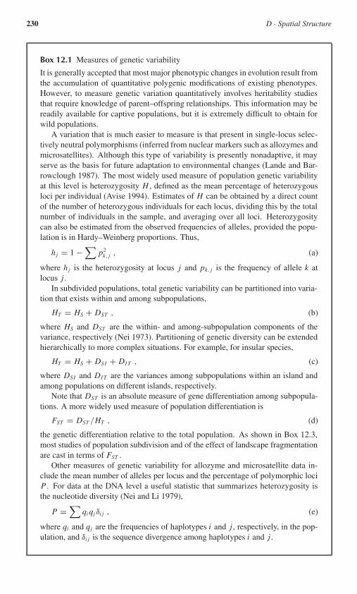
230 D · Spatial Structure

Box 12.1 Measures of genetic variability

It is generally accepted that most major phenotypic changes in evolution result fromthe accumulation of quantitative polygenic modifications of existing phenotypes.However, to measure genetic variation quantitatively involves heritability studiesthat require knowledge of parent–offspring relationships. This information may bereadily available for captive populations, but it is extremely difficult to obtain forwild populations.

A variation that is much easier to measure is that present in single-locus selec-tively neutral polymorphisms (inferred from nuclear markers such as allozymes andmicrosatellites). Although this type of variability is presently nonadaptive, it mayserve as the basis for future adaptation to environmental changes (Lande and Bar-rowclough 1987). The most widely used measure of population genetic variabilityat this level is heterozygosity H , defined as the mean percentage of heterozygousloci per individual (Avise 1994). Estimates of H can be obtained by a direct countof the number of heterozygous individuals for each locus, dividing this by the totalnumber of individuals in the sample, and averaging over all loci. Heterozygositycan also be estimated from the observed frequencies of alleles, provided the popu-lation is in Hardy–Weinberg proportions. Thus,

hj = 1 −∑

p2k, j , (a)

where hj is the heterozygosity at locus j and pk, j is the frequency of allele k atlocus j .

In subdivided populations, total genetic variability can be partitioned into varia-tion that exists within and among subpopulations,

HT = HS + DST , (b)

where HS and DST are the within- and among-subpopulation components of thevariance, respectively (Nei 1973). Partitioning of genetic diversity can be extendedhierarchically to more complex situations. For example, for insular species,

HT = HS + DSI + DIT , (c)

where DSI and DIT are the variances among subpopulations within an island andamong populations on different islands, respectively.

Note that DST is an absolute measure of gene differentiation among subpopula-tions. A more widely used measure of population differentiation is

FST = DST /HT , (d)

the genetic differentiation relative to the total population. As shown in Box 12.3,most studies of population subdivision and of the effect of landscape fragmentationare cast in terms of FST .

Other measures of genetic variability for allozyme and microsatellite data in-clude the mean number of alleles per locus and the percentage of polymorphic lociP . For data at the DNA level a useful statistic that summarizes heterozygosity isthe nucleotide diversity (Nei and Li 1979),

P =∑

qiqj δi j , (e)

where qi and qj are the frequencies of haplotypes i and j , respectively, in the pop-ulation, and δi j is the sequence divergence among haplotypes i and j .

12 · Genetic Structure in Heterogeneous Environments 231

Box 12.2 Effective population size

The effective population size Ne is a measure of how many individuals contributegenes to future generations. More formally, it is defined as the size of an “ideal-ized Wright–Fisher population” that would give the same value for some specificproperty as a real population of size N (e.g., Crow and Kimura 1970). There aredifferent forms of effective size depending on the specific property considered. Thetwo most-used properties are:

� Amount of gene frequency change per generation as measured by its variance,which leads to the variance effective size;

� Probability that two randomly sampled genes have the same parent gene, whichleads to the inbreeding effective size.

The idealized Wright–Fisher model consists of a finite, randomly mating populationof constant size, generations do not overlap, and all individuals produce the samenumber of offspring.

Under these simple assumptions, the probability that two randomly sampledgenes have the same parent gene is given by f = 1

2N (e.g., Ewens 1989), where Nis the size of the ideal population. Thus, the inbreeding effective population sizeNi

e is defined as Nie = 1

2 f, where, here and below, a tilde refers to the quantities

measured in the considered system.A central property of the Wright–Fisher model is that sampling of gametes is

binomial and the variance of the change in gene frequency is

σ 2�q = q(1 − q)

2N, (a)

where q is the allele frequency of a gene in the ideal population. Thus, the varianceeffective population size is given by

N ve = q(1 − q)

σ 2�q

. (b)

Note that these two effective population sizes are not necessarily equal and in somecases can be very different from one another. It is therefore necessary to qualify thetype of Ne being used.

12.2 Basic Models of Population Genetic StructureThe large body of theory developed by population geneticists to investigate theeffects of population subdivision (or structure) on genetic variation (for reviews seeSlatkin 1985, 1987) provided the initial tools for the study of the genetic effects offragmentation. Most of the results were obtained using the so-called island model,which represents an infinite number of subpopulations of size N that exchangemigrants among themselves at a constant rate m (Slatkin 1985, 1987). Box 12.3presents a very general formulation of the island model by Crow and Aoki (1984).

Using the island model, it is possible to show that the subdivision of a large,widespread population into many small local fragments increases genetic drift,which leads to a reduction of within-population genetic variability and an increase

232 D · Spatial Structure

Box 12.3 The island model

Assume that a diploid monoecious species is subdivided into n subpopulations eachof effective size Ne. In every generation each subpopulation exchanges migrants ata constant rate m. Immigrants into any colony are selected from all other subpopu-lations at random, and therefore the migration rate is independent of the geographicdistance between colonies. Let u be the mutation rate from one allele to any of k−1other alleles. Use f0 to denote the probability that two randomly chosen homolo-gous genes from a single colony are identical by descent (IBD), f1 to denote theprobability of IBD for two genes randomly sampled from different colonies, and fto denote the probability of IBD for two genes randomly sampled from the wholepopulation. Under these assumptions and using primes for the next generation, thefollowing set of recurrence equations hold,

f ′0 = v{x[z + (1 − z) f0] + (1 − x) f1} + w[x(1 − z)(1 − f0)

+ (1 − x)(1 − f1)] ,

f ′1 = v{y[z + (1 − z) f0] + (1 − y) f1} + w{y[(1 − z)(1 − f0)

+ (1 − y)(1 − f1)]} ,

f = [ f0 + (n − 1) f1]/n ,

where v = (1 − u)2 + u2

k−1 , w = 1−v

k−1 , x = (1 − m)2 + m2

n−1 , y = 1−xn−1 , and z = 1

2N .

Expressions for f0 and f1 at equilibrium are obtained by dropping the primesand solving the resultant equations. Note that this model leads to a partitioning ofthe total genetic variance into its within- and among-population components ( f 0 andf1, respectively). Thus, the degree of genetic differentiation within the population,FST , can be defined as the proportion of total genetic variation due to the among-population component,

FST = (1 − f ) − (1 − f0)

1 − f= f0 − f

1 − f. (a)

FST can range in value from 0 to 1; a value of 1 indicates that different populationsare fixed for different alleles, while a value of 0 indicates that the collection ofsubpopulations behaves as a single panmictic unit. The equilibrium value for FST

can be derived by replacing the equilibrium values for f0 and f in Equation (b).Assuming that u � m and 1/N � 1, this gives

FST = 1

4Nmβ + 1, (b)

where β = ( nn−1 )

2. Note that FST is independent of the mutation rate and thereforeis a useful measure for population genetic analysis. For the infinite island model,β → 1 and therefore, FST = 1

4Nm+1 .The island model can be extended to consider more complex cases in which sub-

populations are grouped into neighborhoods. Such models are referred to as hier-archical island models. Wright (1951) presented the first analysis of a hierarchical

continued

12 · Genetic Structure in Heterogeneous Environments 233

Box 12.3 continued

model of population subdivision, which was later further analyzed by Slatkin andVoelm (1991). To study this more complex model it is necessary to define theinbreeding coefficient of a subpopulation relative to its neighborhood, FSN , andthat of a neighborhood relative to the whole population, FNT . Following the sameprinciples as those used to obtain an equation for FST at equilibrium, it is possi-ble to obtain equilibrium expressions for FSN and FNT [provided Nm1 � 1; seeVigouroux and Couvet (2000) for the alternative case],

FSN = 1

1 + 4Nεm1, (c)

and

FNT = 1

1 + 4Ncζm2, (d)

where N is the number of individuals within each subpopulation, ε = ( cc−1 )

2, cis the number of subpopulations within each neighborhood, ζ = (

η

η−1 )2, η is the

number of neighborhoods, m1 is the migration rate between populations within thesame neighborhood, and m2 is the migration rate between populations from twodifferent neighborhoods.

in genetic differentiation among populations. The effect of genetic drift, however,is counteracted by the gene flow that results from migration among local popu-lations. Thus, the ultimate effect of fragmentation is determined by the relativestrengths of genetic drift and gene flow, summarized by the combined parameterNm. The degree of population subdivision decreases quite rapidly for increasingNm (Figure 12.1), and therefore it seems only small amounts of gene flow arenecessary to reestablish the connectivity of the landscape and avoid the detrimen-tal effect of population fragmentation. Following this line of reasoning, differentauthors proposed a rule of thumb according to which one migrant individual perlocal population per generation is sufficient to counteract the disruptive effects ofdrift (e.g., Kimura and Ohta 1971). However, this rule is based on a very simplisticmodel that makes a host of unrealistic assumptions (Mills and Allendorf 1996).

Under the island model, the depletion of genetic variation within populations isnot necessarily accompanied by a decrease in total genetic variance, since geneticdrift increases the among-population component of genetic variation. Indeed, theinbreeding effective size of a subdivided population is (e.g., Whitlock and Barton1997)

Ne = nN

1 − FST, (12.1)

which clearly indicates that as FST increases, Ne also increases.Although the island model provides some insights into the effects of fragmen-

tation, its applicability is impaired largely by its many simplifying assumptions.

234 D · Spatial Structure

2 4 6 8 10

0.2

0.4

0.6

0.8

1.0

0.00Effective number of migrants, Nm

Gen

etic

diff

eren

tiatio

n, F

ST

N = 4N =10N =100

Figure 12.1 Genetic differentiation FST as a function of the effective number of migrantsunder the island model.

In real situations, the assumption of selective neutrality is violated and local pop-ulations differ in size. Moreover, local populations are liable to extinction throughdemographic and genetic factors, and therefore the system never reaches geneticequilibrium. These limitations led to the development of a more complex bodyof theory that describes more accurately the ecological and genetic properties offragmented populations.

12.3 Adding Geography: The Stepping-stone ModelThe island model of population subdivision ignores the fact that many species havelimited dispersal capabilities. In cases of limited dispersability, it is more logicalto assume that migration occurs only between adjacent demes. The stepping-stonemodels introduced by Malécot (1968) and Kimura (1953) address these situations.In the simplest version, the infinite one-dimensional stepping-stone model, an in-finite number of colonies with constant effective size Ne is arranged along a linearhabitat (Kimura and Weiss 1964). In this case, the correlation of allele frequenciesbetween demes g steps apart is given by

γ (g) ∝ exp(−g

√2m∞/ma

). (12.2a)

Here, m∞ is the probability that a migrant comes from a very distant populationand represents a long-distance migration parameter, while ma is the probability ofmigration from an adjacent deme (m∞ � ma). Equation (12.2a) indicates thatthe correlation decreases approximately exponentially with distance, and thereforethe genetic differentiation between populations increases quite rapidly. There areequivalent results for two- and three-dimensional stepping-stone models (Kimuraand Weiss 1964). For two-dimensional stepping-stone models,

γ (g) ∝ 1√g

exp(−g

√4m∞/ma

). (12.2b)

12 · Genetic Structure in Heterogeneous Environments 235

For three-dimensional models,

γ (g) ∝ 1

πgexp

(−g

√6m∞/ma

). (12.2c)

Thus, the correlation between alleles falls off much more rapidly as the numberof dimensions increases. The results of stepping-stone models can also be pre-sented in terms of FST , but the equations obtained are more convoluted (see Slatkin1991). However, it is possible to obtain an expression for the relationship betweenFST and the correlation between adjacent demes from equation 3.5 in Kimura andWeiss (1964),

FST ≈ 1

1 + 4Nma[1 − γ (1)] . (12.3)

As the number of dimensions increases, γ (1) decreases [see Equations (12.2a–12.2c)] and so does FST .

Despite the large differences in the assumptions made by the island andstepping-stone models, there is an important similarity between the two-dimensional stepping-stone models and the island model. Populations will bestrongly differentiated if Nm < 1 (m = m∞ + ma), whereas they behave es-sentially as a single panmictic unit if Nm > 4 (Kimura and Maruyama 1971).

Another issue of interest is the amount of genetic variability maintained bypopulations with a stepping-stone structure, one measure of which is the effectivenumber of alleles ne. Maruyama (1970) noted for the one-dimensional stepping-stone model that the effective number of alleles is nd

√µ/2md + 4Nndµ, where nd

is the number of demes, µ is the mutation rate, and md is the migration rate amongadjacent demes. The equivalent quantity for the island model is 1 + 4Nndµ +ndµ/md . Both formulas are valid for large nd . For a panmictic population ofsize nd N , ne = 1 + 4Nndµ. Thus, genetic variability is increased by populationsubdivision and this increase is much greater in a linear stepping-stone structure.

Stepping-stone models lead naturally to the concept of “isolation by distance”,first introduced by Wright (1943) to describe the accumulation of local geneticdifferences under restricted dispersal. A number of techniques are available totest for isolation by distance in natural populations. For example, Mantel’s testof matrix correlation allows the comparison of genetic distance and geographicdistance matrices [see Smouse and Long (1992) for a review]. Slatkin (1993)proposed another method to detect isolation by distance based on analytic theorythat relates measures of isolation by distance to average coalescence times.

12.4 Metapopulation Processes and Population DifferentiationExtensive habitat fragmentation invariably results in the reduction of populationsizes and, therefore, local populations become threatened by extinction throughenvironmental and demographic factors (see Chapters 2 and 4). Nevertheless, newpopulations are continuously formed as colonists re-invade vacant habitat patches.

236 D · Spatial Structure

These dynamics of extinction and recolonization form the basis of metapopulationtheory (for reviews, see Hastings and Harrison 1994; Harrison and Hastings 1996).

Effects of colonization–extinction processesWright (1940) first recognized that extinctions and recolonizations can play animportant role in determining the genetic structure of natural populations. How-ever, the first formal metapopulation genetic models were published almost fourdecades later by Slatkin (1977). In his analysis, Slatkin considers two possibilitiesregarding the formation of propagules:

� “Propagule pool” model (founders are all from the same existing population);� “Migrant pool” model (founders are chosen at random from the entire metapop-

ulation).

Slatkin’s results are presented in terms of measures of genetic variability and seemto indicate that the extinction and recolonization process tends to decrease geneticdifferentiation among colonies.

Both models can be formulated using the principles presented in Box 12.3 forthe island model. However, it is necessary to add terms for the effects of extinctionand recolonization events. The resultant equations for f0, f1, and f are quite con-voluted and were first presented by Slatkin (1977). Wade and McCauley (1988)used these equations and Equation (12.2a) to obtain an expression for FST . Theseauthors noted that the effect of the extinction and recolonization process is to es-tablish an age structure among the array of populations. This allowed them todevelop expressions that describe the genetic variance among populations of eachage class of the metapopulation. Averaging FST across all age classes, they ob-tained a measure of differentiation among all populations, which, for the “migrantpool” model, is given by

FST = 1 + e0(N/K − 1)

2N [1 − L(1 − e0)] , (12.4)

where e0 is the fraction of demes that go extinct, K is the number of founders, mis the migration rate, and L is an abbreviation of (1 − 1

2N )(1 − m)2.Taking the ratio of FST to the expected value under the standard island model,

it is possible to obtain the conditions under which population turnover enhancesor diminishes genetic differentiation among local populations. Genetic differenti-ation is enhanced when K < 2Nm, otherwise it is decreased.

Using a similar approach for the “propagule pool” model, Wade and McCauley(1988) obtained an equivalent expression for FST ,

FST = a + 1−a2N

1 − L(1 − a), (12.5)

where a = e0/(2K ). Here the ratio of FST to the expected value under the standardisland model is always larger than 1, which indicates that in this case populationturnover always increases population differentiation.

12 · Genetic Structure in Heterogeneous Environments 237

The “migrant-pool” and “propagule-pool” models of colonization represent ex-treme ends of what must be a continuum in nature (Wade and McCauley 1988). Toconsider intermediate cases, Whitlock and McCauley (1990) generalized Slatkin’smodels by including a parameter φ to represent the probability that two alleles ina newly formed population come from the same parental population. Thus, φ = 0describes the “migrant pool” and φ = 1 the “propagule pool”. This more generalmodel shows that, at equilibrium, population turnover increases differentiation if

K <2Nm

1 − φ+ 1

2 . (12.6)

This condition is equivalent to the requirement that variance among newly foundedpopulations be greater than variance among populations at equilibrium. Thus, anytendency for founders to move in groups, such as in the dispersal of seeds in fruits,increases the likelihood that population turnover will lead to greater genetic differ-entiation.

Effects of local population dynamicsThe degree of genetic differentiation is also determined by the population dy-namics of local populations. All the models discussed above assume that newlyfounded populations grow back to carrying capacity in a single generation and,therefore, ignore the effect of within-patch population dynamics. This unrealis-tic assumption was relaxed by Ingvarsson (1997), who used a simple exponen-tial growth model to describe the population dynamics of newly recolonized sub-populations. In principle, a delayed period of population growth is expected toincrease genetic drift because the size of recently recolonized subpopulations issmall. However, whether genetic differentiation is increased or not depends onwhether the migration rate is constant or not. If it is, then small populations willreceive few migrants and genetic drift is important, leading to increased differen-tiation. But if the number of migrants is constant, then differentiation is decreasedbecause small populations will be swamped by large number of migrants fromlarge populations.

The relationship between migration rates and population size remains to be es-tablished, as widely divergent hypotheses have been proposed (see the review inSaether et al. 1999). For example, it is possible that the effective number of im-migrants in large populations at or close to their carrying capacity is small, sincecompetition for breeding sites and/or other resources will be strong. Thus, thesuccessful settlement of new immigrants is impaired. Therefore, in real ecologi-cal situations, delayed population growth might lead to decreased differentiation.Clearly, migration patterns are important in determining the degree of genetic dif-ferentiation, a subject we address when discussing the particular case of source–sink metapopulations (see below).

Up to now, we have discussed the effect of population turnover on the degreeof genetic differentiation, but we have not examined its effect on the total amountof genetic variability maintained by a species. Although, as explained before,

238 D · Spatial Structure

extinction and recolonization events can increase among-population variability,they always decrease within-population variability because they act as local popu-lation bottlenecks. The above models help clarify the effect of population turnoveron the partitioning of genetic variance, but they cannot clarify the effect of extinc-tions and recolonizations on the total genetic variability maintained by a species.To address this question, the effect of population turnover on the effective popula-tion size of a species must be considered.

12.5 Metapopulation Processes and Effective Population Size

The derivation of expressions for the effective size of a metapopulation that takeinto account all the relevant parameters is very difficult and leads to mathemati-cally intractable models. For example, in the presence of variance of reproductivesuccess between populations, V , the effective size of a metapopulation is given by(Whitlock and Barton 1997)

Ne = nN

(1 + V )(1 − FST ) + 2NV FST, (12.7)

which indicates, in particular, that Ne increases with FST only when V is low[compare Equations (12.1) and (12.7)]. By combining analytical and simulationapproaches, Whitlock and Barton (1997) successfully provided a formulation ofthe inbreeding effective size that takes into account most of the relevant parame-ters. Their results indicate that metapopulation dynamics can greatly decrease Ne.Indeed, for simple models such as that used by Whitlock and McCauley (1990),when the number of founders is much smaller than the size of the local popula-tions, the metapopulation Ne can be a very small fraction (smaller than 1%) of thatwithout extinction. For more complex metapopulation models that incorporatevariance in reproductive success between demes and explicit local dynamics, theresults can be complex, but it is still possible to understand the effect of individualfactors. In general, when migration rates are low, the resultant increase in geneticdifferentiation tends to increase the metapopulation Ne. However, when local pop-ulation sizes are highly variable (e.g., under chaotic dynamics), the variation indeme reproductive success reduces Ne even when migration rates are low.

Hedrick and Gilpin (1997) used simulations of a much simpler model to studythe effect of metapopulation dynamics on Ne. They used a generalization ofSlatkin’s models that allowed nonimmediate recolonization of extinct demes anddecoupling of gene flow and number of colonists. An interesting result of thisanalysis is the effect of increasing local deme sizes on the effective populationsize. In principle, a proportional increase in Ne would be expected with increasingdeme sizes. Their results show, however, that as deme sizes increase, Ne does notincrease very much and asymptotes quickly. By setting the carrying capacity oflocal colonies to infinity, they show that population turnover can greatly reducetotal genetic variability, even when genetic drift at the local population level isminimal.

12 · Genetic Structure in Heterogeneous Environments 239

0.00

0.25

0.50

0.75

0.00 0.25 0.50 0.75 1.00FST expected

in the absence of selection

FST

exp

ecte

din

the

pre

senc

e of

sel

ectio

n

N=10N=100

1.00

Figure 12.2 Expected FST value for a selected gene relative to that expected for a neutralgene for different population sizes, for the case of overdominance (fitnesses for the threegenotypes are 1, 1 + s, 1). Source: Couvet (2002), with s = 0.01.

From the above discussion it is clear that for most ecologically realistic situa-tions fragmentation of the landscape greatly reduces the effective size and level ofgenetic variability of most species.

12.6 The Effect of Selection on Differentiation: The Island ModelSo far we have ignored the effect of selection on the spatial structure of popula-tions. Selection, however, is an important factor that affects the pattern of geneticvariability and differentiation in natural populations. There are three main reasonswhy we need to study the effect of selection:

� Neutrality of commonly used markers has been repeatedly questioned (e.g.,Pogson et al. 1995).

� Although a particular marker might be neutral, it may be linked to a gene subjectto selection.

� A significant fraction of the genome is composed of genes subject to selection,these genes being responsible for inbreeding depression, local adaptation, andinteraction with other organisms. Inferring the spatial structure for these genesand comparing it to that of neutral genes leads to predictions on important issuessuch as the extent of heterosis and local adaptation.

Spatial structure of selected genesThe extent to which selection influences population structure is determined byits strength relative to that of other forces that modify gene frequencies (drift,migration, and mutation). Assuming that mutation is negligible when compared tothe other forces, then for the selection coefficient s � m, 1/N , the effect of geneticdrift can be disregarded and selection will be one of the main factors determiningthe degree of population structuring. If s � m, 1/N , then the effect of selection isnegligible and the results of neutral models are still valid. In particular, the spatialstructure of neutral genes is a good approximation to the structure of selected geneswhen the population size is small (Figure 12.2).

240 D · Spatial Structure

0.15

0.20

0.0 0.1 0.2 0.3 0.4 0.5Recombination rate

Gen

etic

diff

eren

tiatio

n, F

STN =10 s=0.2N =10 s=0.1N =5 s=0.1

Figure 12.3 FST for a neutral bi-allelic locus as a function of its proximity to a selectedgene (recombination rate) for the case of overdominance, depending on population size andthe intensity of selection (s is as in Figure 12.2) In the absence of selection, the value of mused leads to FST = 0.2. The plot was obtained using a matrix approach, as for Figure 12.2.

The magnitude of the FST expected for selected genes depends on the pattern ofselection being considered. In the case of overdominance, the expected FST valuewill be lower than that expected under neutrality. On the other hand, FST willbe higher for genes responsible for local adaptations than for neutral genes. Fora fitness differential comparable to that observed for most deleterious mutations(s = 0.02, see Chapter 9), the FST for overdominant genes is very close to thatobserved for neutral genes when N =10, but is noticeably different when N =100(Figure 12.2).

The structure of selected alleles is a particularly important study for conserva-tion biology, because it allows us to evaluate the effect of migration on populationviability. This issue is empirically examined in Chapter 15.

Spatial structure of genes linked to selected genesThe study of the structure of neutral genes linked to selected ones concerns a largeportion of the genome. Selected genes within the genome will affect, to variousdegrees, the spatial structure of one or more neutral genes, depending on the prox-imity of these to the selected genes.

As for the spatial structure of selected genes, the influence of selection isstronger when the local population size is large. For the case of genes linked to se-lected genes, however, the recombination rate also has to be considered; the higherthe recombination rate, the less important is the effect of selection (Figure 12.3).

Some good evidence indicates that the indirect effect of selection on the struc-turing of neutral genes is not uncommon. The following examples provide detailsof the processes involved:

� FST values for markers located in low recombining regions of the genome arehigher than those for markers located in regions where recombination is higher(see review in Charlesworth 1998). That FST in the low recombining regionsis higher requires an explanation, one possibility being the overall presence ofgenes responsible for local adaptation.

12 · Genetic Structure in Heterogeneous Environments 241

� The decrease of genetic variability observed with selfing, relative to the caseof random mating, is higher than that expected in the absence of selection (Liuet al. 1998). This could be because the influence of selected genes extendsfurther for consanguineous reproductive systems, since the effective recombi-nation rate is lower.

� Slightly deleterious mutations, which affect the survival of small populations(see Chapter 9), decrease genetic variability at nearby loci: such an effect hasbeen called “background selection”. The low selective differential of such mu-tations means that the effect on the regions that surround each selected genewill be low, but present on a large part of the genome as these mutations aresupposedly numerous.

12.7 Structure and Selection in Source–Sink MetapopulationsNatural environments are heterogeneous and therefore species encounter variationin abiotic and biotic conditions. For many geographically extensive populations, alarge fraction of the individuals may occur in depauperate habitats in which repro-duction is insufficient to balance local mortality (e.g., Pulliam 1988). Populationsin these depauperate habitats, generally termed “sink populations”, may never-theless persist, being maintained by continued migration from more productive“source” areas nearby.

Neutral genetic structureAlthough source–sink metapopulations may occur naturally, human activities haveled to an increase in their occurrence. Indeed, the most likely outcome of fragmen-tation of the landscape is a large tract of forest (the source) kept as a nature reserveor park and a series of small patches (the sinks) embedded in a landscape domi-nated by human development. That small tracts of forest are unable to maintainthemselves may lead natural resource managers to assume that their protectionis not warranted. It is, therefore, important to establish the extent to which sinkpopulations can help maintain or increase the genetic variability of a species and,therefore, contribute to its long-term survival.

The population genetic models of source–sink metapopulations presented byGaggiotti and Smouse (1996) and Gaggiotti (1996) help to clarify this problem.Their studies investigate the effect that different patterns of migration have onthe genetic structure of source–sink metapopulations, specifically modeling thedynamics of local populations. They study a metapopulation that consists of asingle source and a variable number of sink populations and consider the expectednumber of nucleotide differences between two genes drawn at random from thesource–sink metapopulation. The migration patterns considered include constantmigration and different types of stochastic migration.

In real ecological scenarios, migration is an inherently stochastic process andthe results shows that stochasticity has an important impact on the genetic struc-ture of the collection of sinks. Stochastic migration leads to long periods of zeromigration events from the source, during which the effect of genetic drift is greatly

242 D · Spatial Structure

enhanced, which decreases the amount of genetic variability maintained and in-creases the genetic differentiation between sinks. The importance of the stochasticeffect on the genetic structure of the collection of sinks is determined by the rateof population decay and the variance in the number of migrants arriving at thesinks. The effect is maximized when the rate of population decay in the sinks ismoderate, in which case the variance of the genetic parameters is large. The effectof stochasticity increases as the variance in the number of migrants arriving at anygiven sink increases. Thus, the genetic structure of the collection of sinks is mostaffected when stochasticity is introduced by sudden changes (catastrophic events)that preclude the arrival of new migrants to all sinks.

Gaggiotti and Smouse (1996) and Gaggiotti (1996) also show that genetic vari-ability in the collection of sinks may be large even under stochastic migration, andthat population subdivision among the subset of sinks may be significant. Thus,in a fragmented landscape sink populations may serve as temporary refugia thatincrease colonization and gene flow. These findings indicate that the protection ofsink populations could help to alleviate (but not preclude) the detrimental effectsof landscape fragmentation. However, a critical fact is the sort of genetic variabil-ity that accumulates in the sink population. If this variability is unconditionallydeleterious (see Chapter 9), no overall advantages will be associated with such ahigher genetic variability.

Fixation of beneficial allelesAdaptive evolution of a population to the conditions of the habitat patch in whichit lives is determined by the relative strength of opposing forces: natural selectionfavors locally fitter genes, and gene flow reduces the frequency of locally favoredgenes (Mayr 1963; Antonovics 1976). Peripheral (sink) populations may exist atdensities considerably lower than more central (source) populations. Thus, immi-gration rates into sinks may be high relative to the local population abundance andmay suffice to swamp out selection that favors locally fitter genes. This processhas been invoked to explain the “niche conservatism” that seems to characterizemany species (e.g., Holt and Gomulkiewicz 1997a; Kirkpatrick and Barton 1997;Chapter 13).

The above observations lead to the dismissal of the evolutionary potential ofsink populations (e.g., Kirkpatrick and Barton 1997) and metapopulations in gen-eral (e.g., Harrison and Hastings 1996). These observations, however, are based ona highly unrealistic assumption, namely that there is a steady (constant) stream ofmigrants into the sink with each generation. In real ecological situations, however,migrants may or may not arrive at the sink in any particular generation, dependingon environmental fluctuations or the vagaries of founder dispersal (Gaggiotti andSmouse 1996). A thorough investigation of the effect of stochastic migration onthe genetic structure of source–sink metapopulations (Gaggiotti 1996; Gaggiottiand Smouse 1996) reveals that if the variance in the migration process is high,differentiation between source and sink is possible. This is particularly so whenmigration between source and sink is episodic. The model used by Gaggiotti

12 · Genetic Structure in Heterogeneous Environments 243

(1996) assumes selective neutrality. Preliminary results of a model that incorpo-rates selection (Gaggiotti, unpublished) indicate that stochastic migration favorsthe spread of beneficial mutations in sink habitats. Much research (both theoreti-cal and empirical) is needed before the evolutionary potential of sink populationscan be thoroughly evaluated.

12.8 Concluding CommentsUnder the most ecologically realistic scenarios, fragmentation of the landscapeleads to a reduction of genetic variability at the species level. This is becausepopulation turnover increases genetic drift and therefore reduces the effective pop-ulation size.

The outcome of habitat fragmentation is likely to differ depending on whetherthe original distribution of the species was continuous or fragmented. For con-tinuously distributed species, fragmentation disrupts the existing patterns of geneflow and decreases the effective population size. For species with a spatially het-erogeneous distribution, gene flow may not be strongly affected, but the increasedlikelihood of extinction of local populations still decreases the species’ effectivepopulation size. In either case, the evolutionary potential of the species may belargely reduced.

It is important to realize that the use of simple approaches to study complexsituations, such as those arising from the fragmentation of the landscape, can leadto serious misunderstandings. A good example is the notion that the best way tomaintain genetic variability is by protecting a sufficient number of small popula-tions instead of a single large population (e.g., Simberloff 1988; Hanski 1989).This idea is based on the results of the island model of population subdivision, andtherefore rests on a large number of unrealistic assumptions. The results of morecomplex metapopulation models that have been developed over the past decade(see above) clearly indicate that this principle is flawed.

In the past ten years there has been a surge in the number of studies concernedwith the genetic structure of metapopulations and the implications for conservationbiology. Numerous aspects have been addressed and great progress has been made,but some outstanding issues still need to be considered. In particular, a paucityof studies address the effect of selection on the genetic structure of metapopula-tions. Some progress has been made in the study of local adaptation in source–sinkmetapopulations (Holt and Gomulkiewicz 1997a; Gomulkiewicz et al. 1999), buteven in this area many questions still need to be addressed.

13Conservation Implications of Niche Conservatism

and Evolution in Heterogeneous EnvironmentsRobert D. Holt and Richard Gomulkiewicz

13.1 IntroductionSpecies may, in principle, respond to environmental change in several differentways (Pease et al. 1989; Holt 1990; Chapters 10 and 11). Some species may trackenvironmental states to which they are already well adapted and so shift in abun-dance and distribution. Other species may not evolve at all and so become extinct.Some species may evolve adaptively in ways that facilitate their persistence inchanged environments. Yet other species may evolve in ways that hamper theirlong-term viability. A fundamental goal of the discipline of evolutionary conser-vation biology is to understand the factors that govern the relative likelihood ofeach of these outcomes.

Recognizing the importance of directional environmental change in driving ex-tinctions in once-common species raises a profound puzzle. On the one hand, asecologists we know that extinction risk emerges because directional environmen-tal changes lead to lowered population abundances and/or restricted distributions;in effect, species are pushed outside their niches. On the other, as evolutionistswe know that species often have abundant genetic variation, and so can adapt tonovel circumstances. Conservation problems arise precisely because species donot adapt sufficiently to the new environments created by anthropogenic activity.In other words, conservation problems reflect a seeming failure of evolution bynatural selection to adapt species to environmental change.

Such failures are examples of “niche conservatism”. The history of life revealsexamples of both niche conservatism (phylogenetic lineages that retain much thesame ecological niche over substantial spans of evolutionary history) and nicheevolution (Bradshaw 1991; Holt and Gaines 1992). Before proceeding any further,we should be clear about the meaning of “niche” (Schoener 1989). For a specieswith continuous, overlapping generations the intrinsic growth rate r is its expectedper capita birth rate minus its expected per capita death rate, at low densities.Succinctly, if a habitat results in r > 0 for a given species it has conditions that arewithin that species’ niche. By contrast, if r < 0, the habitat has conditions outsidethe niche. (For discrete generations, if the environment is such that the per capitagrowth ratio per generation R0 > 1, the habitat lies within the niche, but if R0 < 1,it is outside.) In effect, the niche of a species is an abstract mapping of the mostfundamental attribute of that species’ population dynamics – its persistence versusits extinction – onto environmental states. A population of a species should persist

244

13 · Niche Conservatism and Evolution in Heterogeneous Environments 245

(in the absence of stochastic fluctuations) if it experiences conditions within itsniche, but go extinct if forced to live outside its niche.

Many conservation problems arise because environmental change forces aspecies’ population outside that species’ ecological niche. Evolution that influ-ences extinction risk often involves niche evolution, such that species expand orshift their niches to incorporate novel environments. We do not downplay therole of other evolutionary processes in conservation (e.g., mutational meltdownin small populations, Lynch et al. 1995a; Chapter 9), but we do contend that anunderstanding of niche conservatism and evolution is integral to an evolutionar-ily informed conservation biology. In this chapter, we review theoretical studieswhich show that an absence of evolutionary responses in changed environments,which at first seems puzzling, actually makes sense when the demographic contextof evolution is considered. Recent theoretical studies provide elements of a con-ceptual framework that allow niche conservatism to be understood, and possiblypredicted. The basic idea is that population dynamics can, at times, constrain evo-lutionary dynamics. At other times, population dynamics facilitate evolutionaryresponses. This chapter provides an overview of these studies and highlights theirimplications for conservation.

Patterns of environmental change are complex in space and time. For concep-tual clarity, we focus on simple situations with a step transition between two envi-ronmental states, or on spatial flows of individuals between two discrete habitats.We also briefly discuss evolution along smooth gradients in time and space. Thesedifferent scenarios illustrate how demographic asymmetries can channel and con-strain the evolution of local adaptation. We provide partial answers to two essentialquestions:

� When does adaptive evolution mitigate extinction risk?� Can we use our understanding of the dynamics of – and constraints on – adap-

tive evolution to guide practical conservation efforts?

13.2 Adaptations to Temporal Environmental ChangeConsider a closed population, such as an insect species on an oceanic island or inan isolated habitat fragment. The population initially is found in a stable environ-ment, at equilibrium within its niche. It then experiences an abrupt environmentalchange, and conditions shift to outside its niche (i.e., absolute fitness R0 < 1). Ifthe environment then stays constant, but the population does not evolve, extinctionis certain (Figure 13.1a). Let us assume that the population has sufficient geneticvariation to potentially persist in the novel environment. Selection increases aver-age fitness, given the assumptions of Fisher’s Fundamental Theorem (Fisher 1958;Burt 1995). However, as long as the average absolute fitness is less than 1, thepopulation will continue to decline, though at a slowing rate. Eventually, mean fit-ness will exceed 1, and the population will start to increase. Such a species shoulddisplay a characteristic U-shaped trajectory (Figure 13.1b).

Even so, this population may still experience a transient window of extinctionrisk. Given sufficient variation to adapt (i.e., evolve a positive growth rate) to

246 D · Spatial Structure

00

00

Popu

latio

n si

ze, N

12

Nc

Time, tPeriod at risk

(b)(a)

Figure 13.1 Population dynamics in a newly created sink habitat. (a) Without evolution: ifevolutionary change is precluded (e.g., because relevant genetic variation is absent), popu-lation size declines toward extinction. (b) With evolution, if there is sufficient genetic vari-ation, a population may adapt quickly (Trajectory 1), and so avoid exposure to the criticallylow sizes that are associated with high extinction risk (i.e., Nt > Nc for all t). However, ifthe population adapts more slowly (Trajectory 2), it spends a period at low abundances, andthus incurs a high risk of extinction (i.e., Nt < Nc for some span of time t). If by chanceextinction is avoided and adaptation continues, the population may eventually rebound.

abrupt environmental change, in a deterministic world a population should even-tually bounce back from low numbers. But when numbers become too low, evenwell-adapted populations may face extinction from demographic stochasticity. Thedotted line in Figure 13.1b marks a critical population size Nc below which we as-sume demographic stochasticity to become a severe problem. For Trajectory 1 inFigure 13.1b the population starts at a high density and evolves a positive growthrate sufficiently fast to rebound before ever entering the “danger zone” of lownumbers. This results in a process of “evolutionary rescue”. By contrast, forTrajectory 2 the initial density is lower and the population evolves slowly, so itexperiences a period of extinction risk. Figure 13.1b illustrates a race betweenan evolutionary process (improved adaptation to the novel environment, increas-ing mean fitness), and an ecological process (declining numbers, as long as meanfitness is less than 1). In Box 13.1 we present an analytic model that explicitlycombines evolution in a quantitative character and population dynamics and re-sults in U-shaped trajectories in numbers.

Given a critical population size Nc below which extinction is probable, we canuse Equation (g) in Box 13.1 to determine whether or not a population trajectoryincludes periods of risk (i.e., Nt < Nc). Figure 13.2 summarizes whether or not apopulation experiences such extinction risk as a function of its initial density, thedegree of initial maladaptation in the novel environment, and the heritability of thetrait that undergoes selection. The basic messages are as follows:

� Populations that are initially rare are highly vulnerable to even moderate envi-ronmental change;

� Even large populations are vulnerable to strong environmental change;� Evolutionary rescue is facilitated by increased genetic variability.

13 · Niche Conservatism and Evolution in Heterogeneous Environments 247

1

01.0 1.5 2.52.0 3.0

h2=0.25h2=0.75

Potential extinction

Certainpersistence

Scal

ed in

vers

ein

itial

pop

ulat

ion

size

, N

c

N0

Initial maladaptation,δ0

2

ω + VP

Figure 13.2 Combinations of initial population size and initial maladaptation that leadto high extinction risk. The vertical axis is an inverse measure of the initial abundance(scaled relative to a critical low size Nc). The measure of initial maladaptation used isδ20/(ω + VP), where δ0 is the distance between the optimal phenotype in the new sink

environment and the initial mean phenotype of the population, ω is an inverse measure ofthe strength of selection, and VP is the phenotypic variance for the character being selected.The quantitative genetic model presented in Box 13.1 is used to derive curves that separatethose situations that lead to population sizes always above Nc (lower left region) from thosein which population sizes fall below Nc for a period of time of high extinction risk (upperright region). Results are shown for two values of heritability, h 2 = 0.25 and 0.75. Source:Gomulkiewicz and Holt (1995).

The analytically tractable model described in Box 13.1 helps to clarify when evo-lution may rescue populations from extinctions. However, the model does not de-scribe extinction directly, for it assumes continuous and deterministically variabledensities, whereas individuals are discrete and numbers change stochastically. Adirect assessment of extinction requires the use of models in which these featuresare respected, which implies counting individuals and alleles. Individual births,deaths, mating events, and mutations are all fundamentally stochastic processes(see Chapters 2 and 3). Analytical treatment of stochastic models that couple de-mographic and genetic dynamics for finite populations is a challenging task, evenfor simple one-locus situations (see Gomulkiewicz et al. 1999). An alternative ap-proach that gives much insight is to use individual-based numerical simulations.We present results from such simulations, in which we track each individual andgene (locus by locus), and directly assess the probability of extinction by repeatedsimulations [extinction occurs when a population declines to zero abundance, andthe probability of extinction in a given environment is the relative frequency of ex-tinctions over a fixed time period for a large number of simulation runs; see Holtet al., unpublished, for technical details of the simulation protocol, which followsthat of Bürger and Lynch (1995)]. Box 13.2 describes the genetic, life-history,and ecological assumptions of these individual-based simulations. The two ap-proaches – analytic treatment and individual-based numerical simulations – leadto mutually reinforcing insights about the potential for evolutionary rescue.

248 D · Spatial Structure

Box 13.1 Modeling adaptation and persistence after environmental change

Here an analytically tractable model to assess the propensity for evolutionary rescueis introduced. More details about the model can be found in Gomulkiewicz and Holt1995 (see also Holt and Gomulkiewicz 1997b).

For a population with discrete generations, the finite rate of increase in popula-tion size Nt in generation t is just the mean fitness W t , Nt+1 = Wt Nt . We assumethat a population is initially at an evolutionary equilibrium in a closed environment,and then experiences an abrupt change in environmental conditions. The averageindividual in the population is maladapted to the novel environment, so much so thatin generation 0 after the environmental change W 0 < 1. (We assume the density islow enough at this time to ignore density dependence.) If there is no evolutionaryresponse, extinction results.

To couple population dynamics to evolution, we assume fitness depends upon asingle trait z with polygenic autosomal inheritance, such that

W (z) = W0 exp(− 1

2 z2/ω)

. (a)

For convenience, we assume that the optimal phenotype in the new environment isat z = 0, and that the initial mean phenotype in the new environment is δ0. Thequantity ω is an inverse measure of the fitness cost of deviations from the optimum.Quantitative traits are often normally distributed, measured on an appropriate scale.We thus assume that the phenotypic distribution pt in generation t can be describedby

pt (z) = (2πVP)−1/2 exp(− 1

2 (z − δt )2/VP

). (b)

Here VP is the phenotypic variance, and δt is the distance of the mean phenotype ingeneration t from the new optimum at z = 0. The mean fitness in generation t is

Wt =∫

W (z)pt (z) dz = W exp(− 1

2 δ2t /(VP + ω)

), (c)

where W = W0√

ω/(VP + ω) is the growth rate attained when the mean phenotypeis optimized.

In standard quantitative-genetic models of selection (Falconer 1989), the meanphenotype of a trait experiencing directional selection changes in accordance with

�δt = δt+1 − δt = h2S , (d)

where h2 is the trait’s heritability (a measure of faithfulness in genetic transmissionof trait values across generations), and S is the selection differential (the differencein mean phenotype between individuals selected to be parents of the next generationand the mean phenotype of the current generation). For our model, we obtain

S =∫

z[W (z)/Wt ]pt (z) dz − δt = − δt VP

VP + ω, (e)

and hence continued

13 · Niche Conservatism and Evolution in Heterogeneous Environments 249

Box 13.1 continued

δt+1 = δt + �δt = ω + (1 − h2)VP

VP + ωδt = kδt . (f)

The quantity k gauges evolutionary inertia; if h2 is near zero, k ≈ 1, and evolutionis slow. As time passes, the mean phenotype approaches the local optimum, and thegrowth rate increases. Some algebra then shows the dynamics of population size tobe described by

Nt = N0Wt exp

(− δ2

0(1 − k2t )

2(VP + ω)(1 − k2)

). (g)

This expression gives U-shaped population trajectories, comparable to those inFigure 13.1b.

Figure 13.3 shows the probability of extinction over 1000 generations (averagedover 400 independent simulation runs, except for the b = 3 curve in Figure 13.3d,which is averaged over 1600 runs), as a function of the magnitude of the abruptchange in the phenotypic optimum caused by environmental change, and as influ-enced by genetic, life-history, and ecological parameters. Figure 13.3a depicts theinfluence of initial population size (carrying capacity) on extinction. Populationsthat are initially small (low K ) or highly maladapted (large change in the optimumphenotype) have a high risk of extinction after an abrupt environmental change.Moreover, a large population does not, by itself, provide insurance against extinc-tion if the degree of initial maladaptation is high. Changes in the number of locithat govern genetic variation in the trait have only a minor effect on the probabil-ity of extinction (although single-loci variation seems to hamper persistence withrespect to polygenic variation, see Figure 13.3b). Populations with a higher muta-tional input of variation survive longer in the changed environment (Figure 13.3c).Species with high fecundities can tolerate more severe changes in the environment(Figure 13.3d). These conclusions qualitatively match those drawn from the ex-tinction model described in Box 13.1 and summarized in Figure 13.2.

If the opportunity for niche evolution occurs primarily through sporadic col-onization of novel environments outside a species’ current niche, or becausea species’ entire population uniformly experiences severe, rapid environmentaldegradation, niche shifts would rarely save species from extinction. This is be-cause populations that experience strong selection on niche characters are pre-cisely those that face a severe risk of extinction. Species that are initially rare orhave low fecundity may be particularly sensitive to environmental change. Thedegree to which such species persist will reflect their ability to disperse, track-ing across space the shifting locations of environments to which they are alreadyadapted.

250 D · Spatial Structure

Box 13.2 An individual-based model for analyzing niche evolution

The individual-based simulation model introduced here allows us to examine bothclosed populations after abrupt environmental change and spatially discrete scenar-ios in which stable sources are coupled with migration to sink habitats (Holt et al.,unpublished).

The model is based on assumptions made by Bürger and Lynch (1995), whostudied adaptation to a continually changing environment for a single polygeniccharacter:

� Genetic assumptions: (a) additive effects of loci, without dominance or epis-tasis (each allele contributes a fixed amount to the phenotypic value, and anindividual’s phenotype is the sum of this quantity over all loci, plus a randomterm); (b) mutational input maintains variation, following the “continuum-of-alleles” model, in which mutational effects are drawn from a normal distribu-tion; (c) free recombination; and (d) in the spatial model, the source populationis in mutation–selection–drift balance.

� Life-history assumptions: (a) discrete generations; (b) dioecious, hermaphro-ditic, monogamous, and random mating.

� Ecological assumptions: (a) in the spatial model, a constant number of immi-grants per generation; (b) “ceiling” density dependence (i.e., population growthis density independent below the carrying capacity, at which growth stopsabruptly); (c) constant fecundity per mated pair; (d) offspring survival proba-bility is a Gaussian function of phenotype.

A census is made of the adults to determine the population size Nt in generationt . After the census, in the spatial model there is immigration at a per generationrate I , followed by random mating. The mating population is limited by a ceiling:if there are more than K adults, K individuals are sampled, without replacementfrom the pool, and are randomly assigned to mating pairs. Individuals produce ga-metes with free recombination among n loci. Mutation occurs on gametes, witha stochastic mutational input nµ per genome (distributed randomly over all loci).Each mated pair produces b offspring, which survive to adulthood with probabilitypi (z) = exp

(− 12 (z − zi )

2/ω2), where z is the realized phenotype of a given indi-

vidual, zi is the optimum phenotype in habitat i (1 = sink, 2 = source), and ω2 isinversely proportional to the strength of stabilizing selection. Survival to adulthoodis the life-history stage at which selection occurs. If the realized phenotype is toofar from the optimum, the mean fitness is below 1, and the population tends to de-cline. Individuals that survive early mortality are adults at the next census, Nt+1.The population is assumed to be at carrying capacity K initially and at selection–mutation–drift equilibrium in the ancestral environment.

In this individual-based model, stochasticity enters at several stages:

� Mutation is stochastic;� Gametic combinations and immigrants (in the spatial model) have multilocus

allelic combinations that vary through random sampling;continued

13 · Niche Conservatism and Evolution in Heterogeneous Environments 251

Box 13.2 continued

� Finally, survival is probabilistic, which leads to both genetic drift and chancefluctuations in population size.

To assess the summary statistics (e.g., the probability of extinction, or adaptation,over a given number of generations), many simulations are run, starting with identi-cal initial conditions, and the relative frequencies of various outcomes are assessed.

One virtue of individual-based simulation models is that they enable compari-son of the impact of various assumptions about the environment, and biology, forscenarios that are very difficult to tackle with analytical models. For example, doeslinkage among loci facilitate, or hamper, local adaptation? What is the effect ofoverlapping generations on niche evolution?

13.3 Adaptations in Population Sources and SinksA frequent scenario in real-world conservation crises is for a species to experienceenvironmental degradation in only part of its geographic range. For instance, thelocalized dumping of toxins or invasion by exotic species could affect a speciesin certain areas, but not in others. Over time, many spatial patterns of habitat al-teration could occur. For instance, degradation caused by the diffusion of a toxincould generate a smooth gradient in habitat quality, emanating from a point toxinsource. By contrast, land clearance could lead to the abrupt juxtaposition of dis-crete habitat types in a complex mosaic.

A simple, but instructive, scenario is to assume that after habitat degradationthere remains a discrete “source” habitat, in which the environment is unalteredand the species can persist at its ancestral evolutionary equilibrium. The degradedpart of the species’ range is represented by a discrete “sink” habitat, in which theconditions are so hostile that the species would go extinct but for recurrent immi-gration from the source. As used here, a “source” habitat is one in which birthsexceed deaths at low densities, so populations are expected to persist. By con-trast, in a “sink” habitat there are fewer births than deaths, so populations declineto extinction in the absence of immigration (Pulliam 1996). Demographic sinkscan also occur if immigration pushes the population size above the local carry-ing capacity, which gives rise to “pseudosinks” as discussed by Watkinson andSutherland (1995).

Niche conservatism occurs if adaptive evolution to the sink habitat does nottake place, even though the species is exposed to such evolution via immigrationfrom the source. Should sink habitats concern conservationists? Sometimes theanswer is surely “yes”. Adaptation to poor environments may enhance the survivalprospects for an entire species; indeed, it may be essential if a species’ originalhabitat shrinks to pathetic fragments of a formerly extensive range. Models ofadaptive evolution in the context of source–sink dynamics give insight into thepotential for such adaptive responses.

252 D · Spatial Structure

Change in optimum phenotype, δ0

1.5 2.0 2.5 3.0 3.50.0

0.2

0.4

0.6

0.8

1.0

K=32

64

1.5 2.0 2.50.0

0.2

0.4

0.6

0.8

1.0

540

n=1

1.0 1.5 2.0 2.50.0

0.2

0.4

0.6

0.8

1.0nµ=0.0025

0.04

0.02

0.010.005

0.0 1.0 2.0 3.00.0

0.2

0.4

0.6

0.8

1.0b=3

45

67

8

(b)(a)

128

Prob

abili

ty o

f ex

tinct

ion

(d)(c)

1.0

Figure 13.3 Probability of extinction over a span of 1000 generations for an individual-based model of a closed population that experiences an abrupt environmental transition.The initial genetic variability results from mutation–selection–drift balance for an ancestralpopulation in a constant, favorable environment. When a mutation occurs in the simulations,a normally distributed random number with mean 0 and variance V is added to the currentallelic value. (a) Effect of the initial density, which equals the carrying capacity K in allexamples. Other parameters: b = 8, n = 10, nµ = 0.01, ω2 = 1, V = 0.05. (b) Effect ofnumbers of loci n. Other parameters as in (a) with K = 64, except for b = 4. (c) Effectof mutational input of variation nµ. Other parameters as in (b) with n = 10. (d) Effect offecundity b. Other parameters as in (b) with n = 10.

To understand the interplay of migration and selection that determines localadaptation is a classic problem in population genetics (Hedrick 2000; see alsoChapter 12), stemming back to J.B.S. Haldane (1930). However, this literaturetraditionally ignored the demographic context within which gene flow and selec-tion occur. A very simple model that explicitly illustrates the importance of de-mography (Holt and Gomulkiewicz 1997a, 1997b) rests on the assumption that anasexual population with discrete generations is situated on a habitat patch. Thispopulation receives recurrent immigrants at a constant rate I (number of immi-grants per generation), all fixed for an allele A2. The absolute fitness of the immi-grants is W2 < 1. With these assumptions, the number of individuals on the patchfollows the recursion N ′ = NW2 + I , which implies the population equilibratesat N ∗ = I/(1 − W2). Now assume a novel mutant allele A1 arises with higherfitness in the local environment, W1 > W2. Can this allele spread by natural se-lection? In each generation, the relative frequency of the allele increases because

13 · Niche Conservatism and Evolution in Heterogeneous Environments 253

of local selection, but it is also reduced because of the dilution by immigration ofindividuals that carry the less-fit allele. The recursion that describes the net effectof these two processes on the frequency p of allele A1 is p′ = (1 − m)(W1/W )p,where W = pW1 + (1 − p)W2 is the mean fitness. The quantity m measures geneflow, which is the percentage of the island population that comprises immigrants;after immigration, m = I/N ′. When the novel mutant is very rare, the populationconsists primarily of the less-fit immigrants, so the total population size is approx-imately N ∗. After substitution, we find that the recursion for the frequency of therare fitter allele becomes p′ = W1 p. The condition for the fitter allele to increasein frequency is that its absolute fitness exceeds 1, irrespective of the fitness of theless-fit allele or of the rate of immigration. The conclusions from this very simplemodel hold much more broadly (Gomulkiewicz et al. 1999). Box 13.3 describesa one-locus model for a “black-hole” sink: a habitat that receives immigrants, butdoes not export emigrants back to the source (which is assumed to have a repro-ductive surplus providing the flux of immigrants).

These genetic models lead to interesting conclusions in terms of conservation.When considering the fate of mutant alleles in a sink habitat, absolute – not rela-tive – fitness is key to adaptive evolution. The “effect” of a mutation is measuredrelative to an ancestral condition (here, fitness of the immigrant). In a “harsh”sink environment, an immigrant has a fitness well below 1. In such environments,only mutants that have a large effect on fitness can be retained and swept to higherfrequencies by selection. By contrast, in a mild sink the absolute fitness of an im-migrant is less than, but close to, 1. In such an environment, mutants of small effectmay be selected. If the rate of adaptation is limited primarily by the appearanceof appropriate mutations, and mutants of small effect appear more frequently thando mutants of large effect (e.g., Orr 1998), then adaptation to a mild sink occursmore rapidly than does adaptation to a harsh sink. In effect, niche conservatism(the absence of adaptive niche evolution) is more likely given sharp contrasts infitness between source and sink habitats.

What about immigration? If fitness is density independent in the sink envi-ronment, then because the rate of immigration I drops out of the recursion, themagnitude of immigration of maladapted genotypes does not directly influence theinitial spread of the locally favored allele. If, instead, fitness is density dependent,declining with population size N , immigration can directly hamper adaptation, be-cause increasing immigration increases local abundances, and thus depresses localfitness. Moreover, even if fitness is initially density independent, once a locallyfavored allele has arisen and spread, the population size will rise, and eventuallythe absolute fitness must become density dependent. At the new demographicequilibrium, recurrent immigration can lower the frequency of the fitter allele be-cause of such density dependence. Moreover, in a diploid model, mating betweenimmigrants and residents further lowers local fitness, because of the continuedgeneration of less-fit heterozygotes. Thus immigration can hamper the degree ofadaptation to the sink environment for both ecological and genetic reasons.

254 D · Spatial Structure

Box 13.3 A diploid, one-locus model for adaptation in a “black-hole” sink

To gain insight into how genetic structure affects adaptation in a “black-hole” sink(a habitat that receives immigrants, but does not export emigrants), we assume thatfitness is governed by variation at a diploid locus with two alleles, A1 and A2.While allele A1 is assumed to be favored in the sink, all immigrants are fixed forA2. The population size in the sink is given by N , and p is the frequency of alleleA1. In each generation, I adults immigrate into the sink habitat (after selection, butbefore reproduction); subsequently, random mating occurs and a census is takenof the population. The viability of an individual with genotype A iAj is vi, j , andall individuals have the same fecundity b. The fitness of genotype AiAj is thusWi, j = bvi, j . As the habitat is a sink for the immigrant genotype type A2A2,W22 < 1. We are interested in assessing the fate of the locally more favorable alleleA1; hence, we assume W12 > W22.

With these assumptions, the number of breeding adults (after viability selectionand immigration) is

Nb = v11Np2 + v12N2p(1 − p) + v22N (1 − p)2 + I . (a)

The first three terms describe the Hardy–Weinberg distribution of genotypes, asmodified by differential mortality; the total population consists of survivors of se-lection plus immigrants (fourth term).

After reproduction, the density of newborns is

N ′ = bNb = NW + bI , (b)

where W = W11 p2 + W122p(1 − p) + W22(1 − p)2 is the mean fitness. Thefrequency p′ of the A1 allele among newborns equals the frequency of A1 in thebreeding parents; thus p′ = (number of A1 alleles in parents)/(Nb) and therefore

p′ = 1

2Nb[2v11Np2 + v12N2p(1 − p)] . (c)

Multiplying both the numerator and denominator of this expression by b and usingEquation (b) gives

p′ = N

N ′ W 1 p , (d)

where W 1 = pW11 + W12(1 − p) is the mean fitness of individuals that carry alleleA1. Equations (b) and (d) describe coupled population and genetic dynamics.

Now consider the fate of the fitter allele when it is rare and the immigrant typeis at demographic equilibrium. To a good approximation, N ≈ N ′, W 1 ≈ W12, andEquation (d) reduces to p′ ≈ pW12. Hence, allele A1 increases in frequency if andonly if W12 > 1. In other words, as in the simpler model described in the text, theinitial spread of a locally favored allele depends upon its absolute – not relative –fitness. Moreover, the alleles that can deterministically increase when rare, can alsopermit the local population to persist without immigration.

13 · Niche Conservatism and Evolution in Heterogeneous Environments 255

50 100 150 200Generation, t

Popu

latio

n si

ze in

sin

k, N

t

00

50

100

150

200

Figure 13.4 Examples of population dynamics in sink populations undergoing adaptiveevolution. The abundances shown are measures after selection and before density regu-lation. Parameters of the individual-based model (see Box 13.2) are the same as in Fig-ure 13.3a with K = 64, but there is now recurrent immigration. Two characteristic runs areshown, for identical initial populations, with constant immigration rates of I = 4 adults pergeneration. The optimum phenotype in the sink is z1 = 2.8; the mean phenotype of immi-grants from the source is z2 = 0. Typically, the sink population stays at low abundance fora lengthy period of time, followed by a period of rapid increases to high abundance, whichcorresponds to a rapid shift in mean phenotype (see Figure 13.5 for two snapshots of thisevolutionary process).

To counter the negative effect of immigration, given density dependence, isthe potential role of immigration as a source of genetic variation for local se-lection, which may be quantitatively much more important than local mutation.Gomulkiewicz et al. (1999) examined this effect in detail for a stochastic modeland concluded that the scope for local adaptation in a sink is often greatest at in-termediate levels of immigration.

We complement these simple analytical one-locus models of adaptive evolutionin sinks with individual-based simulation studies of multilocus evolution, using themodel introduced in Box 13.2 to describe ongoing evolution in coupled sourcesand sinks (Holt et al., unpublished). A large number of source–sink populationpairs are tracked, in each of which a fixed number of immigrants per generationis drawn from a stable source population at its mutation–selection–drift equilib-rium. Figure 13.4 shows two typical simulation runs. In these examples, the sinkenvironment is harsh, so immigration maintains a population at low abundanceonly. A population stays in this state for a while (often a long while), but thenincreases in mean fitness and rapidly grows until limited at the local carrying ca-pacity. Examination of the character states shows that evolution in this system is,in effect, “punctuational”: the sink population is either maladapted or near the lo-cal optimum, and spends very little time between these two (Figure 13.5), unlessimmigration is very large relative to the local carrying capacity. Indeed, in thesesimulations, if immigration is cut off once a population is adapted, the population

256 D · Spatial Structure

Average phenotype, z–1.0 0.0 1.0 2.0 3.0

Prob

abili

ty d

ensi

ty

0

1

2

3

4

5

6t=100t=2000

—

Figure 13.5 Punctuational evolution in a sink habitat. The distribution of average phe-notypes z in 400 populations is shown at two different times. After 100 generations, mostpopulations are still near the source phenotype z2 = 0. After 2000 generations, a substantialnumber of populations are near the sink optimum z1 = 3 (notice that mean phenotypes tendto be somewhat displaced from 3 because of recurrent gene flow from the source). Veryfew populations are in an intermediate state of adaptation. Unless migration is very high(relative to the local carrying capacity), populations in the sink can thus be dichotomizedinto being in a “maladapted” state (near the source optimum), or in an “adapted” state (nearthe sink optimum). Consequently, in a given generation sets of equivalent populations canbe characterized by a “probability of adaptation”. Other parameters are as in Figure 13.4.

continues to persist for a very long time. This near-dichotomy in degree of adapta-tion provides a convenient diagnostic with which to summarize large numbers ofsimulation runs by determining the probability that a population is “adapted” (witha mean genotype near the local optimum, and the population close to its carryingcapacity), or “maladapted” (with a mean genotype near that of the source habitat,and a much lower population size), with few populations at intermediate levels ofadaptation.

Figure 13.6 shows a typical example of the probability of adaptation that occursover 1000 generations as a function of the magnitude of initial maladaptation (ameasure of the difference between the source and sink environments), and at twodifferent immigration rates. A species that does not adapt over this time scaleexhibits niche conservatism. There are several things to note in Figure 13.6:

� We compare Figure 13.6 with Figure 13.3a (for K = 32). In Figure 13.3a, mostclosed populations exposed to a degree of maladaptation of 2.5 go extinct. Bycontrast, if these populations were open, drawing immigrants each generationfrom a source habitat, in each case they would eventually adapt. This illus-trates a simple, but fundamental, role of immigration in heterogeneous environ-ments – immigration sustains populations and thus provides an opportunity forevolution. Immigration, in essence, facilitates adaptation to the local environ-ment by the repeated exposure of individuals to it.

13 · Niche Conservatism and Evolution in Heterogeneous Environments 257

Initial maladaptation, ^z1

2.4 2.6 2.8 3.0 3.2 3.4 3.6

Prob

abili

ty o

f ad

apta

tion

0.0

0.2

0.4

0.6

0.8

1.0I=2I=8

Figure 13.6 The probability of adaptation to the sink environment (within 1000 genera-tions) as a function of sink maladaptation z1 relative to the source for two different immi-gration rates, I = 2 and 8. Whereas adaptation becomes more difficult the more differentthe sink environment is from the source environment, adaptation is facilitated by increasedimmigration. Results shown are averages over 400 populations. Other parameters are as inFigure 13.3a with K = 32.

� Note that the harsher the sink environment is (as measured by the maladaptationof immigrants), the less likely is adaptive evolution. This corresponds with theother theoretical results sketched above.

� Figure 13.6 shows that the probability of adaptation actually increases withan increasing number of immigrants per generation. Rather than gene flowswamping selection, in the initial phases of adaptation to a novel environmentimmigration facilitates adaptation. The reason for this is quite simple. Evolu-tion requires variation. A sink population tends to be low in numbers and thusis not likely to retain variation, or generate much variation by mutation. Themain source of variation in a low-density sink population is immigration frommore abundant persistent sources. Increasing the immigration rate in effect in-creases the sample of variation drawn each generation from the source. Thus, ahigher rate of immigration fuels adaptation by providing more raw material forselection to act upon in the local environment. [See Gomulkiewicz et al. (1999)for a detailed exploration of this effect in the one-locus model of Box 13.3.]

� Once a population has adapted and increased to the carrying capacity, the meanphenotype is displaced from the local optimum (see Figure 13.5, in whichthe mean genotype of adapted populations is lower than the local optimumof 3). Immigration has two distinct negative effects that hamper local adap-tation. First, gene flow from the source (in which there is a different phe-notypic optimum) introduces individuals with locally suboptimal phenotypes,who mate with better-adapted residents. This gene flow hampers the perfec-tion of local adaptation. Moreover, at the carrying capacity immigrants com-pete with residents. This tends to lower absolute fitness, and thereby makes it

258 D · Spatial Structure

harder for locally superior mutants to spread in the local population (Holt andGomulkiewicz 1997a, 1997b; Gomulkiewicz et al. 1999).

These recent theoretical results suggest a bias in the diverse roles immigrationplays in local adaptation. Immigration facilitates adaptive evolution by expos-ing species to novel conditions, and also by providing a potent source of geneticvariation. Immigration also constrains adaptive evolution, because gene flow canswamp locally favored variants, and because immigrants can compete with better-adapted residents. In the initial stages of adaptation to harsh sink habitats, however,the former effects seem to outweigh the latter.

The models discussed here all involve “black-hole” sink habitats, with uni-directional flows out of source habitats. Studies of comparable one-locus andindividual-based models with reciprocal back-flows lead to results broadly consis-tent with the findings summarized here (Kawecki 1995, 2000; Holt 1996; Ronceand Kirkpatrick 2001; Kawecki and Holt 2002). In particular, the insight that theworse the sink environment, the less likely that adaptive evolution will occur there(over some defined time period) appears quite robust.

13.4 Adaptations along Environmental GradientsSo far we have focused on evolution in spatially discrete environments. Such set-tings offer a useful starting point, but it is important to consider a broader rangeof spatial scenarios. Another useful limiting case is to imagine that a species isdistributed along a smooth environmental gradient that influences both popula-tion dynamics and adaptive evolution. Here, we provide a brief overview of workby other authors who have taken this approach, and relate their findings to thediscrete–environment models presented in the preceding section.

In a seminal study, Pease et al. (1989) developed a model for a populationthat grows, adapts, and disperses along a unidirectionally shifting environmentalgradient. The model splices a submodel for local population dynamics (exponen-tial growth or decline) with a submodel for local adaptive evolution (for a sin-gle quantitative trait that affects fitness). Dispersal influences both the dynamicsof abundances (in which individuals on average move from high-density to low-density sites) and the character evolution (in which such movements displace localpopulations away from their local phenotypic optima). The model is described inBox 13.4. It leads to several predictions, which broadly match the results describedabove for evolutionary rescue in abruptly changed environments (Figure 13.2):

� A species is more likely to persist when the environment changes slowly thanwhen the environment changes rapidly;

� The scope for persistence is enhanced with greater genetic variation, and witha greater maximal growth rate.

The influence of movement upon persistence is more complex. Without dispersal,the model by Pease et al. (1989) predicts that local populations are doomed in aconstantly changing environment, even if genetic variation is abundant. Persis-tence thus requires movement, so a species can track suitable habitats. However,

13 · Niche Conservatism and Evolution in Heterogeneous Environments 259

movement also tends to move individuals from productive zones along the gra-dient into unproductive habitats. If sufficiently large, this reproductive drain cancause extinction. This implies an “optimal” rate of movement, measured by themaximal environmental change a species can tolerate. This optimal rate increaseswith the amount of genetic variation available for selection. The reason is that thisincreases the relative importance of local selection versus gene flow in determininglocal phenotypes, which increases the range of environments over which a specieswill be reasonably well adapted.

Important studies by Kirkpatrick and Barton (1997) and Case and Taper (2000)explore the interplay of gene flow and selection along fixed environmental gradi-ents. Box 13.4 also contains a sketch of the Kirkpatrick–Barton model, whichadds density dependence to the Pease et al. (1989) formulation. Also, in theKirkpatrick–Barton model a species occupies a gradient, along which the optimalvalue for a phenotypic character changes. The mean phenotype of a populationinfluences its growth rate, and hence its realized density; maladaptation depresseslocal population size. Gene flow from central populations can inhibit adaptationat the periphery, which depresses fitness and thus local population size; peripheralpopulations therefore tend to be demographic sinks, maladapted to their environ-ment. This model predicts that if the gradient is sufficiently steep, a species’ rangecan be sharply limited by gene flow. Indeed, a species may not be able to persistat all. By contrast, if the gradient is shallow, gene flow does not prevent localadaptation, and a species’ range can expand to fill all available space.

There is an interesting implication of the Kirkpatrick–Barton model for con-servation. Assume a species is limited in its range along a gentle gradient bygene flow and swamps local selection at the range margins. If human activitynow further sharpens the abundance gradient, the swamping effect of gene flow ismagnified relative to local selection. This leads to a degradation in local adapta-tion, and an evolutionary reduction in the range, as marginal populations becomeyet more maladapted to their local environments. This is an example of evolutionhampering conservation goals.

There are similarities, and differences, between the predictions of theKirkpatrick–Barton continuum model and those of the discrete-space source–sinkmodels discussed above. In the discrete-sink model, the worse a sink environmentis, the harder it is for local adaptation to occur. Likewise, in the continuum model,a sharper gradient implies larger differences in locally optimal phenotypes, so dis-persers from sources experience lower fitness in the peripheral sinks. The sharperthe gradient, the larger is this drop in fitness for immigrants, and the more likely itis that gene flow prevents local adaptation and thus constrains the range.

However, the models do differ in the predicted role of immigration. In theKirkpatrick–Barton model, increased immigration can depress population size andeven cause extinction (because too many individuals are drained from sources intoperipheral sink habitats to which they are maladapted). In the discrete source–sinkmodels, immigration could inhibit local adaptation for ecological reasons (givenstrong density dependence in the sink), but it can also facilitate local adaptation

260 D · Spatial Structure

Box 13.4 Modeling adaptation along smooth environmental gradients

Here we describe models used to analyze adaptation and range shifts of populationsthat live in habitats with smooth environmental gradients. We explain a modelby Pease et al. (1989) before introducing its extension by Kirkpatrick and Barton(1997).

The Pease et al. (1989) model has three components. First, changes in popu-lation size N at position x along a gradient are modeled by the reaction–diffusionequation

∂N

∂t= 1

2σ2 ∂2N

∂x2+ Nr . (a)

The first term assumes individuals move at random over short distances (σ is theroot-mean-square distance moved per time unit), whereas the second term describeslocal population growth at a per capita rate r that can depend on population size Nand on the mean phenotype z of individuals at the considered location x . Evolutionoccurs at a single, quantitative character, of mean phenotype z, influenced by manyloci, each of small effect. The local evolutionary dynamics of z incorporate geneflow and selection

∂z

∂t= 1

2σ2 ∂2z

∂x2+ σ 2 ∂ ln N

∂x

∂z

∂x+ VG

∂r

∂z. (b)

The first two terms describe how movement modifies the mean character value at alocation along the gradient. The third term describes the response of the populationto selection, which depends both upon genetic variability VG and on the strength ofthe relationship between the character and fitness.

The final model component is the expression that describes fitness, which linksthe two above equations. Pease et al. (1989) were concerned with global extinctionversus persistence, so they assumed density-independent growth described by thebivariate function of spatial position and mean phenotype

r = r0 − (x − vt)2

2W11(1 − ρ2)+ ρz(x − vt)

(1 − ρ2)√

W11W22− z2

2W22(1 − ρ2). (c)

This function describes how fitness depends jointly upon spatial position (in a time-dependent way), and deviations in mean phenotypes from local optima. The param-eters describe how wide (or fat) the fitness function is along two dimensions, onebeing the phenotypic dimension (for W22), and the other the spatial dimension x−vt(for W11). The maximal per capita growth rate is achieved only in a population atspatial position vt , given that the mean phenotype there is 0; v is the velocity ofmovement of the gradient. The magnitude of spatial variation in the phenotype op-timum is given by ρ, the correlation between location and the value of the optimalcharacter. The second term measures how fitness decays in space away from the(current) spatial optimum. The final term measures how character variation awayfrom a local optimum translates into reduced fitness.

With these expressions at hand, and assuming that selection is weak, Pease et al.(1989) showed that the maximal rate of environmental change a species can with-stand is continued

13 · Niche Conservatism and Evolution in Heterogeneous Environments 261

Box 13.4 continued

vmax ≈ σ

√√√√2r0 + VGρ2

W22(1 − ρ2)−

√σ 2

W11(1 − ρ2). (d)

Inspection of this equation leads to the conclusions stated in the text.Kirkpatrick and Barton (1997) use the same dynamic equations, but assume that

local growth is density dependent and given by

r = r0(1 − N/K ) − 1

2ω

[z(x) − z

]2 − IS

2. (e)

The first term describes logistic population growth, the second term defines howpopulation growth is depressed if the local mean phenotype P deviates from thelocal optimum z(x), with ω being an inverse measure of the strength of stabilizingselection, and the third term measures the intensity of selection in units of pheno-typic variance VP , IS = VP/ω. The optimum is assumed to change linearly withspace, z(x) = gx , in which the quantity g determines the steepness of the environ-mental gradient.

Kirkpatrick and Barton (1997) considered a number of limiting cases of theirmodel. When dispersal is high, and the population is well below carrying ca-pacity, the maximal gradient slope that permits persistence is approximately g =√

VP [4r0 − (2 − h2)IS]/(2σ√

IS). This expression implies that persistence is facil-itated if:

� The environmental gradient is shallow;� Dispersal is low;� Maximal growth rate is high;� Selection is weak;� Heritability is high.

by providing novel genetic variation on which selection can act. The latter effectis not dealt with in the continuum model, which assumes that heritability is fixed.Other differences between the models should be considered in future studies. Thecontinuum model assumes homogeneous bidirectional dispersal, so source popula-tions can be depressed by a net loss of emigrants into sinks. The rates of emigrationexamined in the discrete source–sink models discussed above were low enough forthis effect to be ignored. An open challenge for future work is to develop mod-els for evolution (along gradients comparable to those of the Kirkpatrick–Bartonmodel) that also include the positive effect of migration as a source of novel ge-netic variation in peripheral populations.

Case and Taper (2000) recently combined the Kirkpatrick–Barton model witha Lotka–Volterra model of interspecific competition to examine the interplay ofcharacter displacement and range limitation along a gradient. Space limitationshere preclude a full discussion of their results, but it is worth noting that, in effect,an interspecific competitor at one end of a gradient sharpens the gradient, which

262 D · Spatial Structure

makes it more likely that gene flow can limit range size. In the source–sink mod-els, the reason a given habitat becomes a sink may well be the presence of effectivecompetitors or predators. Changes in community structure can thus lead to addi-tional changes via evolutionary responses (see also Chapters 16 and 17). This is animportant and largely unexplored dimension in evolutionary conservation biology.

13.5 Conservation ImplicationsThere are several general conservation implications that emerge from this widerange of models. A robust result in all the models, involving changes in both timeand space, is that populations exposed to “mild” environmental degradation mayoften be rescued from extinction by evolution. By contrast, severe changes areeither likely to lead to global extinction or to the persistent restriction of a speciesto remnant habitats in which it is already well adapted, without adaptation to novelenvironments.

The specific models have additional implications. For the model of evolutionaryrescue in an abruptly changing environment, the basic message for our rapidlychanging world, alas, is sobering. If the environment changes sufficiently fastso that a species in its initial state reaches low densities over short time scales(e.g., tens of generations), natural selection will be rather ineffective at preventingextinction. However, the theory does suggest two distinct avenues through whichwe might conceivably influence evolution so as to foster conservation:

� Since population size is the product of density and area, populations in largeareas take longer to decline to a given absolute abundance than do populationsin small areas. This justifies the conservation of large fragments (beyond theusual reasons). Habitat fragments maintained as reserves are likely to continueto experience a broad range of secular changes in the environment, and speciesin large fragments, in effect, enjoy a “demographic buffer” against unantici-pated future environmental changes that may require evolutionary responses bya species for it to persist.

� If the rate of decline can be slowed, populations have an enhanced “window ofopportunity” in which to evolve adaptations to environmental stresses. So, if wecannot prevent environmental change, we may be able to reduce the magnitudeof its impact upon a focal species. This lengthens the time scale available forevolutionary change and provides more opportunity for evolution by naturalselection to alter the species’ niche sufficiently to ensure persistence in the novelenvironment.

The models considered in this chapter highlight that we should not automaticallyassume that if a habitat is a demographic sink for a species, that habitat has noconservation value. Such habitats may provide sites within which adaptive evo-lution by the species could occur, and so facilitate its ultimate persistence over awider landscape than that provided by the current source habitats alone. A conser-vationist faced with a choice of habitats should obviously attempt to save source

13 · Niche Conservatism and Evolution in Heterogeneous Environments 263

habitats first. Without these, the species as a whole is doomed over short eco-logical time scales. When possible, it is also clear that the conversion of currentsource habitats into future sink habitats should be prevented. However, if such con-version has already occurred, and the landscape is static, it may still be useful toattempt to save or improve sink habitats, particularly if the sinks are “mild” sinksin which substantial populations can be sustained by a trickle of immigration fromsource habitats. According to the source–sink models discussed here, these are thesites within which significant adaptive evolution to novel environments may oc-cur, buffering the species against further changes in the landscape that destroy ordegrade its original required habitat. In the dynamic landscape of the Pease et al.(1989) model, the crucial leading edge of a species’ range comprises sink popu-lations that provide a toe-hold for a species to shift its range and track changingenvironmental conditions.

The source–sink models suggest a management strategy that may sometimesbe feasible. What matters in adaptive evolution is the overall demographic con-tribution of a habitat, and the pattern of coupling by movement among habitats.We may indirectly be able to facilitate local adaptation to, say, a novel toxin en-countered in a given habitat by improving resources or other habitat conditions, orby removing a predator. These environmental modifications increase the overallfitness and provide a demographic “boost”, which in turn facilitates the efficacy ofselection on traits that reduce the fitness impact of the toxin.

The range of models reviewed here reveals that dispersal has disparate effectsupon species’ survival. In continually changing environments, dispersal may beessential for persistence, but too much dispersal can lead to a substantial mortalityload because individuals move into habitats to which they are maladapted. Thelatter effect can constrain species’ ranges in constant environments, and may eventhreaten persistence when environmental gradients are steep. To counter the latternegative effect of dispersal, genetic variation can be increased and so the capacityof a species to respond to change is enhanced (see Figure 13.3c). The ultimatesource of all variation is, of course, mutation, but in many local populations muta-tional input may be minor relative to another source of variation – gene flow fromspatially separated populations. This effect has just begun to be explored, and theresults provided above suggest that in some circumstances it could be an importantavenue through which immigration facilitates adaptive evolution. This version ofthe effects of dispersal upon evolution and persistence complicates analyses of theultimate conservation importance of different patterns of landscape connectivityand warrants further investigation.

13.6 Concluding CommentsConservation problems exist because humans change the environment in ways thatharm species (as measured in distribution and abundance), because species do notadapt by natural selection to these novel environments, and because actual adapta-tions eventually harm populations. The theoretical studies sketched above suggest

264 D · Spatial Structure

that, in some situations, the evolutionary dynamics of populations may be har-nessed to facilitate species’ preservation. However, these same theoretical resultssuggest that evolution will not be particularly useful in promoting the persistenceof species in radically changed environments, or in environments that comprise aspatial admixture of unchanged and greatly altered habitats. The basic message isthat the demographic context of evolution matters greatly in determining the like-lihood of conservatism versus rapid evolution in altered environments, and thatthis insight should be useful in applied conservation biology. In particular, wehave seen that in spatially heterogeneous environments evolution by natural se-lection improves adaptation less effectively in local environments in which fitnessand population size are both low (as, for example, in a sink habitat, or near themargin of a species’ range). The sharper the difference in fitness between sourceand sink, or the steeper the gradient, the more likely is an absence of evolutionaryresponse to spatial heterogeneity. Conversely, adaptive evolution is likely alonggentle environmental gradients.

Acknowledgments We thank the National Science Foundation for its support (DEB-9528602). We particularly thank Michael Barfield, who has been a collaborator on much ofthe work summarized here, and assisted in figure preparation.

14Adaptive Responses to Landscape Disturbances:

TheoryKalle Parvinen

14.1 IntroductionHabitat loss is probably the most important factor to cause species decline world-wide (Sih et al. 2000), but habitat fragmentation and deterioration are widespreadalso. The habitats of most species are no longer large homogeneous areas, butinstead consist of small patches of habitable environment, often connected bymigration paths. Some of these patches are inhabited, while others are empty.Inhabited patches may become empty because of demographic or environmentalstochasticity, and empty patches may be colonized by dispersers. The collectionof local populations forms a metapopulation, a concept originally introduced byRichard Levins (1969, 1970; see also Hanski and Gilpin 1997; Hanski 1999; andChapter 4).

Dispersal is a key life-history trait in metapopulations, and the evolution of dis-persal rates has attracted particular attention, both in the past (Roff 1974; Hamiltonand May 1977; Comins et al. 1980; Motro 1982a; Motro 1982b; Hastings 1983;Levin et al. 1984; Frank 1986; Pease et al. 1989; Cohen and Levin 1991) and morerecently (Olivieri et al. 1995; Cadet 1998; Gandon 1999; Gandon and Michalakis1999; Parvinen 1999; Travis and Dytham 1999; Travis et al. 1999; Ronce et al.2000a; Gyllenberg and Metz 2001; Heino and Hanski 2001; Metz and Gyllen-berg 2001; Parvinen 2001b; Kisdi 2002; Nagy, in press). Changes in dispersalstrategies provide an option for threatened populations to respond to the fragmen-tation of their habitats. Consequently, success or failure of such adaptation oftendetermines whether a challenged population can persist.

Although the metapopulation model introduced by Levins gives much insightinto the behavior of populations in heterogeneous landscapes, as explained in Sec-tion 4.3, it is based on several simplifying assumptions. Most importantly, indi-vidual dispersal behavior is not described. Therefore it is not possible to study theevolution of dispersal without using more detailed models (see also Section 4.7).Chapter 15 analyzes the evolutionary responses of metapopulation dispersal tohabitat fragmentation based on empirical data. Here, the focus is on the theoreticalanalysis of dispersal evolution in metapopulations with local population dynamics.

Viability and persistence are important concepts from the point of view of con-servation biology. As far as the ecological time scale is concerned, these topicsare examined in Chapter 4. A metapopulation is persistent if the metapopulationextinction equilibrium is unstable. Therefore, if the total population size is close

265

266 D · Spatial Structure

to zero, the growth rate is positive and the metapopulation does not go extinct. Ametapopulation is viable if there exists a nontrivial attractor (i.e., an attractor otherthan the extinction equilibrium). If the metapopulation is not viable, it is doomedto extinction, and so evolution of dispersal cannot be studied. However, persis-tence or viability of the metapopulation at the current moment does not guaranteeits persistence on the evolutionary time scale. It is possible that a metapopula-tion is viable on the ecological time scale, but that natural selection will force themetapopulation to change its dispersal strategy to a nonviable one, and thus causeevolutionary suicide (Ferrière 2000; Gyllenberg and Parvinen 2001; Gyllenberget al. 2002; Chapter 11).

Evolution acts at the level of individuals. To study the evolution of dispersal,it is necessary to consider individual behavior, such as birth, death, immigration,and emigration, in local populations. By combining these events, local populationgrowth or decline can be described. No local population can grow unlimitedly.Therefore, models in which local population growth is fully density regulated,either deterministically or stochastically, are studied. Real metapopulations com-prise only a finite number of habitat patches, and each local population that livesin a habitat patch consists of a finite number of individuals. Any finite metapopu-lation will, however, go extinct in finite time, even though its persistence time canbe long enough to enable evolutionary studies. Yet, for the purpose of theoreticalinvestigation, it is convenient to make at least one of the following simplifying as-sumptions: either the number of patches is large (infinite) or the local populationsizes are large enough to approximate local population dynamics with a determin-istic model.

14.2 Selection for Low DispersalIn nature, most species disperse. There are, however, examples of species whoseevolution seems to have resulted in very low dispersal rates. As described in Sec-tion 15.4, the plant species Centaurea corymbosa lives in a highly fragmentedhabitat. Many suitable sites are available not too far from the extant populations,but dispersal is selected against because of the low colonization ability and un-suitable habitat that surrounds the existing populations. It is important to iden-tify which sort of ecological scenarios can lead to selection for low dispersal, forin rapidly deteriorating environments species that have evolved reduced dispersalabilities may be at much higher risk of extinction.

In a metapopulation with all the local populations at their ecological equilib-rium, and in the absence of environmental disturbances, there is no advantage todispersal. A dispersing individual will never find a better patch than the one it left.Instead, a disperser encounters the possibility of death during dispersal, which isa direct cost to dispersal. If there are no benefits to disperse, only costs, selectionenforces zero dispersal rate in the metapopulation.

This reasoning can be made mathematically precise. Assume that there are npatches of suitable habitat and that local populations are large. Population growthin patches can therefore be described either by a differential equation in continuous

14 · Adaptive Responses to Landscape Disturbances: Theory 267

time, or by a difference equation in discrete time. The dispersal strategy is theemigration rate, the rate at which individuals leave the patches. Dispersers, whichare exposed to a risk of mortality, choose the patch into which they immigrate atrandom, independently of patch quality and local population size. Details of thismodel are described in Box 14.1, which also shows that under such circumstancesthe selection gradient of the dispersal rate is always negative. Selection is thereforeexpected to take the dispersal rate to zero (Hastings 1983; Holt and McPeek 1996;Doebeli and Ruxton 1997; Parvinen 1999). The same phenomenon is observed inboth continuous-time and discrete-time models, and is illustrated in Figure 14.1.

The ecological situation described so far is, however, unrealistic for at leastthree reasons, which are discussed in turn in the following three subsections. Allthree ecological conditions create a positive selection pressure on dispersal. Inthe perspective of population conservation, it is important to identify conditionsunder which these positive selective pressures on dispersal fail to compensate fornegative pressures, and thus result in selection for low dispersal.

Deterministically fluctuating populationsFluctuations, either deterministic or stochastic, in local population growth ratescan make dispersal advantageous. Let Bi be the expected number of offspring thatan individual in patch i will produce, and assume that these random variables areindependent and distributed identically. A nondispersing strategy then experiencesa long-term growth rate equal to the geometric mean of the random variables B.By contrast, a population that consists of always dispersing individuals will spreadthe risk, and grow according to the arithmetic mean. Since the arithmetic mean islarger than the geometric mean, dispersing individuals have a higher fitness thannondispersing individuals. Dispersal is thus selected for (Levin et al. 1984); seealso Kisdi (2002).

Nonequilibrium local population dynamics also cause deterministic fluctua-tions in local population growth rates. Therefore, if a metapopulation can reacha nonequilibrium attractor, this can result in selection for positive dispersal rates.Even dispersal polymorphisms (i.e., the coexistence of several dispersal strategies)can be promoted by temporal variation caused by cyclic or chaotic local dynamics(Holt and McPeek 1996; Doebeli and Ruxton 1997; Johst et al. 1999; Parvinen1999; Kisdi 2002), or can result from temporally and spatially varying carryingcapacities (McPeek and Holt 1992; Mathias et al. 2001).

The type of the resident attractor has a substantial effect on dispersal evolu-tion. Deterministically fluctuating population dynamics are easier to describe withdiscrete-time models. Thus, the discrete-time version of the metapopulation modelmentioned in the previous section is of interest (Parvinen 1999); details are ex-pounded in Box 14.2. If the resident attractor is a two-cyclic orbit, in which localpopulation sizes are large in one year and small in the next year, the resident at-tractor is an in-phase cycle. An alternative is an out-of-phase cycle, in which somelocal populations are large and others are small, and in the next year the roles are

268 D · Spatial Structure

Box 14.1 Ecological conditions that select for vanishing dispersal

In a metapopulation with a finite number of patches, the local population sizesare assumed to be large and the population densities are denoted by Ni in patchi . Population growth rate ri (Ni ) is the difference between the birth rate and deathrate in patch i . Individuals emigrate out of patches with rate m � 0. Emigrantssurvive migration with probability φ = 1 − ρ and choose the patch into which theyimmigrate at random, independently of the local population size. The quantity ρ

can be interpreted as the dispersal risk. The dispersal strategy under selection is theemigration rate m. The following differential equations for i = 1, ..., n describe thesystem,

dNi

dt= ri (Ni )Ni − mNi + φ

n

n∑j=1

mNj . (a)

We assume that the resident population has reached a stable equilibrium Ni in eachpatch. Then a mutant population N ′ = (N ′

1, y2, ..., N ′n) with strategy m ′ initially

grows linearly according to ddt N

′ = MN ′. The invasion fitness λ of the mutant isthe dominant eigenvalue of the matrix M , the elements of which are

Mii = ri (Ni ) − m ′ + φm ′

n,

Mi j = φm ′

nfor i �= j .

(b)

According to matrix theory (Caswell 2001), we have Equation (c) for the selectiongradient,

d

dm ′ λ(m ′)∣∣∣m′=m

= v ∂M∂m′ w

vT w, (c)

where v and w are the left and right eigenvectors of matrix M that correspond to thedominant eigenvalue. Since matrix M is symmetric, the eigenvectors ψ and φ areequal. When m ′ = m, the resident equilibrium satisfies MN = 0, and therefore theequilibrium (N1, N2, ..., Nn) is an eigenvector that corresponds to the eigenvalue 0,which is dominant because the metapopulation equilibrium is assumed to be stable.Using Equation (c) we obtain

d

dm ′ λ(m ′)∣∣∣m′=m

=φ

n

(∑ni=1 Ni

)2 − ∑ni=1 N 2

i∑ni=1 N 2

i

� 0 , (d)

where the inequality follows from the Cauchy–Schwarz inequality. Equality holdsif ρ = 0 and all Ni are equal. Otherwise, the selection gradient is always negative,so the dispersal rate m will evolve to zero. A similar result is also valid in thediscrete-time case (Parvinen 1999).

Section 14.2 explains how deterministic population fluctuations, environmen-tal disturbances, and demographic stochasticity, all ignored here, can change thisresult.

14 · Adaptive Responses to Landscape Disturbances: Theory 269

0.1

0.2

0.3

0.4

0.2 0.4 0.6 0.8 1.0

0.2

0.4

0.6

0.8

+

–

1.0

0.00.0 0

0.0200 400

(a) (b)

Evolutionary timeResident dispersal rate, mD

ispe

rsal

rat

es, m

Mut

ant

disp

ersa

lra

te, m

'

Figure 14.1 Dispersal evolution under equilibrium dynamics: (a) Pairwise invasibility plot(see Box 11.2) and (b) evolutionary dynamics with the currently resident dispersal strategiesshown as points. For any resident strategy, a mutant strategy with a lower dispersal rate caninvade; this results in dispersal strategies that converge to zero. Source: Parvinen (1999).

reversed. There are parameter values for which both types of attractors coexist. Tocalculate the fitness of a mutant, the attractor of the resident must be known.

In the model described in Box 14.1, the effects of habitat fragmentation can beexamined by increasing the probability ρ to not survive dispersal. The quantity ρ

can then be interpreted as the direct risk of dispersal. For extremely low dispersalrisk (ρ ≈ 0), evolutionary branching that results in dispersal polymorphism canbe observed for in-phase cycles (Figure 14.2). However, when dispersal risk isincreased only slightly, selection for low migration is observed. Therefore, a smalldeterioration in the environment can result in a large change in the evolutionarybehavior of the metapopulation. As this change takes the dispersal rates of themetapopulation to zero, it exposes the metapopulation to chance extinction.

For out-of-phase cycles (Figure 14.3), positive dispersal rates can be observedfor much larger dispersal risks than for in-phase cases, as explained in the follow-ing. Consider an individual in a patch in which, in the present year, the number ofoffspring will be high. If those offspring stay in the same patch, they will experi-ence a situation with low fecundity in the next season. By contrast, a dispersingoffspring has a good chance of entering a patch in which the fecundity is poor inthe current season, but will be good in the next season. Therefore, there is a strongbenefit to dispersal, which outweighs the direct cost; thus, dispersal is selected for.

Depending on the dispersal risk, selection is for low dispersal, evolutionarybranching, or high dispersal in the out-of-phase cycle (Figure 14.3). If all individ-uals were to disperse, all local population sizes would be equal in the next timestep. Therefore, if dispersal increases enough, the out-of-phase attractor disap-pears. When that happens, the metapopulation changes to the in-phase attractor(Figures 14.3b, 14.3c, and 14.3d), on which there is selection for low dispersal,unless the dispersal risk is very low (Figure 14.3d).

To conclude, increasing the direct cost of dispersal can cause selection for lowdispersal. Patch synchrony is already known as an ecological factor of the extinc-tion risk of a metapopulation (Allen et al. 1993; Heino et al. 1997a; Lundberg

270 D · Spatial Structure

Box 14.2 Coexisting metapopulation attractors

As in the model described in Box 14.1, we study a metapopulation with a finitenumber of patches in which the local population sizes are large. The model con-sidered here is, however, described in discrete time. Each individual in patch iproduces an average of λi (Ni ) offspring, and thus the population density in patch iin the next generation is λi (Ni )Ni before migration. After reproduction, an individ-ual in a patch migrates with probability m, and survives migration with probabilityφ = 1 − ρ. The population density in patch i in the next time step is thus

Ni,t+1 = (1 − m)λi (Ni,t )Ni,t + φ

n

n∑j=1

mλj (Nj,t)Nj,t . (a)

The choice λi (Ni ) = λ0i e−κi Ni corresponds to the Ricker model (Ricker 1954).Here λ0i is the per capita number of offspring when there is no competition(Ni ≈ 0), and κi is a measure of the strength of competition.

Such a metapopulation does not necessarily have only one feasible attractor. Forsome parameter values, there exists both an in-phase and an out-of-phase cycle. Inthe panel below this is illustrated for the case of two patches. The growth functionsλi are the same as in Figures 14.2 and 14.3. The parameters are λ1 = 10, λ2 = 9,κ1 = 1, κ2 = 1.1, ρ = 0.1, and m = 0.04. The in-phase attractor (0.945, 0.994),(3.65, 3.00) is plotted with open circles and the out-of-phase attractor (0.985, 2.92),(3.63, 1.09) is plotted with filled circles. Combinations of the initial populationdensities from which the metapopulation state enters the in-phase cycle are plottedin gray.

00

1 2 3 4 5

5

6

6

1

2

3

4

Population density N1

Popu

latio

n de

nsity

N2

Since the simple deterministic metapopulation model considered here can featurecoexisting attractors already, it is likely that real metapopulations also have severalpossible ecological attractors. The evolution of dispersal is strongly affected by thetype of resident attractor, as discussed in Section 14.2.

et al. 2000). Notice that a metapopulation in an in-phase cycle is less likely to ex-perience selection for increased dispersal than a metapopulation in an out-of-phasecycle. As dispersal almost always has some cost, it seems that the most probablescenario is that with selection for low dispersal in the in-phase case, and selectionfor high dispersal (or branching) in the out-of-phase case. At first sight, it appears

14 · Adaptive Responses to Landscape Disturbances: Theory 271

0.2 0.4 0.6 0.8 1.0

0.2

0.4

0.6

0.8

+

–

1.0

0.20.0 0.4 0.6 0.8 1.0

0.2

0.4

0.6

0.8

1.0

0.0

+

+

–

0.00.0

00.0

200 400 600 800 1000

0.6

0.2

0.4

00.0

1000 2000 3000

0.8

4000

1.0

0.2

0.4

0.6

(a) (b)

ρ=0.0ρ=0.01

Evolutionary time

Resident dispersal rate, m

Dis

pers

al r

ates

, m

Mut

ant

disp

ersa

lra

te, m

'

Figure 14.2 Dispersal evolution in the two-cyclic in-phase attractor case (upper panels,evolutionary dynamics; lower panels, pairwise invasibility plots). (a) Selection for lowdispersal (ρ = 0.01). (b) Evolutionary branching (ρ = 0.0) in which the population isdivided into two subpopulations, low dispersal and continual dispersal. Source: Parvinen(1999).

this would result in dispersal always being zero. However, a small demographicor environmental disturbance can cause a nondispersing metapopulation to changefrom an in-phase cycle to an out-of-phase cycle, which results in selection fordispersal. The end result could be a long-term evolutionary cycle that oscillatesbetween decreasing dispersal in the in-phase case and increasing dispersal in theout-of-phase case. However, periods would still occur during which dispersal isdangerously low, and the metapopulation would be exposed to extinction becauseof environmental or demographic disturbances. In the next two subsections the di-rect effects of environmental and demographic disturbances on dispersal evolutionare discussed.

Environmental disturbancesEnvironmental disturbances, or catastrophes that result in habitat patches becom-ing empty (and thus open to recolonization), are an essential feature of the classicLevins metapopulation model. The effect of such environmental disturbances onthe evolution of dispersal are considered here. It is clear that, in the presence ofcatastrophes, a metapopulation cannot persist if individuals do not disperse (VanValen 1971). Therefore, it was believed that dispersal always increases when en-vironmental disturbances become more frequent.

272 D · Spatial Structure

0 250 500

ρ=0.25

ρ=0.35

ρ=0.15

ρ=0.0

0.000.00

0.14

0.14

+

–

1

+

–

1

0 1

1

0

+

+–

00

1

+

–

–

1

00

1

+

–

1

000.00

0.000.14

0.14

+

–

0.000.00

0.14

0.14

+

–

0.000.00

0.14

0.14

+

+

0 10000 20000

0 2000010000

0

1

0.0

0.1

–

–

0 250 5000.0

0.1

0

1

Out-of-phase In-phase(a)

(b)

(c)

(d)

Evolutionary time Resident dispersal rate, m

Dis

pers

al r

ates

, m

Mut

ant

disp

ersa

l rat

e, m

'

†

Figure 14.3 Dispersal evolution in the two-cycle out-of-phase attractor case (left column,evolutionary dynamics; right column, pairwise invasibility plots). (a) Selection for lowdispersal (ρ = 0.35). (b) Evolutionary branching (ρ = 0.25) in which the lower branchapproaches zero, and the upper one increases until it becomes extinct at t ≈ 10 000. Themetapopulation then switches to the in-phase cycle, and dispersal strategies stay low. (c) Se-lection for high dispersal (ρ = 0.15) until the out-of-phase cycle disappears (t ≈ 120). Themetapopulation then changes to the in-phase cycle, for which selection for low dispersal isobserved. (d) With ρ = 0.0, the situation is initially similar to that in (c), but when themetapopulation changes to the in-phase cycle (t ≈ 1000), evolutionary branching occurs.Source: Parvinen (1999).

To incorporate catastrophes into an evolutionary metapopulation model thatalso takes local population dynamics into account, it is convenient to assume thatthe number of patches is infinite. Here, a metapopulation model is examined incontinuous time under the simplifying assumption that all patches are ecologi-cally equal and equally coupled by dispersal (Gyllenberg and Metz 2001; Metz

14 · Adaptive Responses to Landscape Disturbances: Theory 273

0.2 0.4 0.6 0.8 1.0Catastrophe rate, µ

Dis

pers

al r

ate,

m

Selection for decreased dispersal

Selection for increased dispersal

Extinction0.6

0.00.0

0.2

0.4

Figure 14.4 Effect of environmental disturbances on dispersal evolution. The region ofparameter values in which lower dispersal is selected for is plotted in light gray, and selec-tion for higher dispersal occurs in the region plotted in dark gray. The metapopulation isnot viable in the white area. Parameters: r(N ) = 1 − N , ρ = 0.55.

and Gyllenberg 2001). Local population growth through birth and death events isdescribed by a per capita growth function g(x), where x is the local populationsize, measured as a density. Individuals emigrate to a disperser pool at a per capitarate m. Dispersal is costly in the sense that a migrating individual may die beforereaching a new patch: individuals in the disperser pool die at the per capita rate ν.Dispersers immigrate to habitat patches at a per capita rate δ. The probability ofdeath during dispersal is thus ρ = ν/(δ + ν), which is a direct cost to dispersal.Immigrants choose their patch at random, independently of local population size.In patches of population size N , catastrophes occur at the rate µ(N ). A catastro-phe wipes out the local population in the patch, but the patch remains habitable.Empty patches can be recolonized by immigrants from the disperser pool. Detailsof this metapopulation model are presented in Section 4.5, in which persistenceand viability are studied on the ecological time scale. Here, the effect of dispersalevolution is described (Gyllenberg and Metz 2001; Metz and Gyllenberg 2001;Gyllenberg et al. 2002; Parvinen 2002; Parvinen et al. 2003).

Figure 14.4 illustrates the effect of an increased level of environmental distur-bances, as described by increasing the (density-dependent) catastrophe rate µ. Inthe absence of catastrophes, the strategy not to disperse is both evolutionarily sta-ble and convergence stable (Section 11.3). For low catastrophe rates, dispersalrates do increase, as expected, with higher rates of local extinction. For high ratesof local extinction, however, selected dispersal rates start to decrease again whenlocal extinctions become more frequent. In other words, evolutionarily stable ratesof dispersal are maximal for intermediate catastrophe rates; around this maximum,selected dispersal rates fall off when the catastrophe rate is either increased or de-creased. Such an intermediate maximum of dispersal rates has also been observedin a discrete-time metapopulation model with natal dispersal and a density regu-lation that imposes a ceiling on local population sizes (Ronce et al. 2000a). If, insuch a situation, catastrophes become more frequent, the metapopulation is subjectto a high extinction risk, unless it is able to evolve quickly to lower dispersal rates.

274 D · Spatial Structure

0.50.00.0

1.0 1.5 2.0Resident dispersal rate, m

0.5

1.0

1.5

2.0

Mut

ant

disp

ersa

l rat

e, m

'

++

–

–

Figure 14.5 Pairwise invasibility plot for dispersal evolution under demographic stochas-ticity. Parameters: K = 5, µ = 0.3, ρ = 0.2.

Demographic stochasticityIf local populations are large, deterministic models can be used to describe localpopulation dynamics. However, if local populations are small (which may often bethe case for species of conservation concern), demographic stochasticity cannot beignored (Cadet et al. 2003; Parvinen et al. 2003). In such a situation, dispersal isselected for even in the absence of catastrophes. Local population sizes then fluc-tuate around the carrying capacity, and individuals always have a chance to find abetter patch when dispersing. In particular, dispersal is beneficial for individuals inoverpopulated patches. As there are more individuals in the overcrowded patchesthan in the less inhabited patches, dispersal is selected for.

In the model explained above with small local population sizes (Metz and Gyl-lenberg 2001; Parvinen et al. 2003), population growth is described by a Markovchain in continuous time with per capita rates for birth bn , death dn , and emigra-tion m. At carrying capacity K , birth and death rates are equal. Figure 14.5 showsa pairwise invasibility plot in which, if the dispersal rate is small, larger dispersalrates are selected for. Therefore, the evolutionarily stable dispersal rate is positive.

Study of the effect of increased disturbances through catastrophes under de-mographic stochasticity reveals interesting details. Evolutionarily stable dispersalrates never become zero. However, it turns out that demographic stochasticityallows a wider range of possible responses to increased catastrophe rates. Evo-lutionarily stable dispersal rates can increase, or have an intermediate maximum,as explained before (Figures 14.6a and 14.6b). Also, patterns of decrease or thatfeature an intermediate minimum are possible responses [Figures 14.6c and 14.6d;see Parvinen et al. (2003) for details].

The results presented in Figure 14.6 demonstrate that demographic stochasticitymust not be ignored when dispersal strategies are predicted. In particular, forsmall rates of local extinction, systematic qualitative departures from the resultspresented in the previous subsection arise: under such conditions, selection favorsmuch higher dispersal rates than expected without demographic stochasticity.

14 · Adaptive Responses to Landscape Disturbances: Theory 275

0.76.5

0.516.5

0.7

8.0

0.93

5

0.00.00.0 0.0

18.0

13.2

13.5(a) (b) (c) (d)

Frequency of environmental disturbance, µ

Sing

ular

dis

pers

alra

te, m

*

Figure 14.6 Different responses in a continuously stable strategy (CSS) of dispersal rate toincreased catastrophe rate µ: (a) monotonic increase, (b) intermediate maximum, (c) mono-tonic decrease, and (d) intermediate minimum. In all four panels, the variation of the catas-trophe rate µ extends over the range of viable metapopulations. Source: Parvinen et al.(2003).

14.3 Dispersal Evolution and Metapopulation ViabilityOlivieri and Gouyon (1997) defined the optimal dispersal strategy as the migrationrate that maximizes a metapopulation’s carrying capacity. In the model studiedby Olivieri and Gouyon (1997), the number of patches is infinite and there is afinite number of states in which a patch can be. If the local population in a patch isdisturbed by a catastrophe, the state in the next season will be 0, which correspondsto an empty patch. If the population is not disturbed, the state will increase byone for the next season, unless the maximum state has been reached. Each patchcan support a local population of K individuals at maximum. The disturbanceprobabilities depend on the current state. At the beginning of a season, adultsreproduce and some of them die. Juveniles either remain in the patch or disperse.Dispersers form a migrant pool and immigrate uniformly to the patches. Dispersedand nondispersed juveniles compete for the space not occupied by adults. In thismodel, the optimal strategy is always larger than the evolutionarily stable strategy(ESS).

An ESS is therefore, in general, different from the optimal strategy. This hasbeen noted already by Comins et al. (1980) and Motro (1982a). Below, the dif-ference between the optimal strategy and the ESS is analyzed in several models.Furthermore, an extreme example of this phenomenon is discussed, evolutionarysuicide, in which evolution itself causes metapopulation extinction.

Effect on population sizeThe effect of the evolution of dispersal on the average metapopulation size in someof the models studied in this chapter is examined here. In Figure 14.7 the averagemetapopulation size in the discrete-time metapopulation model with two patches isplotted for a situation in which there are two coexisting attractors. If the metapopu-lation is in an in-phase cycle, selection for low dispersal occurs, which maximizesthe average metapopulation size (Figure 14.7a). However, if the metapopulation isin an out-of-phase cycle, selection for high dispersal occurs. The optimal strategy(at about m = 0.062) is therefore not evolutionarily stable (Figure 14.7b).

276 D · Spatial Structure

0.0 0.2 0.4 0.6 0.8 1.03.9

4.0

4.1

4.2

4.3

Ave

rage

pop

ulat

ion

size

0.00 0.02 0.04 0.06 0.08 0.10

Dispersal rate, m

4.28

4.29

4.30

4.31

4.32(a) (b)

Figure 14.7 Average population size in the discrete-time metapopulation model with twopatches, (a) in-phase and (b) out-of-phase. The optimal strategy is marked with a dashedline in (b). Parameters are as in Figure 14.3c.

0.0 0.2 0.4 0.6 0.8 1.0 1.20.0

0.1

0.2

0.5 1.0 1.5 2.0

0.2

0.00.0

0.4

0.6

0.8

Ave

rage

loca

lpo

pula

tion

size

Dispersal rate, m

(a) (b)

Figure 14.8 Average local population size in metapopulation models with (a) large or(b) small local populations. The optimal strategies are marked with dashed lines, and theevolutionarily stable strategies with continuous lines. Parameters: (a) as in Figure 14.4 withµ = 0.4; (b) as in Figure 14.5.

In the metapopulation model with large local populations, ESS dispersal rate isnot the optimal strategy. This is illustrated in Figure 14.8a, which shows that theevolutionarily stable dispersal rate is smaller than the optimal rate, just as in thestudy by Olivieri and Gouyon (1997). The situation is the opposite in the metapop-ulation model with finite local populations. In Figure 14.8b, the ESS dispersal rateof m ≈ 0.843 is greater than the dispersal rate of m ≈ 0.809 that maximizes theaverage population size.

Evolutionary suicide in dispersal evolutionA metapopulation is not necessarily viable for all possible dispersal rates. Evolu-tionary suicide results from an initially viable metapopulation that adapts in a waythat it can no longer persist (Ferrière et al. 2000; Gyllenberg and Parvinen 2001;Gyllenberg et al. 2002; Chapter 11). Evolutionary suicide happens if selectiontakes the dispersal rate to the extinction boundary, beyond which the metapopula-tion is no longer viable and so is driven to extinction.

At first sight this seems an impossible scenario. How could such disadvan-tageous dispersal strategies ever be favored by natural selection? As we know,

14 · Adaptive Responses to Landscape Disturbances: Theory 277

–

–

+

–

–

0.0 0.60.0

0.6

Resident dispersal rate, m

Mut

ant

disp

ersa

lra

te, m

'

0.12 0.220.12

0.22

0.12 0.200.12

0.20

0.12 0.200.12

0.20(a) (b) (c) (d)

+

+

–

–+ +

–

–

+

+ +

Figure 14.9 Pairwise invasibility plots that illustrate an evolutionary bifurcation to evolu-tionary suicide: (a) ρ = 0.05, (b) ρ = 0.11, (c) ρ = 0.1175, and (d) ρ = 0.12. Source:Gyllenberg et al. (2002).

evolution operates at the level of individuals – but what is good for an individualis not necessarily good for its population (Chapter 11). Natural selection is said tobe frequency dependent if a strategy’s advantage varies with its overall frequencywithin a population. Typically, in such a setting selection does not maximize thesize of the evolving population. Selection pressures at the individual level maycause a metapopulation to decrease its dispersal rate below a critical threshold,beyond which the metapopulation becomes extinct, as is shown next.

For this, we return to the model with an infinite number of patches and largelocal populations (Gyllenberg and Metz 2001; Metz and Gyllenberg 2001). Pre-viously, the catastrophe rate was assumed to be independent of local populationsize. It may, however, be possible that a large population is less vulnerable tocatastrophes caused, for example, by predation. Therefore, settings in which thecatastrophe rate µ(N ) decreases with local population size N can be of biologicalrelevance. It turns out that evolutionary suicide can be observed in such settingsalso (Gyllenberg et al. 2002).

In the following example, an evolutionarily stable and convergence-stable dis-persal rate exists for a low dispersal risk ρ (Figure 14.9a). When the dispersal riskincreases, this ESS moves toward the lower boundary of viability. Once the dis-persal risk is high enough, another ESS appears, which is not convergence stable(Figure 14.9b). When dispersal risk increases further, these two strategies collide(Figure 14.9c) and finally disappear (Figure 14.9d). In the situation depicted inFigure 14.9d, a mutant with a lower dispersal rate than that of the resident canalways invade the resident. This leads to a decreasing dispersal rate until the ex-tinction boundary is reached. Even then, a mutant with a lower dispersal rate caninvade. This mutant, however, cannot persist. Instead, the mutant, which couldbe called a “kamikaze mutant”, takes the resident away from its attractor and tothe metapopulation extinction equilibrium, which results in evolutionary suicide.Evolutionary suicide has been observed only in the model associated with selec-tion for dispersal rates that are too low. For more examples of evolutionary suicide,see Gyllenberg and Parvinen (2001), Gyllenberg et al. (2002), and Chapter 11.

278 D · Spatial Structure

14.4 Metapopulation Viability in Changing EnvironmentsIn the above sections the environmental factors that affect population dynamics areassumed to be constant or to change very slowly. However, habitats deteriorate andhabitat fragmentation is increasing worldwide at a speed that can be considered faston the evolutionary time scale (Sih et al. 2000). If the metapopulation is unable toadapt to the changing environment, it may become nonviable and go extinct. Onthe other hand, if the metapopulation is able to adapt sufficiently fast, it may remainviable and persist. Such a process is called evolutionary rescue (Gomulkiewicz andHolt 1995; Ferrière 2000; Heino and Hanski 2001); see also Box 1.4, as well asChapters 11 and 13.

To study these effects, we focus on a metapopulation model with an infinitenumber of patches and large populations. Increasing habitat fragmentation can bemodeled by increasing the dispersal risk ρ, and habitat deterioration by increasingthe catastrophe rate µ or by combining elementary landscapes into a heteroge-neous one. The effects of changing these environmental factors are discussed inthe following subsections.

Landscape heterogeneityMost metapopulation models described above assume that habitat patches areidentical and differ only in population size. In reality, patches are never exactlyequal. One way to model patch heterogeneity is to assume that the actual habi-tat landscape is made of a combination of nL elementary landscapes of type i ,i = 1, 2, ..., N with proportions pi , such that

∑nLi=1 pi = 1. Brachet et al. (1999)

studied this generalization of a metapopulation model by Olivieri and Gouyon(1997), which featured two elementary landscapes. Brachet et al. (1999) foundthat, depending on the viable ranges of dispersal in the elementary landscapes,several scenarios are possible. If these ranges overlap, the metapopulation persistsin any mixture of the elementary landscapes. Otherwise, there exists a combinationof the landscapes for which the metapopulation becomes extinct for any dispersalrate, or the metapopulation is viable for two distinct ranges of dispersal rates. InFigure 14.10 the domain of parameters for which the metapopulation is viable isillustrated for two scenarios. In both cases, with low dispersal, the metapopulationis viable in landscape 2, but not in landscape 1. In Figure 14.10a, if we start with aviable metapopulation with a low dispersal rate, and then increase the proportionp1 of elementary landscape 1, the metapopulation becomes extinct, unless it isable to adapt and increase dispersal, and thereby experience evolutionary rescue.If the same procedure is repeated in Figure 14.10b, evolutionary trapping occurs.The dispersal rate of the metapopulation is trapped into one gray region that dis-appears as p1 increases, which results in metapopulation extinction, unless largemutational steps are possible that allow a jump to the other gray region.

Let us now look at an analogous generalization of the model with an infinitenumber of patches and large local populations. This generalized model (Parvinen2002) incorporates several different types of patches with different growth con-ditions and catastrophe rates. In Figure 14.11 an example of dispersal evolution

14 · Adaptive Responses to Landscape Disturbances: Theory 279

1

1

00 1

1

00

(a) (b)

Dispersal rate, m

Prop

ortio

n of

land

scap

e 1,

p1

Figure 14.10 Examples in which dispersal evolution can cause (a) evolutionary rescueand (b) evolutionary trapping. Shaded areas indicate parameter combinations for which themetapopulation is viable. Source: Brachet et al. (1999).

with two types of patches is illustrated. The viable ranges of dispersal in the twoelementary landscapes largely overlap, and therefore the metapopulation is viablefor any proportion p1 of landscape type 1. The evolutionarily singular strategyis not necessarily found between the two singular strategies for metapopulationsthat consist of only one type of patches. Furthermore, evolutionary branching canoccur for some values of the proportion p1.

In Figure 14.11b, a pairwise invasibility plot of such a case is plotted. Strate-gies approach the singular strategy m∗ ≈ 0.17, which is a branching point. Themetapopulation then becomes dimorphic and moves into the domain of protecteddimorphisms (Figure 14.11c). The strategies finally reach the evolutionarily at-tracting dimorphism at approximately (0.11, 0.235) or (0.235, 0.11). This uniqueconvergence-stable dimorphism is evolutionarily stable, and is therefore the finaloutcome of the evolutionary process. This means that spatial heterogeneity, in-volving different patch types with sufficient proportions, together with temporalvariation caused by catastrophes, can result in a dispersal polymorphism throughevolutionary branching.

Increased fragmentationAs mentioned above, increasing habitat fragmentation can be modeled by increas-ing the dispersal risk ρ. In the previous section, evolutionary suicide is discussedin a setting in which the catastrophe rate µ(N ) decreases with local populationsize N . The parameter values for which such suicide happens are now studied inmore detail. Figure 14.12 illustrates the direction of selection on dispersal ratesfor different values of dispersal risk. When dispersal risk increases, we observe anevolutionary bifurcation from an ESS to evolutionary suicide, as illustrated in Fig-ure 14.9. In such a scenario, the metapopulation becomes extinct long before thedispersal risk increases beyond the boundary of ecological viability (Figure 14.12).Such a collapse as a result of slow environmental change is called evolutionarytrapping (Chapters 1 and 11).

280 D · Spatial Structure

0.20.00.0

0.4 0.6 0.8 1.0Fraction of patches of

type 1, p1

0.2

0.4

0.6

0.40.0

0.0

0.4

0.0 0.40.0

0.4(b)(a) (c)

+

–+

–

Sing

ular

dis

pers

alra

te, m

*

Mut

ant

disp

ersa

lra

te, m

'

Resi

dent

dis

pers

alra

te, m

2

Resident dispersalrate, m

Resident dispersalrate, m1

Figure 14.11 Dispersal evolution in heterogeneous landscapes. (a) Singular dispersalrates m∗ in dependence on p1. The thin curve corresponds to ESSs and the thick curveto evolutionary branching points. (b) Pairwise invasibility plot for p1 = 0.6. (c) Do-main of protected dimorphisms (plotted in gray) and direction of evolution for p1 = 0.6.Parameters: nL = 2, ρ = 0.1667. Patch properties: r1(N ) = 1 − N , µ1(N ) = 0.5,r2(N ) = 0.7(1 − N/1.5), µ2(N ) = 0.1. Source: Parvinen (2002).

0.1 0.2 0.3

0.20.0

0.0

0.40.60.8

1.0

1.2

Dispersal risk, ρ

Dis

pers

al r

ate,

m

Selection for decreased dispersal

Extinction

Extinction

Selection forincreaseddispersal

Figure 14.12 Evolutionary suicide resulting from dispersal evolution. The region of pa-rameter values that selects for lower dispersal rates is plotted in light gray; selection forhigher dispersal rates occurs in the regions shown in dark gray. In the white regions themetapopulation is not viable. The catastrophe rate µ(N ) decreases with the local popu-lation size x : evolutionary suicide occurs when the dispersal risk ρ increases beyond athreshold value. Source: Gyllenberg et al. (2002).

Catastrophe rate and temporal uniformizationThe effect of changing the catastrophe rate, while assuming an infinite number ofpatches and large local populations, is now described. Figure 14.4 shows that ifthe initial catastrophe rate is approximately µ = 0.76, and the metapopulationhas adapted to this situation, the dispersal rate is approximately m = 0.18. If theenvironment experienced by the metapopulation deteriorates through an increasein the catastrophe rate, and the metapopulation does not adapt to the new condi-tion, it goes extinct when the catastrophe rate exceeds about µ = 0.9. If, how-ever, the metapopulation adapts, evolution decreases the dispersal rate such thatthe metapopulation stays viable and persistent (at least until the catastrophe rateexceeds µ = 1.0, after which the metapopulation cannot persist with any dispersalstrategy). This is an example of evolutionary rescue that results from dispersalevolution.

14 · Adaptive Responses to Landscape Disturbances: Theory 281

0.1 0.2 0.3 0.4 0.5 0.6

0.5

0.00.0

1.0

1.5

2.0

0.050.00 0.10 0.15 0.20

0.1

0.0

0.2

0.3

0.4

0.5

Catastrophe rate, µ

Dis

pers

al r

ate,

m Selection for decreased dispersal

(a) (b)

Selection for decreased dispersal

Selection for increased dispersal

Extinction Extinction

Selection forincreaseddispersal

Figure 14.13 Evolutionary suicide resulting from dispersal evolution in the presence of anAllee effect. The region of parameter values that selects for lower dispersal rates is plottedin light gray; selection for higher dispersal rates occurs in the regions shown in dark gray. Inthe white regions the metapopulation is not viable. Notice that evolutionary suicide occurswhen the catastrophe rate µ is either increased or decreased. Source: (a) Gyllenberg et al.(2002).

In a second example, we consider an Allee effect in the local growth rate, whichmeans that small local populations have a negative intrinsic growth rate and canonly persist by immigration. In this example, we again assume that the catastropherate is independent of local population size. Under these assumptions, increasingthe catastrophe rate results in evolutionary trapping, or induced evolutionary sui-cide (Figure 14.13a).

Under some circumstances, decreasing the catastrophe rate can also cause pop-ulation extinction. When catastrophes are rare, practically all local populationsreach their carrying capacity. Under such temporal uniformization, selection forlow dispersal rate occurs because all the patches are ecologically equal; conse-quently, the metapopulation is at a high risk of extinction. Decreasing the catastro-phe rate can then cause evolutionary trapping (Figure 14.13b). When catastrophesare rare, and the dispersal rate is high, there are enough dispersers to colonizeempty patches and overcome the negative growth rates that result from the Alleeeffect. Individuals that disperse less avoid the cost of dispersal and therefore have ahigher reproductive output, as long as such less-frequent dispersers are rare. There-fore, dispersal is not selected for. At some point, however, dispersal becomes solimited that most colonizers in empty patches are exterminated by the Allee effect.The metapopulation is then doomed to extinction, and evolutionary suicide occurs(Gyllenberg et al. 2002).

14.5 Concluding CommentsIn this chapter the adaptive responses of dispersal rates to landscape disturbancesare discussed. In the metapopulation models considered here, a deteriorating en-vironment can be modeled either by increasing dispersal risk or by altering thetemporal pattern of environmental disturbances.

It is shown that if all local populations are at their ecological equilibrium, andthere are no environmental disturbances, there is no advantage to dispersal, and a

282 D · Spatial Structure

nondispersing strategy is both evolutionarily stable and convergence stable. Pop-ulation fluctuations, either deterministic or stochastic, create an advantage for dis-persal. This advantage is strongly dependent on population dynamics. A metapop-ulation in an in-phase cycle is less likely to experience selection for increaseddispersal than a metapopulation in an out-of-phase cycle. Increasing dispersal riskcan cause a switch in the evolutionary attractor, which results in selection for lowdispersal. Also, the environmental disturbances create an advantage for dispersal.Therefore, evolutionarily stable dispersal rates initially increase with environmen-tal disturbances. However, this monotonic relation no longer applies when the rateof environmental disturbance is increased further (Ronce et al. 2000a; Parvinenet al. 2003). Demographic stochasticity is a third mechanism that makes disper-sal advantageous. In the presence of demographic stochasticity (i.e., when localpopulations are not very large), positive dispersal rates evolve even if there are noenvironmental disturbances.

Traditionally, metapopulation viability and persistence were studied on the eco-logical time scale, and this remains an important task for conservation biology.However, evolution natural selection can result in metapopulation extinction, eventhough the metapopulation would be viable with such evolution. Selection mayfavor strategies that are initially beneficial for the individuals, but turn out to beharmful for the metapopulation by making it nonviable. Such phenomena of evo-lutionary suicide (Ferrière 2000; Gyllenberg and Parvinen 2001; Gyllenberg et al.2002; Chapter 11) have been observed in dispersal evolution under two ecologi-cal scenarios. In one scenario, the rate of environmental disturbances decreaseswith local population size. In the other, an Allee effect occurs in the local pop-ulation growth rate. Such scenarios may apply to many metapopulations, andtherefore evolutionary aspects of metapopulation conservation should no longer beignored.

This conclusion is strongly supported by the results given in Section 14.4. Weare used to situations in which environmental deterioration causes extinction, asshown in Figures 14.4 and 14.12, in which either the rate of environmental distur-bances or dispersal risk is increased. In Figure 14.4, if the environmental changeis slow enough to allow the metapopulation to adapt, such that evolutionary res-cue can keep the metapopulation viable. In Figure 14.12, evolutionary suicidedrives the metapopulation to extinction prematurely. However, in the presence ofan Allee effect (Figure 14.13), improving the environment by decreasing the rateof environmental disturbance can result in metapopulation extinction through evo-lutionary suicide. Before measures thought to benefit endangered species are putinto effect, it is therefore necessary to clarify their evolutionary consequences.

Metapopulation dynamics are influenced by many life-history parameters. Twodirections for future research thus deserve to be highlighted:

� Evolving dispersal rates may imply changes in other life-history traits, and thusinduce additional costs and benefits to dispersal. For example, the productionof wings consumes resources that could otherwise be allocated to maintenance

14 · Adaptive Responses to Landscape Disturbances: Theory 283

or reproduction, yet the availability of wings is also likely to have beneficialside effects on resource acquisition and predator avoidance.

� Dispersal strategies may evolve jointly with other life-history traits. Studiesof such more complex evolutionary dynamics, which should also involve in-vestigations of the underlying life-history trade-offs, are clearly needed; forinteresting work in this direction see Ronce et al. (2000b) and Kisdi (2002).

Further research on these extensions will help evolutionary conservation biologyto develop predictive tools with which to study metapopulation evolution.

Acknowledgments The author thanks Ulf Dieckmann, Mats Gyllenberg, and Hans Metz,who have been collaborators in much of the work summarized here, and also Odo Diek-mann, Stefan Geritz, and Éva Kisdi for discussions, and the Academy of Finland for finan-cial support.

15Adaptive Responses to Landscape Disturbances:

Empirical EvidenceBruno Colas, Chris D. Thomas, and Ilkka Hanski

15.1 IntroductionPrevious chapters of this book examine the risks of extinction for small and/orisolated populations. Here we try to analyze, from empirical data, how species andmetapopulations can respond to habitat fragmentation. During the past 30 years,metapopulation biology has become recognized as an invaluable perspective inecology, genetics, and evolution (Olivieri et al. 1990), and a considerable body oftheoretical and empirical research has been carried out (for reviews see Harrisonand Hastings 1996; Hanski and Gilpin 1997; Hanski 1999).

The abundance of a species depends not only on the availability of habitats thatmatch the ecological requirements of the species, but also on the life-history char-acteristics that influence the persistence and colonization ability of the local popu-lation, that is its metapopulation dynamics (see Chapter 4). Colonization ability, inparticular, is critical, and depends on traits related to migration and on the abilityto establish a new population from a small propagule size (Box 15.1). Rapid col-onization may compensate for a low probability of local persistence (e.g., Van derMeijden et al. 1985). Besides determining colonization abilities, migration alsoaffects local population viability, especially when local population dynamics aregreatly influenced by spatially uncorrelated stochasticity (e.g., Stacey and Taper1992).

The evolved characters of populations, metapopulations, and species also de-pend on rates of gene flow among populations and on extinction–colonization dy-namics (Olivieri et al. 1995; Storfer 1999). Migration creates gene flow, whichmay result in outbreeding depression (e.g., Waser and Price 1989; Fenster andGalloway 2000; Quilichini et al. 2001) and prevents the evolution of local adap-tations (Storfer 1999), but also decreases inbreeding along with its associateddeleterious effects (Table 15.1). The migration rate itself will evolve. In a land-scape characterized by long-term and large-scale stability, the metapopulation isexpected to reach a large-scale steady state, within which selective processes oper-ate at the local and metapopulation levels and depend on the different demographicparameters, rates of migration, local population size, and extinction and coloniza-tion rates.

Interactions between ecological and evolutionary processes in fragmented land-scapes are likely to have been impacted by the recent growth of human populationsand the associated development that has altered land-use patterns. Natural habitats

284

15 · Adaptive Responses to Landscape Disturbances: Empirical Evidence 285

Box 15.1 Factors involved in species’ distribution and abundance

The geographic range of any species is limited by (Gaston 1994):

� The availability of sites in which the required ecological conditions are met;� The species’ ability to colonize these suitable sites.

The colonization ability of any species is determined by:

� Its dispersal;� Its ability to establish a population from one or a few individuals.

This establishment ability depends on several life-history traits, given that one or afew colonizing individuals reach an unoccupied and suitable site (i.e., one withinwhich a population may occur given the ecological niche of the species):

� The reproductive system: for example, an inbreeding species or a plant speciesable to reproduce vegetatively will colonize a new site more easily from a baseof one or a few individuals than will a strictly outbreeding species;

� The life cycle: for example, an iteroparous colonizer is more likely to produceoffspring than a semelparous one.

have become more fragmented by intensive agriculture, forestry, urban develop-ment, etc. The properties of habitat fragments, such as size, shape, quality, andisolation, have become radically altered over large parts of the globe.

Habitat fragmentation has three major components (Wilcox and Murphy 1985;Andrén 1994):

� Reduction of the pooled area of habitat (habitat loss);� Reduction in the average fragment size;� Increase in the average distance between fragments.

The immediate consequences of habitat fragmentation are that the average sizeof the local populations decreases and the average number of immigrants that ar-rive at particular sites also decreases (Hanski 1999). Small isolated populationsare more prone to extinction than large connected populations for various reasons,which include a greater impact of environmental and demographic stochasticities,Allee effects (Chapter 2), and edge effects. At the level of the metapopulation,after habitat fragmentation, individual migrants have reduced chances of encoun-tering a suitable site, which increases the rate of mortality during migration. Ina metapopulation context, fragmentation may thus increase local extinctions anddecrease colonization rates, and, consequently, may doom a species to extinction(Hanski 1989).

Later consequences of fragmentation concern the genetic effects associatedwith smaller population size and lower migration, which can lead to a higher rateof inbreeding (see Chapter 12). The deleterious effects related to inbreeding cansignificantly impair population survival (Box 15.2). However, lower migrationdoes increase the possibilities of adaptation to marginal habitats (see Chapter 13).

286 D · Spatial Structure

Table 15.1 Examples that suggest deleterious genetic effects associated with higher levelsof fragmentation in natural populations.

Genetic effects Species Reference

Lower survival Bufo bufo Hitchings andLower developmental homeostasis Beebee (1998)

Lower larval survival Bufo calamita Rowe et al. (1999)Lower larval growth rate

Lower amount of phenotypic Salvia pratensis Ouborg et al. (1991)variation Scabiosa columbaria

Lower seed size Ipomopsis aggregata Heschel andLower germination success Paige (1995)Higher susceptibility toenvironmental stress

Lower survival Gentianella germanica Fischer andMatthies (1998)

Thus, the extent to which inbreeding will impair population survival depends onthe relative importance of inbreeding depression and local adaptations [see thediscussion in Mills and Allendorf (1996)].

The effects of fragmentation have been much discussed in conservation biol-ogy [for a review see Hanski and Simberloff (1997)], but how metapopulationsand species cope with fragmentation and evolve thereafter is much less certain.Fragmentation modifies the type of selection that acts on migration, depending onhow fragmentation has already affected the demographic and genetic characters ofthe metapopulation. That leads to the possibility of many interactions.

The goal of this chapter is to show empirical evidence for the evolutionary con-sequences of habitat fragmentation, and their effects on metapopulation viability.First, the effects of fragmentation on migration are examined (Section 15.2), fol-lowed by discussion of a further complexity in which local adaptations are alsoinvolved (Section 15.3). Section 15.4 deals with a threatened species in terms ofits long-term evolution in a naturally highly fragmented landscape. In the finalsection, a summary is attempted of the knowledge concerning the evolutionaryconsequences of habitat fragmentation in natural populations.

15.2 Responses of Migration to Landscape FragmentationPredictions concerning the evolution of migration in response to fragmentation arepresented in Box 15.3 (for explorations of the mechanisms involved, see Chap-ter 14). Different outcomes can occur, depending on the response to fragmentationof local population extinction, survival of migrants, and the proportion of emptypatches. Keeping in mind these results, necessary to interpret the observations,empirical studies are now examined.

15 · Adaptive Responses to Landscape Disturbances: Empirical Evidence 287

Box 15.2 Inbreeding depression in the metapopulation of Melitaea cinxia

The case study of a butterfly metapopulation living in a highly fragmented land-scape has recently demonstrated genetic causes of population extinction. The largemetapopulation of M. cinxia in Finland consists of some hundreds of mostly verysmall local populations (Hanski 1999). Local populations have a high risk of ex-tinction for many reasons, including demographic and environmental stochasticityand parasitism. The caterpillars live in large sibling groups, and often a populationcomprises one group of full siblings. Mating among close relatives must thereforeoccur commonly in local populations. Inbreeding reduces heterozygosity and, ifinbreeding depression increases the risk of extinction, the expectation is that, otherthings being equal, reduced heterozygosity is associated with an elevated risk ofpopulation extinction.

Saccheri et al. (1998) tested this prediction by genotyping a sample of butter-flies from 42 local populations, of which seven went extinct in one year. Previousstudies had shown that those populations most likely to become extinct are charac-terized by small size, are isolated (small numbers of butterflies in the neighboringpopulations, and hence no rescue effect), and the habitat patch has a low densityof nectar flowers (which increases emigration and decreases immigration). In theirstudy, Saccheri et al. (1998) found that, in addition to these ecological factors, thelevel of heterozygosity in the population also made a highly significant contribu-tion to the model that explained the observed extinctions. A recent experimentalstudy by Nieminen et al. (2001) confirmed that inbreeding does, indeed, increasethe risk of local extinction in this species. Laboratory studies have shown thatinbreeding affects several fitness components in M. cinxia, including the egg hatch-ing rate, weight of post-diapause larvae, pupal period (inverse relationship), andadult longevity (Saccheri et al. 1998; Haikola et al. 2001). A single round onlyof brother–sister mating, which must occur commonly in the small populations ofthe M. cinxia metapopulation, was sufficient to reduce the egg hatching rate byabout 30%.

These results suggest that this metapopulation maintains a large genetic load.Apparently, selection against deleterious recessives exposed by local inbreeding isrelatively inefficient, most likely because of a high probability that slightly delete-rious alleles are fixed in small populations and because of gene flow among neigh-boring small local populations. The study by Saccheri et al. (1998) is the first todemonstrate an effect of inbreeding on the extinction of natural populations. It re-mains an open question as to how widespread extinction through inbreeding is inmetapopulations in general.

Effects of patch isolationThe effects of habitat patch isolation on migration rate have been described forseveral butterfly populations. Dempster et al. (1976) and Dempster (1991) foundthat two species of butterflies undertook phenotypic changes in body morphologyfollowing habitat fragmentation and population isolation. For the swallowtail but-terfly, Papilio machaon, and the large blue, Maculinea arion, Dempster examinedthe morphology of museum specimens that had been collected over many years.

288 D · Spatial Structure

Box 15.3 Predicting responses of migration to landscape fragmentation

Generally, migration is selected against locally because the probability of findingfavorable breeding conditions is often higher within the natal patch than movingoutside it. However, at the level of the metapopulation, migration can be selectedfor if the turnover rate of populations is sufficiently high: the increased avail-ability of empty habitat patches, generated by local extinctions, may lead to ametapopulation-wide increase in migration rate (Olivieri et al. 1995; Leimar andNordberg 1997). This is known as the metapopulation effect (Olivieri and Gouyon1997, see Chapter 11), the scope of which was reviewed in Ronce et al. (2000a).

Heino and Hanski (2001) have constructed an individual-based simulationmodel that can be used to study the evolution of migration rate in real landscapeswith particular spatial configurations of the suitable habitat. Individual-based mod-els have their own problems, in particular a large number of model assumptions andparameters, and it is difficult to arrive at conclusive predictions via simulations. Theauthors were able to use two accurately parametrized submodels [on adult move-ments (Hanski et al. 2000) and on extinction–colonization dynamics (Hanski 1994)]as building blocks of the evolutionary model.

Heino and Hanski (2001) further parametrized their individual-based model ofthe evolution of migration to compare two closely related species of checkerspotbutterflies, M. cinxia and M. diamina. Using these parameter values, but allowingthe emigration rate parameter to evolve in the model, they ran the model in thereal landscape for M. diamina and predicted a value of 0.106 (standard deviation0.006) for this parameter (the parameter gives the daily probability of leaving ahabitat patch of 1 hectare). This value does not differ significantly from the valueestimated in an empirical mark–release–recapture study (0.130, 95% confidencelimits of 0.104 and 0.171; Hanski et al. 2000). The great advantage of this modelis that it allows quantitative predictions to be made both for particular individualhabitat patches and for networks of patches. It remains a great empirical challengeto collect sufficient data to test such model predictions.

Heino and Hanski (2001) found that if the primary consequence of habitat frag-mentation was an increase in the local extinction risk through decreased local pop-ulation sizes, the evolutionary response was an increased migration rate. If thequality of the matrix habitat deteriorated, leading to increased mortality during mi-gration, a more complex evolutionary response was detected. In this case, as long ashabitat-patch occupancy did not decrease greatly with increased migration mortal-ity, a reduced migration rate evolved. However, once mortality became so high thatempty patches remained uncolonized for a long time, evolution tended to increasethe migration rate, essentially because of the “metapopulation effect” referred toabove (see also Leimar and Nordberg 1997). Heino and Hanski (2001) present sce-narios in which the increased migration rate in response to habitat fragmentationleads to an “evolutionary rescue” (i.e., a persisting metapopulation) if evolutionof the migration rate occurs, but metapopulation extinction if no evolution occurs.(See Chapters 11 and 14 for a more theoretical treatment of the notion of evolution-ary rescue.)

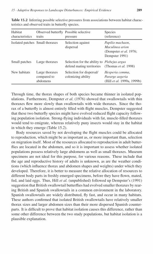
15 · Adaptive Responses to Landscape Disturbances: Empirical Evidence 289

Table 15.2 Inferring possible selective pressures from associations between habitat charac-teristics and observed traits in butterfly species.

Habitat Observed butterfly Possible selective Speciescharacteristics traits pressure (reference)

Isolated patches Small thoraxes Selection against Papilio machaon,dispersal Maculinea arion

(Dempster et al. 1976;Dempster 1991)

Small patches Large thoraxes Selection for the ability to Plebejus argusdefend mating territories (Thomas et al. 1998)

New habitats Large thoraxes Selection for dispersal/ Hesperia comma,compared to colonizing ability Pararge aegeriaabdomens (Hill et al. 1999a, 1999b)

Through time, the thorax shapes of both species became thinner in isolated pop-ulations. Furthermore, Dempster et al. (1976) showed that swallowtails with thinthoraxes flew more slowly than swallowtails with wide thoraxes. Since the tho-rax of a butterfly is almost entirely filled with flight muscles, Dempster suggestedthat these two butterfly species might have evolved reduced flight capacity follow-ing population isolation. Strong-flying individuals with fat, muscle-filled thoraxeswould tend to emigrate, whereas relatively puny insects would stay in the habitatin which they emerge (Table 15.2).

Body resources saved by not developing the flight muscles could be allocatedto reproduction, which might be as important as, or more important than, selectionon migration itself. Most of the resources allocated to reproduction in adult butter-flies are located in the abdomen, and so it is important to assess whether isolatedpopulations possess relatively large abdomens as well as small thoraxes. Museumspecimens are not ideal for this purpose, for various reasons. These include thatthe age and reproductive history of adults is unknown, as are the weather condi-tions (which influence thorax and abdomen shapes and weights) under which theydeveloped. Therefore, it is better to measure the relative allocation of resources todifferent body parts in freshly emerged specimens, before they have flown, mated,fed, and laid eggs. Thus, Hill et al. (unpublished) followed up Dempster’s (1991)suggestion that British swallowtail butterflies had evolved smaller thoraxes by rear-ing British and Spanish swallowtails in a common environment in the laboratory.Spanish swallowtails are widely distributed, fly fast, and occur in many habitats.These authors confirmed that isolated British swallowtails have relatively smallerthorax sizes and larger abdomen sizes than their more dispersed Spanish counter-parts. It is difficult to prove that habitat isolation causes this difference, rather thansome other difference between the two study populations, but habitat isolation is aplausible explanation.

290 D · Spatial Structure

Effects of patch size in relation to other life-history traitsIn similar vein, Thomas et al. (1998) studied a third species of butterfly, Plebejusargus, in isolated metapopulations. Some of the metapopulations inhabited smalland isolated fragments of heathland vegetation, whereas others inhabited muchmore extensive areas of heathland. Within each heathland the butterflies them-selves had quite localized distributions, being restricted to areas with high den-sities of mutualist ants (the caterpillars are tended and protected by ants, whichobtain sugars and amino acid secretions from them). In a large area of heath-land, adult P. argus butterflies that leave their ant-enriched habitat would almostcertainly find another area of suitable breeding habitat somewhere else within theheathland. In contrast, a wandering butterfly might be more likely to leave a smallfragment of heathland vegetation completely, eventually perishing in the surround-ing agricultural land. Surprisingly, butterflies reared in the common environmentthat originated from small heathland fragments were relatively large – indicativeof relatively strong flight capacity. This was contrary to the original expectations,which were that weak fliers would be found in the small heathlands. Of the vari-ous reasonable explanations for this result, one possibility is that large males mightbe better at defending mating territories, so small males displaced from territoriesmight be more likely to emigrate completely, the impact being greatest in smallareas (Thomas et al. 1998, Table 2). The important lesson is that the evolutionof flight ability and migration is often a complex compromise between differentactivities (adult feeding, mating, finding egg-laying sites, avoiding predators, andtrue migration), and any or all of these activities may also be affected by habitatarea and isolation.

Thomas et al. (1998) studied one metapopulation of P. argus in more detail.This metapopulation inhabited a different type of vegetation, limestone grassland.In this case, all of the patches of habitat were within the migration range of at leastone other patch, with a measured exchange rate of 1.4% per generation (Lewiset al. 1997). In this system, adult butterflies from small patches had relativelylarge thoraxes and small abdomens. Two equally plausible explanations are:

� Individuals with large-thoraxes are able to defend territories, so they can staywithin small patches and/or territories, whereas weaker adults are forced out ofsmall patches;

� Small patches receive higher fractions of immigrants or have been recolonizedmore recently than large patches, such that small patches are populated mainlyby strong-flying immigrants and by the offspring of immigrants.

The first of these explanations predicts that migrants between patches will havesmall thoraxes, whereas the second predicts that migrants between patches willhave large thoraxes. These predictions have yet to be tested.

Effects of colonization opportunitiesIn plant species of the Asteraceae family, Cody and Overton (1996) showed thatdispersal can evolve within a few generations only. They studied the evolution of

15 · Adaptive Responses to Landscape Disturbances: Empirical Evidence 291

pappus length of achenes on the mainland and in newly established island popula-tions in British Columbia. They showed that island populations were establishedby achenes with the longest pappus (increasing the ability to be dispersed by wind)in the mainland populations. However, once on an island dispersal can be selectedagainst, because islands are surrounded by an unfavorable habitat (the sea). Af-ter less than five generations of the establishment, pappus length had significantlyreduced in at least one species (Cody and Overton 1996).

A similar sequence in the results of selection pressures might be expected interrestrial habitat islands (Olivieri et al. 1990, 1995). In butterflies, indeed, thereare some indications that large thoraxes and small abdomens may characterize col-onizing populations, the opposite of the syndrome predicted for truly isolated pop-ulations. Dempster (1991) noted an increase in thorax width in Ma. arion during aperiod of population expansion, a reversal of the trend toward small thoraxes in iso-lated populations. Further evidence comes from common-environment rearings ofcolonizing and noncolonizing metapopulations of two other butterfly species. Hu-man activities have generated empty habitat networks for the silver-spotted skipperbutterfly, Hesperia comma (Thomas and Jones 1993). This butterfly is restrictedto fragmented grasslands on calcareous soils in Britain, and it requires very shortand sparse vegetation. H. comma declined steeply when humans introduced thedisease myxomatosis, which killed virtually all of the rabbits that had been re-sponsible for maintaining the short turf favored by this butterfly. As this habitatrapidly became overgrown, the skipper became rare and localized. More recently,both the recovery of rabbits from myxomatosis and climate warming (Thomaset al. 2001a) has restored fragmented habitat networks for H. comma, which isgradually recolonizing them. A metapopulation in East Sussex, characterized bylarge thoraxes and small abdomens, is rapidly expanding its distribution into anempty habitat network, whereas insects from a stable metapopulation elsewherein southern England have relatively small thoraxes and large abdomens (Hill et al.1999a).

The same pattern is seen in expanding populations of the woodland butterflyPararge aegeria. This species is expanding its northern margin in Britain, almostcertainly in response to anthropogenic climate warming (Hill et al. 1999b). Theexpansion is taking place in agricultural landscapes that contain scattered wood-lands, which provide ample opportunity for repeated founder events and selectionfor increased dispersal rate. As predicted, the expanding northern population wasfound to possess larger thoraxes and smaller abdomens than a more stable popu-lation further south (Hill et al. 1999c, Table 2). Interestingly, the difference wasmuch greater in females (the colonizing sex) than in males (Hill et al. 1999c) –male morphology is probably largely determined by mate-location strategy andthermoregulation (van Dyck et al. 1997).

The above examples illustrate the complexity of potential responses to land-scape pattern, which result in both increased and decreased migration rates de-pending on the exact changes that take place in the landscape (Heino and Han-ski 2001) and on the temporal and spatial scales observed. The impacts of other

292 D · Spatial Structure

traits and selection pressures on migration rate (mating strategy, predator evasion,etc.) further complicate the consequences of habitat fragmentation. Nonetheless,these examples do indicate that evolutionary changes in migration rates and inlife-history traits associated with dispersal are likely to be extremely common inmodern landscapes. How often this is of practical concern is another matter. Inany case, the average dispersal traits of organisms that survive in modern, frag-mented landscapes are likely to be different from those of the original fauna andflora (Thomas 2000).

15.3 Fragmentation, Migration, and Local AdaptationHabitat fragmentation has the potential to disrupt any former balance betweengene flow and local selection. Local adaptations might initially be expected to in-crease following habitat fragmentation and isolation, because locally adapted traitswill no longer be diluted by gene flow from populations adapted to other habitats(Dhondt et al. 1990; Storfer 1999). However, in the long term successful colonistsmay be favored at the metapopulation level, a situation analogous to that alreadydescribed for the evolution of migration rates. Selection within individual popula-tions may favor local specialists, but generalists may be more successful colonists(Thomas et al. 2001a). Evolutionary changes may also take place as a result ofthe changing qualities of habitat remnants, caused by disturbance, or because ofchanges in the identities of other species that inhabit the same fragments. Somespecies may develop adaptations to anthropogenic habitats beyond the natural veg-etation fragments, but continue to exchange genes with populations that still residein nearby natural habitats. In the extreme, this could disrupt local adaptations tonatural habitats.

Adaptation to local hostsAn example of the reciprocal influence of extinction–colonization dynamics ina highly fragmented landscape and the evolution of host-plant preference in thebutterfly M. cinxia is provided by the recent study of Hanski and Singer (2001).M. cinxia has two larval host plants in the Åland Islands, SW Finland, Plantagolanceolata and Veronica spicata. A distinct west–east gradient exists in the rel-ative abundances of the two host plants, a gradient that runs parallel to a gradi-ent in the genetically determined preference of female butterflies for the differenthost plants within a distance of 30 km (Kuussaari et al. 2000). Such small-scaleadaptation to the regionally more abundant host plant raises an interesting questionabout metapopulation dynamics. Assume that butterflies in a particular region haveevolved a preference for V. spicata (or vice versa). The proportion of host speciesvaries from one habitat patch to another and, although most patches in a particularregion are dominated by V. spicata, some patches have only Po. lanceolata. Giventhe evolved preferences for the different host plants in female butterflies, will theproportions of different host plants in the habitat patches influence the metapopu-lation dynamics? The answer turns out to be conclusively yes. Habitat patches thatare dominated by the host plant to which the metapopulation in a given region has

15 · Adaptive Responses to Landscape Disturbances: Empirical Evidence 293

adapted have a substantially higher rate of colonization than patches dominatedby the regionally rare alternative host plant (Hanski and Singer 2001). The effectof the female preference for a particular host on colonization probability is likelycaused by the effects of female preference on emigration and immigration in rela-tion to the local proportions of host plants, rather than by spatial variation in larvalperformance.

The reverse question may also be asked; does the extinction–colonization dy-namics influence the evolution of a preference for a particular host plant? Modeland empirical results indicate such an effect, as the model-predicted average host-plant preference in a particular habitat patch network explains a significant amountof within-network variation in preference (Hanski and Heino, unpublished). Thus,in this example colonization probability depends upon a genetically determinedtrait of the colonizers, which is selected both at the level of local populations andat the level of the metapopulation. Other studies elucidate how local adaptationand gene flow promote genetic variation in metapopulations in general (Karban1989; Wade 1990; Antonovics et al. 1994) and how local adaptation may be in-fluenced by gene flow (Holt 1996; Dias 1996; Pulliam 1996). The example ofM. cinxia suggests that gene flow and the establishment of new populations mayalso be influenced by local adaptation.

Adaptation to anthropogenic habitat changeOne form of habitat change is represented by the arrival of a new species. Whenthe European plant Po. lanceolata arrived in North America, it spread rapidlyand became established in irrigated meadows along the eastern slopes of theSierra Nevada mountains. The native checkerspot butterfly Euphydryas edithawas already present in the area. The caterpillars of this butterfly fed naturally onCollinsia parviflora, a plant that shares certain iridoid glycosides with Po. lance-olata. Some females started to lay batches of eggs on Po. lanceolata (Thomaset al. 1987). Larval survival was higher on the introduced plant than on the nativeC. parviflora, and female choice of host plant had a genetic basis (Singer et al.1988). Over a 10-year period the proportion of females that lay on Po. lanceolatawas observed to increase, and resulted in the exclusion of C. parviflora from thediet in at least one population of E. editha (Singer et al. 1993). This is either agreat bonanza for this rare butterfly – Po. lanceolata is widespread – or a seriousrisk. Within the study region, Po. lanceolata is restricted mostly to irrigated land.The newly evolved Plantago-feeding population might have doomed itself to ex-tinction if irrigation had ceased to be economic. In fact, it became extinct when themeadow was converted into a golf course (M.C. Singer, personal communication).

The logging of native forests that are then allowed to regenerate is another glob-ally widespread form of habitat modification. Logging in a different part of theSierra Nevada mountains, in California, provided another new opportunity for an-other metapopulation of E. editha. This metapopulation was quite different fromthe one described above. The butterflies naturally laid their eggs on Pedicularissemibarbata (mainly) and Castilleja disticha, two species of Scrophulariaceae:

294 D · Spatial Structure

Blue-eyed maryCollinsiaparviflora

Checkerspot butterflyEuphydryas editha

PlantainPlantago

lanceoloata

the population was restricted to natural granitic outcrops in an otherwise forestedregion (Singer 1983). Logging created major new openings in the forest, and ren-dered a third species of Scrophulariaceae, Ca. torreyi, suitable as a host plant (fol-lowing the disturbance, the plant grew to be sufficiently large for the caterpillarsto complete their life cycle on it). Huge populations of the butterfly establishedin these new clearings (Singer 1983; Thomas et al. 1996). Vast numbers of but-terflies emerged in the logged habitat and flew back to the natural habitat, witha resultant intense competition in the natural habitat. This set up an asymmetricgene flow from the logged habitat to the natural habitat. Adaptations to the newenvironment, involving the acceptance of Ca. torreyi plants by females, startedto develop. However, these incurred the cost of a reduced level of adaptation (areduced preference for Pedicularis and Castilleja) in nearby populations that stillinhabited the natural rocky outcrops (Singer et al. 1993; Singer and Thomas 1996;Thomas et al. 1996).

If new populations in an anthropogenic habitat risk extinction, any reduced lev-els of adaptation to undisturbed environments are potentially worrying. In the casedescribed above, the forest clearings eventually become overgrown and popula-tions were bound to become locally extinct. But something much more dramatichappened. An aseasonal summer frost killed all of the Ca. torreyi plants in theforest clearings, without harming either of the natural host plants in the rocky out-crops. E. editha larvae were resistant to the frost, but larvae in the forest clearingsstarved because the Collinsia had died, and a year later all the clearing popula-tions of the butterfly had become extinct. Fortunately, the butterflies survived intheir natural habitat. These two examples from E. editha populations illustrate howthe evolutionary adoption of habitats that are created and maintained by humansboth enables species to cope with human activities and, simultaneously, puts themat risk from future changes in land management. Such changes in management

15 · Adaptive Responses to Landscape Disturbances: Empirical Evidence 295

practices and agricultural economics may take place too quickly for the species tocope, a serious problem once the original adaptations to the native habitats havebeen lost (see the discussion of niche conservationism in Chapter 13).

15.4 The Example of Centaurea SpeciesStudies of the metapopulation dynamics of species that live in naturally highlyfragmented habitats, as for Centaurea corymbosa (Asteraceae), can improve ourunderstanding of the long-term consequences of habitat fragmentation.

Evolutionary trapping in Ce. corymbosaThe combined results of population genetic structure, achene dispersal distances,reproductive system, seed sets, and survival following experimental introductions

CentaureaCentaurea corymbosa

allow a general view of the species’ pop-ulation biology: the unique metapopu-lation of Ce. corymbosa has much de-mographic and evolutionary inertia (seeBox 15.4). Many suitable sites (cliffs)are available near the extant populations,as shown by the experimental introduc-tions, but they remain empty because ofthe very low colonization ability. Ach-ene dispersal by gravity and wind is re-stricted to a few tens of centimeters fromthe mother plant, maybe because of thelandscape structure. The unsuitable habi-tat surrounding the existing populationsselects against dispersal (Olivieri et al.1995; Cody and Overton 1996): any ach-enes that leave the cliff almost certainly settle in vegetation within which theyare unable to grow and/or compete successfully. One species of ant (Cremato-gaster scutellaris) disperses some Ce. corymbosa seeds, but probably no fartherthan several meters; in any case, they cannot take a seed from one cliff to another.In addition to low dispersal, Colas et al. (1997) suggested that semelparity andself-incompatibility reinforce the low colonization ability. Indeed, reproductivesuccess of an individual plant mainly depends on its neighbors, and the closer theyare, the greater the probability that they will set seeds (Colas et al. 2001). If, bychance, a few seeds disperse longer distances to a suitable cliff, germinate, anddevelop in to flowering plants, they are likely to die without giving rise to anysurviving progeny unless they flower in the same year and are compatible.

Some convincing examples show that bottlenecks may induce the dissolution ofsystems (heterostyly, self-incompatibility) of selfing-avoidance in plants (Reinartzand Les 1994; Eckert et al. 1996; Barrett 1998). It also seems clear that founderevents might promote the evolution of dispersal (Cody and Overton 1996). How-ever, in the absence of colonization, it seems unlikely that these traits will evolve

296 D · Spatial Structure

Box 15.4 Natural history and genetic structure of Centaurea corymbosa

250 m

North

Unoccupied cliffsCliffs inhabited by Ce. corymbosa

Vineyards and pinewoods

Scrubland

Pinewoods

Ce. corymbosa is a self-incompatible, monocarpic perennial plant, endemic to atiny 3 km2 area situated within a 50 km2 limestone plateau (Massif de la Clape) insouthern France (Colas et al. 1996). Ce. corymbosa lives in clefts of rocks on thetop of cliffs with very open vegetation and almost no soil. Apparently, it cannotstand competition: no plant can be found either on the plateau, in the middle ofthe scrubland, or in the pinewood, down in the depressions. Over all the six ex-tant populations, 350 to 650 flowering plants were counted per year from 1994 to2000 (from five to 250 per year per population). Each population is geographicallyclearly delimited.

Although populations are only 0.3 to 2.3 km apart, gene flow is very restrictedamong them, as evidenced by the very strong genetic differentiation observed onallozymes (Colas et al. 1997) and on microsatellites (Fréville et al. 2001). The cor-relation between geographic and genetic distances among the populations suggeststhat gene flow occurs mainly between adjacent populations. The population geneticstructure for quantitative traits was similar to the genetic structure for molecularmarkers (Petit et al. 2001). This suggests the absence of heterogeneous selectionamong populations (see Bonnin et al. 1996 and Chapter 12 for a discussion of therelationship between neutral and selected characters in methods for measuring pop-ulation genetic differentiation).

Although populations may stretch out along 670 m, each population can be con-sidered as a panmictic unit (no departure from Hardy–Weinberg expectations). Thisis the consequence of pollen dispersal within populations in which about 20% ofthe mating pairs are separated by more than 50 m, as shown by paternity analyses(Hardy et al., unpublished). However, the amount of pollen dispersed to long dis-tances is not sufficient to prevent the lower fertilization rate of ovules of isolatedflowering plants compared to plants situated in dense patches (Colas et al. 1997,2001). Pollen flow seems to be limited mainly by gaps of unoccupied pieces ofland between populations.

15 · Adaptive Responses to Landscape Disturbances: Empirical Evidence 297

Landscape structure

Lack of dispersal

Low colonization abilitySemelparity No founder effects

Self-incompatibility

Figure 15.1 Factors that select against the colonization ability of Ce. corymbosa.

in Ce. corymbosa. Therefore, this species seems to be held within a vicious circle(Figure 15.1), an evolutionary spiral that prevent colonization and might lead toextinction. However, on the basis of historical data (Colas et al. 1997), five pop-ulations have been known from 100 to more than 200 years ago, and none havedisappeared. Since the mean generation time is about 5.5 years (Colas et al., un-published), this represents 20 to 40 generations. The populations are very small,but the extinction rate may be no greater than the rate of colonization of new cliffsin this quite stable habitat. Thus, Ce. corymbosa could be well adapted to its frag-mented habitat.

Fragmentation and Centaurea diversificationCe. corymbosa belongs to the Maculosa group, which comprises 23 taxa (speciesand subspecies), of which most are narrowly endemic (Tutin et al. 1976). Manytaxonomic groups within the huge Centaurea genus [500 species with manysubspecies around the Mediterranean (Bremer 1994)] show this pattern: onewidespread and several narrowly distributed endemics. Fréville et al. (1998) com-pared allozyme diversity in Ce. corymbosa and two related taxa that shared thesame type of habitat in other places of southern France: the widespread Ce. mac-ulosa maculosa and Ce. maculosa albida, which occurs in only one population ofabout 200 flowering individuals. Diversity of the two endemic taxa representeda sample of the diversity of the widespread one, from which they are probablyderived. As in Ce. corymbosa, high allozymic differentiation was found amongpopulations of Ce. maculosa spp., but the amount of differentiation among popu-lations of different taxa was not different from that among populations within taxa.Fréville et al. (1998) suggest that ecological specialization following bottlenecksor founder effects associated with colonization events in Ce. maculosa maculosaresulted in the establishment of new taxa. Although probably very rare, long-distance achene dispersal of these species may occur by adhesion of the barbed

298 D · Spatial Structure

and sticky bristles in the pappus to sheep or to the feathers of birds. In the Mas-sif de la Clape, several cliffs rocks occupied by Ce. corymbosa are also those onwhich pellets from the eagle owl Bubo bubo are found (Colas 1997).

Habitat fragmentation may actually be the cause of wide diversity in Centaureaspecies, as well as in other Mediterranean plants (see review by Thompson 1999a).Some colonization, followed by isolation, would permit divergence (adaptive ornot), potentially generating diversity. In the cliff-dwelling Centaurea species, newspecies might be established as quickly as other species become extinct. In suchcases, rather than allocating all conservation efforts to the conservation of one par-ticular species that may naturally go extinct, it might be better to preserve habitatdiversity to allow species to diverge, evolve, and die. Although this is a long-term,evolutionary perspective that local managers may not find immediately appealing,the role that fragmentation may play in both the generation of diversity and thedecline of genetic diversity should be considered seriously.

Interestingly, it appears from these studies on Centaurea species that the def-inition of a metapopulation depends on the scales of space and time considered.Ce. corymbosa may be considered, as stated above, a unique metapopulation of sixpanmictic populations among which restricted (medium distance) gene flow occurswith very slow extinction–colonization dynamics (probably observable over tensto hundreds of generations). However, it appears from a demographic study, us-ing 40 permanent quadrats on rocks since 1994, that to understand the persistenceof each population requires the processes of migration, extinction, and recolo-nization among quadrats (i.e., patches of plants) to be considered (Colas et al.,unpublished). Every patch may persist for one to several generations, and achenemigration between adjacent suitable rocks (a few meters apart) occurs by gravity,wind, or ant dispersal. Thus, on a time scale of a few generations, each of thesix panmictic units may be considered as an isolated metapopulation itself. Eachhas extinction–colonization processes that occur among patches because of the ef-fects of environmental and demographic stochasticities and ordinary dispersal overshort distances (Colas et al., unpublished). Also, the Maculosa group of Centau-rea species might be considered as a kind of meta-species with rare long-distancedispersal events that result in isolated populations, which may differentiate fromeach other through drift and/or heterogeneous selection. Extinction–colonizationprocesses on this large scale in space and time are closely related to evolutionaryprocesses of speciation and to species’ extinction.

15.5 Concluding CommentsAlmost all habitats have changed dramatically over recent decades and centuries,throughout the world. Changes in directional selection, new evolutionary optima,and changes in the balance between gene flow and selection must be widespreadphenomena. The example of Centaurea species described in Section 15.4 sug-gests that natural fragmentation is probably an important cause of species diver-sity. However, this is a long-term evolutionary consequence of stable landscapeheterogeneity. As suggested in Section 15.3 using the butterfly examples, recent

15 · Adaptive Responses to Landscape Disturbances: Empirical Evidence 299

changes in land use might be too fast for any evolutionary processes to occur. Akey factor in future studies of the effects of fragmentation will probably be whetherfragmentation occurs progressively or suddenly, and whether either allows adap-tive evolution or not.

The examples described in this chapter illustrate some evolutionary conse-quences of these changes. The response of migration rates to fragmentation isidiosyncratic, and depends on how the local extinction or fitness of migrants varieswith patch size. Local adaptations have mixed effects on the metapopulation via-bility, as they might reduce colonization abilities, as well as migration, in particularbetween different habitats. The response may be inefficient because of the manyconstraints that could prevent the metapopulation from responding optimally tolandscape changes, as the interaction between local adaptations and migration inbutterflies show. A common feature of most relevant studies is the large number ofprocesses involved. Further understanding of the evolutionary responses to frag-mentation in terms of inbreeding, local adaptation, or migration is necessary topredict the effect that fragmentation can have on the different species present in alandscape.

It is probably utopian to think that we can determine the critical thresholds forhabitat fragmentation above which most of the biodiversity in a landscape can beconserved:

� First, the relevant scale at which habitat fragmentation becomes important de-pends on the size of the home range of the species, which varies from a fewsquare centimeters to several square kilometers (Mönkkönen and Reunanen1999).

� Second, the minimum patch areas for viable local populations and the maxi-mum isolation distances that allow colonization are species specific, since theydepend on many life-history traits.

� Third, a landscape does not always contain suitable and unsuitable patches,and intermediate habitats may serve as corridors for migration to occur (e.g.,Kirchner et al. 2003). Levin (1995) illustrated the role of plant outliers for geneflow among populations. Depending on the habitat specificity of the species,the matrix surrounding a particular patch may be usable or completely hostileand impossible to cross.

A better understanding of the ecological, genetic, and evolutionary issues relatedto the thresholds of long-term persistence in fragmented landscapes remains one ofthe major challenges in conservation biology. This is not only because of the com-plexity of these thresholds, but also because of their relevance to a large portion ofthe biodiversity that remains.

Acknowledgments We are particularly thankful to Jane Hill. Both Ilkka Hanski and ChrisD. Thomas were supported by the TMR FRAGLAND network. Thanks also to I. Olivieriand H. Fréville for their comments.

Part E

Community Structure

Introduction to Part E

“No man is an island”, and no species of conservation interest exists in isolationfrom others. Ecosystems define the ecological theater, not only for any evolu-tionary play, but also for unfolding tales of population decline or rescue. Thisbook therefore ends with a part on the community-level aspects of evolutionaryconservation biology. In this way, we establish several additional perspectives toour general question on the ecological, demographic, and genetic conditions thatenable or hinder populations to overcome extinction threats through adaptation.

On the ecological side, many density-dependent and frequency-dependent se-lection pressures emerge from interspecific interactions. It is the dependence offocal populations on the abundance of their resources, preys, predators, mutualis-tic partners, and competitors that creates complex webs of fitness effects and thusdetermines the strength and direction of natural selection. An interesting levelon which to express such dependences is the flow of nutrients through ecologicalsystems. Measures of nutrient cycling not only serve as indicators of ecosystemfunctioning, but also provide a convenient platform for resolving the interactionbetween organisms and their environment and for characterizing the implicationsof anthropogenic change.

On the demographic side, density regulation in communities is often nonlin-ear and can result in the coexistence of multiple demographic attractors. An-thropogenic change can, temporarily or permanently, tilt the established balancebetween regulating forces, and so lead to shifts of or even switches between de-mographic equilibria. Attractor switches are bound to bring about qualitativelynew selection pressures and will often prove to be particularly resilient to conser-vation efforts directed at their reversal. Such complex dependences explain whyecosystems can react to altered conditions by displaying intricate cascades of eco-logical and evolutionary responses. Since such responses tend to act on differenttime scales, their study is critical to understand the expected ultimate impact ofdetrimental perturbations as well as conservation interventions.

By definition, genetic factors almost always act within species, not within com-munities. Exceptions can occur through interspecific gene flow. Hybridization is aprime example of such a process and can either exacerbate or ameliorate the perilsof extinction experienced by small populations. However, because of the intro-gression of variant genetic material, hybridization may sometimes rescue only thedemographic and ecological, but not the genetic, identity of challenged popula-tions.

To consider issues of conservation and adaptation at the community level ne-cessitates that the primary target of conservation efforts be clarified. Are we mostinterested in the conservation of life-history patterns, evolutionary lineages, net-works of ecological interactions, current equilibrium states of ecosystems, their

302

Introduction to Part E 303

diversity, or their ecological function? Different targets mandate different types ofinterventions.

It is clear that conservation biology, and especially evolutionary conservationbiology at the community level, is stretching current empirical and theoreticalknowledge beyond its limits. The contributions to this part must therefore be ap-preciated as attempts to push these limits forward. The analyses presented are, ofnecessity, more tentative and hypothetical than those offered in the earlier parts ofthis volume.

In Chapter 16, Bronstein, Dieckmann, and Ferrière point out why a single-species focus may often be too narrow when investigating ecological and evo-lutionary responses to extinction threats. This is especially obvious for tightlycoupled ecological associations, such as those involving mutualists. After a re-view of the range of anthropogenic threats to which mutualists are exposed today,the authors show how the reduction of an established species or the invasion of anon-native species can have dramatic repercussions for mutualistic partners. Ex-pected responses range from benign resilience through the addition or replacementof mutualistic partners to the linked extinction of populations. The potential forsuch complex reaction patterns underlines that environmental threats can induceecological and evolutionary effects that cascade through entire ecological commu-nities.

Chapter 17 describes a framework for conducting analyses of adaptive re-sponses from a whole-ecosystem perspective. Loreau, de Mazancourt, and Holtexplain how to extend the “classic” view of environments being external toevolving populations and constant during their adaptation, by incorporating, first,organism–environment feedbacks for the operation of natural selection and, sec-ond, sufficient ecological resolution to describe such environments. One level onwhich to resolve evolutionarily relevant feedbacks is that of nutrient transport: theindirect ecological and evolutionary effects of nutrient cycling are sometimes sostrong as to modify or even prevail over the selective pressures that arise from di-rect ecological interactions. Based on examples from plant–herbivore evolutionand extending their findings to coevolution in other exploiter–victim systems, theauthors argue that a comprehensive approach to evolutionary conservation biologywill have to merge population-level and ecosystem-level perspectives to predictthe responses of ecological systems to environmental degradation.

Turning from the ecological to the genetic implications of community-level in-teractions, Chapter 18 shows how the fate of endangered species can depend onhybridization with sexually compatible individuals of another species. Illustratedby a variety of empirical examples, Levin points out that the contact between anendangered species and its congener can lead to the rapid disappearance of the for-mer. Hybrids may happen to be sterile or the congener itself may possess a higherfitness than the endangered species. From a conservation point of view, interme-diate situations, in which hybrid derivatives are stabilized, have to be regarded asmixed successes, because the original genetic identity of the endangered species issacrificed, an outcome that is most likely for insular species. At the opposite end

304 Introduction to Part E

of the spectrum, hybridization may also rescue an endangered species, by con-ferring the required local adaptations or by alleviating the deleterious effects ofinbreeding.

Integration of insight at the community level will eventually enable conserva-tion managers to interact, reliably and effectively, with our ecological environ-ment. Years of inventive empirical and theoretical research still separate us fromthis ultimate goal.

16Coevolutionary Dynamics and the

Conservation of MutualismsJudith L. Bronstein, Ulf Dieckmann, and Régis Ferrière

16.1 IntroductionThe vast majority of studies in conservation biology focus on a single species ata time. However, many of the anthropogenic threats that species face occur viadisrupted or enhanced interactions with other organisms. According to one re-cent analysis, interactions with introduced species, such as predators, parasites,and pathogens, are the eighth leading cause of species endangerment worldwide;they are the primary cause of endangerment in Hawaii and Puerto Rico (Czechand Krausman 1997). Altering interactions not only has ecological effects, butalso it can generate selective pressures and evolutionary responses, which may ei-ther favor or disfavor the evolutionary persistence of species and interactions. Anincreased focus on interspecific interactions will thus enlighten our efforts to con-serve species and, more pointedly, our ability to understand when species will andwill not respond evolutionarily to conservation threats. Such a focus is also criti-cal for efforts to conserve communities as units, because interactions are the cru-cial and poorly understood link between threatened species and threatened speciesassemblages.

Different types of interspecific interactions are subject to, and generate, some-what different ecological and evolutionary threats. Predator and pathogen intro-ductions can lead to reduction, local exclusion, or extinction of native species(Savidge 1987; Schofield 1989; Kinzie 1992; Steadman 1995; Louda et al. 1997).Rapid evolution in the enemies and/or the victims may also result (Dwyer et al.1990; Singer and Thomas 1996; Carroll et al. 1998). Conversely, the disappear-ance of enemies (or the introduction of a species into a habitat that lacks enemies)can have consequences that extend across the population, community, and ecosys-tem (Thompson 1996; Fritts and Rodda 1998). The effects of altering competitiveinteractions appear to be qualitatively similar, although smaller in magnitude (Sim-berloff 1981; Williamson 1996). Introducing competitors can reduce populationsof native species, with the possible effects being local exclusion, extinction, orevolutionary change of one or both species (Schofield 1989; Moulton 1993; Co-hen 1994; Dayan and Simberloff 1994).

Antagonistic interactions have been relatively well studied from the evolution-ary, ecological, and conservation perspectives. In contrast, our understanding ofmutualisms – interactions that are mutually beneficial to both species (Box 16.1) –is at a much earlier stage of development (Bronstein 1994, 2001a). The ecological

305

306 E · Community Structure

Box 16.1 Mutualistic interactions

Mutualisms are interspecific interactions in which each of two partner species re-ceives a net benefit. Well-known examples include interactions between plants andmycorrhizal fungi, plants and pollinators, animals and gut bacteria, and corals andzooxanthellae (Herre et al. 1999; Bronstein 2001a). Mutualisms generally involvethe exchange of commodities in a “biological market”: each species trades a com-modity to which it has ready access for a commodity that is difficult or impossiblefor it to acquire (Noë and Hammerstein 1995; see also Douglas 1994). For in-stance, plants provide carbon to their mycorrhizal fungi in return for phosphorus,and plants provide nectar to many animals in return for pollen transport. Although agreat deal is known about the natural history of diverse mutualisms, relatively littleeffort has yet been invested in the study of ecological and evolutionary similari-ties among them (Bronstein 1994). This is particularly surprising in light of theirperceived importance in nature. All organisms are currently believed to associatewith mutualistic species at some point in their lives. Furthermore, mutualisms arethought to lie at the core of major transitions in the history of life, including theorigin of the eukaryotic cell and the invasion of land.

To understand mutualism in an evolutionary conservation context, it is impor-tant to distinguish it from related phenomena with which it is often confused. Mu-tualism is an association between different species; it involves somewhat differentevolutionary forces and poses different conservation challenges than does cooper-ation within species (Dugatkin 1997). Not all mutualisms are symbioses (intimatephysical associations; Douglas 1994); many involve free-living organisms that as-sociate for only part of their lives. Free-living organisms are likely to be vulnerableto somewhat different anthropogenic threats, which raises the interesting problemof how these mutualisms persist when one, but not both, of the partners is at risk.Conversely, not all symbioses are mutualistic. Hence, this chapter does not con-sider how anthropogenic change might affect the evolution of diseases (which areantagonistic symbioses). Finally, not all mutualisms have long evolutionary or co-evolutionary histories. For instance, pairs of invasive species can sometimes formhighly successful mutualisms (Simberloff and von Holle 1999). Evolution may welloccur after the association has formed, however (Thompson 1994). Such evolutioncan change the specificity of the interaction (from more specialized to more gener-alized, or vice versa), as well as its outcome (from mutualistic to antagonistic, orvice versa).

The large majority of mutualisms are rather generalized: each species can obtainthe commodities it requires from a wide range of partner species (Waser et al. 1996;Richardson et al. 2000). Furthermore, many mutualisms are facultative, in the sensethat at least some of the commodity can be obtained from abiotic sources. How-ever, many extremely specialized mutualisms do exist: they are species-specific(i.e., there is only a single mutualist species that can provide the necessary com-modity), and may be obligate as well (i.e., individuals cannot survive or reproducein the absence of mutualists). Box 16.3 provides details of one such specialized mu-tualism. Note that the degree of specificity is not necessarily symmetrical within amutualism. For instance, many orchid species can be pollinated by a single speciesof orchid bee, whereas these bee species visit many different orchids, as well asother plants (Nilsson 1992). The evolutionary flexibilities that result from theseasymmetries in specificity remain almost entirely unexplored.

16 · Coevolutionary Dynamics and the Conservation of Mutualisms 307

effects of disrupting mutualism are known from only a handful of case studies,which have largely involved a single form of mutualism, plant–pollinator inter-actions (see the excellent reviews by Bond 1994, 1995; Allen-Wardell et al. 1998;Kearns et al. 1998). The evolutionary consequences of such disruptions remainvirtually unexplored. This gap in knowledge is of particular concern because mu-tualisms are now believed to be a focus around which diversity accumulates, onboth ecological and evolutionary time scales (e.g., Dodd et al. 1999; Wall andMoore 1999; Bernhard et al. 2000; Smith 2001).

We begin this chapter with a discussion of processes that foster the ecologicaland evolutionary persistence of mutualisms. We go on to discuss the sequence ofevents that can endanger species that depend on mutualists, in the context of someprominent forms of anthropogenic change. With this background, we outline threescenarios for the possible outcomes when the mutualists of a species of interestbecome rare – linked extinction, ecological resilience, and evolutionary response– and distinguish the likelihood of each outcome based on whether the mutualismis relatively specialized or generalized. As we show, simple evolutionary modelscan generate quite useful predictions relevant to the conservation of mutualismsand other species interactions. Furthermore, we show that modeling pairwise as-sociations can form an excellent first step toward addressing the fascinating, butmuch less tractable, problem of coevolution at the community scale.

16.2 Factors that Influence the Persistence of MutualismsThe persistence of mutualisms has long been a puzzle. From the ecological per-spective, the positive feedback inherent to mutualisms led May (1976) to char-acterize mutualisms as an unstable “orgy of mutual benefaction”. Yet, at thesame time, dependence on mutualists also raises the likelihood of Allee effects(see Chapter 2), in which the low abundance of one species can doom its partnerto extinction. From the evolutionary perspective, the major threat to mutualismis the apparent selective advantage that accrues to individuals who reap benefitsfrom partner species without investment in costly commodities to exchange withthem (Axelrod and Hamilton 1981; Soberon Mainero and Martinez del Rio 1985;Bull and Rice 1991; Bronstein 2001b). Slight cheats that arise by mutation couldgradually erode the mutualistic interaction, and lead to dissolution or reciprocalextinction (Roberts and Sherratt 1998; Doebeli and Knowlton 1998). Althoughcheating has been assumed to be under strict control, recent empirical findings (re-viewed by Bronstein 2001b) indicate that cheating is rampant in most mutualisms;in some cases, cheaters have been associated with mutualisms over long spans ofevolutionary time (Després and Jaeger 1999; Pellmyr and Leebens-Mack 1999;Lopez-Vaamonde et al. 2001). Recent theoretical advances have increased our un-derstanding of the ecological and evolutionary persistence of particular forms ofmutualism (e.g., Holland and DeAngelis 2001; Law et al. 2001; Yu 2001; Hollandet al. 2002; Morris et al. 2003; Wilson et al. 2003).

Below, we introduce and discuss a simple general model to describe the ecolog-ical and evolutionary dynamics of a two-species, obligate mutualism in a constant

308 E · Community Structure

Box 16.2 Ecology and evolution of specialized mutualisms: a simple model

We describe the obligate and specialized mutualistic interaction between species X(density NX ) and species Y (density NY ) by a simple Lotka–Volterra model,

dNX

dt= [−rX (x) − cX NX + yNY (1 − αNX )]NX , (a)

dNY

dt= [−rY (y) − cY NY + xNX (1 − βNY )]NY . (b)

The mutualistic traits x and y are measured as per capita rates of commoditiestraded (a visitation rate by a pollinator, for example); thus, xNX and yNY repre-sent the probabilities per unit time that a partner individual receives benefit from amutualistic interaction. Intraspecific competition for commodities provided by thepartner species is expressed by the linear density-dependent factors (1 − αNX ) and(1 − βNY ), as in Wolin (1985). The terms −cX NX and −cY NY measure the detri-mental effect of intraspecific competition on other resources. The mutualism beingobligate, the intrinsic growth rates −rX (x) and −rY (y) are negative, and rX (x) andrY (y) increase with x and y, respectively, to reflect the costs of mutualism.

Ecological dynamics. A standard analysis of the thus defined ecological modelshows that the situation in which both species are extinct, NX = 0 and NY = 0,is always a locally stable equilibrium. Depending on the trait values x and y, twoinner equilibria may also exist in the positive orthant, one being stable (a node) andthe other being unstable (a saddle). The transition between the two cases (zero ortwo equilibria in the positive orthant) is caused by a saddle–node bifurcation. Thecorresponding bifurcation curve is the closed, ovoid curve depicted in Figures 16.1ato 16.1c, which separates a region of trait values that lead to extinction from thedomain of traits that correspond to viable ecological equilibria.

A mathematical approximation of mutation–selection processes. By assumingthat ecological and evolution processes operate on different time scales and thatevolution proceeds through the fixation of rare mutational innovations, the rates ofchange of traits x and y on the evolutionary time scale are given by (Dieckmannand Law 1996)

dx

dt= εX N ∗

X

∂ fx∂x ′

∣∣∣∣x ′=x

, (c)

dy

dt= εY N ∗

Y

∂ fy∂y ′

∣∣∣∣y′=y

. (d)

Parameters εX and εY denote evolutionary rates that depend on the mutation rateand mutation step variance (see Box 11.3 for further details); N ∗

X and N ∗Y are the

equilibrium population densities of resident phenotypes x and y (these factors oc-cur because the likelihood of a mutation is proportional to the number of reproduc-ing individuals); f X (x ′, x, y) and fY (y ′, x, y) are the invasion fitnesses (defined asper capita rates of increase from initial rarity; Metz et al. 1992) of a mutant phe-notype x ′ of species X and of a mutant phenotype y ′ of species Y in a residentassociation x, y. continued

16 · Coevolutionary Dynamics and the Conservation of Mutualisms 309

Box 16.2 continued

Evolutionary dynamics under symmetric versus asymmetric competition. Com-petition between two individuals is symmetric if the detrimental effect of theircompetitive interaction is the same on both individuals; otherwise, their compe-tition is asymmetric. With symmetric competition, we have ∂ f X = −r ′

X (x)∂xand ∂ fY = −r ′

Y (y)∂y. Therefore, from any ancestral state, the process of muta-tion and selection causes the monotonic decrease of the traits x and y toward zero.Thus, all evolutionary trajectories eventually hit the boundary of ecological viabil-ity. Asymmetric competition between two phenotypes of species X that providecommodities at different rates is modeled by replacing the constant competitioncoefficient α with a sigmoid function of the difference in the rate of commod-ity provision (Matsuda and Abrams 1994c; Law et al. 1997; Kisdi 1999). Withsuch a function, a large positive difference implies that α approaches its minimumvalue, whereas a large negative difference results in a value of α close to its max-imum. The absolute value of the slope of this function at zero difference thenprovides a measure of the degree of competitive asymmetry. Likewise, we can de-fine an asymmetric competition function β for species Y . The first-order effecton fitness induced by a small difference ∂x in the rate of commodity provision isthen equal to ∂ fX = [−r ′

X (x) + α′yN ∗X N ∗

Y ]∂x , where N ∗X and N ∗

Y are the popu-lation equilibria that are solutions of −r X (x) − cX NX + yNY [1 − α(0)NX ] = 0and −rY (y) − cY NY + xNX [1 − β(0)NY ] = 0, and α′ = |α′(0)| is the degree ofcompetitive asymmetry. Likewise, we obtain ∂ fY = [−r ′

Y (y) + β ′xN ∗X N ∗

Y ]∂y, withβ ′ = |β ′(0)|. The intersection point of the isoclines ∂ f X/∂x = 0 and ∂ fY /∂y = 0defines a so-called evolutionary singularity (Geritz et al. 1997; Chapter 11). Toinvestigate the existence and stability of this point, we performed an extensive nu-merical bifurcation analysis with respect to the degrees of asymmetry α ′ and β ′;these parameters have the convenient property that they do not influence the ovoiddomain of traits (x, y) that ensure ecological persistence. In general, there is awing-shaped region of parameters α ′ and β ′ in which the evolutionary singularityexists as a stable node within this domain (see gray area in Figure 16.1d). Inter-estingly, the effect of changing the evolutionary rates εX and εY is confined to the“tips” of this wing-shaped region – neither the front edge nor the back edge is af-fected by these parameters, whereas increasing (decreasing) the ratio εX/εY shiftsthe tips toward the upper left (lower right).

environment, first proposed and analyzed by Ferrière et al. (2002). Details of themodel are presented in Box 16.2.

Ecological persistenceThe ecological component of the model extends standard Lotka–Volterra equationsfor mutualisms. Each mutualistic species is characterized by:

� Its intrinsic growth rate;� The rate at which it provides commodities to partners (e.g., services such as

pollination and rewards such as nectar, see Box 16.1);

310 E · Community Structure

� Parameters that measure the strength of intraspecific competition for the com-modities that partners provide in return, as well as for other resources.

The direct cost of producing commodities impacts the intrinsic growth rate of eachspecies, an effect modeled by discounting a baseline intrinsic growth rate by a costfunction for a specific commodity.

The model predicts that the ecological persistence of a mutualism is determinedby three types of factors (Box 16.2):

� Individual life-history traits: the baseline intrinsic growth rates and the shapeof the commodity cost functions.

� Interaction traits: the specific rates of commodity provision, and the strengthof intraspecific competition for commodities provided by partners and for otherresources.

� Species abundance: an Allee effect occurs that results in thresholds on eachspecies’ population size below which mutualism cannot persist.

Individual and interaction traits combine in a complex manner to determine theecological viability of mutualisms and the minimum thresholds that each popu-lation size must exceed for the association to persist. Yet, in general, for fixedindividual and competition parameters, ecological viability is achieved providedthe rates of commodity provision are neither extremely low nor too high. At theboundary of the set of commodity provision rates that permit ecological persis-tence, the system undergoes a catastrophic bifurcation and collapses abruptly.

Evolutionary persistenceThe model described here (Ferrière et al. 2002) provides a general explanationfor the evolutionary origin of cheaters and the unexpected stability of mutualisticassociations in which cheating occurs. To identify factors that promote the evolu-tionary persistence of mutualism, we incorporate an evolutionary dimension withinthe ecological model by assuming that the partners’ rates of commodity provisioncan be subject to rare mutation. The resultant coevolutionary dynamics follow theselection gradients generated by the underlying ecological dynamics (Box 16.2;Hofbauer and Sigmund 1990; Abrams et al. 1993; Dieckmann and Law 1996;Chapter 11), and can have a dramatic impact on the long-term persistence of theassociation. If individuals compete with equal success for the commodity providedby the partner species, regardless of how much those competing individuals investin mutualism (symmetric competition), long-term evolutionary dynamics will al-ways drive the association toward the boundary of the ecologically viable regionof the trait space, irrespective of the ancestral state; this results in evolutionarysuicide (Chapter 11). The mutualism erodes because cheating mutants that in-vest less in mutualism are under no competitive disadvantage and thus are alwaysable to invade, which ultimately drives the partner species to extinction. However,as a rule, competition in nature is asymmetric (Brooks and Dodson 1965; Lawton1981; Karban 1986; Callaway and Walker 1997). Clearly, if any competitive asym-metry within either species gives an advantage to individuals that provide fewer

16 · Coevolutionary Dynamics and the Conservation of Mutualisms 311

0

80

40

800 40

Phenotype, x

0

80

40

800 40

Phenotype, x

0.4 0.60.0 0.2

0.4

0.0

0.6

0.2

Competitive asymmetry in X

Com

petit

ive

asym

met

ry in

Y

(c)

(a)

(b)0

80

40

800 40Phenotype, x

Phen

otyp

e, y

Phen

otyp

e, y

Phen

otyp

e, y

(a) (b)

(c) (d)

Figure 16.1 Competitive asymmetry and the evolutionary persistence of mutualism. Theovoid domain delineates the adaptive rates x and y of commodity provision by each speciesthat make the mutualistic association ecologically viable. Each oriented curve depicts anevolutionary trajectory that starts from a different ancestral phenotypic state. (a) Conver-gence toward an evolutionary attractor that is ecologically viable (filled circle). Specificdegrees of competitive asymmetry are α′ = 0.035 and β ′ = 0.035. (b) Evolutionary sui-cide through selection of ever-reduced mutualistic investments (α ′ = 0.01 and β ′ = 0.01).(c) Evolutionary suicide by runaway selection for ever-increased mutualistic investments(α′ = 0.20 and β ′ = 0.40). (d) Dependence of the adaptive dynamics regime on the de-grees of competitive asymmetry in species X and Y , as measured, respectively, by

√α′

(horizontal axis) and√

β ′ (vertical axis). The gray area shows the convergence to an evo-lutionary attractor that is ecologically viable; the blank area shows evolutionary suicide.The curves (continuous and dashed) that delineate the wing-shaped gray area are bifurca-tion curves obtained from the numerical analysis of Equations (c) and (d) in Box 16.2 (seeFerrière et al. 2002 for further details). Points (a), (b), and (c) correspond to the panels (a),(b), and (c). Parameters: rX (x) = 0.01(x + x2), rY (y) = 0.01(y + y2), cX = 1, cY = 2.Source: Ferrière et al. (2002).

commodities, the evolutionary suicide described above would be unavoidable. Bycontrast, individuals often discriminate among partners according to the quantityof rewards they provide, and associate differentially with higher-reward producers(e.g., Bull and Rice 1991; Christensen et al. 1991; Mitchell 1994; Anstett et al.1998). Such a competitive premium, in effect, generates a selective force that cancounter the pressure to reduce the provision of commodities.

312 E · Community Structure

Three outcomes are then possible (Figure 16.1d), depending on the strength ofthe asymmetry:

� At intermediate degrees of competitive asymmetry, the mutualistic associa-tion evolves toward an ecologically viable evolutionary attractor (Figure 16.1a).Two things can happen at this point: either selection stabilizes the mutualismor it turns disruptive. In either case, the association persists in the long term.

� If the asymmetry is too weak in either species, a selective pressure that favorsa lower provision of commodities predominates in that population. As the totalamount of commodities offered to the partner species decreases, the selectivepressure induced by competitive asymmetry in the partner weakens, and se-lection to reduce the provision of commodities takes over on that side of theinteraction also. Extinction is the inexorable outcome (Figure 16.1b).

� If the asymmetry is too strong on either side, the selective pressure that favorsthe provision of more commodities predominates, which causes runaway selec-tion until the costs incurred are so large that the association becomes non-viable.Again, extinction is the outcome (Figure 16.1c).

Thus, ecological stability alone cannot provide a sufficient condition for the evo-lutionary persistence of a mutualism subject to natural selection. According to theanalysis above, evolutionary suicide is expected to be a general property of mutu-alisms that involve too little or too much asymmetry in intraspecific competitionfor commodities provided by partners.

16.3 Anthropogenic Threats to MutualismsThe ability of mutualisms to persist both on a short-term ecological time scale andon a longer-term evolutionary time scale, therefore, is closely related to the part-ners’ life histories, behaviors, and abundances. Hence, any form of anthropogenicchange that impacts these variables will threaten mutualisms. Below we addressthe known effects on mutualisms of two of the most serious anthropogenic threats,habitat fragmentation and biological invasions.

Habitat fragmentationOne of the more striking effects of human land use, and one that has increaseddramatically in recent decades, is habitat fragmentation. Fragmentation, a phe-nomenon treated in depth in Part D, creates small populations from large onesby weakening or severing their linkage through dispersal. At the species level,problems caused by habitat fragmentation include increases in genetic drift, in-breeding depression, and demographic stochasticity (Chapter 4). As discussed inChapter 14, diverse adaptive responses to fragmentation can be expected. Habitatfragmentation is of major concern beyond the species level also, since organismscan experience the effects of fragmentation indirectly, via its effects on the specieswith which they interact either positively or negatively.

Habitat fragmentation can impact all the factors that promote the ecologicaland evolutionary persistence of mutualisms. Reductions in the population size of

16 · Coevolutionary Dynamics and the Conservation of Mutualisms 313

one species caused by fragmentation can lead to failure of their mutualists as well,with a resultant local ecological instability. Aizen and Feinsinger (1994), for ex-ample, documented that the loss of native bee pollinators from forest fragmentsin Argentina reduced the seed production of about 75% of plant species withinthose fragments; reproduction of some species ceased almost entirely. Habitatloss and edge effects may reduce habitat quality for mutualists, and thus mutual-ist population sizes as well (Jules and Rathcke 1999). Intrinsic life-history traitsand behaviors of mutualists may also be disrupted by fragmentation. For instance,habitat patches may become so isolated that mobile species become unable or un-willing to travel between them (Goverde et al. 2002); this affects the degree towhich they provide mutualistic services and potentially alters the mode and inten-sity of intraspecific competition for these services. Ultimately, persistent isolationof local populations caused by fragmentation may lead to evolutionary changes inlife-history traits linked to mutualism (e.g., Washitani 1996), although many otheroutcomes are also possible (see Sections 16.4 and 16.5).

Biological invasionsIf the loss of partners can raise a major ecological threat to mutualisms, the reversephenomenon – the addition of new species – can be at least equally problematic.A useful rule of thumb is that roughly 10% of the introduced species becomeestablished and 10% of these become troublesome pests (Williamson and Brown1986), commonly in the context of interspecific interactions in their new habitat.

Biological invasions pose a number of threats to mutualisms. Predatory, para-sitic, and pathogenic invaders can greatly reduce native populations or alter their

Argentine antLinepithema humile

life-histories and behaviors, with strong ecolog-ical impacts on the mutualists of those natives.For example, the Argentine ant, a particularly suc-cessful invader worldwide, can decimate popula-tions of ground-dwelling insects (Holway 1998).In Hawaii, these ants substantially reduce insect-pollinator abundance, with potentially disastrousconsequences for the persistence of native plants(Cole et al. 1992). Invaders can sometimes out-compete and displace native mutualists, generallyto the detriment of their partner. Bond and Slingsby (1984) documented how theArgentine ant replaced native ant species as the seed disperser of South AfricanProteaceae, which has led to a reduced seedling establishment. Its preference forseeds that bear relatively small food bodies (elaiosomes) has resulted in a shift inlocal plant communities toward dominance by species with seeds that contain thepreferred rewards (Christian 2001). Perhaps the most important case of mutual-ist replacement is the honeybee, intentionally transported by humans worldwide,but often a rather poor pollinator compared to the native insects they displacecompetitively (Buchmann and Nabhan 1996; Kearns et al. 1998). Invaders mayultimately induce evolutionary modifications in interactions within and between

314 E · Community Structure

species. Such effects have not yet been demonstrated for mutualisms, althoughthey are well-documented for certain other kinds of interaction (e.g., Singer et al.1993).

Not all introduced species have negative impacts, however. Certain in-vaders join native mutualist assemblages with no measurable negative effectson the residents, and probably some positive effects (Richardson et al. 2000).

HoneybeeApis mellifera

Furthermore, invaders can fill the gap created whena native mutualist has been driven to extinction, sav-ing its partner from a similar fate. For example, anintroduced opossum is now an effective pollinator ofFreycinetia baueriana, a New Zealand liana that haslost its bat pollinator (Lord 1991). In the same vein,Janzen and Martin (1982) argued convincingly thatnumerous tree and shrub species in Central Americastill exhibit traits for seed dispersal by gomphotheres,large herbivorous mammals extirpated about 10 000years ago, quite possibly through overhunting by hu-

mans (Martin and Klein 1984). Yet many of these plants thrive today, dispersedeffectively by introduced livestock not too different ecologically from their extinct,coevolved dispersers.

Other anthropogenic threatsOther anthropogenic threats to mutualism are well known, but have been inves-tigated less, so that their impact on factors that promote the ecological and evo-lutionary persistence of these interactions remains unclear. For example, agri-culture clearly poses numerous problems for native plant–pollinator interactions.One problem of particular evolutionary interest is introgression from geneticallyengineered crop plants into related wild species (Snow and Palma 1997), whichcan alter the floral traits that attract pollinators (Lee and Stone 1998). Pollutantsimpact many mutualisms: the effects of automobile exhaust on lichen symbioses(Lawrey and Hale 1979), agrochemicals on pollinators (Buchmann and Nabhan1996), and acid rain on endophytic fungi (Helander et al. 1996; Lappalainen et al.1999) are particularly well documented. Finally, it has been recognized increas-ingly that global change impacts diverse species interactions (Kareiva et al. 1993).For example, elevated levels of CO2 have both direct and indirect effects on mu-tualisms between plants and their root symbionts (Thomas et al. 1991; Diaz 1996;Staddon and Fitter 1998).

Which mutualisms are most at risk?A major goal of conservation biology is to turn isolated case histories, like thosesummarized above, into testable predictions as to which species can be expected tobe most vulnerable to anthropogenic change. One prediction has been cited repeat-edly: organisms that are obligately dependent on a single species have the most tolose from the disruption of that mutualism. In contrast, organisms dependent on a

16 · Coevolutionary Dynamics and the Conservation of Mutualisms 315

broader array of species, or that succeed to some extent without mutualists at all,are believed to be somewhat buffered from the effects of such disruption. In thefollowing two sections we consider first how specialized mutualisms, and then howmore generalized mutualisms, are expected to respond to anthropogenic change.

16.4 Responses of Specialized Mutualisms to ThreatsTo summarize so far, we have seen that any force of anthropogenic change thatdrives down the numbers of one species can reduce indirectly the success of or-ganisms dependent upon that species. What are the likely consequences for specieswith narrow or strict dependences on threatened species? (A classic example ofa species-specific, obligate mutualism commonly thought to be at great risk fromanthropogenic change is the interaction between fig trees and their fig-wasp polli-nators, described in Box 16.3.) We consider three scenarios here:

� An ecological vortex in which both species dwindle to extinction;� Ecological resiliency that buffers organisms from a fate similar to their mutual-

ists;� Evolutionary responses that rescue organisms from their mutualists’ fate.

Rarity of coextinction?We have already cited several examples in which anthropogenic impacts to onespecies have reduced indirectly the success of its mutualists. Interestingly, how-ever, there is no documented case in which such joint failure has led to a linked

Mauritian dodoRaphus cucullatus

extinction, at either the local or global scale. Thecase of the dodo and the tambalacoque tree is of-ten cited in this context, but mistakenly. The dodo,a bird endemic to Mauritius, was hunted to extinc-tion in the 1700s; this has supposedly driven to nearextinction an endemic tree with seeds that could bedispersed by the dodo only (Temple 1977). How-ever, more recent investigations show that over thepast 300 years new individuals have been recruitedinto the tree population, which implicates anotherdisperser or dispersers. Furthermore, morpholog-ical evidence suggests that the dodo was probablymore of a seed predator than a mutualistic seed dis-perser (Witmer and Cheke 1991).

What explains the apparent rarity of coextinc-tion? We can offer three possibilities. First, it is perhaps only very recently thatecological conditions conducive to this phenomenon have appeared. This seemshighly unlikely. Although the current biodiversity crisis is apparently generatinga higher extinction rate than any previous mass extinction event (Wilson 1992),probably 99% of all species that have ever existed on Earth are now extinct, which

316 E · Community Structure

Box 16.3 Is the fig-pollinator interaction a threatened mutualism?

The mutualism between fig trees (about 750 Ficus species) and their pollinatorwasps (family Agaonidae) has long served as a model for the intricate adaptationsand extreme specialization that coevolution can produce. Most fig species are polli-nated exclusively by a single species of fig wasp, which in turn is associated with asingle fig species. The female wasps pollinate fig inflorescences, then deposit theireggs in certain flowers. Their offspring feed on the developing seeds. When thewasps are mature, they mate; the females collect pollen and then depart in search ofan oviposition site. Trees within a fig population generally flower in tight within-tree synchrony, but out of synchrony with each other, which forces the wasps todepart their natal tree. Hence, figs sacrifice some proportion of their seeds to guar-antee that their pollen will be dispersed effectively among individuals (Bronstein1992; Anstett et al. 1997a; Weiblen 2002).

Figs are thought to be of exceptional conservation significance, yet subject toexceptional threats from anthropogenic change (McKey 1989; but see Compton andMcCormack 1999). Their significance is linked to their unusual phenology. Sincetrees flower out of synchrony with each other, they also fruit out of synchrony;this provides one of the only year-round food sources for vertebrates in tropicalhabitats (Shanahan et al. 2001a). Their vulnerability, however, is an outcome ofthis same phenology. Fig wasps are tiny and fragile, and live a day or two at mostas adults. During this brief period, they must transit large distances in search oftheir single mutualist species. Simulation models indicate that fairly high numbersof trees must be present within their flight range to give them any chance of locatinga flowering individual (Bronstein et al. 1990; Anstett et al. 1995, 1997b). Habitatalterations that reduce their chances further – removal of fig trees, fragmentation oftheir habitats, pesticide spraying, etc. – are likely to lower the success of fig fruiting,with potentially disastrous consequences for vertebrate populations.

However, a number of very recent discoveries about this mutualism suggest thatit exhibits more resilience than once thought:

� First, its level of specificity is lower than commonly believed: some figs havedifferent pollinator species in different parts of their range, or even multiplepollinators at a single site (Rasplus 1996).

� Second, figs have remarkable adaptations to attract pollinators from long dis-tances (Gibernau and Hossaert-McKey 1998), as well as adaptations that allowthe inflorescences to persist for weeks while waiting for pollinators to arriveKhadari et al. 1995).

� Finally, fig wasps regularly travel far longer distances than they were once givencredit for (Nason et al. 1998).

These traits help account for situations in which fig–pollinator mutualisms havebeen re-established rapidly after major disruptions (Bronstein and Hossaert-McKey1995; but see Harrison 2000). They may also explain why, although species-specificpollination is certainly an important limit to range extension [since figs cannot oc-cur where their pollinator is unable to persist or disperse (Kjellberg and Valdeyron1990)], figs can also be surprisingly effective colonizing species (Shanahan et al.2001b), as well as aggressive invaders in some habitats (McKey 1989).

16 · Coevolutionary Dynamics and the Conservation of Mutualisms 317

indicates that the risk of coextinction is certainly not a new problem. It may wellbe a growing problem, however.

Second, and much more likely, an absence of evidence may not be evidence ofabsence: coextinction may actually occur, but be extremely difficult to detect. Todetermine the underlying cause of any extinction is problematic, in part because,as discussed in Part A of this book, many factors interact to doom populations oncethey are critically small. Also, the ability of paleontological data to reveal linkedextinctions is limited: the fossil record rarely offers evidence as to why a givenspecies has disappeared, and its temporal resolution is nearly always too crude totest an ecological hypothesis such as this. Our best hope to document coextinctionmay be to observe it in the field while it is happening, although if we see it, it islikely that we would attempt to prevent it.

The final possibility as to why coextinctions have not been documented is thatmutualisms might be more resilient to change than we have given them creditfor. The evolutionary past may have endowed mutualisms with some capacityto respond, ecologically or evolutionary, to current and future challenges – even insituations that, logically, we might expect would doom them. We wish to stress thatwe do not intend to trivialize the risk of coextinction. However, by investigatingthe kinds of mutualisms that seem to have evolved some ecological or adaptiveresilience against coextinction, we can better focus our most intensive conservationefforts on those that do not.

Past adaptations that promote ecological resiliencyGeneralization (Section 16.5) is often considered as a characteristic that buffersmutualisms from anthropogenic change. When specialized mutualisms are exam-ined closely, however, it is discovered that they, too, exhibit adaptations that confersome resiliency. (Some of these are summarized in Box 16.3, for the fig pollinationmutualism.) The explanation for the existence of these traits seems fairly straight-forward: even in the absence of anthropogenic change, most natural environmentsare extremely variable. Surely, the only highly specialized and/or obligate mutu-alisms that have been able to persist to the present day are those able to persist inthe face of variability. Below we consider three kinds of adaptations that help spe-cialists survive in fluctuating environments: an ability to wait, an ability to move,and an ability to generalize. [See Bond (1995) for an expanded discussion of theseand other such traits.] We then consider the degree to which these traits can rescuespecies from anthropogenic change.

We can find no examples of mutualism in which each of the two species has asingle opportunity in its life to attract the single partner upon which it depends. Inthe face of anything other than an extremely constant environment and high popu-lation sizes of mutualists, such a relationship seems doomed to failure. Rather, atleast one of the two species has the opportunity to acquire mutualists either con-tinuously or at repeated intervals. In either case, that organism possesses someability to persist for a while without mutualists (although it possibly experiences

318 E · Community Structure

reduced success while it waits). For instance, certain flowers can persist in a recep-tive state for days or weeks until pollinators arrive (Primack 1985; Khadari et al.1995), and orchid seeds do not germinate until they are invaded by their obligatebeneficial mycorrhizae (Dressler 1981). Finally, many organisms can experienceat least minimal success even when mutualists are entirely absent. That is, theirmutualisms may be specialized, but they are not obligate. For example, plants mayreproduce largely by self-pollination during intervals when pollinators are absent,though the offspring that result are likely to be genetically inferior to those pro-duced in the presence of mutualist pollinators.

Organisms that can wait for mutualists are, as a rule, relatively immobile. Mo-bile species exhibit other suites of traits that increase the success of their mutu-alisms. Certain organisms, both terrestrial and aquatic, show remarkable abilitiesto track species-specific volatile substances released by physically distant, immo-bile mutualists (Ware et al. 1993; Brooks and Rittschof 1995; Elliott et al. 1995;Takabayashi and Dicke 1996). Larger and more cognitively advanced species learnwhere mutualists are likely to be found, and can shift to new areas when this dis-tribution changes (Bronstein 1995).

Finally, specialists often have greater potential to associate successfully withthe “wrong” mutualist than we usually realize, because the switch only occurs

Fig wasp (on fig)Courtella wardi

(or is only obvious) when the “right” mutualist israre or absent. For example, many bees, termedoligolectic species, visit only one or a very fewplant species for pollen. When flowering of theusual host fails, many of these bees can shiftsuccessfully to plant species with which they arealmost never associated under normal conditions(Wcislo and Cane 1996). At a very low, but de-tectable, frequency native fig wasps visit fig speciesthat have been introduced without their own polli-nators (McKey 1989; Nadel et al. 1992); if the na-

tive and exotic figs are related closely enough, both partners within the mismatchedrelationship are able to reproduce, although generally at reduced rates (Hossaert-McKey, unpublished data).

What is the significance of these adaptations for life in environments that varynaturally, in a conservation context? They allow organisms with specialized mu-tualisms to cope with anthropogenic change at the mesoscale (i.e., change that isrelatively local and relatively short in duration). They eliminate the risk of fail-ing catastrophically in response to a brief absence of partners, and they permitpopulations to persist for some time when mutualists are in decline. On the otherhand, this situation cannot necessarily continue for protracted periods. Fitness islikely to decline eventually and, with it, population sizes; as populations decline,inbreeding and other detrimental genetic effects follow. Ultimately, the degree ofresiliency offered by these traits depends on:

16 · Coevolutionary Dynamics and the Conservation of Mutualisms 319

� The nature and spatiotemporal scales of human disturbance, particularly withreference to the nature and scales of variation that the species of interest hasexperienced historically.

� The species’ ability to evolve further in response to environmental change.

Evolutionary responsesThere is abundant evidence that anthropogenic change initiates evolutionary re-sponses within species involved in antagonistic interactions. For example, native

Hawaiian honeycreeper(Iiwi)

Vestiaria coccinea

animals can evolve to feed efficiently on novelfood items (Singer et al. 1993) and to resist novelpathogens (Dwyer et al. 1990). Phenomena like thesehave barely been investigated in mutualistic interac-tions, although it seems probable that they exist. Inthe only such study that we know, Smith et al. (1995)demonstrated that a Hawaiian honeycreeper (whosecoevolved nectar plant was driven to extinction) hasevolved a bill shape within the past 100 years that al-lows it to feed from a more common native species.

The model introduced in Section 16.2 yields someinsights into the ecological and evolutionary dynamicsof specialized mutualisms in a slowly changing envi-ronment. Although a comprehensive analysis lies beyond the scope of this chap-ter, a graphic interpretation of Figure 16.1d suffices to illustrate the potentiallydramatic consequences on the viability of a mutualism’s evolutionary responseto environmental change. Environmental change that affects the degree of com-petitive asymmetry in one or the other species is likely to lead to “evolutionarytrapping” (Chapters 1 and 11): as the coefficient of asymmetry in one speciesslowly decreases or increases, the association tracks an evolutionary attractor thateventually becomes unviable. This can be seen in Figure 16.1d: given that theasymmetry coefficient is fixed for one species, there is a bounded range of asym-metry coefficients for its mutualist species that permits evolutionary stabilizationat an ecologically viable equilibrium. When environmental change causes this pa-rameter to hit the limits of its range, coextinction occurs through rapid evolutionarysuicide of the kind depicted in Figure 16.1c (when the asymmetry coefficient hitsthe upper threshold), or in Figure 16.1b (when the asymmetry coefficient reachesthe lower threshold). Interestingly, the range of asymmetry coefficients that onepopulation may span without compromising the evolutionary persistence of thewhole association is larger if the degree of competitive asymmetry and/or the levelof genetic variability in the partner species is low.

At present, empirical data that would allow direct assessments of whether po-tentially disastrous evolutionary trajectories are occurring or will occur are lack-ing. However, we can offer one suggestion of a likely situation in which such adevelopment may have already started. It has recently been shown that elevatedCO2 levels and global warming can alter flowering phenology and flower nectar

320 E · Community Structure

volumes in certain plant species (Erhardt and Rusterholz 1997; Ahas et al. 2002;Fitter and Fitter 2002; Inouye et al. 2002; Dunne et al. 2003). Phenologies of dif-ferent species appear to be shifting to different degrees, and in different directions:for example, Fitter and Fitter (2002) report that while 16% of British floweringplants are flowering significantly earlier than in previous decades (with an averageadvancement of 15 days in a decade), another 3% of species are flowering signif-icantly later than they once did. This is likely to result in novel groups of plant

Emerald toucanetAulacorhynchus prasinus

species blooming simultaneously, between which indi-vidual pollinator species are becoming able to choosefor the first time. Plants that are currently highly pre-ferred and relatively specialized nectar resources mayprogressively become disfavored by their pollinators,as more rewarding plant species previously matchedwith other pollinators come into competition for thefirst time. Conversely, previously disfavored plantsmay slowly gain competitive advantage among newlycoflowering species that are even less rewarding. It

would thus seem wise to initiate studies of changing mutualisms within chang-ing communities now, so as to be able to predict and possibly prevent incipientlysuicidal evolutionary trajectories.

16.5 Responses of Generalized Mutualisms to ThreatsIn generalized mutualisms, species gain benefits from multiple partner speciesrather than a single one. For example, in contrast to the obligate species-specificmutualism between figs and fig wasps (Box 16.3), figs are involved in facultativeand highly generalized mutualisms with the birds and mammals that disperse theirseeds. There are at least three ways in which generalization can buffer mutualismsfrom a changing environment:

� Rarity or extinction of one species is unlikely to drive the reproductive successof its mutualist to zero, because other beneficial partners are still present. Evenin relatively undisturbed habitats, one commonly sees great year-to-year andsite-to-site variation in the diversity of mutualist assemblages (e.g., Horvitz andSchemske 1990; Jordano 1994; Alonso 1998); quite commonly the successof individual species that benefit from these assemblages does not track thatvariation closely.

� Loss of one partner can spur increases in the abundance of alternative partnersthat might previously have been excluded or suppressed competitively; thesealternative partners can be equally effective, or even more effective, mutualists(e.g., Young et al. 1997).

� Finally, the fairly generalized traits involved in the attraction and reward ofdiverse mutualists can function to attract and reward partners that may haveno common evolutionary history with that species. One such adaptation is theelaiosome, a small lipid-rich body attached to certain seeds, which has evolvedmultiple times and which appeals to diverse seed-dispersing ants worldwide

16 · Coevolutionary Dynamics and the Conservation of Mutualisms 321

(Beattie 1985). Invasive plants with elaiosomes are commonly dispersed bynative ants (Pemberton and Irving 1990), while native plants with elaiosomescan be dispersed (although often comparatively poorly) by invasive ants (Bondand Slingsby 1984; Christian 2001).

Despite such buffering, there is no doubt that in recent years generalized mutu-alisms have suffered major impacts from anthropogenic change. Three examplesof the disruption of generalized plant–pollinator mutualisms should suffice to makethis point:

� Aerial spraying of herbicides in Eastern Canada during the 1970s catastroph-ically decreased populations of generalist bee pollinators. Subsequent repro-ductive failures in both native and crop plants have been well documented(Thomson et al. 1985).

� Shrinking and increasingly isolated plant populations may fail to attract pol-linators, which leads to Allee effects that draw populations downward towardextinction (Groom 1998; Hackney and McGraw 2001).

� Invasive plants can outcompete native species for pollination services, whichresults in the local decline of native populations. For example, purple looses-trife, a weed introduced to North America, has been reducing both the pollinatorvisitation and subsequent seed set of a native congener (Brown et al. 2002).

What kinds of evolutionary dynamics in response to anthropogenic change canbe expected in generalized mutualisms like these? To address this question, itbecomes clear that one must adopt a perspective that goes beyond the purely pair-wise approach that has characterized most theoretical work on mutualism (Stanton2003). Here we introduce a simple adaptive dynamics model to illustrate the dis-turbing potential for evolutionary ripple effects to cascade through more complexecological communities. More generally, we can look upon this model as a contri-bution toward elucidating the importance of community context when addressingquestions in evolutionary conservation biology (Chapter 17).

Flexible mutualistic coadaptationWe focus on an ecological community that comprises two pairs of mutualisticspecies. This setup is chosen because switches between alternative mutualisticpartners are important (as highlighted in Section 16.3), and also in an effort tokeep matters tractable. In Figure 16.2 species 1 and 2, as well as species 3 and4, are coupled through mutualistic interactions. In addition, species 2 and 3 canalso engage in mutualism, as can species 1 and 4; thus, all four species potentiallyare generalists, within the bounds of this simple community structure. We canthink, for example, of species 1 and 3 as two plants and of species 2 and 4 astwo pollinators: species 2 can then pollinate both plants, and species 3 can bepollinated by both pollinators. The alternative couplings (i.e., 2 with 3, and 1 with4) are, however, less efficient than the primary couplings (i.e., 1 with 2, and 3with 4) in enabling the mutualistic exchange of commodities such as pollen andpollination. Intraspecific competition is present in all four species, and we also

322 E · Community Structure

1 2

3 4

Figure 16.2 A pairwise mutualistic community. The strengths of mutualistic interactions(continuous lines) between four species depend on their level of coadaptation. Dashedlines depict competitive interactions. In this model, the mutualistic interactions can evolve,such that species 2 and 3 can gradually switch between their primary (species 1 and 4,respectively) and secondary mutualistic partners (species 3 and 2, respectively).

consider interspecific interactions between species 1 and 3 on the one hand, andbetween species 2 and 4 on the other. Representing this basic setup in terms ofLotka–Volterra systems leads to the model described in Box 16.4.

Coevolutionary responses to environmental disturbancesWe can now utilize this four-species model to explore the evolutionary and co-evolutionary implications of changing environmental conditions. We start from asituation in which all the species are adapted so as to be maximally efficient inexchanging commodities with their primary partners, and thus much less efficientwhen associated with their alternative partners. We then change a single parameterof the model, equivalent to reducing the carrying capacity of species 1 by a fac-tor of 10. This effectively models a situation in which anthropogenic change hasaltered species 1’s environment in a way that makes it less suitable for these organ-isms. In response, we can observe one of the following three dynamical patternsof community reorganization (Figure 16.3):

� Primary reorientation and primary extinction. The reduction in species 1’s car-rying capacity makes it a much less attractive mutualistic partner for Species 2,so species 2 adapts to maximize its coupling with its alternative partner, species3. We refer to this initial evolutionary response to the imposed environmentalchange as primary reorientation, and use analogous terms to refer to the sub-sequent events. Now that the benefit of mutualism received by species 1 fromspecies 2 has been withdrawn, species 1 becomes extinct (Figure 16.3a). Noticethat this extinction is not a direct consequence of the imposed environmentalchange, but, instead, is caused by the evolutionary dynamics that are triggeredby the imposed environmental change.

� Primary reorientation, primary extinction, and secondary reorientation. Afterthe imposed environmental change has reduced the abundance of species 1,species 2 specializes on species 3. Further evolutionary change may then ensue.In particular, because of its reorientation, species 2 becomes a more attractivepartner for species 3, which may induce species 3 to switch from specializingon species 4 to specializing on species 2 (Figure 16.3b). This causes the newly

16 · Coevolutionary Dynamics and the Conservation of Mutualisms 323

Box 16.4 Modeling eco-evolutionary responses of generalized mutualisms to threats

A simple adaptive dynamics model for an ecological community that comprisestwo pairs of mutualistic species (Figure 16.2) can be constructed as follows. Usinga basic Lotka–Volterra model architecture (Box 16.2), the per capita growth ratesin species i = 1, ..., 4 are given by ri + ∑

j ai j Nj with intrinsic growth rates ri andpopulation densities Ni . The symmetric community matrix a contains elementsa11 = −c11, ..., a44 = −c44, which describe intraspecific competition, and elementsa13 = a31 = −c13, a24 = a42 = −c24, which describe interspecific competition.We assume that species 1 and 4 do not interact, a24 = a42 = 0. The remaining sixelements of a describe mutualistic interactions and are determined as follows.

Each species possesses an adaptive trait xi , bounded between 0 and 1, that de-scribes its degree of adaptation to its primary partner (i.e., of species 1 to species 2,of species 2 to species 1, of species 3 to species 4, and of species 4 to species 3),while 1 − xi describes the degree by which species i is adapted to its secondarypartner (i.e., of species 2 to species 3 and vice versa; species 1 and 4 have nosecondary partner). In the case of plant–pollinator interactions, the adaptive traitscould represent morphological or phenological characters. The strength of mutual-istic interactions is ai j = ci jmi j , where j is either the primary or secondary partnerof species i and ci j = cji scales the strength of their interaction. We assume that thelevel of coadaptation, which describes how well the relevant adaptations in speciesi and j match, is given by mi j = ei j xi j xj i + (1 − ei j )[1 − (1 − xi j )(1 − xji)].Here, xi j is the degree of adaptation of species i to species j , which equals xi if jis the primary and 1 − xi if j is the secondary partner. The parameters ei j = eji

measure how essential mutual adaptation is to the strength of the mutualistic inter-action. When ei j is high, the first term in mi j dominates, such that both xi j and xji

have to be high for the interaction to be strong. By contrast, when ei j is low, thesecond term in mi j allows the interaction to be strong if only one species is adaptedto the partner, regardless of how well the partner itself is adapted. Variations in theresultant levels of matching are illustrated in the figure below.

0 1 0 10

1

0

1

0

1

0 1Adaptation to partner in first species

Ada

ptat

ion

to p

artn

erin

sec

ond

spec

ies

(b)(a) (c)

A high level of matching may already be present if just one partner is sufficientlyadapted, panel (a), or it may more strictly require both partners to adapt to one another,panel (c). Such a continuum is described by the model parameters 0 ≤ ei j ≤ 1; the threecases shown correspond to ei j = 0 (a), ei j = 0.5 (b), and ei j = 1 (c). High levels ofcoadaptation are indicated in white, and low levels in black.

324 E · Community Structure

0 500 1000 1500 20000.0

0.2

0.4

0.6

0.8

1.0

0 500 1000 1500 2000

0 500 1000 1500 2000 0 500 1000 1500 2000

0 1000 2000 3000 0 1000 2000 30000.0

0.5

1.0

1.5

2.0

0.0

0.5

1.0

1.5

2.0

0.0

0.5

1.0

1.5

2.0

Ada

ptat

ion

topr

imar

y pa

rtne

r, x

i

Popu

latio

n de

nsity

, Ni

Time, t

Popu

latio

n de

nsity

, Ni

Popu

latio

n de

nsity

, Ni

Time, t

Species 1Species 2Species 3Species 4

(a)

(b)

(c)

Ada

ptat

ion

topr

imar

y pa

rtne

r, x

i

Ada

ptat

ion

topr

imar

y pa

rtne

r, x

i

0.0

0.2

0.4

0.6

0.8

1.0

0.0

0.2

0.4

0.6

0.8

1.0

Figure 16.3 Coevolutionary ripple effects of environmental disturbances. The panels showhow adaptive trait values (left column) and population densities (right column) change overevolutionary time. At the moments in time indicated by the dotted lines, an abrupt envi-ronmental change reduces the carrying capacity of species 1 by a factor of 10. Before that,selection favors full adaptation of all species to their primary mutualistic partners, whereasafter the disturbance alternative coevolutionary responses can unfold. (a) Reorientation ofspecies 2 to species 3 with the resultant extinction of Species 1. (b) The reorientation ofspecies 2 and extinction of species 1 triggers reorientation of species 3 to species 2. (c) Thereorientation of species 2, extinction of species 1, and reorientation of species 3 eventuallylead to the extinction of species 4. Parameters: (a) r1 = −0.1, r2 = r3 = r4 = 1, c11 = 0.5changing to c11 = 5, c22 = c33 = c44 = 1, c13 = c24 = 0, c12 = c23 = c34 = 0.4,e12 = e23 = e34 = 0.8; (b) same as (a), except for c34 = 0.2; (c) same as (a), except forg4 = 0.15 and c24 = 0.1. All evolutionary trajectories are based on the canonical equationof adaptive dynamics (Dieckmann and Law 1996).

formed alliance between species 2 and 3 to thrive, and allows it to dominate thecommunity.

� Primary reorientation, primary extinction, secondary reorientation, and sec-ondary extinction. The ripple effects of the initial environmental change maypropagate even further through the community. After species 2 and 3 have

16 · Coevolutionary Dynamics and the Conservation of Mutualisms 325

maximized their level of coadaptation, species 4, now that it has essentiallylost its mutualistic partner species 3 to species 2, may perish (Figure 16.3c).This illustrates how environmental change that directly affects only one speciescan cascade relatively easily through a community and induce ecological andevolutionary change in species that are several interaction tiers away from theoriginal perturbation.

Much remains to be studied before we will truly understand the likelihood andimplications of coevolutionary cascades in threatened ecological communities. Yetthe simple model considered here already cautions against ignoring the poten-tially wide-ranging consequences of such cascades to the structure and stabilityof ecosystems exposed to environmental change. Since many mutualistic inter-actions link pairs of species relatively tightly, they present a good starting pointfor these explorations. However, we can be quite certain that the likelihood andseverity of coevolutionary cascades will not be fundamentally different when weextend our view to competitive or exploitative ecological interactions.

16.6 Concluding CommentsOnly recently have mutualisms been subject to the same level of attentionfrom evolutionary biologists as antagonistic interactions have received (Bronstein2001a). As a result, it is not surprising that our understanding of how they might re-spond evolutionarily to anthropogenic change remains rudimentary. This is alarm-ing, because mutualisms appear to be both an ecological and evolutionary nexusfor the accumulation of diversity within ecosystems. Further studies of the fate ofmutualisms in response to environmental change are therefore essential if the goalis to conserve higher units of biological organization.

Both empirical and theoretical studies are needed. On the theoretical side, thereis a dire need for more detailed explorations of eco-evolutionary models of thetype tentatively introduced and analyzed in this chapter. A better understandingof the adaptive dynamics that result from mutualistic interactions (Section 16.2)will provide crucial insights with which to probe deeper into the correspondingevolutionary and coevolutionary responses to environmental threats (Sections 16.4and 16.5). Modeling such environmental threats more specifically, rather thanmerely through their effects on compound parameters (as done here), will be vitalto understand the long-term conservation implications of habitat fragmentation, bi-ological invasions, and genetic introgressions. Eventually we will need to considermodels that describe complex webs of interactions realistically, to allow us to as-sess the dangers of both ecological and coevolutionary ripples cascading throughentire communities. No doubt, many surprises are still lurking in the intricateinterplay of mutualistic, competitive, and exploitative interactions [see, e.g., theso-called Red King effect, whereby slower evolution leads to a greater selectiveadvantage (Bergstrom and Lachmann 2003)]. To the extent feasible, we shouldanticipate such surprises by means of careful modeling studies, rather than lettingthem jeopardize expensive and conservation-critical efforts in the field.

326 E · Community Structure

On the empirical side, we need information on where, when, and how mutualis-tic interactions are under natural selection in the context of anthropogenic change,and what the likely outcomes (increased generalization; partner shifts; extinction?)appear to be. In this regard, it is important to point out that, to date, the largemajority of field studies, as well as nearly all the broad conceptual work on theconservation of mutualism, focus on a single type, plant–pollinator mutualisms.Pollination is undoubtedly of critical importance: perhaps 90% of angiospermsare animal-pollinated, and it has been estimated that half the food we consumeis the product of biotic pollination (Buchmann and Nabhan 1996). However, theresponses of a variety of other mutualisms critical to community functions arevirtually unknown. For example, the health of some entire marine ecosystems, in-cluding coral reefs and hydrothermal vents, depends on mutualistic bacterial andalgal symbionts, some of which are clearly sensitive to human activities (Smithand Buddemeier 1992; Knowlton 2003). Thus, in seeking a deeper understandingof the evolutionary conservation biology of mutualisms, it will be essential to takea broader natural history perspective than current knowledge allows.

17Ecosystem Evolution and Conservation

Michel Loreau, Claire de Mazancourt, and Robert D. Holt

17.1 IntroductionA major problem in conservation biology is to decide the target of conservation:should conservation efforts aim to preserve species or ecosystems? The traditionalapproach has, by necessity, focused on particular species threatened by extinction.With the increasing attention on preserving biodiversity at large, for which thespecies-by-species approach falls short, a trend is now emerging that centers onecosystems or habitats as the conservation targets (Schei et al. 1999). These twoapproaches, however, should not be opposed. Species and ecosystems are boundtogether by mutual ecological constraints and a shared evolutionary history, sothat in the long term it may be impossible to conserve one without conservingthe other (Loreau et al. 1995). Species’ traits and their evolution are ultimatelyconstrained by ecosystem processes, just as ecosystem properties are constrainedby the ecological and evolutionary history of interacting species (Holt 1995). Itis the web of interactions at the heart of an ecosystem that maintains both speciesand ecosystems as they are, or (more exactly) as they are evolving.

Another way to address this problem is to phrase it in terms of a basic issuein evolutionary biology: what are the constraints within which natural selectionoperates? Traditionally, evolutionists considered these constraints to arise inter-nally, such as from allocations among competing physiological needs. However,feedbacks via ecosystem processes can also act as constraints, and can channelselection in directions that are different from those expected in the absence of suchconstraints. Box 17.1 contrasts three views of how natural selection operates: the“classic” view of a constant environment, the “modern” view of an organism–environment feedback, and the “ecosystem” view of a web of interactions amongorganisms and abiotic factors. Although inherent in the very definition of anecosystem, rarely has this third view been applied consistently to evolutionaryproblems so far. Recognizing the ecosystem as the proper context within whichnatural selection, and hence evolution, operates is a major challenge for ecologytoday, with important implications in both basic science and applied areas, such asconservation biology and ecosystem management. This challenge emphasizes theneed to overcome the barrier that has increasingly separated population ecologyand evolutionary ecology, on the one hand, from ecosystem ecology, on the otherhand.

In this chapter we show the potential importance of this perspective using plant–herbivore interactions to illustrate:

327

328 E · Community Structure

Box 17.1 Three views of the operation of natural selection

Constant selectionpressure

Herbivores

Organism

Environment

Organism

Environment

Decomposers

DecomposersPlants

Inorganic nutrients

Organism + environment= ecosystem

Organism–environmentfeedback

Natural selection is based on the selective multiplication of types in a populationthrough environmental constraints on organisms:

� In the “classic” view, the environment is regarded as external to the organism andconstant. Although most evolutionary biologists today would probably agreethat this view is an oversimplification of reality, for simplicity’s sake it has been,and still is, widely used in theoretical evolutionary biology as an implicit con-ceptual framework.

� The “modern” view recognizes that organisms modify and interact with theirenvironment, which generates an organism–environment feedback in the opera-tion of natural selection. This feedback is formalized, for instance, in the theoryof adaptive dynamics (see Chapter 11).

� A further step is necessary to understand the full implications of this feedback:an organism’s environment has to be resolved into its real physical, chemi-cal, and biological constituents and their interactions. This is what we call the“ecosystem” view, because an ecosystem is defined as a locally interacting sys-tem of abiotic and biotic components.

Since the environment of each organism or component comprises other organismsor components, the ecosystem concept contains both the organisms and their envi-ronments. In this sense, it provides a higher-level perspective that transcends theduality between organism and environment (Loreau 2002).

� How incorporating organism–environment feedbacks (moving from the first tothe second view of natural selection in Box 17.1) may change the direction ofevolution compared with classic predictions for a constant environment;

� How explicit considerations of nutrient cycling as a key whole-ecosystem pro-cess (moving from the second to the third view of natural selection in Box 17.1)can further alter our view of the very nature of species’ interactions, from bothecological and evolutionary perspectives;

� Some potential interactions between local evolution and biological invasionsand their implications for conservation biology.

17 · Ecosystem Evolution and Conservation 329

17.2 Evolution under Organism–Environment Feedback

If organisms collectively have a significant impact on their environment, to ig-nore the organism–environment feedback may lead to serious flaws in predictionsof the qualitative direction of evolution and expected species’ traits in ecologicalsystems. We focus on the evolution of plant defense against herbivores as an ex-ample, assuming for the time being that herbivores only consume plants and do notprovide them with any indirect benefits (see Section 17.3 for such indirect effects).

Understanding the evolution of plant antiherbivore defense

The classic “resource availability hypothesis” (Coley et al. 1985) proposes thatlow resource availability favors plants with inherently slow growth rates, which inturn favor large investments in antiherbivore defense. This hypothesis has beeninfluential and attractive, because it seemed to explain patterns of plant defenseand herbivory in a wide range of ecosystems. It hinged, however, on a very simpletheoretical argument with a number of simplifying assumptions, in particular thatthe quantity of available resources is unaffected by plants. This implicit assump-tion of a constant environment led Coley et al. (1985) and subsequent authors (deJong 1995; Yamamura and Tsuji 1995) to measure fitness by what they called theplant “realized growth rate”, which in effect is a potential growth rate that ignoresthe feedback generated by plant resource consumption.

This fitness measure may make sense for pioneer species colonizing temporaryenvironments, but is inappropriate for species competing for limited resources inmore stable environments. Whenever plants have accumulated enough biomassto affect the amount of resources in their environment, they compete for theseresources, and their growth hinges on their ability to tolerate low concentrationsof the resource that is limiting. If the environment is homogeneous, fitness isdetermined by the ability to deplete the limiting resource (Tilman 1982). If theenvironment is structured spatially, fitness is determined by the basic reproductionratio (Loreau 1998a). All these fitness measures can be derived as special cases ofthe more general concept of “invasion fitness” in the theory of adaptive dynamics(Metz et al. 1992; Dieckmann 1997; Geritz et al. 1998).

To explore the effects of this organism–environment feedback, we constructed asimple model of evolution of plant allocation to antiherbivore defense in a systemthat incorporates plant–resource dynamics (Loreau and de Mazancourt 1999). As-sume that plants allocate a constant fraction x of a limiting resource to defense, andthe remainder 1 − x to growth. Thus, x measures the level of defense investment.The dynamics of total plant biomass Np can be described by

dNp

dt= r(Nn, x)Np , (17.1a)

r(Nn, x) = rmaxφ(Nn)(1 − x) − ψ (x) − m , (17.1b)

330 E · Community Structure

0.00

0.08

0.06

0.04

0.02

Nutrient supply, Nn

1

1=Total biomass2=Biomass mobilized by growth3=Total productivity4=Productivity allocated to growth

2 + 3

4Opt

imal

allo

catio

n to

defe

nse,

x

Figure 17.1 Evolutionary optimal plant allocation to defense x as a function of nutrientsupply in a spatially structured environment in which fitness is determined by any of thefollowing quantities, total biomass, the part of biomass that is mobilized for growth, totalproductivity, or the part of productivity that is allocated to growth. Plants cannot survivebelow a threshold nutrient supply; the curves start after this threshold. Source: Loreau andde Mazancourt (1999).

where r(Nn, x) is the plant population growth rate per unit biomass, rmax is themaximum rate of resource uptake by plants, φ(Nn) is the plant functional re-sponse to resource concentration Nn [φ(Nn) increases monotonically with Nn andis scaled so that 0 ≤ φ(Nn) ≤ 1], ψ(x) is the rate of herbivory (which is a mono-tonic decreasing function of x), and m is the loss rate of biomass. Resource con-centration also changes with time in dependence on Np, but its dynamic equationis irrelevant to the argument that follows, and so is ignored here.

In the long term, plant biomass reaches an ecological equilibrium such that thepopulation growth rate r(Nn, x) in Equation (17.1) is zero. Plants then controlresource concentration at a level N ∗

n set by Equations (17.1). But this ecologicalequilibrium itself changes gradually because of the natural selection that acts on x .The evolutionary equilibrium is attained when the population growth rate at theecological equilibrium can no longer be increased, that is, when

∂r(Nn, x)

∂x

∣∣∣∣Nn=N∗

n

= 0 . (17.2a)

(It can be shown that r is then indeed maximal.) The solution of Equation (17.2a)provides the evolutionary optimal allocation to defense x . Using Equations (17.1),Equation (17.2a) reduces to

ψ ′(x)(1 − x) + ψ(x) + m = 0 , (17.2b)

where ψ ′(x) is the derivative of ψ with respect to x evaluated at x .It is evident from Equation (17.2b) that the optimal defense investment is af-

fected by features of the plant–herbivore interaction, encapsulated in the functionψ . In general, the higher the intrinsic herbivore voracity, the higher the plant de-fense investment. This is independent of the maximum rate of resource uptakermax, which is also a measure of the maximum growth rate and, indeed, of anyconceivable measure of resource availability.

17 · Ecosystem Evolution and Conservation 331

Sea otterEnhydra lutris

Brown macroalgaeSargassum sp.

Green sea urchinStrongylocentrotus

droebachiensis

These results are based on the assumptions that the environment is homoge-neous and plants have unrestricted global access to the limiting resource. However,usually plants have only local access to resources such as soil nutrients (Hustonand DeAngelis 1994; Loreau 1996, 1998b). A homogeneous environment may beviewed as one extreme in the range of possibilities, the other extreme being a per-fectly structured environment in which each plant occupies an isolated site (Loreau1998a). A model for the latter case, in which competition obeys a “competitive lot-tery” for vacant sites, shows that the outcome is strongly dependent on the factorthat determines a plant’s ability to produce successful propagules that establish invacant sites, which itself determines fitness. The optimal defense investment maythen either increase, stay constant, or decrease with nutrient supply (Figure 17.1).The effects of maximum growth rate, as measured by rmax, are identical to thoseof nutrient supply on the optimal defense investment in the various scenarios.

Clearly, the resource availability hypothesis fails to describe evolution in a sys-tem in which plants and their limiting resources reach an ecological equilibrium.Resource supply and maximum growth rate may increase, decrease, or (in mostcases) have no effect on the optimal investment in defense. A common argumentused to justify this hypothesis is that herbivory is more costly in resource-poorenvironments because lost biomass is more costly to replace. However, this argu-ment ignores that investment in defense is also costly. It is the balance betweenthe two costs that determines the optimal investment, and in most cases this doesnot change in the way assumed in the resource-availability hypothesis. Indeed,the dynamics of coevolution between plants and herbivores, which we have notconsidered here, may contribute an increase to the intensity of their antagonisticinteraction, and hence to plant investment in antiherbivore defense when resourceavailability increases (see Section 17.4).

Conservation implicationsCurrent species’ traits result from the evolution of a dynamic interaction be-tween organisms and their environment. A neat empirical example that shows the

332 E · Community Structure

Num

ber

of s

peci

es

0

2

4

6

8

0

10

5

15

0 162 4 6 8 10 12 14

(b)

(a)

Phlorotannins (%)

Figure 17.2 Frequency distribution of mean levels of phlorotannins, the principal sec-ondary metabolites, in brown macroalgae. (a) From the North Pacific Ocean, where thepredation of sea otters on invertebrate herbivores is important. (b) From Australasia, wheresea otters are absent. The figure shows that Australasian seaweeds have been under strongselection to evolve chemical defenses. Data are average percentage dry weight phlorotan-nins. Source: Steinberg et al. (1995).

importance of evolutionary dynamics in plant defenses is provided by the work ofSteinberg et al. (1995). In the North Pacific, sea otters keep invertebrate herbi-vores like sea urchins at low levels of abundance, which allows the establishmentof luxurious algal beds. By contrast, in comparable environments in Australasia,sea otters are absent and herbivore pressure is high. Corresponding to this, macro-algae have much higher levels of secondary defensive compounds in Australasia(Figure 17.2).

One potential implication of this model for conservation is an initial asymmetrybetween the indirect effect of predator removal and exotic predator introductions.If a predator has had a strong impact on herbivore abundance over evolutionarytime scales, plants in these systems should have a low investment in defense againstherbivory. This makes them vulnerable to increased herbivore numbers followingpredator removal. The introduction of exotic predators can be devastating for her-bivores, but plants may show a more muted initial response to this reduction inherbivory, for they have already experienced low herbivory because of a high in-vestment in defense. Following predator removal or addition, over a longer timescale further changes in the plant communities are expected because of a shift inthe optimal allocation to defense.

17 · Ecosystem Evolution and Conservation 333

17.3 Evolution in an Ecosystem ContextThe organism–environment feedback examined above is simple and direct. In re-ality, ecosystems are complex dynamic systems potentially capable of generatinga multitude of indirect interactions among their components (Puccia and Levins1985; Wootton 1994; Menge 1995) and hence of indirect feedbacks between anorganism and the rest of the ecosystem. Some of these indirect effects are weak orunpredictable (Yodzis 1988), but some can be strong and predictable. In particular,material cycling is a key ecosystem process that drives a circular causal chain inecosystems and transmits predictable indirect effects to their components (Loreau1998a). Therefore, it is likely to affect the evolution of component species.

Indirect ecological effects of material cyclingTraditionally, in ecology plant–herbivore interactions have been considered asantagonistic because herbivores have a negative direct effect on plants throughbiomass consumption. This assumption has been challenged by the so-calledgrazing optimization hypothesis, which states that primary productivity increaseswith grazing and reaches a maximum at a moderate rate of herbivory (Owen andWiegert 1976, 1981; McNaughton 1979, 1983; Hilbert et al. 1981; Dyer et al.1986). This hypothesis is supported by some empirical data, notably from theSerengeti grassland ecosystem (Figure 17.3). One mechanism that could producesuch a beneficial effect is nutrient cycling, which mediates positive indirect effectsamong ecosystem components. Should the traditional view of antagonistic plantsand herbivores be changed, can these even be mutualistic, and under what condi-tions? These questions, which have important consequences for both ecosystemfunctioning and the evolution of plant–herbivore interactions, have been much de-bated over the past 20 years (Silvertown 1982; Belsky 1986; Paige and Whitham1987; Bergelson and Crawley 1992; Paige 1992; Belsky et al. 1993; Mathews1994; Bergelson et al. 1996; Gronemeyer et al. 1997; Lennartsson et al. 1997,1998).

Given the ambiguity in interpretations of empirical data, we attempted to an-swer these questions theoretically using mathematical models. We first identi-fied the ecological conditions under which herbivores increase primary productionand achieve grazing optimization through recycling of a limiting nutrient (Loreau1995; de Mazancourt et al. 1998). These conditions are:

� The proportion of nutrient lost while flowing along the herbivore recycling path-way must be sufficiently less than the proportion of nutrient lost while flowingin the rest of the ecosystem;

� Nutrient inputs into the system must exceed a threshold value, which dependson the sensitivity of plant uptake rate to an increase in soil mineral nutrient.

Contrary to traditional assumptions, nutrient turnover rates have no impacts on thelong-term equilibrium primary production. These results are very general: they donot depend on the structure of the ecosystem or on the functional form of herbivoreconsumption (de Mazancourt et al. 1998). They are also potentially relevant to

334 E · Community Structure

Grazing intensity (%)0 25 50 75 100

0

5

10

15

20

25

Incr

ease

of

prim

ary

prod

uctiv

ity (g

m–2

per

day

)

WB

Figure 17.3 Relationship between the stimulation of above-ground grassland productivityand grazing intensity in the Serengeti National Park, Tanzania. Above-ground net produc-tivity was calculated from positive biomass increments in temporary exclosures. Grazingintensity was calculated as 1 − Np,g/Np,ng , where Np,g is the plant biomass in grazed ar-eas unprotected by fencing and Nn,ng is the plant biomass in the permanent exclosure. Theeffect of soil moisture was not incorporated into the curve (incorporating this extra factorreduced the unexplained variance by 9%). WB indicates the mean and 95% confidenceinterval of wildebeest grazing intensity in these grasslands during the wet season. Source:McNaughton (1979).

natural ecosystems: grazing optimization was found to be likely for an Africanhumid savanna (de Mazancourt et al. 1999) and it can occur even if herbivoryresults in the replacement of a productive plant species by a less productive one(de Mazancourt and Loreau 2000b).

Evolutionary consequences of grazing optimizationThe existence of a positive indirect effect of herbivory on primary production doesnot automatically lead to an indirect mutualism between plants and herbivores,for two reasons. First, increased plant productivity does not necessarily trans-late into increased plant fitness. It is still unclear which plant traits determinefitness. If a plant’s fitness is mainly determined by its biomass, because a greaterbiomass means a greater nutrient stock available for seed production at the endof the season, then no mutualistic interaction with herbivores is possible, becauseplant consumption by herbivory always decreases plant biomass. Alternatively, ifa plant’s fitness is mainly determined by its productivity, because a higher produc-tivity means a larger nutrient flow that is constantly allocated to seed productionor vegetative propagation [as assumed in physiological models of plant resourceallocation; see Mole (1994)], then herbivory can increase plant fitness through in-creased productivity. Reality probably lies between these two extremes, and thuswe may expect herbivory to increase plant fitness in some cases. Second, it is notabsolute fitness, but relative fitness that is important. If two plant types (speciesor genotypes) are mixed, one of them being tolerant (“mutualistic”) and the otherresistant (“antagonistic”) to herbivory, the resistant type is expected to outcompetethe tolerant type because it benefits from the positive indirect effect of increased

17 · Ecosystem Evolution and Conservation 335

nutrient cycling, but does not suffer the negative direct effect of herbivore con-sumption. As a result, tolerance should not evolve, even though it is indirectlybeneficial. This might seem to put to an end the idea of any plant–herbivore indi-rect mutualism, indeed of any evolved indirect interaction, as some authors havesuggested (Belsky et al. 1993).

This conclusion is premature, however, as two factors counteract this advan-tage of antiherbivore defense. First, the spatial structure of the plant–herbivoresystem can generate spatially heterogeneous nutrient cycling. If herbivores re-cycle nutrient in the vicinity of the grazed plants, or plants from the same typeare aggregated, herbivores tend to recycle proportionally more nutrient onto theplants that are grazed more heavily, and thus augment the indirect benefit of graz-ing for the grazed plants. In such conditions, evolution is governed by the balancebetween two conflicting levels of selection, just as in the evolution of altruism(Wilson 1980); individual selection within patches, which favors the resistant typeover the tolerant one because it has a higher relative fitness, and group selectionbetween patches, which favors patches with a higher proportion of the toleranttype because they have a higher average absolute fitness. The outcome of evolu-tion then depends on the strength of spatial aggregation and patch size; toleranceto grazing evolves provided that spatial aggregation is strong enough or patch sizeis small enough (de Mazancourt and Loreau 2000a).

Evolution toward plant–herbivore mutualismAnother factor that counteracts the advantage of antiherbivore defense is its cost.Although the empirical evidence for costs of defense is still equivocal (Simms andRausher 1987; Mole 1994; Bergelson and Purrington 1996; Strauss and Agrawal1999), some cost seems inevitable in many cases because the production of defensediverts resources from other functions, such as growth and reproduction. Thisfactor is investigated in the previous section, and its consequences are exploredfurther here in an ecosystem context. To this end, we constructed a simple modelof a material cycle in a spatially structured ecosystem (Box 17.2). In this model,different plant strategies have different abilities to take up nutrient and to resistherbivory, and there is a trade-off between these two traits. Evolution of the planttraits is analyzed using the theory of adaptive dynamics.

Two major conclusions emerge from this analysis (de Mazancourt et al. 2001).First, for most ecologically plausible trade-offs between nutrient uptake and anti-herbivore defense, evolution in plants leads to a single continuously stable strategy(CSS), that is to a strategy toward which evolution converges and that cannot be in-vaded by any other strategy (Eshel and Motro 1981; Eshel 1983). By ecologicallyplausible trade-off, we mean a trade-off such that plants cannot build defenses thatare completely efficient, even when they allocate all their resources to defense,and such that they cannot increase their nutrient uptake rate beyond a maximumvalue, even when they allocate all their resources to nutrient uptake. The possi-bility of a single CSS has interesting implications for plant coexistence. Previousstudies proposed that the presence of herbivores allows the coexistence of several

336 E · Community Structure

Box 17.2 Modeling the evolution of plant defense in an ecosystem context

HerbivoreNhciNpi

δhNhδiNpi

µpδpNpi

I

xiNniNpi

µhδhNh

Plant jNpj

k(Nn–Nni)lNni

Plant iNpi

Inorganicnutrient

Nni

Inorganicnutrient

Nnj_

As an example of a model of evolution in an ecosystem context, consider the prob-lem of the evolution of a costly plant antiherbivore defense when herbivory con-tributes to recycling a limiting nutrient in the ecosystem.

First, the ecological model setting the scene for evolutionary changes must beconstructed. We assume a spatially structured ecosystem in which each plant oc-cupies a site during its lifetime and absorbs mineral nutrient in a local resource-depletion zone around its roots at this site (Huston and DeAngelis 1994; Loreau1996, 1998b). Mineral nutrient migrates laterally in the soil among the resource-depletion zones through diffusion, transport, or other processes. The flow of min-eral nutrient into a local depletion zone is proportional to a migration coefficientk and the difference between the mean concentration in the soil and the local con-centration. Each resource-depletion zone is replenished with a constant nutrientinflow I , and loses nutrient to the external world at a rate l. The total numberof occupied sites is assumed to be constant, of which plants with strategy i oc-cupy a fraction pi . Herbivory is assumed to be donor controlled – it is deter-mined by the plant’s strategy, and does not depend on herbivore density. Plantstrategies differ in the rates at which they absorb mineral nutrient and are con-sumed by herbivores. There is a trade-off between the ability of plant strategyi to take up nutrient and grow, as measured by its nutrient uptake rate ri , andits ability to resist herbivory, as measured by its herbivore consumption rate ci .Plants are assumed to be equivalent in all other respects. The nutrient stock Npi

in plant strategy i is recycled through two different recycling pathways, those ofthe plant and the herbivore. Part of the nutrient is not consumed by herbivoresand follows the plant pathway; plant detritus is produced at a rate δp , of whicha fraction µp is mineralized and recycled to the local nutrient pool (with nutrientstock Nni ) around the plant. The rest of the plant nutrient stock is consumed by

continued

plant species for some trade-offs (e.g., Holt et al. 1994). However, coexistenceon an ecological time scale does not imply that coexistence can be maintained inthe course of evolution. Although there are differences between the two types ofmodels [in particular, coexistence in Holt et al.’s (1994) ecological model requiresherbivore numerical response, which is not considered in de Mazancourt et al.’s

17 · Ecosystem Evolution and Conservation 337

Box 17.2 continued

herbivores (with nutrient stock Nh per plant) and follows the herbivore pathway;herbivore detritus is produced at a rate δh , of which a fraction µh is recycled anddistributed uniformly among sites.

The model is thus given by the equations

dNni

dt= I − lNni + k

(Nn − Nni

) − xi Nni Npi + µpδp Npi + µhδh Nh , (a)

dNpi

dt= xi Nni Npi − δp Npi − ci Npi , (b)

dNh

dt=

∑ipi ci Npi − δh Nh . (c)

The productivity of plant strategy i is here measured by its nutrient inflow, r Nni Npi .This model is intended to describe ecological interactions on a relatively short

time scale – say, within a year – such that the spatial distribution of plants can beregarded as constant. On a longer time scale, however, this spatial distributionchanges; the plant strategy with the highest reproductive ability increases its occu-pation of space at the expense of other strategies. The dynamics of the fraction ofsites occupied by plant strategy i from year t to t + 1 obeys a “competitive lottery”for vacant sites,

pi (t + 1) = (1 − α)pi (t) + αpi (t)Ri (t)∑j pj (t)Rj (t)

, (d)

where α is the fraction of sites made vacant by mortality each year, and Ri is thereproductive ability of strategy i . We consider two plausible scenarios for the de-termination of Ri :

� It is proportional to biomass, hence to the plant nutrient stock;� It is proportional to plant productivity, as measured by the plant nutrient inflow.

We assume that within each year nutrient concentrations attain equilibrium.To investigate the evolution of plant traits in this model ecosystem, we use the

theoretical framework of adaptive dynamics based on the invasion success of arare mutant strategy invading a resident strategy (Dieckmann 1997; Geritz et al.1998; Chapter 11). Here, the condition for the mutant strategy to invade the res-ident is pmut(t + 1) > pmut(t), which, according to Equation (d), is equivalent toRmut > Rres, this condition being evaluated for pmut → 0 and pres → 1. Thisinvasion condition requires simply that in an environment determined by the res-ident strategy, the mutant has a higher reproductive ability than the resident (deMazancourt et al. 2001).

(2001) evolutionary model], this analysis suggests that herbivore-mediated plantcoexistence may not be an evolutionarily robust phenomenon.

A second major conclusion concerns the nature of the plant–herbivore interac-tion. Our model can be used to explore different ecological and evolutionary sce-narios of herbivore addition or removal, which leads immediately to a problem of

338 E · Community Structure

definition: what is called “mutualism”? The classic approach to identify mutualis-tic interactions in ecology is based on removal experiments or press perturbations(Schoener 1983; Bender et al. 1984; Krebs 1985): if each of two populations isaffected negatively (in density, biomass, or production) after the other has beendepressed or removed, the interaction between them is considered to be mutual-istic. Despite its interest, however, this approach has a number of limitations, inparticular that the effects of a removal or a perturbation may be different on eco-logical and evolutionary time scales. It is therefore useful to distinguish two typesof mutualism: an ecological mutualism, in which each species gains a benefit fromthe presence of its partner in the absence of any evolutionary change (as revealed,e.g., by an ecological press perturbation), and an evolutionary mutualism, in whichthe mutual benefit persists even after evolution has occurred. The conditions forevolutionary mutualism are generally more stringent than those for ecological mu-tualism, because interacting species may have evolved a mutual dependence, sothat the removal of one species may have a negative impact on the other in theshort term, but this negative impact may disappear after each species has had theopportunity to evolve and adapt to the new conditions created by the absence of itspartner (Douglas and Smith 1989; Law and Dieckmann 1998).

This happens in our model. Not surprisingly, when a plant’s reproductive abil-ity is determined by its biomass, herbivory cannot have a positive effect on plantperformance. In contrast, herbivore removal can have a negative effect on plantproductivity, on both ecological and evolutionary time scales, provided that her-bivore recycling efficiency (as measured by the fraction µh of nutrient flowingalong the herbivore pathway that is recycled within the ecosystem) be sufficientlygreater than plant recycling efficiency (as measured by the fraction µp of nutri-ent flowing along the plant pathway that is recycled within the ecosystem). Thus,when a plant’s reproductive ability is determined by its productivity, herbivory canhave a positive effect on plant performance and thus generate a mutualistic in-teraction. The requirements on herbivore recycling efficiency, however, are morestringent for an evolutionary mutualism than for an ecological mutualism. A sur-prising result in this case is that, as herbivore recycling efficiency is increased, theplant–herbivore interaction becomes increasingly mutualistic (first ecologically,then evolutionarily), but at the same time plants evolve to increase their level ofantiherbivore defense because they gain a higher benefit from not being consumedrelative to plants defended less well (Figure 17.4). Thus, mutualism can go hand-in-hand with increased conflict between partners. Although paradoxical at firstsight, such evolutionary conflicts are also known to occur in other mutualistic in-teractions (Anstett et al. 1997b; Law and Dieckmann 1998).

Conservation implicationsThe preceding considerations show that an ecosystem process such as nutrient cy-cling can alter the very nature of species’ interactions, both in an ecological and inan evolutionary sense. We are not aware of direct empirical evidence for the new

17 · Ecosystem Evolution and Conservation 339

Plant defense

Plant–herbivore interaction

Nutrient recycling through the herbivore pathway, µh

AntagonismEcological mutualism

Evolutionary mutualism

0% 100%

Increases

Figure 17.4 Changes in plant–herbivore interaction along a gradient of increasingly ef-ficient herbivore nutrient recycling (µh), with the assumption that the plant reproductiveability is proportional to plant productivity. Plant defense increases as herbivores are moreefficient at recycling the nutrient, but at the same time the interaction becomes more andmore mutualistic. Source: de Mazancourt et al. (2001).

theoretical insights presented above, but their potential implications for conserva-tion biology are profound. Extinction or introduction of herbivores, for instance,can have different effects on plants in different ecosystems and on different timescales. If herbivores recycle nutrients within the local ecosystem less efficientlythan the plants do, their effect should be simple and consistent: their extinctionshould stimulate plant biomass and productivity. However, if they are more effi-cient at recycling nutrients within the local ecosystem, their extinction may leadto a cascade of different effects. Plant productivity may increase as a result of aphysiological response shortly after herbivore extinction, then decrease becauseof an ecological response in the medium term, and finally either increase or de-crease through species replacement or evolutionary adjustments in the long term.In the process, some plant species will become extinct and others will evolve dif-ferent traits, so that ultimately the community may be very different in ways thatcannot be anticipated from a simple consideration of the immediate, direct plant–herbivore interaction.

17.4 Coevolution in Other Exploiter–Victim InteractionsOne important limitation of the models discussed so far is that they assume thatthe rate of herbivory is controlled by plant traits. More realistically, herbivoresmay be expected to show numerical and evolutionary responses to plants. Addingthese extra dimensions can further change the predicted outcome of evolution. Re-cent years have seen a tremendous growth in theoretical studies of coevolution inexploiter–victim systems, considered more broadly to include host–parasitoid andpredator–prey interactions (e.g., Abrams 1986; Brown and Vincent 1992; Seger1992; Dieckmann et al. 1995; Hochberg and Holt 1995; Gandon et al. 1996;Abrams and Matsuda 1997). A full analysis of this problem is beyond the scope ofthis chapter, and as yet little attention has been devoted to the relationship between

340 E · Community Structure

coevolution and ecosystem or landscape processes, or to the implications for con-servation efforts. Some results in the literature, however, can be reinterpreted in afashion relevant to conservation.

One general phenomenon in natural exploiter–victim coevolution is that a formof cross-species frequency-dependent selection arises when there are opposingtactics in the two interacting species, such that adaptation in one favors a pre-cise counter-adaptation in the other (as in “gene-for-gene” systems, Frank 1993).Roughly, allele A in species 1 increases, which favors allele B in species 2, theincrease of which in turn erodes the selective advantage of allele A, which nowdeclines, and allele B in turn declines with a time lag. The time lag inherent inthe cross-species interaction means that models of coevolution often lead to a sus-tained cycling in allele frequency whenever antagonistic species interact throughcomplementary phenotypes or genotypes (Eshel and Akin 1983).

Often these evolutionary cycles (or more complex patterns of fluctuations) arelarge in amplitude, which means that in finite populations alleles can be lost whenthey are rare (Seger 1992). In spatially extended populations with limited disper-sal, this is not a problem. Different local populations can be at different evolu-tionary phases and, with migration, recurrent gene flow will replenish the loss ofgenetic variation (Gandon et al. 1996). However, if habitat destruction and frag-mentation are imposed on a system like this, the populations left behind in thehabitat remnants tend to lose genetic variation. The exact impact of this loss de-pends upon a number of details, but we can readily imagine cases of conservationconcern. Consider a plant species infected by a fungus. Local populations of theplant are likely to have lower effective population sizes, and the fungus may bemore effective at long-distance dispersal. If so, the fungus can maintain its localgenetic diversity, even as the plant loses its genetic pool. This means that remnantplant populations face a long-term risk of severe epidemics, and even extinction,because of a stream of novel pathogen genotypes that immigrate and little geneticreservoir from which the plant can mount an adaptive response. More broadly, co-evolutionary systems often display geographic mosaics (Thompson 1997). Habitatfragmentation disrupts spatial coupling and so is likely to impact ongoing evolu-tion in many coevolutionary interactions.

Hochberg and van Baalen (1998) examined coevolution of exploiter–victim sys-tems along gradients in victim productivity. For a broad range of models, the in-teraction evolves toward greater intensity when productivity is high (e.g., as mea-sured by the investment of each species in attack and defensive strategies). Thereason is that productivity passes from lower to higher trophic levels, which re-sults in greater impacts of the higher trophic levels when productivity is higher.This translates into a greater selection intensity on the trophic interaction relativeto other selective factors. Further, because different genotypes are favored at dif-ferent productivities, genetic diversity as a whole is maximized when there areviable populations present along all the productivity gradient. This is one rationalefor conserving marginal habitats in addition to core productive habitats. It alsosuggests that anthropogenic impacts upon ecosystem processes could indirectly

17 · Ecosystem Evolution and Conservation 341

influence coevolution of natural exploiter–victim systems in a variety of ways. Forinstance, with carbon enrichment plants might have higher carbon:nitrogen ratios,and thus be lower in quality for herbivorous insects. All else being equal, thiswould reduce the productivity of these insects for their own specialist parasitoidsand other natural enemies, which then become less important as limiting factors,and evolve toward lower effectiveness.

17.5 Local Evolution versus Biological InvasionsBiological invasions represent, after habitat loss and fragmentation, one of themost important environmental changes and threats to biodiversity. How does localevolution in ecosystems interact with biological invasions? The two processesbear some resemblance, since in both processes a rare local mutant or externalimmigrant progressively invades a community. However, the two processes donot necessarily obey the same constraints, and thus can have distinctly differentconsequences. To illustrate this, we discuss some potential implications of ourevolutionary analysis of plant–herbivore interactions for situations in which thereis a trade-off in plants between growth and resistance to herbivory.

Our analysis shows that plant evolution usually leads to a single CSS, and thusthat herbivore-mediated plant coexistence may be ecologically, but not evolution-arily, stable. Since a CSS is a strategy that cannot be invaded by any close mutantstrategy, once local evolution has produced this CSS, the community is likely tobe resistant to invasion by another plant species that obeys the same trade-off (Fig-ure 17.5). Species that originate from the same regional pool are likely to sharea common history of environmental constraints, selective pressures, and phylo-genetic relationships, and hence are more likely to obey the same trade-off thanexotic species. Thus, local evolution should result in resistance to invasion byspecies from the same regional pool.

In contrast, if the immigrant is an exotic species that is not subject to the sametrade-off as the resident, the community is much less likely to be resistant to inva-sion. Various scenarios are possible, with either invasion failure, ecological coex-istence, or competitive displacement of the resident community (Figure 17.5). Inparticular, if the exotic species escapes herbivory because local herbivores are notadapted to consume it, it is generally better able to deplete the limiting nutrient,and hence to outcompete resident plants, which require higher nutrient availabilityto compensate for their additional losses to herbivory. Since extinction of the resi-dent plant also entails extinction of the resident herbivore, a catastrophic outcomewith displacement of the resident community by the invader may be likely. Localevolution of the invader after its establishment in the community makes this catas-trophic outcome even more likely, because, being free from the selective pressureof herbivory, the invader can evolve toward a pure strategy of allocating all its re-sources to nutrient uptake, which further increases its competitive ability. Severalexamples of successful invasion by exotic species may conform to this theoreticalscenario (Blossey and Nötzold 1995).

342 E · Community Structure

Residentcommunityis displaced

Invasionfails

Herbivore

Inorganicnutrient

Inorganicnutrient

Herbivore

Herbivore

Coexis-tence

Plant 2Plant 1

Herbivore

Plant withCSS

Inorganicnutrient

Localevolution

Invasion attempt

by Plant 3Plant with

CSS

Plant withCSS

Inorganicnutrient

Inorganicnutrient

Plant 3

Plant 3

Figure 17.5 Theoretical scenarios for the ecological and evolutionary dynamics of simplenutrient–plant–herbivore communities in which local evolution and biological invasion ofplants occur with a trade-off between growth and resistance to herbivory. If the potentialinvader obeys the same trade-off as the resident species and is consumed by the herbivore,invasion usually fails (top right). If, by contrast, the potential invader escapes herbivory,three cases are possible: invasion fails, the invader coexists with the resident (middle right),or the resident community is displaced by the invader (bottom right).

This suggests that local evolution may increase resistance to invasions byspecies from the same historical and biogeographic origin, and at the same timebe impotent against invasions by exotic species that do not share the same evolu-tionary history, in particular the same history of herbivory, as the resident species.Local evolution is no guarantee against the disruption of local communities bysome invasive exotic species, which are, indeed, a major threat to biodiversity.

17.6 Concluding CommentsFocusing on plant–herbivore interactions as major determinants of ecosystem pat-terns and processes, we show that the ecosystem is the proper context within whichevolution shapes species’ traits. In particular, nutrient cycling is a key ecosystemprocess that transmits predictable indirect effects in ecosystems. These indirect

17 · Ecosystem Evolution and Conservation 343

ecological effects can be so strong as to prevail over direct effects and exert ef-fective selective pressures on the species involved, provided that there is sufficientspatial heterogeneity in the system or trade-offs exist between traits associatedwith the direct and indirect effects. Such effects are even able to change the na-ture of plant–herbivore interactions from antagonistic to mutualistic, both in anecological and in an evolutionary sense, under some predictable conditions. Wealso argue that local evolution in ecosystems is likely to increase the resistance toinvasions by species from the same historical and biogeographic origin, but at thesame time be impotent against invasions by exotic species that do not share thesame evolutionary history.

An evolutionary perspective on conservation is useful for two basic reasons.First, an understanding of evolutionary history can provide organizing principlesthat are useful to identify the sensitivity of species to different components of en-vironmental degradation (Holt 1995). Second, evolutionary dynamics themselvescan lead to a dramatic transformation in a species’ ecological properties over shorttime scales (Thompson 1998). Feedback with the environment can also be impor-tant over short time scales. A comprehensive evolutionary conservation biologyhas to merge ecosystem- and population-level perspectives to predict the responsesof ecological systems to environmental degradation.

This strongly suggests that conservation efforts should not only aim to pre-serve species, but also to preserve the rich web of interactions in which species areembedded in natural ecosystems, and which determine their current traits and per-sistence. Awareness of this need, however, provides no guarantee against species’extinction and ecosystem disruptions that are likely to result from environmentalchanges such as biological invasions.

18The Congener as an Agent of Extermination and

Rescue of Rare SpeciesDonald A. Levin

18.1 IntroductionSpecies with small population sizes and narrow distributions are represented infloras and faunas throughout the world. These species are vulnerable to extinctionby natural processes and human disturbance. Many rare species contain ten pop-ulations or less, and some or all of these populations have only a few individuals(Box 18.1; see Schemske et al. 1994; Rhymer and Simberloff 1996).

Whereas there is considerable information on the roles of habitat alteration, in-terspecific competition, pest pressure, and inbreeding in species extinction (Chap-ters 5, 6, 9, and 15), only recently have we realized that hybridization also mayjeopardize the existence of species. This possibility was recognized first by Harperet al. (1961). Its potential importance for both plants and animals was discussedby Rieseberg (1991) and Ellstrand (1992), and further considered by Levin et al.(1996) and Rhymer and Simberloff (1996).

The primary objective of this chapter is to discuss the role of abundant con-geners in the extinction and salvation of rare species. First, I consider the factorsthat contribute to species contact (Section 18.2), and then interactions betweenrare species and congeners (Section 18.3). Examples of species threatened byhybridization (Section 18.4) follow. The outcome of hybridization is not alwaysextinction, as we see in the stabilization of hybrid derivatives (Section 18.5) andthe rescue of rare species through gene flow (Section 18.6).

18.2 Habitat Change and Species ContactContact between rare and common species may be facilitated by habitat alterationson different spatial scales. I consider some scales in order of increasing size.

Species contact may occur through local disturbance. Disturbance reducescompetition between the parental species and hybrids, as well as between theseentities and their ecological associates. Classic examples of disturbance-relatedhybridization include two Ozarkian species of spiderworts (Tradescantia canicu-lata and T. subaspera) and two Louisiana species of Iris (I. hexagona and I. bi-color; Anderson 1949).

The creation of corridors between habitats often enables the expansion of ag-gressive congeners. For example, roadbuilding has allowed many plant species to

344

18 · The Congener as an Agent of Extermination and Rescue of Rare Species 345

Box 18.1 Attributes of rare species

Rare species typically have low abundance and/or small ranges (Gaston 1994). Assuch, rare species might be expected to differ from common ones in that the for-mer may have more difficulty in finding mates, are more likely to be fed upon bygeneralist parasites and predators, and are more likely to have heterospecific neigh-bors (Orians 1997). Rare species tend to differ from common species in that they(Gaston and Kunin 1997):

� Have lower reproductive investment;� Have breeding systems that lean toward self-fertilization or asexual reproduc-

tion;� Have poorer dispersibility;� Utilize a narrower range of resources or less common resources.

All rare species are not the same, and neither are they necessarily similar. Ra-binowitz (1981) proposed alternative forms of rarity based on habitat specificity(narrow or broad), geographic distribution (narrow or wide), and local populationsize (everywhere small or large). With the exception of broad specificity and broaddistribution (and either population size), all combinations of alternative states ofspecificity, distribution, and population size are forms of rarity. Most rare specieshave wide distributions, and nearly all have large populations somewhere in theirranges.

encroach upon the habitats of rare relatives, as discussed below for Argyranthe-mum in the Canary Islands. The alteration of water courses also provides opportu-nities for range expansion and hybridization between fish taxa, such as an endemicand a widespread subspecies of Cobitis taenia in the Dongjin River, Korea (Kimand Yang 1993).

Regional landscape alterations allow the spread of one species into the rangeof another. For example, extensive cultivation followed by the abandonment ofold fields allowed sympatry between the previously allopatric golden-winged (Ver-mivora chrysoptera) and blue-winged (V. pinus) warbler. The blue-winged warbleris expanding its range to the north, as a result of competitive superiority, hybridiza-tion, and/or habitat changes to which it is better adapted (Gill 1987).

Species contact may be made by jumps over geographic and ecological barri-ers. Some species have been transported hundreds or thousands of miles by hu-mans, especially in post-Columbian times. For example, the movement of ballastwater in ships throughout the world has increased the incidence of contact be-tween closely related, but distantly distributed, near-shore marine mammals (Carl-ton 1996). Hundreds of plant species introduced from distant continents have es-caped from gardens and crossed with indigenous species (Heywood 1979).

A notable example of long-distance vertebrate transport is the mallard duck(Anas platyrhynchos), which was introduced into New Zealand, Hawaii, and Aus-tralia from the Northern Hemisphere. Hybridization with A. wyvilliana in Hawaii

346 E · Community Structure

may have contributed to the decline of this species (Rhymer et al. 1994). In NewZealand A. platyrhynchos hybridizes with the indigenous A. supercilosa ssp. su-percilosa, and in Australia the former hybridizes with A. supercilosa ssp. rogersi.

In summary, contact between related species may result from the movementsof species over terrain undisturbed by humans. This is a normal process that mayresult in the formation of hybrid zones. However, disturbance, our movements,and commerce greatly enhance the opportunities for contact.

18.3 Interactions between Rare Species and CongenersThree interactions between a rare species and a congener threaten the former’sexistence: ecological interference; reproductive interference; and hybridization.

Ecological interferenceCompetition between related species has occurred in many plant and animal gen-era, but it seems not to be a prime factor in the extinction of rare species (Carlquist1974; Simberloff and Boecklen 1991; Williamson 1996). However, there are somenotable exceptions to the rule.

Competition increases proneness to extinction of a salamander in the genusPlethodon (Griffis and Jaeger 1998). Each population of the federally endangeredP. shenandoah is surrounded by P. cinereus, which defends territories against con-specifics and heterospecifics. This behavior enhances the potential for P. shenan-doah to become extinct by inhibiting its movements from source to distant sinkpopulations.

Even products of hybridization may be a competitive threat, as found in thefrog Rana. The hybrid derivative R. esculenta was introduced into Spain with itsparental species R. lessonae and R. ridibunda. It is likely that R. esculenta willoutcompete the native endemic R. perizi (Arano et al. 1995).

Ecological interference can happen between species at different trophic levels.Rare species may be free of the pathogens, predators, or parasites that plague theirabundant relatives. Species contact may place the rare species in jeopardy, becauserelated species are often susceptible to attack by the same predators, pathogens, orparasites (Harlan 1976; Fritz et al. 1994).

Domesticated cats may be a reservoir for diseases that can be transmitted toother species. For example, cheetahs display extremely high morbidity and mor-tality from outbreaks of a nearly benign domestic cat virus (feline infectious peri-tonitis virus; Heeney et al. 1990). Their susceptibility may be related in part totheir depauperate gene pool, especially immunological loci (O’Brien et al. 1985).

Parasite shifts from a common to a rare species, or the potential for such, havebeen documented also in fish. For example, helminth parasites associated withthe introduction of the sturgeon (Acipenser stellaturs) devastated populations ofthe native sturgeon (Ac. nudiventris) in the Aral Sea (Bauer and Hoffman 1976).Translocations of guppies (Poecilia) may expose native relatives to exotic trema-todes (Harris 1986).

18 · The Congener as an Agent of Extermination and Rescue of Rare Species 347

Reproductive interferenceReproductive interference is expressed as a reduction in conspecific progeny percapita as a result of interspecific matings (pollinations). Interference may arisefrom failed matings or by the wastage of gametes on nonviable or sterile hybrids.

Conspecific seed production may be reduced by interspecific cross-pollination.Alien pollen may block sites for conspecific pollen (Polemonium; Galen and Gre-gory 1989). Moreover, the presence of heterospecific pollen tubes in styles mayinhibit conspecific pollen tube growth (Petunia; Gilissen and Linskens 1975) ormay cause the abortion of “pure” seed (Erythronium; Harder et al. 1993).

In animals, interspecific mating per se may reduce the reproductive effective-ness of the species that serves as the female. In Drosophila the progeny of promis-cuous females may be destroyed by virus-like P-elements (Engels 1983). In thetsetse fly Glossina, females are killed during coitus by males of another taxon asa result of mechanical mating incompatibility (Vanderplank 1948). A similar sortof incompatibility causes the mortality of female cimicid parasites of birds whenHesperocimex coloradensis females copulate with H. sonorensis males (Ryckmanand Ueshima 1964).

The introduction of American mink (Mustela vison) into Europe has been fol-lowed by a decline in the European mink (M. lutreola; Rozhnov 1993). Femalesof the European mink mate with the larger American mink, and become averse tomating with males of their own species. However, promiscuous females have nooffspring that year, because embryos resorb at an early stage. In the mean time,American mink females mate with conspecific males and have offspring.

The effect of reproductive interference on survival is seen in the plant genusClarkia. In natural and artificial mixtures of C. biloba and its rare derivative C. lin-gulata, the numerically superior C. biloba consistently eliminates its derivative(Lewis 1961). The species cross readily and the proportion of hybrid seed pro-duced by the minor species increases as it becomes less numerous. Hybrids aresterile.

HybridizationHybridization may foster the extinction of a rare species through genetic amal-gamation or fitness decline. Amalgamation involves the formation of fertile F1hybrids and backcross hybrids, and an increase in the size of the hybrid subpopu-lation relative to the rare entity. As the hybrid subpopulation grows, an increasingproportion of the progeny of the rare entity are hybrids. As a result, the minorityentity has a reduced chance of replacing itself, and eventually is assimilated by themore abundant relative (Box 18.2).

The inflow of alien genes may cause a decline in population fitness. In plantsthere are many cases in which F1 hybrids are fertile and vigorous, but the F2 segre-gates or backcross hybrids are either weak or partially sterile (Stebbins 1958; Levin1978). This advanced-generation breakdown results from the disruption of coad-apted genes or chromosomes (Templeton 1986). In the plant genus Zauschnaria,F1 hybrids between Z. cana and Z. septentrionalis are vigorous and semifertile.

348 E · Community Structure

Box 18.2 Minority disadvantage

If species are present in unequal numbers, interference that involves gameticwastage or the production of nonviable or sterile offspring affects the minorityspecies more than the majority one. When mating is at random, the minority speciesis always at a disadvantage, all else being equal, because the proportion of “pure”(= nonhybrid) offspring is a function of the proportional representation of a species:

Frequency of one of the species

Freq

uenc

y of

all

inte

rspe

cific

mat

ings 0.5

0.4

0.3

0.2

0.1

0.00.0 0.2 0.4 0.6 0.8 1.0

0.6

As shown in the figure above, the lower the proportion, the lower is the percentageof offspring that are “pure”, and thus that take part in species replacement fromgeneration to generation. If total progeny number is constant, then hybrids areproduced at the expense of “pure” individuals.

However, the F2 generation consists principally of weak, small, disease-proneplants (Clausen et al. 1940).

The influx of alien genes may be accompanied by an increased susceptibilityto pathogens or predators (herbivores). The literature for plants was reviewedrecently by Fritz (1999).

18.4 Species Threatened by HybridizationMany examples exist of rare species threatened by interspecific hybridization.Nearly all episodes of hybridization involve some form of human intervention,the most common being the introduction of congeners and habitat disturbance(Box 18.3).

One species in which the extinction process is nearly complete is the Cal-ifornia mahogany, Cerocarpus traskiae. The species is restricted to the SantaCatalina Island off southern California, and is known only from a single popula-tion. This species is hybridizing extensively with Ce. betuloides (Rieseberg et al.1989; Rieseberg and Gerber 1995). Few pure plants remain.

A rare invader also may endanger a large local population. A prime exampleinvolves the common native California cordgrass (Spartina foliosa) and the rareinvader, smooth cordgrass (S. alterniflora). The site is San Francisco Bay. Theinvader produces about 21 times as much pollen per square meter as the native

18 · The Congener as an Agent of Extermination and Rescue of Rare Species 349

Box 18.3 The threat to rare Argyranthemum

The composite Ar. coronopifolium, which inhabits the island of Tenerife (Canary Is-lands), is known from only seven populations. Four are isolated, two are in variousstages of hybridization with the weedy and abundant Ar. frutescens, and one is ap-proached by this species (Brochmann 1984; Bramwell 1990); see the figures below.The latter migrated into habitats of Ar. coronopifolium along corridors establishedby roadbuilding. We can see stages in the assimilation of this species at “Riscodel Fraile”, because the site has been monitored for over 30 years. Species contactoccurred in 1965 (Humphries 1976). Hybridization ensued, and by 1981 only a fewmorphologically pure Ar. coronopifolium were embedded in a large hybrid swarmskewed toward Ar. frutescens (Brochmann 1984). By 1996, Ar. coronopifolium haddisappeared. The population contained only hybrids and Ar. frutescens (Levin et al.1996).

4 (hybrid)

5 67

Road Ar. frutescens

Ar. coronopifoliumHybrid

Tenerife

Anaga

Teno

Road

Secondaryroad

23

500 m

1 km

10 km

1 (hybrid)

A t l a n t i c O c e a n

A t l a

n t i c

O c

e a n

A t l a n t i c O c e a n

Distribution of Ar. coronopifolium in relation to Ar. frutescens in Tenerife. The formerspecies occurs only in the Teno and Anaga peninsulas. Source: Levin (2000).

Other rare Argyranthemum species on Tenerife are also threatened by Ar. frutescens(J. Francisco-Ortega, personal communication). One of them, Ar. sundingii, isknown only from one population that contains 12 flowering plants. The abundantrelative was observed recently less than 2 km from it. The species hybridize readily.The other endangered rarity is Ar. vincentii, which is known from two populations,in one of which hybridization is occurring.

350 E · Community Structure

(Antilla et al. 1998). Moreover, the pollen germination rate of the invader is abouttwice that of the native. This is quite important, because the two species are cross-fertile.

The introduction of related species may endanger the existence of rare species,especially on islands. In the British Isles Linaria repens hybridizes with the rareL. vulgaris, and Pinguicula grandiflora hybridizes with the rare Pi. vulgaris (Stace1975). In the Canary Islands, the introduced Arbutus unedo crosses with the rareAr. canariensis (Salas-Pascual et al. 1993); and the endemic Senecio teneriffaeinterbreeds with the introduced Se. vulgaris (Gilmer and Kadereit 1989).

Hybrids have the upper hand in the crayfish Orconectes (Roush 1997). Hybridsof the Kentucky native O. rusticus (rusty crayfish) and the native O. propinquus(blue crayfish) are not only fertile, but also outcompete both species. About 30 ofthe 340 crayfish species found in North America may soon be eliminated by somecombination of competition and hybridization.

Indigenous plants may be threatened by congeners when vast acreages of cropsare planted in their vicinity. Crop populations serve as major sources of pollen,some of which are transported well beyond their borders. Should the crop and wildrelative be cross-compatible, hybridization may ensue, as reviewed by Ellstrandet al. (1999).

Cotton (Gossypium barbadense) is a major crop in many parts of the world,including oceanic islands. Some of these islands have endemic Gossypium species.In the Galapagos Islands, the endemic G. darwinii hybridizes with G. barbadense(Wendel and Percy 1990). In Hawaii, the endemic G. tomentosum hybridizes withthe introduced G. barbadense (DeJoode and Wendel 1992).

The most pervasive domesticated animal is the dog (Canis familiaris). Wilddogs hybridize with several other canids, including the endangered Ethiopian wolfCa. simensis (Gottelli et al. 1994). The wolf is known from fewer than 500 indi-viduals located in small isolated populations. Mitochondrial markers indicate thatmating is between male domestic dogs and female Ethiopian wolves.

The housecat (Felis catus) also threatens the genetic integrity of related species.The wildcat (F. silvestris) has absorbed domestic cat genes throughout its range.Even in northern and western Scotland, where it is thought to be the purest, 80%of the organisms studied had markers from domestic cats (Hubbard et al. 1992).Hybridization between domestic cat genes and the African wild cat (F. libyca)similarly threatens the existence of the latter (Stuart and Stuart 1991).

Many animal species (especially fish) have been introduced as part of restock-ing programs. For example, the introduction of spotted bass (Micropterus punctu-latus) into the drainage of the native smallmouth bass (Mi. dolomieui) resulted inthe introgressive swamping of the native (Avise et al. 1997). In the Lake Chatuge(Georgia) population, 95% of the remaining smallmouth bass mitochondrial DNA(mtDNA) haplotypes and a similar percentage of nuclear genes reside in animalsof hybrid origin.

The time to the extinction of local populations (through either reproductive in-terference and/or swamping) is a function both of the relative abundances of the

18 · The Congener as an Agent of Extermination and Rescue of Rare Species 351

Marguerite daisyArgyranthemum frutescens

rare and abundant species and of the breedingsystems of the species. The smaller the pro-portional representation of the minority species,the sooner the minority species becomes ex-tinct. Also, the closer the population is to ran-dom mating, the sooner the minority speciesbecomes extinct. Partial self-fertilization andasexual reproduction mitigate the minority dis-advantage, because some percentage of off-spring are pure regardless of the species’ pro-portions.

Ellstrand et al. (1999) show how rapidly extinction may occur. If 900 individu-als of a common species cross randomly with 100 individuals of the rare entity, thelatter may become extinct within just two generations. If the rare species crosseswith a conspecific five times more frequently than expected with random mating(assortative mating), the time to extinction will be twice as long as that with ran-dom mating.

Instead of two species meeting en masse, an abundant congener may graduallyinvade populations of the rare species. Let us assume that invaders enter a smallpopulation at some rate, invaders have a fitness advantage, and either no hybridsare formed or they are sterile. The time to replacement is the shortest when theimmigration rate and fitness differential are high – less than 30 generations in somescenarios (Huxel 1999). The production of hybrids with fitness that exceeds thatof the native accelerates the pace of assimilation.

Thus far local populations have been considered here. However, rare speciesmay have several populations. The extinction of a rare species proceeds mostrapidly if all the populations hybridize with the congener. The greater the percent-age of populations, the higher the extinction rate as the proportion of nonhybridiz-ing populations declines (Burgman et al. 1993).

18.5 Stabilization of Hybrid DerivativesInstead of hybridization being followed by the extinction or assimilation of oneof the participants, it may be followed by the stabilization of hybrid derivatives.Stabilization may occur with or without a change in ploidal level.

One rigorous demonstration of hybrid speciation involves Helianthus annuusand He. petiolaris. The former occurs on heavy clay soils, and the latter on drysandy soils. Rieseberg et al. (1996) demonstrated that these species contributed tothe origin of He. anomalus and He. deserticola, which are more xerophytic thanHe. petiolaris. They also parented He. paradoxus, which is confined to brackishor saline marshes. The disparity in habitat tolerances of these derivatives relativeto each other and the parental species is quite extraordinary, and indicates thathybridization can foster unexpected and diverse habitat shifts from the same basicgenetic milieu.

352 E · Community Structure

The stabilization of the Helianthus hybrid derivatives occurred even though F1hybrids between He. annuus and He. petiolaris have pollen viabilities less than

SunflowerHelianthus

annuus

10% and seed viabilities less than 1%. These species differ by atleast three inversions and seven reciprocal translocations, whichare the prime sources of sterility (Rieseberg et al. 1996).

Another well-documented stabilized diploid derivative isI. nelsonii (Arnold 1993). It originated from three-way hy-bridization between I. hexagona, I. fulva, and I. brevicaulis.

Three diploid species in the composite genus Tragopogon(Tr. pratensis, Tr. porrifolius, and Tr. dubius) were introducedfrom Europe into North America in the early 1900s (Own-bey 1950). Hybridization between Tr. dubius and Tr. porri-folius followed by chromosome doubling gave raise to Tr. mirus;and hybridization between Tr. dubius and Tr. pratensis followedby chromosome doubling gave rise to Tr. miscellus (Soltis andSoltis 1993). It is especially notable that each polyploid species

had multiple independent origins. Tr. miscellus may have originated as many as 21times (Soltis et al. 1995).

Another polyploid derivative of recent vintage is the British allohexaploidSe. cambrensis, which is a product of hybridization between Se. vulgaris andSe. squalidus (Ashton and Abbott 1992). Contact between the parental speciesdid not occur until approximately 1910; and the allohexaploid was first discoveredin North Wales in 1948.

Turning to animals, a prime example of a sexual hybrid species is the cyprinidfish Gila seminuda. Its derived from G. elegans and G. robusta (DeMarais et al.1992). Some populations of G. seminuda are quite distinct from one another,which suggests diversification within the species or multiple origins.

Another animal thought to be of hybrid origin is the red wolf (Ca. rufus). Thespecies is thought to have originated through hybridization between the coyote(Ca. latrans) and the grey wolf (Ca. lupus; Wayne and Jenks 1991; Roy et al.1994).

Many stabilized derivatives among vertebrates are unisexual, that is, female(Dawley and Bogart 1989). Most are polyploid. Some may require fertilization,others not. The sperm-dependent species must coexist with a sexual relative, andthus are likely to have some overlap in ecological tolerances. The parthenogeneticspecies are not so restricted, and many have rather divergent tolerances relative totheir progenitors (Vrijenhoek 1994).

Some of the better known animal hybrid taxa are in the fish Poeciliopsis.Hybridization between Po. monacha females and Po. lucida males produced aparthenogenetic species (Vrijenhoek 1994). The presence of genetically distinctlines indicates that this entity has had multiple, independent origins (Quattro et al.1991).

About one-third of the 50 Cnemidophorus (lizard) species are unisexual, hybridderivatives (Dessauer and Cole 1989). Densmore et al. (1989) investigated the

18 · The Congener as an Agent of Extermination and Rescue of Rare Species 353

Red wolfCanis rufus Coyote

Canis latrans

Grey wolfCanis lupus

origin of nine morphologically distinct species from the Cn. sexlineatus speciesgroup. All but one were triploid. MtDNA cleavage maps showed that these specieswere most alike Cn. inornatus ssp. arizonae, which thus was judged to be thefemale parent. Either Cn. costatus or Cn. burti were the male parents.

18.6 Rescue of Rare Species through Gene FlowThe gene pools of endangered species often are depauperate. By augmenting thesepools with novel genes from conspecific populations or related species, the per-sistence of endangered species may be prolonged. The introduction of geneticnovelty may modify the adaptive gestalt of populations and/or increase geneticvariation and heterozygosity.

Several claims have been made that the distribution, ecological tolerances, orstrategies of species are influenced by hybridization. However, even if introgres-sion can be demonstrated, we typically lack prime facie evidence that a transfer ofadaptations has indeed occurred, because the character of the recipient populationsprior to hybridization is unknown.

One way to resolve this problem is to study species in which introgression isrecent and pure populations still exist. Domesticated plants and their wild relativesoffer the best system for doing this. In many species, gene flow from wild popula-tions into domesticates has fostered the genesis of weedy races within a short timespan (Harlan 1992).

A classic example of weed origin through introgression involves the culti-vated radish Raphanus sativus and the wild Ra. raphanistrum (Panetsos and Baker1968). Introgression of Ra. raphanistrum was a prime factor in converting theerstwhile crop into a weed.

A shift in ecological tolerance in association with hybridization has occurredin the finch genus Geospiza on the Galapagos Island of Daphne Major (Grant andGrant 1992, 1996). A drought from 1977 to 1982, followed by unusually high

354 E · Community Structure

D. tryonii at 25ºCHybrid at 25ºCD. tryonii at 31.5ºCHybrid at 31.5ºC0

Eggs

per

fem

ale

Age (days)

13 20 27 34 41 48

10

2030

4050

6070

8

Figure 18.1 The fecundity schedules of D. tryonii and populations derived from hybrid-ization between that species and D. neohumeralis grown at two temperatures. Source:Lewontin and Birch (1966).

precipitation in 1983, greatly reduced the number of large and hard seeds availableto birds and other seed eaters. Hybrids between Ge. fortis and Ge. scandens wereat an advantage relative to the parental species, because their beak morphology al-lowed more efficient foraging for small seeds. The frequency of hybrids increasedsignificantly.

The enhancement of genetic variation within small populations allows moresubstantive responses to selection and an escape from inbreeding depression. Hy-bridization may even be an evolutionary stimulus that enables populations to un-dergo rapid change (Anderson and Stebbins 1954). The Queensland fruit flyspecies Dacus tryonii has extended its range sharply in the past 100 years andinvaded habitats with higher temperature regimens. Lewontin and Birch (1966) ar-gued that introgression from D. neohumeralis promoted this shift. They measuredpopulation growth in the two species and in hybrid populations under differenttemperature regimes for several generations. Eventually, populations derived fromF1 hybrids shifted in the direction of D. tryonii, but were more tolerant of hightemperatures than nonintrogressed populations of this species (Figure 18.1). Thistolerance evolved from the enriched gene pool afforded by hybridization ratherthan from introgression.

Whereas the infusion of novel genes in general may be advantageous for asmall population, novelty at some loci may be crucial for its survival. An ex-ample of such is the self-incompatibility (S) locus in plants. Small populationsmay have a paucity of variation at this locus, a condition that restricts the numberof successful mating combinations. This restriction is apparent in the rare com-posites Hymenoxys acaulis (De Mauro 1990) and Aster furcatus (Reinartz and Les1994). Byers and Meagher (1992) demonstrated that populations with fewer than25 plants are unable to retain large numbers of S-alleles. The introduction of newS-alleles would increase the reproductive success of populations as a whole. Theymay come from conspecific or heterospecific sources.

18 · The Congener as an Agent of Extermination and Rescue of Rare Species 355

18.7 Concluding CommentsThe fate of rare taxa is dependent on many biotic and abiotic variables. Onlyrecently have we begun to appreciate that the presence of related taxa may alsoinfluence this fate. The genetic swamping of rare taxa by their abundant congenersis known in an increasing number of plant and animal genera. This process is facil-itated by reproductive and ecological interference. Such interference may have animmediate impact on population size, whereas the negative effects of hybridizationare likely to be evident only after several generations of hybridization.

The species most threatened by hybridization are likely to have very restrictedranges. In plants, insular species are particularly vulnerable to hybridization be-cause of weak crossing and postzygotic barriers (Levin et al. 1996). Moreover,they often have poorly differentiated floral architecture and unspecialized pollina-tors, which enhance the incidence of interspecific pollination. Rare species arealso vulnerable because hybridization is not likely to be counterbalanced by immi-gration from conspecific populations.

Gene flow from a related species may bolster the adaptive posture of a rarespecies or provide it with the genetic wherewithal to respond to selection. How-ever, little evidence indicates that rare species have, indeed, been rescued by thismechanism. Their small overall population size makes swamping a more likelyoutcome than an altered course of evolution. However, evolutionary novelty asso-ciated with genomic mixing is evident in the many stabilized hybrid derivatives.

19Epilogue

Régis Ferrière, Ulf Dieckmann, and Denis Couvet

“Ecologists traditionally have sought to study pristine ecosystems to try to getat the workings of nature without the confounding influences of human activity.But that approach is collapsing in the wake of scientist’s realization that there areno places left on Earth that don’t fall under humanity’s shadow” (Gallagher andCarpenter 1997).

19.1 IntroductionIndeed, the preoccupation of evolutionary ecologists with the pristine reflects along tradition in western culture and a philosophy that separated humanity andnature (Latour 1999; Gould 2000; Western 2001).

As highlighted by the quote above, currently a large fraction of the world’secosystem structure and dynamics is dominated by human effects (Vitousek et al.1997; Palumbi 2001). By the 20th century, domestic production and settlementhad visibly transformed nearly half of the world’s land surface, and as we enterthe 21st century, human activity is altering biogeochemical cycles and climate ona global scale (Hammond 1998; Western 2001). As a consequence, we must facethe prospect of large-scale extinctions in the near future. While this could becomecomparable in magnitude to some of the catastrophic mass-extinction events ofthe past, the current biodiversity crisis has a unique feature: humankind as theprimary cause. The threat is intrinsic, and because the originator of the trauma hasa presumed capacity to mitigate its own deleterious impact, conservation actionmay be warranted (Novacek and Cleland 2001).

In this closing chapter we argue that evolution in the wake of human-inducedenvironmental change should be the default prediction and should therefore be partof every thorough conservation analysis. By appreciating the potential speed andpervasiveness of anthropogenic evolutionary change, by predicting evolutionarytrajectories where possible, and by managing evolutionary threats and responseswith foresight, evolutionary conservation biologists can help to reduce or steer ourevolutionary impact on the biosphere and thus ameliorate the economic and socialcosts of altered eco-evolutionary processes.

19.2 Humans as the World’s Greatest Evolutionary ForceThe ecological role humans now play in the world and the industrialization ofour agriculture, medicine, and landscape mean that humankind has an overwhelm-ing impact on the evolutionary processes that produce, maintain, and sometimes

356

19 · Epilogue 357

doom biodiversity (Palumbi 2001). One striking feature of contemporary humanactivities is that they raise highly diverse combinations of threats to ecosystems,at a probably unprecedented pace. The evolutionary history of life is marked withenvironmental challenges, in response to which local adaptations, dispersal, andphenotypic plasticity have evolved.

Do historical adaptations to previous environmental challenges help or hin-der populations to respond adequately to current, multifaceted environmentalchanges? An answer to this question is far from obvious. For example, the al-ternation of glaciation and deglaciation episodes during the past million yearscaused repeated drastic changes in the distributions of most temperate-zone species(Dynesius and Jansson 2000). While today’s loss and deterioration of habitats,which result from urban and agricultural development, might be envisaged as im-posing similar challenges for the adaptation of species, the accompanying habitatfragmentation represents a novel impediment to range shifts and gene flow (seeChapters 11 to 14 for theoretical accounts of this issue, and Chapters 12 and 15 foran empirical perspective; see also Davis and Shaw 2001). A wealth of evidencefrom controlled experiments, artificial selection in plant and animal breeding andanalyses of paleontological records underscores that adaptive evolution can pro-ceed on short time scales (Chapters 5 and 6). On the other hand, however, ithas also been demonstrated that, sometimes, genetic interdependence among traits(Chapter 7) can retard evolutionary responses to a point at which evolutionary res-cue becomes unlikely (Davis and Shaw 2001; Etterson and Shaw 2001).

Human activities also impact greatly on the genetic and specific variation ofcommunities upon which selective forces operate, often with deleterious conse-quences. The loss of genetic diversity is expected to hamper adaptation and trappopulations in evolutionary dead ends (Chapters 1 and 5). By contrast, biotic ex-changes, for which humans are effective agents in all regions of the globe, result ininjuriously accelerated evolution (Vitousek et al. 1996; Mooney and Cleland 2001;Novacek and Cleland 2001; Chapters 17 and 18). Some of the more dramatic ex-amples, such as the introduction of Nile perch into Lake Victoria and the resultantloss of at least 200 endemic cichlid species (Witte et al. 1992), offer sobering ex-perimental evidence for the potentially catastrophic effects of invasive species –aggravated in this case by the further alteration of the food web that resulted fromthe lake’s eutrophication in the 1980s (Verschuren et al. 2002). Invaders in generalcan be expected to affect community adaptation in a rapid manner, by matchinglocal selection pressures and by inducing evolutionary responses in native species(Thompson 1998; Huey et al. 2000).

Biotechnology introduces more human-mediated mechanisms that generateevolutionary novelty. Some genetically modified organisms result from the inser-tion of exogenous genes into domestic plants and animals – effectively increasingthe rate at which new traits and trait combinations become available, and thus act-ing akin to macromutations (Chapter 8). When modified traits cross from domestic

358 19 · Epilogue

into wild species, they can undergo rapid spread and thus add to the fuel of evo-lution in natural populations (Abbo and Rubbin 2000; Palumbi 2001). The intro-gressive hybridization of cultivars and their “wild” ancestors can eventually lead tothe evolution of aggressive weeds, the disruption of ecological processes, and theloss of native species (Chapter 18). Macromutations with unknown genetic effectsmay also arise as a result of increases in background mutagen concentrations, fromincreases in the ultraviolet B (UVB) mediation of ozone depletion by nitrous oxideand chlorofluorocarbons, and from nuclear waste storage. Such potentially seriousthreats will require vigilance and careful assessment by evolutionary conservationbiologists.

19.3 Evolutionary Conservation in Anthropogenic LandscapesEvolutionary conservation biology must aim at practical and effective conserva-tion strategies in a world in which human populations and wildlife communitiesare highly integrated. One of the most acute challenges is raised by changes inland use, ranked as the most intensive driver of terrestrial environmental changein the 21st century (Sala et al. 2000; Novacek and Cleland 2001). Projections forthe expected impact of land-use change on the planet’s biota are so stark that anyconservation efforts must be geared realistically against a continual tide of humanactivities. There already are two major directions in the effort to constrain therampant destruction of natural habitats, to which evolutionary conservation biol-ogy should contribute:

� To identify “biodiversity hotspots” at the local scale of preserved areas, and toestablish management priorities accordingly (Myers et al. 2000);

� To define and implement sustainable practices and management programs at thelarger scale of highly populated areas.

On which basis should biodiversity hotspots be identified and ranked for inten-sive study and conservation efforts? Realizing that the current composition andstructure of ecosystems represent the “canopy” of a forest of evolutionary trees,evolutionary conservation biology raises the issue of whether and how we shouldaccount for evolutionary history in defining such conservation targets. It has beenargued that even if we lose 90% of the species on the planet, we may lose only20% of the phylogenetic diversity (because most genera have several species, andthe survival of one might capture most of the genetic variability that exists withinthe whole clade; Nee and May 1997). So is one tuatara worth 200 species ofskinks? The tuatara has been dubbed “the world’s most unique reptile” for be-ing the last surviving species in an order that stretches right back to the Mesozoic(other such “living fossils” include the coelacanth fish, the horseshoe crab, and thenative frogs of New Zealand). As emphasized by Loreau et al. (Chapter 17), evo-lutionary conservation biology in natural sanctuaries does value the phylogeneticuniqueness of the tuatara, but perhaps most importantly stresses the value for long-term and global conservation of a web of ecological interactions, such as those inwhich highly diverse communities of skinks are embedded (Woodruff 2001). As

19 · Epilogue 359

TuataraSphenodon punctatus

Striped skinkClenotus robustus

far as priorities are concerned, two lines of action should therefore be pursued andbalanced under the constraints of limited financial and technical resources:

� Species-specific conservation effort, advocated not only as a matter of estheticsor biophilia, but most importantly whenever such species are critical to main-taining the basic ecological relationships and evolutionary processes within acommunity (Chapters 1–4 and 16–18);

� Conservation of groups of less charismatic and often poorly known organismsthat may perform apparently redundant roles in an ecosystem, so-called “func-tional groups”, to preserve the way that nature evolved to hedge its bets in theface of an uncertain future (Western 2001; Chapter 17).

Species-specific management in biodiversity hotspots raises several importantissues for the genetic arm of evolutionary conservation biology (Hedrick 2001):

� Detecting genetic erosion. Genetic erosion, which is both a symptom and acause of endangerment of small populations, can become a dominant concernin isolated wildlife reserves. The very detection of genetic erosion in smallpopulations is problematic and requires integrated surveys of demography andgenetics, and their interaction.

� Linking inbreeding and adaptations. As a consequence of genetic erosion,inbreeding is expected to impair adaptation primarily (Chapter 5); but, al-though the deleterious impact of inbreeding on population demography hasbeen demonstrated clearly (Nieminen et al. 2001), the long-term consequenceson and through the eco-evolutionary feedback loop remain poorly understood(Chapters 3 and 5). For example, habitat fragmentation has a direct effect onlocal levels of inbreeding, which may in turn alter selective pressures that acton dispersal, and thereby further modify rates of inbreeding (Chapter 12; Perrinand Mazalov 2000; Ebert et al. 2002).

� Managing gene flow in the face of local maladaptation. A fragmented habitatis also the substrate of local maladaptation (Chapters 13 and 15), which canbe amplified by regional environmental change (as demonstrated in a demo-graphic and physiological study of great tits, Parus major, by Thomas et al.2001b). Thus, gene flow in fragmented landscapes subject to global change isnot necessarily beneficial to population persistence and adaptability, and couldbe an important target of active management (Templeton et al. 2001).

360 19 · Epilogue

Even when the priorities listed above are adequately fulfilled, the global net-work of biodiversity hotspots and other protected areas is likely to remain toosmall to avert a rash of extinctions. Overharvesting, resource depletion, and thegrowing ripples of by-products of human activities result in ecological homoge-nization, simplification, and dysfunction in human-dominated landscapes (Western2001). The 1992 Rio Convention on Biological Diversity and a plethora of national

Great titParus major

biodiversity strategies testify to the consensusabout the environmental threats of overcon-sumption and the need for sustainable prac-tices at a global scale (Hempel 1996). Eventhose biodiversity hotspots that do or should re-ceive the highest degree of official protectionare highly vulnerable to threats from outsidethe system, including climate change, pollu-tion, nitrogen deposition, and biological inva-sions (Dobson 1996). On the other hand, evenin human-dominated landscapes not all speciesare losing ground to us. Some live with us and

prosper – in German, these are known as Kulturfolger, culture followers. It is partof the research agenda of evolutionary conservation biologists to help discoverhow to share anthropogenic habitats with wild species to maintain and promotetheir diversity (Rosenzweig 2001, 2003). A growing number of studies pave theway in this respect. For example, “countryside biogeography” shows that somestyles of land use are already compatible with the ecological and evolutionaryneeds of many species (Greenberg et al. 1997; Daily et al. 2001). “Reconciliationecology” aims to combine controlled experiments and the analyses of large-scaleecological patterns to find how to preserve biodiversity in habitats that host highlevels of human activity (Rosenzweig 2003).

To maintain and restore the evolutionary potential of ecosystems that persist inareas heavily impacted by human activities, evolutionary conservation biologistsshould seek ways to harness the forces of evolution to their advantage. Rarelyhas this been attempted so far (Ewald 1994, p. 215; Palumbi 2000), although en-couraging examples come from virulence and pest management, on the basis of afruitful dialogue between theory and practice (Dieckmann et al. 2002). A strikingexample is provided by the use of chemical control in which resistance includesa severe metabolic cost, and so makes resistant organisms less fit when the chem-icals are removed (McKenzie 1996; Palumbi 2001). Methods currently used toachieve successful virulence management impact all three factors that drive evolu-tionary change: variation in fitness-related traits (e.g., in human immunodeficiencyvirus 1 by limiting the appearance of resistance mutations; Wainberg et al. 1996),directional selection (e.g., by varying the choice of antibiotics over time, Lipsitchet al. 2000), and heritability of fitness-related traits (e.g., by artificially increasingthe proportion of individuals without resistance alleles; Mallet and Porter 1992).However, seldom have all three evolutionary factors been manipulated in the same

19 · Epilogue 361

system, and seldom has the engineering of the evolutionary process been attemptedin a systematic fashion. In this vein, recent experimental work on selection at thelevel of the ecosystem (Swenson et al. 2000) opens interesting new directions ofresearch, which may eventually lead to innovative practices in restoration ecology.

19.4 Culture’s Role in the Eco-evolutionary Feedback LoopThe future of biodiversity will be shaped by our awareness of the global threatsand our willingness to take suitable action. Our ability to do so is currently ham-pered by several factors, including the poor state of our biospheric and geosphericknowledge, the ignorance of human impact, and the lack of guidelines for sustain-ability. The paucity of good policies and the lack of incentives to adopt practices indaily life that would be compatible with sustainability are related to the presentlystill weak connection between biodiversity and human welfare (Western 2001).Put in a pointed manner, our systematic alteration of eco-evolutionary processes isindeed hard to fault based on our own evolutionary success to date.

Anthropogenic challenges to biodiversity take on a different complexion, how-ever, when the growing problems of overconsumption, ecological and evolutionaryside effects, and rising costs are considered (Western 2001). The cost of growinghuman consumption can be measured in falling yields, mounting pollution, andrising production costs (Botsford et al. 1997; Daily 1997; Myers and Kent 1998).Nearly half of the world’s marine fish stocks are fully exploited and another quar-ter are overexploited (Botsford et al. 1997; FAO 1999), and a three-fold increasein the amount of pesticides used in agriculture is expected by 2050 (Tilman andLehman 2001). Overall, the real costs of food, resource, energy, and materialsproduction are disguised by subsidies and an oversight of negative externalities(Myers and Kent 1998).

The costs of the side effects of anthropogenic environmental change are moreimmediately visible, as they often have a direct bearing on human health. Ozonethinning and increased UV levels, toxic pollutants, endocrine-mimicking sub-stances, immune suppression (Chivian 1997), and the emergence and spread ofresistant diseases, including HIV, Ebola, and Marburg (Daszak et al. 2000), allcause grave concerns and mandate increasing health expenditures. Not even amoney scale is required to assess the magnitude of the tragedy of “environmen-tal refugees” – millions of people who can no longer gain a secure livelihoodin their homelands because of drought, soil erosion, desertification, deforesta-tion, and other human-induced environmental problems (Myers 2002). Thus,eco-evolutionary responses of ecosystems to human activities result in a globalreduction of ecosystem services to humanity (Daily 1997; Ehrlich 2001). Thisoccurs through the loss of species, genetic diversity, and ecological interactions(as with pollination; Chapter 16; Pimentel et al. 1997), through rising costs, andeven through our sheer inability to access the remaining ecosystem services andavoid the side effects of our impact. This adds to Odum’s (1971), McDonnelland Pickett’s (1993), and O’Neill and Kahn’s (2000) views that both ecology

362 19 · Epilogue

and socioeconomics, because of their limited paradigms, have artificially isolatedhomo oeconomicus from the ecosystems in which it functions.

That large-scale changes in ecosystem function can lead to dramatic societalchanges – including population dislocations, urban abandonment, and state col-lapse (a process that, at a conceptual level, is perhaps akin to evolutionary sui-cide) – has been documented in several outstanding case studies drawn from New

Maya site of Tikal(ca. 800 AD)

and Old World civilizations, including the clas-sic Maya empire of Mesoamerica and the Akka-dian empire of Mesopotamia (Weiss et al. 1993;Thompson et al. 1994; Hodell et al. 1995; Gill2000; deMenocal 2001; Weiss and Bradley 2001).These examples show that, challenged by theunprecedented environmental stress of prolongeddrought, whole empires collapsed and their peoplewere diminished to much lower subsistence levels,whereas in other cases, populations migrated andadapted to new subsistence modes. In all thesecases, the observed societal response reflects aninteraction between human cultural elements (so-cioeconomic, political, and secular stresses) andpersistent century-long shifts in climate. Whatmakes these ancient events relevant to modern

times is that they simultaneously document both the resilience and vulnerability oflarge, complex civilizations to ecosystem variability. Complex societies are nei-ther powerless pawns nor infinitely plastic and adaptive to environmental change(deMenocal 2001).

The vast majority of humanity may currently see little reason to value most ofbiodiversity. However, the hazards, losses, and costs related to ecosystem degrada-tion eventually impact our very survival, production, and reproduction – in short,our fitness (Western 2001); therefore, these processes can be expected to generateselective pressures on the evolution of our own culture and value systems, includ-ing the ethical obligation to preserve biodiversity (Ehrlich 2001). Thus, humansare not isolated from the eco-evolutionary feedback loop that has shaped the pastand will continue to shape the future of biodiversity (Feldman and Laland 1996).The economically dominated cultural background against which the value of biodi-versity is assessed will evolve under the selective pressures that economic activitiesgenerate themselves. Ethics can evolve at rates that easily surpass those of geneticevolution – for example, our circle of “caring” has widened rapidly, through theattribution of rights first to all human beings (as opposed to only some group ofkin, color, or cast), then to domestic animals, then to charismatic animals, andeventually to all organisms and ecosystems (Ehrlich 2000). Evolutionary conser-vation biologists must contribute to and foster the evolution of new ethics that dealwith various aspects of the human predicament, both by forging new paradigmsin the form of sustainable alternatives, and by strengthening selective pressures

19 · Epilogue 363

through public education and interacting vigorously with researchers from otherdisciplines in the biological, earth, and atmospheric sciences, as well as in otherwalks of life (Woodruff 2001).

As principles lie at the basis of conservation and the development of opera-tional policies, we should aim at the development of robust, yet relatively simple,models of interacting ecosystems and societies. Such models should help addressthe central question of identifying critical structures and thresholds for species,processes, and areas in terms of the sustainability of ecosystem services (Holling1992; Costanza et al. 1997; Gatto and De Leo 2000). The integration of ecologicaland economic dynamics in simple models has been initiated in fisheries manage-ment (e.g., Walters 1986). Attempts have already been made to extend such a“systems analysis” approach to incorporate cultural variables that quantify the hu-man valuation of some ecosystem services (Casagrandi and Rinaldi 2002). Theperspective of adding an evolutionary dimension to such models – including im-portant notions such as a geographic mosaic of coevolutionary processes (Thomp-son 1994), and evolutionary constraints that arise from a trade-off between thewelfare of current and future generations (Costanza 1991) – opens exciting newdirections for future research.

19.5 Concluding CommentsUntil the past decade or so, despite large-scale questions and perspectives, con-servation biology provided hardly more than reactive short-term and small-scalesolutions to environmental threats (Western 2001). The necessity for a shift fromsaving things, the products of evolution, to saving the underlying process, evolu-tion itself, has already been advocated strongly (e.g., Mace et al. 1998; Bowen1999; Templeton et al. 2001; Woodruff 2001). Within a broadening scope andincreasing depth of conservation efforts, evolutionary conservation biology has anatural and inevitable role – paving the way to go beyond the separation of human-ity and nature that has been underlying conservation biology so far, ultimately toembrace the processes that shape human-dominated ecosystems as well as thosethat direct the evolution of human culture and ethical systems.

Evolutionary conservation biology is not in competition with the establishedfields of conservation research, and cannot progress on its own. Many of the indi-vidual points raised in this book have been made separately before, and a need formethodological pluralism remains. Evolutionary conservation biology should adda unifying perspective and an invigorated thrust. It is expected that disciplinaryboundaries will be abandoned naturally when conservation researchers start to uti-lize all the tools available to tackle fundamental issues, including:

� Establishing closer links between individual behavior and population dynamics;� Investigating the joint effects of phenotypic plasticity, local adaptation, and the

evolution of dispersal on the viability of a population subject to environmentalchange;

� Analyzing the combined effects of different temporal and spatial scales of en-vironmental change on the adaptive responses of multiple traits;

364 19 · Epilogue

� Examining the role of frequency-dependent selection in the wild, and designingcontrolled experiments to evaluate its impact on population viability;

� Better understanding the ecological and genetic processes that can limit thespeed of population responses to environmental threats – and likewise, thosethat can accelerate the evolution of undesirable adaptations that could provedeleterious to the population;

� Improving our grasp of the ecological and genetic mechanisms that underlieprocesses and patterns of community diversification, via endogenous speciationor exogenous invasions;

� Extending the empirical and theoretical scope of population genetics to thestudy of community genetics.

Ignoring evolutionary mechanisms and dynamics renders all our conservationefforts (and sometimes successes) as temporary only. To develop principles ofsustainability that avoid evolutionary sclerosis or deleterious evolutionary accel-eration may be the most important task ahead for ecologists (Western 2001). Theultimate test of evolutionary biology as a science will not be whether it solvesthe riddles of the past, but rather whether it enables us to manage the biosphere’sfuture. In this sense, by turning around and facing forward in time, evolution-ary biologists become conservation scientists (Woodruff 2001). In such a setting,the traditional dichotomy between one group doing fundamental research and theother doing applied work can be severely counterproductive. Conservation biologyprovides some of the most difficult problems ever tackled by evolutionary biology.If our greatest achievement in the past century was the collective understandingof what evolution meant to our own survival, the challenge of the present centuryis to develop a more predictive evolutionary conservation biology that can man-age human-dominated ecosystems before it is too late to shape our environmentalfuture in a desirable way.

References

Page numbers of reference citations in this volume are given in square brackets.

Abbo S & Rubbin B (2000). Transgenic crops:A cautionary tale. Science 287:1927–1928[358]

Abrams PA (1986). Adaptive responses ofpredators to prey and prey to predators: Thefailure of the arms-race analogy. Evolution40:1229–1247 [339]

Abrams PA & Matsuda H (1997). Fitness mini-mization and dynamic instability as a conse-quence of predator–prey coevolution. Evolu-tionary Ecology Research 11:1–20 [339]

Abrams PA, Matsuda H & Harada Y (1993).Evolutionarily unstable fitness maxima andstable fitness minima of continuous traits.Evolutionary Ecology 7:465–487 [198,310]

Ahas R, Aasa A, Menzel A, Fedotova VG &Scheifinger H (2002). Changes in Europeanspring phenology. International Journal ofClimatology 22:1727–1738 [320]

Aizen MA & Feinsinger P (1994). Forest frag-mentation, pollination, and plant reproduc-tion in a Chaco dry forest, Argentina. Ecol-ogy 75:330–351 [313]

Allee WC (1931). Animal Aggregations.Chicago, IL, USA: University of ChicagoPress [24]

Allee WC (1938). The Social Life of Animals.New York, NY, USA: WW Norton & Co.[24]

Allen JC, Schaffer WM & Rosko D (1993).Chaos reduces species extinction by am-plifying local-population noise. Nature364:229–232 [44, 197, 269]

Allen-Wardell G, Bernhardt P, Bitner R,Burquez A, Buchmann S, Cane J, Cox PA,Dalton V, Feinsinger P, Ingram M, Inouye D,Jones CE, Kennedy K, Kevan P, KoopowitzH, Medellin R, Medellin-Morales S, Nab-han GP, Pavlik B, Tepedino V, Torchio P& Walker S (1998). The potential conse-quences of pollinator declines on the conser-vation of biodiversity and stability of foodcrop yields. Conservation Biology 12:8–17[307]

Alonso LE (1998). Spatial and temporal varia-

tion in the ant occupants of a facultative ant-plant. Biotropica 30:201–213 [320]

Altmann J, Alberts SC, Haines SA, Dubach J,Muruthi P, Coote T, Geffen E, Cheesman DJ,Mututua RS & Saiyalel SN (1996). Behaviorpredicts genetic structure in a wild primategroup. Proceedings of the National Academyof Sciences of the USA 93:5797–5801 [126]

Anderson E (1949). Introgressive Hybridiza-tion. New York, NY, USA: John Wiley &Sons [344]

Anderson E & Stebbins GL (1954). Hybridiza-tion as an evolutionary stimulus. Evolution8:378–388 [354]

Andersson M (1994). Sexual Selection. Prince-ton, NJ, USA: Princeton University Press[51]

Andrén H (1994). Effects of habitat fragmen-tation on birds and mammals in landscapeswith different proportions of suitable habi-tat: A review. Oikos 71:355–366 [285]

Andrewartha HG & Birch LC (1954). TheDistribution and Abundance of Animals.Chicago, IL, USA: University of ChicagoPress [88]

Anstett MC, Michaloud G & Kjellberg F(1995). Critical population size for fig/waspmutualism in a seasonal environment: Effectand evolution of the duration of receptivity.Oecologia 103:453–461 [316]

Anstett MC, Hossaert-McKey M & McKeyD (1997a). Modeling the persistence ofsmall populations of strongly interdependentspecies: Figs and fig wasps. ConservationBiology 11:204–213 [316]

Anstett MC, Hossaert-McKey M & KjellbergF (1997b). Figs and fig pollinators: Evolu-tionary conflicts in a coevolved mutualism.Trends in Ecology and Evolution 12:94–99[316, 338]

Anstett MC, Gibernau M & Hossaert-McKeyM (1998). Partial avoidance of female inflo-rescences of a dioecious fig by their mutu-alistic pollinating wasps. Proceedings of theRoyal Society of London B 265:45–50 [311]

Antilla CK, Dahler CC, Rank NE & Strong DR

365

366 References

(1998). Greater male fitness of a rare invader(Spartina alternifolia, Poaceae) threatens acommon nature (Spartina foliosa) with hy-bridization. American Journal of Botany85:1597–1601 [350]

Antonovics J (1976). The nature of limits tonatural selection. Annals of the MissouriBotanical Garden 63:224–247 [242]

Antonovics J & Bradshaw AD (1970). Evo-lution in closely adjacent plant populationsVIII: Clinal patterns at a mine boundary.Heredity 25:349–362 [111, 116]

Antonovics J, Thrall P, Jarosz A & Stratton D(1994). Ecological genetics of metapopula-tions: The Silene–Ustilago plant–pathogensystem. In Ecological Genetics, ed. RealLA, pp. 146–170. Princeton, NJ, USA:Princeton University Press [293]

Arano B, Lorente G, Garcia-Paris M & Her-rero P (1995). Species translocation men-aces Iberian waterfrogs. Conservation Biol-ogy 9:196–198 [346]

Ariño A & Pimm SL (1995). On the nature ofpopulation extremes. Evolutionary EcologyResearch 9:429–443 [36]

Arnault C & Biemont C (1989). Heat shockdoes not mobilize mobile elements in thegenome of Drosophila melanogaster. Jour-nal of Molecular Evolution 33:388–390[139]

Arnault C, Heizmann A, Loevenbruck C &Biemont C (1991). Environmental stressesand mobilization of transposable elementsin inbred lines of Drosophila melanogaster.Mutation Research 248:51–60 [139]

Arnold ML (1993). Iris nelsonii: Origin andgenetic composition of a homoploid hy-brid species. American Journal of Botany80:577–583 [352]

Arnold SJ & Duvall D (1994). Animal matingsystems: A synthesis based on selection the-ory. The American Naturalist 143:317–348[47]

Ashton PA & Abbott RJ (1992). Multiple ori-gins and genetic diversity in the newly arisenallopolyploid species, Senecio cambrensisRosser (Compositae). Journal of Heredity68:25–32 [352]

Asmussen S & Hering H (1983). BranchingProcesses. Boston, MA, USA: Birkhäuser[50]

Athreya KB & Ney PE (1972). BranchingProcesses. New York, NY, USA: Springer-Verlag [32, 50]

Avise JC (1994). Molecular Markers, Natu-

ral History and Evolution. New York, NY,USA: Chapman & Hall [230]

Avise JC, Pierce PC, Van Den Avyle MJ,Smith MH, Nelson WS & Asmussen MA(1997). Cytonuclear introgressive swamp-ing and species turnover of bass after anintroduction. Journal of Heredity 88:14–20[350]

Axelrod R & Hamilton WD (1981). The evolu-tion of cooperation. Science 211:1390–1396[307]

Ballou JD (1997). Ancestral inbreeding onlyminimally affects inbreeding depression inmammalian populations. Journal of Hered-ity 88:169–178 [133]

Balmford A (1996). Extinction filters and cur-rent resilience: The significance of past se-lection pressures for conservation biology.Trends in Ecology and Evolution 11:193–196 [9]

Barker JSF & Krebs RA (1995). Genetic vari-ation and plasticity of thorax length andwing length in Drosophila aldrichi andDrosophila buzzatii. Journal of Evolution-ary Biology 8:689–709 [142, 147]

Barrett SCH (1998). The evolution of mat-ing strategies in flowering plants. Trends inPlant Science 3:335–341 [295]

Barton NH & Keightley (2002). Understandingquantitative genetic variation. Nature Re-views, Genetics 3:11–21 [187]

Barton NH & Turelli M (1989). Evolution-ary quantitative genetics: How little do weknow? Annual Review of Genetics 23:337–370 [124, 177]

Bateman AJ (1948). Intra-sexual selection inDrosophila. Heredity 2:349–368 [52]

Bauer ON & Hoffman GL (1976). Helminthrange extension by translocation of fish. InWildlife Diseases, ed. Page LA, pp. 163–172. New York, NY, USA: Plenum Press[346]

Beattie AJ (1985). The Evolutionary Ecologyof Ant–Plant Mutualisms. Cambridge, UK:Cambridge University Press [321]

Belovsky GE, Mellison C, Larson C & VanZandt PA (1999). Experimental studies ofextinction dynamics. Science 286:1175–1177 [39]

Belsky AJ (1986). Does herbivory benefitplants? A review of the evidence. The Amer-ican Naturalist 127:870–892 [333]

Belsky AJ, Carson WP, Jense CL & Fox GA(1993). Overcompensation by plants: Herbi-vore optimization or red herring? Evolution-

References 367

ary Ecology Research 7:109–121 [333,335]

Belyaev DK & Borodin PM (1982). The influ-ence of stress on variation and its role in evo-lution. Biologisches Zentralblatt 100:705–714 [137]

Bender EA, Case TJ & Gilpin ME (1984). Per-turbation experiments in community ecol-ogy: Theory and practice. Ecology 65:1–13[338]

Bennett AF & Lenski RE (1993). Evolution-ary adaptation to temperature. II. Thermalniches of experimental lines of Escherichiacoli. Evolution 47:1–12 [91]

Benton TG & Grant A (1999). Elasticity anal-ysis as an important tool in evolutionary andpopulation ecology. Trends in Ecology andEvolution 14:467–471 [58]

Bergelson J & Crawley MJ (1992). Herbivoryand Ipomopsis aggregata: The disadvan-tages of being eaten. The American Natural-ist 139:870–882 [333]

Bergelson J & Purrington CB (1996). Sur-veying patterns in the cost of resistance inplants. The American Naturalist 148:536–558 [335]

Bergelson J, Juenger T & Crawley MJ (1996).Regrowth following herbivory in Ipomop-sis aggregata: Compensation but not over-compensation. The American Naturalist148:744–755 [333]

Berger J (1990). Persistence of different-sizedpopulations: An empirical assessment ofrapid extinction in bighorn sheep. Conserva-tion Biology 4:91–98 [57]

Bergstrom CT & Lachmann M (2003). TheRed King effect: When the slowest runnerwins the coevolutionary race. Proceedingsof the National Academy of Sciences of theUSA 100:593–598 [325]

Bernhard JM, Buck KR, Farmer MA & BowserSS (2000). The Santa Barbara Basin is asymbiosis oasis. Nature 403:77–80 [307]

Berry RJ (1990). Industrial melanism and pep-pered moths (Biston betularia (L)). Biologi-cal Journal of the Linnean Society 39:301–322 [111, 116]

Blossey B & Nötzold R (1995). Evolutionof increased competitive ability in invasivenonindigenous plants: A hypothesis. Journalof Ecology 83:887–889 [341]

Blows MW & Sokolowski MB (1995). The ex-pression of additive and nonadditive geneticvariation under stress. Genetica 140:1149–1159 [147]

Bolnick DI (2001). Intraspecific competi-tion favours niche width expansion inDrosophila melanogaster. Nature 410:463–466 [5]

Bond WJ (1994). Do mutualisms matter? As-sessing the impact of pollinator and dis-persal disruption on plant extinction. Philo-sophical Transactions of the Royal Societyof London B 344:83–90 [307]

Bond WJ (1995). Assessing the risk of plantextinction due to pollinator and disperserfailure. In Extinction Rates, eds. Lawton JH& May RM, pp.174–191. Oxford, UK: Ox-ford University Press [307, 317]

Bond W & Slingsby P (1984). Collapseof an ant-plant mutualism: The Argentineant (Iridomyrmex humilis) and myrmeco-chorous Proteaceae. Ecology 65:1031–1037[313, 321]

Bonnin I, Prosperi J-M & Olivieri I (1996). Ge-netic markers and quantitative genetic varia-tion in Medicago truncatula (Leguminosae):A comparative analysis of population struc-ture. Genetics 143:1795–1805 [296]

Botsford LW, Castilla JC & Petersen CH(1997). The management of fisheries andmarine ecosystems. Science 277:509–515[361]

Bowen BW (1999). Preserving genes, species,or ecosystems? Healing the fractured foun-dations of conservation policy. MolecularEcology 8:S5–S10 [363]

Boyce M (1992). Population viability analysis.Annual Review oof Ecology and Systematics23:481–506 [38, 40]

Brachet S, Olivieri I, Godelle B, Klein E,Frascaria-Lacoste N & Gouyon P-H (1999).Dispersal and metapopulation viability in aheterogeneous landscape. Journal of Theo-retical Biology 198:479–495 [278–279]

Bradshaw AD (1991). Genostasis and the lim-its to evolution. Philosophical Transactionsof the Royal Society of London B 333:289–305 [244]

Brakefield PM & Liebert TG (2000). Evolu-tionary dynamics of declining melanism inthe peppered moth in The Netherlands. Pro-ceedings of the Royal Society of London B267:1953–1957 [94–95]

Bramwell D (1990). Conserving biodiversity inthe Canary Islands. Annals of the MissouriBotanical Garden 77:28–37 [349]

Brauer F (1979). Harvesting strategies for pop-ulation systems. Rocky Mountain Journal ofMathematics 9:19–26 [26]

368 References

Bremer K (1994). Asteraceae. Cladistics andClassification. Portland, OR, USA: TimberPress [297]

Brewer BA, Lacy RC, Foster ML & AlaksG (1990). Inbreeding depression in insularand central populations of Peromyscus mice.Journal of Heredity 81:257–266 [133]

Briggs D & Walters SM (1997). Plant Vari-ation and Evolution, Third Edition. Cam-bridge, UK: Cambridge University Press[94]

Briscoe DA, Malpica JM, Robertson A, SmithGJ, Frankham R, Banks RG & BarkerJSF (1992). Rapid loss of genetic variationin large captive populations of Drosophilaflies: Implications for the genetic manage-ment of captive populations. ConservationBiology 6:416–425 [131]

Brochmann C (1984). Hybridization and dis-tribution of Argyranthemum coronopifolium(Asteraceae-Anthemideae) in the Canary Is-lands. Nordic Journal of Botany 4:729–736[349]

Bronstein JL (1992). Seed predators as mu-tualists: Ecology and evolution of thefig/pollinator interaction. In Insect-Plant In-teractions, Volume IV, ed. Bernays E, pp. 1–44. Boca Raton, FL, USA: CRC Press [316]

Bronstein JL (1994). Our current understand-ing of mutualism. Quarterly Review of Biol-ogy 69:31–51 [305–306]

Bronstein JL (1995). The plant/pollinator land-scape. In Mosaic Landscapes and Ecologi-cal Processes, eds. Fahrig L, Hansson L &Merriam G, pp. 256–288. New York, NY,USA: Chapman and Hall [318]

Bronstein JL (2001a). Mutualisms. In Evolu-tionary Ecology: Perspectives and Synthe-sis, eds. Fox C, Fairbairn D & Roff D,pp. 315–330. Oxford, UK: Oxford Univer-sity Press [305–306, 325]

Bronstein JL (2001b). The exploitation of mu-tualisms. Ecology Letters 4:277–287 [307]

Bronstein JL & Hossaert-McKey M (1995).Hurricane Andrew and a Florida fig pollina-tion mutualism: Resilience of an obligate in-teraction. Biotropica 27:373–381 [316]

Bronstein JL, Gouyon PH, Gliddon C, Kjell-berg F & Michaloud G (1990). Ecologi-cal consequences of flowering asynchrony inmonoecious figs: A simulation study. Ecol-ogy 71:2145–2156 [316]

Brooks JL & Dodson SI (1965). Predation,body size, and composition of plankton. Sci-ence 150:28–35 [310]

Brooks WR & Rittschof D (1995). Chemicaldetection and host selection by the symbioticcrab Porcellana sayana. Invertebrate Biol-ogy 114:180–185 [318]

Brown JH & Kodric-Brown A (1977).Turnover rates in insular biogeography: Ef-fect of immigration on extinction. Ecology58:445–449 [65]

Brown JS & Vincent TL (1992). Organiza-tion of predator–prey communities as anevolutionary game. Evolution 46:1269–1283[339]

Brown BJ, Mitchell RJ & Graham SA (2002).Competition for pollination between an in-vasive species (purple loosestrife) and a na-tive congener. Ecology 83:2328–2336 [321]

Bryant EH, McCommas SA & Combs LM(1986). The effect of an experimental bot-tleneck upon quantitative genetic variationin the housefly. Genetics 114:1191–1211[131]

Bubli OA, Imasheva AG & Loeschcke V(1998). Selection for knockdown resistanceto heat in Drosophila melanogaster at highand low larval densities. Evolution 52:619–625 [148]

Bubli OA, Loeschcke V & Imasheva AG(2000). Effect of stressful and nonstress-ful growth temperatures on variation ofsternopleural bristle number in Drosophilamelanogaster. Evolution 54:1444–1449[142–143, 148–149]

Buchmann SL & Nabhan GP (1996). The For-gotten Pollinators. Washington, DC, USA:Island Press [313–314, 326]

Bull JJ & Rice WR (1991). Distinguishingmechanisms for the evolution of coopera-tion. Journal of Theoretical Biology 149:63–74 [307, 311]

Bürger R (1998). Mathematical propertiesof mutation-selection models. Genetica103:279–298 [201]

Bürger R (1999). Evolution of genetic variabil-ity and the advantage of sex and recombi-nation in changing environments. Genetics153:1055–1069 [175, 181, 184–185, 187]

Bürger R (2000). The Mathematical Theoryof Selection, Recombination, and Mutation.Chichester, UK: John Wiley & Sons [156,173, 177, 184]

Bürger R & Bomze IM (1996). Stationary dis-tributions under mutation-selection balance:Structure and properties. Advances in Ap-plied Probability 28:227–251 [201]

Bürger R & Ewens WJ (1995). Fixation prob-

References 369

abilities of additive alleles in diploid pop-ulations. Journal of Mathematical Biology33:557–575 [158]

Bürger R & Gimelfarb A (2002). Fluctuatingenvironments and the mode of mutation inmaintaining genetic variation. Genetical Re-search 80:31–46 [175]

Bürger R & Hofbauer J (1994). Mutation loadand mutation–selection balance in quantita-tive genetic traits. Journal of MathematicalBiology 32:193–218 [156]

Bürger R & Lynch M (1995). Evolutionand extinction in a changing environment:A quantitative-genetic analysis. Evolution49:151–163 [175–176, 178–182, 186–187,247, 250]

Bürger R & Lynch M (1997). Adapta-tion and extinction in changing environ-ments. In Environmental Stress, Adapta-tion and Evolution, eds. Bijlsma R &Loeschcke V, pp. 209–239. Basel, Switzer-land: Birkhäuser [34, 175, 179, 184]

Bürger R, Wagner GP & Stettinger F (1989).How much heritable variation can be main-tained in finite populations by mutation–selection balance? Evolution 43:1748–1766[178]

Bulmer MG (1980). The Mathematical The-ory of Quantitative Genetics. Oxford, UK:Clarendon Press [173]

Burch CL & Chao L (1999). Evolution bysmall steps and rugged landscapes in theRNA virus φ6. Genetics 151:921–927 [166]

Burgman MA, Ferson S & Akçakaya HR(1993). Risk Assessment in Conservation Bi-ology. London, UK: Chapman & Hall [38,351]

Burns JM (1968). Mating frequencies in natu-ral populations of skippers and butterflies asdetermined by spermatophores counts. Pro-ceedings of the National Academy of Sci-ences of the USA 61:852–859 [25]

Burt A (1995). Perspective: The evolution offitness. Evolution 49:1–8 [245]

Bush GL (1969). Sympatric host race forma-tion and speciation in frugivorous flies ofthe genus Rhagoletis (Diptera: Tephritidae).Evolution 23:237–251 [205]

Butcher D (1995). Muller’s ratchet, epistasisand mutation effects. Genetics 141:431–437[164]

Butlin RK & Tregenza T (1998). Levels ofgenetic polymorphism: Marker loci versusquantitative traits. Philosophical Transac-tions of the Royal Society of London B

353:187–198 [128]Byers DL & Meagher TR (1992). Mate avail-

ability in small populations of plant specieswith homomorphic incompatibility. Journalof Heredity 68:353–359 [354]

Caballero A & Keightley PD (1998). Infer-ences on genome-wide deleterious mutationrates in inbred populations of Drosophilaand mice. Genetica 102/103:229–239 [160]

Cadet C (1998). Dynamique adaptative de ladispersion dans une métapopulation: mod-èles stochastiques densité-dépendants. MScThesis. Paris, France: University of Paris VI[265]

Cadet C, Ferrière R, Metz JAJ & Van Baalen M(2003). The evolution of dispersal under de-mographic stochasticity. The American Nat-uralist 162:427–441 [274]

Cain AJ & Sheppard PM (1954). Natural selec-tion in Cepaea. Genetics 39:89–116 [122]

Callaway RM & Walker LR (1997). Compe-tition and facilitation: A synthetic approachto interactions in plant communities. Ecol-ogy 78:1958–1965 [310]

Calow P (1999). Encyclopedia of Ecology andEnvironmental Management. Oxford UK:Blackwell Publishing [190]

Carlquist S (1974). Island Biology. New York,NY, USA: Columbia University Press [346]

Carlton JT (1996). Biological invasions andcryogenic species. Ecology 77:1653–1655[345]

Carroll SP & Boyd C (1992). Host race radi-ation in the soapberry bug: Natural historywith the history. Evolution 46:1052–1069[111, 116]

Carroll SP, Klassen SP & Dingle H (1998).Rapidly evolving adaptations to host ecol-ogy and nutrition in the soapberry bug. Evo-lutionary Ecology 12:955–968 [305]

Casagrandi R & Rinaldi S (2002). A the-oretical approach to tourism sustainabil-ity. Conservation Ecology 6:13. [online]http://www.consecol.org/vol6/iss1/art13[363]

Case TJ (1999). An Illustrated Guide to The-oretical Ecology. Oxford, UK: Oxford Uni-versity Press [190]

Case TJ & Taper ML (2000). Interspecificcompetition, environmental gradients, geneflow, and the coevolution of species’ bor-ders. The American Naturalist 155:583–605[259, 261]

Castillo-Chavez C & Hsu Schmitz S-F(1997). The evolution of age-structured mar-

370 References

riage functions: It takes two to tango. InStructured-population Models in Marine,Terrestrial and Freshwater Systems, eds.Tuljapurkar S & Caswell H, pp. 533–553.New York, NY, USA: Chapman & Hall [46]

Caswell H (1989). Matrix Population Models.Sunderland, MA, USA: Sinauer AssociatesInc. [42–43]

Caswell H (2001). Matrix Population Mod-els: Construction, Analysis, and Interpre-tation, Second Edition. Sunderland, MA,USA: Sinauer Associates Inc. [32, 34, 42–43, 268]

Caswell H & Cohen JE (1995). Red, white andblue: Environmental variance spectra andcoexistence in metapopulations. Journal ofTheoretical Biology 186:301–316 [23]

Caswell H & Weeks DE (1986). Two-sex mod-els: Chaos, extinction, and other dynamicconsequences of sex. The American Natu-ralist 128:707–735 [46, 48]

Charlesworth B (1980). Evolution in AgeStructured Populations. Cambridge, UK:Cambridge University Press [102]

Charlesworth B (1984). The evolutionary ge-netics of life-histories. In Evolutionary Ecol-ogy, ed. Shorrocks B, pp. 117–133. Oxford,UK: Blackwell [125]

Charlesworth B (1987). The heritability of fit-ness. In Sexual Selection: Testing the Al-ternatives, eds. Bradbury JW & AnderssonMB, pp. 21–40. Chichester, UK: John Wiley& Sons [119]

Charlesworth B (1993a). The evolution ofsex and recombination in a varying envi-ronment. Journal of Heredity 84:345–450[175, 187]

Charlesworth B (1993b). Directional selectionand the evolution of sex and recombination.Genetical Research 61:205–224 [175, 179,185, 187]

Charlesworth B (1994). Evolution in Age-Structured Populations. Cambridge, UK:Cambridge University Press [119, 124–126, 130]

Charlesworth B (1998). Measures of diver-gence between populations and the effect offorces that reduce variability. Molecular Bi-ology and Evolution 15:538–543 [240]

Charlesworth D & Charlesworth B (1987).Inbreeding depression and its evolutionaryconsequences. Annual Review of Ecologyand Systematics 18:237–268 [96, 123, 131–132]

Charlesworth B & Charlesworth D (1997).

Rapid fixation of deleterious alleles can becaused by Muller’s ratchet. Genetical Re-search 67:27–41 [165]

Charlesworth B & Charlesworth D (1998).Some evolutionary consequences of dele-terious mutations. Genetica 102/103:3–19[171]

Charlesworth B & Hughes KA (2000). Themaintenance of genetic variation in life his-tory traits. In Evolutionary Genetics fromMolecules to Morphology, eds. Singh RS &CB Krimbas, pp. 369–391. Cambridge, UK:Cambridge University Press [119, 122–123]

Charlesworth D, Morgan MT & CharlesworthB (1992). The effect of linkage and popu-lation size on inbreeding depression due tomutational load. Genetical Research 59:49–61 [132]

Charlesworth D, Morgan MT & CharlesworthB (1993a). Mutation accumulation in fi-nite outbreeding and inbreeding popula-tions. Genetical Research 61:39–56 [157,165, 168]

Charlesworth D, Morgan MT & CharlesworthB (1993b). The effect of deleterious muta-tions on neutral molecular variation. Genet-ics 134:1289–1303 [162]

Charnov E (1993). Life History Invariants:Some Explorations of Symmetry in Evolu-tionary Ecology. Oxford, UK: Oxford Uni-versity Press [191]

Chivian E (1997). Global environmental degra-dation and biodiversity loss. In Biodiversityand Human Health, eds. Grifo FC & Rosen-thal J, pp. 7–38. Washington, DC, USA: Is-land Press [361]

Christensen KM, Whitham TG & Balda RP(1991). Discrimination among pinyon pinetrees by Clark’s nutcrackers: Effects of conecrop size and cone characters. Oecologia86:402–407 [311]

Christian CE (2001). Consequences of a bi-ological invasion reveal the importance ofmutualism for plant communities. Nature413:635–639 [313, 321]

Christiansen FB (1975). Hard and soft selec-tion in a subdivided population. The Ameri-can Naturalist 109:11–16 [123]

Chung R (1994). Cycles in the two-sex prob-lem: An investigation of a nonlinear de-mographic model. Mathematical PopulationStudies 5:45–73 [48]

Clausen J, Keck DD & Hiesey WM (1940). Ex-perimental Studies on the Nature of Species.

References 371

I. Effect of Varied Environments on WesternNorth American Plants. Publication Number520. Washington, DC, USA: Carnegie Insti-tution of Washington [348]

Clobert J, Danchin E, Dhondt AA & NicholsJD (2001). Dispersal. Oxford, UK: OxfordUniversity Press [79]

Clutton-Brock TH (1989). Mammalian matingsystems. Proceedings of the Royal Society ofLondon B 236:339–372 [47]

Cody ML & Overton JM (1996). Short termevolution of reduced dispersal in island plantpopulations. Journal of Ecology 84:53–61[290–291, 295]

Cohen AS (1994). Extinction in ancient lakes:Biodiversity crises and conservation 40years after J.L. Brooks. Archiv für Hydrobi-ologie, Beiheft, Ergebnisse der Limnologie44:451–479 [305]

Cohen D & Levin SA (1991). Dispersal inpatchy environments: The effects of tempo-ral and spatial structure. Theoretical Popula-tion Biology 39:63–99 [265]

Colas B (1997). Centaurea corymbosa,chronique d’une extinction annoncée. PhDThesis. Tours, France: Université de Tours[298]

Colas B, Riba M & Molina J (1996). Statutdémographique de Centaurea corymbosaPourret (Asteraceae), Hormatophylla pyre-naica (Lapeyr.) Cullen & Dudley (Bras-sicaceae), et Marsilea strigosa Willd.(Marsileaceae-Pteridophyta), trois plantesrares dans le sud de la France. Acta Botan-ica Gallica 143:191–198 [296]

Colas B, Olivieri I & Riba M (1997). Cen-taurea corymbosa, a cliff-dwelling speciestottering on the brink of extinction. A de-mographic and genetic study. Proceedingsof the National Academy of Sciences of theUSA 94:3471–3476 [9, 295–297]

Colas B, Olivieri I & Riba M (2001). Spatio-temporal variation of reproductive successand conservation of the narrow-endemicCentaurea corymbosa (Asteraceae). Biolog-ical Conservation 99:375–386 [295–296]

Colas B, Fréville H, Riba M, Mignot A, ImbertE, Olivieri I & Clobert J. Species viabilityanalysis of a cliff-dwelling, narrow-endemicplant. Unpublished [297–298]

Cole FR, Madeiros AC, Loope LL & ZuehlkeWW (1992). Effects of the Argentine ant onarthropod fauna of Hawaiian high-elevationshrubland. Ecology 73:1313–1322 [313]

Coley PD, Bryant JP & Chapin FS III (1985).

Resource availability and plant antiherbi-vore defense. Science 230:895–899 [329]

Comins HN, Hamilton WD & May RM(1980). Evolutionarily stable dispersalstrategies. Journal of Theoretical Biology82:205–230 [265, 275]

Compton SG & McCormack G (1999). ThePacific Banyan in the Cook Islands: Haveits pollination and seed dispersal mutualismsbeen disrupted, and does it matter? Biodiver-sity and Conservation 8:1707–1715 [316]

Costanza R (1991). Ecological Economics:The Science and Management of Sustain-ability. New York, NY, USA: Columbia Uni-versity Press [363]

Costanza R, d’Arge R, deGroot R, Farber S,Grasso M, Hannon B, Limburg K, Naeem S,O’Neill RV, Paruelo J, Raskin RG, Sutton P& Van den Belt M (1997). The value of theworld’s ecosystem services and natural cap-ital. Nature 387:253–260 [363]

Courchamp F, Clutton-Brock T & Grenfell B(1999). Inverse density dependence and theAllee effect. Trends in Ecology and Evolu-tion 14:405–410 [24, 46]

Couvet D (2002). Deleterious effects of re-stricted gene flow in a metapopulation. Con-servation Biology 16:369–376 [239]

Cowling RM & Pressey RL (2001). Rapidplant diversification: Planning for an evolu-tionary future. Proceedings of the NationalAcademy of Sciences of the USA 98:5452–5457 [11]

Crandall KA, Bininda-Emonds ORP, MaceGM & Wayne RK (2000). Considering evo-lutionary processes in conservation biology.Trends in Ecology and Evolution 15:290–295 [10]

Crow JF & Aoki K (1984). Group selection fora polygenic behavioral trait: Estimating thedegree of population subdivision. Proceed-ings of the National Academy of Sciences ofthe USA 81:6073–6077 [231]

Crow JF & Kimura M (1964). The theory ofgenetic loads. In Proceedings of the XI Inter-national Congress of Genetics, ed. Geerts S,pp. 495–505. Oxford, UK: Pergamon Press[178]

Crow JF & Kimura M (1970). An Introductionto Population Genetics Theory. New York,NY, USA: Harper & Row [97, 121, 131,135, 157–158, 163, 231]

Crow JF & Simmons MJ (1983). The mutationload in Drosophila. In The Genetics and Bi-ology of Drosophila, Vol. 3c, eds. Ashburner

372 References

M, Carson HL & Thompson JN Jr, pp. 1–35. New York, NY, USA: Academic Press[160]

Cruickshank I, Gurney WSC & Veitch AR(1999). The characteristics of epidemics andinvasions with thresholds. Theoretical Popu-lation Biology 56:279–292 [201]

Cuddington KM & Yodzis P (1999). Blacknoise and population persistence. Proceed-ings of the Royal Society of London B266:969–973 [36–37]

Czech B & Krausman PR (1997). Distributionand causation of species endangerment inthe United States. Science 277:1116–1117[305]

Dahlgaard J, Loeschcke V, Michalak P &Justesen J (1998). Induced thermotoler-ance and associated expression of the heat-shock protein HSP70 in adult Drosophilamelanogaster. Functional Ecology 12:786–788 [140]

Daily GC, ed. (1997). Nature’s Services: So-cietal Dependence on Natural Ecosystems.Washington, DC, USA: Island Press [361]

Daily GC, Ehrlich PR & Sanchez-Azofeifa A(2001). Countryside biogeography: Use ofhuman-dominated habitats by the avifaunaof southern Costa Rica. Ecological Applica-tions 11:1–13 [360]

Daley DJ, Hull DM & Taylor JM (1986). Bi-sexual Galton–Watson branching processeswith superadditive mating functions. Jour-nal of Applied Probability 23:585–600 [33–34]

Darroch J & Seneta E (1965). On quasi-stationary distributions in absorbingdiscrete-time finite Markov chains. Jour-nal of Applied Probability 2:88–100 [74]

Darwin C (1859). On the Origin of Species.London, UK: John Murray [188]

Darwin C (1871). The Descent of Man and Se-lection in Relation to Sex. London, UK: J.Murray [51]

Daszak P, Cunningham AA & Hyatt AD(2000). Wildlife ecology – Emerging infec-tious diseases of wildlife – Threats to biodi-versity and human health. Science 287:443–449 [361]

David JR, Moreteau B, Gautier JP, Petavy G,Stockel A & Imasheva AG (1994). Reactionnorms in size characters in relation to growthtemperatures in Drosophila melanogaster:An isofemale line analysis. Genetics Selec-tion Evolution 26:229–251 [142, 147]

Davies NB & Lundberg A (1984). Food dis-

tribution and a variable mating system inthe dunnock (Prunella modularis). Journalof Animal Ecology 53:895–912 [47]

Davies EK, Peters AD & Keightley PD (1999).High frequency of cryptic deleterious mu-tations in Caenorhabditis elegans. Science285:1748–1751 [162]

Davis MB & Shaw RG (2001). Range shiftsand adaptive responses to Quaternary cli-mate change. Science 292:673–679 [357]

Dawley RM & Bogart JP (1989). Evolutionand Ecology of Unisexual Vertebrates. Al-bany, NY, USA: New York State Museum[352]

Dawson PS & Riddle RA (1983). Genetic vari-ation, environmental heterogeneity, and evo-lutionary stability. In Population Biology:Retrospect and Prospect, eds. King CF &Dawson PS, pp. 147–170. New York, NY,USA: Columbia University Press [123]

Dayan T & Simberloff D (1994). Characterdisplacement, sexual dimorphism, and mor-phological variation among British and Irishmustelids. Ecology 75:1063–1073 [305]

De Jong G (1989). Phenotypically plastic char-acters in isolated populations. In Evolution-ary Biology of Transient Unstable Popula-tions, ed. Fontdevila A, pp. 3–18. Heidel-berg, Germany: Springer-Verlag [141]

De Jong G (1990). Quantitative genetics of re-action norms. Journal of Evolutionary Biol-ogy 3:447–468 [141]

De Jong TJ (1995). Why fast-growing plantsdo not bother about defense. Oikos 74:545–548 [329]

DeJoode DR & Wendel JF (1992). Genetic di-versity and origin of the Hawaiian Islandscotton, Gossypium tomentosum. AmericanJournal of Botany 79:1311–1319 [350]

Delpuech J-M, Moreteau B, Chiche J, Pla E,Vouidibio J & David JR (1995). Phenotypicplasticity and reaction norms in temper-ate and tropical populations of Drosophilamelanogaster: Ovarian size and develop-mental temperatures. Evolution 49:670–675[142, 150]

DeMarais BD, Dowling TE, Douglas ME,Minckley WL & Marsh PC (1992). Ori-gin of Gila seminuda (Teleostei: Cyprinidae)through introgressive hybridization: Impli-cations for evolution and conservation. Pro-ceedings of the National Academy of Sci-ences of the USA 89:2747–2751 [352]

De Mauro M (1990). Relationship of breedingsystem to rarity in the lakeside daisy (Hy-

References 373

menoxys acaulis, var. glabra). ConservationBiology 7:542–550 [354]

De Mazancourt C & Loreau M (2000a). Graz-ing optimization, nutrient cycling and spa-tial heterogeneity of plant–herbivore interac-tions: Should a palatable plant evolve? Evo-lution 54:81–92 [335]

De Mazancourt C & Loreau M (2000b). Effectof herbivory and plant species replacementon primary production. The American Natu-ralist 155:735–754 [334]

De Mazancourt C, Loreau M & Abbadie L(1998). Grazing optimization and nutrientcycling: When do herbivores enhance plantproduction? Ecology 79:2242–2252 [333]

De Mazancourt C, Loreau M & Abbadie L(1999). Grazing optimization and nutrientcycling: Potential impact of large herbivoresin a savanna system. Ecological Applica-tions 9:784–797 [334]

De Mazancourt C, Loreau M & Dieckmann U(2001). Can the evolution of plant defenselead to plant–herbivore mutualism? TheAmerican Naturalist 158:109–123 [335–337, 339]

deMenocal PB (2001). Cultural responses toclimate change during the late Holocene.Science 292:667–673 [362]

De Moed GH, de Jong G & Scharloo W (1997).Environmental effects on body size variationin Drosophila melanogaster and its cellularbasis. Genetical Research 70:35–43 [147]

Dempster JP (1991). Fragmentation, isolationand mobility of insect populations. In TheConservation of Insects and their Habitats,eds. Collins NM & Thomas JA, pp. 143–154. London, UK: Academic Press [287,289, 291]

Dempster JP, King ML & Lakhani KH (1976).Status of swallowtail butterfly in Britain.Ecological Entomology 1:71–84 [287, 289]

Dennis B (1989). Allee effects: Populationgrowth, critical density, and the chanceof extinction. Natural Resource Modeling3:481–538 [22, 24–25, 30, 210]

Dennis RLH (1993). Butterflies and ClimateChange. New York, NY, USA: ManchesterUniversity Press [88–89]

Dennis B, Desharnais RA, Cushing JM &Costantino RF (1995). Nonlinear demo-graphic dynamics: Mathematical models,statistical methods, and biological experi-ments. Ecological Monographs 65:261–281[21]

Densmore LD III, Moritz CC, Wright JW

& Brown WM (1989). Mitochondrial DNAanalyses and the origin and relative age ofparthenogenic lizards (genus Cnemidopho-rus). IV. Nine sexlineatis group unisexuals.Evolution 43:969–983 [352]

Dercole F, Ferrière R & Rinaldi S (2002). Eco-logical bistability and evolutionary reversalsunder asymmetrical competition. Evolution56:1081–1090 [209–210, 213]

Després L & Jaeger N (1999). Evolution ofoviposition strategies and speciation in theglobeflower flies Chiastocheta spp. (An-thomyiidae). Journal of Evolutionary Biol-ogy 12:822–831 [307]

Dessauer H & Cole CJ (1989). Diversity be-tween and within nominal forms of unisex-ual lizards. In Evolution and Ecology of Uni-sexual Vertebrates, eds. Dawley RM & Bog-art JP, pp. 49–71. Albany, NY, USA: NewYork State Museum [352]

De Visser JA, Hoekstra RF & Van den EndeH (1997). An experimental test for synergis-tic epistasis and its application in Chlamy-domonas. Genetics 145:815–819 [163]

Dewar RC & Watt AD (1992). Predictedchanges in the synchrony of larval emer-gence and budburst under climatic warming.Oecologia 89:557–559 [90]

Dhondt AA, Adriaensen F, Matthyssen E &Kempenaers B (1990). Nonadaptive clutchsize in tits. Nature 348:723–725 [292]

Dias PC (1996). Sources and sinks in popula-tion biology. Trends in Ecology and Evolu-tion 11:326–330 [293]

Diaz S (1996). Effects of elevated CO2 atthe community level mediated by root sym-bionts. Plant and Soil 187:309–320 [314]

Dickerson GE (1955). Genetic slippage in re-sponse to selection. Cold Spring HarborSymposium. Quantitative Biology 20:213–224 [125]

Dieckmann U (1994). Coevolutionary Dynam-ics of Stochastic Replicator Systems. Jülich,Germany: Central Library of the ResearchCenter Jülich [188, 200]

Dieckmann U (1997). Can adaptive dynam-ics invade? Trends in Ecology and Evolution12:128–131 [329, 337]

Dieckmann U (2002). Adaptive dynamics ofpathogen–host interactions. In Adaptive Dy-namics of Infectious Diseases: In Pursuitof Virulence Management, eds. DieckmannU, Metz JAJ, Sabelis MW & Sigmund K,pp. 39–59. Cambridge, UK: Cambridge Uni-versity Press [188]

374 References

Dieckmann U & Doebeli M (1999). On the ori-gin of species by sympatric speciation. Na-ture 400:354–357 [205–206]

Dieckmann U & Doebeli M (2004). Adaptivedynamics of speciation: Sexual populations.In Adaptive Speciation, eds. Dieckmann U,Doebeli M, Metz JAJ & Tautz D, pp. 76–111. Cambridge, UK: Cambridge UniversityPress [205]

Dieckmann U & Heino M. The adaptive dy-namics of function-valued traits. Unpub-lished [201]

Dieckmann U & Law R (1996). The dynami-cal theory of coevolution: A derivation fromstochastic ecological processes. Journal ofMathematical Biology 34:579–612 [188,197, 199–201, 308, 310, 324]

Dieckmann U, Marrow P & Law R (1995).Evolutionary cycling in predator–prey in-teractions: Population dynamics and thered queen. Journal of Theoretical Biology178:91–102 [200, 215, 339]

Dieckmann U, Metz JAJ, Sabelis MW & Sig-mund K (2002). Adaptive Dynamics of In-fectious Diseases: In Pursuit of VirulenceManagement. Cambridge, UK: CambridgeUniversity Press [360]

Dieckmann U, Doebeli M, Metz JAJ & TautzD, eds. (2004). Adaptive Speciation. Cam-bridge, UK: Cambridge University Press[204]

Diekmann O & Heesterbeek JAP (1999).Mathematical Epidemiology of InfectiousDiseases: Model Building, Analysis and In-terpretation. New York, NY, USA: John Wi-ley & Sons [62]

Diekmann O, Metz JAJ & Sabelis MW(1988). Mathematical models of predator–prey–plant interactions in a patchy environ-ment. Experimental and Applied Acarology5:319–342 [65]

Diekmann O, Metz JAJ & Sabelis MW (1989).Reflections and calculations on a prey–predator–patch problem. Acta ApplicandaeMathematicae 14:23–25 [65]

Diekmann O, Heesterbeek JAP & Metz JAJ(1990). On the definition of the basic repro-duction ratio R0 in models for infectious dis-eases in heterogeneous populations. Journalof Mathematical Biology 28:365–382 [62]

Diekmann O, Gyllenberg M, Metz JAJ &Thieme HR (1998). On the formulation andanalysis of general deterministic structuredpopulation models. I. Linear theory. Journalof Mathematical Biology 36:349–388 [66]

Diekmann O, Gyllenberg M, Huang H, Kirk-ilionis M, Metz JAJ, & Thieme HR (2001).On the formulation and analysis of generaldeterministic structured population models.II. Nonlinear theory. Journal of Mathemati-cal Biology 43:157–189 [63, 66–67]

Dobson AP (1996). Conservation and Biodi-versity. Scientific American Libraries. NewYork, NY, USA: WA Freeman & Company[8, 360]

Dodd ME, Silverton J & Chase MW (1999).Phylogenetic analysis of trait evolutionand species diversity variation among an-giosperm families. Evolution 53:732–744[307]

Doebeli M & Dieckmann U (2000). Evolu-tionary branching and sympatric speciationcaused by different types of ecological inter-actions. The American Naturalist 156:S77–S101 [205]

Doebeli M & Dieckmann U (2003). Specia-tion along environmental gradients. Nature421:259–264 [205, 207]

Doebeli M & Dieckmann U (2004). Adaptivedynamics of speciation: Spatial structure.In Adaptive Speciation, eds. Dieckmann U,Doebeli M, Metz JAJ & Tautz D, pp. 140–167. Cambridge, UK: Cambridge UniversityPress [205, 207]

Doebeli M & Knowlton N (1998). The evo-lution of interspecific mutualisms. Proceed-ings of the National Academy of Sciences ofthe USA 95:8676–8680 [307]

Doebeli M & Ruxton GD (1997). Evolutionof dispersal rates in metapopulation models:Branching and cyclic dynamics in pheno-type space. Evolution 51:1730–1741 [267]

Douglas AE (l994). Symbiotic Interactions.New York, NY, USA: Oxford UniversityPress [306]

Douglas AE & Smith DC (1989). Are en-dosymbioses mutualistic? Trends in Ecologyand Evolution 4:350–352 [338]

Drake JA, Mooney HA, di Castri F, Groves RH,Kruger FJ, Rejmanek M & Williamson M,eds. (1989). Biological Invasions: A GlobalPerspective. Brisbane, Australia: John Wiley& Sons [201]

Drechsler M & Wissel C (1997). Separa-bility of local and regional dynamics inmetapopulations. Theoretical Population Bi-ology 51:9–21 [77]

Dressler RL (1981). The Orchids: Natural His-tory and Classification. Cambridge, MA,USA: Harvard University Press [318]

References 375

Dugatkin LA (1997). Cooperation Among An-imals: An Evolutionary Perspective. NewYork, NY, USA: Oxford University Press[306]

Dunne JA, Harte J & Taylor KJ (2003).Subalpine meadow flowering phenology re-sponses to climate change: Integrating ex-perimental and gradient methods. Ecologi-cal Monographs 73:69–86 [320]

Dwyer G, Levin SA & Buttel L (1990). A sim-ulation model of the population dynamicsand evolution of myxomatosis. EcologicalMonographs 60:423–447 [305, 319]

Dyer MI, DeAngelis DL & Post WM(1986). A model of herbivore feedbackon plant productivity. Mathematical Bio-sciences 79:171–184 [333]

Dynesius M & Jansson R (2000). Evolution-ary consequences of changes in species’geographical distributions driven by Mi-lankovitch climate oscillations. Proceedingsof the National Academy of Sciences of theUSA 97:9115–9120 [357]

Ebert D, Haag C, Kirkpatrick M, Riek M,Hottinger JW & Pajunen VI (2002). A se-lective advantage to immigrant genes in aDaphnia metapopulation. Science 295:485–488 [359]

Eckert CG, Manicacci D & Barrett SCH(1996). Genetic drift and founder ef-fect in native versus introduced popula-tions of an invading plant, Lythrum sali-caria (Lythraceae). Evolution 50:1512–1519[295]

Ehrlich PR (2000). Human Natures: Genes,Cultures, and the Human Prospect. Wash-ington, DC, USA: Island Press [362]

Ehrlich PR (2001). Intervening in evolution:Ethics and actions. Proceedings of the Na-tional Academy of Sciences of the USA98:5477–5480 [361–362]

Ehrlich PR, Dobkin DS & Wheye D (1988).The Birder’s Handbook. New York, NY,USA: Simon and Schuster [31]

Ehrman L, White MM & Wallace B (1991).A long-term study involving Drosophilamelanogaster and toxic media. EvolutionaryBiology 25:175–209 [95]

Eisen EJ (1975). Population size and selectionintensity effects on long-term selection re-sponse in mice. Genetics 79:305–323 [87]

Elena SF & Lenski RE (1997). Test of syner-gistic interactions among deleterious muta-tions in bacteria. Nature 390:395–398 [163]

Elliott JK, Elliott JM & Mariscal RN (1995).

Host selection, location, and association be-haviors of anemonefishes in field settlementexperiments. Marine Biology 122:377–389[318]

Ellstrand NC (1992). Gene flow by pollen: Im-plications for plant conservation genetics.Oikos 63:77–86 [344]

Ellstrand NC, Prentice HC & Hancock FC(1999). Gene flow and introgression fromdomesticated plants into their wild relatives.Annual Review of Ecology and Systematics30:539–563 [350–351]

Emlen JM (1987). Evolutionary ecology andthe optimality assumption. In The Latest onthe Best, ed. Dupre J, pp. 163–177. Cam-bridge, MA, USA: MIT Press [189]

Endler JA (1980). Natural selection on colorpatterns in Poecilia reticulata. Evolution34:76–91 [107]

Engels WR (1983). The P family of transpos-able elements in Drosophila. Annual Reviewof Genetics 17:315–344 [347]

Erhardt A & Rusterholz HP (1997). Effects ofelevated CO2 on flowering phenology andnectar production. Acta Oecologica 18:249–253 [320]

Ernande B, Dieckmann U & Heino M (2002).Fisheries-induced changes in age and sizeat maturation and understanding the poten-tial for selection-induced stock collapse. InThe Effects of Fishing on the Genetic Com-position of Living Marine Resources, ICESCM 2002/Y:06. Copenhagen, Denmark: In-ternational Council for the Exploration ofthe Seas [214]

Errington PL (1940). Natural restocking ofmuskrat-vacant habitats. Journal of WildlifeManagement 4:173–185 [24]

Eshel I (1983). Evolutionary and continu-ous stability. Journal of Theoretical Biology103:99–111 [193, 197, 199, 335]

Eshel I & Akin E (1983). Coevolutionary in-stability of mixed Nash solutions. Journal ofMathematical Biology 18:123–133 [340]

Eshel I & Motro U (1981). Kin selection andstrong stability of mutual help. TheoreticalPopulation Biology 19:420–433 [193, 197,199, 335]

Etienne RS & Heesterbeek JAP (2001). Rulesof thumb for conservation of metapopula-tions based on a stochastic winking-patchmodel. The American Naturalist 158:389–407 [61, 73, 75]

Etterson JR & Shaw RG (2001). Constraintto adaptive evolution in response to global

376 References

warming. Science 292:151–154 [357]Ewald P (1994). Evolution of Infectious Dis-

ease. Oxford, UK: Oxford University Press[360]

Ewens WJ (1989). The effective popula-tion sizes in the presence of catastrophes.In Mathematical Evolutionary Theory, ed.Feldman MW, pp. 9–25. Princeton, NJ,USA: Princeton University Press [231]

Eyre-Walker A & Keightley PD (1999). Highgenomic deleterious mutation rates in ho-minids. Nature 397:344–347 [160]

Falconer DS (1960). Introduction to Quantita-tive Genetics. New York, NY, USA: RonaldPress Company [107]

Falconer DS (1989). Introduction to Quantita-tive Genetics, Third Edition. New York, NY,USA: John Wiley & Sons [248]

Falconer DS & Mackay TFC (1996). Introduc-tion to Quantitative Genetics, Fourth Edi-tion. Harlow, UK: Longman [96, 120, 126–127, 144, 173–174, 177]

Falk DA & Holsinger KE (1991). Genetics andConservation of Rare Plants. Oxford, UK:Oxford University Press [59]

FAO (1999). The State of World Fisheries andAquaculture 1998. Rome, Italy: FAO [361]

Feder ME & Hofmann G (1999). Heat-shock proteins, molecular chaperones andthe stress response: Evolutionary and eco-logical physiology. Annual Review of Physi-ology 61:243–282 [140]

Feder M & Krebs RA (1997). Ecological andevolutionary physiology of heat shock pro-teins and the stress response in Drosophila:Complementary insights from genetic engi-neering and natural variation. In Environ-mental Stress, Evolution and Adaptation,eds. Bijlsma R & Loeschcke V, pp. 155–173.Basel, Switzerland: Birkhäuser [140]

Feder JH, Rossi JM, Solomon J, Solomon N& Lindquist S (1992). The consequencesof expressing HSP70 in Drosophila cells atnormal temperatures. Genes & Development6:1402–1413 [140]

Feldman MW & Laland KN (1996). Gene-culture coevolutionary theory. Trends inEcology and Evolution 11:453–457 [362]

Felsenstein J (1974). The evolutionary advan-tage of recombination. Genetics 78:737–756[165]

Felsenstein J (1981). Skepticism towards SantaRosalia, or why are there so few kinds of an-imals? Evolution 35:124–238 [205]

Fenster CB & Galloway LF (2000). Inbreed-

ing and outbreeding depression in natu-ral populations of Chamaechrita fasciculata(Fabaceae). Conservation Biology 14:1406–1412 [284]

Ferrière R (2000). Adaptive responses to envi-ronmental threats: Evolutionary suicide, in-surance, and rescue. Options Spring, pp. 12–16. Laxenburg, Austria: International Insti-tute for Applied Systems Analysis [188,208, 266, 278, 282]

Ferrière R & Gatto M (1993). Chaotic popu-lation dynamics can result from natural se-lection. Proceedings of the Royal Society ofLondon B 251:33–38 [44]

Ferrière R & Gatto M (1995). Lyapunov expo-nents and the mathematics of invasion in os-cillatory or chaotic populations. TheoreticalPopulation Biology 48:126–171 [188]

Ferrière R, Sarrazin F, Legendre S & Baron J-P(1996). Matrix population models applied toviability analysis and conservation: Theoryand practice using the ULM software. ActaOecologica 17:629–656 [43]

Ferrière R, Belthoff JR, Olivieri I & KrackowS (2000). Evolving dispersal: Where togo next? Trends in Ecology and Evolution15:5–7 [79, 276]

Ferrière R, Bronstein JL, Rinaldi S, Law R& Gauduchon M (2002). Cheating and theevolutionary stability of mutualism. Pro-ceedings of the Royal Society of London B269:773–780 [309–311]

Festa-Bianchet M, Jorgenson JT, Lucherini M& Wishart WD (1995). Life history conse-quences of variation in age of primiparity inbighorn ewes. Ecology 76:871–881 [53]

Fieberg J & Ellner SP (2001). Stochastic ma-trix models for conservation and manage-ment: A comparative review of methods.Ecology Letters 4:244–266 [43]

Fischer M & Matthies D (1998). Effects ofpopulation size on performance in the rareplant Gentianella germanica. Journal ofEcology 86:195–204 [286]

Fisher RA (1918). The correlation between rel-atives on the supposition of Mendelian in-heritance. Transactions of the Royal Societyof Edinburgh 52:399–433 [173]

Fisher RA (1930). The Genetical Theory ofNatural Selection. Oxford, UK: ClarendonPress [119, 166, 174, 189–190]

Fisher RA (1941). Average excess and averageeffect of a gene substitution. Annals of Eu-genics 11:53–63 [174]

Fisher RA (1958). The Genetical Theory of

References 377

Natural Selection, Second Revised Edition.New York, NY, USA: Dover Publications[51, 245]

Fitter AH & Fitter RSR (2002). Rapid changesin flowering time in British plants. Science296:1689–1691 [320]

Fitzsimmons NN, Buskirk SW & Smith MH(1997). Genetic changes in reintroducedrocky mountain bighorn sheep populations.Journal of Wildlife Management 61:863–872 [55]

Foley P (1994). Predicting extinction timesfrom environmental stochasticity and carry-ing capacity. Conservation Biology 8:124–137 [36]

Forbes VE & Calow P (1997). Responses ofaquatic organisms to pollutant stress: The-oretical and practical implications. In Envi-ronmental Stress, Evolution and Adaptation,eds. Bijlsma R & Loeschcke V, pp. 25–32.Basel, Switzerland: Birkhäuser [136]

Frank SA (1986). Dispersal polymorphisms insubdivided populations. Journal of Theoret-ical Biology 122:303–309 [265]

Frank SA (1993). Evolution of host–parasitediversity. Evolution 47:1721–1732 [340]

Frank SA & Slatkin M (1992). Fisher’s funda-mental theorem of natural selection. Trendsin Ecology and Evolution 7:92–95 [190]

Frank K & Wissel C (1994). Ein Modellüber den Einfluß räumlicher Aspekte aufdas Überleben von Metapopulationen. Ver-handlungen der Gesellschaft für Ökologie23:303–310 [73]

Frank K & Wissel C (1998). Spatial aspectsof metapopulation survival: From model re-sults to rules of thumb for landscape man-agement. Landscape Ecology 13:363–379[73]

Frank K & Wissel C (2002). A formula for themean lifetime of metapopulations in hetero-geneous landscapes. The American Natural-ist 159:530–552 [73, 75, 78]

Frankham R (1983). Origin of genetic variationin selection lines. Proceedings of the Thirty-Second Annual Breeders’ Roundtable 32:1–18 [87]

Frankham R (1995a). Conservation genetics.Annual Review of Genetics 29:305–327 [96,99, 133]

Frankham R (1995b). Inbreeding and extinc-tion: A threshold effect. Conservation Biol-ogy 9:792–799 [99]

Frankham R (1995c). Effective populationsize/adult population size ratios in wildlife:

A review. Genetical Research 66:95–107.[162]

Frankham R (1996). Relationship of geneticvariation to populations size in wildlife.Conservation Biology 10:1500–1508 [97,130]

Frankham R & Ralls K (1998). Conservationbiology: Inbreeding leads to extinction. Na-ture 392:441–442 [96]

Frankham R, Lees K, Montgomery ME, Eng-land PR, Lowe E & Briscoe DA (1999).Do population size bottlenecks reduce evo-lutionary potential? Animal Conservation2:255–260 [98]

Frankham R, Ballou JD & Briscoe DA(2002). Introduction to Conservation Genet-ics. Cambridge, UK: Cambridge UniversityPress [97]

Frankham R, Gilligan DM, Lowe E, Wood-worth L, Montgomery ME & Briscoe DA.Unpublished data [99]

Freidlin MI & Wentzell AD (1998). RandomPerturbations of Dynamical Systems, Sec-ond Edition. New York, NY, USA: Springer-Verlag [77–78]

Fréville H, Colas B, Ronfort J, Riba M& Olivieri I (1998). Predicting endemismfrom population structure of widespreadspecies: Case study in Centaurea macu-losa Lam. (Asteraceae). Conservation Biol-ogy 12:1269–1278 [297]

Fréville H, Justy F & Olivieri I (2001).Comparative allozyme and microsatellitepopulation structure in a narrow endemicplant species, Centaurea corymbosa Pourret(Asteraceae). Molecular Ecology 10:879–889 [296]

Fritts TH & Rodda GH (1998). The role of in-troduced species in the degradation of islandecosystems: A case history of Guam. AnnualReview of Ecology and Systematics 29:113–140 [305]

Fritz RS (1999). Resistance of hybrid plantsto herbivores: Genes, environment, or both?Ecology 80:382–391 [348]

Fritz RS, Nichols-Orians CM & Brunsfeld SJ(1994). Interspecific hybridization of plantsand resistance to herbivores: Hypotheses,genetics and variable responses in a diverseherbivore community. Oecologia 97:106–117 [346]

Fry JD, Keightley PD, Heinsohn SL &Nuzhdin SV (1999). New estimates of therates and effects of mildly deleterious muta-tion in Drosophila melanogaster. Proceed-

378 References

ings of the National Academy of Sciences ofthe USA 96:574–579 [160]

Fu YB (1999). Patterns of the purging of dele-terious genes with synergistic interactions indifferent breeding schemes. Theoretical andApplied Genetics 98:337–346 [132]

Fu Y-B, Namkoong G & Carlson JE (1998).Comparison of breeding strategies for purg-ing inbreeding depression via simulation.Conservation Biology 12:856–864 [132]

Gabriel W & Bürger R (1992). Survivalof small populations under demographicstochasticity. Theoretical Population Biol-ogy 41:44–71 [27, 31, 38, 50]

Gabriel W & Bürger R (1994). Extinctionrisk by mutational meltdown: Synergistic ef-fects between population regulation and ge-netic drift. In Conservation Genetics, eds.Loeschcke V, Tomiuk J & Jain SK, pp. 70–84. Basel, Switzerland: Birkhäuser [160]

Gabriel W, Bürger R & Lynch M (1991). Popu-lation extinction by mutational load and de-mographic stochasticity. In Population Bi-ology and Conservation, eds. Seitz A &Loeschcke V, pp. 49–59. Basel, Switzerland:Birkhäuser [31]

Gadgil M & Bossert PW (1970). Life histor-ical consequences of natural selection. TheAmerican Naturalist 104:1–24 [102]

Gaggiotti O (1996). Population genetic modelsof source–sink metapopulations. TheoreticalPopulation Biology 50:178–208 [241–242]

Gaggiotti O. Stochastic migration facilitatesthe spread of beneficial mutations in sinkpopulations. Unpublished [243]

Gaggiotti O & Smouse P (1996). Stochasticmigration and maintenance of genetic varia-tion in sink populations. The American Nat-uralist 147:919–945 [241–242]

Galen C & Gregory T (1989). Interspecificpollen transfer as a mechanism of com-petition: Consequences of foreign pollencontamination for seed set in the alpinewildflower Polemonium viscosum. Oecolo-gia 81:120–123 [347]

Gallagher R & Carpenter B (1997). Human-dominated ecosystems. Science 277:485[356]

Galton F (1889). Natural Inheritance. London,UK: MacMillan [173]

Gandon S (1999). Kin competition, the costof inbreeding and the evolution of dispersal.Journal of Theoretical Biology 200:245–364[265]

Gandon S & Michalakis Y (1999). Evolution-

arily stable dispersal rate in a metapopula-tion with extinctions and kin competition.Journal of Theoretical Biology 199:275–290[265]

Gandon S, Capowiez Y, Dubois Y, MichalakisY & Olivieri I (1996). Local adaptation andgene-for-gene coevolution in a metapopula-tion model. Proceedings of the Royal Societyof London B 263:1003–1009 [339–340]

García-Dorado A & Caballero A (2001). Onthe average coefficient of dominance ofdeleterious spontaneous mutations. Genetics155:1991–2001 [163]

García-Dorado A, López-Fanjul C & CaballeroA (1999). Properties of spontaneous muta-tions affecting quantitative traits. GeneticalResearch 74:341–350 [160]

Gardiner CW (1983). Handbook of Stochas-tic Methods for Physics, Chemistry andthe Natural Sciences. Berlin, Germany:Springer-Verlag [77–78]

Garrett L (1994). The Coming Plague: NewlyEmerging Diseases in a World Out of Bal-ance. London, UK: Virago Press [96]

Gaston KJ (1994). Rarity. London, UK: Chap-man & Hall [285, 345]

Gaston KJ & Kunin WE (1997). Rare–common differences: An overview. In TheBiology of Rarity, eds. Kunin WE & Gas-ton KJ, pp. 12–29. London, UK: Chapman& Hall [345]

Gatto M (1993). The evolutionary optimalityof oscillatory and chaotic dynamics in sim-ple population-models. Theoretical Popula-tion Biology 43:310–336 [197]

Gatto M & De Leo G (2000). Pricing biodi-versity and ecosystem services: The never-ending story. BioScience 50:347–355 [363]

Gebhardt MD & Stearns SC (1988). Reactionnorms for developmental time and weight ateclosion in Drosophila mercatorum. Journalof Evolutionary Biology 1:335–354 [146]

Gebhardt MD & Stearns SC (1992). Pheno-typic plasticity for life-history characters inDrosophila melanogaster: Effect of the en-vironment on genetic parameters. GeneticalResearch 60:87–101 [146]

Geist V (1971). Mountain Sheep. Chicago, IL,USA: University of Chicago Press [53]

Geritz SAH & Kisdi É (2000). Adaptive dy-namics in diploid sexual populations andthe evolution of reproductive isolation. Pro-ceedings of the Royal Society of London B267:1671–1678 [205]

Geritz SAH, Metz JAJ, Kisdi E & Meszéna G

References 379

(1997). Dynamics of adaptation and evolu-tionary branching. Physical Review Letters78:2024–2027 [196, 199, 309]

Geritz SAH, Kisdi É, Meszéna G & MetzJAJ (1998). Evolutionarily singular strate-gies and the adaptive growth and branchingof the evolutionary tree. Evolutionary Ecol-ogy Research 12:35–57 [329, 337]

Geritz SAH, Kisdi É, Meszéna G, Metz JAJ(2004). Adaptive dynamics of speciation:Ecological underpinnings. In Adaptive Spe-ciation, eds. Dieckmann U, Doebeli M,Metz JAJ & Tautz D, pp. 54–75. Cambridge,UK: Cambridge University Press [205]

Gerritsen J (1980). Sex and parthenogenesis insparse populations. The American Naturalist115:718–742 [24, 46]

Gething MJ, ed. (1997). Guidebook to Molec-ular Chaperones and Protein-Folding Cat-alysts. Oxford, UK: Sambrook and ToozePublication at Oxford University Press[140]

Gibernau M & Hossaert-McKey M (1998). Areolfactory signals sufficient to attract fig pol-linators? Ecoscience 5:306–311 [316]

Gibbs HL & Grant PR (1987). Oscillat-ing selection on Darwin’s finches. Nature327:511–513 [110, 116]

Gilissen LJ & Linskens HF (1975). Pollen tubegrowth in styles of self-incompatible Petu-nia pollinated with radiated pollen and for-eign pollen mixtures. In Gamete Competi-tion in Plants and Animals, ed. MulcahyDL, pp. 201–205. Amsterdam, Netherlands:North Holland [347]

Gill FB (1987). Allozymes and genetic similar-ity of blue-winged and golden-winged war-blers. Auk 104:444–449 [345]

Gill RB (2000). The Great Maya Droughts:Water, Life, and Death. Albuquerque, NM,USA: University of New Mexico Press[362]

Gillespie JH (1991). The Causes of MolecularEvolution. Oxford, UK: Oxford UniversityPress [123]

Gillespie JH & Turelli M (1989). Genotype–environment interactions and the main-tenance of polygenic variation. Genetics121:129–138 [123, 148]

Gilligan DM, Woodworth LM, MontgomeryME, Briscoe DA & Frankham R (1997). Ismutation accumulation a threat to the sur-vival of endangered populations? Conserva-tion Biology 11:1235–1241 [97]

Gilmer K & Kadereit JW (1989). The biology

and affinities of Senecio teneriffae SchultzBip., an annual endemic from the CanaryIslands. Botanische Jahrbücher 11:263–273[350]

Gimelfarb A (1988). Processes of pair forma-tion leading to assortative mating in biolog-ical populations: Encounter-mating model.The American Naturalist 131:865–884 [46]

Gingerich PD (1983). Rates of evolution: Ef-fects of time and temporal scaling. Science222:159–161 [110]

Godø OR (2000). Maturation Dynamics ofArcto-Norwegian Cod. IIASA Interim Re-port IR-00-024. Laxenburg, Austria: Inter-national Institute for Applied Systems Anal-ysis [5]

Gomulkiewicz R & Holt RD (1995). Whendoes evolution by natural selection preventextinction? Evolution 49:201–207 [117,186, 220, 247–248, 278]

Gomulkiewicz R, Holt RD & Barfield M(1999). The effects of density dependenceand immigration on local adaptation andniche evolution in a black-hole sink en-vironment. Theoretical Population Biology55:283–296 [243, 247, 253, 255, 257–258]

Gonzalez M & Molina M (1996). On the limitbehavior of a superadditive bisexual Galton–Watson branching process. Journal of Ap-plied Probability 33:960–967 [33]

Goodman D (1987a). Considerations ofstochastic demography in the design andmanagement of natural reserves. NaturalResource Modeling 1:205–234 [21, 27]

Goodman D (1987b). The demography ofchance extinction. In Viable Populations forConservation. ed. Soulé ME, pp. 11–43.New York, NY, USA: Cambridge UniversityPress [21, 27, 38, 77]

Goodnight CJ (1988). Epistasis and the effectof founder events on the additive geneticvariance. Evolution 42:441–454 [148]

Gosselin F & Lebreton JD (2000). Potential ofbranching processes as a modeling tool forconservation biology. In Quantitative Meth-ods for Conservation Biology, eds. Ferson S& Burgman M, pp. 199–225. New York, NY,USA: Springer-Verlag [32–33, 45]

Gottelli D, Sillero-Zubiri C, Applebaum GD,Roy MS, Girman D, Garcia-Moreno J, Os-trander EA & Wayne RK (1994). Moleculargenetics of the most endangered canid: TheEthiopian wolf, Canis simensis. MolecularEcology 3:301–312 [350]

Gould SJ (2000). Deconstructing the “science

380 References

wars” by reconstructing an old mold. Sci-ence 287:253–261 [356]

Gould SJ & Lewontin RC (1979). The span-drels of San Marco and the Panglossianparadigm: A critique of the adaptationistprogramme. Proceedings of the Royal Soci-ety of London B 205:581–598 [190]

Goverde M, Schweizer K, Baur B & ErhardtA (2002). Small-scale habitat fragmentationeffects on pollinator behaviour: Experimen-tal evidence from the bumblebee Bombusveteranus on calcareous grasslands. Biolog-ical Conservation 104:293–299 [313]

Graham JH, Freeman DC & Emlen JM(1993a). Developmental stability: A sensi-tive indicator of populations under stress. InEnvironmental Toxicology and Risk Assess-ment, eds. Landis WG, Hughes JS & LewisMA, pp. 136–158. Philadelphia, PA, USA:American Society for Testing and Materials[142]

Graham JH, Roe KE & West TB (1993b). Ef-fects of lead and benzene on developmentalstability of Drosophila melanogaster. Eco-toxicology 2:185–195 [143]

Grant PR & Grant BR (1992). Hybridization ofbird species. Science 256:193–197 [353]

Grant BR & Grant PR (1996). High survivalof Darwin’s finch hybrids: Effects of beakmorphology and diets. Ecology 77:500–509[353]

Grasman J & HilleRisLambers R (1997). Onlocal extinction in a metapopulation. Eco-logical Modelling 103:71–80 [77]

Grasman J & Van Herwaarden OA (1999).Asymptotic Methods for the Fokker–PlanckEquation and the Exit Problem in Appli-cations. Berlin, Germany: Springer-Verlag[77–78]

Greenberg R, Bichier P & Sterling J (1997).Acacia, cattle and migratory birds in south-eastern Mexico. Biological Conservation80:235–247 [360]

Greene C, Umbanhowar J, Mangel M & CaroT (1998). Animal breeding systems, hunterselectivity, and consumptive use in wildlifeconservation. In Behavioral Ecology andConservation Biology, ed. Caro T, pp. 271–305. New York, NY, USA: Oxford Univer-sity Press [58]

Griffis MR & Jaeger RG (1998). Competi-tion leads to an extinction-prone speciesof salamander: Interspecific territoriality ina metapopulation. Ecology 79:2494–2502[346]

Griffith B, Scott MJ, Carpenter JW & ReedC (1989). Translocation as a species con-servation tool: Status and strategy. Science245:477–480 [45]

Groom MJ (1998). Allee effects limit popula-tion viability of an annual plant. The Ameri-can Naturalist 151:487–496 [321]

Gronemeyer PA, Dilger BJ, Bouzat JL & PaigeKN (1997). The effects of herbivory on pa-ternal fitness in scarlet gilia: Better momsalso make better pops. The American Nat-uralist 150:592–602 [333]

Guckenheimer J & Holmes P (1997). Nonlin-ear Oscillations, Dynamical Systems, andBifurcations of Vector Fields. Third Edition.New York, NY, USA: Springer-Verlag [212,219]

Gyllenberg M. Metapopulations. In BranchingProcesses in Biology: The Ramifications ofLife and Death, eds. Jagers P & HaccouP. Cambridge, UK: Cambridge UniversityPress. In press [61, 73]

Gyllenberg M & Hanski I (1992). Single-species metapopulation dynamics: A struc-tured model. Theoretical Population Biology42:35–62 [64–65]

Gyllenberg M & Hanski I (1997). Habi-tat deterioration, habitat destruction andmetapopulation persistence in a heteroge-neous landscape. Theoretical Population Bi-ology 52:198–215 [64, 72]

Gyllenberg M & Jagers P. Branching pro-cesses and structured population dynamics.In Branching Processes in Biology: TheRamifications of Life and Death, eds. JagersP & Haccou P. Cambridge, UK: CambridgeUniversity Press. In press [66]

Gyllenberg M & Metz JAJ (2001). On fit-ness in structured metapopulations. Journalof Mathematical Biology 43:545–560 [64,66, 79, 213, 265, 272–273, 277]

Gyllenberg M & Parvinen K (2001). Neces-sary and sufficient conditions for evolution-ary suicide. Bulletin of Mathematical Biol-ogy 63:981–993 [209, 211, 266, 276–277,282]

Gyllenberg M & Silvestrov DS (1994).Quasi-stationary distributions of a stochas-tic metapopulation model. Journal of Math-ematical Biology 33:35–70 [61]

Gyllenberg M & Silvestrov DS (1999). Quasi-stationary phenomena for semi-Markov pro-cesses. In Semi-Markov Models and Appli-cations, eds. Janssen J & Limnios N, pp. 33–60. Dordrecht, Netherlands: Kluwer Aca-

References 381

demic Publishers [61, 73]Gyllenberg M & Silvestrov DS (2000). Nonlin-

early perturbed regenerative processes andpseudo-stationary phenomena for stochasticsystems. Stochastic Processes and Their Ap-plications 86:1–27 [61, 73]

Gyllenberg M, Söderbacka G & Ericsson S(1993). Does migration stabilize local pop-ulation dynamics? Analysis of a discretemetapopulation model. Mathematical Bio-sciences 118:25–49 [61]

Gyllenberg M, Högnas G & Koski T (1994).Population models with environmentalstochasticity. Journal of Mathematical Bi-ology 32:92–108 [35]

Gyllenberg M, Osipov AV & Söderbacka G(1996). Bifurcation analysis of a metapop-ulation model with sources and sinks. Jour-nal of Nonlinear Science 6:329–366 [61]

Gyllenberg M, Hanski I & Hastings A(1997). Structured metapopulation models.In Metapopulation Biology: Ecology, Genet-ics and Evolution, eds. Hanski I & GilpinME, pp. 93–122. London, UK: AcademicPress [63–67, 71]

Gyllenberg M, Parvinen K & Dieckmann U(2002). Evolutionary suicide and evolutionof dispersal in structured metapopulations.Journal of Mathematical Biology 45:79–105[64, 68, 71, 188, 211, 213, 266, 273, 276–277, 280–282]

Gyllenberg M, Metz JAJ & Parvinen K.A basic reproduction ratio for structuredmetapopulations. Unpublished [68]

Hackney EE & McGraw JB (2001). Exper-imental demonstration of an Allee effectin American ginseng. Conservation Biology15:129–136 [321]

Haig SM, Belthoff JR & Allen DH (1993).Population viability analysis for a small pop-ulation of red-cockaded woodpeckers andand evaluation of enhancement strategies.Conservation Biology 7:289–301 [100]

Haikola S, Fortelius W, O’Hara RB, KuussaariM, Wahlberg N, Saccheri IJ, Singer MC &Hanski I (2001). Inbreeding depression andthe maintenance of genetic load in Melitaeacinxia metapopulations. Conservation Ge-netics 2:325–335 [287]

Haldane JBS (1930). A mathematical theory ofnatural and artificial selection. VI. Isolation.Proceedings of the Cambridge Philosophi-cal Society 26:220–230 [252]

Haldane JBS (1932). The Causes of Evolution.London, UK: Harper [6, 153, 208]

Haldane JBS (1937). The effect of variationon fitness. The American Naturalist 71:337–349 [156]

Haldane JBS (1949a). Suggestions as to quan-titative measurement of rates of evolution.Evolution 3:51–56 [110]

Haldane JBS (1949b). Parental and fraternalcorrelations in fitness. Annals of Eugenics14:288–292 [123]

Haldane JBS (1953). Animal populations andtheir regulation. New Biology 15:9–24 [24]

Haldane JBS (1962). Conditions for stablepolymorphism at an autosomal locus. Na-ture 193:1108 [124]

Halley JM (1996). Ecology, evolution and1/ f -noise. Trends in Ecology and Evolution11:33–37 [36]

Halley JM & Iwasa Y (1998). Extinction rateof a population under both demographicand environmental stochasticity. TheoreticalPopulation Biology 53:1–15 [24, 35]

Hamilton WD (1967). Extraordinary sex ratios.Science 156:477–488 [191, 199]

Hamilton WD & May RM (1977). Dispersal instable habitats. Nature 269:578–581 [265]

Hammond A (1998). Which World? Scenariosfor the 21st Century. London, UK: Earthscan[356]

Hamrick JL & Godt MJW (1989). Allozymediversity in plant species. In Plant Pop-ulation Genetics, Breeding, and GeneticResources, eds. Brown AHD, Clegg MT,Kahler AL & Weir BS, pp. 43–63. Sun-derland, MA, USA: Sinauer Associates Inc.[97]

Hanski I (1985). Single-species spatial dynam-ics may contribute to long-term rarity andcommonness. Ecology 66:335–343 [65,71]

Hanski I (1989). Metapopulation dynamics:Does it help to have more of the same?Trends in Ecology and Evolution 4:113–114[243, 285]

Hanski I (1994). A practical model ofmetapopulation dynamics. Journal of Ani-mal Ecology 63:151–162 [72, 288]

Hanski I (1998). Metapopulation dynamics.Nature 396:41–49 [65]

Hanski I (1999). Metapopulation Ecology. Ox-ford, UK: Oxford University Press [59–60,65, 72, 79, 265, 284–285, 287]

Hanski I (2001). Spatially realistic the-ory of metapopulation ecology. Naturwis-senschaften 88:372–381 [59]

Hanski IA & Gilpin ME, eds. (1997).

382 References

Metapopulation Biology: Ecology, Genetics,and Evolution. New York, NY, USA: Aca-demic Press [59, 265, 284]

Hanski I & Gyllenberg M (1993). Two gen-eral metapopulation models and the core–satellite species hypothesis. The AmericanNaturalist 142:17–41 [64, 71]

Hanski I & Heino M. Evolution of insect plantpreference driven by extinction-colonizationdynamics. Unpublished [293]

Hanski I & Ovaskainen O (2000). Themetapopulation capacity of a fragmentedlandscape. Nature 404:756–758 [72]

Hanski I & Simberloff D (1997). The metapop-ulation approach, its history, conceptual do-main, and application to conservation. InMetapopulation Biology: Ecology, Genet-ics and Evolution, eds. Hanski I & GilpinME, pp. 5–26. London, UK: Academic Press[59, 286]

Hanski I & Singer M (2001). Spacial dynam-ics and host choice. The American Natural-ist 158:341–353 [292–293]

Hanski I, Alho J & Moilanen A (2000). Esti-mating the parameters of survival and migra-tion of individuals in metapopulations. Ecol-ogy 81:239–251 [288]

Hanson FB & Tuckwell HC (1978). Persis-tence times of populations with large ran-dom fluctuations. Theoretical Population Bi-ology 14:46–61 [28]

Harder LD, Cruzan MB & Thomson JD(1993). Unilateral incompatibility and theeffects of interspecific pollination for Ery-thronium americanum and Erythronium al-bidum (Liliaceae). Canadian Journal ofBotany 71:353–358 [347]

Hardy O, González-Martinez SC, Fréville H,Bocquien G, Mignot A, Colas B & OlivieriI. Fine-scale mapping of gene dispersal ina narrow-endemic, self-incompatible plantspecies. Unpublished [296]

Harlan JR (1976). Diseases as a factor in evo-lution. Annual Review of Phytopathology14:31–51 [346]

Harlan JR (1992). Crops and Man. Madison,WI, USA: American Society of Agronomy[353]

Harper JL, Clatworthy JN, McNaughton IH &Sager GR (1961). The evolution and ecologyof species living in the same area. Evolution15:209–227 [344]

Harrington R, Woiwod I & Sparks T (1999).Climate change and trophic interactions.Trends in Ecology and Evolution 14:146–

150 [90]Harris TE (1963). The Theory of Branch-

ing Processes. Berlin, Germany: Springer-Verlag [32, 50]

Harris PD (1986). Species of Gyrodactylus vonNordmann 1932 (Monogenea Gyrodactyli-dae) from poeciliid fishes, with a descrip-tion of G. turnbulli sp. Nov. from the guppy,Poecilia reticulata Peters. Journal of Natu-ral History 20:183–191 [346]

Harrison RD (2000). Repercussions of ElNiño: Drought causes extinction and thebreakdown of mutualism in Borneo. Pro-ceedings of the Royal Society of London B267:911–915 [316]

Harrison JF & Fewell JH (1995). Thermal ef-fects on feeding behavior and net energy-intake in a grasshopper experiencing largediurnal fluctuations in body temperature.Physiological Zoology 68:453–473 [93]

Harrison S & Hastings A (1996). Genetic andevolutionary consequences of metapopula-tion structure. Trends in Ecology and Evo-lution 11:180–183 [236, 242, 284]

Hassell MP (1975). Density-dependence insingle-species populations. Journal of Ani-mal Ecology 44:283–295 [23]

Hassell MP, Lawton JH & May RM (1976).Patterns of dynamical behaviour in single-species populations. Journal of AnimalEcology 45:471–486 [23]

Hastings A (1980). Disturbance, coexistence,history, and competition for space. Theoreti-cal Population Biology 18:363–373 [202]

Hastings A (1983). Can spatial variation alonelead to selection for dispersal. TheoreticalPopulation Biology 24:244–251 [265, 267]

Hastings A & Harrison S (1994). Metapopu-lation dynamics and genetics. Annual Re-view of Ecology and Systematics 25:167–188 [236]

Hedrick PW (1986). Genetic polymorphismin heterogeneous environments: A decadelater. Annual Review of Ecology and System-atics 17:535–566 [123]

Hedrick PW (1990). Genotype-specific habitatselection: A new model. Heredity 65:145–149 [123]

Hedrick PW (1994). Purging inbreeding de-pression and the probability of extinction:Full-sib mating. Heredity 73:363–372 [132]

Hedrick PW (1995). Gene flow and geneticrestoration: The Florida Panther as a casestudy. Conservation Biology 9:996–1007[10]

References 383

Hedrick PW (2000). Genetics of Populations,Second Edition. Sudbury, MA, USA: Jonesand Bartlett [252]

Hedrick PW (2001). Conservation genetics:Where are we now? Trends in Ecology andEvolution 16:629–636 [359]

Hedrick PW & Gilpin ME (1997). Ge-netic effective size of a metapopulation. InMetapopulation Biology: Ecology, Geneticsand Evolution, eds. Hanski I & Gilpin ME,pp. 165–181. London, UK: Academic Press[238]

Hedrick PW & Kalinowski ST (2000). In-breeding depression in conservation biology.Annual Review of Ecology and Systematics31:139–162 [131–132]

Hedrick PW, Ginevan ME & Ewing EP (1976).Genetic polymorphism in heterogenous en-vironments. Annual Review of Ecology andSystematics 7:1–32 [123]

Hedrick PW, Hedgecock D & Hamelberg S(1995). Effective population size in winter-run chinook salmon. Conservation Biology9:615–624 [132–133]

Heeney JL, Evermann JF, McKeirnan AJ,Marker-Kraus L, Roelke ME, Bush M, WildtDE, Meltzer L, Colly D, Lucas GLJ, Man-ton VJ, Caro T & O’Brien SJ (1990). Preva-lence and implications of feline coronavirusinfections of captive and freeranging chee-tahs (Acinonyx jubatus). Journal of Virology64:1964–1972 [346]

Heino M & Hanski I (2001). Evolution of mi-gration rate in a spatially realistic metapop-ulation model. The American Naturalist157:495–511 [9, 72, 265, 278, 288, 291]

Heino M, Kaitala V, Ranta E & Lindström J(1997a). Synchronous dynamics and ratesof extinction in spatially structured popula-tions. Proceedings of the Royal Society ofLondon B 264:481–486 [269]

Heino M, Metz JAJ & Kaitala V (1997b).Evolution of mixed maturation strategies insemelparous life histories: The crucial roleof dimensionality of feedback environment.Philosophical Transactions of the Royal So-ciety of London B 352:1647–1655 [192,194–195]

Heino M, Metz JAJ & Kaitala V (1998). Theenigma of frequency-dependence. Trends inEcology and Evolution 13:367–370 [7, 46,192]

Heino M, Dieckmann U & Godø OR (2000).Shrinking cod: Fishery-induced change inan oceanic stock. Options, Spring, pp. 6–

8. Laxenburg, Austria: International Institutefor Applied Systems Analysis [5]

Heino M, Dieckmann U & Godø OR (2002).Reaction norm analysis of fisheries-inducedadaptive change and the case of the North-east Arctic cod. ICES CM 2002/Y:14 [5]

Helander ML, Neuvonen S & Ranta H (1996).Natural variation and effects of anthro-pogenic environmental changes on endo-phytic fungi in trees. In Endophytic Fungi inGrasses and Woody Plants, eds. Redin SC& Carris ML, pp. 197–207. Saint Paul, MN,USA: APS Press [314]

Hempel LC (1996). Environmental Gover-nance. Washington, DC, USA: Island Press[360]

Hendry AP & Kinnison MT (1999). The paceof modern life: Measuring rates of contem-porary microevolution. Evolution 53:1637–1653 [4, 84]

Hendry AP, Hensleigh JE & ReisenbichlerRR (1998). Incubation temperature, de-velopmental biology, and the divergenceof sockeye salmon (Oncorhynchus nerka)within Lake Washington. Canadian Journalof Fisheries and Aquatic Sciences 55:1387–1394 [91]

Herre EA, Knowlton N, Mueller UG & RehnerSA (1999). The evolution of mutualisms:Exploring the paths between conflict and co-operation. Trends in Ecology and Evolution14:49–53 [306]

Heschel MS & Paige KN (1995). Inbreedingdepression, environmental stress, and pop-ulation size variation in scarlet gilia (Ipo-mopsis aggregata). Conservation Biology9:126–133 [286]

Heywood V (1979). The future of island flo-ras. In Plants and Islands, ed. Bramwell D,pp. 431–441. New York, NY, USA: Aca-demic Press [345]

Hilbert DW, Swift DM, Detling JK & DyerMI (1981). Relative growth rates and thegrazing optimization hypothesis. Oecologia51:14–18 [333]

Hill WG (1982). Predictions of response to ar-tificial selection from new mutations. Genet-ical Research 40:255–278 [87]

Hill WG & Rasbash J (1986). Models of long-term artificial selection in finite populations.Genetical Research 48:41–50 [87]

Hill WG & Robertson A (1966). The effect oflinkage on limits to artificial selection. Ge-netical Research 8:269–294 [162]

Hill JK, Thomas CD & Lewis OT (1999a).

384 References

Flight morphology in fragmented popula-tions of a rare British butterfly, Hesperiacomma. Biological Conservation 87:277–284 [289, 291]

Hill JK, Thomas CD & Huntley B (1999b).Climate and habitat availability determine20th century changes in a butterfly’s rangemargins. Proceedings of the Royal Society ofLondon B 266:1197–1206 [289, 291]

Hill JK, Thomas CD & Blakeley DS (1999c).Evolution of flight morphology in a butter-fly that has recently expanded its geographicrange. Oecologia 121:165–170 [291]

Hill JK, Lewis OT, Blakeley D & Thomas CD.Flight-related morphologies of swallowtailbutterflies (Papilio machaon) from popula-tions that differ in dispersal rates. Unpub-lished [289]

Hitchings SP & Beebee TJC (1998). Loss ofgenetic diversity and fitness in CommonToad (Bufo bufo) populations isolated by in-imical habitat. Journal of Evolutionary Biol-ogy 11:269–283 [286]

Hochberg ME & Holt RD (1995). Refugeevolution and the population dynamics ofcoupled host–parasitoid associations. Evolu-tionary Ecology Research 9:633–661 [339]

Hochberg ME & Van Baalen M (1998). Antag-onistic coevolution over productivity gradi-ents. The American Naturalist 152:620–634[340]

Hodell DA, Curtis JH & Brenner M (1995).Possible role of climate in the collapse ofclassic Maya civilization. Nature 375:391–394 [362]

Höglund J (1996). Can mating systems affectlocal extinction risks? Two examples of lek-breeding waders. Oikos 77:184–188 [47]

Hoekstra RF, Bijlsma R & Dolman AJ (1985).Polymorphism from environmental hetero-geneity: Models are only robust if the het-erozygote is close in fitness to the favouredhomozygote in each environment. GeneticalResearch 45:299–314 [123]

Hofbauer J & Sigmund K (1988). The Theoryof Evolution and Dynamical Systems. Cam-bridge, UK: Cambridge University Press[61]

Hofbauer J & Sigmund K (1990). Adaptive dy-namics and evolutionary stability. AppliedMathematics Letters 3:75–79 [310]

Hoffmann AA & Merilä J (1999). Heritablevariation under favorable and unfavorableconditions. Trends in Ecology and Evolution14:96–101 [138]

Hoffmann AA & Parsons PA (1988). The anal-ysis of quantitative variation in natural pop-ulations with isofemale strains. Genetics Se-lection Evolution 20:87–98 [146]

Hoffmann AA & Parsons PA (1989). An in-tegrated approach to environmental stresstolerance and life-history variation: Desic-cation tolerance in Drosophila. BiologicalJournal of the Linnean Society 37:117–136[92]

Hoffmann AA & Parsons PA (1991). Evolu-tionary Genetics and Environmental Stress.Oxford, UK: Oxford University Press [137,139–140]

Hoffmann AA & Schiffer M (1998). Changesin heritability of five morphological traitsunder combined environmental stressesin Drosophila melanogaster. Evolution52:1207–1208 [147]

Holbrook S, Schmitt RJ & Stephens JS (1997).Changes in an assemblage of temperate reeffishes associated with a climate shift. Eco-logical Applications 7:1299–1310 [2]

Holland JN & DeAngelis DL (2001). Popula-tion dynamics and the ecological stability ofobligate pollination mutualisms. Oecologia126:575–586 [307]

Holland JN, DeAngelis DL & Bronstein JL(2002). Population dynamics of mutual-ism: Functional responses of benefits andcosts. The American Naturalist 159:231–244 [307]

Holling CS (1992). Cross-scale morphology,geometry, and dynamics of ecosystems.Ecological Monographs 62:447–502 [363]

Holt RD (1990). The microevolutionary conse-quences of climate change. Trends in Ecol-ogy and Evolution 5:311–315 [244]

Holt RD (1995). Linking species and ecosys-tems: Where’s Darwin? In Linking Speciesand Ecosystems, eds. Jones CG & Law-ton JH, pp. 273–279. New York, NY, USA:Chapman & Hall [327, 343]

Holt RD (1996). Demographic constraints inevolution: Towards unifying the evolution-ary theories of senescence and niche con-servatism. Evolutionary Ecology Research10:1–11 [258, 293]

Holt RD & Gaines MS (1992). The analysisof adaptation in heterogeneous landscapes:Implications for the evolution of fundamen-tal niches. Evolutionary Ecology Research6:433–447 [244]

Holt RD & Gomulkiewicz R (1997a). Howdoes immigration influence local adap-

References 385

tation? A reexamination of a famil-iar paradigm. The American Naturalist149:563–572 [242–243, 252, 258]

Holt RD & Gomulkiewicz R (1997b). The evo-lution of species’ niches: A population dy-namic perspective. In Case Studies in Math-ematical Biology, eds. Othmar HG, AdlerFR, Lewis MA & Dallon JC, pp. 25–50.Englewood Cliffs, NJ, USA: Prentice-Hall[248, 252, 258]

Holt RD & McPeek M (1996). Chaotic popula-tion dynamics favors the evolution of disper-sal. The American Naturalist 148:709–718[267]

Holt RD, Grover J & Tilman D (1994). Sim-ple rules for interspecific dominance in sys-tems with exploitative and apparent com-petition. The American Naturalist 144:741–771 [336]

Holt RD, Gomulkiewicz R & Barfield M.The phenomenology of niche evolution viaquantitative traits in a “black-hole” sink: Amechanism for punctuated evolution? Un-published [247, 250, 255]

Holway DA (1998). Effect of Argentine antinvasions on ground-dwelling arthropods innorthern California riparian woodlands. Oe-cologia 116:252–258 [313]

Horvitz CC & Schemske DW (1990). Spa-tiotemporal variation in insect mutualists ofa neotropical herb. Ecology 71:1085–1097[320]

Houghton J (1997). Global Warming: TheComplete Briefing, Second Edition. Cam-bridge, UK: Cambridge University Press[88]

Houle D (1989a). Allozyme associated het-erosis in Drosophila melanogaster. Genetics123:788–901 [128]

Houle D (1989b). The maintenance of poly-genic variation in finite populations. Evolu-tion 43:1767–1789 [131]

Houle D (1992). Comparing evolvability andvariability of quantitative traits. Genetics130:185–204 [120, 126, 129, 145]

Houle D, Morikawa B & Lynch V (1996).Comparing mutational variabilities. Genet-ics 143:1467–1483 [139]

Houle D, Hughes KA, Assimacopoulos S& Charlesworth B (1997). The effects ofspontaneous mutation on quantitative traits.2. Dominance of mutations with effectson LHTs. Genetical Research 138:773–785[121]

Houllier F & Lebreton J-D (1986). A re-

newal equation approach to the dynamicsof stage grouped populations. MathematicalBiosciences 79:185–197 [44]

Hubbard AL, McOrist S, Jones TW, Boid R,Scott R & Easterbee N (1992). Is survival ofEuropean wildcats Felis sylvestris in Britainthreatened by interbreeding with domesticcats? Biological Conservation 61:203–208[350]

Huberman G (1978). Qualitative behavior ofa fishery system. Mathematical Biosciences42:1–14 [26]

Huey RB & Kingsolver JG (1989). Evolutionof thermal sensitivity of ectotherm perfor-mance. Trends in Ecology and Evolution4:131–135 [91]

Huey RB & Kingsolver JG (1993). Evolu-tionary responses to extreme temperaturesin ectotherms. The American Naturalist143:S21–S46 [86, 91, 182]

Huey RB, Gilchrist GW, Carlson ML, Berri-gan D & Serra L (2000). Rapid evolution ofa geographic cline in size in an introducedfly. Science 287:308–309 [90, 357]

Hughes KA (1995a). The evolutionary genet-ics of male life-history traits in Drosophilamelanogaster. Evolution 49:521–537 [120]

Hughes KA (1995b). The inbreeding declineand average dominance of genes affectingmale life-history characters in Drosophilamelanogaster. Genetical Research 65:41–52[130, 132]

Hughes KA (1997). Quantitative genet-ics of sperm precedence in Drosophilamelanogaster. Genetics 145:139–151 [130]

Hughes L (2000). Biological consequences ofglobal warming: Is the signal already ap-parent? Trends in Ecology and Evolution15:56–61 [2]

Hughes KA, Du L, Rod FH & Reznick DN(1999). A test of frequency-dependent matepreference in guppies (Poecilia reticulata).Animal Behaviour 58:907–916 [122]

Hull DM (1998). A reconsideration of Galton’sproblem (using a two-sex population). Theo-retical Population Biology 54:105–116 [33,50]

Humphries CJ (1976). Evolution and en-demism in Argyranthemum Webb ex SchultzBip. (Compositae-Anthemidae). BotanicaMacaronesia 1:25–50 [349]

Hurtado L, Castrezana S, Mateos M, McLau-rin D, Tello MK, Campoy J & Markow T(1997). Developmental stability and envi-ronmental stress in natural populations of

386 References

Drosophila pachea. Ecotoxicology 6:233–238 [143]

Huston MA & DeAngelis DL (1994). Com-petition and coexistence: The effects of re-source transport and supply rates. The Amer-ican Naturalist 144:954–977 [331, 336]

Huxel GR (1999). Rapid displacement of na-tive species by invasive species: Effectsof hybridization. Biological Conservation89:143–152 [351]

Imasheva AG, Loeschcke V, Zhivotovsky LA& Lazenby OE (1997). Effects of ex-treme temperatures on phenotypic variationand developmental stability in Drosophilamelanogaster and Drosophila buzzatii. Bi-ological Journal of the Linnean Society61:117–126 [142–144, 150]

Imasheva AG, Loeschcke V, Zhivotovsky LA& Lazenby OE (1998). Stress temperaturesand quantitative variation in Drosophilamelanogaster. Heredity 81:246–253 [142,146–147, 150]

Imasheva AG, Bosenko DV & Bubli OA(1999). Variation in morphological traitsof Drosophila melanogaster (fruit fly) un-der nutritional stress. Heredity 82:187–192[142–143, 146–147]

Ingvarsson PK (1997). The effect of delayedpopulation growth on the genetic differen-tiation of local populations subject to fre-quent extinctions and recolonizations. Evo-lution 51:29–35 [237]

Inouye DW, Morales MA & Dodge GJ (2002).Variation in timing and abundance of flow-ering by Delphinium barbeyi Huth (Ranun-culaceae): The roles of snowpack, frost, andLa Niña, in the context of climate change.Oecologia 130:543–550 [320]

IUCN (1994). IUCN Red List Categories.Gland, Switzerland: International Union forConservation of Nature and Natural Re-sources [99]

Iwasa Y & Harada Y (1998). Female matepreference to maximize paternal care. II. Fe-male competition leads to monogamy. TheAmerican Naturalist 151:367–382 [52]

Iwasa Y, Pomiankowski A & Nee S (1991).The evolution of costly mate preferences.II. The “handicap” principle. Evolution45:1431–1442 [52]

Jablonski D (1993). The tropics as a sourceof evolutionary novelty through geologicaltime. Nature 364:142–144 [202]

Jacobs J (1984). Cooperation, optimal den-sity and low density thresholds: Yet another

modification of the logistic model. Oecolo-gia 64:389–395 [26]

Jansen VAA & Mulder GSEE (1999). Evolv-ing biodiversity. Ecology Letters 2:379–386[204]

Janzen DH & Martin P (1982). Neotropicalanachronisms: What the gomphotheres ate.Science 215:19–27 [314]

Jimenez JA, Hughes K, Alaks G, Graham L& Lacy RC (1994). An experimental studyof inbreeding depression in a natural habi-tat. Science 266:271–273 [132]

Joffe A & Spitzer F (1967). On multitypebranching processes with ρ ≤ 1. Journalof Mathematical Analysis and Applications19:409–430 [33]

Johnson PA, Hoppensteadt FC, Smith JJ &Bush GL (1996). Conditions for sympatricspeciation: A diploid model incorporatinghabitat fidelity and non-habitat assortativemating. Evolutionary Ecology 10:187–205[205]

Johnston IA & Bennett AF (1996). Animalsand Temperature: Phenotypic and Evolu-tionary Adaptation. Cambridge, UK: Cam-bridge University Press [88]

Johst K, Doebeli M & Brandl R (1999). Evolu-tion of complex dynamics in spatially struc-tured populations. Proceedings of the RoyalSociety of London B 266:1147–1154 [267]

Jones DA & Wilkins DA (1971). Variation andAdaptation in Plant Species. London, UK:Heinemann [94]

Jones LP, Frankham R & Barker JSF (1968).The effects of population size and selectionintensity in selection for a quantitative char-acter in Drosophila. II. Long-term responseto selection. Genetical Research 12:249–266 [87]

Jordano P (1994). Spatial and temporal vari-ation in the avian-frugivore assemblageof Prunus mahaleb: Patterns and conse-quences. Oikos 71:479–491 [320]

Jørgensen T (1990). Long-term changes in ageat sexual maturity of Northeast Arctic cod(Gadus morhua L.). Journal du Conseil In-ternational pour l’Exploration de la Mer46:235–248 [5]

Jorgenson JT, Festa-Bianchet M, Gaillard J-M& Wishart WD (1997). Effects of age, sex,disease, and density on survival of bighornsheep. Ecology 78:1019–1032 [53]

Jules ES & Rathcke BJ (1999). Mechanismsof reduced Trillium recruitment along edgesof old-growth forest remnants. Conservation

References 387

Biology 13:784–793 [313]Junakovic N, di Franco C, Barsanti P &

Palumbo G (1986). Transpositions of copia-like elements can be induced by heat shock.Journal of Molecular Evolution 24:89–93[139]

Kalinowski ST (1999). Conservation Geneticsof Endangered Species. Tempe, AZ, USA:Arizona State University Department of Bi-ology [134]

Kalinowski ST & Hedrick PW (1998). An im-proved method for estimating inbreeding de-pression in pedigrees. Zoo Biology 17:481–497 [131]

Kalinowski ST, Hedrick PW & Miller PS(2000). Inbreeding depression in the Speke’sgazelle captive breeding program. Conser-vation Biology 14:1375–1384 [133–134]

Kallman KD (1989). Genetic control of sizeat maturity in Xiphophorus. In Ecology andEvolution of Livebearing Fishes (Poecili-idae), eds. Meffe GK & Meffe FFS, pp. 163–184. Englewood Cliffs, NJ, USA: Prentice-Hall [107]

Karban R (1986). Interspecific competition be-tween folivorous insects on Erigeron glau-cus. Ecology 67:1063–1072 [310]

Karban R (1989). Fine-scale adaptation of her-bivorous thrips in individual host plants. Na-ture 340:60–61 [293]

Kareiva PM, Kingsolver JG & Huey RB,eds. (1993). Biotic Interactions and GlobalChange. Sunderland, MA, USA: SinauerAssociates Inc. [100, 314]

Karhu A, Hurme P, Karjalainen M, KarvonenP, Karkkainen K, Neale D & Savolainen O(1996). Do molecular markers reflect pat-terns of differentiation in adaptive traits ofconifers? Theoretical and Applied Genetics93:215–221 [128–129]

Karlin S & Taylor HM (1981). A SecondCourse in Stochastic Processes. New York,NY, USA: Academic Press [28]

Kawecki TJ (1995). Demography of source–sink populations and the evolution of eco-logical niches. Evolutionary Ecology Re-search 7:155–174 [258]

Kawecki TJ (2000). Adaptation to marginalhabitats: Contrasting influence of dispersalon the fate of rare alleles with small andlarge effects. Proceedings of the Royal So-ciety of London B 267:1315–1320 [258]

Kawecki TJ & Holt RD (2002). Evolution-ary consequences of asymmetric dispersalrates. The American Naturalist 160:333–347

[258]Kearns CA, Inouye DW & Waser NM (1998).

Endangered mutualisms: The conservationof plant-pollinator interactions. Annual Re-view of Ecology and Systematics 29:83–112[307, 313]

Keightley P (1994). The distribution of mu-tation effects on viability in Drosophilamelanogaster. Genetics 138:1315–1322[162]

Keller LF, Arcese P, Smith JNM, JochacjlaWM & Stearns SC (1994). Selection againstinbred song sparrows during a naturalpopulation bottleneck. Nature 372:356–357[132]

Kettlewell HBD (1973). The Evolution ofMelanism. Oxford, UK: Clarendon Press[93]

Khadari B, Gibernau M, Anstett MC, KjellbergF & Hossaert-McKey M (1995). When figswait for pollinators: The length of fig recep-tivity. American Journal of Botany 82:992–999 [316, 318]

Kiesecker JM, Blaustein AR & Belden LK(2001). Complex causes of amphibian pop-ulation declines. Nature 410:681–684 [2]

Kim JH & Yang SW (1993). Systematic stud-ies of the genus Cobitis (Pisces: Cobotidae)in Korea. IV. Introgressive hybridization be-tween two spined loach subspecies of thegenus Cobitis. Korean Journal of Zoology36:535–544 [345]

Kimura M (1953). “Stepping stone” model ofpopulation. Annual Report of the NationalInstitute of Genetics 3:62–63 [234]

Kimura M (1957). Some problems of stochas-tic processes in genetics. Annals of Mathe-matical Statistics 28:882–901 [158, 163]

Kimura M (1965). A stochastic model con-cerning maintenance of genetic variability inquantitative characters. Proceedings of theNational Academy of Sciences of the USA54:731–735 [201]

Kimura M & Maruyama T (1971). Pattern ofneutral polymorphism in a geographicallystructured population. Genetical Research18:125–131 [235]

Kimura M & Ohta T (1971). Theoretical As-pects of Population Genetics. Monographsin Population Biology. Princeton, NJ, USA:Princeton University Press [233]

Kimura M & Weiss WH (1964). The steppingstone model of genetic structure and the de-crease of genetic correlation with distance.Genetics 49:561–576 [234–235]

388 References

Kimura M, Maruyama T & Crow JF (1963).The mutation load in small populations. Ge-netics 48:1303–1312 [156]

Kingsolver JG (2000). Feeding, growth andthe thermal environment of Cabbage Whitecaterpillars, Pieris rapae L. Physiologicaland Biochemical Zoology 73:621–628 [94]

Kingsolver JG & Woods HA (1997). Ther-mal sensitivity of feeding and digestion inManduca caterpillars. Physiological Zool-ogy 70:631–638 [93–94]

Kinzie RAI (1992). Predation by the intro-duced carnivorous snail Euglandina rosea(Ferussac) on endemic aquatic lymnaeidsnails in Hawaii. Biological Conservation60:149–155 [305]

Kirchner F, Ferdy J-B, Andalo C, Colas B &Moret J (2003). Role of corridors in plantdispersal: An example with the endangeredRanunculus nodiflorus L. Conservation Bi-ology 17:401–410 [299]

Kirkpatrick M (1982). Sexual selection and theevolution of female choice. Evolution 36:1–12 [52, 214]

Kirkpatrick M (1996). Genes and adaptation:A pocket guide to theory. In Adaptation, eds.Rose MR & Lauder GV, pp. 125–128. SanDiego, CA, USA: Academic Press [192,214]

Kirkpatrick M & Barton NH (1997). Evolutionof a species’ range. The American Naturalist150:1–23 [242, 259–261]

Kirkpatrick M & Jarne P (2000). The effectsof a bottleneck on inbreeding depression andthe genetic load. The American Naturalist155:154–167 [157]

Kisdi É (1999). Evolutionary branching underasymmetric competition. Journal of Theo-retical Biology 197:149–162 [309]

Kisdi É (2002). Dispersal: Risk spreading ver-sus local adaptation. The American Natural-ist 159:579–596 [265, 267, 283]

Kisdi É & Meszéna G (1993). Density-dependent life-history evolution in fluctu-ating environments. In Adaptation in aStochastic Environment, eds. Yoshimura J& Clark C, p. 26–62, Lecture Notes inBiomathematics Vol. 98. Berlin, Germany:Springer-Verlag [196, 199]

Kjellberg F & Valdeyron G (1990). Species-specific pollination: A help or a limitation torange extension? In Biological Invasions inEurope and the Mediterranean Basin, eds.diCastri F & Hansen AJ, pp. 371–378. TheHague, Netherlands: Dr W Junk Publishers

[316]Knowlton N (2003). Microbial mutualisms on

coral reefs: The host as habitat. The Ameri-can Naturalist S161. In press [326]

Kokko H & Ebenhard T (1996). Measuringthe strength of demographic stochasticity.Journal of Theoretical Biology 183:169–178[50]

Kondrashov AS & Yampolsky LY (1996a).High genetic variability under the balancebetween symmetric mutation and fluctuat-ing stabilizing selection. Genetical Research68:157–164 [175]

Kondrashov AS & Yampolsky LY (1996b).Evolution of amphimixis and recombina-tion under fluctuating selection in one andmany traits. Genetical Research 68:165–173[175]

Kostitzin VA (1940). Sur la loi logistique et sesgénéralisations. Acta Biotheoretica 5:155–159 [26]

Kozlowski J (1993). Measuring fitness in lifehistory studies. Trends in Ecology and Evo-lution 8:84–85 [191]

Kozlowski J & Wiegert RG (1986). Optimal al-location of energy to growth and reproduc-tion. Theoretical Population Biology 29:16–37 [191]

Krebs CJ (1985). Ecology: The Experimen-tal Analysis of Distribution and Abundance.New York, NY, USA: Harper & Row [338]

Krebs RA & Feder ME (1997). Natural varia-tion in the expression of the heat-shock pro-tein HSP70 in a population of Drosophilamelanogaster and its correlation with toler-ance of ecologically relevant thermal stress.Evolution 51:173–179 [140]

Krebs RA & Loeschcke V (1994). Costs andbenefits of activation of the heat-shock re-sponse in Drosophila melanogaster. Func-tional Ecology 8:730–737 [140]

Kulhavy DL, Hooper RG & Costa R, eds.(1995). Red-cockaded Woodpecker: Recov-ery, Ecology and Management. Nacog-doches, TX, USA: Centre for Applied Stud-ies, Stephen F. Austin State University[100]

Kuussaari M, Singer M & Hanski I (2000).Local specialization and landscape-level in-fluence of host use in a herbivorous insect.Ecology 81:2177–2187 [292]

Kuznetsov YA (1995). Elements of Ap-plied Bifurcation Theory. Berlin, Germany:Springer-Verlag [219]

Lacy RC (1993). Impacts of inbreeding in nat-

References 389

ural and captive populations of vertebrates:Implications for conservation. Perspectivesin Biology and Medicine 36:480–495 [132]

Lacy RC (1997). Importance of genetic vari-ation to the viability of mammalian popu-lations. Journal of Mammology 78:320–355[133]

Lacy RC & Ballou JD (1998). Effectivenessof selection in reducing the genetic loadin populations of Peromyscus polionotusduring generations of inbreeding. Evolution52:900–909 [133]

Lacy RC & Horner BE (1996). Effects of in-breeding on skeletal development of Rattusvillosissimus. Journal of Heredity 87:277–287 [133]

Lande R (1975). The maintenance of geneticvariation by mutation in a polygenic char-acter with linked loci. Genetical Research26:221–235 [175, 178]

Lande R (1976). Natural selection and randomgenetic drift in phenotypic evolution. Evolu-tion 30:314–334 [173, 176–177]

Lande R (1979). Quantitative genetic anal-ysis of multivariate evolution, appliedto brain:body size allometry. Evolution33:402–416 [107–108, 173, 177]

Lande R (1980a). Sexual dimorphism, sexualselection, and adaptation in polygenic char-acters. Evolution 34:292–305 [52]

Lande R (1980b). The genetic covariance be-tween characters maintained by pleiotropicmutations. Genetics 94:203–215 [182–183]

Lande R (1982). A quantitative genetic theoryof life-history evolution. Ecology 63:607–615 [58]

Lande R (1987). Extinction thresholds in de-mographic models of territorial populations.The American Naturalist 130:624–635 [62]

Lande R (1988). Genetics and demography inbiological conservation. Science 241:1455–1460 [25]

Lande R (1993). Risks of population extinc-tion from demographic and environmentalstochasticity and random catastrophes. TheAmerican Naturalist 142:911–927 [27–29,45]

Lande R (1994). Risk of population extinctionfrom fixation of new deleterious mutations.Evolution 48:1460–1469 [53, 157, 159–160, 162–163, 168–169]

Lande R (1995). Mutation and conservation.Conservation Biology 9:782–791 [53, 96,121, 126, 155]

Lande R (1998a). Demographic stochasticity

and Allee effect on a scale with isotropicnoise. Oikos 83:353–358 [30]

Lande R (1998b). Risk of population extinc-tion from fixation of deleterious and reversemutations. Genetica 102/103:21–27 [165–166, 169]

Lande R & Barrowclough GF (1987). Ef-fective population size, genetic variation,and their use in population management.In Viable Populations for Conservation, ed.Soulé ME, pp. 87–123. New York, NY,USA: Cambridge University Press [229–230]

Lande R & Orzack S (1988). Extinction dy-namics of age-structured populations in afluctuating environment. Proceedings of theNational Academy of Sciences of the USA85:7418–7421 [58]

Lande R & Shannon S (1996). The role of ge-netic variation in adaptation and populationpersistence in a changing environment. Evo-lution 50:434–437 [175, 179, 184–185,187]

Lank DB, Smith CM, Hanotte O, Burke TA &Cooke F (1995). Genetic polymorphism foralternative mating behavior in lekking maleruff, Philomachus pugnax. Nature 378:59–62 [123]

Lappalainen JH, Koricheva J, Helander ML& Haukioja E (1999). Densities of endo-phytic fungi and performance of leafminers(Lepidoptera: Eriocraniidae) on birch alonga pollution gradient. Environmental Pollu-tion 104:99–105 [314]

Latter BDH (1970). Selection in finite popu-lation with multiple alleles. II: Centripetalselection, mutation, and isoallelic variation.Genetics 66:165–186 [176]

Latter BDH, Mulley JC, Reid D & Pas-coe L (1995). Reduced genetic load re-vealed by slow inbreeding in Drosophilamelanogaster. Genetics 139:287–297 [99,133]

Latour B (1999). Pandora’s Hope. Cambridge,MA, USA: Harvard University Press [356]

Law R (1979). Optimal life histories underage-specific predation. The American Natu-ralist 114:399–417 [102, 202]

Law R & Dieckmann U (1998). Symbiosisthrough exploitation and the merger of lin-eages in evolution. Proceedings of the RoyalSociety of London B 265:1245–1253 [338]

Law R & Grey DR (1989). Evolution ofyields from populations with age-specificcropping. Evolutionary Ecology Research

390 References

3:343–359 [125]Law R, Marrow P & Dieckmann U (1997). On

evolution under asymmetric competition.Evolutionary Ecology 11:485–501 [309]

Law R, Bronstein JL & Ferrière RG (2001).On mutualists and exploiters: Plant–insectcoevolution in pollinating seed-parasitesystems. Journal of Theoretical Biology212:373–389 [307]

Lawrey JD & Hale JME (1979). Lichen growthresponses to stress induced by automo-bile exhaust pollution. Science 204:423–424[314]

Lawton JH (1981). Asymmetrical competitionin insects. Nature 289:793–795 [310]

Leary RF & Allendorf FW (1989). Fluctuat-ing asymmetry as an indicator of stress inconservation biology. Trends in Ecology andEvolution 4:214–217 [142]

Lee TN & Stone AA (1998). Pollinatorpreferences and the persistence of cropgenes in wild radish populations (Raphanusraphanistrum, Brassicaceae). AmericanJournal of Botany 85:333–339 [314]

Le Galliard JF, Ferrière R & Dieckmann U(2003). The adaptive dynamics of altruismin spatially heterogeneous populations. Evo-lution 57:1–17 [213]

Legendre S, Clobert J, Møller AP & Sorci G(1999). Demographic stochasticity and so-cial mating system in the process of ex-tinction of small populations: The case ofpasserines introduced to New Zealand. TheAmerican Naturalist 153:449–463 [46, 49,51]

Lebreton JD (1981). Contribution à la dy-namique des populations d’oiseaux: Mod-èles mathématiques en temps discret. PhDthesis. Villeurbanne, France: UniversitéLyon I [32]

Lebreton JD, Burnham KP, Clobert J & Ander-son DR (1992). Modeling survival and test-ing biological hypotheses using marked ani-mals: A unified approach with case studies.Ecological Monographs 62:67–118 [21]

Leigh EG Jr (1981). The average lifetime of apopulation in a varying environment. Jour-nal of Theoretical Biology 90:213–239 [21,27, 38]

Leimar O & Nordberg U (1997). Metapop-ulation extinction and genetic variation indispersal-related traits. Oikos 80:448–458[288]

Leirs H, Stenseth NC, Nichols JD, Hines JE,Verhagen R & Verheyen W (1997). Stochas-

tic seasonality and nonlinear density-dependent factors regulate population sizein an African rodent. Nature 389:176–180[21, 45]

Lennartsson T, Tuomi J & Nilsson P (1997).Evidence for an evolutionary history ofovercompensation in the grassland biennalGentianella campestris (Gentianaceae). TheAmerican Naturalist 149:1147–1155 [333]

Lennartsson T, Nilsson P & Tuomi J (1998).Induction of overcompensation in the fieldgentian, Gentianella campestris. Ecology79:1061–1072 [333]

Levin DA (1978). The origin of isolatingmechanisms in flowering plants. Evolution-ary Biology 11:185–317 [347]

Levin DA (1995). Plant outliers: An ecoge-netic perspective. The American Naturalist145:109–118 [299]

Levin DA (2000). The Origin, Expansion, andDemise of Plant Species. Oxford, UK: Ox-ford University Press [349]

Levin SA, Cohen D & Hastings A (1984).Dispersal strategies in patchy environments.Theoretical Population Biology 26:165–191[265, 267]

Levin DA, Francisco-Ortega J & Jansen RK(1996). Hybridization and the extinction ofrare plant species. Conservation Biology10:10–16 [344, 349, 355]

Levins R (1962a). Theory of fitness in a hetero-geneous environment. I. The fitness set andadaptive function. The American Naturalist96:361–373 [190]

Levins R (1962b). Theory of fitness in a het-erogeneous environment. II. Developmentalflexibility and niche selection. The AmericanNaturalist 97:74–90 [190]

Levins R (1968). Evolution in Changing En-vironments. Princeton, NJ, USA: PrincetonUniversity Press [190]

Levins R (1969). Some demographic and ge-netic consequences of environmental hetero-geneity for biological control. Bulletin of theEntomological Society of America 15:237–240 [59, 265]

Levins R (1970). Extinction. In Some Math-ematical Problems in Biology, ed. Gersten-haber E, pp. 77–107. Providence, RI, USA:American Mathematical Society [265]

Lewis H (1961). Experimental sympatric pop-ulations of Clarkia. The American Natural-ist 95:155–168 [347]

Lewis OT, Thomas CD, Hill JK, Brookes MI,Robin Crane TP, Graneau YA, Mallet JL &

References 391

Rose OC (1997). Three ways of assessingthe metapopulation structure in the butter-fly Plebejus argus. Ecological Entomology22:283–293 [290]

Lewontin RC (1974). The Genetic Basis ofEvolutionary Change. New York, NY, USA:Columbia University Press [97, 119]

Lewontin RC (1979). Fitness, survival, and op-timality. In Analysis of Ecological Systems,eds. Horn DJ, Stairs GR & Mitchell RD,pp. 3–22. Columbus, OH, USA: Ohio StateUniversity Press [189]

Lewontin RC (1987) The shape of optimal-ity. In The Latest on the Best, ed. Dupre J,pp. 151–159. Cambridge, MA, USA: MITPress [189]

Lewontin RC & Birch LC (1966). Hybridiza-tion as a source of variation for adaptationto new environments. Evolution 20:315–336[354]

Lewontin RC & Cohen D (1969). On popula-tion growth in a randomly varying environ-ment. Proceedings of the National Academyof Sciences of the USA 62:1056–1060 [29,34]

Lindström J & Kokko H (1998). Sexual re-production and population dynamics: Therole of polygyny and demographic sex dif-ferences. Proceedings of the Royal Societyof London B 265:483–488 [48]

Lipsitch M, Bergstrom CT & Levin BR (2000).The epidemiology of antibiotic resistance inhospitals: Paradoxes and prescriptions. Pro-ceedings of the National Academy of Sci-ences of the USA 97:1938–1943 [360]

Liu F, Zhang L & Charlesworth D (1998).Genetic diversity in Leavenworthia popula-tion with different inbreeding levels. Pro-ceedings of the Royal Society of London B265:293–301 [241]

Livingstone FB (1992). Polymorphism and dif-ferential selection for the sexes. Human Bi-ology 64:649–657 [124]

Loeschcke V, Krebs RA & Barker JSF (1994).Genetic variation for resistance and acclima-tion to high temperature stress in Drosophilabuzzatii. Biological Journal of the LinneanSociety 52:83–92 [140]

Loeschcke V, Krebs RA, Dahlgaard J &Michalak P (1997). High temperaturestress and the evolution of thermal re-sistance. In Environmental Stress, Adap-tation and Evolution, eds. Bijlsma R &Loeschcke V, pp. 175–191. Basel, Switzer-land: Birkhäuser [150]

Loeschcke V, Bundgaard J & Barker JSF(1999). Reaction norms across and geneticparameters at different temperatures for tho-rax and wing size traits in Drosophilaaldrichi and Drosophila buzzatii. Journal ofEvolutionary Biology 12:605–623 [142–143, 147, 150]

Lomnicki A (1988). Population Ecology ofIndividuals. Princeton, NJ, USA: PrincetonUniversity Press [23]

Lopez-Fanjul C & Villaverde A (1989). In-breeding increases genetic variance for vi-ability in Drosophila melanogaster. Evolu-tion 43:1800–1804 [130]

Lopez-Vaamonde C, Rasplus JY, Weiblen GD& Cook JM (2001). Molecular phylogeniesof fig wasps: Partial cocladogenesis of polli-nators and parasites. Molecular Phylogenet-ics and Evolution 21:55–71 [307]

Lord JM (1991). Pollination and seed dispersalin Freycinetia baueriana, a dioecious lianethat has lost its bat pollinator. New ZealandJournal of Botany 29:83–86 [314]

Loreau M (1995). Consumers as maximizers ofmatter and energy flow in ecosystems. TheAmerican Naturalist 145:22–42 [333]

Loreau M (1996). Coexistence of multiplefood chains in a heterogeneous environment:Interactions among community structure,ecosystem functioning, and nutrient dynam-ics. Mathematical Biosciences 134:153–188[331, 336]

Loreau M (1998a). Ecosystem developmentexplained by competition within and be-tween material cycles. Proceedings of theRoyal Society of London B 265:33–38 [329,331, 333]

Loreau M (1998b). Biodiversity and ecosystemfunctioning: A mechanistic model. Proceed-ings of the National Academy of Sciences ofthe USA 95:5632–5636 [331, 336]

Loreau M (2002). Evolutionary processesin ecosystems. In Encyclopedia of GlobalEnvironmental Change, Volume 2, eds.Mooney HA & Canadell J, pp. 292–297.Chichester, UK: John Wiley & Sons [328]

Loreau M & de Mazancourt C (1999). Shouldplants in resource-poor environments in-vest more in antiherbivore defense? Oikos87:195–200 [329–330]

Loreau M, Barbault R, Kawanabe H, HigashiM, Alvarez-Buylla E & Renaud F (1995).Dynamics of biodiversity at the communityand ecosystem level. In Global Biodiver-sity Assessment, ed. United Nations Envi-

392 References

ronment Program, pp. 245–274. Cambridge,UK: Cambridge University Press [327]

Lorimer G (1997). Folding with a two strokemotor. Nature 388:720–723 [140]

Losos JB (1996). Ecological and evolution-ary determinants of the species–area relationin Caribbean anoline lizards. PhilosophicalTransactions of the Royal Society of LondonB 351:847–854 [202]

Losos JB & Schluter D (2000). Analysis of anevolutionary species–area relationship. Na-ture 408:847–850 [202, 207]

Losos JB, Warhelt KI & Schoener TW (1997).Adaptive differentiation following experi-mental island colonization in Anolis lizards.Nature 387:70–73 [5, 116]

Louda SM, Kendall D, Connor J & SimberloffD (1997). Ecological effects of an insect in-troduced for the biological control of weeds.Science 277:1088–1090 [305]

Luckinbill LS & Clare MJ (1985). Selectionfor life span in Drosophila melanogaster.Heredity 55:9–18 [148]

Ludwig D (1996). The distribution of popula-tion survival times. The American Naturalist147:506–526 [38]

Ludwig D, Jones DD & Holling CS (1978).Qualitative analysis of insect outbreak sys-tems: The spruce budworm and forest. Jour-nal of Animal Ecology 47:315–332 [26]

Lundberg P, Ranta E, Ripa J & Kaitala V(2000). Population variability in space andtime. Trends in Ecology and Evolution15:460–464 [270]

Lush JL (1937). Animal Breeding Plans.Ames, IA, USA: Iowa State University Press[173]

Lynch CB (1977). Inbreeding effects upon ani-mals derived from a wild population of Musmusculus. Evolution 31:526–537 [133]

Lynch M & Gabriel W (1990). Mutation loadand the survival of small populations. Evo-lution 44:1725–1737 [121, 159, 164]

Lynch M & Lande R (1993). Evolution andextinction in response to environmentalchange. In Biotic Interactions and GlobalChange, eds. Kareiva PM, Kingsolver JG &Huey RB, pp. 234–250. Sunderland, MA,USA: Sinauer Associates Inc. [86, 175,179, 186]

Lynch M & Walsh B (1998). Genetics andAnalysis of Quantitative Traits. Sunderland,MA, USA: Sinauer Associates Inc. [127–128, 160, 173, 178]

Lynch M, Gabriel W & Wood AM (1991).

Adaptive demographic responses of plank-ton populations to environmental change.Limnology and Oceanography 36:1301–1312 [175, 179]

Lynch M, Conery J & Bürger R (1995a). Mu-tation accumulation and the extinction ofsmall populations. The American Naturalist146:489–518 [53, 96, 133, 156–157, 159,162, 168, 245]

Lynch M, Conery J & Bürger R (1995b). Mu-tational meltdowns in sexual populations.Evolution 49:1067–1080 [96, 121, 156–157, 168]

Lynch M, Latta L, Hicks J & Giorgianni M(1998). Mutation, selection, and the main-tenance of life-history variation in a naturalpopulation. Evolution 52:727–733 [121]

Lynch M, Blanchard J, Houle D, Kibota T,Schultz S, Vassilieva L & Willis J (1999).Perspective: Spontaneous deleterious muta-tion. Evolution 53:645–663 [160]

MacArthur RH (1972). Geographical Ecology:Patterns in the Distribution of Species. NewYork, NY, USA: Harper & Row [77]

MacArthur RH & Wilson EO (1967). The The-ory of Island Biogeography. Princeton, NJ,USA: Princeton University Press [21, 207]

Mace GM, Balmford A & Ginsberg JR,eds. (1998). Conservation in a ChangingWorld. Cambridge, UK: Cambridge Univer-sity Press [363]

Mackay TFC (1980). Genetic variance, fitness,and homeostasis in varying environments:An experimental check of the theory. Evo-lution 34:1219–1222 [123]

Mackay TFC (1981). Genetic variation invarying environments. Genetical Research37:79–93 [123]

Mackay TFC & Fry JD (1996). Polygenicmutation in Drosophila melanogaster: Ge-netic interactions between selection linesand candidate quantitative trait loci. Genet-ics 144:671–688 [124]

Mackay TFC, Lyman RF, Jackson MX, TerzianC & Hill WG (1992a). Polygenic mutationin Drosophila melanogaster: Estimates fromdivergence among inbred strains. Evolution46:300–316 [124]

Mackay TFC, Lyman RF & Jackson MS(1992b). Effects of P-element inser-tions on quantitative traits in Drosophilamelanogaster. Genetics 130:315–332 [162]

Mackay TFC, Fry JD, Lyman RF &Nuzhdin SV (1994). Polygenic mutation inDrosophila melanogaster: Estimates from

References 393

response to selection of inbred strains. Ge-netics 136:937–951 [87, 124]

Mackay TFC, Lyman RF & Hill WG(1995). Polygenic mutation in Drosophilamelanogaster: Non-linear divergenceamong unselected strains. Genetics139:849–859 [124]

Madsen T, Shine R, Loman J & Håkansson T(1992). Why do female adders copulate sofrequently? Nature 355:440–441 [25]

Madsen T, Shine R, Olsson M & Wittzell H(1999). Restoration of an inbred adder pop-ulation. Nature 402:34–35 [3]

Majerus MEN (1998). Melanism: Evolutionin Action. Oxford, UK: Oxford UniversityPress [82, 93–95]

Malécot G (1952). Les processes stochastiqueset la méthode des fonctions génératrices oucaracteréstiques. Publications de l’Institutde Statistique de l’Université de Paris 1 3:1–16 [158]

Malécot G (1968). The Mathematics of Hered-ity. New York, NY, USA: WA Freeman &Company [234]

Mallet J (1989). The evolution of insecticideresistance: Have the insects won? Trends inEcology and Evolution 4:336–340 [111,116]

Mallet J & Porter P (1992). Preventing insectadaptation to insect-resistant crops – Areseed mixtures or refugia the best strategy?Proceedings of the Royal Society of LondonB 250:165–169 [360]

Margulis S (1998a). Differential effects of in-breeding at juvenile and adult life-historystages in Peromyscus polionotus. Journal ofMammology 79:326–336 [132]

Margulis S (1998b). Relationships amongparental inbreeding, parental behaviour andoffspring viability in oldfield mice. AnimalBehaviour 55:427–438 [132]

Martcheva M (1999). Exponential growth inage-structured two-sex populations. Mathe-matical Biosciences 157:1–22 [46, 48]

Martin PS & Klein RG (1984). QuaternaryExtinctions: A Prehistoric Revolution. Tuc-son, AZ, USA: University of Arizona Press[314]

Maruyama T (1970). Effective number of alle-les in a subdivided population. TheoreticalPopulation Biology 1:273–306 [235]

Massot M, Clobert J, Pilorge T, Lecomte J& Barbault R (1992). Density dependencein the common lizard: Demographic conse-quences of a density manipulation. Ecology

73:1742–1756 [21]Matessi C, Gimelfarb A & Gavrilets S (2001).

Long term buildup of reproductive isolationpromoted by disruptive selection: How fardoes it go? Selection 2:41–64 [206]

Mather K (1943). Polygenic inheritance andnatural selection. Biological Reviews 18:32–64 [137]

Mathews JNA (1994). The benefits of over-compensation and herbivory: The differencebetween coping with herbivores and likingthem. The American Naturalist 144:528–533 [333]

Mathias A & Kisdi É (2002). Adaptive di-versification of germination strategies. Pro-ceedings of the Royal Society of London B269:151–155 [209]

Mathias A, Kisdi É & Olivieri I (2001). Di-vergent evolution of dispersal in a hetero-geneous landscape. Evolution 55:246–259[267]

Matsuda H (1985). Evolutionarily stable strate-gies for predator switching. Journal of The-oretical Biology 115:351–366 [196]

Matsuda H & Abrams PA (1994a). Runawayevolution to self-extinction under asymmet-rical competition. Evolution 48:1764–1772[209, 211, 214]

Matsuda H & Abrams PA (1994b). Timidconsumers – self-extinction due to adap-tive change in foraging and anti-predator ef-fort. Theoretical Population Biology 45:76–91 [188, 209, 214]

Matsuda H & Abrams PA (1994c). Plant-herbivore interactions and theory of co-evolution. Plant Species Biology 9:155–161[309]

May RM (1974). Stability and Complexityin Model Ecosystems. Princeton, NJ, USA:Princeton University Press [20]

May RM (1976). Models for two interactingpopulations. In Theoretical Ecology: Princi-ples and Applications, ed. May RM, pp. 49–70. Philadelphia, PA, USA: Saunders [307]

May RM (1977). Thresholds and breakpointsin ecosystems with a multiplicity of steadystates. Nature 269:471–477 [26]

May RM & Nowak MA (1994). Superinfec-tion, metapopulation dynamics, and the evo-lution of diversity. Journal of Theoretical Bi-ology 170:95–114 [202]

May RM & Oster GF (1976). Bifurcations anddynamic complexity in simple ecologicalmodels. The American Naturalist 110:573–599 [23, 44, 197]

394 References

Maynard Smith J (1966). Sympatric specia-tion. The American Naturalist 100:637–650[205]

Maynard Smith J (1982). Evolution and theTheory of Games. Cambridge, UK: Cam-bridge University Press [52, 191, 199]

Maynard Smith J (1998). Evolutionary Genet-ics, Second Edition. Oxford, UK: OxfordUniversity Press [186]

Maynard Smith J & Haigh J (1974). The hitch-hiking effect of a favorable gene. GeneticalResearch 23:23–35 [162]

Maynard Smith J & Hoekstra RF (1980). Poly-morphism in a varied environment: How ro-bust are the models? Genetical Research35:45–57 [123]

Maynard Smith J & Price GR (1973). Logic ofanimal conflict. Nature 246:15–18 [191,199]

Maynard Smith J & Slatkin M (1973). Thestability of predator–prey systems. Ecology54:384–391 [23]

Maynard Smith J, Burian R, Kauffman S, Al-berch P, Campbell J, Goodwin B, Lande R,Raup D & Wolpert L (1985). Developmentalconstraints and evolution. Quarterly Reviewof Biology 60:265–287 [190]

Mayo O (1987). The Theory of Plant Breed-ing, Second Edition. Oxford, UK: ClarendonPress [173–174]

Mayr E (1963). Animal Species and Evolution.Cambridge, MA, USA: The Belknap Pressof Harvard University Press [205, 242]

Mayr E (1982). The Growth of BiologicalThought: Diversity, Evolution, and Inheri-tance. Cambridge, MA, USA: The BelknapPress of Harvard University Press [205]

McCarthy MA (1997). The Allee effect, find-ing mates and theoretical models. Ecologi-cal Modelling 103:99–102 [25]

McColl G, Hoffmann AA & McKechnie SW(1996). Response of two heat shock genesto selection for knockdown heat resis-tance in Drosophila melanogaster. Genetics143:1615–1627 [140]

McCullough DR, ed. (1996). Metapopulationsand Wildlife Conservation. Washington, DC,USA: Island Press [59]

McDonald JF (1995). Transposable elements:Possible catalysts of organismic evolution.Trends in Ecology and Evolution 10:123–126 [139]

McDonnell MJ & Pickett STA (1993). Humansas Components of Ecosystems. New York,NY, USA: Springer-Verlag [361]

McKenzie JA (1996). Ecological and Evolu-tionary Aspects of Insecticide Resistance.Austin, TX, USA: Academic Press [360]

McKenzie JA & Batterham P (1994). Thegenetic, molecular and phenotypic conse-quences of selection for insecticide resis-tance. Trends in Ecology and Evolution9:166–169 [86, 96]

McKey D (1989). Population biology of figs:Applications for conservation. Experientia45:661–673 [316, 318]

McLain DK, Moulton MP & Redfearn TP(1995). Sexual selection and the risk of ex-tinction of introduced birds on oceanic is-lands. Oikos 74:27–34 [52]

McNaughton SJ (1979). Grazing as an opti-mization process: Grass–ungulate relation-ships in the Serengeti. The American Natu-ralist 113:691–703 [333–334]

McNaughton SJ (1983). Compensatory plantgrowth as a response to herbivory. Oikos40:329–336 [333]

McPeek M & Holt RD (1992). The evolutionof dispersal in spatially and temporally vary-ing environments. The American Naturalist140:1010–1027 [267]

Menge BA (1995). Indirect effects in ma-rine rocky intertidal interaction webs: Pat-terns and importance. Ecological Mono-graphs 65:21–74 [333]

Mertz DB (1971). The mathematical demogra-phy of the California condor population. TheAmerican Naturalist 105:437–453 [24]

Meszéna G & Metz JAJ (1999). Species Diver-sity and Population Regulation: The Impor-tance of Environmental Feedback Dimen-sionality. IIASA Interim Report IR-99-045.Laxenburg, Austria: International Institutefor Applied Systems Analysis [7]

Meszéna G, Kisdi É, Dieckmann U, GeritzSAH & Metz JAJ (2001). Evolutionary op-timisation models and matrix games in theunified perspective of adaptive dynamics.Selection 2:193–210 [188, 193]

Metz JAJ & de Roos AM (1992). The role ofphysiologically structured population mod-els within a general individual-based model-ing perspective. In Individual-based Modelsand Approaches in Ecology, eds. DeAngelisDL & Gross LJ, pp. 88–111. London, UK:Chapman & Hall [63]

Metz JAJ & Diekmann O (1986). The Dy-namics of Physiologically Structured Popu-lations, Lecture Notes in Biomathematics,Vol. 68. Berlin, Germany: Springer-Verlag

References 395

[65]Metz JAJ & Gyllenberg M (2001). How should

we define fitness in structured metapopula-tion models? Including an application for thecalculation of evolutionarily stable dispersalstrategies. Proceedings of the Royal Societyof London B 268:499–508 [64, 66, 79, 213,265, 273–274, 277]

Metz JAJ, Nisbet RM & Geritz SAH (1992).How should we define “fitness” for generalecological scenarios. Trends in Ecology andEvolution 7:198–202 [188, 191, 196–200,308, 329]

Metz JAJ, Geritz SAH, Meszéna G, Jacobs FJA& Van Heerwaarden JS (1996a). Adaptivedynamics, a geometrical study of the con-sequences of nearly faithful reproduction.In Stochastic and Spatial Structures of Dy-namical Systems, eds. Van Strien SJ & Ver-duyn Lunel SM, pp. 183–231. Amsterdam,Netherlands: North-Holland [7, 188, 196–197, 199]

Metz JAJ, Mylius SD & Diekmann O (1996b).When Does Evolution Optimize? On theRelation between Types of Density Depen-dence and Evolutionarily Stable Life HistoryParameters. IIASA Working Paper WP-96-004. Laxenburg, Austria: International Insti-tute for Applied Systems Analysis [188,192, 194–195]

Meyer A (1993). Phylogenetic relationshipsand evolutionary processes in east Africancichlid fishes. Trends in Ecology and Evolu-tion 8:279–284 [205]

Michod RE (1979). Evolution of life histo-ries in response to age-specific mortality fac-tors. The American Naturalist 113:531–550[102]

Middleton DAJ & Nisbet RM (1997). Pop-ulation persistence times: Estimates, mod-els, and mechanisms. Ecological Applica-tions 7:107–117 [38]

Miller PS & Hedrick P (1993). Inbreeding andfitness in captive populations: Lessons fromDrosophila. Zoo Biology 12:333–351 [132]

Miller PS & Lacy RC (1999). VORTEX Ver-sion 8 Users Manual. A Stochastic Simula-tion of the Simulation Process. Apple Valley,MN, USA: IUCN/SSC Conservation Breed-ing Specialist Group [130]

Mills LS & Allendorf FW (1996). The one-migrant-per-generation rule in conserva-tion and management. Conservation Biology10:1509–1518 [233, 286]

Mills LS & Smouse PE (1994). Demographic

consequences of inbreeding in remnant pop-ulations. The American Naturalist 144:412–431 [53]

Mills LS, Hayes SG, Baldwin C, Wisdon MJ,Citta J, Mattson DJ & Murphy K (1996).Factors leading to different viability predic-tions for a grizzly bear data set. Conserva-tion Biology 10:863–873 [43]

Mills LS, Doak DF & Wisdom MJ (1999).Reliability of conservation actions based onelasticity analysis of matrix models. Conser-vation Biology 13:815–829 [44]

Mitchell RJ (1994). Effects of floral traits, pol-linator visitation, and plant size on Ipomop-sis aggregata fruit production. The Ameri-can Naturalist 143:870–889 [311]

Mode CJ & Pickens GT (1986). Demographicstochasticity and uncertainty in populationprojections: A study by computer simu-lation. Mathematical Biosciences 79:55–72[32]

Moilanen A (1999). Patch occupancy modelsof metapopulation dynamics: Efficient pa-rameter estimation using implicit statisticalinference. Ecology 80:1031–1043 [72]

Moilanen A (2000). The equilibrium as-sumption in estimating the parameters ofmetapopulation models. Journal of AnimalEcology 69:143–153 [72]

Mole S (1994). Trade-offs and constraintsin plant–herbivore defense theory: A life-history perspective. Oikos 71:3–12 [334–335]

Møller AP & Birkhead TR (1994). The evolu-tion of plumage brightness in birds is relatedto extrapair paternity. Evolution 48:1089–1100 [47]

Møller AP & Legendre S (2001). Allee effect,sexual selection and demographic stochas-ticity. Oikos 92:27–34 [46]

Møller AP & Swaddle JP (1992). Asymmetry,Developmental Stability and Evolution. Ox-ford, UK: Oxford University Press [143]

Mollison D (1991). Dependence of epidemicand population velocities on basic param-eters. Mathematical Biosciences 107:255–287 [201]

Mongold JA, Bennett AF & Lenski RE (1996).Experimental investigations of evolutionaryadaptation to temperature. In Animals andTemperature: Phenotypic and EvolutionaryAdaptation, eds. Johnston IA & Bennett AF,pp. 239–264. Cambridge, UK: CambridgeUniversity Press [92]

Mooney HA & Cleland EE (2001). The evolu-

396 References

tionary impact of invasive species. Proceed-ings of the National Academy of Sciences ofthe USA 98:5446–5451 [201, 357]

Mooney HA & Hobbs RJ, eds. (2000). Inva-sive Species in a Changing World. Washing-ton, DC, USA: Island Press [201]

Mönkkönen M & Reunanen P (1999). On crit-ical thresholds in landscape connectivity: Amanagement perspective. Oikos 84:302–305[299]

Monson G & Sumner L (1981). The DesertBighorn. Tucson, AZ, USA: The Universityof Arizona Press [53]

Morin JP, Moreteau B, Petavy G, ImashevaAG & David JR (1996). Body size and de-velopmental temperature in Drosophila sim-ulans: Comparison of reaction norms withsympatric Drosophila melanogaster. Genet-ics Selection Evolution 28:415–436 [147]

Morris PJ, Ivany LC, Schopf KM & BrettCE (1995). The challenge of paleontologi-cal stasis: Reassessing sources of evolution-ary stability. Proceedings of the NationalAcademy of Sciences of the USA 92:11269–11273 [4]

Morris WF, Bronstein JL & Wilson WG(2003). Three-way coexistence in obligatemutualist-exploiter interactions: The poten-tial role of competition. The American Nat-uralist 161:860–875 [307]

Morton NE, Crow JF & Muller H (1956). Anestimate of the mutational damage in manfrom data on consanguineous marriages.Proceedings of the National Academy of Sci-ences of the USA 42:855–863 [131]

Motro U (1982a). Optimal rates of dispersal.1. Haploid populations. Theoretical Popula-tion Biology 21:394–411 [265, 275]

Motro U (1982b). Optimal rates of dispersal. 2.Diploid populations. Theoretical PopulationBiology 21:412–429 [265]

Moulton MP (1993). The all-or-none patternin introduced Hawaiian passeriformes: Therole of competition sustained. The AmericanNaturalist 141:105–119 [305]

Mouquet N, Mulder GSEE, Jansen VAA &Loreau M (2001). The properties of compet-itive communities with coupled local and re-gional dynamics. In Dispersal, eds. ClobertJ, Danchin E, Dhondt AA & Nichols JD,pp. 311–326. Oxford, UK: Oxford Univer-sity Press [203]

Mousseau TA & Roff DA (1987). Natural se-lection and the heritability of fitness compo-nents. Heredity 59:181–197 [129]

Muir WM & Howard RD (1999). Possible eco-logical risks of transgenic organism releasewhen transgenes affect mating success: Sex-ual selection and the Trojan gene hypothe-sis. Proceedings of the National Academy ofSciences of the USA 96:13853–13856 [208]

Mukai T (1964). The genetic structure of natu-ral populations of Drosophila melanogasterI. Spontaneous mutation rate of poly-genes controlling viability. Genetics 50:1–19 [162–163]

Muller HJ (1950). Our load of mutations.American Journal of Human Genetics2:111–176 [156]

Muller HJ (1964). The relation of recombi-nation to mutational advance. Mutation Re-search 1:2–9 [165]

Myers N (2002). Environmental refugees: Agrowing phenomenon of the 21st century.Philosophical Transactions of the Royal So-ciety of London B 357:609–613 [361]

Myers N & Kent J (1998). Perverse Subsi-dies. Winnipeg, Canada: International Insti-tute for Sustainable Development [361]

Myers N & Knoll AH (2001). The biotic cri-sis and the future of evolution. Proceedingsof the National Academy of Sciences of theUSA 98:5389–5392 [12, 202]

Myers N, Mittermeier RA, Mittermeier CG, daFonsca GAB & Kent J (2000). Biodiversityhotspots for conservation priorities. Nature403:853–858 [358]

Mylius SD & Diekmann O (1995). On evo-lutionarily stable life histories, optimizationand the need to be specific about density de-pendence. Oikos 74:218–224 [188, 194]

Nadel H, Frank JH & Knight JRJ (1992). Es-capees and accomplices: The naturalizationof exotic Ficus and their associated faunasin Florida. Florida Entomologist 75:29–38[318]

Nagy J. Adaptive dynamics of dispersal in avertebrate metapopulation: A case study. InElements of Adaptive Dynamics, eds. Dieck-mann U & Metz JAJ. Cambridge, UK: Cam-bridge University Press. In press [265]

Nason JD, Herre EA & Hamrick JL (1998).The breeding structure of a tropical keystoneplant resource. Nature 391:685–687 [316]

Nee S & May RM (1997). Extinction andthe loss of evolutionary history. Science278:692–694 [358]

Nei M (1973). Analysis of gene diversity insubdivided populations. Proceedings of theNational Academy of Sciences of the USA

References 397

70:3321–3323 [230]Nei M & Li WH (1979). Mathematical model

for studying genetic variation in terms of re-striction endonucleases. Proceedings of theNational Academy of Sciences of the USA76:5269–5273 [230]

Neifakh AA & Hartl DL (1993). Geneticcontrol of the rate of embryonic develop-ment: Selection for faster development atelevated temperatures. Evolution 47:1625–1631 [148]

Nieminen M, Singer MC, Fortelius W, SchöpsK & Hanski I (2001). Experimental confir-mation of inbreeding depression increasingextinction risk in butterfly populations. TheAmerican Naturalist 157:237–244 [287,359]

Nilsson LA (1992). Orchid pollination biology.Trends in Ecology and Evolution 7:255–259[306]

Noach EJK, de Jong G & Scharloo W(1996). Phenotypic plasticity in morpholog-ical traits in two populations of Drosophilamelanogaster. Journal of Evolutionary Biol-ogy 9:831–834 [147]

Noë R & Hammerstein P (1995). Biologicalmarkets. Trends in Ecology and Evolution10:336–339 [306]

Noss RF (1996). Ecosystem as conservationtargets. Trends in Ecology and Evolution11:351 [12]

Novacek MJ & Cleland EE (2001). The currentbiodiversity extinction event: Scenarios formitigation and recovery. Proceedings of theNational Academy of Sciences of the USA98:5466–5470 [356–358]

Nowak MA & May RM (1994). Superinfectionand the evolution of parasite virulence. Pro-ceedings of the Royal Society of London B255:81–89 [202]

Nowak M & Sigmund K (1989). Oscillations inthe evolution of reciprocity. Journal of The-oretical Biology 137:21–26 [197, 199]

O’Brien SJ, Roelke ME, Marker L, NewmanA, Winkler C, Meltzer A, Colly D, Ever-mann L, Bush JFM & Wildt DE (1985). Ge-netic basis for species vulnerability in thecheetah. Science 227:1428–1434 [346]

Odum HT (1971). Environment, Power, andSociety. New York, NY, USA: John Wiley &Sons [361]

Olivieri I & Gouyon P-H (1997). Evolution ofmigration rate and other traits: The metapop-ulation effect. In Metapopulation Biology:Ecology, Genetics and Evolution, eds. Han-

ski I & Gilpin ME, pp. 293–323. London,UK: Academic Press [275–276, 278, 288]

Olivieri I, Couvet D & Gouyon P-H (1990).The genetics of transient populations: Re-search at the metapopulation level. Trends inEcology and Evolution 5:207–210 [284,291]

Olivieri I, Michalakis Y & Gouyon P-H(1995). Metapopulation genetics and theevolution of dispersal. The American Natu-ralist 146:202–228 [265, 284, 288, 291,295]

O’Neill RV & Kahn JR (2000). Homo econo-mus as a keystone species. BioScience50:333–337 [361]

Orians GH (1969). On the evolution of matingsystems in birds and mammals. The Ameri-can Naturalist 103:589–603 [47]

Orians GH (1997). Evolved consequences ofrarity. In The Biology of Rarity, eds. KuninWE & Gaston KJ, pp. 190–208. London,UK: Chapman & Hall [345]

Orr HA (1998). The population geneticsof adaptation: The distribution of factorsfixed during adaptive evolution. Evolution52:935–949 [253]

Otto SP & Whitlock MC (1997). Fixationof beneficial mutations in a population ofchanging size. Genetics 146:723–733 [167]

Ouborg NJ, Van Treuren R & Van DammeJMM (1991). The significance of geneticerosion in the process of extinction. II. Mor-phological variation and fitness componentsin populations of varying size of Salviapratensis L. and Scabiosa columbaria L.Oecologia 86:359–367 [286]

Ovaskainen O & Hanski I (2001). Spatiallystructured metapopulation models: Globaland local assessment of metapopulationcapacity. Theoretical Population Biology60:281–302 [72]

Ovaskainen O & Hanski I (2002). Transientdynamics in metapopulation response to per-turbation. Theoretical Population Biology61:285–295 [72]

Ovaskainen O & Hanski I. How much doesan individual habitat fragment contribute tometapopulation dynamics and persistence?Unpublished [72]

Owen DF & Wiegert RG (1976). Do con-sumers maximize plant fitness? Oikos27:488–492 [333]

Owen DF & Wiegert RG (1981). Mutualismbetween grasses and grazers: An evolution-ary hypothesis. Oikos 36:376–378 [333]

398 References

Ownbey M (1950). Natural hybridizationand amphiploidy in the genus Tragopogon.American Journal of Botany 37:487–499[352]

Paige KN (1992). Overcompensation in re-sponse to mammalian herbivory: From mu-tualistic to antagonistic interactions. Ecol-ogy 73:2076–2085 [333]

Paige KN & Whitham TG (1987). Overcom-pensation in response to mammalian her-bivory: The advantage of being eaten. TheAmerican Naturalist 129:407–416 [333]

Palmer AR (1994). Fluctuating asymmetryanalyses: A primer. In Developmental Sta-bility: Its Origins and Evolutionary Impli-cations. ed. Markow TA, pp. 335–364. Dor-drecht, Netherlands: Kluwer [142]

Palmer AR (1996). Waltzing with asymmetry.Bioscience 46:518–532 [142]

Palmer AR & Strobeck C (1986). Fluctuat-ing asymmetry: Measurement, analysis, pat-terns. Annual Review of Ecology and Sys-tematics 17:391–421 [142]

Palumbi SR (2000). The Evolution Explosion.New York, NY, USA: WW Norton & Co.[360]

Palumbi SR (2001). Humans as the world’sgreatest evolutionary force. Science293:1786–1790 [356–358, 360]

Pamilo P, Nei M & Li W-H (1987). Accumula-tion of mutations in sexual and asexual pop-ulations. Genetical Research 49:135–146[165]

Panetsos C & Baker HG (1968). The origin ofvariation in “wild” Raphanus sativus (Cru-ciferae) in California. Genetica 38:243–278[353]

Park T (1933). Studies in population physiol-ogy. II. Factors regulating initial growth ofTribolium confusum populations. Journal ofExperimental Zoology 65:17–42 [24]

Parsell DA & Lindquist S (1994). Heat shockproteins and stress tolerance. In The Biol-ogy of Heat Shock Proteins and Molecu-lar Chaperones, eds. Morimoto RI, TissièresA & Georgopoulos C, pp. 457–494. ColdSpring Harbor, NY, USA: Cold Spring Har-bor Laboratory Press [140]

Parsons PA (1961). Fly size, emergencetime and sternopleural chaeta number inDrosophila. Heredity 16:445–473 [137,142]

Parsons PA (1987). Evolutionary rates underenvironmental stress. Evolutionary Biology21:311–347 [137]

Partridge L & Barton NH (1993). Optimality,mutation and the evolution of ageing. Nature362:305–311 [126]

Partridge L, Barrie B, Barton NH, Fowler K& French V (1995). Rapid laboratory evolu-tion of adult life-history traits in Drosophilamelanogaster in response to temperature.Evolution 49:538–544 [92–93]

Parvinen K (1999). Evolution of migration ina metapopulation. Bulletin of MathematicalBiology 61:531–550 [265, 267–269, 271–272]

Parvinen K (2001a). Evolutionary Branch-ing of Dispersal Strategies in StructuredMetapopulations. TUCS Technical Report399. Turku, Finland: Turku Centre for Com-puter Science [64]

Parvinen K (2001b). Adaptive MetapopulationDynamics. PhD Thesis, Turku, Finland: Uni-versity of Turku [64, 79, 265]

Parvinen K (2002). Evolutionary branching ofdispersal strategies in structured metapop-ulations. Journal of Mathematical Biology45:106–124 [273, 278, 280]

Parvinen K & Dieckmann U. Evolutionary sui-cide. In Elements of Adaptive Dynamics,eds. Dieckmann U & Metz JAJ. Cambridge,UK: Cambridge University Press. In press[213]

Parvinen K & Dieckmann U. Even frequency-independent selection can cause self-extinction. Unpublished [189]

Parvinen K, Dieckmann U, Gyllenberg M &Metz JAJ (2003). Evolution of dispersal inmetapopulations with local density depen-dence and demographic stochasticity. Jour-nal of Evolutionary Biology 16:143–153[273–275, 282]

Pascual MA, Kareiva P & Hilborn R (1997).The influence of model structure on conclu-sions about the viability and harvesting ofSerengeti wildebeest. Conservation Biology11:966–976 [38]

Pásztor L, Meszéna G & Kisdi É (1996). R0 orr : A matter of taste? Journal of EvolutionaryBiology 9:511–518 [188]

Pearson K (1903). Mathematical contributionsto the theory of evolution. XI. On the in-fluence of natural selection on the variabil-ity and correlation of organs. PhilosophicalTransactions of the Royal Society of LondonA 200:1–66 [173]

Pease CM, Lande R & Bull JJ (1989). A modelof population growth, dispersal, and evo-lution in a changing environment. Ecology

References 399

70:1657–1664 [244, 258–260, 263, 265]Peitgen H-O & Saupe D (1988). The Science

of Fractal Images. New York, NY, USA:Springer-Verlag [36]

Pellmyr O & Leebens-Mack J (1999). Fortymillion years of mutualism: Evidence forEocene origin of the yucca-yucca mothassociation. Proceedings of the NationalAcademy of Sciences of the USA 96:9178–9183 [307]

Pemberton RW & Irving DW (1990). Elaio-somes on weed seeds and the potential formyrmecochory in naturalized plants. WeedScience 38:615–619 [321]

Perrin N & Mazalov V (2000). Local compe-tition, inbreeding, and the evolution of sex-biased dispersal. The American Naturalist155:116–127 [359]

Perrings C, Williamson M, Barbier EB,Delfino D, Dalmazzone S, Shogren J, Sim-mons P & Watkinson A (2002). Biologi-cal invasion risks and the public good: Aneconomic perspective. Conservation Ecol-ogy 6:1 [201]

Petchey OL, Gonzalez A & Wilson HB (1997).Effects on population persistence: The inter-action between environmental noise colour,intraspecific competition and space. Pro-ceedings of the Royal Society of London B264:1841–1847 [36]

Petit C, Fréville H, Mignot A, Colas B, RibaM, Imbert E, Hurtrez-Boussès S, VirevaireM & Olivieri I (2001). Gene flow and localadaptation in two endemic plant species. Bi-ological Conservation 100:21–34 [296]

Phillips PC, Otto SP & Whitlock MC (2000).Beyond the average: The evolutionary im-portance of epistasis and the variability ofepistatic effects. In Epistasis and the Evolu-tionary Process, eds. Wolf J, Brodie III ED& Wade MJ, pp. 20–38. Oxford, UK: OxfordPress [163]

Pimentel D, Wilson C, McCullum C, Huang R,Dwen P, Flack J, Tran Q, Salman T & CliffB (1997). Economic and environmental ben-efits of biodiversity. BioScience 47:747–757[361]

Pimm SL & Redfearn A (1988). The variabil-ity of animal populations. Nature 334:613–614 [36]

Pinxten R & Eens M (1990). Polygyny inthe European starling: Effect of femalereproductive success. Animal Behaviour40:1035–1047 [47]

Poggiale JC (1998). From behavioural to

population level: Growth and competition.Mathematical Computer Modeling 27:41–49 [25]

Pogson GH & Zouros E (1994). Allozymeand RFLP heterozygosities as correlates ofgrowth rate in the scallop Placopecten mag-ellanicus: A test of the associative over-dominance hypothesis. Genetics 137:221–231 [128]

Pogson GH, Mesa DA & Boutilier RG (1995).Genetic population structure and gene flowin the Atlantic cod Gadus morhua: A com-parison of allozyme and nuclear RFLP loci.Genetics 139:375–385 [239]

Pollard E (1979). Population ecology andchange in range of the white admiral butter-fly Ladoga camilla L. in England. Ecologi-cal Entomology 4:61–74 [89]

Pollard E (1988). Temperature, rainfall andbutterfly numbers. Journal of Applied Ecol-ogy 25:819–828 [90]

Pomiankowski A, Isawa Y & Nee S (1991).The evolution of costly mate preferences.I. Fisher and biased mutation. Evolution45:1422–1430 [52]

Poon A & Otto SP (2000). Compensatingfor our load of mutations: Freezing themeltdown of small populations. Evolution54:1467–1479 [167]

Pounds JA, Fogden MPL, Campbell JH & Sav-age JM (1999). Biological responses to cli-mate change on a tropical mountain. Nature398:611–615 [2]

Prevosti A, Ribo G, Serra L, Aguade M, Bal-ana J, Monclus M & Mestres F (1988).Colonization of America by Drosophilasubobscura: Experiment in natural pop-ulations that supports the adaptive roleof chromosomal-inversion polymorphism.Proceedings of the National Academy of Sci-ences USA 85:5597–5600 [90]

Primack RB (1985). Patterns of floweringphenology in communities, populations, in-dividuals, and single flowers. In Popu-lation Structure of Vegetation, ed. WhiteJ, pp. 571–594. Dordrecht, Netherlands:Kluwer Academic Publishers [318]

Puccia CJ & Levins R (1985). QualitativeModeling of Complex Systems. Cambridge,MA, USA: Harvard University Press [333]

Pulliam HR (1988). Sources, sinks, and pop-ulation regulation. The American Naturalist132:652–661 [241]

Pulliam HR (1996). Sources and sinks: Empir-ical evidence and population consequences.

400 References

In Population Dynamics in Space and Time,eds. Rhodes OE, Chesser RK & Smith MH,pp. 45–70. Chicago, IL, USA: University ofChicago Press [251, 293]

Pullin AS, ed. (1995). Ecology and Conserva-tion of Butterflies. London, UK: Chapman &Hall [60]

Quattro JM, Avise JC & Vrijenhoek RC(1991). Molecular evidence for multiple ori-gins of hybridogenetic fish clones (Poecili-idae: Poeciliopsis). Genetics 127:391–398[352]

Quilichini A, Debussche M & Thompson JD(2001). Evidence for local outbreeding de-pression in the Mediterranean island en-demic Anchusa crispa Viv. (Boraginaceae).Heredity 87:190–197 [284]

Rabinowitz D (1981). Seven forms of rarity. InThe Biological Aspects of Biological Con-servation, ed. Synge H, pp. 205–217. Chich-ester, UK: John Wiley & Sons [345]

Ralls K, Ballou JD & Templeton A (1988). Es-timates of lethal equivalents and the cost ofinbreeding in mammals. Conservation Biol-ogy 2:185–193 [96, 132]

Rasplus J-Y (1996). The one-to-one species-specificity of the Ficus–Agaonine mutual-ism: How casual? In The Biodiversity ofAfrican Plants, eds. van der Maesen LJG,van der Burgt XM & van Medenbach deRooy JM, pp. 639–649. Dordrecht, Nether-lands: Kluwer Academic Publishers [316]

Rassi P, Alanen A, Kanerva T & MannerkoskiI (2001). Suomen lajien uhanalaisuus 2000[The red-listed species of Finland in 2000].Helsinki, Finland: Ympäristöministeriö &Suomen ympäristökeskus [59]

Ratner VF, Zabanov SA, Kolesnikova OV &Vasilyeva LA (1992). Induction of mobilegenetic element Dm412 induced by a severeheat shock in Drosophila. Proceedings of theNational Academy of Sciences of the USA89:5650–5654 [139]

Reinartz JA & Les DH (1994). Bottleneck-induced dissolution of self-incompatibilityand breeding system consequences in Asterfurcatus (Asteraceae). American Journal ofBotany 81:446–455 [295, 354]

Renault O & Ferrière R. Population size andpersistence under demographic stochasticityand overcompensatory density dependence.Unpublished [189, 197]

Reznick DN (1982). The impact of predationon life history evolution in Trinidadian gup-pies: The genetic components of observed

life history differences. Evolution 36:1236–1250 [103, 106]

Reznick DN & Bryga H (1987). Life-historyevolution in guppies. 1. Phenotypic andgenotypic changes in an introduction experi-ment. Evolution 41:1370–1385 [106–107]

Reznick DN & Bryga H (1996). Life-historyevolution in guppies (Poecilia reticulata:Poeciliidae). V. Genetic basis of parallelismin life histories. The American Naturalist147:339–359 [103, 112]

Reznick DN & Endler JA (1982). The im-pact of predation on life history evolutionin Trinidadian guppies (Poecilia reticulata).Evolution 36:160–177 [103, 105]

Reznick DN, Bryga H & Endler JA (1990). Ex-perimentally induced life-history evolutionin a natural population. Nature 346:357–359[106–107, 125]

Reznick DN, Butler MJ, Rodd FH & RossP (1996). Life history evolution in guppies(Poecilia reticulata). 6. Differential mortal-ity as a mechanism for natural selection,Evolution 50:1651–1660 [102–105]

Reznick DN, Shaw FH, Rodd FH & Shaw RG(1997). Evaluation of the rate of evolutionin natural populations of guppies (Poeciliareticulata). Science 275:1934–1937 [107–108]

Rhymer JM & Simberloff D (1996). Extinctionby hybridization and introgression. AnnualReview of Ecology and Systematics 27:83–109 [344]

Rhymer JM, Williams MJ & Braun MJ (1994).Mitochondrial analysis of gene flow be-tween New Zealand mallards (A. platyrhyn-chos) and grey ducks (A. superciliosa). Auk111:970–978 [346]

Rice WR (1992). Sexually antagonistic genes:Experimental evidence. Science 256:1436–1439 [124]

Rice WR (1996). Sexually antagonistic maleadaptation triggered by arrested female evo-lution. Nature 381:232–234 [124]

Richardson DM, Allsopp N, D’Antonio C,Milton SJ & Rejmánek M (2000). Plant in-vasions: The role of mutualisms. BiologicalReviews 75:65–93 [306, 314]

Ricker WE (1954). Stock and recruitment.Journal of the Fisheries Research BoardCanada 11:559–623 [270]

Riddle RA, Dawson PS & Zirkle DF (1986).An experimental test of the relationship be-tween genetic variation and environmentalvariation in Tribolium flour beetles. Genet-

References 401

ics 113:391–404 [123]Riedl H & Croft B (1978). The effects of

photoperiod and effective temperatures onthe seasonal phenology of the codling mothLaspeyresia pomonella (Lepidoptera: Tort-ricidae). Canadian Entomologist 110:455–470 [91]

Rieseberg LH (1991). Hybridization in rareplants: Insights from case studies in Ce-rocarpus and Helianthus. In Genetics andConservation of Rare Plants, eds. Falk DA& Holsinger KE, pp. 171–181. Oxford, UK:Oxford University Press [344]

Rieseberg LH & Gerber D (1995). Hy-bridization in the Catalina mountain ma-hogany (Cerocarpus traskiae): RAPD ev-idence. Conservation Biology 9:199–203[348]

Rieseberg LH, Zona S, Aberbom L & Mar-tin TD (1989). Hybridization in the islandendemic, Catalina mahogany. ConservationBiology 3:52–58 [348]

Rieseberg LH, Sinervo B, Linder CR, UngererM & Arias DM (1996). Role of gene inter-actions in hybrid speciation: Evidence fromancient and experimental hybrids. Science272:741–745 [351–352]

Ripa J & Lundberg P (1996). Noise colourand the risk of population extinctions. Pro-ceedings of the Royal Society of London B263:1751–1753 [36]

Riska B, Prout TT & Turelli M (1989). Labo-ratory estimates of heritabilities and geneticcorrelations in nature. Genetics 123:865–872 [128]

Ritland K (1996). A marker-based methodfor inferences about quantitative inheritancein natural populations. Evolution 50:1062–1073 [126]

Roberts G & Sherratt TN (1998). Developmentof cooperative relationships through increas-ing investment. Nature 394:175–179 [307]

Robertson A (1960). A theory of limits in arti-ficial selection. Proceedings of the Royal So-ciety of London B 153:234–249 [87]

Rodd FH & Reznick DN (1997). Variation inthe demography of natural populations ofguppies: The importance of predation andlife histories. Ecology 78:405–418 [112]

Roff DA (1974). The analysis of a populationmodel demonstrating the importance of dis-persal in a heterogeneous environment. Oe-cologia 5:259–275 [265]

Roff DA (1992). The Evolution of Life His-tories: Theory and Analysis. London, UK:

Chapman & Hall [124–126, 188, 191]Roff DA (2002). Life History Evolution. Sun-

derland, MA, USA: Sinauer Associates Inc.[126, 190]

Roff DA & Mousseau TA (1987). Quanti-tative genetics and fitness: Lessons fromDrosophila. Heredity 58:103–118 [120,129]

Ronce O & Kirkpatrick M (2001). Whensources become sinks: Migrational melt-down in heterogeneous habitats. Evolution55:1520–1531 [258]

Ronce O, Perret F & Olivieri I (2000a). Evolu-tionarily stable dispersal rates do not alwaysincrease with local extinction rates. TheAmerican Naturalist 155:485–496 [265,273, 282, 288]

Ronce O, Perret F & Olivieri I (2000b). Land-scape dynamics and evolution of colonizersyndromes: Interactions between reproduc-tive effort and dispersal in a metapopulation.Evolutionary Ecology Research 14:233–260[283]

Root TL (1988). Energy constraints onavian distributions and abundances. Ecology69:330–339 [90]

Rose MR (1982). Antagonistic pleiotropy,dominance, and genetic variation. Heredity48:63–78 [125]

Rosen DE & Bailey RM (1963). The poeciliidfishes (Cyprindontiformes), their structure,zoogeography, and systematics. Bulletin ofthe American Museum of Natural History126:1–176 [101]

Rosenzweig ML (1978). Competitive specia-tion. Biological Journal of the Linnean So-ciety 10:275–289 [205]

Rosenzweig ML (1995). Species Diversity inSpace and Time. Cambridge, UK: Cam-bridge University Press [202, 204, 207]

Rosenzweig ML (2001). Loss of speciationrate will impoverish future diversity. Pro-ceedings of the National Academy of Sci-ences of the USA 98:5404–5410 [202, 360]

Rosenzweig ML (2003). Win–Win Ecology.Oxford, UK: Oxford University Press [360]

Roughgarden J (1979). Theory of PopulationGenetics and Evolutionary Ecology: An In-troduction. New York, NY, USA: Macmillan[190, 194, 215]

Roughgarden J (1995). Anolis Lizards of theCaribbean. Oxford, UK: Oxford UniversityPress [207]

Roush W (1997). Hybrids consummate speciesinvasion. Science 277:316–317 [350]

402 References

Roush RT & McKenzie JA (1987). Ecolog-ical genetics of insecticide and acaricideresistance. Annual Review of Entomology32:361–380 [96]

Rowe G, Beebee TJC & Burke T (1999). Mi-crosatellite heterozygosity, fitness and de-mography in natterjack toads Bufo calamita.Animal Conservation 2:85–92 [286]

Roy MS, Geffen E, Smith D, Ostrander EA& Wayne RK (1994). Patterns of differen-tiation and hybridization in North Ameri-can wolf-like canids, revealed by analysis ofmicrosatellite loci. Molecular Biology andEvolution 11:553–570 [352]

Royama T (1992). Analytical Population Dy-namics. London, UK: Chapman & Hall [24]

Rozhnov VV (1993). Extinction of the Euro-pean mink: Ecological catastrophe or a nat-ural process? Lutreola 1:10–16 [347]

Ruelle D (1989). Chaotic Evolution andStrange Attractor. Cambridge, UK: Cam-bridge University Press [44]

Rutherford SL & Lindquist S (1998). HSP90as a capacitor for morphological evolution.Nature 396:336–342 [140–141]

Ryckman RE & Ueshima N (1964). Biosys-tematics of the Hesperocimex complex(Hemiptera: Cimicidae) and avian hosts(Piciformes: Picidae; Passeriformes: Hiru-dinidae). Annals of the Entomological Soci-ety of America 57:624–638 [347]

Saccheri I, Kuussaari M, Kankare M, VikmanP, Fortelius W & Hanski I (1998). Inbreed-ing and extinction in a butterfly metapopula-tion. Nature 392:491–494 [2, 96, 287]

Saether BE, Engen S & Lande R (1999). Fi-nite metapopulation models with density-dependent migration and stochastic local dy-namics. Proceedings of the Royal Society ofLondon B 266:113–118 [237]

Sala OE, Chapin FS III, Armesto JJ, BerlowE, Bloomfield J, Dirzo R, Huber-Sanwald E,Henneke LF, Jackson RB, Kinzig A, Lee-mans R, Lodge DM, Mooney HA, Oester-held M, Poff NL, Sykes MT, Walker BH,Walker M & Wall DH (2000). Global biodi-versity scenarios for the year 2100. Science287:1770–1774 [358]

Salas-Pascual M, Acebes-Ginoves JR & DelAcro-Aguilar M (1993). Arbutus X andros-terilis, a new interspecific hybrid betweenArbutus canariensis and A. unedo from theCanary Islands. Taxon 42:789–792 [350]

Sarrazin F & Legendre S (2000). Demo-graphic approach to releasing adults versus

young in reintroduction. Conservation Biol-ogy 14:474–487 [58]

Savidge JA (1987). Extinction of an island for-est avifauna by an introduced snake. Ecol-ogy 68:660–668 [305]

Savolainen O (1994). Genetic variation and fit-ness: Conservation lessons from pines. InConservation Genetics, eds. Loeschcke V,Tomiuk J & Jain SK, pp. 27–36. Basel,Switzerland: Birkhäuser [129]

Savolainen O & Hedrick P (1995). Heterozy-gosity and fitness: No association in Scotspine. Genetics 140:755–766 [128]

Schei PJ, Sandlund OT & Strand R, eds.(1999). Proceedings of the Norway/UN Con-ference on the Ecosystem Approach for Sus-tainable Use of Biological Diversity. Trond-heim, Norway: Norwegian Institute for Na-ture Research [327]

Schemske DW, Husband BC, RuckelshausMH, Goodwillie C, Parker IM & Bishop JG(1994). Evaluating approaches to the conser-vation of rare and endangered plants. Ecol-ogy 75:584–606 [344]

Schliewen UK, Tautz D & Pääbo S (1994).Sympatric speciation suggested by mono-phyly of crater lake cichlids. Nature368:629–632 [205]

Schluter D (2000). The Ecology of AdaptiveRadiation. Oxford, UK: Oxford UniversityPress [205]

Schmalhausen II (1949). Factors of Evolution.Philadelphia, PA, USA: Blakiston [139]

Schnell FW & Cockerham CC (1992). Multi-plicative vs. arbitrary gene action in hetero-sis. Genetics 131:461–469 [123]

Schoener TW (1983). Field experiments on in-terspecific competition. The American Nat-uralist 122:240–285 [338]

Schoener TW (1989). The ecological niche.In Ecological Concepts, ed. Cherrett JM,pp. 79–114. Oxford, UK: Blackwell [244]

Schofield EK (1989). Effects of introducedplants and animals on island vegetation:Examples from the Galapagos archipelago.Conservation Biology 3:227–238 [305]

Schroeder M (1991). Fractals, Chaos, PowerLaws: Minutes from an Infinite Paradise.New York, NY, USA: WH Freeman and Co.[36]

Schultz ST & Lynch M (1997). Mutation andextinction: The role of variable mutationaleffects, synergistic epistasis, beneficial mu-tations, and degree of outcrossing. Evolution51:1363–1371 [162–163, 165, 167]

References 403

Schultz ST & Willis JH (1995). Individual vari-ation in inbreeding depression: The roles ofinbreeding history and mutation. Genetics141:1209–1223 [133]

Schuss Z (1980). Theory and Applicationsof Stochastic Differential Equations. NewYork, NY, USA: John Wiley & Sons [77–78]

Searle SR (1971). Topics in variance compo-nent estimation. Biometrics 27:1–76 [128]

Seger J (1992). Evolution of exploiter–victimrelationships. In Natural Enemies: The Pop-ulation Biology of Predators, Parasites, andDiseases, ed. Crawley MJ, pp. 3–25. Ox-ford, UK: Blackwell [339–340]

Selye H (1955). Stress and disease. Science122:625–631 [136]

Sgrò CM & Hoffmann AA (1998a). Effectsof temperature extremes on genetic vari-ances for life-history traits in Drosophilamelanogaster as determined from parent–offspring regression. Journal of Evolution-ary Biology 11:1–20 [147]

Sgrò CM & Hoffmann AA (1998b). Effectsof stress combinations on the expressionof additive genetic variation for fecundityin Drosophila melanogaster. Genetical Re-search 72:13–18 [142, 147]

Shaffer ML (1981). Minimum population sizefor conservation. BioScience 31:131–134[20]

Shaffer ML (1987). Minimum viable popu-lations: Coping with uncertainty. In ViablePopulations for Conservation, ed. SouléME, pp. 69–86. New York, NY, USA: Cam-bridge University Press [20, 45]

Shanahan M, So S, Compton S & CorlettR (2001a). Fig-eating by vertebrate frugi-vores: A global review. Biological Reviews76:529–572 [316]

Shanahan M, Harrison RD, Yamuna R, BoenW & Thornton IWB (2001b). Colonizationof an island volcano, Long Island, PapuaNew Guinea, and an emergent island, Mot-mot, in its caldera lake. V. Colonization byfigs (Ficus spp.), their dispersers and polli-nators. Journal of Biogeography 28:1365–1377 [316]

Sharp PM (1984). The effect of inbreed-ing on competitive male-mating abilityin Drosophila melanogaster. Genetics106:601–612 [133]

Shaw RG (1987). Maximum likelihood ap-proaches to quantitative genetics of naturalpopulations. Evolution 41:812–826 [127]

Shenk TM, White GC & Burnham KP (1998).Sampling-variance effects on detecting den-sity dependence from temporal trends in nat-ural populations. Ecological Monographs68:445–463 [21]

Sibly R & Calow P (1989). A life-cycle theoryof responses to stress. Biological Journal ofthe Linnean Society 37:101–116 [137]

Sih A, Jonsson BG & Luikart G (2000). Habi-tat loss: Ecological, evolutionary and geneticconsequences. Trends in Ecology and Evolu-tion 15:132–134 [265, 278]

Silvela L, Rodgers R, Barrera A & AlexanderDE (1989). Effect of selection intensity andpopulation size on percent oil in maize, Zeamays L. Theoretical and Applied Genetics78:298–304 [87]

Silvertown JW (1982). No evolved mutualismbetween grasses and grazers. Oikos 38:253–259 [333]

Simberloff D (1981). Community effects of in-troduced species. In Biotic Crises in Ecolog-ical and Evolutionary Time, ed. Nitecki M,pp. 53–81. New York, NY, USA: AcademicPress [305]

Simberloff D (1988). Metapopulation dynam-ics: Does it help to have more of the same?Trends in Ecology and Evolution 4:113–114[243]

Simberloff D & Boecklen W (1991). Patternsof extinction in the introduced Hawaiian avi-fauna: A reexamination of the role of com-petition. The American Naturalist 138:300–327 [346]

Simberloff D & von Holle B (1999). Posi-tive interactions of nonindigenous species:Invasional meltdown? Biological Invasions1:21–32 [306]

Simmons MJ & Crow JF (1977). Mutationsaffecting fitness in Drosophila populations.Annual Review of Genetics 11:49–78 [130,132]

Simms EL & Rausher MD (1987). Costs andbenefits of plant resistance to herbivory. TheAmerican Naturalist 130:570–581 [335]

Simpson GG (1944). Tempo and Mode in Evo-lution. New York, NY, USA: Columbia Uni-versity Press [6, 82]

Sinervo B & Lively CM (1996). The rock–paper–scissors game and the evolution of al-ternative male strategies. Nature 380:240–243 [193]

Sinervo B, Svensson E & Comendant T (2000).Density cycles and an offspring quantity andquality game driven by natural selection.

404 References

Nature 406:985–988 [193]Singer MC (1983). Determinants of multiple

host use by a phytophagous insect popula-tion. Evolution 37:389–403 [294]

Singer MC & Thomas CD (1996). Evolution-ary responses of a butterfly metapopulationto human and climate-caused environmentalvariation. The American Naturalist 148:9–39 [294, 305]

Singer MC, Ng D & Thomas CD (1988). Her-itability of oviposition preference and its re-lationship to offspring performance within asingle insect population. Evolution 42:977–985 [293]

Singer MC, Thomas CD & Parmesan C (1993).Rapid human-induced evolution of insectdiet. Nature 366:681–683 [293–294, 314,319]

Slatkin M (1977). Gene flow and geneticdrift in a species subject to frequent localextinctions. Theoretical Population Biology12:253–262 [236]

Slatkin M (1985). Gene flow in natural popu-lations. Annual Review of Ecology and Sys-tematics 16:393–430 [231]

Slatkin M (1987). Gene flow and the geo-graphic structure of natural populations. Sci-ence 236:787–792 [231]

Slatkin M (1991). Inbreeding coefficientsand coalescence times. Genetical Research58:167–175 [235]

Slatkin M (1993). Isolation by distance in equi-librium and non-equilibrium populations.Evolution 47:264–279 [235]

Slatkin M & Lande R (1976). Niche width ina fluctuating environment-density dependentmodel. The American Naturalist 110:31–55[187]

Slatkin M & Voelm L (1991). FST in a hierar-chical island model. Genetics 127:627–629[233]

Smith HF (1936). A discriminant function forplant selection. Annals of Eugenics 7:240–250 [173]

Smith JF (2001). High species diversity infleshy-fruited tropical understory plants. TheAmerican Naturalist 157:646–653 [307]

Smith SV & Buddemeier RW (1992). Globalchange and coral reef ecosystems. AnnualReview of Ecology and Systematics 23:89–118 [326]

Smith TB, Freed LA, Lepson JK & CarothersJH (1995). Evolutionary consequences ofextinctions in populations of a Hawaiianhoneycreeper. Conservation Biology 9:107–

113 [319]Smouse PE & Long JC (1992). Matrix correla-

tion analysis in anthropology and genetics.Yearbook of Physical Anthropology 35:187–213 [235]

Snow AA & Palma PM (1997). Commercial-ization of transgenic plants: Potential eco-logical risks. Bioscience 47:86–96 [314]

Soberon Mainero J & Martinez del Rio C(1985). Cheating and taking advantage inmutualistic associations. In The Biology ofMutualism, ed. Boucher DH, pp. 192–216.New York, NY, USA: Oxford UniversityPress [307]

Soltis DE & Soltis PS (1993). Molecular dataand the dynamic nature of polyploidy. Crit-ical Reviews in Plant Science 12:243–273[352]

Soltis PG, Plunkett G, Novak S & SoltisD (1995). Genetic variation in Tragopogonspecies: Additional origins of the allote-traploids T. mirus and T. miscellus. Ameri-can Journal of Botany 82:1329–1341 [352]

Sorci G, Møller AP & Clobert J (1998).Plumage dichromatism predicts introductionsuccess in New Zealand. Journal of AnimalEcology 67:263–269 [52]

Soulé ME (1976). Allozyme variation, its de-terminants in space and time. In Molecu-lar Evolution, ed. Ayala FJ, pp. 60–77. Sun-derland, MA, USA: Sinauer Associates Inc.[97]

Soulé ME (1980). Thresholds for survival:Maintaining fitness and evolutionary po-tential. In Conservation Biology: AnEvolutionary-Ecological Perspective, eds.Soulé ME & Wilcox BA, pp. 151–170. Sun-derland, MA, USA: Sinauer Associates Inc.[202]

Soulé ME (1987). Viable Populations for Con-servation. New York, NY, USA: CambridgeUniversity Press [26, 59]

Stace CA (1975). Hybridization and the Floraof the British Isles. New York, NY, USA:Academic Press [350]

Stacey PB & Taper M (1992). Environmen-tal variation and the persistence of smallpopulations. Ecological Applications 2:18–29 [284]

Stacey PB, Johnson VA & Taper ML (1997).Migration within metapopulations: The im-pact upon local population dynamics. InMetapopulation Biology: Ecology, Geneticsand Evolution, eds. Hanski I & Gilpin ME,pp. 267–292. London, UK: Academic Press

References 405

[65]Staddon PL & Fitter AH (1998). Does ele-

vated atmospheric carbon dioxide affect ar-buscular mycorrhizas? Trends in Ecologyand Evolution 13:455–458 [314]

Stanton ML (2003). Interacting guilds: Mov-ing beyond the pairwise perspective on mu-tualisms. The American Naturalist 162:S10–S23 [321]

Steadman DW (1995). Prehistoric extinc-tions of Pacific Island birds: Biodiversitymeets zooarcheology. Science 267:1123–1131 [305]

Stearns SC (1992). The Evolution of Life His-tories. Oxford, UK: Oxford University Press[42, 110, 188, 190–191]

Stearns SC & Koella JC (1986). The evolu-tion of phenotypic plasticity in life-historytraits – predictions of reaction norms for ageand size at maturity. Evolution 40:893–913[191]

Stebbins GL (1958). The inviability, weak-ness, and sterility of interspecific hybrids.Advances in Genetics 9:147–215 [347]

Steinberg PD, Estes JA & Winter FC (1995).Evolutionary consequences of food chainlength in kelp forest communities. Proceed-ings of the National Academy of Sciences ofthe USA 92:8145–8148 [332]

Stephens PA & Sutherland WJ (1999). Con-sequences of the Allee effect for behaviour,ecology and conservation. Trends in Ecologyand Evolution 14:401–405 [24, 46]

Stephens PA, Sutherland WJ & FreckletonRP (1999). What is the Allee effect? Oikos87:185–190 [46]

Storfer A (1999). Gene flow and endangeredspecies translocations: A topic revisited. Bi-ological Conservation 87:173–180 [284,292]

Strauss SY & Agrawal AA (1999). The ecol-ogy and evolution of plant tolerance to her-bivory. Trends in Ecology and Evolution14:179–185 [335]

Stuart C & Stuart T (1991).The feral cat prob-lem in southern Africa. African Wildlife45:13–15 [350]

Surtees G & Wright JB (1960). Insect popu-lations at low densities. Pest Infestation Re-search 1960:48–49 [25]

Swenson W, Wilson DS & Elias R (2000).Artificial ecosystem selection. Proceedingsof the National Academy of Sciences of theUSA 97:9110–9114 [361]

Tabachnick WJ & Powell JR (1977). Adaptive

flexibility of “marginal” and “central” pop-ulations of Drosophila willistoni. Evolution31:692–694 [95]

Takabayashi J & Dicke M (1996). Plant-carnivore mutualism through herbivore-induced carnivore attractants. Trends inPlant Sciences 1:109–113 [318]

Tantawy AO & Mallah GS (1961). Stud-ies on natural populations of Drosophila:Heat resistance and geographical variationin Drosophila melanogaster and Drosophilasimulans. Evolution 15:1–14 [142]

Tauber MJ, Tauber CA & Masaki S (1986).Seasonal Adaptations of Insects. Oxford,UK: Oxford University Press [91]

Taylor PD (1989). Evolutionary stability inone-parameter models under weak selection.Theoretical Population Biology 36:125–143[196]

Teesdale C (1940). Fertilization in the tsetsefly, Glossina palpalis, in a population of lowdensity. Journal of Animal Ecology 9:24–26[25]

Temple SA (1977). Plant–animal mutualism:Coevolution with dodo leads to near extinc-tion of plant. Science 197:885–886 [315]

Templeton AR (1986). Coadaptation and out-breeding depression. In Conservation Biol-ogy: The Science of Scarcity and Diversity,ed. Soulé ME, pp. 105–116. Sunderland,MA, USA: Sinauer Associates Inc. [347]

Templeton AR & Read B (1983). The elim-ination of inbreeding depression in a cap-tive herd of Speke’s gazelle. In Genet-ics and Conservation: A Reference forManaging Wild Animal and Plant Popu-lations, eds. Schonewald-Cox CM, Cham-bers SM, MacBride B & Thomas WL,pp. 241–261. Menlo Park, CA, USA: Ben-jamin/Cummings [132–133]

Templeton AR & Read B (1984). Factors elim-inating inbreeding depression in a captiveherd of Speke’s gazelle (Gazella spekei).Zoo Biology 3:177–199 [132–133]

Templeton AR, Robertson RJ, Brisson J &Strasburg J (2001). Disrupting evolution-ary processes: The effect of habitat frag-mentation on collared lizards in the Mis-souri Ozarks. Proceedings of the NationalAcademy of Sciences of the USA 98:5426–5432 [359, 363]

ter Braak JF, Hanski IA & Verboom J (1998).The incidence function approach to model-ing of metapopulation dynamics. In Mod-eling Spatiotemporal Dynamics in Ecology,

406 References

eds. Bascompte J & Solé RV, pp. 167–188.New York, NY, USA: Springer-Verlag [72]

Thévenon S & Couvet D (2002). The impactof inbreeding depression on population sur-vival depending on demographic parame-ters. Animal Conservation 5:53–60 [53]

Thomas CD (2000). Dispersal and extinctionin fragmented landscapes. Proceedings ofthe Royal Society of London B 267:139–145[292]

Thomas CD & Hanski I (1997). Butterflymetapopulations. In Metapopulation Biol-ogy: Ecology, Genetics and Evolution, eds.Hanski I & Gilpin ME, pp. 359–386. Lon-don, UK: Academic Press [60, 65]

Thomas CD & Jones TM (1993). Partial recov-ery of a skipper butterfly (Hesperia comma)from population refuges: Lessons for con-servation in a fragmented landscape. Jour-nal of Animal Ecology 62:472–481 [291]

Thomas CD, Ng D, Singer MC, Mallet JLB,Parmesan C & Billington HL (1987). Incor-poration of a European weed into the dietof a North-American herbivore. Evolution41:892–901 [293]

Thomas RB, Richter DD, Ye H, Heine PR &Strain BR (1991). Nitrogen dynamics andgrowth of seedlings of an N-fixing tree (Gli-ricidia sepium (Jacq.) Walp.) exposed to el-evated atmospheric carbon dioxide. Oecolo-gia 88:415–421 [314]

Thomas CD, Singer MC & Boughton DA(1996). Catastrophic extinction of popu-lation sources in a butterfly metapopula-tion. The American Naturalist 148:957–975[294]

Thomas CD, Hill JK & Lewis OT (1998). Evo-lutionary consequences of habitat fragmen-tation in a localized butterfly. Journal of An-imal Ecology 67:485–497 [289–290]

Thomas CD, Bodsworth EJ, Wilson RJ, Sim-mons AD, Davies ZG, Musche M & Con-radt L (2001a). Ecological and evolutionaryprocesses at expanding range margins. Na-ture 411:577–581 [291–292]

Thomas DW, Blondel J, Perret P, LambrechtsMM & Speakman JR (2001b). Energetic andfitness costs of mismatching resource supplyand demand in seasonally breeding birds.Science 291:2598–2600 [359]

Thomas-Orillard M & Legendre S (1996).Drosophila C virus and host-population dy-namics. Comptes Rendus de l’Académie desSciences de Paris 319:615–621 [58]

Thompson JN (1994). The Coevolutionary

Process. Chicago, IL, USA: University ofChicago Press [306, 363]

Thompson JN (1996). Evolutionary ecologyand the conservation of biodiversity. Trendsin Ecology and Evolution 11:300–303 [305]

Thompson JN (1997). Evaluating the dynamicsof coevolution among geographically struc-tured populations. Ecology 78:1619–1623[340]

Thompson JN (1998). Rapid evolution as anecological process. Trends in Ecology andEvolution 13:329–332 [12, 357]

Thompson JD (1999a). Population differenti-ation in Mediterranean plants: Insights intocolonization history and the evolution of en-demic species. Heredity 82:229–236 [298]

Thompson JN (1999b). The evolution ofspecies interactions. Science 284:2116–2118 [12]

Thompson LG, Davis ME & Mosley-Thompson E (1994). Glacial records ofglobal climate – A 1,500-year tropical icecore record of climate. Human Ecology22:83–95 [362]

Thomson JD, Plowright RC & Thaler GR(1985). Matacil insecticide spraying, pol-linator mortality, and plant fecundity inNew Brunswick forests. Canadian Journalof Botany 63:2056–2061 [321]

Thornhill NW, ed. (1993). The Natural His-tory of Inbreeding and Outbreeding: Theo-retical and Empirical Perspectives. Chicago,IL, USA: University of Chicago Press [96]

Tilman D (1982). Resource Competition andCommunity Structure. Princeton, NJ, USA:Princeton University Press [329]

Tilman D (1994). Competition and biodiver-sity in spatially structured habitats. Ecology75:2–16 [202]

Tilman D & Lehman C (2001). Human-causedenvironmental change: Impacts on plant di-versity and evolution. Proceedings of theNational Academy of Sciences of the USA98a:5433–5440 [203, 361]

Tilman D, May RM, Lehman CL & NowakMA (1994). Habitat destruction and the ex-tinction debt. Nature 371:65–66 [202]

Travis JA (1984). Anuran size at metamorpho-sis: Experimental test of a model based onintraspecific competition. Ecology 65:1155–1160 [19]

Travis JMJ & Dytham C (1999). Habitat per-sistence, habitat availability and the evolu-tion of dispersal. Proceedings of the RoyalSociety of London B 266:723–728 [265]

References 407

Travis JMJ, Murrell DJ & Dytham C (1999).The evolution of density-dependent disper-sal. Proceedings of the Royal Society of Lon-don B 266:1837–1842 [265]

Tuljapurkar S (1990). Population Dynamicsin Variable Environments. Berlin, Germany:Springer-Verlag [43, 45]

Turelli M (1984). Heritable genetic variationvia mutation–selection balance: Lerch’s zetameets the abdominal bristle. TheoreticalPopulation Biology 25:138–193 [177–178]

Turelli M (1985). Effects of pleiotropy on pre-dictions concerning mutation–selection bal-ance for polygenic traits. Genetics 111:165–195 [183]

Turelli M (1988). Population genetic mod-els for polygenic variation and evolution.In Proceedings of the Second Interna-tional Conference on Quantitative Genet-ics, eds. Weir BS, Eisen EJ, Goodman NM& Namkoong G, pp. 601–618. Sunderland,MA, USA: Sinauer Associates Inc. [177]

Turelli M & Barton NH (1994). Genetic andstatistical analyses of strong selection onpolygenic traits: What, me normal? Genet-ics 138:913–941 [177]

Tutin YG, Heywood VH, Burges NA, MooreDM, Valentine DH, Walters SM & Webb DA(1976). Flora Europaea, Vol. 4. Cambridge,UK: Cambridge University Press [297]

Van der Meijden E, de Jong TJ, KlinkhamerPGL & Kooi RE (1985). Temporal and spa-tial dynamics in populations of biennialsplants. In Structure and Functioning of PlantPopulations. 2. Phenotypic and GenotypicVariation in Plant Populations, eds. HaeckJ & Woldendorp JW, pp. 91–103. Ams-terdam, Holland: North-Holland PublishingCompany [284]

Vanderplank FL (1948). Experiments in crossbreeding tsetse flies (Glossina species). An-nals of Tropical Medicinal Parasitology42:131–152 [347]

Van Dyck H, Matthyssen E & Dhondt AA(1997). Mate-locating strategies are relatedto relative body length and wing colourin the speckled wood butterfly Parargeaegeria. Ecological Entomology 22:116–120 [291]

Van Tienderen PH & de Jong G (1986). Sex-ratio under the haystack model – polymor-phism may occur. Journal of Theoretical Bi-ology 122:69–81 [196, 199]

Van Valen L (1971). Group selection and theevolution of dispersal. Evolution 25:591–

598 [271]Vasquez CG & Bohren BB (1982). Population

size as a factor in response to selection for 8-week body weight in White-Leghorns. Poul-try Science 61:1273–1278 [87]

Verboom J, Lankester K & Metz JAJ (1991).Linking local and regional dynamics instochastic metapopulation models. Biologi-cal Journal of the Linnean Society 42:39–55[77]

Verschuren D, Johnson TC, Kling HJ, Edging-ton DN, Leavitt PR, Brown ET, Talbot MR& Hecky RE (2002). History and timing ofhuman impact on Lake Victoria, East Africa.Proceedings of the Royal Society of LondonB 269:289–294 [357]

Vigouroux Y & Couvet D (2000). The hierar-chical island model revisited. Genetics Se-lection Evolution 32:395–402 [233]

Vitousek PM, D’Antonio CM, Loope LL &Westbrooks R (1996). Biological invasionsas global environmental change. AmericanScientist 84:468–478 [357]

Vitousek PM, Mooney HA, Lubchenco J &Melillo JM (1997). Human domination ofEarth’s ecosystems. Science 277:494 [356]

Vrijenhoek RC (1994). Unisexual fish: Modelsystems for studying ecology and evolution.Annual Review of Ecology and Systematics25:71–96 [352]

Waddington CH (1961). Genetic assimilation.Advanced Genetics 10:257–293 [139]

Wade MJ (1990). Genotype–environment in-teraction for climate and competition ina natural population of flour beetles, Tri-bolium castaneum. Evolution 44:2004–2011[293]

Wade MJ & Arnold SJ (1980). The intensityof sexual selection in relation to male sexualbehaviour, female choice, and sperm prece-dence. Animal Behaviour 28:446–461 [47,52]

Wade MJ & McCauley DE (1988). Extinc-tion and recolonization: Their effects on thegenetic differentiation of local populations.Evolution 42:995–1005 [236–237]

Wagner GP (1989). Multivariate mutation–selection balance with constrainedpleiotropic effects. Genetics 122:223–234[183]

Wagner GP & Gabriel W (1990). Quantitativevariation in finite parthenogenetic popula-tions: What stops Muller’s ratchet in the ab-sence of recombination? Evolution 44:715–731 [167]

408 References

Wainberg MA, Drosopoulos WC, Salomon H,Hsu M, Borkow G, Parniak MA, Gu ZX,Song QB, Manne J, Islam S, Castriota G& Prasad VR (1996). Enhanced fidelity of3TC-selected mutant HIV-1 reverse tran-scriptase. Science 271:1282–1285 [360]

Wall DH & Moore JC (1999). Interactions un-derground: Soil biodiversity, mutualism, andecosystem processes. BioScience 49:109–117 [307]

Walters C (1986). Adaptive Management ofRenewable Resources. New York, NY, USA:Macmillan [363]

Wang J, Hill WG, Charlesworth D &Charlesworth B (1999). Dynamics of in-breeding depression due to deleterious mu-tations in small populations: Mutation pa-rameters and inbreeding rate. Genetical Re-search 74:165–178 [132–133]

Ward RD, Skibinski DOF & WoodwarkM (1992). Protein heterozygosity, proteinstructure, and taxonomic differentiation.Evolutionary Biology 26:73–159 [97]

Ware AB, Kaye PT, Compton SG & NoortSV (1993). Fig volatiles: Their role in at-tracting pollinators and maintaining pollina-tor specificity. Plant Systematics and Evolu-tion 186:147–156 [318]

Waser NM & Price MV (1989). Optimal out-crossing in Ipomopsis aggregata: Seed setand offspring fitness. Evolution 43:1097–1109 [284]

Waser NM, Chittka L, Price MV, Williams NM& Ollerton J (1996). Generalization in polli-nation systems, and why it matters. Ecology77:1043–1060 [306]

Washitani I (1996). Predicted genetic con-sequences of strong fertility selection dueto pollinator loss in an isolated populationof Primula sieboldii. Conservation Biology10:59–64 [313]

Watkinson AR & Sutherland WJ (1995).Sources, sinks and pseudo-sinks. Journal ofAnimal Ecology 64:126–130 [251]

Watmough SA & Hutchinson TC (1997).Metal resistance in red maple (Acer rubrum)callus cultures from mine and smelter sitesin Canada. Canadian Journal of Forest Re-search 27:693–700 [95]

Watt KEF (1968). Ecology and Resource Man-agement. New York, NY, USA: McGraw-Hill [24]

Wayne RK & Jenks SM (1991). MitochondrialDNA analysis implying extensive hybridiza-tion of the endangered red wolf Canus rufus.

Nature 351:565–568 [352]Wcislo WT & Cane JH (1996). Floral resource

utilization by solitary bees (Hymenoptera:Apoidea) and exploitation of their storedfood by natural enemies. Annual Review ofEntomology 41:257–286 [318]

Weber KE (1990). Increased selection re-sponse in larger populations. I. Selection forwing-tip height in Drosophila melanogasterat three population sizes. Genetics 125:579–584 [87]

Weber KE & Diggins LT (1990). Increasedselection response in larger populations. II.Selection for ethanol vapor resistance inDrosophila melanogaster, at two populationsizes. Genetics 125:585–597 [87]

Weiblen GD (2002). How to be a fig wasp.Annual Review of Entomology 47:299–330[316]

Weiss H & Bradley RS (2001). What drives so-cietal collapse? Science 291:609–610 [362]

Weiss H, Courty MA, Wetterstrom W, SeniorL, Meadow R, Guichard F & Curnow A(1993). The genesis and collapse of 3rd mil-lennium North Mesopotamian civilization.Science 261:995–1004 [362]

Wells H, Strauss E, Rutter M & Wells P(1998). Mate location, population growthand species extinction. Biological Conserva-tion 86:317–324 [24]

Wendel JF & Percy RG (1990). Allozymediversity and introgression in the Galapa-gos Islands endemic Gossypium darwiniiand its relationship to continental G. bar-badense. Biochemical Systematics and Ecol-ogy 18:517–528 [350]

Westerman JM & Parsons PA (1973). Vari-ation in genetic architecture at differentdoses of gamma-radiation as measuredby longevity in Drosophila melanogaster.Canadian Journal of Genetical Cytology15:289–298 [137, 146]

Western D (2001). Human-modified ecosys-tems and future evolution. Proceedings ofthe National Academy of Sciences of theUSA 98:5458–5465 [356, 359–364]

Western D & Pearl M (1989). Conservation Bi-ology in the 21st Century. Oxford, UK: Ox-ford University Press [59]

White GC (2000). Population viability analy-sis: Data requirements and essential analy-sis. In Research Techniques in Animal Ecol-ogy, eds. Boitani L & Fuller TK, pp. 288–331. New York, NY, USA: Columbia Uni-versity Press [40]

References 409

White EB, DeBach P & Garber MJ (1970).Artificial selection for genetic adaptation totemperature extremes in Aphytis lingnanen-sis. Hilgardiaa 40:161–192 [92]

Whitlock MC (2000). Fixation of new alle-les and the extinction of small populations:Drift load, beneficial alleles, and sexual se-lection. Evolution 54:1855–1861 [164, 167,169]

Whitlock MC & Barton NH (1997). The effec-tive size of a subdivided population. Genet-ics 146:427–441 [233, 238]

Whitlock MC & Bourguet D (2000). Factorsaffecting the genetic load in Drosophila:Synergistic epistasis and correlations amongfitness components. Evolution 54:1654–1660 [163–164]

Whitlock MC & McCauley DE (1990). Somepopulation genetic consequences of colonyformation and extinction: Genetic corre-lation within founding groups. Evolution44:1717–1724 [237–238]

Wielgus RB, Sarrazin F, Ferrière R, ClobertJ (2001). Estimating effects of adult malemortality on grizzly bear population growthand peristence using matrix models. Biolog-ical Conservation 98:293–303 [58]

Wilbur HM (1984). Complex life cycles andcommunity organization in amphibians. InA New Ecology: Novel Approaches to Inter-active Systems, ed. Price PW, pp. 114–131.New York, NY, USA: John Wiley & Sons[19]

Wilcox BA & Murphy DD (1985). Conser-vation strategy: The effects of fragmenta-tion on extinction. The American Naturalist125:879–887 [285]

Williamson M (1996). Biological Invasions.New York, NY, USA: Chapman & Hall[201, 305, 346]

Williamson M & Brown KC (1986). The anal-ysis and modelling of British invasions.Philosophical Transactions of the Royal So-ciety of London B 314:505–522 [313]

Willis JH & Orr HA (1993). Increased heri-table variation following population bottle-necks: The role of dominance. Evolution47:949–957 [131, 148]

Willis K & Wiese RJ (1997). Elimination ofinbreeding depression from captive popula-tions: Speke’s gazelle revisited. Zoo Biology16:9–16 [133]

Wilson DS (1980). The Natural Selection ofPopulations and Communities. Menlo Park,CA, USA: Benjamin/Cummings [335]

Wilson EO (1992). The Diversity of Life. NewYork, NY, USA: WW Norton & Company[315]

Wilson CA, Beckman DW & Dean JM (1987).Calcein as a fluorescent marker of otolithsof larval and juvenile fish. Transactions ofthe American Fisheries Society 116:668–670 [104]

Wilson WG, Morris WF & Bronstein JL(2003). Coexistence of mutualists and ex-ploiters on spatial landscapes. EcologicalMonographs 73:397–413 [307]

Witmer MC & Cheke AS (1991). The dodo andthe tambalacoque tree: An obligate mutual-ism reconsidered. Oikos 61:133–137 [315]

Witte R, Goldschmied T, Wanink J, Van OijenM, Goudswaard K, Witte Maas E & BoutonN (1992). Environmental Biology of Fishes34:1–28 [357]

Wolin CL (1985). The population dynamics ofmutualistic systems. In The Biology of Mu-tualism, ed. Boucher DH, pp. 248–269. NewYork, NY, USA: Oxford University Press[308]

Woodruff DS (2001). Declines of biomes andbiotas and the future of evolution. Proceed-ings of the National Academy of Sciences ofthe USA 98:5471–5476 [358, 363–364]

Woods RE, Sgrò CM, Hercus M & Hoff-mann AA (1999). The association be-tween fluctuating asymmetry, trait variabil-ity, trait heritability, and stress: A mul-tiply replicated experiment on combinedstresses in Drosophila melanogaster. Evolu-tion 53:493–505 [142–143, 146–147]

Woodworth LM (1996). Population Size inCaptive Breeding Programs. PhD Disserta-tion. Sydney, Australia: Macquarie Univer-sity [97]

Wootton JT (1994). The nature and conse-quences of indirect effects in ecologicalcommunities. Annual Review of Ecologyand Systematics 25:443–466 [333]

Wright S (1921). Systems of mating. Genetics6:111–178 [173]

Wright S (1931). Evolution in Mendelian pop-ulations. Genetics 16:97–159 [6, 193]

Wright S (1932). The roles of mutation, in-breeding, crossbreeding and selection inevolution. Proceedings of the 6th Inter-national Congress of Genetics 1:356–366[189, 193]

Wright S (1940). Breeding structure of popula-tions in relation to speciation. The AmericanNaturalist 74:232–248 [236]

410 References

Wright S (1943). Isolation by distance. Genet-ics 28:114–138 [235]

Wright S (1951). The genetical structure ofpopulations. Annals of Eugenics 15:323–354 [232]

Wright S (1967). Surfaces of selective value.Proceedings of the National Academy of Sci-ences of the USA 102:81–84 [193]

Wright S (1969). Evolution and the Genetics ofPopulations, Volume 2. Chicago, IL, USA:University of Chicago Press [189]

Wright S (1977). Evolution and the Genet-ics of Populations. Volume 3. Experimen-tal Results and Evolutionary Deductions.Chicago, IL, USA: University of ChicagoPress [96]

Wright S (1988). Surfaces of selective value re-visited. The American Naturalist 131:115–123 [193]

Yamamura N & Tsuji N (1995). Optimalstrategy of plant antiherbivore defense:Implications for apparency and resource-availability theories. Ecological Research10:19–30 [329]

Yodzis P (1988). The indeterminacy of ecolog-ical interactions as perceived through per-turbation experiments. Ecology 69:508–515[333]

Yodzis P (1989). Introduction to TheoreticalEcology. New York, NY, USA: Harper &

Row [190, 194]Young AG & Clarke GM, eds. (2000). Ge-

netics, Demography and Viability of Frag-mented Populations. Cambridge, UK: Cam-bridge University Press [59]

Young TP, Stubblefield CH & Isbell LA(1997). Ants on swollen-thorn acacias:Species coexistence in a simple system. Oe-cologia 109:98–107 [320]

Yu DW (2001). Parasites of mutualisms. Bi-ological Journal of the Linnean Society72:S29–S46 [307]

Zhivotovsky LA (1997). Environmental stressand evolution: A theoretical study. In Envi-ronmental Stress, Adaptation and Evolution,eds. Bijlsma R & Loeschcke V, pp. 241–255.Basel, Switzerland: Birkhäuser [141]

Zhivotovsky LA, Feldman MW & Bergman A(1996). On the evolution of phenotypic plas-ticity in a spatially heterogeneous environ-ment. Evolution 50:547–588 [141]

Zirkle DF & Riddle RA (1983). Quantitativegenetic response to environmental hetero-geneity in Tribolium confusum. Evolution37:637–639 [123]

Zouros E, Romero-Dorey M & Mallet AL(1988). Heterozygosity and growth in ma-rine bivalves: Further data and possible ex-planations. Evolution 42:1332–1341 [128]

Index

Acer rubrum, 95achenes

dispersal, 295, 297–298pappus length, 291

acid rain, 86, 314Acipenser nudiventris, 346Acipenser stellaturs, 346adaptation(s)

along environmental gradients, 258–262inbreeding and, 359limits to, 109–115local see local adaptationmutualists, promoting ecological resiliency,

317–319versus optimization, 189–198see also adaptive evolution; adaptive

responsesadaptive dynamics, 13, 154, 188–224

canonical equation, 200, 201continuously stable strategy (CSS), 196,

197, 199convergence stability, 199dispersal evolution, 269–281evolutionary singularities, 196–197, 199,

201evolution of diversity, 201–207loss of diversity, 207–217models, 200–201mutualistic interactions, 321–325plant–herbivore interactions, 329–330,

335–338theory, 198–201see also evolutionary branching;

evolutionary collapse; evolutionarydeterioration; evolutionary rescue;evolutionary stability; evolutionarilystable strategy (ESS); evolutionarysuicide; evolutionary trapping; fitness;game theory

adaptive evolution, 188–189, 357loss of diversity and, 207–217optimization principle see optimization,

evolutionaryorigin of diversity and, 201–207rapid see rapid evolutionsee also adaptation(s); adaptive responses

adaptive function, 190adaptive landscapes, 189adaptive responses

to climate change, 88–91, 291

in communitiesby exploiter–victim interactions,

340–341by mutualists, 319, 320

of ecosystems, 3, 302, 326, 327–343,361–362

to environmental change, 6–9, 85–100,171–190, 217–223, 245–249, 265–283,286–300, 315–326, 341–343demographic influences, 172E3-diagrams, 218–220empirical evidence, 284–299in endangered species, 96–99pace, 12, 82–84, 87, 357quantitative genetics models, 176–186

to habitat degeneration or fragmentation, 8,9, 83, 277, 278, 279, 284–299

to pollution, 93–96to thermal stress, 91–93, 94

adaptive speciation, 204–205area effects, 205–207

adder, 25additive genetic model, 173, 174additive genetic variance (VA), 119, 120, 144

estimating, 127, 145, 146evolutionary suicide and, 214–215life-history evolution and, 123

age at maturityevolution, see fish stocks, harvestedguppies, 102, 103–104, 107sexual dimorphism on, 52see also life-history traits

age-structured populations, extinction risk,41–45, 57–58

agriculturethreats to mutualisms, 314see also crop plants; pesticides

agrochemicals, 314see also anthropogenic threats; pollution

air pollution, 82, 86adaptive responses, 93–94, 95see also anthropogenic threats; pollution

Akkadian empire, Mesopotamia, 362Åland Islands, Finland, 60, 292–293Allee effects, 24–27, 30, 38, 41, 46

dispersal evolution, 281, 282in evolutionary collapse model, 210in evolutionary suicide model, 211mutualistic interactions, 307, 310, 321

alleles

411

412 Index

effective number of (ne), 235fixation see under mutationsnearly neutral, 160recessive, 163see also locus/loci; mutations

allelic effects, additivity, 174allopatric speciation, 205altruism, 213–214, 335Ammospiza maritima nigrescens, 30–31amphibians, 1, 2Anas platyrhynchos, 345–346Anas supercilosa ssp. rogersi, 346Anas supercilosa ssp. supercilosa, 346Anas wyvilliana, 345–346Anolis, 116, 207Anolis sagrei, 5, 117anthropogenic threats, 1, 85–86, 136, 356–358

see also climate change; environmentalchange; forest clearings; habitatdestruction; habitat fragmentation;invasions, biological; landscapedisturbances; pollution; water courses,alterations to

antsArgentine, 313butterfly mutualist, 290seed dispersal, 295, 313, 320–321

Aphytes, 91–92Apis mellifera (honeybee), 313–314Arbutus canariensis, 350Arbutus unedo, 350Argyranthemum, 345, 349Argyranthemum coronopifolium, 349Argyranthemum frutescens, 349, 351Argyranthemum sundingii, 349Argyranthemum vincentii, 349Artemia franciscana, 39asexual populations

extinction risk, 38fixation of deleterious mutations, 164–165quantitative genetics models, 182, 184, 185

assortative mating, 206Asteraceae, 290–291, 295Aster furcatus, 354asymmetry

competitive see competition, asymmetricfluctuating (FA), 142–143, 144

Aulacorhynchus prasinus, 320Australia, 82, 345–346

basic reproduction ratios, 62–64, 188maximization approach see optimization,

evolutionaryin metapopulation models, 66, 67–68metapopulation persistence and, 62–63

see also R0; RIbass

smallmouth, 350spotted, 350

beetles, flour, 123–124behavior, individual see altruism; cheating;

colonization; competition; cooperation;dispersal; foraging; immigration; individualinteractions; interaction stochasticity; kinselection; mating; pollination; predation;sexual selection

Beverton–Holt model, 23bighorn sheep, American, 51, 52

population model, 53–57bimaturism, 52biocidal agents, 86biodiversity

adaptive evolution leading to, 201–207habitat fragmentation leading to, 298hotspots, 10, 358, 359–360loss, 226

adaptive evolution causing, 207–217models of evolution, 202–204obligation to preserve, 362–363

biotechnology, 357–358birth rate see fecundityBiston betularia (peppered moth), 82, 83, 94,

95black-hole sinks, 253, 254, 258body size, 17

clines, 82, 90distribution, guppies, 103, 105evolutionary collapse and, 210evolutionary deterioration and, 209at maturity, guppies, 107

bottlenecksevolutionary, 223population see population bottlenecks

branching processesin metapopulations, 75–76in structured populations, 45, 50–51in unstructured populations, 32–34

breeder’s equation, 173, 174Bubo bubo, 298Bufo bufo, 286Bufo calamita, 286butterflies

evolution of migration ability, 287–289,290, 291

flight capacity, 289, 290, 291metapopulations, 59–60rates of evolution, 111responses to climate change, 88–90see also individual species

Canary Islands, 345, 349

Index 413

Canis familiaris, 350Canis latrans, 352, 353Canis lupus, 352, 353Canis rufus, 352, 353Canis simensis, 350Cape Floristic Region (CFR), 10, 11, 17Capreolus capreolus, 21captive breeding, 228captive populations

inbreeding depression, 132measuring quantitative variation, 126–128purging of inbreeding depression, 133–134

carrying capacity (K )times to extinction and, 27, 29, 30, 34–35,

38vulnerability to environmental change and,

249, 252see also population size

Castilleja disticha, 293–294Castilleja torreyi, 294cat

African wild, 350domestic, 346, 350Scottish wild, 350

catastrophes, 20, 43, 136, 172dispersal evolution and, 271–273, 274,

280–281in metapopulation models, 65, 71, 77in quantitative genetics models, 186in source–sink models, 242in unstructured population models, 28see also density dependence

ceiling-growth model, 21–22with demographic stochasticity, 27, 29, 30environmental stochasticity and, 29, 34, 35interaction stochasticity and, 31–32see also density dependence

Centaurea, 295–298diversification, and fragmentation, 297–298Maculosa group, 297–298

Centaurea corymbosa, 296, 298dispersal evolution, 266evolutionary trapping, 6, 9, 295–297

Centaurea maculosa albida, 297Centaurea maculosa maculosa, 297Cepea nemoralis, 122Cerocarpus betuloides, 348Cerocarpus traskiae, 348chaotic population dynamics, 44, 197cheating, 214, 307, 310checkerspot butterflies see Euphydryas editha;

Melitaea cinxiacheetah, 346cichlid fish, 357Clarkia, 347

climate change, 1, 2, 86adaptive responses, 88–91, 291physiological and phenological effects,

88–90rapid adaptations to local conditions, 90–91see also global warming

clines, body size, 82, 90cloud forests, 2Cnemidophorus lizards, 352–353Cobitas taenia, 345cod, Northeast Arctic, 5coevolution, 303

driving extinction, 215in exploiter–victim interactions, 303,

339–341in mutualisms, 305–326predator–prey, 215, 339–340plants and herbivores, 331rapid, 82

coevolutionary dynamics, 308–309, 310–312coevolutionary murder, 215coexistence, herbivore-mediated plant,

335–337cold stress, 150cold tolerance, 91–93, 94Collinsia parviflora, 293, 294colonization

ability, 9, 284, 285Centaurea corymbosa, 295–297fig trees, 316

allopatric, 116opportunities, effects on migration

evolution, 290–292parapatric, 116

colonization–extinction dynamics seeextinction–colonization dynamics

competitionasymmetric, 208–209

in mutualisms, 309, 310–312, 319interspecific, 261–262intraspecific, 4, 5parameters, 23, 36rare species and its congener, 346scramble, 23, 39see also density dependence; individual

interactions; population regulationcompetitive lottery, 331, 337competitive speciation, 205conservation

directed at eco-evolutionary processes,10–12, 356, 361

functional groups, 359niche evolution/conservatism and, 262–263plant–herbivore interactions and, 331–322speciation and, 201–202

414 Index

species-orientated, 12, 16, 327, 359–360targets, 302–303, 327, 343, 358–359time scales, small populations, 167–169see also biodiversity; endangered species;

eco-evolutionary process; ecosystemsconservation demography, 1–2

combined with genetics, 53–57, 111–115conservation ecology, 3conservation genetics, 2–3cooperation, within species, 306

see also altruism, cheating; kin selectioncopper sulfate resistance, 95cordgrass

California, 348–350smooth, 348–350

cotton, 350countryside biogeography, 360Courtella wardi, 318coyote, 352, 353crayfish, 350Crematogaster scutellaris, 295Crenicichla alta, 102crop plants

genetically engineered, 314hybridization with wild congeners, 350see also agriculture; genetically modified

organisms; pesticidescrosses, domestic species with wild species,

350, 357–358see also captive breeding; invasions;

hybrization; introgressionCSS see continuously stable strategyCtenotus robustus, 359cultural evolution, 362, 363C virus, 58Cydia pomonella (codling moth), 83, 91

Dacus neohumeralis, 354Dacus tryonii, 354Daphnia, 125Daphnia pulex, 121Darwin, 110, 188Darwinian Demon, 202deer, roe, 21demographic stochasticity, 20

in adaptive dynamics model, 197in age-structured populations, 43, 44–45in bighorn sheep population model, 55–57dispersal evolution under, 274environmental stochasticity and, 34–36, 45in evolutionary deterioration, 209, 213in two-sex population model, 50–51in unstructured population models, 17, 19,

27–30, 31–32, 39see also density dependence

demographycombined with genetics, 53–57conservation, 1–2

density dependencealong environmental gradients, 259, 261compensatory, 23defined, 19empirical assessment, 21in metapopulation models, 68–72models, diffusion approximation, 28,

34–35, 158overcompensatory, 28, 39in source–sink dynamics, 253stress-induced genetic variation, 148in structured population models, 44, 58undercompensatory, 28in unstructured population models, 17,

19–27, 37–38, 39–40see also Allee effects; catastrophes;

ceiling-growth models; demographicstochasticity; environmentalstochasticity; interaction stochasticity

density-dependent selection, 19, 153, 190see also adaptive dynamics; environmental

feedback loop; fitness;frequency-dependent selection

deterministic modelsage-structured populations, 42–45dispersal evolution in metapopulations,

267–271metapopulations, 60–61, 62–72, 76–78two-sex populations, 46–50

developmental pathways, 140diallel cross design, 146diallelic locus, 125, 206, 217diallelic model, 216, 217diapause, change in timing, 91dimorphisms, protected, 279, 280disease, 3

rapid adaptive response, 82transmission to rare species, 346see also myxomatosis; parasites; pathogens;

virulence managementdispersal (migration), 120, 226, 284

along environmental gradients, 258–261conservation implications, 263costs, 266, 273emigration, in metapopulation models, 65,

66, 71evolution, 223, 227, 265–283

in Centaurea corymbosa, 6, 9, 295–297in changing environments, 278–281under demographic stochasticity, 274deterministically fluctuating populations,

267–271

Index 415

environmental disturbances and, 271–273evolutionary suicide see under

evolutionary suicidemetapopulation viability and, 275–277population size effects, 275–276in response to landscape fragmentation,

286–292between habitat fragments, 229in island model, 232, 233local adaptation in fragmented habitats and,

292–295in metapopulation models, 65–67, 71–72,

73, 77–78polymorphism, 279population differentiation and, 237population size and, 237seed

Centaurea species, 295, 297–298mutualistic, 313, 315, 320–321

in source–sink models, 241–243in stepping-stone model, 73, 234stochasticity, 20, 241–243see also extinction–colonization dynamics;

extinction–colonization stochasticity;gene flow

dodo, Mauritian, 315dogs, domestic and wild, 350domestic species, crosses with wild species,

350, 357–358dominance

fixation of deleterious mutations and, 163interactions, 147

drift load, 156, 157, 161Drosophila, 125, 163

environmental stress, 138, 139, 140–143,144, 145–147, 150

evolutionary suicide, 9heterozygote advantage, 123interspecific mating, 347mutational accumulation studies, 96–98rapid adaptations, 83sexual antagonism, 124

Drosophila aldrichi, 143Drosophila buzzatii, 144Drosophila melanogaster, 137

C virus contamination, 58environmental stress, 141–143, 144,

145–147, 148–150genetic variation, 121, 122, 123, 130, 131inbreeding depression, 132pollution resistance, 5, 95population size restrictions, 98–99thermal adaptation, 92, 93

Drosophila subobscura, 82, 90Drosophila willistoni, 95

ducks, 345–346dunnock, 47

E3-diagrams seeecology–evolution–environment diagrams

eco-evolutionary feedback loop, 192, 197,198, 361–363see also environmental feedback loop

eco-evolutionary process, conservationdirected at, 10–12see also conservation

ecological interference, rare species by itscongener, 346

ecological locking, 4ecological resiliency, mutualists, 317–319ecological speciation, 205ecology, conservation, 3ecology–evolution–environment diagrams

(E3-diagrams), 218–222evolutionary rescue, trapping and induced

suicide, 221, 222fast or large environmental change,

220–222ecosystems

evolution and conservation, 327–343functional groups, 357interactions with societies, 363management, 3nutrient cycling, 302, 328, 338–339,

342–345responses to changing conditions, 302, 326,

361–362view, 303, 327, 328

effective number of alleles (ne), 235effective number of migrants (Nm ), 233, 234,

235effective population size (Ne), 161, 170, 229,

231critical, 167, 168–169evolutionary potential and, 98–99fixation of beneficial mutations and, 167fixation of deleterious mutations and, 158,

160, 161–162genetic diversity and, 97inbreeding, 231, 233, 238for maintaining genetic variation, 121metapopulation processes and, 238–239variance, 231

elaiosomes, 313, 320–321elephants, 16endangered species

adaptive responses, 96–99purging of inbreeding depression, 132,

133–134quantitative assessment, 16–17see also rare species

416 Index

Enhydra lutris (sea otter), 331, 332environmental autocorrelation, 36–37, 39environmental change, 1–3, 6–9, 356,

361–362abiotic, 83, 85–86, 136adaptive responses see under adaptive

responsesallopatric, 116biotic, 83, 136critical rate, 176, 179–180E3-diagrams, 220–222facilitating species contact, 344–346niche conservatism and evolution, 244–264periodically fluctuating, 171, 183–184, 185persistence of mutualisms and, 317–319spatial scale, 86, 251stochastic fluctuations see environmental

stochasticitysustained directional, 171, 176–182time scales, 86, 220–221types, 85–86, 171–172, 175–176see also anthropogenic threats; climate

change; environmental stress; habitatdestruction; habitat deterioration; habitatfragmentation; landscape disturbances;pollution

environmental degradation, 251, 262environmental deterioration see habitat

deteriorationenvironmental feedback loop, 6, 7, 153, 194

dimension, 7, 194–195see also eco-evolutionary feedback loop

environmental gradients, adaptations along,258–262

environmental interaction variable, 63, 65–66environmental stochasticity, 20, 171, 213

autocorrelated, 36–37, 39demographic stochasticity and, 34–36, 45quantitative genetics models, 184–186in structured populations, 43, 45, 58in unstructured populations, 19, 29, 34–37,

39environmental stress, 136–150

defined, 136–137metabolic rate and, 6–8, 9phenotypic variation and, 141–143, 144quantitative genetic variation and, 137–150

estimations, 144–148hypotheses, 138–141predictions, 141

selection experiments, 148–150see also environmental change; thermal

stressepistasis, 163–164

environmental stress and, 147

synergistic, 133, 163–164epistatic variance, 120, 144, 148Erythronium, 347Escherichia coli, 83, 91, 92ESS see evolutionary stable strategyestablishment ability, 284, 285

see also introductions; invasions, biologicalethical aspects, 362–363Euler–Lotka equation, 194Euphydryas editha, 293–295evolution

rapid see rapid evolutionrates, 109, 110–111time scales, in small populations, 167–169see also adaptive evolution; adaptive

responsesevolutionarily stable strategy (ESS), 191–192

attainability, 193dispersal evolution, 274, 275, 276, 277local, 193, 199

evolutionary bottleneck, 223evolutionary branching, 199

in dispersal evolution, 269, 271, 279models, 205, 206point, 196, 197, 279

evolutionary collapse, 208, 209, 210, 217stochastic factors, 213

evolutionary deterioration, 208, 209, 217stochastic factors, 213versus evolutionary suicide, 211

evolutionary game theory, 191–192evolutionary load, 157, 179evolutionary optimization see optimization,

evolutionaryevolutionary potential, 87

population size and, 98–99sink populations, 242–243

evolutionary powerhouses, depletion, 202evolutionary rescue, 6, 8, 152, 222

in abruptly changing environments, 246,247, 248–249, 262

dispersal evolution leading to, 278, 279,280, 281, 282, 288

E3-diagrams, 221, 222in natural systems, 8, 9scale of environmental change and, 220,

221evolutionary responses see adaptive responsesevolutionary singularities, 196–197, 199–201evolutionary slowing down, 196, 197evolutionary stability, 199evolutionary suicide, 6, 8, 208, 211–217

catastrophic bifurcations and, 211–213in coevolving communities, 215dispersal evolution causing, 213, 276–277,

Index 417

279, 280, 282E3-diagrams, 218, 219, 222induced, 223

catastrophe rate and, 281E3-diagrams, 221, 222

metapopulation, 266model, 209, 211in mutualistic interactions, 310, 311, 312,

319in natural systems, 6–8, 9scale of environmental change and, 220,

221in sexual populations, 214–215, 216–217stochastic, 213

evolutionary trapping, 6, 8, 279in Centaurea corymbosa, 295–297dispersal evolution causing, 278, 279, 281E3-diagrams, 221, 222in mutualisms, 319in natural systems, 6, 9

evolvability, 145“exchangeable” subspecies, 10experimental studies

adaptive responses to thermal stress, 91–93extinction dynamics, 39full-sib design, 127, 146, 147population size restrictions, 96–99,

130–134purging of inbreeding depression, 133rapid adaptations, 83selection in guppies, 101, 105–109stress-induced genetic variation, 145,

148–150exploited living resources, selection-induced

extinction, 214see also fish stocks, harvested

exploiter–victim interactionscoevolution, 303, 339–341see also host–parasitoid interactions;

interspecific interactions; plant–herbivoreinteractions; predation; predators

extinction–colonization dynamics, 236–237adaptation to local hosts, 292–293Centaurea corymbosa, 295–297, 298

extinction–recolonization stochasticity, 20extinction risk, 16

age-structured populations, 41–45assessment, 12, 17–18combined effects of demography and

genetics, 53–57inbreeding depression and, 2–3measures, 37–38, 39metapopulations, 59–79methods of alleviating, 99–100niche evolution and, 245–249, 252

populations with structured life cycles, 18,41–58

quantitative genetics models, 176–186spatially structured populations, 18, 59–79two-sex models, 45–53unstructured populations, 17, 19–40see also demographic stochasticity; density

dependence; dispersal stochasticity,environmental stochasticity;extinction–recolonization stochasticity;growth rate; population viability

extinction sieve, 12extinction time, 43, 45

coefficient of variation (CV), 36, 37demographic stochasticity and, 27–30, 32environmental stochasticity and, 29, 34–37interaction stochasticity and, 30–32mating system and, 51as measure of extinction risk, 37–38, 39metapopulation models, 75, 76–77, 78quantitative genetics models, 180–181,

182–183, 184, 185rare species hybridizing with congeners,

350–351small and declining populations, 158–159,

167–169unstructured population models, 17, 21–22,

38–39see also quasi-stationarity

fecundity (birth rate), 119density dependence, 22, 26dispersal and, 268, 269effect of competition, 24environmental stress and, 142, 145, 147in evolutionary collapse, 210in evolutionary suicide, 9, 211, 216growth trade-offs, in plants, 203, 204, 208guppies, 112in life-history evolution, 125, 126in unstructured population models, 41, 42,

45, 50, 54, 56see also demographic stochasticity; density

dependence; heritability; life-historytraits

Felis catus (domestic cat), 346, 350Felis concolor coryi, 10Felis concolor stanleyana, 10Felis libyca, 350Felis silvestris, 350Ficus species (fig trees), 315, 316, 318fig-pollinator interaction, 315, 316, 318, 320finches, Galapagos, 110, 116, 117, 354Finland, 59, 60, 292–293fish

Californian reef assemblage, 2

418 Index

rare species and congeners, 345, 346stocks, harvested, 4, 5, 214, 361

Fisher’s fundamental theorem, 189–190, 245fitness

compensation, nongenetic, 164components, 119–120, 129, 145fixation of deleterious mutations and,

158–159, 160–161invasion, 198, 329maximization approach see optimization,

evolutionarymeasures, 119, 188, 190–191, 329in quantitative genetics models, 173–175,

176, 177sink populations, 253small and declining populations, 155–157,

168–169spatial and temporal variation, 123–124see also density-dependent selection;

frequency-dependent selection; selectionfitness differential, 240fitness landscapes, 189fitness-set approach (Levins), 190fluctuating asymmetry (FA), 142–143, 144focus–periphery models, 227forging, 354forest clearings, 293–294fossil record see paleontological recordfounder effects

in Centaurea corymbosa, 295–297in Centaurea diversification, 297–298

frequency-dependent selection, 121–123, 153in adaptive evolution, 204in exploiter–victim coevolution, 340leading to evolutionary suicide, 6optimization approach and, 190, 192

Freycinetia baueriana, 314fritillary, Glanville see Melitaea cinxiafruit flies see Drosophila; Drosophila

melanogasterFST , 230

effect of selection, 240in island model, 232, 234in metapopulation genetic models, 236, 237in stepping-stone models, 235

functional response, type II, 25fungi, plant, 306, 314, 340fungi, plant/mycorrhizal, 306, 318

Gadus morhua, 5Galapagos finches, 110, 116, 117, 354Galapagos Islands, 350, 353–354game theory, evolutionary, 191–192

see also adaptive dynamicsGarden-of-Eden configuration, 196, 197, 199

Gazella spekei, 133–134gazelle, Speke’s, 133–134gene flow

along environmental gradients, 259in Centaurea corymbosa, 296, 298in fragmented landscapes, 284, 294interspecific, 302in island model, 233management, 359rescuing rare species, 353–354, 355into sink populations, 257–258see also dispersal (migration)

gene-for-gene systems, 340generalization of mutualists see mutualisms,

generalizedgeneration length, mean, 43generation time, 43, 44

endangered species, 99environmental change and, 86estimation, guppies, 104, 108

genesneutral, 240, 241–242selected see selected genes

genetically modified organisms, 357–358see also crop plants

genetic constraints, 6genetic correlations, 108, 124–126, 129–130genetic differentiation, measure see FSTgenetic diversity see genetic variationgenetic drift, 53

effect on genetic variation, 97, 131fixation of mutations by, 156–157, 158–159in guppy populations, 115in island model of population subdivision,

231–233landscape fragmentation and, 229population differentiation and, 237

genetic erosion, 359genetic load, 156–157, 179

in Melitaea cinxia metapopulation, 287genetic structure, population, 226–227,

229–243basic models, 231–234habitat fragmentation and, 235–243source–sink models, 241–243stepping-stone models, 234–235

genetic trade-offs, 124–126, 129–130genetic variance, 120, 144

additive see additive genetic variancedominance variance, 120, 123, 144, 148environmental stochasticity and, 185epistatic variance, 120, 144, 148evolutionary suicide and, 215, 216measures, 120, 144–145nonadditive components, 120

Index 419

in quantitative genetics models, 179–180,181–182, 183–184, 187

genetic variance–covariance matrix, 108genetic variation (diversity), 2–3, 119–135

anthropogenic threats, 357environmental stress and, 83, 137–150hybridization and, 353–354landscape fragmentation and, 229, 243Lewontin’s paradox, 119life histories and, 119–120maintenance, 83, 119, 120–126management, 99–100, 263measuring, 120, 126–131, 144, 145, 146,

230population size and, 96, 130–131population subdivision and, 231–234population viability and, 152sink populations, 242versus molecular variation, 128–129Y -linked in guppies, 107see also mutations; purging; recombination;

transpositionsgenotype–environment interactions, 147, 148,

149Gentianella germanica, 286Geospiza, 353–354Geospiza fortis, 117, 354Geospiza scandens, 354Gila elegans, 352Gila robusta, 352Gila seminuda, 352glaciations, 357global warming, 2, 88

adaptive responses, 88–91greenhouse gases, 2mutualistic interactions and, 314, 319–320see also climate change

Glossina, 347gomphotheres, 314Gossypium barbadense, 350Gossypium darwinii, 350Gossypium tomentosum, 350grasshopper, 93grazing optimization hypothesis, 333–334

evolutionary consequences, 334–335growth rate

as function of temperature, 93, 94intrinsic (r), 188, 190–191, 194, 197long-term, 42maximization approach see optimization,

evolutionarytwo-sex, 49, 55see also carrying capacity; density

dependence; extinction risk; extinctiontime; population size

guppies (Poecilia reticulata), 101–115, 122,125, 346field studies, 104life-history evolution, 101–104limits to adaptation, 109–115rate of evolution, 110, 117–118selection experiments, 105–109

habitat change see environmental change;habitat destruction; habitat deterioration;habitat fragmentation; landscapedisturbances

habitat degradation see habitat deteriorationhabitat destruction, 136, 202

conservation approaches, 358mating stochasticity and, 30–31see also habitat deterioration; habitat

fragmentation; landscape disturbanceshabitat deterioration, 282

dispersal (migration) evolution and, 266,269, 288

evolutionary rescue, 278, 288Fisher’s theorem, 190metapopulation viability and, 61, 282rapid adaptation, 137see also environmental change; habitat

destruction; habitat fragmentation;landscape disturbances

habitat fragmentation, 60, 245–246adaptive responses, 245–249, 251–258colonization–extinction processes, 59, 60,

74, 284, 285, 288, 290–295conservation implications, 262, 299, 359dispersal (migration) evolution and, 266,

269, 299local adaptation/migration and, 251–258,

299source–sink models, 227, 251–258,

259–262speciation rates and, 202, 207see also habitat destruction; habitat

deterioration; landscape disturbances;metapopulation(s)

habitat patches see patches, habitatHardy–Weinberg equilibrium, 128, 230, 254,

296Hawaii, 305, 313, 345–346, 350heat-shock proteins (HSPs), 140–141heat tolerance, 83, 91–93, 94

see also thermal stressheavy metals, 86, 116

tolerance, 83, 94–95, 111see also anthropogenic threats; pollution

Helianthus annuus, 351–352Helianthus anomalus, 351Helianthus deserticola, 351

420 Index

Helianthus paradoxus, 351Helianthus petiolaris, 351–352herbicides, aerial spraying, 321

see also agriculture; agrochemicals;anthropogenic threats; pollution

herbivore–plant interactions seeplant–herbivore interactions

heritability, 87, 120, 144–145in additive genetic model, 174broad-sense, 120, 145, 146estimation, 127, 146life-history traits, 120, 126, 129, 146–147narrow-sense, 120, 145, 146

Hesperia comma, 289, 291Hesperocimex coloradensis, 347Hesperocimex sonorensis, 347heterogeneous environments

genetic structure, 229–243niche conservatism and evolution, 244–264see also habitat fragmentation;

immigration; landscape disturbancesheterosis, allozyme, 128–129heterozygosity, 97, 230

allozyme, 97, 128–129, 131, 230, 296, 297inbreeding effects, 287

heterozygote advantage, 123high-predation communities, guppies,

102–104, 105Hill–Robertson effect, 161–162hitchhiking, 162honeybee, 313–314honeycreeper, Hawaiian, 319host–parasitoid interactions, 339–340

see also diseases, parasites; pathogens,virulence management

host preferences, evolution in fragmentedlandscapes, 292–293

houseflies, 131human activities see anthropogenic threatshybrid derivatives

competing with rare species, 346reduced fitness, 347–348stabilization, 351–353

hybridization, 302, 347–348causing extinction of rare species, 347–348,

358habitat change leading to, 344–346rare species with its congener, 303–304,

344rescuing rare species, 353–354, 355species threatened by, 348–351

Hymenoxys acaulis, 354

immigrationin heterogeneous environments, 256,

257–258in metapopulation models, 65, 66, 68,

77–78into sink habitats, 253–255see also dispersal; habitat fragmentation;

invasions; metapopulation(s); transport,long distance

inbreeding, 96, 226coefficient, 97effective population size, 231, 233, 238effect of stress on genetic variation and, 147effects on genetic variation, 130–131in fragmented habitats, 285–286impairing adaptation, 359

inbreeding depression, 2–3, 41, 83, 131–134,229in bighorn sheep population model, 57hybridization as means of escape, 354management, 10measuring, 131in Melitaea cinxia metapopulation, 287purging, 132–134restricting ability to evolve, 96in small populations, 97–98, 99in structured population models, 54–55

inbreeding load, 131, 134individual-based simulation models

evolution of migration rate, 288guppy population biology and evolution,

112–113niche evolution, 247–249, 250–251, 252source–sink populations, 255–256

individual interactionspopulation regulation resulting from,

19–27, 38see also behavior, individual; demographic

stochasticity; density dependence;environmental stochasticity; interactionstochasticity; mating

industrial melanism, 82, 83, 93–94, 95, 111,116

infinite-allele model, 216–217insecticides see pesticidesinteraction stochasticity, 19, 20, 30–32, 38, 43interspecific interactions, 302, 305

see also coevolution; competition;exploiter–victim interactions;host–parasitoid interactions;hybridization; mutualism; parasites;plant–herbivore interactions; predation;predators

introductions, 116, 357adults versus immature individuals, 58causing species endangerment, 305competitors, 305

Index 421

experiments, guppies, 105–109inbreeding depression and, 132leading to hybridization, 348–350in metapopulation models, 75–76simulated, in guppies, 109–115threats to mutualisms, 313–314see also invasions, biological

introgression, 302, 353, 354, 358invasion fitness, 198, 329invasions, biological, 3, 357

leading to hybridization, 348–350threats to mutualisms, 313–314, 321versus local evolution, 341–342see also immigration; introductions;

transport, long distanceIpomopsis aggregata, 286Iris bicolor, 344Iris brevicaulis, 352Iris fulva, 352Iris hexagona, 344, 352Iris nelsonii, 352“irreplaceability” map, 11island biogeography theory, 59, 207island model of population subdivision,

231–234, 243effect of selection, 239–241hierarchical, 232–233limitations, 233–234versus stepping-stone model, 235see also dispersal; immigration;

metapopulation(s)island populations, migration evolution, 291isofemale line technique, 145, 146, 147isolation by distance, 226, 235

kamikaze mutant, 277keystone species, 16–17killifish (Rivulus hartii), 102, 105kin selection, 213–214Kirkpatrick–Barton continuum model,

259–262Kulturfolger, 360

Lacerta vivipara, 21lag load, 157Lagoda camilla, 88, 89Lande’s phenotypic model of selection, 173,

177, 182landscape disturbances

adaptive responses to, 265–283, 284–299evolutionary conservation and, 358–361see also anthropogenic threats;

environmental change; habitatdestruction; habitat deterioration; habitatfragmentation; heterogeneous

environments; roadbuilding; watercourses, alterations to

land-use changes, 284–285, 358large blue butterfly (Maculinea arion),

287–289, 291Leslie matrix, 42, 43Levins’ fitness-set approach, 190life cycle(s)

graph, 41matrix model, 42–43populations with structured, 18, 41–58timing, effects of climate change, 90, 91

life-history traits, 101, 119–120evolution, 4, 188

in guppies, 101–109optimization see optimization,

evolutionaryrates, 109, 110

genetic correlations, 124–126genetic variation, 83, 119–120, 129–130

effects of stress, 145–147, 150forces maintaining, 120–126

guppieshigh versus low-predation sites, 103–104,

105selection experiments, 105–109

inbreeding depression, 131–134migration evolution and, 290structured population models, 18, 41trade-offs, 202unstructured population models, 17, 39, 41

Linaria repens, 350Linaria vulgaris, 350Linepithema humile, 313linkage

disequilibrium, 125, 153, 206equilibrium, 156

living fossils, 358lizards, 4

Anolis, 5, 116, 117, 207Cnemidophorus, 352–353common, Lacerta vivipara, 21side-blotched, 193

local adaptationto climate change, 90–91in fragmented landscapes, 227, 240,

292–295sink populations, 252–258versus biological invasions, 341–342

locus/lociadditive interactions, 174, 250dominance interactions, 120, 123, 126, 163epistatic interactions, 120, 163–164heterozygous see heterozygositymeasures of heterogeneity, 230

422 Index

mutation rate per, 156, 178, 216percentage of polymorphic, 97, 230sexual antagonistic alleles, 124see also alleles; mutations

loosestrife, purple, 321Lotka–Volterra models, 209, 261–262,

308–309, 322

macroalgae, brown, 331, 332Maculinea arion, 287–289, 291mahogany, California, 348maladaptation

managing gene flow and, 359to newly created environments, 246, 247sink populations, 256, 257see also dispersal; gene flow; local

adaptationmammals, large, 16–17Manduca sexta, 93, 94maple trees, 83, 95marine ecosystems, 5, 326

see also fishmark–recapture studies

checkerspot butterflies, 288guppies, 102, 104, 111–113

Mastomys natalensis, 21material cycling see nutrient cyclingmating

assortative, 206encounters, density dependence, 24–27extinction risks and, 18functions, 25–26, 46–47, 48, 49interspecific, 347stochasticity, 30–32, 33–34strategies, coexistence of three, 193

mating systems, 47extinction risk and, 51, 57–58two-sex models and, 46–50

matrix model, life cycle, 42–43Maya empire, 362mean extinction time see times to extinctionMelanoplus bivittatus, 93Melitaea cinxia (Glanville fritillary), 60

evolutionary rescue, 8, 9host preferences, 292–293inbreeding depression, 287migration evolution, 288

Melitaea diamina, 288metabolic rate, reduced, 6–8, 9metapopulation(s), 59–79, 265

adaptive responses to landscapefragmentation, 227, 265–283, 284–299

attractors, coexisting, 270deterministic models, 60–61, 62–72, 76–78dispersal evolution, 265–283

evolutionary rescue, 8, 9examples, 59–60with few patches, 61guppies, 111–113Levins model, 59, 62–64, 66, 265with many patches, 61persistence, 63–64, 265–266, 282

basic reproduction ratios and, 62–63criterion, structured metapopulations,

69–70density dependence and, 68–70finite metapopulations, 72–78

processeseffective population size and, 238–239in population differentiation, 235–238

propagule pool model, 263, 237source–sink models see source–sink modelsstochastic models, 18, 60–61, 72–78structured models, 64, 65–68

effects of density dependence, 68–72evolutionary suicide, 213

threshold phenomena and basicreproduction ratios, 62–64

viability, 63–64, 70, 71–72, 265–266in changing environments, 278–281dispersal evolution and, 275–277, 282

see also dispersal; habitat fragmentation;immigration; spatial structure

metapopulation effect, 288Micropterus dolomieui, 350Micropterus punctulatus, 350microsatellites, 97, 129, 230, 296migrant pool model, 236, 237migrants, effective number (Nm), 233, 234,

235migration see dispersalmine wastes, polluted, 94–95, 116

see also anthropogenic threats; pollutionminimum viable population, 26mink, 347minority disadvantage, 347, 348mobility

see dispersalmolecular variation, 128–129mollusks, bivalve, 128monogamy, 47, 48, 49

extinction risk and, 51, 52Monte Carlo simulations

extinction models, 27–28, 52, 57quantitative genetics models, 178, 182, 185see also individual-based simulation models

morphological traitschanges, 4, 5, 110–111, 287–289variation, 120, 123, 131, 139

moths, 90, 93–94, 111

Index 423

codling, 83, 91peppered, 82, 83, 94, 95

mouse, oldfield, 133moving optimum model, 173–175

environmental stochasticity and, 186pleiotropy and, 182–183sustained directional environmental change,

176–182Muller’s Ratchet, 165Mustela lutreola, 347Mustela vison, 347mutagens, background, 358mutational meltdown, 96, 121, 153, 157–161

in asexual populations, 164–165time scales, 167–169

mutational stochasticity, 213mutational target hypothesis, 139mutation load, 53, 155, 156, 157mutations, 171, 172

back (reverse), 165–166beneficial, 155, 165–166

fixation, 165–167, 242–243compensatory, 165–166deleterious, 152, 155–157

fixation see belowmildly, 53, 240–241purging, 132–134, 155–157

distribution of effects, 162effects on population viability, 152fixation, 152, 153, 155–170fixation of deleterious, 96–98, 157–165

basic theory, 158–159factors affecting, 161–165see also mutational meltdown

genetic variation due to, 97, 120–121, 122in stressful environments, 139

mutual invasibility, 199mutualisms, 303, 305–326

adaptive dynamics model, 321–325anthropogenic threats, 312–315ecological, 338evolutionary, 338generalized, 306, 317

responses to threats, 320–321migration evolution and, 290persistence, 307–312

ecological dynamics, 308, 309–310evolutionary dynamics, 308–309,

310–312plant–herbivore interactions as, 333,

335–338specialized, 306

responses to threats, 315–320specificity, 306see also fungi, plant; interspecific

interactions; plant–pollinatormutualisms; symbioses

myxomatosis, 82, 291

New Zealand, 51, 345–346niche conservatism, 242, 244–245

source–sink dynamics, 251, 253niche evolution, 5, 91–92, 244–245

along smooth environmental gradients,258–262

conservation implications, 262–263in source and sink habitats, 251–258temporal environmental change, 245–249

nickel (Ni) resistance, 95nuclear waste, 358

see also anthropogenic threats; pollutionnucleotide diversity, 230nutrient cycling, 302, 328, 338–339, 342–343

evolution of plant–herbivore mutualismand, 335, 336–337, 338, 339

indirect ecological effects, 333–334spatially heterogeneous, 335see also ecosystems

ocean warming, 2Ochotona collaris, 59Oncorhynchus nerka (sockeye salmon), 83, 91opossum, 314optimization, evolutionary, 152, 188, 189–198

appropriateness of criteria, 190–191in earlier evolutionary theory, 189–190in evolutionary game theory, 191–192limitations, 192–193, 194–195population viability and, 197–198

orchids, 306, 318Orconectes propinquus, 350Orconectes rusticus, 350organism–environment feedback, 327, 328

evolution under, 329–332see also eco-evolutionary feedback loop;

environmental feedback loopOryctolagus cuniculus, 82outbreeding depression, 284overdominance, 123overexploitation, 3, 4, 5, 361

see also anthropogenic effectsOvis canadensis see bighorn sheepowl, eagle, 298

pairwise invasibility plots, 196–197, 199, 200dispersal evolution, 274, 277, 279, 280versus E3-diagrams, 218, 219

paleontological record, 4, 110, 317panmictic populations, 128, 180

Centaurea, 296, 298genetic analysis, 232, 235

424 Index

panther, 10Papilio machaon, 287–289Pararge aegeria, 289, 291parasites

introductions, 305invading, threats to mutualisms, 313transmission to rare species, 346see also disease; host–parasitoid

interactions; pathogens; virulencemanagement

parent–offspring regression, 127, 146parthenogenetic species, 352Parus major, 359passerines, 51patches, habitat, 59, 265

heterogeneity, dispersal evolution and,278–279

isolated, migration evolution, 287–289numbers, 61, 72, 76, 77–78size, 76–77

migration evolution and, 289, 290in structured metapopulation models, 72see also dispersal; habitat fragmentation;

metapopulation(s); spatial structurepathogens

introduced, 305invading, threats to mutualisms, 313susceptibility of hybrids, 348transmission to rare species, 346see also C virus; disease; myxomatosis;

parasites; virulence managementPedicularis semibarbata, 293–294P-elements, virus-like, 347perch, Nile, 357peripheral populations see sink populationsPeromyscus, 132Peromyscus polionotus, 133Perron–Frobenius theorem, 42persistence

see extinction risk; metapopulation(s);population viability

pesticides (including insecticides), 86, 116,361resistance, 86, 96, 111, 360see also agriculture; crop plants; pollution

pests, agricultural, 86, 91, 96Petunia, 347phenology

effects of climate change, 88–90fig trees, 316mutualistic interactions and, 319–320

phenotypic model of selection, Lande’s, 173,177, 182

phenotypic plasticity, 58, 85phenotypic variance–covariance matrix, 108

phenotypic variation/variance, 120, 144environmental stress and, 141–143, 144evolutionary suicide and, 215

Philomachus pugnax, 123Picoides borealis (red-cockaded woodpecker),

99–100Pieris rapae, 93, 94pika, collared, 59pike cichlid, 102pine, Scots, 129Pinguicula grandiflora, 350Pinguicula vulgaris, 350Pinus sylvestris, 129Plantago lanceolata, 292–293, 294plant–herbivore interactions, 303, 327–343

evolution in ecosystem context, 333–339conservation implications, 338–339grazing optimization, 334–335indirect ecological effects of material

cycling, 333–334towards mutualism, 335–338, 339

evolution under organism–environmentfeedback, 329–332conservation implications, 331–332plant antiherbivore defense, 329–331

local evolution versus biological invasions,341–342

plant–pollinator mutualisms, 306anthropogenic threats, 313–314response to anthropogenic threats, 315, 316,

320, 321, 326plasticity, phenotypic, 58, 85Plebejus argus, 289, 290pleiotropy, 172, 182–183Plethodon cinereus, 346Plethodon shenandoah, 346Poecilia reticulata see guppiesPoeciliopsis, 352Polemonium, 347pollination

see plant–pollinator mutualismspollution, 5, 116

adaptive responses, 93–96atmospheric see air pollutionthreats to mutualisms, 314see also agrochemicals; air pollution;

biocidal agents; genetically modifiedorganisms; heavy metals; mine wastes;nuclear waste; pesticides

polyandry, 47polygynandry, 47polygyny, 47, 48, 49–50

bighorn sheep, 53extinction risk and, 51, 52

polymorphic loci, percentage of, 97, 230

Index 425

polyploidy, 352population bottlenecks

in Centaurea, 295–298genetic variability and, 131, 132, 148reducing evolutionary potential, 98see also small populations

population differentiation, 235–238effect of selection, 239–241

population regulation, 17, 35overcompensatory, 23, 30, 36, 39undercompensatory, 30, 36see also competition; density dependence;

individual interactionspopulation size

ability to evolve and, 96–99critical, 109, 167, 168–169, 246declining

purging and fitness changes, 155–157rate of fixation of mutations, 167time scales for extinction, evolution and

conservation, 167–169dispersal evolution and, 275–276effective see effective population sizeeffects of new mutations and, 155extinction risk and, 38, 45migration rate and, 237purging of inbreeding depression and,

132–133quantitative genetics and, 186–187vulnerability to environmental change and,

246, 247, 249, 252see also carrying capacity; population

bottlenecks; small populationspopulation viability

adaptive evolution and, 188–224age structure, mating system and, 41–58environmental feedback loop and, 7influence of genetic variation, 152selective processes promoting, 152–153spatially structured populations, 59–79unstructured populations, 19–40see also evolutionary collapse; evolutionary

deterioration; evolutionary rescue;evolutionary suicide; evolutionarytrapping; extinction risk; inbreedingdepression; metapopulation(s);optimization, evolutionary; smallpopulations

population viability analysis (PVA), 16–17see also extinction risk; extinction time;

sensitivity analysis; stochastic models ofpopulation dynamics

predation, 82functional response, type II, 25and life history evolution, in guppies,

102–104, 105predators

introductions, 305invading, threats to mutualisms, 313management, 10plant–herbivore interactions and, 332shifts to rare species, 346susceptibility of hybrids, 348

Proteaceae, 313protected dimorphisms, 279, 280Prunella modularis, 47pseudosinks, 251punctuational evolution, in sink habitats,

255–256purging

in declining populations, 155–157inbreeding depression, 132–134see also genetic variation; mutations

quantitative genetics models, 153, 171–187adaptation and extinction in changing

environments, 176–186periodic change, 183–184pleiotropy and changing optima, 182–183single abrupt change, 186stochastic fluctuations, 184–186sustained directional change, 176–182

niche evolution, 247, 248–249response to selection, 173–176, 177,

178–179quasi-stationarity, 32–34quasi-stationary distribution (QSD), 33,

37–38, 45, 74–75

R0, 188, 190–191, 194maximization approach see optimization,

evolutionaryin metapopulation models, 62, 63, 66,

67–68, 77rabbit, European, 82, 291radish, 353Rana esculenta, 346Rana lessonae, 346Rana perizi, 346Rana ridibunda, 346range, species see species range, geographicRaphanus raphanistrum, 353Raphanus sativus, 353Raphus cucullatus, 315rapid evolution, 83

conditions favoring, 116–117empirical evidence, 4, 5, 101–118, 227to local climate change, 90–91see also adaptive responses; dispersal

evolutionrare species, 17

426 Index

Allee effects, 25attributes, 345habitat change and contact with congeners,

344–346interactions with congeners, 346–348

ecological interference, 346hybridization, 347–348reproductive interference, 347

rescue through gene flow, 353–354, 355role of congeners in extinction and rescue,

303–304, 344–355stabilization of hybrid derivatives, 351–353threatened by hybridization, 348–351, 355vulnerability to environmental change, 246see also endangered species; small

populationsreaction–diffusion equations, 201, 260recombination, 139, 172, 240

see also genetic variation; linkagedisequilibrium; sexual populations

recombination load, 157reconciliation ecology, 360Red King effect, 325red noise, 36–37, 39refugees, environmental, 361reinforcement, threatened populations, 5, 10,

228reintroductions, 5, 118reproductive interference, rare species by its

congener, 347reserves, nature, 17, 241, 262resource availability hypothesis, 329, 331restoration, environmental, 83reversal of dominance, 125–126Ricker model, 23, 24, 35, 36, 197Rio Convention on Biological Diversity

(1992), 360risk of extinction see extinction riskRivulus hartii, 102, 105roadbuilding, 344–345, 349rock–paper–scissors game, 193ruff, 123runaway evolution to self-extinction, 209

salamanders, 19, 346salmon, sockeye, 83, 91Salvia pratensis, 286Sargassum sp. (brown macroalgae), 331, 332Scabiosa columbaria, 286scramble competition, 23, 39Scrophulariaceae, 293–294seals, elephant, 47sea otter, 331, 332sea urchins, 331, 332selection

along environmental gradients, 260–261artificial, 110density-dependent, 19

directional, 8, 175, 182, 248driving evolutionary suicide, 218, 222experimental, 101, 110–111genetic variability and, 124, 129

disruptive, 197, 204experiments, 91–93, 187, 357stabilizing, 8, 139

quantitative genetics models, 186–187see also fitness; frequency-dependent

selection; kin selection; sexual selectionselection coefficient (S), 108, 156

fixation of deleterious mutations and, 158,160, 161, 162

population genetic structure and, 239, 240selection differential, 87, 173, 174selection gradient analysis, 107, 108, 109selection history hypothesis, 138–139, 150self-incompatibility, 295

locus (S locus), 354selfing, 241

in absence of pollinators, 318fixation of deleterious mutations and,

164–165semelparity, 295Senecio cambrensis, 352Senecio squalidus, 352Senecio teneriffae, 350Senecio vulgaris, 350, 352sensitivity analysis, 43–44Serengeti grassland ecosystem, 333, 334sex differences

evolution of butterfly flight capacity, 291life-history evolution in guppies, 107see also sexual dimorphism

sex ratiobreeding, 46, 48, 49–50, 52–53, 55primary, 46, 49, 51realized, 48stochasticity, 30–32, 35, 38structured population models, 42

sexual antagonism, 124sexual dimorphism, 47, 52

on age at maturity, 52bighorn sheep, 53guppies, 102see also sex differences

sexually-structured populations, 45–53, 57–58sexual populations

adaptive speciation, 205evolutionary suicide, 214–215, 216–217extinction risks, 18, 38, 50–51fixation of deleterious mutations, 155–170

Index 427

quantitative genetics models, 182, 184, 185sympatric speciation, 206see also recombination

sexual selectionevolutionary suicide and, 214extinction risk and, 51–53

shrimp, brine, 39sink habitats, 227–228, 251

black-hole, 253, 254, 258conservation value, 262–263new, adaptation to, 245–249see also habitat deterioration; habitat

fragmentation; heterogeneousenvironments; spatial structure

sink populationsadaptive evolution, 251–258evolutionary potential, 242–243punctuational evolution, 255–256sources of variation, 257see also dispersal; immigration;

metapopulation(s); source–sink modelssink populations (peripheral populations), 13,

227, 241genetic variability, 242

size-related traits, 145effects of stress, 147–148

skink, 358–359skipper butterfly, silver-spotted (Hesperia

comma), 289, 291small populations, 41

fixation of new mutations, 155–170genetic variation, 130–131quantitative genetics models, 186–187restricted ability to evolve, 96–99time scales for extinction, evolution and

conservation, 167–169see also extinction risk; extinction time;

population bottlenecks; population size;rare species

snails, land, 122soapberry bugs, 110–111societal changes, 362sodium chloride (NaCl) resistance, 95, 98–99source habitats, 251

conservation aspects, 262–263source populations, 242

adaptive evolution, 251–258source–sink models, 227

conservation aspects, 263niche conservatism and evolution, 251–258population genetic structure, 241–243versus Kirkpatrick–Barton continuum

model, 259–261see also immigration; metapopulation(s);

sink populations

sparrowdusky seaside, 30–31song, 132

Spartina alterniflora, 348–350Spartina foliosa, 348–350spatial scale, environmental change, 86, 251spatial structure, 13, 226–228

adaptive speciation and, 205–207fitness and, 123–124genes linked to selected genes, 240–241nutrient cycling in plant–herbivore systems,

335in population models, 18, 59–79, 239–241,

278–279selected genes, 239–240see also dispersal; genetic structure; genetic

variation; habitat fragmentation;heterogeneous environments;metapopulation(s); sink populations;source–sink models

speciationadaptive, 204–207allopatric, 205competitive, 205conservation and, 201–202habitat fragmentation leading to, 298hybrid, 351–353outbursts, 202parapatric, 205rapid, 203reduced rates, 202sympatric, 205, 206

species–area relationships, 207species-orientated conservation, 12, 16, 327,

359–360species range, geographic

expansion, 83, 88–90, 291, 345factors limiting, 285see also Kirkpatrick–Barton continuum

model; niche conservatism; nicheevolution; source–sink models

Sphenodon punctatus (tuatara), 358, 359spruce, sitka, 90stable age distribution, 43stepping-stone dispersal, 73

see also dispersal; immigrationstepping-stone model, 234–235

see also source–sink modelssternopleural bristle number, 142, 146, 148,

149stochastic models of population dynamics,

1–2, 22–37Allee effects, 24–27branching processes, 32–34metapopulations, 18, 60–61, 72–78

428 Index

spatially explicit, 73–75see also individual-based simulation

models; Monte Carlo methods;population viability analysis (PVA)

stochastic processesin evolutionary deterioration, collapse and

suicide, 213individual-based model of niche evolution,

250–251in structured populations, 43–44in unstructured populations, 20see also demographic stochasticity;

environmental stochasticity; interactionstochasticity; quasi-stationarity

stressdefined, 136environmental see environmental stressgenomic, 136

stressor, 137Strongylocentrotus droebachiensis, 331sturgeon, 346subspecies, reinforcement from different, 10susceptible–infected–susceptible (SIS) model,

62swallowtail butterfly, 287–289symbioses, 306

antagonistic, 306see also interspecific interactions;

mutualismssympatric speciation, 205, 206synergistic epistasis, 133, 163–164systems analysis approach, 363

tambalacoque tree, 315thermal niche, evolution, 91–92thermal stress

adaptive responses, 91–93, 94heat-shock proteins, 140inducing increased variation, 145, 148, 150mutation and recombination rates, 139see also climate change; global warming

thorax shape, butterflies, 289, 291time scales

adaptive responses, 12, 82–84, 87, 357see also rapid evolution

environmental change, 86, 220–221fitness variation, 123–124in small and declining populations,

167–169tit, great, 359toucanet, emerald, 320Tradescantia caniculata, 344Tradescantia subaspera, 344

Tragopogon spp., 352transport, long-distance, 345–346

see also dispersal; immigration; invasionstranspositions, mobile genetic elements, 139trees

forest, 86overtopping growth, 208see also acid rain; cloud forests; forest

clearings; habitat destruction;overexploitation; tropical biomes,depletion

Tribolium, 21, 125Trojan gene effect, 208tropical biomes, depletion, 202

see also cloud forests; evolutionarypowerhouses, depletion; habitatdestruction; overexploitation; trees

tsetse fly, 347tuatara, 358, 359two-sex structured models, 41, 45–53

ultraviolet B radiation, 2, 358Uta stansburiana, 193

Verhulst–Pearl logistic model, 22Vermivora chrysoptera, 345Vermivora pinus, 345Veronica spicata, 292–293Vestiaria coccinea, 319viability

metapopulation see undermetapopulation(s)

population see population viabilitysee also extinction risk; extinction time

Vipera berus, 25virulence management, 360

see also disease; host–parasitoidinteractions; myxomatosis; parasites;pathogens

warblers, 345wasps, parasitoid, 91–92water courses, alterations to, 345White Admiral butterfly, 88, 89wolf

Ethiopian, 350grey, 352, 353red, 352, 353

woodland butterfly (Pararge aegeria), 289,291

woodpecker, red-cockaded, 99–100Wright–Fisher model, idealized, 231Wright’s shifting-balance theory, 193

The International Institute for Applied Systems Analysis

is an interdisciplinary, nongovernmental research institution founded in 1972 by leadingscientific organizations in 12 countries. Situated near Vienna, in the center of Europe,IIASA has been producing valuable scientific research on economic, technological, andenvironmental issues for nearly three decades.

IIASA was one of the first international institutes to systematically study global issues ofenvironment, technology, and development. IIASA’s Governing Council states that the In-stitute’s goal is: to conduct international and interdisciplinary scientific studies to providetimely and relevant information and options, addressing critical issues of global environ-mental, economic, and social change, for the benefit of the public, the scientific community,and national and international institutions. Research is organized around three centralthemes:

– Energy and Technology;– Environment and Natural Resources;– Population and Society.

The Institute now has National Member Organizations in the following countries:

AustriaThe Austrian Academy of Sciences

ChinaNational Natural ScienceFoundation of China

Czech RepublicThe Academy of Sciences of theCzech Republic

EgyptAcademy of Scientific Research andTechnology (ASRT)

EstoniaEstonian Association forSystems Analysis

FinlandThe Finnish Committee for IIASA

GermanyThe Association for the Advancementof IIASA

HungaryThe Hungarian Committee for AppliedSystems Analysis

JapanThe Japan Committee for IIASA

NetherlandsThe Netherlands Organization forScientific Research (NWO)

NorwayThe Research Council of Norway

PolandThe Polish Academy of Sciences

Russian FederationThe Russian Academy of Sciences

SwedenThe Swedish Research Council forEnvironment, Agricultural Sciencesand Spatial Planning (FORMAS)

UkraineThe Ukrainian Academy of Sciences

United States of AmericaThe National Academy ofSciences