Working Paper No. 38

February 2007

www.carloalberto.org

THE

CARL

O A

LBER

TO N

OTE

BOO

KS

College Cost and Time to Complete a Degree:Evidence from Tuition Discontinuities

Pietro Garibaldi

Francesco Giavazzi

Andrea Ichino

Enrico Rettore

College Cost and Time to Complete a Degree:

Evidence from Tuition Discontinuities1

Pietro GaribaldiUniversity of Torino and Collegio Carlo Alberto

Francesco GiavazziUniversità Bocconi and MIT

Andrea IchinoUniversity of Bologna

Enrico RettoreUniversity of Padova

January 20072

1Garibaldi is also affiliated with CEPR and IZA. Giavazzi is also affiliated with CEPR and NBER.Ichino is also affiliated with CEPR, CEFifo and IZA. We would like to thank the administrationof Bocconi University for providing the data and for answering our endless list of questions. Wealso thank Joshua Angrist, Barbara Sianesi and seminar participants at Bocconi University, CRESTconference on the Econometric Evaluation of Public Policies - Paris 2005, CEPR Public PolicySymposium 2006, EALE 2006, ESSLE 2006, Koc University, NBER Education Program Meeting2006, Università di Roma Tor Vergata, Sebanci University for helpful comments and suggestions.Our special gratitude goes to Stefano Gagliarducci whose help was determinant in preparing thedata and to Silvia Calò for further assistance.

2 c© 2007 by Pietro Garibaldi, Francesco Giavazzi, Andrea Ichino and Enrico Rettore. Any opin-ions expressed here are those of the authors and not those of the Collegio Carlo Alberto.

Abstract

For many students throughout the world the time to obtain an academic degree extendsbeyond the normal completion time while college tuition is typically constant during theyears of enrollment. In particular, it does not increase when a student remains in a programbeyond the normal completion time. Using a Regression Discontinuity Design on data fromBocconi University in Italy, this paper shows that a tuition increase of 1,000 euro in the lastyear of studies would reduce the probability of late graduation by 6.1 percentage points withrespect to a benchmark average probability of 80%. We conclude suggesting that an upwardsloping tuition profile is efficient in situations in which effort is suboptimally supplied, forinstance in the presence of public subsidies to education, congestion externalities and/orpeer effects.

JEL Classification: I2, C31Keywords: tuition, student performance, regression discontinuity

1 Introduction

For many students enrolled in academic programs throughout the world time

to obtain a degree extends beyond the normal completion time. Interestingly,

this happens while college tuition is typically kept constant during the years

of enrollment and in particular does not increase (actually it often decreases)

when a student remains in a program after its regular end. This paper shows

that these two facts–the time profile of tuition and the speed of graduation–

are related and suggests that if tuition were raised towards the end of a

program, keeping constant the total cost of education, the probability of late

graduation would be reduced. It also suggests that an upward sloping tuition

profile can increase efficiency in the presence of public subsidies to education,

congestion externalities and/or peer effects.

We discuss the link between the time profile of tuition and time to grad-

uation in a simple model of human capital accumulation in which obtaining

a degree is an uncertain outcome and requires time. Whereas the tuition a

student pays initially in a program is a sunk cost, and thus has no effect on

incentives, students anticipate the tuition they will pay later on and react

accordingly. As a result, an upward sloping tuition profile raises students’

effort initially and increases the overall speed of completion. The core of the

paper takes this simple prediction to the data and estimates the causal effect

of a higher tuition in the last regular year of a program on the probability to

obtain a degree beyond the normal completion time.

We base our empirical analysis on detailed administrative data from Boc-

coni University in Milan, a private institution that, during the period for

which we have information (1992-2000), offered a 4-years college degree in

economics. This dataset is informative on the question under study not only

because more than 80% of Bocconi graduates typically complete their degree

in more than 4 years, but also because it offers a unique quasi-experimental

setting to analyze the effect of the tuition profile on the probability of com-

pleting a degree beyond the normal time.

Upon enrollment in each academic year, Bocconi students in our sample

1

are assigned to one of 12 tuition levels on the basis of their income, assessed

by the university administration through the income tax declaration of the

student’s household and through further inquiries. A Regression Disconti-

nuity Design (RDD) can then be used to compare students who, in terms

of family income, are immediately above or below each discontinuity thresh-

old. These two groups of students pay different tuitions to enroll, but should

otherwise be identical in terms of observable and unobservable characteris-

tics determining the outcome of interest, which in our case is the decision

to complete the program in time. Using this source of identification of the

causal effect of a tuition increase, we show that if the fourth year tuition

effectively paid by a student is raised by 1,000 euro, the probability of late

graduation decreases by 6.1 percentage points (with respect to an observed

probability of 80%). This happens through two channels: because a higher

4-th year tuition raises effort in previous years, and because – as we shall

discuss – the 4-th year tuition is a good predictor of the tuition a student

will pay if he stays in the program one more year. We also show that this

decline in the probability of late graduation is not associated with an increase

in the dropout rate or with a fall in the quality of students’ performance as

measured by the final graduation mark.

In light of these results, we proceed to ask whether there might be effi-

ciency reasons suggesting that the time profile of tuition should be upward

sloping in real life academic institutions. We do not know much about the

optimal length of the learning period for given amount of notions to be

learned–this is in fact an issue that has been rarely explored in the liter-

ature. In principle a student could be left to decide the optimal speed at

which she learns, and thus the time to graduation, and there is no reason

why such a time should be the same for all students. In the absence of im-

perfections, private incentives would lead to completion times that are also

socially optimal. We argue, however, that this is not the case at least in the

presence of public subsidies to education, congestion externalities and peer

effects. In the (frequent) situations in which these imperfections exist and

generate externalities, tuition should be raised at the end of a program, rela-

2

tive to the marginal cost of providing education, since effort would otherwise

be sub-optimally supplied.

The paper proceeds as follows. Section 2 describes the related literature.

Section 3 presents the available international evidence on the time to degree

completion and on the time profile of tuition. Section 4 proposes a simple

model of human capital accumulation that delivers our main empirical pre-

diction, namely, the existence of a negative causal effect of the size of tuition

in later years of a program on the probability of obtaining a degree beyond

the normal completion time. Section 5 describes the data, while Section 6

shows how a Regression Discontinuity Design can be used to identify the

causal effect of interest and discusses the robustness of our results with re-

spect to some important complications generated by the institutional setting

in which our evaluation takes place. Finally, Section 7 discusses efficiency,

suggesting that the time profile of tuition should be upward sloping. Section

8 concludes.

2 Related Literature

There is a small literature looking at the effect of financial incentives on the

time to complete a college degree, but its findings are ambiguous and typi-

cally not based on experimental evidence capable to control adequately for

confounding factors and in particular for students’ ability. Among the less

recent non experimental studies, Bowen and Rudenstine (1992) and Ehren-

berg and Mavros (1995) find evidence of an effect of financial incentives, in

particular on completion rates and time to degree, while Booth and Satchell

(1995) find no such evidence.

A more recent study by Hakkinen and Uusitalo (2003) evaluates a reform

of the financial aid system in Finland aimed at reducing incentives to delay

graduation, finding that the reform had some small effect in the desired direc-

tion. Similar in spirit, but with ambiguous findings, is the paper by Heineck

et al. (2006) that evaluates the German reform of 1998 which introduced a

fee on top of the normal tuition for students enrolled in a university program

3

beyond the regular completion time. Both these studies, although based on

the exogenous variation generated by a policy change, cannot fully control

for confounding factors because they identify the effect of a tuition increase

on delayed enrollment only on the basis of a comparison of students before

and after the reform.

Similarly plagued by the likely presence of confounding factors is the

study by Groen et al. (2006) which evaluates the effect of the Graduate

Education Initiative (GEI) financed by the A.W. Mellon Foundation. This

program distributed a total of 80 million dollars to 51 departments in 10

universities with the explicit goal of financing incentives aimed at reducing

students’ attrition and time to degree. By comparing these departments

with a sample of similar control institutions, the study concludes that the

GEI had a modest impact on the outcomes under study, mostly reducing

student attrition rather than increasing degree completion.1

A larger and older literature studies the effect of tuition and financial aid

on college enrollment. Van der Klaauw (2002) exploits the evidence gener-

ated by discontinuities in the rules for the concession of financial aid in a US

college. The methodology used in our paper is inspired by that study. In

terms of substantive results, among the most recent and reliable contribu-

tions based on a quasi-experimental framework, Kane (2003) estimates that

a 1,000$ increase in college costs decreases enrollment rates by 4 percentage

points while Dynarski (2003) finds that a grant aid of 1,000$ increases the

probability of attending college by 3.6 percentage points. Albeit related to

our work, however, the question addressed by this literature is very different.2

Closer to our research goal are instead some recent papers that study, with

mixed results, the effect of merit based financial incentives on indicators of

student’s performance. Angrist and Lavy (2002) run different trials offering

1Other papers study different non-financial incentives affecting graduation times: forexample, demographic characteristics in Siegfried and Stock (2001); supervisor qualityin Van Ours and Ridder (2003) and labor market conditions in Brunello and Winter-Ebmer (2003). Dearden et al. (2002) study instead the effects of financial incentives oneducational choices of highschool graduates.

2See the surveys in Leslie and Brinkman (1987) and Dynarsky (2002).

4

financial incentives to Israeli highschool students aimed at increasing degree

completion and conclude that significant gains can be obtained by offering

cash awards in low-achieving schools. Dynarski (2005) finds substantial pos-

itive effects of merit aid programs in Georgia and Arkansas on the rate of

degree completion. On the contrary, within a randomized field experiment at

a large Canadian university, Angrist, Lang and Oreopulos (2006) find weak

effects of merit scholarship on grades and only for females. Similarly, Leuven

et al. (2006) perform a field experiment in which first year university stu-

dents can earn financial rewards for passing all first year requirements and

find small and non-significant average effects on passing rates and collected

credit points.

Among the papers finding positive effects, Kremer et al. (2005) is partic-

ularly relevant from our viewpoint. These authors conducted a randomized

experiment in Kenia that offered school fees exemption and large cash awards

to girls who scored well on academic exams. Interestingly, they find that fi-

nancial incentives to student performance have positive externalities, since

boys, who were ineligible for the award, also experienced an improvement in

exam scores. The same happened for girls with low pretest scores who were

very unlikely to win. The authors conclude that these large externalities

address some of the equity concerns raised by critics of merit awards, and

provide further rationale for public education subsidies. This is particularly

relevant in our context because, as we argue in Section 7, the existence of

peer effects is one of the reasons that justify an increase in continuation tu-

ition, relative to the marginal cost of providing education, with the goal of

inducing students to exert the socially optimal amount of effort.

To summarize, the mixed results of this literature may be a consequence of

the more general ambiguity of the effects of monetary incentives highlighted

by Gneezy and Rustichini (2000) and certainly require more research based

on (quasi-)experimental evidence, which is our goal in this paper.

5

3 Time to degree and time profile of tuition

around the world

A simple Google search of the words “Time to degree completion” produces

an endless series of documents suggesting that throughout the world there is

a generalized concern for the fact that a large fraction of students remains

in educational programs beyond their normal completion times. Moreover,

in many cases this tendency appear to have increased in recent years.

At the Ph.D. level in the US these are well known facts that have gen-

erated widespread concern. In the representative sample collected by Hoffer

and Welch (2006), the median time to obtain a Ph.D was 9 years in 1978 and

increased to 10.1 years in 2003 with a similar pattern across fields. Such a

number of years is almost twice what most universities consider as the regular

completion time (i.e. 4-5 years). These findings are confirmed also by OSEP

(1990), Ehrenberg and Mavros (1995), Groen et al. (2006) and Siegfried and

Stock (2001).

Perhaps less well known is the fact that a problem exists in the U.S.

also at the undergraduate level where, according to Bound at al (2006),

time to completion of a degree has increased markedly over the last two

decades. These authors compare two cohorts of students who graduated

from highschool in 1972 and in 1992 finding that the fraction receiving a

degree within 4 years dropped from 57.6% to 44.0% and the average time to

degree increased by more than one-quarter of a year. Beyond the fact that

the increase in time to degree is localized among graduates of non-selective

public colleges and universities, they conclude that changes in observable

characteristics of the two cohorts do not contribute to explain the increase

in time to degree.

A long series of documents, available on the internet, confirms this gen-

eral finding. The US Department of Education (2003), reports that first-

time recipients of bachelor’s degrees in 1999-2000 took on average “about

55 months from first enrollment to degree completion”. This is about one

year more than the normal completion time of 45 months. The University

6

of Southern California finds for its graduates of the academic years 96/97 -

00/01 that in all fields more than 12 quarters (the standard duration) are

needed on average to obtain a degree. While in the social sciences the delay

is more limited (12.2 quarters on average) in engineering and natural sciences

completion time reaches 13.5 quarters. A report of the State of Illinois Board

of Higher Education (1999) shows that only “25% of the entering freshmen of

the classes of 1987 through 1992 at the Illinois public universities graduated

within 4 years”, while 45% had not yet graduated at the 5 years mark. Simi-

larly at UCDavis (2004), out of 5153 bachelor’s degrees conferred in 2002-03,

46% obtained a degree in more than 4 years. Even at the level of 2 years

community colleges there is evidence that delayed completion is an issue, as

indicated by Gao (2002), which finds that only 45.2% of the first-time full-

time freshmen at the Collin County Community College in Texas completed

their studies within 150% of the legal duration.

The situation is similar in Canada where a 2003 report of the Associa-

tion of Graduate Studies indicates that “ ... in many universities times to

completion were longer than desired.” Data are less easy to find for other

countries, but the problem of the excessive time to degree completion is cer-

tainly not restricted to North America. A survey conducted by Brunello and

Winter-Ebmer (2003) on 3000 Economics and Business college students in 10

European countries, finds that the percentage of students “expecting to com-

plete their degree at least one year later than the required time ranges from

31.2% in Sweden and 30.8% in Italy to close to zero in the UK and Ireland.

While Swiss and Portuguese students are close to the Anglo-Saxon pattern

(3.5% and 4.6% respectively), French and German students lie in between

these extremes (17.1% and 10% respectively).” The web site of the Spanish

Ministerio de Educacion y Ciencia reports that out of 91238 graduates of

the three year undergraduate program, only 38581 completed their studies

in time, and 33791 needed from 4 to 5 years. For the Netherlands, Van Ours

and Ridder (2003) analyse the administrative data of three universities and

find that “No Ph.D. student defends his or her thesis within three years,

while a few students graduate in three to four years. Most students finish in

7

five to seven years after the start, and after seven years the fraction remains

almost constant, i.e. there are few graduations after seven years”. According

to Hakkinen and Uusitalo (2003) the problem of reducing time to graduation

has been on the Finnish government agenda since at least 1969, given that

Finland is second only to Italy, among OECD countries, in terms of average

age of tertiary graduation.

Indeed, the country where the problem is perhaps more evident is Italy,

which offers the data used in the econometric analysis of this study. As

shown in Table 1 Italy is the Oecd country with the smallest employment

rate in the 25-29 age bracket, the highest enrollment rate in education in the

25-29 age bracket and the (second) lowest university graduation rate in the

35-44 age bracket. Since it is unlikely that cohort effects may explain alone

these figures, it seems that while most Italian youths remain in educational

institutions for a longer period than youths in other comparable countries,

very few of them complete their studies and obtain a degree. This is not

because these Italian youths drop out from a legal point of view, otherwise we

would not see so many of them registered as “non-employed, in education”.

The fact is that Italian students have an abnormal tendency to extend their

permanence in a university program beyond the normal completion time, as

documented in Dornbusch at al. (2000).

Table 2 shows that while on average the mean legal duration of a univer-

sity program was 4.39 years in a representative sample of 1995 graduates, the

median effective duration in the same sample was 7.00 years and the mean

was 7.41. Moreover this tendency appears to be common to all fields. Table

3 shows that out of 1,684,993 students enrolled in Italian universities during

the academic year 1999-00, 41.1% are classified as Fuori Corso, i.e. they have

been enrolled for more than the legal length of their university program. Of

the 171,086 graduates of the same year, 83.5% obtained their degree as Fuori

Corso students.

Interestingly, while throughout the world obtaining a degree within the

normal completion time is becoming the exception rather then the rule, uni-

versity tuition is often structured in a way such that students pay the same

8

for each year of enrollment, whether on schedule or beyond normal comple-

tion time. In some cases–one example is Italy–students pay less when they

enroll as Fuori Corso. We are aware of only three cases that go in the op-

posite direction. In Germany a tuition ranging between 500 and 900 euro

was introduced for Fuori Corso students in different landers between 1998

and 2005, in a period in which regular students paid no fee (see Heineck et

al, 2006). Similarly, the Finnish government passed in 1992 a reform aimed

at reducing financial aid for students who delayed graduation (see Hakkinen

and Uusitalo, 2003). In the same spirit, the Spanish system foresees that

students pay for the credits they acquire by passing exams, but the cost of

each credit increases with the number of times the student tries to pass the

exam.

Outside of these three cases, there seems to be no evidence that academic

institutions pay any attention to the possibility that the time profile of tuition

and the speed of graduation might be related. In the rest of this paper

we show, theoretically and empirically, that a link may instead exist with

possibly important efficiency consequences.

4 A simple theory

We consider a risk neutral individual enrolled in school. The education in-

vestment takes time and has a random outcome: graduation is not guar-

anteed and it can take one or two periods to complete the degree, that is

graduation–if it happens–can happen either in period 1 or in period 2. We

assume that there is no discounting. In each period the probability of gradu-

ating depends linearly on individual effort at time t and we indicate it simply

with et. Market returns depend on whether students have graduated and on

the speed at which they have completed their studies.

At time t = 1 there is the first attempt to graduate. Successful graduation

in the first period leads to a market return equal to βw, where w is the outside

option and β > 1. Education involves both financial and psychological costs.

The tuition at time t = 1 is indicated with τ1 and it represents the marginal

9

technological cost of providing education. Students in each period also face

a (psychological) convex cost of education that we express as

Ct(e) = λ +xe2

t

2

where x is an ability parameter, e is effort and λ is a parameter that in-

dividuals take as given.3 The marginal cost of acquiring education, xet, is

increasing in effort. There is thus a link between ability and effort with bet-

ter students facing a lower marginal cost of effort (a lower x means higher

ability). An obvious interpretation of x is a measure of “learning stress”. For

given effort, students with higher x find it more costly to acquire education.

A student may fail to graduate in period 1, the normal graduation time.

If this happens, she faces a refinancing decision. Students who refinance

education have a second attempt to graduate. The financial cost, that is

tuition at time t = 2 is indicated with τ2, where τ2 is the technological

cost of providing education to a student who has refinanced her education.

Successful graduation in the second period leads to a return equal to βδw

with 0 < δ < 1 but such that βδ > 1. Unsuccessful graduation at the end of

the second period leads to a market return equal to w.

The equilibrium is described by the optimal effort levels (or graduation

probabilities) e1 and e2 at time t = 1 and t = 2. The model is solved

backward, beginning with the effort choice at time t = 2.4

Our main interest is the link between tuition profile and speed of grad-

uation. In this section we derive testable implications concerning the rela-

tionship between these two variables; a discussion of normative implications

is postponed to Section 7.5

3This parameter will play a role in the discussion of peer effects in Section 7.4A model with sequential schooling choices, uncertainty and drop out is described by

Altonji (1993). In that model there is no effort choice and the link between effort and speedof graduation is not analyzed. Most of the emphasis of that paper is on college choice, i.e.humanities versus math, and individuals have different attitudes toward different fields.

5Note that our discussion is for a fixed level of income and does not consider explicitlythe individual’s ability to pay. In this interpretation the time profile of tuition shouldbe read as a pure technological parameter, as if it were associated to the marginal costof providing education. Such restriction is nevertheless consistent with our empiricalspecification.

10

Working backward, we first assume that an individual refinances educa-

tion at time t = 2. We compute optimal effort at time t = 2, and indicate

with U2(e2, τ2) the lifetime utility of an individual that continues education

at time t = 2. The expression is

U2(e2, τ2) = e2βδw + (1 − e2)w −(

τ2 +xe2

2

2+ λ

)

With probability e2 the individual becomes a late graduate and enjoys a

market return equal to βδw while with the complement probability she will

accept the outside option w. The financial cost of education (the tuition) is

τ2 plus the convex cost C2(e). Simple algebra shows that the optimal effort

is

e∗2 =w[βδ − 1]

x(1)

Two remarks are in order

Remark 1 The time profile of tuition does not affect optimal effort in the

second period

Remark 2 The lower the student ability, the lower the effort in the second

period

The first remark derives from the fact that∂e∗2∂τ2

= 0. Tuition is a sunk

cost when the student chooses effort and it affects neither the psychological

cost nor the marginal return, so that it can not have an impact on the

marginal effort. The second remark (which derives from∂e∗2∂x

< 0) suggests a

complementarity between ability and effort. Other things equal, the better

the student the higher the effort.

Refinancing is optimal at time t = 2 if and only if U2(e∗2, τ2) > w where

e∗2 is described by equation 1. Simple algebra (see Section 9.1 in Appendix

A) shows that refinancing requires

x ≤ w2[βδ − 1]2

τ2

(2)

11

a restriction on the parameter x that we assume to be satisfied (remember:

the lower x, the higher the student’s ability). This solves the problem in the

second period.

We now proceed to characterize optimal effort in the first period. We

indicate with U1(e1, τ1) the life time utility for an individual that has just

enrolled

U1(e1, τ1) = e1βw + (1 − e1)Max[U2(e∗2, τ2);w] −

(τ1 +

xe22

2+ λ

)

where the max operator can be eliminated by virtue of equation 2. As shown

in Section 9.2 of Appendix A, the optimal first period effort is

e∗1 =[βw − U2(e

∗2, τ2)]

x(3)

Clearly the effort chosen must be a positive number. Our key empirical

implication immediately follows

Proposition 1 Larger second period tuition increases effort and the gradu-

ation probability in the first period

Since ∂U2

∂τ2< 0 individuals tend to work harder in the first period to avoid

the larger tuition. This in turn implies that, for given quality x, an increase

in second period tuition increases the probability of graduation. The time

profile of tuition does affect the graduation probability. Tuitions is a sunk

cost within each period, but a forward looking student will take into account

the continuation cost of education and respond accordingly.

We are now in a position to summarize the effect of a relative increase in

tuition in the second period An increase in the continuation tuition τ2 leads

to

i. ∂e1

∂τ2> 0. An increase in effort and the graduation probability. This

effect is our key empirical implication and motivates most of the em-

pirical analysis that follows

ii. ∂U2

∂τ2< 0. A reduction in the utility of refinancing. This implies that

there may be an increase in drop out at the end of the first period

12

iii. ∂U1

∂τ2> 0 A decrease in utility from school participation.

The second and third results are both standard and not particularly sur-

prising. An increase in tuition reduces, other things equal, the value of

education and the student’s incentive to refinance. The first result is the

most interesting, and highlights an important link between the time profile

of tuition, effort choice and the speed of graduation. Specifically, it shows

that tuition paid in later periods of a program increases early effort and the

graduation probability. In the model presented above the educational pro-

gram lasts one period and second period tuition refers to the tuition paid

by students who remain in the program beyond the normal completion time.

Note, however that an identical result would hold also in a model in which

the regular educational program lasts two periods and graduating beyond the

normal completion time is impossible. Also in this case, a higher tuition in

the second period would increase effort in the first one with a positive effect

on the chances of graduation. The general point is that tuition paid later in

the program affects early effort and therefore the overall graduation speed.

This is exatly the effect that we test empirically in the remaining part of the

paper.

5 The Bocconi dataset and the institutional

framework

Bocconi is a private Italian university which offers undergraduate and grad-

uate degrees in economics. The administrative data we shall use refer to a

period (1992-1999) when Bocconi offered a 4-years college degree, the same

length of similar economics degrees offered by public universities at that time.

Since then Italian universities–as most universities in Continental Europe–

have shifted to 3-years undergraduate degrees.

Although it differs in many ways from the rest of the Italian university

system, which is almost entirely public, Bocconi matches national averages

as far as the Fuori Corso problem is concerned, which is the focus of this

13

study. The last row of Table 2 shows that, like in the rest of the country,

the median and the mean effective time to obtain a degree are higher than

the legal duration but the difference is smaller at Bocconi. In line with the

national pattern is also the fraction of graduates who obtain a degree in more

than 4 years, which is reported in Table 3. Slightly lower than the national

average is instead the fraction of Fuori Corso students among all students

enrolled, confirming that, at Bocconi, students prolong their studies beyond

the regular time as frequently as elsewhere but for a shorter period. This

will be relevant for the interpretation of our results in Section 7.

From the viewpoint of this study, however, the reason to focus on Bocconi

data is not only its similarity with the rest of the Italian university system

with respect to the Fuori Corso problem. More importantly Bocconi offers

a unique quasi-experimental setting to analyze the effect of tuition on the

probability of delaying degree completion. Upon enrollment in each academic

year, Bocconi students are assigned to different tuition brackets on the basis

of their income assessed by the university administration through the income

tax declaration of the student’s household and through further inquiries. A

Regression Discontinuity Design (RDD) can thus be used to compare stu-

dents who, in terms of family income, are immediately above or below each

discontinuity threshold. These two groups of students pay different tuitions

to enroll, but should otherwise be identical in terms of observable and un-

observable characteristics determining the outcome of interest, which in our

case is the decision to complete the studies in time.

For all the 12,127 students enrolled in the four years undergraduate pro-

gram at Bocconi during the period 1992-1999 we received anonymized admin-

istrative records containing information on: (a) the high school final grade

and type; (b) family income as declared to the government for tax purposes;

(c) the theoretical tuition assigned to each student on the basis of her de-

clared family income; (d) the tuition actually paid, which may differ from the

theoretical tuition for reasons to be explained below; (e) the exams passed

in each year and the related grades; (f) demographic characteristics.

Table 4 reports some descriptive statistics suggesting that Fuori Corso

14

status is correlated with indicators of lower ability and educational perfor-

mance. For example, the fractions of students with top highschool grades,

who graduate cum laude, who come from the public highschool system6 and

from top highschool tracks are all higher for students in time than for stu-

dents Fuori Corso. Interestingly, also the fraction of females is higher among

those who graduate in time, while coming to Bocconi from outside Milan,

where the university is located, does not seem to matter.7 Declared family in-

come is on average higher for students in time, although this obviously does

not say much on the causal relationship between ability to pay and Fuori

Corso status, since family income may be correlated positively or negatively

with students’ ability.8

In the period covered by our data, students at Bocconi were assigned to

one of 12 tuition brackets defined in terms of family income. The highest

bracket is reserved to students who accept without discussion the highest

tuition and who are therefore exempted from producing their tax form. Since

we have no income information on the students assigned to this bracket, we

drop them from the analysis. Note that these students are in any case likely to

be located far away from any relevant discontinuity threshold. The temporal

evolution of tuition in the 11 remaining brackets is described in Figure 1. It

should be noted that, for Italian standards, tuition at Bocconi is fairly high,

ranging, for the observed 11 brackets, between 715 and 6,101 euro per year

(in constant 2000 prices).

The students who do not accept the highest bracket are asked to produce

the tax declaration from the previous fiscal year, which reports their family’s

income. This is the first of three institutional features of our setting that

makes the RDD design of this paper different from a standard design and that

requires proper consideration in our analysis. Families can in principle control

6With very few exceptions, private highschools in Italy are of a significantly lowerquality, admitting those students who do not survive in the public school system.

7Bocconi is one of the very few Italian universities that attracts students from far away.8Given the relatively high tuition at Bocconi, for Italian standards, students with poor

family backgrounds or coming from far away with higher mobility costs, typically enrollonly if they have better highschool grades, which suggest higher ability.

15

their declared taxable income in order to be assigned to a lower bracket.

As a result, while in a typical RDD subjects cannot control the indicator

that determines exposure to treatment, in our case they can and this may

cause an endogenous sorting of students around a discontinuity threshold.

Although this is a possibility we find no evidence that it actually takes place,

as shown in Figure 2 which plots the histogram of family incomes around

two representative discontinuity threshold, the second and the seventh. If

sorting were important we should find a concentration of probability mass

immediately below each discontinuity, but this is not what we see for these

two thresholds (as well as for the others not reported to save on space).

The second institutional feature that differentiates our RDD from the

standard design relates to the fact that Bocconi reserves the right to make

its own re-assessment of the ability to pay of a family on the basis of further

inquiries. As a result of this re-assessment a student may be assigned to a

higher tuition level than the one implied by her declared taxable income.

Moreover, for a variety of reasons (e.g. merit, orphan because of “war or

assimilated reasons”, child of emigrants, etc.), students may have a right to

partial or total tuition exemptions, and may also end up paying less than

what would be implied by their taxable income.

Figure 3 shows what this means for the second and the seventh repre-

sentative thresholds that we have already examined. In each panel the low

theoretical tuition corresponding to each threshold has been normalized to

1. Consider the panel for the seventh threshold. The dark bars are the his-

togram of the tuition effectively paid by students who in theory should pay

the low theoretical level 1 (i.e. they have an income lower than the cut-off

point). The tallest dark bar corresponding to 1 indicates that approximately

50% of the students who should pay the low tuition effectively pay it. The

other dark bars indicate that the remaining half of the students assigned to

the low theoretical tuition pay substantially more or less than what should

theoretically happen on the basis of the fact that their income is below the

cut-off point. The light bars can be interepreted in the same way for the stu-

dents who should pay the high theoretical tuition corresponding to the seven

16

threshold. Also in this case the tallest light bar indicates that most students

effectively pay the high theoretical tuition to which they are assigned (be-

cause their income is above the cut-off point), but many do not comply with

the assignment. The same happens for the second threshold in the other

panel of the figure, as well as for the other thresholds not reported to save

space. Bocconi, unfortunately, refused to give us full information on the

specifc reasons of deviations from theoretical tuition for the cases in which

this happens and thus we cannot control for it. Nevertheless, our analysis

must take into account that while in the vicinity of a threshold assigned tu-

ition is binary, tuition actually paid is potentially continuous and effectively

multi-valued and this means that our RDD differs from the conventional “bi-

nary assignment – binary treatment” design in which counterfactual causal

analysis is typically framed.9.

The third important way in which the RDD of this paper deviates from

the standard design is a direct consequence of the second. It is evident

from Figure 3 that our experimental framework features a large amount of

non-compliance with the assignment: in other words many students pay a

tuition level that differs from the one that they should pay theoretically as

a function of where their income is located with respect to the discontinuity

points. Moreover, Table 5 shows that this non-compliance is correlated with

relevant (i.e. non-ignorable) observable characteristics. In our context, in

which treatment is multivalued, this is equivalent to a fuzzy RDD, but what

is potentially more problematic is that it may imply a significant violation

of the monotonicity assumption which, as discussed in Section 6 below, is

needed for identification in a RDD.10 This assumption requires that, at each

threshold, students assigned to the lower theoretical tuition do not effectively

pay more than if they had been assigned to the higher theoretical tuition of

the same threshold. Consider a student with a family income immediately

below a threshold. Bocconi has a stronger incentive to open her file and

re-assess her income than if the student had been located immediately above

9See, for example, Hahn, Todd and van der Klaauw, 2001.10See, Angrist, Imbens and Rubin (1996) and Hahn, Todd and van der Klaauw (2001).

17

the threshold, because in the first case a small re-assesment would be enough

to increase the tuition obtained from this student. However, once the file is

open the re-assesment may be large and imply a large increase in tuition.

As a result, it is possible that the same student pays effectively more if

assigned immediately below a threshold than if assigned immediately above,

and this would imply a violation of monotonicity. A similar reasoning holds

for the case of a student assigned immediately above a threshold and therefore

having a stronger incentive to ask for a tuition exemption than if she had been

assigned by family income immediately below the threshold. In Section 6.4 we

will perform a formal test suggesting that monotonicity is effectively violated

in our context, but we will also show that our data feature a specic case in

which this violation does not prevent the identification and interpretation of

the causal effect of interest.

We restrict the analysis to students in the fourth year of the program,

i.e. the last regular year of studies.11 This restriction leaves us with 10,216

students, whose distribution across theoretical tuition brackets and Fuori

corso status is described in Table 6. As shown in Figure 4, many variables

which are relevant for our evaluation study display a significant time variation

in these years. While little can be said on the determinants of this time

variation, our econometric analysis will have to control for it in an appropriate

way when pooling together observations from different years.

Finally, note that for the students who finish in time we do not observe

a Fuori Corso tuition. So, what we can measure in the empirical part of

the paper is the effect of the fourth year tuition on the probability of going

Fuori Corso. The theoretical model of Section 4 suggests that fourth year

tuition increases the speed of graduation for two reasons: first because it

induces students to exert more effort in previous years, and second because,

as long as it is a good proxy of the tuition that students would pay if they go

Fuori Corso, it captures the additional effect of Fuori Corso tuition on fourth

11These students are observed between 1995 and 2002, since they first enrolled between1992 and 1999.

18

year effort.12 In the rest of the paper we test the validity of this theoretical

prediction.

6 The evidence

6.1 A Regression Discontinuity Design for our prob-

lem

Let yj be the j-th discontinuity point corresponding to the income level that

separates tuition brackets j and j + 1 in the theoretical assignment rule

adopted by Bocconi University. We focus on the identification of causal

effects for students in a neighborhood of this discontinuity point. Let Y be the

student’s real income and τ t be the theoretical tuition that the student should

pay according to the assignment rule, with l and h being the values of τ t

respectively below and above the discontinuity point (h > l).13 Denote with

τ ph (τ p

l ) the tuition that a student in a neighborhood of the discontinuity would

actually pay if the theoretical tuition assigned to her were h (l). As explained

in Section 5, both τ ph and τ p

l are potentially continuous and effectively multi-

valued. Finally, let Fh (Fl) be the binary Fuori Corso status of a student

under the theoretical tuition assignments h (l).

Under the continuity conditions

E{Fl|Y = y+j } = E{Fl|Y = y−

j } (4)

E{τ pl |Y = y+

j } = E{τ pl |Y = y−

j } (5)

(see Hahn, Todd and van der Klaauw, 2001) the mean effects of being as-

signed to the higher theoretical tuition bracket τ t = h (instead of the lower

one τ t = l) on the tuition actually paid τ p and on the Fuori corso status F

12We estimate that the coefficient of a regression of the tuition effectively paid by astudent on the tuition paid the year before, controlling for income and year effects, is 0.81with a standard error of 0.004. Thus, tuition in a given year is a good predictor of tuitionin the following year.

13In principle, a subscript j should be attached to the values of the theoretical tuition,but since in this sub-section we consider only one generic threshold j we omit this subscriptto simplify notation. It will instead be needed later in Section 6.4.

19

for a student in a neighborhood of the cut-off point are

E{τ p|y+j } − E{τ p|y−

j }. (6)

E{F |y+j } − E{F |y−

j }. (7)

These are the so called Intention-to-Treat effects. For the sake of keeping the

notation simple, here and below we omit time subscripts, but in our context

these equations hold only conditioning on time periods. This because, as we

explained at the end of Section 5, the composition of the pool of Bocconi

students changed over the years with respect to some observables relevant

to the outcome. It is therefore necessary to condition on the time period

to make the students just above the cut-off point comparable to those just

below it with respect to such observables.

To convert the Intention-to-Treat effects into a meaningful causal effect

of τp on F we rely on Angrist, Graddy and Imbens (2000). The exclusion

restriction requires that the theoretical tuition τt affects the Fuori Corso

status F only through the tuition effectively paid τp. This is a plausible

restriction in our context. More critical is the monotonicity condition that

we will discuss in Section 6.4, asserting that no one is induced to pay a lower

(higher) actual tuition if exogenously moved, in terms of theoretical tuition,

from l to h (from h to l). Under these assumptions, the ratio

Λ(yj) =E{F |y+

j } − E{F |y−j }

E{τ p|y+j } − E{τ p|y−

j }, (8)

identifies the mean effect of a unit change in τ p on the probability of going

Fuori Corso at Y = yj for those who are induced to pay a higher actual

tuition because their theoretical tuition increases from l to h (and viceversa).

This is a mean effect in the following sense. At the individual level the mean

is taken by averaging over the causal effect of τ p on F specific to that student

at each value of τ t in the range (l, h). Then, such individual specific mean

effects are averaged over the pool of students whose actual tuition increases

with the theoretical one.

20

6.2 Graphical evidence

Figure 5 plots nonparametric regressions of the variables τ t, τ p and F on

Y respectively for students at the discontinuity thresholds 2 and 7, which

are representative of what we obtain in the other cases. The regressions are

estimated separately above and below the cut-off points to let the possible

jump at the threshold show up if it exists. Thus, these plots offer a visual

image of the intention-to-treat effects defined in equations (6) and (7).

The tuition τ p effectively paid by the student is uniformly not lower than

the theoretical tuition τ t on both sides of the threshold. However, while at

the cut-off point 7 the mean value of τ p above the threshold is higher than

the mean value below, the reverse happens at the cut-off point 2. This again

suggests the possibility that the monotonicity condition is violated.

As for the main outcome of interest, the probability to observe F = 1 is

higher above the cut-off point for discontinuity 7 but the opposite happens

at the second discontinuity. However, the mean impact of τ p on F , which

is the ratio between the jump of Pr(F = 1) and the jump of τ p, turns

out to be negative at both discontinuities. This implies that in both cases

the probability of going Fuori Corso changes in the opposite direction with

respect to the tuition effectively paid when the threshold is crossed.

To gather evidence on the validity of the continuity conditions (4) and (5)

on which our identification strategy relies, we implement an over-identification

test following Lee (2006). Consider the set of pre-intervention outcomes that

meet the following two conditions: they should not be affected by the tuition

system of fourth-year students at Bocconi University, but they should de-

pend on the same unobservables (e.g. ability), likely to affect the Fuori Corso

status F . Two pre-intervention outcomes satisfying these requirements are

family income before enrollment at Bocconi and the grade that a student

receives in her final exam at the end of highschool. Both these variables are

observed at least three years before the fourth year at Bocconi in which our

quasi-experiment is framed. If we found that students on the two sides of

a discontinuity point differ with respect to these variables, we would have

21

to conclude that our identification strategy fails since students assigned to

τ t = h are presumably not comparable to student assigned to τ t = l with

respect to unobservables relevant for the outcome F . Figure 6 shows that no

discontinuity of this kind emerges at the representative discontinuities 2 and

7. A formal test confirming this evidence is described below in Section 6.3.

More generally, in the next Section we go beyond the visual evidence

presented so far, showing how the estimates obtained separately at each

threshold can be aggregated in a single overall estimate. In Section 6.4 we

will then assess the robustness of these estimates with respect to violations

of monotonicity.

6.3 Aggregation of the mean effects at different thresh-

olds

By aiming at a single aggregate estimate of the causal effect of the tuition

effectively paid on the probability of going Fuori Corso we gain precision at

the expense of some insight into how the mean effect of interest varies with

Y . Following Angrist and Lavy (1999), an overall estimate can be obtained

from the equation

F = g(Y ) + βτ p + γt + ε (9)

where g(Y ) is a fourth order polynomial in Y and τ t⊥ε is used as an instru-

ment for τ p. For the reasons explained at the end of Section 5, we include

year-specific effects γt in this regression. This IV estimate of the mean ef-

fect is a weighted average of the RDD estimates at each discontinuity point,

where the weights are proportional to the local covariances cov(τ p, τ t|Y = yj),

j = 1, 10.

In Table 7 we report the Intention-to-Treat, the OLS and the IV results

for the analysis of the Fuori Corso outcome based on equation (9) estimated

separately at each discontinuity point. The final row contains aggregate

results based on the entire sample. There is not enough precision to trust

the estimates obtained separately for each discontinuity point, but when we

focus on the overall estimates in the last row, the results are sufficiently

22

precise.

The overall Intention-to-Treat effect of τ t on τ p (column 1) indicates that

each additional euro of theoretical tuition converts into .59 euro of tuition

actually paid. This because students assigned to the right of a threshold

are more likely to request tuition discounts. However, despite this dilution,

the overall Intention-to-Treat effect of τ t on F (column 2) suggests that

if Bocconi raised the theoretical tuition by 1,000 euro the probability of

going Fuori Corso would decrease by 3.6 percentage points, with respect to

a sample average of approximately 80%.

While the OLS regression of F on τ p suggests a positive effect of the

tuition effectively paid on the probability of going Fuori Corso (column 3),

the IV estimate of the same effect is -.061 and is statistically significant

(column 4). This means that a 1,000 euro increase in paid tuition reduces the

probability of late graduation by 6.1 percentage points, an effect that should

again be evaluated with respect to a sample average of 80% Fuori Corso

students. The large bias of the OLS estimate is due to the confounding factors

(e.g. ability) which are instead controlled for by our Regression Discontinuity

Design.

These results rest of course on the validity of the continuity conditions

(4) and (5) for which we now provide formal support following Lee (2006).

The test is implemented by running the same IV regression (9) using as a

dependent variable a battery of pre-intervention outcomes. The evidence is

reported in Table 8. The first pre-intervention outcome that we consider is

family income before enrollment at Bocconi. This outcome allows to test not

only the validity of the continuity conditions but also the conclusion, based

on Figure 2, that even if families controlled their taxable income there would

be no sorting around thresholds (see Section 5). A negative estimate of the

IV coefficient on τ p in this equation (and of the corresponding ITT) using

τt as an instrument, would indicate that subjects below the cut-off points in

their fourth year have a disproportionally higher (real) family income three

years before. This would suggest the possibility that some of these subjects

are in fact richer but have manipulated their income just enough to pay

23

less once they enroll at Bocconi. No such evidence emerges in the first row

of Table 8. The intention to treat estimate in the first column indicates

that a 1,000 euro increase in the theoretical tuition τ t is associated with

an increase of 380 euro in family income before enrollment. This estimate

is small, statistically not different from zero and its sign is opposite to the

one expected under the sorting hypothesis. Similarly insignificant is the IV

estimate in the third column. We can, therefore, exclude the existence of

sorting around the thresholds on the basis of family income.

The rest of the Table presents evidence on other pre-intervention out-

comes that should not be affected by the tuition system of fourth-year stu-

dents while depending on the same unobservables (e.g. ability), likely to affect

the Fuori Corso status F . In addition to the final highschool grade, that we

already examined in Figure 6 for discontinuities 2 and 7, here we consider

also three other pre-intervention outcomes: the type of highschool attended

by the student, her regional origin and her Grade Point Average (GPA) in

the first year at Bocconi. Attending a highschool designed to prepare for a

university curriculum (Liceo), as opposed to one designed to prepare for di-

rect entrance in the labor market (Istituto Tecnico e professionale), is likely

to be an outcome that depends on ability without being affected by tuition

at Bocconi.14 Going to Bocconi from outside Milan has significantly higher

relocation costs and is typically correlated with a higher student’s quality in

terms of highschool and university performance. Similarly correlated with

ability is the students’ GPA in the first year, but note that this variable is

arguably less likely to be unaffected by the time profile of tuition at Bocconi.

As in the first row of Table 8, also in the other rows of the same table

each coefficient comes from a separate regression. For example, the left cell

of the row corresponding to the final highschool grade indicates that a 1,000

euro increase of the theoretical tuition τ t is associated with an increase of

0.19 percentage points of the grade and this estimate is not only small but

14Although the Italian highschool system is organized according to tracks that shoulddetermine the access to college education, since 1968 all highschool graduates can accessany university in any field, independently of the track chosen during secondary education.

24

also statistically not different from zero. This is exactly what we should find

if our identification strategy is correct and such conclusion is confirmed in

the rest of the table. These proxies of individual ability do not differ across

students assigned to different levels of the theoretical tuition τ t (see the first

column). Moreover, no systematic difference emerges with respect to the

levels of tuition effectively paid τ p in the IV estimates of the third column,

although τ p and pre-intervention outcomes appear to be correlated in the

OLS regressions reported in the second column. The last row of the table

presents results in which the gender of the student is used as the dependent

variable in the regression (9). Although finding the same proportion of fe-

males on both sides of the discontinuities would not support our identification

assumption because gender is not obviously correlated with ability, it is still

the case that finding the opposite would cast doubts on such assumption. It

is therefore reassuring to find no evidence of a threat for our identification

strategy from this test.

Table 8 supports the validity of the continuity conditions (4) and (5) on

which our identification strategy is based. However, before concluding that

we have identified a negative and significant causal effect of continuation tu-

ition on the probability of late graduation, we need to address the possibility

of violations of monotonicity suggested by the institutional framework and

by the visual evidence presented so far. This is done in the next section.

6.4 Testing for monotonicity and assessing the conse-

quences of its failure

While the assumption of monotonicity is reasonable in many applications, it

cannot be safely made in our context since we have both theoretical reasons

for the occurrence of defiance15 and empirical evidence that it does occur at

least at some discontinuity points.

In our context, defiers are students who would pay a higher actual tuition

if their theoretical tuition were to decrease from τ t = h to τ t = l and vicev-

15See Angrist, Imbens an Rubin (2006).

25

ersa. As discussed in Section 5 this may happen if a theoretical assignment to

a lower bracket (based on declared family income) induces the administration

of Bocconi to search more actively for proofs of a student’s effective higher

ability to pay, or if a theoretical assignment to a higher bracket induces the

student to search more actively for ways to obtain a tuition exemption.

As already noted in Section 6.2, an indication that the problem might ex-

ist in our case is offered by the fact that at the second discontinuity threshold

the mean actual tuition paid by students assigned to the lower bracket τ t = l

exceeds the mean actual tuition paid by students assigned to the higher

bracket τ t = h (see Figure 5). Similar evidence can be found at some other

thresholds.

A formal test for the occurrence of defiance has been proposed by An-

grist and Imbens (1995). The monotonicity condition in our case asserts

that τ ph ≥ τ p

l with the strict inequality holding at least for some subjects. In

words, no one would be induced to pay a lower actual tuition if her theo-

retical tuition shifted from low to high, while at least one subject should be

induced to pay a higher tuition in this event. This condition is not directly

testable since the two potential outcomes τ ph and τ p

l of a specific student are

not simultaneously observable. However, a testable implication of the in-

equality is that at each discontinuity the tuition effectively paid by those in

a right neighborhood of the cut-off point must be stochastically larger than

the tuition effectively paid by those in a left neighborhood of the same cut-off

point. That is, the cumulative distribution function (cdf) for those on the

right of the cut-off point should not be above the cdf for those on the left

of it at any value of its support. In our case this implication is violated at

some cut-off points. In Figure 7 we present the estimated difference between

the cdf on the left and the corresponding cdf on the right at the second and

the seventh discontinuities (.95 confidence intervals are plotted). It is evi-

dent that the stochastic dominance hypohesis is rejected at these thresholds

suggesting that defiance occurs at least here.16

16To control for year specific effects at each discontinuity point we estimated the dif-ference among the two cdf’s and its standard errors separately for each calendar year.

26

In general, the failure of monotonicity prevents a causal interpretation of

the IV estimand. This happens because, under the continuity restrictions (4)

and (5), the IV estimand (8) is equal to:

Λ(yj) =E{Fh − Fl|yj, C}E{τ p

h − τ pl |yj, C}α(yj) +

E{Fh − Fl|yj,D}E{τ p

h − τ pl |yj,D} (1 − α(yj)), (10)

where

α(yj) =E{τ p

h − τ pl |yj, C}Pr(C|yj)

E{τ ph − τ p

l |yj, C}Pr(C|yj) + E{τ ph − τ p

l |yj,D}Pr(D|yj ), (11)

with D and C being the pools of defiers and compliers, respectively. In words,

Λ(yj) is a weighted average of the mean effects of τ p on F for compliers and

defiers, respectively. In this expression, the weights add to one but do not

satisfy the non-negativity condition since E{τ ph − τ p

l |yj, C} is by definition

positive while E{τ ph − tp

l |yj,D} is by definition negative. It is therefore in

general possible that even if the mean effect for compliers has the same sign

as the mean effect for defiers, the IV estimand Λ(yj) has the opposite sign.

In this case IV would estimate a totally uninteresting and uninformative

parameter.

To deal with this problem, in Appendix B we propose a simple model

of the occurrence of defiance in our context and show that it has a crucial

implication for our analysis: the weight α(yj) in equation (11) should change

with j.

On the other hand, our empirical evidence suggests that Λ(yj) in (8) does

not change with j in the data. This is shown in Table 9 that reports esti-

mates based on equation (9) for the entire sample, in which the coefficient

β is allowed to differ between three groups of discontinuity thresholds. The

first row of the table reports the estimate for the first three discontinuities.

The other two rows report the difference with respect to the first row, cor-

responding, respectively, to the discontinuities 4-7 and 8-10. Inasmuch as β

estimates Λ(yj) consistently, we observe no statistically significant difference

Then we evaluated the weighted mean of such year-specific differences using as weightsthe inverse of the sampling variances.

27

in this parameter across these three groups of thresholds.17

By inspection of equation (10), for this empirical finding to be consistent

with the existence of defiers, suggested by theory and by the institutional

framework, it must be the case that the mean effect for compliers is equal to

the mean effect for defiers and both of them do not depend on j.

We can therefore conclude that the IV estimates of Table 7 can be inter-

preted causally as estimates of Local Average Treatment Effects (LATE).18 A

1,000 euro increase in the theoretical tuition reduces the probability of late

graduation by 3.6 percentage points, while an increase of the tuition actually

paid reduces the same probability by 6.1 percentage point, in a context in

which late graduation occurs for approximately 80% of students.

6.5 Collateral effects

It could be argued that in order to interpret these findings and draw policy

conclusions one should know whether a higher tuition makes it more likely

that students drop out and whether those students who try to graduate in

time do so at the expense of the quality of the learning process. Table 10

rejects both these hypothesis.

The first row in this table presents estimates based on an equation like

(9) in which the dependent variable is a dummy taking value 1 if the student

drops out after the fourth year. The IV estimate in the last column sug-

gests that an increase of 1,000 euro in the tuition actually paid reduces the

probability of dropping out by 0.01 percentage points. This effect is however

statistically insignificant: there is no evidence that students assigned to a

higher tuition or effectively paying a higher tuition are more likely to drop

out.19

17 As already mentioned, the data do not contain enough information to disaggregatethe estimates for a larger number of threshold groups.

18See Imbens and Angrist (1994).19This result differs from the evidence of Dynarsky (2005) who exploits the introduction

of two large merit scholarship programs in Georgia and Arkansas to show that a reductionof college costs increases significantly the probability of completing a degree. The differencebetween our and her findings, concerning the effect of college costs on dropout rates, maybe explained by the fact that the two studies are based on different quasi-experimental

28

In the second row of the table the dependent variable is the final grad-

uation mark received by the fourth year students in our sample who had

already graduated by the time we obtained the data from Bocconi.20. This

final graduation mark is a number between 66 (passing level) and 110 plus

honors (Laude). 21 It ranges effectively between 77 and honors with a stan-

dard deviation of 7 points, and it is determined by a committee of faculty

members on the basis of the grades obtained in all the exams of the four years

and in the final dissertation. The IV estimate in the last column suggests

that an increase of 1,000 euro in the tuition actually paid reduces the final

mark only by 0.46 points and this effect is again statistically insignificant.

We conclude from this result that if a higher tuition induces students to speed

up their coursework in order to finish earlier, this does not happen at the

expense of the quality of the learning process inasmuch as this is measured

by the final grade.

7 Discussion and extensions

The empirical analysis has established that an increase in tuition towards

the end of the program decreases the probability of late graduation with-

out inducing more dropouts and without reducing the quality of students’

performance, at least as measured by the final graduation mark. In other

words, students who pay more just because they are exogenously assigned to

a higher theoretical tuition, seem to exert more effort in order to graduate

sooner but do not seem to learn less as a consequence of this acceleration of

the learning process.

The size of the effect we have estimated – a mere 1,000 euro increase in

tuition actually paid reduces the probability of late graduation by 6.1 per-

centage points, in a context in which late graduation occurs for approximately

situations and identification assumptions. In particular, her study focuses on tuitiondifferences based on merit (a minimum GPA in highschool and in college), while in ourcase tuition differences are independent of merit.

20 1010 students had not graduated yet by 2004.21 We consider honors as an additional point.

29

80% of students – may look at first puzzling. By postponing graduation a

student delays the moment she joins the labor market. This has an immedi-

ate direct cost in terms of foregone earnings during the additional time spent

in school and also an indirect long term (signalling) cost in terms of wages

and time to find the first job after graduation.22 We have no estimate of the

indirect cost for Bocconi students, but the direct cost is likely to be large.

One year after graduation Bocconi students earn on average 25,000 euro (at

2001 prices) and most of them find a job in few months.23 Not surprisingly,

as reported in Table 2, the effective time to degree at Bocconi, albeit longer

than the legal time to degree, is significantly shorter than in the rest of the

Italian university system. In comparison with these figures, 1,000 euro of

additional tuition may look like a very small cost. What we have estimated,

however is a marginal effect. The expected foregone income from delaying

graduation by one year determines the speed at which students graduate

given the existing tuition profile. What we find is that 1,000 euro make a

significant difference at the margin, once the effect of the expected foregone

income is already taken into account.

One thousand euro could still look too small an amount to produce such

a large shift in the incentive to graduate in time. A possible additional

justification is that the “value” of a given sum of money depends on how

the students earns it. One thousand euro earned on a job could indeed be

a relatively small sum – compared with the effect it has on the incentive to

speed up graduation – but for most students the money to finance education

comes effectively from their parents. An interpretation of our results is then

22Using as instruments “quarter of birth” and “distance from nearest college at entryin junior highschool”, Brodaty et al. (2006) estimate for France that a year of delaywith respect to average completion time causes a significant 3% decrease of the wage anda significant 15% decrease of the probability of employment in the first five years aftergraduation.

23Ichino and Filippin (2005) compare data on a sample of Bocconi graduates with similardata on graduates from the State University of Milan studied by Checchi (2002). Theirmost conservative estimate suggests that in 2001 Bocconi graduates of 1997 earned at least1.5 times more than State University graduates of the same year. And 92% of Bocconigraduates had found a job within one year while the same happened for only 46% of thegratuates at the other institution.

30

that the psycological cost of asking one’s parents, when falling behind school

work, can be quite large.

Our finding – that the speed at which students decide to learn is affected

by the tuition they pay – does not necessarily mean that it is socially optimal

to adopt an upward sloping tuition profile and to increase continuation tu-

ition. We do not know much about the optimal length of the learning period

for given amount of notions to be learned – this is in fact an issue rarely

explored in the literature.24 Each student could choose the speed that she

considers optimal for herself, and different individual characteristics (includ-

ing different preferences for work and leisure) could result in quite different

“optimal” learning speeds. To make a normative argument we need to point

to reasons why individual decisions might be sub-optimal. We see at least

three reasons why this might happen.

The most obvious one is that students, even in some private universities,

are often subsidized. If students (or their families) fail to pay the marginal

technological cost of their education they will not internalize the cost to

society of keeping them one more year in school and will make decisions that

are socially sub-optimal. Using the tuition profile to affect their incentives

can then improve society’s welfare.25

Another example is suggested by the evidence of “peer effects” in educa-

tion. Peer effects in school are at work whenever there is a link between the

individual cost of exercising effort and the average effort elicited by the rest

of the class. There is a large and growing literature on peer effects. As al-

ready mentioned in the Introduction, the experiment conducted in Kenia and

discussed in Kremer et al. (2005)–where girls who scored well on academic ex-

ams were offered cash awards and an exemption from school fees–shows that

24A related issue, also rarely explored, is the choice between a system, such as in un-dergraduate U.K. courses, in which almost all students finish in time (because it is fairlyeasy to get a passing grade) and quality is signalled by grades, and the alternative, morecommon in continental Europe, in which passing grades are harder to get, thus resultingin delayed graduation.

25The optimal time profile of tuition has been recently analysed by Gary-Bobo and Tran-noy (2004) in a model in which both students and universities face imperfect informationon individuals’ ability.

31

financial incentives to students’ performance can have positive externalities:

boys, who were ineligible for the award, also experienced an improvement in

exam scores, and the same happened for girls with low pretest scores who

were very unlikely to win. Evidence of peer effects is also reported by Ding

and Lehrer (2005) in the context of China and by Sacerdote (2001) for the

U.S. The presence of peer effects offers another reason why it may be efficient

to use the time profile of tutition to modify students’ incentives.26

Externalities, however, can also be negative. By postponing graduation

students can produce congestion, in the classroom, the libraries, etc. This

can negatively affect the learning process of their colleagues. Although our

empirical work is mute on these normative issues, they each suggest relevant

arguments why using the time profile of tuition to change the speed at which

a student learns could be optimal.

Finally an upward sloping tuition profile is likely to affect the decision to

enroll in a university. If such a profile were implemented keeping constant

early tuition, fewer people would enter. Conversely, if the early tuition were

reduced, keeping the expected total cost of enrollment constant, the effect

on entry would be difficult to predict. This because it would depend on the

students’ assessment of their own ability and on the odds of graduation for

26The model presented in Section 4 can easily be extended to study peer effects. Assumethere is a continuum of identical individuals and that the psychological cost of educationdepends not only on an individual choice of effort, but also on the average effort exercisedby the class. Let λ, the parameter in the cost of education that each individual takes asgiven be λ = λ0 − λ1e where e is the average effort of the class. The cost function nowimplies a positive externality between the effort decision of each individual and the effortof other students. Studying requires less fatigue when other people also work hard: apeer externality. Since each individual takes as given the average effort, the decentralizedequilibrium is identical to the model solved in the section 4. A central planner thatmaximizes average effort would however internalize the peer externality. Let e2 be thechoice of effort by the central planner that takes into account the peer externality. It isstriaghforwrd to show that e∗2 = e∗2 + λ1

x > e∗2 . In other words, effort is suboptimal in thedecentralized equilibrium. The presence of peer effects naturally calls for an increase intuition in the second period: As we established in Section 4, first-period tuition can notincrease effort since first-period tuition is sunk and does not enter in the determination ofeffort, either in the first or in the second period. Conversely, an increase in second periodtuition increases effort in the first period. It is easy to show that there exists a time profileof tuition that implements the efficient outcome. Setting second period tuition to τ2+ λ1e2

xleads to optimal effort in the second period.

32

given ability. In any event, we leave the discussion of these issues to future

research.

8 Conclusions

This paper questions the way in which university tuition is typically struc-

tured as a function of the year of enrollment of a student. The claim is that

if tuition were raised towards the end of the program, keeping constant the

total cost of education, the probability of late graduation would be reduced.

This result could be of interest for those universities throughout the world

who are concerned by the fact that their students typically graduate beyond

the normal completion time–a tendency that appears to have become more

pronounced recently.

We have first shown in a simple model of human capital accumulation

that there exists a negative causal effect of the size of continuation tuition on

the probability of late graduation. Next we have exploited data from Boc-

coni University–where students are assigned to one of 12 tuition levels on the

basis of their declared family income–to implement a Regression Discontinu-

ity Design (RDD) which allows us to compare students with similar family

income immediately above or below each discontinuity threshold. We show

that these two groups of students pay different tuitions, but are otherwise

identical in terms of observable characteristics determining the probability

of late graduation. Using this source of identification of the causal effect of

a tuition increase, we find that if students in the last regular year of the pro-

gram had to pay 1,000 more euro, their probability of late completion would

decrease by 6.1 percentage points. We also show that such a tuition increase

does not induce more students to drop out and its effect on the speed of de-

gree completion does not occur at the expense of the quality of the learning

process inasmuch as this is measured by grades.

We have also discussed why it might be optimal to use the time profile of

tuition to change student’s incentives inducing them to speed up their studies

and graduate in time. We have argued that when students are subsidized,

33

when peer effects are important or when congestion externalities are relevant,

efficiency considerations suggest that tuition towards the end of the program

and continuation tuition should be raised relative to the marginal cost of

providing education. More theoretical research and different data would be

needed to explore the robustness of these policy conclusions.

9 APPENDIX A

9.1 Optimal Refinancing at t = 2

Refinancing is optimal at time t = 2 if and only if

U2(e∗2, x, τ2) > w

which implies

e∗2w[βδ − 1] + w − τ2 −xe∗22

2− λ > w

where e∗2 is described by equation 1

Simple algebra shows that the condition reads

U2(e∗2, x, τ2) =

w2[β(s)δ − 1]2

x− τ2 − λ + w > w (12)

which is satisfied if

x ≤ w2[β(s)δ − 1]2

τ2

a condition that we assume to be satisfied

9.2 Optimal Effort at t=1

Let’s indicate with U1(e1, x, τ1) the life time utility for an individual at time t = 1

that has decided to enroll. Its expression reads

U1(e1, x, τ1) = e1βw + (1 − e1)Max[U2(e∗2, x, τ2);w]− (1 − τ2) −

xe21

2− λ

which by virtue of equation 12 can be written as

U1(e1, x, τ1) = e1βw + (1 − e1)U2(e∗2, x, τ2) − (1 − τ2) −

xe21

2− λ

The optimal effort reads

e∗1 =[βw − U2(e

∗2, x, τ2)]

x

34

10 Appendix B

Let Yp be the permanent income of the student and let it differ from Y because of

a transitory shock. The theoretical tuition is assigned on the basis of Y according

to the function τ t(Y ), but the administration can acquire collateral information

on the student’s permanent income on the basis of which it can decide to move

the student’s tuition to τp = τ t(Yp). We assume that the administration changes

the student’s tuition if and only if the gain for the administration is large enough,

i.e. if τ t(Yp) − τ t(Y ) > c with c a positive scalar.

As a result, the link between the tuition actually paid by a student whose

current income is in a neighbourhood of the j-th cut-off point, its current income

and its theoretical tuition is:

τ p = τ t(Yp) ⇐⇒ τ t(Yp) > c + lj + (hj − lj)Z. (13)

otherwise she pays τp = τ t(Y ), where Z = I(Y ≥ yj).

We can now distinguish between different relevant cases. The first one is the

case in which τ t(Yp) > c+hj . This is the case in which the administration believes

that the student has a high permanent income and raises her actual tuition to

τ t(Yp) no matter for the theoretical assignment Z and therefore independently

of the side of the discontinuity threshold to which the students is assigned by

transitory income. This is a case in which tuition actually paid by the student

would be the same on the two sides of the cut-off point.

A second case is the one in which τ t(Yp) < c + lj , meaning that the adminis-

tration does not modify the result of the theoretical assignment Z. This is a case

in which perfect compliance occurs.

The third and intermediate case, in which c + lj < τ t(Yp) < c + hj , is the one

that can generate defiance. In this case the administration raises the tuition of the

student to τ t(Yp) only if transitory income assigns the student to the lower tuition

bracket (i.e. if Z = 0). If instead transitory income assigns the student above the

threshold (i.e. if Z = 1), Bocconi is willing to leave the tuition unchanged. As a

consequence, defiance occurs if hj < τ t(Yp) < c + hj , because in this case if Z = 1

Bocconi leaves tuition at hj , while if Z = 0 Bocconi raises tuition above hj . On

35

the contrary, compliance prevails if c + lj < τ t(Yp) < hj27, because in this case

Bocconi leaves tuition at hj if Z = 1, while if Z = 0 tuition is raised above lj but

not above hj .

A similar line of reasoning, applies to the behaviour of the student who has

to decide whether to ask for exemption from tuition or not. Applying for an

exemption is worthwhile only if the gain is sufficiently large to overcome the cost

of the application, that is if τ t(Y ) − τ t(Yp) > b with b a positive constant.

An obvious implication of this model is that in general the weight α(yj) in

(11) depends on j. This because the distribution of Yp|yj and of τ t(Yp)|yj as well

as the theoretical tuitions hj and lj, which are relevant to define the domains of

integration over which the expected values in (11) are evaluated, depend on j.

27 Provided that c+ lj < hj. To simplify the discussion, we maintain that this conditionis satisfied in what follows.

36

References

Altonji, Joseph G. (1993), “The Demand for and Return to Education WhenEducation Outcomes are Uncertain”, Journal of Labor Economics, Vol.

11, No. 1, pp. 48-83

Angrist, Joshua D. and Guido W. Imbens (1995), “Two–Stage Least Squares

Estimation of Average Causal Effects in Models with Variable TreatmentIntensity”, Journal of the American Statistical Association 90, 431–442.

Angrist, Joshua D., Guido W. Imbens and Donald B. Rubin (1996), “Identi-fication of Causal Effects Using Instrumental Variables”, Journal of theAmerican Statistical Association 91, 444–472.

Angrist, Joshua D. and Victor Lavy (1999) “Using Maimonides rule to esti-

mate the effect of class size on scholastic achievment”, Quarterly Journalof Economics, May, pp. 533-575

Angrist, Joshua D. and Victor Lavy (2002), “ The Effect of High School Ma-triculation Awards: Evidence from Randomized Trials”, NBER WorkingPaper No. 9389

Angrist, Joshua D., Kathryn Graddy and Guido W. Imbens (2000), “The In-terpretation of Instrumental Variables Estimators in Simultaneous Equa-

tions Models with an Application to the Demand for Fish”, Review ofEconomic Studies, Vol. 67, Issue 3, pp. 499-527

Angrist, Joshua D., Daniel Lang and Philip Oreopoulos (2006), “ Lead themto water and pay them to drink: an experiment with services and incen-tives for college achievement ”, NBER Working Paper No. 12790

Brodaty, Thomas O., Robert J. Gary-Boboy and Ana Prieto, (2006) “Does

Speed Signal Ability? The Impact of Grade Repetitions on Employmentand Wages”, Paris School of Economics, mimeo.

Booth, Alison L. and Stephen E. Satchell (1995), “The Hazards of Doing aPhD: An Analysis of Completion and Withdrawal Rates of British PhDStudents in the 1980s”, Journal of the Royal Statistical Society Series

A, Vol. 158, No. 2, pp. 297-318

Bound, John, Michael Lovenheim and Sarah Turner (2006), ”Understandingthe Increased Time to the Baccalaureate Degree”, mimeo, Univesrsityof Michigan

37

Ding, Weili and Steven Lehrer, (2005), “Do peers affect student achievement

in China’s secondary schools?” mimeo, Queen’s University.

Bowen, William G. and Neil L. Rudenstine (1992), “In pursuit of the PhD”,

Princeton University Press Princeton, NJ

Brunello, Giorgio and Rudolf Winter-Ebmer (2003), “Why do students ex-pect to stay longer in college? Evidence from Europe”, Economics Let-ters, Vol. 80, No. 2, pp. 247-253

Checchi, Daniele, (2002), “Formazione e Percorsi Lavorativi dei laureati del-lUniversita degli Studi di Milano”, Working Paper n. 14.2002, UniversitaStatale of Milan.

Canadian Association for Graduate Studies (2003) “The Completion of Grad-uate Studies in Canadian Universities: Report and Reccomendations”

Dearden, Lorraine, Carl Emmerson, Christine Frayne, Costas Meghir, KarlAshworth, Jay Hardman, Yvette Hartfree, Sue Maguire, Sue Middleton

and Debbi Smith (2002), “Education Maintenance Allowance: The FirstTwo Years A Quantitative Evaluation”, UK Department for Educationand Skills Research Report No. 352

Dornbusch, Rudi, Andrea Gentilini and Francesco Giavazzi (2000), ItalianLabor Forse Participation: Disguised Unemployment on Campus”, un-

published, Igier, Bocconi University.

Dynarski, Susan (2002). “The Behavioral and Distributional Implications of

Aid for College.” American Economic Review 92:2, 279-285.

Dynarski, Susan (2003). “Does Aid Matter? Measuring the Effect of Stu-

dent Aid on College Attendance and Completion.” American EconomicReview 93:1, 279-288.

Dynarski, Susan (2005). “Building the Stock of College-Educated Labor.”Working paper, Kennedy School, Harvard University.

Ehrenberg, Ronald G., and Panagiotis G. Mavros (1995), “Do Doctoral Stu-dents’ Financial Support Patterns Affect Their Times-To-Degree andCompletion Probabilities?”, Journal of Human Resources, Vol. 30, No.

3, pp. 581-609

38

Filippin, Antonio and Andrea Ichino, (2005) “Gender Wage Gap in Expec-

tations and Realizations”, Labour Economics, February, 12 (1), pp. 125-145.

Gao, Hong (2002), “Examining the Length of Time to Completion at a Com-munity College”, Paper presented at the Annual Meeting of the SouthernAssociation for Institutional Research, Baton Rouge, LA, October 12-15

Gary-Bobo Robert, J. Trannoy, A. (2004), “Efficient Tuition Fees, Examina-

tion, Subsidies”, CES-Ifo Working Paper 1189

Gneezy, Uri and Aldo Rustichini (2000), “A Fine is a Price”, Journal of LegalStudies, Vol. 29, No. 1, pp. 1-18

Groen, Jeffrey, George Jakubson, Ronald G. Ehrenberg, Scott Condie andAlbert Yung-Hsu Liu (2006), “Program Design and Student Outcomes

in Graduate Education”, NBER Working Paper No. 12064

Hahn, Jinyhong, Petra Todd and Wilbert van der Klaauw (2001), “Identifica-tion and Estimation of Treatment Effects with a Regression-DiscontinuityDesign”, Econometrica vol.69, n. 1 (January), pp. 201-209.

Hakkinen, Iida and Roope Uusitalo (2003), “The Effect of a Student AidReform on Graduation: A Duration Analysis”, Uppsala University, De-

partment of Economics Working Paper No. 8

Heineck, Martin, Mathias Kifmann and Normann Lorenz (2006), “A durationanalysis of the effects of tuition fees for long term students in Germany”,University of Konstanz, Centre for European Economic Research Discus-sion Paper No. 5

Hoffer, Thomas B. and Vincent Welch (2006), “Time to Degree of U.S. Re-

search Doctorate Recipients”, National Science Foundation, Directoratefor Social, Behavioral, and Economic Sciences InfoBrief No. 312

Imbens, Guido W. and Joshua D. Angrist (1994), “Identification and Es-timation of Local Average Treatment Effects”, Econometrica, Vol. 62,

No. 2, pp. 467-75

Kane, Thomas J. (2003), “A Quasi-Experimental Estimate of the Impact ofFinancial Aid on College-Going”, NBER Working Paper No. 9703

Kremer, M., Miguel, E. and Thornotn, R. (2005), “Incentives to Learn”,mimeo, Harvard University

39

Lee, David S. (2006), “Randomized Experiments from Non-random Selection

in U.S. House Elections”, forthcoming in Journal of Econometrics”

Leslie, Larry L. and Paul T. Brinkman (1987), “Student Price Response in

Higher Education: The Student Demand Studies”, Journal of HigherEducation, Vol. 58, No. 2, pp. 181-204

Leuven, Edwin, Hessel Oosterbeek and Bas van der Klaauw (2006), “Theeffect of financial rewards on students’ achievement: Evidence from arandomized experiment”, mimeo, University of Amsterdam

Office of Scientific and Engineering Personnel (1990), On Time to the Doctorate:A Study of the Lengthening Time to Completion for Doctorates in Sci-

ence and Engineering

Sacerdote, B., (2001) “Peer Effects with Random Assignment: Results for

Dartmouth Roommates”, Quarterly Journal of Economics 116(2), 681-704.

Siegfried, John J. and Wendy Stock (2001), “So You Want to Earn a Ph.D.in Economics? How Long Do You Think it Will Take?”, The Journal ofHuman Resources 36, 2, 364-378

Illinois Board of Higher Education (1999), “Persistence, Completion, andTime to Degree”, mimeo.

UCDavis (2004), “Undergraduate Time to Degree Completion Rates by Col-lege and Division”, Office of Resource Management and Planning, Issue

Report, March.

US Department of Education (2003), “The Condition of Education 2003”,

Institute of Education Sciences, NCES 2003-067.

van der Klaauw, W., (2002), “Estimating the effect of financial aid offers on

college enrollment: a regression-discontinuity approach”, InternationalEconomic Review, vol. 43, No. 4., pp. 1249-1287.

van Ours, J. C. and G. Ridder, (2003), “Fast track or failure: a study ofthe graduation and dropout rates of Ph D students in economics”, Eco-nomics of Education Review, vol. 22, No. 2, pp. 157-166

40

Table 1: Employment, educational enrollment and educational attainmentof Italian youth older than 25

25-29 years old: 35-44 years old:Employed In education Male graduates Female graduates

Italy 61.1 14.7 11.0 11.0Finland 61.1 10.7 32.0 42.0Greece 68.7 6.4 24.0 19.0Spain 69.7 10.4 25.0 25.0Germany 74.9 7 30.0 21.0France 76.3 5.4 21.0 24.0Australia 78.4 4.5 27.0 32.0Canada 78.6 5.6 39.0 46.0Norway 78.7 11 28.0 30.0Sweden 80.1 13 31.0 35.0United Kingdom 80.3 3.6 28.0 26.0Belgium 80.6 3.9 28.0 31.0Austria 80.7 6.6 19.0 14.0Denmark 80.8 11.5 24.0 32.0United States 81.2 2.9 37.0 38.0Portugal 83.9 4.8 7.0 11.0Switzerland 85.1 5.1 37.0 21.0Ireland 85.4 8.9 37.0 36.0Netherlands 85.9 2.2 27.0 22.0Country Average 77.4 7.3 26.9 27.2

Source: OECD Education at a Glance

41

Table 2: Legal and effective duration of university programs in Italy

Mean Median Meanlegal duration effective duration effective duration

Sciences 4.01 6.0 6.94Chemistry and Pharmacy 4.66 6.0 6.95Geo-biology 4.17 7.0 7.63Medical school 5.77 7.0 8.28Engineering 4.99 7.0 7.73Architecture 4.99 8.0 8.79Agrarian sciences 4.83 7.0 8.21Economics and statistics 4.04 6.0 6.74Political sciences 4.02 6.0 7.23Law 4.02 6.0 7.04Arts 4.02 7.0 7.61Literature 4.02 7.0 7.38Teaching 4.01 7.0 8.55Psychology 4.92 6.0 6.71Total 4.39 7.0 7.41Bocconi University 4.00 5.5 5.00

Source: Representative sample of graduates in 1995 surveyed in 1998 - Standard samplefile “Indagine sull’inseriemento professionale dei laureati dell’anno 1995” , ISTAT. Oursample for statistics concerning Bocconi.

42

Table 3: Fraction of Fuori Corso students in Italy

All Italy Economics in Italy Bocconi University

Enrolled in year 99-00 1684993 237893 8298% of Fuori corso 41.1 43.6 28.9

Graduates in year 99-00 171806 28106 1182% of Fuori corso 83.5 89.9 81.2

Source: Italian Ministry of Education and our sample for statistics concerning Bocconi..

43

Table 4: Descriptive statistics by fuori corso status

Conditional on being Of the totalin time fuori corso

% of the 12127 enrolled from 1992 to 1999 who:are females 44.62 39.57 40.92are from the Milan area 40.58 40.84 40.77graduated from highschool with top grades 28.83 22.01 23.83attended top highschool tracks 70.40 65.98 67.16graduated cum laude from Bocconi 57.76 23.67 32.79have family income (in euro) equal to 41872 38637 39502Total 26.74 73.26 100.00

Source: Statistics for all the students who enrolled in the first year at Bocconi between 1992 and 1999.

44

Figure 1: Time profile of tuition at Bocconi

12

34

56

0 20 40 60 80 100Real income − thousands of Euros, base 2000

tuition structure in 1995 tuition structure in 2002

Re

al tu

itio

n in

th

ou

sa

nd

s o

f E

uro

s

Tuition as a function of real income

Re

al tu

itio

n in

th

ou

sa

nd

s o

f E

uro

s

Average tuition in real termsCalendar year of 4th academic year

tuition by income bracket simple average by year

1995 2002

.715795

6.10194

123

4

5

6

7

8

9

10

11

123

4

5

6

7

8

9

10

11

123

4

5

6

7

8

9

10

11

123

4

5

6

7

8

9

10

11

123

4

5

6

7

8

9

10

11

123

4

5

6

7

8

9

10

11

123

4

5

6

7

8

9

10

11

123

4

5

6

7

8

9

10

11

Source: Statistics for all the students who enrolled in the first year at Bocconi between 1992 and 1999.

45

Figure 2: Histogram of family income around thresholds

02

46

Per

cent

−2 −1 0 1

Income distribution around the threshold

Discontinuity 2

0.5

11.

52

2.5

Per

cent

−3 −2 −1 0 1 2 3 4 5

Income distribution around the threshold

Discontinuity 7

Source: Statistics for the 4th year students who enrolled in the first year at Bocconi between 1992 and 1999.

46

Figure 3: Histogram of paid tuition given a theoretical tuition

05

1015

2025

Per

cent

0 1 2 3 4 5 6 7

t_theo=low t_theo=high

Tuition normalized to t_theo=low

Discontinuity 2

020

4060

Per

cent

0 1 2

t_theo=low t_theo=high

Tuition normalized to t_theo=low

Discontinuity 7

Note: For each discontinuity, all tuition levels (whether theoretical or actually paid) have been divided by τ t = l. Thus, for example,the histogram bar at 1 is for τ t = l while the highest light bar on the right of 1 is for τ t = h.Source: Statistics for the 4th year students who enrolled in the first year at Bocconi between 1992 and 1999.

47

Table 5: Characteristics of 4th year students according to whether their actual tuition is equal to, larger than orsmaller than the theoretical one

For given theoretical tuition, fraction paying:

less same more

Females 44.02 40.87 42.22From Milan area 27.39 44.69 38.50With top highschool grade 39.34 25.03 21.76From top highschool tracks 56.99 71.08 67.06

Source: Statistics for the 4th year students who enrolled in the first year at Bocconi between 1992 and 1999. The sample size is 10,216.

48

Table 6: 4th year students by theoretical tuition bracket and Fuori Corso status

Tuition bracket “in time” Fuori Corso All studentsn.obs. % n.obs. % n.obs %

1 167 14.67 971 85.33 1,138 100.002 79 16.09 412 83.91 491 100.003 63 14.58 369 85.42 432 100.004 117 17.84 539 82.16 656 100.005 86 14.60 503 85.40 589 100.006 174 18.20 782 81.80 956 100.007 182 18.69 792 81.31 974 100.008 356 21.65 1,288 78.35 1,644 100.009 303 25.83 870 74.17 1,173 100.0010 194 24.56 596 75.44 790 100.0011 342 24.91 1,031 75.09 1,373 100.00Total 2,063 20.19 8,153 79.81 10,216 100.00

Source: Statistics for the 4th year students who enrolled in the first year at Bocconi between 1992 and 1999.

49

Figure 4: Time trends of relevant variables

Ave

rag

e h

igh

sch

oo

l gra

de

; m

ax

= 1

Evolution of the quality of 4th year studentsCalendar year of 4th academic year

1995 2002

.85871

.911458 1995

1996

1997

1998

1999

2000

2001

2002

Fra

ctio

n o

f d

rop

ou

t st

ud

en

ts

Evolution of the probability that a 1st year student drops outCalendar year of immatriculation

1992 1999

.094328

.169609

1992

1993

1994

1995

1996

1997

1998

1999

Fra

ctio

n o

f 4

th y

ea

r st

ud

en

ts g

oin

g fu

ori c

ors

o

Evolution of the probability of fuori corso for 4th year studentsCalendar year of 4th academic year

1995 2002

.661854

.879281 19951996

19971998

1999

2000

2001

2002

Th

ou

san

ds

of E

uro

s

Evolution of real income of 4th year studentsCalendar year of 4th academic year

1995 2002

39.3246

40.7123

1995

1996

1997

1998

1999

2000

2001

2002

Source: Statistics for the 4th year students who enrolled in the first year at Bocconi between 1992 and 1999.

50

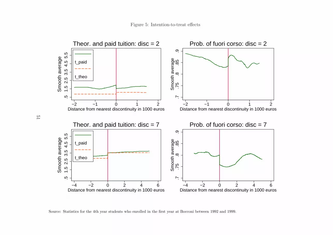
Figure 5: Intention-to-treat effects

.51.

52.

53.

54.

55.

5

−2 −1 0 1 2Distance from nearest discontinuity in 1000 euros

t_paid

t_theo

Sm

ooth

ave

rage

Theor. and paid tuition: disc = 2

.7.7

5.8

.85

.9S

moo

th a

vera

ge

−2 −1 0 1 2Distance from nearest discontinuity in 1000 euros

Prob. of fuori corso: disc = 2

.51.

52.

53.

54.

55.

5

−4 −2 0 2 4 6Distance from nearest discontinuity in 1000 euros

t_paid

t_theo

Sm

ooth

ave

rage

Theor. and paid tuition: disc = 7

.7.7

5.8

.85

.9S

moo

th a

vera

ge

−4 −2 0 2 4 6Distance from nearest discontinuity in 1000 euros

Prob. of fuori corso: disc = 7

Source: Statistics for the 4th year students who enrolled in the first year at Bocconi between 1992 and 1999.

51

Figure 6: Evidence on sorting and continuity conditions

1020

30S

moo

th a

vera

ge

−2 −1 0 1 2Distance from nearest discontinuity in 1000 euros

Pre−Bocconi income: disc=2

.7.7

5.8

.85

.9S

moo

th a

vera

ge

−2 −1 0 1 2Distance from nearest discontinuity in 1000 euros

Highschool grade: disc= 2

3040

50S

moo

th a

vera

ge

−4 −2 0 2 4 6Distance from nearest discontinuity in 1000 euros

Pre−Bocconi income: disc=7

.7.7

5.8

.85

.9S

moo

th a

vera

ge

−4 −2 0 2 4 6Distance from nearest discontinuity in 1000 euros

Highschool grade: disc= 7

Source: Statistics for the 4th year students who enrolled in the first year at Bocconi between 1992 and 1999.

52

Table 7: Regression discontinuity estimates of the effect of tuition on the probability of late graduation (Fuori corso)

Method OLS-ITT OLS-ITT OLS IV-LATE N. of obs.Outcome Paid Tuition Fuori Corso Fuori Corso Fuori CorsoTreatment Paid Tuition Paid TuitionInstrument Theoretical Tuition Theoretical Tuition Theoretical Tuition

Discontinuity 1 -2.5 .42 -.0086 -.17 1376s.e. (2.2) (.54) (.007) (.26)Discontinuity 2 -2.4 .21 .0047 -.088 463s.e. (1.5) (.37) (.011) (.16)Discontinuity 3 .64 -.13 -.012 -.2 563s.e. (1.2) (.31) (.013) (.59)Discontinuity 4 .51 .17 -.0058 .33 636s.e. (.64) (.17) (.01) (.54)Discontinuity 5 -.4 -.2 .017 .5 742s.e. (.54) (.14) (.01) (.77)Discontinuity 6 .52 -.078 .0063 -.15 961s.e. (.41) (.11) (.01) (.25)Discontinuity 7 .11 -.06 .011 -.56 1331s.e. (.25) (.10) (.01) (1.6)Discontinuity 8 .38 -.07 .017 -.19 1453s.e. (.14) (.076) (.014) (.21)Discontinuity 9 .24 -.022 .027 -.095 957s.e. (.12) (.09) (.02) (.38)Discontinuity 10 .57 .11 .046 .2 1734s.e. (.12) (.09) (.022) (.17)All .59 -.036 .0021 -.061 10216s.e. (.05) (.018) (.004) (.031)

Note: Each coefficient (and related robust standard error in parenthesis) is an estimate of β obtained from separate regressions of theform:

W = g(Y ) + βτK + γt + ε

where W is the tuition actually paid τp in column 1 and the Fuori Corso status F in the other columns; τk is the theoretical tuitionτ t in column 1 and 2, and the tuition actually paid τp in column 3 and 4. Estimates in columns 1,2 and 3 are obtained with OLS; incolumn 4 with IV using τ t as an instrument for τp. γt are time dummies.Source: Statistics for the 4th year students who enrolled in the first year at Bocconi between 1992 and 1999.

53

Table 8: Tests for the presence of sorting and for the validity of the continuity conditions

Method OLS-ITT OLS IV-LATE N. of obs.Treatment Paid Tuition Paid TuitionInstrument Theoretical Tuition Theoretical Tuition

Income before Bocconi .38 .75 .66 9800( .46) ( .11) (.81)

Highschool grade .0019 -.013 .0032 10216( .0048) ( .00096) (.0082)

Highschool type -.032 .029 -.055 10216( .02) ( .0042) ( .034)

Family of origin outside Milan -.025 -.017 -.042 10216( .022) ( .0041) ( .038)

GPA in first year at Bocconi -.0024 -.0075 -.0041 10153( .0033) ( .00066) ( .0057)

Female .029 -.0068 .05 10216( .022) ( .0044) ( .038)

Note: Each coefficient (and related robust standard error in parenthesis) is an estimate of β obtained from separate regressions of theform:

S = g(Y ) + βτK + γt + ε

where S is the pre-intervention outcome indicated in the corresponding row of the table; τk is the theoretical tuition τ t in column 1 andthe tuition actually paid τp in column 2 and 3. Estimates in columns 1 and 2 are obtained with OLS; in column 3 with IV using τ t asan instrument for τp. γt are time dummies.Source: Statistics for the 4th year students who enrolled in the first year at Bocconi between 1992 and 1999.

54

Figure 7: A test of monotonicity: CDF crossing

For each discontinuity the figure plots the estimated difference between the cdf of the tuition actually paid by students in a leftneighbourhood of the cut-off point and the corresponding cdf paid by students in a right neighbourhood. 0.95 confidence intervals areplotted as well. The left (right) neighbourhood is defined selecting students whose family income is below (above) the cut-off point byno more than 500 euro.Source: Statistics for the 4th year students who enrolled in the first year at Bocconi between 1992 and 1999.

55

Table 9: Test for the equality of the IV estimand Λ(yj) at different discontinuity thresholds

Method OLS-ITT OLS IV-LATEOutcome Fuori Corso Fuori Corso Fuori CorsoTreatment Theoretical Tuition Paid Tuition Paid TuitionInstrument Theoretical Tuition

IV estimand Λ(yj) -0.065 -0.008 -0.090at the discontinuities (0.027) (0.005) (0.036)1 2 and 3

Deviation of the 0.019 0.016 0.015IV estimand Λ(yj) (0.016) (0.006) (0.013)at the discontinuities4, 5, 6 and 7

Deviation of the 0.013 0.017 0.014IV estimand Λ(yj) (0.018) (0.007) (0.015)at the discontinuities8, 9 and 10

Note: The rows of the table report respectively the coefficients β1,3 β4,7 and β8,10 of the regression

F = g(Y ) + β1,3τKD1,3 + β4,7τ

KD4,7 + β8,10τKD8,10 + γt + ε

where F is the Fuori Corso status; the dummies Di,j denote the discontinuity thresholds from i to j; τk is the theoretical tuition τ t incolumn 1, and the tuition actually paid τp in column 2 and 3. Estimates in columns 1 and 2 are obtained with OLS; in column 3 withIV using τ t as an instrument for τp. γt are time dummies.Source: Statistics for the 4th year students who enrolled in the first year at Bocconi between 1992 and 1999.

56

Table 10: Effect of tuition on on dropout rates and final graduation marks

Method OLS-ITT OLS IV-LATE N. of obs.Treatment Paid Tuition Paid TuitionInstrument Theoretical Tuition Theoretical Tuition

Drop-out -.006 -.004 -.010 10212(.008) (.002) (.013)

Final graduation mark -.29 -.83 -.46 9206(min= 66; max= 110) (.33) (.06) (.52)

Note: Each coefficient (and related robust standard error in parenthesis) is an estimate of β obtained from separate regressions of theform:

W = g(Y ) + βτK + γt + ε

where W is a dummy for dropping out in top panel and the final graduation mark ranging between 66 and 110 (111 in case of honors)with a standard deviation of 7 points in the bottom panel; τk is the theoretical tuition τ t in column 1, and the tuition actually paid τp

in column 2 and 3. Estimates in columns 1 and 2 are obtained with OLS; in column 3 with IV using τ t as an instrument for τp. γt aretime dummies.Source: Statistics for the 4th year students who enrolled in the first year at Bocconi between 1992 and 1999. The smaller sample size inthe bottom panel originates from the fact that 1010 studens had not graduated yet by 2004, when we received the data from Bocconi.

57