ARTICLE IN PRESS

European Journal of Operational Research xxx (2004) xxx–xxx

www.elsevier.com/locate/dsw

Production, Manufacturing and Logistics

Evaluation of time-varying availability in multi-echelonspare parts systems with passivation

Hoong Chuin Lau a,*, Huawei Song a, Chuen Teck See b, Siew Yen Cheng b

a The Logistics Institute––Asia Pacific, National University of Singapore, Singapore 119260b Defense Science and Technology Agency, Singapore Ministry of Defense, Singapore 109679

Received 17 October 2003; accepted 28 June 2004

Abstract

The popular models for repairable item inventory, both in the literature as well as practical applications, assume thatthe demands for items are independent of the number of working systems. However this assumption can introduce aserious underestimation of availability when the number of working systems is small, the failure rate is high or therepair time is long. In this paper, we study a multi-echelon repairable item inventory system under the phenomenonof passivation, i.e. serviceable items are passivated (‘‘switched off’’) upon system failure. This work is motivated by cor-rective maintenance of high-cost technical equipment in the miltary. We propose an efficient approximation model tocompute time-varying availability. Experiments show that our analytical model agrees well with Monte Carlosimulation.� 2004 Published by Elsevier B.V.

Keywords: Inventory; Maintenance; Multi-echelon; Passivation

1. Introduction

Miltary systems such as aircrafts, ships or tanks are expensive and have complex structures that breakdown because the underlying components (line replacable units or LRUs) are either worn out over timeand/or damaged during usage. One way to achieve high-operational readiness (or availability) is to acquireenough spare parts to provide immediate replacement of damaged components. However, since spares arecostly, consume space and become obsolete over time, there is a need to tradeoff the cost of spares withavailability. Logistics planners in the miltary often need to plan for spares according to time-varying

0377-2217/$ - see front matter � 2004 Published by Elsevier B.V.doi:10.1016/j.ejor.2004.06.022

* Corresponding author. Tel.: +65 9767 2913; fax: +65 6872 3072.E-mail address: lauhc@comp.nus.edu.sg (H.C. Lau).

2 H.C. Lau et al. / European Journal of Operational Research xxx (2004) xxx–xxx

ARTICLE IN PRESS

demands, since the utilization rate varies over time. This is known generally as the spares provisioningproblem for corrective maintenance.In almost all existing literature, it is assumed that the demand for LRUs does not depend on the number

of working systems, which means that the LRUs within a system fail independently of each other. Howeverin many situations, it is observed that when an LRU fails, it will affect the demand of the other LRUs with-in the same system. When a system fails, the failed LRU is transported to a repair shop and all the remain-ing system LRUs are switched off to maximise component life, which implies that there is no demand ofthose LRUs until the system has been restored. In other words, the system failure rate equals 0 during re-pair (as explained in [4]). This phenomenon is called passivation.While the assumption of independent demands produces good analytical results for most problems,

availability is seriously understated in scenarios when the number of working systems is small, the failurerate high and repair time long. For example, in [13], EBO (expected backorder) is overestimated by 37.3%without passivation, which cause the availability to be underestimated. In this paper, we study the effect ofpassivation on system availability in these settings. We are concerned with a multi-echelon single-indenturerepairable item inventory model. In this paper, we use the term ‘‘technical system’’ to generally denote amiltary equipment such as an aircraft, ship or tank.This paper is organized as follows. In Section 2, we describe the logistic system structure (based on

assumptions that are also widely accepted in the literature) and the different demand scenarios. A literaturesurvey is provided in Section 3. In Section 4, we develop a mathematical model for the system in terms of asingle-item. In Section 5, we derive the equations which are used in Section 4 based on a dynamic form ofPalm�s theorem. Section 6 shows how to extend the analysis to multiple items so as to compute availabilityunder passivation of a system that comprises a number of items. In Section 7, some experiments are pre-sented to illustrate the effect on availability when passivation is considered. Section 8 concludes the paper.

2. Preliminaries

2.1. Logistic support structure

The literature typically discusses a 2-echelon support structure for illustration except [14]. Although theunderlying principles are the same, the computational gap between 2-echelon and more than 2-echelons isquite substantial. We hence show our approach using 3-echelon structure as an example (see Fig. 1). Ourapproach can be extended easily to 4 echelons and beyond.In the above example, one depot supports a number of repair sites called intermediate site which sup-

ports a number of units where the technical systems are deployed. All the technical systems are identicaland each technical system is composed of multiple LRUs that are connected in series.

Depot

IntermediateSite

IntermediateSite

Unit Unit Unit Unit Unit Unit

Fig. 1. 3-Echelon structure.

H.C. Lau et al. / European Journal of Operational Research xxx (2004) xxx–xxx 3

ARTICLE IN PRESS

Depending on the nature of fault, the repair will occur on-site immediately if the fault can be rectified atthe unit. Otherwise it will be sent to the intermediate site and an order is placed by the unit to be suppliedfrom the intermediate site. If the LRU cannot be repaired at the intermediate site, it will be sent to the depotand an order is placed by the intermediate site. At the unit, the failed LRU will be removed and replaced bya good component should one be available, and the system becomes serviceable after a short delay, the timeto remove and replace the failed LRU. Otherwise, a backorder is generated and the failed system has to waitfor a spare part to arrive. When repair is completed, the working LRU will be sent to its originating supportsite or unit to function as spares. In either case, the organization does so by supplying a serviceable item fora failed item on a one-for-one basis. Underlying assumptions are presented as follows, most of which arealso accepted in the literature.In this paper, we make the following assumptions:

1. There are infinite repair resources, i.e. a failed system can be repaired at once.2. All LRUs are repairable at the depot, i.e. there is no irrepairable item.3. Continuous resupply, i.e. an LRU can be sent up or down the echelon immediately at any time. Thetransport time for each item between two sites is a constant.

4. FCFS (first come first serve) replenishment policy.5. The remove-and-replace time for each item follows an exponential distribution.6. The repair time for each item follows an exponential distribution.7. No lateral supply, i.e. no supply or shipment across sites within the same echelon.

2.2. Demands

The item demand rate is determined by the mean time between failures MTBF (i.e. the expected value oftime duration between two consecutive failures) and the utilization rate UR (i.e. the usage rate of the item).In the stationary-demand problem, we assume the utilization rate for each item is identical over the en-

tire time horizon. Given the number of technical systems deployed at unit Nsys, the following formula isconventionally used to compute the demand rate DR:

DR ¼ UR

MTBF�Nsys: ð1Þ

In the case of time-varying demand, we assume the utilization rate for each item is a time-dependent piece-wise constant function, i.e. the demand for an LRU is given by a non-stationary Poisson process. Given thetime-varying utilization rate UR(t), the following formula is adopted to compute the time-varying demandrate DR(t):

DRðtÞ ¼ URðtÞMTBF

�Nsys: ð2Þ

2.3. Passivation

Due to the effect of passivation, the actual demand rate is dependent on the number of working systems,which changes over time. Hence, even for the stationary problem, the actual demand rate varies with time.Henceforth in this paper, we will only consider the time-varying demands problem under passivation.

4 H.C. Lau et al. / European Journal of Operational Research xxx (2004) xxx–xxx

ARTICLE IN PRESS

Clearly, by setting UR(t) � UR for all t, we can easily handle stationary demands problem as well. LetNsys(t) be the number of available technical systems at time t, the actual time-varying demand rate is com-puted as follows:

DRðtÞ ¼ URðtÞMTBF

�NsysðtÞ: ð3Þ

The computation of Nsys(t) will be discussed in Section 4.Since the demand for an LRU is given by a time-dependent Poisson process, the objective function is

inevitably time-dependent. In this paper, we use the conventional EBO (expected backorder) and Ao (oper-ational availability) as our objective functions. Instead of computing EBO and Ao under steady statepresented in the literature, we will compute EBO and Ao at each time point, thereby capturing the time-varying behavior of the objective functions. Aside from this, we will show how to derive Ao from EBOunder the time-varying scenario.The key result of this paper is an evaluation scheme that, given an allocation of spares at time 0 for each

site in the multi-echelon support structure, efficiently computes EBO and Ao at each time point over a giventime horizon, taking into consideration non-stationary demands and the effects of passivation.

3. Literature survey

METRIC (multi-echelon technique for recoverable item control) is a pioneer study for multi-echelon,single-indenture and multi-repairable-item optimization models presented by Sherbrooke in [18]. In MET-RIC, one central repair site (depot) supports multiple bases where aircrafts are allocated. It assumes thatthere are infinite repair resources at the depot and the failures at bases are Poisson processes. Sherbrookeprovides an optimization procedure for METRIC by employing marginal analysis.METRIC is only an approximation and during its implementation, it was found that expected number

of backorders was underestimated. In [8], Graves proposes an approach to use negative binomial distribu-tion instead of Poisson by introducing variance. This is because the variance-to-mean ratio should be 1 un-der Poisson distribution, but it is usually greater than 1 in practice. Graves produces some test cases andfinds his method achieves higher accuracy than METRIC.The models with limited repair facility have been studied recently because the assumption of infinite

repair facility is unrealistic in industrial applications. In [6], Dı́az and Fu develop a multi-echelon, sin-gle-indenture model, considering limited repair facilities (servers) at the depot where all failed LRUs arerepaired. They provide an aggregation–disaggregation approach, trying to calculate the first two momentsof per-class number in queue and repair under steady state. Unfortunately the variance of per-class numberin queue and repair is derived only for single-server multi-class queuing model due to analytical complexity.In [1,2], Alfredsson proposes OPRAL, a model for optimum spare allocation as well as repair facility

allocation. This model is an offshoot of the commercial software OPUS developed by Systecon AB[15,16]. In his model, it is assumed that each failed LRU requires only one repair resource. Different LRUsmay share a common repair resource. This assumption implies that LRUs can be partitioned into resourcegroups, each of which contains the LRUs that require a particular resource. Therefore, the queue in a re-source group at the repair facility is modelled as M/M/s so that the expected waiting time for an availableresource can be calculated.As far as inventory systems on time-varying demands are concerned, there are two influential works. In

[12], Jung presents a methodology for a repairable inventory system with time-varying demand by imple-menting discrete event simulation. In [21], Slay et al. propose an aircraft sustainability model that canhandle time-varying demand rates but infinite repair resources. The failure at the base is given by a non-

H.C. Lau et al. / European Journal of Operational Research xxx (2004) xxx–xxx 5

ARTICLE IN PRESS

stationary Poisson process whose mean value varies with time. It investigates the objective function andspare allocation only at specific times of interest.

4. Mathematical model

4.1. Notations

In this section, we present a mathematical model for the system in terms of a single-item. This model isapplicable to each item of the system consisting of a number of items. In Section 6, we will show how tocompute the time-varying availability of the multi-item system under passivation by combining the per-formances of all items it has. We adopt and extend the notations of those in [1]. As shown in Fig. 1, thereis one depot supporting multiple intermediate sites. We use 0 to denote the depot and index the interme-diate sites by i, i = 1, . . ., I. Each intermediate site supports multiple units which are indexed by u,u = 1, . . .,U. And we use Ui � f1; . . . ;Ug to denote the units supported by intermediate site i. Given anytwo site i and j, we will use i = q(j) to denote the relationship that site i supports site j.As done in [1], the types of LRU are indexed by k, k = 1, . . .,K. Other notations which are consistent

with those used in OPUS and Dyna-METRIC [9,10,15,16] include

Input variables

T the length of planning horizon;MTBFk mean time between failures of LRU k;TATU

uk mean repair time of LRU k at unit u;TATI

ik mean repair time of LRU k at intermediate site i;TAT0k mean repair time of LRU k at the depot;TPTU

uk transport time of LRU k between unit u and its supporting intermediate site;TPTI

ik transport time of LRU k between intermediate site i and the depot;MTTRuk mean time to remove and replace of LRU k at unit u;NRTSUuk the probability that LRU k cannot be repaired at unit u;NRTSIik the probability that LRU k cannot be repaired at intermediate site i;Nsysu number of technical systems deployed at unit u;QPMk quantity of LRU k that technical system has;UR(t) utilization rate at time t;sUuk number of spares of LRU k at unit u;sIik number of spares of LRU k at intermediate site i;s0k number of spares of LRU k at the depot.

Intermediate variables

DRUukðtÞ incoming demand rate of LRU k at unit u at time t;

DRIikðtÞ incoming demand rate of LRU k at intermediate site i at time t;

DR0k(t) incoming demand rate of LRU k at the depot at time t;kUukðtÞ effective demand rate of LRU k at unit u at time t;kIikðtÞ effective demand rate of LRU k at intermediate site i at time t;k0k(t) effective demand rate of LRU k at the depot at time t, which is equal to the incoming demand

rate at the depot in our case;EBOU

ukðtÞ EBO of LRU k at unit u at time t;EBOI

ikðtÞ EBO of LRU k at intermediate site i at time t;EBO0k(t) EBO of LRU k at the depot at time t.

6 H.C. Lau et al. / European Journal of Operational Research xxx (2004) xxx–xxx

ARTICLE IN PRESS

Decision variable

Aou(t) operational availability of the systems at unit u at time t.

4.2. Time-varying EBO function

With considering passivation, we first divide the time horizon into n periods, which are indexed by t,t = 1, . . .,n, so that (a) the utilization rate in each period is constant and (b) the number of ‘‘up’’ technicalsystems can be regarded as constant, not varying as time in each period.It is obvious that EBO(0) = 0 for all stock positions and Ao(0) = 100%. For t(P1), the incoming de-

mand rate of LRU k at unit u at time t with considering passivation is

DRUukðtÞ ¼

URðtÞMTBFk

�QPMk �Nsysu �Aouðt 1Þ: ð4Þ

So,

kUukðtÞ ¼ ð1NRTSUukÞDRU

ukðtÞ; ð5Þ

DRIikðtÞ ¼

Xu2Ui

NRTSUuk �DRUukðtÞ; ð6Þ

kIikðtÞ ¼ ð1NRTSIikÞDR

IikðtÞ; ð7Þ

k0kðtÞ ¼ DR0kðtÞ ¼XI

i¼1NRTSIik �DRI

ikðtÞ: ð8Þ

The following are intermediate variables for the purpose of computation.

PUukðtÞ random variable representing number of LRU k in the pipeline of unit u at time t;PIikðtÞ random variable representing number of LRU k in the pipeline of intermediate site i at time t;P0k(t) random variable representing number of LRU k in the pipeline of the depot at time t;RPU

ukðtÞ random variable representing number of LRU k in the repair pipeline of unit u at time t;RPI

ikðtÞ random variable representing number of LRU k in the repair pipeline of intermediate site i attime t;

RP0k(t) random variable representing number of LRU k in the repair pipeline of the depot at time t;OSPU

ukðtÞ random variable representing number of LRU k in the order-and-ship pipeline to unit u at time t;OSPI

ikðtÞ random variable representing number of LRU k in the order-and-ship pipeline to intermediatesite i at time t;

f Uuk ðtÞ fraction of LRU k at unit u contributing to the EBO at its supporting site;f IikðtÞ fraction of LRU k at intermediate site i contributing to the EBO at the depot.

In addition, we will use EBO(sjk) to denote EBO given stock level s when the mean pipeline is k. Fol-lowing standard probability, this quantity is computed as

Px>sðx sÞPrfX ¼ xg where X is the pipeline

random variable with mean E[X] = k.Then we have

EBO0kðtÞ ¼ EBO0kðs0kjE½P0kðtÞ Þ ¼Xx>s0k

ðx s0kÞPrfP0kðtÞ ¼ xg; ð9Þ

where E[P0k(t)] = E[RP0k(t)].

H.C. Lau et al. / European Journal of Operational Research xxx (2004) xxx–xxx 7

ARTICLE IN PRESS

EBOIikðtÞ ¼ EBOI

ikðsIikjE½PIikðtÞ Þ; ð10Þ

where

E½PIikðtÞ ¼ E½RPI

ikðtÞ þ E½OSPIikðtÞ þ f I

ikðt TPTIikÞEBO0kðt TPTI

ikÞ; ð11Þ

EBOUukðtÞ ¼ EBOU

ukðsUukjE½PUukðtÞ Þ; ð12Þ

where

E½PUukðtÞ ¼ E½RPU

ukðtÞ þ E½OSPUukðtÞ þ f U

uk ðt TPTUukÞEBO

Iikðt TPTU

ukÞ: ð13Þ

In the following section, we will provide the details on how the above formulae can be computed andimplemented.

5. Derivation of intermediate variables

Under the assumption that the number of items in the pipeline follows a Poisson distribution, the ex-pected number of demands in the pipeline at time t can be computed by a dynamic form of Palm�s theorem.Carrillo [5] presents a generalization of Palm�s theorem by relaxing the input process and service time dis-tribution assumptions.

Theorem 1 (Carrillo [5]). Suppose we have non-homogeneous Poisson input with intensity function k(t) P 0

for t P 0, k(t) = 0 otherwise, and non-stationary service distribution G. Then, the number of arrivals

undergoing service at time t has a Poisson distribution with mean

KðtÞ ¼Z t

0

ð1 Gðs; tÞÞkðsÞds; ð14Þ

where the random service time Y at time t has the distribution P[Y 6 y] = G(t, t + y).

From the assumption of constant transport time, it is easy to know that the number of LRUs in theorder-and-ship pipeline follows a Poisson distribution by Theorem 1 and we can get its mean value asfollows:

E½OSPIikðtÞ ¼

Z t

tTPTIik

NRTSIik �DRIikðsÞds; ð15Þ

E½OSPUukðtÞ ¼

Z t

tTPTUuk

NRTSUuk �DRUukðsÞds: ð16Þ

According to the assumption that the transport time is constant whereas repair time is exponentially dis-tributed, we have to consider the two processes as a whole to compute the expected pipelines. We use repairpipeline to indicate the number of LRUs in retrograde process and repair service. Based on Theorem 1, weassume the repair time X is exponentially distributed with mean 1/l = TAT and the transport time is L,which is constant. So the service time is Y = X + L(Y P L) and the service distribution is

Gðs; tÞ ¼ PrfY 6 t sg ¼ PrfX þ L 6 t sg ¼ PrfX 6 t s Lg ¼ 1 elðtsLÞþ :

So

KðtÞ ¼Z t

0

kðsÞelðtsLÞþ ds: ð17Þ

8 H.C. Lau et al. / European Journal of Operational Research xxx (2004) xxx–xxx

ARTICLE IN PRESS

When demand rate is constant i.e. k(t) � k, and t! 1 which is the scenario in METRIC, we can show theresult of mean pipeline is the same as METRIC as follows:

K ¼ limt!1

Z t

tLkdsþ lim

t!1

Z tL

0

kelðtsLÞ ds ¼ kLþ kTAT ¼ kðLþ TATÞ:

Therefore according to the above conclusion, we can compute the expected number of LRUs in the repairpipeline as follows:

E½RPUukðtÞ ¼

Z t

0

kUukðtÞe

1TATU

uk

ðtsÞds; ð18Þ

E½RPIikðtÞ ¼

Xu2Ui

Z t

0

ð1NRTSIikÞNRTSUukDR

UukðsÞe

1TATI

ik

ðtsTPTUukÞ

þ

ds; ð19Þ

E½RP0kðtÞ ¼Xu

Z t

0

NRTSIqðuÞkNRTSUukDR

UukðsÞe

1TAT0k

ðtsTPTIqðuÞkTPT

UukÞ

þds: ð20Þ

Now we will show how to distribute EBO at the supporting site to its supported sites. Since we assume FCFSreplenishment policy, the waiting time for an available spare from the supporting site of all supported sitesare the same. Therefore, we distribute EBO according to the proportion of demand rate. Given any two sites

i, j that i = q(j), we set fjkðtÞ ¼ NRTSjk�DRjkðtÞDRikðtÞ . Unfortunately, this direct approach is incorrect under passiva-

tion. This is because when an LRU fails, the whole technical system is down, which causes no demand ofother LRUs on it. Hence, we need not compute the demand due to this system. However, it still contributesto the EBO since and as long as it is down. In order to compute the fraction, we introduce some variables.

KUukðtÞ incoming demand rate of LRU k at unit u at time t without passivation;

KIikðtÞ incoming demand rate of LRU k at intermediate site i at time t without passivation;

K0k(t) incoming demand rate of LRU k at the depot at time t without passivation.

We have

KUukðtÞ ¼

URuðtÞMTBFk

�QPMk �Nsysu; ð21Þ

KIikðtÞ ¼

Xu2Ui

NRTSUuk � KUukðtÞ; ð22Þ

K0kðtÞ ¼XI

i¼1NRTSIik � KI

ikðtÞ: ð23Þ

So, the fraction

f IikðtÞ ¼

NRTSIik � KIikðtÞ

K0kðtÞ; ð24Þ

f Uuk ðtÞ ¼

NRTSUuk � KUukðtÞ

KIqðuÞkðtÞ

: ð25Þ

At last, we can compute EBO based on the stock level according to Eqs. (9)–(13).

H.C. Lau et al. / European Journal of Operational Research xxx (2004) xxx–xxx 9

ARTICLE IN PRESS

6. Conversion of EBO into Ao

In [20], Sherbrooke puts forward a variety of availabilities and corresponding formulas. Operationalavailability (Ao) is one of the most important availabilities, which is widely used in practice. In [20], theformula used is:

Ao ¼ MTBF

MTBFþMTTR þWT¼ 1

1þ MTTRMTBF

þ EBO: ð26Þ

The following is one variation of the formula:

Ao ¼ 1

1þPk

EBOkNsys

þ URMTBFk

�QPMk �MTTRk

� � : ð27Þ

This formula suffers several limitations. First, we can only compute Ao under steady state by this formula.We cannot compute Ao in the transient periods even though the demand is given by constant Poisson proc-ess. In most cases such as ours, the demand is given by a non-stationary Poisson process, which may causethe system never to converge to steady state. Secondly, we need to compute the waiting time. While it is wellknown that the waiting time WT ¼ EBO

k by Little�s Law, it is not obvious how to compute waiting time un-der the non-stationary demands case. Experiments show that it does not readily translate to WTðtÞ ¼ EBOðtÞ

kðtÞ .

In a recent paper [17], the authors provide a formula to compute Ao at time t based on an extension of [3].Unfortunately their approach is very time-consuming.

6.1. Intuitive model

We first look at an intuitive model to compute Ao at any time under both stationary and non-stationarydemand cases. The Ao discussed in this section is always within a given unit so that the subscript u is omit-ted. The proposed formula is a recursive formulation, defined as follows:

AoðtÞ ¼ 1

1þPKk¼1

EBOkðtÞNsysðtÞ þ

URðtÞMTBFk

�QPMk �MTTRk

� � ; ð28Þ

where NsysðtÞ ¼ NsysPK

k¼1EBOkðt 1Þ.With this formulation, we can compute EBO and Ao at any unit at any time point t using values de-

rived in time point t 1. This means that we can implement the computation iteratively from one periodto the next. We will compare the results with those of simulation in the next section. Experimental resultsshow our approach yields solutions that match simulation results very well within short computationaltime.

6.2. Proposed model

Although the intuitive model works well in general, it does not produce good results for the case whenthe MTTR is large (see Fig. 4). In the following, we propose a revised model to better approximateavailability.If the demand process is a simple Poisson process with mean k and the service time is exponentially dis-

tributed with mean 1/l, the time-varying availability is given by (see for example, [11])

10 H.C. Lau et al. / European Journal of Operational Research xxx (2004) xxx–xxx

ARTICLE IN PRESS

AðtÞ ¼ lk þ l

þ Að0Þ lk þ l

� �eðkþlÞt: ð29Þ

By setting l = 1/MTTR, the availability is maintenance availability (Am) [20]. We know k ¼ URMTBF=QPM

, sowe can compute maintenance availability at any time by Eq. (29). For the scenario that demand is given bya non-stationary Poisson process, we can show

Amðt2Þ ¼l

kðt2Þ þ lþ Amðt1Þ

lkðt2Þ þ l

� �eðkðt2ÞþlÞðt2t1Þ; ð30Þ

where kðt2Þ ¼ URðt2ÞMTBF=QPM

and Am(0) = 100%.

With this formulation, we can compute Am at any time point iteratively from one period to the next.According to [20], the operational availability can be computed as the product of supply availability (As)

and maintenance availability (Am) where

Am ¼ 1

1þ URMTBF=QPM

�MTTR: ð31Þ

We notice URMTBF=QPM

�MTTR is just the right part of the denominator of Eq. (28). Replacing it with 1Am

1,we can get the formula to compute operational availability at any time for both small MTTR and largeMTTR under both stationary and non-stationary demand cases. The formula is defined as follows:

AoðtÞ ¼ 1

1þPKk¼1

EBOkðtÞNsysðtÞ þ 1

AmkðtÞ 1� � ; ð32Þ

where Amk(t) can be computed according to Eq. (30). Experiment (see Fig. 5) shows our approach matchessimulation results well.

7. Experimental results

In our experiments, we consider a multi-echelon problem where each technical system comprises morethan 50 LRUs. The following two sets of experiments have been conducted:

1. Steady-state Ao computation given a single-spares allocation against METRIC model [16].2. Time-varying demands against Monte-Carlo simulation [7].

The experiments were conducted on a Pentium III 1.2 GHz machine with 512 MB RAM. In all simu-lation models, we set the number of replications to be 1000 which is a fairly standard practice in simulationexperimentation.

7.1. Steady-state Ao without passivation

First, we verify that our model also works under steady state without passivation. In these experiments,we consider a 5-system problem and compute their operational availability under steady state given a fixedspare allocation. We compare the results against the results obtained by METRIC by setting the probabilitydistribution of the pipeline to be Poisson. The average run time per test case is 0.16 s.The following tables give a summary of the results.From Tables 1 and 2, we observe that our results are exactly the same as METRIC.

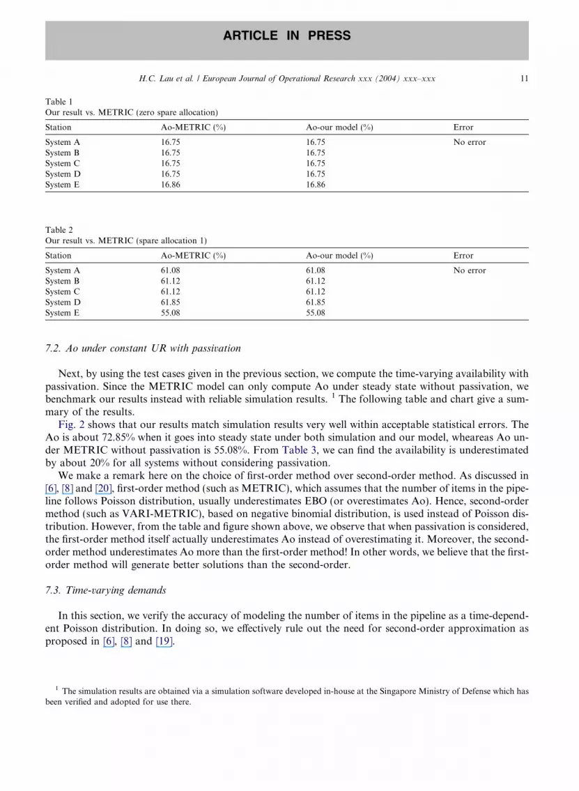
Table 1Our result vs. METRIC (zero spare allocation)

Station Ao-METRIC (%) Ao-our model (%) Error

System A 16.75 16.75 No errorSystem B 16.75 16.75System C 16.75 16.75System D 16.75 16.75System E 16.86 16.86

Table 2Our result vs. METRIC (spare allocation 1)

Station Ao-METRIC (%) Ao-our model (%) Error

System A 61.08 61.08 No errorSystem B 61.12 61.12System C 61.12 61.12System D 61.85 61.85System E 55.08 55.08

H.C. Lau et al. / European Journal of Operational Research xxx (2004) xxx–xxx 11

ARTICLE IN PRESS

7.2. Ao under constant UR with passivation

Next, by using the test cases given in the previous section, we compute the time-varying availability withpassivation. Since the METRIC model can only compute Ao under steady state without passivation, webenchmark our results instead with reliable simulation results. 1 The following table and chart give a sum-mary of the results.Fig. 2 shows that our results match simulation results very well within acceptable statistical errors. The

Ao is about 72.85% when it goes into steady state under both simulation and our model, wheareas Ao un-der METRIC without passivation is 55.08%. From Table 3, we can find the availability is underestimatedby about 20% for all systems without considering passivation.We make a remark here on the choice of first-order method over second-order method. As discussed in

[6], [8] and [20], first-order method (such as METRIC), which assumes that the number of items in the pipe-line follows Poisson distribution, usually underestimates EBO (or overestimates Ao). Hence, second-ordermethod (such as VARI-METRIC), based on negative binomial distribution, is used instead of Poisson dis-tribution. However, from the table and figure shown above, we observe that when passivation is considered,the first-order method itself actually underestimates Ao instead of overestimating it. Moreover, the second-order method underestimates Ao more than the first-order method! In other words, we believe that the first-order method will generate better solutions than the second-order.

7.3. Time-varying demands

In this section, we verify the accuracy of modeling the number of items in the pipeline as a time-depend-ent Poisson distribution. In doing so, we effectively rule out the need for second-order approximation asproposed in [6], [8] and [19].

1 The simulation results are obtained via a simulation software developed in-house at the Singapore Ministry of Defense which hasbeen verified and adopted for use there.

Fig. 2. The effect of passivation (System E given spare allocation 1).

Table 3Ao with passivation vs. without passivation (spare allocation 1)

Station Ao–passivation (%) Ao–no passivation (%) Error (%)

System A 76.50 61.08 20.16System B 76.56 61.12 20.17System C 76.56 61.12 20.17System D 76.72 61.85 19.3System E 72.85 55.08 24.39

12 H.C. Lau et al. / European Journal of Operational Research xxx (2004) xxx–xxx

ARTICLE IN PRESS

In these experiments, we run the test cases with time-varying utilization rate (UR) and compare the re-sults (Ao) against simulation results. The utilization rate is given as follows for all systems at all units: (time0–1500), 0.08 (time 1500–2000), 0.6 (time 2000–2500), 0.3333 (time 2500–3000), 0.5 (time 3000–3500) and0.25 (time 3500–4000) and the following chart gives a summary of the results.From Fig. 3 we can see that our results match those produced by simulation with less than 0.1% absolute

error on average. We also ran the test cases with other spare allocations and achieved results that matchsimulation results very well.

Fig. 3. Our result vs. simulation (time-varying Ao at unit).

H.C. Lau et al. / European Journal of Operational Research xxx (2004) xxx–xxx 13

ARTICLE IN PRESS

7.4. The effect of passivation over varying availabilities

Next, we obtain some results using the previous test cases to study the effect of passivation over a rangeof availability values. The results are shown in Table 4.From Table 4, we observe that (1) the model without passivation always underestimates availability; and

(2) the effect of passivation (i.e. the absolute value of relative error) will increase to a certain peak and thendecrease as availability increases. The phenomenon can be explained as follows. As discussed before, avail-ability is seriously underestimated when the number of working systems is small, the failure rate is highand/or the repair time is long. Hence, when the availability is high such as 95.21%, the number of workingsystems can be regarded as large (since the down systems can be restored quickly with enough spares) andhence the effect of passivation is not keenly felt. On the opposite extreme, when availability is low such as16.78%, the spares are equal or near to zero, thus mitigating the effects of passivation. In all other cases, thenumber of working systems varies frequently as time and hence the effect of passivation is significantly felt.We also measure the effect of passivation as parameters using the examples cited in [13]. Table 5 gives a

summary of the results.From Table 5, we observe that compared with the base case (Test 1), the effect of passivation will be

large when the number of system is small (Test 2), the availability is low with few spares (Test 3), the repairtime is long (Tests 5 & 6), and the failure rate is high (Test 8). Furthermore, we also notice that when thespares are zero, the effect of passivation is trivial (Tests 4 & 7).

7.5. The effect of large MTTR

Finally, we run test cases with large MTTR and compare results against simulation. In this case, MTTRis set to be 300 hour while the MTBF is 500. There are infinite spares and utilization rate varies with time at

Table 4The effect of passivation as Ao

Ao–passivation (%) Ao–no passivation (%) Error (%)

16.78 16.76 0.1227.84 25.13 9.7338.85 35.90 7.5957.51 45.50 20.8865.02 56.09 13.7370.73 65.58 7.2879.60 75.47 5.1987.86 85.94 2.1995.21 95.03 0.19

Table 5The effect of passivation as parameters

Test MTBF TAT Nsys ORG DSU Ao–passivation (%) Ao–no passivation (%) Error (%)

1 40 30 2 0 3 70.41 65.14 7.482 40 30 10 0 3 56.58 54.79 3.163 40 30 2 1 6 94.95 94.20 0.794 40 30 2 0 0 52.63 52.63 0.005 40 7 2 0 3 86.47 86.28 0.226 40 100 2 0 3 37.58 30.53 18.767 40 100 2 0 0 27.40 27.40 0.008 640 30 2 0 3 99.06 99.06 0.00

Fig. 4. Large MTTR by Eq. (28).

Fig. 5. Large MTTR by Eq. (32).

14 H.C. Lau et al. / European Journal of Operational Research xxx (2004) xxx–xxx

ARTICLE IN PRESS

the unit as follows: 0.75 (time 0–500), 0 (time 500–1000), 0.5 (time 1000–1250), 1 (time 1250–1700) and 0.3(time 1700–2000).Fig. 4 shows that we cannot expect to obtain accurate results by applying Eq. (28). This is due to the

effect of time-varying demands. On the other hand, by using the proposed Eq. (32), we overcome this prob-lem and obtain accurate results that match simulation results very well as shown in Fig. 5. We also ranother test cases under other spare allocations and achieved accurate results as well.

8. Conclusion and future work

In this paper, we considered a multi-echelon single-indenture repairable item inventory system for tech-nical corrective maintenance under passivation. We proposed an analytical approach to accurately computetime-varying EBO and operational availability. Our model is particularly relevant in the context of fastchanging business/operating environment, where the assumption of constant demand-rate for inventoryplanning and optimization is no longer realistic. Experiments show that our analytical model is efficientand agrees well with Monte Carlo simulation.In our work, we assume infinite repair resources such that failed systems can be repaired at once. We

note in real-life that repair resources are not infinite since they are costly and consume space. What is chal-lenging as future work is to relax the assumption of infinite repair resources. In practice we also notice fail-

H.C. Lau et al. / European Journal of Operational Research xxx (2004) xxx–xxx 15

ARTICLE IN PRESS

ures sometimes arrive at units and the malfunctioning items are shipped from units to the maintenance de-pot, not individually, but in batches. Thus another interesting research is to handle this.In our model, MTBF is assumed to be an item�s inherent attribute, which is constant over the compo-

nent�s lifespan. We note in real-life that since items will become obsolete or worn-out over time, the prob-ability of failure will be increasing. A natural extension is to hence apply our method to model the effect ofwear-out.

References

[1] P. Alfredsson, Optimization of multi-echelon repairable item inventory systems with simultaneous location of repair facilities,European journal of operational research 99 (1997) 584–595.

[2] P. Alfredsson, OPRAL-A Model for Optimum Resource Allocation, Systecon AB, Box 5205, SE-102 45 Stockholm, Sweden,1999.

[3] R.E. Barlow, F. Proschan, Statistical Theory of Reliability and Life Testing: Probability Models, Silver Spring, MD, 1981.[4] B. Gnedenko, I. Ushakov, Probabilistic Reliability Engineering, Section 6.2, Wiley, New York, 1995.[5] M.J. Carrillo, Extensions of Palm�s theorem: A review, Management Science 37 (1991) 739–744.[6] A. Dı́az, M.C. Fu, Models for multi-echelon repairable item inventory systems with limited repair capacity, European Journal of

Operational Research 97 (1997) 480–492.[7] A. Dubi, Monte Carlo Applications in Systems Engineering, Wiley, New York, 1999.[8] S. Graves, A multi-echelon inventory model for a repairable item with one-for-one replenishment, Management Science 31 (10)

(1985) 1247–1256.[9] R.J. Hillestad, M.J. Carrillo, Models and techniques for recoverable item stockage when demand and the repair process are non-

stationary––Part I: Performance measurement, The RAND Corporation, N-1482-AF, Santa Monica, CA, May 1980.[10] R.J. Hillestad, Dyna-METRIC: Dynamic multi-echelon technique for recoverable item control, The RAND Corporation, 1982.[11] I.N. Kovalenko, N.Yu. Kuznetsov, P.A. Pegg, Mathematical Theory of Reliability of Time Dependent Systems with Practical

Applications, John Wiley & Sons, New York, 1997.[12] W. Jung, Recoverable inventory systems with time-varying demand, Production and Inventory Management Journal 34 (1) (1993)

77–81.[13] A.J. Kaplan, Incorporating redundancy considerations into stockage models, Naval Research Logistics 36 (1989) 625–638.[14] J.A. Muckstadt, A three-echelon, multi-item model for recoverable items, Naval Research Logistics Quarterly 26 (1979) 199–221.[15] OPUS9 Version 1.6 Users Guide, Systecon AB, January 1992.[16] OPUS10 User�s Reference––Logistics Support and Spares Optimization version 3, Systecon AB, May 1998.[17] T. Pham-Gia, N. Turkkan, System availability in a gamma alternating renewal process, Naval Research Logistics 46 (1999).[18] C.C. Sherbrooke, METRIC: A multi-echelon technique for recoverable item control, Operations Research 16 (2) (1968) 122–141.[19] C.C. Sherbrooke, VARI-METRIC: Improved approximation for multi-indenture, multi-echelon availability models, Operations

Research 34 (2) (1986) 311–319.[20] C.C. Sherbrooke, Optimal Inventory Modeling of Systems: Multi-Echelon Techniques, John Wiley & Sons, New York, 1992.[21] F.M. Slay, T.C. Bachman, R.C. Kline, T.J. O�Malley, F.L. Eichorn, R.M. King, Optimizing spares support: The aircraft

sustainability model, Logistics Management Institute, 2000 Corporate Ridge, McLean, VA 22102-7805, October 1996.