BR

ICS

RS

-96-17D

anvyetal.:

Eta-E

xpansionD

oesT

heT

rick(R

evisedV

ersion)

BRICSBasic Research in Computer Science

Eta-Expansion Does The Trick(Revised Version)

Olivier DanvyKaroline MalmkjærJens Palsberg

BRICS Report Series RS-96-17

ISSN 0909-0878 May 1996

Copyright c© 1996, BRICS, Department of Computer ScienceUniversity of Aarhus. All rights reserved.

Reproduction of all or part of this workis permitted for educational or research useon condition that this copyright notice isincluded in any copy.

See back inner page for a list of recentpublications in the BRICSReport Series. Copies may be obtained by contacting:

BRICSDepartment of Computer ScienceUniversity of AarhusNy Munkegade, building 540DK - 8000 Aarhus CDenmark

Telephone:+45 8942 3360Telefax: +45 8942 3255Internet: BRICS@brics.dk

BRICS publications are in general accessible through WWW andanonymous FTP:

http://www.brics.dk/ftp ftp.brics.dk (cd pub/BRICS)

Eta-Expansion Does The Trick ∗

Olivier Danvy Karoline Malmkjær

BRICS †

Aarhus University‡

Jens Palsberg

MIT§

May 1996

AbstractPartial-evaluation folklore has it that massaging one’s source pro-

grams can make them specialize better. In Jones, Gomard, andSestoft’s recent textbook, a whole chapter is dedicated to listingsuch “binding-time improvements”: nonstandard use of continuation-passing style, eta-expansion, and a popular transformation called “TheTrick”. We provide a unified view of these binding-time improvements,from a typing perspective.

Just as a proper treatment of product values in partial evaluationrequires partially static values, a proper treatment of disjoint sums re-quires moving static contexts across dynamic case expressions. This re-quirement precisely accounts for the nonstandard use of continuation-passing style encountered in partial evaluation. Eta-expansion thusacts as a uniform binding-time coercion between values and contexts,be they of function type, product type, or disjoint-sum type. For thelatter case, it enables “The Trick”.

In this article, we extend Gomard and Jones’s partial evaluatorfor the λ-calculus, λ-Mix, with products and disjoint sums; we pointout how eta-expansion for (finite) disjoint sums enables The Trick; wegeneralize our earlier work by identifying that eta-expansion can beobtained in the binding-time analysis simply by adding two coercionrules; and we specify and prove the correctness of our extension toλ-Mix.Keywords: Partial evaluation, binding-time analysis, program spe-cialization, binding-time improvement, eta-expansion, static reduction.

∗To appear in the ACM Transactions on Programming Languages and Systems†Basic Research in Computer Science,Centre of the Danish National Research Foundation.‡Computer Science Department, Ny Munkegade, Building 540, DK-8000 Aarhus C,

Denmark; E-mail: {danvy,karoline}@brics.dk.§Laboratory for Computer Science, NE43-340, 545 Technology Square, Cambridge, MA

02139, USA; E-mail: palsberg@theory.lcs.mit.edu.

1

1 Introduction

Partial evaluation is a program-transformation technique for specializingprograms [11, 24]. As such, it contributes to solving the tension between pro-gram generality (to ease portability and maintenance) and program speci-ficity (to have them attuned to the situation at hand). Modern partialevaluators come in two flavors: online and offline.

1.1 Online partial evaluation

An online partial evaluator specializes programs in an interpretive way[35, 43]. For example, consider the treatment of conditional expressions.An online partial-evaluation function maps a source program and an envi-ronment to a disjoint sum: the result is either a static value or a residualexpression.

PE : Exp→ Env→ Val + ExpPE [[(IF e1 e2 e3)]] ρ = case PE [[e1]] ρ of

inVal(v1)⇒ if v1|Bool

then PE[[e2]] ρelse PE [[e3]] ρ

[] inExp(e1)⇒ inExp(inIF(e1,

case PE [[e2]] ρ ofinVal(v2)⇒ residualize(v2)

[] inExp(e2)⇒ e2end,case PE [[e3]] ρ of

inVal(v3)⇒ residualize(v3)[] inExp(e3)⇒ e3end))

end

At every step, the partial evaluator must perform a binding-time test, i.e.,it must check whether each intermediate result is a static value or a residualexpression. In the case of a conditional expression, the test part is partiallyevaluated first.

• If its result is a static value, and assuming this value is boolean, wetest it and select the corresponding branch accordingly.

2

• If its result is a residual expression, we need to reconstruct the con-ditional expression, deferring the test and the corresponding branchselection until run time. To this end, both conditional branches are(speculatively) processed. Again, the binding time of their result istested. If either result is a static value, it is residualized, i.e., turnedinto a residual expression that will evaluate to this value at run time.(In Lisp, residualizing a static value amounts to quoting it.) If eitherresult is a residual expression, it just fits in the residual conditionalexpression.

1.2 Offline partial evaluation

An offline partial evaluator is divided into two stages:

1. a binding-time analysis determining which parts of the source programare known (the “static” parts) and which parts may not be known (the“dynamic” parts);

2. a program specializer reducing the static parts and reconstructing thedynamic parts, thus producing the residual program.

The two stages must fit together such that (1) no static parts are left in theresidual program and (2) no static computation depends on the result of adynamic computation [22, 30, 31, 42].

Considering again conditional expressions as above, the net effect ofbinding-time analysis is to factor out the binding-time checks. The staticvalues are classified as static, and the residual expressions are classified asdynamic. As a rule, binding-time analyses lean toward safety in the sensethat in case of doubt a dynamic classification is safer than a static one.

1.3 This article

We consider offline partial evaluation, but our results also apply to onlinepartial evaluation.

In an offline partial evaluator, the precision of the binding-time analysisdetermines the effectiveness of the program specializer [11, 24]. Informally,the more parts of a source program are classified to be static by the binding-time analysis, the more parts are processed away by the specializer.

Practical experience with partial evaluation shows that users need tomassage their source programs to make binding-time analysis classify more

3

program parts as static, and thus to make specialization yield better re-sults. Jones, Gomard, and Sestoft’s textbook [24, Chapter 12] documentsthree such “binding-time improvements”: continuation-passing style, eta-expansion, and “The Trick”.

1.4 Continuation-passing style

Evaluating some expressions reduces to evaluating some of their subexpres-sions; for example, evaluating a let expression reduces to evaluating its body,and evaluating a conditional expression reduces to evaluating one of theconditional branches. Classifying such outer expressions as dynamic forcesthese inner expressions to be dynamic as well, even when they are actuallystatic and the context of the outer expression, given a static value, could beclassified as static. For example, in terms such as

10 + (let x = D in 2 end)

and10 + (caseD of inleft(t1)⇒ 1 [] inright(t2)⇒ 2 end)

if D is dynamic, both the let and the case expressions need to be recon-structed. (In the presence of computational effects, e.g., divergence, un-folding such a let expression statically is unsound, since it would preventthe computational effect from occurring at run time.) Both the second ar-guments of + are therefore dynamic, and thus both occurrences of + areclassified to be dynamic as well, even though at run time both expressionsreduce to a value that could have been computed at specialization time.Against this backdrop, moving the context [10 + [·]] inside the let and thecase expressions makes it possible to classify + to be static and thus to com-pute the addition at specialization time. This context move can be achievedeither by a source transformation such as the CPS transformation or by de-limiting the “static” continuation of the specializer and relocating it insidethe reconstructed expression. Both of these continuation-based methods aredocumented in the literature [5, 10, 24, 27]. Note that this change in thespecializer requires a corresponding change in the binding-time analysis.

1.5 Eta-expansion

Jones, Gomard, and Sestoft list eta-expansion as an effective binding-timeimprovement [24]. In an earlier work [14], we showed that a source eta-expansion serves as a binding-time coercion for static higher-order values

4

in dynamic contexts and for dynamic values in potentially static contextsexpecting higher-order values (see Section 3.1). We proposed and provedthe correctness of a binding-time analysis that generates these binding-timecoercions at points of conflict, instead of taking the conservative solution ofdynamizing both values and contexts.

In the same article [14], we also pointed out that an analog problemoccurs for products and that the analog of eta-expansion for products servesas a binding-time coercion for static product values in dynamic contexts andfor dynamic values in potentially static contexts expecting product values(see Section 3.2). We did not, however, present the corresponding binding-time analysis generating these binding-time coercions at points of conflict,nor did we consider disjoint sums.

In summary, eta-redexes provide a syntactic representation of binding-time coercions, either from static to dynamic, or from dynamic to static, athigher type.

1.6 “The Trick”

In their partial-evaluation textbook [24], Jones, Gomard, and Sestoft doc-ument a folklore binding-time improvement, referring to it as “The Trick”.Until now, The Trick has not been formalized. Intuitively, it is used to pro-cess dynamic choices of static values, i.e., when finitely many static valuesmay occur in a dynamic context. Enumerating these values makes it pos-sible to plug each of them into the context, thereby turning it into a staticcontext and enabling more static computation.

The Trick can also be used on any finite type, such as booleans or char-acters, by enumerating its elements. Alternatively, one may wish to cuton the number of static possibilities that can be encountered at a programpoint — for example, only finitely many characters (instead of the wholealphabet) may occur in a regular-expression interpreter [24, Section 12.2].The Trick is usually carried out explicitly by the programmer (see the whileloop in Jones and Gomard’s Imperative Mix [24, Section 4.8.3]).

This enumeration of static values could also be obtained by programanalysis, for example using Heintze’s set-based analysis [18]. Exploiting theresults of such a program analysis would make it possible to automate TheTrick. In fact, a program analysis determining finite ranges of values thatmay occur at a program point does enable The Trick. For example, control-flow analysis [38] (also known as closure analysis [37]) determines a conser-vative approximation of which λ-abstractions can give rise to a closure that

5

may occur at an application site. The application site can be transformedinto a case-expression listing all the possible λ-abstractions and performinga first-order call to the corresponding λ-abstraction in each branch. This de-functionalization technique was proposed by Reynolds in the early seventies[33], and recently cast in a typed setting [29]. Since the end of the eighties, itis used by such partial evaluators as Similix to handle higher-order programs[4]. The conclusion of this is that Jones, Gomard, and Sestoft actually douse an automated version of The Trick [24, Section 10.1.4, Item (1)], even ifthey do not present it as such.

In summary, and according to the literature, The Trick appears as yetanother powerful binding-time improvement. It has not been formalized.

1.7 Overview

In this article we present and prove the correctness of a partial evaluator thatboth automates and unifies the binding-time improvements listed above.Section 2 presents an extension of Gomard and Jones’s λ-Mix which handlesproducts and disjoint sums properly. Section 3 illustrates the effect of eta-expansion in this continuation-based partial evaluator. In particular, eta-expansion of disjoint-sums values does The Trick. Section 4 extends thebinding-time analysis of Section 2 with coercions as eta-redexes. Section 5proves the correctness of this extended partial evaluator. Section 6 assessesour results, and Section 7 concludes.

1.8 Notation

Consistently with Nielson and Nielson [30], we use overlining to denote“static” and underlining to denote “dynamic”. For purposes of annotation,we use “@” (pronounced “apply”) to denote applications, and we abbreviate(e0@e1)@e2 by e0@e1@e2 and e0@(λx.e) by e0@λx.e.

A context is an expression with one hole [2].We assume Barendregt’s Variable Convention [2]: when a λ-term occurs

in this article, all bound variables are chosen to be different from the freevariables. This can be achieved by renaming bound variables.

Eta-expanding a higher-order expression e of type τ1 → τ2 yields theexpression

λv.e@v

where v does not occur free in e [2]. By analogy, “eta-expanding” a product

6

expression e of type τ1 × τ2 yields the expression

pair(fst e, snd e)

and “eta-expanding” a disjoint-sum expression e of type τ1 + τ2 yields theexpression

case e of inleft(x1)⇒ inleft(x1) [] inright(x2)⇒ inright(x2) end.

2 An Extension of λ-Mix handling Products and DisjointSums

Our starting point is Gomard and Jones’s partial evaluator λ-Mix, an offlinepartial evaluator for the λ-calculus [16, 17, 24]. We extend it to handleproducts and disjoint sums. Like Gomard and Jones’s, our binding-timeanalysis is monovariant in that it associates one binding-time type for eachsource expression. Also like Gomard and Jones, only static terms are typed.

Our partial evaluator provides a proper treatment of disjoint sums, wherea dynamic sum of two static values is not approximated to be dynamicif its context of use is static. Instead, this context is duplicated duringspecialization. Bondorf has given a specification of this technique, but noproof of correctness [5]. The technique is also used to specify “one-pass”CPS transformations [13]. Like the CPS transformation, the specificationcan be specified both purely functionally or in a more “direct” style, usingcontrol operators [26].

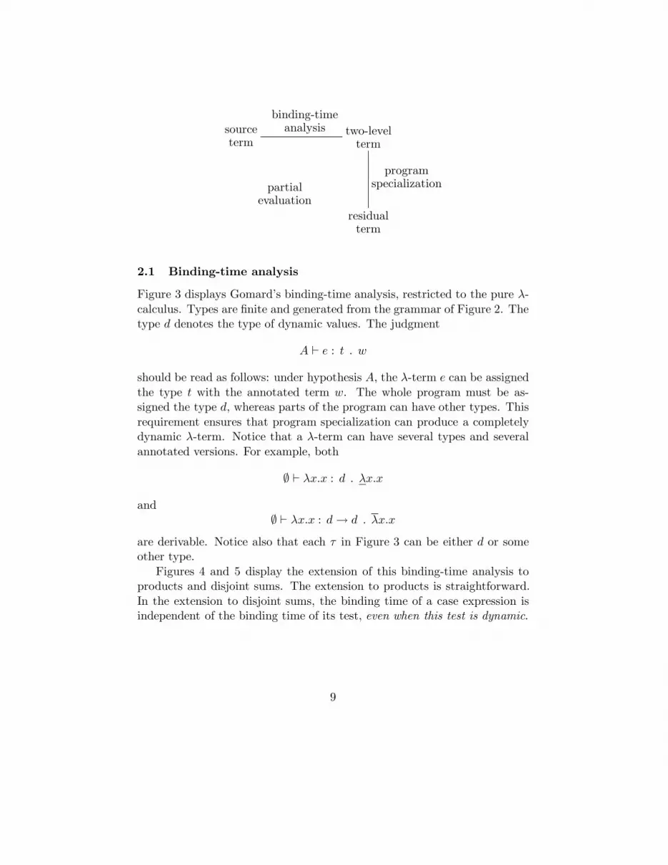
Figure 1 displays the syntax of a λ-calculus with products and disjointsums. Figure 2 displays the syntax of a two-level λ-calculus where eachconstruct, except variables, has two forms: overlined (static) and underlined(dynamic). A two-level λ-term is said to be completely dynamic if all theconstructs in it are underlined. A binding-time analysis (Section 2.1) maps aλ-term into a two-level λ-term. Program specialization (Section 2.2) reducesall the static parts of a two-level λ-term and yields a completely dynamicλ-term. Erasing its annotations yields the residual, specialized λ-term. Thisis summarized in the following diagram:

7

e ::= x |λx.e | e0@e1 | pair(e1, e2) | fst e | snd e |inleft(e) | inright(e) |case e of inleft(x1)⇒ e1 [] inright(x2)⇒ e2 end

Figure 1: BNF of the λ-calculus

τ ::= d | τ1 → τ2 | τ1 × τ2 | τ1 + τ2

e ::= x |λx.e | e0@e1 | pair(e1, e2) | fst e | snd e |λx.e | e0@e1 | pair(e1, e2) | fst e | snd e |inleft(e) | inright(e) |case e of inleft(x1)⇒ e1 [] inright(x2)⇒ e2 endinleft(e) | inright(e) |case e of inleft(x1)⇒ e1 [] inright(x2)⇒ e2 end

Figure 2: BNF of the two-level λ-calculus

A ` x : A(x) . x

A[x 7→ τ1] ` e : τ2 . w

A ` λx.e : τ1 → τ2 . λx.w

A[x 7→ d] ` e : d . wA ` λx.e : d . λx.w

A ` e0 : τ1 → τ2 . w0 A ` e1 : τ1 . w1

A ` e0@e1 : τ2 . w0@w1

A ` e0 : d . w0 A ` e1 : d . w1

A ` e0@e1 : d . w0@w1

Figure 3: Gomard’s binding-time analysis for the pure λ-calculus

8

sourceterm

//

binding-timeanalysis

$$

partialevaluation JJ

JJJJ

JJJJ

two-levelterm

��

programspecialization

residualterm

2.1 Binding-time analysis

Figure 3 displays Gomard’s binding-time analysis, restricted to the pure λ-calculus. Types are finite and generated from the grammar of Figure 2. Thetype d denotes the type of dynamic values. The judgment

A ` e : t . w

should be read as follows: under hypothesis A, the λ-term e can be assignedthe type t with the annotated term w. The whole program must be as-signed the type d, whereas parts of the program can have other types. Thisrequirement ensures that program specialization can produce a completelydynamic λ-term. Notice that a λ-term can have several types and severalannotated versions. For example, both

∅ ` λx.x : d . λx.x

and∅ ` λx.x : d→ d . λx.x

are derivable. Notice also that each τ in Figure 3 can be either d or someother type.

Figures 4 and 5 display the extension of this binding-time analysis toproducts and disjoint sums. The extension to products is straightforward.In the extension to disjoint sums, the binding time of a case expression isindependent of the binding time of its test, even when this test is dynamic.

9

A ` e1 : τ1 . w1 A ` e2 : τ2 . w2

A ` pair(e1, e2) : τ1 × τ2 . pair(w1, w2)

A ` e1 : d . w1 A ` e2 : d . w2

A ` pair(e1, e2) : d . pair(w1, w2)

A ` e : τ1 × τ2 . w

A ` fst e : τ1 . fst wA ` e : τ1 × τ2 . w

A ` snd e : τ2 . snd w

A ` e : d . wA ` fst e : d . fstw

A ` e : d . wA ` snd e : d . sndw

Figure 4: Extension of Gomard’s binding-time analysis to products

A ` e : τ1 + τ2 . w A[x1 7→ τ1] ` e1 : τ . w1 A[x2 7→ τ2] ` e2 : τ . w2

A ` case e ofinleft(x1)⇒ e1

[] inright(x2)⇒ e2end

: τ . casew ofinleft(x1)⇒ w1

[] inright(x2)⇒ w2end

A ` e : d . w A[x1 7→ d] ` e1 : τ . w1 A[x2 7→ d] ` e2 : τ . w2

A ` case e ofinleft(x1)⇒ e1

[] inright(x2)⇒ e2end

: τ . casew ofinleft(x1)⇒ w1

[] inright(x2)⇒ w2end

A ` e : τ1 . w

A ` inleft(e) : τ1 + τ2 . inleft(w)A ` e : τ2 . w

A ` inright(e) : τ1 + τ2 . inright(w)

A ` e : d . wA ` inleft(e) : d . inleft(w)

A ` e : d . wA ` inright(e) : d . inright(w)

Figure 5: Extension of Gomard’s binding-time analysis to sums

10

Static applications: (λx.e)@e1 −→ e[e1/x]

Static decompositions:fst pair(e1, e2) −→ e1 snd pair(e1, e2) −→ e2

Static projections:case inleft(e) of

inleft(x1)⇒ e1[] inright(x2)⇒ e2end

−→ e1[e/x1] case inright(e) ofinleft(x1)⇒ e1

[] inright(x2)⇒ e2end

−→ e2[e/x2]

Figure 6: Operational semantics of the two-level λ-calculus — evaluationrules

Static applications:

(case e0 of inleft(x1)⇒ e1 [] inright(x2)⇒ e2 end)@e −→case e0 of inleft(x1)⇒ e1@e [] inright(x2)⇒ e2@e end

Static decompositions:fst (case e0 of inleft(x1)⇒ e1 [] inright(x2)⇒ e2 end) −→case e0 of inleft(x1)⇒ fst e1 [] inright(x2)⇒ fst e2 end

snd (case e0 of inleft(x1)⇒ e1 [] inright(x2)⇒ e2 end) −→case e0 of inleft(x1)⇒ snd e1 [] inright(x2)⇒ snd e2 end

Static projections:case (case e0 of inleft(x1)⇒ e1 [] inright(x2)⇒ e2 end) of

inleft(x′1)⇒ e′1[] inright(x′2)⇒ e′2end−→ case e0 of

inleft(x1)⇒ case e1 of inleft(x′1)⇒ e′1 [] inright(x′2)⇒ e′2 end[] inright(x2)⇒ case e2 of inleft(x′1)⇒ e′1 [] inright(x′2)⇒ e′2 endend

Figure 7: Operational semantics of the two-level λ-calculus — code-motionrules

11

2.2 Program specialization

Program specialization reduces the static parts of a two-level λ-term. Ourspecification of program specialization has the form of an operational seman-tics. If e and e′ are two-level λ-terms, then e −→ e′ means that e reduces toe′. Figure 6 displays the three basic evaluation rules, and Figure 7 displaysfour “code-motion” rules. We say that a two-level λ-term is in normal formif it cannot be reduced. Each code-motion rule duplicates the static contextof a dynamic case expression and moves the copies to the branches of thecase expression. This creates new redexes, which fits together with the rulefor binding-time analysis of case expressions of Figure 5. Notice that thereis no rule of the form

e@(case e0 of inleft(x1)⇒ e1 [] inright(x2)⇒ e2 end) −→case e0 of inleft(x1)⇒ e@e1 [] inright(x2)⇒ e@e2 end.

This is because such a rule cannot create redexes unless the left-hand sideis already a redex itself.

The code motion rules in Figure 7 occur variously in logic, proof the-ory, CPS transformation, deforestation, and partial evaluation. Similarly toPaulin-Mohring and Werner [32, Section 4.5.4], we use them to move staticvalues toward static contexts, in the simply typed two-level λ-calculus. Foreach context E[·], if e −→ e′, then E[e] −→ E[e′].

Our extension of λ-Mix is correct, as proven in Section 5.

3 Examples

We first briefly summarize how eta-expansion works for functions and prod-ucts, and then we give two examples of how our partial evaluator does TheTrick.

3.1 Coercions for functions

As illustrated in our earlier work [14], for functions, eta-expansion is usefulin two cases. The first is where a dynamic context E[·], expecting a higher-order value of type d (one could be tempted to write “of type τ1→τ2” toclarify that this is a function, but in the present treatment, dynamic termsare not typed), can be coerced into a static context

λv.[·]@v

12

that expects a value of type τ1→τ2. The second useful case is where adynamic higher-order value e of type d (again, one could be tempted towrite τ1→τ2) can be coerced into a static value

λv.e@v

of type τ1→τ2 that will fit into a static context.

3.1.1 A concrete example: Church numerals

Church numerals [2] are defined with a λ-representation for the number zeroand with a λ-representation for the successor function:

zero = λs.λz.z

succ = λn.λs.λz.s@(n@s@z)

Suppose we want to specialize succ with respect to a given numeral, saythe one corresponding to 2, i.e., succ@(succ@zero). A standard binding-time analysis does not allow source arguments to be higher order [24]. Ourbinding-time analysis, however, will produce the following two-level, eta-expanded term (the eta-redex is boxed):

(λn.λs.λz.s@(n@ (λv.s@v) @z))@λs.λz.s@(s@z)

The following Scheme session illustrates Church numerals and their resid-ualization.

> (define zero (lambda (s) (lambda (z) z)))> (define succ

(lambda (n) (lambda (s) (lambda (z) (s ((n s) z))))))> (define succ-gen

(lambda (n)(let* ([s (gensym! "s")]

[z (gensym! "z")])‘(lambda (,s)

(lambda (,z)(,s ,((n (lambda (v) ‘(,s ,v))) z)))))))

> (succ-gen (succ (succ zero)))(lambda (s0) (lambda (z1) (s0 (s0 (s0 z1)))))> (((lambda (s0) (lambda (z1) (s0 (s0 (s0 z1))))) 1+) 0)3>

13

Procedure succ-gen is the generating extension of Procedure succ, i.e.,its associated program specializer [24]. Applying succ-gen to the staticdata gives the same result as specializing succ with respect to the staticdata. In the definition of succ-gen, binding-time information is encodedwith Scheme’s quasi-quote (backquote) and unquote (comma) [7].

3.2 Coercions for products

A similar situation occurs for partially static values: whenever such a valueoccurs in a dynamic context, the value is dynamized, and conversely, when-ever a partially static context receives a dynamic value, the context is dy-namized as well. Let us consider pairs. A static pair p of type d×d can becoerced to

pair(fst p, snd p)

which has type d. A dynamic pair p of type d can be coerced to

pair(fst p, sndp)

which has type d×d.For example, if the following expression occurs in a dynamic context

fst e

where e has type (d→ d)× d, the result of binding-time analysis reads

fst e

where e has type d. If we eta-expand the result, it will read:

fst (pair(λx.(fst e)@x, snd e)).

This term has type d, which matches the type of its context, and the partiallystatic pair e remains partially static, thanks to the coercion.

Conversely, if the value of two expressions e (of type d) and e′ (of typed × d) can occur in the same context, binding-time analysis classifies e′ tobe dynamic and, as a by-product, dynamizes this context. Again, e couldbe eta-expanded to read

pair(fst e, snd e).

This term has type d × d, which avoids dynamizing the context and thusmakes it possible to keep e′ a static pair, thanks to the coercion. (Note thatthe alternative of eta-expanding e′ into pair(fst e′, snd e′) would not be abinding-time improvement, since it would dynamize the present context.)

14

3.3 Coercions for disjoint sums

The same coercions apply to disjoint sums. In the following, we give twoexamples of how The Trick can be achieved by eta-expansion in the pres-ence of our new rules for binding-time analysis and transformation of caseexpressions.

3.3.1 Static injection in a dynamic context

The following expression is partially evaluated in a context where f is dy-namic.

(λv.f@(case v of inleft(a)⇒ a+ 20 [] inright(b)⇒ ... end)@v)@inleft(10)

Assume this β-redex will be reduced. Notice that v occurs twice: once asthe test part of a case expression, and once as the argument of the applicationof f to the case expression. Since f is dynamic, its application is dynamic,and the application of that expression is dynamic as well. Thus the binding-time analysis classifies v to be dynamic, since it occurs in a dynamic context,and in turn both the case expression and inleft(10) are also classified asdynamic. Overall, binding-time analysis yields the following two-level term.

(λv.f@(case v of inleft(a)⇒ a+ 20 [] inright(b)⇒ ... end)@v)@inleft(10)

In this term, both f and v have type d.After specialization (i.e., reduction of static expressions and reconstruc-

tion of dynamic expressions) the residual term (call it (a)) reads as follows.

f@(case inleft(10) of inleft(a)⇒ a+ 20 [] inright(b)⇒ ... end)@inleft(10)

The fact that inleft(10), a partially static value, occurs in the dynamiccontext f@(case v of inleft(a)⇒ a+ 20 [] inright(b)⇒ ... end)@[·] “pollutes”its occurrence in the potentially static context case [·] of inleft(a) ⇒a+ 20 [] inright(b)⇒ ... end, so that neither is reduced statically.

Note that since v is dynamic and occurs twice, a cautious binding-timeanalysis would reclassify the outer application to be dynamic: there is usu-ally no point in duplicating residual code. In that case, the expression istotally dynamic and so is not simplified at all.

In this situation, a binding-time improvement is possible, since inleft(10)will occur in a dynamic context. We can coerce this occurrence by eta-

15

expanding the dynamic context (the eta-redex is boxed).

(λv.f@(case v of inleft(a)⇒ a+ 20 [] inright(b)⇒ ... end)@case v of inleft(a)⇒ inleft(a) [] inright(b)⇒ inright(b) end )

@inleft(10)

Binding-time analysis now yields the following two-level term.

(λv.f@(case v of inleft(a)⇒ a+ 20 [] inright(b)⇒ ... end)@case v of inleft(a)⇒ inleft(a) [] inright(b)⇒ inright(b) end)

@inleft(10)

Here, v is not approximated to be dynamic: it has the type Int+ t, for somet.

Specialization yields the residual term

f@30@inleft(10)

which is more reduced than the residual term (a) above.Let us now illustrate the dual case, where a dynamic injection in a po-

tentially static context dynamizes this context.

3.3.2 Dynamic injection in a static context

The following expression is partially evaluated in a context where d is dy-namic.

(λf. ... f@d ... f@inleft(λx.x) ...)@λv.case v of inleft(a)⇒ a@10 [] inright(b)⇒ ... end

Assume this β-redex will be reduced. Notice that f occurs twice: it isapplied both to a static value and to a dynamic value. The binding-timeanalysis of Figures 3, 4, and 5 thus approximates its argument to be dynamicand yields the following two-level term.

(λf. ... f@d ... f@inleft(λx.x) ...)@λv.case v of inleft(a)⇒ a@10 [] inright(b)⇒ ... end

16

In this term, f has type d.Specialization yields the following residual term (call it (b)).

...(λv.case v of inleft(a)⇒ a@10 [] inright(b)⇒ ... end)@d...(λv.case v of inleft(a)⇒ a@10 [] inright(b)⇒ ... end)@inleft(λx.x)...

The fact that d, a dynamic value, occurs in the potentially static contextf@[·] dynamizes this context, which in turn, dynamizes inleft(λx.x).

In this situation, a binding-time improvement is possible to makeinleft(λx.x) occur in a static context always. We can coerce the bother-ing occurrence of d by eta-expanding it (the eta-redex is boxed).

λf. ...

f@ case d of inleft(a)⇒ inleft(a) [] inright(b)⇒ inright(b) end...f@inleft(λx.x)...

@λv.case v of inleft(a)⇒ a@10 [] inright(b)⇒ ... end

This eta-expansion enables The Trick. Even though d is not staticallyknown, its type tells us that it is either some dynamic value a or somedynamic value b. Program specialization automatically does The Trick, byplugging these values into the enclosing context (see Figure 7).

But this is not enough because now λx.x will be dynamized by thenewly introduced occurrence of a. Indeed, binding-time analysis yields thefollowing two-level term.

λf. ...f@case d of inleft(a)⇒ inleft(a) [] inright(b)⇒ inright(b) end...f@ inleft(λx.x)...

@λv.case v of inleft(a)⇒ a@10 [] inright(b)⇒ ... end

In this term, f has type (d+ t)→ d, for some t.

17

Specialization moves the context of the dynamic case expression in eachof its branches and produces the following residual term (call it (c)).

...case d of inleft(a)⇒ a@10 [] inright(b)⇒ ... end...(λx.x)@10...

This residual term (c) is more reduced than the residual term (b) above.However, the fact that a, a dynamic value, occurs in the potentially

static context [·]@10 dynamizes this context, which in turn dynamizes λx.x.Fortunately, we already solved that problem in Section 3.1, using eta-

expansion. The new eta-redex is boxed.

λf. ...

f@case d of inleft(a)⇒ inleft( λz.a@z ) [] inright(b)⇒ inright(b) end...f@inleft(λx.x)...

@λv.case v of inleft(a)⇒ a@10 [] inright(b)⇒ ... end

Binding-time analysis now yields the following two-level term.

λf. ...f@case d of inleft(a)⇒ inleft(λz.a@z) [] inright(b)⇒ inright(b) end...f@inleft(λx.x)...

@λv.case v of inleft(a)⇒ a@10 [] inright(b)⇒ ... end

Here, f has type ((d→ d) + t) → d, for some t. Thus neither inleft(λx.x)nor λx.x are approximated to be dynamic.

Specialization yields the following residual term.

...(case d of inleft(a)⇒ a@10 [] inright(b)⇒ ... end)...10...

This residual term is more reduced than the term (c) above.

18

3.3.3 A concrete example: Mix’s pending list

The Trick was first used to program Mix, the first self-applicable partialevaluator [25]. Mix’s program specializer is polyvariant and operates ona “pending list”, which is a list of specialization points, subindexed withstatic values. When Mix is self-applied, looking up in this list is a dynamicoperation, even though the specialization points are static. The Trick isused to move the context of this lookup (i.e., the specializer) inside the listto specialize the specialization points at self-application time.

Holst and Hughes have characterized this use of The Trick as the appli-cation of one of Wadler’s theorems for free: Reynolds’s Abstraction theoremin the first-order case [20, 34, 41]. The composition of specialization and listlookup is replaced by the composition of lookup and map of specializationover the list. This achieves a binding-time improvement because it enablesthe specialization of specialization points at self-application time.

In the context of this article, and since the source program has a fixednumber of specialization points, the pending list has a fixed length, and thusit can be formalized as a finite disjoint sum. Eta-expansion over this disjointsum enables The Trick, through which specialization points are specializedat self-application time.

3.4 Conclusions

For functions, products, and disjoint sums, eta-redexes act as binding-timecoercions. Also, and as illustrated in the last example, they synergize. Inparticular, the first eta-expansion of Section 3.3.2 enables The Trick. Eventhough d is unknown, its type tells us that it can be either some (dynamic)value a or b. Program specialization automatically does The Trick and plugsthese values into the surrounding context (see Figure 7).

4 Binding-Time Analysis with Eta-Expansion

In our earlier work [14], we proposed and proved the correctness of a binding-time analysis that generates binding-time coercions for higher-order val-ues at points of conflict, instead of taking the conservative solution of dy-namizing both values and contexts. We pointed out the analogous need forbinding-time coercions for products, but did not present the correspond-ing binding-time analysis generating these binding-time coercions at pointsof conflict. This binding-time analysis can be obtained by extending the

19

A ` e : d . w τ ` z ⇒ m ∅[z 7→ d] ` m : τ . w′

A ` e : τ . w′[w/z]

A ` e : τ . w τ ` z ⇒ m ∅[z 7→ τ ] ` m : d . w′

A ` e : d . w′[w/z]

Figure 8: Extension of Gomard’s binding-time analysis to binding-time co-ercions

d ` e ⇒ e

τ1 ` x ⇒ x′ τ2 ` e@x′ ⇒ e′

τ1 → τ2 ` e ⇒ λx.e′

τ1 ` fst e ⇒ e1 τ2 ` snd e ⇒ e2

τ1 × τ2 ` e ⇒ pair(e1, e2)

τ1 ` x1 ⇒ e1 τ2 ` x2 ⇒ e2

τ1 + τ2 ` e ⇒ case e of inleft(x1)⇒ e1 [] inright(x2)⇒ e2 end

Figure 9: Type-directed eta expansion

binding-time analysis of Figures 3, 4, and 5 with Figures 8 and 9.Figure 8 displays two general eta-expansion rules. Intuitively, the two

rules can be understood as being able (1) to coerce the binding-time type dto any type τ and (2) to coerce any type τ to the type d. The combinationof the two rules allows us to coerce the type of any λ-term to any other type.

Eta-expansion itself is defined in Figure 9. It is type-directed, and thusit can insert several embedded eta-redexes in a way that is reminiscent ofBerger and Schwichtenberg’s normalization of λ-terms [3, 12].

Consider the first rule in Figure 8. Intuitively, it works as follows. Weare given a λ-term e that we would like to assign the type τ . In case we canonly assign it type d and τ 6= d, we can use the rule to coerce the type to beτ . The first hypothesis of the rule is that e has type d and annotated term w.The second hypothesis of the rule takes a fresh variable z and eta-expands itaccording to the type τ . This creates a λ-term m with type τ . Notice that zis the only free variable in m. The third hypothesis of the rule annotates m

20

under the assumption that z has type d. The result is an annotated term w′

with the type τ and with a hole of type d (the free variable z) where we caninsert the previously constructed w. Thus, w′ makes the coercion happen.The second rule in Figure 8 works in a similar way.

With this new binding-time analysis, all the examples of Section 3 nowspecialize well without binding-time improvement. In particular, no tricksare required from the partial-evaluation user — they were a tell-tale of toocoarse binding-time coercions in existing binding-time analyses.

For example, consider again the first example in Section 3.2, that is, theexpression fst e. We assume that the judgment

∅ ` e : (d→ d)× d . w

is derivable, i.e., e has type (d→ d)× d with annotated term w. Moreover,we assume that the expression fst e occurs in a dynamic context, so we needto assign it type d. The following derivation does that, giving the expectedannotated and eta-expanded version of e.

∅ ` e : d . pair(λx.(fst w)@x, snd w)∅ ` fst e : d . fst pair(λx.(fst w)@x, snd w)

To derive the hypothesis we use the second rule in Figure 8. We need thefollowing three judgments:

∅ ` e : (d→ d)× d . w(d→ d)× d ` z ⇒ pair(λx.(fst z)@x, snd z)∅[z 7→ (d→ d)× d] ` pair(λx.(fst z)@x, snd z) : d . pair(λx.(fst z)@x, snd z)

The first judgment is given by assumption; the derivation of the other twoare left to the reader.

5 Correctness

We now state and prove that our binding-time analysis is correct with re-spect to the operational semantics of two-level λ-terms. The statement ofcorrectness is taken from Palsberg [31] and Wand [42], who proved cor-rectness of two other binding-time analyses. The proof techniques are wellknown; we omit the details.

If w is a two-level λ-term, then w denotes the underlying λ-term.We first prove a basic property of the operational semantics of two-level

λ-terms. Let −→−→ be the reflexive and transitive closure of −→.

21

Theorem 5.1 (5.1 (Church-Rosser)) If e −→−→ e′ and e −→−→ e′′, thenthere exists e′′′ such that e′ −→−→ e′′′ and e′′ −→−→ e′′′.

Proof. By the method of Tait and Martin-Lof; the sequence of definitionsand lemmas is standard [2, pp.59–62]. 2

We then prove that if e can be annotated as w, then so can w. Thisenables us to simplify the statements and proofs of subsequent theorems.

Theorem 5.2 (5.2 (Simplification)) If A ` e : τ .w, then A ` w : τ .w.

Proof. By induction on the structure of the derivation of A ` e : τ . w.2

We then prove subject reduction, using a substitution lemma.

Lemma 5.2.1 (5.2.1 (Substitution)) If

A ` w1 : τ . w1 and A′ ` w2 : τ ′ . w2 ,

thenA′′ ` w2[w1/z] : τ ′ . w2[w1/z] ,

where A and A′′ agree on the free variables of w1, where A′ and A′′ agreeon the free variables of w2 except z, and where A′(z) = τ .

Proof. By induction on the structure of the derivation ofA′ ` w2 : τ ′.w2.2

Theorem 5.3 (5.3 (Subject Reduction)) If A ` w : τ . w and w −→w′, then A ` w′ : τ . w′.

Proof. By induction on the structure of the derivation of A ` w : τ . w,using Lemma 5.2.1. 2

Next we prove that if a closed two-level λ-term of type d is reduced to normalform, then all the components of that normal form are dynamic.

Theorem 5.4 (5.4 (Dynamic Normal Form)) Suppose w is a two-levelλ-term in normal form, and suppose A is an environment such that A(x) = dfor all x in the domain of A. If A ` w : d .w, then w is completely dynamic.

22

Proof. By induction on the structure of the derivation of A ` w : d .w.2

Finally, we prove that typability ensures that no “confusion” between staticand dynamic will occur, for example as in (λx.e)@e1.

Theorem 5.5 (5.5 (No Confusion)) If A ` w : τ .w, then the following“confused” terms do not occur in w.

(λx.e)@e1

(λx.e)@e1

fst pair(e1, e2)

fst pair(e1, e2)snd pair(e1, e2)

snd pair(e1, e2)case inleft(e) of inleft(x1)⇒ e1 [] inright(x2)⇒ e2 endcase inleft(e) of inleft(x1)⇒ e1 [] inright(x2)⇒ e2 end

case inright(e) of inleft(x1)⇒ e1 [] inright(x2)⇒ e2 end

case inright(e) of inleft(x1)⇒ e1 [] inright(x2)⇒ e2 end

Proof. Immediate. 2

Together, Theorems 5.2, 5.3, 5.4, and 5.5 guarantee that if we havederived A ` e : d . w, then we can start specialization of w and know that

• if a normal form is reached, then all its components will be dynamic,and

• no confused terms will occur at any point.

We have thus established the correctness of a partial evaluator which au-tomatically does The Trick. Notice that the correctness statement also holdswithout eta-expansion, i.e., for the partial evaluator specified in Section 2.

6 Assessment and Related Work

The two new eta-expansion rules of Figure 8 unify and generalize our earliertreatment of eta-expansion [14], and they are a key part of our explanation

23

of The Trick. Intuitively, the two rules make it possible (1) to coerce thebinding-time type d to any type τ and (2) to coerce any type τ to thetype d. There is no direct rule, however, for coercing for example d → dto d → (d→ d). Such a rule seems to be definable using some notion ofsubtyping.

Our rules for eta-expansion resemble rules for inserting coercions in typesystems with subtyping [19]. The purpose of our rules, however, is not tochange the type of a term to a supertype; two of our coercions can changethe type of a term to any other type.

We have not considered inferring binding-time annotations. This seemspossible, using the technique of Dussart, Henglein, and Mossin [15] — afuture work.

In Jones, Gomard, and Sestoft’s textbook [24], using The Trick requiresthe partial-evaluation user to collect static information under dynamic con-trol (either by hand or by program analysis) and to rewrite the source pro-gram to exploit it. We represent this statically collected information as adisjoint sum.

Jones, Gomard, and Sestoft also restrict static values occurring in dy-namic contexts to be of base type. Values of higher type are dynamized,thereby making their type a base type, namely dynamic. In contrast, thebinding-time analysis of Section 4 provides a syntactic representation ofbinding-time coercions at higher type. This syntactic representation can beinteresting in its own right, in a setting where the binding time “dynamic”retains a type structure [12].

Polyvariant specializers usually select dynamic conditional expressions asspecialization points [6, 24], thus disabling the code-motion rules of Figure7. Experience, however, shows that not all dynamic conditional expressionsneed be treated as specialization points [28]. For these, the code-motionrules of Figure 7 can apply.

A polyvariant binding-time analysis, in contrast to our monovariantbinding-time analysis, associates several binding-time descriptions with eachprogram point [8]. Polyvariance obviates binding-time coercions, by gener-ating several variants instead of coercing them into a single one. Expe-rience, however, shows that polyvariance is expensive [1]. Moreover, ourpersonal experience with Consel’s partial evaluator Schism [9] shows thateta-expansion can speed up a polyvariant binding-time analysis by reducingthe number of variants.

Finally, our results apply to online partial evaluation in that they pro-vide guidelines to structure a typed online partial evaluator. Online partial

24

evaluators usually keep multiple representations of static values, which ob-viates the need for residualization functions. They need, however, to becontinuation-based to be able to achieve The Trick.

7 Conclusion

We have specified and proven the correctness of a partial evaluator for aλ-calculus with products and disjoint sums. The specializer moves staticcontexts across dynamic case expressions, and the binding-time analysisaccounts for this move (Section 2). We have demonstrated that in such apartial evaluator, eta-expansion for disjoint-sum values achieves The Trick,thus characterizing it as a typing property (Section 3). Our binding-timeanalysis automatically inserts binding-time coercions as eta-redexes (Section4), and thus our partial evaluator both unifies and automates the binding-time improvements listed in Jones, Gomard, and Sestoft’s textbook [24,Chapter 12]. Future work includes finding an efficient algorithm for our newbinding-time analysis.

Acknowledgements

Thanks to the referees for insightful comments.The first author is supported by the BRICS Centre (Basic Research In

Computer Science) of the Danish National Research Foundation and ex-presses grateful thanks to the DART project (Design, Analysis and Reason-ing about Tools) of the Danish Research Councils, for support during 1995.The second author was hosted by BRICS during summer 1995. The thirdauthor is supported by the Danish Natural Science Research Council andBRICS.

The diagram of Section 2 was drawn with Kristoffer Rose’s XY-pic pack-age. The Scheme session of Section 3.1.1 was obtained with R. Kent Dybvig’sChez Scheme system.

References

[1] J. Michael Ashley and Charles Consel. Fixpoint computation for poly-variant static analyses of higher-order applicative programs. ACMTransactions on Programming Languages and Systems, 16(5):1431–1448, 1994.

25

[2] Henk Barendregt. The Lambda Calculus — Its Syntax and Semantics.North-Holland, 1984.

[3] Ulrich Berger and Helmut Schwichtenberg. An inverse of the evalua-tion functional for typed λ-calculus. In Proceedings of the Sixth AnnualIEEE Symposium on Logic in Computer Science, pages 203–211, Ams-terdam, The Netherlands, July 1991. IEEE Computer Society Press.

[4] Anders Bondorf. Automatic autoprojection of higher-order recursiveequations. Science of Computer Programming, 17(1-3):3–34, 1991. Spe-cial issue on ESOP’90, the Third European Symposium on Program-ming, Copenhagen, Denmark, May 1990.

[5] Anders Bondorf. Improving binding times without explicit cps-conversion. In William Clinger, editor, Proceedings of the 1992ACM Conference on Lisp and Functional Programming, LISP Point-ers, Vol. V, No. 1, pages 1–10, San Francisco, California, June 1992.ACM Press.

[6] Anders Bondorf and Olivier Danvy. Automatic autoprojection of recur-sive equations with global variables and abstract data types. Scienceof Computer Programming, 16:151–195, 1991.

[7] William Clinger and Jonathan Rees (editors). Revised4 report onthe algorithmic language Scheme. LISP Pointers, IV(3):1–55, July-September 1991.

[8] Charles Consel. Polyvariant binding-time analysis for applicative lan-guages. In Schmidt [36], pages 66–77.

[9] Charles Consel. A tour of Schism: A partial evaluation system forhigher-order applicative languages. In Schmidt [36], pages 145–154.

[10] Charles Consel and Olivier Danvy. For a better support of static dataflow. In Hughes [21], pages 496–519.

[11] Charles Consel and Olivier Danvy. Tutorial notes on partial evaluation.In Susan L. Graham, editor, Proceedings of the Twentieth Annual ACMSymposium on Principles of Programming Languages, pages 493–501,Charleston, South Carolina, January 1993. ACM Press.

[12] Olivier Danvy. Type-directed partial evaluation. In Steele Jr. [39],pages 242–257.

26

[13] Olivier Danvy and Andrzej Filinski. Abstracting control. In MitchellWand, editor, Proceedings of the 1990 ACM Conference on Lisp andFunctional Programming, pages 151–160, Nice, France, June 1990.ACM Press.

[14] Olivier Danvy, Karoline Malmkjær, and Jens Palsberg. The essenceof eta-expansion in partial evaluation. LISP and Symbolic Computa-tion, 8(3):209–227, 1995. An earlier version appeared in the proceed-ings of the 1994 ACM SIGPLAN Workshop on Partial Evaluation andSemantics-Based Program Manipulation.

[15] Dirk Dussart, Fritz Henglein, and Christian Mossin. Polymorphic re-cursion and subtype qualifications: Polymorphic binding-time analysisin polynomial time. In Alan Mycroft, editor, Static Analysis, number983 in Lecture Notes in Computer Science, pages 118–135, Glasgow,Scotland, September 1995. Springer-Verlag.

[16] Carsten K. Gomard. A self-applicable partial evaluator for the lambda-calculus: Correctness and pragmatics. ACM Transactions on Program-ming Languages and Systems, 14(2):147–172, 1992.

[17] Carsten K. Gomard and Neil D. Jones. A partial evaluator for theuntyped lambda-calculus. Journal of Functional Programming, 1(1):21–69, 1991.

[18] Nevin Heintze. Set-Based Program Analysis. PhD thesis, School ofComputer Science, Carnegie Mellon University, Pittsburgh, Pennsylva-nia, October 1992.

[19] Fritz Henglein. Dynamic typing: Syntax and proof theory. Scienceof Computer Programming, 22(3):197–230, 1993. Special Issue onESOP’92, the Fourth European Symposium on Programming, Rennes,February 1992.

[20] Carsten K. Holst and John Hughes. Towards binding-time improve-ment for free. In Simon L. Peyton Jones, Guy Hutton, and Carsten K.Holst, editors, Functional Programming, Glasgow 1990, pages 83–100,Glasgow, Scotland, 1990. Springer-Verlag.

[21] John Hughes, editor. Proceedings of the Fifth ACM Conference onFunctional Programming and Computer Architecture, number 523 in

27

Lecture Notes in Computer Science, Cambridge, Massachusetts, August1991. Springer-Verlag.

[22] Neil D. Jones. Automatic program specialization: A re-examinationfrom basic principles. In Partial Evaluation and Mixed Computation,pages 225–282. North-Holland, 1988.

[23] Neil D. Jones, editor. Special issue on Partial Evaluation, Journal ofFunctional Programming, Vol. 3, Part 3. Cambridge University Press,July 1993.

[24] Neil D. Jones, Carsten K. Gomard, and Peter Sestoft. Partial Evalu-ation and Automatic Program Generation. Prentice Hall InternationalSeries in Computer Science. Prentice-Hall, 1993.

[25] Neil D. Jones, Peter Sestoft, and Harald Søndergaard. MIX: A self-applicable partial evaluator for experiments in compiler generation.LISP and Symbolic Computation, 2(1):9–50, 1989.

[26] Julia L. Lawall and Olivier Danvy. Continuation-based partial evalua-tion. In Carolyn L. Talcott, editor, Proceedings of the 1994 ACM Con-ference on Lisp and Functional Programming, LISP Pointers, Vol. VII,No. 3, Orlando, Florida, June 1994. ACM Press.

[27] Julia L. Lawall and Olivier Danvy. Continuation-based partial eval-uation. Technical Report CS-95-178, Computer Science Department,Brandeis University, Waltham, Massachusetts, January 1995. An ear-lier version appeared in the proceedings of the 1994 ACM Conferenceon Lisp and Functional Programming.

[28] Karoline Malmkjær. Towards efficient partial evaluation. In Schmidt[36], pages 33–43.

[29] Yasuhiko Minamide, Greg Morrisett, and Robert Harper. Typed closureconversion. In Steele Jr. [39], pages 271–283.

[30] Flemming Nielson and Hanne Riis Nielson. Two-Level Functional Lan-guages, volume 34 of Cambridge Tracts in Theoretical Computer Sci-ence. Cambridge University Press, 1992.

[31] Jens Palsberg. Correctness of binding-time analysis. In Jones [23],pages 347–363.

28

[32] Christine Paulin-Mohring and Benjamin Werner. Synthesis of ML pro-grams in the system Coq. Journal of Symbolic Computation, 15:607–640, 1993.

[33] John C. Reynolds. Definitional interpreters for higher-order program-ming languages. In Proceedings of 25th ACM National Conference,pages 717–740, Boston, Massachusetts, 1972.

[34] John C. Reynolds. Types, abstraction and parametric polymorphism.In R. E. A. Mason, editor, Information Processing 83, pages 513–523,Paris, France, 1983. IFIP.

[35] Erik Ruf. Topics in Online Partial Evaluation. PhD thesis, StanfordUniversity, Stanford, California, February 1993. Technical report CSL-TR-93-563.

[36] David A. Schmidt, editor. Second ACM SIGPLAN Symposium on Par-tial Evaluation and Semantics-Based Program Manipulation, Copen-hagen, Denmark, June 1993. ACM Press.

[37] Peter Sestoft. Replacing function parameters by global variables. InStoy [40], pages 39–53.

[38] Olin Shivers. Control-Flow Analysis of Higher-Order Languages orTaming Lambda. PhD thesis, School of Computer Science, CarnegieMellon University, Pittsburgh, Pennsylvania, May 1991. Technical Re-port CMU-CS-91-145.

[39] Guy L. Steele Jr., editor. Proceedings of the Twenty-Third Annual ACMSymposium on Principles of Programming Languages, St. PetersburgBeach, Florida, January 1996. ACM Press.

[40] Joseph E. Stoy, editor. Proceedings of the Fourth International Confer-ence on Functional Programming and Computer Architecture, London,England, September 1989. ACM Press.

[41] Philip Wadler. Theorems for free! In Stoy [40], pages 347–359.

[42] Mitchell Wand. Specifying the correctness of binding-time analysis. InJones [23], pages 365–387.

[43] Daniel Weise, Roland Conybeare, Erik Ruf, and Scott Seligman. Au-tomatic online partial evaluation. In Hughes [21], pages 165–191.

29

Recent Publications in the BRICS Report Series

RS-96-17 Olivier Danvy, Karoline Malmkjær, and Jens Palsberg.Eta-Expansion Does The Trick (Revised Version). May1996. 29 pp. To appear inACM Transactions on Pro-gramming Languages and Systems (TOPLAS).

RS-96-16 Lisbeth Fajstrup and Martin Raußen. Detecting Dead-locks in Concurrent Systems. May 1996. 10 pp.

RS-96-15 Olivier Danvy.Pragmatic Aspects of Type-DirectedPartialEvaluation. May 1996. 27 pp.

RS-96-14 Olivier Danvy and Karoline Malmkjær. On the Idempo-tence of the CPS Transformation. May 1996. 15 pp.

RS-96-13 Olivier Danvy and Rene Vestergaard. Semantics-BasedCompiling: A Case Study in Type-Directed Partial Eval-uation. May 1996. 28 pp. To appear in8th Interna-tional Symposium on Programming Languages, Imple-mentations, Logics, and Programs, PLILP '96 Proceed-ings, LNCS, 1996.

RS-96-12 Lars Arge, Darren E. Vengroff, and Jeffrey S. Vitter.External-Memory Algorithms for Processing Line Seg-ments in Geographic Information Systems. May 1996. 34pp. A shorter version of this paper appears in Spirakis,editor, Algorithms - ESA '95: Third Annual EuropeanSymposium Proceedings, LNCS 979, 1995, pages 295–310.

RS-96-11 Devdatt Dubhashi, David A. Grable, and Alessandro Pan-conesi.Near-Optimal, Distributed Edge Colouring via theNibble Method. May 1996. 17 pp. Appears in Spirakis,editor, Algorithms - ESA '95: Third Annual EuropeanSymposium Proceedings, LNCS 979, 1995, pages 448–459.Invited to be published in a special issue ofTheoreticalComputer Sciencedevoted to the proceedings of ESA '95.

RS-96-10 Torben Brauner and Valeria de Paiva. Cut-Eliminationfor Full Intuitionistic Linear Logic . April 1996. 27 pp. Alsoavailable as Technical Report 395,Computer Laboratory,University of Cambridge.