Embed Size (px)
Citation preview
UNIVERSIDADE PAULISTA – UNIP
PROGRAMA DE PÓS-GRADUAÇÃO EM ENGENHARIA DE PRODUÇÃO
ESTUDO DE IMPACTO AMBIENTAL NO TRANSPORTE DE HORTIFRUTI E
AVALIAÇÃO DA SUSTENTABILIDADE DE MOTORES A COMBUSTÃO INTERNA
(CICLO OTTO)
Dissertação apresentada ao Programa de Pós-Graduação em Engenharia de Produção da Universidade Paulista – UNIP, para obtenção do título de Mestre em Engenharia de Produção.
GILSON TRISTÃO BASTOS DUARTE
SÃO PAULO
2020
UNIVERSIDADE PAULISTA – UNIP
PROGRAMA DE PÓS-GRADUAÇÃO EM ENGENHARIA DE PRODUÇÃO
ESTUDO DE IMPACTO AMBIENTAL NO TRANSPORTE DE HORTIFRUTI E
AVALIAÇÃO DA SUSTENTABILIDADE DE MOTORES A COMBUSTÃO INTERNA
(CICLO OTTO)
Dissertação apresentada ao Programa de Pós-Graduação em Engenharia de Produção da Universidade Paulista – UNIP, para obtenção do título de Mestre em Engenharia de Produção.
Orientadora: Profa. Dra. Irenilza de Alencar Nääs.
GILSON TRISTÃO BASTOS DUARTE
SÃO PAULO
2020
Ficha elaborada pelo Bibliotecário Rodney Eloy CRB8-6450
Duarte, Gilson Tristão Bastos.
Estudo de impacto ambiental no transporte de hortifruti e avaliação da sustentabilidade de motores a combustão interna (ciclo Otto) / Gilson Tristão Bastos Duarte. - 2020.
51 f. : il. color. + CD-ROM
Dissertação de Mestrado Apresentada ao Programa de Pós Graduação em Engenharia de Produção da Universidade Paulista, São Paulo, 2020.
Área de concentração: Sustentabilidade. Orientadora: Prof.ª Dr.ª Irenilza de Alencar Nääs.
1. Impacto ambiental. 2. Logística. 3. Emissões. 4. Combustível
alternativo. I. Nääs, Irenilza de Alencar (orientadora). II. Título.
GILSON TRISTÃO BASTOS DUARTE
Aprovado em: ___/__/____
BANCA EXAMINADORA
___________________________/__/____ Prof.: Dra. Silvia Helena Bonilla Universidade Paulista – UNIP ___________________________/__/____ Profa.: Dra. Irenilza de Alencar Nääs Universidade Paulista – UNIP ___________________________/__/____ Prof.: Dr. Marcelo Kenji Shibuya Instituto Federal de São Paulo - Campus Guarulhos
DEDICATÓRIA
Dedico esse trabalho à Deus, aos meus
familiares, à toda equipe de docentes da
Universidade Paulista – UNIP, e a todos
que contribuíram de alguma forma nesta
jornada.
AGRADECIMENTOS
Agradeço primeiramente à Deus por me abençoar, muito mais do que eu poderia
imaginar, nesta jornada;
À minha esposa Silvia e filhos, Gustavo e Rodrygo, que cederam várias horas de
convivência conjunta, para que eu pudesse me dedicar a este trabalho;
À minha orientadora Profa. Dra. Irenilza de Alencar Nääs, exemplo de competência,
vitalidade, disciplina, profissionalismo e generosidade, que com exímia destreza
apontou com assertividade ímpar os pontos a serem explorados nos materiais por
mim pesquisados;
Ao Prof. Dr. Fábio Romeu de Carvalho, que com seu jeito mineiro de ser, incentivou e
acompanhou à distância essa etapa de minha formação como docente;
À amiga e coautora do meu artigo, Profa. Dra. Nilsa Duarte da Silva Lima, que durante
meu afastamento por motivo de saúde, assumiu com propriedade os estudos de
DataMining, e deu continuidade ao trabalho, estabelecendo parâmetros decisivos para
a conclusão do artigo sobre motores a combustão;
Aos professores do curso, que demonstraram extrema solidariedade e sensibilidade
quando de meu afastamento;
Aos colegas professores do campus Swift de Campinas, que sempre colaboraram
para que eu tivesse disponibilidade para participar do curso;
Aos alunos de graduação do Campus Swift de Campinas, que integraram a equipe do
trabalho de conclusão de curso do Powertrain, por mim orientados;
A todos os colaboradores da Universidade Paulista – UNIP que nos permitiram
usufruir de toda a infraestrutura oferecida nas dependências do Campus Swift;
À toda equipe de laboratório e responsáveis do Instituto Mauá de Tecnologia – IMT
(Centro de pesquisas de Motores e Veículos) através da parceria com seu laboratório
de testes;
Ao Sr. Ricardo Alécio do Departamento de Comunicação e Marketing e ao Eng.
Ricardo de Oliveira do Departamento de Hortifruti cultura do Ceasa-Campinas, pelo
apoio no levantamento de dados;
Aos amigos e colegas que contribuíram de alguma maneira ao longo dessa jornada.

Seja você quem for, seja qual for a posição
social que você tenha na vida, a mais alta
ou a mais baixa, tenha sempre como meta
muita força, muita determinação e sempre
faça tudo com muito amor e com muita fé
em Deus, que um dia você chega lá. De
alguma maneira você chega lá.
(Ayrton Senna)
i
SUMÁRIO
LISTA DE FIGURAS ............................................................................................................................ ii
LISTA DE TABELAS ........................................................................................................................... iii
RESUMO .............................................................................................................................................. iv
ABSTRACT ........................................................................................................................................... v
CAPÍTULO I .......................................................................................................................................... 6
1 CONSIDERAÇÕES INICIAIS ..................................................................................................... 6
1.1 Introdução e Justificativa ..................................................................................................... 7
1.2 Objetivos .............................................................................................................................. 10
1.2.1 Objetivo Geral ............................................................................................................. 10
1.2.2 Objetivos Específicos ................................................................................................ 10
1.3 Metodologia Resumida ...................................................................................................... 10
1.4 Referências Bibliográficas ................................................................................................ 11
CAPÍTULO II ....................................................................................................................................... 14
2 RESULTADOS E DISCUSSÃO ............................................................................................... 14
2.1 Artigo 1 ................................................................................................................................. 14
2.2 Artigo 2 ................................................................................................................................. 30
CAPÍTULO III ...................................................................................................................................... 50
3 CONSIDERAÇÕES FINAIS...................................................................................................... 50
3.1 Conclusões .......................................................................................................................... 50
3.2 Recomendações de Trabalhos Futuros .......................................................................... 50
ii
LISTA DE FIGURAS
Capítulo 1
Figura 1- Composição de refino do óleo bruto. .......................................................... 7
Capítulo 2
Figure 1. Map of Brazil with the country location in the South America, the States, and
the average location of the food production area within the States, and the linear
distance to the CEASA Food Center Distribution located in Campinas, São Paulo,
Brazil. ....................................................................................................................... 18
Figure 2. Schematic of the study system boundaries for the food transportation to the
distribution center. The dotted red line is the object of the current study. ................. 19
Figure 3. Global warming potential (GWP/t of product) of the studied products due to
the freight, from the production area to the distribution center. ................................ 24
Fig. 1. Schematic diagram the flex-fuel engine assembly and instrumentation. ...... 33
Fig. 2. The flow of the data mining process using the Random forest algorithm,
illustrating the data processing steps and classification............................................. 35
Fig. 3. The random tree for classifying the environmental impact of the ethanol and
gasoline blend using the variables ethanol blend and engine rotation. …………...... 40
Fig. 4. The random tree for classifying the environmental impact of the ethanol and
gasoline blend using the variables λ, and the air-fuel ratio. ………............................ 41
Fig. 5. The random tree for classifying the environmental impact of the ethanol and
gasoline mixture using the gasoline blend, λ, engine rotation, and the air-fuel ratio..
.................................................................................................................................. 42
iii
LISTA DE TABELAS
Capítulo 1
Capítulo 2
Table 1. The product, the State the fruit or tub is produced, the amount of production
in a year (t/year), the total distance traveled (total amount transported multiplied by the
number of trips, km) ................................................................................................. 20
Table 2. The product, the State the product comes from, the total distance traveled
(km) and the calculated CO2 emissions (t/yr). .......................................................... 22
Table 1. Technical specifications of the powertrain engine. …………...................... 32
Table 2. Discretization of the environmental impact based on CO2 emissions. …... 35
Table 3. The concentration of CO, CO2, O2, HC, NOx, COc, HCc, F-dilution, dilution,
λ, and the relationship air-fuel for pure gasoline. ………………………...................... 37
Table 4. The concentrations of CO, CO2, O2, HC, NOx, COc, HCc, F-dilution, dilution,
λ, and the air-fuel ratio for blend with ethanol/gasoline blends (25, 50, and 75%). …38
Table 5. The concentrations of CO, CO2, O2, HC, NOx, COc, HCc, F-dilution, dilution,
λ, and the air-fuel ratio for fuel with 100% ethanol. ……………………...................... 39
Table 6. Confusion matrix of the model for the classification of the environmental
impact of ethanol and gasoline blends. ……………………........................................ 40
iv
RESUMO
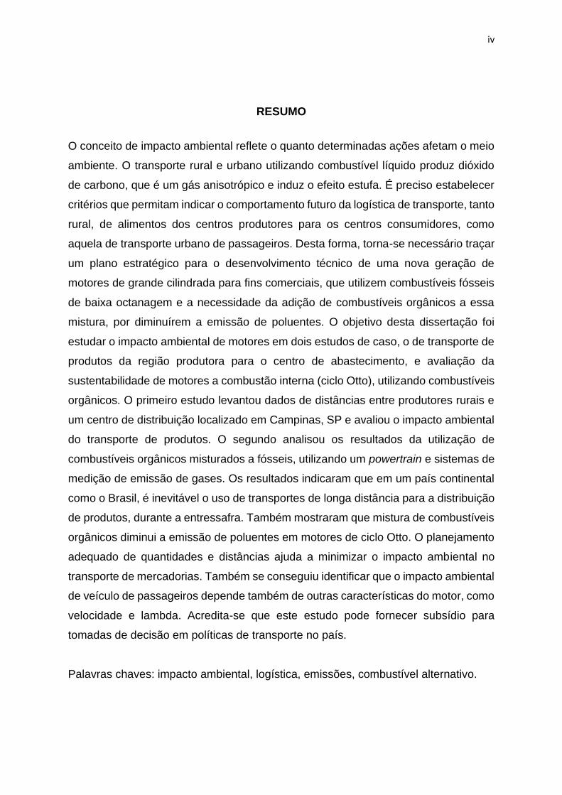
O conceito de impacto ambiental reflete o quanto determinadas ações afetam o meio
ambiente. O transporte rural e urbano utilizando combustível líquido produz dióxido
de carbono, que é um gás anisotrópico e induz o efeito estufa. É preciso estabelecer
critérios que permitam indicar o comportamento futuro da logística de transporte, tanto
rural, de alimentos dos centros produtores para os centros consumidores, como
aquela de transporte urbano de passageiros. Desta forma, torna-se necessário traçar
um plano estratégico para o desenvolvimento técnico de uma nova geração de
motores de grande cilindrada para fins comerciais, que utilizem combustíveis fósseis
de baixa octanagem e a necessidade da adição de combustíveis orgânicos a essa
mistura, por diminuírem a emissão de poluentes. O objetivo desta dissertação foi
estudar o impacto ambiental de motores em dois estudos de caso, o de transporte de
produtos da região produtora para o centro de abastecimento, e avaliação da
sustentabilidade de motores a combustão interna (ciclo Otto), utilizando combustíveis
orgânicos. O primeiro estudo levantou dados de distâncias entre produtores rurais e
um centro de distribuição localizado em Campinas, SP e avaliou o impacto ambiental
do transporte de produtos. O segundo analisou os resultados da utilização de
combustíveis orgânicos misturados a fósseis, utilizando um powertrain e sistemas de
medição de emissão de gases. Os resultados indicaram que em um país continental
como o Brasil, é inevitável o uso de transportes de longa distância para a distribuição
de produtos, durante a entressafra. Também mostraram que mistura de combustíveis
orgânicos diminui a emissão de poluentes em motores de ciclo Otto. O planejamento
adequado de quantidades e distâncias ajuda a minimizar o impacto ambiental no
transporte de mercadorias. Também se conseguiu identificar que o impacto ambiental
de veículo de passageiros depende também de outras características do motor, como
velocidade e lambda. Acredita-se que este estudo pode fornecer subsídio para
tomadas de decisão em políticas de transporte no país.
Palavras chaves: impacto ambiental, logística, emissões, combustível alternativo.
v
ABSTRACT
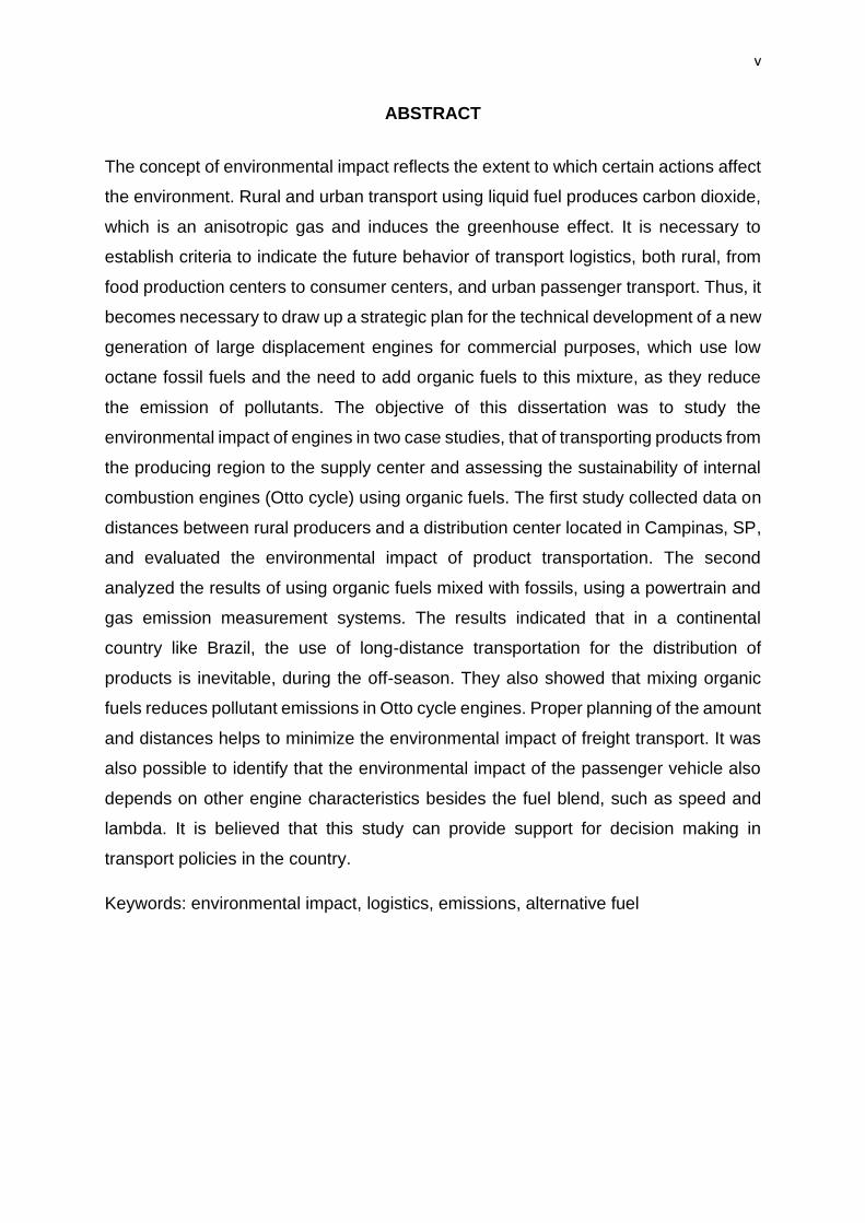
The concept of environmental impact reflects the extent to which certain actions affect
the environment. Rural and urban transport using liquid fuel produces carbon dioxide,
which is an anisotropic gas and induces the greenhouse effect. It is necessary to
establish criteria to indicate the future behavior of transport logistics, both rural, from
food production centers to consumer centers, and urban passenger transport. Thus, it
becomes necessary to draw up a strategic plan for the technical development of a new
generation of large displacement engines for commercial purposes, which use low
octane fossil fuels and the need to add organic fuels to this mixture, as they reduce
the emission of pollutants. The objective of this dissertation was to study the
environmental impact of engines in two case studies, that of transporting products from
the producing region to the supply center and assessing the sustainability of internal
combustion engines (Otto cycle) using organic fuels. The first study collected data on
distances between rural producers and a distribution center located in Campinas, SP,
and evaluated the environmental impact of product transportation. The second
analyzed the results of using organic fuels mixed with fossils, using a powertrain and
gas emission measurement systems. The results indicated that in a continental
country like Brazil, the use of long-distance transportation for the distribution of
products is inevitable, during the off-season. They also showed that mixing organic
fuels reduces pollutant emissions in Otto cycle engines. Proper planning of the amount
and distances helps to minimize the environmental impact of freight transport. It was
also possible to identify that the environmental impact of the passenger vehicle also
depends on other engine characteristics besides the fuel blend, such as speed and
lambda. It is believed that this study can provide support for decision making in
transport policies in the country.
Keywords: environmental impact, logistics, emissions, alternative fuel
6
CAPÍTULO I
1 CONSIDERAÇÕES INICIAIS
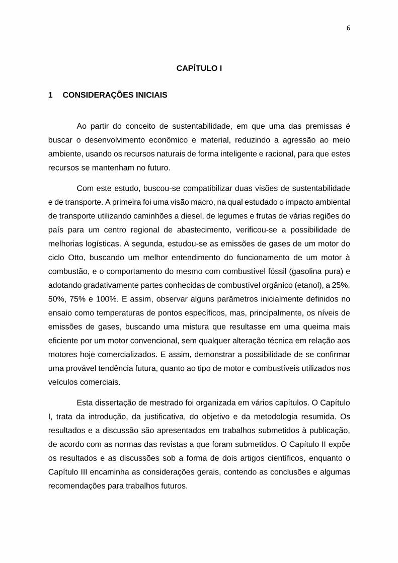
Ao partir do conceito de sustentabilidade, em que uma das premissas é
buscar o desenvolvimento econômico e material, reduzindo a agressão ao meio
ambiente, usando os recursos naturais de forma inteligente e racional, para que estes
recursos se mantenham no futuro.
Com este estudo, buscou-se compatibilizar duas visões de sustentabilidade
e de transporte. A primeira foi uma visão macro, na qual estudado o impacto ambiental
de transporte utilizando caminhões a diesel, de legumes e frutas de várias regiões do
país para um centro regional de abastecimento, verificou-se a possibilidade de
melhorias logísticas. A segunda, estudou-se as emissões de gases de um motor do
ciclo Otto, buscando um melhor entendimento do funcionamento de um motor à
combustão, e o comportamento do mesmo com combustível fóssil (gasolina pura) e
adotando gradativamente partes conhecidas de combustível orgânico (etanol), a 25%,
50%, 75% e 100%. E assim, observar alguns parâmetros inicialmente definidos no
ensaio como temperaturas de pontos específicos, mas, principalmente, os níveis de
emissões de gases, buscando uma mistura que resultasse em uma queima mais
eficiente por um motor convencional, sem qualquer alteração técnica em relação aos
motores hoje comercializados. E assim, demonstrar a possibilidade de se confirmar
uma provável tendência futura, quanto ao tipo de motor e combustíveis utilizados nos
veículos comerciais.
Esta dissertação de mestrado foi organizada em vários capítulos. O Capítulo
I, trata da introdução, da justificativa, do objetivo e da metodologia resumida. Os
resultados e a discussão são apresentados em trabalhos submetidos à publicação,
de acordo com as normas das revistas a que foram submetidos. O Capítulo II expõe
os resultados e as discussões sob a forma de dois artigos científicos, enquanto o
Capítulo III encaminha as considerações gerais, contendo as conclusões e algumas
recomendações para trabalhos futuros.
7
1.1 Introdução e Justificativa
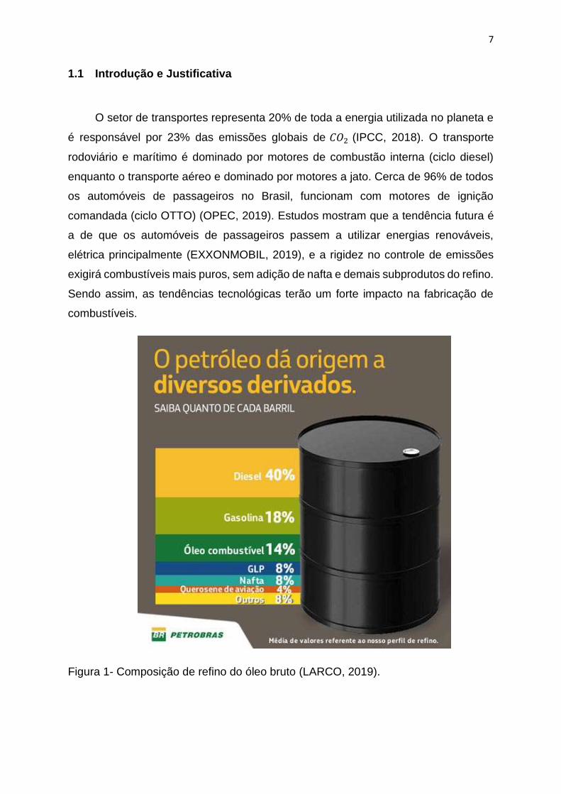
O setor de transportes representa 20% de toda a energia utilizada no planeta e
é responsável por 23% das emissões globais de 𝐶𝑂2 (IPCC, 2018). O transporte
rodoviário e marítimo é dominado por motores de combustão interna (ciclo diesel)
enquanto o transporte aéreo e dominado por motores a jato. Cerca de 96% de todos
os automóveis de passageiros no Brasil, funcionam com motores de ignição
comandada (ciclo OTTO) (OPEC, 2019). Estudos mostram que a tendência futura é
a de que os automóveis de passageiros passem a utilizar energias renováveis,
elétrica principalmente (EXXONMOBIL, 2019), e a rigidez no controle de emissões
exigirá combustíveis mais puros, sem adição de nafta e demais subprodutos do refino.
Sendo assim, as tendências tecnológicas terão um forte impacto na fabricação de
combustíveis.
Figura 1- Composição de refino do óleo bruto (LARCO, 2019).
8
Logo, surge a necessidade de um desenvolvimento conjunto de novos
combustíveis líquidos de baixa octanagem e motores de ignição comandada
(permitem controle no ponto de ignição), para o setor de transportes de longa
distância. Com isso, haverá um aumento na eficiência dos combustíveis de baixa
octanagem, o que permitirá a utilização dos subprodutos do refino de petróleo
(KALGHATGI, 2015).
O segmento de caminhões rodoviários transporta cerca de 60% de todos os
produtos afretados no Brasil (WELLE, 2018). Caminhões a diesel rodam grandes
distâncias das áreas de produção agrícola até os centros de distribuição de alimentos
no país, e esses centros geralmente estão localizados em áreas metropolitanas.
A evolução da demanda de frete de mercadorias está intimamente associada ao
PIB (Produto Interno Bruto) do país. O Banco Mundial examinou 33 países em
diferentes estágios de desenvolvimento e sugeriu que as variações no PIB poderiam
explicar quase 90% da diferença nos volumes de frete rodoviário de mercadorias
(EDWARDS-JONES et al., 2008; MURATORI et al., 2017). A avaliação do transporte
rodoviário de carga é um tanto desafiadora, devido a várias incertezas técnicas e
econômicas (MELAINA e WEBSTER, 2011; ROTHWELL et al., 2016).
Em todo o mundo, existem várias iniciativas para reduzir o número de
intermediários na cadeia de abastecimento alimentar e realocar geograficamente a
produção e o consumo (EDWARDS-JONES et al., 2008; MARIOLA, 2008). Essas
iniciativas compartilham a visão de atender aos diversos critérios de um sistema
alimentar sustentável. Do ponto de vista econômico, a importância é colocada na
redistribuição de mais valor para os agricultores, na reorganização dos fluxos
econômicos e na redução do uso de recursos não renováveis. O desenvolvimento de
cadeias ‘alimentares locais’ pretende ser mais ‘justo’, permitindo a renovação das
relações entre a área metropolitana e a rural (DUPUIS e GOODMAN, 2005). No
debate internacional sobre 'alimentos locais', os impactos ambientais considerados
não se restringem às emissões de GEE. No entanto, as políticas de redução de
carbono podem entregar potenciais compensações na questão geral de
sustentabilidade ambiental, até que outros impactos sejam considerados
(ROTHWELL et al., 2016)
9
A tendência de uso de combustíveis líquidos, derivados do petróleo, e a
necessidade global de redução do nível de emissão de poluentes justificam a adição
do etanol na gasolina pura. Assim, surgiu um motor que melhor se adaptou a essa
mistura e consequentemente emitiu menos poluentes, o motor aspirado com a
ignição. O etanol possui maior octanagem que permite a operação com maiores taxas
de compressão sem entrar em autoignição e com maior eficiência (V.R.ROSO, 2019).
Tecnicamente, esses motores permitem que sejam alterados os tempos de ignição
(antecipar ou atrasar o ponto de ignição, quando necessário), a temperatura de
operação (válvulas termostáticas eletrônicas) e a variação do tempo de injeção de
combustível, conforme detectado pelas sondas lambda no escapamento e os
sensores de pressão do coletor de admissão. No entanto, Barakat et al. (2016)
observaram uma relação linear de baixa inclinação entre o consumo de combustível
e a concentração de etanol. Outros autores (T. TOPGUL, 2006; R. CATALUNA ET
AL., 2008; D. A. GUERRIERI ET AL., 1995) relataram um aumento acentuado no
consumo de combustível usando a mistura etanol-gasolina. Cahyono e Bakar (2011)
encontraram uma diminuição no torque e na potência do motor quando o etanol foi
usado como combustível em contraste com a gasolina. No entanto, esses achados
estão relacionados ao uso da mistura de etanol em motores convencionais de ignição
a gasolina.
A aplicação de técnicas de mineração de dados em testes de misturas de
combustíveis pode identificar informações com mais precisão por meio da aplicação
de algoritmos. Recursos analíticos preditivos, mineração de dados e aprendizado de
máquina podem ser usados para verificações precisas sobre o impacto ambiental de
misturas de combustíveis fósseis e não fósseis, considerando o gerenciamento do
crescimento de dados, integrando e analisando dados para obter insights válidos de
tomada de decisão no uso de combustíveis (SHAH, 2012; RIBEIRO, 2013;
FERREIRA, 2015; HABIB, 2015; JORGE, 2017).
Esta pesquisa se justifica pela escassez de informação científica no conceito de
distribuição de alimentos do produtor para os centros consumidores, indiretamente
pode ser visto como um estudo sobre a pegada de carbono desta operação. Por outro
lado, também se avaliou o impacto ambiental do uso de combustíveis orgânicos, o
que se justifica pela grande utilização no país de frota de veículos comerciais.
10
1.2 Objetivos
1.2.1 Objetivo Geral
Estudar o impacto ambiental de transporte sob duas vertentes, a visão macro de
transporte em longas distâncias e a visão micro, do resultado de diferentes adições de etanol
à gasolina.
1.2.2 Objetivos Específicos
• Estudar o impacto ambiental de transporte utilizando caminhões a
diesel, de legumes e frutas de várias regiões do país para um centro
regional de abastecimento.
• Avaliar as emissões de gases de um motor do ciclo Otto utilizando
diversas misturas de etanol e gasolina. E, determinar a mistura ótima
dos dois combustíveis para rendimento e emissões.
1.3 Metodologia Resumida
O primeiro estudo relata dados disponíveis no centro de distribuição de
alimentos frescos (CEASA-Campinas, localizado a 22 ° 56 'de latitude sul, 46 ° 58' de
longitude oeste e 300 m de altitude). A pesquisa enfocou o volume de alimentos
transportados e a distância das áreas de produção em vários estados do país ao
CEASA
O setor inclui o transporte do produto (alimentos frescos: frutas e legumes;
mamão, tomate e batata) da área rural em vários estados diferentes para o centro de
distribuição de alimentos da CEASA. O valor total transportado foi calculado
considerando o número de viagens multiplicadas pela distância percorrida. A
quantidade total de produto transportado foi encontrada no Relatório CEASA do
centro de distribuição de produtos. Os dados são relativos à distribuição durante os
anos de 2016 e 2017.
11
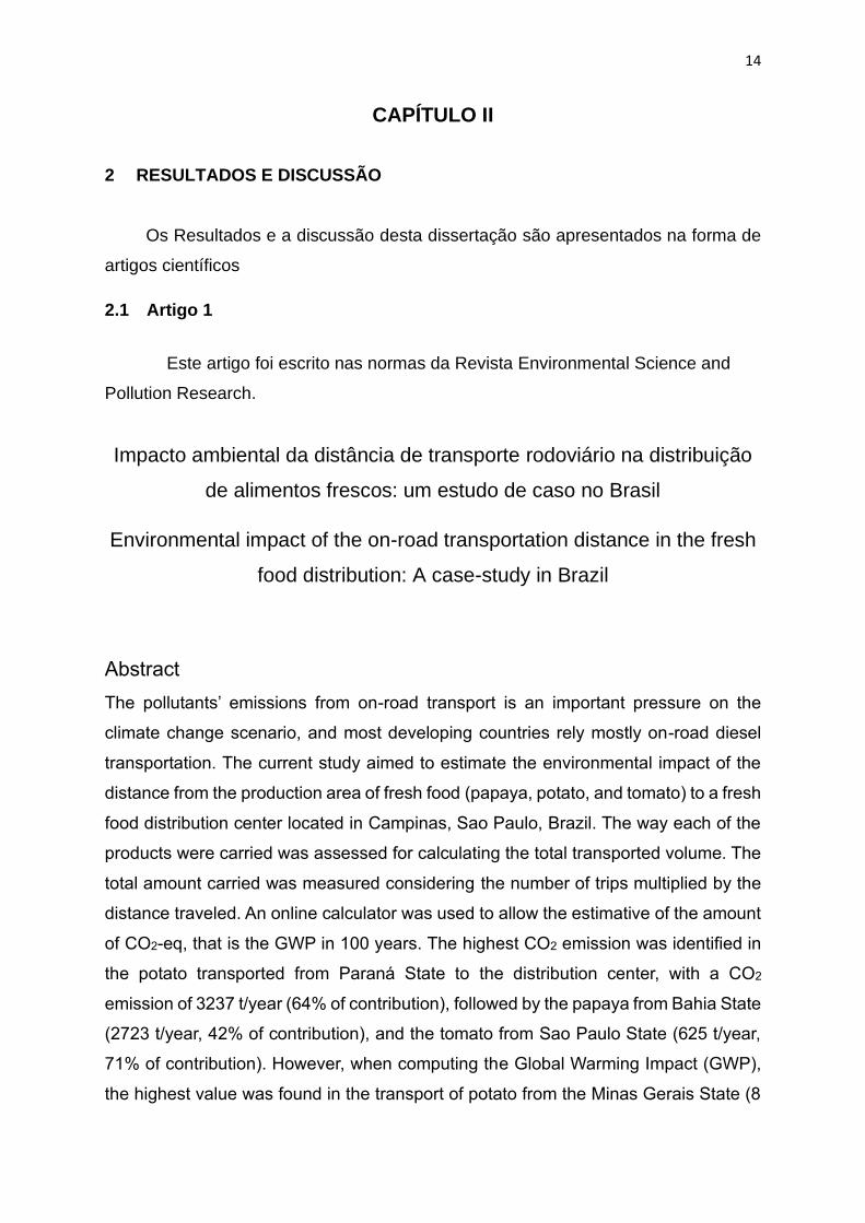
O Segundo estudo relata a pesquisa onde se utilizou de um conjunto Powertrain
para o teste das misturas de combustíveis. O Powertrain trata-se de uma plataforma
móvel, constituída de um motor de 1.598 cm3, quatro cilindros em linha, oito válvulas,
refrigeração por circuito de água sob pressão, com sistema de injeção eletrônica de
combustível multiponto sequencial e um módulo gerenciador (marca Injepro®, modelo
EFI-light v2) que permitiu controlar e acessar o mapa dos atuadores. A plataforma
apresentava todos os sistemas de um veículo automotivo: sistema de alimentação de
combustível e reservatório; sistema de arrefecimento com radiador e ventoinha;
sistema elétrico (alternador e bateria) e de partida (motor de partida).
Os testes foram realizados com etanol (álcool anidro) e gasolina. As misturas
utilizadas no teste de Powertrain foram: gasolina pura (E0), gasolina com 25% de
etanol (E25), gasolina com 50% de etanol (E50), gasolina com 75% de etanol (E75)
e etanol puro (E100). A gasolina padrão brasileira é comercializada com 27% de
etanol (ANP N° 19, 2015; ANP Nº 9, 2017). Diante disso, a extração desse volume de
etanol foi realizada em laboratório através da decantação e separação para fins de
padronização antes do teste.
As metodologias detalhadas se encontram nos artigos, no Capítulo 2.
1.4 Referências Bibliográficas
A. Jorge, G. Larrazabal, P. Guillen, R. L. Lopes, Proceedings of the Workshop on Data Mining for Oil and Gas, 2017, https://doi.org/10.13140/RG.2.2.16408.39681 (accessed October 30 2019). ANP nº 9. Agência Nacional do Petróleo, Gás Natural e Biocombustíveis. http://www.anp.gov.br/images/Consultas_publicas/Concluidas/2018/n_4/4-NT009SPC2017_Minuta_Resolucao_Biocombustiveis.pdf, 2017 (accessed 30 October 2019) (in Portuguese). ANP n° 19. Agência Nacional do Petróleo, Gás Natural e Biocombustíveis. http://nxt.anp.gov.br/NXT/gateway.dll/leg/resolucoes_anp/2015/abril/ranp%2019%20-%202015.xml?f=templates&fn=document-frameset.htm, 2015 (accessed October 30, 2019 (in Portuguese). B. Shah, B. H. Trivedi, Artificial neural network based intrusion detection system: A survey. Int. J. Comput. Appl. 39 (2012) 13-18.
12
D. A. Guerrieri, P. J. Caffrey, V. Rao, Investigation into the vehicle exhaust emissions of high percentage ethanol blends, SAE, 1995, 85–95, https://doi.org/10.4271/950777 (accessed October 30, 2019). DuPuis M, Goodman D (2005) Should we go ‘home’ to eat? Towards a reflexive politics in localism. J Rural Stud 21: 359–371 http://dx.doi.org/10.1016/j.jrurstud.2005.05.011
Edwards-Jones G, Milà i Canals L, Hounsome N, Truninger M, Koerber G, Hounsome B, Cross P, York EH, Hospido A, Plassmann K, Harris IM, Edwards RT, Day GAS, Tomos AD, Cowell SJ, Jones DL (2008) Testing the assertion that ‘local food is best’: The challenges of an evidence-based approach. Trends Food Sci Tech 19: 265e274. https://doi.org/10.1016/j.tifs.2008.01.008
ExxonMobil, 2019, Outlook for Energy: A perspective to 2040, https://corporate. exxonmobil.com/Energy-and-environment/Looking-forward/Outlook-for-Energy/ Outlook-for-Energy-A-perspective-to-2040 Access on: Dec.14, 2019.
IPCC, 2018, Chapter 8: Transport, https://www.ipcc.ch/site/assets/uploads /2018/02/ipcc wg3_ar5_chapter8.pdf Access on: Jan.18, 2020.
J. C. Ferreira, J. de Almeida, A. R. da Silva, The impact of driving styles on fuel consumption: A data-warehouse-and-data-mining-based discovery process. IEEE Trans. Intell. Transp. Syst. 16 (2015) 2653-2662. https://doi.org/10.1109/TITS.2015.2414663
K. Habib, A. I. Umar, Research article anomalies calculation and detection in fuel expense through data mining. Res. J. Inf. Technol, 6 (2015) 44-50. http://dx.doi.org/10.19026/rjit.6.2165
Kalghatgi, Gautam. Petroleum-Based Fuels for Transport[J]. Journal Of Automotive Safety And Energy, 2015, 6(01): 1-16. http://journal08.magtechjournal.com/Jwk_ qcaqyjn/EN/10.3969/j.issn.1674-8484.2015.01.001 Access on: Jul.14, 2019.
Larco Petróleo, Notícias, 2019. http://www.larcopetroleo.com.br/noticias/40-de-um-barril-de-petroleo-viram-diesel-e-18-gasolina-apos-o-refino/ Access on: Jun, 19, 2019.
Mariola MJ (2008) The local industrial complex? Questioning the link between local foods and energy use. Agr Hum Values 25: 193–196 http://dx.doi.org/10.1007/s10460-008-9115-3.
OPEC, 2019, World Oil Outlook 2040 https://www.opec.org/opec_web/static_files_ project/media/downloads/press room/Presentation%20-%20Launch%20of%20the% 202019%20OPEC%20World%20Oil%20Outlook.pdf Access on: Dec.10, 2019.
R. Cataluna, R. Silva, E. W. Menezes, R. B. Ivanov, Specific consumption of liquid
biofuels in gasoline fuelled engines, Fuel 87 (2008) 3362–3368.
13
Rothwell A, Ridoutt B, Page G, Bellotti W (2016) Environmental performance of local
food: trade-offs and implications for climate resilience in a developed city. J Clean Prod
114: 420-430. https://doi.org/10.1016/j.jclepro.2015.04.096
T. Topgul, H. S. Yucesu, C. Çinar, A. Koca, The effects of ethanol–unleaded gasoline blends and ignition timing on engine performance and exhaust emissions, Renew. Energy 31 (2006) 2534–2542. https://doi.org/10.1016/j.renene.2006.01.004
V. R. Roso, N. D. S. A. Santos, C. E. C. Alvarez, F. A. Rodrigues Filho, F. J. P. Pujatti, R. M. Valle, Effects of mixture enleanment in combustion and emission parameters using a flex-fuel engine with ethanol and gasoline, Appl. Therm. Eng. 153 (2019) 463-472. https://doi.org/10.1016/j.applthermaleng.2019.03.012
V. Ribeiro, J. Rodrigues, A. Aguiar, Mining geographic data for fuel consumption estimation, 2013, https://doi.org/10.1109/ITSC.2013.6728221 (accessed October 30 2019)
Welle D (2018) What represents the transport by trucks for Brazilian supply chains? https://www.cartacapital.com.br/economia/o-que-o-transporte-por-caminhoes-representa-para-o-brasil Accessed May 15 2018.
14
CAPÍTULO II
2 RESULTADOS E DISCUSSÃO
Os Resultados e a discussão desta dissertação são apresentados na forma de
artigos científicos
2.1 Artigo 1
Este artigo foi escrito nas normas da Revista Environmental Science and
Pollution Research.
Impacto ambiental da distância de transporte rodoviário na distribuição
de alimentos frescos: um estudo de caso no Brasil
Environmental impact of the on-road transportation distance in the fresh
food distribution: A case-study in Brazil
Abstract
The pollutants’ emissions from on-road transport is an important pressure on the
climate change scenario, and most developing countries rely mostly on-road diesel
transportation. The current study aimed to estimate the environmental impact of the
distance from the production area of fresh food (papaya, potato, and tomato) to a fresh
food distribution center located in Campinas, Sao Paulo, Brazil. The way each of the
products were carried was assessed for calculating the total transported volume. The
total amount carried was measured considering the number of trips multiplied by the
distance traveled. An online calculator was used to allow the estimative of the amount
of CO2-eq, that is the GWP in 100 years. The highest CO2 emission was identified in
the potato transported from Paraná State to the distribution center, with a CO2
emission of 3237 t/year (64% of contribution), followed by the papaya from Bahia State
(2723 t/year, 42% of contribution), and the tomato from Sao Paulo State (625 t/year,
71% of contribution). However, when computing the Global Warming Impact (GWP),
the highest value was found in the transport of potato from the Minas Gerais State (8
15
10-2 in 100 years) followed by the papaya from Rio Grande do Norte State (5 10-2 in
100 years) and the papaya from Bahia (3 10-2 in 100 years). The higher the amount of
product transported by a trip the smaller the environmental impact in the long run. A
proper strategy to reduce the environmental impact would be to have large freight
volume when transporting food from vast distances within continental countries.
Keywords
Papaya; potato; tomato; freight; GHG emissions; Global Warming Potential
Introduction
The world transport sector represents nearly 20% of carbon dioxide (CO2) emissions
from fossil fuel combustion and around 15% of overall greenhouse gas (GHG)
emissions (Forster at al., 2008; IFT, 2010; IEA, 2014). The pollutants’ emissions from
on-road transport cause severe pressure on climate change since the transportation
within the supply chains is a crucial issue in the global carbon dioxide emissions (IEA,
2014; Dente and Tavasszy, 2018). The truck freight sector is a sole contributor to CO2
emissions in large territorial countries such as Brazil that uses mainly diesel truck
transportation. The on-road truck segment hauls about 60% of all freight in Brazil
(Welle, 2018). Diesel on-road trucks travel vast distances from the agricultural
production areas to the food distribution centers in the country, and those centers are
usually located in metropolitan areas.
The evolution of goods’ freight demand is closely associated with the country’ GDP
(Gross Domestic Product). The World Bank examined 33 countries at different
development stages and suggested that the variations in GDP could explain nearly
90% of the difference in goods’ road freight volumes (Edwards-Jones et al., 2008;
Muratori et al., 2017). On-road freight transport assessment is somewhat challenging,
due to several technical and economic uncertainties (Melaina and Webster, 2011;
Rothwell et al., 2016).
Worldwide, there are various initiatives to both reduce the number of intermediaries in
the food supply chain and geographically relocate production and consumption
16
(Edwards-Jones et al., 2008; Mariola, 2008). These initiatives share the vision of
meeting the many criteria of a sustainable food system. From the economic viewpoint,
the importance is placed on the redistribution of increased value for farmers, the re-
arrangement of economic flows, and the reduction of the use of non-renewable
resources. The development of ‘local food’ chains intends to be more ‘just’ and ‘fair,’
allowing renewal of the relations between the metropolitan and the rural area (DuPuis
and Goodman, 2005). Within the ‘local food’ international debate, environmental
impacts considered are not restricted to GHG emissions. However, carbon reduction
policies may deliver potential trade-offs in the overall environmental sustainability
issue, until other impacts are considered (Rothwell et al., 2016). Policy contexts need
to consider how trade-offs will be assessed and managed as governments attempt to
meet the agenda of emissions reductions (Melaina and Webster, 2011; Rothwell et al.,
2016).
There are various ways of representing the environmental impact in the food chain
scenario (Andersson and Ohlsson, 1998; Watkiss, 2005; Coley et al., 2009; Page et al.,
2012; Ligterink et al., 2012; Nocera and Cavallaro, 2016; Caracciolo et al., 2017; Dente
and Tavasszy, 2018). Although other GHG (Nx, NOx, HC, CO) emissions have been
proposed to estimate environmental impact in food supply chains (Ligterink et al.,
2012), carbon dioxide emission has been used to estimate the transportation impact
in several developed countries, that have already established goal towards mitigation
for climate change (Coley et al., 2009; Ligterink et al., 2012; Nocera and Cavallaro,
2016; Quiros et al., 2017; Ligterink, 2017; Dente and Tavasszy, 2018). Nocera and
Cavallaro (2016) proposed an approach to creating simplified emission functions for
road freight transport. The found results were compared to other emission models and
showed the effectiveness of alternative emission mitigation strategies (Dente and
Tavasszy, 2018). Such an analysis does not address the relative cost-effectiveness of
different GHG reduction options, partly due to the significant uncertainties out to 2050
goals (IPCC, 2014). However, the combination of the aims and cost uncertainties
leads to the adoption of a broad range of reduction options to raise the probability of
meeting the cost-effectiveness goals (Nocera and Cavallaro, 2016). The other way of
evaluating environmental impact is the use of Life Cycle Assessment (LCA) approach
(Andersson and Ohlsson, 1998; Hall et al., 2014; Caracciolo et al., 2017). The LCA of
17
two retail distribution networks (Carrefour and 7-11) was carried out by Wang et al.
(2016), and the authors observed that the main impacts were in the use of fossil fuels,
and the most significant factor was the distribution distance. The water footprint was
also used to assess the environmental impact (Page et al., 2012), as well as the food
miles concept (Watkiss, 2005), and the energy efficiency of food systems (Mundler and
Rumpus, 2012).
Global warming potential (GWP) is a relative quantity of how much heat a greenhouse
gas traps in the atmosphere (Quiros and Smith, 2017). It compares the quantity of
heat trapped by a certain mass of the gas to the amount of heat caught by a similar
mass of carbon dioxide. The GWP of an anisotropic gas indicates the amount of
warming a gas causes over a given period (usually 100 years). GWP is equivalent to
an index (GHG, 2011), which uses the CO2 value of 1. The report by the
Intergovernmental Panel on Climate Change (IPCC, 2014) estimates that greenhouse
gas (GHG) emissions must be reduced within the range of 40–70% by 2050 from 2010
levels to avoid a greater than 2 °C increase in the global mean temperature. Such an
aim might avoid the most severe climate change impacts. However, without a clear
policy of mitigation actions to surpass the issues to large emerging economies, and
large territorial countries (i.e., China, Russia, India, and Brazil) that depend on on-road
transportation is a great challenge (Melaina and Webster, 2011; Muratori et al., 2017;
Dente and Travasszy, 2018).
The current study aimed to evaluate for the first time the environmental impact of the
fresh food (papaya, potato, and tomato) transported by on-road diesel trucks from the
different Brazilian States to the CEASA food distribution center located in Campinas,
State of São Paulo, Brazil.
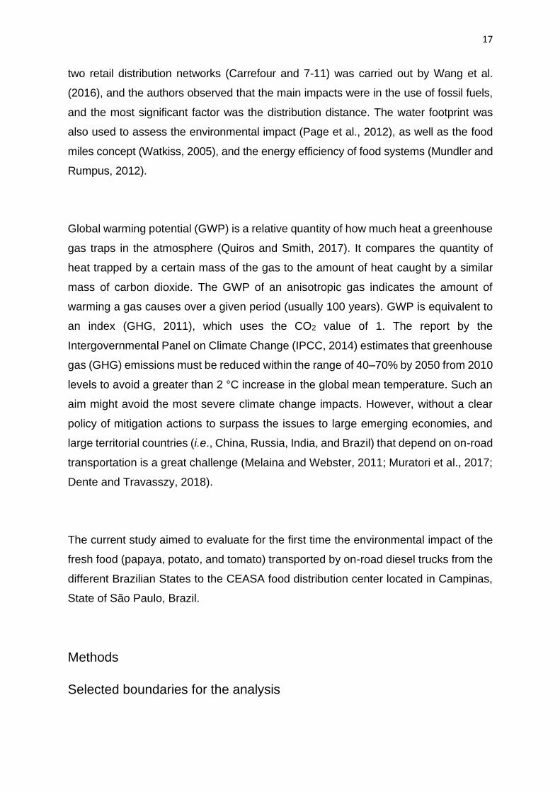
Methods
Selected boundaries for the analysis
18
The present study used data available from the fresh food distribution center (CEASA-
Campinas, located at 22° 56' latitude South, 46° 58' longitude West, and 300 m of
altitude). The research focused on the volume of food transported and distance from
the production areas in several States of the country to the CEASA (Figure 1).
Figure 1. Map of Brazil with the country location in the South America, the States, and the average location of the food production area within the States, and the linear distance to the CEASA Food Center Distribution located in Campinas, São Paulo, Brazil.
The whole supply chain which connects the points of the food production and
distribution center is quite a complicated scenario. Therefore, a sectoral analysis was
established for the present study, as shown in the dotted line of Figure 2. The sector
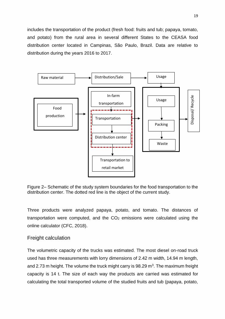
19
includes the transportation of the product (fresh food: fruits and tub; papaya, tomato,
and potato) from the rural area in several different States to the CEASA food
distribution center located in Campinas, São Paulo, Brazil. Data are relative to
distribution during the years 2016 to 2017.
Figure 2– Schematic of the study system boundaries for the food transportation to the distribution center. The dotted red line is the object of the current study.
Three products were analyzed papaya, potato, and tomato. The distances of
transportation were computed, and the CO2 emissions were calculated using the
online calculator (CFC, 2018).
Freight calculation
The volumetric capacity of the trucks was estimated. The most diesel on-road truck
used has three measurements with lorry dimensions of 2.42 m width, 14.94 m length,
and 2.73 m height. The volume the truck might carry is 98.29 m3. The maximum freight
capacity is 14 t. The size of each way the products are carried was estimated for
calculating the total transported volume of the studied fruits and tub (papaya, potato,
Food
production
Crops and fields
In-farm
transportation
Transportation
Distribution center
Transportation to
retail market
Raw material Distribution/Sale Usage
Usage
Packing
Waste
Dis
po
sal/
Rec
ycle
20
and tomato). Tomato and papaya are transported in boxes with the dimensions of 0.36
m of width, 0.55 m length, and 0.31 height (0.061 m3). The boxes are put into the truck
to complete the load.
It was considered that the boxes were placed inside the truck in the longitudinal
position, as in this position the truck might reach the maximum weight possible with
the more significant number of boxes. The total of boxes available was 1,512 boxes.
However, the total capacity being 14 t, the truck might carry only 700 boxes. It was
considered 20 kg of products per box (in the case of tomatoes and papaya). Potatoes
are transported into bags of 50 kg. The total of bags carried was calculated considering
a total of 280 bags per freight that will add up to 14 tons. In each load, the truck
transports 14 t of products. The total amount carried was calculated considering the
number of trips multiplied by the distance traveled. The total quantity of product
transported was found in the CEASA Report of the products distribution center. Data
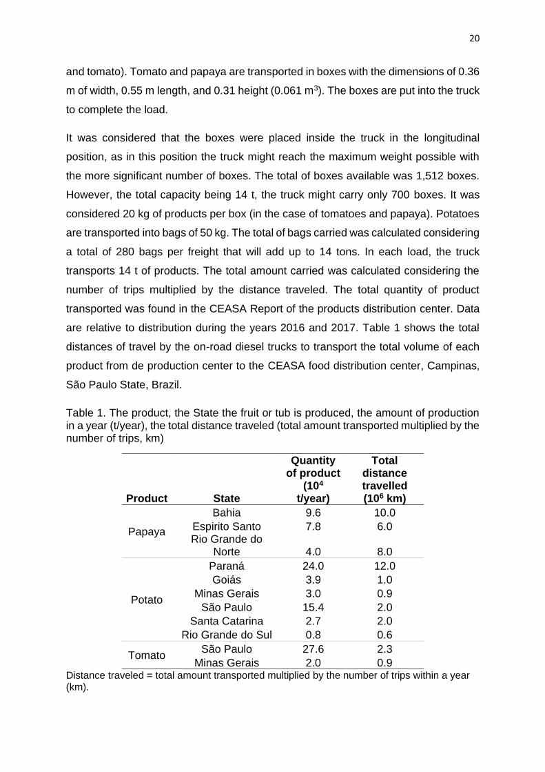
are relative to distribution during the years 2016 and 2017. Table 1 shows the total
distances of travel by the on-road diesel trucks to transport the total volume of each
product from de production center to the CEASA food distribution center, Campinas,
São Paulo State, Brazil.
Table 1. The product, the State the fruit or tub is produced, the amount of production in a year (t/year), the total distance traveled (total amount transported multiplied by the number of trips, km)
Product State
Quantity of product
(104 t/year)
Total distance travelled (106 km)
Papaya
Bahia 9.6 10.0
Espirito Santo 7.8 6.0 Rio Grande do
Norte 4.0 8.0
Potato
Paraná 24.0 12.0
Goiás 3.9 1.0
Minas Gerais 3.0 0.9
São Paulo 15.4 2.0
Santa Catarina 2.7 2.0
Rio Grande do Sul 0.8 0.6
Tomato São Paulo 27.6 2.3
Minas Gerais 2.0 0.9 Distance traveled = total amount transported multiplied by the number of trips within a year (km).
21
Global warming impact assessment
The values of the CO2 equivalent (CO2-eq) emissions were estimated adopting the
100-yr Global Warming Potential (GWP) values used by the Fourth Assessment
Report (AR4) of the IPCC (Forster et al., 2007), and using the online calculator (CFC,
2018). The online calculator allows the user to enter the distance traveled and the
average fuel consumption, and the result is the amount of CO2-eq/year, that is the
GWP in 100 years (Brander, 2012).
It was possible to estimate the GWP for each ton of product in a 100-year time, by
combining the data which might impact the environment for the known period, which
is the concept of GWP (Page et al., 2012). The scope of the total computation of the
environmental impact is beyond the scope of the present study. The role of the
transportation of food products might be expressed in GWP, as found in the current
literature (Nocera and Cavallaro, 2016; Rothwell et al., 2016; Wang et al., 2016;
Muratori et al., 2017).
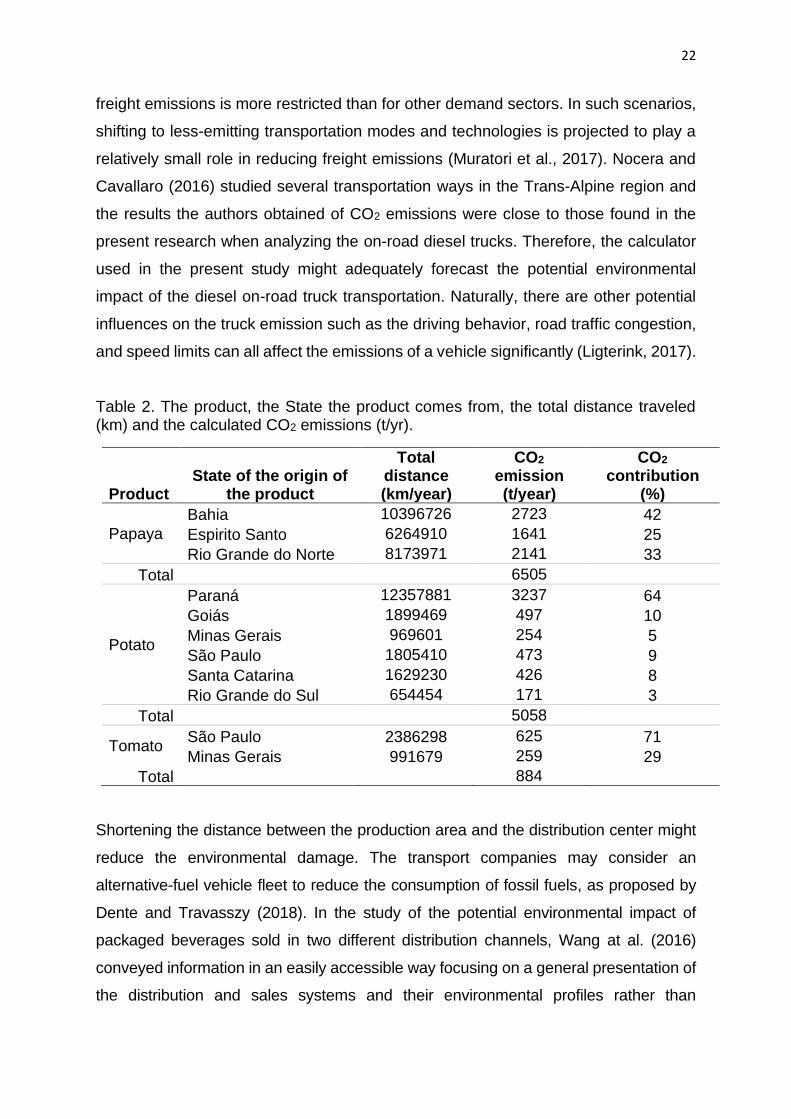
Results and Discussion
The highest values of CO2 emission were found in the potato that comes from Paraná
State, with a CO2 emission of 3237 t/year (64% of contribution), followed by the papaya
from Bahia State (2723 t/year, 42% of contribution), and the tomato from São Paulo
State (625 t/year, 71% of contribution) which was similar to those obtained by Quiros
et al. (2017). The CO2 emissions from the papaya transport were generally high from
the various States. High values were also found for the potatoes transported from
Goiás State (497 t/year), and the other observed values of CO2 emission were
somewhat smaller than the previously cited. The lowest amount observed in the
present study was of the potatoes transported from the Rio Grande do Sul State.
Carbon dioxide emissions from on-road transportation have historically grown with a
correlation to GDP, and there is a limited indication of near-term global decrease the
freight demand from GDP. Over the 21st century, GHG emissions from truck transport
are projected to grow faster than other sectors, with the size of growth reliant on the
amount of a long-term association between freights and the use of carbon fuels. In
climate change mitigation setups that apply a price to GHG emissions, mitigation of
22
freight emissions is more restricted than for other demand sectors. In such scenarios,
shifting to less-emitting transportation modes and technologies is projected to play a
relatively small role in reducing freight emissions (Muratori et al., 2017). Nocera and
Cavallaro (2016) studied several transportation ways in the Trans-Alpine region and
the results the authors obtained of CO2 emissions were close to those found in the
present research when analyzing the on-road diesel trucks. Therefore, the calculator
used in the present study might adequately forecast the potential environmental
impact of the diesel on-road truck transportation. Naturally, there are other potential
influences on the truck emission such as the driving behavior, road traffic congestion,
and speed limits can all affect the emissions of a vehicle significantly (Ligterink, 2017).
Table 2. The product, the State the product comes from, the total distance traveled (km) and the calculated CO2 emissions (t/yr).
Product State of the origin of
the product
Total distance (km/year)
CO2
emission (t/year)
CO2
contribution (%)
Papaya
Bahia 10396726 2723 42
Espirito Santo 6264910 1641 25
Rio Grande do Norte 8173971 2141 33
Total 6505
Potato
Paraná 12357881 3237 64
Goiás 1899469 497 10
Minas Gerais 969601 254 5
São Paulo 1805410 473 9
Santa Catarina 1629230 426 8
Rio Grande do Sul 654454 171 3
Total 5058
Tomato São Paulo 2386298 625 71
Minas Gerais 991679 259 29
Total 884
Shortening the distance between the production area and the distribution center might
reduce the environmental damage. The transport companies may consider an
alternative-fuel vehicle fleet to reduce the consumption of fossil fuels, as proposed by
Dente and Travasszy (2018). In the study of the potential environmental impact of
packaged beverages sold in two different distribution channels, Wang at al. (2016)
conveyed information in an easily accessible way focusing on a general presentation of
the distribution and sales systems and their environmental profiles rather than
23
documenting the complete life cycle assessment methodology and calculation process.
As to the traveled distances, Coley et al. (2009) suggest that when a customer drives a
round-trip distance of more than 7 km to purchase organic vegetables, the carbon
emissions are higher than the emissions from a system using cold storage. Such
storage associated with the packing process, transport to a regional distribution center
and final transport to customer’s doorstep used by large-scale vegetable suppliers is
likely to have a smaller environmental impact. Consequently, some of the thoughts
behind ‘local food’ concept might need to be reviewed (DuPuis and Goodman, 2005).
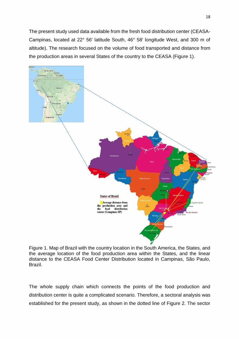
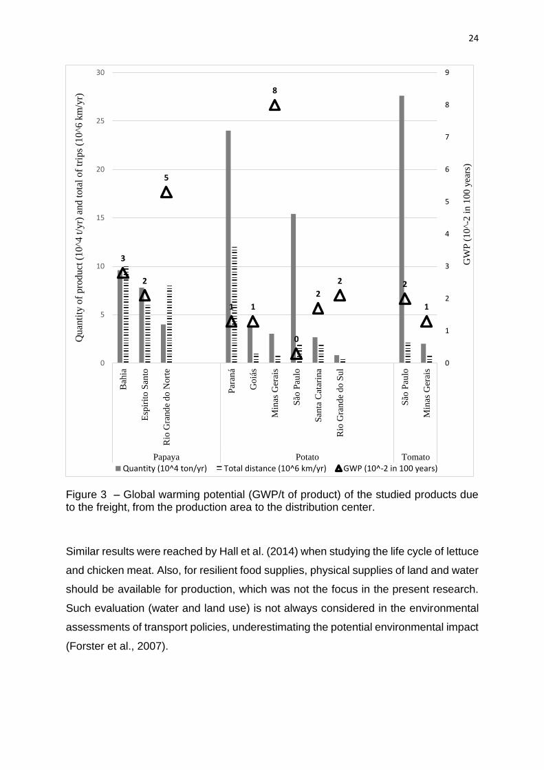
Concerning the environmental impact and the distance traveled, the results of the
current study were not conclusive. The values of GWP/t of product varied (Figure 2),
and were not necessarily proportional to the distance traveled, but the amount was
inversely proportional to the quantity of product transported. However, it was clear that
the potatoes from the State of São Paulo, where Campinas is located, produced a
smaller environmental impact than the product from other States. Such results should
reinforce the ‘local food’ concept. It might be possible that increasing the volume
transported by freight the GWP is maintained within a low level by product where the
distance is high, and the amount of transported product is also high, as shown in
Figure 3 for potatoes transported from Paraná State. While the potatoes transported
from Minas Gerais State, being in small amount generated a high GWP (8 10-2 in 100
years). The higher the amount of product transported per freight the smaller the
environmental impact in the long run.
24
Figure 3 – Global warming potential (GWP/t of product) of the studied products due to the freight, from the production area to the distribution center.
Similar results were reached by Hall et al. (2014) when studying the life cycle of lettuce
and chicken meat. Also, for resilient food supplies, physical supplies of land and water
should be available for production, which was not the focus in the present research.
Such evaluation (water and land use) is not always considered in the environmental
assessments of transport policies, underestimating the potential environmental impact
(Forster et al., 2007).
3
2
5
1 1
8
0
2
2 2
1
0
1
2
3
4
5
6
7
8
9
0
5
10
15
20
25
30
Bah
ia
Esp
irit
o S
anto
Rio
Gra
nd
e d
o N
ort
e
Par
aná
Go
iás
Min
as G
erai
s
São
Pau
lo
San
ta C
atar
ina
Rio
Gra
nd
e d
o S
ul
São
Pau
lo
Min
as G
erai
s
Papaya Potato TomatoG
WP
(1
0^-2
in
10
0 y
ears
)
Quan
tity
of
pro
du
ct (
10
^4
t/y
r) a
nd
to
tal
of
trip
s (1
0^6
km
/yr)
Quantity (10^4 ton/yr) Total distance (10^6 km/yr) GWP (10^-2 in 100 years)
25
Knowing the product consumption potential in the region where the CEASA-Campinas
is located, and the volume produced in a particular region it would be possible to
develop a strategy that would meet the region’s demand for the product with a smaller
environmental impact. However, the interaction of the impacts of consumer choice and
socio-economic systems highlights the inherent interdisciplinarity of food chain
analysis (Edward-Jones et al., 2008). Different scales of production might influence
the environmental impact at the local/global level. Morrow et al. (2010) examined
different policies for reducing GHG emissions and oil consumption in the USA
transportation sector under economy-wide CO2 prices. According to the authors, all
policy scenarios modeled fail to meet the goal of reducing GHG emissions by 14%
below 2005 levels by 2020. Therefore, the mitigation of carbon emissions in large
countries with great territorial distances is a theme of high complexity. Other studies
in developed countries suggest that the energy efficiency of global food systems is
higher due to the increased size and geographic location of producers, which
increases the fuel use for transportation (Watkiss, 2005; Melaina and Webster, 2011;
Rothwell et al., 2016; Muratori et al., 2017). With a rapidly expanding economy and
growing transportation sector, China is also challenged to reduce transportation-
related carbon emissions. As the transportation sector depends on crude oil, large
territorial countries such as China, Brazil, and the USA rely on oil imports to support
domestic demand. Interestingly, research on transportation-related carbon emissions
from China and the United States are often dealing with strategies regarding energy
security in addition to climate change (Morrow et al., 2010; Wang et al., 2007).
While the three-way catalyst, introduced around 1990, has reduced the emissions of
gasoline urban vehicles to small levels, diesel engines used in truck transportation
remain with large CO2 potential emission. The fact that newer light-duty vehicles are not
significantly cleaner than older ones reduces the effectiveness of local urban policy
actions, like low-emission zones, to reduce the carbon emissions of traffic (Ligterink,
2017; Durbin et al., 2018). In the case of transportation from agricultural areas to the
distributing and processing centers, diesel heavy trucks remain as an essential role in
the environmental impact. The deterioration of industrial agriculture, the rising cost of
refrigeration required for storage and transport, and the increased use of biofuels
should change the energy balance back in favor of local foods (Mariola, 2007).
26
However, such a concept might not apply for large territorial countries with food
production areas away from the distribution centers.
In the present study, we faced some questions that could not be answered such as
the unbalanced issues of food transport and local food production. We understood that
such a scenario is more complicated than the current literature points out (Edwards-
Jones et al., 2008; Coley et al., 2009; Mundler and Rumpus, 2012). In a systematic
review on the trends of carbon emissions in the transport sector, Tian et al. (2018)
identified a lack of knowledge on how the application of renewable energy sources
can help mitigate the overall GHG emissions from the transport sector. The authors
encourage greater use of modeling to identify optimal pathways for reducing
transportation-related carbon emissions that consider the environmental impact and
relationships with food suppliers and other industrial sectors.
Conclusions
The Global Warming Impact (in 100 years) was estimated considering the on-road
transportation of fresh food products within Brazilian territory to the distribution center
in Campinas, Sao Paulo State. From the studied fresh food products, the highest
environmental impact was found in the papaya transport from the Northeastern States
to the CEASA in Campinas, São Paulo, followed by the potato and the tomato
transport from several production areas in Brazil. The values of the CO2 emission
depend on the volume of transported product which is dependent on the consumers’
demand.
The larger the volume of products transported by freight the lower the environmental
impact in the long run. Such an effect is also related to the choice of food consumption
in large metropolitan areas. The awareness of the consumer on the environmental
impact might change the diet option; however, it is an option that might arrive after the
embodiment of critical knowledge on the potential harm of climate change.
27
References
Andersson K, Ohlsson T (1998) Life cycle assessment of bread produced on different
scales. Goteborg, Sweden: Chalmers Tekniska Hogskola.
Brander M. (2012) Greenhouse gases, CO2, CO2eq, and carbon: What do all these
terms mean? Econometrics 1-3 < https://ecometrica.com/assets/GHGs-CO2-CO2e-
and-Carbon-What-Do-These-Mean-v2.1.pdf> Accessed 11 September 2018.
Caracciolo F, Amani P, Cavallo C, Cembalo L, D'Amico M, Del Giudice T, Freda R, Fritz
M, Lombardi P, Mennella L, Panico T, Tosco D, Cicia G (2017) The environmental
benefits of changing logistics structures for fresh vegetables. Int J Sustain Transp 12:
233-240 https://doi.org/10.1080/15568318.2017.1337834
CFC- Carbon Footprint Calculator (2018) Vehicle CO2 Emissions Footprint Calculator.
<https://www.commercialfleet.org/tools/van/carbon-footprint-calculator> Accessed 12
December 2018.
Coley D, Howard M, Winter M (2009) Local food, food miles and carbon emissions: A
comparison of farm shop and mass distribution approaches. Food Policy 34: 150–155
https://doi.org/10.1016/j.foodpol.2008.11.001
Dente SMR, Tavasszy L (2018) Policy-oriented emission factors for road freight
transport. Transp Res D 61:33–41. http://dx.doi.org/10.1016/j.trd.2017.03.021
DuPuis M, Goodman D (2005) Should we go ‘home’ to eat? Towards a reflexive politics
in localism. J Rural Stud 21: 359–371 http://dx.doi.org/10.1016/j.jrurstud.2005.05.011
Durbin TD, Johnson K, Miller JW, Maldonado H, Chernich D (2018) Emissions from
heavy-duty vehicles under actual on-road driving conditions. Atmos Environ 2: 4812-
4821 https://doi.org/10.1016/j.atmosenv.2008.02.006
Edwards-Jones G, Milà i Canals L, Hounsome N, Truninger M, Koerber G, Hounsome
B, Cross P, York EH, Hospido A, Plassmann K, Harris IM, Edwards RT, Day GAS,
Tomos AD, Cowell SJ, Jones DL (2008) Testing the assertion that ‘local food is best’:
The challenges of an evidence-based approach. Trends Food Sci Tech 19: 265e274.
https://doi.org/10.1016/j.tifs.2008.01.008
Forster P, Ramaswamy V, Artaxo P, Berntsen T, Betts R, Fahey DW, Haywood J, Lean
J, Lowe DC, Myhre G, Nganga J, Prinn R, Raga G, Schulz M, Dorland RV (2007)
Changes in atmospheric constituents and in radiative forcing. In: Climate Change 2007:
the Physical Science Basis. Cambridge University Press, United Kingdom and New
York, NY, USA. Contribution of Working Group I to the Fourth Assessment Report of
the Intergovernmental Panel on Climate Change.
GHG - Protocol Standard (2011) The greenhouse gas protocol.
http://www.ghgprotocol.org/standards Accessed 10 September 2018.
Hall G, Rothwell A, Grant T, Isaacs B, Ford L, Dixon J, Kirk M, Friel S (2014) Potential
environmental and population health impacts of local urban food systems under climate
28
change: a life cycle analysis case study of lettuce and chicken. Agr Food Secur 3: 6
https://doi.org/10.1186/2048-7010-3-6
IEA-International Energy Agency (2014) CO2 Emission from Fuel Combustion 2012.
http://www.iea.org/co2highlights/co2highlights.pdf Accessed 17 August 2018
IPCC- Intergovernmental Panel on Climate Change (2014) Fifth Assessment Report
(AR5).
ITF-International Transport Forum 2010 Reducing Transport Greenhouse Gas
Emissions – Trends & Data. OECD/ITF. < https://www.itf-oecd.org/real-world-vehicle-
emissions> Accessed 23 October 2018.
Ligterink NE, Tavasszy LA, de Lange R (2012) A velocity and payload dependent
emission model for heavy-duty road freight transportation. Transp Res D 17: 487–491.
https://doi.org/10.1016/j.trd.2012.05.009.
Ligterink NE (2017) Real-world vehicle emissions. The International Transport Forum.
Discussion Paper No. 2017-06 https://www.itf-oecd.org/sites/default/files/docs/real-
word-vehicle-emisions.pdf Accessed 11 September 2018.
Mariola MJ (2008) The local industrial complex? Questioning the link between local
foods and energy use. Agr Hum Values 25: 193–196 http://dx.doi.org/10.1007/s10460-
008-9115-3.
Melaina M, Webster K (2011) Role of fuel carbon intensity in achieving 2050
greenhouse gas reduction goals within the light-duty vehicle sector. Environ Sci Technol
45: 3865–3871 http://dx.doi.org/10.1021/es1037707.
Morrow WR, Gallagher KS, Collantes G, Lee H (2010) Analysis of policies to reduce oil
consumption and greenhouse-gas emissions from the US transportation sector. Energ
Policy 38: 1305–1320 https://doi.org/10.1016/j.enpol.2009.11.006
Mundler P, Rumpus L (2012) The energy efficiency of local food systems: A comparison
between different modes of distribution. Food Policy 37: 609–615
http://dx.doi.org/10.1016/j.foodpol.2012.07.006
Muratori M, Smith SJ, Kyle P, Link R, Mignone BK, Kheshgi HS (2017) Role of the freight
sector in future climate change mitigation scenarios. Environ Sci Technol 51:
3526−3533 https://doi.org/10.1021/acs.est.6b04515
Nocera S, Cavallaro F (2016) Economic valuation of Well-To-Wheel CO2 emissions
from freight transport along the main transalpine corridors. Transp Res D 47: 222–236
https://doi.org/10.1016/j.trd.2016.06.004
Page G, Ridoutt B, Bellotti W (2012) Carbon and water footprint tradeoffs in fresh tomato
production. J Clean Prod 32: 219-226 https://doi.org/10.1016/j.jclepro.2012.03.036
Quiros DC, Smith J, Thiruvengadam A, Huai T, Hu S (2017) Greenhouse gas emissions
from heavy-duty natural gas, hybrid, and conventional diesel on-road trucks during
freight transport. Atmos Environ 168: 36-45
https://doi.org/10.1016/j.jclepro.2012.03.036
29
Rothwell A, Ridoutt B, Page G, Bellotti W (2016) Environmental performance of local
food: trade-offs and implications for climate resilience in a developed city. J Clean Prod
114: 420-430. https://doi.org/10.1016/j.jclepro.2015.04.096
Tian X, Geng Y, Zhong S, Wilson J, Gao C, Chen W, Yua Z, Hao H (2018) A bibliometric
analysis on trends and characters of carbon emissions from transport sector. Transp
Res D 59: 1–10. https://doi.org/10.1016/j.trd.2017.12.009
Wang J, Zhuang H, Lin P-C (2016) The environmental impact of distribution to retail
channels: A case study on packaged beverages. Transp Res D 43: 17–27.
https://doi.org/10.1016/j.trd.2015.11.008
Watkiss P (2005) The validity of food miles as an indicator of sustainable development.
Final Report produced for DEFRA. ED50254 Issue 7. <
http://library.uniteddiversity.coop/Food/DEFRA_Food_Miles_Report.pdf> Accessed
August 10 2018.
Welle D (2018) What represents the transport by trucks for Brazilian supply chains?
https://www.cartacapital.com.br/economia/o-que-o-transporte-por-caminhoes-
representa-para-o-brasil Accessed May 15 2018.
30
2.2 Artigo 2
Este artigo foi escrito nas normas da Revista Fuel Processing Technology.
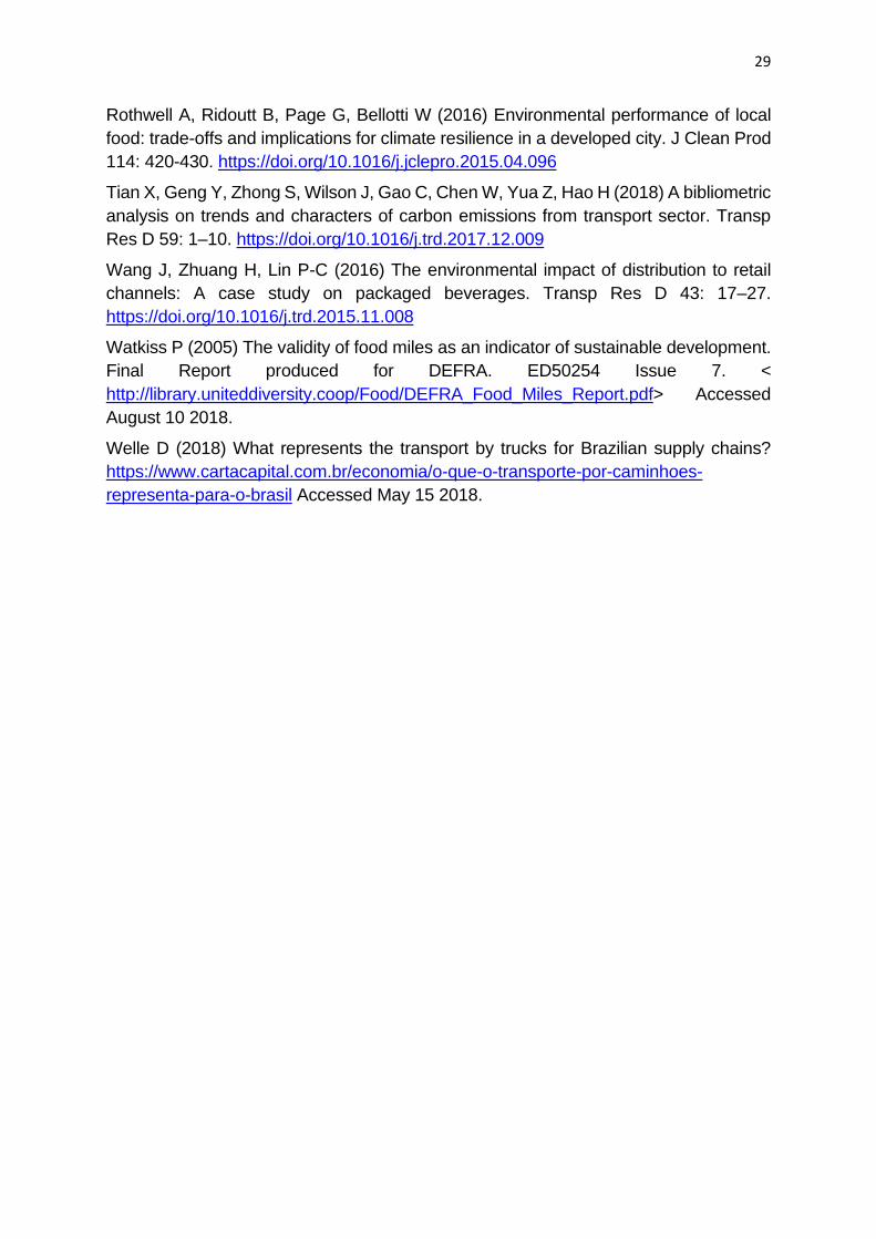
Classifying the Environmental Impact of a Spark Ignition Flex-Fuel Engine Using
Ethanol - Gasoline Blends
Abstract
The present study aimed to classify the environmental impact of concentrations of gasoline and
ethanol mixtures (pure gasoline, 25, 50, 75% ethanol blended to gasoline, and 100% ethanol)
using a flex-fuel engine. The Powertrain used for testing the fuel blends was a mobile platform,
consisting of a 1,598 cm3 flex-fuel engine, four cylinders in line, eight valves, cooling by a
water pressure circuit, with a sequential multipoint electronic fuel injection system and a
management module that allowed to control and access the map of the actuators. We used the
data mining approach to develop a classification model using the ethanol content in gasoline
(0, 25, 50, 75, and 100% ethanol content), the engine rotational speed 900, 2000, and 3000 rpm
and lambda (λ) as attributes. The classification target was the environmental impact concerning
the CO2 emission (‘low,’ ‘average,’ and ‘high’). We used the Random forest algorithm to
develop the models. The mean values showed that the carbon monoxide concentrations for all
studied fuel content were above 0.5% of the volume. The classification models (accuracy 73%,
κ =0.61) indicated that when the ethanol content in the blend is higher than 12.5%, the trend is
that the environmental impact is ‘high’; however, the general classification of the
environmental impact depends also on the engine rotation, the air-fuel ratio, and λ.
Keywords: alternative fuel, ethanol, combustion, spark-ignition engine, flex-fuel engine.
1. Introduction
Non-fossil fuels are considered renewable since they are produced from a natural source
(usually from plants). An example is ethanol (C2H5OH), a natural fuel produced from
sugarcane that is considered an alternative source to fossil fuels [1-4. However, the advantages
of fossil fuel, specifically liquid fuels, used on a large scale in automobiles have characteristics
of high energy density and wide distribution in airports, ports, and roads. The mixture of the
two fuels, gasoline, and ethanol, when properly combined, improves the general energy
efficiency of the vehicles, the torque, and the engine power for application in flex-fuel
31
technology [3,5,6], in addition to reducing emissions of greenhouse gases, carbon dioxide
(CO2), methane (CH4) and nitrous oxide (NO2) when compared to pure gasoline 3,4,6-8].
However, the low ambient temperature might cause an increase in emissions [9], independent
of the ethanol content (EC).
The trend towards the use of liquid fuels, derived from petroleum, and also the global need to
reduce the level of pollutant emissions justify the addition of ethanol in pure gasoline. Thus,
an engine emerged that best adapted to this mixture and consequently emitted less pollutants,
the engine aspirated with the ignition. Ethanol has a higher-octane number that allows the
operation with higher compression rates without entering auto-ignition and with greater
efficiency [3]. Technically, these engines allow the ignition times to be changed (anticipate or
delay the ignition point, when necessary), the operating temperature (electronic thermostatic
valves), and the variation of the fuel injection time, as detected by the λ probes in the exhaust
system and the pressure sensors of the intake manifold. However, Barakat et al. (2016) [10]
observed a low slope linear relationship between fuel consumption and ethanol concentration.
Other authors [11, 12, 13] reported a sharp rise in fuel consumption using the ethanol-gasoline
blend. Cahyono and Bakar (2011) [14] found a decrease in engine torque and power when
ethanol was used as a fuel in contrast to gasoline. However, those findings are related to the
use of ethanol blend in conventional gasoline ignition engine. The ideal is to work with the
mixture with ethanol, in engines with higher compression rates.
The International Energy Agency [4, 7] reports that CO2 emissions from fuel combustion
decreased by around 12% in the European Union, and 16% in the U.S.A. However, overall
levels in the Americas showed little change, as large economies such as Brazil (+ 43%) and
Mexico (+ 24%) increased emissions. Currently, Brazilian standard gasoline is sold with 27%
ethanol in its composition (E27), according to the National Agency of Petroleum, Natural Gas,
and Biofuels [15]. The use of ethanol blend can lead to better air quality in the cities in
comparison, because it reduces CO emissions, despite increasing hydrocarbons (HC) in
conventional engines [16].
The application of data mining techniques in tests of fuel blends can identify information more
accurately through the application of algorithms. Predictive analytics, data mining and machine
learning resources can be used for accurate checks on the environmental impact of fossil, and
non-fossil fuel blends considering managing data growth, integrating and analyzing data to
obtain valid decision-making insights in the use of fuels [17-21]. We did not find in current
32
literature an algorithm to classify the environmental impact when using different blends of
gasoline and ethanol in a flex-fuel engine. Therefore, the objective of the present study was to
classify the environmental impact of gasoline and ethanol blends (pure gasoline, 25, 50, 75%
ethanol blended with gasoline, and 100% ethanol) in a flex-fuel engine using the data mining
approach.
2. Materials and Method
2.1 Powertrain test platform
The Powertrain (a Renault® flex-fuel engine) used was a mobile platform, consisting of a 1,598
cm3 engine, four cylinders in line, eight valves, cooling by water pressure circuit, with
sequential multipoint electronic fuel injection system and a management module (Injepro brand
®, model EFI-light v2) that allowed to control and access the actuators map.
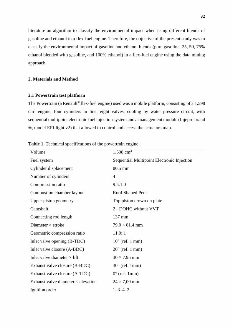
Table 1. Technical specifications of the powertrain engine.
Volume 1.598 cm3
Fuel system Sequential Multipoint Electronic Injection
Cylinder displacement 80.5 mm
Number of cylinders 4
Compression ratio 9.5:1.0
Combustion chamber layout Roof Shaped Pent
Upper piston geometry Top piston crown on plate
Camshaft 2 - DOHC without VVT
Connecting rod length 137 mm
Diameter × stroke 79.0 × 81.4 mm
Geometric compression ratio 11.0: 1
Inlet valve opening (B-TDC) 10° (ref. 1 mm)
Inlet valve closure (A-BDC) 20° (ref. 1 mm)
Inlet valve diameter × lift 30 × 7.95 mm
Exhaust valve closure (B-BDC) 30° (ref. 1mm)
Exhaust valve closure (A-TDC) 0° (ref. 1mm)
Exhaust valve diameter × elevation 24 × 7,00 mm
Ignition order 1–3–4–2
33
The platform featured all the systems of an automotive vehicle with a fuel supply system and
reservoir, cooling system with radiator and fan, electrical system (alternator and battery), and
starter. The engine specifications are presented in Table 1.
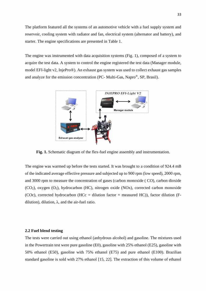
The engine was instrumented with data acquisition systems (Fig. 1), composed of a system to
acquire the test data. A system to control the engine registered the test data (Manager module,
model EFI-light v2, InjePro®). An exhaust gas system was used to collect exhaust gas samples
and analyze for the emission concentration (PC- Multi-Gas, Napro®, SP, Brasil).
Fig. 1. Schematic diagram of the flex-fuel engine assembly and instrumentation.
The engine was warmed up before the tests started. It was brought to a condition of 924.4 mB
of the indicated average effective pressure and subjected up to 900 rpm (low speed), 2000 rpm,
and 3000 rpm to measure the concentration of gases (carbon monoxide ( CO), carbon dioxide
(CO2), oxygen (O2), hydrocarbon (HC), nitrogen oxide (NOx), corrected carbon monoxide
(COc), corrected hydrocarbon (HCc = dilution factor × measured HC)), factor dilution (F-
dilution), dilution, λ, and the air-fuel ratio.
2.2 Fuel blend testing
The tests were carried out using ethanol (anhydrous alcohol) and gasoline. The mixtures used
in the Powertrain test were pure gasoline (E0), gasoline with 25% ethanol (E25), gasoline with
50% ethanol (E50), gasoline with 75% ethanol (E75) and pure ethanol (E100). Brazilian
standard gasoline is sold with 27% ethanol [15, 22]. The extraction of this volume of ethanol
34
was carried through decantation and separation for standardization purposes before the test.
Before starting each data collection, we decontaminate the engine oil. The engine was started
and running at idle (900 rpm), until the thermostatic valve opens (observed when the fan is
running), when the 30 min count starts running at idle, and only then start testing.
The analyzer was maintained for an initial warm-up period, which consisted of 2 fan activation
cycles to ensure the correct measurement of the gases. Within that period, the software reported
that the equipment was heating up. Then, the equipment's leak test was verified by closing the
gas capture probe and waiting for the instructions on the screen to start the tests. Before starting
the measurement, the equipment performs a check to detect the presence of HC residues in the
environment. This procedure aims to confirm that before measurements start, the indicated
value is at its minimum. After the engine was already idling (900 rpm), it was expected 60 s,
which was the estimated time to stabilize the gas reading and thus obtain a lesser variation in
data collection. At the end of the 60 s cycle, a new cycle with a rotation of 2000 rpm and 3000
rpm later, was installed and maintained as the previous test, with data being collected using the
same procedure as the initial one.
2.3 Data analysis
Data on gas concentrations (carbon monoxide (CO), carbon dioxide (CO2), oxygen (O2),
hydrocarbon (HC), nitrogen oxide (NOx), corrected carbon monoxide (COc = dilution factor
× measured CO), corrected hydrocarbon (HCc = dilution factor × measured HC)), dilution
factor (F-dilution), dilution (dilution =CO,% + CO2,%), λ and the air-fuel ratio were measured
and collected in function of engine speed (900, 2000, and 3000 rpm) and fuel mixtures
(gasoline and ethanol content: 0, 25, 50, 75, and 100% ethanol content). For each variable, the
test was performed three times, each time lasting 30 s, to calculate the mean values
(measurements were carried out within the time interval) of gas concentrations, F-dilution,
dilution, λ, and the air-fuel.
Data pre-processing was performed in Excel spreadsheets for further processing in the data
mining software RapidMiner Studio® v9 [23,24]. RapidMiner® is a data mining platform
designed from elementary building blocks, called operators. Each operator performs a specific
action on the data: loading and storing data, transforming data, or inference of a model in the
data [25]. The data set of the tests in the powertrain was loaded, stored, transformed. After this
data pre-processing, a predictive model was inferred through the processes of the operators
35
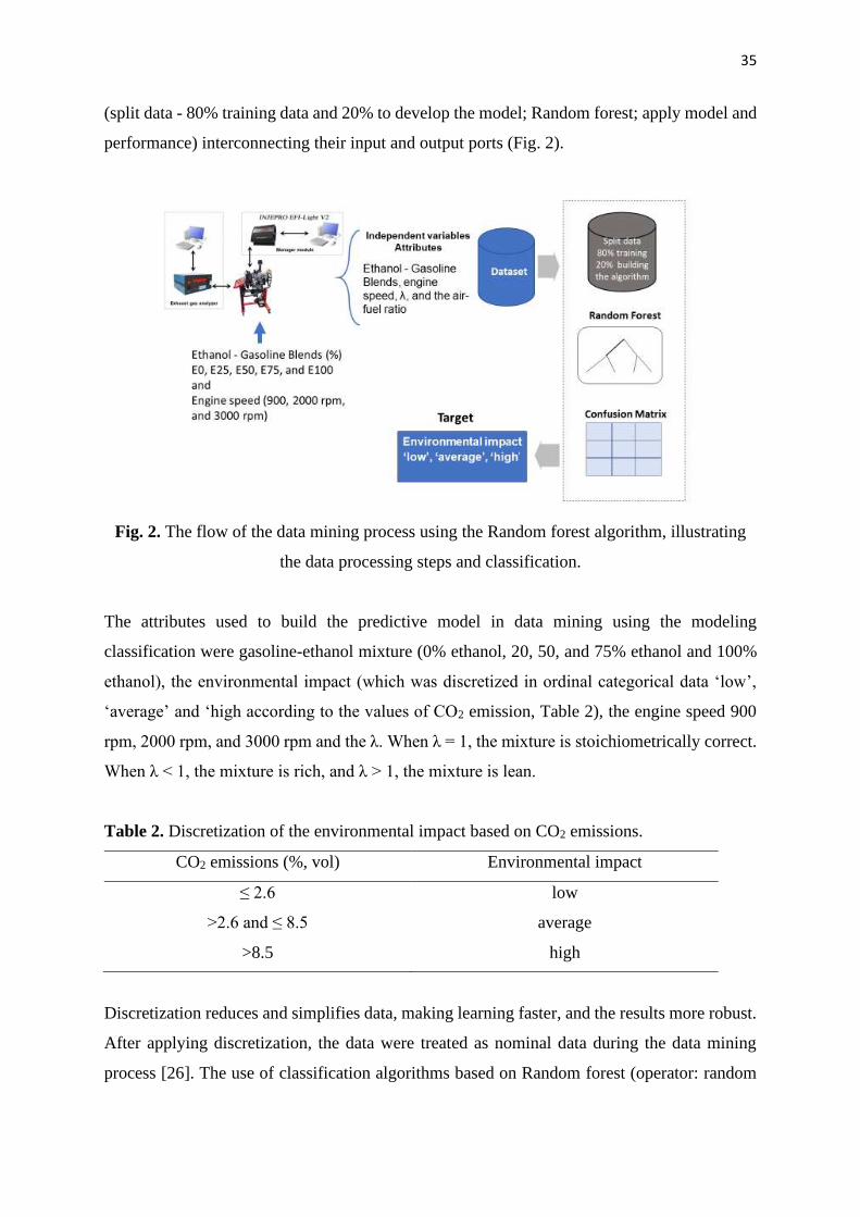
(split data - 80% training data and 20% to develop the model; Random forest; apply model and
performance) interconnecting their input and output ports (Fig. 2).
Fig. 2. The flow of the data mining process using the Random forest algorithm, illustrating
the data processing steps and classification.
The attributes used to build the predictive model in data mining using the modeling
classification were gasoline-ethanol mixture (0% ethanol, 20, 50, and 75% ethanol and 100%
ethanol), the environmental impact (which was discretized in ordinal categorical data ‘low’,
‘average’ and ‘high according to the values of CO2 emission, Table 2), the engine speed 900
rpm, 2000 rpm, and 3000 rpm and the λ. When λ = 1, the mixture is stoichiometrically correct.
When λ < 1, the mixture is rich, and λ > 1, the mixture is lean.
Table 2. Discretization of the environmental impact based on CO2 emissions.
CO2 emissions (%, vol) Environmental impact
≤ 2.6 low
>2.6 and ≤ 8.5 average
>8.5 high
Discretization reduces and simplifies data, making learning faster, and the results more robust.
After applying discretization, the data were treated as nominal data during the data mining
process [26]. The use of classification algorithms based on Random forest (operator: random
36
forest) was applied to generate rules for the prediction of the effect of the mixture of gasoline
and ethanol on the environmental impact due to the air-fuel rotation, and λ. The model
validation was parameterized using the operator split data with a percentage split of 80% for
training and 20% for testing.
The percentage of correctly classified samples compared to the number of all examples is
accuracy (Eq.1). The rate of true positives to all as positive predicted samples is the precision
(Eq. 2). The recall is the ratio of precisely predicted positive observations to all observations
in the target class (Eq. 3). The confusion matrix was calculated to find the prediction accuracy
using the classifying performance. The kappa (κ) is a statistical coefficient of inter-rater
reliability that is applied to evaluate the agreement between two appraisers. In this study, we
assumed that the classification was appropriate when κ ≥ 0.6.
Accuracy = (TP+TN)/(TP+FP+FN+TN) (1)
Precision = TP/(TP+FP) (2)
Recall = TP/(TP+FN) (3)
Where TP = true positives, TN = true negatives, FP = false positives, and FN = false negatives.
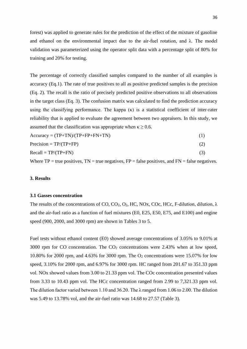
3. Results
3.1 Gasses concentration
The results of the concentrations of CO, CO2, O2, HC, NOx, COc, HCc, F-dilution, dilution, λ
and the air-fuel ratio as a function of fuel mixtures (E0, E25, E50, E75, and E100) and engine
speed (900, 2000, and 3000 rpm) are shown in Tables 3 to 5.
Fuel tests without ethanol content (E0) showed average concentrations of 3.05% to 9.01% at
3000 rpm for CO concentration. The CO2 concentrations were 2.43% when at low speed,
10.80% for 2000 rpm, and 4.63% for 3000 rpm. The O2 concentrations were 15.07% for low
speed, 3.10% for 2000 rpm, and 6.97% for 3000 rpm. HC ranged from 201.67 to 351.33 ppm
vol. NOx showed values from 3.00 to 21.33 ppm vol. The COc concentration presented values
from 3.33 to 10.43 ppm vol. The HCc concentration ranged from 2.99 to 7,321.33 ppm vol.
The dilution factor varied between 1.10 and 36.20. The λ ranged from 1.06 to 2.00. The dilution
was 5.49 to 13.78% vol, and the air-fuel ratio was 14.68 to 27.57 (Table 3).
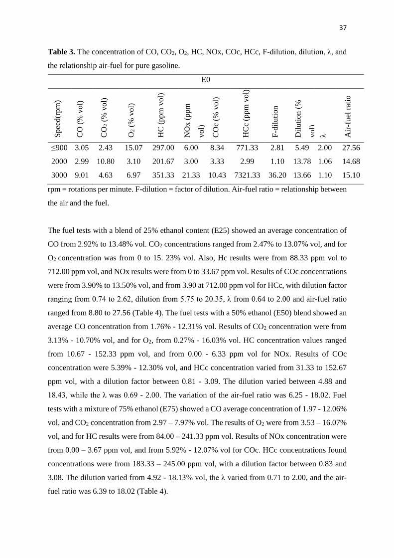
37
Table 3. The concentration of CO, CO2, O2, HC, NOx, COc, HCc, F-dilution, dilution, λ, and
the relationship air-fuel for pure gasoline.
E0
Spee
d(r
pm
)
CO
(%
vol)
CO
2 (
% v
ol)
O2 (
% v
ol)
HC
(ppm
vol)
NO
x (
ppm
vol)
CO
c (%
vol)
HC
c (p
pm
vol)
F-d
iluti
on
Dil
uti
on (
%
vol)
λ
Air
-fuel
rat
io
≤900 3.05 2.43 15.07 297.00 6.00 8.34 771.33 2.81 5.49 2.00 27.56
2000 2.99 10.80 3.10 201.67 3.00 3.33 2.99 1.10 13.78 1.06 14.68
3000 9.01 4.63 6.97 351.33 21.33 10.43 7321.33 36.20 13.66 1.10 15.10
rpm = rotations per minute. F-dilution = factor of dilution. Air-fuel ratio = relationship between
the air and the fuel.
The fuel tests with a blend of 25% ethanol content (E25) showed an average concentration of
CO from 2.92% to 13.48% vol. CO2 concentrations ranged from 2.47% to 13.07% vol, and for
O2 concentration was from 0 to 15. 23% vol. Also, Hc results were from 88.33 ppm vol to
712.00 ppm vol, and NOx results were from 0 to 33.67 ppm vol. Results of COc concentrations
were from 3.90% to 13.50% vol, and from 3.90 at 712.00 ppm vol for HCc, with dilution factor
ranging from 0.74 to 2.62, dilution from 5.75 to 20.35, λ from 0.64 to 2.00 and air-fuel ratio
ranged from 8.80 to 27.56 (Table 4). The fuel tests with a 50% ethanol (E50) blend showed an
average CO concentration from 1.76% - 12.31% vol. Results of CO2 concentration were from
3.13% - 10.70% vol, and for O2, from 0.27% - 16.03% vol. HC concentration values ranged
from 10.67 - 152.33 ppm vol, and from 0.00 - 6.33 ppm vol for NOx. Results of COc
concentration were 5.39% - 12.30% vol, and HCc concentration varied from 31.33 to 152.67
ppm vol, with a dilution factor between 0.81 - 3.09. The dilution varied between 4.88 and
18.43, while the λ was 0.69 - 2.00. The variation of the air-fuel ratio was 6.25 - 18.02. Fuel
tests with a mixture of 75% ethanol (E75) showed a CO average concentration of 1.97 - 12.06%
vol, and CO2 concentration from 2.97 – 7.97% vol. The results of O2 were from 3.53 – 16.07%
vol, and for HC results were from 84.00 – 241.33 ppm vol. Results of NOx concentration were
from 0.00 – 3.67 ppm vol, and from 5.92% - 12.07% vol for COc. HCc concentrations found
concentrations were from 183.33 – 245.00 ppm vol, with a dilution factor between 0.83 and
3.08. The dilution varied from 4.92 - 18.13% vol, the λ varied from 0.71 to 2.00, and the air-
fuel ratio was 6.39 to 18.02 (Table 4).
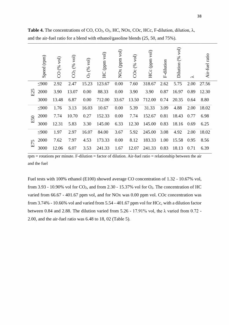
38
Table 4. The concentrations of CO, CO2, O2, HC, NOx, COc, HCc, F-dilution, dilution, λ,
and the air-fuel ratio for a blend with ethanol/gasoline blends (25, 50, and 75%).
S
pee
d (
rpm
)
CO
(%
vol)
CO
2 (
% v
ol)
O2 (
% v
ol)
HC
(ppm
vol)
NO
x (
ppm
vol)
CO
c (%
vol)
HC
c (p
pm
vol)
F-d
iluti
on
Dil
uti
on (
% v
ol)
λ
Air
-fuel
rat
io
E25
≤900 2.92 2.47 15.23 123.67 0.00 7.60 318.67 2.62 5.75 2.00 27.56
2000 3.90 13.07 0.00 88.33 0.00 3.90 3.90 0.87 16.97 0.89 12.30
3000 13.48 6.87 0.00 712.00 33.67 13.50 712.00 0.74 20.35 0.64 8.80
E50
≤900 1.76 3.13 16.03 10.67 0.00 5.39 31.33 3.09 4.88 2.00 18.02
2000 7.74 10.70 0.27 152.33 0.00 7.74 152.67 0.81 18.43 0.77 6.98
3000 12.31 5.83 3.30 145.00 6.33 12.30 145.00 0.83 18.16 0.69 6.25
E75
≤900 1.97 2.97 16.07 84.00 3.67 5.92 245.00 3.08 4.92 2.00 18.02
2000 7.62 7.97 4.53 173.33 0.00 8.12 183.33 1.00 15.58 0.95 8.56
3000 12.06 6.07 3.53 241.33 1.67 12.07 241.33 0.83 18.13 0.71 6.39
rpm = rotations per minute. F-dilution = factor of dilution. Air-fuel ratio = relationship between the air
and the fuel
Fuel tests with 100% ethanol (E100) showed average CO concentration of 1.32 - 10.67% vol,
from 3.93 - 10.90% vol for CO2, and from 2.30 - 15.37% vol for O2. The concentration of HC
varied from 66.67 - 401.67 ppm vol, and for NOx was 0.00 ppm vol. COc concentration was
from 3.74% - 10.66% vol and varied from 5.54 - 401.67 ppm vol for HCc, with a dilution factor
between 0.84 and 2.88. The dilution varied from 5.26 - 17.91% vol, the λ varied from 0.72 -
2.00, and the air-fuel ratio was 6.48 to 18, 02 (Table 5).
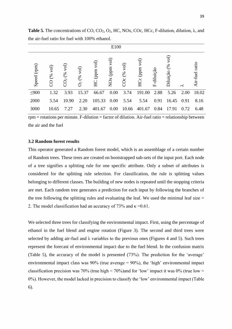
39
Table 5. The concentrations of CO, CO2, O2, HC, NOx, COc, HCc, F-dilution, dilution, λ, and
the air-fuel ratio for fuel with 100% ethanol.
E100
Spee
d (
rpm
)
CO
(%
vol)
CO
2 (
% v
ol)
O2 (
% v
ol)
HC
(ppm
vol)
NO
x (
ppm
vol)
CO
c (%
vol)
HC
c (p
pm
vol)
F-d
iluiç
ão
Dil
uiç
ão (
% v
ol)
λ
Air
-fuel
rat
io
≤900 1.32 3.93 15.37 66.67 0.00 3.74 191.00 2.88 5.26 2.00 18.02
2000 5.54 10.90 2.20 105.33 0.00 5.54 5.54 0.91 16.45 0.91 8.16
3000 10.65 7.27 2.30 401.67 0.00 10.66 401.67 0.84 17.91 0.72 6.48
rpm = rotations per minute. F-dilution = factor of dilution. Air-fuel ratio = relationship between
the air and the fuel
3.2 Random forest results
This operator generated a Random forest model, which is an assemblage of a certain number
of Random trees. These trees are created on bootstrapped sub-sets of the input port. Each node
of a tree signifies a splitting rule for one specific attribute. Only a subset of attributes is
considered for the splitting rule selection. For classification, the rule is splitting values
belonging to different classes. The building of new nodes is repeated until the stopping criteria
are met. Each random tree generates a prediction for each input by following the branches of
the tree following the splitting rules and evaluating the leaf. We used the minimal leaf size =
2. The model classification had an accuracy of 73% and κ =0.61.
We selected three trees for classifying the environmental impact. First, using the percentage of
ethanol in the fuel blend and engine rotation (Figure 3). The second and third trees were
selected by adding air-fuel and λ variables to the previous ones (Figures 4 and 5). Such trees
represent the forecast of environmental impact due to the fuel blend. In the confusion matrix
(Table 5), the accuracy of the model is presented (73%). The prediction for the ‘average’
environmental impact class was 90% (true average = 90%), the ‘high’ environmental impact
classification precision was 70% (true high = 70%)and for ‘low’ impact it was 0% (true low =
0%). However, the model lacked in precision to classify the ‘low’ environmental impact (Table
6).
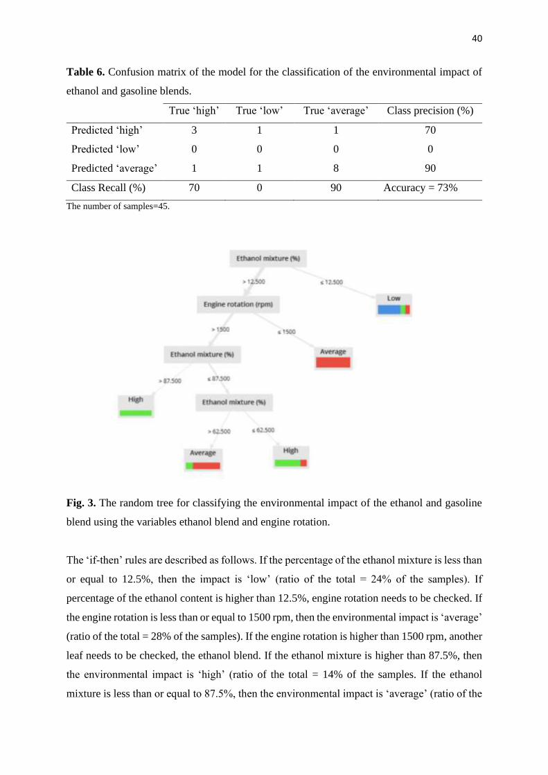
40
Table 6. Confusion matrix of the model for the classification of the environmental impact of
ethanol and gasoline blends.
True ‘high’ True ‘low’ True ‘average’ Class precision (%)
Predicted ‘high’ 3 1 1 70
Predicted ‘low’ 0 0 0 0
Predicted ‘average’ 1 1 8 90
Class Recall (%) 70 0 90 Accuracy = 73%
The number of samples=45.
Fig. 3. The random tree for classifying the environmental impact of the ethanol and gasoline
blend using the variables ethanol blend and engine rotation.
The ‘if-then’ rules are described as follows. If the percentage of the ethanol mixture is less than
or equal to 12.5%, then the impact is ‘low’ (ratio of the total = 24% of the samples). If
percentage of the ethanol content is higher than 12.5%, engine rotation needs to be checked. If
the engine rotation is less than or equal to 1500 rpm, then the environmental impact is ‘average’
(ratio of the total = 28% of the samples). If the engine rotation is higher than 1500 rpm, another
leaf needs to be checked, the ethanol blend. If the ethanol mixture is higher than 87.5%, then
the environmental impact is ‘high’ (ratio of the total = 14% of the samples. If the ethanol
mixture is less than or equal to 87.5%, then the environmental impact is ‘average’ (ratio of the
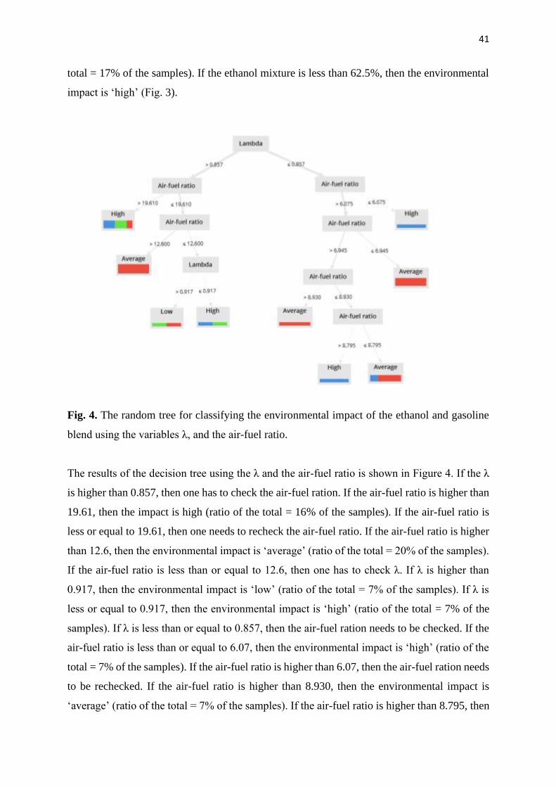
41
total = 17% of the samples). If the ethanol mixture is less than 62.5%, then the environmental
impact is ‘high’ (Fig. 3).
Fig. 4. The random tree for classifying the environmental impact of the ethanol and gasoline
blend using the variables λ, and the air-fuel ratio.
The results of the decision tree using the λ and the air-fuel ratio is shown in Figure 4. If the λ
is higher than 0.857, then one has to check the air-fuel ration. If the air-fuel ratio is higher than
19.61, then the impact is high (ratio of the total = 16% of the samples). If the air-fuel ratio is
less or equal to 19.61, then one needs to recheck the air-fuel ratio. If the air-fuel ratio is higher
than 12.6, then the environmental impact is ‘average’ (ratio of the total = 20% of the samples).
If the air-fuel ratio is less than or equal to 12.6, then one has to check λ. If λ is higher than
0.917, then the environmental impact is ‘low’ (ratio of the total = 7% of the samples). If λ is
less or equal to 0.917, then the environmental impact is ‘high’ (ratio of the total = 7% of the
samples). If λ is less than or equal to 0.857, then the air-fuel ration needs to be checked. If the
air-fuel ratio is less than or equal to 6.07, then the environmental impact is ‘high’ (ratio of the
total = 7% of the samples). If the air-fuel ratio is higher than 6.07, then the air-fuel ration needs
to be rechecked. If the air-fuel ratio is higher than 8.930, then the environmental impact is
‘average’ (ratio of the total = 7% of the samples). If the air-fuel ratio is higher than 8.795, then
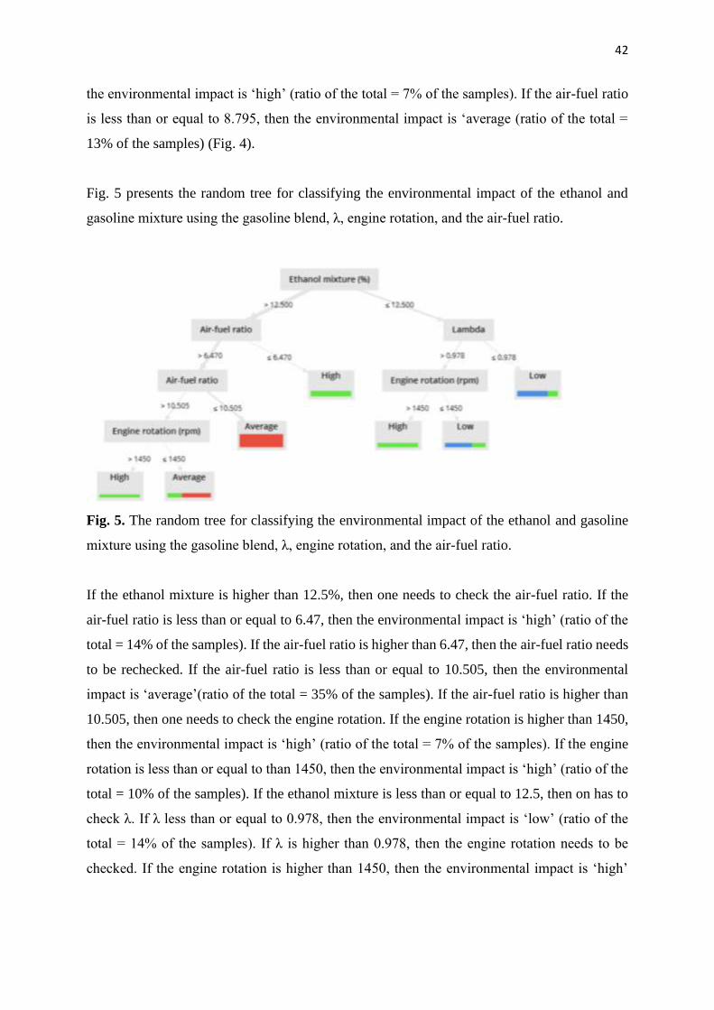
42
the environmental impact is ‘high’ (ratio of the total = 7% of the samples). If the air-fuel ratio
is less than or equal to 8.795, then the environmental impact is ‘average (ratio of the total =
13% of the samples) (Fig. 4).
Fig. 5 presents the random tree for classifying the environmental impact of the ethanol and
gasoline mixture using the gasoline blend, λ, engine rotation, and the air-fuel ratio.
Fig. 5. The random tree for classifying the environmental impact of the ethanol and gasoline
mixture using the gasoline blend, λ, engine rotation, and the air-fuel ratio.
If the ethanol mixture is higher than 12.5%, then one needs to check the air-fuel ratio. If the
air-fuel ratio is less than or equal to 6.47, then the environmental impact is ‘high’ (ratio of the
total = 14% of the samples). If the air-fuel ratio is higher than 6.47, then the air-fuel ratio needs
to be rechecked. If the air-fuel ratio is less than or equal to 10.505, then the environmental
impact is ‘average’(ratio of the total = 35% of the samples). If the air-fuel ratio is higher than
10.505, then one needs to check the engine rotation. If the engine rotation is higher than 1450,
then the environmental impact is ‘high’ (ratio of the total = 7% of the samples). If the engine
rotation is less than or equal to than 1450, then the environmental impact is ‘high’ (ratio of the
total = 10% of the samples). If the ethanol mixture is less than or equal to 12.5, then on has to
check λ. If λ less than or equal to 0.978, then the environmental impact is ‘low’ (ratio of the
total = 14% of the samples). If λ is higher than 0.978, then the engine rotation needs to be
checked. If the engine rotation is higher than 1450, then the environmental impact is ‘high’
43
(ratio of the total = 10% of the samples). If the engine rotation is less than or equal to 1450,
then the environmental impact is ‘low’ (ratio of the total = 10% of the samples) (Figure 6).
4. Discussion
The use of ethanol, particularly in spark-ignition engines, is appealing due to its reasonably
high octane and the fact that it is cleaner than gasoline. The results of the current showed that
the CO concentrations for all fuel mixtures showed values above the reference of CONAMA
(2019) [27], above 0.5% vol. However, HC, at 2000 rpm with a mixture of 25% and 50% EC,
at low speed presented values within the emission limit [15,27]. Considering the HCc results,
they also were within the acceptable limit (lower emissions) at 2000 rpm for E0, E25, E75 and
E100, and at low speed in E50 mixtures and also in E75. The concentrations for CO2 also
showed values within the limit for all fuel mixtures at 2000 rpm [27]. We accept that the [27]
reference is obtained from a vehicle using more complex anti-pollution devices than the model
tested in the present study, such as direct injection, plasma ignition, and recirculation of exhaust
gasses.
The Otto cycle engine is generally not ideal, since other gases that come from incomplete fuel
ignition come out of the exhaust system. However, the ideal fuel ignition would be CO2 + H2O.
When the combustion is ideal, all O2 that enters the engine is used for ignition. The lower the
concentration of this gas in the exhaust system, the closer the combustion is to the ideal [28].
The higher the concentration of CO2 in the exhaust system, the better the combustion. The air-
fuel ratio can also affect the CO2 level. The lack of a rich mixture (O2), the carbon combines
with the oxygen in the burning generating CO (incomplete combustion). CO is considered a
very toxic and reactive gas, so the lower the percentage, the better the combustion. HC also
results from incomplete combustion, in fractionated parts of long chains of non-oxidized fuel.
The lower the concentration of HC, the better the combustion of the mixture [3].
The fuel blends E25, E50, E75, and E100 had a dilution factor of less than 1 for 2000 rpm and
3000 rpm. However, in the test with pure gasoline, the dilution factor went from 36.20 to 3000
rpm. An increase in total hydrocarbon (HC) emissions was detected as the amount of ethanol
in the fuel increased [8]. In the present study, the HCc indicated higher emissions for pure
gasoline (E0) and with a mixture of 25% (E25) of ethanol in a rotation of 3000 rpm.
44
The addition of ethanol to gasoline can help to reduce pollutant gas emissions in ignition
engines [29, 30]. The higher is the EC in the fuel mixture, the lower the environmental impact.
In this study, mixtures with a higher percentage of ethanol had a lower environmental impact
than mixtures with a lower EC that had a more significant environmental impact (‘average’ to
‘high’). According to Schifter et al. (2018) [8], ethanol blended with gasoline in various
concentrations is the most used alternative for positive-ignition engines, in order to incorporate
non-fossil components and diversify energy input in transportation. However, most studies in
current literature apply the gasoline-ethanol blend to design a gasoline engine. In flex-fuel
engines, ethanol generates higher torque. Engines with alcohol need to have a higher
compression ratio (useful volume, between the piston head and the head - fixed volume defined
in the engine construction). If the ideal compression for the ignition is not reached, the burning
of the fuel will not be perfect, generating high values of HC.
CO2 emissions are an increasing trend with the addition of ethanol in gasoline design engines.
The reason is attributing to the complete oxidation of carbon in the fuel. Higher volumetric
efficiency can also be accounted for this unwarranted decrease. It is examined that higher latent
heat of vaporization of ethanol is responsible for the increased production of CO2 [31].
However, by rising the EC, the issue of increasing CO2 can be reduced for slower engine speeds
[32].
Knoll et al. (2009) [33] studied the performance and emissions of conventional vehicles (1999
to 2007) with up to 20% by volume of ethanol. The authors found that the increase in EC
resulted in reductions in both total hydrocarbons, carbon monoxide, and increases in ethanol
emissions and aldehydes. Fuels added to ethanol (E0, E10, E20, and E30) reduce CO, CO2, and
NOX emissions without significant energy loss compared to gasoline in a four-cylinder spark-
ignition engine [34]. The authors carried out combustion tests with gasoline and mixed with
ethanol (50 and 85% v/v) in an engine with a maximum power of 15 kW, performed at eight
different engine speeds, oscillating from 1500 to 5000 rpm, with increments of 500 rpm, the
results showed that the addition of ethanol to gasoline implied a reduction in CO and HC
emissions, in the whole engine speed range. The addition of ethanol increases the values of λ
and makes combustion more complete, reducing gas emissions. Besides, the latent heat of
vaporization of mixed fuels is higher than that of gasoline, providing greater efficiency to the
engine's combustion process [35].
45
In low ethanol content (EC), the CO2 emissions varied between blends, suggesting a
dependence with C and H fuel contents. As the EC rises, the NOx emissions decrease, and the
E-85 (or highest EC fuel) shows the lowest NOx emissions. Such an effect might be associated
with temperature decline at the end of the compression stroke [2]. Suarez-Bertoa et al. (2015)
[9] found an increase in CO2 emissions in blends with high EC (E75 and E85) when compared
to low EC (E5, E10, and E15). In the present study using a flex-fuel engine, the developed
model indicated that low EC (<12.5%) associated with low engine rotation (<1450 rpm) leads
to low environmental impact. On the other hand, high EC associated with either low or high
engine speed tend to lead to average or high environmental impact, agreeing partially with
previous studies [8,29].
The results of the study by Schirmer et al. (2017) [30] indicate that gas emissions using five λ
values and six gasoline/ethanol blends indicate that rich mixtures (λ < 1) tend to produce higher
concentrations of CO and HCs in exhaust gases. As λ increases, the higher quantity of oxygen
in the air leads to smaller amounts of these gases being produced. However, it was observed
that in lean mixtures, HC emissions tend to increase again because combustion may be
incomplete. Tests with increasing EC in the fuel-alcohol blend showed that ethanol helps to
reduce carbon emissions, possibly because of the oxygen contained in ethanol molecules,
resulting in improved combustion and allowing more significant advantage to be taken of the
fuel’s thermodynamic properties [2].
In a previous study, the addition of 40% ethanol to the unleaded gasoline gave the best results
for the reduction of CO emissions by about 30% at 9:1 compression ratio [11]. The addition of
60% ethanol to the unleaded gasoline caused a decrease in CO emissions by about 20%. The
addition of 60% ethanol to gasoline caused a 30% reduction in HC emissions at a high
compression ratio [11]. Therefore, the emissions reduction is not only associated with the
gasoline-ethanol content, but it also relies on other engine-related characteristics, as we found
in the present study. We believe that it is possible to generate ‘If-Then’ rules that would help
appropriate decisions by policymakers in reducing urban pollution in the long run.
46
5. Conclusions
We developed models to classify the environmental impact from a flex-fuel engine and
different blends of gasoline-ethanol. The model forecast that the environmental impact is ‘low’
to ‘average’ when the fuel has a medium to a high percentage of ethanol blended considering
rotation below 2000 rpm. On the other hand, for fuel mixtures with a low percentage of ethanol,
the environmental impact depends on other characteristics of solicitation the engine.
Acknowledgments
The authors thank the University Mauá for allowing the use of the laboratory when we did the
experimental part of the research. We also thank the Universidade Paulista Campus Swift
Engineering undergraduate students who helped to carry on the tests.
References
[1] M. Schwaderlapp, P. Adomeit, A. M. Kolbeck, A., M. Thewes, Ethanol and its potential
for downsized engine concepts. Auto Tech. Review 1 (2012) 48-53.
https://doi.org/10.1365/s40112-012-0022-z
[2] I. Schifter, L. Diaz, J. P. Gómez, U. Gonzalez, Combustion characterization in a single
cylinder engine with mid-level hydrated ethanol-gasoline blended fuels, Fuel 103 (2013) 292-
298. https://doi.org/10.1016/j.fuel.2012.06.002
[3] V. R. Roso, N. D. S. A. Santos, C. E. C. Alvarez, F. A. Rodrigues Filho, F. J. P. Pujatti, R.
M. Valle, Effects of mixture enleanment in combustion and emission parameters using a flex-
fuel engine with ethanol and gasoline, Appl. Therm. Eng. 153 (2019) 463-472.
https://doi.org/10.1016/j.applthermaleng.2019.03.012
[4] IEA – International Energy Agency, CO2 emissions from fuel combustion. Data base
documentation, 2019, http://wds.iea.org/wds/pdf/WorldCo2_Documentation.pdf. (access
October 14, 2019).
[5] R. C. Delgado, A. S. Araujo, V. J. Fernandes Jr, Properties of Brazilian gasoline mixed with
hydrated ethanol for flex-fuel technology, Fuel Process. Technol. 88 (2007) 365-368.
https://doi.org/10.1016/j.fuproc.2006.10.010
[6] T. Venugopal, A. Sharma, S. Satapathy, A. Ramesh, M. K. Gajendra Babu, Experimental
study of hydrous ethanol gasoline blend (E10) in a four stroke port fuel‐injected spark ignition
engine, Int. J. Energy Res. 37 (2013) 638-644. https://doi.org/10.1002/er.1957
47
[7] IEA – International Energy Agency, CO2 Emissions from fuel combustion - Highlights.
Statistics, 2018, https://www.iea.org/statistics/co2emissions/ (accessed October 14, 2019).
[8] I. Schifter, U. González, L. Díaz, L., R. Rodríguez, I. Mejía-Centeno, C. González-Macías,
From actual ethanol contents in gasoline to mid-blends and E-85 in conventional technology
vehicles: Emission control issues and consequences. Fuel 219 (2018) 239-247.
https://doi.org/10.1016/j.fuel.2018.01.118
[9] R. Suarez-Bertoa, A. A. Zardini, H. Keuken, C. Astorga, Impact of ethanol containing
gasoline blends on emissions from a flex-fuel vehicle tested over the Worldwide Harmonized
Light duty Test Cycle (WLTC), Fuel 143 (2015) 173-182.
https://doi.org/10.1016/j.fuel.2014.10.076
[10] Y. Barakat, E. N. Awad, V. Ibrahim, Fuel consumption of gasoline ethanol blends at
different engine rotational speeds, Egypt. J. Pet. 25 (2016) 309-315.
https://doi.org/10.1016/j.ejpe.2015.07.019
[11] T. Topgul, H. S. Yucesu, C. Çinar, A. Koca, The effects of ethanol–unleaded gasoline
blends and ignition timing on engine performance and exhaust emissions, Renew. Energy 31
(2006) 2534–2542. https://doi.org/10.1016/j.renene.2006.01.004
[12] R. Cataluna, R. Silva, E. W. Menezes, R. B. Ivanov, Specific consumption of liquid
biofuels in gasoline fuelled engines, Fuel 87 (2008) 3362–3368.
[13] D. A. Guerrieri, P. J. Caffrey, V. Rao, Investigation into the vehicle exhaust emissions of
high percentage ethanol blends, SAE, 1995, 85–95, https://doi.org/10.4271/950777 (accessed
October 30, 2019).
[14] B. Cahyono, R. Abu Bakar, Effect of ethanol addition in the combustion process during
warm-UPS and half open throttle on port-injection gasoline engine, Am. J. Eng. Appl. Sci. 4
(2011) 66–9.
[15] ANP n° 19. Agência Nacional do Petróleo, Gás Natural e Biocombustíveis.
http://nxt.anp.gov.br/NXT/gateway.dll/leg/resolucoes_anp/2015/abril/ranp%2019%20-
%202015.xml?f=templates&fn=document-frameset.htm, 2015 (accessed October 30, 2019 (in
Portuguese).
[16] R. W. Rice, A. K. Sanyal, A. C. Elrod, R. M. Bata, Exhaust gas emissions of butanol,
ethanol, and methanol–gasoline blend, J. Eng. Gas Turb. Power11(1991) 337–81.
https://doi.org/10.1115/1.2906241
[17] B. Shah, B. H. Trivedi, Artificial neural network-based intrusion detection system: A
survey. Int. J. Comput. Appl. 39 (2012) 13-18.
48
[18] V. Ribeiro, J. Rodrigues, A. Aguiar, Mining geographic data for fuel consumption
estimation, 2013, https://doi.org/10.1109/ITSC.2013.6728221 (accessed October 30 2019)
[19] J. C. Ferreira, J. de Almeida, A. R. da Silva, The impact of driving styles on fuel
consumption: A data-warehouse-and-data-mining-based discovery process. IEEE Trans. Intell.
Transp. Syst. 16 (2015) 2653-2662. https://doi.org/10.1109/TITS.2015.2414663
[20] K. Habib, A. I. Umar, Research article anomalies calculation and detection in fuel expense
through data mining. Res. J. Inf. Technol, 6 (2015) 44-50.
http://dx.doi.org/10.19026/rjit.6.2165
[21] A. Jorge, G. Larrazabal, P. Guillen, R. L. Lopes, Proceedings of the Workshop on Data
Mining for Oil and Gas, 2017, https://doi.org/10.13140/RG.2.2.16408.39681 (accessed
October 30 2019).
[22] ANP nº 9. Agência Nacional do Petróleo, Gás Natural e Biocombustíveis.
http://www.anp.gov.br/images/Consultas_publicas/Concluidas/2018/n_4/4-
NT009SPC2017_Minuta_Resolucao_Biocombustiveis.pdf, 2017 (accessed 30 October 2019)
(in Portuguese).
[23] M. Hofmann, R. Klinkenberg, R. (Eds.). (2014). RapidMiner: Data Mining Use Cases and
Business Analytics Applications. Getting Used to RapidMiner. Chapman & Hall, C.R.C. Press.
Taylor & Francis Group, Boca Raton, FL.
[24] Rapidminer Studio. Predictive Analytics Software, 2020, https://rapidminer.com/
(accessed May 20, 2020).
[25] P. Ristoski, C. Bizer, H. Paulheim, Mining the web of linked data with Rapidminer. Web
Semant. 35 (2015) 142-151. https://doi.org/10.1016/j.websem.2015.06.004
[26] S. Garcia, J. Luengo, J. A. Sáez, V. Lopez, F. Herrera, A survey of discretization
techniques: Taxonomy and empirical analysis in supervised learning. IEEE Trans. Knowl. Data
Eng. 25 (2013) 734-750. https://doi.org/10.1109/TKDE.2012.35
[27] CONAMA. Resolução Nº 493/2019, Programa de Controle da Poluição do Ar por
Motociclos e Veículos similares - PROMOT para controle de emissões de gases poluentes e de
ruído por ciclomotores, motociclos e veículos similares novos.
http://www2.mma.gov.br/port/conama/legiabre.cfm?codlegi=743., 2019 (accessed 11 March
2020) (in Portuguese).
[28] A. K. Thakur, A. K. Kaviti, R. Mehra, K. K. S. Mer, Progress in performance analysis of
ethanol-gasoline blends on SI engine. Renew. Sust. Energ. Rev. 69 (2017) 324–340
https://doi.org/10.1016/j.rser.2016.11.056
49
[29] M. Koç, Y. Sekmen, T. Topgül, H. S. Yücesu, The effects of ethanol–unleaded gasoline
blends on engine performance and exhaust emissions in a spark-ignition engine, Renew.
Energy, 34 (2009) 2101-2106. https://doi.org/10.1016/j.renene.2009.01.018
[30] W. N. Schirmer, L. Z. Olanyk, C. L. B. Guedes, T. P. Quessada, C. B. Ribeiro, M. A.
Capanema, Effects of air/fuel ratio on gas emissions in a small spark-ignited non-road engine
operating with different gasoline/ethanol blends, Environ Sci Pollut Res (2017) 24:20354–
20359. https://doi.org/10.1007/s11356-017-9651-8
[31] A. Elfasakhany, Investigations on the effects of ethanol-methanol-gasoline blends in a
spark-ignition engine. Performance and emissions analysis, Int. J. Eng. Sci. Technol. 18 (2015)
713-719. https://doi.org/10.1016/j.jestch.2015.05.003
[32] C. A. Garcıa, F. Manzini, J. Islas, Air emissions scenarios from ethanol as a gasoline
oxygenated in Mexico City metropolitan area, Renew. Sust. Energ. Rev. (2010) pp. 3032-3040.
https://doi.org/10.1016/j.rser.2010.07.011
[33] K. Knoll, B. West, S. Huff, J. Thomas, J. Orban, C. Cooper, Effects of mid-level ethanol
blends on conventional vehicle emissions, SAE 2009, https://doi.org/10.4271/2009-01-272
(accessed October 30, 2019).
[34] B. Doğan, D. Erol, H. Yaman, E. Kodanli, The effect of ethanol-gasoline blends on
performance and exhaust emissions of a spark ignition engine through exergy analysis. Appl.
Therm. Eng. 120 (2017) 433-443. https://doi.org/10.1016/j.applthermaleng.2017.04.012
[35] G. Najafi, B. Ghobadian, T. Yusaf, S. M. S. Ardebili, R. Mamat, Optimization of
performance and exhaust emission parameters of a SI engine with gasoline-ethanol blended
fuel using response surface methodology. Energy 90 (2015) 1815–29.
50
CAPÍTULO III
3 CONSIDERAÇÕES FINAIS
3.1 Conclusões
Através dos dois artigos que constituem este trabalho, observa-se que o Brasil,
com sua vasta extensão territorial, apresenta uma logística de abastecimento muito
peculiar e mesmo que se desenvolva um planejamento no intuito de aproximar os
centros produtores de alimentos dos grandes centros consumidores, em alguns
períodos da entressafra o abastecimento necessariamente será suprido por regiões
produtoras mais distantes. Pois, no segmento de distribuição de alimentos, a palavra
sazonalidade já não se aplica para justificar a escassez de algum produto. Já o artigo
sobre eficiência energética de mistura de combustíveis (fóssil e renovável), deixa
claro que a utilização de combustíveis renováveis, nas misturas combustíveis, se
torna uma opção bem menos poluente.
Os resultados encontrados confirmam a tendência já comentada anteriormente,
de que os veículos leves serão movidos com energias renováveis, já por sua vez, os
veículos comerciais continuarão a utilizar combustíveis líquidos, pela concentração
energética, pouco volume, rede de distribuição já existente e rapidez de
abastecimento. O que implicará no desenvolvimento de motores alimentados com
combustíveis de octanagem bem mais baixas do que os combustíveis atuais
(utilizando os subprodutos do refino de petróleo), e a tendência de minimizar os
efeitos poluentes desses combustíveis com a utilização de misturas destes com
combustíveis provenientes de produtos orgânicos e renováveis, que são
comprovadamente menos poluentes.
3.2 Recomendações de Trabalhos Futuros
Estudo de motores a combustão interna, ciclo OTTO, conceituais, de grandes cilindradas, com uma taxa de compressão mais adequada, com a clara finalidade de uso comercial, utilizando misturas de diesel e subprodutos do refino, mais combustíveis orgânicos, para atenuar a emissão de poluentes.

51
Estudo logístico de um programa de aproximação dos centros produtores de alimentos dos grandes centros consumidores


