Embed Size (px)
Citation preview
INTERNATIONAL JOURNAL FOR NUMERICAL METHODS IN ENGINEERINGInt. J. Numer. Meth. Engng 2011; 86:1197–1224Published online 2 February 2011 in Wiley Online Library (wileyonlinelibrary.com). DOI: 10.1002/nme.3104
Estimation of the dispersion error in the numerical wave numberof standard and stabilized finite element approximations
of the Helmholtz equation
Lindaura Maria Steffens, Núria Parés and Pedro Díez∗,†
Laboratori de Càlcul Numèric (LaCàN), Universitat Politècnica de Catalunya, C2 Campus Nord UPC,
E-08034 Barcelona, Spain
SUMMARY
An estimator for the error in the wave number is presented in the context of finite element approximationsof the Helmholtz equation. The proposed estimate is an extension of the ideas introduced in Steffensand Díez (Comput. Methods Appl. Mech. Engng 2009; 198:1389–1400). In the previous work, the errorassessment technique was developed for standard Galerkin approximations. Here, the methodology isextended to deal also with stabilized approximations of the Helmholtz equation. Thus, the accuracy of thestabilized solutions is analyzed, including also their sensitivity to the stabilization parameters dependingon the mesh topology. The procedure builds up an inexpensive approximation of the exact solution, usingpost-processing techniques standard in error estimation analysis, from which the estimate of the error in thewave number is computed using a simple closed expression. The recovery technique used in Steffens andDíez (Comput. Methods Appl. Mech. Engng 2009; 198:1389–1400) is based in a polynomial least-squaresfitting. Here a new recovery strategy is introduced, using exponential (in a complex setup, trigonometric)local approximations respecting the nature of the solution of the wave problem. Copyright � 2011 JohnWiley & Sons, Ltd.
Received 21 December 2009; Revised 16 July 2010; Accepted 7 November 2010
KEY WORDS: wave problems; Helmholtz equation; a posteriori error estimation; error estimation ofwave number; dispersion/pollution error; stabilized methods
1. INTRODUCTION
Acoustic wave propagation phenomena are often modeled using the Helmholtz equation, assuminga harmonic character of the solution. Thus, time-dependent acoustic pressure is represented asp(x, t)=u(x)ei�t for a given angular frequency �, and the unknown u(x) is the spatial distributionof the pressure. Function u(x) is the solution of the Helmholtz equation with an associated wavenumber �=�/c, c being the speed of sound [1].
Galerkin approximations of the Helmholtz equation are affected by dispersion (or pollution)errors that may be important especially if the wave number is large with respect to the mesh size.The pollution error, as opposed to the standard interpolation error, is global in nature becausethe error sources affect (pollute) the solution everywhere in the domain, and not only where theresolution of the mesh is not sufficient to properly approximate the solution. Thus, the pollutionerror cannot be removed by local refinement, even if the quantity to be assessed is defined locally.
∗Correspondence to: Pedro Díez, Laboratori de Càlcul Numèric (LaCàN), Universitat Politècnica de Catalunya,C2 Campus Nord UPC, E-08034 Barcelona, Spain.
†E-mail: [email protected]
Copyright � 2011 John Wiley & Sons, Ltd.
1198 L. M. STEFFENS, N. PARÉS AND P. DÍEZ
The effect of the pollution or dispersion error has been extensively addressed in the literatureand, concordantly, a priori estimates for the dispersion error have been derived [1–7]. Also,a posteriori error estimates assessing the accuracy of the finite element approximations of theHelmholtz equation both in global norms or in some specific quantities of interest have beenproposed [8–16]. However, the issue of measuring the dispersion error of the approximations ofthe Helmholtz equation using a posteriori error estimates was first addressed in [17].
The wave number corresponding to the approximate solution is different from the exact one. Thecorresponding error is directly related to the dispersion error and it is, according to practitioners,a good measure in order to assess the overall quality of the numerical solution. The problem ofassessing the error in the wave number is addressed in [17] for standard finite element (Galerkin)approximations. The proposed error estimation strategy is paradoxical in the sense that, in theerror to be assessed, the obvious information is the exact value � and all the efforts are devotedto compute the value of the wave number corresponding to the approximate solution. Note that inthe usual error estimation business the situation is the opposite: the approximate value is availableand the exact value has to be estimated.
In practice, standard Galerkin methods are not competitive for high wave numbers becausecontrolling the pollution effect requires using extremely fine meshes. Numerous approaches allevi-ating this deficiency have been proposed based on modifications of the classical Galerkin approx-imation [4, 18–20]. The Galerkin/least-squares method is one of the most popular techniques. Itprovides a significant reduction in the dispersion error with an extremely simple implementationusing only standard resources available in finite element codes [21].
Stabilized formulations allow eliminating the pollution effect for one-dimensional problems. Intwo dimensions, the pollution effect is reduced substantially but it cannot be completely elimi-nated [6]. Thus, also when using stabilized formulations, the end-user of a finite element acousticcomputation is concerned with the accuracy of the solution in terms of the dispersion. In this work,an extension of [17] is proposed allowing to assess the dispersion error when the approximatesolution is computed using either the standard Galerkin method or the GLS method.
The assessment of the dispersion error aims at obtaining a good estimate of the value of thenumerical wave number, corresponding to the approximate solution. Here, the definition of thenumerical wave number provided in [17], based on the idea of fitting the numerical solution intoa modified equation, is adopted. This strategy requires obtaining an inexpensive approximationof the solution of the modified problem using post-processing techniques. Here, a new recoverytechnique is introduced, using exponential functions rather than polynomials, to take advantage ofthe nature of the solutions of wave propagation problems.
The remainder of the paper is structured as follows. Section 2 introduces the notation and thedescription of the problem to be solved along with the standard and stabilized Galerkin formulations.Section 3 describes the main ideas of the paper. First, the basics of the dispersion error assessmentare reviewed. Then, the extension to stabilized formulations is described. Finally, the standardpolynomial recovery is recalled and the novel exponential post-processing technique is introduced.Section 4 contains four numerical examples demonstrating the efficiency of the proposed techniqueboth in academic and practical examples.
2. PROBLEM STATEMENT
2.1. Acoustic modeling: the Helmholtz equation
The acoustic pressure u(x) is a complex function taking values in the spatial domain �⊂Rd (beingd =1, 2 or 3). The function u is determined as the solution of the Helmholtz equation
−�u−�2u = f in �, (1)
which is stated for a given wave number � as the Fourier transform of the transient wave equation.Equation (1) has to be complemented with proper boundary conditions on ��. For interior problems,three types of boundary conditions are considered: Dirichlet, Neumann and Robin (or mixed).
Copyright � 2011 John Wiley & Sons, Ltd. Int. J. Numer. Meth. Engng 2011; 86:1197–1224DOI: 10.1002/nme
ESTIMATION OF THE DISPERSION ERROR FOR THE HELMHOLTZ EQUATION 1199
Thus, the boundary �� is partitioned into three disjoint sets �D, �N and �R such that ��=�D ∪�N ∪�R and its associated boundary conditions are
u = u on �D, (2a)
∇u ·n = g on �N, (2b)
∇u ·n =Mu on �R, (2c)
where n is the outward normal to � and u, f,g and M are the prescribed data, which are assumedto be sufficiently smooth.
Remark 1For interior acoustic wave propagation problems g =−i�c�vn and Mu =−i�c�Anu, where c isthe speed of sound in the medium, � is the mass density, vn corresponds to the normal velocity of avibrating wall producing the sound that propagates within the medium, and the coefficient An is theadmittance and represents the structural damping and i is the standard imaginary unit. For exteriorproblems, reduced to fictitious domains, M is a linear operator called the Dirichlet-to-Neumann(DtN) map relating Dirichlet data to the outward normal derivative of the solution on the fictitiousboundary �R. It is worth noting that in general the data g and M depend on the wave number�. A notation explicitly stating the dependence of �, for instance g(�) and M(�), would be moreaccurate but for the sake of simplicity this dependence is omitted in the notation.
The boundary value problem defined by Equations (1) and (2) is readily expressed in itsweak form introducing the solution and test spaces U :={u ∈H1(�),u|�D = u} and V :={v∈H1(�),v|�D =0}. Here, H1(�) is the standard Sobolev space of complex-valued square integrablefunctions with square integrable first derivatives. The weak form of the problem then reads: findu ∈U such that
a(�;u,v)= l(�;v) ∀v∈V, (3)
where
a(�;u,v) :=∫
�∇u ·∇v d�−
∫�
�2uv d�−∫
�R
Muv d�,
l(�;v) :=∫
�f v d�+
∫�N
gv d�
the symbol · denotes the complex conjugate, a(�; ·, ·) is a sesquilinear form and l(�; ·) is anantilinear functional depending on � through the Neumann boundary conditions g. The notationadopted marks the explicit dependence of � on the forms a(�; ·, ·) and l(�; ·). Although not standard,this is useful in the following to assess the error in the wave number. It is worth noting thatthe sesquilinear form a(�; ·, ·) is not elliptic but satisfies the inf–sup condition and the Gärdinginequality. However, for large wave numbers �, the upper bound for the inf–sup condition is toocrude [1]. Moreover, the inf–sup property is not carried over from V to a discrete subspace yieldingto a loss of stability which produces spurious dispersion in the discrete approximations.
2.2. Galerkin finite element approximation
The Galerkin approximation is obtained from a partition TH of the domain � into nonoverlappingelements and introducing the discrete spaces UH ⊂U and VH ⊂V associated with the parametersof the discretization, namely, the characteristic element size H , and the degree of the polynomialapproximation inside the elements p. The discrete finite element solution is then u H ∈UH such that
a(�;u H ,v)= l(�;v) ∀v∈VH . (4)
In practice, low-order Galerkin approximations to the Helmholtz equation involving high wavenumbers are corrupted by large dispersion or pollution errors due to the loss of stability of a(�; ·, ·).
Copyright � 2011 John Wiley & Sons, Ltd. Int. J. Numer. Meth. Engng 2011; 86:1197–1224DOI: 10.1002/nme
1200 L. M. STEFFENS, N. PARÉS AND P. DÍEZ
The wave number � characterizes the oscillatory behavior of the exact solution: the larger thevalue of �, the stronger the oscillations. Hence, the rule of thumb is used in computations: eachwavelength is resolved by a certain fixed number of elements. For linear elements, the rule ofthumb is stated as �H =constant<1. However, it is widely known that this rule is not sufficientto obtain reliable results for large �. The dispersion error, which is related to the phase lag of theFE-solution, can only be controlled when �2 H/p is small. This undermines the practical utility ofthe Galerkin finite element method since severe mesh refinement is needed for large wave numbers.The performance of finite element computations at high wave numbers can be improved by usingstabilization techniques. These techniques, which are extremely simple to implement, alleviate thedispersion effect of the finite element solution without requiring mesh refinement.
2.3. Galerkin/least-squares finite element approximation
Stabilized finite element methods were originally developed for fluid problems [22]. The firstupwind type stabilized methods [23] subsequently gave rise to consistent stabilization techniques—ensuring that the exact solution u is also a solution of the weak stabilized problem. Among thesetechniques, the Galerkin/least-squares method (GLS) has been successfully applied both to fluidsand to the Helmholtz equation [24, 25].
The idea behind stabilized finite element methods is to modify the variational form a(�; ·, ·) (and,accordingly, the right-hand side) in such a way that the new variational form is unconditionallystable. In particular, the weak form of consistent stabilized methods is obtained from (3) by addingextra terms over the element interiors which are a function of the residual of the differentialequation to ensure consistency. For instance, the additional stabilization terms of the GLS methodare an element-by-element weighted least-squares formulation of the original differential equation.
The weak form of the GLS method associated with the partition TH is: find u ∈U such that
a(�;u,v)+(Lu− f,�HLv)� = l(v) ∀v∈V, (5)
where Lu =−�u−�2u is the indefinite Helmholtz operator, �=⋃neln=1 �n denotes the union of
element interiors of TH , nel being the number of elements of TH and (·, ·)� is the reduced L2
inner product, where integration is carried out only on the element interiors (i.e. the singularities atinterelement boundaries are suppressed in the reduced inner product). Note that the GLS formulationdepends on the stabilization parameter �H which has to be properly defined to make the form onthe l.h.s. unconditionally stable.
Remark 2The exact solution u verifies Equation (5) for any choice of the stabilization parameter �H sinceLu− f =0. That is, the GLS method is consistent for any choice of �H .
The GLS finite element approximation of u is u H ∈UH such that
aGLS(�,�H ;u H ,v)= lGLS(�,�H ;v) ∀v∈VH , (6)
where
aGLS(�,�;u,v) :=a(�;u,v)+(Lu,�Lv)�
and
lGLS(�,�;v) := l(�;v)+( f,�Lv)�.
Note that for the sake of simplicity, the same notation, u H , for the Galerkin and GLS finiteelement approximations has been used. A different notation for the GLS/FE approximation, forinstance uGLS
H , would be more precise. However, since the error estimation strategy is valid forany approximation u H ∈VH of u, there is no need to distinguish between u H and uGLS
H or anyother approximation. Moreover, note that �H =0 results in the Galerkin approximation.
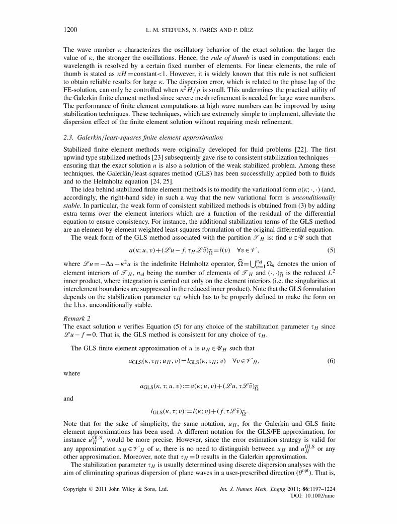
The stabilization parameter �H is usually determined using discrete dispersion analyses with theaim of eliminating spurious dispersion of plane waves in a user-prescribed direction (�opt). That is,
Copyright � 2011 John Wiley & Sons, Ltd. Int. J. Numer. Meth. Engng 2011; 86:1197–1224DOI: 10.1002/nme
ESTIMATION OF THE DISPERSION ERROR FOR THE HELMHOLTZ EQUATION 1201
the goal is that the GLS/FE approximation has no phase lag if the exact solution is a plane wavein the direction �opt. Different definitions for the parameter �H depending on the underlying sizeand topology of the mesh may be found in the literature [20, 25].
Unfortunately, it is not possible in general to design a stabilization parameter �H that confersthe ability of fully removing the dispersion error on the GLS method. The reason is twofold. First,a general signal consists of plane waves going in an infinite number of directions. Even if there aredirectionally prevalent components in this decomposition, they are not necessarily known a priori.Moreover, it is not clear whether the GLS method improves the approximations of solutions thatare not dominant in the preferred direction. Second, the parameter �H is derived for particularstructured topology meshes. The optimal behavior obtained for some particular structured meshes(which are of limited use in real-life applications) is partially lost when general unstructuredmeshes are used.
2.4. Matrix form
The Galerkin or GLS finite element approximation u H is expressed in terms of the basis-functions{N j } j=1,. . .,nnp
spanning UH , namely
u H =nnp∑j=1
N j u jH =NuH ,
where nnp is the number of nodes in the mesh, u jH is the complex nodal value associated with the
mesh node x j , N= [N 1, N 2, . . . , N nnp ] and uTH = [u1
H ,u2H , . . . ,u
nnpH ].
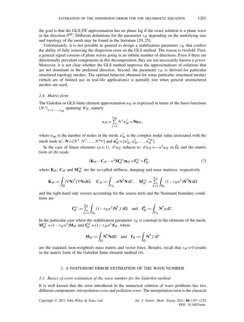
In the case of linear elements (p=1), Lu H reduces to Lu H =−�2u H in �, and the matrixform of (6) reads
(KH −CH −�2M�HH )uH = f�H
H +fNH , (7)
where KH , CH and M�HH are the so-called stiffness, damping and mass matrices, respectively
KH :=∫
�(∇N)T(∇N)d�, CH :=
∫�R
MNTNd�, M�HH :=
nel∑n=1
∫�n
(1−�H �2)NTNd�
and the right-hand side vectors accounting for the source term and the Neumann boundary condi-tions are
f�HH :=
nel∑n=1
∫�n
(1−�H �2)NT f d� and fNH :=
∫�N
NTg d�.
In the particular case where the stabilization parameter �H is constant in the elements of the mesh,M�H
H = (1−�H �2)MH and f�HH = (1−�H �2)fH , where
MH :=∫
�NTNd� and fH :=
∫�
NT f d�
are the standard (non-weighted) mass matrix and vector force. Besides, recall that �H =0 resultsin the matrix form of the Galerkin finite element method (4).
3. A POSTERIORI ERROR ESTIMATION OF THE WAVE NUMBER
3.1. Basics of error estimation of the wave number for the Galerkin method
It is well known that the error introduced in the numerical solution of wave problems has twodifferent components: interpolation error and pollution error. The interpolation error is the classical
Copyright � 2011 John Wiley & Sons, Ltd. Int. J. Numer. Meth. Engng 2011; 86:1197–1224DOI: 10.1002/nme
1202 L. M. STEFFENS, N. PARÉS AND P. DÍEZ
error arising in elliptic problems and pertains to the ability of the discretization to properlyapproximate the solution
eint :=u−uintH =u(x)−
nnp∑j=1
N j (x)u(x j ), (8)
where uintH is the approximation of u in UH coinciding with u at the mesh nodes x j , j =1,2, . . . ,nnp.
Thus, the pollution error is defined as:
epol :=uintH −u H =
nnp∑j=1
N j (x)(u(x j )−u jH ).
In standard thermal and elasticity problems, the error in the finite element solution is equivalentto the interpolation error, and converges at the same rate. This error is local in nature because itmay be reduced in a given zone by reducing the mesh size locally in this zone.
The pollution error, however, is especially relevant in the framework of Helmholtz problems dueto the blowup of the inf–sup and continuity constants of the weak form when the wave number islarge (i.e. the inf–sup constant tends to zero and the continuity constant tends to ∞ as � tends to ∞).In transient wave problems, pollution is associated with the variation of the numerical wave speedwith the wavelength. This phenomenon results in the dispersion of the different components ofthe total wave. In the steady Helmholtz problem, the word dispersion is also used and correspondsto the error in the numerical wave number �H , which is therefore identified with the pollution.In other words, the FE error is decomposed into two terms
FE error =u−u H =eint +epol = Interpolation error +Dispersion/pollution error,
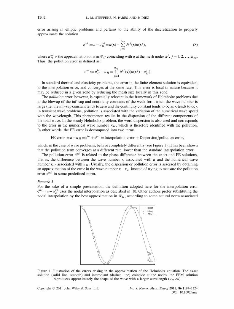
which, in the case of wave problems, behave completely differently (see Figure 1). It has been shownthat the pollution term converges at a different rate, lower than the standard interpolation error.
The pollution error epol is related to the phase difference between the exact and FE solutions,that is, the difference between the wave number � associated with u and the numerical wavenumber �H associated with u H . Usually, the dispersion or pollution error is assessed by obtainingan approximation of the error in the wave number �−�H instead of trying to measure the pollutionerror epol in some predefined norm.
Remark 3For the sake of a simple presentation, the definition adopted here for the interpolation erroreint =u−uint
H uses the nodal interpolation as described in (8). Other authors prefer substituting thenodal interpolation by the best approximation in UH , according to some natural norm associated
Figure 1. Illustration of the errors arising in the approximation of the Helmholtz equation. The exactsolution (solid line, smooth) and interpolant (dashed line) coincide at the nodes, the FEM solution
reproduces approximately the shape of the wave with a larger wavelength (�H <�).
Copyright � 2011 John Wiley & Sons, Ltd. Int. J. Numer. Meth. Engng 2011; 86:1197–1224DOI: 10.1002/nme
ESTIMATION OF THE DISPERSION ERROR FOR THE HELMHOLTZ EQUATION 1203
exactmodFEM
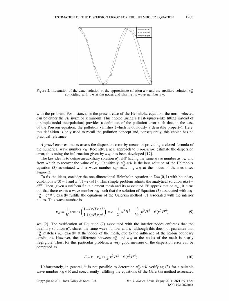
Figure 2. Illustration of the exact solution u, the approximate solution u H and the auxiliary solution umH
coinciding with u H at the nodes and sharing its wave number �H .
with the problem. For instance, in the present case of the Helmholtz equation, the norm selectedcan be either the H1 norm or seminorm. This choice (using a least-squares-like fitting instead ofa simple nodal interpolation) provides a definition of the pollution error such that, in the caseof the Poisson equation, the pollution vanishes (which is obviously a desirable property). Here,this definition is only used to recall the pollution concept and, consequently, this choice has nopractical relevance.
A priori error estimates assess the dispersion error by means of providing a closed formula ofthe numerical wave number �H . Recently, a new approach to a posteriori estimate the dispersionerror, thus using the information given by u H , has been developed [17].
The key idea is to define an auxiliary solution umH ∈U having the same wave number as u H and
from which to recover the value of �H . Intuitively, umH ∈U is the best solution of the Helmholtz
equation (3) associated with a wave number �H matching u H at the nodes of the mesh, seeFigure 2.
To fix the ideas, consider the one-dimensional Helmholtz equation in �= (0,1) with boundaryconditions u(0)=1 and u′(1)= i�u(1). This simple problem admits the analytical solution u(x)=ei�x . Then, given a uniform finite element mesh and its associated FE approximation u H , it turnsout that there exists a wave number �H such that the solution of Equation (3) associated with �H ,um
H =ei�H x , exactly fulfills the equations of the Galerkin method (7) associated with the interiornodes. This wave number is
�H = 1
Harccos
(1−(�H )2/3
1+(�H )2/6
)≈�− 1
24�3 H2 + 3
640�5 H4 +O(�7 H6) (9)
see [2]. The verification of Equation (7) associated with the interior nodes enforces that theauxiliary solution um
H shares the same wave number as u H , although this does not guarantee thatum
H matches u H exactly at the nodes of the mesh, due to the influence of the Robin boundaryconditions. However, the difference between um
H and u H at the nodes of the mesh is nearlynegligible. Thus, for this particular problem, a very good measure of the dispersion error can becomputed as
E =�−�H ≈ 124�3 H2 +O(�5 H4). (10)
Unfortunately, in general, it is not possible to determine umH ∈U verifying (3) for a suitable
wave number �H ∈R and concurrently fulfilling the equations of the Galerkin method associated
Copyright � 2011 John Wiley & Sons, Ltd. Int. J. Numer. Meth. Engng 2011; 86:1197–1224DOI: 10.1002/nme
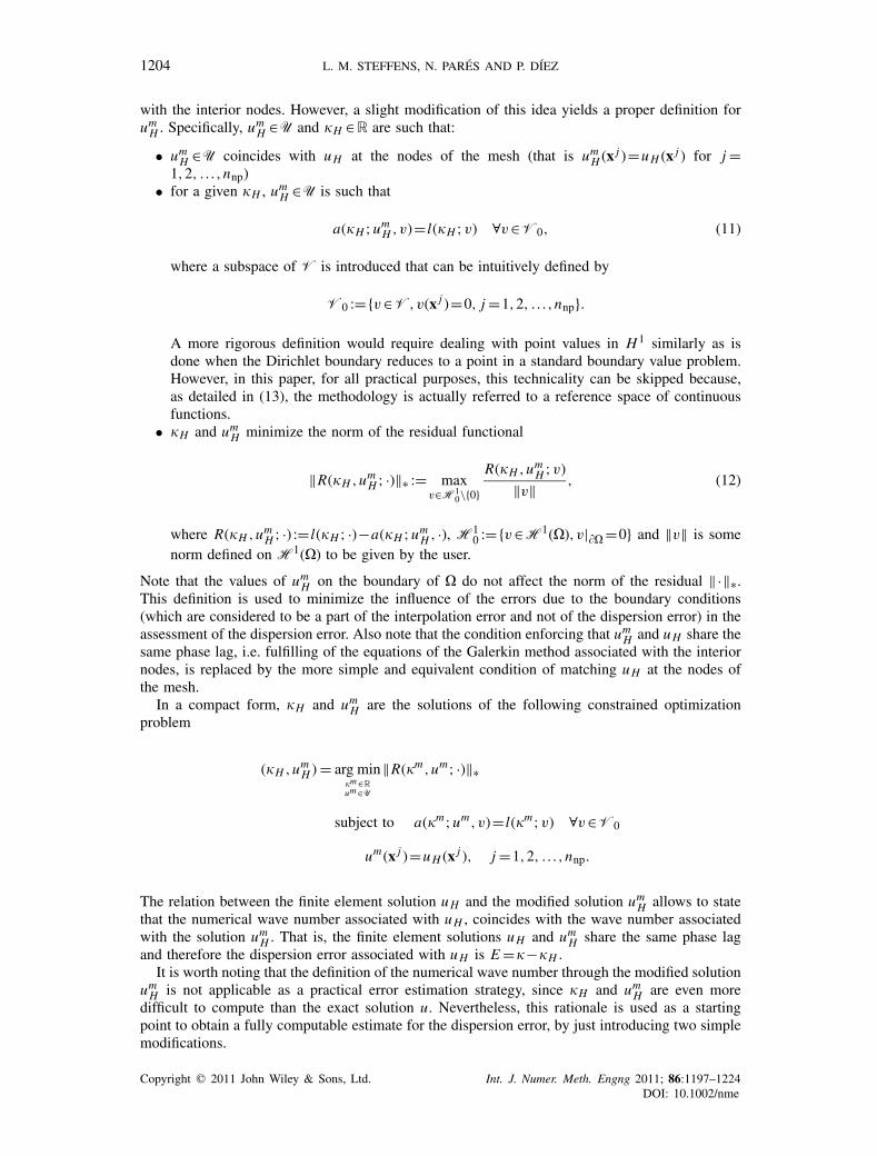
1204 L. M. STEFFENS, N. PARÉS AND P. DÍEZ
with the interior nodes. However, a slight modification of this idea yields a proper definition forum
H . Specifically, umH ∈U and �H ∈R are such that:
• umH ∈U coincides with u H at the nodes of the mesh (that is um
H (x j )=u H (x j ) for j =1,2, . . . ,nnp)
• for a given �H , umH ∈U is such that
a(�H ;umH ,v)= l(�H ;v) ∀v∈V0, (11)
where a subspace of V is introduced that can be intuitively defined by
V0 :={v∈V,v(x j )=0, j =1,2, . . . ,nnp}.
A more rigorous definition would require dealing with point values in H1 similarly as isdone when the Dirichlet boundary reduces to a point in a standard boundary value problem.However, in this paper, for all practical purposes, this technicality can be skipped because,as detailed in (13), the methodology is actually referred to a reference space of continuousfunctions.
• �H and umH minimize the norm of the residual functional
‖R(�H ,umH ; ·)‖∗ := max
v∈H10\{0}
R(�H ,umH ;v)
‖v‖ , (12)
where R(�H ,umH ; ·) := l(�H ; ·)−a(�H ;um
H , ·), H10 :={v∈H1(�),v|�� =0} and ‖v‖ is some
norm defined on H1(�) to be given by the user.
Note that the values of umH on the boundary of � do not affect the norm of the residual ‖·‖∗.
This definition is used to minimize the influence of the errors due to the boundary conditions(which are considered to be a part of the interpolation error and not of the dispersion error) in theassessment of the dispersion error. Also note that the condition enforcing that um
H and u H share thesame phase lag, i.e. fulfilling of the equations of the Galerkin method associated with the interiornodes, is replaced by the more simple and equivalent condition of matching u H at the nodes ofthe mesh.
In a compact form, �H and umH are the solutions of the following constrained optimization
problem
(�H ,umH ) = arg min
�m∈Rum∈U
‖R(�m,um; ·)‖∗
subject to a(�m;um,v)= l(�m;v) ∀v∈V0
um(x j )=u H (x j ), j =1,2, . . . ,nnp.
The relation between the finite element solution u H and the modified solution umH allows to state
that the numerical wave number associated with u H , coincides with the wave number associatedwith the solution um
H . That is, the finite element solutions u H and umH share the same phase lag
and therefore the dispersion error associated with u H is E =�−�H .It is worth noting that the definition of the numerical wave number through the modified solution
umH is not applicable as a practical error estimation strategy, since �H and um
H are even moredifficult to compute than the exact solution u. Nevertheless, this rationale is used as a startingpoint to obtain a fully computable estimate for the dispersion error, by just introducing two simplemodifications.
Copyright � 2011 John Wiley & Sons, Ltd. Int. J. Numer. Meth. Engng 2011; 86:1197–1224DOI: 10.1002/nme
ESTIMATION OF THE DISPERSION ERROR FOR THE HELMHOLTZ EQUATION 1205
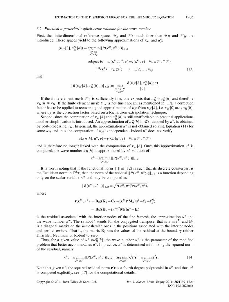
3.2. Practical a posteriori explicit error estimate for the wave number
First, the finite-dimensional reference spaces Uh and Vh much finer than UH and VH areintroduced. These spaces yield to the following approximations of �H and um
H
(�H [h],umH [h]) = arg min
�m∈Rum∈Uh
‖R(�m,um; ·)‖∗,h
subject to a(�m;um,v)= l(�m;v) ∀v∈Vh ∩V0
um(x j )=u H (x j ), j =1,2, . . . ,nnp (13)
and
‖R(�H [h],umH [h]; ·)‖∗,h := max
v∈Vh\{0}v|��=0
R(�H [h],umH [h];v)
‖v‖ .
If the finite element mesh Vh is sufficiently fine, one expects that umH ≈um
H [h] and therefore�H [h]≈�H . If the finite element mesh Vh is not fine enough, as mentioned in [17], a correctionfactor has to be applied to recover a good approximation of �H from �H [h], i.e. �H [0]=c f �H [h],where c f is the correction factor based on a Richardson extrapolation technique.
Second, since the computation of �H [h] and umH [h] is still unaffordable in practical applications
another simplification is introduced. An approximation of umH [h] in Uh , denoted by u∗, is obtained
by post-processing u H . In general, the approximation u∗ is not obtained solving Equation (11) forsome �H and thus the computation of �H is independent. Indeed u∗ does not verify
a(�H [h];u∗,v)= l(�H [h];v) ∀v∈Vh ∩V0
and is therefore no longer linked with the computation of �H [h]. Once this approximation u∗ iscomputed, the wave number �H [h] is approximated by �∗ solution of
�∗ =arg min�m∈R
‖R(�m,u∗; ·)‖∗,h .
It is worth noting that if the functional norm ‖·‖ in (12) is such that its discrete counterpart isthe Euclidean norm in Cnnp , then the norm of the residual ‖R(�m,u∗; ·)‖∗,h is a function dependingonly on the scalar variable �m and may be computed as
‖R(�m,u∗; ·)‖∗,h =√
r(�m,u∗)′r(�m,u∗),
where
r(�m,u∗) := B0((Kh −Ch −(�m)2Mh)u∗−fh −fNh )
= B0((Kh −(�m)2Mh)u∗−fh)
is the residual associated with the interior nodes of the fine h-mesh, the approximation u∗ andthe wave number �m . The symbol ′ stands for the conjugated transpose, that is v′ ≡ vT, and B0is a diagonal matrix on the h-mesh with ones in the positions associated with the interior nodesand zero elsewhere. That is, the matrix B0 sets the values of the residual at the boundary (eitherDirichlet, Neumann or Robin) to zero.
Thus, for a given value of u∗ ≈umH [h], the wave number �∗ is the parameter of the modified
problem that better accommodates u∗. In practice, �∗ is determined minimizing the squared normof the residual, namely
�∗ :=arg min�m∈R
‖R(�m,u∗; ·)‖∗,h =arg min�m∈R
√r′r=arg min
�m∈R
r′r. (14)
Note that given u∗, the squared residual norm r′r is a fourth degree polynomial in �m and thus �∗is computed explicitly, see [17] for the computational details.
Copyright � 2011 John Wiley & Sons, Ltd. Int. J. Numer. Meth. Engng 2011; 86:1197–1224DOI: 10.1002/nme
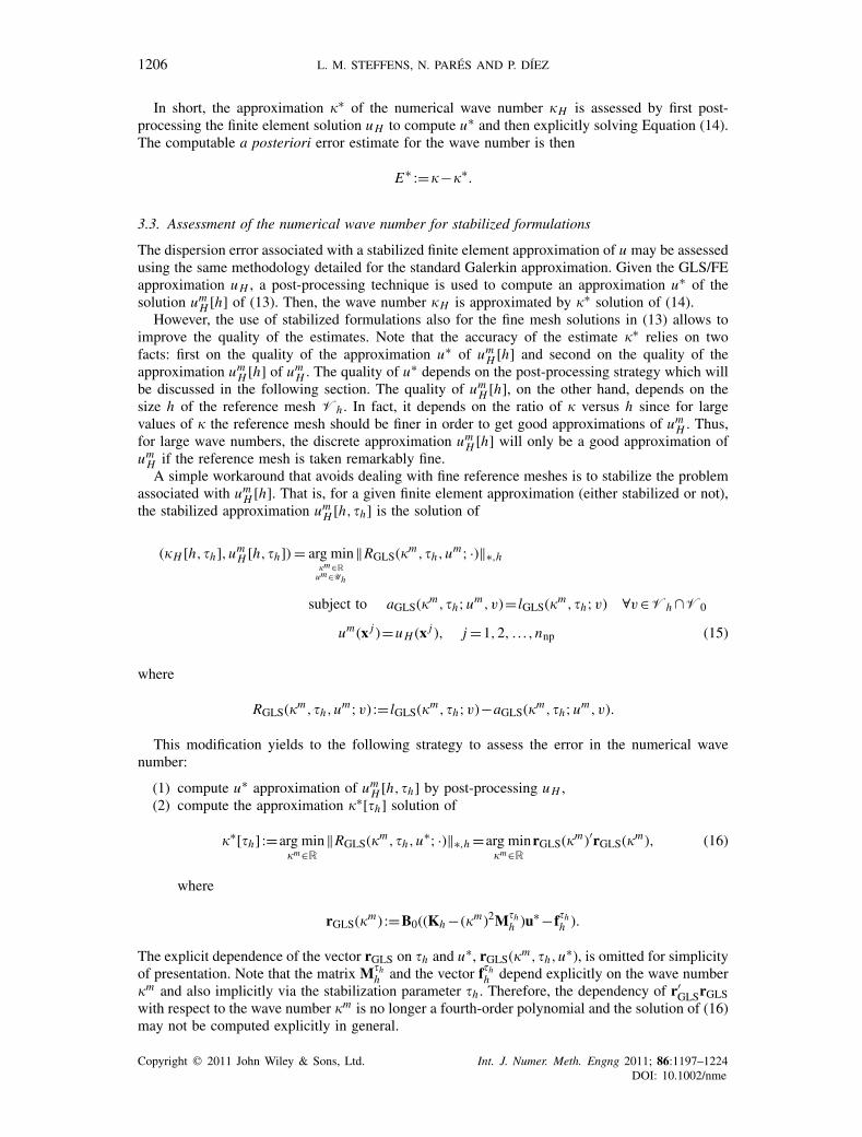
1206 L. M. STEFFENS, N. PARÉS AND P. DÍEZ
In short, the approximation �∗ of the numerical wave number �H is assessed by first post-processing the finite element solution u H to compute u∗ and then explicitly solving Equation (14).The computable a posteriori error estimate for the wave number is then
E∗ :=�−�∗.
3.3. Assessment of the numerical wave number for stabilized formulations
The dispersion error associated with a stabilized finite element approximation of u may be assessedusing the same methodology detailed for the standard Galerkin approximation. Given the GLS/FEapproximation u H , a post-processing technique is used to compute an approximation u∗ of thesolution um
H [h] of (13). Then, the wave number �H is approximated by �∗ solution of (14).However, the use of stabilized formulations also for the fine mesh solutions in (13) allows to
improve the quality of the estimates. Note that the accuracy of the estimate �∗ relies on twofacts: first on the quality of the approximation u∗ of um
H [h] and second on the quality of theapproximation um
H [h] of umH . The quality of u∗ depends on the post-processing strategy which will
be discussed in the following section. The quality of umH [h], on the other hand, depends on the
size h of the reference mesh Vh . In fact, it depends on the ratio of � versus h since for largevalues of � the reference mesh should be finer in order to get good approximations of um
H . Thus,for large wave numbers, the discrete approximation um
H [h] will only be a good approximation ofum
H if the reference mesh is taken remarkably fine.A simple workaround that avoids dealing with fine reference meshes is to stabilize the problem
associated with umH [h]. That is, for a given finite element approximation (either stabilized or not),
the stabilized approximation umH [h,�h] is the solution of
(�H [h,�h],umH [h,�h]) = arg min
�m∈Rum∈Uh
‖RGLS(�m,�h,um; ·)‖∗,h
subject to aGLS(�m,�h;um,v)= lGLS(�m,�h;v) ∀v∈Vh ∩V0
um(x j )=u H (x j ), j =1,2, . . . ,nnp (15)
where
RGLS(�m,�h,um;v) := lGLS(�m,�h;v)−aGLS(�m,�h;um,v).
This modification yields to the following strategy to assess the error in the numerical wavenumber:
(1) compute u∗ approximation of umH [h,�h] by post-processing u H ,
(2) compute the approximation �∗[�h] solution of
�∗[�h] :=arg min�m∈R
‖RGLS(�m,�h,u∗; ·)‖∗,h =arg min�m∈R
rGLS(�m)′rGLS(�m), (16)
where
rGLS(�m) :=B0((Kh −(�m)2M�hh )u∗−f�h
h ).
The explicit dependence of the vector rGLS on �h and u∗, rGLS(�m,�h,u∗), is omitted for simplicityof presentation. Note that the matrix M�h
h and the vector f�hh depend explicitly on the wave number
�m and also implicitly via the stabilization parameter �h . Therefore, the dependency of r′GLSrGLS
with respect to the wave number �m is no longer a fourth-order polynomial and the solution of (16)may not be computed explicitly in general.
Copyright � 2011 John Wiley & Sons, Ltd. Int. J. Numer. Meth. Engng 2011; 86:1197–1224DOI: 10.1002/nme
ESTIMATION OF THE DISPERSION ERROR FOR THE HELMHOLTZ EQUATION 1207
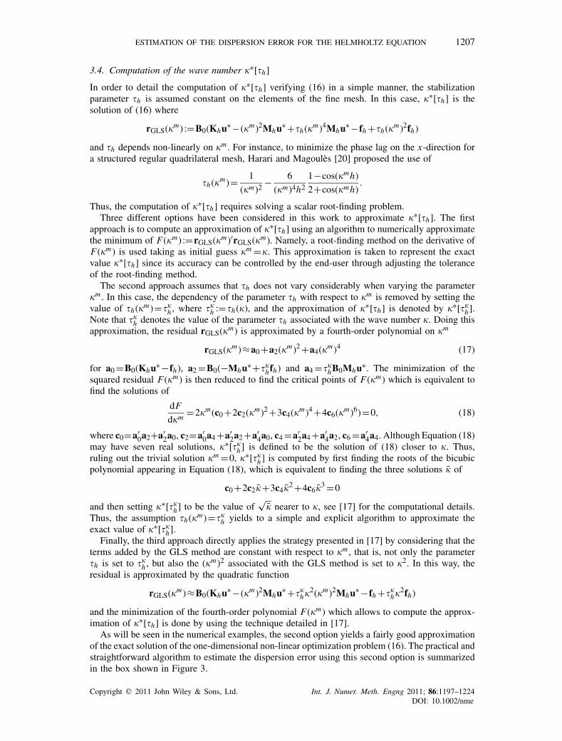
3.4. Computation of the wave number �∗[�h]
In order to detail the computation of �∗[�h] verifying (16) in a simple manner, the stabilizationparameter �h is assumed constant on the elements of the fine mesh. In this case, �∗[�h] is thesolution of (16) where
rGLS(�m) :=B0(Khu∗−(�m)2Mhu∗+�h(�m)4Mhu∗−fh +�h(�m)2fh)
and �h depends non-linearly on �m . For instance, to minimize the phase lag on the x-direction fora structured regular quadrilateral mesh, Harari and Magoulès [20] proposed the use of
�h(�m)= 1
(�m)2− 6
(�m)4h2
1−cos(�mh)
2+cos(�mh).
Thus, the computation of �∗[�h] requires solving a scalar root-finding problem.Three different options have been considered in this work to approximate �∗[�h]. The first
approach is to compute an approximation of �∗[�h] using an algorithm to numerically approximatethe minimum of F(�m) :=rGLS(�m)′rGLS(�m). Namely, a root-finding method on the derivative ofF(�m) is used taking as initial guess �m =�. This approximation is taken to represent the exactvalue �∗[�h] since its accuracy can be controlled by the end-user through adjusting the toleranceof the root-finding method.
The second approach assumes that �h does not vary considerably when varying the parameter�m . In this case, the dependency of the parameter �h with respect to �m is removed by setting thevalue of �h(�m)=��
h , where ��h :=�h(�), and the approximation of �∗[�h] is denoted by �∗[��
h].Note that ��
h denotes the value of the parameter �h associated with the wave number �. Doing thisapproximation, the residual rGLS(�m) is approximated by a fourth-order polynomial on �m
rGLS(�m)≈a0 +a2(�m)2 +a4(�m)4 (17)
for a0 =B0(Khu∗−fh), a2 =B0(−Mhu∗+��hfh) and a4 =��
hB0Mhu∗. The minimization of thesquared residual F(�m) is then reduced to find the critical points of F(�m) which is equivalent tofind the solutions of
dF
d�m=2�m(c0 +2c2(�m)2 +3c4(�m)4 +4c6(�m)6)=0, (18)
where c0=a′0a2+a′
2a0, c2=a′0a4 +a′
2a2 +a′4a0, c4 =a′
2a4 +a′4a2, c6 =a′
4a4. Although Equation (18)may have seven real solutions, �∗[��
h] is defined to be the solution of (18) closer to �. Thus,ruling out the trivial solution �m =0, �∗[��
h] is computed by first finding the roots of the bicubicpolynomial appearing in Equation (18), which is equivalent to finding the three solutions � of
c0 +2c2�+3c4�2 +4c6�
3 =0
and then setting �∗[��h] to be the value of
√� nearer to �, see [17] for the computational details.
Thus, the assumption �h(�m)=��h yields to a simple and explicit algorithm to approximate the
exact value of �∗[��h].
Finally, the third approach directly applies the strategy presented in [17] by considering that theterms added by the GLS method are constant with respect to �m , that is, not only the parameter�h is set to ��
h , but also the (�m)2 associated with the GLS method is set to �2. In this way, theresidual is approximated by the quadratic function
rGLS(�m)≈B0(Khu∗−(�m)2Mhu∗+��h�2(�m)2Mhu∗−fh +��
h�2fh)
and the minimization of the fourth-order polynomial F(�m) which allows to compute the approx-imation of �∗[�h] is done by using the technique detailed in [17].
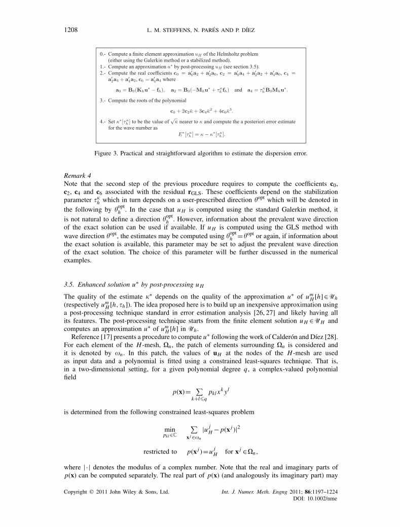
As will be seen in the numerical examples, the second option yields a fairly good approximationof the exact solution of the one-dimensional non-linear optimization problem (16). The practical andstraightforward algorithm to estimate the dispersion error using this second option is summarizedin the box shown in Figure 3.
Copyright � 2011 John Wiley & Sons, Ltd. Int. J. Numer. Meth. Engng 2011; 86:1197–1224DOI: 10.1002/nme
1208 L. M. STEFFENS, N. PARÉS AND P. DÍEZ
Figure 3. Practical and straightforward algorithm to estimate the dispersion error.
Remark 4Note that the second step of the previous procedure requires to compute the coefficients c0,c2, c4 and c6 associated with the residual rGLS. These coefficients depend on the stabilizationparameter ��
h which in turn depends on a user-prescribed direction �opt which will be denoted in
the following by �opth . In the case that u H is computed using the standard Galerkin method, it
is not natural to define a direction �opth . However, information about the prevalent wave direction
of the exact solution can be used if available. If u H is computed using the GLS method withwave direction �opt, the estimates may be computed using �opt
h =�opt or again, if information aboutthe exact solution is available, this parameter may be set to adjust the prevalent wave directionof the exact solution. The choice of this parameter will be further discussed in the numericalexamples.
3.5. Enhanced solution u∗ by post-processing u H
The quality of the estimate �∗ depends on the quality of the approximation u∗ of umH [h]∈Uh
(respectively umH [h,�h]). The idea proposed here is to build up an inexpensive approximation using
a post-processing technique standard in error estimation analysis [26, 27] and likely having allits features. The post-processing technique starts from the finite element solution u H ∈UH andcomputes an approximation u∗ of um
H [h] in Uh .Reference [17] presents a procedure to compute u∗ following the work of Calderón and Díez [28].
For each element of the H -mesh, �n , the patch of elements surrounding �n is considered andit is denoted by �n . In this patch, the values of uH at the nodes of the H -mesh are usedas input data and a polynomial is fitted using a constrained least-squares technique. That is,in a two-dimensional setting, for a given polynomial degree q , a complex-valued polynomialfield
p(x)= ∑k+l�q
pkl xk yl
is determined from the following constrained least-squares problem
minpkl∈C
∑x j ∈�n
|u jH − p(x j )|2
restricted to p(x j )=u jH for x j ∈�n,
where |·| denotes the modulus of a complex number. Note that the real and imaginary parts ofp(x) can be computed separately. The real part of p(x) (and analogously its imaginary part) may
Copyright � 2011 John Wiley & Sons, Ltd. Int. J. Numer. Meth. Engng 2011; 86:1197–1224DOI: 10.1002/nme
ESTIMATION OF THE DISPERSION ERROR FOR THE HELMHOLTZ EQUATION 1209
be found solving the real-valued constrained optimization
min�(pkl )∈R
∑x j ∈�n
|�(u jH )−�(p(x j ))|2
restricted to �(p(x j ))=�(u jH ) for x j ∈�n.
Once the polynomial is obtained in �n it is evaluated to find the nodal values of u� in the nodesof the h-mesh lying in element �n of the H -mesh. This approach allows recovering the curvaturesof the solution coinciding with u H at the nodes where it is computed.
This simple and straightforward strategy provides fairly good results. However, this approachdoes not use specific information about the differential operator or the exact solution. The use ofanalytical information about the natural solutions of the differential operator yields an alternativeapproach to compute u∗.
The approach to compute u∗ also requires solving a local constrained least-squares problem foreach element �n . Instead of using a polynomial representation for u∗|�n
an exponential fittingis used. This is a natural choice because the exact solution of the 2D homogeneous Helmholtzequation is an infinite sum of plane waves of the form Aeik·x, where k=�[cos(�),sin(�)].
Thus, in each patch �n , u H is approximated by an exponential field of the form
A(x)eip(x),
where A(x) and p(x) are polynomial fields representing the amplitude and wave direction. Thefields A(x) and p(x) are determined by a constrained least-squares criterion and hence, they aretaken as those minimizing
min∑
x j ∈�n
|u jH − A(x j )eip(x j )|2
restricted to A(x j )eip(x j ) =u jH for x j ∈�n .
Using a standard technique to linearize the exponential least-squares fitting transforms the previousproblem into an equivalent linear constrained least-squares problem
min∑
x j ∈�n
| ln(u jH )− ln(A(x j )eip(x j ))|2
restricted to ln(A(x j )eip(x j ))= ln(u jH ) for x j ∈�n .
Splitting the real and imaginary part of the previous problem yields a simple strategy to computeln(A(x)) and p(x) independently using a restricted least-squares fitting, namely:
min∑
x j ∈�n
| ln(|u jH |)− ln(A(x j ))|2
restricted to ln(A(x j ))= ln(|u jH |) for x j ∈�n
and
min∑
x j ∈�n
|arg(u jH )− p(x j )|2
restricted to p(x j )=arg(u jH ) for x j ∈�n,
where arg(·) denotes the argument of a complex number and a polynomial fitting of ln(A(x)) andp(x) is considered.
The only intricate part of this strategy involves the input data, arg(u jH ), of the least-squares
problem for p(x). The non-unique arguments associated with the data u jH have to be carefully
selected so that the polynomial fitting yields proper results.
Copyright � 2011 John Wiley & Sons, Ltd. Int. J. Numer. Meth. Engng 2011; 86:1197–1224DOI: 10.1002/nme
1210 L. M. STEFFENS, N. PARÉS AND P. DÍEZ
4. NUMERICAL EXAMPLES
The strategy to assess the error in the wave number presented in the previous sections is validatedin four numerical examples. The performance of the estimates of the dispersion error is shown bothfor Galerkin and GLS approximations. Moreover, the influence of the post-processing techniqueyielding u∗ in the resulting effectivity is also discussed.
The finite element approximations are computed using triangular and quadrilateral meshes oflinear (resp. bilinear) elements, p=1. Different definitions of the stabilization parameter �H areused to compute the GLS approximations depending on the underlying topology of the mesh.In particular, for structured and unstructured quadrilateral meshes the following definition of theparameter, designed to minimize the dispersion error of plane wave in the direction �opt on cartesianmeshes, is used [20, 25]:
�H = 1
�2
(1− 6
(�h)2
(1−cos(�h cos�opt)
2+cos(�h cos�opt)+ 1−cos(�h sin�opt)
2+cos(�h sin�opt)
)).
For triangular meshes, the definition derived for hexagonal meshes, namely
�H = 1
�2
(1− 8
(�h)2
3− f (�h,�opt)
3+ f (�h,�opt)
),
where f (�h,�)=cos(�h cos�)+2cos(�h cos�/2)cos(√
3�h sin�/2) is used because it providesgood results also for unstructured meshes.
For non-uniform meshes, the stabilization parameter is not constant over the whole mesh. Ineach element �n a different stabilization parameter is used depending on its characteristic elementsize hn . This characteristic element size is taken as the smallest side of the element both forquadrilateral and triangular meshes.
As mentioned in Section 2.3 the parameter �H depends on a user-prescribed direction �opt. Theinfluence of the selection of this direction in the reduction of the dispersion error is studied in thefollowing examples.
4.1. Example 1: 1D strip
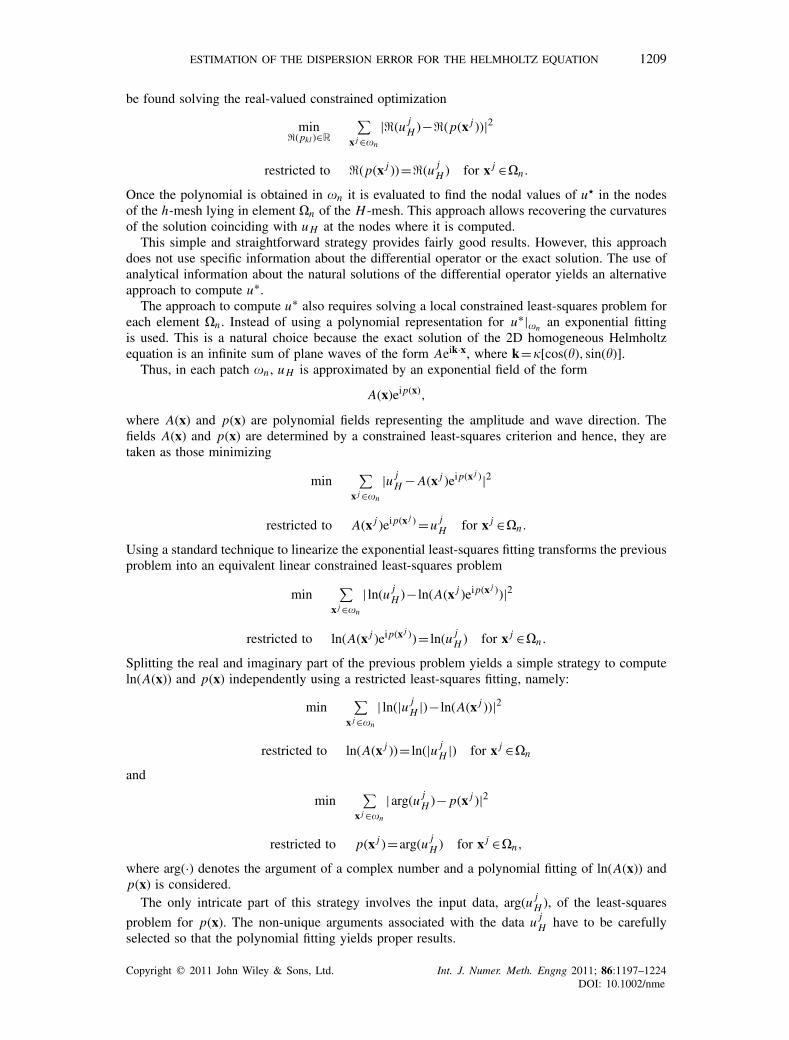
The first example models a plane wave propagating in the x-direction in a two-dimensionalrectangular domain, with length L =1 and width V =√
3/8, see Figure 4. The boundary conditionsare specified in order to yield the exact solution u(x, y)=ei�x : Dirichlet on the left-hand side,Robin on the right-hand side and Neumann homogeneous on the upper and lower sides to maintainthe one-dimensional character of the solution. That is, the data entering in Equation (2) are u =1on x =0, Mu = i�u on x =1 and g =0 on y =0 and y =√
3/8. The performance of the Galerkinand GLS finite element solutions is studied for �=8�. Owing to the 1D character of the problem,the stabilization angle used in all the GLS computations (both for the coarse and fine meshes) isset to 0, that is, �opt =�opt
h =0. Note that the solution of the problem is independent of the widthof the domain V and the value
√3/8 has been selected in order to accommodate a hexagonal
triangular mesh.
Figure 4. Example 1; 1D strip: problem setup.
Copyright � 2011 John Wiley & Sons, Ltd. Int. J. Numer. Meth. Engng 2011; 86:1197–1224DOI: 10.1002/nme
ESTIMATION OF THE DISPERSION ERROR FOR THE HELMHOLTZ EQUATION 1211
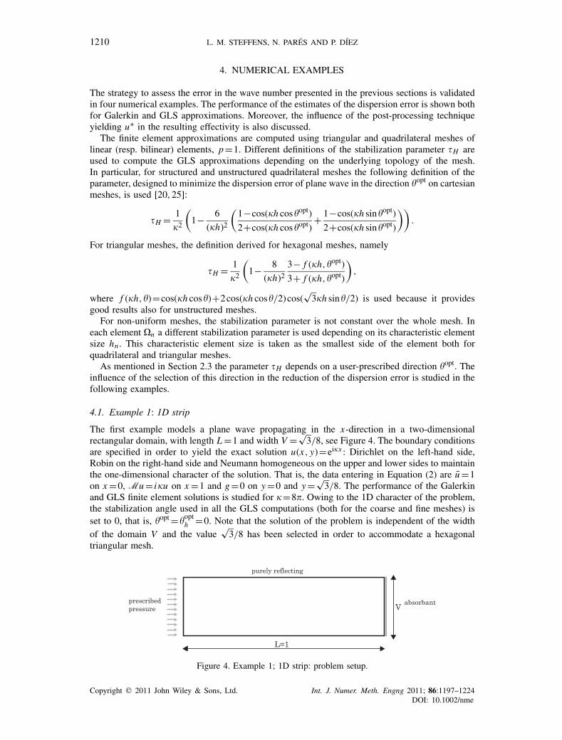
Table I. Example 1: assessment of the dispersion error for a uniform coarse quadrilateral mesh (24×2elements) a successively refined reference meshes for the Galerkin approximations of the solution.
Galerkin Epri =1.02211
Option 1 Option 2h E[h] c f E[h] E[h,�h] c f E∗ E∗[�h] E∗[��
h] Option 3
H/2 0.76790 1.02387 1.02211 1.01428 1.01469 1.01486 1.03682H/4 0.95869 1.02261 1.02211 1.01428 1.01469 1.01486 1.03682H/8 1.00627 1.02224 1.02211 1.01227 1.01232 1.01232 1.01368H/16 1.01815 1.02214 1.02211 1.01214 1.01215 1.01215 1.01249H/32 1.02112 1.02212 1.02211 1.01210 1.01210 1.01210 1.01218H/64 1.02186 1.02211 1.02211 1.01208 1.01208 1.01208 1.01210
The truth error estimates (left) are computed using the fully non-linear solution yielding to E[h] and E[h,�h].The exponential post-processed solution (right) u∗ obtained from u H and then different options are used torecover the wave number �∗ associated with u∗ only for the Galerkin approximation.
First, the influence of the selection of the finite reference mesh associated with Vh is studied.If the finite element mesh Vh is sufficiently fine, one expects that um
H ≈umH [h,�h]≈um
H [h] andtherefore �H ≈�H [h,�h]≈�H [h]. If the finite element mesh Vh is not fine enough, one shouldapply a correction factor to �H [h] to account for the finite size h of the reference mesh and recovera good approximation of �H , see [17]. This correction factor is not necessary for the estimate�H [h,�h]. That is when the reference problem is also stabilized.
A uniform coarse mesh of 24×2 quadrilateral elements is used for both the Galerkin and theGLS method. The dispersion error associated with the Galerkin approximation can be assessedusing the a priori estimate of the wave number given by (9)
Epri =�−�pri =�− 1
Harccos
(1−(�H )2/3
1+(�H )2/6
),
which in this case is taken as the actual error in the wave number due to the one-dimensionalcharacter of the solution (up to the pollution errors introduced by the Robin boundary conditions).Note that the GLS solution is, for this particular mesh and problem, dispersion free. Thus, the Robinboundary conditions are the unique perturbation producing errors in the approximations of �.
The different a posteriori estimates of the dispersion error are computed using a series of succes-sively nested reference meshes, both triangular and quadrilateral. For the quadrilateral meshes,refinement is performed only in the x-direction and thus maintaining two rows of elements onall the reference meshes, due to the one-dimensional character of the solution: for h = H/2 eachquadrilateral in the coarse mesh is divided into two new ones yielding a mesh of 48×2 elements,for h = H/4, each quadrilateral element is divided into four new ones yielding a mesh of 96×2elements, etc.
The first columns of Table I show the truth estimates of the dispersion error E[h] :=�−�H [h] andE[h,�h] :=�−�H [h,�h] where the numerical wave numbers �H [h] and �H [h,�h] are computedsolving the non-linear problems (13) and (15), respectively, and c f =n2
r /(n2r −1) stands for the
correction factor applied to �H [h], where nr = H/h. Note that these truth estimates are computa-tionally unaffordable in real applications, because they involve many resolutions of the problemin the reference mesh. They are computed in academic problems to see the effectivity of theproposed practical estimates. As can be seen, both the estimates cf E[h] and E[h,�h] assessingthe dispersion error of the Galerkin approximation are in very good agreement with the a prioriestimate. It is worth noting that the estimate E[h,�h] yields very good results even for the caseh = H/2 being less sensitive than cf E[h] to the choice of the reference mesh size.
The last columns in Table I correspond to the practical estimates obtained from the recoveredsolution u∗. In this case u∗ is computed using the exponential fitting. Four different estimates arecomputed. The first is the estimate proposed by Steffens and Díez [17], E∗ :=�−�∗, associatedwith the assessed wave number obtained from (14) and enhanced by its multiplicative factor.
Copyright � 2011 John Wiley & Sons, Ltd. Int. J. Numer. Meth. Engng 2011; 86:1197–1224DOI: 10.1002/nme
1212 L. M. STEFFENS, N. PARÉS AND P. DÍEZ
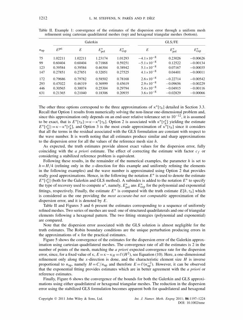
Table II. Example 1: convergence of the estimates of the dispersion error through a uniform meshrefinement using cartesian quadrilateral meshes (top) and hexagonal triangular meshes (bottom).
Galerkin GLS/FE
nnp Epri E E∗pol E∗
exp E E∗pol E∗
exp
75 1.02211 1.02211 1.23174 1.01293 −4.1×10⁻⁸ 0.23026 −0.0062699 0.60404 0.60404 0.71868 0.59251 −5.1×10⁻⁸ 0.12522 −0.00134123 0.39584 0.39584 0.46304 0.38942 5.1×10⁻⁸ 0.07167 −0.00035147 0.27851 0.27851 0.32051 0.27525 4.1×10⁻⁸ 0.04401 −0.00011
172 0.79686 0.79782 0.58502 0.78168 2.6×10⁻⁸ −0.22714 −0.00542293 0.47022 0.46319 0.36999 0.45619 2.9×10⁻⁸ −0.09656 −0.00229446 0.30565 0.30074 0.25304 0.29794 5.4×10⁻⁸ −0.04915 −0.00116631 0.21365 0.21040 0.18306 0.20935 3.6×10⁻⁸ −0.02829 −0.00066
The other three options correspond to the three approximations of �∗[�h] detailed in Section 3.3.Recall that Option 1 results from numerically solving the non-linear one-dimensional problem and,since this approximation only depends on an end-user relative tolerance set to 10−12, it is assumedto be exact, that is E∗[�h] :=�−�∗[�h]. Option 2 is associated with �∗[��
h] yielding the estimateE∗[��
h] :=�−�∗[��h], and Option 3 is the most crude approximation of �∗[�h] since it considers
that all the terms in the residual associated with the GLS formulation are constant with respect tothe wave number. It is worth noting that all estimates produce similar and sharp approximationsto the dispersion error for all the values of the reference mesh size h.
As expected, the truth estimates provide almost exact values for the dispersion error, fullycoinciding with the a priori estimate. The effect of correcting the estimate with factor c f orconsidering a stabilized reference problem is equivalent.
Following these results, in the remainder of the numerical examples, the parameter h is set toh = H/4 (refining only in the x-direction for this example and uniformly refining the elementsin the following examples) and the wave number is approximated using Option 2 that providesreally good approximations. Hence, in the following the notation E∗ is used to denote the estimateE∗[��
h] (both for the Galerkin and GLS method). A subindex is added to the notation E∗ to specifythe type of recovery used to compute u∗, namely, E∗
pol ans E∗exp for the polynomial and exponential
fittings, respectively. Finally, the estimate E∗ is compared with the truth estimate E[h,�h] whichis considered as the one providing the most accurate-but not computable approximation of thedispersion error, and it is denoted by E .
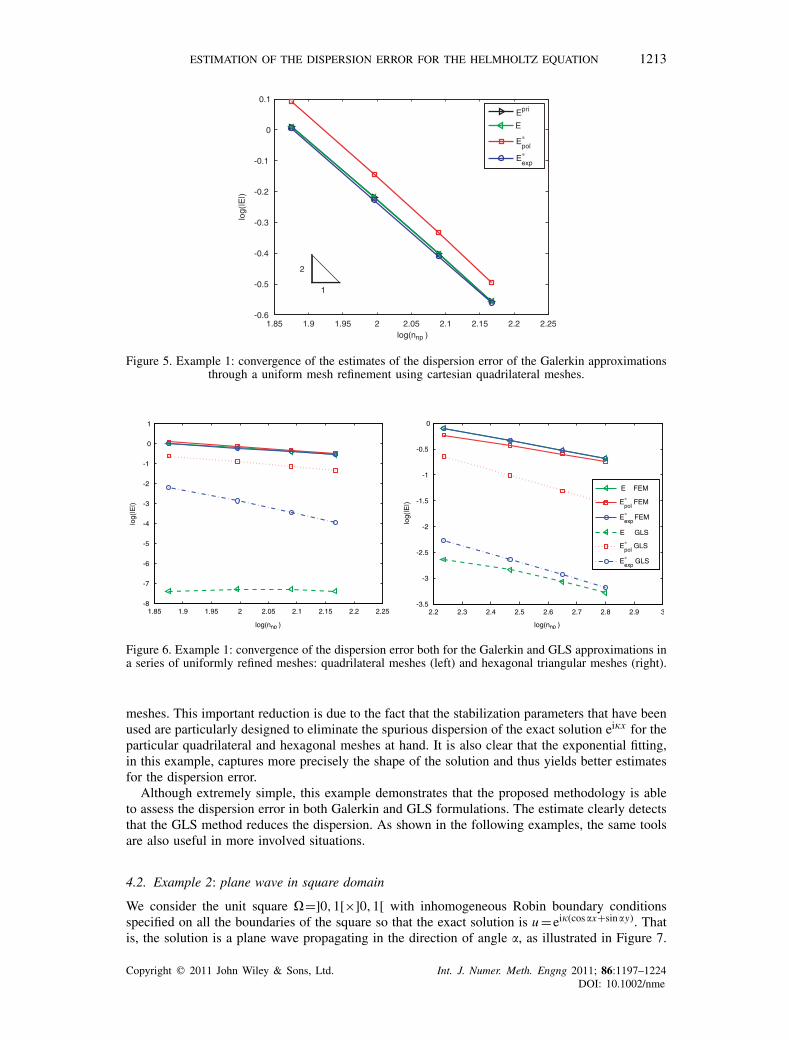
Table II and Figures 5 and 6 present the estimates corresponding to a sequence of uniformlyrefined meshes. Two series of meshes are used: one of structured quadrilaterals and one of triangularelements following a hexagonal pattern. The two fitting strategies (polynomial and exponential)are compared.
Note that the dispersion error associated with the GLS solution is almost negligible for thetruth estimates. The Robin boundary conditions are the unique perturbation producing errors inthe approximations of � for the practical estimates.
Figure 5 shows the convergence of the estimates for the dispersion error of the Galerkin approx-imation using cartesian quadrilateral meshes. The convergence rate of all the estimates is 2 in thenumber of points of the mesh, matching the a priori expected convergence rate for the dispersionerror, since, for a fixed value of �, E =�−�H =O(H2), see Equation (10). Here, a one-dimensionalrefinement only along the x-direction is done, and the characteristic element size H is inverseproportional to nnp, namely H =C/nnp and therefore E =O(n−2
np ). However, it can be observedthat the exponential fitting provides estimates which are in better agreement with the a priori orreference estimates.
Finally, Figure 6 shows the convergence of the bounds for both the Galerkin and GLS approxi-mations using either quadrilateral or hexagonal triangular meshes. The reduction in the dispersionerror using the stabilized GLS formulation becomes apparent both for quadrilateral and hexagonal
Copyright � 2011 John Wiley & Sons, Ltd. Int. J. Numer. Meth. Engng 2011; 86:1197–1224DOI: 10.1002/nme
ESTIMATION OF THE DISPERSION ERROR FOR THE HELMHOLTZ EQUATION 1213
1.85 1.9 1.95 2 2.05 2.1 2.15 2.2 2.25-0.6
-0.5
-0.4
-0.3
-0.2
-0.1
0
0.1
log(n )
Epri
E∗pol
E∗exp
1
2
E
log(
|E|)
np
Figure 5. Example 1: convergence of the estimates of the dispersion error of the Galerkin approximationsthrough a uniform mesh refinement using cartesian quadrilateral meshes.
1.85 1.9 1.95 2 2.05 2.1 2.15 2.2 2.25-8
-7
-6
-5
-4
-3
-2
-1
0
1
log(
|E|)
log(n )
2.2 2.3 2.4 2.5 2.6 2.7 2.8 2.9 3-3.5
-3
-2.5
-2
-1.5
-1
-0.5
0
E FEM
E FEM
E GLS
E GLS
E FEM
E GLS
log(
|E|)
log(n )
Figure 6. Example 1: convergence of the dispersion error both for the Galerkin and GLS approximations ina series of uniformly refined meshes: quadrilateral meshes (left) and hexagonal triangular meshes (right).
meshes. This important reduction is due to the fact that the stabilization parameters that have beenused are particularly designed to eliminate the spurious dispersion of the exact solution ei�x for theparticular quadrilateral and hexagonal meshes at hand. It is also clear that the exponential fitting,in this example, captures more precisely the shape of the solution and thus yields better estimatesfor the dispersion error.
Although extremely simple, this example demonstrates that the proposed methodology is ableto assess the dispersion error in both Galerkin and GLS formulations. The estimate clearly detectsthat the GLS method reduces the dispersion. As shown in the following examples, the same toolsare also useful in more involved situations.
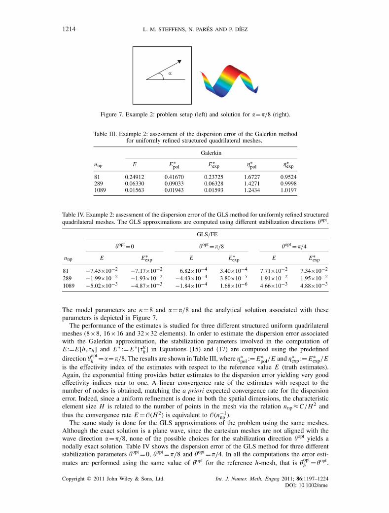
4.2. Example 2: plane wave in square domain
We consider the unit square �=]0,1[×]0,1[ with inhomogeneous Robin boundary conditionsspecified on all the boundaries of the square so that the exact solution is u =ei�(cos�x+sin�y). Thatis, the solution is a plane wave propagating in the direction of angle �, as illustrated in Figure 7.
Copyright � 2011 John Wiley & Sons, Ltd. Int. J. Numer. Meth. Engng 2011; 86:1197–1224DOI: 10.1002/nme
1214 L. M. STEFFENS, N. PARÉS AND P. DÍEZ
α
Figure 7. Example 2: problem setup (left) and solution for �=�/8 (right).
Table III. Example 2: assessment of the dispersion error of the Galerkin methodfor uniformly refined structured quadrilateral meshes.
Galerkin
nnp E E∗pol E∗
exp ∗pol ∗
exp
81 0.24912 0.41670 0.23725 1.6727 0.9524289 0.06330 0.09033 0.06328 1.4271 0.99981089 0.01563 0.01943 0.01593 1.2434 1.0197
Table IV. Example 2: assessment of the dispersion error of the GLS method for uniformly refined structuredquadrilateral meshes. The GLS approximations are computed using different stabilization directions �opt.
GLS/FE
�opt =0 �opt =�/8 �opt =�/4
nnp E E∗exp E E∗
exp E E∗exp
81 −7.45×10⁻² −7.17×10⁻² 6.82×10⁻⁴ 3.40×10⁻⁴ 7.71×10⁻² 7.34×10⁻²
289 −1.99×10⁻² −1.93×10⁻² −4.43×10⁻⁴ 3.80×10⁻⁵ 1.91×10⁻² 1.95×10⁻²
1089 −5.02×10⁻³ −4.87×10⁻³ −1.84×10⁻⁴ 1.68×10⁻⁶ 4.66×10⁻³ 4.88×10⁻³
The model parameters are �=8 and �=�/8 and the analytical solution associated with theseparameters is depicted in Figure 7.
The performance of the estimates is studied for three different structured uniform quadrilateralmeshes (8×8, 16×16 and 32×32 elements). In order to estimate the dispersion error associatedwith the Galerkin approximation, the stabilization parameters involved in the computation ofE :=E[h,�h] and E∗ := E∗[��
h] in Equations (15) and (17) are computed using the predefined
direction �opth =�=�/8. The results are shown in Table III, where ∗
pol := E∗pol/E and ∗
exp := E∗exp/E
is the effectivity index of the estimates with respect to the reference value E (truth estimates).Again, the exponential fitting provides better estimates to the dispersion error yielding very goodeffectivity indices near to one. A linear convergence rate of the estimates with respect to thenumber of nodes is obtained, matching the a priori expected convergence rate for the dispersionerror. Indeed, since a uniform refinement is done in both the spatial dimensions, the characteristicelement size H is related to the number of points in the mesh via the relation nnp ≈C/H2 andthus the convergence rate E =O(H2) is equivalent to O(n−1
np ).The same study is done for the GLS approximations of the problem using the same meshes.
Although the exact solution is a plane wave, since the cartesian meshes are not aligned with thewave direction �=�/8, none of the possible choices for the stabilization direction �opt yields anodally exact solution. Table IV shows the dispersion error of the GLS method for three differentstabilization parameters �opt =0, �opt =�/8 and �opt =�/4. In all the computations the error esti-mates are performed using the same value of �opt for the reference h-mesh, that is �opt
h =�opt.
Copyright � 2011 John Wiley & Sons, Ltd. Int. J. Numer. Meth. Engng 2011; 86:1197–1224DOI: 10.1002/nme
ESTIMATION OF THE DISPERSION ERROR FOR THE HELMHOLTZ EQUATION 1215
1.8–6
–5
–4
–3
–2
–1
0
log(
|E|)
E FEME Q–0E Q–π/8E Q–π/4
log(nnp)
–6
–5
–4
–3
–2
–1
0
log(
|E|)
E FEM
E Q–0
E Q–π/8
E Q–π/4
2 2.2 2.4 2.6 2.8 3 3.2 1.8
log(nnp)
2 2.2 2.4 2.6 2.8 3 3.2
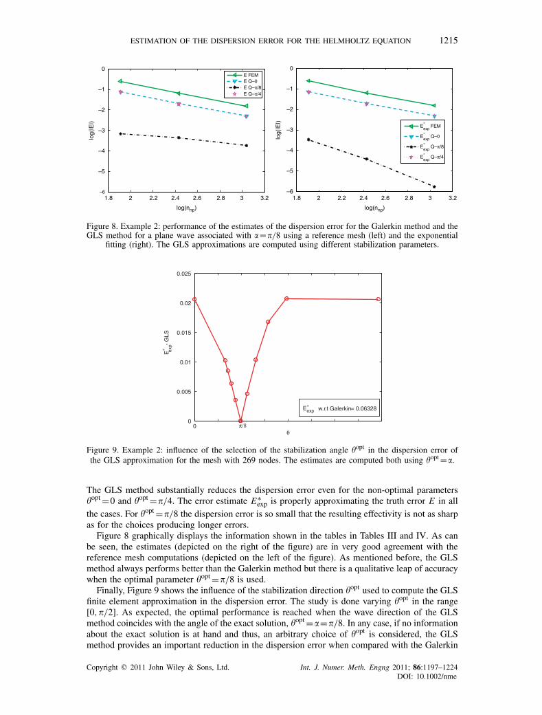
Figure 8. Example 2: performance of the estimates of the dispersion error for the Galerkin method and theGLS method for a plane wave associated with �=�/8 using a reference mesh (left) and the exponential
fitting (right). The GLS approximations are computed using different stabilization parameters.
00
0.005
0.01
0.015
0.02
0.025
θ
E-
GLS
π/8
w.r.t Galerkin = 0.06328E
Figure 9. Example 2: influence of the selection of the stabilization angle �opt in the dispersion error ofthe GLS approximation for the mesh with 269 nodes. The estimates are computed both using �opt =�.
The GLS method substantially reduces the dispersion error even for the non-optimal parameters�opt =0 and �opt =�/4. The error estimate E∗
exp is properly approximating the truth error E in allthe cases. For �opt =�/8 the dispersion error is so small that the resulting effectivity is not as sharpas for the choices producing longer errors.
Figure 8 graphically displays the information shown in the tables in Tables III and IV. As canbe seen, the estimates (depicted on the right of the figure) are in very good agreement with thereference mesh computations (depicted on the left of the figure). As mentioned before, the GLSmethod always performs better than the Galerkin method but there is a qualitative leap of accuracywhen the optimal parameter �opt =�/8 is used.
Finally, Figure 9 shows the influence of the stabilization direction �opt used to compute the GLSfinite element approximation in the dispersion error. The study is done varying �opt in the range[0,�/2]. As expected, the optimal performance is reached when the wave direction of the GLSmethod coincides with the angle of the exact solution, �opt =�=�/8. In any case, if no informationabout the exact solution is at hand and thus, an arbitrary choice of �opt is considered, the GLSmethod provides an important reduction in the dispersion error when compared with the Galerkin
Copyright � 2011 John Wiley & Sons, Ltd. Int. J. Numer. Meth. Engng 2011; 86:1197–1224DOI: 10.1002/nme
1216 L. M. STEFFENS, N. PARÉS AND P. DÍEZ
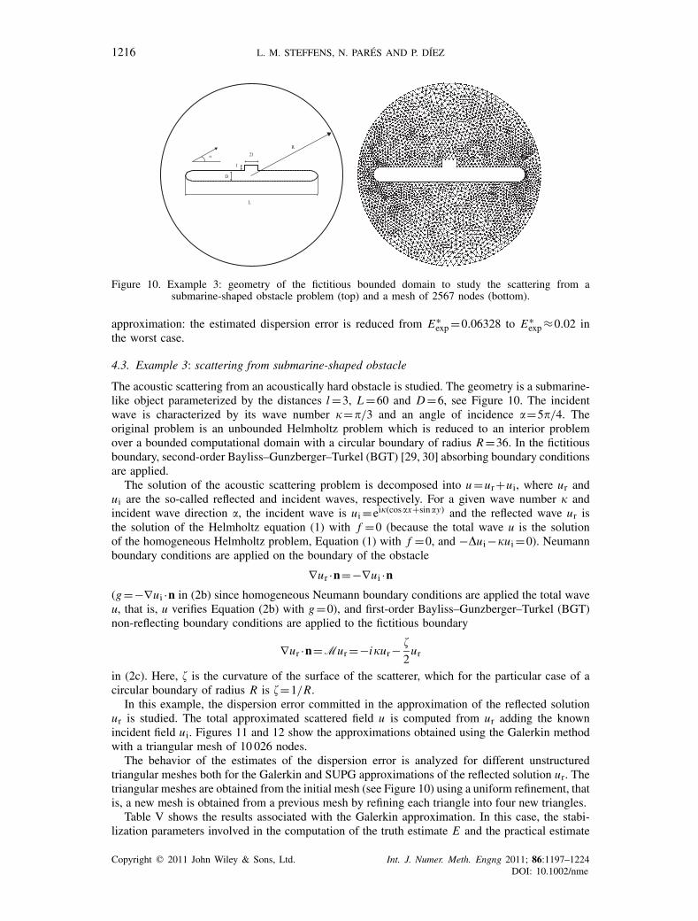
Figure 10. Example 3: geometry of the fictitious bounded domain to study the scattering from asubmarine-shaped obstacle problem (top) and a mesh of 2567 nodes (bottom).
approximation: the estimated dispersion error is reduced from E∗exp =0.06328 to E∗
exp ≈0.02 inthe worst case.
4.3. Example 3: scattering from submarine-shaped obstacle
The acoustic scattering from an acoustically hard obstacle is studied. The geometry is a submarine-like object parameterized by the distances l =3, L =60 and D =6, see Figure 10. The incidentwave is characterized by its wave number �=�/3 and an angle of incidence �=5�/4. Theoriginal problem is an unbounded Helmholtz problem which is reduced to an interior problemover a bounded computational domain with a circular boundary of radius R =36. In the fictitiousboundary, second-order Bayliss–Gunzberger–Turkel (BGT) [29, 30] absorbing boundary conditionsare applied.
The solution of the acoustic scattering problem is decomposed into u =ur +ui, where ur andui are the so-called reflected and incident waves, respectively. For a given wave number � andincident wave direction �, the incident wave is ui =ei�(cos�x+sin�y) and the reflected wave ur isthe solution of the Helmholtz equation (1) with f =0 (because the total wave u is the solutionof the homogeneous Helmholtz problem, Equation (1) with f =0, and −�ui −�ui =0). Neumannboundary conditions are applied on the boundary of the obstacle
∇ur ·n=−∇ui ·n(g =−∇ui ·n in (2b) since homogeneous Neumann boundary conditions are applied the total waveu, that is, u verifies Equation (2b) with g =0), and first-order Bayliss–Gunzberger–Turkel (BGT)non-reflecting boundary conditions are applied to the fictitious boundary
∇ur ·n=Mur =−i�ur −
2ur
in (2c). Here, is the curvature of the surface of the scatterer, which for the particular case of acircular boundary of radius R is =1/R.
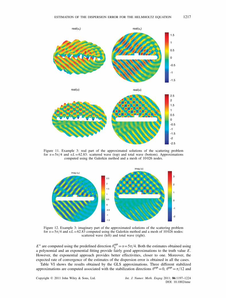
In this example, the dispersion error committed in the approximation of the reflected solutionur is studied. The total approximated scattered field u is computed from ur adding the knownincident field ui. Figures 11 and 12 show the approximations obtained using the Galerkin methodwith a triangular mesh of 10 026 nodes.
The behavior of the estimates of the dispersion error is analyzed for different unstructuredtriangular meshes both for the Galerkin and SUPG approximations of the reflected solution ur. Thetriangular meshes are obtained from the initial mesh (see Figure 10) using a uniform refinement, thatis, a new mesh is obtained from a previous mesh by refining each triangle into four new triangles.
Table V shows the results associated with the Galerkin approximation. In this case, the stabi-lization parameters involved in the computation of the truth estimate E and the practical estimate
Copyright � 2011 John Wiley & Sons, Ltd. Int. J. Numer. Meth. Engng 2011; 86:1197–1224DOI: 10.1002/nme
ESTIMATION OF THE DISPERSION ERROR FOR THE HELMHOLTZ EQUATION 1217
real(ur) real(ur)
-1.5
-1
-0.5
0
0.5
1.5
1
real(u) real(u)
2.5
2
1.5
1
0.5
0
-0.5
-1
-1.5
-2
-2.5
Figure 11. Example 3: real part of the approximated solutions of the scattering problemfor �=5�/4 and �L =62.83: scattered wave (top) and total wave (bottom). Approximations
computed using the Galerkin method and a mesh of 10 026 nodes.
imag (u )r
-1.5
0
2.5
-1
1
2
1.5
-0.5
0.5
-2
0
3
-1
1
2
imag (u)
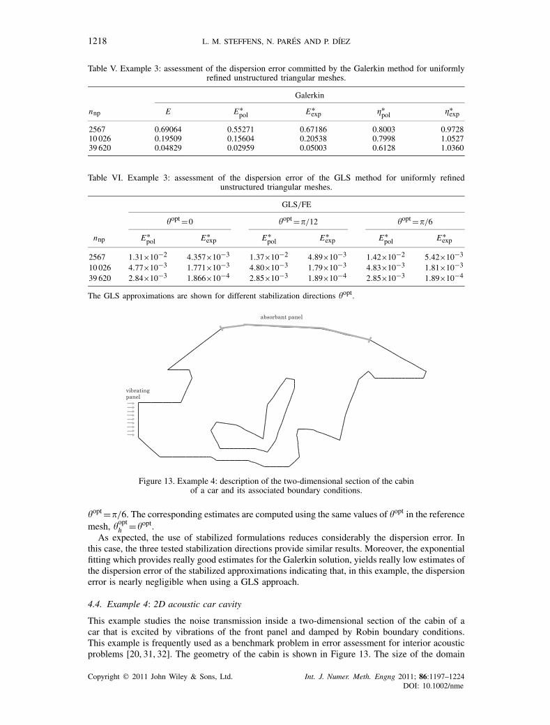
Figure 12. Example 3: imaginary part of the approximated solutions of the scattering problemfor �=5�/4 and �L =62.83 computed using the Galerkin method and a mesh of 10 026 nodes:
scattered wave (left) and total wave (right).
E∗ are computed using the predefined direction �opth =�=5�/4. Both the estimates obtained using
a polynomial and an exponential fitting provide fairly good approximations to the truth value E .However, the exponential approach provides better effectivities, closer to one. Moreover, theexpected rate of convergence of the estimates of the dispersion error is obtained in all the cases.
Table VI shows the results obtained by the GLS approximations. Three different stabilizedapproximations are computed associated with the stabilization directions �opt =0, �opt =�/12 and
Copyright � 2011 John Wiley & Sons, Ltd. Int. J. Numer. Meth. Engng 2011; 86:1197–1224DOI: 10.1002/nme
1218 L. M. STEFFENS, N. PARÉS AND P. DÍEZ
Table V. Example 3: assessment of the dispersion error committed by the Galerkin method for uniformlyrefined unstructured triangular meshes.
Galerkin
nnp E E∗pol E∗
exp ∗pol ∗
exp
2567 0.69064 0.55271 0.67186 0.8003 0.972810 026 0.19509 0.15604 0.20538 0.7998 1.052739 620 0.04829 0.02959 0.05003 0.6128 1.0360
Table VI. Example 3: assessment of the dispersion error of the GLS method for uniformly refinedunstructured triangular meshes.
GLS/FE
�opt =0 �opt =�/12 �opt =�/6
nnp E∗pol E∗
exp E∗pol E∗
exp E∗pol E∗
exp
2567 1.31×10⁻² 4.357×10⁻³ 1.37×10⁻² 4.89×10⁻³ 1.42×10⁻² 5.42×10⁻³
10 026 4.77×10⁻³ 1.771×10⁻³ 4.80×10⁻³ 1.79×10⁻³ 4.83×10⁻³ 1.81×10⁻³
39 620 2.84×10⁻³ 1.866×10⁻⁴ 2.85×10⁻³ 1.89×10⁻⁴ 2.85×10⁻³ 1.89×10⁻⁴
The GLS approximations are shown for different stabilization directions �opt.
Figure 13. Example 4: description of the two-dimensional section of the cabinof a car and its associated boundary conditions.
�opt =�/6. The corresponding estimates are computed using the same values of �opt in the referencemesh, �opt
h =�opt.As expected, the use of stabilized formulations reduces considerably the dispersion error. In
this case, the three tested stabilization directions provide similar results. Moreover, the exponentialfitting which provides really good estimates for the Galerkin solution, yields really low estimates ofthe dispersion error of the stabilized approximations indicating that, in this example, the dispersionerror is nearly negligible when using a GLS approach.
4.4. Example 4: 2D acoustic car cavity
This example studies the noise transmission inside a two-dimensional section of the cabin of acar that is excited by vibrations of the front panel and damped by Robin boundary conditions.This example is frequently used as a benchmark problem in error assessment for interior acousticproblems [20, 31, 32]. The geometry of the cabin is shown in Figure 13. The size of the domain
Copyright � 2011 John Wiley & Sons, Ltd. Int. J. Numer. Meth. Engng 2011; 86:1197–1224DOI: 10.1002/nme
ESTIMATION OF THE DISPERSION ERROR FOR THE HELMHOLTZ EQUATION 1219
is characterized by the maximum horizontal and vertical lengths, Lx =2.7m and L y =1.1m,respectively. The source term entering in Equation (1) is f =0, and as mentioned in Remark 1, forinterior acoustic wave propagation problems, the Neumann and Robin boundary conditions enteringin Equation (2) are of the form g =−i�c�vn and Mu =−i�c�Anu, where in this case the materialparameters are c=340m/s standing for the speed of sound of the medium and �=1.225kg/m3
standing for the mass density. The vibrating front panel is excited with a unit normal velocityvn =1m/s, whereas the roof is considered to be an absorbent panel with associated admittanceAn =1/2000m(Pas)−1. The rest of the boundary is assumed to be perfectly reflecting and thusvn =0m/s. Finally, a wave number of �≈9.7 has been considered in the computations (equivalentto a frequency of 525Hz).
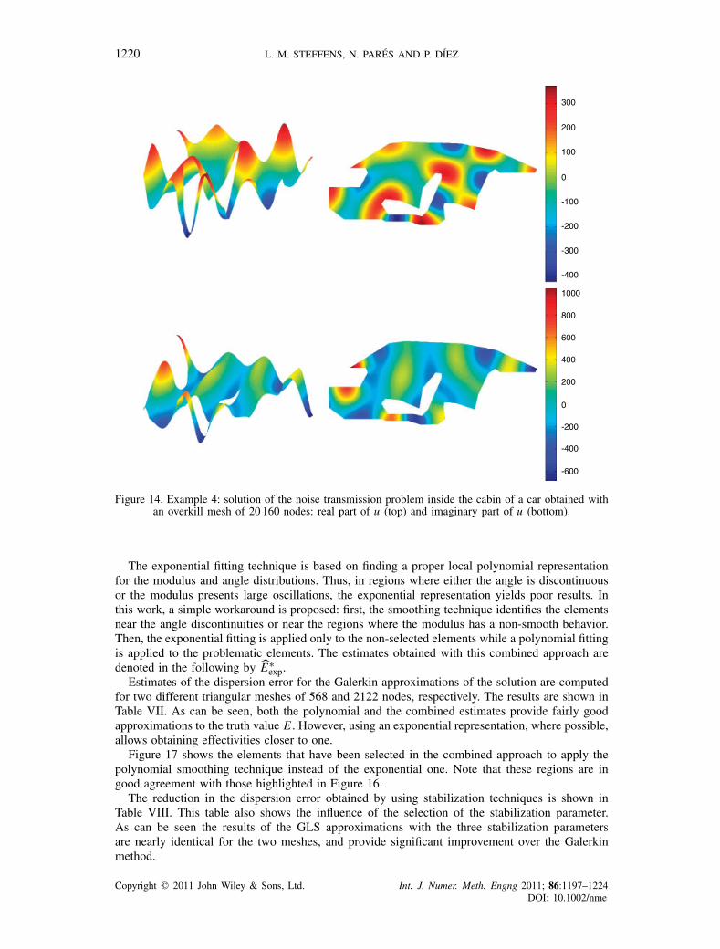
In this problem, the exponential fitting presented above yields bad estimates, worse than thestandard polynomial fitting. This is due to the fact that the solution is extremely complex withouta predominant direction. At many points of the domain, the solution can be expressed as a sumof several plane waves with similar amplitudes. Thus, the exponential fitting fails to properlyapproximate the local behavior of the modified solution in the vicinity of these points. Actually,the exponential recovery in these zones introduces unrealistic discontinuities resulting in badestimates. In the following, this phenomenon is described in detail, as well as the proposedremedy.
It is well known that the exact solution of the 2D homogeneous Helmholtz equation can beexpressed as an infinite sum of plane waves traveling in different directions. In the previousexamples, the solutions were either a single plane wave traveling in a predefined direction (seeexamples 1 and 2) or had a prevalent plane wave direction, although the prevalent wave directionmay vary from different zones of the domain (see the scattered solution of example 3). The soundtransmission inside a car cabin is a more complex phenomenon and the solution does not presentclear prevalent directions but is a combination of different plane waves with similar amplitudes(see Figure 14).
Even if the exact solution has no prevalent directions, one can consider an exponential repre-sentation of the exact solution of the problem
u(x)=r (x)ei�(x),
where r (x) and �(x) are the real-valued functions providing the modulus and angle of u, respectively.In the cases where the solution does not have a prevalent direction two phenomena may appear: onthe one hand the angle distribution �(x) may present discontinuities coinciding with areas wherethe modulus vanishes, and, on the other hand, the modulus distribution r (x) may present a highlynon-linear and non-smooth behavior in some regions.
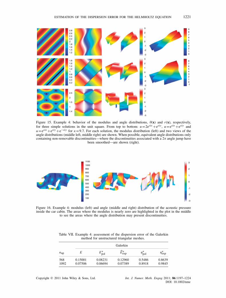
To illustrate these phenomena, the modulus and angle distributions of three simple solutions areshown in Figure 15. First, the solution u =2e�ix +e�iy is considered. Note that, in this case, the planewave traveling in the x-direction, e�ix , prevails over the wave traveling in the y-direction, e�iy . Ascan be seen in Figure 15, the standard representation of the angle distribution �(x) is a discontinuousfunction, which can be easily post-processed to recover a continuous angle distribution. Moreover,the modulus does not present large variations over small regions. In this case, the exponential fittingdescribed in Section 3.5 provides accurate approximations of u. The second example, u =e�ix +e�iy ,shows that if the solution is obtained combining two plane waves of the same amplitude, and thusit does not have any prevalent direction, angle discontinuities appear in some predefined straightlines. As the number of plane waves that comprise the solution u increases, see for instance thethird example u =e�ix +e�iy +e−�iy , the modulus and angle distributions may present areas with ahighly non-linear and non-smooth behavior. Note that, although the angle distribution only presentspoint or removable discontinuities at nine points of the domain, obtaining a globally smoothangle distribution from the standard angle representation is not a trivial task. Figure 16 shows thebehavior of the modulus and angle distribution associated with the acoustic pressure inside the carcabin. As can be seen, it is not easy to clearly identify the regions where the angle distribution isdiscontinuous.
Copyright � 2011 John Wiley & Sons, Ltd. Int. J. Numer. Meth. Engng 2011; 86:1197–1224DOI: 10.1002/nme
1220 L. M. STEFFENS, N. PARÉS AND P. DÍEZ
-300
-100
300
-200
0
200
100
-400
-400
200
1000
-200
0
800
600
-600
400
Figure 14. Example 4: solution of the noise transmission problem inside the cabin of a car obtained withan overkill mesh of 20 160 nodes: real part of u (top) and imaginary part of u (bottom).
The exponential fitting technique is based on finding a proper local polynomial representationfor the modulus and angle distributions. Thus, in regions where either the angle is discontinuousor the modulus presents large oscillations, the exponential representation yields poor results. Inthis work, a simple workaround is proposed: first, the smoothing technique identifies the elementsnear the angle discontinuities or near the regions where the modulus has a non-smooth behavior.Then, the exponential fitting is applied only to the non-selected elements while a polynomial fittingis applied to the problematic elements. The estimates obtained with this combined approach aredenoted in the following by E∗
exp.Estimates of the dispersion error for the Galerkin approximations of the solution are computed
for two different triangular meshes of 568 and 2122 nodes, respectively. The results are shown inTable VII. As can be seen, both the polynomial and the combined estimates provide fairly goodapproximations to the truth value E . However, using an exponential representation, where possible,allows obtaining effectivities closer to one.
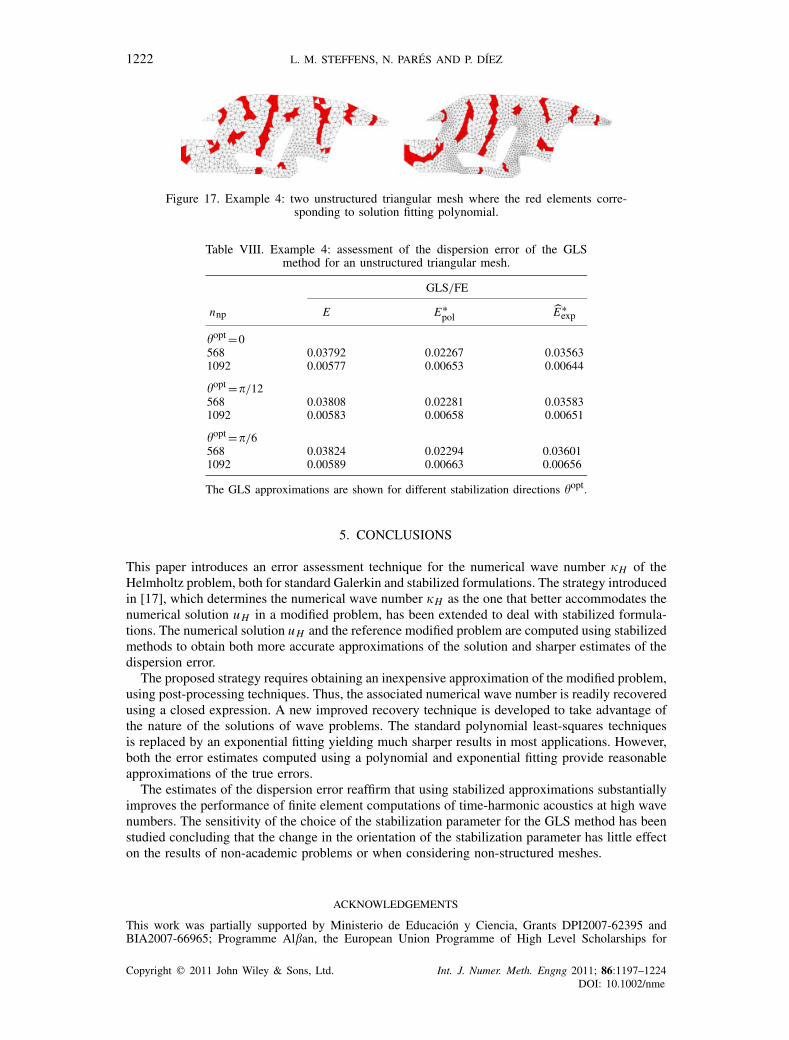
Figure 17 shows the elements that have been selected in the combined approach to apply thepolynomial smoothing technique instead of the exponential one. Note that these regions are ingood agreement with those highlighted in Figure 16.
The reduction in the dispersion error obtained by using stabilization techniques is shown inTable VIII. This table also shows the influence of the selection of the stabilization parameter.As can be seen the results of the GLS approximations with the three stabilization parametersare nearly identical for the two meshes, and provide significant improvement over the Galerkinmethod.
Copyright � 2011 John Wiley & Sons, Ltd. Int. J. Numer. Meth. Engng 2011; 86:1197–1224DOI: 10.1002/nme
ESTIMATION OF THE DISPERSION ERROR FOR THE HELMHOLTZ EQUATION 1221
1.4
2
2.8
1.81.6
2.2
2.62.4
1.2
0.4
1
1.8
0.80.6
1.2
1.61.4
0.2
1.4
1.5
2.5
1
2
-2
0
3
-1
1
2
-3
-2
0
3
-1
1
2
-3
-2
0
3
-1
1
2
-3
2
5
9
43
6
87
10
2
543
6
87
10-1
Figure 15. Example 4: behavior of the modulus and angle distributions, �(x) and r (x), respectively,for three simple solutions in the unit square. From top to bottom: u =2e�ix +e�iy , u =e�ix +e�iy andu =e�ix +e�iy +e−�iy for �=9.7. For each solution, the modulus distribution (left) and two views of theangle distributions (middle left, middle right) are shown. When possible, equivalent angle distributions onlycontaining non-removable discontinuities—where the discontinuities associated with a 2� angle jump have
been smoothed—are shown (right).
300
700
1100
400
500
1000
900
200
800
600
100
-2
0
3
-1
1
2
-3
Figure 16. Example 4: modulus (left) and angle (middle and right) distribution of the acoustic pressureinside the car cabin. The areas where the modulus is nearly zero are highlighted in the plot in the middle
to see the areas where the angle distribution may present discontinuities.
Table VII. Example 4: assessment of the dispersion error of the Galerkinmethod for unstructured triangular meshes.
Galerkin
nnp E E∗pol E∗
exp ∗pol ∗
exp
568 0.15001 0.08231 0.12960 0.5486 0.86391092 0.07506 0.06694 0.07389 0.8918 0.9845
Copyright � 2011 John Wiley & Sons, Ltd. Int. J. Numer. Meth. Engng 2011; 86:1197–1224DOI: 10.1002/nme
1222 L. M. STEFFENS, N. PARÉS AND P. DÍEZ
Figure 17. Example 4: two unstructured triangular mesh where the red elements corre-sponding to solution fitting polynomial.
Table VIII. Example 4: assessment of the dispersion error of the GLSmethod for an unstructured triangular mesh.
GLS/FE
nnp E E∗pol E∗
exp
�opt =0568 0.03792 0.02267 0.035631092 0.00577 0.00653 0.00644
�opt =�/12568 0.03808 0.02281 0.035831092 0.00583 0.00658 0.00651
�opt =�/6568 0.03824 0.02294 0.036011092 0.00589 0.00663 0.00656
The GLS approximations are shown for different stabilization directions �opt.
5. CONCLUSIONS
This paper introduces an error assessment technique for the numerical wave number �H of theHelmholtz problem, both for standard Galerkin and stabilized formulations. The strategy introducedin [17], which determines the numerical wave number �H as the one that better accommodates thenumerical solution u H in a modified problem, has been extended to deal with stabilized formula-tions. The numerical solution u H and the reference modified problem are computed using stabilizedmethods to obtain both more accurate approximations of the solution and sharper estimates of thedispersion error.
The proposed strategy requires obtaining an inexpensive approximation of the modified problem,using post-processing techniques. Thus, the associated numerical wave number is readily recoveredusing a closed expression. A new improved recovery technique is developed to take advantage ofthe nature of the solutions of wave problems. The standard polynomial least-squares techniquesis replaced by an exponential fitting yielding much sharper results in most applications. However,both the error estimates computed using a polynomial and exponential fitting provide reasonableapproximations of the true errors.
The estimates of the dispersion error reaffirm that using stabilized approximations substantiallyimproves the performance of finite element computations of time-harmonic acoustics at high wavenumbers. The sensitivity of the choice of the stabilization parameter for the GLS method has beenstudied concluding that the change in the orientation of the stabilization parameter has little effecton the results of non-academic problems or when considering non-structured meshes.
ACKNOWLEDGEMENTS
This work was partially supported by Ministerio de Educación y Ciencia, Grants DPI2007-62395 andBIA2007-66965; Programme Al�an, the European Union Programme of High Level Scholarships for
Copyright � 2011 John Wiley & Sons, Ltd. Int. J. Numer. Meth. Engng 2011; 86:1197–1224DOI: 10.1002/nme
ESTIMATION OF THE DISPERSION ERROR FOR THE HELMHOLTZ EQUATION 1223
Latin America, scholarship no. E06D100641BR and Publishing Arts Research Council under grant no.98–1846389.
REFERENCES
1. Ihlenburg F. Finite Element Analysis of Acoustic Scattering. Springer: New York, 1998.2. Ihlenburg F, Babuska I. Dispersion analysis and error estimation of Galerkin finite element methods for the
Helmholtz equation. International Journal for Numerical Methods in Engineering 1995; 38:3745–3774.3. Ihlenburg F, Babuska I. Finite element solution of the Helmholtz equation with high wave number. Part 1: the
hp-version of the FEM. Computers and Mathematics with Applications 1995; 38:9–37.4. Babuska I, Ihlenburg F, Paik ET, Sauter SA. A generalized finite element method for solving the Helmholtz
equation in two dimensions with minimal pollution. Computer Methods in Applied Mechanics and Engineering1995; 128:325–359.
5. Gerdes K, Ihlenburg F. On the pollution effect in FE solutions of the 3D-Helmholtz equation. Computer Methodsin Applied Mechanics and Engineering 1999; 170(1–2):155–172.
6. Babuska I, Sauter SA. Is the pollution effect of the FEM avoidable for the Helmholtz equation considering highwavenumber? SIAM Review 2000; 42(3):451–484.
7. Ainsworth M. Discrete dispersion relation for hp-version finite element approximation at high wave number.SIAM Journal on Numerical Analysis 2004; 42(2):553–575.
8. Oden JT, Prudhomme S, Demkowicz L. A posteriori error estimation for acoustic wave propagation problems.Archives of Computational Methods in Engineering 2005; 12(4):343–389.
9. Irimie S, Bouillard P. A residual a posteriori error estimator for the finite element solution of the Helmholtzequation. Computer Methods in Applied Mechanics and Engineering 2001; 190(31):4027–4042.
10. Bouillard P. Admissible fields and error estimation for acoustic FEA with low wave numbers. Computers andStructures 1999; 73(1–5):227–237.
11. Bouillard P. Influence of the pollution on the admissible field error estimation for FE solutions of the Helmholtzequation. International Journal for Numerical Methods in Engineering 1999; 45(7):783–800.
12. Peraire J, Patera AT. Asymptotic a posteriori finite element bounds for the outputs of noncoercive problems:the Helmholtz and Burgers equations. Computer Methods in Applied Mechanics and Engineering 1999;171(1):77–86.
13. Babuska I, lhlenburg F, Strouboulis T, Gangaraj SK. A posteriori error estimation for finite element solutions ofHelmholtz equation. Part I: the quality of local indicators and estimators. International Journal for NumericalMethods in Engineering 1997; 40(18):3443–3462.
14. Babuska I, Ihlenburg F, Strouboulis T, Gangaraj K. A posterori error estimation for finite element solutions ofHelmholtz. Part II: estimation of the pollution error. International Journal for Numerical Methods in Engineering1997; 40:3883–3900.
15. Stewart JR, Hughes TJR. Explicit residual-based a posteriori error estimation for finite element discretizationsof the Helmholtz equation. Computation of the constant and new measures of error estimator quality. ComputerMethods in Applied Mechanics and Engineering 1996; 131(3–4):335–363.
16. Stewart JR, Hughes TJR. A posteriori error estimation and adaptive finite element computation of the Helmholtzequation in exterior domains. Finite Elements in Analysis and Design 1996; 22(1):15–24.
17. Steffens LM, Díez P. A simple strategy to assess the error in the numerical wave number of the finiteelement solution of the Helmholtz equation. Computer Methods in Applied Mechanics and Engineering 2009;198:1389–1400.
18. Babuska I, Melenk JM. The partition of unity method. International Journal for Numerical Methods in Engineering1997; 40:727–758.
19. Franca LP, Dutra do Carmo EG. The Galerkin gradient least-squares method. Computer Methods in AppliedMechanics and Engineering 1989; 74(1):41–54.
20. Harari I, Magoulès F. Numerical investigations of stabilized finite element computations for acoustics. WaveMotion 2004; 39:339–349.
21. Harari I, Hughes TJR. Galerkin/least-squares finite element methods for the reduced wave equation withnonreflecting boundary conditions in unbounded domains. Computer Methods in Applied Mechanics andEngineering 1992; 98(3):411–454.
22. Donea J, Huerta A. Finite Element Methods for Flow Problems. Wiley: Chichester, 2003.23. Hughes TJR, Brooks AN. A multi-dimensional upwind scheme with no crosswind diffusion. Finite Element
Methods for Convection Dominated Flows (Collection of Papers Presentation at Winter Annual Meeting of theAmerican Society of Mechanical Engineers (ASME)), vol. 34, New York, 1979; 19–35.
24. Hughes TJR, Franca LP, Hulbert GM. A new finite element formulation for computational fluid dynamics.Computer Methods in Applied Mechanics and Engineering 1989; 73:173–189.
25. Harari I, Nogueira CL. Reducing dispersion of linear triangular elements for the Helmholtz equation. Journal ofEngineering Mechanics 2002; 128(3):351–358.
26. Wiberg N-E, Zeng LF, Li XD. Error estimation and adaptivity in elastodynamics. Computer Methods in AppliedMechanics and Engineering 1992; 101:369–395.
Copyright � 2011 John Wiley & Sons, Ltd. Int. J. Numer. Meth. Engng 2011; 86:1197–1224DOI: 10.1002/nme

1224 L. M. STEFFENS, N. PARÉS AND P. DÍEZ
27. Díez P, Calderón G. Goal-oriented error estimation for transient parabolic problems. Computational Mechanics2007; 39(5):631–646.
28. Calderón G, Díez P. Análisis de diferentes estimadores de error de postproceso para adaptatividad orientada alresultado. Revista Internacional de Métodos Numéricos Cálculo y Diseño Ingeniería 2006; 22(2):193–213.
29. Bayliss A, Gunzburger M, Turkel E. Boundary conditions for the numerical solution of elliptic equations inexterior regions. SIAM Journal on Applied Mathematics 1982; 42(2):430–451.
30. Djellouli R, Farhat C, Macedo A, Tezaur R. Finite element solution of two-dimensional acoustic scatteringproblems using arbitrarily shaped convex artificial boundaries. Journal of Computational Acoustics 2000;8(1):81–99.
31. Bouillard P, Ihlenburg F. Error estimation and adaptivity for the finite element method in acoustics: 2D and 3Dapplications. Computer Methods in Applied Mechanics and Engineering 1999; 176(1):147–163.
32. Suleau S, Deraemaeker A, Bouillard P. Dispersion and pollution of meshless solutions for the Helmholtz equation.Computer Methods in Applied Mechanics and Engineering 2000; 190:639–657.
Copyright � 2011 John Wiley & Sons, Ltd. Int. J. Numer. Meth. Engng 2011; 86:1197–1224DOI: 10.1002/nme