Estimation of diffuse attenuation of ultraviolet light in optically shallow Florida Keys waters from MODIS measurements

AUTHOR QUERY FORM

Journal: RSE Please e-mail or fax your responses and any corrections to:Praveen Kumar, JenivE-mail: [email protected]: +1 619 699 6721

Article Number: 8826

Dear Author,

Please check your proof carefully and mark all corrections at the appropriate place in the proof (e.g., by using on-screen annotationin the PDF file) or compile them in a separate list. Note: if you opt to annotate the file with software other than Adobe Reader thenplease also highlight the appropriate place in the PDF file. To ensure fast publication of your paper please return your correctionswithin 48 hours.

For correction or revision of any artwork, please consult http://www.elsevier.com/artworkinstructions.

Any queries or remarks that have arisen during the processing of your manuscript are listed below and highlighted by flags in theproof. Click on the ‘Q’ link to go to the location in the proof.

Location in article Query / Remark: click on the Q link to goPlease insert your reply or correction at the corresponding line in the proof

Q1 Please confirm that given names and surnames have been identified correctly.

Q2 No corresponding author and correspondence address was indicated in manuscript. Please check andprovide the necessary details.

Q3 Please provide an update for reference “Cannizzaro et al., in press”.

Q4 Please provide an update for reference “Lee et al., in press”.

Please check this box if you have nocorrections to make to the PDF file. □

Thank you for your assistance.

Our reference: RSE 8826 P-authorquery-v11

Page 1 of 1

UNCO

RRECTED P

RO

OF

1 Highlights

2 Remote Sensing of Environment xxx (2013) xxx–xxx

4

5 Estimation of diffuse attenuation of ultraviolet light in optically shallow Florida6 Keys waters fromMODIS measurements7

8 Brian B. Barnes a, Chuanmin Hu a, Jennifer P. Cannizzaro a, Susanne E. Craig b, Pamela Hallock a, David L. Jones a, John C. Lehrter c, Nelson Melo d,e,9 Blake A. Schaeffer c, Richard Zepp f

1011

a College of Marine Science, University of South Florida, 140 7th Avenue South, St Petersburg, FL, 33701, USA12

b Dalhousie University, Department of Oceanography, Halifax, Nova Scotia, Canada13

c National Health and Environmental Effects Research Laboratory, Gulf Ecology Division, United States Environmental Protection Agency, Gulf Breeze, FL, USA14

d Cooperative Institute for Marine and Atmospheric Studies, University of Miami, Miami, FL, USA15

e National Oceanic and Atmospheric Association Atlantic Oceanographic and Meteorological Laboratory, Miami, FL, USA16

f National Exposure Research Laboratory, United States Environmental Protection Agency, Athens, GA, USA

1718

19 • UV water clarity data were derived from MODIS measurements over optically shallow waters.20 • Different spatiotemporal patterns were seen in Florida Keys visible and UV water clarity.21 • Approach is resilient to satellite instrument calibration uncertainties.22 • Coral research and monitoring can benefit from synoptic UV water clarity data.23

24

25

Remote Sensing of Environment xxx (2013) xxx

RSE-08826; No of Pages 1

0034-4257/$ – see front matter © 2013 Published by Elsevier Inc.http://dx.doi.org/10.1016/j.rse.2013.09.024

Contents lists available at ScienceDirect

Remote Sensing of Environment

j ourna l homepage: www.e lsev ie r .com/ locate / rse

Please cite this article as: Barnes, B.B., et al., Estimation of diffuse attenuation of ultraviolet light in optically shallow Florida Keys waters fromMODIS measurements, Remote Sensing of Environment (2013), http://dx.doi.org/10.1016/j.rse.2013.09.024

http://dx.doi.org/10.1016/j.rse.2013.09.024

http://www.sciencedirect.com/science/journal/00344257


Original text:

Inserted Text

""

Original text:

Inserted Text

""

Original text:

Inserted Text

""

Original text:

Inserted Text

""

1Q2

2

3Q1

4

5678910

11

12131415161718192021222324252627

52

53

54

55

56

57

58

59

60

61

62

63

64

65

66

Remote Sensing of Environment xxx (2013) xxx–xxx

RSE-08826; No of Pages 14

Contents lists available at ScienceDirect

Remote Sensing of Environment

j ourna l homepage: www.e lsev ie r .com/ locate / rse

Estimation of diffuse attenuation of ultraviolet light in optically shallowFlorida Keys waters from MODIS measurements

OO

FBrian B. Barnes a, Chuanmin Hu a, Jennifer P. Cannizzaro a, Susanne E. Craig b, Pamela Hallock a, David L. Jones a,John C. Lehrter c, Nelson Melo d,e, Blake A. Schaeffer c, Richard Zepp f

a College of Marine Science, University of South Florida, 140 7th Avenue South, St Petersburg, FL, 33701, USAb Dalhousie University, Department of Oceanography, Halifax, Nova Scotia, Canadac National Health and Environmental Effects Research Laboratory, Gulf Ecology Division, United States Environmental Protection Agency, Gulf Breeze, FL, USAd Cooperative Institute for Marine and Atmospheric Studies, University of Miami, Miami, FL, USAe National Oceanic and Atmospheric Association Atlantic Oceanographic and Meteorological Laboratory, Miami, FL, USAf National Exposure Research Laboratory, United States Environmental Protection Agency, Athens, GA, USA
R
0034-4257/$ – see front matter © 2013 Published by Elsehttp://dx.doi.org/10.1016/j.rse.2013.09.024

Please cite this article as: Barnes, B.B., et al.,MODIS measurements, Remote Sensing of En

Pa b s t r a c t
a r t i c l e i n f o
28

29

30

31

32

33

34

35

36

37

38

39

Article history:Received 29 May 2013Received in revised form 13 September 2013Accepted 25 September 2013Available online xxxx

Keywords:Water clarityLight penetrationUltra-violet lightRemote sensingShallow waterCoral reef

40

41

42

43

44

45

46

47

48

49

RRECTED Diffuse attenuation of solar light (Kd, m

−1) determines the percentage of light penetrating thewater column andavailable for benthic organisms. Therefore, Kd can be used as an index ofwater quality for coastal ecosystems thatare dependent on photosynthesis, such as the coral reef environments of the Florida Reef Tract. Ultraviolet (UV)light reaching corals can lead to reductions in photosynthetic capacity as well as DNA damage. Unfortunately,field measurements of Kd(UV) lack sufficient spatial and temporal coverage to derive statistically meaningfulpatterns, and it has been notoriously difficult to derive Kd in optically shallow waters from remote sensing dueto bottom contamination. Here we describe an approach to derive Kd(UV) in optically shallowwaters of the FloridaKeys using variations in the spectral shape of MODIS-derived surface reflectance. The approach used a principalcomponent analysis and stepwise multiple regression to parsimoniously select modes of variance in MODIS-derived reflectance data that best explained variance in concurrent in situ Kd(UV) measurements. The resultingmodels for Kd(UV) retrievals in waters 1–30 m deep showed strong positive relationships between derived andmeasured parameters [e.g., for Kd(305) ranging from 0.28 to 3.27 m−1; N= 29; R2=0.94]. The predictivecapabilities of these models were further tested, also showing acceptable performance [for Kd(305), R2 =0.92; bias=−0.02m−1; URMS=23%]. The same approach worked reasonably well in deriving the absorp-tion coefficient of colored dissolved organic matter (CDOM) in UV wavelengths [ag(UV), m−1], as Kd(UV) isdominated by ag(UV). Application of the approach to MODIS data showed different spatial and temporalKd(305) patterns than the Kd(488) patterns derived from a recently validated semi-analytical approach,suggesting that different mechanisms are controlling Kd in the UV and in the visible. Given the importanceof water clarity and light availability to shallow-water flora and fauna, the new Kd(UV) and ag(UV) dataproducts provide unprecedented information for assessing and monitoring of coral reef health, and couldfurther assist ongoing regional protection efforts.

© 2013 Published by Elsevier Inc.

5051

O
C
67

68

69

70

71

72

73

74

75

76

77

78

79

80

UN1. Introduction

The necessity of light for photosynthetic energy creation restrictszooxanthellate corals to shallow, oligotrophic environments whichcan present potential exposure to ultraviolet (UV) radiation. Whilelight is critical for photosynthesis, exposure to intense UV radiationcan cause oxidative stress (Foyer, Lelandais, & Kunert, 1994; Jokiel,1980) in corals and other reef flora (Fisk & Done, 1985; Hoegh-Guldberg & Jones, 1999; Lesser, Stochaj, Tapley, & Shick, 1990).Tolerance to incident UV radiation may depend on the concentrationof colored dissolved organic matter (CDOM, aka gelbstoff or yellowmatter) within the surrounding water column (West & Salm, 2003;Zepp et al., 2008). CDOM is a byproduct of terrestrial or marineplant matter decay (Shank, Lee, Vähätalo, Zepp, & Bartels, 2010).

vier Inc.

Estimation of diffuse attenuavironment (2013), http://dx.d

Spectrally, the CDOM absorption coefficient (ag) is the highest inthe UV wavelengths, and it decreases with increasing wavelengthwith an exponential spectral slope (S; Bricaud, Morel, & Prieur, 1981).Exposure to UV light, especially in stratified surface waters, will causephotobleaching and oxidation of CDOM (Fichot & Benner, 2012; Häderet al., 1998; Moran & Zepp, 1997; Shank, Zepp, Vähätalo, Lee, & Bartels,2010; Zepp et al., 2008), which will subsequently reduce the CDOM-induced light attenuation and increase the UV light potentially reachingcoral reef environments.

Despite the wealth of scientific literature describing the relationshipbetween light and coral health, there are surprisingly few implementedprograms to monitor light availability at coral reefs, primarily due tologistical and financial constraints. To overcome this difficulty, the U.S.NOAA's Coral Watch Program has implemented an experimental light

tion of ultraviolet light in optically shallow Florida Keys waters fromoi.org/10.1016/j.rse.2013.09.024



http://www.sciencedirect.com/science/journal/00344257


Original text:

Inserted Text

"givenname"

Original text:

Inserted Text

"givenname"

Original text:

Inserted Text

"givenname"

Original text:

Inserted Text

"givenname"

Original text:

Inserted Text

"givenname"

Original text:

Inserted Text

"givenname"

Original text:

Inserted Text

"givenname"

Original text:

Inserted Text

"givenname"

Original text:

Inserted Text

"givenname"

Original text:

Inserted Text

"givenname"

Original text:

Inserted Text

"surname"

Original text:

Inserted Text

"surname"

Original text:

Inserted Text

"surname"

Original text:

Inserted Text

"surname"

Original text:

Inserted Text

"surname"

Original text:

Inserted Text

"surname"

Original text:

Inserted Text

"surname"

Original text:

Inserted Text

"surname"

Original text:

Inserted Text

"surname"

Original text:

Inserted Text

"surname"

T

OO

F

81

82

83

84

85

86

87

88

89

90

91

92

93

94

95

96

97

98

99

100

101

102

103

104

105

106

107

108

109

110

111

112

113

114

115

116

117

118

119

120

121

122

123

124

125

126

127

128

129

130

131

132

133

134

135

136

137

138

139

140

141

142

143

144

145

146

147

148

149

150

151

152

153

t1:1

t1:2

t1:3

t1:4

t1:5

t1:6

t1:7

t1:8

t1:9

t1:10

t1:11

t1:12

t1:13

t1:14

t1:15

t1:16

t1:17

n = 54

R2 = 0.39

Fig. 1. Relationship between in situmeasured Kd(380) and that derived from Johannessenet al. (2003) algorithm using the MODIS/A RRS as the algorithm inputs. Solid line is 1:1reference, while dotted lines show ±50% error.

2 B.B. Barnes et al. / Remote Sensing of Environment xxx (2013) xxx–xxx

ORREC

stress product over the global ocean (http://coralreefwatch.noaa.gov/satellite/lsd/index.html). However, the product is only based onsatellite-estimated surface photosynthetically available radiation in thevisible wavelengths (PAR) without accounting for spatial variation inlight attenuation or for depth-dependent changes in radiation reachingthe benthos, noted by Yentsch et al. (2002) as crucial for all coral studies.This omission is due to a lack of reliable algorithms to derive lightattenuation (or water clarity) from satellite data in optically shallowenvironments (see Barnes et al., 2013; Zhao, Barnes, et al., 2013).‘Optically shallow’ is defined here as waters where the bottom isvisible from an above-water instrument, which includes the environ-ments inhabited by many zooxanthellate corals. This lack of satellitewater clarity data stands in direct contrast to sea surface temperature(SST) data from satellites, which are not adversely affected in opticallyshallow environments (e.g., Hu et al., 2009). As a result, data productsbased on satellite-derived SST are currently used almost exclusively topredict coral bleaching (see Strong, Liu, Meyer, Hendee, & Sasko, 2004;Strong, Liu, Skirving, & Eakin, 2011).

Estimation of water clarity or diffuse light attenuation coefficient(Kd, m−1, see Table 1 for list of symbol definitions) in optically shallowenvironments from satellite measurements has been problematic inthe past due to bottom contamination of the satellite-derived remotesensing reflectance (RRS). Most inversion algorithms are developedand validated for waters without the benthic contribution to the RRS.For example, Johannessen, Miller, and Cullen (2003) described anempirical relationship between Kd(UV) and a reflectance ratio betweenthe blue and green wavelengths for optically deep waters ranging fromturbid estuarine to offshore oligotrophic. However, benthic albedo varieswith wavelength for disparate bottom types (see Hochberg, Atkinson, &Andréfouët, 2003, Werdell & Roesler, 2003). As a consequence, applica-tion of the Johannessen et al. (2003) algorithm to optically shallowwatersis likely to produce large errors in the retrieved Kd(UV). Fig. 1 showsperformance of this algorithm in optically shallow waters, usingdata collected for this study. Benthic contamination has similarly beenshown to cause errors in retrievals of water-column chlorophyll-a con-centrations (Cannizzaro & Carder, 2006; Cannizzaro et al., in press;Carder, Cannizzaro, & Lee, 2005; Hu, 2008; Schaeffer, Hagy, Conmy,Lehrter, & Stumpf, 2012) and Kd in visible wavelengths (Zhao, Barnes,et al., 2013). Similar errors are likely to occur for Kd(UV) retrievals usingother empirical algorithms (e.g., Fichot, Sathyendranath, & Miller, 2008;Smyth, 2011) because of the bottom interference.

Nevertheless, instruments such as the Moderate Resolution ImagingSpectroradiometer (MODIS) onboard the U.S. National Aeronautics andSpace Administration (NASA) satellites Aqua (2002–present) and Terra(2000–present) provide medium-resolution (1 km) RRS data for all oftheworld's optically shallow regions once every 1–2days. In the FloridaKeys region, Barnes et al. (2013) described a modified quasi-analyticalalgorithm (QAA, Lee, Carder, & Arnone, 2002) to remove bottom

UNC 154

155

156

157

158

159

160

161

162

163

164

165

166

167

168

169

170

171

Table 1Description of symbols.

Symbol Description Units

Kd Diffuse attenuation coefficient for downwellingirradiance

m−1

Ed Downwelling irradiance Wnm−1m−2

Ed(0–) Subsurface downwelling irradiance Wnm−1m−2

L Radiance Wnm−1m−2 sr−1

R ReflectanceRRS Remote sensing reflectance sr−1

at Total absorption coefficient m−1

ag Absorption coefficient of gelbstoff (CDOM) m−1

ap Absorption coefficient of suspended particles m−1

aph Absorption coefficient of phytoplankton pigments m−1

ad Absorption coefficient of particulate detritus m−1

S Spectral slope of agλ Wavelength nmz Depth m

Please cite this article as: Barnes, B.B., et al., Estimation of diffuse attenuaMODIS measurements, Remote Sensing of Environment (2013), http://dx.d

ED P

Rcontamination and subsequently derive Kd in the visible from MODISAqua (MODIS/A) measurements. However, since MODIS does not collectRRS data in UV wavelengths, estimation of Kd(UV) requires an approachwhich is both resilient to variable bottom contamination and which canextrapolate beyond the measured visible satellite data. While Kd(UV) islinearly proportional to Kd in the visible bands [Kd(VIS)] in oligotrophicopen-ocean waters (Lee et al., in press), in optically complex environ-ments, spatiotemporal differences between the relative concentrationsof various water constituents (see Bricaud et al., 1981; DeGrandpre,Vodacek, Nelson, Bruce, & Blough, 1996) generally preclude use ofKd(VIS) to derive Kd(UV).

Algorithms based on neural networks (Ioannou, Gilerson, Gross,Moshary & Ahmed, 2011, 2013; Jamet, Loisel, & Dessailly, 2012), matrixinversion models (Brando & Dekker, 2003; Phinn, Dekker, Brando, &Roelfsema, 2005), or empirical orthogonal functions (EOF; aka principalcomponents analysis; Craig et al., 2012; Fichot et al., 2008; Fischer,Doerffer, & Grassl, 1986; Gower, Lin, & Borstad, 1984, Mueller, 1976;Sathyendranath, Hoge, Platt, & Swift, 1989, 1994; Sathyendranath,Prieur, & Morel, 1989; Toole & Siegel, 2001) have the potential to over-come the difficulty of deriving Kd in optically shallow waters, providedthat data from these environments are included in the training datasets.The latter approach, which entails partitioning variations in the mea-sured reflectance through the use of an EOF, has previously been usedto estimate water properties in the UV (Fichot et al., 2008). This generalapproach, including its published variants discussed below, will hereinbe termed the ‘EOF method.’ The EOF method is used to reduce hyper-or multispectral reflectance data to a few uncorrelated variables (EOFmodes, aka eigenvectors), which retain most of the variance in theoriginal data. Assuming that a particular water constituent affectsthe measured reflectance, varying concentrations of that constituentshould be correlated to one or more of the EOF modes.

Although the methodology for application of the EOF methodhas varied in the past, results have typically shown success of this ap-proach in modeling water parameters. The inputs to the EOF methodincludedmeasured reflectance (R; Gower et al., 1984; Mueller, 1976;Sathyendranath et al., 1994), simulated reflectance (Sathyendranathet al., 1989), simulated radiance (L; Fischer et al., 1986), and measuredRRS (Craig et al., 2012; Fichot et al., 2008; Toole & Siegel, 2001), fromregions ranging from coastal to open ocean. Water parameters derivedfrom the EOFmethod included secchi disk depth (Mueller, 1976), chloro-phyll concentration (Craig et al., 2012), fluorescence (Sathyendranathet al., 1989), inherent optical properties (IOPs) including absorptioncoefficients (Craig et al., 2012) and scattering coefficients (Gower


http://coralreefwatch.noaa.gov/satellite/lsd/index.html

http://coralreefwatch.noaa.gov/satellite/lsd/index.html


T

172

173

174

175

176

177

178

179

180

181

182

183

184

185

186

187

188

189

190

191

192

193

194

195

196

197

198

199

200

201

202

203

204

205

206

207

208

209

210

211

212

213

214

215

216

217

218

219

220

221

222

223

224

225

226

227

228

229

230

231

232

233

234

235

236

237

238

3B.B. Barnes et al. / Remote Sensing of Environment xxx (2013) xxx–xxx

C

et al., 1984), salinity and nutrient concentrations (Toole & Siegel,2001), Kd for both visible and ultraviolet wavebands (Fichot et al.,2008), and others. Fichot et al. (2008) and Craig et al. (2012) furtherdemonstrated the effectiveness of this approach using in situ measuredRRS, which had been resampled to wavelengths of satellite instruments.To our knowledge, however, validation of the EOF method usingsatellite-derived data as an input (e.g., MODIS RRS) has yet to be reported.In the present study, our approach is distinct from other published EOFmethods through 1) use of satellite-derived data as input, 2) parsimoni-ous model selection via stepwise forward addition, and 3) measure ofthe predictive ability of models through leave-one-out-cross validation(see Sections 3.3 and 3.4 for details).

Thus, given the pressing need for synoptic information on the UVlight field reaching coral reef environments, the objective of this studywas to develop and validate amethod to estimate Kd and ag in UVwave-lengths from MODIS/Aqua measurements over optically shallow waters.The method is based on a new approach to implement the EOF method,as well as extensive field data collected from the Florida Keys region foralgorithm tuning and validation.

2. Study area — Florida Keys

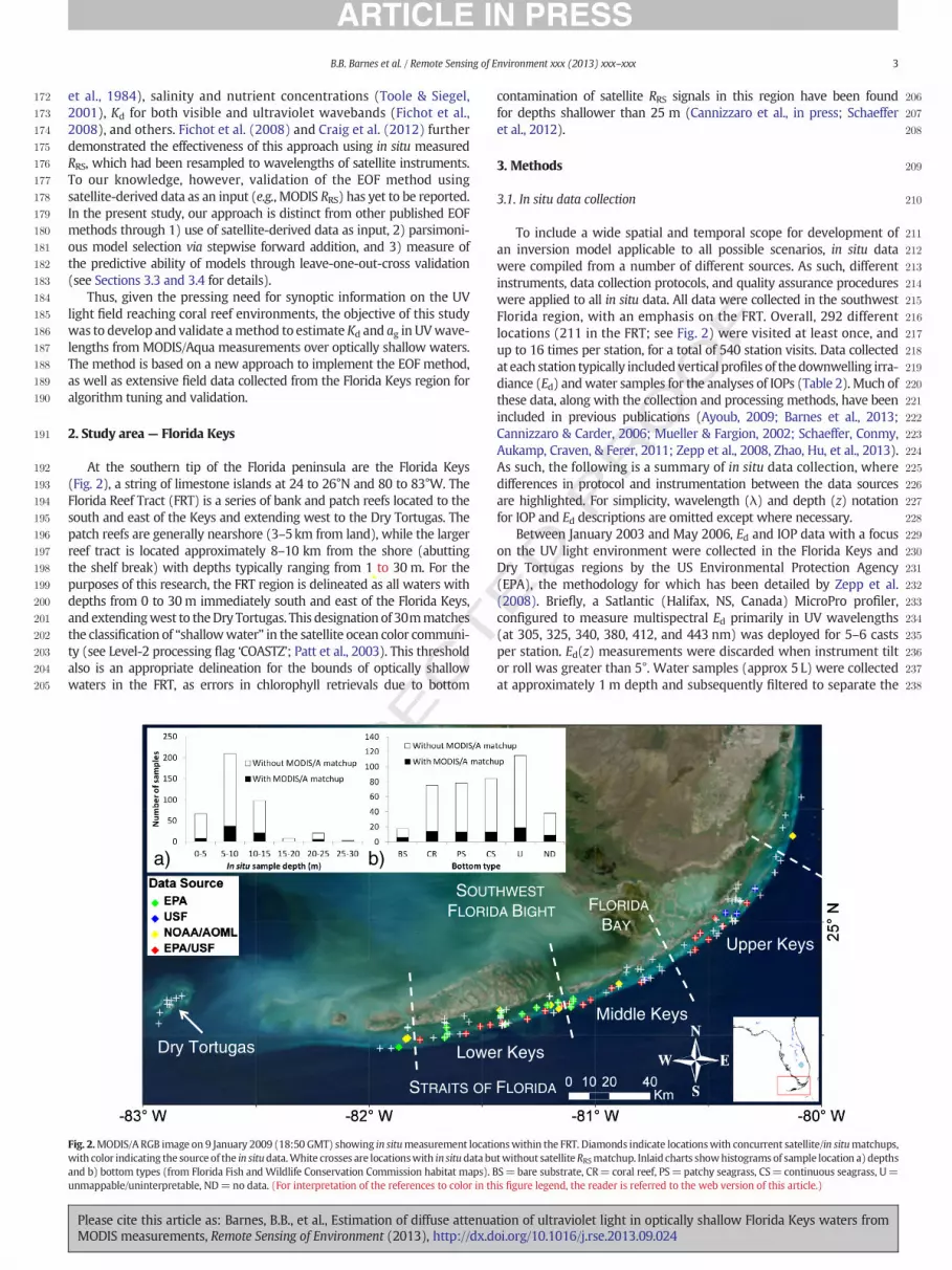
At the southern tip of the Florida peninsula are the Florida Keys(Fig. 2), a string of limestone islands at 24 to 26°N and 80 to 83°W. TheFlorida Reef Tract (FRT) is a series of bank and patch reefs located to thesouth and east of the Keys and extending west to the Dry Tortugas. Thepatch reefs are generally nearshore (3–5km from land), while the largerreef tract is located approximately 8–10 km from the shore (abuttingthe shelf break) with depths typically ranging from 1 to 30 m. For thepurposes of this research, the FRT region is delineated as all waters withdepths from 0 to 30m immediately south and east of the Florida Keys,and extendingwest to theDry Tortugas. This designation of 30mmatchesthe classification of “shallowwater” in the satellite ocean color communi-ty (see Level-2 processing flag ‘COASTZ’; Patt et al., 2003). This thresholdalso is an appropriate delineation for the bounds of optically shallowwaters in the FRT, as errors in chlorophyll retrievals due to bottom

UNCO

RRE

Lowe

STRAITS OF

SOUT

FLORID

Dry Tortugas

a) b)

Fig. 2.MODIS/A RGB image on 9 January 2009 (18:50 GMT) showing in situmeasurement locatiwith color indicating the source of the in situdata.White crosses are locationswith in situdata buand b) bottom types (from Florida Fish and Wildlife Conservation Commission habitat maps). Bunmappable/uninterpretable, ND=no data. (For interpretation of the references to color in th


ED P

RO

OF

contamination of satellite RRS signals in this region have been foundfor depths shallower than 25 m (Cannizzaro et al., in press; Schaefferet al., 2012).

3. Methods

3.1. In situ data collection

To include a wide spatial and temporal scope for development ofan inversion model applicable to all possible scenarios, in situ datawere compiled from a number of different sources. As such, differentinstruments, data collection protocols, and quality assurance procedureswere applied to all in situ data. All data were collected in the southwestFlorida region, with an emphasis on the FRT. Overall, 292 differentlocations (211 in the FRT; see Fig. 2) were visited at least once, andup to 16 times per station, for a total of 540 station visits. Data collectedat each station typically included vertical profiles of the downwelling irra-diance (Ed) andwater samples for the analyses of IOPs (Table 2). Much ofthese data, along with the collection and processing methods, have beenincluded in previous publications (Ayoub, 2009; Barnes et al., 2013;Cannizzaro & Carder, 2006; Mueller & Fargion, 2002; Schaeffer, Conmy,Aukamp, Craven, & Ferer, 2011; Zepp et al., 2008, Zhao, Hu, et al., 2013).As such, the following is a summary of in situ data collection, wheredifferences in protocol and instrumentation between the data sourcesare highlighted. For simplicity, wavelength (λ) and depth (z) notationfor IOP and Ed descriptions are omitted except where necessary.

Between January 2003 and May 2006, Ed and IOP data with a focuson the UV light environment were collected in the Florida Keys andDry Tortugas regions by the US Environmental Protection Agency(EPA), the methodology for which has been detailed by Zepp et al.(2008). Briefly, a Satlantic (Halifax, NS, Canada) MicroPro profiler,configured to measure multispectral Ed primarily in UV wavelengths(at 305, 325, 340, 380, 412, and 443 nm) was deployed for 5–6 castsper station. Ed(z) measurements were discarded when instrument tiltor roll was greater than 5°. Water samples (approx 5 L) were collectedat approximately 1 m depth and subsequently filtered to separate the

r Keys

Middle Keys

Upper Keys

FLORIDA

HWEST

A BIGHT FLORIDA

BAY

onswithin the FRT. Diamonds indicate locationswith concurrent satellite/in situmatchups,twithout satelliteRRSmatchup. Inlaid charts showhistograms of sample location a) depthsS=bare substrate, CR=coral reef, PS=patchy seagrass, CS= continuous seagrass, U=is figure legend, the reader is referred to the web version of this article.)



Original text:

Inserted Text

"–"

T

239

240

241

242

243

244

245

246

247

248

249

250

251

252

253

254

255

256

257

258

259

260

261

262

263

264

265

266

267

268

269

270

271

272

273

274

275

276

277

278

279

280

281

282

283

284

285

286

287

288

289

290

291

292

293

294

295

296297298

299

300

301

302

303

304

305

306

307

308

309

310

311

312

313

314

315

316

317

318

319

320

321

322

323

324

325

326

327

328

329

330

331

332

333

334

335

336

Table 2t2:1

t2:2 Description of in situ data.

t2:3 Source Dates (month/year) Samples MODIS/AMatchups Kd instrument:wavelengths (nm)

ag wavelengths(nm)

ap wavelengths(nm)

ad wavelengths(nm)

t2:4 EPA 1/03, 6/03, 8/03, 9/03, 2/04,6/04, 11/04, 1/05, 2/05, 6/05,8/05, 11/05, 3/06, 5/06

191 28 Satlantic MicroPro:305, 325, 340, 380, 412, 443

305, 325, 340, 380, 440 305, 325, 340, 380, 440 ND

t2:5 USF 5/04, 7/04, 9/04, 6/05, 7/05 39 4 ND 200–800 400–800 400–800t2:6 NOAA/

AOML8/09, 12/09, 5/10, 12/10, 5/11,8/11, 10/11, 12/11, 2/12

34 8 Biospherical PRR-2600,PUV-2500:PAR, 305, 330, 380, 443, 490,555, 589, 625, 683

200–800 400–800 400–800

t2:7 EPA/USF

4/11, 7/12, 8/12 144 34 Satlantic HyperPro:349–803

200–750 350–800 350–800


UNCO

RREC

dissolved (0.2 μm membrane filters) and particulate (0.7 μm nominalpore size glass-fiber filters — GF/F) water constituents, respectively.The GF/Fs were processed using the quantitative filter technique (Kiefer& SooHoo, 1982; Pegau et al., 2003; Roesler, 1998; Yentsch, 1962). APerkin Elmer Model Lambda 35 UV–visible spectrophotometer wasused for measurement of absorption coefficients due to particulates (ap)and gelbstoff (ag).

Additional water samples were collected by the University of SouthFlorida (USF) over the course of five cruises spanningMay2004 and July2005. Water samples were collected from the surface using Niskinbottles as described by Ayoub (2009) and processed in a mannerdetailed by Cannizzaro and Carder (2006), Mueller and Fargion(2002), and Ayoub (2009). Samples were filtered on GF/F filtersusing the quantitative filter technique, from which ap spectra weremeasured using a custom-made, 512-channel spectral radiometer(350–850 nm; Bissett, Patch, Carder, & Lee, 1997). Hot methanolextraction (Kishino, Takahashi, Okami, & Ichimura, 1985; Roesler,Perry, & Carder, 1989) was used to remove pigments from theseGF/Fs, which were re-analyzed to measure detrital absorption (ad).Phytoplankton absorption spectra were then calculated as aφ= ap− ad.Water sampleswere furtherfiltered through a0.2μmfilter, andprocessedto measure ag spectra using a Perkin Elmer Lambda 18 UV–visiblespectrophotometer. A pathlength of 10 cm was used for measurementof ag spectra from this, and all other, data sources.

The NOAA Atlantic Oceanographic and Meteorological Laboratory(AOML) has conducted approximately bi-monthly cruise surveys aboardthe R/V F.G. Walton Smith in the Florida Keys region as part of its SouthFlorida Program (SFP) since 1999 (see Zhao, Hu, et al., 2013). A subsetof those cruises included collection of Ed profiles and water samples(using a Niskin rosette at approximately 1 m depth) for IOP analysis.For the former, Biospherical Instruments, Inc. (San Diego, CA) ProfilingReflectance Radiometer (PRR-2600) and Profiling Ultraviolet Radiometer(PUV-2500) were used to collect Ed at 305, 330, and 380nm (PUV-2500)and 380, 443, 490, 555, 589, 658, and 683 nm (PRR-2600). Both instru-ments also recorded photosynthetically available radiation (PAR) profileswith depth. Typically 2 to 6 casts were collected for each instrument ateach station visited within two hours of local solar noon. Ed(z) data forwhich the instrument tilt or roll was greater than 10° were excludedfrom further analysis. Water samples were processed using the samemethods and instrumentation as the USF dataset.

In April 2011 and July/August 2012, in situ IOP and Ed data werecollected through a joint EPA/USF effort. At each depth, hyperspectral(400–735 nm, interpolated to every 1 nm) Ed profiles were collectedusing a Satlantic HyperPRO (for details see Barnes et al., 2013). Ed(z)measurements were discarded when instrument tilt or roll was greaterthan 5°. Water samples were collected from just below the surface formeasurement of both ag and ap. Similar to the methods used for theUSF and NOAA/AOML datasets, water samples were filtered on GF/Ffilters using the quantitative filter technique. A Shimadzu UV1700dual beam spectrophotometer was used for measurement of ap, ad(after warm methanol extraction), and ag spectra (see Schaeffer et al.,


ED P

RO

OF2011 for details). Residual scattering was removed from these spectra

by subtracting from each wavelength the mean of each measuredvalue between 790 and 800nm (Pegau et al., 2003).

All Ed profiles were processed to derive Kd via Lambert–Beer's law(Gordon, 1989; Smith & Baker, 1981), using linear regression betweendepth and

lnEd z;λð Þ

Ed 0−;λð Þ� �

: ð1Þ

For the EPA/USF and NOAA/AOML data sources, ln(Ed) at severalwavelengths for each profile was plotted against measurement depth,and the longest sequence of approximately log-linear decay in Edwas manually selected. Only data within this portion of the profilewere used in the derivation of Kd via the linear regression. Also, forthe EPA/USF and NOAA/AOML data sources, Kd derived from eachstation was further assessed for quality control by testing the similarityof replicate profiles (i.e., measurement repeatability). Specifically, Kd(λ)from any station was only considered reliable if the difference in Kd(λ)from two or more replicate profiles was less than 0.01m−1 and/or thecoefficient of variation for two or more replicate profiles was less than10%. The individual Kd(λ) measurements which fit either of theseconditions were averaged to yield the final Kd(λ) used in subsequentanalyses. In the NOAA/AOML dataset, both the PRR and PUV instrumentscollected profiles for certain wavebands (PAR and 380 nm). For stationswhere both instruments were deployed, data for these wavebands fromthe different instruments were considered replicates.

As there were no instances of concurrent in situ data from any ofthe four data sources, no attempts were made to identify or reconcileany differences between instruments as they pertain to calibration orperformance.

3.2. Satellite data collection

All MODIS/A Level-1A data from the Florida Keys region and withinthe years 2002–2012 (4566 files) were downloaded from the NASAGoddard Space Flight Center (GSFC) ocean color website http://oceancolor.gsfc.nasa.gov/. Only MODIS/A data were used due tothe striping and scan mirror damage on MODIS/Terra, which limitits utility for ocean color research (Franz, Kwiatkowska, Meister, &McClain, 2008). Using default processing parameters and SeaDASversion 6.4, level-2 RRS at all visible bands (412, 443, 469, 488, 531,547, 555, 645, 667, and 678 nm), as well as the level-2 processingflags, were created at 250m resolution. For most MODIS bands, thisspatial resolution was achieved by SeaDAS via interpolation fromnative 1 km or 500m resolution. RRS data from each band were sub-sequently mapped to a cylindrical equidistant projection with bounds24 to 26 N and 80 to 83 W, and stored in Hierarchical Data Format 4(HDF4) files.

RRS data concurrent (i.e., same day and collocated) with in situsamples were extracted from these HDF4 files and stored in ASCII text


http://oceancolor.gsfc.nasa.gov/

http://oceancolor.gsfc.nasa.gov/


T

337

338

339

340

341

342

343

344

345

346

347

348

349

350

351

352

353

354

355

356

357

358

359

360

361

362

363

364365366

367

368

369

370

371

372

373

374

375

376

377

378

379

380

381

382

383

384

385

386

387

388

389

390

391

392

393

394

395

396

397

398

399

400

401

402

403

404

405

406

407

408

409

410

411

412

413

414

415

416

417

418

419

420

421

422

423

424

425

426

427428429430431432433434435436437438439440441442443444445446447448449450451452

453

454

455

456

457

458


UNCO

RREC

files. RRS datawere removed from analysis if theywere flagged by any ofthe standard level-2 processing flags (Patt et al., 2003). Also, anyMODIS/A-derived spectrum with negative RRS at any wavelength wasdiscarded to exclude any data with potential atmospheric correctionfailures. All image processing and data extraction were performedusing IDL version 8.0 (Interactive Data Language; Exelis Visual Informa-tion Solutions). The concurrent satellite RRS and in situ measured waterparameters that passed all quality control procedures are hereaftertermed ‘matchups,’ while the matchup data from all parameters is the‘training dataset.’ In total, concurrent MODIS/A RRS spectra were foundfor 74 of the 408 (18%) stations sampled, which represents the maxi-mum possible number of matchups for any given parameter (numberof matchups varies by parameter due to sampling differences betweenthe four in situ data sources).

Once validated, the algorithm described below was applied to theentire time series of MODIS/A RRS in the Florida Keys region. Twolocations, A (24.548°N, 81.397°W; Lower Keys) and B (24.651°N,81.098°W; Middle Keys), were selected from within the FRT accordingto their repeated and long term in situ sampling. Time series of derivedwater parameters were extracted for these two stations and binnedby month. Image-wide monthly mean climatologies (2002–2012)of Kd(305) were also created for July and January to show represen-tative summer and winter conditions, respectively. MODIS/A RRS fromthese two months were also processed to derive Kd(488) using thealgorithm described by Barnes et al. (2013), from which monthlymean climatologies were calculated. Percent penetration of light tothe benthos was calculated as:

Penetration %ð Þ ¼ 100e −Kdzð Þ; ð2Þ

where z is the bottom depth from a bathymetry database providedby the United States Geological Survey (USGS).

3.3. Algorithm development

Previously published variants of the EOF method often involved acursory investigation of the shape of individual EOF modes to visuallyinterpret how various water constituents might contribute to eachmode (Craig et al., 2012; Fichot et al., 2008; Fischer et al., 1986; Toole& Siegel, 2001). Explaining the first two modes is typically straightfor-ward, while subsequent modes require more conjecture. Despite thelack of apparent physical meaning, these subsequent modes may bemost effective at representing the variance in the model (see von Storch& Zwiers, 1999). Measures of correlation to a concurrently measuredwater parameter have also been used to determine the contributionof water constituents to individual EOF modes (Fischer et al., 1986;Sathyendranath et al., 1989, 1994; Toole & Siegel, 2001). Whenempirically modeling measured parameters, mode selection haspreviously included statistical justification using Radj

2 (Fichot et al.,2008) or confidence intervals of multiple regression coefficients (Craiget al., 2012; Mueller, 1976).

Mueller (1976) utilized different modes for estimation of differentparameters. In contrast, while noting that certain EOF modes werenegligibly contributing to the models for different parameters, Fichotet al. (2008) and Craig et al. (2012) used EOF modes 1–4 in the finalmodels for all parameters to maintain consistency. In all of these works,only the first several (typically 4) modes were considered, owing to thehigh percentage of total variance (generally ~99%) explained by thesemodes.

In this paper, we demonstrate the implementation of a stepwise,forward-addition procedure for selection of EOF modes to be retainedfor use in modeling water parameters. This approach removes theguesswork and ambiguity from the EOF mode selection process. Assuch, statistically defensible mode selection is straightforward formodel application to derive water parameters. Mueller (1976) andCraig et al. (2012) utilized multiple regression of EOF modes (aka


ED P

RO

OF

principal components regression) to model water parameters. Ourapproach expands on this, while ensuring parsimony, through theforward addition of EOF modes (i.e., stepwise multiple regression).As such, this process increases the statistical power of the multipleregression by including only independent variables that are significantlycontributing to the explained variance of the dependent variable(Gauch, 1993). Inclusion of superfluous predictor variables will alwaysincrease the R2 and Fisher's test statistic (F) of a multiple regression(Cohen, Cohen,West, &Aiken, 2003). Although an EOFmodemay explaina tiny portion of the total variance in RRS, it may still be relevant inderiving water parameters (see von Storch & Zwiers, 1999).

Each water parameter was modeled independently using a modifica-tion of the EOFmethod. The term ‘parameter’ is used to describeKd, ag, aφ,or ad at a specificwavelength [for example,Kd(305) or ag(490)], and therewere 1930 parameters included in the training dataset. For each waterparameter, only matchups with valid in situ data were included inthe analyses. The number of matchups (N) varied by water parameterdue to differences in sampling between the various projects from whichdata were collected and because of quality-control procedures. Allwater parameters were log transformed to account for their approx-imately log-normal distribution (Campbell, 1995). For simplicity, wewill describe algorithm implementation for Kd(305), although allmeasured water parameters with matchup satellite RRS were analyzedin the samemanner. All statistical analyses were performed usingMatlabR2011a (Mathworks).

First, to focus on variability in spectral shape (as opposed to variabilityin amplitude), MODIS/A RRS spectra from Kd(305) matchups werenormalized by:

RRS λð Þh i ¼ RRS λð ÞZ 678

412RRS λð Þdλ

; ð3Þ

where bRRS(λ)N is the normalized spectra (Craig et al., 2012). An EOFwas then performed on the matchup MODIS/A bRRSN, which partitionedthe variance in the bRRSN along 10 modes. Since the 10 visible MODISbands were used in this analysis, these 10 modes explain 100% of thevariance in the bRRSN. The resulting scores for each of these EOF modeswere used as the independent variables in a stepwisemultiple regression(i.e., stepwise principal components regression), with the dependentvariable being the matchup in situ log10[Kd(305)]. The significance ofthis global (i.e., all inclusive) model was tested using 1000 permutations.If the significance level of the globalmodel was greater than alpha (0.05),no further analysis was performed to model or estimate this waterparameter fromMODIS/A data. However, if the global model was signifi-cant, stepwise multiple regression was further used to test the individualexplanatory effect of each EOFmode on log10[Kd(305)]. A finalmodelwasconstructed by sequentially adding the EOF modes to the model whichyielded the largest partial F. Addition of EOF modes to the model wasstopped if addition of the next EOFmode raised either 1) the significancelevel over alpha or 2) the adjusted coefficient of multiple determination(Radj2 ) over that of the global model (see Blanchet, Legendre, & Borcard,2008). This approach allows parsimonious determination of the EOFmodes that are contributing to the variance in Kd(305). Coefficients ofdetermination (R2) in log-space are primarily used to describe thestatistical relationships between these parsimoniously selected EOFmodes and the matching in situ log10[Kd(305)], hereafter termed‘model’ results.

3.4. Predictive validation statistical methods

To test the ‘predictive’ ability of the approach, leave-one-out-cross-validation was performed for each significant model result. To do so,multiple linear regression was performed, using only the significantEOF modes as independent variables and excluding data from one ofthe matchups. The EOF scores for the excluded matchup bRRSN were



T

459

460

461

462

463

464

465

466467

468469470471472473474475476

477

478

479

480

481

482

483

484

485

486

487

488

489

490

491

492

493

494

495

496

497

498

499

500

501

502

503

504

505

506

507

508

509

510

511

512

513

514

515

516

517

518

t3:1

t3:2

t3:3

t3:4

t3:5

t3:6

t3:7

t3:8

t3:9

t3:10

t3:11

t3:12

t3:13

t3:14

t3:15

t3:16

t3:17

t3:18

t3:19

t3:20

t3:21

t3:22

t3:23

t3:24

t3:25

t3:26

t3:27

t3:28

t3:29

t3:30

t3:31

t3:32


then combined with the multiple linear regression coefficients to predictlog10[Kd(305)] for that matchup. This process was repeated N times,with each iteration excluding a different matchup. The predicted log10[Kd(305)] values were compared to the in situ measured log10[Kd(305)]values using simple linear regression. Unbiased root mean squaredpercent error (URMS; Hooker, Lazin, Zibordi, & McLean, 2002) and biasof this predictivemodel were calculated on the non-transformed data as:

bias ¼ 1N

XNi¼1

predi−measið Þ; ð4Þ

and

URMS ¼ffiffiffiffiffiffiffiffiffiffiffiffiffiffiffiffiffiffiffiffiffiffiffiffiffiffiffiffiffiffiffiffiffiffiffiffiffiffiffiffiffiffiffiffiffiffiffiffiffiffiffiffiffiffiffiffiffiffiffiffiffiffiffiffi1N

XNi¼1

predi−measið Þpredi þmeasið Þ=2ð Þ

� �2;

vuut ð5Þ

where pred and meas represent predicted and measured values at isample number. As a benchmark for URMS, the NASA mission goal forsatellite-derived chlorophyll-a retrievals is 35% accuracy (Hooker,Esaias, Feldman, Gregg, & McClain, 1992). Gregg and Casey (2004)found Sea-viewing Wide Field-of-view Sensor (SeaWiFS) default algo-rithms applied over global ocean waters show RMS greater than 0.2for log transformed chlorophyll-a, which corresponds to relative RMSuncertainties over 58%.

4. Results

4.1. Model development and validation

A total of 1930 in situ parameters [e.g., Kd(305)] were tested usingthis approach, of which 1319 showed significant global models.Table 3 presents a summary of performance for selected parameters.In the following results and discussion, only results from Kd and ag at305 and 340 nm are described in detail. The rationale for the focus on

UNCO

RREC

Table 3Model and prediction performance for selected parameters.

Parameter MODIS/A matchups Model R2 Prediction R2 Prediction F Predicti

Kd(305) 29 0.94 0.92 313.9 ≪0.01Kd(325) 28 0.97 0.95 526.7 ≪0.01Kd(340) 28 0.96 0.94 386.0 ≪0.01Kd(380) 54 0.89 0.86 331.0 ≪0.01Kd(410) 20 0.84 0.77 60.7 ≪0.01Kd(440) 22 0.79 0.68 42.8 ≪0.01Kd(490) 23 0.74 0.65 39.6 ≪0.01Kd(555) 23 Model not significantKd(670) 18 0.74 0.37 9.5 b0.01ag(280) 40 0.81 0.76 118.6 ≪0.01ag(305) 65 0.87 0.84 320.4 ≪0.01ag(325) 65 0.84 0.79 235.2 ≪0.01ag(340) 65 0.81 0.74 183.1 ≪0.01ag(380) 63 0.68 0.62 100.7 ≪0.01ag(410) 37 0.31 0.25 11.4 b0.01ag(440) 60 0.26 0.19 13.8 ≪0.01ag(490) 32 Model not significantag(555) 32 Model not significantag(670) 35 Model not significantaφ(410) 21 0.81 0.58 26.8 ≪0.01aφ(440) 21 0.84 0.66 36.7 ≪0.01aφ(490) 21 0.83 0.64 33.5 ≪0.01aφ(555) 21 0.73 0.44 15.2 ≪0.01aφ(670) 21 0.63 0.07 1.5 0.236ad(410) 21 0.59 0.46 16.2 ≪0.01ad(440) 21 0.59 0.47 17.1 ≪0.01ad(490) 21 0.74 0.56 24.2 ≪0.01ad(555) 21 0.63 0.47 17.0 ≪0.01ad(670) 21 0.73 0.53 21.6 ≪0.01


ED P

RO

OF

these specific parameters is that they represent application of theapproach in both the UVA (315–400 nm) and UVB (280–315 nm)wavebands, which can lead to photoinhibition and DNA damage, re-spectively (Lesser & Lewis, 1996; Zepp et al., 2008). While Kd (anddepth) determines the light exposure to the benthos, ag is the dominantcomponent of water absorption for blue and UVwavelengths in the FRTregion (Zepp et al., 2008). As an example, Fig. 3 shows the percentagecontributions of particulate and dissolved matter absorption coeffi-cients to the total non-water absorption coefficient at 440 nm. Formost water samples, especially for those collected from the FRT, totalnon-water absorption is dominated by ag, with minimal contributionsfrom non-living detrital particles (ad).

Kd and ag at 305 and 340 nm all showed highly significant positiverelationships between the in situ measurements and model results(Fig. 4). For Kd(305), 29 matchups were included in the training datasetwith in situ values ranging from 0.28 to 3.27 m−1. Regression of themodel results and measured values (in log-space) showed an R2 of0.94, F of 438 and p-value≪0.01. Kd(340) showed very similar resultsacross all statistical indices (N = 28; range = 0.17–2.27 m−1; R2 =0.96; F=577; p≪ 0.01). Strong positive relationships were also seenfor ag(305) (N = 65; range = 0.10–3.19 m−1; R2 = 0.87; F = 433;p≪ 0.01), and ag(340) (N= 65; range = 0.02–1.50 m−1; R2 = 0.81;F = 271; p ≪ 0.01), which had triple the number of matchups asKd(UV), yet suffered little decrease in R2.

The predictive ability of this approach, using leave-one-out-cross-validation, showed slightly lower statistical performance than themodel results (Fig. 5). Nevertheless, the regression of the prediction re-sults with in situ values again showed strong positive relationships forKd(305) (R2 =0.92; F=314; p≪ 0.01; bias=−0.02m−1; URMS=23%), Kd(340) (R2 = 0.94; F = 386; p ≪ 0.01; bias = −0.01 m−1;URMS = 20%). Slightly lower R2 and URMS were seen for ag(305)(R2=0.84; F=320; p≪ 0.01; bias=−0.02m−1; URMS=30%), andag(340) (R2 = 0.74; F= 183; p≪ 0.01; bias =−0.01 m−1; URMS=40%), yet the increased number ofmatchup data points greatly decreasedthe p-values for these parameters.

on p-value Prediction Bias (m−1) Prediction URMS (%) EOF modes in model

−0.02 23 1, 3, 2, 9−0.01 17 1, 2, 3, 7, 9−0.01 20 1, 3, 2, 9−0.01 27 1, 4, 2, 6, 3−0.01 32 1, 2, 30.00 33 1, 3, 70.00 26 1, 3, 2

0.00 13 4, 1, 2, 7−0.06 29 1, 3, 7, 6, 4−0.02 30 1, 3, 6, 5, 4−0.02 35 1, 3, 6, 5, 4−0.01 40 1, 3, 6, 5, 2−0.01 46 1, 3, 6−0.02 60 3−0.02 70 1, 3

0.00 52 2, 1, 6, 9, 4, 80.00 45 2, 1, 6, 9, 4−0.00 50 2, 1, 4, 9, 60.00 94 1, 4, 9, 2, 5−0.00 82 2, 4, 1, 9−0.00 103 4, 9−0.00 106 4, 90.00 94 4, 9, 1, 2−0.00 102 4, 9, 10.00 99 4, 2, 9, 1



519

520

521

522

523

524

525

526

527

528

529

530

531

532

533

534

535

536

537

538

539

540

541

542

543

544

545

546

547

548

549

550

551

552

553

ad(440)

100 0

0 10050

50

1000

50

Fig. 3. Ternary plot showing percent contributions of water constituents CDOM, detritus,and phytoplankton pigments to the total non-water absorption coefficient at 440 nm forthe FRT (red circles) and adjacent waters. (For interpretation of the references to colorin this figure legend, the reader is referred to the web version of this article.)


4.2. Application within the Florida Keys region

The application of any empirical algorithm should generally berestricted to the same spatiotemporal bounds and range of environmen-tal conditions as the training dataset. To accentuate this limitation, we

UNCO

RRECT

Measu

Mod

eled

(m

-1)

Kd305

n = 29

R2 = 0.94

ag305

n = 65

R2 = 0.87

a)

c)

Fig. 4. Relationships between measured and modeled a) Kd(305), b) Kd(340), c) ag(3


D P

RO

OF

have applied this approach to estimate Kd(305) from satellite/in situmatchups (from the same data sources listed above) for waters adjacentto the FRT. Such retrievals yielded poor predictive relationships for bothStraits of Florida (Fig. 6, open squares; N=9; URMS=126%) and FloridaBay (Fig. 6, open triangles;N=4;URMS=65%)waters. Incorporating theStraits of Floridamatchups into the training dataset greatly improved thepredictive performance of this approach (Fig. 6, closed squares; URMS=36%). However, much less improvement was seen when Florida Bay wa-ters were included in the training dataset (Fig. 6, closed triangles;URMS=60%). The latter is likely due to the small number of matchupsin this large and diverse region, but again highlights the need to limitapplication of this approach to the range of environmental conditions(e.g., water properties and bottom types) representedwithin the trainingdataset.

As suchwe have strived to incorporate in situ data spanningmultipleyears, with inclusion of data from all seasons and a variety of bottomtypes into our FRT training dataset. Further, the training dataset includ-ed a range of in situ values of at least one order of magnitude for most ofthe parameters being modeled and predicted. Nevertheless, the samelogistical and financial limitations that plague established long-termmonitoring programs hindered our ability to compile a training datasetthat included all possible environments andwater conditions (aswell ascombinations thereof) in the study area.

Such effect is also clearly seen when the developed model is appliedto MODIS/A data to create a Kd(305) map covering the entire FloridaKeys region (Fig. 7, top panel). Even within the FRT, there appear to belocations forwhichKd(305) has not beenproperly derived. For example,in the shallow reefs (depths as shallow as intertidal; Dustan & Halas,1987) of the Upper Keys region, the spatial pattern in Kd(305) appearsto be associated with changes in depth. In the FRT, Kd (on the scale ofmonthly climatologies) should instead decrease with distance to shore
E
red (m-1)

Kd340

n = 28

R2 = 0.96

ag340

n = 65

R2 = 0.81

b)

d)

05), d) ag(340). Solid line is 1:1 reference, while dotted lines show±50% error.



TED P

RO

OF

554

555

556

557

558

559

560

561

562

563

564

565

566

567

568

569

Measured (m-1)

Pre

dict

ed (

m-1

)

Kd305

URMS = 23%

Bias =-0.02

Kd340

URMS = 20%

Bias = -0.01

ag305

URMS = 30%

Bias = -0.02

ag340

URMS = 40%

Bias = -0.01

a) b)

c) d)

Fig. 5. Relationships between measured and predicted (via leave-one-out-cross-validation) a) Kd(305), b) Kd(340), c) ag(305), d) ag(340). Solid line is 1:1 reference, while dotted linesshow ±50% error.


RECand according to inundation from Florida Bay waters through channels

between the islands (see Barnes et al., 2013). This effect of bottomcontamination appears to be limited to waters shallower than 4.5 m.The training dataset used for this study includes locations just over1m deep, but such stations were primarily inshore as opposed to off-shore, and thewaters from these inshore stationswere relatively turbid(i.e., less bottom contamination than for offshore clear water with thesame water depth). This exclusion of extremely shallow, offshore,

UNCO

R

Measured Kd(305) (m-1)

Pre

dict

ed K

d(30

5) (

m-1

)

Fig. 6. Predictive performance of the EOF approach to deriveKd(305) (m−1) forwaters in the Stronly FRTdata in the training dataset, whilefilled symbols represent retrievalswithwhen local sashow ±50% error.


clear-water reef locations from the training dataset was primarilylogistical (access by boat is limited due to the depth), but also dueto quality control of the measured Kd (reliable Kd is difficult tomeasure in clear shallow waters due to the surface wave-focusingeffect). Thus, we suggest limiting the application of the developedmodel to sites deeper than 4.5 m. This limit, however, does notrepresent a deficiency of the overall approach, and could be remediedwith a more inclusive training dataset.

, Straits of Florida, Florida Bay

Training Dataset, FRT onlyFRT and Straits of FloridaFRT and Florida Bay

aits of Florida (squares) and FloridaBay (triangles). Open symbols showperformanceusingmples are also included in the training dataset. Solid line is 1:1 reference,while dotted lines



TED P

RO

OF

570

571

572

573

574

575

576

577

578

579

580

581

582

583

584

585

586

587

588

589

590

591

592

593

594

595

596

597

598

599

600

601

602

603

604

605

606

607

608

609

610

611

612

613

614

615

616

617

618

619

620

621

622

623

624

625

626

627

628

629

Fig. 7. (Top) Image showing Kd(305) (m−1) derived fromMODIS/Ameasurements on9 January 2009 (same as Fig. 2) using the EOFmodel developed in this study. Land ismasked in black.White indicates coastline, clouds or algorithm failure. (Bottom) Monthly mean time series of MODIS/A derived Kd(305) for two stations A (black) and B (gray), with error bars showingstandard errors. In situ measured Kd(305) are also shown for stations A and B. White arrow shows example location of shallow waters (b4.5 m) for which Kd(305) retrievals arequestionable.


UNCO

RREC5. Discussion

5.1. Spatio-temporal variability of Kd in the FRT

Within the FRT, excluding these noted regionswhere retrievals fromthe EOFmodel may be erroneous, the spatial changes in derived Kd(305)appear to be reasonable. Specifically, a strong onshore-offshore gradientin Kd(305) is apparent, which has also been described for Kd(488) fromMODIS/A data (Barnes et al., 2013), and is consistent with previous re-ports (Ayoub, 2009; Lapointe & Clark, 1992, Szmant & Forrester, 1996).Kd(305) of the Upper, Middle, and Lower Keys regions also shows spatialpatterns similar to the Kd(488) patterns demonstrated by Barnes et al.(2013). However, there is a conspicuous difference in the seasonalityof Kd(305) and Kd(488) (see below). The temporal patterns at individuallocations have been validated by in situ measurements, suggesting thevalidity of the spatial Kd(305) patterns and its temporal contrast withKd(488). For example, Kd(305) time series at stations A and B derivedfor the entire span of MODIS/A measurements (Fig. 7, bottom graph)show Kd(305) fluctuations that are verified by the occasional in situdata from these locations (note that these in situ data were not used inthe training dataset due to lack of concurrent MODIS/A RRS). It is alsoworth noting that the largest peak in Kd(305) for one of the time series(Middle Keys, Station B; Fig. 7) coincides with the January 2010 coldevent in Florida (see Barnes & Hu, 2013; Barnes, Hu, & Muller-Karger,2011; Lirman et al., 2011), yet a similar peak was not seen in the LowerKeys time series (Station A). The Kd(305) peak at Station Bmay be poten-tially attributed to cold event related die-offs of the Everglades fauna andsubsequent CDOM release.

Although the spatial patterns of Kd(305) and Kd(488) may be similar,their temporal changes can be drastically different. Fig. 8 shows monthlymean climatology (2002–2012) images of Kd(305) and Kd(488) for Julyand January to represent conditions for summer andwinter, respectively.


In these images, data from locations shallower than 4.5 m have beenmasked. If the shallow areas were completely surrounded by deeperwater, Kd data for the shallow areas were filled by interpolation fromthe adjacent deeper data. In the FRT, Kd(488) is generally higher in thewinter than in the summer (Fig. 8) via a regular seasonal cycle (Barneset al., 2013). In contrast, Kd(305) shows reversed temporal changes formuch of the FRT, as seen in the July/January ratio images in Fig. 8. Thehigher Kd(305) in July than in January is possibly driven by summerprecipitation, which can lead to excessive CDOM-rich terrestrial runoff.Increased CDOM production from seagrass degradation is also expectedin warmer waters (Stabenau, Zepp, Bartels, & Zika, 2004). Finally, evenin dry summers, Everglades waters are occasionally released into FloridaBay to minimize adverse hypersalinity effects on seagrasses, providinganother potential source of CDOM to downstream FRT environments.The contrast between the July/January ratios for Kd(305) and Kd(488)suggests that, unlike oligotrophic open-ocean waters where Kd(305) islinearly proportional to Kd(488) (Lee et al., in press), the shallow FloridaKeys waters are more optically complex and one cannot rely solely onKd(VIS) to infer information on Kd(UV). This finding is not an artifact ofdifferences between algorithms being used, as there was a great deal ofscatter between concurrent Kd(UV) and Kd(VIS) retrievals when bothwere derived using the EOF approach.

Fig. 8 also highlights themuch higher Kd(305) than Kd(488) through-out the FRT region. Consequently, the percent penetration of UV light tothe benthos is much lower than that of blue light. In fact, the only loca-tionswith appreciable 305nm light reaching the benthos are the offshoreshallow coral reef environments, especially in the Upper Keys region.

5.2. Potential use in coral reef assessment

In the context of coral reef research and monitoring, the potentialuses of this long-term (2002–present), spatially synoptic dataset of UV



TED P

RO

OF

630

631

632

633

634

635

636

637

638

639

640

641

642

643

644

645

646

647

648

649

650

651

652

653

654

655

656

657

658

659

660

661

662

663

664

665

666

667

668

669

670

671

672

673

674

675

676

677

678

679

680

681

682

683

684

685

686

687

688

689

690

691

692

693

July January

Kd(305)

Kd(488)(Barnes et al., 2013)

Kd(305)


Kd(305) % Penetration

Kd(305)% Penetration

July / January

Kd(305)


Kd(305)% Penetration

Kd(488) % Penetration(Barnes et al., 2013)



Fig. 8.Mean Kd(305) and Kd(488) for July 2004 and January 2005 derived fromMODIS/A measurements using the EOF model developed in this study. Also shown are their July/Januaryratios. The bottom panels show the corresponding percent light reaching the benthos and their July/January ratios.


UNCO

RREC

light penetration are numerous. Although the satellite measurementfrequency is often semi-weekly due to cloud cover, the spatial and tem-poral coverage of this dataset is much higher than any in situ researchand monitoring programs (e.g., 2month repeat sampling for the NOAAAOML South Florida Program; see Kelble & Boyer, 2007). Thus, thisnew dataset could provide plentiful informationwith which to researchthe individual and combined effects of light and temperature on coralreefs in the FRT. In particular, a better understanding of the variationin UV light availability may help explain the distribution of coralsaway from tidal channels through the Keys (Ginsburg & Shinn, 1964,1993), but seemingly contradictory success of nearshore reefs relativeto offshore reefs (Lirman & Fong, 2007). Indeed, these offshore reefsare the only areas in the FRT for which appreciable levels of UV lightreach the benthos. Thus, the offshore reefs may be more susceptible tothe combined effects of UV and thermal oxidative stresses. However,there are complex interactions betweenwater-column light absorptionand temperature (e.g., radiative transfer) that confound a simple ‘either/or’ explanation of UV and thermal stress on coral communities. Further,as reefs are often net exporters of CDOM (Boss & Zaneveld, 2003), thesenew products could be used to investigate the change in Kd(UV) orag(UV) for waters flowing over a reef, potentially providing insightinto reef function. A thorough investigation of the direct and long-termimpacts of satellite-derived SST and light availability on coral reef healthin the Florida Keys is beyond the scope of this work.

The availability of long-term UV and visible light data in the FloridaKeys allows for statistical assessment of the spatio-temporal patternsin light conditions within the FRT waters (see Section 5.1; Barneset al., 2013). Such analyses can differentiate coral reef locations withdistinct Kd(UV) and Kd(VIS) regimes, either according to mean conditionor by annual or seasonal variability. The Florida Keys National MarineSanctuary (FKNMS) is currently undergoing re-zonation of specific pro-tection areas, in an effort to more effectively manage and protect themarine resources (NOAA 2007, 2012). As with the Kd(VIS) patterns,


synoptic accounting of the UV light availability in the FRT and its effecton corals could be valuable in informing this rezoning process.

Beyond the FRT, the range of in situ values used in the trainingdataset and subsequently modeled using this approach are similar toother reported coral environments. Using Kd(UV) as an example, ourtraining fits within measurements reported by Dunne and Brown(1996), and Shick, Lesser, and Jokiel (1996), for a Maldives atoll lagoon[Kd(UVB)= 0.39m−1], Thailand coastal island [Kd(UVB)= 0.78m−1],Thailand inshore fringing reef [Kd(UVB) = 1.61 m−1], Belize BarrierReef [Kd(UVB) = 0.21 m−1], Hawaii estuary [Kd(320) approximately1m−1], and offshore Hawaii reef [Kd(320)=0.2m−1]. Also, the rangeof Kd (at 305, 320, 340, and 380 nm) observed at coral reef locationssurrounding Malaysia (Kuwahara, Nakajima, Othman, Kushairi, & Toda,2010) almost exactly matches the spread of the training dataset used inthis FRT study. As such, beyond the general applicability of the approachto other environments, the particular parameterization of the modelspresented here may be directly applicable to coral reef environmentsworldwide.

5.3. Algorithm novelty — importance of stepwise model selection

While the use of EOF methods to derive water quality parameterssuch as Kd is not new, the method presented here shows improvementover previously published EOF methods primarily through its imple-mentation of the stepwise, forward addition procedure for selectionof the EOF modes to be retained in the models. This approach allowsfor parsimonious and statistically defensible mode selection formodel application to the various measured parameters discussed inthis paper as well as for application of this EOF method to anyother region.

When applied to each of the in situ measured parameters, anotherimportant consequence of this new approach in implementing theEOF method is a ranking of the relative importance of the EOF modes



694

695

696

697

698

699

700

701

702

703

704

705

706

707

708

709

710

711

712

713

714

715

716

717

718

719

720

721

722

723

724

725

726

727

728

729

730

731

732

733

734

735

736

737

738

739

740

741

742

743

744

745

746

747

748

749

750

751

752

753

754

755

756


in explaining variations in the parameter of interest. As seen in previousworks (Craig et al., 2012; Fichot et al., 2008; Mueller, 1976), the modeselection varied not only by IOP or Kd, but also by wavelength withinan IOP or Kd (Fig. 9). In contrast to visual interpretation of the modes,this listing gives a more definitive indication of the meaning (in termsof effect on water parameters) of various portions of the eigenvectors(loadings by wavelength) for each mode (Fig. 10). For example, thisanalysis allows definitive assessment ofmode4 as representing changesin bRRSN according to ad. Above approximately 550 nm, these changesare also concomitant with variability due to aφ. Further, low detritalcontributions (Fig. 3) are confirmed by the modes most often selectedfor ad retrievals (4 and 9) which account for a total of 1.46% of thetotal variance in bRRSN. Not surprisingly, Kd retrievals do not generallyinclude these modes, further highlighting the relatively small contribu-tions of ad to total attenuation in the FRT.

It is important to note thatmost of the EOFmodes discussed here arenot ‘significant’ according to common selection rules (e.g., Rule N;Preisendorfer, Zwiers, & Barnett, 1982; von Storch & Zwiers, 1999).Using the Kd305 matchups (n = 29) as an example, we performed1000 EOF analyses on randomly generated noise (simulating 10 bRRSNbands for those 29 matchups). From these EOFs, we calculated the95th percentile for the variance explained by each mode. As such, onlymode 1 in our model explains more variance in bRRSN than would bepredicted for random noise, and is thus ‘significant’ at α=0.05. Howev-er, this does not mean that subsequentmodes are noise as predictors inthe stepwise multiple regression. The forward selection process onlyincludes independent variables that are significantly contributing tothe variance in the dependent variable (in this case, log[Kd(305)]), andthe stopping procedures ensure parsimony. To demonstrate this, wehave performed the stepwise multiple regression model for Kd(305)data 1000 times, each with a different random (noise) predictor addedto the 10 EOF modes. The noise variable was only selected in 53 cases(5.3%), very close to the acceptable significance level of the procedure.

UNCO

RRECT

Kd

ad

Fig. 9. Parsimoniously selected EOFmodes for all parameters (bywavelength) tested. Thickness(thickest=highest F-statistic, medium thickness= second highest, thinnest= third or lower,


In contrast, EOF mode 3 (a ‘non-significant’ mode that explains only1.77% of the variance in bRRSN) was selected in 99.3% of iterations.

ED P

RO

OF

5.4. Algorithm performance — resilience to instrumentcalibration uncertainties

As mentioned in the methods section, no attempts were made toquantify differences between performance of the various instrumentsused to collect the in situ data. The reason for this lack of intercalibrationstemsmostly from the fact that, due to the various data sources, instru-ments were not used concurrently. However, given the diversity ofinstrumentation used in the creation of the training dataset, the perfor-mance of the EOF model for prediction of many parameters indicatesacceptable intercalibration errors between instruments.

The EOF approach described here is also likely resilient to certaincalibration errors or drift of the satellite instrument, mostly stemmingfrom the stepwise procedure formodel selection. EOFmodes are includ-ed in the final model only if they parsimoniously explain a significantportion of the variance in the dependent variable. Although the fewMODIS/A spectrawith negative RRS (indicating failure of the atmospher-ic correction) were excluded from this analysis in effort to have themost accurate possible training dataset, performance of the modelsdid not generally suffer if such data were not excluded. As the normali-zation procedure (see Section 3.3; Craig et al., 2012) focuses on thespectral shape, negative RRS (which have no physical meaning) maystill carry some information useful in modeling water parameters.

More importantly, a slow drift of calibration errors in one ormore ofthe satellite RRS bands could potentially be partitioned into one particu-lar EOFmode. This is especially true if the matchups extend beyond thestart of the instrument drift (i.e., some of the matchup RRS data areunaffected by the drift). Since the variation in the dependent variableis not likely to be explained by an EOF mode which has partitioned

ag

aφ

of the lines indicate relative contribution to themodel, as determined by partial F-statisticyet still significant).



RRECTED P

RO

OF

757

758

759

760

761

762

763

764

765

766

767

768

769

770

771

772

773

774

775

776

777

778

779

780

781

782

783

784

785

786

787

788

789

790

791

792

793

794

795

796

Fig. 10. EOF modes for Kd(305) matchups, showing percent contribution to the total variance in bRRSN. Modes did not greatly differ for the various parameters tested.


UNCOthe instrument drift, it is unlikely that the calibration error would be

represented in the final model.Actual conditions of the MODIS/A instrument blue bands (412 and

443nm) allowed for testing of such resilience of this approach. Startingin early 2011, deterioration in these bands required a change in theradiometric calibration (Bryan Franz, NASA/GSFC, personal comm.).This change was implemented in SeaDAS version 6.4 but not in SeaDASversion 6.2. As such, by processing all MODIS/A data (especially from2011 to 2012) with the outdated SeaDAS version (6.2), we were ableto extract RRS which included calibration drift in the 412 and 443 nmbands. These RRS data were analyzed in the same manner as describedabove. Interestingly, most of the resulting EOF modes (and subsequentmodel performances) were quite similar to those from the SeaDASversion 6.4 processing (Fig. 10), with one exception being EOF mode 6,which explained 0.21% of the total variance in Kd(305) bRRSN matchups.This mode showed indications of seemingly random variance in all ofthe MODIS/A bands except those at 412 and 443 nm. For this mode,near-zero loadings in the blue bands could reflect stability relative toeach other (i.e., improper calibration) independent of the variance in allother bands. Also, only 14 of the 1158 (1.2%) significant models (onemodel for each parameter) included EOF mode 6 as parsimoniously


explaining variance in that parameter. Given that EOF mode 6 showed aspectral shape thatfits expectations for the instrument drift and generallydoes not explain in situ parameters, we conclude that EOF mode 6 likelypartitioned the variance in RRS associated with the instrument drift.

The resilience of the EOF model to instrument degradation orcalibration uncertainties is particularly important to construct seamlessenvironmental data records (EDRs) of Kd and ag using more than onesatellite instrument. For example, at the time of this writing, MODIS/Aexceeded its 5-yearmission design by 6years. In case of unexpectedmal-function, themore recently launchedVisible Infrared ImagingRadiometerSuite (VIIRS; 2011–present) and other future sensors (whichmay extendmeasurements to 340 or 350nm; e.g. Fishman et al., 2012)maybe used tocontinue theMODIS/A observations to formmulti-decadalKd and ag EDRsto address environmental problems associated with changing climateand increased anthropogenic activities.

6. Conclusions

The new approach in implementing the EOF method developed inthis study improves over its predecessors in its requirements forparsimonious model selection. The method has been applied directly



Original text:

Inserted Text

"–"

T

797

798

799

800

801

802

803

804

805

806

807

808

809

810

811

812

813

814

815

816

817

818

819

820

821

822

823

824

825

826

827

828

829

830

831

832833834835836837838839840841842843844845846847848849850851852853854855856857858859860861862863864865866Q3

867868869870871872873874875876877878879880881882883884885886887888889890891892893894895896897898899900901902903904905906907908909910911912913914915916917918919920921922923924925926927928929930931932933934935936937938939940941942943944945946947948949950951952


UNCO

RREC

to satellite-derived RRS data, with validation procedures designed toestimate performance of its prediction capacity. The approach should beapplicable to other regions, although performance is limited beyond thebounds of the training dataset. The success of the approach to deriveKd(UV) and ag(UV) for a large dynamic range in the study region showsits applicability in optically shallow environments and outside the rangeof the measured RRS. The contrasting seasonal changes in Kd(UV) andKd(VIS) suggests that the former cannot be derived from the latterthrough spectral extrapolation or empirical regression, as they maybe controlled by different forces. The contrast also highlights the needformore research andmonitoring of the long-term and large-scale effectsof UV light reaching the shallow-water benthos. The establishedMODIS/Abased long-term Kd(UV) EDR makes such research possible, especiallywhen combined with other environmental variables such as SST andsurface radiation.

Acknowledgements

This work was funded by the U.S. NASA through its Gulf of Mexicoprogram, Ocean Biology and Biogeochemistry program, Decision Supportprogram, and Water and Energy Cycle program. The authors wish tothank NOAA National Geophysical Data Center (Wessel & Smith, 1996)for providing coastline shapefiles, Florida Fish and Wildlife ConservationCommission's Fish and Wildlife Research Institute for providing benthichabitat maps, USGS for providing bathymetry data, and NASA/GSFCOcean Biology Processing Group (OBPG) for providing MODIS data andSeaDAS software, as well as two anonymous reviewers whose commentshelped to greatly enhance this manuscript. Collection of in situ data wasfunded, in part, by NOAA-NURC subcontract No. 2004-19B and the U.S.Environmental Protection Agency Gulf Ecology Division Grant No. X7-96465607-0. Several coauthors work for the U.S. Environmental Pro-tection Agency, but the views expressed in this article do not necessarilyrepresent the views or policies of EPA. Mention of trade names, products,or services does not convey, and should not be interpreted as conveying,official EPA approval, endorsement or recommendation. Support forN. Melo was provided by NOAA's AOML.

References

Ayoub, L. M. (2009). Can colored dissolved organic material protect coral reefs by reducingexposure to ultraviolet radiation? (PhD dissertation). : University of South Florida.

Barnes, B. B., & Hu, C. (2013). A hybrid cloud detection algorithm to improve MODIS seasurface temperature data quality and coverage over the Eastern Gulf of Mexico. IEEETransactions on Geoscience and Remote Sensing, 51, 3273–3285.

Barnes, B. B., Hu, C., & Muller-Karger, F. (2011). An improved high-resolution SSTclimatology to assess cold water events off Florida. Geoscience and RemoteSensing Letters, IEEE, 8, 769–773.

Barnes, B. B., Hu, C., Schaeffer, B.A., Lee, Z., Palandro, D. A., & Lehrter, J. C. (2013).MODIS-derived spatiotemporal water clarity patterns in optically shallow FloridaKeys waters: A new approach to remove bottom contamination. Remote Sensing ofEnvironment, 134, 377–391.

Bissett, W. P., Patch, J. S., Carder, K. L., & Lee, Z. P. (1997). Pigment packaging and Chla-specific absorption in high-light oceanic waters. Limnology and Oceanography, 42,961–968.

Blanchet, F. G., Legendre, P., & Borcard, D. (2008). Forward selection of explanatoryvariables. Ecology, 89, 2623–2632.

Boss, E., & Zaneveld, J. R. V. (2003). The effect of bottom substrate on inherent opticalproperties: evidence of biogeochemical processes. Limnology and Oceanography, 48,346–354.

Brando, V. E., & Dekker, A. G. (2003). Satellite hyperspectral remote sensing for estimatingestuarine and coastal water quality. IEEE Transactions on Geoscience and RemoteSensing, 41, 1378–1387.

Bricaud, A., Morel, A., & Prieur, L. (1981). Absorption by dissolved organic matter of thesea (yellow substance) in the UV and visible domains. Limnology and Oceanography,26, 43–53.

Campbell, J. W. (1995). The lognormal distribution as a model for bio-optical variability inthe sea. Journal of Geophysical Research, Oceans, 100, 13237–13254.

Cannizzaro, J. P., & Carder, K. L. (2006). Estimating chlorophyll a concentrationsfrom remote-sensing reflectance in optically shallow waters. Remote Sensingof Environment, 101, 13–24.

Cannizzaro, J. C. Hu, Carder, K. L., Kelble, C. R., Melo, N., Johns, E. M., Vargo, G. A., et al. (inpress). On the accuracy of SeaWiFS ocean color data products on the West FloridaShelf. Journal of Coastal Research. http://dx.doi.org/10.2112/JCOASTRES-D-12-00223.1(in press).


ED P

RO

OF

Carder, K., Cannizzaro, J. P., & Lee, Z. (2005). Ocean color algorithms in opticallyshallow waters: Limitations and improvements. In R. J. Frouin, M. Babin, & S.Sathyendranath (Eds.), Proc. SPIE 5885, Remote Sensing of the Coastal Environment,588506. Bellingham, WA.

Cohen, J., Cohen, P., West, S. G., & Aiken, L. S. (2003). Appliedmultiple regression/correlationanalysis for the behavioral sciences. Mahwah, N.J.: L. Erlbaum Associates.

Craig, S. E., Jones, C. T., Li, W. K. W., Lazin, G., Horne, E., Caverhill, C., et al. (2012). Derivingoptical metrics of coastal phytoplankton biomass from ocean colour. Remote Sensingof Environment, 119, 72–83.

DeGrandpre, M.D., Vodacek, A., Nelson, R. K., Bruce, E. J., & Blough, N. V. (1996). Seasonalseawater optical properties of the U.S. Middle Atlantic Bight. Journal of GeophysicalResearch, Oceans, 101, 22727–22736.

Dunne, R. P., & Brown, B. E. (1996). Penetration of solar UVB radiation in shallow tropicalwaters and its potential biological effects on coral reefs; Results from the centralIndian Ocean and Andaman Sea. Marine Ecology-Progress Series, 144, 109–118.

Dustan, P., & Halas, J. (1987). Changes in the reef-coral community of Carysfort reef, KeyLargo, Florida: 1974 to 1982. Coral Reefs, 6, 91–106.

Fichot, C. G., & Benner, R. (2012). The spectral slope coefficient of chromophoric dissolvedorganic matter (S275–295) as a tracer of terrigenous dissolved organic carbon inriver-influenced ocean margins. Limnology and Oceanography, 57, 1453–1466.

Fichot, C. G., Sathyendranath, S., &Miller, W. L. (2008). SeaUV and SeaUVC: Algorithms forthe retrieval of UV/Visible diffuse attenuation coefficients from ocean color. RemoteSensing of Environment, 112, 1584–1602.

Fischer, J., Doerffer, R., & Grassl, H. (1986). Factor analysis of multispectral radiances overcoastal and open ocean water based on radiative transfer calculations. Applied Optics,25, 448–456.

Fishman, J., Iraci, L. T., Al-Saadi, J., Change, K., Chavez, F., Chin, M., et al. (2012). The UnitedStates' next generation of atmospheric composition and coastal ecosystem measurement:NASA's Geostationary Coastal and Air Pollution Events (GEO-CAPE) Mission. BAMS,1547–1566. http://dx.doi.org/10.1175/BAMS-D-11-00201.1.

Fisk, D. A., & Done, T. J. (1985). Taxonomic and bathymetric patterns of bleaching incorals, Myrmidon Reef (Queensland). Proc 5th Intl Coral Reef Congr, 6. (pp. 149–154).

Foyer, C. H., Lelandais, M., & Kunert, K. J. (1994). Photooxidative stress in plants.Physiologia Plantarum, 92, 696–717.

Franz, B.A., Kwiatkowska, E. J., Meister, G., & McClain, C. R. (2008). Moderate resolutionimaging spectroradiometer on terra: Limitations for ocean color applications.Journal of Applied Remote Sensing, 2, 023525. http://dx.doi.org/10.1117/1.2957964.

Gauch, H. G. J. (1993). Prediction, parsimony and noise. American Scientist, 81, 468–478.Ginsburg, R. N., & Shinn, E. A. (1964). Distribution of reef-building community in Florida

and the Bahamas. American Association of Petroleum Geologists Bulletin, 48, 527.Ginsburg, R. N., & Shinn, E. A. (1993). Preferential distribution of reefs in the Florida Reef

Tract: the past is key to the present. In R. N. Ginsburg (Ed.), Global Aspects of CoralReefs. Health, Hazards, and History (pp. 21–26). Miami, FL: University of Miami.

Gordon, H. R. (1989). Can the Lambert–Beer Law Be applied to the diffuse attenuationcoefficient of ocean water? Limnology and Oceanography, 34, 1389–1409.

Gower, J. F. R., Lin, S., & Borstad, G. A. (1984). The information content of different opticalspectral ranges for remote chlorophyll estimation in coastal waters. InternationalJournal of Remote Sensing, 5, 349–364.

Gregg, W. W., & Casey, N. W. (2004). Global and regional evaluation of the SeaWiFSchlorophyll dataset. Remote Sensing of Environment, 93, 463–479.

Häder, D. P., Kumar, H. D., Smith, R. C., & Worrest, R. C. (1998). Effects on aquaticecosystems. Journal of Photochemistry and Photobiology B: Biology, 46, 53–68.

Hochberg, E. J., Atkinson, M. J., & Andréfouët, S. (2003). Spectral reflectance of coral reefbottom-types worldwide and implications for coral reef remote sensing. RemoteSensing of Environment, 85, 159–173.

Hoegh-Guldberg, O., & Jones, R. J. (1999). Photoinhibition and photoprotection insymbiotic dinoflagellates from reef-building corals. Marine Ecology ProgressSeries, 183, 73–86.

Hooker, S. B., Esaias, W. E., Feldman, G. C., Gregg, W. W., & McClain, C. R. (1992). Anoverview of SeaWiFS and ocean color. NASA Tech. Memo., Vol. 104566, GoddardSpace Flight Center Greenbelt, MD: National Aeronautics and Space Administration.

Hooker, S. B., Lazin, G., Zibordi, G., & McLean, S. (2002). An evaluation of above- andin-water methods for determining water-leaving radiances. Journal of Atmosphericand Oceanic Technology, 19, 486–515.

Hu, C. (2008). Ocean color reveals sand ridge morphology on the West Florida Shelf. IEEEGeoscience and Remote Sensing Letters, 5, 443–447.

Hu, C., Muller-Karger, F. E., Murch, B., Myhre, D., Taylor, J., Luerssen, R., et al. (2009). Build-ing an automated integrated observing system to detect sea surface temperatureanomaly events in the Florida Keys. IEEE Transactions on Geoscience and RemoteSensing, 47, 1607–1620.

Ioannou, I., Gilerson, A., Gross, B., Moshary, F., & Ahmed, S. (2011). Neural networkapproach to retrieve the inherent optical properties of the ocean from observationsof MODIS. Applied Optics, 50, 3168–3186.

Ioannou, I., Gilerson, A., Gross, B., Moshary, F., & Ahmed, S. (2013). Deriving ocean colorproducts using neural networks. Remote Sensing of Environment, 134, 78–91.

Jamet, C., Loisel, H., & Dessailly, D. (2012). Retrieval of the spectral diffuse attenuationcoefficient Kd(λ) in open and coastal ocean waters using a neural network inversion.Journal of Geophysical Research, Oceans, 117, C10023.

Johannessen, S.C., Miller, W. L., & Cullen, J. J. (2003). Calculation of UV attenuation andcolored dissolved organic matter absorption spectra from measurements of oceancolor. Journal of Geophysical Research, Oceans, 108, 3301.

Jokiel, P. L. (1980). Solar ultraviolet radiation and coral reef epifauna. Science, 207,1069–1071.

Kelble, C., & Boyer, J. N. (2007). Southern estuaries hypothesis cluster: Waterquality. Comprehensive Everglades Restoration Plan Assessment Team Final 2007 SystemStatus Report.


http://dx.doi.org/10.2112/JCOASTRES-D-12-00223.1

http://dx.doi.org/10.1175/BAMS-D-11-00201.1

http://dx.doi.org/10.1117/1.2957964


Original text:

Inserted Text

"J. C. Hu"

Original text:

Inserted Text

"K. L."

Original text:

Inserted Text

"C. R."

Original text:

Inserted Text

"E. M."

Original text:

Inserted Text

"G. A."

Original text:

Inserted Text

"L. T."

Original text:

Inserted Text

"tot he"

Original text:

Inserted Text

"S. B."

Original text:

Inserted Text

"W. E."

Original text:

Inserted Text

"G. C."

Original text:

Inserted Text

"W. W."

Original text:

Inserted Text

"C. R."

T

953954955956957958959960961962963964965966967Q49689699709719729739749759769779789799809819829839849859869879889899909919929939949959969979989991000100110021003100410051006100710081009101010111012

101310141015101610171018101910201021102210231024102510261027102810291030103110321033103410351036103710381039104010411042104310441045104610471048104910501051105210531054105510561057105810591060106110621063106410651066106710681069107010711072

1074


RREC

Kiefer, D. A., & SooHoo, J. B. (1982). Spectral absorption by marine particles of coastalwaters of Baja California. Limnology and Oceanography, 27, 492–499.

Kishino, M., Takahashi, M., Okami, N., & Ichimura, S. (1985). Estimation of the spectralabsorption coefficients of phytoplankton in the sea. Bulletin of Marine Science, 37,634–642.

Kuwahara, V. S., Nakajima, R., Othman, B. H. R., Kushairi, M. R. M., & Toda, T. (2010).Spatial variability of UVR attenuation and bio-optical factors in shallow coral-reefwaters of Malaysia. Coral Reefs, 29, 693–704.

Lapointe, B., & Clark, M. (1992). Nutrient inputs from the watershed and coastaleutrophication in the Florida keys. Estuaries and Coasts, 15, 465–476.

Lee, Z. P., Carder, K. L., & Arnone, R. (2002). Deriving inherent optical properties fromwater color: A multi-band quasi-analytical algorithm for optically deep waters.Applied Optics, 41, 5755–5772.

Lee, Z. P., Hu, C., Shang, S., Du, K., Lewis,M., & Arnone, R. (in press). Penetration of UV–Visiblesolar light in the global oceans. Journal of Geophysical Research (in press).

Lesser, M. P., & Lewis, S. (1996). Action spectrum for the effects of UV radiation onphotosynthesis in the hermatypic coral Pocillopora damicornis.Marine EcologyProgress Series, 134, 171–177.

Lesser, M. P., Stochaj, W. R., Tapley, D. W., & Shick, J. M. (1990). Bleaching in coral reefanthozoans: Effects of irradiance, ultraviolet radiation, and temperature on theactivities of protective enzymes against active oxygen. Coral Reefs, 8, 225–232.

Lirman, D., & Fong, P. (2007). Is proximity to land-based sources of coral stressors anappropriate measure of risk to coral reefs? An example from the Florida Reef Tract.Marine Pollution Bulletin, 54, 779–791.

Lirman, D., Schopmeyer, S., Manzello, D., Gramer, L. J., Precht, W. F., Muller-Karger, F., et al.(2011). Severe 2010 cold-water event caused unprecedented mortality to corals ofthe Florida Reef tract and reversed previous survivorship patterns. PLoS ONE, 6,e23047.

Moran, M.A., & Zepp, R. G. (1997). Role of photoreactions in the formation of biologicallylabile compounds from dissolved organic matter. Limnology and Oceanography, 42,1307–1316.

Mueller, J. L. (1976). Ocean color spectra measured off the Oregon coast: Characteristicvectors. Applied Optics, 15, 394–402.

Mueller, J. L., & Fargion, G. S. (2002). Ocean optics protocols for satellite ocean color sensorvalidation, revision 3. Greenbelt, MD: NASA Goddard Space Flight Center Center.

National Oceanic and Atmospheric Administration (2012). Florida Keys National MarineSanctuary marine zoning and regulatory review, summary of scoping comments. : Officeof National Marine Sanctuaries, National Oceanic and Atmospheric Administration.

National Oceanic and Atmospheric Association (2007). Florida Keys National MarineSanctuary revised management plan: National Ocean Service, US Department of Commerce.

Patt, F. S., Barnes, R. A., Eplee, R. E., Jr., Franz, B.A., Robinson, W. D., Feldman, G. C., et al.(2003). Algorithm updates for the fourth SeaWiFS data reprocessing. In S. B.Hooker, & E. R. Firestone (Eds.), NASA Technical Memorandum 2003–206892.

Pegau, W. S., Zaneveld, J. R. V., Mitchell, B. G., Kahru, M., Wieland, J., & Stramska, M.(2003). Inherent optical properties: Instruments, characterization, field measure-ments, and data analysis protocols. In J. L. Mueller, G. S. Fargion, & C. R. McClain(Eds.), Ocean optics protocols for satellite ocean color sensor validation, revision 4(pp. 1–76). Greenbelt, MD: NASA Goddard Space Flight Center.

Phinn, S. R., Dekker, A. G., Brando, V. E., & Roelfsema, C. M. (2005). Mapping waterquality and substrate cover in optically shallow coastal and reef waters: Anintegrated approach. Marine Pollution Bulletin, 51, 459–469.

Preisendorfer, R. W., Zwiers, F. W., & Barnett, T. P. (1982). Foundations of principalcomponent selection rules. Scripps Institution of Oceanography Reference Series,81–4, La Jolla, CA: Scripps Institution of Oceanography (192 pp.).

Roesler, C. S. (1998). Theoretical and experimental approaches to improve the accuracy ofparticulate absorption coefficients derived from the quantitative filter technique.Limnology and Oceanography, 43, 1649–1660.

Roesler, C. S., Perry, M. J., & Carder, K. L. (1989). Modeling in situ phytoplanktonabsorption from total absorption spectra in productive inland marine waters.Limnology and Oceanography, 34, 1510–1523.

UNC

1073


ED P

RO

OF

Sathyendranath, S., Hoge, F. E., Platt, T., & Swift, R. N. (1994). Detection of phyto-plankton pigments from ocean color: Improved algorithms. Applied Optics, 33,1081–1089.

Sathyendranath, S., Prieur, L., & Morel, A. (1989). A three-component model of oceancolour and its application to remote sensing of phytoplankton pigments in coastalwaters. International Journal of Remote Sensing, 10, 1373–1394.

Schaeffer, B.A., Conmy, R. N., Aukamp, J., Craven, G., & Ferer, E. J. (2011). Organic andinorganic matter in Louisiana coastal waters: Vermilion, Atchafalaya, Terrebonne,Barataria, and Mississippi regions. Marine Pollution Bulletin, 62, 415–422.

Schaeffer, B.A., Hagy, J.D., Conmy, R. N., Lehrter, J. C., & Stumpf, R. P. (2012). An approachto developing numeric water quality criteria for coastal waters using the SeaWiFSsatellite data record. Environmental Science & Technology, 46, 916–922.

Shank, G. C., Lee, R., Vähätalo, A., Zepp, R. G., & Bartels, E. (2010). Production ofchromophoric dissolved organic matter from mangrove leaf litter and floatingSargassum colonies. Marine Chemistry, 119, 172–181.

Shank, G. C., Zepp, R. G., Vähätalo, A., Lee, R., & Bartels, E. (2010). Photobleaching kineticsof chromophoric dissolved organic matter derived from mangrove leaf litter andfloating Sargassum colonies. Marine Chemistry, 119, 162–171.

Shick, J. M., Lesser, M. P., & Jokiel, P. L. (1996). Effects of ultraviolet radiation on corals andother coral reef organisms. Global Change Biology, 2, 527–545.

Smith, R. C., & Baker, K. S. (1981). Optical properties of the clearest natural waters(200–800 nm). Applied Optics, 20, 177–184.

Smyth, T. J. (2011). Penetration of UV irradiance into the global ocean. Journal ofGeophysical Research, Oceans, 116, C11020.

Stabenau, E. R., Zepp, R. G., Bartels, E., & Zika, R. G. (2004). Role of the seagrass Thalassiatestudinum as a source of chromophoric dissolved organic matter in coastal southFlorida. Marine Ecology Progress Series, 282, 59–72.

Strong, A. E., Liu, G., Meyer, J., Hendee, J. C., & Sasko, D. (2004). Coral Reef Watch 2002.Bulletin of Marine Science, 75, 259–268.

Strong, A. E., Liu, G., Skirving, W., & Eakin, C. M. (2011). NOAA's Coral ReefWatch programfrom satellite observations. Annals of GIS, 17, 83–92.

Szmant, A.M., & Forrester, A. (1996). Water column and sediment nitrogen andphosphorus distribution patterns in the Florida Keys, USA. Coral Reefs, 15, 21–41.

Toole, D. A., & Siegel, D. A. (2001). Modes and mechanisms of ocean color variabil-ity in the Santa Barbara Channel. Journal of Geophysical Research, Oceans, 106,26985–27000.

von Storch, H., & Zwiers, F. W. (1999). Statistical analysis in climate research. Cambridge,New York: Cambridge University Press.

Werdell, P. J., & Roesler, C. S. (2003). Remote assessment of benthic substrate compositionin shallow waters using multispectral reflectance. Limnology and Oceanography, 48,557–567.

Wessel, P., & Smith,W. H. F. (1996). A global, self-consistent, hierarchical, high-resolutionshoreline database. Journal of Geophysical Research, Solid Earth, 101, 8741–8743.

West, J. M., & Salm, R. V. (2003). Resistance and resilience to coral bleaching: Implicationsfor coral reef conservation and management. Conservation Biology, 17, 956–967.

Yentsch, C. S. (1962). Measurement of visible light absorption by particulate matter in theocean. Limnology and Oceanography, 7, 207–217.

Yentsch, C. S., Yentsch, C. M., Cullen, J. J., Lapointe, B., Phinney, D. A.M., & Yentsch, S. W.(2002). Sunlight and water transparency: Cornerstones in coral research. Journal ofExperimental Marine Biology and Ecology, 268, 171–183.

Zepp, R. G., Shank, G. C., Stabenau, E., Patterson, K. W., Cyterski, M., Fisher, W., et al. (2008).Spatial and temporal variability of solar ultraviolet exposure of coral assemblages inthe Florida Keys: Importance of colored dissolved organic matter. Limnologyand Oceanography, 53, 1909–1922.

Zhao, J., Barnes, B. B., Nelo, M., English, D., Lapointe, B., Muller-Karger, F., et al. (2013).Assessment of satellite-derived diffuse attenuation coefficients and euphotic depthsin south Florida coastal waters. Remote Sensing of Environment, 131, 38–50.

Zhao, J., Hu, C., Lapointe, B., Melo, N., Johns, E., & Smith, R. (2013). Satellite-observed blackwater events off Southwest Florida: Implications for coral reef health in the FloridaKeys National Marine Sanctuary. Remote Sensing, 5, 415–431.
O


Original text:

Inserted Text

"Z. P."

Original text:

Inserted Text

"D.A. M"

Documents

Estimation of diffuse attenuation of ultraviolet light in optically shallow Florida Keys waters from MODIS measurements