Estimating Weights of Times and Transfers for Hyperpath Travelers

1 Kurauchi, Schmöcker, Fonzone, Hemdan, Shimamoto and Bell

Estimation of Weights of Times and Transfers for 1

Hyperpath Travellers 2

Fumitaka Kurauchi 3 Associate Professor, Department of Civil Engineering, Gifu University 4 1-1 Yanagido, Gifu, 501-1193, Japan 5 Tel: +81-58-293-2443 / Fax: +81-58-293-2393; E-mail: [email protected] 6 7 Jan-Dirk Schmöcker 8 Associate Professor, Department of Urban Management, Kyoto University, 9 Kyoto University Katsura, Nishikyo-ku, Kyoto, 615-8540, Japan 10 Tel: +81-75-383-3239 / Fax: +81-75-383-3236; E-mail: [email protected] 11 12 Achille Fonzone 13 Lecturer, Transport Research Institute, Edinburgh Napier University 14 Merchiston Campus, 10 Colinton Road, Edinburgh, EH10 5DT, UK 15 Tel: +44 (0)131 455 2898; E-mail: [email protected] 16 17 Seham Mohamed Hassan Hemdan 18 Master Course Student, Department of Civil Engineering, Gifu University 19 1-1 Yanagido, Gifu, 501-1193, Japan 20 Tel: +81-58-293-2417 / Fax: +81-58-293-2393; E-mail: [email protected] 21 22 Hiroshi Shimamoto 23 Senior Lecturer, Department of Urban Management, Kyoto University 24 Kyoto University Katsura, Nishikyo-ku, Kyoto, 615-8540, Japan 25 Tel: +81-75-383-3235 / Fax: +81-75-383-3236; E-mail: [email protected] 26 27 Michael G H Bell 28 Professor, Department of Civil and Environmental Engineering, Imperial College London 29 London, SW7 2BU, UK 30 Tel: +44 (0)20 7594 6091; E-mail: [email protected] 31 32 Word Count: 5,487 words + 5 figures + 3 tables = 7,487 words 33 34 Key Words: Hyperpath choice, weight of times, stated preference survey, cross nested logit 35 model 36 37

TRB 2012 Annual Meeting Paper revised from original submittal.


Abstract 38

In high frequency transit networks travellers are often assumed to reduce their travel time by 39

identifying sets of attractive lines. Most transit assignment models have been developed using 40

this concept. The question of valuing transfer penalties and waiting times compared to on-41

board travel times has been largely ignored in these assignment models. Contrary, the 42

literature estimating values of times for public transport passengers largely ignores the 43

complexity of choices faced by transit travellers in large cities. This paper therefore attempts 44

to close this gap by addressing following questions: Do different passenger groups choose 45

different strategies at stops? A web-based survey was conducted and data from 593 46

individuals from various countries obtained. Hyperpath selection is formulated as a discrete 47

choice model and the relative weights are estimated. To consider the correlation among 48

alternatives within the hyperpath nested logit models are used. Our results indicate that 49

individual specific attributes indeed significantly influence passengers’ hyperpath selection. 50 51

Introduction 52

Transport modelling – both in traffic and transit fields – has been traditionally based on the 53

assumption of the utility maximisation principle. In public transport networks with high 54

frequency services this has led to strategy-based or “hyperpath” route choice models in which 55

passengers reduce their travel time by identifying for each node a set of attractive lines, each 56

of which might be the fastest from the node, depending on its and other lines’ arrival time. 57

Several assignment models have been developed using hyperpaths but the question of valuing 58

transfer penalties and waiting times compared to on-board travel times has been largely 59

ignored in this set of literature. Contrary, the literature estimating values of times for public 60

transport passengers largely ignores the complexity of choices faced by travellers, especially in 61

networks where passengers can choose several lines from a stop. 62

63

This paper therefore attempts to close this gap by addressing following questions: Do different 64

passenger groups choose different strategies at stops? For example, do younger passengers 65

choose more complex strategies as they value transfer penalties lower? Similarly, some 66

passenger groups might weight the waiting time at stops higher, leading to larger sets of lines 67

considered at stops. 68

69 Given this objective a web-based survey was conducted and responses from various countries 70

selected. Stated preference questions were formulated which hyperpath the respondents 71

would take. A hyperpath is defined as a set of elementary paths which minimises the expected 72

travel time under a given strategy. We assume that travellers adopt the strategy “Take the first 73

line arriving” (from the set in the hyperpath). By using the stated preference data, hyperpath 74

selection is analysed through a discrete choice model and the relative weights are estimated. A 75

challenge for this study is the consideration of the influence of correlations among alternatives. 76

In particular the shortest path will be part of different hyperpaths. Therefore the assumption 77



of independent and irrelevant attributes does not hold. To overcome this problem, we attempt 78

to estimate the parameters comparing multinomial logit and cross-nested logit models. 79

The reminder of the paper is structured as follows. The next section reviews the existing 80

literature concerning hyperpath choice modelling and value of time estimation. We then 81

describe the web survey and present sample characteristics. The method to calculate expected 82

on-board and waiting time based on the frequency of the service is described in the following 83

section. Descriptive analysis discussing influence of socio-demographic characteristics on the 84

choice strategy is reported. Discrete choice models are then estimated considering these 85

findings. Our final section summarises the contribution of this study. 86

87 Literature Review 88

Hyperpath modelling approaches 89

It is generally assumed that transit passengers assume the optimal is the one that minimises 90

their expected travel time consisting of waiting time and on-board time as well as potentially 91

other factors such as crowding or seat availability. In networks with few uncertainties, e.g. 92

regular arrival times, low congestion, the set of attractive services will be smaller as passengers 93

can better estimate whether it is advantageous to let slow services pass in order to wait for the 94

faster service that might arrive soon. This behavioural assumption has led to a fairly large set 95

of literature. 96

A dilemma frequently faced by passengers is whether to take the next vehicle arriving or to 97

wait for a more attractive line, i.e. a line with shorter travel time. This family of issues is 98

referred to as the common lines problem. Lampkin and Saalmans are the first to describe a 99

model in which passengers at stops ignore lines that are obviously “bad” and choose the first 100

vehicle to arrive among the other routes (1). This introduces the aforementioned notion of 101

“strategy”, i.e. a choice set of attractive lines and a selection rule. Chriqui and Robillard extend 102

the work by presenting a probabilistic framework for the common lines problem (2). 103

Seminal progress is then made by Spiess and Florian who combine the common lines problem 104

and the equilibrium assignment problem in a linear programming framework (3). Passengers 105

choose a set of routes to minimise their expected travel times provided they always board the 106

first vehicle to arrive which serves one of their chosen routes. Costs consist of link travel costs 107

and node delay costs. To find the solution, a non-linear mixed integer program with a total 108

travel time objective plus flow conservation and non-negativity constraints was formulated 109

and converted into a linear program. 110

The approach is given a graph theoretic framework by Nguyen and Pallottino, who firstly 111

introduce the concept of hyperpaths to the transit assignment literature (4). A hyperpath 112

connecting an origin to a destination includes all the elemental paths that could be used by a 113

passenger, and thus encapsulates his strategy. The share of traffic on each link leaving any 114



node in a hyperpath is proportional to the respective service frequencies on those links, so the 115

distribution of traffic across the elemental paths can be calculated sequentially. 116

We also adopt the Spiess and Florian approach, though several improvements to the realism of 117

this decision making process have been proposed: For instance Gentile et. al present a model 118

considering the availability of information on waiting times at stops (5). In our stated 119

preference questions we do, however, not give any information about e.g. bus countdown 120

information. Nökel and Wekeck further note that travellers can improve their strategy by 121

considering how long they have already waited at the bus stop (6). This is however, also not 122

explored further in our work as we ask participants for an “instantaneous decision” which 123

strategy they adopt. Finally, Fonzone and Bell consider the bounded rationality of public 124

transport users in complex choice situations and explore the consideration of myopic travellers 125

in transit assignment (7). As described below, we keep our choice scenarios though to a fairly 126

low complexity, so that bounded rationality can be ignored. 127

Route choice criteria and values of time for PT passengers 128

All of the above transit route choice models used for assignment assume that the expected 129

travel time is a sum of on-board travel and waiting time and secondly that travel and waiting 130

have the same weight. (It should be noted though that in conceptual assignment studies at 131

least linear multipliers for the weights of waiting time are not of interest and hence a 132

discussion is often omitted). 133

Literature focused on travel behavioural has found though a number of other factors that 134

explain route choice and much effort has been made to analyse the value of walking, waiting, 135

on-board time and transfer penalties in this literature (eg. 8, 9) Such research mainly attempts 136

to estimate the relative weights of the different components of the overall travel time through 137

mode choice analysis. Little effort has been made to directly obtain the weights of time by 138

observing transit hyperpath choice. This means that the issue of route choice complexity and 139

weights of time for the different stages of a transit journey have not been analysed together. 140

Our study described in the following allows to give, at least some tentative, answers whether 141

different weights also result in different route choice strategies. 142

Data 143

The survey tool 144

In order to reach a large number of people in geographically distant places, and to allow for 145

sufficient time for respondents to answer the numerous and not always simple questions, a 146

web-based survey was developed. Potential respondents have been contacted principally by 147

email. The main, but not exclusive, distribution channels were mailing lists of engineering 148

students and transport specialists. Responses were collected between November 2009 and 149

January 2010. 150

151



The questionnaire1 is made up of three sections and 36 questions. Besides the English version, 152

translations in Chinese, German, Italian and Japanese were provided. In average respondents 153

took around 20 min to complete the survey. 154

155

The first section, “Personal information” concerns age, gender, working status as well as place 156

where respondents live and study. Respondents are further asked on how often they use 157

public transport for various trip purposes such as commuting, other business related trips, 158

personal/family business as well as other activities. In the section “Actual behaviour” 159

respondents were asked to consider a trip by public transport they frequently make. Initial 160

results for this analysis are presented in (10). Additionally respondents were asked some 161

general questions on the perception of the service quality in their city, in particular service 162

congestion and service reliability. 163

164

In the final part of the survey hypothetical route choice scenarios are depicted to respondents 165

through simplified maps as in Figure 1. Respondents are presented with information on the 166

service frequency without specification of the service reliability (“Passes every ….minutes on 167

average”). Our hypothesis is that experienced service levels will influence one’s perception of 168

the service reliability in these SP questions. To ensure that travel time uncertainty is derived 169

only from the uncertain waiting time, it was noted that the on-board travel time is fixed 170

(“takes precisely … minutes”). The question for scenario A was formulated as “You know that 171

there are two lines with the characteristics as shown in the picture which serve your route 172

from D to A. You have no other information. What will your strategy be at Stop D?” 173

174

In scenarios A, B and E the respondent had to choose one strategy out of 3 options. For 175

example the choices for scenario A were given “You will definitely use Line 1”, “You will 176

definitely use Line 2”, “You will take the first line arriving”. In scenario C the choice set 177

increases to seven options (L1, L2, L3, L12, L13, L23 and L123) which illustrates the rapid 178

increase in choice set size even for simple networks. Note that the choice set for B consists of 179

nine options (three options at origin node times three options at interchange node). However, 180

in the subsequent analysis it is not considered that the choice at the initial boarding point and 181

at the interchange point might be correlated, so that the choice in scenario B decomposes into 182

two scenarios of type A. This leaves us with in total three answers per respondent to answers 183

of type A (one from A and two from B). The values for frequency and on-board travel time 184

were chosen to keep the total expected travel similar for all options in all questions. This is to 185

evaluate the attitude of travelers towards hyperpath when only small gains are possible 186

choosing the best strategy. 187 188

1 Available at https://academictrial.qualtrics.com/SE?SID=SV_096hoL4rFUU9cDa&SVID=



A: Two line scenario B: Double two line scenario

C: Three line scenario D: Two line scenario with intermediate stop on one line (Two questions of this type)

E: Two line scenario with intermediate stops on both lines

Figure 1 Illustration of the survey questions 189

Sample characteristics 190

597 respondents completed the online survey and are considered in the following. Figure 2 191

summarises the sample characteristics. 38% of the respondents are female and more than 80% 192

are less than 40 years old (Figure 2a). The vast majority of respondents are either students or 193

employees (Figure 2c), and respondents come from 106 different work/study cities, which 194

have been taken as reference to determine respondents’ country of residence (Figure 2d). 195

Samples from 25 countries are included with especially UK and Italy being more represented 196

than other target countries due to the way the survey was publicised on mailing lists and to 197

personal contacts. The large geographic scale is believed to be a fairly unique feature of this 198

survey. 199

a) Gender

b) Age

Male, 371Female,

226

0% 20% 40% 60% 80% 100%

Gen

der

Less than 19, 25

20-29, 32830-39, 135

40-49, 6450-59, 28

60 and over, 17

0% 20% 40% 60% 80% 100%

Age



c) Occupation

d) Country of residence

Figure 2 Individual characteristics

201

Our sample is clearly biased as to age, gender and occupation of respondents compared to the 202

real distribution of transit users. The choice of the web as platform for the survey is likely to 203

have brought forward a bias towards lower values in the age distribution. Due to these sample 204

distribution it is likely that further biases not accounted for in our questionnaire also exist such 205

as income and educational level. An additional bias in our survey is that respondents can be 206

considered expert transit users. Figure 6 illustrates the frequency of trips by public transport 207

for each trip objective. Almost 50% of the respondents use public transport more than 2-3 208

times per week for commuting alone. This is not surprising given that transit users will also 209

have been more likely to complete the survey. 210

211 Figure 3 Frequency of trips by public transport for each trip objective 212

213

Extending the survey to a larger population group is clearly an area for future work. However, 214

as some of these socio-demographic characteristics are controlled for in the logit choice 215

modelling they do not invalidate the presented results. The biases should however be kept in 216

mind in the following section describing some aggregate results regarding the answers to the 217

hypothetical scenarios. 218

219 Choice Characteristics 220

The on-board travel time is taken directly from the survey questions. Let fl denote the 221

frequency of a line, j a hyperpath, and Aj the set of all lines in a hyperpath. (Note that in our 222

questions a line is always equal to a link). We further define A+jb and A-

jb as the set of all lines in 223

j that depart and arrive from/to node b respectively. Eq. (1) then denotes the waiting time wbj 224

at a boarding node b for hyperpath j which is calculated as expected frequency over all lines l 225

Not employed,

11 Student, 283

Employee, 279

Self-Employed,

17

Retired, 5

(blank), 2

0% 20% 40% 60% 80% 100%

Occ

up

atio

n

UK, 175 Italy, 123

Other EU, 95

US+Canada, 61

JPN, 76

China, 47

Others, 20

0% 20% 40% 60% 80% 100%

Co

un

try

0% 10% 20% 30% 40% 50% 60% 70% 80% 90% 100%

Commuting

Work-related

Personal bussiness

Leisure

Once a month 2-3 Times a month Once a Week

2-3 Times a Week More than 2-3 Times a week (blank)



included in the hyperpath as first proposed in (3). We assume γ = 1 which implicitly assumes an 226

exponential headway distribution. Changing γ to ½ would presume regular service arrivals. It 227

should be noted, however, that the effect of γ and our β coefficient for waiting time cannot be 228

distinguished which to some degree limits our result interpretation. For example, some 229

respondents might interpret the information “Passes every 15 minutes” so that they assume 230

they can expect to wait in average 7.5 minutes (regular arrival) whereas others might assume 231

that it is likely that wait longer. This will hence influence the value of our waiting time 232

coefficient. If we would change our parameter γ to say ½ this would hence in our estimated 233

results only lead to doubling the waiting time value. 234

jbAl

l

bjf

w

(1) 235

The expected waiting time on a hyperpath is then calculated as 236

jIb

bjbjj ww (2) 237

Where Ij denotes the set of all nodes traversed by hyperpath j and πbj denotes the hyperpath 238

specific probability of traversing a node b. This probability is calculated as the expected 239

frequency of traversing a node when travelling on j. It takes the value 1 at the origin node d 240

and for intermediate nodes b is calculated as in (3). 241

jd

jbjd

Al

l

AAl

l

bjf

f

(3) 242

As we assume in our equations that all passengers traversing intermediate nodes have to 243

change at these, the value in Eq. (3) applied to intermediate nodes is also the expected 244

number of transfers for a path. Finally regarding, path complexity, we consider in our model 245

two definitions, firstly, a binary value regarding whether a hyperpath is simple (i.e. only a 246

single line is considered at each node) or not. Alternatively, we define path complexity as the 247

number of lines involved in a path. 248

Descriptive Analysis 249

Influence of socio-demographic characteristics on choice strategy 250

As described above and in Figure 1 we have data from five hypothetical networks. For 251

simplicity in the following we ignore data from network C where passengers face seven options, 252

leaving us with six data points per respondents, each with a choice between three options. 253

Table 1 summarises the characteristics of the hyperpaths for each question. The letters behind 254

the scenario number represent the network type as in Figure 1. Note that B-1 and B-2 255

represent the first and second decisions for the route choice shown in Figure 1 b). Further we 256

asked respondents two questions with network type D. The first alternative, Line 1 (L1) is set 257



to be the option with shorter on-board time, Line 2 (L2) is set to be the option with shorter 258

waiting time, and the third option is to board the vehicle whichever comes first (L1+L2). Note 259

that the number of transfers for the third alternative in case D cannot be an integer since the 260

transfer may only happen when respondents use the upper line. In all scenarios, the total 261

travel time of the third alternative (L1+L2) is smallest. 262

263 Table 1 Settings of hypothetical questions 264

265

Relation between individual attributes and choices 266

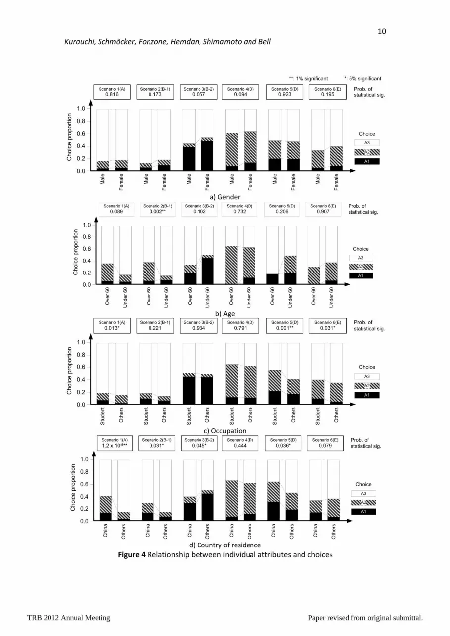
Figure 4 summarises the relation between individual attributes and choices. To understand 267

whether the attribute has a statistical significant effect on the choice we construct chi-square 268

tests with the results reported above the attributes. We remind that the total travel time 269

should be minimum for Alternative A3, and this alternative is the most popular in most of the 270

scenarios. However, in Scenario 4, A2 is more popular than A3. The network used in this 271

scenario is d) in Figure 1, and the travellers must transfer if they use Line 1 which is the line 272

used in alternative A1 and also included in the complex hyperpath A3 . This can be considered 273

as evidence that people dislike transfer. 274

275

Figure 4a suggests female tend to choose the complex hyperpath less often but the difference 276

is not significant for any scenario. Figure 4b suggests that age is more significant though it is 277

not fully clear whether older people indeed dislike the complex strategy A3 as our chi-square 278

test for scenario 2(B-1) suggests. Also whether respondents are students appears to influence 279

the choice. Compared to non-students they appear to take the alternative A2 with low waiting 280

time but longer on-board time more often (Figure 4 c). Finally, looking at 4d, the behaviour of 281

the respondents living in China seems to be slightly different from others (we also test for 282

difference between other countries, but could not find significant differences). Respondents 283

living in China tend to avoid complex alternatives. This might be because the vehicles are often 284

overcrowded and hence they want to avoid transfers. Based on these findings we consider age, 285

occupation and country of residence as independent variables in our subsequent discrete 286

choice analysis. 287 288

Scenario

On

-bo

ard

tim

e

Wai

tin

g ti

me

Tota

l Tra

vel T

ime

Nu

mb

er o

f Tr

ansf

er

On

-bo

ard

tim

e

Wai

tin

g ti

me

Tota

l Tra

vel T

ime

Nu

mb

er o

f Tr

ansf

er

On

-bo

ard

tim

e

Wai

tin

g ti

me

Tota

l Tra

vel T

ime

Nu

mb

er o

f Tr

ansf

er

1 (A) 10 15 25 0 14 5 19 0 13 3.75 16.75 0

2 (B-1) 10 15 25 0 14 10 24 0 12.4 6 18.4 0

3 (B-2) 10 15 25 0 20 10 30 0 16 6 22 0

4 (D) 10 20 30 1 20 6 26 0 16.25 7.5 23.75 0.375

5 (D) 12 16 28 0 16 8 24 1 15.2 6.4 21.6 0.8

6 (E) 10 30 40 1 15 20 35 1 13 18 31 1

Line 1 (A1) Line 2 (A2) Line 1 + Line 2 (A3)



a) Gender

b) Age

c) Occupation

d) Country of residence

Figure 4 Relationship between individual attributes and choices

Ma

le

Fe

ma

le

Ma

le

Fe

ma

le

Ma

le

Fe

ma

le

Ma

le

Fe

ma

le

Ma

le

Fe

ma

le

Ma

le

Fe

ma

le

Scenario 1(A)

0.816Scenario 2(B-1)


0.057Scenario 4(D)

0.094Scenario 5(D)

0.923Scenario 6(E)

0.195

1.0

0.8

0.6

0.4

0.2

0.0

Prob. of

statistical sig.

Ch

oic

e p

rop

ort

ion

A1

A2

A3

Choice

**: 1% significant *: 5% significant

Ove

r 6

0

Un

de

r 6

0

Scenario 1(A)


0.002**Scenario 3(B-2)

0.102Scenario 4(D)

0.732Scenario 5(D)

0.206Scenario 6(E)

0.907

1.0

0.8

0.6

0.4

0.2

0.0

Prob. of

statistical sig.

Ch

oic

e p

rop

ort

ion

A1

A2

A3

Choice

Ove

r 6

0

Un

de

r 6

0

Ove

r 6

0

Un

de

r 6

0

Ove

r 6

0

Un

de

r 6

0

Ove

r 6

0

Un

de

r 6

0

Ove

r 6

0

Un

de

r 6

0

Stu

de

nt

Oth

ers

Stu

de

nt

Oth

ers

Stu

de

nt

Oth

ers

Stu

de

nt

Oth

ers

Stu

de

nt

Oth

ers

Stu

de

nt

Oth

ers

Scenario 1(A)

0.013*Scenario 2(B-1)


0.934Scenario 4(D)

0.791Scenario 5(D)

0.001**Scenario 6(E)

0.031*

1.0

0.8

0.6

0.4

0.2

0.0

Prob. of

statistical sig.

Ch

oic

e p

rop

ort

ion

A1

A2

A3

Choice

Ch

ina

Oth

ers

Ch

ina

Oth

ers

Ch

ina

Oth

ers

Ch

ina

Oth

ers

Ch

ina

Oth

ers

Ch

ina

Oth

ers

Scenario 1(A)

1.2 x 10-5**Scenario 2(B-1)

0.031*Scenario 3(B-2)

0.045*Scenario 4(D)

0.444Scenario 5(D)

0.036*Scenario 6(E)

0.079

1.0

0.8

0.6

0.4

0.2

0.0

Prob. of

statistical sig.

Ch

oic

e p

rop

ort

ion

A1

A2

A3

Choice



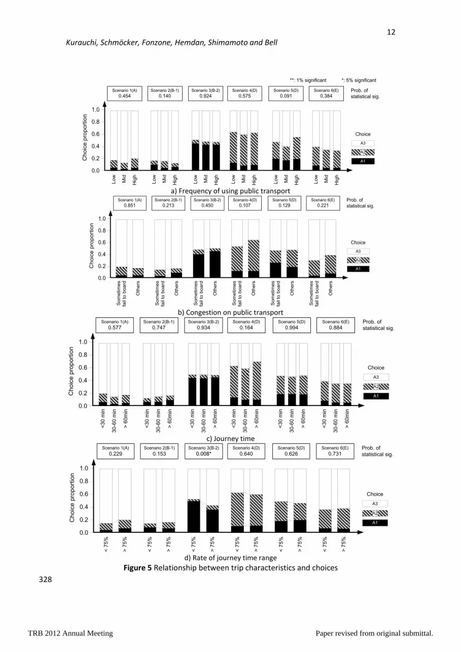
Relation between transit experiences and choices 291

Further to socio-demographics we asked respondents about their transit experiences as we 292 hypothesise that these may also influence their strategy choice. In the survey we asked 293 respondents some general questions about their transit usage frequency as well as some 294 detailed questions “having in mind the most frequent one-way trip you typically make by public 295 transport”. 296

297

We firstly categorised the sample into high, medium and low frequent user groups according 298

to their usage frequency. We hypothesize that frequent users might be more likely to choose 299

the complex strategies even in our hypothetical scenarios. Figure 5a illustrates that this is not 300

the case which suggests that the familiarity of public transport does not influence the choice 301

strategy as much as one might expect. 302

303

It is also reasonable to assume that the usually experienced level of congestion on the service 304

may influence the choice. Those who experience high a level of congestion might avoid 305

transfers in order to avoid that they cannot find a seat, or cannot even get onto the vehicle at 306

very crowded transfers. However, judging from Figure 5b, the above relation cannot be 307

observed clearly. In subsequent analysis, distinguishing four levels of experienced congestion, 308

we do though find some statistically significant differences in choice strategy, so that we 309

consider congestion level to be a factor worth considering in subsequent analysis. 310

311

The relation between the respondent’s average journey time and his/her route choice strategy 312

is illustrated in Figure 5c. Also, here we cannot find any statistically significant relationship. In 313

the survey we ask respondents additionally also about their minimum and maximum 314

experienced journey time. With this information we construct the rate of journey time range 315

as follows: 316

[Rate of journey time range] = [Maximum journey time – Minimum journey time] / [Average 317

journey time]. 318

We find that this measure of journey time uncertainty might have an influence on choice. In 319

particular in Scenario 3 those who experience more variation in journey time are more likely to 320

choose complex strategies (Figure 5d). Based on these findings we consider rate of journey 321

time range as explanatory factors in the discrete choice analysis. 322

323

326 327



a) Frequency of using public transport

b) Congestion on public transport

c) Journey time

d) Rate of journey time range

Figure 5 Relationship between trip characteristics and choices

328

Lo

w

Scenario 1(A)



0.924Scenario 4(D)

0.575Scenario 5(D)

0.091Scenario 6(E)

0.384

1.0

0.8

0.6

0.4

0.2

0.0

Prob. of

statistical sig.

Ch

oic

e p

rop

ort

ion

A1

A2

A3

Choice

**: 1% significant *: 5% significant

Mid

Hig

h

Lo

w

Mid

Hig

h

Lo

w

Mid

Hig

h

Lo

w

Mid

Hig

h

Lo

w

Mid

Hig

h

Lo

w

Mid

Hig

h

So

me

tim

es

fail to

bo

ard

Oth

ers

Oth

ers

Oth

ers

Oth

ers

Oth

ers

Oth

ers

Scenario 1(A)



0.450Scenario 4(D)

0.107Scenario 5(D)

0.129Scenario 6(E)

0.221

1.0

0.8

0.6

0.4

0.2

0.0

Prob. of

statistical sig.

Ch

oic

e p

rop

ort

ion

A1

A2

A3

Choice

So

me

tim

es

fail to

bo

ard

So

me

tim

es

fail to

bo

ard

So

me

tim

es

fail to

bo

ard

So

me

tim

es

fail to

bo

ard

So

me

tim

es

fail to

bo

ard

Scenario 1(A)



0.934Scenario 4(D)

0.164Scenario 5(D)

0.994Scenario 6(E)

0.884

1.0

0.8

0.6

0.4

0.2

0.0

Prob. of

statistical sig.

Ch

oic

e p

rop

ort

ion

A1

A2

A3

Choice

<3

0 m

in

30

-60

min

> 6

0m

in

<3

0 m

in

30

-60

min

> 6

0m

in

<3

0 m

in

30

-60

min

> 6

0m

in

<3

0 m

in

30

-60

min

> 6

0m

in

<3

0 m

in

30

-60

min

> 6

0m

in

<3

0 m

in

30

-60

min

> 6

0m

in

< 7

5%

> 7

5%

Scenario 1(A)



0.008*Scenario 4(D)

0.640Scenario 5(D)

0.626Scenario 6(E)

0.731

1.0

0.8

0.6

0.4

0.2

0.0

Prob. of

statistical sig.

Ch

oic

e p

rop

ort

ion

A1

A2

A3

Choice

< 7

5%

> 7

5%

< 7

5%

> 7

5%

< 7

5%

> 7

5%

< 7

5%

> 7

5%

< 7

5%

> 7

5%



Discrete Choice Modelling 329

330

Utility function 331

In order to control for socio-demographic factors and to distinguish the importance of the 332

different on-board travel time, waiting time and choice complexity we make use of random 333

utility maximisation models. In the following firstly multinominal logit models (MNL) are 334

employed and then cross-nested logit models (CNL) to capture correlation between attributes. 335

As the underlying assumptions and the model formulation of multinominal logit models and 336

nested versions are well published in e.g. (11) and widely applied we describe the models in 337

the following only as far as needed with respect to our specific data set. 338

We assume that each traveller i associates a certain utility with hyperpath j of scenario k, 339

where j might be a simple hyperpath consisting of a single line or a complex hyperpath 340

consisting of several routes. This utility Vijk can be expressed as follows 341

jk

T

igijkV Yβ (4) 342

where Yjk represents a vector of hyperpath specific attributes for alternative j of scenario k, 343

and g(i) represents the group of traveller i. This group is defined by socio-demographic 344

attributes. Note that since the model is estimated based on the data from hypothetical 345

scenarios, there should not be any hidden preference among alternatives. Therefore, we omit 346

the alternative-specific constants. By the same reason, the individual attributes should always 347

relate with hyperpath specific attributes. For example, if age seems to be influential for choice, 348

the parameters such as on-board travel time are prepared respectively for each age group. The 349

set of parameters βg are to be estimated. Based on the findings above, we consider following 350

person specific and path specific attributes: 351

Socio-demographic attributes and personal transit

experiences characterising user group g

Age

Occupation

Country of residence (China)

Rate of journey time range

Usually experienced congestion on public

transport

Hyperpath specific attributes Yjk

On-board travel time

Expected waiting time

Expected number of transfers

352

MNL and CNL model specification 353

The model becomes a random utility model by adding the error ijk to account for unobserved 354

choice factors. 355



ijkijkijk VU (5) 356

Assuming a Gumbel distribution of the error terms and utility maximization following choice 357

hyperpath choice probability Pijk can be derived (see e.g. 11, 12): 358

kCl

ilk

ijk

ijkU

UP

)exp(

)exp(

(6) 359

Where Ck denotes the choice set for scenario k. The choice set is scenario-specific in our case 360

as in our MNL model formulation we treat each choice separately but jointly estimate the 361

parameters. The choice set is not varied according to individuals. 362

In the cross nested logit model (or logit model with overlapping nests) the choice probability 363

takes the form: 364

mmikCCijkijk PPP (7) 365

where Cm denotes the choices in nest m. PikCm denotes the marginal probability of choosing 366

nest m and Pijk|Cm the conditional probability of choosing hyperpath j for scenario k within nest 367

m. Following (11) and (13) the probability of the nests can be estimated as: 368

n Cj

V

jn

Cj

V

jm

ikCn

n

nijk

m

m

mijk

m

e

e

P

/1

/1

(8) 369

m

mijk

mijk

m

Cj

V

jm

V

jm

Cijk

e

eP

/1

/1

(9) 370

where parameters m (in our case m= {1,2}) and αjm are to be fixed a priori or estimated. The 371

m express a measure of the correlation in the utility of the nests and the αjm the degree to 372

which a hyperpath j belongs to nest m. Following constraint on αjm is imposed: 373

121 jj (10) 374

Hyperpath 1 is assumed to be a fixed member of Nest 1 only (α11=1, α12=0) and Hyperpath 2 375

belongs to Nest 2 only (α21=0, α22=1). The degree to which hyperpath 3 belongs to either nest 376

is not fixed so that α3m are to be estimated. 377



For the calibration of the MNL and CNL models we use the BIOGEME software, version 2.0 (14). 378

BIOGEME software can further handle logit models with panel data, and the serial correlation 379

has been considered at the estimation using this feature. 380

Comparison of MNL and CNL without individual attributes 381

First the estimation results by MNL and CNL are compared. To avoid the complex model, we 382

only used hyperpath-specific attributes. Table 2 summarises the result. To justify the 383

importance of considering on-board and waiting time separately, the MNL using only total 384

travel time (=on-board time + waiting time) is also estimated. Comparing the values of 385

adjusted rho square for the MNL using total travel time is 0.188 and the value improves to 386

0.248 just by treating on-board time and waiting time separately, and introducing the number 387

of transfers. Also the model fitness improves by applying CNL. All hyperpath specific variables 388

are found to be influential on the hyperpath choice. The relative weight of waiting time 389

compared with on-board time is 0.870 for MNL, and 0.922 for CNL, though in general the 390

literature suggests that the waiting time value is higher than the on-board time value. In the 391

questions, we described only that ‘(the vehicle) passes every 10minutes on average’, so that 392

respondents could equally presume a regular service arrival which means the waiting time 393

parameter should be doubled as discussed previous section. Looking at the parameters for the 394

CNL model, relative weights of the two nest,1 and 2 are found to be significant and1 is far 395

larger. This may be because we define L1 as the alternative with shorter on-board time, and it 396

is hence always advantageous to include it in the choice set. The relative weight for A3 (L1+L2) 397

is smaller for the first nest. Also judging from the model fitness, CNL gives better results than 398

MNL and we continue using this model in the following section. 399

Table 2 The result of the estimation (MNL vs CNL) 400

401 402

403

MNL (by total travel time) MNL CNL

Number of observations

Number of samples

Likelihood ratio test 1435.394 1894.422 1946.328

Adjusted rho-square 0.188 0.248 0.254

Parameters (t-value)

total travel time -0.279 (-24.57)*

In-vehicle time - -0.361 (-18.15)* -0.232 (-11.52)*

Waiting time - -0.314 (-24.68)* -0.214 (-19.13)*

Number of transfers - -1.44 (-11.43)* -0.636 (-6.83)*

Variance for panel data 0.916(9.99)* 0.904 (8.58)* 0.522 (9.55)*

Parameters for CNL model

Lambda1 - - 5.25 (2.89)*

Lambda2 - - 1.85 (3.83)*

alpha11 - - 1.00 (fixed)

alpha31 - - 0.301 (7.99 (=0), -18.57(=1))*

alpha22 - - 1.00 (fixed)

alpha32 - - 0.699 (18.57(=0), -7.99(=1))*

* statistically significant at 5% level

3462

597



CNL with individual attributes 404

To better understand the relative importance of our person specific explanatory factors we 405

include these in our model. We specify several models and Table 3 summarises the result of 406

the model with the best fit. Regarding age we find that subdividing those over 60 into more 407

groups is not significant, possibly due to our low sample size for this population group. Our 408

results confirm the findings of Figure 4 that people living in China seem to behave differently. 409

They do not seem to care much about the travel time, but dislike transfers. This may be 410

because the public transportation facilities in China are designed without considering 411

transferring enough. Regarding the experience of crowded train, contrary to our expectation, 412

people who sometimes fail to board put higher weight on travel time, waiting time, but lower 413

weight on the number of transfers. One explanation might be that that people who do not 414

care much about transfers have therefore a higher chance of failing to board. An alternative 415

explanation might be that crowding is mostly experienced in large cities where transferring is 416

simpler. We further find that respondents who experience uncertain travel times have higher 417

on-board and weighting time values but value the number of transfers comparatively less. This 418

is according to our expectations as these passengers might “become easier nervous” if waiting 419

times and on-board travel times are longer. 420

421

Looking at the model fitness, the value of adjusted rho square are 0.273. Comparing this to the 422

result of CNL without individual attributes, the value improved around 0.02. The estimates for 423

the CNL model are all statistically significant, which justifies the CNL model structure. 424

425 Table 3 The result of the estimation (CNL with individual attributes) 426

427 428

429

Age 60+

Country of residence China

Crowded train

Rate of travel time range <75% >75%

Occupation All Student others Student others All

82 230 275 78 68 949 1109 521

14 39 47 13 13 164 190 90

Travel Time-0.100

(-1.78)

-0.154

(-4.71)**

-0.395

(-8.84)**

-0.069

(-1.34)

-0.518

(-5.05)**

-0.302

(-12.64)**

-0.319

(-12.64)**

-0.336

(-10.56)**

Waiting Time-0.214

(-5.92)**

-0.183

(-9.40)**

-0.282

(-10.80)**

-0.142

(-4.86)**

-0.382

(-6.26)**

-0.212

(-15.25)**

-0.254

(-15.11)**

-0.258

(-12.99)**

Number of Transfers-0.447

(-0.79)

-1.190

(-3.99)**

-0.582

(-2.24)*

-0.195

(-0.41)

-0.476

(-0.78)

-0.946

(-5.97)**

-0.987

(-5.88)**

-0.821

(-4.00)**

Lambda1

Lambda2

alpha11

alpha31

alpha22

alpha32

Num. of Samples

*: 5% significant, **: 1% significant

<75%

60-

All

Others

All

Sometimes fail to board others

>75%

0.273Adjusted rho-square

Estimated

parameters for

each user category

User categories

Num. of Observations

1.00(fixed)

0.490(7.07(=0), -7.37(=1))**

3312

570

2045.925

0.672(9.87)**

2.80(6.74)**

1.58(7.76)**

1.00(fixed)

0.510(7.37(=0), -7.07(=1))**

Estimated Variance for panel data

Estimated

Parameters for

CNL model

Number of observations

Number of samples

Likelihood ratio test



Conclusions 430

In this study, we estimated the values of time in transit hyperpath choice using the data 431

obtained by web-based survey. The values of in-vehicle time, waiting time and the penalty for 432

the transfer are estimated. As a result, the structure of the cross-nested logit model is found to 433

be statistically significant, and the parameters obtained by the CNL are different from the ones 434

by the MNL. We further evaluated the importance of individual attributes and found that these 435

indeed to some degree explain an individual’s choice strategy. Among others we find that 436

people living in China dislike transferring in general. Students are, in general less concerned 437

with waiting time. Also age and transit experiences seem to influence choice but some of our 438

findings should be reconsidered with sample sizes that include less biased samples and 439

possibly some more detailed questions on transit experiences. 440

We believe that our findings are of interest to transit operators and planners. Also one 441

application for our findings will be their inclusion in “multi-class transit assignment” to 442

understand in how far network results are sensitive to user group specific time values. 443

In future studies, we aim to not only collect more responses from a wider spread sample. In 444

the survey, we also did not vary the values of the SP question for different respondents. Also 445

our modelling approach might be refined. For example one would expect that the membership 446

to the nests is governed by the expected frequency of the two elementary paths that make up 447

the hyperpath. This would mean that the parameter should be estimated as a function of 448

the line frequencies. 449

References 450

(1) Lampkin, W. and P. D. Saalmans (1967). The Design of Routes; Service Frequencies and 451

Schedules of a Municipal Bus Undertaking: A Case Study, Operational Research Quarterly, 452

18(4), 375-397. 453

(2) Chiriqui, C. and Robilland, P. (1975) Common Bus Lines, Transportation Science, 9, 115-121. 454

(3) Spiess, H and Florian, M. (1989). Optimal Strategies: A new assignment model for transit 455

networks. Transportation Research B, 23 (2), 83-102. 456

(4) Nguyen, S. and Pallotino, S. (1988) Equilibrium Traffic Assignment for Large Scale Transit 457

Networks, European Journal for Operatinal Research, 37, 176-186. 458

(5) Gentile, G., S. Nguyen, and S. Pallottino (2005) Route choice on transit networks with online 459

information at stops. Transportation science, Vol. 39, No. 2, p. 289-297. 460

(6) Nökel, K. and S. Wekeck (2009). Boarding and alighting in frequency-based transit 461

assignment. Paper presented at 88th Annual Transportation Research Board Meeting, 462

Washington D.C., January 2009. 463



(7) Fonzone A. and Bell, M. G. H. (2010). Bounded rationality in hyperpath transit assignment: 464

The locally rational traveller model. 89th Annual TRB Meeting, Washington, DC, USA. 465

(8) Wardman M. (2004). Public transport values of time, Transport Policy, 11, 363-377. 466

(9) Kurauchi F., Hirai, M. and Iida, Y. (2004). Experimental Analysis on Mode Choice Behaviour 467

for Merged Public Transport System, Proceedings of Infrastructure Planning, Vol. 30, CD-ROM 468

(in Japanese). 469

(10) Fonzone, A., Schmöcker, J-D., Bell, M.G.H., Gentile, G., Kurauchi, F., Nökel, K. And Wilson, 470

N.H.M. (2010). Do Hyper-Travellers Exist? Initial Results of an International Survey on Public 471

Transport User Behaviour. Presented at the 12th World Conference on Transport Research, 472

Lisbon, Portugal, 11-15 July 2010. 473

(11) Train, K.E. (2003) Discrete Choice Methods with Simulation. Cambridge University Press. 474

(12) Ben-Akiva, M. and Lerman, S.R. (1985). Discrete Choice Analysis: Theory and Applications 475

to Travel Demand. MIT Press, London, England. 476

(13) Ben-Akiva, M. and Bierlaire, M. (1999). Discrete Choice Methods and their applications to 477

short Term Travel Decisions. Chapter 2 in Hall, R. (Ed.), The Handbook of Transportation 478

Science. Kluwer, Dordrecht, The Netherlands. 479

(14) Bierlaire, M. (2003). BIOGEME: A free package for the estimation of discrete choice 480

models, Tutorial. Available online. 481


Documents

Estimating Weights of Times and Transfers for Hyperpath Travelers