Embed Size (px)
Citation preview

Estimating the Total Fertility Rate from MultipleImperfect Data Sources and Assessing its Uncertainty
Leontine Alkema, Adrian E. Raftery,Patrick Gerland, Samuel J. Clark, Francois Pelletier 1
Working Paper no. 89Center for Statistics and the Social Sciences
University of Washington
November 21, 2008
1Leontine Alkema, Earth Institute and Statistics Department, Columbia University, New York,NY 10027; Email: [email protected]. Adrian E. Raftery, Departments of Statistics and Sociol-ogy, University of Washington, Seattle, WA 98195-4320; Email: [email protected]. PatrickGerland, Population Estimates and Projections Section, United Nations Population Division, NewYork, NY 10017; Email:[email protected]. Samuel J. Clark, Department of Sociology, University ofWashington, Seattle, WA 98195-3340; Email: [email protected]. Francois Pelletier, Mor-tality Section, United Nations Population Division, New York, NY 10017; Email: [email protected] research was partially supported by Grant Number 1 R01 HD054511 01 A1 from the NationalInstitute of Child Health and Human Development. Its contents are solely the responsibility ofthe authors and do not necessarily represent the official views of the National Institute of ChildHealth and Human Development or those of the United Nations. Its contents have not been for-mally edited and cleared by the United Nations. This research was also partially supported bya seed grant from the Center for Statistics and the Social Sciences, by a Shanahan Fellowship atthe Center for Studies in Demography and Ecology and by the Blumstein-Jordan professorship, allat the University of Washington. The authors are grateful to Thomas Buettner, Gerhard Heiligand Taeke Gjaltema for helpful discussions and insightful comments. Alkema thanks the UnitedNations Population Division for hospitality.

Abstract
We develop a new methodology for estimating and assessing the uncertainty of the totalfertility rate over time. The estimates are based on multiple imperfect estimates from dif-ferent data sources, including surveys and censuses, and different methods, both direct andindirect. We take account of measurement error by decomposing it into two sources: biasand variance. We estimate both bias and variance by linear regression on data quality covari-ates. We estimate the total fertility rate using a local smoother, and we assess uncertaintyusing the weighted likelihood bootstrap. Based on a data set for seven countries in west-ern Africa, we found that retrospective surveys with a recall period of more than five yearstended to overestimate the total fertility rate, while direct estimates and older observationsunderestimated fertility. The measurement error variance was larger for observations with aone-year time span, for observations that were collected before the mid 1990s, and for oneDemographic Health Survey (in Mauritania in 1990). Cross-validation showed that takingdifferences in data quality between observations into account gave better calibrated confi-dence intervals and reduced bias: on average the width of confidence intervals was reducedby about 40%.
KEY WORDS: Bayesian Inference, Demographic and Health Survey, Local smoother, Ret-rospective surveys, United Nations, Variable selection, Weighted LikelihoodBootstrap.

1 Introduction
Estimating demographic indicators is challenging for many developing countries because oflimited data and varying data quality. Most of the literature on quality of fertility datahas focused on the development of indirect estimation methods (Brass 1964; Brass et al.1968; Trussell 1975; United Nations 1983; Brass 1996; Feeney 1998). These techniquesdeal with biases that are caused by recall lapse errors in retrospective estimates of fertilityrates (Som 1973; Potter 1977; Becker and Mahmud 1984; Pullum and Stokes 1997). Theindirect estimation methods correct for reporting biases by reconciling information fromrecent fertility (in the last year or years) with lifetime fertility. They are typically basedon one data source, and underlying assumptions can lead to problems with respect to theaccuracy of the indirect estimates (Moultrie and Dorrington 2008). These methods deal withbias only, and not with differences in the variance of the measurement error. There are nomethods for estimating fertility rates in developing countries over time based on differentdata sources that assess the uncertainty of the estimates.
Methods have been developed for estimating child mortality rates for countries with lim-ited data and varying data quality. Murray et al. (2007) used a local regression model toestimate child mortality for all the countries in the world. In their approach data quality wastaken into account by excluding extreme outliers from the data set and allowing for biasesin observations from vital registration systems. They assessed model uncertainty by varyingthe smoothing parameter of the local regression. This approach does not allow for biasesin observations from other sources, nor does it take differences in measurement errors be-tween observations into account. Varying the smoothing parameter does not provide formalstatistical confidence bounds for the estimates (Silverwood and Cousens 2007). Hill et al.(1998) and the Interagency Group for Child Mortality Estimation (UNICEF, WHO, WorldBank and UNPD, 2007) fitted piecewise linear splines to log-transformed child mortalityrates. In their approach, data quality is taken into account by assigning a weight to eachobservation, which depends on its data quality covariates (e.g. data collection process) andexpert judgement. This approach does not adjust for biases in the different data sources.
In this paper we introduce a new methodology for estimating the total fertility rate(TFR) over time and assessing its uncertainty for countries with limited data from multiplesources with varying data quality. We first estimate average biases and measurement errorvariance for subsets of TFR estimates with the same set of data quality covariates by linearregression, based on what has been observed in different countries in the same region. Wethen adjust the TFR estimates by subtracting the estimated biases, and assign weights basedon the estimated measurement error variances. Next we estimate the TFR trajectories byapplying a weighted local smoother to the bias-adjusted TFR estimates. Finally, we use theweighted likelihood bootstrap to derive statistical confidence intervals for our estimates.
Assessing the accuracy of an estimation method, including its uncertainty assessment,is important to validate whether modeling assumptions hold, but it is often not done. Wedescribe model calibration criteria to assess the accuracy of our methods.
We apply our methodology to data from seven countries in western Africa. Some ofthese countries have been experiencing some of the highest fertility rates in the world inrecent years. We first describe the data, and then we describe how to analyze bias andmeasurement error variance for different data sources, estimate the TFR over time, carry out
1
the uncertainty assessment and validate the model. We present the results of the modelingapproach for the TFR in the seven countries in western Africa and compare the results ofour method, that takes data quality into account, to the results of a similar method thattreats all observations equally.
2 DATA
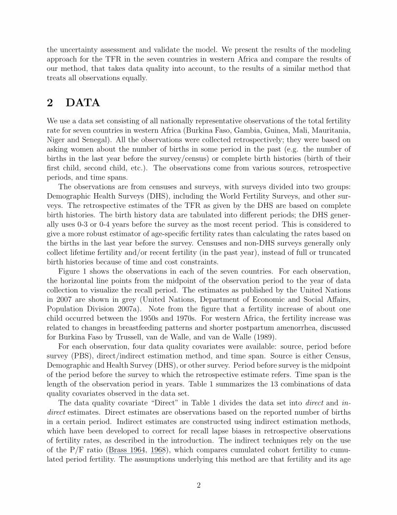
We use a data set consisting of all nationally representative observations of the total fertilityrate for seven countries in western Africa (Burkina Faso, Gambia, Guinea, Mali, Mauritania,Niger and Senegal). All the observations were collected retrospectively; they were based onasking women about the number of births in some period in the past (e.g. the number ofbirths in the last year before the survey/census) or complete birth histories (birth of theirfirst child, second child, etc.). The observations come from various sources, retrospectiveperiods, and time spans.
The observations are from censuses and surveys, with surveys divided into two groups:Demographic Health Surveys (DHS), including the World Fertility Surveys, and other sur-veys. The retrospective estimates of the TFR as given by the DHS are based on completebirth histories. The birth history data are tabulated into different periods; the DHS gener-ally uses 0-3 or 0-4 years before the survey as the most recent period. This is considered togive a more robust estimator of age-specific fertility rates than calculating the rates based onthe births in the last year before the survey. Censuses and non-DHS surveys generally onlycollect lifetime fertility and/or recent fertility (in the past year), instead of full or truncatedbirth histories because of time and cost constraints.
Figure 1 shows the observations in each of the seven countries. For each observation,the horizontal line points from the midpoint of the observation period to the year of datacollection to visualize the recall period. The estimates as published by the United Nationsin 2007 are shown in grey (United Nations, Department of Economic and Social Affairs,Population Division 2007a). Note from the figure that a fertility increase of about onechild occurred between the 1950s and 1970s. For western Africa, the fertility increase wasrelated to changes in breastfeeding patterns and shorter postpartum amenorrhea, discussedfor Burkina Faso by Trussell, van de Walle, and van de Walle (1989).
For each observation, four data quality covariates were available: source, period beforesurvey (PBS), direct/indirect estimation method, and time span. Source is either Census,Demographic and Health Survey (DHS), or other survey. Period before survey is the midpointof the period before the survey to which the retrospective estimate refers. Time span is thelength of the observation period in years. Table 1 summarizes the 13 combinations of dataquality covariates observed in the data set.
The data quality covariate “Direct” in Table 1 divides the data set into direct and in-direct estimates. Direct estimates are observations based on the reported number of birthsin a certain period. Indirect estimates are constructed using indirect estimation methods,which have been developed to correct for recall lapse biases in retrospective observationsof fertility rates, as described in the introduction. The indirect techniques rely on the useof the P/F ratio (Brass 1964, 1968), which compares cumulated cohort fertility to cumu-lated period fertility. The assumptions underlying this method are that fertility and its age
2
●
●
●
●
●
●
●
●
●●●
●●
●●
●●●●
●
●
●●
●●
●
1950 1970 1990
45
67
89
Burkina Faso
Year
TF
R
●●●●●●●●●●●●●●●●●●●●●●●●●●●●●●●●●●●●●●●●●●●●●●●●●●●●
●
●
●
●
●
●
●
●
●
●●
●●
●●
●●●●
●
●
●●
●●
●
●● ●
●
●
●
●
●
●
●
1950 1970 19904
56
78
9
Gambia
Year
TF
R
●●●●●●●●●●●●●●●●●●●●●●●●●●●●●●●●●●●●●●●●●●●●●●●●●●●●●●●
● ●
●
●
●
●
●
●
●
● ●●●
●
●●
●
●
●●
●●●
●
●●
●●●
●
1950 1970 1990
45
67
89
Guinea
Year
TF
R ●●●●●●●●●●●●●●●●●●●●●●●●●●●●●●●●●●●●●●●●●●●●●●●●●●●●●●●● ●●●
●
●●
●
●
●
●
●●●
●
●●
●
●●
●
●
●
●●
●
●●
●
●
●●
●●● ●
●
●●
●
●
● ● ●
1950 1970 1990
45
67
89
Mali
Year
TF
R ●●●●●●●●●●●●●●●●●●●●●●●●●●●●●●●●●●●●●●●●●●●●●●●●●●●●
●
●
●●
●
●
●
●
●
●
●●
● ●●
●●
●
●
● ●●
●●
●
●
●
●
●
●●
●
●
●●●
●
●
●
●
●
●
●
●
●●●
●
1950 1970 1990
45
67
89
Mauritania
Year
TF
R
●●●●●●●●●●●●●●●●●●●●●●●●●●●●●●●●●●●●●●●●●●●●●●●●●●●●
●
●
●
●
●
●
●
●●
●
●
●●●
●
●
●
●
●
●
●
●
●
●●
●
●●
●●
●●
●●
●●
●●
●●
●● ●
●●
●
●
1950 1970 1990
45
67
89
Niger
Year
TF
R
●●●●●●●●●●●●●●●●●●●●●●●●●●●●●●●●●●●●●●●●●●●●●●●●●●●●●●●●
●
●
●
●
●
●●
●
●
●●
●
●
●●●
●●
●
●
●
●
●●
●●
●
●●
●●●
●
● ●●
●
●●
●
●●
●
●●
●
●
●
●●
●
●●
●
●●
●
1950 1970 1990
45
67
89
Senegal
Year
TF
R
●●●●●●●●●●●●●●●●●●●●●●●●●●●●●●●●●●●●●●●●●●●●●●●●●●●●●●●●
●
●
●
●●
●
●●
●●
●
●
● ●●
●
●●
●
●●
●
●●
●
●
●
●●
●
●●
●
●
●
●
Legend
●
●
Direct observationIndirect observationRecall periodUN estimates
Figure 1: Direct observations (dot) and indirect observations (cross) for different datasources. The black horizontal line extends from the midpoint of the observation periodto the year of data collection. The UN estimates are plotted as grey circles.
3

Table 1: Summary of fertility data set for seven countries in western Africa. The numberof observations for each observed combination of the data quality covariates: Source, PeriodBefore Survey (PBS — based on the midpoint of the period before the survey to which theretrospective estimate refers), Direct (specifying whether the observation is a direct or anindirect estimate), and Time Span (the number of years that the observation refers to).
Combination Source PBS Direct Time span # Obs.
1 Census 0-1 Year No 1 Year 182 Census 0-1 Year Yes 1 Year 203 Survey 0-1 Year No 1 Year 124 Survey 0-1 Year Yes 1 Year 125 Survey 1-5 Years No 3 Years 16 DHS 1-5 Years No 3 Years 157 DHS 1-5 Years No 4-5 Years 78 DHS 1-5 Years Yes 3 Years 139 DHS 1-5 Years Yes 4-5 Years 2310 DHS 1-5 Years Yes 5+ Years 111 DHS 5-10 Years Yes 4-5 Years 2312 DHS 5-10 Years Yes 5+ Years 2213 DHS 10+ Years Yes 4-5 Years 50
distribution are constant over time, and that the fertility of non-surviving women is equalto the fertility of surviving women (whose number of children is reported). Under theseassumptions cohort and period fertility are equal, and deviations from equality are used toadjust the observed fertility rates. Several variations of the P/F ratio are used to relax theseassumptions (Trussell 1975; United Nations 1983; Feeney 1998). However, because of theproblems with the indirect estimation techniques (Moultrie and Dorrington 2008), indirectestimates can be biased too. Therefore direct estimates are included in the data set as wellas indirect ones.
3 METHODS
We now describe our methodology, which consists of four steps. First, the bias for each TFRobservation is estimated by regression on the data quality covariates, and subtracted fromthe observation. Then the measurement error variance is estimated, also by regression ondata quality covariates. Next, the TFR trajectory for each country is estimated by weightedlocal smoothing of the bias adjusted observations, the weights being the reciprocals of theestimated measurement error variances. Finally, we assess the uncertainty of our TFRestimates using the weighted likelihood bootstrap.
4

3.1 Modeling data quality
Some observations of the TFR are better than others, depending on the quality of theunderlying data. We decompose data quality into two components: bias and measurementerror variance. Bias refers to systematic over- or underestimation of the TFR, due, forexample, to the observation being based on an unrepresentative sample of the populationbecause of missing data or selection bias. Measurement errors occur randomly during thedata collection process, and include sampling and non-sampling errors. Sampling errorsoccur if the observation is based on a subset of the population. Non-sampling errors areerrors that are made during the data collection and input. Unlike sampling errors, non-sampling errors have many different sources and are often hard to detect and control. Formany estimates of fertility rates, non-sampling errors are bigger (United Nations 1982).
Previous work on the quality of demographic estimates has usually not distinguishedbetween bias and variance, and we emphasize the importance of doing so because these aredistinct and can point in different directions. For example, some observations can have largebiases but small measurement errors, while others are unbiased but less precise. Therefore itis important to account for bias and variance separately. We deal with bias by adjusting theobservations, and with variance by weighting them. For example, a biased observation withsmall measurement error variance is adjusted and then assigned a high weight. An unbiasedobservation with large measurement error variance is not adjusted but gets assigned a lowweight.
Our probability model for observation ycts (in year t = 1, . . . , Tc for observation s =1, . . . , nct) is
ycts|fct ∼ N(fct + δcts, σ2cts) (t = 1, . . . , Tc; s = 1, . . . , nct),
where ycts is the s-th estimate of the TFR for country c in year t, fct is the unobserved trueTFR in year t for country c, δcts is the bias of observation ycts, and σ2
cts is the observation-specific error variance. We use data quality covariates to assess the bias and error variance ofeach TFR estimate, extending the work by Hill et al. (1998) and the Interagency group forchild mortality estimation (UNICEF, WHO, World Bank and UNPD, 2007) on differencesin error variance in child mortality rates, and the work of Gerland (2007) on examining theassociations between data quality covariates and the data quality of mortality and fertilityrate estimates. In our approach, we use linear regression to estimate how bias and errorvariance depend on the data quality covariates, and we combine the observations from theseven countries in western Africa to estimate both.
Estimating bias
Bias is estimated as a function of the data quality covariates, using linear regression. Theadvantage of this approach, as compared to indirect estimation methods, is that no assump-tions are made about the age structure of the fertility rates or the trends in fertility over time.Multiple data sources are modeled and adjusted simultaneously, and biases are estimatedbased on what has been observed in the seven countries in western Africa.
To examine the association between bias and the data quality covariates, unbiased esti-mates of the TFR are needed. By saying an estimate is unbiased, we do not mean that it is
5
correct or even necessarily of high quality; we mean that it does not substantially over- orunderestimate the TFR. Here, we assume that the estimates of the TFR published by theUnited Nations Population Division (United Nations, Department of Economic and SocialAffairs, Population Division 2007b), are unbiased, so that E[uct] = fct, where uct denotes theUN estimate for country c, year t. We take the published UN estimates as the least biasedavailable because they are based on the UN analysts’ expert knowledge of the shortcomingsof the multiple data sources used, as well as information on mortality, population counts andmigration to ensure internal consistency of intercensal birth cohorts.
With the UN estimates taken as unbiased estimates of the TFR, the bias δcts of observa-tion ycts is the expected value of the difference dcts = ycts − uct between the observation andthe UN estimate, so that E[dcts] = δcts. We estimate the biases δcts by regressing dcts on thedata quality covariates using the model
E[dcts] = xctsβ,
where the row xcts of the design matrix X contains the data quality covariates. Thus thebiases δcts can be estimated from the relationship δcts = xctsβ.
The next question is which predictors to include in the bias regression model. There arefour data quality covariates, and each of these is a categorical variable that can take severalvalues. We code these as dummy variables and consider the possibility of including or exclud-ing each of them. Dummy variables for the individual DHS surveys (each of which generatesmultiple observations), as well as the observation year, year of data collection and the level ofthe TFR (as given by the UN estimates) are also candidates to put into the model. To selectthe best model we use Bayesian model selection (Raftery 1995). Specifically we consider allpossible subsets of predictors and choose the one with the best value of BIC. This is doneusing the bicreg function from the BMA package in the statistical language R (Raftery,Painter, and Volinsky 2005), available at http://cran.r-project.org/web/packages/BMA.
The estimated biases δcts are then subtracted from the observation to get the bias-adjustedobservations
zcts = ycts − δcts∼ N(fct, ρ
2cts), (1)
where ρ2cts is the observation-specific error variance of the bias-adjusted observation.
Estimating measurement error variance
A similar approach is used for estimating the measurement error variances, specifically thevalues of ρ2
cts in Eq. (1). We assume that the absolute differences between the UN estimatesand the bias-adjusted observations, zcts, are proportional to the absolute differences betweenbias-adjusted observations and the true TFR, so that
E|zcts − uct| ∝ E|zcts − fct|.
It follows from Eq. (1) that E|zcts − fct| =√
2πρcts, and so
E|zcts − uct| ∝ ρcts.
6
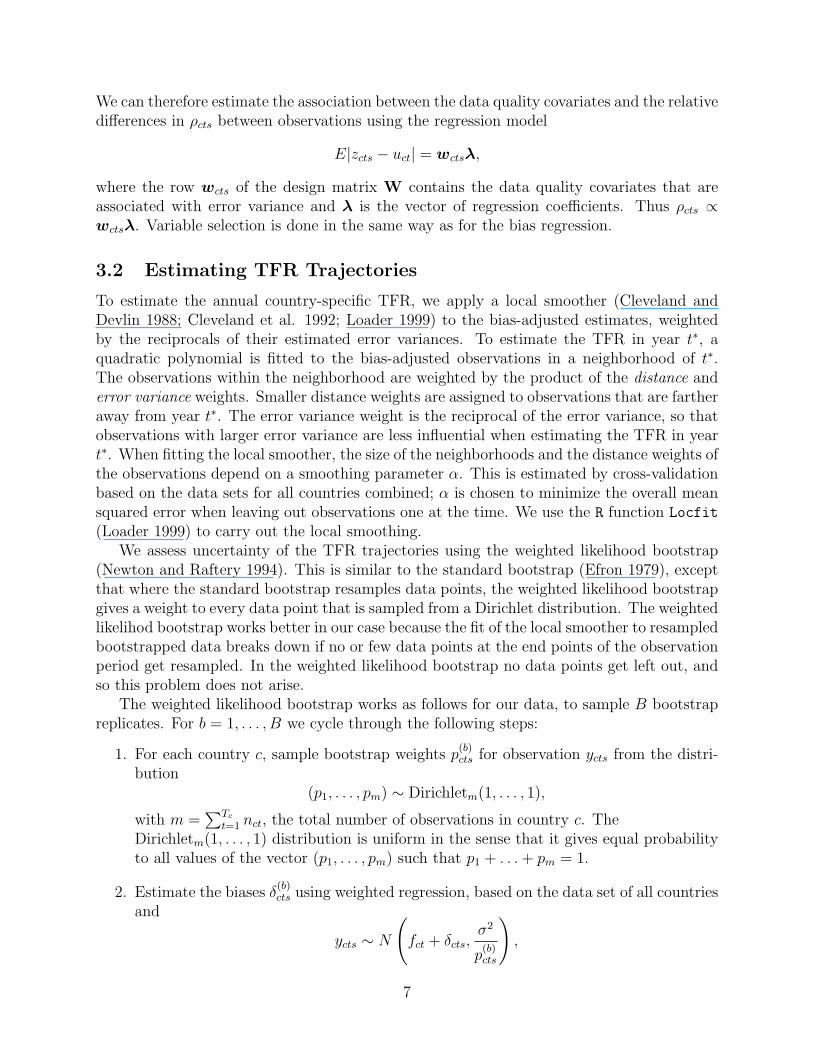
We can therefore estimate the association between the data quality covariates and the relativedifferences in ρcts between observations using the regression model
E|zcts − uct| = wctsλ,
where the row wcts of the design matrix W contains the data quality covariates that areassociated with error variance and λ is the vector of regression coefficients. Thus ρcts ∝wctsλ. Variable selection is done in the same way as for the bias regression.
3.2 Estimating TFR Trajectories
To estimate the annual country-specific TFR, we apply a local smoother (Cleveland andDevlin 1988; Cleveland et al. 1992; Loader 1999) to the bias-adjusted estimates, weightedby the reciprocals of their estimated error variances. To estimate the TFR in year t∗, aquadratic polynomial is fitted to the bias-adjusted observations in a neighborhood of t∗.The observations within the neighborhood are weighted by the product of the distance anderror variance weights. Smaller distance weights are assigned to observations that are fartheraway from year t∗. The error variance weight is the reciprocal of the error variance, so thatobservations with larger error variance are less influential when estimating the TFR in yeart∗. When fitting the local smoother, the size of the neighborhoods and the distance weights ofthe observations depend on a smoothing parameter α. This is estimated by cross-validationbased on the data sets for all countries combined; α is chosen to minimize the overall meansquared error when leaving out observations one at the time. We use the R function Locfit
(Loader 1999) to carry out the local smoothing.We assess uncertainty of the TFR trajectories using the weighted likelihood bootstrap
(Newton and Raftery 1994). This is similar to the standard bootstrap (Efron 1979), exceptthat where the standard bootstrap resamples data points, the weighted likelihood bootstrapgives a weight to every data point that is sampled from a Dirichlet distribution. The weightedlikelihod bootstrap works better in our case because the fit of the local smoother to resampledbootstrapped data breaks down if no or few data points at the end points of the observationperiod get resampled. In the weighted likelihood bootstrap no data points get left out, andso this problem does not arise.
The weighted likelihood bootstrap works as follows for our data, to sample B bootstrapreplicates. For b = 1, . . . , B we cycle through the following steps:
1. For each country c, sample bootstrap weights p(b)cts for observation ycts from the distri-
bution(p1, . . . , pm) ∼ Dirichletm(1, . . . , 1),
with m =∑Tc
t=1 nct, the total number of observations in country c. TheDirichletm(1, . . . , 1) distribution is uniform in the sense that it gives equal probabilityto all values of the vector (p1, . . . , pm) such that p1 + . . .+ pm = 1.
2. Estimate the biases δ(b)cts using weighted regression, based on the data set of all countries
and
ycts ∼ N
(fct + δcts,
σ2
p(b)cts
),
7
where σ2 is the error variance for all observations combined. The bias-adjusted obser-vations are given by z
(b)cts = ycts − δ(b)
cts.
3. Estimate the differences in error variance ρ(b)cts using weighted regression, based on the
data set of all countries and
z(b)cts ∼ N
(fct,
ρ2(b)cts
p(b)cts
).
4. Estimate the TFR by fitting the local smoother to the bias-adjusted observations z(b)cts,
taking into account the differences in error variance ρ(b)cts and the bootstrap weights
p(b)cts. The distance weights and the local neighborhoods in the local smoother vary
by bootstrap replicate too, because the smoothing parameter α is re-estimated withineach bootstrap replicate.
3.3 Model validation
We validate the method by cross-validation, in which some observations are left out, whilethe method is applied to the remaining observations (called the “training data set”). Wethen assess how well the resulting predictive distributions agree with what actually happened(the left-out observations). More precisely, we assess whether the predictive distributionsare calibrated, meaning that the prediction intervals contain the truth the right proportionof the time. We use the following measures of calibration: (a) the proportion of left-outobservations that fall outside their confidence intervals, (b) the average bias of the estimatedTFR compared to the left-out observation, (c) the standardized absolute prediction error,and (d) the probability integral transform histogram of the left-out observations.
The confidence intervals for the left-out observations ycts are based on
ycts ∼ N(fct + δcts, ν2cts). (2)
In Eq. (2), fct is the median TFR, δcts is the estimated bias, and ν2cts is the estimated
total variance, all estimated from the training data set and the data quality covariates ofobservation ycts. The predictive variance of the observations is
ν2cts = Var(fct) + ρ2
cts,
where the variance of the TFR Var(fct) and the observation-specific error variance ρ2cts are
estimated from the training data set.The bias in the set of left-out observations, with respect to the estimated TFR, is esti-
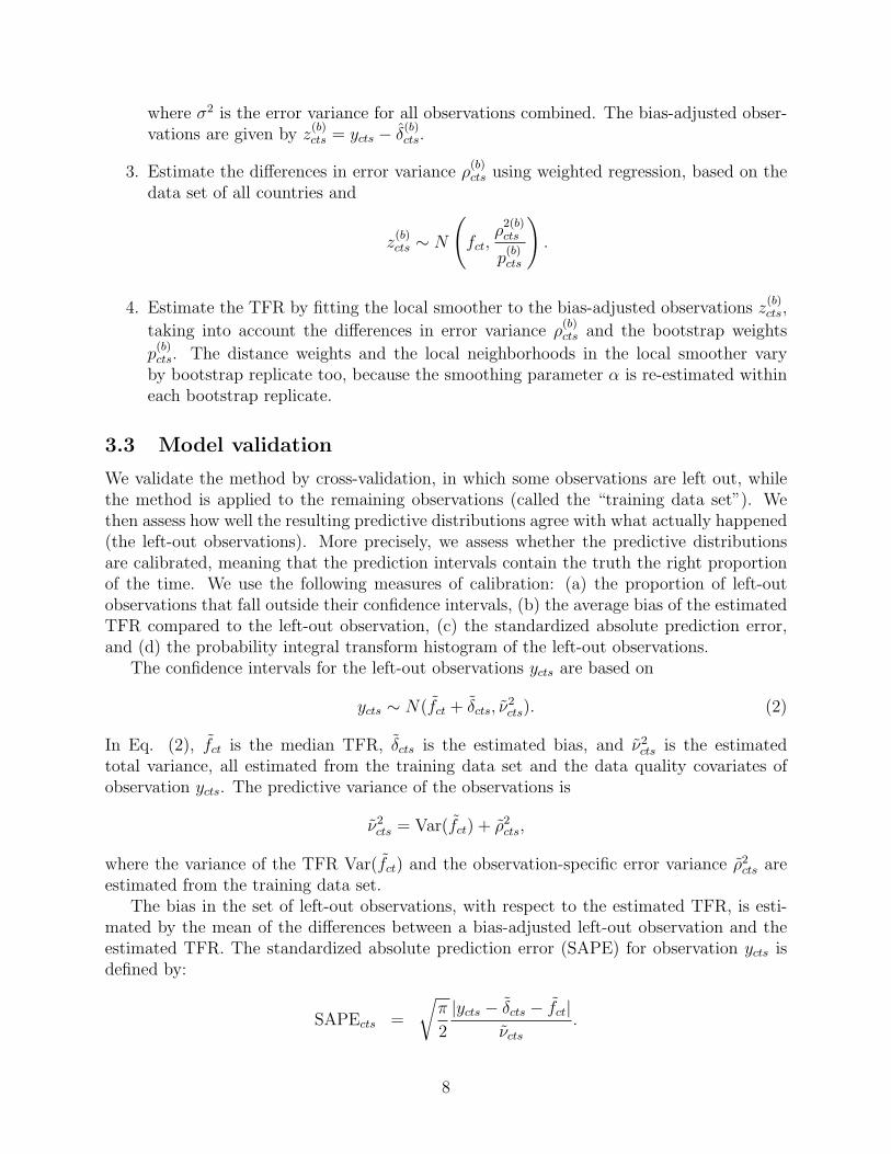
mated by the mean of the differences between a bias-adjusted left-out observation and theestimated TFR. The standardized absolute prediction error (SAPE) for observation ycts isdefined by:
SAPEcts =
√π
2
|ycts − δcts − fct|νcts
.
8
If our modeling assumptions hold, the mean SAPE is around 1, because E|ycts− δcts− fct| =√2/πνcts. A larger value of the mean SAPE indicates that the left-out observations are more
spread out than expected, while a smaller value says they are less so.Our last calibration criterion is the probability integral transform (PIT) histogram. The
probability integral transform for the left-out observation ycts is
PITcts = Φ
(ycts − δcts − fct
νcts
),
where Φ(·) is the cumulative distribution function of the standard normal distribution. FromEq. (2) it follows that the PIT values should be approximately uniformly distributed between0 and 1 if our model is valid. Calibration is compared between models by comparing thehistograms of the PIT values of the left-out observations. For a histogram with H bars, eachbar with width 1/H should contain about a proportion 1/H of the PIT values and thus haveheight 1. The summary criterion for model comparison in terms of PIT values is given bythe area of the PIT histogram that is located above one, as this represents the deviationfrom uniformity of the PIT values (Berrocal et al. 2007). We call this the “PIT area”. Ifthe TFR estimates are unbiased, a smaller value of the PIT area means a better calibratedmodel.
For more complete details of our methodology, see Alkema (2008).
4 RESULTS
4.1 Bias regression
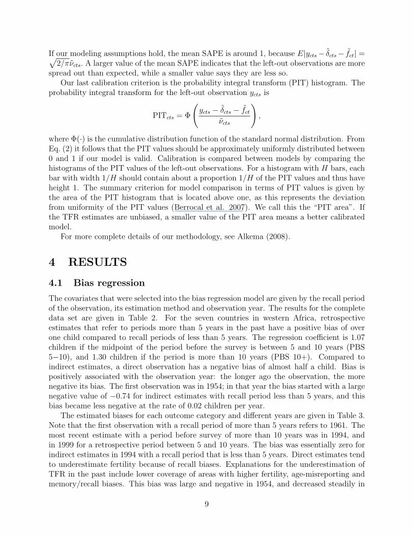
The covariates that were selected into the bias regression model are given by the recall periodof the observation, its estimation method and observation year. The results for the completedata set are given in Table 2. For the seven countries in western Africa, retrospectiveestimates that refer to periods more than 5 years in the past have a positive bias of overone child compared to recall periods of less than 5 years. The regression coefficient is 1.07children if the midpoint of the period before the survey is between 5 and 10 years (PBS5−10), and 1.30 children if the period is more than 10 years (PBS 10+). Compared toindirect estimates, a direct observation has a negative bias of almost half a child. Bias ispositively associated with the observation year: the longer ago the observation, the morenegative its bias. The first observation was in 1954; in that year the bias started with a largenegative value of −0.74 for indirect estimates with recall period less than 5 years, and thisbias became less negative at the rate of 0.02 children per year.
The estimated biases for each outcome category and different years are given in Table 3.Note that the first observation with a recall period of more than 5 years refers to 1961. Themost recent estimate with a period before survey of more than 10 years was in 1994, andin 1999 for a retrospective period between 5 and 10 years. The bias was essentially zero forindirect estimates in 1994 with a recall period that is less than 5 years. Direct estimates tendto underestimate fertility because of recall biases. Explanations for the underestimation ofTFR in the past include lower coverage of areas with higher fertility, age-misreporting andmemory/recall biases. This bias was large and negative in 1954, and decreased steadily in
9
Table 2: Results of bias regression model.
Coefficient Std. Error t-value
Intercept −0.74 0.11 −6.5PBS 5 - 10 Years 1.07 0.10 11.0PBS 10+ Years 1.30 0.10 13.4Direct −0.45 0.09 −4.9Year - 1954 0.02 0.003 6.3
Table 3: Estimated biases for different observation years and outcome categories.
Obs. year Direct PBS< 5 Years 5 - 10 Years 10+ Years
1954 Yes −1.19No −0.74
1961 Yes −1.06 0.01 0.24No −0.61
1970 Yes −0.89 0.18 0.40No −0.44
1980 Yes −0.70 0.37 0.59No −0.25
1994 Yes −0.44 0.63 0.85No 0.01
1999 Yes −0.35 0.73No 0.11
2004 Yes −0.25No 0.20
absolute value, at the rate of 0.02 children per year. Biases also increase with the recallperiod of the observation, illustrated when reading the table from left to right. Observationswith a recall period that is less than 5 years tend to have a slightly negative bias, whileobservations with longer recall periods have a positive bias.
The positive bias of observations with longer recall periods is not surprising in lightof Figure 1, where almost all observations with long recall periods (long horizontal lines)are higher than the UN estimates. Differences in survival rates partly explain the positivebias of retrospective estimates: the estimates are based on the birth histories of the womenwho survived until the year of the survey. Thus a positive correlation between fertilityand female survival results in overestimation of the total fertility rate. The positive biases ofretrospective estimates may also be due in part to age misreporting and other data reportingissues (Ewbank 1981; United Nations 1982; Pullum 2006).
Figure 2(a) shows the outcomes of the bias regression model for Burkina Faso. Theobservations in Burkina Faso are plotted with grey dots and the UN estimates are given by
10
1950 1970 1990
45
67
89
Burkina Faso
Year
TF
R
●●●●●●●●●●●●●●
●●
●●
●●
●●●●●●●●●●●●●●●●●●●●●●●●●●●●●●●●
●
●
●
●
●
●●
●
●
●
●
●
●
●●
●
●
● ●●●
●●●●
●
●
●
●
●
●●
●
●
●
●
●
●
●
●
●
●
●●
●
●
●●
●
●
●
●
●
●
●
●●●
●
●
●
●
●●
●●
●
●
●
●
●
Bias−adjusted obs.UN estimatesObservations
1950 1970 1990
45
67
89
Burkina Faso
Year
TF
R ●
●
●
●
●
●
●
●
●●
●
●
●●
●
●
●
●
●
●
●
●●●
●
●
●
●
●●
●●
●
●
●
●
●
●
Example of 95% CI for TFRBias−adjusted obs.
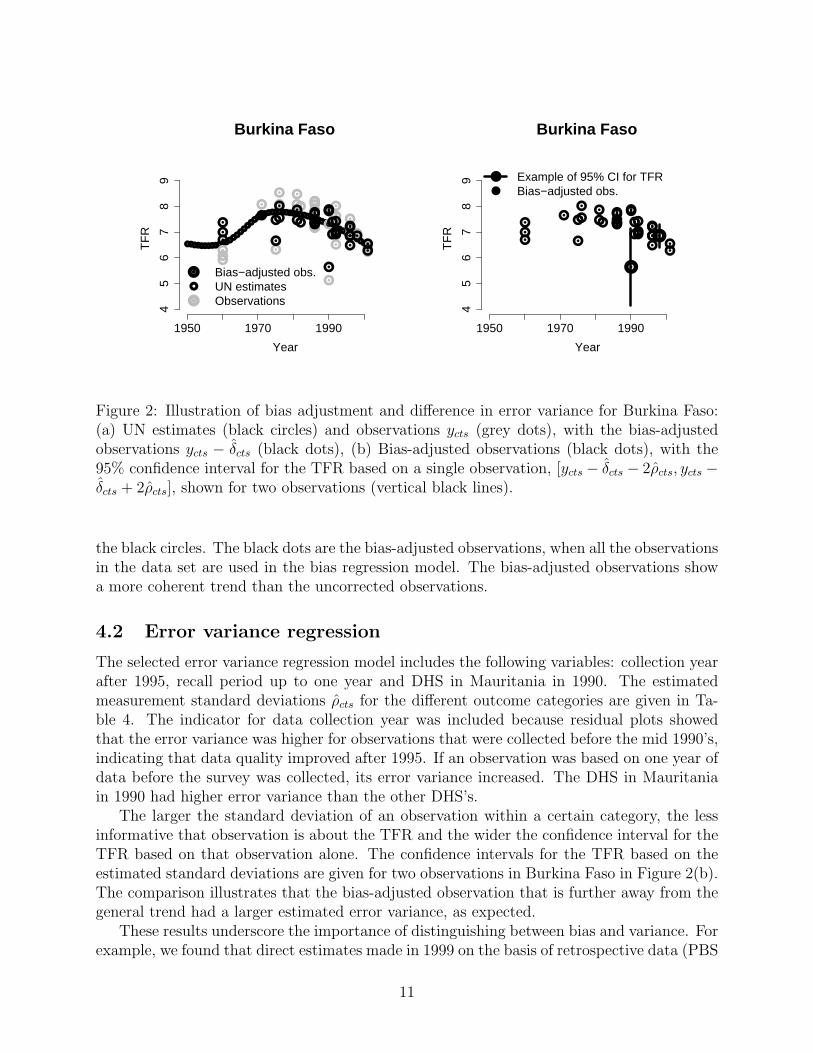
Figure 2: Illustration of bias adjustment and difference in error variance for Burkina Faso:(a) UN estimates (black circles) and observations ycts (grey dots), with the bias-adjustedobservations ycts − δcts (black dots), (b) Bias-adjusted observations (black dots), with the95% confidence interval for the TFR based on a single observation, [ycts − δcts − 2ρcts, ycts −δcts + 2ρcts], shown for two observations (vertical black lines).
the black circles. The black dots are the bias-adjusted observations, when all the observationsin the data set are used in the bias regression model. The bias-adjusted observations showa more coherent trend than the uncorrected observations.
4.2 Error variance regression
The selected error variance regression model includes the following variables: collection yearafter 1995, recall period up to one year and DHS in Mauritania in 1990. The estimatedmeasurement standard deviations ρcts for the different outcome categories are given in Ta-ble 4. The indicator for data collection year was included because residual plots showedthat the error variance was higher for observations that were collected before the mid 1990’s,indicating that data quality improved after 1995. If an observation was based on one year ofdata before the survey was collected, its error variance increased. The DHS in Mauritaniain 1990 had higher error variance than the other DHS’s.
The larger the standard deviation of an observation within a certain category, the lessinformative that observation is about the TFR and the wider the confidence interval for theTFR based on that observation alone. The confidence intervals for the TFR based on theestimated standard deviations are given for two observations in Burkina Faso in Figure 2(b).The comparison illustrates that the bias-adjusted observation that is further away from thegeneral trend had a larger estimated error variance, as expected.
These results underscore the importance of distinguishing between bias and variance. Forexample, we found that direct estimates made in 1999 on the basis of retrospective data (PBS
11
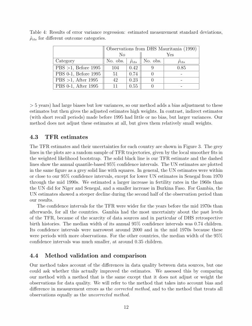
Table 4: Results of error variance regression: estimated measurement standard deviations,ρcts for different outcome categories.
Observations from DHS Mauritania (1990)No Yes
Category No. obs. ρcts No. obs. ρcts
PBS >1, Before 1995 104 0.42 9 0.85PBS 0-1, Before 1995 51 0.74 0 -PBS >1, After 1995 42 0.23 0 -PBS 0-1, After 1995 11 0.55 0 -
> 5 years) had large biases but low variances, so our method adds a bias adjustment to theseestimates but then gives the adjusted estimates high weights. In contrast, indirect estimates(with short recall periods) made before 1995 had little or no bias, but larger variances. Ourmethod does not adjust these estimates at all, but gives them relatively small weights.
4.3 TFR estimates
The TFR estimates and their uncertainties for each country are shown in Figure 3. The greylines in the plots are a random sample of TFR trajectories, given by the local smoother fits inthe weighted likelihood bootstrap. The solid black line is our TFR estimate and the dashedlines show the annual quantile-based 95% confidence intervals. The UN estimates are plottedin the same figure as a grey solid line with squares. In general, the UN estimates were withinor close to our 95% confidence intervals, except for lower UN estimates in Senegal from 1970through the mid 1990s. We estimated a larger increase in fertility rates in the 1960s thanthe UN did for Niger and Senegal, and a smaller increase in Burkina Faso. For Gambia, theUN estimates showed a steeper decline during the second half of the observation period thanour results.
The confidence intervals for the TFR were wider for the years before the mid 1970s thanafterwards, for all the countries. Gambia had the most uncertainty about the past levelsof the TFR, because of the scarcity of data sources and in particular of DHS retrospectivebirth histories. The median width of its annual 95% confidence intervals was 0.74 children.Its confidence intervals were narrowest around 2000 and in the mid 1970s because thesewere periods with more observations. For the other countries, the median width of the 95%confidence intervals was much smaller, at around 0.35 children.
4.4 Method validation and comparison
Our method takes account of the differences in data quality between data sources, but onecould ask whether this actually improved the estimates. We assessed this by comparingour method with a method that is the same except that it does not adjust or weight theobservations for data quality. We will refer to the method that takes into account bias anddifference in measurement errors as the corrected method, and to the method that treats allobservations equally as the uncorrected method.
12
●
●
●
●
●
●●
●
●
●
●
●
●
●●
●
●
● ●●●
●●●●
●
●
●
●●
●●
●
●
1960 1970 1980 1990 2000
45
67
89
Burkina Faso
Year
TF
R
●
●
●
●
●
●●
●
●
●
●
●
●
●●
●
●
● ●●●
●●●●
●
●
●
●●
●●
●
●
●●
●
●
●
●
●●
●
●
●
●
●
●
●
●●
●
1970 1980 1990 2000
45
67
89
Gambia
YearT
FR
●●
●
●
●
●
●●
●
●
●
●
●
●
●
●●
●
●
●
●
●
●●
●
●
●●
●
●
●
●
●
●
●●●
●
●
●●
●
●●
●
●
1960 1970 1980 1990 2000
45
67
89
Guinea
Year
TF
R
●
●
●
●
●●
●
●
●●
●
●
●
●
●
●
●●●
●
●
●●
●
●●
●
●
●
●
●
●
●●
●●
●
●
●
●
●
●
●
●●
● ●
●
●
●●
●
●
● ●●
●
1960 1970 1980 1990 2000
45
67
89
Mali
Year
TF
R
●
●
●
●
●●
●●
●
●
●
●
●
●
●
●●
● ●
●
●
●●
●
●
● ●●
●
●
●
●●
●
●
●
●
●
●
●
●
●●
●
●
●
●●●
●
●
●
●
●
●
●
●
●
●
●●
●
●
1970 1980 1990 2000
45
67
89
Mauritania
Year
TF
R
●
●
●●
●
●
●
●
●
●
●
●
●●
●
●
●
●●●
●
●
●
●
●
●
●
●
●
●
●●
●
●
●
●●
●
●
●
●
●
●
●
●
●
●
●
●
●●
●
●
●
●
●
●●
●
●●
●
●
●
1960 1970 1980 1990 2000
45
67
89
Niger
YearT
FR
●
●●
●
●
●
●
●
●
●
●
●
●
●
●
●●
●
●
●
●
●
●●
●
●●
●
●
●
●
●
●
●
●
●●
●
● ●
●
●●
●
●
●
● ●
●
●
●●
●
●
●
●
●
●●
●
●
●
●
●●
●
●
●●
●
●
●
●
●
1960 1970 1980 1990 2000
45
67
89
Senegal
Year
TF
R
●
●
●
●
●
●●
●
● ●
●
●●
●
●
●
● ●
●
●
●●
●
●
●
●
●
●●
●
●
●
●
●●
●
●
●●
●
●
●
●
●
Legend
● ObservationsUN estimatesTrajectories95% CI
Figure 3: Median estimates and confidence intervals for the TFR. The annual median esti-mates are shown by the solid line and the annual 95% confidence intervals (CI) by verticallines. The grey lines are a random sample of TFR trajectories, given by the local smootherfits in the weighted likelihood bootstrap. The observations are displayed as black dots andthe UN estimates by the grey line with squares.
13
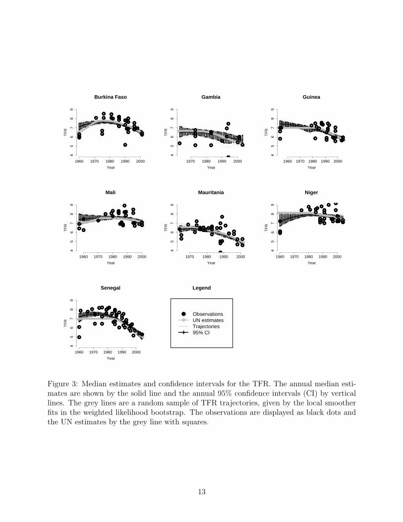
Table 5: Validation results for the corrected and uncorrected methods: Bias (the averagedistance between left-out observations and the median TFR estimate), SAPE (the standard-ized absolute prediction error), PIT area (the area above one in the PIT histogram), and theproportion of left-out observations that falls outside their 80% and 95% confidence intervals.
Leaving out Method Bias SAPE PIT Proportion of observationsarea <80 >80 <95 >95
50 Observations Corrected −0.02 1.06 0.05 0.08 0.11 0.04 0.04Uncorrected −0.06 1.00 0.11 0.12 0.04 0.03 0.01
DHS’s Corrected 0.03 1.23 0.14 0.14 0.13 0.04 0.07Uncorrected 0.21 1.08 0.19 0.07 0.14 0.01 0.04
Figure 4 shows the confidence intervals for the TFR for both methods in the sevencountries in western Africa. The two methods differed most at the start of the observationperiod, with the uncorrected method giving lower estimates than the corrected method.For most countries the uncorrected method peaked in the mid 1980s, at a TFR that washigher than the estimate from the corrected method. In Gambia, the only country without aDHS survey, the uncorrected method gave lower estimates than the corrected method for allyears. The confidence intervals were generally much narrower for the corrected method —on average 40% narrower. In most cases, the UN estimates were inside the 95% confidenceintervals of both methods.
To validate the methods, we left out different subsets of the observations, implementedthe methods without them, and then compared the resulting predictive distributions withthe observations themselves. The subsets left out for this cross-validation exercise were:(i) random subsets of observations: 10 different subsets of 50 observations, and (ii) oneDHS at a time (there were 22 DHS’s in total). Leaving out one survey at the time andthen examining how the left-out observations fit into the uncertainty assessment is the mostrealistic scenario in terms of adding “new” observations to the data set, that are independentof the observations that were already in the data set. We did this for the uncorrected methodas well as the corrected method.
The results are summarized for the two left-out categories in Table 5. The averagebias was 0.03 children or less for both categories for the corrected method, and somewhatlarger for the uncorrected method: 0.21 children for the left-out DHS’s. Uncertainty wasslightly underestimated in the corrected method, as shown by the standardized absoluteprediction error (SAPE), which is larger than one for both outcomes, and by the proportionsof observations that fell outside the confidence intervals.
The PIT histograms in Figure 5 do not show any systemmatic lack of calibration forthe corrected method, but they clearly indicate the bias in the uncorrected method. Thisis confirmed by the better values of the PIT area for the corrected method compared tothe uncorrected method. Overall, we conclude that our corrected method is reasonably wellcalibrated, and that taking account of data quality is worthwhile in that it removes thesystematic biases in the uncorrected method.
14

●
●
●
●
●
●●
●
●
●
●
●
●
●●
●
●
● ●●●
●●●●
●
●
●
●●
●●
●
●
1960 1970 1980 1990 2000
45
67
89
Burkina Faso
Year
TF
R
●
●
●
●
●
●●
●
●
●
●
●
●
●●
●
●
● ●●●
●●●●
●
●
●
●●
●●
●
●
●●
●
●
●
●
●●
●
●
●
●
●
●
●
●●
●
1970 1980 1990 2000
45
67
89
Gambia
Year
TF
R
●●
●
●
●
●
●●
●
●
●
●
●
●
●
●●
●
●
●
●
●
●●
●
●
●●
●
●
●
●
●
●
●●●
●
●
●●
●
●●
●
●
1960 1970 1980 1990 2000
45
67
89
Guinea
Year
TF
R
●
●
●
●
●●
●
●
●●
●
●
●
●
●
●
●●●
●
●
●●
●
●●
●
●
●
●
●
●
●●
●●
●
●
●
●
●
●
●
●●
● ●
●
●
●●
●
●
● ●●
●
1960 1970 1980 1990 2000
45
67
89
Mali
Year
TF
R
●
●
●
●
●●
●●
●
●
●
●
●
●
●
●●
● ●
●
●
●●
●
●
● ●●
●
●
●
●●
●
●
●
●
●
●
●
●
●●
●
●
●
●●●
●
●
●
●
●
●
●
●
●
●
●●
●
●
1970 1980 1990 2000
45
67
89
Mauritania
Year
TF
R
●
●
●●
●
●
●
●
●
●
●
●
●●
●
●
●
●●●
●
●
●
●
●
●
●
●
●
●
●●
●
●
●
●●
●
●
●
●
●
●
●
●
●
●
●
●
●●
●
●
●
●
●
●●
●
●●
●
●
●
1960 1970 1980 1990 2000
45
67
89
Niger
YearT
FR
●
●●
●
●
●
●
●
●
●
●
●
●
●
●
●●
●
●
●
●
●
●●
●
●●
●
●
●
●
●
●
●
●
●●
●
● ●
●
●●
●
●
●
● ●
●
●
●●
●
●
●
●
●
●●
●
●
●
●
●●
●
●
●●
●
●
●
●
●
1960 1970 1980 1990 2000
45
67
89
Senegal
Year
TF
R
●
●
●
●
●
●●
●
● ●
●
●●
●
●
●
● ●
●
●
●●
●
●
●
●
●
●●
●
●
●
●
●●
●
●
●●
●
●
●
●
●
Legend
● ObservationsUN estimates95% CI, uncorrected method95% CI, corrected method
Figure 4: 95% Confidence intervals for the TFR for the corrected method (grey), and theuncorrected method (black). The solid line shows the annual median estimates and the 95%confidence intervals are plotted with dashed lines. The observations are displayed as blackdots and the UN estimates by the grey line with squares.
15

Corrected method
PIT outcomes
Den
sity
0.0 0.2 0.4 0.6 0.8 1.0
0.0
0.5
1.0
1.5
Uncorrected method
PIT outcomes
Den
sity
0.0 0.2 0.4 0.6 0.8 1.0
0.0
0.5
1.0
1.5
Figure 5: Histograms of the outcomes of the probability integral transforms for the left-outobservations when leaving out one DHS at a time for the corrected and the uncorrectedmethod.
5 DISCUSSION
We have proposed a new approach to estimating the total fertility rate over time from multi-ple data sources of varying quality, and applied it to seven countries in western Africa. Ourapproach consists of four steps: bias adjustment, estimation of measurement error variance,local smoothing of the bias-adjusted values with weights based on the error variance, anduncertainty assessment using the weighted likelihood bootstrap. We assessed the resultsby cross-validation, and found that our method was reasonably well calibrated. Compari-son with a similar method that excludes the first two steps showed that taking account ofdata quality removed clear biases and greatly reduced the average width of the confidenceintervals.
One limitation of our method is that a data source that is deemed “unbiased” is needed topredict bias and measurement error variance. This data source does not have to be perfector even of high quality, but is required to have no systematic tendency to substantiallyover- or underestimate TFR. We have used the existing UN estimates for this purpose. Itwould also be possible to identify one of the common data sources, most likely the DHS’s,as unbiased. However, when using one single data source as a baseline for the analysis,data quality problems in that data source (such as those that we found for the 1990 DHS inMauritania) may well be missed.
Our general approach could be applied with appropriate modifications to the estimation ofother demographic quantities, including mortality. However, our methodology was developedfor an overall rate (the TFR), while often age-specific rates are desired. The method could beapplied directly to age-specific fertility rates, but this has the disadvantage that adherence
16
to overall patterns is not guaranteed. A possible alternative would be to use our presentmethodology in combination with age-specific fertility schedules.
References
Alkema, L. (2008). Uncertainty Assessments of Demographic Estimates and Projections.Ph. D. thesis, University of Washington.
Becker, S. and S. Mahmud (1984). A validation study of backward and forward preg-nancy histories in Matlab, Bangladesh. World Fertility Survey Scientific Reports 52,International Statistical Institute.
Berrocal, V., A. E. Raftery, and T. Gneiting (2007). Combining spatial statistical andensemble information in probabilistic weather forecasts. Monthly Weather Review 135,1386–1402.
Brass, W. (1964). Uses of census or survey data for the estimation of vital rates. Paperpresented at the African Seminar on Vital Statistics.
Brass, W. (1996). Demographic data analysis in less developed countries. Population Stud-ies 50, 451–467.
Brass, W., A. J. Coale, P. Demeny, and D. F. Heisel et al. (eds.) (1968). The Demographyof Tropical Africa. Princeton NJ: Princeton University Press.
Cleveland, W., E. Grosse, and W. Shyu (1992). Chapter 8.
Cleveland, W. S. and S. J. Devlin (1988). Locally weighted regression: An approach toregression analysis by local fitting. Journal of the American Statistical Association 83,596–610.
Efron, B. (1979). Bootstrap methods: another look at the jackknife. Annals of Statistics 7,1–26.
Ewbank, D. C. (1981). Age Misreporting and Age-Selective Underenumeration: Sources,Patterns, and Consequences for Demographic Analysis. National Academy Press.
Feeney, G. (1998). A new interpretation of Brass’ P/F Ratio method applicable whenfertility is declining. http://www.gfeeney.com/notes/pfnote/pfnote.htm.
Gerland, P. (2007). Unpublished notes on Weighting scheme for emperical data on age-specific mortality and fertility rates, based on data quality covariates.
Hill, K., R. Pande, M. Mahy, and G. Jones (1998). Trendsin child mortality in the developing world: 1960 to 1996.http://www.un.org/esa/population/publications/wwp2004/wwp2004 vol3 final/%6.pdf, UNICEF, New York.
Loader, C. (1999). Local Regression and Likelihood. Springer, New York.
Moultrie, T. A. and R. Dorrington (2008). Sources of error and bias in methods of fertilityestimation contingent on the P/F Ratio in a time of declining fertility and risingmortality. Demographic Research 19(46), 1635–1662.
17

Murray, C. J. L., T. Loakso, K. Shibuya, K. Hill, and A. D. Lopez (2007). Can we achieveMillennium Development Goal 4? New analysis of country trends and forecasts ofunder-5 mortality to 2015. Lancet 370, 1040–1054.
Newton, M. A. and A. E. Raftery (1994). Approximate Bayesian inference with theweighted likelihood bootstrap (with discussion). Journal of the Royal Statistical Soci-ety, Series B 56, 3–48.
Potter, J. (1977). Problems in using birth-history analysis to estimate trends in fertility.Population Studies 31, 335–364.
Pullum, T. and S. Stokes (1997). Identifying and adjusting for recall error, with applicationto fertility surveys. In L. Lyberg and P. Biemer and et al. (Ed.), Survey Measurementand Process Quality, pp. 711–732. New York: John Wiley and Sons.
Pullum, T. W. (2006). An assessment of age and date in the DHS sur-veys, 1985 - 2003. Technical report. DHS Methodological Reports 5,http://www.measuredhs.com/pubs/pub details.cfm?ID=664&srchTp=type.
Raftery, A. E. (1995). Bayesian model selection in social research (with discussion). Soci-ological Methodology 25, 111–196.
Raftery, A. E., I. Painter, and C. T. Volinsky (2005). BMA: An R package for BayesianModel Averaging. 5 (2), 2–8. R News.
Silverwood, R. and S. Cousens (2007). Comparison of spline- and loess-based ap-proaches for the estimation of child mortality. Presentation at the Inter-AgencyCoordination Group on Child Mortality Estimation, Geneva, 7 March 2007 Slides athttp://www.who.int/whosis/mort/20080306mtg Present Day1 Session6 DrSilverwood.pdf.
Som, R. (1973). Recall Lapse in Demographic Enquiries. New York: Asia Publishing House.
Trussell, J., E. van de Walle, and F. van de Walle (1989). Norms and behaviour in Burk-inabe fertility. Population Studies 43, 429–454.
Trussell, T. (1975). A re-estimation of the multiplying factors for the Brass technique fordetermining children survivorship rates. Population Studies 29, 97–108.
UNICEF, the World Health Organization (WHO), World Bank, and United Nations Pop-ulation Division (UNPD) (2007). Levels and trends of child mortality in 2006 esti-mates developed by the interagency group for child mortality estimation. Workingpaper http://www.childinfo.org/files/infant child mortality 2006.pdf.
United Nations (1982). National household survey capability programme. Non-samplingerrors of household surveys: sources, assessment and control. New York: UnitedNations Department of Technical Cooperation for Development and Statistical Of-fice http://unstats.un.org/unsd/publication/unint/DP UN INT 81 041 2.pdf.
United Nations (1983). Manual X, Indirect Techniques forDemographic Estimation. United Nations, New York.http://www.un.org/esa/population/publications/Manual X/Manual X.htm.
United Nations, Department of Economic and Social Affairs, Population Division (2007a).World Population Prospects: The 2006 Revision, CD-ROM Edition - ExtendedDataset in Excel and ASCII formats. United Nations publication, Sales No. E.07.XIII.7.
18

United Nations, Department of Economic and Social Affairs, Population Di-vision (2007b). World Population Prospects. The 2006 Revision, Vol. I,Comprehensive Tables. United Nations publication, Sales No. E.07.XIII.2,http://www.un.org/esa/population/publications/wpp2006/wpp2006.htm.
19