Essential Convexity and Complexity of Semi-Algebraic Constraints

Logical Methods in Computer ScienceVol. 8(4:5)2012, pp. 1–25www.lmcs-online.org

Submitted Dec. 06, 2009Published Oct. 10, 2012

ESSENTIAL CONVEXITY AND COMPLEXITY OF SEMI-ALGEBRAIC

CONSTRAINTS

MANUEL BODIRSKY a, PETER JONSSON b, AND TIMO VON OERTZEN c

a CNRS/LIX, Ecole Polytechnique, 91128 Palaiseau, Francee-mail address: [email protected]

b Department of Computer and System Science, Linkopings Universitet, SE-581 83, Sweden.e-mail address: [email protected]

c Max-Planck-Institute for Human Development, Konigin-Luise-Strasse 5, 14195 Berlin, Germany,and University of Virginia, Department of Psychology, Charlottesville, USA.e-mail address: [email protected]

Abstract. Let Γ be a structure with a finite relational signature and a first-order def-inition in (R; ∗,+) with parameters from R, that is, a relational structure over the realnumbers where all relations are semi-algebraic sets. In this article, we study the compu-tational complexity of constraint satisfaction problem (CSP) for Γ: the problem to decidewhether a given primitive positive sentence is true in Γ. We focus on those structures Γthat contain the relations ≤, {(x, y, z) | x+y = z} and {1}. Hence, all CSPs studied in thisarticle are at least as expressive as the feasibility problem for linear programs. The centralconcept in our investigation is essential convexity: a relation S is essentially convex if forall a, b ∈ S, there are only finitely many points on the line segment between a and b thatare not in S. If Γ contains a relation S that is not essentially convex and this is witnessedby rational points a, b, then we show that the CSP for Γ is NP-hard. Furthermore, wecharacterize essentially convex relations in logical terms. This different view may open upnew ways for identifying tractable classes of semi-algebraic CSPs. For instance, we showthat if Γ is a first-order expansion of (R; +, 1,≤), then the CSP for Γ can be solved inpolynomial time if and only if all relations in Γ are essentially convex (unless P=NP).

1998 ACM Subject Classification: F.2.2, F.4.1, G.1.6.2010 Mathematics Subject Classification: 68Q17.Key words and phrases: Constraint Satisfaction Problem, Convexity, Computational Complexity, Linear

Programming.a Manuel Bodirsky has received funding from the European Research Council under the European Com-

munity’s Seventh Framework Programme (FP7/2007-2013 Grant Agreement no. 257039).b Peter Jonsson is partially supported by the Center for Industrial Information Technology (Ceniit) under

grant 04.01 and by the Swedish Research Council (VR) under grants 2006-4532 and 621-2009-4431.

LOGICAL METHODSl IN COMPUTER SCIENCE DOI:10.2168/LMCS-8(4:5)2012c© M .Bodirsky, P. Jonsson, and T. v. OertzenCC© Creative Commons

http://creativecommons.org/about/licenses

2 M .BODIRSKY, P. JONSSON, AND T. V. OERTZEN

1. Introduction

Linear Programming is a computational problem of outstanding theoretical and practicalimportance. It is known to be computationally equivalent to the problem to decide whethera given set of linear (non-strict) inequalities is feasible, i.e., defines a non-empty set:

Linear Program FeasibilityINPUT: A finite set of variables V ; a finite set of linear inequalities of the form a1x1 + · · ·+akxk ≤ a0 where x1, . . . , xk ∈ V and a0, . . . , ak are rational numbers where the numeratorsand denominators are represented in binary.QUESTION: Does there exist an x ∈ R|V | that satisfies all inequalities?

This problem can be viewed as a constraint satisfaction problem, where the allowedconstraints are linear inequalities with rational coefficients, and the question is whetherthere is an assignment of real values to the variables such that all the constraints aresatisfied. For formal definitions of concepts related to constraint satisfaction, we refer thereader to Section 2.1. It is obvious that this problem cannot be formulated with a finiteconstraint language; however, we will later on (Proposition 2.12) see that the feasbilityproblem for linear programs is polynomial-time equivalent to the constraint satisfactionproblem for the structure

Γlin :=(R; {(x, y, z) | x+ y = z},≤, {1}

).

It is well-known that linear programming can be solved in polynomial time; moreover,several algorithms are known that are efficient also in practice. In this article, we studyhow far Γlin can be expanded such that the corresponding constraint satisfaction problemremains polynomial-time solvable. An important class of relations that generalizes the classof relations defined by linear inequalities is the class of all semi-algebraic relations, i.e.,relations that have a first-order definition over (R; ∗,+) using parameters from R. By thefundamental theorem of Tarski and Seidenberg, it is known that a relation S ⊆ Rn is semi-algebraic if and only if it has a quantifier-free first-order definition in (R; ∗,+,≤) usingparameters from R. Geometrically, we can view semi-algebraic sets as finite unions of finiteintersections of the solution sets of strict and non-strict polynomial inequalities.

We propose a framework for systematically studying the computational complexity ofexpansions of Γlin by semi-algebraic relations. In this framework, a constraint satisfactionproblem is given by a (fixed and finite) constraint language Γ. All the constraints inthe input of such a feasibility problem must be chosen from this constraint language Γ(a formal definition can be found in Section 2.1). This way of parameterizing constraintsatisfaction problems by their constraint language has proved to be very fruitful for finitedomain constraint satisfaction problems [1,7–9,14]. Since the constraint language is finite,the computational complexity of such a problem does not depend on how the constraintsare represented in the input. We believe that the very same approach is very promising forstudying the complexity of problems in real algebraic geometry. In Section 6 we will discussa connection between some of the CSPs with semi-algebraic constraint languages and openproblems in convex geometry and semidefinite programming.

One of the key reasons why linear program feasibility can be decided in polynomial timeis that the feasible regions of linear inequalities are convex. Convexity is not a necessarycondition for tractability of semi-algebraic constraint satisfaction problems, though. It is,for instance, well-known that linear program feasibility can also be decided in polynomial

ESSENTIAL CONVEXITY AND COMPLEXITY OF SEMI-ALGEBRAIC CONSTRAINTS 3

time when some of the input constraints are disequalities, i.e., constraints of the forma1x1 + · · · + akxk 6= a0 for rational values a0, . . . , ak. However, we show that if Γlin ⊆ Γand Γ contains a relation S with rational a, b ∈ S such that on the line segment L betweena and b there are infinitely many points that are not in S, then the CSP(Γ) is NP-hard.This motivates the notion of essential convexity : a set S ⊆ Rk is essentially convex if for allp, q ∈ S there are only finitely many points on the line between p and q that are not in S.One of our central results is a logical characterization of essentially convex semi-algebraicrelations in Section 4. This characterization can be used to show several results that arebriefly described next.

A relation is called semi-linear if it has a first-order definition with rational parameters1

in the structure (R; +,≤). From the perspective of constraint satisfaction, the set of semi-linear relations is a rich set. For example, every relation S ⊆ Qk with finitely many elementsis semi-linear; thus, every finitary relation on a finite set can be viewed as a semi-linearrelation. In Section 5.1, we show that when we add a finite number of semi-linear relationsto Γlin, then the resulting language either has a polynomial-time or an NP-hard constraintsatisfaction problem. This result is useful for studying optimization problems: note thatlinear programming can be viewed as optimizing a linear function over the feasible pointsof a set of linear inequalities. This view suggests an immediate generalization: optimize alinear function over the feasible points of an instance of a constraint satisfaction problemfor semi-linear constraint languages. We completely classify the complexity of this problemin Section 5.2.

Another application concerns temporal reasoning. A temporal constraint language Γis a structure (R;R1, . . . , Rl) with a first-order definition in (R;<). Many computationalproblems in artificial intelligence and scheduling can be modeled as constraint satisfactionproblems for temporal constraint languages. The complexity of the CSP for temporal con-straint languages Γ has been completely classified recently [6]; there are 9 tractable classesof temporal constraint satisfaction problems. Often, temporal languages are extended withsome mechanism for expressing metric time, i.e., the ability to assign numerical values tovariables and performing some kind of arithmetic calculations [11]. It has been observedthat many metric languages Γ are semi-linear and satisfy Γlin ⊆ Γ, and if such a languageis polynomial-time solvable, then it is a subclass of the so-called Horn-DLR class [21]. Ourresult shows that this is not a coincidence: whenever Γ is not a subclass of Horn-DLR, thenthe CSP(Γ) is NP-hard.

2. Preliminaries

2.1. Constraint Satisfaction Problems. A first-order formula2 is called primitive posi-tive (pp) if it is of the form

∃x1, . . . , xn.(ψ1 ∧ · · · ∧ ψm)

1We deviate from model-theoretic terminology as it is used e.g. in [24] in that we only allow rationaland not arbitrary real parameters in first-order definitions. Our definition conincides with the definition ofsemi-linear sets given in e.g. [12, 13].

2Our terminology is standard; all notions that are not explicitly introduced can be found in standardtextbooks, e.g., in [19].


where ψi are atomic formulas, i.e., formulas of the form x = y or S(xi1 , . . . , xik) where S isthe relation symbol for a k-ary relation in Γ. We call such a formula a pp-formula, and asusual a pp-formula without free variables is called a pp-sentence.

Let Γ = (D;S1, . . . , Sl) be a structure with domain D and a finite relational signature.The constraint satisfaction problem for Γ (CSP(Γ) in short) is the computational problemto decide whether a given primitive positive sentence Φ involving relation symbols for therelations in Γ is true in Γ. The conjuncts in a pp-sentence Φ are also called the constraints ofΦ, and to emphasize the connection between the structure Γ and the constraint satisfactionproblem, we typically refer to Γ as a constraint language. By choosing an appropriate con-straint language Γ, many computational problems that have been studied in the literaturecan be formulated as CSP(Γ) (see e.g. [5, 9]).

When studying the complexity of different CSPs, it is often useful to be able to derivenew relations from old. If Γ = (D;S1, . . . , Sl) is a relational structure and S ⊆ Dk isa relation, then (Γ, S) denotes the expansion (D;S, S1, . . . , Sl) of the structure Γ by therelation S. We say that an n-ary relation S is pp-definable in Γ if there exists a pp-formulaφ with free variables x1, . . . , xn such that (x1, . . . , xn) ∈ S iff φ(x1, . . . , xn) holds in Γ.The following simple but important result explains the importance of pp-definability forconstraint satisfaction problems.

Lemma 2.1 (Jeavons et al. [20]). Let Γ be a relational structure, and let S be pp-definableover Γ. Then CSP((Γ, S)) is polynomial-time equivalent to CSP(Γ).

2.2. Semi-algebraic and semi-linear relations. We say that a relation S ⊆ Dn is first-order definable in a structure Γ with domain D if there exists a formula φ(x1, . . . , xn) usinguniversal and existential quantification, disjunction, conjunction, negation, and atomic for-mulas over Γ (where x1, . . . , xn denote the free variables in φ) such that φ(a1, . . . , an) istrue over Γ if and only if (a1, . . . , an) ∈ S. We always admit equality when building atomicformulas, i.e., we have atomic formulas of the form t1 = t2 for terms t1, t2 formed fromfunction symbols for Γ and variables. We say that S is first-order definable in Γ with pa-rameters from A, for A ⊆ D, if additionally we can use constant symbols for the elementsof A in the first-order definition of S.

A set S ⊆ Rn is called semi-algebraic if it has a first-order definition in (R; ∗,+) usingparameters from R. Note that the order ≤ of the real numbers is first-order definable in(R; ∗,+), since

a ≤ b ⇔ ∃c. b = a+ c ∗ c .We need some basic algebraic and topological concepts and facts.

Definition 2.2 (Section 3.1 in [2]). A set S ⊆ Rn is open if it is the union of open balls,i.e., if every point of S is contained in an open ball contained in S. A set S ⊆ Rn is closedif its complement is open. The closure of a set S, denoted S, is the intersection of all closedsets containing S. Equivalently, S = {x ∈ Rn | ∀r > 0 ∃y ∈ S. (y − x)2 < r2}. A point p inS is a boundary point if for every ε > 0, the n-dimensional open ball with radius ε aroundp contains at least one point in S and one point not in S. The set of boundary points isdenoted ∂S. The interior of S, denoted by S◦, is S \ ∂S.

Note that the interior of S consists of all p ∈ S such that there exists an ε > 0 with thefollowing property: the n-dimensional open ball with radius ε around p is contained in S.Also note that a finite union of closed sets is closed.


Proposition 2.3 (Proposition 2.2.2. in [4]). The closure of a semi-algebraic relation issemi-algebraic.

We use the notion of dimension dim(S) ∈ N of a semi-algebraic set S as defined in [4].

Definition 2.4 (Section 2.8 in [4]). Let S ⊆ Rk be a semi-algebraic set, and let P(S)be the ring of polynomial functions on S, i.e., the ring of functions S → R which are therestriction of a polynomial. Then the dimension of S, denoted by dim(S), is the maximallength of chains of prime ideals of P(S), i.e., the maximal d such that there exist distinctprime ideals I0, I1, . . . , Id of P(S) with I0 ⊂ I2 ⊂ · · · ⊂ Id.

To work with this definition of dimension, we need some more concepts.

Definition 2.5 (see [4]). Let S ⊆ Rk and T ⊆ Rl be semi-algebraic sets. A functionf : S → T is semi-algebraic if the set {(x1, . . . , xk, y1, . . . , yl) | f(x1, . . . , xk) = (y1, . . . , yl)}is a semi-algebraic subset of Rk+l.

As usual, bijective functions f : S → T such that S′ ⊆ S is open if and only if f(S′) ⊆ Tis open are called homeomorphisms.

Lemma 2.6 (Propositions 2.8.5, 2.8.9, and 2.8.13 in [4]). Let S ⊆ Rn be semi-algebraic.

• If S = S1 ∪ S2 then dim(S) = max(dim(S1),dim(S2)).• If there is a semi-algebraic homeomorphism from S to (0, 1)d, then dim(S) = d.• dim(S \ S) < dim(S).

In particular, if S ⊆ T , then dim(S) ≤ dim(T ).A set V ⊆ Rn is called an (algebraic) variety if it can be defined as a conjunction of

the form p1 = 0∧ · · · ∧ pm = 0 where p1, . . . , pm are polynomials in the variables x1, . . . , xnwith coefficients from R. We allow terms in polynomials to have degree zero.

Lemma 2.7. Let V ⊆ Rn be a variety and let L ⊆ Rn be a line. If infinitely many pointsof L are in V , then L ⊆ V .

Proof. Let V be defined by p1(x1, . . . , xn) = 0 ∧ · · · ∧ pm(x1, . . . , xn) = 0, and let l1, . . . , lnbe univariate linear polynomials such that L = {(l1(x), . . . , ln(x)) | x ∈ R}. For each pi, theunivariate polynomial pi(l1(x), . . . , ln(x)) equals 0 infinitely often. So it is always 0, and itfollows that every point on L satisfies p1 = 0 ∧ · · · ∧ pm = 0.

Theorem 2.8 (Tarski and Seidenberg; Proposition 5.2.2 in [4]). Every first-order formulaover (R; ∗,+,≤) with parameters from R is equivalent to a quantifier-free formula withparameters from R.

By an interval we mean either an open, half-open, or closed interval with more thanone element. An ordered structure (D;≤, . . .) is o-minimal (see [23], Definition 3.1.18)if for any first-order definable S ⊆ D with parameters from D there are finitely manyintervals I1, . . . , Im with endpoints in D ∪ {±∞} and a finite set D0 ⊆ D such that S =D0 ∪ I1 ∪ · · · ∪ Im. The following is an easy and well-known consequence of Theorem 2.8.

Theorem 2.9 (see e.g. [23]). Let R1, . . . , Rn be semi-algebraic relations. Then (R;≤, R1, . . . , Rn) is o-minimal.

A set S ⊆ Rn is called semi-linear if it has a first-order definition in (R; +,≤) withparameters from Q; we also call first-order formulas over (R; +,≤) with parameters from


Q semi-linear. It has been shown in [12, 13] that it is decidable whether a given first-order formula over (R; ∗,+,≤) with parameters from Q defines a semi-linear relation ornot. A set V ⊆ Rn is called a linear set if it can be defined as a conjunction of the formp1 ≥ 0∧· · ·∧pm ≥ 0 where p1, . . . , pm are linear polynomials in the variables x1, . . . , xn withcoefficients from Q. It is not hard to see that every semi-linear relation S can be viewed asa finite union of linear sets. We also have quantifier elimination for semi-linear relations.

Theorem 2.10 (Ferrante and Rackoff [15]). Every semi-linear relation has a quantifier-freedefinition over (R; +,−,≤) with parameters from Q.

2.3. Definability of Rational Expressions. The following elementary lemma will beneeded for the observation that the feasibility problem for linear programs is polynomial-time equivalent to CSP(Γlin); it is also essential for the hardness proofs in Section 3 and forproving the dichotomy result for metric temporal constraint reasoning.

Lemma 2.11. Let n0, n1, . . . , nl ∈ Q be rational numbers. Then the relation {(x1, . . . , xl) |n1x1 + · · ·+ nlxl = n0} is pp-definable in (R; {(x, y, z) | x+ y = z}, {1}). Furthermore, thepp-formula that defines the relation can be computed in polynomial time.

Proof. We first note that we can assume that n0, n1, . . . , nl are integers. To see this, supposethat the rational coefficients n0, . . . , nl are represented as pairs of integers (a0, b0), . . . , (al, bl)

where ai denotes the nominator and bi the denominator. Let c =∏li=0 bi and create a new

sequence of coefficients n′0, . . . , n′l = (a0 · c/b0, 1), . . . , (al · c/bl, 1). The resulting equation

is obviously equivalent. It is also clear that it only takes polynomial time to compute suchcoefficients.

Before the actual proof, we note that x = 0 is pp-definable by x + x = x, and wetherefore freely use the terms 0 and 1 in pp-definitions. Similarly, x = −1 is pp-definableby x+ 1 = 0. The proof is by induction on l. We first show how to express equations of theform n1x1 + n2x2 = x3. By setting x2 to −1 and x3 to 0, this will solve the case l = 1. Forpositive n1, n2, the formula n1x1 + n2x2 = x3 is equivalent to

∃u1, . . . , un1 , v1, . . . , vn2 . u1 = x1 ∧n1−1∧i=1

x1 + ui = ui+1

∧ v1 = x2 ∧n2−1∧i=1

x2 + vi = vi+1

∧ un1 + vn2 = x3 .

However, this formula is exponential in the representation size of n1 and n2, and cannot beused in polynomial-time reductions.

Let bit(n, i) denote the i-th lowest bit in the binary representation of an integer n and1 ≤ i ≤ blog nc+ 1. The following formula is equivalent to the previous one (we are still inthe case that both n1 and n2 are positive) and has polynomial length in the representationsize of n1 and n2. Write m1 for blog n1c+ 1 and m2 for blog n2c+ 1.


∃a1, ..., am1 , b1, ..., bm2 , c1, ..., cm1 , d1, ..., dm2 . a1 = x1 ∧m1∧i=2

ai−1 + ai−1 = ai

∧ b1 = x2 ∧m2∧i=2

bi−1 + bi−1 = bi

∧ c1 = bit(n1, 1)a1 ∧m1∧i=2

bit(n1, i)ai + ci−1 = ci

∧ d1 = bit(n2, 1)b1 ∧m2∧i=2

bit(n2, i)bi + di−1 = di

∧ cm1 + dm2 = x3

If l = 2, and n1 = 0 or n2 = 0, then the proof is similar. If n1 and n2 have differentsigns, we replace the conjunct cm1 + dm2 = x3 in the formula above appropriately bycm1 + x3 = dm2 or dm2 + x3 = cm1 . If both n1 and n2 are negative, then we use thepp-definition ∃x′3.(−n1x1 − n2x2 = x′3 ∧ x′3 + x3 = 0).

Equalities of the form n1x1+n2x2 = n0 can be defined by ∃x3.(n1x1+n2x2 = x3∧x3 =n0). Now suppose that l > 2. By the inductive assumption, there is a pp-definitionφ1(x1, x2, u) for n1x1 + n2x2 + u = n0 and a pp-definition φ2(x3, . . . , xl, u) for n3x3 + · · ·+nlxl = u. Then ∃u.(φ1 ∧ φ2) is a pp-definition for n1x1 + · · · + nlxl = n0. It is clear thatthe pp-definition given above can be computed in time which is polynomial in the numberof bits needed to represent the input.

By extending the previous result to inequalities, we prove that CSP(Γlin) and linearprogram feasibility are polynomial-time equivalent problems. The dichotomy for metrictemporal reasoning follows immediately by combining this result and Theorem 5.2.

Proposition 2.12. The linear program feasibility problem is polynomial-time equivalent toCSP(Γlin).

Proof. It is clear that an instance of CSP(Γlin) can be seen as a linear program feasibilityproblem, since the three different relations in the constraint language, x + y = z, x = 1,x ≤ y, are linear.

For the opposite direction, let Φ be an arbitrary instance of the linear program feasibilityproblem. Given a linear equality L(x1, . . . , xk) ≡ c1x1+· · ·+ckxk = c0, let φL(x1,...,xk) denotethe pp-definition of L(x1, . . . , xk) in (R; {(x, y, z) | x+y = z}, {1}) obtained in Lemma 2.11.Construct an instance Ψ of CSP(Γlin) by replacing each occurrence of a linear inequalityconstraint c1x1 + · · · clxl ≤ c0 in Φ by a φc1x1+···+clxl−y=0 ∧ y ≤ c0; use fresh variables fory and for the existentially quantified variables introduced by φL. The resulting formula Ψcan be rewritten as a primitive positive sentence over Γ without increasing its length and,by Lemma 2.11, the length of Ψ is polynomial in the length of Φ. Since Φ is satisfiable ifand only if Ψ is satisfiable, this shows that the problems are polynomial-time equivalent.


3. Hardness

We consider relations that give rise to NP-hard CSPs in this section. We first need somedefinitions: a relation S ⊆ Rk is convex if for all p, q ∈ S, S contains all points on the linesegment between p and q. We say that a relation S ⊆ Rk excludes an interval if there arep, q ∈ S and real numbers 0 < δ1 < δ2 < 1 such that p+ (q− p)y 6∈ S whenever δ1 ≤ y ≤ δ2.Note that we can assume that δ1, δ2 are rational numbers, since we can choose any twodistinct rational numbers γ1 < γ2 between δ1 and δ2 instead of δ1 and δ2.

Definition 3.1. We say that S ⊆ Rn is essentially convex if for all p, q ∈ S there are onlyfinitely many points on the line segment between p and q that are not in S.

If S is not essentially convex, and if p and q are such that there are infinitely manypoints on the line segment between p and q that are not in S, then p and q witness that Sis not essentially convex. The following is a direct consequence of Theorem 2.9, and we willuse it in the following without further reference.

Corollary 3.2. If S is a semi-algebraic relation that is not essentially convex, then Sexcludes an interval. If S is an essentially convex semi-algebraic relation, and a, b are twodistinct points from S, then the line segment between a and b contains an interval I withI ⊆ S.

The next proposition will be used several times in the sequel; it clarifies the relationbetween finite unions of varieties and essentially convex relations.

Proposition 3.3. Let W be a finite union of varieties V1, . . . , Vk ⊆ Rn, and let C ⊆W beessentially convex. Then, there is an i ≤ k such that C ⊆ Vi.Proof. Let J ⊆ {1, . . . , k} be minimal such that C ⊆

⋃i∈J Vi. If |J | = 1, then there is

nothing to show. So suppose for contradiction that there are distinct i, j ∈ J . Then theremust be points a, b ∈ C such that a ∈ Vi and a /∈ Vl for all l ∈ J \ {i}, and b ∈ Vj andb /∈ Vl for all l ∈ J \ {j}. By essential convexity of C and Corollary 3.2, the line segment Lbetween a and b must contain an interval I that lies in C. Since J is finite, there must bel ∈ J such that infinitely many points on I are from Vl. By Lemma 2.7, all points on theline through a and b are from Vl; this contradicts the choice of a and b.

The rest of the section is divided into two parts. We first prove that if S ⊆ Rk is asemi-algebraic relation that is not essentially convex and this is witnessed by two rationalpoints p and q, then CSP((Γlin, S)) is NP-hard. In the second part, we prove that if S ⊆ Rkis a semi-linear relation that is not essentially convex, then this is witnessed by rationalpoints and, consequently, CSP((Γlin, S)) is NP-hard.

3.1. Semialgebraic relations and rational witnesses. We begin with the special casewhen S is a unary relation. The hardness proof is by a reduction from CSP(({0, 1};R1/3))where

R1/3 = {(1, 0, 0), (0, 1, 0), (0, 0, 1)} .This NP-complete problem is also called Positive One-In-Three 3Sat [16, LO4], whichis the variant of One-In-Three 3Sat where we have the extra requirement that in allinput instances of the problem, no clause contains a negated literal.

Lemma 3.4. Let S ⊆ R be a unary relation. If S excludes an interval and this is witnessedby rational points p and q, then CSP((Γlin, S)) is NP-hard.


Proof. We know that there are rational numbers 0 < δ1 < δ2 < 1 such that p+ (q− p)y 6∈ Swhenever δ1 ≤ y ≤ δ2. Let

a = sup{δ2 − δ1 | 0 < δ1 < δ2 < 1 and [p+ (q − p)δ1, p+ (q − p)δ2] ∩ S = ∅},i.e., the least upper bound on the length (scaled to the interval [0,1]) of excluded intervalsbetween p and q. Choose rational numbers δ1, δ2 such that

• there exists y ∈ [δ1 − d, δ1] such that p+ (q − p)y ∈ S; and• there exists y ∈ [δ2, δ2 + d] such that p+ (q − p)y ∈ S.• S ∩ [p+ (q − p)δ1, p+ (q − p)δ2] = ∅.where d = (δ2 − δ1)/5. It is easy to see that such δ1, δ2 exist; we simply need to find δ1, δ2such that S ∩ [p+ (q− p)δ1, p+ (q− p)δ2] = ∅ and δ2 − δ1 is sufficiently close to a. Clearly,for any ε > 0, there exist suitable δ1, δ2 such that a− (δ2 − δ1) < ε.

Now, define p′ = p+ (q − p)(δ1 − d), q′ = p+ (q − p)(δ2 + d), and

U(y) ≡ ∃z.(z = p′ + (q′ − p′)y ∧ S(z) ∧ 0 ≤ y ≤ 1).

Observe that U is pp-definable in Γlin∪{S} by Lemma 2.11 combined by the fact that p′ andq′ are rational numbers. We claim that U contains at least one point in the interval [0, d′],at least one point in the interval [1 − d′, 1], and no points in the interval [d′, 1 − d′] whered′ = 1/7. Let us consider the interval [0, d′]. The point (expressed in p and q) correspondingto y = 0 is p′ (which equals p+ (q− p)(δ1− d)) while the point corresponding to y = 1/7 is

p′ +(q′ − p′)

7= p+ (q − p)(δ1 − d) +

p+ (q − p)(δ2 + d)− p− (q − p)(δ1 − d)

7

= p+ (q − p)(δ1 − d) +(q − p)((δ2 + d)− (δ1 − d))

7

= p+ (q − p)(δ1 − d) +(q − p)(δ2 − δ1 + 2d)

7

= p+ (q − p)(δ1 − d) +(q − p)(5d+ 2d)

7= p+ (q − p)(δ1 − d) + (q − p)d= p+ (q − p)δ1

We know that the choice of δ1 and δ2 implies that there is at least one point in S onthe line segment between p+ (q − p)(δ1 − d) and p+ (q − p)δ1. The other two cases can beproved similarly.

We show NP-hardness by a polynomial-time reduction from CSP(({0, 1};R1/3)). Let φbe an arbitrary instance of this problem and let V denote the set of variables appearing inφ. Construct a formula

ψ ≡∧v∈V

U(v) ∧∧

R1/3(vi,vj ,vk)∈φ

vi + vj + vk ≥6

7∧

∧R1/3(vi,vj ,vk)∈φ

vi + vj + vk ≤11

7.

Lemma 2.11 implies that ψ is pp-definable in (R; {(x, y, z) | x + y = z}, {1},≤, U) (and,consequently, pp-definable in (R; {(x, y, z) | x+ y = z}, {1},≤, S)) and the formula can beconstructed in polynomial time. We now verify that the formula ψ has a solution if andonly if φ has a solution.


Assume that there exists a satisfying truth assignment f : V → {0, 1} to the formulaφ. We construct a solution g for ψ as follows: arbitrarily choose a point t0 ∈ [0, d′] suchthat t0 ∈ U and a point t1 ∈ [1 − d′, 1] such that t1 ∈ U . Let g(v) = t0 if f(v) = 0and g(v) = t1, otherwise. Clearly, this assignment satisfies every literal of the type U(v).Each literal vi + vj + vk ≥ 6/7 is satisfied, too, since g(vi) + g(vj) + g(vk) = 2 · t0 + t1 ≥2 · 0 + (1 − d′) = 1 − d′ = 6/7. Similarly, each literal vi + vj + vk ≤ 11/7 is also satisfied:g(vi) + g(vj) + g(vk) = 2 · t0 + t1 ≤ 2 · d′ + 1 = 9/7.

Assume now instead that there exists a satisfying assignment g : V → R for the formulaψ. Each variable obtains a value that is in either the interval [0, d′] or in the interval [1−d′, 1].If a variable is assigned a value in [0, d′], then we consider this variable ‘false’, i.e., havingthe truth value 0; analogously, variables assigned values in [1− d′, 1] are considered ‘true’.

We continue by looking at an arbitrary literal R1/3(vi, vj , vk) in φ and its correspondinginequalities (1) vi+vj+vk ≥ 6/7 and (2) vi+vj+vk ≤ 11/7. If all three variables are assignedvalues within [0, d′], then their sum is at most 3d′ = 3/7 which violates inequality (1). If twoof the variables appear within [1−d′, 1], then their sum is a least 0+2(1−d′) = 12/7 whichviolates inequality (2); naturally, this inequality is violated if all three variables appearwithin [1− d′, 1], too. If exactly one variable appears within [1− d′, 1], then the sum of thevariables is at least 1 − d′ = 6/7 and at most 1 + 2d′ = 9/7. We see that both inequality(1) and (2) are satisfied. Hence, we can define a satisfying assignment f : V → {0, 1} for φ:

f(v) =

{0 if 0 ≤ g(v) ≤ d′1 otherwise

This concludes the proof.

It is now straightforward to lift Lemma 3.4 to relations with arbitrary arities.

Lemma 3.5. Let S ⊆ Rk be a semi-algebraic relation that is not essentially convex, andthis is witnessed by two rational points p = (p1, . . . , pk) and q = (q1, . . . , qk). Let Γ be thestructure (Γlin, S). Then, CSP(Γ) is NP-hard.

Proof. Define

U(y) ≡ ∃z.k∧i=1

zi = pi + (qi − pi)y ∧ S(z) ∧ 0 ≤ y ≤ 1

where z = (z1, . . . , zk). By Corollary 3.2, U excludes an interval and CSP(Γ) is NP-hardby Lemma 3.4 since U is pp-definable in Γ.

Remark 3.6. If S is not essentially convex and this is witnessed by non-rational pointsonly, then the problem CSP(Γ) for Γ = (R; {(x, y, z) | x + y = z}, {1},≤, S) might still besolvable in polynomial time. Consider for instance the binary relation

S = {(x, y)∣∣ (|x+ y| ≤ 1) ∧ (y =

√2x→ |x+ y| = 1)} .

Clearly, S is not essentially convex; however, the only witnesses are (√

2 − 1, 2 −√

2) and(−√

2 + 1,−2 +√

2) (see Figure 1).We show that CSP(Γ) can be solved in polynomial time. To see this, define

S′ = {(x, y) | (|x+ y| ≤ 1) ∧ (x 6= 0 ∨ y 6= 0)}and ∆ = (R; {(x, y, z) | x + y = z}, {1},≤, S′}. We first prove that a primitive positivesentence is true in Γ if and only if it is true in ∆. Clearly, if a primitive positive sentence is


y=x√2

Figure 1: Illustration of relation S

true in Γ, then it is also true in ∆, since the relations in ∆ are supersets of the correspondingrelations in Γ. Conversely, suppose that Φ is primitive positive and true in ∆. Let α bean assignment of the variables of Φ that satisfies all conjuncts in Φ. Since ∆ is semi-linear,we can assume that α is rational (see Lemma 3.7). The only relations that are differentin Γ and in ∆ are the relations S and S′. Since S′ \ S contains irrational points only, theassignment α shows that Φ is also true in ∆. Finally, CSP(∆) can be solved in polynomialtime by the results in Section 5.1 (note that the constraint |x + y| ≤ 1 is equivalent to aconjunction of four linear inequalities).

3.2. Semilinear relations. In the previous section, we showed that there exists a semi-algebraic relation S that is not essentially convex, but CSP((R; {(x, y, z) | x+y = z}, {1},≤, S)) is polynomial-time solvable. If we restrict ourselves to semi-linear relations S, then thisphenomenon cannot occur: indeed, in this section we prove that if a semi-linear relationS is not essentially convex, then this is witnessed by rational points (Lemma 3.9), andCSP((R; {(x, y, z) | x+ y = z}, {1},≤, S)) is NP-hard.

Lemma 3.7. Every non-empty semi-linear relation S contains at least one rational point.

Proof. Assume first that S is a non-empty unary relation such that S ∩ Q = ∅. If Scontains infinitely many points, then it also contains an interval due to o-minimality of S;this contradicts that S ∩ Q = ∅. So we assume that S contains a finite number of points.Consider the unary relation S′ = {min(S)} and note that it can be pp-defined in (Γlin, S) byS′(x) ≡ S(x)∧x ≤ p where p denotes a suitably chosen rational number. By Theorem 2.10,S′ has a quantifier-free definition φ over (R; +,−,≤) with parameters from Q, and we canwithout loss of generality assume that φ is in disjunctive normal form, and contains asingle disjunct since |S′| = 1. Assume without loss of generality that every conjunct of thisdisjunct of φ is of one of the following forms: x ≥ c, x ≤ c, or x 6= c (where c denotes somerational number). Let a = max{c | (x ≥ c) ∈ φ} and b = min{c | (x ≤ c) ∈ φ}. If a = bthen S′ = {a} and we have a contradiction since a is a rational number. If a < b, then S′

contains an infinite number of points (regardless of the number of disequality constraintsin φ) and we have a contradiction once again.

Assume now that ar(S) = d > 1. Arbitrarily choose a point s = (s1, . . . , sd) ∈ Swith a maximum number of rational components. Assume without loss of generality that


s1, . . . , sk′ , k′ < k are rational points and consider the unary relation

U(xk) ≡ ∃x1, . . . , xk−1.(S(x1, . . . , xk) ∧ x1 = s1 ∧ · · · ∧ xk′ = sk′).

We get a contradiction since U ∩Q = ∅, U is non-empty, and U is semi-linear.

Corollary 3.8. Let S ⊆ Rk be a semi-linear relation and let s ∈ S be arbitrary. Then,every open k-dimensional ball B around s of radius ε > 0 contains a rational point in S.

Proof. If there is an ε such that B does not contain any rational point in S, then there isa linear set P within B such that S ∩ P only contains irrational points. This contradictsLemma 3.7.

A hyperplane is a set V = {x ∈ Rk | p(x) = 0} where p is a linear term such that∅ ⊂ V ⊂ Rk (this makes sure that the degree of p is one). We do not require that thecoefficients in p are rational; it is important to note that this differs from the definition ofa linear set. If all coefficients appearing in p are rational, then we say that the hyperplaneis rational.

Lemma 3.9. If T is a semi-linear relation that is not essentially convex, then this iswitnessed by rational points, and CSP((Γlin, T )) is NP-hard.

Proof. If there are rational witnesses of the fact that T is not essentially convex, thenNP-hardness follows from Lemma 3.5 and we are done.

Assume now that there exists a relation T that is not essentially convex but T lacksrational witnesses. Arbitrarily choose such a T with minimal arity k. We first consider thecase when k = 1. Arbitrarily choose witnesses p, q ∈ T . By o-minimality, there are finitelymany intervals I1, . . . , Im with endpoints in R ∪ {±∞} and a finite set D0 ⊆ R such thatT = D0 ∪

⋃mi=1 Ii. Now, apply the following process to D0 and I1, . . . , Im.

• if there is a point d ∈ D0 and an interval Ij , 1 ≤ j ≤ m, such that d is in Ij , then removed from D0 and replace Ij with Ij ∪ {d};• repeat until D0 is not changed.

After these modifications, the sets I1, . . . , Im are still (open, half-open, or closed) inter-vals, and for every point d ∈ D0, there exists an εd > 0 such that [d− εd, d+ εd]∩ T = {d}.

Assume without loss of generality that p 6∈ Q. If p ∈ D0, then choose rational numbersp−, p+ such that p− εp < p− < p < p+ < p+ εp; this is always possible since the rationalsare a dense subset of the reals. Consider the semi-linear relation

T ′(x) ≡ T (x) ∧ p− ≤ x ≤ p+

and note T ′ = {p}. However, p is not a rational number which contradicts Lemma 3.7.We may thus assume that p 6∈ D0 and that p is a member of an interval I ∈ {I1, . . . , Im}.Arbitrarily choose one rational point p′ ∈ I; once again, this is possible since the rationalsare a dense subset of the reals. Note that p′, q witness that T is not essentially convex. Ifq ∈ Q, then we are done so we assume that q 6∈ Q. We see that q 6∈ D0 by reasoning asabove. Consequently, q is a member of an interval J ∈ {I1, . . . , Im} and I 6= J . Finallychoose a rational point q′ ∈ J and note that p′, q′ are rational points witnessing that T isnot essentially convex.

Assume instead that k > 1. Let Sk denote the set of relations S that satisfy 1, 2, and3:

(1) S is a semi-linear relation of arity k,


(2) S is not essentially convex, and(3) for every pair of witnesses that S is not essentially convex, at least one is irrational.

We now conclude the proof by considering two different cases.

Case 1: There exists an S ∈ Sk and a finite set of rational hyperplanes H1, . . . ,Hh such

that S ⊆⋃hj=1Hj . Choose the hyperplanes such that h is minimal. Let v, w ∈ S be

arbitrarily chosen witnesses for the fact that S excludes an interval, and let I denote thisinterval.

Suppose first that h = 1, i.e., that there is a single hyperplane H such that S ⊆ H.Obviously, x = (x1, . . . , xk) ∈ H ⇔ c1x1 + · · · + ckxk = c0 for some rational constantsc0, . . . , ck. We assume without loss of generality that at least one ci, say ck, is non-zero.Define the relation S′ by

S′(x1, . . . , xk−1) ≡ ∃y.(S(x1, . . . , xk−1, y) ∧ y =c0 − c1x1 − . . .− ck−1xk−1

ck) .

Let v′ = (v1, . . . , vk−1) and w′ = (w1, . . . , wk−1), and note that v′, w′ are witnesses of anexcluded interval in S′. If S′ lacks rational witnesses of essential non-convexity, then thefact that S′ has arity k−1 contradicts the choice of T . Hence, S′ has two rational witnessest = (t1, . . . , tk−1) and u = (u1, . . . , uk−1). This implies that

t′ =

(t1, . . . , tk−1,

c0 − c1t1 − . . .− ck−1tk−1ck

)and

u′ =

(u1, . . . , uk−1,

c0 − c1u1 − . . .− ck−1uk−1ck

)are rational witnesses for S, which leads to a contradiction.

Next, suppose that h ≥ 2. Let H ′1 = S ∩ (H1 \⋃hj=2Hj) and H ′2 = S ∩ (H2 \⋃

j∈{1,3,...,h}Hj). By the minimal choice of h, H ′1 and H ′2 are non-empty. Furthermore,

they are semi-linear so we can choose rational points pi ∈ H ′i, 1 ≤ i ≤ 2, by Lemma 3.7.We now claim that at most a finite number of points on the line segment between p1 andp2 lie in S. Suppose to the contrary that infinitely many points lie on the line segment.Then, there must be one Hi, i ≥ 1, such that infinitely many points from Hi lie on the linesegment. Hence, Hi (since it is a variety) must contain the entire line by Lemma 2.7. Thisleads to a contradiction since p1 and p2 are chosen so that |{p1, p2} ∩Hj | ≤ 1, 1 ≤ j ≤ h.Thus, we have found rational witnesses for essential non-convexity of S and obtained acontradiction since S ∈ Sk.Case 2: There is no S ∈ Sk such that there exists a finite set of rational hyperplanes

H1, . . . ,Hh and S ⊆⋃hj=1Hj . Arbitrarily choose S ∈ Sk, let v, w ∈ S be arbitrarily chosen

witnesses for the fact that S excludes an interval, and let I denote such an interval.If there exists a rational hyperplane H such that {v, w} ⊆ S ∩H, then the semi-linear

relationS′(x1, . . . , xk) ≡ S(x1, . . . , xk) ∧H(x1, . . . , xk)

excludes an interval and this is witnessed by v and w. Obviously, S′ ∈ Sk and S′ ⊆ H.This contradicts the assumptions for this case so we assume that {v, w} (and consequentlyI) do not lie on any rational hyperplane.

Next, we prove a couple of facts.


Fact 1: I ⊆ S \ S. We show that there is no point e ∈ I and an ε > 0 such that the openk-dimensional ball B around e with radius ε satisfies B ∩ S = ∅. Assume to the contrarythat there is a point e ∈ I satisfying this condition. By Corollary 3.8, there exist rationalpoints in S arbitrary close to v and w. Thus, one can find rational points v′, w′ ∈ S suchthat the line segment L between v′ and w′ passes through B and L′ = L ∩B has non-zerolength. In other words, v′ and w′ are rational witnesses of an excluded interval and we haveobtained a contradiction.

Fact 2: There exists a finite set {H1, . . . ,Hh} of rational hyperplanes such that S \ S ⊆⋃hi=1Hi. Let φ be a first-order definition of S and let ψ = D1∨ · · · ∨Dn be a quantifier-free

definition of S in disjunctive normal form; such a ψ exists due to Theorem 2.10. Notethat every parameter appearing in ψ is rational: initially, every parameter in φ is rational,the quantifier elimination does not add any irrational parameters, and the conversion todisjunctive normal form does not introduce any new parameters. Let l1, . . . , lm denote theliterals appearing in φ. For each li ≡ p(x1, . . . , xk)r 0 (where r ∈ {≤, <,=, 6=, >,≥}), createa hyperplane Hi = {(x1, . . . , xk) ⊆ Rk | p(x1, . . . , xk) = 0}. In other words, we let theboundary of the subspace defined by li define a hyperplane Hi. It is now easy to see thatS \ S ⊆ ∂S ⊆

⋃mi=1Hi. Furthermore, every hyperplane H1, . . . ,Hm is rational.

We are now ready to prove the second case of the proof. By Fact 1, I ⊆ S \ S. The set

S \ S is a subset of⋃hi=1Hi where H1, . . . ,Hh are rational hyperplanes by Fact 2. Hence,

I is a subset of some Hi by Proposition 3.3, a contradiction.

4. Essentially Convex Relations

Before we present a logical characterization of essentially convex semi-algebraic relations,we give examples that show that two more naive syntactic restrictions of first-order formulasare not powerful enough for defining all essentially convex semi-algebraic relations. Bothof those restrictions are motivated by classes of essential convex semi-linear relations thathave appeared in the literature, cf. [21]. When S is a subset of Rn, we write ¬S for thecomplement of S, i.e., for Rn \ S.

We start with an example that shows that not every essentially convex semi-algebraicrelation can be defined by conjunctions of first-order formulas of the form

p1 6= 0 ∨ · · · ∨ pk 6= 0 ∨ φwhere p1, . . . , pk are polynomials with coefficients from R, and where φ defines a convex set.It is easy to see that every relation that can be defined by such a conjunction is essentiallyconvex.

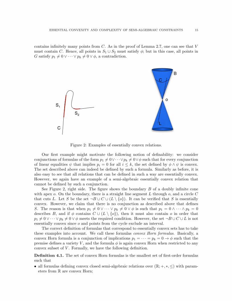
See Figure 2, left side. The figure shows a 1-dimensional variety C ⊆ R2, given as{(p(t), q(t)) | t ∈ R} for polynomials p and q. The figure also shows two marked segmentsS1, S2 on the curve C. The marked segments are chosen such that one end point is containedin interior of the convex hull of the other three end points of the segments.

Let S be the set ¬C ∪ S1 ∪ S2. Clearly, S is essentially convex. Now, suppose forcontradiction that S has a definition ψ as described above. Let H be the convex hull ofS1∪S2. The crucial observation is that the set G := (H ∩C)\ (S1∪S2) is infinite. Since nopoint from G is in S, there must be a conjunct p1 6= 0 ∨ · · · ∨ pk 6= 0 ∨ φ in ψ that excludesinfinitely many points from G. In particular, the variety V defined by p1 = · · · = pk = 0


contains infinitely many points from C. As in the proof of Lemma 2.7, one can see that Vmust contain C. Hence, all points in S1 ∪ S2 must satisfy φ; but in this case, all points inG satisfy p1 6= 0 ∨ · · · ∨ pk 6= 0 ∨ φ, a contradiction.

S1

S2

C

B

L

C

o

Figure 2: Examples of essentially convex relations.

Our first example might motivate the following notion of definability: we considerconjunctions of formulas of the form p1 6= 0∨· · ·∨pk 6= 0∨φ such that for every conjunctionof linear equalities ψ that implies pi = 0 for all i ≤ k, the set defined by φ ∧ ψ is convex.The set described above can indeed be defined by such a formula. Similarly as before, it isalso easy to see that all relations that can be defined in such a way are essentially convex.However, we again have an example of a semi-algebraic essentially convex relation thatcannot be defined by such a conjunction.

See Figure 2, right side. The figure shows the boundary B of a doubly infinite conewith apex o. On the boundary, there is a straight line segment L through o, and a circle Cthat cuts L. Let S be the set ¬B ∪ C ∪ (L \ {o}). It can be verified that S is essentiallyconvex. However, we claim that there is no conjunction as described above that definesS. The reason is that when p1 6= 0 ∨ · · · ∨ pk 6= 0 ∨ φ is such that p1 = 0 ∧ · · · ∧ pk = 0describes B, and if φ contains C ∪ (L \ {o}), then it must also contain o in order thatp1 6= 0 ∨ · · · ∨ pk 6= 0 ∨ φ meets the required condition. However, the set ¬B ∪C ∪ L is notessentially convex since o and points from the cycle exclude an interval.

The correct definition of formulas that correspond to essentially convex sets has to takethese examples into account. We call these formulas convex Horn formulas. Basically, aconvex Horn formula is a conjunction of implications p1 = · · · = pk = 0→ φ such that thepremise defines a variety V , and the formula φ is again convex Horn when restricted to anyconvex subset of V . Formally, we have the following definition.

Definition 4.1. The set of convex Horn formulas is the smallest set of first-order formulassuch that

• all formulas defining convex closed semi-algebraic relations over (R; +, ∗,≤) with param-eters from R are convex Horn;


• Suppose that p1, . . . , pk are polynomials, φ is a first-order formula that defines a setU ⊆ Rn, and for every semi-algebraic convex set C contained in the set defined byp1 = · · · = pk = 0, the set C ∩ U can be defined by a convex Horn formula, and hasstrictly smaller dimension than the set defined by ψ ≡ (p1 6= 0 ∨ · · · ∨ pk 6= 0 ∨ φ). Thenψ is also convex Horn.• Finite conjunctions of convex Horn formulas are convex Horn.

For example, the formula (x2 − y 6= 0) ∧ (y ≥ 1), describing the half-plane above y = 1with exception of the standard parabola, is convex Horn. Every convex set C contained inthe set defined by x2− y = 0 consists of at most one point, and hence is 0-dimensional andcan be defined by a convex Horn formula.

We can prove properties about the set of all convex Horn formulas by induction overthe level of a convex Horn formula, which is defined as follows. The level of a formula thatdefines a convex closed semi-algebraic relation is 0. Now, suppose we have already definedconvex Horn formulas of level smaller than i, and let ψ be a convex Horn formula that doesnot have level smaller than i. Then ψ has level i if it is the finite conjunction of formulasψ′ ≡ (p1 6= 0 ∨ · · · ∨ pk 6= 0 ∨ φ) such that for every semi-algebraic convex set C containedin the set defined by p1 = · · · = pk = 0, the intersection of C with the set defined by φ isconvex Horn, has level at most i− 1, and strictly smaller dimension than the set defined byψ′. Since the intersection of sets of dimension n has at most dimension n, it follows directlyfrom the definition of convex Horn formulas that the level of a convex Horn formula φ isbounded by the dimension of the set defined by φ.

Looking back at the formula (x2 − y 6= 0) ∨ (y ≥ 1), we claim that it is convex Horn oflevel one: every convex set contained in the parabola consists of at most one point, and canhence be described by a convex Horn formula of level zero. For another example, consider(x2 − y 6= 0) ∨ (z ≥ 0), i.e., the same parabola in three dimensions on one side side of thex-y-plane. Each convex subset of x2 − y = 0 is a point, a straight line, or a line segment inthe z direction and can again be described by a level zero convex Horn formula.

We are now ready to logically define essentially convex semi-algebraic sets via convexHorn formulas. This is done in two steps; we first prove (in Proposition 4.2) that every setdefined by a semi-algebraic convex Horn formula is essentially convex. The rest of the sectionis devoted to proving the other direction—the final result can be found in Theorem 4.6.

Proposition 4.2. Any set S defined by a convex Horn formula ψ over (R; ∗,+,≤) isessentially convex.

Proof. Our proof is by induction over the level of ψ. Let m denote the number of freevariables in ψ. If the level of ψ is 0, then S = {x ∈ Rm | ψ(x)} is a closed convex set and,in particular, essentially convex.

Assume that all relations defined by convex Horn formulas of level < i are essentiallyconvex. Arbitrarily choose a convex Horn formula ψ ≡ p1 6= 0 ∨ · · · ∨ pk 6= 0 ∨ φ withlevel i. Define S = {x ∈ Rm | ψ(x)}, V = {x ∈ Rm | p1(x) = · · · = pk(x) = 0}, andU = {x ∈ Rm | φ(x)}. Since ψ is level-i convex Horn, we know that for every semi-algebraicconvex set C such that C ⊆ V , the set C ∩ U can be defined by a convex Horn formula oflevel smaller than i and dim(C ∩ U) < dim(S).

Suppose for contradiction that there are a, b ∈ S and an infinite set I of points on theline segment L between a and b that is not contained in S. In particular, I ⊆ V sinceS = ¬V ∪ U . By Lemma 2.7, all points on the line through a and b are in V . However, aand b are in S and therefore in U so L∩U is not essentially convex. We now note that L is


a semi-algebraic convex set that is a subset of V so L∩U can be defined by a convex Hornformula of level smaller than i. Consequently, L ∩ U is essentially convex by the inductiveassumption which leads to a contradiction.

Finally, suppose that ψ is a finite conjunction of convex Horn formulas of level at mosti. Since the intersection of finitely many essentially convex relations is essentially convex,we are done also in this case.

Next, we need some preparations for the proof of the converse implication (Theo-rem 4.6): we show that semi-algebraic relations can be defined by a special type of for-mula (Lemma 4.4), and that the closure S of an essentially convex relation S is convex(Lemma 4.5).

Definition 4.3. Let S be a semi-algebraic relation. We say that a first-order formula φ isa standard defi of S if

• φ(x1, . . . , xk) defines S ⊆ Rk over (R; ∗,+,−,≤) with parameters from R;• φ is in quantifier-free conjunctive normal form;• if we remove any literal from φ, then the resulting formula is not equivalent to φ; and• all literals are of the form t ≤ 0 or t 6= 0.

Lemma 4.4. Every semi-algebraic relation S has a standard definition. If S is even semi-linear, then it has a standard definition φ that does not involve the function symbol formultiplication and irrational parameters.

Proof. By Theorem 2.8, we know that S has a quantifier-free definition over (R; ∗,+,≤) withparameters from R, and it is clear that such a definition can be rewritten in conjunctivenormal form φ. Replace a clause α in φ with a literal of the form a < b by two clauses α1

and α2 obtained from α by replacing a < b by a ≤ b and by a 6= b, respectively. In thesame way we can eliminate occurrences of a = b from φ using ≤. Literals of the form a ≤ b(a 6= b) can then be replaced by a− b ≤ 0 (and a− b 6= 0, respectively). Finally, we removeliterals from φ as long as the resulting formula is equivalent to the original formula.

If S is semi-linear, then by Theorem 2.10 we know that S has a quantifier-free definitionover (R; +,−,≤) with parameters from Q, and it is then clear that the formula constructedfrom φ as above will be a standard definition of S without the function symbol for multi-plication and irrational parameters.

Lemma 4.5. The closure S of an essentially convex relation S is convex.

Proof. Let a, b ∈ S. We will show that all points c on the line segment between a and b arein S. We have to show that for every ε > 0 there is a point c′ in S such that the distancebetween c and c′ is smaller than ε. Since a ∈ S and b ∈ S, there are points a′ ∈ S andb′ ∈ S that are closer than ε/2 to a and b, respectively. Let L be the line from a′ to b′. Itis clear that there are infinitely many points on L that are at distance less than ε from c.Hence, since a′ and b′ are in S and S is essentially convex, there must be one such point inS, and we are done.

Theorem 4.6. A semi-algebraic relation S ⊆ Rn is essentially convex if and only if it hasa convex Horn definition. Moreover, when S is even semi-linear then S has a semi-linearconvex Horn definition.

Proof. We have already seen in Proposition 4.2 that every relation defined by a convex Hornformula is essentially convex. We now show the more difficult implication of the statement.


Let φ be a standard definition of S. The proof is by induction on the dimension d of S. Ford = 0, the set S consists of at most one point, and the statement is trival. Otherwise, if|S| ≥ 2, then by essential convexity, Corollary 3.2, and Lemma 2.6 we have that dim(S) ≥ 1.

For d > 0, we will construct two formulas φ1, φ2 such that φ is equivalent to φ1 ∧ φ2.Thereafter, we will show that φ1 is equivalent to a conjunction of convex Horn formulas,and that φ2 defines a closed convex relation (and consequently is convex Horn). Since finiteconjunctions of convex Horn formulas are also convex Horn, φ is then equivalent to a convexHorn formula.

We begin by writing all clauses of φ as α→ β where α is either ‘true’ or a conjunctionof polynomial equalities and β is either ‘false’ or a disjunction of inequalities. This is alwayspossible since a clause

(p1 ≤ 0 ∨ · · · ∨ pk ≤ 0 ∨ q1 6= 0 ∨ · · · ∨ qm 6= 0)

is logically equivalent to

(q1 = 0 ∧ · · · ∧ qm = 0)→ (p1 ≤ 0 ∨ · · · ∨ pk ≤ 0).

Next, we rewrite all clauses α→ β where α is not equal to ‘true’, as (α→ (β ∧ φ)). Let φ1be the conjunction of all the implications of the type (α→ (β ∧φ)) and φ2 the conjunctionof the remaining implications, i.e., those of the type (true → β). The formula φ1 ∧ φ2 isclearly equivalent to the formula φ.

We begin by studying the formula φ1. Let α → (β ∧ φ) be a clause from φ1, let V bethe variety defined by α, and let U be the set defined by β ∧ φ. Observe that U ⊆ S. Wenow show that the intersection of the set U with a semi-algebraic convex set C ⊆ V can bedefined by a convex Horn formula. We make two claims about the set U ∩ C:

Claim 1. U ∩ C is essentially convex. For arbitrary points a, b ∈ U ∩ C, let Lab denote theline segment from a to b, and Xab = {x ∈ Lab | x 6∈ U ∩C}. Suppose for contradiction thatthere exist a, b ∈ U ∩ C such that Xab is an infinite set. Since a, b ∈ C and C is convex,Lab ⊆ C which implies that Xab = {x ∈ Lab | x 6∈ U}. Moreover, C ⊆ V so Xab ⊆ V . Nowrecall that a, b ∈ S since U ∩C ⊆ U ⊆ S: thus, there are infinitely many points (those thatare in Xab) between a, b ∈ S that are in V but not in U . This shows that no point in Xab

satisfies α→ (β ∧ φ), and Xab ∩ S = ∅. This fact contradicts the essential convexity of S.

Claim 2. U ∩ C has smaller dimension than S. Let T be the set S \ (U ∩ C). It sufficesto show that U ∩ C is a subset of T \ T , because Lemma 2.6 asserts that dim(T \ T ) <dim(T ) ≤ dim(S).

The set S must contain a point p that is not in V , because if S ⊆ V then we couldreplace the clause of φ that was re-written to α→ (β ∧ φ) by β and obtain a formula thatis equivalent to φ; this contradicts the assumption that φ is a standard definition of S.

To show that (U ∩C) ⊆ T \T , let x be an arbitrary point in U ∩C. Only finitely manypoints on the line segment between p and x can be from (U ∩ C) ⊆ V , because otherwiseProposition 3.3 implies that V must contain the entire line between x and p, including p,a contradiction. Also the set S contains all but finitely many points on the line segmentbetween p and x: this is by essential convexity of S, since x ∈ U ∩ C ⊆ S and p ∈ S.Hence, we can choose a sequence of points from T = S \ (U ∩ C) on this line segment thatapproaches x, which shows that x ∈ T .


Since U ∩C is semi-algebraic, essentially convex, and has smaller dimension than S, itfollows by the inductive assumption that it can be defined by a convex Horn formula. Thus,φ1 is equivalent to a finite conjunction of convex Horn formulas.

We claim that φ2 defines a closed convex set D. This follows from Lemma 4.5, since Dis in fact the closure of S. To see this, observe that D is clearly a closed set, D containsS, and hence S ⊆ D = D. To prove that D ⊆ S, let y be from D \ S. Consider theclauses α1 → (β1 ∧ φ), . . . , αl → (βl ∧ φ) of φ1, and let Vi, for 1 ≤ i ≤ l, be the variety{x ∈ Rk | x satisfies αi}. There must be a point q in S that is not contained in the setW =

⋃i≤l Vi; otherwise, Proposition 3.3 implies that there exists an i ≤ l such that S ⊆ Vi.

In other words, all points in S satisfy αi. This is in contradiction to the assumption that φ isa standard definition of S, since in this case the formula φ is equivalent to the formula wherethe clause of φ that has been rewritten to αi → (βi∧φ) is replaced by βi. Only finitely manypoints on the line segment L between q and y can be from W , because otherwise Lemma 2.7implies that W contain the entire line between y and q, including q, a contradiction. Hence,y ∈ S.

Finally, consider the case that S is semi-linear. By Lemma 4.4, we can choose φ to bea standard definition which is semi-linear (and only uses parameters in Q). Then the proofabove leads to a semi-linear convex Horn definition of S.

5. Applications

5.1. Semi-linear constraint languages. We will now show that a finite semi-linear ex-pansion Γ of Γlin has a polynomial-time tractable constraint satisfaction problem if and onlyif all relations of Γ are essentially convex (unless P = NP). Recall that a relation is semi-linear if it has a first-order definition in (R; +, 1,≤). A quantifier-free first-order formulain CNF is called Horn-DLR [21] (where ‘DLR’ stands for disjunctive linear relations) if itsclauses are of the form

p1 6= 0 ∨ · · · ∨ pk 6= 0

or of the formp1 6= 0 ∨ · · · ∨ pk 6= 0 ∨ p0 ≤ 0

where p0, p1, . . . , pk are linear terms with rational coefficients. A semi-linear relation iscalled Horn-DLR if it can be defined by a Horn-DLR formula.

Theorem 5.1 (see [10, 21, 22]). Let Γ be a structure with domain R whose relations areHorn-DLR. Then CSP(Γ) is in P.

In this section, we show the following.

Theorem 5.2. Let Γ = (Γlin, S1, . . . , Sl) be a constraint language such that S1, . . . , Sl aresemi-linear relations. Then, either each relation S1, . . . , Sl is Horn-DLR and CSP(Γ) is inP, or CSP(Γ) is NP-complete.

In order to prove Theorem 5.2, we need to characterize convex and essentially convexsemi-linear relations. This is done in Lemma 5.3 and Theorem 5.4, respectively.

Let P1, . . . , Pn be (possibly unbounded) polyhedra defined such that Pi = {x ∈ Rk | Aix ≤bi}. Bemporad et al. [3] define the envelope of P1, . . . , Pn (env(P1, . . . , Pn)) as the polyhe-dron


{x ∈ Rk | A′1x ≤ b′1, . . . , A′nx ≤ b′n}where A′ix ≤ b′i is the subsystem of Aix ≤ bi obtained by removing all the inequalities notvalid for the other polyhedrons P1, . . . , Pi−1, Pi+1, Pn. We note that if P1, . . . , Pn are definedwith coefficients from Q, then env(P1, . . . , Pn) can be described by rational coefficients, too.By combining Theorem 3 with Remark 1 in [3], it follows that

⋃ni=1 Pi is convex if and only

if⋃ni=1 Pi = env(P1, . . . , Pn).

Lemma 5.3. A closed semi-linear relation S is convex if and only if it has a primitivepositive definition in (R; +, 1,≤).

Proof. It is straightforward to verify that relations with a primitive positive definition in(R; +, 1,≤) are convex; each relation defines a convex set and the intersection of convexsets is convex itself.

For the converse, let φ = ψ1 ∨ · · · ∨ ψm be a quantifier-free definition of S over thestructure (R; +,−,≤) with parameters from Q, written in disjunctive normal form. If thereis a disjunct ψi that contains a literal p 6= q, for linear terms p and q, then split the disjunctinto two; one containing p− q < 0 and one containing p− q > 0. By repeating this process,every literal p 6= q can be removed. Similarly, every literal p = q can be replaced byp− q ≤ 0 ∧ q− p ≤ 0. Thus, we may assume that every literal appearing in the ψi is of thetype p ≤ 0 or p < 0, for a linear term p. Let D1, . . . , Dm be the sets defined by ψ1, . . . , ψm,respectively.

Now recall that the topological closure operator preserves finite unions, i.e., D1 ∪ · · · ∪Dm = D1 ∪ · · · ∪Dm. Hence,

S = D1 ∪ · · · ∪Dm ⊆ D1 ∪ · · · ∪ Dm = D1 ∪ · · · ∪Dm = S = S

and S = D1 ∪ · · · ∪ Dm. We now note that if P = {x ∈ Rk | Ax ≤ b, Cx < d} and P 6= ∅,then P = {x ∈ Rk | Ax ≤ b, Cx ≤ d}, cf. Case (i) of Proposition 1.1 in [17]. Thus, each Di

equals {x ∈ Rk | Aix ≤ bi} for some rational Ai, bi. Furthermore, S =⋃mi=1 Di is convex

so S = env(D1, . . . , Dm). This implies that S = {x ∈ Rk | C1x ≤ d1, . . . , Cmx ≤ dm}for some rational matrices C1, . . . , Cm and rational vectors d1, . . . , dm. It is easy to seethat each Cix ≤ di is pp-definable in (R; +, 1,≤) by the same technique as in the proof ofLemma 2.11, and this concludes the proof.

Theorem 5.4. A semi-linear relation S is essentially convex if and only if S is Horn-DLR.

Proof. We first prove that every Horn-DLR relation S is essentially convex. Let φ be aHorn-DLR definition of S. Suppose for contradiction that there are a, b ∈ S and an infiniteset I of points on the line segment L between a and b is not contained in S. Since φ hasfinitely many conjuncts, there is a conjunct ψ in φ that is false for an infinite subset I ′ of I.If ψ is of the form p1 6= 0 ∨ · · · ∨ pk 6= 0, then all points in I ′ satisfy p1 = · · · = pk = 0. ByLemma 2.7, the entire line L satisfies p1 = · · · = pk = 0. This contradicts the assumptionthat a ∈ L and b ∈ L satisfy φ. If ψ is of the form p1 6= 0 ∨ · · · ∨ pk 6= 0 ∨ p0 ≤ 0, then allpoints in I ′ satisfy p1 = · · · = pk = 0 and p0 > 0. Again by Lemma 2.7 we find that botha and b must satisfy p1 = · · · = pk = 0. Since a, b also satisfy ψ, we conclude that bothpoints satisfy p0 ≤ 0. But then also all points in L must satisfy p0 ≤ 0, which contradictsthe fact that the points in I ′ satisfy p0 > 0.

The other direction of the statement can be derived from Theorem 4.6 as follows. LetS be an essentially convex semi-linear relation. By Theorem 4.6, S has a semi-linear convex


Horn definition ψ. We prove by induction on the level of ψ that ψ is Horn-DLR. If the levelis 0, then S is closed and convex and the claim follows from Lemma 5.3. Now suppose thatψ has level i > 0 and is of the form p1 6= 0∨· · ·∨pk 6= 0∨ψ′, where p1 = · · · = pk = 0 definesa set V , and ψ′ defines a set U such that for every semi-algebraic convex set C ⊆ V the setC ∩ U has a convex Horn definition of level strictly smaller than i. Since ψ is semi-linear,the terms p1, . . . , pk are linear. Hence, V is convex, and by taking C := V in the statementabove we see that V ∩ U has a convex Horn definition of level strictly smaller than i. Bythe inductive assumption, V ∩ U has a definition by a Horn-DLR formula φ with clausesφ1, . . . , φm. Then φ′ =

∧1≤i≤m(p1 6= 0 ∨ · · · ∨ pk 6= 0 ∨ φi) is clearly Horn-DLR. We claim

that φ′ defines S. First suppose that a ∈ ¬V . In this case, a clearly satisfies φ′ and this isjustified by the fact ¬V ⊆ S. Suppose instead that a ∈ V . Then a satisfies φ′ if and onlyif it satisfies φ, and since φ defines V ∩ U this is the case if and only if a satisfies ψ′.

Finally, the statement holds if ψ is the conjunction of finitely many convex Horn for-mulas (which are Horn-DLR by inductive assumption).

Proof of Theorem 5.2. If all relations of Γ are Horn-DLR, then CSP(Γ) can be solved inpolynomial time (Theorem 5.1). Otherwise, if there is a relation S from Γ that is not Horn-DLR, then Theorem 5.4 shows that S is not essentially convex, and NP-hardness of CSP(Γ)follows by Lemma 3.9.

So we only have to show that CSP(Γ) is in NP. Let Φ be an arbitrary instance ofCSP(Γ). By Theorem 2.10 every relation of Γ has a quantifier-free definition in conjunctivenormal form over (R; +,−,≤) with rational parameters. One can now non-deterministicallyguess one literal from each clause of in the defining formula for each constraint and verify– in polynomial-time by Theorem 5.1 – that all the selected literals are simultaneouslysatisfiable.

5.2. Generalized linear programming. In this section, we study generalizations of thefollowing problem.

Linear Programming (LP)

INPUT: A finite set of variables V , a vector c ∈ Q|V |, a number M ∈ Q, and a finiteset of linear inequalities of the form a1x1 + · · · + anxn ≤ a0 where x1, . . . , xn ∈ V anda0, . . . , an ∈ Q. All rationals are given by numerators and denominators represented inbinary.QUESTION: Is there a vector x ∈ R|V | that satisfies the inequalities and cTx ≥M?

We generalize LP as follows. Let Γ be a structure (Γlin, R1, . . . , Rm) such thatR1, . . . , Rmare semi-linear relations.

Generalized Linear Programming for Γ (GLP(Γ))

INPUT: A finite set of variables V , a vector c ∈ Q|V |, a number M ∈ Q, and a finite set Φof expressions of the form R(x1, . . . , xk) where R is a relation from Γ and x1, . . . , xk ∈ V .

QUESTION: Is there a vector x ∈ R|V | that satisfies the constraints and cTx ≥M?

This can indeed be viewed as a generalization of LP because of Proposition 2.12: theproblem LP is polynomial-time equivalent to the problem GLP(Γlin).


Theorem 5.5. Let Γ = (R; Γlin, R1, . . . , Rl) be a structure with semi-linear relations R1, . . . , Rl.Then, either each Ri is Horn-DLR and GLP(Γ) is in P, or GLP(Γ) is NP-hard.

Proof. If there is an Ri that is not Horn-DLR, then the relation Ri is not essentially convexby Theorem 5.4, and CSP((Γlin, Ri)) is NP-hard by Theorem 5.2. Clearly, GLP(Γ) is NP-hard, too.

Assume instead that each Ri is Horn-DLR. We present an algorithm that actually solvesa more general problem that includes GLP(Γ). Let Φ be an arbitrary satisfiable Horn-DLRformula3 over variable vector x = (x1, . . . , xn) and let c be a rational n-vector.

We assume additionally that Φ∧D is satisfiable for every disequality literal (i.e., literalp(x) 6= a) D appearing in Φ. If Φ ∧ D is not satisfiable, then every occurrence of D in Φcan be removed without changing the set defined by the formula. Furthermore, this checkcan be carried out in polynomial time by Theorem 5.1. Hence, we may assume that Φhas this additional property (which we will refer to as (∗)) without loss of generality. LetΦ = Φ′∧Φ′′ where Φ′ consists of the clauses not containing any disequality literal p(x) 6= a,and Φ′′ consists of the remaining clauses.

Given Φ, our algorithm returns one of the following three answers:

• ‘unbounded’: for every K ∈ Q, there exists a solution y such that cT y ≥ K;• ‘optimum: K’: there exists a K ∈ Q and a solution y such that cT y = K, but there is no

solution y′ such that cT y′ > K;• ‘optimum is arbitrarily close to K’: there exists a K ∈ Q such that there is no solutiony satisfying cT y ≥ K, but for every ε > 0 there is a solution y′ with cT y′ ≥ K − ε.

We claim that the following algorithm solves the task described above in polynomial time.

Step 1. Maximize cT x over Φ′ (by using some polynomial-time algorithm for linear pro-gramming). Let K denote the optimum. If K =∞, then return ‘unbounded’ and stop.

Step 2. Check whether Φ ∧ cT x = K is satisfiable. Note that cT x = K has a primi-tive positive definition in Γlin, which furthermore can be computed in polynomial time byLemma 2.11. Therefore this check can be reduced to deciding satisfiability of Horn-DLRs.If Φ∧ cT x = K is satisfiable, then return ‘optimum: K’. If this is not the case, then return‘optimum is arbitrarily close to K’.

We first show that the algorithm runs in polynomial time. Step 1 takes polynomial timesince maximizing cT x over Φ′ is equivalent to solving a linear program with size polynomiallybounded in the size of Φ. Finally, Step 2 takes polynomial time due to Lemma 2.11 andTheorem 5.1.

Next, we prove the correctness of the algorithm. Correctness is obvious if the algorithmanswers ‘optimum: K’ in Step 2. For the remaining cases, we need to make a couple ofobservations. Define S = {x ∈ Rn | x satisfies Φ} and S′ = {x ∈ Rn | x satisfies Φ′}.Let D1, . . . , Dm denote the disequality literals appearing in Φ. Let Hi be the set {x ∈Rn | x does not satisfy Di}, 1 ≤ i ≤ m, and note that each Hi is a hyperplane.

Observation 1. The formula Φ− ≡ Φ ∧D1 ∧ · · · ∧Dm is satisfiable.

3Note that if we are given an instance of CSP((Γlin, R1, . . . , Rl)), then it can be transformed into anequivalent Horn-DLR formula in polynomial time since there is only a finite number of relations in the givenstructure. Hence, there is no loss of generality in considering Horn-DLR formulas instead of CSP instances.Also note that the resulting formula is (up to a multiplicative constant depending on the structure) of thesame size as the CSP instance.


Otherwise, S ⊆ H1∪· · ·∪Hm. The set S is essentially convex and each Hm is a variety,so there exists an 1 ≤ i ≤ m such that S ⊆ Hi by Proposition 3.3. Consequently, Φ ∧Di isnot satisfiable which contradicts the fact that Φ has property (∗).Observation 2. For every ε > 0 there is a y ∈ S satisfying |cTw − cT y| < ε.

Let d(·, ·) denote the Euclidean distance in Rn, i.e., d(a, b) =√∑n

i=1(ai − bi)2, and || · ||the corresponding norm, i.e., ||a|| =

√aTa.

Arbitrarily choose a point z that satisfies Φ−; this is always possible by Observation 1.Consider the line segment L between z and w. Note the following: if H is a hyperplane inRn, then either H intersects L in at most one point or L ⊆ H. Also note that w, z ∈ S′and S′ is convex so L ⊆ S′. Arbitrarily choose a clause C ∈ Φ′′ and assume C = (p1(x) 6=0 ∨ · · · ∨ pk(x) 6= 0 ∨ p0(x) ≤ 0). Assume that there exist two distinct points a, b ∈ L suchthat p1(a) = p1(b) = 0. If so, then every point c ∈ L satisfies p1(c) = 0. This is not possiblesince z ∈ L satisfies D1 ∧ · · · ∧Dm, and in particular p1(z) 6= 0. Hence, at most one pointc ∈ L satisfies p(c) = 0, and c is the only point in L that potentially does not satisfy theclause C. This implies that only finitely many points in L do not satisfy Φ′′, and it followsthat for every δ > 0 there is a point y ∈ S such that d(w, y) < δ.

We proceed by showing that if w, y ∈ Rn and d(w, y) = d, then |cTw − cT y| ≤ ||c|| · d.This follows from the Cauchy-Schwarz inequality (that is, |aT b| ≤ ||a|| · ||b|| for vectors a, bin Rn):

|cTw − cT y| = |cT (w − y)| ≤ ||c|| · ||w − y|| = ||c|| · d(w, y) = ||c|| · d.

To find a vector y that satisfies |cTw − cT y| < ε, we simply choose y ∈ S such thatd(w, y) < ε

||c|| ; we know that such a y exists by the argument above.

If the algorithm outputs ‘unbounded’ in Step 2, then arbitrarily choose a sufficientlylarge number k and note that there exists a vector w ∈ S′ such that cTw ≥ k. By Obser-vation 2, there exists a vector y ∈ S such that |cTw − cT y| < 1. Hence, S has unboundedsolutions, too.

Assume finally that the algorithm answers ‘optimum is arbitrarily close to K’ in Step 3;Observation 2 immediately proves correctness in this case.

6. Open Problems

The most prominent open question is whether there are there are essentially convex relationsS with a first-order definition in (R; ∗,+) such that CSP((Γlin, S)) is NP-hard. Resolvingthis question is probably difficult, since the following closely related problem is of unknowncomputational complexity:

Feasibility of Convex Polynomial InequalitiesINPUT: A set of variables V , a set of polynomial inequalities each of which defining a con-vex set; the coefficients of the polynomials are rational numbers where the numerators anddenominators are represented in binary.QUESTION: Is there a point in R|V | that satisfies all inequalities?

One may note that the problems we have considered could be easier since they aredefined over finite constraint languages. On the other hand, convexity is much more restric-tive than essential convexity; moreover, we are only given polynomial inequalities (there


are convex semi-algebraic relations that cannot be defined as the intersection of convexpolynomial inequalities). Still, the computational complexity of the Feasibility Problem ofConvex Polynomial Inequalities is open.

Convex semi-algebraic relations are of particular interest in the quest for efficientlysolvable semi-algebraic constraint languages because of a conjectured link to semidefiniteprogramming. Every semidefinite representable set is convex and semi-algebraic. Recently,Helton, Vinnikov and Nie showed that the converse statement is true in surprisingly manycases and conjectured that it remains true in general [18].

Acknowledgements

We would like to thank Johan Thapper for pointing out inaccuracies in an earlier versionof the article, Frank-Olaf Schreyer for helpful discussions in the early stages of this work,and the referees for their detailed remarks.

References

[1] L. Barto and M. Kozik. Constraint satisfaction problems of bounded width. In Proceedings of FOCS,pages 595–603, 2009.

[2] S. Basu, R. Pollack, and M.-F. Roy. Algorithms in Real Algebraic Geometry, 2nd edition. Springer-Verlag, 2009.

[3] A. Bemporad, K. Fukuda, and F. Torrisi. Convexity recognition of the union of polyhedra. Computa-tional Geometry, 18(3):141–154, 2001.

[4] J. Bochnak, M. Coste, and M.-F. Roy. Real Algebraic Geometry. Springer-Verlag, 1998.[5] M. Bodirsky. Constraint satisfaction problems with infinite templates. In H. Vollmer, editor, Complexity

of Constraints (a collection of survey articles), volume 5250 of Lecture Notes in Computer Science, pages196–228. Springer, 2008.

[6] M. Bodirsky and J. Kara. The complexity of temporal constraint satisfaction problems. Journal of theACM, 57(2):41 pp, 2009. An extended abstract appeared in the proceedings of STOC’08.

[7] A. A. Bulatov. Tractable conservative constraint satisfaction problems. In Proceedings of LICS’03, pages321–330, Ottawa, Canada, 2003.

[8] A. A. Bulatov. A dichotomy theorem for constraint satisfaction problems on a 3-element set. Journalof the ACM, 53(1):66–120, 2006.

[9] A. A. Bulatov, A. A. Krokhin, and P. G. Jeavons. Classifying the complexity of constraints using finitealgebras. SIAM Journal on Computing, 34:720–742, 2005.

[10] D. Cohen, P. Jeavons, P. Jonsson, and M. Koubarakis. Building tractable disjunctive constraints. Jour-nal of the ACM, 47(5):826–853, 2000.

[11] T. Drakengren and P. Jonsson. Computational complexity of temporal constraint problems. In Handbookof Temporal Reasoning in Artificial Intelligence, pages 197–218. Elsevier, 2005.

[12] F. Dumortier, M. Gyssens, L. Vandeurzen, and D. V. Gucht. On the decidability of semilinearity forsemialgebraic sets and its implications for spatial databases. Journal on Computer and System Sciences,58(3):535–571, 1999.

[13] F. Dumortier, M. Gyssens, L. Vandeurzen, and D. V. Gucht. On the decidability of semilinearity forsemialgebraic sets and its implications for spatial databases - corrigendum. Journal on Computer andSystem Sciences, 59(3):557–562, 1999.

[14] T. Feder and M. Y. Vardi. The computational structure of monotone monadic SNP and constraintsatisfaction: a study through Datalog and group theory. SIAM Journal on Computing, 28:57–104, 1999.

[15] J. Ferrante and C. Rackoff. A decision procedure for the first order theory of real addition with order.SIAM Journal on Computing, 4(1):69–76, 1975.

[16] M. Garey and D. Johnson. A guide to NP-completeness. CSLI Press, Stanford, 1978.[17] M. A. Goberna, V. Jornet, and M. M. L. Rodrıguez. On linear systems containing strict inequalities.

Linear Algebra and its Applications, 360:151 – 171, 2003.


[18] J. W. Helton and J. Nie. Sufficient and necessary conditions for semidefinite representability of convexhulls and sets. SIAM Journal on Optimization, 20(2):759–791, 2009.

[19] W. Hodges. A shorter model theory. Cambridge University Press, Cambridge, 1997.[20] P. Jeavons, D. Cohen, and M. Gyssens. Closure properties of constraints. Journal of the ACM, 44(4):527–

548, 1997.[21] P. Jonsson and C. Backstrom. A unifying approach to temporal constraint reasoning. Artificial Intelli-

gence, 102(1):143–155, 1998.[22] M. Koubarakis. Tractable disjunctions of linear constraints: Basic results and applications to temporal

reasoning. Theoretical Computer Science, 266:311–339, 2001.[23] D. Marker. Model Theory: An Introduction. Springer, New York, 2002.[24] D. Marker, Y. Peterzil, and A. Pillay. Additive reducts of real closed fields. Journal of Symbolic Logic,

57(1):109–117, 1992.

This work is licensed under the Creative Commons Attribution-NoDerivs License. To viewa copy of this license, visit http://creativecommons.org/licenses/by-nd/2.0/ or send aletter to Creative Commons, 171 Second St, Suite 300, San Francisco, CA 94105, USA, orEisenacher Strasse 2, 10777 Berlin, Germany

Documents

Essential Convexity and Complexity of Semi-Algebraic Constraints