ESA Space Weather Programme Study Alcatel Consortium

A Prototype Real-Time Forecast Service of Space Weather and Effects

Using Knowledge-Based Neurocomputing

WP3220 and WP3210

Henrik Lundstedt

Version October, 2100

ESA Officer: A. Hilgers, ESTEC

2

Henrik Lundstedt

Swedish Institute of Space Physics Solar-Terrestrial Physics Division

Scheelev. 17 SE-223 70 Lund, Sweden

TABLE OF CONTENTS

1.Introduction 5 2. Models based on Knowledge-Based Neurocomputing 7 2.1 Predictions of long-term solar activity 7 2.1.1 As described by sunspot numbers and

solar magnetic field data 7 2.2 Prediction of medium- and short-term solar activity 8 2.2.1 Coronal mass ejections 9 2.2.2 Proton events 10 2.2.3 Solar flares 10 2.2.4 Coronal holes 11 2.3 Prediction of solar wind parameters 12 2.3.1 Solar wind velocity 12 2.3.2 Solar wind Bz component 14 2.4 Prediction of electron flux in magnetosphere 14 2.5 Prediction of geomagnetic activity 14

3

2.5.1 Daily Ap index 14 2.5.2 Hourly Kp, Dst and AE index 15 2.5.3 Local geomagnetic field 17 2.5.4 Aurora 18 2.6 Prediction of communication conditions 18 2.6.1 Plasma frequency foF2 18 2.7 Prediction of effects 19 2.7.1 Satellite anomalies 19 2.7.2 Satellite drag 19 2.7.3 Geomagnetically induced currents 19 2.8 Table Summary of KBN models 20 3. Prototype Overview 22 3.1 Front Page 22 3.2 User Guide 23 3.3 Sun Stoplight Applets 24 3.3.1 Nowcasts 24 3.3.2 Forecasts 26

3.4 L1 Stoplight Applet 27 3.4.1 Nowcasts 28 3.4.2 Forecasts 28 3.5 Earth Stoplight 28 3.5.1 Now casts 29 3.5.2 Forecasts 30 3.6 Plot tools 31 3.7 Database 32 3.8 Demo functions 32 3.8.1 Test a Dst geomagnetic storm model 33 3.8.2 Create a prototype event 39

3.9 Case study 40 3.10 Extension of Prototype 44

3.10.1 Procedures for updating the Space Weather Prototype 44 3.10.2 Procedures for updating predictions

with new data and results 44 3.10.3 Defining methods for taking into

account feedback from users 45 Summary 45 Acronyms 46 Acknowledgements 46 Appendix

A1 Html links 46 A1.1 Forecast input data 46 A1.2 What is space weather? 46

4

A1.3 space weather glossary 46

A2 Most common neural networks 46 A2.1 Multilayer-error-back propagation 47 A2.2 Elman recurrent neural network 48 Á.2.3 Self Organized Map network 49 A2.4 Radial Basis Function network 50

A3 Java programs and applets developed 51 References 53 1. Introduction Space weather refers to conditions in space that can influence technological systems and endanger human health and life. The effects are described in detail in WP 1300 and 1400. Space weather services require real-time forecasts. The available services worldwide and a suggested future service are described in WP 3110. IRF-Lund offers space weather service, being a Regional Warning Center within the International Space Environment Service. Space weather forecast service must be available in real-time to mitigate the effects for the users. The service must also be useful and understandable to the user. Space weather deals with real-world problems, i.e. conditions and processes that most often are described as nonlinear and chaotic. Real-world data means outliers and data gaps. Neurocomputing techniques have therefore been successful in modeling and forecasting space weather conditions and effects, simply because they can describe non-linear chaotic dynamic systems. They are also robust and still work despite data problems. Also expert systems, genetic algorithms, hybrid systems such as neurofuzzy systems and combinations of neural networks and MHD models have been used. We therefore recommend the use of integrated methods, herewith using all knowledge available. Such integrated systems are “Knowledge-Based Neurocomputing” (KBN, 2000). Traditionally Artificial Intelligence (AI) represented the symbolic approach to knowledge processing and coding. Recently, however AI (the new AI) also includes soft computing methods such as neural networks, fuzzy systems, genetic algorithms and so on.. The term Intelligent Hybrid Systems (HIS) is used for the focusing on the integrating of soft computing methods. We however prefer using the term KBN since it emphasizes the processing, representation of knowledge using neural networks. Neural networks (Lundstedt 1997; Haykin 1994, see appendix) can map a vector of input (or nodes) to a vector of outputs through layers of nonlinear functions. There is a class of neural networks that is called recurrent, because past outputs are fed back to the system in addition to inputs. The past outputs are termed "context nodes" and represent the internal state of the neural network. Since formally the neural networks can be rewritten as a set

5

of differential equations, this number also indicates the number of differential equations needed to model the dynamics e.g. described by the AE index (of course such equations would still need to be driven by the solar wind input). Recently the AE dynamics was investigated using Elman recurrent neural networks (Gleisner and Lundstedt, 2001). When the number of context nodes is varied so as to minimize the network prediction error for validation data, it turns out that the optimal number of context nodes is 4. This provides an indication of a low number of magnetospheric degrees of freedom. In (Vassiliadis et al., 2001) we identify the freedom degrees with four current systems in the magnetosphere. This is an important illustration of how neural network model can be physically interpreted. Neural networks are not black boxes to quote Omlin and Giles (KBN, 2000), “Until recently, it was a widely accepted myth that neural networks were black boxes, i.e. the knowledge stored in their weights after training was not accessible to inspection, analysis, and verification. Since then, research on that topic has resulted in a number of algorithms for extracting knowledge in symbolic form from trained neural networks…” The first prediction of the Dst-index, characterizing the global magnetospheric state, using only solar wind parameters and neural networks was developed over 10 years ago and presented at the IAGA meeting in Vienna 1991 (Lundstedt, 1991). Many similar studies of the solar wind interaction have after that been carried out. Three thesis in Lund have been published (Wu, 1997; Wintoft, 1997 and Gleisner, 2000). It was found in (Wu and Lundstedt, 1996) that a neural network gives the best prediction of Dst, by creating by itself a mathematical function for the solar wind-magetospheric coupling, i.e. better than with a predefined coupling function. The first Artificial Intelligence (AI) approach to model the solar-terrestrial system was presented in late 80-ties by Lundstedt (Lundstedt, 1990). An inductive expert system was used. After that we have been working on the Lund Space Weather Model (Lundstedt, 1998, 1999) that is based on AI techniques or Knowledge-Based Neurocomputing (Lundstedt, 1997). The prototype is an implementation of part of that model. During the work on the Lund Space Weather Model several forecast modules have been developed based on neural networks. New forecast modules have also been developed for the use within the prototype 1. The prototype has been implemented in Java. 2. Models based on AI techniques and KBN Here follows a description of different models based on AI/KBN, developed by several research groups. The models developed by the Lund group is part of the development of the Lund Space Weather Model, which is an intelligent hybrid system (IHS) . A similar IHS but for only the magnetosphere/ionosphere the so called Magnetospheric

6

Specification Model (MSM) has been developed by the Rice group and implemented by Stirling Software for NOAA/SEC. Html links to input data for forecasts can be found in appendix A1. 2.1 Prediction of long-term solar activity 2.1.1 As described by the sunspot number and solar magnetic field data Long-term solar activity refers to activity on years, associated with the 11 years solar cycle. Predictions of long-term solar activity are important because of the solar effect on satellite drag, communication and climate changes. Many groups have developed neural network prediction models of the sunspot number (Ashmall and Moore, 1998; Conway et al., 1998; Calvo et al., 1995; Fessant et al., 1995; Liszka, 1993) in order to predict the the time and amplitude of the solar cycle maximum. The sunspot number (R) is given by

where f is the number of individual spots, g is the number of sunspot groups and k is a coefficient to adjust for differences in the observer or telescope. In their study, Calvo et al. started by constructing an attractor. In this way they obtained the embedded dimension and therefore how many variables they need to describe the dynamic system. From that they learned how many input nodes they needed for the neural network. They found they needed twelve input nodes i.e. 12 yearly values for a prediction of next year value. Ashmall and Moore on the other hand found they needed monthly values (one monthly value each year) to predict next year. Mundt et al., 1991 showed that the solar activity dynamics could be described by a chaotic system. That implies that forecasts longer ahead than a couple of years are impossible, if not further information is available. Schatten et al., (1978) found a relation between that solar magnetic field strength at solar poles at solar cycle minimum and the coming amplitude of the solar cycle maximum. With that precursor knowledge Ashmall and Moore managed to improve their predictions. They predicted the monthly maximum for solar cycle to be 160±10 in January 2000. The observed maximum seemed to have occurred around July 2000 with a maximum of 169.1 (Figure 1).

R = k(10g + f )

7

Figure 1 shows monthly sunspot number R for cycles 15, 22 and 23. Latest value plotted is for August 2001. No predictions, using neural networks and the less noisy monthly sunspot group number constructed by Hoyt and Schatten, (1998) have been developed. It spans over a 385-year period. Wavelet studies have however been carried out in order to study the Maunder minimum. Studies about how long-term solar activity might be related to to climate changes are carried out at IRF-Lund. 2.2 Predictions of medium- and short-term solar activity Medium-term solar activity refers to activity on days to months associated with active regions. Short-term activity refers to activity on hours to days. 2.2.1 Coronal mass ejections Coronal mass ejections (CMEs) are the ways the Sun gets rid of its magnetic field globally in huge loops. Largest mass ejected: 5-50 billion tons. Frequency of occurrence: 3.5/day events (solar activity max) and 0.2 events/day (solar min). Speed: 50-2000km/s. Fast CMEs with associated shocks cause the most severe space weather effects.

8

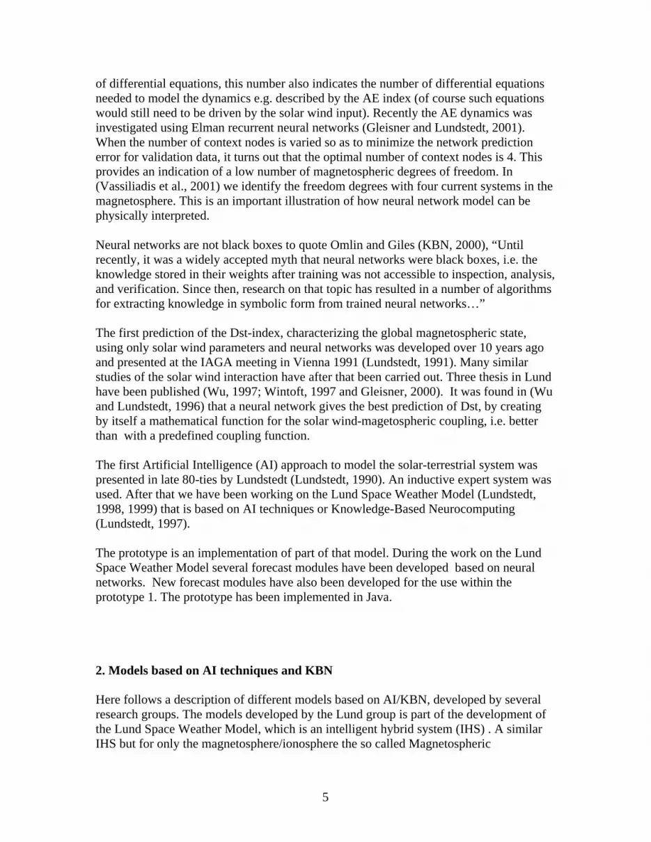
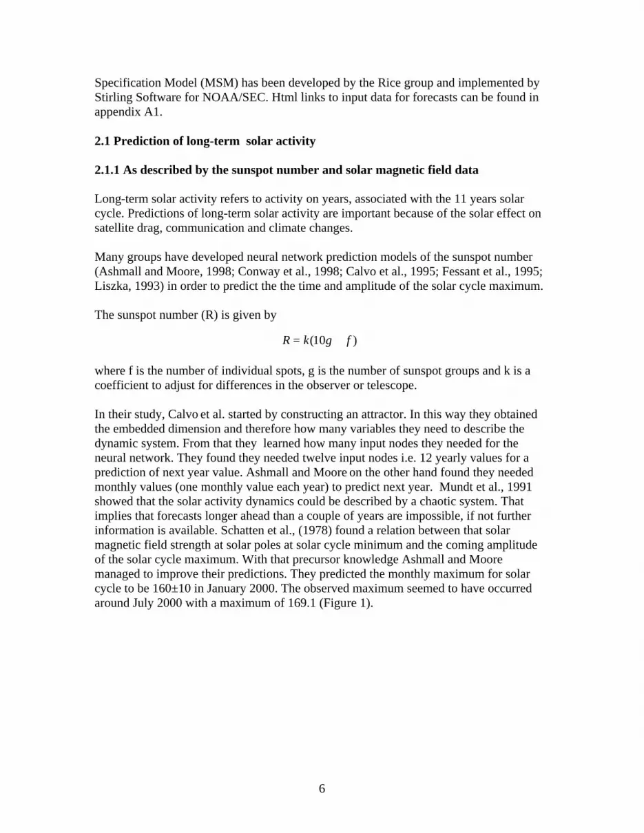
Figure 2 shows a halo coronal mass ejection, observed by LASCO on board SOHO on September 24, 2001. Observations with the coronagraph LASCO onboard SOHO give us information about CMEs. Together with observations, using the EIT instrument onboard, is it possible to determine whether or not a halo CME (Figure 2) is headed directly at us or from us. No method, based on KBN, exists today capable of predicting CMEs. However, a new method based on wavelet power spectra of SOHO/MDI mean field measuremets, seemed to be able to detect CMEs (Lundstedt et al.,2001; Boberg and Lundstedt, 2000). The wavelet power spectra of the solar mean magnetic field show peaks at times of CMEs. The mean field signal of the CME is now studied by the Lund group to see whether or not it’s possible to forecast CMEs with the use of neural networks from the signal. 2.2.2 Proton events Fast CMEs cause proton events that can last several days. Proton events often cause satellite problems. A proton event is defined from the proton flux (Appendix A3). The proton flux is measured by GOES (Figure 3).

9

Figure 3 shows the proton flux (proton event) caused by a coronal mass ejection on September 23, 2001. Xue et al. (1997) have developed predictions of proton events. They used a MLP neural network and as inputs solar flare location, duration, X-ray flux and radio flux. Most successful have Gabriel and colleagues (2000) been, using a neurofuzzy system with X-ray solar flare flux intensity as input and as output proton events days ahead. 2.2.3 Solar flares

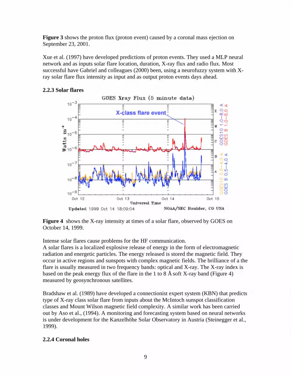
Figure 4 shows the X-ray intensity at times of a solar flare, observed by GOES on October 14, 1999.

Intense solar flares cause problems for the HF communication. A solar flares is a localized explosive release of energy in the form of electromagnetic radiation and energetic particles. The energy released is stored the magnetic field. They occur in active regions and sunspots with complex magnetic fields. The brilliance of a the flare is usually measured in two frequency bands: optical and X-ray. The X-ray index is based on the peak energy flux of the flare in the 1 to 8 Å soft X-ray band (Figure 4) measured by geosynchronous satellites. Bradshaw et al. (1989) have developed a connectionist expert system (KBN) that predicts type of X-ray class solar flare from inputs about the McIntoch sunspot classification classes and Mount Wilson magnetic field complexity. A similar work has been carried out by Aso et al., (1994). A monitoring and forecasting system based on neural networks is under development for the Kanzelhöhe Solar Observatory in Austria (Steinegger et al., 1999). 2.2.4 Coronal holes

10

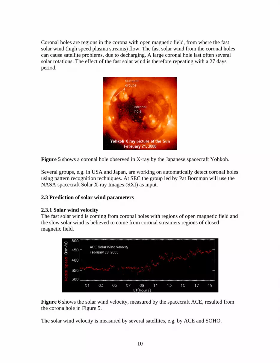
Coronal holes are regions in the corona with open magnetic field, from where the fast solar wind (high speed plasma streams) flow. The fast solar wind from the coronal holes can cause satellite problems, due to decharging. A large coronal hole last often several solar rotations. The effect of the fast solar wind is therefore repeating with a 27 days period.

Figure 5 shows a coronal hole observed in X-ray by the Japanese spacecraft Yohkoh. Several groups, e.g. in USA and Japan, are working on automatically detect coronal holes using pattern recognition techniques. At SEC the group led by Pat Bornman will use the NASA spacecraft Solar X-ray Images (SXI) as input. 2.3 Prediction of solar wind parameters 2.3.1 Solar wind velocity The fast solar wind is coming from coronal holes with regions of open magnetic field and the slow solar wind is believed to come from coronal streamers regions of closed magnetic field.

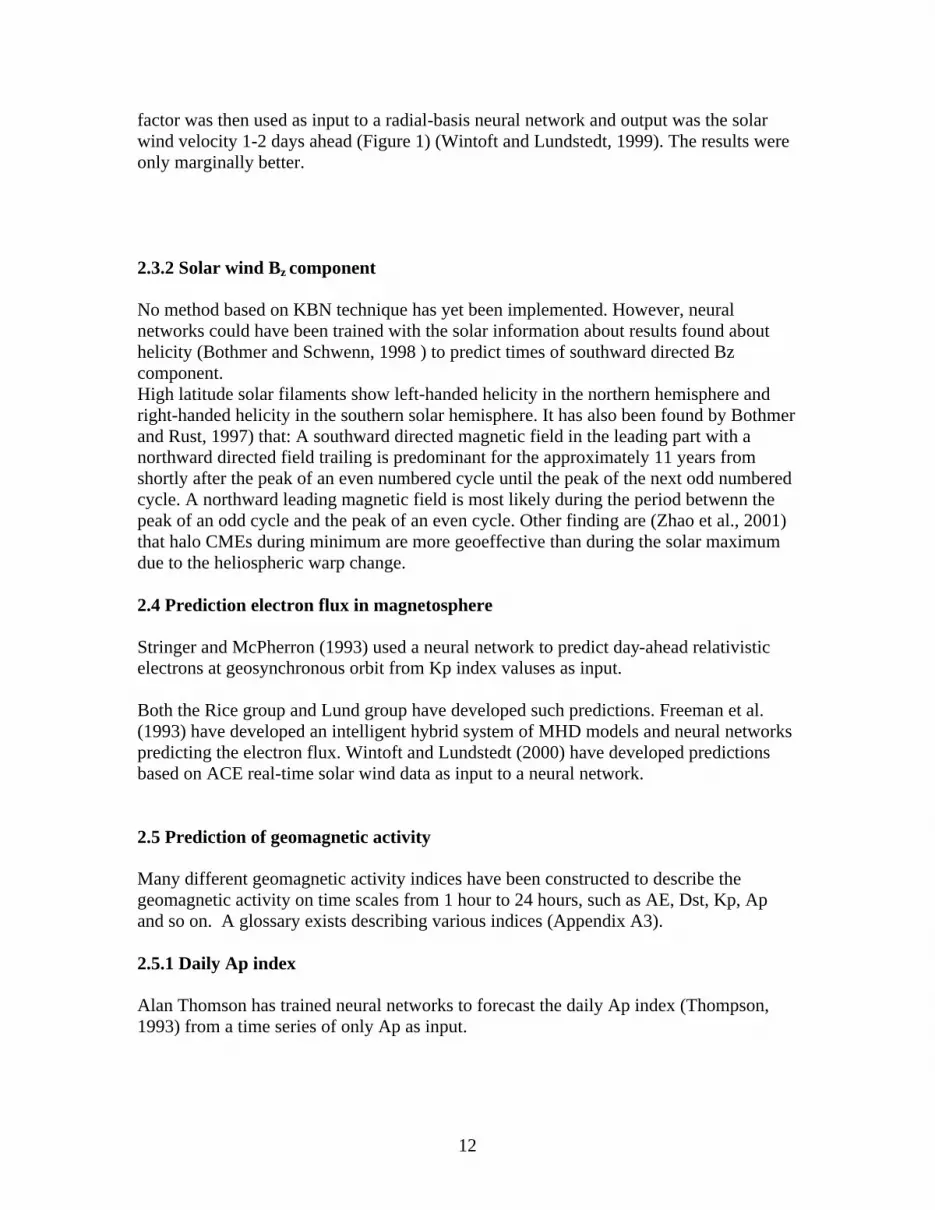
Figure 6 shows the solar wind velocity, measured by the spacecraft ACE, resulted from the corona hole in Figure 5. The solar wind velocity is measured by several satellites, e.g. by ACE and SOHO.

11

Since the solar wind velocity is determined by the solar magnetic field topology it should be possible to predict the velocity from ground or space based observed solar magnetograms (images of the solar magnetic field). In Lund predictions have been developed of the solar wind velocity (V) from only solar magnetic field data using a hybrid system of a RBF network and a MHD-model (Wintoft and Lundstedt, 1997). A potential field model Hoeksema (1984) was used to calculate the magnetic field strengths on the same field line at the photosphere BO=B(RO) and the source surface (=2.5RO) BS=B(RS) from WSO magnetograms. The RMS magnetic field BRMS was computed from daily WSO magnetograms. By defining a vector x(t) = (BO, BS, BRMS) the input to the network was the time series x(t-2), x(t-1), x(t) and the V(t+3) i.e. the velocity three days ahead the output. The RBF network was trained on magnetograms during solar cycle 21 and tested on solar cycle 22. A correlation coefficient of 0.58, a RMSE (root mean square error) of 90 km/s and an average relative variance of 0.68 was obtained. The KBN is doing a better job than the method presented by Wang and Sheely. They reached a correlation coefficient of 0.4 for daily solar wind parameters.

Figure 7. A radial bases function network was trained with input a time-series fs (t - 4),..fs

(t) of the expansion factor fs (t), fs = (Rps/Rss)2 Bps/Bss. The predicted output was daily

solar wind velocity V(t + 2) (---) two days ahead. Solid line in the plot is the daily average solar wind velocity and the thin line the hourly value.

In a second study we used as input a time series of only the expansion factor. From WSO solar magnetograms, via a potential field model, the expansion factor was derived. That

12

factor was then used as input to a radial-basis neural network and output was the solar wind velocity 1-2 days ahead (Figure 1) (Wintoft and Lundstedt, 1999). The results were only marginally better. 2.3.2 Solar wind Bz component No method based on KBN technique has yet been implemented. However, neural networks could have been trained with the solar information about results found about helicity (Bothmer and Schwenn, 1998 ) to predict times of southward directed Bz component. High latitude solar filaments show left-handed helicity in the northern hemisphere and right-handed helicity in the southern solar hemisphere. It has also been found by Bothmer and Rust, 1997) that: A southward directed magnetic field in the leading part with a northward directed field trailing is predominant for the approximately 11 years from shortly after the peak of an even numbered cycle until the peak of the next odd numbered cycle. A northward leading magnetic field is most likely during the period betwenn the peak of an odd cycle and the peak of an even cycle. Other finding are (Zhao et al., 2001) that halo CMEs during minimum are more geoeffective than during the solar maximum due to the heliospheric warp change. 2.4 Prediction electron flux in magnetosphere Stringer and McPherron (1993) used a neural network to predict day-ahead relativistic electrons at geosynchronous orbit from Kp index valuses as input. Both the Rice group and Lund group have developed such predictions. Freeman et al. (1993) have developed an intelligent hybrid system of MHD models and neural networks predicting the electron flux. Wintoft and Lundstedt (2000) have developed predictions based on ACE real-time solar wind data as input to a neural network. 2.5 Prediction of geomagnetic activity Many different geomagnetic activity indices have been constructed to describe the geomagnetic activity on time scales from 1 hour to 24 hours, such as AE, Dst, Kp, Ap and so on. A glossary exists describing various indices (Appendix A3). 2.5.1 Daily Ap index Alan Thomson has trained neural networks to forecast the daily Ap index (Thompson, 1993) from a time series of only Ap as input.

13

In a diploma work for IRF-Lund Ann Hoberg (1999) developed a neural network model to predict Ap from predictions of solar wind velocity. The solar wind velocity was predicted from solar magnetograms, potential models and a neural network as described earlier. Similar work has also been carried out by Detman et al., at SEC. 2.5.2 Hourly indices Kp, Dst, AE Many groups (Freeman et al., 1993; Detman, 1994; Lundstedt 1991, 1992a; Lundstedt and Wintoft, 1994, Wu, 1997, Gleisner 2000) have used the solar wind data to predict geomagnetic activity. Different solar wind parameters have been selected as inputs for the neural networks. Most, often the solar wind velocity (V), density (n), and the southward directed magnetic field (Bz) for a time history, have been used. However, the electric field (Ey) and dynamic pressure (p) and other magnetic field component and standard deviation have also been used as input.

Figure 8 shows the predictions of Kp available in real-time on the web. The neural networks use solar wind data as input from ACE. During the Bastille event, the proton event caused by the halo CME of July 14, 2000, resulted in incorrect values of solar wind velocity and density.

14

The predictions of the Kp index (Boberg et al. 2000) in Figure 8 are available in real-time on Lund's web site (www.irfl.lu.se/spwfo.html). Combined MLP neural networks were used with a time series of solar wind parameters n, V, and Bz as input . An Elman recurrent neural network manage to accurately predict all phases of a geomagnetic storm as described by the Dst index an hour ahead. As an average for the test data predictions one hour ahead the correlation coefficient between the observed and predicted Dst reached 0.92 and the corresponding prediction efficiency (1 – average relative variance) was 85% (Wu and Lundstedt, 1996). The important thing is that the models never use Dst as input. We only use solar wind data as input! The neural networks learn by themselves the solarwind-magnetosphere coupling function. The start from scratch.

Figure 9 shows a prediction of Dst two hours ahead using only solar wind data as input and based on an Elman recurrent neural network. Predictions of Dst are available in real-time on Lund’s web site. AE has been predicted by Hernadez et al., (1993) and more recently by Gleisner and Lundstedt (2000). The predictions are available on the Lund’s web site 2.5.3 Local geomagnetic field In (Gleisner and Lundstedt, 2001) predictions of the local geomagnetic field is for the first time presented using a hybrid neural network. After subtraction of a secularly

15

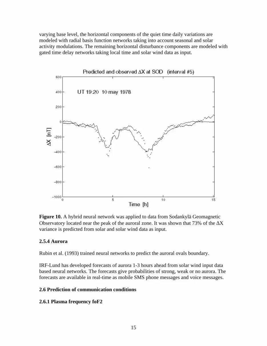
varying base level, the horizontal components of the quiet time daily variations are modeled with radial basis function networks taking into account seasonal and solar activity modulations. The remaining horizontal disturbance components are modeled with gated time delay networks taking local time and solar wind data as input.

Figure 10. A hybrid neural network was applied to data from Sodankylä Geomagnetic Observatory located near the peak of the auroral zone. It was shown that 73% of the ∆X variance is predicted from solar and solar wind data as input. 2.5.4 Aurora Rubin et al. (1993) trained neural networks to predict the auroral ovals boundary. IRF-Lund has developed forecasts of aurora 1-3 hours ahead from solar wind input data based neural networks. The forecasts give probabilities of strong, weak or no aurora. The forecasts are available in real-time as mobile SMS phone messages and voice messages. 2.6 Prediction of communication conditions 2.6.1 Plasma frequency foF2

16

With both solar and solar wind data as input the foF2 has been predicted (Wintoft and Cander, 1999a) both 1 hour and 24 hours ahead.

Figure 11 shows prediction of δ (i.e. foF2 variation with solar cycle, season and diurnal variation removed) one hour ahead from AE as input. For predictions one hour ahead the overall RMS error on the training set in 1980 was 0.581 MHz with a correlation of 0.976 and 0.661 MHz with correlation ogf 0.97 on test set in 1981. Predictions of foF2 from substorm index AE, local time and seasonal information have also been developed (Figure 11) (Wintoft and Cander, 2000). Predictions up to 6 hours ahead were possible. Since AE maybe predicted from solar wind input only, it would also be possible to predict the plasma frequency directly from solar wind input. 2.7 Prediction of effects 2.7.1 Satellite anomalies Within the ESA SPEE contract Wu et al., developed predictions of satellite anaomalies based on the Kp index. Now within the ESA contract SAAPS predictions have been developed directly from solar wind input. (Wintoft et al., 2000).

17

2.7.2 Satellite drag Williams (1991) has developed neural networks predictions of the satellite drag based on inputs about F10.7 cm solar radio fluxes. 2.7.3 Geomagnetically induced currents Kronfeldt has developed predictions based on ACE solar wind data and GIC measurements. The trained neural networks are running in real-time and the predictions are available on the Lund’s web site

Figure 12 shows predicted versus measured GIC, 6 April 2000 2.8 Summary of KBN models Input parameters Output KBN method Reference Daily sunspot number

Daily sunspot number

SOM and MLP Liszka 93;97

Monthly sunspot number

Date of solar cycle maximum and amplitude

MLP and Elman Macpherson et al.,95, Conway et al.,98

Monthly sunspot number and aa

Date of solar cycle maximum and amplitude

Elman recurrent neural network

Ashmall and Moore, 98

18

Yearly sunspot number

Date of solar cycle maximum and amplitude

MLP Calvo et al., 95

McIntosh sunspots class and M.Wilson magn. complexity

X class solar flare MLP expert system Bradshaw et al., 1989

X-ray flux Proton event Neuro fuzzy system Gabriel et al., 00 Flare location, duration, X-ray and radio flux

Proton event MLP Xue et al., 97

Photospheric magnetic field, expansion factor

Solar wind velocity 1-3 days ahead

RBF neural network and potential field model

Wintoft and Lundstedt, 97;99

ΣKp Relativitic electrons in magnetosphere day-ahead

MLP Stringer and McPherron, 93

Solar wind n, V, Bz relativistic electrons MLP Wintoft and Lundstedt, 00

Solar wind Vfrom photospheric B

Daily geomagnetic index Ap

MLP Detman et al., 00

Ap Ap MLP A. Thompson, 93 Solar wind n, V, Bz Kp 3 hrs ahead MLP Boberg et al. 00 Solar wind n,V,B, Bz

Dst 1-8 hrs ahead Elman Lundstedt, 91, Wintoft and Lundstedt, 94, Wu and Lundstedt, 97

Solar wind n,V ,B,Bz

AE 1 hr ahead Elman Gleisner and Lundstedt, 99

Solar wind V2Bs and √nV2 , LT, local geomag ∆ Xe, ∆Yw

local geomagnetic field ∆X, ∆Y

MLP,and RBF Gleisner and Lundstedt, 00

Solar wind n, V, Bz none, weak or strong aurora

MLP Lundstedt et al., 00

foF2 foF2 1 hour ahead MLP Wintoft and Lundstedt, 99

AE, local time, seasonal information

foF2 1-24 hrs ahead MLP Wintoft and Cander, 00

foF2, Ap, F 10.7 cm 24 hrs ahead MLP Wintoft and Cander, 99

ΣKp sat. anomaly MLP Wintoft and Lundstedt., 00

Solar wind n, V, Bz GIC Elman, MLP Kronfeldt et al., 2001

Table 1 shows predictions of space weather and effects based on KBN.

19

Two workshops on “AI Applications in Solar-Terrestrial Physics” have been held in Lund, 1993 and 1997. 3. Prototype Overview The Lund group has developed a very extensive prototype in Java, forecasting, warning, informing about ongoing activity and explaining the space weather and effects. As mentioned in the introduction, the prototype is based on ideas from the work of the Lund Space Weather Model, all back in the late eighties.

Figure 13. Lund Space Weather Forecast Service front web page. For this event a halo CME and an X class solar flare have occurred on the Sun (red light), a warning (yellow light) for the CME to arrive at L1 is turned on and the conditions are quiet (green light) at Earth. 3.1 Front Page The stoplights show the activity at Sun, L1 and at Earth. The status is updated ever 5 minutes. This front web page shall give the user a fast general overview of what is happening and if actions should be taken. Whether activity is ongoing (red), if there is warning for activity (yellow) or if it’s quiet (green) at the Sun at L1 or at Earth. The latest SOHO solar images are available by clicking on the Sun. 3.2 User Guide An introduction to what space weather is and which effects it can cause is given in the User Guide frame. Both a visual dictionary and glossary is available. The User Guide

20

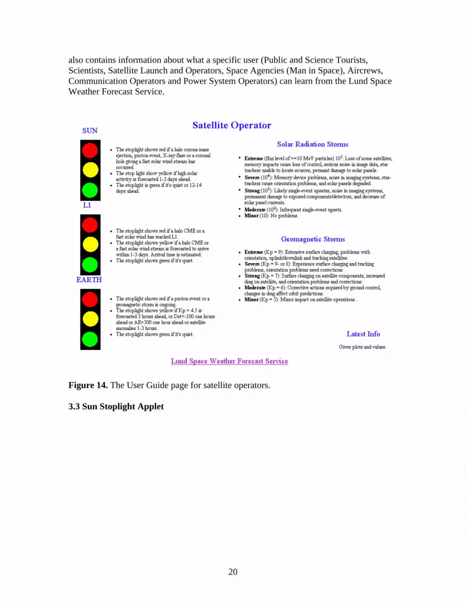
also contains information about what a specific user (Public and Science Tourists, Scientists, Satellite Launch and Operators, Space Agencies (Man in Space), Aircrews, Communication Operators and Power System Operators) can learn from the Lund Space Weather Forecast Service.

Figure 14. The User Guide page for satellite operators. 3.3 Sun Stoplight Applet

21

Figure 15. The Sun Stoplight applet is shown. 3.3.1 Nowcasts - red/green light • X-ray solar flares Data from GOES is available in real-time for the database. The stoplight turns red if a major X-ray flare occurs. No warning or forecast of flares is implemented. As earlier mentioned forecasts have been developed, e.g. Bradshaw et al., 1989. • Proton events Data from GOES is available in realtime for the database. The stoplight turns red if a proton event has taken place. No warnings or forecasts is implemented. As earlier mentioned, forecasts have been developed, e.g. by Gabriel et al., 2000. • Halo coronal mass ejections

22

Information about the latest halo CME is received as an e.mail from Simon Plunkett at GSFC/NASA. This information is based on observations with EIT and LASCO instrument on board SOHO. If a halo CME has occurred then the stoplight turns red. A relationship given by Gopalswamy et al., (2000) between the initial speed of the halo CME and the arrival time of the CME at Earth, has been implemented in Java for the prototype. The average acceleration is related to the initial speed according to Gopalswamy as: a = 1.41 – 0.003u, where a is the acceleration in m/s2 and u the initial CME speed in km/s. Fast CMEs (u>405 km/s) are decelerated and slow CME (u<405 km/s) are accelerated. The arrival time can then simply be derived from s = ut + 1/2at2, where s is distance traveled. The velocity of the CME when it has reached Earth is calculated from v = u + at. The estimated arrival time and speed is available as latest info. These estimates are also used to set a warning, yellow light, on the L1 stoplight. They are not used as input to forecast models for the Earth stoplight. The forecasts are not accurate enough. • High speed plasma streams from coronal holes Several methods are available, giving information about high speed plasma streams, i.e the fast solar wind from coronal holes at L1. The prototype tells us whether or not a High Speed Plasma Stream (HSPS) (Lindblad et al., 1989) will take place 1-3 days ahead. Using the photospehric and coronal magnetic fields as input (computed from solar magnetograms either observed by MDI on board SOHO or observed by e.g. Wilcox Observatory (WSO)), the solar wind can be derived and forecasted (Figure 1) (Wintoft and Lundstedt, 1999). To work in real-time we need real-time magnetograms. WSO offers daily magnetogram plots. MDI also offers magnetograms. A relationship between the solar source surface magnetic field strength and the solar wind velocity was found by Hoeksema (1984). For it to work in real-time it requires real-time magnetograms and that the source surface magnetic field is computed. Various relations between the distance of the projected Earth on the Sun to the heliospheric current sheet and the solar wind velocity have been found (e.g. V(km/s)=408 + 473sin2λ by Hakamado & Munakata ). For that to work in real-time we need real-time synoptic charts of the source surface. Updated MDI synoptic charts of the photospheric field are available. Otherwise synoptic charts of source surface from last rotation are available i.e. 27 days earlier. The distance can however be hard to define at times of high solar activity when the current sheet is very warped. Bartels diagrams of solar mean field data can give a probability of occurrence of high speed plasma streams (Lundstedt and Hoeksema, 1992). It’s based on recurrency and works for stable magnetic sector structures. Slow solar wind occurs at sector boundaries and then increases. Daily mean field data has been available from WSO at Stanford and from MDI on board SOHO.

23

A relationship between the size and position of a coronal hole, observed with the X-ray Yohkoh satellite, and the solar wind velocity has been found by (Sapporo). These results are however preliminary. Real-time solar wind data is available from spacecraft ACE and SOHO. A neural network can learn from earlier rotation velocity profiles, last days velocity profiles and from that forecast the velocity 1-3 days ahead. From that it can be concluded whether or not a high speed solar wind will reached L1 1-3 days ahead. At this first stage we have chosen the last approach to include solar wind speed stream information for the prototype. A more advanced method will later be included, based on our earlier networks using WSO magnetograms. Green light means quiet conditions 3.3.2 Forecasts – yellow light • Solar activity 7-14 days ahead Solar MDI images, derived at Stanford, about the far side quiet or high activity is now used for the first time for warnings. Using these images we can warn for quiet/high activity times 7-14 days ahead.

Figure 16 shows solar activity on Earth and farside, derived from MDI data. • Solar activity 1-3 days ahead We have also included forecasts and warnings of solar activity 1-3 days ahead from the Space Environment Center in Boulder in the prototype. These forecasts will later be replaced with warnings and forecasts from IRF-Lund based on SOHO/MDI solar magnetic field data.

24

Figure 17 shows a SOHO/MDI solar magnetogram for the very active region AR9393 on March 29, 2000. This region produced an X20 solar flare on Aril 2, 2001. 3.4 L1 Stoplight Applet 3.4.1 Nowcasts – red/green light • The L1 stoplight turns red when a halo CME, shock or a fast solar wind has arrived

at L1. Green light means quiet conditions. 3.4.2 Forecasts – yellow light • Yellow light is shown for warnings of a halo CME or a fast solar wind coming 1-3

days ahead.

25

Figure 18. The L1 Stoplight applet is shown. 3.5 Earth Stoplight Applet 3.5.1 Nowcasts – red/green light • Geomagnetic storm The Earth stoplight turns red if a geomagnetic storm is ongoing (Dst �-50 for at least two hours, derived from neural network nowcasting) • Communication condition The Earth stoplight turns red if the communication conditions are disturbed, described by foF2. • Geomagnetically induced current The Earth stoplight turns red if an enhanced geomagnetically induced current is measured. Green light means quiet conditions.

26

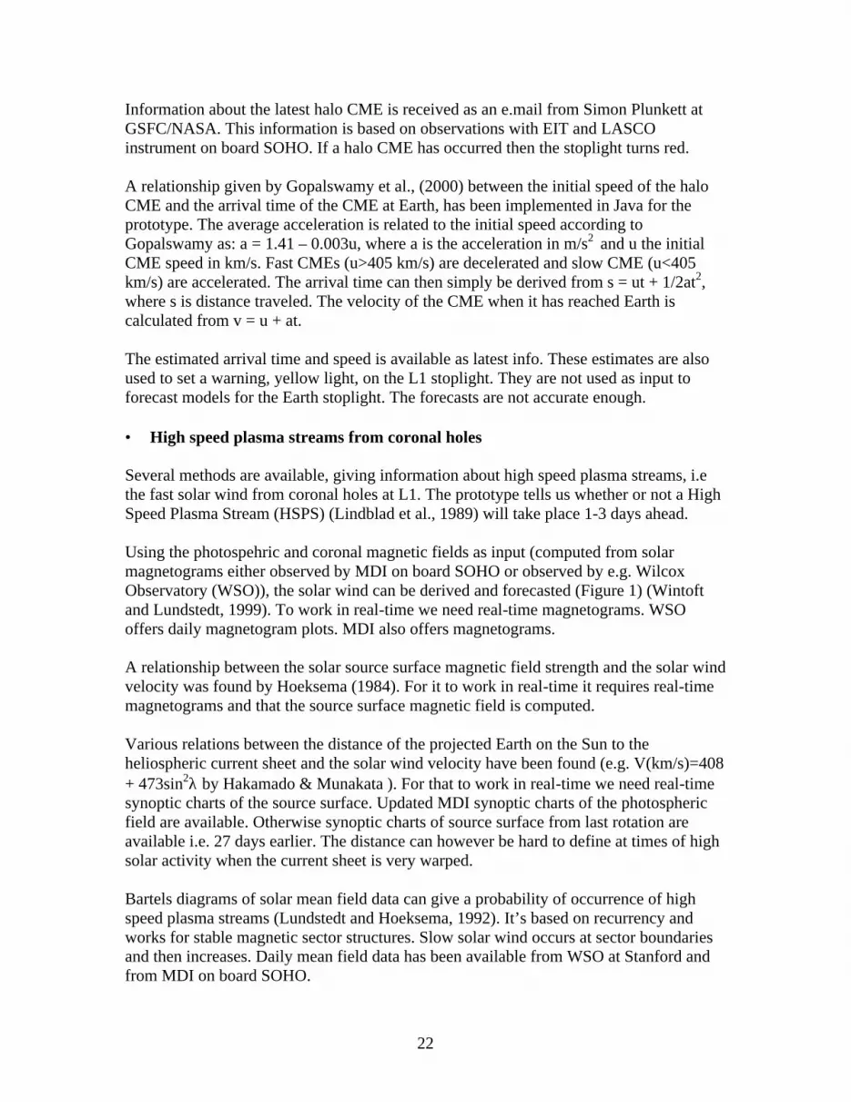
Figure 19. The Earth Stoplight applet is shown. 3.5.2 Forecasts – yellow light • Satellite anomalies A satellite anomaly is forecasted. This prediction model based on neural networks was developed within SAAPS (Wintoft, 2001). • Satellite drag Forecast models will be implemented later. • Communication condition Forecast models will be implemented later. • Geomagnetic storm Geomagnetic storms are forecasted, indicated by a Kp (>4.5), Dst (�-50nT) or an AE (>500nT) value. These models are well tested and described in many publications (Lundstedt, 1999). By clicking on “latest info” we also inform whether or not Dst minimum will occur within 5 hours.

27

• Geomagnetic induced current (GIC) (GIC) is forecasted. This is a recent developed model based on real-time solar wind data and measured GIC values. The work is carried out in collaboration with a Swedish power company. Real-time GIC data is not available to public. • Aurora Aurora is forecasted. The probability for no, weak or strong aurora is given. Presently, forecasts are offered for Northern Scandinavia. For cats for lower latitudes are planned. Green light is again on if the conditions are quiet. 3.4 Plot tools All the stoplight applets include tools for plots and data studies. The plot tools have also been developed in Java.

28

Figure 20. Example of a plot showing near side and far side solar activity. A plot of the magnetic flux intensity (pixel intensity) of the near and solar far side is shown in Figure 20. These values are used as input for neural networks to forecast high/low solar activity 7-14 days ahead. The plot tools have all common functions and can plot all the data available to the prototype.

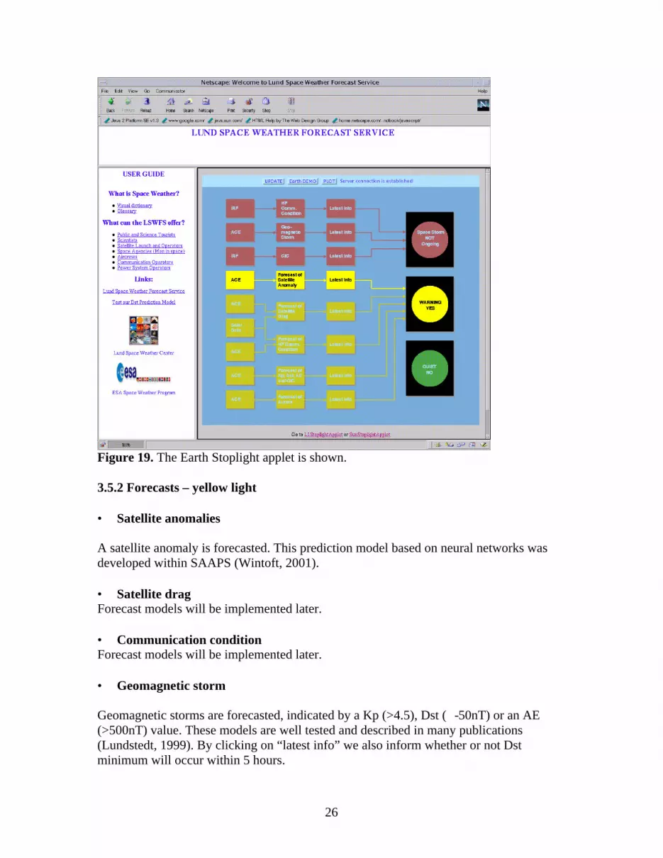
Figure 21. Illustrate Latest Info function. 3.5 Database The prototype is connected to a very extended database, also written in Java, which is updated in real-time. Within the ESA SAAPS projects a database was developed in Java. The database includes OMNI solar wind data 1982-1999, ACE solar wind data, GOES-8 and 10 electron flux and proton flux and Kp. This data base has now been extensively expanded to serve the prototype with real-time and historical data. 3.6 DEMO functions

29

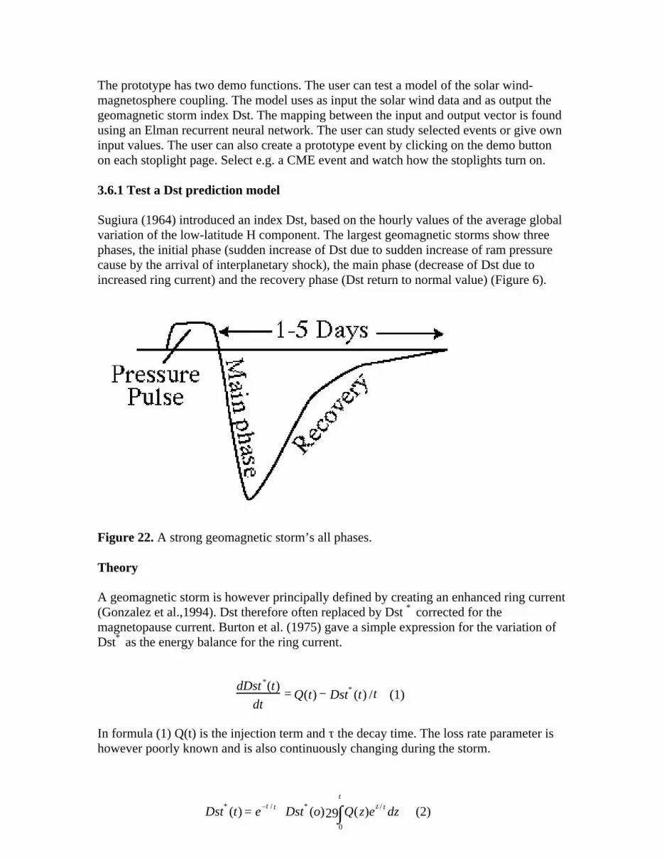
The prototype has two demo functions. The user can test a model of the solar wind-magnetosphere coupling. The model uses as input the solar wind data and as output the geomagnetic storm index Dst. The mapping between the input and output vector is found using an Elman recurrent neural network. The user can study selected events or give own input values. The user can also create a prototype event by clicking on the demo button on each stoplight page. Select e.g. a CME event and watch how the stoplights turn on. 3.6.1 Test a Dst prediction model Sugiura (1964) introduced an index Dst, based on the hourly values of the average global variation of the low-latitude H component. The largest geomagnetic storms show three phases, the initial phase (sudden increase of Dst due to sudden increase of ram pressure cause by the arrival of interplanetary shock), the main phase (decrease of Dst due to increased ring current) and the recovery phase (Dst return to normal value) (Figure 6).

Figure 22. A strong geomagnetic storm’s all phases. Theory A geomagnetic storm is however principally defined by creating an enhanced ring current (Gonzalez et al.,1994). Dst therefore often replaced by Dst * corrected for the magnetopause current. Burton et al. (1975) gave a simple expression for the variation of Dst* as the energy balance for the ring current.

In formula (1) Q(t) is the injection term and τ the decay time. The loss rate parameter is however poorly known and is also continuously changing during the storm.

Dst* (t) = e−t / τ Dst* (o) + Q(z)ez / τdz0

t

∫

(2)

dDst *(t)

dt= Q(t) − Dst* (t) /τ (1)

30

The formal solution of equation (1) is given by (2). A second order differential equation for Dst was given by Vassiliadis et al. (1996).

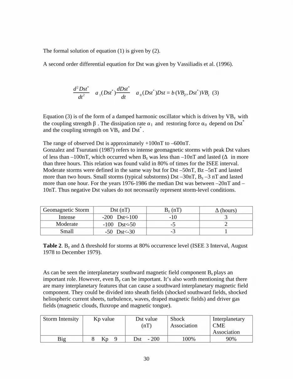
Equation (3) is of the form of a damped harmonic oscillator which is driven by VBz with the coupling strength β . The dissipation rate α1 and restoring force α0 depend on Dst* and the coupling strength on VBz and Dst* . The range of observed Dst is approximately +100nT to –600nT. Gonzalez and Tsurutani (1987) refers to intense geomagnetic storms with peak Dst values of less than –100nT, which occurred when Bz was less than –10nT and lasted (∆) in more than three hours. This relation was found valid in 80% of times for the ISEE interval. Moderate storms were defined in the same way but for Dst –50nT, Bz –5nT and lasted more than two hours. Small storms (typical substorms) Dst –30nT, Bz –3 nT and lasted more than one hour. For the years 1976-1986 the median Dst was between –20nT and –10nT. Thus negative Dst values do not necessarily represent storm-level conditions. Geomagnetic Storm Dst (nT) Bz (nT) ∆ (hours)

Intense -200�Dst<-100 -10 3 Moderate -100�Dst<-50 -5 2

Small -50�Dst<-30 -3 1 Table 2. Bz and ∆ threshold for storms at 80% occurrence level (ISEE 3 Interval, August 1978 to December 1979). As can be seen the interplanetary southward magnetic field component Bz plays an important role. However, even By can be important. It’s also worth mentioning that there are many interplanetary features that can cause a southward interplanetary magnetic field component. They could be divided into sheath fields (shocked southward fields, shocked heliospheric current sheets, turbulence, waves, draped magnetic fields) and driver gas fields (magnetic clouds, fluxrope and magnetic tongue). Storm Intensity Kp value Dst value

(nT) Shock Association

Interplanetary CME Association

Big 8 � Kp � 9 Dst � - 200 100% 90%

d2 Dst*

dt2 + α1(Dst* )dDst*

dt+ α0 (Dst* )Dst = β (VBZ , Dst* )VBz (3)

31

Intense Kp = 7 -200�Dst<-100 80% 80% Moderate 5 � Kp � 6 -100�Dst<-50 40% 40%

Table 3 shows the relation between geomagnetic indices Kp and Dst for storm types. The statistics are valid for August 1978 – October 1982 i.e. during solar maximum period. During declining phases dominate high speed plasma streams from coronal holes. The forecast model the user can test is a forecast model of the Dst variation, based on trained recurrent Elman neural network (appendix). The neural network has learned the variation of the geomagnetic activity only from the variation of the solar wind variation. The recurrent neural network learns both the solar wind magnetosphere coupling and the recovery phase by itself. Three independent data sets are used for the training (training set), optimization (validation set), and testing (test set) of the neural network. During training, the weights of the network are found from the error backpropagation algorithm. Several different networks are trained where the type of inputs and number of hidden units are varied. Then the validation set is used to determine the optimal network. Finally, the optimal network is tested on the test set to determine how well it will work for new data. The differential equation governing the evolution of Dst are solved implicity by the Elman neural network model.

Here f() is a linear transfer function, Wij are the connection weights between the hidden and output layers, wjk are the connection weights between the input and hidden layers, Vj (t) is the output of hidden unit j at time t, S1 is the number of hidden units, Q(t) stands for the coupling function at time t, and τw is length of the delay line. Using as input n, V, B, Bs (=-Bz if Bz < 0 and 0 if Bz >= 0) Wu and Lundstedt (1997) managed to obtain the values given in table 3 for the correlation coefficient between the predicted Dst and observed for 1-8 hours ahead, for ARV (average relative variance, i.e. the mean squared error normalized by the variance of the data) and RMSE (root-mean square error).

Hours ahead Correlation coeff. ARV RMSE (nT) 1 0.92 0.15 13.8

Dst(t + T ) = f (Wij , tanh(w jk ,Q(t)) = WijVj(t ) (4)j=1

S1

∑

Vj (t) = tanh w jkQ(t − k +1) + w jkVk (t +1)k=τ w +1

τ w + S1

∑k=1

τ w

∑

(5)

32

2 0.90 0.18 15.3 3 0.88 0.23 16.9 4 0.86 0.26 18.4 5 0.84 0.29 19.5 6 0.82 0.33 20.7 7 0.80 0.36 21.7 8 0.77 0.40 23.1

Table 4. Dst Prediction accuracy for 1 to 8 hours ahead. Even better prediction values for 1 hour ahead are shown in Figure 7, namely 0.94 and 11.6 nT. Geomagnetic storms are very accurately predicted 1-2 hours ahead and predictions 3-5 hours ahead are useful in practical operation according to their acceptable accuracy. To predict the duration of the geomagnetic storm we also need a model of the solar wind variation. As mentioned earlier there are many solar wind features that can cause a storm. The dominating features also differ during the solar cycle. During solar maximum interplanetary CMEs (ICME) dominates. Much attention has been paid on magnetic clouds, even if they occur only in one out of six fast ICME/driver gas events. During the declining phase coronal holes have dominant effect on interplanetary medium. High speed plasma streams from coronal holes can create intense magnetic fields if the streams interact with streams of lower speeds. Although it is clear that there are more large Dst events during solar maximum than solar minimum, that is not the case for auroral zone (AE) activity. Alfven waves associated with coronal holes produce continuous substorms and increased AE index. Substorms are related to geomagnetic induced currents and therefore of importance for the effects on power systems. From the above it’s clear that the solar/solar wind impact on Earth atmosphere is much more complex than a question of occurrence of CME magnetic clouds. In order to develop a useful forecast service we therefore must include all kind of events caused by the different solar wind features. The different solar wind features during a solar cycle have been studied (Wintoft and Lundstedt, 1998) using a SOM neural network. Such a network could have classified the features and been used to select the proper network modeling the solar wind magnetosphere coupling. Test the model A test forecast model of Dst has been developed for the prototype. The user can study selected events or give values for the solar wind velocity V, density and southward magnetic field component Bz or By. The neural network is then forecasting the Dst value 1 hour ahead. The result and solar wind input values can be plotted (Figure 23 ) Again no Dst value as input is given as is done for other models e.g. those based on Burton et al.,1975.

33

Figure 23. The forecast model shows a prediction of Dst 1 hour ahead for the selected main phase event May 2, 1998. The observed Dst value for minimum was –205 nT. Our model predicts –212 nT. Dst is forecasted one hour ahead for the three phases of a geomagnetic storm. The solar wind data values used as input are shown and can also be plotted (Figure 24). The user can change the input and then make a new forecast and now see what changes that caused in the Dst value. The user can also create a time series of input values from scratch and see what Dst that will result in.

34

Figure 24 shows the solar wind data (n, V, By and Bz) and the Dst value for the May main phase event. 3.6.2 Create a prototype event The DEMO button function gives the user the possibility to create a specific event.

Figure 25. The demo function illustrated.

35

In this case a halo CME has arrived at L1 and a warning for a halo CME is also turned on. 3.7 Case study

Figure 26. A web site http://www.irfl.lu.se/swprogint/selectedevents.html dedicated to the selected cases. Cases were selected to show how well the prototype worked for interesting events. Both times of halo CMEs and one coronal hole caused high speed plasma stream were selected. Table 5 shows the observed quantities and tables 6-8 show the predicted quantities by the prototype. The event Jan 6-11 has been studied in detail by the Lund group (Wu, Lundstedt, 1998). The forecast of Dst worked very well. It was also found that the optimal combination of different solar wind parameters used as inputs outperform the single optimal coupling functions in terms of prediction accuracy.

36

Figure 27 shows how well our Elman neural network forecasted Dst one hour ahead for the Jan 6-11 event. The correlation coefficient was as high as 0.94 and the RMSE only 11.6 nT. The inputs to the network were n, V, B, By and Bz. The Sun stoplight shows forecasts of both quiet and activity times from MDI data 7-13 days in advance and forecasts of solar activity 1-3 days (SEC forecasts). It also shows nowcasts of x-ray solar flare flux, proton flux and if a halo CME has occurred. The messages about halo CMEs events will be replaced by automatic detection methods developed by us. Only the forecasts of SEC of solar activity can be shown for the selected events. The results are shown in table 5. As earlier also mentioned, we are planning to replace these forecasts with forecasts developed by us and based on KBN. The L1 stoplight shows forecasts of arrival of halo CMEs and fast solar wind at L1. It also shows nowcasts of whether or not a halo CME and fast solar wind have arrived at L1. The forecasts for the events can be tested and the results are shown in table 6. Finally the Earth stoplight shows forecasts of satellite anomalies, satellite drags (not implemented), plasma frequency foF2, Kp, Dst, AE, GIC and aurora. It also shows nowcasts of GIC, geomagnetic storms (Dst�-50), and plasma frequency. The forecasts can be tested for the events and the results are shown in table 8.

37

Date V(Sun) V(1AU) T(1AU) Dst(min) 23/1/74 - 740 km/s 2d, 6h -66 nT 6/1/97 200 km/s 550 km/s 3d, 12d -78 nT 4/11/97 830 km/s 450 km/s 2d, 16h -110 nT 20/4/98 1640 km/s 500 km/s 3d, 10h -69 nT 2/5/98 1040 km/s 850 km/s 1d, 12h -205 nT 4/4/00 1000 km/s 600 km/s 2d, 0h -321 nT

Table 5. Observed Quantities for the selected events. T is the arrival time of the solar feature.

Date Solar activity 1-3 days ahead

Solar activity 7-14 days ahead

23/1/74 SEC NaN 6/1/97 SEC NaN 4/11/97 SEC NaN 20/4/98 SEC NaN 2/5/98 SEC NaN 4/4/00 SEC NaN

Table 6. Forecasted Quantities at Sun. Far side solar images started to be available August 7 2000 i.e. after time of selected events. The solar activity forecasts 1-3 days from SEC will be replaced by forecasts derived at Lund.

Date Halo CME arrival

at L1 (T-1h) Halo CME

velocity at L1 Fast coronal hole

solar wind at L1 one day ahead

23/1/74 - - 675 km/s 6/1/97 4d, 13h 480 km/s - 4/11/97 2d, 6h 530 km/s - 20/4/98 1d, 1h 1230 km/s -

2/5/98 1d, 18h 690 km/s -

4/4/00 1d, 20h 660 km/s -

Table 7. Forecasted Quantities at L1

The prediction of the arrival time of the halo CME is based on the implementation of the Golpaswamy’s methods (section 3.4.1 c). The prediction of the arrival time of the fast solar wind is based on a neural network model. As can be seen the forecasts of the arrival

38

time of the halo CMEs based on Gopalswamy et al., (2000) are only acceptable for the events 2/5/98 and 4/4/00. For the January 97 event the arrival time differs from the observed with more than one day. For the 20/4 98 event the velocity value is totally wrong.

Date Dst (min) 1 hr ahead

Dst 2,3,4,5 hrs

ahead

Satellite anomaly

within a day

Disturbed HF communication conditions 1-6 hrs ahead

GIC 1hr ahead

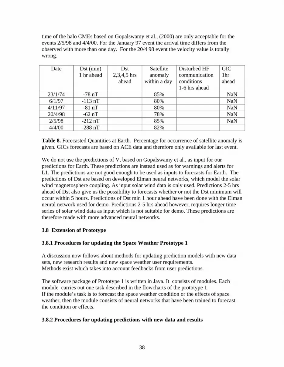
23/1/74 -78 nT 85% NaN 6/1/97 -113 nT 80% NaN 4/11/97 -81 nT 80% NaN 20/4/98 -62 nT 78% NaN 2/5/98 -212 nT 85% NaN 4/4/00 -288 nT 82%

Table 8. Forecasted Quantities at Earth. Percentage for occurrence of satellite anomaly is given. GICs forecasts are based on ACE data and therefore only available for last event. We do not use the predictions of V, based on Gopalswamy et al., as input for our predictions for Earth. These predictions are instead used as for warnings and alerts for L1. The predictions are not good enough to be used as inputs to forecasts for Earth. The predictions of Dst are based on developed Elman neural networks, which model the solar wind magnetosphere coupling. As input solar wind data is only used. Predictions 2-5 hrs ahead of Dst also give us the possibility to forecasts whether or not the Dst minimum will occur within 5 hours. Predictions of Dst min 1 hour ahead have been done with the Elman neural network used for demo. Predictions 2-5 hrs ahead however, requires longer time series of solar wind data as input which is not suitable for demo. These predictions are therefore made with more advanced neural networks. 3.8 Extension of Prototype 3.8.1 Procedures for updating the Space Weather Prototype 1 A discussion now follows about methods for updating prediction models with new data sets, new research results and new space weather user requirements. Methods exist which takes into account feedbacks from user predictions. The software package of Prototype 1 is written in Java. It consists of modules. Each module carries out one task described in the flowcharts of the prototype 1 If the module’s task is to forecast the space weather condition or the effects of space weather, then the module consists of neural networks that have been trained to forecast the condition or effects. 3.8.2 Procedures for updating predictions with new data and results

39

With new data sets To update the predictions with a new data set, we have to retrain the neural network. If the input variables are the same then the topology of the neural network doesn’t have to be changed. With new research results: Here we have to consider how the new research results can be described. The new results can be coded into the neural network. If that is the case, then the topology has to be changed. The neural network has then to be retrained. It could also be that we have to include a new module in our prototype. The new module will then consist of new trained neural networks. With new space weather user requirements: Here it depends on what the new user requirements are. It could be that the new requirements could be taken care of by another module already existing in the prototype, but not used earlier by the specific user. However it could also be that a new module has to be developed and new neural networks trained. 3.8.3 Defining methods for taking into account feedback from users We offer forecasts of aurora to science tourism company “Kiruna Vetenskapsturism” in Kiruna. These forecasts are based on trained neural networks with input data ACE solar wind data and events of aurora seen in Kiruna region. These predictions can be improved by using more advanced neural network methods. However, we can also retrain the neural networks by adjusting the weights so the neural network will predict correctly the events reported by new observers. We have therefore asked pilots and the personal at airport in Kiruna to inform us about whether they actually observed or not observed an aurora when we predicted it. 4. Summary We have developed a real-time forecast service of space weather and effects using knowledge-based neurocomputing (KBN) prototype. The prototype is connected to a data server and is updated every 20 minutes. The user can also manually update the prototype. A real-time forecast service is a great challenge. Data is often missing or bad. Since it’s based on KBN the prototype is easy to improve with new models, data and information. The prototype is written in Java and is therefore running in any environment. We forecast both the space weather and effects. Much information is given to the user so he or she understands what specifics the prototype can offer him or her. We do not think there exist today a good enough model for the solar wind, used together with a solar wind-magnetosphere coupling model. There are to many different solar wind features and first of all we do not know how the solar wind Bz varies more that a couple hours ahead.

40

The solar information can be used for warnings and alerts, but not as forecasts for users. However, the solar wind-magnetopshere and solar wind-effects models are accurate enough to produce useful forecasts of the space weather and effects hours ahead. The forecasts are heavily dependent on a L1 monitor such as ACE. A European L1 monitor is therefore very much wanted. The user can test our Dst forecast model as an example of forecast models. The neural network model is trained on only solar wind data. The user can herewith study the solar wind magnetosphere coupling, learn how the solar wind conditions can influence Earth’s magnetosphere and ionosphere, and also become familiar with recurrent neural networks. Acronyms ACE = Advanced Composite Explorer GIC = Geomagnetic Induced Currents HSPS = High speed plasma stream ICME= Interplanetary Coronal Mass Ejection IHS = Intelligent Hybrid Systems KBN = Knowledge-Based Neural Computing MLP = Multi Layer Perceptron neural network SAAPS = Satellite Anomaly Analysis Prediction System SOHO= SOlar Heliospheric Observatory SOM = Self Organizing Maps SPEE = Study of Plasma energetic electron Environment and Effects TDN = Time delay neural network Acknowledgements I thank the members of the Alcatel consortium for many interesting and stimulating discussions. I would also like to thank my colleagues at IRF. Appendix A1 Html links A1.1 Forecast input data - http://www.irfl.lu.se/HeliosHome/spwdata.html A1.2 What is space weather - http://www.irfl.lu.se/HeliosHome/spacew2.html A1.3 A glossary of space weather terms - http://www.irfl.lu.se/HeliosHome/spacew9.html A2 Most Common neural networks A2.1 Multi-layer error-back-propagation (MLBP) A2.2 Elman recurrent neural network A2.3 Self Organized Map (SOM) A2.4 Radial Basis Function (RBF) network

41

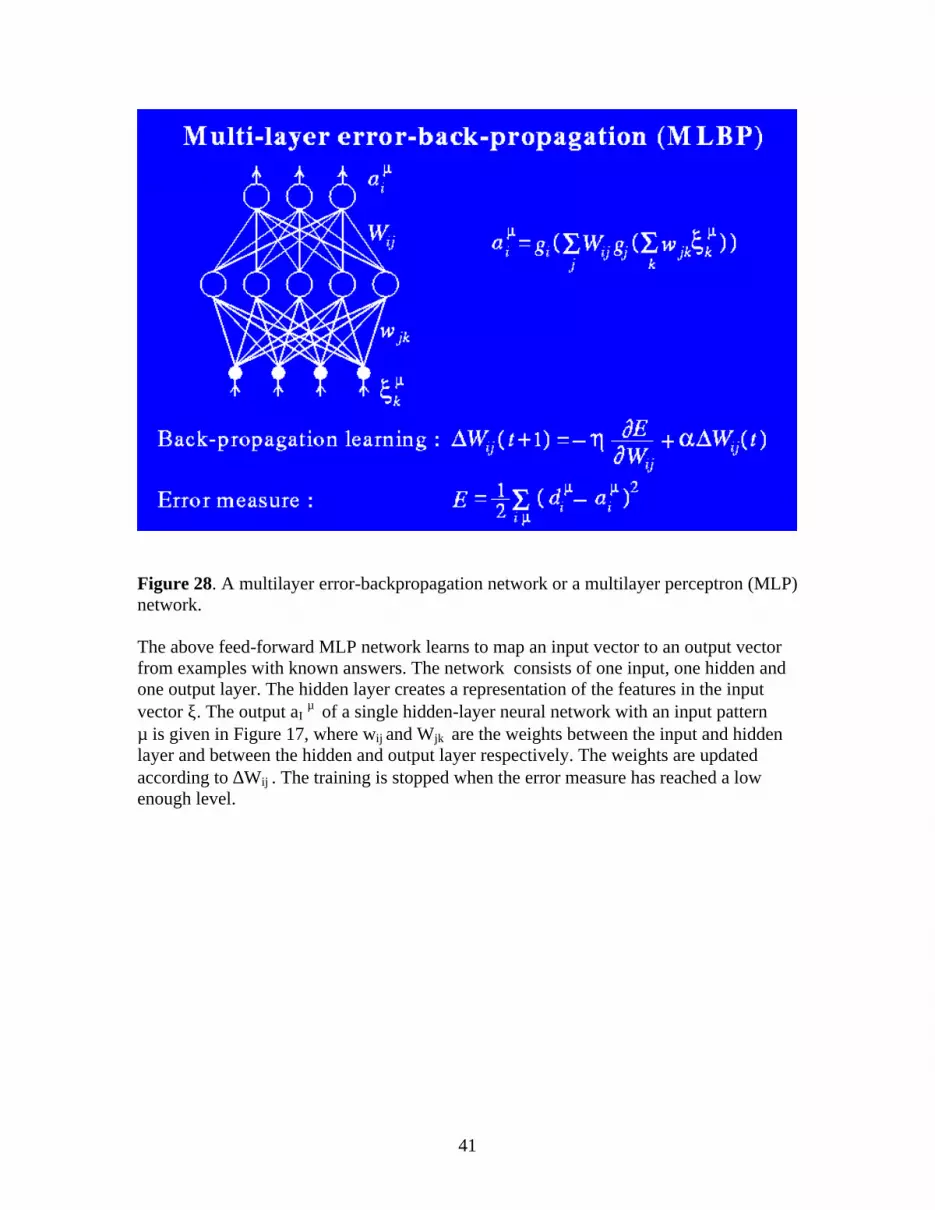
Figure 28. A multilayer error-backpropagation network or a multilayer perceptron (MLP) network. The above feed-forward MLP network learns to map an input vector to an output vector from examples with known answers. The network consists of one input, one hidden and one output layer. The hidden layer creates a representation of the features in the input vector ξ. The output aI

µ of a single hidden-layer neural network with an input pattern µ is given in Figure 17, where wij and Wjk are the weights between the input and hidden layer and between the hidden and output layer respectively. The weights are updated according to ∆Wij . The training is stopped when the error measure has reached a low enough level.

42

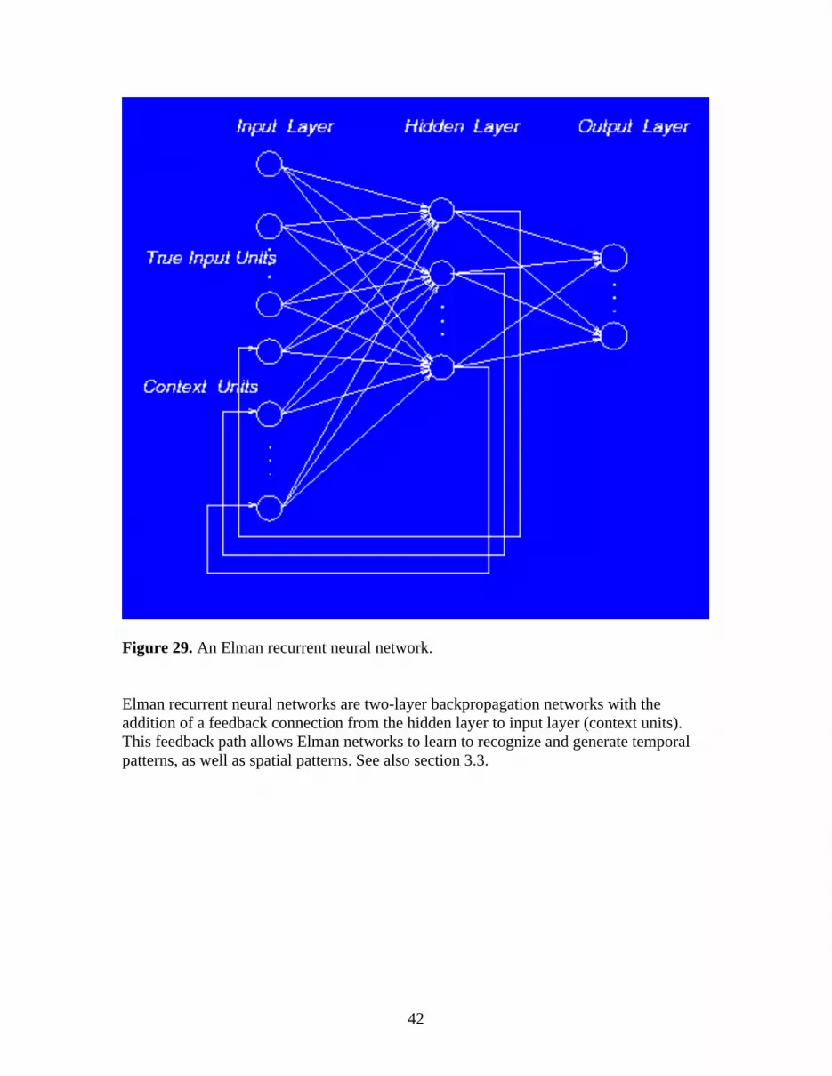
Figure 29. An Elman recurrent neural network. Elman recurrent neural networks are two-layer backpropagation networks with the addition of a feedback connection from the hidden layer to input layer (context units). This feedback path allows Elman networks to learn to recognize and generate temporal patterns, as well as spatial patterns. See also section 3.3.

43

Figure 30. A self-organized map (SOM) network. An unsupervised neural network, the self-organized map neural network (SOM) clusters similar input patterns on a map. The net input to a node is given by hI

µ . Τhe learning rule is given by ∆ij .

44

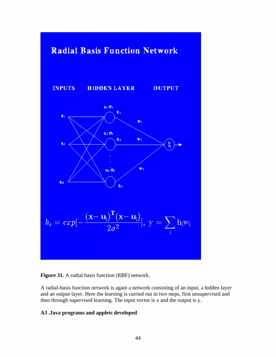
Figure 31. A radial basis function (RBF) network. A radial-basis function network is again a network consisting of an input, a hidden layer and an output layer. Here the learning is carried out in two steps, first unsupervised and then through supervised learning. The input vector is x and the output is y. A3 .Java programs and applets developed

45

Here follows a list of Java programs, applets, classes developed to illustrate our approach. UpdateCMEDatabase - This class reads emails for a specific user at email server "pop3://www.irfl.lu.se", and writes the coded part of each CME email to a text file. The coded information of this text file is then converted to CME objects, which are stored in the database. UCMEO - This class contains the specific structure of the CME objects. Methods of read and write CME-data are found in this class. UCMEODB - This class is the database interface for storing/retrieving objects of the class UCMEO. CMEmodel - This class calculates travel time and arrival time for a given CME. UpdateGICDatabase - This class reads a text file that contain predictions of GICs. Since this text file is updated every tenth minute, a comparison using the most recent received GIC forecast is made disabling multiple storing of GIC objects of the same forecast date. Finally, the data is stored in the database. GIC - This class contains the specific structure of the GIC objects. Methods of read and write GIC-data are found in this class. GICDB - This class is the database interface for storing/retrieving objects of the class GIC. LatestKpData - This class obtains the latest Kp forecast from the server at "http://sol.irfl.lu.se", and stores the data in the database. Kp - This class contains the specific structure of the Kp objects. Methods of read and write Kp-data are found in this class. KpDB - This class is the database interface for storing/retrieving objects of the class Kp. LatestGOES08part - This class reads the latest GOES08 particle data obtained from the Internet at "ftp://ftp.sec.noaa.gov/pub/lists/particle/G8part_5m.txt". The data is updated every fifth minutes. after the data is obtained, it is stored in the database. GOES08part - This class contains the specific structure of the GOES08part objects. Methods of read and write GOES08part-data are found in this class. GOES08partDB - This class is the database interface for storing/retrieving objects of the class GOES08part.

46

Similar as the above three classes, classes of LatestGOES08xray, GOES08xray, GOES08xrayDB, LatestGOES10part, GOES10part, GOES10partDB, LatestGOES10xray, GOES10xray and GOES10xrayDB have also been made. Stoplight - This class collects space weather input data, calculates current status and makes a string showing the explanation for the current status (cause and effects). The status and explanation are made available to applets via remote method invocation, RMI. StoplightApplet - This class, the Applet, uses remote methods to obtain information from the Stoplight server. This applet shows the stoplight and based on the current status received from the server, lights the green, yellow or red light. StoplightExplanationApplet - This class, the Applet, shows the explanation graph. The applet first asks the Stoplight server about the current status and then, based on the received information, colours graphic elements and displays the text as appropriate. There are also a number of classes made not mentioned above that handles, supports and enables the remote methods, graphical and explanatory details of the prototype. A more thorough and technical description of the Java implementation is given in (Hasanov and Lundstedt, 2001). References Ashmall, J. and V. Moore,:1998, Long Term Prediction of Solar Activity Using Neural Networks, in the Proceedings of "AI Applications in Solar-Terrestrial Physics", July 29-31, 1997 in Lund, Sweden, edited by I. Sandahl and E. Jonsson, ES WPP-148, April 1998. Aso,T. and T. Ogawa.:1994, Introduction of neural network in short-term prediction of solar flares, in proceedings of "AI Applications in STP", Lund 22-24 September 1993. Boberg, F., P. Wintoft and H. Lundstedt: 2000, Real time Kp predictions from solar wind data using neural networks, in Physics and Chemistry of Earth, Vol. 25, No 4. Boberg, F. and H. Lundstedt: 2000, Coronal mass ejections detected in solar mean magnetic field, GRL, Vol. 27, No.9, October 1. Bothmer, V. and R. Schwenn.:1998, Structure and Origin of Magnetic Clouds in the Solar Wind, Ann. Geophys., 16, 1.

47

Bradshaw, G.., R. Fozzard and L. Ceci.: 1989, A Connectionist Expert System That Actually Works, Advances in Neural information Processing Systems 1, edited by david S. Touretzky, Morgan Kaufman Publishers, Inc Brown, J.C., K.P. Macpherson, A.J. Conway, C.R. Mcinnes, and G. Janin,: 1994, Neural network approach to solar activity prediction, Eur. Space Oper. Cent. contact 9810/92/D/IM,final report, Univ. of Glasgow, Scotland. Burton, R.K., McPherron, R.L.. and Russell, C.T., (1975), An Empirical Relationship Between Interplanetary Conditions and Dst, J. Geophys. Res., 80, 4204. Calvo, R.A., H.A. Ceccatto, and R.D. Piacentini:1995, Neural network prediction of solar activity, Astrophys. J., 444, 916, 1995. Conway, A.J., K.P. Macpherson, G. Blacklaw, and J.C. Brown: 1998, A neural network prediction of solar cycle 23, J. Geophys. Res., 103, 29,733-29,742. Fessant, F. S. Bengio, D. Collobert.:1995, On the Prediction of Solar Activity Using Different Neural Network Models, Annales Geophysica. Freeman, J. and A. Nagai.:1993, The Magnetospheric Specification and Forecast Model: Moving from Real-time to Prediction, in Solar-Terrestrial Predictions –IV Proceedings of a Workshop at Ottawa, Canada may 18-22, 1992. Gleisner, H., Solar Wind and Geomagnetic Activity - Predictions Using Neural Networks, Thesis, Lund University 2000. Gonzalez, W.D. and B.T. Tsurutani.:1987, Criteria of interplanetary parameters causing intense geomagnetic storms (Dst<-100nT), Planet. Space Sci., 35,1101. Gopalswamy,N., Lara, A., Lepping, R.P., Kaiser, M.L., Berdichevsky, D. and St. Cyr, O.C.: 2000, Interplanetary acceleration of coronal mass ejections, Geophys. Res. Lett., 27, 145. Haykin, S.:1994, Neural networks, a comprehensive foundation, Macmillan College Publishing Company. New York. Hernandez, J.V., T. Tajima and W. Horton:1993, Neural Net Forecasting for Geomagnetic Activity, Geophys. Res. Letters, Vol. 20, No. 23, December 14. Hoyt, D.V., and K.H. Schatten.:1998, Solar Physics, 126, 407. Knowledge-Based Neurocomputing, 2000, edited by Ian Cloete and Jacek M. Zurada, MIT Press.

48

Lindblad. B.A., Lundstedt. H. and Larsson,B.:1989, A Third Catalogue of High-Speed Plasma Streams in the Solar Wind – Data 1978-1982, Solar Physics, 123, 177. Liszka, L.:1993, Modelling of pseudo-indeterministic processes using neural networks, in proceedings of "AI Applications in STP", Lund 22-24 September 1993. Lundstedt, H.: 1990, An Inductive Expert System for Solar-Terrestrial Predictions, in Proceedings of a Workshop at Leura, Australia, October 16-20, 1989. Lundstedt, H.:1991, Neural networks and predictions, in IAGA programs and abstract, XX General Assembly, IUGG, Vienna 1991. Lundstedt,H. and Hoeksema,J.T.:1992, Neural Images of the Interplanetary Magnetic Field and Predictions of Geomagnetic Storms 27 Days Ahead, in Eos, Ocober 27. Lundstedt, H.:1997, AI Techniques in Geomagnetic Storm Forecasting, invited review paper in Magnetic Storms, Geophysical Monograph 98, AGU. Lundstedt, H.:1998, Lund Space Weather Model: Status and future plans, invited presentation, in the Proceedings of the second workshop on AI Applications in Solar-Terrestrial Physics, July 29-31, 1997, Lund, Sweden, ESA WPP-148. Lundstedt, H.:1999, The Swedish Space Weather Initiatives, in Proccedings of theWorkshop on Space Weather, 11-13 November 1998, ESTEC, Noordwijk, The Netherlands, WPP-155, March 1999. Macpherson, K.P., A.J. Conway and J.C. Brown, Prediction of solar and geomagnetic activity data using neural networks, J. Geophys. Res., Vol. 100, No. All, pp 21,735-21,744, 1995 Mundt, M.D., Maguire II, W.B. and Chase R.R.P. :1991, Chaos in the Sunspot Cycle: Analysis and Prediction, J. Geophys. Res.,Vol. 96, No. A2, 1705-1716. O’Brien, T.P. and McPherron.R.L.:1999, An Empirical Phase-Space Analysis of Ring Current Dynamics: Solar Wind Control of Injection and Decay, JGR. Rubin, A.G, D.A. Hardy and K.H. Bounar: 1993, Neural Network Predictions of the Midnight Equatorward Auroral Oval Boundary, in Solar-Terrestrial Predictions – IV Proceedings of a Workshop at Ottawa, Canada May 18-22, 1992. Steinegger, M., A. Veronig, A. Hausmeier, M. Messeotti and W. Otruba.:1999, A neural network approach to solar flare alerting, presented at the 11th Cambridge Workshop "Cool Stars, Stellar System and the Sun", Puerto de la Cruz, Tenerife, Spain, 4-8 October 1999.

49

Stringer, G.A. and R.L. McPherron:1993, Neural network predictions of day-ahead relativistic electrons at geosynchronous orbit, in proceedings of "AI Applications in STP", Lund 22-24 September 1993. Thompson, A. W.P.:1993, Neural networks and non-linear prediction of geomagnetic activity, in proceedings of "AI Applications in STP", Lund 22-24 September 1993. Vassiliadis, D., A.J. Klimas, and D.N. Baker.:1996, Nonlinear ARMA models for the Dst index and their physical interpretation, in Proceedings of the third international conference on substorms (ICS-3), Versailles, France, may 13-17, 1996. Vassiliadis, D., A.J. Klimas, H. Gleisner, H. Lundstedt , G.P. Pavlos.: 2001, The number of large-scale degrees of freedom in the magnetosphere, submitted to Eos February. Willians, K.E.. 1991, Prediction of solar activity with neural network and its effect on on orbit prediction, John Hopkins APL Technical Digest, Vol. 12, No. 4. Wintoft, P. and H. Lundstedt.: 1998, Identification of Geoeffective Solar Wind Structures with Self-Organized Maps, in Proceedings of the second workshop on AI Applications in Solar-Terrestrial Physics, July 29-31, 1997, Lund, Sweden, ESA WPP-148. Wintoft, P. and H. Lundstedt:1999, A Neural Network Study of the Mapping from Solar Magnetic Fields to the Daily Average Solar Wind Velocity, J. of Geophys. Res., Vol. 104, No A4, 6729-6736, April. Wintoft, P., and L.R. Cander.:1999, Twenty-four hour predictions of foF2 using time-delay neural networks, Radio Science. Wintoft, P. and L.R. Cander.: 1994, Ionospheric foF2 Storm Forecasting using Neural Networks, Phys. Chem. Earth, Vol. 25, No. 4, pp 267-273. Wintoft, P. and Lj. R. Cander.:2000a, Ionospheric f0F2 Storm Forecasting using Neural Networks, Phys. Chem. Earth, Vol. 25, No. 4, pp 267-273. Wintoft, P. and H. Lundstedt, 2000b, Neural Network Prediction of Geosynchronous Relativistic Electron Flux From Solar Wind Data, in The First S-RAMP Conference, Sapporo, Japan; October 2-6, 2000. Wu, J.-G. and H. Lundstedt.:1996, Prediction of Geomagnetic Storms From Solar Wind Data Using Elman Recurrent Neural Networks, Geophys. Res. Letters, 23, 319-322. Wu,J.-G. and H. Lundstedt.:1997, Geomagnetic storm predictions from solar wind data with the use of dynamic neural networks, J. Geophys., res., 102, 14255-14268. Wu, J-G.: 1997, Space Weather Physics: Dynamic Neural Network Studies of Solar Wind-Magnetosphere Coupling, Thesis, Lund University, Sweden.

50

Wu, J-G., and H. Lundstedt.:1998, Space Weather Forecasting on the 1997 January Halo CME Event Using Neural Network Models, in Proceedings of the second workshop on AI Applications in Solar-Terrestrial Physics, July 29-31, 1997, Lund, Sweden, ESA WPP-148. Zhao, X.P., Hoeksema, J.T. and Marubashi, K.: 2001, Magnetic cloud Bz events and their dependence on cloud parameters, J. Geophys. Res., Vol. 106, No. A8,15,643-15656.