Equivalence of OLAP Dimension Schemas

Carlos A. Hurtado and Claudio Gutierrez

Department of Computer ScienceUniversidad de Chile

churtado,cgutierr@dcc.uchile.cl

Abstract. Dimension schemas are abstract models of the data hierar-chies that populate OLAP warehouses. Although there is abundant workon schema equivalence in a variety of data models, these works do notcover dimension schemas. In this paper we propose a notion of equiv-alence that allows to compare dimension schemas with respect to theirinformation capacity. The proposed notion is intended to capture dimen-sion schema equivalence in the context of OLAP schema restructuring.We offer characterizations of schema equivalence in terms of graph andschema isomorphisms, and present algorithms for testing it in well knownclasses of OLAP dimension schemas. Our results also permit to comparethe expressiveness of different known classes of dimension schemas.

1 Introduction

OLAP dimensions are data hierarchies that populate data warehouses. Theseentities are hierarchically organized information that define the perspective uponwhich the data is viewed. As an example, in a data warehouse we may havedimensions describing products, stores and time, which may be used to visualizethe facts generated by a sales process.

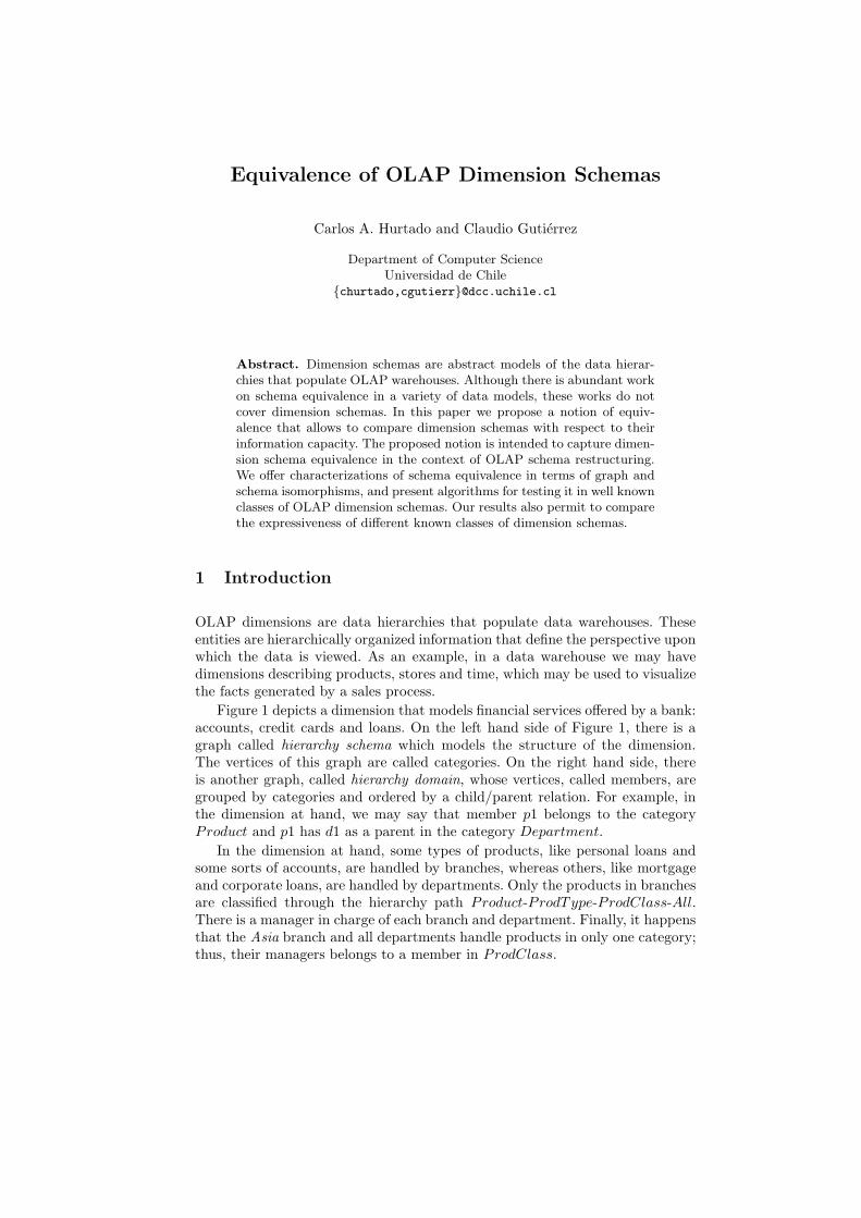
Figure 1 depicts a dimension that models financial services offered by a bank:accounts, credit cards and loans. On the left hand side of Figure 1, there is agraph called hierarchy schema which models the structure of the dimension.The vertices of this graph are called categories. On the right hand side, thereis another graph, called hierarchy domain, whose vertices, called members, aregrouped by categories and ordered by a child/parent relation. For example, inthe dimension at hand, we may say that member p1 belongs to the categoryProduct and p1 has d1 as a parent in the category Department.

In the dimension at hand, some types of products, like personal loans andsome sorts of accounts, are handled by branches, whereas others, like mortgageand corporate loans, are handled by departments. Only the products in branchesare classified through the hierarchy path Product-ProdType-ProdClass-All.There is a manager in charge of each branch and department. Finally, it happensthat the Asia branch and all departments handle products in only one category;thus, their managers belongs to a member in ProdClass.

2

m1 m2 m3 Manager

b1 b2d1 d2

Account Loan CredCard

all

(A) (B)

BLoan AccA AccB

m4

b3

p1 p2 p3 p4 p5 p6 p7

Branch

Product

All

Department

ProdClass

ProdType

Fig. 1. The dimension Product: (A) hierarchy schema; (B) child/parent relation.

1.1 Dimension Schemas

A dimension schema is an abstract model of a dimension commonly used tosupport summarizability reasoning in OLAP applications [HM02], that is, totest whether aggregate views defined for some categories can be correctly de-rived from a set of precomputed views defined for other categories. A dimensionschema, being an abstract representation of a dimension, represents the set ofpossible dimensions that conforms to it. This set reflects the information ca-pacity of the schema. Thus when we perform reasoning on the schema, we inferproperties of all the dimensions in the set.

A central drawback of traditional dimension schemas is that they do notaccount for structural heterogeneity. Such schemas model dimensions in whichmembers in a category c should have a parent in every category directly abovec, a condition we refer to as homogeneity. This restriction is unnatural sincein many application domains the members of a category have parents (resp.,ancestors) in different sets of categories. As an example, in the hierarchy domainof Figure 1 (B), some products are under branches while some others are underdepartments.

In previous work [HM02] we introduced semantically rich dimension schemasto support summarizability reasoning in heterogeneous dimensions. In our set-ting, dimension schemas are modeled as a hierarchy schema along with a set ofintegrity constraints, called dimension constraints. The hierarchy schema rep-resents a set of links for the child/parent relation, that is, whenever we have achild/parent relationship between two members in two categories, the categoriesmust be directly connected in the hierarchy schema. Dimension constraints arestatements that specify legal paths allowed in the hierarchy domain. The con-straints are used to place further restrictions to let the schema capture moreprecisely different sets of dimensions.

For example, we may require that all the products handled by some branchare not handled by departments, and vice versa. This is stated by the constraint

3

saying that each product can have ancestors in either the path 〈Product, Branch〉or the path 〈Product,Department〉, but not in both. Other constraints mayexpress that the ancestor of some members rollup to members that form a par-ticular path in the hierarchy schema. For example we model that “the man-ager of the Asia branch rolls up to a product class (because the manager han-dles products that belong to a single product class)” as “〈Branch = Asia〉 ⇔〈Branch,Manager, ProdClass〉”. The expressions in brackets are atomic state-ments (called atoms). It turns out that Boolean combinations of atoms areneeded to support summarizability reasoning [HM02].

Simple forms of these constraints characterize typical classes of OLAP schemas.For example, the condition of homogeneity of the edge (ProdType, ProdClass)can be expressed with the constraint 〈ProdType, ProdClass〉, which asserts thateach product type belongs to a product class. In this sense, the class of schemaswith dimension constraints subsumes other classes of schemas in OLAP (seeSection 2.4) such as the dimension schemas of Jagadish el al. [JLS99], called inthis paper canonical, which partially solves the limitations of traditional OLAPmodels by allowing several bottom categories, but keeping the homogeneity re-striction. Canonical schemas allow unbalancedness, that is, they can have severalbottom categories. In this form, members in different bottom categories may haveancestors in different hierarchy paths in the schema.

Different classes of dimension schemas are classified in [Hur02] where for“traditional OLAP” we refer to the basic class of homogeneous schemas with asingle bottom category (balanced schemas).

1.2 Problem Statement

Similarly to the case of general database schemas, two dimension schemas canbe compared with respect to their information capacity. Schemas with the sameinformation capacity can be used to simulate each other. In a typical modelingscenario the user starts with some schema and proceeds to restructure it. In thecontext of OLAP, it is very important that the restructuring process preservesschema equivalence because the schema is more useful for reasoning about datathan it is just as a container of data. So we would like to keep the informationon the schema as precise as possible to capture the set of instances as tight aspossible.

The goal of this paper is to study dimension schema equivalence in the con-text of OLAP schema restructuring. Formal notions of schema equivalence arefundamental to sit restructuring techniques on solid grounds. For example, Milleret al. [MIR94] argue that the restructuring task may be addressed following twodifferent strategies: (i) build a desired schema and then test whether it is equiv-alent to the original schema; (ii) use a set of primitives to transform the originalschema into a desired schema. In both approaches, we need to define underwhich conditions two dimension schemas are equivalent. In the first approachwe need algorithms for the equivalence test. The second approach requires a setof well defined dimension transformations. The central desirable properties of

4

Branch

Product

Department

Manager

ProdType

All

ProdClass

Branch

Product

All

Manager

ProdType

ProdClass

Dept&AsiaBranch Department

ProdType

Dept&AsiaManager

DeptProduct

All

BranchProduct

Branch

BranchManager

ProdClass

AsiaBranch

AsiaBranchProduct

(A) (B) (C)

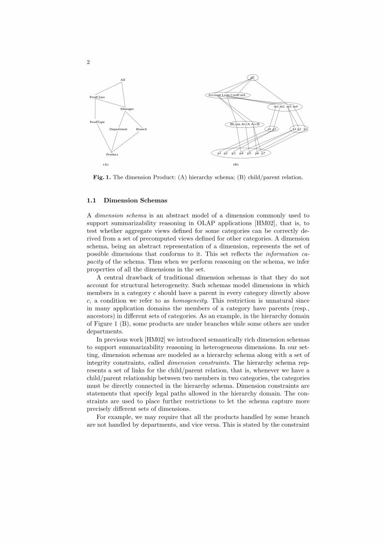
Fig. 2. Product hierarchy schemas.

such a set, soundness and completeness [Alb00], depend on the notion of schemaequivalence used as well.

We cast the restructuring task as a process in which the structure of thedimension (i.e. its hierarchy schema) changes but its data hierarchy (hierarchicaldomain) does not.

Example 1. Consider the hierarchy schemas shown in Figure 2. The three hier-archy schemas can be used to model the hierarchy domain of Figure 1. Hierar-chy schema (A) is the same as the one of Figure 1. Hierarchy schema (B) hasAsia branch grouped with departments in a single category. Finally, in hierar-chy schema (C), the products (bottom members) are split into three categories:DeptProduct, AsiaBranchProduct, and BranchProduct, the branches are splitinto Branch and AsiaBranch, and the managers are split into the categoriesDep&AsiaManager and BranchManager. Notice that the dimension havinghierarchy schema (C) along with the hierarchy domain of Figure 1 is homoge-neous.

Schema equivalence has been formalized by requiring the existence of a bijec-tive mapping between the instances of two equivalent schema [Hul86]. Example 1shows that a great deal of flexibility in OLAP dimension modeling can be cap-tured by restructuring processes in which members are reorganized into differentcategories but their hierarchy domain does not change. Thus at the schema level,the correctness of a restructuring process may be formalized by requiring theexistence of bijective instance mappings between the schemas which preservehierarchy domains. As members are associated with facts in datacubes, thismapping restriction guarantees that the aggregate data are preserved throughdifferent dimension instances in the restructuring process, thus avoiding aggre-gate data re-computations, and keeping users to browse aggregate data usingthe same hierarchy domain.

Example 2. Consider the following dimension schemas. The dimension schemaproductA has the hierarchy schema of Figure 1 (A) along with the dimension

5

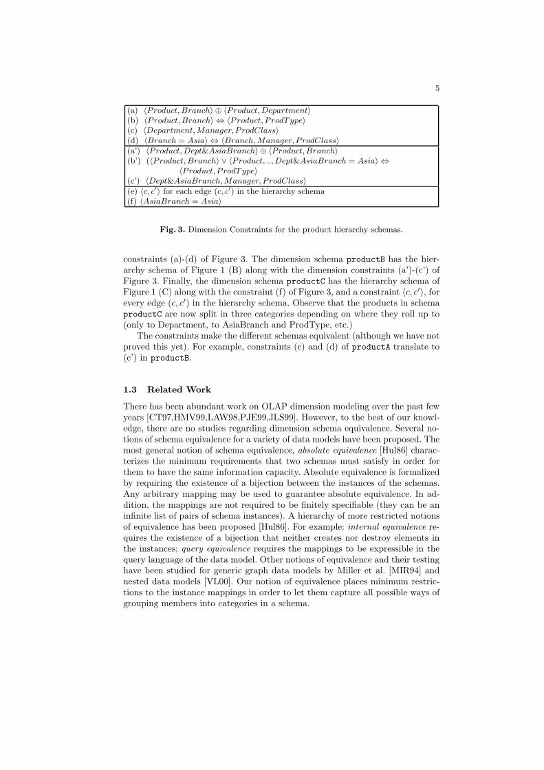
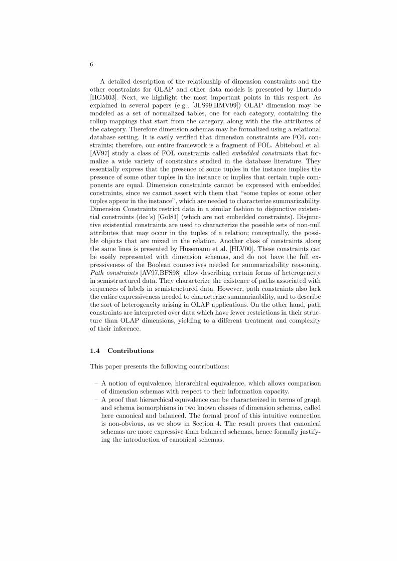
(a) 〈Product,Branch〉 ⊕ 〈Product, Department〉(b) 〈Product,Branch〉 ⇔ 〈Product, P rodType〉(c) 〈Department,Manager,ProdClass〉(d) 〈Branch = Asia〉 ⇔ 〈Branch, Manager,ProdClass〉(a’) 〈Product, Dept&AsiaBranch〉 ⊕ 〈Product,Branch〉(b’) (〈Product, Branch〉 ∨ 〈Product, .., Dept&AsiaBranch = Asia〉 ⇔

〈Product, P rodType〉(c’) 〈Dept&AsiaBranch,Manager,ProdClass〉(e) 〈c, c′〉 for each edge (c, c′) in the hierarchy schema(f) 〈AsiaBranch = Asia〉

Fig. 3. Dimension Constraints for the product hierarchy schemas.

constraints (a)-(d) of Figure 3. The dimension schema productB has the hier-archy schema of Figure 1 (B) along with the dimension constraints (a’)-(c’) ofFigure 3. Finally, the dimension schema productC has the hierarchy schema ofFigure 1 (C) along with the constraint (f) of Figure 3, and a constraint 〈c, c′〉, forevery edge (c, c′) in the hierarchy schema. Observe that the products in schemaproductC are now split in three categories depending on where they roll up to(only to Department, to AsiaBranch and ProdType, etc.)

The constraints make the different schemas equivalent (although we have notproved this yet). For example, constraints (c) and (d) of productA translate to(c’) in productB.

1.3 Related Work

There has been abundant work on OLAP dimension modeling over the past fewyears [CT97,HMV99,LAW98,PJE99,JLS99]. However, to the best of our knowl-edge, there are no studies regarding dimension schema equivalence. Several no-tions of schema equivalence for a variety of data models have been proposed. Themost general notion of schema equivalence, absolute equivalence [Hul86] charac-terizes the minimum requirements that two schemas must satisfy in order forthem to have the same information capacity. Absolute equivalence is formalizedby requiring the existence of a bijection between the instances of the schemas.Any arbitrary mapping may be used to guarantee absolute equivalence. In ad-dition, the mappings are not required to be finitely specifiable (they can be aninfinite list of pairs of schema instances). A hierarchy of more restricted notionsof equivalence has been proposed [Hul86]. For example: internal equivalence re-quires the existence of a bijection that neither creates nor destroy elements inthe instances; query equivalence requires the mappings to be expressible in thequery language of the data model. Other notions of equivalence and their testinghave been studied for generic graph data models by Miller et al. [MIR94] andnested data models [VL00]. Our notion of equivalence places minimum restric-tions to the instance mappings in order to let them capture all possible ways ofgrouping members into categories in a schema.

6

A detailed description of the relationship of dimension constraints and theother constraints for OLAP and other data models is presented by Hurtado[HGM03]. Next, we highlight the most important points in this respect. Asexplained in several papers (e.g., [JLS99,HMV99]) OLAP dimension may bemodeled as a set of normalized tables, one for each category, containing therollup mappings that start from the category, along with the the attributes ofthe category. Therefore dimension schemas may be formalized using a relationaldatabase setting. It is easily verified that dimension constraints are FOL con-straints; therefore, our entire framework is a fragment of FOL. Abiteboul et al.[AV97] study a class of FOL constraints called embedded constraints that for-malize a wide variety of constraints studied in the database literature. Theyessentially express that the presence of some tuples in the instance implies thepresence of some other tuples in the instance or implies that certain tuple com-ponents are equal. Dimension constraints cannot be expressed with embeddedconstraints, since we cannot assert with them that “some tuples or some othertuples appear in the instance”, which are needed to characterize summarizability.Dimension Constraints restrict data in a similar fashion to disjunctive existen-tial constraints (dec’s) [Gol81] (which are not embedded constraints). Disjunc-tive existential constraints are used to characterize the possible sets of non-nullattributes that may occur in the tuples of a relation; conceptually, the possi-ble objects that are mixed in the relation. Another class of constraints alongthe same lines is presented by Husemann et al. [HLV00]. These constraints canbe easily represented with dimension schemas, and do not have the full ex-pressiveness of the Boolean connectives needed for summarizability reasoning.Path constraints [AV97,BFS98] allow describing certain forms of heterogeneityin semistructured data. They characterize the existence of paths associated withsequences of labels in semistructured data. However, path constraints also lackthe entire expressiveness needed to characterize summarizability, and to describethe sort of heterogeneity arising in OLAP applications. On the other hand, pathconstraints are interpreted over data which have fewer restrictions in their struc-ture than OLAP dimensions, yielding to a different treatment and complexityof their inference.

1.4 Contributions

This paper presents the following contributions:

– A notion of equivalence, hierarchical equivalence, which allows comparisonof dimension schemas with respect to their information capacity.

– A proof that hierarchical equivalence can be characterized in terms of graphand schema isomorphisms in two known classes of dimension schemas, calledhere canonical and balanced. The formal proof of this intuitive connectionis non-obvious, as we show in Section 4. The result proves that canonicalschemas are more expressive than balanced schemas, hence formally justify-ing the introduction of canonical schemas.

7

– A class of schemas –frozen schemas– that act as normal forms for dimen-sions schemas, in the sense that any dimension schema can be reduced viasome well defined transformation to a unique (up to isomorphism) frozenschema. It is proved that hierarchy equivalence test for frozen dimensionreduces to a simple form of schema isomorphism. This result leads to otherimportant property of dimension schemas, namely, that heterogeneous di-mension schemas can always be transformed into homogeneous schemas. Wesketch an algorithm that performs such transformation in an efficient way,and study its complexity.

– Complexity bounds and a study of algorithmic aspects of hierarchical equiv-alence testing. In particular, we present a characterization of hierarchicalequivalence in terms of mappings between minimal dimensions instance con-tained by the schemas. This leads to an algorithm for testing hierarchicalequivalence. We show that the algorithm is more efficient than testing hier-archical equivalence by reducing the schemas to frozen schemas.

1.5 Outline

The remainder of the paper is organized as follows. In Section 2 we review themain concepts related to schemas and state the notation. Section 3 introduceshierarchical equivalence and show its relation with balanced schemas. Section4 studies hierarchical equivalence of canonical schemas, and shows that in thiscontext hierarchical equivalence corresponds exactly with graph isomorphismof the corresponding hierarchy schemas. In Section 5 we generalize this resultto dimension schemas, that is allowing to compare different hierarchy schemasand constraints. The notion of frozen schema is introduced and studied, alongwith the algorithmic aspects of hierarchical equivalence are studied. Finally, inSection 6 we briefly conclude and outline further work. The complete proofs arepresented in the full version of this paper [HG03].

2 Preliminaries

2.1 Basic Graph Terminology

A (directed) graph G is a pair of sets (V,E) where E ⊆ V × V . Elements v ∈ Vare called vertices and pairs (u, v) ∈ E (directed) edges; u and v are adjacentvertices. A path in G from v to w is a sequence of vertices v = v0, . . . , vn = wsuch that (vi, vi+1) ∈ E. We say that v reaches w. The length of a path is n. Acycle is a path with v = w. A dag is a directed acyclic graph. A sink in a dag is adistinguished vertex w reachable from every other vertex in the graph. A sourcein a dag is a distinguished vertex v from which every other vertex of the graphis reachable. A shortcut in a dag is a path of length > 1 between two adjacentvertices. Given a vertex v of G, an upgraph is the subgraph of G generated by vand all the vertices reachable from it.

Given two graphs G = (V,E) and G′ = (V ′, E′), a graph morphism is a func-tion φ : V → V ′ preserving edges, that is, (u, v) ∈ E implies (φ(u), φ(v)) ∈ E′.

8

The morphism φ is called an isomorphism (resp. monomorphism, epimorphism)if φ as a function is bijective (resp. injective, onto).

2.2 Dimension Instance

Assume the existence of (possibly infinite) sets of categories C, and of membersM.

Definition 1 (Hierarchy Schema). A hierarchy schema is a dag H = (C,),where C ⊆ C, having a distinguished category All ∈ C which is a sink.

Definition 2 (Hierarchy Domain). A Hierarchy domain is a dag h = (M,<)where M ⊂ M, having a distinguished member all ∈ M which is a sink, andwithout shortcuts.

The last condition in Definition 2 (no shortcuts) avoids redundancies (tran-sitive edges) in the representation of the data.

Given a child/parent relation <, its reflexive and transitive closure, denoted≤, is called rollup relation, and is a partial order between members.

Definition 3 (Dimension Instance). A dimension instance d over a hierarchyschema (C,) is a graph morphism d : (M,<) → (C,) such that:

1. (M,<) is a hierarchy domain;2. d(all) = All;3. x ≤ y ∧ x ≤ z implies d(y) 6= d(z).

The fact that d is a graph morphism in Definition 3 states that wheneverwe have a child/parent relationship m1 < m2 between some pair of membersm1 ∈ c1 and m2 ∈ c2, then there is an edge c1 c2 in the hierarchy schemarepresenting links between categories c1 and c2. Condition 3 of Definition 3 isa basic restriction in OLAP data modeling [HMV99,CT97,LAW98], and statesthat the rollup relation ≤ is functional (i.e., single valued) between every pairof categories. This motivates to introduce the rollup mapping between two cat-egories c1 and c2 of a dimension d, denoted Γ c2

c1d, which is the restriction of ≤

to d−1(c1) and d−1(c2).

2.3 Dimension Schema

Next we formalize the notions of dimension constraint and dimension schema.

Definition 4 (Dimension Constraint). Let H = (C,) be a hierarchy schema,c ∈ C, K ⊆ M. The language of constraints (with root c) has the following atoms:

1. Path atoms: 〈c, c1, · · · , cn〉, where cc1 · · · cn is a path in H;2. Equality atoms: 〈c, .., c′ = k〉, where c′ is such that there is a path from c

to c′, and k ∈ K.A dimension constraint with root c is a Boolean combination φ of atoms of

the above kind.

9

Dimension constraints consider the usual connectives ¬,∧,∨,⇒,⇔, and ⊕for exclusive disjunction. In addition, ⊥ and > will denote the false and the trueproposition, respectively.

Definition 5 (Semantics of Constraints). Let d : (M,<) → (C,) be adimension instance, and φ a constraint with root c. Then d |= φ if and only if

for all m ∈ d−1(c), d |= φ[c/m],where d |= φ[c/m] is defined recursively as follows:

1. d |= 〈c, c1, . . . , cn〉[c/m] iff there is a path mx1 · · ·xn in (M,<) with d(xi) ∈ci.

2. d |= 〈c, .., c′ = k〉[c/m] iff d(k) ∈ c′ and m ≤ k.3. d |= (φ ∧ψ)[c/m] iff d |= φ[c/m] and d |= ψ[c/m]. Similarly for ∨ and the

other Boolean connectives.

Given a hierarchy schema H and two sets of constraints Σ,Σ′ over H , wesay that Σ is equivalent to Σ′, if for all dimension instances d over H it holds:d |= Σ iff d |= Σ′.

Now we are ready to introduce the concept of Dimension Schema. The fol-lowing definition extends Definition 3 in the presence of constraints.

Definition 6 (Dimension Schema). A dimension schema is a pair (H,Σ)where H is a hierarchy schema and Σ is a set of constraints.

A dimension instance d over a dimension schema D = (H,Σ) is a dimensioninstance d over H such that d |= Σ. The set of dimensions instances over D willbe denoted by I(D).

Definition 7 (Schema Equivalence and Isomorphism).Let D = (H,Σ) and D′ = (H ′, Σ′) be to dimension schemas.1. D and D′ are equivalent, denoted D ≡ D′, iff H = H ′ and Σ is equivalent

to Σ′.2. D and D′ are isomorphic, denoted D ∼= D′, iff there exists a graph iso-

morphism f : H → H ′ such that (f(H), f(Σ)) ≡ (H ′, Σ′), where f(Σ) standsfor Σ modulo renaming by f .

Notice that the notion of equivalence of Definition 7 implies isomorphism.

2.4 Classes of Dimension Schemas

The model we have presented subsumes the dimension models presented in theliterature. The following definition formalizes two classes of dimension schemasthat arise in OLAP.

Definition 8 (Classes of Dimension Schemas). Let D = (H,Σ) be a di-mension schema.

1. D is canonical iff H has no shortcuts and Σ is equivalent to 〈c, c′〉 | cc′.

2. D is balanced iff D is canonical and H has a source.

10

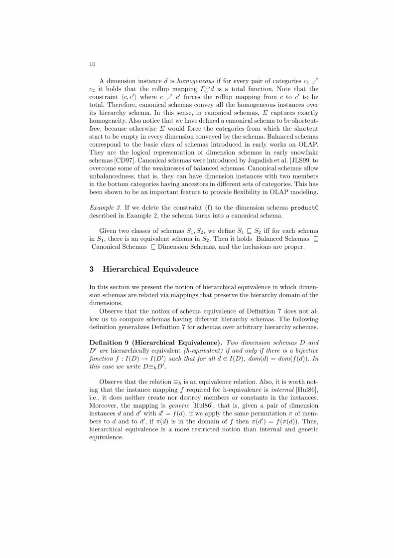
A dimension instance d is homogeneous if for every pair of categories c1 c2 it holds that the rollup mapping Γ c2

c1d is a total function. Note that the

constraint 〈c, c′〉 where c c′ forces the rollup mapping from c to c′ to betotal. Therefore, canonical schemas convey all the homogeneous instances overits hierarchy schema. In this sense, in canonical schemas, Σ captures exactlyhomogeneity. Also notice that we have defined a canonical schema to be shortcut-free, because otherwise Σ would force the categories from which the shortcutstart to be empty in every dimension conveyed by the schema. Balanced schemascorrespond to the basic class of schemas introduced in early works on OLAP.They are the logical representation of dimension schemas in early snowflakeschemas [CD97]. Canonical schemas were introduced by Jagadish et al. [JLS99] toovercome some of the weaknesses of balanced schemas. Canonical schemas allowunbalancedness, that is, they can have dimension instances with two membersin the bottom categories having ancestors in different sets of categories. This hasbeen shown to be an important feature to provide flexibility in OLAP modeling.

Example 3. If we delete the constraint (f) to the dimension schema productC

described in Example 2, the schema turns into a canonical schema.

Given two classes of schemas S1, S2, we define S1 v S2 iff for each schemain S1, there is an equivalent schema in S2. Then it holds Balanced Schemas vCanonical Schemas v Dimension Schemas, and the inclusions are proper.

3 Hierarchical Equivalence

In this section we present the notion of hierarchical equivalence in which dimen-sion schemas are related via mappings that preserve the hierarchy domain of thedimensions.

Observe that the notion of schema equivalence of Definition 7 does not al-low us to compare schemas having different hierarchy schemas. The followingdefinition generalizes Definition 7 for schemas over arbitrary hierarchy schemas.

Definition 9 (Hierarchical Equivalence). Two dimension schemas D andD′ are hierarchically equivalent (h-equivalent) if and only if there is a bijectivefunction f : I(D) → I(D′) such that for all d ∈ I(D), dom(d) = dom(f(d)). Inthis case we write D≡hD

′.

Observe that the relation ≡h is an equivalence relation. Also, it is worth not-ing that the instance mapping f required for h-equivalence is internal [Hul86],i.e., it does neither create nor destroy members or constants in the instances.Moreover, the mapping is generic [Hul86], that is, given a pair of dimensioninstances d and d′ with d′ = f(d), if we apply the same permutation π of mem-bers to d and to d′, if π(d) is in the domain of f then π(d′) = f(π(d)). Thus,hierarchical equivalence is a more restricted notion than internal and genericequivalence.

11

All

ba

c d

(A)

All

(B)

e

f g

h

j

All

i

(C)

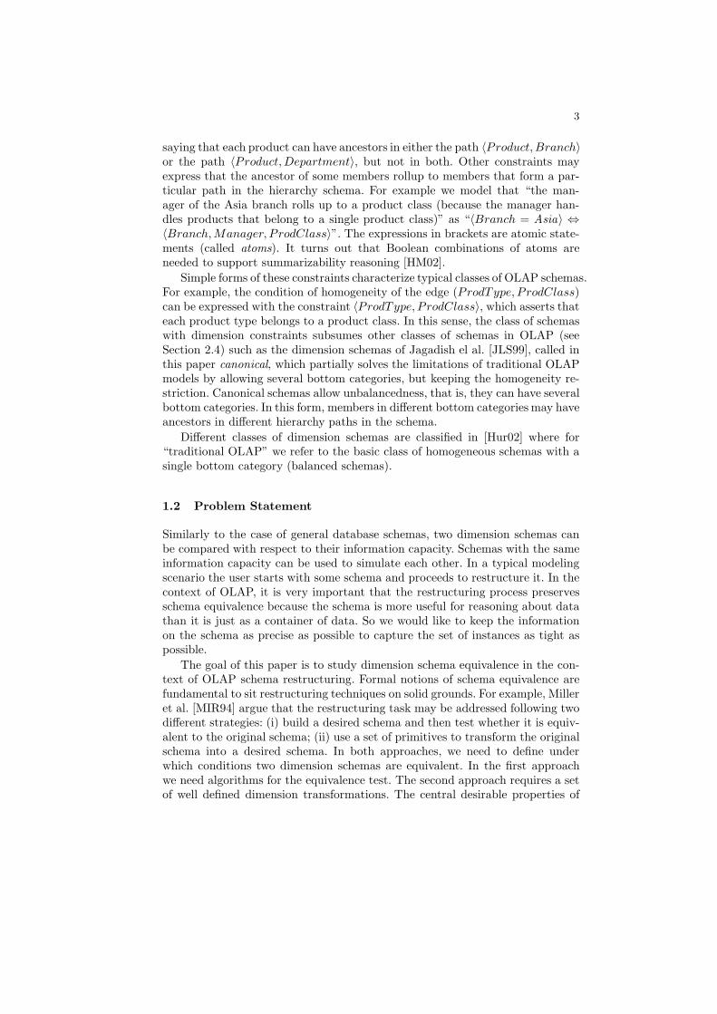
Fig. 4. Three hierarchy schemas.

Example 4. Consider the dimension schemas D1 = (A,Σ1), D2 = (B,Σ2) andD3 = (C,Σ3), where A,B,C are the hierarchy schemas in Figure 4, Σ1 = Σ3 = ∅and Σ2 = ¬〈e, f〉 ∨ ¬〈e, g〉. Then D1≡hD2 via mapping the members of c tof , the members of d to g, and the members of a and b to e. However, it is notthe case that D1≡hD3. Indeed, given a member m, there is a unique dimensioninstance in I(D3) whose child/parent relation is m < all, but there are twodimension instances in I(D2) whose child/parent relation is m < all.

It is not difficult to check that if D ∼= D′ then D≡hD′. We end this section

by showing that it is straightforward to show that the converse also holds forbalanced schemas.

A dimension instance d is exact if d is bijective. It is easily verified that allcanonical dimension schemas have an exact dimension instance.

Theorem 1 (h-Equivalence of Balanced Schemas). Two balanced dimen-sion schemas D = (H,Σ) and D′ = (H ′, Σ′) are h-equivalent if and only if Hand H ′ are (graph) isomorphic.

Proof. (Sketch.) One direction is obvious.Assume that D≡hD

′ via f . Consider an exact dimension d of (H,Σ). Then asgraphsH ∼= dom(d) ∼= dom(f(d)). Now, becauseD′ is balanced there is a (graph)monomorphism µ : dom(f(d)) → H ′ with µ(all) = All (if µ(v) = µ(w) forv 6= w, the source of dom(f(d)) would have two ancestors in the same category,violating condition 3 of Definition 3.) Hence there is a monomorphism H → H ′.By the same argument on the reverse direction, there is a monomorphism H ′ →H . Hence because H,H ′ are finite graphs, H ∼= H ′.

4 Hierarchical Equivalence of Canonical Schemas

This section extends the results of Theorem 1 to canonical dimensions. The im-portance of this result is twofold: (1) The notion of h-equivalence has a simpleand intuitive characterization as graph isomorphism in canonical schemas (this

12

All

onme

j k b

gf

a

c e

All

(A) (B)

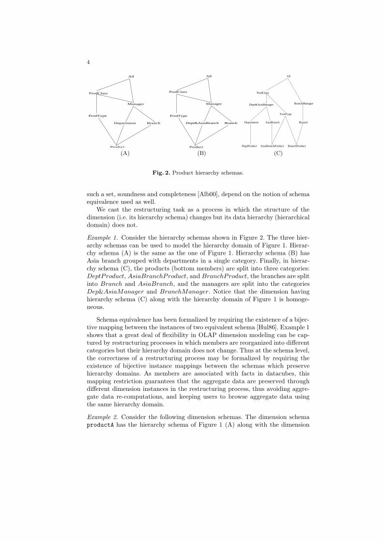
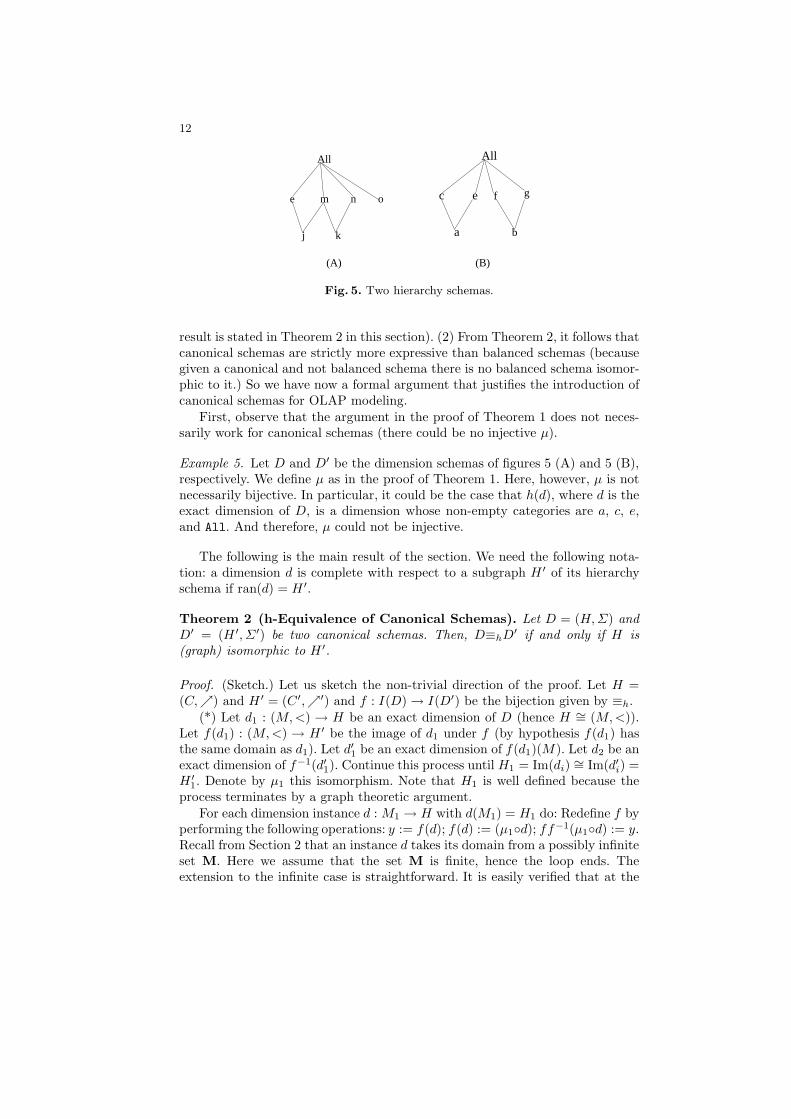
Fig. 5. Two hierarchy schemas.

result is stated in Theorem 2 in this section). (2) From Theorem 2, it follows thatcanonical schemas are strictly more expressive than balanced schemas (becausegiven a canonical and not balanced schema there is no balanced schema isomor-phic to it.) So we have now a formal argument that justifies the introduction ofcanonical schemas for OLAP modeling.

First, observe that the argument in the proof of Theorem 1 does not neces-sarily work for canonical schemas (there could be no injective µ).

Example 5. Let D and D′ be the dimension schemas of figures 5 (A) and 5 (B),respectively. We define µ as in the proof of Theorem 1. Here, however, µ is notnecessarily bijective. In particular, it could be the case that h(d), where d is theexact dimension of D, is a dimension whose non-empty categories are a, c, e,and All. And therefore, µ could not be injective.

The following is the main result of the section. We need the following nota-tion: a dimension d is complete with respect to a subgraph H ′ of its hierarchyschema if ran(d) = H ′.

Theorem 2 (h-Equivalence of Canonical Schemas). Let D = (H,Σ) andD′ = (H ′, Σ′) be two canonical schemas. Then, D≡hD

′ if and only if H is(graph) isomorphic to H ′.

Proof. (Sketch.) Let us sketch the non-trivial direction of the proof. Let H =(C,) and H ′ = (C′,′) and f : I(D) → I(D′) be the bijection given by ≡h.

(*) Let d1 : (M,<) → H be an exact dimension of D (hence H ∼= (M,<)).Let f(d1) : (M,<) → H ′ be the image of d1 under f (by hypothesis f(d1) hasthe same domain as d1). Let d′1 be an exact dimension of f(d1)(M). Let d2 be anexact dimension of f−1(d′1). Continue this process until H1 = Im(di) ∼= Im(d′i) =H ′

1. Denote by µ1 this isomorphism. Note that H1 is well defined because theprocess terminates by a graph theoretic argument.

For each dimension instance d : M1 → H with d(M1) = H1 do: Redefine f byperforming the following operations: y := f(d); f(d) := (µ1d); ff−1(µ1d) := y.Recall from Section 2 that an instance d takes its domain from a possibly infiniteset M. Here we assume that the set M is finite, hence the loop ends. Theextension to the infinite case is straightforward. It is easily verified that at the

13

b

f

a

c e

All

g

k

All

onme

j

k

All

onme

j

b

f

a

c e

All

g

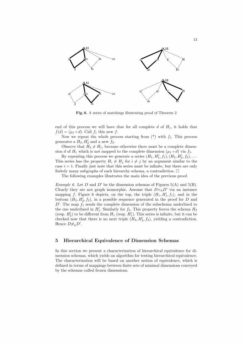
Fig. 6. A series of matchings illustrating proof of Theorem 2

end of this process we will have that for all complete d of H1, it holds thatf(d) = (µ1 d). Call f1 this new f .

Now we repeat the whole process starting from (*) with f1. This processgenerates a H2, H

′

2 and a new f2.Observe that H2 6= H1, because otherwise there must be a complete dimen-

sion d of H1 which is not mapped to the complete dimension (µ1 d) via f1.By repeating this process we generate a series (H1, H

′

1, f1), (H2, H′

2, f2), . . .This series has the property Hi 6= Hj for i 6= j by an argument similar to thecase i = 1. Finally just note that this series must be infinite, but there are onlyfinitely many subgraphs of each hierarchy schema, a contradiction.

The following examples illustrates the main idea of the previous proof.

Example 6. Let D and D′ be the dimension schemas of Figures 5(A) and 5(B).Clearly they are not graph isomorphic. Assume that D≡hD

′ via an instancemapping f . Figure 6 depicts, on the top, the triple (H1, H

′

1, f1), and in thebottom (H2, H

′

2, f2), in a possible sequence generated in the proof for D andD′. The map f1 sends the complete dimension of the subschema underlined tothe one underlined in H ′

1. Similarly for f2. This property forces the schema H2

(resp. H ′

2) to be different from H1 (resp. H ′

1). This series is infinite, but it can bechecked now that there is no next triple (H3, H

′

3, f3), yielding a contradiction.Hence D 6≡hD

′.

5 Hierarchical Equivalence of Dimension Schemas

In this section we present a characterization of hierarchical equivalence for di-mension schemas, which yields an algorithm for testing hierarchical equivalence.The characterization will be based on another notion of equivalence, which isdefined in terms of mappings between finite sets of minimal dimensions conveyedby the schemas called frozen dimensions.

14

5.1 Frozen Equivalence

We introduce a notion of equivalence, frozen equivalence, defined in terms ofinjective mappings between special kinds of dimension instances, called frozen.Intuitively, a frozen dimension is a minimal dimension conveyed by a dimensionschema. Frozen dimensions were introduced in previous work [HM02] to test im-plication of dimension constraints. In order to test whether a dimension schemasatisfies a dimension constraint α, we only need to check α in each frozen di-mension of the schema, which yields a finite set of tests (exponential in the sizeof the schema). In this section we use the notion of frozen dimension for givingan algorithmic version of h-equivalence.

Let D = (H,Σ) be a dimension schema, we denote by ConstD(c) the set ofconstants k that occur in atoms of the form 〈ci, .., c = k〉 in Σ.

Definition 10 (Frozen Dimension). Given a dimension schema D and c ∈C, a frozen dimension with root c is a dimension instance d : (M,<) → (C,<)of D such that:

1. d is injective (i.e., each category has at most one member);2. d−1(c) is a source of (M,<);

There could be infinitely many frozen dimensions, but there are only finitelymany up to isomorphism, where isomorphism is defined as follows: d is isomor-phic to d′ iff there exists a graph mapping f : (M,<) → (M ′, <′) such thatd = d′ f , and if k ∈ ConstD(cj) and d(k) = cj = d′(k), then f(k) = k.

From now one, we will consider frozen dimensions up to isomorphism. Givena dimension schema D and a category c of it, we denote by Frozen(D, c) the setof frozen dimensions of D (up to isomorphism) with root c, and by Frozen(D)the union of all Frozen(D, c) for all categories c of D.

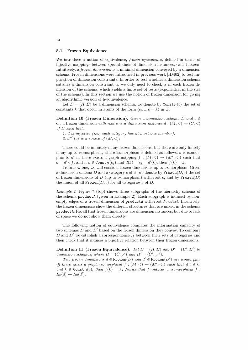
Example 7. Figure 7 (top) shows three subgraphs of the hierarchy schema ofthe schema productA (given in Example 2). Each subgraph is induced by non-empty edges of a frozen dimension of productA with root Product. Intuitively,the frozen dimensions show the different structures that are mixed in the schemaproductA. Recall that frozen dimensions are dimension instances, but due to lackof space we do not show them directly.

The following notion of equivalence compares the information capacity oftwo schemas D and D′ based on the frozen dimension they convey. To compareD and D′ we establish a correspondence Ω between their sets of categories andthen check that it induces a bijective relation between their frozen dimensions.

Definition 11 (Frozen Equivalence). Let D = (H,Σ) and D′ = (H ′, Σ′) bedimension schemas, where H = (C,) and H ′ = (C′,′):

Two frozen dimensions d ∈ Frozen(D) and d′ ∈ Frozen(D′) are isomorphiciff there exists a graph isomorphism f : (M,<) → (M ′, <′) such that if c ∈ Cand k ∈ ConstD(c), then f(k) = k. Notice that f induces a isomorphism f :Im(d) → Im(d′).

15

Branch

Product

All

Department

Manager

ProdType

ProdClass

Product

ProdClass

Dept&AsiaBranch

ProdClass

ProdType

Manager

All

Product

BranchDept&AsiaBranch

ProdClass

ProdType

Manager

All

Department

Manager

Product

All

Department

Manager

f1 f2 f3

Branch:AsiaBranch

ProdClass

ProdType ProdType

Manager

f2 f3f’1

Branch

Product

All

ProdType

ProdClass

Dept&AsiaBranch Branch

Product

All

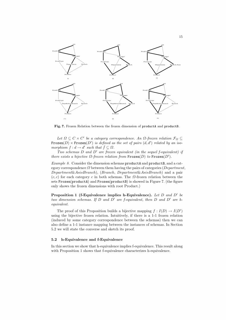
Fig. 7. Frozen Relation between the frozen dimension of productA and productB.

Let Ω ⊆ C × C′ be a category correspondence. An Ω-frozen relation FΩ ⊆Frozen(D) × Frozen(D′) is defined as the set of pairs (d, d′) related by an iso-morphism f : d→ d′ such that f ⊆ Ω.

Two schemas D and D′ are frozen equivalent (in the sequel f-equivalent) ifthere exists a bijective Ω-frozen relation from Frozen(D) to Frozen(D′).

Example 8. Consider the dimension schemas productA and productB, and a cat-egory correspondenceΩ between them having the pairs of categories (Department,Department&AsisBranch), (Branch, Department&AsisBranch) and a pair(c, c) for each category c in both schemas. The Ω-frozen relation between thesets Frozen(productA) and Frozen(productB) is showed in Figure 7. (the figureonly shows the frozen dimensions with root Product.)

Proposition 1 (f-Equivalence implies h-Equivalence). Let D and D′ betwo dimension schemas. If D and D′ are f-equivalent, then D and D′ are h-equivalent.

The proof of this Proposition builds a bijective mapping f : I(D) → I(D′)using the bijective frozen relation. Intuitively, if there is a 1-1 frozen relation(induced by some category correspondence between the schemas) then we canalso define a 1-1 instance mapping between the instances of schemas. In Section5.2 we will state the converse and sketch its proof.

5.2 h-Equivalence and f-Equivalence

In this section we show that h-equivalence implies f-equivalence. This result alongwith Proposition 1 shows that f-equivalence characterizes h-equivalence.

16

Firstly, we will introduce frozen schemas, dimension schemas that are normalforms, in the sense that every dimension schema is h-equivalent to a frozenschema.

Definition 12 (Frozen Schema). A frozen schema is a dimension schema Dsuch that each category c in D has a unique frozen dimension d and Im(d) isexactly the upgraph of c.

The following are some basic properties of frozen schemas: their dimensioninstances are homogeneous; they do not have shortcuts; and they subsume canon-ical schemas.

Example 9. The dimension schema productC given in Example 2 is a frozenschema, because its constraints cause each category c to have a single frozendimension with root c. The category AsiaBranch is the only category whosefrozen dimension has a constant (Asia). Schemas productA and productB arenot frozen schemas since they convey several frozen dimensions with the categoryProduct as root.

Next, we show that testing h-equivalence of frozen schemas defined over thesame set of constants reduces to testing whether the schemas are isomorphic.This result generalizes Theorem 2 because canonical schemas are frozen schemas.

Note that two isomorphic frozen dimension must have the same set of con-stants. We will say that two frozen schemas are normalized w.r.t. a set of con-stants if for all c ∈ C and c′ ∈ C′ it holds ConstD(c) = ConstD′(c′), i.e., theirequality atoms mention the same constants for each category.

Theorem 3 (h-Equivalence of Frozen Schemas). Let D and D′ be two nor-malized frozen schemas. Then D and D′ are h-equivalent iff they are isomorphic(i.e., D≡hD

′ iff D ∼= D′).

The proof is a generalization of the proof of Theorem 2. This theorem alsoshows that dimension schemas are more expressive than canonical schemas be-cause some frozen schemas are not isomorphic to any canonical schema. Thatis, there are dimension schemas for which there are no h-equivalent canonicalschemas.

Finally, we prove the main result of this section.

Theorem 4 (h-Equivalence of dimension Schemas). Let D and D′ be twonormalized frozen dimension schemas. Then D and D′ are f -equivalent iff theyare h-equivalent.

Proof. (Sketch.) One direction is Proposition 1.So assume that D and D′ are h-equivalent. First define a schema trans-

formation that takes D and produces a frozen schema Df h-equivalent to D.The transformation works as follows: (1) Compute the frozen dimensions of Dusing the DIMSAT algorithm presented in previous work [HM02]; (2) Reversethe graph (C,′) and do a topological sort of the resulting graph. (3) Follow

17

the topological sort, and for each category c with more than one frozen dimen-sion, split c into c1, . . . , cn (preserving adjacent edges). Add constraints to theschema in order to have a single frozen dimension in each category c1, . . . , cn.This process yields a new dimension schema with a single frozen dimension ineach category; (4) For each category cj of the schema delete adjacent edges thatdo not match the frozen dimension.

Each split in step (3) induces induces the following category correspondencebetween the hierarchy schemas before and after the split: (c, cj) for all 1 ≤ j ≤ n,and for the remaining categories c′ that appear in both hierarchy schemas wehave (c, c′). It is not difficult to verify that this category correspondence inducesa bijective frozen relation between the old and the new schema. By composingthese frozen relations we get a bijective frozen relation between D and Df .

In the same manner, we built a frozen schema D′

f and a bijective frozenrelation between D′ and D′

f . Hence, we have bijective frozen relations D → Df

and D′ → D′

f . Also, from Theorem 3 we know that Df∼= D′

f via some µ. Fromµ we can derive a bijective frozen relation between Df and D′

f . Composing theserelations we derive the statement of the theorem.

Example 10. The bijective frozen relation of Figure 7 shows that the schemasproductA and productB of Example 2 are h-equivalent. By a simmilar proce-dure it can be easily verified that schema productC is h-equivalent to schemasproductA and productB.

5.3 Transforming Dimension Schemas into Homogeneous Schemas

From the proof of Theorem 4 it follows that any dimension schema can betransformed into a hierarchically equivalent homogeneous schema. In Figure 8we sketch an algorithm to perform such a transformation.

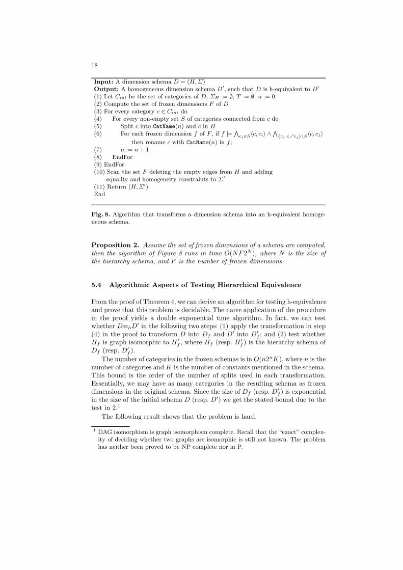
The algorithm outputs dimension schemas having the constraints that statethe homogeneity condition. The schemas may also have additional constraintswith equality atoms. Path atoms other than the ones that state the homogeneitycondition are irrelevant for the resulting schemas because a path atom is either⊥ or > in every instance of a homogeneous schema. In Line 2 the algorithmcomputes the set of frozen dimensions of D. In Line 5, for each category c ofD and subset S of categories directly above c, the algorithm adds to H a newcategory CatName(n) (the function CatName(n) returns a name for a new categorywhen a integer n is given) connected to the categories that are connected to c;then, the set of frozen dimensions F is updated in order to keep them consistentwith the fact that the new category CatName(n) represents the members thathave parents only in categories in S. In Line 10 the algorithm does a traversalof the set F deleting empty edges in the hierarchy schema, and adding to Σ′

equality atoms associated to the constants that appear in F . In this step thealgorithm also adds the constraints of the form 〈c, c′〉 (homogeneity constraints)for each edge (c, c′) in the resulting hierarchy schema.

In previous work [HM02] we provided an algorithm to compute the set offrozen dimensions of a schema in exponential time on the size of the schema.Thus, we can prove:

18

Input: A dimension schema D = (H,Σ)Output: A homogeneous dimension schema D′, such that D is h-equivalent to D′

(1) Let Cini be the set of categories of D, ΣH := ∅; T := ∅; n := 0(2) Compute the set of frozen dimensions F of D

(3) For every category c ∈ Cini do(4) For every non-empty set S of categories connected from c do(5) Split c into CatName(n) and c in H

(6) For each frozen dimension f of F , if f |=∧

ci∈S〈c, ci〉 ∧

∧cj :ccj\S

〈c, cj〉

then rename c with CatName(n) in f ;(7) n := n + 1(8) EndFor(9) EndFor(10) Scan the set F deleting the empty edges from H and adding

equality and homogeneity constraints to Σ′

(11) Return (H,Σ′)End

Fig. 8. Algorithm that transforms a dimension schema into an h-equivalent homoge-neous schema.

Proposition 2. Assume the set of frozen dimensions of a schema are computed,then the algorithm of Figure 8 runs in time O(NF2N ), where N is the size ofthe hierarchy schema, and F is the number of frozen dimensions.

5.4 Algorithmic Aspects of Testing Hierarchical Equivalence

From the proof of Theorem 4, we can derive an algorithm for testing h-equivalenceand prove that this problem is decidable. The naive application of the procedurein the proof yields a double exponential time algorithm. In fact, we can testwhether D≡hD

′ in the following two steps: (1) apply the transformation in step(4) in the proof to transform D into Df and D′ into D′

f ; and (2) test whetherHf is graph isomorphic to H ′

f , where Hf (resp. H ′

f ) is the hierarchy schema ofDf (resp. D′

f ).

The number of categories in the frozen schemas is in O(n2nK), where n is thenumber of categories and K is the number of constants mentioned in the schema.This bound is the order of the number of splits used in each transformation.Essentially, we may have as many categories in the resulting schema as frozendimensions in the original schema. Since the size of Df (resp. D′

f ) is exponentialin the size of the initial schema D (resp. D′) we get the stated bound due to thetest in 2.1

The following result shows that the problem is hard.

1 DAG isomorphism is graph isomorphism complete. Recall that the “exact” complex-ity of deciding whether two graphs are isomorphic is still not known. The problemhas neither been proved to be NP complete nor in P.

19

Theorem 5 (Testing h-Equiv.). Testing whether two dimension schemas Dand D′ are h-equivalent is co-NP hard.

The proof is a reduction of VALIDITY (given a proposition P, is P satisfiedby all truth assignments?) to this problem.

We end this section by sketching an exponential time algorithm for testingh-equivalence: (1) compute the frozen dimensions of D and D′; and (2) for everybinary relation between categories, test whether it induces a bijective frozenmapping.

Step 1 can be done in exponential time on the size of the schema. (See [HM02]for detailed bounds.) The number of binary relations between categories we need

to test in Step 2 is O(2n2

). For each such relation, we have to compute theinduced frozen relation R, i.e. we need to test for each pair of frozen dimensionsd ∈ Frozen(D) and d′ ∈ Frozen(D′) whether (d, d′) ∈ R. This test can be done

in 2n2

operations of O(n) steps each, since we need to check at most 2n2

possibleisomorphisms between d and d′. Also, we have to perform one test for each pairof frozen dimensions d and d′. Since the number of frozen dimensions of a givenschema is exponential in the size of the schema, Step 2 can be accomplished intime exponential on the size of the schemas.

6 Conclusion and Further Work

In this paper we have presented a series of results that give conceptual insightsinto the problem of modeling OLAP dimension schemas. In particular, our frame-work: allowed us to compare different classes of dimension schemas introducedin a variety of OLAP models; and provides a formal basis to further research onschema restructuring in OLAP warehouses.

Dimension schemas enriched with dimension constraints give users flexibilityto choose among several options the best suited for the application at hand.Further work needed to turn this flexibility into practical OLAP applicationsincludes the definition of normal forms, restructuring operators, and implemen-tation issues.

Acknowledgments We thank Alberto Mendelzon for fruitful suggestions on earlyversions of this work. This research was supported by Millenium Nucleus, Centerfor Web Research (P01-029-F), Mideplan, Chile.

References

[Alb00] J. Albert. Theoretical foundations of schema restructuring in heterogeneousmultidatabase systems. In Proceedings of the ACM Conference on Informa-tion and Knowledge Management, Washington, DC, USA, 2000.

[AV97] S. Abiteboul and V. Vianu. Regular path queries with path constraints. InProceedings of the 16th ACM Symposium on Principles of Database Systems,Tucson, Arizona, USA, 1997.

20

[BFS98] P. Buneman, W. Fan, and Weinstein S. Path constraints on semistructuredand structured data. In Proceedings of the 17th ACM Symposium on Princi-ples of Database Systems, Seattle, Washington, USA, 1998.

[CD97] S. Chaudhuri and U. Dayal. An overview of data warehousing and OLAPtechnology. In ACM SIGMOD Record 26(1), March 1997.

[CT97] L. Cabibbo and R. Torlone. Querying multidimensional databases. In Pro-ceedings of the 6th International Workshop on Database Programming Lan-guages, East Park, Colorado, USA, 1997.

[Gol81] B. A. Goldstein. Constraints on null values in relational databases. InProceedings of the 7th International Conference on Very Large Data Bases,Cannes, France, 1981.

[HG03] C. Hurtado and C. Gutierrez. Equivalence of OLAP dimension schemas(extended version). In Technical Report, Departamento de Ciencias de laComputacin, Universidad de Chile, TR/DCC-2003-7, 2003.

[HGM03] C. Hurtado, C. Gutierrez, and A. Mendelzon. Capturing summarizabilitywith integrity constraints in OLAP. In Technical Report, Departamento deCiencias de la Computacin, Universidad de Chile, TR/DCC-2003-6, 2003.

[HLV00] B. Huseman, J. Lechtenborger, and G. Vossen. Conceptual data warehousedesign. In Proceedings of the International Workshop on Design and Man-agement of Data Warehouses (DMDW), Stockholm, Sweden, 2000.

[HM02] C. Hurtado and A. Mendelzon. OLAP dimension constraints. In Proc. PODS2002, Madison, USA, 2002.

[HMV99] C. Hurtado, A. Mendelzon, and A. Vaisman. Maintaining data cubes underdimension updates. In Proceedings of the 15th IEEE International Conferenceon Data Engineering (ICDE), Sydney, Australia, 1999.

[Hul86] R. Hull. Relative information capacity of simple relational databaseschemata. In SIAM Journal of Computing 15(3):865-886, 1986.

[Hur02] C. Hurtado. Structurally heterogeneous OLAP dimensions. In Ph.D. Thesis,Department of Computer Science, University of Toronto, 2002.

[JLS99] H. V. Jagadish, L. V. S. Lakshmanan, and D. Srivastava. What can hierar-chies do for data warehouses? In Proc. of the 25th International Conferenceon Very Large Data Bases, Edinburgh, Scotland, UK, 1999.

[LAW98] W. Lehner, H. Albrecht, and H. Wedekind. Multidimensional normal forms.In Proceedings of the 10th Statistical and Scientific Database ManagementConference, Capri, Italy., 1998.

[MIR94] R. Miller, Y. Ioannidis, and R. Ramakrishnan. Schema equivalence in het-erogeneous systems: Bridging theory and practice. In Information Systems,vol. 19, no.1, 1994.

[PJE99] T. B. Pedersen, C. S. Jensen, and Dyreson C. E. Extending practical pre-aggregation in on-line analytical processing. In Proceedings of the 25th Inter-national Conference on Very Large Data Bases, Edinburgh, Scotland, 1999.

[VL00] Millist W. Vincent. and Mark Levene. Restructuring partitioned normal formrelations without information loss. SIAM Journal on Computing, 29(5):1550–1567, 2000.