Enhancing ultrasonic sensor performance by optimization of the driving signal

E L S E V I E R Measurement 14 (1995) 219-228

Measurement

Enhancing ultrasonic sensor performance by optimization of the driving signal

U. Grimaldi *, M. Parvis Dipartimento di Elettronica, Politecnico di Torino, Corso Duca degli Abruzzi 24, 10129 Torino, Italy

Abstract

The issue arising from limitations in sensor performance is crucial in most measuring systems, so it is a matter of high interest to define strategies able to optimize a sensor's behaviour. This paper describes a method for determining a sensor driving signal that enhances the sensor capabilities in stimulation-and-response-based measuring systems. The method is based on a signal theory approach and is quite general, enabling the best performance for different kinds of sensors to be obtained, provided that they can be described in terms of transfer functions and that the required performance can be represented by suitable functionals. The method's capabilities are shown in an application involving the measurement of the time-of-flight of ultrasonic pulses. A resolution improvement of more than one order of magnitude is achieved with respect to the standard approaches, still employing low-cost low-damping devices.

Keywords: Ultrasonic sensors; Signal processing; Time-of-flight measurement

1. Introduction

The accuracy of a measuring system is often limited by the performance of the sensor employed, so it is very important to develop techniques allowing to exploit sensors at their best. One of the fields in which the quality of the measurement results is strongly dependent on the sensor capabilities is that of the stimulation-and-response measurements. Even though the measuring system configuration as well as the kind of sensors used vary greatly depending on each specific application, the problems related to the response detection are nevertheless similar in every case; a typical example is where the information about the measured quan- tity is encoded in the time-of-flight of the transmitted signal. In this case, which is of our main concern, in order to obtain good resolution it is

* Corresponding author.

0263-2241/95/$09.50 © 1995 Elsevier Science B.V. All rights reserved SSDI 0263-2241(94)00028-6

important to have response signals, usually referred to as echoes, which are easy to detect and accu- rately to characterize in the time domain.

Unfortunately, although it is quite easy to pre- dict the echo due to a given stimulation (since the sensor dynamic characteristics are usually well known), very often it is far more difficult to find an "opt imum" stimulation, which is able to produce a response signal with the desired characteristics.

Furthermore, the narrower the sensor band- width, the more critical is the determination of such best stimulation, since a narrow band causes a signal distortion; on the other hand, narrow- band sensors are usually cheaper than the broad- band ones and have higher efficiency and lower sensitivity to disturbing phenomena.

Although the problem has already been tackled and solved satisfactorily for many applications [ 1-6] , the solutions proposed contain at least one of the following limitations:

220 U. Grimaldi, M. Parvis/Measurement 14 (1995) 219 228

- t h e y are tailored to each specific examined situation;

- t h e y are not optimal, since norms are not defined, according to which different solutions could be compared; they involve the application of heuristic strategies; they are very often for broad-band devices only. Our opinion is that in several cases these limita-

tions can be overcome by adopting an approach embedding an optimization technique drawn from signal theory, viewing the measuring system as a communication channel as shown in the following.

One advantage of this approach is that the effects of the time-invariant phenomena affecting the signal propagation are included in the channel model and therefore they are no longer uncertainty sources in the measurement.

The diffraction occurring when the transmitted signal encounters media discontinuities that have dimensions comparable to the signal wavelength is an example of a pernicious phenomenon. If the signal path does not vary during the use of the sensor, as for example in ultrasonic thermometry applications, the echo distortion induced by the diffraction can be greatly reduced adopting the proposed technique.

Unfortunately, in other situations, lor example related to ultrasonic distance measurement, where the diffraction can vary during the use of the sensor, its effect cannot be taken into account in the channel model and therefore the sensor performance can degrade.

Nevertheless, even in such cases, the proposed method can make the diffraction effects less important since the resolution improvements the method provides permits to employ signals with lower frequency. The use of lower frequencies shifts the dimension of the media discontinuities that cause diffraction to higher values, which are less likely to be encountered in real situations.

2. Problem formulation

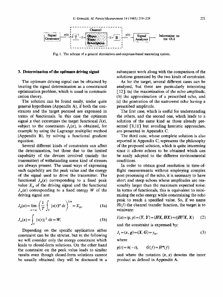
A typical stimulation-and-response-based measuring system (Fig. 1) includes:

a signal generator, producing the driving signal xtt); a transmitter T; the object under investigation (OUI); the transmitted signal passes through the OUI and reaches the receiver, generally corrupted by some kind of noise; a receiver R, which can sometimes be the same physical device used for the transmitter, provided that the transmitted signal and its echo do not overlap; a signal analyser, which extracts the information on the OUI from the echo y(t). Note that the transmitter T, the OU1 and the

receiver R can be viewed as a communication channel, where the response y(t) is the channel output corresponding to the input x(t). The channel transfer function acts as a filter and the noise corrupts the filtered signal.

The design of a time-of-flight measuring system able to give good accuracy can be approached in three different ways, which can be adopted jointly in order to obtain the best results: (1) The settlement of the channel characteristics,

i.e. the design of a suitable transmitter and receiver, e.g. making them broad-band or choosing devices having high working frequencies. This is the strategy that probably leads to the best results [ 1,4], but it is usually very expensive.

!2) The employment of sophisticated detection strategies, e.g. those based on self- or cross- correlation techniques. These techniques, though powerful [3,6,7], are often rather costly, as they usually require high sampling rates for the received signal and heavy digital processing.

(3) The use of a stimulation signal able to produce a short echo, which is easy to detect [8-11] . This approach has to deal with the physical limitations of both the OUI and the transducer employed, but it is very cheap, especially when the frequencies involved are sufficiently low.

We shall use the third strategy, developing a method for determining a driving signal which permits a sub-period accuracy in the time-of-flight measurement even when adopting very simple and cheap detection strategies.

U. Grimaldi, M. Parvis/Measurement 14 (I 995) 219-228 221

; . . . . . . . . . . . . . . . ',

x(t) i ~ ] r-2-q I y(t) IGenerat°r ~ - - ~ l 1 ~ l A~n~]y~er J

Information on the OUI

Fig. 1. The scheme of a general stimulation-and-response-based measuring system.

3. Determination of the optimum driving signal

The optimum driving signal can be obtained by treating the signal determination as a constrained optimization problem, which is usual in communication theory.

The solution can be found easily, under quite general hypotheses (Appendix A), if both the constraints and the target pursued are expressed in terms of functionals. In this case the optimum signal x that extremizes the target functional I(x), subject to the constraints Jk(X), is obtained, for example by using the Lagrange multiplier method (Appendix B), by solving a functional gradient equation.

Several different kinds of constraints can affect the determination, but those due to the limited capability of the devices involved (mainly the transmitter) of withstanding some kind of stresses are always present. The usual ways of expressing such capability are the peak value and the energy of the signal used to drive the transmitter. The functional Jp(x) corresponding to a fixed peak value Xp of the driving signal and the functional Jw(x) corresponding to a fixed energy W of the driving signal are:

Jp(x) = lira Ix(t)l" dt ) = Xp, (la) n ~ o o

dw(x)--fr Ix(t)l 2 d t= W, (lb)

Depending on the specific application either constraint can be the stricter, but in the following we will consider only the energy constraint which leads to closed-form solutions. On the other hand the constraint on the peak value leads to similar results even though closed-form solutions cannot be usually obtained: they will be discussed in a

subsequent work along with the comparison of the solutions generated by the two kinds of constraint.

As for the target, several different cases can be analysed, but three are particularly interesting [ 12]: (a) the maximization of the echo amplitude, (b) the approximation of a prescribed echo, and (c) the generation of the narrowest echo having a prescribed amplitude.

The first case, which is useful for understanding the others, and the second one, which leads to a solution of the same kind as those already presented I8,11] but avoiding heuristic approaches, are presented in Appendix C.

The third case, whose complete solution is also reported in Appendix C, represents the philosophy of the proposed solution, which is quite interesting since it allows echoes to be obtained which can be easily adapted to the different environmental conditions.

In order to obtain good resolution in time-of- flight measurements without employing complex post-processing of the echo, it is necessary to have short and steep echoes whose amplitudes are reasonably larger than the maximum expected noise. In terms of functionals, this is equivalent to mini- mizing the echo energy while constraining the echo peak to reach a specified value. So, if we name H(f) the channel transfer function, the target is to minimize:

I(x)=(y,y)=(Y, Y)=(HX, HX)=([HI2X, X) (2)

and the constraint is expressed by:

Jl=(x,g)=(X, G)=yp, (3)

where

g(t) = h(- t), G(f) = H*(f)

and where the notation (x, x) denotes the inner product as defined in Appendix A.

222 U. Grimaldi. M. Parvis/Measurement 14 (1995) 219 228

The minimization obviously has to be constrained also on the maximum energy W which can be supplied to the transmitter:

J2 :(x, x) = (X, X ) : W. (4)

The solution of the minimization (Appendix C) is:

- V2Z1H*(f ) (5)

X ( f ) - iH(f)l 2 + ,~2 '

where 2, and /~2 are the Lagrange multipliers, to be computed by solving the system of non-linear equations:

" ~ l f ~ 'H(f)' 2 d/'=),'p, (6a) J , = - 5 - IHif)l~+£~ .

2 - 4 ( I H ( ~ _ - 2 2 ) : d f= W (6b)

The constraint on the energy settles a limit to the maximum attainable echo peak amplitude, which corresponds to the so called matched driving signal (Appendix C):

Yp ma,, = ~ / W l[hll, 17)

where the notation Ilhl[ denotes the norm of h (Appendix A). Eq. (6) has therefore solutions only for yp ~<yp max'

Eq. (5) allows two interesting remarks related to the value of 22 (in both cases 21 acts only as a scaling factor): - If 22 is large in comparison with the maximum

value of [H(f)l 2, the input signal X ( f ) approaches the matched signal (Eq. (C.3)):

,/w Xmatch(f) = ~ H * ( f ) , (8)

the available input energy is used to reach the prescribed echo peak value, concentrating it in the frequency range in which IH(f)l is large. In these conditions the echo tends to be very long.

- If 22 is small in comparison with the minimum value of IH(f)] 2, the input signal X ( f ) tends to be proportional to the inverse channel transfer function H - l ( f ) , so the echo tends to approxi- mate a delta-like pulse.

The relationship between 21, 22 and W is non- linear, but an inspection of the J2 expression (Eq. (6)) shows that the larger W is, the smaller is 22, so, as expected, echoes of increasing narrowness are generated by spreading the available input energy into zones where IH(f)[ is small. In other words, the available input energy can be used either to generate large echoes, at the price of their long duration, or to generate short echoes, at the price of their small peak amplitude.

Summarizing, the application of the optimization to a real case requires a five-step procedure: ( 1 ) determine the channel transfer function; (2) determine the amount of energy the transmitter

can withstand; (3) determine the maximum noise expected; (4) choose the echo peak amplitude in order to

have an acceptable signal-to-noise ratio; t5) apply the optimization procedure to compute

the driving signal that allows to obtain the narrowest echo having the prescribed amplitude.

4 . A p r a c t i c a l a p p l i c a t i o n

It is useful to show an example referring to a typical ultrasonic measuring system equipped with low-cost piezoelectric transducers. Such transducers are common in commercially available equip- ments and can be modelled with a second-order transfer function, similar in transmission and in reception:

1

H ~ ( / ) = G . f 2+o " .2, (9) • 2 j ~ o . f - . l

where the damping ratio ¢ usually has values in the range 0.001 to 0.1 depending on the transducer type.

Since usually the OUI has an almost constant frequency response over the frequency range used, the overall channel transfer function has the form:

H( f ) = K H 2 ( f ) , (10)

where K is a scaling factor which depends on several circumstances, such as media attenuation,

U. Grimaldi, M. Parvis/Measurement 14 (1995) 219-228 223

transducer efficiency and so on. Its actual value is very important when dealing with a particular application, since it determines the minimum echo amplitude the receiver can detect, but it does not influence the theoretical aspects of the discussion.

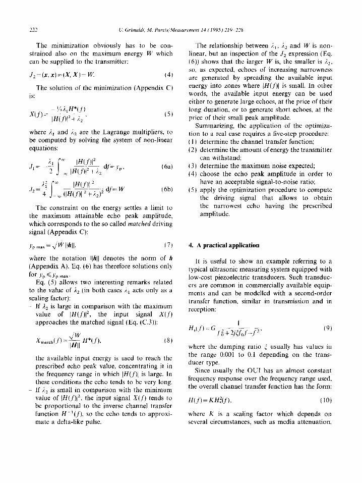
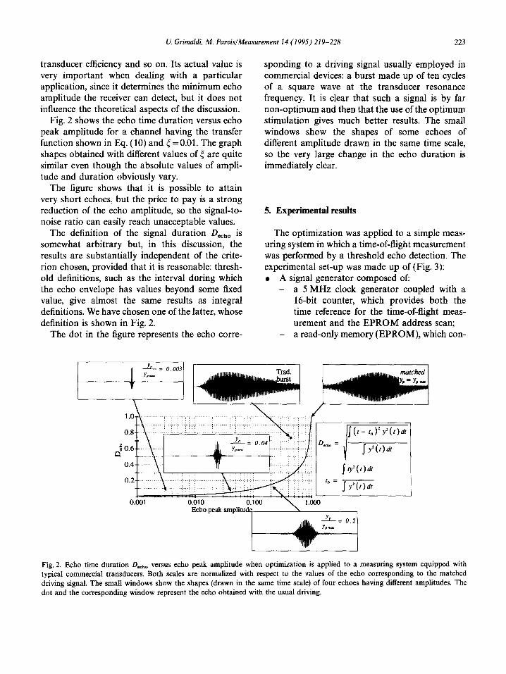
Fig. 2 shows the echo time duration versus echo peak amplitude for a channel having the transfer function shown in Eq. (10) and ~ =0.01. The graph shapes obtained with different values of ~ are quite similar even though the absolute values of amplitude and duration obviously vary.

The figure shows that it is possible to attain very short echoes, but the price to pay is a strong reduction of the echo amplitude, so the signal-to- noise ratio can easily reach unacceptable values.

The definition of the signal duration Deeho is somewhat arbitrary but, in this discussion, the results are substantially independent of the crite- rion chosen, provided that it is reasonable: threshold definitions, such as the interval during which the echo envelope has values beyond some fixed value, give almost the same results as integral definitions. We have chosen one of the latter, whose definition is shown in Fig. 2.

The dot in the figure represents the echo corre-

sponding to a driving signal usually employed in commercial devices: a burst made up of ten cycles of a square wave at the transducer resonance frequency. It is clear that such a signal is by far non-optimum and then that the use of the optimum stimulation gives much better results. The small windows show the shapes of some echoes of different amplitude drawn in the same time scale, so the very large change in the echo duration is immediately clear.

5. Experimental results

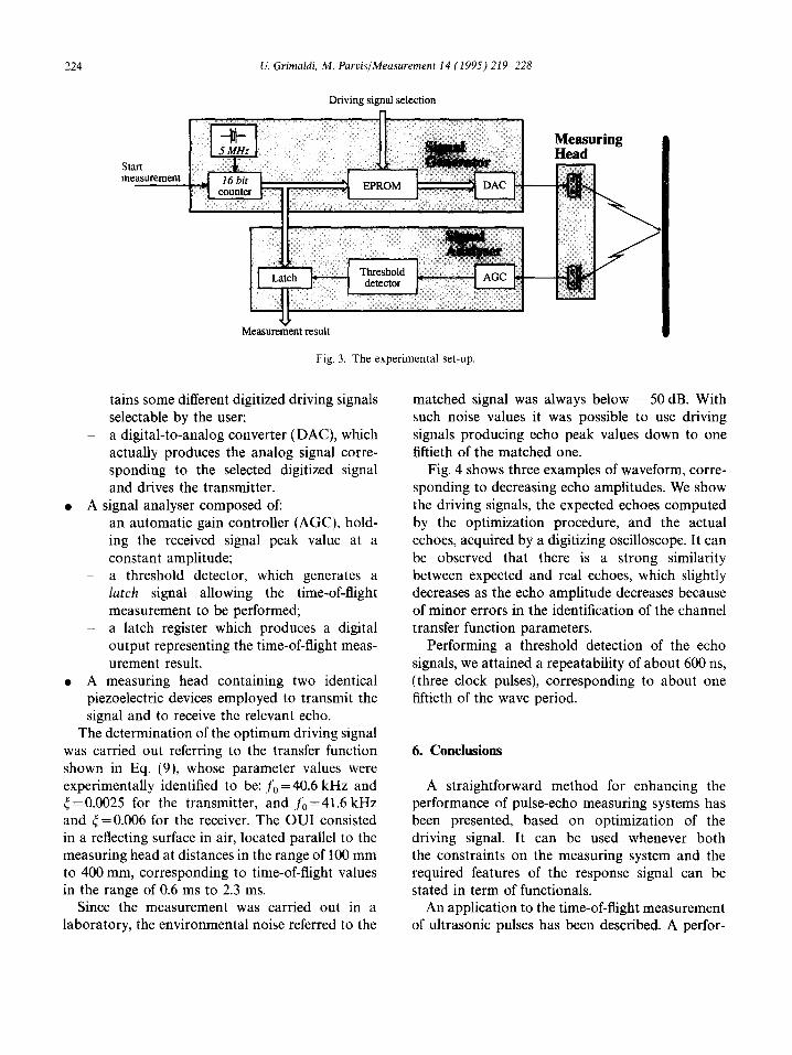
The optimization was applied to a simple measuring system in which a time-of-flight measurement was performed by a threshold echo detection. The experimental set-up was made up of (Fig. 3): • A signal generator composed of:

- a 5 MHz clock generator coupled with a 16-bit counter, which provides both the time reference for the time-of-flight measurement and the EP RO M address scan;

- a read-only memory (EPROM), which con-

Yr = O. 003 t yp~

!

................... 'T i ................... T " : ........... i T T i iI: ~ . . . . i l

~ I . . . . . . ' "! T ~'i '7 ; D,~, : ~ 2 I Y2{t}dt

...... : ~ ~ i i i i ~ i I ~ty ( t )dt

......... ! !~ ............ i ~ ! ! ~! ......... ; '{:"!IP!!'I _ _ f y 2 ( t ) d = ~ - -

0.001 . . . . . 0£610 . . . . . . 02i00 " N i i r o o Echo peak amplitu&

Ye = O.

\ 1.0

0.8

0.6

0.4

0.2

Fig. 2. Echo time duration Dccho VerSUS echo peak amplitude when optimization is applied to a measuring system equipped with typical commercial transducers. Both scales are normalized with respect to the values of the echo corresponding to the matched driving signal. The small windows show the shapes (drawn in the same time scale) of four echoes having different amplitudes. The dot and the corresponding window represent the echo obtained with the usual driving.

224 U. Grimaldi, M. Parvis/Measurement 14 (1995) 219 228

Driving signal selection

Start measurement

Measuring Head

I

Measurement result

Fig. 3. The experimental set-up.

tains some different digitized driving signals selectable by the user;

- a digital-to-analog converter (DAC), which actually produces the analog signal corresponding to the selected digitized signal and drives the transmitter.

• A signal analyser composed of: - an automatic gain controller (AGC), hold-

ing the received signal peak value at a constant amplitude;

- a threshold detector, which generates a latch signal allowing the time-of-flight measurement to be performed;

- a latch register which produces a digital output representing the time-of-flight measurement result.

• A measuring head containing two identical piezoelectric devices employed to transmit the signal and to receive the relevant echo.

The determination of the optimum driving signal was carried out referring to the transfer function shown in Eq. (9), whose parameter values were experimentally identified to be: fo=40.6 kHz and 4=0.0025 for the transmitter, and f o = 4 1 . 6 k H z and ¢ = 0.006 for the receiver. The OUI consisted in a reflecting surface in air, located parallel to the measuring head at distances in the range of 100 mm to 400 mm, corresponding to time-of-flight values in the range of 0.6 ms to 2.3 ms.

Since the measurement was carried out in a laboratory, the environmental noise referred to the

matched signal was always below - 5 0 dB. With such noise values it was possible to use driving signals producing echo peak values down to one fiftieth of the matched one.

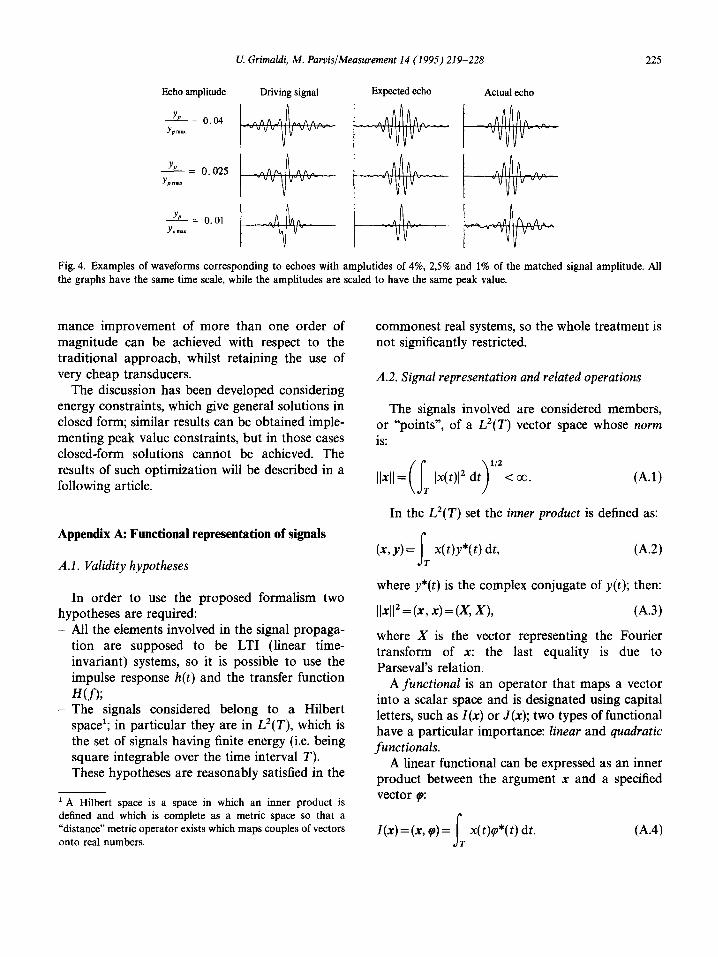
Fig. 4 shows three examples of waveform, corresponding to decreasing echo amplitudes. We show the driving signals, the expected echoes computed by the optimization procedure, and the actual echoes, acquired by a digitizing oscilloscope. It can be observed that there is a strong similarity between expected and real echoes, which slightly decreases as the echo amplitude decreases because of minor errors in the identification of the channel transfer function parameters.

Performing a threshold detection of the echo signals, we attained a repeatability of about 600 ns, (three clock pulses), corresponding to about one fiftieth of the wave period.

6. Conclusions

A straightforward method for enhancing the performance of pulse-echo measuring systems has been presented, based on optimization of the driving signal. It can be used whenever both the constraints on the measuring system and the required features of the response signal can be stated in term of functionals.

An application to the time-of-flight measurement of ultrasonic pulses has been described. A perfor-

U. Grimaldi, M. Parvis/ Measurement 14 (1995) 219-228 225

Echo amplitude Driving signal Expected echo Actual echo

Ye-~ -~vv v V vvv-- I - - v v v v v v - - "

Y" = 0.025 _~A~l A^ . . . . A~A.___ ~AAA -

YP"~ I vv V~v v- -

Yr-~ -'VV . . . . . . vV v V v'~-"

Fig. 4. Examples of waveforms corresponding to echoes with amplutides of 4%, 2,5% and 1% of the matched signal amplitude. All the graphs have the same time scale, while the amplitudes are scaled to have the same peak value.

mance improvement of more than one order of magnitude can be achieved with respect to the traditional approach, whilst retaining the use of very cheap transducers.

The discussion has been developed considering energy constraints, which give general solutions in closed form; similar results can be obtained imple- menting peak value constraints, but in those cases closed-form solutions cannot be achieved. The results of such optimization will be described in a following article.

Appendix A: Functional representation of signals

A.I. Validity hypotheses

In order to use the proposed formalism two hypotheses are required: - All the elements involved in the signal propaga-

tion are supposed to be LTI (linear time- invariant) systems, so it is possible to use the impulse response h(t) and the transfer function

H(T); - T h e signals considered belong to a Hilbert

space1; in particular they are in L2(T), which is the set of signals having finite energy (i.e. being square integrable over the time interval T). These hypotheses are reasonably satisfied in the

1A Hilbert space is a space in which an inner product is defined and which is complete as a metric space so that a "distance" metric operator exists which maps couples of vectors onto real numbers.

commonest real systems, so the whole treatment is not significantly restricted.

A.2. Signal representation and related operations

The signals involved are considered members, or "points", of a L2(T) vector space whose norm is:

,,x,l=(I T [x(t)] z d t ) l /2< ~ . (A.1)

In the L2(T) set the inner product is defined as:

(x, y)= fT x(t)y*(t) dt. (A.2)

where y*(t) is the complex conjugate of y(t); then:

IIxll2 =(x, x)=(x, x), (A.3)

where X is the vector representing the Fourier transform of x: the last equality is due to Parseval's relation.

A functional is an operator that maps a vector into a scalar space and is designated using capital letters, such as I(x) or J(x); two types of functional have a particular importance: linear and quadratic functionals.

A linear functional can be expressed as an inner product between the argument x and a specified vector ~:

I(x) = (x, ~)= ~ x(t)~o*(t) dt. (A.4) Jr

2 2 6 U. Grimaldi, M. Parvis/ Measurement 14 (1995) 219-228

One of the purposes of linear functionals is to generate a vector from another: the convolution product, for computing the output of a linear system having impulse response h(t), obtained as I(x) by putting tp( r )=h( t -z) , is an example of such use.

Quadratic functionals are usually associated with energy concepts and are expressed in the form

I (x) = (Lx, x), (A.5)

where L is a linear operator.

A.3. Directional derivative and gradient vector

For a continuous functional the directional derivative is defined as its variation with respect to the variation of x along a given direction u:

I(x + eu) - I(x) Dfl(x) = lim (A.6)

e~O E

If (x, y) = (V, x) and (Lx, y)=(x, Ly), as in the majority of the cases of practical interest, any directional derivative of a functional can be expressed by a gradient vector VI:

Dfl(x) = (VI, u). (A.7)

The points in which the functional gradient vanishes correspond to extreme values of the functional, i.e. are extremizing points:

VI (x )=0 ~ X:Xextr. (A.8)

The gradients of linear and quadratic functionals are, respectively:

V{(x, ~)} = tp, V{(Lx, x)} = 2Lx. (A.9)

then be obtained by solving the gradient equation:

V [I (x) + 2J (x)] = 0, (B. 1 )

which gives a family of extremizing vectors x(2). The seeked vector is then obtained by solving

the constraint equation:

J(x(2)) = Co, (B.2)

thus obtaining the value of the Lagrange multiplier L

The method can be extended to problems having any number of constraints obtaining gradient equations in the form:

n c

VI(x)+ ~ 2kVJk(x)=O. (B.3) k = l

In this case the values of the corresponding Lagrange multipliers can be found by simulta- neously applying the constraint functionals to x(21, ..., 2,o), where nc is the number of constraints, and solving the resulting system of equations.

Appendix C: Optimum signals for alternative targets

C.1. Maximization of the echo peak value

This target is important when the aim is simply to detect the presence of the echo in a noisy environment: in this case it is necessary to achieve the maximum possible echo amplitude.

Let to be the time at which the echo reaches its maximum value y(to). We have to maximize the functional:

Appendix B: Lagrange multiplier method

The Lagrange multiplier method is commonly used to solve constrained optimization problems requiring to extremize a functional l(x) subject to a constraint J(x)=co. The method is based on the consideration that a vector x that extremizes I(x) extremizes I ' (x)=l(x)+co as well, since Co is a constant.

The solution of the constrained problem can

I =(x, g) = (X, G)= y(to), (C.1)

where g(t) = h( to- t) and then G(f) = H*(f)e -j2~yto. It is subject to the constraint on the maximum allowed driving signal energy W:

d =(x, x) = (X, X ) = W. (C.2)

The solution of Eq. (B.3) leads to the optimum driving signal:

Xmatch(t ) = ~--7-W h ( to - t), II II

U. GrimaldL M. Parvis/Measurement 14 (1995) 219-228 227

Xraatch(f)=l" ~ H*(f)e -j2~y,°, (C.3)

which, except for the delay to and a normalization factor, is the conjugate of the channel transfer function (i.e. the time reverse of its impulse response). Such a signal is said to be matched to the channel and allows the maximum peak value of the echo to be obtained with the available energy.

The expressions of Ymatch(t) and Ymatch(f) are then:

t , /w Ymatch( ) = [ I - ~ f~-oo h( to-z)h( t -z)dz ,

^ "2n "t Ymateh(f)=]~-IH(f)r~e-I J o. (C.4)

And the echo peak value yp max is:

yp max=llxll Iltill = x / ~ Iltill. (c.5)

C.2. Approximation of a prescribed echo

Sometimes it is necessary to obtain a specific echo: this can be due to a special analyzing device, or to some special information about the OUI to be extracted.

If the available input energy is larger than (or at least equal to) that of a signal obtained as a deconvolution of the echo required r(t), then the solution is trivial and corresponds to the decon- volved signal:

X "~" R(f) dodJ) = H--- ~ , (C.6)

where R(f) is the Fourier transform of r(t). If this does not happen, for example because

R(f) has an appreciable energy content whereas H(f) is very small, only an approximation of r(t) can be achieved. In this case the target may be to minimize the energy of the difference between r(t) and the actual echo, which is the square of the difference between the vectors representing them:

l (x)= IIr- h®xll 2 =(r-h®x, r - h ® x ) = ( R - - H X , R - H X ) , ( C . 7 )

where the symbol "®" designates the convolution product.

The constraint is again on the input signal energy:

J=(x, x) = (X, X)= W. (C.8)

The optimum signal in this case is given by:

R(T)H*(f) X(f) = IH---~ T- ~ , (C.9)

where 2 is obtained by applying the constraint to X(f) itself, i.e. by solving:

f fo~ IR(f)lzlH(f)[2 df= (C.10) J = (iH(f)12 + 2)2

I4(.

From this equation it is seen that the larger the available energy W is, the smaller is the value of the Lagrange multiplier: increasing values of W cause the optimum signal X(f) to progressively approach the deconvolution of the output, expressed by Eq. (C.6).

The solution obtained is similar to those adopted in [ 5,8,10,11], which were determined by applying heuristic algorithms. Those algorithms simply con- sist in determining X(f) as a deconvolution of a suitable signal which could be a Gaussian pulse or a raised cosine, somehow "cutting down" the insta- bility arising when H(f) approaches zero by modi- fying it according to heuristic expedients. The advantage of the analytical approach is that such heuristic expedients are no longer necessary: once the available energy is set, the best approximating signal is immediately determined.

C.3. The shortest echo having a predefined amplitude

A signal with fixed peak amplitude has a duration related to the signal energy. Therefore, to obtain a short echo, it is necessary to minimize the echo energy. In terms of functionals the target is to minimize:

I(x)=(y,y)=(Y, Y )=(HX, HX)=(I~2X, X) (C.11)

and the constraint on the peak amplitude yp is

228 U. Grimaldi, M. Parvis/Measurement 14 (1995) 219-228

expressed by: References

J l (x , g) = (X, G) = yp, (C.12)

where

G ( t ) = h ( - t ) , G ( f ) = H * ( f ) .

The min imiza t ion obvious ly has to be con- s t ra ined also on the m a x i m u m energy W which can be suppl ied to the t ransmit ter :

J2=(x , x) = (X, X ) = W. (C.13)

Eqn. (B.3) then becomes:

21HIZX+ )~IG+ 222X= 0, (C.14)

whose solut ion is:

- V2,21G x - in12 + (c . l s )

where )~ and )L z are the Lagrange mult ipl iers , to be c o m p u t e d by solving the system of non- l inear equat ions:

/ - V221G G ~ J'=l, ' )

The system has a solut ion only for echo peak less than the ma tched value (Eq. (C.5)). An a l terna- tive form for Eqs. (C.15) and (C.16) is given in the art icle a long with a discussion abou t the impl ica- t ions of the Lagrange mul t ip l ier values.

[ 1 ] E.P. Papadakis and K.A. Fowler, Broad-band transducers: Radiation field and selected applications, J. Acoust. Soc. Am. 5t1(3) (1971) 729-745.

[2] C. Canali, G. De Cicco, B. Morten, M. Prudenziati and A. Taroni, A temperature compensated ultrasonic sensor operating in air for distance and proximity measurements, IEEE Trans. Ind. Electron. IE-29(4) (November 1982) 336-341.

[3] R.N. Carpenter and P.R. Stepanishen, An improvement in the range resolution of ultrasonic pulse echo systems by deconvolution, J. Acoust. Soc. Am. 75(4) (April 1984) 1084-1091.

[4] P. Kleinschmidt and V. M~igori, Ultrasonic robotic- sensors for exact short range distance measurement and object identification, Ultrasonics Syrup. Proc., IEEE, Vol. 1, 1985, pp. 457-462.

[5] H. Ermert, J. Schmolke and G. Weth, An adaptive ultrasonic sensor for object identification, Ultrasonics Syrup. Proc., IEEE, 1986, pp. 555-558.

[6] G. Hayward and Y. Gorfu, A digital hardware correlation system for fast ultrasonic data acquisition in peak power limited applications, IEEE Trans. Ultrason. Ferroel. Freq. Control UFFC-35(6) (November 1988) 800-808.

[7] D. Marioli, C. Narduzzi, C. Offelli, D. Petri, E. Sardini and A. Taroni, Digital time-of-flight measurement for ultrasonic sensors, IEEE Trans. Instrum. Meas. IM-41 (1) (February 1992) 93-97.

~8] J. Smolke, D. Hiller, H. Ermert, J.O. Schaefer and G. Grfibner, Generation of optimal input signals for ultra- sound pulse-echo systems, Ultrasonics Symp. Proc., IEEE, 1982, pp. 929-934.

[9] P. Kleinschmidt, Method for pulse triggering of a piezoelectric sound-transmitting transducer, US Patent No. 4,376,255, March 8, 1983.

V10] C, Chassaignon and J.F. de Bellaval, Input signal optimisation of ultrasonic transducers for nondestructive testing, Proc. Ultrason. Int., London, 1985, pp. 557-562.

[ 11 ] G. Hayward and J.E. Lewis, A theoretical approach for inverse filter design in ultrasonic applications, IEEE Trans. Ultrason. Ferroelec. Freq. Control UFFC-36(3) (May 1989) 356-364.

[12] L.E. Franks, Signal Theory, Prentice-Hall, Englewood Cliffs, NJ, 1969.

Documents

Enhancing ultrasonic sensor performance by optimization of the driving signal