Embed Size (px)
Citation preview

The authors gratefully acknowledge comments and suggestions from Phil Dybvig, Marco Espinosa, Derek Laing, Victor Li,
Will Roberds, Peter Rousseau, Bruce Smith, Alan Stockman, and Steve Williamson as well as participants at the 1997
European Econometrics Society Meetings in Toulouse, the Midwest Mathematical Economics Conference at Washington
University, the 1997 AEA Meetings in New Orleans, and seminars at Academia Sinica, the Atlanta Fed, the St. Louis Fed,
and Penn State. The views expressed here are those of the authors and not necessarily those of the Federal Reserve Banks
of Atlanta or Dallas or the Federal Reserve System. Any remaining errors are the authors= responsibility.
Please address questions of substance to Zsolt Becsi, Research Department, Federal Reserve Bank of Atlanta, 104 Marietta
Street, N.W., Atlanta, Georgia 30303-2713, 402/521-8785, 404/521-8058 (fax), [email protected]; Ping Wang,
Department of Economics, Pennsylvania State University, University Park, Pennsylvania 16802, 814/865-1525, 814/863-
4775 (fax), [email protected]; or Mark A. Wynne, Research Department, Federal Reserve Bank of Dallas, 2200 N. Pearl
Street, Dallas, Texas 75222, 214/922-5159, 214/922-5194 (fax), [email protected].
Questions regarding subscriptions to the Federal Reserve Bank of Atlanta working paper series should be addressed to the
Public Affairs Department, Federal Reserve Bank of Atlanta, 104 Marietta Street, N.W., Atlanta, Georgia 30303-2713,
404/521-8020. The full text of this paper may be downloaded (in PDF format) from the Atlanta Fed=s World-Wide Web site
at http://www.frbatlanta.org/publica/work_papers/.
Endogenous Market Structures and Financial Development
Zsolt Becsi, Ping Wang, and Mark A. Wynne
Federal Reserve Bank of Atlanta
Working Paper 98-15
August 1998
Abstract: Existing theories that emphasize the significance of financial intermediation for economic development
have not addressed two important empirical facts: (i) the relationship between financial and real activities depends
crucially on the stage of development, and (ii) financial and industrial market structures vary widely across
otherwise similar countries. To explain these observations, we develop a dynamic general equilibrium model
allowing for endogenous market structures in which financial deepening spurs real activity through intermediate
product broadening. We show the possibility of multiple steady-state equilibria and characterize how these
equilibria respond to various shocks. In particular, we examine the determinants of financial deepening, product
broadening, the saving rate, the loan-deposit interest rate spread, and the degree of competitiveness of financial
and product markets. We find that the dynamic interactions between financial and real activities depend critically
on the synergy of financial and industrial competitiveness.
JEL classification: E44, O41, L16
Key words: financial intermediation, economic development, imperfect competition

Endogenous Market Structures and Financial Development
1 Goldsmith (1969) and King and Levine (1993) establish that growth correlates positively with
many indicators of financial development using cross-country data, while Jayaratne and Strahan (1996)
find that bank branch deregulation spurs growth using cross-state data. However, De Gregorio and
Guidotti (1992) and Fernandez and Galetovic (1994) qualify these results and show that the relationship
varies with the stage of economic development. More specifically, Fernandez and Galetovic (1994) find
that the positive relationship within the OECD countries is much weaker than within non-OECD countries -
indeed, such a correlation is nearly absent when Japan is excluded from the OECD sample. For twelve
Latin American countries, De Gregorio and Guidotti (1992) conclude that the development of the real and
the financial sectors are negatively related using panel data analysis with six-year averages.
2 Financial market competition has been examined by Shaffer (1995) and Scotese and Wang
(1996). Shaffer (1995) estimates the extent of competition in the commercial banking industry for fifteen
industrialized countries and finds much variation across countries, with five countries showing statistically
significant evidence of market power. Scotese and Wang (1996) suggest different market power may be
responsible for cross-country differences in the real effects of financial innovation over the business cycle.
For industrial market structure, similar variation is documented, for example, in the twelve-industry, six-
country study of Scherer et al. (1975) and in the survey by Caves (1989), however, Schmalensee (1989)
argues that there is little variation among industrialized countries.
I. INTRODUCTION
The importance of financial intermediation in determining the level of real economic activity has
been known for some time. Walter Bagehot (1915) was the first to emphasize the links between the real
and financial sectors, and the crucial nature of these links was further elucidated by Schumpeter (1934) and
Knight (1951). In recent years a growing body of empirical work has been devoted to establishing
relationships between financial intermediation and economic development. The newer literature has
documented two key observations. First, the correlation between financial and real activity depends on the
stage of development and may in some cases be negative, which we refer to as “stage-dependent financial
development.”1 Second, the degrees of competitiveness of financial and product markets vary significantly
across otherwise similar countries, which we refer to as “heterogenous market structures.”2 Most of the
recent theoretical papers examining the relationship between financial intermediation and economic
development have focused on the emergence of financial intermediation in dynamic general-equilibrium
models based on the growth-promoting role of such intermediation in overcoming market frictions. While
these models have provided significant insights into the relationship between the financial and real sectors,

2
3 As originally illuminated by Gurley and Shaw (1960) financial intermediaries exist to transform
securities issued by firms into securities that have desirable characteristics for final savers. As Fama
(1980) pointed out, when the financial sector is perfectly competitive and there are no frictions, intermedia-
tion is inessential to real activity. To ensure an active role for financial intermediaries, technological
frictions such as asset indivisibility and imperfect risk diversification are usually considered. Of course,
financial intermediaries can arise to overcome incentive frictions due to asymmetric information with
respect to borrowers and incompleteness of financial contracts (Townsend, 1983; Bernanke and Gertler,
1989). See Pagano (1993), Galetovic (1994) and Becsi and Wang (1997) for critical literature surveys.
4The funds pooling idea is, also, explored by Besley, Coate and Loury (1993) in their study of the
workings of the ROSCA and by Cooley and Smith (1996) in their analysis of indivisible assets.
they are unable to address the aforementioned empirical facts. To explain these important observations, we
develop the idea that financial deepening (or increases in the ratio of intermediated loans to output) spurs
real activity through production specialization (or uses of more sophisticated intermediate goods production
processes) with a special emphasis on an active role for financial and industrial market structures.
Economies where market structures are endogenous typically exhibit multiple equilibria which is the basis
for explaining both empirical regularities mentioned above.
Recent theoretical work of financial intermediation and economic development has examined
various roles played by the financial sector to justify the emergence of financial intermediaries.3 For
instance, Diamond and Dybvig (1983) and Bencivenga and Smith (1991) stress the liquidity management
role of banks: by converting liquid funds into longer term investments, financial intermediation improves
the performance of the real sector. Williamson (1986a) and Greenwood and Jovanovic (1990) highlight the
risk pooling and monitoring functions of financial intermediaries: by pooling savings for diversified
investment projects and monitoring the behavior of the borrowing firms, banks ensure higher expected rates
of returns. One common theme of these papers is that financial intermediaries provide access to the
benefits of pooled funds and economies of scale.4 We take up this theme and assume financial interme-
diaries’ primary role is to pool household funds that are directly loaned to producers, because individuals

3
5 Also, fixed bank setup cost exceed average wealth. Thus, individuals must pool their funds in
order to pay the fixed cost and be able to gain access to banking services. We do not consider the
possibility that fixed costs of forming coalitions may exceed potential profits.
6 An exception is Williamson (1986b) who analyzes how the monopoly power of a fixed number
of banks affects real activity and how the number of households may have external effects on the operation
of the financial sector. Also, Allen and Gale (1993) analyze the effects of imperfect competition on
financial markets. However, their emphasis is on risk-sharing and financial instruments while banks are
not explicitly analyzed.
have too little wealth to finance projects by themselves or diversify away firm-specific risks.5
However, as Stiglitz (1993) and others have remarked, the literature has overlooked that markets
with economies of scale can be imperfectly competitive.6 This neglect may be innocuous when thinking
about countries where there are many small banks, but it is less so for many countries where there exist few
large banks. In contrast, our paper considers the endogenous determination of market structure for both the
real and the financial sectors. Thus, we depart from the previous literature by allowing both real and
financial sectors to be monopolistically competitive in the sense of Chamberlin. Intermediate goods-
producing start-ups have fixed setup costs, which imply increasing returns and justify the construction of a
monopolistically competitive intermediate goods sector. Similarly, financial intermediaries pay fixed setup
costs and act monopolistically competitive in the loan market; their number, too, is determined
endogenously. Thus, market structures and competitiveness in both sectors are endogenous, determined by
exogenous intermediation and production costs as well as other preference and technology parameters.
Greater competitiveness in product and financial markets is equivalent to a greater variety or
sophistication of products and services. Variety can be thought of as one form of profit-driven innovation,
an idea familiar from the endogenous growth literature. As in neo-Schumpeterian endogenous growth
models, greater variety or competition in the product market directly increases aggregate production. As
Romer (1986) notes the effect is formally indistinguishable from an externality. While not critical for our
main results, we also allow financial market competition to increase production possibilities. However, we

4
7 Similarly, Aghion and Howitt (1992) assume externalities from innovations affect production
costs. However, in their model innovations are variable cost-reducing.
8 The thick-market externality is different than Diamond’s (1982) trade or search externalities. We
show later that the multiplicity originates from monopolistic competition, not from the externality.
posit that this occurs indirectly by lowering producers’ fixed costs.7 This externality can be thought of in
many ways. For instance, much financial innovation shows up as new services or instruments that
transform firms’ cost structure from sunk costs to variable costs, leasing being a notable example.
Alternatively, with greater competition comes improved access to loan services, more public information
and reduced search costs all of which lower the up-front costs to producers. Finally, more financial
intermediaries can be thought of as reducing the aggregate probability of being denied a loan thus lowering
the cost of obtaining funds.
A central concern of the present paper is how the “industrial organization” of the banking and
production sectors influences real and financial development. We show that the competitiveness of
intermediate goods producers has two opposing effects on intermediate goods production. On the one
hand, more goods market competition produces a “market-induced demand” effect that increases the size of
investment loans; on the other, more competition creates an “intermediate-goods mark-up” effect that
reduces loan sizes. The two opposing effects are a primary reason for the existence of multiple steady-state
equilibria in our model. The competitiveness of financial intermediaries affects the competitiveness of
intermediate goods producers mainly through production costs, which works in two conflicting ways.
Market structures in both sectors are linked, because, for one, financial intermediaries exercise market
power as a lender to start-ups in the intermediate goods sector. Thus, more financial market competition
has a positive “financial mark-up” effect on variable costs by narrowing the spread between lending and
borrowing rates. Alternatively, more competition has a negative external effect on fixed costs by reducing
the setup costs of intermediate goods firms, which can be referred to as the “thick-market externality”
effect.8 Thus, the industrial organization of banking and production sectors becomes an integral part of the

5
However, financial market thickness does increase the likelihood of indeterminacy.
dynamic interactions between financial and real activities through these four channels.
The main focus of our paper is the characterization of steady-state equilibria with a financially
intermediated production. In particular, we examine how preference, technology and cost parameters affect
the degree of financial deepening and production specialization, the loan-deposit interest spread, and the
saving rate, as well as the entry of intermediate good and banking firms. We show the properties of the
multiple equilibria vary with the degree of sophistication in the intermediate goods production process.
More specifically, for a more developed economy, technological advances result in production
specialization and financial deepening and discourage banking competition, whereas banking development
that reduces the costs of financial intermediation narrows the interest rate spread, leading to production
specialization and financial deepening, encouraging banking competition and reducing the size of loans.
For a less developed economy, some of these findings may change, thus explaining the “stage-dependent
financial development” observation. Moreover, our results suggest that the degree of competitiveness of
the product market compared to that of the financial market depends on the stage of development with a
negative correlation found in developed economies and a positive correlation in less developed economies.
This provides a theoretical explanation for the “heterogenous market structures” observation. Finally, we
find that the relationships between financial deepening, the saving ratio, and real output may also vary,
depending on the competitiveness of the intermediate goods sector.
II. THE MODEL
There are three sectors. The final goods sector produces a single final good from two sources.
The first source is output from a “traditional” technology that is a linear function of productive capital.
The second source of output is a “modern” technology employing reproducible intermediate goods as
specified in Romer (1986) in which the breadth of intermediate products enhances output. The first source

6
9 Without loss of generality, this paper focuses primarily on the behavior of banks, because banks
are typically the sole financial agents in LDCs and are also very important even in advanced economies.
Mayer (1990) shows, among eight industrialized countries during 1970-85, intermediated loans were the
dominant source of external funds, generally contributing a greater share of external financing than short-
term securities, bonds and shares combined. Thus, throughout the paper, we will use the terms “bank” and
“financial intermediary” interchangeably.
of output acts as an outlet for savings and a source of consumption when the modern technology is not
feasible. The modern technology can be an engine of economic development through increases in the
number of intermediate goods that can be regarded as enabling a sophisticated production process with
increased specialization. It is feasible to produce with the modern technology once a fixed setup cost is
paid. While the composition of savings matters for development, we focus on equilibria where individuals
have moved from direct capital accumulation via the traditional sector to financially intermediated
accumulation via the modern sector. Thus, we introduce the non-intermediated “traditional” sector simply
to establish conditions under which financial intermediation emerges.
An intermediate goods firm can produce only after it pays a fixed start-up cost. Intermediate goods
are produced using bank-financed capital according to a decreasing-returns technology that permits a
positive markup to cover the start-up cost.9 While individual firms are monopolistically competitive in the
output market, they are perfectly competitive in the input market. The output of each intermediate goods
firm is subject to an idiosyncratic random shock. The firms producing intermediate goods arrange
financing with the banking sector before the realization of this shock. Start-up costs and idiosyncratic risks
require pooling of funds and risks and give rise to the banking sector.
Banks pool risks by offering households a safe rate of return on the interest-bearing portion of their
deposit. They also pool household funds to finance the fixed start-up costs of the intermediate goods firms.
The financial intermediary sector is also monopolistically competitive. There is a fixed cost for setting up a
bank. Individual banks can affect their lending rates to the intermediate goods producers, but competition

7
10 We do not consider market power of the intermediary vis-à-vis households for analytical
tractability. Williamson (1986b) imposes a similar assumption based on the observation that there are few
substitutes for intermediary loans but many for intermediary deposits (such as government securities).
That is, individual banks have monopoly power only over the market for loans and act as price-takers in the
market for deposits.
forces them to break even.10 By allowing monopolistic competition in both the intermediate goods and
banking sectors, we can relate financial deepening to production specialization.
Households choose a path of consumption of a single good, shares of productive capital in the
traditional sector, and the amount of funds to be deposited with the banking sector. During any particular
period, banks determine the total amount of funds lent to the intermediate goods sector at the same time
they set the interest rate on deposits but prior to realization of the random output shocks in the intermediate
goods sector. This is possible because banks are assumed to know the distribution of shocks and returns.
After the uncertainty in the intermediate goods sector is resolved, the amount of intermediate goods
production is determined, after which final goods are produced.
At this point we want to emphasize that the traditional sector exists simply to establish a rate-of-
returns-dominancy condition under which the financial sector emerges. It is not the purpose of this paper to
study the development process from traditional to modern production technology. Rather, the focus of the
paper is to understand the steady-state properties of the financially intermediated equilibrium. Second,
idiosyncratic risks in the intermediate goods sector help justify the active role of banks in addition to banks’
funds-pooling function. Our handling of the uncertainty aspect is in a barebone fashion to focus on the
characterization of a symmetric, certainty-equivalent equilibrium. The main emphasis of the paper is to
highlight the role of endogenous market structures of the intermediate goods and the financial sectors.
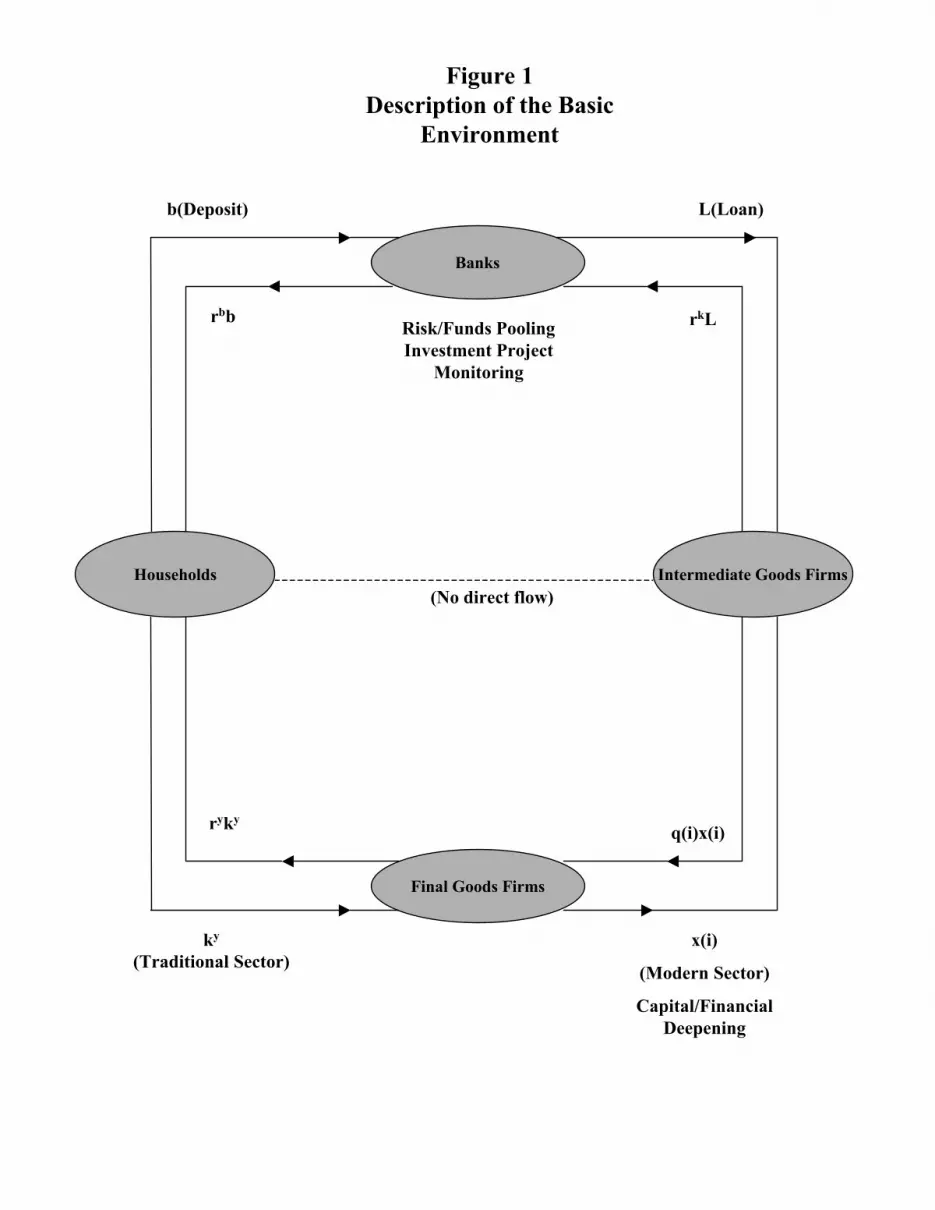
We characterize the optimizing behavior of households, banks, intermediate goods producers, and
final good producers, respectively, in the following subsections. A brief summary of the structure of the
model is provided in Figure 1 (with notation to be defined later).

8
11That is, interest rates subscripted period t denote returns from holding instruments between
periods t-1 and t.
ct% b
t%1% k
y
t%1 ' (1 % rb
t ) (bt& e
b
t ) % (1 % ry
t )ky
t (1)
yt' max{A
y
t ky
t % F({xt(i)}
Nt
i'0, Nt) & Sy, 0} (2)
IIA. Households
The economy is populated by a continuum of households of mass 1. Household preferences are
given by the standard time separable utility function where denotes consumption at date j4
t'0
$t ln(ct) c
tt
and the discount factor satisfies . The representative household enters period holding bank$ 0 < $ < 1 t
deposits, , and a stock of physical capital, all of which is employed in the final goods sector, . Duringbt
ky
t
the period, these assets generate (gross) rates of return of ( ) and ( ) respectively.11 The1% rb
t 1% ry
t
representative household faces the budget constraint
with and given. Here is the total amount of funds supplied to the banking sector duringb0
ky
0 bt%1&b
t
period , which consist of interest-bearing deposits, , and a banking fee, . For analytic convenience,t bt
eb
t
we assume that this fee is levied proportional to household funds, i.e., , where . eb
t ' e0
bt e
0> 0
IIB. Production
Production of the final (consumption) good is carried out by means of the composite technology
The composite technology consists of a linear “traditional” technology and a “modern” technologyAy
t ky
t
. The constant-returns traditional technology is introduced for convenience and plays(F({xt(i)}
Nt
i'0, Nt)
little role in driving any of the results except to produce a simple condition to ensure the emergence of
financial intermediation. The modern technology is assumed to take the Romer (1986) form:
with which is a strictly concave production function that isF({xt(i)}
Nt
i'0, Nt) / m
Nt
0
xt(i)Ddi 0 < D # 1
9
12 The Dixit-Stiglitz type constant-returns-to-scale form will always produce a constant mark-up,
independent of economic activity.
13 A similar assumption below will ensure that no individual can internally finance the production
of intermediate goods. These assumptions highlight the funds pooling role of financial intermediaries,
which has been supported historically by the emergence of the informal “rotating savings and credit
association” (ROSCA). See Besley, Coate, and Loury (1993).
xt(i) ' max {A
x
t (i)G (kx
t (i)) & Sx (Mt; i ), 0} (4)
homogeneous of degree . Thus output of the final good depends on capital allocated to final goodsD
production and a variety of intermediate inputs , where the number (or, more precisely, mass) ofky
t xt(i)
intermediate goods is measured by . Neither input is essential to production since final good output canNt
be produced using either intermediate goods, direct capital or both. The adoption of the Romer technology
in the modern sector gives rise to a simple analysis of a non-trivial mark-up.12 We also assume that there is
a fixed cost associated with production of the final good, , which exceeds the wealth of any singleSy
individual. The existence of this cost prevents any one individual from owning a final-goods producing
firm.13
The optimization problem faced by the final goods producer is as follows:
maxk
y
t , x t (i)
By
t ' yt& m
N t
0
qt(i)x
t(i)di & r
y
t ky
t (3)
where is given by (2), denotes the price of the i'th intermediate good and we assume that the finalyt
qt(i)
good is the numeraire.
The technology for producing the intermediate goods is given by the following:
where denotes capital allocated to production of the i'th intermediate good, and the productionkx
t (i)
technology is specified as: . We also assume that there is a fixed costG(k x(i))/k x(i)", 0 < " < 1
associated with the production of the intermediate goods, . One can think of this fixed cost as primarilySx

10
14 We can use N and M to indicate the degree of competitiveness in the corresponding market.
Note that since both are measures (rather than cardinalities), pure monopoly requires these values
approaching zero (rather than unity).
15 If we reinterpret our start-up cost as the information acquisition cost considered in Williamson
(1986b), then his setup regarding the production fixed cost can be encompassed by our form with .( ' 0
maxk
x
t (i)
Bx
t (i) ' qt(i) x
t(i) & (1 % r
k
t (i))kx
t (i)(5)
the establishment cost incurred in starting up a project, x(i), that requires external finance. In other words,
it is the cost of putting together the financing needed to operate the i’th intermediate goods investment
project for one period. Furthermore, this cost is assumed to depend on the number of monopolistic banks.
Specifically, an increase in the number of banks ( ) will intensify financial market thickness andMt
financial innovation that reduce the resources needed to put together the financing for intermediate goods
production.14 Accordingly, we hypothesize that the fixed cost has the form .15 Sx (Mt; i ) / Sx
0 M&(t , (>0
In short, this consideration captures the Diamond-like thick-market externality in a different context.
The profit maximization problem faced by the typical intermediate goods producer is as follows:
where the technology for producing is specified as in (4) and is the gross unit cost of capitalxt(i) 1% r
k
t (i)
(i.e., the cost from the principle and the interest of the bank loan).
For simplicity, we assume that has a stationary distribution with two possible realizationsAx
t (i)
with and where{(1%*)A, (1&*)A} Pr( A x (i) ' (1 % *)A ) ' 2(i) Pr( A x (i) ' (1 & *)A ) ' 1 & 2(i)
and . Denote the certainty equivalent value of as . In the steady-state analysisA > 0 0 < * < 1 A x Ax
below, we will consider only the symmetric, certainty-equivalent equilibrium allocation, which enables us
to focus on the relationships between financial deepening and production specialization. Throughout the
paper, we will refer to an increase in as a positive technological shock and will assume that the bankA
knows the distribution that generates the outcomes of this process but not the individual realizations of1
across firms. This ex-ante uncertainty about the outcomes of investment projects is used only to2(i)

11
16 The existence of such a fixed cost is consistent with empirical evidence of financial economies to
scale for small banks (Berger et al., 1993 and Clark, 1988) and a negative correlation of unit bank costs
and financial development (Sussman and Zeira, 1995).
17 Each bank holds a market portfolio of loans that is not accessible to households unless they can
afford to pay the fixed costs. Thus, banks act like a mutual fund. While a stock market could perform the
same function, one does not observe widespread direct (and diversified) holding of equities or loans.
18As Allen (1991) points out, firms tend to have relationships with many financial intermediaries
simultaneously. Households also have simultaneous relationships although maybe to a lesser extent.
maxDt%1, Lt%1
Bb
t ' Et m
Nt%1
0
(1 % rk
t%1 (i) )Lt%1
(i)di & (1 % rb
t%1 )Dt%1
& Sb & m
Nt%1
0
µ(i)Lt%1
(i)di (6)
motivate the existence of financial intermediation and is inessential to our main points.
IIC. The banking sector
Households make deposits with banks that are then lent to firms in the intermediate goods sector.
The bank's profit maximization problem is as follows:
subject to the balance sheet constraint
eb
t%1
Mt%1
% Dt%1
' m
Nt%1
0
Lt%1
(i)di (7)
Here denotes the unit cost of processing a loan to the i'th intermediate goods industry, while is theµ(i) Sb
fixed cost incurred to set up and run a bank.16 Note that with the balance sheet identity (7), it is a matter of
indifference whether we specify the bank’s profit function using gross or net rates of interest. Also, risk-
neutral banks pool loans with firm-specific risks to achieve risk diversification.17 For simplicity, the funds
obtained from households, , and the loans made to intermediate goods producers, , are assumedbt%1
kx
t%1(i)
to be distributed equally over all banks.18 The household funds are divided into net deposits, ,Mt%1
Dt%1
12
19Banking fees are a real resource cost for households. There will be a cost to society if some
percentage of these fees “evaporates” as banks transform deposits to loans.
and banking fees, , that are earmarked as bank capital.19 Thus, equating funds inflows and outflowseb
t%1
gives:
Dt%1
'b
t%1& e
b
t%1
Mt%1
(8a)
Lt%1
(i) 'k
x
t%1(i)
Mt%1
(8b)
III. OPTIMIZATION
We characterize the equilibrium using the first-order conditions for each sector’s optimization
problem. First, from the Final Goods Sector we obtain the following first-order conditions for an interior
equilibrium:
Ay
t ' ry
t (9)
qt(i) '
MF({xt(i)}
Nt
i'0,Nt)
Mxt(i)
' Dm
Nt
0
x(i)D&1di ' qt (10)
These conditions plus the assumptions of free entry and symmetry (such that for all and thusx(i) ' x i
) allow us to writemN
0
x(i)di ' xN
Nx D 'Sy
1 & DN(11)
where for convenience we have dropped all time subscripts. To ensure that intermediate goods production

13
20 Notice that under the Romer-type technology (which differs from the Dixit-Stiglitz form), the
elasticity is no longer fixed.
21 Optimization with monopoly power implies: .qt(i)
dxt(i)
dkx
t (i)% x
dqt(i)
dxt(i)
dxt(i)
dkx
t (i)' 1% r
k
t (i)
q (N, x) ' DN x D&1 ' DSy
(1 & DN) x(12)
is positive, we assume . Substituting (11) into (10) yieldsN < 1/D
Thus, intermediate input prices increase with the elasticity parameter .20 D
In the Intermediate goods Sector we also focus on an interior solution and the first-order
condition (conditional on realizations of ),21A x(i)
Dqt(i)
dxt(i)
dkx
t (i)' Dq
t(i)"A
x
t (i) (kx
t (i) )"&1 ' (1 % rk
t ) (13)
In obtaining the first equality, we have imposed ex post symmetry for the intermediate goods firms. Under
symmetry, the free entry condition for the intermediate goods sector is simply . qtx
t' (1 % r
k
t )kx
t
Combining equation (13) with the free entry condition and the technology (4) gives us the following
expressions for the supply of intermediate goods ( ), the capital stock allocated to intermediate goodsxs
t
production and the gross loan rate:
xs
t 'D "
1 & D "
Sx
0
M(t
(14)
1 % rk
t ' D q (N, x) "Ax
t (kx
t )"&1 (15)
kx
t 'S
x
0
Ax
t (1&D" )M(t
1
"(16)

14
22 Inserting (8) into (16) yields: . Thus, we have1 % r k (i) 'Dq"A x ( M L(i) )"&1
, which proves the claim. (r k / (1% r k ))(dr k /r k ) ' ("& 1)dL /L
rk
t%1(i) 1 & Ei
r kL& µ (i) ' r
b
t%1 (18)
rk
t%1 & rb
t%1 '1
"(1 & " )(1 % r
b
t%1 ) % µ ' (1 & " )(1 % rk
t%1 ) % µ (19)
As monopoly power of the individual firms increases or as the elasticity of demand falls (lower or )," D
the mark-up of each intermediate goods producer increases, thus allowing for a higher loan rate while
maintaining zero profit.
Equating demand for intermediate goods from (11) and supply from (14) yields an expression for
the equilibrium number of intermediate goods firms
N (1 & DN) ' Sy 1 & D"
Sx
0D"
D
M D((17)
The (ex-ante) first-order conditions of the Banking Sector are
where is the inverse of the interest rate elasticity of the demand forEi
r kL/ &[L(i) /r k(i)][dr k(i)/dL(i)]
bank loans. It can be shown that the financial mark-up (of the loan rate over the deposit rate) is
.22 The mark-up term is inversely related to the bank’s degree of marketr k (i) Ei
r kL' (1 & " )(1 % r k )
power, since as goes to infinity, goes to zero. Using this to replace the mark-up term in (18)M r k Er k L
yields where we have invoked symmetry and dropped the index forrk
t%1 ' ( rb
t%1 % µ % (1 & " ) )/"
individual intermediate goods producers. The loan-deposit interest rate differential is thus
so that . In a perfectly competitive framework , the mark-ups of(r k & µ) & r b ' (1 & " )(1 % r k ) " ' 1
the firms are driven to zero and the loan-deposit interest rate differential is nothing but the unit loan

15
(1 & " (1&e0))(1% r
k
t%1 ) & e0µ N
t%1k
x
t%1 ' Sb Mt%1 (20)
processing cost, .µ
Equations (6), (7), (8) and (19) can be combined to yield:
bt%1
' Nt%1
kx
t%1 (21)
Before proceeding we might note that we can get a preview of some of our main results from an
examination of equations (17) and (20). Recall that equation (17) is the expression for the equilibrium
number of intermediate goods firms. This equation defines the locus GG in Figure 2. The GG locus has a
unique peak at . Equation (20) also gives us a relationship between the size of the bankingN ' 1/(2D)
sector and the size of the intermediate goods sector. This relationship is linear with a slope determined by
(among other things) the fixed cost associated with the operation of a bank, bank capital requirements, and
the cost of processing loans. This locus is plotted as BB and BB’ in Figure 2, illustrating two possible
equilibria at and . E0
E1
Throughout the analysis we have assumed a thick market externality that arises from the existence
and development of the banking sector. This externality is captured by allowing the fixed cost of putting
together the financing for an intermediate goods project to decline with the size of the banking sector, i.e.
by allowing . To see what a difference the existence of this externality makes to our analysis, Figure( > 0
3 shows the equilibrium values for N when we assume that . In the absence of the externality, the( ' 0
equilibrium size of the intermediate goods sector is determined by equation (17) alone. Figure 3 shows two
possible solutions, and . Thus, the thick market externality per se plays no role in generating theE0
E1
possibility of multiple equilibria.
To close the system we assume that the returns from the intermediate goods (or “high tech”) sector

16
23 This assumption also implies that in the steady-state equilibrium there will be no output
produced by means of the “traditional” technology and all output will be intermediated.
dominate those of the final goods (or “traditional”) sector, so that which ensures theEtr
b
t%1 > Etr
y
t%1
existence of the banking sector.23 Then the Household Sector's first-order conditions are
ct' (1 % r
b
t (1&e0) )b
t& b
t%1 (22)
1 ' Et$ (1 % (1&e
0)r
b
t%1 )c
t
ct%1
(23)
which can be combined to yield
1 ' Et$ (1 % (1&e
0)r
b
t%1 )b
t
bt%1
(1% (1&e0)r
b
t )&b
t%1
bt
(1% (1&e0)r
b
t%1)&b
t%2
bt%1
(24)
We can now summarize all optimization, feasibility, technology and free entry conditions to define
an interior, financially intermediated equilibrium,
Definition 1. An equilibrium with financial intermediation (EFI) is a tuple of positive
quantities and prices satisfying:{ct,b
t,x
t,k
x
t ;yt,D
t,L
t,N
t,M
t;r
b
t , rk
t ,qt}
t$0
(i) (consumer optimization and budget constraints) equations (22) and (23);
(ii) (final-good producer optimization and technology) equations (2) and (10);
(iii) (intermediate-goods producer optimization, technology and free entry) equations (14)-(16);
(iv) (bank optimization, free entry and balance sheet conditions) equations (8a), (8b), (18), (20) and
(21);
(v) (active financial intermediation) .Etr
b
t%1 > Etr
y
t%1

17
r b '$&1&1
1&e0
/ r b ($,e0) (25)
IV. STEADY-STATE EQUILIBRIUM
Throughout the rest of the paper, we will focus only on characterizing the properties of steady-state
equilibrium with financial intermediation. Consider,
Definition 2. A steady-state equilibrium with financial intermediation (SSEFI) is an EFI with
all quantities and prices converging to some positive constant values.
Thus, from (24) we obtain the steady-state deposit rate:
where . In the absence of the banking fee, and the steady-state depositMr b/M$ < 0, Mr b/Me0
> 0 e0' 0
rate is simply the pure rate of time preference. The steady-state loan rate is then obtained using equations
(19) and (25):
r k '1
"
$&1&1
1&e0
%µ%(1&") / r k ($,e0, µ,") (26)
where , , , and . Thus, an increase in the consumerMr k/M$ < 0 Mr k/Me0
> 0 Mr k/Mµ > 0 Mr k/M" < 0
banking fee or the loan processing cost or the mark-up of the intermediate good producers will lead to a
higher steady-state loan rate.
Equation (11) allows us to write
x 'Sy
N (1&DN )
1
D/ x(N; Sy,D) (27)
where iff , and the effect of on is ambiguous. Thus, whenMx/MN > (<) 0 N > (<)1/(2D) Mx/MSy > 0 D x
is sufficiently small, an increase in the number of intermediate goods firms lowers the scale ofN
18
M 'D"S
x
0
1&D"
1
( N(1&DN )
Sy
1
D( / M (N; Sx
0,Sy,",(,D) (29)
production for each individual firm.
Utilizing equations (11) and (12), we have the following expression for :q
q ' D(1&DN )
Sy
1
D&1
N
1
D / q (N; Sy,D) (28)
where iff , and ; again, the sign of is ambiguous. Mq/MN > (<) 0 N < (>) 1/[D(2&D)] Mq/MSy < 0 Mq/MD
When is sufficiently small, an increase in raises the marginal product of (and thus ) due to aN N x q
lower and a wider range of intermediate products. In this case, the aggregate induced demand effect onx
dominates the intermediate-good mark-up effect. In order for the negative markup effect to dominate, ax
larger critical value of is required, specifically which is greater than .N 1/[D(2&D)] 1/(2D)
To characterize the steady-state value of , we manipulate (17) to obtainM
where iff , , , and , while the effectMM/MN > (<) 0 N < (>) 1/(2D) MM/MSy < 0 MM/MSx
0 > 0 MM/M" > 0
of is ambiguous. From equation (14), since depends negatively on , the number of banks and theD Sx M
scale of production for each intermediate goods firm must be inversely related. Consequently, when isN
sufficiently small (large), an increase in will be associated with a larger (smaller) . How and N M M N
are related depends crucially on how the competitiveness of banks affects the costs of intermediate goods
production. The negative correlation between and arises because as increases banks increase theM N M
interest rate spread (or the financial mark-up) to offset falling profit margins in the banking sector. The
increase the interest rate spread lowers profit margins for intermediate goods producers causing to fall. N
By contrast, the thick financial markets externality through the setup costs of intermediate goods producers
causes and to be positively correlated. This effect is dominant when is small (and only arisesM N N
19
24 Recall that the following relationship is derived from equation (19) which is obtained based on
the manipulated form of the free-entry condition, (17).
when is not zero). Thus, in general, the market structures of the intermediate goods sector and of the(
banking sector may not be parallel: it is possible to have a highly concentrated banking sector with very
competitive intermediate goods production, or vice versa.
Next, substituting (29) into (15) we can derive a relationship between and that consolidatesk x N
the implications of the free entry assumption:24
k x '1
D" Ax
1
" Sy
N (1&DN)
1
"D(30)
We can also use equations (16) and (26) to obtain another relationship between and that summarizesk x N
the implication of the assumption that production is carried out efficiently:
1%1
"
$&1&1
1&e0
%µ%(1&") ' " AxD2 1&DN
Sy
1
D&1
N
1
D(k x)"&1(31)
Finally, it remains to derive the steady-state levels of , , and . From equation (21) we findb c D L
that , while from (22) steady-state consumption can be expressed as b ' Nk x
. The steady-state values of and are obtained from equations (8a)c ' r b b (1&e0) ' r b Nk x (1&e
0) D L
and (8b). Of course, by Walras’s law, one of the constraints and equilibrium conditions is redundant and
thus need not be used in solving the steady state.
The results of this section can be summarized with the following proposition:
Proposition 1. (Existence) Under proper conditions, there exists steady-state equilibrium with
financial intermediation which has a block-recursive structure,
(i) steady-state equilibrium are determined by (25) and (26); (r b, r k )

20
25 As the reader can easily check, the FE locus is horizontal when there is no thick-market
externality; ie. when , equation (15) is independent of M (and hence N).( ' 0
(ii) steady-state equilibrium are determined by (30) and (31);(k x,N )
(iii) steady-state equilibrium are determined by (27)-(29);(x,q,M )
(iv) steady-state equilibrium are determined subsequently by the steady-state version of(c,b,D,L )
equations (8a), (8b), (21) and (22).
The key task for characterizing the steady-state equilibria is to examine using (30) and(k x,N)
(31). For illustrative purposes, we will call the “free entry” relationship, (30), the FE locus and the
“production efficiency” relationship, (31), the PE locus (see Figures 4a,b). It is straightforward to show
that the FE locus is U-shaped, with a trough at , and two vertical asymptotes at andN ' 1/(2D) N ' 0
. Equation (15) implies that and are inversely related. The discussion of equation (29)N ' 1/D k x M
therefore indicates that the effect of on is negative (positive) as is sufficiently small (large). N k x N
Notably, the non-monotonicity of the FE locus is mainly due to the thick-market externality in that a thicker
financial market associated with greater entry of banks leads to a lower real cost for intermediate goods
producers to start up an investment project.25
On the other hand, the PE locus is bell-shaped with a peak at . TheN ' 1/(2D&D2) > 1/(2D)
shape of the PE locus is determined primarily by the effect of the competitiveness of intermediate goods
firms, , on the price of intermediate goods, . Along the PE locus, the value of the marginal product ofN q
capital is equal to the rental price . From equation (16), the value of the marginal product ofk x 1%r k
capital depends positively on the marginal product for any given and on which equals the marginalk x q
product of . The discussion of equation (28) thus implies that when is sufficiently small, an increase inx N
will, by enlarging the market (induced) demand, raise the value of the marginal product of capital forN
fixed . In order to maintain the value of the marginal product of capital at a constant rental price, k x k x

21
26 This can be easily shown by establishing the condition under which the minimum value of ofk x
the FE locus is strictly less than the maximum value of of the PE locus.k x
must increase given diminishing returns. Alternatively, when is large the intermediate-good mark-upN
effect dominates the induced demand effect so that an increase in lowers and the value of the marginalN q
product of capital and causes to fall. Thus, it is the opposing effects of market demand andk x
intermediate-good mark-up that give the non-monotonic shape to the PE locus. Importantly, the non-linear
behavior underlying the product efficiency condition for the intermediate goods market is the key driving
force to the multiplicity result to be derived below.
The position of the FE locus is determined by the values of , , , and , while the positionSy A x " D
of the PE locus will be determined by , , , , and . More specifically, for fixed , an increaseSy A x $ e0
µ N
in or a decrease in discourages the entry of intermediate goods firms, thus requiring to increaseSy A x k x
to maintain zero profit. This is reflected by an upward shift of the FE-locus. For fixed , an increase inN
or a decrease in reduces the value of the marginal product of capital. Given the same rental price,Sy A x
must decrease to raise the value of the marginal product of capital to the original level and the PE-locusk x
shifts down. On the other hand, a decrease in or an increase in or raises the rental price of capital. $ e0
µ
For fixed , must fall so that the value of the marginal product of capital will increase to maintainN k x
equality with the higher rental price. Thus, the PE-locus shifts down and the FE-locus is unaffected.
For sufficiently high , , and , or for sufficiently low and , the two curves will intersectA x e0
µ Sy $
each other twice to produce a high- equilibrium and a low- equilibrium.26 Since ,N N 1/[D(2&D)]>1/(2D)
around the high- equilibrium the FE locus must be upward-sloping and the PE locus must be downward-N
sloping. However, around the low- equilibrium, while the PE locus must be upward sloping, the slope ofN
the FE locus could be negative (as in Figure 4a) or positive (as in Figure 4b). We will refer to the high-N
equilibrium (H) as the benchmark case I and the other two types of equilibria, low- (L in Figure 4a) andN
intermediate- (I in Figure 4b) as the alternative cases II and III, respectively. Note that even whenN

22
and the FE locus is horizontal, cases I and II still arise. Therefore, the thick-market externality only( ' 0
increases the types of equilibria from two to three by allowing for the intermediate- equilibrium but is notN
essential in obtaining multiplicity in the first place. This differs from the financial fragility model of
Cooper and Ejarque (1994) in which multiple equilibria occur as a result of the participation externality (in
that a larger mass of agents joining the intermediary can lower the fixed setup costs). These results can be
summarized by,
Proposition 2. (Multiplicity) In general, there are multiple steady-state equilibria with financial
intermediation, depending on the degree of competitiveness of the financial and intermediate goods
markets.
V. COMPARATIVE-STATIC ANALYSIS
We will begin by focusing our attention on the comparative-static results of the benchmark case
(see Table 1) and relegate our discussion of the alternative cases to the end of this section to contrast with
the benchmark case. An autonomous increase in the fixed cost of intermediate goods production, ,Sx
0
requires a more competitive banking sector to offset its negative effect. Such a change, however, will not
affect any other endogenous variables. On the other hand, an increase in the fixed cost of setting up and
running a banking firm, , reduces the profit margin and thus discourages bank entry. Again, it has noSb
effect on any other endogenous variables, in contrast with the Cournot solution in the oligopolistic
competition model of Williamson (1986b) where a higher banking fixed cost only widens the loan-deposit
interest rate spread to ensure profitability without changing the number of banks. Furthermore, an increase
in the fixed cost of final goods production, , has a direct positive effect on capital and intermediateSy
goods production as well as a direct negative effect on the price of the intermediate goods. It also reduces
the degree of intermediate goods production specialization, which under the benchmark case (where

23
) tends to lower and and raise . Thus, its effects on these endogenous variablesN, [(D(2&D))&1,D&1] k x x q
are ambiguous.
A technological improvement (i.e., a higher ) induces more entry into the intermediate goodsA x
sector and boosts intermediate goods production, leading to a lower price. Under the benchmark case, N
and are inversely related and a technological improvement decreases the number of banks. TheM
financially intermediated output ( ) is nonetheless unambiguously higher.F&Sy
An increase in the “effective” cost of financial intermediation, due to an increase in the degree of
impatience or in banking fees and loan processing costs, requires a larger loan-deposit interest rate
differential to maintain profitability. A higher interest rate on loans discourages the entry of intermediate
goods firms and investment in the intermediate goods sector and increases the intermediate goods price.
The intermediated output falls, whereas the number of banks rises under the benchmark case.
We are now prepared to highlight the main findings for the benchmark case where the intermediate
goods sector exhibits a high degree of competitiveness as measured by a high- .N
Proposition 3. (Characterization of High- Equilibrium) The steady-state high-N equilibriumN
has the following features:
(i) Financial deepening, production specialization and real output enhancement are positively
related with respect to alternations in production technology or financial intermediation costs.
(ii) The degrees of competitiveness in the banking and intermediate goods sectors are negatively
related in response to production technology and financial intermediation costs variations.
(iii) Reacting to shocks to financial intermediation costs or time preferences, the level of real output
and the saving rate are always positively related.
Thus, production technological advances result in a larger number of intermediate goods (product-

24
27 With any shock and across all equilibria, we obtain a positive correlation between financial
development and the saving rate, . More generally, as Pagano (1993) argues, the correlation(1&e0)Nk x/y
between intermediation and savings may be sensitive to how intermediation is modeled and where shocks
occur. For instance, Bencivenga and Smith (1991) show that economies with intermediation need not have
higher savings rates than economies without it. Such a comparison is left for future research because in
our model this would involve comparing savings with a traditional sector and savings with a modern sector.
ion specialization), an ambiguous effect on the financial intermediation ratio (financial deepening as
measured by the total intermediated loans to output ratio), but it discourages banking competition at the
same time it encourages competition among intermediate goods producers. Thus, the positive correlation
between production specialization and financial deepening that has been observed by Goldsmith (1969),
McKinnon (1973), Shaw (1973), and King and Levine (1993) need not obtain a priori for technology
shocks. However, the model does predict a positive correlation for bank cost shocks. Banking develop-
ment that reduces the effective cost of financial intermediation will narrow the loan-deposit interest rate
differential, discourage banking competition, and induce production specialization and financial deepening.
Thus, the finding of Sussman and Zeira (1995) that the cost of financial intermediation falls as per capita
output rises may be a result of bank development, and the direction of causation is theoretically
indeterminate.
Moreover, banking development results in a negative correlation between the number of banks and
the size of loan, consistent with the empirical findings in Petersen and Rajan (1994) using U.S. National
Survey of Small Business Finances data. Furthermore, with any banking (or taste) shock, we obtain a pos-
itive correlation between financial development and the saving rate and between financial development and
output.27 However, for technology shocks the correlation between intermediation and development is ambi-
guous. The ambiguity arises because the negative direct effect is offset by the effect of increased competi-
tion among intermediate-good producers. Finally, for case I bank sector competitiveness and output are
negatively correlated for most shocks. Thus, financial development and competitiveness are not
synonymous.
25
28 Again technology shocks have an ambiguous effect on savings. The ambiguity of savings
responses arises for all equilibria because an increase in has a negative effect on savings whenN
and a positive effect when . N<[D(2&"D)]&1 N>[D(2&"D)]&1
Finally, we turn to the alternative cases of low- (in that ) and intermediate- (in thatN N<1/(2D) N
) equilibria (i.e., L and I in Figures 4a and 4b, respectively). It may be useful toN, [1/(2D), 1/(D(2&D))]
note that all three types of equilibria may be dynamically stable and that it may be possible to have the
high-N equilibrium Pareto-dominate the other two in views of the consumers. Whether an economy ends
up with one particular type of equilibrium will be history-dependent, relying on economic as well as
institutional factors, and influenced by individual expectations, based on self-fulfilling prophecies. We will
not discuss the detailed comparative statics under the two alternative cases (see Tables 2a and 2b). Instead,
we will highlight a few interesting findings contrasting with the benchmark case.
On the one hand, while a positive shock to production technology increases output for all three
equilibria, it results in a lower degree of production specialization for both of the alternative cases, contrary
to the benchmark case. Moreover, the number of banks is lower (higher) in case II (III). Thus, one ob-
serves a parallel market structure for the real and financial sectors in the low-N case but a dissimilar mar-
ket structure for the two sectors in the other two cases (high-N and intermediate- ). On the other hand, aN
positive shock to the financial technology (say lower banking fees or loan processing costs) leads to a lower
degree of production specialization and lower net output for both of the alternative cases. The number of
banks is lower (higher) for case II (III). As a consequence, the positive correlation between financial inter-
mediation and real activities is possibly negative in the low- equilibrium, which explains the stage-N
dependent financial development observation. Finally, while a positive correlation between the financial
intermediation ratio and the saving rate holds for all cases, the relationship between real output and saving
may be negative (in the low- case and in the intermediate- case for ).28N N N, [(2D)&1, (D(2&"D))&1)
These results are summarized by the following:

26
Proposition 4. (Characterization of Low- and Intermediate- Equilibria) The steady-stateN N
properties of the low-N and intermediate-N equilibria differ from those of the high-N equilibrium in the
following aspects.
(i) For both alternative equilibria, financial deepening, production specialization, and real output
enhancement are negatively related with respect to production technology changes.
(ii) For low-N equilibrium, the degrees of competitiveness in the banking and intermediate goods
sectors become positively related in response to production technology and financial
intermediation costs disturbances.
(iii) For both alternative equilibria, when financial intermediation costs or time preferences change,
the level of real output and the saving rate may be negatively related.
VI. CONCLUDING REMARKS
We have constructed a dynamic general equilibrium model with technological frictions that arise
when transforming savings into investment. The banking sector emerges endogenously to facilitate pooling
of funds to overcome indivisibilities and to diversify borrower-specific risks. We depart from the previous
literature by allowing both financial and real sectors to be monopolistically competitive in the sense of
Chamberlin. We prove the existence of the steady-state equilibrium with a financially intermediated pro-
duction process and examine how preference, technology, and setup and loan processing cost parameters
affect the degree of financial deepening and product specialization, the saving rate, the loan-deposit interest
spread, and the entry of intermediate goods and financial firms. We also show the possibility of multiple
equilibria associated with different degrees of sophistication in the intermediate goods production process.
Our results suggest that, for a more developed economy, technological advances result in product-
ion specialization and financial deepening and discourage banking competition, whereas banking develop-
ment that reduces the effective costs of financial intermediation narrows the interest rate spread, leading to
27
production specialization and financial deepening, encouraging banking competition and reducing the size
of loans. For a less developed economy, some of the results will change, thus explaining why the correla-
tion between financial and real activity varies across different stages of economic development, i.e., the
“stage-dependent financial development” observation. Moreover, we find that, despite the positive correla-
tion between the financial intermediation ratio and the saving rate in the less developed economy cases, real
and financial activity may be negatively related. In fact, one of the provocative insights to come from this
analysis is that economic development, financial deepening, and bank sector competitiveness are all non-
monotonically related to one another, which generates testable empirical implications, in particular for
understanding the role endogenous market structures played in financial and economic development and for
providing plausible explanation of the “heterogeneous market structure” observation.
Finally, we note that the positive relationship between the financial intermediation ratio and the
saving rate in the benchmark case need not hold in short-run transition to the steady state. Specifically, our
comparative statics are derived around the steady-state equilibrium with financial intermediation in which
the traditional sector vanishes. In the short run, an industrial transformation from the traditional to the
modern sector accompanied by financial deepening would create a negative wealth effect on the rate of
aggregate savings due to the presence of startup costs for intermediated production, which may offset the
positive induced saving effect. For future work, it may be interesting to explore the underlying transitional
dynamics to compare with observed financial sector evolving processes. To our knowledge, there are only
two studies of transitional dynamics -- Greenwood and Jovanovic (1990) and Chen, Chiang and Wang
(1996). However, neither consider market imperfections. Of course, in so doing, one must simplify greatly
the structure of the model in order to produce any analytical results. Moreover, one may extend our
framework to reexamine the welfare effects of monetary policy with an active banking sector. In
particular, the degree of financial deepening and production specialization may now be sensitive to changes
in the money growth rate and imposition of an interest rate ceiling.
28
References
Aghion, Philippe and Peter Howitt. “A Model of Growth Through Creative Destruction.” Econometrica
60:2 (1992): 323-51.
Allen, Franklin. “Discussion.” in Alberto Giovannini and Colin Mayer eds., European Financial
Integration, Cambridge University Press, New York, (1991), 64-68.
Allen, Franklin and Douglas Gale. Financial Innovation and Risk Sharing. Cambridge: MIT Press (
1994).
Bagehot, Walter, Lombard Street: A Description of the Money Market. E.P. Dutton and Company, New
York, NY (1915).
Becsi, Zsolt and Ping Wang, “Financial Development and Growth,” Economic Review. Federal Reserve
Bank of Atlanta. (Fourth Quarter 1997): 46-62.
Berger, Allen N., William C. Hunter and Stephen G. Timme. “The Efficiency of Financial Institutions: A
Review and Preview of Research Past, Present, and Future.” Journal of Banking and Finance 17
(April 1995): 221-249.
Bencivenga, Valerie R., and Bruce D. Smith. “Financial Intermediation and Endogenous Growth.” Review
of Economic Studies 58 (1991): 195-209.
Bernanke, Ben, and Mark Gertler. “Agency Costs, Net Worth, and Business Fluctuations.” American
Economic Review 79 (1) (March 1989): 14-31.
Besley, Timothy, Stephen Coate and Glenn Loury. “The Economics of Rotating Savings and Credit
Associations.” American Economic Review 83 (4) (September 1993):792-810.
Caves, Richard E. “International Differnces in Industrial Organization.” in Richard Schmalensee and
Robert D. Willig ed., Handbook of Industrial Organization, Vol. 2, North-Holland, Amsterdam,
the Netherlands, (1989), 1225-1250.
Chen, Been-Lon, Yeong-Yuh Chiang, and Ping Wang. “A Schumpeterian Model of Financial Innovation
and Endogenous Growth.” (November 1996).
Clark, Jeffrey A. “Economies of Scale and Scope At Depository Institutions: A Review of the Literature.”
Economic Review. Federal Reserve Bank of Kansas City. (September/October 1988): 16-33.
Cooley, Thomas F. and Bruce D. Smith. “Indivisible Assets, Equilibrium and the Value of Intermediary
Output.” Journal of Financial Intermediation 4 (1) (January 1995): 48-76.
Cooper, Russell and João Ejarque, “Financial Intermediation and Aggregate Fluctuations: A
Quantitative Analysis,” NBER Working Paper No. 4819 (August 1994).
De Gregorio, Jose , and Pablo E. Guidotti. “Financial Development and Economic Growth.” IMF
29
Working Paper 92/101 (December 1992).
Diamond, Peter. “Aggregate Demand Management in Search Equilibrium.” Journal of Political Economy
90 (October 1982): 881-894.
Diamond, Douglas and Phil Dybvig. “Bank Runs, Deposit Insurance and Liquidity.” Journal of Political
Economy 85 (April 1983): 191-206.
Dixit, Avinash and Joseph Stiglitz. “Monopolistic Competition and Optimum Product Diversity.”
American Economic Review 67 (1977): 297-308.
Fama, Eugene F. “Banking in the Theory of Finance, “ Journal of Monetary Economics, 6 (1980): 39-57.
Fernandez, David G. and Alexander Galetovic. “Schumpeter Might be Right -- But Why? Explaining the
Relationship Between Finance, Development and Growth.” SAIS Working Paper in International
Economics No. 96-01, John Hopkins University (April 1994).
Galetovic, Alexander. “Finance and Growth: A Synthesis and Interpretation of the Evidence.” Board of
Governors of the Federal Reserve System International Finance Discussion Paper No. 477 (August
1994).
Goldsmith, Raymond W. Financial Structure and Development. Yale University Press, New Haven, CT
(1969).
Greenwood, Jeremy, and Boyan Jovanovic. “Financial Development, Growth, and the Distribution of
Income.” Journal of Political Economy 98 (5, Part 1) (1990): 1076-1107.
Gurley, John G. and Edward S. Shaw. Money in a Theory of Finance. The Brookings Institution,
Washington, DC (1960).
Jayaratne, J. And Strhan, P. E. “The Finance-Growth Nexus: Evidence from Bank Branch Deregulation.”
Quarterly Journal of Economics 111 (3) (August 1996): 639-670.
King, Robert G., and Ross Levine. “Finance and Growth: Schumpeter Might Be Right.” Quarterly
Journal of Economics 108 (August 1993): 717-737.
Knight, Frank. Economic Organization. Harper and Row, New York, NY (1951).
Mayer, C. “Financial System, Corporate Finance and Economic Development.” in Glenn Hubbard (ed.),
Asymmetric Information, Corporate Finance and Investment. University of Chicago Press,
Chicago, IL (1990).
McKinnon, Richard I. Money and Capital in Economic Development. Brookings Institute, Washington,
DC (1973).
Pagano, Marco. “Financial Markets and Growth: An Overview.” European Economic Review 37 (May
1993), 613-622.

30
Petersen, Mitchell A. and Raghuram G. Rajan, “The Effect of Credit Market Competition on Lending
Relationships, NBER Working Paper No. 4921 (November 1994).
Romer, Paul M. “Increasing Returns, Specialization, and External Economies: Growth as Described by
Allyn Young.” Rochester Center for Economic Research Working Paper No. 64 (December
1986).
Scherer, Fredric M., A. Beckstein, E. Kaufer and R. D. Murphy. The Economics of Multi-Plant
Operation: An International Comparisons Study. Harvard University Press, Cambridge, MA
(1975).
Schmalensee, Richard. “Inter-Industry Studies of Structure and Performance.” in Richard Schmalensee and
Robert D. Willig ed., Handbook of Industrial Organization, Vol. 2, North-Holland, Amsterdam,
the Netherlands, (1989), 951-1009.
Schumpeter, Joseph A. , The Theory of Economic Development: An Inquiry Into Profits, Capital, Credit,
Interest, and the Business Cycle. Harvard University Press, Cambridge, MA (1934; German
edition 1911).
Scotese, Carol and Ping Wang. “Financial Innovation and Economic Development Over the Business
Cycle.” Working Paper, Indiana University, Bloomington, IN (November 1996).
Shaffer, Sherrill. “Market Conduct and Aggregate Excess Capacity in Banking: A Cross-Country
Comparison.” Working Paper, Federal Reserve Bank of Philadelphia, Philadelphia, PA (June
1995).
Shaw, E.S. Financial Deepening in Economic Development. Oxford University Press, New York, NY
(1973).
Stiglitz, Joseph. 1993. “Overview.” In Finance and Development: Issues and Experience, edited by
Alberto Giovannini, New York: Cambridge University Press.
Sussman, Oren and Joseph Zeira. “Banking and Development.” Center for Economic Policy Research
Discussion Paper No. 1127 (February 1995).
Townsend, Robert M. “Financial Structure and Economic Activity.” The American Economic Review 73
(5) (December 1983): 895-911.
Williamson, Stephen D. “Costly Monitoring, Financial Intermediation, and Equilibrium Credit Rationing.”
Journal of Monetary Economics 18 (1986a): 159-179.
. “Increasing Returns to Scale in Financial Intermediation and the Non-Neutrality of Government
Policy.” Review of Economic Studies 53 (1986b): 863-875.

Table 1
Comparative Static Results:
High-N Equilibrium (Case I)
Setup Costs Technology Discount
Factor
Intermediation Costs
Effect on Sx
0 Sy A x $ e0
µ
0 0 0 - + +r k&r b
0 - + + - -N
+ ? - - + +M
0 ? ? + - -k x
0 ? + + - -x
0 ? - - + +q
Saving rate 0 ? ? + - -
Intermediated
output
0 ? + + - -
Notes: 1. Intermediated output is equal to ; the saving rate is measured by Nx D&Sy
. Thus, the financial intermediation ratio will be positively(1&e0)Nk x/(Nx D&Sy) Nk x/y
correlated with the saving rate.
2. The effects of changes in are simply the negative of the effects of changes in . Sb Sx
0
3. Case I corresponds to the “H” equilibrium in Figure 4a.

Table 2a
Comparative Static Results:
Low-N Equilibrium (Case II)
Setup Costs Technology Discount
Factor
Intermediation Costs
Effect on Sx
0 Sy A x $ e0
µ
0 + - - + +N
+ ? - - + +M
0 ? ? + - -k x
Saving rate 0 ? ? + - -
Intermediated
output
0 ? + - + +
Note: Case II corresponds to the “L” equilibrium in Figure 4a.
Table 2b
Comparative Static Results:
Intermediate-N Equilibrium (Case III)
Setup Costs Technology Discount
Factor
Intermediation Costs
Effect on Sx
0 Sy A x $ e0
µ
0 + - - + +N
+ ? + + - -M
0 + - + - -k x
Saving rate* 0 + - -(0) ?(-) +(0)
Intermediated
output
0 ? + - + +
Notes: 1. Case III corresponds to the “I” equilibrium in Figure 4b.
2. A * indicates that the result obtains for . Results in N, ( (D(2&"D))&1, (D(2&D))&1 ]
parentheses refer to the case . When the results N' (D(2&"D))&1 N, [(2D)&1, (D(2&"D))&1)
are just like case I and II.
Banks
Households
rbb
b(Deposit) L(Loan)
rkL
Figure 1
Description of the Basic
Environment
Intermediate Goods Firms
Final Goods Firms
(No direct flow)
Risk/Funds Pooling
Investment Project
Monitoring
ryky
q(i)x(i)
ky
(Traditional Sector)
x(i)
(Modern Sector)
Capital/Financial
Deepening

Figure 2
M
0 N
BB
BB1
E1
GG
1/(2ρρ) 1/ρρ
E0

Figure 3
M
N0 E0 E11/(2ρρ) 1/ρρ

Figure 4a
Diagrammatic Analysis of Steady-State Equilibria
(Cases I and II)
kx
N
FE
1/ρρ0
1/(2ρρ) 1/(ρρ(2-ρρ))
PE
LH

Figure 4b
Diagrammatic Analysis of Steady-State Equilibria
(Case III)
kx
FE
0N1/ρρ1/(2ρρ) 1/(ρρ(2-ρρ))
I
H
PE


