Electron–phonon interaction and electronic decoherence in molecular conductors

Electron–phonon interaction and electronic decoherencein molecular conductors

Horacio M. Pastawskia,*, L.E.F. Foa Torresa, Ernesto Medinab

a Facultad de Matem�aatica Astronom�ııa y F�ıısica, Universidad Nacional de C�oordoba, Ciudad Universitaria, 5000 C�oordoba, Argentinab Centro de F�ıısica, Instituto Venezolano de Investigaciones Cient�ııficas, Apartado 21827, Caracas 1020A, Venezuela

Received 12 October 2001

Abstract

We perform a brief but critical review of the Landauer picture of transport that clarifies how decoherence appears in

this approach. On this basis, we present different models that allow the study of the coherent and decoherent effects of

the interaction with the environment in the electronic transport. These models are particularly well suited for the

analysis of transport in molecular wires. The effects of decoherence are described through the D’Amato–Pastawski

model that is explained in detail. We also consider the formation of polarons in some models for the electron-vibra-

tional interaction. Our quantum coherent framework allows us to study many-body interference effects. Particular

emphasis is given to the occurrence of anti-resonances as a result of these interferences. By studying the phase fluc-

tuations in these soluble models we are able to identify inelastic and decoherence effects. A brief description of a general

formulation for the consideration of time-dependent transport is also presented. � 2002 Elsevier Science B.V. All

rights reserved.

PACS: 71.38.)k; 73.40.Gk; 85.35.Be

Keywords: Electron–phonon; Decoherence; Molecular devices; Tunneling time

1. Introduction

Electronic transport in biological and organic molecules has become a very exciting field [1,2] that bringstogether ideas and results developed during the past two decades in many branches of Physics, Chemistryand Biology. On the basis of this synergic interaction one can foresee very innovative results. Much of itswealth comes from the fact that molecules are intrinsically quantum objects, and quantum mechanics al-ways defies our classical intuition. When this happens, we are almost certain to find new ‘‘unexpectedphenomena’’ leading to prospective applications. In turn, with a few exceptions, it is not yet clear howNature exploits quantum effects in biological systems. However, it seems likely that evolution has made use

Chemical Physics 281 (2002) 257–278

www.elsevier.com/locate/chemphys

*Corresponding author. Fax: +54-351-4334-054.

E-mail address: [email protected] (H.M. Pastawski).

0301-0104/02/$ - see front matter � 2002 Elsevier Science B.V. All rights reserved.

PII: S0301-0104 (02 )00565-7

mail to: [email protected]

of the details of the quantum tunneling process in modulating charge transport [3]. Hence, by pursuing anexploration of dynamical quantum phenomena at the molecular level one may also expect to be moreprepared to discover Her hidden ways.

A paradigmatic example of the above situation is the electron transfer in DNA strands [2]. There isevidence that at least two mechanisms are present in this case: (1) A coherent tunneling between the basepairs constituting the donor and acceptor centers. (2) An inelastic sequential hopping through bridgingcenters. Theoretically, there is a need to unify the description of these extreme regimes as well as to study thepossible role of vibrations and distortions of the DNA structure. Our present understanding of these basicphysical processes comes from the field of Quantum Transport, which evolved from the description of non-crystalline materials [4] and reached its climax with nanoelectronic [5] devices. Since these last structuresmay have a very small length scale the term ‘‘artificial atoms’’ [6] is amply justified. Many of the phenomenaappearing in these systems could be summarized in the fact that the wave nature of electrons made themsusceptible to interference phenomena. These can be assimilated to the propagation of light in somecomplex Fabry–Perrot interferometer producing either well-defined fringes or ‘‘speckle-patterns’’. Failuresin that simplistic description is essentially due to interactions with excessively complex environmental de-grees of freedom (such as thermal vibrations), and our lack of control over them is interpreted as ‘‘deco-herence’’ [7]. This often justifies the use of a classical description of the transport process. However, if one isto borrow some idea from the theory of solid state physics, it could be that coherent interactions betweenelectrons and lattice distortions give rise to new effects such as assisted tunneling [8] or even supercon-ductivity. Indeed both phenomena could give striking results in organic systems [9,10]. One is then com-pelled to develop new tools to describe electron–phonon (e–ph) coherent processes in molecular devices.

In what follows we will make a brief description of quantum interference phenomena establishing aground level language based on the simplest physical models. While following our personal pathway ofmany years through the general ideas of transport in the quantum regime, we expect to induce a newperspective into the subtle mechanisms that lead to the degradation of the simple quantum effects throughthe interactions with the environment (i.e. decoherence). As a token, we will visualize coherent effectsemerging from the electron–lattice interaction that can be exploited in new useful ways.

In Section 1 we recall the Landauer ideas [11] for transport which will also serve to adopt a basiclanguage and gives a conceptual framework into which the phenomenological aspects of decoherence canfit. In Section 2 we review the D’Amato–Pastawski (DP) model [12] for coherent and decoherent transportcommenting its strengths and limitations. In Section 3 we introduce a polaronic model that hints at theproperties of the complete e–ph Fock space. This not only sheds light on the decoherence process but canalso be used to predict new phenomena such as the coherent emission of phonons. We devote Section 4 to abrief description of the time dependent transport. Section 5 gives a general perspective.

2. Landauer’s picture for transport

The framework that inspired most of the described experimental developments in mesoscopic electronicswas the Landauer’s [11] simple but conceptually new approach. Besides the ‘‘sample’’ or device, he ex-plicitly incorporated the description of the electric reservoirs connected to ‘‘the sample’’. The role of res-ervoirs can be played not only by electrodes but also could be spatial regions (localized LCAO) where theelectrons lose their quantum coherence. This last situation describes transport in the hopping regime [13](we will see more on this latter). The simplest mathematical description is obtained if one thinks them asone-dimensional wires that connect the individual orbitals i to electronic reservoirs characterized by thestatistical distribution function fiðeÞ. In that case, the electronic states are plane waves describing thedifferent boundary conditions of electrons ‘‘in’’ or ‘‘out’’ the reservoir. An electron out from reservoirconnected to ‘‘site’’ i has a probability Tj;iðeÞ to enter the reservoir connected to site j. A representation of

258 H.M. Pastawski et al. / Chemical Physics 281 (2002) 257–278

such a situation for the case of three reservoirs is sketched in Fig. 1. The current per spin state injected byreservoir j is obtained by the application of the Kirschhoff’s law (i.e. a balance equation [13])

Ij ¼ eZ

deXi

Ti;jðeÞvj1

2NjfjðeÞ

�� Tj;iðeÞvi

1

2NifiðeÞ

�: ð1Þ

The meaning of this equation is obvious: it balances currents. Each reservoir j emits electrons with anenergy availability controlled by a Fermi distribution function fiðeÞ ¼ 1=½exp½ðe � liÞ=kBT þ 1�, with achemical potential, li ¼ l0 þ dli, displaced from its equilibrium value l0. One can assimilate Vi ¼ dli=e asvoltages. The density of those outgoing states is 1

2NiðeÞ (half the total) and their speed vi. It was essential in

Landauer’s reasoning to note that in a propagating channel the density of states Ni is inversely proportionalto the speed obtained from the corresponding group velocity

Ni � 2=ðvihÞ: ð2ÞThis is immediately satisfied in one-dimensional wires but its validity is much more general. This funda-mental fact remained unnoticed in the early discussions of quantum tunneling [5] and it is the key to un-derstand conductance quantization. The Gj;i ¼ e2=hTj;iðeÞ are hence Landauer’s conductances per spinchannel. For perfect transmitting samples Tj;i is either 1 or 0 and one obtains the conductance quantizationin integer multiples of e2=h.

Notice that there is no need for the traditional ½1� fjðeÞ� factor to exclude transitions to already oc-cupied final states. In a scattering formulation, any in state contains a linear combination of out states.Although two different in states (e.g. on the left and right electrodes) could end in the same final out state,unitarity of quantum mechanics assures that both sets are orthogonal. Here the transmission coefficientsmay depend on the external parameters such as voltages.

An important particularity of our Eq. (1) is that it does not exclude sites i ¼ j from the sum. Thiscontrasts with the original multichannel description [14] and is of utmost importance in the treatment oftime dependent problems where Vi ¼ ViðtÞ as will be seen in Section 4. Our Eq. (1), always used with Eq.(2), has a full quantum foundation within the Keldysh formulation of Quantum Mechanics (e.g. Ref. [15],Eqs. (5.6–7)). It can be fully expressed in terms of quantities obtained from a Hamiltonian model such aslocal density of states and Green’s functions. We adopt here a notation consistent with these formaldevelopments.

2.1. Phenomenology of decoherence

A first alternative to include decoherence in steady state quantum transport was inspired in theLandauer’s formulation. There, the leads, while accepting a quantum description of their spectrum of

Fig. 1. Representation of a three probe measurement. The voltmeter may be strongly coupled and is a source of decoherence.

H.M. Pastawski et al. / Chemical Physics 281 (2002) 257–278 259

propagating excitations, are the ultimate source of irreversibility and decoherence: electrons leaving theelectrodes toward the sample are completely incoherent with the electrons coming from the other elec-trodes. In fact, it is obvious that a wire connected to a voltmeter, by ‘‘measuring’’ the number of electrons init, must produce some form of ‘‘collapse’’ of the wave function leading to decoherence (see Fig. 1). Besides,no net current flows toward a voltmeter. The leads are then a natural source of decoherence which can bereadily described in the Landauer picture if one uses the Landauer conductances together with the Kirs-chhoff balance equations. This fact was firstly realized by B€uuttiker [16]. Let us see how it works for the caseof a single voltmeter in the linear response regime. In matrix form

ILI/IR

0@ 1A ¼½GL;R þG/;L� �GL;/ �GL;R

�G/;L ½GR;/ þGL;/� �G/;R

�GL;R �GR;/ ½G/;R þGL;R�

24 35 VL

V/

VR

0@ 1A24 35: ð3Þ

Here the unknowns are IL, IR and V/ ¼ dl/=e. The second equation must be solved with the voltmetercondition I/ � 0

0 ¼ ehT/;Lðdl/ � dlLÞ þ

ehTR;/ðdl/ � dlRÞ; ð4Þ

giving us dl/ to be introduced in the third equation

IR ¼ � ehTR;LðdlL � dlRÞ �

ehTR;/ðdl/ � dlRÞ ¼ �IL ð5Þ

to obtain the current

IR ¼ eheTTR;LðdlL � dlRÞ

with

eTTR;L ¼ TR;L þTR;/T/;L

TR;/ þ T/;L: ð6Þ

The first term can be identified with the coherent part, while the second is the incoherent or sequential part,i.e. the contribution to the current originated from particles that interact with the voltmeter. This corre-sponds to an effective conductance ofeGGR;L ¼ GR;L þ ðG�1

R;/ þG�1/;LÞ

�1; ð7Þ

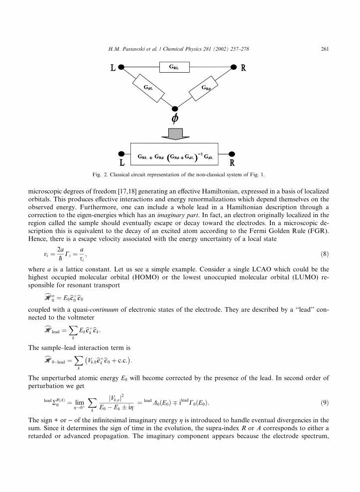
which can be identified with the electrical circuit of Fig. 2. This classical view clarifies the competitionbetween coherent and incoherent transport. However, this circuit does not imply that in Quantum Me-chanics one cannot modify one of the resistances without deeply altering the others. This fact can becomevery relevant in partially coherent regimes.

So far with the phenomenology. The next important step is to connect these quantities with actual modelHamiltonians. This connection was made explicit by the contribution of D’Amato and Pastawski [12].

3. The DP model for decoherence

3.1. Reducing the Hamiltonian

Let us first review the basic mathematical background that made possible the selection of a simpleHamiltonian that best represents the complex sample–environment system. The objective was to find asimple way to account for the infinite degrees of freedom of a thermal bath and/or electrodes and use theexact solution in the Landauer’s transport equation. First, we recall that one can always eliminate the


microscopic degrees of freedom [17,18] generating an effective Hamiltonian, expressed in a basis of localizedorbitals. This produces effective interactions and energy renormalizations which depend themselves on theobserved energy. Furthermore, one can include a whole lead in a Hamiltonian description through acorrection to the eigen-energies which has an imaginary part. In fact, an electron originally localized in theregion called the sample should eventually escape or decay toward the electrodes. In a microscopic de-scription this is equivalent to the decay of an excited atom according to the Fermi Golden Rule (FGR).Hence, there is a escape velocity associated with the energy uncertainty of a local state

vi ¼2a�h

Ci ¼asi; ð8Þ

where a is a lattice constant. Let us see a simple example. Consider a single LCAO which could be thehighest occupied molecular orbital (HOMO) or the lowest unoccupied molecular orbital (LUMO) re-sponsible for resonant transportcHHo

0 ¼ E0bccþ0 bcc0coupled with a quasi-continuum of electronic states of the electrode. They are described by a ‘‘lead’’ con-nected to the voltmetercHHlead ¼

Xk

Ekbccþk bcck:The sample–lead interaction term iscHH0�lead ¼

Xk

Vk;0bccþk bcc0�þ c:c:

�:

The unperturbed atomic energy E0 will become corrected by the presence of the lead. In second order ofperturbation we get

leadRRðAÞ0 ¼ lim

g!0þ

Xk

Vk;oj j2

E0 � Ek � ig¼ lead D0ðE0Þ � ileadC0ðE0Þ: ð9Þ

The sign + or ) of the infinitesimal imaginary energy g is introduced to handle eventual divergencies in thesum. Since it determines the sign of time in the evolution, the supra-index R or A corresponds to either aretarded or advanced propagation. The imaginary component appears because the electrode spectrum,

Fig. 2. Classical circuit representation of the non-classical system of Fig. 1.


described by the density of states NleadðeÞ, is continuum in the neighborhood of energy E0 þ DðE0Þ. Thismakes possible the irreversible decay into the continuum set of states k, not included in the bounded de-scription. The general functional dependence of D0ðE0Þ � iC0ðE0Þ is better expressed in terms of the Wig-ner–Brillouin perturbation theory

leadD0ðeÞ ¼ }

Z 1

�1

Vk;0j j2

e � EkNleadðEkÞdEk; ð10Þ

where } stands for principal value and NleadðEkÞ is the density of states at the lead. Similarly

leadC0ðeÞ ¼ pZ 1

�1Vk;0j j2NleadðEkÞd½e � Ek�dEk: ð11Þ

The evaluation of Eqs. (11) and (8) at e ¼ E0 constitutes the FGR. Of course these quantities satisfy theKramers–Kroning relations

D0ðeÞ ¼1

p}

Z 1

�1

C0ðe0Þe � e0

de0: ð12Þ

An explicit functional dependence on the variable e contains eventual non-FGR behavior. The FGRdescribes reasonably electrons in an atom decaying into the continuum (electrode states), or propa-gating electrons decaying into different momentum states by collision with impurities or interaction witha field of phonons or photons. In some of these cases, we have to add some degrees of freedom to thesum (the phonon or photon coordinates). A process a may produce contributions aRR

0 to the total self-energy RR

0cHH�0 !

interactions

cHH0 ¼ cHHð�Þ0 þ bRRR

0 ðeÞ ð13Þ

with bRRRðAÞ0 ðeÞ ¼ D0ðeÞð � iC0ðeÞÞbccþ0 bcc0 ð14Þ

¼X

a

aD0ðeÞð � iaC0ðeÞÞbccþ0 bcc0: ð15Þ

Besides, the best way to do perturbation theory to infinite order is the framework of Green’s functions.The unperturbed retarded Green’s functions are defined as the matrix elements of the resolvent operatorbGGoRðeÞ ¼ lim

g!0þ½ðe þ igÞII � cHHo��1 ð16Þ

for the isolated sample. It is practical to represent this as a matrix, GoRðeÞ, whose elements are written interms of the eigen-energies Eo

a and eigen-functions wðoÞa ðrÞ ¼

Pi ua;iuiðrÞ of the isolated sample as

GoRi;j ðeÞ ¼ lim

g!0þ

Xa

ua;iu�a;je þ ig � Eo

a

¼ GoAj;i ðeÞ

h i�: ð17Þ

The Local Density of States at orbital i is calculated as

Noi ¼ i

2plimg!0þ

½GoAi;i ðeÞ � GoR

i;i ðeÞ�: ð18Þ

The Fourier transform

GoRi;j ðt2 � t1Þ ¼

Z 1

�1

de2p�h

exp

�� i

�heðt2 � t1Þ

�GoR

i;j ðeÞ ð19Þ


is solution of�� i�h

o

ot2IþHo

�GoRðt2 � t1Þ

�i;j

¼ di;jdðt2 � t1Þ ð20Þ

with t2 > t1. The identity matrix is Ii;j ¼ di;j. Hence GoRi;j ðt2 � t1Þ is �i=�h times the probability amplitude that

a particle placed in jth orbital at time t1 be found in ith one at time t2. The advantage of the method is thatGR

i;jðtÞ can be calculated numerically from GRi;jðeÞ without a detailed knowledge of the eigen-solutions of the

perturbed system. For GRi;jðeÞ one uses:

GRðeÞ ¼ ½e1� ðH0 þ RRðeÞÞ��1 ð21Þ

¼ GoRðeÞ þGoRðeÞX1n¼1

RRðeÞGoRðeÞ� �n ð22Þ

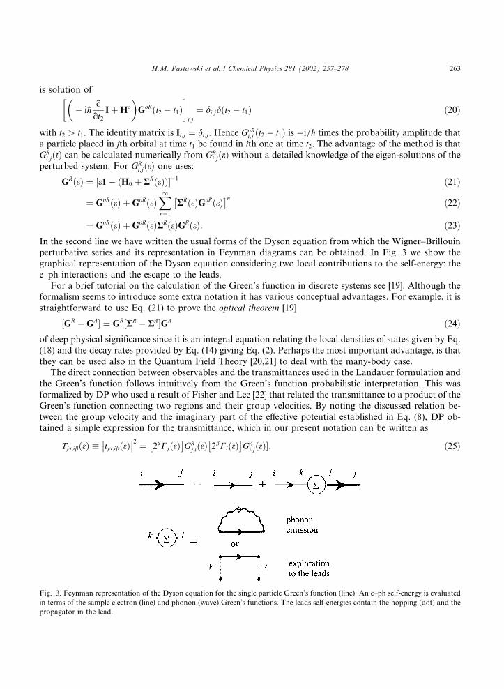
¼ GoRðeÞ þGoRðeÞRRðeÞGRðeÞ: ð23ÞIn the second line we have written the usual forms of the Dyson equation from which the Wigner–Brillouinperturbative series and its representation in Feynman diagrams can be obtained. In Fig. 3 we show thegraphical representation of the Dyson equation considering two local contributions to the self-energy: thee–ph interactions and the escape to the leads.

For a brief tutorial on the calculation of the Green’s function in discrete systems see [19]. Although theformalism seems to introduce some extra notation it has various conceptual advantages. For example, it isstraightforward to use Eq. (21) to prove the optical theorem [19]

½GR �GA� ¼ GR½RR � RA�GA ð24Þof deep physical significance since it is an integral equation relating the local densities of states given by Eq.(18) and the decay rates provided by Eq. (14) giving Eq. (2). Perhaps the most important advantage, is thatthey can be used also in the Quantum Field Theory [20,21] to deal with the many-body case.

The direct connection between observables and the transmittances used in the Landauer formulation andthe Green’s function follows intuitively from the Green’s function probabilistic interpretation. This wasformalized by DP who used a result of Fisher and Lee [22] that related the transmittance to a product of theGreen’s function connecting two regions and their group velocities. By noting the discussed relation be-tween the group velocity and the imaginary part of the effective potential established in Eq. (8), DP ob-tained a simple expression for the transmittance, which in our present notation can be written as

Tja;ibðeÞ � tja;ibðeÞ�� 2 ¼ 2aCjðeÞ

� �GR

j;iðeÞ 2bCiðeÞ� �

GAi;jðeÞ�: ð25Þ

Fig. 3. Feynman representation of the Dyson equation for the single particle Green’s function (line). An e–ph self-energy is evaluated

in terms of the sample electron (line) and phonon (wave) Green’s functions. The leads self-energies contain the hopping (dot) and the

propagator in the lead.


The left supra-index a in aC indicates each of the independent processes producing the decay fromthe LCAO modes (right subindex) associated with the physical channel. In the basis of indepen-dent channels the complex part of the self-energy is diagonal. Hence the sum over initial states andprocesses in the physical channels R and L of Eq. (1) determines a conductance including spinchannels:

GR;L ¼ 2e2

h4Tr½CRðeÞGR

R;LðeÞCLðeÞGAL;RðeÞ�: ð26Þ

This matrix expression is simply a compact way to write Eq. (1), using Eqs. (25) and (8) together tocompute the linear response conductance between any pair L and R of electrodes. The sum of initial statesat left (L) is the result of the product of the diagonal CLðeÞ form of the broadening matrix, while the finaltrace is the sum over final states at right (R). With different notations, these basic ideas recognize by nowmany applications to the field of molecular electron transfer [23].

Originally, Fisher and Lee considered only the escape velocity to the leads (i.e. a ¼ b ¼ lead). Our pointis that any other process which contributes to the decay giving an imaginary contribution to the self-energywould be described by Eq. (25). In particular, this will be true for a ‘‘decoherence’’ velocity that degradesthe coherent current. This view was proposed in DP [12] adopting a discrete (tight-binding) description ofthe spatial variables at each point (or orbital) in the real space a decay rate was assigned which is balancedby the particles reinjection in the same site, described as local reservoirs.

We now show how the DP model applies to a simple tunneling system. Consider the unperturbedHamiltonian,

cHH0 ¼XNi¼1

Eibccþi bcci(

þXj 6¼ið Þ

Vi;j bccþi bccjhþ bccþj bccii

): ð27Þ

Since the indices i and j (sites) refer to any set of atomic orbitals, the interactions are not restricted tonearest neighbors. However, for the usual short range interactions, the Hamiltonian matrix has the ad-vantage of being sparse. The local dephasing field is represented by

/bRRR ¼XNi¼1

�i /Cbccþi bcci; ð28Þ

where /C ¼ �h=ð2s/Þ. We consider for simplicity only two one-dimensional current leads L and R connectedto the first. and the Nth orbital states, respectively,

leadsbRRR ¼ �i LCbccþ1 bcc1�þ RCbccþNbccN�: ð29Þ

We see that the first state has escape contributions both, toward the current lead at the left, LC1, and to theinelastic channel associated to this site, /C1. The on-site chemical potential will ensure that no net currentflows through this channel.

3.2. The solution for incoherent transport

To simplify the notation we define the total transmission from the channels at each site as:

ð1=giÞ ¼XNþ1

j¼0

Tj;i ¼4pN1

LC1 for i ¼ 0;

4pNi/C1 for 16 i6N ;

4pNNRCN for i ¼ N þ 1:

8<: ð30Þ


The last equality follows from the optical theorem of Eq. (24). The balance equation becomes

Ii � 0 ¼ ð1=giÞdli þXNj¼0

Ti;jdlj; ð31Þ

where the sum adds all the electrons that emerge from a last collision at other sites (js) and propagatecoherently to site i where they suffer a dephasing collision. These include the electrons coming from thecurrent source i.e. Ti;LdlL and the current drain. In Eq. (31), since we refer all voltages to the right one, thenTi;RdlR � 0. The first term accounts for all the electrons that emerge from this collision on site i to have afurther dephasing collision either in the sample or in the leads. The net current is identically zero at anydephasing channel (lead). The other two equations are

IL � �I ¼ ð1=g1ÞdlL �XNj¼0

TL;jdlj;

IR � �I ¼ �XNj¼0

TR;jdlj:

ð32Þ

Here we need the local chemical potentials which can be obtained from Eq. (31). In a compact notation, thesecoefficients can be arranged in a matrix form which excludes the leads that are current source and sink:

W ¼

1=g1 � T1;1 �T1;2 �T1;3 � � � �T1;N�T2;1 1=g2 � T2;2 �T2;3 � � � �T2;N�T3;1 �T3;2 1=g3 � T3;3 � � � �T3;N

..

. ... ..

. ...

�TN ;1 �TN ;2 �TN ;3 � � � 1=gN � TN ;N

26666664

37777775: ð33Þ

Then, the chemical potential in each site can be calculated from Eq. (31) as

dli ¼XNj¼1

ðW�1Þi;jTj;0dl0: ð34Þ

Replacing these chemical potentials back in Eq. (32) the effective transmission can be calculated

eTTR;L ¼ TR;L þXNj¼1

XNi¼1

TR;j W�1

� �j;iTi;L: ð35Þ

The first contribution in the RHS comes from electrons that propagate quantum coherently through thesample. The second term contains the incoherent contributions due to electrons that suffer their firstdephasing collision at site i and their last one at site j.

Until now the procedure has been completely general, there is no assumption involving the dimensio-nality or geometry of the sample. The system of Fig. 4 was adopted in DP only because it has a simple

Fig. 4. Pictorial representation of the DP model for the case of a linear chain.


analytical solution for Ti;j in various situations ranging from tunneling to ballistic transport. We summarizethe procedure for the linear response calculation. First, we calculate the complete Green’s function in atight-binding model. Since the Hamiltonian is sparse this is relatively inexpensive if one uses the decimationtechniques described in [18]. With the Green’s functions, we evaluate the transmittances between every pairof sites in the sample (i.e. nodes in the discrete equation) and write the transmittance matrix W. Then, wesolve for the current conservation equations that involve the inversion of W.

What are the limitations of this model? A conceptual one is the momentum demolition produced by thelocalized scattering model. Therefore, by decreasing s/, the dynamics is transformed continuously fromquantum ballistic to classical diffusive. To describe the transition from quantum ballistic to classicalballistic, one should modify the model to have the scattering defined in phase space or energy basis. Whilethe first is well suited for scattering matrix models [24], the last is quite straightforward as will be shown innext Section. The other aspect is merely computational. Since the resulting matrix W is no longer sparse,this inversion is done at the full computational cost. A physically appealing alternative to matrix inversionwas proposed in DP. The idea was to expand the inverse matrix in series in the dephasing collisions, re-sulting ineTTR;L ¼ TR;L þ

Xi

TR;igiTi;L þXi

Xj

TR;igiTi;jgjTi;L þXi

Xj

Xl

TR;igiTi;jgjTi;lglTl;L þ � � � ð36Þ

The formal equivalence with the self-energy expansion in terms of locators or local Green’s function jus-tifies identifying gi as a locator for the classical Markovian equation for a density excitation [25] generatedby the transition probabilities T s. Notice that Eq. (36) can also be rearranged as

eTTR;L ¼ TR;L þXNi¼1

eTTR;igiTi;L: ð37Þ

This has the structure of the Dyson equation, graphically represented in Fig. 5. We notice that according tothe optical theorem gi ¼ s/2p�hNi, while both transmittances entering the vertex are proportional to 1=s/,the whole vertex is proportional to the dephasing rate. The arrows make explicit that transmittances are theproduct of a retarded (electron) and an advanced (hole) Green’s function. Obviously, one can sum theterms of Eq. (36) to obtain the result of Eq. (6) for phenomenological decoherence.

Many of the results contained in the DP paper for ordered and disordered systems were extended ingreat detail in a series of papers by Datta and collaborators [26] and are presented in a didactic layout in abook. In the following section, we will illustrate how the previous ideas work by considering again ourreference toy model for resonant tunneling.

Fig. 5. Feynman diagram for the Dyson equation of the transmittance. It is equivalent to a particle–hole Green’s function in the ladder

approximation where a rung is represented by a dot.


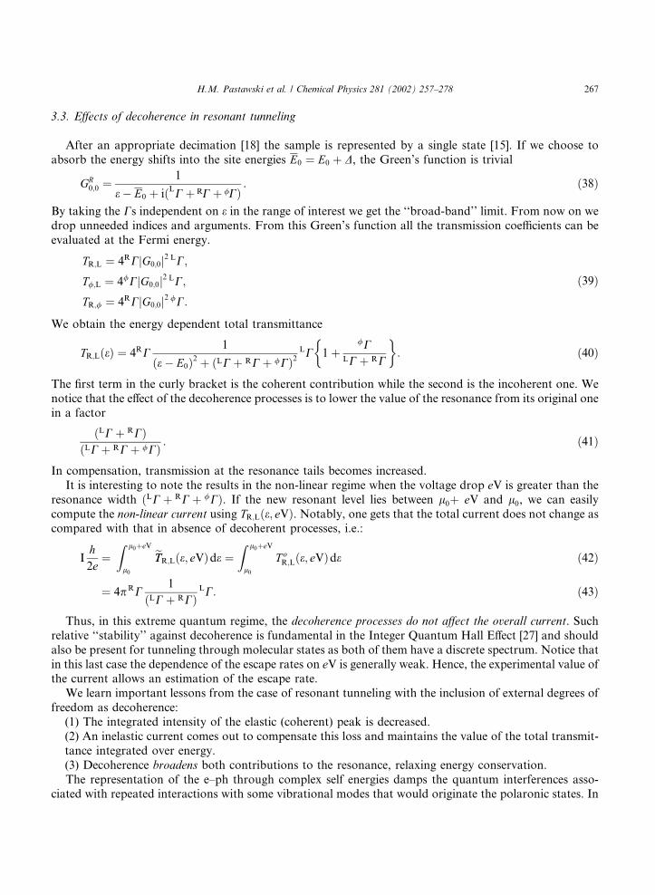
3.3. Effects of decoherence in resonant tunneling

After an appropriate decimation [18] the sample is represented by a single state [15]. If we choose toabsorb the energy shifts into the site energies E0 ¼ E0 þ D, the Green’s function is trivial

GR0;0 ¼

1

e � E0 þ iðLC þ RC þ /CÞ: ð38Þ

By taking the Cs independent on e in the range of interest we get the ‘‘broad-band’’ limit. From now on wedrop unneeded indices and arguments. From this Green’s function all the transmission coefficients can beevaluated at the Fermi energy.

TR;L ¼ 4RC G0;0j j2 LC;

T/;L ¼ 4/C G0;0j j2 LC;

TR;/ ¼ 4RC G0;0j j2 /C:

ð39Þ

We obtain the energy dependent total transmittance

TR;LðeÞ ¼ 4RC1

ðe � E0Þ2 þ ðLC þ RC þ /CÞ2LC 1

!þ

/CLC þ RC

": ð40Þ

The first term in the curly bracket is the coherent contribution while the second is the incoherent one. Wenotice that the effect of the decoherence processes is to lower the value of the resonance from its original onein a factor

LC þ RCð ÞðLC þ RC þ /CÞ : ð41Þ

In compensation, transmission at the resonance tails becomes increased.It is interesting to note the results in the non-linear regime when the voltage drop eV is greater than the

resonance width ðLC þ RC þ /CÞ. If the new resonant level lies between l0þ eV and l0, we can easilycompute the non-linear current using TR;Lðe; eVÞ. Notably, one gets that the total current does not change ascompared with that in absence of decoherent processes, i.e.:

Ih2e

¼Z l0þeV

l0

eTTR;Lðe; eVÞde ¼Z l0þeV

l0

T oR;Lðe; eVÞde ð42Þ

¼ 4pRC1

ðLC þ RCÞLC: ð43Þ

Thus, in this extreme quantum regime, the decoherence processes do not affect the overall current. Suchrelative ‘‘stability’’ against decoherence is fundamental in the Integer Quantum Hall Effect [27] and shouldalso be present for tunneling through molecular states as both of them have a discrete spectrum. Notice thatin this last case the dependence of the escape rates on eV is generally weak. Hence, the experimental value ofthe current allows an estimation of the escape rate.

We learn important lessons from the case of resonant tunneling with the inclusion of external degrees offreedom as decoherence:

(1) The integrated intensity of the elastic (coherent) peak is decreased.(2) An inelastic current comes out to compensate this loss and maintains the value of the total transmit-tance integrated over energy.(3) Decoherence broadens both contributions to the resonance, relaxing energy conservation.The representation of the e–ph through complex self energies damps the quantum interferences asso-

ciated with repeated interactions with some vibrational modes that would originate the polaronic states. In


what follows we will explore some simple Hamiltonian models where decoherence is not introduced at suchan early stage. Instead of calculating transition rates, the approach will be to consider the many-bodyproblem and to compute the quantum amplitudes for each state in the Fock space.

4. The electron–phonon models

4.1. A state conserving interaction model

Let us consider a simple model that complements that of DP by providing an explicit description of asingle extended vibrational mode whose quanta in a solid would be optical phonons,cHHph ¼ �hx0

bbbþbbb: ð44ÞThe electrons are described by

cHHe ¼X1i¼�1

Eibccþi bcci �Xj 6¼ið Þ

Vi;jbccþi bccjhþ Vj;ibccþj bccii: ð45Þ

The orbitals between 1 and N ¼ Lx=a define our region of interest. Orbitals at the edge are connected withthe electrodes, where Vi;j ¼ V , through tunneling matrix elements V0;1 ¼ V1;0 � VL and VN ;Nþ1 ¼ VNþ1;N � VR.The results will be simpler when VLðRÞ � V . Electrons and phonons are assumed to be coupled through alocal interaction

cHHe–ph ¼XNi¼1

�Vgbccþi bcciðbbbþ þ bbbÞ: ð46Þ

To build the e–ph Fock space we consider a single electron propagating in the leads while the number n ofvibronic excitations is well defined. While this election neglects the phonon mediated electron–electroninteraction, it still has non-trivial elements that are the basis for the development of the concept of phononlaser (SASER) [28]. This model will be called State Conserving Interaction (SCI).

The total energy, which is conserved during the transport process, is

E ¼ ek þ n�hx0 with 06 ek 6 eF :

Here ek is the kinetic energy of the incoming electron on the left lead and n is the number of phonons beforethe scattering process. A scheme of the complete e–ph Fock space is shown in Fig. 6. It is clear that anelectron that impinges from the left when the well has n phonons, can escape through the left or rightelectrodes leaving behind a different number of phonons. Since these are physically different situations, theoutgoing channels with different number of phonons are orthogonal and therefore cannot interfere. This isrepresented in the fact that the sum of transmittances over final channels satisfy unitarity.

The physical analysis of the excitations can be simplified resorting to a new basis to refer the e–ph states.We notice that, if we neglect the interaction with the leads, we can diagonalize the electronic Hamiltonianwithout affecting the form of the e–ph interaction. First we diagonalize the electronic system finding theannihilation operators bcca ¼

PNi¼1 ua;ibcci at eigenstates wa with energies Ea and wave functions ua;i ¼ hijai

cHH0 ¼XNa¼1

Eabccþa bcca and cHHe–ph ¼XNi¼0

�Vgbccþa bccaðbbbþ þ bbbÞ: ð47Þ

The Hamiltonian cHHe–ph is just a linear field for the harmonic oscillator where the field amplitude is pro-portional to the density of the electrons that disturbs the lattice. Hence, the excitations, called Holsteinpolarons, are easily obtained. The interesting point is that with the proposed Hamiltonian one can diag-


onalize simultaneously every electron subspace. i.e. in this model the phonons do not cause transitionsbetween electronic levels. The new excitations are described by

baaþk

� �nj0p;ki ¼X1n0¼0

vn;n0 ðbbbþÞn0bccþk j0i; ð48Þ

which is valid at every electron space index a. These operators represent polarons in the energy basisanalogous to the Holstein’s local polaron model [28,29]. The ‘‘polaronic’’ ground state is related to the

vacuum state by j0p;ki ¼P1

n¼0 v0;nðbbbþÞnbccþk j0i. The polaronic energies are lower than those of electrons plus

phonons

Ea;n0 ¼ Ea þ �hx0 n0�

þ 1

2

��

Vg�� 2�hx0

with n0 ¼ haaþaai: ð49Þ

Since phonons do not produce transitions between electron energy states, this model introduces decoher-ence through a SCI. The lesson we learn from this is that by writing the interactions in different basis we canchoose the quantum numbers that are conserved: e.g. local densities in the DP model and energy eigenstatesin the SCI model.

4.2. Coherent and decoherent effects in electronic transport

The general problem of the electronic transport has been solved within the formalism of Keldysh [15,31]in a FGR decoherent approximation [32]. However, here we will solve the full many-body problem. Fig. 6makes evident that the phonon emission/absorption can be viewed as a ‘‘vertical’’ hopping in a two di-mensional network. Once we notice that the Fock-space is equivalent to the electron tight-binding modelwith an expanded dimensionality [28,30], we see that the transmittances can be calculated exactly from theSchr€oodinger equation. While excitations are best discussed in the polaronic basis, for the electron transport

Fig. 6. Scheme for the problem of an electron plus a single phonon mode. The interacting system in the upper figure is transformed

into polaronic modes associated to spatial eigenstates which interact weakly through the leads (lower figure).


it is preferable the use of the asymptotic states.There, when the charge is outside the interacting region, thee–ph product states constitute the natural basis. Recently, this model has gained additional interest as it hasbeen used to explain inelastic effects in STM through molecules [34], to study the transport in molecularwires [35] and to investigate Peierls’s like distortions induced by current in organic compounds [36].

A transport calculation is simpler if we prune the Fock space to include only states within some range ofn allowing a non-perturbative calculation which can be considered variational in n. Thus, we are not re-stricted to a weak e–ph coupling. To obtain the transmittances between different channels several methodscan be adopted. One possibility is to solve for the wave function iteratively [33]. An alternative is to obtainGreen’s functions to get the transmittances. In this case, the horizontal ‘‘dangling chains’’ in the Fock spacecan be eliminated through a decimation procedure [12,18] introducing complex self-energies in the corre-sponding ‘‘sites’’.

For simplicity, let us consider the case of a single state of energy E0 in the region of interest which we willcall the ‘‘resonant’’ state. It could be interpreted as a HOMO or LUMO state depending on the situation. Itinteracts with a dispersionless phonon mode, and it is coupled to a source and drain of charge. The problemfor an electron that tunnels through the system can be mapped to the one-body problem shown in Fig. 7.

Let us consider an asymptotic incoming scattering state consisting of a wave packet built with e–phstates in the left branch corresponding to n0 phonons, i.e. an electron coming from the left while there are n0phonons in the well. When it arrives at the resonant site where it couples to the phonon field, it can eitherkeep the available energy E as kinetic energy or change it by emitting or absorbing n phonons. Each of theseprocesses contributes to the total transmittance which is given by

Ttot ¼Xn

Tn0þn;n0 : ð50Þ

In Fig. 8(a) we show the total transmittance (thick line) for a case where n0 is zero and the e–ph coupling isweak. There, the appearance of satellite peaks at energies E0 þ n�hx0 can be appreciated. To discriminate theprocesses contributing to the current, we include with a dashed line, the elastic contribution to thetransmittance, i.e. that due to electrons which are escaping to the right without leaving vibrational exci-tations behind. This makes almost all of the main peak and only decreasing portions of the satellite peaks.The elastic contribution at the satellite peaks corresponds to a sum of virtual processes consisting of theemission of phonons followed by their immediate reabsorption. The inelastic component associated withthe emission of one phonon is shown with a dotted line.

While the total transmittance (thick line) shows a smooth behavior, the elastic component (dashed line)exhibits a strong dip in the region between the first two resonances. Therefore, almost all of the transmittedelectrons within this energy range will be scattered to the inelastic channels. This sharp drop in the elastictransmittance is produced by a destructive interference between the different possible ‘‘paths’’ in the Fock-space connecting the initial and the final channels. These paths can be classified essentially as a direct

Fig. 7. Each site is a state in the Fock space: The lower row represents electronic states in different sites with no phonons in the well,

the sites in black are in the leads. Higher rows correspond to higher number of phonons. Horizontal lines are hoppings and vertical

lines are e–ph couplings.


‘‘path’’ between the incoming and outgoing channels and the same path dressed with virtual emission andabsorption processes. The first inelastic component (dotted line) also shows a similar behavior in the valleybetween the second and third resonances. The main factors that control the magnitude of these antireso-nances are the escapes to the leads and the e–ph coupling. This concept was introduced in [18,37] to extendthe Fano-resonances [38] observed in spectroscopy to the problem of conductance. Perfect antiresonancescorrespond to situations where both the real and the imaginary part of the transmission amplitude are zero.In the present case, such a perfect interference condition does not occur, and there is a non-zero minimumtransmission at the dips. Through a similar analysis one could tailor the geometrical parameters of thesystem (as done in [39]) to optimize the phonon emission.

An alternative way to appreciate this interference effect is to plot the path followed by the transmissionamplitude in the complex plane when the kinetic energy of the incoming electron is changed [40,41]. A plotfor the elastic transmission amplitude is shown in Fig. 8(c). For e ¼ 0, there is no transmission. If the energyis increased, one starts to follow the path in the figure anti-clockwise. After reaching the point

(a)

(b) (c)

Fig. 8. (a) Transmittance as a function of the incident electronic kinetic energy. The total transmittance is shown with a thick solid line,

the elastic component with a dashed line and T1;0 with a dotted line. The non-interacting transmittance is also shown with a thin line. In

(b) the phase shift of the elastic transmittance as a function of the energy and for the non-interacting case (dotted line) are shown. (c)

shows the path of the elastic transmission amplitude in the complex plane when the electronic energy is changed. The full circles

correspond to the first and second peaks shown in (a). These results are obtained with E0 ¼ �1:5, VL ¼ VR ¼ 0:1, Vg ¼ 0:1 and

�hx0 ¼ 0:2:


corresponding to the first resonance, the transmission starts to decrease and the curve develops a turningnear the origin. The first antiresonance takes place at the point of minimum distance from the origin.

In order to rationalize the main processes involved in the first two peaks, let us represent them sche-matically in Fig. 9. Panel (a) shows the standard elastic process in which no phonon is emitted. Panel (b) is anotable effect that occurs when the phonon emission is virtual. Notice that this virtual process can havestrong consequences. In Fig. 8 it produces an increase of the transmittance in almost two orders of mag-nitude. Panel (d) shows a real inelastic process which is expected to give a peak if the initial energy satisfiesE ¼ E0 þ �hx0. Notably, one must expect also a contribution when e ¼ E0 which corresponds to the virtualtunneling into the resonant state before emitting a phonon as shown in panel (c).

Another interesting quantity that we can explore with the present formalism is the phase of the trans-mitted electron through different channels,

gm;n ¼1

2ilnGR

m;n

GAn;m

; ð51Þ

whose energy derivative gives information on the dynamics of the process. Fig. 8(b) shows the phase shift ofthe elastic transmission probability. For reference, the phase shift in the absence of e–ph interaction is alsoshown with a dotted line. It increases by p over the width of the non-interacting transmission resonance.The same occurs in the interacting case. However, it can be seen that each satellite peak has associated aphase fluctuation. Instead of an increase in the phase by p which would occur for real resonant peaks,across each ‘‘satellite peak’’ associated with the virtual processes, there is a phase dip that results in con-secutive resonances having phases close to �p=2. These phase dips are a manifestation of the anti-reso-nances shown in Fig. 8(a) for the elastic transmittance. For perfect zero transmission points, one has anabrupt phase fall of p instead of the smooth phase slip shown in the Fig. 8(b) [40].

Let us consider a more general case in which there are initially n0 phonons in the scattering region. Thevertical hopping matrix element connecting states with n0 and n0 þ 1 phonons is

ffiffiffiffiffiffiffiffiffiffiffiffiffin0 þ 1

pVg. Then, under

these conditions, the adimensional parameter,

egg ¼ffiffiffiffiffiffiffiffiffiffiffiffiffin0 þ 1

p� �Vg

�hx0

� �2

¼ ðn0 þ 1Þg; ð52Þ

characterizes the strength of the e–ph interaction. It presents two regimes according to the importance ofthis interaction.

Fig. 9. Schematic representation of the processes that lead to the elastic and inelastic components of the peaks in the total trans-

mittance. (a) and (b) correspond to the first and second peaks of the elastic transmittance, respectively. (c) and (d) correspond to the

inelastic part. The well’s ground state is represented by a solid line and the first excited polaron state by a dotted line. The final polaron

states at the right of the well are also shown. These states have an energy equal to the incident electron kinetic energy. The final polaron

state is depicted with a solid line for the elastic case and with a dotted line for the inelastic situation. The level corresponding to the

electron final energy is also shown as a solid line for this case.


In the limit egg � 1 the vertical processes are in a perturbative regime. The ‘‘vertical hopping’’ffiffiffiffiffiffiffiffiffiffiffiffiffin0 þ 1

pVg

will not be able to delocalize the initial state along this ‘‘vertical direction’’ and therefore the elastic con-tribution is the most important. In Fig. 10(a), we show with a thick line the transmission probability for acase where g ¼ 0:25 in presence of 10 phonons. Notice that ‘‘satellite’’ resonances corresponding to phononemission and absorption are separated by �hx0 from the main resonance. For comparison, the curve inabsence of e–ph interaction is also included with a dotted line. We see that, as with the DP model, the mainresonance peak decreases and presents a general broadening where we can recognize details of the exci-tation structure of the phonon field. The phase shift as a function of the electronic energy is shown in (b).The solid line is the phase shift for the elastic component of the total transmittance. There, we can ap-preciate the phase fluctuations that appear even in the elastic transmission.

On the other hand, if eggJ 1, the e–ph interaction is in the non-perturbative regime. This can be achievedeither by a strong Vg , or by a high n. The second situation would correspond to the case of high tem-peratures or a far from equilibrium phonon population. In that case, the total transmittance can be ob-tained by summing the transmittances for the different possible initial conditions weighted by theappropriate thermal factor [42]. In any of these situations, the resulting strong e–ph coupling leads to abreakdown of perturbation theory. A similar case is found for the quantum dots studied in [43]. There, incontrast to the situation in bulk material, the studied quantum dots show a strong e–ph coupling. Inmolecular wires, where elementary excitations (e or ph) are highly confined, one can expect a similarscenario.

In Fig. 11(a), we show the transmittance as a function of the incident electron kinetic energy for the casewhere Vg is strong (egg ¼ 4) and there are no phonons in the well before the scattering process. In contrast tothe perturbative regime, where the energy shift of the peaks (�V 2

g =�hx0 ¼ �g�hx0) is small, here the energyshift is important and the inelastic contributions to the total transmittance dominate. In the limit of weakcoupling between the scattering region and the leads, the transmission probability through the channel withn phonons becomes the standard Frank–Condon factor: expð�gÞgn=n!.

Fig. 11(b) shows the total transmittance as a function of the incident electron kinetic energy for anextreme case where there are 300 phonons in the well before the scattering process. The electron can absorbor emit as many phonons, Neff ¼ 4

ffiffiffin

pVg=�hx0, as allowed by the interaction strength. This means that the

phonon spectrum, weighted on the local e–ph state n, will be quite independent on the details of the spectral

(a) (b)

Fig. 10. (a) Total transmittance as a function of the incident electronic kinetic energy. The solid line corresponds to the case in which

there are 10 phonons in the well before the scattering process. The dotted line corresponds to the case in which there is no interaction

with the vibrational degrees of freedom. (b) Phase shift in units of p as a function of the incident electronic kinetic energy. The solid line

is the phase shift for the elastic transmission. The dotted line corresponds to the non-interacting case. The parameters of the Ham-

iltonian in units of the hopping V are: E0 ¼ 0, VL ¼ VR ¼ 0:05, Vg ¼ 0:004 and �hx0 ¼ 0:02.


densities at the far end of the effective vertical chain i.e. the states n� Neff . Hence, the spectral density willshow the typical form of a one a dimensional band even when we take Neff ¼ 4ðVg=�hx0Þ

ffiffiffin

p � N . Thisfeature manifests in the transmittance presented in Fig. 11(b). The unperturbed resonant peak is a dottedline which contrasts with the total transmission in presence of phonons shown with a continuous line. Itstrace follows the structure of the phonon excitation with the typical square root divergences at the bandedges smoothed out by the inhomogeneity in the hopping elements and the uncertainty introduced by theescape to the leads.

5. The solution of time dependence

Finally, we would like to present the basic features of time dependent transport. This is relevant since acoherent ‘‘time of flight’’ should be shorter than any conformational correlation time [44]. The basic idea toget the physics of time dependent phenomena is to obtain the evolution of an arbitrary initial boundarycondition of the form ½wðXjÞw�ðXkÞ�source. Since here Xj ¼ ðrj; tjÞ with general tj, this essentially generalizes adensity matrix introducing temporal correlations that define the energy of this injected particle. The‘‘density’’ at a later time is obtained from the exact solution of the Schr€oodinger equation

wðX2Þw�ðX1Þ½ � ¼ �h2Z Z

GRðX2;XjÞ wðXjÞw�ðXkÞ� �

sourceGAðXk;X1ÞdXj dXk: ð53Þ

In order to establish a correspondence with the Danielewicz solution to the Schr€oodinger equation in theKeldysh formalism, we used the continuous variable Green’s function which is related to the exact discreteone in the open system by

GRðri;rj; eÞ ¼Xk;l

GRk;lðeÞukðriÞu�

l ðrkÞ: ð54Þ

Now, the key is to recognize that in any Green’s function, a macroscopically observable time is t ¼ 12½tj þ tk�

(time center). Its Fourier transform is an observable frequency x. Meanwhile, energies are associated withinternal time differences tj � tk (time chords). Within this scheme, the time correlated initial condition(source), determining the occupation of a local orbital is expressed in terms of the time independent localdensity of states NiðeÞ

Fig. 11. (a) and (b) show the total transmittance as a function of the incident kinetic electronic energy. The area under the elastic

transmittance is filled with a pattern of lines. As before, the dotted line corresponds to the non-interacting case. In (a), the solid line

corresponds to the case in which there are no phonons in the well before the scattering process and Vg ¼ 0:100, �hx0 ¼ 0:05. In (b), the

solid line corresponds to the case in which there are 300 phonons in the well before the scattering process and Vg ¼ 0:0015 and

�hx0 ¼ 5:010�4. The parameters in units of the hopping V are: E0 ¼ 0, VL ¼ VR ¼ 0:05.


uiðtÞu�i ðtÞ� �

source¼Z

de2p�h

Zddt uiðt

�þ 1

2dtÞu�i ðt � 1

2dtÞ�source

exp½ i⁄iedt� ¼Z

deNiðeÞf ðe; tÞ; ð55Þ

and the occupation factor f ðe; tÞ. Introducing this notation in Eq. (53) one can identify the dynamicaltransmittances Ti;jðe;xÞ. We refer to [15] for a detailed manipulation of the time integrals. The basic result is

Ti;jðe;xÞ ¼ 2CiðeÞGRi;j e�

þ 12�hx�2CjðeÞGA

j;i e�

� 12�hx�: ð56Þ

The time dependent transmittance is then

Ti;jðe; tÞ ¼Z

Ti;jðe;xÞ exp½�ixt� dx2p

; ð57Þ

where one recovers our old steady state transmittance as

Ti;jðeÞ � Ti;jðe;x ¼ 0Þ ¼Z t

�1Ti;jðe; t � tiÞdti ¼

Z 1

tTi;jðe; tf � tÞdtf : ð58Þ

Eq. (53) then becomes

IjðtÞ ¼2eh

ZdeXi

Ti;jðeÞfjðe; tÞ�

�Z t

�1dtiTj;iðe; t � tiÞfiðe; tiÞ

�; ð59Þ

which is the Generalized Landauer–B€uuttiker Equation (GLBE) [25,15]. According to Eq. (58), the first termaccounts for the particles that are leaving the reservoir at site j at time t to suffer a dephasing collision atsome future time at orbital i. The second accounts for particles that having had a previous dephasingcollision at time ti at the i orbital reach site j at time t.

In the GLBE formulation the essential features of time dependence in transport is contained in thetransmittances. Since the spectrum is continuous, we can keep the lowest order in the frequency expansione.g.,

Ti;jðe;xÞ ’ Ti;jðeÞ1� ixs1 þ ðxs2Þ2 þ � � �

: ð60Þ

According to Ref. [15, Eq. (4.5)] the propagation time sP is identified with the first significant coefficient inthis expansion. Typically, it results the first order,

sP ¼ i�h2

GRi;jðeÞ

o

oeGR

i;jðeÞ�1

�þ GA

j;iðeÞo

oeGA

j;iðeÞ�1

�¼ � i�h

2

o

oeln

GRi;jðeÞ

GAj;iðeÞ

" #; ð61Þ

which can be identified with the Wigner time delay. This propagation time was evaluated in various simplesystems in [15] recovering the ballistic and diffusive times for clean and impure metals, respectively. In adouble barrier system, in the resonant tunneling regime, the propagation time is determined by the life-timeinside the well. In fact, using the functions of Section 3.3, one gets for the propagation through the resonantstate

sP ¼ �h

2ðLC þR CÞ: ð62Þ

From these considerations, we see that sP represents a limit to the response in frequency (admittance) of thedevice. Typically, one gets Gx ¼ G0=ð1� ixsPÞ. This is in fair agreement with the experimental results [45].

As another striking example, we mention the ‘‘simple’’ case of tunneling through a barrier [46] of length Land height U exceeding the kinetic energy e of the particle. For barriers long enough the expansion isdominated by the second-order term in Eq. (60) and one gets


sP ¼ L=

ffiffiffiffiffiffiffiffiffiffiffiffiffiffiffiffiffiffiffiffi2

mðU � eÞ

r; ð63Þ

which, within our non-relativistic description, can be extremely short provided that the barrier is highenough. This is the time that one has to compare with vibronic and configurational frequencies [47].

The general propagation times can also be calculated in more complex situations such as disorderedsystems [48] and those affected by incoherent interactions [15].

6. Perspectives

We have presented the general features of quantum transport in mesoscopic systems. There, interactionswith environmental degrees of freedom introduce complex phenomena whose overall effect is to decreasethe clean interferences expected for an isolated sample. Such degradation can be accounted for as deco-herence. We introduced various simple models which present decoherence. We started presenting thesimplest phenomenological models of B€uuttiker, by discussing its connection with the Hamiltonian de-scription of the DP model. Various simple models for resonant tunneling devices including e–ph interac-tions were introduced. We feel that they contain the essential coherent and decoherent effects induced bythe vibronic degrees of freedom.

Ref. [12] showed that in disordered systems, the effective transmittance away from the resonances keepsits form as a superposition of tails from different resonances. This applies to both the DP and SCI models.This justifies the simplification of using a single resonant state.

Our results for this model make quite clear how complex many body interactions result in the loss of thesimple interferences of one body description. Essentially, each external degree of freedom coupled with theelectronic states leads to two situations producing decoherence:

(1) By real emission or absorption of phonons, they open additional scattering channels contributing in-coherently to the transport. This situation is represented in the DP decoherence model, as well as in thevarious polaronic models presented here. Those are real processes which can be detected by measuring achange in the bath state (phonon models) or energy dissipated (DP model) within the sample.(2) However, even when the e–ph processes might be virtual , they would add new alternatives to thequantum phase of the outgoing state. This strongly limits an attempt to control the electron phaseand hence is manifested as decoherence.The study of the coherent component in the presence of decoherent processes gives a first, though im-

perfect, hint to the conditions of the transport processes. In particular, it can show how decoherence canaffect the interference between different propagation pathways. Once they are summed up, the conductance,which is a square modulus, would manifest the effect of a diminished interference. This approach wasadopted in a recent work [49] that addressed the delocalizing effect of decoherence on transport in thevariable range hopping regime.

It is also worthwhile to mention that the randomization of the quantum phase introduced by the virtualprocesses can be as much effective [50] as those involving a real energy exchange in producing decoherence.In fact, it has been found recently that this practical uncertainty is the mechanism through which quantumchaos contributes to dissipation and irreversibility [51]. Such quantum chaotic systems have intrinsic de-coherence time scales which contrast with the extreme quantum regime of a resonant tunneling wheredecoherence, if any, is controlled by the environment.

We want to close this section mentioning the connections of the results in Section 4 with other ongoingresearch on various hot issues of electronic transport. While the problem of tunneling times [46,52] is acontroversial one, it has important practical aspects [45]. Indeed, molecular electronics opens the wholeissue of quantum dynamical processes to a fresh consideration. One aspect is the effect of decoherence on


frequency response. A related issue under study is the interconnection between decoherence times, irre-versibility and dynamical chaos [50]. Having shown the subtle relation between spectral properties and timedependences, one foresees that our models can provide new insight to this topic. The analysis of theconsequences of the spectral complexity of many-body systems is a fully unexplored field ahead. Onceagain, technology pushes us to the frontiers of the conceptual understanding of Quantum Mechanics andStatistical Physics.

Acknowledgements

We acknowledge P.R. Levstein and F. Toscano for critical discussions. We acknowledge financialsupport of bi-national programs of Antorchas-Vitae and CONICET-CONICIT as well as local supportfrom SeCyT-UNC. HMP and LEFFT are affiliated with CONICET.

References

[1] C. Joachim, J.K. Gimzewski, A. Aviram, Nature 408 (2000) 541;

M.A. Reed, J.M. Tour, Sci. Am. 282 (6) (2000) 68.

[2] C. Dekker, M. Ratner, Phys. World 14 (2001) 29.

[3] H. Frauenfelder, P.G. Wolynes, R.H. Austin, Rev. Mod. Phys. 71 (1999) S419.

[4] P.W. Anderson, Rev. Mod. Phys. 50 (1978) 191.

[5] L. Esaki, Rev. Mod. Phys. 46 (1974) 237.

[6] M. Kastner, Phys. Today 46 (1993) 25.

[7] S. Washburn, R.A. Webb, Rep. Prog. Phys. 55 (1993) 1311.

[8] V.J. Goldman, D.C. Tsui, J.E. Cunningham, Phys. Rev. B 36 (1987) 7635.

[9] B.C. Stipe, M.A. Rezaei, W. Ho, Phys. Rev. Lett. 81 (1998) 1263;

H. Park et al., Nature 407 (2000) 57.

[10] J.H. Schon, A. Dodabalapur, Z. Bao, Ch. Kloc, O. Schenker, B. Batlogg, Nature 410 (2001) 189.

[11] R. Landauer, Phys. Lett. 85A (1981) 91;

R. Landauer, IBM J. Res. Develop. 1 (1957) 223;

R. Landauer, Philos. Mag. 21 (1970) 863.

[12] J.L. D’Amato, H.M. Pastawski, Phys. Rev. B 41 (1990) 7411.

[13] V.L. Nguyen, B.Z. Spivak, B.I. Shklovskii, [JETP Lett. 41 (1985) 42], Pisma Zh. �EEksp.Teor. Fiz. 41 (1985) 35;

E. Medina, M. Kardar, Phys. Rev. B 46 (1992) 9984.

[14] M. B€uuttiker, Phys. Rev. Lett. 57 (1986) 1761.

[15] H.M. Pastawski, Phys. Rev. B 46 (1992) 4053.

[16] M. B€uuttiker, IBM J. Res. Dev. 32 (1988) 63.

[17] P.O. L€oowdin, J. Chem. Phys. 19 (1951) 1396, these projection techniques were discussed in the context of a real space

Renormalization Group Decimation in;

C.E.T. Gonc�alves da Silva, B. Koiller, Solid State Commun. 40 (1981) 215;

J.V. Jos�ee, Phys. Rev. Lett. 49 (1982) 334.

[18] P. Levstein, H.M. Pastawski, J.L. D’Amato, J. Phys.: Condens. Matter 2 (1990) 1781.

[19] H.M. Pastawski, E. Medina, Rev Mex. Fis. 47S1 (2001) 1, also available at cond-mat/0103219.

[20] L.V. Keldysh, Zh. Eksp. Teor. Fiz. 91 (1986) 1815 [Sov. Phys. JETP 64 (1986) 1075];

L.P. Kadanoff, G. Baym, Quantum Statistical Mechanics, Benjamin, New York, 1962.

[21] P. Danielewicz, Ann. Phys. (N. Y.) 152 (1984) 239.

[22] D.S. Fisher, P.A. Lee, Phys. Rev. B 23 (1981) 6951;

F. Sols, Ann. Phys. (N. Y.) 214 (1992) 386.

[23] J.N. Onuchic, P.C.P. de Andrade, D.N. Beratan, J. Chem. Phys. 95 (1991) 1131;

V. Mujica, M. Kemp, M.A. Ratner, J. Chem. Phys. 101 (1994) 6856;

M.D. CoutinhoNeto, A.A. daGama, Chem. Phys. 203 (1996) 43.

[24] F. Gagel, K. Maschke, Phys. Rev. B 54 (1996) 13889.

[25] H.M. Pastawski, Phys. Rev. B 44 (1991) 6329.


[26] S. Datta, J. Phys. Condens. Matter 2 (1990) 8023;

Electronic Transport in Mesoscopic Systems, Cambridge U. P., Cambridge, 1995, and references therein.

[27] I. Knittel, F. Gagel, M. Schreiber, Phys. Rev. B 60 (1999) 916.

[28] E.V. Anda, S.S. Makler, H.M. Pastawski, R.G. Barrera, Braz. J. Phys. 24 (1994) 330.

[29] N.S. Wingreen, K.W. Jacobsen, J.W. Wilkins, Phys. Rev. Lett. 61 (1988) 1396;

Phys. Rev. B 40 (1989) 11834.

[30] J.A. Støvneng, E.H. Hauge, P. Lipavsk�yy, V. �SSpi�ccka, Phys. Rev. B 44 (1991) 13595.

[31] H. Haug, A.-P. Jauho, Quantum Kinetics in Transport and Optics of Semiconductors, Springer, Heidelberg, 1998;

A.P. Jauho, N.S. Wingreen, Y. Meir, Phys. Rev. B 50 (1994) 5528.

[32] R.G. Lake, G. Klimeck, S. Datta, Phys. Rev. B 47 (1993) 6427.

[33] J. Bon�cca, S.A. Trugman, Phys. Rev. Lett. 75 (1995) 2566;

Phys. Rev. Lett. 79 (1997) 4874.

[34] N. Mingo, K. Makoshi, Phys. Rev. Lett. 84 (2000) 3694.

[35] E.G. Emberly, G. Kirczenow, Phys. Rev. B 61 (2000) 5740.

[36] H. Ness, S.A. Shevlin, A.J. Fisher, Phys. Rev. B 63 (2001) 125422.

[37] J.L. D’Amato, H.M. Pastawski, J.F. Weisz, Phys. Rev. B 39 (1989) 3554.

[38] U. Fano, Phys. Rev. 124 (1961) 1866.

[39] L.E.F. Foa Torres, H.M. Pastawski, S.S. Makler, Phys. Rev. B 64 (2001) 193304.

[40] H.W. Lee, Phys. Rev. Lett. 82 (1999) 2358.

[41] T. Taniguchi, M. B€uuttiker, Phys. Rev. B 60 (1999) 13814.

[42] K. Haule, J. Bon�cca, Phys. Rev. B 59 (1999) 13087.

[43] S. Hameau, Y. Guldner, O. Verzelen, R. Ferreira, G. Bastard, J. Zeman, A. Lemaiitre, J.M. G�eerard, Phys. Rev. Lett. 83 (1999)

4152;

O. Verzelen, S. Hameau, Y. Guldner, J.M. G�eerard, R. Ferreira, G. Bastard, Jpn. J. Appl. Phys. 40 (2001) 1.

[44] M.A. Ratner, PNAS 98 (2001) 387.

[45] E.R. Brown, T.C.L.G. Sollner, C.D. Parker, W.D. Goodhue, C.L. Chen, Appl. Phys. Lett. 55 (1989) 1777.

[46] M. B€uuttiker, R. Landauer, Phys. Rev. Lett. 49 (1982) 1739;

Phys. Scr. 32 (1985) 429;

R. Landauer, Th. Martin, Rev. Mod. Phys. 66 (1994) 217.

[47] A. Nitzan, J. Jortner, J. Wilkie, A.L. Burin, M. Ratner, J. Phys. Chem. B 104 (2000) 5661.

[48] V.N. Prigodin, B.L. Altshuler, K.B. Efetov, S. Iida, Phys. Rev. Lett. 72 (1994) 546;

H.M. Pastawski, P.R. Levstein, G. Usaj, Phys. Rev. Lett. 75 (1995) 4310;

H.M. Pastawski, G. Usaj, P.R. Levstein, Chem. Phys. Lett. 261 (1996) 329.

[49] E. Medina, H.M. Pastawski, Phys. Rev. B 61 (2000) 5850.

[50] R.A. Jalabert, H.M. Pastawski, Phys. Rev. Lett. 86 (2001) 2490.

[51] F.M. Cucchietti, H.M. Pastawski, R. Jalabert, Physica A 283 (2000) 285;

F.M. Cucchietti, H.M. Pastawski, D.A. Wisniacki, Phys. Rev. E 65 (2002) 045206 (R).

[52] C.J. Bolton-Heaton, C.J. Lambert, V.I. Falco, V. Prigodin, A.J. Epstein, Phys. Rev. B 60 (1999) 10569.


Documents

Electron–phonon interaction and electronic decoherence in molecular conductors