Efficient k-NN classification based on homogeneous clusters

Artificial Intelligence Review manuscript No.(will be inserted by the editor)

Efficient k-NN Classification based on HomogeneousClusters

Stefanos Ougiaroglou · Georgios Evangelidis

Received: date / Accepted: date

Abstract The k-NN classifier is a widely used classification algorithm. However,exhaustively searching the whole dataset for the nearest neighbors is prohibitive forlarge datasets because of the high computational cost involved. The paper proposesan efficient model for fast and accurate nearest neighbor classification. The modelconsists of a non-parametric cluster-based preprocessing algorithm that constructsa two-level speed-up data structure and algorithms that access this structure toperform the classification. Furthermore, the paper demonstrates how the proposedmodel can improve the performance on reduced sets built by various data reductiontechniques. The proposed classification model was evaluated using eight real-lifedatasets and compared to known speed-up methods. The experimental resultsshow that it is a fast and accurate classifier, and, in addition, it involves lowpre-processing computational cost.

Keywords nearest neighbors · classification · clustering

1 Introduction

A classifier is a data mining algorithm that assigns new data items to a set ofpredefined classes (Han et al, 2011). There are two major categories of classifiers:eager and lazy (James, 1985). Eager classifiers, e.g., decision trees (Rokach, 2007),build a model based on the available training data, and then, they classify all newdata items using this model. On the other hand, lazy classifiers do not build anymodel. They consider the whole Training Set (TS) as a model. When a new itemarrives and must be classified, they perform classification by scanning the availabletraining data.

The main lazy classification method is the k-Nearest Neighbor (k-NN) classi-fier (Dasarathy, 1991). It makes classification predictions by searching in TS forthe k nearest items (neighbors) to a new item. The latter is assigned to the most

Stefanos Ougiaroglou · Georgios EvangelidisDept. of Applied Informatics, University of Macedonia, Thessaloniki, Greece{stoug,gevan}@uom.grFirst author is supported by the Greek State Scholarships Foundation (IKY).

2 S. Ougiaroglou, G. Evangelidis

common class among the retrieved k nearest neighbors. Ties (two or more classesare most common) are resolved either randomly or by the one nearest neighbor.The latter is the approach adopted in this paper. The k-NN classifier, in its sim-plest form, must compute all distances between the new item and all items in TS.Therefore, the computational cost of searching depends on the size of TS and itmay be prohibitive for large datasets and time-constrained applications.

The reduction of the cost of k-NN classifier remains an open research issuethat has attracted the interest of many researchers. Many methods have beenproposed to speed-up k-NN searching. A possible categorization of these methodsis: (i) Multi-attribute Indexes, (ii) Data Reduction Techniques (DRTs)1, and, (iii)Cluster-Based Methods (CBMs). DRTs, contrary to the other two categories, havethe extra benefit of the reduction of storage requirements. The effectiveness oftraditional multi-dimensional indexes (Samet, 2006) highly depends on the datadimensionality. In dimensions higher than ten, the curse of dimensionality mayrender their performance even worse than that of sequential search.

DRTs reduce the computational cost of k-NN classifier by building a smallrepresentative set of the initial training data. This set is called Condensing Set(CS). The idea behind DRTs is to apply the k-NN classifier over the CS attemptingto achieve accuracy as high as when using the original TS. DRTs can be dividedinto two main categories: (i) selection (or filtering) (Garcia et al, 2012), and, (ii)abstraction (or generation) (Triguero et al, 2012) algorithms. Both have the samemotivation but differ on the way that they build the CS. Selection algorithms selectsome “real” TS items as representatives (or prototypes). In contrast, abstractionalgorithms generate representatives by summarizing similar items. In general, allDRTs produce their CS by keeping or generating for each class, a sufficient numberof representatives.

CBMs pre-process the training items and group them into clusters. For eachnew item, they dynamically form an appropriate training subset of the initial TS,which then is used to classify the new item. This subset is usually called referenceset. Contrary to DRTs, CBMs do not reduce the size of TS.

In our previous work (Ougiaroglou et al, 2012), we demonstrated that DRTsand CBMs can be combined in a hybrid classification method to achieve the de-sirable performance. In particular, we proposed a pre-processing algorithm to con-struct a data structure and a fast algorithm to classify new items by accessingthis structure. The main disadvantage of our method was that both algorithmswere parametric and required a trial-and-error procedure to properly adjust theirparameters.

In Ougiaroglou and Evangelidis (2012b), our motivation was the developmentof a fast and non-parametric classification model for large and high dimensionaldata. Here, we extend this work by presenting a new model variation and newexperiments. The complete contribution of our work is: (i) the development ofan efficient and non-parametric classification model that combines two speed-upstrategies, namely, DRTs and CBMs, and, (ii) the proposal of a variation of ourmodel that is applied on data stored in a CS and is able to further improve theperformance of DRTs. The main goal of the variation is extra fast classification.

1 DRTs have two points of view: (i) item reduction, and, (ii) dimensionality reduction. Weconsider them from the first point of view.

Efficient k-NN Classification based on Homogeneous Clusters 3

The rest of this paper is organized as follows. Section 2 briefly presents relatedwork. Sections 3 and 4 consider in detail the proposed classification model and itsvariation, respectively. Section 5 presents the experimental evaluation, and, finally,Section 6 concludes the paper.

2 Related work

The earliest and best known DRT is the Condensing Nearest Neighbor (CNN)rule (Hart, 1968) that belongs to the selection category. CNN-rule keeps for eachclass a sufficient number of representatives for the close-class-borders data areasand removes the items of the “internal” class data areas. The idea is that, sincethe “internal” items do not define decision boundaries between classes, they canbe removed without affecting accuracy.

CNN uses two lists, S and T . Initially, it places an item in S and all the otheritems in T . Then, it classifies the content of T using the content of S by employingthe 1-NN classifier. The misclassified items are moved from T to S. This procedurecontinues until all items of T are correctly classified by the content of S or, in otherwords, until there is no move from T to S during a complete pass of T . The contentof S constitutes the Condensing Set (CS). At the end, the remaining items of Tcan be correctly classified by the contents of S. The idea is that if an item ismisclassified, it probably lies in a close-class-border data area, and so, it shouldbe placed in CS. An advantage of CNN-rule is that it automatically determinesthe size of CS based on the level of noise in the data and the number of classes(the higher the number of classes, the more the decision boundaries). On the otherhand, a disadvantage of CNN-rule is that the resulting CS depends on the orderof items in TS.

Many other selection algorithms either extend CNN-rule or are based on thesame idea. Some of them are: the Reduced NN rule (Gates, 1972), the SelectiveNN rule (Ritter et al, 1975), the Modified CNN rule (Devi and Murty, 2002), theGeneralized CNN rule (Chou et al, 2006), and, the IB algorithms (Aha et al, 1991;Aha, 1992). However, CNN-rule continues to be the reference algorithm and isused for comparison purposes in many research papers.

IB2 is an incremental one-pass version of CNN-rule. Therefore, it is a very fastalgorithm. It belongs to the family of IB selection algorithms (Aha et al, 1991;Aha, 1992). IB2 works as follows: When a new TS item x arrives, it is classified bythe 1-NN rule by examining the contents of the current CS. If x is misclassified, itis put in CS. Then, x is removed. IB2 is a non-parametric algorithm that highlydepends on the order of items in TS. Contrary to CNN-rule, IB2 does not ensurethat its CS can correctly classify all examined training data.

Chen and Jozwik’s algorithm (CJA) (Chen and Jozwik, 1996) is also a well-known DRT that belongs to the abstraction category. CJA initially retrieves themost distant items, X and Y in TS. The distance of X and Y defines the diameterof the dataset. Then, based on these two items, CJA divides the TS into twosubsets: items that lie closer to X are placed in SX while items that lie closerto Y are placed in SY . The algorithm continues by dividing the subset with thelargest diameter. This procedure terminates when the number of subsets is equalto a user-predefined threshold. Finally, for each created subset, CJA places in CSa mean item (centroid) labeled by the most common class in the subset.


CJA is the ancestor of the family of Reduction by Space Partitioning (RSP)algorithms (Sanchez, 2004) that are a popular set of three abstraction algorithmsknown as RSP1, RSP2, and RSP3. RSP1 computes as many centroids as thenumber of different classes in each subset. Obviously, it builds larger CSs thanCJA. However, it can achieve higher classification accuracy. RSP1 and RSP2 differto each other on how they choose the next subset that will be split. RSP1 uses thecriterion of the larger diameter while RSP2 uses the criterion of overlapping degree.Finally, RSP3 does not depend on the criterion used. It continues splitting the non-homogeneous subsets and terminates when all of them become homogeneous (i.e.,contain items of a specific class). RSP3 is the only RSP algorithm (CJA included)that automatically determines the size of CS. Moreover, contrary to CNN-rule,CJA and RSP build CSs that do not depend on the data order in TS.

RHC is a recently proposed abstraction DRT (Ougiaroglou and Evangelidis,2012a). Like RSP3, it is based on the concept of homogeneity. RHC keeps on con-structing clusters until all of them are homogeneous. In particular, it iteratively ex-ecutes k-Means clustering (McQueen, 1967) on the data of each non-homogeneouscluster. Moreover, like CJA and RSP algorithms and contrary to CNN-rule, RHCis independent on the data order in TS. Finally, RHC is faster and achieves higherreduction rates than RSP3 and CNN, and also has acceptable accuracy.

The reduction rates of many DRTs depend on the level of noise in the data.Thus, achieving high reduction rates usually requires the application of a noiseremoval routine before the data reduction procedure (Lozano, 2007; Toussaint,2002). These noise removal routines are known as editing algorithms. Editing al-gorithms remove noisy items and smooth the decision boundaries by removingsome close-class-border items. Although editing algorithms cannot be character-ized as typical DRTs (they do not aim at high reduction rates), they constitute asubcategory of selection DRTs. A well-known editing algorithm is ENN-rule (Wil-son, 1972). It removes the irrelevant items by employing a simple rule: if the classlabel of a TS item does not agree with the majority of its k nearest neighbors, itis removed. Thus, ENN-rule computes all distances among the items in TS, i.e.,N×(N−1)

2 distances. Finally, some DRTs, such as IB3 (Aha et al, 1991), integratethe idea of editing in their main data reduction procedure (see Garcia et al (2012);Triguero et al (2012) for details).

Many other DRTs have been proposed during the past decades. Since our pur-pose is not to extensively review all DRTs, in this paper we present in detail onlythe DRTs that were used in our experiments. For the interested reader, selectionand abstraction algorithms are reviewed and compared to each other in Garcia et al(2012) and Triguero et al (2012), respectively. Also, both of these papers presentinteresting taxonomies. Other relevant reviews can be found in Jankowski andGrochowski (2004); Grochowski and Jankowski (2004); Lozano (2007); Toussaint(2002); Wilson and Martinez (2000); Brighton and Mellish (2002); Olvera-Lopezet al (2010).

Hwang and Cho proposed a CBM (Hwang and Cho, 2007) that uses the k-Means algorithm (McQueen, 1967) to find clusters in the data. Each cluster isdivided into the core and the peripheral sets. Items lying in a certain distancefrom the cluster centroid are characterized as “core” items, whereas the rest arecharacterized as “peripheral” items. If an unclassified item x lies within the “corearea” of the nearest cluster, it is classified by applying the k-NN classifier on theitems of this cluster. Otherwise, the k-NN classifier is applied on the reference


set formed by the union of the items of the nearest cluster and the “peripheral”items of adjacent clusters. The performance of Hwang and Cho method dependson three input parameters as well as the selection of the initial means for k-meansclustering.

We have used the Hwang and Cho method in our experiments. However, thereare many other CBMs of interest. The Cluster-based Tree (Zhang and Srihari,2004) is a CBM which is based on searching in a cluster hierarchy and can beused for either metric or non-metric spaces. Wang (2011) presented an algorithmfor fast k-NN classification that prunes the search space by using the k-Meansclustering and the triangle inequality. Finally, Karamitopoulos and Evangelidis(2009) proposed a CBM for fast time series classification.

3 SUDS Classification Model

The proposed classification model includes two major stages: (i) pre-processing,which is applied on the TS items in order to construct a Speed-up Data Structure(SUDS), and, (ii) classification, which uses SUDS and applies the proposed hybridclassifier. In this section, we present the pre-processing algorithm as well as thehybrid classifier.

3.1 Speed-Up Data Structure Construction Algorithm (SUDSCA)

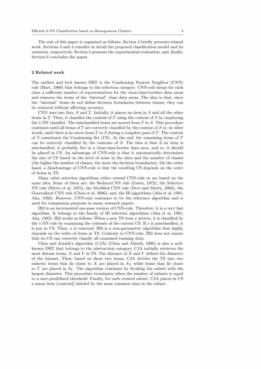
The pre-processing algorithm builds SUDS by finding homogeneous clusters in TS.A cluster is homogeneous if it contains items of a specific class only. The SUDSConstruction Algorithm (SUDSCA) repetitively executes the k-Means clusteringalgorithm until all of the identified clusters become homogeneous. SUDS is a two-level data structure. Its first level is a list of centroids (or representatives) of theidentified homogeneous clusters. Each one represents a data area of a specificclass and indexes the “real” cluster items which are in the second level of SUDS.Figure 1 shows how SUDS is constructed and Algorithm 1 summarizes the stepsof the corresponding algorithm.

Initially, SUDSCA finds the mean items (class-centroids) of each class in TSby averaging its items (Figure 1(b)). Then, it executes the k-Means clusteringalgorithm using these class centroids as initial means. Thus, for a dataset with Mclasses, SUDSCA initially identifies M clusters (Figure 1(c)). SUDSCA continuesby analyzing the M clusters. If a cluster is homogeneous, it is added to SUDS.The cluster centroid is added to the first level of SUDS as representative of thespecific class and indexes the cluster items that are added to the second level.On the other hand, for each non-homogeneous cluster X, k-Means is executed onits items and identifies as many clusters as the number of distinct classes in Xfollowing the aforementioned procedure(Figure 1(d)). The repetitive execution ofk-Means terminates when all constructed clusters are homogeneous. Following thisalgorithm, SUDSCA constructs few large clusters for internal class data areas, andmany small clusters for close-class-border data areas.

SUDSCA can be easily implemented using a simple queue data structure thatstores the unprocessed clusters. Initially, the whole TS constitutes an unprocessedcluster and it becomes the head of the queue (line 1 in Algorithm 1). In each


(a) (b)

(c) (d)

Fig. 1 SUDS construction by finding homogeneous clusters in the training dataset

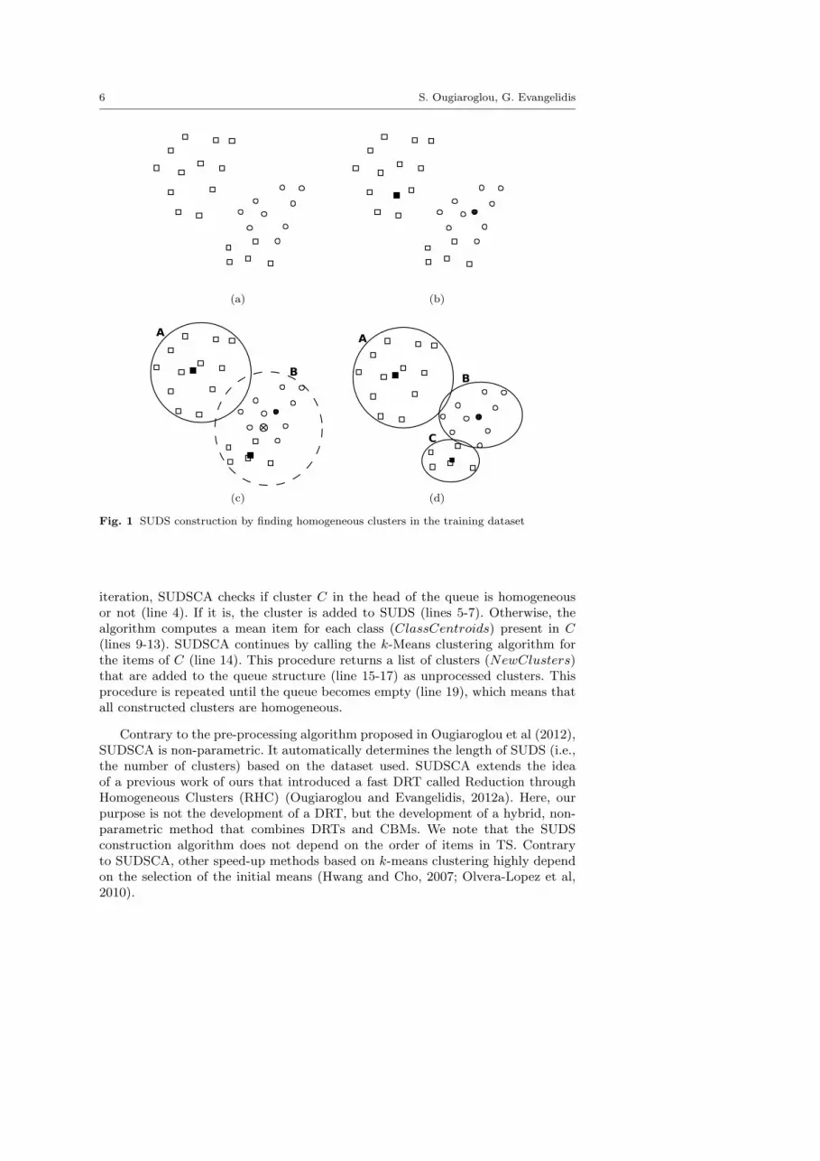
iteration, SUDSCA checks if cluster C in the head of the queue is homogeneousor not (line 4). If it is, the cluster is added to SUDS (lines 5-7). Otherwise, thealgorithm computes a mean item for each class (ClassCentroids) present in C(lines 9-13). SUDSCA continues by calling the k-Means clustering algorithm forthe items of C (line 14). This procedure returns a list of clusters (NewClusters)that are added to the queue structure (line 15-17) as unprocessed clusters. Thisprocedure is repeated until the queue becomes empty (line 19), which means thatall constructed clusters are homogeneous.

Contrary to the pre-processing algorithm proposed in Ougiaroglou et al (2012),SUDSCA is non-parametric. It automatically determines the length of SUDS (i.e.,the number of clusters) based on the dataset used. SUDSCA extends the ideaof a previous work of ours that introduced a fast DRT called Reduction throughHomogeneous Clusters (RHC) (Ougiaroglou and Evangelidis, 2012a). Here, ourpurpose is not the development of a DRT, but the development of a hybrid, non-parametric method that combines DRTs and CBMs. We note that the SUDSconstruction algorithm does not depend on the order of items in TS. Contraryto SUDSCA, other speed-up methods based on k-means clustering highly dependon the selection of the initial means (Hwang and Cho, 2007; Olvera-Lopez et al,2010).


Algorithm 1 SUDS Construction AlgorithmInput: TS Output: SUDS

1: Enqueue(Queue, TS)2: repeat3: C ← Dequeue(Queue)4: if C is Homogeneous then5: Compute the mean vector (class-centroid) M of C6: Put M into the first level of SUDS7: Put the items of C into the second level of SUDS and associate them to M8: else9: ClassCentroids← ∅10: for each Class L in C do11: CentroidL ← Compute the mean vector of items that belong to L12: ClassCentroids ← ClassCentroids ∪ CentroidL13: end for14: NewClusters ← k-Means(C, ClassCentroids)15: for each cluster X in NewClusters do16: Enqueue(Queue, X)17: end for18: end if19: until Queue is empty20: return SUDS

3.2 Hybrid Classification Algorithm based on Homogeneous Clusters (HCAHC)

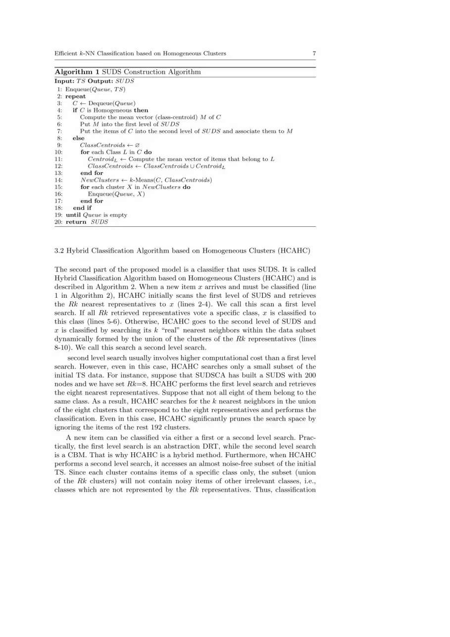
The second part of the proposed model is a classifier that uses SUDS. It is calledHybrid Classification Algorithm based on Homogeneous Clusters (HCAHC) and isdescribed in Algorithm 2. When a new item x arrives and must be classified (line1 in Algorithm 2), HCAHC initially scans the first level of SUDS and retrievesthe Rk nearest representatives to x (lines 2-4). We call this scan a first levelsearch. If all Rk retrieved representatives vote a specific class, x is classified tothis class (lines 5-6). Otherwise, HCAHC goes to the second level of SUDS andx is classified by searching its k “real” nearest neighbors within the data subsetdynamically formed by the union of the clusters of the Rk representatives (lines8-10). We call this search a second level search.

second level search usually involves higher computational cost than a first levelsearch. However, even in this case, HCAHC searches only a small subset of theinitial TS data. For instance, suppose that SUDSCA has built a SUDS with 200nodes and we have set Rk=8. HCAHC performs the first level search and retrievesthe eight nearest representatives. Suppose that not all eight of them belong to thesame class. As a result, HCAHC searches for the k nearest neighbors in the unionof the eight clusters that correspond to the eight representatives and performs theclassification. Even in this case, HCAHC significantly prunes the search space byignoring the items of the rest 192 clusters.

A new item can be classified via either a first or a second level search. Prac-tically, the first level search is an abstraction DRT, while the second level searchis a CBM. That is why HCAHC is a hybrid method. Furthermore, when HCAHCperforms a second level search, it accesses an almost noise-free subset of the initialTS. Since each cluster contains items of a specific class only, the subset (unionof the Rk clusters) will not contain noisy items of other irrelevant classes, i.e.,classes which are not represented by the Rk representatives. Thus, classification


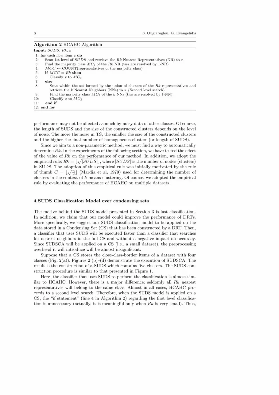
Algorithm 2 HCAHC AlgorithmInput: SUDS, Rk, k

1: for each new item x do2: Scan 1st level of SUDS and retrieve the Rk Nearest Representatives (NR) to x3: Find the majority class MC1 of the Rk NR (ties are resolved by 1-NR)4: MCC ← COUNT(representatives of the majority class)5: if MCC = Rk then6: Classify x to MC1

7: else8: Scan within the set formed by the union of clusters of the Rk representatives and

retrieve the k Nearest Neighbors (NNs) to x {Second level search}9: Find the majority class MC2 of the k NNs (ties are resolved by 1-NN)10: Classify x to MC2

11: end if12: end for

performance may not be affected as much by noisy data of other classes. Of course,the length of SUDS and the size of the constructed clusters depends on the levelof noise. The more the noise in TS, the smaller the size of the constructed clustersand the higher the final number of homogeneous clusters (or length of SUDS).

Since we aim to a non-parametric method, we must find a way to automaticallydetermine Rk. In the experiments of the following section, we have tested the effectof the value of Rk on the performance of our method. In addition, we adopt theempirical rule: Rk = ⌊

√|SUDS|⌋, where |SUDS| is the number of nodes (clusters)

in SUDS. The adoption of this empirical rule was initially motivated by the ruleof thumb C = ⌊

√n2 ⌋ (Mardia et al, 1979) used for determining the number of

clusters in the context of k-means clustering. Of course, we adopted the empiricalrule by evaluating the performance of HCAHC on multiple datasets.

4 SUDS Classification Model over condensing sets

The motive behind the SUDS model presented in Section 3 is fast classification.In addition, we claim that our model could improve the performance of DRTs.More specifically, we suggest our SUDS classification model to be applied on thedata stored in a Condensing Set (CS) that has been constructed by a DRT. Then,a classifier that uses SUDS will be executed faster than a classifier that searchesfor nearest neighbors in the full CS and without a negative impact on accuracy.Since SUDSCA will be applied on a CS (i.e., a small dataset), the preprocessingoverhead it will introduce will be almost insignificant.

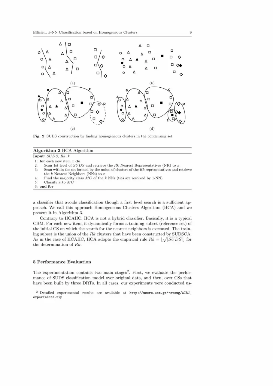
Suppose that a CS stores the close-class-border items of a dataset with fourclasses (Fig. 2(a)). Figures 2 (b)–(d) demonstrate the execution of SUDSCA. Theresult is the construction of a SUDS which contains five clusters. The SUDS con-struction procedure is similar to that presented in Figure 1.

Here, the classifier that uses SUDS to perform the classification is almost sim-ilar to HCAHC. However, there is a major difference: seldomly all Rk nearestrepresentatives will belong to the same class. Almost in all cases, HCAHC pro-ceeds to a second level search. Therefore, when the SUDS model is applied on aCS, the “if statement” (line 4 in Algorithm 2) regarding the first level classifica-tion is unnecessary (actually, it is meaningful only when Rk is very small). Thus,


(a) (b)

(c) (d)

Fig. 2 SUDS construction by finding homogeneous clusters in the condensing set

Algorithm 3 HCA AlgorithmInput: SUDS, Rk, k

1: for each new item x do2: Scan 1st level of SUDS and retrieve the Rk Nearest Representatives (NR) to x3: Scan within the set formed by the union of clusters of the Rk representatives and retrieve

the k Nearest Neighbors (NNs) to x4: Find the majority class MC of the k NNs (ties are resolved by 1-NN)5: Classify x to MC6: end for

a classifier that avoids classification though a first level search is a sufficient ap-proach. We call this approach Homogeneous Clusters Algorithm (HCA) and wepresent it in Algorithm 3.

Contrary to HCAHC, HCA is not a hybrid classifier. Basically, it is a typicalCBM. For each new item, it dynamically forms a training subset (reference set) ofthe initial CS on which the search for the nearest neighbors is executed. The train-ing subset is the union of the Rk clusters that have been constructed by SUDSCA.As in the case of HCAHC, HCA adopts the empirical rule Rk = ⌊

√|SUDS|⌋ for

the determination of Rk.

5 Performance Evaluation

The experimentation contains two main stages2. First, we evaluate the perfor-mance of SUDS classification model over original data, and then, over CSs thathave been built by three DRTs. In all cases, our experiments were conducted us-

2 Detailed experimental results are available at http://users.uom.gr/~stoug/AIRJ_experiments.zip


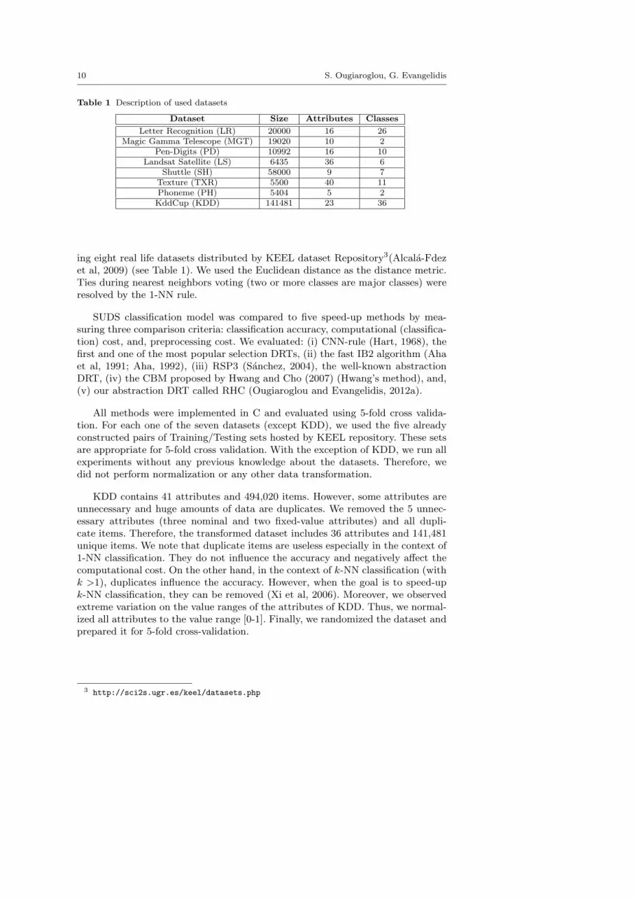
Table 1 Description of used datasets

Dataset Size Attributes Classes

Letter Recognition (LR) 20000 16 26Magic Gamma Telescope (MGT) 19020 10 2

Pen-Digits (PD) 10992 16 10Landsat Satellite (LS) 6435 36 6

Shuttle (SH) 58000 9 7Texture (TXR) 5500 40 11Phoneme (PH) 5404 5 2KddCup (KDD) 141481 23 36

ing eight real life datasets distributed by KEEL dataset Repository3(Alcala-Fdezet al, 2009) (see Table 1). We used the Euclidean distance as the distance metric.Ties during nearest neighbors voting (two or more classes are major classes) wereresolved by the 1-NN rule.

SUDS classification model was compared to five speed-up methods by mea-suring three comparison criteria: classification accuracy, computational (classifica-tion) cost, and, preprocessing cost. We evaluated: (i) CNN-rule (Hart, 1968), thefirst and one of the most popular selection DRTs, (ii) the fast IB2 algorithm (Ahaet al, 1991; Aha, 1992), (iii) RSP3 (Sanchez, 2004), the well-known abstractionDRT, (iv) the CBM proposed by Hwang and Cho (2007) (Hwang’s method), and,(v) our abstraction DRT called RHC (Ougiaroglou and Evangelidis, 2012a).

All methods were implemented in C and evaluated using 5-fold cross valida-tion. For each one of the seven datasets (except KDD), we used the five alreadyconstructed pairs of Training/Testing sets hosted by KEEL repository. These setsare appropriate for 5-fold cross validation. With the exception of KDD, we run allexperiments without any previous knowledge about the datasets. Therefore, wedid not perform normalization or any other data transformation.

KDD contains 41 attributes and 494,020 items. However, some attributes areunnecessary and huge amounts of data are duplicates. We removed the 5 unnec-essary attributes (three nominal and two fixed-value attributes) and all dupli-cate items. Therefore, the transformed dataset includes 36 attributes and 141,481unique items. We note that duplicate items are useless especially in the context of1-NN classification. They do not influence the accuracy and negatively affect thecomputational cost. On the other hand, in the context of k-NN classification (withk >1), duplicates influence the accuracy. However, when the goal is to speed-upk-NN classification, they can be removed (Xi et al, 2006). Moreover, we observedextreme variation on the value ranges of the attributes of KDD. Thus, we normal-ized all attributes to the value range [0-1]. Finally, we randomized the dataset andprepared it for 5-fold cross-validation.

3 http://sci2s.ugr.es/keel/datasets.php


5.1 Performance of SUDS classification model over original data

5.1.1 Experimental Setup

CNN-rule, IB2, RSP3 and RHC are non-parametric methods, that is, they donot use user-defined parameters in order to reduce the training data. On theother hand, Hwang’s method is parametric. In addition to parameter k (number ofnearest neighbors to search), which is used by all methods during the classificationstep, it uses three extra parameters: (i) C: the number of clusters constructed bythe k-Means clustering algorithm, (ii)D: the distance threshold used to divide eachcluster into core and peripheral sets, and, (iii) L: the number of adjacent clustersthat will be used. C and D are used during the preprocessing step, while L duringthe classification step (see Section 2 or Hwang and Cho (2007) for details). Theseparameters should be tuned. For each dataset, we built eight Hwang’s classifiersusing eight different C values. More specifically, each classifier i=1,. . . ,8, usedC = ⌊

√n2i ⌋, where n is the number of TS items. The first classifier, i.e. i=1,

is based on the rule of thumb C = ⌊√

n2 ⌋ (Mardia et al, 1979). We decided to

build additional classifiers that use smaller C values than C = ⌊√

n2 ⌋ based on the

observation that Hwang and Cho defined C=10 for a dataset with 60919 items(they did not find the optimal C value). For the other two parameters, we adoptedthe values suggested by Hwang and Cho in their experiments.

Although SUDSCA is non-parametric, HCAHC is a parametric classifier. Inaddition to k, it uses the Rk parameter. We built 29 HCAHC classifiers, forRk=2,3,. . . ,30, and we also considered the automatic determination of Rk (seeSection 3). We refer to that classifier as HCAHC-sqrt. For both HCAHC andHwang’s method, we report only the most accurate classifiers for each cost level,i.e., the performance of a classifier was omitted if it achieved lower accuracy andinvolved higher computational cost than another classifier that achieved equal orhigher accuracy and involved lower computational cost.

During the classification step, all methods involve parameter k. The DRTsperform k-NN classification using their CS, while Hwang’s method does this over asmall reference set that is dynamically formed for each new item. Finally, HCAHCsearches for k nearest neighbors when it performs a second level search. We usedthe best k values for each method and dataset, i.e., the value that achieved thehighest classification accuracy. In effect, we ran the cross validation many timesfor different k values and kept the best one. Of course, we did not use different kvalues for each fold.

For the first seven datasets, we run all experiments twice: on non-edited and onedited data (noise-free datasets). For editing purposes, we used ENN-rule (Wilson,1972) by setting k=3 (according to Wilson and Martinez (2000), k=3 is a goodvalue). The goal was to study how noise affects the performance of each method.The complete procedure that we followed during our experimentation is shownin Figure 3. For KDD, ENN-rule eliminates all items of some rare classes. Morespecifically, the ENN-rule edited KDD dataset contains fewer than 23 classes (from4 to 7 fewer classes - depending on the fold). Therefore, we decided to skip theedited version of KDD. We note that the execution of ENN-rule on KDD wasan extremely costly procedure. It involved the computation of 113,185×113,184

2 × 5folds ≃ 32 billion distances. SH is also imbalanced as it contains two rare classes.


Fig. 3 Classification procedure of the experimental study

However, ENN-rule did not eliminate these rare classes. Thus, we decided to runexperiments on the edited SH.

5.1.2 Pre-processing performance

Tables 2 and 3 present the pre-processing computational costs in terms of mil-lions (M) of distance computations (how many distances were computed duringpre-processing) performed by each method on non-edited and edited data. As weexpected, SUDSCA and RHC were executed very fast in comparison to the otherapproaches, and were comparable in performance to IB2, which is a one-pass al-gorithm. This happened because: (i) the construction of SUDS and of the RHCcondensing set are based on the repetitive execution of the fast k-Means cluster-ing algorithm, and, (ii) in both cases, k-Means uses the mean items of the classesas initial centroids, and thus, clusters are consolidated very quickly. It is worthmentioning that SUDSCA and RHC pre-processing could become even faster hadwe used a different k-Means stopping criterion than the full clusters consolidation(no item move from one cluster to another during a complete algorithm pass).

Table 2 Preprocessing Cost on non-edited data (in millions of distance computations)

Dataset CNN IB2 RSP3Hwang’s method RHC/

i=1 i=3 i=5 i=7 SUDSCA

LR 163.03 23.37 326.52 88.88 63.66 26.35 10.89 41.85MGT 277.18 34.61 511.67 120.22 72.64 21.74 10.64 4.09PD 11.75 1.78 86.66 28.80 11.27 5.97 1.70 2.88LS 18.59 2.22 37.70 16.74 12.44 4.54 0.81 1.69SH 45.30 8.26 17410.12 744.82 399.23 105.13 34.78 16.83TXR 5.57 0.84 27.63 14.86 7.43 3.89 0.83 3.63PH 13.45 1.96 20.31 9.87 3.70 1.33 0.74 0.65KDD 384.90 55.58 20278.87 5440.21 2155.75 955.06 309.97 81.59

Avg. 114.97 16.08 4837.43 808.05 340.77 140.50 46.29 19.15


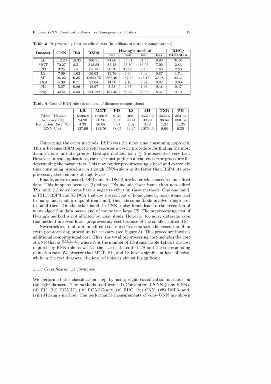
Table 3 Preprocessing Cost on edited data (in millions of distance computations)

Dataset CNN IB2 RSP3Hwang’s method RHC/

i=1 i=3 i=5 i=7 SUDSCA

LR 112.20 18.35 300.51 74.60 55.31 31.45 9.93 31.05MGT 70.27 8.51 318.82 85.28 33.80 16.33 7.06 2.83PD 9.25 1.51 85.15 26.76 12.06 5.18 1.83 2.83LS 7.09 1.02 30.63 13.76 9.60 3.43 0.87 1.74SH 26.02 6.35 15652.75 867.40 367.52 146.12 37.18 22.41TXR 4.39 0.71 27.04 14.76 7.16 4.27 0.82 3.00PH 5.57 0.86 15.67 5.58 2.65 1.03 0.48 0.47

Avg. 33.54 5.33 2347.22 155.45 69.73 29.69 8.31 9.19

Table 4 Cost of ENN-rule (in millions of distance computations)

LR MGT PD LS SH TXR PH

Edited TS size: 15306.8 12160.2 8734 4681 46314.2 4345.6 3837.4Accuracy (%): 94.98 80.96 99.30 90.41 99.79 98.64 880.14

Reduction Rate (%): 4.33 20.08 0.67 9.07 0.18 1.24 11.25ENN Cost: 127.99 115.76 38.65 13.25 1076.46 9.68 9.35

Concerning the other methods, RSP3 was the most time consuming approach.This is because RSP3 repetitively executes a costly procedure for finding the mostdistant items in data groups. Hwang’s method for i ≥ 5 is executed very fast.However, in real applications, the user must perform a trial-end-error procedure fordetermining the parameters. This may render pre-processing a hard and extremelytime consuming procedure. Although CNN-rule is quite faster than RSP3, its pre-processing cost remains at high levels.

Finally, as we expected, DRTs and SUDSCA are faster when executed on editeddata. This happens because: (i) edited TSs include fewer items than non-editedTSs, and, (ii) noisy items have a negative effect on these methods. One one hand,in RHC, RSP3 and SUDCA that use the concept of homogeneity, noisy items leadto many and small groups of items and, thus, these methods involve a high costto build them. On the other hand, in CNN, noisy items lead to the execution ofmany algorithm data passes and of course to a large CS. The preprocessing cost ofHwang’s method is not affected by noisy items. However, for noisy datasets, eventhis method involved lower preprocessing cost because of the smaller edited TS.

Nevertheless, to obtain an edited (i.e., noise-free) dataset, the execution of anextra preprocessing procedure is necessary (see Figure 3). This procedure involvesadditional computational cost. Thus, the total preprocessing cost includes the costof ENN that is N∗(N−1)

2 , whereN is the number of TS items. Table 4 shows the costrequired by ENN-rule as well as the size of the edited TS and the correspondingreduction rate. We observe that MGT, PH, and LS have a significant level of noise,while in the rest datasets, the level of noise is almost insignificant.

5.1.3 Classification performance

We performed the classification step by using eight classification methods onthe eight datasets. The methods used were: (i) Conventional k-NN (conv-k-NN),(ii) IB2, (iii) HCAHC, (iv) HCAHC-sqrt, (v) RHC, (vi) CNN, (vii) RSP3, and,(viii) Hwang’s method. The performance measurements of conv-k-NN are shown


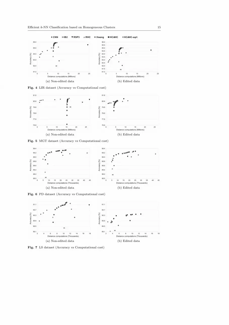
in Table 5 while the measurements of the speed-up methods are depicted in Fig-ures 4-20. In particular, each figure includes two diagrams for each dataset, onecorresponding to the non-edited TS and one to the edited TS.

The figures show the cost measurements (in terms of millions or thousands dis-tance computations) on the x-axis and the corresponding accuracy on the y-axis.The cost measurements indicate how many distances were computed in order toclassify all testing items. Since, we used a cross-validation schema, cost measure-ments are average values.

Almost in all cases, HCAHC and HCAHC-sqrt had very good performance.HCAHC can even reach the accuracy level of conv-k-NN (see Table 5). All dia-grams show that rule Rk = ⌊

√|SUDS|⌋ is a good choice for the determination

of Rk. With the exception of the SH and KDD datasets, HCAHC achieved betterclassification performance than all DRTs. On the other hand, although HCAHCand HCAHC-sqrt achieved higher accuracy than Hwang’s method in all datasets,for the MGT, SH, PH AND KDD datasets, Hwang’s method may be preferablebecause it achieved accuracies close to those of HCAHC and HCAHC-sqrt at alower computational cost.

Table 5 compares the performance on non-edited data of conv-k-NN with thatof HCAHC with an Rk value that achieves the highest possible accuracy (notethat we have not conducted experiments for Rk > 30 and for Rk = ⌊

√|SUDS|⌋).

Observe that the accuracy measurements are almost similar with significant gainsin computational cost. In LS and PH, HCAHC achieved slightly better accuracythan conv-k-NN. This is because the reference sets formed by HCAHC during thesecond level searches do not contain items of irrelevant classes.

Concerning the SH and KDD dataset, all DRTs built very small CSs. Thus, thek-NN classifiers that were applied on these CSs, were not only accurate but veryfast as well. HCAHC and HCAHC-sqrt were able to achieve even higher accuracylevels than all DRTs but, it involves higher computational cost.

All figures show that when the speed-up methods are performed over editeddata, they are faster than when they performed over non-edited data. However, insome cases, either the cost gains are not very high or the classification accuracy issignificantly reduced. On the other hand, in the cases of MGT, which is a very noisydataset, editing is a necessary preprocessing procedure for all speed-up methods. InFigure 5, we observe that the cost gains are high, while the classification accuracyis not reduced significantly.

Table 5 Conv-k-NN vs HCAHC over non-edited data

DatasetConv-k-NN HCAHC

Acc(%) Cost(M) Acc(%) Cost(M) Rk

LR 96.01 64.00 95.90 9.41 43MGT 81.32 57.88 81.27 16.26 63PD 99.37 19.34 99.33 2.45 20LS 91.22 6.63 91.25 1.10 15SH 99.82 538.24 99.82 227.26 29TXR 99.02 4.84 99.02 0.71 18PH 90.10 4.67 90.23 1.08 11KDD 99.71 3202.68 99.71 429.31 10

Avg. 94.5715 487.29 94.5663 85.97


(a) Non-edited data (b) Edited data

Fig. 4 LIR dataset (Accuracy vs Computational cost)


Fig. 5 MGT dataset (Accuracy vs Computational cost)


Fig. 6 PD dataset (Accuracy vs Computational cost)


Fig. 7 LS dataset (Accuracy vs Computational cost)



Fig. 8 SH dataset (Accuracy vs Computational cost)


Fig. 9 TXR dataset (Accuracy vs Computational cost)


Fig. 10 PH dataset (Accuracy vs Computational cost)

Fig. 11 Non-edited KDD dataset (Accuracy vs Computational cost)


5.1.4 Non parametric statistical test of significance

The experimentation is complemented by the application of a non-parametricstatistical test of significance (Sheskin, 2011; Garcıa et al, 2009). More specifi-cally, the experimental measurements were validated by the Wilcoxon signed rankstest (Demsar, 2006), which compares each pair of methods taking into considera-tion their performance in each dataset used. We ran Wilcoxon test considering allcomparison criteria as having the same significance. As a consequence, we ran thetest on 45 measurements, 24 for non-edited data and 21 for edited data.

Of course, we could not include tests for all variations of HCAHC and Hwang’smethod (for the different tested values of Rk and i parameters respectively). Foreach dataset we chose a good representative variation for each one of these para-metric algorithms. Our criterion was high performance, i.e., relatively high accu-racy and low classification cost (we do take into account the cost of the correspond-ing preprocessing algorithms). The parameter values for the selected classifiers areshown in Table 6.

Additionally to the parametric HCAHC (HCAHC-Rk), we ran the test forHCAHC-sqrt. Consequently, HCAHC-sqrt and HCAHC-Rk are compared to eachone of the four other speed-up methods. Note that the execution of HCAHC impliesthe execution of SUDSCA during the preprocessing phase. Table 7 illustrates theresults of Wilcoxon signed ranks tests. The last table column lists the Wilcoxonsignificant level. If that value is not higher than 0.05, one can claim that thedifference between the pair of methods is significant.

As we expected, there is no statistically significant difference between HCAHCand RHC. Both have the same preprocessing cost, RHC classifiers are faster thanHCAHC classifiers, but HCAHC classifiers are more accurate than RHC classifiers.One the other hand, the statistical test confirms that the proposed method per-forms better than all other methods, with the exception of IB2. In almost all cases(14/15), both HCAHC approaches achieve highest accuracies than IB2. However,they lose slightly in terms of the other two comparison criteria. The test showsthat there is not significant difference between HCAHC-sqrt and Hwang-i. How-ever, considering that both preprocessing and classification algorithms of Hwang’smethod are parametric and SUDSCA and HCAHC-sqrt are not parametric, oneconcludes that the SUDS model is preferable.

Table 6 Parameter values selected for the Wilcoxon signed ranks test

LR MGT PD LS SH TXR PH KDD

Non-edited dataRk 10 23 6 15 9 5 11 2i 7 3 7 4 3 5 4 1

Edited dataRk 8 17 5 5 2 3 7 -i 7 5 7 4 1 5 3 -


Table 7 Wilcoxon signed ranks test

Methods wins/losses/ties Wilcoxon

HCAHC-sqrt vs CNN 31/14/0 0.039HCAHC-sqrt vs IB2 20/25/0 0.756HCAHC-sqrt vs RSP3 36/9/0 0.000HCAHC-sqrt vs Hwang-i 26/19/0 0.271HCAHC-sqrt vs RHC 15/15/15 0.245

HCAHC-Rk vs CNN 33/12/0 0.003HCAHC-Rk vs IB2 21/24/0 0.340HCAHC-Rk vs RSP3 40/5/0 0.000HCAHC-Rk vs Hwang-i 30/15/0 0.027HCAHC-Rk vs RHC 15/15/15 0,111

5.2 Performance of SUDS classification model over Condensing Sets

5.2.1 Experimental Setup

The second part of our experimentation concerns the performance of SUDS modelwhen applied on CSs. To build the CSs, we executed the four DRTs that we hadused in Subsection 5.1, i.e. (i) CNN, (ii) IB2, (iii) RSP3, and (iv) RHC, on thetraining sets presented in Table 1. Then, we applied SUDS model on the fourconstructed CSs. Of course SUDS can be combined with any DRT. Once again,we executed all experiments twice on non-edited data and on edited data usingENN-rule. Figure 12 depicts the procedure that we followed during this stage ofour experimentation.

Fig. 12 Classification using SUDS model on the condensing set

During the classification step, we executed HCA (Algorithm 3). Like HCAHC,HCA uses the Rk parameter. We executed several experiments with different Rkparameter values. In addition, we built an HCA classifier that uses the empiricalrule: Rk = ⌊

√|SUDS|⌋. In all cases, this rule was proven to be a good choice

for the determination of Rk. For that reason, in the figures presented in Subsec-tion 5.2.3 below, we have included only the performance of the HCA classifier thatuses the empirical rule.

Additionally to the performance of HCA, the diagrams presented in subsec-tion 5.2.3 include the performance measurements obtained by the three DRTs (i.e.,


application of k-NN classifier on their CSs). In this way, we can easily concludewhether the SUDS model can significantly improve the performance of the DRTs.Finally, as in Section 5.1, for each method and dataset, we used the k parameterthat achieved the highest classification accuracy.

5.2.2 Preprocessing performance

SUDS construction constitutes an extra preprocessing step that is applied afterthe construction of CS (see Figure 12). Thus, additionally to the cost shown inTables 4-3, the total preprocessing cost involves the cost overhead of SUDSCAexecution. Table 8 shows the preprocessing overheads for each DRT on non-editedand edited training sets.

The computational cost overheads depend on the size of each CS. RSP3 achievedthe lowest reduction rates, and so, it involves the highest overhead. In contrast,RHC achieves the highest reduction rates and thus it involves a small overhead. Inall cases, overheads added by SUDSCA are almost insignificant. Considering thatthe preprocessing is executed only once, the small preprocessing overhead does notconstitute a problem in real-life data mining applications. Actually, efficient datapreprocessing implies fast predictions during the classification step.

Table 8 SUDSCA preprocessing overhead (in millions of distance computations)

DatasetNon-edited data Edited data

CNN IB2 RSP3 RHC CNN IB2 RSP3 RHC

LR 2.777 2.158 8.489 1.512 1.688 1.478 7.425 1.072MGT 1.375 0.914 1.577 0.802 0.220 0.159 0.358 0.131PD 0.072 0.045 0.218 0.035 0.043 0.034 0.161 0.025LS 0.208 0.122 0.333 0.076 0.054 0.042 0.104 0.025SH 0.061 0.052 0.188 0.035 0.034 0.028 0.134 0.024TXR 0.071 0.054 0.243 0.043 0.038 0.035 0.264 0.032PH 0.102 0.080 0.144 0.083 0.032 0.025 0.055 0.024KDD 0.323 0.247 0.624 0.285 - - - -

Avg. 0.624 0.459 1.477 0.359 0.301 0.257 1.215 0.190

5.2.3 Classification performance

Figures 13-20 show the performance measurements for the classification stage ofour experimentation. Each figure includes two diagrams, one for non-edited andone for edited data. The diagrams show the performance of the three DRTs whenusing or not using the SUDS model. Each diagram shows the performance of eightclassifiers, two for each DRT: (i) k-NN classifier over its CS, (ii) HCA that usesthe empirical rule over SUDS.

HCA classifier performed better than k-NN classifier over CSs. An HCA clas-sifier avoids a large number of distance computations and, at the same time, keepsthe classification accuracy as high as k-NN classifier. This happens because HCAavoids the distance computations between a new item and items that have beenassigned to distant clusters. The performance improvements are significant in both


edited and non-edited datasets. However, they are higher in the case of non-editeddata.

For RSP3, the cost gains are higher than those of the other two methods. Forinstance, in the cases of LIR, PD, SH, TXR datasets, the class labels of the testingitems were predicted four or three times faster. The performance improvementsfor CNN and RHC are not as high but they deserve to be mentioned.

A final comment: SUDS classification model is able to significantly speed-upthe predictions of class labels when it is applied on data stored in CSs constructedby DRTs by adding a small cost overhead during the preprocessing phase. Thisapproach is appropriate when extremely fast classification is required.

6 Conclusions

Speeding-up distance based classifiers is a very important issue in data mining. Inthis paper, we presented and evaluated a new classification model. The motivationof our work was the development of a non-parametric method that has low pre-processing cost and is able to classify new items fast and with high accuracy.

We presented an efficient classification model which includes a non-parametricfast pre-processing algorithm that builds a two-level data structure, and a classi-fier that makes predictions by accessing this structure. In addition, based on thesame motivation, we applied the proposed classification model on data stored incondensing sets constructed by DRTs. The goal of this adoption is to improve theperformance of the DRTs. The proposed HCAHC and HCA classifiers are para-metric since they use parameter Rk (number of cluster representatives to use in afirst level search). However, we demonstrated that Rk can be automatically deter-mined and render the proposed classification model non-parametric. Experimentalresults based on eight real-life datasets showed that the proposed model achievedthe aforementioned goals.

References

Aha DW (1992) Tolerating noisy, irrelevant and novel attributes in instance-basedlearning algorithms. Int J Man-Mach Stud 36(2):267–287

Aha DW, Kibler D, Albert MK (1991) Instance-based learning algorithms. MachLearn 6(1):37–66

Alcala-Fdez J, Sanchez L, Garcıa S, del Jesus MJ, Ventura S, i Guiu JMG, OteroJ, Romero C, Bacardit J, Rivas VM, Fernandez JC, Herrera F (2009) Keel: asoftware tool to assess evolutionary algorithms for data mining problems. SoftComput 13(3):307–318

Brighton H, Mellish C (2002) Advances in instance selection for instance-basedlearning algorithms. Data Min Knowl Discov 6(2):153–172

Chen CH, Jozwik A (1996) A sample set condensation algorithm for the classsensitive artificial neural network. Pattern Recogn Lett 17:819–823

Chou CH, Kuo BH, Chang F (2006) The generalized condensed nearest neigh-bor rule as a data reduction method. In: Proceedings of the 18th InternationalConference on Pattern Recognition - Volume 02, IEEE Computer Society, Wash-ington, DC, USA, ICPR ’06, pp 556–559



Fig. 13 LIR dataset (Accuracy vs Computational cost)


Fig. 14 MGT dataset (Accuracy vs Computational cost)


Fig. 15 PD dataset (Accuracy vs Computational cost)


Fig. 16 LS dataset (Accuracy vs Computational cost)



Fig. 17 SH dataset (Accuracy vs Computational cost)


Fig. 18 TXR dataset (Accuracy vs Computational cost)


Fig. 19 PH dataset (Accuracy vs Computational cost)

Fig. 20 Non-edited KDD dataset (Accuracy vs Computational cost)


Dasarathy BV (1991) Nearest neighbor (NN) norms : NN pattern classificationtechniques. IEEE Computer Society Press

Demsar J (2006) Statistical comparisons of classifiers over multiple data sets. JMach Learn Res 7:1–30

Devi VS, Murty MN (2002) An incremental prototype set building technique.Pattern Recognition 35(2):505–513

Garcia S, Derrac J, Cano J, Herrera F (2012) Prototype selection for nearestneighbor classification: Taxonomy and empirical study. IEEE Trans PatternAnal Mach Intell 34(3):417–435

Gates GW (1972) The reduced nearest neighbor rule. ieee transactions on infor-mation theory. IEEE Transactions on Information Theory 18(3):431–433

Grochowski M, Jankowski N (2004) Comparison of instance selection algorithms ii.results and comments. In: Artificial Intelligence and Soft Computing - ICAISC2004, LNCS, vol 3070, Springer Berlin / Heidelberg, pp 580–585

Han J, Kamber M, Pei J (2011) Data Mining: Concepts and Techniques. TheMorgan Kaufmann Series in Data Management Systems, Elsevier Science

Hart PE (1968) The condensed nearest neighbor rule. IEEE Transactions on In-formation Theory 14(3):515–516

Hwang S, Cho S (2007) Clustering-based reference set reduction for k-nearestneighbor. In: 4th international symposium on Neural Networks: Part II–Advances in Neural Networks, Springer, ISNN ’07, pp 880–888

James M (1985) Classification algorithms. Wiley-Interscience, New York, NY, USAJankowski N, Grochowski M (2004) Comparison of instances seletion algorithms

i. algorithms survey. In: Artificial Intelligence and Soft Computing - ICAISC2004, LNCS, vol 3070, Springer Berlin / Heidelberg, pp 598–603

Karamitopoulos L, Evangelidis G (2009) Cluster-based similarity search in timeseries. In: Proceedings of the Fourth Balkan Conference in Informatics, IEEEComputer Society, Washington, DC, USA, BCI ’09, pp 113–118

Lozano M (2007) Data Reduction Techniques in Classification processes (PhdThesis). Universitat Jaume I

Mardia K, Kent J, Bibby J (1979) Multivariate Analysis. Academic PressMcQueen J (1967) Some methods for classification and analysis of multivariate ob-

servations. In: Proc. of 5th Berkeley Symp. on Math. Statistics and Probability,Berkeley, CA : University of California Press, pp 281– 298

Olvera-Lopez JA, Carrasco-Ochoa JA, Martınez-Trinidad JF, Kittler J (2010) Areview of instance selection methods. Artif Intell Rev 34(2):133–143

Olvera-Lopez JA, Carrasco-Ochoa JA, Trinidad JFM (2010) A new fast prototypeselection method based on clustering. Pattern Anal Appl 13(2):131–141

Ougiaroglou S, Evangelidis G (2012a) Efficient dataset size reduction by findinghomogeneous clusters. In: Proceedings of the Fifth Balkan Conference in Infor-matics, ACM, New York, NY, USA, BCI ’12, pp 168–173

Ougiaroglou S, Evangelidis G (2012b) A fast hybrid k-nn classifier based onhomogeneous clusters. In: Artificial Intelligence Applications and Innovations,Springer Berlin Heidelberg, IFIP Advances in Information and CommunicationTechnology, vol 381, pp 327–336

Ougiaroglou S, Evangelidis G, Dervos DA (2012) An adaptive hybrid and cluster-based model for speeding up the k-nn classifier. In: Proceedings of the 7th in-ternational conference on Hybrid Artificial Intelligent Systems - Volume PartII, Springer-Verlag, Berlin, Heidelberg, HAIS’12, pp 163–175


Ritter G, Woodruff H, Lowry S, Isenhour T (1975) An algorithm for a selectivenearest neighbor decision rule. IEEE Trans on Inf Theory 21(6):665–669

Rokach L (2007) Data Mining with Decision Trees: Theory and Applications. Seriesin machine perception and artificial intelligence, World Scientific PublishingCompany, Incorporated

Samet H (2006) Foundations of multidimensional and metric data structures. TheMorgan Kaufmann series in computer graphics, Elsevier/Morgan Kaufmann

Sanchez JS (2004) High training set size reduction by space partitioning and pro-totype abstraction. Pattern Recognition 37(7):1561–1564

Sheskin D (2011) Handbook of Parametric and Nonparametric Statistical Proce-dures. A Chapman & Hall book, Chapman & Hall/CRC

Toussaint G (2002) Proximity graphs for nearest neighbor decision rules: Recentprogress. In: 34th Symposium on the INTERFACE, pp 17–20

Triguero I, Derrac J, andFrancisco Herrera SG (2012) A taxonomy and experi-mental study on prototype generation for nearest neighbor classification. IEEETransactions on Systems, Man, and Cybernetics, Part C 42(1):86–100

Wang X (2011) A fast exact k-nearest neighbors algorithm for high dimensionalsearch using k-means clustering and triangle inequality. In: The 2011 Interna-tional Joint Conference on Neural Networks (IJCNN), pp 1293 –1299

Wilson DL (1972) Asymptotic properties of nearest neighbor rules using editeddata. IEEE trans on systems, man, and cybernetics 2(3):408–421

Wilson DR, Martinez TR (2000) Reduction techniques for instance-based learningalgorithms. Machine Learning 38(3):257–286

Xi X, Keogh E, Shelton C, Wei L, Ratanamahatana CA (2006) Fast time seriesclassification using numerosity reduction. In: Proceedings of the 23rd interna-tional conference on Machine learning, ACM, New York, NY, USA, ICML ’06,pp 1033–1040

Zhang B, Srihari SN (2004) Fast k-nearest neighbor classification using cluster-based trees. IEEE Trans Pattern Anal Mach Intell 26(4):525–528

Garcıa S, Molina D, Lozano M, Herrera F (2009) A study on the use of non-parametric tests for analyzing the evolutionary algorithms’ behaviour: a casestudy on the cec’2005 special session on real parameter optimization. Journal ofHeuristics 15(6):617–644

Documents

Efficient k-NN classification based on homogeneous clusters