Effects of health insurance on labour supply - UNU-MERIT

#2017-050

Effects of health insurance on labour supply: Evidence from the health care fund for the poor in Viet Nam Nga Lê, Wim Groot, Sonila M. Tomini and Florian Tomini

Maastricht Economic and social Research institute on Innovation and Technology (UNU‐MERIT) email: [email protected] | website: http://www.merit.unu.edu Maastricht Graduate School of Governance (MGSoG) email: info‐[email protected] | website: http://www.maastrichtuniversity.nl/governance Boschstraat 24, 6211 AX Maastricht, The Netherlands Tel: (31) (43) 388 44 00

Working Paper Series

UNU-MERIT Working Papers ISSN 1871-9872

Maastricht Economic and social Research Institute on Innovation and Technology UNU-MERIT Maastricht Graduate School of Governance MGSoG

UNU-MERIT Working Papers intend to disseminate preliminary results of research carried out at UNU-MERIT and MGSoG to stimulate discussion on the issues raised.

Effects of health insurance on labour supplyEvidence from the Health Care Fund for the Poor

in Vietnam

Nga Le ∗ Wim Groot† Sonila M. Tomini‡ Florian Tomini§

March 15, 2019

Abstract

The expansion of health insurance in emerging countries raises concerns aboutthe unintended negative effects of health insurance on labour supply. This paperexamines the labour supply effects of the Health Care Fund for the Poor (HCFP)in Vietnam in terms of the number of work hours per month and the labourforce participation (the probability of employment). Employing various matchingmethods combined with a Difference-in-Differences approach on the VietnamHousehold Living Standard Surveys 2002-2006, we show that HCFP, which aims toprovide poor people and disadvantaged minority groups with free health insurance,has a negative effect on labour supply. This is manifested in both the averagenumber of hours worked per month and the probability of employment, suggestingthe income effect of the HCFP. Interestingly, the effects are mainly driven bythe non-poor recipients living in rural areas, raising the question of the targetingstrategy of the programme.

JEL Classifications: I13, J22Keywords: Vietnam, Health care fund for the poor,

health insurance, labour supply

∗UNU-MERIT/MGSoG, Maastricht University, the NL, [email protected]†TIER and CAPHRI School for Public Health and Primary Care, Maastricht University, the NL,

[email protected]‡UNU-MERIT/MGSoG, Maastricht University, the NL, [email protected]§Centre for Primary Care and Public Health Queen Mary University, London, [email protected]

1 Introduction

The expansion of public health insurance to the poor and vulnerable has received alarge amount of attention because of its potential effects on reducing catastrophic out-of-pocket spending and increasing access to health care (Lagomarsino et al.Lagomarsino et al., 20122012). Suchimpacts are particularly important for the poor who normally cannot afford to pay out-of-pocket. These are hence especially desirable for many low and middle income countries(LMIC) with a large proportion of poor population who normally do not have the financialresources to buy health insurance (ibid.). Many emerging economies in Asia, LatinAmerica and Africa are making progress towards Universal Health Coverage (UHC) toreduce the financial hardship for those seeking health care (Rodin and de FerrantiRodin and de Ferranti, 20122012;Lagomarsino et al.Lagomarsino et al., 20122012). The momentum on achieving UHC is rather strong as manycountries have increased or committed to increase government spending on total healthexpenditure (Lagomarsino et al.Lagomarsino et al., 20122012). The ambition towards UHC has also receivedsupport and active participation from important donors and international organizations(ibid.).

However, there have been concerns about the unintended labour market consequencesof health insurance in general and health insurance for the low income populationin particular. For instance, it has been shown that social health insuranceexpansion in East Europe and Central Asia during 1990-2004 has been associatedwith higher unemployment (Wagstaff and Moreno-SerraWagstaff and Moreno-Serra, 20092009) and reduced aggregateemployment (Wagstaff and Moreno-SerraWagstaff and Moreno-Serra, 20152015) while increasing the aggregate share ofself-employment (ibid.). Even though the authors failed to control for political changeswhich potentially caused unemployment, their findings provoked some debate on thepotential negative impacts of health insurance on the labour market. From a theoreticalperspective, the theory of static labour supply (Chou et al.Chou et al., 20022002; RosenRosen, 20142014) predictsa negative labour supply effect of health insurance which is not tied to employment dueto the income effect.

In the context of the UHC movement, there has been a renewed interest in thelabour supply effects of health insurance. However, there is currently inadequate andinconclusive evidence on the topic. A recent systematic review on the topic (Le et al.Le et al.,20172017) suggests that empirical evidence in LMIC is relatively scarce and sporadic probablydue to data limitations. The existing literature on the labour supply effects of pro-poorhealth insurance programmes is mainly represented by studies on the American healthcaresystem, where the evidence is mixed (ibid.), whereas, the evidence beyond the US is verylimited (ibid.). This creates a knowledge gap, especially for LMIC where health insurancecoverage is expanding. Therefore, to fill this gap, it is necessary to seek for more evidenceto guide policy making.

In Vietnam, this is crucially relevant as health coverage is being expanded rapidlywith assertive political commitment which has been translated into recent legal documentssuch as the Health Insurance Law versions of 2008 and 2014. In its latest strategicdocument, the government aims at a coverage rate of more than 90 percent by 2020(Socialist Republic of VietnamSocialist Republic of Vietnam, 20162016).

This paper investigates the effects of the Health Care Fund for the Poor (hereafter,HCFP) on the labour supply of the beneficiaries in Vietnam. Using pre-treatmentmatching techniques combined with a Difference-in-Differences approach on a panel ofVietnam Household Living Standards Surveys (VHLSS) during 2002-2006, we evaluatethe labour supply effects of the programme in terms of monthly work hours and the

1

probability of working. We separate the effects for urban and rural individuals as well asthe poor and non-poor people among the treated individuals. This paper contributes tofilling the gap in our knowledge on the impact of health insurance on the labour supplyand presents empirical evidence on this sporadically researched topic in the context ofLMIC.

2 Literature Review

The potentially distorting effects of health insurance and welfare benefits have beendiscussed thoroughly in theory. The budget constraint approach argues that government-provided health insurance, as financed by tax, is similar to a welfare benefit and hencecan be considered as a positive income shock for low income individuals and those whohave high health expenses (Boyle and LaheyBoyle and Lahey, 20102010). Therefore, a non-contributory healthscheme may reduce labour supply due to the income effect.

Similarly, the static labour supply theory states that individuals make a trade-offbetween labour supply and leisure at a given wage level (Chou and StaigerChou and Staiger, 20012001; RosenRosen,20142014). Therefore, the provision of welfare benefits increases household income but alsopotentially reduces labour force participation (RosenRosen, 20142014). Importantly, as argued byChou and StaigerChou and Staiger (20012001), the income effect of non-contributory health insurance may bestronger than that of other welfare benefits as it not only increases income (in the formof the subsidy) but also reduces variation in consumption resulting from the removal ofunexpected catastrophic health expenses. Therefore, compulsory health insurance whichis not tied to employment may make paid work less attractive due to the consumptionsmoothing (Chou and StaigerChou and Staiger, 20012001). The magnitude of the income effect, however,depends on the share of health expenses in total household expenses (ibid.).

Despite being used widely, these theories implicitly use a broad definition of welfarebenefits which also includes public health insurance. Therefore, the income effect of healthinsurance is viewed similarly to that of other social transfers which normally have a moredirect income push. In the context of LMIC, this direct income effect of public healthinsurance is not always as obvious as in the case of cash transfers due to the negligiblehealth premiums of many public schemes (e.g. in Vietnam the annual premium of healthinsurance for the poor in 2003 under HCFP was little more than 2.5 USD). Besides,the assumption of removal of catastrophic health costs is not always warranted, as thisdepends on the breadth and depth of the coverage.

In addition, there are concerns about moral hazard arising from welfare programmes.GruberGruber (20102010) argues that non-contributory welfare provision is negatively correlated withlabour supply as it ‘raises the incentive for individuals to be poor’ in order to qualify forthe benefits (GruberGruber, 20102010, p.500). It is important to note that Gruber’s definitionrefers to the American welfare system wherein welfare benefits also contain medical care(GruberGruber, 20102010, chapter 17). Therefore, his argument is not only applicable to in-cash andin-kind transfers but also health insurance for the poor, particularly Medicaid in the US.Even though this view has been considered debatable (Banerjee et al.Banerjee et al., 20172017), it seemsconsistent with theoretical predictions which suggest that increased welfare may drawmore people into welfare programmes while not inducing them to leave (see the modelsin Ham and Shore-SheppardHam and Shore-Sheppard, 20052005; StrumpfStrumpf, 20112011).

These theoretical arguments indicate a negative effect of health insurance on laboursupply. Nevertheless, it is important to emphasize that these models are framed in

2

the context of Medicaid in the US and might not be applicable to LMIC. They seemto ignore the in-kind benefits of health insurance which potentially have a positivehealth impact on recipients. With better access to healthcare, the poor may becomehealthier, more productive and hence can work more to increase their income. Thishealth fostering argument combined with a human rights based approach is widely usedby UHC proponents. Nevertheless, data on health status are normally unavailablein labour market surveys to test this hypothesis (StrumpfStrumpf, 20112011). Additionally, theempirical evidence of the effects of health insurance on health is rather thin, especiallyfor adults (Sommers et al.Sommers et al., 20122012). Furthermore, the health-improvement assumption doesnot always hold true because health insurance is not easily translated into better health(Levy and MeltzerLevy and Meltzer, 20042004), as this depends on the generosity of the coverage as well asthe infrastructure availability.

The empirical literature on the labour supply effects of health insurance in LMICis rather limited. According to a recent systematic review (Le et al.Le et al., 20172017), 47 outof 63 post-2000 publications reviewed are about the US. Similarly, the literature witha particular focus on low income recipients is mainly concentrated on the US, withmixed results (ibid.). RosenRosen (20142014) shows that those without Medicaid tend to workaround six hours more per week while an increase in eligibility reduces the employmentlikelihood by 1.7-7.2 percentage points (Dave et al.Dave et al., 20152015). Other studies, however,find insignificant results of Medicaid introduction and expansion on labour supply interms of work hours (Gooptu et al.Gooptu et al., 20162016) and labour force participation (StrumpfStrumpf, 20112011;Ham and Shore-SheppardHam and Shore-Sheppard, 20052005). This inconclusive result is also confirmed by anotherreview by Gruber and MadrianGruber and Madrian (20022002) who reviewed the US literature published before2000.

There is no study for Vietnam on the labour supply effects of health insurance forthe poor. Recent evaluations of health insurance in Vietnam have instead investigatedthe effects of health insurance expansion on out-of-pocket spending (Jowett et al.Jowett et al., 20032003;WagstaffWagstaff, 20102010; NguyenNguyen, 20122012; Nguyen and WangNguyen and Wang, 20132013), healthcare utilization (WagstaffWagstaff,20072007, 20102010; NguyenNguyen, 20122012; Nguyen and WangNguyen and Wang, 20132013; GuindonGuindon, 20142014; Palmer et al.Palmer et al.,20152015) and health outcomes (GuindonGuindon, 20142014). Two studies specifically assessing HCFP(WagstaffWagstaff, 20072007, 20102010) also fall into this category. However, results from these two studiesare relatively sensitive to the methodological choices made, which make one questionthe robustness of the results presented. For example, WagstaffWagstaff (20072007) used a singledifference and Propensity Score Matching to find that HCFP substantially increasedservice utilization while in another study using triple differences, the author concludedthat HCFP did not change service utilization albeit reducing out-of-pocket payment(WagstaffWagstaff, 20102010). Thus, the evidence of the impacts of HCFP on these outcomes is limitedand inconclusive, whereas the labour supply effects in particular are under-studied.

3 The Vietnam Health Care Fund For The Poor

The expansion of health coverage in Vietnam has recently accelerated owing toimprovements in living standards in fast-growing regions as well as the global push forUHC. After the 1986 Reform, normally referred to as ‘Doi Moi’, wherein the economy wasshifted from a centrally planned system to a more open and market-oriented economy,the Vietnamese government has conducted a plethora of healthcare reforms (WagstaffWagstaff,20102010) to improve healthcare access and coverage. One illustration is HCFP, which was

3

introduced in 2003 as a subsidized health scheme for the poor and ethnic minority peoples.The aim was to tackle ever increasing out-of-pocket payment, especially for the poor andvulnerable (WagstaffWagstaff, 20102010).

HCFP was founded under the Decision 139/2002/QD-TTg(Socialist Republic of VietnamSocialist Republic of Vietnam, 20022002), under which provincial governments are mandatedto allocate an annual sum for the Provincial Agency of Labour, Invalids and SocialAffairs - a subordinate body under Ministry of Labour, Invalids and Social affairs(MOLISA) - to buy health insurance cards and then have them delivered to the poorwithin the province. The budget was allocated annually based on a list of poor peopleproposed by the agency which gathered information from lower level agencies at districtand commune levels via hierarchical reporting. The fund was co-financed by both thecentral and provincial governments and was introduced to replace a previous programmecalled Free Health Card (FHC) for the Poor.

According to the Decision, HCFP is to target the poor as defined byMOLISA’s national poverty line issued under Decision 1143/2000/QD-LDTBXH(Socialist Republic of VietnamSocialist Republic of Vietnam, 20002000). However, in practice the specification of poorhouseholds at local level was done via community meetings and consultation with localauthorities who would then submit an annual list of poor people to provincial authorities.The fund targeted everyone living in the most disadvantaged communes listed underProgramme 135 - one of the largest poverty reduction programmes in Vietnam underDecision 135/1998/QD-TTg (Socialist Republic of VietnamSocialist Republic of Vietnam, 19981998) - or those belongingto ethnic minority groups who live in the poorest Central Highland and Northern Westprovinces.

HCFP pays 100 percent of the insurance premium for the poor (around 2.5 USDper person per year in 2003) to ensure that every poor person can get free access toany healthcare facility affiliated with the national social health insurance scheme. TheFund then directly pays to service providers upon utilization (according to Decision139/2002/QD-TTg). This is to ensure that the poor, by law, do not have to pay out-of-pocket in advance. Even though the regulation requires that provincial authorities buyhealth insurance for the poor, during the implementation process, provincial governmentscan chose to either i) buy and issue free health insurance cards for the poor and henceautomatically enrol them into the national social health insurance scheme, or ii) directlyreimburse service providers for healthcare services delivered (Tran et al.Tran et al., 20112011).

In practice, many provincial governments normally use both approaches: i) issuinghealth insurance and ii) providing free healthcare services for the poor irrespective ofthe availability of health insurance cards (Tran et al.Tran et al., 20112011). In the latter case, poorcertificates, which serve as an identification for the poor, can be used instead whenseeking free treatment. Qualitative evidence also shows that some provinces tried to shiftthe financial burden to the social health insurance system by enrolling sick people into thenational insurance scheme while providing user-fee exemption and direct reimbursementto the remaining poor (Tran et al.Tran et al., 20112011). Therefore, some policy modifications weremade in 2005 to remove direct reimbursement and ensure that the poor have healthinsurance (ibid.). This crucial right was then embraced in subsequent health regulations(i.e. Health Insurance Law versions of 2008 and 2014). However, the flexibility andinconsistency during the early stage of implementation as aforementioned complicatesour analysis, as we cannot disentangle the effects of health insurance issued under HCFPand its precedent FHC because the health insurance card could be absent if the poorused poor certificates upon healthcare seeking. Therefore, in this analysis, we decide not

4

to separate the two, which is consistent with previous studies like WagstaffWagstaff (20102010).

4 Data and Methodology

4.1 Data

We use panel data from the Vietnamese Household Living Standards Surveys (VHLSS)2002-2006. VHLSS is a nationally representative multi-purpose household survey inVietnam, conducted every two years since 2002. It covers many areas includingdemographics, expenditure, income, health, labour supply, education and so on. Thissurvey originated from the well-known World Banks Living Standards MeasurementSurveys (LSMS) and was renamed VHLSS since 2002. Data collection is currently carriedout by Vietnam’s General Statistical Office (GSO) with technical support from the WorldBank Vietnam.

All surveys during our study period use the same master sample for sampling, whichis extracted from the Vietnamese Population Census 1999. However, they differ in samplesize. Importantly, all surveys have two different samples, one larger sample coveringall general information and income, and one smaller sample with additional details onexpenditure. In each survey, the expenditure component of the household questionnairesis only used for the small sample. As this research uses information on expenditure-basedpoverty, we use the small samples of all surveys. The small sample sizes in 2002, 2004 and2006 are respectively more than 30,000, 9,000 and 9,000 households. However, becauseVHLSS uses a sample rotating approach where only half of the large sample in a previoussurvey is re-sampled in the next round, this significantly reduces the sample size of thepanel.

Importantly, during data crunching we find a large number of matching errors inthe panel, which is consistent with what is found by McCaigMcCaig (20092009). The authorsuggested that around 10 percent of matches given by GSO’s 2002-2004 official datawere imprecise just simply by looking at demographic information such as gender, ageand name of the individual (ibid.). The matching errors in VHLSS 2002-2004 panelled to mismatches in the longer panel 2002-2006 that is used in this paper. The poorlymatched panel creates biased estimates of many household characteristics (e.g. householdsize, household consumption as illustrated in McCaigMcCaig (20092009)) and influences estimationson many dynamic issues like labour supply, changes in health status and so on (ibid.).Therefore, in this paper, we use the revised household and individual identifiers providedopenly on the author’s website (McCaigMcCaig, 20172017) to correct for the wrong matches.

After data verification and cleaning, we get a panel which includes 6,816 observationsin 2002, 7,459 observations in 2004, and 7,441 observations in 2006. We adopt theuniversally accepted working age definition and only keep individuals aged between 16and 65 although labour regulations in Vietnam do not set the upper bound11. The agecut-offs reduce the sample size to 4,025, 4,723 and 5,095 individuals respectively. We alsoremove 338 observations who were covered in 2002 under the FHC scheme. The finalpanel is unbalanced and consists of 3,687, 4,723 and 5,095 observations in 2002, 2004 and2006.

One important note about the data is that the survey design in 2002 is relatively

1 According to Vietnam’s labour law in 1992 and its amendment in 2004, legal workers are those whoare above fifteen.

5

simplified compared to the other two waves. Questions on health insurance in the 2002survey are at the household level while information in 2004 and 2006 is for each householdmember. We hence assume that if a household is covered with HCFP or FHC in 2002,everyone within the family is covered. This assumption is reasonable given the factthat poverty status in Vietnam is specified at household level via community meetings.Another data issue is that the 2002 survey merely asked information on HCFP and itsprecedent FHC while ignoring other health schemes applicable to the working-age poor(namely health insurance for students, health insurance for social assistance recipientsand people of merit: the invalid, the handicapped, mothers of war martyrs). Therefore,in our definition of covered and uncovered groups in 2002, we cannot separate the effectof HCFP from other health insurance schemes for the poor (if any). This issue will bediscussed further in section 7.

4.2 Treatment definition and methods

In our definition, covered in 2004 and 2006 is defined as being covered by either HCFP orFHC, and not covered by any other type of health insurance. Covered in 2002 is specifiedas being covered by either HCFP or FHC, and maybe covered by any other type of healthinsurance - we simply do not have any information about this. Similarly, uncovered refersto being covered by neither HCFP nor FHC, but maybe covered by other types of healthinsurance the poor are eligible for. We then define treatment and control groups. In ourdata, the baseline year is 2002, before the introduction of HCFP in 2003. Treatmentinclude three sub-groups: i) those covered only in 2006 (group 1), ii) those covered onlyin 2004 (group 2) and iii) those covered in both 2004 and 2006. We bundle these threeinto one treatment group. Those uncovered in all three years form a pool of potentialcontrol individuals for matching techniques.

We combine pre-treatment matching with Difference-in-Differences (DD) to evaluatethe effect. Eligibility of health insurance for the poor via HCFP or FHC schemes wasnot random yet mainly based on poverty status and geographic locations. We thereforeuse these criteria in our pre-treatment matching to determine a control group beforeconducting DD estimations.

In our empirical setup, certain assumptions need to be satisfied for the validity ofour causal results. Most importantly, the parallel trend assumption must be satisfied.By combing matching with DD, we assume a parallel trend conditional on the matchingcovariates. Further diagnosis, however, is needed to confirm this parallel trend oncethe matching is done. Unfortunately, we only have one pre-treatment period, making itimpossible to test the trend leading to treatment. Regarding post-treatment trend, inour specification, we allow time-varying treatment effect (see the specifications below),therefore the parallel trend after treatment is relaxed. The choice of matching covariatesbecomes critically important. We have strong evidence to show that the covariates usedfor matching are relevant for determining both selection into the programme and laboursupply outcomes. We use expenditure-based poverty status22, location (urban or rural)geographical region, and ethnicity - determinants of HCFP eligibility - as mandated bylaw (Socialist Republic of VietnamSocialist Republic of Vietnam, 20022002) and hence used for implementing the HCFPpolicy. We also include healthcare utilization as a proxy for the unobserved health statusdue to evidence that sick and poorer people among the poor might have been prioritisedin getting covered (Tran et al.Tran et al., 20112011). Additionally, self-reported health status is also

2 We use poverty line (GlewweGlewwe, 20032003) in 2002 to identify who were poor in the baseline year 2002.

6

an important variable in modelling labour supply (ParsonsParsons, 19821982). Finally, we includeindividual and household characteristics that determine labour supply, including age,gender, literacy, marital status, work sector (farm/non-farm), household size, dependencyratio33, female headed household (dummy). These determinants of labour supply aredefined based on our diagnostic Probit regressions before matching. We also base onlabour supply theories (e.g. Heckman and MaCurdyHeckman and MaCurdy (19801980) and empirical evidence(Contreras and PlazaContreras and Plaza, 20102010; Contreras et al.Contreras et al., 20112011; Humphries and SarasuaHumphries and Sarasua, 20122012) tospecify these relevant characteristics.

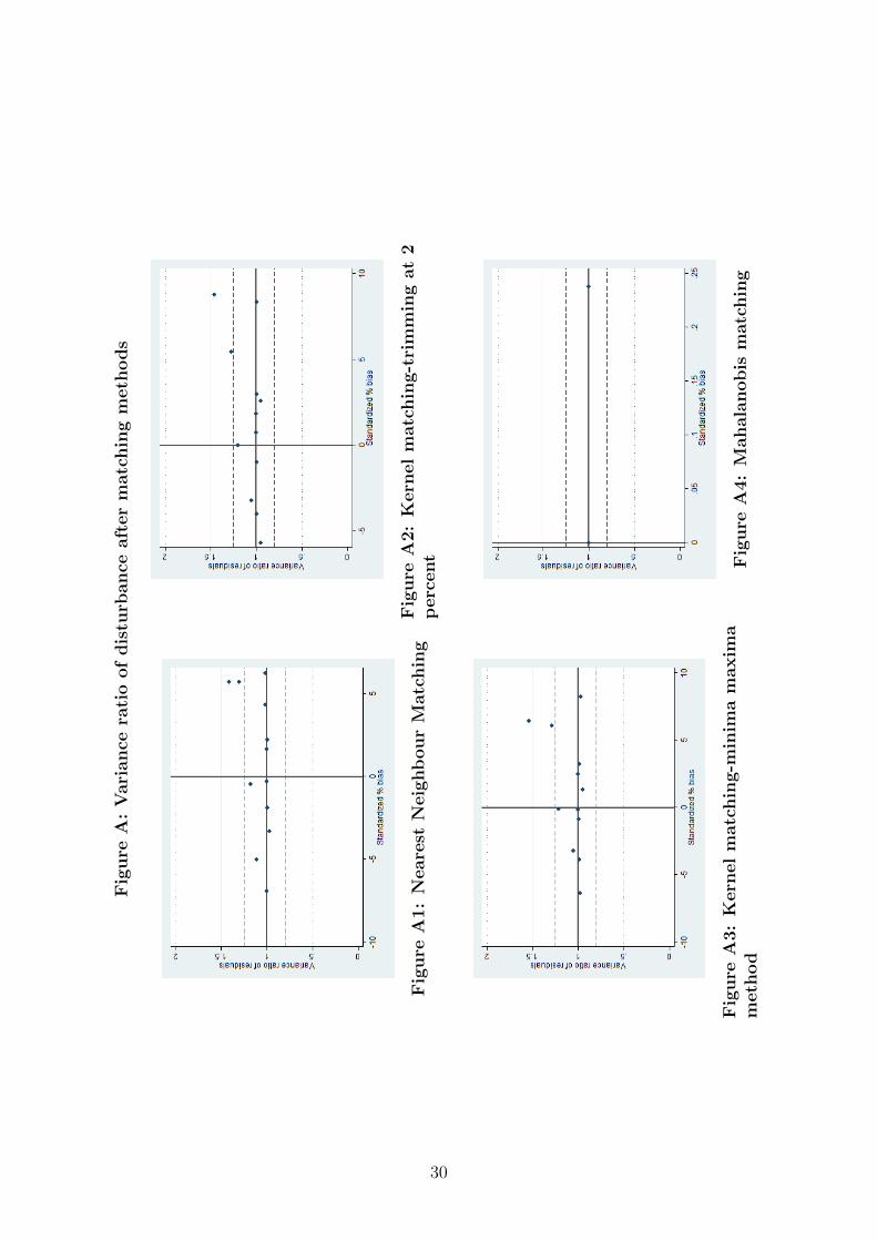
Importantly, due to criticism of and concern about Propensity Score Matching (PSM)methods (see King and NielsenKing and Nielsen, 20162016), we deliberately choose Mahalanobis matchingover the widely used PSM. However, following the advice by King and NielsenKing and Nielsen (20162016),we also conduct a number of PSM attempts (including Kernel algorithms, and nearestneighbour matching) and then compare matching results regarding efficiency, and levelof bias reduction before switching to the Mahalanobis metric. T-test results are reportedin the Appendices while Figure A illustrates the variance ratios of disturbance of allmatchings.

Based on the diagnostic tests (Appendices A7-A11) and disturbance illustrations(Figure A in the Appendices), we conclude that PSM in our case is not an optimalchoice due to its inability to completely remove imbalances between the treated and theuntreated. Consequently, PSM methods result in a very small number of off-supportobservations even though we know with certainty that treatment selection bias is anissue because health insurance for the poor was not randomly assigned. This is probablydue to, what is explained by King and NielsenKing and Nielsen (20162016), the blindness of PSM to manyimbalances as the method tries to approximate a perfect randomization. We also findthat Mahalanobis matching in our case is more efficient by fully removing imbalances andbias between the two groups.

The technique, however, comes with a trade-off: after the Mahalanobis matching,we have to remove from the baseline 402 off-support treated observations which are notcompatible with any observations in the potential control group. This number of trimmedobservations is relatively large in the total number of 666 treated observations in 2002.Based on the T-Test results (see the Appendices) the imbalances mostly come from twohousehold characteristics, i.e. the household size and whether the household is headedby a female. These two covariates appear to be important determinants of the treatmentassignment in our diagnostic regressions. Therefore, we use Mahalanobis matching as themost stringent method. We, however, also use other matching metrics and report theresults from all matching techniques.

We use two dependent variables: i) number of hours worked per month on average(this is left-censored as only relevant for those being employed) and ii) probability ofemployment as a binary choice. We employ a two-part model for analysing the numberof hours worked. Particularly, in the first part, a Probit regression is used to examinethe determinants of being employed for all working-age individuals. The second partthen uses OLS to examine the effect of the HCFP on the number of hours worked forthose who are employed. Regarding labour force participation (dependent variable 2),we use the Linear Probability Model. We use individual fixed effect (the treatment level)to account for unobserved time-invariant characteristics. Because of the high level ofdiscretion of the local authorities in implementing the HCFP (Tran et al.Tran et al., 20112011, see), as

3 This is defined as the total number of dependants aged below 16 or above 65 over the total householdsize.

7

well as regional differences in terms of healthcare facilities and inputs, we also control forcommune fixed effects. We use clustered standard errors by household for all regressions44. The specifications are as follows:

hourict = αtreatict + βyeart + δX ′ict + ωc + µci + εict (1)

employit = αtreatict + βyeart + δX ′ict + ωc + µci + εict (2)

where:i, c and t respectively denote individual, commune and time subscripts.

‘hour’ denotes the number of hours worked per month on average in Part 2 of thetwo part model (this regression is only ran on employed individuals).

‘employ’ denotes the probability of being employed for all individuals. ‘employ’equals 1 if currently employed and equals 0 otherwise.

‘treat’ equals 1 for treated individuals, ‘treat’ equals 0 for the control.yeart denotes year dummies with t runs from 0 to 2 that respectively denotes 2002,

2004 and 2006X’ is the vector of time-variant variables that explain labour supply. X’ also includes

the intercept.ωc is the commune fixed effectsµci is the individual fixed effectsεict is the idiosyncratic error termα is the average treatment effect (ATT) of interest

Time-variant individual and household characteristics in vector X’ consist of age, agesquared, literacy, marital status, household size and dependency ratio. Additionally, weproxy for health status by the number of healthcare visits per year. We also account forthe effects of labour demand by specifying the geographical regions where the individualsare living using the variable ‘urban’ and the availability of programme 135, one ofthe largest and most important poverty reduction programmes targeting the poorestcommunes in Vietnam. We control for the farming sector, which is the most common forthe Vietnamese rural poor, and type of work (wage-employment in particular). Finally,because the majority of our sample work in the agriculture sector, we try to control forseasonal effects by adding interview month.

5 Results

Difference-in-Differences Matching estimates for the number of hours worked arepresented in Table 11. Part 1 of the two part model is presented in Appendix A2A2.

As suggested in Table 11, the HCFP has a negative effect on the number of hoursworked. On monthly average, those covered with free health insurance via the HCFPwork around 5.2-5.8 hours less compared to those uncovered by the scheme. This finding

4 We assume that the residual of work hours is likely to correlated within household and report householdclustered standard errors in the main results. However, we also run clustered error by commune to testif the residual is correlated within local labour markets. The results are reported in the Appendices

8

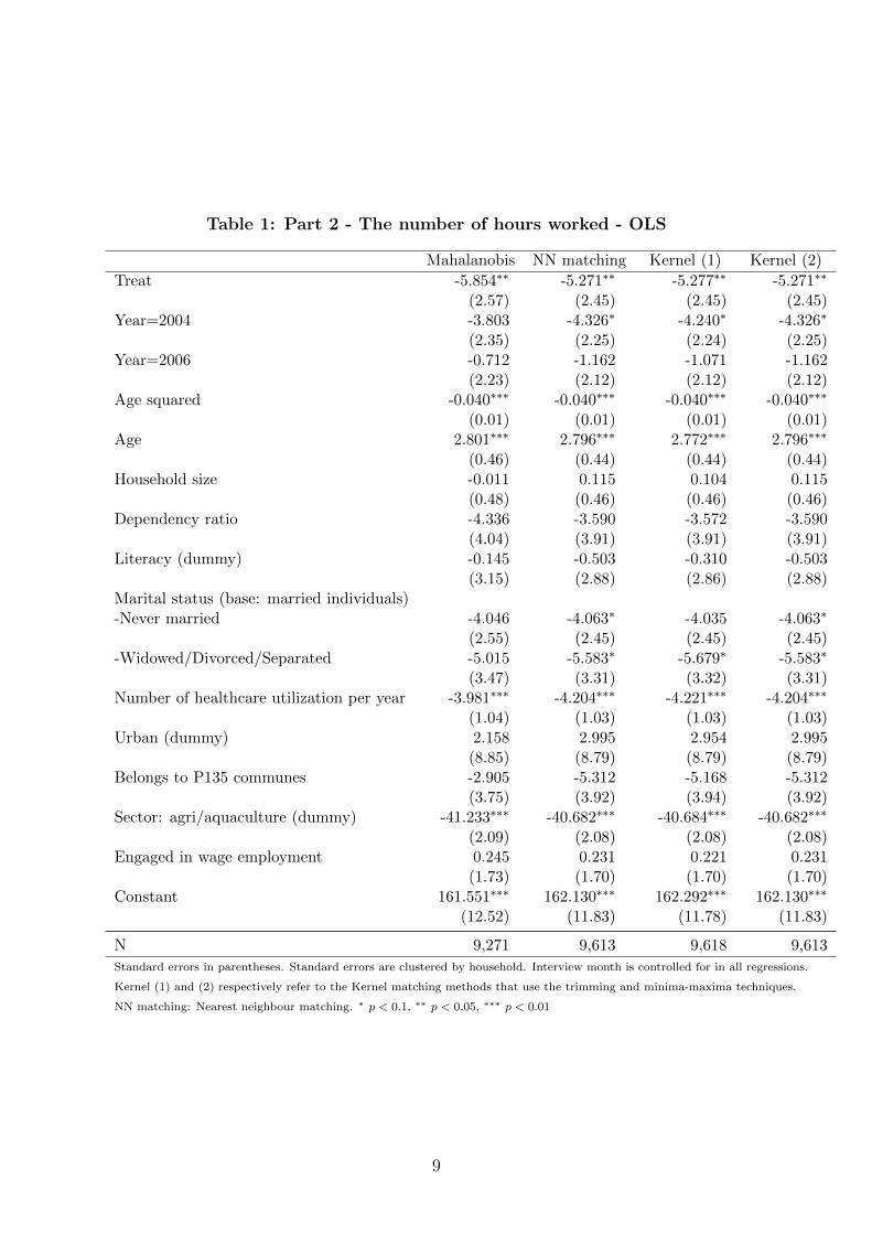
Table 1: Part 2 - The number of hours worked - OLS

Mahalanobis NN matching Kernel (1) Kernel (2)

Treat -5.854∗∗ -5.271∗∗ -5.277∗∗ -5.271∗∗

(2.57) (2.45) (2.45) (2.45)Year=2004 -3.803 -4.326∗ -4.240∗ -4.326∗

(2.35) (2.25) (2.24) (2.25)Year=2006 -0.712 -1.162 -1.071 -1.162

(2.23) (2.12) (2.12) (2.12)Age squared -0.040∗∗∗ -0.040∗∗∗ -0.040∗∗∗ -0.040∗∗∗

(0.01) (0.01) (0.01) (0.01)Age 2.801∗∗∗ 2.796∗∗∗ 2.772∗∗∗ 2.796∗∗∗

(0.46) (0.44) (0.44) (0.44)Household size -0.011 0.115 0.104 0.115

(0.48) (0.46) (0.46) (0.46)Dependency ratio -4.336 -3.590 -3.572 -3.590

(4.04) (3.91) (3.91) (3.91)Literacy (dummy) -0.145 -0.503 -0.310 -0.503

(3.15) (2.88) (2.86) (2.88)Marital status (base: married individuals)-Never married -4.046 -4.063∗ -4.035 -4.063∗

(2.55) (2.45) (2.45) (2.45)-Widowed/Divorced/Separated -5.015 -5.583∗ -5.679∗ -5.583∗

(3.47) (3.31) (3.32) (3.31)Number of healthcare utilization per year -3.981∗∗∗ -4.204∗∗∗ -4.221∗∗∗ -4.204∗∗∗

(1.04) (1.03) (1.03) (1.03)Urban (dummy) 2.158 2.995 2.954 2.995

(8.85) (8.79) (8.79) (8.79)Belongs to P135 communes -2.905 -5.312 -5.168 -5.312

(3.75) (3.92) (3.94) (3.92)Sector: agri/aquaculture (dummy) -41.233∗∗∗ -40.682∗∗∗ -40.684∗∗∗ -40.682∗∗∗

(2.09) (2.08) (2.08) (2.08)Engaged in wage employment 0.245 0.231 0.221 0.231

(1.73) (1.70) (1.70) (1.70)Constant 161.551∗∗∗ 162.130∗∗∗ 162.292∗∗∗ 162.130∗∗∗

(12.52) (11.83) (11.78) (11.83)

N 9,271 9,613 9,618 9,613

Standard errors in parentheses. Standard errors are clustered by household. Interview month is controlled for in all regressions.

Kernel (1) and (2) respectively refer to the Kernel matching methods that use the trimming and minima-maxima techniques.

NN matching: Nearest neighbour matching. ∗ p < 0.1, ∗∗ p < 0.05, ∗∗∗ p < 0.01

9

is consistent across different matching techniques. Besides, the negative effect is moreprominent in 2004 than in 2006, suggesting that the negative effect (probably due to theincome effect) kicks in rather quickly.

The effects of control variables are very consistent and intuitive. Age has a concaverelationship with the number of hours worked. Seeking more healthcare is associatedwith working less. Notably, the effect of work sector is rather large: those working inthe agricultural sector, on average, work approximately 40 hours less than those workingin the non-farm sector. This large effect indicates that the HCFP may have the largesteffects on those working in agriculture.

Table 22 presents Difference-in-Differences Matching estimates of the second outcome:the probability of employment. As suggested, the HCFP has a negative effect on labourforce participation. On average, those covered with free health insurance during HCFPare 2.8 percentage points less likely to participate in the labour market. This result isvery consistent across different matching methods. This effect does not change over timeas the effects of the time dummies are statistically insignificant.

The effects of other control variables on labour force participation are rather intuitive.Similar to the effect on the number of hours worked, age has a concave relationship withlabour force participation. Interestingly, those living in a family with more dependantsare less likely to participate in the labour market probably due to the care burden athome. Literate people are 7.5- 7.7 percentage points more likely to get employed. Thosewho are not married are more likely to work. Seeking more healthcare is associated witha smaller likelihood of labour force participation. Those working in agriculture are 25percentage points more likely to participate in the labour market. Those working in asalary job (compared to self-employment) are approximately 21 percentage points morelikely to work.

10

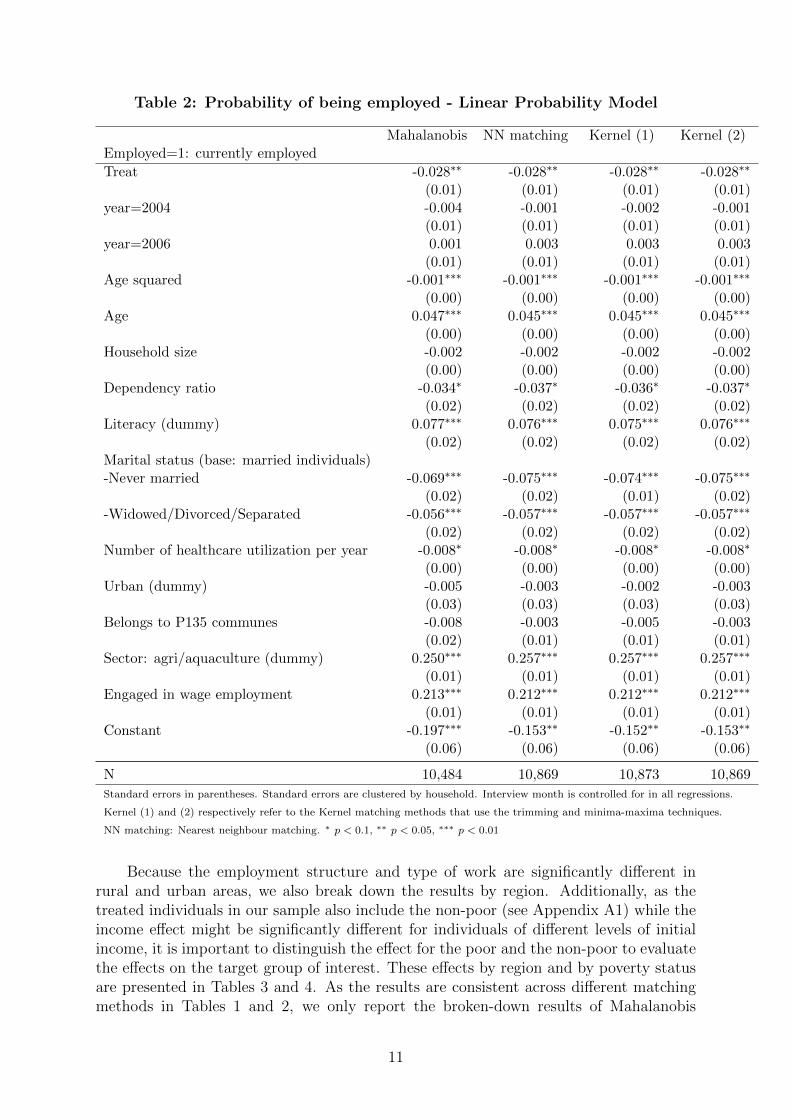
Table 2: Probability of being employed - Linear Probability Model

Mahalanobis NN matching Kernel (1) Kernel (2)Employed=1: currently employed

Treat -0.028∗∗ -0.028∗∗ -0.028∗∗ -0.028∗∗

(0.01) (0.01) (0.01) (0.01)year=2004 -0.004 -0.001 -0.002 -0.001

(0.01) (0.01) (0.01) (0.01)year=2006 0.001 0.003 0.003 0.003

(0.01) (0.01) (0.01) (0.01)Age squared -0.001∗∗∗ -0.001∗∗∗ -0.001∗∗∗ -0.001∗∗∗

(0.00) (0.00) (0.00) (0.00)Age 0.047∗∗∗ 0.045∗∗∗ 0.045∗∗∗ 0.045∗∗∗

(0.00) (0.00) (0.00) (0.00)Household size -0.002 -0.002 -0.002 -0.002

(0.00) (0.00) (0.00) (0.00)Dependency ratio -0.034∗ -0.037∗ -0.036∗ -0.037∗

(0.02) (0.02) (0.02) (0.02)Literacy (dummy) 0.077∗∗∗ 0.076∗∗∗ 0.075∗∗∗ 0.076∗∗∗

(0.02) (0.02) (0.02) (0.02)Marital status (base: married individuals)-Never married -0.069∗∗∗ -0.075∗∗∗ -0.074∗∗∗ -0.075∗∗∗

(0.02) (0.02) (0.01) (0.02)-Widowed/Divorced/Separated -0.056∗∗∗ -0.057∗∗∗ -0.057∗∗∗ -0.057∗∗∗

(0.02) (0.02) (0.02) (0.02)Number of healthcare utilization per year -0.008∗ -0.008∗ -0.008∗ -0.008∗

(0.00) (0.00) (0.00) (0.00)Urban (dummy) -0.005 -0.003 -0.002 -0.003


(0.02) (0.01) (0.01) (0.01)Sector: agri/aquaculture (dummy) 0.250∗∗∗ 0.257∗∗∗ 0.257∗∗∗ 0.257∗∗∗

(0.01) (0.01) (0.01) (0.01)Engaged in wage employment 0.213∗∗∗ 0.212∗∗∗ 0.212∗∗∗ 0.212∗∗∗

(0.01) (0.01) (0.01) (0.01)Constant -0.197∗∗∗ -0.153∗∗ -0.152∗∗ -0.153∗∗

(0.06) (0.06) (0.06) (0.06)

N 10,484 10,869 10,873 10,869

Standard errors in parentheses. Standard errors are clustered by household. Interview month is controlled for in all regressions.



Because the employment structure and type of work are significantly different inrural and urban areas, we also break down the results by region. Additionally, as thetreated individuals in our sample also include the non-poor (see Appendix A1A1) while theincome effect might be significantly different for individuals of different levels of initialincome, it is important to distinguish the effect for the poor and the non-poor to evaluatethe effects on the target group of interest. These effects by region and by poverty statusare presented in Tables 33 and 44. As the results are consistent across different matchingmethods in Tables 11 and 22, we only report the broken-down results of Mahalanobis

11

matching in Tables 33 and 44According to Table 33, the HCFP effects on the number of hours worked are more

evidenced for the non-poor treated individuals while being statistically insignificant forthe poor. This surprising result indicates that the income effect of HCFP is more relevantfor the non-poor than the poor. On average, the treated non-poor are working 5.6 hoursless than the non-poor control individuals and this effect is significant at 5 percent level. Incontrast, for the poor, the effect is statistically insignificant. Table 33 also suggests that thenegative effect of health insurance is mainly driven by rural individuals. Approximately,rural treated individuals work 8.3 hours less than rural control individual and this effectis significant at one percent level. The effect for the urban individuals is, however,statistically insignificant.

12

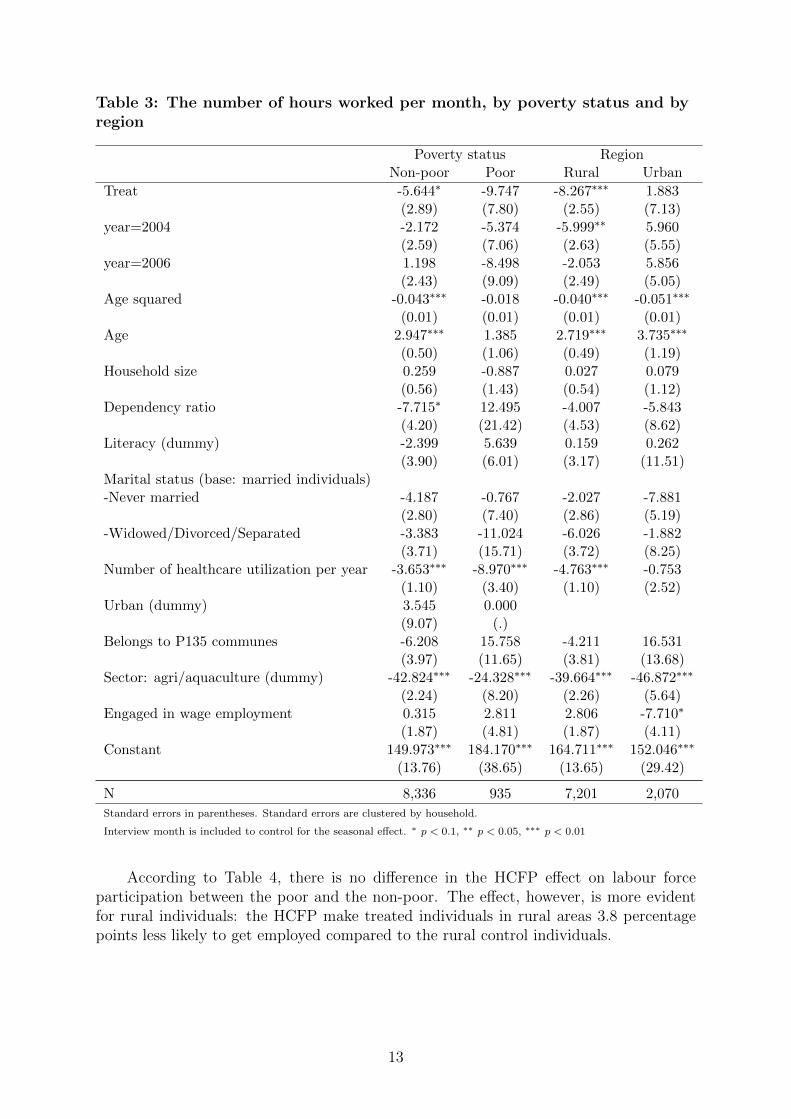
Table 3: The number of hours worked per month, by poverty status and byregion

Poverty status RegionNon-poor Poor Rural Urban

Treat -5.644∗ -9.747 -8.267∗∗∗ 1.883(2.89) (7.80) (2.55) (7.13)

year=2004 -2.172 -5.374 -5.999∗∗ 5.960(2.59) (7.06) (2.63) (5.55)

year=2006 1.198 -8.498 -2.053 5.856(2.43) (9.09) (2.49) (5.05)

Age squared -0.043∗∗∗ -0.018 -0.040∗∗∗ -0.051∗∗∗

(0.01) (0.01) (0.01) (0.01)Age 2.947∗∗∗ 1.385 2.719∗∗∗ 3.735∗∗∗

(0.50) (1.06) (0.49) (1.19)Household size 0.259 -0.887 0.027 0.079

(0.56) (1.43) (0.54) (1.12)Dependency ratio -7.715∗ 12.495 -4.007 -5.843

(4.20) (21.42) (4.53) (8.62)Literacy (dummy) -2.399 5.639 0.159 0.262

(3.90) (6.01) (3.17) (11.51)Marital status (base: married individuals)-Never married -4.187 -0.767 -2.027 -7.881

(2.80) (7.40) (2.86) (5.19)-Widowed/Divorced/Separated -3.383 -11.024 -6.026 -1.882

(3.71) (15.71) (3.72) (8.25)Number of healthcare utilization per year -3.653∗∗∗ -8.970∗∗∗ -4.763∗∗∗ -0.753

(1.10) (3.40) (1.10) (2.52)Urban (dummy) 3.545 0.000

(9.07) (.)Belongs to P135 communes -6.208 15.758 -4.211 16.531


(2.24) (8.20) (2.26) (5.64)Engaged in wage employment 0.315 2.811 2.806 -7.710∗

(1.87) (4.81) (1.87) (4.11)Constant 149.973∗∗∗ 184.170∗∗∗ 164.711∗∗∗ 152.046∗∗∗

(13.76) (38.65) (13.65) (29.42)

N 8,336 935 7,201 2,070

Standard errors in parentheses. Standard errors are clustered by household.

Interview month is included to control for the seasonal effect. ∗ p < 0.1, ∗∗ p < 0.05, ∗∗∗ p < 0.01

According to Table 44, there is no difference in the HCFP effect on labour forceparticipation between the poor and the non-poor. The effect, however, is more evidentfor rural individuals: the HCFP make treated individuals in rural areas 3.8 percentagepoints less likely to get employed compared to the rural control individuals.

13

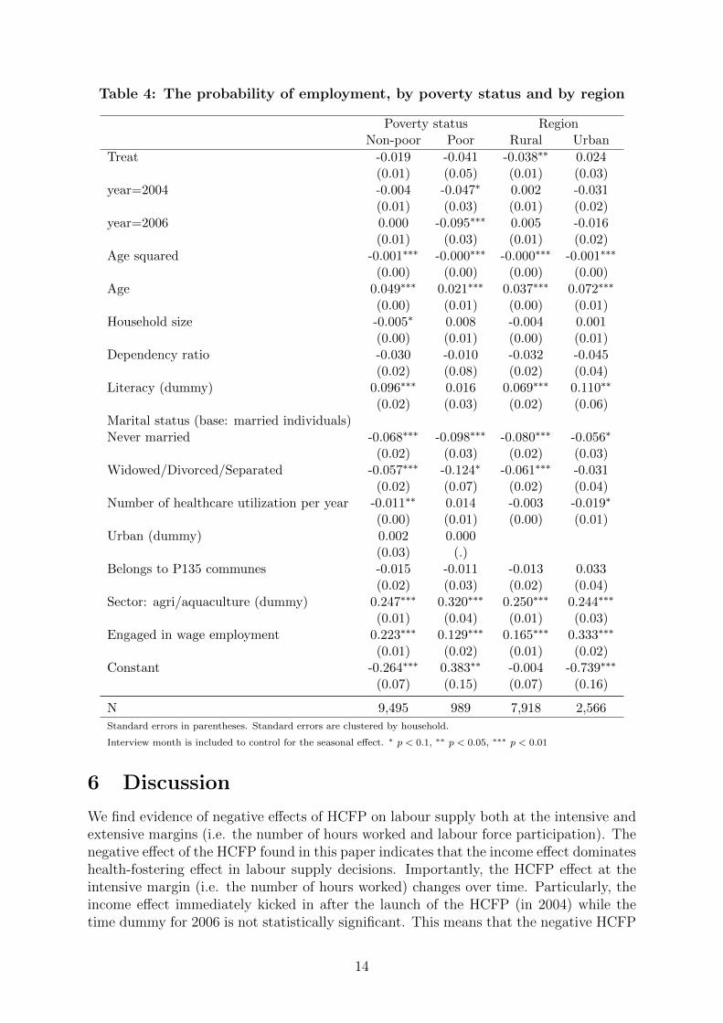
Table 4: The probability of employment, by poverty status and by region


Treat -0.019 -0.041 -0.038∗∗ 0.024(0.01) (0.05) (0.01) (0.03)

year=2004 -0.004 -0.047∗ 0.002 -0.031(0.01) (0.03) (0.01) (0.02)

year=2006 0.000 -0.095∗∗∗ 0.005 -0.016(0.01) (0.03) (0.01) (0.02)

Age squared -0.001∗∗∗ -0.000∗∗∗ -0.000∗∗∗ -0.001∗∗∗

(0.00) (0.00) (0.00) (0.00)Age 0.049∗∗∗ 0.021∗∗∗ 0.037∗∗∗ 0.072∗∗∗

(0.00) (0.01) (0.00) (0.01)Household size -0.005∗ 0.008 -0.004 0.001


(0.02) (0.08) (0.02) (0.04)Literacy (dummy) 0.096∗∗∗ 0.016 0.069∗∗∗ 0.110∗∗

(0.02) (0.03) (0.02) (0.06)Marital status (base: married individuals)Never married -0.068∗∗∗ -0.098∗∗∗ -0.080∗∗∗ -0.056∗

(0.02) (0.03) (0.02) (0.03)Widowed/Divorced/Separated -0.057∗∗∗ -0.124∗ -0.061∗∗∗ -0.031

(0.02) (0.07) (0.02) (0.04)Number of healthcare utilization per year -0.011∗∗ 0.014 -0.003 -0.019∗

(0.00) (0.01) (0.00) (0.01)Urban (dummy) 0.002 0.000

(0.03) (.)Belongs to P135 communes -0.015 -0.011 -0.013 0.033



(0.01) (0.02) (0.01) (0.02)Constant -0.264∗∗∗ 0.383∗∗ -0.004 -0.739∗∗∗

(0.07) (0.15) (0.07) (0.16)

N 9,495 989 7,918 2,566

Standard errors in parentheses. Standard errors are clustered by household.


6 Discussion

We find evidence of negative effects of HCFP on labour supply both at the intensive andextensive margins (i.e. the number of hours worked and labour force participation). Thenegative effect of the HCFP found in this paper indicates that the income effect dominateshealth-fostering effect in labour supply decisions. Importantly, the HCFP effect at theintensive margin (i.e. the number of hours worked) changes over time. Particularly, theincome effect immediately kicked in after the launch of the HCFP (in 2004) while thetime dummy for 2006 is not statistically significant. This means that the negative HCFP

14

effect on the number of hours worked is stronger for those covered in 2004 than thosecovered in 2006 (this group also included those covered in both years).

Our finding of the negative effects both at intensive and extensive margins of laboursupply is interesting given the very small health premium subsidized (around 2.5 USD in2003, equivalent of approximately 1/40 of the annual poverty line in 2003) as well as thelow cost of public healthcare services in Vietnam. One may have argued that the incomeincrease relative to the total income of those treated non-poor individuals is not largeenough to trigger the income effect from the first year of implementation. However, it isimportant to note our-of-pocket payments in Vietnam in 2003 were very high, at around63 percent of total health spending (World BankWorld Bank, 20182018). Therefore, the income effect informs of reduced health expenses are large enough to trigger the negative labour supplyeffects.

Importantly, we find that the effect on the number of hours worked is mainly drivenby the non-poor, especially those living in rural areas (see Table 33). These includenon-poor ethnic minority peoples living in disadvantaged areas and hence qualifying thecategorical targeting criteria. They can also be the near-poor who were not poor basedon the World Bank expenditure based poverty line but were defined as poor by thelocal community. Or they were mistakenly covered due to lots of other implementationcomplications - this comprises the real inclusion error of the programme. Meanwhile,in Vietnam the poor in rural regions often comprise ethnic minority individuals livingin remote and disadvantaged areas where health access and health literacy are limited(CuongCuong, 20102010), and that it often takes some time to raise their awareness of publicprogrammes. Therefore, during the first stage of HCFP wherein direct reimbursement wasconducted in many provinces, the programme might not be able to benefit the poorest ofthe poor probably due to their lower take-up rate (caused by lack of knowledge and limitedaccessibility) and lower healthcare utilization compared to the non-poor who normallylive closer to local healthcare centres. Unfortunately, information regarding distance tothe nearest healthcare delivery points was not asked in all three data periods so we couldnot test this hypothesis. Additionally, other studies that looked at utilization and out-of-pocket payment of this specific programme (WagstaffWagstaff, 20102010, 20072007) only examined theaverage treatment effect for those covered and did not delve deeper into this povertyangle, so it is difficult to justify this extrapolation.

Most of the existing literature only evaluated the short-term effect - normally rightafter an intervention. In this paper we have taken advantage of the three-wave panel andexamined the effects one year and three years after the intervention. We find that thetreatment effect on the number of hours worked changes over time: it kicks in quicklyafter the intervention but then loses its effect over time.

It is difficult to compare our results with the existing literature due to the over-representation of studies on the US healthcare system as well as the inconclusiveness ofthe empirical evidence in the US (see the systematic review by Le et al.Le et al., 20172017). We haveevidence of Medicaid, Childrens Health Insurance Programme (CHIP) and AffordableCare Act in the US but the evidence of these studies is rather mixed with differenttarget groups of low-income beneficiaries (ibid.). Our estimates regarding the effect onthe number of hours worked are smaller in size compared to an effect size of 6 hoursper week (or on average 24 hours per month) suggested by RosenRosen (20142014) for Medicaidrecipients. This might reflect the larger generosity, and hence bigger income effect, ofthe Medicaid programme compared to the HCFP in Vietnam. Regarding labour forceparticipation, the results in the literature are rather mixed. Our results are contrary

15

to findings by StrumpfStrumpf (20112011) and Ham and Shore-SheppardHam and Shore-Sheppard (20052005) who suggested thatthe introduction and expansion of Medicaid did not affect the likelihood of labour forceparticipation. In another randomized experiment on Medicaid by Baicker et al.Baicker et al. (20142014),the authors also found no significant effect on employment 55. In contrast, our results areconsistent with other studies that found that low-income childless adults reduced theiremployment likelihood due to the Affordable Care Act (Guy et al.Guy et al., 20122012) and a state-levelhealth insurance expansion in Wisconsin, the US (Dague et al.Dague et al., 20172017).

The finding of a negative net effect of the HCFP on the number of hours worked forthe non-poor raises concern in the context of moving toward UHC in Vietnam. The keyquestion for policy makers would be how to better target the poor to ensure equity whileavoiding unintended labour supply distortions.

This study comes with a data limitation caveat. Effects of health insurance subsidiesother than the HCFP cannot be adequately accounted for due to data limitations in2002. The health section of 2002’s questionnaire does not include any question on healthcoverage. The information on HCFP and FHC is however asked at the household level inanother section on public subsidies and assistance benefits. This is inconsistent with thedesign of the later surveys in 2004 and 2006, where different types of health insuranceare specified for each household member (and hence the level of analysis is at individuallevel). This data limitation leads us to assume HCFP coverage for the whole family ifa household answered that at least one person within the family received this healthscheme in 2002. Additionally, due to not being asked, the coverage of other types ofhealth insurance in 2002 is unknown, potentially leading to an under-or-over estimationof the effect magnitude depending how these health insurances are distributed amongtreatment and control groups in 2002. However, this data unavailability does not biasour estimates if we assume that conditional on the matching observables, the distributionof other types of health insurance between the treatment and control groups in 2002are compatible. In this case, the bias caused by other types of health insurance in 2002would be cancelled out in the pre-treatment difference (in mathematical terms, it equatestreatment minus control in the baseline).

7 Conclusion

By using matching methods combined with Difference-in-Differences, we evaluated thelabour supply effects of free health coverage under the HCFP for the benefit recipients inVietnam. We examined labour supply responses at both intensive and extensive margins:the number of hours worked and employment likelihood (labour force participation).We found that the effects of free health insurance on the number of hours worked andlabour force participation were both negative and statistically significant at five percentlevel. Importantly, the effects were mainly driven by the non-poor people living in ruralareas. This raises the question of the targeting strategy of the programme, highlightsthe importance of infrastructure availability as well as awareness raising and improvinghealth literacy for the poor when designing such public health schemes.

We contribute to the existing literature in several ways. First, we help fill theknowledge gap for LMIC where health insurance coverage is rapidly expanding yetunguided by empirical evidence on labour market effects. Second, we analyse the labour

5 The authors used the information about whether or not an individual has an earning as a measure foremployment

16

supply effects over a longer time span after the intervention. This allows us to capturethe time change of the income effect induced by health insurance. Third, we dig deeperinto the poverty perspective to unravel the mechanisms behind labour market distortionsof health insurance.

References

Baicker, K., Finkelstein, A., Song, J., and Taubman, S. (2014). The impact of medicaidon labor market activity and program participation: evidence from the oregon healthinsurance experiment. American Economic Review, 104(5):322–28.

Banerjee, A. V., Hanna, R., Kreindler, G. E., and Olken, B. A. (2017). Debunking thestereotype of the lazy welfare recipient: Evidence from cash transfer programs. TheWorld Bank Research Observer, 32(2):155–184.

Boyle, M. A. and Lahey, J. N. (2010). Health insurance and the labor supply decisions ofolder workers: Evidence from a US Department of Veterans Affairs expansion. Journalof public economics, 94(7):467–478.

Chou, S.-Y., Liu, J.-T., and Hammitt, J. K. (2002). Health insurance andhouseholds’ precautionary behaviors-an unusual natural experiment. NBERWorking Paper No. 9394. NBER Working Paper No. 9394. Available athttp://www.nber.org/papers/w9394.

Chou, Y.-J. and Staiger, D. (2001). Health insurance and female labor supply in Taiwan.Journal of Health Economics, 20(2):187–211.

Contreras, D., De Mello, L., and Puentes, E. (2011). The determinants of labour forceparticipation and employment in chile. Applied Economics, 43(21):2765–2776.

Contreras, D. and Plaza, G. (2010). Cultural factors in women’s labor force participationin chile. Feminist Economics, 16(2):27–46.

Cuong, N. V. (2010). Public health services and health care utilization inVietnam. Munich Personal RePEc Archive 33610. Available at https://mpra.ub.uni-muenchen.de/33610.

Dague, L., DeLeire, T., and Leininger, L. (2017). The effect of public insurance coveragefor childless adults on labor supply. American Economic Journal: Economic Policy,9(2):124–54.

Dave, D., Decker, S. L., Kaestner, R., and Simon, K. I. (2015). The effect of Medicaidexpansions in the late 1980s and early 1990s on the labor supply of pregnant women.American Journal of Health Economics, 1(2):165–193.

Glewwe, P. (2003). Procedure for calculating nominal and realexpenditures, and poverty indicators, for the 2002 VHLSS. Available athttp://microdata.worldbank.org/index.php/catalog/2306/download/34491.

Gooptu, A., Moriya, A. S., Simon, K. I., and Sommers, B. D. (2016). Medicaid expansiondid not result in significant employment changes or job reductions in 2014. Healthaffairs, 35(1):111–118.

17

Gruber, J. (2010). Public finance and public policy. Macmillan, third edition.

Gruber, J. and Madrian, B. C. (2002). Health insurance, labor supply, and job mobility:a critical review of the literature. NBER Working Paper No. 8817. Available athttp://www.nber.org/papers/w8817.

Guindon, G. E. (2014). The impact of health insurance on health services utilization andhealth outcomes in Vietnam. Health Economics, Policy and Law, 9(04):359–382.

Guy, G. P., Atherly, A., and Adams, E. K. (2012). Public health insurance eligibilityand labor force participation of low-income childless adults. Medical Care research andreview, 69(6):645–662.

Ham, J. C. and Shore-Sheppard, L. D. (2005). Did expanding Medicaid affect welfareparticipation? ILR Review, 58(3):452–470.

Heckman, J. J. and MaCurdy, T. E. (1980). A life cycle model of female labour supply.The Review of Economic Studies, 47(1):47–74.

Humphries, J. and Sarasua, C. (2012). Off the record: Reconstructing women’s laborforce participation in the european past. Feminist Economics, 18(4):39–67.

Jowett, M., Contoyannis, P., and Vinh, N. D. (2003). The impact of public voluntaryhealth insurance on private health expenditures in Vietnam. Social Science & Medicine,56(2):333–342.

King, G. and Nielsen, R. (2016). Why propensity scores should not be used for matching.Harvard working paper series at http://j.mp/2ovYGsW.

Lagomarsino, G., Garabrant, A., Adyas, A., Muga, R., and Otoo, N. (2012). Movingtowards universal health coverage: health insurance reforms in nine developingcountries in Africa and Asia. The Lancet, 380(9845):933–943.

Le, N., Groot, W., Tomini, S., and Tomini, F. (2017). Effects of health insurance onlabour supply: a systematic review. UNU MERIT working paper series 2017-017.Available at http://www.merit.unu.edu/publications/wppdf/2017/wp2017-017.pdf.

Levy, H. and Meltzer, D. (2004). What do we really know about whether health insuranceaffects health. Health policy and the uninsured, pages 179–204.

McCaig, B. (2009). The reliability of matches in the 2002-2004 VietnamHousehold Living Standards Survey Panel. Discussion paper. Centre forEconomic Policy Research, Australian National University. Available athttps://www.rse.anu.edu.au/media/604599/dp622.pdf.

McCaig, B. (2017). Note on VHLSS. Data retrieved from Brian McCaig’s website,https://sites.google.com/site/briandmccaig/home/notes-on-vhlsss.

Nguyen, C. V. (2012). The impact of voluntary health insurance on health care utilizationand out-of-pocket payments: New evidence for Vietnam. Health economics, 21(8):946–966.

18

Nguyen, H. and Wang, W. (2013). The effects of free government health insurance amongsmall childrenevidence from the free care for children under six policy in Vietnam. TheInternational journal of health planning and management, 28(1):3–15.

Palmer, M., Mitra, S., Mont, D., and Groce, N. (2015). The impact of health insurancefor children under age 6 in Vietnam: a regression discontinuity approach. Social Science& Medicine, 145:217–226.

Parsons, D. O. (1982). The male labour force participation decision: health, reportedhealth, and economic incentives. Economica, 49(193):81–91.

Rodin, J. and de Ferranti, D. (2012). Universal health coverage: the third global healthtransition? The Lancet, 380(9845):861.

Rosen, G. (2014). Determinants of employment: Impact of medicaid and CHIP amongunmarried female heads of household with young children. Social work in public health,29(5):491–502.

Socialist Republic of Vietnam (1998). Decision 135/1998/QD-TTg on socio-economicdevelopment plan for the most difficulty communes in mountainous areas and isolatedregions. Prime Minister of Vietnam.

Socialist Republic of Vietnam (2000). Decision 1143/2000/QD-LDTBXH on poverty lineduring 2001-2005. Ministry of Labour, the Invalids and Social Affairs of Vietnam.

Socialist Republic of Vietnam (2002). Decision 139/2002/qd-ttg on healthcare for thepoor. Prime Minister of Vietnam.

Socialist Republic of Vietnam (2016). Decision 1167/Q-TTg on target adjustments forexpanding health insurance coverage in Vietnam during 2016-2020. Prime Minister ofVietnam.

Sommers, B. D., Baicker, K., and Epstein, A. M. (2012). Mortality and access to careamong adults after state Medicaid expansions. New England Journal of Medicine,367(11):1025–1034.

Strumpf, E. (2011). Medicaid’s effect on single women’s labor supply: Evidence from theintroduction of Medicaid. Journal of Health Economics, 30(3):531–548.

Tran, V. T., Hoang, T. P., Mathauer, I., and Nguyen, T. (2011). Health financingreview of Vietnam with a focus on social health insurance: Bottlenecks in institutionaldesign and organizational practice of health financing and options to accelerate progresstowards universal coverage. World Health Organisation report series.

Wagstaff, A. (2007). Health insurance for the poor: initial impacts of Vietnam’s healthcare fund for the poor. World Bank Policy Research Working Paper No. 4134. Availableat https://ssrn.com/abstract=961760.

Wagstaff, A. (2010). Estimating health insurance impacts under unobservedheterogeneity: the case of Vietnam’s health care fund for the poor. Health economics,19(2):189–208.

19

Wagstaff, A. and Moreno-Serra, R. (2009). Europe and central Asia’s great post-communist social health insurance experiment: Aggregate impacts on health sectoroutcomes. Journal of health economics, 28(2):322–340.

Wagstaff, A. and Moreno-Serra, R. (2015). Social health insurance andlabor market outcomes: Evidence from Central and Eastern Europe,and Central Asia, pages 83–106. Emerald Insight. Available athttp://www.emeraldinsight.com/doi/abs/10.1108/S0731-2199

World Bank (2018). Country data of Vietnam. World Bank. Retrieved on 5 Sep 2018from https://data.worldbank.org/country/vietnam.

20

Appendices

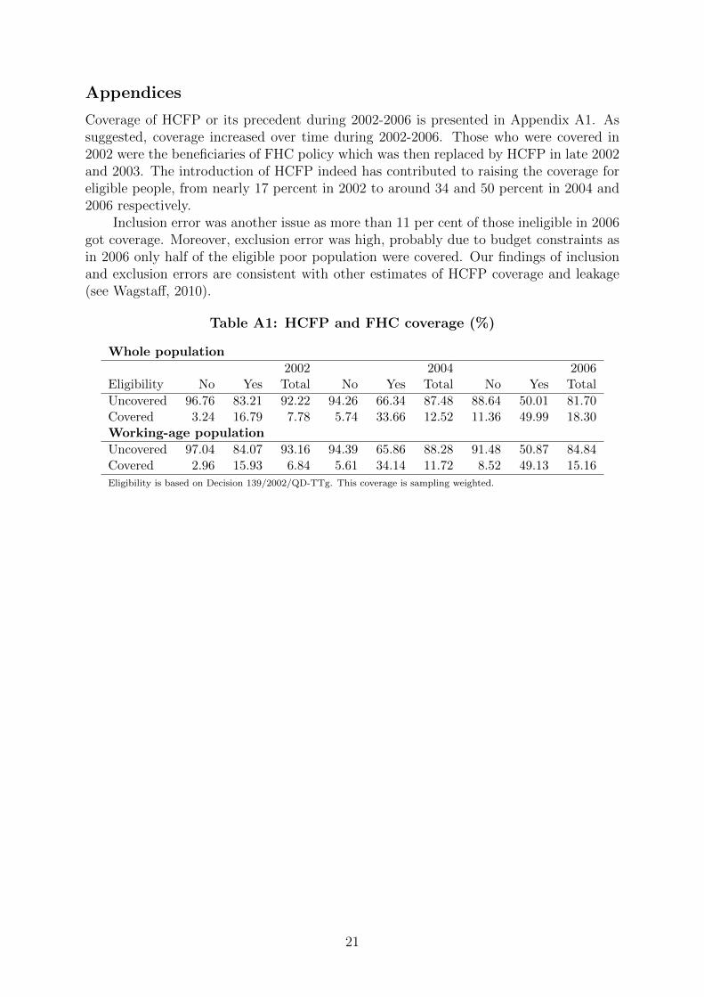
Coverage of HCFP or its precedent during 2002-2006 is presented in Appendix A1A1. Assuggested, coverage increased over time during 2002-2006. Those who were covered in2002 were the beneficiaries of FHC policy which was then replaced by HCFP in late 2002and 2003. The introduction of HCFP indeed has contributed to raising the coverage foreligible people, from nearly 17 percent in 2002 to around 34 and 50 percent in 2004 and2006 respectively.

Inclusion error was another issue as more than 11 per cent of those ineligible in 2006got coverage. Moreover, exclusion error was high, probably due to budget constraints asin 2006 only half of the eligible poor population were covered. Our findings of inclusionand exclusion errors are consistent with other estimates of HCFP coverage and leakage(see WagstaffWagstaff, 20102010).

Table A1: HCFP and FHC coverage (%)

Whole population

2002 2004 2006Eligibility No Yes Total No Yes Total No Yes Total

Uncovered 96.76 83.21 92.22 94.26 66.34 87.48 88.64 50.01 81.70Covered 3.24 16.79 7.78 5.74 33.66 12.52 11.36 49.99 18.30Working-age population

Uncovered 97.04 84.07 93.16 94.39 65.86 88.28 91.48 50.87 84.84Covered 2.96 15.93 6.84 5.61 34.14 11.72 8.52 49.13 15.16

Eligibility is based on Decision 139/2002/QD-TTg. This coverage is sampling weighted.

21

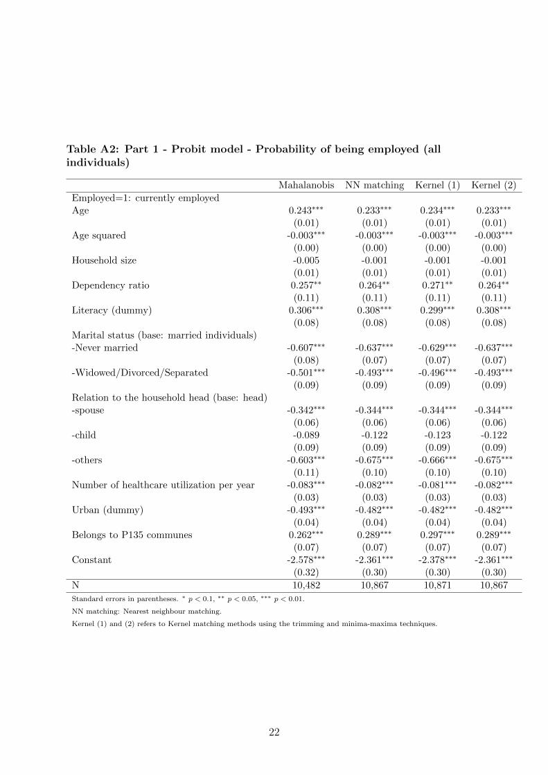
Table A2: Part 1 - Probit model - Probability of being employed (allindividuals)


Employed=1: currently employedAge 0.243∗∗∗ 0.233∗∗∗ 0.234∗∗∗ 0.233∗∗∗

(0.01) (0.01) (0.01) (0.01)Age squared -0.003∗∗∗ -0.003∗∗∗ -0.003∗∗∗ -0.003∗∗∗

(0.00) (0.00) (0.00) (0.00)Household size -0.005 -0.001 -0.001 -0.001

(0.01) (0.01) (0.01) (0.01)Dependency ratio 0.257∗∗ 0.264∗∗ 0.271∗∗ 0.264∗∗

(0.11) (0.11) (0.11) (0.11)Literacy (dummy) 0.306∗∗∗ 0.308∗∗∗ 0.299∗∗∗ 0.308∗∗∗



(0.09) (0.09) (0.09) (0.09)Relation to the household head (base: head)-spouse -0.342∗∗∗ -0.344∗∗∗ -0.344∗∗∗ -0.344∗∗∗

(0.06) (0.06) (0.06) (0.06)-child -0.089 -0.122 -0.123 -0.122

(0.09) (0.09) (0.09) (0.09)-others -0.603∗∗∗ -0.675∗∗∗ -0.666∗∗∗ -0.675∗∗∗


(0.03) (0.03) (0.03) (0.03)Urban (dummy) -0.493∗∗∗ -0.482∗∗∗ -0.482∗∗∗ -0.482∗∗∗

(0.04) (0.04) (0.04) (0.04)Belongs to P135 communes 0.262∗∗∗ 0.289∗∗∗ 0.297∗∗∗ 0.289∗∗∗

(0.07) (0.07) (0.07) (0.07)Constant -2.578∗∗∗ -2.361∗∗∗ -2.378∗∗∗ -2.361∗∗∗

(0.32) (0.30) (0.30) (0.30)

N 10,482 10,867 10,871 10,867

Standard errors in parentheses. ∗ p < 0.1, ∗∗ p < 0.05, ∗∗∗ p < 0.01.

NN matching: Nearest neighbour matching.

Kernel (1) and (2) refers to Kernel matching methods using the trimming and minima-maxima techniques.

22

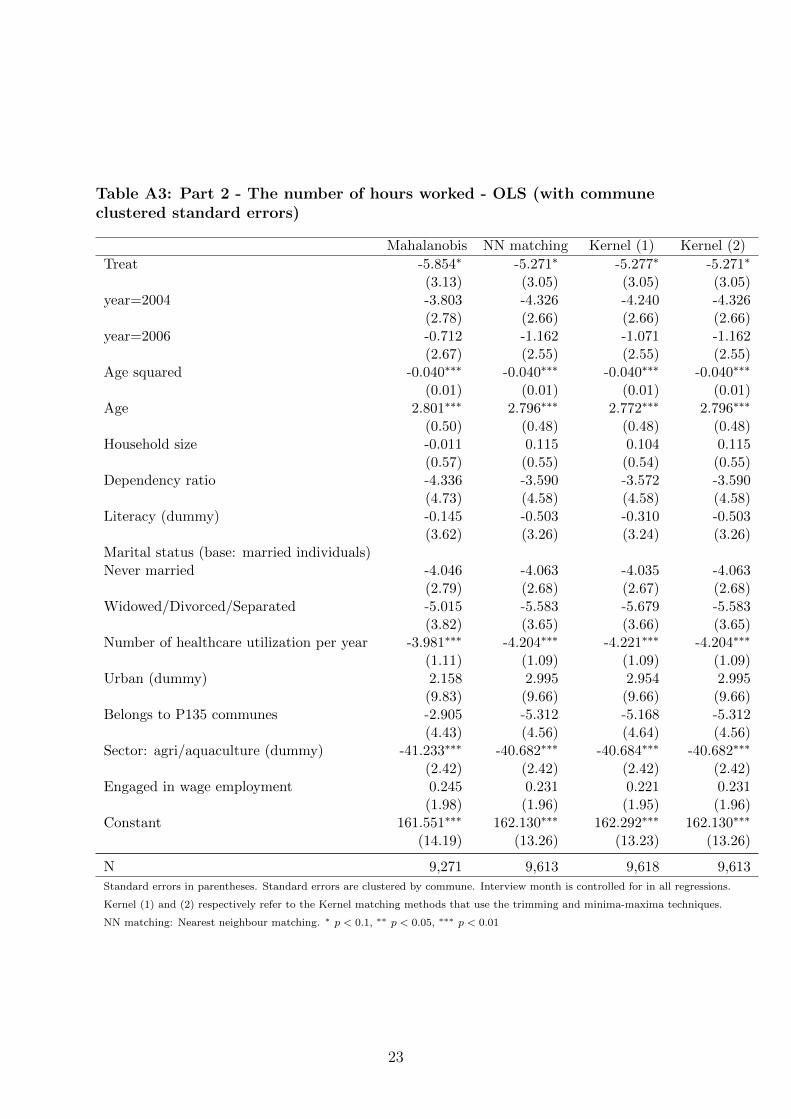
Table A3: Part 2 - The number of hours worked - OLS (with communeclustered standard errors)


Treat -5.854∗ -5.271∗ -5.277∗ -5.271∗

(3.13) (3.05) (3.05) (3.05)year=2004 -3.803 -4.326 -4.240 -4.326

(2.78) (2.66) (2.66) (2.66)year=2006 -0.712 -1.162 -1.071 -1.162

(2.67) (2.55) (2.55) (2.55)Age squared -0.040∗∗∗ -0.040∗∗∗ -0.040∗∗∗ -0.040∗∗∗

(0.01) (0.01) (0.01) (0.01)Age 2.801∗∗∗ 2.796∗∗∗ 2.772∗∗∗ 2.796∗∗∗

(0.50) (0.48) (0.48) (0.48)Household size -0.011 0.115 0.104 0.115


(4.73) (4.58) (4.58) (4.58)Literacy (dummy) -0.145 -0.503 -0.310 -0.503

(3.62) (3.26) (3.24) (3.26)Marital status (base: married individuals)Never married -4.046 -4.063 -4.035 -4.063

(2.79) (2.68) (2.67) (2.68)Widowed/Divorced/Separated -5.015 -5.583 -5.679 -5.583


(1.11) (1.09) (1.09) (1.09)Urban (dummy) 2.158 2.995 2.954 2.995



(2.42) (2.42) (2.42) (2.42)Engaged in wage employment 0.245 0.231 0.221 0.231

(1.98) (1.96) (1.95) (1.96)Constant 161.551∗∗∗ 162.130∗∗∗ 162.292∗∗∗ 162.130∗∗∗

(14.19) (13.26) (13.23) (13.26)

N 9,271 9,613 9,618 9,613

Standard errors in parentheses. Standard errors are clustered by commune. Interview month is controlled for in all regressions.



23

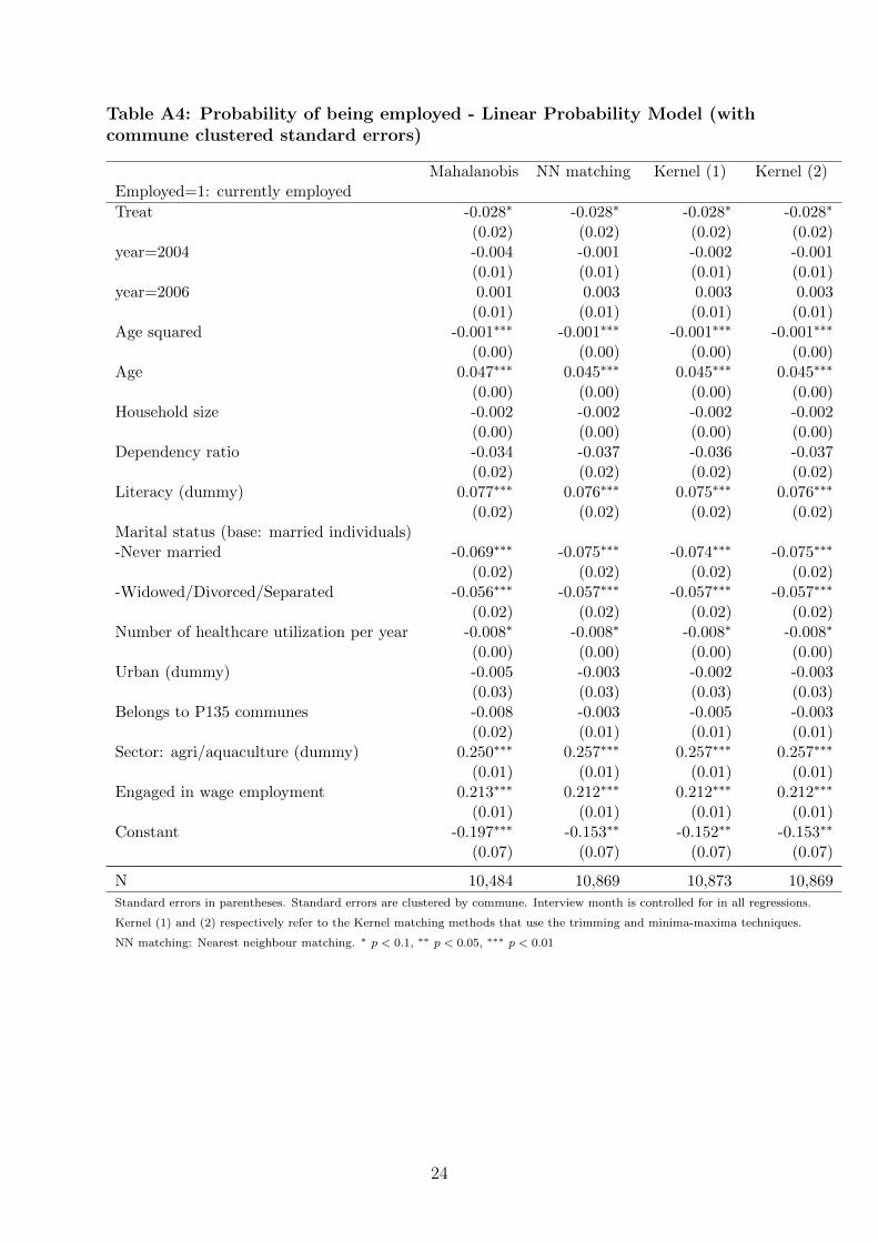
Table A4: Probability of being employed - Linear Probability Model (withcommune clustered standard errors)

Mahalanobis NN matching Kernel (1) Kernel (2)Employed=1: currently employed

Treat -0.028∗ -0.028∗ -0.028∗ -0.028∗

(0.02) (0.02) (0.02) (0.02)year=2004 -0.004 -0.001 -0.002 -0.001

(0.01) (0.01) (0.01) (0.01)year=2006 0.001 0.003 0.003 0.003

(0.01) (0.01) (0.01) (0.01)Age squared -0.001∗∗∗ -0.001∗∗∗ -0.001∗∗∗ -0.001∗∗∗

(0.00) (0.00) (0.00) (0.00)Age 0.047∗∗∗ 0.045∗∗∗ 0.045∗∗∗ 0.045∗∗∗

(0.00) (0.00) (0.00) (0.00)Household size -0.002 -0.002 -0.002 -0.002


(0.02) (0.02) (0.02) (0.02)Literacy (dummy) 0.077∗∗∗ 0.076∗∗∗ 0.075∗∗∗ 0.076∗∗∗



(0.02) (0.02) (0.02) (0.02)Number of healthcare utilization per year -0.008∗ -0.008∗ -0.008∗ -0.008∗

(0.00) (0.00) (0.00) (0.00)Urban (dummy) -0.005 -0.003 -0.002 -0.003




(0.01) (0.01) (0.01) (0.01)Constant -0.197∗∗∗ -0.153∗∗ -0.152∗∗ -0.153∗∗

(0.07) (0.07) (0.07) (0.07)

N 10,484 10,869 10,873 10,869

Standard errors in parentheses. Standard errors are clustered by commune. Interview month is controlled for in all regressions.



24

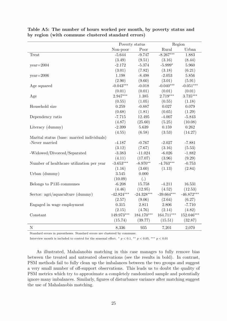
Table A5: The number of hours worked per month, by poverty status andby region (with commune clustered standard errors)


Treat -5.644 -9.747 -8.267∗∗∗ 1.883(3.49) (9.51) (3.16) (8.44)

year=2004 -2.172 -5.374 -5.999∗ 5.960(3.01) (7.82) (3.18) (6.21)

year=2006 1.198 -8.498 -2.053 5.856(2.90) (9.60) (3.01) (5.91)

Age squared -0.043∗∗∗ -0.018 -0.040∗∗∗ -0.051∗∗∗

(0.01) (0.01) (0.01) (0.01)Age 2.947∗∗∗ 1.385 2.719∗∗∗ 3.735∗∗∗

(0.55) (1.05) (0.55) (1.18)Household size 0.259 -0.887 0.027 0.079

(0.68) (1.81) (0.65) (1.29)Dependency ratio -7.715 12.495 -4.007 -5.843

(4.87) (25.60) (5.25) (10.08)Literacy (dummy) -2.399 5.639 0.159 0.262

(4.55) (6.58) (3.53) (14.27)Marital status (base: married individuals)-Never married -4.187 -0.767 -2.027 -7.881

(3.12) (7.67) (3.16) (5.53)-Widowed/Divorced/Separated -3.383 -11.024 -6.026 -1.882

(4.11) (17.07) (3.96) (9.29)Number of healthcare utilization per year -3.653∗∗∗ -8.970∗∗ -4.763∗∗∗ -0.753

(1.16) (3.60) (1.13) (2.84)Urban (dummy) 3.545 0.000

(10.09) (.)Belongs to P135 communes -6.208 15.758 -4.211 16.531


(2.57) (9.06) (2.64) (6.27)Engaged in wage employment 0.315 2.811 2.806 -7.710

(2.15) (4.76) (2.14) (4.82)Constant 149.973∗∗∗ 184.170∗∗∗ 164.711∗∗∗ 152.046∗∗∗

(15.74) (39.77) (15.51) (32.87)

N 8,336 935 7,201 2,070

Standard errors in parentheses. Standard errors are clustered by commune.


As illustrated, Mahalanobis matching in this case manages to fully remove biasbetween the treated and untreated observations (see the results in bold). In contrast,PSM methods fail to fully clean up the imbalances between the two groups and suggesta very small number of off-support observations. This leads us to doubt the quality ofPSM metrics which try to approximate a completely randomized sample and potentiallyignore many imbalances. Similarly, figures of disturbance variance after matching suggestthe use of Mahalanobis matching.

25

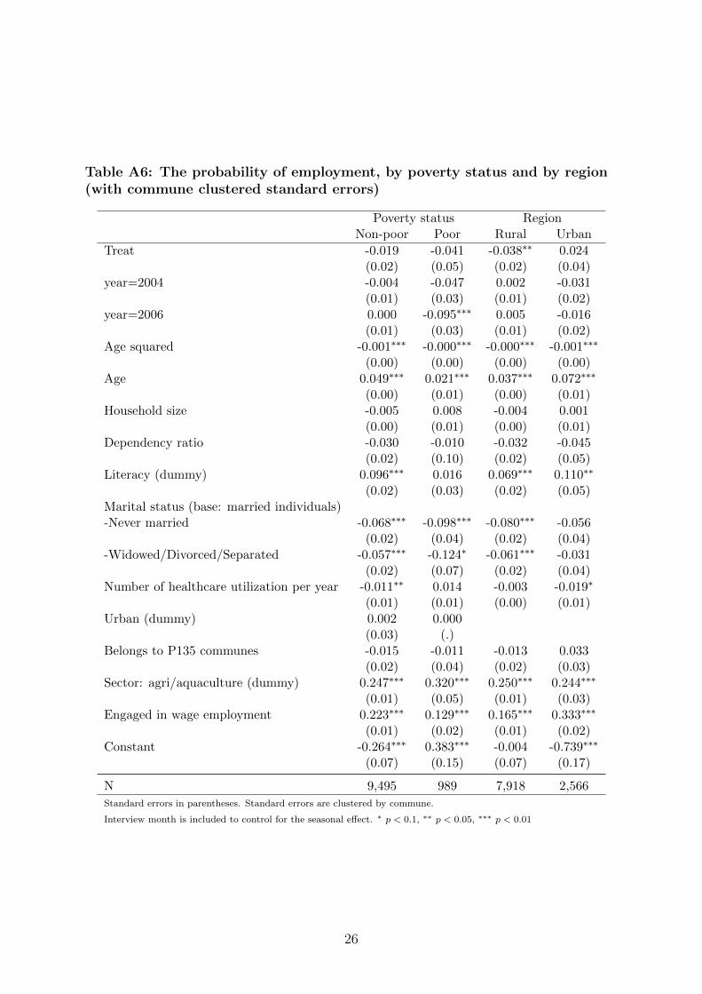
Table A6: The probability of employment, by poverty status and by region(with commune clustered standard errors)


Treat -0.019 -0.041 -0.038∗∗ 0.024(0.02) (0.05) (0.02) (0.04)

year=2004 -0.004 -0.047 0.002 -0.031(0.01) (0.03) (0.01) (0.02)

year=2006 0.000 -0.095∗∗∗ 0.005 -0.016(0.01) (0.03) (0.01) (0.02)

Age squared -0.001∗∗∗ -0.000∗∗∗ -0.000∗∗∗ -0.001∗∗∗

(0.00) (0.00) (0.00) (0.00)Age 0.049∗∗∗ 0.021∗∗∗ 0.037∗∗∗ 0.072∗∗∗

(0.00) (0.01) (0.00) (0.01)Household size -0.005 0.008 -0.004 0.001


(0.02) (0.10) (0.02) (0.05)Literacy (dummy) 0.096∗∗∗ 0.016 0.069∗∗∗ 0.110∗∗

(0.02) (0.03) (0.02) (0.05)Marital status (base: married individuals)-Never married -0.068∗∗∗ -0.098∗∗∗ -0.080∗∗∗ -0.056

(0.02) (0.04) (0.02) (0.04)-Widowed/Divorced/Separated -0.057∗∗∗ -0.124∗ -0.061∗∗∗ -0.031

(0.02) (0.07) (0.02) (0.04)Number of healthcare utilization per year -0.011∗∗ 0.014 -0.003 -0.019∗

(0.01) (0.01) (0.00) (0.01)Urban (dummy) 0.002 0.000

(0.03) (.)Belongs to P135 communes -0.015 -0.011 -0.013 0.033



(0.01) (0.02) (0.01) (0.02)Constant -0.264∗∗∗ 0.383∗∗∗ -0.004 -0.739∗∗∗

(0.07) (0.15) (0.07) (0.17)

N 9,495 989 7,918 2,566

Standard errors in parentheses. Standard errors are clustered by commune.


26

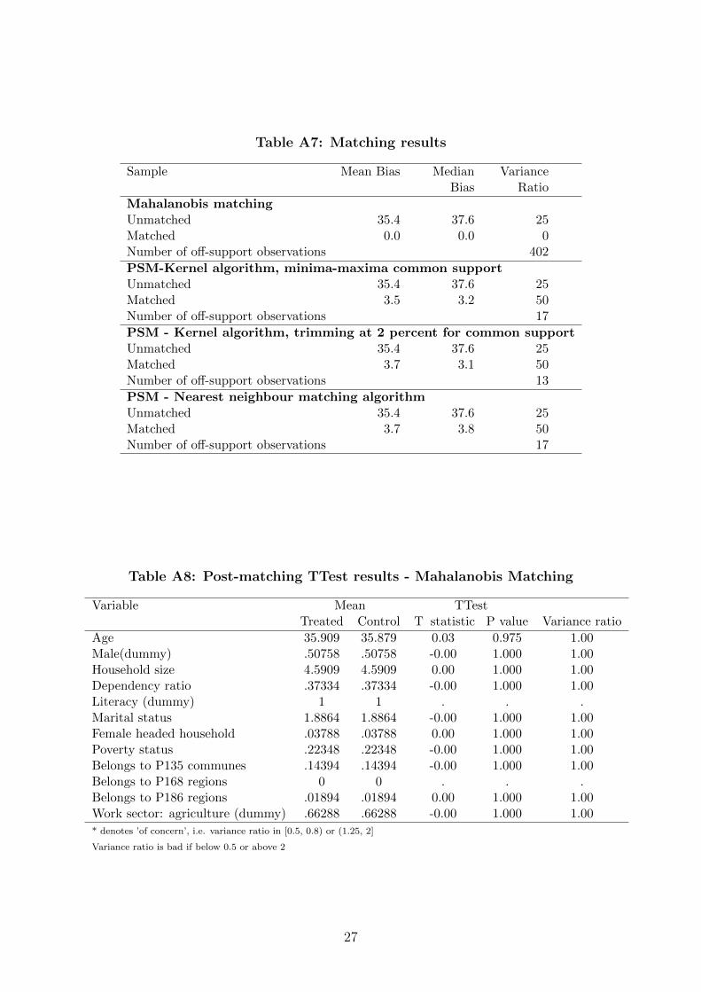
Table A7: Matching results

Sample Mean Bias MedianBias

VarianceRatio

Mahalanobis matchingUnmatched 35.4 37.6 25Matched 0.0 0.0 0Number of off-support observations 402

PSM-Kernel algorithm, minima-maxima common supportUnmatched 35.4 37.6 25Matched 3.5 3.2 50Number of off-support observations 17

PSM - Kernel algorithm, trimming at 2 percent for common supportUnmatched 35.4 37.6 25Matched 3.7 3.1 50Number of off-support observations 13

PSM - Nearest neighbour matching algorithmUnmatched 35.4 37.6 25Matched 3.7 3.8 50Number of off-support observations 17

Table A8: Post-matching TTest results - Mahalanobis Matching

Variable Mean TTestTreated Control T statistic P value Variance ratio

Age 35.909 35.879 0.03 0.975 1.00Male(dummy) .50758 .50758 -0.00 1.000 1.00Household size 4.5909 4.5909 0.00 1.000 1.00Dependency ratio .37334 .37334 -0.00 1.000 1.00Literacy (dummy) 1 1 . . .Marital status 1.8864 1.8864 -0.00 1.000 1.00Female headed household .03788 .03788 0.00 1.000 1.00Poverty status .22348 .22348 -0.00 1.000 1.00Belongs to P135 communes .14394 .14394 -0.00 1.000 1.00Belongs to P168 regions 0 0 . . .Belongs to P186 regions .01894 .01894 0.00 1.000 1.00Work sector: agriculture (dummy) .66288 .66288 -0.00 1.000 1.00

* denotes ’of concern’, i.e. variance ratio in [0.5, 0.8) or (1.25, 2]

Variance ratio is bad if below 0.5 or above 2

27

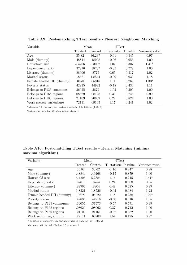
Table A9: Post-matching TTest results - Nearest Neighbour Matching


Age 35.82 36.237 -0.61 0.545 0.97Male (dummy) .48844 .48998 -0.06 0.956 1.00Household size 5.4206 5.3032 1.02 0.307 1.41*Dependency ratio .37816 .38207 -0.35 0.729 1.00Literacy (dummy) .88906 .8775 0.65 0.517 1.02Marital status 1.8521 1.8544 -0.09 0.930 1.18Female headed HH (dummy) .0678 .05316 1.11 0.269 1.30*Poverty status .42835 .44992 -0.78 0.434 1.11Belongs to P135 communes .36055 .3879 -1.02 0.309 1.00Belongs to P168 regions .08629 .08128 0.33 0.745 0.99Belongs to P186 regions .21109 .20609 0.22 0.824 1.00Work sector: agriculture .72111 .69145 1.17 0.241 1.02



Table A10: Post-matching TTest results - Kernel Matching (minimamaxima algorithm)


Age 35.82 36.62 -1.16 0.247 0.98Male (dummy) .48844 .49268 -0.15 0.879 1.00Household size 5.4206 5.2884 1.16 0.245 1.54*Dependency ratio .37816 .3754 0.24 0.808 0.95Literacy (dummy) .88906 .8804 0.49 0.625 0.99Marital status 1.8521 1.8526 -0.02 0.984 1.22Female headed HH (dummy) .0678 .05222 1.18 0.238 1.29*Poverty status .42835 .44216 -0.50 0.616 1.05Belongs to P135 communes .36055 .37573 -0.57 0.571 0.99Belongs to P168 regions .08629 .08062 0.37 0.712 1.00Belongs to P186 regions .21109 .21161 -0.02 0.982 1.00Work sector: agriculture .72111 .68208 1.54 0.125 0.97



28

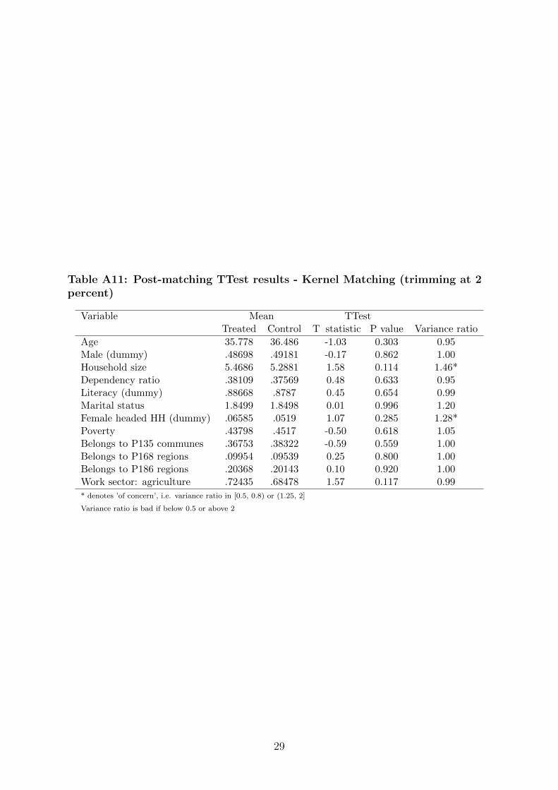
Table A11: Post-matching TTest results - Kernel Matching (trimming at 2percent)


Age 35.778 36.486 -1.03 0.303 0.95Male (dummy) .48698 .49181 -0.17 0.862 1.00Household size 5.4686 5.2881 1.58 0.114 1.46*Dependency ratio .38109 .37569 0.48 0.633 0.95Literacy (dummy) .88668 .8787 0.45 0.654 0.99Marital status 1.8499 1.8498 0.01 0.996 1.20Female headed HH (dummy) .06585 .0519 1.07 0.285 1.28*Poverty .43798 .4517 -0.50 0.618 1.05Belongs to P135 communes .36753 .38322 -0.59 0.559 1.00Belongs to P168 regions .09954 .09539 0.25 0.800 1.00Belongs to P186 regions .20368 .20143 0.10 0.920 1.00Work sector: agriculture .72435 .68478 1.57 0.117 0.99



29

Fig

ure

A:

Vari

ance

rati

oof

dis

turb

ance

aft

er

matc

hin

gm

eth

od

s

Fig

ure

A1:

Neare

stN

eig

hb

our

Matc

hin

gF

igure

A2:

Kern

el

matc

hin

g-t

rim

min

gat

2p

erc

ent

Fig

ure

A3:

Kern

el

matc

hin

g-m

inim

am

axim

am

eth

od

Fig

ure

A4:

Mahala

nob

ism

atc

hin

g

30

The UNU‐MERIT WORKING Paper Series 2017-01 The economic impact of East‐West migration on the European Union by Martin

Kahanec and Mariola Pytliková 2017-02 Fostering social mobility: The case of the ‘Bono de Desarrollo Humano’ in Ecuador

by Andrés Mideros and Franziska Gassmann 2017-03 Impact of the Great Recession on industry unemployment: a 1976‐2011

comparison by Yelena Takhtamanova and Eva Sierminska 2017-04 Labour mobility through business visits as a way to foster productivity by

Mariacristina Piva, Massimiliano Tani and Marco Vivarelli 2017-05 Country risk, FDI flows and convergence trends in the context of the Investment

Development Path by Jonas Hub Frenken and Dorcas Mbuvi 2017-06 How development aid explains (or not) the rise and fall of insurgent attacks in Iraq

by Pui‐Hang Wong 2017-07 Productivity and household welfare impact of technology adoption: Micro‐level

evidence from rural Ethiopia by Tigist Mekonnen 2017-08 Impact of agricultural technology adoption on market participation in the rural

social network system by Tigist Mekonnen 2017-09 Financing rural households and its impact: Evidence from randomized field

experiment data by Tigist Mekonnen 2017-10 U.S. and Soviet foreign aid during the Cold War: A case study of Ethiopia by Tobias

Broich 2017-11 Do authoritarian regimes receive more Chinese development finance than

democratic ones? Empirical evidence for Africa by Tobias Broich 2017-12 Pathways for capacity building in heterogeneous value chains: Evidence from the

case of IT‐enabled services in South Africa by Charlotte Keijser and Michiko Iizuka 2017-13 Is innovation destroying jobs? Firm‐level evidence from the EU by Mariacristina

Piva and Marco Vivarelli 2017-14 Transition from civil war to peace: The role of the United Nations and international

community in Mozambique by Ayokunu Adedokun 2017-15 Emerging challenges to long‐term peace and security in Mozambique by Ayokunu

Adedokun 2017-16 Post‐conflict peacebuilding: A critical survey of the literature and avenues for

future research by Ayokunu Adedokun 2017-17 Effects of health insurance on labour supply: A systematic review by Nga Le, Wim

Groot, Sonila M. Tomini and Florian Tomini\ 2017-18 Challenged by migration: Europe's options by Amelie F. Constant and Klaus F.

Zimmermann 2017-19 Innovation policy & labour productivity growth: Education, research &

development, government effectiveness and business policy by Mueid Al Raee, Jo Ritzen and Denis de Crombrugghe

2017-20 Role of WASH and Agency in Health: A study of isolated rural communities in Nilgiris and Jalpaiguri by Shyama V. Ramani

2017-21 The productivity effect of public R&D in the Netherlands by Luc Soete, Bart Verspagen and Thomas Ziesemer

2017-22 The role of migration‐specific and migration‐relevant policies in migrant decision‐making in transit by Katie Kuschminder and Khalid Koser

2017-23 Regional analysis of sanitation performance in India by Debasree Bose and Arijita Dutta

2017-24 Estimating the impact of sericulture adoption on farmer income in Rwanda: an application of propensity score matching by Alexis Habiyaremye

2017-25 Indigenous knowledge for sustainable livelihoods: Lessons from ecological pest control and post‐harvest techniques of Baduy (West Java) and Nguni (Southern Africa) by Leeja C Korina and Alexis Habiyaremye

2017-26 Sanitation challenges of the poor in urban and rural settings: Case studies of Bengaluru City and rural North Karnataka by Manasi Seshaiah, Latha Nagesh and Hemalatha Ramesh

2017-27 Heterogeneous effects of bilateral investment treaties by Rod Falvey and Neil Foster‐McGregor

2017-28 Willingness to pay for agricultural risk insurance as a strategy to adapt climate change by Tigist Mekonnen

2017-29 Social protection investments, human capital, and income growth: Simulating the returns to social cash transfers in Uganda by Stephan Dietrich, Daniele Malerba, Armando Barrientos, Franziska Gassmann, Pierre Mohnen, Nyasha Tirivayi, Susan Kavuma and Fred Matovu

2017-30 Opening and linking up: Firms, global value chains and productivity in Latin America by Pierluigi Montalbano, Silvia Nenci and Carlo Pietrobelli

2017-31 Husbands' return migration and wives' occupational choices by Clotilde Mahé 2017-32 The need to customise innovation indicators in developing countries by Michiko

Iizuka and Hugo Hollanders 2017-33 Economic diversification: Explaining the pattern of diversification in the global

economy and its implications for fostering diversification in poorer countries by Clovis Freire

2017-34 How inequality hurts growth: Revisiting the Galor‐Zeira model through a Korean case by Bogang Jun, Mary Kaltenberg and Won‐Sik Hwang

2017-35 Is the demand‐pull driver equally crucial for product vs process innovation? by Herbert Dawid, Gabriele Pellegrino and Marco Vivarelli

2017-36 Testing linear growth rate formulas of non‐scale endogenous growth models by Thomas HW Ziesemer

2017-37 Promoting structural transformation: Strategic diversification vs laissez‐faire approach by Clovis Freire

2017-38 On the relationship between the breadth of PTAs and trade flows by Rod Falvey and Neil Foster‐McGregor

2017-39 Occupational choice of return migrants: Is there a 'Jack‐of‐all‐trades' effect? by Clotilde Mahé

2017-40 Rates of return to antipoverty transfers in Uganda by Stephan Dietrich, Daniele Malerba, Armando Barrientos and Franziska Gassmann

2017-41 Multinational firms and the extractive sectors in the 21st century: Can they drive development? by Rajneesh Narula

2017-42 Financial mechanism to invest in knowledge from natural resource revenues: Experiences from Bolivia, Chile, Colombia and Peru by Michiko Iizuka, Fernando Vargas, Jakob Baumann

2017-43 Ageing, human capital and demographic dividends with endogenous growth, labour supply and foreign capital by Anne Edle von Gäßler and Thomas Ziesemer

2017-44 The healthy immigrant paradox and health convergence by Amelie F. Constant 2017-45 Stock‐flow consistent data for the Dutch economy, 1995‐2015 by Joan Muysken,

Bas Bonekamp and Huub Meijers 2017-46 Emergent structures in faculty hiring networks, and the effects of mobility on

academic performance by Robin Cowan and Giulia Rossello 2017-47 Institutional diversity in the Euro area: any evidence of convergence? by Salvador

Pérez‐Moreno, Elena Bárcena‐Martín and Jo Ritzen 2017-48 A profile of non‐farm household enterprises in Sub‐Saharan Africa by Paula Nagler 2017-49 Does publicly provided health care affect migration? Evidence from Mexico by

Clotilde Mahé 2017-50 Effects of health insurance on labour supply: Evidence from the health care fund for

the poor in Viet Nam by Nga Lê, Wim Groot, Sonila M. Tomini and Florian Tomini

Documents

Effects of health insurance on labour supply - UNU-MERIT