arX

iv:c

ond-

mat

/020

7198

v1 [

cond

-mat

.sof

t] 8

Jul

200

2

Effect of Variable Surrounding on Species

Creation

Aleksandra Nowicka1, Artur Duda2, and Miros law R. Dudek3

1 Institute of Microbiology, University of Wroc law, ul. Przybyszewskiego 63/7754-148 Wroc law, Poland

2 Institute of Theoretical Physics, University of Wroc law, pl. Maxa Borna 950-204 Wroc law, Poland

3 Institute of Physics, Zielona Gora University, 65-069 Zielona Gora, Poland

Abstract

We construct a model of speciation from evolution in an ecosystem consisting of alimited amount of energy recources. The species posses genetic information, which isinherited according to the rules of the Penna model of genetic evolution. The increasein number of the individuals of each species depends on the quality of their genotypesand the available energy resources. The decrease in number of the individuals resultsfrom the genetic death or reaching the maximum age by the individual. The amount ofenergy resources is represented by a solution of the differential logistic equation, wherethe growth rate of the amount of the energy resources has been modified to includethe number of individuals from all species in the ecosystem under consideration.

The fluctuating surrounding is modelled with the help of the function V (x, t) =1

4x4 + 1

2b(t)x2, where x is representing phenotype and the coefficient b(t) shows the

cos(ωt) time dependence. The closer the value x of an individual to the minimum ofV (x, t) the better adapted its genotype to the surrounding. We observed that the lifespan of the organisms strongly depends on the value of the frequency ω. It becomes theshorter the often are the changes of the surrounding. However, there is a tendency thatthe species which have a higher value aR of the reproduction age win the competitionwith the other species.

Another observation is that small evolutionary changes of the inherited genetic

information lead to spontaneous bursts of the evolutionary activity when many new

species may appear in a short period.

1 Introduction

There have appeared many papers and books on the dynamics in ecologicalsystems. Many of them start from the Lotka-Volterra model [1, 2] which de-scribes populations in competition. Usually the populations are represented by

1

the various types of the predator-prey systems. They may exhibit many inter-esting features such as chaos (e.g. the recent papers on the topic [3] – [6]) andphase transitions (e.g. [3, 7, 8]). The possible existence of chaos became evidentsince the work of May [9, 10]. However, usually the studies concerning chaosin biological populations do not contain the discussion of the role of the inher-ited genetic information in it. The discussion of a predator-prey model withgenetics has been started by Ray et al. [11], who showed that the system passesfrom the oscillatory solution of the Lotka-Volterra equations into a steady-stateregime, which exhibits some features of self-organized criticality (SOC). Ourstudy [8] on the topic was the Lotka-Volterra dynamics of two competing pop-ulations, prey and predator, with the genetic information inherited accordingto the Penna model [12] of genetic evolution and we showed that during timeevolution, the populations can experience a series of dynamical phase transi-tions which are connected with the different types of the dominant phenotypespresent in the populations. Evolution is understoood as the interplay of thetwo processes: mutation, in which the DNA of the organisms experiences smallchemical changes, and selection, through which the better adapted organismshave more offsprings than the others. The problem of speciation from evolutionhas been studied recently by McManus et al. [13] in terms of a microscopicmodel. They confirmed that the mutation and selection are sufficient for theappearance of the speciation. We followed their result and in this study weconsider a closed ecosystem with a variable number of species competing forthe same energy resources. The total energy of the ecosystem cannot exceedthe value Ω and every individual costs a respective amount of energy units. Weshow that the small evolutionary changes of the inherited genetic informationresult in the bursts of evolutionary activity during which new species appear.Some of the species become better adapted to the fluctuating surrounding andthey win the competition for the energy resources.

Our model belongs to the class of Lotka-Volterra systems describing oneprey (represented by a self-regenerating energy resources of the ecosystem) anda variable number of the predators competing for the same prey.

2 Evolution of energy resources

All species in the ecosystem under consideration use the same energy resources.In the model, the number NE(t) of the energy units available for the speciessatisfies the differential equation

dNE(t)

dt= εENE(t)(1 − γE

N(t)

Ω)(1 −

NE(t)

Ω) (1)

with the initial condition

1

ΩNE(t0) = α, (2)

where N(t) represents the total number of all individuals in the ecosystem (fromall species), εE is the regeneration rate coefficient of the energy resources, γE

2

represents relative decrease of εE caused by the living organisms. The equationmeans that regeneration of the energy resources in the ecosystem takes sometime and its speed depends on the number of the living organisms. The aboveequation also ensures that the size of the species cannot be too big and thenumber of the species coexisting in the same ecosystem is limited. Otherwisethey would exhaust all the energy resources of the ecosystem necessary for lifeprocesses.

In the case when N(t) = 0, i.e., if there are no living organisms in theecosystem, the Eq.1 reduces to the well known logistic differential equationwith the following analytical solution [14]

1

ΩNE(t) =

α

α + (1 − α) exp−εE(t − t0), (3)

and the initial condition Eq.2.We adapt the above solution into our model (Eq.1). To this end we assume

that the individuals from all species in the ecosystem under consideration mayreproduce only at discrete time t = 0, 1, 2, 3, . . . (otherwise N(t) = const),whereas NE(t) remains a continuous function of t between these discrete timevalues. Say, if there is N(t0) individuals at the discrete time value t = t0 thenthe value N(t) remains constant (N(t) = N(t0)) in the whole time interval[t0, t0 + 1). The analytical solution of Eq.1 in this time interval is the following

1

ΩNE(t) =

α

α + (1 − α) exp−εE(1 − γEN(t)Ω )(t − t0)

for t < t1, (4)

where the initial condition is represented by Eq.2 and t1 = t0 + 1. At timet = t1 the species reproduce themselves and a new value, N(t1), becomes theinitial condition for the next time interval, [t1, t1 + 1). The numbers N(t)(t = 0, 1, 2, 3, . . .) result from the computer simulation of mutation and selectionapplied to the species in the ecosystem according to the Penna model [12] ofgenetic evolution. The Penna model of evolution represents evolution of bit-strings (genotypes), where the different bit-strings replicate with some ratesand they mutate. Hence, in our model we have two types of dynamics, thecontinuous one for the number NE(t) of energy units and the discrete one forgenetic evolution of bit-strings.

3 Species evolution

We restrict ourselves to diploid organisms and we follow the biological speciesconcept that the individuals belonging to different species cannot reproducethemselves, i.e., they represent genetically isolated groups. The populationsof each species are characterized by genotype, phenotype and sex. Once theindividuals are diploid organisms there are two copies of each gene (alleles)in their genome - one member of each pair is contributed by each parent. Inour case, the genotype is determined by 2L alleles (we have chosen L = 16 in

3

computer simulations) located in two chromosomes. We agreed that the firstL′ sites in the chromosomes represent the housekeeping genes [15], i.e. thegenes which are necessary during the whole life of every organism. We assumedthat there also exist L − L′ additional ”death genes”, which are switched onat a specific age a = 1, 2, . . . , L − L′ of living individual. The idea of thechronological genes has been borrowed from the Penna model [12, 16, 17] ofbiological ageing. The term ”death gene” has been introduced by Cebrat [18]who discussed the biological meaning of the genes which are chronologicallyswitched on in the Penna model. The maximum age of individuals is set toa = L−L′. It is the same for all species. All species have also the same numberL′ of the housekeeping genes and the same number L − L′ of the chronologicalgenes. However, they differ in the reproduction age aR, i.e., the age at whichthe individual can produce the offsprings. The individuals can die earlier dueto inherited defective genes. We assume, that it is always the case, when anindividual reaches the age a and in its history until the age a there have appearedthree inactive genes in the genotype (inactive gene means two inactive alleles).

We make a simplified assumption, that all organisms fulfill the same lifefunctions and each function of an organism (does not matter what species) hasbeen coded with a bit-string consisting of 16 bits generated with the help of acomputer random number generator. We have decided on L different functionsand the corresponding bit-strings represent the patterns for the genes. Thegenes of all species are represented by bit-strings which differ from the respec-tive pattern by a Hamming distance H ≤ 2. Otherwise the bit-strings do notrepresent the genes. In order to distinguish the species, we have introduced theconcept of an ideal predecessor, called Eve, who uniquely determines all indi-viduals belonging to the particular species. Namely, the individuals have geneswhich may differ from the genes of Eve only by a Hamming distance H ≤ 1.Genes, which differ from the genes of Eve by a Hamming distance H > 1 and,simultaneously, which differ from the pattern by a Hamming distance H ≤ 2represent mutated genes. They are potential candidates to contribute to a newspecies but they are considered as the inactive genes for the species under con-sideration. If there happens another individual with the mutant gene in thesame locus then these two mutants can mate (different sex is necessary as wellas the age a ≥ aR) and they can produce offsrings. In the latter case the newspecies is created with Eve who represents Eve of the old species except for themutant genes. In our computer simulations the new species ususally are extinctdue to the mechanism of genetic drift. However, after long periods of ’stasis’there happen bursts of the new species which are able to live for a few thousandsof generations or even more. They also can adapt better to the surrounding andthey can dominate other species. The small changes of the inherited geneticinformation are realized through the point mutations.

A point mutation changes a single bit within the 16-bit-string representationof a gen and according to the above assumptions the gene affected by a mutationmay pass to one of three states: S = 1 (gene specific for the species), S = 2(mutant gene, potential candidate of a new species), S = 0 (defected gene). Inthe model, the bit-string representing a defected gene (S = 0) can be mutated

4

-1,0 -0,5 0,0 0,5 1,0

phenotype (x)

0,0

0,1

0,2

V(x

)b=0.5b=-0.4

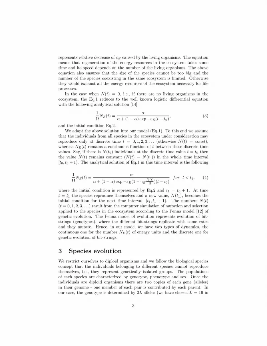
Figure 1: Phenotype-surrounding interaction function V (x, t) = 12x4 + 1

2b(t)x2

for two values of b(t) (0.5 and -0.4).

with probability p = 0.1. Hence, there is still a possibility for back mutations.Genes are mutated only at the stage of the zygote creation - one mutation perindividual.

The life cycle of diploids needs an intermediate stage when one of the twocopies of each gene is passed from the parent to a haploid gamete. Next, thetwo gametes produced by parents of different sex unite to form a zygote.

In the model, phenotype is defined as a fractional representation of the 16-bit-string genes, where each gene is translated uniquely into a fractional numberx from the interval [−1, 1]. The phenotype is coupled with the surrounding withthe help of the function V (x, t) as follows:

V (x, t) =1

4x4 +

1

2b(t)x2 (5)

where the fluctuations of the surrounding are represented by the coefficient b(t).The function V (x, t) has one minimum, x = 0, for b > 0 and two minima,x = ±

√

|b|, for b < 0 as in Fig.1. We use them to calculate gene quality, q, inthe variable surrounding

q = e−(V (x,t)−Vmin(t))/T , q ∈ [0, 1], (6)

where the parameter T has been introduced to control selection. The smallervalue of T the stronger selection. Next, we calculate the fitness Q of the indi-viduals, say at age a, to the surrounding with the help of the average

Q =1

L′ + a

L′+a∑

i=1

qi (7)

with

5

qi = max q(1)i δ(S

(1)i , 1), q

(2)i δ(S

(2)i , 1), (8)

where the indices (1) and (2) denote, respectively, the first allele and the secondallele at locus i = 1, 2, . . . , L′ + a and Si = 0, 1, 2 represent their states. Thesymbols δ() denote Kronecker delta. The inactive alleles and mutant genes donot contribute to Q and always Q ∈ [0, 1].

We decided to determine the amount of possible offsprings by projectingthe fitness of the parents, QF (female) and QM (male), onto the number ofproduced zygotes

Nzygote = max1, 10 × min(QF , QM ), (9)

where at least one zygote is produced and the maximum number of zygotesis equal to 10. In the computer simulations, the zygotes are mutated, afterthey are created, and they can be eliminated if at least one housekeeping genebecomes inactive. The individuals may reproduce themselves after they reachthe age a = aR. The genotypes of the parents who are better adapted tothe surrounding generate more offsprings. The mutants, if they happen (theyposses genes with the Hamming distance H > 1 from Eve) cannot mate withthe non-mutants.

We assume that the sex of a diploid individual is determined with the help ofa random number generator at the moment when it is born and it is unchangedduring its life.

4 Computer algorithm

We investigate the species with respect to speciation. In most computer simula-tions we observed evolving single species and analyzed the offsprings of the newmutant species originating from the old one. The secondary order speciation,i.e., the speciation taken place from the mutant species, has not been consid-ered. However, we investigated the case when initially there are a few speciesin the ecosystem and the results qualitatively were the same as for single initialspecies.

In the simulation, it is very important to prepare the genetic information ina proper way. It is obvious that in the evolution process some genes are not nec-essary during the whole life, e.g., they may become important only near the endof life, and it is possible that they could be defective since the individual underconsideration was born. Therefore, first we prepare the initial species in thetime independent surrounding for a few thousands generations until the inher-ited genetic information is represented by a steady state flow between suceedinggenerations. Then the distribution of inactive genes becomes time independent.Only after that we switch on the fluctuations of the surrounding, which in ourcase are represented by the coefficient b(t) = − 1

2 − cos(ωt), and all the initiallyprepared species are put together in the ecosystem. Hence, the computer algo-rithm consists of two blocks: preparation and evolution in variable surrounding.

6

INITIAL SPECIES PREPARATION:

(1) generate L bit-strings (16 bits) representing life functions of the or-ganism and which are the patterns for genes

(2) generate Ns predecessors (Eve) of the initial species (Hamming dis-tance of each gene from the respective pattern, H <= 2, and thenS1 = 1, S2 = 1, . . . SL = 1)

(3) for each Eve, representing the species 1, 2, . . . , Ns construct NM malesand NF females (NM = NF ) who have each gene at distance H ≤ 1from the corresponding gene of Eve.

(4) evolve separately each species 1, 2, . . . , Ns as follows:

(i) increase the age of all individuals by 1

(ii) remove from the population all individuals who should die be-cause they have exceeded the maximum age (L − L′) or duringtheir life until now they have collected three inactive ”chrono-logical” genes.

(iii) [optionally] the Verhulst factor is applied, i.e. every individ-ual survives with the same probability (1 − (NM + NF )/Nmax),where Nmax is the maximum allowed number of individuals inthe population under consideration.

(iV) select at random a female and a male for whom a ≥ aR and letthem produce Nzygotes according to Eq.9.

(V) each zygote is mutated. We assume that the housekeeping genescannot be inactive. Therefore, at least one defected housekeepinggene kills zygote. The total numer of the zygotes in the popu-lation which survive cannot exceed the number εpop(NE/Ω)NR,where NR is the total number of pairs of individuals, femaleand male, whose age a ≥ aR. The parameter εpop controls theallowed number of zygotes.

(Vi) Decrease the total number of energy units by the number N(t)of all individuals (parents and their new-born offsprings), i.e.,NE(t) = NE(t − 1) − N(t)

(Vii) regenerate the ecosystem energy according to Eq.4

(Viii) goto (i) unless the stop criterion is fulfilled

SPECIES IN VARIABLE SURROUNDING:

(5) all Ns species are put together in the ecosystem.

(6) t = t + 1

(7) calculate b(t) representing surrounding fluctuation

(8) check all individuals from the old species with respect to mutants(who have, at least at one locus, k = 1, . . . , L, two bit-strings rep-resenting the pair of the alleles at state S(1) = 2 and S(2) = 2). Ifthere is in the population an individual representing a mutant then

7

create Eve, the pattern of new species, and look for other mutants inthe same species consistent with the created Eve. Determine a newvalue of the reproduction age aR ∈ [1, L − L′] for the species withthe help of the computer random number generator. Remove newspecies from the old species.

(9) step (i) from above

(10) step (ii) from above

(11) step (iii) from above

(12) step (iV) from above

(13) step (V) but now NR concerns all species.

(14) step (Vi), where N(t) concerns all species

(15) step (Vii)

(16) goto (6) unless the end of the simulation

5 Results and discussion

Limiting the amount of energy resources in the ecosystem introduces strongselection between the species competing for the resources. In our case the se-lection takes place through limiting the number of the new-born offsprings inthe ecosystem. Namely, in the model, their number cannot exceed the valueεpop(NE(t)/Ω)NR, where NR is the number of parents, female and male, fromall species. Thus, the individuals who are better adapted to the environment(larger value of Q, Eq.7) dominate other individuals because they produce moreoffsprings. In our model, the better adaptation results from the phenotype xcloser to the minimum xmin of the function V (x, t). We could expect that ina time independent surrounding the mutations decreasing the fitness of the or-ganism lead to its elimination and in result to the elimination of the affectedgenes. However, in a changing environment the species need an ability to reactto new situations. The quality of genes in a fluctuating surrounding is changing,i.e., we cannot tell any more that some genes are bad and some are good. Therewill be preferred genes which adapt better to the changes.

In Fig.2, we show the effect of the changing environment on the old pop-ulation (aR = 5, L = 16, L′ = 5), which was aging in a time independentsurrounding through 40000 generations. The changing enviroment is modelledwith the help of the coefficient b(t) in the function V (x, t) (Eq.5). We havechosen

b(t) = −1

2− cos(ωt), (10)

where ω denotes the frequency of the environment changes. We should takeinto account that although we have a single species, in the example presented inFig.2, there are also present energy resources in the ecosystem which regeneratethemselves according to Eq.4. Thus, we have a kind of the Lotka-Volterra system

8

20000 30000 40000 50000 60000 70000time (t)

0,000

0,005

0,010

0,015

0,020

0,025

0,030

Num

ber

of in

divi

dual

s/en

ergy

uni

t

0,000

0,005

0,010

0,015

0,020

0,025

0,030

Num

ber

of e

nerg

y un

its/to

tal e

nerg

y of

eco

syst

em [

x 1/

40]

b(t)=-1.17b(t)=-0.5-cos(0.001*t)

Figure 2: The effect of the transition from the time independent surrounding(b(t) = −1.17, t < 40000) to the one varying in time (b(t) = − 1

2 − cos(0.001t),t ≥ 40000) on the size of the single species (aR = 5, amax = 11) and on thenumber of the energy units available for the species. The bottoom curve followsthe size changes of the species whereas the upper curve shows the correspondingenergy changes in the ecosystem.

with the species as the predator and the energy as the prey. Once the fluctuatingenvironment changes fitness Q of all individuals, the number of the new-bornoffsprings follows the environment fluctuations and in consequence there appearthe energy oscillations. Notice, that in a changing environment the size of thepopulation under consideration undergoes much stronger fluctuations than inthe time-independent case. It is connected with the changes of the inheritedgenetic information.

In Fig.3 we have presented the age profiles of the fraction of the inactive”chronological” genes in the population from Fig.2. The profiles concerning thegenerations at t = 20000 and t = 40000 refer to time independent surrounding.Although we have introduced in the model the back mutations for the inactivegenes (the bit-strings corresponding to inactive genes may mutate into anotherbit-string with probability ρ = 0.1) we can observe that, while time is increas-ing, the shape of the profiles tends to the one which is time independent. Itdetermines the average life span of individuals which is ranging from the agea = 1 to a = 7. On the other hand, the profiles corresponding to time dependentenvironment show both shrinking and enlarging of the life span. Effectively, thepopulation becomes much younger than during its previous evolution in the timeindependent surrounding. More frequent fluctuations of the surrounding makethis effect even stronger. It is evident from Fig.4 where the same old species,under consideration, experiences the surrounding changing with the higher fre-quency ω = 0.01. We can observe that the effect of the frequently changingenvironment becomes more destructive for the older members of the species.

9

1 2 3 4 5 6 7 8 9 10 11genotype site specific for age a

0

0,2

0,4

0,6

0,8

1

frac

tion

of d

efec

ted

gene

s sp

ecif

ic f

or a

ge a

t=20000t=40000t=50000t=100000t=140000

Figure 3: The effect of the change of the time independent surrounding tothe one varying in time, at t ≥ 40000, on the distribution of the defected”chronological” genes for the situation presented in Fig.2.

1 2 3 4 5 6 7 8 9 10 11genotype site specific for age a

0

0,2

0,4

0,6

0,8

1

frac

tion

of d

efec

ted

gene

s sp

ecif

ic f

or a

ge a

t=20000t=40000t=50000t=100000t=140000

Figure 4: The same as in in Fig.2 but ω = 0.01.

10

0 20000 40000 60000 80000 100000 120000 140000time (t)

0

0,1

0,2

0,3

0,4

0,5

phen

otyp

e (x

)

Figure 5: The phenotype evolution for the situation presented in Fig.2.

All our simulation were done with a constant mutation rate (one mutation pergenome) and we did not discuss the effect of the various values of the mutationrate on the above results.

The evolution of the average phenotype of the species from the example inFig.2 has been shown in Fig.5. The same data, but presented with the help ofa histogram have been shown in Fig.6.

Notice, that there is a trend to minimize the environment fluctuations andthe genes, which were well adapted in the time independent environment, donot have the ability to follow the environment fluctuations. They can be eveneliminated from the genetic bank of the species if the fluctuations become morefrequent.

The environmental changes influence the size of all species in the ecosystemend this is the reason that some of them may be eliminated. The regenerationof the energy resources in the ecosystem takes some time and too rapid a growthof some species, e.g., mutant species, acts as a sudden cataclysm for the otherspecies. The Lotka-Volterra systems have a self-regulatory character and thereexist threshold values for the fraction of destroyed population above which thesystem returns to its previous state ([19],[8]). However, in the case of geneticpopulations, if the catastrophe is applied for many generations, one can observethat the age profile of the fraction of defective genes in the population may looseits stability and next the species becomes extincted ([8]). Thus the appearanceof the new species, even for a relatively short period, can eliminate the oldspecies.

In our computer simulations we associate a new value, aR, of the reproduc-tion age with every new species appearing in the course of evolution. The valueis determined with the help of a computer random number generator. Thus,we have also the possibility to investigate the effect of the reproduction age onthe adaptation of the species to the fluctuating surrounding. We have observed

11

0 0,1 0,2 0,3 0,4phenotype (x)

0

500

1000

1500

2000

2500

3000

num

ber

of p

heno

type

s (x

)t<40000t>40000, frequency=0.001t>40000, frequency=0.01

Figure 6: The histogram of the average usage of the phenotype x in the evolv-ing species (from Fig.2) when there is time independent surrounding (r.h.mhistogram), and when there is fluctuationg environment.

that the events, representing the appearance of the new species with the smallvalue aR (aR ∼ 1), are usually represented by short duration ”bursts” of thepopulation size and they vanish as rapidly as they have appeared. In the exam-ple from Fig.7 the are represented by the highest blobs painted in black, at thebottoom of the figure. It is easy to explain the phenomenon, as in this case thelife span of individuals practically is shrinking to the activity of single gene andthe individuals die after they reproduce themselves. The active genes cannoteffectively adapt to the changing environment. How important the range of lifespan for species stability is, can be also concluded from the histograms in Fig.8.

There are presented histograms of the average usage of the phenotype x ofthe species representing the predecessor (aR = 5) and two descendant species(aR = 2, 7). It is evident that the average value x representing the specieswith aR = 2 oscillates far away from the optimum values (variable minimaof V (x, t)), because there is an insufficient number of genes adapted to thevariable surrounding. The situation is a little bit better with the predecessor(old species). However, it is evident that it cannot be stable over a long timein a variable surrounding. The most stable species is the one for which aR = 7,because in its population there are inherited genes which have adapted to thevariable surrounding (the range of x is almost symmetric with respect to x = 0).

In this study, we did not discuss the mechanism of speciation in the newspecies. We have restricted our analysis to the ”first order” speciation originat-ing from old species and we discussed in detail its effect on the inherited geneticinformation. We could expect a chain of events representing speciation withthe species being better and better adapted to the environment. The youngerthe species the more probable speciation, and one should observe peaks in thenumber of the speciation events in a short period.

12

0 5000 10000 15000 20000time (t)

0,0

0,2

0,4

0,6

0,8

1,0N

umbe

r of

ene

rgy

units

/Tot

al e

nerg

y

0,0

0,2

0,4

0,6

0,8

1,0

Num

ber

of in

divi

dual

s/en

ergy

uni

t [ x

25]

Figure 7: The effect of the speciation from the old species (earlier aging for40000 generations in time independent environment) in a fluctuating environ-ment (b(t) = − 1

2 − cos(0.01t) on the evolution of the energy resources. Inthe bottom part of the figure there have been shown a few examples of the newspecies created in the course of the evolution. The energy cost of the new speciescreation or extinction is reflected by the terrace-like changes in the upper curve.The survived species have not been shown for clarity of the picture.

-0,2 0 0,2 0,4phenotype (x)

0

0,1

0,2

0,3

0,4

0,5

norm

aliz

ed n

umbe

r of

eve

nts

with

phe

noty

pe (

x)

aR=5, OLDaR=7, MUTANTaR=2, MUTANT

Figure 8: Histograms of the phenotype usage in the environment changing withthe frequency ω = 0.02 in the case of three species: the predecessor population(aR = 5), and two descendant populations (aR = 7,aR = 2). The frequency ofthe environment changes, ω = 0.02.

13

6 Conclusions

We have discussed a model of species evolution in an ecosystem where the en-ergy resources regenerate themselves according to a logistic differential equation.The model belongs to the class of the Lotka-Volterra systems where the energyresources represent prey and the species represent predator. The number ofthe species present in the ecosystem under consideration results from evolution,which is understoood as the interplay of the two processes only, mutation andselection. We observed that after long periods of ’stasis’ there happen bursts ofthe new species which are able to live for thousands of generations. We haveobserved that in a variable surrounding the species, for which the reproductionage aR is too small, they are very unstable even if their size substantially exceedsthe size of the populations specific for other species. In our model, they usuallycause the elimination of other species. Simultaneously, the resulting increase inthe energy resources makes the next speciations possible.

There are two approaches to the description of species evolution: the onewith continuous evolutionary changes and the theory of punctated equilibrium[20, 21], according to which the evolutionary activity occurs in bursts. It isoften the case that the mathematical models concerning the species evolutionare restricted to pure species dynamics consideration or pure genetics evolution.We have shown that the inclusion of the genetic information into the populationdynamics makes the use of Bak-Sneppen [20, 21] extremal dynamics (SOC)possible.

14

References

[1] V. Volterra, Theorie mathematique de la lutte pour la vie, Gauthier-Villars,Paris 1931

[2] L.E. Reichl, A Modern Course in Statistical Physics, Edward Arnold (Pub-lishers) 1980, pp. 641-644

[3] R. Gerami and M.R. Ejtehadi, Eur. Phys. J. B 13, 601 (2000)

[4] B.E. Kendall, Chaos, Solitons and Fractals 12, 321 (2001)

[5] V. Rai, W.M. Schaffer, Chaos, Solitons and Fractals 12, 197-203 (2001)

[6] J. Vandermeer, Lewi Stone, B. Blasius, Chaos, Solitons and Fractals 12,265-276 (2001)

[7] A.F. Rozenfeld, E.V. Albano, Physica A 266 322 (1999)

[8] A. Duda, P. Dys, A. Nowicka, M.R. Dudek, Int. J. Mod. Phys. C 11, 1527-1538 (2000)

[9] R.M. May, Science 186, 645-647 (1974)

[10] R.M. May, Nature 216, 459-467 (1976)

[11] T.S. Ray, L. Moseley, N. Jan, Int. J. Mod. Phys. C 9, 701 (1998)

[12] T.J.P. Penna, J. Stat. Phys. 78: 1629 (1995)

[13] S. MCManus, D.L. Hunter, and N. Jan, T. Ray, L. Moseley, Int. J. Mod.Phys. C 10, 1295-1302 (1999)

[14] J.H.E. Cartwright and O. Piro, Int. J. Bifurc. Chaos 2, 427-449 (1992)

[15] E. Niewczas, A. Kurdziel, and S. Cebrat, Int. J. Mod. Phys. C 11, 775(2000)

[16] T.J.P. Penna and D. Stauffer, Int. J. Mod. Phys. C 6, 233 (1995)

[17] Moss de Oliveira,S., P.M.C. de Oliveiraand D. Stauffer. 1999. Evolution, Money, War, and Computers, Teubner,Stuttgart-Leipzig

[18] S. Cebrat, Physica A 258, 493 (1998)

[19] A. Pekalski and D. Stauffer, Int. J. Mod. Phys. C 9, 777 (1998)

[20] P.Bak, K. Sneppen, Phys. Rev. lett. 71, 4083 (1993)

[21] K. Sneppen, Physica A 221, 168-179 (1995)

15