Embed Size (px)
Citation preview
- ".
Economic Assessment
Environmental impact Statement
NESHAPS for Radionuclides
Background Information Document Volume 3

40 CPR Part 61 National Emission Standards for Hazardous Air Pollutants
Economic Assessment
Environmental Impact Statement for NESHAPS Radionuclides
VOLUME 3
BACKGROUND INFORMATION DOCUMENT
September 1989 U.S. Environmental Protection Agency
Office of Radiation Programs Washington, D.C. 20460

The Environmental Protection Agency is promulgating National Emission Standards for Hazardous Air Pollutants (NESHAPs) for Radionuclides. An Environmental Impact Statement (EIS) has been prepared in support of the rulemaking. The EIS consists of the following three volumes:
VOLUME I - Risk Assessment Methodology
This document contains chapters on hazard identification, movement of radionuclides through environmental pathways, radiation dosimetry, estimating the risk of health effects resulting from expose to low levels of ionizing radiation, and a summary of the uncertainties in calcul.ations of dose and risks.
VOLUME I1 - Risk Assessments
This document contains a chapter on each radionuclide source category studied. The chapters include an introduction, category description, process description, control technology, health impact assessment, supplemental control technology, and cost. It has an appendix which contains the inputs to all the computer runs used to generate the risk assessment.
VOLUME 111 - Economic Assessment This document has chapters on each radionuclide source category studied. Each. chapter includes an introduction, industry profile, summary of emissions, risk levels, the benefits and costs of emission controls, and economic impact evaluations.
Copies of the EIS in whole or in part are available to all interested persons; an announcement of the availability appears in the Federal Reqister. For additional information, contact James Hardin at (202) 475-9610 or write to:
Director, Criteria and Standards Division Office of Radiation Programs (ANR-460) Environmental Protection Agency 401 M Street, SW Washington, DC 20460

LIST OF PREPmERS
Various staff members from EPA% Office of Radiation Programs contributed in the development and preparation of the EIS.
Terrence McLaughlin Chief, Environmental Standards Branch
James Hardin Health Physicist Project Officer
Byron Bunger Economist Author/Reviewer
Fran Cohen Attorney Advisor Reviewer
Albert Colli Environmental Author/Reviewer Scientist
Larry Gray Environmental Scientist
W. Daniel Hendricks Environmental Scientist
Paul Magno Environmental Scientist
Christopher B. Nelson Environmental Scientist
Reviewer
Author
Dr. Neal S. Nelson Radiobiologist Author
Barry Parks Health Physicist Reviewer
Dr. Jerome Pushkin Chief Bioeffects Author/Reviewer Analysis Branch
Jack L. Russell Engineer Author/Reviewer
Dr. James T. Walker Radiation Biophysicist
Author
Larry Weinstock Attorney Advisor Reviewer
An EPA contractor, S. Cohen and Associates, Inc., McLean, VA, provided significant technical support in the preparation of the EIS.

The purpose of this report is to analyze the economic factors affecting the regulation of radionuclides
in the twelve categories listed below. For each ,category, the industry was profiled and analyses
regarding the cost of applying the controls suggested in the Volume I1 of the Background Information
Document, the cost effectiveness of the controls, and their effect on production costs and on regional
and local economies were performed.
The categories considered were:
I. The Uranium Fuel Cycle Facilities
2. Underground Uranium Mines
3. Inactive Uranium Mill Tailings
4. Licensed Uranium Mill Tailings
5. High-Level Waste Disposal Facilities
6. Department of Energy Facilities
7. Department of Energy Radon Facilities
8. Elemental Phosphorus
9. Phosphogypsum Stacks
10. Coal Fired Boilers
I I . Nuclear Regulatory Commission Licensed and non-DOE Federal Facilities
12. Surface Uranium Mines
The data regarding the control options was developed for Volume I1 and was incorporated into the
economic analysis. Other economic data was gathered from public available information.

TABLE OF CONTENTS
m ...
PREFACE . . . . . . . . . . . . . . . . . . . . . . . . . . . . . . . . . . . . . . . . . . . . . . . . 111
LIST OF PREPARERS . . . . . . . . . . . . . . . . . . . . . . . . . . . . . . . . . . . . . . . . . v
INTRODUCTION . . . . . . . . . . . . . . . . . . . . . . . . . . . . . . . . . . . . . . . . . . . . . . . vii
. . . . . . . . . . . . . . . . . . . . . . . . . . . . . . . . . . . . . . . . . . . . . . . . TABLE OF CONTENTS ix
LIST OF TABLES . . . . . . . . . . . . . . . . . . . . . . . . . . . . . . . . . . . . . . . . . . . . . . xviii
LIST O F FIGURES . . . . . . . . . . . . . . . . . . . . . . . . . . . . . . . . . . . . . . . . . . . . xxix
. . . . . . . . . . . . . . . . . . . . . . . . . . . . . . . . . . . 1 . URANIUM FUEL CYCLE FACILITIES 1 1
. . . . . . . . . . . . . . . . . . . . . . . . . . . . . . . . . . . . . . . . 1.1 Introduction and Summary 1-1
. . . . . . . . . . . . . . . . . . . . . . . . . . . . . . . . . . . . . . . . . . . . . . . 1.2 Industry Profile 1-2 . . . . . . . . . . . . . . . . . . . . . . . . . . . . . . . . . . . . . . . . . . . . . 1.2.1 Introduction 1-2
. . . . . . . . . . . . . . . . . . . . . . . . . . . . . . . . . . . . . . . . . . . 1.2.2 Uranium Mills 1-2 . . . . . . . . . . . . . . . . . . . . . . . . . . . . . . . 1.2.3 Uranium Conversion Facilities 1-2
. . . . . . . . . . . . . . . . . . . . . . . . . . . . . . . . . . . 1.2.4 Fuel Fabrication Facilities 1-5 . . . . . . . . . . . . . . . . . . . . . . . . . . . . . . . . . 1.2.5 Light Water Power Reactors 1-5
. . . . . . . . . . . . . 1.3 Current Emissions, Risk Levels. and Feasible Controls Methods 1-5 . . . . . . . . . . . . . . . . . . . . . . . . . . . . . . . . . . . . . . . . . . . . . 1.3.1 Introduction 1-5
. . . . . . . . . . . . . . . . . . . . 1.3.2 Current Emissions and Estimated Risk Levels 1-7 . . . . . . . . . . . . . . . . . . . . . . . . . . . . . . . . . . . . 1.3.2.1 Uranium Mills 1-7
. . . . . . . . . . . . . . . . . . . . . 1.3.2.2 Uranium FueI Conversion Facilities 1-9
. . . . . . . . . . . . . . . . . . . . . 1.3.2.3 Uranium Fuel Fabrication Facilities 1-9 . . . . . . . . . . . . . . . . . . . . . . . . . . . . . 1.3.2.4 Nuclear Power Reactors 1-13
. . . . . . . . . . . . . . . . . . . . . . . . . . . . . . . . . . . . . 1.3.3 Control Technologies 1-13 . . . . . . . . . . . . . . . . . . . . . . . . . . . . . . . . . . . 1.3.3.1 Uranium Mills 1-13
. . . . . . . . . . . . . . . . . . . . . . . . 1.3.3.2 Uranium Conversion Facilities 1-15 . . . . . . . . . . . . . . . . . . . . 1.3.3.3 Uranium Fuel Fabrication Facilities 1-15
. . . . . . . . . . . . . . . . . . . . . . . . . . . . . 1.3.3.4 Nuclear Power Reactors 1-15
. . . . . . . . . . . . . . . . . . . . . . . . . . 1.4 Industry Cost and Economic Impact Analysis 1-16
REFERENCES . . . . . . . . . . . . . . . . . . . . . . . . . . . . . . . . . . . . . . . . . . . . . . 1-17
. . . . . . . . . . . . . . . . . . . . . . . . . . . . . . . . . . 2 . UNDERGROUND URANIUM MINES 2-1
'tj 2.1 Introduction . . . . . . . . . . . . . . . . . . . . . . . . . . . . . . . . . . . . . . . . . . . . . . . 2-1

. . . . . . . . . . . . . . . . . . . . . . . . . . . . . . . . . . . . . . . . . . . . . . . 2.2 Industry Profile 2-1 2.2.1 Demand . . . . . . . . . . . . . . . . . . . . . . . . . . . . . . . . . . . . . . . . . . . . . . . 2-1 . . . . . . . . . . . . . . . . . . . . . . . . . . . . . . . . . . . . . . . . . 2.2.2 Sources of Supply 2-2 . . . . . . . . . . . . . . . . . . . . . . . . . . . . . . . . 2.2.2.1 Domestic Production 2-2 . . . . . . . . . . . . . . . . . . . . . . . . . . . . . . . . . . . . . . . . . . 2.2.2.2 Imports 2-3
. . . . . . . . . . . . . . . . . . . . . . . . . . . . . . . . . . . . . . . 2.2.2.3 Inventories 2-3 . . . . . . . . . . . . . . . . . . . . . . . . 2.2.2.4 Secondary Market Transactions 2-3
. . . . . . . . . . . . . . . . . . . . . . . . . . . . . . . . . . . . . . . . 2.2.3 Financial Analysis 2-4 . . . . . . . . . . . . . . . . . . . . . . . . . . 2.2.3.1 Homestake Mining Company 2-4
. . . . . . . . . . . . . . . . . . . . . . . . . . . . . . . . . . . . . . . 2.2.3.2 Rio Algom 2-5 . . . . . . . . . . . . . . . . . . . . . . . . . . . . 2.2.3.3 Plateau Resources Limited 2-5
. . . . . . . . . . . . . . . . . . . . . . . . . . . . . . . . . . . 2.2.3.4 Western Nuclear 2-5 . . . . . . . . . . . . . . . . . . . . . . . . . . . . . . . . 2.2.4 Industry Forecast and Outlook 2-6
. . . . . . . . . . . . . . . . . . . . . 2.2.4.1 Projections of Domestic Production 2-6 . . . . . . . . . . . . . . . . . . . . . . . . . . . . . . 2.2.4.2 Near-Term Projections 2-7
. . . . . . . . . . . . . . 2.3 Current Emissions, Risk Levels, and Feasible Control Methods 2-8 . . . . . . . . . . . . . . . . . . . . . . . . . . . . . . . . . . . . . . . . . . . . . 2.3.1 Introduction 2-8
. . . . . . . . . . . . . . . . . . . . 2.3.2 Current Emissions and Estimated Risk Levels 2-8 . . . . . . . . . . . . . . . . . . . . . . . . . . . . . . . . . . . . . . 2.3.3 Control Technologies 2-8 . . . . . . . . . . . . . . . . . . . . . . . . . . . . . . . . . . . . . . 2.3.3.1 Introduction 2-8
. . . . . . . . . . . . . . . . . . . . . . . . . . . . . . . . . . . 2.3.3.2 Alternatrve One 2-11 . . . . . . . . . . . . . . . . . . . . . . . . . . . . . . . . . . 2.3.3.3 Alternative Two 2-13
. . . . . . . . . . . . . . . . . . . . . . . . . . . . . . . . . . . . 2.4 Analysis of Benefits and Costs 2-13 . . . . . . . . . . . . . . . . . . . . . . . . . . . . . . . . . . . . . . . . . . . . 2.4.1 Introduction 2-13
. . . . . . . . . . . . . . . . . . . . . . . . . . . . . 2.4.2 Least-Cost Control Technologies 2-13
. . . . . . . . . . . . . . . . . . . . . . . . . . . . . 2.4.3 Benefits of Controf Alternatives 2-21 . . . . . . . . . . . . . . . . . . . . . . . . . . . . . . . . 2.4.4 Costs of Control Alternatives 2-21
. . . . . . . . . . . . . . . . . . . . . . . . . . . . . . . . . . . . . . . 2.4.5 Sensitivity Analysis 2-21
. . . . . . . . . . . . . . . . . . . . . . . . . . 2.5 Industry Cost and Economic Impact Analysis 2-28 . . . . . . . . . . . . . . . . . . . . . . . . . . . . . . . . . . . . . . . . . . . . 2.5.1 Introduction 2-28
. . . . . . . . . . . . . . . . . . . . . . . . . . . . . . . . . . . 2.5.2 Production Cost Impacts 2-28 . . . . . . . . . . . . . . . . . . . . . . . . . . . . . . . . . 2.5.3 Economic Impact Analysis 2-28
. . . . . . . . . . . . . . . . . . . . . . . . . . . . . . 2.5.4 Regulatory Flexibility Analysis 2-30
REFERENCES . . . . . . . . . . . . . . . . . . . . . . . . . . . . . . . . . . . . . . . . . . . . . . . 2-31
. . . . . . . . . . . . . . . . . . . . . . . . . . . . . . . . . . . . . . . . . 3 . INACTIVE MILL TAILINGS 3-1
. . . . . . . . . . . . . . . . . . . . . . . . . . . . . . . . . . . . . . . . 3.1 Introduction and Summary 3-1 . . . . . . . . . . . . . . . . . . . . . ,' 3.1.1 Rulemaking History and Current Regulations 3-1
A / i . . . . . . . . . . . . . . . . . . . . . . . . . . . . . . . . . . . . . . . . . . 1 3.2 Inactive Industry Profile 3-3
. . . . . . . . . . . . . . . . . . . . . . . . . . . . . . . 3.2.1 Current Status of Inactive Mills 3-3 . . . . . . . . . . . . . . . . . . . . . . . . . . . . . . . . . . . 3.2.2 Use of Inactive Mill Sites 3-3
. . . . . . . . . . . . . . . . . . . . . . . . . 3.3 Current Emissions. Risks. and Control Methods 3-5

TABLEOFCONTENTS
. . . . . . . . . . . . . . . . . . . . . . . . . 3.3.1 Current Emissions and Estimated Risk Levels 3-6 . . . . . . . . . . . . . . . . . 3.3.1 . 1 Development of the Radon Source Terms 3-6
. . . . . . . . . . . . . . . . . . . 3.3.1.2 Demographic and Meteorological Data 3-6 . . . . . . . . . . . . . . . . 3.3.1.3 Exposures and Risks to Nearby Individuals 3-8
. . . . . . . . . . . . 3.3.1.4 Exposures and Risks to the Regional Population 3-8 . . . . . . . . . . . 3.3.1.5 Exposures and Risks under Alternative Standards 3-8
. . . . . . . . . . . . . . . . . . . . . 3.3.1.6 Distribution of Fatal Cancer risk 3-12 . . . . . . . . . . . . . . . . . . . . . . . . . . . . . . . . . . . . . 3.3.2 Control Technologies 3-12
. . . . . . . . . . . . . . . . . . . . . . . . . . . . . . . . . . . . 3.4 Analysis of Benefits and Costs 3-15 . . . . . . . . . . . . . . . . . . . . . . . . . . . . . . . . . . . . . . . . . . . . . . 3.4.1 Benefits 3-16 3.4.2 Costs . . . . . . . . . . . . . . . . . . . . . . . . . . . . . . . . . . . . . . . . . . . . . . 3-16
. . . . . . . . . . . . . . . . . . . . . . . . . . . . . . . . . . . . . . . 3.5 Economic Impact Analysis 3-25
REFERENCES . . . . . . . . . . . . . . . . . . . . . . . . . . . . . . . . . . . . . . . . . . . . . . 3-28
. . . . . . . . . . . . . . . . . . . . . . . . . . . . . . . . . . . . . . . . . . 4 . LICENSED MILL TAILINGS 4-1
. . . . . . . . . . . . . . . . . . . . . . . . . . . . . . . . . . . . . . . . 4.1 Introduction and Summary 4-1 . . . . . . . . . . . . . . . . . . . . . . 4.1 1 Rulemaking History and Current Regulations 4-2
. . . . . . . . . . . . . . . . . . . . . . . . . . . . . . . . . . . . . . . . . . . . . . . . 1 4.2 Industry Profile 4-3 4.2.1 Demand . . . . . . . . . . . . . . . . . . . . . . . . . . . . . . . . . . . . . . . . . . . . . . . 4-3
. . . . . . . . . . . . . . . . . . . . . . . . . . . . . . . . . . . . . 4.2.1.1 Uranium Uses 4-5 . . . . . . . . . . . . . . . . . . . . . . . . . . . . . . . . . . . . . . . . 4.2.2 Sources of Supply 4-10
. . . . . . . . . . . . . . . . . . . . . . . . . . . 4.2.3 Industry Structure and Performance 4-21 . . . . . . . . . . . . . . . . . . . . . . . . 4.2.4 Economic and Financial Characteristics 4-24
. . . . . . . . . . . . . . . . . . . . . . . . . . . . . . 4.2.4.1 Employment Analysis 4-24 . . . . . . . . . . . . . . . . . . . . . . . . . 4.2.4.2 Community Impact Analysis 4-26
. . . . . . . . . . . . . . . . . . . . . . . . . . . . . . . . . 4.2.4.3 Financial Analysis 4-27 . . . . . . . . . . . . . . . . . . . . . . . . . . . . . . . 4.2.5 Industry Forecast and Outlook 4-31
. . . . . . . . . . . . . . . . . . . . 4.2.5.1 Projections of Domestic Production 4-33 4.2.5.2 Near-Term Projections . . . . . . . . . . . . . . . . . . . . . . . . . . . . . 4-34
. . . . . . . . . . . . . 4.2.6 Evaluation of Forecasts and Uranium Market Demand 4-36 . . . . . . . . . . . . . . . . . . . . . . . . . 4.2.6.1 Domestic Uranium Resources 4-36
. . . . . . . . . . . . . . . . . . . . . . . . . . 4.2.6.2 Total Electricity Generation 4-42 . . . . . . . . . . . . . . . . . . . . . . . . . . . . 4.2.6.3 Employment Projections 4-44
. . . . . . . . . . . . . . . . . . . . . . . . 4.3 Current Emissions. Risks. and Control Methods 4-47
. . . . . . . . . . . . . . . . . . . 4.3.1 Current Emissions and Estimated Risk Levels 4-49 4.3.1.1 Methodology for the Assessment of Risks
. . . . . . . . . . . . . . . . . . . . . from Operating and Standby Mills 4-49 4.3.1.2 Methodology for the Assessment of
Post-disposal Risks . . . . . . . . . . . . . . . . . . . . . . . . . . . . . . . . 4-53 4.3.1.3 Methodology for the Assessment of Risks
. . . . . . . . . . . . . . . . . . . . . . . . . . . . from New Impoundments 4-56
TABLE OF CONTENTS
b l z s
4.3.1.4 Exposures and Risks from Operating and . . . . . . . . . . . . . . . . . . . . . . . . . . . . . . . . . . . . Standby Mills 4-56
. . . . . . . . . . . . . . . . . . . . . 4.3.1.5 Post-disposal Exposures and Risks 4-59
. . . . . . . . . 4.3.2 Technologies for Long-term Post-disposal Emission Control 4-63
. . . . . . . . . . . . . . . . . . . . . . . . . . . . . . . . . . . . 4.4 Analysis of Benefits and Costs 4-65
4.4.1 Benefits and Costs of Reducing Allowable Limits From 20 pci/m2/sec . 4-66 . . . . . . . . . . . . . . . 4.4.1.1 Benefits of Reducing the Allowable Limits 4-66
. . . . . . . . . . . . . . . . . 4.4.1.2 Costs of Reducing the Allowable Limits 4-67 4.4.2 Benefit And Costs of Reducing Allowable Emissions During 4perations 4-73
. . . . 4.4.2.1 Methods of Reducing Allowable Limits to 20 pCi/m2/sec 4-73 4.4.2.2 Benefits of Reducing Allowable Limits to 20 pCi/m /sec . . . . 4-75
. . . . . . 4.4.2.3 Costs of Reducing Allowable Limits to 20 pCi/m2/sec 4-75 4.4.3 Analysis of Benefits and Costs of Promulgating Future Work
Practice Standards . . . . . . . . . . . . . . . . . . . . . . . . . . . . . . . . . . . . . . . . 4-77 . . . . . . . . . . . 4.4.3.1 Work Practices for New Tailings Impoundments 4-80
4.4.3.2 Comparison of Control Technologies for . . . . . . . . . . . . . . . . . . . . . . . . . . New Tailings Impoundments 4-81
. . . . 4.4.3.3 Benefits of Promulgating Future Work Practlce Standards 4-82 . . . . . . 4.4.3.4 Costs of Promulgating Future Work Practice Standards 4-89
. . . . . . . . . . . . . . . . . . . . . . . . . . . . . . . . . . . . . . . . . . . . . 4.5 Economic Impacts 4-95 4.5.1 Increased Production Cost . . . . . . . . . . . . . . . . . . . . . . . . . . . . . . . . . . 4-95 4.5.2 Regulatory Flexibility Analysis . . . . . . . . . . . . . . . . . . . . . . . . . . . . . . 4-98
REFERENCES . . . . . . . . . . . . . . . . . . . . . . . . . . . . . . . . . . . . . . . . . . . . . 4-101
5 . HIGH-LEVEL WASTE DISPOSAL . . . . . . . . . . . . . . . . . . . . . . . . . . . . . . . . . . . . . . 5-1
. . . . . . . . . . . . . . . . . . . . . . . . . . . . . . . . . . . . . . . . 5.1 Introduction and Summary 5-1
. . . . . . . . . . . . . . . . . . . . . . . . . . . . . . . . . . . . . . . . . . . . . . . 5.2 Industry Profile 5-1 . . . . . . . . . . . . . . . . . . . . . . . . . . . . . . . . . . . . . . . . . . . . . 5.2.1 Introduction 5-1
. . . . . . . . . . . . 5.2.2 Facilities for the Ultimate Disposal of High-Level Waste 5-2 5.2.2.1 The Waste Isolation Pilot Plant (WIPP) . . . . . . . . . . . . . . . . . . . 5-2 5.2.2.2 Yucca Mountain Geologic Repository . . . . . . . . . . . . . . . . . . . . 5-2
. . . . . . . . . . . . . . . . . . . . . . . . . 5.2.3 Demand for High-Level Waste Storage 5-2 5.2.4 Supply of High-Level Waste Storage . . . . . . . . . . . . . . . . . . . . . . . . . . . 5-3
5.3 Current Emissions. Risk Levels and Feasible Control Methods . . . . . . . . . . . . . . 5-3 5.3.1 Introduction . . . . . . . . . . . . . . . . . . . . . . . . . . . . . . . . . . . . . . . . . . . . . 5-3
. . . . . . . . . . . . . . . . . . . . . . . . . . 5.3.2 Current Emissions and Estimated Risk 5-3 5.3.3 Control Technologies . . . . . . . . . . . . . . . . . . . . . . . . . . . . . . . . . . . . . . 5-4
5.4 Analysis of Benefits and Costs . . . . . . . . . . . . . . . . . . . . . . . . . . . . . . . . . . . . . 5-4 5.4.1 Introduction . . . . . . . . . . . . . . . . . . . . . . . . . . . . . . . . . . . . . . . . . . . . . 5-4 5.4.2 Least-Cost Control Technologies . . . . . . . . . . . . . . . . . . . . . . . . . . . . . . 5-4
TABLE OF CONTENTS
h s
. . . . . . . . . . . . . . . . . . . . . . . . . . . . . . . . . . . 5.4.3 Health and Other Benefits 5-5
. . . . . . . . . . . . . . . . . . . . . . . . . . . 5.5 Industry Cost and Economic Impact Analysis 5-5
REFERENCES . . . . . . . . . . . . . . . . . . . . . . . . . . . . . . . . . . . . . . . . . . . . . . . 5-6
. . . . . . . . . . . . . . . . . . . . . . . . . . . . . . . . 6 . DEPARTMENT OF ENERGY FACILITIES 6-1
. . . . . . . . . . . . . . . . . . . . . . . . . . . . . . . . . . . . . . . . 6.1 Introduction and Summary 6-1 . . . . . . . . . . . . . . . . . . . . . . . . . . . . . . . . . . . . . . . . . . . . . . . 6.2 Industry Profile 6-1 . . . . . . . . . . . . . . . . . . . . . . 6.3 Current Risk Levels. and Feasible Control Methods 6-3 . . . . . . . . . . . . . . . . . . . . . . . . . . . . . . . . . . . . . . . . . . . . . 6.3.1 Introduction 6-3
. . . . . . . . . . . . . . . . . . . . . . . . . . . . . . . . . . . . . . . 6.3.2 Facility Descriptions 6-3 . . . . . . . . . . . . . . . . . . . . . . . . . . . . . . . . . . . . . . 6.3.3 Control Technologies 6-6
. . . . . . . . . . . . . . . . . . . . . . . . . . . . . . . . . . . . . 6.4 Analysis of Benefits and Costs 6-7 . . . . . . . . . . . . . . . . . . . . . . . . . . . . . . . . . . . . . . . . . . . . . . 6.4.1 Introduction 6-7
. . . . . . . . . . . . . . . . . . . . . . . . . . . . . . . . . 6.4.2 Cost of Control Technologies 6-7 . . . . . . . . . . . . . . . . . . . . . . . . . . . . . . . . . . 6.4.3 Health and Other Benefits 6-10
. . . . . . . . . . . . . . . . . . . . . . . . . . . . . . . . 6.5 Industry Cost and Economic Impacts 6-11
REFERENCES . . . . . . . . . . . . . . . . . . . . . . . . . . . . . . . . . . . . . . . . . . . . . . 6-12
. . . . . . . . . . . . . . . . . . . . . . . . . . . . . . 7 . DEPARTMENT OF ENERGY RADON SITES 7-1
. . . . . . . . . . . . . . . . . . . . . . . . . . . . . . . . . . . . . . . . 7.1 Introduction and Summary 7-1
. . . . . . . . . . . . . . . . . . . . . . . . . . . . . . . . . . . . . . . . . . . . . . . 7.2 Industry Profile 7-1 . . . . . . . . . . . . . . . . . . . . . . . 7.2.1 Feed Materials Production Center (FMPC) 7-2
. . . . . . . . . . . . . . . . . . . . . . . . . . . . . . 7.2.2 Niagara Falls Storage Site (NFSS) 7-2 . . . . . . . . . . . . . . . . . . . . . . . . . . . . . . . . . . . 7.2.3 Weldon Spring Site (WSS) 7-2
. . . . . . . . . . . . . . . . . . . . . . . . . . . . . . 7.2.4 Middlesex Sampling Plant (MSP) 7-3 7.2.5 Monticello Uranium Mill Tailings (MUMT) Pile . . . . . . . . . . . . . . . . . . 7-4
. . . . . . . . . . . . . . 7.3 Current Emission, Risk Levels. and Feasible Control Methods 7-4 7.3.1 Introduction . . . . . . . . . . . . . . . . . . . . . . . . . . . . . . . . . . . . . . . . . . . . . 7-4
. . . . . . . . . . . . . . . . . . . . 7.3.2 Current Emissions and Estimated Risk Levels 7-4 . . . . . . . . . . . . . . . . . . . . . . . . . . . . . . . . . . . . . . . . . . . 7.3.2.1 FMPC 7-4 . . . . . . . . . . . . . . . . . . . . . . . . . . . . . . . . . . . . . . . . . . . 7.3.2.2 NFSS 7-7
7.3.2.3 WSS . . . . . . . . . . . . . . . . . . . . . . . . . . . . . . . . . . . . . . . . . . . . 7-7 . . . . . . . . . . . . . . . . . . . . . . . . . . . . . . . . . . . . . . . . . . . . 7.3.2.4 MSP 7-7 . . . . . . . . . . . . . . . . . . . . . . . . . . . . . . . . . . . . . . . . . . 7.3.2.5 MUMT 7-8
. . . . . . . . . . . . . . . . . . . . . . . . . . . . . . . . . . . . . . 7.3.3 Control Technologies 7-8
. . . . . . . . . . . . . . . . . . . . . . . . . . . . . . . . . . . . . 7.4 Analysis of Benefits and Costs 7-9 7.4.1 Costs and Benefits of Meeting Various Radon Flux Rates . . . . . . . . . . . 7-9
. . . . . . . . . . . . . . . . . . . . . . . . . . . . . . . . . . . . . . . . . . 7.4.1.1 FMPC 7-10
. . . . . . . . . . . . . . . . . . . . . . . . . . . . . . . . . . . . . . . . . . 7.4.1.2 NFSS 7-10 . . . . . . . . . . . . . . . . . . . . . . . . . . . . . . . . . . . . . . . . . . . 7.4.1.3 WSS 7-10 . . . . . . . . . . . . . . . . . . . . . . . . . . . . . . . . . . . . . . . . . . . 7.4.1.4 MSP 7-14
. . . . . . . . . . . . . . . . . . . . . . . . . . . . . . . . . . . . . . . . . 7.4.1.5 MUMT 7-14 . . . . . . . . . . . . . . . . . . . . . . . . . . . . . . . . . . . . . . . 7.4.2 Sensitivity Analysis 7-14
. . . . . . . . . . . . . . . . . . . . . . . . . . 7.5 Industry Cost and Economic Impact Analysis 7-15
REFERENCES . . . . . . . . . . . . . . . . . . . . . . . . . . . . . . . . . . . . . . . . . . . . . . 7-19
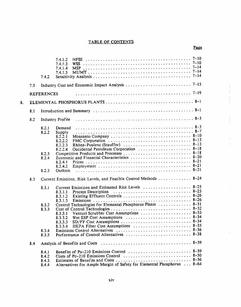
. . . . . . . . . . . . . . . . . . . . . . . . . . . . . . . . . . . 8 . ELEMENTAL PHOSPHORUS PLANTS 8-1
. . . . . . . . . . . . . . . . . . . . . . . . . . . . . . . . . . . . . . . . 8.1 Introduction and Summary 8-1
. . . . . . . . . . . . . . . . . . . . . . . . . . . . . . . . . . . . . . . . . . . . . . . 8.2 Industry Profile 8-3
8.2.1 Demand . . . . . . . . . . . . . . . . . . . . . . . . . . . . . . . . . . . . . . . . . . . . . . . 8-3 . . . . . . . . . . . . . . . . . . . . . . . . . . . . . . . . . . . . . . . . . . . . . . . 8.2.2 Supply 8-7
. . . . . . . . . . . . . . . . . . . . . . . . . . . . . . . . 8.2.2.1 Monsanto Company 8-10 . . . . . . . . . . . . . . . . . . . . . . . . . . . . . . . . . 8.2.2.2 FMC Corporation 8-13
. . . . . . . . . . . . . . . . . . . . . . . . . . . 8.2.2.3 Rhbne-Poulenc (Stauffer) 8-13 . . . . . . . . . . . . . . . . . . . . . 8.2.2.4 Occidental Petroleum Corporation 8-18
. . . . . . . . . . . . . . . . . . . . . . . . . . . 8.2.3 Competitive Products and Processes 8-18 . . . . . . . . . . . . . . . . . . . . . . . . 8.2.4 Economic and Financial Characteristics 8-20
. . . . . . . . . . . . . . . . . . . . . . . . . . . . . . . . . . . . . . . . . . 8.2.4.1 Prices 8-21 . . . . . . . . . . . . . . . . . . . . . . . . . . . . . . . . . . . . . 8.2.4.2 Employment 8-21
. . . . . . . . . . . . . . . . . . . . . . . . . . . . . . . . . . . . . . . . . . . . . . 8.2.5 Outlook 8-21
. . . . . . . . . . . . . 8.3 Current Emissions. Risk Levels. and Feasible Control Methods 8-24
. . . . . . . . . . . . . . . . . . . 8.3.1 Current Emissions and Estimated Risk Levels 8-25 . . . . . . . . . . . . . . . . . . . . . . . . . . . . . . . 8.3.1.1 Process Description 8-25
. . . . . . . . . . . . . . . . . . . . . . . . . . . 8.3.1.2 Existing Effluent Controls 8-26 . . . . . . . . . . . . . . . . . . . . . . . . . . . . . . . . . . . . . . . 8.3.1.3 Emissions 8-26
8.3.2 Control Technologies for Elemental Phosphorus Plants . . . . . . . . . . . . . 8-31 . . . . . . . . . . . . . . . . . . . . . . . . . . . . . . . . 8.3.3 Cost of Control Technologies 8-32
. . . . . . . . . . . . . . . . . . . . 8.3.3.1 Venturi Scrubber Cost Assumptions 8-33 . . . . . . . . . . . . . . . . . . . . . . . . . . 8.3.3.2 Wet ESP Cost Assumptions 8-34
. . . . . . . . . . . . . . . . . . . . . . . . . . . . 8.3.3.3 SD/FF Cost Assumptions 8-34 . . . . . . . . . . . . . . . . . . . . . . . 8.3.3.4 HEPA Filter Cost Assumptions 8-35
. . . . . . . . . . . . . . . . . . . . . . . . . . . . . . 8.3.4 Emissions Control Alternatives 8-36 . . . . . . . . . . . . . . . . . . . . . . . . . . 8.3.5 Performance of Control Alternatives 8-38
. . . . . . . . . . . . . . . . . . . . . . . . . . . . . . . . . . . . 8.4 Analysis of Benefits and Costs 8-39
. . . . . . . . . . . . . . . . . . . . . . . . . 8.4.1 Benefits of Po-210 Emissions Control 8-39 . . . . . . . . . . . . . . . . . . . . . . . . . . . 8.4.2 Costs of Po-210 Emissions Control 8-50
. . . . . . . . . . . . . . . . . . . . . . . . . . . . . . 8.4.3 Estimates of Benefits and Costs 8-56 . . . 8.4.4 Alternatives for Ample Margin of Safety for Elemental Phosphorus 8-64
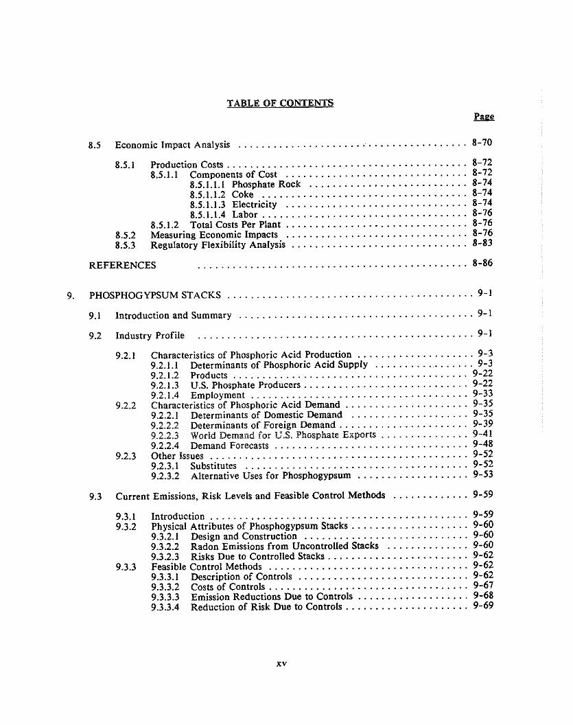
TABLE OF CONTENTS &g-e
. . . . . . . . . . . . . . . . . . . . . . . . . . . . . . . . . . . . . . . 8.5 Economic Impact Analysis 8-70
. . . . . . . . . . . . . . . . . . . . . . . . . . . . . . . . . . . . . . . . . 8.5.1 Production Costs 8-72 . . . . . . . . . . . . . . . . . . . . . . . . . . . . . . . 8.5.1 . 1 Components of Cost 8-72 . . . . . . . . . . . . . . . . . . . . . . . . . . . 8.5.1.1.1 Phosphate Rock 8-74 . . . . . . . . . . . . . . . . . . . . . . . . . . . . . . . . . . . 8.5.1.1.2 Coke 8-74 . . . . . . . . . . . . . . . . . . . . . . . . . . . . . . . 8.5.1.1.3 Electricity 8-74
. . . . . . . . . . . . . . . . . . . . . . . . . . . . . . . . . . . 8.5.1.1.4 Labor 8-76 . . . . . . . . . . . . . . . . . . . . . . . . . . . . . . . 8.5.1.2 Total Costs Per Plant 8-76 . . . . . . . . . . . . . . . . . . . . . . . . . . . . . . . 8.5.2 Measuring Economic Impacts 8-76 . . . . . . . . . . . . . . . . . . . . . . . . . . . . . . 8.5.3 Regulatory Flexibility Analysis 8-83
REFERENCES
. . . . . . . . . . . . . . . . . . . . . . . . . . . . . . . . . . . . . . . . . . 9 . PHOSPHOGYPSUM STACKS 9-1
. . . . . . . . . . . . . . . . . . . . . . . . . . . . . . . . . . . . . . . . 9.1 Introduction and Summary 9-1
. . . . . . . . . . . . . . . . . . . . . . . . . . . . . . . . . . . . . . . . . . . . . . . 9.2 Industry Profile 9-1
. . . . . . . . . . . . . . . . . . . . 9.2.1 Characteristics of Phosphoric Acid Production 9-3 . . . . . . . . . . . . . . . . . . 9.2.1.1 Determinants of Phosphoric Acid Supply 9-3
. . . . . . . . . . . . . . . . . . . . . . . . . . . . . . . . . . . . . . . . 9.2.1.2 Products 9-22 . . . . . . . . . . . . . . . . . . . . . . . . . . . . 9.2.1.3 U.S. Phosphate Producers 9-22
. . . . . . . . . . . . . . . . . . . . . . . . . . . . . . . . . . . . . 9.2.1.4 Employment 9-33 . . . . . . . . . . . . . . . . . . . . . 9.2.2 Characteristics of Phosphoric Acid Demand 9-35
9.2.2.1 Determinants of Domestic Demand . . . . . . . . . . . . . . . . . . . . 9-35 . . . . . . . . . . . . . . . . . . . . . . 9.2.2.2 Determinants of Foreign Demand 9-39
. . . . . . . . . . . . . . . 9.2.2.3 World Demand for U.S. Phosphate Exports 9-41 . . . . . . . . . . . . . . . . . . . . . . . . . . . . . . . . . 9.2.2.4 Demand Forecasts 9-48
. . . . . . . . . . . . . . . . . . . . . . . . . . . . . . . . . . . . . . . . . . . . 9.2.3 Other Issues 9-52 . . . . . . . . . . . . . . . . . . . . . . . . . . . . . . . . . . . . . . 9.2.3.1 Substitutes 9-52
. . . . . . . . . . . . . . . . . . . 9.2.3.2 Alternative Uses for Phosphogypsum 9-53
. . . . . . . . . . . . . 9.3 Current Emissions, Risk Levels and Feasible Control Methods 9-59
9.3.1 Introduction . . . . . . . . . . . . . . . . . . . . . . . . . . . . . . . . . . . . . . . . . . . . 9-59 . . . . . . . . . . . . . . . . . . . . 9.3.2 Physical Attributes of Phosphogypsum Stacks 9-60
. . . . . . . . . . . . . . . . . . . . . . . . . . . . 9.3.2.1 Design and Construction 9-60 . . . . . . . . . . . . . . 9.3.2.2 Radon Emissions from Uncontrolled Stacks 9-60
. . . . . . . . . . . . . . . . . . . . . . . . 9.3.2.3 Risks Due to Controlled Stacks 9-62 . . . . . . . . . . . . . . . . . . . . . . . . . . . . . . . . . . 9.3.3 Feasible Control Methods 9-62
. . . . . . . . . . . . . . . . . . . . . . . . . . . . . 9.3.3.1 Description of Controls 9-62 . . . . . . . . . . . . . . . . . . . . . . . . . . . . . . . . . . 9.3.3.2 Costs of Controls 9-67
. . . . . . . . . . . . . . . . . . . 9.3.3.3 Emission Reductions Due to Controls 9-68 . . . . . . . . . . . . . . . . . . . . . 9.3.3.4 Reduction of Risk Due to Controls 9-69
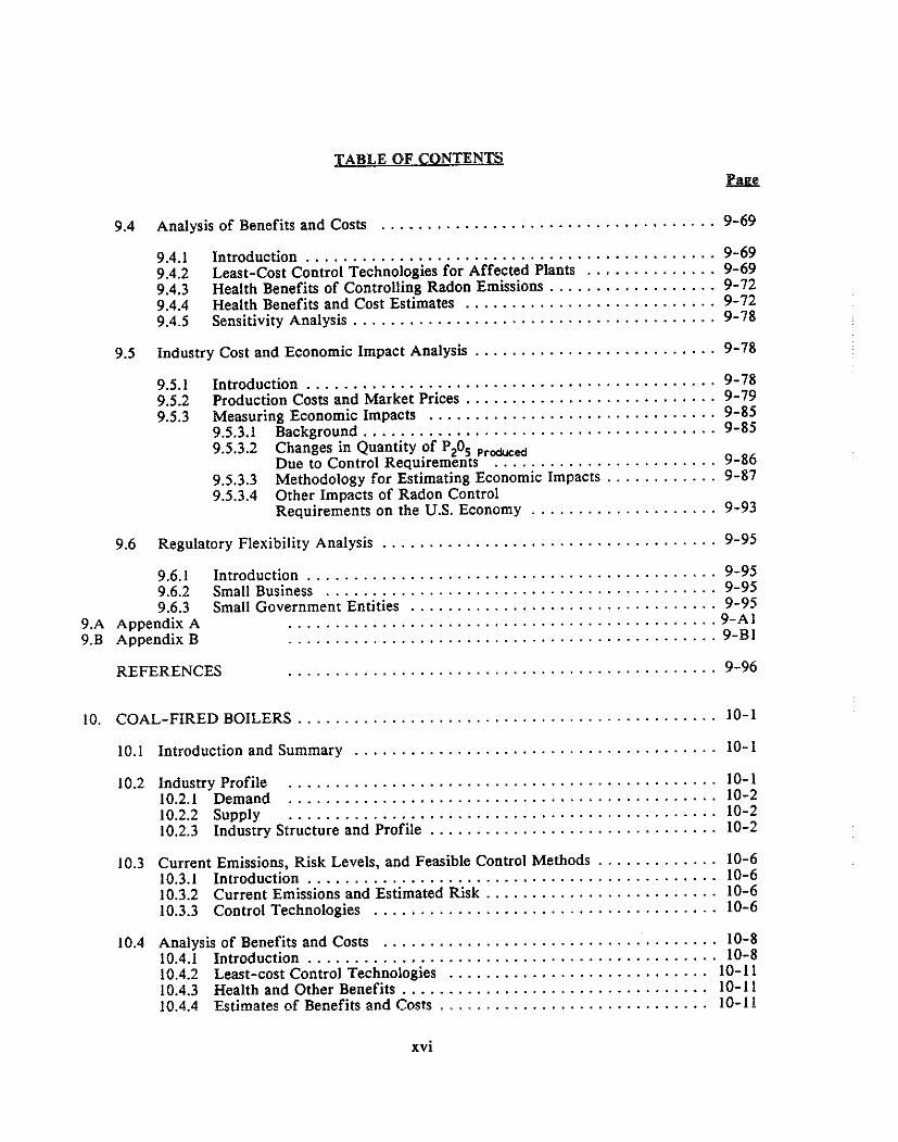
TABLE OF CONTENTS
. . . . . . . . . . . . . . . . . . . . . . . . . . . . . . . . . . . . 9.4 Analysis of Benefits and Costs 9-69
. . . . . . . . . . . . . . . . . . . . . . . . . . . . . . . . . . . . . . . . . . . . 9.4.1 Introduction 9-69 . . . . . . . . . . . . . . 9.4.2 Least-Cost Control Technologies for Affected Plants 9-69 . . . . . . . . . . . . . . . . . . 9.4.3 Health Benefits of Controlling Radon Emissions 9-72 . . . . . . . . . . . . . . . . . . . . . . . . . . . 9.4.4 Health Benefits and Cost Estimates 9-72 . . . . . . . . . . . . . . . . . . . . . . . . . . . . . . . . . . . . . . . 9.4.5 Sensitivity Analysis 9-78
. . . . . . . . . . . . . . . . . . . . . . . . . . 9.5 Industry Cost and Economic Impact Analysis 9-78
. . . . . . . . . . . . . . . . . . . . . . . . . . . . . . . . . . . . . . . . . . . . 9.5.1 Introduction 9-78 . . . . . . . . . . . . . . . . . . . . . . . . . . . 9.5.2 Production Costs and Market Prices 9-79 . . . . . . . . . . . . . . . . . . . . . . . . . . . . . . . 9.5.3 Measuring Economic Impacts 9-85 . . . . . . . . . . . . . . . . . . . . . . . . . . . . . . . . . . . . . . 9.5.3.1 Background 9-85 9.5.3.2 Changes in Quantity of PZ05 Pr-ed
. . . . . . . . . . . . . . . . . . . . . . . . Due to Control Requirements 9-86 . . . . . . . . . . . . 9.5.3.3 Methodology for Estimating Economic Impacts 9-87
9.5.3.4 Other Impacts of Radon Control . . . . . . . . . . . . . . . . . . . . Requirements on the U.S. Economy 9-93
. . . . . . . . . . . . . . . . . . . . . . . . . . . . . . . . . . . . 9.6 Regulatory Flexibility Analysis 9-95
. . . . . . . . . . . . . . . . . . . . . . . . . . . . . . . . . . . . . . . . . . . . 9.6.1 Introduction 9-95 . . . . . . . . . . . . . . . . . . . . . . . . . . . . . . . . . . . . . . . . . . 9.6.2 Small Business 9-95 . . . . . . . . . . . . . . . . . . . . . . . . . . . . . . . . . 9.6.3 Small Government Entities 9-95
9.A Appendix A . . . . . . . . . . . . . . . . . . . . . . . . . . . . . . . . . . . . . . . . . . . . . . 9-A1 9.B Appendix B . . . . . . . . . . . . . . . . . . . . . . . . . . . . . . . . . . . . . . . . . . . . . . 9-B1
REFERENCES . . . . . . . . . . . . . . . . . . . . . . . . . . . . . . . . . . . . . . . . . . . . . . 9-96
. . . . . . . . . . . . . . . . . . . . . . . . . . . . . . . . . . . . . . . . . . . . . . 10 COAL-FIRED BOILERS 10-1
. . . . . . . . . . . . . . . . . . . . . . . . . . . . . . . . . . . . . . . 10.1 Introduction and Summary 10-1
. . . . . . . . . . . . . . . . . . . . . . . . . . . . . . . . . . . . . . . . . . . . . . 10.2 Industry Profile 10-1
. . . . . . . . . . . . . . . . . . . . . . . . . . . . . . . . . . . . . . . . . . . . . . 10.2.1 Demand 10-2
. . . . . . . . . . . . . . . . . . . . . . . . . . . . . . . . . . . . . . . . . . . . . . 10.2.2 Supply 10-2 . . . . . . . . . . . . . . . . . . . . . . . . . . . . . . . 10.2.3 Industry Structure and Profile 10-2
. . . . . . . . . . . . . 10.3 Current Emissions. Risk Levels. and Feasible Control Methods 10-6 . . . . . . . . . . . . . . . . . . . . . . . . . . . . . . . . . . . . . . . . . . . . 10.3.1 Introduction 10-6
. . . . . . . . . . . . . . . . . . . . . . . . . 10.3.2 Current Emissions and Estimated Risk 10-6 . . . . . . . . . . . . . . . . . . . . . . . . . . . . . . . . . . . . . 10.3.3 Control Technologies 10-6
. . . . . . . . . . . . . . . . . . . . . . . . . . . . . . . . . . . . 10.4 Analysis of Benefits and Costs 10-8 . . . . . . . . . . . . . . . . . . . . . . . . . . . . . . . . . . . . . . . . . . . . 10.4.1 Introduction 10-8
. . . . . . . . . . . . . . . . . . . . . . . . . . . . 10.4.2 Least-cost Control Technologies 10-11 . . . . . . . . . . . . . . . . . . . . . . . . . . . . . . . . . 10.4.3 Health and Other Benefits 10-11
. . . . . . . . . . . . . . . . . . . . . . . . . . . . . 10.4.4 Estimates of Benefits and Costs 10-1 1

REFERENCES . . . . . . . . . . . . . . . . . . . . . . . . . . . . . . . . . . . . . . . . . . . . . 10-17
. . . . . . . . . . . . . . . . . . 1 1 . NRC-LICENSED AND NON-DOE FEDERAL FACILITIES 11-1
. . . . . . . . . . . . . . . . . . . . . . . . . . . . . . . . . . . . . . . 11.1 Introduction and Summary 11-1
. . . . . . . . . . . . . . . . . . . . . . . . . . . . . . . . . . . . . . . . . . . . . . 11.2 Industry Profile 11-2
. . . . . . . . . . . . . 11.3 Current Emissions. Risk Levels. and Feasible Control Methods 11-3 . . . . . . . . . . . . . . . . . . . . . . . . . . . . . . . . . . . . . . . . . . . . 11.3.1 Introduction 11-3 . . . . . . . . . . . . . . . . . . . 11.3.2 Current Emissions and Estimated Risk Levels 11-3
. . . . . . . . . . . . . . . . . . . . . . . . . . . . . . . . . . . . . 11.3.3 Control Technologies 11-6
. . . . . . . . . . . . . . . . . . . . . . . . . . . . . . . . . . . . 11.4 Analysis of Benefits and Costs 11-7 . . . . . . . . . . . . . . . . . . . . . . . . . . . . . . . . 11.5 Industry Cost and Economic Impact 11-7
REFERENCES . . . . . . . . . . . . . . . . . . . . . . . . . . . . . . . . . . . . . . . . . . . . . 11-10
. . . . . . . . . . . . . . . . . . . . . . . . . . . . . . . . . . . . . . . . 12 . SURFACE URANIUM MINES 12-1
. . . . . . . . . . . . . . . . . . . . . . . . . . . . . . . . . . . . . . . 12.1 Introduction and Summary 12-1
. . . . . . . . . . . . . . . . . . . . . . . . . . . . . . . . . . . . . . . . . . . . . . 12.2 Industry Profile 12-1 . . . . . . . . . . . . . . . . . . . . . . . . . . . . . . . . . . . . . . . . . . . . 12.2.1 Introduction 12-1
. . . . . . . . . . . . . . . . . . . . . . . . . . . . . . . . . . . . . 12.2.2 Demand for Uranium 12-1 . . . . . . . . . . . . . . . . . . . . . . . . . . . . . . . . . . . . . . . 12.2.3 Supply of Uranium 12-2
. . . . . . . . . . . . . 12.3 Current Emissions. Risk Levels. and Feasible Control Methods 12-7
. . . . . . . . . . . . . . . . . . . . . . . . . . . . . . . . . . . . . . . . . . . . 12.4 Analysis of Benefits 12-7
. . . . . . . . . . . . . . . . . . . . . . . . . . 12.5 Industry Cost and Economic Impact Analysis 12-7
REFERENCES . . . . . . . . . . . . . . . . . . . . . . . . . . . . . . . . . . . . . . . . . . . . . . 12-8
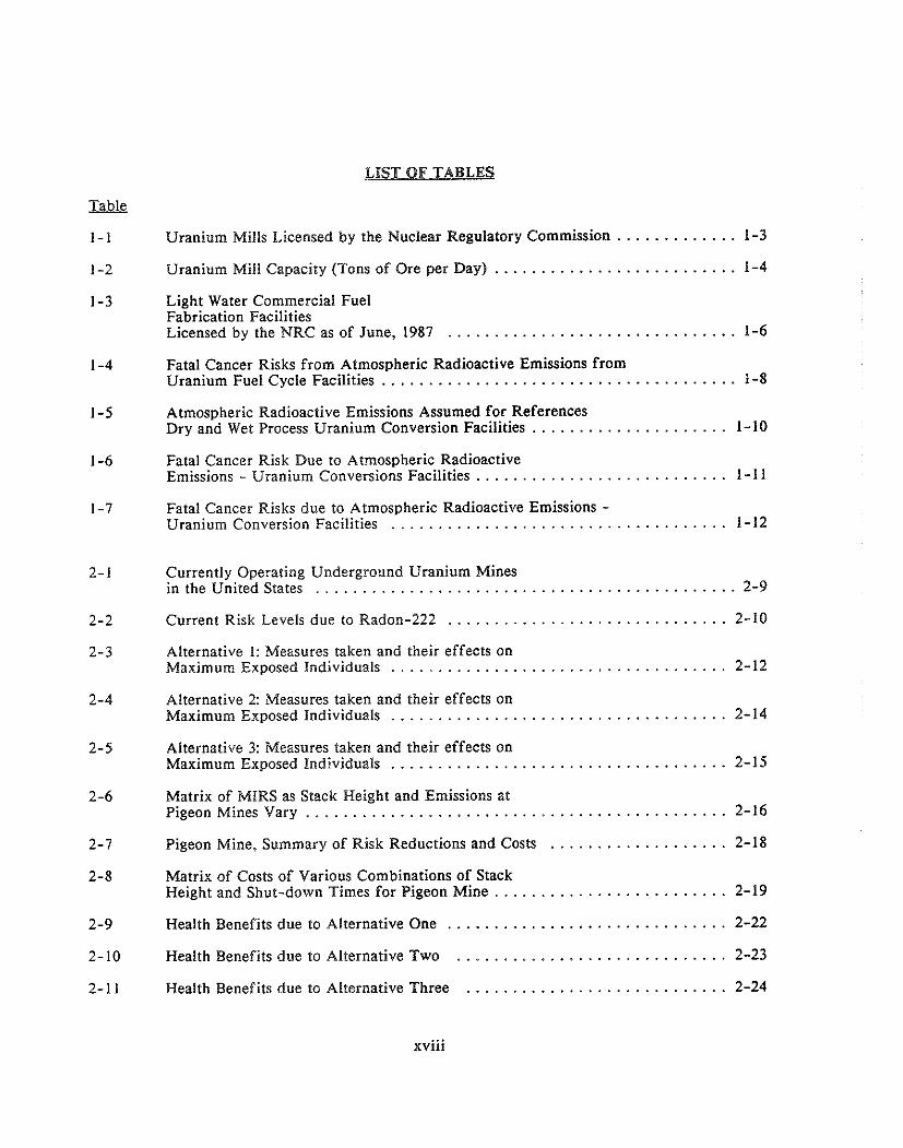
Uranium Mills Licensed by the Nuclear Regulatory Commission . . . . . . . . . . . . . 1-3
. . . . . . . . . . . . . . . . . . . . . . . . . . Uranium Mill Capacity (Tons of Ore per Day) 1-4
Light Water Commercial Fuel Fabrication Facilities Licensed by the NRC as of June. 1987 . . . . . . . . . . . . . . . . . . . . . . . . . . . .
Fatal Cancer Risks from Atmospheric Radioactive Emissions from . . . . . . . . . . . . . . . . . . . . . . . . . . . . . . . . . . . . . . Uranium Fuel Cycle Facilities 1-8
Atmospheric Radioactive Emissions Assumed for References Dry and Wet Process Uranium Conversion Facilities . . . . . . . . . . . . . . . . . . . . . 1-10
Fatal Cancer Risk Due to Atmospheric Radioactive Emissions . Uranium Conversions Facilities . . . . . . . . . . . . . . . . . . . . . . . . . . . 1-11
Fatal Cancer Risks due to Atmospheric Radioactive Emissions . . . . . . . . . . . . . . . . . . . . . . . . . . . . . . . . . . . . . Uranium Conversion Facilities 1-12
Currently Operating Underground Uranium Mines . . . . . . . . . . . . . . . . . . . . . . . . . . . . . . . . . . . . . . . . . . . . . in the United States 2-9
Current Risk Levels due to Radon-222 . . . . . . . . . . . . . . . . . . . . . . . . . . . . . . 2-10
Alternative I : Measures taken and their effects on . . . . . . . . . . . . . . . . . . . . . . . . . . . . . . . . . . . . Maximum Exposed Individuals 2-12
Alternative 2: Measures taken and their effects on Maximum Exposed Individuals . . . . . . . . . . . . . . . . . . . . . . . . . . . . . . . . . . . . 2-14
Alternative 3: Measures taken and their effects on . . . . . . . . . . . . . . . . . . . . . . . . . . . . . . . . . . . . Maximum Exposed Individuals 2-15
Matrix of MIRS as Stack Height and Emissions at Pigeon Mines Vary . . . . . . . . . . . . . . . . . . . . . . . . . . . . . . . . . . . . . . . . . . . . . 2-16
. . . . . . . . . . . . . . . . . . . Pigeon Mine. Summary of Risk Reductions and Costs 2-18
Matrix of Costs of Various Combinations of Stack Height and Shut-down Times for Pigeon Mine . . . . . . . . . . . . . . . . . . . . . . . . . 2-19
Health Benefits due to Alternative One . . . . . . . . . . . . . . . . . . . . . . . . . . . . . . 2-22
Health Benefits due to Alternative Two . . . . . . . . . . . . . . . . . . . . . . . . . . . . . 2-23
Health Benefits due to Alternative Three . . . . . . . . . . . . . . . . . . . . . . . . . . . . 2-24

LIST OF TABLES
. . . . . . . . . . . . . . . . . . . . . . . . . . . . . . . . . . . . . . . . . Costs of Alternative One 2-25
. . . . . . . . . . . . . . . . . . . . . . . . . . . . . . . . . . . . . . . . Costs of Alternative Two 2-26
. . . . . . . . . . . . . . . . . . . . . . . . . . . . . . . . . . . . . . . Costs of Alternative Three 2-26
. . . . . . . . . . . . . . . . . . . . . . . . Number of Miners and Shifts per Day by Mine 2-29
. . . . . . . . . . . . . . . . . . . Number of Miners and Mining Operations by County 2-29
Status and Planned Remedial Action at Inactive . . . . . . . . . . . . . . . . . . . . . . . . . . . . . . . . . . . . . . . . . . . . . . . . Uranium Mill Sites 3-4
Summary of Radon-222 Emissions from Inactive Uranium Mill Tailings Disposal Sites . . . . . . . . . . . . . . . . . .
Estimated Number of Persons Living Within 5 km of the Centroid of Tailings Disposal Sites for Inactive Mills . . . . . . . . . . . . . . . . . . . . . 3-9
Estimated Exposures and Risks to Nearby Populations . . . . . . . . . . . . . . . . . . . . . . . . . . . . . . . . . . Assuming Alternative Flux Rates 3-10
Estimated Fatal Cancers Per Year in the Regional (0-80km) . . . . . . . . . . . . . . . . . . . . . . . . . Populations Assuming ~I ternat ive Flux Rates 3-11
Estimated Distribution of Fatal Cancer Risks to the Regional (0-80km) Populations Assuming Alternative Flux Rates . . . . . . . . . . . . . . . . . . 3-13
Total and Annualized Risk and Reduction of Risk (Committed Cancers) of Loweri:g the Allowable Limit to 6 pci/m2/sec and to 2 pCi/m /sec . . . . . . . . . . . . . . . . . .
. . . . . . . . . . . . . . . . . . . . . Costs of Achieving the Doe Approved Design Flux 3-19
. . . . . . . . . . . . . . . . . . . . . . . . . . Costs of Achieving the 6 pci/m2/sec Option 3-20
. . . . . . . . . . . . . . . . . . . . . . . . . . Costs of Achieving the 2 p~i /m2/sec Option 3-21
Incremental Present Value Costs of Loyering the Allowable . . . . . . . . . . . . . . . . . . . . . . . . . . . Limit to 6 p~ i /m2/sec and to 2 pCi/m /sec 3-22
Incremental Annualized Cost of Lowering the Allowable Limit . . . . . . . . . . . . . . . . . . . . . . . . . . . . . . . . to 6 pci/m2/sec and to 2 p~ i /m2/sec 3-23
Status of U.S. Nuclear Power Plants as of December 31. 1986 . . . . . . . . . . . . . . . 4-6
Deliveries of Uranium to DOE Enrichment Plants by Domestic Utilities . . . . . . . . . . . . . . . . . . . . . . . . . . . . . . . . . . . . . . . 4-7
LIST OF TABLES
p&g-e
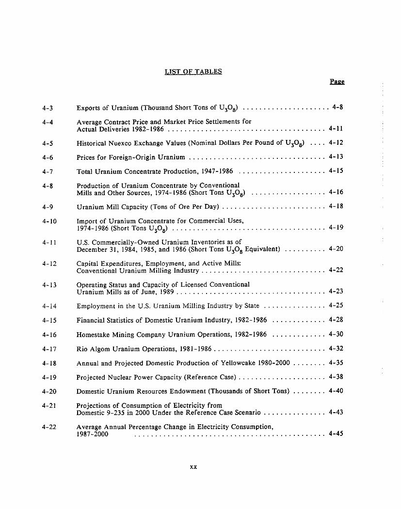
. . . . . . . . . . . . . . . . . . . . . . Exportso. Uranium (Thousand Short Tons of U.0. 4-8
Average Contract Price and Market Price Settlements for . . . . . . . . . . . . . . . . . . . . . . . . . . . . . . . . . . . . . . . . . . Actual Deliveries 1982- 4-1 1 .......... Historical Nuexco Exchange Values (Nominal Dollars U308 ) . . . . 4-12
. . . . . . . . . . . . . . . . . . . . . . . . . . . . . . . . . Prices for Foreign-Origin Uranium 4-13
. . . . . . . . . . . . . . . . . . . . . Total Uranium Concentrate Production. 1947- 1986 4-15
Production of Uranium Concentrate by Conventional . . . . . . . . . . . . . . . . . . Mills and Other Sources. 1974-1986 (Short Tons U308 ) 4-16
0. . . . . . . . . . . . . . . . . . . . . . . . . . Uranium Mill Capacity (Tons Ore Per Day) 4-18
Import of Uranium Concentrate for Commercial Uses. . . . . . . . . . . . . . . . . . . . . . . . . . . . . . . . . . . . . . 1974-1986 (Short Tons U308 ) 4-19
U.S. Commercially-Owned Uranium Inventories as of December 31. 1984. 1985. and 1986 (Short Tons U308 Equivalent) . . . . . . . . . . 4-20
Capital Expenditures. Employment. and Active Mills: . . . . . . . . . . . . . . . . . . . . . . . . . . . . . . Conventional Uranium Milling Industry 4-22
Operating Status and Capacity of Licensed Conventional Uranium Mills as of June. 1989 . . . . . . . . . . . . . . . . . . . . . . . . . . . . . . . . . . . . 4-23
Employment in the U.S. Uranium Milling Industry by State . . . . . . . . . . . . . . . 4-25
Financial Statistics of Domestic Uranium Industry. 1982-1986 . . . . . . . . . . . . . 4-28
Homestake Mining Company Uranium Operations. 1982-1986 . . . . . . . . . . . . . 4-30
Rio Algom Uranium Operations. 198 1 . 1986 . . . . . . . . . . . . . . . . . . . . . . . . . . . 4-32
Annual and Projected Domestic Production of Yellowcake 1980-2000 . . . . . . . . 4-35
Projected Nuclear Power Capacity (Reference Case) . . . . . . . . . . . . . . . . . . . . . 4-38
Domestic Uranium Resources Endowment (Thousands of Short Tons) . . . . . . . . 4-40
Projections of Consumption of Electricity from Domestic 9-235 in 2000 Under the Reference Case Scenario . . . . . . . . . . . . . . . 4-43
Average Annual Percentage Change in Electricity Consumption. 1987-2000 . . . . . . . . . . . . . . . . . . . . . . . . . . . . . . . . . . . . . . . . . . . . . . 4-45

LIST OF TABLES
E%s
Average Annual Percentage Change in Per Capita . . . . . . . . . . . . . . . . . . . . . . . . . . . . . . . . Electricity Consumption, 1987-2000 4-46
Employment Projects 1987-2000 (Person Years) . . . . . . . . . . . . . . . . . . . . . . . . 4-48
Summary of Operable Tailings Impoundment Areas Radium-226 Content at Operating and Standby Mills . . . . . . . . Summary of Radon Source Terms Calculated for Operable Mill Tailings Impoundments . . . . . . . . . . . . . . . . . . . . . . . . . . . . . . . 4-52
Estimated Number of Persons Living Within 5 km of the Centroid of Tailings Impoundments of Licensed Mills . . . . . . . Summary of Uranium Mill Tailings Impoundment Areas, Flux
. . . . . . . . . . . . . . . . . . . . Rates, and Post-UMTRCA Radon-222 Release Rates 4-55
Estimated Exposures and Risks to Individuals Living Near Operable Tailings Impoundments with No Controls. . . . . . . . . . . . . . . . . . . . . . 4-57
Estimated Fatal Cancers per Year in the Regional (0-80km) Populations Around Operable Tailings Impoundments . . . . . . . . . . . . . . . . . . . 4-58
Estimated Distribution of the Fatal Cancer Risk to the Regional Populations from Operable Tailings Piles . . . . . . .
Estimated Exposures and Risks to Nearby Populations Assuming Alternative Flux Rates . . . . . . . . . . . . . . . . . . . . . . . . . . . . . . . . . . 4-60
Estimated Fatal Cancers per Year in the Regional Populations . . . . . . . . . . . . . . . . . . . . . . . . . . . . . Assuming Alternative Radon Flux Rates 4-61
Estimated Distribution of Fatal Cancer Risk to the Regional . . . . . . . . . . . . . . . . . . . . . . . . . Populations Assuming Alternative Flux Rates 4-62
Total and Annualized,Risk and Reduction f Risk of Lowering P the Allowable flux Limit to 6 and 2 pCi/m /sec . . . . . . . . . . . . . . . . . . . . . . . . 4-68
Costs of Achieving the 20 pCi/m2/sec Option . . . . . . . . . . . . . . . . . . . . . . . . . . . . . . . . . . . . . . . . . . (1988 Dollars, Millions) 4-69
Costs of Achieving the 6 pCi/mZ/sec Option (1988 Dollars, Millions) . . . . . . . . . . . . . . . . . . . . . . . . . . . . . . . . . . . . . . . . . . 4-70
Costs of Achieving the 2 pCi/m2/sec Option (1988 Dollars, Million) . . . . . . . . . . . . . . . . . . . . . . . . . . . . . . . . . . . . . . . . . . 4-71
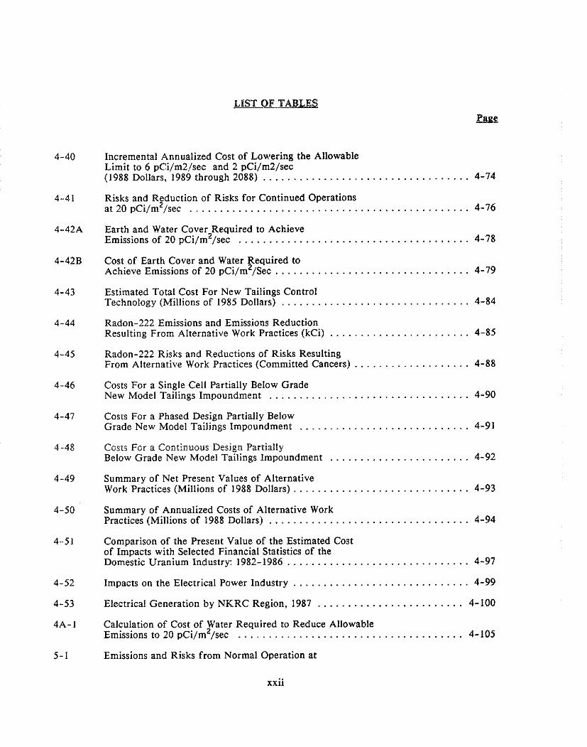
Incremental Present Value Cost of Lowering the Allowable Limit to 6 pCi/m2/sec and 2 pCi/m2/sec . (1988 Dollars, 1989 through 2088) . . . . . . . . . . . . . . . . . . . . . . . . . . . . . . . . . . 4-72
LIST OF TABLES
Incremental Annualized Cost of Lowering the Allowable Limit to 6 pCi/m2/sec and 2 pCi/m2/sec (1988 Dollars, 1989 through 2088) . . . . . . . . . . . . . . . . . . . . . . . . . . . . . . . . . . 4-74
Risks and Reduction of Risks for Continued Operations at 20 pci/m2/sec . . . . . . . . . . . . . . . . . . . . . . . . . . . . . . . . . . . . . . . . . . . . . . 4-76
Earth and Water Cover Required to Achieve Emissions of 20 p ~ i / m 2 / s e c . . . . . . . . . . . . . . . . . . . . . . . . . . . . . . . . . . . . . . 4-78
Cost of Earth Cover and Water Required to Achieve Emissions of 20 p ~ i / m 2 / ~ e c . . . . . . . . . . . . . . . . . . . . . . . . . . . . . . . . 4-79
Estimated Total Cost For New Tailings Control Technology (Millions of 1985 Dollars) . . . . . . . . . . . . . . . . . . . . . . . . . . . . . . . 4-84
Radon-222 Emissions and Emissions Reduction Resulting From Alternative Work Practices (kCi) . . . . . . . . . . . . . . . . . . . . . . . 4-85
Radon-222 Risks and Reductions of Risks Resulting From Alternative Work Practices (Committed Cancers) . . . . . . . . . . . . . . . . . . . 4-88
Costs For a Single Cell Partially Below Grade New Model Tailings Impoundment . . . . . . . . . . . . . . . . . . . . . . . . . . . . . . . . . 4-90
Costs For a Phased Design Partially Below Grade New Model Tailings Impoundment . . . . . . . . . . . . . . . . . . . . . . . . . . . . 4-91
Costs For a Continuous Design Partially Below Grade New Model Tailings Impoundment . . . . . . . . . . . . . . . . . . . . . . . 4-92
Summary of Net Present Values of Alternative Work Practices (Millions of 1988 Dollars) . . . . . . . . . . . . . . . . . . . . . . . . . . . . . 4-93
Summary of Annualized Costs of Alternative Work Practices (Millions of 1988 Dollars) . . . . . . . . . . . . . . . . . . . . . . . . . . . . . . . . . 4-94
Comparison of the Present Value of the Estimated Cost of Impacts with Selected Financial Statistics of the Domestic Uranium Industry: 1982-1986 . . . . . . . . . . . . . . . . . . . . . . . . . . . . . . 4-97
Impacts on the Electrical Power Industry . . . . . . . . . . . . . . . . . . . . . . . . . . . . . 4-99
Electrical Generation by NKRC Region, 1987 . . . . . . . . . . . . . . . . . . . . . . . . 4-100
Calculation of Cost of Water Required to Reduce Allowable Emissions to 20 pci/m2/sec . . . . . . . . . . . . . . . . . . . . . . . . . . . . . . . . . . . . . 4-105
Emissions and Risks from Normal Operation at

. . . . . . . . . . . . . . . . . . . . . . . . . . . . . . . . . . . . . . . . . . HLW Disposal Facilities 5-4
. . . . . . . . . . . . . . . . . . . . . . . . . . . . . . . . . . . . Department of Energy Facilities 6-2
. . . . . . . . . . . . . . . . . . . . . Summary of Estimated Risks Around DOE Facilities 6-4
DOE Facilities Fatal Cancer Risks With and Without Supplementary . . . . . . . . . . . . . . . . . . . . . . . . . . . . . . . . . . . . . . . . . . . . Alternative 4 Controls 6-8
Controls. Risk Reduction. and Costs Associated with . . . . . . . . . . . . . . . . . . . . . . . . . . . . . . . . . . . Meeting Alternative 4. by Facility 6-9
. . . . . . . . . . Exposures and Risks to Nearby Individuals From DOE Radon Sites 7-5
Estimated Fatal Cancers Per Year; in the Regional (0-80km) . . . . . . . . . . . . . . . . . . . . . . . . . . . . . . . . Populations Around DOE Radon Sites 7-6
Costs and Reduced Risks Resulting from Covering the Sources to Lower Radon Flux Rates to 20 pCi/m2/sec . . . . . . . . . . . . . .
Costs and Reduced Risks Resulting from Covering the Sources to Lower . . . . . . . . . . . . . . . . . . . . . . . . . . . . . . . . . . . Radon Flux Rates to pCi/m2/sec 7-12
Costs and Reduced Risks Resulting from Covering the Sources to Lower Radon Flux Rates to 2 pCi/m2/sec . . . . . . . . . . . . .
Reduction in Emissions and Cancer Rates Attributable to Controls: U.S. Totals . . . . . . . . . . . . . . . . . . . . . . . . . . . . . . . . . . . . . . . . . . 7-15
Incremental Costs and Risk Reductions for Various Flux Standards . . . . . . . . . . . . . . . . . . . . . . . . . . . . . . . . . . .
Net Present Value of Cost of Supplemental Contracts to Meet a Flux of 20 pCi/m2/sec at DOE Radon Facilities: U.S. Total . . . . . . . . . . . . . . . . . . . . . . . . . . . . . . . . . . . . . . . . . . . . . . 7-18
Production and Shipment of Elemental Phosphorus .. 1964-1987 (tons) . . . . . . . 8-4
. . . . . . . . . . . . . . . . . . . . . . . . . . . . . . . . . . . . . Uses for Phosphorus Chemicals 8-5
. . . . . . . . . . . . . . . . . . Elemental Phosphorus Producers and Estimated Capacity 8-8
U.S. Capacities for Phosphorus and Phosphorus Chemicals - 1985 . . . . . . . . . . . . 8-9
. . . . . . . . . . . . . . . . . . . . . . . . . . . ElementaI Phosphorus Production Capacity 8-11
Revenues from Elemental Phosphorus Production and Total Corporate Revenues 8-12
. . . . . . . . . . . . . . . . . . . . . . . . Elemental Phosphorus Market Share: Monsanto 8-14
LIST OF TABLES
Ems
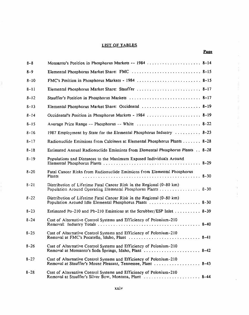
Monsanto's Position in Phosphorus Markets .. 1984 . . . . . . . . . . . . . . . . . . . . . 8-14
Elemental Phosphorus Market Share: FMC . . . . . . . . . . . . . . . . . . . . . . . . . . . 8-15
FMC's Position in Phosphorus Markets . 1984 . . . . . . . . . . . . . . . . . . . . . . . . . 8-15
Elemental Phosphorus Market Share: Stauffer . . . . . . . . . . . . . . . . . . . . . . . . . 8-17
Stauffer's Position in Phosphorus Markets . . . . . . . . . . . . . . . . . . . . . . . . . . . . 8-17
Elemental Phosphorus Market Share: Occidental . . . . . . . . . . . . . . . . . . . . . . . 8-19
Occidental's Position in Phosphorus Markets . 1984 . . . . . . . . . . . . . . . . . . . . . 8-19
Average Price Range .. Phosphorus .. White . . . . . . . . . . . . . . . . . . . . . . . . . 8-22
1987 Employment by State for the Elemental Phosphorus Industry . . . . . . . . . . 8-23
Radionuclide Emissions from Calciners at Elemental Phosphorus Plants . . . . . . . 8-28
Estimated Annual Radionuclide Emissions from Elemental Phosphorus Plants . . 8-28
Populations and Distances to the Maximum Exposed Individuals Around Elemental Phosphorus Plants . . . . . . . . . . . . . . . . . . . . . . . . . . . . . . . . . . . . . . 8-29
Fatal Cancer Risks from Radionuclide Emissions from Elemental Phosphorus Plants . . . . . . . . . . . . . . . . . . . . . . . . . . . . . . . . . . . . . . . . . . . . . . 8-30
Distribution of Lifetime Fatal Cancer Risk in the Regional (0-80 km) Population Around Operating Elemental Phosphorus Plants . . . . . . . . . . . . . . . . 8-30
Distribution of Lifetime Fatal Cancer Risk in the Regional (0-80 km) Population Around Idle Elemental Phosphorus Plants . . . . . . . . . . . . . . . . . . . . 8-30
Estiinated Po-210 and Pb-210 Emissions at the Scrubber/ESP Inlet . . . . . . . . . . 8-39
Cost of Alternative Control Systems and Efficiency of Polonium-210 Removal: Industry Totals . . . . . . . . . . . . . . . . . . . . . . . . . . . . . . . . . . . . . . . . 8-40
Cost of Alternative Control Systems and Efficiency of Polonium-210 Removal at FMC's Pocatello. Idaho. Plant . . . . . . . . . . . . . . . . . . . . . . . . . . . . 8-41
Cost of Alternative Control Systems and Efficiency of Polonium-210 Removal at Monsanto's Soda Springs. Idaho. Plant . . . . . . . . . . . . . . . . . . . . . . 8-42
Cost of Alternative Control Systems and Efficiency of Polonium-210 Removal at Stauffer's Mount Pleasant. Tennessee. Plant . . . . . . . . . . . . . . . . . . 8-43
Cost of Alternative Control Systems and Efficiency of Polonium-210 Removal at Stauffer's Silver Bow. Montana. Plant . . . . . . . . . . . . . . . . . . . . . . 8-44
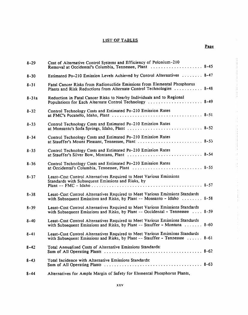
Cost of Alternative Control Systems and Efficiency of Polonium-210 . . . . . . . . . . . . . . . . . . . . Removal at Occidental's Columbia, Tennessee, Plant 8-45
Estimated Po-210 Emission Levels Achieved by Control Alternatives . . . . . . . . 8-47
Fatal Cancer Risks from Radionuclide Emissions from Elemental Phosphorus Plants and Risk Reductions from Alternate Control Technologies . . . . . . . . . . . 8-48
Reduction in Fatal Cancer Risks to Nearby Individuals and to Regional . . . . . . . . . . . . . . . . . . . . . Populations for Each Alternate Control Technology 8-49
Control Technology Costs and Estimated Po-210 Emission Rates . . . . . . . . . . . . . . . . . . . . . . . . . . . . . . . . . . . at FMC's Pocatello, Idaho, Plant 8-51
Control Technology Costs and Estimated Po-210 Emission Rates . . . . . . . . . . . . . . . . . . . . . . . . . . . . . at Monsanto's Soda Springs, Idaho, Plant 8-52
Control Technology Costs and Estimated Po-210 Emission Rates . . . . . . . . . . . . . . . . . . . . . . . . . at Stauffer's Mount Pleasant, Tennessee, Plant 8-53
Control Technology Costs and Estimated Po-210 Emission Rates . . . . . . . . . . . . . . . . . . . . . . . . . . . . . at Stauffer's Silver Bow, Montana, Plant 8-54
Control Technology Costs and Estimated Po-210 Emission Rates . . . . . . . . . . . . . . . . . . . . . . . . . . . at Occidental's Columbia, Tennessee, Plant 8-55
Least-Cost Control Alternatives Required to Meet Various Emissions Standards with Subsequent Emissions and Risks, by
. . . . . . . . . . . . . . . . . . . . . . . . . . . . . . . . . . . . . . . . . Plant -- FMC - Idaho . . 8-57
Least-Cost Control Alternatives Required to Meet Various Emissions Standards with Subsequent Emissions and Risks, by Plant -- Monsanto - Idaho . . . . . . . . 8-58
Least-Cost Control Alternatives Required to Meet Various Emissions Standards with Subsequent Emissions and Risks, by Plant -- Occidental - Tennessee . . . . 8-59
Least-Cost Control Alternatives Required to Meet Various Emissions Standards with Subsequent Einissions and Risks, by Plant -- Stauffer - Montana . . . . . . . 8-60
Least-Cost Control Alternatives Required to Meet Various Emissions Standards with Subsequent Emissions and Risks, by Plant .. Stauffer - Tennessee . . . . . . 8-61
Total Annualized Costs of Alternative Emissions Standards: . . . . . . . . . . . . . . . . . . . . . . . . . . . . . . . . . . . . . . Sum of All Operating Plants 8-62
Total Incidence with Alternative Emissions Standards: . . . . . . . . . . . . . . . . . . . . . . . . . . . . . . . . . . . . . . Sum of All Operating Plants 8-63
Alternatives for Ample Margin of Safety for Elemental Phosphorus Plants,
. . . . . . . . . . . . . . . . . . . . . . . . . . . . . . According to Various Emissions Levels 8-65
Alternatives for Ample Margin of Safety for Elemental Phosphorus Plants. . . . . . . . . . . . . . . . . . . . . . . . . . . . . . . . Using Different Control Technologies 8-68
. . . . . . . . . . . . . . . . . . . . . . . . . . . . . . . . . . . . . Cost of Elemental Phosphorus 8-73
. . . . . . . . . . . . . . . . . Costs of Phosphate Rock Used in Phosphorus Production 8-75
. . . . . . . . . . . . . . . . . . . . Costs of Electricity Used in Phosphorus Productions 8-77
Labor Costs . . . . . . . . . . . . . . . . . . . . . . . . . . . . . . . . . . . . . . . . . . . . . . 8-78
. . . . . . . . . . . . . . . . . . . . . . . . . . . . . . . . Summary of Cost Estimates. by Plant 8-79
Revenues from Elemental Phosphorus Production and Total Corporate Revenues 8-82
. . . . . . . . . . . . . . . . . . . . . . . . . . . . . . . . . . . . Impact on Capital Expenditures 8-84
Production of Phosphoric Acid. Wet Process Phosphoric Acid. . . . . . . . . . . . . . . . . . . . . . . . . . . . . . . . . . and Phosphate Fertilizer Metric Tons 9-4
Price of Phosphoric Acid. Sulfur. Phosphate Rock and Diarnmonium Phosphate . . . . . . . . . . . . . . . . . . . . . . . . . . . 9-8
. . . . . . . . . . . . . . . . . . . . . . . . . . . . . . . Phosphate Fertilizer Production Costs 9-10
Phosphate Rock Statistics on World . . . . . . . . . . . . . . . . . . . . . . . . . . . . . . . . . . . . . Supply Rock Mining Capacity 9-13
Phosphate Rock Statistics on World . . . . . . . . . . . . . . . . . . . . . . . . . . . . . . . . Supply Demonstrated Rock Reserves 9-14
. . . . . . . . . . . . . . . . . . . . . . . . . . . . . U.S. Sulphur Recover Trends 1980-1985 9-21
. . . . . . . . . . . . . . . . . . . . . . . . . . . . Financial Condition of Phosphate Industry 9-25
Producers of Phosphate Rock. Wet Process Phosphoric. . . . . . . . . . . . . . . . and Phosphate Fertilizers (Thousand Metric Tons Per Year) 9-26
Capacities of Major Phosphoric Acid Producers. Estimates . . . . . . . . . . . . . . . . . . . . . . . . . . . . . . . . for 1988/89 (Metric Tons Per Year) 9-27
. . . . . . . . . . . . . . . . . . . . . . . . . . Operating Rates for U.S. Fertilizer Producers 9-28
. . . . . . . . . . . . . . . . . . . . . Employment in the Phosphate Industry (Thousands) 9-34
U.S. Exports of Phosphate Fertilizers . . . . . . . . . . . . . . . . . . . . . . . . . . . (Thousand Metric Tons. Thousand Dollars) 9-45
LIST OF TABLES
EBs
Trade in Phosphate Products by Major Exporter. 1981-1984 Phosphate Fertilizer (Metric Tons. P205) . . . . . . . . . . . . . . . . . . . . . . . . . . . . . 9-47
Summary of World Phosphate Fertilizer Demand Forecasts (Million Nutrient Metric Tons P205) . . . . . . . . . . . . . . . . . . . . . . . . . . . . . . . . 9-49
Forecasts of Fertilizer Demand by Region and . . . . . . . . . . . . . . . . . . . . . . . . . . . . . . . . . . . . . . . . . . . . . Source. 1995-2000 9-51
. . . . . . . . . . . . . . . . . . . . . . . . . . . . . . . . . . . . . . . . . . . . . . Stack Parameters 9-61
Radon Flux Rates by Regional Group . . . . . . . . . . . . . . . . . . . . . . . . . . . . . . . 9-63
Incremental Cancer Risks Associated With Exposure to Radon Emitted From Phosphogypsum Stacks with No Controls . . . . . . . . . . 9-64
Control Parameters for Representative Stacks . . . . . . . . . . . . . . . . . . . . . . . . . . 9-66
Reduction in Risk to the Most Exposed Individual . . . . . . . . . . . . . . . . . . . . . . 9-70
Reduction in Risk to Population Within 80km of Stack . . . . . . . . . . . . . . . . . . . 9-71
Cost Effectiveness of Control in Terms of Emission Reductions . . . . . . . . . . . . 9-73
Cost of Controlling Radon in Dollars Per IOOO/MT of Plant Capacity. Annualized Over A Five Year Period . . . . . . . . . . . . . . . . . . . . 9-80
World Market Share of U.S. P 0 Producers Exports in Absence of Radon Control Measures in 166 MT (Lower Phosphate Rock Cost) . . . . . . . . . 9-89
World Market Share of U.S. P 0 Producers Exports in Absence of Radon Control Measures in 1 6 8 MT (Higher Phosphate Rock Cost) . . . . . . . . . 9-90
Coal Ash Distribution by Boiler Type . . . . . . . . . . . . . . . . . . . . . . . . . . . . . . . 10-4
Numbers and Capacities of Industrial Boilers . . . . . . . . . . . . . . . . . . . . . . . . . . 10-5
Typical Uranium and Thorium Concentrations in Coal . . . . . . . . . . . . . . . . . . . 10-7
U-238 Emission Factors for Coal-Fired Utility Boilers . . . . . . . . . . . . . . . . . . . 10-9
Th-232 Emission Factors for Coal-Fired Utility Boilers . . . . . . . . . . . . . . . . 10-10
Estimated Radiation Dose Rates from Large Coal-Fired Utility Boilers . . . . . . 10-12
Estimated Radiation Dose Rates from the Keference Coal-Fired Industrial Boiler . . . . . . . . . . . . . . . . . . . . . . . . . . .
LIST OF TABLES
10-8 Estimated Distribution of the Fatal Cancer Risk to the Regional (0-80km) Populations from A11 Coal-Fired Utility Boilers . . . . . . . . . . . . . . . . 10-14
10-9 Estimated Distribution of the Fatal Cancer Risk to the Regional (0-80km) Populations from All Coal-Fired Industrial Boilers . . . . . . . . . . . . . 10-15
. . . . . . . . . . . . 11-1 NRC Licensed and Non-DOE Facilities Fatal Cancers Per Year 11 -4
11-2 Costs and Benefits for Controls on the Two Sources for Which Controls are Required . . . . . . . . . . . . . . . . . . . . . . . . . . . . . . . . . . . 11-8
. . . . . . . . . 12-1 Number of Significant Production Surface Uranium Mines by State 12-4
12-2 Reasonably Assured Resources by Mining Method At the End of 1986 in the U.S. (million pounds of U30,,)
. . . . 12-3 United States and Selected Foreign Uranium Resources as of End of 1986. 12-6

LIST OF FIGURES
. . . . . . . . . . . . . . . . . . . . . . . . . . . . . . . . . . Costs of Controls by Stack Height 2-19
. . . . . . . . . . . . . . . . . . . . . . . . . . . . . . . Cost of Lowering the Allowable Flux 3-24
. . . . . . . . . . . . . . . . . . . . . . . . . . . . . . . . . . . . . . . Sources of Uranium Supply 4-37
. . . . . . . . . . . . . . . . . . . . . . . . . . . . . . . . . . . . . . . . U.S. Uranium Production 4-37
. . . . . . . . . . . . . . . . . . . . . . . . . . . Model Impoundment Emissions (kCi/Year) 4-86
. . . . . . . . . . . . . . . . . . . . . . . . . . . . . . . . . . Price of Pz05 and Related Products 9-7
. . . . . . . . . . . . . . . . . . . . . . . . . . . . . . . . . Uses for Phosphoric Acid. 1985-86 9-23
. . . . . . . . . . . . . . . . . . . . . . . . . . . . . . . . United States Fertilizer Consumption 9-38
. . . . . . . . . . . . . . . . . . . . . . . . . . . . . . U.S. P205 Exports (Lower Rock Costs) 9-92
. . . . . . . . . . . . . . . . . . . . . . . . . . . . . . U.S. P205 Exports (Higher Rock Costs) 9-92
. . . . . . . . . . . . . . . Uranium Production U.S. Open-Pit Mines and Total Output 12-3


CHAPTER 1
URANIUM WEL. C V a E

1. U R A N I U M F U E L CYCLE FACILITIES
1.1 Introduction and Summarv
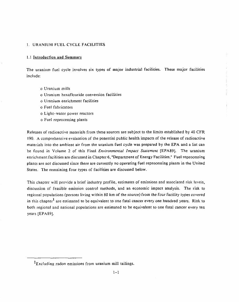
The uranium fuel cycle involves six types of major industrial facilities. These major facilities
include:
o Uranium mills
o Uranium hexaflouride conversion facilities
o Uranium enrichment facilities
o Fuel fabricators
o Light-water power reactors
o Fuel reprocessing plants
Releases of radioactive materials from these sources are subject to the limits established by 40 CFR
190. A comprehensive evaluation of the potential public health impacts of the release of radioactive
materials into the ambient air from the uranium fuel cycle was prepared by the EPA and a list can
be found in Volume 2 of this Final Environn~ental Impact Stalement [EPA89]. The uranium
enrichment facilities are discussed in Chapter 6 , "Department of Energy Facilities." Fuel reprocessing
plants are not discussed since there are currently no operating fuel reprocessing plants in the United
States. The remaining four types of facilities are discussed below.
This chapter will provide a brief industry profile, estimates of emissions and associated risk levels,
discussion of feasible emission control methods, and an economic impact analysis. The risk to
regional populations (persons living within 80 km of the source) from the four facility types covered 1 in this chapter are estimated to be equivalent to one fatal cancer every one hundred years. Risk to
both regional and national populations are estimated to be equivalent to one fatal cancer every ten
years [EPA89].
l ~ x c l u d i n ~ radon emissions from uranium mill tailings.
1-1

1.2 Industrv Profile
1.2.1 Introduction
The four major components of the uranium fuel cycle included in this chapter are uranium mills,
uranium conversion facilities, fuel fabrication facilities, and nuclear power facilities. These facilities
are licensed by the Nuclear Regulatory Commission (NRC) or the Agreement States. Each of these
four facility types are briefly described below. More detailed descriptions for some may be found
in complementary chapters for uranium mill tailing piles and uranium enrichment plants. A fifth
major component, uranium enrichment facilities, are owned by the Federal government and operated
by contractors under the direction of the Department of Energy (DOE). Enrichment facilities are
considered in Chapter 6.
1.2.2 Uranium Mills
A detailed profile of the uranium mill industry is contained in Chapter 4: "Licensed Uranium Mill
Tailings." Although there are 27 uranium mills within the U.S., only four were operating in 1988.
Of the remainder, eight were on standby, fourteen were being decommissioned and one was never
operated. The four operating mills have a total capacity of 9,600 tons of ore per day, reflecting a
decline in capacity from 50,000 tons per day in 1981 when 21 plants were in operation, (Tables l -
I and 1-2 present data on milling capacity and the recent capacity trends). These developments are
due to a combination of I ) rising imports and 2) declining demand resulting from cancellation of
nuclear power plant construction projects. Domestic production of yellowcake, the product of
uranium milling, is expected to increase over ten percent by the year 2000, but short-run forecasts
of domestic production call for a continuing decline [DOE87b]. The financial strength of the
industry has weakened considerably since its peak demand years in late 1970's and early 1980's. The
industry was unprofitable for three of the past five years.
1.2.3 Uranium Conversion Facilities
There are two commercially operating conversion facilities in the United States. These facilities
purify uranium oxide or yellowcake to uranium hexafluoride (UF6), the chemical form of the
uranium entering the enrichment plant. The two conversion facilities are the Allied Chemical
Corporation facility at Metropolis, Illinois and the Kerr-McGee Nuclear Corporation at Sequoyah,
Oklahoma. The Allied plant is a dry process plant with a capacity of 12,600 metric tons per year and
has been operational since 1968, while the Kerr-McGee plant is a wet process plant with a capacity

Table 1-1: Uranium Mills Licenses by the U.S. Nuclear Regulatory Commission as of December I . 1988
Licensee
American Nuclear Anaconde Atlas Minerals Bear Creek Uranium Bodum Resources Chevron Resources Conoco-Pioneer Cotter Dawn Mining Exxon Exxon Minerals Homestake Mining BP American Minerals Exploration Pathfinder Mines Pathfinder Mines Petrotomics Plateau Resources Quivira Rio Alogm TVA Umetco Minerals Umetco Minerals Umetco Minerals U N C Mining Western Nuclear Western Nuclear
Location
Gas Hills. WY
Moab, U T Converse Co., WY Marouez. NM ~ a n n a aria, T X Falls City, T X Cannon City, CO Ford, WA Ray Point, T X Converse Co., WY Grants, NM Seboyeta, NM Sweetwater Co., WY Gas Hills, WY Shirley Basin, WY Shirley Basin, WY Shootaring, U T Ambrosia Lake, NM La Sat, U T Edgemont, SD Gas Hills, WY Blanding, UT Uravan, CO Church Rock, NM Jeffrey City, WY Wellpinit, WA
Rated Capacity
(tons/day)
950 6000 1400 2000 2000 2500 3400 1200 450 - -
3200 3400 1600 3000 2500 1700 1500 750 - -
750 - -
1400 2000 1300 3000 1700 2000
STATUS CODES: PROCESS CODES:
= Facility Operating 1 = Acid Leach Facility Shutdown 2 = Alkaline Leach
= Facility Being Decommissioned 3 = Solvent Extraction = Facility Built, Never Operated 4 = Carbonate Leach
5 = Eluex 6 = Caustic Precipitation 7 = Column ion exchange
Status Process
SOURCE: [EPA89]
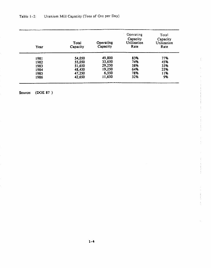
Table 1-2 Uranium Mill Capacity (Tons of Ore pea Day)
Year
Operating Total Capacity Capacity
Total Operating Utilization Utilization Capacity Capacity Rate Rate
Source: (DOE 87 )
of 9,100 tons per year that has operated since 1970 [AEC7J, DOE881. It is anticipated that the
existing uranium conversion plants will be able to accommodate the future demand for uranium by
nuclear power plants.
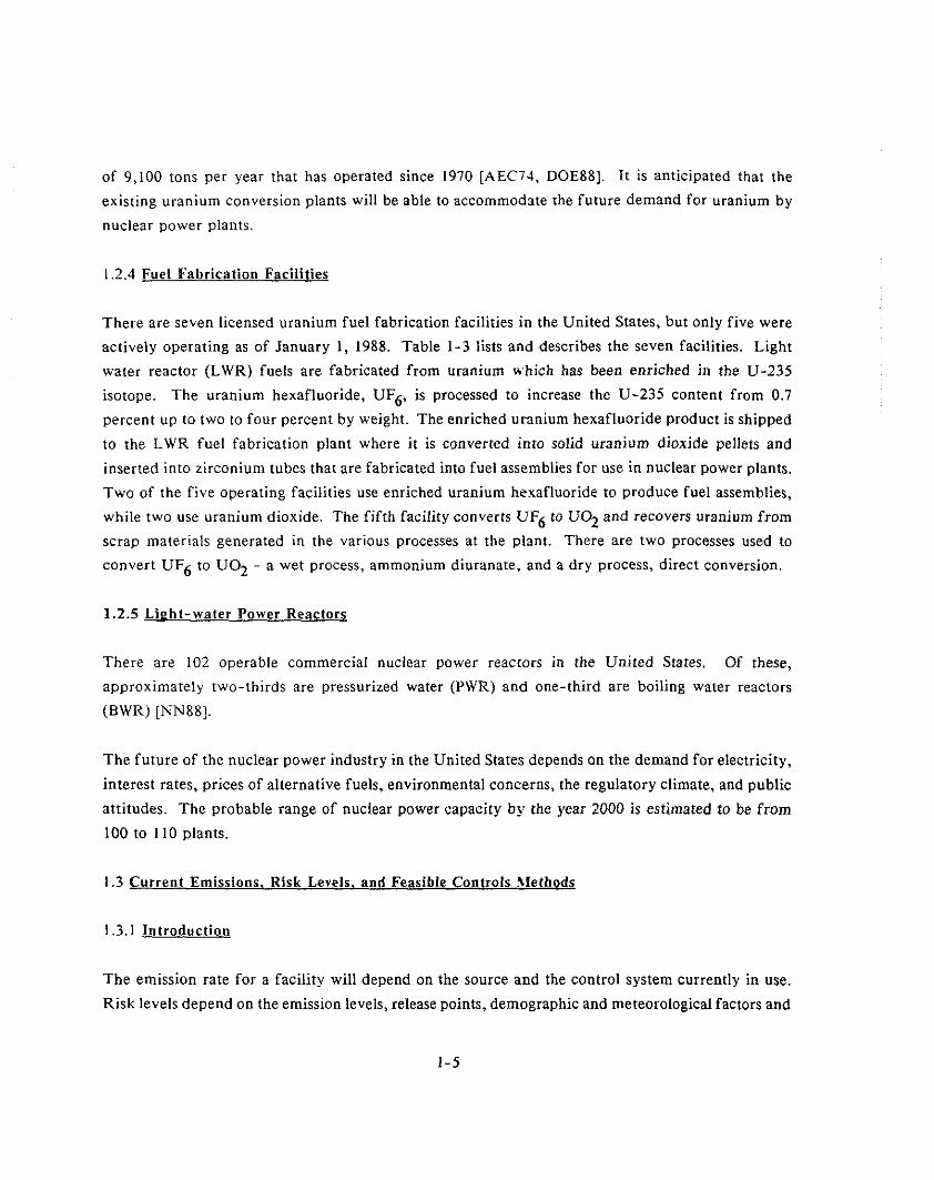
1.2.4 Fuel Fabrication Facilities
There are seven licensed uranium fuel fabrication facilities in the United States, but only five were
actively operating as of January 1, 1988. Table 1-3 lists and describes the seven facilities. Light
water reactor (LWR) fuels are fabricated from uranium which has been enriched in the U-235
isotope. The uranium hexafluoride, UFg, is processed to increase the U-235 content from 0.7
percent up to two to four percent by weight. The enriched uranium hexafluoride product is shipped
to the LWR fuel fabrication plant where it is converted into solid uranium dioxide pellets and
inserted into zirconium tubes that are fabricated into fuel assemblies for use in nuclear power plants.
Two of the five operating facilities use enriched uranium hexafluoride to produce fuel assemblies,
while two use uranium dioxide. The fifth facility converts UF6 to U02 and recovers uranium from
scrap materials generated in the various processes at the plant. There are two processes used to
convert UF6 to U 0 2 - a wet process, ammonium diuranate, and a dry process, direct conversion.
1.2.5 Lieht-water Power Reactors
There are 102 operable commercial nuclear power reactors in the United States. Of these,
approximately two-thirds are pressurized water (PWR) and one-third are boiling water reactors
(BWR) [NNSS].
The future of the nuclear power industry in the United States depends on the demand for electricity,
interest rates, prices of alternative fuels, environmental concerns, the regulatory climate, and public
attitudes. The probable range of nuclear power capacity by the year 2000 is estimated to be from
100 to 110 plants.
1.3.1 Introduction
The emission rate for a facility wilt depend on the source and the control system currently in use.
Risk levels depend on the emission levels, release points, demographic and meteorological factors and

Table 1-3: Light Uater Commercial Fuel Fabrication Fac i l i t ies Licensed by the Nuclear Regulatory Cmiaaion as o f June, 1987.
1980 Operating Proccas Used operating License
Fac i l i ty t o Convert Capacity as of L i censee ~oca t ion operations UF6 t o UOZ Final Product ttonslycar) J m 1987 = = = S = I E = = ~ - l = I L ~ ~ = 3 ~ = - ~ 3 - - - C - _--a___I__E==l====_
Advanced Nuclear Fuels
Babcock L Nilcox - CNFP
Babcock & U i lcox
Rf chland, LEU a/ Conversion Dry L Uet Complete Fuel 650 NO Vashington (UF6 t o U02), A s s b l i e s
Fabrication L Scrap Recovery; Corercia1 LUR Fuel
Lynchburg, Virginia
LEU Fabrication; Use W2 Powder (250) YES Cwuicrcial LUR Fuel --- t o P d u c e Fuel
Assnblier
m l l o , Authorized Decontam- Vet WZ Powder Pennsylvania ination; Pmding
Nuclear Rcactor service operations
Combustion Uindsor, LEU Fabrication; Use UOZ Powder (150) YES Engineering Connecticut Commer~ial LUR Fuel --- t o Produce Fuel
Y Asanblies 0
Colbustion Hematite, LEU cmversion D ~ Y W ? Powder Engineering Uiaswri (UF6 t o U02) &
scrap Recovery
150 YES
General Ui Lmington, LEU C m v e r ~ i m Dry P Vet Conplcta Fuel 1,5W YES Electric North Camlina (UF6 t o WZ) L Assnblies
Fabrication; Commercial LUR Fuel
Vestinghwse Colulbia, LEU Conversion Dry L Uet Complete Fuel 750 YES Electric South Carolina (UF6 t o W); A s s b l i e s
Fabricstion 8 Scrap Recovery; Collercial LUR Fuel
- - - - - - - TOTAL 3,m
a1 Low enrichment uranium
Source: CEPA893

the pathways for exposure or ingestion. Estimates of exposure and lifetime fatal cancer risks to
nearby individuals and to those within an 80 kilometer radius serve as the basis for the risk
assessments. The risks are summarized in Table 1-4 for both nearby and regional populations
[EPA89].
1.3.2 Current Emissions and Estimated Risk Leveh.
1.3.2.1 Uranium Mills
Emissions of radionuclides from uranium mills include those created during ore storage and milling
processes, and those emitted by the mill tailings. Radon emissions from mill tailings piles are
discussed in Chapter 4 of this volume and are not considered in this chapter.
Emissions from ore storage result from the drying of the ore and its subsequent entrainment by wind
or from transfer operations. The milling process includes the crushing and grinding of ore and the
leaching of uranium from the ore through either acid or alkaline processing, depending upon the
lime content of the ore. The precipitate that is formed is then dried in large ovens and packaged for
transport. After the uranium product that can be extracted by leaching is separated from the ore,
the remaining ore is pumped as slurry to a tailings impoundment area. A portion of the liquid is
recovered and recycled, while the remainder is allowed to evaporate, producing a solid tailings pile
composed of a sand fraction and a slime fraction. Active tailings piles contain both wet and dry
areas. As sections dry out, the tailings can become a source of windblown dust. The dried slime
component is particularly prone to becoming windborne due to its small particle size. The process
steps that generate the significant emissions (other than radon from tailings piles) are crushing,
drying, and packaging. Ninety percent of the U-234 and U-238 are released from the dryer area,
while the Th-230 and Ra-226 emissions result primarily from operations such as crushing.
Emissions for this source category are analyzed in detail in Chapter 4 of Volume 2 of the
Environmenlal lnzpact Statement, including a description of the basis for the site-specific and model
facilities used to assess the airborne releases of radionuclides from uranium mills. Also presented is
information on the source term, meteorological, and demographic assumptions. Site-specific source
term, meteorological, and demographic data for each of the four operating mills and for six of the
seven mills on standby, were supplied as input to the assessment codes. A model mill was used for
the assessment of doses and risks from the tailings piles of inactive mills. Outputs of the codes
include estimates of: dose equivalents to the most exposed individuals (mrem/y); lifetime fatal

Table 1-4 Fatal Cancer Risks from Atmospheric Radioactive Emission from Uranium Fuel Cycle Facilities (Excluding Radon from Tailing Piles)
Highest Individual Regional (0-80 km) Lifetime Fatal Population
Facility Cancer Risk Deaths/y
Uranium Mills Ambrosia Lake 2E-7 3E-5 Homestake 2E-4 2E-3 La Sal 2E-6 3E-5 Lucky Mc IE-7 7E-6 Panna Maria 3E-6 5E-5 Sherwood IE-6 8E-5 Shirley Basin 6E-7 9E-5 Shootaring 2E-7 7E-7 Sweetwater 7E-7 2E-5 White Mesa 6E-7 2E-5 Model Inactive Tailings 2E-4 IE-4
---- Total 2E-3
Uranium Conversion Dry 3E-5 8E-4 Wet 4E-5 6E-4
Fuel Fabrication 4E-6 8E-5
Nuclear Power Reactors Pressurized Water Reactors 3E-6
Boiling Water Reactors
cancer risk to the most exposed individuals; dose equivalents to the regional (0-80 km) population
(person-rem/y); and the number of cancer deaths in the regional population per year of operation
(deaths/year).
The fatal cancer risks are summarized in Table 1-4 for both nearby and regional populations affected
by either operating or closed mills. The total deaths per year in the 80 km regional population for
uranium mill segment of the source category is estimated to be 2E-3.
Two processes are used to convert uranium oxide to uranium hexaflouride. The dry hydrofluor
process generates higher uranium emissions than the solvent extraction process since large amounts
of dust are produced in the sampling, pre-treatment, and reaction stages. The solvent extraction
process releases uranium as both soluble and insoluble aerosols which are vented to the environment.
The atmospheric emissions used in the risk assessments for the reference dry and wet conversion
facilities are shown in Table 1-5. The plant parameters utilized are specific to each plant [NRC 84,
NRC85bI. Table 1-4 shows fatal cancer risks due to atmospheric radioactive emissions. The risk to
nearby individuals of fatal cancer is estimated at 3E-5 and 4E-5 for the dry and wet processes,
respectively. The lifetime risk to the regional population is 8E-4 and 6E-4 fatal cancers per year for
the dry and wet processes, respectively (see Table 1-6). The total risk for all uranium conversion
facilities is estimated to be 1E-3 fatal cancers per year of operation in the regional populations, with
a total of about 900,000 persons.
1.3.2.3 Uranium Fuel Fabrication Facilities
A model fuel fabrication facility was developed to estimate the risks associated with this class of
facilities. The Westinghouse plant at Columbia, South Carolina was used as the basis for the model
facility for most emissions.
Table 1-7 shows the expected emissions from the model plant. The climatological and demographic
data utilized are representative of the area proximate to the Westinghouse Facility a t Columbia,
South Carolina which was the basis for the model plant. The predominant exposure pathway is via
inhalation, primarily of U-234. On a regional basis the risk of fatal cancers is estimated to be 8E-
5 per year of operation. The total risk for an assumed industry of five operating fuel fabrication
facilities is approximately 4E-4 fatal cancers per year.

Table 1-5 Atmospheric Radioactive Emissions Assumed for Reference Dry and Wet Process Uranium Conversion Facilities.
Emissions Solubility Class (%)(a) Facility Process Radionuclide (Ci/year) D W Y
Allied Corp. Dry u-~at%?l@) 0.10000 56 30 14 Metropolis, IL Th-230 0.00050 0 0 100
Ra-226@) 0.00001 100 0
Sequoya Fuels Wet ~ - ~ a t y - ~ l ( ' ) 0.050 65 5 30 Sequoga, OK Th-230 0.005 0 0 100
Ra-2261') 0.005 0 100 0
(a) Solubility classes D, W, and Y refer to the retention of inhaled radionuclides in the lungs; representative half-times for retention are less than 10 days for class D, 10-100 days for class W, and greater than 100 days for class W, and greater than 100 days for class Y.
@) Particle size 3.4 um.
CC) Particle size (uml % (Average: 1980- 1984)
SOURCE: [EPA 891

Table 1-6 Fatal Cancer Risks due to Atmospheric Radioactive Emissions- Uranium Conversion Facilities
Process
Nearby Regional (0-80 Km) Individuals Lifetime Population Fatal Cancer Risk Deathslyear
Dry 3E-5 8E-4
Wet
Source: EPA 89

Table 1-7 Fatal Cancer Risks due to Atmospheric Radioactive Emissions- Uranium Conversion Facilities
Nearby Regional (0-80 Km) lndlviduals Liletime Population
Process Fatal Cancer Risk Deathslyear
b = y r Wet 4E-5 6E-4
Source: EPA 89
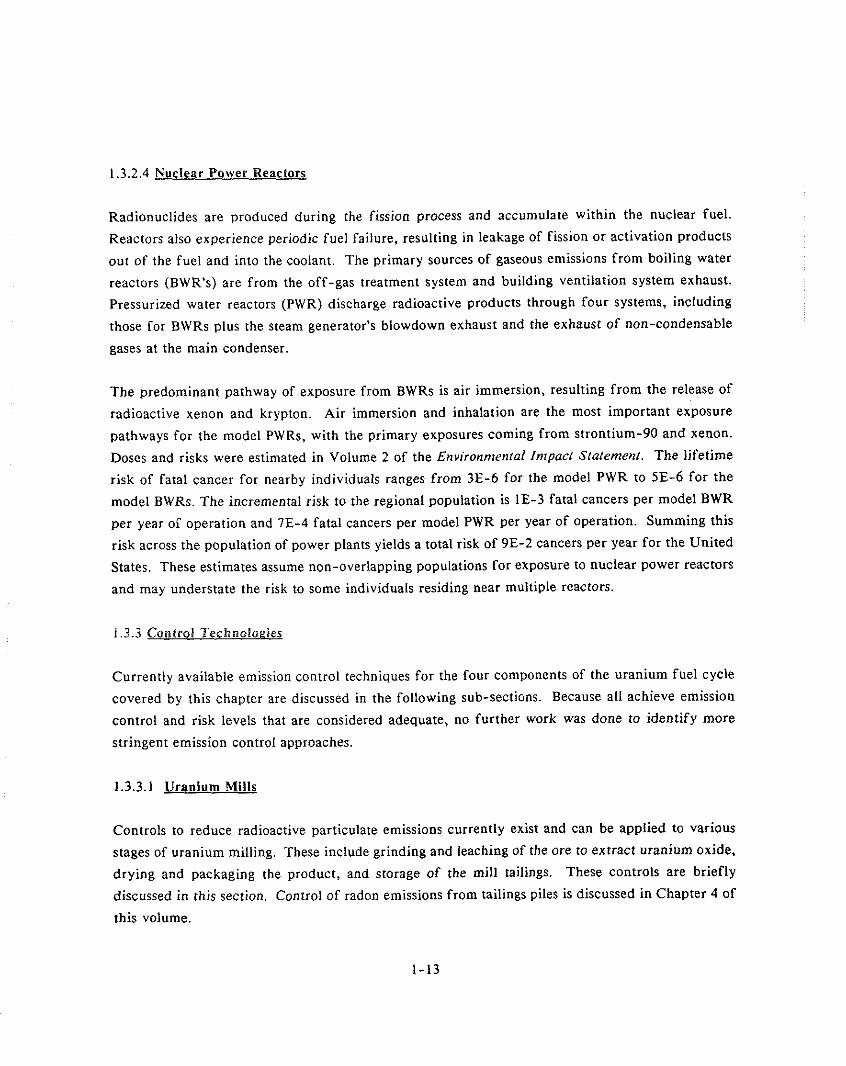
1.3.2.4 Nuclear Power Reactors
Radionuclides are produced during the fission process and accumulate within the nuclear fuel.
Reactors also experience periodic fuel failure, resulting in leakage of fission or activation products
out of the fuel and into the coolant. The primary sources of gaseous emissions from boiling water
reactors (BWR's) are from the off-gas treatment system and building ventilation system exhaust.
Pressurized water reactors (PWR) discharge radioactive products through four systems, including
those for BWRs plus the steam generator's blowdown exhaust and the exhaust of non-condensable
gases at the main condenser.
The predominant pathway of exposure from BWRs is air immersion, resulting from the release of
radioactive xenon and krypton. Air immersion and inhalation are the most important exposure
pathways for the model PWRs, with the primary exposures coming from strontium-90 and xenon.
Doses and risks were estimated in Volume 2 of the Envirotznzenlal lnzpact Staterne?zt. The lifetime
risk of fatal cancer for nearby individuals ranges from 3E-6 for the model PWR to 5E-6 for the
model BWRs. The incremental risk to the regional population is IE-3 fatal cancers per model BWR
per year of operation and 7E-4 fatal cancers per model PWR per year of operation. Summing this
risk across the population of power plants yields a total risk of 9E-2 cancers per year for the United
States. These estimates assume non-overlapping populations for exposure to nuclear power reactors
and may understate the risk to some individuals residing near multiple reactors.
1.3.3 Control Technoloeies
Currently available emission control techniques for the four components of the uranium fuel cycle
covered by this chapter are discussed in the following sub-sections. Because all achieve emission
control and risk levels that are considered adequate, no further work was done to identify more
stringent emission control approaches.
1.3.3.1 Uranium Mills
Controls to reduce radioactive particulate emissions currently exist and can be applied to various
stages of uranium milling. These include grinding and leaching of the ore to extract uranium oxide,
drying and packaging the product, and storage of the mill tailings. These controls are briefly
discussed in this section. Control of radon emissions from tailings piles is discussed in Chapter 4 of
this volume.

Controls for emissions from the milling operations - - grinding, leaching, drying and packaging - - have been evaluated by the NRC [NRCSO]. Milling dust is controlled by the placing of exhaust
hoods at the crusher, screens and transfer points. The off-gases from the drying operation are passed
through a dust separation system before discharge. Air exhaust hoods are placed in the packaging
area and run through a dust collector prior to venting. The use of wet scrubbers is the primary
method of removing dust from the exhaust gases. Rated collection efficiencies vary from
approximately 94 to 99.9 percent depending upon the type of scrubber.
The cost for each additional tenth of a percent of improl-ement of efficiency increases as the
efficiency level increases. For example, a medium-energy venturi scrubber, with 99.7 percent rated
efficiency, costs $305,000 (in 1980 prices) over a fifteen year lifetime, while a high-energy venturi
scrubber, with 99.9 percent rated efficiency, costs $430,000. The additional 0.2 percent of efficiency
costs $125,000.
A variety of controls for windblown radioactive particulates from mill tailings piles have also been
analyzed and are discussed in Volume 2, Chapter 4 of Eirvironmeiltal Impact SIatement. These
include: wetting of tailings, the use of tank trucks or sprinkling systems; leaching of tailings;
solidification of tailings; application of stabilizers such as latex or polymers to tailings surfaces; and
covering of tailings, either above or below ground. The application of latex stabilizers to the tailings
piles is a cost-effective method for controlling dust from the piles. This method is currently in use
and has proved effective for up to one year per application. Its cost is estimated at $1.03 million for
an annual application to a 30 hectares pile.
The stationary sprinkling system is the second most cost effective alternative. When installed and
operated by existing maintenance personnel, this alternative is more cost-effective than the
application of latex stabilizers. The cost of a stationary sprinkling system to cover a total of 30
hectares is estimated to be $1.9 million. Some evidence at specific plants indicate that this cost can
be reduced considerably [EPA89]. An added advantage of such a system is that evaporation of the
tailings pond water, an operational goal of each milling operation, would be substantially increased.
The value of this benefit has not been estimated.

1.3.3.2 Uranium Conversion Facilities
Well-proven particulate control technologies such as fabric filters and scrubbers can be added to the
existing control systems at uranium hexafluoride conversion plants to reduce emissions. The
selection of additional controls must take into account the presence of moisture and corrosive
contaminants (particularly fluorine) in some of the exhaust lines.
A previous study has estimated the cost of providing additional fabric filters for both the wet and
dry process plants [TEKBI]. The estimated capital costs of the systems (1979 $) are approximately
$2.1 million and $4.5 million for the wet and dry plant, respectively. The total annual costs
(operating and maintenance) for the wet and dry process plants are approximately $0.6 million and
$1.3 million, respectively [EPA89].
1.3.3.3 Uranium Fuel Fabrication Facilities
Current control techniques for fuel fabrication facilities depend upon the processes involved. The
ammonium diuranate facility process gases are processed through wet scrubbers and high efficiency
particle air (HEPA) filters with 90 and 95 percent efficiency, respectively. Ventilation off-gases are
sent through roughing and HEPA filters prior to discharge. The direct conversion facility process
gas is passed through sintered metal filters to remove solids and then to scrubbers for HF removal,
dilution and final discharge.
1.3.3.4 Nuclear Power Reactors
Nuclear power reactors in use in the U.S. are of two types: boiling water reactors (BWRs) and
pressurized water reactors (PWRs). While there are common approaches to control of radionuclide
emissions released to the atmosphere from the two types of reactors, there are also differences in
approach.
Both types of reactor use HEPA filters and charcoal filtration units to remove particulate and
radioiodine emissions from building and ventilation exhausts. HEPA filters are designed and treated
to ensure 99.97 percent efficiency for particulate emissions. Charcoal fitters can be designed for
various levels of efficiency, the most common of which has a decontamination factor of 100. Both
also employ various strategies to delay the release of noble gases, allowing those with shorter lives
to decay before being released. Both BWRs and PWRs also employ various indirect methods of

reducing atn~ospheric eniissions. These are applied to individual pumps, tanks and valves on a case-
by-case basis.
There are also control strategies and methods that are applied to BWRs or PWRs uniquely, depending
on their special features. Because there are so many possible configurations, and the cost of each
element depends on factors specific to the application, there is no concise summary of costs for
controlling radioactive emissions from nuclear power reactors.
1.4 Industrv Cost and Economic I m ~ a c t Analvsis
Any radionuclide emission control costs imposed on the uranium fuel cycle facilities would be
expected to weaken further the position of the domestic nuclear industry. Alternative sources of
nuclear fuel supply from imports and the alternatives to nuclear electric power will become more
attractive if uranium fuel production costs increase.

REFERENCES
U. S. Atomic Energy Commission, Fuels and Materials Directorate of Licensing, E~~virottntet~lal Survey of the Uranium Fuel Cycle, April 1974.
Dolezal, W., personal communication with Dave Goldin, SC&A, Inc., September 1988.
U.S. Department of Energy, Domeslic Uranium Mining and Milling Industry: 1986 Viabilily Assessmet~l, DOEIEIA-0477 (86), November 23, 1987.
U.S. Environmental Protection Agency, Radiological Impact Caused b y Entissiotts of Radiorruclides in Air i~r the United Stales, preliminary report, EPA 52017-79-006, August 1979.
U. S. Environmental Protection Agency, Final Rule for Radotr-222 Emissiotts front Lice~tsed Umtrium Mill Tailittgs, Backgrour~d Inforrnatio~t Document for Final Rules, volume 11, EPA 1520-1-84-022-2, October 1984.
U. S. Environmental Protection Agency, Radionuclides: Background I~t forntaf ion Documetrt for Final Rules, volume I , EPA 52011-84-022-2, October 1984.
Risk Assessntents, Vol. 2.
Nuclear News, February 1988.
U. S. Nuclear Regulatory Commission, E~rvironmen~al Statemettt Relaled to Operalion of Shirley Basin Mill, December 1974.
U. S. Nuclear Regulatory Commission, Fittal Generic Environme~~tal Impact Stafentenf on Urattiun~ Milling, September 1980.
U. S. Nuclear Regulatory Commission, Technical Guidance for Sititrg Criteria Developnlent, NUREG//CR-2239, November 1982.
U. S. Nuclear Regulatory Commission (NRC), Environmenfal Intpact Appraisal for the Reltewal of Source Licetzse No. SUB-526, NUREG-1071, May 1984.
U. S. NRC, Environntet~fal Assessntenf /or Renewal of Special Nuclear Material License No. SNM-1 /07 , NUREG-I 118, May 1985.
U. S. NRC, op cit., August 1985.


CHAPTER 2
UNDERGROUND URANIUM MINES

2.1 INTRODUCTION
Underground uraniunl mines are part of the domestic uranium industry that provides commercial
nuclear power plants their fuel. Other industrial categories in this industry are surface uranium
mines, uranium mills and other segments of the nuclear fuel cycle. All these activities are dependent
to a degree on nuclear power plants to generate demand for their output.
As is detailed in Chapter 4 of this volume, "Licensed Uranium Mill Tailings," and summarized in this
chapter, the demand for the products of domestic uranium production has been falling for some
time. Most mines and mills have gone out of production and many are permanently closed. The
remaining are analyzed here.
This chapter provides a brief profile of the uranium industry, describes the options for reducing
radon emissions from underground mines, the health benefits attributable to each option, the costs
attributable to each option and the impacts a regulation would have on the industry, the miners, their
c.omniunities and the U.S. economv.
2.2 l t~dustrv Profile
The U.S. uranium mining industry is an integral part of a domestic uranium production industry that
includes companies engaged in uranium exploration, mining, milling, and downstream activities
leading to the production of fuel for nuclear power plants. The product of uranium mining is
uranium ore.
1.2.1 Demand
Domestic producers of uranium ore send it to uranium mills. The mills have two markets for their
production: the U.S. nuclear power industry and exports. The nuclear power industry is by far
the more important of the two. Military uses, once the only source of demand for uranium, have
been supplied solely by government stockpiles since 1970 [DOE 87al.
Demand for domestic uranium has declined since the late 1970s. In 1979, utilities delivered 15,450
tons of domestic uranium oxide to DOE for enrichment, 86 percent more than 1986 deliveries.
Exports too have declined substantially. In 1979, exports amounted to 3,100 tons, almost four times
as much as in 1986. A number of negative forces have combined to cause the current depressed state

of the indust ry . Perhaps most importantly, the g rowth in electrici ty generated by nuclear plants nnd
t h e expansion of nuclear power capacity has been niuch slower than had been f o r e c a s t i n the mid-
1970s. 'This slower growth is d u e in part to numerous construstion delays and cancellat ions. Second,
impor ts have begun to play a major role in the U.S. u ran ium market. Impor t restr ict ions were
gradually wi thdrawn between 1975 and 1985. T h e result has been a steady increase in u ran ium
impor t s f r o m nations possessing high grade ( and thus low cost ) uranium deposits . Expectations a r e
tha t a growing portion o f utility requirements will besupp l i ed by foreign-origin u ran ium dur ing the
second half o f this decade [ JFA 85al.
Also con t r ibu t ing to the cu r ren t downtu rn in the uranium indust ry a re the large inventories being
held by both producers a n d utilities. Utilities, anticipating a g rowing need fo r u ran ium, entered in to
long- term contrac ts to purchase large amounts o f domestically-produced u ran ium. As actual needs
fel l shor t o f expected needs d u e to nuclear power plant construction delays a n d cancellat ions, large
inventor ies accumulated . These inventory supplies, current ly est imated to cover f o u r to f ive years
o f uti l i ty requirements , adversely af fec t suppliers in two ways. They may ex tend t h e d o w n t u r n in
u ran ium d e m a n d f o r a number o f years by decreasing the need f o r utilities t o en te r into n e w
contracts. Also, h igh interest rates increased inventory holding costs, leading some utilities to
con t r ibu te to c u r r e n t excess supply by o f fe r ing inventory stocks f o r sale o n the spot marke t
[ J F A XSa]. More detail o n uranium uses can be found in Chap te r 4 of this volume.
7.2.2. Sources of Supply
T h e u ran ium used to fue l nuclear reactors is suppl ied b y domest ic a n d foreign producers , inventories
held by utilities, a n d secondary market transactions s u c h as producer- to-producer sales,
ut i l i ty-to-uti i i ty sales a n d loans, and uti l i ty-to-producer sales. T h e role of each is described in the
fo l lowing sections.
7 .2 .2 . I D o m e ~ t i c Product ion
T a b l e 4 -7 i n C h a p t e r 4 shows trends in domestic production of u ran ium concentra te f r o m 1947 to
1986, by state. Tota l product ion was relatively constant a t 10.500 to 12,500 tons p e r year unti l 1977,
when it began a n increase that peaked in 1980 a t 21,852 tons. Production has decl ined almost eve ry
year since, reaching on ly 6 ,753 tons in 1986 [DOE 87b].
A second source of uranium is the import market. Until 1975, foreign uranium was effectively
banned from U.S. markets by a Federal law prohibiting the enrichment of imports for domestic use.
This restriction was lifted gradually after 1975. and was eliminated completely in 1984. From 1975
through 1977, imports amounted to a small portion of total domestic requirements, and U.S. exports
actually exceeded imports in each year from 1978 through 1980. By 1986, however, imports supplied
44 percent of U.S. requirements. Table 4-10 in chapter 4 lists U.S. imports from 1974 through 1986
[DOE 87a].
Historically, the primary sources of U.S. uranium imports were Canada, South Africa and Australia.
In 1986, 59 percent of U.S. uranium imports were from Canada, and 41 percent were froin Australia
and South Africa [DOE 87aj.
Forecasts of import penetration call for the import share to grow through the 1990's. The Departnlent
of Energy projects that without government intervention, between the years 1990 and 2000 imports
will range between 50 and 64 percent of domestic utility requirements, depending on demand.
2.2.2.3 Inventories
Utilities hold uranium inventories in order to meet changes in the scheduling of various stages of the
fuel cycle, such as minor delays in deliveries of uranium feed. Uranium inventories also protect the
utilities against disruption of nuclear fuel supplies. The average "forward coverage" currently desired
by domestic utilities (in terms of forward reactor operating requirements) is 18 months for natural
uranium (U308) and seven months for enriched uranium hexafluoride (UF6) [DOE 85aj. Table 4-
I I in chapter 4 lists inventories of commercially-owned natural and enriched uranium held in the
United States as of December 31, 1984, 1985, and 1987. DOE-owned inventories are not included.
The uranium inventory owned by utilities alone at the end of 1984 represented almost four years of
forward coverage.
2.2.2.4 Secondarv Market Transactions
The secondary market for uranium includes producer-to-producer sales, utility-to-utility sales and
loans, and utility-to-producer sales. The secondary market, by definition, does not increase the
supply of uranium, only the alternatives for purchasing it. As such, secondary transactions can have
a significant impact on the demand for new production and on the year-to-year changes in
inventories. The secondary market has been significant in recent years. During 1986, sales of 6,800
tons of U308 equivalent were rnade between domestic utilities and suppliers in the secondary rnnrket.
2.2.3 Fi~taticiai Analysis
Selected financial data for the domestic uranium industry for 1982 to 1986 are shown in Table 4-
i n ch-:>'?r 4. The data cover a subset of firms (the same firms for all years) that represent over
80 percent of the assets in the industry in each year. The firnis included are those for which uranium
operations could be separated from other aspects of the organization's business, and for which an
acceptable level of consistency in financial reporting practices was available for all years.
As shown in Table 4-18 in chapter 4, net income accruing to the uranium industry was positive in
only two years, 1982 and 1983. The returns on assets (net income divided by total assets) in these
years were 0.7 and 1.4 percent respectively, and aggregate net earnings totalled $69.8 million. In
1984, 1985, and 1986, the returns on assets were -10.3, -21.6, and -2.3 percent, and aggregate net
losses reached $765.7 niillion. The 10% in 1984 alone was $304.7 million on revenues of $608.9
million. Thus, the aggregate loss for the five years was $695.9 million. In 1977, 146 firms were
involved in domestic uranium exploration, 135 in mining 3nd 26 in milling. In contrast, only 31
firms were actively engaged in exploration, 1 1 in mining and 5 in milling toward the end of 1986.
Of these firms, only 27 percent had positive net income aft?r meeting operating expenses and other
obligations such as payment of taxes and recovery of depletion, depreciation and an~ortization. Many
of the firms (55 percent) reported net losses; the remaining 18 percent either had left the industry
or had no data to provide.
Most of the financial impro\,erneiit in 1986 stemmed from the slowdown or the coinpietion of
writeoffs of discontinued operations, revaluation of assets and abandonments. The domestic uranium
industry is significantly smaller than before, and its financial state will depend on higher product
prices or demand [DOE 87aj.
Company-specific information on uranium production, rebenues, profits, and plans is provided in
the f o l l o ~ i n g paragraphs. More detail is provided in Chapter 4.
Honlestake Mining Company owns one conventional uranium mine and a 3400 ton per day mill in
Grants. New Mexico. During 1984, production of uranium was reduced to the niinimurn level at
which satisfactory unit costs could be maintained. Mine production has been confined to one mine
operating on n five-day-week schedule for ten months of the year. Uranium concentrate was also
reco\t.red From solution mining and ion-exchange. in 1986, uranium accounted for 14 percent of
the company's revenues. and 21 percent of operating earnings. The high profitability of the sector
For the year is attributed to existing contracts, expiring in 1987, that provide for sale prices above
currenr spot prices and production costs [AR 84, AR 85, AR 861.
2.2.3.2 Rio Aleom
Rio Algom is a Canadian corporation engaged in the mining of a wide variety of materials, including
copper, steel, and uranium. In 1986, uranium operations accounted for 26 percent of corporate
revenue, but most (89 percent) was from Canadian production. In the United States, the company
owns one uranium mine and a 750 ton per day mill in La Sal, Utah.
In 1986, the company produced 457 tons of uranium oxide from its Utah 112ine. The mine operated
at approximately 50 percent of capacity in 1986, while the mill operated at capacity due to a
significant amount of toll milling [AR 861.' In 1987, the La Sal mill produced about 350 tons of
uraniunl oxide using both company ore and ore from the Thornberg mine. The mill was placed on
standby in September of 1988, because the Lisbon and Thornberg mines' reserves were depleted [EPA
891.
2.2.3.3 Plateau Resources Limited
Plateau Resources, a wholly owned subsidiary of Consumers Power Co., was organized in I976 to
acquire, explore, and develop properties for the mining, milling, and sale of uranium. All operations
were suspended in 1984 because of depressed demand and ail uranium assets were written down by
$46 n~il l ion after taxes in 1984 and $21 million in 1985, to an estimated net realizable value of
approximately $34 million. There is no assurance that the amount will ever be realized however.
2.2.3.4 Western Nuclear
Western Nuclear, a subsidiary of Phelps Dodge Corporation, owns two mine and mill complexes, one
in \Vyoming and one in Washington. The capacities of its mills are 1700 and 2000 tons per day,
respectively. The Wyoming mill has been on standby since the early 1980s, and decommissioning is
anticipated. The Washington complex operated intermittently from 1981 through 1984. In late 1984,
' "Toll milling" is the processing of ore from another company's mines on a contract basis
Phelps Dodge wrote off its entire "Energy" operation, o f which Western Nuclear was a major part
[AR 83, AR 851.
2.2.4 lnduslry Forecast a i ~ d Oullook
This section presents projections of total U.S. utility market requirements, domestic uranium
production, from both conventional and non-conventional sources, imports, employment and
electricity consumption. Developed for a 14-year period (1987-2000), these projections are
considered "near term." A basic assumption of the near term projections is that current market
conditions, as defined by the Department of Energy's Energy Information Administration
(DOE,EI.A), will continue unchanged through the end of this century. This section is based on the
reference case projections in EIA's Domestic Uranium Mining and Milling Industry: 1986 Viability
Assessment [DOE 8721.
2.2.4.1 Proiections of Dorneslic Productior~
The EIA's Reference case2 forecasts, for the 1987-2000 time period, are based on the output of EIA's
economic model, Domestic Evaluation of Uranium Resources and Economic Analysis (EUREKA).
The EUREKA model's methodology goes beyond the scope of this study; it is fully described in
Appendix C of the 1986 Viability Assessment. The EIA examines future developments in the
domestic uranium industry and in the domestic and international uranium markets under current 3 market conditions and under certain hypothetical supply disruption scenarios . The current market
conditions are generally the same as those presented in Sections 4.2.1-4.2.4 of this study and are based
on historical trends in the domestic uranium industry as outlined in both the Viability Assessment
and rhe EIA's Uranium Industry Annual 1986.
'prior to the 1986 Viability Assessn7en1, EIA published two reference cases: a Lower Reference case and an Upper Reference case, each with a low, a mean, and a high range of projected values. In 1986, however, only the Lower Reference case was published. It is referred to simply as the Reference case. As before, low, mean and high projected values were produced by EIA. This study uses the mean.
The Refersnce case ir? the lP86 Viabiliry Assessnler~t uses the underlying assumptions for the Lower Reference case described in Conln~ercial Nuclear Power 1987: Prospects /or !he Uuited Stales and fhe IYorld [DOE 87al.
3 ~ h e s e scenarios, the "current disruption status" scenario and the "projected disruption status" scenario, are used to test the viability of the U.S. uranium industry, to examine the ability of this industr) to respond to an abrogation of various fractions of contracts for uranium imports intended for domestic end use. Both of these bear only tangentially on this study and will not be discussed further here.
2.2.4.2 Near-Term Proiections
Total domestic production of U308, from both conventional and non-con\entional uraniurii sources,
for 1980-1986 is shown in Table 4-18 of chapter 4, along with reference case projections for 1987-
2000. Annual domestic production peaked at 21,900 short tons after milling in 1980, and declined
to 6,750 short tons in 1986. Production is projected to remain below its 1980 peak. For example,
EIA has projected domestic U308 production in 1992 at 6,450 short tons, while the output in the year
2000 is estimated to be 7,500 short tons. Annual domestic production from conventional mining
sources (i.e., from milling ore obtained from underground or open-pit mines, which historically has
accounted, on average, for roughly 70 percent of total annual domestic production) has fallen more
steeply: from 85 percent in 1980 to 53 percent in 1985. Houever, it increased from its 1985 level of
3,275 short tons to 5,825 short tons in 1986. This increase uas due to an increase in the U30,
concentration of the ore milled in that year.
Changes in the market, such as the ban on iniports of uranium ore or concentrate fro111 South Africa
and iYamibia4, could influence conventional production much more than non-conventional U30,
production, because non-conventional U308 producers tend to have lower marginal costs of
production than do conventional producers. Therefore, production from non-conventional sources
tends to be less affected by fluctuations in uranium market prices. Wet process phosphoric acid,
copper waste dumps, and bellyriunl ores constitute by-product methods of production of U30,. The
second significant non-conventional source is in situ leaching. By-product and in situ leaching both
accounted for 79 percent of the total non-conventional annual production of U30, in 1986. Other
sources include mine water, and heap leaching, which accounted for the remaining 21 percent of total
annual non-con\~entional production in 1986.
The Reference case ElA projections of doriiestic U308 production through the year 2000 are based
on a unit by unit review of nuclear power plants that are new. operating, under construction, or units
for which orders have been placed and for which licenses are currently being processed. Under EIA's
Reference case, nuclear generating capacity is expected to increase from 94.0 GWe in 1987 to 103.0
GWe in the year 2000 (Table 4-19). Historical and forecast data of total enrichment feed deliveries
(demand), net imports, and total production are graphed in Figure 4-1 [DOE 87al. Historical data
4 ~ h e U.S. Congress passed the Comprehensive Anti-Apartheid Act of 1986 on October 2, 1986. Section 309 of that Act forbade the import into the United States of uranium ore or concentrate of South African of Namibian origin after January 1, 1987. However, natural or enriched uranium hexafluoride from these countries may be imported, according to a regulation issued by the U.S. Department of the Treasury on which the U.S. Nuclear Regulatory Commission has concurred [EPA 87bI.
and reference case projections for conventional and non-conventional production of domestic
uranium are plotted in Figure 4-2.
2.3 Current Emissions. Risk Levels, and Feasible Control hlethods
In this section, the current risks due to radon emissions from underground uranium mines are
described, ways of reducing these risks are discussed and the effects of two alternative rules for
reducing the risks to maximum exposed individuals due to radon emissions from uranium mines are
estimated.
1.3.2 Current Emissions and Estimated Risk Levels
Due to the ongoing decline of the uranium industry, the list of firms in operation, shown in Table
2 - I, has continued to shrink. As of the fall of 1988, fourteen mines were producing and one other,
the Schwartzwalder mine owned by the Cotter Corporation, was on standby and was being explored.
Three of the producing mines, Pigeon, Pinenut and Kanab North, all owned by Energy Fuels
Nuclear, Inc., were breccia-pipe mines, which will be mined out in two to five years. Sheep
Mountain # I will operate for five more years. Only the Mt. Taylor mine, with an expected life of
twenty years, has the possibility of operating for a significant amount of time. Section 23, owned
by the Honiestake Mining Company, has an expected life of only 1.25 years. Information regarding
the expected life of the other eight mines is not available.
Estimates of current emissions and risk levels for these fifteen mines, ranked by maximum individual
risk (MIR), are shown in Table 2-2. Although Section 23 has the highest rate of radon emissions,
the highest individual risk is due to the La Sal mine and the highest population risk is due to
emissions from the Schwartzwalder mine.
2.3.3 Control Technoioeies
2.3.3.1 Introduction
After extensive efforts to devise control technologies that would reduce the emissions of radon-222
from underground mines, it was concluded that no suitable technology is available [EPA 891. The
approaches discussed here seek to limit the emissions of the mines by restricting their days of
operation and to reduce the risks from radon emissions to nearby populations by installing stacks that
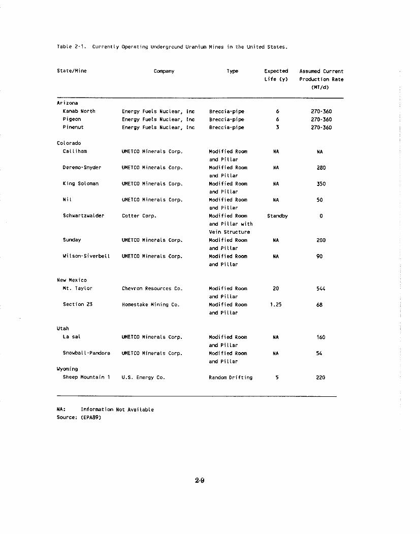
Table 2-2 . Currenriy Operating Underground Uren im Mines i n the United States.
Type Expected Assuned Current
L i f e ( y ) Production Rate
(MT/d)
Arizona
Kanab North Energy Fuels Nuclear, Inc
Pigeon Energy Fuels Nuclear, Inc
P i nenut Energy Fuels Nuclear, Inc
Colorado
Calliham UMETCO Minerals Corp.
Deremo-Snyder UMETCO Minerals Corp.
King Soloman UMETCO Minerals Corp.
Hi l UMETCO Minerals Coro.
Schuartzualder Cotter Corp.
Sunday UMETCO Minerals Corp.
Yi lson-Siverbel l UMETCO Minerals Coro.
New Mexico
M t . Taylor Chevron Resources Co.
Section 23 Hanestake Mining Co
Utah
La sal UMETCO Minerals Corp.
Snouball-Pandora UMETCO Minerals Coro.
Waning
Sheep Mountain 1 U.S. Energy Co.
Modified Roan
and P i l l a r
Modified Roan
and P i l l a r
Modified R o a n and P i l l a r
Modified Roam
and P i l Lar
Modified Room
and P i l l a r u i t h
Vein Structure
Modified Room
and Pi l i a r
Modified Room
and P i l l a r
Modified Room
and P i l l a r
Modified Roan
and P i l l a r
Modified Room
and P i l l a r
Modified Room
and P i l l a r
Randm D r i f t i n g
NA NA
NA 280
N A 350
NA 50
Standby 0
NA: Information Not Available
Source: (EPA89)
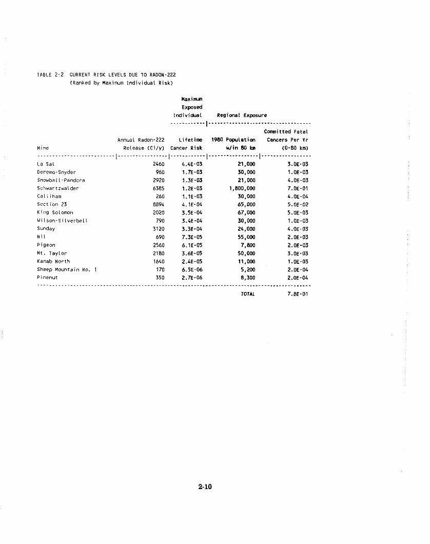
T A B L E 2-2 CURRENT RISK LEVELS DUE TO RAOON-222 (Ranked by Maximum Individual Risk)
Maxim
Expsed Individual Regional Exposure _________...~___________...____~~~.~..~.........
Cmitted Fatal Annual Radon-222 Lifetime 1980 Poprlation Cancers Per Yr
Nine Release (Cily) Cancer Risk ulin 80 km (0-80 km) ............................................................................................. L a Sat 2460 4.4E-03 21,000 3.OE-03 Derema-Snyder 960 1.7E-03 30,000 1.OE-03 Snowball-Pandora 2920 1.3E-03 21.0W 4.OE-03 Schuartruaider 6385 1.2E-03 1,800,000 7.OE-01 Catiiham 260 l.lE-03 30,000 4.OE-04 Sect icn 23 8894 4.1E-04 65,000 5.OE-02
King Soiomon 2020 3.5E-04 67,000 5.OE-03 Witson-Silverbell 790 3.4E-04 30,000 1.OE-03 Sunday 3120 3.3E-04 24.000 4.OE-03 N i l 690 7.3E-05 55,000 2.OE-03
Pigeon 2560 6.1E-05 7 . m 2.OE-03 Mt. Taylor 2180 3.6E-05 50,000 3.OE-03 Kanab North 1640 2.4E-05 11,MO 1.OE-03 Sheep Mountain No. 1 170 6.5E-06 5,200 2.OE-04 Pinenut 350 2.7E-06 8,300 2.OE-04 .............................................................................................
TOTAL 7.8E-01
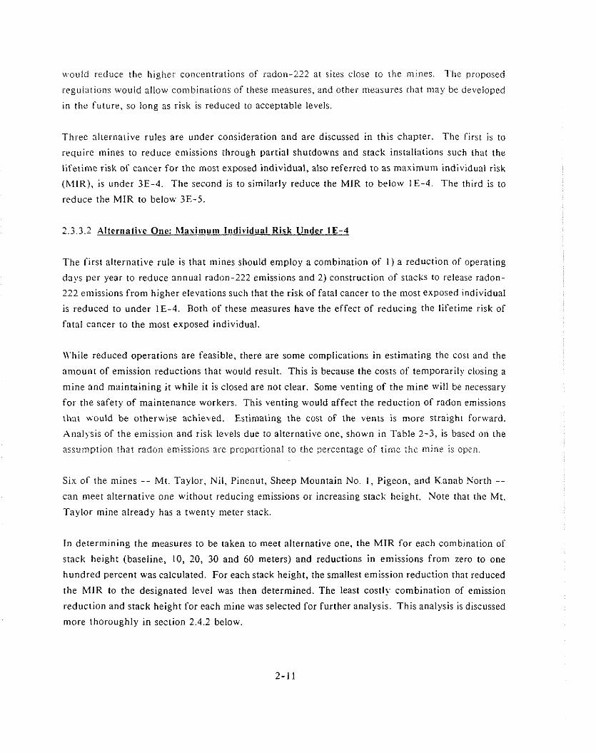
would reduce the higher concentrations of radon-222 at sites close to the mines. Tlie proposed
regulations would nilow colnbinations of these measures, and other liieasures that may be developed
in the future, so long as risk is reduced to acceptable levels.
Three alternative rules are under consideration and are discussed in this chapter. The first is to
require mines to reduce eniissions through partial shutdowns and stack installations such that the
lifetime risk of cancer for the most exposed individual, also referred to as maximum individual risk
(MlR), is under 3E-4. The second is to similarly reduce the MIR to below IE-4. The third is to
reduce the MIR to below 3E-5.
2.j.3.2 Alteroatire One: lrlaxilnu~n Individual Risk Under 1E-4
The first alternative rule is that ~ilines should employ a combination of I) a reduction of operating
days per year to reduce annual I-adon-222 emissions and 2) construction of stacks to release radon-
222 emissions from higher elevations such that the risk of fatal cancer to the niost exposed individual
is reduced to under IE-4. Both of these measures have the effect of reducing the lifetime risk of
fatal cancer to the most exposed individual.
While reduced operations are feasible, there are some complications in estimating the cost and the
amount of emission reductions that would result. This is because the costs of temporarily closing a
mine and maintaining it while it is closed are not clear. Some venting of the mine will be necessary
for the safety of maintenance workers. This venting would affect the reduction of radon emissions
that would be otherwise achieved. Estimating the cost of the vents is more straight forward.
Analysis of the eniission and risk levels due to alternative one, shown in Table 2-3, is based on the
assuniption that radon emissions are proportional to the percentage of time the mine is open.
Six of the mines - - MI. Taylor, Nil, Pinenut, Sheep Mountain No. 1, Pigeon, and Kanab North -- can nieet alternative one without reducing emissions or increasing stack height. Note that the Mt.
Taylor mine already has a twenty meter stack.
In determining the measures to be taken to meet alternative one, the MIR for each combination of
stack height (baseline, 10, 20, 30 and 60 meters) and reductions in eniissions from zero to one
hundred percent was calculated. For each stack height, the smallest emission reduction that reduced
the h4IR to the designated level was then determined. The least costl>- combination of emission
reduction and stack height for each mine was selected for further analysis. This analysis is discussed
more thoroughly in section 2.4.2 below.

Table 2-3': Alternat ive 1: neasures leken and Their Ef fects on M a x i m Exposed Indiv iduals and
Poprlations u i t h i n 80 km
mine
Al ternat ive 1: M I R BELW 3E-4 ..........................................................................................
Reduction Annual Risk t o Reduction
Stack Emission +ran i n i t i a l P a p l a t i o n i n P ~ p l t a t i o n
Height Reduction M I R M l R w i th in 80 km Risk
La Sal 0 95% 2.2E-04 Schuartzualder 0 75% 3.OE-04 Call iham 0 75% 2.8E-04 Deremo-Snyder 0 85% 2.6E-04 Snowball-Pandora 0 80% 2.OE-04 Ui lson-Si lverbel l 0 15% 2.9E-04 King Solomon 0 15% 3.OE-04 Section 23 0 30% 2.9E-04 Sunday 0 10% 3.OE-04 M t . Taylor 20 0% 3.M-05 Sheep Mountain No. 1 0 0% 6.5E-06 Pinenut 0 OX 2.E-06 Kanab North 0 0% 2.4E-05 N i l 0 OX 7.3E-05 Pigeon 0 OX 6 .1~-05
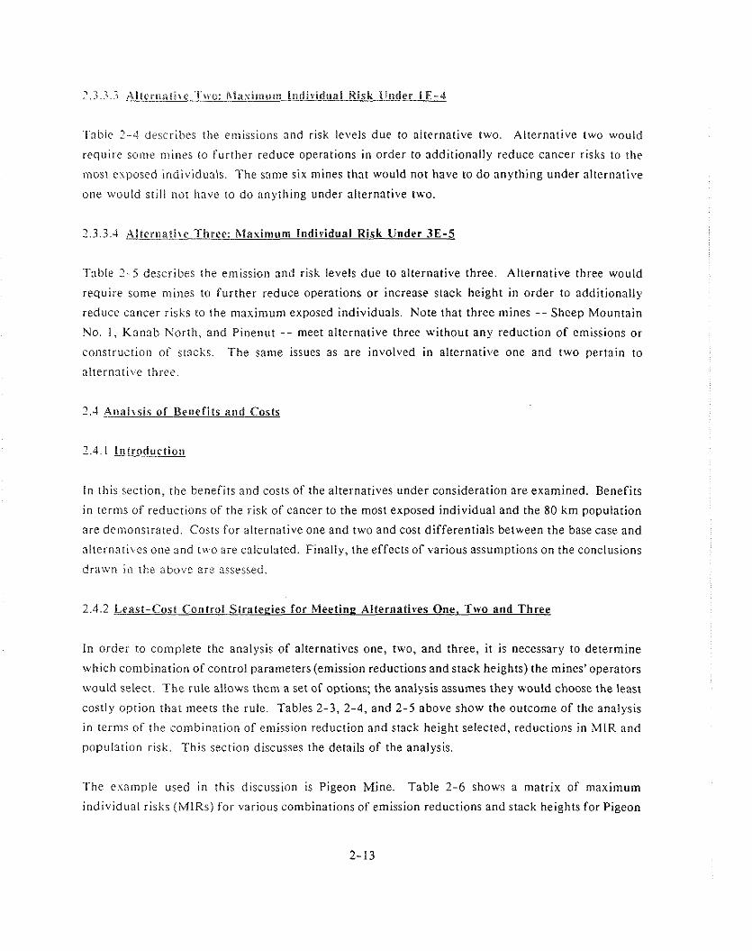
Tnble 2 - 4 describes the eniissions and risk levels due to alternative two. Alternative two would
require soilie inines to t'urtlier reduce operations in order to additionally reduce cancer risks to the
111ost exposed individunls. The same six mines that would not have to do anything under alternative
one would still nor have to do anything under alternative two.
2.3.3.J Alternatibe Three: hlasitnurn lrrdividual Risk tinder 3E-5
Tnble 2 - 5 describes the emission and risk levels due to alternative three. Alternative three would
require some mines to further reduce operations or increase stack height in order to additionally
reduce cancer risks to the niaxinium exposed individuals. Note that three mines - - Sheep Mountain
No. I . Knnab North, and Pinenut - - meet alternative three without any reduction of emissions or
construction of stacks. The same issues as are involved in alternative one and two pertain to
nlternntive three.
2 .4 Ar~alvsis of Bet~efi ts and Costs
i n this section, the benefits and costs of the alternatives under consideration are examined. Benefits
in terrus of reductions of the risk of cancer to the most exposed individual and the 80 km population
are denionstrated. Costs for alternative one and two and cost differentials between the base case and
alternati\es one and t u o are calculated. Finally, the effects of various assuniptions on the conclusions
drnivii i n the above are assessed.
2.4.2 Least-Cost Conrrol Strategies for Meeting Alternatives One. Two and Three
In order to con~plete the analysis of alternatives one, two, and three, it is necessary to determine
which combination of conrrol parameters (emission reductions and stack heights) the mines' operators
would select. T h e rule allows them a set of options; the analysis assumes they would choose the least
costly option that meets the rule. Tables 2-3, 2-4, and 2-5 above show the outcome of the analysis
in ternls of the combination of enlission reduction and stack height selected, reductions in MIR and
population risk. This section discusses the details of the analysis.
The example used in this discussion is Pigeon Mine. Table 2-6 shows a matrix of maximum
individual risks (MIRs) for various combinations of emission reductions and stack heights for Pigeon
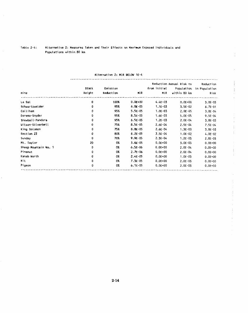
Table 2-4: A l te rm t i ve 2: Measures Taken and Their Effects on nsxi.un Exposed lndividusls and
Poplet ions within 80 km
Alternative 2: M l R BELW 1E-4
Reduction Annual Risk to Reduction
Stack Emission from i n i t i a l Population i n Population
Height Reduct ion HlR M I R within 80 km Risk
La Sal
Schuartzualder
Calliharn
oeremo-Snyder
Snouball-Pandora
UiIson-Silverbel l
King S o l a n
Section 23 Sunday
M t . Taylor
Sheep nountain No.
Pinenut
Kanab North
N i I
Pigeon
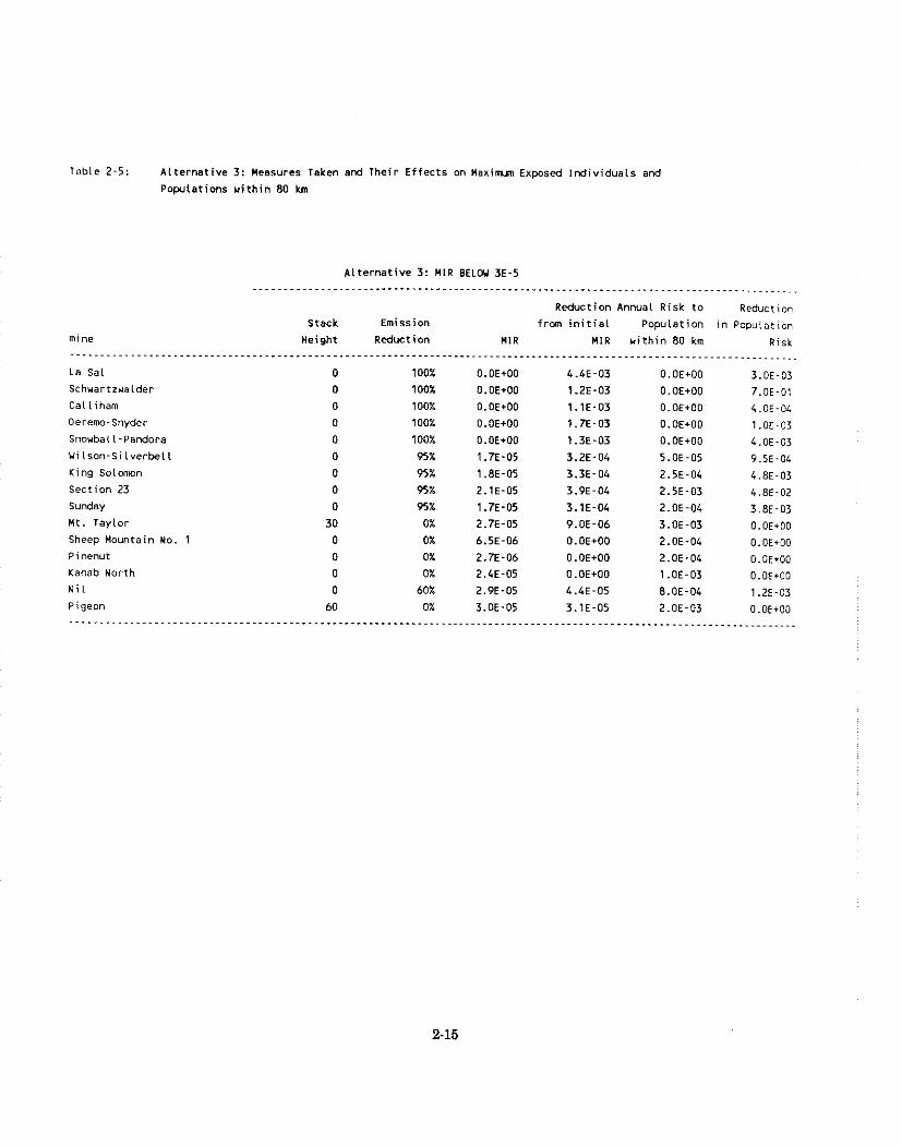
Table 2-5: A l t e rna t i ve 3: nessures Taken a d Their E f f ec t s on M a x i m Exposed I n d i v i d u a l s and
Pop l le t ions w i t h i n 80 km
A l te rna t i ve 3: HIR BELW 3E-5
mine
~ ~ ~ ~ ~ ~ . . . . . . . . . . Reduction Annuat Risk t o Reduction
Stack Emission frm i n i t i a l Populat ion i n Popuiation
Height Reduct i on M l R HlR w i t h i n 80 km Risk
La Sal
Schvartzvalder
Cal l iham
Cerema-Snyder
Snoubaii-Pandora
Wi lson-Si lverbelL
King Soloman
sec t i on 23
Sunday
M t . Taylor
sheep Mountain No. 1 Pinenut
Kanab North
Ni 1
Pigeon

Teble 2 - 6 : Matrix of nlRs as Stack Height and Emissions e t Pigeon Mine Vary
R I S K TO NEAREST INDIVIDUAL ( I I l R ) R E D U C T ~ O ~ REDUCTION
I N STACK HEIGHT I N EMISS~ON EMISSION
LEVEL o M 10 II 2 0 M 3 0 w 60 n LEVEL
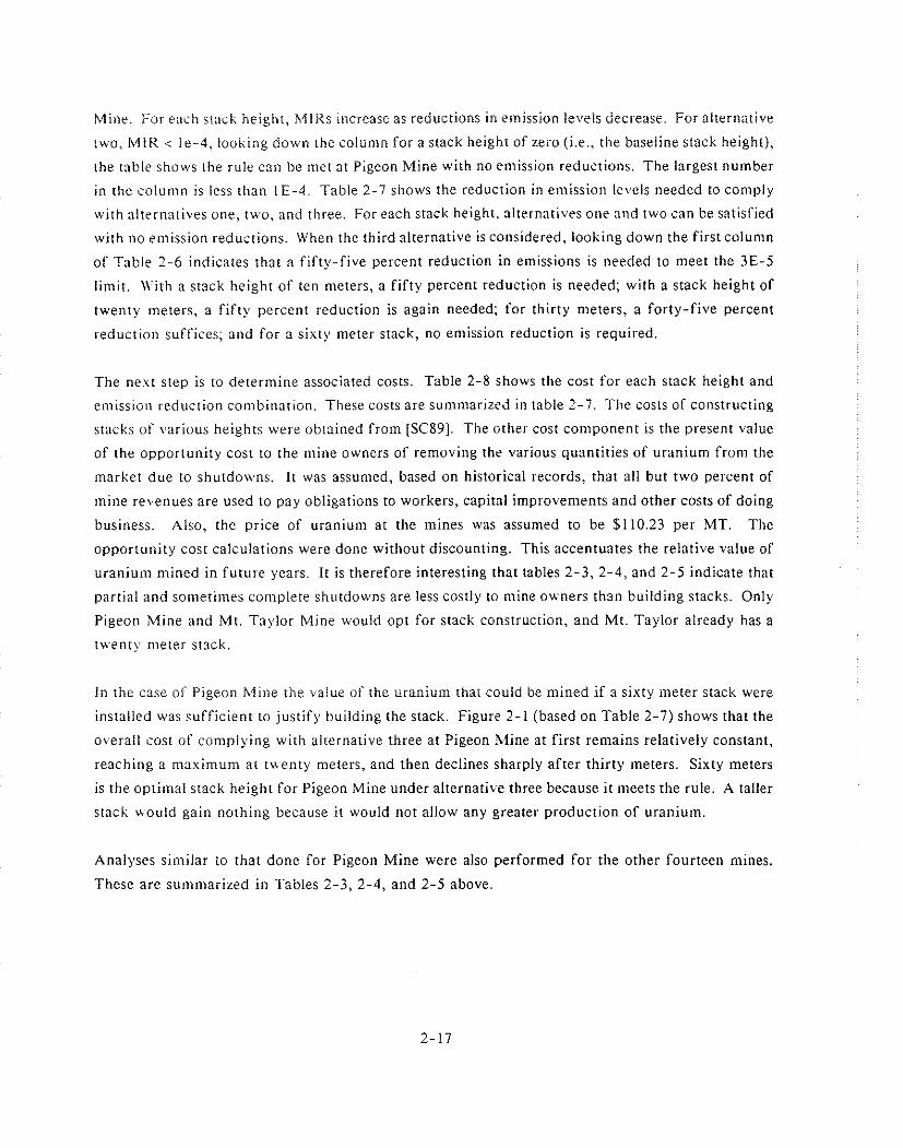
Mine. For e;~cll stack height, MlRs increase as reductions in ernission levels decrease. For alternative
two, MlR < le-4, looking down the column for a stack height of zero (i.e., the baseline stack height),
the table shows the rule can be met at Pigeon Mine with no enlission reductions. The largest number
in the column is less than I€-4. Table 2-7 shows the reduction i n emission levels needed to comply
with alternatives one, two, and three. For each stack height, 3lternatives one and two can be satisfied
with no emission reductions. When the third alternative is considered, looking down the first colunln
of Table 2-6 indicates that a fifty-five percent reduction in emissions is needed to meet the 3E-5
limit. \\'ith a stack height of ten meters, a fifty percent reduction is needed; with a stack height of
twenty meters, a fifty percent reduction is again needed; for thirty meters, a forty-five percent
reduction suff'ices; and for a sixty meter stack, no emission reduction is required.
The next step is to determine associated costs. Table 2-8 shows the cost for each stack height and
emission reduction combination. These costs are summarized in table 2 - 7 . The costs of constructing
stacks of \:ariaus heights were obtained from [SC89]. The other cost component is the present value
of the opportunity cost to the mine owners of removing the various quantities of uranium from the
market due to shutdowns. It was assumed, based on historical records, that all but two percent of
mine re\-enues are used to pay obligations to workers, capital improvements and other costs of doing
business. Also, the price of uranium at the mines was assumed to be $1 10.23 per MT. The
opportunity cost calculations were done without discounting. This accentuates the relative value of
uranium mined in future years. It is therefore interesting that tables 2-3, 2-4, and 2-5 indicate that
partial and sometimes complete shutdowns are less costly to mine owners than building stacks. Only
Pigeon Mine and Mr. Taylor Mine would opt for stack construction, and Mt. Taylor already has a
twenty meter stack.
In the case of Pigeon hline the value of the uranium that could be mined if a sixty meter stack were
installed was sufficient to justify building the stack. Figure 2-1 (based on Table 2-7) shows that the
overall cost of complying with alternative three at Pigeon hline at first remains relatively constant,
reaching a maximum at twenty meters, and then declines sharply after thirty meters. Sixty meters
is the optitiial stack height for Pigeon Mine under alternative three because i t meets the rule. A taller
stack would gain nothing because it would not allow any greater production of uranium.
Analyses similar to that done for Pigeon Mine were also performed for the other fourteen mines.
These are summarized in Tables 2-3, 2-4, and 2-5 above.
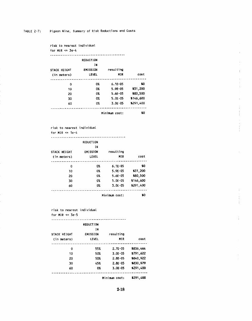
TABLE 2 - 7 : Piaeon Mine. Surmery of Risk Reductions and Costs
r isk to nearest individual for MlR <= 3e-4
REDUCTION I N
STACK HEIGHT EMlSSlON resulting ( i n meters) LEVEL MIR Cost .......................................................
0 0% 6.1E-05 10 10 OX 5.9E-05 531,200
20 OX 5.6E-05 380,500
30 OX 5.OE-05 5146.600
60 0% 3.OE-05 5291.400 .......................................................
M i n i m cost: M
r isk to nearest individual for MIR <= le-4
REDUCTION I N
STACK HEIGHT EMISSION resulting ( in meters) LEVEL MIR cost .......................................................
0 OX 6.1E-05 M 10 0% 5.9E-05 131,200 20 OX 5.6E-05 380,500
30 0% 5.OE-05 S146,M)O
60 0% 3.OE-05 5291,400 .......................................................
M i n i m cost: M
r isk to nearest individual for MlR <= 3e-5 ...........................................
REOUCTlON IN
STACK HEIGHT EMISSION resulting
( i n neters) LEVEL MlR cost
M i n i m cost: 5291,400
2-18

TABLE 2-8: Matrix of Costs of Various Ccnbinations of Stack Height and
shutdoun lime for Pigeon Wine.
The last colum i s the cost o f shutdoun by percent of
The f i r s t rou is the cost of constructing stacks of various heights. a one year shutdown Other rous are swns of costs of shutdown and of coostrwting stacks. - - - . .~~~--- - - - .~. . .~~~.~--- - - - ........-......-..-..-.......-.-........*....-...--.-.-..--.----------.-*.. I percent of cost of
0 H 10 I4 20 M 30 U 60 M I year shutdoun shutdown ..........................................................................................................
$0 $31,200 $80,500 $146,600 1291.4W I 0% $ 0 $76,042 $107,242 $156,542 $222,642 $367.442 I 5% $76.042
$152.084 $183,284 $232,584 $298,684 U 4 3 . W 1 1 0% 1152,084 $228.126 $259,326 '6308,626 $374,726 1519.52t 1 15% $228,126 $304,169 $335,369 $384,669 U50.769 1595,569 1 20% $304,169 $380.211 $411,411 $460.71 1 1526,811 5671.611 1 25% 5380,211 $456,253 $487,453 $536,753 $602,853 1747,653 1 30% U56.253 $532,295 $563,495 $612,795 $678,895 SE23.695 1 35% 1532,295 $608,337 $639,537 $688.837 $754.937 1899.737 1 40% $608,337 $63,379 $715,579 $764.879 $830,979 $975.779 1 45% 5684,379 $760,422 $791,622 $840.922 $907,022 $1,051,822 1 50% 1760,422 $836,464 f867.664 $916.964 $983.064 11,127,864 1 55% $836,464 $912,506 $943,706 $993.006 51,059,106 $1,203,906 1 60% 1912.506 $988,548 $1,019,748 $1,069,048 $1,135,148 11,279,9481 65% $988,548
51,064,590 $1,095,790 $1,145,090 $1,211,190 11,355,990 1 70% $1,064,590 $1,140,632 $1,171,832 $1,221,132 $1.287.232 $1,432,032 1 75% 11,140,632 $1,216,675 $1,247,875 $1,297,175 $1,363,275 $1,508,073 1 80% 11,216,675 $1,292,717 $1,323,917 $1,373,217 $1,439,317 11,584,117 1 85% $1,292,717 $1,368,759 $1,399,959 $1,449,259 $1.515.359 11,664,159I 90% 51,368,759 $1,444,801 $1,476,001 $1,525,301 51,591,401 $1,736,201 I 95% $1.444.801 $1,520,843 $1,552,043 $1,601,343 $1,667,443 $1,812,243 1 100% $1,520,843
..........................................................................................................
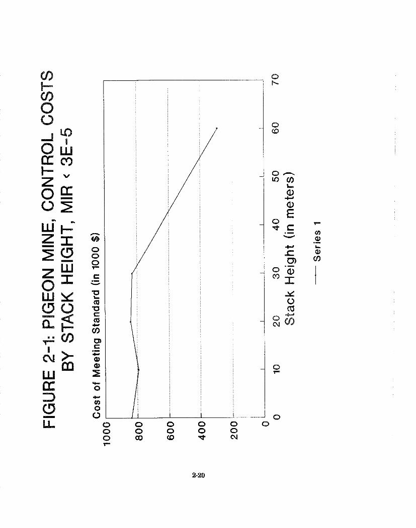
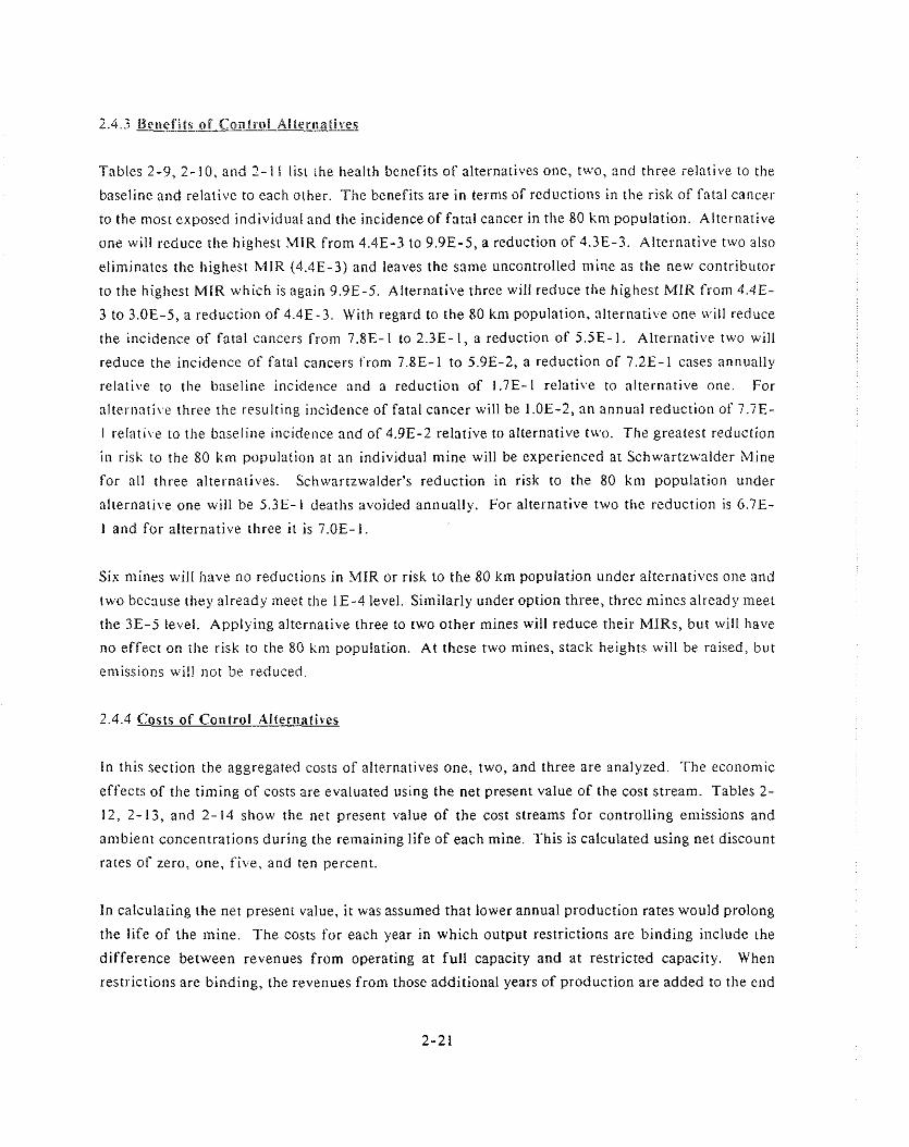
Tables 2-9, 2-10, and 1 - 1 1 list the health benefits of alternatives one, two, and three relative to the
baseline and relative to each other. The benefits are in terms of reductions in the risk of fatal cancer
to the most exposed individual and the incidence of fatal cancer in the 80 k ~ n population. Alternative
one will reduce tlie highest MIR fro111 4.4E-3 to 9.9E-5, a reduction of 4.3E-3. Alternative two also
eliminates the highest MIR (4.4E-3) and leaves the same uncontrolled mine as the new contributor
to the highest MIR which is again 9.9E-5. Alternative three will reduce the highest MIR from 4 .4E-
3 to 3.OE-5, a reduction of 4.4E-3. With regard to the 80 krn population, alternative one will reduce
the incidence of fatal cancers froill 7.8E-1 to 2.3E-I, a reduction of 5.5E-I. Alternative two will
reduce the incidence of fatal cancers from 7.8E-I to 5.9E-2, a reduction of 7.2E-1 cases annually
relative to the baseline incide~,ce and a reduction of l.7E-I re1atiL.e to alternative one. For
alternati\e three the resulting incidence of fatal cancer will be 1.OE-2, an annual reductio~l of 7.7E-
I relative to the baseline incidence and of 4.9E-2 relative to alternative two. The greatest reduction
in risk to the 80 km population at an individual mine will be experienced at Schwartzwalder Mine
for all three alternatives. Schwartzwalder's reduction in risk to the 80 krn population under
alternative one will be 5.3E-I deaths avoided annually. For alternative two tlie reduction is 6.7E-
1 and for alternative three it is 7.OE-1.
Six mines will have no reductions in MIR or risk to the 80 km population under alternatives one and
two because they already meet the 1E-4 level. Similarly under option three, three mines already meet
the 3E-5 level. Applying alternative three to two other mines will reduce their MIRs, but will have
no effect on tlie risk to the 80 km population. At these two mines, stack heights will be raised, but
emissions will not be reduced.
2.4.4 Costs o f Co~itrol Alterr~alives
I n this section the aggregated costs of alternatives one, two, and three are analyzed. The economic
effects of the timing of costs are evaluated using the net present value of the cost stream. Tables 2-
12, 2-13, and 2-14 show the net present value of the cost streams for controlling emissions and
ambient concentrations during the remaining life of each mine. This is calculated using net discount
rates of zero, one, fi\:e, and ten percent.
In calculating the net present value, it was assumed that lower annual production rates would prolong
the life of the mine. The costs for each year in which output restrictions are binding include the
difference between revenues from operating at full capacity and at restricted capacity. When
restrictions are binding, the revenues from those additional years of production are added to the end

Table 2-9 : Health Benefits Due to Alternative One
mine
Initial Risk of Fatal Cancer ALTERNATIVE 1: MlR B E L W 3E-4 .................--......--..---I---.------..-.----...-.--..----.-------.-------.....-...-.-
Comnitted Fatal Annual Risk to
Maximum Cancers Per Yr Reduction Papuletion Reduction in Individual Risk (0-80 km) MlR in MlR uithin 80 km Poplation Risk
La Sal Calliham Oeremo-Snyder Schwartzwalder Snouball-Pandora
King Solomon Wilson-Silverbell Section 23 Sunday Mt. Taylor Nil Pinenut
Sheep Mountain No. Pigeon
Kanab North
Totals: 7.8E-01 2.3E-01 5.5E-01
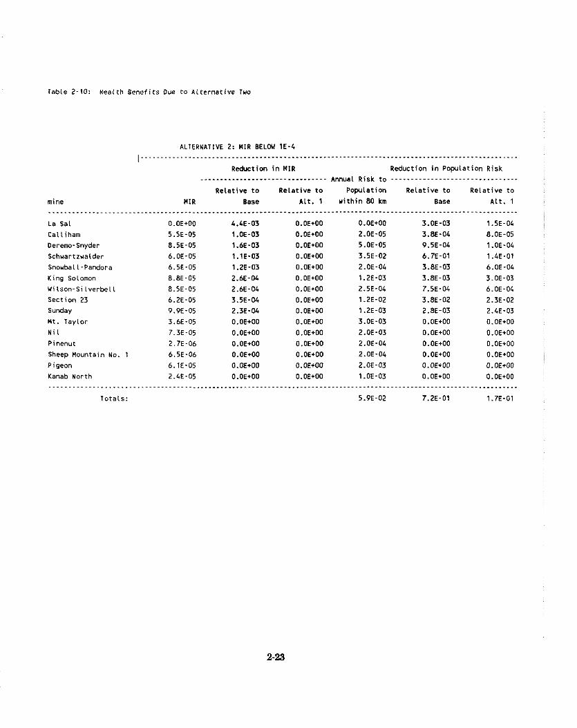
l n b l e 2-10: Health Benefi ts Due t o Aiternative Two
mine
ALTERNATIVE 2: W I R BELW 1E-4 ................................................................................................
Reduction in MlR Reduction i n P o p l a t i o n Risk Amual Risk to
Relat ive t o Relat ive t o Population Relat ive t o Relat ive t o
M l R Base A L ~ . 1 u i t h i n 80 km Base A L t . 1
La Sal
Calliham
Derm-Snyder
Schvartzvalder
Snouball-Pandora
King Solomon
Wi lson-Si lverbel l
Sect ion 23
sunday
Ht. Taylor
N i l
Pinenut
Sheep Mountain No. 1
Pigeon
Kanab North
Totals:

Toble 2.11: Wealth Benefi ts Due t o Al ternat ive Three
mine
ALTERNATIVE 3: HIR BELOU 3E-5 , ............................................................................................... Reduction i n W I R Reduction i n Popl la f ion Risk
................................ Risk to
Relat ive t o Relat ive t o Population Relat ive t o Relat ive t o
M I R Base I l t . 2 w i th in 80 km Base A l t . 2
La Sal
Cal l iham
Oeremo-Snyder
Schnartzwalder
Snoubali-Pandora
King Solomon
Wilson-Si lverbel l
Section 23
Sunday
Mt. Taylor
N i l
Pinenut
Sheep Mountain No.
Pigeon
Kanab North
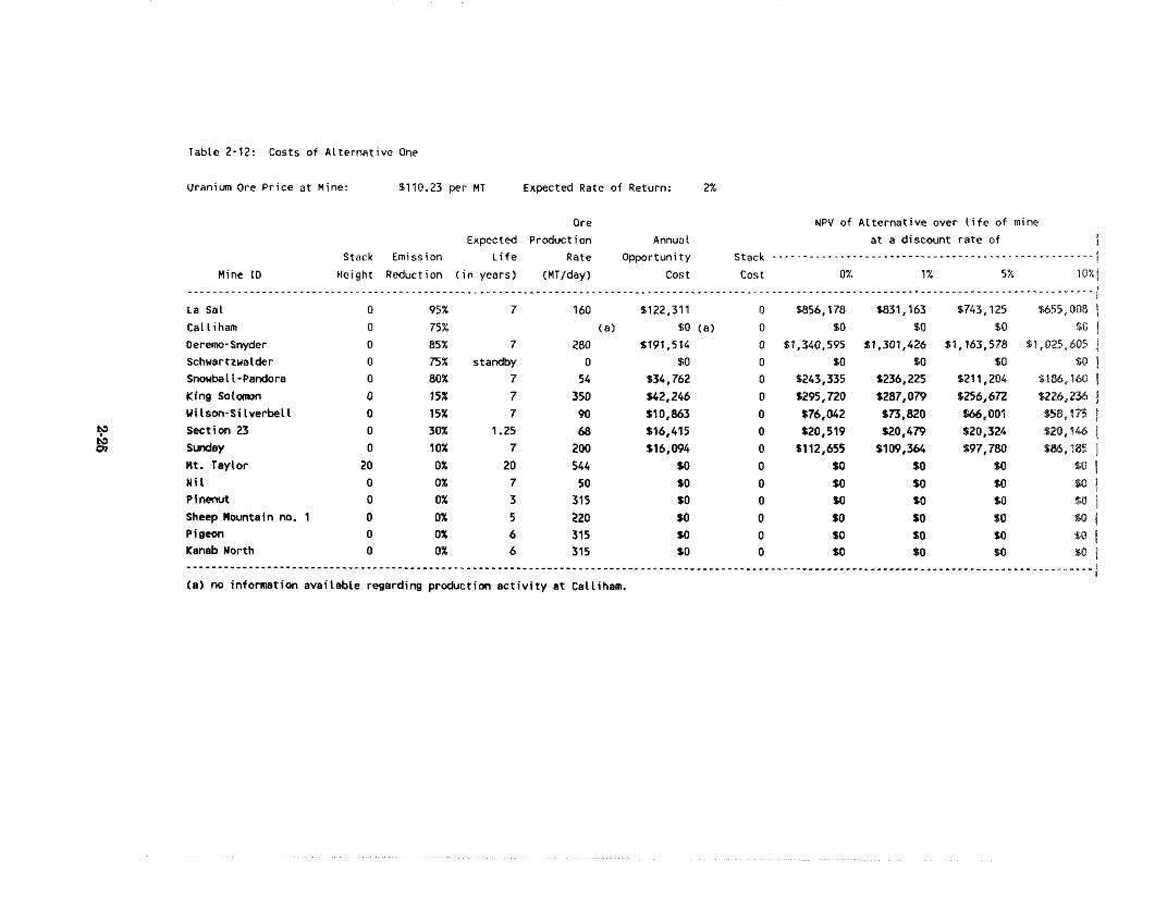
Table 2-12: Casts of A l ternat ive One
Uranium Ore Pr ice a t Mine: $110.23 per MT Expected Rate of Return: 2%
Ore NPV of Atternat ive over l i f e of mine
Expected Production Annual a t a discount r a t e o f 1 Stack Emission L i f e Rate Opportunity s tack I
Mine I0 Hcight Reduction ( i n years) (MTlday) Cost Cost 077 1% 5% 10771 .................................................................................................................................................. I La Sal 0 95% 7 160 $122,311 0 8856,178 $831,163 1743,125 $655.008 j Calliham 0 75'6 ( a ) $0 (a ) 0 $0 $0 $0 So 1 Oerm-Snyder 0 85% 7 280 $191,514 0 $1,340,595 S1.301.426 $1,163,578 51,025,605 j schuartzualder 0 75% standby 0 $0 0 $0 SO SO So 1 Snoubatt-Pardora 0 80% 7 54 $34,762 0 $243.335 $236,225 1211,204 6186,160/ King S o k m ~ ~ 0 15% 7 350 $42.246 0 $295,720 1287,079 1256,672 1226,234j Wilson-Si lverbel l 0 15% 7 90 $10.863 0 $76,042 173,820 Mb.001 158,IK )
z Section 23 0 30% 1.25 68 $16.415 0 $20,519 120,479 520,324 520,146 1 0 Sunday 0 1 OX 7 200 116,094 0 $112,655 $109.364 197,700 186,185 1
nt. Taylor 20 OX 20 544 $0 o SO SO SO N i l
I 0 0% 7 50 SO 0 M SO M
P i n e w t 0 0% 3 315 SO 0 SO SO SO SQ i $0 1
Sheep Mwnta in na. 1 0 0% 5 220 SO 0 SO $0 SO Pigeon 0 0% 6 315 $0 0 $0 SO SO
I Kanab North 0 0% 6 315 SO 0 SO SO I 0
s.0 1 so I .................................................................................................................................................. I
(a) no information avaitabte regarding production a c t i v i t y a t Calliharn.

Table 2-13: Costs of A l ternat ive Two
Uranium Ore Pr ice a t Mine: $110.23 per MT Expected Rate of Return: 2%
Ore NPV of A l te rna t i ve over L i f e o f mine
Expected Production Annual a t a discount r a t e of 1 Stack Emission L i f e Rate Opportunity stack .....................................................
Mine I D Height Reduction ( i n years) (MT/day) Cost Cost 077 1% 5% i O % / .................................................................................................................................................. I La Sal 0 100% 7 160 $128,749 0 $901,240 $874.908 $782,237 6689,683 1 Calliham 0 95% (a) $0 ( a ) 0 80 50 $0 $0 i Oeremo-Snyder 0 95% 7 280 $214,045 0 $1,498,312 $1,454,535 $1,300,469 61,146,265 1 Schwartzwalder 0 95% standby 0 $0 0 10 $0 SO so 1 Snowball-Pandora 0 95% 7 54 141,280 0 t2BB.960 1280,517 $250,805 S221,065 1 King S o l m 0 75% 7 350 $21 1,228 0 11,478,598 S1,435,397 $1,283,358 S1,131#382 1 UiLson-Si lverbelt 0 75% 7 90 $54,316 0 $380,211 S369.102 1330.006 1290,8751 Section 23 0 75% 1.25 68 $41.039 0 551.298 $51,197 350,810 150,M 1
'9 S ~ Y 0 70% 7 ZOO $112,655 0 S788.585 S765.545 $684.457 E603,m71 N M t . Taylor 20 0% 20 544 SO 0 SO SO SO I0 I m
N i l 0 0% 7 50 SO 0 SO SO SO so 1 Pimnut 0 0% 3 315 $0 0 SO SO SO So 1 Sheep M a n t a i n no. 1 0 0% 5 220 SO 0 M SO M Plpeon 0 0% 6 315 SO 0 SO SO SO So 1
1
Kanab Worth 0 0% 6 315 SO 0 SO $0 SO E --------------------------------------------------.----.-.------.-------..-------...----..------.-~-~~-~~------------------~---.--~-~..---.---- " - - i (a) no information avai lab le regarding product ion a c t i v i t y a t Calliham.

of tiie tii i~e strennr. Tlie iniiiie with tile liighesi cost is Derenlo-Snyder Mine, under ai ter~~ntives one
:~i id two, n~ id King Solonloii Mine under alternative three.
2 . 5 l~ttluslrv Cost and Ecor~ornic Irapacl A~~a lvs i s
111 this section the effects of the alternatives analyzed on economic entities are considered. This
includes assessing the relative impact of regulation on production costs, identifying which sectors of
the economy might experience adverse (or beneficial) economic effects, and the potential of the
regulation to affect small economic entities, such as small firms or small counties.
2 . j . 2 Production Cost lrnni~cts
For purposes of illustration, these costs can be compared with the assumed return on uranium mining
of 7 percent, based on the experience of the last decade. Also, the trend towards closing all mines
indicntes that profits xilay well be insufficient to sustain operations in the industry and any additional
costs m a y speed the demise of the mines.
2.5.3 E c o ~ ~ o m i c Impact Arialvsis
Although the cost of regulating uranium mines could result i n mine closures, the effects of these
closures would be isolated to a small group of people - - the stockholders of the corporations who
on n the mines, the 230 nliners considered in Table 2-15 who currently work in six of the mines, and
the miners in the other mines for which no data was available. The enlploynlent and community
situation at the other mines, though undocumented, is likely to be similar to that for the mines
represented in Table 2-15, The effects of mine closure would not spread to the larger economy
because I) in the depressed market for uranium there are other producers of ore -- U.S. surface
mines, by-product producers, and foreign mines -- who could continue to meet the current price and
to respond competitively in case of increased demand and 2) the miners live i n different counties and
constitute a small proportion of workers in each.
As discussed in section 2.2, most underground uranium mines are subsidiaries of large corporations.
hlost of the direct costs of compliance will be borne by stockholders or owners. Because operators
of underground uranium mines currently have little or no monopoly power they will not be able to
pass these costs on to the electric power industry.
Table 2-16 shows the number of nliners at each of the six mines along with the total population in
the respective county. It also shows the number of mining establishnlents in the county and contrasts

TABLE 2 - ! 5 : M&r o i nioers and Shifts Per Oey by nine For the Six nines Uhere Informstion Is Avaitabte
n ine Shifts/Dey Perswnel ............................................. Schuartzualder Section 23 Ut. Taylor Pigeon Kanab North Pinenut .............................................
TOTAL 230
TABLE 2-16: Nmber of Miners and Mining Operations by County For the Six Mines Uhere Information i s Avai lable
Nunber Total Mining County of nine Establish- Establish-
Mine County Population Uorkers ments ments
Schuartzualder Jefferson 427400 31 10387 7 Section 23 Grant na 27 580 10
Cibola 23000 na na na M t . Taylor McKinley 65800 57 92 1 4 P i gem Coconino 86100 38 2101 4 Kanab North Coconino 86100 42 2101 4 Pinenut nohave 76600 35 1827 d
d = withheld t o prevent disclosure of pr ivate information na = not avai lable
Sources: County Business Patterns, 1986 Bureau of Census, PersoMl C m n i c a t i o n
t l u t wit11 the total ~iurnber of wo~hpiaces. Because the number of miners involved i s such a sli~aii
proportion of the overali population, no effect on unemploy~~ient rates is expected. The oiily ripple
el'i'r.ct would be the effect of mine closure on uranium mill employees who are also very smail in
number.
2.5.4 Reeulatorv Fleribilitv Ai~alvsis
As shown in the previous sections, the major effects of the regulations will fall on relatively large
entities, the corporations that own the mines. Effects on unemployment rates in counties where the
mines are located will be unnieasurable, since the miners represent well under one percent of the
county populations.
REFERENCES
AR84 The annual reports of all uranium-producing companies were examined for the years 1976-1986. The reference, AR, is followed by a date. The specific company reference is to be found in the text.
AR85 The annual reports of all uranium-producing companies were examined for the years 1976-1986. The reference, AR, is followed by a date. The specific company reference is to be found in the text.
AR86 The annual reports of all uranium-producing companies were examined for the years 1976-1986. The reference, AR, is followed by a date. The specific company reference is to be found in the text.
DOE87a Department of Energy, Domestic Uranium Mining artd Milling Industry: 1986 Viability Assessnte~rt, DOE/EIA-0477(86), November 2 3 , 1987.
DOE87b Department of Energy, Uranium Industry Aftnual 1986, DOE/EIA-0478186). October 9, 1987.
EPA 89 Risk Assessnte~tt, Vo1.2
JFA85a Jack Faucett Associates, Economic Profile of the Urartiunt Mining 111dustr.v. Prepared for U.S. Environmental Protection Agency, January 1985.

CHAPTER 3
INACTIVE URANIUM MIU TAILINGS


3.1 111troduction and Suininarv
The inactive uranium mill tailings source category is comprised of tailings and other wastes at 24
former processing sites designated as Title I sites under the Uranium Mill Tailings Radiation Control
Act (UMTRCA) of 1978. Radon-222, the decay product of the residual radium-226 in the tailings,
is emitted to the air from the tailings. Radon emissions from licensed uranium mill tailings sites are
addressed in Chapter 4.
The purpose of this chapter is to examine the costs, benefits, and economic ilnpacts of reducing the
maximum allowable levels of radon-222 emissions after closure from the 20 pci/m2/sec limit
established under UMTRCA. Options that are evaluated include reducing radon-222 emissions to
a maximum of 6 pci/m2/sec, and to a maximum of 2 pCi 'm2/sec.
The remainder of this introduction provides a brief summary of the rulemaking history and the
current regulations. A profile of the inactive uranium milling industry is given in Section 3.2.
Section 3.3 addresses current emissions, risk levels and feasible control methods. Section 3.4 provides
estimated benefits and costs of the proposed options. The economic impacts are considered in
Section 3.5.
3.1.1 Rulemaking Historv arid Current Regulations
In enacting the UMTRCA (Public Law 95-604, 42 USC 7901), Congress found that:
o "Uranium mill tailings located at active and inacti\.e mill operations may pose a
potential and significant radiation health hazard to the public, and that ..."
o "Every reasonable effort should be made to provide for the stabilization, disposal, and
control in a safe and environmentally sound manner of such tailings in order to
prevent or minimize radon diffusion into the environment and to prevent or minimize
other environmental hazards ..."
To these ends, the Act required tlie EPA to set generally applicable standards to protect the public
against both radiological and notlradiological hazards posed by residual radioactive materials at
uraniulii mill tailings sites. Residual radioactive material means ( I ) tailings waste resulting from the
valuable constituents, and (2) other wastes, including unprocessed ores or low-grade materials at sites
related to uranium ore processing. The term "tailings" is used to refer to all of these wastes.
UMTRCA divided uranium mill tailings sites into two groups: Title 1 covering inactive and
abandoned sites, and Title I1 covering those sites for which licenses had been issued by the Nuclear
Regulatory Commission (NRC), by its predecessor or by an Agreement State. Twenty-four sites
have been designated Title I sites under UMTRCA. Under the Act, the EPA developed generally
applicable standards go\erning the remedial activities of the Secretary of Energy or his designee
under Section 275a of the Atomic Energy Act of 1954 for those sites identified under Title I. The
Department of Energy (DOE) is responsible for tlie cleanup and long-term stabilization of the tailings
at these sites, consistent with the generally applicable standards developed by the EPA.
Under UMTRCA, the EPA was required to promulgate standards before the DOE could begin
cleanup of the Title I sites. These standards required, to the maximum extent practicable, that these
operations be colisistent with the requirements of the Solid Waste Disposal Act (SWDA), as amended.
The SWDA includes the pro\~isions of the Resource Conservation and Reco\.ery Act (RCRA).
Because some buildings had been found to be contaminated with tailings resulting in high radiation
levels, interim standards for buildings were published in the Federal Regisrev on April 22, 1980. This
allowed the DOE to proceed with the cleanup of off-site tailings contamination without waiting for
the forliial promulgation of a regulation through the EPA rulemaking process. During this time,
proposed standards for the cleanup of tlie inactive mill tailings were published for comment.
The proposed cleanup standards were followed by proposed disposal standards, published in the
Fede~.al Regislev on January 9, 1981. The disposal standards apply to the tailings a t the 24 designated
sites and are designed to place them in a condition that would remain safe for a long time. The final
UMTRCA standards for the disposal and cleanup of inactive uranium mill tailings were issued on
January 5, 1983.
The American Mining Congress and others immediately petitioned the Tenth Circuit Court of
Appeals for a review of the standards. On September 3, 1985, the Tenth Circuit Court upheld the
inactive mill tailings standards except for the ground-water protection portions, which were
reinanc1t.d to EPA for revision. The EPA is currently developing new standards under this rule. The
disposnl standard that applies to the 24 Title 1 sites (40 CFR 192, Subpart A) requires long-term
stabilizntion of the tailings and establishes n design standard limiting the average radon-222 en1ission
rate to 20 pCi/ni2/sec or less.
3.2 Inactive Industry Profile
3.2.1 Ciirreiit Status of I~iact ire hlills
A typical site contains the mill buildings where ore was processed to renlove the uranium, ore storage
areas, and a tailings pile covering approximately 50 acres. The tailings pile is usually made by
depositing slurried sand wastes on flat ground to form a pond into which there is further deposition
of slurried sand, finer grained wastes ("slimes"), and process water. The water has since evaporated
or seeped into the ground, leaving a large pile of mostly sand-like material. Some inactive sites also
contain dried up raffinate ponds, special ponds where contaminated process water was stored until
it evaporated. Mill buildings, ore storage areas, and dried up raffinate ponds are usually heavily
contaminated with radioactive material. The amount of tailings produced by a mill is about equal
in both weight and volume to the ore processed, since the recovered uranium is only a small part of
the ore.
j.2.2 Use of lnactire hlill Sites
Mousing and other structures tha t remain from milling operations have been frequently put to use.
Housing at Tuba City, Naturita, Slick Rock, Shiprock, and Mexican Hat is occupied. Buildings on
mill sites at Gunnison, Naturita, Shiprock, Green River, and Mexican Hat are being used for
warehousing, schools, and for other purposes. Further, buildings are still used for company activities
at several sites. A sewage disposal site is operating at the former site in Salt Lake City. The pressure
for use of sites in urban areas is likely to increase with time as a result of population growth. The
status and current reclamation schedule for inactive uranium mill sites are presented in Table 3-1.

Table 3-1. Status and Planned Remedial Action at i nac t i ve Uranium M i l l S i tes ( a ) .
S i t e auanti t y
of Tai l ings
(1,000,000 tons)
Proposed
Act ion
Schedule(b)
Star t F in ish
Monument Val ley, AZ 1.2
Tuba Ci ty , AZ 0.8
Durango, CO 1.6
Grand Junction, CO 1.9
Gunnison, CO 0.5
Maybell, CO 2.6
Naturi ta, CO 0.6
New R i f l e , CO 2.7
Old R i f l e , CO 0.4
S l i c k Rock (NC)(d), CO 0.04
S l i c k Rock (UC)(e), CO 0.35
Louman, ID 0.09 Ambrosia Lake, NM 2.6
Shiprock, NM 1.5
B e l f i e l d , ND ... Bowman, ND ... Lakeview, OR 0.13
Canonsburg, PA 0.4
F a l l s C i t y , T X 2.5
Green River, UT 0.12
Mexican Hat, UT 2.2
Sai t Lake Ci ty , UT 1.7 Converse County, UY 0.19
Riverton, UY 0.9
Removal t o Mexican Hat S i t e
S t a b i l i z a t i o n i n place
Removal t o Bodo Canyon S i t e
Removal t o Cheney S i t e
Removal t o L a n d f i l l S i t e
s t a b i l i z a t i o n i n place
Removal t o Dry F ia ts S i t e
Removal t o Estes Gulch S i t e
Removal t o Estes Gulch S i te
Removal t o S l i c k Rock (UC)
S tab i l i za t ion i n place S tab i l i za t ion i n p lace
S tab i l i za t ion i n p lace
S tab i l i za t ion i n p lace
Removal t o Bouman S i t e
S tab i l i za t ion i n place
Removal S tab i l i za t ion i n place
S t a b i l i z a t i o n i n p lace
S t a b i l i z a t i o n i n p lace
S tab i l i za t ion i n place
Removal t o S . Cl ive S i t e
S t a b i l i z a t i o n i n place
Removal t o UMETCO's Gas
H i l l s Licensed S i t e
FY90 FY91
U U ( c ) FY9O
UU FY9O
UU FY93
FY90 FY92
FY91 FY92
FY91 FYPZ
UU FY92
UU FY92
DONE
DONE FY92 FY92
UU FY9O
DONE
FY92 FY93
FY92 FY93
DONE
DONE FY9O FY92
UU DONE
UU FY91
DONE
UU FY89
UU FY9l
(a) DOE88
(b) The s t a r t and f i n i s h dates refer t o construct ion a c t i v i t i e s t o s t a b i l i z e and cover
the t a i l i n g s . The f i n i s h dates do not include development and implimentation of
the Survei l lance and Monitoring Program or C e r t i f i c a t i o n tha t the remedial act ion i s
cwp le te .
(c) UU = underuay, i.e., remedial act ions t o s t a b i l i z e the t a i l i n g s have been
i n i t i a t e d .
(d) North Continent p i l e
( e ) Union Carbide p i l e .
3.3 Current E~nissinns, Kivks, and Control ~ e t h n d s '
All but one of the 24 processing sites designated under Title I of the UhlTRCA are situated in tlie
generally semi-arid to arid western United States. The site locations vary from isolated, sparsely
populated, rural settings to populated, urban co~llnlunities.
The tailings contain residual radioactive materials, including traces of unrecovered uranium and most
of the daughter products, as well as various heavy metals and other elements, often at levels
exceeding established standards. The DOE'S Uranium Mill Tailings Remedial Action Program
(UMTRAP) calls for the removal of tailings from sites in highly populated areas or where the long-
term stabilization is threatened by flooding or could result in the contamination of groundwater.
Under Public Law 95-604 the DOE is to complete disposal and stabilization b!. the end of fiscal year
(FY) 1994.
To date, disposal at seven sites has been completed and tailings at all sites are scheduled to be covered
by February 1993 (DOE88). As can be seen in Table 3-1, once the DOE planned actions are
completed, there will be a total of 19 disposal sites. However, since the remedial action at the 0
Con\.erse County site calls for disposal under 40 feet of cover, there will be 18 sites where there is
3 a potential for radon-222 emissions that could cause risks to public health.
Pre\.ious analyses have shown that the only effective nieans of controlling radon emissions from the
tailings is to bury the tailings with an earthen cover thick enough to attenuate the radon flux from
the iailings. The UMTRCA standards require that the cover be designed so that the average radon
flux does not exceed 20 pCi/ni2/sec. The design flux from the covers approved by the DOE range
from the UMTRCA limit of 20 p ~ i / m 2 / s e c down to 0.5 p~i/m'/sec.
At sites where remedial action is pending, no controls are currently in place to reduce radon
emissions. Thin interim earthen covers have been used at some sites. These are intended primarily
to control wind erosion of the tailings and may reduce the amount of radon released to the air. At
sites where long-term stabilization under UMTRCA has been completed, thick earthen covers have
been placed on the tailings. As discussed in detail in Volume 2 of this E~lviro~~nlerilal Inlpact
Slalenletil (Appendix B) earthen covers reduce the amount of radon released to the air by retaining
h he source for the following section on emissions, risks and control methods is Chapter 8, Volume 2 of the E~i~:~ro~rnzet~ra l Inlpacl Slalen~ent (EPA89).

tlic radon under the cover long enough for it to decay. It is assumed that these covers reduce the
radon flux to the flux for which they were designed
3.3.1 Current Emissions and Estimated Risk Levels
The radon releases from the tailings at the 18 inactive sites that will remain once UMTRCA disposal
is coliipleted are assessed on a site-by-site basis. The following sections discuss how the radon release
rates are developed and the sources of the meteorological and demographic data used in the
assessment.
3.3.1.1 Deuelo~lnellt of the Radon Source T e r m
Estiliiates for the radon source terms for the post-UMTRCA disposal sites are based on the DOE's
estimated radon fluxes through the approved cover designs and the areas of the disposal sites. The
DOE's design fluxes and the areas of the disposal sites are those reported in DOE88. For the
alternative fluxes of 6 and 2 pCi/ni2/sec, the source ternis are calculated using the lower of the design
f lu s or the appropriate flux limit. The areas of the final disposal sites, the cover design flux rate,
and the radon source terms calculated for each pile are presented in Table 3-2.
3.3.1.2 Demograahic a ~ i d hleteoroloeical Data
T o assess the exposures and risks that result f rom the release of radon-222, site-specific
nieteoroiogical and demographic data have been used. Demographic data for the nearby (0-5 km)
individuals are developed for each site by surveys conducted during site visits (PNL84). These
demographic data have been updated by the DOE and S C B r for certain piles (see Appendix A of
Vol I 1 for details). The results of that survey are summarized in Table 3-3. Data for the populations

Table 3-2. Sumnary o f Radon-222 Emissions f rom Inact ive U r a n i m M i l l Ta i l ings Disposal Sites.(a)
Area of Cover - Radon-222 Releases (Ci/y)- s i t e Design Design 6 pCi/mZ/s 2 pCilm2Is
(acres) Flux f l u x L imi t L im i t (pCi/mZ/s)
Arizona Tuba C i t y
Colorado Durango -Bod0 Canyon Grand Junct ion - Cheney S i t e Gunnison - L a n d f i l l S i t e Maybel l Natu r i ta - M i l l S i t e NeulOld R i f l e - Estes Gulch S l i c k Rock - Combined
Idaho Lowman
Neu Mexico Ambrosia Lake Shiprock
North Dakota BoumanlBelfield
Oregon Lakevieu
Pennsylvania Canonsburg
Texas F a l l s C i t y
Utah Green R ive r Mexican Hat Salt Lake C i t y - S. C l ive
Totals 857 1.3E+03 5.9E+02 2.2Et02
( a ) Emnissions are calculated based on the area of the s i t e aod the loner of the given f l u x
l i m i t and the DOE approved design f lux.
(b) Final cover design not available, design f l u x of 5 pCilmZ/sec assumed due t o the fac t that only residual contamination ex is ts a t t h i s s i te .
bctwectl 5-80 hnj arc generated using the computer code SECPOP. Meteorological data are obtained
frotn the nearest station with suitable joint frequency arrays. Details of the inputs that were provided
to the AIRDOS/DRTAB/RADRISK codes are presented in Appendix A of Volume 2 of the
E I I I J I ~ ~ I I I ~ C I I ~ ~ In~yocl Sfalcnze~~l.
3.3.1.3 Esnosures and Risks to Nearby individuals
The AIRDOS-EPA and DARTAB model codes are used to estimate the increased chance of lung
cancer for individuals living near a tailings impoundment and receiving the maximum exposure.
Estimates for the exposure and risk to nearby individuals once UMTRCA disposal is completed, as
well as under alternative flux rates of 6 and 2 pCi/m2/sec are shown in Table 3-4. The lifetime fatal
cancer risks for individuals residing near inactive disposal sites range from 4E-7 to 2E-4. The
maximum lifetime fatal cancer risk of about 2E-4 is estimated at the Shiprock site in New Mexico
at a distance of 750 meters froni the impoundment center.
3.3.1.4 E s ~ o s u r e s and Risks to the Reeional Ponulation
Collective population'risks, in deaths per year, for the region wound the mill site are calculated from
the annual exposure in person-WLM (working level months) for the population in the assessment
area. Collective exposure calculations expressed in person-WLM are performed for each mill by
~nultiplying the estimated concentration in each annular sector by the population in that sector. The
estimated regional fatal cancers per year in the regional populations are presented for the-DOE
approved design flux and for alternative fluxes of 6 and 2 pci/m2;sec in Table 3-5.
3.3.1.5 Esnosures and Risks Under Alternative Standards
Once the tailings piles are stabilized and disposed of a t the DOE cover design flux, the radon-222
emission rates will all be at or below the UMTRCA design limit of 20 pci/m2/sec. As mentioned
above, alternative flux limits of 6 and 2 p ~ i / m 2 / s e c are also evaluated. The exposures and risks
under each of the alternative standards are presented in Tables 3-4 and 3-5, respectively. These
estimates show that the maximum lifetime fatal cancer risk could be reduced from 2E-4 at the DOE
design flux to 7E-5 at a limit of 6 pcijm2/sec, and to 2E-5 a t a limit of 2 pci/m2/sec. The number
of deaths per year that will occur in the regional population would be reduced by about one-half
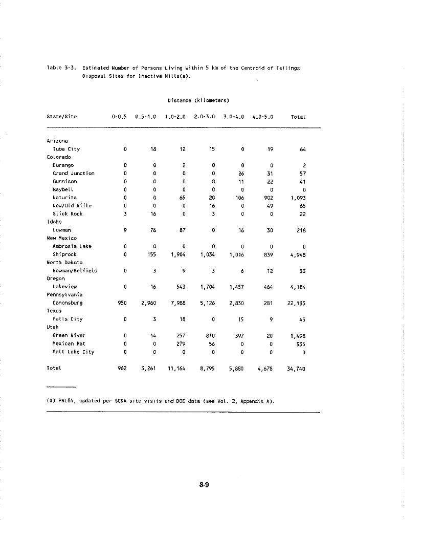
Table 3 - 3 . Estimated Nwnber of Persons L iv ing U i t h i n 5 km of the Centroid of Ta i l i ngs
Disposal S i tes fo r Inac t i ve M i l l s f a ) .
Distance (ki lwneters)
State/Si te 0-0.5 0.5-1.0 1.0-2.0 2.0-3.0 3.0-4.0 4.0-5.0 Tota l
Arizona
Tuba C i t y
Colorado
Durango
Grand Junction
Gunni son
Maybell
Na tu r i ta
NewlOLd R i f l e
S l i c k Rock
Idaho
L o m n
Neu Mexico
Ambrosia Lake
Shiprock
North Dakota
B o m n / B e l f i e l d
Oregon
Lakeview
Pennsylvania
Canonsburg Texas
F a l l s C i t y
Utah
Green River
Mexican Hat
Sa l t Lake C i t y
Total
(a) PNL84, updated per SC&A s i t e v i s i t s and DOE data (see Vol. 2, Appendix A).
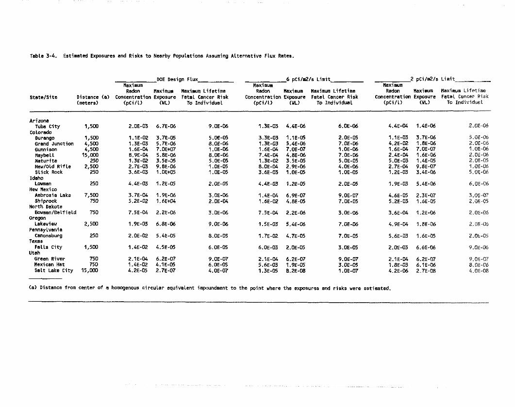
Table 3-4. Estimated Exposures and Risks t o Nearby Populations Assuming Alternative FLux Rates.
DOE Design Flux 6 pc i l rd ls Limit 2 pCi/&/s Limit Maximum Maximum Maximum Radon Maximum Maximum Lifetime Radon Maximum Maximua Lifetime Radon naximum Elaxioum Li fet iac
Statelsite Distance (a) Concentration Exposure Fatal Cancer Risk Concentration Exposure Fatal Cancer Risk Concentration Exposure Fatal Cancer Risk (meters) (pc i l l ) (UL) To Individual (pc i l l ) (UL) To Individual (pCi l l ) (VL) To IndividusV
Arizona Tuba City
Colorado Durango Grand Junction Gunnison naybe 1 1 Naturita NewlOLd R i f l e Slick Rack
I d a b Loman
New Uexico Ambrosia Lake Shiprock
North Dakota BournsnlBelfieLd
Oregon Lakeview
Pennsylvania Canonsbtrrg
Texas Falls City 1,5W 1.4E-02 4.5E-05 6.OE-05 6.OE-03 2.OE-05 3.OE-05 2.OE-03 6.6E-06 9.Of-06
Utah Green River 750 2.1E-04 6.2E-07 9.OE-07 2.1E-04 6.2E-07 9.OE-07 2.1E-04 6.2E-07 9.OE-07 Hexican Hat 750 1.4E-02 4.1E-05 6.OE-05 5.6E-03 1.9E-05 3.OE-05 1.8E-03 6.1E-06 B.OE-D6 Salt Let@ City 15,WO 4.2E-05 2.7E-07 4.0E-07 1.3E-05 8.2E-08 1.OE-07 4.2E-06 2.7E-08 4.OE-OB
(8) Distanca from center of a honqlenous circular equivalent impoundment t o the p i n t where the exposures and r isks were estioated.
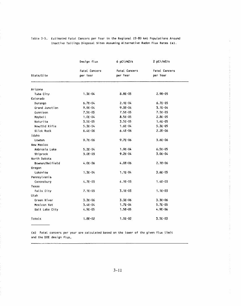
Table 3-5. Estimated Fatal Cancers per Year i n the Regional (0-80 km) Populations Around
Inac t i ve Tai l ings Disposal S i tes Assming A l te rna t i ve Radon Flux Rates (a) .
Oesign f l u x 6 pCi/m2/s 2 pCi/mZ/s
Fatal Cancers Fatal Cancers Fatal Cancers
per Year per Year per Year
Arizona
Tuba C i t y
Colorado
Ourango
Grand Junct ion
Gunni son
Maybel l
Natu r i ta
New/OLd R i f Le
S l i ck Rock
Idaho
Lowman
New Mexico
Ambrosia Lake
Shiprock
North Dakota
Bouman/Belfield
Oregon
Lakeview
Pennsylvania
Canonsburg
Texas
Fa l l s C i t y
Utah
Green River
Mexican Hat
Sal t Lake C i t y
Totals 1.8E-02 1.OE-02 3.5E-03
(a) Fatal cancers per year a re calculated based on the loner of the given f l u x l i m i t
a r d the DOE design f l u x .
(fro111 2E-2 to I E-2) at a l i t l l i t of 6 p~i/n12/sec. At a limit of 2 p ~ i / m 2 / s e c , the deaths pcr year
\vould bc reduced by about nine-tenths (from 2E-2 to 3E-3).
3.3.1.6 I)istril~utiotl of the Fatal Ca~lcer Risk
The fl-equency distribution of the estimated lifetime fatal cancer risk for all inactive uranium mill
tailings piles for each alternative are presented in Table 3-6. This distribution is developed by
simply summing the frequency distributions projected for each of the 18 facilities. The distribution
does not account for overlap in the populations exposed to radon-222 released from more than a
single mill. Given the remote locations of these facilities and the relatively large distances between
mills, this simplification does not significantly understate the lifetime fatal cancer risk to any
indi\,idual.
Previous studies habe examined the feasibility, effectiveness, and cost associated with various options
for controlling releases of radioactive materials from uranium mill tailings (NRC80, EPA82, EPA83,
EPA86). These studies ha \ e concluded that long-term stabilization and control will be required to
protect the public from the hazards associated with these tailings. The standards for long-term
disposal, established for these Title 1 sites under UMTRCA, provide for controls to prevent misuse
of the tailings, protect water resources, and limit releases of radon-222 to the air. The UMTRCA
standard established a design standard to limit long-term radon releases to an average flux no greater
than 20 pci/m2/sec.
Both active and passive controls are available to reduce radon-222 emissions from tailings. Active
controls require that some institution, usually a government agency, take the responsibility for
continuing oversight of the piles, and for making repairs to the control system when needed. Fences,
warning signs, periodic inspections and repair, and restrictions on land use are measures that may be
used by the oversight agency. Passive controls are measures of sufficient permanence to require little
or no active intervention. Passive controls include measures such as thick earth or rock covers,
barriers (dikes) to protect against floods, burial below grade. and moving piles out of flood prone
areas or away from population centers. Of the two methods, active or institutional controls are not
preferred for long-term stabilization of radon-222 emissions, since institutional performance of
oversight duties over a substantial period of time may not be reliable.
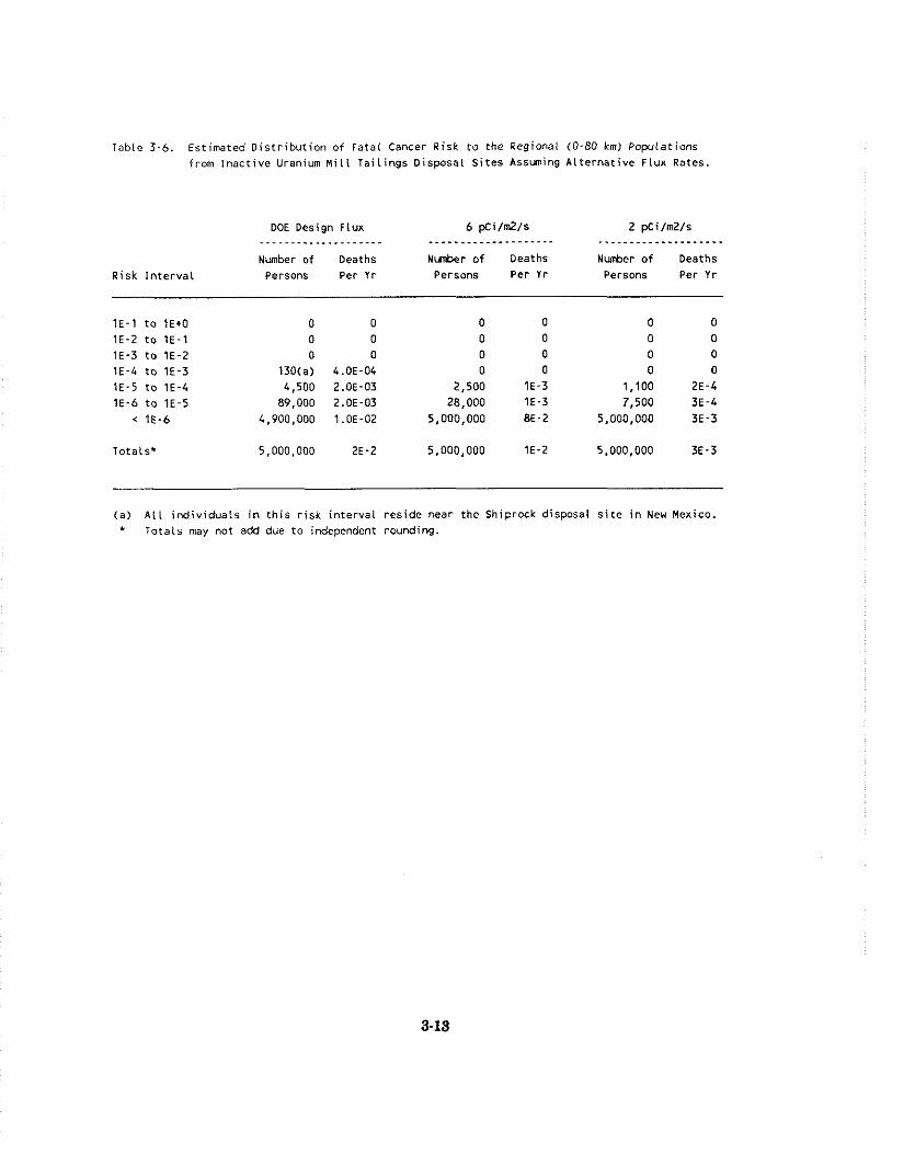
Table 3 - 6 . Estimated D is t r ibu t ion of Fatal Cancer Risk t o the Regional (0-80 kin) Populations from Inactive Uranium h i l l TaiLings Disposal s i tes Asswing Alternative Flux Rates.
DOE Design Flux 6 p t i l d / s 2 pti/rn2/s .................... .-.-.........-----.- ..-.......-......... Number of Deaths Nunber of Oeaths Number o f Deaths
Risk In te rva l Persons Per Yr Persons Per Yr Persons Per Y r
Totals* 5,000.000 ZE-2 5.000.000 1E-2 5,000,000 3E-3
( a ) A l l ind iv iduals i n th is r i sk in terval reside near the Shiprock disposal s i t e i n New Mexico. * Totals may not add due t o independent rounding.
l'revious studies (see above) lhave identified a nuinber of options to provide long-term control of
radon-222 e~nissions fro111 the tailings. These include earthen or synthetic covers, extraction of
radiuni from the tailings, chemical Fixation, and sintering. These long-term control options are
discussed in detail in Volume 2 of this E~~virorrme~ttal Inlpact Slateme111 (Appeudix 5).
In comparison to other control technologies earth covers have been shown to be cost-effective
(NRC80). Apart from cost considerations, there are other benefits that accrue by using earth covers
as a method to control radon-222 emissions. For example, synthetic covers, such as plastic sheets,
do not reduce gamma radiation. However, earth covers that are thick enough to reduce radon-222
emissions will reduce gamma radiation to insignificant levels. Further, chemical and physical stresses
over a substantial period of time destabilize synthetic covers. while earthen covers are stable over the
long run pro\ided the erosion caused by rain and wind is contained with \egetation or rock covers,
and appropriate precautions are taken against natural catastrophes.
Earthen covers also reduce the contamination of ground\\-ater that results from two alternative
control methods: storing radioactive materials in underground rnines(underground mines are typically
located under tlie water table), or using the leaching process to extract radioactive and non-
radioactive contaminants from mill tailings. Moreover, although underground mine disposal is an
effective method to protect against degradation and intrusion by man, it ne\,ertheless incurs a social
cost. For example, storing tailings in underground mines eliminates the future development of the
mines' residual resources.
Finally, earthen covers provide more effective long-term stabilization than either water or soil
cement coJ7ers. Soil cement covers are comparable to earthen covers in terms of cost-effectiveness,
but the long-term performance of these is as yet unknown. Water covers do not provide the long-
term stability required for tlie 1000-year time periods required. Moreover, earth covers are more
effective stabilizers in arid regions than are water spraying control technologies.
Covering the dried tailings with earth is an effective method for reducing radon-222 emissions and
is already in use at inactive tailings impoundments. uired for a given amount - cf-control varies with the type of earth and radon-222 exhalation rate. --
Earth covers decrease radon-222 emissions by the retaining radon-222 released from the tailings long
enough to allow a significant portion to decay in the cover. A rapid decrease in radon-222 emissions
is ilnnlediately achie\t.d by applying almost any type of earth. High-moisture content earths provide
greater radon-222 emission reduction because of their smaller diffusion coefficient.
In practice, eartlien co \e r designs must take into account uncertainties in tlie nieasured values of the
specific cover materinls used, the tailings to be covered, and predicted long-term values of
equilibrium moisture content for the specific location. The uncertainty in predicting reductions in
radon-222 flux increases rapidly as the required radon-222 emission limit is lowered.
The cost of adding earth covers depends on the location of the tailings impoundment, its layout, the
availability of earth, the topography of the disposal site, its surroundings, and the hauling distance.
Another factor affecting costs of cover material is its ease of excavation. i n general, the more
difficult the excavation, tlie more elaborate and expensive the equipment required and the higher the
cost. The availability of materials, such as gravel, dirt, and clny, also affects costs. If the necessary
materials are not available locally, they must be purchased and/or hauled, and costs could increase
significantly as a result.
This section presents the benefits and costs of reducing the allowable radon emissions after closure
from tlie maximuin limit of 20 p ~ i / n ~ 2 / s e c established under UMTRCA. Options which are
e\:alunted include lowering radon emissions to a maximum of 6 pCi/m2/sec or a maximum of 2
p ~ i , ' n i ~ / s e c .
This analysis assumes that UMTRCA is in place and that all controls required under UMTRCA will
be met regardless of any provisions resulting from this reconsideration of the CAA standards.
Therefore, the beginning point of this analysis (i.e., the baseline) assumes that all controls required
by UMTRCA are met, specifically that radon emission levels will be limited to a maximum of 20
pci/m2/sec and that nieasures will be undertaken to achieve the long-run stability required by the
UhlTRCA rules.
Benefits are measured as reductions i n the estimates of committed fatal cancers resulting from lower
allowable emissions. Results are presented in terms of both total benefits and average annual
benefits. For the calculation of total benefits a 100-year time period is assumed.
All costs are tiicasured i n I988 dollars and represent the cost of both the disposal and stabilization of
the 1:lilrngs. Cost eslimntes are calculated assuming no remedial actions have taken place. The costs
of mccting the DOE design flux, the 6 p ~ i / m 2 / s e c and the 2 pci/m2/sec are then estimated. The cost
of the alternative standards are the incremental costs from the baseline (DOE design flux) to the 6
or 2 pci /m2/sec alternative. Results are presented in net present value and annualized cost, and are
estimated using real interest rates of zero, one percent, five percent and ten percent. A 100-year
time period is used.
3.4.1 Benefits
It is assumed that reductions in the radon flux rate provided by increasing the depth of cover will
yield proportional reductions i n committed cancers. The resulting estimates of committed cancers
per year on a pile-by-pile basis are presented abo\e for the DOE cover design flux, 6 and 2
pci/m2/sec options in Table 3-5.
Table 3-7 summarizes the estimates of risk and reduction of risk (committed cancers) for the various
regulatory options. The table presents these estimates for the 100-year period as well as annual
averages. Over the 100-year time frame, the 6 pCi/m2/sec option lowers regional risks by 0.8
conimitted cancers. The incremental benefit of lowering the allowable flux rate from 6 pci/m2/sec
to 2 i/rn2/sec is estimated as 0.65 committed cancers.
For reasons described in Section 3.3.2, the supplemental control selected for long-term radon-222
control at inactive tailings inipoundments is the earthen cover control option. The thickness of cover
required to achieve a given radon flux is a function of the initial radon flux from the pile. Five
operations are required to place earthen covers on inactive tailings piles. These include: regrading
slopes. procurement and placing of the dirt cover, placing gravel on the pile tops, placing of rip-
rap on the pile sides, and reclamation of the borrow pits. The estimation of earth cover thicknesses
and the costs for the five operations are described in detail in Appendix B of Volume 2 of the
E ~ i i ~ i r o ~ i n i e ~ r ~ a l Inipaci S la ie~nr~i r .
Three overhead cost factors were used to adjust the cost of earth cover described above. First, a
factor of 1.07 was applied to reflect general industry overhead and costs, (for a discussion of cost
factors see Appendix B, Volume 2). Second, a project cost factor of 3.4, based upon UMTRAP
experience, was applied to reflect additional government costs for community participation,

Table 3-7: Total and Annualized Risk end Reduction of Risk ( C m i t t e d Cancers)
of Louering the Allowable Flux Limit t o 6 and 2 pCi/Q/sec.
20 pdCi/Q/sec 6 pCilQ/sec 2 p€i/Q/sec Baseline Option opt ion
I===.;;;;;;=z===;;,===================z=z======,================e~==========-----------------l *----------------
Risk Risk Risk
Reduction frm Reduction f r ~ Reduction f r w
Risk Risk 20 pCi /d /sec Risk 20 p C i / d l s e c 6 pCi /d /sec
Baseline Baseline Baseline ................................................................................................................. I
Risk 1.8 1.00 0.35
Cancers avoided
over 100 years:
Risk 0.0180 0.0100 0.0035
Annual cancers
avoided:

teclinology development atid evaluation, site acquisition, costs for a planning contractor, management
support,design, construstion management, and associatedservices. Finally, since rnanyof these items
rept-esent sunk costs, an alternative factor of 2.4, which measures only estimated future costs, is also
included in the analysis.
The estimates of costs on a pile-by-pile basis are presented for the DOE design flux, 6 and 2
pci/rn2/sec options in Tables 3-8, 3-9, and 3-10, respectively. Achieving the DOE design flux is
estimated to cost between $136 and $418 niillion. In contrast, reaching the 6 pci /m2/sec option is
estinlated to cost from $157 to $483 million, while compliance with the 2 pci/m2/sec option would
entail costs estimated to reach between $188 and $579 million.
Expenditures to meet the DOE design flux or the 6 and 2 pci/m2/sec options are assumed to begin
in 1989 and be accomplislied over five years. Dollar expenditures are in equal amounts in each of
the five years in current dollars.
Table 3-1 I provides the incremental present value costs for the three radon fluxes and added costs
for lowering the allowable flux. Estimates for each of the DOE project cost factors and each of the
four real interest rates, are included. Lowering the allowable flux rate to 6 p~i /n i ' / sec will entail
added present value costs of between $13 and $64 million depending on assumptions as to project cost
and discount rates, while attainment of a 2 pci/rn2/sec flux rate would entail costs of $33 to $161
niillion. The incremental costs of moving from the 6 pCi/m2/sec option to the 2 ~ C i / m 2 / s e c option
is estimated to range from $19 to $96 million.
The present value costs are also shown graphically in Figure 3-1. This graph indicates that the
marginal cost per unit of radon flux reduction is lower between 20 pci/m2/sec and 6 p ~ i / n ~ 2 / s e c than
between 6 p ~ i / m 2 / s e c and 2 p~i / rn2/sec . This reflects the increasing depth of cover required per
unit decrease in radon flux. Figut-e 3-1 also shows that the cost per unit of radon flux reduction is
lo\ver at higher real interest rates reflecting the reduced present value of future cash streams.
Table 3-12 provides similar estimates to those given in Table 3-1 1, except the values in 3-12 are
presented on an annualized cost basis. For the 6 pci/m2/sec option, added costs on an annualized
basis range from $1.1 to $4.8 million depending on cost factor and discount rate assumptions. For
the 2 pci/m2/sec option, added costs vary from $2.6 to $1 1.8 million.
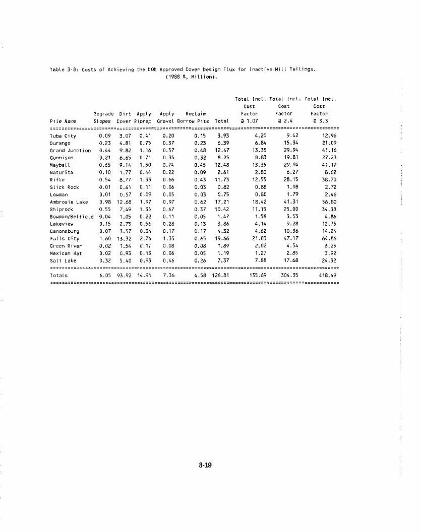
Table 3 - 8 : Costs of Achieving the DOE Approved Cover Oesign Flux fo r i n a c t i v e M i l l T a i l i n g s (1988 8 , M i l l i o n ) .
Tota l I n c l . Tota l i n c l . T o t a l i n c l .
cost cos t cos t
Regrade D i r t Apply Apply Reclaim Factor Factor Factor P i l e Name Slopes Cover R iprap Gravel Borrou P i t s Tota l @ 1.07 @ 2.4 @ 3.3 ii=iiiiiiiiii__z==i======z=~=======z===========zs=============~=======~======z====z=====~===========
Tuba C i t y 0.09 3.07 0.41 0.20 0.15 3.93 4.20 9.42 12.96 Durango 0.23 4.81 0.75 0.37 0.23 6.39 6.84 15.34 21.09 Grand Junct ion 0.44 9.82 1.16 0.57 0.48 12.47 13.35 29.94 41.16 Gunnison 0.21 6.65 0.71 0.35 0.32 8.25 8.83 19.81 27.23 Maybel I 0.65 9.14 1.50 0.74 0.45 12.48 13.35 29.94 41.17
N a t u r i t a 0.10 1.77 0.44 0.22 0.09 2.61 2.80 6.27 8.62 R i f l e 0.54 8.77 1.33 0.66 0.43 11.73 12.55 28.15 38.70 S l i c k Rock 0.01 0.61 0.11 0.06 0.03 0.82 0.88 1.98 2.72 ~owman 0.01 0.57 0.09 0.05 0.03 0.75 0.80 1.79 2.46 Ambrosia Lake 0.98 12.68 1.97 0.97 0.62 17.21 18.42 41.31 56.80 Shiprock 0.55 7.49 1.35 0.67 0.37 10.42 11.15 25.00 34.38 Bouman/Bel f ie ld 0.04 1.05 0.22 0.11 0.05 1.47 1.58 3.53 4.86 Lakevieu 0.15 2.75 0.56 0.28 0.13 3.86 4.14 9.28 12.75 Canonsburg 0.07 3.57 0.34 0.17 0.17 4.32 4.62 1.0.36 14.24 F a l l s C i t y 1.60 13.32 2.74 1.35 0.65 19.66 21.03 47.17 64.86 Green River 0.02 1.54 0.17 0.08 0.08 1.89 2.02 4.54 6.25 Mexican Hat 0.02 0.93 0.13 0.06 0.05 1.19 1.27 2.85 3.92 s a l t Lake 0.32 5.40 0.93 0.46 0.26 7.37 7.88 17.68 24.32 .................................................................................................... ----------...........- ~-~~...~~-~---...~~--~----~...~~--------.~.~-~-------~~--------------------~~~
Tota ls 6.05 93.92 14.91 7.36 4.58 126.81 135.69 304.35 418.49 .................................................................................................... ....................................................................................................
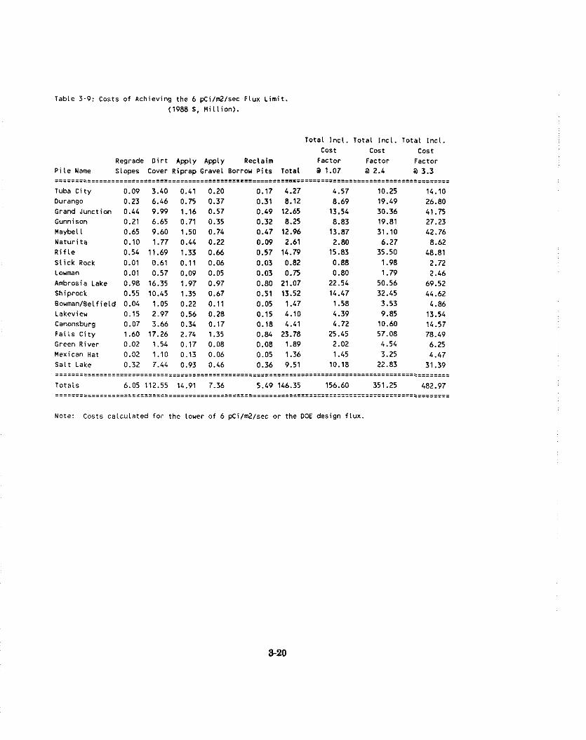
Table 3-9: Costs of Achieving the 6 pCi/rn2/sec Flux L i m i t .
(1988 S, M i l l i o n ) .
Total I n c l . Tota l I n c l . Total I nc l . cost cost cost
Regrade D i r t Apply Apply Reclaim Factor Factor Factor P i l e Name slopes Cover Riprap Gravel Borrou P i t s Total a 1.07 @ 2.4 @ 3.3 ==i====i==iSSiiE=Sl============~===========~===============~========~======z=============~========
Tuba C i t y 0.09 3.40 0.41 0.20 0.17 4.27 4.57 10.25 14.10 Durango 0.23 6.46 0.75 0.37 0.31 8.12 8.69 19.49 26.80 Grand Junct ion 0.44 9.99 1.16 0.57 0.49 12.65 13.54 30.36 41.75 Gunnisan 0.21 6.65 0.71 0.35 0.32 8.25 8.83 19.81 27.23 Maybel l 0.65 9.60 1.50 0.74 0.47 12.96 13.87 31.10 42.76 N a t u r i t a 0.10 1.77 0.44 0.22 0.09 2.61 2.80 6.27 8.62 R i f l e 0.54 11.69 1.33 0.66 0.57 14.79 15.83 35.50 48.81 S l i c k Rock 0.01 0.61 0.11 0.06 0.03 0.82 0.88 1.98 2.72 Louman 0.01 0.57 0.09 0.05 0.03 0.75 0.80 1.79 2.46 Ambrosia Lake 0.98 16.35 1.97 0.97 0.80 21.07 22.54 50.56 69.52 Shiprock 0.55 10.45 1.35 0.67 0.51 13.52 14.47 32.45 44.62 6owman/8elfield 0.04 1.05 0.22 0.11 0.05 1.47 1.58 3.53 4.86 Lakeview 0.15 2.97 0.56 0.28 0.15 4.10 4.39 9.85 13.54 Canonsburg 0.07 3.66 0.34 0.17 0.18 4.41 4.72 10.60 14.57 F a l l s C i t y 1.60 17.26 2.74 1.35 0.84 23.78 25.45 57.08 78.49 Green River 0.02 1.54 0.17 0.08 0.08 1.89 2.02 4.54 6.25 Mexican Hat 0.02 1.10 0.13 0.06 0.05 1.36 1.45 3.25 4.47 s a l t Lake 0.32 7.44 0.93 0.46 0.36 9.51 10.18 22.83 31.39 iiliiii:lil=ILTIEEE================================================================zx====z========
Tota ls 6.05 112.55 14.91 7.36 5.49 146.35 156.60 351.25 482.97 -------~...~...~~~---~~---~~~--~~~~......~-----~---~~~~~~~-----~-~-~~~---~~-------------- .......................................................................................... ========
Note: Casts ca l cu la ted fo r the lower of 6 pCi/m2/sec or the OOE design f l ux .

i a b l e 3-10: Costs o f Achieving the 2 pCilrn21sec Flux L i m i t .
(1988 $, M i l l i o n ) .
Tota l I n c l . Total I n c l . Tota l I n c l . cost cos t cos t
Regrade D i r t Apply Apply Reclaim Factor Factor Factor P i l e Name Slopes Cover Riprap Gravel Borrow P i t s Tota l @ 1.07 @ 2.4 @ 3.3 -------..-.---------.-..-.------.-----------.--------------------...----------.-------------------- ---..------------..--------------------------------------------------------------------------------
Tuba C i t y 0.09 4.22 0.41 0.20 0.21 5.14 5.50 12.33 16.96 Durango 0.23 7.96 0.75 0.37 0.39 9.70 10.38 23.27 32.00 Grand Junc t i on 0.44 12.32 1.16 0.57 0.60 15.09 16.15 36.23 49.81 Gunnison 0.21 6.65 0.71 0.35 0.32 8.25 8.83 19.81 27.23 Maybel l 0.65 12.61 1.50 0.74 0.61 16.11 17.24 38.67 53.17 Natu r i t a 0.10 2.50 0.44 0.22 0.12 3.38 3.62 8.12 11.17 R i f l e 0.54 14.36 1.33 0.66 0.70 17.58 18.81 42.20 58.03 S l i c k Rock 0.01 0.83 0.11 0.06 0.04 1.05 1.13 2.53 3.48 Lowman 0.01 0.75 0.09 0.05 0.04 0.93 1 .OO 2.24 3.08 Ambrosia Lake 0.98 20.30 1.97 0.97 0.99 25.20 26.97 60.49 83.18 Shiprock 0.55 13.15 1.35 0.67 0.64 16.35 17.50 39.25 53.97 BoumanIBel f ie ld 0.04 1.32 0.22 0.11 0.06 1.76 1.88 4.22 5.81 Lakevieu 0.15 4.10 0.56 0.28 0.20 5.28 5.65 12.68 17.43 Canonsburg 0.07 4.34 0.34 0.17 0.21 5.12 5.48 12.30 16.91 F a l l s C i t y 1.60 22.74 2.74 1.35 1.11 29.54 31.61 70.89 97.48 Green R ive r 0.02 1.54 0.17 0.08 0.08 1.89 2.02 4.54 6.25 Mexican Hat 0.02 1.35 0.13 0.06 0.07 1.62 1.74 3.90 5.36 S a l t Lake 0.32 9.31 0.93 0.46 0.45 11.47 12.27 27.53 37.85 ................................................................................................... ...................................................................................................
Tota l s 6.05 140.34 14.91 7.36 6.85 175.50 187.79 421.21 579.16 ................................................................................................... ...................................................................................................
Note: Costs c a l c u l a t e d f o r the lower o f 2 pCilrn2lsec or the DOE des ign f l u x .
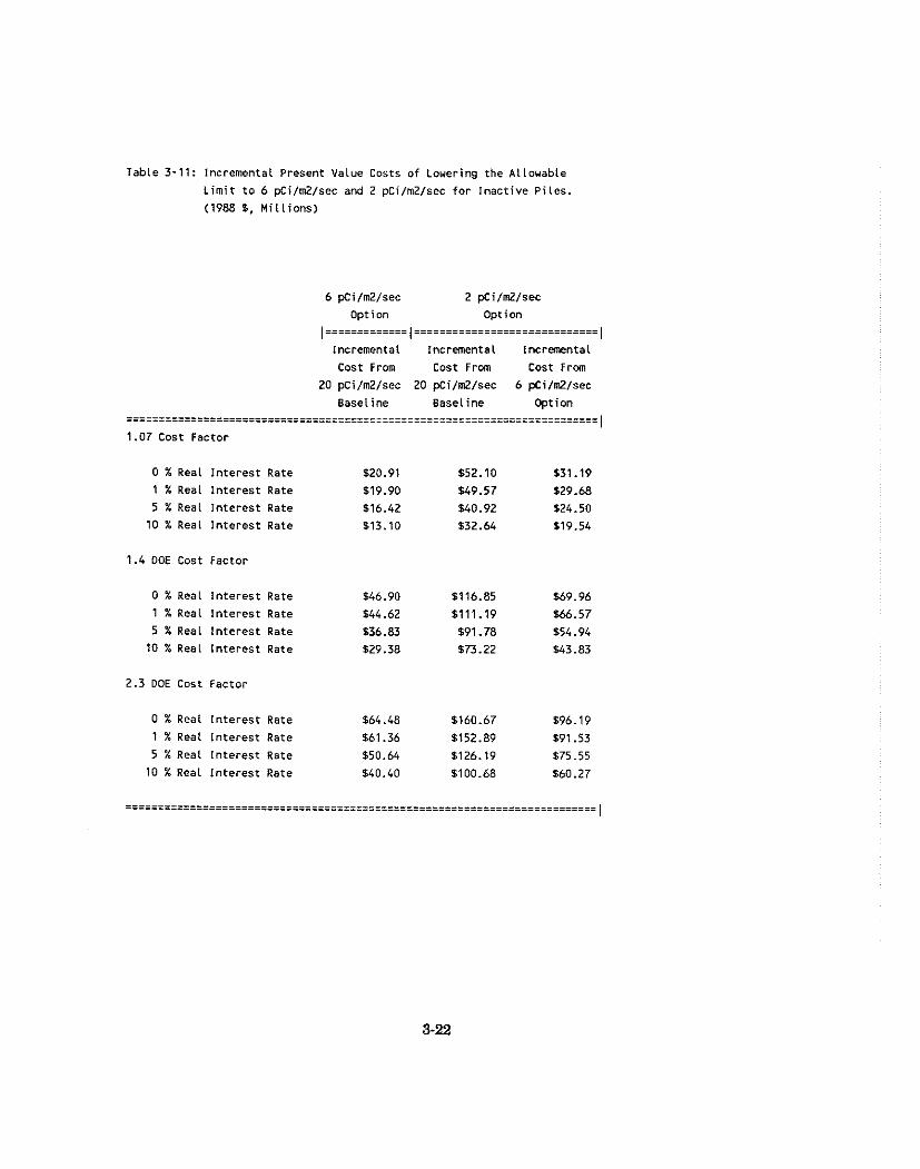
Table 3-11: Incremental Present Value Costs of Lowering the Al louable
L i m i t t o 6 pCi/mZ/sec and 2 pci/mZ/sec f o r Inac t i ve P i l e s .
(1988 $, M i l l i o n s )
6 pci/m2/sec 2 pci/mZ/s=
Option Option I = = E = I = ~ ~ E ~ = E ~ ~ ~ ~ ~ ~ = = = = = = = = = = = = = = ~ = = = = = = = = = = ~
Incremental Incremental Incremental
Cost From Cost F r m Cost F r m
20 pci/m2/sec 20 pci/mZ/sec 6 pCi/mZ/sec
Basel ine Basel ine Option -------------------------------..-~-~--..-------------..-.--...----------- -------------------------------------........-.........-----------..------ I 1.07 Cost Factor
0 % Real I n t e r e s t Rate $20.91 $52.10 $31.19 1 % Real I n t e r e s t Rate $19.90 $49.57 129.68 5 % Real I n t e r e s t Rate $16.42 $40.92 124.50 10 % Real I n t e r e s t Rate $13.10 $32.64 $19.54
1.4 DOE Cost Factor
0 % Real I n t e r e s t Rate $46.90 $116.85 569.96 1 % Real I n t e r e s t Rate $44.62 6111.19 W . 5 7 5 % Real I n t e r e s t Rate $36.83 $91.78 154.94
10 % Real I n t e r e s t Rate $29.38 $73.22 S43.83
2.3 DOE Cost Factor
0 % Real I n t e r e s t Rate $64.48 $160.67 196.19 1 % Real I n t e r e s t Rate $61.36 $152.89 '691.53 5 % Real I n t e r e s t Rate $50.64 $126.19 $75.55 10 % Real I n t e r e s t Rate $40.40 $100.68 $60.27
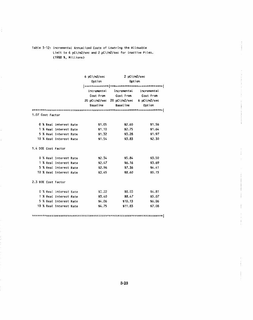
Table 3-12: lncremental Annualized Costs of Louering the Allowable
L im i t t o 6 pCiIm2lsec and 2 pCilm2lsec f o r Inact ive Pi les.
(1988 1, N i l l i o n s )
6 pCilm2lsec 2 pCilm2lsec
Option Option l i ~ = = = _ i i i = i = = = l i i i = = = = = = = = = = = = = = = = = = = = = z = = = = = l
lncremental lncremental Incremental
Cost From Cost From Cost From
20 pCi/m2/sec 20 pCilm2lsec 6 pCilm2Isec
Baseline Base1 ine Option ........................................................................... I 1.07 Cost factor
0 % Real In te res t Rate $1.05 $2.60 $1.56 1 % Real In te res t Rate $1.10 $2.75 $1.64 5 % Real in te res t Rate 51.32 $3.28 $1.97
10 % Real In te res t Rate $1.54 $3.83 $2.30
1.4 DOE Cost Factor
0 % Real In te res t Rate $2.34 $5.84 $3.50 1 % Real In te res t Rate $2.47 $6.16 $3.69
5 % Real In te res t Rate $2.96 $7.36 $4.41 10 % Real In te res t Rate 53.45 $8.60 $5.15
2.3 DOE Cost Factor
0 % Real In te res t Rate $3.22 $8.03 $4.81
1 % Real In te res t Rate $3.40 $8.47 $5.07 5 % Real in te res t Rate $4.06 $10.13 $6.06
10 % Real In te res t Rate $4.75 $11.83 $7.08
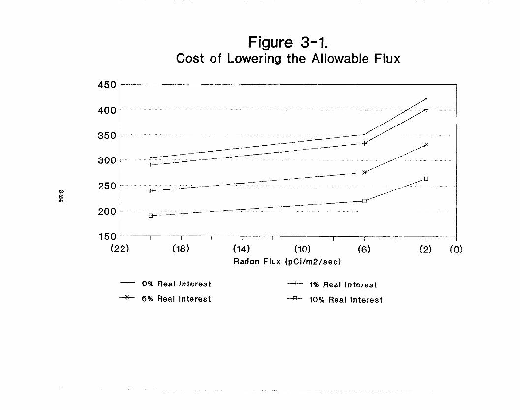
Figure 3-1. Cost of Lowering the Allowable Flux
r--1 (22) (18) (14) (10) (6 (2) (8)
Radon Flux (pCi/rn2/sec)
- 0% Real lnterest
* 5% Real lnterest
-t 1% Real lnterest
-s- 10% Real lnterest
The purpose of this section is to evaluate the economic impacts of Federal and state expenditures to
comply with the costs associated with lowering the allowable radon-222 emission rate. No attempt
is made to quantify these impacts, instead a qualitative discussion is given.
The costs of regulatory remedial actions, for any inactive mills not on Indian lands, are shared by the
Federal and State governments. The Federal Government is accountable for ninety percent of these
costs. in the case of Indian lands, however, the Federal Government is solely responsible for any
costs associated with the disposal of tailings. Thus, these regulations ha1.e no impact on the uranium
industry. In addition, there will be no impact on small businesses.
Any regulatory remedial action is expected to have positive economic impacts at both the state and
local levels. The inipacts are the result of fiscal injections and could be measured in terrns of
increased local employment. income and standards of living. These funds would come from the
Federal (DOE) and State budgets. The expenditures are transfer payments, i.e., the funds are
genernted through taxes and spent on particular programs or areas. In most cases these expenditures
will result in higher Federal expertditures within each state than would have occurred without these
programs. There will be no disproportionate increase, however, in Federal taxes paid by residents
of these states.
REFERENCES
PNLS-I
U.S. Department of Energy, "Annual Status Report on the Uranium Mill Tailings Remedial Action Program," Washington, D.C., December 1988.
U.S. Environmental Protection Agency, Final Eilvironmeirral Impact Slaien~eili for Renledial Aclioii S tar~dards for. Ir~aclive Urarziunt Proccssitlg Silc~s (40 CFR 192), Vol.1, EPA 52014-82-013-1, Officeof RadiationPrograms, Washington, D.C., October 1982.
U.S. Environmental Protection Agency, Fiital E~zvironn~eir~nl lnzpacl Slnlen~eiii /or Slatrdards for the Cor~lrol of By-P~.oducl Materials fronl Urailiun7 Oi-c Processi~lg (40 CFR 192), Vol, 1, EPA 52011-83-008-1, Office of Radiation Programs, Washington, D.C. 1983
U.S. Environmental Protection Agency, Firla1 Rule for Rndorl-222 Eniissioirs Iron1 Licetised Urar~iunm Mill Tailirlgs, EPA 520/l-86-009, OFfice of RAdiation Programs, Washington, D.C., August 1986.
Risk Assessnie11ts, Vol. 2.
Personal communication, Energy and Minerals Department, Mine Inspection Bureau, State of New Mexico, December 1985.
U.S. Nuclear Regulatory Conimission, Firla1 Geileric E i n ~ i ~ ~ o i i n ~ e ~ ~ ~ a l lnzpacl Staten7etli oii Ur.ariiuni il4illiiig, NUREG-0706, Washington, D.C., September 1980.
Pacific Northwest Laborztory. "Estimated Population Near Uranium Tailings," PNL- 4959, WC-70, Richland, \\'A, Janurary 1984.

4. LICENSED MILL TAILINGS
4.1 Introduction and Summary
The licensed uranium mill tailings source category comprises the tailings impoundments and
evaporation ponds created by conventional acid or alkaline leach processes at uranium mills licensed
by the Nuclear Regulatory Commission (NRC) or the Agreement States. Recovery of uranium by
conventional milling results in the release of uranium and i n decay products to the air. The risks
associated with the release of uranium and other radionuclides in the form of particulates are
addressed in the proposed regulation for the uranium fuel cycle source category (Chapter I). This
assessment addresses only radon-222 released from the tailings impoundments and their associated
evaporation ponds. Previous evaluations have shown that radon releases from other milling operations
are insignificant [NRCBO, EPA82, EPA83, EPA86J.
In August 1988, the conventional uranium milling industry in the United States consisted of 26
licensed facilities. The licensed conventional uranium mills that have operated are in Colorado, New
Mexico, South Dakota, Texas, Utah, Washington, and Wyoming. Only 4 of the 26 licensed facilities
were operating; 8 were on standby status; and 14 were being or have been decommissioned. The mills
on standby status are being maintained, but they are not processing uranium ore. When demand for
uranium increases, these standby mills can resume milling. The decommissioned mills have been
dismantled and have either been moved off-site or disposed of on-site. These mills can never resume
operations. Their associated tailings impoundments are either being reclaimed, or plans to reclaim
them have been made. Three other mills have been licensed, but two were never constructed, and
one was built but never operated. These three mills are not discussed further here [EPA89].
The purpose of this chapter is to examine the costs, benefits, and economic impacts of three separate
decisions that need to be addressed in promulgating the new Clean Air Act standards for release of
radionuclides from licensed uranium mill tailings piles. The f i t decision to address is whether to
reduce the limit on allowable radon-222 emissions after closure from the current Uranium Mill
Tailings Radiation Control Act (UMTRCA) standard of 20 pCilmz/sec. Options that are evaluated
include allowable limits of 6 p~ i /m2/sec and 2 pci(m2/sec.

The second decision to consider is whether to reduce the limit on allowable emissions of operating
mills without curtailing the operation of the mills. The limit to be considered is a maximum average
radon emission of 20 pci/m2/sec during the operational life of the facility.
While the first two decisions are focused on existing piles, the third is concerned with future tailings
impoundments. The decision to be addressed for future tailings is whether work practice standards
should be promulgated for the control of radon emissions from operating mills in the future. Options
that are investigated include the replacement of the traditional single cell impoundment with phased
or continuous disposal impoundments.
The remainder of this introduction provides a brief summary of the rulemaking history and current
regulations. A profile of the uranium milling industry is given in Section 4.2. Included are industry
characteristics such as demand and supply, financial and community analyses, and projections of
industry production and employment. Section 4.3 addresses current emissions, risk levels and feasible
control methods. Section 4.4 provides estimated benefits and costs for each of the options under the
separate decision frameworks. The economic impacts are considered in Section 4.5.
4.1.1 Rulemakine Historv and Current Reeulations
On January 13, 1977, the EPA issued Environmental Protection Standards for Nuclear Power
Operations. These standards (40 CFR 190) limit the total individual radiation dose during normal
operations from uranium fuel cycle facilities, including licensed uranium mills. However, when 40
CFR 190 was promulgated, considerable uncertainty existed regarding the public health risk from
radon-222 and the best method for managing new manmade sources of this radionuclide. Therefore,
the doses caused by emissions of radon-222 are excluded from the limits established in 40 CFR 190.
On April 6, 1983, the Agency proposed National Emission Standards for Hazardous Air Pollutants
(NESHAPS) for radionuclides under Section 112 of the Clean Air Act (CAA). At that time, it
determined that uranium fuel cycle facilities should be exempt from the NESHAP for NRC-Licensed
Facilities, since they were already subject to the dose limits of 40 CFR 190. During the comment
period, it was noted however, that radon-222 emissions from operating uranium mills posed
significant public health risks and that such emissions were not subject to any current or proposed
EPA standards.
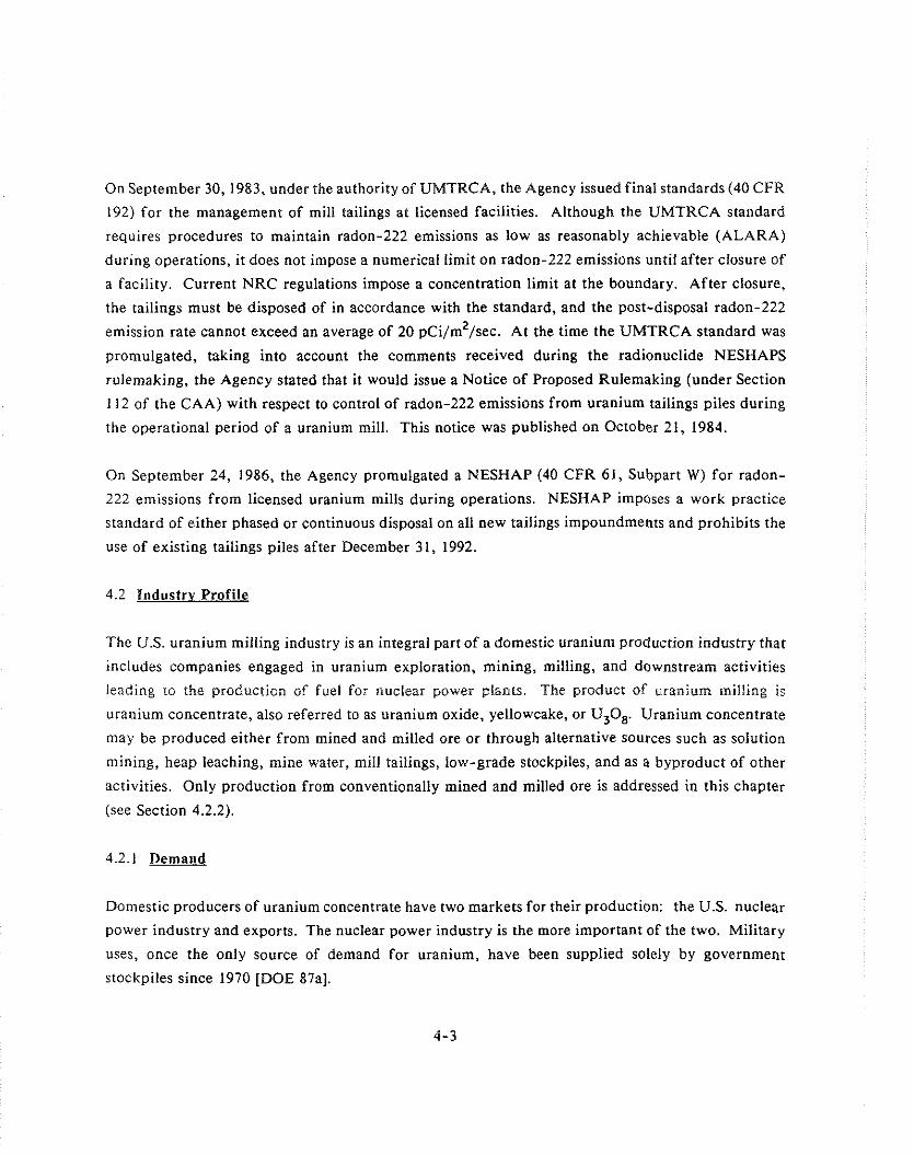
On September 30,1983, under the authority of UMTRCA, the Agency issued final standards (40 CFR
192) for the management of mill tailings at licensed facilities. Although the UMTRCA standard
requires procedures to maintain radon-222 emissions as low as reasonably achievable (ALARA)
during operations, it does not impose a numerical limit on radon-222 emissions until after closure of
a facility. Current NRC regulations impose a concentration limit at the boundary. After closure,
the tailings must be disposed of in accordance with the standard, and the post-disposal radon-222
emission rate cannot exceed an average of 20 p~i /m*/sec . At the time the UMTRCA standard was
promulgated, taking into account the comments received during the radionuclide NESHAPS
rulemaking, the Agency stated that it would issue a Notice of Proposed Rulemaking (under Section
112 of the CAA) with respect to control of radon-222 emissions from uranium tailings piles during
the operational period of a uranium mill. This notice was published on October 21, 1984.
On September 24, 1986, the Agency promulgated a NESHAP (40 CFR 61, Subpart W) for radon-
222 emissions from licensed uranium mills during operations. NESHAP imposes a work practice
standard of either phased or continuous disposal on all new tailings impoundments and prohibits the
use of existing tailings piles after December 31, 1992.
4.2 lndustrv Profile
The U.S. uranium milling industry is an integral part of a domestic uranium production industry that
includes companies engaged in uranium exploration, mining, milling, and downstream activities
leading to the production of fuel for nuclear power piants. The product of uranium milling is
uranium concentrate, also referred to as uranium oxide, yellowcake, or U30s Uranium concentrate
may be produced either from mined and milled ore or through alternative sources such as solution
mining, heap leaching, mine water, mill tailings, low-grade stockpiles, and as a byproduct of other
activities. Only production from conventionally mined and milled ore is addressed in this chapter
(see Section 4.2.2).
4.2.1 Demand
Domestic producers of uranium concentrate have two markets for their production: the U.S. nuclear
power industry and exports. The nuclear power industry is the more important of the two. Military
uses, once the only source of demand for uranium, have been supplied solely by government
stockpiles since 1970 [DOE 87al.

Demand for domestic uranium has declined since the late 1970s. In 1979, utilities delivered 15,450
tons of domestic uranium oxide to DOE for enrichment, 86 percent more than 1986 deliveries.
Exports, too, have declined substantially. In 1979, exports amounted to 3,100 tons, almost four times
as much as in 1986. A number of negative forces have combined to cause the current depressed state
of the industry. Perhaps most importantly, the growth in electricity generated by nuclear plants and
the expansion of nuclear power capacity has been much slower than had been forecast in the mid-
1970s. This slower growth is due in part to numerous construction delays and cancellations. Second,
imports have begun to play a major role in the U.S. uranium market. The import restrictions were
gradually withdrawn between 1975 and 1985. The result has been a steady increase in uranium
imports from nations possessing high grade (and thus low cost) uranium deposits. Expectations are
that a growing portion of utility requirements will be supplied by foreign-origin uranium during the
second half of this decade [JFA SSa].
Also contributing to the current downturn in the uranium industry are the large inventories being
held by both producers and utilities. Utilities, anticipating a growing need for uranium, entered into
long-term contracts to large amounts of domestically-produced uranium. As actual needs
fell short of expected needs due to nuclear power plant construction delays and cancellations, large
inventories accumulated. These inventory supplies, currently estimated to cover four to five years
of utility requirements, adversely affect suppliers in two ways. They may extend the downturn in
uranium demand for a number of years by decreasing the need for utilities to enter into new
contracts. Also, high interest rates increased inventory holding costs, Leading some utilities to
contribute to current excess supply by offering inventory stocks for sale on the spot market [JFA
Sja].
The focus of the remainder of this section is total U.S. demand for uranium, not just demand for
domestic production or production from conventional mills. The first subsection details historical
uses of uranium. The concluding subsection provides a brief description of uranium prices and
pricing mechanisms.

4.2.1 .I Uranium Uses
Military Applications
In the early 1950s. the U.S. government's need for uranium for defense uses far exceeded the world's
production capability. A federally funded production incentives piogram was then instituted. The
incentives program was so effective that the government phased it out in the 1960s and terminated
its purchase program in 1970. The government still has sufficient stockpiles to meet military
requirements well into the future.
Nuclear Power Plants
Since 1971, utilities which use uranium as fuel for nuclear power plants, have been virtually the only
source of demand for current uranium production. Commercial generation of nuclear powered
electricity began in 1957 with the operation of the first central station reactor at Shippingport,
Pennsylvania. At the end of 1986, 100 nuclear reactors were licensed to operate in the United States,
with 85.2 gigawatts of net generating capacity [DOE 87~1.
Demand for uranium by utilities may be directly linked to the fuel requirements of currently
operating or planned nuclear power plants. The status of U.S. nuclear power plants as of December
31, 1986 is shown in Table 4-1. Because of the long lead times associated with the ordering,
construction and permitting of nuclear power plants, it is extremely uniikely that any additional
orders for new nuclear plants will result in operable capacity before 1998 [DOE 87cl. Historical
consumption data for utilities are not available. The closest approximation is statistics on deliveries
by utilities of uranium to DOE enrichment plants. Deliveries for 1977 to 1986 are listed in Table 4-2.
Exports
Exports of uranium by producers have declined steady since 1979. In 1984, at 1,100 tons of U30,,
exports were the lowest since 1976. Current commitments for exports total only 4,400 tons for
1985-2000 [DOE 85b]. Exports for 1977-1986 are shown in Table 4-3.
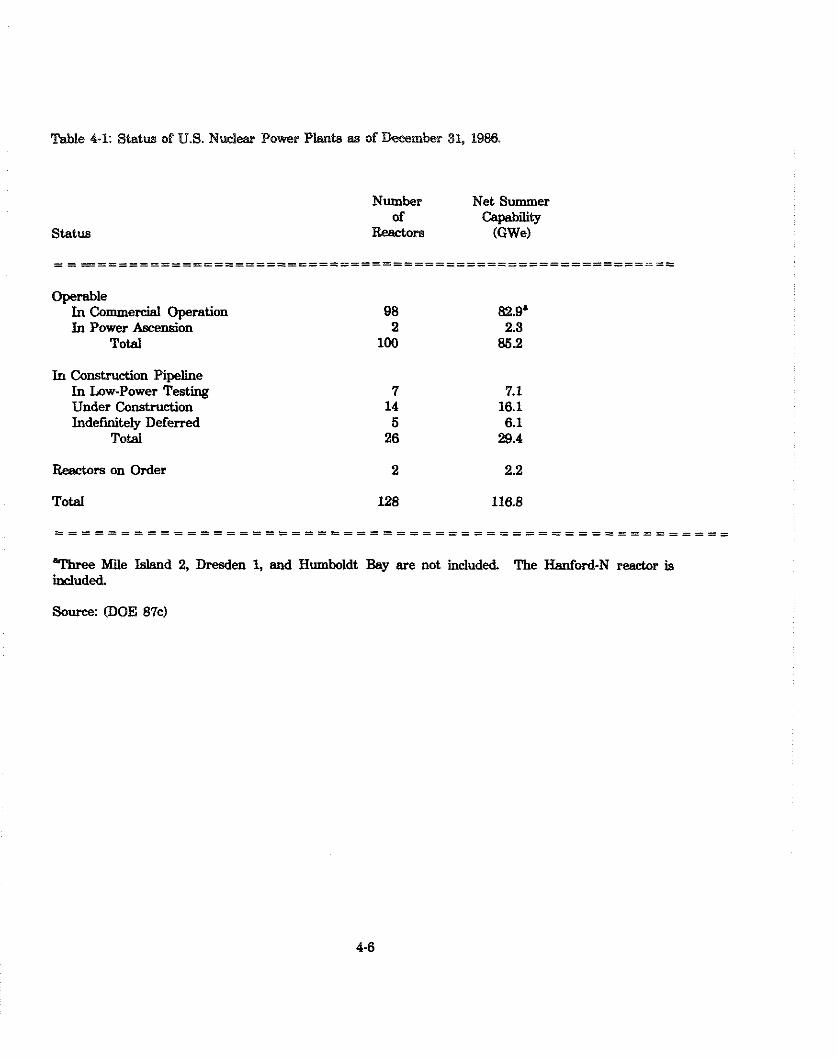
Table 4-1: Status of U.S. Nuclear Power Plants as of Decetnkr 31. 1986.
Status
Number Net Summer of Capab'ity
Reactors (GWe)
Operable In Commercial Operation In Power Ascension
Total
In Construction Pipeline In Low-Power Testing Under Construction Indefmitely Deferred
Total
Reactors on Order 2 2.2
Total 128 116.8
Wm=e Mile Island 2, headen 1, and Humboldt Bay are not included. The Hauford-N reactor is Muded.
Source: (DOE 87c)
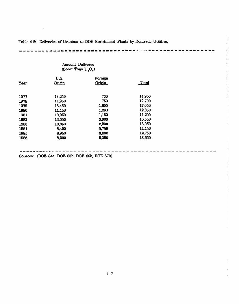
Table 4-2: Deliveries of Uranium to DOE E~chrnent Plants by Domeetic Utilities.
Amount Delivered (Short Tons U,O,)
U.S. Foreign Year Qjg& Total
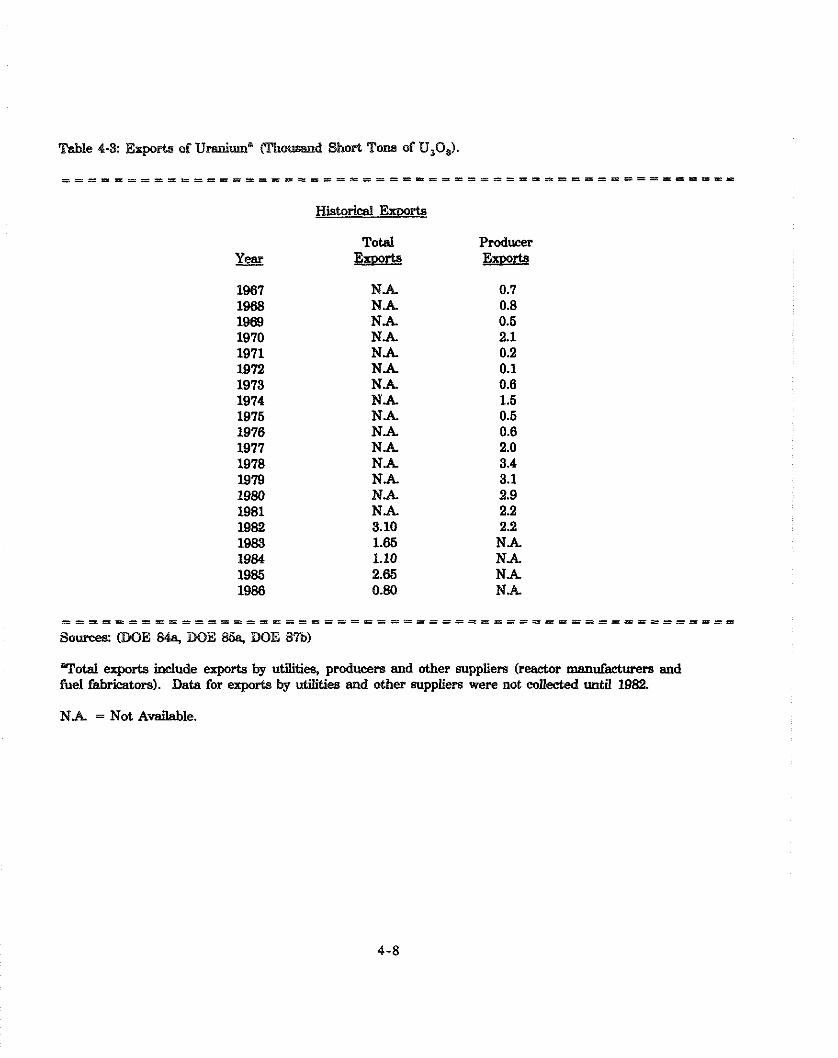
Historical Exwrts
Total E.zB&
NA. NA. NA. NA. NA. NA. NA. NA. NA. NA. NA. NA. NA. NA. NA. 3.10 1.65 1.10 2.65 0.80
Producer ExDorts
0.7 0.8 0.6 2.1 0.2 0.1 0.6 1.6 0.6 0.6 2.0 3.4 3.1 2.9 2.2 2.2 N .A. N A N A N.A.
. . . . . . . . . . . . . . . . . . . . . . . . . . . . . . . . . . . . . . . . . . . . . . . . . . . . So-: (DOE 848, DOE 85% DOE 8%)
Total exports include exports by utilitiee, producers and other suppliers (reactor manufacturer8 and fuel fabricators). Data for exports by utilities and other suppliers were not coU.eded until 1982.
NA. = Not Available.
Two basic types of pricing arrangements dominate the procurement of uranium: contract pricing and
market pricing. In contract pricing, prices and their escalation factors, if any, are determined when
the contract is signed. In market pricing, the price is commonly determined just before delivery and
is based on the market price prevailing at that time. Some market price contracts contain a floor
price, set a t the time the contracts are signed, that serves as a minimum on the eventual settled price.
Pricing arrangements that cannot be classified as either market or contract pricing are grouped in a
third category. This other category refers primarily to supply arrangements wherein the buyer has
direct control of a uranium property. Among 1986 deliveries of uranium, 36 percent used contract . pricing, 49 percent used market pricing, and 15 percent used other pricing arrangements [DOE 87a].
The concept of market pricing is probably the most complex of the three types. While it is common
to refer to a market or spot price for uranium, there is actually no centralized spot or futures market.
Contracts are negotiated between a producer and a utility either, through a middleman such as a
nuclear power plant manufacturer or through a broker. The price commonly referred to as the spot
price for uranium is a price published by the Nuclear Exchange Corporation (NUEXCO), the
principal uranium broker. This price, which NUEXCO calls the uranium exchange value, is a
monthly estimate of the price at which transactions for immediate delivery could have been
concluded as of the last day of the month [DOE 87~1 .
Hisforical Prices and Pricing Mechanisms
Until 1968, prices were largely determined by the Atomic Energy Commission. In the early years
of the commercial uranium market, 1968 through 1973, the price of uranium declined and remained
low despite conditions of excess long-term demand. Beginning in 1973, the price of uranium jumped
due to immediate industry requirements, a surge in long term contracting resulting from changes in
procedures for enrichment service contracts, and other factors.
At the same time, the terms under which long-term contracts were priced began to change. Until
1973, contracting was typically under fixed price contracts with inflation provisions. However, in
1973, producers resisted signing fixed price contracts, because, as a result of production cost
increases, they were losing money on previous fixed price contracts, and because they anticipated
price rises in the future. In 1974, when the uranium market became a seller's market, market price
contracts became popular. These contracts were written to guarantee the producer a base
rate-of-return on investment. In a short time, market price contracts became the norm.
In 1979-1980, the seller's market for uranium ended, and the uranium market witnessed a sharp
decline in prices due to postponements and cancellations of nuclear reactors, the build-up of uranium
inventories at utilities, and the growing competition from low-priced imported uranium. A sharp
decline in the nominal price of uranium began in 1980, dropping from over $40 per pound of U,O,
at the end of 1979 to $23.50 per pound by August 1981. In real terms (adjusted for inflation), the
price had actually begun dropping in 1976. The price in August 1981 in constant dollars was half
of what it had been in 1976. The price has continued to drop slowly from 1980 through 1987 [DOE
87al.
The average contract prices for deliveries made between 1982 and 1986 is given in Table 4-4. Market
price settlements for the same period are included with contract prices because, as settled prices, they
are similar to contract prices. This procedure gives a generally comprehensive average price for
actual deliveries (except for deliveries made under litigation settlements or other pricing
arrangements). Historical NUEXCO exchange values, or "spot prices" are listed in Table 4-5.
Prices of Foreign-Origin Uranium
Prices of imported uranium are substantially lower than domestic contract prices. The average price
paid for 1986 deliveries of imported uranium was $20.07 per pound of U308, approximately
one-third less than the amount paid for domestic-origin uranium, $30.01 [DOE 87a]. Table 4-6
shows the average price paid by domestic customers for 1981 to 1986 deliveries of foreign-origin
uranium.
4.2.2. Sources of S U D D I ~
The uranium used to fuel nuclear reactors is supplied by domestic and foreign producers, inventories
held by utilities, and secondary market transactions such as producer-to-producer sales,
utility-to-utility sales and loans, and utility-to-producer sales. The role of each is described in the
following sections.

Table 4-4: Average Contract Pr ice and lisrket Price Set t laents
fo r hctual Deliveries 1982-1986. (Year of Delivery Dollars)
(a) (a)(b) Reported glantity: Quantity: Adjusted
Year o f Price Price Reported Price Not Reported Price Delivery (Sllb) (mil l ion Lbs) ( n i l l i m Lbs) (Sllb)
Notes: (a) Price excludes uranium delivered under L i t i g s t i m settlements.
(b) Thc adjusted pr ice is a weighted average of reportai prices snd pr ice est imtes for respondents t o the E l A survey dm did mt supply pr ice information. Price estimates are based m regression anslysis of the reported prices.
Source : (DOE 8i%)

Table 4-6: Historical Nuexco Exchange Values. (NoIllinal Dollars Per Pound of U,O,)
As of December 31
. . . . . . . . . . . . . . . . . . . . . . . . . . . . . . . . . . . . . . . . . . . . . . . . . .
Source: INUEXCO 871
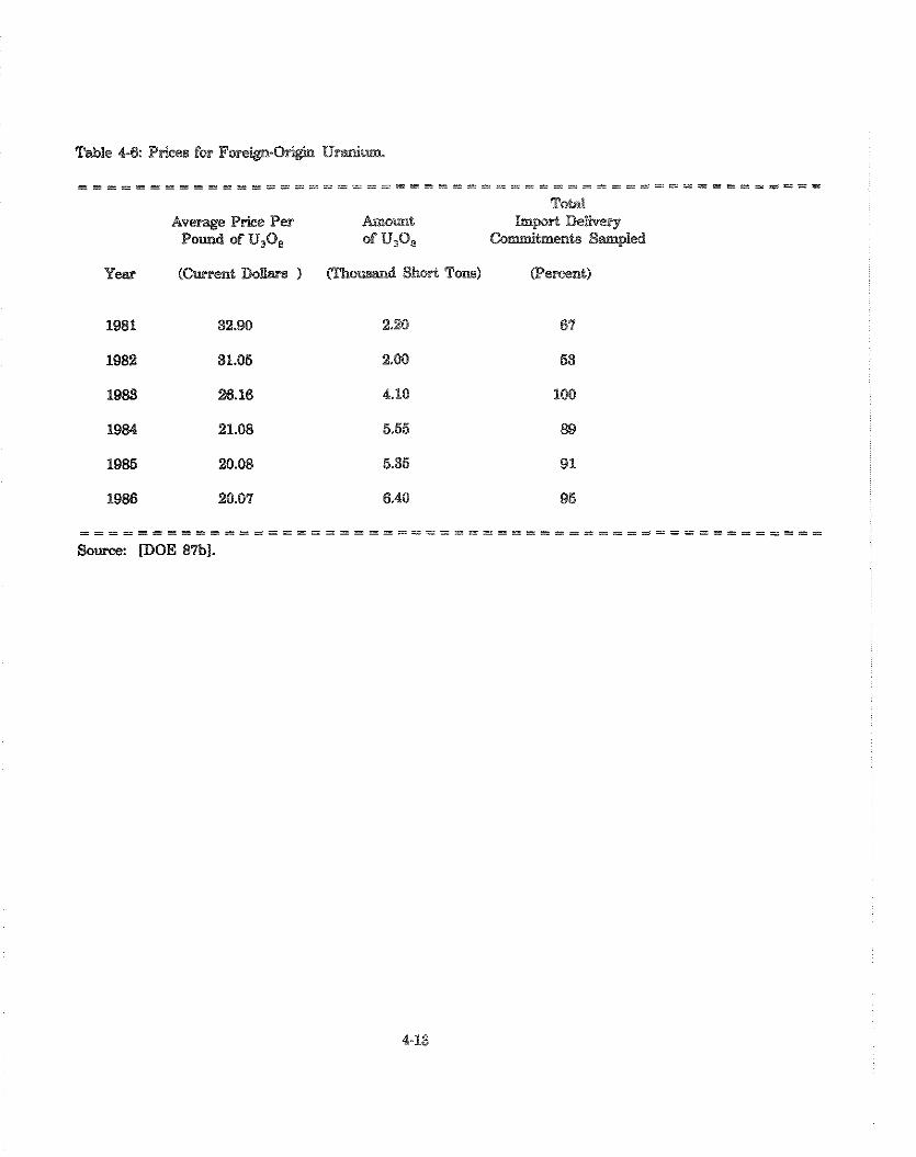
Table 4-6: Prices for Foreign-O+ U&m.
. . . . . . . . . . . . . . . . . . . . . . . . . . . . . . . . . . . . . . . . . . . . . . . . . . . .
Total Average Price Pee h o m t Impp0I.e Detivepy
Pound of U,O, of U,O, Gommimenb W p I d
. . . . . . . . . . . . . . . . . . . . . . . . . . . . . . . . . . . . . . . . . . . . . . . . . . . .
Source: [DOE 87bl.

Dolnestic Production
Table 4-7 shows trends in domestic production of uranium concentrate from 1947 to 1986, by state.
Total production was relatively constant at 10,500 to 13,000 tons per year until 1977, when it began
an increase that peaked in 1980 at 21,852 tons. Production has declined almost every year since,
reaching only 6,753 tons in 1986 [DOE 87b].
Coinciding with the overall decline in domestic production is a decline in the share of production
represented by conventional mills. Historically, conventional milling accounted for, on average,
approximately 70 percent of U.S. production. By 1985, the conventional share of production had
fallen to a low of 53.8 percent, but in 1986 it rose to 65.6 percent (Table 4-8). This increase in
market share is the result of an increase in the U308 content of the ore being milled. Only high grade
ores can be cost-effectively milled under current market conditions.
By contrast, non-conventional uranium production has not declined as severely, and the share of
uranium produced by non-conventional methods has increased consistently. This is explained by the
low marginal cost of producing uranium as a by-product or from the water in a closed underground
mine. According to an unofficial 1983 DOE estimate, 50 percent of non-conventional production
is from by-product recovery, 40 percent is from in sifu leaching, and ten percent from heap leaching
and mine water processing. Wet process phosphoric acid, copper waste dumps, and bellyrium ores
constitute by-product methods of production of U308. The second significant non-conventional
source is in siiu leaching. In 1986, by-product and in siiu leaching, together, accounted for 79
percent of the total non-conventional annual production of U308. Other less important sources
include mine water, and heap leaching, which accounted for 21 percent of total non-conventional
~ roduc t ion in 1986.
The result of the decline in demand for conventional production has been severe overcapacity and
mill shutdowns [DOE 85al. Milling capacity, which almost doubled between 1975 and 1980 when the
price of uranium was high and optimistic demand forecasts stimulated investment in milling facilities,
once enjoyed a utilization rate of 94 percent [JFA 85a]. In December 1986, capacity utilization was
about 32 percent at operating mills. The number of operating mills has declined dramatically also,
from 20 in 1981 to a low of two in June 1985 [DOE 85a]. NUEXCO indicates that six mills operated
in 1987, and Volume 2 of the Environmental Impact Stafemenf reports that only four were operating

Table 4-7: Total Uraniua Concmtrste Production, 1947-1986,
Year(s) Colorado New tiexico Texas Utah w i n g Others(s) Total
notes: (a) Includes, for various years, Arizona, Colorado, Florida, Louisians, Swth Dakota, Texas, Utah, ard Usshingtm.
(b) Data we= rwt wLLestcd.
(c) Included i n the 'othersu category.
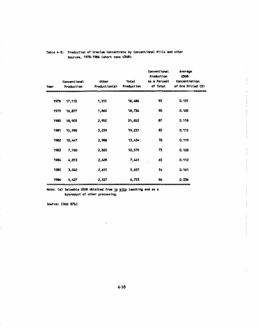
Table 4-8: Production of Uraniw Concentrate by Cmventicnal R i l l s Md other Scurces, 1978-1986 (8hort ton8 UYY))
conventicnaL Aver6ge Production
C ~ n v e n t i o ~ l Other Total As a Percent Cmcentratian Year P d u c t i o n ~roductim(a) ~ r o h t i o n of Total of Ore M i l l & ( X )
a-
Note: (a) saleabLe U308 obtain& frrm &u Leaching a d as a byproduct of other processing.
in 1988 (Table 4-13), but industry sources predict that the number of operating millscould drop to
three within two to five years. Uranium mill capacities and utilization levels are listed in Table 4-9.
A second source of uranium is the import market. Until 1975, foreign uranium was effectively
banned from U.S. markets by a Federal taw prohibiting the enrichment of imports for domestic use.
This restriction was lifted gradually after 1975, and was eliminated completely in 1984. From 1975
through 1977, imports amounted to a small portion of total domestic requirements, with U.S. exports
exceeding imports in each year from 1978 through 1980. By 1986, however, imports supplied 44
percent of U.S. requirements. Table 4-10 lists U.S. imports from 1974 through 1986 [DOE 87a].
The primary sources of U.S. uranium imports have been Canada, South Africa and Australia. In 1986,
59 percent of U.S. uranium imports were from Canada, and 41 percent were from Australia and South
Africa [DOE 87a].
Forecasts of import penetration call for the import share to grow through the 1990s. The Department
of Energy projects that without government intervention, between the year 1990 and 2000 imports
will range between 50 and 64 percent of domestic utility requirements, depending on demand levels.
Inventories
Utilities hold uranium inventories in order to meet changes in the scheduling of various stages of the
fuel cycle, such as minor delays in deliveries of uranium feed. Uranium inventories also protect the
utilities against disruption of nuclear fuel supplies. The average "forward coverage" currently desired
by domestic utilities (in terms of forward reactor operating requirements) is 18 months for natural
uranium (U308) and seven months for enriched uranium hexafluoride (UFd [DOE 85aI.
Table 4- I1 lists inventories of commercially-owned natural and enriched uranium held in the United
States as of December 31, 1984, 1985, and 1986. DOE-owned inventories are not included. The
uranium inventory owned by utilities alone at the end of 1984 represented almost four years of
forward coverage.
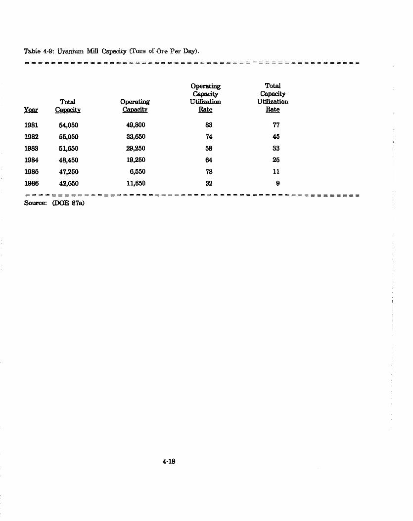
opera- Total Capacitp- pac city
Total @@rating U M m Utilization YS Capacitv Q4@2!&! - Rate - Rate
. . . . . . . . . . . . . . . . . . . . . . . . . . . . . . . . . . . . . . . . . . . . . . . . . . . . - - - - ------------- Source: (DOE 8711)
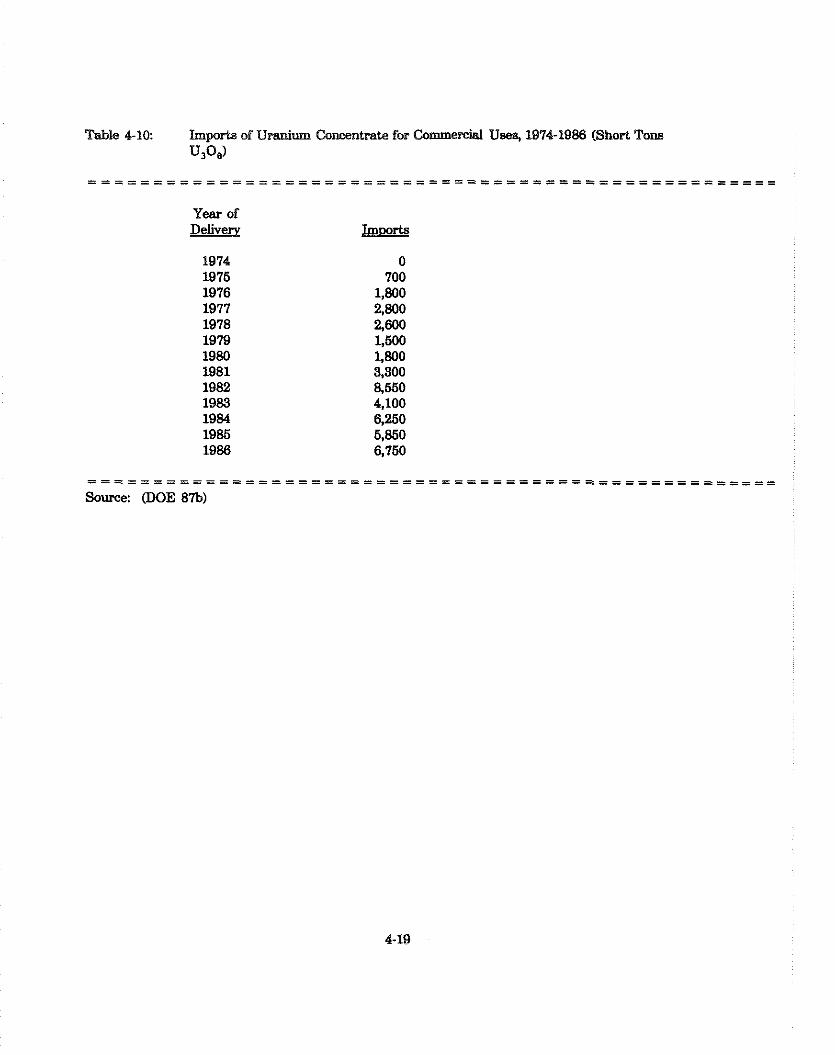
Table 4-10: Imp* of Uraoiurn ancentrate for Come& Uses, 1974-1986 (Short Tons U30J
Year of Delivery
1974 1976 1976 1977 1978 1979 1980 1981 1982 1983 1984 1986 1986
. . . . . . . . . . . . . . . . . . . . . . . . . . . . . . . . . . . . . . . . . . . . . . . . . . . . . Source: (DOE 87b)

Table 4-11: U.S. Commercially-Owned Uranium Inventories as of December 31, 1984, 1985, and 1988 (Short TOM U,O, Equivalent)
Owner Caterrow Natural Enriched - Natural Enriched Enriched
Utilities 48,360 31,750 44,100 32,460 41,660 30,900 Suppliers 12.ooo 500 - 700 12.400 450
TOTAL 60,360 32,250 66,260 33,160 63,960 31,360
. . . . . . . . . . . . . . . . . . . . . . . . . . . . . . . . . . . . . . . . . . . . . . . . . . . . . . . . . . . . . . . . . . . . . . . . . . . . . . . . . . . . . . . . . . . . . . . . . . . . . . . .
Source: [DOE 87bl
Secot~dary Market Transactions
The secondary market for uranium includes producer-to-producer sales, utility-to-utility sales and
loans, and utility-to-producer sales. The secondary market, by definition, does not increase the
supply of uranium, only the alternatives for purchasing it. As such, secondary transactions can have
a significant impact on the demand for new production and on the year-to-year changes in
inventories. The secondary market has been significant in recent years. During 1986, sales of 6,800
tons of U308 equivalent were made between domestic utilities and suppliers in the secondary market.
4.2.3 Industrv Structure and Performance
The number of firms participating in the domestic uranium milling industry declined between 1977
and 1985, but has since increased. In 1977, 26 companies owned active uranium mills. In 1983, the
number had fallen to 11, and in June 1985, there were only two [DOE 87bl. In 1987, six companies
operated six mills and by August 1988, only four mills continued to operate. The status of the
industry can also be seen in trends in employment and capital expenditures (Table 4-12). Capital
expenditures in 1986 were $1 million, compared to $72 million in 1981 (1986 dollars) [DOE 87a,
DOE 87b]. Employment in 1984 was 513 person-years, compared to 2,367 in 1981 [DOE 87al.
Mining and milling production data for individual companies are collected by DOE but are not
available to the public. However, some data on operating status are published. These are listed, by
f i rm and mill. in Table 4- 13.
A wide variety of companies are represented within the uranium industry. In the industry's early
years, holdings were dominated by independent mining and exploration companies. Since then,
mergers, acquisitions, and the entry of conglomerates have considerably altered industry structure.
During the 1970s, the oil embargo and forecasts of growing demand for nuclear power made entry
into the uranium market attractive to oil companies and utilities. Of the six mills operating in 1987,
three were owned by foreign mining companies, one an American mining company, one by a
subsidiary of an oil company, and another by a subsidiary of a chemical company. These ownership
characteristics influence the current and future financial viability of the industry. The desire of the
parent companies to weather a downturn in the uranium market and to retain an interest in producing

Table 4-12: Gapital ExpendiLurea, EmploylnenI, and Active anventiod Uranim Industry.
Capital Expenditures YS w o n Constant 1986 $1
1981 72
1982 l2
1983 3
1984 8
1985 9
1986 1
Employment person-Years1
2,367
1,956
1,618
987
514
513
Number of Active Mills At Year-End
--*
14
l2
8
4
6
= m = = = = = = = = = = = = = F = = = = = = = = I = = = = = = = = = = = = = = = = = = = s = = = = = = = = - =
Sources: (DOE 8'7% DOE 8%)

Table 4-13. Operating status of licensed conventional uraniun m i l l s as of June, 1989. June 1989.(a)
S ta te lH i l l
Colorado
Canon C i ty Uravan
New Mexico
L-Bar
Churchrock Blueuater Ambrosia Lake
Homestake South Dakota
Edgemont
Texas
Panna Maria
Conquista Ray Point
Utah
Whi t e Mesa Rio Algom
Moab shootaring
Washington Dawn Sheruood
Wyoming
Lucky Mc Spl i r Rock Umetco
Bear Creek Shir ley Basin
Sweetwater Highland
FAP
Pet ro tmics
Owner
Operating Status(b)
Reclamation
Status(c)
Cotter Corp. Umetco Minerals
BP American
United Nuclear Anaconda Kerr-McGee Homestake
TVA
Chevron
ConocolPioneer Exxon
Umetco Minerals Rio Algom Atlas
Plateau Resources
Dawn Mining
Western Nuclear
Pathfinder
Western Nuclear
UmetCO Minerals
Rocky M t . Energy Pathf i rder Minerals Expl.
Exxon
American Nuclear Corporation
Pet ro tmics
Standby standby
D e c m i s s i m
D e c m i s s i m D e c m i s s i m
Standby Active
D e c m i s s i m
Active
D e c m i s s i m
D e c m i s s i m
Active
Standby
D e c m i s s i m standby
D e c m i s s i m
Standby
Standby
Decannissim D e c m i s s i m
Decannissim Active
standby
Decannissim D e c m i s s i m
D e c m i s s i m
Future I n Progress
Cover i n Place In Progress
I n Progress I n Progress
Future
Campleted
Future I n Progress
Completed
Future I n Progress
I n Progress Future
I" Progress
Future
future I n Progress
I n Progress In Progress
Future Future
Cover i n Place Unknown
Design Approval
( a ) Data obtained from conversations with cognizant personnel in Agreement States and the NRC,
c o m n t s sutmitted by indiv idual companies and the Anerican Minining Cmgress during the publ ic comnent period, and s i t e v i s i t s . Does not include m i l l s Licensed hrt rot constructed.
(b) Active m i l l s are current ly processing ore and producing yelloucake. Standby m i l l s are not current ly processing ore but are capable of restar t ing. A t m i l l s designated by "Decmission", the m i l l s t ructure has been or i s being dismantled and no future m i l l i ng u i l l occur.
(C) Terms t o describe reclamation status are as follows: "Future". inpoundment i s being maintained t o accept addit ional t a i l i ngs and reclamation a c t i v i v i t i e s have not yet started; "Design Approval Pending", f i n a l disposal design has been sutmitted f o r regulatory approval and reclamation
a c t i v i t i e s are underuay; " I n Progress", act ive reclamation has begm but f i n a l cover i s not completed; Cover i n Place", f i n a l cover has been campleted but f i n a l s tab i l i za t ion has not been completed; and "Completed", disposal and s tab i l i za t i on have been accmplished i n accordance r i t h Umtrca standards.

properties is a function of their perception of the prospects for long-term profitability in domestic
uranium operations. Some firms continue to invest and to acquire properties, while others withdraw
from an extremely soft market. Foreign firms appear to have adopted a longer term viewpoint than
have some of their domestic counterparts. It is likely that the industry will continue to undergo
structural change. This change will depend on domestic and foreign demand, costs of production,
and the industry's ability to compete with lower-priced imports [DOE 87al.
4.2.4 Economic and Financial Characteristie
4.2.4.1 Emolovment Analvsis
Department of Energy estimates of employment in the uranium milling industry from 1984 to 1986
are listed in Table 4-14. Additional detail at the state level was obtained through discussions with
staff of the departments of mining or natural resources in the states with uranium mills. This is
provided in the following paragraphs. Historically, New Mexico and Wyoming have been the nation's
leading producers of uranium and have jointly been responsible for an estimated 70 to 75 percent of
total uranium concentrate production. Following the peak production period of 1981 and 1982, and
since the onset of the production decline in the latter part of 1982, it is estimated that approximately
7000 jobs have been lost in New Mexico as production fell from 253 million tons in 1982 to 36
million in 1984 [NM 851.'
The trend in Wyoming has been similar. In 1980, seven uranium mine-milt complexes and one
uranium mill employed a total of 2451 people. In 1981, employment dropped to 1361 people. In
1984, employment was down to 454 workers [WY 80, 81, and 841.
In Washington, before 1982 there were two mine-mill complexes: Midnight Mines (owned and
operated by Dawn Mining Company) and the Sherwood Mine (owned by Western Nuclear, a
subsidiary of Phelps Dodge Corporation). In 1981, Dawn employed 50 workers, and in 1982 it
employed 42. In 1981, Sherwood employed 45 workers, while in 1982 it employed 14 miners plus
98 maintenance workers. Both mine-mill complexes are currently inactive and unemployment
(estimated at 40 percent from 1982 to 1983) was estimated to be as high as 80 percent [WA 851.
' Employment and output estimates by state sources may not agree with those provided by the U.S. Department of Energy and presented elsewhere in this report, due to differences in data collection procedures.
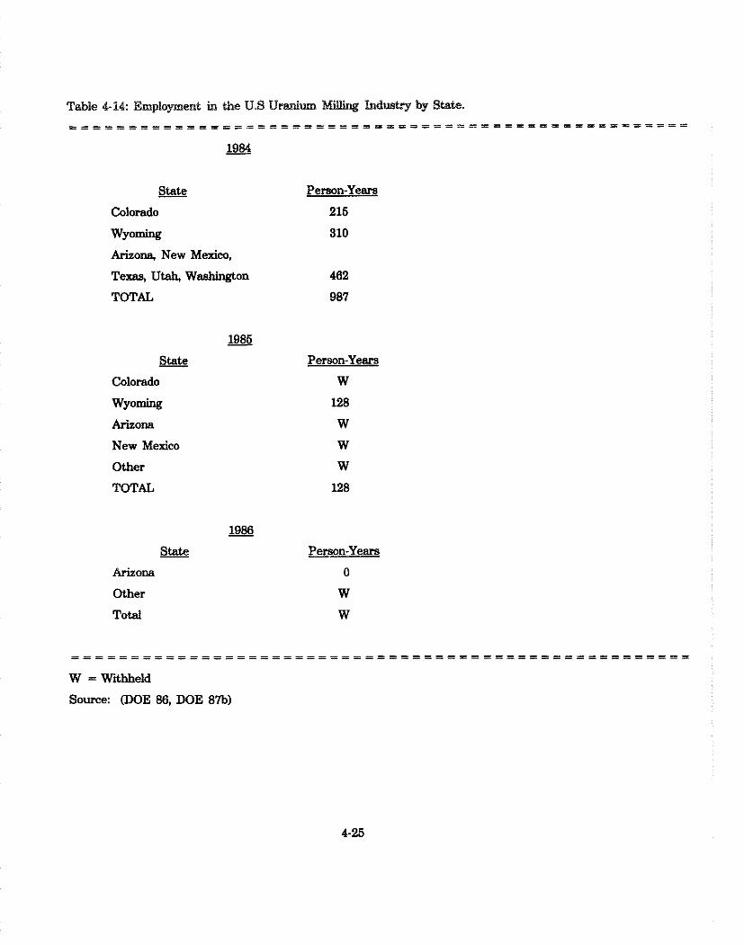
Table 4-14: Emplo~ent in the U.9 Uraniuoo industry By Stab.
. . . . . . . . . . . . . . . . . . . . . . . . . . . . . . . . . . . . . . . . . . . . . . . . . . . . . . .
&&g
State Person-Years
Colorado 215
Wyoming 310 Arizona, New Mexico,
Texas, Utah, Washington 462
TOT& 987
1985 - State - Person-Years
Colorado W
WYO- 128 Arizona W
New Mexico W
Other W
WTAL 128
1986 State Person-Years
Arizona 0
Other W
Total W
. . . . . . . . . . . . . . . . . . . . . . . . . . . . . . . . . . . . . . . . . . . . . . . . . . . . . . . . . . . . . . . . . . . . . . . . . . . . . . . . . . . . . . W = Withheld
Source: (DOE 86, DOE 87b)
In Colorado, there were 508 mineral industry operations in 1980, 100 of which were engaged in the
production of uranium. By 1985, however, there were only two mines or mine/mill complexes:
Centennial and Schwartzwaider. In 1980, the uranium industry employed approximately 1594
individuals [Nugent 801, whereas it is estimated that the two operations now employ about 200 people
[Co 851.
In Texas, there were, until recently, three mills: the Conquista Project (Conoco), Ray Point (Exxon)
and the Panna Maria complex (Chevron). The Conquista complex, it is estimated, employed over 500
people during its peak period from 1979 to 1980, and the Panna Maria complex about 250 people
during its peak period from 1981 to 1983. The Conquista Project and Ray Point have been closed
and are being decommissioned. The Panna Maria was operating at the close of 1987, but at a
considerably reduced rate. Employment there reached a low of seven to eight people in 1985.
Current employment is unknown [TX 851.
4.2.4.2 Communitv Impact Analvsis
The impact of trends in uranium milling on small communities dependent on uranium milling
facilities tends to vary depending on the location of the mines, the importance of uranium mining
and milling to the state, and the nature of the work force. Texas and Washington serve as interesting
case studies.
In Washington, the uranium facilities are located primarily in the Spokane Indian Reservation. Mining
soon became the main economic activity as the mining companies were under contractual obligation
to draw 51 percent of their labor force from the Indian community. When the two Washington
mine-mill complexes, Midnight Mines and Sherwood Mines, closed in 1983-1984, the unemployment
rate rose to about 80 percent. This is perhaps partly attributable to the absence of any other mining
activity on the reservation which might have absorbed some of the displaced workers. This high
unemployment rate also suggests limited mobility on the part of miners and workers. Thus, in the
case of Washington it would seem that the employment effects were concentrated, and felt largely
by the Indian community which served as the principal source of labor for uranium mining and
milling within the state [WA 851.
In Texas, by contrast, the community impacts of the uranium industry are less significant. Most
uranium industry employees were originally farmers and ranchers, maintaining and upgrading their
properties during the lifetime of their mining careers. Moreover, they were mostly a commuting work
force so there was no residual pool of unemployed persons in the vicinity of the mines once the
decline in employment took place in the early 1980s. There were no uranium mining communities
as such in the State of Texas which were dependent on the mining and production of uranium for
their subsistence. Moreover, many workers were absorbed by the then booming petroleum and lignite
industries [TX 851.
In the case of both Colorado and Utah, the ability to absorb unemployed uranium workers is limited.
In Colorado, this has been due to the depressed state of the mining industry in general within the
state [CO 851. In New Mexico, where uranium mining and milling are considered an important
economic activity, there were areas of concentrated impact - such as Gallup, the Laguna Pueblo area
and the Navajo Indian Reservation. The wide scale reduction in employment observed in recent
years, the reduction in sales and sales tax revenues, the loss of severance payments, a significant
amount of out-migration to Nevada and several other states, and a concomitant reduction in income
tax revenue have combined to make the impact significant and state-wide as opposed to
community-specific [NM 851.
4.2.4.3 Financial Analvsis
Selected financial data for the domestic uranium industry for 1982 to 1986 are shown in Table 4-15.
The data cover a subset of firms (the same firms for all years) that represent over 80 percent of the
assets in the industry in each year. The firms included are those for which uranium operations
could be separated from other aspects of the organization's business, and for which an acceptable
level of consistency in financial reporting practices was available for all years. Financial data on the
milling industry alone are not available.
As shown in Table 4-15, net income accruing to the uranium industry was positive in only two years,
1982 and 1983. The returns on assets (net income divided by total assets) in these years were 0.7 and
1.4 percent respectively, and aggregate net earnings totalled $69.8 million. In 1984, 1985, and 1986,
the returns on assets were -10.3, -21.6, and -2.3 percent, and aggregate net losses reached $765.7
million. The loss in 1984 alone was $304.7 million on revenues of $608.9 million. Thus, the
aggregate loss for the five years was $695.9 million. In 1977, 146 firms were involved in domestic
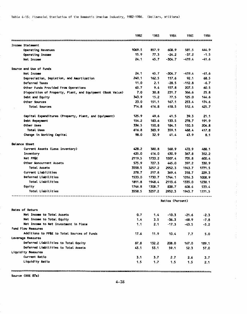
'Table 4-15: Financial S t a t i s t i e s of the m s t i c U~snlum Industry, 1m-a-1W. (bull&rs, n i i l i m s i
I n m u S t a t m t Operating Revenues Operating I n m r Net Incow
m r c e and Use of Funds Net In- Depreciation, Depletion, and Amortization Deferred Taxes Other Funds Provided F r m Operations Disposition of Property, Plant, and Equipment ( k k Vslue) Debt and Equity Other Sources
Total Sarrces
Capital Expnditures (Property, Plant, and Equipmt) Debt Repaymt Other User
Total Uses Change i n barking Capital
Balance Sheet Current Assets (Less inventory) Inventory Net PPPE Other Noncurrent Assets
Total Assets Current L iab i l i t i es Deferred L iab i l i t i es
Total L iab i l i t i es Equity
TotaL L iab i l i t i es
Rates of Return Net I n m r t o Total Assets Net I n m u t o Total Equity Net In- t o Net Investment i n Place
Fund F l w Measures Additions t o PP&E to Total Sources of Funds
Leverage measures Deferred L iab i l i t i es t o Total Equity Deferred L iab i l i t i es t o Total Assets
Liquidity Medsures Current Ratio Liquidi ty Ratio
Y10.8 568.9 472.9 W . 1 416.0 430.9 367.8 352.2
1733.2 1507.4 705.8 6W.4 727.3 445.0 397.2 330.9
3257.2 2952.3 1943.7 1771.5 217.8 369.4 318.7 229.3
1730.7 1744.1 1M6.3 1W8.9 1948.4 2113.6 1335.0 1U8.1 1W.7 8 3 . 7 608.6 533.4 3257.2 2952.3 1943.7 177l.5
Ratios (Percent)
Sarrce (WE 87s)
4-23

uranium exploration, 135 in mining and 26 in milling. In contrast, only 31 firms were actively
engaged in exploration, I I in mining and 5 in milling toward the end of 1986. Of these firms, only
27 percent had positive net income after meeting operating expenses and other obligations such as
payment of taxes and recovery of depletion, depreciation and amortization. Fifty-five percent
reported net losses; the remaining 18 percent either had left the industry or had no data to provide.
Most of the financial improvement in 1986 stemmed from the slowdown or the completion of
writeoffs of discontinued operations, revaluation of assets and abandonment?.. The domestic uranium
industry is significantly smaller than before, and its financial state will depend on higher product
prices or demand [DOE 87al.
Company-specific information on uranium production, revenues, profits, and plans is provided in
the following paragraphs.
Homestake Mining Company
Homestake Mining Company owns one conventional uranium mine and a 3400 ton per day mill in
Grants, New Mexico. During 1984, production of uranium was reduced to the minimum level at
which satisfactory unit costs could be maintained. Mine production has been confined to one mine
operating on a five-day-week schedule for ten months of the year. Uranium concentrate was also
recovered from solution mining and ion-exchange. In 1986, uranium accounted for 14 percent of
the company's revenues, and 21 percent of operating earnings. The high profitability of the sector
for the year is attributed to existing contracts, expiring in 1987, that provide for sale prices above
current spot prices and production costs. Selected financial statistics are presented in Table 4-16 [AR
84, AR 85, AR 861.
Rio Algom
Rio Algom is a Canadian corporation engaged in the mining of a wide variety of materials, including
copper, steel, and uranium. In 1986, uranium operations accounted for 26 percent of corporate
revenue, but most (89 percent) was from Canadian production. In the United States, the company
owns one uranium mine and a 750 ton per day mill in La Sal, Utah.

Tabla 4-16: Hwestake l l ining eapsny U r ~ i l i . Operati-, 1982 Operetlms
Revenues ( m i Llions dollara) 63.70 58.60 57.90 68.20 49.80
Operating In- (mil l ions dollars) 15.60 11.40 19.60 2 2 . ~ 0 12.70
Sales o f UMB (mil l ions pounds) HlA 1.13 1.13 0.94 1.05
Sole8 Price Per Pound of UMB (a) 46.20 49.76 53.21 49.m 47.50
Depreciation, Depletion, and A w r t i z a t i m ( 8 i l l i m s dollars) 20.00 14.30 4.40 12.50 4.30
Additions t o Pmperty, Plant, and Equipvnt ( m i L l i m s dollars) 1.00 0.W 0.70 0.W 0.00
Ident i f iab le Assets (millions dollar 80.M 73.W 66.90 43.70 24.90
(a) Prices based on Long-term contracts that were t o expire i n 1986 and 1987.
NlA - mt available
Source: CAR 84b, 85b, 86b)

In 1986, the company produced 457 tons of uranium oxide from its Utah mine. The mine operated
at approximately 50 percent of capacity in 1986, while the mill operated at capacity due to a significant amount of toll milling [AR 861.~ In 1987, the La Sal mill produced about 350 tons of
uranium oxide using both company ore and ore from the Thornberg mine. The mill was placed on
standby in September, because the Lisbon and Thornberg mines' reserves are depleted [EPA 891.
Selected financial statistics on Rio Algom uranium operations are presented in Table 4-17.
Plateau Resources Limited
Plateau Resources, a wholly owned subsidiary of Consumers Power Co., was organized in 1976 to
acquire, explore, and develop properties for the mining, milling, and sale of uranium. All operations
were suspended in 1984 because of depressed demand and all uranium assets were written down by
$46 million after taxes in 1984 and $21 million in 1985, to an estimated net realizable value of
approximately $34 million. There is no assurance that the amount will ever be realized however. The
company's 800 ton per day mill at Ticaboo, Utah, which was constructed in 1980 and 1981, has never
been active. It does, however, remain on standby and could be activated [AR 84, 85, 861.
Western Nuclear
Western Nuclear, a subsidiary of Phelps Dodge Corporation, owns two mine and mill complexes, one
in Wyoming and one in Washington. The capacities of its mills are 1700 and 2000 tons per day,
respectively. The Wyoming mill has been on standby since the early 1980s. and decommissioning is
anticipated. The Washington complex operated intermittently from 1981 through 1984. In late 1984,
Phelps Dodge wrote off its entire "Energy" operation, of which Western Nuclear was a major part
[AR 84, AR 851.
4.2.5 Industrv Forecast and Outlook
This section presents projections of total U.S. utility market requirements, domestic uranium
production, from both conventional and non-conventional sources, imports, employment and
electricity consumption. Developed for a 14-year period (1987-2000), these projections are
considered "near term." A basic assumption of the near term projections is that current market
* "Toll milling" is the processing of ore from another company's mines on a contract basis.
4-31
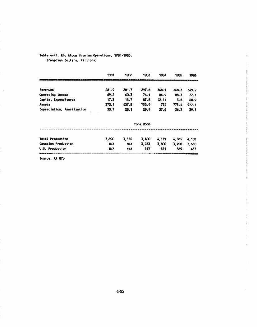
Table 4-17: Rio Rlgotl Uranium Operations, 1981-1986. ( C e d i a n Dollars. RiLLions)
Revenuer 281.9 281.7 297.6 368.1 368.3 349.2 Opcreting In- 69.2 60.3 76.1 86.9 88.3 77.1 Capital Expenditures 17.3 13.7 87.8 (2.1) 3.8 60.9 Assets 372.1 427.8 752.9 774 77S.4 977.1 Depreciation, Amrtization 30.7 28.q 29.9 37.6 36.2 39.5
Total Pmduction M i a n Pmduction U.S. Pmduction
3,9W 3,550 3,403 4,111 4,M5 4,107 NIA NIA 3,233 3,8[1[3 3,7W 3,650 NIA NIA 167 311 365 457

conditions, as defined by the Department of Energy's Energy Information Administration (DOE,
EIA), will continue unchanged through the end of this century. This section is based on the
reference case projections in EIA's Domestic Uranium Mining and Milling Induslry; 1986 Vinhitiry
Assessnlertt [DOE 87a].
4.2.5.1 Proiections of Domestic Production
The EIA's Reference case3 forecasts for 1987-2000 are based on the output of EIA's economic model,
Domestic Evaluation of Uranium Resources and Economic Analysis (EUREKA). The EUREKA
model's niethodology goes beyond the scope of this study; it is fully described in Appendix C of the
1986 Viability Assessn~ent. The EIA examines future developments in thedomestic uranium industry
and in the domestic and international uranium markets under current market conditions and under
certain hypothetical supply disruption scenarios4. The current market conditions are generally the
same as those presented in Sections 4.2.1-4.2.4 of this study and are based on historical trends in the
domestic uranium industry as outlined in both the Viability Assessmenl and the EIA's Uranium
It~dustry Artnual 1986. In addition to the uranium prices, production and imports as well as the
exploration expenditures, capital expenditures, and employment data developed for inclusion as
"current market conditions," the EIA includes one important assumption: that the Act of Congress
forbidding imports of uranium from South Africa and Namibia will be enforced5. Also taken into
3 ~ r i o r to the I986 Viabiiity Assessmenl, E I A published two reference cases: a Lower Reference case and an Upper Reference case, each with a low, a mean, and a high range of projected values. In 1986, however, only the Lower Reference case was published. It is referred to simply as the Reference case. As before, low, mean and high projected values were produced by EIA. This study uses the mean. The Reference case in the 1986 Viability Assessment uses the underlying assumptions for the Lower Reference case described in Commercial Nuclear Power 1987: Prospects for the Utlited Sfa les at~d the World [DOE 87al.
' ~ h e s e scenarios, the "current disruption status" scenario and the "projected disruption status" scenario, are used to test the viability of the U.S. uranium industry, to examine the ability of this industry to respond to an abrogation of various fractions of contracts for uranium imports intended for domestic end use. Both of these bear only tangentially on this study and will not be discussed further here.
he U.S. Congress passed the Comprehensive Anti-Apartheid Act of 1986 on October 2, 1986. Section 309 of that Act forbade the import into the United States of uranium ore or concentrate of South African of Namibian origin after January 1, 1987. However, natural or enriched uranium hexafluoride from these countries may be imported, according to a regulation issued by the U.S. Department of the Treasury on which the U.S. Nuclear Regulatory Commission has concurred [EPA87b].
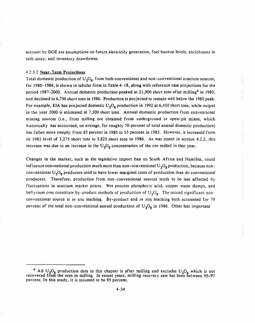
account by DOE are assumptions on future electricity generation, fuel burnup levels, enrichment in
tails assay, and inventory drawdowns.
4.2.5.2 Near-Term Proieetionh
Total domestic production of U,O,,, from both conventional and non-conventional uranium sources,
for 1980-1986, is shown in tabular form in Table 4-18, along with reference case projections for the
period 1987-2000. Annual domestic production peaked at 21,900 short tons after milling6 in 1980,
and declined to 6,750 short tons in 1986. Production is projected to remain well below the 1980 peak.
For example, EIA has projected domestic U308 production in 1992 at 6,450 short tons, while output
in the year 2000 is estimated at 7,500 short tons. Annual domestic production from conventional
mining sources (i.e., from milling ore obtained from underground or open-pit mines, which
historically has accounted, on average, for roughly 70 percent of total annual domestic production)
has fallen more steeply: from 85 percent in 1980 to 53 percent in 1985. However, it increased from
its 1985 level of 3,275 short tons to 5,825 short tons in 1986. As was stated in section 4.2.2, this
increase was due to an increase in the U308 concentration of the ore milled in that year.
Changes in the market, such as the legislative import ban on South Africa and Namibia, could
influence conventional production much more than non-conventional U308 production, because non-
conventional U308 producers tend to have lower marginal costs of production than do conventional
producers. Therefore, production from non-conventional sources tends to be less affected by
fluctuations in uranium market prices. Wet process phosphoric acid, copper waste dumps, and
bellyrium ores constitute by-product methods of production of U30s The second significant non-
conventional source is 111 situ leaching. By-product and in situ leaching both accounted for 79
percent of the total non-conventional annual production of U308 in 1986. Other less important
All U308 production data in this chapter is after milling and excludes U30 which is not recovered from the ores in milling. In recent years, milling recovery rate has been tetween 95-97 percent. In this study, it is assumed to be 95 percent.
4-34
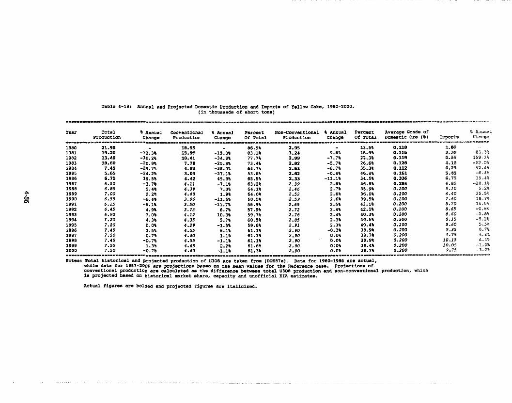
Tabla 4-10: Annual and Pro jwtad Domst ic Prodvction and Import. of Y m l l c n Cake, 1980-2000. ( i n thoumands of short ton81
- - - - - - - . m - - - - - - - - = - - - - - - - - - - - ~ s ~ ~ - ~ m ~ m - - m ~ - ~ ~ - - ~ ~ ~ " ~ ~ ~ . ~ ~ ~ ~ ~ ~ . * ~ ~ ~ = ~ ~ - - m ~ ~ ~ ~ ~ m ~ ~ . - . ~ ~ ~ ~ ~ ~ ~ ~ - . ~ ~ - - - ~ - ~ - - . . - - ~ = m - = ~ ~ - - - m - ~ ~ . - = - m - - - . = = - = - - ~ ~ ~ ~ - - - - - - - -
Yaar Total (t Annual Cmvsntional I Annual Puelrnt Ron-conventional b m u a l Parcent Average Qradm of 8 Aria-l ~ r o d u c t i o n Change P r o d u ~ t i ~ n Change Of Total P m d ~ o t i o n Change Of Total D-.tic Ore (I) 1mporV.a h o g -
. . . . . . . . . . . . . . . . . . . . . . . . . . . . . . . . . . . . . . . . . . . . . . . . . . . . . . . . . . . . . . . . . . . . . . . . . . . . . . . . . . . . . . . . . . . . . . . . . . . . . . . . . . . . . . . . . . . . . . . . . . . . . . . . . . . . . . . . . . . . . . . . . . . . .
1980 21.90 - 10.95 - 86.58 2.95 - 13.5% 0.118 1.- - 1981 19-20 -12.3% 15.96 -15.88 83.18 3.24 9.8% 16.9% 0.115 3.30 83.3\ 1982 l3.40 -30.2% 10.41 -34.88 77.7% 2.99 -7.7% 22.3% 0.119 8.55 159.1% 1983 10.60 -20.9% 7.18 -25.30 73.4% 2.82 -5.70 26.68 0.118 4.10 -52.0* 1984 7.45 -29.7% 4.82 -38.0% 64.7% 2.63 -6.78 35.38 0.111 6.25 52.6% 1985 5.65 -24.2% 3.03 -37.10 53.68 2.62 -0.48 46.48 0.161 5.85 -6.48 1986 6.75 19.5% 4.42 45.98 65.5% 2.33 -11.13 34.5% 0.336 6.75 15. dB 1987 6.50 -3.711 4.11 -7.1% 63.28 2.39 2.88 36.80 0.284 4.85 -28.1t 1988 6.85 5.48 4.39 7.0% 64.18 2.16 2.7% 35.90 0.200 5.10 5.2% 1989 7.00 2.2% 4.48 1.9% 64.0% 2.52 2.6% 36.00 0.200 6.10 2 5 . 5 % 1990 6.55 -6,4% 3.96 -11.51 60.50 2.59 2.60 39.58 0.200 7.60 1S.T\ 1991 6.15 -6.111 3.50 -11.78 56.9% 2.65 2.58 43.1% 0.200 8.70 14.5% 1992 6.45 4.9'1 3.73 6.78 57.90 2.72 2.48 42.1% 0.200 8.65 -0.m 1993 6.90 7.0% 4.12 10.3% 59.7% 2.78 2.4% 40.38 0.200 8.60 -0.64 1994 7.20 4.3% 4.35 5.7% 60.58 2.85 2.38 39.58 0.200 8.15 -5 .2% 1995 7.20 0.0% 4.29 -1.56 59.68 2.91 2.38 40.48 0.200 8.60 4 . 5 8 1996 7.45 3.5% 4.55 6.1% 61.1% 2.90 -0.3% 38.9% 0.200 9.35 8.7'L 1997 7.50 0.7% 4.60 1.18 61.38 2.90 0.0% 38.7% 0.200 9.75 4.3% 1998 7.45 -0.7% 4.55 -1.1% 61.18 2.90 0.0% 38.98 0.200 10.15 4.1% 1999 7.55 1.38 4.65 2.28 61.6% 2.90 0.00 38.4% 0.200 10.05 -P.OQ 2000 7.50 -0.7% 4.60 -1.18 6 1 . 3 2.90 0.08 38.7% 0.200 9.75 -3.a .--.---- 1--~......-------.--.-----.--.~~~~~~~~~~~*~~~~.~~~~~.~..~~~.~~~~~~~~~~~.~.~~~~~~~~~~~~.~~..~~~~~~~..~m~------~-~-..-~--------*-----=--=-----=--
IIOtssr Total himtoriaal and Pr0j.ct.d produotion o f U308 are ( a k a from (WB87s). Data fo r 1980-1986 are iIetUa1, w h i h d.U fo r 1087-2000 a r e p r n j ~ t i m . baaed on th. man v.1u.m fo r th. R*f.r.na. .am.. Projmetiona of conV*ntional Production arm aa10~1.t.d a. t h e differeno. batvr.n t o t a l U3OB production and non-eonv.nciona1 produotion, which is projected basad on historical markst share, capacity and unof f i c ia l XIA estutes.
Actual f igurea are bc1d.d and projrr ted f i g u e s are i t a l i c i zed .
sources include mine water, and heap leaching, which accounted for the remaining 2 L percent of rota1
annual non-conventional vroduction in 1986.
The Reference case EIA projections of domestic US08 production through the year 2000 are based
on a unit by unit review of nuclear power plants that are new. operating, under construction, or units
for which orders have been placed and for which licenses are currently being processed. Under EIA's
Reference case, nuclear generating capacity is expected to increase from 94.0 GWe in 1987 to 103.0
G\Ve in the year 2000 (Table 4- 19). Historical and forecast data of total enrichment feed deliveries
(demand), net imports, and total production are graphed in Figure 4-1 [DOE 87al. Historical data
and reference case projections for both conventional and non-conventional production of' domestic
uranium are plotted in Figure 4-2.
4.2.6 Evaluation of Forecasts and Uranium Market Demand
This section compares the EIA forecasts for total domestic production of U308 to total domestic
uranium resources, and discusses the relationship of the EIA forecasts to total electricity generation.
4.2.6.1 Domestic Uranium Resources
The projection of domestic U308 production shown in Table 4-18 indicates that a total of a little over
98,000 short tons of U308 will be produced domestically over the next fourteen years. Over this
time period, perhaps 38,400 short tons of U308 will be produced from by-product sources. A
discussion of the potential for by-product technology is presented below, followed by a discussion
of the extent of other domestic U308 resources.
By-products
The most significant domestic source of by-product uranium is phosphate mining and processing.
One source [JFA 19861 has estimated that current phosphate by-product production of uranium is
at approximately one-fourth of its capacity. It is likely to remain below its capacity well into the
next century. However, over the full fifteen-year period a substantial amount of U308 is likely to

FIGURE 4-2: U.S. URANIUM PRODUCTION I--1PBS AXD rn0JECROW x 0 'YEhl fODO
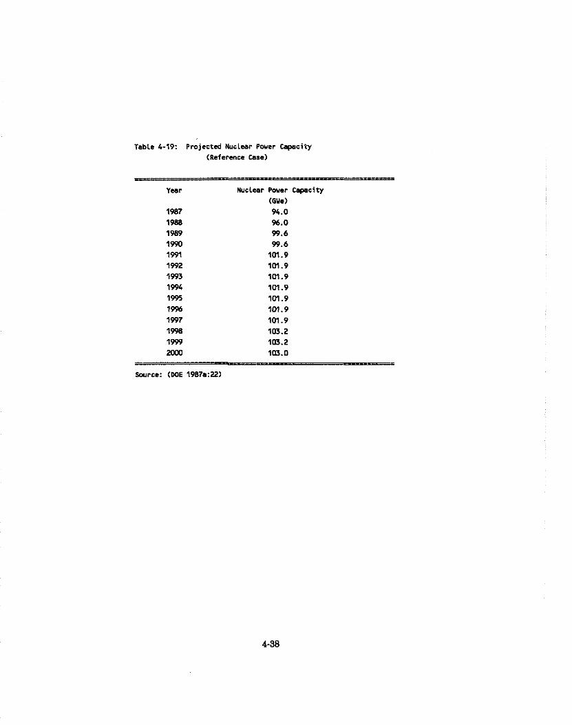
Table 4-19: Projected Nuclear Pwer Capacity (Reference Case)
Nuclear Power Capacity
(GYe) 94.0 W.0 99.6 99.6
1M .9 1M.9 1M.9 1M.9 1M .9 1M.9 1m .9 103.2 103.2 103.0
Source: (WE 1987a:22)
be obtained from this technology, perhaps as much as 15,000 short tons, in the Reference-case
scenario. In addition, there may be technological innovations which would make it feasible to obtain
U308 from phosphate rock.
Other potential sources of by-product uranium are: copper waste dumps; the red mud obtained when
alumina is removed from bauxite; and the beryllium ores of west-central Utah. A modest amount
of U308 is currently obtained from copper produced in Utah and Arizona. DOE estimated, in 1980,
[DOE 801 that 500 to 1000 tons of by-product U308 could be obtained annually from copper ores.
Also, DOE estimated that a few hundred short tons per year could be obtained annually from red
mud, and that 17 short tons could be obtained from beryllium ores annually, when an already
developed plan to recover uranium is employed.
Other Domestic Resources
DOE estimates of the total "endowment" of domestic U308 resources, are shown in Table 4-20. The
"endowment" is defined as all U308 contained in deposits containing at least .01 percent (100 ppm)
of U30s The resource estimates shown are grouped according to resource category, and by "forward
cost of recovery." The three resource categories used by DOE, the primary source for the
information contained in Table 4-20, are those used by the International Atomic Energy Commission,
and the OECD nuclear power agency:
o Reasonably Assured Resources (RAR): The uranium that occurs in
known mineral deposits of such size, grade, and configuration that it
could be recovered within the given cost ranges, with currently proven
technology. Estimates of tonnage and grade are based on specific
sample data and measurements of the deposits and on knowledge of
deposit characteristics. RAR correspond to DOE'S Reserve category.
o Estimated Additional Resources (EAR): The uranium in addition to
RAR that is expected to occur, mostly on the basis of direct geological
evidence, in extension of well-explored deposits, little explored
deposits, and undiscovered deposits believed to exist along well-
defined geological trends with known deposits, such that the uranium
can subsequently be recovered within the given cost ranges. Estimates

3 l ' B B
& : h " Oi ," 8 D m - - ' * * e
of tonnage and grade are based on available sampling data and on
knowledge of the deposit characteristics, as determined in the best
known parts of the deposit or in similar deposits. EAR corresponds
to DOE's Provable Potential Resource category.
o Speculative Resources (SR): Uranium in addition to EAR that is
thought to exist, mostly on the basis of indirect evidence and
geological extrapolations, in deposits discoverable with existing
exploration techniques. The locations of deposits in this category can
generally be specified only as being somewhere within given regions
or geological trends. As the term implies, the existence and size of
such deposits are speculative. The estimates in this category are less
reliable than estimates of EAR. SR corresponds to DOE's Possible
Potential Resources plus Speculative Potential Resource categories.
For each forward cost category of undiscovered resources, the estimates of resources at each cost
level are cumulative and include all lower-cost resources within that category.
The "forward cost of recovery" of uranium resources represents estimates of most future costs of
mining, processing, and marketing U308, exclusive of return to capital. These estimates include the
costs of transportation, environment and waste management, construction of new operating units,
and maintenance of all operating units, future exploration and development costs. Also, appropriate
indirect costs such as those for office overhead, taxes and royalties are included. Table 4-20 presents
estimates of all U308 resources having a "forward cost recovery" of no more than $100/lb [DOE 87bl.
In addition to estimated U308 resources in the endowment, there are some large lower grade U308
resources. The most significant of these are Chattanooga Shale deposits, seawater, and the marine
phosphorites from which U308 is currently obtained as a by-product of phosphoric acid production.
It is estimated that the Gassaway Member of Chattanooga Shale is 55 to 70 ppm U308 and contains
about 5 million tons of U308, as well as larger amounts of vanadium, ammonia, sulfur and oil [MSR
781.
Seawater represents a huge, very low-grade source of uranium, averaging 3 to 4 parts per billion,
and containing perhaps five billion tons of U308. Using very optimistic assumptions, the cost of
recovery using current technology has been estimated to be $1400/lb of U308, albeit, a MIT study
suggests that improved technology could reduce the cost to $300/lb, and possibly to $100 or less per
pound [CA 79, RO 791.
If, 38,400 short tons of U308 is produced over the next fourteen years as a result of by-product
technology, then given our forecasts (presented earlier for total domestic production) approximately
60,000 short tons of U308 would have to be obtained from other domestic sources. A relatively
insignificant quantity of U308 could be obtained from existing tailings piles. It has been estimated
[DOE 87a] that 127,000 short tons of U308 could be extracted from mill tailings piles at a forward
cost of $100 or less per pound. Hence, the near term scenario indicates that 60,000 tons will be
obtained from other domestic sources over the next fourteen years.
Excluding speculative resources, Table 4-20 suggests that there are about 675 thousand short tons
U308 with a forward cost of recovery of no more than $30 per pound. Of these, 161,000 tons are
included in the Reasonably Assured Resources category. Given the estimate of total domestic
production in Table 4- 18 (98,000 tons), it does not appear likely that the price of U308 will rise
above $30 per pound.
4.2.6.2 Total Electricitv Generation
Corresponding to the production scenario of domestic U308 production for the year 2000 are a range
of possible projections of total electricity consumption. One end of this range represents the
situation in which electricity is produced from conventional Fission. (i.e., from U-235) and uranium
imports from South Africa and Namibia continue to be restricted. In this situation, perhaps as much
as one quarter of all electricity is derived from conventional fission of domestically produced
uranium. The percentage of electricity may be lower than this as a result of greater use of electricity
from alternative sources, e.g., coal or solar. In constructing our scenarios, we have assumed that
there is no technological innovation which would permit either a cessation or a substantial reduction
in the construction of new uranium-fueled nuclear power plants. Under various assumptions, the
percentage of electricity derived from conventional fission of domestically produced uranium might
be as low as two percent, or lower if current technology changes.
A range of projections of total electricity consumption in the year 2000 is presented in Table 4-21.
The projections correspond to the previously presented Reference case scenario for total domestic
U308 production under the assumptions that 2, 5, 10 and 25 percent of electricity is derived from
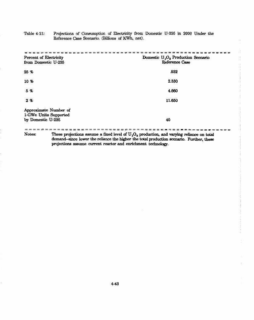
Table 4-21: Projecliom of ion of E l d u t y fmm Bommtie U-236 in 2000 Under the Reference Case Scenario. WiUiom of KGVh, net).
- - - = = = = = = . . . . . . . . . . . . . . . . . . . . . . . . . . . . . . . . . . . . . . . . . . . . . . . . .
Percent of Electricity Domeatic U30B Production Scenario from Domestic U-235 Reference Csae
Approximate Number of 1-GWe Units Supported by Domestic U-235
. . . . . . . . . . . . . . . . . . . . . . . . . . . . . . . . . . . . . . . . . . . . . . - - - - - - - - - - - - - - - - - - - - - - - - - - - - - - - - - - - - - - - - - - - - - - = = = = = = Notes. These projections assume a fixed level of U30B production, and varying reliance on total
demand-since lower the reliance the higher the total production scenario. Further. these projections assume current reactor and enrichment technology.
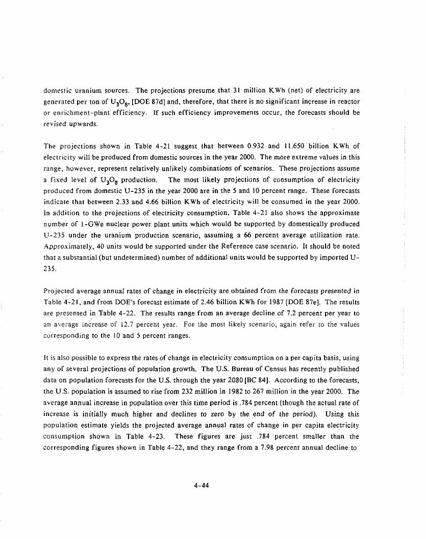
doniestic uranium sources. The projections presume that 31 million K w h (net) of electricity are
generated per ton of U308, [DOE 87d] and, therefore, that there is no significant increase in reactor
or enrichment-plant efficiency. If such efficiency improvements occur, the forecasts should be
revised upwards.
The projections shown in Table 4-21 suggest that between 0.932 and 11.650 billion Kwh of
electricity will be produced from domestic sources in the year 2000. The more extreme values in this
range, however, represent relatively unlikely combinations of scenarios. These projections assume
a fixed level of U3Oa production. The most likely projections of consumption of electricity
produced from domestic U-235 in the year 2000 are in the 5 and 10 percent range. These forecasts
indicate that between 2.33 and 4.66 billion Kwh of electricity will be consumed in the year 2000.
In addition to the projections of electricity consumption, Table 4-21 also shows the approximate
number of I-GWe nuclear power plant units which would be supported by domestically produced
U-235 under the uranium production scenario, assuming a 66 percent average utilization rate.
Approximarely, 40 units would be supported under the Reference case scenario. It should be noted
that a substantial (but undetermined) number of additional units would be supported by imported U-
235.
Projected average annual rates of change in electricity are obtained from the forecasts presented in
Table 4-21, and from DOE'S forecast estimate of 2.46 billion Kwh for 1987 [DOE 87el. The results
are presented in Table 4-22. The results range from an average decline of 7.2 percent per year to
an average increase of 12.7 percent year. For the most like15 scenario, again refer to the values
corresponding to the 10 and 5 percent ranges.
It is also possible to express the rates of change in electricity consumption on a per capita basis, using
any of several projections of population growth. The U.S. Bureau of Census has recently published
data on population forecasts for the U.S. through the year 2080 [BC 841. According to the forecasts,
the U.S. population is assumed to rise from 232 million in 1982 to 267 million in the year 2000. The
average annual increase in population over this time period is .784 percent (though the actual rate of
increase is initially much higher and declines to zero by the end of the period). Using this
population estimate yields the projected average annual rates of change in per capita electricity
consumption shown in Table 4-23. These figures are just ,784 percent smaller than the
corresponding figures shown in Table 4-22, and they range from a 7.98 percent annual decline to
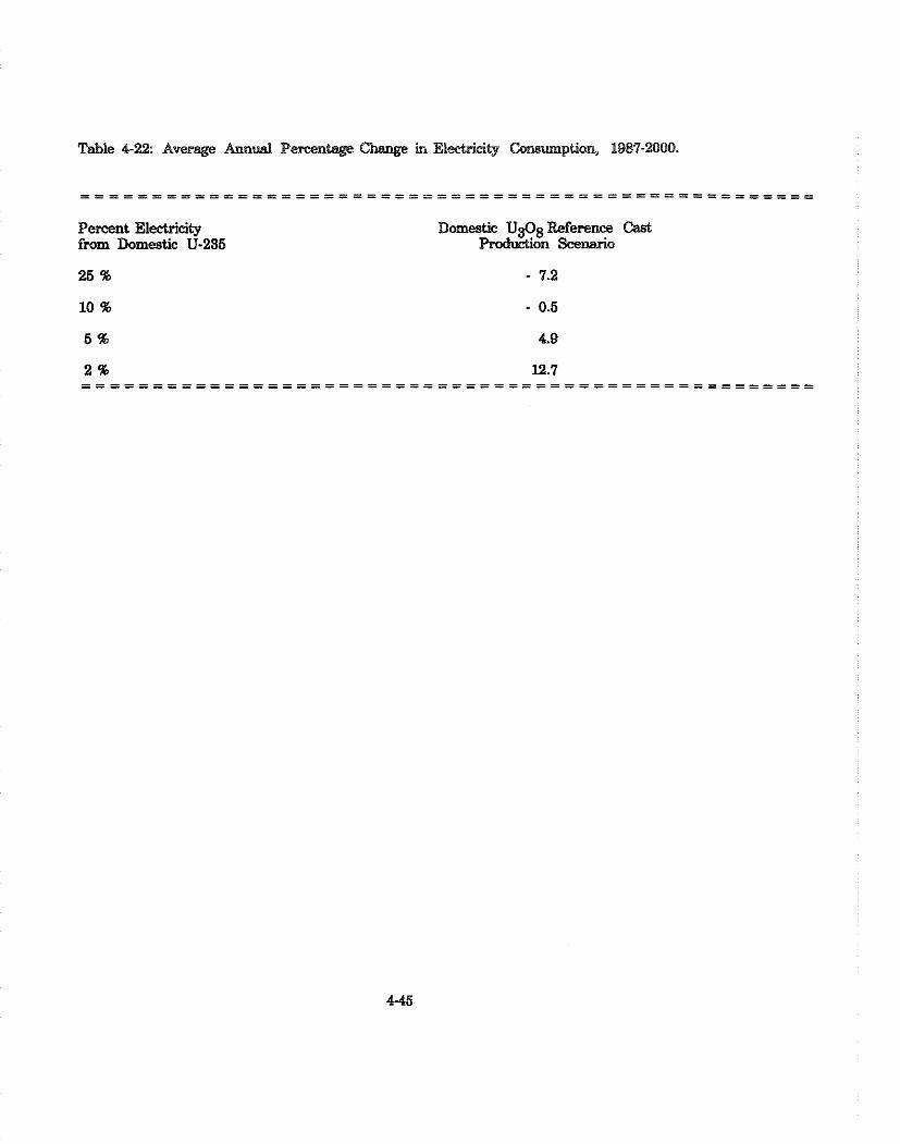
Table 4-22: Average Annual Percentage in Electricit8 ption, 1987-2000.
Percent Electricity from Domestic U-236
Domestic U308 Reference Cast Prodtrtion Scenario
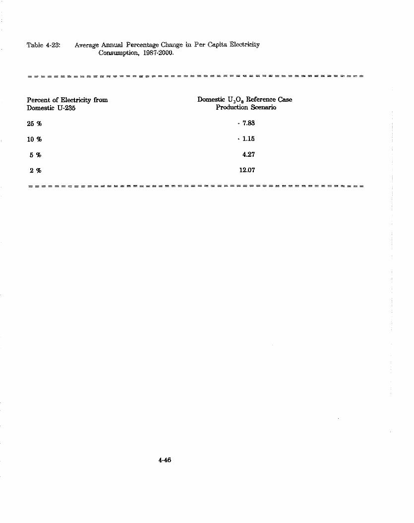
Table 4-25: Average Ann& Percentege C M in b"m Capib EIeCtdciQ Comup~pLion, 1887-2000.
Percent of Electricity from Domedic U-235
25 %
10 %
5 %
2 %
Domestic U,O, Reference Case Production Scenario
- 7.89 - 1.15 4.27
12.07
1 1.92 percent annual increase. For the most likely scenario, modest average annual decline of I.20
percent to an average annual increase of 3.87 percent is expected.
4.1.6.3 Emolovment Proiections
Employment projections and historical data for the uranium milling industry are presented in Table
4-14. Forecasts based upon the Reference case scenario show employment growing slowly from 1992
to 1997 after a stagnant, relatively cyclical period from 1987-1991.
The projections are developed in the following manner. Output per person-year is used as a measure
of productivity. Data for this variable are obtained by dividing total annual uranium concentrate
production from 1967-1986 by each year's total employment in the milling industry, and averaging
the results over the 20-year period. The resulting productivity factor of 7.44 short tons per person-
year is then divided into the relevant years of the production forecasts summarized in Table 4-18.
Average historical productivity is considered suitable for use in projecting future employment
because no technological innovations in uranium processing are expected which might affect mill
productivity.
4.3 Current Emissions. Risks, and Control Methods
Uranium mills extract uranium from ores which contain only 0.01 to 0.3 percent U308. The mills
are typically located near uranium mines in the western United States in areas of iow population
density. Since the uranium ores typically contain a low percentage of uranium, virtually all of the
ore input to the mill remains as waste which is disposed of in the tailings impoundment. The
impoundment areas are formed from dikes built with tailings sands or with soil and rock from the
pond area. As the pond is filled, the dikes are raised with mill tailings sands.
During the operating period of the mill, radon releases from the tailings are required to be
maintained ALARA. The addition of wet tailings provides a water cover which reduces the radon
emissions. The beaches are sprayed to prevent wind erosion and control the radon. At the end of
the operating period, the tailings pond is dewatered, and the spraying of water on the beaches is
discontinued. This is done so that the tailings can dry sufficiently to provide a stable base for the
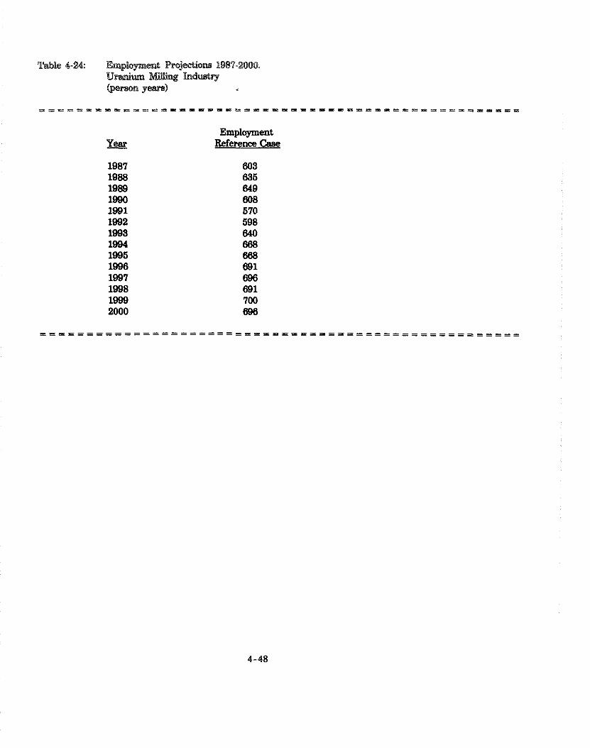
Table 4-24: EmpIopea& ProjeeLiow 1981-2000. Uranim LndWry @emn yeare)
Employment EE Reference Case

heavy equipment needed lo regrade the impoundment and place the earthen covers required to meet
the long-term disposal criteria of the UMTRCA standard.
4.3.1 Current Emissions and Estimated Risk Levels
The evaluation of the risks caused by emissions of radon from licensed conventional uranium mills
involves three distinct assessments: the risks that result from the continued use of existing
impoundments at the 1 I facilities that are operating or on standby; the risks that wilt occur once all
existing piles are disposed of; and the risks that will result from future tailings impoundments. As
in the 1986 NESHAPS rulemaking for this source category, the exposures and risks for existing
impoundments are assessed on a site-by-site basis, while risks from future impoundments are
assessed using model impoundments to represent the alternative technologies. The following sections
detail how the radon release rates are developed and identify the sources of the meteorological and
demographic data used in the assessment.
4.3.1.1 Methodoloev for the Assessment of Risks from Ooeratine and Standbv Mills
The overall risk from operating and standby mills includes risks resulting from emissions during
the operating or standby phase, the drying out and disposal phase, and the post-disposal phase. The
following sections detail how the radon release rates were developed for each of these phases to
obtain the source terms for the 11 operating and standby mills. The sources of the meteorological
and demographic data used in the assessment are atso discussed.
Development of the Radon Source Terms
The radon source terms are estimated based on the radon flux rate per unit area and the area of the
tailings. This assessment uses the same basic methodology for estimating radon releases and radon
source terms that was used in the 1986 NESHAPS rulemaking [EPA86]. For each phase, the
methodology involves two estimates: the radon flux per unit area, and the wet and dry areas of the
tailings pile.
For both the operating or standby phase and the drying and disposal phase, the radon flux per unit
area is calculated on the assumption that 1 pci/m2/sec radon-222 is emitted per pCi/g radium-226
in the tailings. This number could be lower because of moisture and other factors, but the

conservative value was used since the piles continue to dry out. In the calculations of the specific
flux rates, the radium concentrations of the tailings used are those reported in previous studies by
the EPA and the NRC [EPA83, NRCBO]. For the post-disposal phase, the assumed radon flux per
unit area is the design flux of the approved cover, if known, or the 20 pci/m2/s (2 pci/m2/s for
facilities in Colorado) limit established by the regulatory authorities responsible for the
implementation of the UMTRCA disposal standard.
Since water and earth covers effectively attenuate radon during the operating or standby phase, the
calculated radon flux rate is applied only to the dry area of the operable pile and any associated
evaporation ponds. The areas of the wet and dry fractions of the piles have been updated from
information obtained during the public comment period. Where new information was not provided,
areas are estimated from aerial photographs taken of each pile in 1986.
During the drying and disposal phase the calculated radon flux rates are applied to the total areas of
the impoundment and any associated evaporation ponds. For the post-disposal phase, the radon flux
is applied only to the area of the impoundment. The areas of any associated evaporation ponds are
not included since the radium contamination in these ponds is removed and transferred to the main
impoundment prior to stabilization. The total areas of the piles, along with the areas that are
estimated to be covered, ponded, wet, or dry, and the radium concentrations in the tailings are
shown in Table 4-25.
To obtain the radon source term for each facility, it was necessary to define the duration o f each of
the three phases. The operating or standby phase is defined to be fifteen years. While it is
recognized that some of the impoundments do not have 15 years of capacity remaining at full
production, the limited processing that is now occurring makes it possible that these impoundments
could remain operational for that length of time. The drying out disposal period is defined to
require five years, based on industry and DOE experience to date. Finally, the post-disposal period
is defined as fifty years. The sum of the emissions estimated for each period was divided by 70 to
obtain the average release per year for input to the assessment codes. The radon source terms
calculated for each pile are given in Table 4-26.

Table 4-25. S m a r y of operable r a i l i n g s impoundnent areas and radiun-226
content a t operating and standby m i l l s .
- Surface Area (acres)- Average
Ra-226
Total Covered Ponded Yet Dry (pCi/g)
Colorado
Canon C i t y - Primary
Canon C i t y - Secondary
Canon C i t y - Total
New Mexico
Anbrosia Lake - Secondary
Anbrosia Lake - Evap. Ponds
Anbrosia Lake - Total
Homestake - Primary
Homestake - Secondary
Homestake - Total
Texas
Panna Maria
Utah
Uhi t e Mesa
Rio A l g m - Lover
Shootaring
Washington
Shervood
U y m i ng
Lucky Mc - P i l e 1-3
Lucky Mc - Evap. Ponds
Lucky nc - Total
Sh i r ley Basin
Sweetwater
Tota ls
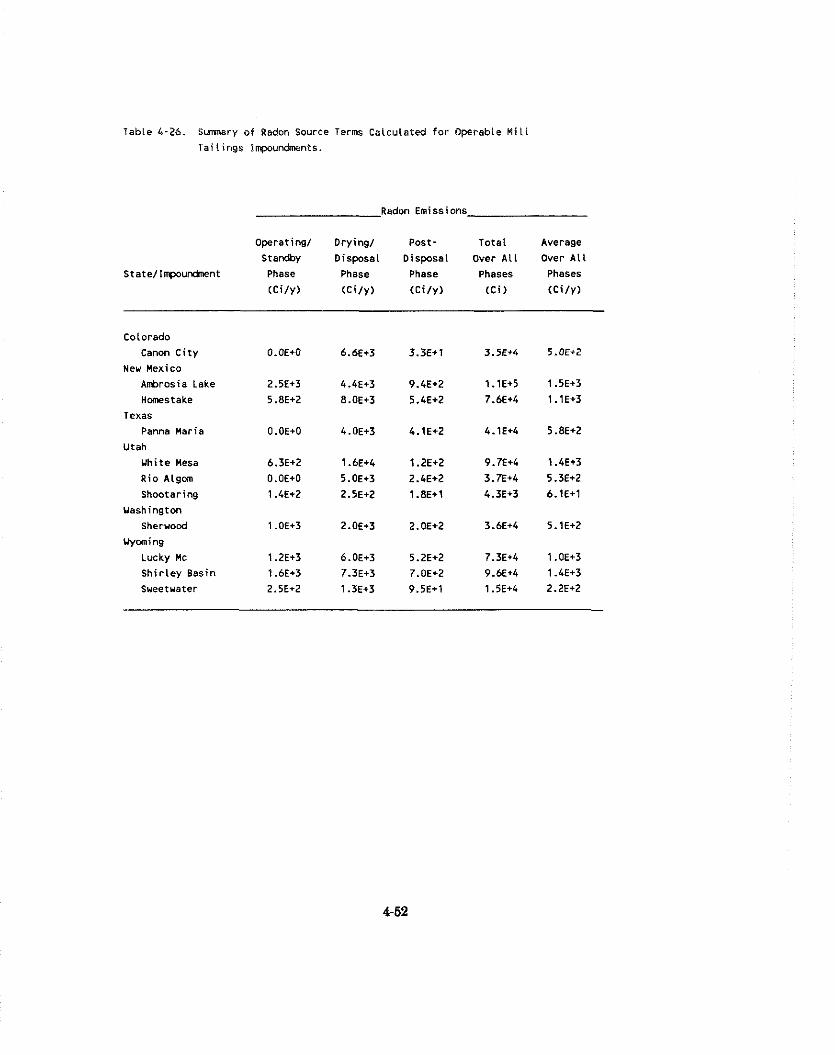
Table 4-26. S m s r y of Radon Source Terms Csiculated for Operable M i l l
Tai l ings lnpoundments.
Radon Emissions
Operating1 Drying/ Post- Total Average
Standby Disposal Disposal Over A11 Over A l l
StatellrrqxuKment Phase Phase Phase Phases Phases
( C i l ~ ) (C i l y ) (Ci ly) ( c i ) ( c i l y )
Colorado
Canon Ci ty
Neu Mexico
Anhrosia Lake
Hms take
Texas
Panna Maria
Utah
Uhi t e Mesa
Rio ALgm
Shootaring
Uashington
shervood
Yyming
L U C ~ Y nc
Shir ley Basin
Sweetwater
Demographic and Meteorologicai Data
Site-specific meteorological and demographic data are used in assessing the exposures and risks that
result from the release of radon. Demographic data for the nearby individuals (0-5 km) are
developed by visits to each site [PNL84]. The results of these surveys for all 26 licensed facilities are
shown in Table 4-27. The regional population data were generated using the computer code
SECPOP. Meteorological data are from the nearest station. Details of the inputs to the
AIRDOS/DARTAB/RADRISK codes are presented in Volume 2 of this Environmental Impact
Slalemertt.
4.3.1.2 Methodoloev for the Assessment of Post-Disposal Risks
The UMTRCA rule-making (40 CFR 192) established requirements for the long-term stabilization
and disposal of uranium mill tailings. In addition to protection of groundwater and long-term
isolation to prevent misuse of tailings, the UMTRCA standards require that the tailings cover be
designed to limit the radon flux to a maximum of 20 p ~ i / m 2 / s e c . The NRC and the Agreement
States, which are responsible for implementing She UMTRCA requirements at licensed facilities,
require licensees to demonstrate that the cover designs will achieve the 20 pCi/m2/s at the end of
1,000 years.
Development of Radon Source Terms
As was done for the assessment of Inactive Tailings (see Chapter 3), the post-disposal source terms
for each of the sites was estimated on the basis of the area of the tailings impoundments and the
design flux or measured performance of the cover. Where information on the design flux or cover
performance was unavailable, the UMTRCA limit of 20 p ~ i / m 2 / s (2 p ~ i / m 2 / s for facilities in
Colorado) was used. Table 4-28 summarizes the areas, radon flux rates through the covers, and
estimated annual emissions for each of the 26 licensed facilities once disposal is complete.
Source of Demographic and Meteorological Data
The demographic and meteorological data used to assess the post-UMTRCA disposal risks were
obtained in the same manner as those used in the assessment risks from operable and standby
impoundments. Table 4-27 summarizes the nearby (0-5 km) population around each of the sites.
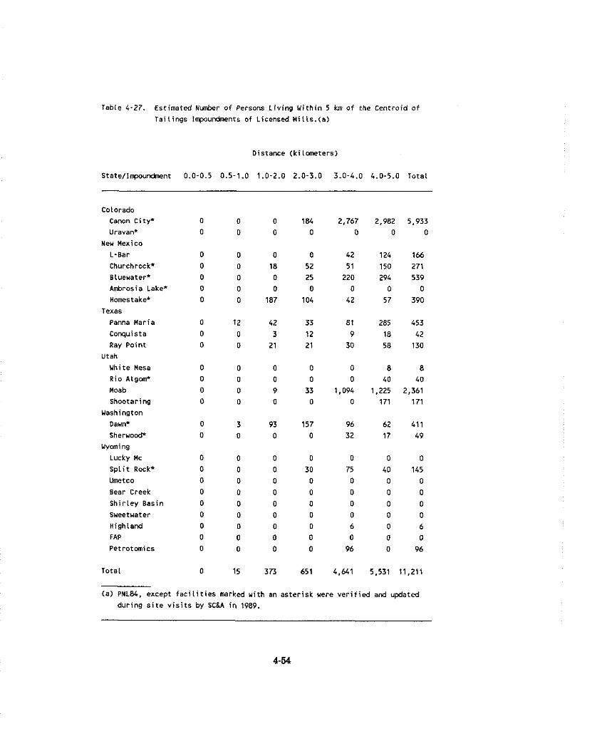
Table 4-27. Estimated Hunber af Persons L iv ing Wi th in 5 km of the Centroid o f Tai l ings lmpountments of Licensed MiIts.(a)
Distance (ki lometers)
State/lmpou&nt 0.0-0.5 0.5-1.0 1.0-2.0 2.0-3.0 3.0-4.0 4.0-5.0 Total
Colorado Canon City' Uravan*
New Mexico
L-Bar
Churchrock'
Bluewater*
Ambrosia Lake*
Homestake*
Texas
Panna Maria
Conquista
Ray Point
Utah
Whi t e Mesa
Rio A l g w *
Moab
Shootaring
Washington
Dawn*
S h e r u o d
Wyoming
~ u c k y nc
S p l i t Rock*
Umetco
Bear Creek
Shi r ley Basin
Sweetwater
Highland
FAP
P e t r o t m i c s
Total 0 15 373 651 4,641 5,531 11,211
(a) PNL84, except f a c i l i t i e s marked with an aster isk were v e r i f i e d and updated
dur ing s i t e v i s i t s by SCtA in 1989.
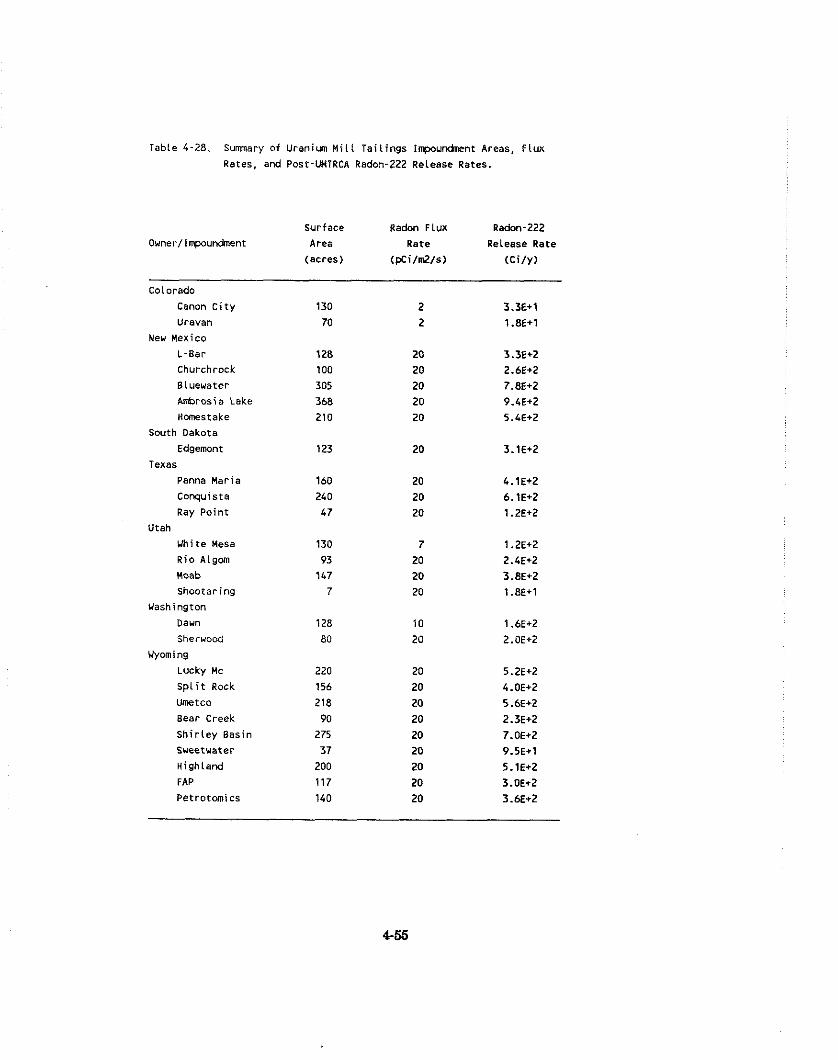
Table 4-28. Sumnary of Uren im M i l l Tai l ings inpourdment Areas, Flux
Rates, and Post-UnTRCA Radon-222 Release Rates.
Colorado
Canon C i ty
Uravan
N ~ Y Mexico
L-Bar
Churchrock
Bluewater
Arbrosia Lake
Homestake
South Oakota
Edgemont
Texas
Panna Maria
Conquista
Ray Point
Utah
Whi t e Mesa
Rio Algom
Moab
shootaring
Washington
Daun
Sheruood
Wyoming
Lucky Mc
S p l i t Rock
umetco
Bear Creek
Shir ley Basin
Sueetuater
Highland
F AP
Petrotomics
Surface
Area
(acres)
Radon Flux
Rate
(pci/m2/s)
Radon-222
Release Rate
(Ci ly)
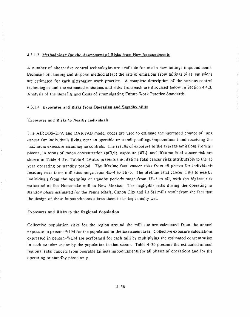
A number of alternative control technologies are available for use in new tailings impoundments.
Because both timing and disposal method affect the rate of emissions from tailings piles, emissions
are estimated for each alternative work practice. A complete description of the various control
technologies and the estimated emissions and risks from each are discussed below in Section 4.4.3,
Analysis of the Benefits and Costs of Promulgating Future Work Practice Standards.
4.3.1.4 Exoosures and Risks from Ooeratine and Standbv hfilts
Exposures and Risks to Nearby Individuals
The AIRDOS-EPA and DARTAB model codes are used to estimate the increased chance of lung
cancer for individuals living near an operable or standby tailings impoundment and receiving the
maximum exposure assuming no controls. The results of exposure to the average emissions from all
phases, in terms of radon concentration (pCi/l), exposure (WL), and lifetime fatal cancer risk are
shown in Table 4-29. Table 4-29 also presents the lifetime fatal cancer risks attributable to the 15
year operating o r standby period. The lifetime fatal cancer risks from a11 phases for individuals
residing near these mill sites range from 4E-4 to 5E-6. The lifetime fatal cancer risks to nearby
individuals from the operating or standby periods range from 3E-5 to nil, with the highest risk
estimated a t the Homestake mill in New Mexico. The negligible risks during the operating or
standby phase estimated for the Panna Maris, Canon City and La Sal mills result from the fact that
the design of these impoundments allows them to be kept totally wet.
Exposures and Risks to the Regional Population
Collective population risks for the region around the mill site are calculated from the annual
exposure in person-WLM For the population in the assessment area. Collective exposure calculations
expressed in person-WLM are performed for each mill by multiplying the estimated concentration
in each annular sector by the population in that sector. Table 4-30 presents the estimated annual
regional fatal cancers from operable tailings impoundments for all phases of operations and for the
operating or standby phase only.
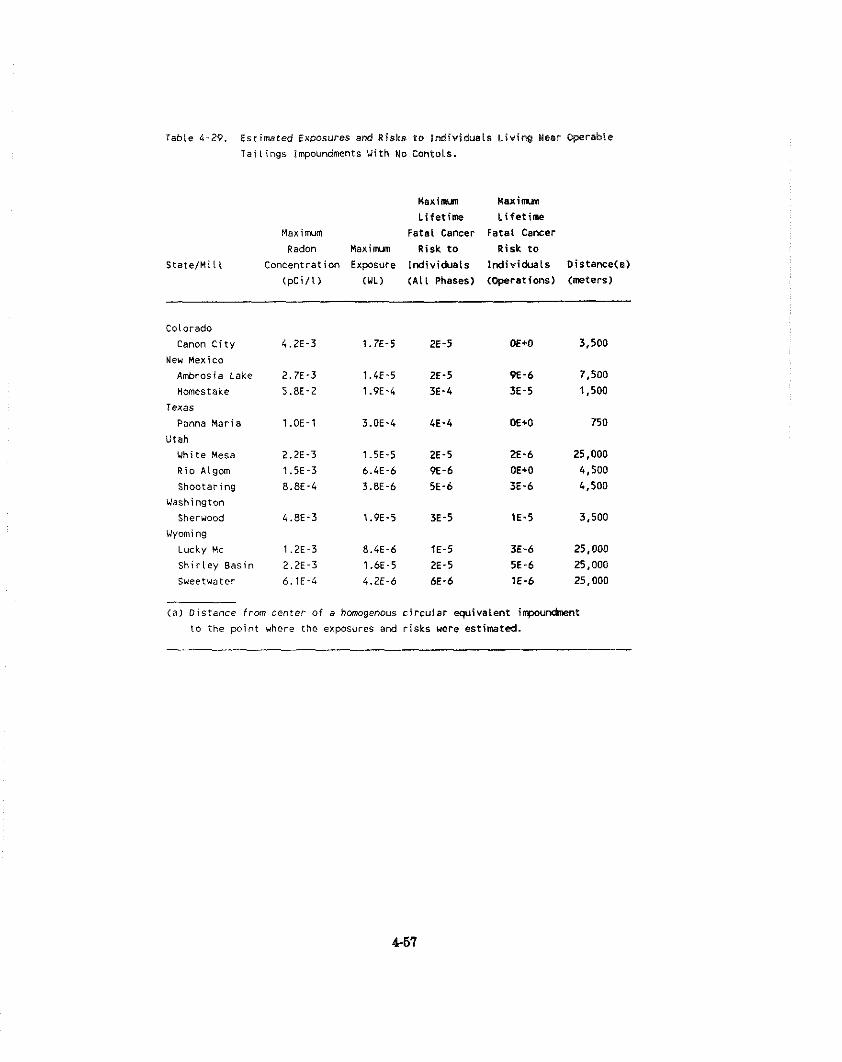
7abie 4-29, Estimated ExpSUreS and Risks to lndivldusls L i v i q j Near Operable Tailings Impoundments With No Contols.
M a x i m M a x i m Lifetim Lifetinre
Maximum Fetal Cancer Fatal Cancer Radon M a x i m Risk to Risk to
StatefMiII Concentration Exposure Individuals Individuals Distance(a) (pCil0 (WL) (AIL Phases) (Oprations) (meters)
Colorado Canon City
New Mexico Ambrosia Lake
Homestake Texas
Panna Maria
Utah White Mesa
Rio Algom
Shootaring Washington
Sheruood Wyoming
Lucky Mc
Shirley Basin Sweetwater
( a 1 Distance from center of a homogenous circular equivalent irnpourxhent t o the point vhere the exposures and risks were estimated.
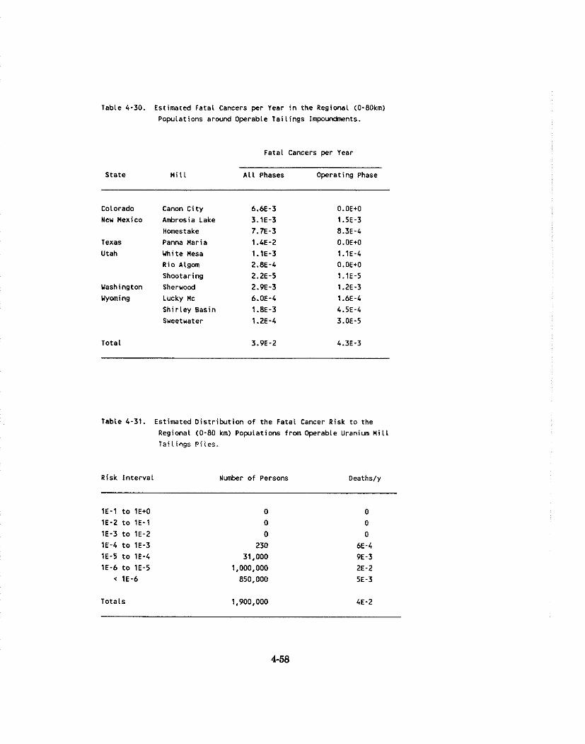
Table 4-30. Estimated Fatal Cancers per Year i n the Regional (0-8Okm)
Populations around Operable Tai l ings Iwundnents.
Fatal Cancers per Year
State M i l l A l l Phases Operating Phase
Colorado Canon C i ty
New Mexico Ambrosia Lake
Homestake Texas Panna Maria
Utah Yhi t e Mesa
Rio ~ l g o m
Shootaring
Washington Sheruood
Wyming ~ u c k y nc
Shir ley Basin
Sueetuater
Total
Table 4-31. Estimated D is t r ibu t ion o f the Fatal Cancer Risk t o the
Regional (0-80 km) Populations from Operable Uraniun n i l l Tai l ings Pi les.
Risk In te rva l Nunber of Persons Oeaths/y
Totals
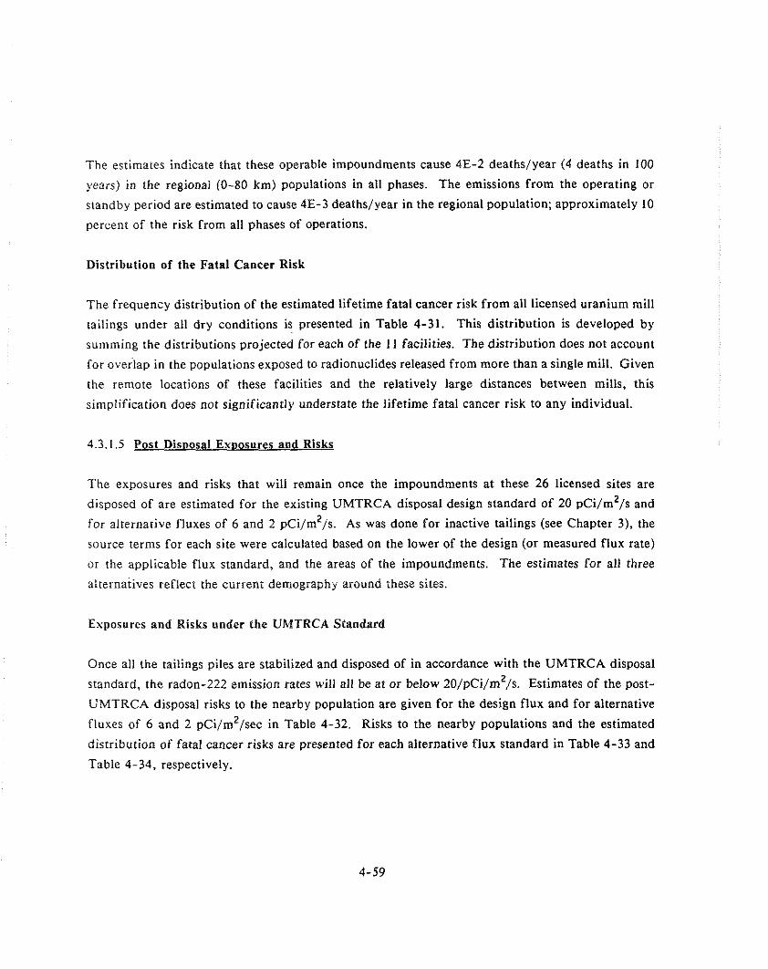
The estimates indicate that these operable impoundments cause 4E-2 deaths/year (4 deaths in 100
years) in the regional (0-80 km) populations in all phases. The emissions from the operating or
standby period are estimated to cause 4E-3 deathslyear in the regional population; approximately 10
percent of the risk from all phases of operations.
Distribution of the Fatal Cancer Risk
The frequency distribution of the estimated lifetime fatal cancer risk from all licensed uranium mill
tailings under all dry conditions is presented in Table 4-31. This distribution is developed by
sulllming the distributions projected for each of the I I facilities. The distribution does not account
for overlap in the populations exposed to radionuclides released from more than a single mill. Given
the remote locations of these facilities and the relatively large distances between mills, this
simplification does not significantly understate the lifetime fatal cancer risk to any individual.
4.3.1.5 Post Disoosal Exoosures and Risks
The exposures and risks that will remain once the impoundments at these 26 licensed sites are
disposed of are estimated for the existing UMTRCA disposal design standard of 20 pCi/m2/s and
for alternative fluxes of 6 and 2 p ~ i / m 2 / s . As was done for inactive tailings (see Chapter 3), the
source terms for each site were calculated based on the lower of the design (or measured flux rate)
or the applicable flux standard, and the areas of the impoundments. The estimates for all three
alternatives reflect the current demography around these sites.
Exposures and Risks under the UMTRCA Standard
Once all the tailings piles are stabilized and disposed of in accordance with the UMTRCA disposal
standard, the radon-222 emission rates will all be at or below 20/p~i/m'/s. Estimates of the post-
UMTRCA disposal risks to the nearby population are given for the design flux and for alternative
fluxes of 6 and 2 p ~ i / m 2 / s e c in Table 4-32. Risks to the nearby populations and the estimated
distribution of fatal cancer risks are presented for each alternative flux standard in Table 4-33 and
Table 4-34, respectively.
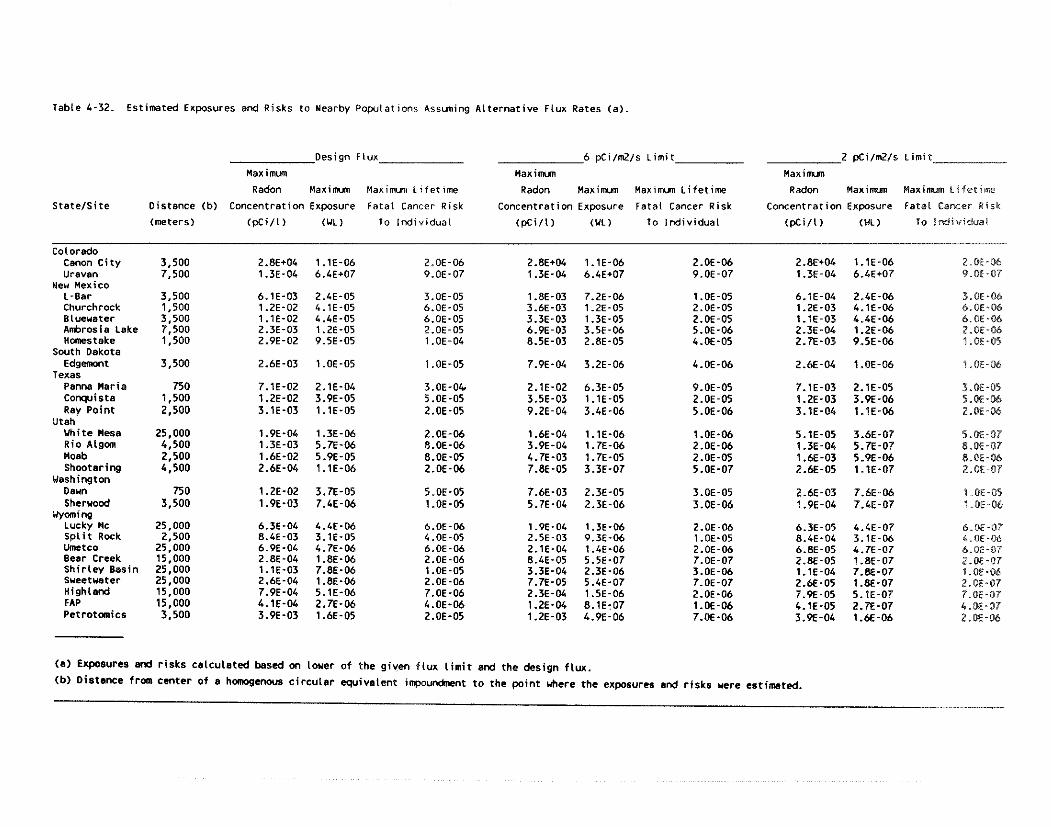
Table 4-32. Estimated Exposures and Risks t o Nearby Populations Assuning Al ternat ive Flux Rates ( a )
Design Flux 6 pCilm2ls Limit 2 pt i lm2ls L i m i t
M a x i m M a x i m M a x i m
Radon M a x i m Maximum Lifet ime Radon M a x i m M a x i m Lifet ime Radon n a x i m Naxinirn Lifet ime
Sta te ls i te Distance (b) Concentration Exposure Fatal Cancer Risk Concentration Exposure Fatal Cancer Risk Concentration Exposure Fatal Cancer f f i s h
(meters) ( W i l l ) (UL) To Individual ( W i l l ) (WL) To l rd iv idua l ( W i l l ) (WL) To Individual
Colorado Canon C i ty Uravan
New Mexico L-Bar Churchrock Blueuater Anbrosia Lake Honestake
Swth Dakota E d g m t
Texas Pama Maria Conquista Ray Point
Utah White Mesa Rio A lgm Moab Shootaring
Washington Damn Shermood
Waning Lucky Wc Sp l i t Rock Umtco Bear Creek Shir ley Basin Sweetwater Highland FAP Petrotmics
(a) Exposures snd r i s ks calculated based on lover of the given f lux l i m i t and the design f lux.
(b) Oistence f ran center of a hanogemus c i rcu la r equivalent i w u n h r n t t o the point uhere the exposures and r i sks were estirnsted.
Table 4 - 3 3 . Estimated Fatal Cancers per Year i n the Regional (0-80 kin) Popl la t ions
Assuming Al ternat ive Radon Flux Rates (a ) .
Design f lux 6 pCi/&/s 2 p c i l d l s
Fatal Cancers Fatal Cancers Fa ta l Cancers
per Year per Year per Year
Colorado
Canon Ci ty
Uravan
New Mexico
L-Bar
Churchrock
Bluewater
Ambrosia Lake
Hamestake
south Dakota
Edgemont
Texas
Panna Maria
Conquista
Ray Point
Utah
Whi t e Mesa
Rio Algom
Moab
Shootaring
Washington
Dawn
Sheruood
Wyoming
Lucky Mc
Sp l i t Rock
Umetco
Bear Creek
Shir ley Basin
Sweetwater
Highland
f AP
Petrofomics
Total
( a ) Fatal cancers per year
and the design f lux .
are caiculated based on the lower of the g iven flux l i m i t
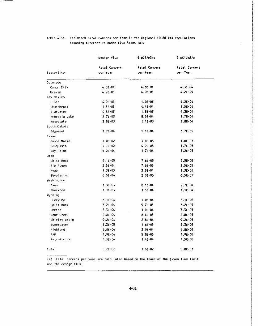
Table 4 - 3 3 . Estimated Fatal Cancers per Year i n the Regionel (0-80 kin) Pop l la t i ons
Assuming A l t e r n a t i v e Radon Flux Rates (a).
Design f l u x 6 pCi lnVls 2 pCi lnVls
Colorado
Canon C i t y
Uravan
New Mexico
L-Bar
Churchrock
Bluewater
Ambrosia Lake
Homestake
South Dakota
Edgemont
Texas
Panna Maria
Conquista
Ray Point
Utah
White Mesa
Rio Algom
Moab
Shootaring
Washington
Dawn
Shervood
Wyoming
Lucky Mc
Spl i t Rock
Umetco
Bear Creek
Sh i r l ey Basin
Sweetuater
Highland
FAP
Petrotomics
Fata l Cancers Fata l Cancers Fa ta l Cancers
per Year per Year pe r Year
Total 5.2E-02 1.6E-02 5.8E-03
( a ) Fatal cancers per year are ca lcu la ted based on the louer o f the g i ven f lux Limi t
and the design f l u x .

The estimates show that for nearby individuals the maximum lifetime fatal cancer risk will range
from 3E-4 to 9E-7 once disposal activities are completed. The number of deaths/year that will
occur in the regional populations around these 26 sites is estimated to be 5E-2 assuming the design
flux.
Exposures and Risks under Alternative Disposal Standards
As shown in Tables 4-32 through 4-34, at 6 p ~ i / m 2 / s the maximum individual lifetime fatal cancer
risk is 9E-05 at the Panna Maria site, a reduction from 3E-04 under the UMTRCA disposal
standard. The estimated deaths per year are reduced from 5E-02 to 2E-02. Similarly, at 2 pci/m2/s,
the maximum individual risk is reduced by a factor of three to 3E-05, and the deaths/year from all
26 sites is reduced to 6E-3.
4.3.2 Technoloeies for Lone-term Post-dis~osal Emission Control
Previous studies have examined the feasibility, effectiveness, and cost associated with various options
for conjrolling releases of radioactive materials from uranium mill tailings [NRC80, EPA82, EPA83,
EPA861. These studies have concluded that long-term stabilization and control is required to protect
the public from the hazards associated with these tailings. The standards for long term disposal
established for these sites under UMTRCA, require controls that prevent misuse of the tailings,
protect water resources, and limit releases of radon-222 to the air. The UMTRCA standard
established a design standard to limit long-term radon releases to an average flux no greater than 20
p ~ i , ' m ~ / s e c .
Both active and passive controls are available to reduce radon-222 emissions from tailings. Active
controls require that some institution, usually a government agency, bear the responsibility for
continuing oversight of the piles, and making repairs to the control system when needed. Fencing,
warning signs, periodic inspections and repairs, and restrictions on land use are measures that may
be used by the oversight agency. Passive controls, on the other hand, are measures of sufficient
permanence to require little or no active intervention. Passive controls include measures such as
thick earth or rock covers, barriers (dikes) to protect against floods, burial below grade, and moving
piles out of flood prone areas, or away from population centers. Of the two methods, active or
institutional controls are not preferred for long term stabilization of radon-222 emissions, since
institutional performance of oversight duties over a substantial period of time is not reliable.

Previous studies (see above) have identified a number of options to provide long-term control of
radon-222 emissions from the tailings. These include earthen or synthetic covers, extraction of
radium from the tailings, chemical fixation, and sintering. These long-term control options are
discussed in detail in Volume 2 of this Environmental Impact Slalemenl.
In comparison to other control technologies earth covers have been shown to be cost-effective
[NRC80]. Apart from cost considerations, there are other benefits that accrue by using earth covers
as a method to control radon-222 emissions. For example, synthetic covers, such as plastic sheets,
do not reduce gamma radiations. However, earth covers that are thick enough to reduce radon-222
emissions will reduce gamma radiation to insignificant levels. Further, chemical and physical stresses
over a substantial period of time destabilize synthetic covers, while earthen covers are stable over the
long run provided the erosion caused by rain and wind is contained with vegetation and rock covers,
and appropriate precautions are taken against natural catastrophes, e.g., floods and earthquakes.
Earthen covers also reduce the likelihood of contaminating ground water that result from either
storing radioactive materials in underground mines, (underground mines are typically located under
the water table) or by using the leaching process to extract radioactive and non-radioactive
contaminants from mill tailings. Moreover, although underground mine disposal is an effective
method to protect against degradation and intrusion by man, it nevertheless incurs a social cost. For
example, storing tailings in underground mines eliminates the future development of the mines'
residual resources. Again, earthen covers with proper vegetation and rock covers can protect against
human intrusion, without incurring such social costs.
Finally, earth covers provide more effective long term stabilization than either water or soil cement
covers. Albeit, soil cement covers are comparable to earthen covers in terms of cost effectiveness,
their long term performance is as yet unknown. Water covers, on the other hand, do not provide the
long term stability required for the time periods required, which are at least 1000 years. Moreover,
earth covers are more effective stabilizers than water spraying control technology in arid regions.
Covering the dried tailings with dirt is an effective method for reducing radon-222 emissions and
is already in use at inactive tailings impoundments. The depth of soil required for a given amount
of control varies with the type of earth and radon-222 exhalation rate.
Earth covers decrease radon-222 emissions by retaining radon-222 released from the tailings long
enough so that a significant portion will decay in the cover. A rapid decrease in radon-222 emissions
is initially achieved by applying almost any type of earth. The high-moisture content earths provide
greater radon-222 emission reduction because of their smaller diffusion coefficient.
In practice, earthen cover designs must take into account uncertainties in the measured values of the
specific cover materials used, the tailings to be covered, and predicted long-term values of
equilibrium moisture content for the specific location. The uncertainty in predicting reductions in
radon-222 flux increases rapidly as the required radon-222 emission limit is reduced.
The cost of adding earth covers varies widely with location of the tailings impoundment, its layout,
availability of earth, the topography of the disposal site, its surroundings, and hauling distance.
Another factor affecting costs of cover material is its ease of excavation. In general, the more
difficult the excavation, the more elaborate and expensive the equipment and the higher the cost.
The availability of materials such as gravel, dirt, and clay will also affect costs. If the necessary
materials are not available locally they must be purchased and/or hauled and costs could increase
significantly.
4.4 Analvsis of Benefits and Costs
This section presents the benefits and costs of three separate decisions that may be addressed in
promulgating the new Clean Air Act standards for release of radionuclides from licensed uranium
mill tailings piles. The first decision concerns the limit on allowab1e radon-222 emissions after
closure. Options that are evaluated include reducing radon-222 emissions from the 20 pci/m2/sec
limit established under UMTRCA ro 6 p ~ i / m 2 / l s c and 2 pci/rn2/sec.
The second decision investigates the means by which the emissions from active mills can be reduced
to the 20 pci/m2/sec limit established under UMTRCA while operations continue. This can be
accomplished through the application of earth and water covers to portions of the dry areas of the
piles in order to reduce average emissions for the entire site to the 20 pci/m2/sec limit.
While the first two decisions are focused on existing piles, the third is concerned with future tailings
impoundments. Here alternative work practices for the control of radon emissions from operating
niills in the future are evaluated. Options that are investigated include the replacement of the
traditional single cell impoundment with phased and continuous disposal impoundments.
This analysis assumes that UMTRCA is in place and that all controls required under UMTRCA will
be met regardless of any provisions resulting from this reconsideration of the CAA standards. The
beginning point of this analysis (i.e. the baseline) therefore assumes that ail controls required by
UMTRCA are met, specifically that radon emission levels will be limited to 20 pci/m2/sec and that
measures will be undertaken to achieve the long-run stability required by the UMTRCA rules.
Benefits are measured as reductions in the estimates of committed cancers resulting from lower
allowable emissions. Results are presented in terms of both total benefits and average annual
benefits. For the calculation of total benefits a 100-year time period is assumed.
All costs are measured in 1988 dollars and represent the cost of both the disposal and long-term
stabilization of the tailings. Cost estimates are calculated assuming no remedial actions have taken
place. The costs of meeting the alternative standards are the incremental costs from the baseline (20
pCi/m2/sec) to the 6 or 2 pci/m2/sec alternative. Results are presented in net present value and
annualized cost, and are estimated using real interest rates of zero, one percent, five percent and ten
percent. As with benefits, a 100-year time period is assumed.
4.4.1 Benefits and Costs of Reducine Post Closure Emissions from 20 w ~ i / m ~ / s e c
This section presents the benefits and costs of reducing the allowable radon-222 emissions from the
maximum limit of 20 p ~ i / m 2 / s e c established under the UMTRCA standard. Options which are
evaluated include lowering allowable radon emissions to a maximum of 6 pci/m2/sec or a maximum
of 2 pCi/m2/sec.
Although existing impoundments may be in use or on standby with additional available capacity, the
control options evaluated in this analysis are based on the simplifying assumption that operations
have ceased, that the tailings are sufficiently dry to allow the use of heavy equipment, and that the
piles have their current dimensions.
4.4.1.1 Benefits of Reducine the Allowable Limits
I t is assumed that reductions in the radon flux rare provided by increasing the depth of cover will
4-66
yield proportional reductions in committed cancers. The resulting estimates of committed cancers
per year on a pile-by-pile basis are presented above for the 20.6 and 2 pci/m2/sec options in Table
4-35.
Table 4-35 summarizes the estimates of risk and reduction of risk (committed cancers) for the
various regulatory options. The table presents these estimates for the 100 year period as well as
annual averages. Over the 100 year time frame the 6 pci/m2/sec option lowers local and regional
risks by 3.6 committed cancers. The incremental benefit of lowering the allowable flux rate from
6 pci/m2/sec to 2 pci/m2/sec is estimated as 1.0 committed cancer.
For reasons described above, the supplemental control selected for long-term radon-222 control at
existing tailings impoundments is the earth cover control option. The thickness of cover required to
achieve a given radon flux is a function of the initial radon flux from the pile. Five basic steps or
operations are required to implement the supplemental controls for existing tailings piles. These
include regrading slopes, procurement and placing of the dirt cover, placing gravel on the pile tops,
placing of rip-rap on the pile sides, and reclamation of the borrow pits. The estimation of earth
cover thicknesses and the costs for the five operations are described in detail in Appendix B of
Volume 2 of this Environmental lmpact Statement.
In order to properly reflect general industry overhead and costs, an overhead cost factor of 1.07 is
used to adjust the cost of earth cover described above, (see Appendix B, Volume 2 for a discussion
of cost factors). Estimates of costs, with and without the overhead cost factor, are presented for
each pile for the 20, 6 and 2 p~ i /m2/sec options in Tables 4-36, 4-37, and 4-38, respectively.
Achieving the 20 ~ ~ i / m ' / s e c option is estimated to cost between $560 to $599 million. In contrast,
reaching the 6 pci/m2/sec option is estimated to cost from $728 to $779 million while compliance
with the 2 p ~ i / m 2 / s e c option would entail costs estimated to reach between $882 to $943 million.
Table 4-39 provides the incremental present value costs for the two radon fluxes and added costs
for lowering the allowable flux. Estimates for each of the four real interest rates are included
assuming an overhead cost factor of 1.07. Reducing the allowable flux rate to 6 pCi/m2/sec will
entail added present value costs of between $113 and $180 million depending on assumptions as to
real interest rates, while attainment of a 2 pci/m2/sec flux rate would entail added costs of $216 to
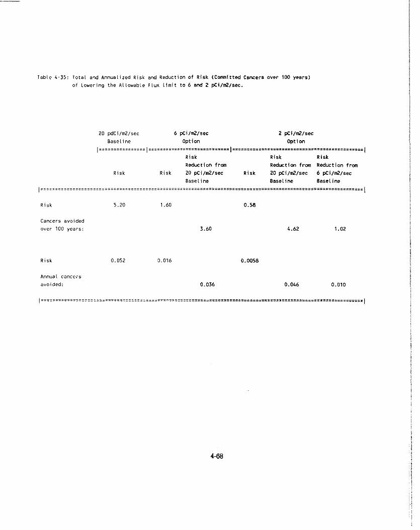
Tablc 4 . 3 5 : Total ond Annualized Risk and Reduction of Risk ( C m i t t e d Cswers over 100 years)
of Lowering the Aliouabie Flux l i m i t to 6 end 2 pCi/mZ/sec.
20 ~dCi/mZ/sec 6 pCilm2lsec 2 pfi/mZ/sec
Baseline Option Opt ion ~l_lj~ll=liiiiili~i======================~====~=========~======~==========s=====z==========~
Risk Risk Risk I
Reduction f r m Reduction f r m Reduction f r m
Risk Risk 20 pfi/mZ/sec Risk 20 pCilmZlsec 6 pCi/mZ/sec
Baseline Baseline Baseline ~i=ziiiiii==i=ii========~================~==============z======z=~=======z=======z======================~=======~
Risk 5.20 1.60 0.58
Cancers avoided
over 100 years:
Risk 0.052 0.016
Annual cancers
avoided: 0.036 0.046 0.010
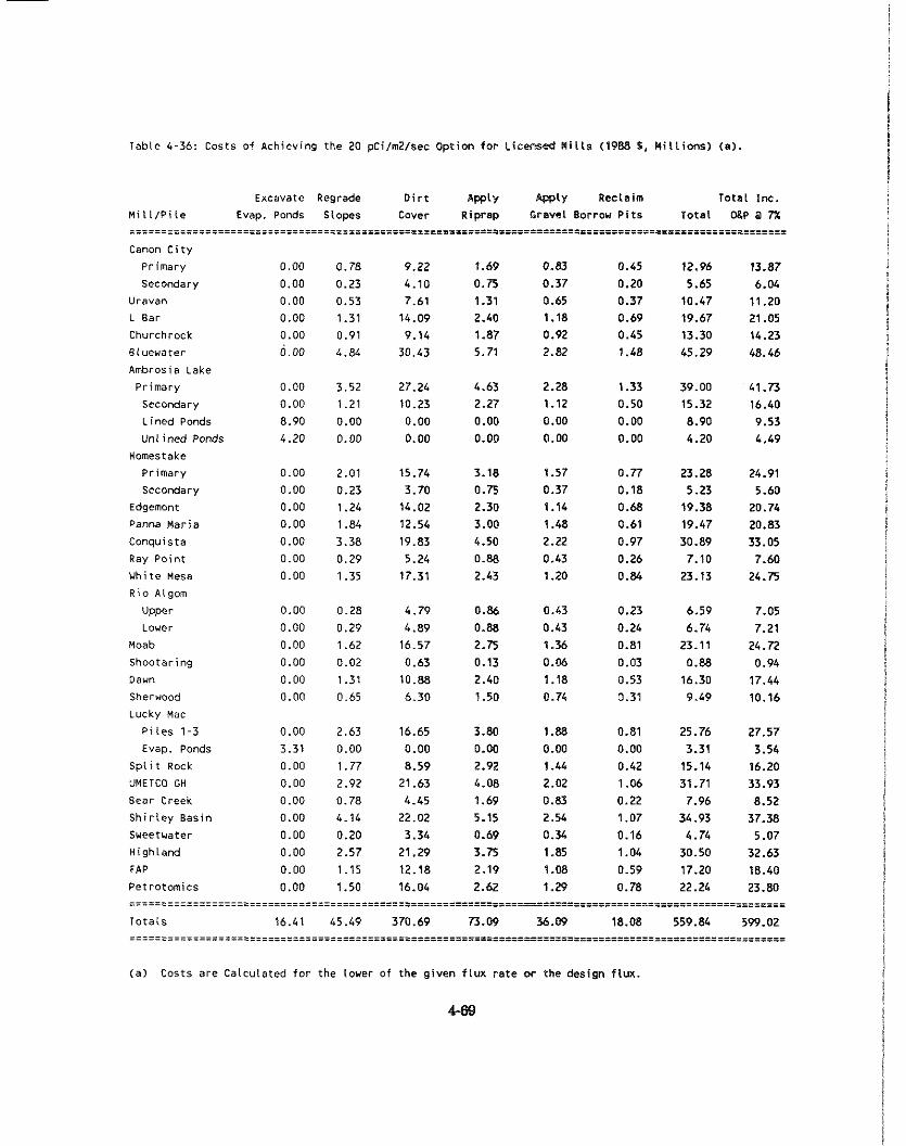
Table 4-36: Costs of Achieving the 20 pCi/m2/sec Option for Lifwsed Wills (1988 5 , Millions) ( 0 ) .
Excavate Regrade D i r t Apply k w t y Reclaim Total Inc. MilIlPiie Evap. Ponds Slopes Cover Riprap Gravel Borrov Pits Total OgP @ 7% ====T i lS i==== l= i i i i ~==========z======~==================~x~=====~======~==========~=~~===========~=======
Canon City Primary 0.00 0.78 9.22 1.69 0.83 0.45 12.96 13.87 Secondary 0.00 0.23 4.10 0.75 0.37 0.20 5.65 6.04
Uravan 0.00 0.53 7.61 1.31 0.65 0.37 10.47 11.20 L Bar 0.00 1.31 14.09 2.60 1.18 0.69 19.67 21.05 Churchrock 0.00 0.91 9.14 1.87 0.92 0.45 13.30 14.23 Bluewater 0.00 4.84 30.43 5.71 2.82 1.48 45.29 48.46 Ambrosia Lake Primary 0.00 3.52 27.24 4.63 2.28 1.33 39.00 41.73
Secondary 0.00 1.21 10.23 2.27 1.12 0.50 15.32 16.40 Lined Ponds 8.90 0.00 0.00 0.00 0.00 0.00 8.90 9.53 Unlined Ponds 4.20 0.00 0.00 0.00 0.00 0.00 4.20 4.49
Homestake Primary 0.00 2.01 15.74 3.18 1.57 0.77 23.28 24.91 Secondary 0.00 0.23 3.70 0.75 0.37 0.18 5.23 5.60
Edgemont 0.00 1.24 14.02 2.30 1.14 0.68 19.38 20.74 Panna Maria 0.00 1.84 12.54 3.00 1.48 0.61 19.47 20.83 Conquista 0.00 3.38 19.83 4.50 2.22 0.97 30.89 33.05 Ray Point 0.00 0.29 5.24 0.88 0.43 0.26 7.10 7.60 White Mesa 0.00 1.35 17.31 2.43 I .20 0.84 23.13 24.75 R i o Algom
Upper 0.00 0.28 4.79 0.86 0.43 0.23 6.59 7.05 Lower 0.00 0.29 4.89 0.88 0.43 0.24 6.74 7.21
Noab 0.00 1.62 16.57 2.75 1.36 0.81 23.11 24.72 Shootaring 0.00 0.02 0.63 0.13 0.06 0.03 0.88 0.94 Dawn 0.00 1.31 10.88 2.40 1.18 0.53 16.30 17.44 Shervood 0.00 0.65 6.30 1.50 0.74 0.31 9.49 10.16 Lucky Mac
Piles 1-3 0.00 2.63 16.65 3.80 1 .88 0.81 25.76 27.57 Evap. Ponds 3.31 0.00 0.00 0.00 0.00 0.00 3.31 3.54
Spli t Rock 0.00 1.77 8.59 2.92 1 .U 0.42 15.14 16.20
UMETCO GH 0.00 2.92 21.63 4.08 2.02 1.06 31.71 33.93 Bear Creek 0.00 0.78 4.45 1.69 0.83 0.22 7.96 8.52 Shirley Basin 0.00 4.14 22.02 5.15 2.54 1.07 34.93 37.38 Sueetuater 0.00 0.20 3.34 0.69 0.54 0.16 4.74 5.07 Highland 0.00 2.57 21.29 3.75 1.85 1.04 30.50 32.63 FAP 0.00 1.15 12.18 2.19 1.08 0.59 17.20 18.40 Petrotomics 0.00 1.50 16.04 2.62 1.29 0.78 22.24 23.80
Totals 16.41 45.49 370.69 73.09 36.09 18.08 559.84 599.02
( a ) Costs are Calculated for the lover of the given flux rate w the design flux.
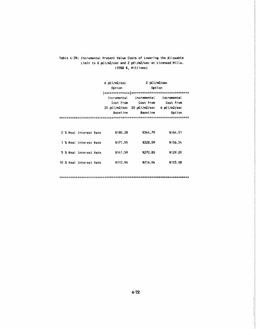
Table 4-39: Incremental Present Value Costs o f Lowering the Allowable
L i m i t t o 6 pCi/nQ/sec and 2 pCilm2lsec a t L icmsed M i l l s .
(1988 I, M i l l i o n s )
6 pci/nQ/sec 2 pCilm2Iser:
Option Option ................................................
Incremental Incremental Incremental
Cost Frm Cost Frm Cost F r m
20 pci/m2/sec 20 pCilm2/sec 6 pCilm2Isec
Easeline Baseline Option -----....------------------..------------------------------------------- ------------......-----..-----------------------------------------------
0 % Real In te res t Rate $180.28 $344.79 $164.51
1 X Real In te res t Rate $171.55 $328.09 $156.54
5 X Real In te res t Rate $141.59 $270.80 $129.20
10 X Real i n te res t Rate $112.96 1216.04 $1 03.08
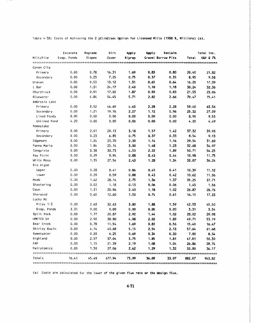
Table 4-38: Costs of Achieving the 2 pCi/wZ/sec Option fo r Licensed M i l l s (1988 S, M i l l i o n s ) (a ) .
Excavate Regrade D i r t APPLY WLy Reclaim Tota l Inc.
M i l l t P i l e Evap. Ponds Slopes Cover Riprap Gravel Borrou P i t s Total OgP a i%
Canon C i t y
Primary 0.00 0.78 16.31 1.69 0.83 0.80 20.40 21.82 Secondary 0.00 0.23 7.25 0.75 0.37 0.35 8.95 9.58
Uravan 0.00 0.53 13.12 1.31 0.65 0.64 16.25 17.39 L Bar 0.00 1.31 24.17 2.40 1.18 1.18 30.24 32.36 Churchrock 0.00 0.91 17.02 1.87 0.92 0.63 21.55 23.06 Bluewater 0.00 4.84 54.45 5.71 2.82 2.66 70.47 75.41 Ambrosia Lake
Primary 0.00 3.52 46.69 4.63 2.28 2.28 59.40 63.56 Secondary 0.00 1.21 19.76 2.27 1.12 0.96 25.32 27.09 Lined Ponds 8.90 0.00 0.00 0.00 0.04 0.00 8.90 9.53 Uniined Pond 4.20 0.00 0.00 0.00 0.00 0.00 4.20 4.49
Homestake
Primary 0.00 2.01 29.13 3.18 1.57 1.42 37.32 39.93 Secondary 0.00 0.23 6.85 0.75 0.37 0.33 8.54 9.13
Edgemont 0.00 1.24 23.70 2.30 1.14 1.16 29.54 31.60 Panna Maria 0.00 1.84 25.14 3.00 1.48 1.23 32.68 34.97 Conquista 0.00 3.38 38.73 4.50 2.22 1.89 50.71 54.25 Ray Point 0.00 0.29 8.94 0.88 0.43 0.44 10.98 11.75 White Mesa 0.00 1.35 27.54 2.43 1.20 1.34 33.87 36.24 Rio Algom
upper 0.00 0.28 8.41 0.86 0.43 0.41 10.39 11.12 Loser 0.00 0.29 8.59 0.88 0.43 0.42 10.62 11.36
Moab 0.00 1.62 28.14 2.75 1.36 1.37 35.25 37.71 Shootaring 0.00 0.02 1.18 0.13 0.06 0.06 1.45 1.56 Dawn 0.00 1.31 20.96 2.40 1.18 1.02 26.87 28.76 Sherwood 0.00 0.65 12.60 1.50 0.74 0.61 16.10 17.23
Lucky MC
P i l e s 1-3 0.00 2.63 32.63 3.80 1.88 1.59 42.53 45.50 Evap. Ponds 3.31 0.00 0.00 0.00 0.W 0.00 3.31 3.54
S p l i t Rock 0.00 1.77 20.87 2.92 1.U 1.02 28.02 29.98 UMETCO GH 0.00 2.92 38.80 4.08 2.02 1.89 49.71 53.19 Bear Creek 0.00 0.78 11.54 1.69 0.83 0.56 15.40 16.47 Shir ley Basin 0.00 4.14 43.68 5.15 2.% 2.13 57.64 61.68 Sueetwater 0.00 0.20 6.25 0.69 0.Y 0.30 7.80 8.34 Highland 0.00 2.57 37.04 3.75 1.85 1.81 47.01 50.30 FAP 0.00 1.15 21.39 2.19 1.08 1.04 26.86 28.74 Petrotomics 0.00 1.50 27.06 2.62 1.29 1.32 33.80 36.17
Totals 16.41 45.49 677.94 73.09 36.W 33.07 882.07 943.82 -------
( a ) Casts are ca lculated for the lover o f the given flux r a t e or the design f l u x .
$345 million. The added costs of reducing the allowable limit from 6 p ~ i / r n ~ / s e c to 2 pci/m2/sec
ranges between $103 million and $165 million.
Table 4-40 provides similar estimates to those given in Table 4-39 except the values in 4-40 are
presented on an annualized cost basis. For the 6 p ~ i / m 2 / s e c option, added costs on an annualized
basis range from $9 to $13 million depending on discount rate assumptions. For the 2 p ~ i / m ~ / s e c
option, added costs vary from $17 to $25 million. The added annualized cost of reducing the
allowable limit from 6 pci/m2/sec to 2 aci/m2/sec ranges between $8 to $12 million.
4.4.2 Benefits and Costs of Reducine. Allowable Emissions During Ooeration
This section presents the benefits and costs of reducing radon-222 emissions to the 20 pci/m2/sec
UMTRCA limit without curtailing the ol~eration of the tailings impoundments. As in the preceding
analysis, benefits are measured in terms of maximum exposure and maximum lifetime fatal cancer
risks both to nearby and regional (0-8Okm) populations.
Costs are measured in nominal 1988 dollars, and represent the incremental change in costs associated
with the cost of water and earth cover needed to achieve the 20 pci/m2/sec standard. Results are
given using net present values, and are also annualized using real rates of interest of 0, 1, 5 and 10
percent. A 100-year time period is also used in generating these estimates.
4.4.2.1 Methods of Reducine Averaee Emissions to 20 Ki/no2/sec
In this analysis, it is assumed that average radon emissions can be reduced through the saturation of
some portion of the dry areas of the tailings piles without interfering with the operation of the mills.
The area that must be saturated depends upon the proportion of the pile that is currently dry, and
thus currently emitting radon, and the average radium content of the pile. In cases where the tailings
pile is unlined, it is assumed that a dirt cover is applied before the area is saturated, to protect
groundwater from contamination. A dirt cover that would reduce emissions to 20 p ~ i / m 2 / s e c is
considered sufficient to prevent the contamination of ground water once the area is saturated. In
instances where piles are lined, the application of earth cover is not necessary as the liner wilt protect
the ground water from contamination.
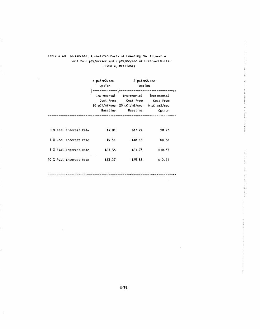
Table 4-40: lncremental Annualized Costs of Louering the Allowable
Limit to 6 pCi/d/sec aml 2 pCi/m2/sec a t Licensed M i l l s .
(19M 5. Mi l l ions)
6 pci/m2/sec 2 pCi/m2/sec Opt ion O p t i m
I E S = = = = ~ ~ E = = E E = I E = = = = = = = = = = = = = = = = = : = = = = = = = = = = = = = lncremental lncremental Incremental
Cost Frm Cost From Cast Frm
20 pCi/m2/sec 20 pCi/m2/sec 6 pCi/wZ/sec
Baseline Baseline Option -~~-------~-----------~...--------...~~~------~---------~~~~~~~~.~...~~~ -------------~~~-~----~-----~-----------~--------~~-------~....~~------~
0 X Real lnterest Rate $9.01 $17.24 $8.23
1 X Real Interest Rate $9.51 $18.18 $8.67
5 % Real Interest Rate 811.36 521.73 $10.37
10 X Real interest Rate $13.27 125.38 612.11
In this analysis, no emissions are assumed for the ponded and wet areas of the piles, while the dry
areas are assumed emit radon-222 at the rate of 1 pci/m2/sec for a concentration of 1 pCi/g of Ra-
226 found in the tailings. All covered areas are assumed to emit radon at the rate of 20 pci/m2/sec.
Table 4-42.4, on page 4-78, reproduces the summary of operable tailings impoundment areas
presented in Table 4-25, along with the average flux rates of the piles, and the areas of the piles that
must be covered and/or saturated in order to reduce average emissions to the 20 pci/m2/sec limit.
4.4.2.2 Benefits of Reducine Allowable Flux Limit to 20 oci/m2/sec
The benefits of reducing allowable emissions during operations to 20 pci/m2/sec are presented, both
in terms of reductions in maximum individual risk and in cancer deaths per year, for each site in
Table 4-41. The risks for the 20 pCi/m2/sec are the risks presented for the post-closure option
adjusted to represent the fifteen year operating or standby phase. The largest reduction in cancer
deaths was for the White Mesa plant in Utah at 1.IE-02 and 1.6E-1 cancer deaths per year and for
the 15 year operating period, respectively. Because design factors at the Panna Maria, Canon City,
and La Sal mills allow the tailing to be kept totally wet, risks remain negligible for the entire
operating and standby phase.
4.4.2.3 Costs of Reducing Allowable Flux Limit to 20 ~ C i / m 2 / s e q
Costs resulting from the reduction of allowable emissions to meet the UMTRCA standard are of two
basic types. First, where the dry areas of the pile are unlined, an earth cover must be applied before
the area can be saturated. This is primarily to prevent contamination of underground water resulting
from absorption into the earth beneath the tailings, and is incurred only in the first year of the
operation. The second cost, the cost of the water used in the saturation process, is incurred annually
over the active life of the mill site. These costs are discussed in detail below.
Water Cost
In order to effectively attenuate the release of radon from the saturated areas, a constant moisture
level must be maintained on the tailings surfaces. Thus, water must be added to the piles to
compensate for evaporation, with the amount required dependent upon the area to be kept moist and
regional evaporation rates. An estimate of the amount of water needed has been calculated for each
site and is presented in Appendix A to this chapter.

Table 4-41. Risks and Reduction o f Risks f o r Continued Operations a t 20 pCilm2lsec ( a )
S t a t e / M i l l L i f e t i m e L i f e t i m e Fa ta l Cancers Fa ta l Cancers Reductions in Reductions i n ReducPians in
Fa ta l Cancer Fata l Cancer Per Year Per Year Fata l Cancer Fata l Cancers Fata l Cancers
Risk t o R isk t o Risk t o Per Year Over 15 Years
I n d i v i d u a l s i n d i v i d u a l s I nd i v i dua l s
(Current) (20 pCilrn2lsec) (Current) (20 pCilm21sec)
Colorado Canon C i t y * O.OE+OO O.OE+OO O.OE+OO O.OE+OO O.OE+OO O.OE+OO O.OE+OO
New Mexico Ambrosia Lake 9.OE-06 4.3E-06 1.5E-03 1.5E-03 4.7E-06 O.OE+OO O.OE+OO
Homestake 3.OE-05 2.1E-05 8.3E-04 8.3E-04 8.6E-06 O.OE+OO O.OE+OO
Texas Panna Maria* O.OE+OO O.OE+OO O.OE+OO O.OE+OO O.OE+OO O.OE+OO O.OE*OO
Utah
White Mesa 2.OE-06 4.3E-07 1.1E-02 9.1E-05 1.6E-06 l.lE-02 1.6E-01
Rio Algom* O.OE+OO O.OE+OO O.OE+OO O.OE+OO C.OE+OO O.OE+OO O.OE+OO
Shootar ing 3.OE-06 4.3E-07 'l.1E-05 6.5E-06 2.6E-06 4.5E-06 6.8E.05
Washington
Sheruood 1.OE-05 2.1E-06 1.2E-03 1.1E-03 7.9E-06 1.OE-04 1.5E-03 Wyoming
Luck Mc 3.OE-06 1.3E-06 1.6E-04 1.6E-04 1.7E-06 O.OE+OO O.OE+OO S h i r l e y Basin 5.OE-G6 2.1E-06 4.5E-04 4.5E-04 2.9E-06 O.OE+OO O.OE+OO Sveetuater 1.OE-06 4.3E-07 3.OE-05 3.OE-05 5.7E-07 O.OE+OO O.OE+OO
Tota l 6.3E-05 3.3E-05 1.5E-02 4.2E-03 3.OE-05 1.1E-02 1.7E-01
(a ) R isks and reduc t i on of r i s k s are ca l cu la ted f o r 15 year opera t ion and standby phase only. * Design of m i l l a l lows f o r t a i l i n g s t o be kept t o t a i l y wet d u r i n g operat ions.
Generally, water can be pumped by the mill companies from underwater sources or from nearby
rivers to which the mills have access and water rights. Hence, the cost of the water to the mills is
the cost of the energy needed to operate the pumping facility. These costs are based on the area to
be saturated, evaporation rates, the vertical distance water must be lifted. and local industrial rates
for electric power. These data and the calculations of the costs are also presented in Appendix A to
this chapter. The annual cost of water is presented for each plant in Table 42B.
Earth Cost
In cases where the dry areas of the piles are unlined, an earth cover must be applied prior to
saturation to prevent ground water contamination. The amount of earth cover required depends
upon the size of the area to be saturated and whether the area to be saturated is protected by a liner.
The cost of earth cover is estimated in the same manner as in the section dealing with the cost of
achieving the post-closure 20 pCi/m2/sec option (Table 4-36), with the exception that only the cost
of regrading slopes, applying dirt cover, and reclaiming borrow pits are considered. The cost of
earth cover is presented for each plant in Table 42B. In addition, Table 42B contains the present
value total cost (earth and water), and annualized present value total cost for each mill and for all
mills combined.
4.4.3 Analvsis of Benefits and Costs of Promuleatine Future Work Practice Standards
This section presents the benefits and costs of using alternative control technologies for future
railings piles. The alternative methods of disposal of radioactive tailings are compared to the base
case control technology of the single cell design. Benefits are measured in terms of the incremental
change in committed fatal cancers, presented in terms of both total and annual averages. A 100 year
time frame is used to calculate total benefits.
Costs are measured in nominal 1988 dollars, and represent the incremental change in costs associated
with the disposal and stabilization of mill tailings. Results are given using net present values, and
are also annualized using real rates of interest of 0, 1, 5 and 10 percent. A 100-year time period is
also used in generating these estimates.
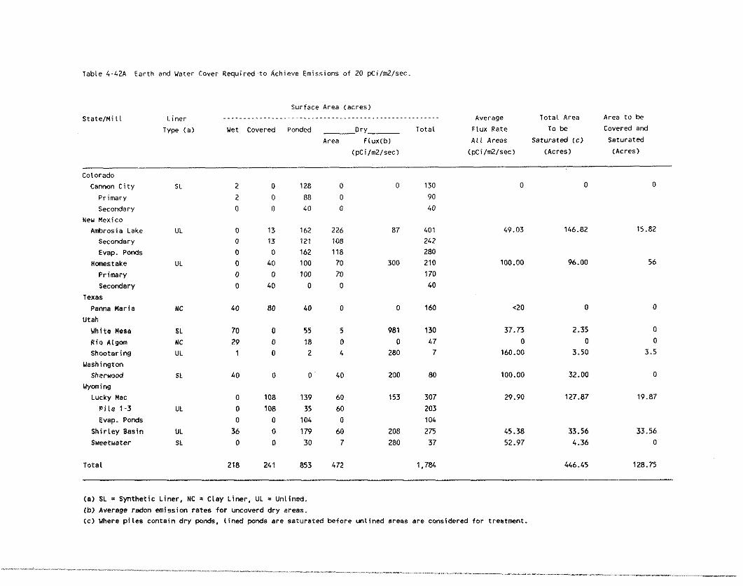
Table 4-42A Earth and Water Cover Required t o Achieve Emissions of 20 pCi/mZ/sec
Surface Area (acres)
S t a t e l M i l l Liner Average Total Area Area t o be ......................................................
~ y p e (a) Uet Covered Ponded Dry Total Flux Rate To be Covered and
Area FLux(b1 A L L Areas Saturated (c) Saturated
(pCiImZlsec) (pCi/m2/sec) (Acres) (Acres)
-
Colorado
Cannon C l t y
Primary
Secondary New Mexico
Ambrosia Lake
Secondary
Evap. Ponds
Homestake
Primary
Secondary
Texas
Psnna Ueria
Utah
UhitO Plena Rio ~ l g m Shootarlng
Washington
S h e r ~ o d
Vymlns Lucky Mac
P i l e 1-3 Evap. Ponds
Sh i r ley Basin
Sueetuater
Total
(a) SL = Synthet ic Liner, NC = Clay l i n e r , UL = Unlined.
(b) Average redon emission rates f o r uncaverd d r y areas. (c) Where p l l e s contain dry ponds, Lined ponds ere saturated before unlined areas are considered for treatment.
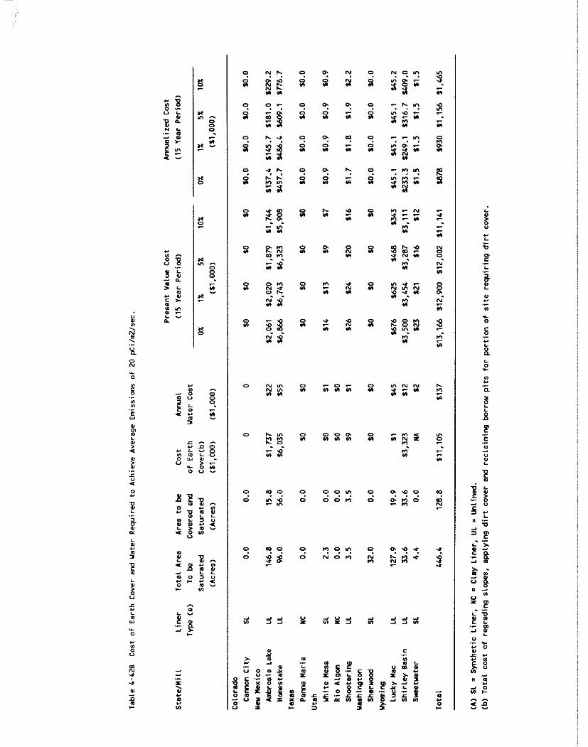
? 9: ? 9 9 3 ' " 4 4 a 5 % a a ; 8 L O * ' - ; 4 s z * .-- *
r - - 5 8 m u 9 Z k -
4 u E
0 N L O 0 - 0 - O L O N N C N L O m * m m .. m m J m * '2
H
- - .- = . c r a r M
U 1 C .- C 2 m 111 .- z S 2' m L
U 0 , ? 2 2 c 5.- u r n - O n , $ E ~ E - e l e l z ; : :
= 2 k q 2 s S - 4 -
2 ~ o z ; z . - r . ; g - a 2 E . S l l b f f i W I * I d * * U z C 3 = f ,- b 0 U
4.4.3.1 \\'orli Practices for New Tallinns l m ~ o u n d m e n t ~
Tailings impoundments constructed in the future must, at minimum, meet current Federal standards
for prevention of groundwater contamination and airborne particulate emissions (20 p ~ i / m ~ / s e c ) .
The baseline tailings impoundment will have synthetic liners, be built partially below grade and have
earthen dams or embankments to facilitate decommissioning. A means for dewatering the tailings
after the area is filled should also be incorporated. This conventional design allows the maintenance
of a water cover during the milling and standby periods thus maintaining a very low level of
radon-222 emissions. Dewatering of the tailings can be accelerated using wells and/or built-ins.
A synthetic liner is placed along the sides and bottom. Cover material may be added after the
impoundment has reached capacity or is not going to be used further and the tailings have dried.
Two alternatives to the work practices assumed in this baseline model of new tailings impoundments
are evaluated in this analysis. These alternatives are discussed in the following sections.
Phased Disposal
The first alternative work practice which is evaluated for model new tailings impoundments is
phased disposal. In phased or multiple cell disposal, the tailings impoundment area is partitioned
into cells which are used independently of other cells. After a cell has been filled, it can be
dewatered and covered, and another cell used. Tailings are pumped to one initial cell until it is full.
Tailings are then pumped to a newly constructed second cell and the former cell is dewatered and
then left to dry. After the first cell drys, it is covered with earth obtained from the construction of
a third cell. This process is continued sequentially. This system minimizes emissions a t any given
time since a cell can be covered after use without interfering with operations as opposed to the case
of a single cell.
Phased disposal is effective in reducing radon-222 emissions since tailings are initially covered with
water and finally with earth. Only during a drying-out period of about 5 years for each cell are
there any radon-222 emissions from a relatively small area. During mill standby periods, a water
cover could be maintained on the operational cell. For extended standby periods, the cell could be
dewatered and a dirt cover applied.
Continuous Disposal
The second alternative work practice, continuous disposal, is based on the fact that water can be
4-80

removed from the tailings slurry prior to disposal. The relatively dry dewatered (25 to 30% moisture)
tailings can then be dumped and covered with soil almost immediately. No extended drying phase
is required, and therefore very little additional work would be required during final closure.
Additionally, ground water problems are minimized.
To implement a dewatering system would introduce complications in terms of planning, design, and
modification of current designs. Acid-based leaching processes do not generally recycle water, and
additional holding ponds with ancillary piping and pumping systems would be required to handle the
liquid removed from the tailings. Using trucks or conveyor systems to transport the tailings to
disposal areas might also be more costly than slurry pumping. Thus, although tailings are more easily
managed after dewatering, this practice would have to be carefully considered on a site-specific
basis.
Various filtering systems such as rotary vacuum and belt filters are available and could be adapted
to a tailings dewatering system. Experimental studies would probably be required for a specific ore
to determine the filter media and dewatering properties of the sand and slime fractions.
Modifications to the typical mill ore grinding circuit may be required to allow efficient dewatering
and to prevent filter plugging or blinding. Corrosion-resistant materials would be required in any
tailings dewatering system due to the highly corrosive solutions which must be handled. Continuous
covering of dewatered tailings is not practiced at any uranium mills in the United States, but it has
been proposed at several sites in the Southwestern and Eastern United States [MA 831. Tailings
dewatering systems have been used successfully at nonferrous ore beneficiation mills in the United
States and Canada [RO 781.
4.4.3.2 Cornoarison of Control Technoloeies for New Tailings Imooundments
To meet current Federal radon-222 emission standards, new tailings areas will have synthetic liners
with either earthen dams or embankments, and also incorporate a means of dewatering the tailings
at final closure. These new tailings can either be stored below or partially above grade. Although,
below grade storage provides the maximum protection from windblown emissions, water erosion, and
eliminates the potential for dam failure, it nevertheless is not cost effective in comparison to partially
above grade disposal technology.
Previous analysis of work practices for new model tailings have estimated costs for a range of
alternative control technologies [EPA 861. These estimated costs,in millions of 1985 dollars, are listed
in Table 4-43. These cost estimates suggest that storage of tailings partially above grade is cost
effective in comparison to fully below grade designs. Completely below grade designs are estimated,
on average, to increase costs by twenty percent.
Partially below grade piles have been shown to be cost effective compared to above grade
impoundments. Excavation costs for the final dirt cover are incurred in both cases. Using the
excavated pit, from which the earth cover is taken, to store tailings provides benefits in terms of
windblown emissions, water erosion, and dam failure a t no cost. In addition, dam construction cost
is minimized because the sides of the excavation pit replace part of the dam.
The twenty percent increase in costs over partially above grade disposal are not justified by the
benefits gained from completely below grade disposal. As prior excavation has provided all the dirt
required for cover, the increase in costs associated with further excavation to fully below grade are
not believed to justify the associated benefits. The cost of additional excavation is greater than the
benefit as the bulk of the benefits to be derived from reducing windblown emissions, water erosion,
and dam failure have already been captured. For our purposes, therefore, only designs that are
partially above grade are considered.
Also dropped from consideration is the continuous trench pile design. This technology has little
operational advantage over the continuous single cell design, and is more costly.
A number of alternative control technologies are available to reduce radon-222 emissions and
subsequent risks from tailings disposal. Both timing and disposal method affect the rate of emissions
from tailings piles. The control alternatives, their emissions, and their potential benefits are
reviewed here.
Emissions From New Model Impoundments
The single cell impoundment is the most prominent control technology used to dispose of radioactive
tailings, and as such is used as a yardstick with which to compare the performance of the alternative
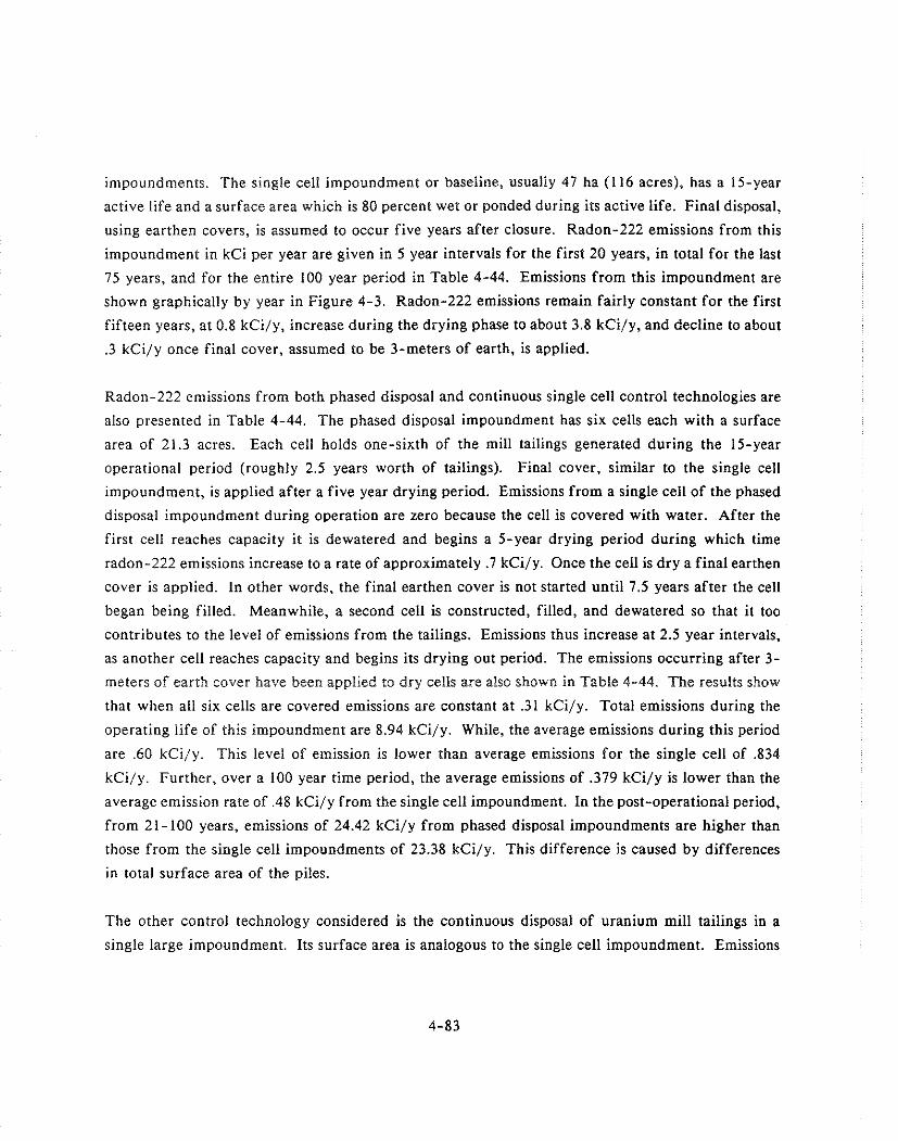
impoundments. The single cell impoundment or baseline, usually 47 ha (1 16 acres), has a 15-year
active life and a surface area which is 80 percent wet or ponded during its active life. Final disposal,
using earthen covers, is assumed to occur five years after closure. Radon-222 emissions from this
impoundment in kCi per year are given in 5 year intervals for the first 20 years, in total for the last
75 years, and for the entire 100 year period in Table 4-44. Emissions from this impoundment are
shown graphically by year in Figure 4-3. Radon-222 emissions remain fairly constant for the first
fifteen years, at 0.8 kCi/y, increase during the drying phase to about 3.8 kCi/y, and decline to about
.3 kCi/y once final cover, assumed to be 3-meters of earth, is applied.
Radon-222 emissions from both phased disposal and continuous single cell control technologies are
also presented in Table 4-44. The phased disposal impoundment has six cells each with a surface
area of 21.3 acres. Each cell holds one-sixth of the mill tailings generated during the 15-year
operational period (roughly 2.5 years worth of tailings). Final cover, similar to the single cell
impoundment, is applied after a five year drying period. Emissions from a single cell of the phased
disposal impoundment during operation are zero because the cell is covered with water. After the
first cell reaches capacity it is dewatered and begins a 5-year drying period during which time
radon-222 emissions increase to a rate of approximately .7 kCi/y. Once the cell is dry a final earthen
cover is applied. In other words, the final earthen cover is not started until 7.5 years after the cell
began being filled. Meanwhile. a second cell is constructed, filled, and dewatered so that it too
contributes to the level of emissions from the tailings. Emissions thus increase at 2.5 year intervals,
as another cell reaches capacity and begins its drying out period. The emissions occurring after 3-
meters of earth cover have been applied to dry cells are also shown in Table 4-44. The results show
that when all six cells are covered emissions are constant at .31 kCi/y. Total emissions during the
operating life of this impoundment are 8.94 kCi/y. While, the average emissions during this period
are .60 kCi/y. This level of emission is lower than average emissions for the single cell of ,834
kCi/y. Further, over a 100 year time period, the average emissions of ,379 kCi/y is lower than the
average emission rate of .48 kCi/y from the single cell impoundment. In the post-operational period,
from 21-100 years, emissions of 24.42 kCi/y from phased disposal impoundments are higher than
those from the single cell impoundments of 23.38 kCi/y. This difference is caused by differences
in total surface area of the piles.
The other control technology considered is the continuous disposal of uranium mill tailings in a
single large impoundment. Its surface area is analogous to the single cell impoundment. Emissions
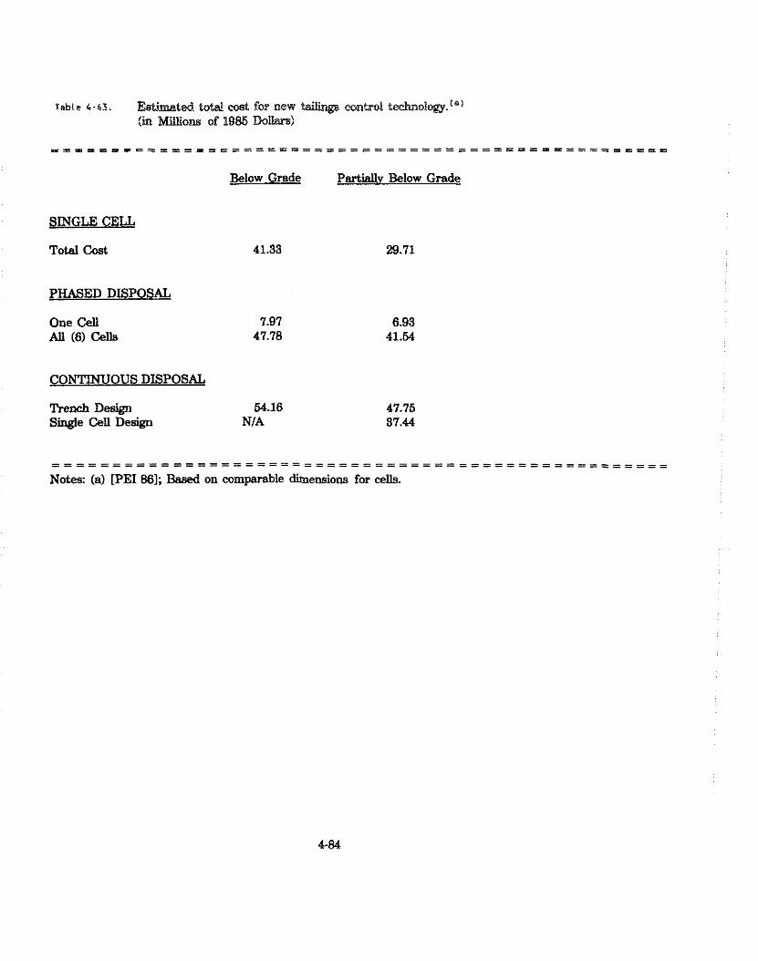
Tab(@ 6 - 4 3 . E s ~ t d total cost for new conLrol LecAnology.(') (in W o n s of 1986 Dollere)
_ = E - _ m = = _ = = = = = = = = = = = = = P = = = = = = = = = = = = = = = = = = = = = = = = = = = = = = =
Below Grade PartiaUv Below Grade
SINGLE CELL
Total Cost
PHASED DISPOSAL
One Cell All (6) Ceb
CONTINUOUS DISPOSAL
Trench Design 54.16 47.76 S i e Cell D e w N/A 37.44
. . . . . . . . . . . . . . . . . . . . . . . . . . . . . . . . . . . . . . . . . . . . . . . . . . . .
Notes: (a) [PEI 861; Based on comparable dimensions for cells.

labie 4 - 4 4 . Redm-222 Emissions srul Emissions Reducrim Resuiting frm Aiternerive Work Practices (kCi).
Single Contirws Cell Phased Sinple Baseline Disposal Cet 1 ,=.iiiE.i.E,I.lilS=III=EIEI=E~.====~=~===~=~==(.=..=l=~~~===~iii=l~===z=~~===-=~
Emissions Emissions Emissions Emissions Reduction Reduction Reductim Reductico
Time frun fran f ran frun Period Emissions Emissions Easeline Continuaa Emissions Baseline Phased ___________________---zss===~==~==z========~~===========~=====~==zs=====x=====~=========~ -------------.--------
Operational Phase
0-5 4.16 0.48 3.68 1.11 1.58 2.57 -1.11
16-20 12.47 4.57 7.91 -3.09 1.48 10.59 3.09
Total 24.95 13.51 11.45 -5.79 7.71 17.23 5.m
Post Operational Phase
All Phsses
0-100 48.33 37.93 10.41 -8.31 29.61 18.71 8.31
===iS=====Sr===i=il=============s=======z===========================~====================
Annual Average 0.483 0.379 0.104 -0.083 0.296 0.187 0.083
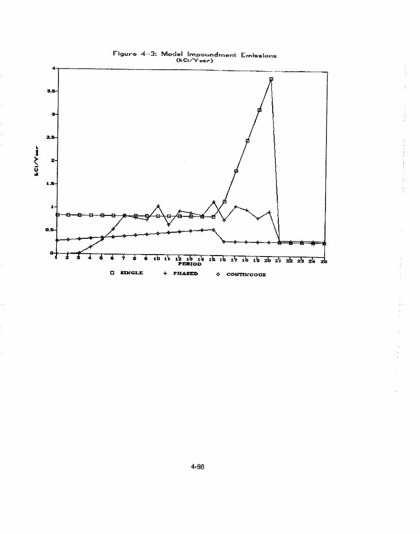

froin this impoundment are estimated assuming that 1/15 of the surface area consists of dewatered
tailings that are uncovered at any time over the 15-year operational life. The final 1/15 surface area
is assumed to be covered at the end of the operational period. Emissions from this impoundment
during operation are low, since the tailings which are dried by a vacuum filter prior to disposal can
be covered immediately. Elimination of the drying period substantially reduces radon-222 emissions.
The emissions from this impoundment are given in Table 4-44, and suggest that during the
operational phase of the impoundment, on average, approximately .416 kCi/y of radon-222
contaminates the biosphere. These emissions are lower than either the baseline or the phased
disposal technologies. Over the entire 100 year period, in comparison to the other control
technologies, this impoundment on average discharges ,296 kCi/y, the lowest level of radon-222.
Committed Fatal Cancers From New Model Impoundments
The risks associated with each type of impoundment are measured in terms of committed fatal
cancers. Benefits of the phased and continuous impoundments are measured as the incremental
reduction in committed fatal cancers. The risks are estimated from the following equation assuming
that the model impoundment has an impact in proportion to that of the current licensed mills:
X = iulz)(w) 11)
where:
x - - committed fatal cancers from model impoundments
P - - total committed fatal cancers attributed to existing impoundments
7. -. - emissions from existing impoundments
W - - emission from model impoundment
Risks for a 100-year period, shown in Table 4-45, are estimated from equation (1) based on the rate
of .0113 fatal cancers per kCi/y, and the emission rate from each impoundment. The continuous
single cell approach always produces the lowest risk level. The phased disposal approach produces
slightly higher risks than the single cell baseline during the post-operational phase, although i t
produces lower risks during the operational phase and over all phases.
The summary details of risk reductions that demonstrate this pattern are as follows: During the
operational period the risk of cancer is reduced, relative to the single cell baseline, by 0.129 if
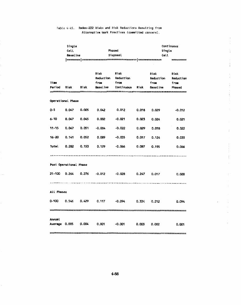
Single Continms
Celt Phased Single geneline Disposal c e l l
1 1 ----- cil- I--- - Risk Risk Risk Risk Reduction Reduction Reduction Reduction
T i m f m fm f roa f m Period Risk Risk geseline Continuws Risk BBseline Phased
Operationel Phase
Total 0.2U 0.153 0.129 -0.066 0.057 0.195 0.066
Post Operationel Phase
ALL Phases
O-IW 0.546 0.425' 0.117 -0.094 0.m 0.2l2 0.094
AMual
Average 0.m 0.004 0.m -0.m 0 .03 0.m 0.m
phased disposal is adopted and by 0.195 if the continuous single cell method is used. The risk
reduction associated with using the continuous single cell relative to the phased approach is 0.066.
In the post-operational phase, phased disposal raises the risk by 0.012 while the continuous single cell
approach lowers it by 0.017 relative to the baseline and by 0.028 relative to phased disposal.
4.4.3.4 Costs of Promuleatine Future Work Practice Standardg
Estimated Cost of New Model Tailings Impoundments
Costs for partially above-grade single cell, phased disposal, and continuous single cell disposal
tailings impoundments are developed in Volume 2 of this Et~virottnlenlal Impacl Statement.
Total costs for each design are shown in Tables 4-46 through 4-48, which indicate that the phased
partially above grade disposal impoundment is the most expensive design (% 54.02 million), while the
single cell partially above grade impoundment ($36.55 million) is the least expensive. Costs for the
continuous single cell design ($ 40.82 million) are only slightly more than those of the single cell
impoundment, although the uncertainties surrounding the technology used in this design are the
largest. The volumes or surface areas and the unit costs that were used in calculating the cost figures
are also provided in Tables 4-46 through 4-48. The equations used to calculate volumes and surface
areas are discussed in detail in the Volume 2 of this Environmental Impact Statement as are the
sources and methods used to calculate unit costs.
This section reviews the costs associated with each of the control technologies discussed above.
Present values of the costs for each impoundment are shown in Table 4-49. These costs are
discounted over a 100-year period at the real rate of interest of 0, 1, 5, and 10 percent. The
annualized costs discounted using the same real rates of interest are given in Table 4-50. The results
suggest that the most costly technology is the phased disposal impoundment and the least costly is the
single cell.
When these costs are annualized using the same real rate of interest, phased disposal technology is
again found to be the most costly in comparison to not only the baseline but also to the continuous
single cell impoundment when the real rate of interest is below 10 percent. When the real rate of
interest is 10 percent, the continuous single cell approach becomes most expensive.

Tsble 4-&6. h t r for a Single Cell Part ial ly beta,
Grde nw W e 1 Tsilin(ls I--t ( 8 , 1988).
vo1ua or Arm Unit Unit (cU. e t . Cort coat cost
I t n or sq. at.) (S1C.Y.) (S1C.R.) ($,mil.>
Exutvat ion
Grading
Cover Grade
Cqpact Tota 1
Gravel Cap
Dsl l tonst. Grade
ecpact Total
Synthetic Liner
Urbtotal: Direct Cost
Indirect Cost a 7 Percent
Total Cost
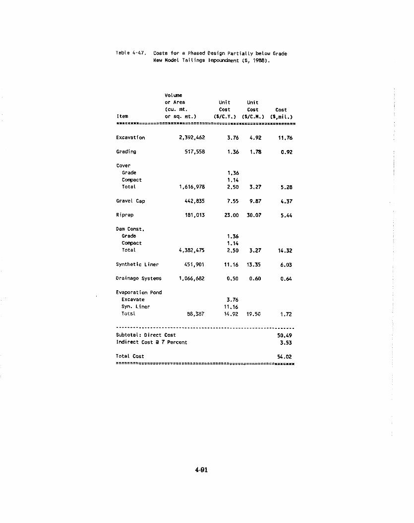
Table 4-47. Costs f o r a Phased Besign Pe r t i a l l y telou Grade Ueu Madel Tai l ings Inpoundment (S, 1988).
V0lune or Area Uni t Unit (CU. mt. cost cost cost
1 tern o r sq. mt.) 0 I C . Y . ) (S/C.M.) ($,mi[.) =iii==lllili=l=E==E=============zs=====a================~======
Excavation 2,392,462 3.76 4.92 11.76
Grading 517,558 1.36 1.78 0.92
Cover trade 1.36 Carpact 1.14 Total 1,616,978 2.50 3 .27 5.28
Gravel Cap 442,835 7.55 9 .87 4.37
Dam Const. Grade 1.36 Compact 1.14 Totat 4,382,475 2.50 3.27 14.32
Synthetic Liner 451,901 11.16 13.35 6.03
Drainage Systems 1,066,682 0.50 0.60 0.64
Evaporation Pond Excavate 3.76 Syn. Liner 11.16 Total 88,387 14.92 19.50 1.72
---------..------------.----------*-*-.-.----.-----.--.-------- Subtotal: Di rect Cost 50.49 Indi rect Cost a 7 Percent 3.53
Total Cost 54.02 ..............................................................
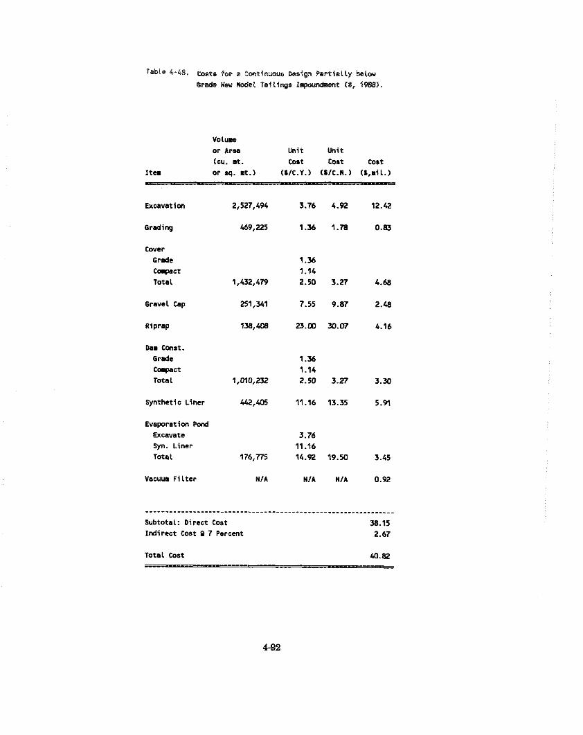
Volume or Area Unit Unit (CU, a. cost cost cost
It= or sq. m t . ) (S1C.Y.) (S1C.R.) ($,mil.)
Excavation 2,527,494 3.76 4.92 12.42
cover Grade 1.36 Coqsct 1.14 Total 1,432,479 2 . 9 3.27 4.68
Gravel Cap 251,341 7.55 9.87 2.48
Dam const. Grade 1.36 Coqact 1.14 Total 1,010,232 2.50 3.27 3.30
synthatic Liner wra 11.16 13.35 5.91
Evaporation Pond Excavate 3.76 Syn. Liner 11.16 Total 176,775 14.92 19.50 3.45
Vacuue F i Lter NIA NIA M I A 0.92
............................................................... Subtotal: Direct Cost 38.15 Indirect Cost a 7 Percent 2.67
Total Cost 40.82
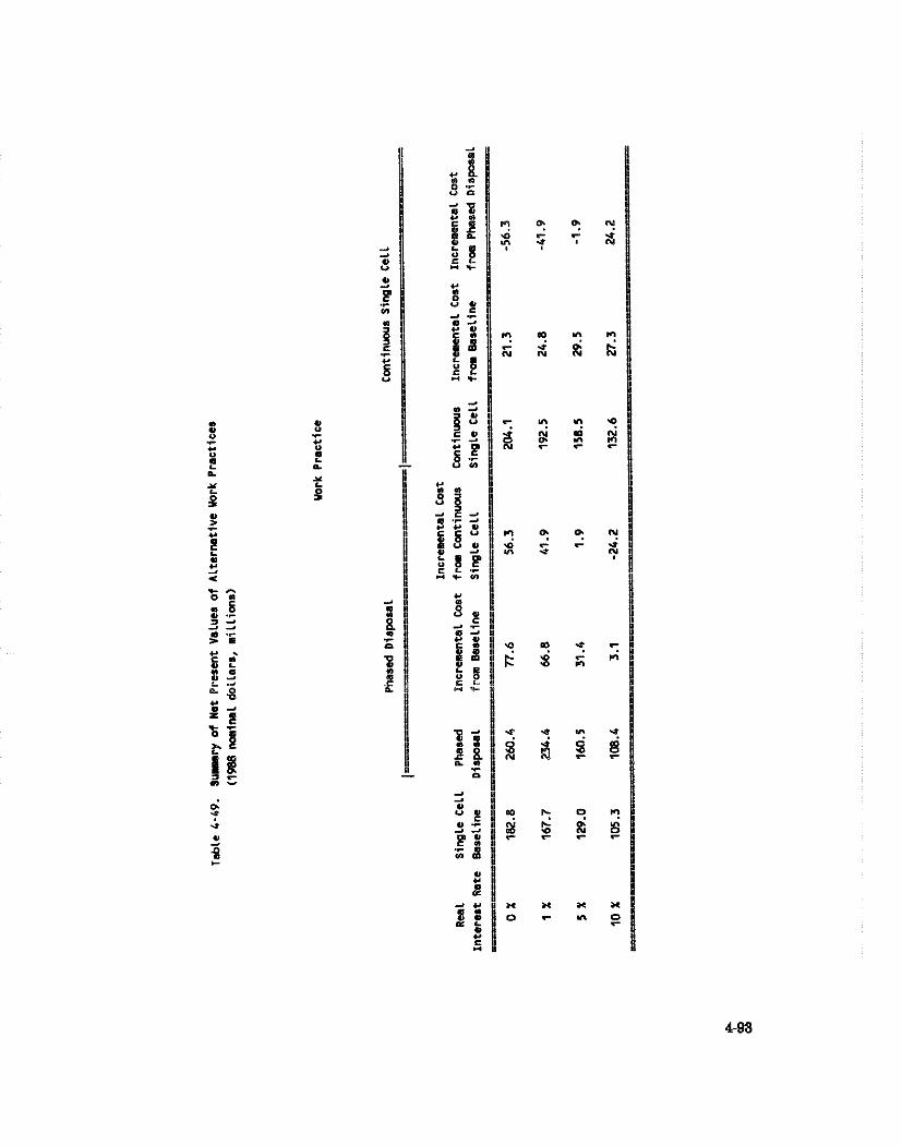
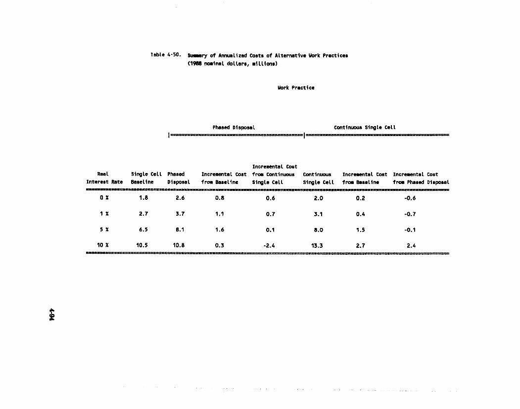
Table 4-50. m r y of h n w l i z e d Costs of Alternative Wrk Practices (1980 nminal d0llar8, 11lLions)
uork Practice
Phased Dirrponl Continuous Single Cel l
Ir I P - Incremental Cost
Rea 1 Single Cell Phased Incremental Coat from Eontinuous Continuous I n c r m n t a l Coat I n c r m n t a l Cost Intereat Rate Baseline Dispolal frw Baseline Single Cell SiwLe Cell frm Baseline trm Phased Disponl
4.5 Economic Imnacts
Any regulatory alternative will increase the cost of domestically produced U30B. The amount of this
impact will depend on the regulation selected. The impact of consumers and investors is evaluated
assuming that the present value of the additional cost for future and existing piles was $250 million
at a 10 percent real rate of interest. This figure is roughly equal to the incremental costs associated
with a work practice for active plants that limits allowable emissions to an average of 20 pCi/m2/sec 2 while in operation, a post-closure flux rate of no more than 2 pCi/m /sec, and assuming new
impoundments utilize the phased disposal control presented in sections 4.4. In this section, the
effects of such regulatory costs are evaluated. The impact of any of the alternative regulations from
section 4.4 will be smaller and can be scaled from the impacts calculated here. If the U.S. uranium
industry created an annuity payment to cover the added cost of this regulation, the payments
required per year would be $66 million in each year for 5 years, or $41 million for each year For
10 years. The impact of these cost increases on investors in this industry or purchasers of electricity
is also analyzed
4.5.1 Increased Production Cost
The added production cost resulting from the regulation may, or may not, be passed on to the
consumers of U308 (electric utilities). If the added cost is translated into higher prices for U30,
ceteris paribus, then the consumers of electric power will ultimately be charged higher rates,
depending on the rulings of state and IocaE public utility commissions. Customers of utilities with
a high reliance on nuclear generating capacity would face the highest increases. If the U.S. uranium
milling industry is unable to pass on the disposal costs internalized by this regulation as a result of
market competition from foreign producers or other Factors, then the added cost will be ultimately
paid by investors in the industry
No attempt is made to quantify these impacts, instead a qualitative evaluation based on two extreme
situations is made. The first case is based on the assumption that the uranium mills are unable to
pass on the costs of regulation in the form of higher U30s prices. The second case assumes that the
producers are able to recover all the costs associated with the disposal of tailings through increased
U308 prices. The results generated under these assumptions then will provide the Iower and upper
bound, respectively, of the likely impacts. In fact, some of these costs will surely find their way into
the rate base of utilities with nuclear generating capacity. In addition, since some owners of these
existing impoundments are no longer operating nor do they have any intention of ever operating in
this industry in the future, their cost of disposal must be borne by the investors in these firms.
It is assumed in the first case that no portion of the cost of the regulation can be passed on to the
purchaser of U30,. Selected average financial statistics for 1982- 1986 from the domestic uranium
industry (presented in Section 4.4) are given in Table 4-51. These data are compared to the present
value cost impacts of the regulation and to the required annuity payment to amortize these costs over
five or ten years. The 1982-1986 period is one in which the industry had been contracting and
experiencing substantial losses due to excess capacity in production. The present value cost of the
regulation would be about five times the industry losses over this period. It is equal to about 10
percent of the book value of industry assets and about 15 percent of industry liabilities.
In the second case it is assumed that the uranium industry is able to recover the entire increase in the
tailings disposal cost be charging higher U308 prices. This increased input cost to electric utilities
will ultimately be added to the rates paid by electric power consumers.
The revenue earned by the industry for generating 2.4 trillion kilowatt hours of electricity in 1986
was 121.40 billion dollars. The 1987 present value of the regulation (estimated to be $250 million)
is less than I percent (.06%) of the U.S. total electric power revenue for the same year. Table 4-52
presents the relationship of the regulatory cost to power generation.
The increased cost of total generation reflects a change in ehe average cost per unit for the nation.
The regional impacts will vary from this mean, based in part, on the dependence on nuclear power
by region as shown in Table 4-53. The ERCOT region, for example, with no nuclear generating
capacity would probably feel no effect from the cost of the regulation in higher electricity prices,
and other regions, like MAIN and SERC would suffer the greatest effects. As for a specific
customer or community, the level of impact is dependent upon the percent of generation from
nuclear power that their particular electrical utility utilizes. For example, Commonwealth Edison of
Illinois and Duke Power of North Carolina have two of the highest percentage of power from nuclear
sources, so their customers would be more severely impacted than customers in other utilities.
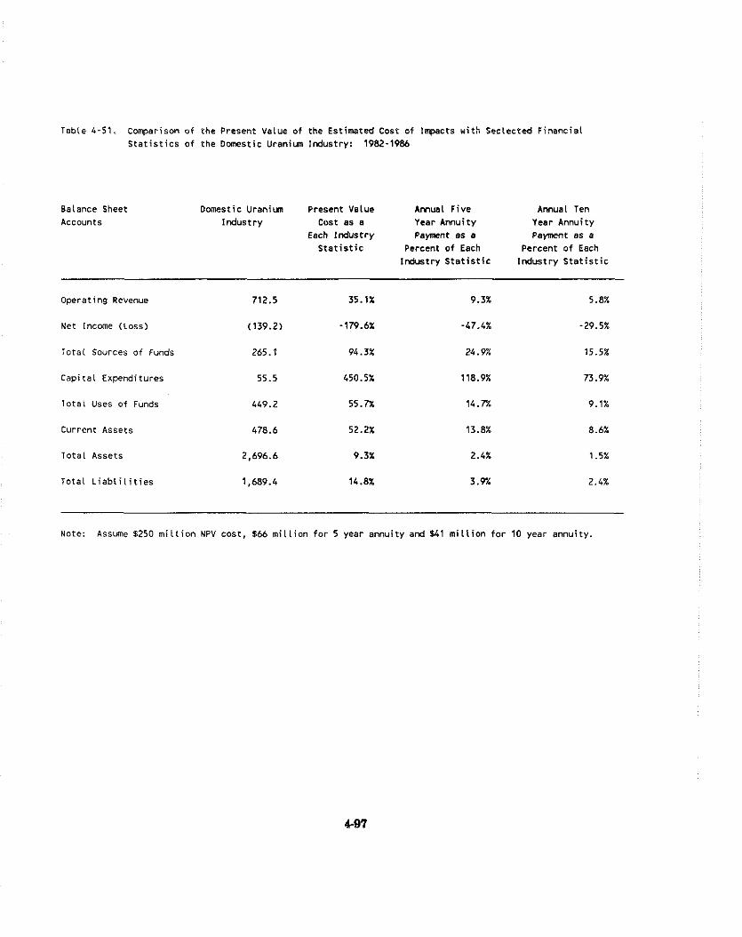
Toble 6-51. Comparison o+ the Present Velue of the Estimated Cost of lnpects wi th Seclected Financial S t a t i s t i c s o f the D m s t i c U r a n i m Industry: 1982-1986
Balance Sheet Domestic U r a n i m Present Value Arnual Five Annual Ten Accounts Indust ry Cost as a Year Annuity Year Annuity
Each Indust ry Payment as a Payment as a S t a t i s t i c Percent o f Each Percent o f Each
Industry S t a t i s t i c lndus t ry S t a t i s t i c
Operating Revenue
Net Income (Loss)
Total Sources of Funds
Capital Expenditures
T o t a l Uses of Funds
Current Assets
Total Assets
Total L i a b l i l i t i e s
Note: Assume $250 m i l l i o n NPV cost, $66 m i l l i o n f o r 5 year annuity and 141 m i l l i o n f o r 10 year annuity.
4.5.2 Reeulatorv Fleribilitv Analvsis
The Regulatory Flexibility Act (RFA) requires regulators to determine whether proposed regulations
would have significant economic impact on a substantial number of small businesses or other small
entities. If such an impact exits, they are required to consider specific alternative regulatory
structures to minimize the small entity impacts without compromising the objective of the statute
under which the rule is enacted. Alternatives specified for consideration by the RFA are tiering
regulations, performance rather than design standards, and small firms exemptions. Most firms that
own uranium mills are divisions or subsidiaries of major U.S. and international corporations. Many
of these uranium milling operations are parts of larger diversified mining firms which are engaged
in many raw materials industries and uranium represents only a small portion of their operations.
Others are owned by major oil companies or by electric utilities who were engaged in horizontal and
vertical integration, respectively, during the 1960s and 70s. In 1977, there were 26 companies
operating uranium mills and at the start of 1986 only two were operating. The future of this
industry suggests that only a limited number of these existing facilities will ever operate again. It
is also expected that the high level of financial risk and capital requirements will continue to attract
only large diversified firms and electric utilities to this industry. Thus, no significant impact on
small businesses is expected.

l ab i e 4 - 5 2 . Impacts of Regulation on Elec t r i ca l Pouer Industry.
Total E lec t r i c Nuclear E lec t r i c Power Industry Pouer Industry
GnlV
1987 M i l l i o n K i l l oua t t .
Hours Generation
Present Value of Added
Costs for Disposal per M i l l i o n Ki louatt-Hours
Annual Cost of 5 Year Annuity per M i l l i o n
Ki i louat-HOUTS
Annual Cost of 10 Year Annuity per M i l l i o n
Ki l louat-Hours
Note: Assune $250 NPV cost, $173 per Year f a r 5 Year Annuity, S97 for 10 Year Annuity.
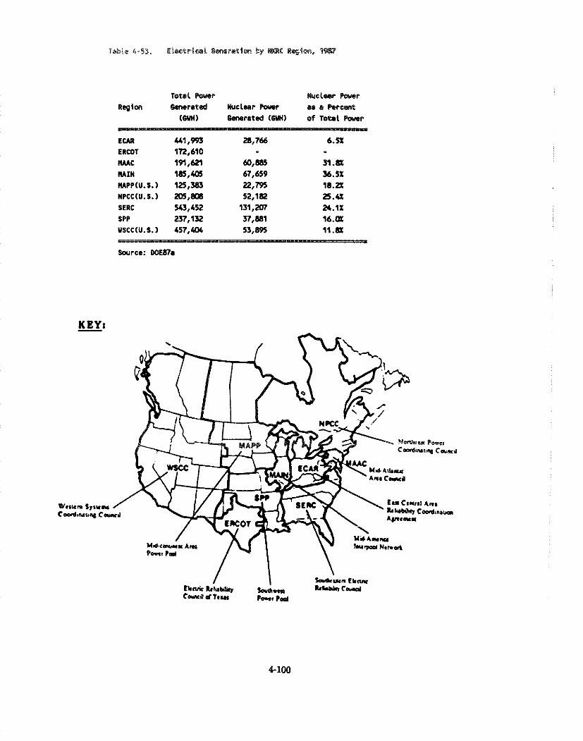
E U R ERCOT M A C M X N MPP(U.S.) NPCC(U.S.> SERC
SPP YSCC(U.S.)
Source: DC€.97a
KEY: -
V.sun Ips cdlrullq
~brUicIrlubl*). m- C-s .r Tern Pa*, P P I
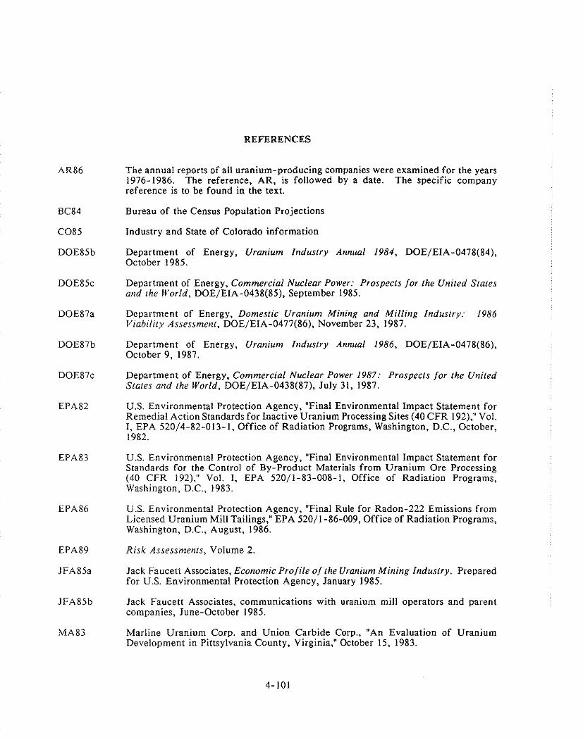
REFERENCES
The annual reports of all uranium-producing companies were examined for the years 1976-1986. The reference, AR, is followed by a date. The specific company reference is to be found in the text.
Bureau of the Census Population Projections
Industry and State of Colorado information
Department of Energy, Uranium Industry Annual 1984, DOE/EIA-0478(84), October 1985.
Department of Energy, Commercial Nuclear Power: Prospects for the United States and the World, DOE/EIA-0438(85), September 1985.
Department of Energy, Domestic Uranium Mining and Milling Industry: 1986 Viability Assessme~rt, DOE/EIA-0477(86), November 23, 1987.
Department of Energy, Uranium Industry Annual 1986, DOEIEIA-0478(86), October 9, 1987.
Department of Energy, Commercial Nuclear Power 1987: Prospects for the United States and the World, DOEIEIA-0438(87), July 31, 1987.
U.S. Environmental Protection Agency, "Final Environmental Impact Statement for Remedial Action Standards for Inactive Uranium Processing Sites (40 CFR 192)," Vol. I, EPA 520/4-82-013-1, Office of Radiation Programs, Washington, D.C., October, 1982.
U.S. Environmental Protection Agency, "Final Environmental Impact Statement for Standards for the Control of By-Product Materials from Uranium Ore Processing (40 CFR 1921," Vol. I, EPA 520/1-83-008-1, Office of Radiation Programs, Washington, D.C., 1983.
U.S. Environmental Protection Agency, "Final Rule for Radon-222 Emissions from Licensed Uranium Mill Tailings," EPA 520/1-86-009, Office of Radiation Programs, Washington, D.C., August, 1986.
Risk Assessments, Volume 2.
Jack Faucett Associates, Eco~lomic Profile o f the Uranlun? .Mining i~rdustry. Prepared for U S . Environniental Protection Agency, January 1985.
Jack Faucett Associates, communications with uranium mill operators and parent companies, June-October 1985.
Marline Uranium Corp. and Union Carbide Corp., "An Evaluation of Uranium Development in Pittsylvania County, Virginia," October 15, 1983.

Health and Safety Analysis Center, Mine Safety and Health Administration (MSHA), Department of Labor, "1987 Uranium Mines Address Listing with Workers and Employee Hours," Fourth Quarter, 9 February 1988.
Personal communication, Energy and Minerals Department, Mine Inspection Bureau, State of New Mexico, December 1985.
U.S. Nuclear Regulatory Commission, "Final Generic Environmental Impact Statement on Uranium Milling," NUREG-0706, Washington, D.C., September, 1980.
Nugent, J.W., A Summary of Mineral Industry Activities in Colorado, 1980: Part 11, Metal-Nonmetal," Colorado Department of Natural Resources, Division of Mines.
NUEXCO, NUEXCO Monthly Report, #233, February, 1988.
NUEXCO, NUEXCO Monthly Report, January, 1988.
Organization for Economic Cooperation and Development, Uranium: Resources. Production, and Demand, Paris, December 1983.
PEI Associates, oral communication, August-October 1985.
Battelle Pacific Northwest Laboratories, U.S. Uranium Mining Industry: Background Information on Economics and Emissio~~s, PNL-5035, March 1984.
Robinsky, E.I., "Tailing Disposal by the Thickened Discharge Method for Improved Economy and Environmental Control," in Volume 2, Proceedings of the Second International Tailings Symposium, Denver, CO, May 1978.
Rogers, V.C., K. K. Neilson and D. R. Kalkwarf, Radon Attenuation Handbook for Uranium Mill Tailings Cover Design, NUREG/CR-3533, prepared for the U. S. Nuclear Reguiatory Commission, Washington, D.C., April, 1984.
Personal communication, Texas Railroad Commission, State of Texas, December 1985.
Wyoming State Inspector of Mines, 1980, 1981, and 1984 annual reports
Personal communication, Department of Natural Resources, Division of Geology and Earth Resources, State of Washington, December 1985.
Zimmerman, Charles F., Uranium Resources on Federal Lands, Lexington, MA: Lexington Books, 1979.
APPENDIX A
CALCULATION OF WATER COSTS

To maintain a constant moisture level on the tailing surfaces, sufficient water must be added to the
piles to compensate for evaporation. This water can be pumped by the mill companies from
groundwater sources or from rivers to which the mills have access and water rights. Hence, the cost
of the water to the mills is the cost of the energy needed to pump it. These costs are based on the
area to be saturated, evaporation rates. the vertical distance water must be lifted, and industrial
electric rates. These data and the calculations of the costs are presented in tables 4A- 1.
The amount of water required to compensate for evaporation depends on the area to be kept moist
and on evaporation rates. Areas to be kept saturated range from 2.4 acres at White Mesa Mill to
146.8 acres at Ambrosia Lake Mill. Evaporation rates were obtained from the NOAA Evaporation
Atlas for the Cotrtiguous 48 United ~tates. ' The free water surface evaporation (FWS) map was used.
According to the atlas, FWS "...closely represents the potential evaporation from adequately watered
natural surfaces such as vegetation and soil."' Evaporation rates ranged from 33 inches per year at
the Sherwood Mill in the State of Washington to 50 inches per year at the Ambrosia Lake Mill in
New Mexico. Converting inches per year to feet per year and multiplying by the acreage to be kept
saturated yields the number of acre-feet of water that must be replaced each year.
Since the mines and mills own rights to groundwater or river water, the cost of water is the cost of
pumping it. Table 4A- I converts the volume of annual water loss to evaporation measured in acre-
feet per year to the weight of water pumped in pounds per year. The weight of water to be lifted
ranges from 24 million pounds per year at White Mesa Mill to 1.6 billion pounds per year at
Ambrosia Lake Mill. Table 4A-1 also shows the estimated vertical lift at each mil:. Sherwood Mil:
has no need to pump water for the purpose of saturating tailings because it has surplus water from
other operations. Homestake Mill must lift water 800 feet.
The work done pumping the water equals the product of the weight of water in pounds pumped
times the vertical distance it is lifted. These computations are also performed in Table 4A-I. This
product times two is the foot-pounds of work done in a normal year, assuming that the pumps used
have 50 percent efficiency. This value is converted into kilowatt hours which is then multiplied by
' U.S. Department of Commerce, National Oceanic and Atmospheric Administration, National Weather Service, NOAA Technical Report NWS 33, "Map 3 of 4: Annual FWS Evaporation", Evaporation Atlas of the Contiguous 48 United States, Washington D.C., June 1982.
Atlas, p. 4 .
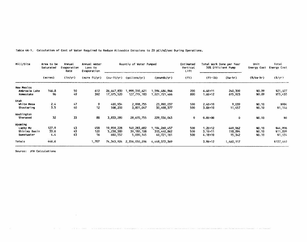
Table 4A-1. Calculat ion of Cost of Water Required t o Reduce Al lauable Emissions t o 20 pCiln2lsec During Operations.
H i I l l S i t e Area t o be Annual Annual Water Quant iy of Water Punped Estimated Total Work Done per Year Unit Tota t Saturated Evaporation Loss t o Ver t ica l 50% Ef f i c ien t P v r p Energy Cost Energy Cost
Rate Evaporation L i f t
(acres) ( i n l y r ) (acre f t l y r ) ( c u - f t l y r ) (ga l lons lyr ) (poundslyr) ( f t ) (Slku-hr9 <S/yr) ( f t - l b ) (ku-hr)
Neu Mexico Anixosis Lske 146.8 50 612 26,647,830 1,999,310,621 1,594,484,966 200 6.4E+ll 240,300 H m s t a k e 96 49 392 17,075,520 127,715.183 1,021,721,466 800 1.6E+12 615,923
Utah White Mesa 2.4 47 9 400,934 2,998,755 23,990,037 500 2.4E+10 9,039 Shootaring 3.5 40 12 508.200 3,801,047 30,408,377 500 3.0E+10 11,457
Washington sherwwd 32 33 88 3,833,280 28,670,755 229,336,043 0 O.OE+OO 0
Waning ~ u c k y MC 127.9 43 458 19,959,228 149,283,682 1,194,269,457 500 1.2E+12 449,962 Sh i r l ey Basin 33.6 43 120 5,238,380 39,180,108 313,440,862 500 3.1E+ll 118,094 Sweetwater 4.4 43 16 680,552 5,090,145 40,721,161 500 4.1E+10 15,342
Source: JFA Celculst ions
the cost of electricity per kilowatt hour to give the annual cost of water. Because Sherwood Mill
does not have to pump water, its cost is zero. The highest pumping cost is for Homestake Mill in
New Mexico. The annual cost of pumping one billion gaflons of water per year 800 vertical feet is
$55,000. The total cost for all mills is $137,000.
If the mills had to buy surface water rights the cost would be higher. For example, in New Mexico,
surface water rights sold for $750 to $3000 per acre foot in 1988-89. At the lower price Ambrosia
Lake Mill would have to pay $459,000 annually for water to compensate for evaporation. At the
higher price, the cost would be $1.8 million annually. Water right prices do not account for the cost
of transporting the water.
CHAPTER 5
HIGH-LEVEL WASTE DISPOSAL FACILITIES


5. NLGN-LEVEL WASTE DISPOSAL
5.1 Introduction and Summary
The facilities planned for the ultimate disposal of high-level nuclear waste have been designed to
result in negligible releases of radionuclides to the environment. The benefits of further reductions
of emissions are expected to be low and the costs per unit of benefit are expected to be high. No cost
study has been conducted and no economic impact analysis can be performed.
5.2 Industrv Profile
5.2.1 Introduction
This chapter addresses the ultimate disposal of high-level nuclear waste generated by the commercial
nuclear power industry and by the Department of Defense. .Although no facilities for this purpose
currently exist, the federal government has taken responsibility for finding suitable permanent
storage facilities. These facilities will be operated by the Department of Energy. The facility for
the disposal of high-level waste from the nuclear power industry will be licensed by the Nuclear
Regulatory Commission. Although the facilities will not be privately owned, it is expected that
private contractors will be selected to operate them.
Two facilities devoted to the ultimate disposition of high-level nuclear waste are currently being
planned. A third facility, a monitored retrievable storage facility (MRS) is also being planned.
However, since the MRS facility is not to be used as a final disposal site, it is not considered in this
report. The facilities under consideration are [EPA89]:
I ) The Waste Isolation Pilot Plant (WIPP) -- under construction in Carlsbad, New Mexico.
2) The Yucca Mountain Geologic Repository -- not yet under construction, but to be located in Yucca Mountain, Nevada.
These facilities will be devoted to three types of waste [EPA89].
1) Spent nuclear fuel where there is no intent to reprocess;
2) High-level waste from the reprocessing of spent nuclear fuel; and
3) Transuranic wastes

The role played by each facility is discussed below
5.2.2 Facilities for the Ultimate Disoosal of Hieh-Level Waste
The design features and operations of the two facilities under consideration are discussed below:
5.2.2.1 The Waste Isolation Pilot Plant (WIPP1
The WIPP is for the disposal of defense radioactive wastes, primarily transuranic wastes. The facility,
currently being constructed in Carlsbad, New Mexico, performs the two main phases of waste
disposal--first, the receipt and final packaging of the waste and, second, its permanent underground
storage--at a single location. The packages it receives are of two types, contact-handled and remote-
handled waste. Damaged casks are decontaminated, overpacked or repaired. They are then
transported underground into a mined repository in a salt formation.
5.2.2.2 Yucca hlountain Geoloeic Re~osi lory
This facility, planned for construction in Yucca Mountain, Nevada, will first receive and package
and then permanently store high-level wastes produced by commercial activities.
5.2.3 Demand for Hieh-Level Waste Manaeement
One of the major issues of the nuclear age is what to do with the high-level waste generated by
nuclear power reactors and weapons production facilities. Spent fuel and other high-level wastes
have accumulated on-site at nuclear power plants and weapons plants, and at interim storage sites.
The projected generation of spent fuel by the year 2000 [EPA89] will be 95,000 metric tons of heavy
metal. The absence of a permanent storage site to handle spent fuel complicates the planning process
for power companies and involves an interim storage cost for companies that operate reactors. High
level waste management costs include both the cost of disposal and the cost of potential liability in
the event of an accident. Thus, there is a very real demand for the services of high-level waste
d i s ~ o s a l facilities.
5.2.4 Sunply of tiieh-Level Waste hlanaeement
No facility for the management of high-level waste currently exists. However, two facilities are
envisioned, one is in the planning stages, and one is under construction. The projected quantity of
high-level and transuranic waste to be disposed of by the turn of the century is about 70,000 metric
tons of uranium (MTU) or equivalent. Sixty-two thousand MTU of this will be spent fuel from
civilian reactors and 8,000 MTU will be defense waste. The projected supply of high-level waste
disposal falls short of the 95,000 MTU required to meet the needs of firms and agencies operating
nuclear reactors [EPA89]. The difference will be made up by at-reactor storage and interim off-
site storage. Thus, the projected services of the high-level waste facilities fall slightly short of the
projected demand.
5.3 Current Emissions. Risk Levels, and Feasible Control hlethods
5.3.1 Introduction
Since all facilities for high-level waste disposal are still in the planning or construction stages, there
are no current emissions of radionuclides from the sites. However, estimates of the emissions have
been made as part of the planning process. Most of the atmospheric emissions are expected to come
from routine receiving, unpacking and decontamination of shipping casks, or from accidental
droppage of casks during handling. All handling of the materials is to be done in "hot cells" which
are equipped with multiple stage high-efficiency particulate air (HEPA) filters to remove most of
the airborne contaminates before air from the hot cells is released to the atmosphere.
For most of the wastes, the casks in which they are shipped or stored are the major emission control
devices. The HEPA filters are considered to be backup protection.
5.3.2 Current Emissions and Estimated Risk
Table 5-1 gives the total estimated quantities of radioactive emissions and the estimated risk for each
facility under normal operation [EPA89].
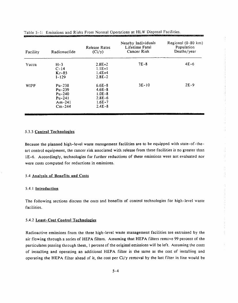
Table 5-1: Emissions and Risks From Normal Operations at HLW Disposal Facilities.
Nearby Individuals Regional (0-80 km) Release Rates Lifetime Fatal Population
Facility Radionuclide ( C ~ / Y ) Cancer Risk Deaths/year
Yucca H-3 2.8E+2 C-14 l.lE+I Kr-85 1.4E+4 1- 129 2.8E-2
5.3.3 Control Technoloeies
Because the planned high-level waste management facilities are to be equipped with state-of-the-
art control equipment, the cancer risk associated with release from these facilities is no greater than
IE-6. Accordingly, technologies for further reductions of these emissions were not evaluated nor
were costs computed for reductions in emissions.
5.4 Analvsis of Benefits and Costs
5.4.1 Introduction
The following sections discuss the costs and benefits of control technologies for high-level waste
facilities.
5.4.2 Least-Cost Control Technoloeies
Radioactive emissions from the three high-level waste management facilities are entrained by the
air flowing through a series of HEPA filters. Assuming that HEPA filters remove 99 percent of the
particulates passing through them, I percent of the original emissions will be left. Assuming the costs
of installing and operating an additional HEPA filter is the same as the cost of installing and
operating the HEPA filter ahead of it, the cost per Ci/y removal by the last filter in line would be
one hundred times as niuch, because the previous filter has removed 99 percent of the particulates
entering i t and leaves the next filter with just one percent as much input to filter
5.4.3 Health and Other Benefits
The health benefits of adding another HEPA filter would be to reduce the incidence of cancer
attributable to a facility to one percent of the original amount. Nationwide, the number of cancers
attributable to these facilities would drop from 1E-6 per year to 1E-8 per year, a reduction of 9E-
5.5 Industrv Cost and Economic Impact Analysis
Since this rulemaking does not involve a proposal for emission control for high-level waste
management facilities beyond the levels in the proposed designs, it will have no economic impact.
If there were proposals for further emission controls, they would affect an industry that has yet to
be born and which would be in a position to pass on the associated costs to the federal government.
The government could pass on some of the costs to the commercial nuclear power industry in fees
collected in exchange for storage. The nuclear power industry is likely to benefit from the overall
project, since one of the industry's major operational, planning and political problems is the handling
and interim storage of high-level waste.
REFERENCES
EPA89 Risk Assessntnrl, Vol. 2.

6. DEPARTklENT OF ENERGY FAClLITlES
6.1 introduction and Summarv
The Department of Energy (DOE) owns or directs the activities of numerous facilities across the
country that emit radionuclides into the air. Twenty-seven facilities are mentioned in this chapter.
The Feed Materials Production Center (FMPC) at Fernald, Ohio is discussed in chapter seven.' The
primary task of many of these facilities is the support of nuclear weapons production and research
for the Department of Defense. Many of the facilities also support research of biomedical studies,
environmental and safety aspects of nuclear energy, nuclear waste processing, advanced nuclear
energy production, fusion research, non-nuclear energy studies, basic research in high energy
physics, and training. The names and locations of these facilities are listed in Table 6-1.
Because each facility is unique, risk assessments were conducted on a facility by facility basis. The
overall risk for all of these DOE facilities is estimated at 3E-I fatal cancers per year.
6.2 Industrv Profile
A wide variety of facilities and of functions that they fulfill are covered in this chapter. Broadly
speaking the functions can be classified into nuclear weapons research and production, basic physics
or energy research, nuclear waste disposal and management, reactor testing and training, medical
applications or health effects of radionuclides, and environmental studies. Over a dozen facilities are
involved partially or solely in nuclear weapons design, testing, and production. Over half a dozen
are involved in the nuclear power production or research fields while at least four laboratories are
conducting basic research in physics. Several facilities are involved in waste disposal and
management activities and over half a dozen in health, biomedical, or environmental research.
The level of activities at these facilities is dependent upon a host of factors including past nuclear
activities and their waste products; current and future military requirements, priorities, and funding
levels; research for advanced nuclear power processes; waste disposal requirements and regulations;
further research into health effects; and biomedical applications of radionuclides. Some of the
facilities or their components are on stand-by status while others are closed down and
decommissioned at this time.
' DOE recently arrived at an agreement with the State of Ohio to clean up this site.
6- 1.

Table 6-1: Department of Energy Facilities
Facility Location
Los Alamos National Laboratory Oak Ridge Reservation Savannah River Plant R M I Company Feed Materials Production Center Hanford Reservation Brookhaven National Laboratory Mound Facility Idaho National Engineering Laboratory Lawrence-Berkeley Laboratory Paducah Gaseous Diffusion Plant Lawrence Livermore/Sandia Laboratory Portsmouth Gaseous Diffusion Plant Argonne National Laboratory Pinellas Plant Nevada Test Site Knolls Atomic Power Laboratory Battelle Memorial Institute Fermi National Accelerator Laboratory Sandia National Laboratories/Lovelace Bettis Atomic Power Laboratory Knolls Atomic Power Laboratory Rocky Flats Plant Pantex Plant Knolls Atomic Power Laboratory Ames Laboratory Rockwell International
Los Alamos, New Mexico Oak Ridge, Tennessee Aiken, South Carolina Ashtabula, Ohio Fernald, Ohio Richland, Washington Long Island, New York Miamisburg, Ohio Upper Snake River, Idaho Berkeley, California Paducah, Kentucky Livermore, California Piketon, Ohio Argonne, Illinois Pinellas County, Florida Nye County, Nevada Kesselring, New York Columbus, Ohio Batavia, Illinois Albuquerque, New Mexico West Miflin, Pennsylvania Windsor, Connecticut Jefferson Co., Colorado Amarillo, Texas Schenectady, New York Ames, Iowa Santa Susana, California

6.3 Current Risk Levels and Feasible Control Methods
6.3.1 lnlroduction
The summary findings reported in this section are based upon an assessment of each facility which
determined the emissions, source release point(s), demographic data. meteorological information, etc.
The risk assessment utilizes the AIRDOS-EPA/DARTAB/RADRlSK computer codes [EPA89].
Radionuclides that contributed at least 90 percent of the collective contribution are identified i n the
supporting documentation cited above. The specific processes and emission controls for some of the
facilities such as the Oak Ridge Y-12 plant are classified.
Table 6-2 presents the risks to the populations living within 80 km of DOE facilities and the
maximum estimated risk to nearby individuals for each facility.
6.3.2 Facilitv Descriotions
Emission characteristics by facility and radionuclide type and resultant risks are presented in the
supporting documentation for each of the facilities [EPA89]. Discussion of the four facilities that
result in effective dose equivalents of over 1 mrem/y follows. Although previously listed, R M I
Company is no longer included in thls discussion due to their installation of additional controls in
1988 which has reduced their EDE to below I mrem/y.
The Los Alamos Nat~onal Laboratory has major sources emitting over a dozen radionuclides with no
source contributing more than a small fraction of the emissions. Each of the facilities has its own
control mechantsms which vary in removal or containment efficiency and effectiveness. Not all
radionuclide emissions from Los Alamos National Laboratory are controlled

Table 6-2 Su1111iiary of Estimated Risks Around DOE Facilities
0-80 K m Population
Estimated Deaths
Maximurn Estimated Risk to
Nearby individuals (Lifetime)
Site per Year (0-80 K m )
Los AIamos Laboratory, NM Oak Ridge National Lab. TN savannah River Plant, GA RMI Co., OH Feed Materials Production Ctr, G A Hanford Reservation. WA Brookhaven ~ a t i o n a l ' ~ a b . , NY Mound Facility, OH Idaho National Eng. Lab, ID Lawrence Berkeley Lab., CA Paducah Gaseous Diff. Plant, K Y Lawrence Livermore Lab./Sandia
Livermore Lab., CA Portsmouth Gaseous Diff. Plant, OH Areonne National Lab.. IL ~inlellas Plant, F L Nevada Test Site, NV Knolls Lab-Kesslring, NY Battelle Memorial Inst., OH Fermi National Lab, 1L Sandia National Lab./Lovelace, NM Bettis Atomic Power Lab, PA Knolls Lab-Windsor, C T Rocky Flats Plant, CO Pantex Plant, TX Knolls Lab-Knolls, CT Ames Laboratory, IA Rocketdyne Rockwell, CA
Source: [EPA89]

Emissions from Oak Ridge Reservation are composed primarily of Xe-133, H - 3 and Kr-85. The
major release point is the central disposal facility source stack composed of three internal sources of
radioactive exhaust, each with its own emission control technology. Practical control technologies
require that the effluents be removed from low flow rate air streams which will require installation
prior to the centralized stack.
The Savannah River Plant is used primarily to produce plutonium and tritium for use in the
production of nuclear weapons. The largest sources of emissions are the fuel reprocessing areas, the
three production reactors, and the heavy water rework plant. Tritium is released from six of
Savannah's facilities while Argon-41 is released exclusively from the operating reactors in roughly
equal proportions. Carbon- 14 is released from the three operating reactors and the separation plalrts
in roughly equal proportions. Tritium is the principal source of radiation dose to the off-site
population.
Current controls at the Savannah River Plant utilize a continuous monitoring system to detect le\els
exceeding a specified limit. When emissions exceed the threshold limit the air flow is diverted to a
Hopcalite stripper and zeolite beds for tritium removal. The efficiency level of the controls varies
with operating conditions which cannot be reported for security reasons. Emission from the
production reactors consists of a system of prefilters to remove particulates from the incoming air,
moisture separators, HEPA filters, and charcoal filters for iodine removal.
Feed Materials Production Center produces uranium metal and other materials for DOE facilities.
Raw materials are dissolved in nitric acid and separated by liquid organic extraction. The recovered
uranium is reconverted to uranyl nitrate and processed further to become uranium tetraflouride.
Purified metal is made by reacting the uranium tetraflouride with metallic magnesium in a
refractory-lined vessel. These processes result in estimated lifetime fatal cancer risks to nearby
individuals of 3E-5. Risks of fatal cancers to the population residing within 80 km is 3 E - 3 deaths
per year. The number of persons living within 80 km of Feed Materials Production Center is 3.3
million.
The estimated risk levels for regional populations are shown in Table 6-2 for the baseline conditions.
Only the Savannah River Plant and the Oak Ridge Reservation cause more than 1E-2 fatal cancer
deaths per year. The maximum individual risk of 2E-4 was due to emission released from Los
Alamos Laboratory in New Mexico. The risks for the other facilities are progressively less,
Individual facility dosage levels are estimated and may be found in the supporting documentation
[EPA89].

6.3.3 Control Technoloeies
The Los Alamos National Laboratory has a multiplicity of sources and emissions which are subject
to further controls. The Meson Physics Facility which utilizes a linear proton accelerator could
reduce its emissions by about 95 percent by using a holding tank approach at a cost of about $1.6
million in capital and $90,000 per year for operations.
The Oak Ridge Reservation has several components which are technically subject to supplementary
controls including the Central Radioactive Gas Disposal Facility (CRGDF), various processes of the
Y-12 plant, and the diffusion plant's purge cascade. Controls for tritium emitted in water vapors
from C R G D F are feasible and can achieve 90 percent efficiency, at a capital cost of $1.66 million.
Uranium-234 and -238 emissions can be further controlled by a second stage of HEPA filters which
retain a 99 percent efficiency rate in series mode or can achieve a 99.95 percent efficiency in a
primary control mode. The capital cost of adding HEPA filters to the fabrication facility is estimated
to be $2.65 million. The increased power requirements and the cost of HEPA filter replacement will
increase operating costs by about $92,000 per year. Significant additional costs may be incurred if
there are additional structural requirements.
The Savannah River Plant could improve the collection efficiency of a number of elements of its
operations. The 200-H area tritium facilities could reduce their normal emissions by 25 percent
through the use of a palladium catalyst and the recycling of effluent gases through the stripper in
combination with hydrogen swapping. The cost of these enhancements would be about $65 million
with an expected system life of 15 years. A procedure that could reduce tritium emissions from
production reactor area stacks by up to 90 percent after an extended period of steady state operations
(about six years) is the use of vapor phase catalytic exchange with cryogenic distillation. Gross costs
estimates for this process range from $20 to 40 million plus annual operating costs of $1.5 to 2 million
with a 30 year system life. Emissions from the separation plants which are quite small could be
subject to further controls. Carbon-14 can be captured by an absorber system based on flaked
barium hydroxide octahydrate. The noble gases (particularly Kr-85) could be captured by one of
several processes using cryogenic distillation, fluorocarbon absorption, or absorption on mordenite
beds, all of which have a decontamination factors of about 100. Such off-gas treatment systems are
estimated to cost $50 million per plant plus $3 million for operation annually.
The Feed Materials Production Center is discussed in chapter seven. Improvements to the current
controls can be made by using Goretex bags instead of wool bags in its dust collection system coupled

with continuous stack monitoring and administrative controls. HEPA filters could also be used as a
supplrnlentnry control for particulates.
6.4 Analysis of Benefits atid Costs
6.4.1 Introduction
Four alternatives for controlling radionuclide emissions were evaluated. The first two had no effect
on either costs or benefits. The third alternative is to require controls on any facility from which
the emissions exceed 3 mrem/y EDE (effective dose equivalent). Oak Ridge National Laboratory and
Los Alamos National Laboratory would both have to install controls to meet alternative 3. Alternative
4 is to require controls on all facilities from which emissions exceed I mrem/y EDE. Savannah River
and FhlPC would have to install controls to meet alternative 4. So would Oak Ridge and Los
Alamos, since alternative 4 is more stringent than alternative 3. Controls that would reduce emissions
below I mrem/y at all four facilities are considered in the following.
Emissions estimates were made for all the facilities, both with and without the supplementary
controls, where appropriate. Estimated dose equivalents and associated fatal cancer risks were also
estimated. Some of these control technologies are not well demonstrated for these source types and
map require further developmental efforts. Other supplementary controls are well established and
not costly, but may provide only minor additional benefits. Some controls are not strictly speaking
controls, but avoidance or minimization of initial contamination or activation and improved
administrative or engineering procedures. Table 6-3 provides the risks to the 80 km population and
to the most exposed individual both before and after installation of supplementary controls. Table
6-4 shows which controls are included in the analysis, the net present value (NPV) of their cost
stream, and the decrease in risk to both the 80 km population and the most exposed individual.
6.4.2 Cost of Control Technoloeies
The control evaluated at Los Alamos National Laboratory was an atmospheric pressure storage system
that delays the release of emissions until some products can break down. The estimated capital cost
is $1,600,000 and the operating cost is $90,000. The NPV of these costs over a 25 year period, with
a discount rate of 5 percent, is $2,792,000.
At Oak ridge the controls evaluated were combinations of HEPA filters and high-energy venturi
scrubbers at three emission sources with capital costs of $800,000, $400,000 and $1,450,000 and
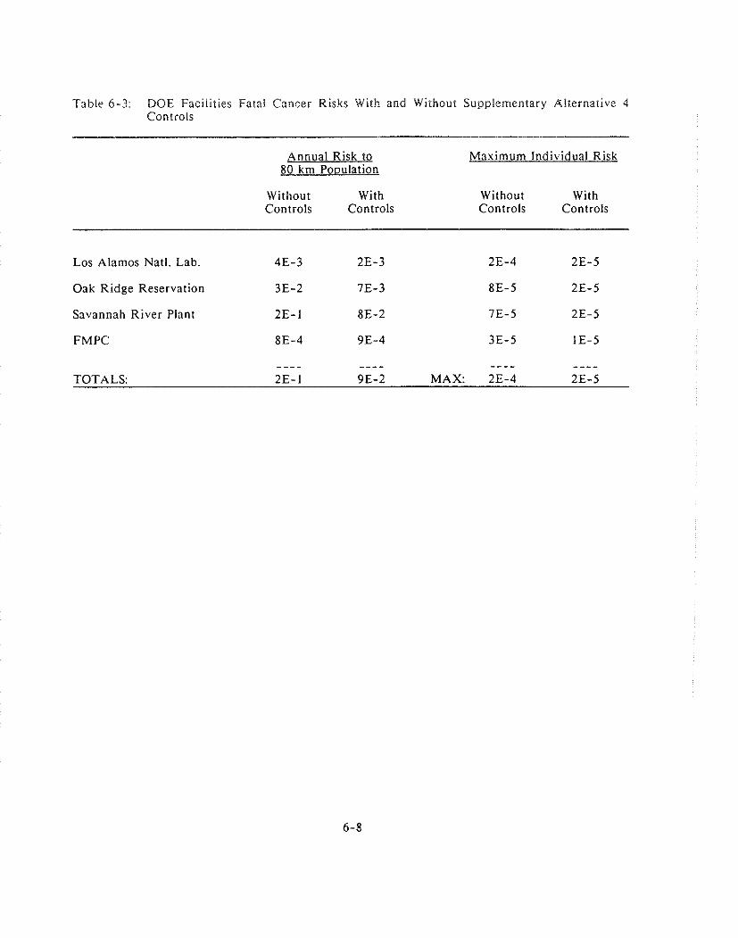
Table 6-3: DOE Facilities Fatai Cancer Risks With and Without Supplementary Alternative 4 Controls
Annual Risk to 80 km Po~ula t ion
Maximum Individual Risk
Without With Without With Controls Controls Controls Controls
Los Alamos Natl. Lab. 4E-3 2E-3 2E-4 2E-5
Oak Ridge Reservation 3E-2 7E-3 8E-5 2E-5
Savannah River Plant 2E-l 8E-2 7E-5 2E-5
FMPC 8E-4 9E-4 3E-5 1E-5
---- ---- ---- ---- TOTALS: 2E-1 9E-2 MAX: 2E-4 2E-5

Tahlc 6-4: Controls, Risk Reduction, and Costs Associated With Meeting Alternative 4, by Facility
Estimated Control Cost in Thousands Decrease in Decrease in
Regional Maximum NPV Population Individual Supplemental Capital Operating Discount Rate = 5%
Facility Risk Risk Control 25 Years
Los Alamos 2E-3 2E-4 Atmospheric $1,600 $90 $2,792 National Pressure Air Laboratory Storage System
Oak Ridge 2E-2 6E-5 HEPA Filter, $4,310 $92 $5,401 Venturi Scrubber, Tritiated Water Sieve Dryer
Savannah I E - l 5E-5 Vapor Phase $1 30.000 $8,000 $236,561 River Catalatic Exchange
with Cryogenic Distillation, Integrated Off-Gas Treatment System
FMPC IE-4 2E-5 HEPA Filter $4,200 $1 11 $5,564
- - -. TOTAL: 9E-2
operating costs of $79,000, $13,000, and $50,000 per year respectively. At a fourth emission source
a tritiated water/ sieve dryer system would be installed with a capital cost of $1,600,000 and no
operating cost. Capital costs for supplementary controls at Oak Ridge total $4,3 10,000 and operating
costs total $92,000 annually. The NPV for supplementary controls at Oak Ridge is $5,401,000.
Supplementary controls evaluated at Savannah River include a vapor phase catalytic exchange with
cryogenic distillation and an integrated off-gas treatment system. The first has an estimated capital
cost of $20 to 40 million, taken here to be $30,000,000, and operating costs of approximately
$2,000,000 per year. The second supplementary control has a capital cost of $50,000,000 per plant
and an operating cost of $3,000,000 per year per plant. Two plants would be fitted with this control
for a total capital cost of $100,000,000 and a total operating cost of $6,000,000 per year. The total
for all supplementary controls required to meet alternative 4 a t the Savannah River Plant is
$130,000,000 for capital cost and $8,000,000 annually for operating costs. The NPV of the
supplementary controls required by Savannah River to meet alternative 4 is $236,561,000.
T o meet the requirements of alternative 4, FMPC will require installation of HEPA filters at a capital
cost of $4,200,000 and an operating cost of $1 11,000 per year. The NPV of these costs is $5,564,000.
These estimates do not consider structural modifications that might be needed in order to install the
filters.
For all four plants the total capital cost of meeting the requirements of alternative 4 is estimated to
be $140,110,000 and the yearly operating cost to be $8,293,000. The aggregated NPV of these costs
evaluated with a five percent discount rate over a twenty-five pear assumed life expectancy is
$250,319,000. The NPV is somewhat insensitive to the choice of discount rates, varying from
$347,435,000 when the rate is zero to $202,649,000 when the rate is ten percent.
6.4.3 Health and Other Benefits
The health benefits of supplementary controls are estimated through the application of computer
models of emission dispersion and the resulting inhalation and ingestion of various radioactive
constituents and their effect on the body. Table 6-3 presents summary information on both the 80
km population and the maximum individual risk of fatal cancer due to the four facilities analyzed
here with and without supplementary controls required to meet alternative 4. In preparing these
estimates, detailed organ exposures are calculated for each facility. The risk to nearby individuals
and to regional populations of fatal cancer is also documented [EPA89]. The level of maximum
individual risk ranges from a high of 2E-4 at Los AIamos to a low of 3E-5 at FMPC. Wit11
supplementary controls, the greatest maximum individual risk drops to 2E-5. The aggregated risk
for 80 km populations drops to from 2E-1 to 9E-Z when alternative 4 is implemented.
6.5 Ilidustry Cost and Economic Imoacts
Since the costs of these control actions will be borne by the Federal government there is no assignable
direct private industry cost. If controls were impleniented at any of these facilities, the major burden
would be in the form of higher taxes, increased government debt, or reduction in other government
services.
REFERENCES
EPA89 Risk Assessnter~l, Vol. 2 .
CHAPTER 7
DEPARTMENT OF ENEROV RADON FAClUTlES

7. DEPARTMENT OF ENERGY RADON SITES
7.1 introducfion and Summarv
Five Federal facility sources of potential radon exposure are reviewed. Four of the five
facilities are no longer active, but are repositories of previously discarded radioactive residues
from uranium mining, mills, uranium metal production, assaying and storage of uranium
materials. The fifth facility, the Feed Materials Production Center near Fernald, Ohio,
continues to produce purified uranium metal and components for DOE facilities.
Estimates of radon emissions and flux rates are indicated as are the associated risks to the
population from these emissions. The costs of further control of these emissions are estimated
and the associated benefits are evaluated.
Seven fatal cancers every century are attributable to the operation of these facilities. Over
half of these cancers can be traced to the Middlesex Sampling Plant.
7.2 Industrv Profile
The Department of Energy (DOE) Radon source category consists of five sites owned or
controlled by the Federal government and operated or maintained under the authorit! of
DOE. These five sites are described in IEPA84j. They contain significant quantities of
radium-bearing wastes and are:
o Feed Materials Production Center (FMPC),
o Niagara Falls Storage Site (NFSS),
o Weldon Spring Site (WSS),
o Middlesex Sampling Plant (MSP), and
o Monticello Uranium Mill Tailings Pile (MUMT).
7.2.1 Feed Materials P roduc t io~~ Center (FMPC1
The. FMPC is located near Fernald, Ohio, and is currently operated under contract by
Westinghouse Materials Company of Ohio for the DOE. The facility produces purified
uranium metal and components for use at other DOE facilities. The feed materials include
ore concentrates, recycled uranium from spent reactor fuel, and various uranium compounds.
Thorium can also be processed at the site. The primary source of radon emissions a t the
FMPC is pitchblende residues stored in two concrete storage tanks referred to as silos. The
residues resulted from the recovery of uranium from pitchblende ores during World War 11.
7.2.2 Niaeara Falls Storaee Site (NFSS]
The NFSS, located in Lewiston, New York, is a DOE surplus facility operated by Bechtel
National, Inc. The 77 ha site is part of the former Lake Ontario Ordnance Works and is
used solely for storage of uranium and pitchblende residues. The residues were formerly
stored in six buildings that were originally part of the facility's water treatment plant and in
a pile nearby. Subsequently, by the end of 1986, the residues were consolidated in the Interim
1Vaste Containment Facility (IWCF).
Descriptions of the consolidation process can be found in the annual environmental reports
[BEC87]. The IWCF structure comprises the short-term closure system for the wastes until
the long-term management plan is completed. The selected long-term plan calls for in-place
management as described in the final environmental impact statement [DOE86]. The IWCF
occupies 4 ha of the site and measures 274 m by 137 m. The structure's outer perimeter is
composed of a dike and cutoff wall, both of which are constructed of compacted clay which
forms a finished structure with an engineered compacted clay cover that sits directly over the
wastes and extends beyond the perimeter dike. This cover is the principal barrier against
moisture intrusion and radon emanation. The 0.9 m of clay is covered with 0.3 m of general
soil and 0.15 m of top soil.
7.2.3 Weldon Spring Site (WSS)
The WSS, located near Weldon Spring, Missouri, is a surplus DOE facility that also stores
uranium and thorium wastes. The site was operated by Bechtel National, Inc. in a caretaker
status until 1986 when M-K Ferguson Company assumed control as Project Management
Contractor Tor the WSS Remedial Action Project. The site consists of two separate properties:
the 89 ha \\'eldon Spring Chemical Plant together with the Weldon Spring Raffinate Pits
form one (WSCP), and the other is the 3.6 ha Weldon Spring Quarry (WSQ) area, which is
about six kilometers southwest of the raffinate pits.
The raffinate pits area is a remnant of the Weldon Spring Chemical Plant. The pits received
residues and waste streams from uranium mining operations and washed slag residues from
uranium metal production. Pits one and two contain neutralized raffinates from these sources
while pits three and four contain similar wastes plus thorium-contaminated raffinate solids
from processing thorium recycle products. Surface water covers pits three and four
continuously, but pits one and two may be occasionally exposed due to seasonal evaporation.
The quarry site was initially used to dispose of radioactive thorium in drums, and
subsequently thorium-contaminated building rubble, process equipment, and contaminated
equipment. The Army also subsequently disposed of TNT-contaminated stone and earth to
cover these thorium residues and finally, in 1969, placed contaminated equipment and rubble
from the chemical plant in the pits.
7.2.4 hliddleseu Satnoline Plant (MSP)
The MSP site of Middlesex, New Jersey, was used by the Manhattan Engineering District
and the Atomic Energy Commission between 1943 and 1967 for sampling, weighing, assaying,
and storing uranium and thorium ores. Upon termination of operations, the site was
decontaminated and released to the U.S. Marine Corps for use as a training center.
Radiological surveys of the site and nearby private residences revealed contamination from
windblown materials and use of materials as fill. DOE took responsibility for the site and its
cleanup, which was completed in 1982.
The Middlesex Municipal Landfill also required remedial action, which was initiated in 1984
and completed in 1986. The contaminated materials were consolidated in storage piles, which
are surrounded by concrete curbing and covered with a hypalon material to prevent the
movement of materials.

7.2.5 Monticello Uranium Mill Tailings (MUMT) Pile
The MUMT pile is located in Monticello, Utah, and has been inactive since 1960.
Approximately 817,000 tons of uranium mill tailings were impounded in four separate areas.
The Federal government purchased the mill in 1948. It was subsequently operated by the
Atomic Energy Commission until 1960 when it was permanently shut down. The tailings
were stabilized in 1961 by grading, leveling and diking. The tailings were then covered with
0.3 m of gravel and another 0.3 m of soil, which was seeded. Further demolition and
decontamination activities were conducted in 1974 and 1975 to reduce radiation levels and
improve the site's appearance but cover on the site remains poor. The 1986 environmental
monitoring report concludes that the EPA standard for a flux rate of 20 p ~ i / m 2 / s e c is
exceeded at all of the tailings piles [SE87].
7.3 Current Emissions. Risk Levels, and Feasible Control Methods
7.3.1 Introduction
Current emissions are a function of source types, concentrations of contaminants, and current
control methods. Risk levels are a function of the emission levels, release points,
demographic and meteorological factors, and the pathways for exposure or ingestion.
Estimates of exposure and lifetime fatal cancer risks are given for people living near the
facilities and those within an 80-kilometer radius. These risks are summarized in Tables 7- I
and 7-2. [EPA89] Supplementary control options and costs are also noted.
7.3.2 Current Emissions and Estimated Risk Levels
In the following sections the best available estimates of current emissions and risk levels are
presented for each facility.
7.3.2.1 Feed Materials Production Center
The residues stored at FMPC are estimated to have a radium concentration of 0.2 ppm or
about 200,000 pCi/g radium-226. The estimated 11,200 kg of residues contain about 1,760
Curies of radium. A report determined that the facility is within DOE and EPA guidelines
and regulations for the emission of radon, but additional radon control was recommended to
meet the dose standards in Subpart A of 40 CFR 191 should cracking in the silos occur
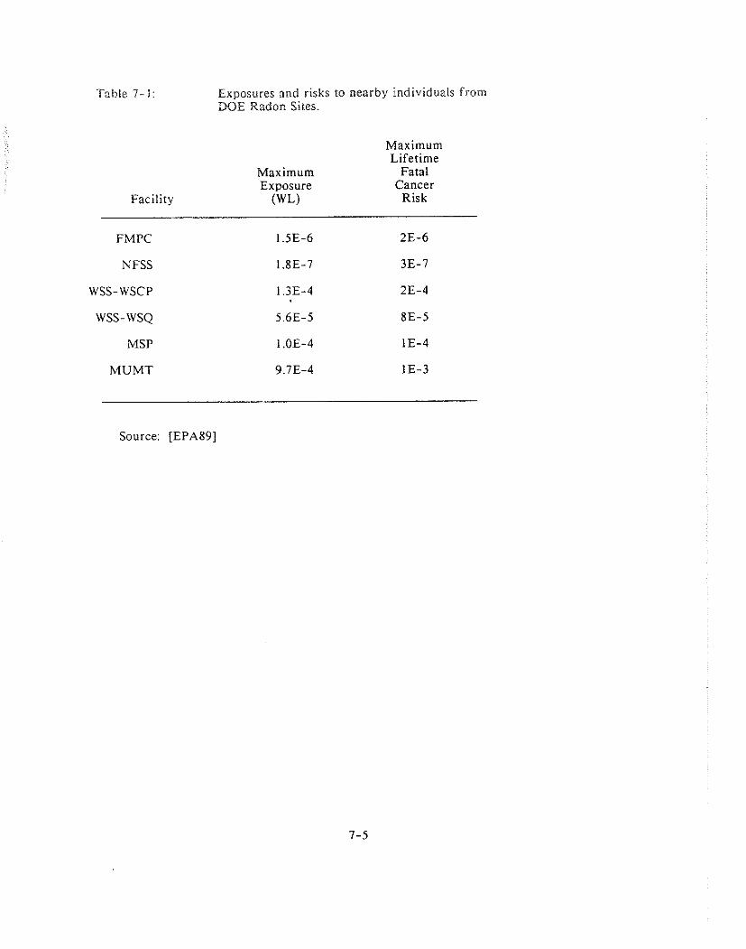
Exposures and risks to nearby individuals from DOE Radon Sites.
Maximum Lifetime
Maximum Fatal Exposure Cancer
Facility (WL) Risk
FMPC
NFSS
WSS-WSCP
WSS-WSQ
MSP
M U M T
Source: [EPA89]
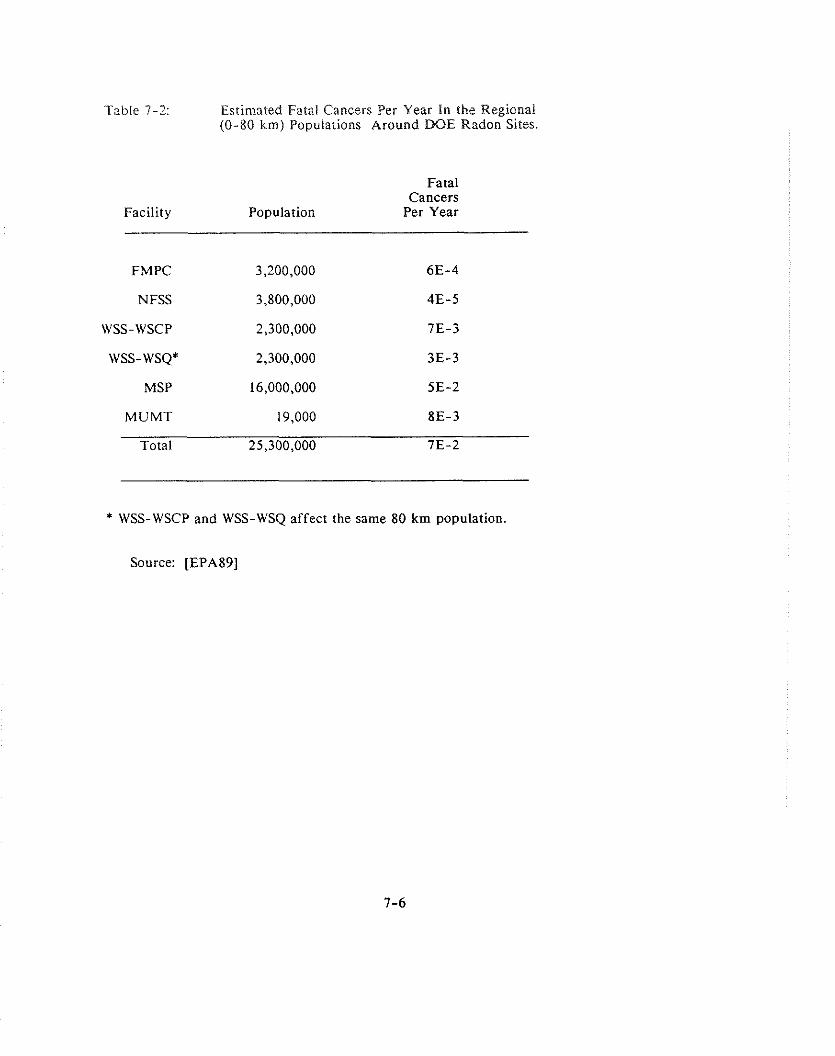
Table 7-2: Estimated Fatal Cancers Per Year In the Regional (0-80 k m ) Populations Around DOE Radon Sites.
Fatal Cancers
Facility Population Per Year
FMPC 3,200,000 6E-4
NFSS 3,800,000 4E-5
WSS-WSCP 2,300,000 7E-3
WSS- WSQ* 2,300,000 3E-3
MSP 16,000,000 SE-2
MUMT 19,000 8E-3
Total 25,300,000 7E-2
* WSS-WSCP and WSS-WSQ affect the same 80 km population.
Source: [EPA89]
[Gr87]. Measurements were made of radon flux emissions Front the silos in 1984 and 1985,
but subsequent structural improvements have had a significant impact on the emission levels.
Therefore, no current valid emission information is available.
Radon-222 release rates were estimated at 2.5 Ci/yr based upon the radium content of the
residues and a calculated flux rate through the concrete domes and foamed exterior [Na 85).
The estimated radon flux rate is 85 p ~ i / m 2 / s e c . The cancer risk to the most exposed
individual is about 2E-6.
7.3.2.2 Niaeara Falls Storaee Site
The NFSS consolidated the wastes on a 4 ha site a t the I\VCF. Radon measurements at the
site boundary during 1986 range between 0.17 and 0.36 pCi/l, including background. The
background level was monitored at 0.31 pCi/l. Measured flux rates for radon are not
available from the pile. The current estimated releases as stated in the closure/post-closure
plan are 0.25 Ci/yr. The estimated radon flux rate consistent with this annual estimate is 0.06
pCi/m2/sec. The risk for the most exposed individual is about 3E-7.
7.3.2.3 Weldon Snrine Site
The \VSS's environmental radon monitoring program covers 31 sites. The boundary radon
monitors at \VSCP read between 0.18 and 0.49 pCi/l, including background. The readings
from the background location were measured a t 0.47 pCi/l, while off-site monitors north of
the pits and closer than the background monitors recorded levels of 0.22 to 0.36 pCi/l. The
on-site n~onitors at the raffinate pits and the quarry ranged between 0.31 and 0.64 and 0.24
and 1.86 pCi/l, respectively. The estimated release rates of Radon-222 are 29 Ci/y for the
WSCP and 14 Ci/y for the WSQ. The estimated radon flux rates are 2.7 pCi/m2/sec a t WSCP
and 3.7 pci/m2/sec at WSQ. The cancer risk to nearby individuals is estimated at 2E-4 for
WSCP and 8E-5 for WSQ.
7.3.2.4 hliddlesex Samnline Plant
Samples of the piles at the MSP show concentration of 40 pCi/g of radium-226. There are
twenty monitors at the MSP, and one off-site background monitor. The monitoring reports
indicate that the range of readings are 0.3 to 1.2 pCi/l, including background, at MSP, with
the background site registering 2.0 pCi/l. The off-site location is apparently at a higher
radiation level than the site itself. The radon flux rates are not available, but are estimated
based on a source strength of I pCi/g of radium-226 resulting in 1 pci/m2/sec of radon-
222. This results in an estimated radon flux rate of 40 p ~ i / m 2 / s e c . Given the dimensions
of the waste piles, this converts to 25 Ci/yr not accounting for attenuation by the hypalon
cover. The risk level for nearby individuals is 1E-4.
7.3.2.5 Monticello Uranium Mill Tailines Pile
The MUMT was found to exceed the EPA standard for radon flux of 20 pCi/m2/sec at each
of the four tailings piles. Radon emission measurements range from 133 to 765 pci/m2/sec
for these piles and a portion of the pile has migrated b>- as much as 500 m off-site. The
average flux rate of the material that has migrated is 40 pci/m2/sec or 37 Ci/yr. The
estimated radon flux rate averaged over all the piles is 228 p ~ i / m 2 / s e c . The total radon-222
release is estimated by DOE at 1,595 Ci/yr [SE87]. This facility has the highest lifetime fatal
cancer risk for nearby individuals of the five facilities considered in this chapter: 1E-3.
7.3.3 Control Technoloeies
Each of the five facilities was evaluated for supplementary controls and costs that would be
required to reduce the radon emissions to levels of 20. 6, and 2 pci/m2/sec. This cost
estimation assumed that all wastes remain at their current sites, that the current storage
configurations would be maintained, and that the wastes would be covered with dirt to
sufficient depth to reduce the radon emissions to the target levels.
The radon emission rate from the two FMPC silos, using the estimated 2.5 Ci/y source term
is calculated to be 85 p ~ i / m 2 / s e c . The FMPC would require 2.1, 2.3, and 3.3 meters of dirt,
costing $56,000, $79,000, and $83,000, respectively, to meet the target levels of 20, 6, and
2 pci/m2/sec.
The NFSS's current rate of radon flux of 0.25 Ci/yr is equivalent to 0.06 pci/m2/sec which
is below the lowest target level; therefore, there are no additional costs to meet these goals.
Currently the pits and quarry a t WSS contain water which keeps radon fluxes at the relatively
low levels of 2.7 and 3.7 p ~ i / m 2 / s e c respectively. Therefore the flux rates meet the target
levels of 2 and 6 p ~ i / m 2 / s e c without controls. However, before dirt can be applied to the
pits, they must be dried out. When this is done, the flux rate increases to 460 pci/m2/sec at
pits 1, 2, and 3 and to 1 1 p ~ i / m 2 / s e c at pit 4. The control flux rates were calculated
assuming that the pits and quarry are dry. Earth cover of 1.6, 2.3, and 2.8 meters would be
required to reduce the emission rates to 20, 6, and 2 pci/m2/sec, respectively for pits 1, 2,
and 3. Pit 4 needs no cover to meet 20 p~ i /m2/sec , and .3 and .9 meters to meet 6 and 2
pCi/m2/sec, respectively. The associated costs are $1.73, $2.96, and $4.26 million. Control
techniques have not been devised to achieve alternate radon levels for the quarry site.
The MSP site would require 0.8, 1.4, and 2.1 meters of dirt, with associated costs of $419,000,
$720,000, and $997,000 respectively, to meet the target levels of 20, 6, and 2 pci/m2/sec.
Covering the MUMT piles exhibited the highest costs, requiring 2.4, 3.4, and 4.4 meters of
earth to meet the target levels of 20, 6, and 2 p ~ i / m 2 / s e c at costs of $26.8, $39.2, and $50.2
million, respectively.
7.4 Analvsis of Benefits and Costs
7.4.1 Costs and Benefits of Meetine Various Radon Flux Rates
The analysis considers only the incremental costs relative to the baseline of supplementary
controls to meet the target emission levels of 20, 6, and 2 p~i /m2/sec . The benefits are
estimated as the number of fatal cancers avoided and the reduction in maximum individual
risk by applying supplementary control measures to meet the three target emission flux rates.
Proportional reductions in the emission rates are converted into proportional reductions in the
risks. The benefits are estimated by calculating the nearby and regional (up to 80 kilometers
distance) population exposure to the radionuclides. The population exposure levels and risks
of fatal cancers are a function not only of the emissions and their controls, but also of the
population distribution in the vicinity of the facility, the meteorology, farming and food
distribution and consumption patterns, atmospheric transport of the contaminants, and the
inhalation or ingestion pathways.
The controls for four of the five facilities are assumed to be completed within one year.
Implementation of controls for the fifth facility, the Niagara Falls Storage Site (NFSS), is
expected to take ten years, but explicit control costs were not provided since the current
emission flux rates are already well below the lowest target levels and, as mention above, the
interim remedial actions would temporarily increase the emission levels and the number of
fatal cancers. The following paragraphs present the findings of the analysis for each of the
facilities. Table 7-3 summarizes the benefits and costs of supplemental control measures
needed to meet a flux rate of 20 pci/m2/sec. Table 7-4 provides the same measures for a flux rate of 6 p ~ i / m 2 / s e c and Table 7-5 for one of 2 pci/m2/sec.
7.4.1.1 Feed hiaterials Production Center
The FMPC facility is estimated to have an emission flux rate of 85 pci/m2/sec resulting in
a fatal cancer risk rate of 6E-4 per year [EPA89]. The costs of further reducing the emissions
to a target level of 20 pci/m2/sec is estimated at approximately $56,000, which would be
expended in a single year to cover the wastes with a greater depth of dirt. On an annualized
basis, given a discount rate of five percent, the cost would be $2,800 per year for one
hundred years.
7.4.1.2 Niaeara Falls Storaee Site
The NFSS facility, as stated above, is the one facility that is already well below the target
emission rates. The current emission strength of 0.25 Ci/yr translates into an equivalent
radon flux of 0.06 p ~ i / m 2 / s e c which is three percent of the lowest target level of 2.0 and 0.3
percent of the highest target level of 20 pci/m2/sec. If the proposed remedial actions were
taken, the emission levels would sharply increase for a period of ten years, thereby increasing
the total numbers of cancers for the first 100 years by a factor of nearly ten, from 6.OE-3 to
4.6E-2. No costs of this remedial action were estimated since the facility already meets the
target emission levels.
7.4.1.3 W'eldon Soring Site
The WSS facility is composed of four pits at the WSCP site and a quarry, the WSQ, at another
location with varying emission rates that also fluctuate due to seasonal weather patterns. The
WSCP has an estimated radon flux of 2.7 pci/m2/sec and WSQ one of 3.7 pci/m2/sec.
Together they generate a fatal cancer risk of 1E-2 per year or approximately I fatal cancer
in a century. The WSCP pits are filled with water much of the time. When dry they would
release radon a t a flux rate of 460 pci/m2/sec a t pits I , 2, and 3 and l l pci/m2/sec a t pit 4.
Dirt depths of up to three meters would be required to reduce the flux rates of the dried out

I A E L E 7 - 3 : Costs and reduced Risks Resulting f rom Covering the Sources t o Louer Radon
Flux Rates t o 20 pCi/m^2lsec
I I I
F a c i l i t y / ............... I, FMPC I
I NFSS I
I USS-USCP* I
I USS-USQ*' I
1 MSP I
I MUM1 I
Estimated I I Annual Fatal Cancers i n I I I n i t i a l Radon I I 80 km P o p l l a t i a , I M a x i m Ind iv idual Risk I
Flux Rate I I.................. .............I............................... I (pCilmA2/sec) I Control Costs I Resultant I Averted I Resultant I Reduction I ....... ..................................................................................... I
85 1 156,000 1 1E-04 1 5E-04 I 5E-07 I 2E-06 I I I I I I I
0.06 1 So I 4E-05 I OEtOO I 3E-07 I OE+OO I I I
199.6 1 $1,730,000 I I I
3.7 1 NA I I I
LO 1 $419.000 I I I
228 1 826,800,000 1 .....................................
TOTAL: I 829,005,000 1
I 4E-02 I
I 3E-03 I
I 3E-02 I
I 7E-04 1
................ TOTAL: I
7E-02 I
I OE+OO I
I 2E-02 I
I 7E-03 I
............. TOTAL: I
-4E-03 I
I I IE-03 I -9E-04 I
I I 8E-05 I OE+OO I
I I 8E-05 I 2E-05 I
I I 1E-04 I 9E-04 I
............................... MAXIMUM: I MAXIMUM: I
1E-03 I 9E-04 I
+ Based on f l u x ra tes wi th p i t s d r ied out. Note that f l u r a t e i s cu r ren t l y 2.7 p€i/mA2/sec due t o uater cover. The r i sks therefore exceed the i n i t i a l r isks. ** No contro l has been devised fa r WSS-USQ.
[Source: Calculat ions by JFAl
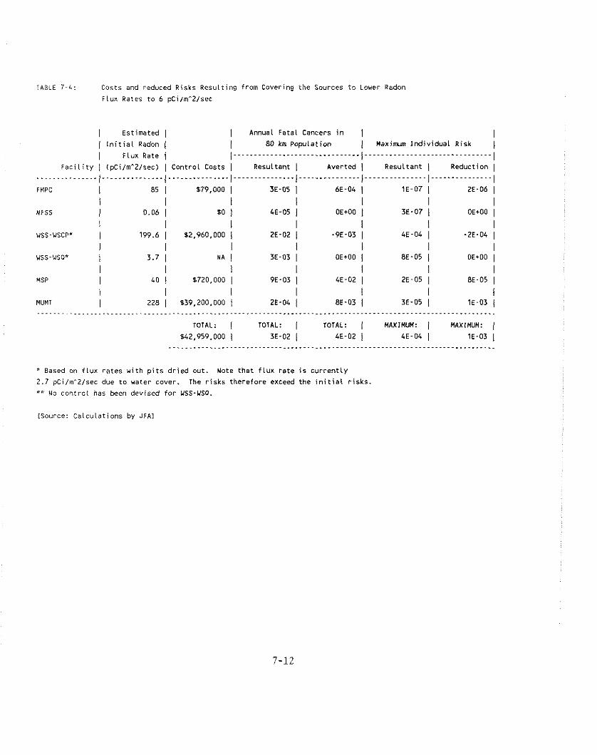
TABLE 7 - 4 : Costs and reduced Risks Result ing from Covering the Sources t o Lower Radon FLux Rates t o 6 pCilm^2/sec
I Estimated I I Annual Fatal Cancers i n I I ( I n i t i a l Radon ( 1 80 km Populat ion I Uaximm I n d i v i d u a l Risk I I Flux Rate / ~._________________.............I............................... 1
F a c i l i t y 1 (pCilm^2/sec) I Cont ro l Costs I Resultant I Averted ( Resultant / Reduction I ~ ~ . . ~ _ _ _ _ ~ . ~ ~ ~ _ ~ ~ _ ~ ~ _ ~ ~ ~ _ _ _ ~ _ ~ ~ ~ _ _ ~ ~ ~ ~ ~ ~ ~ ~ ~ ~ ~ ~ ~ ~ ~ ~ ~ . ~ ~ ~ ~ ~ ~ ~ ~ . . . ~ ~ ~ ~ . . ~ ~ . ~ ~ ~ ~ ~ ~ ~ ~ ~ ~ ~ ~ ~ ~ ~ ~ ~ ~ ~ ~ ~ ~ . ~ ~ ~ ~ ~ ~ ~ ~ . . ~ . . ~ . . I FMPC I 85 1 $79,000 1 3E-05 I 6E-04 I 1E-07 1 ZE-06 /
I I I I I I I NFSS 1 0.06 1 I0 1 4E-05 I OE+OO I 3E-07 I OE+OO I
I I I I I I I USS-WSCP* 1 199.6 1 $2,960,000 / 2E-02 I -9E-03 I 4E-04 I -2E-04 I
i I I WSS-USQ* 1 3.7 / M A I
I I I KSP I 40 1 8720.000 1
I I I MUMT I 228 1 $39.200.000 /
TOTAL: TOTAL: 1 TOTAL: 1 MAXIMUM: I MAXIMUM: 1 $42,959,000 1 3E-02 I 4E-02 I 4E-04 I 1E-03 I
Based on f l u x ra tes w i t h p i t s d r i e d out. Note t h a t f l u x ra te i s c u r r e n t l y
2.7 pCi/m*2/sec due t o water cover. The r i s k s therefore exceed the i n i t i a l r i sks .
** NO cont ro t has been devised for USS-USQ.
[Source: Calcu la t ions by J F A I

[Source: Calculat ions by J F A I
TABLE 7-5: Costs and reduced Risks Resulting fran Covering the Sources t o Lower Radon
Flux Rates t o 2 pCi/mA2/sec
I Estimated I I Annual Fatal Cancers i n I 1 I I n i t i a l Radon I I 80 km Pop l la t ion I M a x i m Ind iv idual Risk I I Flux Rate I I................... ............I............................... 1
F a c i l i t y I <pCi/mA2/sec) I Control Costs I Resultant I Averted I Resultant I Reduction I . ............................................................................................................. I FMPC 1 85 / $83,000 1 1E-05 I 6E-04 I 5E-08 I 2E-06 I
I I I I I I I NFSS 1 0.06 1 So I 4E-05 I OE+OO I 3E-07 I OE+OO I
I I I I I I I WSS-USCP' I 199.6 1 84,260,000 1 5E-03 I 2E-03 I 1E-04 I 5E-05 I
I I I I I I I USS-USQL" I 3.7 1 *A I 3E-03 I OE+OO / 8E-05 I OE+OO I
I I I I I I I MSP I 40 / $997,000 1 3E-03 I 5E-02 I 8E-06 I 9E-05 /
I I I I I I I MUMT I 228 / $50,200,000 1 7E-05 I 8E-03 I 1E-05 I 1E-03 I ................................................................................................................
TOTAL: I TOTAL: I TOTAL: I MAXIMUM: 1 MAXIMUM: I $55,540,000 1 1E-02 I 6E-02 I 1E-04 I 1E-03 I
................................................................................
* Based on f l u x rates u i t h p i t s d r ied out. Note that f l u x r a t e i s cu r ren t l y
2.7 pCi/mA2/sec due t o water cover.
*" No con t ro l has been devised f o r USS-USQ.
[Source: Calculat ions by JFAI
pits to as low as 2 p~ i /m2 / sec for pits 1, 2, and 3. Pit 4 would require a cover of up to one
meter to meet this lowest target level. There is insufficient information to develop a cost of
achieving the supplementary control target levels for the quarry site [DOE88]. Once the pils
are dried out and the higher fluxes are occurring, the total cost of supplementary controls
sufficient to meet the target level emission rate of 20 pci/m2/sec at the pits is $1,730,000,
while the annualized payment is $87,000. This would actually increase emissions and risk
to the population and to the most exposed individual. Reducing the flux to 2 pci/m2/sec
would reduce risks. This would cost $4,260,000.
7.4.1.4 Middlesex S a m ~ l i n e Plant
The MSP facility's emission rate is estimated at 40 p~i /m2/sec , causing an estimated 5E-2
fatal cancers per year. Supplemental controls that meet the target emission rates would
reduce the fatal cancer risks to between 3E-2 and 3E-S per year. The supplemental control
cost is between $419,000 and $997,000.
7.4.1.5 Monticello Uranium Mill Tailines Pile
The MUMT piles have an estimated emission rate of 228 pci/m2/sec, which could result in
an estimated 8E-3 fatal cancers per year. The least stringent of the control levels (20
p~i /m2/sec) would reduce the number of fatal cancers per year to 7E-4, while maintaining
flux levels at 2 p~ i /m2 / sec would further reduce the number of deaths by a factor of ten.
The supplemental control costs would be $26,800,000.
7.4.2 Sensitivity Analysis
Tables 7-3, 7-4, and 7-5 presented data regarding the toss and benefits of meeting various
flux rate standards at each facility. In the fotlowing, the effects of changing the flux rate
standard and the social discount rate are demonstrated.
Tables 7-6 and 7-7 demonstrate that there is a small national benefit of reducing the target
flux rate to 6 pci/m2/sec or to 2 p~i /m2/sec . The first additional increment would provide
four fewer fatal cancers nationally per century and the second two fewer.
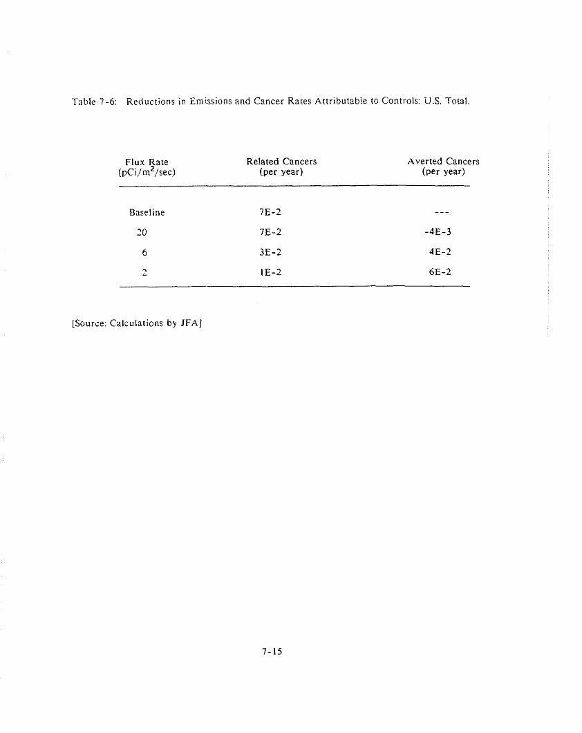
Table 7 -6 : Reductions in Emissions and Cancer Rates Attributable to Controls: U.S. Total.
Flux Rate (~c i /m' / sec)
Related Cancers (per year)
Averted Cancers (per year)
Baseline
20
6
1 -
[Source: Calcul3tions by JFA]

Table 7-7: Incrernentsl Costs and Risk Reductions for Var iws FLUX Standards
I I I I
Flux Standard I Total Control I (pCilmA2/sec) I Cost
I I Incremental / I Fatal Cancers I Reduction i n I
Incremental I Averted I Fatal Cancers I Control cost I (per 100 vr) I ( p r 100 yr) I
.---.. I OE+OO I -...-. I I I I
529,005.000 1 -4E-01 I -4E-01 I I I I
113,954,000 1 4E+00 I 4E+00 I I I I
112.581,000 I 6E+OO I 2E+OO 1
[Source: Calculations by JFAI

The other factor in the costs and benefits analysis of section 7.4.1 was the question of
discounting the costs to compute net present value. Table 7-8 demonstrates that for a 20
pci/m2/sec flux rate standard, calculation of NPV of the cost of national requirement of
supplementary controls does not vary at all. This is because the costs are all at the beginning
of the 100 year period of analysis, where changes in discount rates have no effect.
7.5 lndustrv Cost and Economic I m ~ a c t Analvsis
Since the costs of these control actions will be borne by the Federal government, there is no
assignable direct private industry cost. Only the FMPC is currently operating; the other four
facilities are now surplus or storage facilities solely and therefore do not raise on-going
capital or operations and maintenance costs.

Net Present Value of Cost of Supplen~ental Controls to Meet a Flux
of 20 pci/m2/sec at DOE Radon Facilities: U.S. TOTAL.
NPV
RATE (in millions of dollars)
Note: Values rounded to one decimal place.
[Source: Calculations by JFA]

REFERENCES
Bechtel National, Inc., Closure/Posl-Closure Plan for the Iirterinz iVa.sr~, Corttairrntertl Facility a1 the Niagara Falls Slorage Sile, DOE/OR/20722- 8 5 , Oak Ridge, Tennessee, May 1986.
Bechtel National, Inc., Niagara Falls Storage Sile. Airnual Site Et~virottntertlal Report, Calendar year 1986, DOE/OR/20722-150, Oak Ridge, Tennessee, June 1987.
U.S. Department of Energy, Final Environmetttal Intpact Statentenl, Lorrg- lernt Matragemetrt o/ [he Existir~g Radioactive Wasles and Residues ar (he Niagara Falls Storage Si te , DOE/EIS-0109F, April 1986.
U.S. Department of Energy, Draft Ertvirottntertlal Intpact Slalenrertt. Rentedial Aclioir at the lt'eldort Spri i~g Site, DOE/EIS-0117D. February 1987.
U.S. Environmental Protection Agency, Backgrout~d In/orntation Docunteitt for Firral Rules. Volume I I , Appendix C . Radon Entissiotts from Departnlen~ o f Errergy artd Nuclear Regulatory Contntissioit-Licerrsed Facilities, EPA 520/1-84-022-2, Washington, D. C., October 1984.
Risk Assessnrerzls. Vol. 2.
Grurnski, Joseph T., Feasibilily Invesligalion for Corttrol of Radott Entissiotrs /ram [he K-65 Silos, Feed Materials Production Center, Westinghouse Materials Company of Ohio, July 30, 1987.
Sewell, Michael, and Larick Spencer, Envirotrntental Moiritorirtg Report or1 Deparmrent of Energy Facilities a! Grand Junclion, Colorado, and Morzficelio, Uinh, for calendar year 1986, UNC/GJ-HMWP-2, UNC, Grand Junction, CO, March 1987.
Nazaroff, W. W., et al., Almospheric Envirottnten~, 19:1:31-46, (1985).


GWAPTER 8
EEMENTAL PHOSPHORUS


8. ELEMENTAL PHOSPHORUS PLANTS
8.1 l~~t roduct ion and Summary
The Elemental Phosphorus Plant source category consists of five operating and three standby facilities
that produce elemental phosphorus by the electric furnace method. These plants have been evaluated
in previous EPA assessments under Section 112 of the Clean Air Act and are subject to the NESHAP
(40 CFR 61, Subpart K) promulgated on February 5, 1985. The NESHAP established an emissions
limit of 21 Curies per year (Ci/y) for polonium-210 (Po-210) released f rom calciners and nodulizing
kilns.
This chapter updates the assessment made during the 1983-1985 radionuclides NESHAPS rulemaking
period (EPA84). Revisions have been made where necessary to reflect the changes in emissions or
control technology as reported to the EPA under provisions of the NESHAP. It also incorporates the
exposure and risk assessments for two idle plants in Florida that were not addressed in the risk
assessment of the 1984 rulemaking.
The five plants currently producing elemental phosphorus are owned by Monsanto Company, FMC
Corporation, Rhone-Poulenc (Stauffer), S.A., and Occidental Petroleum Company. The current
radionuclide emissions at each of these plants have been measured and current emissions control
technologies have been evaluated. The feasibility of various emission control technologies was
evaluated and the performance and cost of these alternatives evaluated.
Current emissions at each of the five operating plants are estimated as listed below:
Units: Ci/y
Facilitv Po-210 Pb-210
FMC 10. 0.14
Monsanto 1.4 0.35
Stauffer, M T 0.74 0.11
Stauffer, T N 0.28 0.058
Occidental 0.31 0.064

These emissions are est imated t o resu l t i n a n a t i o n a l cancer inc idence ra te o f 8 E - 0 2 p e r year (see
sec t ion 8-3). Va r i ous a l ternat ives for r e d u c i n g b o t h rad ionuc l i de emissions a n d r i sks are evaluated
in t h e cu r ren t s tudy. A s u m m a r y o f these a l te rna t ives is presented in the table b e l o w . For each of
n i n e d i f f e r e n t Po-210 emissions levels and for four comb ina t i ons of c o n t r o l technologies, costs a n d
bene f i t s - measured in cancers p e r year - were de te rm ined . T h e f i r s t set of a l te rna t ives are based
on emiss ion levels r a n g i n g from 10 Ci/y o f Po -210 t o 0.01 C i / y . In add i t ion , four a l te rna t ives we re
eva lua ted tha t apply d i f f e r e n t comb ina t i ons of control technologies t o d i f f e ren t p lan ts . These are
based on the size (measured in te rms o f annual e lemen ta l phosphorus p r o d u c t i o n capac i t y ) o f t he f i v e
p lan t s under considerat ion.
Summary o f A l t e r n a t i v e s
i n c i e a e n t a l T o t a l I n c r e m e n t a l T o t a l A l t e r n a t i v e i n c i d e n c e l s c i d e n c e I n c i d e n c e A n n u a l i z e d A n n u a l i z e d
c e d e c t i o n R e d u c t i o n C o s t C o s t E M l S S l O Y S LEVELS 1. ( 1 0 . 0 C i l y ) 8E-0; - - . . . . . . 11 . ( 2 . 0 C i l y ) 3 E - 0 2 5 E - 0 2 5 E - 0 2 2 . 4 3 2 . 4 3 I l l . ( 1 . 0 C i l y ) 2 E - 0 2 7E - 03 6 E - 0 2 2 .74 5 . 1 7 I V . ( 0 . 7 5 C i l y ) 2 E - 0 2 5 E - 0 3 6 E - 0 2 1 .30 6 . 4 7 V . ( 0 . 6 0 C i l y ) 1 E - 0 2 5 E - 0 3 6 E - 0 2 1 .52 7 . 9 9 V I . ( 0 . 2 0 C i l y ) 4 E - 0 3 8 E - 0 3 7E - 02 4 .34 1 2 . 3 3 V I I . ( 0 . 1 0 C i l v ) 3 E - 0 3 9 E - 0 4 7 E - 0 2 15 .59 2 7 . 9 2 V I I I . ( 0 . 0 6 C i l y ) 1 E - 03 2 E - 0 3 8 E - 0 2 0 .39 2 8 . 3 1 I X . ( 0 . 0 1 C i l y ) 3 E - 0 4 8E - 06 8E - 02 3 . 2 8 3 1 . 5 9
CONTROL TECHNOLOGIES I . 8E - 02 -. . . . . . . X . 3 E - 0 2 5 E - 0 2 5 E - 0 2 2 . 4 3 2 .43 X I . 2 E - 0 2 7 E - 0 3 5 E - 0 2 2.35 4 .78 X I I . 7 E - 0 3 1 E - 0 2 7 E - 0 2 12.70 17 .48 X I I I . 8E - 04 6 E - 0 3 8 E - 0 2 12 .02 2 9 . 5 0
I . No A d d i t i o n a l E m i s s i o n s C o n t r o l R e q u i r e d X . H i g h E n e r g y S c r u b b e r s o n L a r g e P l a n t s X I . n i g h E n e r g y S c r u b b e r s o n A l l P l a n t s X l l . F a b r i c F i l t e r s o n L a r g e P l a n t s ; H i g h E n e r g y S c r u b b e r s o n O t h e r s X I I I . HEPA F i l t e r s o n L a r g e P l a n t s ; 6 0 0 SCA P r e c i p i t a t o r s o n O t h e r s
T h i s chapter i s d i v i d e d i n t o four sections. T h e f o l l o w i n g section, 8.2, is a p r o f i l e o f t he e lemen ta l
phospho rus (P4) i ndus t r y . I t i s f o l l o w e d b y a desc r i p t i on o f cu r ren t r ad ionuc l i de emissions, r i s k levels

and feasible control niethods. Section 8.4 outlines both the reductions in risks and the increases in
costs that could result Fro111 the installation and operation of these vnrious control technologies on the
different plants. The final section describes potential econon~ic impacts.
8.2 l~idustrv Profile
Production of elemental phosphorus (P4) in the United States utilizes about 10 percent of all
phosphate rock mined annually. Elemental phosphorus is used principally as an intermediate in the
production of high purity phosphoric acids and salts as well as a variety of phosphorus chemicals for
industry and home use. The major derivatives of elemental phosphorus are detergent phosphate
materials, mainly sodium tripolyphosphate (STPP).
8.2.1 Demand
U.S. production of elemental phosphorus peaked in 1969 at 623 thousand short tons (tons), then
declined steadily to a low of 359 thousand tons in 1985. In 1986, production of elemental phosphorus
totalled about 364 thousand tons, a one percent increase over 1985, but a 42 percent decrease from
1969. Production in 1987, however, was only 343 tons [MCP85]. Plant production and shipments
between 1964 and 1987 are listed in Table 8-1.
The manufacture of thermal or furnace grade phosphoric acid accounts for approximately 85 percent
of domestic elemental phosphorus consumption. Other chemicals, principally phosphorus
pentasulfide, phosphorus pentoxide, and phosphorus trichloride use over 10 percent. Direct uses,
n~iscellaneous chen~icals and alloys consume less than 5 percent [MCP85]. A chart of the intermediate
and end products of the elemental phosphorus industry is provided in Table 8-2 below.
Phosphorus is used principally as an intermediate in the production of high purity phosphoric acids
and salts, as well as a variety of phosphorus chemicals for industry and home use. Detergent
phosphate materials, chiefly sodium tripolyphosphate (STPP), are the major commercial derivatives
of elemental phosphorus. Commercial phosphates also include other sodium phosphates, and calcium
and potassium phosphates, used in a variety of detergents, cleaners, personal care products, water
treatment and food. The detergent market is comprised of household detergents (85 to 90 percent)
and industrial detergents ( I0 to 15 percent). Accounting for over 60 percent of elemental phosphorus
use in 1970, detergent applications have since declined because of environmental concern regarding
the role of phosphorus in eutrophication.

Table 8-1: Production and Sbtpmenl OF Elemental Phosphorus - - 1964-1987 (Tens).
Year
1987 1986 1985 1984 1983 1982 1981 1980 1979 1978 1977 1976 1975 1974 1973
Source:
Production
343,329 363,717 359,196 386,063 365,622 361,189 426,067 431,730 459,541 441,274 430,291 436,655 449,506 524,175 525,523 540,089 545,089 596,555 622,982 613,343 587,006 565,550 555,368 503,880
Total Shipments Including Interplant Transfers
Bureau of the Census, U.S. Department of Commerce, Current Industrial Reports: Inorganic Chemicals, annuals, 1968,-1984, Table 1.
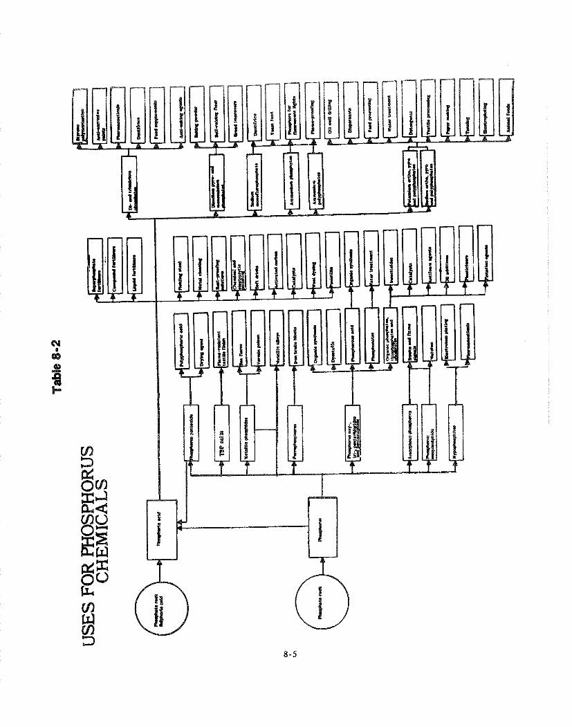

Controls or bans on the use of phosphates in detergents have been in place for some time i n New
York, Indiana, Michigan, Wisconsin. Minnesota, Connecticut, and Maine. In the past two years,
the District of Columbia, Virginia, Maryland, and North Carolina have restricted phosphate use.
Soutll Carolina, Oregon and Illinois are considering phosphrlte bans. Phosphate-containing detergents
are now unavailable to about 30 percent of the U.S. population and to LOO percent of Canada's
[C\\'88J]. The use of STPP in detergents has dropped froin 1.4 billion pounds in 1980 to 1.2 billion
pounds in 1985, and is predicted to fall to 1.1 billion pounds by 1990 [CW88j].
Metals treating is a second major end use of elemental phosphorus. Valuable in controlling corrosion,
phosphorus is used in aluminum polishing and paint bases. Demand for phosphorus in metals treating
depends heavily on denland for automobiles and durable goods, the major end users of these
products, and thus tends to fluctuate with the business cycle. For example, with a slump i n the
automobile and other consuming industries between 1979 and 1980, consumption of elemental
phosphorus products by these industries fell by 25 to 33 percent [CEN84, CEN81J.
A third major market for elemental phosphorus is the food and beverage industry. Phosphoric acid
is used in soft drinks, powdered drinks, baby foods, puddings, baking powder, and dentrifices, for
example. Demand for these products has grown slowly in the past decade, but has been below the
industry's forecasts, possibly because of the decline in sales of cakes and cookies as part of the
national trend toward physical fitness, and a reformulation of soft drinks [CEN83, CEN8ll .
Chemical derivatives of phosphorus, other than phosphoric acid, at 10 percent of consumption, are
equal to the food and beverage industry i n importance to the elemental phosphorus market. Current
uses include lubricating oils, insecticides, flame-resistant textile finishes, matches, and
pharmaceuticals. In the last half of the 1970s, these uses were considered the market with the highest
growth potential. Some companies added capacity during the period to produce pentasulfide,
trichloride, and oxychloride phosphorus compounds, which are then used in agricultural chemicals,
lubricating oil additives, and many other products. However, growth in these uses has been impeded
by the longer life of lubricating oils, and competition from substitute products. Furthermore, though
in the early 1980s producers increased investment in R&D, no new significant uses of phosphorus
products have been discovered. Growth in non-acid uses has been about 3 percent per year since the
middle 1970s [CENBI, CEN781.

The export market is the only othel- niajor consumer of U.S.-produced elemental phosphorus. Most
countries that have a continuing requirement for phosphorus produce it domestically, largely because
water transportation requires extensive precautions. However, exports have accounted for some 5 to
7 percent of U.S. elemental phosphorus production since the middle of the 1970s [CEN84, CEN791.
In 1986, most of the 22 thousand short tons (6.1 percent of production) of elemental phosphorus
exports were destined for Japan (42 percent), Brazil (32 percent), Mexico (I4 percent), and Taiwan
(7 percent) [MY87].
Annual U.S. consumption of elemental phospliorus appears to have dropped to a plateau in the range
of 325 to 350 thousand tons per year. Some industry observers expect long term domestic demand
to increase at up to 2 percent per year. More pessimistically, U.S. demand will remain essentially
unchanged or decline slightly. Co~isumption would decline if the ban on phosphate detergents were
accentuated or if organophosphate pesticides were to lose additional market share. Most other
applications, such as use in metal finishing and flame retardants, will probably have relatively static
demand patterns, subject to swings in the o\'erall economy [CEN84].
In 1988, four corporations operated a total of five elemental phosphorus plants in the United States.
The largest producer is FMC Corporation (1 plant), followed by Rhone-Poulenc, which purchased
2 Stauffer Chenlical plants in 1987, Monsanto ( I plant) and Occidental (1 plant). The corporations,
plants, capacity, and plant en~ployment are listed in Table 8-3.
Elemental phosphorus producers are vertically integrated which means that most of the P4 produced
is used captively downstream in other company operations. All producers operate phosphate rock
mines in the \aicinity of their elemental phosphorus plants. After manufacturing the elemental
phosphorus, producers ship it to burning plants, where it is converted to other chemicals for use in
consumer and industrial products. For example, elemental phosphorus produced at FMC's Pocatello
plant is shipped to five other plants for production of phosphorus-based chemicals [FMC86]. The
mix of chemicals produced varies, depending on the producer's cost and'market structure. Table 8-4
presents the location of and phosphorus chemical production capacity at the various downstream
plants of each company.
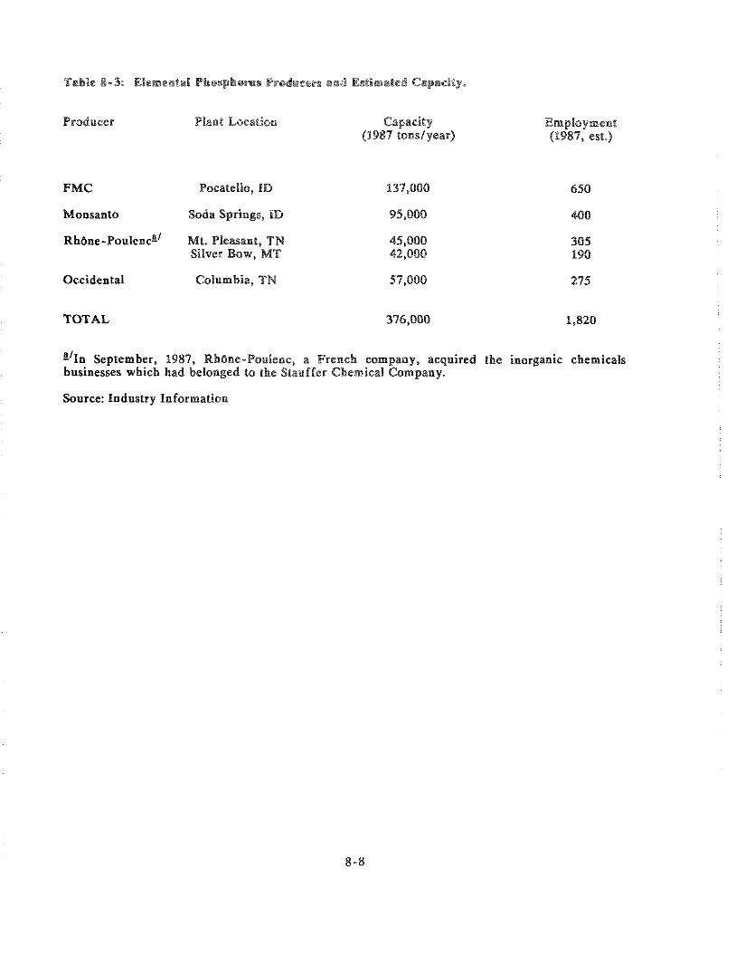
Producer Plant Location Capacity (1987 tonslyear)
FMC Pocatello, ID
Monsanto Soda Springs, ID
~ h ~ n e - ~ o u t e n c " l t . Pleasant, TN Silver Bow, MT
Occidental Columbia, TN
Employment (1987, esk.)
TOTAL 376,000 1,820
"1n September, 1987, RhBne-Poulenc, a French company, acquired the inorganic chemicals businesses which had belonged to the Stauhfer Chemical Company.
Source: Industry Information

+ehls 8-48 w.S. Cagacitis~ for ghc.pbow and ghc ehsl icala - 1985. (*usan& of sbr t tan8)
Ccupany and Plant Location
Thermal sssic Inorganic Intermediates Phosphoric ------ ------ ------ &dim
Phosphorus Acid EL, P2S5 P205 Hypophosphate (PI Banis) (Pa Basis) (elemental phosphorus (PI) Basin) (P4 Basis)
Charleston, SC ntrnsld, OH
Carteret, NJ Green River, NY Idwrence. IS Revark, U Nitro, W Pocatello, ID
MoNsANm Anniston, AL Augusta, GA Carondelet, WO Columbia, TN xearny, UJ long Beach, CA nilwaukee. WI
OCCIDBN&A Columbia, llS Godwin, M Jefferson, IN niller, TX Riagara Palls, NP
silver Bow, WS Tarpon Springe, FL
T(YPAI.
S'Albright 6 Wilson, Inc.'s thermal acid and phosphorus chemicals plants vere purchased by Albright & Wilson, Ltd. (subsidiary of Tenneco, Inc.) from mbil.Corporstion early in 1985.
With recent flat deinand and little future growth expected, capacity for elemental phosphorus has
been reduced. I t is unlikely that facilities previously closed in Florida in the early 1980s will be
restarted, since electric power costs, which account for about 20 percent of total production costs,
are significantly higher there than in Tennessee and in the Northwest. Capacity in Tennessee was
also reduced as demand weakened. Most recently, in 1986, Monsanto shut down its plant in
Columbia. TN.
With the various shutdowns and consolidations, the real U.S. capacity for elemental phosphorus has
dropped, from its peak of 686,000 tons in 1969, to about 360,000 tons at the end of 1987 [MCP85].
Capacity in the industry from 1964 to 1987, by producer, is presented in Table 8-5.
All elemental pliosphorus producers in the U.S. are major corporations, with the smallest corporation,
Stauffer, ranked in 1985 as number 235 in Forlurle's list of the 500 largest U.S. Companies. Since
the acquisition of Stauffer's inorganic chemical operations by Rhone-Poulenc in 1987, FMC, ranked
in 1987 as number 131 in Fortune's list, is the smallest corporation producing P4 in the U.S.
Elemental phosphorus represents a relatively small portion of the total revenues from corporate
production, ranging from an estimated 0.5 percent for Occidental to 5.6 percent for FMC (Table
8-6). Since elemental phosphorus is an intermediate good consumed in other company products,
however, its importance to company operations is more significant than revenues would indicate.
The operating and market characteristics of each producer are described below
8.2.2.1 hlonsanto Co~nnanv
In 1985, hlonsanto, with a total of 168,000 tons per year of operating capacity in two elemental
phosphorus plants, was the largest producer of elemental phosphorus. The Soda Springs, Idaho plant,
with three furnaces, was built in the middle and late 1960s and rated at 90,000 tons per year of
capacity. The Columbia, Tennessee plant, with six furnaces, was constructed in the 1940s and
modernized in the 1960s [SR186]. Originally rated at 134,000 tons per year, operating capacity was
reduced to 78,000 tons [CEN84]. This plant was shut down in 1986, leaving Monsanto with only
95,000 tons per year operating capacity.
Monsanto is the most diversified producer of elemental phosphorus, dominating in most of the
nonagricultural markets. The company has been aggressive in developing new markets and upgrading
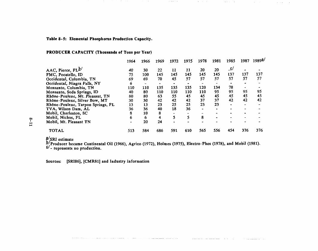
Table 8-5: Elemental Phosphorus Production Capacity.
PRODUCER CAPACITY (Thousands of Tons per Year)
1964 1966 1969 1972 1975 1978 1981 1985 1987 1989~'
b/ AAC, Pierce, FL- 40 30 22 11 11 20 20 -el - - FMC, Pocatello, ID 75 100 145 145 145 145 145 137 137 137 Occidental, Columbia, TN 69 69 70 45 57 57 57 57 57 57 Occidental, Niagra Falls, NY 6 - - - - - - - - - Monsanto, Columbia, TN 110 110 135 135 135 120 134 78 - - Monsanto, Soda Springs, ID 40 80 110 110 110 110 95 95 95 95 Rhbne-Poulenc, Mt. Pleasant, TN 80 80 63 55 45 45 45 45 45 45 Rhbne-Poulenc, Silver Bow, MT 30 30 42 42 42 37 37 42 42 42 RhBne-Poulenc, Tarpon Springs, FL 13 13 23 25 25 23 23 - - - TVA, Wilson Dam, AL 36 36 40 18 36 - - - - Mobil, Charleston, SC 8 10 8 - - - - - - -
m Mobil, Nichos, FL 6 6 4 5 5 8 - - - - Mobil, Mt. Pleasant TN - 20 24 - - - - - I-
- I-
TOTAL 513 584 686 591 610 565 556 454 376 376
8' RI estimate b/Sproduccr became Continental Oil (19661, Agrico (1972), Holmes (1975), Electro-Pbos (1978), and Mobil(1981). El- represents no production.
Sources: [SRI86], [CMR81] and Industry Information

Table 8-6: Revenues lrom Elemental Phosphoms Productlon and Total Coporate Revenues (1986).
Estimated Elemental
Phosphorus ~evenuea '
(in millions)
FMC $174.7
Monsanto $121.1
RhBne-Poulenc $110.9
Total Corporate Revenue
(in millions)
Occidental $72.7 $15,525.2
TOTAL $479.4 $33,590.9
i l ~ s t ima t ed revenue = estimated production x price Estimated production = 85 percent of capacity Price = $0.75 per pound or $1,500 per ton Revenue for RhBne-Poulenc = 51,642 FF x S0.1571FF
Elemental Phosphorus
as a Percent of Total Revenue

P, to high-value specialty products. The company's share of each end use market within the
industry, and the share of each end use within the company's line of phosphorus products, are listed
in Tables 8-7 and 8-8 [SR180].
The value of production froiii Monsanto's elemental phosphorus plants in 1983 is estimated to have
amounted to $199.5 million (Table 8-6), or 1.7 percent of total corporate revenues of $6,879.0 million.
8.2.2.2 FhlC Corporation
The second largest American producer of elemental phosphorus is FMC Corporation. FMC operates
a single plant, with four furnaces and an operating capacity of 137,000 tons per year, in Pocatello,
Idaho. Furnaces in the plant are maintained on a rotating schedule in which each furnace is
completely refitted or rebuilt every six to eight years [SRI83].
Phosphate rock for FMC's elemental phosphorus plant is obtained from low grade shale a t the Gay
mine, a mine operated jointly by FMC and Simplot. The entire FMC share (80 percent) of the Gay
mine's output is used to produce elemental phosphorus. With the Gay mine expected to be depleted
by 1990, FMC will probably shift its mining to land it has leased or subleased from Federal and State
governments in Caribou County, Idaho. The company is believed to hold all the permits required for
this change [SRI86]. Siniplot operates the mine and supplies FMC with 1.5-1.6 million tons of 53-54
percent BPL furnace grade rock per year.
FMC's largest market area for its elemental phosphorus products is in builders and water treatment
for detergents, with other ~iiarket areas small by comparison. Details of FMC's market position are
provided in Tables 8-9 and 8-10 [SRI83].
In 1986, the value of elemental phosphorus production for FMC was approximately $174.7 million,
or 5.7 percent of total corporate revenues of $3,078.9 million (Table 8-6).
The subject of numerous acquisitions in recent years, the Stauffer Chemical Company has changed
completely since 1985. Effective March 15, 1985, Chesebrough-Pond's, Inc., a $3 billion per year
producer of toiletries and food products, acquired Stauffer for approximately $1.3 billion. At the
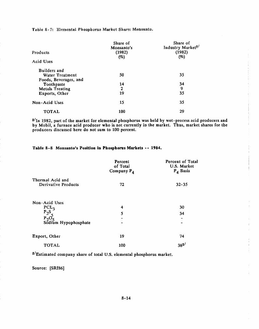
Table 8-4 : Eleraemld Phosphows Market Share: Momsento.
Products
Acid Uses
Builders and Water Treatment
Foods, Beverages, and Toothpaste
Metals Treating Exports, Other
Non-Acid Uses
Share of Monsanto's
(1982) (%)
Share of Industry ~ a r k e t i '
(1982) (%)
TOTAL 100 29
s11n 1982, part of the market for elemental phosphorus was held by wet-process acid producers and by Mobil, a furnace acid producer who is not currently in the market. Thus, market shares for the producers discussed here do not sum to 100 percent.
Table 8-8 Monsanlo's Position in Phosphorus Markets - - 1984.
Thermal Acid and Derivative Products
Non- Acid Uses PCL3 PzS< ~ 2 < 5 Sod~um Hypophosphate
Percent of Total
Company P4
Percent of Total U.S. Market
P4 Basis
Export, Other 19 74
TOTAL 100 38i1
i l~s t imated company share of total U.S. elemental phosphorus market.
Source: [SRI86]
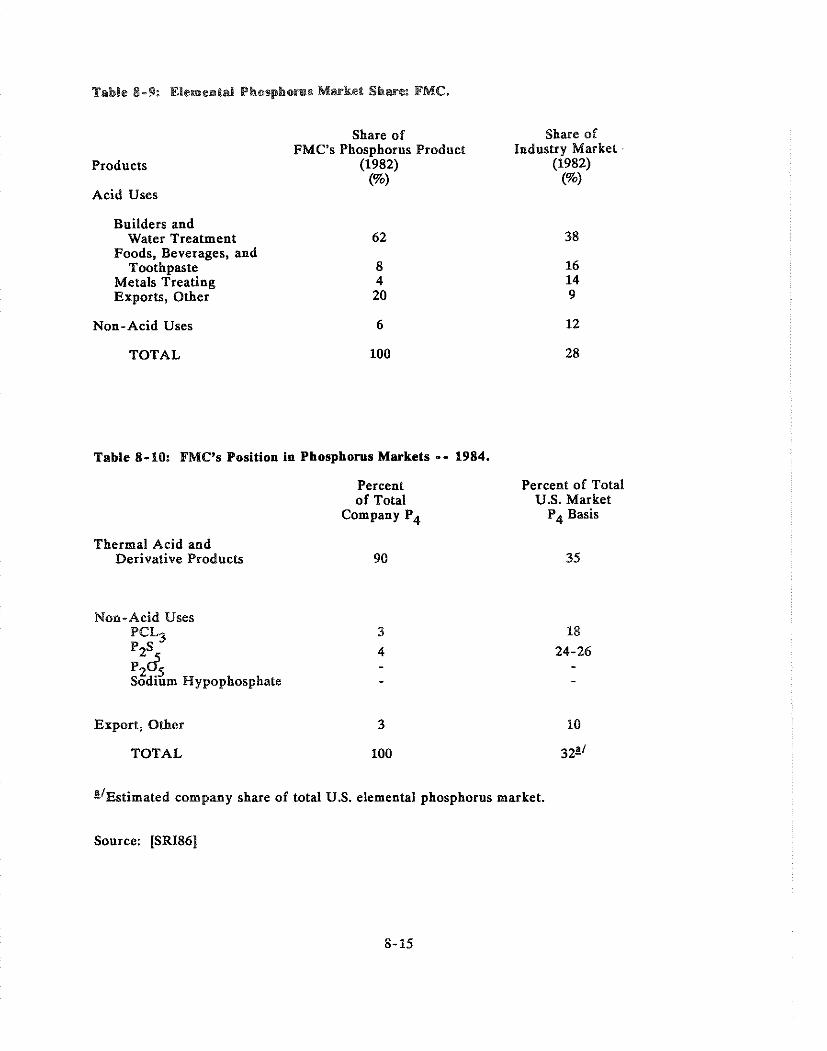
Table 8-9: Elemental Phosphoms Market Share: FMC.
Products
Acid Uses
Builders and Water Treatment
Foods, Beverages, and Toothpaste
Metals Treating Exports, Other
Non-Acid Uses
TOTAL
Share of FMCs Phosphorus Product
(1982) (%)
Table 8-10: FMC's Position in Phosphorus Markets - - 1984.
Thermal Acid and Derivative Products
Percent of Total
Company P4
90
Non-Acid Uses PCL3 3
P2Sc 4
~ 2 % Sod~um Hypophosphate
Export, Other
TOTAL
Share of Industry Market
(1982)
Percent of Total U.S. Market
P4 Basis
t l ~ s t i m a t e d company share of total U.S. elemental phosphorus market.
Source: [SRI86]
end of 1986, Cliesebrougli-Pond's was acquired by Unilever, Ltd., a $24 billion per year
Dutch-British conglomerate. I n July 1987, Imperial Chemical Industries, PLC, bought Stauffer
Chemical from Unilever f'or $1.69 billion in cash. Finally, in September, 1987, RhBne-Poulenc, S.A.
of France, acquired Stauffer's inorganic chemicals businesses, which had sales of $540 million and
employed 3,600 people in 1986, from imperial Chemical Industries for $522 million. This acquisition
made Rlione-Poulenc the biggest producer of specialty phosphates and regenerated sulfuric acids in
the world.
The most recent publicly available information on RhBne-Poulenc's P,+ operations was published by
SRI International in February 1986. A t that time, these operations belonged to Stauffer. Therefore,
the following presentation of company data is presented using Stauffer's name. It is worth noting
that Rhone-Poulenc also purchased the name Stauffer. Both plants continue to use the Stauffer name.
The third largest American producer of elemental phosphorus is Stauffer Chemical Company, with
two plants and an annual capacity of 87,000 tons. Stauffer's Mt. Pleasant, Tennessee plant has five
furnaces and capacity of 45,000 tons per year. The Silver bow, Montana plant has two furnaces and
capacity of 42,000 tons per year.
The source of phosphate rock for Stauffer's Tennessee plant is the company's Globe mine in Mt.
Pleasant, which is operated at about 0.4 to 0.5 million metric tons per year of ore and, in 1985, had
reserves for 10- I5 years of elemental phosphorus production. The sources of rock for the Montana
plant are mines in Wooley Valley, Idaho, ~ G o m i n g , and Utah. The first is the primary source, with
45 million metric tons of reserves in 1980. AII rock mined by Stauffer in Tennessee is used to
produce elemental phosphorus. A portion of the rock mined in the western states is sold to other
users. possibly to phosphate producers in Canada [SR186].
Stauffer is considered the second most diverse producer of elemental phosphorus. In the early 1970s
when environmental concerns were mounting, Stauffer turned its focus away from the laundry
detergent market to produce phosphorus compounds for end-use areas that at the time were more
highly valued. One such product is chlorinated trisodium phosphate, a cleanser and bacteriocide used
in dishwashing compounds and metal cleaners. The company is expected to continue its focus on
these areas, plus food uses and miscellaneous phosphorus chemicals. The market position of Stauffer
in each end-use area is indicated in Table 8-1 1 and 8-12 [SRI83]. In 1986, the value of production

Table 8-11: Elemental Phosphorus Market Share: Stauller.
Products
Acid Uses
Share of Share of Stauffer's Phosphorus Product Industry Market
(1.982) (1982) (%) (%I
Builders and Water Treatment Neg. Neg.
Foods, Beverages, and Toothpaste 35 50
Metals Treating 3 8 Exports, Other 31 25
Non-Acid Uses 31 29
TOTAL 100 16
Table 8-12: Stauffer's Position in Phosphorus Markets -- 1984.
Thermal Acid and Derivative Products
Non-Acid Uses PCL,
Percent of Total
Company P4
P2S 3 8-9
~2$5 2 Sodium Hypophosphate 24
Export, Other
TOTAL
Percent of Total U.S. Market
P4 Basis
5'~stimated company share of total U.S. elemental phosphorus market.
Source: [SRI86]

i'rom Stauffer's elementai pl~ospl~orus platits was estimated to equal $109.4 inillion. This represents
1.3 percent of Rhone-Poulcnc's total revenues of $8,107.8 million (Table 8-6).
8.2.2.4 Occidental Petroleurn Corfloral io~~
The smallest producer of elemental phosphorus is Occidental Petroleum, with one three-furnace plant
in Columbia, Tennessee. The annual capacity of the plant is 57,000 tons.
Occidental uses captive washed rock (61-62 percent BPL) obtained from a local mine where the
company owns 2,300 acres of reserves. In 1980, the reserves were estimated at 8 to I0 million metric
tons, with about 12 to 14 years of remaining life [SRI86].
Occidental's market has been dominated by builder phosphates manufactured at facilities in Texas
and Indiana. Little change is expected in the next few years, though some decline in the company's
position in phosphorus pentasulfide (P2S5) products has occurred due to the entry cf FMC into this
market. As of 1985, Occidental had ceased production of PzSS, but was tolling Pq through another
P2S5 producer to supply its customers. As these contracts expire, Occidental will phase out its P2Ss
business. The position of Occidental in each end-use market is detailed in Tables 8-13 and 8-14
[SR186].
In 1983, elemental phosphorus is estimated to have contributed $71.7 million to Occidental's total
corporate revenues of $15,525.2 million, or 0.5 percent (Table 8-6). The company is known to have
attempted to sell its industrial phosphate operations in the early 1980s, but has since renewed its
power contract through 1993 [SR186].
8.2.3 Corn~etitive Products and Processes
Consumption of elemental phosphorus in detergents, the major end use of elemental phosphorus,
has been affected significantly by the availability of substitutes. With the controls or bans on
phosphates recently imposed in sonie states, and threat of regulation by others, detergent
manufacturers have reformulated their products, replacing phosphorus with carbonates, silicates,
citrates, zeolites, NTA and nitrilotriacetic acid. Sodium carbonate (soda ash) is used in markets that
havecompletely banned phosphorus. Though relatively inexpensive, sodiumcarbonate is less effective
in cleaning than sodium tripolyphosphate (STPP), sometimes leaving residues on fabrics and being

Table 8-13: Elemental Phosphoms M~arket Share: Occidental.
Products
Acid Uses
Builders and Water Treatment
Foods, Beverages, and Toothpaste
Metals Treating Exports, Other
Non-Acid Uses
TOTAL
Share of Occidental's
11982)
Neg. 5
23
Table 8-14: Occidental's Position in Phosphorus Markets -- 1984.
Share of Industry Market
(1982) (%)
Thermal Acid and Derivative Products
Non-Acid Uses
Hypophosphate
Export, Other
TOTAL
Percent of Total
Company P4
Neg. 8
Percent of Total U.S. Market
P4 Basis
"'Estimated company share of total U.S. elemental phosphorus market.
Source: [SRI86]
less thorough as a soil defloccul:lnt. (FMC and Stauffer are among the producing firms). Citrates
are another \ iable alternative. With their high solubility characteristics, citrates have beconie the
major builder used in heavy-duty liquid laundry detergents. However, citrates may cake when
prepared in powders and thus are not attractive substitutes in powder formulations.
A third product competing with STPP for use in detergents is zeolites, sodium aluminosilicates that
soften water by ion exchange. Alone, zeolites are not as effective as STPP in cleaning, but are often
combined \vith it to produce a builder system with lower phosphate content. Since 1978, zeolites have
become commercially significant. The fourth challenge to STPP in detergents is NTA. In 1970, use
of NTA as a builder was voluntnrily suspended in response to an unpublished government report
suggesting the conipound was teratogenic. In 1980, EPA issued a statement that NTA posed no threat
to human health. NTA is now considered anlong the most attractive alternatives to STPP.
Another source of competition for the elemental phosphorus industry is the phosphoric acid produced
from phosphate rock through wet process methods. Wet process acid has historically been less pure
than acid produced fro111 elemental phosphorus (called thermal process acid). When thermal acid costs
and prices were low, it was not economical for wet process acid producers to purify their product to
compete with the thermal acid. However, the increasingly high costs and prices of thermal acid have
opened some traditional markets to wet process acid manufacturers who can now produce comparably
pure acids a t a competitive price. For example, Olin Corporation, a wet acid producer, had a seven
percent share of the market for phosphorus in detergents in 1984.
8.2.4 Economic and Financial Characteristics
The major economic and social factors affecting demand for phosphorus derivatives are population
growth, G N P growth, and to a lesser extent, demand for certain durable goods.
The largest end use for ele~ilental phosphorus, detergents, has historically grown about one percent
per year, approximately equal to population growth. With the controls on phosphates imposed in
some states and subsequent reformulation of detergents, this use declined in the 1970s. By 1981,
demand appeared to have restabilized at a one percent per year growth rate [CENBI].
Demand for phosphorus in food and beverages has reached maturity and closely follows changes in
GNP. Historically, the use of oil additives has grown at GNP rates or less. Uses in metal treating
are iiiore cyclical, fluctuating with demand For durable goods, especially autoniobiles [CEN84,
CEN78).
Most (approximately 80 percent) elemental phosphorus is used captively to produce phosphoric acid
and derivatives. The meaning of the price data available for elemental phosphorus is, therefore,
somewhat anibiguous. Manufacturer and co-producer transfer values are considerably below the list
price published by the nianufacturers of 90 to 100 cents per pound.
Table 8-15 compares the published list price and the actual average trading price for P4 from 1960
to 1984. In 1983 and 1984, the list price is 30 percent higher than the average sales price. Because
it is probably more representative of the real price, the average sales value has been used in the
calculation of corporate elemental phosphorus revenues; an estimate of $0.75 per pound or $1500
per ton was selected.
Because the market for Pq is a slow-growth market, and because most P q i s sold captively within each
company, it is expected that these prices, stable since 1983, will continue within the same range
throughout the 1980s.
In 1987, approximately 1,820 persons were employed directly by the elemental phosphorus industry.
Employment in each state is listed in Table 8-16. Estimated employment in each plant was listed
in Table 8-3. Direct employment in the elemental phosphorus industry represents only a part of
the employment that could be affected by a change in demand for elemental phosphorus. Others
potentially affected would include phosphate rock miners and workers in other phosphorus chemical
manufacturing facilities.
Current forecasts for the elemental phosphorus industry indicate low growth and weak prospects for
industry expansion. Major factors leading to the forecast are increasing costs of production,

Table 8-19: Average Price Range -- Bhoephoms - - While. (Cents per Pound - - FOB Plant)
Price - 1 9 6 0 u 1 9 7 0 1 9 8 0 1 9 8 2 1 9 8 3 1 9 8 4 1 9 8 5 1 9 8 8
Trade List 19 19 19 53 80 80 90 91 91 91 91
Avg. sales' 16 15 15 45 61 68 70
Average sales values include captive interplant transfers, no merchant market pricing.
Source: [MPC85]

Table 8-16: 1987 Employment by State for the Elemental Plbrosphonrs Industry.
State
Idaho Tenaesee Montana
Number of Employees

competition from substitutes, consumer and social trends, and lack of new uses for elemental
phosphorus and its derivatives.
Changes in the cost of elenrental phosphorus in recent years have been largely influenced by
electricity costs, which have been increasing steadily and are expected to continue to increase. The
increased cost of phosphorus and its derivatives has made substitutes more attractive. Substitutes in
detergents, such as zeolites, NTA, and wet process phosphoric acid, are attractive both economically
and because of environmental concerns and. in the case of zeolites and NTA, restrictions on
phosphate use. Other uses of elemental phosphorus are deterred by substitutes and/or social factors.
Phosphate-containing insecticides, a small market for the industry which had been growing at about
10 percent per year, face competition from non-phosphate insecticides. Uses in lubricating oils are
increasing, but the lubricating oils are also lasting longer, offsetting the gains. Detergent uses
resumed a slight upward trend in 1981-1984, but are still threatened by growth in consumer use of
liquid detergents, trends toward lower washing temperatures, and use of zeolite builders in place of
phosphates in formulas. As mentioned previously, bans on phosphates have been imposed, removed,
and re-imposed in some states. Additional states may join New York, Indiana,.Michigan, Wisconsin,
Minnesota, Connecticut, and Maine in banning or controlling phosphates. In the past two years, the
District of Colunlbia, Virginia, Maryland, and North Carolina have restricted phosphate use. South
Carolina, Oregon and Illinois are considering phosphate bans. On the brighter side for detergent uses
are the continued consumer demand for the new concentrated detergent powders, which have high
concentrations of phosphates, and demand fo r phosphates in industrial detergents, which has been
gro\ving in the 1980s at 3 percent per year or greater [CEN84, CEN821.
8.3 Current Emissions. Risk Levels. and Feasible Control Methods
The Elemental Phosphorus Plant source category consists of eight facilities that produce elemental
phosphorus by the electric furnace method. In 1988, five of these plants were operating, while three
were not. These plants have been evaluated in previous EPA assessments under Section 112 of the
Clean Air Act, and are subject to the NESH.AP (40 CFR 61, Subpart K ) pronlulgated on February
5, 1985. The NESHAP established an emissions limit of 21 Curies per year (Cilyr.) for polonium-
210 released from calciners and nodulizing kilns. This analysis examines alternative standards for
emissions of radionuclides from calcining operations in the manufacture of elemental phosphorus.
Radionuclides of the uraniurn series, including polonium 210 (Po-210), lead (Pb-210), and uranium
238 (U-238), occur naturally in phosphate rock. The exhaust gases from phosphate rock nodulizing
calciners at elemental phosphorus plants are considerably enriched with radionuclides because the Po-
210 and Pb-210 volatize at the elevated temperatures in the calciner. As the exhaust gases cool, the
radionuclides condense on the surface of mineral particulate matter or condense to for111 new
particles. In the absence of adequate particulate controls, these emissions are vented to stacks for
release to the atmosphere. The EPA conducted emission tests a t several elemental phosphorus plants
to characterize and quantify uncontrolled particulate and radionuclide emissions from the calciners
and controlled emissions from the existing control systems.
Emissions of particulate matter and condensed radionuclides from these plants can be reduced by the
application of modern particulate control technology. Presently, low pressure drop scrubbers are
being used to reduce emissions of particulate matter from the nodulizing calciners. Emission control
efficiencies for these low-pressure drop scrubbers are relatively low compared to those for high
pressure drop scrubbers, wet electrostatic precipitators (ESP), or fabric filters (baghouses). These
more efficient devices could potentially be used to control particulate and condensed radionuclide
emissions from calciners at elemental phosphorus plants.
8.3.1 Current Emissions and Estimated Risk Levels
The following section includes a description of the elemental phosphorus production process, of
existing effluent controls and of current radionuclide emissions. In addition, there is a brief
examination of various tecl~noiogies available for the control of these emissions as well as a
presentation of the cost of purchasing, installing and maintaining them.
8.3.1.1 Process Descr i~ t ion
Volume 2 of the E~ls i ro~ i~ne~ i ta l In~pacl Slatemell1 [EPA89] and the supporting report on Airborne
Emission Cor~rrol Techriolog~i for the elemental phosphorus industry [SAI84] provide detailed data on
each plant, including design, operation, source and radionuclide content of phosphate rock processed,
and analyses of particulate and radionuclide emissions from various parts of the processing.
Recently, Midwest Research Institute completed a study entitled, Characterization and Control of
Radionuclide Enzissiorzs from Elenlerilal Phosphorus Producliorl, that updates the information

contained in SA184. These docunients provide a more detailed discussion of the elemental phosphorus
industry and are incorporated by reference.
Crushed and screened phosphate rock is fed into calciners and heated to the melting point, about 1300
degrees C. After calcining, the hot nodules are passed through coolers and into storage bins prior to
being fed into electric furnaces, The furnace feed consists of the nodules, silica and coke.
Phosphorus and carbon nlonoxide (CO) are driven off as gases and vented near the top of the furnace.
Furnace off-gases pass through dust collectors and then through water spray condensers where the
phosphorus is cooled to the molten state. The mix of phosphorus and water (phossy water) and mud
are then processed to recover the phosphorus. Clean off-gases from the condensers contain a high
concentration of CO and are used as fuel in the calciners.
8.3.1.2 Existiog Effluent C o ~ ~ l r o l s
Emissions from the calciners are typically controlled by low energy scrubbers. Since the 1984
assessment of this source category, one plant has upgraded its calciner emission controls by installing
a high energy scrubber system. Emissions f rom nodule coolers, transfer points and furnace tap holes
are controlled by either fabric filters or wet scrubbers. Screening plant emissions are usualiy
controlled by fabric filters. Fugitive dust and radon gas emissions are not controlled.
8.3.1.3 Emissions
Through the period 1975 to 1980, EPA measured the radionuclideemission rates from three elemental
phosphorus plants: FMC in Pocatello, Idaho [EPA77], ~ t a u f f e r ' in Silver Bow, Montana [AnSla],
and Monsanto in Columbia, Tennessee [An8lb]. Measurements were made from release points
representative of all major process operations in the production of elemental phosphorus.
All the emitted radionuclides are released as particulates except for radon-222, which is released as
a gas. Essentially all the radon-222 and greater than 95 percent of the lead-210 and Po-210 emitted
from these facilities are released from the calciner stacks. The high calcining temperatures volatize
h he Stauffer Chemical Company is currently owned by Rhone-Poulenc, S.A. Because Rhone- Poulenc also acquired the name, Stauffer, the company's elemental phosphorus plants have retained this name.
8-26

the Pb-210 and Po-210 from the phosphate rock, resulting in release of much greater quantities of
these radionuclides than of the uraniuni, thorium and radium radionuclides. Analyses of doses and
risks from these en~issions show the emissions of Po-210 and, to a lesser degree emission of Pb-210
to be the major contributors to risk from radionuclide emissions from the elemental phosphorus
plants.
In 1983, EPA conducted extensive additional radionuclide testing at the FMC plant in Pocatello
[EPA84c, Ra84aI and at the Stauffer plant in Silver Bow [EP;\84d, Ra84bl. In early 1984, limited
emission testing was done at the Monsanto plant in Soda Springs, Idaho [EPA84e, Ra84cI. This
testing was limited to calciner off-gas streams and focused prinlarily on Pb-210 and Po-210 emissions
in order to obtain additional information on these emissions and to obtain data on particle size
distribution and lung clearance classification of these radionuclides in the calciner off-gases.
Sampling of the calciner at Monsanto's Soda Springs plant was hampered by unavailability of suitable
sampling locations. The major results of the testing are summarized in Table 8-17, which shows the
estimated annual calciner enlissions for the three plants studird.
Table 8-18 presents the estiniated annual calciner emission rates for each of the eight elemental
phosphorus plants. These values were used to estimate the radiation doses and fatal cancer risks from
the plants.
The lung-clearance classifications and particle size distributions (AMAD) used in this assessment are
the same as were used in the 1984 BID.
Table 8-19 shows the number of people living within 80 kilometers of these sites and the source of
the meteorological data used in the calculations.
Table 8-20 gives estimates of the lifetime risk to the nearby individuals and the number of fatal
cancers to the regional population. These data are taken from Volume 2 of the Efzviro~zn~ental Impacf
Slarenle~ll.
The total number of fatal cancers per year in the regional populations around elemental phosphorus
plants is estimated at 0.077. The DARTAB computer code provides the frequency distribution of
lifetime fatal cancer risks for each elemental phosphorus plant. It gives the number of people in each
of a series of lifetime risk intervals and the number of cancer deaths that occur annually within each
interval. This information is summarized in Tables 8-21 and 8-22 for operating and idle plants,

Table 8-17: N;idio~aucliile Erniscio~is from C a i c E ~ ~ e r s a t Elerneiital Phcsphorus Plants ( 1983- 1984 Emission Test Results)
FhlC - Pocotello, ID 2 0.004 0 I: 8.60 Stnuffer - Silver Bow, MT , 2 0.0006 0.1 1 0.74 kIons3nto-Soda Springs, ID I 0.006 j.60 2 1 .OO
SOURCE: [EPA89]
' ~ n n i p l i n ~ at the Monsato - Soda Springs, ID plant was hampered by the unavailability of suitable sampling locations.
Table 8-18: Estimated An~tual Radionuclide Emissions from Elemental Phosphorus Plants.
Emissions (Ci/vearl
Plant U-238 Pb-210 Po-110
OPERATING PLANTS
FMC - Pocatello, ID 0.0032 0.14 10.0
hlonsanto - Soda Springs, JD 0.0005 0.35 1.4
Stauffer - Silver Bow, MT 0.0006 0.1 1 0.7d
Stauffer - Mt. Pleasant, TN 0.0003 0.058 0.28
Occidental - Columbia. TN 0.0001 0.064 0.31
lDLE PLANTS
hlonsanto - Columbia, TN 0.0020 0.41 0.61
Stnuffer - FL 0.0035 0.19 0.15
hlobil - Pierce, FL 0.0016 0.012 0.013
SOURCE: [EPA89]

T a b l e 8-19: Populatioils and Distsrtces to the Maxilnum Exposed lrrdi!iduals Arolrrld E le tne~~t i l l P i ~ o s p l ~ o r u s Plants.
O P E R A T I N G PLANTS
F M C , Idaho
Monsanto , ldnho
Stnuffer , Montana
S tau f fe r , Tennessee
Occidental . Tennessee
I D L E P L A N T S
Monsanto , Tennessee
Stauffer , Florida
Mobil , Florida
S O U R C E : [EPA89]
Number of Distance t o Source of People wi t l i i t~ hlaxilnurn Exposed hleteorological 80 k m I ~ ~ d i t i d u a l ( m ) Da ta
170,000 1,800 Pocatello, ID
100,000 4.000 Soda Springs, ID
7 1,000 2,500 Butte, M T
560,000 1,500 Nashvil le, T N
920,000 1 .500 Nashvil le, T N
Nashvil le, T N
T a m p a , F L
Orlando. F L
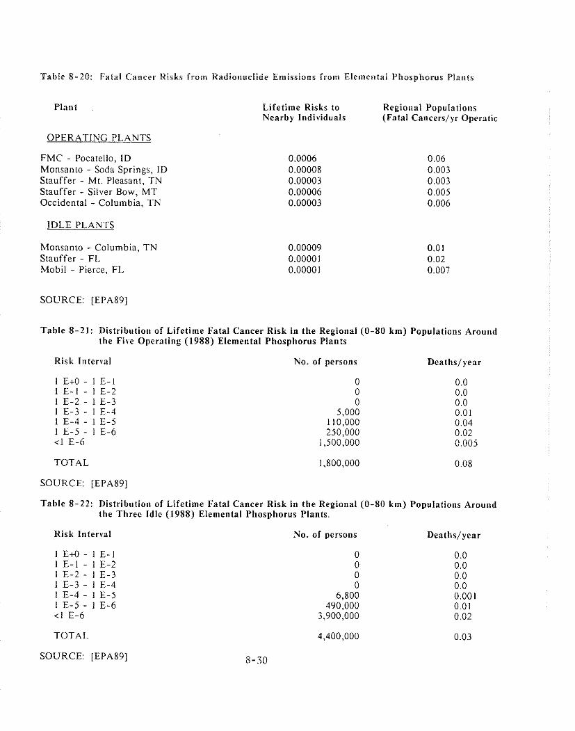
Table 8-20: Fatal Cancer Risks From Radior~uclide Emissions from Elemel~tal P l~osp l~o rus Plants
Plant
OPERATING PLANTS
FMC - Pocatello, ID Monsanto - Soda Springs, ID Stauffer - MI. Pleasant, TN Stauffer - Silver Bow, MT Occidental - Columbia, T N
IDLE PLANTS
Monsanto - Columbia, TN Stauffer - FL Mobil - Pierce, FL
Lifetime Risks to Regiolial Populatioris Nearby l~~d iv idua l s (Fatal Cancers/yr Operatic
SOURCE: [EPA89]
Table 8-21: Dis t r ibu t io~~ of Lifetime Fatal Cancer Risk in the Regional (0-80 km) Popu la t i o~~s Aroul~d the F i ~ e Operating (1988) Elemental Phosphorus Plants
Risk Interval No. of persolis Deaths/year
I E+O- I E-I 0 0.0 I E- I - I E-2 I E-2 - I E-3 1 E-3 - I E-4
TOTAL 1,800,000 0.08
SOURCE: [EPA89]
Table 8-22: Distributiot~ of Lifetime Fatal Cancer Risk in the Regio~ial (0-80 km) Populations A r o u ~ ~ d the Three Idle (1988) Elemental Phosphorus Plants.
Risk Interval No. of persons Deaths/year
1 E-I - I E-2 1 E-2 - I E-3 1 E-3 - 1 E-4
TOTAL
SOURCE: [EPA89]
respectively. Data on the idle plants are included in unlikely case that a plant recommences
operations. Risks for idle plants presented here will not occur unless one or more of these idle plants
resunies operation. These data reflect the number of deaths expected to occur annually within the
0-80 km populations.
8.3.2 Conlrol Technoloeies for Elerne~~ta l P h o s ~ h o r u s Plants
The nodulizing kiln or calciner is by far the most significant source of Po-210 emissions from
elemental phospliorus production. This section, based on information in MRI88, describes and
assesses control technologies that can be used to reduce those emissions. Generally Po-210 and Pb-
210 are volatilized in the kiln or calciner and condeme on the fine particles in the calciner particulate
matter emission stream (PM st re an^). The control systems currently installed in the industry
effectively collect large particles, but are not as effective in controlling fine particle emissions.
Consequently, the technologies examined in this section are those that have been demonstrated to
achieve high control efficiencies on fine particles.
Control of Po-210 and Pb-210 e~nissions is complicated by two factors. First, because the
temperature of the flue gas leaving the kiln may be 400°C (750°F) or higher, significant
concentrations of Po-210 can remain in the vapor phase. Second. the exhaust contains relatively high
concentrations of SO2 and HF. these acid gases can condense in the control system leading to
subsequent corrosion and deterioration of perforn~ance. Mechanisms for cooling the exhaust gases
and reducing the acid gas concentration in the gases are discussed in detail in MRI88.
Four fine PM stream control techniques are examined in this stud!.:
o u e t electrostatic precipitators (wet ESP's)
o venturi scrubbers
o spray dryers with pulse jet fabric filters (SD/FFs)
o high efficiency particulate air (HEPA) filters
The wet ESP and venturi scrubber are the control systems used at operating elemental phosphorus
plants. The SD,'FF and HEPA filters were selected as high-efficiency PM control devices that have
excellent potential for controlling Po-210 and Pb-210 emissions but that have not been applied to
:lemental phosphorus plants. The SD/FF systems have been applied successfully to combustion
.ources and mineral and metallurgical furnaces and have demonstrated high control efficiencies for

condensible niet:ils and acid gases. The HEPA Filter hns been demonstrated to achieve high control
efficiencies on rndionuclide eniissions from uranium industry processes.
Four of the five operating elemental phosphorus facilities currently operate spray towers as either
the primary control system or as a gas conditioning technique. These spray towers will remove coarse
particulate matter as well as acid gases from the gas stream. All of the control techniques, except the
SD/FF, can benefit from the reduced temperature, gas volume, and acid gas concentration that results
from the installation of a spray tower upstream of the primary fine PM control device. Technical
atid engineering details on these control technologies are de\.eloped in MRI88.
8.3.3 Cost of Control Techaoloeies
The capital and annualized costs for each of the applicable control devices were determined following
the guidelines established in Capiral and Operatirig Cosls of Selecled Air Pollution Cortlrol Syslents
(GARD Martual) [GARD78] and the EAB Cost Cor~trol Martual [EAB87]. These manuals were
prepared for the U.S. Environmental Protection Agency (EPA) to provide technical assistance to
regulatory agencies in estimating the cost of air pollution control systems. The costs in the GARD
Manual are based on December 1977 costs; those in the EAB Cost Cotttrol Marlual, on 1986costs. The
costs were adjusted to mid-1988 dollars using indices provided in Chentical E~tgineerirtg and by the
Bureau of Labor Statistics. Since the same basic procedure was used to cost each of the control
techniques, a cost program was developed for use on a microcomputer. The paragraphs below
describe the general cost methodology and key assumptions used to estimate the costs of the various
control options. Detailed assuniptions for each operating facility are presented in Appendices A
through E of MRI88.
The costs were calculated assuming that each of the fine PM control measures, with the exception
of the SD/FF, were added to control the exhaust from an existing spray tower. The existing system
removes most of the large particles, quenches and cools the exhaust gas stream (thus, reducing gas
volunle and ensuring condensation of gaseous radionuclide emissions) and properly conditions the
stream for treatment by the other options.
Capital costs include the direct and indirect costs to purchase and install the necessary ductwork,
control device, fan systems, and stack. Direct capital costs include instruments, controls, taxes,
freight, foundations, supports, erection and handling, electrical work, piping, insulation, painting,
and site preparation. Indirect capital costs include engineering and supervision, construction and

field expenses, construction fees, startup performance test, and contingencies. Table 4-4 in MU188
presents the assumptions used for direct and indirect cost estimates based on information given in
the CARD hlarr~rnl. All ductwork was sized based on a gas velocity of 20 meters per second (m/s)
(4,000 ft/min). Site-specific estimates of the length of additional ductwork to connect the existing
control system with the add-on control device were developed for the analyses in Section 5. Stack
diameters were calculated to provide a stack gas velocity of 18 m/s (3,600 ftlmin). All stack heights
are assumed to be 15 m (50 f t) for the add-on equipment. With the exception of connecting
ductwork, no special retrofit costs were included in the cost analyses. Based on information collected
during plant visits, MU1 determined that no retrofit problems should be expected at the operating
facilities.
Annualized costs include the total utility costs, the total operating labor costs, the total maintenance
costs, the total overhead costs, the capital charges, and the total waste disposal costs. The annualized
costs were based on 8,640 hours per year of operation (360 days)2. The utility costs reflect actual
utility costs in the area of each facility as presented in Appendices A through E of MRI88. The
operating and maintenance labor costs were determined using an average hourly wage of $12/hour(h).
The operating labor hours per shift for each control device were 4 h/shift for SD/FF's, 2 h/shift
for scrubbers, and I h/shift for ESP's. The maintenance labor was assumed to be 1 h/shift for ESP's
and scrubbers and 2 h/shift for SD/FF's.
The quantity of sludge or dry waste collected by the add-on control devices was determined based
on the efficient! of particulate removal. In the case of the SD/FF, the quantity of lime added to the
system also is considered. The cost to dispose of the waste in a secured landfill was assumed to be
$?O/ton. The waste is considered to be hazardous for these calculations because of the concenriation
of radioactive material. (For comparison, it should be noted that the cost of disposing of
nonhazardous wastes is approximately $5/ton.)
8.3.3.1 Venturi Scrubber Cost Assumotions
The capital and annualized costs for venturi scrubbers were based on procedures established in the
G A R D manual and on equipment costs established therein. Because of the large airflow encountered
' The effect of this assumption is probably to overestimate the operating and maintenance costs vis i2 I J ~ S actual operating time. As was stated in section 8.2, it is assumed that the operating plants are producing for 7,400 hours (85 percent of capacity).
at most kilns, two identical scrubber systems in parallel were assumed on each kiln's exhaust stream.
Radial fans were evaluated because of their ability to operate at high pressures and temperatures in
an abrasive gas stream. The costs of the starter motor, direct and V-belt drives, and dampers are
included in the fan costs. The corrosiveness (fluorides) of the gas stream entering a scrubber from
the rotary kiln calciner requires that fabricated equipment cost estimates be based on the use of a
combination of Hastelloy and Type 316 stainless steel. Plate thickness of the fan housing and
ductwork was determined based on system static pressure. Details on the cost inputs for venturi
scrubber control options for each facility are presented in Appendices A through E of [MR188] for
the individual facilities.
8.3.3.2 \Vet ESP Cost Assu~n~tiorls
Capital and annualized costs for the ESP were based on an EPA cost update. A primary factor that
affects ESP costs is material of construction. The corrosiveness (fluorides) of the gas stream entering
an ESP from the rotary kiln calciner requires that fabricated equipment, ductwork and ESP housing
be constructed of a corrosion-resistant material. Costs for these components were based on the use
of Type 316 stainless steel. Collecting electrodes also were assumed to be constructed from Type 316
stainless steel.
8.3.3.3 SD/FF ~ b s t Assumotions
Spray dryer/fabric filter systems provide efficient collection of both condensible PM and acid gases.
Key design parameters that affect system performance and costs are lime addition, gas temperature
entering the FF. FF air-to-cloth ratio, and pressure drop through the system. Lime addition rates
were calculated under the assumption of a 1.5:l stoichiometric ratio of lime to H F and SOz combined.
The gas temperature at the FF inlet was assumed to be 150°C (300°F). An air-to-cloth ratio of 1:1.2
m2/m3/min (4:1 ft2/ft3/min) and a system pressure drop of 3.1 kPa (12.5 in. w.c.) were used.
Total direct costs for the SD/FF unit were estimated on the basis of the cost equation:
C = 7.1 15 Q ~ . ~ ~ ~
where:
C = total direct cost, $x103 in December 1987
Q = volumetric flow, acfm
This cost equation is based on comprehensive information collected by EPA as a part of the municipal
waste conibustion study. Vendors contacted during this study indicated that these costs would
provide reasonable c30 percent estimates.
8.3.3.4 HEPA Filter Cost Assum~tions
Calciner gas stream characteristics that affect HEPA filter design and costs are moisture content,
inorganic acid content, and loading in the gas stream to be treated. A spray tower is assumed to exist
upstream of the HEPA filtration system; the high moisture content of the spray tower exit gases
requires twatment of the gases by a de-mister and re-heater of the HEPA system. Because the
exhaust gases are corrosive, Type 304 stainless steel housings and filter frames, acid-corrosion
resistant filter media, and vinyl-clad aluminum separators are included in the cost of the system and
replacement filters to provide the best available corrosion resistance. Because the PM loading in the
gas stream exceeds the recomnlended maximum of 2.3 nlg/m3 (0.001 g/acf), the cost of a pre-
filtration slstem is included in the total system cost. Estimated costs of the HEPA system, consisting
of the pre-filters, HEPA filters, pre-filter/HEPA filter bank housing, de-mister, re-heater, and
de-mister, reheater housing were obtained from equipment vendors.
A major operating cost for HEPA filters is filter replacement. The operating life of a HEPA depends
on the increase in pressure drop resulting from particle collection within the filter media. A general
guideline used to design filter systems is 4 lb/1,000 ft3/min rated capacity (1.82 kg/1,000 ft3/min).
Filter life \\as estimated by assuniing a HEPA capacity of 7.9 lb/1,000 ft3/niin (3.6 kg/1,000 ft3/min)
per filter based on vendor information. The methodology used to estimate filter life consisted of the
lollo\r ing steps:
I. Obtain particle size distribution in spray tower exist gas stream from test data (where
available);
2. Predict the mass of particles removed by pre-filtration using design pre-filter removal
efficiencies for a given particle size;
3. Predict mass of particles removed by HEPA filter using filter design HEPA removal
efficiencies;
4. Assume n I'ilter capacity i'or HEPA filter and calculate HEPA filter operating life with
and without use of a pre-filter;
5 . Calculate pre-filter life as two times the HEPA filter life without the use of a pre-
filter: and
6 . Calculated HEPA filter life as the HEPA capacity divided by the particulate loading
rate into the HEPA filter.
Estinlates of the labor cost to replace pre-filters and HEPA filters as they are exhausted is based on
0.25 hours of labor per filter per replacement cycle. For example, filter replacement for a 36 filter
bank r e ~ u i r e s 9 hours.
Exhausted filters are expected to exhibit increased concentrations of particulate matter containing
Po-210 and Pb-210. T o reduce the risk of inhalation of particles that may become airborne as a
result of filter handling during the replacement process, an automatic bagout containment system is
included in the system cost. Automatic bagout facilitates removal of exhausted filters without direct
operator contact. Heavy duty PVC bags are installed inside the filter housing between the filters and
the housing access door. When the door is opened, the bags form a barrier between the operator and
the contaminated filter. By working through the bag, the operator can remove the filter and draw
it into the bag without direct contact. The cost of replacement bags was included in the estimate of
re~lacenlent material cost.
8.3.4 Emissions Control Alter~tatives
As outlined above, four fine PM control techniques were identified as having potential for control
of Po-210 and Pb-210 eniissions from calciners--venturi scrubbers, wet electrostatic precipitators
(ESP's), spray dryers with pulse jet fabric filters (SD/FF's) and high energy particulate air (HEPA)
filters. Ten different control alternatives based on these four technologies were examined. Four of
the alternatives are based on venturi scrubbers at different pressure drops ( P's), four are based on
wet ESP's with different specific collecting areas (SCA's), and one each is based on a SD/FF system
and a HEPA filter system. The paragraphs below describe the control alternatives and the
assumptions that were used to assess performance and cost of these systems.
Four of the control alternatives comprise venturi scrubbers operated downstream from a spray tower.
Four different pressut-e drops were examined--2.5 kPa (10 in. w.c.), 6.2 kPa (25 in. w.c.), 10 kPa (40
in. w.c.), and 20 kPn (80 in. w.c.). The values from 2.5 kPa to 10 kP3 represent the range of P's for
venturi scrubbers at recently installed control systems on elemental phosphorus plant calcining
operations. The 20 kPa level was selected as a control alternative that is more stringent than the
controls typically used in the industry, but that has been applied to other metallurgical processing
facilities. Two other assumptions were made in evaluating the performance and costs of the venturi
scrubber control alternatives. First, a spray tower was assumed to be used upstream from the venturi
to control acid gases and condition the gas stream for the venturi. All of the operating facilities
except FMC currently have a spray tower as a part of their control system that is assumed to be
useable as the conditioning system for the venturi. Second, for all the venturi scrubber control
alternatives, the L/G ratio was assumed to be 1.3 l/m3 (10 ga1/1,000 ft3). This value was selected
because it represents the upper end of the range typically found in venturi scrubber applications.
A cyclonic mist eliniinator also was assumed for all venturi scrubber alternatives. Note that although
FMC does not have a spray tower in its systems, no tower was costed for this study. The low energy
scrubber that FMC has in place as assumed to provide coarse PM control and gas conditioning.
The four ESP control alternatives that were considered comprised spray towers for acid gas control
and gas stream conditioning followed by flat-plate wet ESP's. The four SCA levels that were
considered were 39.4 (m/s)-' (200 ft2/kacfm), 78.8 (m/s)-' (400 ft2/kacfm), 118 (m/s)-'
(600 ft2/kacfm), and 158 (m/s)-1 (800 ft2/kacfm). These four SCA levels are higher than the SCA
n t the one wet ESP that is applied to a nodulizing kiln. However, that unit is an older unit with
relatively low PM removal efficiency. The range of 39.4 to 158 (m/s)-' (220 to 800 ft3/kacfm) is
representative of the SCA ievels typically found on metallurgical and mineral processing facilities.
The spray tower upstream from the ESP will remove acid gases from the gas stream and reduce the
temperature to 65' to 70°C (150' to 160°F) to assure that the Po-210 and Pb-210 are condense before
entering the ESP.
The ninth control alternative is the SD/FF control system. For this alternative, the exhaust stream
is vented directly to the spray dryer without pretreatment. No SD/FF systems have been applied to
elemental phosphorus facilities. However, they were selected as a stringent control technique because
they have been demonstrated to control acid gases and condensation PM in other metallurgical and
mineral processing operations suchas aluminum reduction and glass manufacturing. Key assumptions
made to estimate performance and cost are that sufficient moisture will be added to reduce gas
temperature to 120°C (250°F) at the inlet to the FF, that lime will be added at a 1.5 stoichiometric

ratio for HF and SO2 combined, and that a pulse jet fabric filter capable of maintaining an outlet
grain loading of 0.023 g/dscm (0.01 g/dscf) will be installed.
The final control alternative comprises a spray tower scrubber, a reheat system, a prefilter, and a
HEPA filter in sequence. The spray tower is used to reduce the acid content of the gas stream and
to remove larger sized PM. The reheat system is needed to raise the gas stream temperature
sufficiently to prevent condensation of moisture and inorganic acids in the HEPA filter. The
prefilter is used to reduce the PM loading to the HEPA filter and thereby extend its life. The HEPA
filter system has not been applied to elemental phosphorus facilities and generally is not applied to
furnaces that generate gas volumes as large as those generated by elemental phosphorus process
calciners or nodulizing kilns. However, the system was selected for consideration because HEPA
filters have been used successfully to control radionuclide emissions from uranium processing
facilities and they do provide a much greater level of control than is provided by the other control
alternatives.
8.3.5 Performance of Control Alternatives
The performance of each of the 10 control alternatives was calculated based on the reduction from
baseline emissions that could be achieved by application of the control alternative. For each control
alternative and each operating facility, annual emissions of Po-210 and Pb-210 were estimated using
the procedures desiribed in Section 4 of MRI88. The estimates of Po-210 and Pb-210 emission rates
at the scrubber/ESP inlet, based on the assumptions that a spray tower is located upstream from
primary control device are given in Table 8-23.
The estimate for FMC, Monsanto, and Stauffer, Montana, are based on tests conducted by EPA in
1983 and 1988 that measured emissions at the outlet of low-energy scrubbers a t those facilities.
Because the control systems at the two Tennessee plants consist of spray tower scrubbers, the emission
estimates for those two facilities are based on the baseline emissions from those facilities. Separate
estimates were developed for moving grate calciners (FMC) and rotary kilns (all other facilities).

Table 8-23: Estimated Po-210 arid Plr-210 Emissioes a t the Scrubber/ESP Inlet
Control efficiencies also were developed for the SD/FF and the HEPA. The resultant efficiencies
are 99.82 percent for rotary kilns and 99.85 percent for grate kilns. For the HEPA filter, the
efficiency was assumed to be 99.998 percent as described above. Nationwide and plant specific
capital and annualized cost summaries for each control alternative are presented in Tables 8-24
through 8-29. The estimated Po-210 removal efficiency of each control technology is also presented
in these tables.
8.4 Analysis of Benefits and Costs
This section examines the benefits and the costs of alternative Po-210 standards for emissions from
elemental phosphorus plants. Although Pb-210 emissions comprise an important part of total
radionuclide emissions, the control of Pb-210 is similar to that of Po-210, therefore the following
section refers only to the control of Po-210 enlissions. It is assumed that Pb-210 emissions are
reduced in proportion to Po-210 emissions.
8.4.1 Benef i ts of Po-210 Emissions C o ~ ~ t r o l
The health benefits that accrue to society over time from the control of Po-210 emissions at the
elemental phosphorus plants consist largely of the reduction in expected lung cancers and, to a lesser
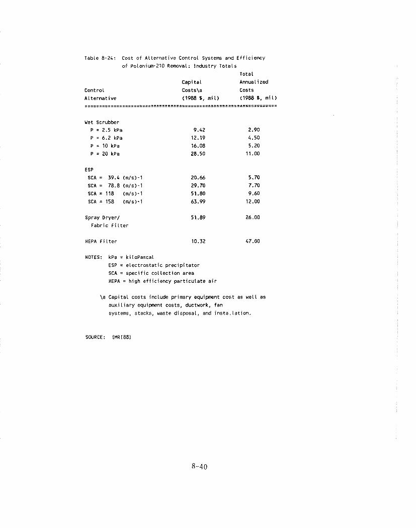
Table 8-24: Cost o f A i ternat ive Control Systems and E f f i c iency
of Poloniun-210 Removal: Industry Totals
Total
Capi ta l Annualized
Control Costs\a Costs
A l te rna t i ve (1988 S, m i l ) (1988 1, m i l ) i===========iiiiiiE==========z=====================================
Wet Scrubber P = 2.5 kPa
P = 6.2 kPa
P = 10 kPa
P = 20 kPa
ESP
SCA = 39.4 (m/s)-1
SCA = 78.8 (m/s)-1
SCA = 118 (m/s)-1
SCA = 158 (mls)-1
Spray Dryer/
Fabric F i l t e r
HEPA F i l t e r 10.32 47.00
NOTES: kPa = kiioPascal
ESP = e iec t ros ta t i c p rec ip i ta to r
SCA = spec i f i c c o l l e c t i o n area
HEPA = high e f f i c iency p a r t i c u l a t e a i r
\a Capi ta l costs include primary equipnent cost as wel l as
a u x i l i a r y equipnent costs, ductuork, fan
systems, stacks, waste disposal, and insta. la t ion.
SOURCE: CMR1881
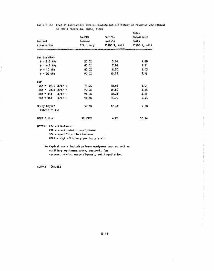
Table 8-25: Cost of l i i l e r ~ e i u e Control S y s I I m a d E t t i c i m c y of Pwlmiua-210 Rertivat at FRC'a, Pocsteilo, lab, PLsnt.
Total Po-240 Capital hw l ised
Control R w a l mats\* Costs
A l t e r ~ t i v e Ef f ic imcy (1W $, s i t ) (1% X, m i l )
Uet Scrubber P = 2.5 kPa P = 6.2 kPa P = 10 kPe P 3 20 kP4
ESP SCA = 39.4 (.Is)-? 71 .a 10.64 2.M SCA = 78.8 (m/s)-1 W.G% 15.50 2.84 SCA = 118 (./s)-l %.a 20.28 3.65 SCA = 158 (01s)-1 98.6% 24.79 4.43
Spray Dryer1 Fabric F i l t e r
HEPA F i l t e r 99.998% 4 .M 10.14
WTES: kPa = kiloPascal ESP = electrostatic precipitator SCA = specif ic collection area HEPA = high efficiency particulate a i r
\a Capital costs include p r i m r y q u i p . m t cost ss u e l l ss auxi l iary equipment costs, ducruork, fan systems, stacks, uaste disposal, and instal lat ion.
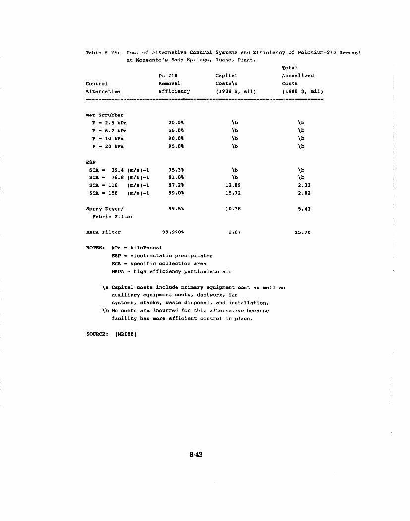
T b l e 8 -26 , Cost of Al ternat ive Control Syateme and BIficisncy of ~olonium-210 m v a l a t Wnaanto's Soda Springa, Idaho, Plant.
Tota l
W-210 Capi ta l Annualized
Control R-val Costs\a Costa
Al ternat ive Efficiency (1988 5 , a i l ) (1988 $, mil )
wet Scrubber
P - 2.5 *Pa 20.08 P - 6.2 *Pa 55.0%
P - 10 *Pa 90.0%
P - 20 *Pa 95.0%
ESP
SCA - 39.4 ( m / s ) - 1 75.3% \h
SCA - 78.8 (m/s)-1 91.09 \h
SCA - 118 ( m / s ) - 1 97.2% 12.89 SCA - 158 (m/s)-1 99.0% 15.72
Spray Dryer/ 99.5% 10.38
Fabric F i l t e r
HBPA F i l t e r 99.998% 2.87
NOTES: *Pa - ki lopascal
ZSP - e l e c t r o s t a t i c p r e c i p i t a t o r
SCA - s p e c i f i c co l l ec t ion a rea
HBPA - high e f f i c i ency p a r t i c u l a t e a i r
\a Capi ta l cos t8 include primary equipment cos t as well a s
aux i l i a ry equipment cos ta , ductwork, f a n
s y s t e m , s tacks , waste di6posa1, and i n s t a l l a t i o n .
\b No cos t s a r e incurred f o r t h i s a l t e rna t ive because
f a c i l i t y has ware e f f i c i e n t control i n place.

Tabie 8-27: Cost o f A l te rna t i ve Control System end E f f i c i e n c y o f Poionium-210
Removal a t the Stauf fer Mount Pleasant, Temessee, PLant.
Tota l
Po-210 Capi t a l Annualized
Control Rernova l Costs\a Costs A l te rna t i ve E f f i c iency (198B $, m i [ ) (1988 S, m i l ) ............................................................................
Vet Scrubber
P = 2.5 kPa 20. 0% 1.46 0.59
P 1 6.2 kPa 55.0% 1.87 0.75
P = 10 kPa 90.0% 2.46 0.93
P = 20 kPa 95.0% 5.23 1.61
ESP
SCA = 39.4 (m/s)-1 75.0% 3.14 0.64
SCA = 78.8 (m/s)-1 92.9% 4.39 0.85
SCA = 118 (m/s)-1 96.4% 5.95 1.12
SCA= 158 (m/s)-1 96.4% 7.39 1.37
Spray Dryer/ 99.6% 6.58 3.12 Fabric F i l t e r
HEPA F i l t e r 99.998% 1.02 7.45
NOTES: kPa = k i lopascal
ESP = e l e c t r o s t a t i c p r e c i p i t a t o r
SCA = spec i f i c c o l l e c t i o n ares
HEPA = h igh e f f i c iency p a r t i c u l a t e a i r
\a Capi ta l costs include primary equipnent cost as wel l as
a u x i l i a r y equipnent costs, ductwork, fan
systems, stacks, vaste disposal, and i n s t a l l a t i o n .
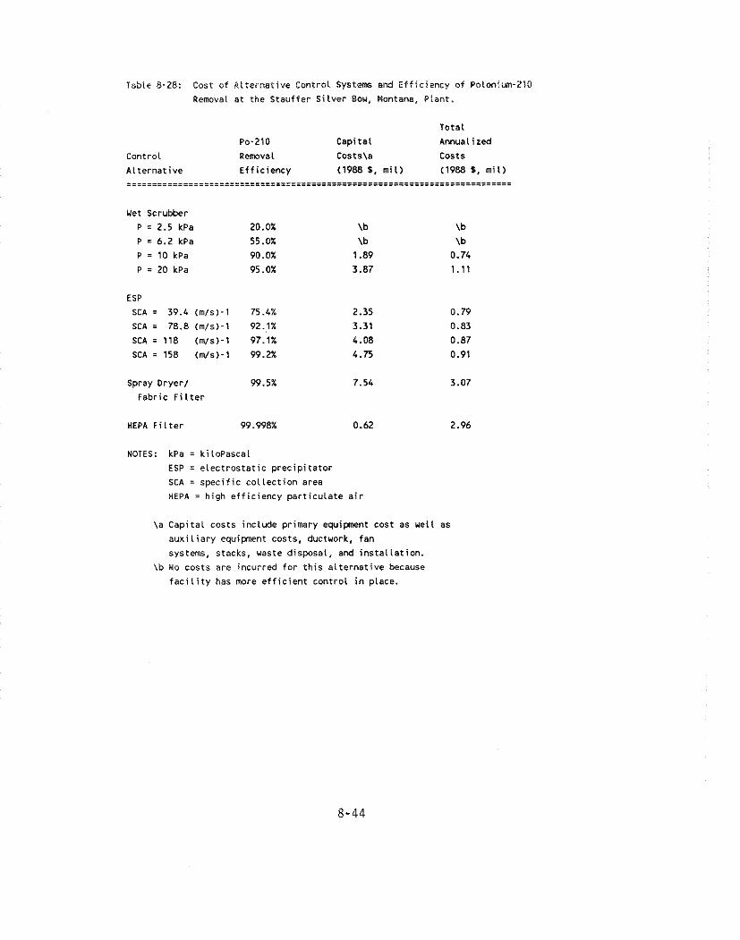
Tsble 8-28: Cost of Alternative Control Systems and Efficiency o f Polonim-210
Remaval at the Stauffer Silver Sou, Montana, Plant.
Total Po-210 Capital Annualized
Control Removal Costs\a Costs
Alternative Efficiency (1988 1, mil) (1988 1, mil) ...........................................................................
Vet Scrubber P = 2.5 kPa 20.0% \b \b P = 6.2 kPa 55.0% \b \b P = 10 kPa 90. OX 1.89 0.74 P = 20 kPa 95.0% 3.87 1.11
ESP SCA = 39.4 (rn/s)-1 75.4% 2.35 0.79
SCA = 78.8 (m/s)-1 92.1% 3.31 0.83 SCA = 118 (m/s)-1 97.1% 4.08 0.87 SCA = 158 (m/s)-l 99.2% 4.75 0.91
Spray Dryer/ 99.5% 7.54 3.07 Fabric Filter
HEPA Filter 99.998% 0.62 2.96
NOTES: kPa = kilopascal ESP = electrostatic precipitator SCA = specific collection area HEPA = high efficiency particulate air
\a Capital costs include primary equipnent cost as well as auxiliary equipnent casts, ductuork, fan
systems, stacks, waste dispasal, and installation. \b No costs are incurred for this alternative because
facility has more efficient control in place.
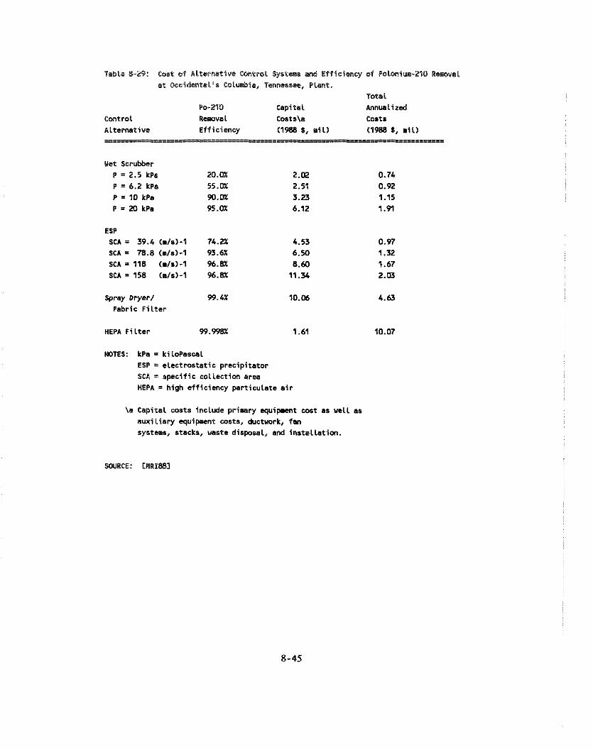
Tabte 8-23: Cost a9 Alternstiire Contml Syntcso snd Ef f ic imcy of Polonium-230 R w v s l a t OccidmtalLs CoLu&ia, Tmnessn, PLsnt.
Total Po-210 Capital Annwliaed
Contmt Recwvsl Coata\a Costs A l t e r ~ t i v e Efficiency (1988 1, m i l ) ('1988 8 , mil) -
Uet Scrubber P = 2.5 kPs 20.0% 2.02 P = 6.2 kPa 55.0% 2.51 P = 10 kPa W.0% 3.23 P = X ) kPa 95.0% 6.12
ESP SCA = 39.4 (m/s)-1 74.Z 4.53 SCA = 78.8 (./a)-1 93.62 6.50 SCA = 118 - 1 96.82 8.60 SCA = 158 (.Is)-1 96.8% 11.34
Spray Dryer/ 59.4% 10.06 Fabric F i l t e r
HEPA F i l t e r 59.9982 1.61 10.07
NOTES: kPa = LiloPascal ESP = electmstat ic precipitator SCA = specif ic collection area HEPA = high eff iciency particulate a i r
\a Capital u u t s include primary quip.ent uut as well as aux i l ia ry q u i w n t wsts, ductwrk, fan systems, stacks, waste disposal, and instal lat ion.
SOURCE: ERR1881
extent, the reduction i n non-hazardous particulate emissions near the site. The health benefits
associated with the reduction of Po-210 emissions are determined to be the major component of the
total health benefits due to any reduction of emissions at these plants. The efficiency of the
particulate control technologies in terms of Po-210 removal and control is, therefore, of great
importance in the calculation of the expected health benefits under alternative control scenarios.
Tables 8-24 through 8-29 presented the estimated efficiencies of Po-210 control of the various
control alternatives. in this section, the expected benefits of the proposed alternate standards are
estimated by applying proportionate reductions to the estimated health risks currently generated in
the population residing within 80 Lni of the five operating plants. This method assumes a
proportionate reduction in fatal cancers for given statutory reductions in Po-210 emissions. The
proportionate reduction assumption is consistent with AlRDOS computer code procedures for
e\.aluating population exposures in the affected areas and with the RADRISK code for translating
exposures into expected fatal cancers, based on the linear dose-response model.
The results of analyses to determine the efficiencies of various alternatives for controlling the
polonium-210 and lead-210 en~issions from calciner off-gas systems at the five operating elelliental
phosphorus plants are summarized in Table 8-30. As described above, the control alternatives
considered were the installation of wet (Venturi) scrubbers, electrostatic precipitators (ESP), a spray
dryer followed do~vnstream by a fabric filter (SD/FF), and high efficiency particulate air (HEPA)
filters. The table presents the reduction in emissions that would result from the installation of the
ten different control technologies on each of the operating plants. As discussed above, baseline
emissions were estimated for each operating plant under the assumption that low-energy or spray
scrubbers were present at each plant. The emissions reductions are estimated assuming that additional
s)stems are added to these wet scrubbers. For the Spray Dryer/Fabric Filter system, the estimates
are determined by first removing the low energy wet scrubber (the baseline emissions are divided by
0.35) and adding the SD/FF.
Lifetime risks to nearby individuals and incidences of fatal cancers per year in the regional
populations were presented in Table 8-20. Table 8-31 and Table 8-31a present the benefits of the
installation of the xarious emission control technologies in terms of fatal cancer risk. Table 8-31
presents total risk figures for each plant and for each control technology. Table 8-31a estimates the

Table 8-30: Estimated Po-210 Emission Leveis Achieved by Control Atternatives.
Emission Leveis (Cilyear)
Controi FMC Monsanto Stauffer Stauffer Occidental
Alternative Idaho Idaho Montana Tennessee Tennessee
Baseiine (*) 10.000 30.000 2.400 0.280 0.310
Wet Scrubber
P = 2.5 kPa 8.000 21.000 1.700 0.200 0.220
P = 6.2 kPa 4.000 14.000 1.100 0.130 0.140
P = 10 LPa 2.000 3.000 0.240 0.028 0.031 P = 20 kPa 1.000 1.500 0.120 0.014 0.016
ESP SCA = 39.4 (m/s)-1 2.900 7.400 0.590 0.070 0.080
SCA = 78.8 (m/s)-1 1.000 2.700 0.190 0.020 0.020
SCA = 118 tm/s)-1 0.380 0.840 0.070 0.010 0.010 SCA ' 158 (m/s)-1 0.140 0.290 0.020 0.010 0.010
Spray Dryer/ 0.043 0.150 0.012 0.001 0.002 Fabric Filter
NOTES: kPa = kilopascal ESP = eiectrostatic precipitator SCA = specific collection area
HEPA = high efficiency particulate air (*) Emissions uith iou energy or spray scrubber. Additional s y s t w
are added to these vet scrubbers except with the Spray Dryer/
Fabric Fiiter control alternative.
SOURCE: [MU1881
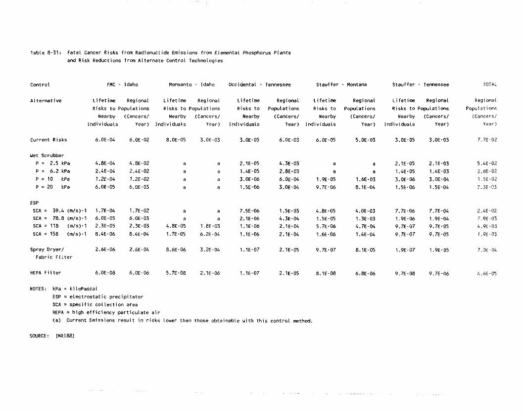
Table 8-31: Fatal Cancer Risks from Radionuclide Emissions f r w Elemental Phosphorus Plants
and Risk Reductions from Al ternate Control Technologies
Control FMC - Idaho Monsanto - Idaho Occidental - Tennessee Stauffer - nontana Stauffer - Tennessee
A l te rna t i ve L i fe t ime Regional L i fe t ime Regional L i fe t ime Regional L i fe t ime Regional L i fe t ime Regional
Risks t o Populations Risks t o Populations Risks t o Papl la t ions Risks t o Populations Risks t o P o p l a t i o n s
Nearby (Cancers/ Nearby (Cancers/ Nearby (Cancers/ Nearby (Cancers/ Nearby (Cancers/
Ind iv iduals Year) Ind iv iduals Year) Ind iv iduals Year) Ind iv iduals Year) Ind iv iduals Year)
Current Risks 6.OE-04 6.OE-02 8.OE-05 3.OE-03 3.OE-05 6.OE-03 6.OE-05 5.OE-03 3.OE-05 3.OE-03
Wet scrubber
P = 2.5 kPa 4.8E-04 4.8E-02 a a 2.1E-05 4.3E-03 a a 2.1E-05 2.1E-03 P = 6.2 kPa 2.4E-04 2.4E-02 a a 1.4E-05 2.8E-03 a a 1.4E-05 1.4E-03 P = 10 kPe 1.2E-04 1.2E-02 a a 3.OE-06 6.OE-04 1.9E-05 1.6E-03 3.OE-06 3.OE-04 P = 20 kPa 6.OE-05 6.OE-03 a a 1.5E-06 3.OE-04 9.7E-06 8.1E-04 1.5E-06 1.5E-04
ESP
SCA = 39.4 (m/s)-1 1.7E-04 1.7E-02 a a 7.5E-06 1.5E-03 4.8E-05 4.OE-03 7.7E-06 7.7E-04 SCA = 78.8 (m/s)-1 6.OE-05 6.OE-03 a a 2.1E-06 4.3E-04 1.5E-05 1.3E-03 1.9E-06 1.9E-04 SCA = 118 (m/s)-1 2.3E-05 2.3E-03 4.8E-05 1.8E-03 l . lE-06 2.1E-04 5.7E-06 4.7E-04 9.7E-07 9.7E-05 SCA = 158 (m/s)-1 8.4E-06 8.4E-04 1.7E-05 6.2E-04 l . lE-06 2.1E-04 1.6E-06 1.LE-04 9.7E.07 9.7E-05
Spray Dryer/ 2.6E-06 2.6E-04 8.6E-06 3.2E-04 l . lE-07 2.1E-05 9.7E-07 8.1E-05 1.9E-07 1.PE-05 Fabric F i l t e r
HEPA F i l t e r 6.OE-08 6.OE-06 5.7E-08 2.1E-06 1.1E-07 2.1E-05 8.1E-08 6.8E-06 9.7E-08 9.7E-06
NOTES: kPa = ki lopascal
ESP = e lec t ros ta t i c p rec ip i ta to r
SCA = spec i f i c c o l l e c t i o n area
HEPA = h igh e f f i c i e n c y par t i cu la te a i r
(a) Current Emissions r e s u l t i n r i s k s louer than those obtainable wi th t h i s contro l method.
SOURCE: lMR1881
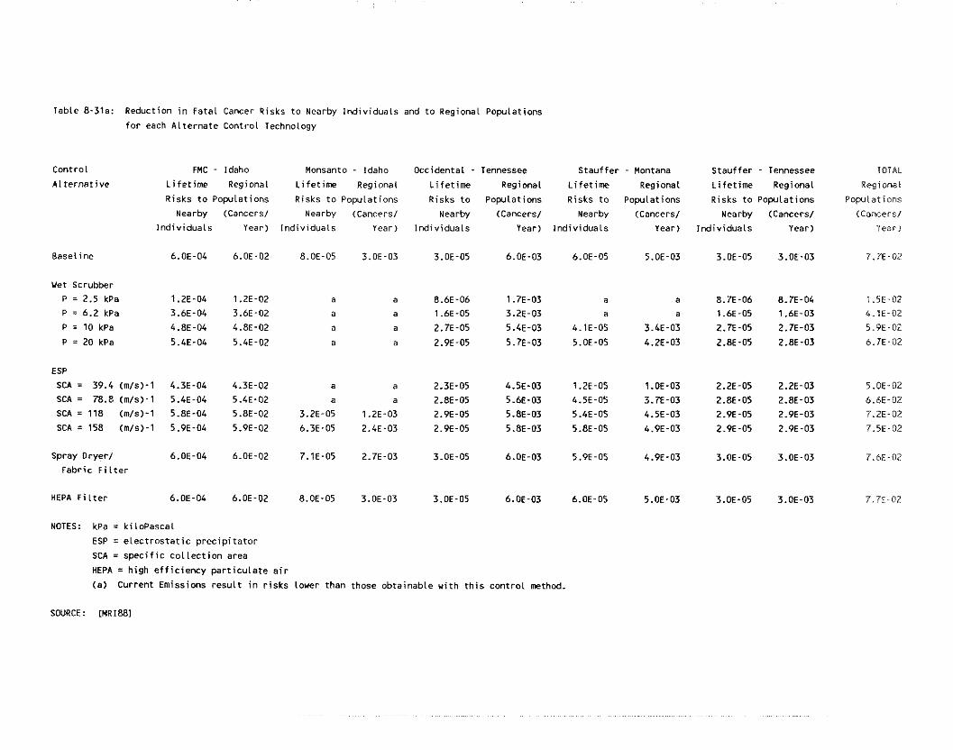
Table 8-31a: Reduction i n Fatal Cancer Risks t o Nearby lnd iv iduals and t o Regional Populations
fa r each Al ternate Control Technology
Control
A l te rna t i ve
FMC - Idaho Monsanta - Idaho Occidental - Tennessee Stauffer - Montana
L i fe t ime Regional L i fe t ime Regional L i fe t ime Regional L i f e t i m Regional
Risks t o Populatians Risks t o Populations Risks t o Populations Risks t o Populations
Nearby (Cancers1 Nearby (Cancers1 Nearby (Cancers1 Nearby (Cancers1
Ind iv iduals Year) Ind iv iduals Year) Individuals Year) Ind iv iduals Year)
Baseline 6.OE-04 6.OE-02 8.OE-05 3.OE-03 3.OE-05 6.OE-03 6.OE-05 5.OE-03
Wet Scrubber
P = 2.5 kPa 1.2E-04 1.2E-02 a a 8.6E-06 1.7E-03 a a P = 6.2 kPa 3.6E-04 3.6E-02 a a 1.6E-05 3.2E-03 a a
P = 10 kPa 4.8E-04 4.8E-02 a a 2.7E-05 5.4E-03 4.1E-05 3.4E-03
P = 20 kPa 5.4E-04 5.4E-02 a a 2.9E-05 5.7E-03 5.OE-05 4.2E-03
ESP
SCA = 39.4 (m/s)-1 4.3E-04 4.3E-02 a a 2.3E-05 4.5E-03 1.2E-05 1.OE-03 SCA = 78.8 (m/s)-1 5.4E-04 5.4E-02 a a 2.8E-05 5.6E-03 4.5E-05 3.E-03 SCA = 118 tm/s)-1 5.8E-04 5.8E-02 3.2E-05 1.2E-03 2.9E-05 5.8E-03 5.4E-05 4.5E-03 SCA = 158 (m/s)-1 5.9E-04 5.9E-02 6.3E-05 2.4E-03 2.9E-05 5.8E-03 5.8E-05 4.9E-03
Spray Oryer l 6.OE-04 6.OE-02 7.1E-05 2.7E-03 3.OE-05 6.OE-03 5.9E-05 4.9E-03
Fabric F i l t e r
HEPA F i l t e r 6.OE-04 6.OE-02 8.OE-05 3.OE-03 3.OE-05 6.OE-03 6.OE-05 5.OE-03
NOTES: kPa = ki lopascal
ESP = e l e c t r o s t a t i c p rec ip i ta to r
SCA = speci f ic c o l l e c t i o n area
HEPA = high e f f i c iency par t i cu la te a i r
(a ) Current Emissions r e s u l t i n r i s k s lower than those obtainable wi th t h i s contro l method.
Stauffer - Tennessee TOTAL
L i fe t ime Regional Regionai
Risks t o Populations Populations
Nearby (Cancers1 (Cancers/
Ind iv iduals Year) Year)

total reduction in risk due to each control alternative. The current risks at both the Monsanto plant
and at the Stauffer, Montana, plant are lower than certain control technologies would allow.
As stated previously, both the baseline emissions rates and the risk estimates are discussed in detail
in Volume 2 of the E~tviro~zn~e~rral lnlpacl Slalen?e~tl. The PM removal efficiency of each alternative
control technology was estimated in MR188.
8.4.2 Costs of Po-210 Emissions Control
The control technologies described above lead to a unique least-cost choice of technology to achieve
a given level of emissions control for each of the five operating plants. These emissions levels and
costs for each plant are presented i n Tables 8-32 through 8-56,
The Po-210 removal efficiency of the SD/FF and the ESP's was derived by dividing the emission
levels achieved by each alternative control technology by the baseline emissions for each technology.
Removal efficiency for the scrubbers and for the HEPA filter are taken from MR188. In Tables 8-
32 through 8-36, the removal efficiency is applied to three Po-210 emissions scenarios: the baseline
emission rate, the baseline rate plus a 10 percent safety margin, and the baseline rate plus a 25
percent safety margin. Emission reductions are then calculated for each control alternative using the
appropriate Po-210 removal efficiency rate. Further sensitivity analysis could be conducted by
allowing for specific measurement error and variability in the stated efficiencies.
Tables 8-32 to 8-36 also present the annualized costs of installing and operating the ten alternative
control systems. The impact of these costs is then estimated both as a cost per ton of elemental
phosphorus produced and as a percentage of the revenues derived from the production and sale of
elemental phosphorus at each plant. As was stated in section 8.2, the cost per ton of Pq is estimated
to be $1,500. Revenues from the sale of this product are derived by assuming that the plants produce
and sell 85 percent of estimated annual Pq capacity at this price. Revenues,would change if actual
production varied from this estimate of 85 percent.
The cost of the control technologies varies by plant. For FhlC cost ranges from $1.37 to $8.71 per
ton of P4 capacity, and from 0.92 to 5.81 percent of 1987 P,, revenues. or Monsanto, the costs of
those technologies which would improve current Po-210 emissions (1.4 Ci/y) range from $2.89 to

TebLr 8-32: Cmtrol Techmlcpy Costs encl Eel imted Po-210 Emissim mtes st FRC's Poatello, Idahc, Plant.
Est iwted Po-210 Emission Rate
Control p0-z1o - - - - - - - - - - - - - - - - - - - - - - - - - - -*----- Total Estimated Percent of h l t e r ~ t i v e Remvai t& 10 Percent 25 Percent Annualized CostlTon Value of
E f f i c imcy Safety Safety Safety Contml of P4 1987 P4 Rargin Rargin Rargin S y s t n Pmduced Revenues
(Cily) (Cily) (Cily) Cost (1987) ( m i 1 Slyr)
Bsseline Po-210 Emission Rate C*) 1 0 . m 11.m 12.500 Uet Scrubber
P = 2.5 kpa M.WT 8 . W 8.- 1 o . m 1.60 $1.37 0.92% P = 6.2 LPS 60.m 4 . m 4.400 5 . m 2.11 $1.81 I .ZIX P = 10 kpa 80.m 2 . m 2 . a 2.500 2.43 $2.09 1.35% P = M kPa W.03 1 . m I .lW I .254 3.75 $3.22 2.15%
ESP S U = 39.4 (.Is)-I 71.W 2.WO 3.15'0 3.625 2.m $1.73 1.15% S U = 78.8 (mls)-I W.WT 1 . m 1.1W 1 .ZM 2.84 $2.44 1.6% SCA = 118 (mls)-1 %.MX 0.380 0.418 0.475 3.65 13.13 2.05% S U = 158 (.Is)-I 98.601: 0.140 0.154 0.175 4.43 $3.80 2.54%
Spray Dryer1 99.57X 0.043 0.047 0.054 9.70 $8.33 5.55% Fabric F i l t e r
HEPh F i l t e r 99.W 0.- 0.mOZ 0.MOe 10.14 $8.71 5.81%
NOTES: kPa = k i loPascal
ESP = electrostatic precipitator S U = specif ic collection area HEPA = high eff iciency particulate a i r
(a) Enissions with Lw energy or spray scrubber. M d i t i m l sys tas are Bdded t o these wet scrubbers except with the spray Diyerl Fabric F i l t e r control a l te re t i ve .

Table 8-33; Control Technoio~y Garbs d PetimPd Po-210 Emissicn Rates at h e a n t o h S a Sp~ings, IdahO, PLant.
Estimted Po-270 Emission Rate (b)
control po-2q(, ~ o t s i Estimted Percmt of Alternetive R e s ~ v s i wc 10 Percent 25 Percent Ivmuat izd CostlTon Value of
€If iciency Safety Safety Satety Cantrol of Ph 15'87 P4 Margin e r g i n llargin S y s t n Produced Revenues (ci/y) ( C i t y ) (Cily) cost (1987)
( m i l Olyr)
8sseLine Po-210 Emission Rate (*> 30.m 33 .W 39.5CD Uet Scrubber
P = 2.5 kPa M.0% 2 4 . m 26.400 3Q.m a a a P = 6.2 kPa 5 5 . a 13.503 14.850 16.875 n a I )
P = 10 kPa W.0% 3 . m 3.MO 3.750 n a II
P = K) kPs 95.0% 1.503 1.650 1.875 a a a
ESP SCA = 39.4 (.Is)-? 75.33% 7.400 8.140 9.250 a a a
S U = 78.8 (.Is)-'I 9 1 . a 2.7M 2.970 3.37s c a a
SCA = 118 I s - 97.202 0.840 0.924 1 ,050 2.33 12.89 1.922 SCA = 158 (81s)-1 59.03% 0.2% 0.319 0 . M 2.R2 $3.49 2.33%
Spray Dryer/ W.5(X 0.150 0.165 0.188 5.43 16.72 4 . a Fabric F i l t e r
HEPA F i l t e r 99.998X O.OW6 0 . W 7 0.W08 15.70 $19.44 1 2 . W
NOTES: kPe = k i loPascal ESP = etectmstat ic precipitator SCA = specif ie w l i e c t i o n ares HEPA = high efficiency particulate a i r
(*I Emitsions with Low energy or apray scrubber. A d d i t i w l sys teu are ddded t o these wet s c r u b r s except with the Spray Bryerl Fabric F i l t e r m t r o L a t tere t ive .
( e ) Ho costs are incurred for th is alternative, because f a c i l i t y has m r e e f f i c ien t m r m l i n place.
(b) Ekcwse the u i ss ions a t th i s f a c i l i t y are currently est imted s t 1.4 Cily, higher es t imtes included i n th i s table are theoretical.
SOURCE: Cl4RJ881
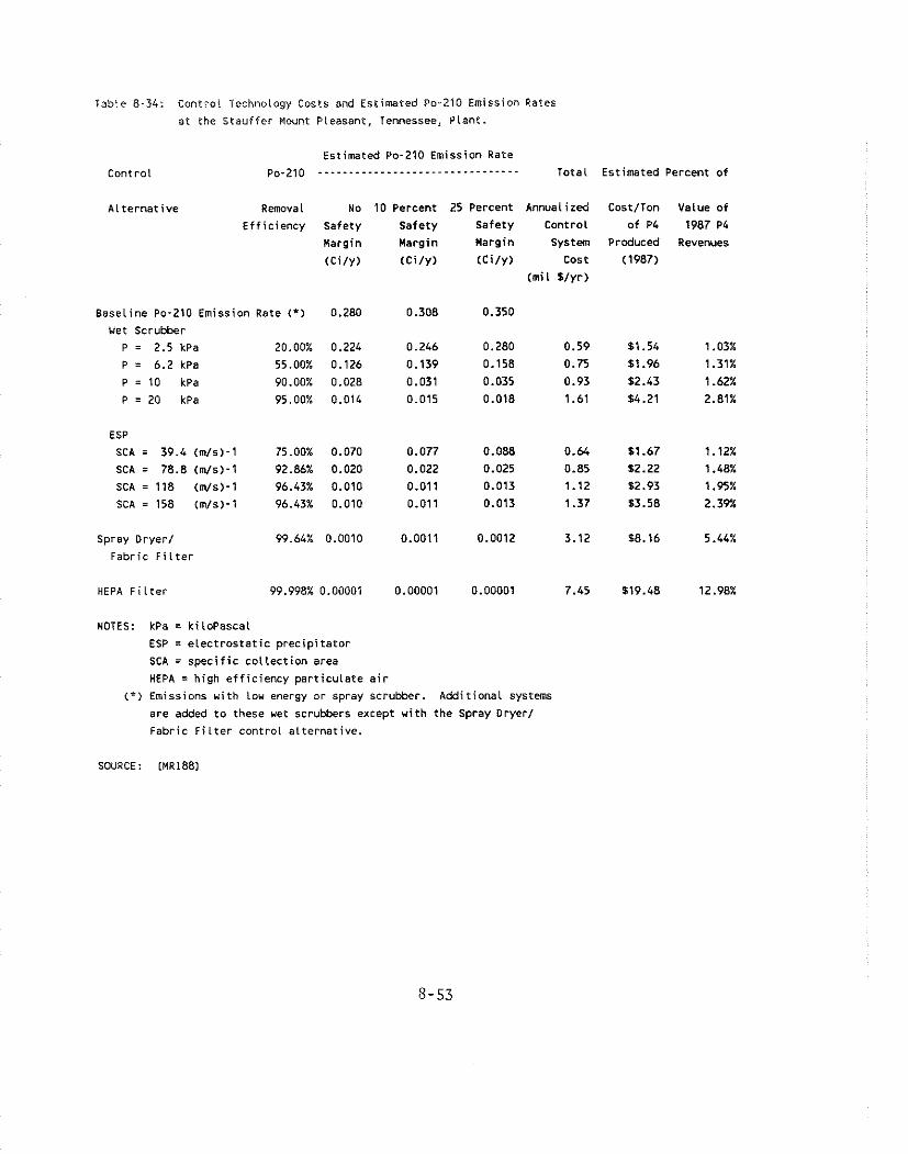
t a b l e 8-34: Control Technology Costs and Estiinated Po-210 Emission Rates
a t the Stauf fer Mount Pleasant, Tennessee, Plant.
Estimated Po-210 Emission Rate
Control po.*lo ................................ Tota l Estimated Percent o f
A l t e r n a t i v e Renwval No 10 Percent 25 Percent Annualized Cost/Ton Value o f
E f f i c iency Safety Safety Safety Control o f P4 1987 P4
Margin Margin Margin System Produced Revenues
(Ci/y) ( c i l y ) ( C i l y ) cost (1987) (mi l W y r )
Basel ine Po-210 Emission Rate (*) 0.280 0.308 0.350
Uet Scrubber P = 2.5 kPa 20.00% 0.224 0.246 0.280 0.59 $1.54 1.03%
P = 6.2 kPa 55.00% 0.126 0.139 0.158 0.75 $1.96 1.31%
P = 10 kPa 90.00% 0.028 0.031 0.035 0.93 12.43 1.62%
P = 20 kPa 95.00% 0.014 0.015 0.018 1.61 $4.21 2.81%
ESP SCA = 39.4 (m1s)-1 75.00% 0.070 0.077 0.088 0.64 $1.67 1.12%
SCA = 78.8 (m/s)-1 92.86% 0.020 0.022 0.025 0.85 12.22 1.48%
SCA = 118 (m/s)-1 96.43% 0.010 0.011 0.013 1.12 $2.93 1.95%
SCA = 158 (m/s)-1 96.43% 0.010 0.011 0.013 1.37 $3.58 2.39"A
Spray Oryer l 99.64% 0.0010 0.0011 0.0012 3.12 88.16 5.44%
Fabric F i l t e r
HEPA F i l t e r 99.998% 0.00001 0.00001 0.00001 7.45 $19.48 12.98%
NOTES: kPa = ki loPascal
ESP = e l e c t r o s t a t i c p rec ip i ta to r
SCA = s p e c i f i c c o l l e c t i o n area
HEPA = h igh e f f i c i e n c y par t i cu la te a i r
(") Emissions w i th Lou energy or spray scrubber. Addi t ional systems
are added t o these wet scrubbers except w i th the Spray Dryer/
Fabric F i l t e r cont ro l a l ternat ive.
SOURCE: CMR1881
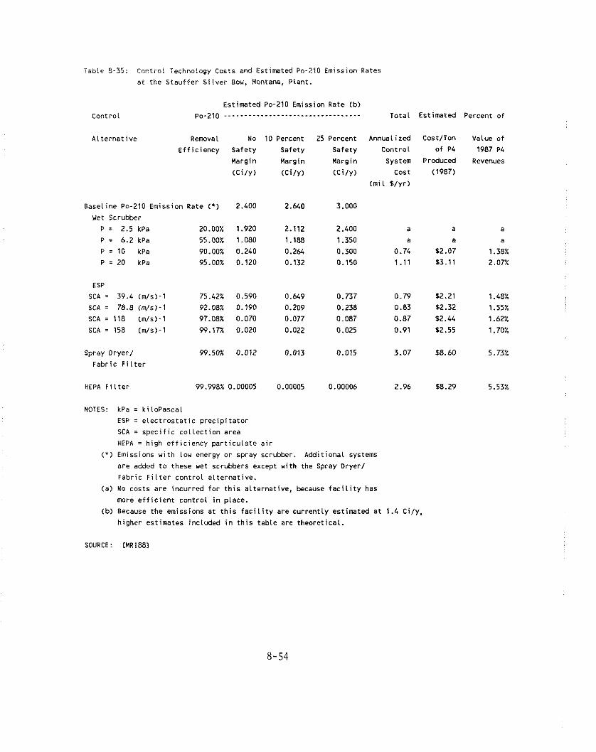
Tabie 8-35: Control lechnoiogy Costs and Estimated Po-210 Emission Rates
at the Stauf fer S i lver Bow, Montana, Plant.
Estimated Po-210 Emission Rate (b)
Control po.210 .................................. Tota l Estimated Percent of
A l te rna t i ve Removal No 10 Percent 25 Percent Annualized CostITon Value of
E f f i c iency Safety Safety Safety Control of P4 1987 P4
Margin Margin Margin System Produced Revenues
( C i l y ) (C i l y ) ( C i l y ) cost (1987) (m i l f l y r )
Baseline Po-210 Emission Rate (*) 2.400 2.640 3.000
Uet Scrubber
P = 2.5 kPa 20.00% 1.920 2.112 2.400 a a a
P = 6.2 kPa 55.00% 1.080 1.188 1.350 a a a
P - 1 0 kPa 90.007 0.240 0.264 0.300 0.74 12.07 1.38%
P = 20 kPa 95.00% 0.120 0.132 0.150 1.11 83.11 2.07%
ESP
SCA = 39.4 (m/s)-1 75.42% 0.590 0.649 0.737 0.79 $2.21 1.48%
SCA = 78.8 tm/s)-1 92.08% 0.190 0.209 0.238 0.83 $2.32 1.55%
SCA = 118 (m1s)-1 97.08% 0.070 0.077 0.087 0.87 $2.44 1.677
SCA = 158 (m1s)-1 99.17% 0.020 0.022 0.025 0.91 12.55 1.70X
Spray Dryer/ 99.50% 0.012 0.013 0.015 3.07 88.60 5.73%
Fabric F i l t e r
NOTES: kPa = k i lopascal
ESP = e l e c t r a s t a t i c p rec ip i ta to r
SCA = spec i f i c c o l l e c t i o n area
HEPA = high e f f i c i e n c y par t i cu la te a i r
(*) Emissions w i th low energy o r spray scrubber. Addit ional systems
are added t o these wet scrubbers except v i t h the Spray Dryer1
Fabric F i l t e r contro l a l te rna t i ve .
( a ) No costs are incurred fo r t h i s a l ternat ive, because f a c i l i t y has
more e f f i c i e n t contro l i n place.
(b) Because the emissions at t h i s f a c i l i t y are current ly estimated a t 1.4 Ci ly .
higher estimates included i n t h i s table are theoret ical.
SOURCE : CMR1881
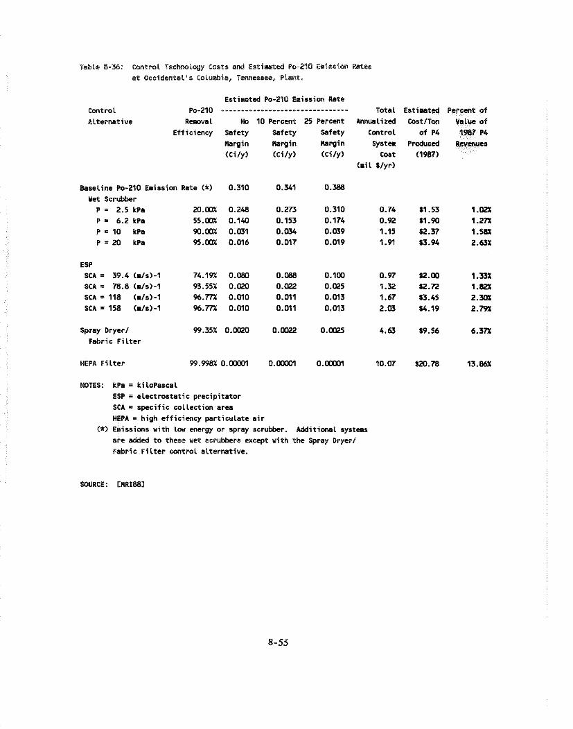
Table 8-34: ContmL Technology Costs and Esri.st& Po-210 Emission &tea
s t Occidental's Colurbis, Tcnnessw, PLenT.
Estiurted Po-210 Emission Rate Control Po-210 ................................ Total Est iwted Percent o f Alternative Rewva l Wo 10 Percent 25 Percent h u a l i z e d CostlTon Value of
Ef f iciency Safety Safety Safety Control o f P4 1981 P4 llargin llargin llargin system Produced Revewes (Cily) t e i l y ) (Cily) Coat (1987)
( m i l Slyr)
Bsaeline Po-210 Emission Rate (*) 0.310 0.341 0.588 Uet Scrubber
P = 2.5 kPa 20.00% 0.248 0.273 0.310 0.74 $1.53 I .02% P = 6.2 kPa 55.00% 0.140 0.153 0.174 0.92 $1.90 1.27% P = 10 kPa W.WX 0.031 0.034 0.039 1.15 52.37 1.56% P = 20 kPa 95.00% O.M6 0.W7 0.M9 1.91 $3.94 2.63%
ESP S U = 39.4 (.lo)-1 74.19% 0.080 0 . W 0.1M 0.97 S2.M 1.33% SCA = 78.8 (m1s)-1 93.55% O.L)20 0.022 0.025 1.32 $2.72 1.82% SCA = 118 (.Is)-1 %.7?% O.MO O.M1 O.M3 1.67 $3.45 2 . m SCA = 158 (m/s)-1 96.77% O.MO O.M1 0.M3 2.03 $4.19 2.792.
Spray Dryer/ 99.35% 0.WO 0.0222 0.0025 4.63 19.56 6.37% fabr ic F i l t e r
HEPA F i l t e r 99.998% O.Moo1 0 . m 0 . m 10.07 $20.78 1 3 . W
NOTES: kPa = ti loPssca1 ESP = e lec tmstat ic precipitator S U = specif ic collection area HEPA = high efficiency particulate a i r
<*I E~iss ions with Lw energy or spray scrubber. Additional systcro are d i e d t o these wet scrubbers except with the Spray Dryer1 Fabric F i l t e r control alternative.
$19.44 per ton capacity, and from 1.92 to 12.96 percent of Pq revenues. For Rhone-Poulenc, the costs
range from $1.54 to $19.48 per ton capacity in Tennessee and from $2.07 to $8.60 per ton cnpncit).
in Montana. The control technology costs range from 1.03 to 12.98 percent of the Tennessee plant's
1987 PL revenues and from 1.38 to 5.73 percent of the Montana plant's revenues. The control
technology costs a t the Occidental plant in Columbia, Tennessee, demonstrate ranges similar to the
other plants.
8.4.3 Estimates of Benefits and Costs.
Tables 8-37 through 8-41 present summaries of both the benefits and the costs of the control of Po-
210 emissions on the five operating elemental phosphorus plants. For each of the plants, nine
alternative emissions levels were examined, ranging from 10 Ci/y to 0.01 ci/y. A Po-210 emissions
limit of 10 Ci/y represents a "no additional control" limit, as the highest current emissions rate at any
plant is 10 Ci/y. No safety margin is assumed in these tables.
For each plant, the least-cost control method required to meet a given emissions level was chosen for
presentation. The annualized cost for the least-cost technology is presented as is the emission limit
that would be achieved by that technology, assuming no safety margin. Also presented in each table
is the annual risk, in cancers per year, that would result from the installation of the least-cost
technology.
The plant-by-plant analysis presented in Tables 8-37 through 8-41 is summarized, for all plants, in
Tables 8-42 and 8-43. The first of these tables presents the total annualized costs of alternative
emissions levels. Also presented is the increase in cost required to move from a given emissions level
to a lower one. At an emissions rate of 10 Ci/y, there is no cost to the industry, as no additional
emissions control is required. A cost of $2.4 million per year is experienced by the industry to meet
an emissions level of 2 Ci/y. A further reduction to emissions of I Ci/y would increase cost to
industry by $2.7 million. An emissions level of 0.01 Ci/y is estimated to cost $31.6 million per year.
Table 8-43 presents the total incidence and the incidence reduction achieved by alternative emissions
levels. At a level of 10 Ci/y of Po-210, the total number of cancers per year remains unchanged, at
an estimated 8E-02 per year (see Table 8-21). At an emissions level of 2.0 Ci/y, the incidence of
cancer falls to 3E-02, a reduction of SE-02 cancers per year. At 1.0 Ci/y, the annual incidence
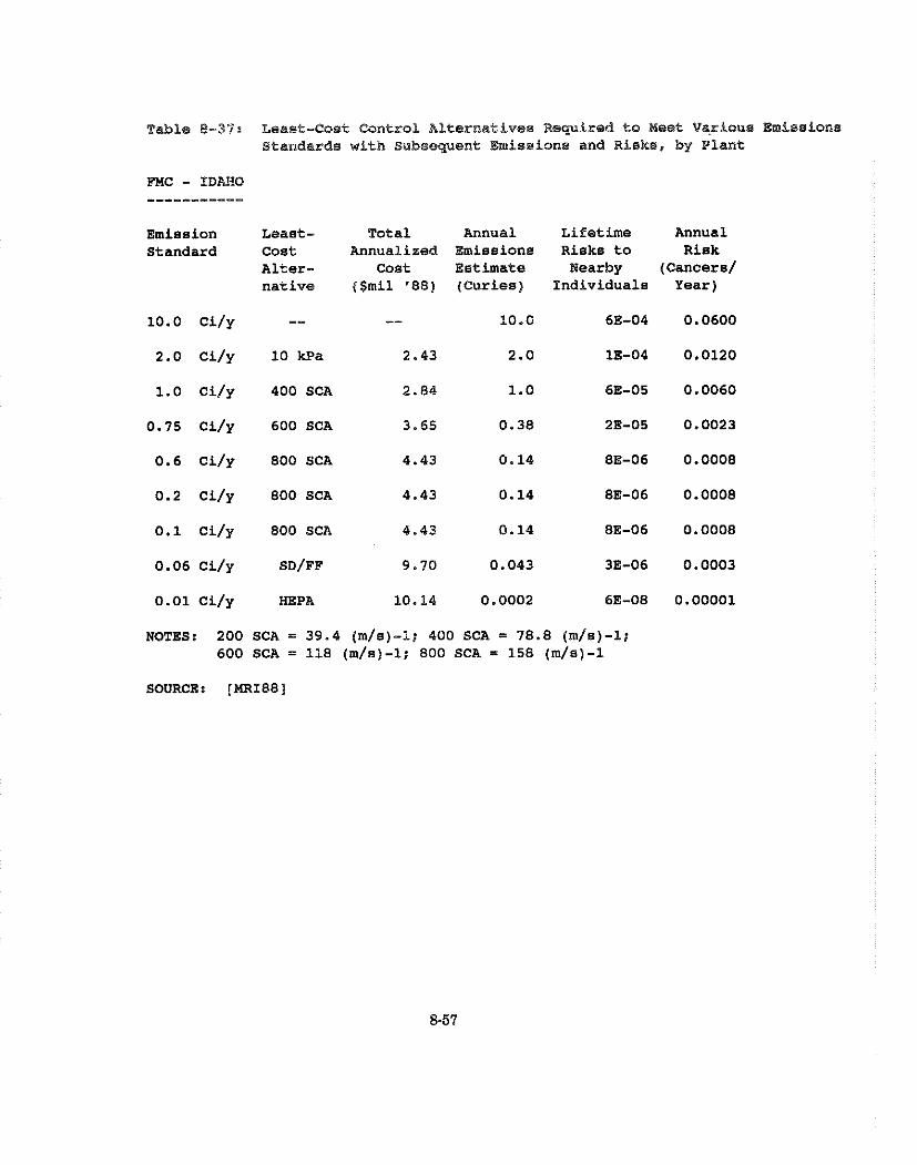
Table 8-37s Least-Cost Control AEternatives Revired to met Various Emissions Standards with Subseguent Emissions and Risks, by Plant
FMC - IDAHO
Emission Least- Total Annual Lifetime Annual Standard Cost Annualized Emissions Risks to Risk
Alter- Cost Estimate Nearby (Cancers/ native ($mil '88) (Curies) Individuals Year)
1.0 ci/y 400 SCA 2.84 1.0 6E-05 0.0060
0.75 Ci/y 600 SCA 3.65 0.38 2E-05 0.0023
0.6 ci/y 800 SCA 4.43 0.14 BE-06 0.0008
0.2 Ci/y 800 SCA 4.43 0.14 BE-06 0.0008
0.1 ci/y 800 SCA 4.43 0.14 8E-06 0.0008
NOTES: 200 SCA = 39.4 (m/s)-1; 400 SCA = 78.8 (m/s)-1; 600 SCA = 118 ( m ) - ; 800 SCA = 158 (m/s)-1
SOURCE: [=I881
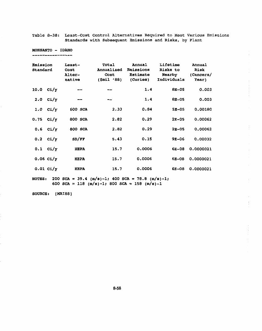
Table 8-38: Least-Cost Control Alternatives Rewired to Meet Various Emissions Standards with Subsequent Emissions and Risks, by Plant
MONSANTO - IDAHO
Emission Leaat- Total Annual Lifetime Annual standard Cost Annualized Emissions Risks to Risk
Alter- Cost Estimate Nearby (Cancers/ native ($mil '88) (Curies) Individuals Year)
1.0 ci/y 600 SCA 2.33 0.84 5E-05 0.00180
0.75 Ci/y 800 SCA 2.82 0.29 2E-05 0.00062
0.6 ci/y 800 SCA 2.82 0.29 2E-05 0.00062
NOTES: 200 SCA = 39.4 (m/s)-1; 400 SCA = 78.8 (m/s)-1; 600 SCA = 118 (m/s)-1; 800 SCA = 158 (m/s)-1
SOURCE: [MRIBB]
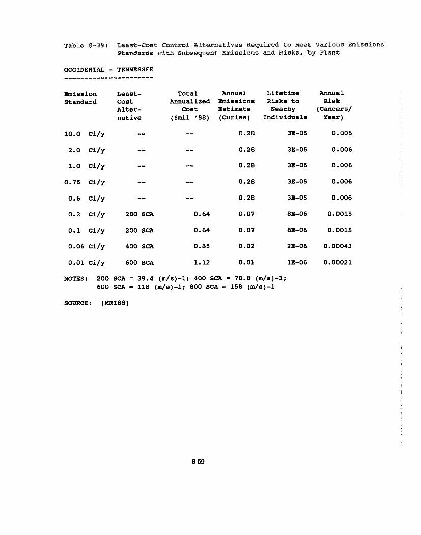
Table 8-39: Least-Cost Control Alternatives Reguired to Heet Various Emissions Standards with Subseguent Emissions and Risks, by Plant
OCCIDENTAL - TENNESSEE
Emission east- Total Annual Lifetime Standard Cost Annualized Emissions Risks to
Alter- Cost Estimate Nearby native ($mil '88) (Curies) Individuals
0.2 ci/y 200 SCA 0.64 0.07 8E-06
0.1 ci/y 200 SCA 0.64 0.07 8E-06
0.06 ci/y 400 SCA 0.85 0.02 2E-06
0.01 ci/y 600 SCA 1.12 0.01 1E-06
Annual Risk
(cancers/ Year )
NOTES: 200 SCA = 39.4 (m/s)-1; 400 SCA = 78.8 (m/s)-1; 600 SCA = 118 (ma)-; 800 SCA = 158 (m/s)-1
SOURCE: [MRI88]
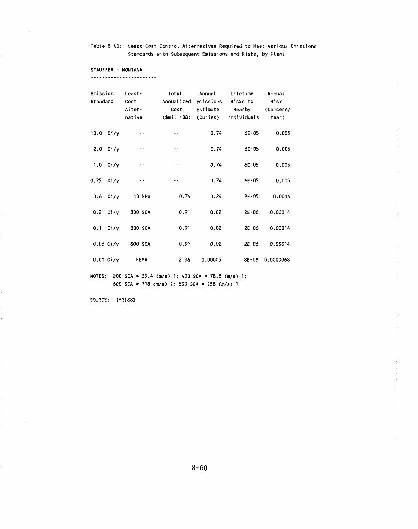
Table 8-40: Least-Cost Controi ALternatives Required t o Meet Various Emissions
Standards w i th Subsequent Emissions and Risks, by Pkanf
STAUFFER - MONTANA
Emission Least- Total Annual L i fe t ime Annual
Standard Cost Annualized Emissions Risks t o Risk
A l t e r - Cost Estimate Nearby (Cancers/
nat ive (5miL '88) (Curies) Ind iv iduals Year)
1.0 C i ry . . . . 0.74 6E-05 0.005
0.75 c i r y . . . . 0.74 6E-05 0.005
0.6 C i ry 10 kPa 0.74 0.24 2E-05 0.0016
0.2 C i ry 800 SCA 0.91 0.02 2E-06 0.00014
NOTES: 200 SCA = 39.4 (m/s)-1; 400 SCA = 78.8 (m/s)-1;
600 SCA = 118 ( m / s ) - 1 ; 800 SCA = 158 (m/s)-1
SOURCE: lMR1881
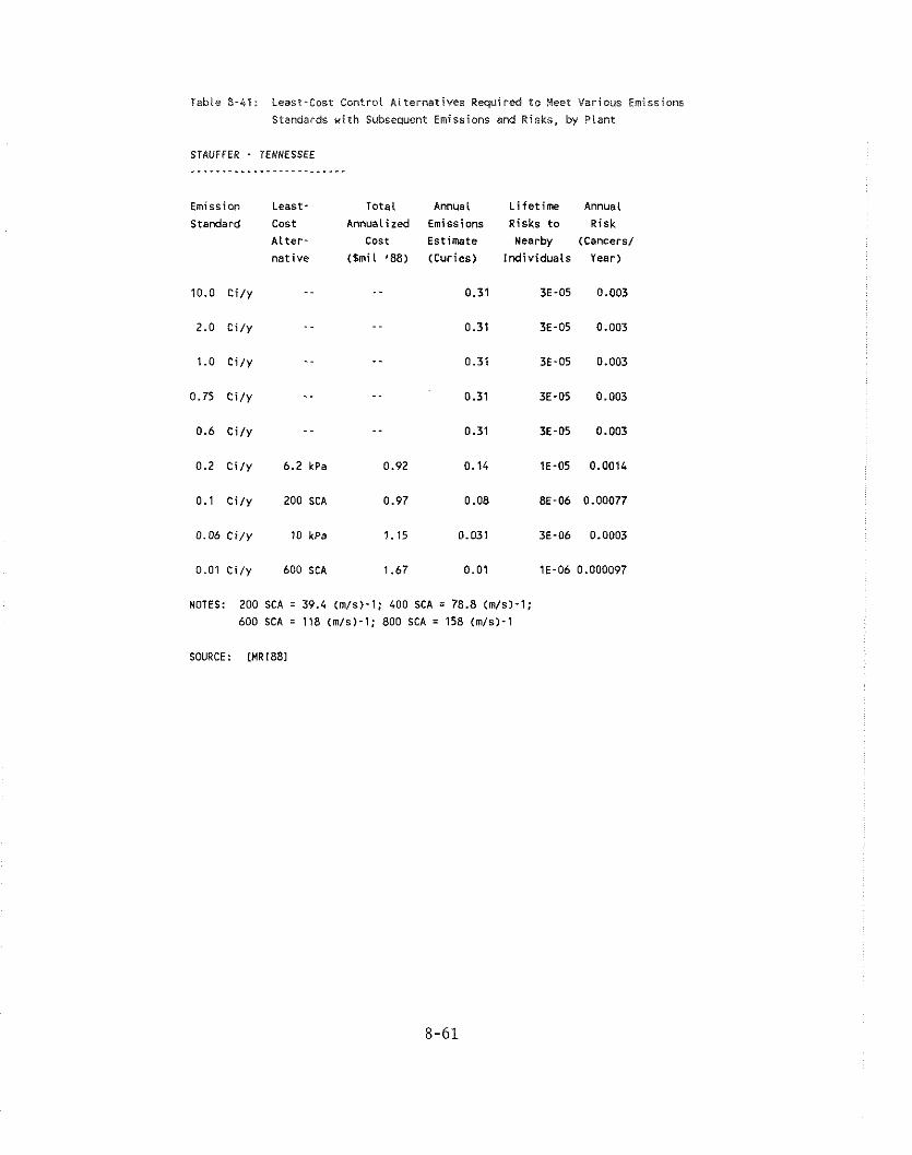
Teble 8 -41 : Least-Cost Controi A l ternat ives Required t o Meet Various Emissions
Standards w i th Subsequent Emissions and Risks, by P lant
STAUFFER - TENNESSEE
Emission Least- Total Annua l L i fe t ime Annual
Standard Cost Annualized Emissions Risks t o Risk
A l t e r - Cost Estimate Nearby (Cancers/
na t i ve ($mil '88) (Curies) Ind iv iduals Year)
10.0 C i l y . . . . 0.31 3E-05 0.003
2.0 C i l y . . . . 0.31 3E-05 0.003
1.0 C i l y . . . . 0.31 3E-05 0.003
. . . . 0.75 C i l y 0.31 3E-05 0.003
0.6 C i l y . . . . 0.31 3E-05 0.003
0.2 C i l y 6.2 kPa 0.92 0.14 1E-05 0.0014
0.01 C i l y 600 SCA 1.67 0.01 1E-06 0.000097
NOTES: 200 SCA = 39.4 (mls)-1; 400 SCA = 78.8 (m1s)-1;
600 SCA = 118 (m1s)-1; 800 SCA = 158 (m1s)-1
SOURCE: CUR1881

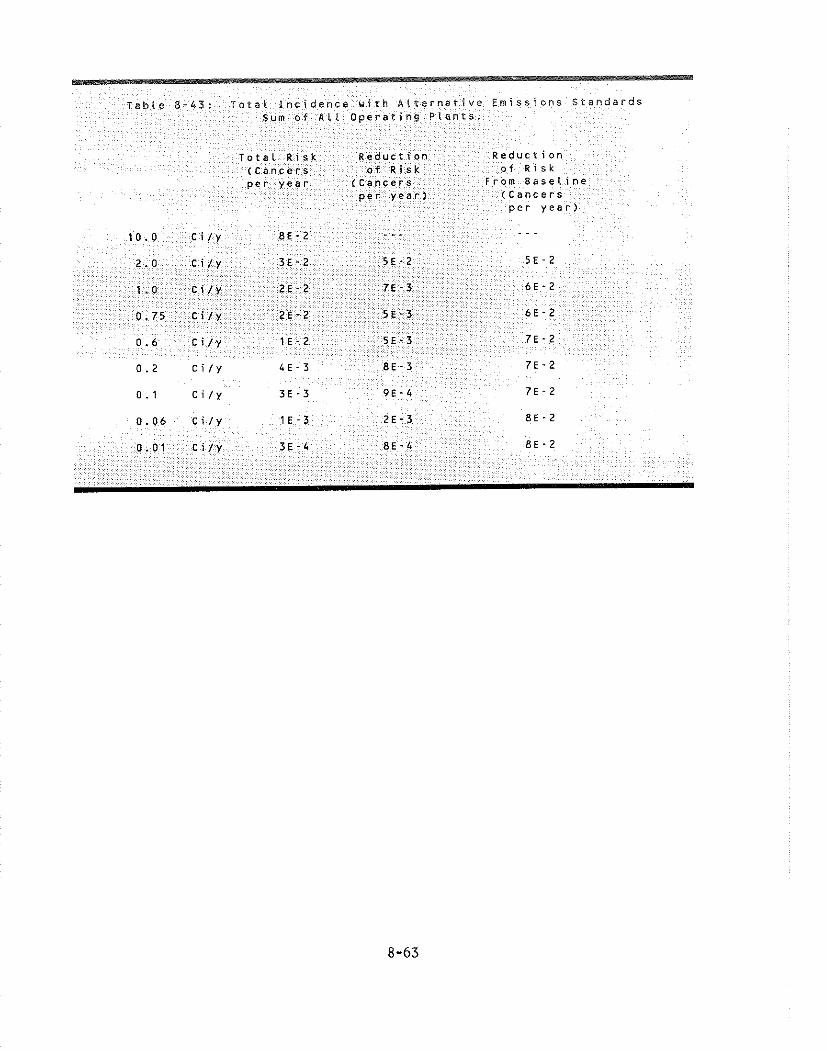
becomes 2E-02, a reduction from current levels of 6E-02 cancers per year. At a level of 0.01 Ci/y,
the annual incidence falls to 3E-04, a reduction of 8E-02 cancers per year.
8.4.4 Alternatives for Amwle Marein of Safetv for Elemental Phoswhorus Plants.
Table 8-44 presents the same benefit and cost information on an alternative-by-alternative basis
rather than a plant-by-plant basis. For each alternative emission level, the least-cost control system,
its annualized cost, the corresponding incidence and incidence reduction are presented. This
information is shown for all plants as is the total cost and the total incidence. The change in cost
from alternative to alternative is shown a t the bottom of each section of the table. As in Tables 8-
37 through 8-41, the emissions levels analyzed range from 10.0 Ci jy to 0.01 Ci/y.
Table 8-44a is a continuation of Table 8-44 involving a shift in emphasis from emissions to control
technologies. Certain control technologies have been selected for analysis. As before, Alternative
I is the "no additional control" alternative. As no new control equipment is required, there are no
additional costs to the industry and no reduction in cancers per year.
Alternative X would require high energy scrubbers on the two largest plants and no further controls
on the smallest plants. A large plant was defined as having a production capacity over 75,000 tons
per year of elemental phosphorus, i.e., Monsanto and FMC. This alternative is identical to alternative
11, which limited emissions to 2.0 Ci/y, with a cost to the industry of $2.43 million per year. The
alternative would reduce incidence by 0.0569 cancers per year.
Alternative XI , requiring high energy scrubbers on all plants, would cost the industry an estimated
$4.78 million per year. The incidence of cancer would be reduced by 0.06 cancers per year. Two
other alternatives were examined, one requiring SD/FF on the two large plants and high energy
scrubbers on small plants, and another requiring HEPA filters on the large plants and 600 SCA
precipitators on the smaller ones. The costs and benefits of each are presented as Alternatives XI1
and XI11 in Table 8-44a.
The results of the analysis of costs and benefits are summarized in section 8.1, the Introduction and
Summary.
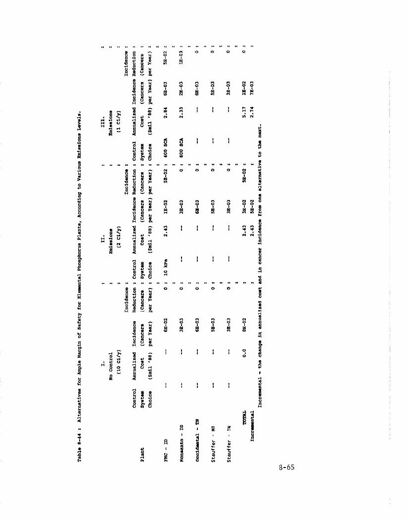
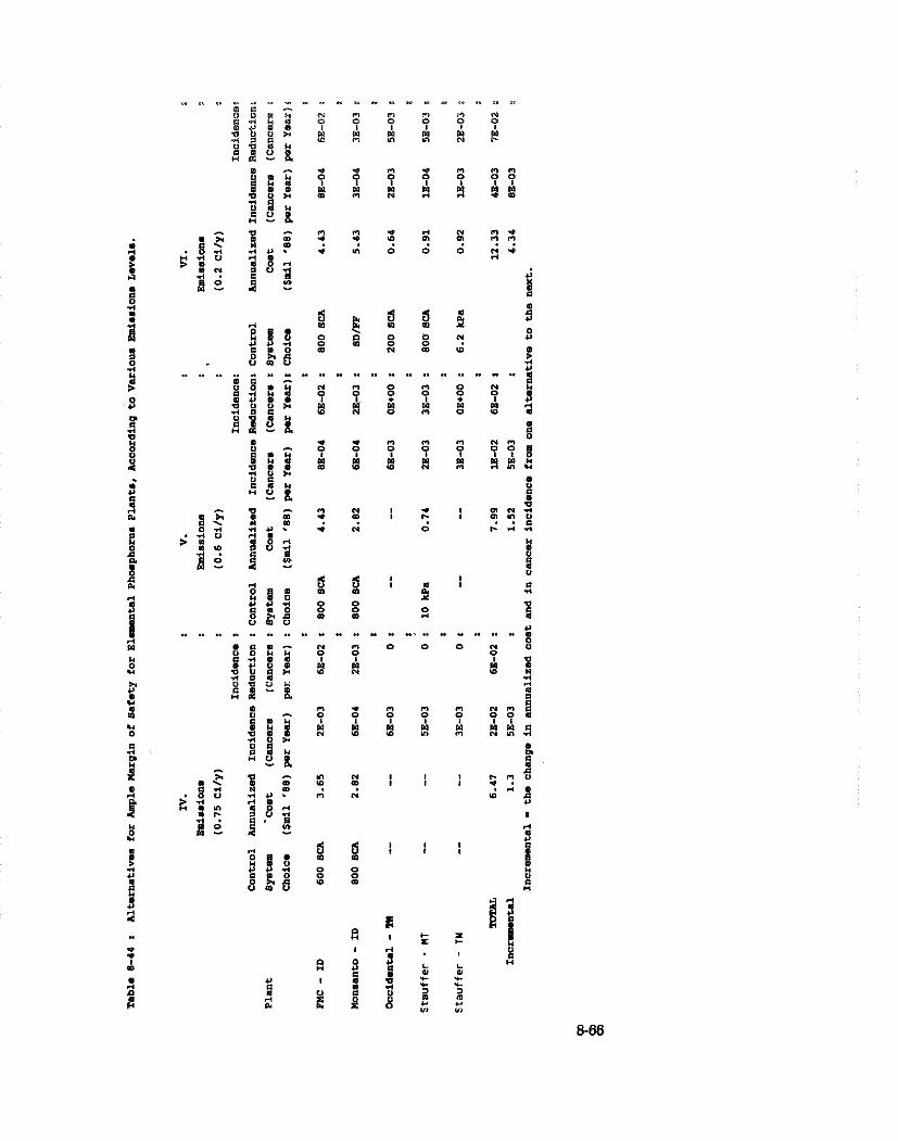
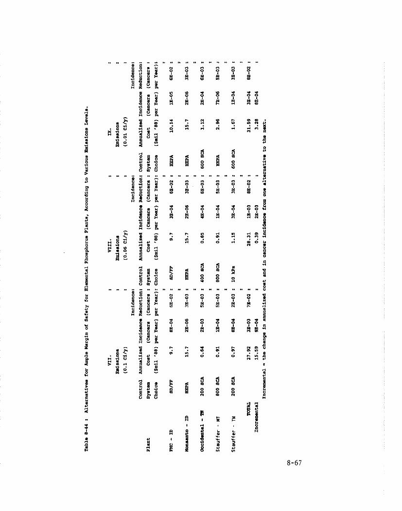
n n E 0 0 U
A i l ! a e r(
* m z 1 1 - ( D O Y N .
C
S *

I*
!i N " " C t C I N C I i l G 3 0 B o o 0 c o I I
3 j ; * 4 i 4 4 x E 8 U S * . 2 U X .
:&,.; 0 0 0 0 N . 0
8 3 2 . 3 u w 3 : V " " * YI
r( " ' 9 M I * ! ! % E X . & 0 -
N C I " C I * I N N 2 1 7 0 7 y 7 0 0 0 I
? , 8 * ! R 8 B R R B . o 5 e
j 2 ^ 0 0 0 o 0 " - 8 1 % ? 4 9 8 2 3 z s - N N 4
2 " . a o r ( e C jjus rl
6 * U
2 3 U
r(
1 5 L1 b j s s 9 n s s 2 ' 0 E 4
rl m 8 8 6 B w " . . " " " " .............. " " .......... s i


Econon~ic impacts occur when regulations alter the costs of production. Changes in the cost of
production may lead to a change in product price and demand, thus altering the structure of the
market in which the product is sold. The impacts on producers, consumers, workers and communities
may be positive or negative, may depend on the overall state of the economy, and may be transitional
or permanent. The impacts may represent losses in economic efficiency or they may be
distributional, indicating shifts among economic entities (e.g., among firms or among groups of
workers).
Government regulations generally occur when the market fails to meet all of the objectives of society.
Regulations are designed to mend the market imperfections by, for example, internalizing to a
polluter the cost of environmental damage caused by that pollution.
As shown in the previous sections of this chapter, limiting the allowable emissions of polonium-210
at various alternative levels below 10 Ci/y would require the five plants operating in 1988 to install
and operate pollution control equipment designed to reduce its particulate emissions. The technology
selected by the affected plant would depend on the level of standards and individual firm
preferences. Varying levels and proportions of capital and operating expenses would be incurred
based on the technology selected. These costs would result in an increase in the unit production cost
of the affected facilities. The sum of these pollution control expenditures is referred to as the private
real resource cost.
When a regulation imposes real resource costs on firms that change the unit cost of production,
manufacturers will attempt to minimize the effect on profitability. This may result in attenlpts to
reduce input costs including raw materials and wages, or to increase prices. If there is an increase
in price, quantity demanded of the product may be reduced, and demand for competitors' output or
substitute products ma), increase. These changes can lead to layoffs at the affected plant, reduced
income in the community where the plant is located, and effects on the structure of the market.
These effects on market structure include shifts in the price elasticity for the product, decreases in
overall quantity demanded, and redistribution of market positions for each competitor and producer
of substitute products.
The extent to which a regulated manufacturer may effectively pass on increases in cost will depend
on the competitive environment in which the products are produced and sold and on the elasticity
of demand. The elasticity of demand is a measure of the sensitivity of the colisumers to changes in
price. In some markets, a small change in price could lead to a large reduction in volume sold, while
in other markets large price changes may have only marginal effects on volume. As a regulated
manufacturer increases prices, quantity of the products demanded will usually fall. The rate at which
volume falls will determine the change in total revenues that results from a change in price. If the
market price of the product changes (all manufacturers incur higher costs), consumers use less of the
product and some of the utility associated with consumption of the product will be lost. Consumers
who continue to use the same amount of the product a t higher prices will have to allocate a larger
portion of their budgets to this consumption, thus reducing savings o r consumption of other goods
and services.
The control of Po-210 emissions through the setting of an emissions standard will result in changes
in the cost of producing elemental phosphorus only if an emission standard lower than 10 Ci/y is
chosen, according to the emissions data gathered during 1988 (see section 8.3). The structure of this
industry and the nature of the market in which the output is utilized adds significant uncertainty to
the measurement and allocation of expected economic impacts. Some of these characteristics include
the following:
o The industry has contracted substantially over the past two decades, closing over
half the plants and reducing capacity enormously.
o Elemental phosphorus is an intermediate product utilized to produce chemical
compounds used in consumer goods that are sold in highly competitive markets
(detergents, soft drinks, etc. - see section 8.2).
o All plants are owned by large, highly integrated Fortune 500 corporations that
consume virtually all the Pq output in company-owned chemical plants.
o The owners of the P4 plants own or have extraction leases for phosphate rock, an
exhaustible resource that is the principle input to production.
o The plant most likely to require new emissions control equipment is the largest
plant, accounting for over one-third of industry capacity.

o The affected plant has among the lowest production costs due to economies of
scale and regional differences in input prices.
o The long range prospects for current elemental phosphorus markets are uncertain,
and extensive industry research and development efforts over the past fifteen
years have failed to develop any significant new markets.
o Bans or restrictions on phosphate use in detergents have been imposed in some
states.
These and other factors make it difficult to predict the ability or desirability of the regulated plant(s)
to pass on all or part of these pollution control costs to consumers through price increases. In the next
section, the costs of producing elemental phosphorus at the currently operating plants are compared.
A subsequent section presents some methods for bounding the potential economic impacts of the
proposed alternatives.
8.5.1 Production Costs
The primary components of the cost of producing elemental phosphorus are phosphate rock, coke,
electricity and labor. Together, these account for 80 to 88 percent of the cost of producing a ton of
phosphorus. Prices of these materials for each producer and plant vary, with the western plants
having a significant cost advantage compared to Tennessee plants. The components of cost for
elemental phosphorus and estimated costs for each plant are described in the following section.
8.5.1.1 Comoonents of Cost
The inputs to elemental phosphorus production were investigated for a hypothetical Tennessee plant
by Arthur D. Little [ADL73], and for FMC by EPA in 1984 [EPA84e]. Additional data on costs are
published in SRl's Chen~ical Ecotlonzics Hatidbook. The ranges in the amounts and prices of each
input needed to produce a ton of phosphorus seen in these studies are provided in Table 8-45. Prices
are indexed to June, 1988, dollars.
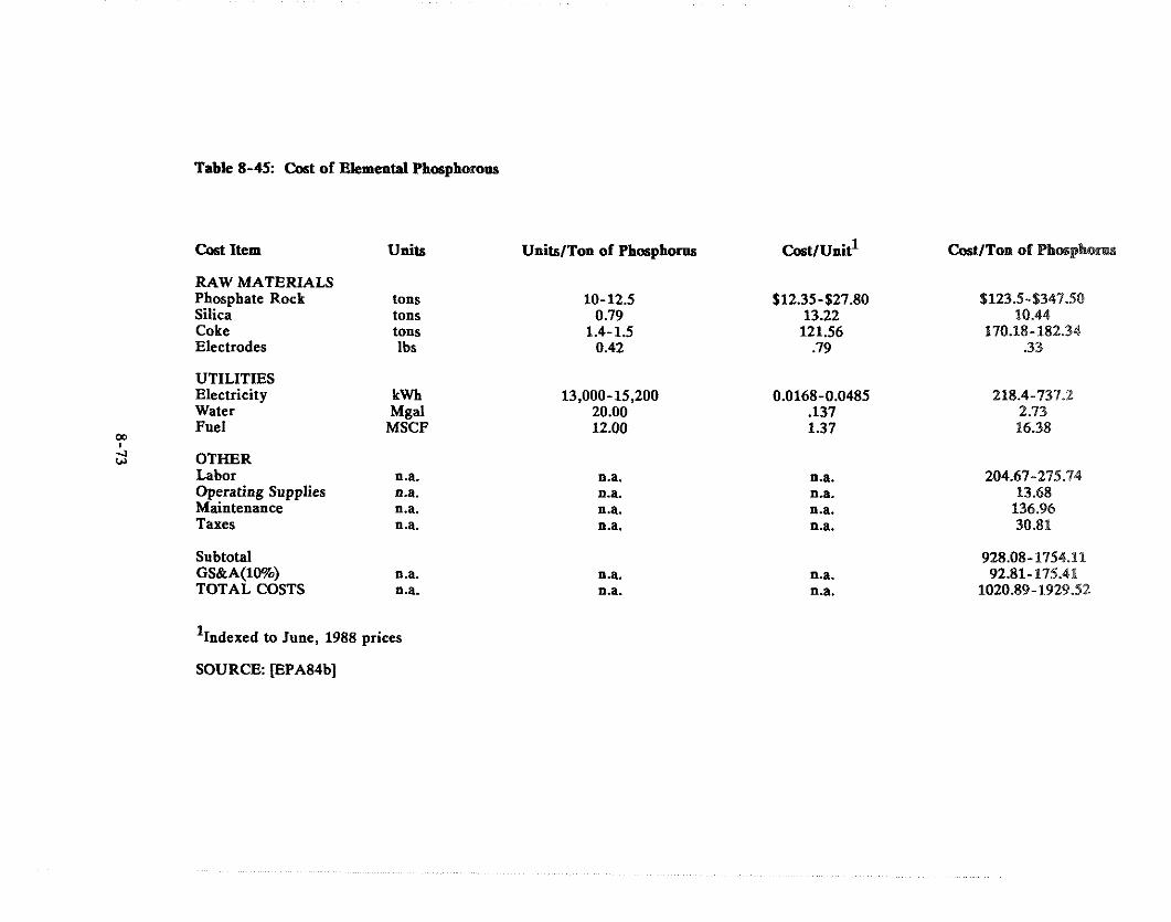
Table 8-45: Cost of Elemental phosphor or^^
Cost Item
RAW MATERIALS Phosphate Rock Silica Coke Electrodes
UTILITIES Electricity Water Fuel
4" .l w OTHER
Labor Operating Supplies Maintenance Taxes
Subtotal GS&A(10%) TOTAL COSTS
Units
tons tons tons Ibs
kwh Mgal
MSCF
'~ndexed to June, 1988 prices
UnitslTon of Phosphorus
SOURCE: [EPA84b]
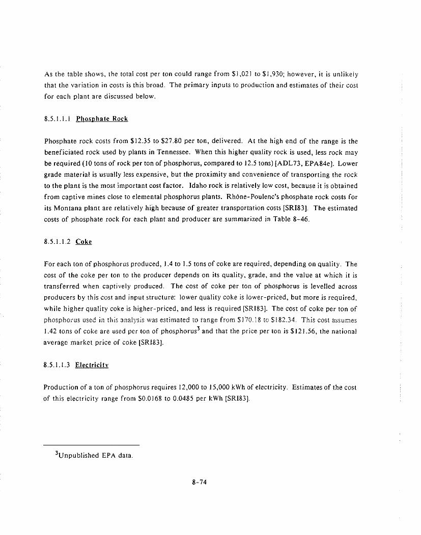
As the table shows, the total cost per ton could range from $1,021 to $1,930; however, i t is unlikely
that the variation in costs is this broad. The primary inputs to production and estimates of their cost
for each plant are discussed below.
8.5.1.1.1 Phosnhate Rock
Phosphate rock costs from $12.35 to $27.80 per ton, delivered. At the high end of the range is the
beneficiated rock used by plants in Tennessee. When this higher quality rock is used, less rock may
be required (10 tons of rock per ton of phosphorus, compared to 12.5 tons) [ADL73, EPA84el. Lower
grade material is usually less expensive, but the proximity and convenience of transporting the rock
to the plant is the most important cost factor. Idaho rock is relatively low cost, because it is obtained
from captive mines close to elen~ental phosphorus plants. Rhone-Poulenc's phosphate rock costs for
its Montana plant are relatively high because of greater transportation costs [SRI83]. The estimated
costs of phosphate rock for each plant and producer are summarized in Table 8-46.
For each ton of phosphorus produced, 1.4 to 1.5 tons of coke are required, depending on quality. The
cost of the coke per ton to the producer depends on its quality, grade, and the value at which it is
transferred when captively produced. The cost of coke per ton of phosphorus is levelled across
producers by this cost and input structure: lower quality coke is lower-priced, but more is required,
while higher quality coke is higher-priced, and less is required [SR183]. The cost of coke per ton of
phosphorus used i n this analysis was estimated to range from $170.18 to $182.34. This cost assumes
1.42 tons of coke are used per ton of phosphorus3 and that the price per ton is $121.56, the national
average market price of coke [SR183].
8.5.1.1.3 Electricitv
Production of a ton of phosphorus requires 12,000 to 15,000 kwh of electricity. Estimates of the cost
of this electricity range from $0.0168 to 0.0485 per kwh [SRI83].
' ~npub l i shed EPA data.

Table 8-46: Costs of Phosphate Rock Used in Phosphorus Production
Producer Location
Monsanto Columbia, TN Soda Springs, ID
FMC Pocatello, ID
Stauffer c Mt. Pleasant, TN Silver Bow, MT
Occidental Columbia, T N U VI
'indexed to June, 1988 prices.
Unit Cqst $/Ton
Tons of Phosphate Rock Mined/ Ton of Phosphorus
Phosphate Rock Cost $/Ton
SOURCE: [JFA86]
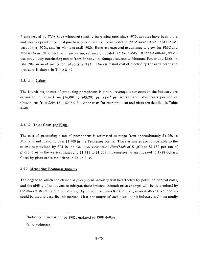
Plants served by TVA have witnessed steadily increasing rates since 1976, as rates have been more
and more dependent on coal purchase commitments. Power rates in Idaho were stable until the last
part of the 1970s. and for Montana until 1980. Rates are expected to continue to grow for FMC and
Monsanto in Idaho because of increasing reliance on coal-fired electricity. RhBne-Poulenc, which
was previously purchasing power From Bonneville, changed sources to Montana Power and Light in
late 1982 in an effort to control costs [SR183]. The estimated cost of electricity for each plant and
vroducer is shown in Table 8-47.
The fourth major cost of producing phosphorus is labor. Average labor costs in the industry are
estimated to range from $36,001 to $43.201 per year4 per worker and labor costs per ton of
phosphorus from $204.13 to $275.015. Labor costs for each producer and plant are detailed in Table
8-48.
8.5.1.2 Total Costs tier Plant
The cost of producing a ton of phosphorus is estimated to range from approximately $1,260 in
Montana and Idaho, to over $1,700 in the Tennessee plants. These estimates are comparable to the
estimates provided by SRI in the Chemical Ecorlonlics Handbook of $1,070 to $1,180 per ton of
phosphorus in the western states and Sl ,3 I5 to $1,555 in Tennessee, when indexed to 1988 dollars.
Costs by plant are summarized in Table 8-49.
8.5.2 Measurine Economic l n i ~ a c t s
The degree to which the elemental phosphorus industry will be affected by pollution control costs,
and the ability of producers to mitigate these impacts through price changes will be determined by
the market structure of the industry. As noted in sections 8.2 and 8.5.1, several alternative theories
could be used to describe this market. First, the output of each plant in this industry is almost totally
41ndustry information for 1983, updated to 1988 dollars.
'JFA estimates
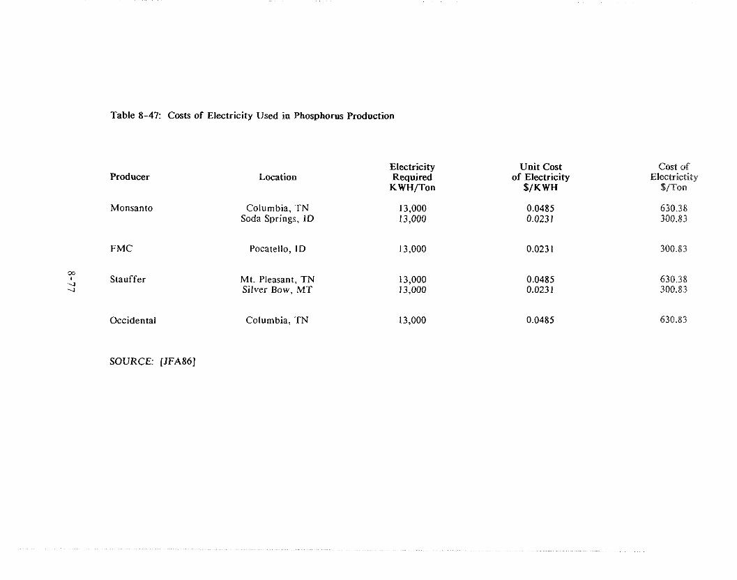
Table 8-47: Costs of Electricity Used in Phosphorus Production
Producer
Monsanto
FMC
05
.J Stauffer
.J
Occidental
Location
Columbia, TN Soda Springs, ID
Mt. Pleasant, TN Silver Bow. MT
Columbia, TN
Electricity Required
KWH/Ton
Unit Cost of Electricity
$/KWH
cost of Electrictity
$/Ton
SOURCE: [JFA86]
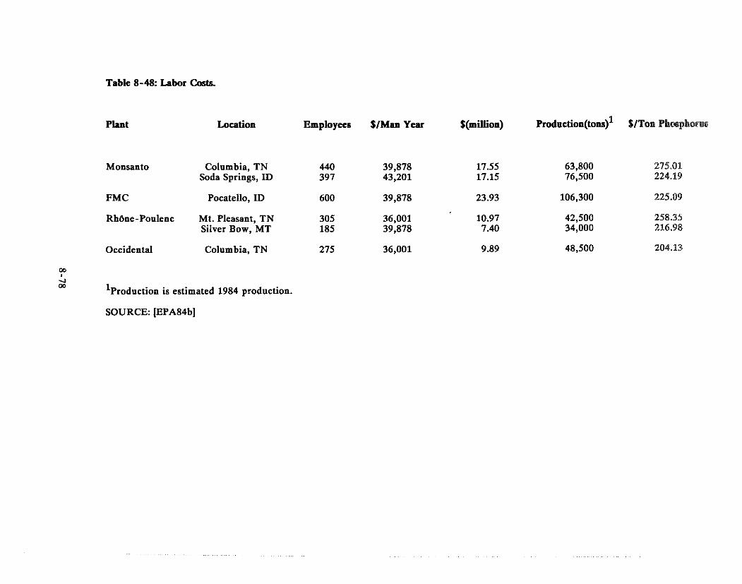
Table 8-48: Labor Costs.
P h t Location Employees $/Man Year $(million) ~rodaetion(tons)~ $/Ton Phogpborue
Monsanto Columbia, TN 440 39,878 17.55 Soda Springs, ID 397 43,201 17.15
FMC Pocatello, ID 600 39,878 23.93
RhBne-Poulenc Mt. Pleasant, TN 305 36,001 10.97 Silver Bow, MT 185 39,878 7.40
Occidental Columbia, TN 275 36,001 9.89
m 21 m
'production is estimated 1984 production.
SOURCE: [EPA84b]
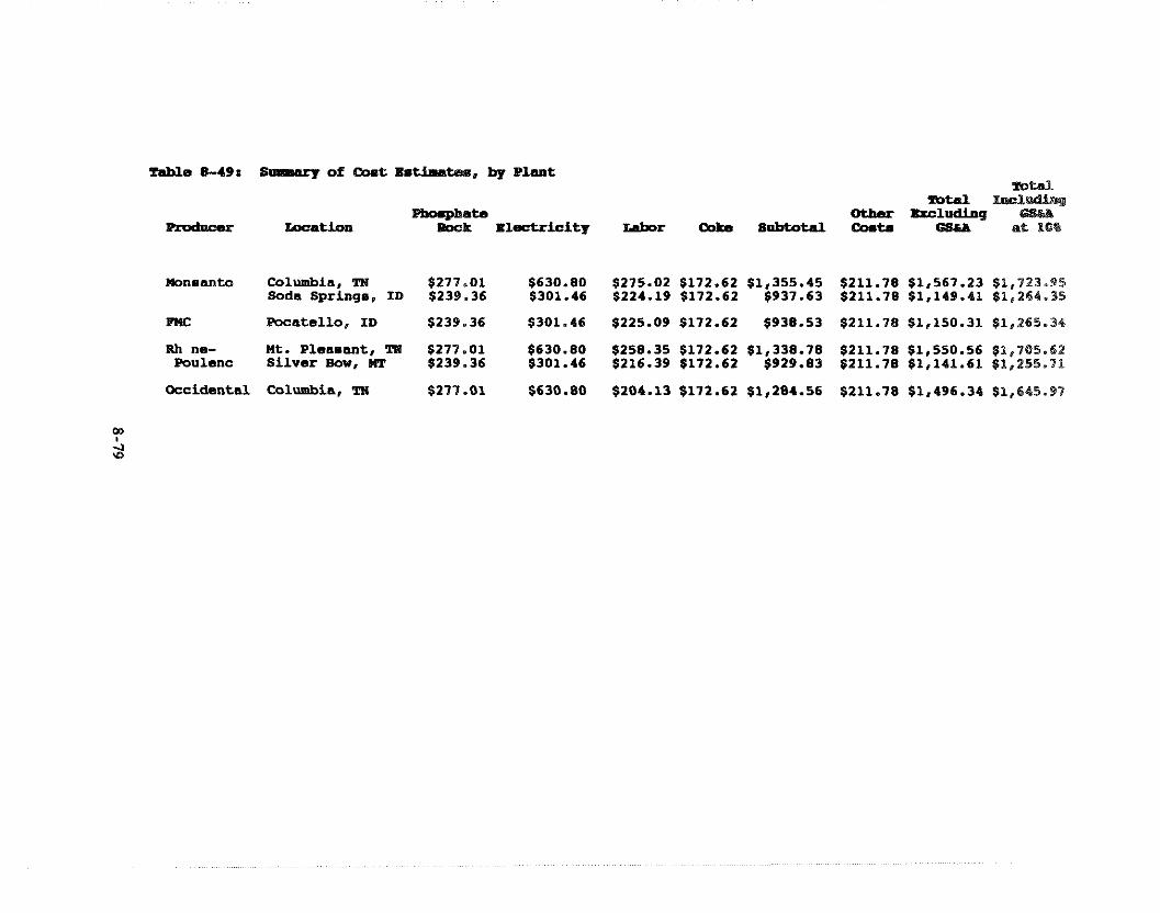
Table 8-19: Sumwry of CMe X s t b a t e p , by Plant m u
mtel +ncl Other hcloding GIPILh
Prodomr Tocatfon PoFk X l I I C t T i C i t y Labor Coke *+dl Om+. QlUL a: 101 Phorphate
m n e a n t o Columbia, TN $277.01 $630.80 $275.02 $172.62 $1,355.45 $211.78 $1 ,567 .23 $1,723.95 Soda Springe , I D $239.36 $301.46 $224.19 $172.62 $937.63 $211.78 $1 ,149 .41 $1,264.35
Rh no- M t . P l e a s a n t , TH $277.01 $630.80 $258.35 $172.62 $1,338.78 $211.78 $1,550.56 $1,705.62 Poulsnc S i l v e r Sow, IIT $239.36 $301.46 $216.39 $172.62 $929.83 $211.78 $1,141.61 $1,255.71
Occ identa l Columbia, TH $277 -01 $630.80 $204.13 $172.62 $1,284.56 $211.78 $1,496.34 $1,645.97
consun~ed by other plants owned by the parent corporation. The downstream plants process this
elemental phosphorus into t~arious con~pounds of phosphorus that are sold as inputs to the production
of highly-competitive goods. Substitute inputs for the phosphorus are available and widely used.
Thus, the demand for elemental phosphorus is derived from the demand for products in highly-
competiti\.e, price-sensitive markets. Therefore, phosphorus producers may face a flat demand
curve. as in a competitive market, even though there are only four producing companies. A flat or
nearly-flat demand curve suggests that the manufacturer would have little opportunity to pass on
increases in unit costs through price increases.
An alternative description of the elemental phosphorus industry is that it is an oligopoly with a strong
price leadership. There are only four manufacturers, and production costs a t the western plants are
lower than at plants elsewhere. The low-cost manufacturers have the ability to set the market price
at a profit-maximizing production level. The higher cost manufacturers would thus be price takers,
because, if market price were set at the marginal cost of the low-cost producers, the higher-cost
producers would have to sell their product at this price, even if it meant losing money on each unit
sold, or leave the industry. As seven higher-cost plants have been closed over the past two decades,
it would appear that the cost of closing these plants was less than the cost of selling products below
their individual marginal cost of production.
A collusive oligopoly will attempt to operate as a monopoly, setting industry marginal revenue equal
to industry marginal cost to determine output. The price is then established by the demand curve at
a level above that which would exist in a competitive market. Thus, industry maximizes its profit.
Output and revenue for each manufacturer are determined by the manufacturer's marginal costs and
the price level. While i t may not be possible in the absence of collusion for the oligopoly to operate
in this fashion, firms in such an industry would likely be able to maintain price above marginal cost
(the competitive price) and thus earn excess profits.
Firms in any market will determine their level of output based on their marginal cost. By definition,
fixed costs do not vary with the level of output. Therefore, they do not enter into the production
rate decision since firms in general will continue to produce as long as marginal revenue is greater
than or equal to marginal cost. The cost of regulatory compliance presents a special case. While the
expenditures for pollution control capital equipment are clearly fixed costs, operating costs for this
equipment are not so clearly categorized. Usually, operating cost is thought of as a variable cost.
That is, if no production occurs, no operating costs are accrued. However, in the case of these
particular regulations of the elemental phosphorus industry, the capital and operating costs vary
little with output. The assumption here is that any minimal costs required to meet a standard may
be viewed os fixed costs, suggesting that no changes in output or price would be expected as a result
of the compliance with the standards. In this case, all the impacts will be born by the affected
manufacturer in the form of lower profits. If an en~issions limit of 10 Ci/y is chosen, there would
be no cost and no economic impact.
Thnt phosphate rock is an exhaustible resource owned by the regulated industry requires some special
consideration. The resource stock is an asset held by its owner, :he value of which is determined by
the size of the asset and the present value of the difference between market price and extraction cost
in any period. The rate of extraction selected by the owner of the resource will depend on the
structure of the market in which the resource is sold, forecasts of the future prices for the product,
and forecasts of interest rates. If, for example, the resource owner expected the rate of growth in
the net price (market price less extraction cost) to be less than the interest rate, that owner would
extract the resource as quickly as possible and convert it to a new asset that would return at least the
market rate of interest. In general, it would be expected that a monopolist would set prices high
enough that the extraction rate would be slower than that of a producer in a competitive market. In
an oligopoly, the resource would be extracted faster than in the monopoly, but slower than in the
conlpetitive market, either the price and extraction rates approaching the competitive case as the
number of firms in the industry became larger. In this case, several stocks of the exhaustible
resource are available with each plant being fed by a specific mine. The low-cost producer is able
to earn a higher return from its resource than are the other plants. This higher return allows the
low-cost producer to earn an economic rent on its stocks of phosphate rock. By imposing a new
environn~ental cost that is mostly fixed cost, the available rent that could be earned by the low-cost
producer is reduced by the amount of the pollution abatement costs.
While i t is uncertain to what extent product prices and quantity demanded of elemental phosphorus
will be affected by these standards, if an emissions level of 10 Ci/y is chosen, there will be no change
in production levels at the regulated facility. It is assumed that the product price is unchanged.
Therefore, there are no consumer impacts, no change in employment levels and no community
impacts. The entire impact of the standard would be calculated as a reduction in profits for the
affected firms. Table 8-50 presents the estimated value of elemental phosphorus production, the total
revenue of the parent corporation, and the percent of total revenues accounted for by elemental
phosphorus in 1986. In that year, Monsanto and FMC, the two firms potentially affected by the 1984
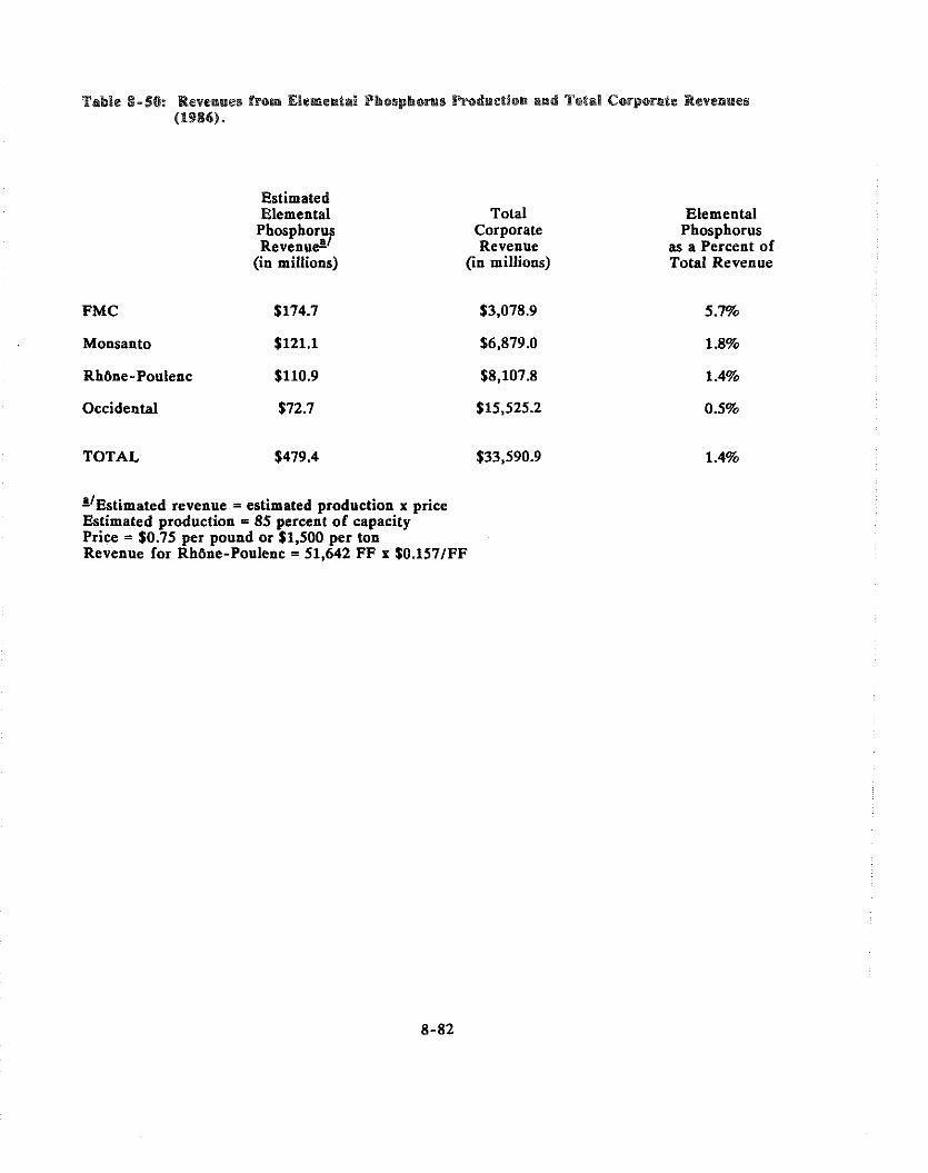
Table 8-So: Revenues from Elemental Phcsphoms Pwdiuctlo~ m d Total Coporate Revenues (1986).
Estimated Elemental
Phosphorus ~ e v e n u & l
(in millions)
Total Corporate Revenue
(in millions)
FMC $174.7 $3,078.9
Monsanto $121.1 $6,879.0
Occidental $72.7 $15,525.2
TOTAL $479.4 $33,590.9
"~stimated revenue = estimated production x price Estimated production = 85 percent of capacity Price = $0.75 per pound or $1,500 per ton Revenue for RhBne-Poulenc = 51,642 FF x S0.157IFF
Elemental Phosphorus
as a Percent of Total Revenue

regulation, had 1.8 and 5.7 percent of their re\enues associated with elemental phosphorus
production. In 1987, elemental phosphorus revenues accounted for an estimated 5.7 percent of FMC's
total corporate revenues. Table 8 -51 shows the level of capital expenditures normally undertaken
by each firm, required capital expenditures under different regulatory alternatives and the percentage
of total capital expenditures represented by the pollution control capital expenditures.
8.5.3 Reeulatorv Flevibilitv Analvsis
The Regulatory Flexibility Act (RFA) requires regulators to determine whether proposed regulations
would have a significant economic impact on a substantial number of small businesses o r other small
entities. If such impacts exist, regulators are required to consider specific alternative regulatory
structures to minimize the small entity impacts without compromising the objective of the statute
under which the rule is enacted. Alternatives specified for consideration by the RFA are tiering
regulations, performance rather than design standards, and small f i rm exemptions.
The four firms operating plants in this industry are major diversified corporations, the smallest of
which was ranked 131 on the Fo,-lu,~r list of the 500 largest U.S. companies in 1987. The Pocatello
plant accounts for over one-third of national production and probably enjoys the lowest cost structure
due to economies of scale and regional cost differences. It is unlikely that this situation will change
after the imposition of a Po-210 standard. In light of the fact that the four smallest plants in the
elemental phosphorus industry are expected to incur no compliance costs as a result of any regulatory
alternatives under consideration, no significant small business impact will occur.
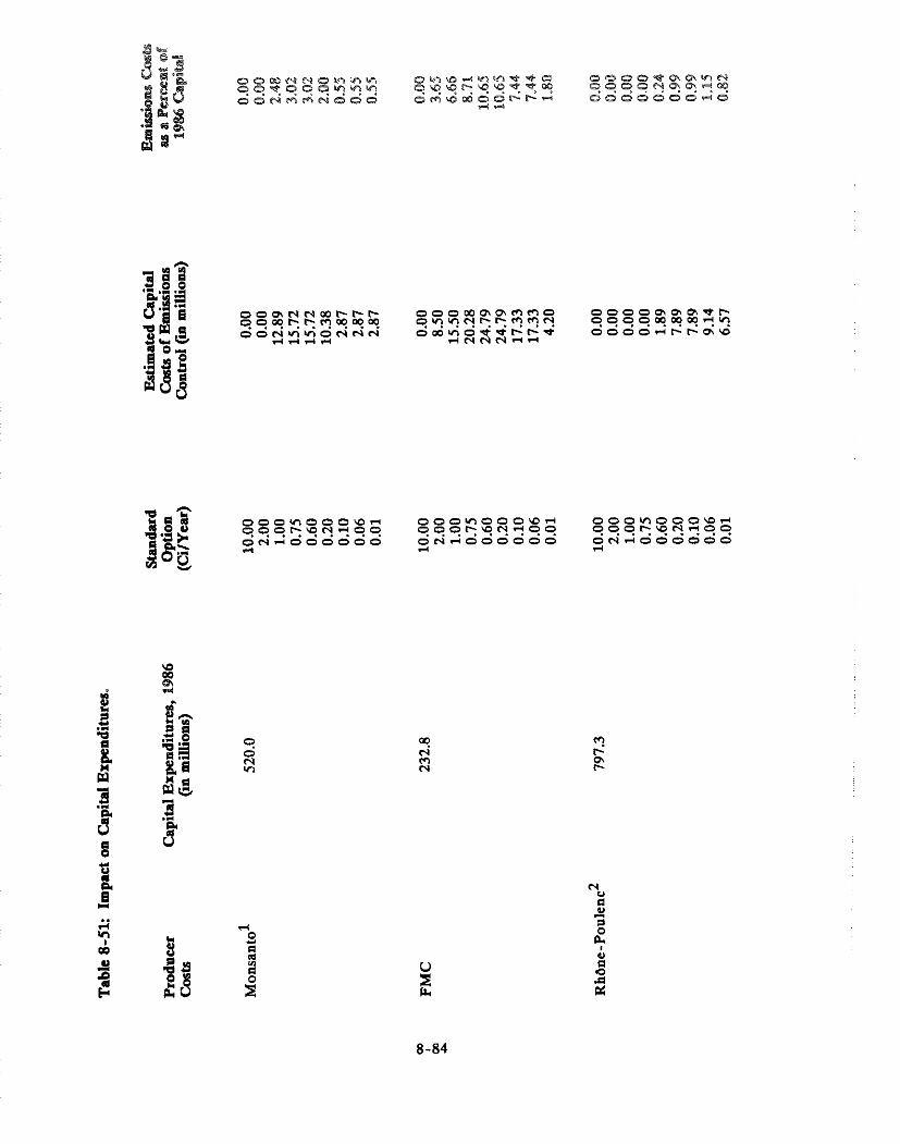

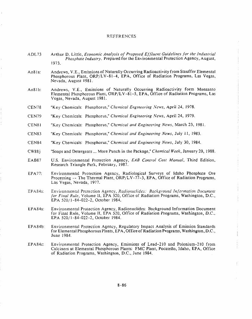
REFERENCES
Arthur D. Little, Ecortonzic Analysis o/ Proposed Ef/lurrrt Guidelines /or the industrial Phosphate Irtdustry. Prepared for the Environmental Protection Agency, August,
1973.
Andrews, V.E., Emissions of Naturally Occurring Radioactivity from Stauffer Elemental Phosphorous Plant, ORP/LV-81-4, EPA, Office of Radiation Programs, Las Vegas, Ne\.ada, August 1981.
Andrews, V.E., Emissions of Naturally Occurring Radioactivity form Monsanto Elemental Phosphorous Plant, ORP/LV-81-5, EPA, Office of Radiation Programs, Las Vegas, Nevada, August 1981.
"Key Chemicals: Phosphorus," Chenzical Erlgrrrrering .Vews, April 24, 1978.
"Key Chemicals: Phosphorus," Chentical Ertgirteering Y e w s , April 24, 1979.
"Key Chemicals: Phosphorus," Chenlical artd Errgineerirtg News, March 23, 1981.
"Key Chemicals: Phosphorus," Chentical artd Ertgitteerirrg News, July 11, 1983.
"Key Chemicals: Phosphorus," Chemical artd Etigineerittg News, July 30, 1984.
"Soaps and Detergents ... More Punch in the Package," Chentical Week, January 20, 1988.
U.S. Environmental Protection Agency, EAB Control Cost Martual, Third Edition, Research Triangle Park, February, 1987.
Environmental Protection Agency, Radiological Surveys of Idaho Phosphate Ore Processing - - The Thermal Plant, ORP/LV-77-3, EPA, Office of Radiation Programs, Las Vegas, Nevada, 1977.
En\~ironmental Protection Agency, Radioriuclides: Background Infornmtion Docun7eizt for Fittal Rule, Volume 11, EPA 520, Office of Radiation Programs, Washington, D.C., EPA 520/1-84-022-2, October 1984.
Environmental Protection Agency, Radionuclides: Background Information Document for Final Rule, Volume 11, EPA 520, Office of Radiation Programs, Washington, D.C., EPA 520/1-84-022-2, October 1984.
Environmental Protection Agency, Regulatory Impact Analysis of Emission Standards for Elemental Phosphorous Plants, EPA, Office of Radiation Programs, Washington, D.C., June 1984.
Environmental Protection Agency, Emissions of Lead-210 and Polonium-210 from Calciners at Elemental Phosphorous Plants: FhlC Plant, Pocatello, Idaho, EPA, Office of Radiation Programs, Washington, D.C., June 1984.
Environmental Protection Agency, En~issions of Lead-210 and Polonium-210 from Calciners at Elemental Phosphorous Plants: Stauffer Plant, Silver Bow, Montana, EPA, Office of Radiation Programs, Washington, D.C., August 1984. "Preliminary Analysis of Potential Impacts of $70 Million Compliance Cost at FMC Plant," memorandum from Rod Lorang and Barry Galif, Sobotka, Inc. to Byron Bunger, EPA, February 6, 1984.
Vol. 2., Eiiviror~nrerrtal In~pact Statement
FhlC Corp., Annual Report, 1986.
GARD, Inc. Capital a i~d Operati~rg Costs of Selected Air Pollutio~t Control Systems, prepared for the U. S. Environmental Protection Agency, Research Triangle Park, N.C., December, 1978.
Mannsville Chemical Products Corp., "Phosphorus," Chenrical Products Synopsis, Cortland, New York, January 1985.
Midwest Research Institute, Analysis of Achievable Po-210 Emission Reductions and Associated Costs for FMC's Pocatello, Idaho, Plant, For the Office of Radiation Programs, EPA, under contract number 68-02-3817, August, 1984.
Midwest Research Institute, for Office of Air Quality Planning and Standards, U. S. Environmental Protection Agency, Characteri:atior~ and Conlrol o f Radionuclide Enrissions fronr Elenzeiltal Phosphorus Production, Research Triangle Park, N.C., February 19, 1989.
William Stowasser, "Phosphate Rock," Mi~rerals Yearbook, 1986 pre-print, Volume 1, 1987, p.14.
Radian Corporation, Emission Testing of Calciner Off-gases at FMC Elemental Phosphorous Plant, Pocatello, Idaho, \'olumes I and 11, Prepared for the Environmental Protection Agency under Contract No. 68-02-3174, Work Assignment No. 131, Radian Corporation, P.O. Box 13000, Research Triangle Park, NC, 1984.
Radian Corporation, Emission Testing of Calciner Off-gases a t Monsanto Elemental Phosphorous Plant, Soda Springs, Idaho, Volumes I and 11, Prepared for the Environn~ental Protection Agency under Contract No. 68-02-3174, Work Assignment No. 133, Radian Corporation, P.O. Box 13000, Research Triangle Park, NC, 1984.
Radian Corporation, Emission Testing of Calciner Off-gases a t Monsanto Elemental Phosphorous Plant, Soda Springs, Idaho, Volumes I and 11, Prepared for the Environn~ental Protection Agency under Contract No. 68-02-31 74, Work Assignment No. 133, Radian Corporation, P.O. Box 13000, Research Triangle Park, NC, 1984.
Science Applications, Inc., Airbor~re En~ission Control Technology for the Elemental Phosphorous Industry, Final Report to the Environmental Protection Agency, Prepared under Contract No. 88-01-6429, SAI, P.O. Box 2351, La Jolla, CA, January 1984.
SRI, Chenlical Ecorronlics Handbook, March 1980
SRI, Chen~ical Ecorronrics Handbook, January 1983.

SKIS6 SRI, Clic,nlrc.ml Eco~rontlcs Na~idhook. February 1986

CHAPTER 9
PHOSPMOGVPSUM


9. PHOSPNOGVPSUM STACKS
9.1 Introduction and Summary
Phosphogypsum stacks are one of twelve industrial sources of radionuclide emissions for which EPA
is required to consider controls. In the case of phosphogypsum, the emission of concern is radon.
Section 9.2 profiles the phosphate fertilizer industry that generates the phosphogypsum. Section 9.3 describes the controls for radon emissions, their costs, and the reduction of emissions and of the risk
of lung cancer that they would provide. Section 9.4 considers the cost per unit of emission reduction
attributable to the different combinations of control parameters. Section 9.5 assesses the impact radon
control would have on the U.S. economy. Section 9.6 provides an analysis of the regulatory flexibility
of the controls.
The overall conclusions regarding controls on phosphogypsum stacks to reduce the risk of cancer due
to radon emissions are: 1) the controls that will reduce risk the most can be provided to the fourteen
phosphogypsum stacks for which data was available for about $251 million (discounted at 5 percent),
2) the most stringent controls would reduce risk to the 80 km populations by 3E-1, and 3) using the
most expensive version of the controls will add an average of $14 per ton to the cost of producing
phosphoric acid and reduce the export of phosphoric acid from the U.S. by approximately 11 percent
over the next thirty years.
9.2 Industrv Profile
Phosphogypsum is a waste product resulting from the production of wet process phosphoric acid used
in the manufacture of fertilizer and animal feed. Phosphate-bearing ore is mined and then processed
to remove clay and other impurities. The purified ore is called phosphate rock. The phosphate rock
is then reacted with sulfuric acid, producing phosphoric acid and the waste product phosphogypsum
(calcium sulfate). Of all the marketable phosphate rock mined in the United States annually, about
90 percent is used in the production of wet-process phosphoric acid (WPPA). Thermal phosphoric
acid is produced with the remaining 10 percent.
Phosphorus, along with potassium and nitrogen, is one of the primary nutrients which plants require.
All living things contain phosphorus, a basic element essential to life. It ensures the transfer and
storage of energy and plays a role in the metabolic process. Phosphorus is not naturally very
abundant in soils, as it is constantly removed by crops and natural losses. Phosphate applications help
produce high crop yields and improve the biological quality of the crop. The phosphate mineral itself
is very insoluble and is therefore a poor source of phosphorus for plants. Thus, the phosphate rock

is treated with excess sulfuric acid to produce merchant-grade WPPA, containing 52 to 54 percent
P205 (phosphorus pentoxide, the unit commonly used to express phosphorus content) [St85l.
1 The U.S. phosphate industry was the world leader in downstream fertilizer products after initiating
major expansions in the 1970s. However, in the 80s many foreign rock producers have been investing
in their own downstream product facilities with the result that in the near future all major rock
exporters and producers will have their own phosphoric acid and fertilizer production capability.
The 1980s have been a difficult period for the U.S. phosphate industry. Besides the rapid growth
of foreign production capacity, the domestic industry has suffered from rapid changes in demand for
phosphate fertilizer. As a result, sales of phosphate products have declined, losses have been incurred
throughout the industry and several companies have filed for bankruptcy, closed their phosphate
operations, or sold their phosphate operations. Nevertheless, the U.S. industry continues to dominate
the domestic market and total production and exports have shown promise of improving, though the
value of sales has not improved. Phosphate fertilizer sales were $3.9 billion in 1987, down from $4.5
billion in 1984. Sales in the second quarter of 1988, however, increased 12 percent from levels in
1987 [DOC88a, TFI88bl.
However, the outlook for the domestic phosphate industry is complicated by the depletion of major
phosphate rock deposits in central Florida. The Bone Valley of Florida, which contains many of the
lowest cost deposits in the world, is being rapidly depleted. Many nearby deposits are available or
could be developed, but at a higher cost and lower grade. Over the next 20 years, there will be a
high level of mine replacement. Average production costs in Florida will be rising faster than those
in much of the rest of the world, where current mines can continue production for many years
[BSC85a].
Morocco and Florida represent the two sides of the phosphate industry. The Moroccan state-owned
company has aggressively expanded phosphate rock, acid and fertilizer capacity even when the
international market had excess capacity. And while Florida production costs are now the lowest,
Morocco has a variety of cost advantages, including closer proximity to key export markets [BSC85a].
The future of the U.S. phosphate industry depends on its ability to remain competitive against
countries like Morocco.
ownst stream fertilizer products include: diammoniurn phosphate, and triple super phosphate, as well as some items manufactured in smaller quantities.
9-2
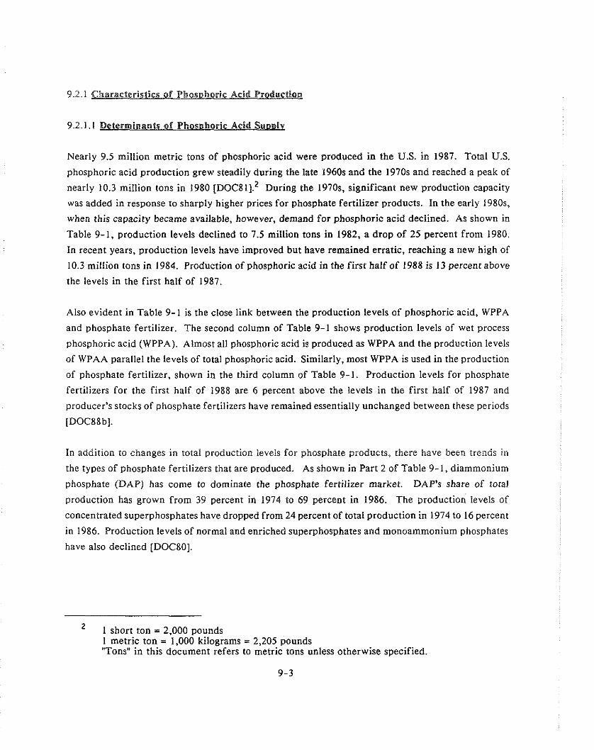
9.2.1 Characteristics of Phosahoric Acid Production
9.2.1.1 Determinants of Phosohoric Acid Sunoly
Nearly 9.5 million metric tons of phosphoric acid were produced in the U.S. in 1987. Total U.S.
phosphoric acid production grew steadily during the late 1960s and the 1970s and reached a peak of
nearly 10.3 million tons in 1980 [ D O C ~ I ] . ~ During the 1970s, significant new production capacity
was added in response to sharply higher prices for phosphate fertilizer products. In the early 1980s,
when this capacity became available, however, demand for phosphoric acid declined. As shown in
Table 9-1, production levels declined to 7.5 million tons in 1982, a drop of 25 percent from 1980.
In recent years, production levels have improved but have remained erratic, reaching a new high of
10.3 million tons in 1984. Production of phosphoric acid in the first half of 1988 is 13 percent above
the levels in the first half of 1987.
Also evident in Table 9- 1 is the close link between the production levels of phosphoric acid, WPPA
and phosphate fertilizer. The second column of Table 9-1 shows production levels of wet process
phosphoric acid (WPPA). Almost all phosphoric acid is produced as WPPA and the production levels
of WPAA parallel the levels of total phosphoric acid. Similarly, most WPPA is used in the production
of phosphate fertilizer, shown in the third column of Table 9-1. Production levels for phosphate
fertilizers for the first half of 1988 are 6 percent above the levels in the first half of 1987 and
producer's stocks of phosphate fertilizers have remained essentially unchanged between these periods
[DOC88 b].
In addition to changes in total production levels for phosphate products, there have been trends in
the types of phosphate fertilizers that are produced. As shown in Part 2 of Table 9-1, diammonium
phosphate (DAP) has come to dominate the phosphate fertilizer market. DAP's share of total
production has grown from 39 percent in 1974 to 69 percent in 1986. The production levels of
concentrated superphosphates have dropped from 24 percent of total production in 1974 to 16 percent
in 1986. Production levels of normal and enriched superphosphates and monoammonium phosphates
have also declined [DOC80].
I short ton = 2,000 pounds I metric ton = 1,000 kilograms = 2,205 pounds "Tons" in this document refers to metric tons unless otherwise specified.

Table 9-1: Production of Phosphoric Acid, Wet Process Phosphoric Acid end Phosphate Fertitizer.
(Part 1 of 2)
M e t r i c T o n s ....----....---........--.--*----..----.-----------------...-.-------------.-.*----.-----
YEAR TOTAL YET PROCESS TOTAL
PHOSPHORIC A C I D PHOSPHORIC A C I D PHOSPHATE F E R T I L I Z E R
PRWUCTION PERCENT OF P R W U C T I O N PRWUCTION PERCENT OF
1970 BASE 1970 BASE
S o u r c e : B u r e a u o f t h e Census, C u r r e n t industrial R e p o r t s
Sumnary r e p o r t s f o r 1987, 1986, 1985, J a n u a r y 1982, 1980, 1979, 1978, 1976, 1974, 1973.
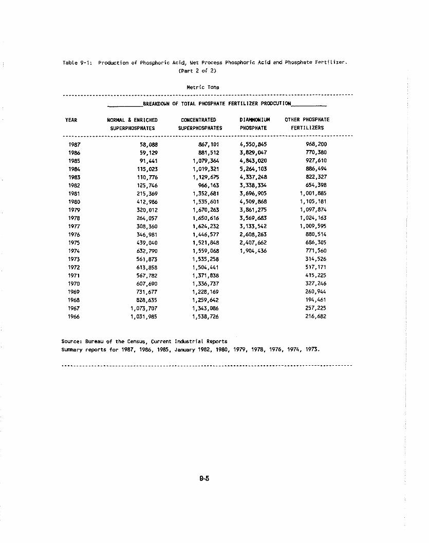
Table 9-1: Production of Phosphoric Acid, Uet Process Phosphoric Acid and Phosphate F e r t i l i z e r
(Part 2 of 2)
Metric Tons - * - - - - - - - - - - - - - . - - - - - - - - - - - . - - - - - - - * - . - - - - - - - - - - - - - - - * - - - - - - - - * - - - - - - - - - - - - . - - - - - - . - - - - - - - - - - - - - - -
BREAKDOWN OF TOTAL PHOSPHATE FERTILIZER PRODCUTION
YEAR NORMAL 8 ENRICHED CONCENTRATED DIMMONIW OTHER PHOSPHATE SUPERPHOSPHATES WPERPHOSPHATES PHOSPHATE FERTILIZERS
Source: Bureau of the Census, Current Industrial Reports
Sunnary reports fo r 1987, 1986, 1985, January 1982, 1980, 1979, 1978, 1976, 1974, 1973.

Price Trends
Spot prices of WPPA have varied considerably in the 1970s and 1980s. These changes have an
enormous influence on the cost of phosphate fertilizers. WPPA represents 70 percent of the
production costs of diammonium phosphate and 69 percent of the cost of granular triple super
phosphate (TSP) [TFI87c]. TSP also requires some phosphate rock in its production, contributing
another 9 percent of its production cost. Table 9-2 shows the prices for phosphoric acid and
fertilizer in absolute and constant dollars. Table 9-2 also gives prices for sulfur and phosphate rock,
the two most important inputs to WPPA. These inputs will be discussed in detail later in this chapter.
Figure 9-1 graphs the changes in prices of the commodities listed in Table 9-2. The prices con-
sidered in these exhibits are for the export market for product loaded and leaving from terminals
in the Gulf of Mexico. Prices in this market are more volatile than prices determined by long term
contracts. The price for WPPA shipped under long-term contracts, however, are not often published.
In the early 1970s, fertilizer prices were restrained in the U.S. by the national wage and price
controls. After wage and price controls ended, prices increased rapidly, reaching a high in the
middle of 1974. The price for phosphoric acid in 1974 was $712 per ton (1982 dollars). It dropped
by 62 percent to $271 (1982 dollars) by 1977 and rebounded to $439 (1982 dollars) per ton in 1980.
Prices have declined since 1980, to $257 per ton (1982 dollars) in the spot market in April 1988.
The April 1988 price, in current dollars, was $307.50 [BSC88b].
Plants and Ooeratina Caoacitr
There are 20 operating WPPA plants in the U.S. [TVABSJ. According to the Tennessee Valley
Authority, six of their plants were indefinitely closed in the mid-1980s. Two other plants, owned
by the bankrupt Beker Industries Company, are closed and for sale. The eight plant shutdowns have
resulted in a U.S. WPPA capacity reduction of 1.4 million tons per year. The 20 plants in operation
give the U.S. a capacity of 11.5 million tons of WPPA. Since 1984, the 20 operating plants have
increased overall capacity by 735,000 tons, although one of these plants reduced capacity by 100,000
tons [TVA88]. There are 11 WPPA plants operating in Florida, comprising 67 percent of the capacity
of U.S. plants still in operation. Louisiana has 4 operating WPPA plants and the remainder are
distributed among North Carolina, Mississippi, Texas, Idaho and Wyoming.
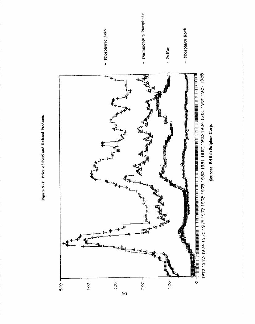

Table 9 - 2 : Brice of Phosphoric Acid, Sulr"arr
Phosphate ROC): a d B i m i u n Phosphate.
(Average of Monthly Prices) .-.---.-------.-..-..*.---"*------------------*-
PHOSPHORIC PHOSPHATE DIUlllMllW AClD SULFUR ROCK PHOSPHATE
CONSTANT DOLLARS 1982 DOLLARS
PHOSPHORlC PHOSPHATE AClD SULFUR ROCK
1972 $239.70 $33.73 $16.72 1973 $313.97 $36.31 $27.38 1974 1711.81 $49.70 S65.61 1975 S606.03 $92.02 $80.94 1976 1320.59 $64.14 $59.17 1977 $270.86 $55.42 $41.67 1978 S280.18 156.03 U2.W 1979 $371.93 1106.05 $43.79 1980 1439.27 $143.26 $51.93 1981 $363.70 1118.35 $48.05 1982 1310.54 $110.31 $39.17 1983 $258.38 186.94 $30.76 1984 $277.49 $91.40 130.74 1985 $245.96 $119.96 $29.52 1986 $244.85 $117.11 $28.05 1987 $213.16 $86.60 $23.19 1988 1251.23 $77.05 526.67
olAnnowlun PHOSPHATE
$193.46 $243.10 $415.35 1417.02 $189.91 $197.99 1192.92 $250.69 1260.50 $205.63 1180.67 $175.29 $175.24 $151.53 $135.15 $147.62 1154.59
A l l data are i n do l la rs per metric ton. Phosphoric acid and d i a m n i u n phosphate prices are FOB US Gulf; phosphate rock i s FOB Florida, and sul fur i s FOB Vancouver. GMP Deflator used t o complte constant-dol lar series. Source: Data plrchased frm B r i t i s h Sulphur Corp., June 5, 1988.

Production Costs
Estimates of the production costs of WPPA are available from a variety of sources. Table 9-3 shows
estimates from The Fertilizer Institute (TFX). The data are from an industry survey of U.S. producers
of 1986 costs. According to the TFI estimates, sulfuric acid represents 49 percent of the cost of
producing phosphoric acid. Over 96 percent of the cost of sulfuric acid is accounted for in
purchasing the sulfur itself. Phosphate rock represents another 31 percent of the production cost of
phosphoric acid. Energy costs represent 6 percent of production costs. Per ton of phosphoric acid
requires 2.74 tons of sulfuric acid and 3.55 tons of phosphate rock. Plants with an annual capacity
over 400,000 tons enjoy a considerable cost advantage over smaller plants. According to the TFI
survey, large plants had an average production rate of $229 per ton, compared to $289 for plants
with a capacity under 400,000 tons. The average cost in 1986 was $239.35 per ton [TFI87d].
Traditionally, phosphoric acid production occurred almost entirely in tandem with fertilizer
production. However, improved transportation options and heightened international competition has
created a distinct market for the production and sale of phosphoric acid.
Transoortation Costs
The markets a nation's phosphate industry serves depend in large measure on transportation costs.
In March 1988, the cost to ship a ton of phosphoric acid from the Gulf of Mexico to India averaged
$48, a little over 15 percent of the current U.S. price [BSC88a]. North African producers have a
transportation advantage over U.S. producers for many markets. According to estimates by Zellars-
Williams for the cost of shipping one type of phosphate, DAP fertilizer, Morocco and Tunisia have
a $5 per ton advantage shipping to northern Europe and India. Freight costs to China are essentially
the same for both regions [Ze86].
Few U.S. phosphoric acid producers have their own shipping fleets. The notable exception is
Occidental Petroleum Co., which has a dedicated fleet of three vessels supplying contract deliveries
of phosphoric acid to the Soviet Union. Office Cherifien Des Phosphates (OCP) of Morocco and ICM
of Tunisia both ship phosphoric acid, using captive tonnage. Brazil and India, important phosphoric
acid consumers, have both invested in dedicated fleets of phosphoric acid tankers, but the bulk of
their import requirement continues to be met by outside carriers.
With the exception of phosphoric acid, phosphate products do not require specialized handling
facilities and these products can be readily shipped in conventional bulk carriers. The market for

Table 9-3: Phosphate Fer t i l i ze r Pmduction Coats
........................................................ Cost pi- Percent of m t r i c ton t o t a l cost
Uet Process Phosphoric Acid Sulfuric Acid 130.07 49.31: PhDsphate Rock 81.24 30.8% Elect r ic i ty 6.44 2.4% steam 10.22 3.9% Operating Labor 4.iU 1.8% other 31.21 11.8%
Total 263.88 I m X
D i a u m i r u Phosphate Phosphoric Acid 126.W 70.5% Anhydrous h w n i a 30.02 16.7% Elect r ic i ty 1.68 0.92% steam 3.53 2.0% Operating Labor 1.91 1.1% Other 16.42 8 . a
Total 180.45 1mX
Granular Tr ip le Super Phosphate
Phosphoric Acid 88.71 69.5% Phosphate Rock 10.98 8.6% Elect r ic i ty 2.95 2.3% Natural 6ss 2.27 1.a Operating Labor 2.58 2.0% other M.19 15.8%
Source: Phosphate Fer t i l i ze r Pmduct im Cost Survey, Year Ended Deceikr 31,1986. Coqi led by N a t i o ~ L Fer t i l i ze r Develop.ent Center f o r
The Fer t i l i ze r Institute, may 1,1997. pp.2-5. -*------------------.-----------------------------------
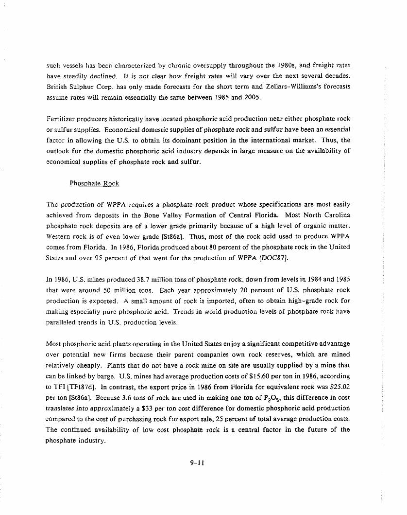
such vessels has been characterized by chronic oversupply throughout the 1980s, and freight rates
have steadily declined. It is not clear how freight rates will vary over the next several decades.
British Sulphur Corp. has only made forecasts for the short term and Zellars-Williams's forecasts
assume rates will remain essentially the same between 1985 and 2005.
Fertilizer producers historically have located phosphoric acid production near either phosphate rock
or sulfur supplies. Economical domestic supplies of phosphate rock and sulfur have been an essential
factor in allowing the U.S. to obtain its dominant position in the international market. Thus, the
outlook for the domestic phosphoric acid industry depends in large measure on the availability of
economical supplies of phosphate rock and sulfur.
Phos~hate Rock
The production of WPPA requires a phosphate rock product whose specifications are most easily
achieved from deposits in the Bone Valley Formation of Central Florida. Most North Carolina
phosphate rock deposits are of a lower grade primarily because of a high level of organic matter.
Western rock is of even lower grade [St86a]. Thus, most of the rock acid used to produce WPPA
comes from Florida. In 1986, Florida produced about 80 percent of the phosphate rock in the United
States and over 95 percent of that went for the production of WPPA [WC87].
In 1986, U.S. mines produced 38.7 million tons of phosphate rock, down from levels in 1984 and 1985
that were around 50 million tons. Each year approximately 20 percent of U.S. phosphate rock
production is exported. A small amount of rock is imported, often to obtain high-grade rock for
making especially pure phosphoric acid. Trends in world production levels of phosphate rock have
paralleled trends in U.S. production levels.
Most phosphoric acid plants operating in the United States enjoy a significant competitive advantage
over potential new firms because their parent companies own rock reserves, which are mined
relatively cheaply. Plants that do not have a rock mine on site are usually supplied by a mine that
can be linked by barge. U.S. mines had average production costs of $15.60 per ton in 1986, according
to TFI [TFI87d]. In contrast, the export price in 1986 from Florida for equivalent rock was $25.02
per ton [St86a]. Because 3.6 tons of rock are used in making one ton of P205. this difference in cost
translates into approximately a $33 per ton cost difference for domestic phosphoric acid production
compared to the cost of purchasing rock for export sale, 25 percent of total average production costs.
The continued availability of low cost phosphate rock is a central factor in the future of the
phosphate industry.
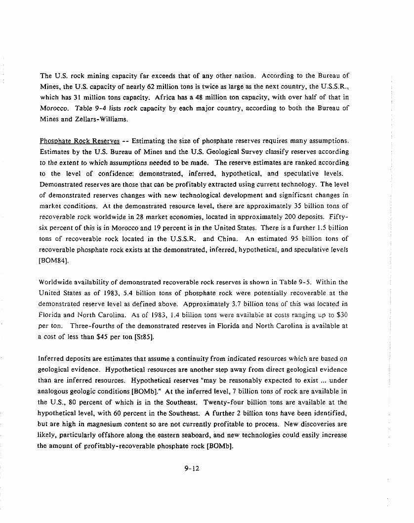
The U.S. rock mining capacity far exceeds that of any other nation. According to the Bureau of
Mines, the U.S. capacity of nearly 62 million tons is twice as large as the next country, the U.S.S.R.,
which has 31 million tons capacity. Africa has a 48 million ton capacity, with over half of that in
Morocco. Table 9-4 lists rock capacity by each major country, according to both the Bureau of
Mines and Zellars-Williams.
Phosohate Rock Reserves -- Estimating the size of phosphate reserves requires many assumptions.
Estimates by the U.S. Bureau of Mines and the U.S. Geological Survey classify reserves according
to the extent to which assumptions needed to be made. The reserve estimates are ranked according
to the level of confidence: demonstrated, inferred, hypothetical, and speculative levels.
Demonstrated reserves are those that can be profitably extracted using current technology. The level
of demonstrated reserves changes with new technological development and significant changes in
market conditions. At the demonstrated resource level, there are approximately 35 billion tons of
recoverable rock worldwide in 28 market economies, located in approximately 200 deposits. Fifty-
six percent of this is in Morocco and 19 percent is in the United States. There is a further 1.5 billion
tons of recoverable rock located in the U.S.S.R. and China. An estimated 95 billion tons of
recoverable phosphate rock exists at the demonstrated, inferred, hypothetical, and speculative levels
[BOM84].
Worldwide availability of demonstrated recoverable rock reserves is shown in Table 9-5. Within the
United States as of 1983. 5.4 billion tons of phosphate rock were potentially recoverable at the
demonstrated reserve level as defined above. Approximately 3.7 billion tons of this was located in
Florida and North Caroiina. As of 1983, 1.4 billion tons were avaiiable at costs ranging up to $30
per ton. Three-fourths of the demonstrated reserves in Florida and North Carolina is available at
a cost of less than $45 per ton [St85].
Inferred deposits are estimates that assume a continuity from indicated resources which are based on
geological evidence. Hypothetical resources are another step away from direct geological evidence
than are inferred resources. Hypothetical reserves "may be reasonably expected to exist ... under
analogous geologic conditions [BOMb]." At the inferred level, 7 billion tons of rock are available in
the U.S., 80 percent of which is in the Southeast. Twenty-four billion tons are available a t the
hypothetical level, with 60 percent in the Southeast. A further 2 billion tons have been identified,
but are high in magnesium content so are not currently profitable to process. New discoveries are
likely, particularly offshore along the eastern seaboard, and new technologies could easily increase
the amount of profitably-recoverable phosphate rock [BOMb].

- - - - . - - - - - . - - - - - - - - - " - - - - - - - - - - - - - - - - - - - - - - - . - - - - - - - - - - - - - - - - - - - - - - - - - - - - - - - - - - - - - " - - - - " w - - - - - - - - - - - - - - - - - - - - - - - - - " - " "
(U IUXf f l TWS PER YUR, DRY BASIS)
WCAT1W WRW PHOSPHATE ROCK CAPACllT,UW \I Z e l l e r a - U i l l i s u Reek Pmdusticn Forrcart\2 ----------------------*----------- -*-*---------------.-----------------.---------*-
1985 1990 15% XUl 1985 1990 1995 iU!U 2WS
WIRW AMERSCA 61.7 67.1 62.2 45.9 48.1 58.0 58.6 56.2 52.3 United States 61.7 67.1 62.2 45.9
CUmUL AMERICA 1.0 2.5 2.5 3.5 0.6 1.8 2.3 2.3 2.3 lluim 1.0 2.5 2.5 3.5
WITH AMERICA 4.5 7.0 9.0 10.0 3.8 5.0 5.0 5.0 5.0 Brazi 1 4.5 7.0 8.0 8.0 Peru - 1.0 2.0
WESTERN EUROPE 0.5 0.6 0.6 1.1 0.8 0.8 0.8 0.8 0.8 F i n l d 0.5 0.5 0.5 1.0 Turkey - 0.1 0.1 0.1
EASTERN EUROPE 31.0 36.0 45.0 50.0 31.0 35.1 YI.9 42.6 45.1 USSR 31.0 36.0 45.0 50.0
AFRICA Algeria
Egypt mmsm Smlgsl W t h Af~icI), Rep.
Toe0 Tunisia
A S I A
chi^ Israel
I rw Jordan Syria
OCEUIIA Australis 1.0 1.0 T.0 3.0 Chrirt.ar Island U 1.8 1.8 3.0 3.0 Nauru 2.0 2.0 2.0
WRLD TOTAL \4 290.9 351.5 404.8 426.5 142.6 171.4 1 . ZW.2 221.2
\1 m r c e : U.F. Stowucr, P-te Rock: W r l d Rcuurces, Upp ly d O h , 1986. Figure8 for a l l years are U.S. Bureau of llinca estimates based on the size o f the reserve base. Unfawrablc e ~ i c s may a l t e r the f o r r u s t a d mck capacities i n future years. \Z Source: P m t e Rock lWI86, by Zellars-UiLLiur. Blanks .w data i s mt available. This data are mt di rect ly m S t a m u r e t i r t o . Ih ltaruw d i m t o of rq.sity in d y o u aoll. mt *LY hn h. -it). u i l l be ud tul lY. Z. l~-Ui l l i . . ' * -ion tacrt my . L b tcu or vrud -it)., rp.s imLLy in w. Ilrrcklu, l -la ef h. &tm nrrb di t f .mt -Loot..
U h r i s m b i n d c ~ n d m a n d o o m . \4 CvvPt accurl tely -1-0 wrld to ta ts brtnr, tho two m u r o as bath do not m u i n a l l the ur data.
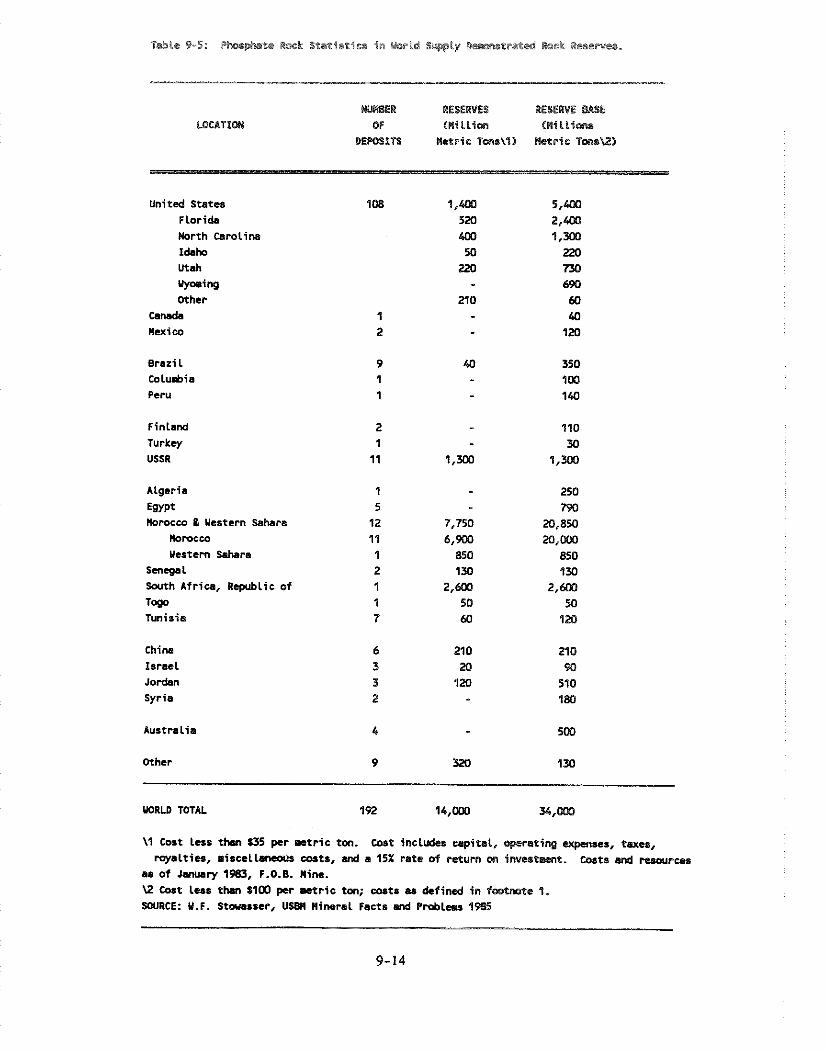
WUllSER RESERVES RESERVE WSE OF 6 R i l l i m Oni t licnr
DEWSITS lrctric Tarr\l9 Betrie TmsU)
United States Florida
HDrth Csrolins Idaho Utah
W-inp Other
CaMda Rexim
Brari 1 t o l u h i a
Peru
Finland
Turkey USSR
Algeria
Egypt Morocco P Uestern Sahara
Momcm
Yestern Sahara Senegal South Africa, Republic of
Toso Tunisia
chi^ Is rae l Jordan
Syria
Australia 4 - 5M)
Other 9 328 1M
WRU) TOTAL 192 14,DW %#a
\'I Cost leas than $35 per r t r i c ton. cost ineludes cqaifsl, operating upauer, tax=., myalties, a i r s e l l m o r i s coats, d a 15% rate of return on inveatunt. Coats d w p c c s
as of January 1983, F.O.B. Mine. U C o l t Less than $100 per w r i c ton; sort8 M defined i n footnote 1. SOURCE: U.F. Stcwasser, US8N n i m r a l Facts d Pmblnu '1985
There are many unknowns in estimating resource reserves. For example, there is speculation about
a new deposit in North Carolina. Details have not been finalized and tests will take two years to
complete after they have begun. Should this deposit be realized, an estimated 70 to 90 million metric
tons of new phosphate rock reserves could be added to North Carolina reserves and the costs could
be as low as $7 to $10 per ton [BSC87b].- -- The price of phosphate rock has followed a similar
set of swings as has the price of WPPA. Table 9-2 lists phosphate rock export prices between 1972
and 1988. Prices have fallen from around $45 per ton in 1980 and 1981 to between $27 and $31 per
ton in 1987 and 1988 [BSC88b].
Production -- Rock production forecasts require a number of assumptions concerning the
price and demand for phosphate rock, as well as operating costs in future years for known but
undeveloped deposits. William Stowasser at the U.S. Bureau of Mines and Zellars-Williams have
made the most careful production forecasts. While both sources anticipate similar trends, Stowasser
is considerably more pessimistic concerning the prospects for U.S. rock production after the year
2000.
Stowasser forecasts that U.S. production of phosphate rock will be 46.4 million tons per year by the
year 2000 [St851 and will decline significantly after that to about 28 million metric tons in 2010
[BOM88d]. Stowasser reexamined this forecast in June of 1988 after a survey of company's
production plans and did not significantly modify his forecast [BOM88c]. The production level in
the year 2000 is within the range of production achieved in the mid-1980s. Rock production from
Florida is expected to decline at a rapid rate after 2010 as reserves in currently operating mines in
the Bone Valley are exhausted. Production from North Carolina will increase through 2000 and be
about 10 million tons in 2010. Other U.S. production will remain about the same. These forecasts
assume an economically competitive technology will not be developed that would permit utilizing
undeveloped central Florida phosphate resources [BOM88c]. Thus, in Stowasser's forecast, sufficient
domestic supply will not be available after the year 2000 to satisfy demand at production levels being
met in the 1980s. Such a scenario would force major increases in the price of phosphate rock.
The Zellars-Williams supply estimate is more optimistic and forecasts 56.2 million tons per year in
the year 2000 and 52.3 in 2005. The accuracy of both of these forecasts depends on trends in the
phosphate markets, such as the demand and price of phosphate rock. For example, the current
oversupply situation in the world could cause the decline to occur several years later as rock sales
may be below production capacity. However, each forecast expects that there will be a decline in
rock capacity in the U.S. in the next 20 to 25 years.

The forecasts of production described above do not indicate the future price of phosphate rock.
Industry experts have consistently avoided forecasting price levels. However, some indication OF
future prices for phosphate rock can be found from examining forecasts of the cost of producing
phosphate rock. A study by Fantel, Stowasser and others at the Bureau of Mines examined 201
mines. Fantel, et. al., made separate estimates for mines operating in 1981 and for undeveloped
mines. The study estimated that mines operating in 1981 could produce, in 1995, 10.8 million tons
a year of rock for between $18 and $30 and another 1.4 million tons for between $30 and $40. This
estimate assumed the mines operated at full capacity since 1981. The study also forecasted that
undeveloped mines could produce 10.3 million tons for between $27 and $35, another 21.8 million
tons for between $35 and $45 per ton [Fa83]. The estimate for undeveloped reserves is based on
production levels that would be attained 10 years after development is initiated.
To estimate production costs in the year 2000, it is necessary to make several assumptions. The study
described above noted that the forecast for currently operating mines should be revised in the future
if the mines do not operate at full capacity. Because they have frequently operated below capacity,
it is reasonable to assume that the developed reserves continue at 1981 production levels until the year
2000. It is necessary to assume that the new reserves begin, on average, to be developed in 1990 and
that the cost of production estimates in this study are spread evenly over the cost range given. With
these assumptions, it is apparent that the marginal cost of production at 1980 production levels, such
as 40 million tons, would be $43 per ton in 1981 dollars. The average cost of production would be
$33 per ton. Assuming that the price of phosphate rock equals the marginal cost of production and
adjusting for inflation, this forecast suggests that the U.S. open market price of phosphate rock will
almost double from current prices by the year 2000.
Not all domestic phosphoric acid producers will be forced to pay more for phosphate rock. This is
because many phosphoric acid producers have captive rock mining capacity and the average cost of
production is approximately ten dollars below the marginal cost. Consequently, the production costs
for all phosphoric acid producers will not increase to the full extent of the potential price increase.
However, if production cost is measured using the opportunity cost to the producer, the production
cost for all producers would increase.
Maintaining current rock production will require major capital investment by the phosphate industry
during the next several decades. Fantel, et. al, at the Bureau of Mines, estimate that the initial capital
cost to develop new potential surface phosphate mines is between $75.20 and $88.40 per ton. They
project that U.S. mining capacity will decline by 39 million tons between 1981 and 1995, assuming
the plants operate at full capacity. Since many plants have been operating below market capacity,
it is reasonable to extend the operating levels to the year 2000. Replacing this capacity will require
industry investment of between $2.9 and $3.4 billion before the year 2000 IFa851. However, the
higher costs of production diminish the incentives for this level of investment.
Though phosphate rock mining capacity in the U.S. is expected to decline, both Zellars-Williams and
the Bureau of Mines expect rock mining capacity to grow rapidly throughout the rest of the world.
The Bureau of Mines projects that Morocco will increase its capacity to 44 million tons per year by
the year 2000 and that the People's Republic of China will increase its capacity from 13 to 40 million
tons per year. Many other countries will also expand so that world capacity will grow from 291
million tons in 1985 to 436 million tons in the year 2000 [St86b]. Country by country projections by
both the Bureau of Mines and Zellars-Williams are contained in Table 9-4.
Sulfur
Approximately 60 percent of sulfur used in the U.S. is consumed in the production of phosphoric
acid [Mo85]. Sulfur is produced in the U.S. either as a by-product from the processing of other
materials (known as "recovered sulfur") or from mining. Most U.S. sulfur is recovered at natural gas
wells, during the refining of petroleum and during the processing of some minerals, such as copper.
Sulfur is also mined at a small number of sites. In the case of recovered sulfur, the supply is
insensitive to the price and demand for sulfur so long as its price is low enough that it does not
dominate the decision to produce natural gas or petroleum. The supply of recovered sulfur is
extremely sensitive to changes in the use of natural gas and petroleum products. The burden for
adjusting to shifts in demand rests on sulfur mines.
Most sulfur is used in production processes, such as making phosphoric acid, after being converted
into sulfuric acid. According to a survey sponsored by The Fertilizer Institute, the cost of obtaining
sulfur represents 96 percent of the cost of producing sulfuric acid. Each ton of sulfur can produce
3 tons of sulfuric acid [TFI87c]. Because of this increase in weight and volume, sulfur is usually
transported to the ~ l a n t where it will be used and then converted into sulfuric acid. However, a
number of processes described in the following text produce sulfuric acid instead of elemental sulfur.
In addition, some sulfuric acid users are too small to engage in converting sulfur into sulfuric acid,
and, consequently, purchase acid directly.
Sulfur resources are abundant throughout the world. Billions of tons of sulfur could be recovered
from coal and oil shale but cost-competitive processes are not available. However, some sulfur is

now extracted as a by product from these sources in order to meet environmental standards.
Following is a review of the current sources of sulfur and forecasts of future supply of sulfur.
Current Production Recovered Sulfur -- Recovered sulfur supplied 52 percent of U.S. sulfur
production in 1986. Recovered sulfur provides a similar proportion, 55 percent, of world
production. The sulfur is recovered where petroleum is processed and where sour natural gas is
taken from the ground. "Sweet" and "sour" refer to oil and gas sources with relatively small and large
quantities of sulfur, respectively. Texas, Mississippi and Louisiana produced 47 percent of U.S.
recovered sulfur in 1986 [MOSS]. The quantity of sulfur in oil and gas varies greatly.
In recent years, there has been a trend towards the production of a higher proportion of sour energy
sources. This trend reflects the depletion of easier-to-refine sweet oil and gas. Sour natural gas is
poisonous and highly corrosive and, consequently, more expensive to refine.
i n the international market, Canada is the dominant exporter. Canada has been producing recovered
sulfur for decades. Not until the mid-1960s. with the growth of the phosphate fertilizer industry,
was there an important international market for sulfur. Canada, consequently, has had substantial
inventories. Canada had an inventory of 20.4 million tons in 1979, which had shrunk to 6.7 million
tons by 1987. ~ a n a d a produced 5.9 million tons in 1987 [Ph88]. Production in the U.S. and U.S.S.R.
exceeds Canadian production but in both countries the sulfur is largely used domestically.
Current Production of ~ i n e d Sulfur -- Two technologies are most important in the mining of sulfur:
Frasch mining and pyrite mining. The Frasch technology extracts the sulfur by pumping large
quantities of superheated water into underground deposits. The melted sulfur settles at the bottom
of the well and is pumped out. While Frasch is the only technology used in the U.S., several other
extraction methods are used elsewhere. There are four domestic sulfur mining producers, with four
sulfur plants operating in 1986 in Texas and Louisiana and several plants idle. Three of the four
producers, Freeport Minerals Co., Farmland Industries and Texasgulf Chemicals Co. are phosphoric
acid producers. The fourth producer, Penzoil Sulfur Co., does not produce phosphoric acid.
Farmland Industries sulfur mines were last reported closed. Throughout the world, Frasch mining
contributes a little over 20 percent of sulfur production [Mo87].
Sulfur is mined outside the U.S. from pyrite deposits. The sulfur in these deposits is usually
recovered as sulfuric acid (H2S04) instead of as elemental sulfur. While phosphoric acid plants use
sulfuric acid, the cheapest form to transport is elemental sulfur. Thus, while sulfur from pyrite
deposits represents 19 percent of world production, it is not an attractive supply source for U.S.

demand. The economics o f pyrite deposits are often improved by the presence of valuable minerals
within the deposit. Such minerals, including copper, lead, gold, zinc, and silver, make deposits less
rich in sulfur stili profitabie to exploit [Bu86].
In general, the location of sulfur production has benefitted U.S. producers of phosphoric acid in
comparison with foreign competitors. Because the U.S. is an important oil and gas producer and
consumer and because the U.S. has developed Frasch mines, domestic phosphoric acid producers have
had convenient, ample sources of sulfur supply. Many foreign phosphoric acid producers, however,
have little or no domestic sulfur production. Morocco, for example, imports most of its sulfur from
Canada. Phosphoric acid production cost estimates by Zellars-Williams gave U.S. producers a cost
per ton for sulfuric acid approximately $5 lower than Morocco producers. This difference amounts
to a $13.70 cost advantage per ton of phosphoric acid.
Prices -- Because significant inventories of sulfur existed in the late 1960% the increased demand for
phosphoric acid and the corresponding increase in demand for sulfur did not lead to wide swings in
price of sulfur as in the price of phosphate rock and phosphoric acid. Sulfur prices increased at
almost half the rate of phosphate rock prices in the early 1970s. Nevertheless, the price increase was
substantial. Between 1972 and the middle of 1980, sulfur prices had increased from $17 to $127 per
ton, then dropped to $84 in late 1983 and stood at $94 in the spring of 1988 [BSCSSb]. Table 9-2
shows the sulfur export prices between 1972 and 1988.
Forecasts of Mined Sulfur Suooly -- D.A. Buckingham, with the U.S. Bureau of Mines and with
assistance from Jacobs Engineering Go. (the parent company of Zellars-Williams), estimated in 1986
the availability of mined elemental sulfur and pyrite in market economy countries through the year
2005. This study focused on 36 developed operations. Buckingham projected that 152 million tons
of elemental sulfur are available throughout the world at less than $90 per ton (January 1984 dollars)
[Bu86]. Approximately 23 percent of these developed reserves, 34.8 million tons, are in the United
States. In a 1988 article, Bnckingham revised his estimate for the United States upward to 41.6
million tons at essentially the same cost, $93.50 (January 1986 dollars). Another 19.9 million tons are
available at a cost of less than $136 per ton (January 1986 dollars) [Bu88].
In 1986, U.S. Frasch mines produced slightly more than 4 million tons of sulfur [Mo87]. At this rate
of production, developed reserves would be depleted in approximately fifteen years. Buckingham
projects that production from these reserves will decline steadily. Production levels will decline to
2.5 million tons in the late 1990s and will be below 500,000 tons by year 2001. These projections
indicate that unless new mines are developed in the near future, domestic Frasch mines in the future
will supply only a small portion of U.S. sulfur demand.
In terms of world supplies of sulfur, pyrite is a more important source than elemental sulfur from
Frasch mines. Buckingham estimates that 256 million tons are available at production costs of $43
per ton or less (January 1984 dollars) [Bu86]. This cost corresponds to the 1984 market price of pyrite
concentrate. Pyrite generally sells for approximately one third the price per ton of elemental sulfur.
In addition, a portion of pyrite is available as a co-product. In these cases, the value of the other
metals found with the pyrite cover some or all of the mining costs and the pyrite could be
economically mined at a lower price level [Tu87].
The Bureau of Mines research described in the preceding paragraphs presents only a partial picture
of the availability of elemental sulfur from Frasch mines and sulfuric acid from pyrite mines.
Because of the narrow focus of the study on developed deposits, nearly 90 percent of the sulfur
resources identified by the U.S. Geological Survey were not examined [Tu87]. Insufficient data,
however, are available with which to make production cost estimates for these other reserves.
Forecasts of Recovered Sulfur Production -- Because recovered sulfur is a by-product, forecasts of
the supply of recovered sulfur are neccessarly based on forecasts of the production of petroleum,
natural gas and other products from which sulfur is recovered. Although forecasts of these products
are available, it is not clear to industry experts what ratio of sweet to sour petroleum and natural gas
will be used in the U.S. or elsewhere [Mo88b]. Consequently, authorities in the sulfur field avoid
forecasting the supply of recovered sulfur.
Only approximately 15 percent of U.S. natural gas reserves are sour, when sour is defined as gas
containing by volume 5 percent or more H2S content. Such an estimate would represent a reserve of
I08 million tons of recoverable sulfur. Crude oil processed in the U.S. has gone from 65 percent
sweet in 1964 to only 40 percent in 1980 [BSC85h]. The trend toward a higher proportion of sour
oil has continued in the 1980s. Table 9-6 shows the trend in sulfur production from petroleum and
natural gas between 1980 and 1985. For petroleum refining, the trend has been towards a steadily
higher ratio of sulfur to oil. Between 1980 and 1985 the quantity of sulfur recovered for the same
quantity of oil increased by 45 percent. In the case of natural gas, the trend has been erratic with
the ratio of sulfur to gas increasing 61 percent between 1980 and 1983 but dropping slightly in 1984
and then rising slightly in 1985 [Mo85]. The Department of Energy projects that in the year 2000,
6,679.5 million barrels of oil will be refined and 20.02 trillion cubic feet of natural gas will be in
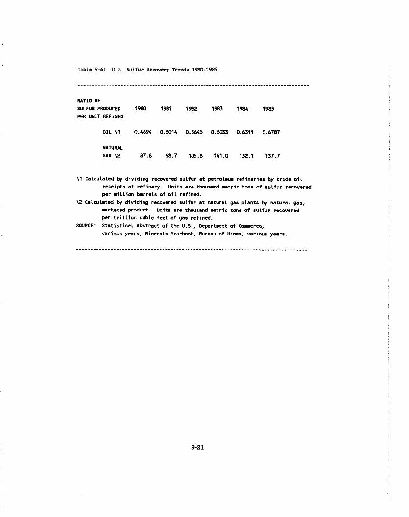
Table 9-6: U.S. Sulfur Rewvery T r d r 7980-1965
RATIO OF
SULFURPRODUCED 1980 1981 1982 1983 11184 1985 PER UNIT REFINED
OIL \1 0.4694 0.5014 0.5643 0.6033 0.6311 0.6787
NATURAL
GAS U 87.6 98.7 105.8 141.0 132.1 137.7
\1 Calculated by div id ing rewvered sulfur a t petroleum ref iner ies by crude o i l receipts a t refinery. Units are thousand metric tons o f su l fur recovered per e i l l i m bsrrels of o i l refined.
U Calculated by div id ing recovered sulfur a t M t u r a l gas plants by natural pas, ~ r k e t e d product. Units are t h w ~ n d v t r i c t m s o f ru l fu r recovered per t r i l l i o n cubic feet o f gas refined.
SOURCE: Sta t i s t i ca l Abstract o f the U.S., Department of C-rce, various years; Rinerals Yearbook, Bureau of nines, various years.
supply [EIA88]. These forecasts imply a supply of approximately 7.2 million tons of recovered
sulfur in the year 200~3 , compared to 5.8 million tons in 1986.
The U.S.S.R. should become a major exporter in the near future as it completes development of the
Astrakhan natural gas development. The addition of the U.S.S.R. as a major exporter will lower
Morocco sulfur costs. In 1985, Morocco imported 65 percent of its sulfur from Canada and 19
percent from the U.S. at much higher transportation costs than it would experience with the U.S.S.R
[BSCS6].
Summary -- There is little risk of a shortage of sulfur in the next several decades. However, sources
of supply will change. In the past decade, the U.S. phosphate industry has had a competitive
advantage because of relatively low priced and nearby sulfur supplies. In the next several decades
this advantage will end and most U.S. phosphoric acid producers will experience relatively higher
sulfur costs. At the same time, the relative price of sulfur for Morocco and other North African
producers will decline as sulfur supplies increase in nearby regions.
9.2.1.2 Products
In 1987, the U.S. produced 9.5 million metric tons of phosphoric acid. Wet-process phosphoric acid
(WPPA) comprised 94 percent of this production. Fertilizer uses claimed 89 percent of ail phosphoric
acid production and a higher proportion of WPPA production. The remaining 5 percent was used
in the production of animal feed supplement and other food additives. About 72 percent of the
WPPA used in fertilizers was used to produce mixed phosphate fertilizers; the rest went into direct
applications (fertilizer products that have primarily one plant nutrient) [DOC871. Mixed fertilizers
have two or more nutrients. Diammonium phosphate (DAP), for example, is a mixed fertilizer with
18 percent nitrogen and 46 percent phosphate [Vr86]. A chart of intermediate and end products of
the WPPA industry is provided in Figure 9-2.
9.2.1.3 U.S. Phosphate Producers
The fertilizer industry is devoted to the production and marketing of three basic nutrients: nitrogen,
potassium and phosphate. The scope of the fertilizer industry includes production of ammonia,
3 ~ h i s estimate uses the most recent ratios of sulfur recovered to fuel refined. Since, as noted, these ratios are increasing, this should be regarded as a conservative forecast.
9-22
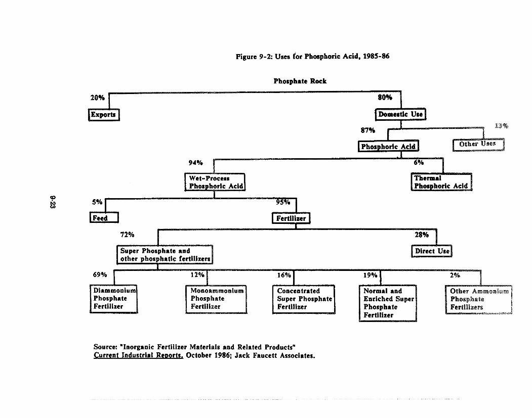
Figure 9-2: Usea for Phosphoric Acid, 1985-86
Phosphate Rock
20%
Phos horlc Acld 6
Source: "Inorganic Fertilizer Materials and Related Products" Current Industrial R e ~ 0 r t t October 1986; Jack Fsucett Associates.
ammonium nitrate, urea, phosphates (diammonium phosphate, triple superphosphate, and others),
nitrophosphates, mixed plant foods, superphosphates, phosphoric acid and potash
According to the most recent Department of Commerce census, the phosphate industry had $3.6
billion in assets in phosphate fertilizer manufacturing facilities IDOC86bI and another $3.3 billion
in phosphate rock mines [DOC82b]. Table 9-7 shows other information from the industry census.
Phosphoric acid producers are generally not single-product firms. Few companies are totally
dependent on fertilizer production; most fertilizer production is a subsidiary activity of a large,
diversified corporation.
Most of these companies are vertically integrated from phosphate rock production to fertilizer
production. The largest WPPA producers are also among the largest phosphate rock producers.
Each of the largest phosphate rock producers owns basic fertilizer production facilities either directly
or through equity interest in chemical producing companies. Some also have interests in sulfur
reserves. Table 9-8 gives a geographical breakdown of the major phosphate fertilizer producers and
their capacities to mine phosphate rock and produce phosphoric acid and several phosphate fertilizers. In many cases the production facilities are linked in a single plant. Where it is clear that mines and
plants are closely linked, Table 9-8 lists the facilities together. This information is summarized in
Table 9-9.
In 1984, 22 U.S. companies accounted for 33 percent of world phosphate rock production; 12
companies in Florida and one in North Carolina produced 87 percent of the U.S. total [Ga85]. Most
of the fertilizer production plants in Florida are located in Polk and Hillsborough counties in Central
Florida.
Most chemical fertilizer producers have been operating below capacity since the early 1980s, at 79
percent capacity for WPPA on average. The lowest rates occurred in 1982, when the industry
averaged 63 percent of capacity [TFI86B]. This information is summarized in Table 9-10.
The Fertilizer Institute sponsors periodic surveys of member companies to collect general financial
information for the integrated fertilizer manufacturing industry. TFI survey results show that the
return on total assets was less than one percent, either positive or negative in 1982, 1983, and 1985.
In 1984 and 1986, the return on total assets was a positive 5 percent and a negative 5 percent,
respectively [TFI87b]. These low rates of return have been blamed on poor demand for fertilizer and
on excess capacity.
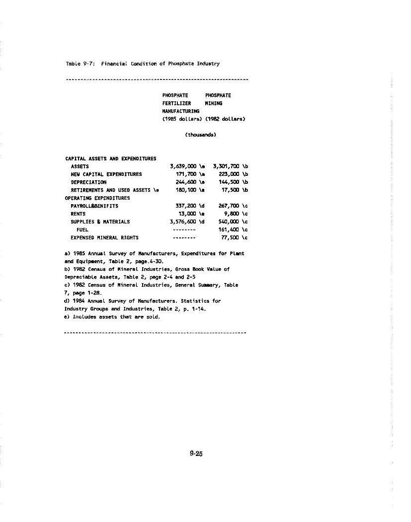
Table 9-7: F i n s n c i a l t ad i t im o f Phcsphsle I n d u s t r y
PHOSPHATE PHOSPHATE FERTILIZER I I IN I f f i IVI)(UFACNRIffi (1985 d o l l a r s ) (1982 d o l l a r s )
(thousands)
CAPITAL ASSETS AND EXPENDINRES ASSETS NEU CAPITAL EXPENDINRES DEPRECIATION
RETIREIIENTS AND USED ASSETS \e
OPERATING UPENDINRES PAYROLLeBENIFITS RENTS SUPPLIES B MTERIALS
FUEL EXPENSED MINERAL RIGHTS
a) 1985 Annual Survey of Manufacturers, Expenditures f o r P l a n t and Equipment, Teb le 2, page.4-U). b) 1982 C m r u s of M i n e r a l Indust r ies , Gross Bmk Value of Deprec iab le Assets, Tab le 2, page 2-4 and 2-5 c) 1982 Cmsus of n i n e r a l Indust r ies , G m e r a l Summary, Table 7, page 1-28. d) 1984 Annual Survey of Nanufacturers. S t a t i s t i c s f o r
I n d u s t r y Grmps Md Indust r ies , Table 2, p. 1-14. e) IncLudes asse ts that are rold.

Table 9-8: Producers of Phosphate Rock, Wet Process Phosphoric Acid and Phosphate FerFi lTrer.
(Thoussnd Metr ic Tons Per Year) PLAN? PHOSPHATE PHOSPHORlC AMMONIUM
COMPANY LOCAT l ON STATUS ROCK ACID PHOSPHATE .........*-.---------...--.--.....-.-.-..---.**--...-----*-.-- " - - - - " - - * - - - - - - - - . - - - - - - - - - - - - . - - - -
CONCENTRATED SUPERPHOSPHATE -....*-..-....-..
Freeport McMoran Donaldsonvil le, LA Pierce, F l Uncle Sam, LA Fort Green, FL Payne Creek, FL Taft, LA
Arcadian Corp Geismar, LA Barton Chem (U. R. Grace) Bartou, F l C F Indust r ies Plant City, F I
Plant City. FL Chevron Chemical Co Rock Springs, UY
Vernal, UT Conserv (Agrimont) Nichols, F l Comi nco Garrison, MT Estech, Inc Watson Mine, FL Farmland Industr ies Pierce, FL F lor ida Phosphate Corp Lakeland, FL Ford Motor Co Dearborn, M I Gardinier Tampa, F I
Fort Meade, FL Grace, U. R . & Co Barton. FL
Hooker's Pra i r ie , FL Four Corners, FL
I M C F e r t i l i z e r , Inc Bonnie. F l Barton, FL Brewster. FL
Kaiser Steel Corp Fontana, CA Hobi l Chemical Co Fort Keade, FL
Nichols, FL Pasadena, T X
Monsanto Co Henry, ID Nu-West indus t r ies Coda, ID
Dry Valley, I D Uingate Creek, FL Pascagoula, MS
Occidental Ag Chemicals Uhi te Springs, F l Columbia, TN
Presnel l Phosphates Columbia, TN Royster Co Kulberry, FL
Piney Point, FL Simplot, J. R. Pocatello, 10
Fort Hal l , ID Smoky Canyon. UY
Stauf fer Chemical Co Leefe. UY M t Pleasant, TN Uooley Valley, ID
Tennessee Val ley Au thor i t y Muscle Shoals, AL Texasgulf (Aquitaine) Lee Creek, NC USS Agri-Chemicals Barton, FL
For t Heade, F l
OPERAT 1 NG OPERATING OPERATING OPERATING OPERATING PLANNED OPERATING OPERATING EXPANSION OPERATING OPERATING OPERATING OPERATING OPERATING OPERATING OPERATING OPERATING OPERATING OPERATING OPERATING OPERATING OPERATING OPERATING OPERATING OPERATING OPERATING OPERATING OPERATING OPERATING OPERATING OPERATING OPERATING OPERATINC PLANNED OPERATING OPERATING OPERATING OPERATING EXPANSION OPERATING EXPANSION OPERATING OPERATING OPERATING OPERATING OPERATING OPERATINC EXPANSON OPERATING EXPANSION
Total Uni ted States 60,174.9 9.263.2 7,734.0
For completeness, t h i s tab le includes c q a n i e s that on ly produce phosphate rock and do not produce phosphoric acid. SWRCE: Yational F e r t i k i r e r Developnent Center, Tennessee Val ley Authori ty. "North American F e r t i l i z e r Capacity Data," pp. 7-10, July 1988.
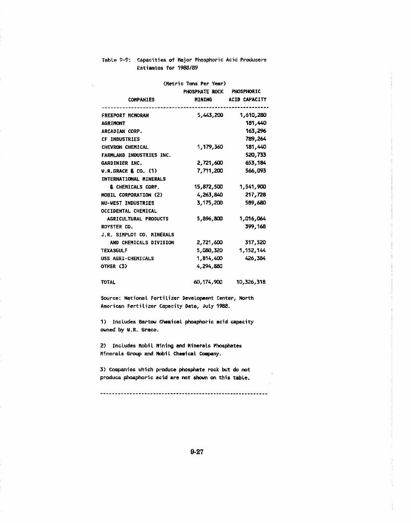
Table 9-9: Eapseiries of Mjor Phosphoric Acid Prcducers Estilf ltea for 1988189
t n e t r i c Taw Per Year) PrnSPtL%TE ROCK PrnSPIMI IC
UV(PAN1ES R l N I f f i ACID CAPACIrY -----------------------*-*--------------------------------
FREEWRT UCRORAM 5 , 4 4 3 , m 1,610,280 A G R I W T 181,440 ARCADIAN CORP. 163,296 CF INDUSTRIES 789,264 CHEVRI)( CHEMICAL 1,179,360 181,440 FARMLAND INDUSTRIES INC. 520,733 GARDINIER INC. 2,721,6M 653,184 U.R.GRACE & CO. (1) 7,711,200 566,093 lNTERN4TION.A.L I I I N E M L S
& CHUIICALS COUP. l5 ,872 ,5W 1,541,WO l K l 8 I L CORPORATIOH (2) 4,263,840 217,728 NU-UEST IHDUSTRIES 3 , 1 7 5 , m 589,680 OCCIDEKTAL CHEMICAL
AGRICULNRAL PRODUCTS 5,896,800 l,M6,064 ROYSTER CO. 399,168 J.R. SINPLOT CO. MINERALS
AND CHEBICALS D IV IS ION 2,721,6W 317,520 TEXASGULF 5,080,320 1,152,144 USS AGRI-CHEMICALS 1,814,400 426,384 OTHER (3) 4,294,880
TOTAL 60,174,WO 10,326,318
Source: Wtiaral Fer t i l i zer DeveLopKnt Center, m r t h h r i c e n Fer t i l i ze r Capacity b t s , July 1988.
1) Includes Bartat Chemical phosphoric acid capc i ty owned by U.R. Grace.
2) includes Wil nining and Rinersls Phosphates Bineraas G m u p snd WiL Chnissl Coqany.
3) C-nies which prcduce phosphate mck but & not prDduce phosphoric acid are not shown on this table.
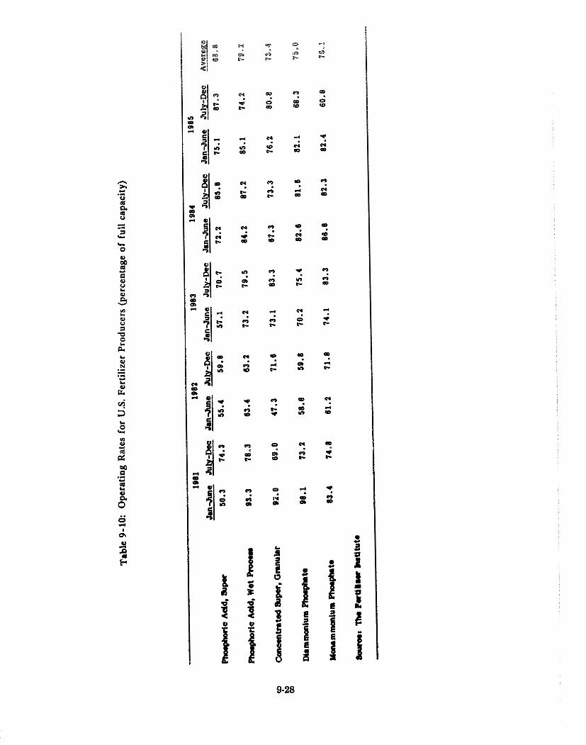
In order to cut losses, firms have been re-organizing and consolidating. Beker has filed for
bankruptcy under Chapter 11 and no longer operates any plants. Over 17 percent of U.S. capacity
has either been recently sold or is closed awaiting higher prices. Another 17 percent of current
capacity is somewhat insulated from price shifts because it is owned by farm cooperatives. Following
is a short description of the corporate structure and activities of those publicly owned chemical 4 manufacturers with WPPA operating capacity of over 500,000 tons . Four privately owned companies
also have a capacity over 500,000 tons. They are C.F. Industries, Gardinier Inc., Nu-West Industries,
and Occidental Chemical Agricultural Products, Inc. Data are not available to describe their financial
status.
W.R. Grace and Comoany -- Grace is a highly diversified company with a 624,000 ton capacity in
phosphoric acid production and 8,500,000 ton capacity in phosphoric rock mining. Grace had sales
of $3.7 billion in 1986, with $2.5 billion in specialty chemicals. Grace went through major
restructuring in 1986 and had losses from continuing operations of $324 million in 1986.
As part of its restructuring, Grace has announced its intent to divest its agricultural chemicals
business and in 1986 it set aside $221 million to cover losses from that move [Ri87]. Grace closed
its Four Corners plant during the 1986/1987 season. As of July 1988, however, a report from the
Tennessee Valley Authority shows Grace operating its wet process acid plants in Hooker's Prairie and
in Four Corners, both in Florida [TVA88]. Green Markets reported in March 1988 that Grace had
sold more of its retail fertilizer operation and plans to sell the remainder of its fertilizer business by
the end of 1988 [GM88d].
Farmland Industries. Inc. -- Farmland Industries, Inc., is a regional agricultural cooperative based
in Kansas City, Missouri. Farmland is owned by 2,186 local cooperatives and serves a federated
network in 19 midwestern states and Canada. Farmland had $2.6 billion in sales in 1987 and profits
of $55.2 million. Petroleum, food marketing, agricultural chemicals and feed are its four principal
sectors. Agricultural chemicals represented 20.2 percent of total sales. Sales of all agricultural
chemicals were $528.5 million in 1987, down from $573.6 million in 1986. This sector had operating
income of $1.3 million, after a loss of $38.4 million in 1986 and $49 million in 1983.
Farmland has a phosphoric acid operating capacity of 574,000 tons in Pierce, Florida, representing
5 percent of the entire industry capacity. Farmland has a phosphate rock mining capacity of 2
4 Unless otherwise indicated, the information for each of the companies that is provided in this
section came from annual corporate reports for the years 1982 to 1987.
million tons; this operation was closed as of January 1988. Its total fertilizer capacity is 3.6 million
tons, including operations in ammonia, ammonia nitrate and urea. In addition, Farmland has a
proposed phosphate mining operation in Hardee County, Florida with a 40 million ton reserve
[TVA88].
In 1987, Farmland sold 3.58 million short tons of phosphate and nitrogen fertilizers. Unit sales
increased in 1987 by 25 percent, but at lower prices so that revenue from fertilizer sales increased
only $13.9 million. Growth came from an expansion of sales to industry and from exports. Sales to
non-members represented 27 percent of total sales of agricuitural chemicals.
In some years, losses in phosphate operation have been fully offset by gains in other agricultural
chemicals. While Farmland had operating income of $2.7 million for agricultural chemicals in 1985,
the phosphate division lost $42 million in that year. In 1985, Farmland closed a sulfur mine that
services phosphate production and charged the $3.7 million cost against phosphate operations. In
1984, phosphate operations lost $1 2 million while agricultural chemicals overall had positive operating
income of $38 million. In 1983, total phosphate losses amounted to $8.3 million.
AMAX -- AMAX is a diversified energy development and minerals company with extensive
operations in aluminum, coal and molybdenum as well as many other minerals. AMAX had modest
and successful operations in phosphate and potash throughout the 1970% with average sales between
1973 and 1979 of $43.7 million. AMAX expanded the phosphate operations with a purchase of the
Big Four mine in Florida in July 1980. Beginning in 1982, AMAX phosphate operations have been
consistently unprofitable; in 1984 AMAX announced its desire to get out of the business.
In 1984, AMAX began to phase out the agricultural chemicals segment and set aside $195 million for
losses on properties and investments in that segment. In December of 1985, AMAX had a tentative
agreement to sell its phosphate operation for $40 million. However, a July 1988 listing of production
capacities by the Tennessee Valley Authority continues to show AMAX with a closed 2.5 million ton
capacity phosphate rock mine in Big Four but lists its 190,000 ton phosphoric acid capacity in Piney
Point, Florida as sold [TVA88]. Because all AMAX facilities have ceased operations, the firm is not
included in Table 9-8.
Total sales for AMAX in 1986 were $1.3 billion, with earnings of $89.4 million. Because of changes
in the organization of the company annual report, it is not possible to reliably analyze the change in
total sales during the mid-1980s. The 1986 annual report gave 1985 sales of $1.2 billion with an
operating loss of $106.5 million. Losses in that division during those years were $17.3, $214.4 and
$17.1 million, respectively.
International Minerals and Chemicals (IMC) -- IMC is a diversified chemical producer. Up to 1986,
its sales were concentrated in animal and fertilizer products. That year it acquired Mallinckrodt, Inc.,
a producer of medical products, drugs, chemicals, laboratory reagents for $700 million. Fertilizer
sales dominate IMC financial activity. In 1986, IMC fertilizer sales represented 53 percent of total
net sales of $1.6 billion. Animal products, including feed grade phosphate and other feed additives,
and Mallinckrodt, Inc. represented 11 percent and 40 percent, respectively. Phosphate chemicals
represented 41 percent of total IMC fertilizer sales.
In 1987, IMC owned or operated 15 percent of U.S. phosphoric acid capacity. It owns 25 percent of
the U.S. phosphate rock mining capacity in Florida.
Most of the WPPA is produced at its New Wales, Florida facility (1.7 million tons of WPPA
manufacturing capacity). The phosphate rock is mined at a nearby plant. In 1987, 45 percent of its
New Wales production was sold domestically, 38 percent was exported and 17 percent was used by
IMC to manufacture its own brand of fertilizer. The plant operated at 85 percent capacity in 1987.
In 1986, IMC reported operating losses of $61.0 million, but by 1987 sales had picked up, yielding
$67.1 million in operating profits. Nevertheless, IMC fertilizer sales have been flat since 1986,
reflecting lower average product prices.
IMC has also been cutting operating costs. It reported developing a process to reduce the amount of
sulfuric acid needed per unit of P205 product. It has sold most of its retail outlets in the midwest.
IMC Fertilizer Group employment has been reduced to 5,525 in 1986 from 6,687 in 1981.
Texasnulf Chemicals Comoany -- Texasgulf Chemicals Company has operations primarily in
phosphate and sulfur, but also in potash and soda ash. Texasgulf is a division of Elf Aquitaine, S.A.
(EAI). EAI is a U.S. subsidiary of Elf, a multinational company based in Paris with operations in
oil, gas, chemicals and pharmaceuticals. EAI's 1986 sales were $1.7 billion. The sales for Texasgulf
were $474, $461 and $547 million in 1984, 1985 and 1986, respectively. Texasgulf had assets of $2.2
billion in 1986.
Texasgulf has a phosphoric acid plant in Lee Creek, North Carolina, with a capacity of 1,270,000
tons, 10 percent of U.S. capacity. It also has a phosphoric mining capacity of 5.6 million tons. The
Lee Creek plant was expanded, beginning in the mid-1970s. The expansion was completed in 1986.
This plant is unusual in a number of ways. It disposes of its gypsum by blending it with clay and
returning it to the mine. It also removes the overburden in its Lee Creek mine with dredges.

The Lee Creek wet-process plant produces a high quality phosphoric acid that has been sold for
industrial grade acid and for animal feed. Texasgulf produces several types of calcium phosphate
animal feeds in North Carolina and Nebraska.
Freeoort-McMoRan. Inc. -- Freeport-McMoRan, Inc. (FMI) has operations in agricultural minerals,
oil, gas, geothermal energy and uranium. Revenues in 1986 totaled $629.7 million. Because of a $277
million write down of oil and gas related assets, its operating loss in 1986 was $147 million. Revenues
were $722 million and $842 million in 1985 and 1984, respectively, and operating income was a positive $156 million and $170 million, respectively. The agricultural minerals sector earned $39
million in 1986 and $62 million in 1985.
FMI's sulfur operations are as important as its phosphate operations and depend heavily on demand
for phosphates. Sales of phosphate and sulfur in 1986 were $161.5 and $161.3 million, respectively.
In mid-1986, FMI conveyed its sulfur, phosphate and geothermal properties, among others, to
Freeport-McMoRan Resource Partners, Limited Partnership (FRP) and approximately 19 percent of
FRP was sold in a public offering.
FMI produces phosphoric acid in its Uncle Sam plant in Louisiana. This plant produced 715,500 tons
in 1986 and 714,000 tons in 1985. FMI produced 332,200 tons of DAP in 1986.
Freeport Uranium Recovery Company produces uranium oxide at recovery facilities at the Uncle Sam
plant and at the Agrico plant in Donaldsonville, Louisiana. These operations produced 1,720,000
pounds of uranium oxide in 1983.
The Uncle Sam plant has limited space to store its phosphogypsum. As a consequence, FMI has
worked with Davy McKee and the Florida Institute of Phosphate Research to test technology to
recycle phosphogypsum into sulfuric acid and aggregate. FMI is spending $3 to $4 million on a demonstration plant at Uncle Sam that will consume 33 tons of phosphogypsum per day [L188].
Construction of the plant was halted in the summer of 1987 because of engineering problems, but was
resumed in the spring of 1988. An FMI spokesperson said that the plant will begin operation in the
early fall of 1988 [GM88d].
The FMI phosphate rock mine was shut down in April 1982, because of weak demand for phosphate
rock, and reopened in April 1984. During this time, FMI purchased rock from others. At the end
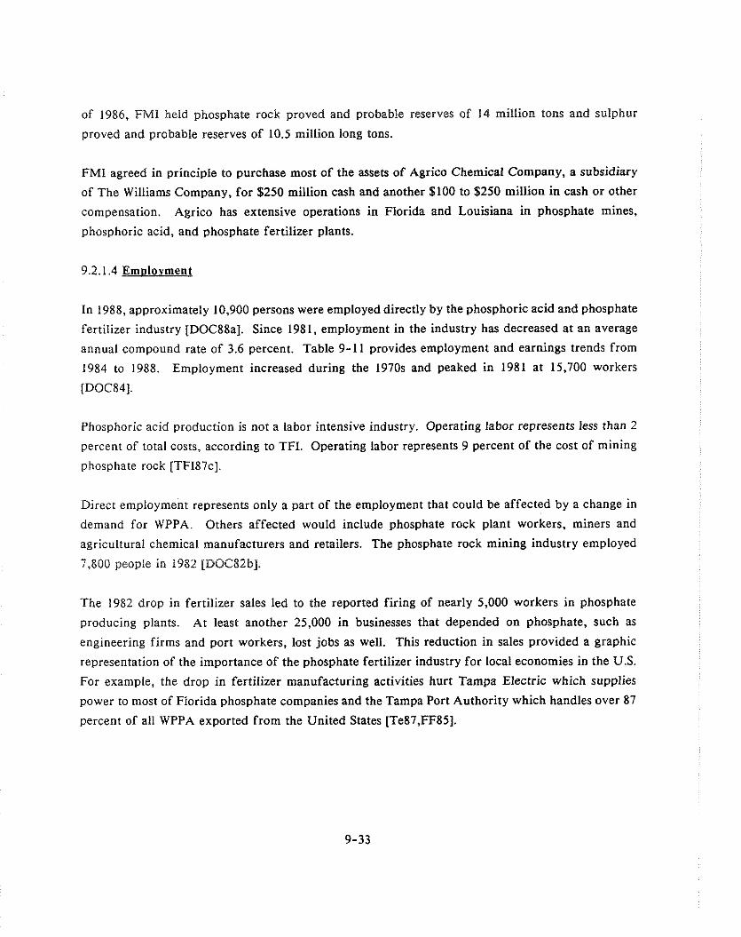
of 1986, FMI held phosphate rock proved and probable reserves of 14 million tons and sulphur
proved and probable reserves of 10.5 million long tons.
FMI agreed in principle to purchase most of the assets of Agrico Chemical Company, a subsidiary
of The Williams Company, for $250 million cash and another $100 to $250 million in cash or other
compensation. Agrico has extensive operations in Florida and Louisiana in phosphate mines,
phosphoric acid, and phosphate fertilizer plants.
In 1988, approximately 10,900 persons were employed directly by the phosphoric acid and phosphate
fertilizer industry [DOC88a]. Since 1981, employment in the industry has decreased at an average
annual compound rate of 3.6 percent. Table 9-1 1 provides employment and earnings trends from
1984 to 1988. Employment increased during the 1970s and peaked in 1981 at 15,700 workers
[DOC84].
Phosphoric acid production is not a labor intensive industry. Operating labor represents less than 2
percent of total costs, according to TFI. Operating labor represents 9 percent of the cost of mining
phosphate rock [TFI87c].
Direct employment represents only a part of the employment that could be affected by a change in
demand for WPPA. Others affected would include phosphate rock plant workers, miners and
agricultural chemical manufacturers and retailers. The phosphate rock mining industry employed
7,800 people in 1982 [DOC82b].
The 1982 drop in fertilizer sales led to the reported firing of nearly 5,000 workers in phosphate
producing plants. At least another 25,000 in businesses that depended on phosphate, such as
engineering firms and port workers, lost jobs as well. This reduction in sales provided a graphic
representation of the importance of the phosphate fertilizer industry for local economies in the U.S.
For example, the drop in fertiIizer manufacturing activities hurt Tampa Electric which supplies
power to most of Florida phosphate companies and the Tampa Port Authority which handles over 87
percent of all WPPA exported from the United States [Te87,FF85].

Tsblc 9- l l : Eqlcyrcn'l i n the P b p h a t e Industry, t thasnds)
*Nural
Percent th.nge 1 1985 1986/1 1987/1 1988/2 1m-85 1980-85
Total Eqloycmt 13 13 11.2 10.9 10.9 -1 -3.6
Production Workers 8.9 8.7 7.8 7.8 7.8 1.6 -4.6
Average Hourly Uage ($1 11.54 12.12 12.73 13.75 -- 8.9 8
Notes: 11 Estimated. /2 Forecast.
Source: international Trade Colission, U.S. Department of Corerce, U.S. Industr ial Outlmk 1988, January 1988, p.14-3.
9.2.2 Characteristic$ of Phosohoric Acid Demand
The demand for WPPA is largely determined by the demand for phosphate fertilizers. Widespread
chemical fertilizer use is a relatively recent phenomenon. In the early- to mid-1960's world and
domestic fertilizer use expanded rapidly. The "Green Revolution" of this time brought high yielding
varieties of grain crops which required more intensive fertilizer application than did traditional
varieties [Te87]. Between 1970 and 1983, fertilizer use per acre grew about 271 percent in low
income countries and 107 percent in middle income countries. The largest per acre increases were
reported by India (a 246 percent increase) and the People's Republic of China (a 332 percent increase)
[WB86].
Fertilizer use has not increased evenly for all nutrients. Nitrogen use has increased more rapidly than
have phosphate and potassium use, due primarily to the favorable response of crop yield to
nitrogenous fertilizer. The share of phosphates in total plant nutrient consumption in the U.S. has
declined from about 33 percent in 1960 to about 23 percent in 1986 [Vr86]. Figure 9-3 traces the
growth of plant nutrient use in the United States.
Given its relatively small share of domestic and world phosphate use (about 5 percent, see figure 9-
2), fluctuations in animal feed consumption are of limited importance to the phosphate industry.
Consumption of phosphate supplements for animal feeds and other minor uses has varied in the past
decade, reaching a high of 661,920 tons in 1984 [DOC87]. Demand for phosphate animal feed
supplements dropped because of a decrease in the recommended supplement ratios and the increased
availability of a substitute, fish meal. Almost all phosphate supplements are in the calcium
phosphate form. Exports of phosphate supplements represented only 5 to 6 percent of 1983 domestic
production [SRISS].
Demand for WPPA in the United States depends directly on those factors which affect the demand
for fertilizer. Some of these factors are acreage planted, application rates, crop prices, prices of other
fertilizers, farm income, population, and weather. It is important to understand how these are
interrelated in order to understand what has determined the growth of phosphate fertilizer demand
in the 1980s and the soft prices which have characterized the domestic and international markets.
The consumption of any agricultural nutrient depends upon the acreage of different crops and the
application rates on specific crops. Some crops use more phosphate than others and respond much
better to one type of fertilizer than to another. Food grain production requires lower proportions of
nutrients per acre than does feed grain production [WH88]. In the United States, corn uses the most
phosphate fertilizer per acre of the major crops, while soybeans and wheat use the least [Vr86].
Planting pattern changes on U.S. farms have favored growth of phosphate demand. Almost every
year since 1964, more acres have been harvested with corn than any other major crop including
wheat, cotton and soybeans. In addirion, a greater proportion of corn acreage has been fertilized over
the years than any other major crop. Approximately 85 percent of the corn acreage harvested in 1987
received phosphate applications, compared to roughly 50 percent of cotton, 48 percent of wheat and
29 percent of soybean acreage. In fact, U.S. farms used more fertilizer of all types on corn than on
any other crop. Almost 98 percent of corn planted received some type of fertilizer in 1985, compared
to about 75 percent of the wheat planted and 38 percent of the soybeans [Vr86]. Finally, major crops
(which include corn, wheat, soybeans and cotton) are fertilized more intensively than non-major
crops (such as sorghum, oats, barley, rice, rye, peanuts, potatoes). The percentage of acres planted
to major crops has been increasing since 1964, while acreage of non-major crops harvested decreased
13 percent between 1964 and 1985 [WH88].
Application rates have been an important factor influencing fertilizer demand in the U.S. Use on
corn and other crops increased dramatically between I964 and 1980, due more to higher application
rates than to an increase in the proportion of acreage either harvested or fertilized. For example,
while corn acreage increased by about 36 percent between 1964 and 1980, nitrogen use rose 272
percent, phosphate use increased 118 percent and potassium increased 225 percent. In the early
1980% phosphate application per acre began declining [ ~ r 8 6 f . Since 1985, the rate of phosphate
fertilizer use has been linked more closely to increases in acreage planted and fertilized than to
application rates [Vr861.
Since 1983, the acreage of major crops planted has depended in large part on U.S. government price
support programs. Under the payment-in-kind program of 1983, U.S. farmers agreed not to grow
crops on a total of 77 million acres (37 percent of the land sowed with grains, cotton and rice). In
return for idling their land, farmers got up to 80 percent of the quantity of grain they would
5 The decline in phosphate application rates is generally explained as follows: Unlike nitrogen
and potash, any phosphate not used by the crop remains in the soil and is available for a future crop. As this fact became known, farmers decreased phosphate use. Also, new tilling and crop management practices have allowed farmers to increase yields using less phosphate (see E.A. Harre, "Emerging Trends in World Phosphate Market," National Fertilizer Development Center, Circular No. 2-228, September 1987).

normally have grown. The in-kind payments came from crops that had been stored by the
government [Wb86].
In 1985, the Food Security Act was passed to increase grain exports, reduce inventories and support
farm income [St85]. Through a variety of different measures, including set-asides, paid land
diversions and the Long-Term Conservation Reserve, U.S. crop-planted acreage decreased from 363
million acres in 1981 to 305 million acres in 1987 [WH87]. Farmers have responded to the acreage
reduction by using somewhat higher quantities of fertilizer per acre on the remaining acreage but in
general the acreage reduction has led to a reduction in demand for phosphate fertilizers.
These programs, aided by dry weather and the drop in the number of operating farms between 1985
and 1987, have begun to reduce the reserves of surplus agricultural commodities accumulated by the
U.S. Department of Agriculture (USDA). In 1988, corn stocks are expected to fall by 400 million
bushels, wheat stocks by 200 million bushels, and soybean stocks by 20 million bushels [WH87].
Fertilizer and crop prices also affect the demand for plant nutrients. In general, as the fertilizer price
to crop price ratio decreases, the application rate per acre increases. As crop prices rise relative to
fertilizer prices, farmers wish to increase yields and hence increase fertilizer use.
Because the full effect of reduced phosphate application does not occur immediately, farmers may
be highly-responsive to fertilizer price increases in the short run. Phosphate is depleted from the
soil more slowly than nitrogen, for example, and the effects of decreased phosphate application only
become apparent once the level in the soil is depleted. It is estimated that a 10 percent reduction in
phosphate application in the first year will reduce corn yields by 3 percent in the first year and 4
percent in the third year. Wheat yields are more sensitive in the long run: a 10 percent reduction
in phosphate application will reduce yields 1 percent in the first year but by 7 percent in the third
year [GA079].
Fertilizers represent only about 7 percent of total farm costs; phosphate fertilizers account for about
1 percent of total farm costs. On the other hand, fertilizers account for a large part of the variable
costs of crop production: 50 percent of wheat production costs, 35 percent of corn costs and 20
percent of soybean costs [GA079].
Finally, fertilizer use is also affected by changes in farm income. Net farm income, in 1967 dollars,
was lower in 1985, $9.5 billion, than in 1971, $12.4 billion. Yet this still represented an improvement
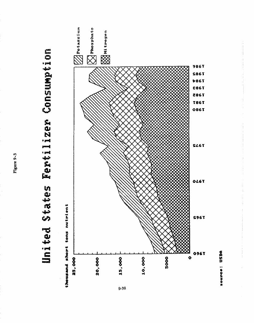
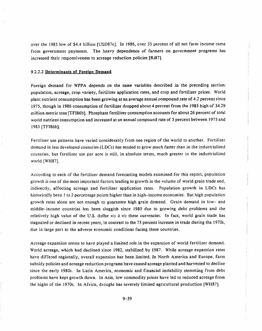
over the 1983 low of $4.4 billion [USD87e]. In 1986, over 33 percent of all net farm income came
from government payments. The heavy dependence of farmers on government programs has
increased their responsiveness to acreage reduction policies [Ri87].
9.2.2.2 Determinants of Foreien Demand
Foreign demand for WPPA depends on the same variables described in the preceding section:
population, acreage, crop variety, fertilizer application rates, and crop and fertilizer prices. World
plant nutrient consumption has been growing a t an average annual compound rate of 4.2 percent since
1975, though in 1986 consumption of fertilizer dropped about 4 percent from the 1985 high of 34.29
million metric tons [TFI86b]. Phosphate fertilizer consumption accounts for about 26 percent of total
world nutrient consumption and increased at an annual compound rate of 3 percent between 1975 and
1985 [TFI86b].
Fertilizer use patterns have varied considerably from one region of the world to another. Fertilizer
demand in less developed countries (LDCs) has tended to grow much faster than in the industrialized
countries, but fertilizer use per acre is still, in absolute terms, much gea te r in the industrialized
world [WH87].
According to each of the fertilizer demand forecasting models examined for this report, population
growth is one of the most important factors leading to growth in the volume of world grain trade and,
indirectly, affecting acreage and fertilizer application rates. Population growth in LDCs has
historically been 1 to 2 percentage points higher than in high-income economies. But high population
growth rates alone are not enough to guarantee high grain demand. Grain demand in low- and
middle-income countries has been sluggish since I980 due to growing debt problems and the
relatively high value of the U.S. dollar vis a vis these currencies. In fact, world grain trade has
stagnated or declined in recent years, in contrast to the 75 percent increase in trade during the 1970s.
due in large part to the adverse economic conditions facing these countries.
Acreage expansion seems to have played a limited role in the expansion of world fertilizer demand.
World acreage, which had declined since 1982, stabilized by 1987. While acreage expansion rates
have differed regionally, overall expansion has been limited. In North America and Europe, farm
subsidy policies and acreage reduction programs have caused acreage planted and harvested to decline
since the early 1980s. In Latin America, economic and financial instability stemming from debt
problems have kept growth down. In Asia, low commodity prices have led to reduced acreage from
the highs of the 1970s. In Africa, drought has severely limited agricultural production [WH87].

Fertilizer application rates have varied substantially across regions as well. The developed regions
(North America and Western Europe) have mature agricultural industries, and fertilizer gains made
through technological advances have been minimal since the early 1980s. Growth of fertilizer
consumption has been strongest in those regions where fertilizer use has not matured, such as Latin
America, Asia and Africa. Thus, while application rates are higher in the developed regions, growth
rates of application per acre over time are much lower [WH88].
Differences in application rates by region also reflect variations in cropping patterns, soil quality and
climatic conditions: Acreage shifts to coarse (or animal feed) grains in Western Europe have brought
about an increase in the demand for fertilizer nutrients since coarse grains are fertilized more
intensively than other crops [WH88]. In Latin America, fertilizer use has been among the lowest in
the world due to high natural soil fertility. However, Latin America is the only region in the world
where the application rate for phosphates is greater than that for nitrogen, due to differences in soil
fertility and differing crop needs. According to Wharton Econometric Forecasting Associates
(WEFA), the nitrogen-to-phosphate ratio in 1987 was 0.8 in Latin America, compared to 2.8 in North
America, 1.2 in Africa, and 3.2 in Asia [WH88]. Hence, acreage shifts in Latin America have a
relatively large impact in phosphate fertilizer consumption.
World demand for fertilizer has also been affected by shifts in crop prices. The general oversupply
of farm commodities in Japan, Western Europe and North America in the early 1980s has changed
the demand for plant nutrients. The Green Revolution in the 1960s introduced new, higher-yielding
varieties of grains to the developing world, dramatically increasing yields and bringing many
countries close to self-sufficiency in food. While the initial impact of the Green Revolution was to
dramatically increase dependence on chemical fertilizers, by the early 1980s, it also enabled many
countries to reduce their reliance on grain imports. By 1987, low world grain prices adversely
affected acreage planted and fertilizer use in many grain-producing countries, particularly in the U.S.
and Europe.
Domestic and export fertilizer prices have fluctuated very differently within different regions and
countries. The reasons for these fluctuations are varied and include weather, government crop and
fertilizer pricing policies, decisions to invest in new capacity, and capacity utilization. These
elements have resulted in shortages and oversupplies of particular types of fertilizer at various times
[WH87,WH88].

In general, however, over-investment in plant capacity relative to demand (both foreign and
domestic) has led to lower fertilizer prices in all countries. Aggressive pricing policies by large
suppliers such as Morocco have further increased the downward pressure on prices. In fact, by 1987
this situation had led a number of developed countries (European Economic Community, U.S. and
Australia) to impose minimum prices, quotas and/or dumping margins on fertilizer imports.
Regulatory agencies in these countries found that LDC imports had been sold below their fair market
value and had caused material damage to domestic suppliers. These trade restrictions generally
resulted in higher domestic prices in these countries [Co87].
Finally, demand for fertilizer depends on the availability of foreign exchange, particularly for LDCs.
Oil price increases in the 1970s, while causing balance-of-payments problems, also directed more
money to Western bankers who were then willing to increase loan portfolios in LDCs. LDCs used
the increased availability of foreign exchange to buy farm supplies and inputs, pushing up the
demand for fertilizer in the 1970s and early 1980s. This situation lasted until rising interest rates
in the 1980s, low commodity prices, and ensuing Third World debt service problems restricted the
availability of foreign exchange in LDCs. Thus, despite drops in fertilizer prices in the 1980s, many
less-developed economies were unable to import their full requirements. In the 1980% aid and
concessionary loans have played an important role in determining fertilizer imports and use.
9.2.2.3 World Demand for U.S. Phosohate Exoorts
World exports of the three plant nutrients, nitrogen, phosphorus and potassium, presently amount to
approximately one-third of total world consumption, but this percentage has been declining. Most
of the decline, particularly in phosphate trade, has been felt by the United States, since exports from
African, Near East and Far East producers have actually increased.
In general, the share of the world phosphate trade held by the developed countries has been declining,
though production from the developed economies still dominate world trade. The large increase in
the LDC's share of world phosphate trade in the 1980s was largely due to the increase in Morocco's
WPPA production capacity and the development of new plants in the Philippines. The Moroccan
phosphate industry is government owned and has been pursuing an aggressive pricing policy aimed
at increasing its share of the world market [Co87].
The regions most dependent on imports were Africa (which imports over 70 percent of its nutrient
requirements, and about 58 percent of its phosphate needs), the Far East (which imports 40 percent
on average, and 45 percent of its phosphate needs) and Latin America (importing 48 percent overall,
and 55 percent of its phosphate requirements). In contrast, the developed countries imported on
average 36 percent of their nutrient needs and 25 percent of their phosphate needs. Most trade by
centrally planned economies was with other centrally planned economies [Co87].
U.S. Exoort Market
In recent years, U.S. phosphoric acid exports (which do not include phosphate fertilizers) have
typically been less than 10 percent of total domestic output [St86a]. Exports, however, of phosphate
fertilizers represent a much higher proportion of phosphate fertilizer production. The U.S. is the
largest exporter of phosphate fertilizer to the world. But the U.S. share of the phosphate fertilizer
export market has decreased from 53 percent in 1981-82 to about 47.6 percent in 1985-86. In 1987,
according to The Fertilizer Institute, the U.S. exported 620,777 tons of merchant grade phosphoric
acid, 2,686,104 tons of concentrated superphosphate and 6,564,300 tons of DAP. These export levels
are a significant improvement over the levels reported by the Bureau of Census for 1985 and 1986
[Ye88,St86a]. Table 9-12 shows the level of the U.S. exports between 1979 and 1986.
U.S. exports have met increasing competition since the mid- 1980s. Many phosphate rock producers
in less developed countries have increased their capacity to convert phosphate rock into fertilizer.
The resulting oversupply of phosphate commodities partially explains the soft and falling export
prices of the late 1980s [St86a].
High tariffs on U.S. exports of phosphate rock and phosphate fertilizer also affect the demand for
U.S. product. Domestic fertilizer companies paid about $200 million in tariffs in 1985. The Indian
government alone collected $40 million from U.S. manufacturers. Such tariffs decrease the
competitiveness of U.S. producers in the international market [St86a].
Nevertheless, foreign demand for U.S. phosphate fertilizer seems to have strengthened in 1987.
Consumption of U.S. fertilizer by the rest of the world rose 2 percent in 1986/87 and 3 percent in
1987/88. Demand grew most rapidly in Asia and Latin America. Several major importers such as
India and China have reduced their fertilizer reserves so that more of their demand is being reflected
in increased imports than in preceding years [Te87].
The devaluation of the U.S. dollar in 1987 increased the competitiveness of U.S. producers with
respect to foreign producers. Relaxed foreign exchange constraints in many LDC's have helped to
increase U.S. exports to LDCs. Improved demand and reduced phosphate commodity stocks also
helped push up phosphate fertilizer prices [Te87).
In addition, U.S. exporters have organized into a cartel-like operation to help promote their product
more effectively abroad. In 1987, almost all U.S. exports were handled by The Phosphate Chemical
Export Association (Phoschem), an association for the export of phosphate chemicals from the United
States. Phoschem operates as a membership association under the provisions of the Webb-Pomerane
Act of 1918 and is regulated by the Department of Commerce and the Department of Justice. The
Act permits U.S. companies to effectively organize export operations in the face of overseas
competition when this competition is considered to be, as U.S. manufacturers allege, in the form of
a cartel. After nearly disbanding during the very soft 1985 export market, the organization has
rebounded.
Trade in WPPA occurs at two levels. Of the $1.6 billion in phosphate fertilizer sales in 1985, 18
percent was in phosphoric acid and the remainder was in finished fertilizers, especially diammonium
phosphate (DAP) [DOC86a]. The distribution of sales varies with each year. Large sales in recent
years of phosphoric acid to the U.S.S.R. by Occidental Petroleum Co. and large sales of DAP to China
have made the export market erratic. As described in the section on demand for phosphoric acid,
in recent years competition has intensified in the markets for phosphate fertilizers and phosphoric
acid.
Foreign Com~etit ion
Two types of foreign producers have cut into the U.S. export market. The first is new production
in countries that have traditionally been important importers. The second is expanded production
facilities in exporting countries. Importing countries such as The People's Republic of China and
India have expanded fertilizer production capacities. Some of these facilities are not competitive with
imports but are nevertheless protected from foreign competition. To a limited extent, these facilities
have merely switched from importing finished fertilizers to importing phosphoric acid. Less
developed countries are the primary competitors in the export market. Most of the LDC's new
phosphate production capacity has been initiated by state owned enterprises. Other developed
countries have production capacities that, with a few exceptions, cover only a portion their domestic
needs. Western Europe has in recent years cut back production that supplied primarily domestic
needs, in response to increased costs and environmental concerns.

Table 9-12: U.S. Exports of P b p h D r i c Acid
(Part 1 of 2)
(lhwxd Metric Tons, T h o u d WLtars)
......................................................... LESS THAH 65% P205 GREATER THNI 65% PM5 TOTAL - - V U U E
WANTIN VALUE WANTIlY VALUE
SOURCE: Uillism Stansser, Bureau of Mines, YPhosphate Rock,' ninerala Ywrbmk, Preprint of 1986, 1985, 1984, 1982, 1980, 1978-79, 1977 and 1976. ALM, Dewrtnnt of C-rce, U.S. Exports.
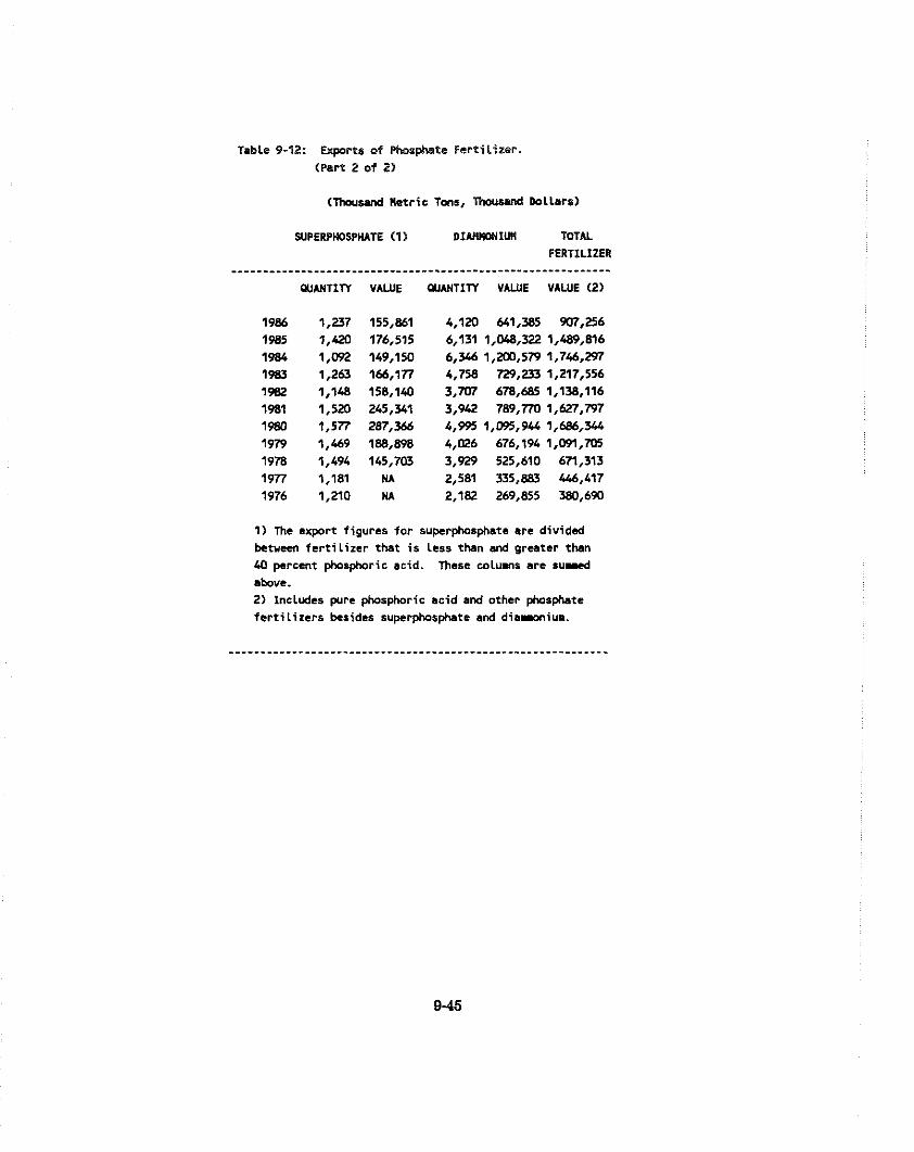
Table 9-12: Exparts of Phoaphote Fer t i l i zer . (Part 2 o f 2)
(Thousand Uetrie Tons, Thousand Dollars)
SUPERPHOSPHATE (1) DIMMHIUU TOTAL FERTILIZER
WWTITY V A W E WANTITY V U U E VALUE (2)
1) The export figures fo r superphosphate are divided beturn, f e r t i l i z e r that i s Less than and greater than 40 percent phosphoric acid. These columns are s u v d above. 2) Includes pure phosphoric acid and other phosphate f e r t i l i z e r s besides superphosphate and diawonium.

In 1986, Monsanto Chemical Co. and FMC Corp. filed an anti-dumping petition with the U.S.
Department of Commerce over imports of industrial phosphoric acid from Belgium and
Israel[CMR86]. While this dispute does not directly affect the agricultural phosphoric acid market,
it is an indication of the increased level of competition.
Table 9-13 shows the major exporting countries. The U.S. has maintained its dominant position in
the phosphate fertilizer trade with over half of all sales. Morocco stands out as the key foreign
competitor. Morocco is the leading exporter of phosphate rock and in recent years has dramatically
expanded its phosphoric acid and fertilizer capacity. Moroccan phosphate fertilizer exports nearly
doubled between the 1981/1982 season and the 1984/85 season and have continued to increase
capacity. Phosphoric acid exports, which are more important to Morocco than are phosphate
fertilizer, have also nearly doubled during this period [FA085]. The Moroccan industry is operated
by the state owned company, Office Cherifien des Phosphates (OCP). OCP has its own fleet of ships
designed to transport phosphoric acid. Many in the industry believe OCP will operate at a ioss in
order to expand its market share and to bring in foreign currency.
Outlook
The predominance of domestically protected foreign production and state owned export competition
has led Zellars-Williams to label the U.S. the "residual supplier." As world demand for phosphate
product fluctuates, the production of U.S. firms goes up and down [Ze86]. This is because the U.S.
firms are among the only ones that will not operate at a loss for prolonged periods. British Sulphur
Corporation echoes Zellars-Williams' analysis and predicts that continued overcapacity in the
international market will force the U.S. industry to consolidate to only 4 or 5 producers [BSC87b].
Since 1981, the U.S. has been unable to sustain the rate of growth of its phosphate exports. Zellars-
Williams forecasts' that phosphate fertilizer exports from the U.S. will decline from 4.45 million tons
in 1985 to 3.08 million tons in year 2005, while African exports will increase 1985 to 8 million in year 6 2005. In Zellars-Williams' forecast, U.S. exports are fairly strong until the year 2000, when exports
are projected to be at 5.3 million tons. However, between the year 2000 and 2005, U.S. exports
plunge 42 percent. This decline coincides with the expected exhaustion of prime central Florida
phosphate reserves and the need to develop new, more expensive reserves.
6~e l la r s -~ i l l i ams ' estimates of export differ from those given in Table 9-14, because this table reports exports on a "fertilizer year" (July 1 to June 30) instead of a calendar year.
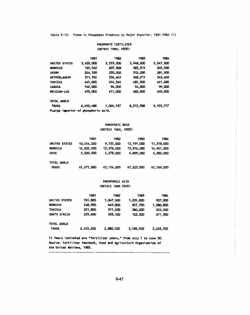
Table 9-13: Trade in PhDsphate Product6 by W j o ~ Ucpcrtcr, 4981-1984 (1)
PHOSPHATE FERTlLIZER OHETRIC TONS, P M 5 )
1981 UNITED STATES 3,403,000 HOROCM 125,542 USSR* 254,100 NETHERLANDS* 311,765 N N I S I A 445,600 CANADA 162,MO BELGIUH-LUX 4iU,000
TOTAL WRLD
TWSE 6,450,486 7,064,137 8,213,908 9,193,717 *Large i q o r t e r of p h o s p h o r i c a c i d .
PHOSPHATE ROCK
(HETRIC TONS, P M 5 )
1981 1982 1983 1984 UNITED STATES 10,554,000 9,735,WO 13,197,000 11,318,MO m)ROCCO 15,635,m 13,976,000 13,976,000 14,951,000 USSR 5,OM,000 5,278,000 4,899,000 4,YU,MO
TOTAL WRLD TRADE 45,271,000 43,154,000 47,223,000 47,769,000
PHOSPHORIC ACID (METRIC TONS P 2 S )
1981 1982 1983 1984 UNITED STATES 761,SW 1,047,500 1,235,000 937,000 IY)ROttO 548,900 649,800 857,MO 1,090,800 N N I S I A 251,8M 311,500 380,000 333,500 SOUTH AFRICA m r 6 0 0 228,100 123,m 211,900
TOTAL WRLD TRADE 2,453,203 2,880,500 3,189,500 3,258,MO
1) Years i n d i c a t e d a r e ' f e r t i l i z e r years," fn, J u l y 1 t o June 30. Source: F e r t i l i z e r Yearbook, F m d and A g r i c u l t u r e O r g a n i z a t i o n o f
t h e U n i t e d Nat ions, 1985. ......................................................................
The decline in U.S. exports can be expected to continue as the less developed countries expand their
phosphoric acid and fertilizer capacities. Zellars-Williams forecasts that the U.S. share of the
phosphate rock export market will fall to 15.5 percent in the year 2005, from 23.1 percent in 1984.
Zellars-Williams also forecasts that the Moroccan share of the export market will go from 31.4
percent in 1984 to 46.5 percent in 2005.
9.2.2.4 Demand Forecasts
There are a number of multi-equation models used for forecasting phosphate fertilizer demand. The
models are of varying degrees of sophistication, use a variety of estimation methodologies and have
differing time horizons. They all include, to one degree or another, the set of variables discussed in
the preceding section; population, acreage of major crops harvested, fertilizer application rates,
fertilizer and crop supply and prices, crop mix and yield estimates.
Forecasters disagree on the outlook for the world as a whole. The Food and Agriculture Organization
(FAO) predicts that worldwide phosphate demand will grow less than one percent per year up to the
end of the century. Zellars-Williams and WEFA analysts have a more optimistic outlook, estimating
annual growth at 1.3 and 2.4 percent, respectively. Their optimism is based largely on the prediction
that grain prices will increase due to grain stock depletion by 1995. While both sets of analysts expect
North American phosphate demand to recover from its lows of the mid- 1980s, neither expect acreage
or production to increase to their early-1980 levels.
Table 9-14 provides a basis for comparison of the forecasts for four years of interest. The shorter-
range forecasts provided by, or imputed from, the various models generally agree on the level of
demand over the next few years. The more recent forecasts are substantially more conservative over
the long run, reflecting new information about government-sponsored acreage reduction programs
in the U.S. and Europe. For example, the 1979 Chase Econometrics forecast estimated that U.S.
agricultural demand would grow 3 percent per year between 1979 and 2000, while the 1985 Bureau
of Mines forecast implies a U.S. growth rate of 1.3 percent for 1983 through 2000. The earlier
forecast also did not anticipate the drop in economic growth rates in LDCs and the emergence of
Third World debt problems. The other forecasts provided in Table 9-14 were performed after 1983
and provide more pessimistic assessments due to these events.
However, all forecasters agree that phosphate fertilizer demand (and therefore demand for WPPA)
in developed market economies will grow at a substantially lower rate than demand in other regions
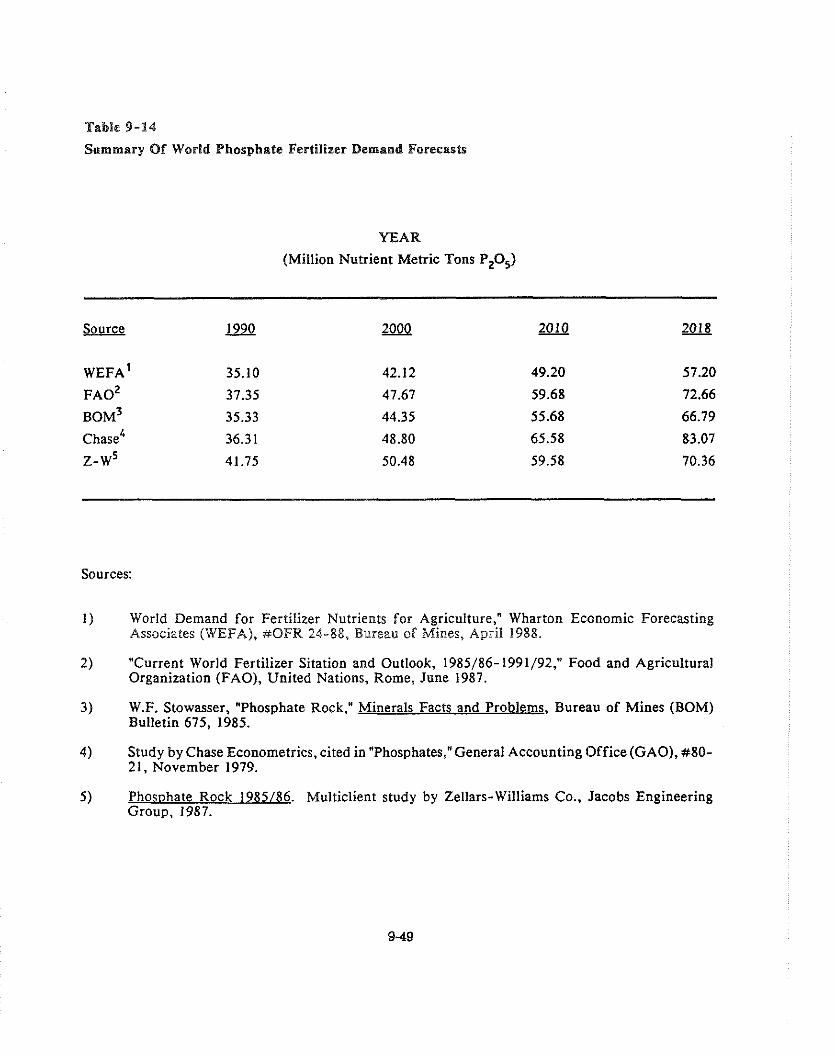
Table 9-14
Summary Of World Phosphate Fertilizer Demand Forecasts
YEAR
(Million Nutrient Metric Tons PzOs)
Sources:
1) World Demand for Fertilizer Nutrients for Agriculture," Wharton Economic Forecasting Associates (WEFA), #OFR 24-88, Bureau of Mines, April 1988.
2) "Current World Fertilizer Sitation and Outlook, 1985/86-1991/92." Food and Agricultural Organization (FAO), United Nations, Rome, June 1987.
3) W.F. Stowasser, "Phosphate Rock," Minerals Facts and Problems, Bureau of Mines (BOM) Bulletin 675, 1985.
4) Study by Chase Econometrics, cited in "Phosphates," General Accounting Office (GAO), #80- 21, November 1979.
5) Phos~hate Rock 1985186. Multiclient study by Zellars-Williams Co., Jacobs Engineering Group. 1987.
(see Table 9-15). The lower estimates reflect the fact that the developed market economies have
more mature agricultural industries and thus potential fertilizer gains are minimal. In addition, new
ideas for fertilizer application currently being implemented in these countries have resulted in
reduced fertilizer requirements.
Forecasters agree that demand for fertilizer in Western Europe will be stable or decreasing over the
next 20 years. These assessments are based on the maturation of the agriculture industry in these
countries, and more specifically on the expectation that Western European governments will
implement programs to reduce agricultural subsidies and stimulate a decline in crop acreage. On the
other hand, WEFA analysts note that a possible future shift from food grain to feed grain production
will stimulate phosphate fertilizer use [WH88].
Analysts at Zellars-Williams estimate that population pressures and the pursuit of food self-
sufficiency policies in Asia will keep demand for phosphate fertilizers in that region growing at an
annual rate of about 3.4 percent at least until the year 2005. WEFA analysts estimate a lower 2.7
percent growth rate for the same time period. Their lower growth estimate reflects beliefs concerning
fertilizer use in Asia. WEFA analysts believe that Asian countries will experience diminishing returns
to fertilizer applications by 1995, leading to reduced fertilizer requirements in that region [WH88].
Most of the future demand for phosphate fertilizers in Africa will result from increased application
rates rather than increased acreage. Climatic conditions and destructive farming practices are likely
to continue to turn much African land into desert. WEFA projects that acreage in the region will
grow less than one percent per year [WH88].
All forecasters seem to agree that Latin America has tremendous potential for growth in agriculture
and fertilizer usage over the next 25 years. This optimistic assessment is based on the fact that
certain countries in the region are the lowest-cost producers of corn, soybeans and wheat, and hence
will be producing increasing shares of these major crops in the future. In addition, analysts expect
agriculture in the region to become more intensive. Agricultural policy will seek to meet production
targets by increasing yields rather than opening new lands for cultivation.
Thus, in general, most of the growth in demand will come from LDCs in Asia and Latin America.
Within Asia, most of the growth is expected to come from the People's Republic of China; in Latin
America, most of the growth is expected to come from Brazil and Mexico, although the debt and

i r b t e 9-45: Fsraus'Ls BI Fer t i l i ze r Deuanl by Rcglon ond w r e c , "1-m
(WTlLim N e r r i c 7ms Pi%)
1995 mR3 ZW5 t w o ......................... ......................... ---------------- -----
RECi lU I VEFA ZU FA0 UEFA ZU FA0 (I) UEFA ZU UEFA .................................................................................................. NORTH M E R I U 5.0 5.6 4.2 5.6 5.9 5.3 6.2 6.2 6.8
UTIK M E R I C A 2.8 3.1 3.3 3.2 3.6 2.6 3.5 3.8 3.9
UESTERN EUROPE 4.9 6.6 5.2 4.9 7.0 4.8 7.5 4.8
AFRICA 3.6 3.5 0.8 I .5 2.3 0.5 1.6 2.5 1.7
ASIA 11.4 14.2 10.8 13.0 15.7 15.1 14.5 16.7 16.0
CHINA 6.8 3.4 7.8 12.0 8.3
OCEANIA 1.0 1.3 I .2 1.1 1.3 0.4 1.1 1.3 1.2
CENTRALLY PUNNED
E C W Y 12.0 12.2 11.4
E. EUROPE 3.6 3.5 3.9 3.6 4.2 4.6 4.4
USSR 8.3 8.7 9.0 10.1 9.7 11.1 $0.5
(1) Refers to 1997198 (only).
Swrces: "Uorld Demand for Fe r t i l i ze r Kutr imts for Agriculture," UEFA, #OFR-24-88, for Bureau of Mines, April 1988; Phosphate Rock 1985186, ZaLLars-UiLLiams, 1987; 'Current UorLd Fer t i l i ze r Sitr tst im and O u t l ~ o t , ~ Food and Agriculture Organizatiw of the United m t i m s , June 1987. ---------------------------------------------*------------------------------------"*--------------
foreign exchange problems of both countries are expected to dampen import consumption and
encourage further investment in domestic capacity.
Most of the forecasts mentioned do not deal directly with U.S. exports. Zellars-Williams, however,
expects U.S. exports to increase until 1990 and to fall by almost 50 percent between 1990 and the year
2005 [Ze86]. This reflects the expectation that an increasing share of WPPA will be supplied by
LDCs. WEFA expects an average growth in exports of 2.0 percent per year until 1996 [WHSS].
Phosphate exports, according to the WEFA analysis, will constitute over half of the total identified
demand for U.S. produced phosphates over the forecast period. Thus, the outlook for the domestic
phosphate industry is unclear.
9.2.3 Other Issues
9.2.3.1 Substitutes
Besides phosphate ore, guano (igneous apatite and marine phosphorites) is the only significant source
of phosphorus. However, it is no real substitute for phosphate rock as a raw material for producing
phosphate fertilizers. Guano accounts for about 3 percent of world production of phosphate. All
large accumulations of guano were formed on the surface of the earth by seabirds. The composition
of these deposits varies with the degree of leaching by surface waters. Chile holds most of the world
guano supply [StSS].
In some limited cases, phosphate rock can be used directly as a fertilizer, instead of first being
converted into phosphoric acid. According to Ed Harre at the National Fertilizer Development
Center, approximately a million tons of phosphate rock is used in this way each year around the
world, mostly in the Soviet Union. The rock must be finely ground and even then only a small
percent of the P205 can be absorbed by the crops. The yield response is best in very acidic soils.
A potential substitute for the production of phosphoric acid is the production of nitrophosphate (NP)
fertilizers. In this process, nitric acid is substituted for sulfuric acid. NP is produced in Europe,
India and China but not in the U.S. One study estimates that sulfur prices would have to double, to
$200 per ton for the process to become economically attractive. In any case, environmental concerns
remain with NP. With NP, the radium in the phosphate rock is absorbed into the fertilizer instead
of remaining in the waste product [P187,P188]. Consequently, the radon emissions from the spreading
of the radium over millions of acres of farmland would certainly exceed the emissions from
phosphogypsum stacks.

Spent acid from aluminum bright dipping is a substitute for WPPA in the manufacture of ammonium
phosphates only. The spent acid is recovered from aluminum bright-dip baths and may be used in
the production of fluid mixed fertilizers. This product is being used for this purpose in the midwest
and southeast, where most bright-dip plants are located. Its price per unit of P205 is usually lower
than the price for WPPA. But the availability of this spent acid has been declining in recent years
as large U.S. bright-dipped aluminum alloy manufacturers have installed acid regeneration units in
their plants. Increased regeneration activity has been concurrent with the decision of auto
manufacturers to use less bright-dip trim on cars [SRi86].
Thermal phosphoric acid is also a substitute, but its production costs are much higher and the
production of thermal phosphoric acid presents other environmental problems.
9.2.3.2 &&native Uses for Phosohoevnsum
Alternative uses for phosphogypsum attempt to exploit the material's two key properties: its physical
similarity to natural gypsum, and its sulfur and calcium content. Industrial and agricultural uses for
phosphogypsum are nothing new: research into sulfuric acid production from phosphogypsum started
at least as early as World War I [BSC85g]. Applications in building materials were common in Europe
until the 1950s and in the U.K. until the 1970s [BSC87f] and are still found in Asia [FIPgX]. Below
is a review of the current uses of phosphogypsum and of the limited data available on radiation levels
from these uses.
Current Uses -- Alter~lative uses in the United States are fairly recent phenomena, and are a small
scale; one industry source estimates that only about 5 percent of U.S. phosphogypsum output is put
to use in some way [An88]. The end of this section summarizes the information available on uses of
phosphogypsum by U.S. companies. By contrast, a 1981 study by a United Nations researcher
estimated that 14 percent of world phosphogypsum output was reprocessed [Ca88].
Most of the research in the U.S. has focused on two uses: the use of phosphogypsum as a road base,
usually mixed with other material, and processing of phosphogypsum into sulfuric acid and aggregate,
a solid material that can be used for a variety of construction purposes. Agricultural applications,
more common overseas, have been somewhat limited in the United States. Other uses for
phosphogypsum have been tried on a small scale but never widely adopted.

Building Materials -- Much effort has been devoted to the development of methods which use
phosphogypsum as a construction material. Many of these are the same as uses for natural gypsum;
for example, plaster and wallboard. The use of phosphogypsum in building materials is hence
doubly attractive where natural gypsum is expensive or impossible to obtain locally and disposal of
phosphogypsum poses economic or environmental problems. For example, in Japan, where there are
no natural deposits of gypsum and land for dumping is scarce, the Nissan company has developed
and installed its own advanced phosphoric acid production technology to produce high-quality
byproduct gypsum.
There is no evidence that phosphogypsum straight from a stack is suitable for use in construction
materials. The phosphogypsum must be produced in a purer form than is usual in the US., and then
dried, or processed. It is then combined with some other substance (often flyash) and compacted to
make bricks, blocks or boards, or molded into plaster. Laboratory tests at the University of Miami
found that, depending on moisture content, compacted phosphogypsum can achieve compressive
strength as high as 1000 pounds or more per square inch [Ch87]. Phosphoric acid plants in Austria,
Japan, and Belgium have been designed to produce as a byproduct high-quality phosphogypsum
specifically for construction purposes [Ca88]. Construction uses in Europe have become more
common as restrictions on dumping at sea have been imposed; at least one German firm sells
wallboard and other construction materials fashioned from phosphogypsum [L185]. The Donau
Chemie Company in Austria has one 50,000 ton per year phosphoric acid plant where all of the
byproduct phosphogypsum is recycled into building materials [Ca88]. A technique for purifying
phosphogypsum to make it suitable for building materials has been patented by the American
company United States Gypsum but has never seen commercial usage [Mn88]. There is no evidence
that phosphogypsum has found a building materials market in America.
Road Base -- Phosphogypsum is well-suited for use as a road bed. Either the aggregate from a
cement and acid process or unprocessed waste gypsum may be used. Unprocessed phosphogypsum
for use in road beds, mixed with flyash, cement, or other materials, has found an increasing but
limited market in America. Since July 1984, Mobil Mining and Minerals in Pasadena, Texas has
taken phosphogypsum from inactive stacks, mixed it with 6 percent cement, and sold it as "Gypsum
Aggregate." As of December 1986, over 300 projects utilizing a total of 340,000 tons of Mobil
phosphogypsum had been completed [FIP88]. Mobil's Gypsum Aggregate has a number of other uses,
including railroad base and embankment construction. However, despite the good engineering
qualities of gypsum from phosphogypsum in this use, it is profitable to produce and sell as a road
base only where there is no natural local source for aggregate material because of high transportation
costs. Some of Mobil's success in this area is because the Houston area has few sources of aggregate.
In Florida, some unknown number of private roads and parking lots have a phosphogypsum base;
but since they were built informally, little is known about the details of their construction [L185j.
Circular Grate Technoloav -- The alternative use which has received the most attention in recent
years and which holds the most promise for the future concerns the processing of phosphogypsum
to produce sulfuric acid and a solid material, called aggregate. There are a number of techniques of
this type, generically referred to as "cement-acid processes." The most discussed technique for this
is known as the "circular grate process." The process can be varied to produce various forms of
aggregate appropriate for different applications [Ke86]. As mentioned, the production of sulfuric
acid from phosphogypsum dates back at least 50 years, but the high energy costs of earlier techniques
rendered them economically infeasible under most conditions. However, some recent studies indicate
that us2 of the circular grate process can lead to rates of return as high as 25 to 38 percent [Mc87c].
A pilot project at Freeport McMoRan's Uncle Sam plant in Louisiana, co-sponsored by the Florida
Institute of Phosphate Research and the Davy McKee Corporation, is expected to use 35 tons of
phosphogypsum and other inputs each day and produce 29 tons of sulfuric acid and 25 tons of
aggregate per day when it begins operation which is expected to be in early September of 1988
[Mc87c,LL88].
Where there is no nearby cement supply, other technologies can be profitable; for example, the
Fedmis Division of Sentrachem Ltd. in South Africa operates a 70,000 ton per year cement and acid
plant. Forty percent of Fedmis phosphogypsum output goes into profitable recycling. The Fedmis
example is unusual because reasonably priced cement is not available in the region surrounding the
Fedmis plant. Cement produced elsewhere and shipped to the area is not competitive because of the
high relative cost of transporting cement.
Strong demand for aggregate in Florida is expected to last for several decades, as the state's
population is forecast to increase to over 15 million by the year 2000 [DOC88c]. With higher
population there will be a need for more roads. Most of the aggregate used to build roads in Florida
has to be brought in from outside the state; since many phosphate producers are located there, there
are some hopes in the phosphate industry that both the road and phosphogypsum problems may be
solved at once, using the circular grate technology [BSC87g]. However, some sources in companies
not directly involved in the circular grate process are skeptical about this new technology. Several
people in the industry argue that low sulfur prices and high transportation costs for aggregate make
the technology unprofitable. Others doubt that it is technically feasible. However, it is estimated
that the circular grate process could produce sulfuric acid at a cost of $21.65 per short ton, compared
to $43.70 per short ton for the more traditional sulfur burning process [BSC87h]. Iowa State
University has developed a similar process using a fluid bed reactor rather than a circular grate, but
this approach has never left the test-plant stage [Mn881.
Agriculture -- Phosphogypsum also has properties which make it potentially useful in agriculture.
As a fertilizer, it contains significant amounts of sulfur and calcium, both beneficial to growing
plants. According to Mike Lloyd of the Florida Institute for Phosphate Research, the sulfur content
is in a form usable by the soil directly, without any processing of the phosphogypsum. Of 18
American companies for which information is available, 8 currently sell some amount of
phosphogypsum for agricultural use; 3 have done so in the past but have stopped recently, usually
because the sales proved unprofitable. However, in all cases these sales have been small compared
to total phosphogypsum output, occasionally as much as 5 percent but often less than I percent of
total phosphogypsum produced by the firm. Application rates have been estimated as varying
between one half and 3 tons per acre, depending on locale and crop [Mc88].
There are two reasons why phosphogypsum is not used more for agricultural purposes. First, only
a limited number of crops benefit from phosphogypsum. Second, the potential profits from the
phosphogypsum are small relative to its bulk. Consequently, even at little or no cost for the material,
it is not profitable to transport phosphogypsum for long distances.
In other countries, phosphogypsum is used as a fertilizer. In India, the Gujarat State Fertilizer
Company has been making high-quality gypsum from phosphogypsum and also converting it into
ammonium sulfate fertilizer at a facility with 205-210 metric tons per day capacity [FIP88]. As a soil
additive, it can be used to remove aluminum toxicity [Lt88]. Kt is also used to make clay and other
tough soils more porous, improving drainage [FIP881.
Sulfur Recovery -- As the price of sulfur has risen, more research has focused on potential methods
of recovering the sulfur from phosphogypsum. A significant proportion of the energy and capital
costs in the acid-cement techniques goes into producing commercial-quality cement. This fact has
led at least one source to comment that the use of these techniques should be considered as cement
production rather than acid production [FIP88]. Elemental sulfur can be produced via thermal
processing of gypsum (natural or byproduct). Due to energy and capital costs, this technique has been
feasible only when the supply of sulfur is extremely limited--for example, it has been used abroad
when wartime blockades or government import controls have cut sulphur supplies [L185]. The British
Sulphur Corporation has speculated that environmental considerations may lead to more thermal
processing of waste gypsum to yield elemental sulfur, even when it is not "strictly profitable
[BSC87g]."
Radiation Considerations -- A few studies of radon and radioactivity hazards in alternative uses of
phosphogypsum have been completed. One University of Florida study of agricultural applications
estimated the radionuclide uptake by plants, the resultant concentration in food, and the subsequent
doses to consumers, for applications of one ton of phosphogypsum per acre every four years. The
study claimed to find no significant radiological problems implied for horizons of up to 50 years
[FIP88].
University of Miami engineering professor Wen F. Chang claims that radon emissions from
phosphogypsum are greatly reduced when it is compacted (to make bricks, for example). He
estimates that emissions can be reduced 80 to 95 percent compared to the powder form, depending
on the force of compression [Ch88].
Two experiments have measured radon concentration in enclosed rooms fashioned from
phosphogypsum panels [FIP88]. The first study was conducted by researchers from the University
of Miami and Jacobs Engineering, the second by a University of Miami professor. In each study,
the 'worst case' was examined: the rooms were windowless and ventless and constructed entirely from
the wallboard. In addition, the wallboard was painted on the outside of the room to minimize the
escape of radon gas. In both cases, radon concentration in the structure approached or was as high
as (EPA or Florida state) screening levels. In addition, the former study measured radon emissions
when the panels were painted on the surface facing the inside of the room and found that emissions
were reduced by 95 percent. Wen F. Chang, the University of Miami professor who performed the
second experiment, claims that painting the phosphogypsum panels reduces emissions to negligible
levels, and that the materials he has produced experimentally will pass any building code [Ch88].
Little data on radon emissions in roadbase use is currently available, although a University of Miami
study has examined the impact of a phosphogypsum roadbase in Polk County, Florida on local
groundwater quality [FIP88]. Neil Anderson, venture manager of the phosphogypsum project at
Mobil Mining and Minerals, claims that radon emissions from an installed phosphogypsum roadbase
of Mobil Gypsum Aggregate (without an intact covering such as asphalt) are I to 2 picocuries per
square meter per second, and when the roadbase has an intact covering the emissions are essentially
none [An88]. However, such coverings almost always develop cracks which allow disproportionate
amounts of gas to escape. Mr. Anderson states that a hydration reaction takes place when the
phosphogypsum is mixed with cement, reducing the radon emissions. The following section
summarizes alternative uses of phosphogypsum by various companies.
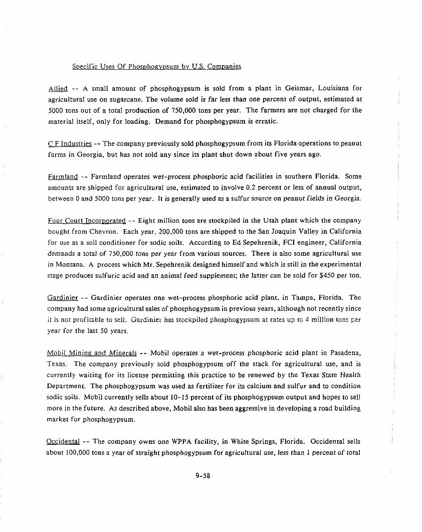
Soecific Uses Of Phosohoavosum by U.S. Comoanies
Allied -- A small amount of phosphogypsum is sold from a plant in Geismar, Louisiana for
agricultural use on sugarcane. The volume sold is far less than one percent of output, estimated at
5000 tons out of a total production of 750,000 tons per year. The farmers are not charged for the
material itself, only for loading. Demand for phosphogypsum is erratic.
C F Industries -- The company previously sold phosphogypsum from its Florida operations to peanut
farms in Georgia, but has not sold any since its plant shut down about five years ago.
Farmland -- Farmland operates wet-process phosphoric acid facilities in southern Florida. Some
amounts are shipped for agricultural use, estimated to involve 0.2 percent or less of annual output,
between 0 and 5000 tons per year. It is generally used as a sulfur source on peanut fields in Georgia.
Four Court Incoroorated -- Eight million tons are stockpiled in the Utah plant which the company
bought from Chevron. Each year, 200,000 tons are shipped to the San Joaquin Valley in California
for use as a soil conditioner for sodic soils. According to Ed Sepehrenik, FCI engineer, California
demands a total of 750,000 tons per year from various sources. There is also some agricultural use
in Montana. A process which Mr. Sepehrenik designed himself and which is still in the experimental
stage produces sulfuric acid and an animal feed supplement; the latter can be sold for $450 per ton.
Gardinier -- Gardinier operates one wet-process phosphoric acid plant, in Tampa, Florida. The
company had some agricultural sales of phosphogypsum in previous years, although not recently since
it is not profitable to sell. Gardinier has stockpiled phosphogypsum at rates up to 4 million tons per
year for the last 50 years.
Mobil Mining and Minerals -- Mobil operates a wet-process phosphoric acid plant in Pasadena,
Texas. The company previously sold phosphogypsum off the stack for agricultural use, and is
currently waiting for its license permitting this practice to be renewed by the Texas State Health
Department. The phosphogypsum was used as fertilizer for its calcium and sulfur and to condition
sodic soils. Mobil currently sells about 10-15 percent of its phosphogypsum output and hopes to sell
more in the future. As described above, Mobil also has been aggressive in developing a road building
market for phosphogypsum.
Occidental -- The company owns one WPPA facility, in White Springs, Florida. Occidental sells
about 100,000 tons a year of straight phosphogypsum for agricultural use, less than 1 percent of total
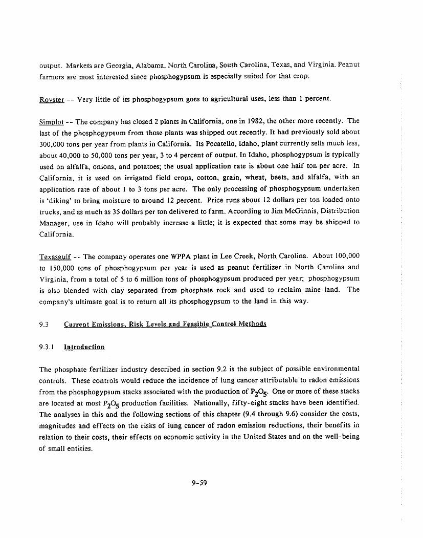
output. Markets are Georgia, Alabama, North Carolina, South Carolina, Texas, and Virginia. Peanut
farmers are most interested since phosphogypsum is especially suited for that crop.
Rovster -- Very little of its phosphogypsum goes to agricultural uses, less than 1 percent.
Simolot -- The company has closed 2 plants in California, one in 1982, the other more recently. The
last of the phosphogypsum from those plants was shipped out recently. It had previously sold about
300,000 tons per year from piants in California. Its Pocatello, Idaho, plant currently sells much less,
about 40,000 to 50,000 tons per year, 3 to 4 percent of output. In Idaho, phosphogypsum is typically used on alfalfa, onions, and potatoes; the usual application rate is about one half ton per acre. In
California, it is used on irrigated field crops, cotton, grain, wheat, beets, and alfalfa, with an
application rate of about 1 to 3 tons per acre. The only processing of phosphogypsum undertaken
is 'diking' to bring moisture to around I2 percent. Price runs about 12 dollars per ton loaded onto
trucks, and as much as 35 dollars per ton delivered to farm. According to Jim McGinnis, Distribution
Manager, use in Idaho will probably increase a little; it is expected that some may be shipped to
California.
Texaseulf -- The company operates one WPPA plant in Lee Creek, North Carolina. About 100,000
to 150,000 tons of phosphogypsum per year is used as peanut fertilizer in North Carolina and
Virginia, from a total of 5 to 6 million tons of phosphogypsum produced per year; phosphogypsum is also blended with clay separated from phosphate rock and used to reclaim mine land. The
company's ultimate goal is to return all its phosphogypsum to the land in this way.
9.3 Current Emissions. Risk Levels and Feasible Control Methods
9.3.1 Introduction
The phosphate fertilizer industry described in section 9.2 is the subject of possible environmental
controls. These controls would reduce the incidence of lung cancer attributable to radon emissions
from the phosphogypsum stacks associated with the production of P209 One or more of these stacks
are located at most P205 production facilities. Nationally, fifty-eight stacks have been identified.
The analyses in this and the following sections of this chapter (9.4 through 9.6) consider the costs,
magnitudes and effects on the risks of lung cancer of radon emission reductions, their benefits in
relation to their costs, their effects on economic activity in the United States and on the well-being
of small entities.

Because the parameters affecting the radon emissions from all these stacks are not available and
because economic data is available for P205 producers linked to only a subset of the stacks, detailed
economic analysis is done for fourteen of the fifty-eight stacks. Details of the selection of the
fourteen appear in section 9.5.
9.3.2 Phvsical Attributes of Phosohoevosum Stacks
9.3.2.1 Desien and Construction
Phosphogypsum is created when phosphate rock and sulfuric acid are combined to produce P2O5
The amount of phosphogypsum produced is approximately five times that of the Pt05 produced. For
disposal, the phosphogypsum is carried by a slurry and deposited on large piles known as stacks.
The stacks are large. Their bases range from 2 hectares to 284 hectares and some currently reach a
height of 50 meters. The quantity of phosphogypsum deposited in a stack in a year may reach
1,550,000 metric tons.
While the stacks are irregular in shape, they roughly resemble a rectangular box, with sloping sides.
While the sides of most stacks are sloped with one vertical meter for every three horizontal meter,
stacks in Louisiana and Mississippi have a more gradual slope, about one in eight. (Table 9-16) For
the purpose of modeling, it is also assumed that the length of the base of a stack is twice its width.
The tops of the stacks are constantly changing as a slurry of phosphogypsum is deposited first on one
segment, and then on another, of the tops. A road around the top and dikes to contain the new
deposits of phosphogypsum are frequently rebuilt to accommodate the changing dimensions of the
sides and top. When one section of the top is filled, it is allowed to dry and the flow of slurry is
diverted to another section. Much of the top is under water at any time, not only while the slurry
is settling, but also because portions of the tops are used for water storage as part of the waste water
management plan for the production facility.
Radon emissions from uncontrolled stacks depend on the flux, or rate of release of radon from the
phosphogypsum in the various portions of a stack, and on the areas of these portions. Radon flux
from the sides differs from the fluxes from the top. On top, the portions that are under water have
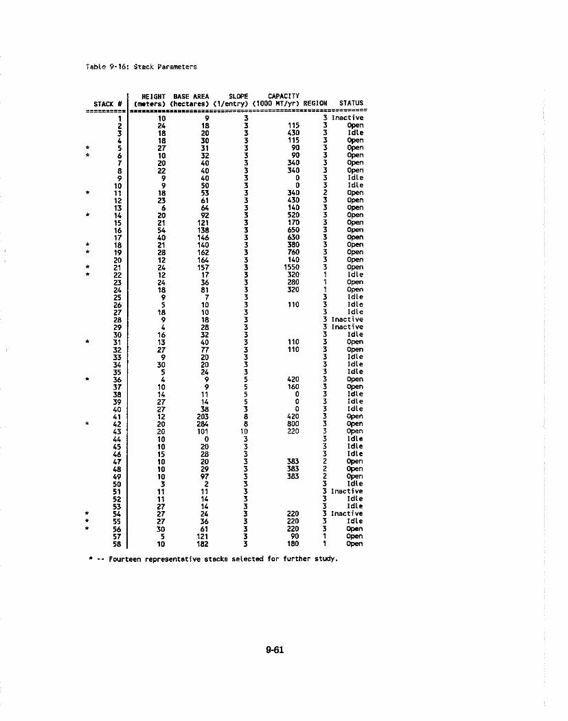
Table 9-16: Stack Parsmeters
STACK iY ==========
1 2 3 4 * 5
t 6 7 8 9
10 . 11 12 13
t 14 15 16 17 18
* 19 20
t 21 . 22 23 24 25 26 27 28 29 30
a 31 32 33 34 35 * 36 37 38 39 40 41 * 42 43 44 45 46 47 48 49 50 51 52 53 * 54 55
* 56 57 58
HEIGHT BASE AREA SLWE CAPACITY ( ~ t e r s ) (hectares) ( l lentry) (1000 IiTlyr) REGION STATUS
EE_IS--I--..I.D...3-- ....................................... 10 9 3 3 Inactive 24 18 3 115 3 open 18 20 3 430 3 I d l e 18 30 3 115
90 3 open
27 31 3 3 open 10 32 3 w 3 pen 20 40 3 340
40 3 340 3 open
22 9 40 3 0 9 50 3 0
; 'z: 3 ld le
18 53 3 340 2 open 23 61 3 430
140 3 Open
6 64 3 3 open 20 92 3 520 3 OPen 21 121 3 170
138 3 650 3 Open
54 3 630
3 apen 40 146
140 3 380 3 qm
21 3 Open 28 162 3 7M) 3 Open 12 164 3 140 3 Open 24 157 3 1550 3 Open 12 17 3 320 1 Id le 24 36 3 280 1 Open 18 81 3 320 1 Open 9 7 3 3 Id le 5 10 3 110 3 Id le
18 10 3 3 Id le 9 18 3 3 Inactive 4 28 3 3 Inactive
16 32 3 3 Id le 13 40 3 110
77 3 110 3 Open
27 0 70 3 ; 'z:
3 id le 3 l d l e 3 Open 3 open 3 Id le 3 I d l e 3 I d l e 3 open 3 Open 3 Open 3 ld le 3 ld le 3 ld le 2 open 2 open 2 open 3 l d l e 3 lnactive 3 l d l e 3 l d l e 3 lnactive 3 l d l e 3 open 1 Open 1 Open
* - - Fourteen representative stacks selected for further study.

no flux while the dry portions and the roads have differing fluxes. Since roads, dikes, and
underwater portions of the top are in relatively constant ratios to each other as the stack grows,
weighted averages of the fluxes on the top can be computed for each geographical region. This is
the value used in computations of rota1 radon emissions from the tops of the stacks. Radon emissions
for a stack equal the sum of the products of its top and sides and its flux rates.
Radon flux also depends on the composition of the phosphate rock that went into the Pz05 production
and on the rainfall of the region. Flux rates were developed for three regions of the nation. Region
one contains Idaho, Utah, and Wyoming; region two is North Carolina and northern Florida; and
region three is the rest of the United States. (Table 9-17)
Calculations of radon emissions from each stack considered were done using a computer model that
first computes the areas of the sides and top of each stack, and then its radon emissions as it grows,
and areas and emissions of each stack after they reach their full sizes and are closed. Table 9-18
shows the total, uncontrolled, current emissions for each stack as calculated by the model.
9.3.2.3 Risks Due to Uncontrolied Stacks
The emissions shown in Table 9-18 result in some risk of lung cancer to the population. Two kinds
of risk were considered, risk to the individual most exposed to each stack and risk to the population
within an 80 km radius of each stack. These risks were calculated for each stack individually based
on its emissions by running the AIRDOS-EPA computer code. The results of these runs for the
fourteen stacks are also shown in Table 9-18.
9.3.3 Feasible Control Methods
9.3.3.1 Descriotion of Controls
The primary control technique considered for the reduction of radon emissions from phosphogypsum
stacks is to cover the stacks with a layer of dirt. To meet a given standard a sufficient thickness of
dirt must be used. The thickness of dirt needed depends on the desired standard, the radon flux rate
from the stack, and the properties of the dirt used. The major option available is whether to add dirt
on the sides while the stack is in operation or wait until it is closed. The top can only be covered
after the stack is closed.
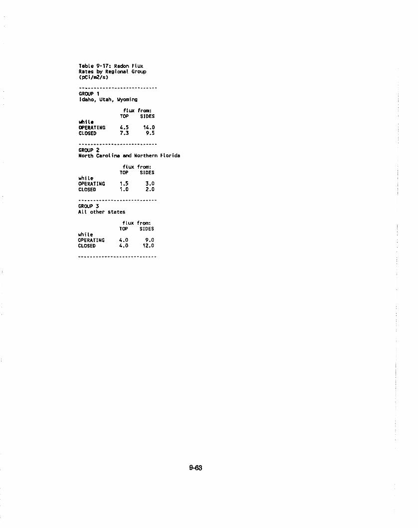
Table 9-17: Radon flux Rates by Regionsl Grwp (pciln2ls)
GRWP 1 Idaho, Utah, Uyoming
f lux from: TOP SIDES
uhi lc OPERATING 4.5 14.0 CLOSED 7.3 9.5
. . . . . . . . . . . . . . . . . . . . . . . . . . . GRWP 2 North Carolina and Northern Florida
f lux from: TOP SIDES
u h i l e OPERATING 1.5 3 .0 CLOSED 1 .O 2.0
. . . . . . . . . . . . . . . . . . . . . . . . . . . GRWP 3 A l l other states
f lux from: TOP SIDES
u h i l e OPERATING 4.0 9.0 CLOSED 4.0 12.0
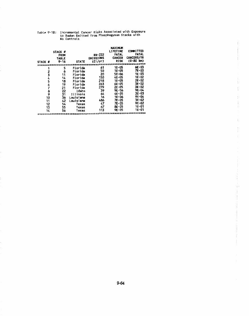
Table 9-18: Incremental Cancer ~ i s k s Associated u i th Expsure t o Re& Emitted from Phosphqysun Stacks w i th No Ccmtrots
STACK U
STACK U FRCU RN-222
TABLE EMISSICUS 9-16 STATE (Cilyr)
:I==_=.llI=1=3=3=I==============: 5 Florida 61 6 Florida 50
11 Florida 20 14 Florida 150 18 Florida 218
W U I W LIFETIME
FATAL CANCER
RISK :=z==s====:
1E-05 1E-05 5E-06 LE-05 1E-05 AF-05
FATAL CAYCERS/YR
(0-80 km) -- = = ====
-- -- -- .- 7 21 Florida 279 2E-05 3E-02 8 22 Idaho 39 9E-06 9E-04 9 31 I l l i n o i s 6L LE-05 3E-03
10 36 ~ou is iana 16 1E-06 PE-M 11 L2 Louisiana 486 7E-05 3E-02 - 05 PE-02

The computer model used to analyze the control alternatives provides three scenarios. Scenario 1 is
to cover the sides while the stack is in operation and the top when it is closed, scenario 2 is to cover
the sides and top when the stack is closed, and scenario 3 is to do nothing. The model also allows
flux standards to be set a tany level. These levels are considered: 20 pci/m2/sec, 6 pci/m2/sec, and
2 pci/m2/sec.
Since all stacks already have radon fluxes of less than 20 ~ c i / m ~ / s e c , only the latter two fluxes were
analyzed. The model calculates a thickness of dirt based on the highest flux rate from any portion
(top or sides) of the stack at any time. Runs were made for the following four combinations:
1. flux standard = 6 pci/m2/sec and scenario = 1
2. flux standard = 6 p~i /m2/sec and scenario = 2
3. flux standard = 2 p~i /m2/sec and scenario = 1
4. flux standard = 2 p~i /m2/sec and scenario = 2
In the model, the ratio of the covered to uncovered flux (R) is computed for each stack and flux
standard. Thickness is then found from equation (1).
(1) R = exp(-B * thickness) where B is a property of the soil cover, and R is the ratio of controlled flux to uncontrolled flux
Table 9-19 shows the ratios and thicknesses of dirt for flux standards of 6 pci/m2/sec and
2p~i/m'/sec The thickness of dirt applied to most portions of each stack in each situation is greater
than is needed to meet the flux standard. The exact emission change resulting from the actual
amount of dirt applied is calculated. These emission reductions are greater than required to meet
the stated standard. However, the convenience of applying a uniform thickness of dirt to an entire
stack was considered to offset the savings of adjusting the amount of dirt used on each portion of
the stack in each situation. In particular, it was not contemplated that dirt would be removed from
the sides of a stack after it was closed in cases where the sides of a closed stack have a lower radon
flux rate than those of an open stack.
To cover the stacks, various preparations must be made and specific steps followed. First drains must
be laid on the stack. The drains prevent acidic water from seeping from the stack and killing the
ground cover. Vertical drains are installed every 30 meters around the base and slant upward to a
spacing at the top proportional to the spacing at the bottom. A peripheral drain is installed every ten

Table 9-19: Control Parameters f o r Representative Stacks
STACK U FRCU
TABLE [ _ _ _ _ _ _ _ _ _ _ _ _ _ _ . _ [ 1 _ _ _ _ _ - - - - - - - - - - - [ STACK 11 9-16 STATE "BW RATIO THICKNESS RATIO THICKNESS
- . . - . . -- .. .. . ... ~ ~~ -~
T in I Flor ida 1.80 0.400 0.51 0.133 1.12
------------------ _ ______ 1 5 2 6 3 11 I 1L
- . . . . . -- .. .. -~~
6 i 1 F lor ida 1.70 0.401 0.54 0.133 1.19
==I==EII.IE==.EIEIS=============m=====aaa====~=====*======
Flor ida 1.80 0.400 0.51 0.133 1.12 Flor ida 1.80 0.400 0.51 0.133 1.12 Flor ida 1.80 0.400 0.51 0.133 1.12 Flor ida 1.70 0.401 0.54 0.133 1.19
Where:
- 7 21 8 22 9 31 10 36 11 42 12 51 13 55 14 56
RATIO = the r a t i o of radon f l u x (pE/m62-sec) from a covered surface t o tha t f rom an uncovered surface end i s given by:
.. -. Flor ida 1.70 0.401 0.54 0.133 1.19
Idaho 0.83 0.429 1.02 0.143 2.34 I l l i n o i s 1.30 0.400 0.71 0.133 1.55
Louisiana 2.30 0.400 0.40 0.133 0.88 Louisiana 2.20 0.400 0.42 0.133 0.92
Texas 1.70 0.401 0.54 0.133 1.19 Texas 1.70 0.401 0.54 0.133 1.19 Texas 1.70 0.401 0.54 0.133 1.19
THICKNESS = s o i l thickness on the stack (given above i n meters). B = an enp i r i ca l l y estimated coe f f i c ien t that i s a funct ion of s o i l
moisture content (described i n the tex t of t h i s report). STD.6 = the f lux standard tha t allows 6 pEi/mA2-sec. 570.2 = the f l u x standard tha t allows 2 pEi/mA2-sec.
meters of vertical height and connected to the vertical drains. If the entire stack is covered at
closure, as in scenario two, then all drains are installed simultaneously. But if the stack is covered
during operation, then vertical drains are installed continuously as the stack progresses and peripheral
drains are installed each time the stack grows ten meters in height.
Once the drains are in place, dirt is hauled to the site, placed on the stack, graded and compacted.
The dirt is then seeded with grass. The grass and drains require annual maintenance. Dirt is assumed
to be added every time the stack grows 3 meters in height. Before the top is covered, a synthetic
cover is placed over it. Then dirt is hauled, placed, graded and compacted over the cover and grass
is planted and maintained. No drains are installed on the top.
If the regulations required scenario one, covering the sides as the stack grows, existing stacks would
have to install drains, cover their sides and plant grass right away. The program closes operating
stacks when their tops get too small to accommodate more slurry. The minimum size needed for the
top depends on the level of activity. If a large amount of Pz05 is being produced, a large top is
needed. The stack is closed when the area of the top in square meters is less than .32 times the
amount of P205 produced per year measured in metric tons.
9.3.3.2 Costs of Controls
Costs of controlling radon emissions were computed by the Basic model for each of the fourteen
stacks and for each of the four combinations of flux standards and scenarios. In computing the costs,
the following cost items were included from the Appendix to Volume 2:
ITEM
dirt costs
purchase price of dirt
haulage costs of dirt
grading and placement of
seeding costs
peripheral drains
downspouts
maintenance
synthetic cover for top
COST
$22.56 per cubic meter
dirt
$0.62 per square meter
$27.62 per meter
$27.62 per meter
$0.29 per square meter
$1.70 per square meter
The distribution of costs over time depends on the scenario. For scenario one, the initial year
includes expenditures for installing downspouts, dirt and grass on the existing sides. If the stack has
reached significant height, the first year's activities are of major scale. The following years all
include maintenance costs that are a function of the amount of grass and drains in place as well as
the cost of adding vertical drains and covering the newly developed sides. Every ten vertical meters,
i.e., every two or three years, depending on the geometry of the stack and the rate of deposit of
phosphogypsum, costs are incurred for the installation of peripheral drains. When the stack is closed,
all costs for covering and seeding the top are incurred in that year. For scenario two, cover top and
sides in the closure year, all costs for drains, cover, and seeding for the whole stack are incurred in
a single year. Once the stack is closed, there is only an annual maintenance cost.
The only costs of control that increase as standards are made more stringent are those that are
associated with the volume of dirt needed for coverage. All the costs of laying pipe, seeding and
cover and drain maintenance are dependent on the geometry of the stack only and are incurred in
any case in which control activity is required.
Appendix A to Chapter 9 lists the emission reductions and costs of attaining them by applying
controls to the fourteen stacks. The costs, emissions after controls, and emission reductions are stated
year by year for each of the fifty years, except that once the stack is closed the only cost is
maintenance which is constant for the rest of the period. Showing each year's cost allows the pattern
of costs and emission reductions to become apparent.
9.3.3.3 Emission Reductions Due to Controls
Reductions of radon emissions for each stack were computed by the computer program. For
example, if the sides of a stack were covered with a thickness of dirt, then the R value associated
with that thickness was multiplied by the product of the flux rate and area of the sides. If the sides
were not covered, then emissions equal the product of the flux rate and the area of the sides. As
stated above, the emission reductions from each stack over the fifty years considered will be larger
than the minimum amount needed to just meet the standard.
The major difference between scenario 2 and scenario 1 is that in scenario 2, the sides are not
covered while the stack is in operation. This does not reduce the monetary cost of coverage, but it
does delay certain expenditures, sometimes for years, and there is no maintenance cost for those
years. With regard to emissions under scenario 2 there is no emission reduction until the stack is
closed. Again, this delay is often for many years. Differences with respect to standards are that the
maximum allowable flux rates are cut by two thirds, to 2p~i /m2/sec but the amount of dirt needed
is just over twice as much.
9.3.3.4 Reduction of Risk Due to Controls
The benefit of the reduction in radon emissions is the reduction in the risk of lung cancer due to the
emissions. Table 9-20 shows the reduction in risk to the most exposed individual and Table 9-21
shows the reduction in risk to the population within 80 km of each stack. Even though there are
numerous technical details involved in measuring the exposures of the population and of the most
exposed individual, including running the AIR-DOS computer code, these risks vary approximately
in proportion to the emission rate from the stack in question. A single run of AIR-DOS was done
using the initial emission levels. Changes in risk are computed using the proportional relationship.
Therefore the reduction in allowable flux rates to 2 pci/m2/sec will reduce cancer rates to one third
their level if the rate were 6 pci/m2/sec.
In computing the changes in risk to the population, the current emissions were assumed to continue
for fifty years and the emissions with controls in place over those fifty years were totaled. The ratio
of controlled to uncontrolled emissions was then computed and applied to the initial risks levels. In
computing the changes in risk to the most exposed individual, the current emissions were distributed
over seventy years, and seventy years of controlled emissions were totaled. The ratios of these values
were used to compute the new risk levels.
9.4 pnalvsis of Benefits and Costs
9.4.1 Introduction
In this section the costs, emission reductions, and risk reductions are analyzed with respect to four
combinations of scenarios and standard to establish their relative costs and benefits.
The options under consideration are to control to 20 p~i /m2/sec , 6 pci/m2/sec, or 2 pci/m2/sec
Control to 20 pci/m2/sec is based on risk levels for other industries, and the lower levels are studied
to determine if a tighter standard is justified on economic grounds. The decision to require further
control depends on the benefits, costs, and other considerations discussed below. In this section,
cost of reduction of radon emissions from each stack per time period is the primary measure of
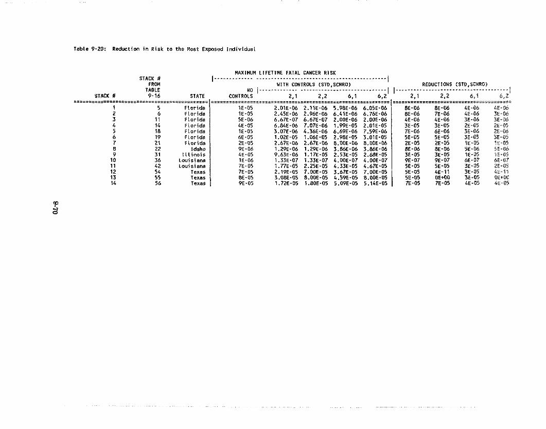
Table 9-20: Reductioo i n Risk t o the Uost Exposed Individual
MAXIMUN LIFETIME FATAL CANCER RISK STACK # I-s.-_.__..-.- ...._.-..-______.--.-.~..~.--.--...-~--.----~
FRW W l T H CMlTROLS (SI0 ,SCNRO) REDUCTIWS (STQ.SCNUO> TABLE +,o I...-.-.--.-.. ...---..--.--..-..-..-......-I
STACK II 9 - 1 6 STATE CONTROLS 2 .1 2 . 2 6.1 6.2 2.1 2,2 & I '5-2 ~ ~ D 1 . I . ~ ~ ~ ~ ~ ~ ~ ~ 5 ~ z ~ ~ ~ ~ ~ ~ ~ ~ ~ ~ ~ ~ ~ ~ ~ ~ ~ ~ ~ ~ ~ x ~ ~ ~ ~ ~ I 1 1 1 ~ ~ ~ ~ ~ ~ ~ ~ ~ ~ ~ ~ ~ ~ ~ ~ ~ ~ ~ ~ ~ ~ ~ ~ ~ ~ ~ ~ 2 ~ ~ ~ ~ ~ ~ ~ ~ ~ ~ ~ ~ ~ ~ ~ ~ ~ ~ ~ ~ ~ ~ ~ ~ ~ ~ ~ ~ l ~ ~ ~ ~ ~ ~ ~ ~ ~ ~ ~ ~ z ~ ~ ~ ~ ~ ~ ~ ~ ~ ~ ~ ~ ~ ~ ~ ~ ~ ~ ~ ~ ~ ~ ~ ~ ~ * ~
5 Florida 6 Florida
11 Florida 14 Florida 18 Floriddl 19 Florida 21 F\orids 22 Idaho 31 l l l i no is 36 Louisiana 42 Louisiana 54 Texae 55 Texas 56 T@xs$
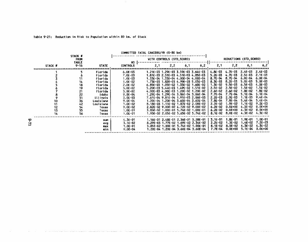
Table 9-21: Reductiw, i n Risk to Population within 80 km. of Stack
STACK X FRM
COMMITTED FATAL CANCERSIYR (0-80 knl) I _ _ _ _ _ _ _ _ _ _ _ _ _ ___________________--- . . . - - - -*- .**- . - - - - - I W I T H CONTROLS (STO.SCNR0) REDUCTIONS (STD.SCWR0)
l d a l E un I............. .......... 1. .......-.-.--.- II----------.------.-----;----------I .,."... .." , I, STACK # 9-16 STATE CONTROLS 2-1 2.2 6.1 6 2 2.1 2.2 6,l 6.2' ____ _ _ _ _ _ _ _ _ _ _ _ _ _ _ _ - - - - - - - - - - - - - - - - - - - - - - - - - - ( I I I I I I I I I I I I I I I I I I I I I I I I I I I I I I I I I I I I I I I I I I I I I I I I I I I I I I I I I I I I I I I I I ~ I ~ ~ ~ ~ ~ ~ ~ ~ ~ ~ ~ ~ ~ ~ ~ ~ ~ ~ ~ ~ ~ ~ ~ ~ ~ ~ ~ .............................................
FLorida Florida Florida Florida Florida FLorida FLorida
Idaho I l l i n o i s
Louisiana Louisiana
Texas Texas Texas
effectiveness. Since no portion of any stack has a flux rate of more than 15.0 pci/m2/sec., well
under the 20 pci/m2/sec limit, the choice is between 2 p~ i /m2/sec , 6 pci/m2/sec. or no control.
Control costs and emission reductions for each stack under each standard are computed in the model.
There are two scenarios to consider. The sides can be covered with dirt while the stack is operating
and the top covered when the stack is closed (scenario I), or the whole stack can be covered at closure
of the stack (scenario 2). Table 9-22 shows the total emission reductions and cumulative discounted
costs due to the emission reductions under each scenario and standard, for each stack and for all
stacks taken together.
9.4.3. Health Benefits of Controlline Radon Emissions
Lung cancer rates are directly related to radon emissions. The issue is the size of the risks of lung
cancer posed by phosphogypsum stacks and the reduction of the risk that will result from the control
chosen. The AIRDOS computer code was run based on current estimates of emissions from the
stacks. Two measures of risk were then calculated for each stack:
1. The risk to most exposed individual, usually one living near the base of a stack, measured as the number of chances per one million trials. This measure assumes the most exposed individual remains subject to the estimated radiation level for seventy years.
2. The probability that the general population will get cancer due to the stack's emissions, measured as the number of cases per one million persons. This measure considers the effects of one year of emissions on the population located within 80 km of each stack. The rule of thumb for estimating the risk to the entire U.S. is to double the risk to the 80 km population.
In cases where individuals may live within 80 km of more than one stack, the risk to the most
exposed individual, shown in Table 9-20, was based upon only the closest stack. Risks to the 80 km
populations were summed over all fourteen stacks. These are shown in Table 9-21.
9.4.4 Health Benefits and Cost Estimates
The greatest aggregate reduction in the risk of cancer in the 80 km region is obtained by setting the
flux rate at 2 pci/m2/sec and requiring the sides of the stacks to be covered continuously as the stack
grows (scenario one). The second greatest aggregate reduction is obtained with a flux rate of 6
pci/m2/sec and scenario one. Scenario two does not control emissions as effectively as scenario one
primarily because several idle stacks will not grow to their maximum size (at least as long as they

TABLE 9-22: EFFECTlVEWlESS OF CWTROLS (S rmrrd Over 50 Vears)
CUWLATIVE REDUCTIWS I N EUISSIOMS DUE TO CONTROLS STACK # DIFFERENT STANDARDS, SCENARIO CMBINATIONS
F R M I__________________-------------------------------------- TABLE STO=2,SCNRD=l STO=Z,SCNRO=Z STD=6,SCNRO=1 STD=6,SCNRO=2
I STACK # 9-16 C i C i C i C i
IIr5E==5E..E======s======~============ 1 5 Florida 2 6 Florida 3 11 Florida 4 14 Florida 5 18 Florida 6 19 Florida 7 21 Florida 8 22 Idaho 9 31 l l l i m i s
10 36 Louisiana 11 42 Louisiana 12 54 Texas 13 55 Texas 14 56 Texas
=====i==5==1=1.E.EEi_==I========a======== Sun
zt Li===Il_ll==lllllll..-------====I
.E==ESIE=======IESE====================*================
3.2E+03 3.2E+03 1.9E+03 1.9E+03 2.8E+03 2.6E+03 1.)2+03 1.6E+03 4.&+02 4.6E+02 4.6E+02 4.6E+02 7.2E+03 7.2E+03 4.3E+03 4.3Ec03 1.1E+04 9.4E+03 6.6E+03 5.7E+03 1.3E+04 1.3E+04 7.6E+03 7.6E+03 1.2E+04 1.2E+04 7.OE+03 7.OE+03 1 .lE+03 O.OE+OO 7.3E+02 O.OE+OO 3.5E+03 3.3E+03 2.1E+03 2.OEc03 6.8E+02 6.8E+02 4.4E+02 4.4E+02 5.4E+O2 l.lE-02 3.4E+02 1.lE-02 1 .&+03 O.OE+OO 9.7E+02 0 .OE+OO 2.1E+03 O.OE+OO 1.2E+03 0 .OE+OO 5.8E+03 5.7E+03 3.5E+03 3.4E+03 ==..3=E.=IEIE131.============i-====
6.4E+& 5.7E+04 3.9Et04 3.4E+04 1.3E104 1.3E+04 7.6E+03 7.6E+03 4.6E+02 O.OE+OO 3.4E+02 O.OE+OO
SSE..E..lliliEZ... ..............................

TABLE 9-22: EFFECTIVENESS OF CONTROLS (SumKd Over 50 Years) (Contiwed)

TABLE 9-22: EFFECTIMNESS OF MMlROLS (Sunned Over 50 Years9 ( C o n t i w e d )
W L A T I V E COST OF E U l S S I W REDUCTIM(5 I N WPV STACK # DIFFERENT STANDARDS, SCENARIO CCIIBIMATIWS
FRCU (d iscant rate =. 01) TABLE I---------------.----------"------------"--*------"------l
STACK # 9-16 STD=Z.SCWROrl STO=Z.SCKRO=Z STD=6,SCNRG=l STD4,SCNRO=2

TABLE 9-22: EFFECTIVENESS OF C a T R O L S ( S m Over 50 Veers) (Contimedl
WLATIVE COST OF EWISSIW REDUCTIONS I N KPV STACK # DIFFERENT STANDARDS, SCENARIO CWBINATIO)(S
FROn (discwnt rate = .05) TABLE ] - - - - - - - - - - - - - - - - - - - - - - - - - - - - - - - - - - - - - - - - - - - - - - - - - - - - - - - -
STACK b' 9-16 STD=2,SCNRO.l STD=2,SCWRO.2 STD=6,SCNRD;l STD=6,SCNRO=2 I
.= .E~=I I I I I I==i . l l .=======~
1 5 2 6 3 11 4 14 5 18 6 19 7 21 8 22 9 31
10 36 11 42 12 54 13 55 14 56
........................ Total Cost
avs
illlllilli=l...==i)ss====x~
.I.......IEEE.E.I.====================================x=
$1,386,824 $7,114,867 $3,986,672 $3,824,408 16,548.332 $5,636,277 $3,530,867 $3,024,320 16,911,048 16,865,421 16,911,048 16,865,421
524,319,818 523,928,961 $12,923,013 $12,71l,WO S23.504.981 117,393,402 $12,626,224 $9,220,181 $42,749,076 $42,015,546 $22,671,862 522,251,337 S43.5BB.260 $43,476,727 $23,152,279 $23,040,746 13,365,828 SO $1,711,123 SO
$10,561,823 $9,032,556 15,304,183 $4,519,757 $1,975,297 Sl.955.990 11,182,677 $1,163,370
$55,457,303 $54,445,872 $32,255,469 131,402,650 $4,060,513 $0 $2,172,620 $0 $5,207,936 SO S2.766.258 SO
$15,445,719 $15,035,505 $8,192,490 57,971,494 .3I~.E3I~EESEE.III========~z=====================*======
5251,082,759 5226,901,125 $139,386.7&4 $125,994,775 517,934,483 $16,207,223 S9.956,lW 58,999,627 555,457,303 554,445,872 $32,255,469 $31,402,650 51,975,297 SO 11,182,677 SO
I==E====S..I.EII=II==============================*======
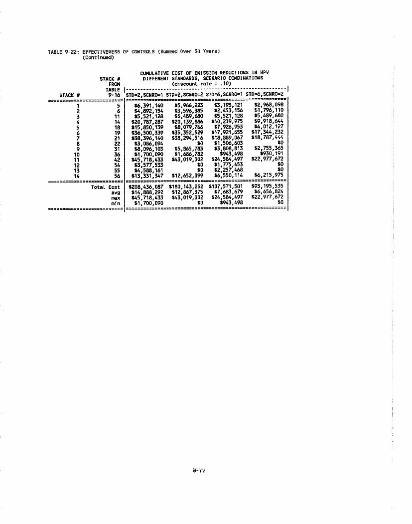
TABLE 9-22: EFFECTIMNESS OF CWTROLS ( S k Over 50 Years) (Continued)
remain idle) and will therefore continue to emit from both their sides and top. Under scenario one,
the tops of these stacks will not be covered but the sides are covered the first year.
Looking only at individual stacks that are open and growing and wilt be shut down in a few years,
after reaching full size, the difference between scenario one and scenario two is minor. If scenario
two is chosen, a requirement to cover the sides of idle stacks would reduce the number of fatal
cancers per year significantly.
The pattern of reduction of cancer risks to the 80 km population evident in Table 9-21 deviates
slightly from the pattern of emission reductions shown in Table 9-22. In particular, a standard of
2 pci/m2/sec combined with scenario two results in a larger reduction of emissions than a standard
of 6 p~i /m2/sec combined with scenario one. The reason is that each stack has a different number
of persons living close to it and a different initial emission of radon. Thus emission reductions at
each stack due to different policy options will have different relative effects on reduction of cancer
risks.
With respect to costs, a flux rate of 2 p~ i /m2/sec combined with scenario one is the most costly, as
shown in Table 9-22. Switching to scenario two results in a small reduction in cost while switching
to 6 pci/m2/sec results in a larger cost reduction. A flux rate limit of 6 pci/m2/sec and scenario two
is the least costly of the combinations studied.
9.4.5. Sensitivitv Analvsis
The ranking of the costs of the four combinations discussed in the preceding paragraph is not altered
as the discount rate is changed. This was ascertained in Table 9-22 for discount rates of 0,0.01,0.05
and 0.10.
9.5 Industrv Cost and Economic Imoact Analvsis
9.5.1. Introduction
Phosphogypsum is the major by-product of phosphate fertilizer production, an international industry.
Historically, the United States was the world's chief supplier of the industry's raw and processed
products. But as discussed in section 9.2, the United States' market share will decline sharply in the
future due to rising costs of phosphate rock to U.S. producers -- as the better deposits are
depleted -- and to improved supply of sulfuric acid to the United States' competitors.
In this section, two economic issues related to the control of radon emissions from phosphogypsum
stacks are considered: 1) the increase in the cost of P205 production and 2) the impact these costs
will have on the United States's economy and export revenues.
The analyses are performed using detailed data on the fourteen phosphogypsum stacks used in Tables
9-19 through 9-22. Two kinds of data are available for these stacks: first, production cost data for
the P205 production associated with the stack and, second, the stack parameters required to assess the
cost of controlling radon emissions from the stacks.
To estimate the effect of controls on U.S. exports a model was developed which estimates market
shares for the U.S. and the rest of the world's P205 industry over the next thirty years in major
regional markets. The model used two scenarios, one scenario using relatively lower U.S. phosphate
rock costs in the production cost estimate and a second using relatively higher U.S. phosphate rock
costs.
Radon control costs were produced by the model described in section 9.3 using stack parameters
and input costs provided in section 9.3 and the appendix, respectively. For various discount rates,
0, .01, .05, and .lo, the net present value (NPV) was calculated for the flow of costs and the
annualized payment corresponding to each NPV was then computed. Annualized regulatory costs for
each of the eleven producers -- which use the fourteen stacks -- per 1000 MT of P205 are provided
in Table 9-23. In computing the annualized costs of the regulation, i t was assumed that the NPV of
the fifty year cost stream was paid off in the first five years the regulation was in effect. Five years
roughly approximates the average remaining lifespan of the fourteen existing stacks.
The production cost data come from Zellars-Williams and are based on detailed descriptions of
individual plant production functions. These data include both the expected quantities and prices
of resources used in the production of P205, including sulphur, phosphate rock, and waste disposal;
and credits for steam production and cogeneration of electricity. In addition, the source of the
phosphate rock used by each plant is identified. Estimates for each variable are made for the years
1990, 1995, 2000, and 2005.
Trends in market prices for P205 are shown in Table 9-2 and Figure 9-1. An estimate of 1986
production costs for P205 is shown in Table 9-3. For 1986, the price of P205 (FOB U.S. Gulf)
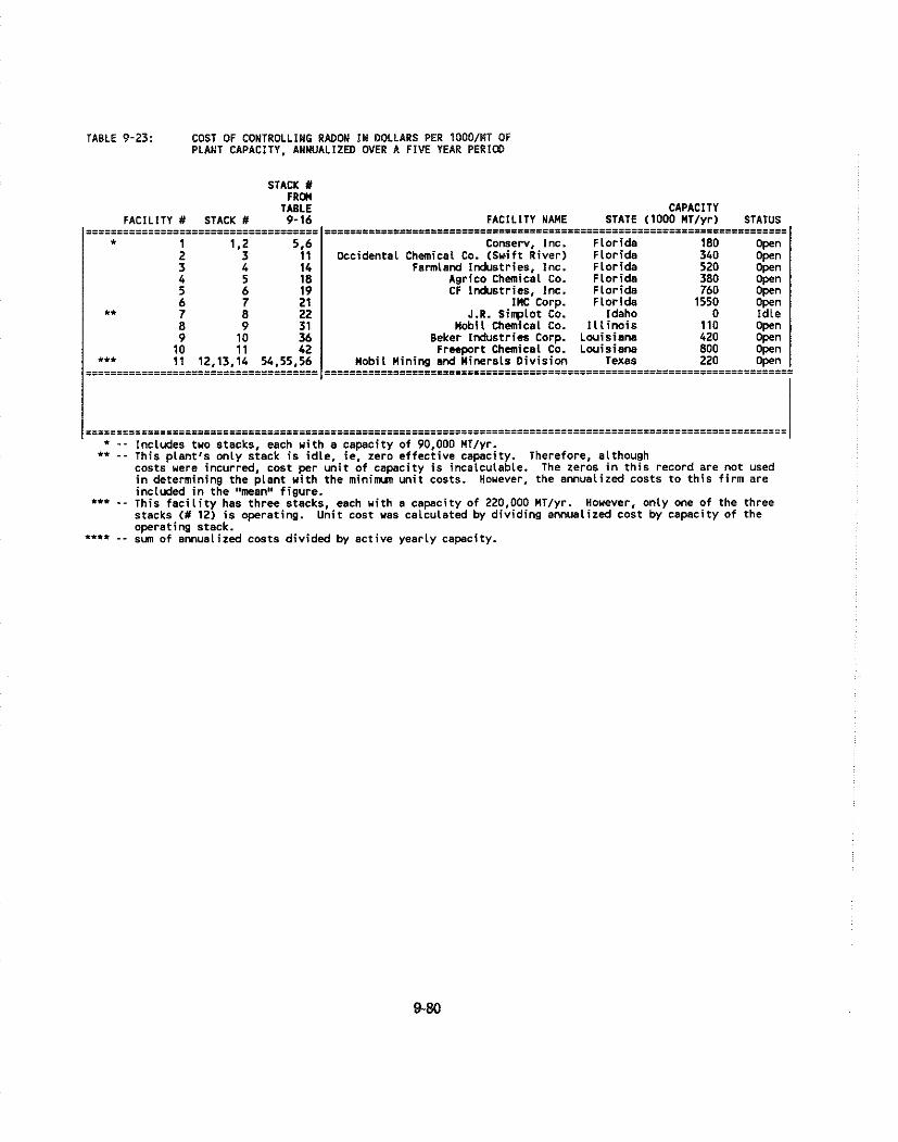
TABLE 9-23: COST OF CONTROLLIWG RADON I N DOLLARS PER 1000/WT OF PLANT CAPACITY, ANNUALIZED OVER A FIVE Y E A R PERlCQ
STACK X FRW
TABLE FACILITY # STACK # 9-16
-------------------------======= 1 1.2 5.6
CAPACITY FACILITY NAME STATE (1000 MT/yr) STATUS
i n determining the p lant u i t h the m i n i m un i t costs. Houever, the annualized costs t o t h i s f i r m are included in the "man" f igure.
*** - - This f a c i l i t y has three stacks, each u i t h a capacity of 220,000 WT/yr. Houever, only one of the three stacks (# 12) i s operating. Uni t cost was calculated by div ld lng amualized cost by capacity of the operating stack. "" -- sun of annualized costs divided by act ive yearly capacity.
:
** 7 8 22 8 9 31 9 10 36
10 11 42 *.* 11 12,13,14 54.55.56 illllliSillllllll.ls===s=============
EESII=III==========================ms===m=================m===============
Conserv, Inc. F lor ida 180 open Occidental Chemical Co. (Swift River) F lor ida 340 o w
Farmland industries, lnc. F lor ida 520 open Agrico Chemical Co. Flor ida 380 open CF Industries, Inc. F lor ida 760 open
I M C C o r ~ . F lor ida 1550 O~en J.R. Sinplot CO. Idaho 0 idle
Wobil Chemical co. I l l i n o i s 110 Open Beker lnhrstr ies Corp. Lwis iana 420 open
Freeport Chemical Co. Louisiana 800 Open Mobil Mining and Minerals O iv is iw, Texas 220 open I....5..E...E.IIEI. ........................................................

TABLE 9-23 (cont'd): COST OF CONTROLLlNG RADON I N DOLLARS PER 1000 MT OF PLANT CAPACITY, ANNUALIZED OVER A F I V E YEAR PERlCQ
STACK 11 FRW
TABLE I - . - - - - - - - . . - . -.---.....------..----.----------------------- F A C I L I T Y STACK I 9-16 0 0.01 0.05
I 0.1
- -- 0 9 31 9 10 36
10 11 42 ."" 11 12.13.14 54.55.56
aggregate annualized costs .**. mean max min
..................................
$29,348 $27,154 $22,177 119,416 $1,344 11,249 11.086 11.068
$20,643 $19,035 116.012 115,076 830,743 $28,931 $25,947 $25,777
........................................................................................................ $81,858,249 879,002,947 165,646,675 160,947,215
$14,078 $12,949 110,643 $9.713 $30,743 $28,931 525.947 125,777
S 0 $0 SO SO Il.=il.iiS=S.l.S... .................................................
r = discount rate. II _ _ see f i r s t page of th is table. ** .. see f i r s t page of t h i s table. *** - - see f i r s t page of th is table. '**' - - see f i r s t page of th is table.
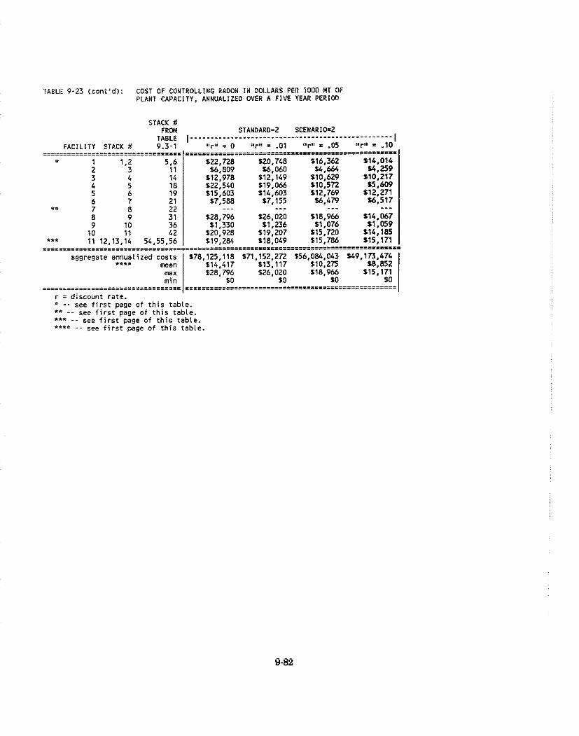
TABLE 9-23 (cone'd): COST OF CONTROLLING RADON I N DOLLARS PER ?OD0 MT OF PLANT CAPACITY, ANNUALIZED OVER A F IVE YEAR P E R l M
STACK # FROH
,ABLE ,--------------------------------------------------l F A C I L I T Y STACK f 9.3-1 a,rt, = 0 Borta = -01 * m r * = .05 mr" = .lo
- -- 8 9 31 9 10 36 10 11 42
*** 1 1 12.13.14 54.55.56
aggregate annualized costs *""" mean max mi n
I_E1SiiiiiiiSill__==_=.==============
$28.796 $26.020 518,966 114,067 $1,330 $1,236 11,076 51,059 $20,928 $19.207 $15.720 114,185 $19,284 118.049 $15,786 115,171
E====i_=E====i=E=========================================*=============================xm
$78,125,118 $71,152,272 156,084,043 U9.173.474 $14.417 $13,117 110,275 58,852 $28,796 126.020 118,965 515.171
$0 SO $0 SO EiE.EIS..=.=.==iiii================================z
r = discount ra te . a - - see f i r s t page of t h i s table.
- - see f i r s t page of t h i s table . *** - - see f i r s t page of t h i s table . *+"* - - see f i r s t page o f t h i s table .
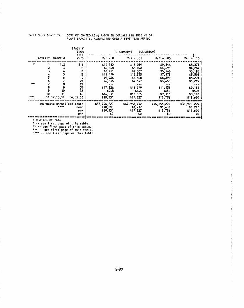
TABLE 9-23 ( C m t ' d ) : COSY OF CONTROLLING RADOM IN DOLLARS PER 1000 WT OF PLANT CAPACITY, AMWUALIZED OVER A FIVE YEAR PERlDD
STACK S FRW STANDARDs6 SCENARIO=$
TABLE I------.---.-- FACILIIY STACK # 9- 16 = 0 +* = .0$ llrE' = .05
I ",." I .10 .................................. -----...--.--...------- "-. . - - - - . - -* - - - - - - - - . - - - - - - - - - -* -* - - - - - - - - - - -
* 1 1.2 5.6 $14,762 $13,059 99.646 U1,275 2 3 1 1 $6.848 16.098 $4,695 U,2& 3 4 14 $8,251 17,387 15,740 55,195 4 5 18 S14.479 $12,315 17.675 15,505 5 6 19 $9,936 W.890 %,8W %,221
rt 6 7 21 $4,836 S .347 53.450 $3,215 7 II 7 , - - - --- - - - - - -
aggregate annualized costs **** mean max min
i=i=i=lE=======i=l==========a=====
$53,796,222 $47,966,432 $36,356,225 $31,970,295 $10.095 U1.937 16,635 15.747 $19.531 917,527 913.786 $12.690
SO SO SO SO ====ill=iiiiiii.=.========z================================s======s=
r = discount rate. * - - see f i r s t page of this tabte. ** - - see f i r s t page of this table. "* - - see f i r s t page of this table. *"' - - see f i r s t page of this table.
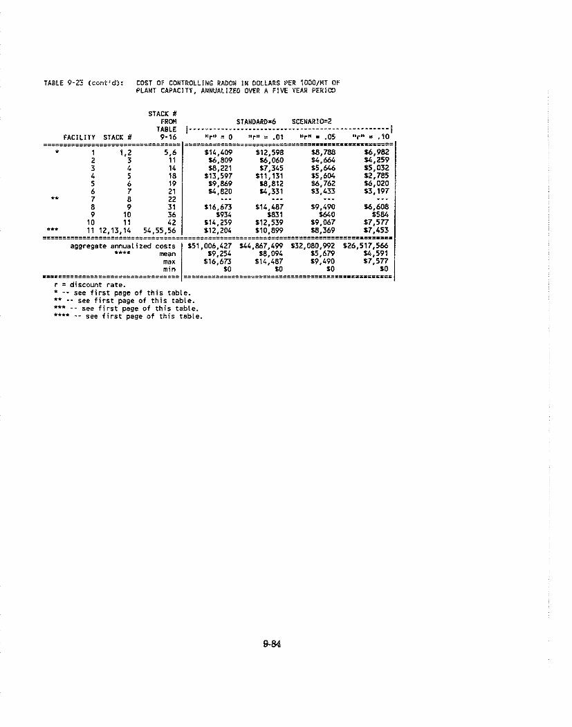
TABLE 9-29 (cont'd): COST OF CONTROLLING RADON II DOLLARS PER 1000/M? OF PLANT CAPACITY, ANNUALIZED OVER A FIVE YEAR PERIOO
STACK # FRW STANDARD-6 SCENARI0=2
TABLE F A C I L I T Y STACK El 9-16 #ar" = 0 urn, .01 mr+e = .05 " r l ' = . 1 0 ~~~~~~~~~~~~~~~~~~~~~~~~~~~~-~~~~~ .................................................... .................................. .............................. . 1 1.2 5.6 114,409 912,598 fB.788 56.982
2 3 11 S6.809 56,060 14.664 I4,259 3 4 14 fB.221 $7,345 15,646 15,032 4 5 18 $13,597 111,131 $5,604 f 2,785 5 6 19 S 9,869 18,812 56,762 56,020 6 7 21 SL, 820 14,331 $3,433 13,197 .. 7 R >> . - - - - - - - - - - -
aggregate annualized costs $51,006,427 144,867,499 $32,080,992 $26,517,566 .*** r a n / S9,254 18.094 15.679 14.591 ma% $16.673 $14.487 S9.490 $7.577 I
..=*s==zz======z=s ====ms==zx=============================== =========I r = discount rate. L _ _ see f i r s t page of t h i s table. *' - - see f i r s t page of t h i s table. *'* - - see f i r s t page of th is table. *"* - - see f i r s t page of this table.
averaged $279.38 per metric ton and the estimated production costs totaled $263.88. P2Q5 prices for
the first half of 1988 averaged $306.50. While these prices and costs are snapshots of a highly
variable market, they are consistent in estimating the order of magnitude of the costs of producing
*2O5'
Runs of the control cost model, the results of which are displayed in Table 9-23, produced annualized
radon emission control costs per 1000 MT of P205 for each combination of emission flux standard,
scenario and discount rate. For each plant the most costly combination of these factors was
considered. For all runs, the highest cost per 1000 MT of P205 production of controlling radon
emissions, from any of the eleven plants is estimated to be $30.74 per ton of P205 This amounts to
12 per cent of the 1986 production cost, 11 per cent of the 1986 average price, and 10 per cent of the
average price for the first half of 1988. The smallest maximum annualized cost of radon emission
control at any plant was $1.34. Whiie the larger of these cost increases is significant, the ultimate
economic impact depends on the effects of the increases on the domestic and international markets.
9.5.3. Measurine Economic Imoacts
9.5.3.1 Background
The approach to measuring the economic impacts of controlling radon emissions from
phosphogypsum stacks used in this section is to trace the initial round of effects on the U.S. economy.
The initial round of effects is generally the largest and easiest to identify. Adjustments made by the
rest of the world will not be traced in this section.
First round effects include changes in the relative price and real output of P205, which lead directly
to:
o changes in the prices and amounts of the inputs to P205 used, including phosphate rock, sulfuric acid, land and labor;
o changes in the amounts of resources used in the transportation of these inputs and outputs;
o changes in the amounts of P205 exported and in the trade balance and foreign exchange related to these exports.
These first round effects are discussed below. The nature of economic effects in further rounds of
adjustment will depend on the opportunity cost of using resources in P205 production and the
substitutability of other products for PzQY For example, if a decline in the sale and profitability
of P205 produced in Florida led to decisions not to begin new phosphogypsum stacks, the land that
would have been used for the stack becomes available for other purposes. If these other purposes
create economic activity then the new activity should be added to the ledger as the economic activity
attributable to the stack is subtracted. The activity attributable to the alternative use is the
opportunity cost of using the land for a stack. If the opportunity cost is relatively high, then the loss
due to not proceeding with the stack is relatively low, but if opportunity costs for using a resource
are low, then the loss of economic activity from not being able to open it is relatively high.
A concept related to this is the unemployment of resources. If resources have a low utilization rate,
then the reduction in economic activity of not using them in P205 production is high as alternative
uses are not available and the resources become idle. In short, the economic impact of a change in
usage of P205 plants will depend on the level to which resources are employed in the vicinities of the
plants affected by the controls.
9.5.3.2. Chanees in Ouantitv of PzO. Produced Due to Control Reauirements
Changes in the quantity of Pz05 produced in the United States will be a direct result of the change
in production costs attributable to the regulations. A reduction will take place if domestic producers
of P205 lack the ability or inclination to absorb the cost increase and therefore raise their prices
relative to the level they would have charged in the absence of regulation. As was described in
section 9.2, the phosphate fertilizer industry during the 1980s has generally experienced decreased
demand and lower relative prices. As a consequence some companies have sold their phosphate
fertilizer plants or gone out of business. This economic history makes it unlikely that producers will
be able or willing to absorb the cost of the controls.
Domestic producers are expected to pass on the cost of the controls. These price increases are
unlikely to jeopardize U.S. producers hold on the domestic market. The cost of production of foreign
producers, including transportation costs to the U.S., do not make foreign producers competitive in
the U.S. market, even after the controls. Since there is no direct substitute for phosphate fertilizer,
the reduction in domestic demand for phosphate fertilizer because of the increase in price will be
limited. Because there is no good estimate of the price elasticity of demand for phosphate fertilizer,
it is not possible to estimate the magnitude of this effect.
It is possible to estimate the effect of the controls on U.S. market share in the rest of the world.
When the specific costs of controlling radon emissions from phosphogypsum stacks are added to the

production costs of U.S. producers, but not to those of foreign producers, shifts in market shares
result. The magnitude of the changes are not readily predictable from the average control costs
computed above, because of variation in the control costs faced by each plant and because a firm's
share of a market is not affected until the price at which it can supply the product exceeds the lowest
price at which a competing firm or nation is willing to offer the product. To determine the impact
of radon control costs on world markets, a model of world Pz05 markets was constructed and is
described below.
9.5.3.3 Methodoloev for Estimatine Economic Imoacts
Over the next thirty years, a host of factors will influence the level of production, prices and trade
patterns that will develop for phosphate products. Demand for fertilizer will increase at different
rates around the world. New production capacity will be built; sources of phosphate rock and sulfur
and the prices of those products will change. Transportation costs between importing and exporting
countries will change. To analyze these relationships and to develop a basis from which to estimate
the cost of the controls on the phosphate industry over the next 30 years, a computer model was
developed for this study. Below is a description of the model and the forecasts made with it.
Model Structure
The model developed to analyze these uncertainties uses the sources described in section 9.2. In
particular, the model makes use of plant-specific production cost estimates from Zellars-Williams,
alternative phosphate rock mining costs from William Stowasser at the Bureau of Mines, and
phosphate fertilizer demand estimates from WEFA.
The model contains forecasts of production levels, production costs, transportation costs and demand
for six regions and the United States. Production forecasts are not available beyond the year 2005.
Consequently, production forecasts for 201 8 were produced separately and combined with the others.
WPPA is sold in several forms. Some countries purchase the acid and domestically produce various
fertilizers while other countries purchase finished fertilizers, such as diammonium phosphate. For
simplicity, the model considers only phosphoric acid production costs. This implicitly assumes that
no exporting country has a comparative advantage in producing various fertilizers.
The model considers the production and transport costs of each supplier and ranks the lowest to
highest suppliers for each region. Each supplier is assumed to maximize profits by supplying those
regions where its costs are lowest. Thus, if Morocco is the lowest cost supplier in more regions than
it can supply, Morocco is assumed to favor markets where its transportation costs are lowest.
The model is modified to allow for some special cases where noncompetitive domestic production is
assumed to receive special support to overcome foreign competition. The model does not, however,
consider cases where state-owned enterprises may export below cost for prolonged periods in order
to obtain foreign exchange. This possibility is a serious concern to many in the phosphate industry
because much of the foreign competition is state owned. Nevertheless, it is not possible to reliably
forecast political influences on financial decisions.
A detailed description of the methodology, data sources and assumptions used in the forecasting
model is given in Appendix B.
Forecast of Trade Levels Without Controls
Two scenarios, a lower phosphate rock cost, and a higher phosphate rock cost, were developed for
the model. The only variable changed between the scenarios is the cost of mining phosphate rock in
the United States. As was described in section 9.2, this factor is of primary importance in
determining the outlook for the phosphate fertilizer industry. The lower phosphate rock cost scenario
uses phosphate rock mining cost estimates developed by Zeliars-Williams (ZW) and the higher
phosphate rock costs scenario uses rock mining cost estimates developed by experts at the U.S. Bureau
of Mines.
The higher phosphate rock cost, lower exports, scenario anticipates export levels in 1990 of 6.5
million tons. This scenario predicts exports will decline to 3.7 million tons in 1995 and continue
declining to 1.8 million tons in the year 2000 and 0.6 million tons in 2005. The U.S. is expected to
stop exporting phosphate fertilizer products sometime after 2005 and before 2018. Tables 9-24 and
9-25 show these forecasts for both scenarios by region. Because the model could not incorporate
all the factors which influence the regional trade levels, the regional forecasts are not as reliable as
the aggregate forecast.
The lower phosphate rock cost, higher exports, scenario uses the same rock cost estimates for 1990
as the previous forecast and consequently anticipates identical export levels in 1990. In 1995, export
levels are forecast to decline to 4.5 million tons. In the years 2000, 2005 and 2018, exports are
forecast to be 2.9, 1.9 and 0.6 million tons, respectively. Thus, the lower phosphate rock costs
scenario forecasts a similar trend as the previous scenario but forecasts a'slower rate of decline in
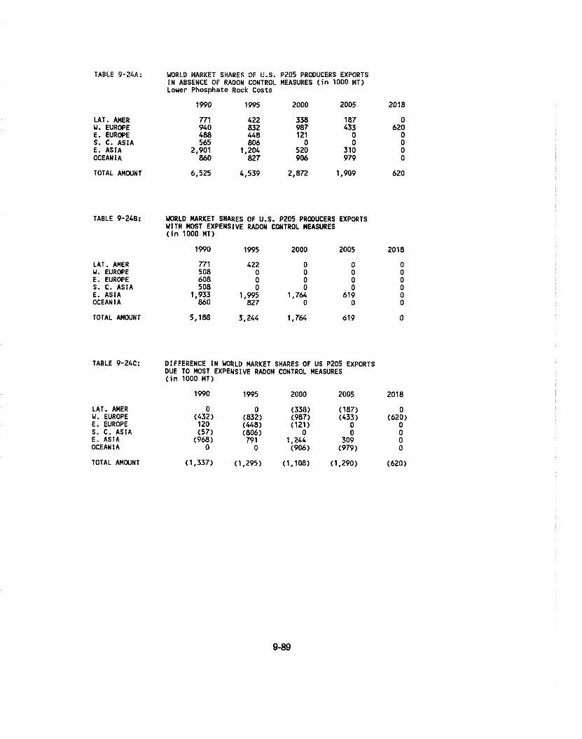
TABLE 9-244: WRLD MARKET SHARES OF U.S. P205 PRCaUCERS EXPORTS I N ABSENCE OF RADON CDUTROL MEASURES ( in 1000 MT) Loner Phosphate Rock Costs
LAT. AMER 771 422 3UI 187 0 U. EUROPE 940 832 987 433 620 E. EUROPE 488 448 121 0 0 S. C. ASIA 565 806 0 0 0 E. ASIA 2,901 1.204 520 310 0 OCEANIA 860 827 906 979 0
TOTAL AMOUNT 6,525 4,539 2,872 1,909 620
TABLE 9-248: UMILD PARKET SHARES OF U.S. P205 PRCOUCERS EXPORTS W I T H MOST EXPENSIVE RADON CONTROL MEASURES ( in 1000 MT)
1990 1995 2000 2005 2018
-~ .~ ~~
E. ASlA OCEANIA
TOTAL AMOUNT 5,188 3,244 1,764 619 0
TABLE 9-24C: DIFFERENCE IN MRLD MARKET SHARES OF US P205 EXPORTS DUE TO MOST EXPENSIVE RADON CONTROL MEASURES ( i n 1000 MT)
LAT. AMER 0 0 (338) (187) 0 V. EUROPE (432) (832) (987) (433) (620) E. EUROPE 120 (448) (121) 0 0 S. C. ASIA (57) (806) 0 0 0 E. ASIA (968) 79 1 1,244 309 0 OCEANIA 0 0 (906) (979) 0
TOTAL AMOUNT (1,337) (1,295) (1,108) (1,290) (620)
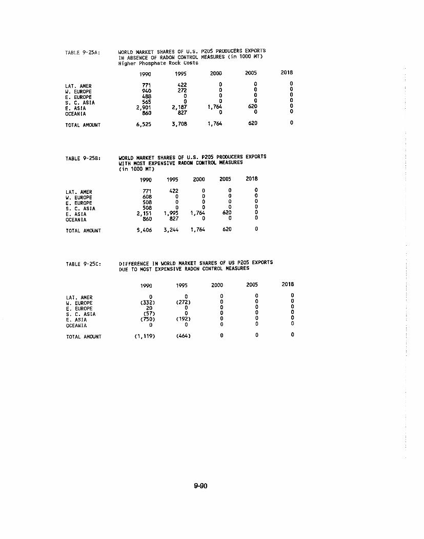
TABLE 9-25A: M R L D HARKET SHARES OF U.S. P Z 0 5 PRCDUCERS EXPORTS I M ABSENCE OF RADON CONTROL MEASURES ( in 1 0 0 0 MT) Higher Phosphate Rock Costs
LAT. AMER V. EUROPE E. EUROPE S. C. A S I A E. A S I A OCEANIA
TOTAL AMWNT
TABLE 9 - 2 5 8 : UMILO MARKET SHARES OF U.S. P 2 0 5 PRmUCERS EXPORTS U l T H MOST EXPENSIVE RADON CONTROL MEASURES ( i n 1000 MT)
LAT. AMER 771 4 2 2 0 0 0 U. EUROPE 608 0 0 0 0 E. EUROPE 5 0 8 0 0 0 0 S. C. A S I A 5 0 8 0 0 0 0 E. A S I A 2 ,151 1,995 1,764 620 0 OCEANIA 8 6 0 827 0 0 0
TOTAL AMWNT 5 , 4 0 6 3,244 1 , 7 6 4 6 2 0 0
TABLE 9-25C: DIFFERENCE I N W R L D MARKET SHARES OF US P 2 0 5 EXPORTS DUE TO n o s 7 EXPENSIVE RADON CONTROL MEASURES
TOTAL AMOUNT 11,119) ( 4 6 4 ) 0 0 0
export levels. Several important factors shed light on the model's forecasts. As explained in section
9.2, U.S. producers are expected to experience marginally higher costs for sulfur and North Africa
is expected to have a similar decrease in costs. Changing sulfur costs accounts for a $10 to $15 per
ton shift in phosphoric acid production costs between the U.S. and the major competitors in North
Africa. The most important factor influencing the pessimistic outlook for U.S. phosphate exports is
the cost of mining phosphate rock. Even the lower phosphate rock costs scenario allows for an
increase in phosphate rock costs for U.S. producers over time.
Forecast of Trade Levels With Controls
To estimate the trade impacts of the proposed controls, both scenarios of the model were run with
the added costs of the controls included. For each U.S. plant, the highest cost option for that plant
that was calculated in the previous section was added to the production cost of that plant in the
model. The forecasts are shown in Tables 9-24 and 9-25. The forecasts for trade levels with and
without the controls under the lower phosphate rock costs scenario are also illustrated on Figure 9-
4. In the lower phosphate rock costs scenario, the controls are projected todecrease exports by 1.3
million tons in 1990. This effect remains at 1.3 million tons in the year 1995, 1.1 million tons in the
year 2000, 1.3 million in 2005,and drop to 0.6 million tons by 2018. Assuming a continuous change
in export levels during the years not specifically forecast, the controls are forecast to decrease exports
by 31.0 million tons over the next 30 years using the lower phosphate rock costs scenario.
Using the higher phosphate rock costs scenario, the controls are forecast to decrease exports by 1.1
million tons in 1990 and by 464,000 tons in 1995. No effect on exports is projected by the year 2000
and beyond. Assuming a continuous change in export levels during the years not specifically
forecast, the controls are forecast to decrease exports by 5.1 million tons over the next 30 years using
the lower phosphate rock costs scenario. The forecasts for trade levels with and without the controls
under the higher phosphate rock costs scenario are illustrated on Figure 9-5.
The effects of the decrease in exports of phosphate products on the trade balance depends to some
extent on the form in which the phosphoric acid is exported. If the phosphoric acid is exported
directly, the loss in export revenue is approximately $307.50 per ton of P205 (1988 dollars). If the
phosphoric acid is first converted into phosphate fertilizer, the loss in export revenue is greater. For
example, diammonium phosphate (DAP) uses 0.478 tons of P205 to produce per ton of DAP. DAP
sold for $188.60 per ton in 1988. Thus, the decrease in export level from a one ton decrease in P205
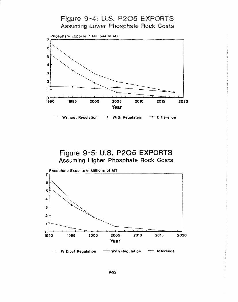
Fiaure 9-4: US. P205 EXPORTS urnin in^ bower Phosphate Rock Costs
Phosphate Exports in Millions of M I 7 1
Year
- Without Regulation + With Regulation * Difference
Fiaure 9-5: U.S. P205 EXPORTS ~ s i u r n i n ~ Higher Phosphate Rock Costs
Phosphate Exports in Millions of M T
I
Year
Without Regulation + With Regulation * Difference

exports that has been converted into BAP is approximately $394.50 per ton of Pz05 (1988 dollars).
In 1985, 17.8 percent of the revenue from phosphate products came from the export of P205 and
82.2 percent came from the export of finished fertilizer. Because the preponderance of P20, is
exported as finished fertilizer and the principal phosphate fertilizer is DAP, the revenue effects of
the controls are described in terms of a weighted average of Pz05 and DAP exports.
The two scenarios predict that the effect on export revenue in 1990 will be a reduction in export
revenue of $410 million for the low cost scenario and $343 miIlion for the high cost. The higher
phosphate rock cost, lower export, scenario predicts that the cumulative revenue loss over the next
30 years will be $1.4 billion. The lower rock costs, higher export, scenario predicts that the
cumulative revenue loss will be $9.5 billion. The revenue loss in the higher rock cost scenario is
limited to the next ten years, with no loss in exports by the year 2000 and beyond. These estimated
economic impacts of the standard are obviously dependent upon the many assumptions in developing
the model that are described in Appendix B. The export revenue effects of the standard in the early
years of the controls are much more reliable than the forecasts for 20 or 30 years in the future. The
decrease in export revenues in 1990 is estimated to be approximately a little under one half a billion
dollars. A revenue loss of this magnitude would continue were it not for the general decline in
phosphate exports that is forecast in both scenarios.
The shifts in the markets for Pz05 are the most notable direct effects of radon control costs.
However, there are some spinoffs as noted above. These are discussed below.
Inouts: Sulfuric Acid
Most sulfuric acid used in the production of P205 is the by-product of other activities such as
removal of sulfur from gas or oil. Reductions in the demand for sulfuric acid for use in P205
production would reduce the prices at which this residual could be sold, and thereby increase the
net costs of oil and gas desulfurization. These effects are expected to be minor.
Inouts: Phosohate Rock
Phosphate rock is exported to some of the world's other PZ05 producing nations. If the United
States loses some exports of PZ05 to other countries due to increased regulatory costs, it is likely
that exports of phosphate rock to these nations will increase. This will mitigate some of the losses
of revenue that would accompany loss of Pz05 markets. In many cases the increased sale of
phosphate rock will bring revenues to the same firms that lost revenue due to declines in P205 sales.
These effects, however, will be short term because the U.S. is not expected to remain a significant
phosphate rock exporter for many years.
Inouts: Labor
Since the value of labor required to produce Pz05 is a small proportion of the total value of all
inputs, the absolute size of the shift in the labor market will be small. This small impact may be
magnified or diminished by the local employment situation. In areas that are experiencing economic
growth, there will be demand for labor that will be able to absorb the relatively small number of
persons affected. This is especially true in Florida, where population growth can be expected to
generate demands for increased levels of construction activity, and where the largest concentration
of workers in the Pz05 industry is clustered. It should also be noted that the regulations require
increased ongoing activity in the form of the labor and other employment of resources and equi~ment
needed to lay drains on the stacks, move and place dirt on the stacks, and maintain the cover and
drains. The first two activities will occur so long as any stacks remain open and the last will be
required for all closed stacks.
Inouts: Land
The land for existing stacks is already in use and its quantity and location will not be changed by
the regulation. The regulation could affect the decision to start new stacks and would therefore
affect the land requirements in the future.
Some reduction in the transportation of PZ05 exports can be anticipated. On the other hand,
increased transportation of phosphate rock will partially mitigate the reduction. However, since
most transport of these materials is by foreign-owned ships, this reduction will not affect U.S.
interests.
9.6 Reeulatorv Flexibilitv Analvsis
9.6.1 Introduction
The Regulatory Flexibility Act was signed into law on September 19, 1980. Its purpose is to call to
the attention of federal agency personnel any impacts on small "entities" such as small business, small
organizations, or small governmental jurisdictions that may unduly hamper them. The hope of the
law's authors was that if federal agencies were aware of negative impacts on small entities due to a
rulemaking, they would modify the rule, if possible, to reduce the damage.
Two kinds of small entities are potentially affected by the rulemaking on phosphogypsum stacks:
small business and small government. However, the analysis below shows that entities falling under
the definition of the act are not adversely affected in a significant way.
9.6.2 Small Business
The business entities directly affected by the phosphogypsum rules under consideration are large
corporations. They include large, internationally operated chemical companies, oil firms and fertilizer
producers. For most of these firms, P205 production is but one of numerous activities including
phosphate rock mining and processing, fertilizer production, or chemical production. The amount
of investment and risk involved in these productions is large, too large for a firm that could qualify
as a small business to engage in.
9.6.3 Small Governmental Entities
The definition of a small county is one with less than 50,000 citizens. However, the counties in
Florida with the highest concentration of phosphoric acid production have greater than 50,000
citizens.

REFERENCES
BOMa
BOMb
Arnax Corporation, annual reports, 1982, 1985, 1986.
Conversation with Neil Anderson of Mobil Mining and Minerals, 6/14/88.
Babitzke, Herbert R., Barsotti, Aldo F., Coffman, Joseph S., Thompson, Jerrold G., and Bennett, Harold J. The Bureau of Mines Minerals Availability System: An Update of Information Circular 8654 ( IC 8887), Bureau of Mines, 1982.
Boyd, B.W. Sulphur and Sulphuric Acid: Where is Canada Headed?, Canada, Department of Energy, Mines and Resources, Mineral Policy Sector, July 1983.
Boyd, B.W. Sulphur Market Profile, Canada Department of Energy, Mines and Resources, Mineral Policy Sector, December 14, 1983.
Bureau of Mines, Department of the Interior, ResourceReserveDe finitions: Principles o f a Resource/Reserve Classification for Minerals. (joint publication with U.S. Geological Survey).
. Sedimentary Phosphate Resource Classification System o f the U.S. Bureau o f Mines and the U.S. Geological Survey, Circular #882, n.d., p.3.
. Minerals Yearbook, 1970, 1972, 1974, 1975, 1978-79, 1980, 1982, 1984, 1985.
. Phosphate Rock Availability - World, 1984.
. An Appraisal of Minerals Availability for 34 Commodities, 1987.
. Mineral Commodity Summaries, 1987.
, Mineral Commodity Survey, 1987.
. "Phosphate Rock 1987 Crop Year," Mineral Industry Survey, August 19, 1987.
. "Directory of Companies Producing Phosphate Rock in the United States--1988," Mineral Industry Survey, January 25, 1988.
. "End Uses of Sulfur and Sulfuric Acid in 1987," Mineral Industry Surveys, June 17, 1988.
. "Marketable Phosphate Rock," Mineral Industry Survey, January, February, and March 1988 issues.
. "Phosphate Rock in 1987," Mineral Industry Survey, January 4, 1988.
. "Sulfur," Mineral Commodity Summaries, 1988.
. "Sulfur in April 1988," Mineral Industry Survey, June 3, 1988.

BSC
. World Demand for Fertilizer Nutrients for Agriculture. OFR 24-88, prepared by Wharton Econometric Forecasting Associates, April 1988.
. "Phosphate," Fertilizer Trends, pp. 19-28, NFDC/TVA, 1982.
Bridges, Darwin. Fertilizer Trends, National Fertilizer Development Center, Tennessee Valley Authority, 1986.
British Sulfur Corporation, World Guide to Fertilizer, Processes and Consfrucfors, List of world nitrophosphates and phosphates production facilities, phosphate rock treatment, phosphogypsum processing, other phosphorus and phosphoric acid-related firms.
. "Export Prices," Phosphorus and Potassium, November-December 1985, pp. 10-12.
. "False Hopes for Superphosphoric Acid," Phosphorus and Potassium, November-December 1985, pp. 6-7.
. "The Florida Phosphate Industry in Transition," Phosphorus and Potassium, November-December 1985, pp. 25-27.
. "Freights: Rates Holding a Steady Course," Phosphorus and Potassium, November-December 1985, pp. 13-14.
. World Fertilizer Products: World Statistics, June 1985.
. "Long-term Price Trends--Stability Returns," Phosphorus and Potassium, November-December 1985, p. 4.
. "World Markets," Phosphorus and Potassium, November-December 1985, pp. 15-17.
. "Phosphogypsum, a Source of Sulfur Dioxide: New Signs of Life?" Phosphorus and Potassium # 137, May-June 1985.
. World Sulphur Resources, 3rd ed., 1985.
. "Morocco Develops Its P205 Industry," Sulphur, May-June 1986, pp. 24-25.
. "Sulphuric Acid--Supply/Demand Prospects," Sulphur, January- February 1986, p. 5.
. World Directory o f Fertilizer Manufacturers, photocopy of chapter on United States, 1986.
. Availability o f Elemental Sulfur and Pyrite Concentrate--Market Economy Countries: A Minerals Availability Appraisal. Bureau of Mines Information Circular IC 9106, 1986.
British Sulphur Corporation. "Dealing with Mining Wastes in the Phosphate Industry," Phosphorus and Potassium, September-October 1987.
9-97

. "Phosphate Fertilizer Outlook Unlikely to Lift Sulphur Demand," Sulphur, November-December 1987, p. 5.
. Phosphorus and Potassium, various issues.
. "The Search for Backhauls," Phosphorus and Potassium, March-April 1987.
. "Will the Market Turn Around in 1987?", Sulphur, January-February 1987.
. World Fertilizer News Summary, June 1987.
. "Sulfuric Acid from Phosphogypsum: Will It Ever Impact the Sulfur Market?" Sulfur, July-August 1987.
. "Phosphogypsum: The Newest Sulphur Resource." Sulphur # 190, May-June 1987.
. "Phosphogypsum: The Newest Sulphur Resource." Lloyd, G.M., Kendron, T.J., and Marten, J.H., Sulphur No. 190, May-June 1987, p. 30.
. "World Markets" Phosphorus and Potassium, March-April, 1988.
British Sulphur Corp., Data purchased by Jack Faucett Associates, July 5, 1988.
Buckingham, D.A. "The Availability of U.S. Frasch Sulphur," Industrial Minerals, January 1988.
Chang, Wen. Reclamation, Reconstruction and Reuse of Phosphogypsum for Building Materials. Prepared by University of Miami under a grant from the Florida Institute of Phosphate Research. January, 1987.
Conversation with Mr. Chang, 7/5/88.
Chemical Marketing Reporter. "Phosphoric Acid Bid Launched by Monsanto and FMC Corporation," Chemical Marketing Reporter, December 1, 1986.
Chevron Corporation, annual reports, 1983, 1984, 1985, 1986.
. Census of Manufacturers, 1982: General Summary.
. Census of Mineral Industries, 1982; Subject Series.
Department of Commerce, Bureau of the Census. Annual Survey o f Manufacturers, 1983.
. "Inorganic Fertilizer Materials and Related Products", Current Industrial Reports: Seasonal adjustment supplement, 1966 to 1976;Summary for 1973; Summary for 1976; Summary for 1978; Summary for 1979; January 1982; January 1983; 1985; 1986; September 1987; November 1987.

DOC80 . Current Industrial Reports. "Phosphatic Fertilizer Materials": Summary for 1980.
. Current Industrial Reports. "Sulfuric Acid": 1981; 1984; 1988.
. "Agricultural Chemicals," 1983 U.S. Industrial Outlook, January 1983.
. U.S. Exports, 1986.
. 1985 Annual Survey of Manufacturers. Expenditures for Plant and Equipment. Bureau of the Census.
. U.S. Industrial Outlook, 1988.
Survey of Current Business, Bureau of Economic Analysis, Department of Commerce, August 1988.
State Population Projections, Bureau of the Census. Most recent revised forecast as of 7/5/1988,:
J.W. Couston. Curre111 World Fertilizer Situation and Oullook, 1985/86-1991/92. F A 0 Commission on Fertilizers, 1987.
Cyanamid Corporation, annual reports, 1981, 1982, 1983, 1985, 1986, 1987.
Dayton, Stanley L. "Phosphate Rock: World Output Increases, Prices Weaken and Competition Intensifies," Engineering and Mining Journal, April 1988.
Eckert, G.F. "Sulphur Demand Improves Slowly," Engineering and Mining Journal, April 1988.
Elf Aquitaine Inc., annual reports, 1984, 1985, 1986, 1987.
. Petroleum Suppfy Annual 1984, Volume 2 , June 1985.
Energy Information Administration, Department of Energy. Annual Energy Outlook 1985. With Projections to 1995, February 1986.
. Petroleum Supply Annual 1986, June 1987.
. Short-term Energy Outlook, Annual Supplement 1987, October 1987.
Annual Energy Outlook 1987. Energy Information Administration, Department of Energy, March 28, 1988, p. 39 and 40. Base case forecasts were used.
. Phosphate Rock Plants--Background Information for Promulgated Standards (EPA-450/3-79-01 76). Office of Air, Noise and Radiation, EPA April 1982.
EPA84 Environmental Protection Agency. Radionuclide: Background information Document for Final Rules, 52011-84-022-I, October 1984.
9-99
FIP
FMI82
Ga85
Fantel, R.J., Sullivan, D.E., and Peterson, G.R. Phosphate Rock Availability-- Domestic: A Minerals Availabilify Program Appraisal (IC 8937). Bureau of Mines, August 1983.
Fantel, R.J., Anstett, T.F., Peterson, G.R., Porter, K.E. and Sullivan, D.E. Phosphate Rock Availability--World: A Minerals Availability Program Appraisal (IC 8989). Bureau of Mines, 1984.
R.J. Fantel, G.R. Peterson, and W.F. Stowasser (Bureau of Mines, Department of the Interior). "The Worldwide Availability of Phosphate Rock," Natural Resources Forum, FAO/UN, 1985.
Fertilizer Yearbook, Food and Agriculture Organization, United Nations, 1985 and 1986.
Farmland Industries Inc., annual reports, 1983, 1984, 1985, 1986, 1987.
Fertilizer Focus: "Focus on Tampa--No. 1 in Phosphates," Fertilizer Focus, April 1, 1983.
. "Focus on: Phoschem Aims for Stability in Phosphates Market," Fertilizer Focus, September 1985, p 18.
. "Focus on Phosphoric Acid Trade," Fertilizer Focus, October 1987.
. "Opinion: The Acid Freight Market in 1986," Fertilizer Focus, January 1987.
Florida Institute of Phosphate Research. Proceedings of the Second Workshop on By- Products of Phosphate Industries, conducted by the Department of Civil and Architectural Engineering, University of Miami, under a grant sponsored by the Florida Institute of Phosphate Research, May, 1985.
. DAP Quality Seminar (Publication No. 01-000-041), conducted by Florida Institute of Phosphate Research, Tennessee Valley Authority, and The Fertilizer Institute, August 1986.
. Proceedings of the Third Workshop on By-Products of Phosphate Industries, conducted by the Department of Civil and Architectural Engineering, University of Miami, under a grant sponsored by the Florida Institute of Phosphate Research, November, 1986.
. Proceedings of the Second International Symposium on Phosphogypsum, organized by the University of Miami under a grant from the Florida Institute of Phosphate Research, January, 1988 (two volumes).
. Publications. Florida Institute of Phosphate Research.
Freeport McMoRan Inc., annual reports, 1982, 1983. 1984, 1985, 1986.
Galvin, James J. "The U.S. Phosphate Industry," Fertilizer Focus, June 1985.
General Accounting Office. Phosphates: A Case Study o f a Valuable. Depleting Mineral in America, November 30, 1979 (GAO # 80-21).
W.R. Grace & Co., annual report, 1986, 1987 second quarter report.
Green Markets. Green Markets Trade Overview, May 18, 1987.
Green Markets. Monthly Statistical Supplement, March 28, 1988.
Green Markets. "Sales, profits, production up in last half of 1987 in North America," Green Markets, March 7, 1988.
Green Markets. "Dispute between U.S. Bureau of Mines, industry, comes to a head," Green Markets, February 8, 1988.
Green Markets. "Grace sells 28 more retail outlets, granulation plant could go this month," Green Markets, March 21. 1988.
Green Markets. "Freeport resuming construction of pilot gypsum conversion plant," Green Markets, March 21, 1988.
Harre, E.A. and Isherwood, K.F., "World Phosphate Fertilizer Supply-Demand Outlook." Ch. 8 in Khasawneh et. al. The Role of Phosphorus in Agriculture, 1980.
Harre, Edwin. Emerging Trends in the World Phosphate Market. NFDC/TVA, September 1987.
Hrabik, Joseph A,, and Godesky, Douglas J. Economic Evaluation of Borehole and Conventional Mining Systems in Phosphate Deposits ( IC 8929). Bureau of Mines, 1983.
International Minerals and Chemicals Co., annual report 1987.
International Monetary Fund. International Financial Statistics Yearbook, 1987.
Kaiser Aluminum & Chemicals Corporation, annual reports, 1982, 1983, 1984, 1985, 1986.
Kendron, T.J. (Davy McKee Corp.) and Lloyd, G.M. (Florida Institute of Phosphate Research). Phosphogypsum to Sulfuric Acid With Cogeneration--A Competitive Edge. Paper presented at the Second International Symposium on Phosphogypsum, December, 1986.
King, Harriet, and Wilson, Linda J. "The Boom in Phosphate Bans," Chemical Week, June 3, 1987.
Lloyd, G. Michael Jr. Phosphogypsum: A Review of the Florida Institute o f Phosphate Research Programs to Develop Uses for Phosphogypsum, Florida Institute of Phosphate Research, December 1985.
Mike Lloyd, Florida Institute of Phosphate Research, Personal Communications, March 18, 1988.
Mannsville Chemicai Products Corporation. "Phosphoric Acid (Wet Process)," Chemical Products Synopsis, December 1985.
McGinty, Robert. "Phosphate Producers Prepare for a Comeback," Chemical Week, June 10, 1987.
. "Phosphate Producers Seek a Tax Cut," Chemical Week, June 3,1987.
. "A New Way to Undercut Phosphogypsum Stacks,' Chemical Week, July 8, 1987.
Conversation with James McGinnis of Simplot Corp., 6/16/88.
Conversation with James Moon, Jacobs Engineering, 7/1/1988.
Mobil Corporation, annual report 1986.
Montedison Group, annual reports, 1985, 1986, 1987.
Morse, David E. Mineral Commodity Summaries. 1988, Bureau of Mines, 1988.
Personal communications with David Morse, Bureau of Mines, June 14, 1988 and with J.S. Platou, The Sulfur Institute, June 14, 1988.
"Sulfur," Minerals Yearbook, Bureau of Mines, 1985 and 1986 preprint.
Morris, R.J. "The Worfd Market for Plant Nutrient Sulphur," Sulphur/87, 1987, pp. 5-22.
Phillips, Robert Q. Canada's Position in World Sulphur Markets, paper presented at 39th Annual Technical Meeting of The Petroleum Society of CIM, June 13th, 1988.
Platou, J.S. "The Competitive Position of Sulphuric Acid vs. Nitric Acid for Phosphate Fertilizer Production," Sulphur/87, 1987, pp.203-218.
Conversation with J.S. Platou, The Sulphur Institute, August 2, 1988.
Rivoire, John. "For Fertilizers, the Worst is Over," Chemical Week, July 8, 1987.
Russell, Alison. "Phosphate Rock: Trends in Processing and Production," Industrial Minerals, September 1987.
Rhone-Poulenc, annual report 1986
Spangenberg, Dale R., Carey, Edward F., and Takosky, Paula M. Minerals Availability Commodity Directory on Phosphate (IC 8926). Bureau of Mines, 1983.
SRI International, Animal Feeds, Phosphate Supplements, March 1985, p. 201.
. Agricultural Phosphate Industrial Overview, September 1986.
Stowasser, William. "Phosphate Rock," Mineral Facts and Problems, 1985 Edition (Bureau of Mines Bulletin 675), Bureau of Mines.
. "Phosphate Rock," preprint from the 1986 Minerals Yearbook, Bureau of Mines.
. Phosphate Rock: World Resources, Supply and Demand. Bureau of Mines, 1986.
Teleki, Deneb. "The Outlook for North American Fertilizers," FertilizerFocus, Feb. 1987.
The Fertilizer Institute. Ammonia Production Cost Survey, Year Ended December 31, 1986 (compiled by National Fertilizer Development Center, Economics and Marketing Staff, Tennessee Valley Authority).
. Fertilizer Facts and Figures, Vol 1986, No.1. September 1986.
. Fertilizer Financial Facts for Year Ended December 31, 1986 (compiled by National Fertilizer Development Center, TVA), May 1, 1987.
. Fertilizer Record, January 1988 (production and disappearance data, January 1988).
. Phosphate Fertilizer Production Cost Survey, Year Ended December 31. 1986 (compiled by National Fertilizer Development Center, Economics and Marketing Staff, Tennessee Valley Authority), May 1, 1987.
. Phosphate Rock Production Cost Survey, Year Ended December 31, 1986 (compiled by National Fertilizer Development Center, Economics and Marketing Staff, Tennessee Valley Authority), May I , 1987.
. Memo from Whitney Yelverton containing summary data for fiscal year 1987. October 1987.
Turner, Billie. "Obstacles to International P205 Trade and M e a s u r e s Required to Promote Its Growth," Fertilizer Focus, September 1983.
Tully, J.J. and Ziebold, S.A. "Economics of Manufacture of Sulfuric Acid from Pyrites Compared to Sulfur," Sulphur/87, 1987, pp. 219-234.
North American Fertilizer Capacity Data. National Fertilizer Development Center, Tennessee Valley Authority, July 1988.
. Commercial Fertilizers, Consumption for Year Ended June 30 1983, Crop Reporting Board, November 1983.
. Fertilizers-price to farmer and average crop/fertilizer price ratios, 1977-1986. ASCS, USDA.
United States Department of Agriculture. Agricultural Prices, October 1987.
. Agricultural Resources: Inputs, Situation and Outlook Report. Economic Research Service, January 1987.
. Economic Indicators of the Farm Sector Costs of Production, 1986, Economic Research Service, Nov. 1987.
. Farm Production Expenditures 1986 Summary, National Agricultural Statistics Survey, July 1987.
. Agricultural Statistics 1986, Washington: GPO, 1987, (see Tables 532 and 585).
United States Steel, annual reports, 1982, 1983, 1984, 1985.
USX Corporation, annual reports, 1986, 1987.
Vroomen, Harry. Fertilizer Use and Price Statistics, 1960-85, Economic Research Service, USDA.
Wharton Econometric Forecasting Associates. U.S. and World Fertilizer Service Long- Term Forecast and Analysis. No.1, 1987.
World Demand for Fertilizer Nutrients for Agriculture, prepared by The WEFA Group, Wharton Econometric Forecasting Associates, for the Bureau of Mines, Dept. of Interior, OFR-24-88, April 1988.
The Williams Companies (owners of Agrico Chemical Company), annual reports 1984, 1985, 1986.
World Bank. World Development Report 1986, Oxford University Press, 1986.
Personal communication with Whitney Yelverton, The Fertilizer Institute, March 29, 1988.
Zellars-Williams Co. Phosphate Rock 1985/86: A Multiclient Study by Zellars- Williams Co., June 1986.

Appendix A:

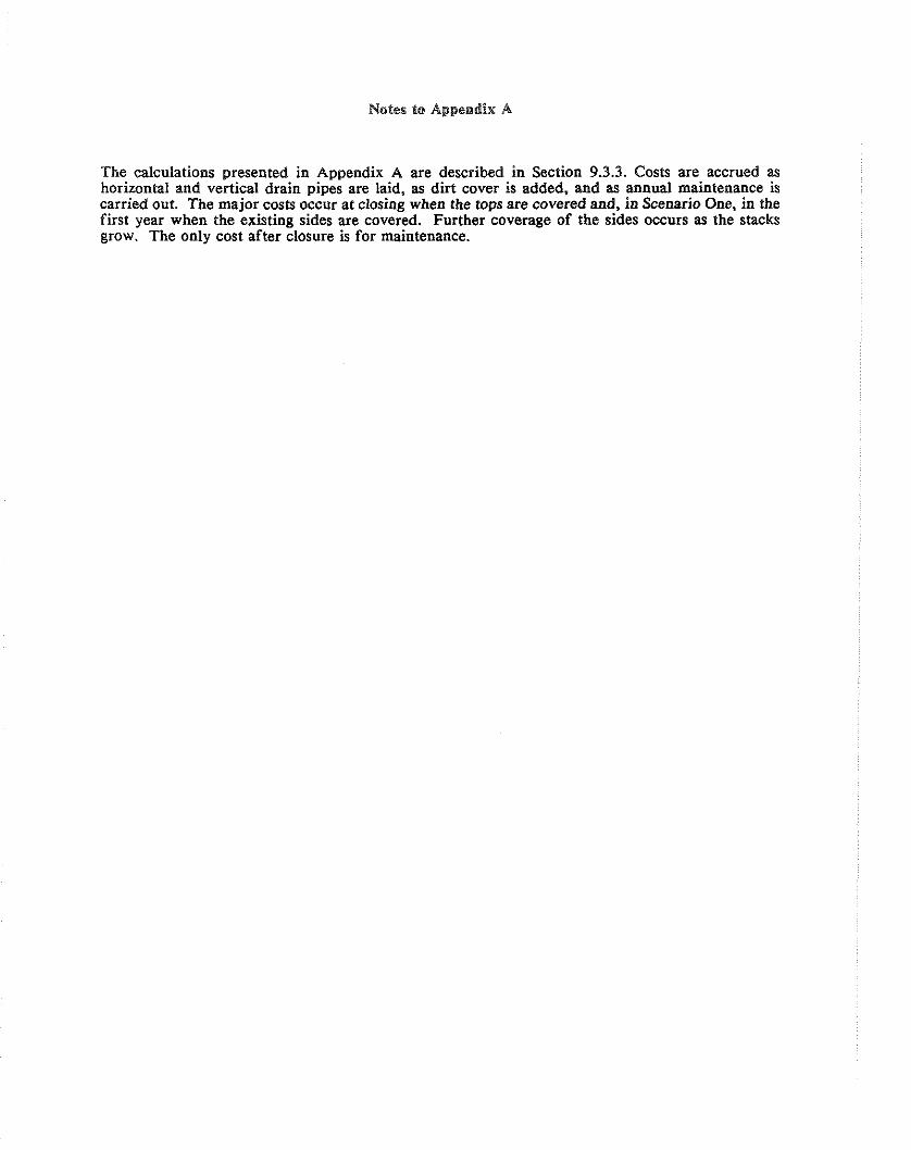
Notes to Appendix A
The calculations presented in Appendix A are described in Section 9.3.3. Costs are accrued as horizontal and vertical drain pipes are laid, as dirt cover is added, and as annual maintenance is carried out. The major costs occur at closing when the tops are covered and, in Scenario One, in the first year when the e~isting sides are covered. Further coverage of the sides occurs as the stacks grow. The only cost after closure is for maintenance.
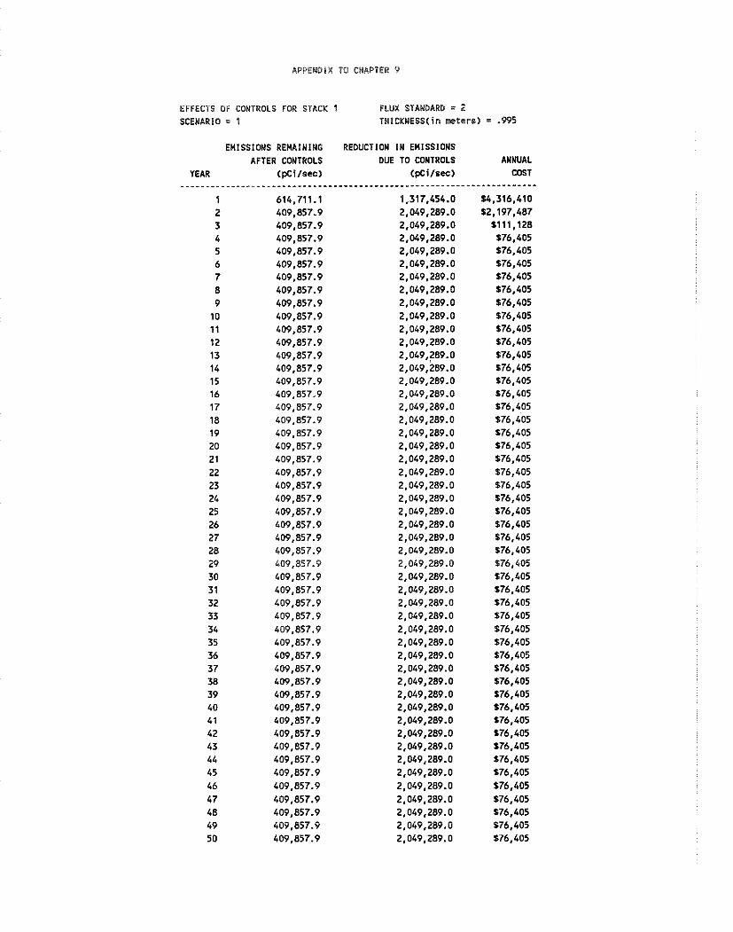
APPENDIX 10 CHAPTER 9
EFFECTS OF CONTROLS FOR STACK 1 FLUX STANDARD = 2 SCENARIO = 1 THICKNESS(in mters) = .W5
EMISSIONS REHAINlNC AFTER CONTROLS
YEAR (pCilsec)
REDUCTION I W EMISSIONS DUE TO CWTROLS ANNUAL
(pcilsec) COST
1,317,454.0 U.316.410 2,049,289.0 $2,197,487 2,049,289.0 $111,128 2,049,289.0 176,405 2,049,289.0 $76.405 2,049,289.0 $76,405 2,049,289.0 $76,405 2,049,289.0 $76.405 2,049,289.0 $76,405 2,049,289.0 $76,405 2,049,289.0 $76,405 2,049,289.0 $76,405 2,049,289.0 $76,405 2,049,289.0 $76,405 2,049,289.0 176.405 2,049,289.0 $76.405 2,049,289.0 $76,405 2,049,289.0 $76.4'05 2,049,289.0 $76.405 2,049,289.0 $76,405 2,049,289.0 $76,405 2,049,289.0 $76,405 2,049,289.0 $76,405 2,049,289.0 $76,405 2,049,289.0 $76,405 2,049,289.0 $76,405 2,049,289.0 $76.405 2,049,289.0 176,405 2,049,289.0 $76.405 2,049,289.0 $76.405 2,049,289.0 $76,405 2,049,289.0 $76,405 2,049,289.0 $76,405 2,049,289.0 $76.405 2,049,289.0 $76,405 2,049,289.0 $76,405 2,049,289.0 176,405 2,049,289.0 $76,405 2,049,289.0 $76,405 2,049,289.0 $76,405 2,049,289.0 576,405 2,049,289.0 176.405 2,049,289.0 176.405 2,049,289.0 $76,405 2,049.289.0 $76,405 2,049,289.0 176,405 2,049.289.0 $76,405 2,049,289.0 $76,405 2,049,289.0 176,405 2,049,289.0 $76,405

APPENDIX 10 CHAPTER 9
EFFECTS OF CONTROLS FOR STACK 2 FLUX STANDARD = 2 SCENARIO = 1 THlCKNESS(in meter!
EMISSIONS REMAINING AFTER CONTROLS
YEAR (pCi/sec)
1 993,836.9 2 956,465.9 3 917,843.4 4 877,780.5 5 836,037.1 6 792,286.9 7 746.080.0 8 386,833.5 9 386,833.5
10 386,833.5 11 386,833.5 12 386,833.5 13 386,833.5 14 386,833.5 15 386,833.5 16 386,833.5 17 386,833.5 18 386,833.5 19 386,833.5 20 386,833.5 21 386,833.5 22 386,833.5 23 386,833.5 24 386,833.5 25 386,833.5 26 386,833.5 27 386,833.5 28 386,833.5 29 386,833.5 30 386,833.5 31 386,833.5 32 386,833.5 33 386,833.5 34 386,833.5 35 386,833.5 36 386,833.5 37 386,833.5 38 386,833.5 39 386,833.5 40 386,833.5 41 386,833.5 42 386,833.5 43 386,833.5 44 386,833.5 45 386,833.5 46 386,833.5 47 386,833.5 48 386,833.5 49 386,833.5 50 386,833.5
REDUCTION IN EMISSIONS DUE TO CONTROLS
(pCi/sec>
602,931.3 681,670.4 763,046.1 847,456.5 935,407.9
1,027,588.0 1,124,943.0 1,934,167.0 1,934,167.0 1,934,167.0 1,934.167.0 1,934,167.0 1,934,167.0 1,934,167.0 1,934,167.0 1,934,167.0 1,934,167.0 1,934,167.0 1,934,167.0 1,934,367.0 1,934,167.0 1,934,167.0 1,934,167.0 1,934,167.0 1,934.167.0 1,934.167.0 1,934,167.0 1,934,167.0 1,934,267.0 1,934,167.0 1,934,167.0 1,934,167.0 1,934,167.0 1,934,167.0 1,934,167.0 1,934,167.0 1,934,167.0 1,934,167.0 1,934,167.0 1,934,167.0 1,934,167.0 1,934.167.0 1,934,167.0 1,934,167.0 1,934,167.0 1,934.167.0 1,934,167.0 1,934,167.0 1,934,167.0 1,934,167.0
ANNUAL COST
. - - - - - - - - - * - - 11,959,538
591,304 $534,857 546,429
$581,340 156,025
1644.854 13,228,241
581,277 581,277 581,277 581,277 581,277 181.277 $81,277 E81,277 $81,277 581,277 581,277 581,277 581,277 581,277 s1.277 581,277 581,277 181.277 s1.277 $81,277 %81,2i7 581,277 581,277 581,277 581.277 581,277 581,277 581,277 sa1,277 sa1.277 181.277 581,277 581,277 581,277 581,277 581,277 581,277 581,277 581,277 s81.277 581,277 LB1,277
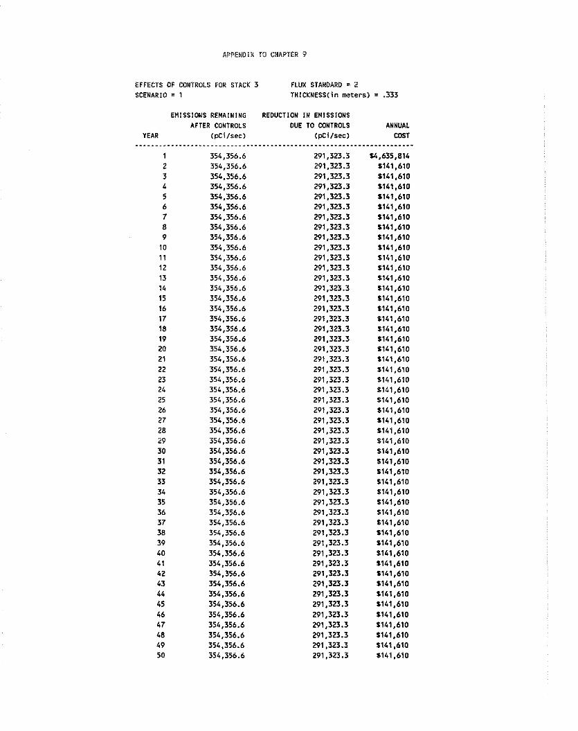
APPEHDiii TO CHAPTER 9
EFFECTS OF CONTROLS FOR STACK 3 FLUX STANDARD = 2 SCENARIO I 1 THICKNESS(in meters) = .333
EMISSIONS REMAINING AFTER CONTROLS
YEAR (pCi/sec)
REDUCTION IN EMISSIONS DUE TO CONTROLS
(pCi1sec) ANNUAL COST -
S4.635.814 $141,610 $141,610 5141,610 5141,610 $141,610 $141,610 5141.610 5141,610 $141,610 1141.610 $141,610 $141.610 $141,610 $141,610 $141,610 S141.610 $141,610 1141,610 $141,610 5141,610 $141,610 $141,610 $141,610 $141.610 $141,610 $141,610 1141,610 $141,610 $141,610 1141.610 5141.610 1141,610 $141,610 $141,610 $141,610 $141.610 $141,610 $141.610 $141,610 $141.610 $141,610 $141,610 $141.610 $141,610 $141,610 $141,610 $141,610 1141,610 $141.610
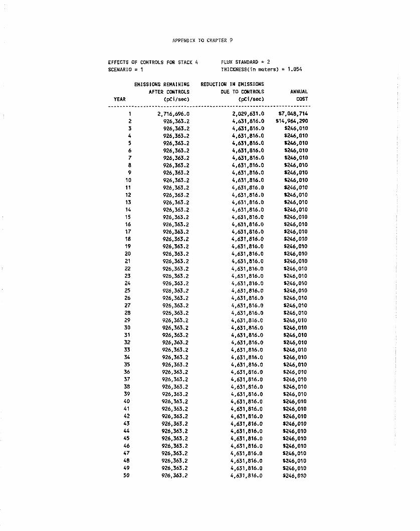
APPENDIX TO CNAPTER 9
EFFECTS OF CONTROLS FOR STACK 4 FLUX STANDARD D 2 SCENARIO = 1 THICKNESS(in rneterl
EMISSIONS REMAINING REDUCTION IN EMISSIONS AFTER CONTROLS DUE TO CONTROLS
YEAR (pc i l sec ) (pc i lsec ) ANNUAL
COST
57,048,774 114,964,290
$246.010 $246.010 1246,010 1246,010 1246,010 1246,010 $246,010 9246.010 1246,010 1246,010 1246,010 1246,010 1246,010 $246,010 1246,010 5246,010 $246,010 1246,010 1246,010 $246.010 $246,010 $246.010 1246,010 0246.010 9246.010 1246.010 5246,010 1246,010 5246,010 1246,010 $246,010 1246.010 5246.010 5246,010 $246,010 $246.010 $246.010 1246,010 $246,010 1246,010 $246,010 1246,010 1246,010 $246.010 1246.010 1246,010 $246,010 $246.010
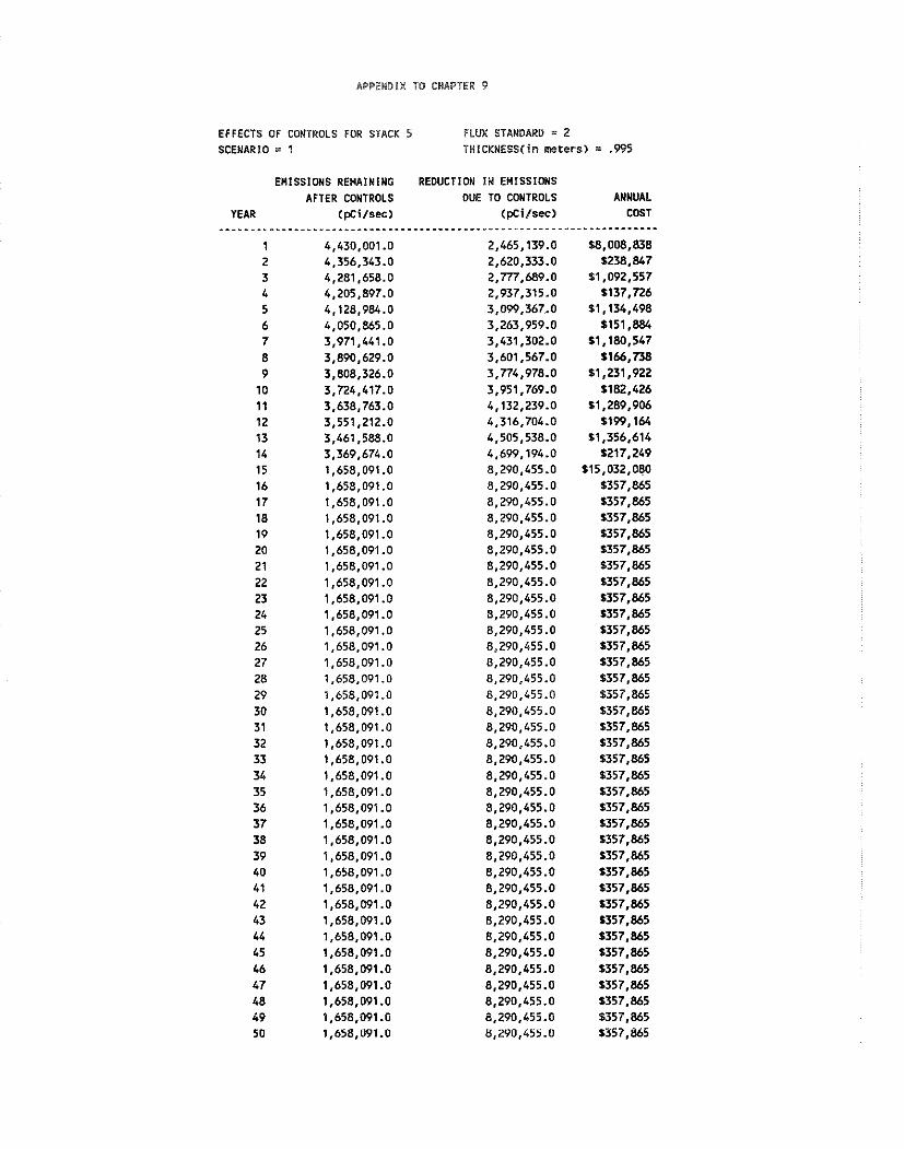
APPENDIX TO CHAPTER 9
EFFECTS OF CONTROLS FOR STACK 5 FLUX STANDARD = 2 SCENARIO = 1 TMICKNESS(in meters) = .995
EMISSIONS REMAINING AFTER CONTROLS
YEAR ( p ~ i l s e c )
REDUCTION It4 EMISSIMlS OUE TO CONTROLS
(pci lsec) - - - - - - - . . - . - - -*------ - - . - -
2,165,139.0 2,620,333.0 2,777.689.0 2,937,315.0 3,099.367.0 3,263,959.0 3,431,302.0 3,601,567.0 3,774,978.0 3,951,769.0 4,132,239.0 4,316,704.0 4,505,538.0 4,699,194.0 8,290.455.0 8,290,455.0 8,290,455.0 8,290,455.0 8,290,455.0 8,290,455.0 8,290,455.0 8,290,455.0 8,290,455.0 8,290,455.0 8,290,455.0 8,290,455.0 8,290,455.0 8,290,455.0 8,290,455.0 8,290,455.0 8,290,455.0 8,290,455.0 8,290,455.0 8,290,455.0 8,290,455.0 8,290,455.0 8,290,455.0 8,290,455.0 8,290,455.0 8,290,455.0 8,290,455.0 8,290,455.0 8,290,455.0 8,290,455.0 8,290,455.0 8,290,455.0 8,290,455.0 8,290,455.0 8,290,455.0 8,290,455.0
ANNUAL COST
.------------ 58,008,838 1238,847
$1,092,557 1137,726
51,134,498 1151,884
11,180,547 1166.738
11,231,922 $182,426
11,289,906 1199,164
51,356,614 5217.249
515,032.0~0 5357,865 5357,865 1357,865 1357,865 1357,865 5357,865 1357,865 1357,865 1357,865 1357,865 5357,865 1357,865 1357,865 S357.865 1357,865 $357.865 $357.865 1357,865 5357,865 1357,865 1357,865 1357,865 1357,865 1357,865 s357,865 5357,865 1357,865 1357,865 1357,865 1357.865 1357,865 1357,865 1357.865 5357,865 1357,865
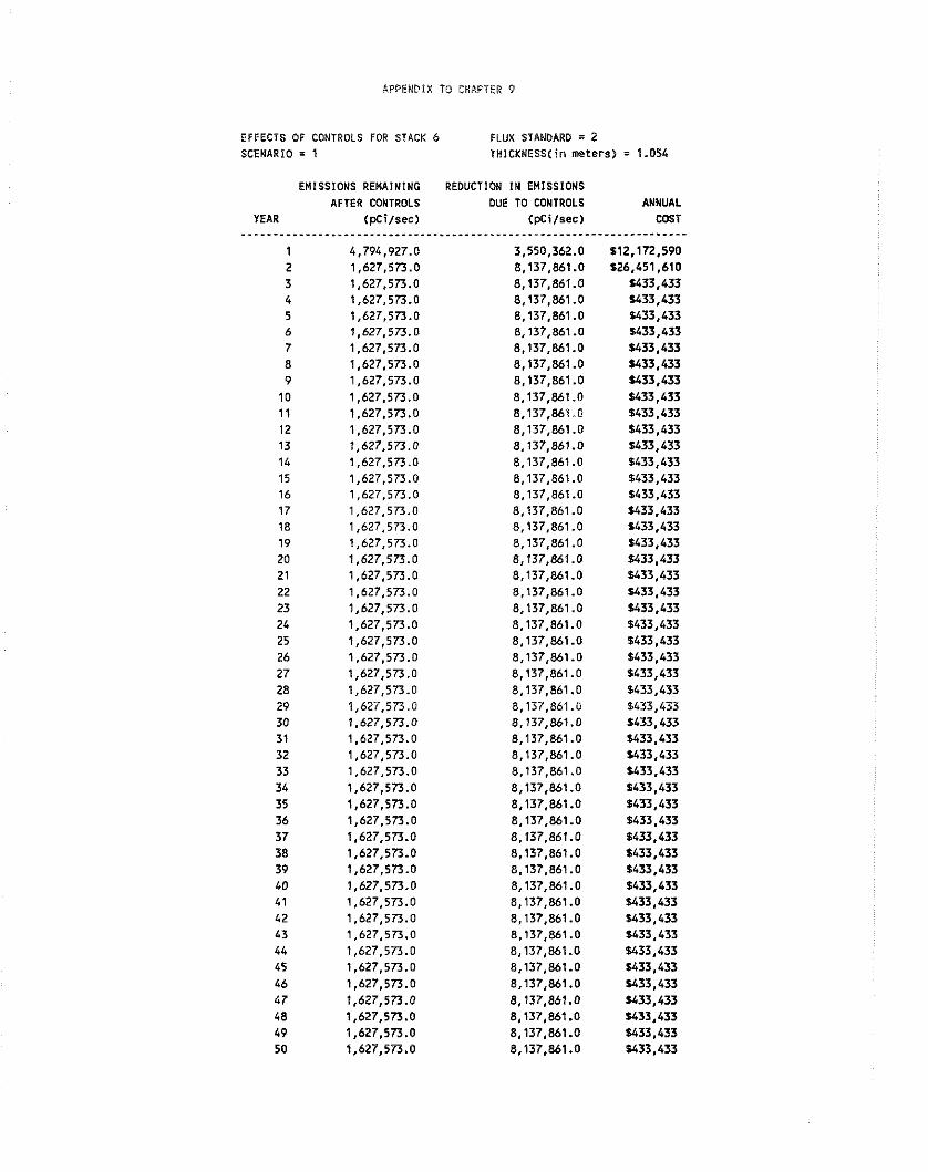
APPENDIX 70 CHAPTER 9
EFFECTS OF CONTROLS FOR STACK 6 FLUX STRNDARD = 2 SCENARIO = 1 THICKNESS(in meters) = 1.054
EMISSIONS REMAINING AFTER CONTROLS
YEAR (pCi/sec) --*---.-----.-..-----..-*---.-.
1 4,794,927.0 2 1,627,573.0 3 1,627,573.0 4 1,627,573.0 5 1,627,573.0 6 1,627,573.0 7 1,627,573.0 8 1,627.573.0 9 1,627,573.0 10 1,627,573.0 1 1 1,627,573.0 12 1,627,573.0 13 1,627.573.0 14 1,627.573.0 15 1,627,573.0 16 1,627,573.0 17 1,627,573.0 18 1,627,573.0 19 1,627,573.0 20 1,627,573.0 21 1,627,573.0 22 1,627,573.0 23 1,627,573.0 24 1,627,573.0 25 1,627,573.0 26 1,627,573.0 27 1,627,573.0 28 1,627,573.0 29 1,627,573.0 30 1,627,573.0 31 1,627,573.0 32 1,627,573.0 33 1,627,573.0 34 1,627,573.0 35 1,627,573.0 36 1,627,573.0 37 1,627,573.0 38 1,627,573.0 39 1,627,573.0 40 1,627,573.0 41 1,627,573.0 42 1,627,573.0 43 1,627,573.0 44 1,627,573.0 45 1,627,573.0 46 1,627,573.0 47 1,627,573.0 48 1,627,573.0 49 1,627,573.0 50 1,627,573.0
REDUCTION IN EMISSIONS DUE TO CONTROLS
( P C i l s e c ) -.-----"-...-.------------
3,550,362.0 8,137,861 .O 8,137,861.0 8,137,861 .O 8,137,861.0 8,137,861.0 8,137,861.0 8,137,861.0 8,137,861.0 8,137,861 .O 8,137,869.0 8,137,861.0 8,137,861.0 8,137,861.0 8,137,861.0 8,137,861.0 8.137.861.0 8,137,861.0 8,137,861.0 8,137,861 .O 8,137,861.0 8,137,861.0 8,137,861 .O 8,137,861 .O 8,137,861 .O 8,137,861 .O 8,137,861 .O 8,137,861.0 8,137,861.0 8,137,861.0 8,137,861.0 8,137,861.0 8,137,861 .O 8,137,861.0 8,137,861.0 8,137,861.0 8,137,861.0 8.137.861.0 8,137,861.0 8,137,861 .O 8,137,861.0 8,137,861.0 8,137,861.0 8,137,861.0 8,137,861 .O 8,137,861 .O 8,137,861.0 8,137,861 .O 8,137.861.0 8,137,861.0
ANNUAL COST --------.----
312,172,590 $26,451,610
1433,433 1433,433 1433,433 1433,433 $433,433 $433,433 I433,433 1433,433 $433.433 1433,433 1433,433 $433,433 1433,433 1433,433 1433,433 1433,433 1433,433 1433,433 1433,433 1433,433 1433,433 1433,433 1433.433 1433,433 1433,433 1433,433 8633,433 5433,433 1433,433 U33,433 1433,433 $433,433 $433,433 1433.433 $433.433 1433,433 1433,433 1433,433 1433.*33 1433,433 1433,433 1433,433 5433.433 1433,433 1433,433 1433,433 1433,433 5433,433
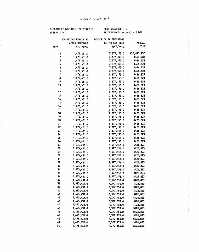
APPENDIX TO CHAPTER 9
EFFECTS OF CONTROLS FOR STACK 7 FLUX STANDARD = 2 SCENARIO = 1 THICKNESS(in neters) = 1.054
EMISSIONS REHAlUlUG AFTER CONTROLS
YEAR (pCi/sec)
1 1,475,431.0 2 1,475,431.0 3 1,475,431.0 4 1,475,431.0 5 1,475.431.0 6 1,475,431.0 7 1,475.431.0 8 1,475,431.0 9 1,475,431.0 10 1,475,431.0 1 1 1,475,431.0 12 1,475,431.0 13 1,475,431.0 14 1,475,431.0 15 1,475,431.0 16 1,47$,431.0 17 1,475.431.0 18 1,475,431.0 19 1,475,431.0 20 1,475,431 .O 21 1,475,431 .O 22 1,475,431.0 23 1,475,431.0 24 1.475.431.0 25 1,475,431.0 26 1,47$,431.0 27 1,47$,431.0 28 1,475,431.0 29 1.475.431.0 30 1,475,431.0 31 1,475,431.0 32 1,475,431.0 33 1,475,431.0 34 1,475.431.0 35 1,475,431.0 36 1,475,431.0 37 1,475,431.0 38 1,475,431.0 39 1,475,431.0 40 1,475,431.0 41 1,475,431.0 42 1,475,431 .O 43 1,475,431.0 44 1,475.431.0 45 1,475,431.0 46 1,475,431.0 47 1,475,431.0 48 1,475,431.0 49 1,475,431.0 50 1,475.431.0
REDUCTION IU EMISSIONS DUE TO CONTROLS
(pCi/aec) .*------------------*----.
7,377,153.0 7,377,153.0 7,377.153.0 7,377,153.0 7,377,153.0 7,377,153.0 7,377,153.0 7,377,153.0 7,377,153.0 7,377,153.0 7,377,153.0 7,377,153.0 7,377,153.0 7,377,153.0 7,377,153.0 7,377,153.0 7,377,153.0 7,377,153.0 7,377,153.0 7,377,153.0 7,377,153.0 7,377,153.0 7,377,153.0 7,377,153.0 7,377,153.0 7,377,153.0 7,377,153.0 7,377,153.0 7,377,153.0 7,377,153.0 7,377,153.0 7,377,153.0 7,377,153.0 7,377,153.0 7,377,153.0 7,377,153.0 7,377,153.0 7,377,153.0 7,377,153.0 7,377.153.0 7,377,153.0 7,377,153.0 7,377,153.0 7,377,153.0 7,377,153.0 7,377,153.0 7,377,153.0 7,377.153.0 7,377,153.0 7,377.153.0
ANNUAL COST
$37,895,730 1549,788 1426,823 1426.823 U26.823 1426.823 U26.823 U26.823 U26.823 $426.823 U26.823 $426.823 U26,823 $426.823 $426,823 U26.823 1426,823 $426.823 5426.823 $426,823 $426,823 $426,823 1426,823 1426,823 5426,823 $426,823 1426,823 $426,823 $426,823 $426,823 $426.823 $426,823 %26,823 $426,823 $426.823 5426.823 1426,823 U26.823 $426,823 5426.823 U26.823 $426,823 U26.823 $426.823 $426,823 %26,823 1426,823 $426,823 3426,823 %26,823
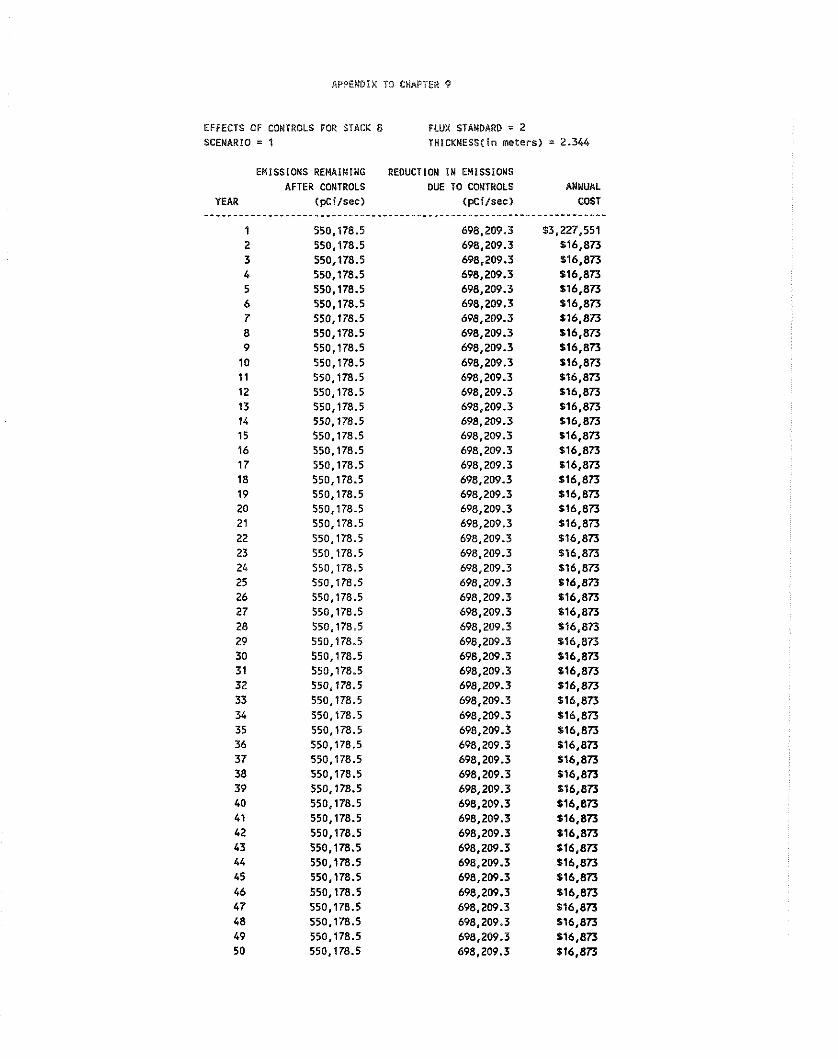
EFFECTS OF CONTROLS FOR STACK 8 FLUX STANDARD = 2 SCENARIO = Z THlCKNESS(in meters) = 2.344
EMISSIONS REMAlNING REOUCTIOU I N EMISSIONS AFTER CONTROLS DUE TO CONTROLS ANNUAL
YEAR (pcilsec) (pci/sec) COST

APPENDIX TO CHAPTER 9
EFFECTS OF CONTROLS FOR STACK 9 FLUX STANDARD = 2 SCENARIO = 1 THICKNESS(in meters) = 1.378
EMISSIONS REMAlNlWC AFTER CONTROLS
YEAR (pCilsec) - - - - - - - - - - - - - - - - - - * - - - - - - - * - - - .
1 1,200,790.0 2 1,158,819.0 3 1,115,519.0 4 1,070,704.0 5 1,024,134.0 6 975,501.7 7 924,381.0 8 486,211.5 9 486,211.5
10 486,211.5 11 186.21 1.5 12 486,211.5 13 486,211.5 14 486,211.5 15 486,211.5 16 486,211.5 17 486,211.5 18 486.211.5 19 486,211.5 20 486,211.5 21 486,211.5 22 486,211.5 23 486,211.5 24 486,211.5 25 486,211.5 26 486.211.5 27 486,211.5 28 486,211.5 29 486,211.5 30 486,211.5 31 486,211.5 32 486,211.5 33 486,211.5 34 486,211.5 35 486,211.5 36 486,211.5 37 486,211.5 38 486,211.5 39 486,211.5 40 486,211.5 41 486,211.5 42 486,211.5 43 486,211.5 44 486,211.5 45 486,211.5 46 486,211.5 47 486,211.5 48 486,211.5 49 486,211.5 50 486,211.5
REOUCTION I K EWISSlOWS DUE 10 COWTROLS
(pci lsec) .--------------------------.
841,112.2 929,542.9
1,020,m.o 1,115,196.0 1,213,317.0 1,315,783.0 1,423,492.0 2,431,058.0 2,431,058.0 2,431,058.0 2,431,058.0 2,431,058.0 2,431,058.0 2,431,058.0 2,431,058.0 2,431,058.0 2,431,058.0 2,431,058.0 2,431,058.0 2,431,058.0 2,431,058.0 2,431,058.0 2,431,058.0 2,431,058.0 2,431,058.0 2,431,058.0 2,431,058.0 2.431,058.0 2,431,058.0 2,431,058.0 2,431,058.0 2,431,058.0 2,431,058.0 2,431,058.0 2,431,058.0 2,431,058.0 2,431,058.0 2,431,058.0 2,431,058.0 2,431,058.0 2,431,058.0 2,431,058.0 2,L31,058.0 2,431,058.0 2,431,058.0 2,431,058.0 2,431,058.0 2,431.058.0 2,431,058.0 2,431,058.0
ANNUAL WST
"----------. $3,703,130
Sb9.588 $813,694 158.680
$877,891 569,201
b964.019 15,345,845
$101,419 $101,419 $101,419 5101,419 $101.419 $101,419 $101.419 $101.419 1101,419 5101,419 1101,419 $101,419 1101,419 1101.419 $101,419 $101,419 1101.419 1101,419 1101,419 1101,419 $101,419 $101,419 1101,419 b101.419 $101,419 $101,419 S101.419 $101,419 1101.419 1101,419 $101,419 1101,419 1101,419 $101.419 $101,419 $101.419 1101.419 1101,419 1101,419 1101,419 1101,419 $101.419

APPENDIX TO CHAPTER 9
EFFECTS OF CONTROLS FOR STACK 10 FLUX STANDARD I 2 SCENARIO = 1 TnlCKNESSfin meters) = .779
EMISSIONS REMAINING AFTER CONTROLS
YEAR (pcilsec) -..----*-..--..--...-----.....
1 86,530.8 2 86,530.8 3 86,530.8 4 86,530.8 5 86,530.8 6 86,530.8 7 86,530.8 8 86,530.8 9 86.530.8 10 86,530.8 1 1 86,530.8 12 86,530.8 13 86,530.8 14 86,530.8 15 86,530.8 16 86,530.8 17 86,530.8 18 86,530.8 19 86,530.8 20 86,530.8 21 86,530.8 22 86,530.8 23 86,530.8 24 86,530.8 25 86,530.8 26 86,530.8 27 86,530.8 28 86,530.8 29 86,530.8 30 86,530.8 31 86,530.8 32 86,530.8 33 86,530.8 34 86,530.8 35 86,530.8 36 86,530.8 37 86,530.8 38 86,530.8 39 86,530.8 40 86,530.8 41 86,530.8 42 86,530.8 43 86,530.8 44 86,530.8 45 86,530.8 46 86,530.8 47 86,530.8 48 86,530.8 49 86,530.8 50 86,530.8
REDUCTION IN EMISSIONS DUE TO CONTROLS ANNUAL
( ~ C i l s e c ) COST ....----....-*.------.-.--------.---7.---
432,654.1 $1,617,673 432,654.1 124,004 432,654.1 1 24,004 432,654.1 $24,004 432,654.1 524,004 432,654.1 $24,004 432,654.1 $24,004 432,654.1 $24,004 432,654.1 $24,004 432.654.1 124,004 432,654.1 124,004 432,654.1 $24,004 432,654.1 $24,004 432,654.1 $24,004 432,654.1 $24,004 432,654.1 $24,004 432,654.1 $24,004 432,654.1 $24.004 432,654.1 $24.004 432,654.1 $24,004 432,654.1 $24,004 432,654.1 $24,004 432,654.1 $24,004 432,654.1 $24,004 432,654.1 $24.004 432,654.1 $24,004 432,654.1 $24,004 432,654.1 $24,004 432,654.1 $24,004 432,654.1 $24,004 432,654.1 $24,004 432,654.1 $24,004 432,654.1 $24,004 432,654.1 $24,004 432,654.1 $24,004 432,654.1 $24,004 432,654.1 $24,004 432,654.1 $24,004 432,654.1 124,004 432,654.1 124.004 432,654.1 124,004 432,654.1 124,004 432,654.1 124,004 432,654.1 124,004 432,654.1 124,004 432,654.1 124,004 432.654.1 124,004 432,654.1 124,004 432,654.1 $24,004 432,654.1 124,004

APPENDIX TO CMAPrER 9
EFFECTS OF CONTROLS FOR STACK 11 FLUX STAMDARD 2 SCENARIO = 1 TktlCKMESS(in meters) = .814
EMISSlOMS REUAlNlNG AFTER CONTROLS
YEAR ( p c i l s e c )
1 7,231,534.0 2 6,872,522.0 3 3,216,295.0 4 3,216,295.0 5 3,216.295.0 6 3,216,295.0 7 3,216,295.0 8 3,216,295.0 9 3,216,295.0
10 3,216,295.0 11 3,216,295.0 12 3,216,295.0 13 3,216,295.0 14 3,216,295.0 15 3,216,295.0 16 3,216,295.0 17 3,216,295.0 18 3,216,295.0 19 3,216,295.0 20 3,216,295.0 21 3,216,295.0 22 3,216,295.0 23 3,216,295.0 24 3,216,295.0 25 3,216,295.0 26 3,216,295.0 27 3,216,295.0 28 3,216,295.0 29 3,216,295.0 30 3,216,295.0 31 3,216,295.0 32 3,216,295.0 33 3,216,295.0 34 3,216,295.0 35 3,216,295.0 36 3,216,295.0 37 3,216,295.0 38 3,216,295.0 39 3,216,295.0 40 3,216,295.0 41 3,216,295.0 42 3,216,295.0 43 3,216,295.0 44 3,216,295.0 45 3,216.295.0 46 3,216,295.0 47 3,216,295.0 48 3,216,295.0 49 3,216,295.0 50 3,216,295.0
REDUCTION IN EnlSSIOWS DUE TO CONTROLS
(pc i l sec ) .----------.---------.----.
8,165,137.0 8,875,178.0
16,081,480.0 16,081,480.0 16,081,480.0 16,081,480.0 16,081,480.0 16,081,480.0 16,081,480.0 16,081,480.0 16,081,480.0 16,081,480.0 16,081,480.0 16,081.480.0 16,081,480.0 16,081,480.0 16,081,480.0 16,081,480.0 16,081,480.0 16,081,480.0 16,081,480.0 16,081,480.0 16,081,480.0 16,081,480.0 16,081,480.0 16,081.480.0 16,081,480.0 16,081.480.0 16,081,480.0 16,081,480.0 16,081,480.0 16,081,480.0 16,081,480.0 16,081,480.0 16,081,480.0 16,081,480.0 16,081,480.0 16,081,480.0 16,081,480.0 16,081,480.0 16,081,480.0 16,081,480.0 16,081,480.0 16,081,480.0 16,081,480.0 16,081,480.0 16,081,480.0 16,081,480.0 16,081,480.0 16,081,480.0
ANNUAL COST

APPENDIX 16 CHAPTER 9
EFFECTS OF CONTROLS FOR STACK 12 FLUX STANDARD = 2 SCENARIO = 1 THICKNESS(^^ meters) = 1.054
EMISSIONS REUAINING AFTER CONTROLS
YEAR (pCilsec) ------*---------------.------.
1 476,006.1 2 476,006.1 3 476,006.1 4 476,006.1 5 476,006.1 6 476,006.1 7 476,006.1 8 476,006.1 9 476,006.1
10 476,006.1 11 476.006.1 12 476,006.1 13 476,006.1 14 476,006.1 15 476,006.1 16 476,006.1 17 476,006.1 18 476,006.1 19 476,006.1 20 476,006.1 21 476,006.1 22 476,006.1 23 476,006.1 24 476,006.1 25 476,006.1 26 476,006.1 27 476,006.1 28 476,006.1 29 476,006.1 30 476,006.1 31 476,006.1 32 476,006.1 33 476,006.1 34 476,006.1 35 476,006.1 36 476,006.1 37 476,006.1 38 476,006.1 39 476.006.1 40 476,006.1 41 476,006.1 42 476,006.1 43 476,006.1 44 476,006.1 45 476,006.1 46 476,006.1 47 476,006.1 48 476,006.1 49 476,006.1 50 476,006.1
REDUCTION I N EMlSSlONS DUE TO CONTROLS
(pcilsec)
1,019,749.0 1,019,749.0 1,019,749.0 1,019.749.0 1,019,749.0 1,019,749.0 1,019,749.0 1,019,749.0 1.019.749.0 1,019,749.0 1,019,749.0 1,019,749.0 1,019,749.0 1,019,749.0 1,019,749.0 1,019,749.0 1,019,749.0 1,019,749.0 1,019,749.0 1,019,749.0 1,019,749.0 1,019,749.0 1,019,749.0 1,019,749.0 1,019,749.0 1,019,749.0 1,019,749.0 1,019,749.0 1,019,749.0 1,019,749.0 1,019,749.0 1.019.749.0 1,019,749.0 1,019,749.0 1,019,749.0 1,019,749.0 1,019.749.0 1,019,749.0 1,019,749.0 1,019,749.0 1,019.749.0 1,019,749.0 1,019,749.0 1,019,749.0 1,019,749.0 1,019,749.0 1,019,749.0 1,019,749.0 1,019.749.0 1,019,749.0
ANNUAL COST
. - - - - - - - - - - - $3,519,421
139,430 $69.991 139,430 $39,430 $39.430 $39,430 $39.430 $39,430 $39.430 $39,430 $39.430 539.430 $39,430 $39.430 $39,430 $39,430 $39,430 139,430 $39,430 $39,430 $39,430 139,430 $39,430 139.430 139,430 239,430 $39,430 $39,430 $39,430 139,430 $39,430 $39,430 $39,430 139.430 $39,430 $39,430 $39,430 S39,430 539,430 $39.430 $39.430 539.430 $39,430 $39,430 139,430 139,430 $39.430 139.430 S39,UO
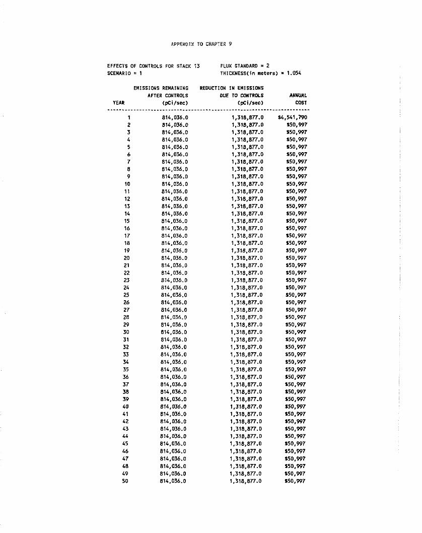
APPENDIX TO CHAPTER 9
EFFECTS OF CONTROLS FOR STACK 13 FLUX STANDARD = 2 SCENARIO = 1 THICKNESS( in meters) = 1.054
EMISSICUS REHAlNING REDUCTIW I N E M l S S l f f l S AFTER CONTROLS DUE TO CONTROLS ANNUAL
YEAR CpCiIsec) ( P C i l S e C ) COST

APPENDIX TO CHAPTER 9
EFFECTS OF CONTROLS FOR STACK 14 FLUX STANDARD = 2 SCENARIO = 1 THICKNESS(in neters) = 1.054
EMISSIONS REMAINING AFTER CONTROLS
YEAR (pCi/sec) ------------..---*------------.
1 1,421,334.0 2 737,686.8 3 737,686.8 4 737,686.8 5 737,686.8 6 737,686.8 7 737,686.8 8 737,686.8 9 737,686.8
10 737,686.8 11 737,686.8 12 737.686.8 13 737,686.8 14 737,686.8 15 737,686.8 16 737,686.8 17 737,686.8 18 737,686.8 19 737,686.8 20 737,686.8 21 737,686.8 22 737,686.8 23 737,686.8 24 737,686.8 25 737,686.8 26 737,686.8 27 737,686.8 28 737,686.8 29 737,686.8 30 737,686.8 31 737.686.8 32 737,686.8 33 737,686.8 34 737,686.8 35 737,686.8 36 737,686.8 37 737,686.8 38 737,686.8 39 737,686.8 40 737,686.8 41 737,686.8 42 737,656.8 43 737,686.8 44 737,686.8 45 737,686.8 46 737,686.8 47 737,686.8 48 737,686.8 49 737,686.8 50 737,686.8
REDUCTION I N EMISSIONS DUE TO CONTROLS
(pcilsec)
2,146,276.0 3,688,433.0 3,688,433.0 3,688,433.0 3,688,433.0 3,688,433.0 3,688,433.0 3,688,433.0 3,688,433.0 3,688,433.0 3,688,433.0 3,688,433.0 3,688,433.0 3,688,433.0 3,688,433.0 3,688,433.0 3,688,433.0 3,688,433.0 3,688,433.0 3,688,433.0 3,688,433.0 3,688,433.0 3,688,433.0 3,688,433.0 3,688,433.0 3,688,433.0 3,688,433.0 3,688,433.0 3,688,433.0 3,688,433.0 3,688,433.0 3,688,433.0 3,688,433.0 3,658,433.0 3,688,433.0 3,688,433.0 3,688,433.0 3,688,433.0 3,688,433.0 3,688,433.0 3,688,433.0 3,688,433.0 3,688,433.0 3,688,433.0 3,688,433.0 3,688,433.0 3,688,433.0 3,688,433.0 3,688,433.0 3,688,433.0
ANNUAL COST --- - - - - - - - - - -
$7,385,325 16,473,889
1154,915 1154,915 $154,915 1154,915 1154,915 1154,915 1154,915 1154,915 $154,915 $154.915 1154,915 1154,915 1154,915 1154,915 1154,915 1154,915 $154,915 $154,915 $154,915 1154,915 1154,915 1154,915 1154,915 $154,915 $154,915 5154,915 $154,915 $154,915 $154,915 $154,915 1154,915 1154.915 1154,915 $154,915 1154,915 1154,915 1 154,915 1154,915 $154,915 $154,915 $154,915 $154,915 1154,915 $154,915 1154,915 1154,915 $154,915 1154,915
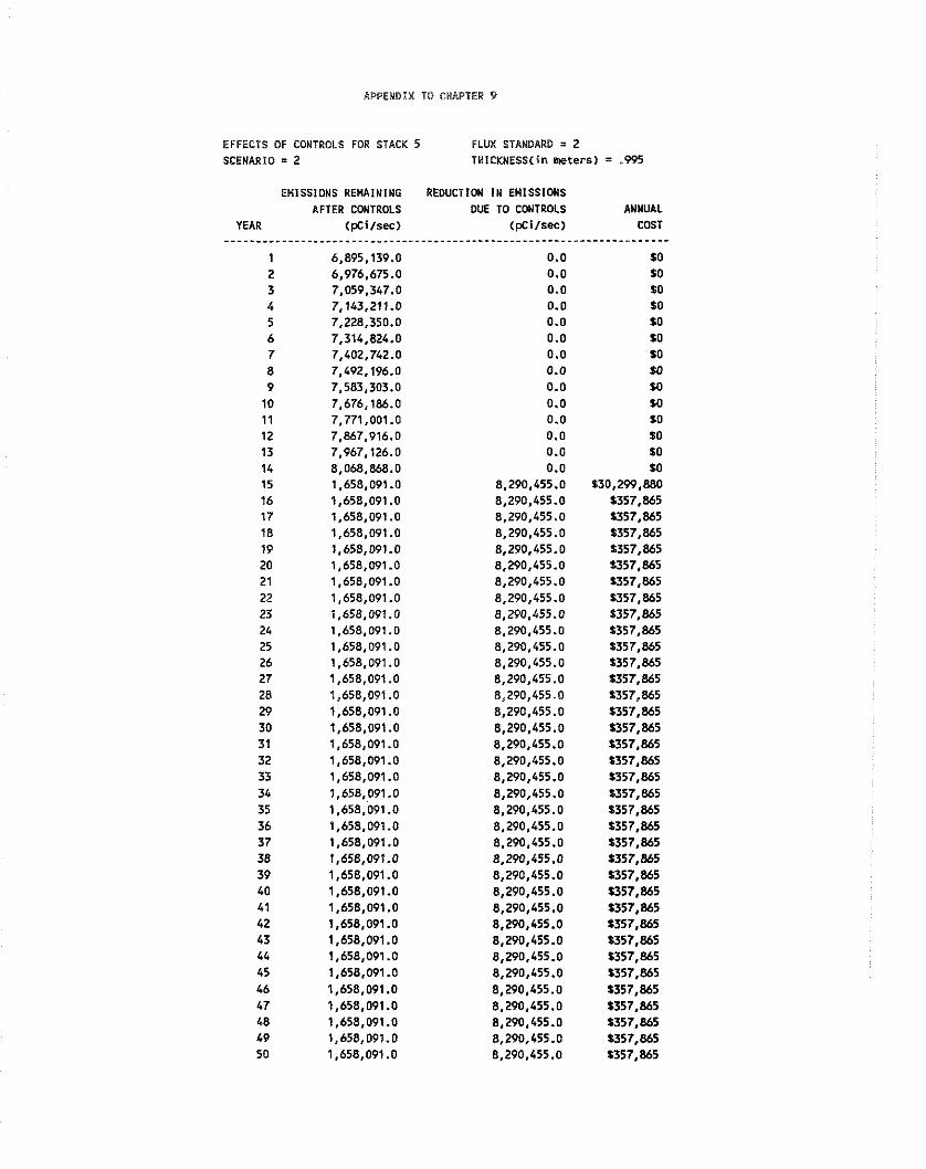
APPEMDIX TO CHAPTER 9
EFFECTS OF CONTROLS FOR STACK 5 FLUX STANDARD = 2 SCENARIO = 2 THICKNESS(in m t e r s ) = .995
EMISSIONS REMAINING REDUCTION I N EHlSSlONS
AFTER CONTROLS DUE TO CONTROLS ANNUAL YEAR ( ! X i / s e c ) ( W i l s e c ) COST
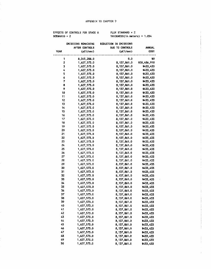
APPENDIX TO CHAPTER 9
EFFECTS OF CONTROLS FOR STACK 6 FLUX STANDARD = 2 SCENARIO = 2 THICKNESS(in neters) = 1.054
EMISSIONS REMAINING AFTER CONTROLS
YEAR (pCi/sec) -------------.---------------.
1 8,345,288.0 2 1,627,573.0 3 1,627,573.0 4 1,627,573.0 5 1,627,573.0 6 1,627,573.0 7 1,627,573.0 8 1,627,573.0 9 1,627,573.0 10 1,627,573.0 1 1 1,627,573.0 12 1.627.573.0 13 1.627.573.0 14 1,627,573.0 15 1,627,573.0 16 1,627,573.0 17 1,627,573.0 18 1,627.573.0 19 1,627,573.0 20 1,627,573.0 21 1,627,573.0 22 1,627,573.0 23 1,627,573.0 24 1,627,573.0 25 1,627,573.0 26 1,627,573.0 27 1,627,573.0 28 1.627.573.0 29 1,627,573.0 30 1,627,573.0 31 1,627,573.0 32 1,627,573.0 33 1,627,573.0 34 1,627,573.0 35 1,627,573.0 36 1,627,573.0 37 1,627,573.0 38 1,627,573.0 39 1,627,573.0 40 1,627,573.0 41 1,627,573.0 42 1,627,573.0 43 1,627,573.0 44 1,627,573.0 45 1,627,573.0 46 1,627,573.0 47 1,627,573.0 48 1,627,573.0 19 1,627,573.0 50 1,627,573.0
REDUCTION IN EUlSSlONS DUE TO CONTROLS
(~Cilsec) ANNUAL COST
SO 538,486,910
5433,433 5433,433 $433,433 5433.433 U33.433 U33.433 U33.433 5433,433 U33.433 1433.433 5433.433 5433,433 5433.433 U33.433 5433,433 5433.433 5433,433 $433,433 U33.433 5433.433 5433,433 5433.433 U33.433 5433,433 5433,433 5433.433 1433.433 $433,433 $433,433 U33.433 1433.433 5433,433 U33.433 U33.433 U33.433 U33.433 5433.433 U33.433 5433,433 1433.433 5433,433 U33.433 U33.433 U33.433 U33.433 5433.433 $433.433 1433.433

APPENDIX TO CNAPTER 9
EFFECTS OF CONTROLS FOR STACK 7 FLUX STANDARD = 2 SCENARIO = 2 THICKNESSCin wters) = 1.054
EMISSIONS REMAINING AFTER CONTROLS
YEAR (pCilsec) ---.-------------------------. 1 1,475,431.0 2 1,475,431 .O 3 1,475,431.0 4 1,475,431.0 5 1,475,431.0 6 1,475,431.0 7 1,175,431 .O 8 1,475,131.0 9 1,475,431.0
10 1,475.431.0 11 1,475,431.0 12 1,475,431.0 13 1,475,431.0 14 1,475,431.0 15 1.475.431.0 16 1,475,431 .O 17 1,475,431.0 18 1,475,431.0 19 1,475,431.0 20 1,475.431.0 21 1,475,431 .O 22 1,475,431.0 23 1,475,431.0 24 1,475.431.0 25 1,475,431.0 26 1,475,431.0 27 1,475,431.0 28 1,475,431 . O 29 1,475,431.0 30 1,475,431.0 31 1,475,431.0 32 1,475.431.0 33 1,475,431.0 34 1,475,431 .O 35 1,475,431.0 36 1,475,431.0 37 1,475,431.0 38 1,475,431 .O 39 1,475,431.0 40 1,475,431.0 41 1,475.431.0 42 1,475,431.0 43 1,475,431.0 44 1,475,431.0 45 1,475,431.0 46 1,475,431.0 47 1,475.431.0 48 1,475,431.0 49 1,475,431.0 50 1,475,431.0
REDUCTION IN EMISSIONS DUE TO CONTROLS
(pCiIsec) ANNUAL
COST - - - - - - - - - - - - - - $37,895,730
1426.823 1426.823 1426,823 1426.823 1426,823 1426.823 1426.823 1426,823 1426,823 1426.823 U26.823 1426,823 1426,823 1426,823 1426,823 U26.823 $426.823 U26.823 1426,823 %26,823 1426,823 %26,823 U26,823 U26.823 U26.823 1426,823 1426,823 5426.823 %26,823 U26.823 %26,823 U26,823 1426.823 1426,823 5426,823 1426,823 1426,823 5426.823 5426.823 1426,823 1426,823 1426,823 $426,823 1426,823 1426,823 U26.823 $426.823 %26,823 1426,823
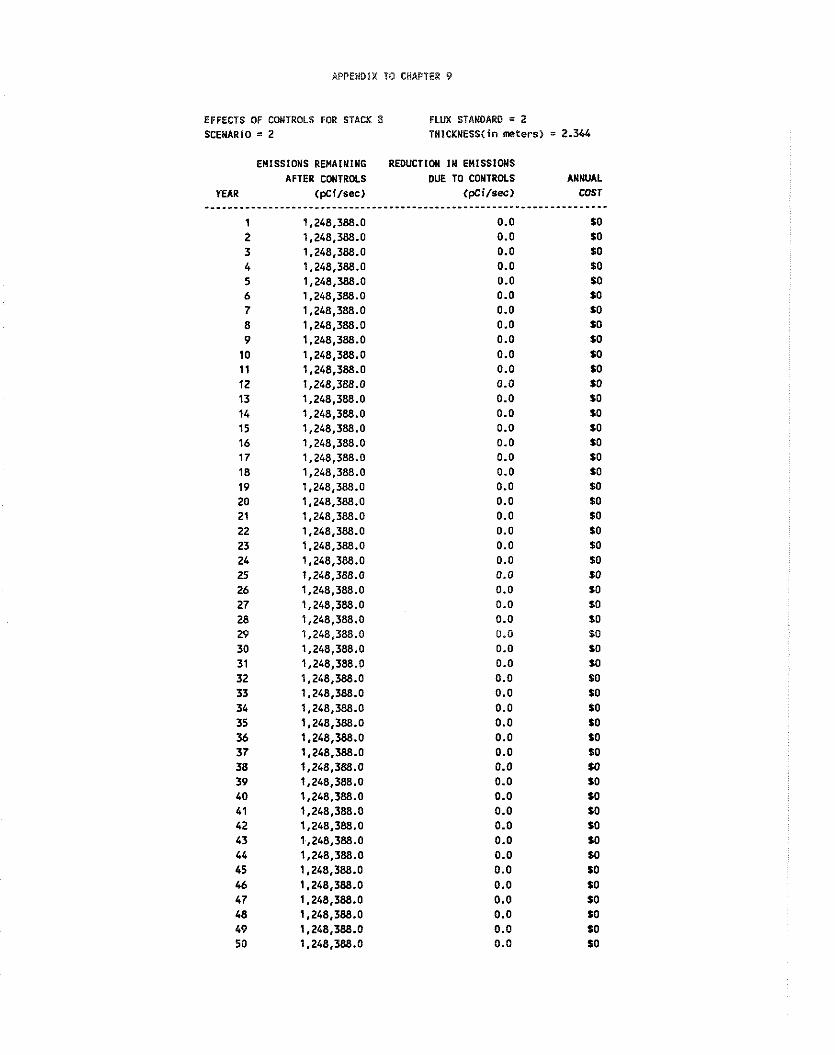
APPEMDIX TO CHAPTER 9
EFFECTS OF COWTROLS FOR STACK 8 FLUX STANDARD = 2 SCENARIO = 2 THICKNESS(in meters) = 2.344
EUISSIONS REWAIYING REDUCTION I N EUISSIONS
AFTER CONTROLS DUE TO CONTROLS ANNUAL
YEAR (pci/sec) (pci/ses> mr
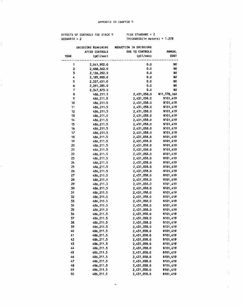
EFFECTS OF COMTROLS FOR STACK 9 FLUX STANDARD = 2 SCENARIO = 2 ?HlCKNESS(in meters) = 1.378
EMISSIONS REMAlNING AFTER CONTROLS
YEAR (pCilsec)
1 2,041,902.0 2 2,088,362.0 3 2,136,292.0 4 2,185,900.0 5 2,237.451 .O 6 2,291,285.0 7 2,347,873.0 8 486,211.5 9 486,211.5
10 486,211.5 11 486,211.5 12 486,211.5 13 486,211.5 14 486,211.5 15 486,211.5 16 486,211.5 17 486,211.5 18 486,211.5 19 486,211.5 20 486,211.5 21 486,211.5 22 486,211.5 23 486,211.5 24 486,211.5 25 486,211.5 26 486,211.5 27 486,211.5 28 486,211.5 29 486.211.5 30 486,211.5 31 486,211.5 32 486,211.5 33 486,211.5 34 486,211.5 35 486,211.5 36 486,211.5 37 486,211.5 38 486,211.5 39 486,211.5 40 486,211.5 41 486,211.5 42 486,211.5 43 486,211.5 44 486,211.5 45 486,211.5 46 486,211.5 47 486,211.5 48 486,211.5 49 486,211.5 50 486,21!.5
REDUCTION IN EMISSIONS DUE TO CONTROLS
(pcilsec) .--*---------.--------------
0.0 0.0 0.0 0.0 0.0 0.0 0.0
2,431,058.0 2,431,058.0 2,431,058.0 2,431,058.0 2,431,058.0 2,431,058.0 2,431,058.0 2,431,058.0 2,431,058.0 2,431,058.0 2,431,058.0 2,431,058.0 2,431,058.0 2,431,058.0 2,431.058.0 2,431,058.0 2,431,058.0 2,431,058.0 2,431,058.0 2,431,058.0 2,431,058.0 2,431,058.0 2,431,058.0 2,431,058.0 2,431,058.0 2,431,058.0 2,431,058.0 2,431,058.0 2,431,058.0 2,431,058.0 2,431,058.0 2,431,058.0 2,431,058.0 2,431,058.0 2,431,058.0 2.431.058.0 2,431,058.0 2,431,058.0 2,431,058.0 2,431,058.0 2,431,058.0 2,431,058.0 2,431,058.0
ANNUAL COST
- - - - - - - - - - - - - - SO so SO SO $0 $0 so
$11,578,160 $101,419 5101,419 $101,419 $101,419 $101,419 $101,419 S101.419 $101,419 $101,419 $101,419 $101,419 $101,419 5101,419 $101,419 1101,419 2101,419 $101,419 $101.419 S101.419 2101,419 $101,419 $101,419 S101.419 $101,419 $101,419 S101.419 1101.419 $101,419 5101.419 1101.419 $101,419 $101,419 $101.419 s101.419 s101.419 5101.419 2101.419 s101.419 5101,419 s101.419 SlM.419 S101.Ll9
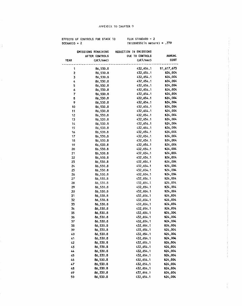
APPENDIX TO CHAPTER 9
EFFECTS OF CONTROLS FOR STACK 10 FLUX STANDARD = 2 SCENARIO = 2 TWlcKMESS(in meters) = . T 9
EMlSSlONS REMAINING AFTER CONTROLS
YEAR (pc i lsec)
REDUCTION IN EMlSSlONS DUE TO CONTROLS
(pc i lsec) ANNUAL
COST - - - - - - - - - - - * -
$1,617,673 $24.004 $24,004 S 24,004 $24.004 S24.004 $24.004 $24,004 124,004 124,004 $24,004 $24,004 524,004 $24,004 $24,004 $24,004 $24,004 $24,004 524,004 124,004 $24,004 $24,004 $24,004 $24,004 $24,004 124.004 $24,004 $21,004 $24,004 $24,004 124.004 $24,004 $24.004 S24.004 124.004 124,004 $24.004 524.004 $24,004 $24,004 124,004 124.004 124.004 $24,004 124,004 $24,004 s24.004 $24,004 $24.004 124,004

APPEMOIX TO CHAPTER 9
EFFECTS OF CONTROLS FOR STACK 12 FLUX STANDARD = 2 SCENARIO = 2 THICKNESS(in meters) = 3.054
EMISSIONS REMAINING REDUCTION IN EMISSIONS AFTER CONTROLS DUE TO CONTROLS ANNUAL
YEAR ( W i l s e c ) (pcilsec) COST -------------------------------------.------*-------------------------
1 1,495,756.0 0.0 SO 2 1,495,756.0 0.0 SO 3 1,495,756.0 0.0 SO 4 1,495,756.0 0.0 SO 5 1,495,756.0 0.0 SO 6 1,495,756.0 0.0 SO 7 1,495,756.0 0.0 SO 8 1,495,756.0 0.0 SO 9 1,495,756.0 0.0 SO 10 1,495,756.0 0.0 SO 1 1 1,495,756.0 0.0 SO 12 1,495,756.0 0.0 SO 13 1,495,756.0 0.0 SO 14 1,495,756.0 0.0 SO 15 1,495,756.0 0.0 SO 16 1,495,756.0 0.0 SO 17 1,495.756.0 0.0 SO 18 1,495,756.0 0.0 SO 19 1,495,756.0 0.0 SO 20 1,495,756.0 0.0 SO 21 1,495,756.0 0.0 SO 22 1,495,756.0 0.0 SO 23 1,495,756.0 0.0 SO 24 1,495,756.0 0.0 SO 25 1,495.756.0 0.0 SO 26 1,495,756.0 0.0 SO 27 1,495,756.0 0.0 SO 28 1,495,756.0 0.0 SO 29 1,495,756.0 0.0 SO 30 1,495,756.0 0.0 SO 31 1,495,756.0 0.0 SO 32 1,495,756.0 0.0 SO 33 1,495.756.0 0.0 SO 34 1,495,756.0 0.0 SO 35 1,495,756.0 0.0 SO 36 1,495,756.0 0.0 SO 37 1,695,756.0 0.0 SO 38 1,495,756.0 0.0 SO 39 1,495,756.0 0.0 SO 40 1,495,756.0 0.0 SO 41 1,495,756.0 0.0 M 42 1,495,756.0 0.0 M 43 1,495,756.0 0.0 SO 44 1,495,756.0 0.0 SO 45 1,495,756.0 0.0 SO 46 1,495,756.0 0.0 SO 47 1,495,756.0 0.0 SO 48 1,495,756.0 0.0 $0 49 1,495,756.0 0.0 SO 50 !,495,756.0 0.0 SO
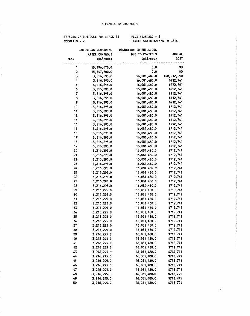
APPERDIX 10 CHAPTER 9
EFFECTS OF CONTROLS FOR STACK 11 FLUX STANDARD = 2 SCENARIO = 2 THICKNESS(in meters) = .814
EHlSSlONS REMAINIUG AFTER CONTROLS
YEAR (pcilsec)
REDUCTION I N EMlSSIONS DUE TO CONTROLS
(pci/sec) - - - - * * - - - - - - - - - - - - - - - - - - - -
0.0 0.0
16,081,480.0 16,081,480.0 16,081,480.0 16,081,480.0 16,081,480.0 16,081,480.0 16,081,480.0 16,081,480.0 16,081,480.0 16,081,480.0 16,081,480.0 16,081,480.0 16,081,480.0 16,081,480.0 16,081,480.0 16,081,480.0 16,081,480.0 16,081,480.0 16,081,480.0 16,081,480.0 16,081,480.0 16,081,480.0 16,081,480.0 16,081,480.0 16,081,480.0 16,081,480.0 16,081,CSO.O 16,081,480.0 16,081,480.0 16,081,480.0 16,081,480.0 16,081,480.0 16,081,480.0 16,081,480.0 16,081,480.0 16,081.480.0 16,081,480.0 16,081,480.0 16,081,480.0 16,081,480.0 16,081,480.0 16,081,480.0 16,081,480.0 16.081.480.0 16,081,480.0 16,081,480.0 16,081,480.0 16,081,480.0
ANNUAL COST
- - - " - - - - - - - - - $0 $0
$50,212,090 $712,741 $712,741 $712,741 $712,741 $712.741 $712,741 $712,741 $712,741 1712,741 $712,741 $712,741 $712,741 $712,741 $712.741 1712,741 $712,741 $712,741 $712,741 $712,741 $712,741 $712,741 $712.741 $712.741 $712,741 $712,741 $712,741 $712,741 $712,741 $712,741 $712.741 $712,741 $712.741 $712.741 1712.741 $712,741 $712,741 $712,741 $712.741 $712,741 1712,741 $712,741 $712,741 $712,741 $712,741 $712,741 $712,741 0712,741
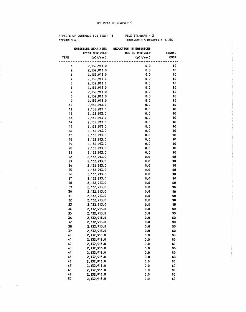
APPENDIX 10 CHAPTER 9
EFFECTS OF CONTROLS FOR STACK $3 FLUX STANDARD * 2 SCENARIO = 2 THICKNESS(in meters) = 1.054
EMISSlONS REMAINING REDUCTION 1II EMISSIONS AFTER CONTROLS OUE TO CONTROLS ANNUAL
YEAR (pcilsec) (pCi/sec) COST

APPENDIX TO CWPiPIER 9
EFFECTS OF CONTROLS FOR STACK 14 FLUX STANDARD = 2 SCENARIO = 2 ?HICKNESS(in meters) = 1.054
EHISSfONS REHAINING AFTER CONTROLS
YEAR ( W i l ~ e c )
REDUCTION IN EMISSIONS DUE TO CONTROLS ANNUAL
(pcilsec) COST -----------------------.--*------------- 0.0 M
3,688,433.0 S13,776,220 3,688,433.0 1154.915 3,688,433.0 $154,915 3,688,433.0 $154.915 3,688,433.0 $154.915 3,688,433.0 $154,915 3,688.43.0 $154.915 3,688,433.0 5154,915 3,688,433.0 $154,915 3,688,433.0 $154,915 3,688,433.0 $154,915 3,688,433.0 5154,915 3,688,433.0 $154,915 3,688,433.0 $154,915 3,688,433.0 $154,915 3,688,433.0 $154.915 3,688,433.0 1154.915 3,688,433.0 $154.915 3,688,433.0 $154,915 3,688,433.0 $154,915 3,688,433.0 $154.915 3,688,433.0 $154,915 3,688,433.0 $154,915 3,688,433.0 $154,915 3,688,433.0 $154.915 3,688,433.0 $154,915 3,688,433.0 $154.915 3,688,433.0 $154,915 3,688,433.0 $154,915 3,688,433.0 $154,915 3,688,433.0 $154,915 3,688,433.0 $154,915 3,688,433.0 $154,915 3,688.433.0 1154,915 3,688,433.0 1154,915 3,688,433.0 $154.915 3,688,433.0 $154.915 3,688,433.0 $154,915 3,688,433.0 1154,915 3.688.433.0 5154,915 3,688,433.0 $154,915 3,688,433.0 $154,915 3,688,433.0 $154,915 3,688,433.0 $154,915 3,688,433.0 $154,915 3.688.433.0 $154,915 3,688,433.0 $154,915 3,688,433.0 1154,915 3,688,433.0 $154,915
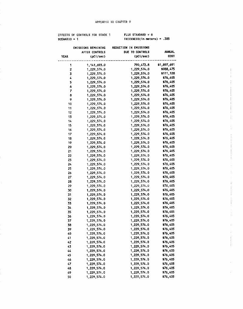
APPENDIX 10 CHAPTER 9
EFFECTS Of CONTROLS FOR STACK 1 FLUX STANDARD = 6 SCENARIO = 1 THICKNESS(in meterr
EMISSIONS REHAININC AFTER CONTROLS
YEAR (pCi/sec) *-------A-----------.---*.---7-
1 1,141,693.0 2 1,229,574.0 3 1,229,574.0 4 1,229,574.0 5 1,229,574.0 6 1,229,574.0 7 1,229,574.0 8 1,229,574.0 9 1,229,574.0 10 1,229,574.0 1 1 1,229,574.0 12 1,229,574.0 13 1,229,574.0 14 1,229,574.0 15 1,229,574.0 16 1,229,574.0 17 1,229,574.0 18 1,229.574.0 19 1,229,574.0 20 1,229,574.0 21 1,229,574.0 22 1,229,574.0 23 1,229,574.0 24 1,229,574.0 25 1,229,574.0 26 1,229,574.0 27 1,229,574.0 28 1,229,574.0 29 1,229,574.0 30 1,229.574.0 31 1,229,574.0 32 1,229,574.0 33 1,229,574.0 34 1,229,574.0 35 1,229,574.0 36 1,229,574.0 37 1,229,574.0 38 1,229,574.0 39 1,229,574.0 40 1,229.574.0 41 1,229,574.0 42 1,229,574.0 43 1,229,574.0 44 1,229,574.0 45 1,229,574.0 46 1,229,574.0 47 1,229,574.0 48 1,229,574.0 19 1,229,574.0 50 1,229,574.0
REDUCTION IN EMlSSlONS DUE TO CONTROLS
(pCi/sec) -----------*--------------.
790,472.8 1,229,574.0 1,229,574.0 1,229,574.0 1.229.574.0 1,229,574.0 1,229,574.0 1,229,574.0 1,229,574.0 1,229,574.0 1,229,574.0 1,229,574.0 1,229,574.0 1,229,574.0 1,229,574.0 1,229,574.0 1,229,574.0 1,229,574.0 1,229,574.0 1,229,574.0 1,229.574.0 1,229,574.0 1,229,574.0 1,229,574.0 1,229,574.0 1,229,574.0 1,229,574.0 1,229,574.0 1,229.574.0 1,229,574.0 1,229,574.0 1,229,574.0 1,229.574.0 1,229,574.0 1,229,574.0 1,229,574.0 1,229,574.0 1,229,574.0 1,229.574.0 1,229,574.0 1,229,574.0 1,229,574.0 1,229,574.0 1,229,574.0 1,229,574.0 1,229,574.0 1,229,574.0 1,229,574.0 1,229,574.0 1,229,574.0
ANNUAL COST ----
$1,897,691 $988.475 5111,128 $76,405 $76,405 276,405 $76,405 $76,405 276,405 576,405 $76,405 $76,605 576.405 576,405 $76.405 $76,405 $76,405 176,405 $76,405 $76,405 $76,405 $76,405 $76,405 $76,405 $76,405 176,405 $76,405 $76.405 576,405 $76,405 $76,405 576,405 176,405 $76,405 $76,405 $76,405 176,405 576,405 $76,405 $76.405 $76,405 $76.405 176,405 576,405 176,405 576,405 $76,405 $76,405 $76.405 $76,405

APPENDIX TO CHAPTER 9
EFFECTS OF CONTROLS FOR STACK 2 FLUX STANDARD = 6 SCENARIO = 1 THICKNESS(in meters) = .XI5
EHlSSIONS REMAINING AFTER CONTROLS
YEAR (pCi/sec)
1 1,235,009.0 2 1,229,134.0 3 1,223,062.0 4 1,216,763.0 5 1,210,200.0 6 1,203,322.0 7 1,196,057.0 8 1,160,500.0 9 1,160,500.0
10 1,160,500.0 11 1,160,500.0 12 1,160,500.0 13 1,160,500.0 14 1,160,500.0 15 1,160,500.0 16 1,160,500.0 17 1,160,500.0 18 1,160,500.0 19 1,160,500.0 20 1,160,500.0 21 1,160,500.0 22 1,160,500.0 23 1,160,500.0 24 1,160,500.0 25 1,160,500.0 26 1,160,500.0 27 1,160,500.0 28 1,160,500.0 29 1,160,500.0 30 1,160,500.0 31 1,160,500.0 32 1,160,500.0 33 1,160,500.0 34 1,160,500.0 35 1,160,500.0 36 1,160,500.0 37 1,160.500.0 38 1,160,500.0 39 1,160,500.0 10 1,160.500.0 41 1,160.500.0 42 1,160,500.0 43 1,160,500.0 44 1,160,500.0 45 1,160,500.0 46 1,160,500.0 47 1,160,500.0 48 1,160,500.0 49 1,160,500.0 50 1,160,500.0
REDUCTIOW IN EMlSSlONS DUE TO CWTROLS
(pCilsec) .------------------.*-----.
361,758.9 409,002.3 457,827.8 508,474.0 561,244.8 616,552.8 674,966.1
1,160,501.0 1,160,501.0 1,160,501.0 1,160,501.0 1,160,501.0 1,160,501.0 1,160,501.0 1,160,501.0 1,160,501.0 1,160,501 .O 1,160,501.0 1,160,501.0 1,160,501.0 1,160,501.0 1,160,501.0 1,160,501.0 1,160,501.0 1,160,501.0 1,160,501.0 1,160,501.0 1,160,501.0 1,160,501 .O 1,160,501.0 1,160.501.0 1,160,501.0 1,160,501.0 1,160,501.0 1,160,501.0 1,160.501.0 1,160,501.0 1,160,501.0 1,160,501.0 1,160,501.0 1,160,501.0 1,160,501.0 1,160,501.0 1,160,501.0 1,160,501.0 1,160,501.0 1,160,501.0 1,160,501.0 1,160.50t.0 1,160,501.0
ANNUAL COST ------
$852.614 $91,304
1240,901 $46.429
$264,900 $56.025
1296,885 11,434,479
S81.277 181.277 S81.277 S81.277 S81.277 S81.277 S81.277 S81.277 $81,277 S81.277 S81.277 S81.277 S81.277 S81.277 S81,277 S81.277 181.277 sE1.277 S81.277 sE1.277 281.277 S81.277 S81.277 S81.277 S81.277 S81.277 $81.277 S81.277 S81.277 S81.277 S81,277 S81.277 S81.277 S81.277 S81.277 $81.277 S81.277 581,277 S81.277 sa1.277 681,277 S81.277

APPENDIX 10 CHAPTER 9
EFFECTS OF CONTROLS FOR STACK 3 FLUX STANDARD 6 SCENARIO = 1 THltKNESS(in meters) = .333
EMISSIONS REMAINING AFTER CONTROLS
YEAR (pCi/sec) -.---------.--.----..---...*-.
1 354.356.6 2 354,356.6 3 354,356.6 4 354,356.6 5 354,356.6 6 354,356.6 7 354.356.6 8 354,356.6 9 354,356.6 10 354,356.6 1 1 354,356.6 12 354,356.6 13 354,356.6 14 354,356.6 15 354,356.6 16 354,356.6 17 354,356.6 18 354,356.6 19 354,356.6 20 354,356.6 21 354,356.6 22 354,356.6 23 354,356.6 24 354,356.6 25 354,356.6 26 354,356.6 27 354,356.6 28 354,356.6 29 354,356.6 30 354,356.6 31 354,356.6 32 354,356.6 33 354,356.6 34 354,356.6 35 354,356.6 36 354,356.6 37 354,356.6 38 354.356.6 39 354,356.6 40 354,356.6 41 354,356.6 42 354,356.6 43 354,356.6 44 354,356.6 45 354,356.6 46 354,356.6 47 354,356.6 48 354,356.6 49 354,356.6 50 354,356.6
REDUCTION I N EMISSIONS DUE TO CONTROLS
(pci/sec)
291,323.3 291,323.3 291,323.3 291,323.3 291,323.3 291,323.3 291,323.3 291,323.3 291,323.3 291,323.3 291,323.3 291,323.3 291,323.3 291,323.3 291,323.3 291,323.3 291,323.3 291,323.3 291,323.3 291,323.3 291,323.3 291,323.3 291,323.3 291,323.3 291,323.3 291,323.3 291,323.3 291,323.3 291,323.3 291,323.3 291,323.3 291,323.3 291,323.3 291,323.3 291,323.3 291,323.3 291,323.3 291,323.3 291,323.3 291,323.3 291,323.3 291,323.3 291,323.3 291,323.3 291,323.3 291,323.3 291,323.3 291,323.3 291,323.3 291,323.3
ANNUAL COST
, - - - - - - - - - - - - t4,635,814 $141,610 1141.610 $141.610 $141,610 $141,610 1141.610 $141,610 $141,610 $141,610 $141.610 S141.610 $141,610 $141.610 $141,610 $141,610 $141,610 $141,610 $141,610 $141,610 $141,610 $141,610 $141,610 S141,610 S141.610 S141.610 $141,610 $141,610 0141,610 $141,610 $141,610 $141,610 1141,610 $141,610 $141,610 $141,610 $141,610 $141,610 $141,610 5141,610 $141,610 1141,610 $141,610 $141,610 1141,610 $141.610 $141.610 $141.610 $141,610 $141,610

kPPEMOIX 10 CHAPTER Q
EFFECTS OF CONTROLS FOR STACK 4 FLUX STANDARD = 6 SCENARIO = I THlCKNESS(in meterr
EUISSIONS REMAINING REDUCTION I N EMISSIONS AFTER CONTROLS DUE TO CONTROLS
YEAR (pCi /sec) ( W i f s e c ) ANNUAL
cosr , - - - - - - - - - - - -
$3.103.321 %,541,975
$246,010 $246.010 $246,010 1246,010 $246,010 3246.010 S246,OlO $246.010 $246,010 $246.010 $246,010 $246.010 1246,010 $246,010 $246,010 $246,010 $246,010 $246,010 1246,010 1246,010 1246.010 $246,010 1246,010 5246,010 $246,010 1246,010 $246,010 $246,010 $246,010 $246,010 $246,010 $246,010 $246,010 6246,010 $246.010 $246,010 $246,010 $246,010 $246,010 $246,010 $246,010 S246.010 $246,010 1246.010 6246,010 $246,010 $246,010 5246,010
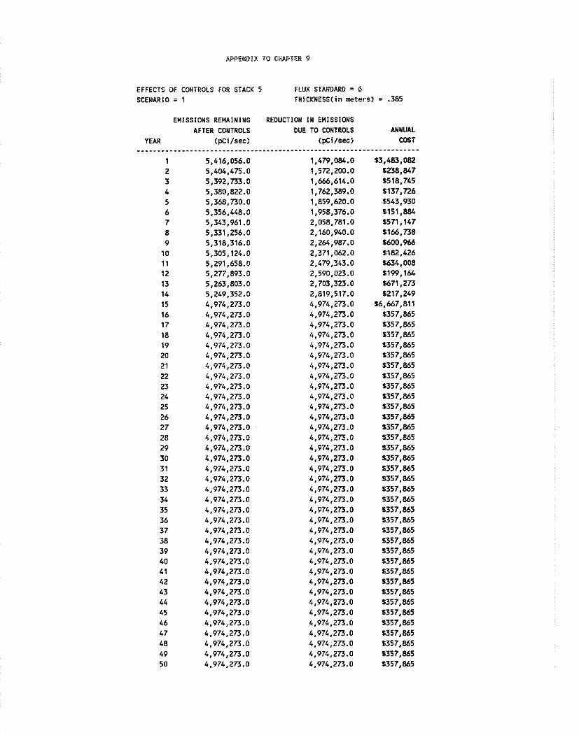
APPENDIX TO CHAPTER 9
EFFECTS OF CONTROLS FOR STACK 5 FLUX STANDARD = 6 SCENARIO = 1 THICKNESS( in meters) = .385
EMISSIONS REMAINING REDUCTION I N EMISSIONS AFTER CONTROLS DUE TO CONTROLS ANNUAL
YEAR (pci/sec) (pcilsec) COST
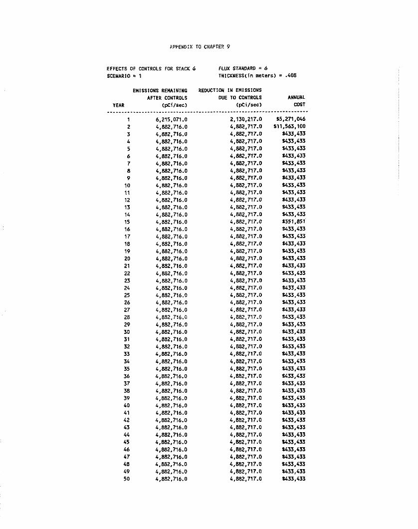
APPEYDIX TO CHAPTER 9
EFFECTS Of CONTROLS FOR STACK 6 FLUX STANDARD = 6 SCENARIO 2 1 THICKNESS(in mters) = .408
EMISSIONS REMAINING AFTER CONTROLS
YEAR (Wi lsec) - - - - - * - - - - - - - * - - - - - - - - - - . - - - - - .
1 6,215,071.0 2 4,882,716.0 3 4,882,716.0 4 4,882,716.0 5 4,882,716.0 6 4,882,716.0 7 4,882,716.0 8 4,882,716.0 9 4,882,716.0
10 4,882,716.0 11 4,882,716.0 12 4,882,716.0 13 4,882.716.0 14 4,882.716.0 15 4,882,716.0 16 4,882,716.0 17 4,882,716.0 18 4,882,716.0 19 4,882,716.0 20 4,882,716.0 21 4,882,716.0 22 4,882.716.0 23 4,882,716.0 24 4,882,716.0 25 4,882,716.0 26 4,882,716.0 27 4,882,716.0 28 4,882,716.0 29 4,882,716.0 30 4,882,716.0 31 4,882,716.0 32 4,882,716.0 33 4,882,716.0 34 4,882,716.0 35 4,882,716.0 36 4,882,716.0 37 4,882,716.0 38 4,882,716.0 39 4,882,716.0 40 4,882,716.0 41 4,882,716.0 42 4,882,716.0 43 4,882,716.0 44 4.882.716.0 45 4,882,716.0 46 4,882.716.0 47 4,882,716.0 48 4,882,716.0 49 4,882,716.0 50 4,882,716.0
REDUCTION IN EMISSIONS DUE TO CONTROLS
CpCilsec) ANNUAL
COST

APPENDIX 10 CHAPTER 9
EFFECTS OF CONTROLS FOR STACK 7 FLUX STANDARD 1 6 SCENARIO = 1 THICKNESS(in meters) = .&08
EMISSlONS REMAINING AFTER CONTROLS
YEAR ( p c i l s e c ) -------------.-.----.---------.
1 4,426,291.0 2 4,426,291.0 3 4,426,291.0 4 4,426,291.0 5 4,426,291.0 6 4,426,291.0 7 4,426,291 .O 8 4,426,291 .O 9 4,426,291.0 10 4,426,291.0 1 1 4,426,291 .O 12 4,426,291.0 13 4,426,291 .O 14 4,426,291 .O 15 4,426.291.0 16 4,426,291.0 17 4,426.291.0 18 4,426,291.0 19 4,426,291 .O 20 4,426,291 .O 21 4,426,291.0 22 4,426,291.0 23 4,426,291 .O 24 4,426,291.0 25 4,426,291 .O 26 4,426,291.0 27 4,426,291.0 28 4,426,291.0 29 4,426,291 .O 30 4,426,291 .O 31 4,426,291.0 32 4,426,291.0 33 4,426,291 .O 34 4,426,291 .O 35 4,426,291 .O 36 4,426,291.0 37 4,426,291.0 38 4,426,291 .O 39 4,426,291.0 40 4,426,291.0 41 4,426,291.0 42 4,426,291 .O 43 4,426,291 .O 44 4,426,291.0 45 4,426,291.0 46 4,426,291 .O 47 4,426,291 .O 48 4,426,291 .O 49 4,426,291.0 50 4,426,291 .O
REDUCTION IN EUISSIONS DUE TO CONTROLS
(pc i l sec ) ANNUAL COST

APPENDIX TO CHAPTER 9
EFFECTS OF CONTROLS FOR STACK 8 FLUX STANDARD 6 SCENARIO 1 THlCKNESS(in meters) = 1.021
EMISSIONS REMAINING AFTER CONTROLS
YEAR (pe i lsec )
REDUCTION IN EMISSIONS DUE TO CONTROLS
(pci l~ec)
465,472.9 465,472.9 465,472.9 465,472.9 465,472.9 465,472.9 165,472.9 465,472.9 465,472.9 465,472.9 465.472.9 465,472.9 465,472.9 465,472.9 465,472.9 465,472.9 465,472.9 465,472.9 465,472.9 465,472.9 465,472.9 465,472.9 465,472.9 465,472.9 465,472.9 465,472.9 465,472.9 465.472.9 465,472.9 465,472.9 465,472.9 465,472.9 465,472.9 465,472.9 465,472.9 465,472.9 465,472.9 465,472.9 465,472.9 465,472.9 465,472.9 465,472.9 465,472.9 465,472.9 465,472.9 465,472.9 465,472.9 465,472.9 465.472.9 465,472.9
ANNUAL COST
.---.*-------- S1,4W,111
116,873 $16.873 $16.873 $16.873 516.873 $16,873 S 16,873 $16,873 516,873 116,873 516.873 $16.873 $16,873 $16,873 116.873 $16.873 516.873 116.873 $16,873 $16.873 $16.873 $16,873 $16.873 116,873 $16,873 116,873 $16,873 $16,873 $16,873 516,873 516,873 $16,873 116,873 $16.873 $16,873 $16,873 $16,873 $16,873 $16.873 116,873 116,873 516,873 $16,873 $16,873 $16,873 $16,873 $16,873 116,873 516,873
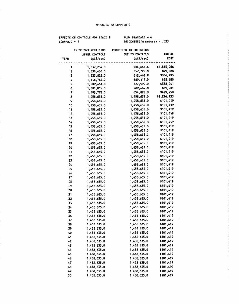
APPENDIX 10 CHAPTER 9
EFFECTS OF CONTROLS FOR STACK 9 FLUX STANDARD = 6 SCENARIO = 1 THlCKNESS(in meters) = .533
EMISSIONS REMAlNlNG AFTER CONTROLS
YEAR (Wilsec) - - - - - - - - - - - - - - * - - * - - * - - . - - - - - - .
1 1,537,234.0 2 1,530,636.0 3 1,523,828.0 4 1,516,782.0 5 1,509,461.0 6 1,501,815.0 7 1,493,778.0 8 1,458,635.0 9 1,458,635.0
10 1,458,635.0 11 1,458.635.0 12 1,458,635.0 13 1,458,635.0 14 1,458,635.0 15 1,458,635.0 16 1,458,635.0 17 1,458,635.0 18 1,458,635.0 19 1,458,635.0 20 1,458,635.0 21 1,458,635.0 22 1,458,635.0 23 1,458,635.0 24 1,458,635.0 25 1,458,635.0 26 1,458,635.0 27 1,458,635.0 28 1,458,635.0 29 1,458,635.0 30 1,458,635.0 31 1,458,635.0 32 1,458,635.0 33 1,458,635.0 34 1,458,635.0 35 1,458,635.0 36 1,458,635.0 37 1,458,635.0 38 1,458,635.0 39 1,458,635.0 40 1,458.635.0 41 1,458,635.0 42 1,458,635.0 43 1,458,635.0 44 1,458,635.0 45 1,458,635.0 46 1,458,635.0 47 1,458,635.0 48 1,458,635.0 49 1,458,635.0 50 1,458,635.0
REDUCTION I N EMISSIOWS DUE TO CONTROLS ANNUAL
(pcilsec) COST
504.M7.4 51,565,006 557,725.8 549.588 612,463.9 $356.993 669,117.9 $58,680 727,WO.O $388.441 789,469.8 169.201 854,095.0 5429.750
1,458,635.0 $2,296,933 1,458,635.0 $101,419 1,458,635.0 $101,419 1,458,635.0 $101,419 1,458,635.0 1101,419 1,458,635.0 $101,419 1,458,635.0 1101,419 1,458,635.0 $101.419 1,458,635.0 $101,419 1,458,635.0 5101,419 1,458,635.0 S101,419 1,458,635.0 $101.419 1,458,635.0 $101.419 1,458,635.0 $101,419 1,458,635.0 $101,419 1,458,635.0 $101,419 1,458,635.0 $101,419 1,458,635.0 $101.419 1,458,635.0 1101,419 1,458,635.0 1101,419 1,458,635.0 $101.419 1,458,635.0 $101.419 1,458,635.0 $101,419 1,458,635.0 S101.419 1,458,635.0 $101,419 1,458,635.0 $101,419 1,458,635.0 $101,419 1,458,635.0 $101,419 1,458,635.0 $101,419 1,458,635.0 $101,419 1,458,635.0 1101,419 1,458,635.0 $101,419 1,458,635.0 1101,419 1,458,635.0 $101,419 1,458,635.0 $101,419 1,458,635.0 $101,419 1,458,635.0 $101,419 1,458,635.0 $101,419 1,458,635.0 $101,419 1,458,635.0 $101,419 1,458.635.0 1101,419 1.458.635.0 1101.419 1,458,635.0 $101.419
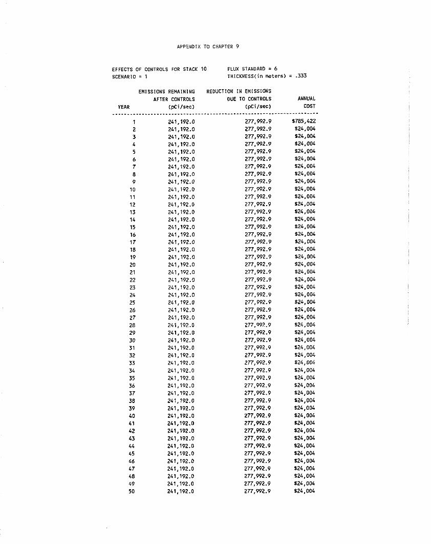
RPPENDlX TO CHAPTER 9
EFFECTS OF CONTROLS FOR STACK 10 FLUX STANDARD = 6 SCENARIO = 1 THiCKNESS(in meters)
EMISSIONS REMAINING AFTER CONTROLS
YEAR (pcilsec)
REDUCTION IN EMISSIONS DUE TO CONTROLS
(pcilsec) ....-----------.-------.**---
277.992.9 277.992.9 277.992.9 277,992.9 277,992.9 277,992.9 277,992.9 277,992.9 277,992.9 277,992.9 277.992.9 277,992.9 277.992.9 277,992.9 277,992.9 277.992.9 277,992.9 277,992.9 277,992.9 277,992.9 277,992.9 277,992.9 277,992.9 277,992.9 277,992.9 277,992.9 277,992.9 277,992.9 277.992.9 277,992.9 277,992.9 277.992.9 277,992.9 277,992.9 277,992.9 277,992.9 277.992.9 277,992.9 277,992.9 277,992.9 277.992.9 277.992.9 277,992.9 277,992.9 277.992.9 277,992.9 277,992.9 277,992.9 277,992.9 277,992.9
ANNUAL COST
* - - - - - - - - - .
1785,422 $24,004 $24,004 S24,OO.C $24,004 $24,004 $24,004 $24.004 $24,004 $24,004 $24,004 124,004 $24,004 $24,004 $24,004 $24.004 $24,004 $24,004 $24,004 124.004 $24,004 $24,004 $24,004 $24,004 $24,004 524,004 $24,004 924,004 824,004 $24,004 $24.004 $24,004 524,004 f 24,004 624,004 $24,004 $24,004 $24.004 $24,004 $24,004 $24,004 $24,004 $24.004 124,004 $24,004 $24,004 124,004 124,004 $24,004 124,004

APPEYDIX TO CHAPTER 9
EFFECTS OF CONTROLS FOR STACK 11 FLUX STANDARD = 6 SCENARIO = 1 THlCKNESS( in meters) = 333
EMISSIONS REMAINING AFTER CONTROLS
YEAR (pci/sec) ---"--"----------------------.
1 10,304,620.0 2 10,212,840.0 3 9,268,822.0 4 9,268,822.0 5 9,268,822.0 6 9,268,822.0 7 9,268,822.0 8 9,268,822.0 9 9,268,822.0 10 9,268,822.0 1 1 9,268,822.0 12 9,268,822.0 13 9,268,822.0 14 9,268,822.0 15 9,268,822.0 16 9,268,822.0 17 9,268,822.0 18 9,268,822.0 19 9,268,822.0 20 9,268,822.0 21 9,268,822.0 22 9,268,822.0 23 9,268,822.0 24 9,268,822.0 25 9,268,822.0 26 9,268,822.0 27 9.268,822.0 28 9,268,522.0 29 9,268,822.0 30 9,268,822.0 31 9,268,822.0 32 9,268,822.0 33 9,268,822.0 34 9,268,822.0 35 9,268,822.0 36 9,268,822.0 37 9,268,822.0 38 9,268,822.0 39 9,268,822.0 40 9,268,822.0 41 9,268,822.0 42 9,268,822.0 43 9,268,822.0 44 9,268,822.0 45 9,268,822.0 46 9,268,822.0 47 9,268,822.0 48 9,268,822.0 49 9,268,622.0 50 9,268,822.0
REDUCTION IN ENISSIONS DUE TO COMTROLS
(pCi/sec>
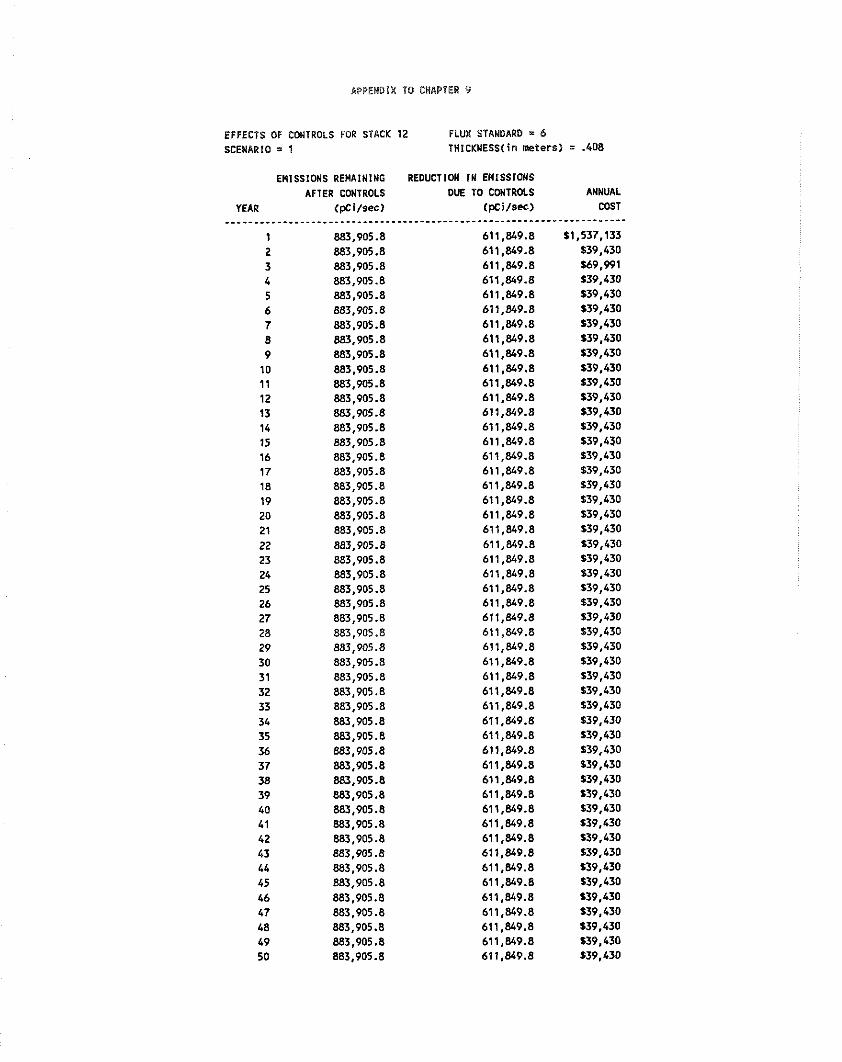
APPENDIX TO GWAPTER 9
EFFECTS OF CONTROLS FOR STACK 12 FLUX STANDARD = 6 SCENARIO 1 THICKNESS(in nx?ters) = .408
EMISSIONS REMAINING
AFTER CONTROLS YEAR (pCi/sec)
--------------.----..-------.. 1 883,905.8 2 883,905.8 3 883,905.8 4 883,905.8 5 883,905.8 6 883.905.8 7 883.905.8 8 883,905.8 9 883.905.8
10 883.905.8 11 883.905.8 12 883,905.8 13 883,905.8 14 883,905.8 15 883,905.8 16 883,905.8 17 883,905.8 18 883,905.8 19 883,905.8 20 883,905.8 21 883,905.8 22 883,905.8 23 883,905.8 24 883,905.8 25 883,905.8 26 883,905.8 27 883,905.8 28 883,905.8 29 883,905.8 30 883,905.8 31 883,905.8 32 883,905.8 33 883,905.8 34 883,905.8 35 883,905.8 36 883,905.8 37 883,905.8 U1 883,905.8 39 883,905.8 40 883,905.8 41 883,905.8 42 883,905.8 43 883,905.8 44 883,905.8 45 883,905.8 46 883,905.8 47 883,905.8 48 883,905.8 49 883,905.8 50 883,905.8
REDUCTION I N WISSIWS DUE TO CWTROLS
rpci/sec) ------------------.------.
611,849.8 611,849.8 611,849.8 611,849.8 611,849.8 611,849.8 611,849.8 611,849.8 611,849.8 611,849.8 611,849.8 611,849.8 611,849.8 611,849.8 611,849.8 611,849.8 611,849.8 611,849.8 611.849.8 611,849.8 611,849.8 61 1,849.8 611,849.8 611,849.8 611,849.8 611,849.8 611,849.8 611,849.8 611,849.8 611,849.8 611,849.8 611,849.8 611,849.8 611.849.8 611,849.8 611,849.8 611,849.8 611,849.8 611,849.8 611,849.8 611,849.8 611,849.8 611,849.8 611,849.8 611,849.8 611,849.8 611,849.8 611,849.8 611.849.8 611,849.8
ANNUAL COST
$1,537,153 $39,430 169,991 $39,430 $39,430 $39,430 $39.430 139,430 $39,430 $39.430 539,430 $39.430 $39,430 $39,430 $39,430 139,430 $39,430 $39,430 $39,430 $39,430 $39,430 $39.430 $39,430 139,430 $39,430 $39.430 139,430 $39,430 139,430 $39,430 539,430 139,430 $39.430 $39,430 $39,430 $39,430 139.430 139.430 $39.430 $39,430 $39,430 $39,430 $39,430 $39,430 $39.430 139.430 $39,430 $39.430 $39.430 539,430
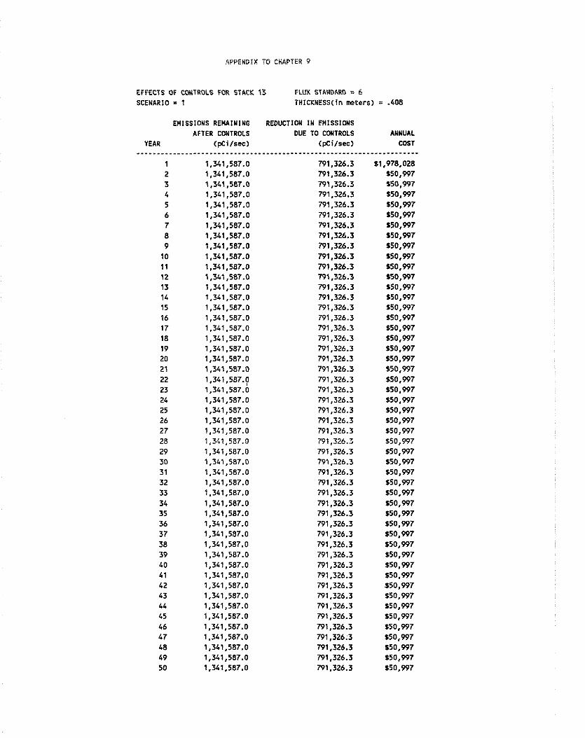
APPEMDIX 70 CHAPTER 9
EFfECTS OF CONTROLS FOR STACK 13 FLUX STRNDARD = 6 SCENARIO = 1 THICKNESSCin meters) = .408
EMISSIONS REUAlNlNG REDUCTION IN EMISSIONS AFTER CONTROLS DUE TO CONTROLS ANNUAL
YEAR (pcilsec) (pCi/sec) COST
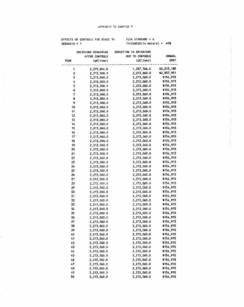
APPENDIX TO CHAPTER 9
EFFECTS OF CONTROLS FOR STACK 14 FLUX STANDARD = 6 SCENARIO = 1 THICKNESS(in meters
EMISSIONS REMAlNlNG AFTER COWTRMS
YEAR (pcilsec)
1 2,279,844.0 2 2,213.060.0 3 2,213,060.0 4 2,213,060.0 5 2,213,060.0 6 2,213,060.0 7 2,213,060.0 8 2,213,060.0 9 2.213.060.0
10 2,213,060.0 11 2,213,060.0 12 2,213,060.0 13 2,213,060.0 14 2,213,060.0 15 2,213,060.0 16 2,213,060.0 17 2,213,060.0 18 2,213,060.0 19 2,213,060.0 20 2,213,060.0 21 2,213,060.0 22 2,213,060.0 23 2,213,060.0 24 2,213,060.0 25 2,213,060.0 26 2,213.060.0 27 2,213,060.0 28 2,213,060.0 29 2,213,060.0 30 2,213,060.0 31 2,213.060.0 32 2,213,060.0 33 2,213,060.0 34 2,213,060.0 35 2,213,060.0 36 2,213,060.0 37 2,213,060.0 38 2,213,060.0 39 2,213,060.0 40 2,213,060.0 41 2,213,060.0 42 2,213.060.0 43 2,213,060.0 44 2,213,060.0 45 2,213,060.0 46 2,213,060.0 47 2,213,060.0 48 2,213.060.0 49 2,213,060.0 50 2.213.060.0
REDUCTION I N EMISSIONS DUE TO CONTROLS
(pcilsec) .---------------*-----------.
1,287,766.0 2,213,060.0 2,213,060.0 2,213,060.0 2,213,060.0 2,213,060.0 2,213,060.0 2,213,060.0 2,213,060.0 2,213,060.0 2,213,060.0 2,213,060.0 2,213,060.0 2,213,060.0 2,213,060.0 2,213,060.0 2,213,060.0 2,213,060.0 2,213,060.0 2,213,060.0 2,213,060.0 2,213,060.0 2,213,060.0 2,213,060.0 2,213,060.0 2,213,060.0 2,213,060.0 2.213,q60.0 2,213,060.0 2,213,060.0 2,213,060.0 2,213,060.0 2,213,060.0 2,213,060.0 2,213,,060.0 2,213,060.0 2,213,060.0 2.213.060.0 2,213,060.0 2,213,060;O 2,213,060.0 2,213,060.0 2,213,060.0 2,213,060.0 2,213,060.0 2,213,060.0 2,213,060.0 2,213,060.0 2.213.060.0 2,213,060.0
ANNUAL COST
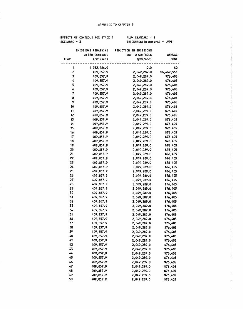
APPENDIX YO CHAPTER 9
EFFECTS OF CONTROLS FOR STACK 1 FLUX STANDARD = 2 SCEMARIO = 2 TNICKNESS<in meters) = .W5
EMISSIONS REMAINING REDUCTION IN ENlSSlONS AFTER CONTROLS DUE TO CONTROLS ANNUAL
YEAR (pCi/sec) (pCi/sec> COST
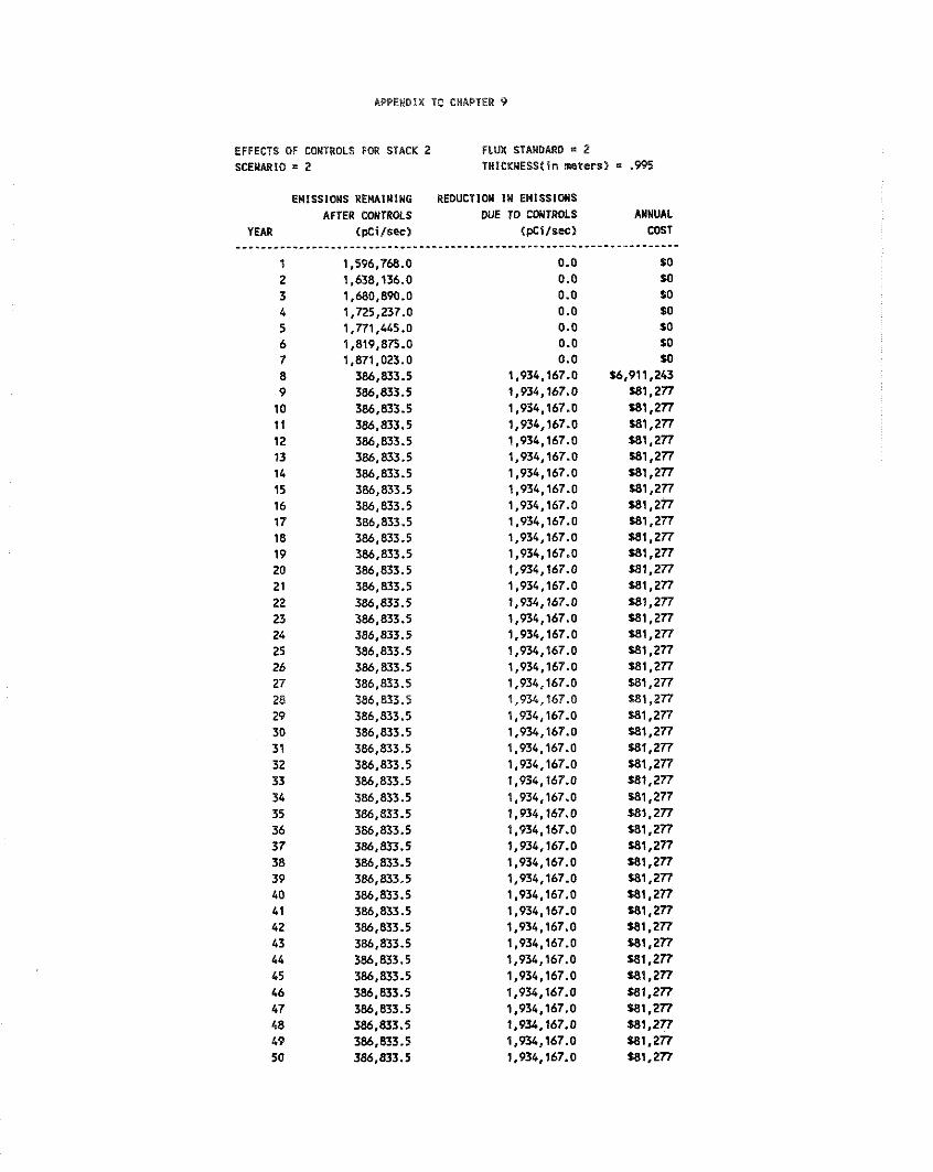
APPENDIX TO CHAPTER 9
EFFECTS OF CONTROLS FOR STACK 2 FLUX STANDARD 2 SCENARIO 2 THICKNESS(in meters) = .W5
EMISSIONS REMAINING AFTER CONTROLS
YEAR (pCil%ec) - - - . - - - - - - - - - - - * - - - * - - - - - - - - - - -
1 1,596,768.0 2 1,638,136.0 3 1,680,890.0 1 1,725,237.0 5 1,771,445.0 6 1,819.875.0 7 1,871.023.0 8 386,833.5 9 386,833.5
10 386,833.5 11 386,833.5 12 386,833.5 13 386,833.5 14 386,833.5 15 386,833.5 16 386,833.5 17 386,833.5 18 386,833.5 19 386,833.5 20 386,833.5 21 386,833.5 22 386,833.5 23 386,833.5 24 386,833.5 25 386,833.5 26 386,833.5 27 386,833.5 28 386,833.5 29 386,833.5 30 386,833.5 31 386,833.5 32 386,833.5 33 386,833.5 34 386,833.5 35 386,833.5 36 386,833.5 37 386.833.5 38 386,833.5 39 386,833.5 40 386,833.5 41 386,833.5 42 386.833.5 43 386,833.5 44 386.833.5 45 386,833.5 46 386,833.5 47 386.833.5 48 386.833.5 49 386,833.5 50 386,833.5
REDUCTION I N Enlssrms WE TO CONTROLS
<pci/s=> -*---------.----*-.*------.
0.0 0.0 0.0 0.0 0.0 0.0 0.0
1,934,167.0 1,934,167.0 1,934,167.0 1,934,167.0 1,934.167.0 1,934,167.0 1,934,167.0 1,934,167.0 1,934.167.0 1,934,167.0 1,934,167.0 1,934,167.0 1,934,167.0 1,934,167.0 1,934,167.0 1,934,167.0 1,934,167.0 1,934,167.0 1,934,167.0 1,934.167.0 1,934,167.0 1,934,167.0 1,934,167.0 1,934,167.0 1,934,167.0 1,934,167.0 1,934,167.0 1,934,167.0 1,934,167.0 1,934,167.0 1,934,167.0 1,934,167.0 1,934,167.0 1,934,167.0 1,934,167.0 1,934,167.0 1,934,167.0 1,934,167.0 1,934,167.0 1,934,167.0 1,934.167.0 1.934,167.0 1,934,167.0
ANNUAL COSY
. - --------*--
so so so so SO SO so
$6,911,243 581,277 581,277 581,277 581,277 581.277 581,277 581,277 581,277 581,277 581,277 581,277 581,277 581,277 581,277 581,277 581. 277 f81,277 S81.277 581,277 S81.277 581,277 581,277 581,ZTI S81.277 S81,277 581,277 581.277 181,277 581,277 581.277 f81,277 581.277 581,277 f81 ,277 f81.277 581,277 181,277 f81.277 581.277 581,277 581,277 581,277

APPEMDlX TO CHAPTER 9
EFFECTS OF CONTROLS FOR STACK 3 FLUX STANDARD = 2 SCENARIO = 2 THICKMESS(in meters) = .333
EMISSIONS REMAIWINC REOUCTIOW IN E M I S S I W S AFTER CONTROLS DUE TO CONTROLS ANNUAL
YEAR (pcilsec) (pcilsec) COST

EFFECTS OF CONTROLS FOR STACK 4 FLUX STANDARD = 2 SCENARIO = 2 THICKNESS(in meters) = 1.054
EMISSIONS REElPlWIWt REDUCTlOIl I N EWISSIONS AFTER CONTROLS OUE TO CONTROLS ANNUAL
YEAR ( p C i / s e c ) ( S i l s e c ) COST

APPEWDIX TO CHAPTER 9
EFFECTS OF CONTROLS FOR STACK 1 FLUX STANDARD = 6 SCENARIO = 2 THICKNESS(in meters) = .385
EUISSIONS RENAlNING AFTER CONTROLS
YEAR (~Cilsec)
1 1,932,166.0 2 1,229,574.0 3 1,229,574.0 4 1,229,574.0 5 1,229,574.0 6 1,229,574.0 7 1.229.574.0 8 1,229,574.0 9 1,229.574.0 10 1,229,574.0 1 1 1,229,574.0 12 1,229,574.0 13 1,229,574.0 14 1,229,574.0 15 1,229,574.0 16 1,229,574.0 17 1,229,574.0 18 1,229,574.0 19 1,229,574.0 20 1,229,574.0 21 1,229,574.0 22 1,229,574.0 23 1,229,574.0 24 1,229,574.0 25 1,229,574.0 26 1,229.574.0 27 1,229,574.0 28 1,229,574.0 29 1,229,574.0 30 1,229,574.0 31 1,229,576.0 32 1,229,574.0 33 1,229,574.0 34 1,229,574.0 35 1,229,574.0 36 1,229,574.0 37 1,229,574.0 38 1,229,574.0 39 1,229,574.0 40 1,229,574.0 41 1,229,574.0 42 1,229,574.0 43 1,229,574.0 44 1,229,574.0 45 1,229,574.0 46 1,229,574.0 47 1,229,574.0 48 1,229.574.0 49 1,229.574.0 50 1,229,574.0
REDUCTION i W EUISSIWS DUE TO CONTROLS
(pci/sec) . * - - - - - - - * - - - - - - - - - - - - - - - - - -
0.0 1,229,574.0 1,229,574.0 1,229,574.0 1,229,574.0 1,229,574.0 1,229.574.0 1,229.574.0 1,229,574.0 1,229,574.0 1,229,574.0 1,229,574.0 1,229,574.0 1,229,574.0 1,229,574.0 1,229,574.0 1,229,574.0 1,229,574.0 1,229,574.0 1,229,574.0 1,229,574.0 1,229,574.0 1,229,574.0 1,229,574.0 1,229,574.0 1,229,574.0 1,229,574.0 1.229,574.0 1,229,374.0 1,229.574.0 1,229,574.0 1.229.574.0 1.229.574.0 1,229,574.0 1.229.574.0 1,229,574.0 1.229.574.0 1,229,574.0 1.229.574.0 1,229,574.0 1,229,574.0 1,229,574.0 1,229,574.0 1,229,574.0 1,229.574.0 1,229,574.0 1,229.574.0 1,229.574.0 1,229,574.0 1,229,574.0
ANNUAL COST

EFFECTS OF CONTROLS FOR STACK 2 FLUX STAWDARD 6 SCENARIO = 2 THICKNESS(in nreters) = .385
EMISSIONS REMAIMING AFTER CONTROLS
YEAR CpCilsec) -----------*-----..----------.
1 1,596,768.0 2 1,638,136.0 3 1,680,890.0 4 1,725,237.0 5 1,771,445.0 6 1,819,875.0 7 1,871,023.0 8 1,160,500.0 9 1,160,500.0 10 1,160,500.0 1 1 1,160,500.0 12 1,160,500.0 13 1,160,500.0 14 1,160,500.0 15 1,160,500.0 16 1,160,500.0 17 1,160,500.0 18 1,160,500.0 19 1,160,500.0 20 1,160,500.0 21 1,160.500.0 22 1,160,500.0 23 1.160.500.0 24 1,160,500.0 25 1,160,500.0 26 1,160,500.0 27 1,160,500.0 28 1,160,500.0 29 1,160,500.0 30 1,160,500.0 31 1,160,500.0 32 1,160,500.0 33 1,160,500.0 34 1,160,500.0 35 1,160,500.0 36 1,160,500.0 37 1,160.500.0 38 1,160,500.0 39 1,160,500.0 40 1,160,500.0 41 1,160,500.0 42 1,160,500.0 43 1,160,500.0 44 1,160,500.0 45 1,160,500.0 46 1,160,500.0 47 1,160,500.0 48 1,160,500.0 49 1,160,500.0 50 1,160,500.0
REDUCTION IN EHlSSlfflS DUE TO CONTROLS
( p c i l s e c )
0.0 0.0 0.0 0.0 0.0 0.0 0.0
1.160.501.0 1,160,501.0 1,160,501.0 1,160,501.0 1,160,501.0 1,160,501.0 1,160,501.0 1,160,501.0 1,160,501.0 1,160,501.0 1,160,501.0 1,160,501.0 1,160,501.0 1,160,501.0 1,160,501.0 1,160,501.0 1,160,501.0 1,160,501.0 1,160,501.0 1,160,501.0 1,160,501 .O 1,160,501.0 1,160,501.0 1,160,501.0 1,160,501.0 1,160,501.0 1,160,501.0 1,160,501.0 1,160,501.0 1,160,501.0 1,160,501.0 1,160,501.0 1,160,501.0 1,160,501.0 1,160,501.0 1,160,501.0 1,160,501.0 1,160,501.0 1,160,501.0 1,160,501.0 1,160,501.0 1,160,501.0 1,160,501.0
ANNUAL COST
- - - - - - - - - - - - SO SO $0 so $0 so so
S3.052.193 $81,277 $81,277 $81,277 $81,277 $81,277 $81.277 $81,277 $81 ,277 $81,2?7 W1.277 $81,277 $81,277 $81,277 $81,277 $81.277 181,277 $81,277 $81,277 $81,277 ~ 1 , 2 7 7 181,277 Wl.277 $81,277 $81,277 $81.277 $81,277 W1,277 $81,277 $81.277 $81,277 $81,277 U11.277 W1,277 $81,277 $81,277 U11.277 $81,277 $81,277 $81,277 $81,277 $81,277 W1.277
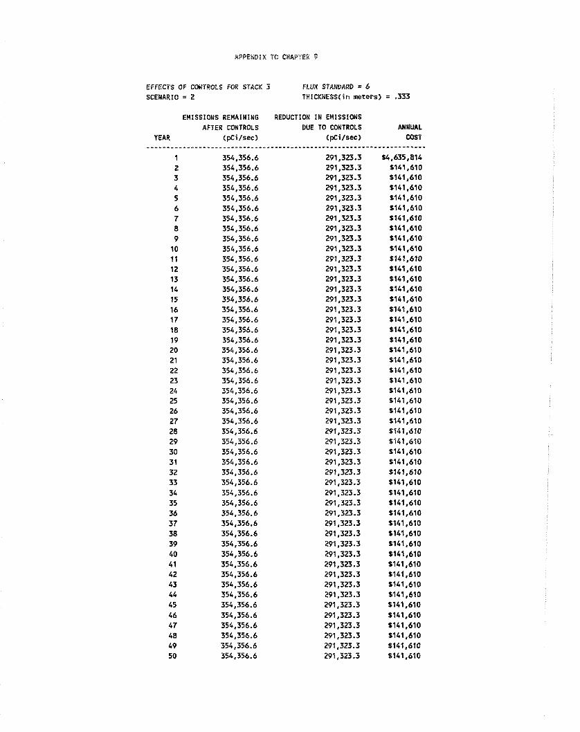
EFFECTS OF MNTROLS FOR STACK 3 FLUX STANDARD = 6 SCEWARIO = 2 TnICKUESS(in meters) = .333
EMISSlONS REHAlNlNG AFTER CONTROLS
YEAR (pc i l sec ) - - - - - * * - - - - - " * - - - - - - - " - * - - - - - - -
1 354,356.6 2 354,356.6 3 354,356.6 4 354,356.6 5 354,356.6 6 354,356.6 7 354,356.6 8 354,356.6 9 354,356.6
10 354,356.6 11 354,356.6 12 354,356.6 13 354,356.6 14 354,356.6 15 354,356.6 16 354,356.6 17 354,356.6 18 354,356.6 19 354,356.6 20 354,356.6 21 354,356.6 22 354,356.6 23 354,356.6 24 354,356.6 25 354,356.6 26 354,356.6 27 354,356.6 28 354,356.6 29 354,356.6 30 354,356.6 31 354,356.6 32 354,356.6 33 354,356.6 34 354,356.6 35 354,356.6 36 354,356.6 37 354,356.6 38 354,356.6 39 354,356.6 40 354,356.6 41 354,356.6 42 354,356.6 43 354,356.6 44 354,356.6 45 354,356.6 46 354,356.6 47 354.356.6 48 354,356.6 49 354,356.6 50 354,356.6
REDUCTION IN EMISSIONS DUE TO CONTROLS
(pci/sec) - - - - - - - - - - - * - - - - - - - - - - - - - - .
291,323.3 291,323.3 291,323.3 291,323.3 291,323.3 291,323.3 291,323.3 291,323.3 291,323.3 291,323.3 291,323.3 291,323.3 291,323.3 291,323.3 291,323.3 291,323.3 291,323.3 291,323.3 291,323.3 291,323.3 291,323.3 291,323.3 291,323.3 291,323.3 291,323.3 291,323.3 291,323.3 291,323.3 291,323.3 291,323.3 291,323.3 291,323.3 291,323.3 291,323.3 291,323.3 291,323.3 291,323.3 291,323.3 291,323.3 291,323.3 291,323.3 291,323.3 291,323.3 291,323.3 291,323.3 291,323.3 291,323.3 291,323.3 291,323.3 291,323.3
ANNUAL COST --------.---
S4.635.814 $141,610 $141,610 $141,610 $141,610 $141,610 $141,610 $141,610 S141.610 $111,610 $141,610 $141.610 t141.610 f141.610 S141,610 $141,610 $141.610 1141.610 1141.610 $141,610 $141,610 $141,610 $141,610 5141,610 $141,610 L141.610 1141.610 $141,610 5141,610 5141,610 1141.610 $141,610 $141.610 1141,610 $141.610 $141,610 $141,610 $141,610 S141.610 $141,610 $141,610 $141,610 5141.610 $141,610 $141,610 $141,610 $141,610 $141,610 5141.610 9141.610

APPEMDIX TO CHAPTER 9
EFFECTS OF CONTROLS FOR STACK 4 FLUX STANDARD = 6 SCENARIO = 2 THlCKNESS(in nreters) = .408
EMISSIONS REMAINING AFTER CONTROLS
YEAR (pcilsec)
REDUCTION IN EMlSSlONS DUE TO CONTROLS
(pCilsec) ANNUAL COST
. - - - - - - - - - - - . so
19,566,817 1246,010 1246,010 1246,010 U46.010 1246,010 1246,010 $246,010 1246,010 $246,010 $246,010 $246,010 $246.010 $246,010 $246,010 $246,010 $246.010 1246,010 $246,010 1246,010 S246,OlO 1246,010 1246,010 0246,010 $246,010 $246,010 1246,010 1246,010 1246.010 1246.010 $246.010 1246,010 1246,010 $246,010 $246,010 1246,010 $246,010 $246,010 1246.010 1246,010 1246.010 1246,010 1246.010 1246,010 1246,010 $246,010 $246,010 $246.010 $246,010

APPElQlX 10 CHAPTER 9
EFFECTS OF CONTROLS FOR STACK 5 FLUX STANDARD = 6 SCENARIO = 2 THICKNESS(in neters) = .385
EMISSIONS REMAINING AFTER CONTROLS
YEAR CpCilsec) -----------*-------.--------".
1 6,895,139.0 2 6,976,675.0 3 7,059,347.0 4 7,143,211.0 5 7,228,350.0 6 7,314,824.0 7 7,402,742.0 8 7,492,196.0 9 7,583,303.0 10 7,676,186.0 11 7,771,001.0 12 7,867,916.0 13 7,967,126.0 14 8,068,868.0 15 4,974,273.0 16 4,974.273.0 17 4,974.273.0 18 4,974.273.0 19 4,974,273.0 20 4,974.273.0 21 4,974,273.0 22 4,974,273.0 23 4,974,273.0 24 4,974,273.0 25 4,974,273.0 26 4,974,273.0 27 4,974.273.0 28 4,974.273.0 29 4,974,273.0 30 4,974,273.0 31 4,974,273.0 32 4,974,273.0 33 4,974,273.0 34 4,974,273.0 35 4.974.273.0 36 4.974.273.0 37 4,974.273.0 38 4,974,273.0 39 4,974,273.0 40 4,974,273.0 41 4,974,273.0 42 4,974,273.0 43 4,974,273.0 44 4,974.273.0 45 4,974,273.0 46 4,974,273.0 47 4,974,273.0 48 4,974,273.0 49 4,974,273.0 50 4,974,273.0
REOUCTIGU IN EMISSIONS DUE TO CONTROLS
tpCi/sec)
0.0 0.0 0.0 0.0 0.0 0.0 0.0 0.0 0.0 0.0 0.0 0.0 0.0 0.0
4,974.273.0 4,974,273.0 4,974,273.0 4,974,273.0 4,974,273.0 4,974,273.0 4,974,273.0 4,974,273.0 4,974.273.0 4,974,273.0 4,974,273.0 4,974,273.0' 4,974,273.0 4,974,273.0 4,974,273.0 4,,974,273.0 4,974,273.0 4,974,273.0 4,974,273.0 4,974,273.0 4,974.273.0 4,974,273.0 4,974.273.0 4,974,273.0 4,974,273.0 4,974,273.0 4,974.273.0 4,974,273.0 4,974,273.0 4,974,273.0 4,974.273.0 4,974,273.0 4,974,273.0 4,974,273.0 1,974,273.0 4,974,273.0
ANNUAL M)ST
SO SO $0 so SO $0 so so SO SO so SO SO $0
$13,308,340 $357,865 1357,865 5357,865 $357.865 $357,865 $357,865 1357,865 $357,865 $357,865 s357.865 5357.865 $357,865 1357,865 1357,865 1357.865 1357.865 $357,865 $357,865 $357,865 $357,865 $357.865 $357,865 $357.865 $357,865 $357.865 1357.865 s357.865 $357,865 1357,865 5357.865 1357,865 1357,865 $357.865 1357.865 S357.865
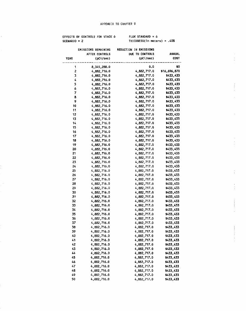
APPENDIX 10 CMAPIER 9
EFFECTS OF CWTROLS FMI STACK 6 FLUX STANDARD = 6 SCENARIO = 2 TH!CKNESS(in neters) = .408
EMISSIONS REMAINING AFTER CONTROLS
YEAR (peilsec) ------------*---------.-.-*--.
1 8,345,288.0 2 4,882,716.0 3 4,882,716.0 4 4,882,716.0 5 4,882,716.0 6 4,882,716.0 7 4,882,716.0 8 4,882,716.0 9 4,882,716.0 10 4,882,716.0 11 4,882,716.0 12 4,882,716.0 13 4,882,716.0 14 4,882.716.0 15 4,882,716.0 16 4,882,716.0 17 4,882,716.0 18 4,882,716.0 19 4,882,716.0 20 4,882,716.0 21 4,882,716.0 22 4,882,716.0 23 4,882,716.0 24 4,882,716.0 25 4,882,716.0 26 4,882,716.0 27 4,882,716.0 28 4,882,716.0 29 4,882,716.0 30 4,882,716.0 31 4,882,716.0 32 4,882.716.0 33 4,882,716.0 34 4,882.716.0 35 4,882,716.0 36 4,882,716.0 37 4,882,716.0 38 4,882,716.0 39 4,882,716.0 40 4,882,716.0 41 4,882,716.0 42 4,882,716.0 43 4,882,716.0 44 4,882,716.0 45 4,882.716.0 46 4,882,716.0 47 4,882,716.0 48 4,882,716.0 49 4,882,716.0 50 4,882,716.0
REDUCTION IN EMISSIONS DUE TO CONTROLS
(pcilsec) - - - - . - - - - - - - - - - - - - - - - - - * - -
0.0 4,882,717.0 4,882.717.0 1,882,717.0 4,882,717.0 4,882,717.0 4.W.717.0 4,882,717.0 4,882,717.0 4,882,717.0 4,882,717.0 4,882,717.0 4,882,717.0 4,882,717.0 4,882.717.0 4,882,717.0 4,882,717.0 4,882,717.0 4,882,717.0 4,882,717.0 4,882,717.0 4,882,717.0 4,882,717.0 4,882,717.0 4,882,717.0 4,882,717.0 4,882,717.0 4,882,717.0 4,882,717.0 4,882,717.0 4,882,717.0 4,882,717.0 4,882,717.0 4,882,717.0 4,882,717.0 4,882,717.0 4,882,717.0 4,882,717.0 4,882,717.0 4,882,717.0 4,882,717.0 4,882,717.0 4,882,717.0 4,882,717.0 4,882,717.0 4,882,717.0 4,882,717.0 4,882,717.0 4,882,717.0 4,882,719.0
ANNUAL COST

APPENDIX TO CHAPTER 9
EFFECTS OF COKTROLS FOR STACK 7 FLUX STANDARD = 6 SCENARIO 2 THICKNESS(in meters) = .408
EMISSIONS REMAINING AFTER CONTROLS
YEAR ( p ~ i / s e c )
REOUCTlON IN EMISSIONS DUE TO CONTROLS
(pCi/sec) -----------------------.-. 4,426,293.0 4,426,293.0 4,426,293.0 4,426,293.0 4,426,293.0 4,426,293.0 4,426,293.0 4,426,293.0 4,426,293.0 4,426,293.0 4,426,293.0 4,426,293.0 4,426,293.0 4.426.293.0 4,426,293.0 4,426,293.0 4,426,293.0 4,426.293.0 4,426,293.0 4,426,293.0 4,426,293.0 4,426,293.0 4,426,293.0 4,426,293.0 4,426,293.0 4,426,293.0 4,426,293.0 4,426,293.0 4,426,293.0 4.426.293.0 4,426,293.0 4,426,293.0 4,426,293.0 4,426,293.0 4,426,293.0 4,426,293.0 4,426,293.0 4,426,293.0 4,426,293.0 4,426,293.0 4,426,293.0 4,426,293.0 4,426,293.0 4,426,293.0 4,426,293.0 4,426,293.0 4,426.293.0 4,426,293.0 4,426,293.0 4,426,293.0
ANNUAL U M T
516,437,950 1426,823 1426,823 1426,823 1426,823 1426.823 1426.823 1426,823 1426,823 1426.823 1426.823 1426,823 1426.823 $426.823 1426,823 $426.823 1426,823 1426,823 1426,823 1426,823 1426.823 1426,823 1426,823 1426,823 1426,823 1426,823 1426,823 M26.823 %26,823 1426,823 1426,823 1426,823 1426,823 1426,823 1426.823 1426,823 1426.823 1426,823 1426,823 1426,823 1426.823 1426,823 1426,823 1426,823 1426.823 1426,823 1426,823 1426,823 1426,823 S426,823

APPENDlX 10 CHAPTER 9
EFFECTS OF CONTROLS FOR STACK 8 FLUX STANDARD = 6 SCENARIO = 2 THICKNESS(in meters) = 1.021
EMISSIONS REMAlNlNC AFTER CONTROLS
YEAR (pCilsec) --.-------------------------- 1 1,248,388.0 2 1,248,388.0 3 1,248,388.0 4 1,248,388.0 5 1,248,388.0 6 1,248,388.0 7 1,248,388.0 8 1,248,388.0 9 1,248,388.0 10 1,248,388.0 1 1 1,248.388.0 12 1,248,388.0 13 1,248,388.0 14 1,248,388.0 15 1,248,388.0 16 1,248,388.0 17 1,248,388.0 18 1,248,388.0 19 1,248,388.0 20 1,248,388.0 21 1,248,388.0 22 1,248,388.0 23 1,248,388.0 24 1,248,388.0 25 1,248,388.0 26 1,248,388.0 27 1,248,388.0 28 1,248,388.0 29 1,248,388.0 30 1,248,388.0 31 1,248,388.0 32 1,248,388.0 33 1,248,388.0 34 1,248,388.0 35 1,248,388.0 36 1,248,388.0 37 1,248,388.0 38 1,248,388.0 39 1,248,388.0 40 1,248,388.0 41 1,248,388.0 42 1,248,388.0 43 1,248,388.0 44 1,248,388.0 45 1,248,388.0 46 1,248,388.0 47 1,248,388.0 48 1,248,388.0 49 ?,248,388.0 50 1.248.388.0
REDUCTION IN EMISSIONS DUE TO CONTROLS
(pcilsec) ---*----------*---.-------.
0.0 0.0 0.0 0.0 0.0 0.0 0.0 0.0 0.0 0.0 0.0 0.0 0.0 0.0 0.0 0.0 0.0 0.0 0.0 0.0 0.0 0.0 0.0 0.0 0.0 0.0 0.0 0.0 0.0 0.0 0.0 0.0 0.0 0.0 0.0 0.0 0.0 0.0 0.0 0.0 0.0 0.0 0.0 0.0 0.0 0.0 0.0 0.0 0.0 0.0
ANNUAL COST
so SO so SO so so SO so so SO so so so so so so so so s 0 SO so so so SO so so SO so SO so SO so SO so SO so so SO SO $0 so so SO so so SO so SO SO so

APPENDIX TO CHAPTER 9
EFFECTS OF CONTROLS FOR STACK 9 FLUX STANDARD = 6 SCENARIO = 2 THICKNESS(in mterr
EHISSIONS REMAINING AFTER CONTROLS
YEAR ( p c i l s e c ) ------------------.-------.--. 1 2,041.902.0 2 2,088,362.0 3 2.136.292.0 4 2,185,900.0 5 2,237,451.0 6 2,291,285.0 7 2,347.873.0 8 1,458,635.0 9 1,458,635.0
10 1,458,635.0 11 1,458,635.0 12 1,458,635.0 13 1,458,635.0 14 1,458,635.0 15 1,458,635.0 16 1,458,635.0 17 1,458,635.0 18 1,458,635.0 19 1,458,635.0 20 1,458,635.0 21 1,458,635.0 22 1,458,635.0 23 1,458,635.0 24 1,458,635.0 25 1,458,635.0 26 1,458,635.0 27 1,458,635.0 28 1,458,635.0 29 1,458,635.0 30 1,458,635.0 31 1,458,635.0 32 1,458,635.0 33 1,458,635.0 34 1,458,635.0 35 1,458,635.0 36 1,458,635.0 37 1,458,635.0 38 1,458,635.0 39 1,458,635.0 40 1,458,635.0 41 1,458,635.0 42 1,458,635.0 43 1,458,635.0 44 1,458,635.0 45 1,458,635.0 46 1,458,635.0 47 1,458,635.0 48 1,458.635.0 49 1,458,635.0 50 1,458,635.5
REDUCTION I N EMISSIONS DUE TO CONTROLS
( p c i l s e c )
0.0 0.0 0.0 0.0 0.0 0.0 0.0
1,458,635.0 1,458,635.0 1,458,635.0 1,458,635.0 1,458,635.0 1,458,635.0 1,458,635.0 1,458,635.0 1,458,635.0 1,458,635.0 1,458,635.0 1,458,635.0 1,458,635.0 1,458,635.0 1,458,635.0 1,458,635.0 1,458,635.0 1,458,635.0 1,458,635.0 1,458,635.0 1,458,635.0 1,458,635.0 1,458,635.0 1,458,635.0 1,458,635.0 1,458,635.0 1,458,635.0 1,458,635.0 1,458,635.0 1,458,635.0 1,458,635.0 1,458,635.0 1,458,635.0 1,458,635.0 1,458,635.0 1,458,635.0 1,458,635.0 1,458,635.0 1,458,635.0 1,458,635.0 1,458,635.0 1,458,635.0 1,458,635.0
ANNUAL COST
* - - - - - - - SO SO SO so SO so M
54,910,701 $101,419 $101.419 $101,419 $101,419 0101,419 $101,419 $101,419 1101,419 1101,419 $101.419 $101.419 $101,419 $101,419 $101,419 $101.419 $101,419 $101,419 1101,419 1101,419 $101,419 $101,419 $101,419 1101,419 1101,419 $101,419 9101,419 9101.419 $101,419 $101,419 $101,419 $101,419 5101,419 $101,419 5101.419 $101,419 5101,419 1101.419 $151,419 1101.419 5101,419 1101,419 $101,419
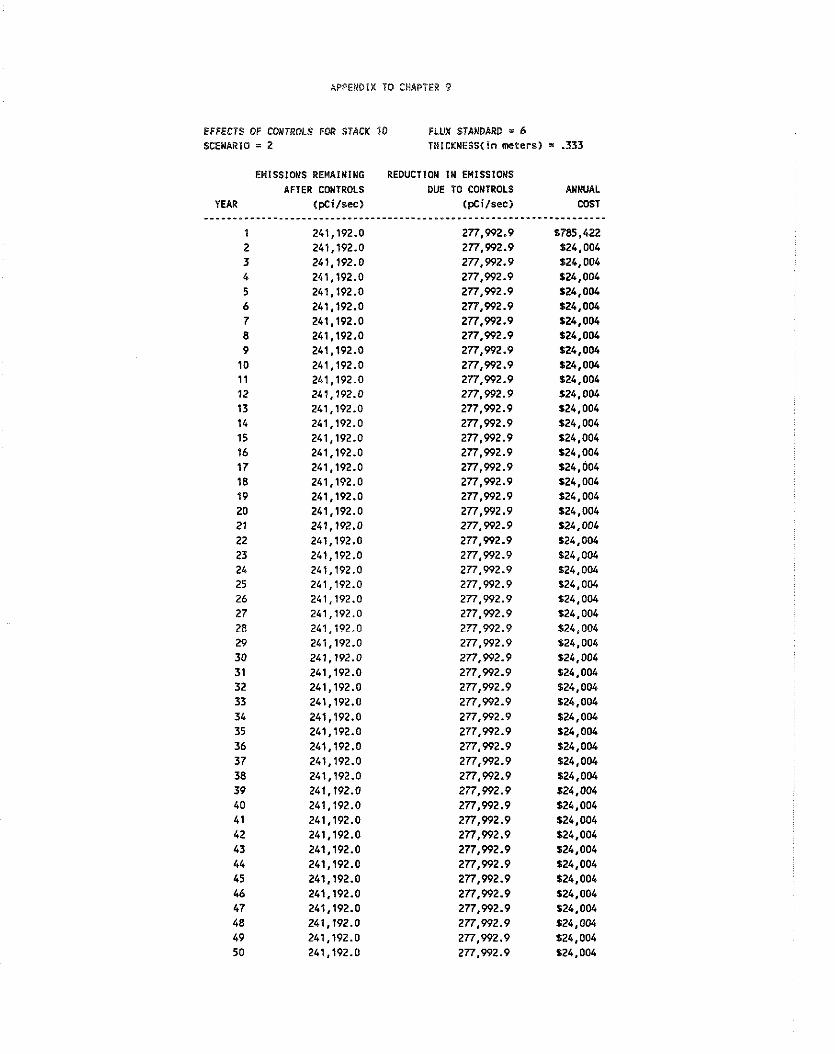
APPENDIX TO CHAPTER 9
EFFECTS OF CONTROLS FOR STACK SCENARIO = 2
EHISSlONS REHAINING AFTER CONTROLS
YEAR ( p C i l s e c )
10 FLUX STANDARD = 6 THICKNESSCin meters)
REDUCTION IN EUISSIONS DUE TO CONTROLS
(pCilsec) .-------.-.----.-...------.-*-
277.992.9 277.992.9 277,992.9 277.992.9 277,992.9 277.992.9 277.992.9 277.W2.9 277.992.9 277.992.9 277.992.9 277,992.9 277,992.9 277,992.9 277,992.9 277,992.9 277,992.9 277,992.9 277,992.9 277,992.9 277,992.9 277,W2.9 277,992.9 277.992.9 277,992.9 277.992.9 277,992.9 277,992.9 277.992.9 277,992.9 277,992.9 277,992.9 277,992.9 277,992.9 277,992.9 277.992.9 277.992.9 277,992.9 277,992.9 277,992.9 277.992.9 277.992.9 277.992.9 277.992.9 277.992.9 277,992.9 277.992.9 277.992.9 277.992.9 277.992.9
= .333
ANNUAL COST
- - - - - - - - - - - 1785,422 $24.004 $24,004 $24.004 $24,004 524,004 $24,004 $24,004 $24,004 $24,004 $24.004 $24.004 124,004 $24,004 124.004 $24,004 $24,004 $24.004 124,004 124,004 $24.004 $24,004 124,004 S24.004 324,004 124,004 324,004 $24,004 $24.004 324,004 $24,004 124,004 124,004 $24.004 124,004 124.004 $24,004 $24.004 $24,004 124,004 $24.004 524,004 $24,004 $24,004 $24.004 124,004 $24,004 124,004 $24.004 324.004
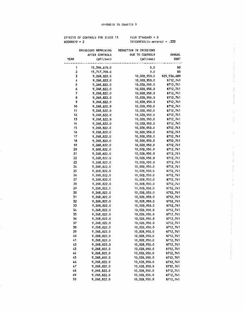
APPENDIX TO CHAPTER 9
EFFECTS OF CONTROLS FOR STACK 11 SCENARIO = 2
EMISSIONS REMAINING REOUC AFTER CONTROLS
YEAR (pCi/sec) - - - * - - - - - - - - - - . - - - - - - - - - * - * - - - - - - - - * .
1 15,396,670.0 2 15.747.700.0 3 9,268,822.0 4 9,268,822.0 5 9,268.822.0 6 9,268,822.0 7 9,268,822.0 8 9,268,822.0 9 9,268,822.0
10 9,268,822.0 11 9,268,822.0 12 9,268,822.0 13 9,268,822.0 14 9,268,822.0 15 9,268,822.0 16 9,268,822.0 17 9,268,822.0 18 9,268,822.0 19 9,268,822.0 20 9,268,822.0 21 9,268,822.0 22 9,268,822.0 23 9,268,822.0 24 9,268,822.0 25 9,268,822.0 26 9,268,822.0 27 9,268,822.0 28 9,268,822.0 29 9,268,822.0 30 9,268,822.0 31 9,268,822.0 32 9,268,822.0 33 9,268,822.0 34 9,268,822.0 35 9,268,822.0 36 9,268,822.0 37 9,268,822.0 38 9,268,822.0 39 9,268,822.0 4 0 9,268,822.0 4 1 9,268,822.0 42 9,268,822.0 43 9,268,822.0 44 9,268,822.0 45 9,268,822.0 46 9,268,822.0 47 9,268,822.0 48 9,268,822.0 49 9,268,822.0 50 9,268,822.0
FLUX STANDARD = 6 TnlCKNESS(in nrters) = .333
:TION IN EMISSIONS DUE TO CONTROLS ANNUAL
(pCi lsec) COST
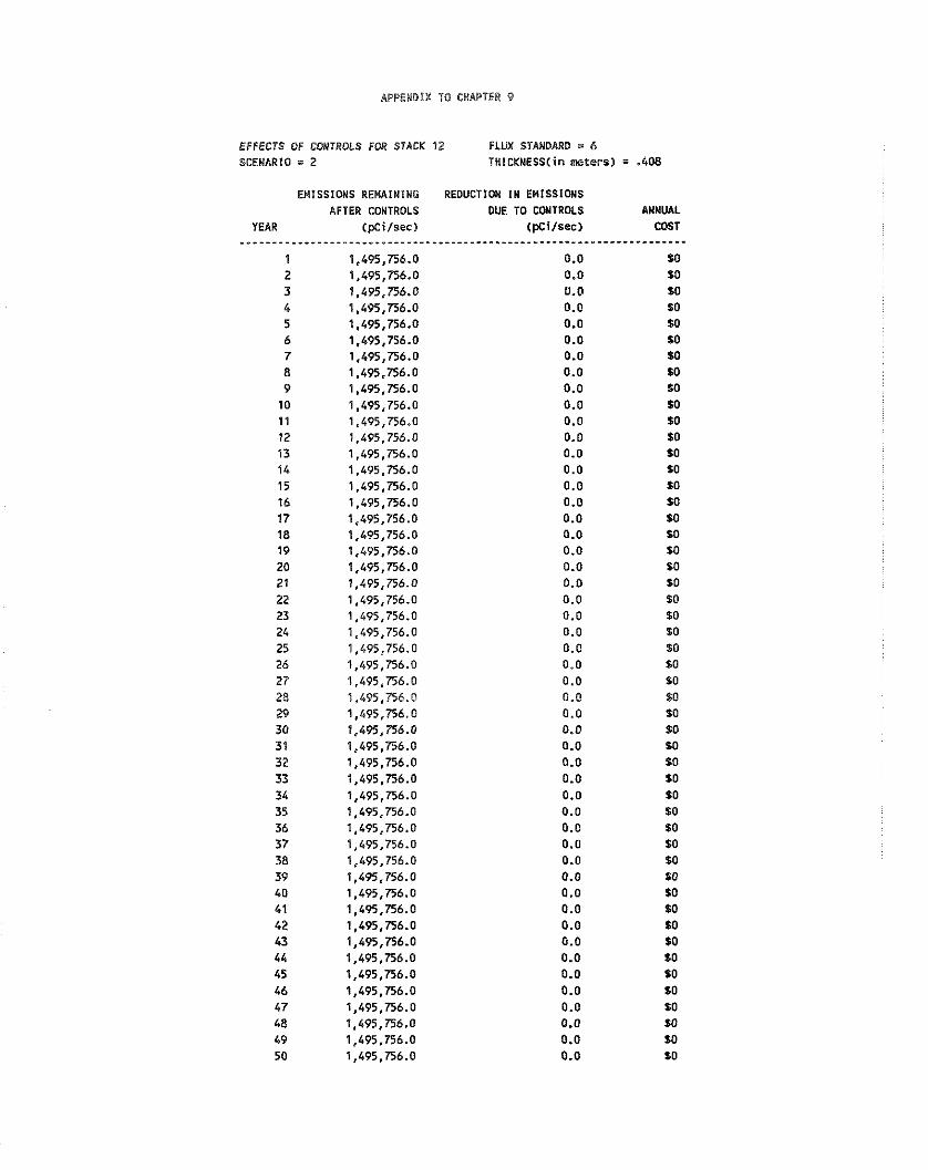
APPENDIX TO CHAPTER 9
EFFECTS OF COWTROLS F D R STACK 12 FLUX STANDARD = 6 SCENARIO = 2 THICKNESS(in meters) = .408
EMISSIONS REMAlNlNG AFTER CONTROLS
YEAR (pCi/sec> --*----.-**----- .------------ .
1 1,495,756.0 2 1,495,756.0 3 1,495,756.0 4 1,495,756.0 5 1,495,756.0 6 1,495,756.0 7 1,495,756.0 8 1,495,756.0 9 1,495,756.0 10 1,495,756.0 1 1 1,495,756.0 12 1,495,756.0 13 1,495,756.0 14 1,495,756.0 15 1,495,756.0 16 1.495.756.0 17 1,495,756.0 18 1,495,756.0 19 1,495,756.0 20 1,495,756.0 21 1,495,756.0 22 1,495,756.0 23 1,495,756.0 24 1,495,756.0 25 1,495,756.0 26 1,495,756.0 27 1,495,756.0 28 t,&95,756.0 29 1,695.756.0 30 1.495,756.0 31 1,495,756.0 32 1,495,756.0 33 1,495,756.0 34 1,495,756.0 35 1,495,756.0 36 1,495,756.0 37 1,495,756.0 38 1,495,756.0 39 1,495,756.0 40 1,495,756.0 41 1,495,756.0 42 1,495,756.0 43 1,495,756.0 44 1,495,756.0 45 1,495,756.0 46 1,495,756.0 47 1,495,756.0 48 1,495,756.0 49 1.495.756.0 50 1,495,756.0
REDUCTION I N EHISSIONS OUE TO CONTROLS
(pcilsec) ANMUAL COST
. - - - - - - - - - - SO SO w so so so SO so SO SO so s 0 SO so SO so so SO SO SO so so $0 $0 $0 SO SO SO so so so so so so so so so so so so SO so SO so so SO SO so so so

IPPEMDlX TO CHAPTER 9
EFFECTS OF CONTROLS FOR STACK 13 FLUX STANDARD = 6 SCENARIO = 2 TnlCKNESS(in meters) = .408
EMISSIONS REMAINING REDUCTION IN EHISSIONS AFTER CONTROLS DUE TO CONTROLS ANNUAL
YEAR (pCifsec) (pcilsec) COST
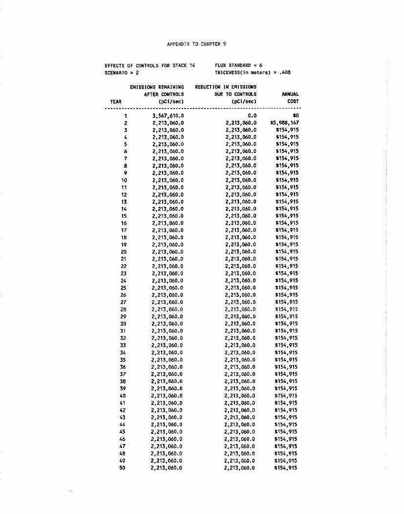
APPENDIX TO CHAPTER 9
EFFECTS OF CONTROLS FOR STACK 14 FLUX STANDARD = 6 SCENARIO = 2 THICKNESS(in meters) = .108
EMISSIONS REMAINiNC AFTER CONTROLS
YEAR (pCi/sec) - - - - -* - - - - -* - - - - - - - - - - - - - - - - .
1 3,567,610.0 2 2,213,060.0 3 2,213,060.0 4 2,213,060.0 5 2,213,060.0 6 2,213,060.0 7 2,213,060.0 8 2,213,060.0 9 2,213,060.0
10 2,213,060.0 11 2,213,060.0 12 2,213,060.0 13 2,213.060.0 14 2,213,060.0 15 2,213,060.0 16 2,213,060.0 17 2,213,060.0 18 2,213,060.0 19 2,213,060.0 20 2,213,060.0 21 2,213,060.0 22 2,213,060.0 23 2,213,060.0 24 2,213,060.0 25 2,213,060.0 26 2,213,060.0 27 2,213,060.0 28 2,213,060.0 29 2,213,060.0 30 2,213,060.0 31 2,213,060.0 32 2,213,060.0 33 2,213,060.0 34 2,213,060.0 35 2,213,060.0 36 2,213,060.0 37 2,213,060.0 38 2,213,060.0 39 2,213,060.0 40 2,213,060.0 41 2,213,060.0 42 2,213,060.0 43 2,213,060.0 44 2,213,060.0 45 2,213,060.0 46 2,213,060.0 47 2,213,060.0 48 2,213,060.0 49 2,213,060.0 50 2,213,060.0
REDUCTION I N EMlSSlONS DUE TO CONTROLS
( p c i l ~ e c ) ANNUAL
COST . - - - - - - - - - - - - -
$0 $5,988,147
5154.915 1154,915 $154,915 1154.915 $154.915 $154,915 $154,915 $154,915 $154,915 $154.915 $154,915 $154,915 $154,915 $154.915 $154,915 $154,915 1154,915 $154.915 $154,915 $154,915 $154,915 $154,915 1154,915 $154.915 $154,915 1154,915 $154.915 $154,915 1154.915 1154,915 $154,915 $154,915 $154.915 $154,915 1154,915 $154.915 $154,915 $154.915 1154.915 $154,915 $154,915 $154,915 $154,915 $154,915 $154,915 $154.915 $154,915 $154,915


Appendix B:

Av~endix B: Description Of The Trade Forecasting hlodel
9.B.I Introduction
Many uncertainties exist in forecasting the supply and demand of WPPA. The model that was
developed uses various supply, demand, and cost forecasts in an attempt to test the competitiveness
of the United States phosphate industry over the next 30 years. The data used includes:
I) Plant specific cost and capacity data for 32 plants in the US., Morocco, Tunisia, Senegal,
Israel, and Jordan. This data, from a study by Zellars-Williams, [ZE86] includes detailed
production costs and supply forecasts until 2005. The regions of the world covered by this
data include all regions that are significant net exporters of phosphoric acid and phosphate
fertilizers.
2) A consumption forecast by region through 2010 by Wharton Econometric Forecasting
Associates [WEFASS].
3) Freight forecasts by Zellars-Williams through 2005 from the major exporters to the major
importers.
4) Alternative rock mining costs from a U.S. Bureau of Mines study by R. Fantel, William
Stowasser and others [Fags].
With the exception of WEFA's consumption forecast, all of the forecasts do not go beyond 2005.
Therefore some limited assumptions were made to extend the forecasts to the year 2018. Various
modifications to the data sources listed above were also necessary to reconcile the data sources. All
of these modifications and the operation of the model are described below.
WPPA is sold in several different forms. Some countries purchase the acid and domestically produce
various fertilizers, while other countries purchase finished fertilizers. For simplicity, the model
focuses only on the comparative cost of producing phosphoric acid and does not consider the cost of
producing specific fertilizers, such as diammonium phosphate and triple superphosphate.
The purpose of the model is to identify the low cost suppliers for each importing region over the next
thirty years. The mode1 considers six regions: Latin America, Western Europe, Eastern Europe, South
Central Asia, East Asia, and Oceania. There are three exporting regions which are North America,
Africa, and West Asia. Below is a description of the calculations made for the years 1985, 1990,
1995, 2000, 2005, and 2018.
9.8.2 hfodel Structure
The model begins by comparing the quantity of phosphoric acid each importing region needs lo
import to satisfy its demand and the cost of each exporting plant. The appropriate transportation cost
is added into the plants' production cost to represent the final cost for that particular exporting
country. The model ranks suppliers for each importing region, from the lowest to the highest cost
supplier. The supply is then distributed in each region, beginning with the lowest cost supplier, until
all demand is satisfied. In this way each supplier is assumed to maximize profits by first supplying
those regions where its costs are the lowest.
Several alterations were made to the data that is used in the model. First, the Zellars-Williams supply
forecast included Turkey in its Western Europe figures, whereas the WEFA consumption forecast
included Turkey in its Asian figures. In addition, WEFA and Zellars-Williams organized Asian
supply and demand differently. Section 9.B.3 describes how the data was modified.
WEFA's consumption figures were extended to 2018 by taking the 2010 figures and using the WEFA
1.9 percent annual growth rate forecast for consumption until 2010.
The Zellars-Williams supply forecast was extremely conservative, predicting increases only where
firm plans had been announced at the time the forecast was made. As a result, many regions showed
only very slight increases after 1995 despite highly favorable production conditions. Under Zeflars-
Williams' cautious supply forecast, world supply increases from 34 million metric tons in 1985 to 37
million in 1995 and drops to 34 million in 2005. In comparison, WEFA's consumption forecast
increases from 33 million in 1985 to 38.5 in 1995 to 45.6 million in 2005. Zellars-Williams'
consumption forecast is even higher, 59.8 million in 2005 IZE861. Consequently, Zellars-Williams"
supply forecast was revised to increase at a rate comparable to the increase in world demand. More
detail on the assumptions made in revising their supply estimates are given in section 9.B.4.
Production capacities and costs for individual phosphoric acid plants were taken from a Zellars-
Williams' study [ZE86]. All United States plants were included except for two: Arcadian's plant in
Geismar, Louisiana and Mississippi Chemical Co. plant in Pascagoula, Mississippi. Capacities for
these two plants were obtained from the Tennessee Valley Authority, [TVA88] and their costs were
assumed to be the same as those for Mobil's plant in Pasadena, Texas.

Kueu u! sue!l l !~-slel laz moij alqel!eAe sem e l e a '5661 ~ a l j e %u!le~ado aq ll!ls ll!m leql sau!w a ~ ! j s e
pue SaAJasai y 3 0 ~ aleqdsoqd umo sa!ueduros amos 'lood ep!lo[d leI lua3 aql wor j sawos ysor asoqm
slueid ol pa!ldde pue palem!,sa sem aspd ys01 aql s!q~ wor j pue 'vdd,+j 10j ~ s e s a ~ o j Klddns aql w o r j
palelnsles sem oooz u! papaau ysor 30 lunome a q l '[sged] lsos JO sa8ue1 u!elras u!ql!.n a(qe[!ei\e
ysor j o Ki!iuenb aq] saleuqsa q s y m uosrajad pue lalued 'rassemols Kq Kpnls s a u ! ~ J O neaina
's'n e u o r j uayei alam salem!lsa s o 3 7301 'sasrnosal mau wor j slsos ysoi aleqdsoqd aql a$eu!lsa 01
'padolahap aq 01 paau sasJnosar ysoi K)!lenb lam01 'mau pue palaldap auosaq saArasar is03 .no( plo se
'5661 u! 8u!uu!Saq ' e p ! ~ o ~ u! sisos 7301 ~aq8!q 13a[jal oj paseamu! alam sjso3 uo!l3npo~d 'ase3 laq io
aql UI 'swe![1!~-srellaz Lq pajsesaroj se a1aM slsos 'ases auo u1 .ep!Jo[d [elluas w o r j ysor Iraq3
u!elqo qs!qm '5.n aql u! palesol sjueid r o j so!Jeuass is03 luaIajJ!p om] lapun unr scm l apou a q l
.slueld ' ~ n Suome sa~nso l s aulos lsadxa
Klsno!~qo Kaql s!sKleue i!aql u! '1a~amoH ' S O O ~ Kq as013 iq%!ur slueid q s ! q ~ ssan8 01 % u ! ~ e q p!oAe 01 raqs!q s!qr ie sa!r!sedes J!j!sadS lueld ]day sme!1[!,+j-sre[laZ teqj Klay!( s! 11 .suol s!rraru
0 0 0 ' ~ 8 0 ' ~ I aq plnom K~!~edes sales!pu! elep s!j!sads lueld i!aql q8noql 'Ki!sedes JO suoi s!rlam
000'906'8 01 sllej es!ramv q i i o ~ JOJ Al!sedes pa~eu!isa .swe!il!M-sie1laZ ' $ 0 0 ~ leak aql IOJ srsesaioj
W d n s 's'n ale8al8Se .rure![l!M-slellaZ u! ' J a~amoH 'sasearsap l o sasearsu! ou a le a ~ a q l 000;
PuoAaq inq oooz arojaq sarea~su! Kl!sede~ ' s u o ! ~ ~ ~ [ o J ~ , s m e ! l ~ ! ~ - s r e l l a ~ u! slueid ~!j!3adS 103 '500: ~ o j slsesaloj srue!l[!,+j-sre[[az aqr se awcs aql aq 08 paunsse a.iam 8 1 0 ~ u! sa!l!~edes uo!l3npo1d 's'n
.paAa!qse
aq ll!m a l e x j o s a y o u o s a pue sa!uouosa aArns Bu!urea[ pue pa ln icu Kllnj aAeq [[!M sralrodxa 's'n -uou jo sa!r]snpu! aleqdsoqd aq) sooz ,iq asnesaq alqeuosear s! s!ql ' ~ 0 0 ~ U! se a w m aql u!euai
or paunsse aram slsos ' ~ 0 0 ~ pue 5861 uaamlaq (s~el lop luelsuos u!) 8u!u![sap ajam slsos qs!qm u!
slueld '5.n-uou i o j ' 5 0 0 ~ pue 5861 uaanlaq iuap!na asealsu! j o ale1 a q ~ 8u!nu!luos Kq sooz WOJJ
8 1 0 ~ 01 lno palsarord arazh slueid 'Sn Ile JOJ slsos ' ~ ' 8 . 6 uo!lsas u! paq!Jssap suo!ldasxa a u o s ql!M
.uo!8a1 ~ e q i l o j lSo3 a 8 e i a ~ e aql le asnpold 01 paunsse ale slueld al!sodruo>
asaqJ. .uo!Sai ]eq] u! slueld WOJJ Klddns leuo!l?ppe aq] j o wns aql luasaldar qs!qm pappe aJam -- e!sv lsafi JaqlO pue e3!1jv r aq to -- slucld al!sodwo3 o m ~ 'suo!leu B U ! ] J O ~ X ~ y n - u o u ~ o r e ~ aq)
are qs!qm ' laers~ pue 'uepJor 'le8auaS 'e!s!unl '0330~0pJ JOJ a(qel!eile osle sem elep s!j!sads meld
' s a ~ n 8 l j s!aq) u? papnpu! epeuea aheq s1se3a.10~ u w ! ~ a w v q l ~ o ~ i1e
asncaaq Aluo papnlsur ale slueid om] a s a q l .Lf?mqanv K a l l e ~ aassauual aql WOIJ pau!clqo osle a1a.n
epeue3 JOJ s(aAal Kl!3ede~ uo!l3npo~d .uo?j3npoid uelpeuva ~ a q ~ o lie ~ u a s a ~ d a ~ oa pappr: seM epeuea
r a q i o pallea jueld a)!soduro3 e pue 'Aprils ,sure!ll?fi-sJellaZ aq) u! papnjsu? scm l u ~ i d uc!pcue3 a u o
of these cases and Zellars-Wiliiams' estimate of the cost to the company of mining its own rock was
used.
The second scenario of the model allowed for significantly higher rock mining costs for a variety of
U.S. plants. The U.S. plants were divided into two groups according to where their rock is supplied.
Plants receiving rock from central Florida were given rock costs in line with the Stowasser study
described earlier. The range of rock costs found in the Zellars-Williams cost data was maintained
but each plant's rock costs were increased by a similar proportion so that the average rock costs
corresponded to Stowasser's forecast. The exhaustion of cheaper rock begins in the 1995 period and
the full costs are attributed by the year 2000. The higher rock costs were incorporated into the total
WPPA costs by assuming 3.55 tons of rock are used per metric ton of WPPA produced.
9.8.3 Distribution of Exoorters Total Suooly
When distributing a plant's production among several regions, the model makes a few simple
assumptions. First, if supplier X can competitively supply four different regions and, for example,
X ranks third in all four regions, then each region receives an equal portion of supplier X's
production. If supplier X then appears fourth on another region's ranking, that region will receive
nothing from supplier X because X's production will have already been sold for that year.
In the non-U.S. net exporting regions, Africa and West Asia, domestic demand is assumed to be
supplied by the many other plants in those countries for which plant specific costs are not available.
Other excess capacity in those countries was assigned to composite plants called Other Africa or Other
West Asia. The cost attributed to this other production is the average of all the individual costs for
that region. This production is also available for export.
If supplier X is a non-U.S. producer, then all of its production will be exported.
For North America, a different assumption is made because cost data is available for all but two small
plants, and supply is expected to fall rather than increase. In the case where supplier X is a U.S.
plant and X is the third lowest cost supplier in four regions, the supply available from X is divided
by 6, with one share going to each of the four importing regions, and two shares going to the U.S.
market. The U.S. market always gets two shares, which assumes each producer continues to be
actively involved in the large U.S. market. This assumption is consistent with American producer's
past behavior.

9.8.4 Modifications to Zellars-Williams and WEFA Data
The Zellars-\Villiams supply forecast was altered so that Turkey appeared in its West Asia figures.
Because Turkey has some indigenous phosphate rock supply, Turkey's supply was forecasted to
decline at only half the rate of decline forecast for Western Europe. Turkey's supply was then
subtracted from the Western European figure and added to the West Asia figure.
WEFA's consumption forecast included all of Asia in one figure, whereas Zellars-Williams divided
Asia into East, West, and South Central. The following method was used to divide WEFA's Asian
consumption forecast. First, Turkey's consumption was calculated by taking their 1985 consumption
and using WEFA's annual growth rates to forecast their consumption. A growth rate of 2.1 percent
was used through 1995 and 1.9 percent was used thereafter. Next, Turkey's consumption figures
were added to Zellars-Williams' West Asia consumption figures. Third, the percent of total Asian
consumption represented by each region of Asia was calculated using the Zellars-Williams
consumption figures, which were constant for all of the forecasted years. These percentages were
then applied to the WEFA Asian consumption forecasts to derive the final subdivided Asian
consumption forecasts.
As explained earlier, Zellars-Williams' supply forecast was modified to allow for new plant
construction that has not already been announced. Special attention was given to how the new supply
was distributed among existing producing countries. The regional trends in production levels
identified by Zellars-Williams between 1985 and 1990 were projected to continue in future years.
Had the rate of growth between 1985 and 1990 been used, however, an unrealistically high supply
level would have been forecasted. Instead, the WEFA projected rate of growth of demand was used.
This assumes that, in the long run, supply and demand will grow at the same rate. Those regions
experiencing growth in capacity between 1985 and 1990 were assumed to continue to have high rates
of growth in the coming decade. These countries, such as Morocco, are also the countries that have
substantial demonstrated phosphate rock reserves. The specific steps to calculate each region's supply
are described below:
1 ) The increase in world supply between 1985 and 1990 was estimated and each region was
allocated its proportion of that supply. As in: (A-B)/C; where:
A=1990 regional forecast.
B=1985 regional forecast.
C=Net new world supply between 1985 and 1990.
2) The world supply of phosphoric acid after 1990 was estimated by using a 2.1 percent
annual growth rate until 199.5 and 1.9 percent thereafter.

CHAPTER 10
COAL- FIRED BOILERS

10. COAL-FIRED BOILERS
10.1 I~tlroduction atid Summary
On November 8, 1979 the Environmental Protection Agency listed radionuclides as a hazardous air
pollutant under the provisions of section 112 of the Clean Air Act. Subsequently, EPA investigated
the necessity of regulating coal-fired boilers in the utility and industrial sectors. These two types of
boilers account for approximately 90 percent of the heat generated by burning coal. The remaining
10 percent is generated by residential and commercial boilers for the purpose of space and water
heating. For this analysis, only coal-fired utility and industrial boilers will be considered.
The coal used to fire boilers contains radionuclides and their daughter products which are not
destroyed during combustion. Instead, the radionuclides attach themselves to particulate emissions
and are either removed from the exhaust with control devices or released into the air.
Currently, there are no Federal or state regulations specifically limiting the emissions of radionuclides
from coal-fired industrial boilers. However, air emissions from coal-burning facilities are regulated
by state and Federal guidelines designed to meet the ambient standardsset forth by the Federal Clean
Air Act. These standards affect several pollutants emitted by coal-burning facilities, in particular
particles 10 microns or less in diameter (PMIO), sulfur dioxide, oxides of nitrogen, CO and lead (40
CFR 50.6, 50.7, 50.8, 50.1 I , 50.12). Emissions of radionuclides are positively correlated to emissions
of particulate matter; therefore, regulations governing particulate matter emissions also control
radionuclide emissions. These regulations include: the PMlO ambient standard, prevention of
significant deterioration, new source performance standards, and state air quality implementation
olans.
10.2 Industry Profile
The main function of large coal-fired boilers in the utility sector is the generation of electricity.
Industry, however, depends upon coal-fired boilers for the production of process steam, space
heating, and other industrial purposes. Information on utility boilers is far more complete, accurate,
and accessible than that on industrial boilers. The furnaces and coal used by both sectors, and
therefore the emissions created, are highly similar. There are, however, some differences in the
boilers used.

lO.2.l Demand
In 1982, approxinlately 20 percent of the United States' energy needs were met by burning coal. Of
the coal used, 74 percent was used to generate electricity and 24 percent was used by industry for
purposes other than the generation of electricity [EIABS]. For both industrial and utility applications
bituminous, sub-bituminous, and lignite coals are used more often than anthracite coal. Although
natural gas, oil, and nuclear fission can be used to generate electricity, the combined use of these
energy sources in the generation of electricity has declined in recent years. It is expected that coal
will supply more than half of the electricity generated in the United States in the foreseeable future.
On average, the United States coal mines provide more than 16 million tons of coal per week. This
amount fluctuates greatly, ranging from 20 million tons per week to less than 10 million. Coal
production can decrease for a variety of reasons, ranging from weather to miners' strikes and
vacations [EIA87].
The three primary coal producing regions in the United States are the western, interior, and
Appalachian regions. In 1985, in terms of quantity of coal produced, the Appalachian region was
the most productive, followed by the western and interior regions. In that year, the Appalachian
region produced 427.2 million short tons of coal, valued at 13.8 billion dollars. The western region
produced 268.7 short tons of coal at a value of 3.9 billion dollars. Coal production in the interior
region in 1985 was 187.8 million short tons valued at 4.6 billion dollars [EIA87].
10.2.3 Industrv Structure and Profile
In 1986, there were approxiniately 1200 coal-fired utility boilers in the United States, with a net
generating capacity of 305 giga-watts (GW) [EIA85]. There are three types of power plants designed
to operate and serve three load classes: base load, intermediate load, and peaking plants. Base load
power plants operate near full capacity most of the time. Intermediate load plants operate a t varying
levels of capacity each day. Finally, peaking plants operate only during periods of high demand,
about 700-800 hours a year. Coal-fired utility boilers are primarily used in base and intermediate
load plants. Coal is rarely the primary fuel for a peaking plant.

There are three general types of coal-firing utility boilers: stoker furnaces, cyclone furnaces, and
pulverized-coat furnaces. Stoker furnaces are usunlly small, older boilers ranging in capacity from
7.3 to 73 mega-watts (MW). Stoker furnaces require about 3.3 kg of coal per kilowatt-hour and are
less efficient than furnaces handling pulverized coal. Cyclone furnaces are high temperature
con~bustion chambers for burning crushed coal. As of 1974, only 9 percent of the coal-fired utility
boiler capacity was of the cyclone type, and no boilers of this kind have been ordered by utilities in
the past seven years [Co75]. Pulverized coal furnaces burn coal that has been pulverized to a fine
powder. A carefully proportioned mixture of pulverized coal and air is injected into the combustion
zone. The pulverized coal-fired boiler is now the most prevalent type of coal-burning unit in the
utility sector. There are two types of pulverized coal-fired boilers; dry bottom and wet bottom. Dry
bottom are the most prevalent, with 76 percent of the coal-firing utility boilers being of this type.
Of the remaining coal-firing utility boilers, I I percent are pulverized wet bottom, 1 1 percent are
cyclone, and 2 percent are stoker. The amount and type of residue produced when coal is burned
differs with the type of furnace and coal used. As coal is burned, the minerals in the coal melt and
condense into a glass-like ash; the quantity of ash depends upon the mineral content of the coal. A
portion of the ash settles to the bottom of the boiler, bottom ash, and the remainder enters the flue,
fly ash. The distribution between bottom ash and fly ash depends upon the firing method, the ash
fusion temperature of the coal, and the type of boiler bottom, wet or dry. Table 10-1 displays the
percent of fly and bottom ash produced by various types of coal and furnaces.
Coal-fired industrial boilers are used primarily to produce process steam, generate electricity for the
industry's on-site use, and provide space and water heat. Boilers are used in almost all industries;
however, the primary users are smelters, steel, aluminum, and copper manufacturers, pulp and paper
manufacturers, and the chemical industry. There are three main types of boilers used in the
industrial sector. These are: water tube, fire tube, and cast iron. Water tube boilers heat the water
to a high-pressure, high-temperature steam by passing the water through tubes which are heated
externally by contact with high combustion gases. Fire tube and cast iron boilers heat the water by
transferring heat from the hot gases inside the tubes to circulating water outside the tubes. The only
difference between the two types is that cast iron is used in the construction of the tubes instead of
steel which is used in fire tube boilers. Table 10-2 displays the number and capacity of industrial
boilers in the United States. There are two main types of furnaces used for industrial coal-fired
boilers. These are the pulverized coal furnace and the stoker furnace, as described in the previous
text.

Table: 10-1: Coal Ash Dlstributlon by Boiler Type.
Percent Flv AshlPereent Bottom Ash
Furnace Type Bituminous Lignite Anthracite
Pulverized Dry Bottom 80120 35/65 85/15
Pulverized Wet Bottom 65/35
Cyclone 13.5186.5 30170
Stoker 60140 35/65 5/95
SOURCE: [Me861
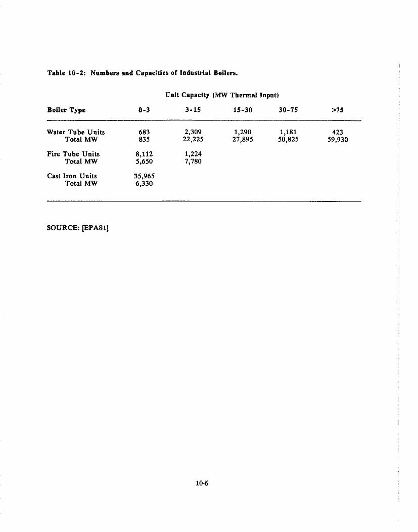
Table 10-2: Numbers and Caparlties of lndustrlal Boilers.
Unit Capacity (MW Thermal Input)
Boiler Type 0-3 3-15 15-30 30-75 >75
Water Tube Units 683 2,309 1,290 1,181 423 Total MW 835 22,225 27,895 50,825 59,930
Fire Tube Units 8,112 1,224 Total MW 5,650 7,780
Cast Iron Units 35,965 Total MW 6,330
SOURCE: [EPA81]
10.3 Curreut Emissions, Risk Levels, and Fensible Control b'lethods
Coal contains mineral matter, including sninll quantities of naturally occurring radionuclides. The
radionuclides of primary interest are uranium-238 and thorium-232 as well as their decay products,
Po-210 and Pb-210. Table 10-3 shows the uranium and thorium content in different types of coal.
In addition to the concentration of mineral matter, several other factors have substantial influence
upon the harmful emissions from coal-fired boilers. These factors include furnace design, capacity,
heat rate, and ash partitioning. Ash partitioning, or the proportion of ash that is fly ash versus
bottom ash, is a function of the firing method, type of coal, and type of furnace used.
10.3.2 Current E~nissions and Estimated Risk
Measurements have shown that certain radionuclides are partitioned unequally between bottom and
fly ash jBe78, Wa821. One explanation for this phenomenon is that certain elements are preferentially
concentrated on the particle surfaces, resulting in their depletion in the bottom ash and their
enrichment in the fly ash [Sm80]. The highest concentration of the trace elements in fly ash is found
in .5 to 10 micrometer diameter particulates, the size range that can be inhaled and deposited in the
lung. These fine particles are less effectively removed by particulate control devices than larger
particles. Uranium is enriched in fly ash relative to bottom ash, particularly in particles less than 1
micron in diameter. Thorium, however, shows virtually no small particle enrichment and is only
slightly enriched in f ly ash.
10.3.3 Control Technoioeies
The National Ambient Air Quality Standards require air emission controls for virtually all coal-fired
utility boilers in the United States. There are four types of conventional control devices commonly
used for control of particulate matter in utility boilers: electrostatic precipitators (ESP), mechanical
collectors, wet scrubbers, and fabric filters. Particulate emissions from industrial boilers are
controlled by similar devices. In theory, ESP, wet scrubbers, and fabric filters are all capable of
greater than 99.8 percent collection efficiencies for ash as small as one micron in diameter. A t
present, almost all collectors are at least 98 percent efficient during normal operation.
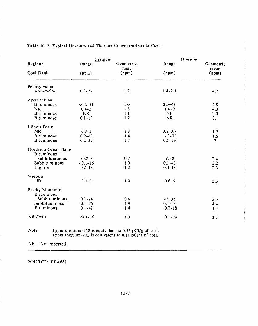
Table 10-3: Typical Uranium and Thorium Concentrations i n Coal.
Regiol~/
Coal Rank
Uranium Ranee Geometric -
mean ( P P ~ ) ( P P ~ )
Thorium Ranee Geoinelric
Pennsylvania Anthracite 0.3-25
Appalachian Bituminous <0.2- 1 1 N R 0.4-3 Bituminous NR Bituminous 0.1-19
Illinois Basin NR Bituminous 0.2% Bituminous 0.2-59
Northern Great Plains Bituminous
Subbituminous <0.2-3 Subbituminous <0.1-16 Lignite 0.2-13
Western NR
Rocky Mountain Bituminous
Subbituminous 0.2-23 Subbituminous 0.1-76 Bituminous 0.1-42
All Coals <0.1-76 1.3 <0.1-79
Note: l p p m uranium-238 is equivalent to 0.33 pCi/g of coal. t ppm thorium-232 is equivalent to 0.11 pCi/g of coal.
NR - Not reported
SOURCE: [EPA88]

The risk assessment of utility boilers is based on reference (actuai) facilities selected to represent
large and typical utility boilers. The reference facilities were selected from a data base of almost one
thousand utility boilers maintained by the EPA's Office of Air Quality Planning and Standards
(OAQPS). The boilers in the data base account for virtually all of the coal used by utility boilers.
The risk assessment of industrial boilers is based on a single reference plant. The reference plant has
the largest estimated release of total particulates of the industrial boilers in OAQPS' data base of
about 500 industrial boilers [EPA89]. The coal-fired industrial boilers in the OAQPS data base
represent a stratified random sample of more than 2,000 industrial boilers located throughout the
United States. In selecting the reference utility boilers, the boilers in the data base were classified
according to the number of persons living within 50 kilometers of the plant. Urban plants were
defined as having 3,000,000 persons or more, suburban plants as having 800,000 to 3,000,000 persons,
rural plants as having 100,000 to 800,000 persons, and remote plants as having less than 100,000
persons. This classification shows 34 utility boilers located in urban areas, 234 located in suburban
areas, 567 located in rural areas, and 150 located in remote areas. For each location, the large
reference plant and the typical reference plant were chosen based on the estimate of total particulate
emissions. The large reference plants were used in the evaluation of the risks to nearby individuals
and the typical reference plants were used to evaluate the magnitude and distribution of the
population risk. Tables 10-4 and 10-5 give a summary of U-238 and Th-232 emission factors by
coal-fired utility boiler type and control technique.
10.4 A~ialvsis of Benefits and Costs
10.4.1 Introduction
As already mentioned, there are currently several state and Federal regulations regarding the
emissions from coal-fired boilers. Therefore, any cost-benefit analysis would be of further specific
regulations and more stringent controls. In order to determine the amount of further regulations
necessary, the radionuclide related risks from coal-fired emissions must first be assessed. Several
assumptions were made in carrying out risk calculations in order to lend conservatism to the results.
Food input parameters were computed for the food growing capabilities of each population category.
For urban and remote utility boilers it was assumed that individuals residing in the fallout region
of these plants also supplied all of their own meat and milk. In the case of suburban utilities, i t was
assumed that half of the ingested fruit and vegetables were grown a t home and that the remainder
of the fruits and vegetables as well as the meat and milk were supplied regionally. For urban
utilities, it was assumed that everything was supplied regionally and nothing was grown at home.
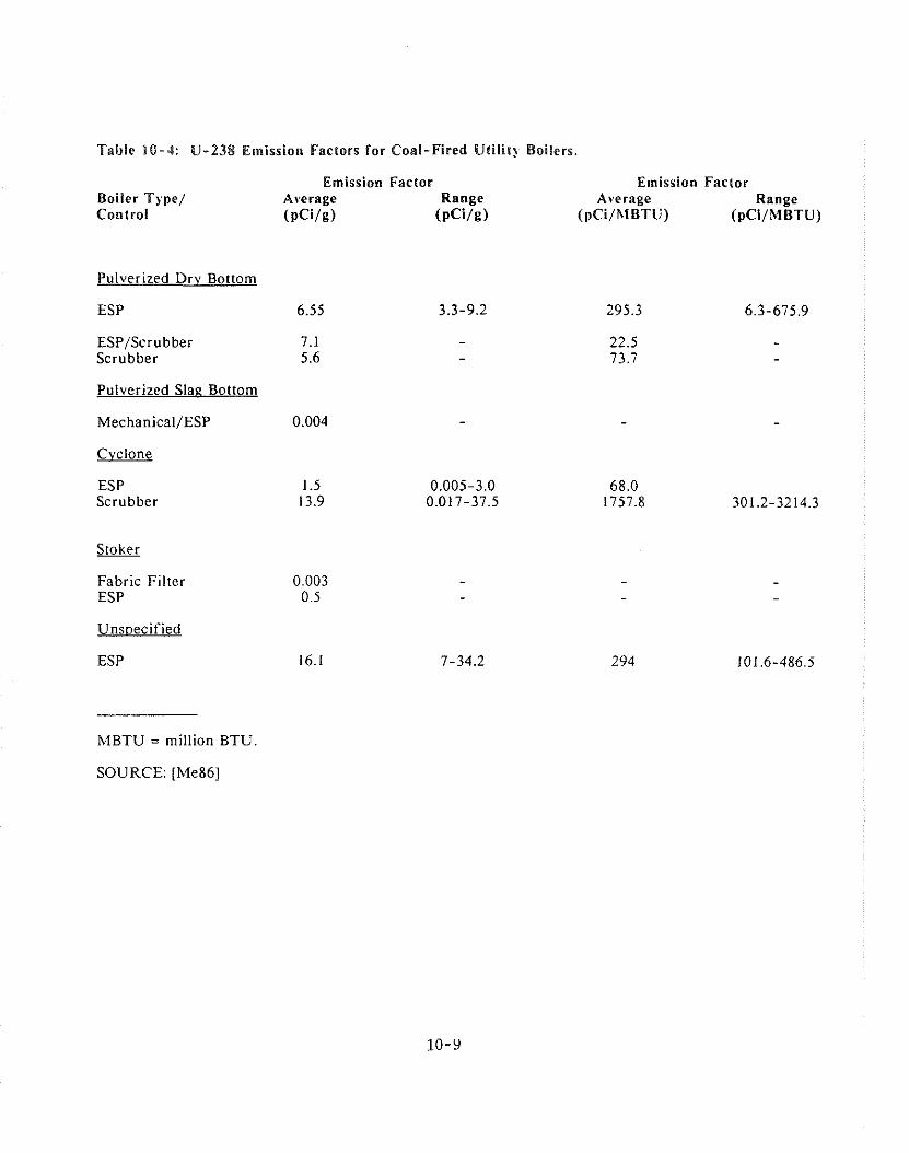
Table 10-4: U-238 Ernission Factors for Coal-Fired Utilil? Boilers.
Emission Factor Emission Factor Boiler Type/ Average Range Average Range Coiitrol ( P C ~ / P ) (pCi/g) (pCi/hlBTU) (pCI/MBTU)
Pulverized Drv Bottom
ESP 6.55
ESP/Scrubber Scrubber
Pulverized Slae Bottom
Mechanical/ESP 0.004
Cyclone
ESP Scrubber
Fabric Filter ESP
Unsoecified
ESP
MBTU = million BTU.
SOURCE: [Me861
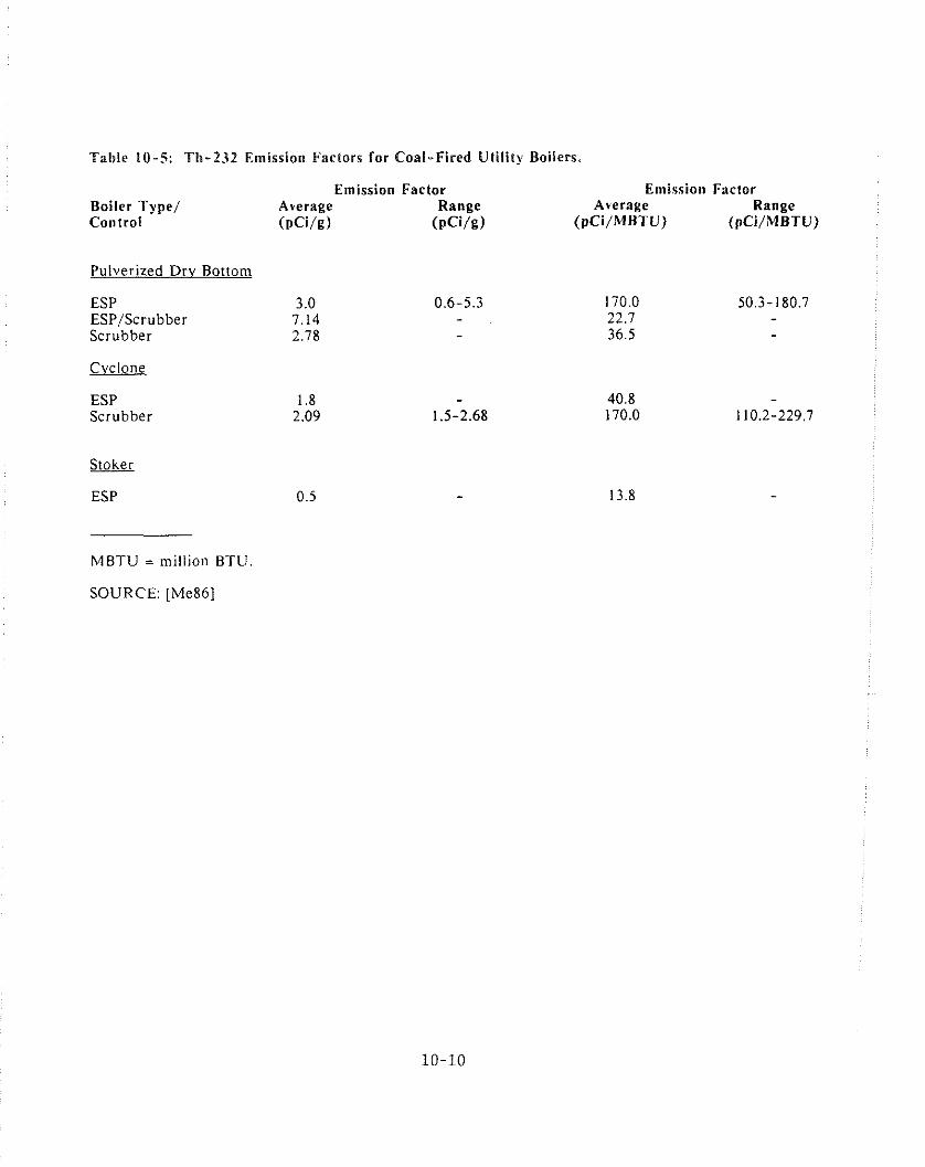
Table 10-5: TI,-2.32 Emissio~i Factors tor Coal-Fired Utility Boilers.
Emission Factor Boiler Type/ Average Range Co~~tro t ( ~ C i / g ) ( ~ C i i g )
Pulverized Drv Bottom
ESP ESPiScrubber Scrubber
Cvclone
ESP Scrubber
&&g
ESP
MBTU = million BTU
SOURCE: [Me861
Emiss io~~ Factor Average Range
(pCi/MHTU) (pCiiMBTU)
10.4.2 Least-Cost Control Tecli~~oloeies
Selection of particulate control devices for a particular utility is a function of several variables,
including boiler capacity, boiler type, inlet loading, fly ash characteristics, and inlet particle size
distribution. Virtually all coal-fired utility boilers in the United States are required to have air
emission controls in order to meet National Air Quality Standards (NAAQS). The least costly option
for increased control of radionuclide emissions is continued reliance on on-going measures taken to
conform to clean air act requirements for NAAQS and the precursors of acid rain. These tend to be
updated as new technologies become available. For example, the recent development of highly
temperature resistant fabrics has resulted in the increased use of fabric filters in the reduction of
boiler emissions. However, increased efficiency of control technologies will be expensive because
the current technologies comprised mainly of electrostatic precipitators (ESP), mechanical collectors,
wet scrubbers, and fabric filters are now at least 98 percent effective during normal operation.
10.4.3 Health and Other Benefits
Table 10-6 shows the estimated radiation dose rates from large coal-fired utility boilers for each
population category. Similar data is displayed in Table 10-7 for a reference coal-fired industrial
boiler. Tables 10-8 and 10-9 show the estimated distribution of the fatal cancer risk to the regional
populations from all coal-fired utility and industrial boilers.
10.4.4 Estimates of Benefits and Costs
Existing boilers can be retrofitted with additional electrostatic precipitators to reduce emissions to
the level prescribed for new sources (13 ng/J). Although a full evaluation of supplementary control
options and costs has not been performed for industrial boilers; it is known that existing boilers could
be retrofitted with ESPs. It is estimated that retrofitting ESPs at industrial boilers with heat inputs
over 2E+6 MBTU/hr would reduce particulate emissions by a factor of two. The cost and health
benefits are not known. With all coal-fired utility boilers operating with particulate emissions of 13
ng/J (0.03 lb/MBTU) of heat input, the current 12,500 million MBTU annual heat input would
result in about 0.17 billion kg of particulate releases. The source term and potential health impact
would therefore be reduced by about a factor of two. The estimate of the total deaths per year would
drop to 0.2. The EPA's office of Air Quality Planning and Standards has estimated the costs of
retrofitting all existing utility coal-fired boilers to meet the control level of 13ng/J to be about $13
billion in capital costs (1982 dollars) and about $3.4 billion in annual costs [RC83].
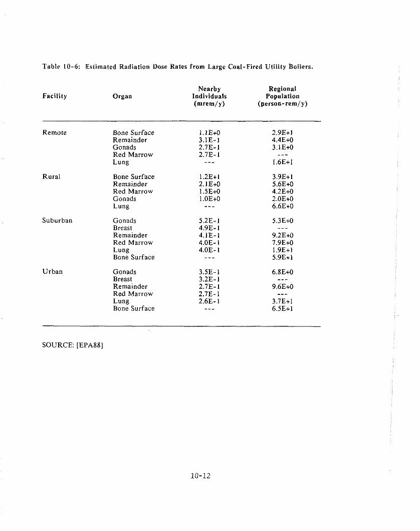
Table 10-6: Estimaled Radiation Dose Rates from Large Coal-Fired Utility Boilers.
Facility Organ Nearby Regional
Individuals Population ( m r - 4 ~ ) (person- rem/ y)
Remote Bone Surface Remainder Gonads Red Marrow Lung
Rural Bone Surface Remainder Red Marrow Gonads Lung
Suburban Gonads Breast Remainder Red Marrow Lung Bone Surface
Urban Gonads Breast Remainder Red Marrow Lung Bone Surface
SOURCE: [EPA88]
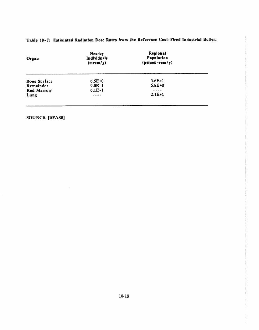
Table 10-7: Estimated Radiatton Dose Rates from the Reference Coal-Fired lndustrlal Boiler.
Organ Nearby
Individuals (mreml y)
Regional Popuiation
(person-remly)
Bone Surface Remainder Red Marrow Lung
SOURCE: [EPA88]

Table 10-8: Estfmated DIstrlbutlon o l the Fatal Cemeer Rlsk Lo tbe reglonaf (0-8l)kat) populations from all Coal-Fired Utility Boilers.
Risk Intenral
Number of Persons
1E- 1 to 1E+O 1E-2 to 1E-1 1E-3 to 1E-2 1E-4 to 1E-3 1E-5 to 1E-4 1E-6 to 1E-5 Less than 1E-6
Totals
SOURCE: [EPA88]

Table 10-9: Estimated Distribution of the Fatal Cancer Risk to the regional (0-80km) populations from at1 Coal-Fired industrial Boilers.
Risk Interval
Number o l Persons
IE- 1 to 1E+O 1E-2 to 1E-1 1E-3 to 1E-2 1E-4 to 1E-3 1E-5 to 1E-4 1E-6 to 1E-5 Less than 1E-6
Totals
* The results of the risk assessment of the model facility indicate that there may be individuals in this risk interval. However, data are insufficient to provide quantitative estimates.
SOURCE: [EPA88]

Figures published in the Federal Register predict the capital costs to utilities of retrofitting existing
coal-fired boilers to meet Clean Air Act requirenients pertaining to criteria air pollutants to be
slightly higher. Capital improvement costs are estimated to be approximately $15 billion and the
subsequent operating costs are estimated to be approximately $3 billion a year [FR83].
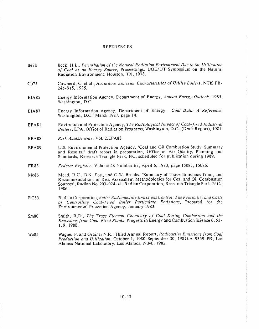
REFERENCES
Beck, H.L., Perlurhatio~r o/ [he Nalural Radialiorl E~ lv i ror~n te~~ f Duc lo [he Ulilizalion of Coal as at1 E~rcrgy Source, Proceedings, DOEIUT Symposium on the Natural Radiation Environment, Houston, TX, 1978.
Cowherd, C. et al., Hazardous En1issiorl Characterislics o f Utility Boilers, NTlS PB- 245-915, 1975.
Energy Inforniation Agency, Department of Energy, An~zual E~tcrgy Outlook, 1985, Washington, D.C.
Energy Information Agency, Department of Energy, Coal Data: A Reference, Washington, D.C.; March 1987, page 14.
Environmental Protection Agency, The Radiological Inlpacl o/ Coal-/ired I~zduslrial Boilers, EPA, Office of Radiation Programs, Washington, D.C., (Draft Report), 1981.
Risk Assessnre~rls, Vol. 2.EPA88
U.S. Environmental Protection Agency, "Coal and Oil Combustion Study: Summary and Results," draft report in preparation, Office of Air Quality, Planning and Standards, Research Triangle Park, NC, scheduled for publication during 1989.
Federal R e ~ i s l e r , Volume 48 Number 67, April 6, 1983, page 15085, 15086,
Mead, R.C., B.K. Post, and G.W. Brooks, "Summary of Trace Emissions from, and Recommendations of Risk Assessment Methodologies for Coal and Oil Combustion Sources", Radian No. 203-024-41, Radian Corporation, Research Triangle Park, N.C., 1986.
Radian Corporation, Boiler Radiorruclide Enzissioizs Control: TheFeasibiiiry at2d Costs of Corrlrollirrg Coal-Fired Boiler Particulate Emissions, Prepared for the Environmental Protection Agency, January 1983.
Smith, R.D., The Trace Elenlerrl Chenlistry of Coal During Contbusriorl and the Enlissio~rs /ram Coal-Fired Plants, Progress in Energy and Combustion Science 6,53- 119, 1980.
Wagner P. and Greiner N.R., Third Annual Report, Radioactive Emissior1s from Coal Producliorr and Uliliratior1, October 1 , 1980-September 30, 1981LA-9359-PR, Los Alamos National Laboratory, Los Alamos, N.M., 1982.


CHAPTUR II
NRC-LICENSED FAClUTlES AND NON-DOE FEDERAL FAClUTlES

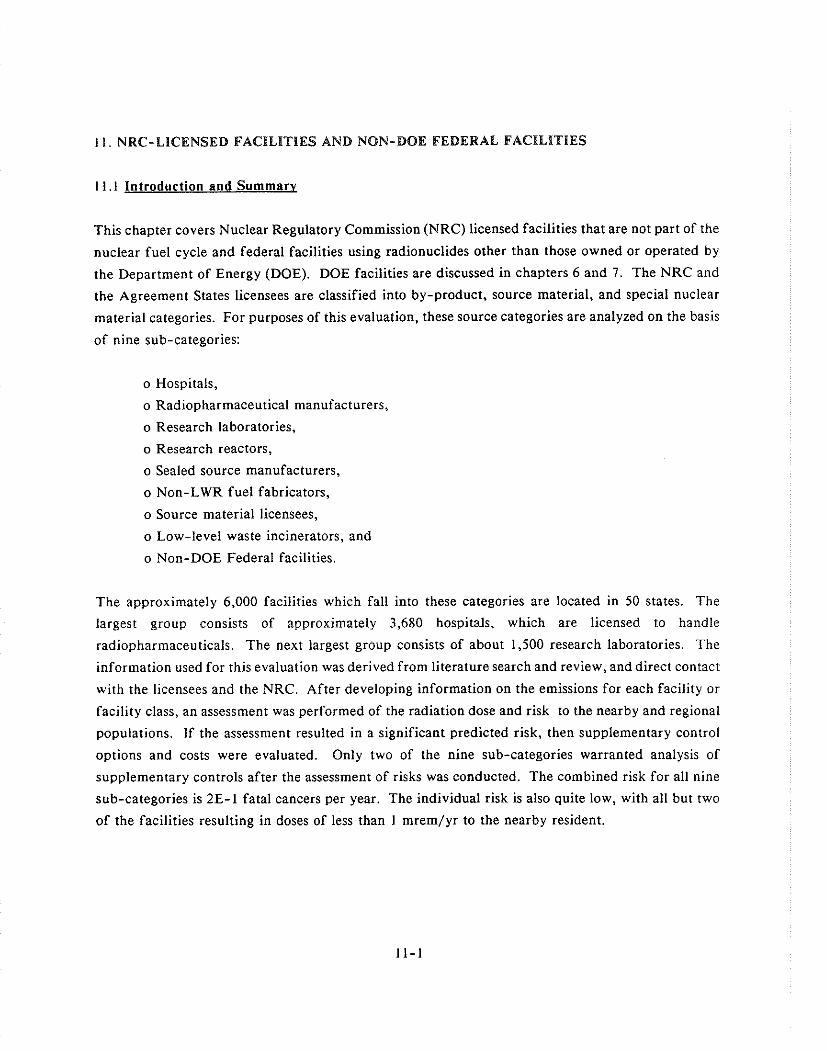
I I . NRC-LICENSED FACILITlES AND NON-DOE FEDERAL FACILITIES
11.1 Introduction and Summary
This chapter covers Nuclear Regulatory Commission (NRC) licensed facilities that are not part of the
nuclear fuel cycle and federal facilities using radionuclides other than those owned or operated by
the Department of Energy (DOE). DOE facilities are discussed in chapters 6 and 7. The NRC and
the Agreement States licensees are classified into by-product, source material, and special nuclear
material categories. For purposes of this evaluation, these source categories are analyzed on the basis
of nine sub-categories:
o Hospitals,
o Radiopharmaceutical manufacturers,
o Research laboratories,
o Research reactors,
o Sealed source manufacturers,
o Non-LWR fuel fabricators,
o Source material licensees,
o Low-level waste incinerators, and
o Non-DOE Federal facilities.
The approximately 6,000 facilities which fall into these categories are located in 50 states. The
largest group consists of approximately 3,680 hospitals, which are licensed to handle
radiopharmaceuticals. The next largest group consists of about 1,500 research laboratories. The
information used for this evaluation was derived from literature search and review, and direct contact
with the licensees and the NRC. After developing information on the emissions for each facility or
facility class, an assessment was performed of the radiation dose and risk to the nearby and regional
populations. If the assessment resulted in a significant predicted risk, then supplementary control
options and costs were evaluated. Only two of the nine sub-categories warranted analysis of
supplementary controls after the assessment of risks was conducted. The combined risk for all nine
sub-categories is 2E-I fatal cancers per year. The individual risk is also quite low, with all but two
of the facilities resulting in doses of less than 1 mrem/yr to the nearby resident.

11.2 Industry Profile
Due to the large number and variety of sources, it is not feasible nor useful to develop a detailed
industry profile. A brief description of each sub-category follows. Over half of the hospitals in the
United States handle radiopharmaceuticals [AHA86]. The most prevalent use is for radionuclide
imaging to aid in diagnosis of diseases. A smaller number of hospitals also use radionuclides for
therapeutic purposes. Two-thirds of hospitals using therapeutic amounts of radiopharmaceuticals are
located in urban areas.
Radiopharmaceutical manufacturers, which number about 120, fall into three sub-categories. There
are 15 large firms which manufacture the pharmaceuticals, 70 small- to medium-sized firms which
alter the chemical form of the nuclides, and 35 nuclear pharmacy operators which repackage the
material into convenient quantities for distribution.
There are approximately 1,500 research laboratories which use radionuclides in unsealed forms. Over
half of these laboratories are associated with academic institutions and the remainder with
government or private research facilities [CENSl,BAT83,NRC88]. The academic laboratories
frequently involve a large number of release points within a generalized area and use small amounts
of a large number of radionuclides. Twenty-nine radionuclides were identified as in use. One use
of radioactively-labeled chemicals is to trace dynamic processes.
There were 70 research and test reactors operating as of December, 1987. These reactors range in
power level from zero to 10,000 kilowatts and are generally operated by universities for use in
teaching and research. Although there are a number of different designs, the most common is the
General Atomics TRIGA reactor.
Sealed-source manufacturers take radionuclides in unsealed form and put them into permanently
sealed containers. There are two sub-categories of sealed source manufacturers - those that seal
tritium gas into self-luminous lights (three manufacturers) and those who utilize other radiation
sources (eight manufacturers which release more than exempt quantities of radionuclides).
Four facilities fabricate uranium fuel for research reactors or naval propulsion reactors. The process
is similar to that used in the uranium fuel cycle, whereby enriched U 0 2 is formed into pellets which
are stacked inside tubes and then bundled into fuel assemblies.
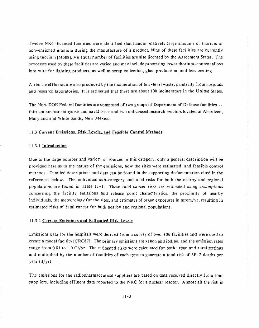
Twelve NRC-licensed facilities were identified that handle relatively large amounts of thorium or
non-enriched uranium during the manufacture of a product. Nine of these facilities are currently
using thorium [Mo88]. An equal number of facilities are also licensed by the Agreement States. The
processes used by these facilities are varied and may include processing lower thorium-content alloys
into wire for lighting products, as well as scrap collection, glass production, and lens coating.
Airborne effluents are also produced by the incineration of low-level waste, primarily from hospitals
and research laboratories. It is estimated that there are about 100 incinerators in the United States.
The Non-DOE Federal facilities are composed of two groups of Department of Defense facilities -- thirteen nuclear shipyards and naval bases and two unlicensed research reactors located a t Aberdeen,
Maryland and White Sands, New Mexico.
11.3 Current Emissions. Risk Levels, and Feasible Control Methods
11.3.1 Introduction
Due to the large number and variety of sources in this category, only a general description will be
provided here as to the nature of the emissions, how the risks were estimated, and feasible control
methods. Detailed descriptions and data can be found in the supporting documentation cited in the
references below. The individual sub-category and total risks for both the nearby and regional
populations are found in Table 1 1 - 1 . These fatal cancer risks are estimated using assumptions
concerning the facility emissions and release point characteristics, the proximity of nearby
individuals, the meteorology for the sites, and estimates of organ exposures in mrem/yr, resulting in
estimated risks of fatal cancer for both nearby and regional populations.
11.3.2 Current Emissions and Estimated Risk Levels
Emissions data for the hospitals were derived from a survey of over 100 facilities and were used to
create a model facility [CRC87]. The primary emissions are xenon and iodine, and the emission rates
range from 0.01 to 1.0 Ci/yr. The estimated risks were calculated for both urban and rural settings
and multiplied by the number of facilities of each type to generate a total risk of 6E-2 deaths per
year (d/yr).
The emissions for the radiopharmaceutical suppliers are based on data received directly from four
suppliers, including effluent data reported to the NRC for a nuclear reactor. Almost all the risk is

Table 11-1 NRC Licensed and Non-DOE Facilities Fatal Cancers Per Year
Fatal Cancers Category No. of Facilities (d/yr) .............................................................. Hospitals 3680 6 ~ - 2
Radiopharmaceutical Manufacturers
Research Laboratories 1500 8E-3
Research Reactors 7 0 4E-2
Sealed Source Manufacturers 11 2E-2
Non-LWR Fuel Fabricator 4 2E-4
Source Material Licensee 12 1E-3
Low-level Waste 100 1E-3
Non-DOE Federal ~acilities 15 1E-3
TOTAL 6000 2E-1

accounted for by the facility that operates the nuclear reactor. The total risk is obtained by summing
the risks from all sixteen facilities, and is estimated to be 2E-2 d/yr .
Emissions data were gathered from 46 research laboratories and compared to information from other
available sources [BAT83, CRC871. Approximately forty-one percent of all laboratories have
emissions that are either zero or below the lower limits of detection of their monitoring equipment.
A model facility was developed using a weighted average of the remaining facilities by type and
multiplying by the number of facilities (622) having non-zero emissions. The total risk is estimated
to be 8E-3 d/yr.
Emissions data were collected for the four largest emitters among research and test reactors. The
resulting risks were extrapolated to the entire population based upon the contribution of the four
largest emitters to the total emissions. The ratio was calculated based on Ar-41 emissions which were
found to be fifty-nine percent of the total emissions for this sub-category. The total risk is estimated
to be 4E-2 d/yr .
A model sealed source facility was estimated based upon the average emissions of four non-tritium
manufacturers. Kr-85 is released in curie amounts and Co-60, Am-241, Ir-192, and Cf-252 in
microcurie amounts. The tritium lighting producers all submitted information on their effluents so
these data were used directly with site-specific information on meteorology. The total risk of 2E-
2 d /yr is equal to the sum of the estimated doses from the three lighting facilities and the product
of the total emissions of the model facility and the total number of facilities.
Operating reports were used for the emissions from non-LWR fuel fabricators. U-234 and U-235
are the nuclides which make the largest contribution to dose. Actual site characteristics, facility data,
and local meteorological data were utilized. Total risk for this category is estimated to be 2E-4 d/yr.
Two reference facilities to represent source material licensees were used for the estimate of thorium
and uranium emissions and their associated risks. The risk was obtained by multiplying the results
by the number of facilities in this category. The total risk for this category is estimated to be 1E-
3 d/yr.
Effluent data for 35 incinerators are available from a survey for the estimate of emissions from low-
level waste [CRC87]. A model facility was created based upon these data. Data for the largest emitter
was also modified. The model facility is estimated to result i n IE-5 fatal cancers per year, while the
maximum emitter is estimated to result in 2E-4 fatal cancers per year. The total risk for this
category, obtained by scaling up the risks from the model facility by a factor of 100, is estimated to
be 1E-3 d/yr.
With respect to non-DOE federal facilities, a single model, was used to represent both Naval
shipyards and the two non-licensed research reactors in Maryland and New Mexico. The model was
based on emissions measured at the shipyards. Effluent monitoring at Department of Defense
shipyards and bases reveals few measurable radionuclide releases [Mass]. The Navy estimates
maximum releases of noble gases to be 0.01 - 0.4 Ci/yr and of Co-60, 0.001 Ci/yr. An actual West-
coast shipyard was used as the model facility to estimate the risks based upon the above emission
rates. The risks from all DOD facilities is estimated to be IE-3 d/yr.
The calculated risks summarized above are combined to provide an estimated baseline risk for the
active category of 2E-1 d/yr. The sub-category with the largest collective risk is hospitals.
11.3.3 Control Technoloeies
Depending upon the effluent stream type and characteristics, various emission control technologies
are currently in use. The most frequently used control systems consist of high efficiency particulate
air (HEPA) filters. These control devices are used by hospitals, radiopharmaceutical suppliers,
laboratories, sealed-source manufacturers, fuel fabricators, source material licensees, and non-DOE
federal facilities. Charcoal filters are used to capture iodine, decay traps are used to hold radioactive
gases until the short-lived products decay, desiccant columns are used by lighting manufacturers to
remove tritium, and one facility bas installed a catalytic recombiner to convert tritium gas to tritiated
water. Waste incinerators utilize afterburners, venturi scrubbers, and gas scrubbers to remove
pollutants. Fuel fabricators are known to use gas scrubbers as well.
Only two of the nine sub-categories are estimated to have a high enough dose and resulting risk level
to warrant further evaluation of supplementary controls. For the sub-category of hospitals, it is not
possible to accurately estimate supplementary control costs due to the large number of facilities and
the lack of knowledge of current controls and configurations. One radiopharmaceutical manufacturer
is estimated to have releases resulting in a dose greater than I mrem/yr, but is already using charcoal
filters. The efficiency of this control technology can be enhanced via three methods: cooling the
effluent, reducing the humidity, or decreasing the flow rate. It is crudely estimated that the
increased control cost for this facility might be $350,000, which could achieve a 99 and 75 percent
reduction in radioiodine and noble, gases respectively. The associated risk reduction would be from
8E-3 to 3E-3 d/yr. The second facility that is estimated to have releases resulting in doses greater
than 1 mremjyr is a sealed source manufacturer, which would require a catalytic recombiner to
achieve a 99 percent reduction in emissions. The estimated cost of this control is between $1.7 and
$7.0 million. This would result in a reduction of the risk by 4E-3 d/yr. However, because the doses
and risks associated with facilities in this category are not accurately known, the total number of
necessary controls cannot he ascertained.
11.4 Analvsis of Benefits and Costs
Only two of the nine sub-categories are projected to have releases resulting in doses high enough to
warrant evaluation of supplementary controls. Moreover, these sub-categories contained only a few
sources which resulted in significant doses. However, this conclusion is based on incomplete data.
Table 11-2 presents the costs of the controls. The estimated benefit of supplementary controls for
the facility " D radiopharmaceutical manufacturer is 1.5E-2 d/yr, assuming acapital cost of $350,000.
This translates into a net present value between $320,000 and $350,000 and an annualized cost
ranging from $3,200 to $3,500.
The total number of cancer deaths averted are also presented in Table 11-2. The total number of
fatal cancers averted due to supplementary controls for the Sealed Source facility " C is estimated to
be 4E-1 over the course of a century. A wide range of costs was considered since an engineering
study of the specific requirements was not performed. The study that was completed gave "low-
cost" and "high-cost" estimates. The net present value ranges from $1,550,000 to $7,000,000 and the
annualized payment ranges from $20,000 to $70,000.
11.5 Industrv Cost and Economic Imoact
Industry costs and economic impact for this category can only be roughly approximated. The 6,000
facilities are not well characterized and emission data are incomplete.
Most of the sources in the several industries considered in this chapter are not likely to require
supplementary controls. For the two sources that may require supplementary controls, the costs to
one, Radiopharmaceutical "D, are under half a million dollars and will avert 1.5 cancer deaths per
century. The cost for the other, Sealed Source " C , is over 11.5 million and will avert 0.4 cancer
deaths per century.

Table I 1-2 Costs and Benefits for Controls on the Two Sources for which Controls are Required
Net Social
Discount Facility Rate (%)
Radio- 0 pharmaceutical " D I
Sealed Source "C" low-cost
Sealed Source "C" high-cost
NPV of Control
Cost ($/cent)
. - - - - - - - - 350,000
346,000
Cancer Deaths
Averted (d/cent) ------------ 1.5E+O

Should either of these sources be controlled, any economic effects would be localized to-the firm and
its immediate customers and suppliers.
As an alternative approach, a survey conducted by the Nuclear Regulatory Commission [NRCSI] can
be used to estimate impacts associated with regulatory options under consideration. Approximately
3,000 facilities licensed to possess radionuclides were surveyed and about half responded. Doses
caused by each of these facilities were estimated using compliance procedures from [EPA89(A)].
Based on this analysis capital costs of $5 million and operating costs of $2 million/yr are estimated
for a three mrem/yr standard; capital costs of $25 million and annual operating costs of $12
million/yr for a one mrem/yr standard; and capital costs of $60 million and annual operating costs
of $35 million/yr for a 0.3 mrem/yr standard.
REFERENCES
American Hospital Association, Artrzuai Survey o/ Nosprtals, Chicago: Illinois, 1986.
Battelle, Inc., Ait Ecoitomic Study o/ lhe Radionuclides Ir~dustry, Washington, D.C., for the U.S. Nuclear Regulatory Commission, NUREG/CR-2048, 1981.
Centaur Associates, Inc., An Econonzic Study o f the Radionuclides Industry, Washington, D. C., for the U. S. Nuclear Regulatory Commission, NUREG/CR-2048, 1981.
Council of Radiation Control Program Directors (CRCPD), Inc., Compilation o f State- by-stale Low-level Radioactive Waste Information, for U. S. Department of Energy, Frankfort: Kentucky, DOE/ID/12377, 1987.
Risk Assessmenls, Vol. 2
Environmental Protection Agency, Background Information Document: Procedures Approved for Demonstrating Compliance With 40CFR Part 61, Subpart I , January 1989.
Manengo, J.J., et a]., Environmental Monitoring and Disposal o f Radioactive Wastes from U. S. Naval Nuclear Powered Ships and Their Support Facilities 1987, Naval Nuclear Propulsion Program, NT-88- 1, Washington: D.C., 1988.
Moriarty, M., personal communication, U. S. Nuclear Regulatory Commission, Washington: D. C., 1988.
Screeiting Techniques for Determining Compliance with Environmental Standards, NCRP Commentary No. 3; Revision of January 1989.
A Survey of Radioactive Releases from By-Product Material Facilities, J.R. Cook, U.S.N.R.C., August 1981, [NUREG-08191.
Nuclear Regulatory Commission, An Economic Study o/ the Radionuclides Industry, Washington, D. C., 1988.

CHAPTER 12
SURFACE URANIUM MINES

12. S U R F A C E URANILIM M I N E S
12.1 lntroduction and Summary
Surface uranium mines represent a depressed segment of a declining industry which serves a small
number of potential customers. They face declining demand for their output and price competition
from both underground mines and foreign producers. All but two of the hundreds of surface
uranium mines that operated from the 1950s to the early 1980s are currently inactive.
Controls on surface mines to reduce particulate radionuclidc emissions and radon fluxes consist of
applying a layer of cover over the top of the closed mine area. The costs of this procedure are
measured in thousands or millions of dollars Per mine.
12.2 Industrv Profile
12.2.1 Introduction
Surface uranium mines are a subset of the U.S. uranium mining industry. Uranium is also produced
by underground mines which are discussed in Chapter 2. U n n i u m is used to produce electricity and
nuclear weapons. Chapters 1, 3, and 4 also discuss aspects of the uranium industry. The number of
active surface uranium mines has sharply declined in recent years due to competition from
underground mines and foreign producers, and to declines in demand for uranium for both of its
uses.
12.2.2 Demand for Uranium
Uranium is an input to two industries: nuclear power production and nuclear weapon production
[EPA89]. The demand for uranium from ore for these industries is currently in decline. The demand
for fuel for nuclear reactors must either be more or less constant or slightly on the increase. Since
the military has made no recent purchases of uranium, their demand has neither increased or
decreased.
Uranium is used as a fuel in nuclear power plants, after being milled and enriched. Although there
was rapid growth in this segment of the electric power industry from the late 1950s to the early
1980s, recent years have seen a total and abrupt stop in construction of new units. The factors
contributing to this decline included escalating costs, a general decline in the growth rate of the

power generation industry, and increasing public concern for safety. Also, the financing and
management of some plants under construction led to severe financial problems. Some plants were
abandoned in mid-construction, while others were completed, but have not yet been commissioned.
The only demand for uranium by the U.S. nuclear power industry in the near future will be to fuel
existing power plants including those waiting to be commissioned. This source of demand will
decline as plants age and are decommissioned.
The second source of demand for uranium is the production of nuclear weapons which use uranium
as an input. Currently, weapons production reactors are closed due to problems with safety and with
past improper waste storage practices that have been discovered to pose a threat to nearby
populations. When these plants reopen, there will be a continuous, but not very large, demand for
uranium.
12.2.3 SUDD~V of Uranium
Surface uranium mines currently operate a t a small percentage of their overall capacity. (See Figure
12- 1.) As recently as 1980 they produced 20.8 million pounds of U308 from 50 mines. In 1986, they
produced about 2 million pounds of U308 from four mines. In 1988, there were two active surface
uranium mines [EPA89]. All the mines studied in this chapter with respect to emission control are
currently inactive. Some are unreclaimed and others are reclaimed. The mines studied are located
in South Dakota, Wyoming, Colorado, Arizona, and Texas [EPA89]. As illustrated by Table 12-1,
surface mining took place in other states as well, but not to the same extent.
A major problem facing surface uranium mines is competition from underground mines and foreign
producers. Table 12-2 demonstrates that underground mining is especially dominant when prices are
low, in the $30/lb. range. Table 12-3 illustrates the international competitive situation, especially
for reasonably assured reserves (RAR). The U.S. is not competitive with Australia at lower price
levels.
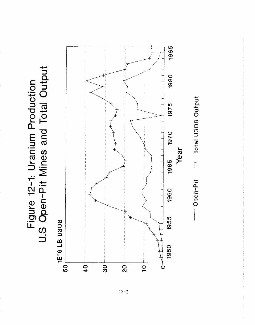
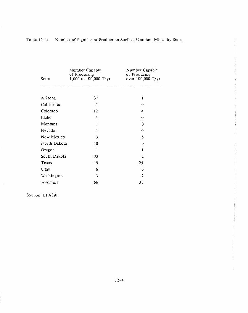
Table 12-1: Number of Significant Production Surface Uranium Mines by State.
Number Capable Number Capable of Producing of Producing
State 1,000 to 100,000 T/yr over 100,000 T/yr
Arizona
California
Colorado
Idaho
Montana
Nevada
New Mexico
North Dakota
Oregon
South Dakota
Texas
Utah
Washington
Wyoming
Source: [EPA89]
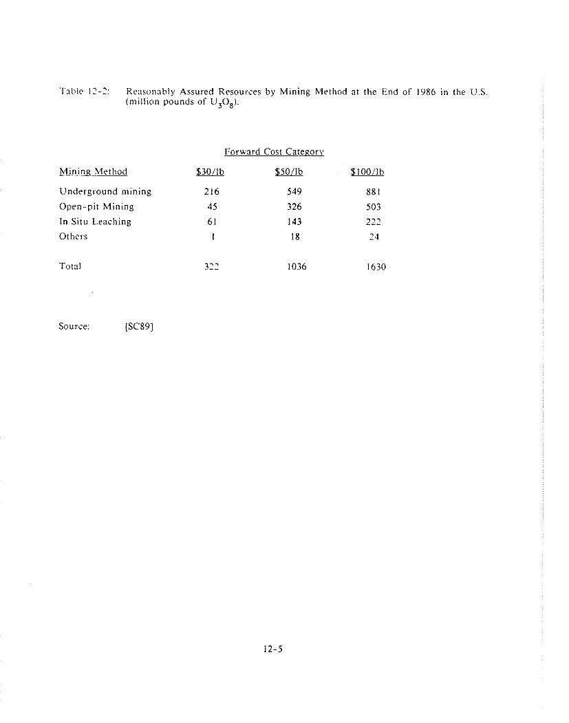
1-nhlc 12-2: Kensonnhly Assured Resources by Mining Method a t the End of 1986 in the U.S (mill ion pounds o f U308).
Minine. Method
Underg round mining
Open-p i t Mining
In Situ Leaching
Othe r s
Tota l
Source: [SC89]
Forward Cost Catenorv
$30/lb $.Qfb
216 549
45 326
61 143
I 18

'1-nble 12-3: Unitcd Srntes and Selected Foreign Uranium Resources ns of End of 1986.
TOTAL RESERVES
Reasonablv Assured Resources* Estimated Additional Resources*
Country $30/lb $50/lb $50/lb
United States 322 1036 1350 2370
Canada 416 603 268 528
Australia 1101 1347 668 998
* hlillion Pounds U308
Source: [SCS9]
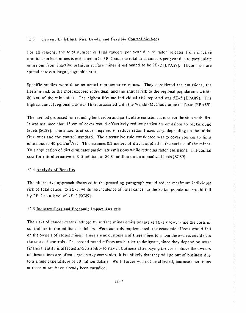
12.3 Current Emissions. Risk 1,evels. a n d Feasible Control hletliodc
For all regions, the tot31 number of fatal cancers per year due to radon releases from inactive
uranium surface mines is estimated to be 3E-2 and the total fatal cancers per )ear due to particulate
emissions from inactive uranium surface mines is estimated to be 2E-? [EPA89]. These risks are
spread across a large geographic area.
Specific studies were done on actual representative mines. They considered the emissions, the
lifetime risk to the most exposed individual, and the annual risk to the regional populations within
80 km. of the mine sites. The highest lifetime individual risk reported was 5E-5 [EPA89]. The
highest annual regional risk was 1E-3, associated with the Wright-McCradg mine in Texas [ € P . ~ 8 9 ] .
The method proposed for reducing both radon and particulate emissions is to cover the sites with dirt.
I t was assumed that 15 cm of cover would effectively reduce particulate emissions to background
levels [SC89]. The amounts of cover required to reduce radon fluxes vary, depending on the initial
flux rates and the control standard. The alternative rule considered was to cover sources to limit 2 emissions to 40 pCi/m /sec. This assumes 0.2 meters of dirt is applied to the surface of the mines.
This application of dirt eliminates particulate emissions while reducing radon emissions. The capital
cost for this alternative is $15 million, or $0.8 million on an annualized basis [SC89].
12.4 Analysis of Benefits
The alternative approach discussed in the preceding paragraph would reduce maximum individual
risk of fatal cancer to 2E-5, while the incidence of fatal cancer to the 80 km population would fall
by 2E-2 to a level of 4E-3 [SC89].
12.5 lndustrv Cost and Economic lmaact Analvsis
The risks of cancer deaths induced by surface mines emissions are relatively low, while the costs of
control are in the millions of dollars. Were controls implemented, the economic effects would fall
on the o\vners of closed mines. There are no customers of these mines to whom the owners could pass
the costs of controls. The second round effects are harder to designate, since they depend on what
financial entity is affected and its ability to stay in business after paying the costs. Since the owners
of these mines are often large energy companies, it is unlikely that they will go out of business due
to a single expenditure of 10 million dollars. Work forces will not be affected, because operations
at these mines have already been curtailed.
REFERENCES
Risk A.s.sessmertls, Val. 2,
SC&A, Inc., "Radiological Monitoring at Inactive Surface Uranium Mines," prepared for the U.S. En\:ironmental Protection Agency, Office of Radiation Programs, Washington, D.C., February 1989.