EARLY LIFE ADVERSITY, HOME ENVIRONMENT AND

CHILDREN’S COMPETENCE DEVELOPMENT

Dorothea Blomeyer+, Katja Coneus*, Manfred Laucht+, Friedhelm Pfeiffer*

+ Central Institute of Mental Health (ZI), Mannheim * Centre for European Economic Research (ZEW), Mannheim

June 2009, comments welcome

This paper investigates the role of early life adversity and home resources in terms of

competence formation from infancy to adolescence. We study complementarity factors

between cognitive, motor and noncognitive abilities and social as well as academic

competencies, and discuss alternative educational policies to improve competence de-

velopment. Our data are taken from the Mannheim Study of Children at Risk, an epi-

demiological cohort study following the long-term outcome of early life adversity. Re-

sults indicate that organic and psychosocial initial risks are important for the develop-

ment of competencies, as well as socio-emotional home resources in childhood and

economic resources during the transition to higher secondary school track. Abilities

acquired in preschool age predict achievement at school age. There is a remarkable sta-

bility in the inequality of the home environment. This is presumably a major reason for

the evolution of inequality in competence development from birth to adolescence.

Keywords: Organic and Psychosocial Risks, Socio-Emotional and Economic Home Resources, Intelligence, Persistence, Peer Relationship, School Achievement JEL-classification: D87, I12, I21, J13 Acknowledgements: We gratefully acknowledge support from the Leibniz Association, Bonn, through the grant “Noncognitive Skills: Acquisition and Economic Consequences”. Dorothea Blomeyer and Manfred Laucht thank the German Research Foundation and the Federal Ministry of Education and Research for their support in conducting the Mannheim study of children at risk. For helpful discussions, we thank Anja Achtziger, Lex Borghans, Liam Delaney, Bart Golsteyn, James Heckman, Winfried Pohlmeier and our ZEW col-leagues. For competent research assistance, we are grateful to Mariya Dimova, York Heppner and Moritz Meyer. Any remaining errors are our own. Corresponding author: Friedhelm Pfeiffer, Centre for European Economic Research (ZEW), P.O. Box 103443, D-68034 Mannheim. Tel.: +49-621-1235-150, E-mail: pfeiffer@zew.de

1

I. INTRODUCTION

This paper contributes to the recent multidisciplinary literature on early life adversity,

human development and inequality (Heckman, 2007). Starting from conception, deep-

seated skills are formed in a dynamic interactive process between adult caregivers and

children. Research based on only a subset of relevant factors may contain some bias.

The relationship between early childhood risks (both organic and psychosocial in na-

ture), ongoing parental investments and competence development is analyzed in order to

gain an understanding of the childhood skill multiplier.

The paper contributes to the literature in the following ways. We examine the relation-

ship between initial organic and psychosocial conditions, socio-emotional and economic

home resources and the formation of basic abilities during development, and of compe-

tencies in social and academic life. Stage-specific parameters of the technology of skill

formation (Cunha and Heckman, 2007, 2009) are assessed together with complemen-

tarities between basic abilities in childhood and social and educational achievement at

school age. Reversed causality between parental child-rearing and ability formation is

taken into account. Having a child with high cognitive (or noncognitive) abilities is

likely to increase parental investment (home environment) in order to boost develop-

ment (and vice versa). Our study is based on unique data from a developmental psycho-

logical approach. The data provide detailed measurements of early risk conditions, pa-

rental stimulation and responsiveness, and child outcome.1 Psychometric assessments

were conducted for cognitive, motor and noncognitive abilities during infancy, toddler-

hood, preschool age, elementary school age and secondary school age, representing sig-

nificant stages of development.

Our findings demonstrate that interpersonal differences in cognitive, motor and noncog-

nitive abilities are consistently associated with early life adversity and the socio-

emotional home environment, with the relationship being specific to age and abilities.

The findings are in line with the literature on the childhood skill multiplier for lifelong

1 The data are taken from the Mannheim Study of Children at Risk (abbr. MARS, which has been derived

from the German title: MAnnheimer Risikokinder Studie), an epidemiological cohort study that follows

children from birth to adulthood (Blomeyer et al., 2009, Laucht et al., 1997, 2004).

2

competence formation summarized by Heckman (2007). Children are exposed to a ma-

trix of organic and psychosocial risks, and each factor by itself contributes to their de-

velopment as well as the sum of all factors. During childhood, the inequality of socio-

emotional home resources is a major reason for the further evolution of inequality. The

quality of parental stimulation and responsiveness is important for competencies in

stage-specific ways. Pre-school factors have significant consequences for school

achievement.

Our measure of noncognitive abilities, persistence, is significantly related to socio-

emotional home environment throughout the early life course. The highest association is

observed during preschool and elementary school years (the ages of 4.5 and 8 years).

Cognitive abilities, measured by the IQ, are strongly related to the home environment

during pre-school age and only weakly during school age. The influence of the socio-

emotional home resources declines continuously with age, being highest during infancy.

Interestingly, the relationship between the home environment and motor abilities, meas-

ured with the MQ, is positive, albeit of lower magnitude and not statistically significant.

Interindividual differences in the MQ are already primarily determined by the initial

organic risk conditions.

There is strong evidence for synergies in the development of abilities. Higher cognitive

and motor abilities are helpful for the development of higher noncognitive abilities, and

higher motor and noncognitive abilities are helpful for the development of higher cogni-

tive abilities (see also Duckworth and Seligman, 2005, among others). Moreover, it has

been demonstrated that abilities at preschool age predict social competencies and school

grades at the age of 8. Children with higher cognitive, motor and noncognitive abilities

at preschool age have more satisfying peer relationships, interests and better grades in

math, reading and spelling at primary school age. Higher cognitive, motor and noncog-

nitive abilities at primary school age predict a higher-track secondary school attendance

in Germany, starting at the age of ten years or later. These findings demonstrate dy-

namic complementarities (Heckman, 2007) in competence formation.

The availability of economic family resources creates an additional differential factor

for development and inequality during adolescence. Children with similar cognitive,

motor and noncognitive abilities who have access to more economic resources more

3

often attend a higher-track secondary school. This effect is statistically significant, al-

though of moderate quantitative magnitude. If economic resources increase by 1%, the

probability of entering higher-track secondary schooling increases by 0.18%.

Our findings are also related to the literature on the stability of personality traits

(Kadzin et al., 1997, Mischel et al., 1988, among others). We contribute to this literature

by using psychometric assessments rather than maternal ratings of children's abilities

and by applying the analytical framework of the technology of skill formation

(Heckman, 2007). The stability of personality traits is associated with the stability of

socio-emotional home resources during childhood.

Our findings with respect to early life adversity contribute to recent findings on long-

term outcomes of birth weight, among others by Black et al. (2007), and on the role of

height for socio-economic outcomes, among others Case and Paxson (2008). The psy-

chometric measures of initial organic and psychosocial conditions in our data extend the

knowledge regarding the variety of early risk factors and competence measures. Besides

low birth weight, neonatal complications and adverse psychosocial conditions like ma-

ternal discord or psychiatric disorders of parents also contribute to the children’s devel-

opment. A related strand of literature deals with the consequences of maltreatment in

childhood for depression in adulthood (Danese et al., 2007, among others). Maltreat-

ment is an important part of early life adversity , with long-term negative outcomes.

We conclude that advantages from beneficial home environments and disadvantages

from adverse home environments cumulate during the developmental course. The qual-

ity of home resources does not differ a great deal over time in social reality. In addition

to the adverse factors from initial risks, for disadvantaged children, the early develop-

ment of cognitive abilities is hindered by a low quality of adult care. This disadvantage

continues, and noncognitive ability formation at school age is impaired. Children are

again hindered during the transition to a higher-track secondary school, when low eco-

nomic home resources constitute an additional barrier. According to our interpretation,

there is still an underinvestment in public resources during preschool age for children

who grow up in an adverse home environment. In our study, alternative policies are

examined, which are based on our empirical findings and may help children build their

competencies in the early life course.

4

Although the evidence on the role of home resources for competence development pre-

sented in this paper and the literature summarized, among others, in Heckman (2007)

and Todd and Wolpin (2007) is conclusive, some caveats remain. Our results are based

on observations from groups of children who often experience a stable beneficial or

adverse home environment during the early life course. It is a question of considerable

public and scientific interest whether disadvantaged children, who experience adversity

in childhood, can develop competence and resilience if they find beneficial and indi-

vidually well-adapted help after childhood. This is a matter for future research.

The paper is organized as follows. Section 2 introduces the data while section 3 exam-

ines the evolution of economic and socio-emotional home resources and competencies

from birth to 11 years. Section 4 discusses our estimates of the developmentally specific

technology of skill formation. Section 5 studies complementarities between abilities in

childhood and social competencies and school achievement at school age. Alternative

compensating policies during the early life course based on these estimates are investi-

gated in section 6. Conclusions are drawn in section 7.

II. EARLY ORGANIC AND PSYCHOSOCIAL RISKS

The MARS project follows infants who are at risk for later developmental disorders in

order to examine the impact of initial adverse conditions on the probability of negative

health and socio-economic outcomes (Laucht et al., 1997, 2004).2 To control for con-

founding effects related to home resources and the infant’s medical status, only first-

born children with singleton births to German-speaking parents of predominantly (>

99.0 percent) European descent, born between February 1986 and February 1988 were

enrolled in the study. The first 110 children were included consecutively into the study,

irrespective of risk-group status. These children form our approximate normative sam-

ple.

2 Infants were recruited from two obstetric and six children's hospitals in the Rhine-Neckar region of

Germany. Children with severe physical handicaps, obvious genetic defects or metabolic diseases were

excluded. The initial participation rate was 64.5 percent, with a slightly lower rate in families from low

socio-economic backgrounds.

5

To separate the independent and combined effects of organic and psychosocial risks on

child development, children were selected according to combinations of different risk

factors. Infants were rated according to the degree of "organic" risk and the degree of

"psychosocial" risk.3 Each risk factor was scaled as either no risk, moderate risk or high

risk, resulting in a 3x3 design (Figure 1). All groups are roughly equal in size, with a

slight oversampling in the high-risk combinations. Sex is distributed evenly in all sub-

groups. After the exclusion of children with missing values in some waves, 364 children

(174 boys, 190 girls), or 95 percent of the 382 infants in the initial wave, remained.

Organic risk is determined by the degree of pre-, peri- or neonatal complications. The

risk factors and their prevalence in the sample are shown in Table A1. Pre- and perinatal

variables were extracted from maternal obstetric and infant neonatal records and are

used for organic risk classification. Organic risk is classified as follows:

1. The non-risk group consists of infants who were born full-term, had normal birth

weight and no medical complications (items 1–4).

2. The moderate-risk group contains infants who had experienced premature births or

premature labor, or EPH gestosis of the mother but no severe complications (items

5–7).

3. The high-risk group comprises infants who had very low birth weight or a clear case

of asphyxia with special-care treatment or neonatal complications, such as seizures,

respiratory therapy or sepsis (items 8–10).

Psychosocial risk is determined according to a risk index proposed by Rutter and Quin-

ton (1977), which measures the presence of eleven unfavorable family characteristics,

for example martial discord or low-skilled parents. The "enriched" family adversity in-

dex includes adverse family factors during a period of one year prior to birth, as re-

ported in Table A2. Information for the psychosocial risk rating was taken from a stan-

dardized parent interview conducted at the 3-month assessment. Psychosocial risk is

classified as follows:

3 The relevance of APGAR (Appearance, Pulse, Grimace, Activity and Respiration) and birth weight for

adult outcomes has been demonstrated by Almond et al. (2005) and Black et al. (2007), among others.

Other aspects of the initial risk matrix, such as neonatal complications, or maternal discord, have not been

widely investigated in economic research.

6

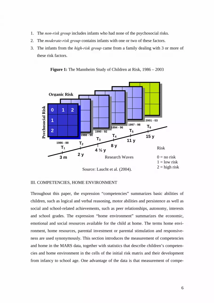
1. The non-risk group includes infants who had none of the psychosocial risks.

2. The moderate-risk group contains infants with one or two of these factors.

3. The infants from the high-risk group came from a family dealing with 3 or more of

these risk factors.

Figure 1: The Mannheim Study of Children at Risk, 1986 – 2003

Source: Laucht et al. (2004).

III. COMPETENCIES, HOME ENVIRONMENT

Throughout this paper, the expression “competencies” summarizes basic abilities of

children, such as logical and verbal reasoning, motor abilities and persistence as well as

social and school-related achievements, such as peer relationships, autonomy, interests

and school grades. The expression “home environment” summarizes the economic,

emotional and social resources available for the child at home. The terms home envi-

ronment, home resources, parental investment or parental stimulation and responsive-

ness are used synonymously. This section introduces the measurement of competencies

and home in the MARS data, together with statistics that describe children’s competen-

cies and home environment in the cells of the initial risk matrix and their development

from infancy to school age. One advantage of the data is that measurement of compe-

Risk

0 = no risk 1 = low risk 2 = high risk

1990 - 92

1986 - 88

T1

2 y

T2 4 ½ y

T3

8 y

T4

2

Research Waves 3 m

15 y Psyc

hoso

cial

Ris

k

1997 - 981994 - 96

11 y

T5

1 2

Organic Risk

0

1 T6

2001 - 03

1988 - 90

7

tencies and home starts in early infancy (at the age of three months), in addition to the

availability of early risk conditions.

1. Cognitive, motor and noncognitive abilities

The terms cognitive, motor, and noncognitive abilities indicate three different, yet de-

pendent and important basic dimensions of human capital and personality. Cognitive

abilities include memory capacity, information processing speed, linguistic and logic

skills, and general problem-solving abilities (IQ). Motor abilities are assessed as fine

and gross motor skills and body coordination (MQ) (for a detailed description of the

measurement of cognitive and motor abilities in MARS, see the appendix IQ, MQ).

Our main dimension of noncognitive abilities measures the child's ability to pursue a

particular activity and its continuation in the face of distracters and obstacles, defined as

persistence (P). The ratings were generated by experts4 on 5-point rating scales adapted

from the New York Longitudinal Study NYLS (see Thomas and Chess, 1977). P is a

deep-seated noncognitive ability related to effort regulation, perseverance, persistence

and self-discipline.5 Until the age of 2, P is measured together with attention span

within the same scale. Persistence was derived from a combination of a standardized

parent interview and structured direct observations in four standardized settings on two

different days in both familiar (home) and unfamiliar (laboratory) surroundings in order

to reduce measurement errors. P is available throughout the first five waves.

Table 1 contains summary statistics of the abilities IQ, MQ and P in the nine risk groups

of MARS. Note that the IQ and the MQ have been normalized in each developmental

stage to a mean of 100 and a standard deviation of 15 in an approximate normative

sample of 110 children. For reasons of clarity, we restrict the presentation to the ages of

4 At the ages of 3 months and 2 years, the interrater reliability was measured in a subsample of 30 chil-

dren. Satisfactory interrater agreement was obtained between two raters (3 months: mean κ = 0.68, range

0.51 - 0.84; 2 years: mean κ = 0.82, range 0.52 - 1.00). To avoid distortions resulting from parental judg-

ment or one-time observations in an unfamiliar surrounding, a mean score was formed out of all 5 ratings. 5 We examined further dimensions from the NYLS scales, among them the initial reaction to a new

stimulation, the length of time needed to adapt, and the prevailing mood. Our econometric analysis re-

vealed that these dimensions showed no systematic correlations with the cognitive abilities, which seems

to be in line with the early literature. Studies cited by Thomas and Chess (1977) indicated that none of

these temperament measures were associated with the level of the IQ.

8

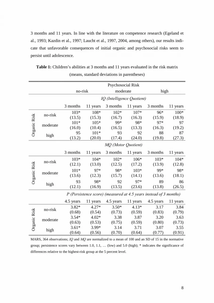
3 months and 11 years. In line with the literature on competence research (Egeland et

al., 1993; Kazdin et al., 1997; Laucht et al., 1997, 2004, among others), our results indi-

cate that unfavorable consequences of initial organic and psychosocial risks seem to

persist until adolescence.

Table 1: Children’s abilities at 3 months and 11 years evaluated in the risk matrix

(means, standard deviations in parentheses)

Psychosocial Risk

no-risk moderate high

IQ (Intelligence Quotient)

3 months 11 years 3 months 11 years 3 months 11 years

no-risk 103* (13.5)

108*(15.3)

102*(16.7)

107*(16.3)

96* (15.9)

100*(18.9)

moderate 101* (16.0)

105*(10.4)

99*(16.5)

98*(13.3)

97* (16.3)

97(19.2)

Org

anic

Ris

k

high 95 (13.2)

101*(20.0)

93(17.4)

92(24.0)

88 (19.8)

87(27.3)

MQ (Motor Quotient)

3 months 11 years 3 months 11 years 3 months 11 years

no-risk 103* (12.1)

104*(13.0)

102*(12.5)

106*(17.2)

103* (13.9)

104*(12.8)

moderate 101* (13.6)

97*(12.3)

98*(15.7)

103*(14.1)

99* (13.6)

98*(18.1)

Org

anic

Ris

k

high 93 (12.1)

98*(16.9)

92(13.5)

97*(23.6)

89 (13.8)

86(26.5)

P (Persistence score) (measured at 4.5 years instead of 3 months)

4.5 years 11 years 4.5 years 11 years 4.5 years 11 years

no-risk 3.82* (0.68)

4.27*(0.54)

3.50*(0.73)

4.13*(0.59)

3.17 (0.83)

3.84(0.79)

moderate 3.54* (0.63)

4.02*(0.53)

3.38(0.75)

3.87(0.59)

3.20 (0.80)

3.63(0.73)

Org

anic

Ris

k

high 3.61* (0.64)

3.99*(0.56)

3.14(0.70)

3.71(0.64)

3.07 (0.77)

3.55(0.91)

MARS, 364 observations; IQ and MQ are normalized to a mean of 100 and an SD of 15 in the normative

group; persistence scores vary between 1.0, 1.1, … (low) and 5.0 (high); * indicates the significance of

differences relative to the highest-risk group at the 5 percent level.

9

Organic and psychosocial risk factors exhibit equally negative effects, but are specific

to the areas they affect. Until the age of 11, the individual differences in children’s abili-

ties, according to the mean and the standard deviations, have increased. Initial inequal-

ity in the risk matrix is magnified over time. While psychosocial risks primarily influ-

ence cognitive and socio-emotional functioning, the impact of early organic risks is

concentrated on motor and cognitive functioning.

There is a monotonic decrease in the IQ and the MQ in (nearly) all risk dimensions.

Differences in average IQ, MQ and P increase between the ages of 3 months and 11

years in the risk matrix. At the age of 3 months, the children free of any risk have an

average IQ of 103 compared to the children with high organic and high psychosocial

risk, whose average IQ is 88. In addition, differences in the standard deviations increase

with risk, from 13.2 in the no-risk group to 19.8 in the highest-risk group (Table 1). The

results for the MQ provide a similar picture.

Average persistence decreases monotonically along both risk dimensions. There is a 23

percent difference between the no-risk and the high-risk group of children at the age of

4.5 years (3.8 vs. 3.1, Table 1), and the heterogeneity of P (measured with the standard

deviation) increases along with the risk dimensions. At the age of 11 years, children

without any risk have an average IQ of 108 (SD 15.3), compared to the children with

the highest organic and psychosocial risk, who achieve an average score of 87 (SD 27.3)

(Table 1). The average gap in cognitive abilities at the age of 11 between the no-risk

and the maximum-risk group has increased from 15 to 21.6 The results for the MQ at the

age of 11 are very similar to the results for the IQ.

Our findings reveal that initial risk conditions are important in terms of inequality of

cognitive, motor and noncognitive abilities, and that the cumulative effect of organic

and psychosocial risk corresponds to the sum of the single risk effects. Differences in

average cognitive, motor and noncognitive abilities accelerate during childhood. Het-

erogeneity increases with the risk dimensions. Significant sex differences were observed

6 The difference is greater when compared to the IQ difference between Romanian adoptees at maximum

risk and a group of English adoptees without comparable risk (which amounts to 17, see Beckett et al.,

2006).

10

in the IQ only at the ages of 2 and 4.5 (the IQ of girls is 6% higher), and in P after the

age of two years (girls score higher, 0.42 at 4.5 years and 0.22 at 11 years).

2. Home environment

There are two types of home resource variables by which the children were assessed in

their early life cycle, summarized under socio-emotional categories, H (HOME score),

and economic categories, which were measured by the monthly net equivalence income

per household member, Y (Table 2). In MARS, the socio-emotional home resources

were rated with the Home Observation for Measurement of the Environment (HOME,

Bradley, 1989), adapted to German living conditions. All items were evaluated by

trained home visitors (interviewers), who were in contact with the primary caregiver. H

is the sum of all items.7

When the children are aged 3 months, H consists of six subscales: (1) emotional and

verbal responsibility of the mother, (2) acceptance of the child, (3) organization of the

environment, (4) provision of appropriate play materials, (5) maternal involvement with

the child, and (6) variability. At the age of 2 years, H comprises the six subscales plus

the caretaking activities. At the age of 4.5 years, H consists of the original subscales

plus the caretaking activities items and items related to the parent interview. At the age

of 8 and 11 years, MARS adopted the original HOME, which consists of 6 subscales

and 81 items.

Both measures of a child’s home resources decline steadily along with the psychosocial

risk dimension (Table 2). Within the group of children with high psychosocial risk, Y is

on average 60 percent of the value of the no-risk group in infancy. The differences in

the average H in the risk matrix show a similar pattern, although the gap is numerically

smaller. For the group of children with high psychosocial risk, H is 87 percent of that of

the no-risk group. In fact, this is a large gap, because parental stimulation and respon-

siveness are important resources for development. Parent-child interaction is the “cradle

of action” (Heckhausen and Heckhausen (2008, 384): “Maternal contingency behavior

7 Todd and Wolpin (2007) also use the total HOME score (more specifically, they use a short version of

the HOME score that is available in the NLSY79-CS, starting at age 3-5). Cunha and Heckman (2008)

use single items, such as theatre visits, musical instruments and books.

11

(also known as responsive behavior) seems to be conducive to the formation of general-

ized contingency expectations...”).

Table 2: H and Y in children aged 3 months and 11 years evaluated in the risk matrix

(means, standard deviations in parentheses)

Psychosocial Risk

no-risk moderate high

H: HOME score

3 months 11 years 3 months 11 years 3 months 11 years

no-risk 106* (12.9)

108*(6.5)

102*(12.9)

105*(10.2)

93 (17.0)

92(19.8)

moderate 105* (14.2)

107*(6.9)

100(12.9)

99(12.6)

95 (14.1)

92(21.7)

Org

anic

Ris

k

high 106* (10.5)

106*(9.1)

100*(12.7)

98(10.8)

94 (18.6)

94(16.6)

Y: monthly net equivalence income per head

3 months 11 years 3 months 11 years 3 months 11 years

no-risk 1,275* (775)

1,699*(681)

1,122*(542)

1,632(832)

775 (465)

1,256(643)

moderate 1,293* (649)

1,644*(627)

903(239)

1,325(555)

948 (774)

1,325(641)

Org

anic

Ris

k

high 1,180* (403)

1,806*(629)

927(295)

1,425(495)

863 (344)

1,355(636)

MARS, 364 observations; for the initial risk matrix, compare Table A1 and A2 and the text. Y in DEM; H

is normalized to a mean = 100 and an SD = 15 in the normative group for purposes of comparison; *

indicates significance of mean differences relative to the high-risk group at the 5 percent level.

The relationship between H and Y is of special interest for reasons of policy interven-

tion. Although the relationship is positive (a higher Y is associated with a higher H), the

magnitude seems to be rather low. If economic resources were doubled, H would on

average be 8 to 10 percent higher. The partial elasticity of H with respect to Y is on av-

erage 0.08, with some variation over time (t1=0.06, t2=0.09, t3=0.11, t4=0.08, t5=0.07).

3. Social competencies

Social competencies of children were assessed in two ways. From the ages of 4.5 to 11

years, the Scales for Levels of Functioning (Marcus et al., 1993) were used, and from 8

12

to 11 years, the Perceived Competence Scales were administered (Harter and Pike,

1984; German version by Asendorpf and van Aken, 1993). Based on expert and self-

ratings, respectively, these aim at measuring independence in everyday life (autonomy),

hobbies (interests), and integration into groups and social life (peers). The results are

shown in Table 3.

Table 3: Social competencies at the age of 8 years evaluated for children in the risk

matrix (means, standard deviations in parentheses)

Psychosocial Risk

no-risk moderate high

interests / autonomy (expert ratings)

no-risk 5.09* / 4.64* (0.74 / 0.81)

4.87* / 4.84* (0.89 / 0.73)

4.37 / 4.78* (1.17 / 0.98)

moderate 4.98* / 4.83* (0.68 / 0.88)

4.42* / 4.52 (0.75 / 1.15)

4.09 / 4.35 (0.99 / 1.13)

Org

anic

Ris

k

high 4.92* / 4.59 (0.83 / 1.04)

4.31 / 4.26 (1.06 / 1.31)

3.95 / 4.07 (1.21 / 1.42)

peer relations (expert- / self-rated)

no-risk 4.82* / 18.23 (0.92 / 3.0)

4.62* / 18.20 (0.89 / 3.56)

4.57* / 18.36 (1.15 / 3.73)

moderate 4.48* / 18.50 (0.89 / 3.68)

4.45* / 18.06 (0.94 / 3.35)

4.39 / 17.84 (1.05 / 3.64)

Org

anic

Ris

k

high 4.81* / 19.11 (0.91 / 3.03)

4.41 / 18.27 (1.02 / 3.4)

3.98 / 18.49 (1.24 / 2.79)

MARS, 364 observations; social competence scores range from 1.0 (low), 1.1, … to 5.0 (high), self-

concept scores range from 10 (low) to 24 (high); * indicates significant mean differences relative to the

high risk group at the 5 percent level.

In addition to the expert-rated Levels of Functioning scale, the self-rating indicating

perceived peer acceptance is included to facilitate comparison. Peer acceptance is a

subscale of the Harter Scales, and consists of 6 items, each ranging from 1 to 4. The

items correspond to children’s self-perceptions regarding their peer relationships. For

example, children were asked how many friends they have, whether they are among

those children who easily find others to play with, or whether they see themselves as

lonely, because they are not asked to join in other children’s play.

13

Table 3 contains the means of the competencies variables evaluated at the age of 8 years

for the cells of the risk matrix. Initial risk effects cumulate and all social adjustment

scores decrease with both dimensions of the risk matrix. The gaps in social competen-

cies at the age of 8 years are significant. The difference between the no-risk and the

high-risk groups amounts to roughly 25 percent. However, two exceptions are worth

mentioning. First, if there is no psychosocial risk, organic risks seem to lose their asso-

ciation with regard to autonomy, interests and peers. When pursuing various interests

and popularity with peers, the initial psychosocial risk load seems to be, on average,

more harmful than organic risks. Second, based on the self-rating, little variation in the

cells of the risk matrix emerged. From the child’s viewpoint, the differences in social

life seem to be less significant compared to the expert ratings.

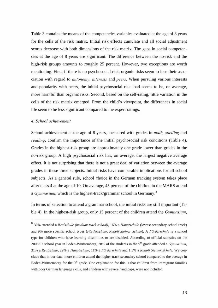
4. School achievement

School achievement at the age of 8 years, measured with grades in math, spelling and

reading, confirm the importance of the initial psychosocial risk conditions (Table 4).

Grades in the highest-risk group are approximately one grade lower than grades in the

no-risk group. A high psychosocial risk has, on average, the largest negative average

effect. It is not surprising that there is not a great deal of variation between the average

grades in these three subjects. Initial risks have comparable implications for all school

subjects. As a general rule, school choice in the German tracking system takes place

after class 4 at the age of 10. On average, 45 percent of the children in the MARS attend

a Gymnasium, which is the highest-track/grammar school in Germany.8

In terms of selection to attend a grammar school, the initial risks are still important (Ta-

ble 4). In the highest-risk group, only 15 percent of the children attend the Gymnasium,

8 30% attended a Realschule (medium track school), 16% a Hauptschule (lowest secondary school track)

and 9% more specific school types (Förderschule, Rudolf Steiner Schule). A Förderschule is a school

type for children who have learning disabilities or are disabled. According to official statistics on the

2006/07 school year in Baden-Württemberg, 28% of the students in the 9th grade attended a Gymnasium,

31% a Realschule, 29% a Hauptschule, 11% a Förderschule and 1.3% a Rudolf Steiner Schule. We con-

clude that in our data, more children attend the higher-track secondary school compared to the average in

Baden-Württemberg for the 9th grade. One explanation for this is that children from immigrant families

with poor German language skills, and children with severe handicaps, were not included.

14

compared to 74 percent in the no-risk group. Average Gymnasium attendance decreases

(nearly) monotonically along the two dimensions of our risk design, but there are two

exceptions. First, for children born without psychosocial risk, there seems to be no dif-

ference between the moderate and the high organic risk groups, and second, for children

born without organic risk, the no-risk and the moderate psychosocial risk groups are

similar.

Table 4: School achievement (grades) at age 8 and higher-track

secondary school attendance at age 11

Psychosocial Risk

no-risk moderate high

Grades in reading, spelling and math a) at age 8

no-risk 2.0*/ 2.1*/ 2.1* 2.2*/ 2.2*/ 2.1* 2.3/ 2.6 / 2.4*

moderate 2.2*/ 2.2*/ 2.2* 2.4 / 2.4*/ 2.4 2.8 / 2.9 / 2.7

Org

anic

Ris

k

high 2.1*/ 2.2*/ 2.3* 2.4 / 2.4 / 2.6 2.8 / 3.0 / 2.9

Higher-track secondary school attendance Gymnasium / Realschule / others b) at age 11 (in percent)

no-risk 74* / 24* / 02* 77* / 09* / 14* 43 / 21* / 36

moderate 45 / 40* / 15* 38 / 38* / 34* 33 / 23 / 44

Org

anic

Ris

k

high 54* / 23* / 23* 27 / 38 / 45 15 / 28 / 67

MARS, 322 to 357 observations, depending on the available information; a) in the German educational

system, grades range from 1.0 (excellent) to 6.0 (insufficient), b)Haupt-, Förder- and Rudolf-Steiner-

Schule, *indicates significant mean differences relative to the high-risk group at the 5 percent level.

5. First-order temporal correlations

The longitudinal dimension of the data is utilized to examine the stability of the meas-

ured competencies and home resources over time. Table 5 summarizes the first-order

temporal correlations for cognitive, motor and noncognitive abilities and social compe-

tencies. These correlations provide empirical measures of the interpersonal rate of con-

15

solidation in competencies. While they are presumably lower for some abilities, for ex-

ample noncognitive abilities during childhood, they may be higher for others, for exam-

ple motor abilities. A high value is an indication that interpersonal differences have

been stable between two periods. Taking measurement errors and further factors of in-

fluence into account (discussed in section 4 below), a correlation coefficient between

0.30 and 0.49 indicates low consolidation; a value between 0.5 and 0.69 indicates mod-

erate consolidation, and values above 0.70 suggest high consolidation of interpersonal

differences over time.

Table 5: First-order temporal correlations

3 months - 2 years

2 years - 4.5 years

4.5 years - 8 year

8 years - 11 years

Basic abilities

IQ 0.34 0.72 0.74 0.81

MQ 0.35 0.63 0.53 0.60

P 0.03 0.42 0.59 0.64

Social competencies

Peers n.a. n.a. 0.31 0.65

Interests n.a. n.a. 0.58 0.64

Autonomy n.a. n.a. 0.33 0.56

MARS, 364 observations; all correlation coefficients are significant at the 5 percent level with the excep-

tion of the P correlation from 3 months to 2 years; n.a.=not applicable

Table 5 suggests that interpersonal differences in cognitive and motor abilities in our

sample consolidate during preschool age. The correlations vary between 0.63 and 0.72,

suggesting a relatively high degree of stability of interpersonal differences in the IQ.

The first-order temporal correlations for persistence are lower. They indicate only mod-

erate stability until the age of 4.5 years and an increase in stability thereafter. There is

moderate stability of social competencies between the ages of 4.5 and 8 years and con-

solidation thereafter. Social competencies such as good peer relationships and interests

that demonstrate children’s social integration seem to consolidate at an age between 8

and 11 years or later.

16

With respect to the economic and socio-emotional home resources, Y and H, a high sta-

bility from birth until the age of 11 years is evident. In all cases, the first-order temporal

correlations exceed the value of 0.7. This demonstrates that children experience a rela-

tively high degree of stability of their economic as well as socio-emotional home envi-

ronment, irrespective of whether it is adverse or beneficial.

IV. ABILITY FORMATION IN THE EARLY LIFE COURSE

1. Econometric approaches

Factors that are responsible for the production of abilities, Θt, in period t, can be sum-

marized with the term “technology of skill formation” (Cunha and Heckman, 2007; see

equation (1)). For our study, Θ represents the vector of cognitive, motor, and noncogni-

tive abilities. E represents initial conditions, Θt-1 the vector of abilities from the period

before, and It age-specific investments intended to enhance abilities.

(1)

The epidemiological cohort data allow a detailed look at early organic and psychosocial

conditions. Moreover, the data contain comprehensive psychometric assessments as

well as psychological expert ratings of abilities and stage-specific home resources. Data

quality helps to reduce measurement errors. It is assumed that equation (1) can be repre-

sented in a Cobb-Douglas form. Taking the natural logarithm (lower case letters indi-

cate the natural logarithm) yields equation (2):

(2)

where j, k, l are indices for the basic abilities IQ, MQ and P, and i = 1, …, N is an index

for the child. There are five different time periods. The variable R contains all nine cells

of the two-dimensional risk matrix in MARS. The error term, ε, represents random fac-

tors related to abilities.

In the econometric analysis, we focus on the role of socio-emotional home resources, H,

in period t and the stock of abilities from period t-1 for the production of abilities. The

Cobb-Douglas form (equation (2)) implies that actual abilities can be produced continu-

j j,R h, j j j k, j k l, j l jt ,i 0,t t t ,i t t 1,i t t 1,i t t 1,i t ,ihθ α α α θ α θ α θ ε− − −= + ⋅ + ⋅ + ⋅ + ⋅ +

( )t t t t-1f I , ,EΘ Θ=

17

ously by socio-emotional home resources and the stock of abilities available from the

past period. All parameters can be interpreted as partial elasticity. While early life ad-

versity can have lasting effects on the level of abilities, the Cobb-Douglas production

function implies that change remains possible in each period.

The relationship between parental investments and children’s abilities may be recipro-

cal, leading to reversed causality. Having a child with high abilities is likely to increase

H in order to support development. A child with low abilities may be a source of stress

for the parents, which may even lead to a reduction of H. If parental investment depends

on ability in such a way, then OLS estimates of equation (2) may be biased downwards,

since children with higher abilities also have higher socio-emotional home resources.

To address the endogeneity of H, we compare OLS with two-stage least square results

(2SLS). In the first stage, we estimate H as a function of the ability under consideration,

for instance the IQ, and use the economic home resources, Y, as an additional variable.

This is equivalent to using Y as an instrument for H in equation (2).

Monthly net equivalence income per head, Y, is partially related to H, one necessary

condition for an instrumental variable. We find a significant (partial) correlation in each

period (reported in section 3 above). On average, a 10% increase in Y is associated

roughly with a 1% increase in H. A second condition for Y being a valid instrument is

that it should only affect abilities due to its relation to H. As the exogeneity of an in-

strument is not testable for the one-instrument case, we have to assume that the socio-

emotional home resources (parental care or parental responsiveness) cause ability de-

velopment. While parental care itself may depend on the availability of economic home

resources, the latter do not have a direct impact on ability formation. This seems to be

plausible and does not rule out that direct pathways from Y to some competencies exist,

for instance social achievement and grades at school age. Furthermore, the choice for

higher secondary education in adolescence directly depends on the availability of eco-

nomic resources (compare section 5 below).

According to our data, the influence of Y on children’s abilities is never significant in

addition to H and the level of past abilities in equation (2). The associations are domi-

nated by the variation of socio-emotional home resources and past abilities, and not by

the inequality of per capita income in the family. Thus, under the assumption that finan-

18

cial resources have no direct impact on abilities, a comparison between OLS and 2SLS

might be helpful to assess lower and upper bounds for the causal relationship between H

and abilities.

A different, though related source of bias may stem from omitted variables that create

correlations between abilities and the error term. To reduce the ability bias, we include

all available lags of abilities in addition to the values of the past (one period lag) abili-

ties into the equation (2). To reduce the bias from unobserved variables correlated with

right-hand variables, it helps us to use all abilities from the distant past (see

Wooldridge, 2005). Further econometric approaches are discussed below.

2. Econometric results

Table 6 documents the estimates of the different econometric approaches for the IQ and

P. There are columns for OLS results without and with additional lags and for 2SLS

results without and with lags. A significance level of 5 percent was chosen throughout

the study. Each equation contains the set of dummies from the initial risk matrix, R.

Starting with age 4.5, this set of dummies was not jointly significant at the 5 percent

level for cognitive and noncognitive abilities, and the estimates beginning at age 4.5

were performed without R.

Our first conclusion corresponds to motor abilities. Although the partial elasticity of

MQ and H is always positive, it lacks statistical significance at the 5% level. Motor

abilities strongly depend on early organic and psychosocial conditions (compare Table 1

above), and only weakly on socio-emotional home resources during childhood. In fact,

there appears to be a high degree of stability in interpersonal differences in the MQ dur-

ing the early life course. For reasons of clarity, we do not report the results for the MQ

equation in Table 6, but rather in the appendix (Table A3).

The OLS estimates indicate that H is positively related to cognitive and noncognitive

ability development at all developmental stages (Table 6). However, the role of socio-

emotional home resources and the level of abilities from the past period for ability for-

mation changes in a way that is specific to age and abilities. P is always significantly

associated with H, with the estimated partial elasticity varying between 0.30 and 0.53.

The highest values for the elasticity are estimated to occur at the ages of 4.5 and 8 years.

19

This is consistent with findings reported in Cunha and Heckman (2008), who estimate

parameters of the technology of skill formation for three stages, starting with stage 1

from age 6-7 to age 8-9 and ending with stage 3 from age 10-11 to 12-13. The IQ is

positively related to H until the age of 4.5 years, with an estimated partial elasticity

varying between 0.55 at three months and 0.38 at the age of 4.5 years. At school age,

the elasticity drops to 0.19. Although this is still positive, it is no longer significant at

the 5% level.

The estimated elasticity of the past abilities steadily increases during the early course of

life. It is low until toddlerhood and increases thereafter. With increased levels of abili-

ties, the child reaches higher levels of independence. During development, the socio-

emotional home environment loses its strong relationship with abilities at preschool age.

The more abilities children acquired during childhood, the higher the stock of cognitive

abilities at school age will be, when the relationship to socio-emotional home resources

decreases. Our stage-specific estimates at secondary school age (11 years) for the IQ at

primary school age (8 years) varies around 0.9, a value which is comparable in magni-

tude with the findings from Cunha and Heckman (2008). However, our estimates of the

parameters of past abilities are lower for the pre-school period and for noncognitive

abilities, P. For the pre-school period, our results seem to be in line with Cunha et al.

(2008), who studied the parameters of the technology of skill formation for two periods

(age 0 to 4 years and age 5 to 14 years). Comparable to our results, self-productivity is

low in early childhood and increases when children grow older, although in an ability-

specific way. Cunha et al. do not regard motor abilities in their research, but according

to our study, self-productivity in motor abilities is already high in early childhood.

When significant, the 2SLS estimates for the IQ and P equation are higher compared to

the OLS results (Table 6) (with one exception: at preschool age, the coefficient for the P

equation is lower for the 2SLS estimate). In the third period (age 4.5 years), for exam-

ple, the coefficient in the IQ equation is 0.53, compared to 0.38 for OLS. In infancy and

toddlerhood, the difference is wider. If parents provide a higher H for their first-born

children with a higher IQ, the OLS underestimates the partial elasticity as a result of

reversed causality. Assuming that Y has no direct impact on ability and that the relation-

ship is linear, 2SLS identifies a causal impact.

20

Table 6: Econometric findings for ability formation, IQ and P equation (2)

(standard errors in parentheses)

IQt Pt

OLS OLS + lags

2SLS 2SLS + lags

OLS OLS + lags

2SLS 2SLS + lags

t = 3 months a) Ht 0.54* 2.37* 0.30* 0.66 (0.14) (0.98) (0.14) (0.73)Adj. R2/F-test 0.10 2.54 0.02 1.15 t = 2 years a) Ht 0.37* 1.57* 0.36*** 1.33** (0.08) (0.45) (0.11) (0.58)IQt-1 0.23* 0.09 0.11 0.001 (0.06) (0.10) (0.08) (0.11) Pt-1 0.13* 0.16* -0.07 0.18* (0.06) (0.09) (0.07) (0.11)Adj. R2/F-test 0.30 6.94 0.12 3.49 t = 4.5 years Ht 0.38* 0.37* 0.50* 0.51* 0.54* 0.53* 0.04 -0.02 (0.09) (0.09) (0.18) (0.20) (0.22) (0.22) (0.40) (0.43)IQt-1 0.53* 0.53* 0.50* 0.50* 0.55* 0.53* 0.67* 0.65* (0.06) (0.06) (0.07) (0.07) (0.12) (0.12) (0.14) (0.14) Pt-1 0.02 0.02 0.008 0.01 0.16* 0.18* 0.19* 0.21* (0.03) (0.03) (0.03) (0.03) (0.06) (0.06) (0.07) (0.07)Adj. R2/F-test 0.58 0.58 71.12 45.28 0.34 0.34 29.85 19.38 t = 8 years Ht 0.19 0.18 0.31 0.24 0.43* 0.38* 0.64 0.53 (0.16) (0.15) (0.35) (0.37) (0.18) (0.18) (0.45) (0.50)IQt-1 0.84* 0.77* 0.82* 0.76* 0.27* 0.21* 0.24* 0.19 (0.08) (0.10) (0.10) (0.10) (0.10) (0.12) (0.13) (0.14)Pt-1 0.09* 0.08* 0.08* 0.07 0.29* 0.28* 0.28* 0.27* (0.04) (0.04) (0.05) (0.05) (0.05) (0.05) (0.05) (0.06)Adj. R2/F-test 0.64 0.64 37.61 17.87 0.36 0.35 27.92 13.10 t = 11 years Ht 0.17 0.16 -0.59 -0.90 0.39* 0.38* 0.89 1.38* (0.15) (0.15) (0.51) (0.59) (0.18) (0.19) (0.61) (0.70)IQt-1 0.88* 0.75* 1.02* 0.89* 0.22* 0.32* 0.12 0.19 (0.07) (0.07) (0.12) (0.11) (0.07) (0.09) (0.13) (0.13)Pt-1 0.11* 0.11* 0.15* 0.14* 0.29* 0.25* 0.26* 0.22* (0.05) (0.05) (0.06) (0.06) (0.05) (0.05) (0.06) (0.07)Adj. R2/F-test 0.76 0.78 49.14 19.28 0.36 0.39 25.68 9.19

MARS, 364 observations, all variables in natural logarithm; estimates include a constant. MQ equation

not reported here. a the equations for 3 months and 2 years contain nine dummies for the cells in the peri-

natal risk matrix; + lags: in this column, all available lags of IQ, MQ and P are included in addition to the

one period lag, although the coefficients are not reported here; * indicates significance at the 5 percent

level, based on heteroscedastically robust standard errors; for OLS, the Adj. R² for 2SLS F-tests are re-

ported.

21

If the assumption applies, the socio-emotional home resources are even more important

for child development than the OLS results suggest. Although this seems to be in line

with evidence on the eminent role of the home environment in early childhood, as dis-

cussed by Amor (2003), Heckhausen and Heckhausen (2008) and Cunha et al. (2008),

among others, a caveat remains within our analyses. 2SLS estimates produce higher

standard errors (for the year 4.5 and the IQ equation (2), the point estimate is 0.53 with

a standard error of 0.18 compared to OLS: 0.38, 0.7). Therefore, the difference from the

OLS is not well-determined from a statistical point of view. OLS results with lower

standard errors may even be closer to the “true” parameters of the technology of ability

formation. Nevertheless, 2SLS estimates demonstrate that socio-emotional home re-

sources might be more important for cognitive ability than OLS results suggest. There-

fore, we regard the 2SLS results as an upper bound and the OLS results as a lower

bound of the “true” value of the elasticity. We will compare policy conclusions based

on the upper and the lower bounds in section VI below.

Including all available lags in order to reduce an omitted variable bias changes neither

the coefficient of H nor those of the lagged abilities (one period lag) a great deal (Table

6, columns 3 and 5). Omitted past abilities do not seem to bias OLS or 2SLS estimates.

3. Further estimates

A further set of regression analyses was performed including Ht-1 instead of Ht in equa-

tion (2). In this case, the estimated coefficients for all abilities remain (almost) un-

changed, while the estimated coefficients for the lagged socio-emotional home re-

sources do not change much (results available upon request). The main reason for this

finding is that the interpersonal variation of H remains fairly constant over time.

If a sex indicator is included in equation (2), the respective coefficients are significant

(in Model 1) only in two of the five periods. The estimated difference varies around

0.02 and 0.04, if significant. All other coefficients remain unaffected. From a produc-

tion function point of view, cognitive and noncognitive ability formation seems to be

rather similar between boys and girls. If we additionally include height (and/or weight),

the explanatory power of Model 1 does not increase, and the additional coefficients fail

to reach significance. This confirms research from Case and Paxson (2008).

22

A set of quantile regressions was performed to examine differences for each quantile of

the ability distribution, starting at the age of 2 years. The set of results for the IQ is re-

ported in Table A4. The quantile estimates suggest that the partial elasticity of H with

respect to the IQ is slightly lower at the tails of the IQ distribution (or slightly higher in

the middle area). For children with rather low or rather high cognitive abilities, H seems

to be less important compared to children with medium abilities. At the age of 11 years

and for the 50th and 60th percentile of the IQ distribution, the partial elasticity of H with

respect to the IQ becomes significant (see Table A4). We conclude that the production

of abilities depends on the level of abilities, although the number of observations in our

data is too low to quantify the differences more precisely. In the group of children with

low or high IQ measures, socio-emotional home resources have a lower association with

the IQ.

Table A5 documents separate regression results for the verbal and the nonverbal IQ in

order to investigate whether there is evidence for sensitive investment periods regarding

the two dimensions of cognitive abilities. The partial elasticity of H with respect to the

verbal IQ is higher in comparison to the nonverbal IQ at all developmental stages (Table

A5). We conclude that socio-emotional home resources have a closer relationship to

verbal than to the (more fundamental) figural reasoning and understanding. The window

of ability formation by improved socio-emotional home resources seems to be smaller

for the nonverbal aspects of cognitive ability, such as logical reasoning, and longer for

the verbal and linguistic dimension of cognitive ability.

V. ABILITIES AS PREDICTORS OF COMPETENCIES AT SCHOOL AGE

In this section, we proceed with the analysis of competence formation during the transi-

tion from preschool to primary and from primary to secondary school. We try to shed

some light on complementarities between basic cognitive, motor and noncognitive abili-

ties and social and school achievement during the early life course. We assess the mag-

nitude of preschool factors for school achievement in order to further examine the child-

hood skill multiplier (Heckman, 2007). In addition, we analyze whether higher secon-

dary school track still improves cognitive and noncognitive abilities.

23

1. Abilities at preschool age as predictors of social competencies at primary school age

We present findings from regression models in order to explain four measures of social

competencies at primary school age. On the right-hand side of the regression equation,

home resources, H and Y, and the level of IQ, MQ and P measured at preschool age are

included. The results from OLS estimates, documented in Table 7, demonstrate substan-

tial complementarities between abilities acquired during childhood and social compe-

tencies which a child achieves at elementary school age, and several differences be-

tween the four competencies.

Table 7: The partial elasticity of preschool abilities and home resources for social com-

petencies at school age (t= 8 years, means and standard errors in parentheses)

interests autonomy peer relations: expert-rated self-rated

Ht 1.44* (0.18) 0.07 (0.26) 0.76* (0.20) 0.27 (0.23)

Yt -0.00 (0.02) -0.04 (0.03) -0.00 (0.03) 0.03 (0.03)

IQt-1 0.54* (0.10) 0.07 (0.14) 0.12 (0.12) 0.13 (0.11)

MQt-1 0.21* (0.07) 0.65* (0.10) 0.29* (0.08) 0.05 (0.09)

Pt-1 0.13* (0.04) -0.06 (0.07) 0.21* (0.06) 0.05 (0.06)

Adj. R² 0.60 0.23 0.29 0.04

Observations 364 364 363 352

MARS, OLS regressions, including a constant, with heteroscedastically robust standard errors; all vari-ables in natural logarithm; * indicates significance at the 5 percent level.

Cognitive, motor and noncognitive abilities at preschool age predict interests at primary

school age, motor abilities predict autonomy, and motor and noncognitive abilities pre-

dict peer relations. There are significant associations between the indicator of social

competence, peers, and H, the MQt-1 and Pt-1. Interests are additionally associated with

the IQ acquired until the previous stage. Autonomy, measuring maturity in everyday life,

is solely linked to the past MQ. Contemporary H enhances both popularity among peers

(peer relations), and the variety of actively followed interests (interests), according to

expert ratings. The findings demonstrate complementarities in competence formation,

indicating that higher basic cognitive, motor and noncognitive abilities acquired in

childhood help children to perform better with regard to social competencies at school

24

age. Children from adverse home environments suffer twofold, due to poor investments

in their abilities until preschool age and due to insufficient support during primary

school age.

Surprisingly, however, there is no significant association with the self-rated peer rela-

tions. None of our observations are related to the child’s self-rating of social relation-

ships and friendships (last column, Table 7). Findings from self-ratings differ from

those of expert ratings for various reasons. This discrepancy might be caused, among

other things, by a self-protection mechanism employed by children at risk to cope with a

situation in which emotional support is continuously lacking. To overcome their misery,

they rate their peer relationships as satisfactory. Another explanation is that children

with lower levels of basic abilities are satisfied with a smaller variety in terms of their

peer relationships and their interests.

2. Abilities at preschool age as predictors of grades at primary school age

Findings from linear regressions predicting school grades by preschool factors are sum-

marized in Table 8. Grades for reading, spelling and math are evaluated in primary

school at the age of 8 years, two years before ability tracking takes place in the German

educational system. All grade equations include the current H, the current Y and the

cognitive, motor and noncognitive abilities measured at the age of 4.5 years. In an addi-

tional model, the IQ is divided into the verbal and the nonverbal abilities, V-IQ and NV-

IQ, respectively.

Note that a negative coefficient in Table 8 implies a better grade. The estimates can be

interpreted in terms of partial elasticity since the (natural) logarithm has been used for

all variables. The IQ and P at preschool age are significantly related to better grades in

reading and spelling as well as in math, with similar coefficients, while the MQ is not

(Table 8). Persistence is an important predictor for later achievement in school, which is

in line with Duckworth and Seligman (2005), among others. Interestingly, neither H nor

Y is related to the grades received at age 8.

Considering two different dimensions of IQ, only the NV-IQ remains a significant pre-

dictor of better grades. Accordingly, the level of fundamental cognitive abilities, such as

logical and figural reasoning and noncognitive abilities tends to be more important for

25

predicting school achievement at the primary school level than verbal abilities. When

interpreting this result, it has to be kept in mind that our sample included only children

of German-speaking parents. However, if this result could be replicated in other sam-

ples, it would be of utmost importance for policies to foster human capital, since our

results (see Table 6) point to a very short timeframe (until early childhood) for improv-

ing logical reasoning through improved socio-emotional home resources.

Table 8: The partial elasticity of preschool abilities and home resources for school

grades a) at primary school age (t=8 years, standard errors in parentheses)

reading spelling math

IQ V-/NV-IQ IQ V-/NV-IQ IQ V-/NV-IQ

Ht -0.10 -0.05 -0.64 -0.62 -0.49 -0.57 (0.43) (0.41) (0.43) (0.39) (0.42) (0.40)

Yt -0.02 -0.02 -0.06 -0.07 -0.04 -0.04 (0.02) (0.06) (0.05) (0.05) (0.06) (0.06)

IQt-1 -0.84* -0.60* -0.66* (0.19) (0.19) (0.19)

NV-IQt-1 -0.96* -1.18* -1.16* (0.23) (0.21) (0.23)

V-IQt-1 -0.26 0.16 0.21 (0.23) (0.21) (0.20)

MQt-1 -0.17 0.009 -0.21 0.001 -0.10 0.04 (0.13) (0.13) (0.12) (0.12) (0.12) (0.12)

Pt-1 -0.32* -0.23 -0.29* -0.19* -0.25* -0.22* (0.10) (0.10) (0.10) (0.10) (0.10) (0.10)

Adj. R² 0.19 0.24 0.20 0.27 0.17 0.23 Observations 327 327 322 322 327 327

MARS, a) in the German educational system, grades range from 1.0 (excellent) to 6.0 (insufficient); OLS regressions for reading, spelling and math including a constant, heteroscedastically robust standard errors, all variables in natural logarithm; * indicates significance at the 5 percent level.

3. Abilities at primary school age as predictors of higher-track school attendance

Findings from probit models predicting secondary school attendance are summarized in

Table 9. All probit estimates for attending the Gymnasium include the stage-specific

home resources H and Y, and the cognitive, motor and noncognitive abilities. These are

26

measured at primary school age (8 years), two years before tracking takes place. In a

further specification, the total IQ is split into verbal and non-verbal cognitive abilities.

In addition, all available lags of the three abilities are included in the probit equation to

reduce a potential bias from endogeneity (Wooldridge, 2005).

IQ, MQ and P at primary school age are significantly related to the probability of at-

tending Gymnasium. The magnitude of P is lower compared to the IQ and higher com-

pared to the MQ. If the verbal and the non-verbal IQ are considered separately, the NV-

IQ tends to be slightly more important than the V-IQ. Using all lags of ability (Table 9)

reduces some of the coefficients in the probit equation without changing the conclu-

sions. Home resources increase the probability of attending the Gymnasium. H is as

important as the IQ, and, at this stage of transition from primary to secondary school,

economic resources, Y, become relevant. If Y is 10% higher, the probability of attending

the Gymnasium increases by 1.8%, all else being equal.

Table 9: Average marginal effects for attending the Gymnasium

(standard errors in parentheses)

IQ IQ; + lags a)

Ht 0.82* (0.37) 0.60* (0.38)

Yt 0.15* (0.05) 0.18* (0.05)

IQt-1 1.03* (0.15) 0.84* (0.19)

MQt-1 0.37* (0.15) 0.33* (0.16)

Pt-1 0.49* (0.12) 0.38* (0.11)

Pseudo R² 0.29 0.32

Observations 357 357

MARS, a) this specification contains all available additional lags in abilities; although not reported here, these lags are jointly significant (LR-tests: 86.18*, 71.35*); * indicates significance at the 5 percent level.

Basic cognitive, motor and noncognitive abilities are developed in the interaction with

adequate socio-emotional home resources during the early life course. They predict

school achievement, help children to perform in terms of grades, and predict higher-

track school attendance.

27

A numerical examination illustrates the importance of the stock of abilities and socio-

emotional home resources (all values are taken from the estimation with all lags in-

cluded) for higher secondary school track. If the IQ at age 8 were 103.75 instead of 100

(i.e. 10% higher), the average marginal probability of attending the Gymnasium would

increase by 8.4%. If P at age 8 were 10% higher, the average marginal probability

would increase by 3.8%. If H at age 11 were 10% higher, the average marginal prob-

ability would increase by 6%, and if Y at age 11 were to increase by 10%, the marginal

increase in the probability would be 1.8%. This suggests the existence of some credit

market constraints at the age of 10 years. Bright children from poor households have a

lower chance of entering into a higher-track secondary school. The magnitude is moder-

ate in our data. Out of 1,000 children from poorer households, 18 will be constrained in

the school transition, according to our estimates. This demonstrates that cognitive and

noncognitive ability “constraints” from lower socio-emotional home resources at pre-

school age and/or from initial organic and psychosocial conditions are more important

than credit constraints in the period of transition from primary to secondary school.

VI. POLICIES TO IMPROVE COMPETENCE DEVELOPMENT

What conclusions can be drawn from our investigation for education policies? Assume

that the government has two objectives: it intends to improve competencies at secon-

dary school age and to increase the share of children entering the Gymnasium. Since

ability formation is a cumulative and dynamic process, the government faces alterna-

tives in the early life course that we would like to illustrate numerically.9 The govern-

ment either helps children early in their life to overcome constraints through poor socio-

emotional home resources, or it helps children later, at school age, to overcome credit

constraints, or both.

Assume that the government is willing to raise Y for all households by 10% (i.e. an in-

crease of 103 DEM (Deutsche Mark) per child on average in nominal terms 1986/1987,

1st wave, 151 DEM in nominal terms 1997/1998, 5th wave). A 10% increase in Y has no

direct implication for the formation of cognitive, motor and noncognitive abilities dur-

ing childhood. However, let us assume for the sake of simplicity that on average, it is

9 For a theoretical analysis of optimal human capital investment over the life cycle, compare Cunha and Heckman (2007), and for an application for Germany, see Pfeiffer and Reuß (2008).

28

related to a 1% increase in H. In order to help children acquire competencies it may be

necessary to improve their access to parental stimulation and responsiveness or emo-

tional resources. Although in social reality, low economic and poor socio-emotional

home resources are often related, the child can profit directly only from improved socio-

emotional home resources alone (see section 5). Assuming a causal relationship, an im-

provement of H by 1% would require a 10% increase in Y. Families either receive a

direct 10% income support or H is increased by other means (for example, direct emo-

tional support for the children).

We take all direct and indirect multiplier and accelerator effects from the age-dependent

1% increase in H into account. We regard the OLS estimates as a lower bound, and the

2SLS estimates as an upper bound of the policy effect. The impacts of age-dependent

policies are summarized in Table A6. Looking at the columns, Table A6 documents the

percentage point increases of a 1 % increase in H at five developmental stages during

the life course. Looking at the rows, Table A6 documents the resulting effects at a spe-

cific developmental stage. From the lower and upper bound effects, a set of similar and

a set of different policy implications can be derived. Both bounds indicate that the early

childhood years are optimal for bolstering basic cognitive abilities, while the frame for

improving noncognitive abilities broadens until adolescence. While both bounds clearly

indicate that childhood is of utmost importance for competencies at secondary school

age, the results for the upper bound suggest that infancy and toddlerhood are even more

relevant than preschool age. Interestingly enough, the lower bound results indicate that

policies during infancy, toddlerhood and preschool age have effects of similar magni-

tude. This can be concluded from the estimated high association between socio-

emotional home resources and noncognitive abilities (P) at the ages of 4.5 and 8 years

and the induced multiplier and accelerator effects.

However, the precision of the upper bound (2SLS) results needs to be further investi-

gated based on populations with a higher number of observations. Note that standard

errors of the 2SLS estimates are relatively high (see section 5). Therefore, the further

policy analyses rest upon the OLS results. If the upper bound results had been taken

instead, policies that are directed to earlier stages would have been even more effective.

29

If policy had successfully raised H by 1% at the age of three months (2 years, 4.5 years),

then the IQ would have increased until the age of 11 years by 1.11% (1.06%, 1.10%),

the MQ by 0.56% (0.31%, 0.19%) and P by 0.60% (0.96%, 0.94%). The probability of

entering the Gymnasium would be higher by an amount of 1.3% (1.3%, 1.1%). If H had

been increased by 1% at each of the 3 developmental stages in childhood, the resulting

effects on abilities could be added (for example the IQ would have increased by

1.11+1.06+1.10% =3.27%). Such a policy would increase the probability of entering

Gymnasium by 3.7% in our sample.

We compare these policies for improving the socio-emotional home resources available

in childhood with an increase in economic home resources during the transition to sec-

ondary school age. A 10% increase of Y implemented when the child is 11 years old

would increase the probability of attending the Gymnasium by 1.8% (see section 6).

Through an improvement of socio-emotional home resources at secondary school age,

such a policy would also be helpful in further increasing noncognitive abilities, while it

has no measurable impacts on cognitive and motor abilities. Both policy approaches

(additional support in early childhood versus support at secondary school age) are suc-

cessful in raising the probability of entering the Gymnasium. However, they differ in

their success in improving competencies.

The policy of supporting children at secondary school age mainly reduces credit market

constraints and, to some degree, improves noncognitive abilities. The policy of support-

ing students at preschool age or earlier would help to overcome a lack of socio-

emotional home resources. Therefore, this policy is likely to be more effective in im-

proving basic abilities. As a result of complementarities in development, higher social

and school competencies will emerge. Indeed, a combination of both types of policies

should be preferable for children who have been left behind. To help these children,

support should be extended continuously during all developmental stages. It should be

designed to overcome constraints in the availability of socio-emotional home resources

in early childhood and credit market constraints in adolescence.

30

VII. CONCLUSIONS

This paper contributes to uncovering the relationship of early life adversity and home

resources with competence formation in childhood as well as complementarities be-

tween children’s early and later achievement. Using data taken from the MARS, an epi-

demiological cohort study from birth to adulthood, our findings demonstrate that socio-

emotional home resources are significantly related to ability formation during child de-

velopment. The strength of the association differs between abilities and over time,

which is in line with Heckman (2007).

Advantages from favorable socio-emotional home resources and disadvantages from

poor socio-emotional home resources cumulate across development. Starting life with

risk and growing up in an unfavorable environment impedes the development of cogni-

tive and motor abilities. The disadvantage continues during the early life cycle until

school age, a stage particularly important for noncognitive ability formation (Heckman,

2000). Disadvantaged children are impeded once again when the transition to higher-

track secondary school attendance takes place. At this stage, low economic home re-

sources create an additional barrier.

We conclude that investment in better socio-emotional home resources during child-

hood is necessary for improving the development of cognitive and noncognitive abili-

ties, as well as social and school competencies. Economic support at school age addi-

tionally increases the probability of entering the Gymnasium because it reduces credit

market constraints. Future research on competence formation based on economic mod-

els should focus on more specific characteristics of the early parent-child relationship

and early child development. We are still lacking information about the variety of par-

ent-child interaction in infancy from representative data. Knowledge on early develop-

mental risks, both from the organic and the psychosocial dimension, and on parental

responsiveness, is necessary in order to foster competencies. Better data are needed to

improve research on the parent-child relationship as the cradle of lifelong action.

31

References

Angermaier, Michael (1974). Psycholinguistischer Entwicklungstest, Beltz, Weinheim.

Asendorpf, Jens B., and Marcel A.G. van Aken (1993). Deutsche Versionen der Selbst-

konzeptskalen von Harter. Zeitschrift für Entwicklungspsychologie und Pädagogi-

sche Psychologie, 25 (1), 64-96.

Almond, Douglas, Kenneth Y. Chay, and David S. Lee (2005). The Cost of Low Birth

Weight. Quarterly Journal of Economics, 120 (3), 1031-1083.

Amor, David J. (2003). Maximizing Intelligence. New Brunswick, Transaction Publi-

shers.

Bayley, Nancy (1969). Bayley Scales of Infant Development, Psychological Corporati-

on, New York.

Beckett, Celia, Barbara Maughan, Michael Rutter, Jenny Castle, Emma Colvert, Chris-

tine Groothues, Jana Kreppner, Suzanne Stevens, Thomas O'Connor, and Edmund J.

S. Sonuga-Barke (2006). Do the Effects of Early Severe Deprivation on Cognition

Persist Into Early Adolescence? Findings from the English and Romanian Adoptees

Study. Child Development, 77 (3), 696-711.

Black, Sandra E., Paul J. Devereux, and Kjell Salvanes (2007). From the Cradle to the

Labor Market? The Effect of Birth Weight on Adult Outcomes. Quarterly Journal of

Economics, 122 (1), 409-439.

Blomeyer, Dorothea, Katja Coneus, Manfred Laucht and Friedhelm Pfeiffer (2009).

Initial Risk Matrix, Home Resources, Ability Development and Children’s Achieve-

ment. Journal of the European Economic Association 7(2-3), 638-648.

Bradley, Robert H. (1989). The Use of the HOME Inventory in Longitudinal Studies of

Child Development. In: Marc H. Bornstein, and Norman A. Krasnegar (Eds.), Stabi-

lity and continuity in mental development: Behavioral and biological perspectives.

Hillsdale, New Jersey: Lawrence Erlbaum, 191-215.

Case, Anne, and Christina Paxson (2008). Stature and Status: Height, Ability, and Labor

Market Outcomes. Journal of Political Economy 116(3), 499-532.

Cattell, Raymond B. (1960). Culture Fair Intelligence Test, Scale 1 (Handbook). 3 ed.,

IPAT, Champaign, Ill.

Cunha, Flavio, and James J. Heckman (2007). The Technology of Skill Formation. The

American Economic Review, 97 (2), 31-47.

32

Cunha Flavio, and James J. Heckman (2008). Formulating, Identifying and Estimating

the Technology of Cognitive and Noncognitive Skill Formation. Journal of Human

Resources, 43 (4), 738-782.

Cunha Flavio, James J. Heckman and Susanne M. Schennach (2008). Estimating the

Technology of Cognitive and Noncognitive Skill Formation. Unpublished Manusc-

ript, University of Chicago.

Cunha, Flavio, and James J. Heckman (2009). The Economics and Psychology of Ine-

quality and Human Development. Cambridge, MA: NBER Working Paper 14695.

Duckworth, Angela M. and M. E. P. Seligman (2005). Self-Discipline Outdoes IQ in

Predicting Academic Performance in Adolescents. American Psychological Society

16 (12), 939--944.

Danese, Andrea, Carmine M Pariante, Avshalom Caspi, Alan Taylor and Richie Poulton

(2007): Childhood Maltreatment Predicts Adult Inflammation in a Life-Course Stu-

dy. Proceedings of the National Academy of Sciences 104 (4), 1319-1324.

Egeland, Byron, Elizabeth A. Carlson, and Alan Sroufe (1993). Resilience as Process.

Development and Psychopathology, 5, 517-528.

Harter, Susan, and Robin Pike (1984). The Pictorial Scale of Perceived Competence and

Social Acceptance for Young Children. Child Development, 55 (6), 1969-1982.

Heckhausen, Heinz, and Jutta Heckhausen (2008). Motivation and Action. Cambridge,

Cambridge University Press.

Heckman, James J. (2000). Policies to Foster Human Capital. Research in Economics,

54, 3-56.

Heckman, James J. (2007). The Economics, Technology and Neuroscience of Human

Capability Formation. Proceedings of the National Academy of Sciences, 104 (3),

132250-5.

Kazdin, Alan E., Helena C. Kraemer, Ronald C. Kessler, David J. Kupfer, and David R.

Offord (1997). Contributions of risk-factor research to developmental psychopatho-

logy. Clinical Psychology Review, 17 (4), 375-406.

Kirk, Samuel A., James J. McCarthy, and Winifred D. Kirk (1968). Illinois Test of Psy-

cholinguistic Abilities, University of Illinois Press, Urbana.

33

Köhler, Götz, and Heinz Egelkraut (1984). Münchner Funktionelle Entwicklungsdia-

gnostik für das 2. und 3. Lebensjahr: Handanweisung, Institut für soziale Pädiatrie

und Jugendmedizin der Universität, München.

Laucht, Manfred, Günter Esser, and Martin H. Schmidt (1997). Developmental outcome

of infants born with biological and psychosocial risks. Journal of Child Psychology

and Psychiatry, 38 (7), 843-854.

Laucht, Manfred, Martin H. Schmidt, and Günter Esser (2004). The development of at-

risk children in early life. Educational and Child Psychology, 21 (1), 20-31.

Marcus, Alexander, Bernd Blanz, Günter Esser, Joachim Niemeyer, and Martin H.

Schmidt (1993). “Beurteilung des Funktionsniveaus bei Kindern und Jugendlichen

mit psychischen Störungen.” Kindheit und Entwicklung, 2, 166-172.

Mischel, Walter, Yuichi Shoda, and Philip K. Peake (1988). The Nature of Adolescent

Competencies Predicted by Preschool Delay of Gratification. Journal of Personality

and Social Psychology, 54 (4), 687-696.

Pfeiffer, Friedhelm, and Karsten Reuß (2008). Age-Dependent Skill Formation and Re-

turns to Education. Labour Economics, 15 (4), 631-646.

Rutter, Michael, and David Quinton (1977). Psychiatric disorder – ecological factors

and concepts of causation. In Ecological factors in human development (pp 173-

187), edited by Harry McGurk. North Holland, Amsterdam.

Todd, Petra E., and Kenneth L. Wolpin (2007). The Production of Cognitive Achieve-

ment in Children: Home, School and Racial Test Score Gaps. Journal of Human Ca-

pital 1(1), 91-136.

Thomas, Alexander, and Stella Chess (1977). Temperament and Development, Brun-

ner/Mazel, New York.

Weiss, Rudolf, and Jürgen Osterland (1977). Grundintelligenztest CFT 1, Westermann,

Braunschweig.

Weiss, Rudolf (1987). Grundintelligenztest CFT 20, Hogrefe, Göttingen.

Wooldridge, Jeffrey M. (2005). Simple Solutions to the Initial Conditions Problem in

Dynamic, Nonlinear Panel Data Models with Unobserved Heterogeneity. Journal of

Applied Econometrics, 20, 39-54.

Zimmer, Renate, and Meinhart Volkamer (1984). Motoriktest für 4-6jährige Kinder

(MOT 4-6), Beltz, Weinheim.

34

Table A1: Definition of organic risk

Items of the Risk Index Definition N Non-risk group: all of the items #1 to 4

1 normal birth weight 2.500–4.200 g 118

2 normal gestational age 38–42 weeks 118

3 no signs of asphyxia pHa ≥ 7.2

lactic acidb ≤ 3.5 mmol/l CTG

a score ≥ 8

118

4 no surgical delivery except elective 118

Moderate-risk group: one or more of the items #5 to #7

5 EPH gestosis edemab proteinuriac hypertoniad

53

6 premature birth ≤ 37 weeks 151

7 signs of risk of premature birth premature labor tocolytic treatment cerclagee

43

High-risk group: one or more of the items #8 to #10

8 very low birth weight ≤ 1.500 g 46

9 clear case of asphyxia pHa ≤ 7.1

lactic acida ≥ 8.00 mmol/l CTG

b score ≤ 4

treated neonatally for ≥ 7 days

38

10 neonatal complications seizures respiratory therapy sepsis

83

aThe pH value measures an acid or basic effect of a hydrous solution. For individuals, a low pH value and lactic acid are indicators of low blood oxygen. A CTG (cardioto-cograph) measures the child’s heartbeat during pregnancy and labor, and through this, pathological values also indicate a lack of blood oxygen. bAn edema, also known as hydropsy, is the increase of interstitial fluid in any organ during swelling. cProteinuria is an indicator of possible severe damage to the metabolism or of kidney disease. dHyper-tonia is an indicator of a possible disease of the blood vessel system. eCerclage is an operative sealing of the cervix to prevent premature birth.

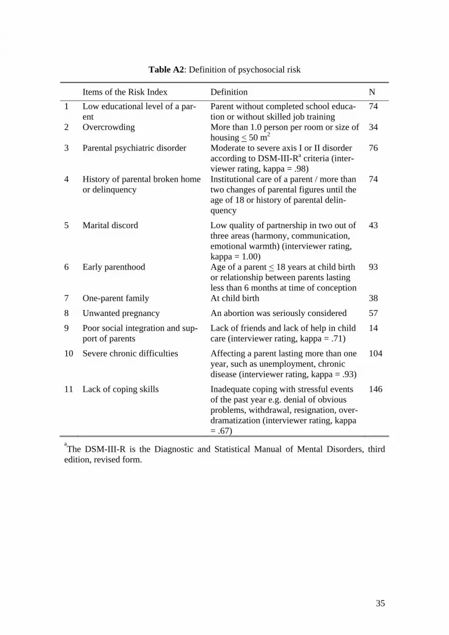
35

Table A2: Definition of psychosocial risk

Items of the Risk Index Definition N 1 Low educational level of a par-

ent Parent without completed school educa-tion or without skilled job training

74

2 Overcrowding More than 1.0 person per room or size of housing < 50 m2

34

3 Parental psychiatric disorder Moderate to severe axis I or II disorder according to DSM-III-Ra criteria (inter-viewer rating, kappa = .98)

76

4 History of parental broken home or delinquency

Institutional care of a parent / more than two changes of parental figures until the age of 18 or history of parental delin-quency

74

5 Marital discord Low quality of partnership in two out of three areas (harmony, communication, emotional warmth) (interviewer rating, kappa = 1.00)

43

6 Early parenthood Age of a parent < 18 years at child birth or relationship between parents lasting less than 6 months at time of conception

93

7 One-parent family At child birth 38

8 Unwanted pregnancy An abortion was seriously considered 57

9 Poor social integration and sup-port of parents

Lack of friends and lack of help in child care (interviewer rating, kappa = .71)

14

10 Severe chronic difficulties Affecting a parent lasting more than one year, such as unemployment, chronic disease (interviewer rating, kappa = .93)

104

11 Lack of coping skills Inadequate coping with stressful events of the past year e.g. denial of obvious problems, withdrawal, resignation, over-dramatization (interviewer rating, kappa = .67)

146

aThe DSM-III-R is the Diagnostic and Statistical Manual of Mental Disorders, third

edition, revised form.

36

Table A3: Econometric findings for ability formation, MQ equation (2)

Ability Ht IQt-1 MQt-1 Pt-1 Adj. R²

t = 11 years MQt

a) 0.13 0.34* 0.66* -0.01 0.56

t = 8 years MQt

a) 0.12 0.00 0.42* 0.00 0.38

t = 4.5 years MQt

a) 0.04 0.26* 0.72* 0.10* 0.56

t = 2 years MQt

a) 0.00 0.07 0.31* 0.15* 0.23

t = 3 months (eight risk indicators, relative to maximum risk)

MQt 0.16 (0.14*, 0.11*, 0.03*, 0.13*, 0.08*, 0.02*, 0.15*, 0.10*) 0.11

MARS, 364 observations, all variables in natural logarithm; coefficients from OLS regressions, including a constant and performed for each ability; a) the equation contains additional indicator variables for be-longing to a cell in the initial risk matrix; * indicates significance at the 5 percent level.

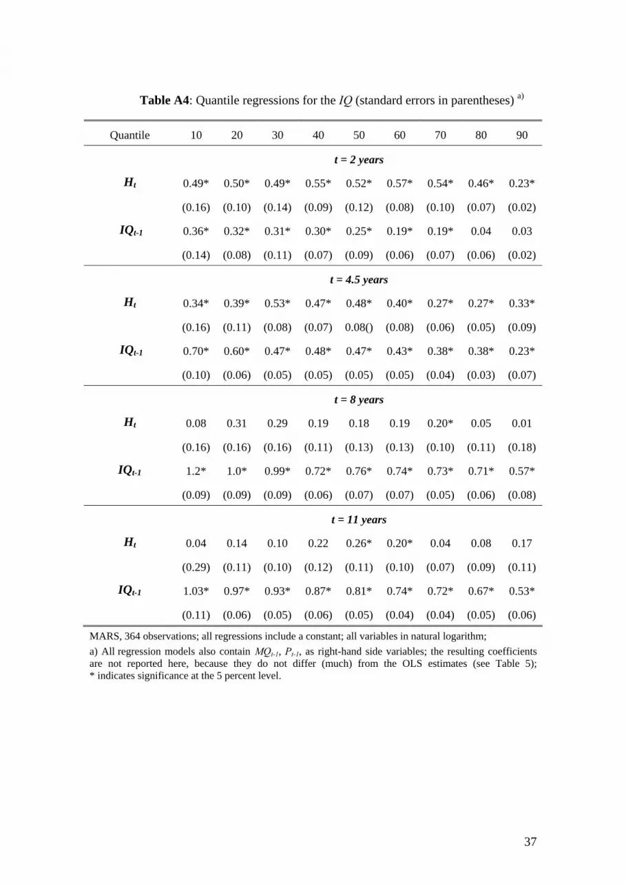
37

Table A4: Quantile regressions for the IQ (standard errors in parentheses) a)

Quantile 10 20 30 40 50 60 70 80 90

t = 2 years

Ht 0.49* 0.50* 0.49* 0.55* 0.52* 0.57* 0.54* 0.46* 0.23*

(0.16) (0.10) (0.14) (0.09) (0.12) (0.08) (0.10) (0.07) (0.02)

IQt-1 0.36* 0.32* 0.31* 0.30* 0.25* 0.19* 0.19* 0.04 0.03

(0.14) (0.08) (0.11) (0.07) (0.09) (0.06) (0.07) (0.06) (0.02)

t = 4.5 years

Ht 0.34* 0.39* 0.53* 0.47* 0.48* 0.40* 0.27* 0.27* 0.33*

(0.16) (0.11) (0.08) (0.07) 0.08() (0.08) (0.06) (0.05) (0.09)

IQt-1 0.70* 0.60* 0.47* 0.48* 0.47* 0.43* 0.38* 0.38* 0.23*

(0.10) (0.06) (0.05) (0.05) (0.05) (0.05) (0.04) (0.03) (0.07)

t = 8 years

Ht 0.08 0.31 0.29 0.19 0.18 0.19 0.20* 0.05 0.01

(0.16) (0.16) (0.16) (0.11) (0.13) (0.13) (0.10) (0.11) (0.18)

IQt-1 1.2* 1.0* 0.99* 0.72* 0.76* 0.74* 0.73* 0.71* 0.57*

(0.09) (0.09) (0.09) (0.06) (0.07) (0.07) (0.05) (0.06) (0.08)

t = 11 years

Ht 0.04 0.14 0.10 0.22 0.26* 0.20* 0.04 0.08 0.17

(0.29) (0.11) (0.10) (0.12) (0.11) (0.10) (0.07) (0.09) (0.11)

IQt-1 1.03* 0.97* 0.93* 0.87* 0.81* 0.74* 0.72* 0.67* 0.53*

(0.11) (0.06) (0.05) (0.06) (0.05) (0.04) (0.04) (0.05) (0.06)

MARS, 364 observations; all regressions include a constant; all variables in natural logarithm; a) All regression models also contain MQt-1, Pt-1, as right-hand side variables; the resulting coefficients are not reported here, because they do not differ (much) from the OLS estimates (see Table 5); * indicates significance at the 5 percent level.

38

Table A5: The partial elasticity of H on the nonverbal (NV-IQ) and the verbal (V-IQ)

dimensions of intelligence a) (standard errors in parentheses)

Ability 2 years 4.5 years 8 years 11 years

NV-IQ 0.22 0.29* -0.06 0.21

(0.16) (0.08) (0.12) (0.10)

V-IQ 0.42* 0.44* 0.30* 0.24*

(0.07) (0.07) (0.11) (0.10)

IQ b) 0.38* 0.38* 0.19 0.17

(0.07) (0.07) (0.13) (0.10)

MARS, 364 observations, all OLS regressions include a constant, all variables in natural logarithm; * indicates significance at 5 percent level. a) All regression models also contain MQt-1, Pt-1; the resulting coefficients are not reported here, because results do not differ (much) from the OLS (see Table 5). b) Taken from Table 5 to facilitate comparison.

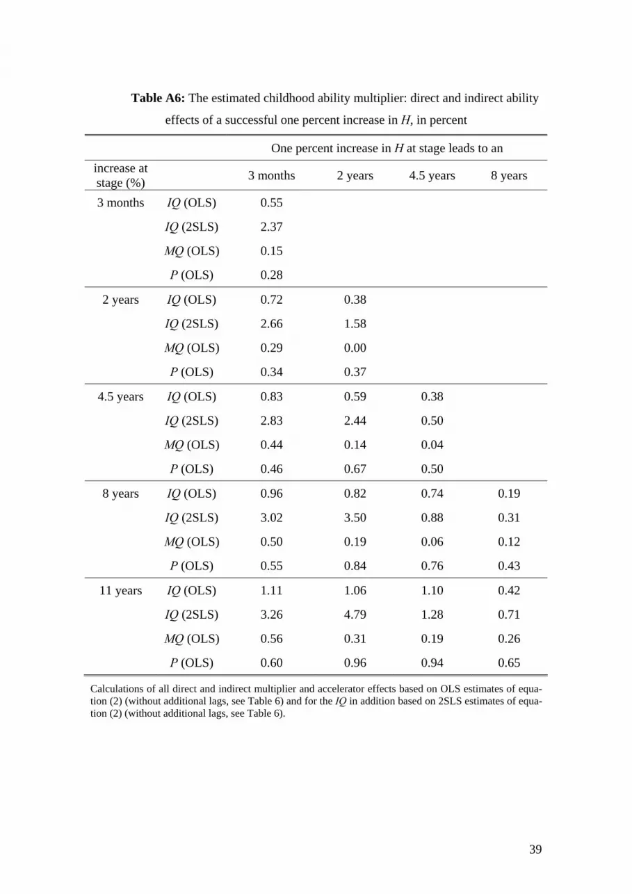
39

Table A6: The estimated childhood ability multiplier: direct and indirect ability

effects of a successful one percent increase in H, in percent

One percent increase in H at stage leads to an increase at stage (%) 3 months 2 years 4.5 years 8 years

3 months IQ (OLS) 0.55

IQ (2SLS) 2.37

MQ (OLS) 0.15

P (OLS) 0.28

2 years IQ (OLS) 0.72 0.38

IQ (2SLS) 2.66 1.58

MQ (OLS) 0.29 0.00

P (OLS) 0.34 0.37

4.5 years IQ (OLS) 0.83 0.59 0.38

IQ (2SLS) 2.83 2.44 0.50

MQ (OLS) 0.44 0.14 0.04

P (OLS) 0.46 0.67 0.50

8 years IQ (OLS) 0.96 0.82 0.74 0.19

IQ (2SLS) 3.02 3.50 0.88 0.31

MQ (OLS) 0.50 0.19 0.06 0.12

P (OLS) 0.55 0.84 0.76 0.43

11 years IQ (OLS) 1.11 1.06 1.10 0.42

IQ (2SLS) 3.26 4.79 1.28 0.71

MQ (OLS) 0.56 0.31 0.19 0.26

P (OLS) 0.60 0.96 0.94 0.65

Calculations of all direct and indirect multiplier and accelerator effects based on OLS estimates of equa-tion (2) (without additional lags, see Table 6) and for the IQ in addition based on 2SLS estimates of equa-tion (2) (without additional lags, see Table 6).

40

APPENDIX: MEASUREMENT OF IQ AND MQ

3 months: Cognitive abilities, IQ, were measured using the Mental Developmental In-

dex (MDI) of the Bayley Scales of Infant Development (Bayley, 1969). The fine and

gross motor abilities, MQ (called the motor quotient), were assessed by the Psychomo-

tor Developmental Index (PDI) of the Bayley Scales.

2 years: The IQ was derived from the Mental Developmental Index (MDI) of the

Bayley Scales of Infant Development. A differentiation is made between verbal abili-

ties, V-IQ, and nonverbal cognitive abilities, NV-IQ. The verbal ability score is derived

from the items of the Bayley Scales indicating language development, in combination

with the expressive and the receptive language scales of the Münchener Funktionale

Entwicklungsdiagnostik (MFED) (Köhler and Egelkraut, 1984). The nonverbal cogni-

tive abilities are derived from the nonverbal items of the Bayley Scales, indicating ba-

sic, general abilities such as perception and logical and figural reasoning. The MQ was

assessed by the Psychomotor Developmental Index (PDI) of the Bayley Scales.

4.5 years: The composite score of the IQ contained the Columbia Mental Maturity

Scale (CMMS) (Burgmeister et al., 1972) and the subtest "sentence completion" of the

Illinois Test of Psycholinguistic Abilities (ITPA), (Kirk et al., 1968; for the German

version, see Angermaier, 1974). From these, a differentiation is made between V-IQ,

language-dependent abilities and NV-IQ, indicating nonverbal abilities. The MQ was

derived from the Test of Motor Abilities (MOT) 4-6 (Zimmer and Volkamer, 1984).

8 years: The composite score of the IQ was assessed by the Culture Fair Test (CFT) 1

(Weiss and Osterland, 1977), measuring nonverbal skills, such as the ability to perceive

and integrate complex relationships in new situations, and the subtest "sentence comple-

tion" of the ITPA, mentioned above, indicating verbal reasoning (V-IQ). The MQ was

assessed with the body coordination test for children (KTK) (Kiphard and Shilling,

1974).

11 years: The IQ was measured with the CFT 20 (Cattell, 1960; for the German version

see Weiss, 1987) and a vocabulary test of the CFT 20, again allowing verbal, V-IQ, and

nonverbal abilities, NV-IQ, to be distinguished. The MQ at age 11 years was assessed

by means of a short version of the body coordination test for children (KTK).