Optimization Methods and SoftwareVol. 20, No. 2–3, April–June 2005, 389–400

Dynamical approaches and multi-quadratic integerprogramming for seizure prediction

WANPRACHA CHAOVALITWONGSE† ‡‡ §§ ¶¶, PANOS M. PARDALOS† ‡ § ‡‡,LEONIDAS D. IASEMIDIS††† ‡ ‡‡, DENG-SHAN SHIAU¶ §§ ¶¶

and J. CHRIS SACKELLARES§ ¶ †† §§ ¶¶*

†Department of Industrial and Systems Engineering,‡Department of Computer Science,

§Department of Biomedical Engineering,¶Department of Neuroscience,††Department of Neurology,

‡‡Center for Applied Optimization,§§McKnight Brain Institute, University of Florida, Gainesville, FL, USA,

¶¶ Malcolm Randall V.A. Medical Center, Gainesville, FL, USA†††Department of Biomedical Engineering and

‡‡‡Center for Systems Science and Engineering Research,Arizona State University, Tempe, AZ, USA

(Received 5 February 2003; Revised 29 July 2003; in final form 9 September 2003)

In this article, we present dynamical approaches and multi-quadratic integer programming techniquesto study the problem of seizure prediction. The data used in our studies consist of continuous intracranialelectroencephalograms (EEGs) from patients with temporal lobe epilepsy. The results of this studycan be used as a criterion to pre-select the critical electrode sites that can be used to predict epilepticseizures.

Keywords: Multi-quadratic 0–1 programming problem; Dynamical approaches; EEG; Seizureprediction

1. Introduction

In recent years, several quantitative system approaches incorporating statistical techniques,dynamical systems and optimization have been used to study brain disorders. Epilepsy isamong the most common brain disorders in the nervous system and consists of more than 40clinical syndromes affecting 50 million people worldwide (∼1% of the population). Epilepsy

*Corresponding author. Department of Neuroscience, McKnight Brain Institute, University of Florida, 100Newell Drive Gainesville Florida 32611, USA. Tel: (352) 376-1611 ext. 5635. Fax: (352) 376-4822. Email:sackellares@mbi.ufl.edu

Optimization Methods and SoftwareISSN 1055-6788 print/ISSN 1029-4937 online © 2005 Taylor & Francis Group Ltd

http://www.tandf.co.uk/journalsDOI: 10.1080/10556780512331318173

390 W. Chaovalitwongse et al.

is characterized by intermittent seizures, that is, intermittent paroxysmal rhythmic electricaldischarges within the cerebrum that disrupt normal brain function.

During the seizure, the sudden development of synchronous neuronal firing, potentials, inthe cerebral cortex that may begin locally in a portion of one cerebral hemisphere or beginsimultaneously in both cerebral hemispheres. When neuronal networks are activated, theyproduce a change in voltage potential, which can be captured in electroencephalogram (EEG)recordings. These changes are reflected by wriggling lines along the time axis in typicalEEG recordings. From EEG recordings, to draw on advances from the epilepsy field andother rapidly changing fields of biomedicine, we focus our research on the prediction ofepileptic seizures to enable effective and safe treatment for patients with epilepsy. Althoughepileptic seizures appear to occur randomly, recent studies in epileptic patients suggest thatseizures are deterministic rather than random. Consequently, studies of the spatiotemporaldynamics in EEG recordings, from patients with temporal lobe epilepsy, demonstrated apreictal transition, characterized by a progressive convergence (entrainment) of dynamicalmeasures [e.g., short-term maximum Lyapunov exponents (STLmax)] at specific anatomicalareas and cortical sites, in the neocortex and hippocampus, of ∼ 0.5 − 1 h duration beforethe ictal onset [1–5]. Although the existence of the preictal transition period has recentlybeen confirmed and further defined by other investigators [6–10], the characterization of thisspatiotemporal transition is still far from complete. For instance, even in the same patient,different set of cortical sites may exhibit preictal transition from one seizure to the next. Inaddition, this convergence of the normal sites with the epileptogenic focus (critical corticalsites) is reset after each seizure. Therefore, complete or partial postictal resetting of preictaltransition of the epileptic brain, affects the route to the subsequent seizure, contributing to theapparently non-stationary nature of the entrainment process. In those studies, however, thecritical site selections are not trivial but extremely important, because most groups of brainsites are irrelevant to the occurrences of the seizures and only certain groups of sites havedynamical convergence in the preictal transition. In this study, we tested the hypothesis thatthe set of cortical sites with minimum difference in STLmax (most converged) prior to thecurrent seizure and then reset after the seizure is most likely to converge again before. Toselect the most converged cortical sites, we formulate this problem as a multi-quadratic 0–1programming problem. In this article, we propose two approaches to solve this problem.

This article is organized as follows. The background of estimation of STLmax and thespatiotemporal dynamical analysis is described in section 2. The multi-quadratic 0–1 pro-gramming for selection of critical cortical sites is addressed in section 3. In section 4, themethod used to test the hypothesis and results is presented. The conclusions are discussed insection 5.

2. Background

The EEG recordings from multiple sites in the cerebral neocortex and hippocampus were per-formed for clinical diagnostic purposes in patients with refractory epilepsy.A typical electrodemontage for such recordings is shown in figure 1. The EEG onset of a typical epileptic seizureof a focal origin recorded with this montage is illustrated in figure 2.

2.1 Estimation of short term largest lyapunov exponents (STLmax)

The electroencephalogram has been the most utilized signal to assess brain function owing toits excellent time resolution (milliseconds). However, traditional signal processing theory, on

Seizure prediction 391

Figure 1. Graphic illustration of placement of subdural electrode strips and depth electrodes. 3A depicts the inferiorsurface of the cerebrum; the left lateral aspect of the cerebrum is shown in 3B. Electrode strips are placed over the leftorbitofrontal (LOF), right orbitofrontal (ROF), left subtemporal (LST) and right subtemporal (RST) cortex. Depthelectrodes are placed in the left temporal (LTD) and right temporal (RTD) lobes.

the basis of simple assumptions regarding the system that produces the signal (e.g., linearityassumption) has not successfully characterized and quantified the predictive properties in theEEG. The EEG has statistical properties that depend on both time and space. Components ofthe brain (e.g., neurons, sets of neurons) are densely interconnected and the EEG recordedfrom one brain site is inherently related to the activity at other sites. These components

Figure 2. Ten-second EEG recording of the onset of a typical epileptic seizure obtained from 32 electrodes. Eachhorizontal trace represents the voltage recorded from electrode sites listed in the left column (see figure 1 for anatomicallocation of electrodes).

392 W. Chaovalitwongse et al.

may functionally interact at different time instants. This makes the EEG a multidimensionalnonstationary time series of spatial extent.

As the EEG is a nonstationary signal, selection of the appropriate time scale is crucial. Oneneeds to find sample length that are spatially long enough to calculate the signal properties ofinterest but short enough to meet the stationary assumptions. In addition, dynamical measuresmust properly weigh transients in the signal. In a spontaneously bursting neuronal network inbrain, chaos can be demonstrated by the presence of unstable fixed-point behavior. Lyapunovexponents are among the global dynamical invariants studied for detecting chaos and nonlinearstructure in time series analysis. Lyapunov exponents are defined as the local divergence withina finite-time horizon, are a more useful measure of predictability of nonlinear systems and amore powerful tool for testing nonlinearity of time series.

The method we employ in this research for estimation of STLmax, an estimate of Lmax

for nonstationary data, called STL (short-term Lyapunov) is taking in consideration possiblenonstationarities in the EEG. We apply the STL algorithm to EEG tracings from several brainsites, to create a set of Lmax time series containing local (in time and in space) information aboutthe brain as a dynamical system [4]. It will be shown that it is at this level of spatiotemporalanalysis that reliable detection of the preictal transition is derived. The method for estimationof STLmax is explained in detail elsewhere [4, 11, 12]. Herein, we will present only a shortdescription of our method.

The estimation of Lyapunov exponents starts with a well-established technique for visual-izing the dynamical behavior of a multivariable system; that is, to generate the phase spaceportrait of the system. A phase space portrait is created by treating each time-dependent vari-able of the system as a component of a vector in a multidimensional space, usually calledstate or phase space of the system. Each vector in the phase space represents an instantaneousstate of the system. These time-dependent vectors are plotted sequentially in the phase spaceto represent the evolution of the state of the system over time.

In principle, sampling of a single observable over time can approximate the position (state)of the system in a space spanned by the system variables related to this observable. Thistechnique for the reconstruction of the phase space from one observable can be used for theEEG. In this case, a multidimensional phase space can be created from a single electrodeEEG recording. Thus, in such an embedding, each state is represented in the phase space bya vector X(t) whose components are the delayed versions of the original single channel EEGtime series x(t), that is,

X(t) = [x(t), x(t − τ), . . . , x(t − (p − 1)τ )]where X(t) is the vector in the phase space at time t , τ is the time delay between successivecomponents of X(t), and p is the embedding dimension of the reconstructed phase space.

The geometrical properties of the phase portrait of a system can be expressed quantitativelyusing measures that ultimately reflect the dynamics of the system. For example, the complexityof an attractor is reflected in its dimension. The larger the dimension of an attractor, the morecomplicated it appears in the phase space. The embedding dimension (p) is the dimensionof the phase space that contains the attractor and it is always a positive integer. On the otherhand, the attractor’s dimension (D) may be a positive non-integer (fractal). D is directly relatedto the number of variables of the system and is inversely related to the existing coupling amongthem. According to Takens, the embedding dimension p should be at least equal to 2D + 1in order to correctly embed an attractor in the phase space. The measure most often usedto estimate D is the phase space correlation dimension (v). In this framework, we employedmethods for calculating the correlation dimension from experimental data described by Mayer-Kress [13] and Kostelich [14] to approximate D of the epileptic attractor. In the EEG data we

Seizure prediction 393

have analyzed to date, D is found to be between 2 and 3 during an epileptic seizure. Therefore,for the reconstruction of the phase space we have used an embedding dimension p of 7.

After the construction of the embedding phase space from a data segment x(t) of durationT is made with the method of delays, the maximum Lyapunov exponent (Lmax) is defined asthe average of local Lyapunov exponents Lij in the state space as follows:

Lmax = 1

Nα

∑α

Lij

where Nα is the total number of the local Lyapunov exponents that are estimated from theevolution of adjacent points (vectors) in the state space according to:

Lij = 1

�tlog2

|X(ti + �t) − X(tj + �t)||X(ti) − X(tj )|

where �t is the evolution time allowed for the vector difference δ(λ)xk

= |X(ti) − X(tj )| toevolve to the new difference δ(λ)

xk= |X(ti + �t) − X(tj + �t)|, where λ = 0, . . . , Nα−l and

�t = k × dt with dt the sampling period of the original time series (dt = 5 ms in our EEGdata). An illustration of the estimation of Lmax in the state space is given in figure 3.

2.2 Spatio-temporal dynamical analysis

Although a great deal is now known about low dimensional chaos, the erratic motion ofdynamical systems described by a few variables is understood in systems where the number

Figure 3. Diagram illustrating the estimation of Lmax measures in the state space. The fiducial trajectory, the firstthree local Lyapunov exponents (L1, L2, L3), is shown.

394 W. Chaovalitwongse et al.

of chaotic degrees of freedom becomes very large. Typically, such systems show disorder inboth space and time and are said to exhibit spatiotemporal chaos. Spatiotemporal chaos occurswhen the system of coupled dynamical systems gives rise to dynamical behavior that exhibitsboth spatial disorder (as in rapid decay of spatial correlations) and temporal disorder (as innonzero Lyapunov exponents). This is an extremely active and rather unsettled area of research.The system under consideration (brain) has a spatial extent and, as such, information aboutthe transition of the system towards the ictal state should also be included in the interactionsof its spatial components. The preictal transition, progressive convergence of STLmax profiles,is further evidence of spatiotemporal chaos in the brain (shown in figure 4). The spatialdynamics of this transition are captured by considering relationship of the STLmax betweendifferent cortical sites. For example, if a similar transition occurs at different cortical sites, theSTLmax of the involved sites are expected to converge to similar values prior to the transition.We have called such participating sites ‘critical sites’, and such a convergence ‘dynamicalentrainment’. More specifically, in order for the dynamical entrainment to have a statisticalcontent, we have allowed a period over which the mean of the differences of the STLmax valuesat two sites is estimated. We have used 60 STImax values (i.e., moving windows of ∼10 minat each electrode site) to test the dynamical entrainment at the 0.01 statistical significancelevel. We employ the T -index as a measure of dynamical entrainment of STLmax profiles overtime.

The T -index, the test statistic from the well-known paired t-test for comparisons of meansof paired dependent observations, was employed as a measure of statistical distance betweenthe pairs of STLmax profiles over a time window. The Tij index at time t between the STLmax

profiles of electrode sites i and j is then defined as:

Ti,j (t) = (N)1/2|E{STLmaxi(t) − STLmaxj

(t)}|σi,j (t)

Figure 4. Convergence of five STLmax profiles from critical cortical sites over 2 h between seizures 9 and 10 (patient1). The ictal periods of the two seizures are denoted by vertical lines.

Seizure prediction 395

Figure 5. The T -index profile among five critical cortical sites whose STLmax profiles are depicted in figure 4. Thecortical sites are dynamically entrained ∼60 min prior to seizure’s 10 onset. The statistical thresholds are representedby the two horizontal lines.

where E{ } denotes the average of all paired-differences STLmaxi(t) − STLmaxj

(t) within amoving window wt(λ) defined as:

wt(λ) = 1 for λ ∈ [t − N − 1, t] and wt(λ) = 0 for λ �∈ [t − N − 1, t]where N is the length of the moving window and σi,j (t) is the sample standard deviation of theSTLmaxi

(t) - STLmaxj(t) within the moving window wt(λ). Asymptotically, Tij index follows

a t-distribution with N − 1 degrees of freedom. In the estimation of the Ti,j (t) indices fromour data, we used N = 60. A critical value, Tα/2, from the t-distribution with N − 1(= 59)

degrees of freedom at significance level α, is used to test the null hypothesis H0: ‘brain sites i

and j acquire identical STLmax values within time window wt(λ).’ For the T -index to rejectH0, Tij (t) should be greater than 2.662(= T0.005,59).

An example of a T -index profile is shown in figure 5. This profile is estimated according tothe previously described procedure from the two STLmax profiles of figure 4. The two criticalvalues T1 = 2.662 and T2 = 5.000 are also shown as horizontal lines. From inspection ofthis figure, it is clear that the considered electrode sites are dynamically entrained at the 0.01significance level (T < T1) about 60 min prior to seizure 10.

3. Multi-quadratic 0–1 programming

In this article, we refer to the Sherrington-Kirkpatric Hamiltonian that describes the mean-field theory of the spin glasses where elements are placed on the vertices of a regular lattice,the magnetic interactions hold only for nearest neighbors and every element has only twostates (Ising spin glasses [15–19]). One of the most interesting problems about this model

396 W. Chaovalitwongse et al.

is the determination of the minimal energy states (ground state problem). For many yearsthe Ising model has been a powerful tool in studying phase transitions in statistical physics.Such an Ising model can be described by a graph G(V, E) having n vertices {v1, . . . , vn} andeach edge (i, j) ∈ E having a weight (interaction energy) Jij . Each vertex vi has a magneticspin variable σi ∈ {−1, +1} associated with it. An optimal spin configuration of minimumenergy is obtained by minimizing the Hamiltonian H(σ) = ∑

1≤i≤j≤n jij σiσj over all σi ∈{−1, +1}n. This problem is equivalent to the combinatorial problem of quadratic bivalentprogramming [19].

Quadratic 0–1 programming has been extensively used to study Ising spin glass models[15–19], which motivated us to use quadratic 0–1 programming to select the critical (mostconverged) cortical sites, where each electrode has only two states (selected and not selected),and to determine the minimal-average T -index state. Initially, we formulated this problem asa quadratic 0–1 knapsack problem with objective function to minimize the average T -index(a measure of statistical distance between the mean values of STLmax among electrode sitesand the knapsack constraint to identify the number of critical cortical sites [1]. Owing to theexistence of resetting of the brain after seizure onset [20,21], that is, divergence of STLmax

profiles after seizures, we have to ensure that the optimal group of critical sites shows thisdivergence by adding a quadratic constraint into quadratic 0–1 problem. We formulated thisproblem as a multi-quadratic 0–1 problem with objective function to minimize the averageT -index among electrode sites with the knapsack constraint to identify the number of criticalcortical sites and the quadratic constraint to ensure that the selected critical sites reset afterthe seizure onset.

Let A, B be two n × n matrices, whose each elements aij and bij represent the T -indices between electrodes i and j within 10 min windows before and after the seizure onset,respectively. Tα/2 is the critical value of T -index, as previously defined, to reject H0: ‘twobrain sites acquire identical STLmax values within time window.’ n is the total number ofimplanted cortical sites, which is a constant, k is the number of critical cortical sites, whichis a previously determined parameter. Define x = {x1, . . . , xn}, where each xi represents thecortical electrode site i. If the cortical site i is selected to be one of the critical electrode sites,then xi = 1; otherwise, xi = 0.

min xTAx

s.t.n∑

i=1

xi = k

xTBx ≥ Tαk(k − 1)

where xi ∈ {0, 1}∀i ∈ {1, . . . , n}.To solve this problem, we considered two computational approaches. In the first approach,

we linearized the quadratic objective function and the quadratic constraint by introducing anew variable for each product of two variables and adding some additional constraints, andthen formulated this problem as a linear 0–1 problem. In the second approach, we appliedthe Karush–Khun Tucker optimality conditions to the Lagrangian function of the originalproblem, and then formulated these conditions as a linear mixed integer 0–1 problem.

3.1 Linearization of multi-quadratic 0–1 Programming

For each product xixj , we introduce a new 0–1 variable, xij = xixj for i �= j . Notethat xii = x2

i = xi for xi ∈ {0, 1}. After linearization, the equivalent linear 0–1 problem is

Seizure prediction 397

given by:

min∑

i

∑i

aij xij

s.t.n∑

i=1

xi = k

xij ≤ xi, for i = 1, . . . , n

xij ≤ xj , for j = 1, . . . , n

xi + xj − 1 ≤ xij , for i, j = 1, . . . , n∑i

∑j

bij xij ≥ Tαk(k − 1)

where xi ∈ {0, 1} and 0 ≤ xij ≤ 1, i, j = 1, . . . , n.The number of continuous variables has been increased to O(n2). Although, applying

CPLEX 7.0, we can solve problems with n = 30, this approach will be computationallyinefficient as n increases. Future technology will make it possible for larger values of n.

3.2 Applying the KKT optimality conditions to the multi-quadratic 0–1 problem

Consider the quadratic problem with a knapsack constraint given by:

min xTAx

s.t.n∑

i=1

xi = k, xi ≥ 0, i = 1, . . . , n.

Then, the Lagrangian function of this problem is given by:

z(x) = xTAx + s

(n∑

i=1

xi − k

).

We note that the T -index matrix, A, has the same property as the Euclidean distance matrix,which is positive semidefinite; therefore, the T -index matrix is also positive semidefinite. TheKarush–Kuhn Tucker optimality conditions of the Lagrangian function are given by:

−Ax + s + y = 0, where y ≥ 0n∑

i=1

xi = k, where x ≥ 0

ytx = 0.

In the above KKT conditions, we replace the last constraint, which is not a linear constraint,with yi ≤ µ(l − xi), for i = l, . . . , n, where µ is an arbitrary large number, and then formulate

398 W. Chaovalitwongse et al.

this problem as a linear mixed integer 0–1 problem, which minimizes the slack.

minn∑

i=1

si

s.t.n∑

i=1

xi = k

−n∑

j=1

aij xj + si + yi = 0, for i = 1, . . . , n

yi − µ(1 − xi) ≤ 0, for i = 1, . . . , n

where xi ∈ {0, 1} and yi, si ≥ 0, for i = 1, . . . , n.Consequently, we need to add one more quadratic constraint, xTBx ≥ Tαk(k − 1), to ensure

that the critical cortical sites (solution of this problem) reset after seizure onset. Thus, thisproblem becomes a multi-quadratic problem. To solve this multi-quadratic problem, we modifythe linear mixed integer 0–1 problem from the above formulation by adding the first-orderderivative of the quadratic constraint and some additional constraints. The equivalent linearmixed integer 0–1 problem is given by:

minn∑

i=1

si

s.t.n∑

i=1

xi = k

−n∑

j=1

aij xj + si + yi = 0, for i = 1, . . . , n

yi − µ(1 − xi) ≤ 0, for i = 1, . . . , n

hi − µxi ≤ 0, for i = 1, . . . , n

−n∑

j=1

bij xj + hi ≤ 0, for i = 1, . . . , n

n∑j=1

hi ≥ Tαk(k − 1)

where xi ∈ {0, 1} and yi, si, hi ≥ 0, for i = 1, . . . , n.Applying CPLEX 7.0, this problem can be easily solved with n = 30. Because the number

of 0–1 variables is O(n), this formulation is very efficient and is used to solve this multi-quadratic 0–1 problem iteratively. Although more electrodes will be implanted in the future(as n increases), this formulation is still applicable because it is computationally efficient.

4. Method and results

Having defined that electrode sites, which participate in preictal transition, must be entrainedprior to seizures, we hypothesize that ‘the electrode sites that are most entrained during the

Seizure prediction 399

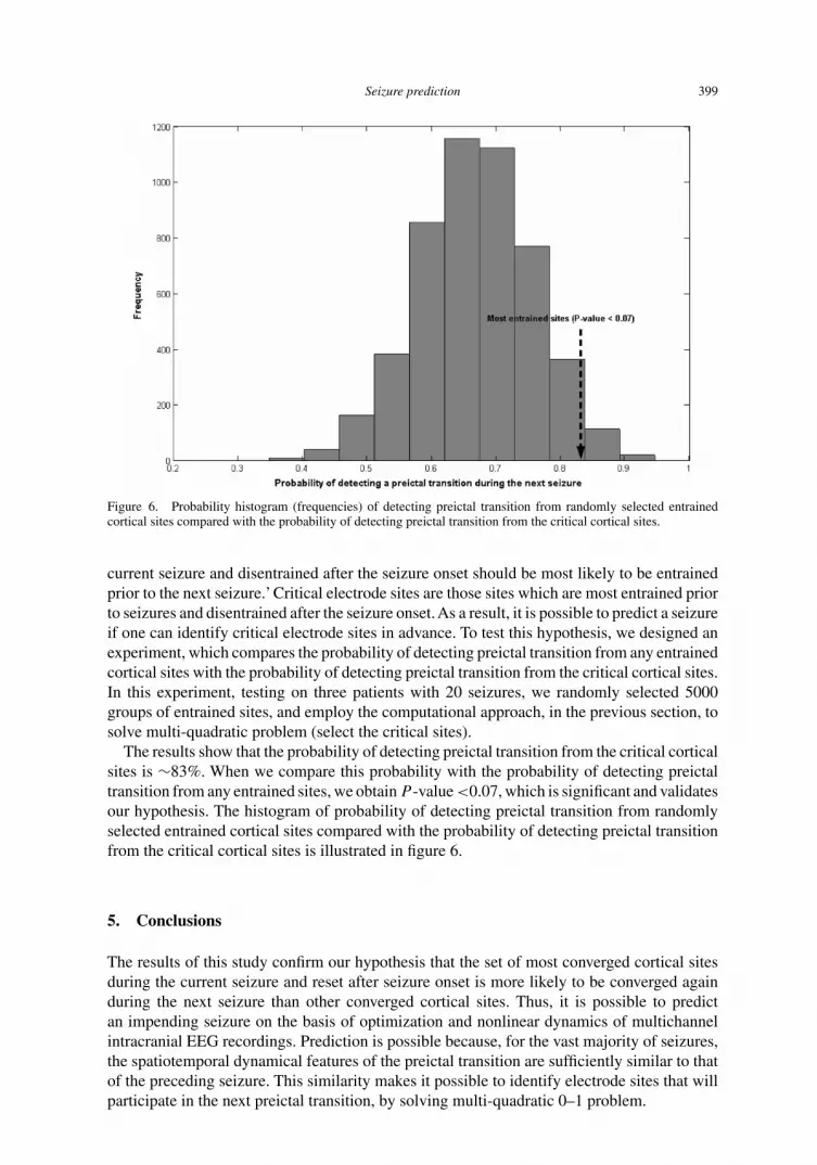
Figure 6. Probability histogram (frequencies) of detecting preictal transition from randomly selected entrainedcortical sites compared with the probability of detecting preictal transition from the critical cortical sites.

current seizure and disentrained after the seizure onset should be most likely to be entrainedprior to the next seizure.’ Critical electrode sites are those sites which are most entrained priorto seizures and disentrained after the seizure onset. As a result, it is possible to predict a seizureif one can identify critical electrode sites in advance. To test this hypothesis, we designed anexperiment, which compares the probability of detecting preictal transition from any entrainedcortical sites with the probability of detecting preictal transition from the critical cortical sites.In this experiment, testing on three patients with 20 seizures, we randomly selected 5000groups of entrained sites, and employ the computational approach, in the previous section, tosolve multi-quadratic problem (select the critical sites).

The results show that the probability of detecting preictal transition from the critical corticalsites is ∼83%. When we compare this probability with the probability of detecting preictaltransition from any entrained sites, we obtain P -value <0.07, which is significant and validatesour hypothesis. The histogram of probability of detecting preictal transition from randomlyselected entrained cortical sites compared with the probability of detecting preictal transitionfrom the critical cortical sites is illustrated in figure 6.

5. Conclusions

The results of this study confirm our hypothesis that the set of most converged cortical sitesduring the current seizure and reset after seizure onset is more likely to be converged againduring the next seizure than other converged cortical sites. Thus, it is possible to predictan impending seizure on the basis of optimization and nonlinear dynamics of multichannelintracranial EEG recordings. Prediction is possible because, for the vast majority of seizures,the spatiotemporal dynamical features of the preictal transition are sufficiently similar to thatof the preceding seizure. This similarity makes it possible to identify electrode sites that willparticipate in the next preictal transition, by solving multi-quadratic 0–1 problem.

400 W. Chaovalitwongse et al.

Although evidence for the characteristic preictal transition utilized by the seizure predictionalgorithm employed in this study was first reported by our group in 1991 [1], further studieswere required before a practical seizure prediction algorithm was feasible. Development ofa seizure prediction algorithm was complicated because the cortical sites participating in thepreictal transition varied from seizure to seizure. This problem was overcome by the useof our proposed approaches to solve multi-quadratic 0–1 problem. Because the algorithmselects candidate electrode sites and by analyzing continuous EEG recordings of several daysof duration, the computational approach to solve the optimization problem has to be veryefficient. At present, we can efficiently solve multi-quadratic 0–1 problem. However, futuretechnology may allow physicians to implant thousands of electrode sites, n > 1000, in thebrain. This procedure will extract more information and allow us to have a more understandingabout the brain. Therefore, to solve this optimization problem with n > 1000, we may needcomputationally fast heuristic approaches in the future.

References[1] Iasemidis, L.D., Pardalos, P., Sackellares, J.C. and Shiau, D.-S., 2001, Quadratic binary programming and

dynamical system approach to determine the predictability of epileptic seizures. Journal of CombinatorialOptimization, 5, 9–26.

[2] Iasemidis, L.D., Shiau, D.-S., Pardalos, P.M. and Sackellares, J.C., 2002, Phase entrainment and predictabilityof epileptic seizures. In: P.M. Pardalos and J. Principe (Eds) Biocomputing (Kluwer Academic Publishers).

[3] Iasemidis, L.D., Sackellares, J.C., Zaveri, H.P. and Williams, W.J., 1990, Phase space topography of theelectrocorticogram and the Lyapunov exponent in partial seizures. Brain Topography, 2, 187–201.

[4] Iasemidis, L.D. and Sackellares, J.C., 1991, The temporal evolution of the largest Lyapunov exponent onthe human epileptic cortex. In: D.W. Duck and W.S. Pritchard (Eds) Measuring Chaos in the Human Brain(Singapore: World Scientific).

[5] Iasemidis, L.D., Shiau, D.-S., Sackellares, J.C. and Pardalos, P., 1999, Transition to epileptic seizures: optimiza-tion. In: D.Z. Du, P.M. Pardalos and J. Wang (Eds) DIMACS series in Discrete Mathematics and TheoreticalComputer Science, Vol. 55 (American Mathematical Society).

[6] Martinerie, J., Adam, C., Le Van Quyen, M., Baulac, M., Clemenceu, S., Renault, B. and Varela, F.J., 1998,Epileptic seizures can be anticipated by non-linear analysis. Nature Medicine, 4, 1173–1176.

[7] Elger, C.E. and Lehnertz, K., 1998, Seizure prediction by non-linear time series analysis of brain electricalactivity. European Journal of Neuroscience, 10, 786–789.

[8] Lehnertz, K. and Elger, C.E., 1998, Can epileptic seizures be predicted? Evidence from nonlinear time seriesanalysis of brain electrical activity. Physics Review Letters, 80, 5019–5022.

[9] LeVan Quyen, M., Martinerie, J., Baulac, M. and Varela, F., 1999, Anticipating epileptic seizures in real timeby non-linear analysis of similarity between EEG recordings. NeuroReport, 10, 2149–2155.

[10] LeVan Quyen, M. et al., 2001, Anticipation of epileptic seizures from standard EEG recordings. Lancet, 357,183–188.

[11] Wolf, A., Swift, J.B., Swinney, H.L. and Vastano, J.A., 1985, Determining Lyapunov exponents from a timeseries. Physica D, 16, 285–317.

[12] Iasemidis, L.D., Principe, J.C. and Sackellares, J.C., 2000, Measurement and quantification of spatiotemporaldynamics of human epileptic seizures. In: M. Akay (Ed.) Nonlinear Biomedical Signal Processing, Vol. II (IEEEPress).

[13] Mayer-Kress, G. (Ed.), 1986, Dimension and Entropies in Chaotic Systems (Berlin: Springer-Verlag).[14] Kostelich, E.J., 1992, Problems in estimating dynamics from data. Physica D, 58, 138–152.[15] Athanasiou, G.G., Bachas, C.P. and Wolf, W.F., 1987, Invariant geometry of spin-glass states. Physical Review

B, 35, 1965–1968.[16] Barahona, F., 1982, On the computational complexity of spin glass models. Journal of Physics A: Mathematical

and General, 15, 3241–3253.[17] Barahona, F., 1982, On the exact ground states of three-dimensional Ising spin glasses. Journal of Physics A:

Mathematical and General, 15, L611–L615.[18] Mezard, M., Parisi, G. and Virasoro, M.A., 1987, Spin Glass Theory and Beyond (Singapore: World Scientific).[19] Horst, H., Pardalos, P.M. and Thoai,V., 2000, Introduction to Global Optimization (2nd edn) (Dordrecht: Kluwer

Academic Publishers).[20] Sackellares, J.C., Iasemidis, L.D., Gilmore, R.L. and Roper, S.N., 1997, Epileptic seizures as neural resetting

mechanisms. Epilepsia, 38, S3, 189.[21] Shiau, D.S., Luo, Q., Gilmore, R.L., Roper, S.N., Pardalos, P., Sackellares, J.C. and Iasemidis, L.D., 2000,

Epileptic seizures resetting revisited. Epilepsia, 41, S7, 208–209.