UNIVERSIDAD DE CHILEFACULTAD DE CIENCIAS FÍSICAS Y MATEMÁTICASDEPARTAMENTO DE INGENIERÍA INDUSTRIAL

DYNAMIC PROBLEMS IN REVENUE MANAGEMENT: STRUCTURE ANDAPPROXIMATION.

TESIS PARA OPTAR AL GRADO DEDOCTORA EN SISTEMAS DE INGENIERÍA

DANA MARÍA PIZARRO

PROFESOR GUÍA:JOSÉ CORREA HAEUSSLER

MIEMBROS DE LA COMISIÓN:SANTIAGO BALSEIRO

OMAR BESBESMARCELO OLIVARES ACUÑA

GUSTAVO VULCANO

Este trabajo ha sido parcialmente nanciado por ANID-PFCHA/Doctorado Nacional/2016# 21161440

SANTIAGO DE CHILE2020

RESUMEN DE LA MEMORIA PARA OPTARAL TÍTULO DE DOCTORA EN SISTEMAS DE INGENIERÍAPOR: DANA MARÍA PIZARROFECHA: 2020PROF. GUÍA: JOSÉ CORREA HAEUSSLER

DYNAMIC PROBLEMS IN REVENUE MANAGEMENT: STRUCTURE ANDAPPROXIMATION.

A pesar de que los orígenes del Revenue Management se remontan a su utilización por lascompañías aéreas en la era posterior a la desregulación en los Estados Unidos, hoy en díaes muy utilizada por diversas industrias como hoteles, empresas de alquiler de automóvilesy retailers. Desde entonces, la investigación en esta área creció y se convirtió en una de lasramas más exitosas de la investigación operativa. Cuánto, a qué precio y cuándo venderson las preguntas claves que el Revenue Management pretende responder para maximizarlos ingresos esperados de un vendedor. Diferentes supuestos llevan a diferentes modelosy, en consecuencia, surgen nuevos desafíos tanto teóricos como algorítmicos. En esta tesisabordamos algunos de ellos, estudiando desde enfoque teórico de un problema de determi-nación de precios dinámicos hasta el estudio del gap de optimalidad de algunos problemasde decisión online y la relación entre algunos de ellos.

En el primer capítulo, estudiamos el problema al que se enfrenta un vendedor dotado deuna sola unidad de producto para la venta en un horizonte innito con el n de maximizar susingresos esperados. La empresa se compromete previamente a la función de precio y el com-prador es estratégico y tiene una valoración privada por el ítem. Nuestro objetivo es estudiarla importancia, en términos de los ingresos esperados del vendedor, de observar el tiempo dellegada del comprador. En ese sentido, nuestro principal resultado establece que el ingresoesperado cuando el vendedor observa la llegada del comprador es a lo mas aproximadamente4,91 veces el obtenido cuando el vendedor no observa la llegada del comprador.

En el segundo capítulo, mostramos que si tenemos un mecanismo posted price con unacierta garantía de aproximación, podemos obtener prophet inequality (en el mismo escenario)con la misma garantía de aproximación. Este resultado, junto con el trabajo de Chawla etal. [41], implican que el problema de diseñar mecanismos de posted price es equivalente alde encontrar reglas de parada para el problema de tiempo de parada óptimo.

Por último, en el tercer capítulo presentamos una clase general de problemas de de-cisión online, llamado Dynamic Resource Constrained Reward Collection (DRCRC), quecomprende varios problemas estudiados por separado en la literatura. Debido a la dicultadde resolver el problema de forma óptima, es habitual desarrollar heurísticas fáciles de re-solver y que sean una buena aproximación para el ingreso óptimo esperado. Así, estudiamosla pérdida de ingresos bajo una heurística estudiada en la literatura, proporcionando unaúnica prueba de la pérdida de ingresos para los problemas incluidos en la clase DRCRC,recuperando resultados existentes para algunos problemas y obteniendo nuevos para otros.

i

ii

RESUMEN DE LA MEMORIA PARA OPTARAL TÍTULO DE DOCTORA EN SISTEMAS DE INGENIERÍAPOR: DANA MARÍA PIZARROFECHA: 2020PROF. GUÍA: JOSÉ CORREA HAEUSSLER

DYNAMIC PROBLEMS IN REVENUE MANAGEMENT: STRUCTURE ANDAPPROXIMATION.

Although the origins of Revenue Management date back to its use by airlines in the post-deregulation era in the U.S., nowadays is heavily used by a variety of industries such ashotels, car rental companies and retailers. Since then, research in this area grew and becameone of the most successful branches of operation research. How much, at what price andwhen to sell are the key questions that Revenue Management aims to answer in order tomaximize the expected revenue of a seller. Dierent assumptions carry to dierent modelsand consequently, new theoretical and algorithmic challenges arise. In this thesis, we addresssome of them, going from a theoretical approach of a dynamic pricing problem to the studyof the optimality gap for some online decision problems and the relation between some ofthem.

In the rst chapter, we study the problem faced by a seller endowed with a single unitfor sale over an innite time horizon in order to maximize her expected revenue. The rmpre-commits to the price function and the buyer is strategic and has a private value forthe item. Our goal is to study the importance, in terms of seller's expected revenue, ofthe observability of the buyer's time arrival. Our main result states that, in a very generalsetting, the expected revenue when the seller observes the buyer's arrival is at most roughly4.91 times the expected revenue when the seller does not know the time when the buyerarrives.

In the second chapter, we show that if we have a posted price mechanism with a certainapproximation guarantee, this can be turned into a prophet inequality (in the same setting)with the same approximation guarantee. This result, together with the work by Chawla etal. [41], imply that the problem of designing posted price mechanisms is actually equivalentto that of nding stopping rules for a prophet.

Finally, in the third chapter we introduce a general class of online decision problems,namely Dynamic Resource Constrained Reward Collection (DRCRC) that comprises sev-eral problems studied separately in the literature. In particular, the class of DRCRC ad-mits as special cases the classes of network revenue management problems, dynamic pricingproblems, online matching problems, to name a few. Due to the diculty of solving thedecision-maker problem optimally, it is usual to develop heuristics to approximate the op-timal expected revenue. Thus, we study the revenue loss under a well studied certaintyequivalent heuristic, providing a unifying proof for the revenue loss for DRCRC, recoveringsome existing results for some problems and obtaining new ones for others.

iii

iv

I was taught that the way of progress is neither swift nor easy.Marie Curie.

v

vi

Aknowledgements

First of all, thanks to José, who was an excellent advisor since the beginning of my Ph.D.I would like to thank you not only for the way you share your knowledge and passion forresearch, but also for your commitment to your students and projects. You're denitely thebest advisor I could have had! Thank you for trusting on me!

Secondly, I would like to thank Gustavo Vulcano, with whom I have worked most ofmy years of research in the Ph.D, and from whom I have learned a lot, not only from hisacademic knowledge but also from the way he works. Thank you for your advices, your work,and especially for your patience! Thank you also for opening the doors of the UniversidadTorcuato Di Tella, you really made me feel at home!

Thirdly, I would like to thank Omar Besbes and Santiago Balseiro, who have given methe opportunity to work with them and spend some time at Columbia University. They aredenitely the perfect match: Omar always has the right intuition for everything and a listof papers related to each thing in his head, Santiago is always in every detail and always hasthe answer to the issues, knowing not only which theorem is useful, but in which book andon which page to nd it. I denitely learn a lot from both of you! Thanks a lot for that!

I would also like to thank my co-authors Victor Verdugo and Pato. It was a pleasure towork with you! Thanks Victor because I always made you crazy with questions and advicesand you were (and you are) always there, like a good academic brother.

On the other hand, I want to thank to Victor Bucarey, who is somehow "guilty" of mypassage through this Ph.D. Thanks a lot for the long talks, for always giving me supportwhen I needed it, for the company during most of these years in Chile and for being a greatfriend!

Thanks to all my colleagues at DSI, because without the lunches, the seminars and theouting plans, the experience would not have been the same. In particular, thanks to thosewho have become more than colleagues: Verito, Richi, Seba, Coni, Renny, Edu1, Edu2, Vale,Colombia, Feña. Your friendship and the innite memories with you is one of the best thingsI will take with me from Chile.

vii

Thanks also to the república team: minions de José.. denitely the most nerdy talksduring my Ph.D. were during lunches with you!

I also want to thank the people who supported me and were part of my path from theother side of the mountain range. First of all, thanks to the good crazy girls: Peque, Vikyand Sole, because without them my life would not be the same. Thank you because distanceshowed us that true friendships not only survive to it, but get stronger with every diculty.

Thank you to my brothers and sisters: Aixa, Matu, Maqui, Yair and Alejo, who were andare always there, in the best and in the worst moments; and to my parents, who have alwayssupported and accompanied me in each and every decision I have taken.. you are denitelymy inspiration.

Thanks to Franco and Sasha who, during each visit to Argentina, each kiss, hug and Ilove you recharged me with new energy to go on. Thank you for saying chau Dana!!! toevery plane that passes by, it keeps me close despite the distance. I love you both to innityand beyond.

Thanks to all my family and friends, without their unconditional love I would not havemade it.

viii

Contents

Introduction 1

1 On the observability of the arrival time of consumers in a dynamic pricing

problem 5

1.1 Introduction . . . . . . . . . . . . . . . . . . . . . . . . . . . . . . . . . . . . 51.2 Contributions . . . . . . . . . . . . . . . . . . . . . . . . . . . . . . . . . . . 81.3 Related literature . . . . . . . . . . . . . . . . . . . . . . . . . . . . . . . . . 91.4 Model description . . . . . . . . . . . . . . . . . . . . . . . . . . . . . . . . . 12

1.4.1 The buyer's problem. . . . . . . . . . . . . . . . . . . . . . . . . . . . 131.4.2 The seller's problem . . . . . . . . . . . . . . . . . . . . . . . . . . . 14

1.5 Analysis of the model with an observable arrival . . . . . . . . . . . . . . . . 161.5.1 Uniform valuation case . . . . . . . . . . . . . . . . . . . . . . . . . . 19

1.6 Analysis of the model with unobservable arrival . . . . . . . . . . . . . . . . 221.6.1 Monotone hazard rate valuation distribution . . . . . . . . . . . . . . 221.6.2 A feasible periodic price function . . . . . . . . . . . . . . . . . . . . 231.6.3 Revenue analysis . . . . . . . . . . . . . . . . . . . . . . . . . . . . . 25

1.7 Bounding the value of observability . . . . . . . . . . . . . . . . . . . . . . . 251.7.1 An upper bound for the value of observability . . . . . . . . . . . . . 251.7.2 A lower bound for the value of observability . . . . . . . . . . . . . . 26

2 Connection between posted price mechanisms and prophet inequalities 29

2.1 Introduction . . . . . . . . . . . . . . . . . . . . . . . . . . . . . . . . . . . . 292.2 Contributions . . . . . . . . . . . . . . . . . . . . . . . . . . . . . . . . . . . 302.3 Related literature . . . . . . . . . . . . . . . . . . . . . . . . . . . . . . . . . 322.4 Preliminaries . . . . . . . . . . . . . . . . . . . . . . . . . . . . . . . . . . . 34

2.4.1 Myerson's optimal mechanism . . . . . . . . . . . . . . . . . . . . . . 352.4.2 Posted-price mechanisms . . . . . . . . . . . . . . . . . . . . . . . . . 352.4.3 About probability distributions and the virtual valuation . . . . . . . 36

2.5 Reduction from prophets to pricing . . . . . . . . . . . . . . . . . . . . . . . 362.6 Reduction from pricing to prophets . . . . . . . . . . . . . . . . . . . . . . . 38

2.6.1 Reduction overview . . . . . . . . . . . . . . . . . . . . . . . . . . . . 38

ix

2.6.2 Valuation Mapping Lemma . . . . . . . . . . . . . . . . . . . . . . . 382.6.3 From posted prices to online selection . . . . . . . . . . . . . . . . . . 41

2.7 Implications of the reduction . . . . . . . . . . . . . . . . . . . . . . . . . . . 422.7.1 Improved lower bounds for PPMs . . . . . . . . . . . . . . . . . . . . 432.7.2 Bounding the revenue of Myerson's optimal mechanism . . . . . . . . 44

3 Dynamic optimization problems: a unifying approach 46

3.1 Introduction . . . . . . . . . . . . . . . . . . . . . . . . . . . . . . . . . . . . 463.2 Contributions . . . . . . . . . . . . . . . . . . . . . . . . . . . . . . . . . . . 473.3 Related literature . . . . . . . . . . . . . . . . . . . . . . . . . . . . . . . . . 483.4 Model . . . . . . . . . . . . . . . . . . . . . . . . . . . . . . . . . . . . . . . 493.5 Certainty Equivalent Heuristic . . . . . . . . . . . . . . . . . . . . . . . . . . 503.6 Bound on the cumulative reward loss for DRCRC problems . . . . . . . . . . 523.7 Dual problem and sucient conditions for Assumption 2 . . . . . . . . . . . 54

3.7.1 Continuum of actions . . . . . . . . . . . . . . . . . . . . . . . . . . . 553.7.2 Finite set of actions . . . . . . . . . . . . . . . . . . . . . . . . . . . . 58

3.8 Notable applications with continuum of actions . . . . . . . . . . . . . . . . 603.8.1 Network Dynamic Pricing Problem . . . . . . . . . . . . . . . . . . . 603.8.2 Dynamic Bidding in Repeated Auctions . . . . . . . . . . . . . . . . 63

3.9 Notable applications with nite set of actions . . . . . . . . . . . . . . . . . 663.9.1 Network Revenue Management Problem . . . . . . . . . . . . . . . . 663.9.2 Choice-Based Network Revenue Management Problems . . . . . . . . 683.9.3 Stochastic Depletion Problems . . . . . . . . . . . . . . . . . . . . . . 703.9.4 Online Matching . . . . . . . . . . . . . . . . . . . . . . . . . . . . . 713.9.5 Order Fulllment Problem . . . . . . . . . . . . . . . . . . . . . . . . 723.9.6 Other applications . . . . . . . . . . . . . . . . . . . . . . . . . . . . 74

Conclusion 75

Bibliography 76

A Appendix to Chapter 1 88

A.1 Technical results . . . . . . . . . . . . . . . . . . . . . . . . . . . . . . . . . 88A.2 Proofs for Section 1.5 . . . . . . . . . . . . . . . . . . . . . . . . . . . . . . . 90

A.2.1 Proof of Proposition 1 . . . . . . . . . . . . . . . . . . . . . . . . . . 90A.2.2 Proof of Theorem 1 . . . . . . . . . . . . . . . . . . . . . . . . . . . . 92A.2.3 Proof of Lemma 1 . . . . . . . . . . . . . . . . . . . . . . . . . . . . . 92

A.3 Proof for Section 1.6 . . . . . . . . . . . . . . . . . . . . . . . . . . . . . . . 93A.3.1 Proof of Lemma 2 . . . . . . . . . . . . . . . . . . . . . . . . . . . . . 93

A.4 Proof for Section 1.7.1 . . . . . . . . . . . . . . . . . . . . . . . . . . . . . . 94A.4.1 Proof of Theorem 2 . . . . . . . . . . . . . . . . . . . . . . . . . . . . 94

B Appendix to Chapter 2 97

x

B.1 Proofs for Section 2.4 . . . . . . . . . . . . . . . . . . . . . . . . . . . . . . . 97B.1.1 Proof of Proposition 2 . . . . . . . . . . . . . . . . . . . . . . . . . . 97B.1.2 Proof of Proposition 3 . . . . . . . . . . . . . . . . . . . . . . . . . . 97

B.2 Proof for Section 2.5 . . . . . . . . . . . . . . . . . . . . . . . . . . . . . . . 98B.2.1 Proof of Lemma 3 . . . . . . . . . . . . . . . . . . . . . . . . . . . . . 98B.2.2 Proof of Theorem 4 . . . . . . . . . . . . . . . . . . . . . . . . . . . 98

B.3 Proofs for Section 2.6 . . . . . . . . . . . . . . . . . . . . . . . . . . . . . . . 100B.3.1 Proof of Proposition 4 . . . . . . . . . . . . . . . . . . . . . . . . . . 100B.3.2 Proof of Proposition 5 . . . . . . . . . . . . . . . . . . . . . . . . . . 100B.3.3 Proof of Lemma 4 . . . . . . . . . . . . . . . . . . . . . . . . . . . . . 101B.3.4 Proof of Theorem 5 . . . . . . . . . . . . . . . . . . . . . . . . . . . . 101

C Appendix to Chapter 3 104

C.1 Additional material . . . . . . . . . . . . . . . . . . . . . . . . . . . . . . . . 104C.1.1 Static Probabilistic Control Heuristic . . . . . . . . . . . . . . . . . . 104C.1.2 Finite set of actions . . . . . . . . . . . . . . . . . . . . . . . . . . . . 106C.1.3 Dynamic bidding in repeated auctions . . . . . . . . . . . . . . . . . 107

C.2 Proof Theorem 6 . . . . . . . . . . . . . . . . . . . . . . . . . . . . . . . . . 109C.3 Proofs for Section 3.7 . . . . . . . . . . . . . . . . . . . . . . . . . . . . . . . 117

C.3.1 Proof of Proposition 7 . . . . . . . . . . . . . . . . . . . . . . . . . . 117C.3.2 Proof of Lemma 7 . . . . . . . . . . . . . . . . . . . . . . . . . . . . . 119C.3.3 Proof of Lemma 8 . . . . . . . . . . . . . . . . . . . . . . . . . . . . . 123C.3.4 Proof of Lemma 9 . . . . . . . . . . . . . . . . . . . . . . . . . . . . . 124

C.4 Proofs for Section 3.8 . . . . . . . . . . . . . . . . . . . . . . . . . . . . . . . 125C.4.1 Proof of Proposition 9 . . . . . . . . . . . . . . . . . . . . . . . . . . 125

C.5 Auxiliary Results . . . . . . . . . . . . . . . . . . . . . . . . . . . . . . . . . 126

xi

xii

Introduction

Revenue Management can be dened as the art of being ecient in the allocation of goodsand services with limited inventory over a given selling horizon. Due to consumers in amarket are heterogeneous, and not all have the same willingness to pay for the product orservice the company oers, it may be optimal for the seller to oer the product to dierentsegments at dierent prices. For instance, one way to do this is through discounts, oeringdynamic prices (i.e., prices changing over time), or simply oering higher quality service ata higher price. This requires decisions to be made about how much product to sell to eachtype of costumer and at what price to do so, which is the basis of revenue management.

Its origins date back to the seventies with a work by Littlewood, who was the rst topropose a solution method for the seat inventory control problem for a single leg ight withtwo fare classes. Basically, this problem from the airline industry states as follows: there area nite number of seats of a single leg ight to be allocate to customers who arrive over time.Two fare classes are considered, with levels fl and fh, with fl < fh. Once a booking requestis received, the airline should decide whether to accept or reject it. The goal is to search for abooking control policy maximizing the expected revenue for the whole selling horizon. Notethat in general it is not easy to nd it because if the decision-maker rejects a lot of demandof low fare class, there could be empty seats at the end of the selling horizon and thereforethe policy is sub-optimal; on the contrary, if he accepts too many requests for low fare classat the beginning of the selling horizon, it may be that later high fare class demand must berejected due to lack of capacity, losing revenue. To solve this problem, Littlewood assumedthat demand for low fare class comes before demand for high fare class and his policy consistson stop accepting the low fare booking requests once revenue from selling another low fareseat is exceeded by the expected revenue of selling the same seat at the higher fare. Thatis, demand for low fare class should be accepted as long as fl ≥ fhP(Dh > C), where Dh

represents the demand for high fare class and C is the inventory left. This leads to the wellknown Littlewood's Rule that characterizes the optimal amount of inventory to be reservedto satisfy demand from high fare class.

Few years later, as response to the deregulation of U.S. domestic and internationalairlineswhich led to the arrival of competition on the market American Airlines im-plemented the Littlewood Rule and pioneered the real application of revenue management

1

in the world. Since then, the airline revenue management problem has received a lot ofattention throughout the years and continues to be of interest. Furthermore, nowadays rev-enue management is one of the most successful areas of operations management, both for itsusage in practice by several industries and for its theory developments.

One of the cornerstones of the revenue management on which a large number of scientistsstarted working during the last few decades is dynamic pricing. Dynamic pricing aims atmaximizing prots by dynamically changing oer prices within the selling horizon in orderto optimally exploit changes in demand or competition-related conditions. Intertemporalprice discrimination, which is regarded as the basis of dynamic pricing, has been studiedsince the seminal work of Coase [42]. He considers a monopolist who sells a durable goodto a large set of customers with dierent valuations and analyzes how the seller has toprice the product in a way that at the beginning the price is high enough to capture high-valuation customers and then sequentially reduce the price to capture customers with smallervaluation. If this strategy works, it results in extracting a large fraction of the consumersurplus. However, Coase argues that if high-valuation customers anticipate that prices willdecrease, they would wait for a lower fare. This, in equilibrium, will lead the seller to oerthe product at marginal cost. This result does not hold when supply is innite or the goodis perishable because consumers may not have the incentive to wait for the lower price.

How to optimally adjust prices periodically is a question that can be studied under severalmodel variants, including number of items to sell (single vs. multiple), the relative positionof the seller in the market (monopolistic vs. oligopolistic), the degree of rationality of theconsumers, the seller's ability to change prices over time, and the length of the horizon (nitevs. innite). Despite the progress in studying dierent settings of the problem, most existingliterature relies on the seller's ability to know the buyer's arrival to the market. When theseller can observe the arrival of the buyer, she can make the price function contingent on thebuyer's arrival time, improving her prots. However, it may not be realistic in some contexts,such as online marketplaces, and this motivated us to think about what is the additionalrent that the seller can obtain by having the ability to observe the arrival of the customers.To this end, in the rst chapter we study how important is to observe the arrival time ofthe buyer in terms of the seller's expected revenue in a simple model. More specically, ifwe dened the value of observability as the worst case ratio between the expected revenue ofthe seller when she observes the buyer's arrival and that when she does not, our main statesthat, in a very general setting, the value of observability is at most 4.911. To show that,we fully characterize the observable setting and use this solution to construct a random andperiodic price function for the unobservable case.

Broadly speaking, the questions that are addressed in revenue management are also stud-ied in the Mechanism Design literature, which aims to nd the rules of a system so that,in equilibrium, the desired objective of the decision-maker is optimized. One of the mostrelevant mechanisms developed in the last decade is the Posted Price Mechanism (PPM).In this setting, consumers are faced with take-it-or-leave-it oers, and therefore strategic

2

behaviour of consumers simply vanishes. Each customer buys the oered item if and only ifhis valuation is not lower than the observed price. Because the problem of computing theprice seems to be much simpler than optimal auctions, online sales have been moving froman auction format to a posted price format, which has received signicant attention in thelast decade from researchers on computer science trying to understand the approximationguarantees that can be obtained through this type of mechanism.

In that way, Hajiaghayi et al. [79] and later Chawla et al. [41] established a surprisingconnection between sequential posted price mechanisms and prophet inequalities, an oldtheory arising in optimal stopping. Implicitly they show that any prophet type inequalitycan be turned into a posted price mechanism with the same approximation guarantee. Asa consequence, most follow up work in the eld concentrated on prophet inequalities andthen applied the obtained results to sequential posted price mechanisms. A question thatremained unsolved is whether the converse also holds, that is, if we have a sequential postedprice mechanism with a certain approximation guarantee, can this be turned into a prophetinequality (in the same setting) with the same approximation guarantee?

In the second chapter of the thesis we answer this question on the positive implying thatthe problem of designing sequential posted price mechanisms is actually equivalent to that ofnding stopping rules for a prophet. Our reduction is robust to multiple settings includinghaving matroid constraints and downward-closed feasibility constraints, or dierent arrivalorderings such as deterministic, random, or worst case. The crux of our analysis is a newLemma in mechanism design that we believe may nd applications that go beyond thescope of this thesis stating that for any random variable X, there exists another randomvariable Y whose ironed virtual valuation is distributed as X. As a consequence of our mainresults we obtain improved lower bounds for the performance of sequential posted pricemechanisms in the bayesian single-parameter setting by carrying the lower bounds on i.i.d.prophet inequalities of Hill and Kertz [81] to the pricing setting.

PPM is one of the problems studied in the literature of online optimization, which iswidely used to aord problems where the decision-maker has to choose a feasible actionimmediately after an arrival and there is uncertainty or there is no information aboutthe future. Due to the complexity of computing the optimal policy, even for problems withmoderate size, researchers work to nd heuristics that are easy to implement and have a goodrevenue performance compared to the oine optimum, that is, with the optimum obtainedif the problem is solved with complete information.

These class of problems have received special interest in the last decades both in theRevenue Management and in Computer Science community. One drawback of the mostexisting literature is that they study each of the problems separately. However, it is possibleto dene a general model that allow us to think each of them as particular cases of it, and thisis part of the contributions of the third chapter of the thesis. Explicitly, we dene a classof problems: dynamic resource constrained reward collection (DRCRC), which comprises a

3

lot of the online decision problems studied in the literature, and thus the model involvedis more general. In words, a problem in DRCRC states as follows: opportunities arriveover a nite time horizon. Upon arrival, a decision-maker must choose an action by relyingonly on present and past information, whereas future information is uncertain. Such actionshave associated some resources consumption with nite initial inventory and a rewardcollection. The goal of the decision-maker is to select actions maximizing his total expectedreward subject to the resource consumption constraints. We consider a certainty equivalentheuristic and we study its performance for the DRCRC class of problems, yielding a unifyingproof to the perfomance of the heuristic for the studied problems that are special cases ofthe class DRCRC.

Most of the material in this thesis has been or will be published. The rst chapter isbased on joint work with José Correa and Gustavo Vulcano [47], whose results have recentlyappeared in the proceedings of the 21st ACM Conference on Economics and Computation.The material in Chapter 2 is based on joint work with José Correa, Patricio Foncea andVictor Verdugo [45], results published in Operations Research Letters. Finally, the materialin Chapter 3 is based on a working paper with Omar Besbes and Santiago Balseiro [19].

Each chapter will be organized as follows: rst we present an introduction to the problemand the main contributions of the chapter. Then, we carry out a brief review of the mostrelevant literature regarding our goals and after that we make a more precise denition ofthe model/problem to be studied during the chapter. Finally, we present the results. Inorder to facilitate the reading and understanding of the thesis, we refer the proofs in theappendix of each chapter.

4

Chapter 1

On the observability of the arrival time

of consumers in a dynamic pricing

problem1

1.1 Introduction

In recent years we have witnessed an enormous amount of work in dynamic pricing anddynamic mechanism design. Driven by the increasingly important online marketplaces, thearea has been particularly active in Economics, Operations Management and ComputerScience. Although the borders are blurred, often research in operations management dealswith nding optimal or approximately optimal dynamic pricing mechanisms (see, e.g., [26,38, 69]), in economics the central interest is to nd optimal dynamic mechanisms (see, e.g.,[29, 114]) which may involve departing from basic pricing schemes, while in computer sciencethe interest is in designing simple mechanisms which are approximately optimal (see, e.g.,[28, 41, 45]).

One drawback of part of the literature is the underlying assumption that the seller is in-formed of the buyers' arrivals. This assumption allows the seller to update the pricing/mech-anism when observing a new arrival. In some contexts, such as in online marketplaces, it maybe dicult for the seller to distinguish interested buyers from other trac on the websiteand therefore assuming that the seller observes the buyers' arrivals may not be realistic. Theextent to which this observational ability produces additional rents to the seller is the mainsubject of this chapter.

Specically, we consider a simple, yet fundamental, model in which one seller interactswith a single buyer. The seller holds a single item whose value is normalized to zero, while

1This chapter of the thesis is based on joint paper with José Correa and Gustavo Vulcano [47]

5

the buyer has a private random valuation for it. The buyer arrives according to an arbitrarydistribution over the nonnegative reals. As usual in the literature, both the buyer and theseller discount the future but they do it at dierent rates, the buyer being more impatientthan the seller. The goal of the seller is to set up a price function so as to maximize herexpected discounted revenue. On the buyer's side, upon arrival, he observes the price functionand decides to buy at the time that is most protable for him. The ability of the seller toobserve the buyer arrival (or not) determines two dierent situations. In the observable case,the seller observes the buyer arrival and thus the price function she sets may be dependenton it. In the unobservable case this ability is absent and therefore the seller has to set a pricecurve from the beginning of the selling horizon only knowing the arrival distribution. Thesetwo scenarios naturally lead to dene the value of observability for a given instance of theproblem as the ratio between the revenue of the seller in the observable case and that in theunobservable case. A particular instance of the problem is dened by the arrival distributionof the buyers and their valuation distribution, and the discount rates for both the buyer andthe seller. Then, the more general value of observability (VO) is dened as the supremumof the corresponding instance-specic VO taken over all possible distributions and discountrates, which corresponds to the worst-case ratio between the revenue of the seller in theobservable and unobservable cases. The focus of our work is to bound this worst-case ratio.

There are two equivalent interpretations for this model that are worth highlighting. First,on the demand side, the model with a single buyer could be equivalently interpreted as havinga continuum of buyers with total mass equal to 1. In the observable case, the innitesimalmass of buyers is represented by the probability density function (pdf) of the buyer's privatevaluation. This interpretation is extended by also accounting for the pdf of the buyers'arrival distribution in the unobservable case. On the supply side, we assume a unit supplywhich is innitesimally partitioned so that it can be taken as unlimited.

Second, our VO result can also be interpreted as the price of discrimination. To see this,consider the innitesimal buyer view of our model just introduced, where the seller sets apersonalized price curve for each arriving buyer so that the total expected discounted revenueshe obtains is the same as that achieved in the observable case. On the other hand, if theseller does not have this power, she should oer the same pricing policy for all customerssince the beginning of the selling horizon. The latter problem is exactly the same as theunobservable case described above. Therefore, if we dene the price of discrimination asthe additional rent the seller can obtain by tracking each buyer arrival time and posting apersonalized price curve, it becomes equivalent to the value of observability. Thus, we arealso providing a bound for the price of discrimination, i.e., for the additional rent the sellercan obtain by oering a personalized price curve for each customer.

The value of price discrimination is being studied by researchers in operations due to itspractical interest. Although most of them are focused on how to do price discrimination, arecent work by Elmachtoub et al. [56] studies when doing price discrimination is worthwhileand when it is not. Specically, they provide lower and upper bounds on the ratio between the

6

revenue achieved from charging each costumer his own valuation and the revenue obtainedthrough a single price strategy and they also compare the prot obtained when the sellerobserves some information before xing the pricing policy (but not the buyer valuation) withthe one earned by each of the two strategies described above.

Motivating Example

A key diculty in evaluating the value of observability is that the unobservable case istypically very hard to solve and standard approaches to tackle dynamic pricing or mechanismdesign problems based on optimal control fail.

To better grasp this diculty and the dierence between the observable and unobservablecases let us describe a quick example. Take a buyer with valuation uniformly distributedin [0, 1] and arrival time distributed as an exponential with mean 1. Also assume the sellerdiscount rate is 1 while that of the buyer is extremely large (so that in the end the buyeris myopic, he will buy as long as the price is below his valuation). Then, if the seller canobserve the buyer's arrival in our dynamic pricing setting, she will start pricing at 1 andthen decrease the price suddenly in a continuous fashion until hitting the customer valuation,where the transaction is executed. In this way, she will be extracting all the consumer surplus,with expected value 1/2. Thus, in expectation, the seller gets

∫∞0

(e−t/2)e−tdt = 1/4 (here,the rst e−t represents the discounting and the second e−t represents the density of theexponential).

On the other hand, in the unobservable case, if we assume that the seller needs to seta decreasing price function then the problem is relatively easy to solve. Indeed, the sellerwould need to maximize, over all decreasing functions p(·), the quantity

∫∞0

(e−t(1− p(t))−(1 − e−t)p′(t))e−tp(t)dt. Note that for a decreasing p(t), trade occurs between t and t + dtif either the buyer arrived in that interval and his valuation is above p(t) (hence the terme−t(1− p(t))), or the buyer arrived before t and his valuation is between p(t) and p(t + dt)(hence the term −(1−e−t)p′(t)). In both cases the discounted revenue for the seller is e−tp(t).The solution of this problem turns out to be p(t) = e−t, which results in an expected revenueof 1/6. Overall the ratio of the revenues between the observable and non observable casesis 3/2, and therefore this suggests that V O ≥ 3/2. However, the seller's strategy space isricher than that of decreasing price functions. Suppose that she splits the time horizon intoshort intervals of length ε and considers a periodic price function that sets price 1 for therst ε− ε2 time units of each interval and a quickly decreasing price (from 1 to 0) in the lastε2 time units of each interval. As the buyer is myopic he will buy at the rst point in timein which the price is below his valuation and since ε is very small the probability that thebuyer arrives when the price is 1 is close to 1. Thus, even in the unobservable case the selleris able to obtain a revenue arbitrarily close to 1/4.

Furthermore, when the discount rate of the buyer is not too large strategic behaviorcomes into play, which adds an additional layer of diculty in formulating the problem, as

7

we discuss in Section 1.4.2. It should be noted that if both the buyer and seller discount atequal rates then the optimal pricing function is simply constant in both the observable andunobservable cases, therefore strategic behavior vanishes, there is no delay on trade, and theresulting expected revenues for the seller are equal. Thus we assume throughout that thebuyer's discount rate is strictly larger than that of the seller.

1.2 Contributions

We summarize contributions of Chapter 1 below.

Firstly, we revisit the observable case. Although this problem is far from new, we write theseller's problem as an optimal control problem. Due to this problem is dicult to solve, wepropose a relaxation by computing the rst order condition of the equilibrium constraints.In fact, we show that the problems are equivalent and we use Euler-Lagrange optimalityconditions to derive a characterization of the optimal pricing policy as the solution of anordinary dierential equation. We also prove a key result (Lemma 1) establishing that inthe optimal pricing the seller extracts a constant fraction of the total revenue within a shorttime, that solely depends on the seller's discount rate.

Secondly, we turn to study the unobservable case. Unfortunately, this problem is muchharder to analyze and obtaining an explicit solution seems hopeless. However, we describedand model the problem under some assumptions over the primitives of the problem. It isworth mentioning that for the main purpose of the work it is enough to to exhibit a pricingpolicy that can recover a constant fraction of the revenue of the optimal solution in theobservable case.

Finally, we prove that for arbitrary arrival and valuation distributions of the buyer andarbitrary discount rates of both the seller and the buyer, the value of observability is boundedabove by a small constant. To this end, we search for a particular pricing policy for theunobservable case that allows us to compare the seller's expected revenue under this policywith the optimal expected revenue for the observable case. The main idea is to use thesolution of the observable case and try to repeat it over time to contract a periodic pricefunction. Of course this is not possible since already that solution takes innite amount oftime to implement. Thus the aforementioned key result comes into play and allows us to dothis repeated pricing within small time windows. The second obstacle is that we should becareful with the buyer's strategic behavior. To avoid this issue, we simply introduce emptyspace, say by using a very high price, before each application of the optimal observablepricing so as to make a buyer, arriving within this empty space, behave as in the observablecase. Again, this comes at a loss of a constant fraction of the revenue. Finally, a dicultyarises since the arrival distribution might now impose a lot of weight in regions where ourprice is too low. To overcome this we apply a random shift to our price curve which allowsus to treat the buyer's arrival time as if it were uniform on a given interval. Ultimately, bycarefully dealing with these three obstacles we are able to show that the proposed pricing

8

scheme obtains an expected revenue of at least a fraction 1/4.911 = 0.203 of the optimalrevenue in the observable case.

For the special and relevant case of valuation distributions having monotone hazard rate,which includes several of the standard distributions, we show that the situation is muchsimpler. Indeed it is enough to consider a xed price curve (i.e., the price is constant overthe whole period) to recover a fraction 1/e of the revenue in the observable case. We furthernote that xed pricing cannot guarantee a constant in general.

This result is somewhat surprising because of several factors: (i) the generality of themodel; (ii) the bound is totally independent of the model primitives; and (iii) simple pricingstrategies, such as xed pricing, fail to guarantee a constant bound. We also note that ourresult is robust to the distribution of arrivals. Indeed, even if the arrival time of the buyerwas chosen by an adversary that knows the price function of the seller (but does not knowthe realization of the random shift) then our bound on the VO still applies.

Let us highlight that we also provide a lower bound for the VO by solving, numerically,the unobservable case for a particular tractable instance.

1.3 Related literature

Although the literature on dynamic pricing is extensive, next we present a brief review of theliterature, with more emphasis on those related to the problem considered in this chapter.For further reading see [13, 15, 27, 65, 75, 124, 129, 136].

Typically, the literature studies a game between a seller and one or more buyers. Theseller owns an item or a set of items, and the buyers have private valuations for them. Thegame takes place over a time interval since either the buyers arrive over time or since thebuyers and the seller discount the future dierently, which implies that there is delay ontrade. Then, there are several features that characterize a pricing problem. For instance,whether there is a single of multiple buyers and sellers, the inventory to sell, the informationabout the valuation for the items, the length of the selling horizon, how buyers arrive to themarket, how do the decide when to buy and how do both buyers and sellers discount thefuture, are some of them. In what follows, we make a small survey of the related literaturefor some dierent model variants.

Almost all papers consider a monopoly. By avoiding competition between multiple sellers,the authors signicantly reduce the mathematical complexity of their models, which alreadycontain the interaction between customers and sellers and between customers themselves.Some papers in which a monopoly is considered are [14, 48, 46, 92]. Like those, in thischapter we also consider that there is only one seller. However, an oligopoly is generallya more realistic setting. Liu and van Ryzin [100] consider an oligopoly and point out thatcompetition reduces the market power and therefore the prots of each individual seller.

9

Although Aviv and Pazgal [14] and Elmaghraby et al. [57] consider a monopoly, they examineoligopolies with respect to their proposals for potential model extensions.

In relation to the type of consumers, it is usual to consider myopic (see, e.g., [6, 86,101]), or strategic (see, e.g., [14, 31, 127]) consumers. Myopic consumers are those whopurchase at the rst time they are able to achieve a positive surplus. Considering this kindof consumers, future prices have no inuence on purchasing decisions. On the other hand,strategic consumers decide when to buy in order to maximize their surplus, even though thatmay imply waiting to buy. That is, they take into account all future purchase opportunitiesand delay making a purchase if necessary in order to achieve a higher surplus. It is worthmentioning that some authors consider the presence of both myopic and strategic consumersin their model (see, e.g., [92, 135]). Motivated by the presence of strategic consumers in themarket and the related recent literature, our model follows this trend, with a single strategicconsumer.

Regarding the arrival of consumers, some papers assume that it is simultaneous at thebeginning of the selling horizon. This is mainly because allows to model some applications,as well as it makes the problem mathematically more tractable (see, e.g., [25, 64, 99, 48, 92]).For instance, Gallego et al. [64] presents a model in which a monopolist wants to sell a xedinventory of a product to consumers arriving at the beginning of the two selling periods (themarket size is xed) with a decreasing willingness to pay for the product. The seller commitsto a markdown price path for the two periods and, given that, each consumer determinesin which (if either) of the two period will purchase. They prove that, in equilibrium, asingle-price policy is optimal if all consumers are strategic and the seller knows the demand.Without any of these conditions, it can be optimal to implement a two-price markdownpolicy. On the contrary, other authors model a dynamic pricing problem with customersarriving sequentially during the selling horizon. In this case, customers typically arrivefollowing a Poisson process (see, e.g., [14, 57, 31]). However, there are papers considering adierent sequential arrival of consumers. For example, Su [127] considers customers beinginnitesimally small and that they arrive continuously according to a deterministic ow ofconstant rate. Wu et al. [133] consider a market size as a random variable with a generaldistribution, while Gershkov et al. [69] considers that the arrivals are described by a Markovcounting process. In particular, we consider that the buyer arrives according to a knowndistribution.

About how to discount the future, some of the literature only considers discount factoron the customer side. For instance, Correa et al. [31] and Kremer et al. [92] assume thatall strategic consumers have an identical discounting factor. That is, the buyer's surplusis discounted by an identical rate for all buyers. The higher a discount factor is, the moreimpatient the buyers are. On the other hand, Aviv and Pazgal [14] and Cachon and Swinney[35] consider a model where only discount the valuation over time, thus resulting in minorchanges in the model and results. On the other hand, it is possible to include discountingon the part of sellers and customers in their models. Instead of assuming that both seller

10

and buyers have the same rate discount (see, e.g., [25, 68, 69]), we consider that buyer'srate discount is grater than the seller's one, which means that the buyer is more impatientthan the seller. Regarding that, Osadchiy and Vulcano [112] nd that the most benecialscenarios occur when the seller's discount factor is lower than the customer's and therefore,the seller can take advantage of the customer's impatience. Others papers in which bothseller and buyers have no the same rate discount are Mantin and Granot [105] and Correaet al. [31]. It is worth mentioning that some authors model the impatience of buyers byconsidering a deadline to make a decision of whether to buy or not and when, or an explicitwaiting cost (see, e.g., [107, 113, 127]).

Another key feature of our work, is that we study a pricing problem in a continuous timesetting. The literature considering continuous time pricing models is rather limited (see[31, 67]), and most of the work is over discrete time, e.g. [26, 46, 48].

Despite the fact that there are a large number of recent scientic papers in dynamicpricing, we are interested in studying the importance, in terms of seller's expected revenue,of the observability of the buyer's time arrival to the market, which is a question that it hasnot been studied yet. In particular, we bound the additional rent the seller can obtainedwhen she is able to observe the arrival time of the buyer before oering the price curve. Tothis end, we dene what we called observable casethe seller observes the buyer's arrivaland then set a price curve maximizing her expected revenue, and the unobservable casethe seller is not able to observe the arrival and therefore she should x the prices since thebeginning.

Regarding the observable case, this problem is far from new and indeed already Stokey[126] notes that intertemporal price discrimination happens only due to the dierence indiscount rates. Later, Landsberger and Meilijson [96] precisely show that this price discrimi-nation through time is optimal, while Shneyerov [125] considers the situation in which thereare multiple units to sell. These both works studied the problem from a mechanism designapproach. The observable case has been studied also from a pricing approach by Wang [132].As in the latter, we take a pricing approach (rather than a mechanism design) which, as usualin this literature, allows us to write the seller's problem as an optimal control problem andfurthermore to fully characterize its solution. Although Shneyerov [125] considers a verysimilar situation to ours, they characterize the optimal price function through the maximumprinciple and, therefore, it involves a rather complicated hamiltonian. On the contrary, ourapproach is simpler, and based on the Euler-Lagrange optimality conditions we can derive asimpler ODE which we prove has a unique solution.

Although the unobservable case has not been studied in the literature in the context weconsider, some papers does not assume complete information about the arrival time. Forinstance, Caldentey et al. [38] consider a setting where the buyers are characterized notonly by their valuation but also by their arrival time. However, their approach dier fromours because their goal is to characterize optimal price curves minimizing the worst-case

11

regret of the seller. The setting they consider is also dierent: both the buyer and thesellerin fact they rst consider only one buyer but then do the analysis for more buyersdiscount at the same rate. Furthermore, they consider a nite horizon and both myopic andstrategic consumersin the case of one buyer, they consider that he may be either myopicor strategic. Another related paper is the one by Bergemann and Strack [21], who considersa setting where the arrival time and the valuation is private information of each buyer andunobservable to the seller. The main dierence with our model is that they consider boththe seller and the buyers discount the future at the same rate, which is necessary to theirapproach to work.

Organization

We start with the precise model description in Section 1.4, including describing the buyer'sproblem and the seller's problem in Section 1.4.2. This latter section includes the formu-lations of the standard observable case and the more challenging unobservable case. Bothcases are later analyzed in detail in Sections 1.5 and 1.6, respectively. Finally, the boundsfor the VO are established in Section 1.7.

1.4 Model description

We study the problem faced by a rm (seller) endowed with a single unit for sale over aninnite time horizon. The value of the item for the seller is normalized to zero. We take arevenue management (RM) point of view and assume that the seller cannot replenish thisunit throughout the selling horizon. On the demand side, a single consumer will arrive at atime that follows a cumulative distribution function (cdf) G : [0,∞]→ [0, 1] and density g.The buyer has a private valuation v for the item with cdf F : [0, v] → [0, 1] and density f .Both G and F are common knowledge. As it is standard in the literature we can equivalentlythink that the seller has unlimited supply, and that on the consumer side we have a mass ofconsumers with arrivals distributed as G and valuation distributed as F .

The interaction between the seller and the buyer is formalized as a Stackelberg game inwhich the seller is the leader and pre-commits to a price function p(t) over time in order tomaximize her expected revenue. The buyer is the follower and has to decide whether andwhen to purchase the item, given the price function set up by the seller.

We discuss two possible variants of this problem. In the observable case, the seller is ableto track the buyer's arrival time τ and from that moment onwards she commits to a pricefunction p : [τ,∞] → [0, v]. In the unobservable case, the seller does not see the buyer'sarrival time (although she does know the arrival time distribution G) and since time 0 shecommits to a price function p : [0,∞]→ [0, v].

Even though for the ease of exposition the game between the seller and the buyer ispresented as if the seller were to announce the price function in a rst stage, and the buyer

12

were going to decide if and when to purchase in the second stage, strictly speaking, thegame can also be described as a simultaneous game with no need of precommitment sincethe calculation of the price function and the timing of the buyer's purchase decision arebased on common knowledge information.

For technical reasons, in both cases we impose the mild condition that the price function pis lower semi-continuous and dierentiable almost everywhere2. In what follows, we introducethe buyer's and the seller's problems, as well as some preliminary denitions and results.

1.4.1 The buyer's problem.

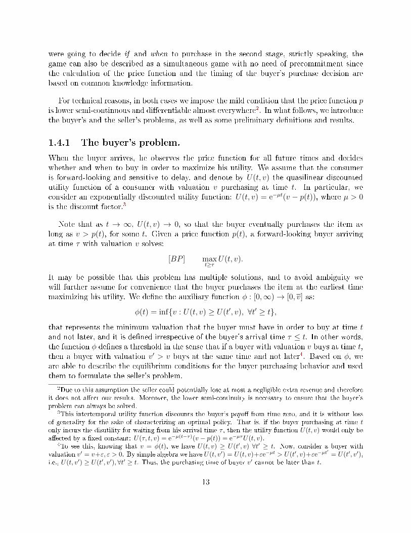
When the buyer arrives, he observes the price function for all future times and decideswhether and when to buy in order to maximize his utility. We assume that the consumeris forward-looking and sensitive to delay, and denote by U(t, v) the quasilinear discountedutility function of a consumer with valuation v purchasing at time t. In particular, weconsider an exponentially discounted utility function: U(t, v) = e−µt(v − p(t)), where µ > 0is the discount factor.3

Note that as t → ∞, U(t, v) → 0, so that the buyer eventually purchases the item aslong as v > p(t), for some t. Given a price function p(t), a forward-looking buyer arrivingat time τ with valuation v solves:

[BP ] maxt≥τ

U(t, v).

It may be possible that this problem has multiple solutions, and to avoid ambiguity wewill further assume for convenience that the buyer purchases the item at the earliest timemaximizing his utility. We dene the auxiliary function φ : [0,∞)→ [0, v] as:

φ(t) = infv : U(t, v) ≥ U(t′, v), ∀t′ ≥ t,that represents the minimum valuation that the buyer must have in order to buy at time tand not later, and it is dened irrespective of the buyer's arrival time τ ≤ t. In other words,the function φ denes a threshold in the sense that if a buyer with valuation v buys at time t,then a buyer with valuation v′ > v buys at the same time and not later4. Based on φ, weare able to describe the equilibrium conditions for the buyer purchasing behavior and usedthem to formulate the seller's problem.

2Due to this assumption the seller could potentially lose at most a negligible extra revenue and thereforeit does not aect our results. Moreover, the lower semi-continuity is necessary to ensure that the buyer'sproblem can always be solved.

3This intertemporal utility function discounts the buyer's payo from time zero, and it is without lossof generality for the sake of characterizing an optimal policy. That is, if the buyer purchasing at time tonly incurs the disutility for waiting from his arrival time τ , then the utility function U(t, v) would only beaected by a xed constant: U(τ, t, v) = e−µ(t−τ)(v − p(t)) = e−µτU(t, v).

4To see this, knowing that v = φ(t), we have U(t, v) ≥ U(t′, v) ∀t′ ≥ t. Now, consider a buyer withvaluation v′ = v+ε, ε > 0. By simple algebra we have U(t, v′) = U(t, v)+εe−µt > U(t′, v)+εe−µt

′= U(t′, v′),

i.e., U(t, v′) ≥ U(t′, v′),∀t′ ≥ t. Thus, the purchasing time of buyer v′ cannot be later than t.

13

1.4.2 The seller's problem

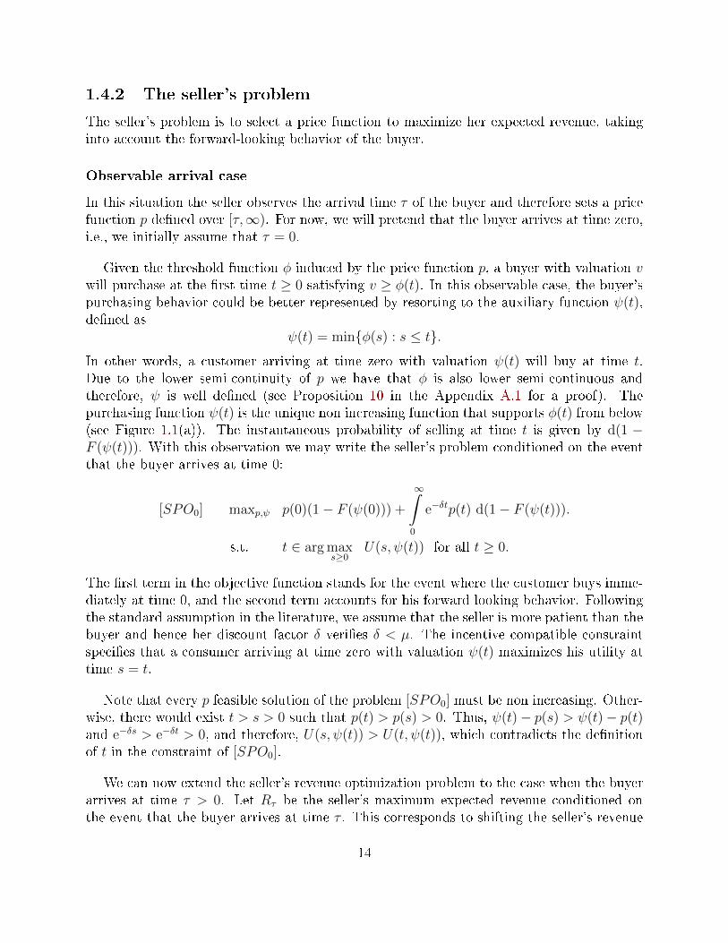
The seller's problem is to select a price function to maximize her expected revenue, takinginto account the forward-looking behavior of the buyer.

Observable arrival case

In this situation the seller observes the arrival time τ of the buyer and therefore sets a pricefunction p dened over [τ,∞). For now, we will pretend that the buyer arrives at time zero,i.e., we initially assume that τ = 0.

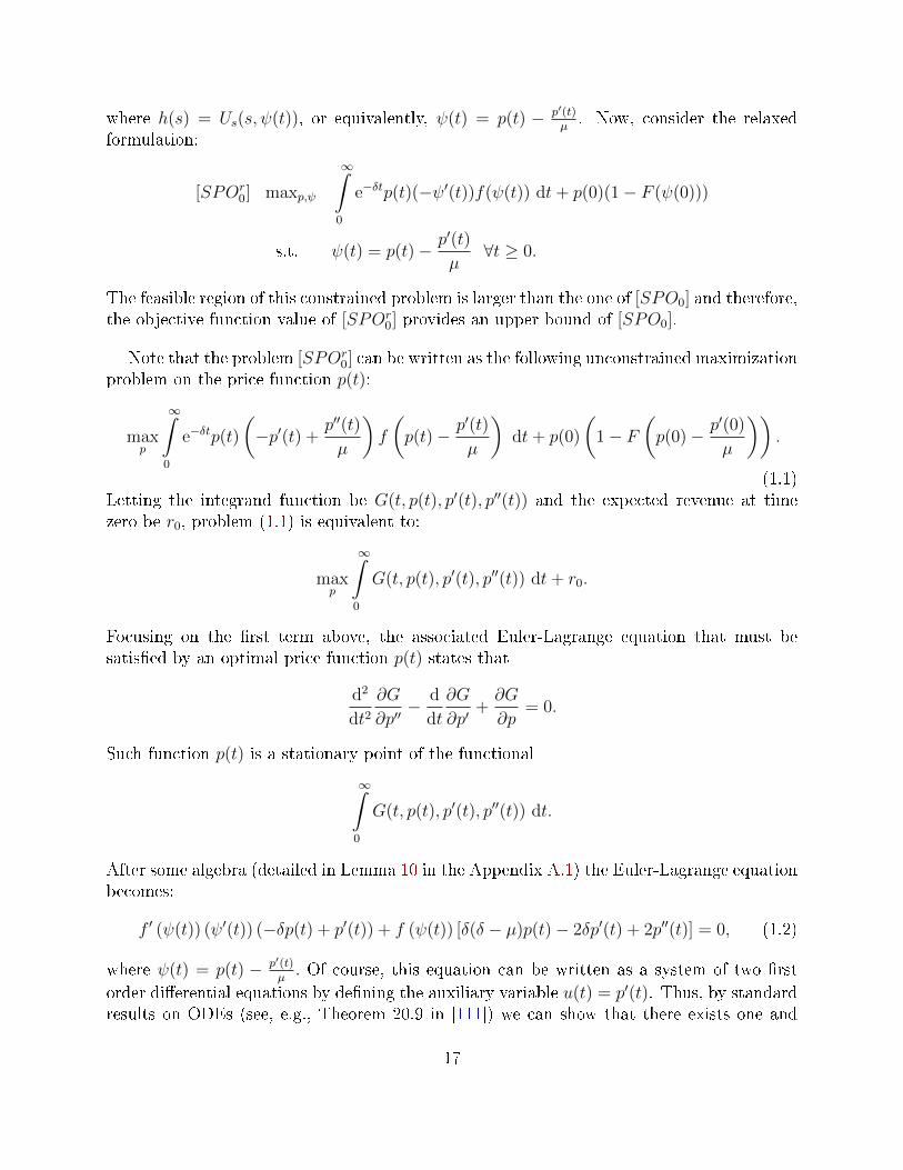
Given the threshold function φ induced by the price function p, a buyer with valuation vwill purchase at the rst time t ≥ 0 satisfying v ≥ φ(t). In this observable case, the buyer'spurchasing behavior could be better represented by resorting to the auxiliary function ψ(t),dened as

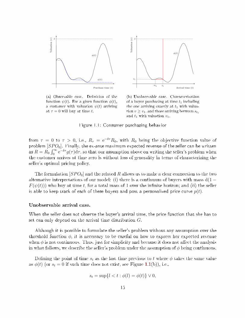
ψ(t) = minφ(s) : s ≤ t.In other words, a customer arriving at time zero with valuation ψ(t) will buy at time t.Due to the lower semi-continuity of p we have that φ is also lower semi-continuous andtherefore, ψ is well dened (see Proposition 10 in the Appendix A.1 for a proof). Thepurchasing function ψ(t) is the unique non increasing function that supports φ(t) from below(see Figure 1.1(a)). The instantaneous probability of selling at time t is given by d(1 −F (ψ(t))). With this observation we may write the seller's problem conditioned on the eventthat the buyer arrives at time 0:

[SPO0] maxp,ψ p(0)(1− F (ψ(0))) +

∞∫0

e−δtp(t) d(1− F (ψ(t))).

s.t. t ∈ arg maxs≥0

U(s, ψ(t)) for all t ≥ 0.

The rst term in the objective function stands for the event where the customer buys imme-diately at time 0, and the second term accounts for his forward looking behavior. Followingthe standard assumption in the literature, we assume that the seller is more patient than thebuyer and hence her discount factor δ veries δ < µ. The incentive compatible constraintspecies that a consumer arriving at time zero with valuation ψ(t) maximizes his utility attime s = t.

Note that every p feasible solution of the problem [SPO0] must be non increasing. Other-wise, there would exist t > s > 0 such that p(t) > p(s) > 0. Thus, ψ(t)− p(s) > ψ(t)− p(t)and e−δs > e−δt > 0, and therefore, U(s, ψ(t)) > U(t, ψ(t)), which contradicts the denitionof t in the constraint of [SPO0].

We can now extend the seller's revenue optimization problem to the case when the buyerarrives at time τ > 0. Let Rτ be the seller's maximum expected revenue conditioned onthe event that the buyer arrives at time τ . This corresponds to shifting the seller's revenue

14

φ(t)

ψ(t)

v

Purchase time (t)

Valu

ati

on

(v)

(a) Observable case. Denition of thefunction ψ(t). For a given function φ(t),a customer with valuation ψ(t) arrivingat τ = 0 will buy at time t.

φ(t)

t1

v1

st1

v

Arrival time (t)

Valu

ati

on

(v)

(b) Unobservable case. Characterizationof a buyer purchasing at time t1 includingthe one arriving exactly at t1 with valua-tion v ≥ v1, and those arriving between st1and t1 with valuation v1.

Figure 1.1: Consumer purchasing behavior

from τ = 0 to τ > 0, i.e., Rτ = e−δτR0, with R0 being the objective function value ofproblem [SPO0]. Finally, the ex-ante maximum expected revenue of the seller can be writtenas R = R0

∫∞0

e−δτg(τ)dτ , so that our assumption above on writing the seller's problem whenthe customer arrives at time zero is without loss of generality in terms of characterizing theseller's optimal pricing policy.

The formulation [SPO0] and the related R allows us to make a clear connection to the twoalternative interpretations of our model: (i) there is a continuum of buyers with mass d(1−F (ψ(t))) who buy at time t, for a total mass of 1 over the innite horizon; and (ii) the selleris able to keep track of each of these buyers and post a personalized price curve p(t).

Unobservable arrival case.

When the seller does not observe the buyer's arrival time, the price function that she has toset can only depend on the arrival time distribution G.

Although it is possible to formulate the seller's problem without any assumption over thethreshold function φ, it is necessary to be careful on how to express her expected revenuewhen φ is not continuous. Thus, just for simplicity and because it does not aect the analysisin what follows, we describe the seller's problem under the assumption of φ being continuous.

Dening the point of time st as the last time previous to t where φ takes the same valueas φ(t) (or st = 0 if such time does not exist, see Figure 1.1(b)), i.e.,

st = supl < t : φ(l) = φ(t) ∨ 0,

15

the seller's problem can be described as follows:

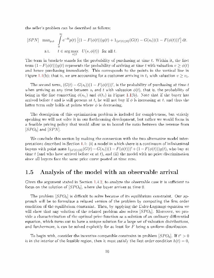
[SPN ] maxp,φ

∞∫0

e−δtp(t)[(1− F (φ(t)))g(t) + 1φ′(t)≤0(G(t)−G(st))(1− F (φ(t)))′

]dt.

s.t. t ∈ arg maxs≥t

U(s, φ(t)) for all t.

The term in brackets stands for the probability of purchasing at time t. Within it, the rstterm (1−F (φ(t)))g(t) represents the probability of arriving at time t with valuation v ≥ φ(t)and hence purchasing immediately. This corresponds to the points in the vertical line inFigure 1.1(b); that is, we are accounting for a customer arriving in t1 with valuation v ≥ v1.

The second term, (G(t)−G(st))(1− F (φ(t)))′, is the probability of purchasing at time twhen arriving at any time between st and t with valuation φ(t), that is, the probability ofbeing in the line connecting φ(st1) and φ(t1) in Figure 1.1(b). Note that if the buyer hasarrived before t and is still present at t, he will not buy if φ is increasing at t, and thus thelatter term only holds at points where φ is decreasing.

The description of this optimization problem is included for completeness, but strictlyspeaking we will not solve it in our forthcoming development, but rather we would focus ina feasible pricing policy that would allow us to bound the ratio between the revenue from[SPO0] and [SPN ].

We conclude this section by making the connection with the two alternative model inter-pretations described in Section 1.1: (i) a model in which there is a continuum of innitesimalbuyers with point mass 1φ′(t)≤0(G(t)−G(st))(1−F (φ(t)))′+ (1−F (φ(t)))g(t), who buy attime t (and who have arrived before or at t), and (ii) the model with no price discriminationsince all buyers face the same price curve posted at time zero.

1.5 Analysis of the model with an observable arrival

Given the argument stated in Section 1.4.2, to analyze the observable case it is sucient tofocus on the solution of [SPO0], where the buyer arrives at time 0.

The problem [SPO0] is dicult to solve because of its equilibrium constraint. Our ap-proach will be to formulate a relaxed version of the problem by computing the rst ordercondition of the equilibrium constraint. Then, by applying the Euler-Lagrange equation wewill show that any solution of the relaxed problem also solves [SPO0]. Moreover, we pro-vide a characterization of the optimal price function as a solution of an ordinary dierentialequation, which turns out to have a unique solution for a large set of valuation distributions,and furthermore, it can be solved explicitly for at least for F being a uniform distribution.

To begin with, consider the incentive compatible constraint in problem [SPO0]. If t∗ > 0is in the interior of the feasible region, then it must satisfy the rst order condition h(t) = 0,

16

where h(s) = Us(s, ψ(t)), or equivalently, ψ(t) = p(t) − p′(t)µ. Now, consider the relaxed

formulation:

[SPOr0] maxp,ψ

∞∫0

e−δtp(t)(−ψ′(t))f(ψ(t)) dt+ p(0)(1− F (ψ(0)))

s.t. ψ(t) = p(t)− p′(t)

µ∀t ≥ 0.

The feasible region of this constrained problem is larger than the one of [SPO0] and therefore,the objective function value of [SPOr

0] provides an upper bound of [SPO0].

Note that the problem [SPOr0] can be written as the following unconstrained maximization

problem on the price function p(t):

maxp

∞∫0

e−δtp(t)

(−p′(t) +

p′′(t)

µ

)f

(p(t)− p′(t)

µ

)dt+ p(0)

(1− F

(p(0)− p′(0)

µ

)).

(1.1)Letting the integrand function be G(t, p(t), p′(t), p′′(t)) and the expected revenue at timezero be r0, problem (1.1) is equivalent to:

maxp

∞∫0

G(t, p(t), p′(t), p′′(t)) dt+ r0.

Focusing on the rst term above, the associated Euler-Lagrange equation that must besatised by an optimal price function p(t) states that

d2

dt2∂G

∂p′′− d

dt

∂G

∂p′+∂G

∂p= 0.

Such function p(t) is a stationary point of the functional

∞∫0

G(t, p(t), p′(t), p′′(t)) dt.

After some algebra (detailed in Lemma 10 in the Appendix A.1) the Euler-Lagrange equationbecomes:

f ′ (ψ(t)) (ψ′(t)) (−δp(t) + p′(t)) + f (ψ(t)) [δ(δ − µ)p(t)− 2δp′(t) + 2p′′(t)] = 0, (1.2)

where ψ(t) = p(t) − p′(t)µ. Of course, this equation can be written as a system of two rst

order dierential equations by dening the auxiliary variable u(t) = p′(t). Thus, by standardresults on ODEs (see, e.g., Theorem 20.9 in [111]) we can show that there exists one and

17

only one solution to the initial value problem given p(0) and p′(0) under mild continuity anddierentiability conditions. These conditions hold if we for instance assume that p(0) > 0and p′(0) < 0. While the former is natural to assume, the latter makes sense in the contextof this observable case with price commitment, where a forward-looking consumer will neverbuy within an ε-interval starting at zero if the price is non decreasing at zero. Therefore,for a large set of valuation distributions, we have that the relaxed problem has exactly onesolution.

Let us highlight that though we know that in the observable case ψ(t) is non increasingby construction -and indeed we use this fact to formulate the seller's problem- [SPOr

0] couldpotentially have an optimal solution with a generic function ψ(t). However, the followingresult establishes that this does not happen. In other words, if ψ(t) corresponds to an optimalsolution of the seller's relaxed problem, then it must be a non decreasing function. A proofis provided in Appendix A.2.1

Proposition 1. Assume that the density function f is strictly positive. If the price func-tion p(t) is a continuously dierentiable optimal solution of the relaxed problem [SPOr

0], then

the optimal purchasing function ψ(t) = p(t)− p′(t)µ

is non increasing.

Proposition 1, along with the upper bound dened by the solution to [SPOr0], allow us to

show that any solution of [SPOr0] also solves the seller's problem [SPO0], proof provided in

Appendix A.2.2.

Theorem 1 Any solution of the relaxed problem [SPOr0] such that p is dierentiable with

continuous derivative also solves the seller's problem [SPO0].

Theorem 1 allows to simplify the solution of the seller's problem [SPO0]. Furthermore,we show that the solution of the relaxed problem is a solution of an autonomous system ofordinary dierential equations.

Thus, to solve the seller's problem [SPO0], rst we formulate the Euler-Lagrange equa-tion (1.2) and solve it. Its solution will depend on the initial values p(0) > 0 and p′(0) < 0.Then, we replace that solution in problem (1.1) and solve it in terms of the scalar vari-ables p(0) and p′(0). Finally, using these optimal initial values, we can recover the optimalprice function p(t) and purchasing function ψ(t) which are the optimal solutions of theoriginal seller's problem [SPO0].

To conclude this subsection, we present a following technical result that states that iffor a given parameter c ∈ (0, 1), we need to ensure that the seller earns a fraction 1 − cof her expected revenue in problem [SPO0], it is enough to look at the problem until timeT = ln(1/c)/δ. A proof of the Lemma is provided in Appendix A.2.3.

Lemma 1. For a given parameter c ∈ (0, 1), up to time T = ln(1/c)/δ, the seller's expected

18

revenue in the observable arrival case is at least (1− c)R0; i.e.,

T∫0

e−δtp(t)d(1− F (ψ(t))) ≥ (1− c)R0,

where p(t) is the solution from (1.2) to the observable case problem.

For instance, if we want to reach at least half of R0 and we normalize the seller's ratediscount to 1, from this result we conclude that it is enough to consider the problem untilT = ln(2). This implies that the time needed to get a big fraction of R0 is relatively smalland, moreover, it does not depend on the valuation distribution.

Before moving on to the unobservable case, in the next section we will do the analysis ofthe observable case for a particular instance of the problem. In particular, we will assumethe valuation distribution is uniformly distributed between 0 and 1.

1.5.1 Uniform valuation case

Assume that the buyer's valuation is Unif[0, 1]. Then, the problem [SPOr0] becomes:

maxp

∞∫0

G(t, p(t), p′(t), p′′(t))dt+ p(0)(1− ψ(0)), (1.3)

where G(t, p(t), p′(t), p′′(t)) = e−δtp(t)(−p′(t) + p′′(t)

µ

).

Formulating the Euler-Lagrange equation (1.2) in this case, we obtain

p′′(t)− δp′(t) +δ2 − δµ

2p(t) = 0,

which is a second order ordinary dierential equation in the function p(t) with constantcoecients and thus, it can be solved explicitly. In fact, its solution is given by:

p(t) = c1e12t(δ−√−δ(δ−2µ)) + c2e

12t(δ+√−δ(δ−2µ)),

where c1, c2 are constants to be determined.

Note that δ +√−δ(δ − 2µ) > 0 and δ −

√−δ(δ − 2µ) < 0 due to µ > δ. Therefore,

the optimal pricing function is a sum of a negative exponential function and a positiveexponential function. Thus, p(t) could in principle go to innity when t goes to innity.However, p(t) ∈ [0, 1] for all t, and therefore, it must be the case that c2 = 0. Thus, theoptimal price function is a negative exponential function of the form:

p(t) = p(0)e12t(δ−√−δ(δ−2µ)).

19

In order to simplify the notation, dene the positive constant A = −δ +√−δ(δ − 2µ).

We are left with computing c1 = p(0). Replacing the function p(t) in the unconstrainedproblem (1.1), we can rewrite it as a maximization problem over p(0) as follows:

maxp(0)

p2(0)

∞∫0

e−(δ+A)t

(A

2+A2

4µ

)dt+ p(0)

(1− p(0)− p(0)

A

2µ

).

Solving this problem, we obtain p(0) = 2µ(δ+A)(A+2µ)(A+2δ)

. Noting that p′(t) = −12Ap(0)e−

12At, we

also obtain p′(0) = − Aµ(δ+A)(A+2µ)(A+2δ)

.

Therefore, the pricing function that solves the Euler-Lagrange equation is given by

p(t) =2µ(δ + A)

(A+ 2µ)(A+ 2δ)e−

A2t,

with corresponding purchasing function

ψ(t) =δ + A

A+ 2δe−

A2t.

In conclusion, we have that the negative exponential functions p(t) and ψ(t) are the solutionsof the seller's problem [SPO0] for a consumer's valuation Unif[0, 1], and moreover, we havethat the purchasing function is a positive multiplicative scaling the pricing function.

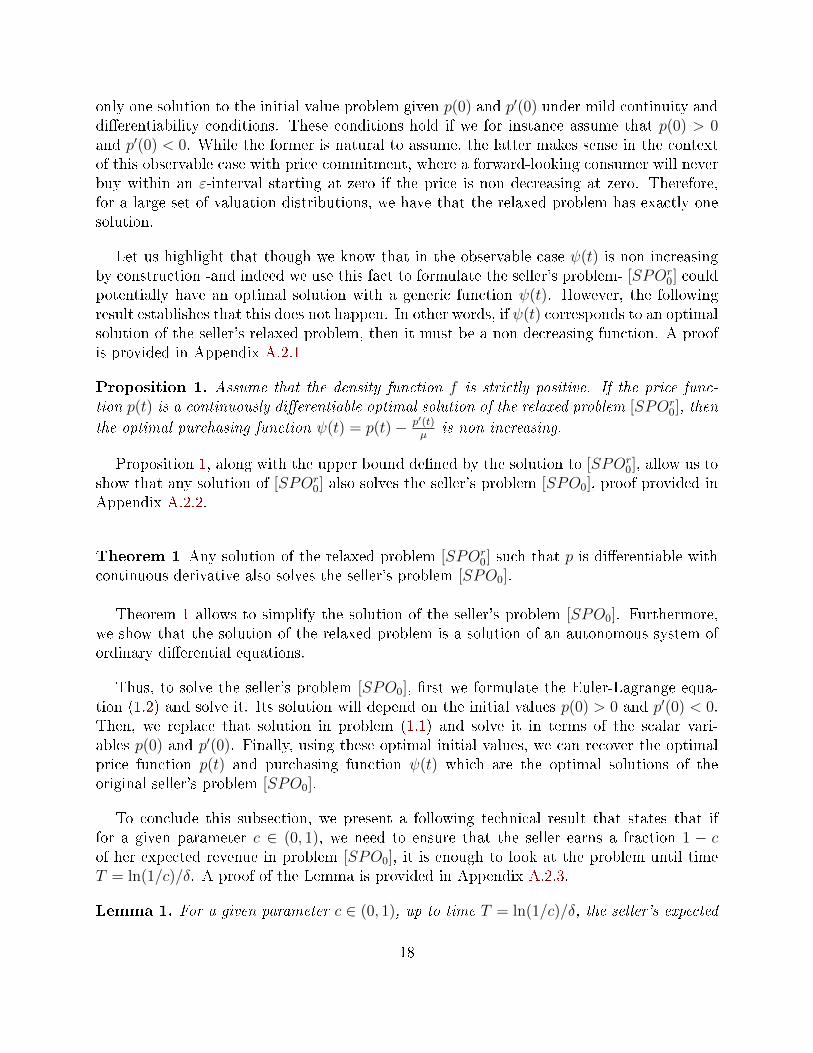
In what follows, we analyze the optimal curves obtained for some specic values of thediscount rates µ and δ, corresponding to dierent levels of asymmetry in the patience of theseller and the buyer. Without loss of generality, we normalize the discount rate of the sellerby setting δ = 1.

In Figure 1.2, the left panel captures the case where the buyer is ve times more impatientthan the seller, whereas the right panel illustrates the scenario where he is only 50% moreimpatient. In panel (a), when the buyer is noticeably more impatient, we can observe thatthe optimal initial values of p(0) and p′(0) are greater than in panel (b), and that bothprice and purchasing optimal functions decrease faster. These curves reect the fact thatwhen facing a more impatient consumer (panel (a)), the seller will price more aggressivelyearly in the horizon but will also drop the price quicker. Noting that the decreasing pricepattern plays the role of a valuation discovery mechanism, the wider span of the pricingin (a) attempts to keep in the market a low valuation consumer by oering an attractiveenough price relatively soon. On the contrary, when the buyer is more patient (panel (b)),the seller can oer a slow decaying price curve so that a consumer with mid to low valuationwill buy later (compared to (a)) but at a higher price.

The fact that the seller takes advantage of the buyer's impatience is conrmed when com-puting the ex-ante expected revenue by solving [SPO0] in both cases, leading to values 0.3125and 0.2574, respectively.

20

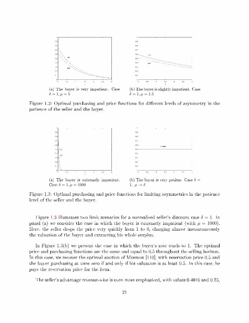
(a) The buyer is very impatient. Caseδ = 1, µ = 5

(b) The buyer is slightly impatient. Caseδ = 1, µ = 1.5

Figure 1.2: Optimal purchasing and price functions for dierent levels of asymmetry in thepatience of the seller and the buyer.

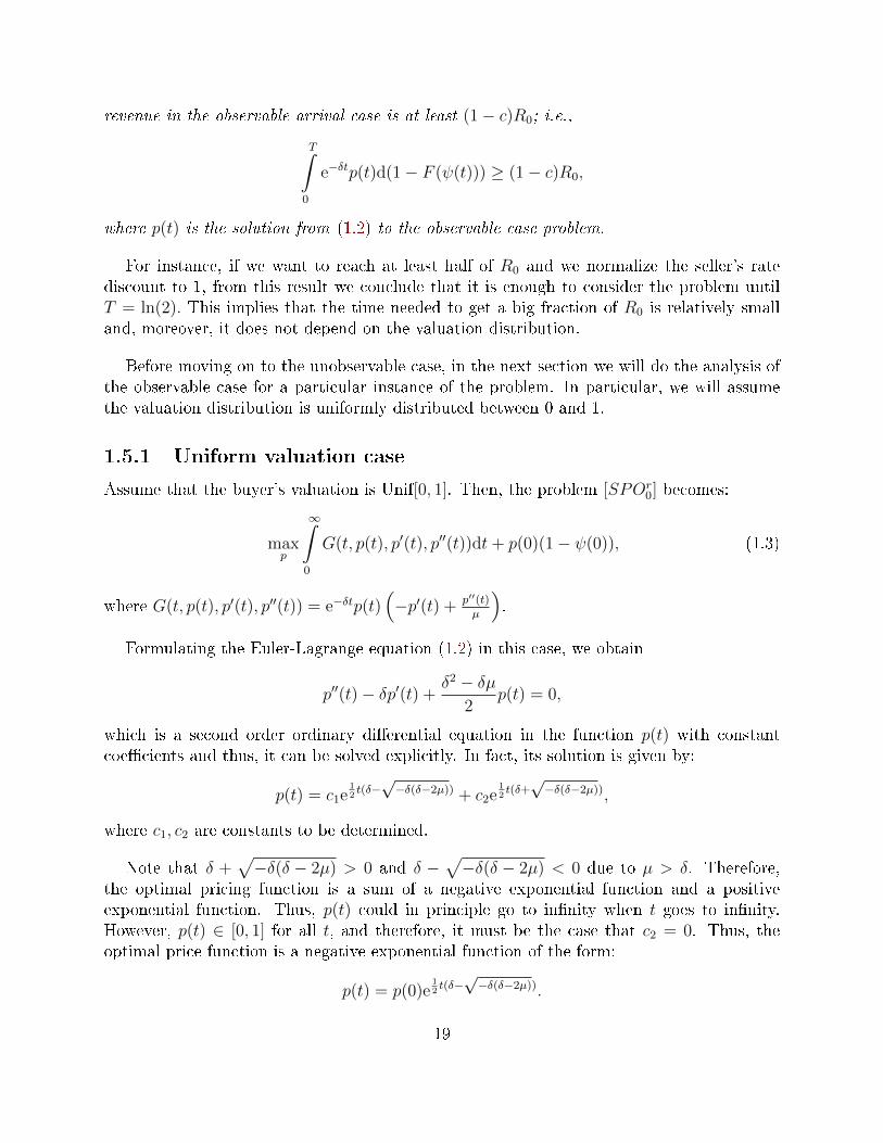
(a) The buyer is extremely impatient.Case δ = 1, µ = 1000

(b) The buyer is very patient. Case δ =1, µ→ δ

Figure 1.3: Optimal purchasing and price functions for limiting asymmetries in the patiencelevel of the seller and the buyer.

Figure 1.3 illustrates two limit scenarios for a normalized seller's discount rate δ = 1. Inpanel (a) we consider the case in which the buyer is extremely impatient (with µ = 1000).Here, the seller drops the price very quickly from 1 to 0, charging almost instantaneouslythe valuation of the buyer and extracting his whole surplus.

In Figure 1.3(b) we present the case in which the buyer's rate tends to 1. The optimalprice and purchasing functions are the same and equal to 0.5 throughout the selling horizon.In this case, we recover the optimal auction of Myerson [110], with reservation price 0.5 andthe buyer purchasing at time zero if and only if his valuation is at least 0.5. In this case, hepays the reservation price for the item.

The seller's advantage revenue-wise is even more emphasized, with values 0.4016 and 0.25,

21

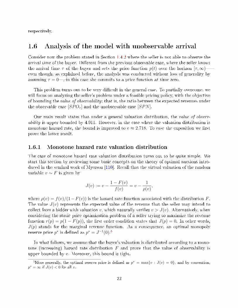
respectively.

1.6 Analysis of the model with unobservable arrival

Consider now the problem stated in Section 1.4.2 where the seller is not able to observe thearrival time of the buyer. Dierent from the previous observable case, where the seller knowsthe arrival time τ of the buyer and sets the price function p(t) over the horizon [τ,∞)even though, as explained before, the analysis was conducted without loss of generality byassuming τ = 0, in this case she commits to a price function at time zero.

This problem turns out to be very dicult in the general case. To partially overcome, wewill focus on analyzing the seller's problem under a feasible pricing policy, with the objectiveof bounding the value of observability ; that is, the ratio between the expected revenues underthe observable case [SPOτ ] and the unobservable case [SPN ].

Our main result states that under a general valuation distribution, the value of observ-ability is upper bounded by 4.911. However, in the case where the valuation distribution ismonotone hazard rate, the bound is improved to e ≈ 2.718. To ease the exposition we rstprove the latter result.

1.6.1 Monotone hazard rate valuation distribution

The case of monotone hazard rate valuation distribution turns out to be quite simple. Westart this section by reviewing some basic concepts on the theory of optimal auctions intro-duced in the seminal work of Myerson [110]. Recall that the virtual valuation of the randomvariable v ∼ F is given by

J(v) := v − 1− F (v)

f(v)= v − 1

ρ(v),

where ρ(v) = f(v)/(1−F (v)) is the hazard rate function associated with the distribution F .The value J(v) represents the expected value of the revenue that the seller may intend tocollect from a bidder with valuation v, which naturally veries v > J(v). Alternatively, whenconsidering the static price optimization problem of a seller trying to maximize the revenuefunction r(p) = p(1− F (p)), the rst order condition states that J(p) = 0. In other words,J(p) stands for the marginal revenue function. As a consequence, an optimal monopolyreserve price p∗ is dened as p∗ = J−1(0).5

In what follows, we assume that the buyer's valuation is distributed according to a mono-tone (increasing) hazard rate distribution F and prove that the value of observability isupper bounded by e. Moreover, this bound is tight.

5More generally, the optimal reserve price is dened as p∗ = maxv : J(v) = 0, and by convention,p∗ =∞ if J(v) < 0 for all v.

22

Indeed, we know from Section 1.4.2 that the optimal seller's expected revenue in the

observable case is given by R = R0

∞∫0

e−δtg(t)dt, where R0 is the objective function value of

problem [SPO0] and therefore veries R0 ≤ E(v), the expected value of the valuation drawnfrom F . Hence, the seller's expected revenue in the observable case is upper bounded by

E(v)

∞∫0

e−δtg(t)dt.

For the unobservable case, consider the feasible, xed pricing policy p(t) = p∗ for all t,where p∗ = J−1(0) is the optimal monopoly price. Then, the seller's expected revenue is atleast

∞∫0

e−δtp∗(1− F (p∗))g(t)dt = p∗(1− F (p∗))

∞∫0

e−δtg(t)dt.

Finally, by Lemma 3.10 (p.325) of Dhangwatnotai et al. [50], it follows that p∗(1−F (p∗)) ≥1eE(v), and this the claimed bound follows.

The bound is tight in the case of exponentially distributed valuation (F (v) = 1 − e−v)and a myopic buyer (with µ = ∞), and when the seller does not discount revenues (i.e.,δ = 0). In this setting, in the observable case, the seller will announce a price curve thatspans all the support [0, v] (e.g., p(t) = 1/t), and the consumer will buy immediately whenhis valuation v = p(t). In this case, the ex-ante expected revenue is E(v) = 1. In orderto get the revenue for the unobservable case, the seller will oer a xed price p maximizingp(1− F (p)) = pe−p. This function is maximized at p = 1 with optimal revenue e−1.

1.6.2 A feasible periodic price function

We start by noting that using xed pricing does not work in general. For instance, considerthe game where the buyer's valuation is distributed according to a truncated Pareto distri-bution with parameter 1, that is, with cdf F (x) = (1 − 1/x)M/(M − 1) for x ∈ [1,M ],and again µ = ∞ and δ = 0. Here, we have that the expected value of the buyer'svaluation is M lnM/(M − 1) whereas p∗(1 − F (p∗)) = M/(M − 1), leading to the ratioE(v)/p∗(1−F (p∗)) = lnM growing withM . Note then that the ratio grows arbitrarily largeindependent on the arrival distribution.

Thus, to bound the value of observability in the general case we need to consider a pricingpolicy that allows us to compare the expected revenue in the observable and unobservablecase. We dene it in Section 1.6.2 and present our main result in Section 1.6.3.

The feasible pricing policy p we consider is periodic and depends on the optimal pricingpolicy p of [SPO0]. The length of the period will be 2T where T is such that until time Tthe seller's expected revenue in the observable case when the buyer arrives at time zero is

23

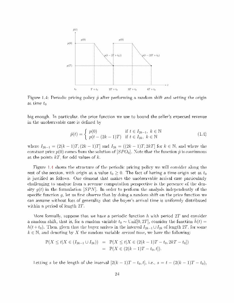
p(t− (T + t0)) p(t− (2T + t0)

p(t)

t0

t

T + t0 3T + t0 4T + t02T + t0

p(0)

p(0) p(0)

p(T )

Figure 1.4: Periodic pricing policy p after performing a random shift and setting the originat time t0

big enough. In particular, the price function we use to bound the seller's expected revenuein the unobservable case is dened by

p(t) =

p(0) if t ∈ I2k−1, k ∈ Np(t− (2k − 1)T ) if t ∈ I2k, k ∈ N (1.4)

where I2k−1 = (2(k − 1)T, (2k − 1)T ] and I2k = ((2k − 1)T, 2kT ] for k ∈ N, and where theconstant price p(0) comes from the solution of [SPO0]. Note that the function p is continuousat the points kT , for odd values of k.

Figure 1.4 shows the structure of the periodic pricing policy we will consider along therest of the section, with origin at a value t0 ≥ 0. The fact of having a time origin set at t0is justied as follows. One element that makes the unobservable arrival case particularlychallenging to analyze from a revenue computation perspective is the presence of the den-sity g(t) in the formulation [SPN ]. In order to perform the analysis independently of thespecic function g, let us rst observe that by doing a random shift on the price function wecan assume without loss of generality that the buyer's arrival time is uniformly distributedwithin a period of length 2T .

More formally, suppose that we have a periodic function h with period 2T and considera random shift, that is, for a random variable t0 ∼ Unif[0, 2T ], consider the function h(t) =h(t+ t0). Then, given that the buyer arrives in the interval I2k−1∪ I2k of length 2T , for somek ∈ N, and denoting by X the random variable arrival time, we have the following:

P(X ≤ t|X ∈ (I2k−1 ∪ I2k)) = P(X ≤ t|X ∈ (2(k − 1)T − t0, 2kT − t0])

= P(X ∈ (2(k − 1)T − t0, t]).

Letting s be the length of the interval [2(k − 1)T − t0, t], i.e., s = t − (2(k − 1)T − t0),

24

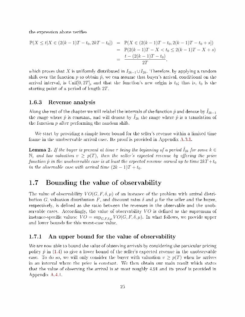
the expression above veries

P(X ≤ t|X ∈ (2(k − 1)T − t0, 2kT − t0]) = P(X ∈ (2(k − 1)T − t0, 2(k − 1)T − t0 + s])

= P(2(k − 1)T −X < t0 ≤ 2(k − 1)T −X + s)

=t− (2(k − 1)T − t0)

2T,

which proves that X is uniformly distributed in I2k−1∪I2k. Therefore, by applying a randomshift over the function p to obtain p, we can assume that buyer's arrival, conditional on thearrival interval, is Unif[0, 2T ], and that the function's new origin is t0; that is, t0 is thestarting point of a period of length 2T .

1.6.3 Revenue analysis

Along the rest of the chapter we will relabel the intervals of the function p and denote by I2k−1

the range where p is constant, and will denote by I2k the range where p is a translation ofthe function p after performing the random shift.

We start by providing a simple lower bound for the seller's revenue within a limited timeframe in the unobservable arrival case. Its proof is provided in Appendix A.3.1.

Lemma 2. If the buyer is present at time τ being the beginning of a period I2k for some k ∈N, and has valuation v ≥ p(T ), then the seller's expected revenue by oering the pricefunction p in the unobservable case is at least the expected revenue earned up to time 2kT+t0in the observable case with arrival time (2k − 1)T + t0.

1.7 Bounding the value of observability

The value of observability V O(G,F, δ, µ) of an instance of the problem with arrival distri-bution G, valuation distribution F , and discount rates δ and µ for the seller and the buyer,respectively, is dened as the ratio between the revenues in the observable and the unob-servable cases. Accordingly, the value of observability V O is dened as the supremum ofinstance-specic values: V O = supG,F,δ,µ V O(G,F, δ, µ). In what follows, we provide upperand lower bounds for this worst-case value.

1.7.1 An upper bound for the value of observability

We are now able to bound the value of observing arrivals by considering the particular pricingpolicy p in (1.4) to give a lower bound of the seller's expected revenue in the unobservablecase. To do so, we will only consider the buyer with valuation v ≥ p(T ) when he arrivesin an interval where the price is constant. We then obtain our main result which statesthat the value of observing the arrival is at most roughly 4.91 and its proof is provided inAppendix A.4.1.

25

This bound can be written as a function of W−1, the negative branch of the well knownLambert function6.

Theorem 2 For any valuation distribution and arrival time distribution, the value of ob-servability is at most − 2W−1(−1/(2

√e))+1

(eW−1(−1/(2√e))+1/2−1)

2 ≈ 4.911.

It is worth noting that our result is robust in the sense that it holds independently ofthe arrival distribution. That is, even in the case where the buyer arrival is adversarialtheworst possible for the seller, we prove that the seller's expected revenue in the observablecase is at most 4.911 times the seller's expected revenue if she does not observe the buyer'sarrival.

1.7.2 A lower bound for the value of observability

Unfortunately, it is not straightforward to obtain a lower bound for the value of observability.The diculty stems from the complexity of solving the unobservable case, even numerically,as discussed in Section 1.6. In order to partially overcome this diculty, we consider aparticular problem instance that can be solved numerically via dynamic programming.

Suppose that the valuation of the buyer is distributed uniformly in [0, 1], and that hearrives at one of two possible times. Specically, we assume that the buyer arrives eitherat time 0 with probability β, or at time T with probability 1 − β, for some predeterminedvalue T > 0. We dene the threshold valuation α as the value so that if the buyer arrivesat time 0 with valuation v ≥ α, then he would buy before time T . This implies that,conditioned on that by time T the seller has not sold the item, the buyer's valuation is themixture of two uniforms: (i) a Unif[0, α] accounting for the mass of buyers who arrived at 0and decided to wait for a good price to be oered after T , with weight β, and (ii) a Unif[0, 1]distribution accounting for the buyer arriving at time T , with weight 1 − β. Assume alsothat the seller's discount rate is normalized to δ = 1, and that the buyer discounts the futureat rate µ.

The general approach would be to decouple the problem in two independent subproblemsthat occur sequentially over time, by resorting to dynamic programming. Assume for nowthat the value of α is given. Then, we could solve the whole problem by backward induction.If there are no purchasing deviationsin the sense that if the buyer arrives with valuation atleast α, he will not buy after T, we can solve these two subproblems separately and thenlink them through the threshold α occurring at time T . Furthermore, each subproblem, oncewe condition on the information available at times 0 and T , corresponds to the observable

6The Lambert W function is dened as the multivalued function that satises z = W (z) exp(W (z)) forany complex number z. If x is real then for 1/e ≤ x < 0 there are two possible real values of W (x).We denote the branch satisfying −1 ≤ W (x) by W0(x)namely, the principal branch, and the branchsatisfying W (x) ≤ −1 by W−1(x)- referred to as the negative branch.

26

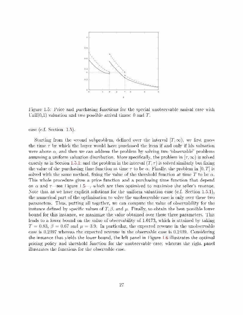
0 1 2 3 4 50

0.2

0.4

0.6

0.8

1

t

T

α

τ

Figure 1.5: Price and purchasing functions for the special unobservable arrival case withUnif(0,1) valuation and two possible arrival times: 0 and T .

case (c.f. Section 1.5).

Starting from the second subproblem, dened over the interval [T,∞), we rst guessthe time τ by which the buyer would have purchased the item if and only if his valuationwere above α, and then we can address the problem by solving two observable problemsassuming a uniform valuation distribution. More specically, the problem in [τ,∞) is solvedexactly as in Section 1.5.1; and the problem in the interval (T, τ) is solved similarly but xingthe value of the purchasing time function at time τ to be α. Finally, the problem in [0, T ] issolved with the same method, xing the value of the threshold function at time T to be α.This whole procedure gives a price function and a purchasing time function that dependon α and τsee Figure 1.5, which are then optimized to maximize the seller's revenue.Note that as we have explicit solutions for the uniform valuation case (c.f. Section 1.5.1),the numerical part of the optimization to solve the unobservable case is only over these twoparameters. Thus, putting all together, we can compute the value of observability for theinstance dened by specic values of T, β, and µ. Finally, to obtain the best possible lowerbound for this instance, we maximize the value obtained over these three parameters. Thisleads to a lower bound on the value of observability of 1.0173, which is attained by takingT = 0.83, β = 0.67 and µ = 3.9. In particular, the expected revenue in the unobservablecase is 0.2397 whereas the expected revenue in the observable case is 0.2439. Consideringthe instance that yields the lower bound, the left panel in Figure 1.6 illustrates the optimalpricing policy and threshold function for the unobservable case; whereas the right panelillustrates the functions for the observable case.

27

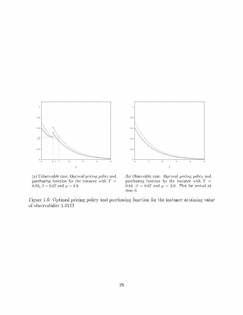
0 1 2 3 4 50

0.2

0.4

0.6

0.8

1

t

T

α

τ

(a) Uobservable case. Optimal pricing policy andpurchasing function for the instance with T =0.83, β = 0.67 and µ = 3.9.

0 1 2 3 4 50

0.2

0.4

0.6

0.8

1

t

(b) Observable case. Optimal pricing policy andpurchasing function for the instance with T =0.83, β = 0.67 and µ = 3.9. Plot for arrival attime 0.

Figure 1.6: Optimal pricing policy and purchasing function for the instance attaining valueof observability 1.0173

28

Chapter 2

Connection between posted price

mechanisms and prophet inequalities1

2.1 Introduction

In the last few years online sales (particularly in ebay) have been moving from an auctionformat, to a posted price format [55] and the basic reason for this trend switch seems to bethat posted price mechanisms are much simpler than optimal auctions yet ecient enough. Inaddition, in recent years several companies have started to apply personalized pricing to selltheir products. Under this policy, companies set dierent prices (or oer dierent discounts)for dierent consumers based on purchase history or other factors that may aect theirwillingness to pay. Examples of such companies include Lexis-Nexis, Orbitz, and Safeway(see, e.g.,[123, 106, 90]).

The basic setting is as follows. Suppose a seller has an item to sell through a (sequential)posted price mechanism (PPM). In such a mechanism, consumers arrive one at a time andthe seller proposes to each consumer a take-it-or-leave-it oer. The rst consumer acceptingthe oer pays that price and takes the item. These type of mechanisms are very exibleand adapt very well to dierent scenarios [41]. Furthermore, their simplicity and the factthat strategic behaviour vanishes make them very suitable for a number of applications. Ofcourse PPMs are suboptimal and therefore the study of their approximation guarantees hasbeen an extremely active area in the last decade.

The recent survey by Lucier [102] is an excellent starting point in the area, where manyvariants of PPMs are described. In particular these can be: Anonymous (the oered price isthe same for all consumers); Static (the possibly dierent prices to oer do not evolve as the

1This chapter of the thesis is based on joint paper with Jose Correa, Patricio Foncea and Victor Verdugo[45]

29

mechanism progresses), Order-Oblivious (the order in which agents arrive can be chosen byan adaptive adversary). Furthermore, we may even use PPMs when selling multiple objectsand even have constraints on the subsets of consumers that can be served. Typical sideconstraints include selling multiple copies of an item, say we can serve at most k consumers,or having matroid constraints, or even more general downward-closed family constraints.

In the last decade a lot of eort from the computer science community has been devotedto understand the approximation guarantees that can be obtained through PPMs, wherethe natural benckmark is that given by the optimal mechanism of Myerson [110]. In aninuential paper Chawla et al. [41] establish an interesting connection between (revenuemaximizing) PPMs and prophet inequalities, a problem arising in optimal stopping theory.Here a gambler is faced to a sequence of random variables and has to pick a stopping time sothat the value he gets is as close as possible to the expectation of the maximum of all randomvariables, interpreted as what a prophet, who knows the realizations in advance, could get.They implicitly show that any prophet type inequality can be turned into a posted pricemechanism with the same approximation guarantee. This is obtained by noting that a PPMfor revenue maximization can be seen as (threshold) stopping rule for the gambler but onthe virtual values. As a consequence, the follow up work in the eld concentrated on prophetinequities and then applied the obtained results to sequential posted price mechanisms.

In this chapter we ll a gap in this line of research by proving the converse of the latterresult, namely, that any posted price mechanism can be turned into a prophet type inequalitywith the same approximation guarantee. The core of the result is a way to go back fromvirtual values to arbitrary distributions which may nd applications beyond the scope ofthis thesis. This result amounts not only to apply approximation guarantees from prophetinequalities to PPMs, but also to carry over the lower bounds. We observe that actuallythough our reduction we can improve the best known lower bound for sequential PPMs (inwhich the arrival order is either random or selected by the seller) in the single item case, thek-uniform matroid case, the general matroid case, and the general downward-closed familycase.

2.2 Contributions

We summarize contributions of Chapter 1 below.

Firstly, we provide a simple proof of the reduction from prophet inequalities to postedprice mechanism, already studied by Chawla et al. [41]. The basic observation for obtainingthis reduction is that price-based revenue maximization can be seen as prophet inequalitieson the virtual values.

Secondly, we introduce a key result, namely Valuation Mapping Lemma, stating that forany distribution F there is another distribution G whose virtual value distributes accordingto F . That is, if we consider the operator that picks an arbitrary probability distribution over

30

the nonnegative reals and returns the distribution of the ironed virtual valuation function,the Valuation Mapping Lemma states that this operator is surjective (onto) over the spaceof distributions. Interestingly, the lemma gives an explicit construction so we can easilyinterpret the thresholds as prices for the sequential posted price problem. It is somewhatsurprising that this basic result was missing from the auction theory literature and we believeit may prove useful in settings beyond PPMs.

Thirdly, we answer the natural question arising from the above mentioned result of Chawlaet al. [41] of whether the converse of their result also holds. In other words, we answer thequestion: does the existence of a PPM with a certain approximation guarantee impliesthe existence of a (threshold) prophet inequality with the same approximation guarantee?The main result of this chapter is to answer this question on the positive. Specically, weprove that if we take an instance of the sequential posted price problem and there is aPPM obtaining a revenue within a factor α of Myerson's optimal mechanism, then there isa threshold stopping rule that obtains a fraction α of what a prophet could obtain. Themain diculty on the proof of this result comes from taking an arbitrary distribution in theprophet inequality problem and map it back to a sequential posted price problem. Here iswhere the valuation mapping lemma, that holds for arbitrary distributions, comes into playgiving a way to go from virtual valuations to arbitrary distributions.

A remarkable feature of the Valuation Mapping Lemma is that when mapping a distri-bution F into another distribution G whose virtual value distributes like F , we can actuallyobtain a regular G (i.e., monotone non-decreasing virtual value). Of course, in principlethere are many G's that satisfy the statement of the lemma, however we can identify oneexplicitly with this appealing property. Together with the reduction theorems, this impliesthat the posted price problem can be reduced to a prophet inequality problem, which can inturn be reduced to a posted price problem with regular valuation distributions. Thereforedesigning PPMs in general is equally hard from an approximation perspective to designingPPMs when the underlying valuations are regular.

It is worth mentioning that our result is very robust to dierent settings: it works withdierent ordering such as random, adversarial, or best possible, as well when there aremultiple items and constraints on the allowed allocation sets.

Finally, we translate all known upper and lower bounds from PPMs into prophet inequali-ties, and back. A particular case where this gives new results in the case of sequential postedprice mechanisms (SPM, [41]). Here the seller has to choose an order of the buyers and apick a price for each buyer so as to maximize revenue. The current best known lower boundfor this problem was obtained a decade ago by Blumrosen and Holenstein [28] and evaluatesto√π/2 ≈ 1.253. Moreover, this lower bound is the best known lower bound when the

feasibility constraint is a k-uniform matroid, a general matroid, and even the intersection oftwo matroids. With our result we can improve the lower bound in these settings to 1.341 byusing the lower bound for the i.i.d. prophet inequality designed by Hill and Kertz [81] over

31

three decades ago. On the other hand, we can also use our framework to derive a new simpleand purely probabilistic proof of the ex ante relaxation bound on the revenue of Myerson'soptimal mechanism [41, 7]. It is worth mentioning that, although our results are presentedin the context of single-parameter mechanism design, they also follow more generally formulti-parameter domains by considering the reduction introduced by Chawla et al. [41].

2.3 Related literature

The connection between prophet inequalities and mechanism design was initiated by Haji-aghayi et al. [79] and further developed by Chawla et al. [40]. The key idea behind thisconnection was to implement prophet inequality's algorithms using thresholds that couldbe identied with prices. In particular, Chawla et al. [40] considers a pricing auction inadversarial order and obtain an upper bound of 4 with respect to the optimal mechanism.This was later improved by Chawla et al. [41] who gave several new approximation factorsfor PPMs in multiparameter settings, for the case of adversarial order (order-oblivious postedprice) and when the designer was allowed to choose the order (sequential posted price). In theformer case, they gave tight approximations for uniform and partition matroids (a constantfactor of 2), and lower bounds for general matroids, intersection of matroids and downward-closed systems. Studying the prophet inequality problem, Kleinberg and Weinberg [91] gaveimproved upper bounds of 2 for general matroids and 4p− 2 for intersection of p matroids,as well as a lower bound of O(p) for this second setting, while Babaio et al.[18] and Ru-binstein [119] presented a lower bound in downward-closed systems of log(n)/2 log(log(n)).Rubinstein also found a new upper bound of O(log(r) log(n)) on downward-closed systems(where r is the size of the largest feasible set) and a lower bound of O(n) if the system is notdownward-closed. In the case of sequential posted prices, Yan [134] used the correlation gapto nd upper bounds of e

e−1for general matroids and p+ 1 for intersection of p-matroids.

During the last years several other variants of the problem have been studied, includingcombinatorial prophet inequalities (see, e.g., [37, 120]), combinatorial auctions (see, e.g.,[7, 61]), and polymatroids constraints for auctions (see, e.g., [54]). Attention has also beenpayed to settings with limited information or prior-independent, where the designer mustlearn the distribution in order to run the mechanism (see, e.g., [50, 43, 16, 73, 109, 17,36]). Very recently, Dütting et al. [52] developed a general framework to obtain prophetinequalities using the concept of balanced prices, which allowed them to match and improveprevious upper bounds in combinatorial auctions with sub-additive valuations and matroidconstraints.

In the more specic setting where only one item must be allocated, the sequential postedprice problem can be very simply stated as follows. Consider n > 1 buyers with valuationdistributions represented by non-negative, independent random variables Y1, . . . , Yn. If buyeri is oered a price above his value then he takes the item and the seller obtains a gain equalto the oered price, otherwise the buyer is discarded and the seller continues with buyer i+1.

32

The goal is thus to nd prices p1, . . . , pn maximizing the expected revenue of the seller. Forthis problem, the performance of anonymous pricing (i.e., all prices have to be equal) wasconsidered by Alaei et al. [8] and Dütting et al. [53]. Chawla et al. [41] obtain upper boundsof 2 and e

e−1for order-oblivious and sequential posted price mechanism respectively. Later,

Esfandiari et al. [59] studied the prophet secretary setting were the arrival order is random,and provided an approximation factor of e

e−1and a lower bound of 1.33 when the algorithm's

prices may depend on the number of buyers that have rejected but not on their valuationdistributions. The same approximation factor was found by Correa et al. [44] in the randomorder case, but where the algorithm's prices are static and had to be decided beforehandonly based on the underlying distributions. Furthermore in the case of i.i.d. distributions,they found a 1.34 approximation factor which by the work of [81] is also tight. Abolhassaniet al. [2] considered a relaxation of the i.i.d. setting under a large market assumption andshowed that in both adversarial and random order a 1.36 approximation is possible.

Prophet-Inequalities

For xed n > 1, let X1, . . . , Xn be non-negative, independent random variables and Tntheir set of stopping rules. A classic result of Krengel and Sucheston, and Gairing [93, 94]asserts that E(maxX1, . . . , Xn) ≤ 2 supE(Xt) : t ∈ Tn, and that 2 is the best possiblebound. The study of this type of inequalities, known as prophet inequalities, was initiatedby Gilbert and Mosteller [70] and attracted a lot of attention in the eighties (see, e.g.,[81, 89, 91, 122, 121]). In particular Samuel-Cahn [122] noted that rather than looking atthe set of all stopping rules one can (quite naturally) only look at threshold stopping rulesin which the decision to stop depends on wether the value of the currently observed randomvariable is above a certain threshold (and possibly on the rest of the history). Two decadeslater the problem was brought up to the attention of the computer science community bythe work of Chawla et al. [41] who noted a close connection between PPMs and prophetinequalities. The basic observation of Chawla et al. is that a PPM reduces to a (threshold)prophet inequality but applied to the virtual values [110]. The work of Chawla et al. wasinuential in that most follow-up work is directly on the context of prophet inequalities andthen applies the implied results to PPMs.

The connection has also been useful to improve old results form prophet inequalities.Indeed, an interesting special case which we mention since we will use it later on, occurswhen the random variables are also identically distributed. Here, the constant 2 can belowered. Indeed, Hill and Kertz [81] provided family of bad" instances from which Kertz[89] proved the best possible bound one could expect is β ≈ 1.341, the unique solution to∫ 1

01

y(1−ln(y))+(β−1)dy = 1. Hill and Kertz also proved a bound of 1 + 1/(e− 1) ≈ 1.582 which

was very recently improved by Abolhassan et al. [2] to 1.355 and nally Correa et al. [44]proved that β is a tight value.

33

Organization

In Section 2.4 we introduce formally the online selection problem and the auction problem.We also introduce necessary notation and some useful remarks and results about distributionsand its virtual valuation. In Section 2.5 we show the reduction from prophet inequalitiesto posted price mechanisms, result that is stated formally in Theorem 4. We remark thatthis approach has been considered extensively in mechanism design, and we include it forcompleteness, by showing a simple proof. In Section 2.6 we show our main result statedformally in Theorem 5, that is, the reduction from posted price mechanisms to prophetinequalities. Finally, in Section 2.7 we show some consequences of Theorem 5, including theimproved lower bound for SPMs in more detail.

2.4 Preliminaries

We start this section by giving a formal denition of an instance of the two problems westudy throughout this chapter: the online selection problem and the auction problem.

Online Selection Problem. An instance of this problem corresponds to a tuple (X,F , T ),where X is the ground set of n elements and each set in T ⊆ 2X is called feasible selection.For each element x ∈ X there is a random variable wx, called weight, distributed according toFx with support contained in R+ and nite expectation, and F = Fx : x ∈ X. We assumethem to be independent. The random variables are presented in an order σ : [n]→ X, andan algorithm for the problem has to decide whether to select or not an element of X whenarrived. An algorithm is correct if it outputs a feasible selection.

An algorithm is an α-approximation if the expected weight of the output selection is atleast α · E

(maxA∈T

∑x∈Awx

), that is, an α fraction of the expectation of the maximum

weight over feasible selections. In the latter, the expectation is taken over F and the (pos-sibly) algorithm internal randomness.

Multi-Item Mechanism Design. Consider a single seller who provides a set of n items givenby I. For each item i ∈ I, there exists a buyer having a random valuation vi for that item.We denote by Gi the distribution of the valuation vi, and we assume this to have a supportcontained in R+ and that vi is integrable. We denote by G = Gi : i ∈ I the set of valuationdistributions. There exists a set of feasibility constraints for the seller, T ⊆ 2I , and everyset in T is called a feasible allocation. Therefore, an instance for this problem is given by atuple (I,G, T ).

This setting is known to be the single-parameter domain. We assume the valuationdistributions to be independent, an they are known by the seller. Buyers arrive in anarbitrary order described by σ : [n]→ I.

34

2.4.1 Myerson's optimal mechanism

In his seminal work, Myerson [110] characterizes the mechanism maximizing the revenuefor single-parameter domains. In order to analize the optimization problem, he introducesa quantity called virtual valuation, that allows to solve the problem in an equivalent andsimpler maximization setting.

Denition 1. Given a random variable v with distribution G and density g, the virtualvaluation of v corresponds to the function φG(t) = t − (1 − G(t))/g(t). We say that G isregular if φG is monotone non-decreasing.

In the regular case, the optimal mechanism computes the virtual valuation for each buyerand then it allocates to a subset of them maximizing its total virtual value. Recall that amechanism is called incentive-compatible if each player has a weakly dominant strategy oftruthful reporting.

Theorem 3 ([110]) If the distributions in G are regular, the expected revenue of anyincentive-compatible single-parameter mechanism M is equal to its expected virtual sur-plus, given by E

(∑x∈M φ+

x (vx)), whereM is the allocation provided by the mechanism, and

φ+x = max0, φx.

In particular, when the distributions are regular, the optimal mechanism by Myersonis incentive-compatible and so it satises the above conditions in the theorem. When thedistributions are not regular, Myerson considered an ironed virtual valuation for its analysis[110], denoted by φG when the valuation distribution is G. More specically, take Q(θ) =θG−1(1− θ) and let R be the concave hull of Q, namely, R(θ) is given by

minx,θ1,θ2∈[0,1]

xQ(θ1) + (1− x)Q(θ2) : xθ1 + (1− x)θ2 = θ .

The ironed virtual valuation is φG(t) = R′(1 − G(t)). It is worth mentioning that, whenthe valuation is regular, the ironed virtual valuation corresponds to the virtual valuation,φG = φG. If the context is clear, we omit the subscript on the notation for the (ironed)virtual valuation.

2.4.2 Posted-price mechanisms

In this chapter, we will work with a particular set of mechanisms, called posted-price mech-anism (PPM). It works as follows: once a buyer arrives, the seller oers a price in a take-it-or-leave-it fashion, that is, if the valuation of the buyer for the item is greater than or equalto the price, then the buyer accepts the oer and purchases the item; it rejects otherwise.

The posted price mechanism,M, upon arrival of a buyer preferring item i ∈ I, computesa price pi. This price is a function of the history at time t, which corresponds to the current

35

allocation and to the set of buyers arrived up to this point and their valuations. For short,we call the history Ht = (σt, At−1,Vt−1), where σt is the order in which the buyers arrivedup to time t, At−1 denotes the current allocation and Vt−1 = vσ(j) : j ∈ 1, . . . , t − 1 isthe set of valuation realizations for the buyers so far arrived. Note that buyer i gets the itemwith probability (1−Gi(pi) and pays pi. Therefore, the expected revenue of the mechanismis just E(

∑i∈I pi(1−Gi(pi))).

We assume that the mechanism xes a price equal to +∞ when by adding the itempreferred by the buyer yields to an infeasible allocation.

2.4.3 About probability distributions and the virtual valuation

We recall that F is a distribution if it is a right-continuous and non-decreasing function,with limit equal to zero in −∞ and equal to one in +∞.

In general, F is not invertible but we work with its generalized inverse, given by F−1(y) =inft ∈ R : F (t) ≥ y.

We denote by ω0(F ) = inft ∈ R : F (t) > 0 and ω1(F ) = supt ∈ R : F (t) < 1, and wecall the interval (ω0(F ), ω1(F )) the support of F . If ω0(F ) or ω1(F ) are nite, we includethem in the support.

Below we present two useful technical results (see Chapter 2 in [87] for more details). Weprovide a proof in Appendix B.1.1 and Appendix B.1.2, respectively.

Proposition 2. Let X be a real-valued random variable with distribution function F andF−1 its generalized inverse. Then, F−1(u) ≤ x if and only if F (x) ≥ u.

Proposition 3. Let X be a real-valued random variable with distribution function F and letU be uniformly distributed in [0, 1]. Then, F−1(U) has distribution F .

2.5 Reduction from prophets to pricing

In this section we provide a reduction from the problem of online selection to multi-itemauction problem by providing a PPM that calls a threshold based algorithm for the former.The idea of constructing posted-price mechanisms from existing prophet inequalities hasbeen exploited extensively the last decade from the work of Chawla et al. [41]. In fact, thisreduction is between lines in their work, although is not written in a general context. Forthe sake of completeness, we include a simple proof of this reduction in this section. The keyidea behind the reduction is to convert an auction instance (I,G, T ) into an online selectionone (I,Gφ, T ), where Gφ = Gφ

i : i ∈ I and Gφ is the distribution of the virtual valuationφ+(v) where v ∼ G.

36

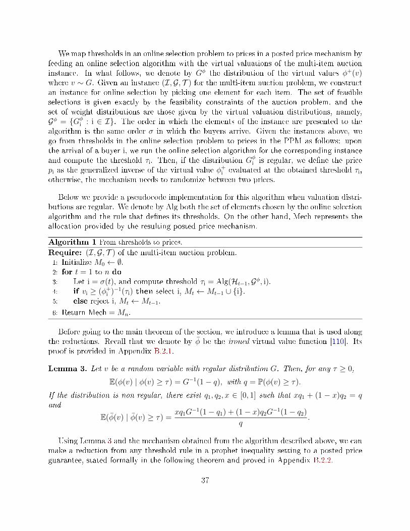
We map thresholds in an online selection problem to prices in a posted price mechanism byfeeding an online selection algorithm with the virtual valuations of the multi-item auctioninstance. In what follows, we denote by Gφ the distribution of the virtual values φ+(v)where v ∼ G. Given an instance (I,G, T ) for the multi-item auction problem, we constructan instance for online selection by picking one element for each item. The set of feasibleselections is given exactly by the feasibility constraints of the auction problem, and theset of weight distributions are those given by the virtual valuation distributions, namely,Gφ = Gφ

i : i ∈ I. The order in which the elements of the instance are presented to thealgorithm is the same order σ in which the buyers arrive. Given the instances above, wego from thresholds in the online selection problem to prices in the PPM as follows: uponthe arrival of a buyer i, we run the online selection algorithm for the corresponding instanceand compute the threshold τi. Then, if the distribution Gφ

i is regular, we dene the pricepi as the generalized inverse of the virtual value φ+

i evaluated at the obtained threshold τi,otherwise, the mechanism needs to randomize between two prices.

Below we provide a pseudocode implementation for this algorithm when valuation distri-butions are regular. We denote by Alg both the set of elements chosen by the online selectionalgorithm and the rule that denes its thresholds. On the other hand, Mech represents theallocation provided by the resulting posted price mechanism.

Algorithm 1 From thresholds to prices.

Require: (I,G, T ) of the multi-item auction problem.1: Initialize M0 ← ∅.2: for t = 1 to n do3: Let i = σ(t), and compute threshold τi = Alg(Ht−1,Gφ, i).4: if vi ≥ (φ+

i )−1(τi) then select i, Mt ←Mt−1 ∪ i.5: else reject i, Mt ←Mt−1.6: Return Mech = Mn.

Before going to the main theorem of the section, we introduce a lemma that is used alongthe reductions. Recall that we denote by φ be the ironed virtual value function [110]. Itsproof is provided in Appendix B.2.1.

Lemma 3. Let v be a random variable with regular distribution G. Then, for any τ ≥ 0,

E(φ(v) | φ(v) ≥ τ) = G−1(1− q), with q = P(φ(v) ≥ τ).

If the distribution is non-regular, there exist q1, q2, x ∈ [0, 1] such that xq1 + (1 − x)q2 = qand

E(φ(v) | φ(v) ≥ τ) =xq1G

−1(1− q1) + (1− x)q2G−1(1− q2)

q.

Using Lemma 3 and the mechanism obtained from the algorithm described above, we canmake a reduction from any threshold rule in a prophet inequality setting to a posted priceguarantee, stated formally in the following theorem and proved in Appendix B.2.2.

37

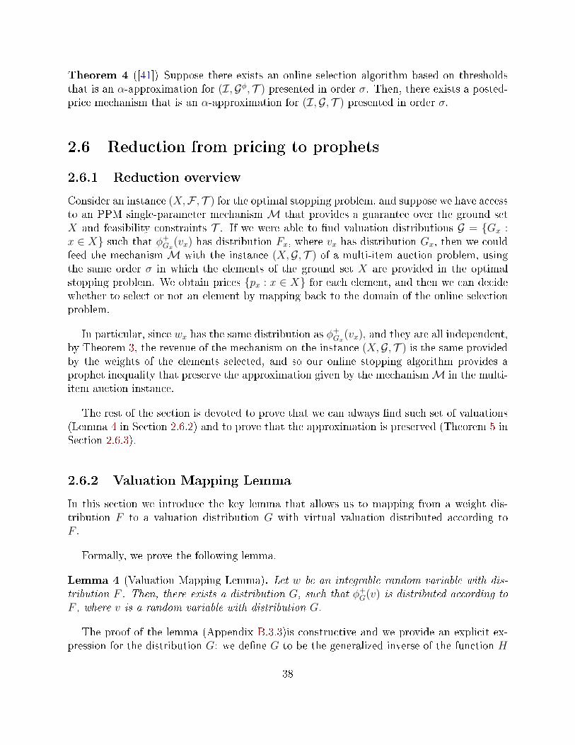
Theorem 4 ([41]) Suppose there exists an online selection algorithm based on thresholdsthat is an α-approximation for (I,Gφ, T ) presented in order σ. Then, there exists a posted-price mechanism that is an α-approximation for (I,G, T ) presented in order σ.

2.6 Reduction from pricing to prophets

2.6.1 Reduction overview

Consider an instance (X,F , T ) for the optimal stopping problem, and suppose we have accessto an PPM single-parameter mechanism M that provides a guarantee over the ground setX and feasibility constraints T . If we were able to nd valuation distributions G = Gx :x ∈ X such that φ+

Gx(vx) has distribution Fx, where vx has distribution Gx, then we could

feed the mechanismM with the instance (X,G, T ) of a multi-item auction problem, usingthe same order σ in which the elements of the ground set X are provided in the optimalstopping problem. We obtain prices px : x ∈ X for each element, and then we can decidewhether to select or not an element by mapping back to the domain of the online selectionproblem.

In particular, since wx has the same distribution as φ+Gx

(vx), and they are all independent,by Theorem 3, the revenue of the mechanism on the instance (X,G, T ) is the same providedby the weights of the elements selected, and so our online stopping algorithm provides aprophet inequality that preserve the approximation given by the mechanismM in the multi-item auction instance.

The rest of the section is devoted to prove that we can always nd such set of valuations(Lemma 4 in Section 2.6.2) and to prove that the approximation is preserved (Theorem 5 inSection 2.6.3).

2.6.2 Valuation Mapping Lemma

In this section we introduce the key lemma that allows us to mapping from a weight dis-tribution F to a valuation distribution G with virtual valuation distributed according toF .

Formally, we prove the following lemma.

Lemma 4 (Valuation Mapping Lemma). Let w be an integrable random variable with dis-tribution F . Then, there exists a distribution G, such that φ+

G(v) is distributed according toF , where v is a random variable with distribution G.

The proof of the lemma (Appendix B.3.3)is constructive and we provide an explicit ex-pression for the distribution G: we dene G to be the generalized inverse of the function H

38

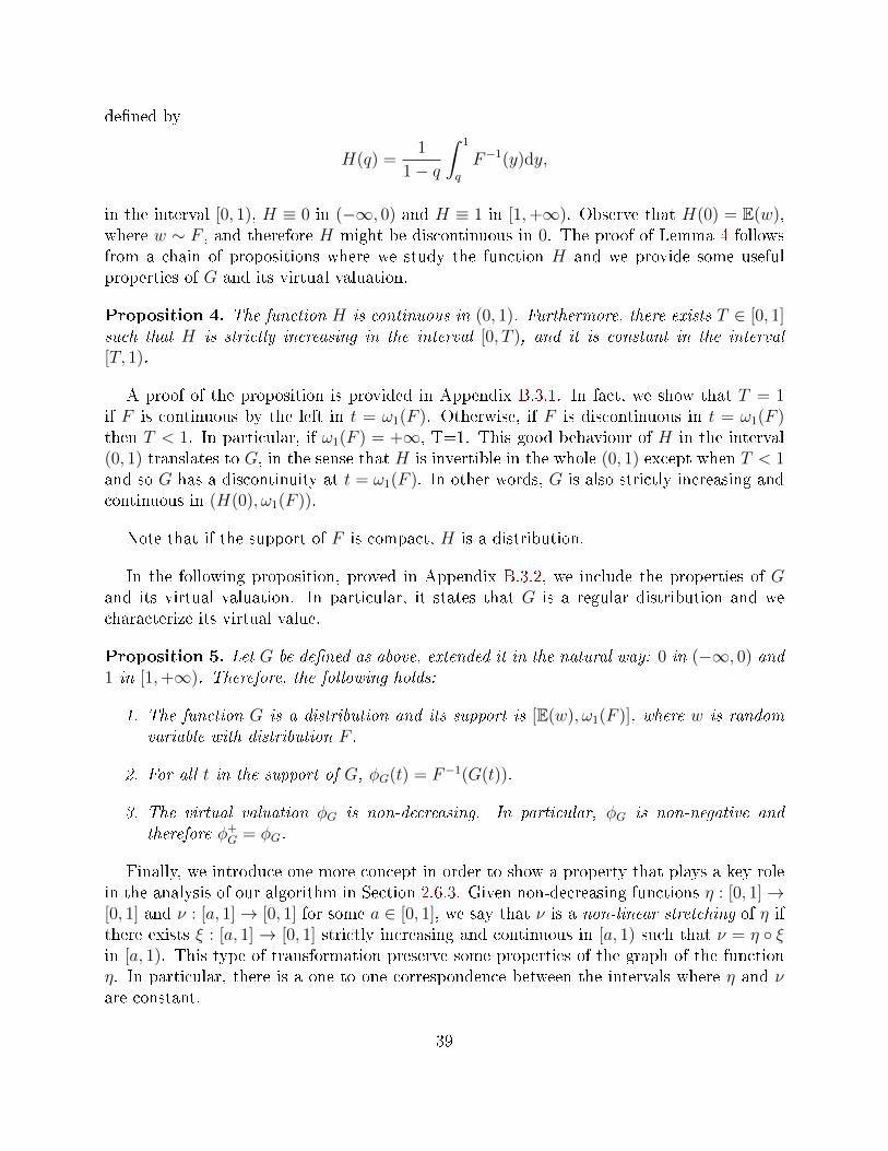
dened by

H(q) =1

1− q

∫ 1

q

F−1(y)dy,

in the interval [0, 1), H ≡ 0 in (−∞, 0) and H ≡ 1 in [1,+∞). Observe that H(0) = E(w),where w ∼ F , and therefore H might be discontinuous in 0. The proof of Lemma 4 followsfrom a chain of propositions where we study the function H and we provide some usefulproperties of G and its virtual valuation.

Proposition 4. The function H is continuous in (0, 1). Furthermore, there exists T ∈ [0, 1]such that H is strictly increasing in the interval [0, T ), and it is constant in the interval[T, 1).

A proof of the proposition is provided in Appendix B.3.1. In fact, we show that T = 1if F is continuous by the left in t = ω1(F ). Otherwise, if F is discontinuous in t = ω1(F )then T < 1. In particular, if ω1(F ) = +∞, T=1. This good behaviour of H in the interval(0, 1) translates to G, in the sense that H is invertible in the whole (0, 1) except when T < 1and so G has a discontinuity at t = ω1(F ). In other words, G is also strictly increasing andcontinuous in (H(0), ω1(F )).

Note that if the support of F is compact, H is a distribution.

In the following proposition, proved in Appendix B.3.2, we include the properties of Gand its virtual valuation. In particular, it states that G is a regular distribution and wecharacterize its virtual value.

Proposition 5. Let G be dened as above, extended it in the natural way: 0 in (−∞, 0) and1 in [1,+∞). Therefore, the following holds:

1. The function G is a distribution and its support is [E(w), ω1(F )], where w is randomvariable with distribution F .

2. For all t in the support of G, φG(t) = F−1(G(t)).

3. The virtual valuation φG is non-decreasing. In particular, φG is non-negative andtherefore φ+

G = φG.

Finally, we introduce one more concept in order to show a property that plays a key rolein the analysis of our algorithm in Section 2.6.3. Given non-decreasing functions η : [0, 1]→[0, 1] and ν : [a, 1]→ [0, 1] for some a ∈ [0, 1], we say that ν is a non-linear stretching of η ifthere exists ξ : [a, 1] → [0, 1] strictly increasing and continuous in [a, 1) such that ν = η ξin [a, 1). This type of transformation preserve some properties of the graph of the functionη. In particular, there is a one to one correspondence between the intervals where η and νare constant.

39

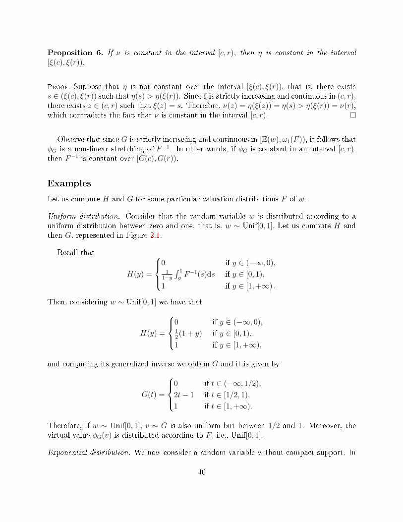
Proposition 6. If ν is constant in the interval [c, r), then η is constant in the interval[ξ(c), ξ(r)).

Proof. Suppose that η is not constant over the interval [ξ(c), ξ(r)), that is, there existss ∈ (ξ(c), ξ(r)) such that η(s) > η(ξ(r)). Since ξ is strictly increasing and continuous in (c, r),there exists z ∈ (c, r) such that ξ(z) = s. Therefore, ν(z) = η(ξ(z)) = η(s) > η(ξ(r)) = ν(r),which contradicts the fact that ν is constant in the interval [c, r).

Observe that since G is strictly increasing and continuous in [E(w), ω1(F )), it follows thatφG is a non-linear stretching of F−1. In other words, if φG is constant in an interval [c, r),then F−1 is constant over [G(c), G(r)).

Examples

Let us compute H and G for some particular valuation distributions F of w.

Uniform distribution. Consider that the random variable w is distributed according to auniform distribution between zero and one, that is, w ∼ Unif[0, 1]. Let us compute H andthen G, represented in Figure 2.1.

Recall that

H(y) =

0 if y ∈ (−∞, 0),

11−y

∫ 1

yF−1(s)ds if y ∈ [0, 1),

1 if y ∈ [1,+∞) .

Then, considering w ∼ Unif[0, 1] we have that

H(y) =

0 if y ∈ (−∞, 0),12(1 + y) if y ∈ [0, 1),

1 if y ∈ [1,+∞),

and computing its generalized inverse we obtain G and it is given by

G(t) =

0 if t ∈ (−∞, 1/2),

2t− 1 if t ∈ [1/2, 1),

1 if t ∈ [1,+∞).

Therefore, if w ∼ Unif[0, 1], v ∼ G is also uniform but between 1/2 and 1. Moreover, thevirtual value φG(v) is distributed according to F , i.e., Unif[0, 1].

Exponential distribution. We now consider a random variable without compact support. In

40

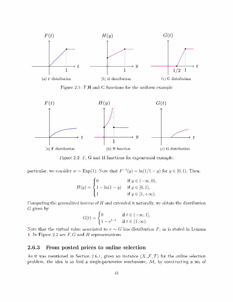
t

F (t)

1

(a) F distribution

y

H(y)

1

(b) H distribution

t

G(t)

11/2

(c) G distribution

Figure 2.1: F,H and G functions for the uniform example

t

F (t)

(a) F distribution

y

H(y)

1

(b) H function

t

G(t)

(c) G distribution

Figure 2.2: F, G and H functions for exponential example.

particular, we consider w ∼ Exp(1). Note that F−1(y) = ln(1/1− y) for y ∈ [0, 1). Then,

H(y) =

0 if y ∈ (−∞, 0),

1− ln(1− y) if y ∈ [0, 1),

1 if y ∈ [1,+∞).

Computing the generalized inverse of H and extended it naturally, we obtain the distributionG given by

G(t) =

0 if t ∈ (−∞, 1],

1− e1−t if t ∈ (1,∞).

Note that the virtual value associated to v ∼ G has distribution F , as is stated in Lemma4. In Figure 2.2 are F,G and H representations.

2.6.3 From posted prices to online selection

As it was mentioned in Section 2.6.1, given an instance (X,F , T ) for the online selectionproblem, the idea is to feed a single-parameter mechanism, M, by constructing a set of

41

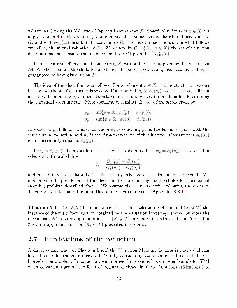
valuations G using the Valuation Mapping Lemma over F . Specically, for each x ∈ X, weapply Lemma 4 to Fx, obtaining a random variable (valuation) vx distributed according toGx and with φGx(vx) distributed according to Fx. To not overload notation, in what followswe call φx the virtual valuation of Gx. We denote by G = Gx : x ∈ X the set of valuationdistributions and consider the instance for the PPM given by (X,G, T ).

Upon the arrival of an element (buyer) x ∈ X, we obtain a price px given by the mechanismM. We then dene a threshold for an element to be selected, taking into account that φx isguaranteed to have distribution Fx.

The idea of the algorithm is as follows. For an element x ∈ X, if φx is strictly increasingin neighbourhood of px, then x is selected if and only if wx ≥ φx(px). Otherwise, φx is at inan interval containing px and this translates into a randomized tie-breaking for determiningthe threshold stopping rule. More specically, consider the boundary prices given by

p−x = infp ∈ R : φx(p) = φx(px),p+x = supp ∈ R : φx(p) = φx(px).

In words, if px falls in an interval where φx is constant, p−x is the left-most price with thesame virtual valuation, and p+

x is the right-most value of that interval. Observe that φx(p+x )

is not necessarily equal to φx(px).

If wx > φx(px), the algorithm selects x with probability 1. If wx = φx(px), the algorithmselects x with probability

θx =Gx(p

+x )−Gx(px)

Gx(p+x )−Gx(p−x )

,

and rejects it with probability 1 − θx. In any other case the element x is rejected. Wenow provide the pseudocode of the algorithm for constructing the thresholds for the optimalstopping problem described above. We assume the elements arrive following the order σ.Then, we state formally the main theorem, which is proven in Appendix B.3.4.

Theorem 5 Let (X,F , T ) be an instance of the online selection problem, and (X,G, T ) theinstance of the multi-item auction obtained by the Valuation Mapping Lemma. Suppose themechanismM is an α-approximation for (X,G, T ) presented in order σ. Then, Algorithm2 is an α-approximation for (X,F , T ) presented in order σ.

2.7 Implications of the reduction

A direct consequence of Theorem 5 and the Valuation Mapping Lemma is that we obtainlower bounds for the guarantees of PPM's by considering lower bound instances of the on-line selection problem. In particular, we improve the previous known lower bounds for SPMwhen constraints are on the form of downward closed families, from log n/(3 log log n) to

42

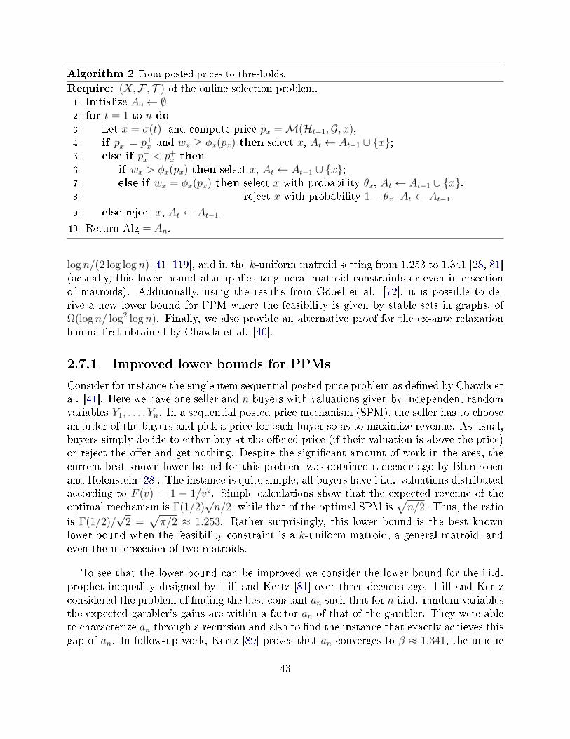
Algorithm 2 From posted prices to thresholds.

Require: (X,F , T ) of the online selection problem.1: Initialize A0 ← ∅.2: for t = 1 to n do3: Let x = σ(t), and compute price px =M(Ht−1,G, x),4: if p−x = p+

x and wx ≥ φx(px) then select x, At ← At−1 ∪ x;5: else if p−x < p+

x then

6: if wx > φx(px) then select x, At ← At−1 ∪ x;7: else if wx = φx(px) then select x with probability θx, At ← At−1 ∪ x;8: reject x with probability 1− θx, At ← At−1.9: else reject x, At ← At−1.10: Return Alg = An.

log n/(2 log log n) [41, 119], and in the k-uniform matroid setting from 1.253 to 1.341 [28, 81](actually, this lower bound also applies to general matroid constraints or even intersectionof matroids). Additionally, using the results from Göbel et al. [72], it is possible to de-rive a new lower bound for PPM where the feasibility is given by stable sets in graphs, ofΩ(log n/ log2 log n). Finally, we also provide an alternative proof for the ex-ante relaxationlemma rst obtained by Chawla et al. [40].

2.7.1 Improved lower bounds for PPMs

Consider for instance the single item sequential posted price problem as dened by Chawla etal. [41]. Here we have one seller and n buyers with valuations given by independent randomvariables Y1, . . . , Yn. In a sequential posted price mechanism (SPM), the seller has to choosean order of the buyers and pick a price for each buyer so as to maximize revenue. As usual,buyers simply decide to either buy at the oered price (if their valuation is above the price)or reject the oer and get nothing. Despite the signicant amount of work in the area, thecurrent best known lower bound for this problem was obtained a decade ago by Blumrosenand Holenstein [28]. The instance is quite simple; all buyers have i.i.d. valuations distributedaccording to F (v) = 1 − 1/v2. Simple calculations show that the expected revenue of theoptimal mechanism is Γ(1/2)

√n/2, while that of the optimal SPM is

√n/2. Thus, the ratio

is Γ(1/2)/√

2 =√π/2 ≈ 1.253. Rather surprisingly, this lower bound is the best known

lower bound when the feasibility constraint is a k-uniform matroid, a general matroid, andeven the intersection of two matroids.

To see that the lower bound can be improved we consider the lower bound for the i.i.d.prophet inequality designed by Hill and Kertz [81] over three decades ago. Hill and Kertzconsidered the problem of nding the best constant an such that for n i.i.d. random variablesthe expected gambler's gains are within a factor an of that of the gambler. They were ableto characterize an through a recursion and also to nd the instance that exactly achieves thisgap of an. In follow-up work, Kertz [89] proves that an converges to β ≈ 1.341, the unique

43

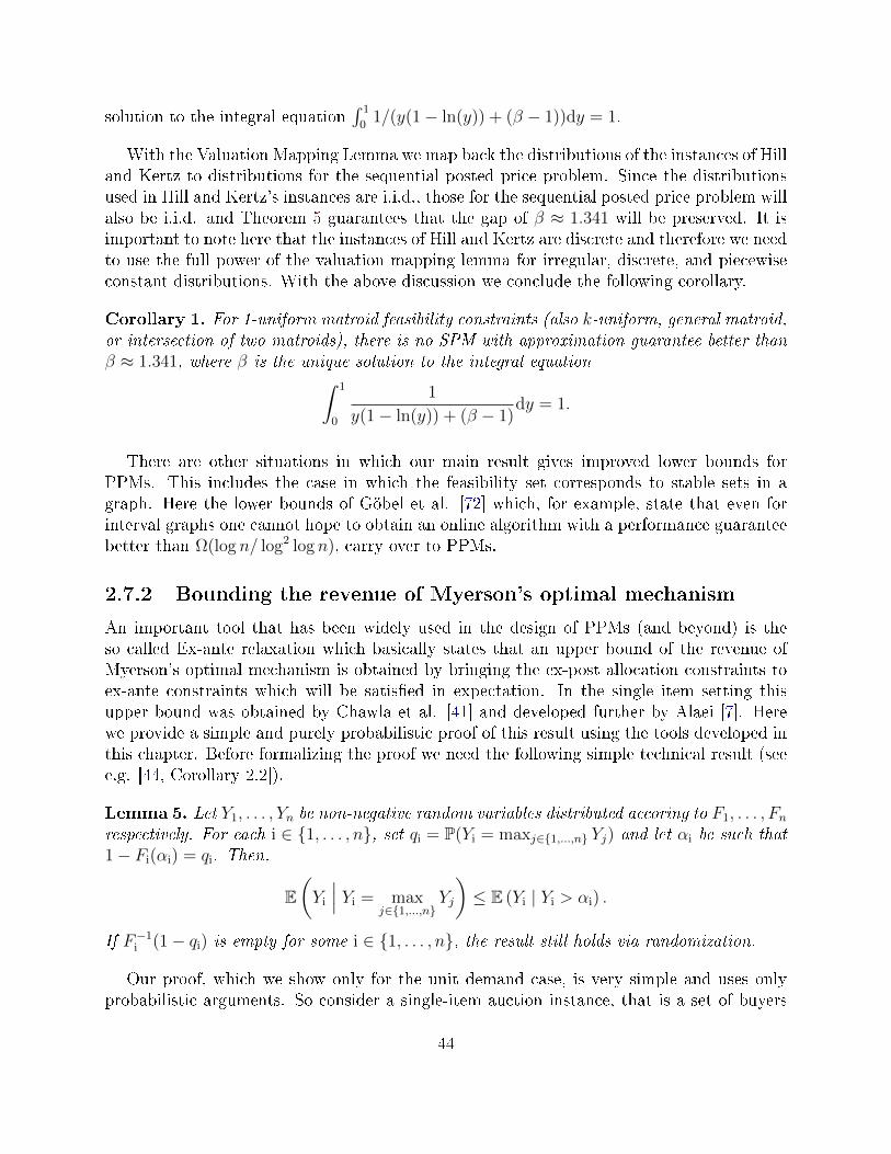
solution to the integral equation∫ 1

01/(y(1− ln(y)) + (β − 1))dy = 1.

With the Valuation Mapping Lemma we map back the distributions of the instances of Hilland Kertz to distributions for the sequential posted price problem. Since the distributionsused in Hill and Kertz's instances are i.i.d., those for the sequential posted price problem willalso be i.i.d. and Theorem 5 guarantees that the gap of β ≈ 1.341 will be preserved. It isimportant to note here that the instances of Hill and Kertz are discrete and therefore we needto use the full power of the valuation mapping lemma for irregular, discrete, and piecewiseconstant distributions. With the above discussion we conclude the following corollary.

Corollary 1. For 1-uniform matroid feasibility constraints (also k-uniform, general matroid,or intersection of two matroids), there is no SPM with approximation guarantee better thanβ ≈ 1.341, where β is the unique solution to the integral equation∫ 1

0

1

y(1− ln(y)) + (β − 1)dy = 1.

There are other situations in which our main result gives improved lower bounds forPPMs. This includes the case in which the feasibility set corresponds to stable sets in agraph. Here the lower bounds of Göbel et al. [72] which, for example, state that even forinterval graphs one cannot hope to obtain an online algorithm with a performance guaranteebetter than Ω(log n/ log2 log n), carry over to PPMs.

2.7.2 Bounding the revenue of Myerson's optimal mechanism

An important tool that has been widely used in the design of PPMs (and beyond) is theso called Ex-ante relaxation which basically states that an upper bound of the revenue ofMyerson's optimal mechanism is obtained by bringing the ex-post allocation constraints toex-ante constraints which will be satised in expectation. In the single item setting thisupper bound was obtained by Chawla et al. [41] and developed further by Alaei [7]. Herewe provide a simple and purely probabilistic proof of this result using the tools developed inthis chapter. Before formalizing the proof we need the following simple technical result (seee.g. [44, Corollary 2.2]).

Lemma 5. Let Y1, . . . , Yn be non-negative random variables distributed accoring to F1, . . . , Fnrespectively. For each i ∈ 1, . . . , n, set qi = P(Yi = maxj∈1,...,n Yj) and let αi be such that1− Fi(αi) = qi. Then,

E(Yi

∣∣∣ Yi = maxj∈1,...,n

Yj

)≤ E (Yi | Yi > αi) .

If F−1i (1− qi) is empty for some i ∈ 1, . . . , n, the result still holds via randomization.

Our proof, which we show only for the unit demand case, is very simple and uses onlyprobabilistic arguments. So consider a single-item auction instance, that is a set of buyers

44

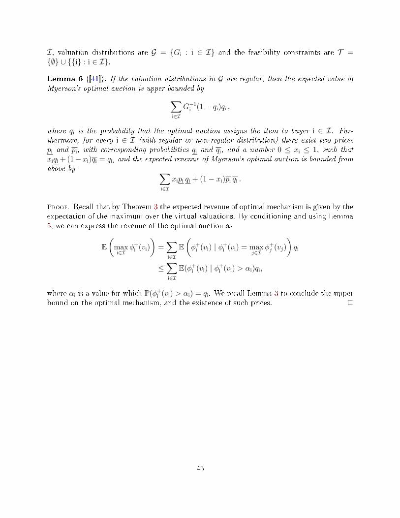
I, valuation distributions are G = Gi : i ∈ I and the feasibility constraints are T =∅ ∪ i : i ∈ I.

Lemma 6 ([41]). If the valuation distributions in G are regular, then the expected value ofMyerson's optimal auction is upper bounded by∑

i∈I

G−1i (1− qi)qi ,

where qi is the probability that the optimal auction assigns the item to buyer i ∈ I. Fur-thermore, for every i ∈ I (with regular or non-regular distribution) there exist two pricespi and pi, with corresponding probabilities qi and qi, and a number 0 ≤ xi ≤ 1, such thatxiqi + (1−xi)qi = qi, and the expected revenue of Myerson's optimal auction is bounded fromabove by ∑

i∈I

xipi qi + (1− xi)pi qi .

Proof. Recall that by Theorem 3 the expected revenue of optimal mechanism is given by theexpectation of the maximum over the virtual valuations. By conditioning and using Lemma5, we can express the revenue of the optimal auction as

E(

maxi∈I

φ+i (vi)

)=∑i∈I

E(φ+

i (vi) | φ+i (vi) = max

j∈Iφ+j (vj)

)qi

≤∑i∈I

E(φ+i (vi) | φ+

i (vi) > αi)qi,

where αi is a value for which P(φ+i (vi) > αi) = qi. We recall Lemma 3 to conclude the upper

bound on the optimal mechanism, and the existence of such prices.

45

Chapter 3

Dynamic optimization problems: a

unifying approach1

3.1 Introduction

Dynamic optimization problems with resources constraints arise across a variety of disparateapplications. For example, retailers engage in dynamic pricing with inventory constraints,airlines and hotels engage in dynamic capacity allocation problems with limited seat or roomcapacity, advertisers engage in real-time bidding campaigns with limited budget. Due to theimportance and centrality of these problems, various classes of dynamic optimization prob-lems have received signicant attention in industry but also across academic communities inOperations Research, Computer Science, and Economics. A signicant focus of the literaturehas been on the development of ecient algorithms to optimize performance.

While the literature on these problems is rich and extensive (we discuss the literaturein detail as we present our main results and associated corollaries), studies have focused onspecic applications, or classes of applications. As such, arguments are specialized for specicsettings and do not directly apply to other settings, typically requiring to re-develop, fromscratch, proofs when faced with a new type of dynamic optimization problems with resourceconstraints. While, from a practical perspective, problems such as those mentioned abovecan appear very dierent, these problems do admit some common mathematical structure.In the present work, we elucidate such common structure and derive important theoreticalimplications of such commonalities.

1This chapter of the thesis is based on a working paper with Omar Besbes and Santiago Balseiro [19].

46

3.2 Contributions

We summarize contributions of Chapter 3 below.

Firstly, we introduce and dene a general class of problems: dynamic resource constrainedreward collection (DRCRC) problems. This class admits as special cases a variety of prob-lems studied completely separately in the literature. Broadly speaking, a DRCRC problemis dened as follows. A decision-maker is endowed with some resources at time 0 and faces anite (discrete) time horizon. At each period, the decision-maker is presented with a stochas-tic opportunity (independent of other periods), and must select an action; the action leadsto some stochastic resource consumption and reward collection. The goal of the decision-maker is to select a sequence of actions to maximize her total expected rewards subject tothe resource constraints. We assume that the decision-maker knows the distribution of thevarious stochastic components, and, as such, this problem can be formulated as a discreteand nite time dynamic program, with the state given by the vector of resources available.

Notably, the DRCRC class of problems generalizes and brings under the same umbrella ahost of classical problems studied separately. In particular, we show how the proposed classof DRCRC problems encompass the following classical problems: Network dynamic pricingproblems (see, e.g., [66]) Dynamic bidding in repeated auctions with budgets, (see, e.g., [20]),Network revenue management problems (see, e.g., [129]), Choice-based revenue managementproblems (see, e.g., [128]), Stochastic Depletion problems (see, e.g., [39]), Order fulllmentproblems (see, e.g., [3]), and Online matching problems (see, e.g., [5]).

Secondly, we provide a unied analysis of a uid" certainty-equivalent control. Althoughfrom a theoretical perspective, DRCRC problems can be formulated through a dynamicprogram, one natural question is whether the DRCRC formulation lends itself to analysis(beyond a generic analysis of a general dynamic program) that can applied to all specialcases, or whether problems should be specialized rst to be able to derive properties ofinterest. We indeed show that the general DRCRC formulation can lead to unied analysis,through the study of a central heuristic in the stochastic dynamic optimization literature.

Thus, our second layer of contribution is the analysis domain. In particular, we character-ize the performance of a classical uid" certainty-equivalent control for the general DRCRCclass of problems.

In more detail, solving even a special case of a DRCRC problem to optimality is typicallyimpossible due to the curse of dimensionality; indeed the state space is driven by the numberof resources. This has brought forward the need for heuristics for such problems, and manysuch heuristics have been developed for subsets of the problems above. A notable heuris-tic for dynamic optimization problems is the so-called certainty-equivalent heuristic, whichinvolves solving a deterministic problem in each period by using proxies for random quanti-ties, implementing the prescribed decisions for that period, and repeating the process overtime. Such certainty-equivalent heuristics have been shown to be near-optimal under some

47

conditions in various special cases of DRCRC problems. A notable example of a certainty-equivalent heuristic is the so-called uid" one, in which the random quantities are replacedby their expectations. We will refer to this heuristic as CE. Such policies are sometimesalso referred to as re-solving" or model predictive control" in the various related streamsof literature. To analyze the performance of the heuristic, we measure the gap between theoptimal performance and that of the CE heuristic, and characterize the dependence of thisgap on the scale of the system.

More specically, we establish two types of sucient conditions for the CE heuristic tolead to a small" performance gap. The rst set of sucient conditions are stated in termsof local smoothness of the initial deterministic proxy problem as a function of the resourcevector. The second, alternative, set of sucient conditions are expressed in terms of thedual Lagrangian function. In particular, the analysis leads to a dichotomy between twofundamental cases: that when the set of actions is a continuum, and that when it is nite.For the former, the CE heuristic guarantees O(log T ) performance gap (where T is the lengthof the horizon), whereas for the latter, it guarantees O(1) gap.

In essence, the analysis establishes that the classes of DRCRC problems, under saidsucient conditions is easy" in that the CE heuristic is extremely eective. Intuitively,the CE heuristic enables the decision-maker to implement good decisions through the proxyproblem while controlling very closely the path of the resource constraints.

Thirdly, after developing our theoretical results and the dichotomy between nite andcontinuum of actions, we establish the mapping from a series of classical problems to aDRCRC problem and state the corollaries that one obtains from the general analysis of theCE heuristic. This allows to recover versions of various existing results but also to obtain suchresults under weaker conditions (see, e.g., the case of dynamic pricing in Section 3.8.1), or toobtain new results in the literature for the performance of the uid CE heuristic (see, e.g.,the case of dynamic bidding with budgets in Section 3.9.2 or the case of dynamic assortmentoptimization in Section 3.8.2). We discuss the related literature in detail when we discussthe various specialized problems.

Overall, this paper introduces a novel general formulation of dynamic optimization prob-lems. We illustrated how this formulation lends itself to analysis through a unied analysis ofthe CE heuristic. As such, the DRCRC class oers a useful and powerful intermediate classof problems between the specialized versions previously studied in the literature and a fullygeneral dynamic program, and this work opens up the possibility of further generalizationsof arguments developed for special cases of DRCRC problems.

3.3 Related literature

We left the description of the related literature to Section 3.8 and Section 3.9, where weestablish the mapping from a series of classical problems to a DRCRC problem.

48

Organization

In Section 3.4 we describe the model for the class of DRCRC problems. In Section 3.5we present the certainty equivalent heuristic (CE) we analyze along the work, whereas inSection 3.6 we study its performance for the general class of DRCRC problems, providing anexplicit bound for the reward loss, formally stated in Theorem 6. In Section 3.7 we presentsucient conditions for the guarantee of CE, depending on whether the set of actions isnite or not. Finally, in Sections 3.8 and 3.9 we review a set of special cases of the proposedDRCRC class of problems. For each class, we rst establish when and how it falls under aspecial case of a DRCRC problem. In turn, we establish implications of Theorem 6. As wewill see, the result allows to recover some existing results in the literature as special cases,but also have as a direct corollary new results for classes of problems studied in the literature.

3.4 Model

We consider a dynamic decision-making problem with a nite time horizon T , over whicha decision-maker collects rewards subject to resource constraints. We refer to this problemas the Dynamic Resource Constrained Reward Collection (DRCRC) problem. There are Lresources and the decision-maker is initially endowed with initial capacities C ∈ RL

+ for theresources.

In each period t, an opportunity arises and each opportunity is characterized by a classθ ∈ Θ, where Θ is a nite set of types.2 Classes are drawn independently from a distributionp ∈ ∆(Θ). Upon observing an opportunity, the decision-maker takes an action a ∈ A, whereA is the set of feasible actions. Upon taking an action a, the decision-maker collects a rewardthat depends on the opportunity class θ, the action a, and an idiosyncratic shock ε. Shockslie in a space E and are drawn independently from a distribution f ∈ ∆(Θ).3 Shocks arerevealed to the decision-maker after an action is taken and are meant to capture exogenousfactors that are idiosyncratic to the opportunity. We denote by r : Θ × A × E → R, thereward function, where r(θ, a, ε) denotes the reward when class is θ, the action is a, and theshock is ε. Taking an action consumes resources and we assume that the amount of resourcesconsumed depends on the opportunity class θ and the value of the shock ε. We denote byy : Θ×A×E → RL, the vector-valued resource consumption function. In particular yl(θ, a, ε)represents the consumption of resource l if class θ arrived, the decision maker chose an actiona, and the shock was ε.

To ensure that the problem is feasible, we assume there is a null action a0 in A thatconsumes no resources and generates no reward. That is, for every opportunity class θ and

2Here, we assume niteness of the set of classes for expository purposes. Our results readily extend tomore general spaces.

3In the general model, to simplify notation, we make the probability distribution of ε independent of theaction and the class but any dependencies may be modeled by modifying reward and consumption functions,and in some applications, it might be convenient to consider some dependence.

49

idiosyncratic shock ε, we have r(θ, a0, ε) = 0 and yl(θ, a0, ε) = 0 for every resource l.

We denote the history up to time t − 1 as Ht−1 = θs, as, εst−1s=1. We let Π denote the

set of all non-anticipating policies, i.e., the set of policies such that the action at time t,at, depends on the observed class of the opportunity in time t and the history up to (andincluding) time t − 1. That is, for a policy π, at = aπt (θt,Ht−1)4. The decision maker'sobjective is to choose a policy π ∈ Π that maximizes her expected rewards earned during thehorizon. Taking into account that the consumption's constraints must hold almost surely,the stochastic optimization formulation of the decision-maker may be written as follows.

J∗(C, T ) = supπ∈Π

E

(T∑t=1

r(θt, aπt , εt)

)

s.tT∑t=1

yl(θt, aπt , εt) ≤ Cl, ∀l ∈ [L] (a.s.) ,

(3.1)

where [L] denotes the set 1, . . . , L.

Note that in general, this is a dynamic program with potentially a high number of dimen-sions and the curse of dimensionality precludes solving this problem to optimality. Giventhis, various heutistics can considered and their performance can be assessed through theresulting optimality gap

J∗(C, T )− Jπ(C, T ),

where Jπ(C, T ) represents the expected reward obtained by the decision-maker if policy πis implemented. We refer to the expression above as the reward loss of the heuristic givenby π.

3.5 Certainty Equivalent Heuristic

As it was mentioned in Section 1.4, the optimal solution of the stochastic formulation of theDRCRC is not easy to compute. A common and central heuristic in the theory of dynamicdecision-making under uncertainty is based on the certainty equivalent principle: replacequantities by their expected values and take the best actions given the current history.Specically, at each point of time t, we solve an optimization problem obtained by using thehistory up to t−1 and replacing the random quantities in problem (3.1) by their expectations.

That is, if we denote by Φ the set of all class-dependent probability distributions φ :Θ → ∆(A), and by ρ ∈ RL

+ a non-negative parameter representing the vector of availableinventory divided by the number of remaining periods, at time t we solve the following

4To simplify notation we will write aπt to refer to the action taken at time t given the policy π

50

parametric programming problem for ρ = ρt, which we refer to as the deterministic problem:

J(ρ) = maxφ∈Φ

∑θ∈Θ

pθ

∫A

Eε (r(θ, a, ε)) dφθ(a)

s.t∑θ∈Θ

pθ

∫A

Eε (yl(θ, a, ε)) dφθ(a) ≤ ρl, ∀l ∈ [L].

(3.2)

Because the distributions of classes and shocks are independent and identically distributed(i.i.d.) and we allow for randomized actions, we can restrict attention without loss to static,randomized controls in the deterministic problem. Fixing the parameter ρ, for each classθ ∈ Θ and a set of actions A ∈ A, the decision variable φθ(A) gives the probability ofchoosing an action a ∈ A given that the arrival belongs to class θ.

In what follows, we assume that problem (3.2) admits an optimal solution. We denoteby φ∗ρ an optimal solution when the parameter is ρ. We will provide sucient conditions forexistence of an optimal solution in Section 3.7.5

The Certainty Equivalence Principle leads to a natural heuristic for the decision-maker: ateach point in time t, choose actions according to a solution φ∗ρt to (3.2) with ρt = ct/(T−t+1)and ct the capacity remaining at beginning of time t. We call this heuristic the CertaintyEquivalent Heuristic (CE) and denote the corresponding policy by πCE. The heuristic isformally presented in Algorithm 3.

The certainty equivalence heuristic has been extensively studied in the literature for spe-cic applications. Our aim is to characterize its performance for the broader class of DRCRCproblems. Thus, as the family of DRCRC problems encompasses a large number of applica-tions that have been studied in the literature separately, by analyzing the performance of theCE heuristic, we shall recover some already known results and, in the process, obtain newresults for other applications, while highlighting very general sucient conditions to ensuregood" performance of the CE heuristic.

Remark. An alternative uid" heuristic involves solving the deterministic problem onceat the beginning of the horizon with ρ1 = C/T and then implementing the static controlρ1 until capacity runs out. This static control is more computationally tractable as it doesnot need to resolve the deterministic problem, but typically yields worse performance (see,Appendix C.1.1 for further details).

5When an optimal solution does not exist, it suces for our purpose to work with a 1/T approximatelyoptimal solution.

51

Algorithm 3 Certainty Equivalence Heuristic (CE)1: Initialize c1 ← C,2: for t = 1 to T do

3: ρt ← ct/(T − t+ 1)4: φ∗ρt ← optimal solution of Problem 3.2 with ρ = ρt.5: observe the opportunity class θt6: draw an action at with probability φ∗ρt(θt, at)7: if y(θt, at, ε) ≤ ct, ∀ε ∈ E , then8: choose the action at9: observe the shock εt10: ct+1 ← ct − y(θt, at, εt)11: else

12: choose the null action a0

13: ct+1 ← ct

3.6 Bound on the cumulative reward loss for DRCRC

problems

In this section we study the performance of the CE heuristic for the general class of DRCRCproblems. To this end, we rst introduce some denitions and conditions on the primitives.

We will assume that the reward and consumption functions are bounded. For a vectorx ∈ Rn, we denote by ‖x‖ = (

∑ni=1 xi)

1/2 its `2-norm and denoted by ‖x‖∞ = maxi |xi| its`∞-norm.

Assumption 1. The following hold:

1. There exists r∞ ∈ R++ such that |r(θ, a, ε)| ≤ r∞ for all θ ∈ Θ, a ∈ A, and ε ∈ E.

2. There exist y2, y∞ ∈ R++ such that ‖y(θ, a, ε)‖ ≤ y2 and ‖y(θ, a, ε)‖∞ ≤ y∞ for allθ ∈ Θ, a ∈ A, and ε ∈ E.

Recall that ρ1 is the vector of initial inventory divided by the amount of periods toconsider. We assume that, in the neighborhood of ρ1, the optimal objective value of thedeterministic problem J(ρ) is locally smooth as well as that the consumption constraints arebinding.

Assumption 2. There exist δ,K ∈ R++ with δ < minj∈[L](ρ1)j such that for every ρ with‖ρ− ρ1‖ < δ, then it holds that:

1. The function J(ρ) satises J(ρ) ≥ J(ρ1) +∇J(ρ1)(ρ− ρ1)− K2‖ρ− ρ1‖2.

2. The optimal solution φ∗ρ satises Eθ∼p,a∼φ∗ρ,ε∼f (y(θ, a, ε)) = ρ.

52

We will refer to inequality given in Assumption 2.1 as J(ρ) admitting aK-lower downwardquadratic (K-LDQ) envelope in N (ρ1, δ), where we denote by N (ρ1, δ) the ball of radius δcentered at ρ1

6. See Figure 3.1 (a) for an example of a function admitting a K-LDQ envelopeand its envelope. This condition is a weaker and local notion of the K-strongly smoothcondition for concave functions, which requires the inequality in Assumption 2.1 to hold forevery pair of parameters ρ, ρ′. A sucient condition for J(ρ) to admit a K-LDQ envelope isthat its gradient is locally K-Lipschitz continuous at ρ1 for all ρ ∈ N (ρ1, δ), that is,

‖∇J(ρ1)−∇J(ρ)‖ ≤ K‖ρ1 − ρ‖ .

See Lemma 3.4 in [33] for a proof of the previous fact.

We are now ready to state our performance bound of the CE heuristic under Assump-tions 1 and 2. Specically, in Theorem 6 we state that the reward loss of the heuristic givenby CE is on the order of log T , giving an explicitly expression for the bound.

Theorem 6 Let JCE be the expected performance of Algorithm 3. Then, under Assump-tions 1 and 2, the reward loss satises

J∗ − JCE ≤ 1

2y2

2K log T +

[Ψ + 14

y2∞δ2

]J(ρ1),

where Ψ = y∞ρ1−δ and ρ1 the smallest component of vector ρ1.

We note that the result above applies across all DRCRC problems, and only requiresAssumption 2. Consider a regime in which C and T are scaled proportionally, i.e., C =ρ1T for some ρ1 ∈ RL

++. Theorem 6 implies that, in such a regime, the CE heuristic isasymptotically optimal in the sense that JCE/J∗ → 1 as T →∞ because the reward collectedby the CE heuristic grows as T → ∞. Furthermore, the optimality gap is of order K log Tif K > 0 and of order 1 if K = 0. In other words, we already see appearing clear distinctionamong DRCRC problems driven by the value of K in Assumption 2.

At a more detailed level, the dependency on the number of resources L enters our boundindirectly via the constants y2, y∞, and K. Interestingly, when resource consumption isuniformly bounded, i.e., y∞ < ∞, the dependency on the number of resources is mostlydriven by y2

2. While in the worst case we could have y22 = Ω(L), in many settings of

interest, one will have y22 = O(1) and obtain bounds that are independent of the number

of resources. This could happen, for example, if every opportunity consumes only a nitesubset of resources.

The proof of the theorem can be found in Appendix C.2. The main idea of the proofof Theorem 6 is to analyze the performance of the CE heuristic up to the stopping time τ ,

6More specically, N (x, r) represents the set of all points at distance less or equal to r from x, where thedistance is the one induced by the `2−norm: N (x, r) = y ∈ Rn : ‖x− y‖ ≤ r.

53

where τ is the rst time that a resource is close to depletion or the ratio of capacity to timeremaining ρt leaves the ball N (ρ1, δ) dened in Assumption 2. Using that the deterministicproblem gives an upper bound on the optimal value of the stochastic problem, that is,J∗ ≤ TJ(C/T ) (see, e.g., [66] for specialized argument), we can bound the reward loss asfollows

J∗ − JCE ≤ TJ(ρ1)− JCE ≤ E

(τ∑t=1

J(ρ1)−τ∑t=1

r(θt, aπCE

t , εt)

)− E

(T∑

t=τ+1

J(ρ1)

), (3.3)

where aπCE

t denotes the action taken by the CE heuristic and the second inequality followsbecause r(θt, aπ

CE

t , εt) ≥ 0 since the null action a0 is feasible. The second term of the right-hand side can be written as E(T − τ)J(C/T ), which is on the order of O(1), as we establishin Lemma 16. This follows because, under the CE heuristic, the ratio ρt behaves like amartingale by Assumption 2.2 and, as result, the heuristic never runs out of resources nor ρtleaves the ball N (ρ1, δ) too early. The rst term is shown to be of order O(log T ). To see this,note that up to time τ actions are not constrained by resources and the expected rewardat period t satises E

(r(θt, a

πCE

t , εt) | ρt)

= J(ρt) because the CE heuristic takes actionsaccording to φ∗ρt . Therefore, using Assumption 2.1 we can upper bound the rst term by∇J(ρ1)E (

∑τt=1(ρ1 − ρt))+K/2E (

∑τt=1 ‖ρ1 − ρt‖2). The rst term is zero because ρt behaves

like a martingale, while the second term can be bounded using that martingale dierencesare orthogonal. Putting everything together, we then conclude that J∗−JCE = O(K log T ).

In what follows, we analyze the reward loss depending on whether the set of actions isnite or not. Specically, we provide sucient conditions on the problem primitives forAssumption 2 to be satised. These conditions shall yield closed-form expressions for thevalues of δ and K values. Though we have bounded the reward loss for those problemsincluded in DRCRC, we will show that for an important subfamily of problems, the resultis valid with K = 0 and, therefore, we recover a constant reward loss instead of order log T .

3.7 Dual problem and sucient conditions for Assump-

tion 2

Before stating sucient conditions for Assumption 2, we introduce a dual of Problem 3.2in which we dualize the consumption constraints. To this end, let µ ∈ RL

+ be the vectorof Lagrange multipliers associated with the consumption constraints of Problem 3.2. Letr : Θ × A → R+ denote the expected reward function, i.e., r(θ, a) = Eε(r(θ, a, ε)). In thesame way, for each l ∈ [L], let y : Θ × A → RL

+ denote the expected resource consumption

54

function, i.e., y(θ, a) = Eε(y(θ, a, ε)). Then, the Lagrangian function is given by

L(φ, µ) =∑θ∈Θ

pθ

∫A

r(θ, a) dφθ(a) + µ>

ρ−∑θ∈Θ

pθ

∫A

y(θ, a) dφθ(a)

=

∑θ∈Θ

pθ

∫A

(r(θ, a)− µ>y(θ, a)

)dφθ(a) + µ>ρ.

Dene, for each θ ∈ Θ, the function gθ : RL → R

gθ(µ) = supa∈A

r(θ, a)− µ>y(θ, a)

. (3.4)

The Lagrange dual function, for xed ρ ≥ 0, is given by

Ψρ(µ) = supφa∈∆(A)

L(φ, µ) = µ>ρ+∑θ∈Θ

pθ supa∈A

r(θ, a)− µ>y(θ, a)

= µ>ρ+

∑θ∈Θ

pθgθ(µ) ,

where the second equality follows from optimizing point-wise over actions. The dual problemof Problem 3.2 is then given by

infµ∈RL+

Ψρ(µ) . (3.5)

In what follows, we will assume that the dual solution for ρ = ρ1, namely µ1, is interior;that is, µ1 > 0. We introduce this assumption to guarantee that all resource constraints arebinding for ρ = ρ1, but we believe our results still hold without this assumption.

3.7.1 Continuum of actions

We rst assume that the set of A is a continuum. In this case we will give a closed-formexpression for values K > 0 and δ for which Assumption 2 holds and we obtain, undercertain conditions that we explain below, a reward loss of the order of O(K log T ).

We now present a condition under gθ that is sucient to ensure that the deterministicproblem has zero duality gap for every positive parameter ρ. Furthermore, we prove that theproblem admits an optimal, deterministic solution. The latter implies that when the set ofactions is a continuum, under assumption SC 1, randomization in the deterministic problemis not needed.

SC 1. For each θ ∈ Θ, gθ(µ) is dierentiable in µ, and for every µ ≥ 0, gθ(µ) is achievedfor an action a ∈ A.

Proposition 7. Under Assumptions 1 and SC 1, strong duality holds, i.e., J(ρ) = infµ∈RL+ Ψρ(µ)

for all ρ > 0. Furthermore, J(ρ) admits a deterministic optimal solution for all ρ.

55

A proof is provided in Appendix C.3.1. In addition to condition SC 1, we need to makeanother regularity assumption over the function gθ, stated below, to ensure Assumption 2holds for this particular cases of DRCRC.

SC 2. There exists positive real numbers κ and ν ≤ µ with µ = minl∈[L] µ1l such that for all

θ ∈ Θ and µ ∈ N (µ1, ν), gθ(µ) satises

gθ(µ) ≥ gθ(µ1) +∇gθ(µ1)>(µ− µ1) +

κ

2‖µ− µ1‖2 . (3.6)

In what follows we will refer to property (3.6) as gθ admitting a κ-lower upward quadratic(κ-LUQ) envelope in N (µ1, ν). See Figure 3.1 (b) for an example of a function admittinga κ-LUQ and its envelope. Note that admitting a κ-LUQ envelope is a weaker and localnotion of the κ-strongly convex condition, which requires (3.6) to hold for every pair of dualvariables µ, µ′.

Lemma 7. Suppose that Assumptions SC 1 and SC 2 hold. If µ1 > 0, Assumption 2 holdswith K = 1/κ and δ = (νκ)/2.

A proof is provided in Appendix C.3.2. We obtain the following result as a corollary.

Corollary 2. Suppose that Assumptions 1, SC 1, and SC 2 hold and that µ1 > 0. Then thereward loss of the certainty equivalent heuristic is of order O(κ−1 log T ) for DRCRC problemswith a continuum set of actions.

Geometric interpretation. The deterministic function J(ρ) can be easily shown to beconcave and non-decreasing. Assumption SC 2 states that the dual function admits a κ-LUQenvelope in a neighborhood of the Lagrange multiplier µ1. In Figure 3.1 (b) we represent thedual function for a one-resource problem. By duality, this allows us to prove the smoothnesscondition on the deterministic function stated in the rst statement of Assumption 2, whichis represented in Figure 3.1 (a) and consists of J(ρ) admitting a K-LDQ envelope.

Sucient conditions on the primitives

The assumptions presented above are stated in terms of gθ(µ), which is a derived object,and, in general, might not be easy to verify. We now present sucient conditions on theprimitives of the problem for Assumptions SC 1 and SC 2 to hold, which, in turn, implyAssumption 2 and allows us to recover a reward loss of order O(log T ) for DRCRC problemswith a continuum set of actions.

CA 1. For each θ ∈ Θ, r(θ, a) is upper-semicontinuous in a.

CA 2. For each θ ∈ Θ, y(θ, a) is continuous in a.

CA 3. For each µ ≥ 0, the set A∗µ =a∗ ∈ A : a∗ ∈ arg maxar(θ, a)− µ>y(θ, a)

is not

56

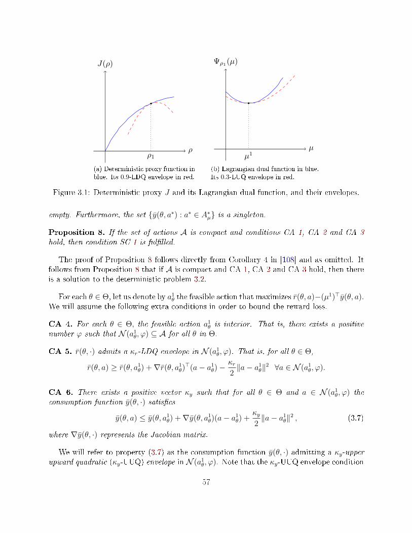
ρ

J(ρ)

ρ1

(a) Deterministic proxy function inblue. Its 0.9-LDQ envelope in red.

µ

Ψρ1(µ)

µ1

(b) Lagrangian dual function in blue.Its 0.3-LUQ envelope in red.

Figure 3.1: Deterministic proxy J and its Lagrangian dual function, and their envelopes.

empty. Furthermore, the set y(θ, a∗) : a∗ ∈ A∗µ is a singleton.

Proposition 8. If the set of actions A is compact and conditions CA 1, CA 2 and CA 3hold, then condition SC 1 is fullled.

The proof of Proposition 8 follows directly from Corollary 4 in [108] and as omitted. Itfollows from Proposition 8 that if A is compact and CA 1, CA 2 and CA 3 hold, then thereis a solution to the deterministic problem 3.2.

For each θ ∈ Θ, let us denote by a1θ the feasible action that maximizes r(θ, a)−(µ1)>y(θ, a).

We will assume the following extra conditions in order to bound the reward loss.

CA 4. For each θ ∈ Θ, the feasible action a1θ is interior. That is, there exists a positive

number ϕ such that N (a1θ, ϕ) ⊆ A for all θ in Θ.

CA 5. r(θ, ·) admits a κr-LDQ envelope in N (a1θ, ϕ). That is, for all θ ∈ Θ,

r(θ, a) ≥ r(θ, a1θ) +∇r(θ, a1

θ)>(a− a1

θ)−κr2‖a− a1

θ‖2 ∀a ∈ N (a1θ, ϕ).

CA 6. There exists a positive vector κy such that for all θ ∈ Θ and a ∈ N (a1θ, ϕ) the

consumption function y(θ, ·) satises

y(θ, a) ≤ y(θ, a1θ) +∇y(θ, a1

θ)(a− a1θ) +

κy2‖a− a1

θ‖2 , (3.7)

where ∇y(θ, ·) represents the Jacobian matrix.

We will refer to property (3.7) as the consumption function y(θ, ·) admitting a κy-upperupward quadratic (κy-UUQ) envelope in N (a1

θ, ϕ). Note that the κy-UUQ envelope condition

57

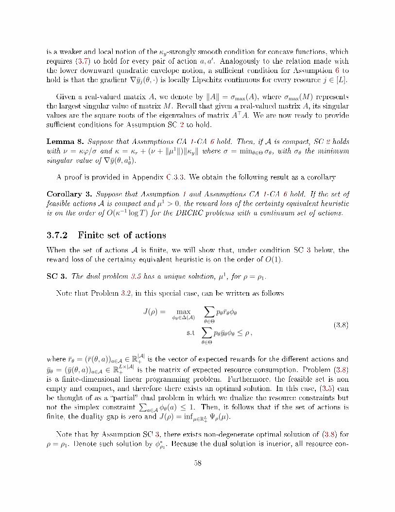
is a weaker and local notion of the κy-strongly smooth condition for concave functions, whichrequires (3.7) to hold for every pair of action a, a′. Analogously to the relation made withthe lower downward quadratic envelope notion, a sucient condition for Assumption 6 tohold is that the gradient ∇yj(θ, ·) is locally Lipschitz continuous for every resource j ∈ [L].

Given a real-valued matrix A, we denote by ‖A‖ = σmax(A), where σmax(M) representsthe largest singular value of matrixM . Recall that given a real-valued matrix A, its singularvalues are the square roots of the eigenvalues of matrix A>A. We are now ready to providesucient conditions for Assumption SC 2 to hold.

Lemma 8. Suppose that Assumptions CA 1-CA 6 hold. Then, if A is compact, SC 2 holdswith ν = κϕ/σ and κ = κr + (ν + ‖µ1‖)‖κy‖ where σ = minθ∈Θ σθ, with σθ the minimumsingular value of ∇y(θ, a1

θ).

A proof is provided in Appendix C.3.3. We obtain the following result as a corollary

Corollary 3. Suppose that Assumption 1 and Assumptions CA 1-CA 6 hold. If the set offeasible actions A is compact and µ1 > 0, the reward loss of the certainty equivalent heuristicis on the order of O(κ−1 log T ) for the DRCRC problems with a continuum set of actions.

3.7.2 Finite set of actions

When the set of actions A is nite, we will show that, under condition SC 3 below, thereward loss of the certainty equivalent heuristic is on the order of O(1).

SC 3. The dual problem 3.5 has a unique solution, µ1, for ρ = ρ1.

Note that Problem 3.2, in this special case, can be written as follows

J(ρ) = maxφθ∈∆(A)

∑θ∈Θ

pθrθφθ

s.t∑θ∈Θ

pθyθφθ ≤ ρ ,(3.8)

where rθ = (r(θ, a))a∈A ∈ R|A|+ is the vector of expected rewards for the dierent actions andyθ = (y(θ, a))a∈A ∈ RL×|A|

+ is the matrix of expected resource consumption. Problem (3.8)is a nite-dimensional linear programming problem. Furthermore, the feasible set is nonempty and compact, and therefore there exists an optimal solution. In this case, (3.5) canbe thought of as a partial dual problem in which we dualize the resource constraints butnot the simplex constraint

∑a∈A φθ(a) ≤ 1. Then, it follows that if the set of actions is

nite, the duality gap is zero and J(ρ) = infµ∈RL+ Ψρ(µ).

Note that by Assumption SC 3, there exists non-degenerate optimal solution of (3.8) forρ = ρ1. Denote such solution by φ∗ρ1 . Because the dual solution is interior, all resource con-

58

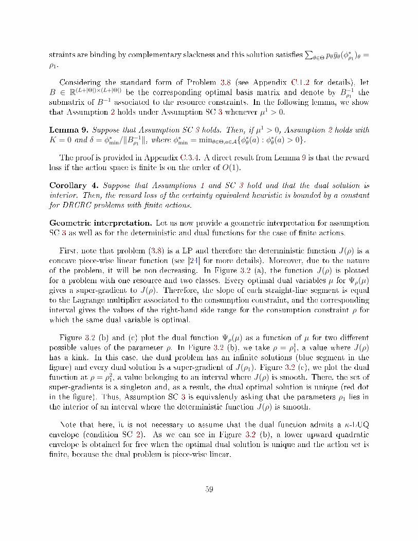
straints are binding by complementary slackness and this solution satises∑

θ∈Θ pθyθ(φ∗ρ1

)θ =ρ1.

Considering the standard form of Problem 3.8 (see Appendix C.1.2 for details), letB ∈ R(L+|Θ|)×(L+|Θ|) be the corresponding optimal basis matrix and denote by B−1

ρ1the

submatrix of B−1 associated to the resource constraints. In the following lemma, we showthat Assumption 2 holds under Assumption SC 3 whenever µ1 > 0.

Lemma 9. Suppose that Assumption SC 3 holds. Then, if µ1 > 0, Assumption 2 holds withK = 0 and δ = φ∗min/‖B−1

ρ1‖, where φ∗min = minθ∈Θ,a∈Aφ∗θ(a) : φ∗θ(a) > 0.

The proof is provided in Appendix C.3.4. A direct result from Lemma 9 is that the rewardloss if the action space is nite is on the order of O(1).

Corollary 4. Suppose that Assumptions 1 and SC 3 hold and that the dual solution isinterior. Then, the reward loss of the certainty equivalent heuristic is bounded by a constantfor DRCRC problems with nite actions.

Geometric interpretation. Let us now provide a geometric interpretation for assumptionSC 3 as well as for the deterministic and dual functions for the case of nite actions.

First, note that problem (3.8) is a LP and therefore the deterministic function J(ρ) is aconcave piece-wise linear function (see [24] for more details). Moreover, due to the natureof the problem, it will be non-decreasing. In Figure 3.2 (a), the function J(ρ) is plottedfor a problem with one resource and two classes. Every optimal dual variables µ for Ψρ(µ)gives a super-gradient to J(ρ). Therefore, the slope of each straight-line segment is equalto the Lagrange multiplier associated to the consumption constraint, and the correspondinginterval gives the values of the right-hand side range for the consumption constraint ρ forwhich the same dual variable is optimal.

Figure 3.2 (b) and (c) plot the dual function Ψρ(µ) as a function of µ for two dierentpossible values of the parameter ρ. In Figure 3.2 (b), we take ρ = ρ1

1, a value where J(ρ)has a kink. In this case, the dual problem has an innite solutions (blue segment in thegure) and every dual solution is a super-gradient of J(ρ1). Figure 3.2 (c), we plot the dualfunction at ρ = ρ2

1, a value belonging to an interval where J(ρ) is smooth. There, the set ofsuper-gradients is a singleton and, as a result, the dual optimal solution is unique (red dotin the gure). Thus, Assumption SC 3 is equivalently asking that the parameters ρ1 lies inthe interior of an interval where the deterministic function J(ρ) is smooth.

Note that here, it is not necessary to assume that the dual function admits a κ-LUQenvelope (condition SC 2). As we can see in Figure 3.2 (b), a lower upward quadraticenvelope is obtained for free when the optimal dual solution is unique and the action set isnite, because the dual problem is piece-wise linear.

59

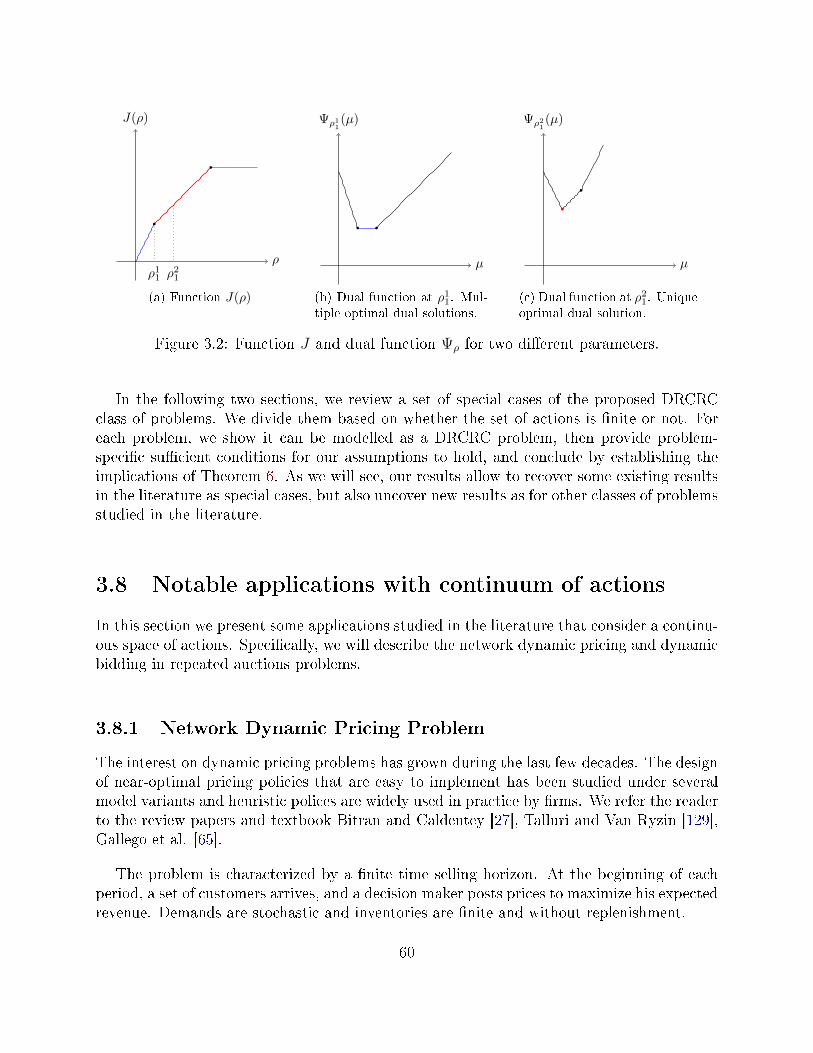
ρ

J(ρ)

ρ11 ρ21

(a) Function J(ρ)

µ

Ψρ11(µ)

(b) Dual function at ρ11. Mul-tiple optimal dual solutions.

µ

Ψρ21(µ)

(c) Dual function at ρ21. Uniqueoptimal dual solution.

Figure 3.2: Function J and dual function Ψρ for two dierent parameters.

In the following two sections, we review a set of special cases of the proposed DRCRCclass of problems. We divide them based on whether the set of actions is nite or not. Foreach problem, we show it can be modelled as a DRCRC problem, then provide problem-specic sucient conditions for our assumptions to hold, and conclude by establishing theimplications of Theorem 6. As we will see, our results allow to recover some existing resultsin the literature as special cases, but also uncover new results as for other classes of problemsstudied in the literature.

3.8 Notable applications with continuum of actions

In this section we present some applications studied in the literature that consider a continu-ous space of actions. Specically, we will describe the network dynamic pricing and dynamicbidding in repeated auctions problems.

3.8.1 Network Dynamic Pricing Problem

The interest on dynamic pricing problems has grown during the last few decades. The designof near-optimal pricing policies that are easy to implement has been studied under severalmodel variants and heuristic polices are widely used in practice by rms. We refer the readerto the review papers and textbook Bitran and Caldentey [27], Talluri and Van Ryzin [129],Gallego et al. [65].

The problem is characterized by a nite time selling horizon. At the beginning of eachperiod, a set of customers arrives, and a decision maker posts prices to maximize his expectedrevenue. Demands are stochastic and inventories are nite and without replenishment.

60

Mapping to a DRCRC problem

In this setting, there is a set of N dierent products to sell during a nite, discrete horizon.An arrival class θ ∈ Θ represents a customer class characterized by their valuation for theproducts. The set of actions A = RN

+ consists of the set of all feasible price vectors to postfor the products.

For each customer class θ, the idiosyncratic shock ε represents some private informationon the consumer willingness to pay. Then, given θ, posted prices a ∈ A = RN

+ and arealization of the shock ε, we denote by D(θ, a, ε) ∈ RN

+ the induced vector of demand.The reward function is given by r(θ, a, ε) = a>D(θ, a, ε) and the consumption function isy(θ, a, ε) = AθD(θ, a, ε). In the latter expression, Aθ ∈ RL×N is a matrix where Anlθ representsthe units of resource l needed to serve a customer class θ with a single unit of product n.

Sucient Conditions for Assumption 2

Let D(θ, a) = Eε[D(θ, a, ε)] denote the expected demand and r(θ, a) = a>D(θ, a) the corre-sponding expected reward function. The deterministic problem can be expressed as follows:

J(ρ) = maxφ∈Φ

∑θ∈Θ

pθ

∫A

r(θ, a)dφθ(a)

s.t∑θ∈Θ

pθ

∫A

AθD(θ, a)dφθ(a) ≤ ρ.

(3.9)

We map conditions CA 1-CA 6 to sucient conditions for this particular problem. Thefollowing conditions together with µ1 > 0 and compactness of the set of actions A aresucient for Lemma 8 to hold.

The expected demand function D(θ, a) is continuous in a.

The expected resource consumption AθD(θ, a) at a maximizer of (a−Aθµ)>D(θ, a) isunique.

For each θ ∈ Θ, the price vector maximizing (a−A>θ µ)>D(θ, a), namely a1θ, is interior.

That is, there exists a positive number ϕ such that N (a1θ, ϕ) ⊆ A for all θ in Θ.

The expected revenue function r(θ, ·) admits a κr-LDQ envelope in N (a1θ, ϕ).

There exists a positive vector κy such that the expected demand function D(θ, ·) admitsa κy-UUQ envelope in N (a1

θ, ϕ).

In particular, under the conditions above, from Lemma 7, Assumption 2 holds with K =1/κ and δ = (νκ)/2, where κ = κr + (ν + ‖µ1‖)‖κy‖, ν = κϕ/σ, and σ is a lower bound on

61

the minimum singular value of Aθ∇D(θ, a1θ). Therefore, by Corollary 2, the revenue loss of

the certainty equivalent heuristic is on the order of O(log T ) for the network dynamic pricingproblem with a continuum set of feasible prices. Another implication of our result is thatthe optimal pricing policy associated with the deterministic proxy is deterministic and thedecision maker does not need to randomize over posted prices.

It is worth mentioning that in the literature this problem is typically analyzed in thedemand space, i.e., for each class θ, the decision variables are the expected demands λ =D(θ, a) instead of the prices a (see, e.g., Jasin [82]). In many cases, this leads to a moretractable problem because constraints become linear and, under additional conditions, theobjective becomes concave. The issue, however, is that restrictive assumptions are neededfor this reformulation of the problem to go through. For example, it is typically assumed thatthe reward function is concave in the demand space and the demand function is invertible.Our result yield similar performance guarantees for the CE heuristic and only requires localsmoothness properties of the revenue function, which typically leads to weaker assumptions.This is an important departure from previous work, even when specializing the analysis.

Finally, note that, if we consider a nite set of feasible prices, the proxy deterministicproblem problems reduces to a linear program and therefore it is enough to assume thedual solution for ρ = ρ1 is unique and interior to obtain a constant revenue loss for the CEheuristic.

Connection with literature

Several papers study heuristics for the network dynamic pricing problem. For example, Kun-numkal and Topaloglu [95] and Erdelyi and Topaloglu [58] consider a dynamic programmingformulation. Both papers consider an airline network in which prices aect the probabilityof the arrival request. In the former, the authors propose a stochastic approximation algo-rithm for choosing prices dynamically and prove its convergence. In the latter, they developtwo methods for making pricing decisions based on a decomposition of the original dynamicprogram.

Closer to the specialization of our results are Maglaras and Meissner [103] and Jasin[82]. The former established that a CE heuristic for the pricing problem will always yieldan asymptotic weak decrease in the revenue loss compared to a static control. Jasin [82]considers a single customer class and present a certainty equivalent heuristic akin to theCE one. Our general result recovers his bound on the logarithmic revenue loss but oursucient conditions are weaker than his. Interestingly, Jasin [82] also proves that resolvingless frequently yield a revenue loss of the same order and proposes another heuristic thatinvolves solving only a single optimization at the beginning of the selling horizon.

62

3.8.2 Dynamic Bidding in Repeated Auctions

A special case of a DRCRC problem is the problem faced by a bidder participating in asequence of repeated auctions to buy opportunities. The bidder has a budget constraintthat limits his total expenditure over the horizon and aims to maximize his cumulativeutility. This model is mainly motivated by internet advertising markets in which advertisersbuy opportunities to display advertisementsan event referred to as an impression viarepeated auctions subject to budget constraints.

Mapping to a DRCRC problem

In this setting, the decision maker is an advertiser. The advertiser is present in the marketfor T periods and one impression is auctioned per period. Upon the arrival of an impressionat time t, the advertiser determines a real-valued valuation θt ∈ Θ ⊂ (0,Θmax] for theimpression, which is distributed according to p ∈ ∆(Θ), and chooses an action at ∈ A =[0,Θmax] representing his bid in the auction. We denote by C the budget of the advertiser.The shock ε captures all exogenous uncertainty in the auction, such as the bids of thecompetitors and any potential randomization of the auction. For simplicity, we assume thatε is independent of the buyer's valuation θ but our model can be easily be modied toaccount for correlation. The auction is characterized an allocation rule q : A × E → [0, 1]together with a payment rule m : A × E → R, which determine the probability that theimpression is allocated to the advertiser and his expected payment as a function of his bidand the exogenous shock, respectively.

The reward earned by the advertiser and his budget consumption, given a, ε and θ canbe expressed as r(θ, a, ε) = (θq(a, ε)−m(a, ε)) and y(θ, a, ε) = m(a, ε), respectively. Givenan action a, we introduce the interim allocation and interim payment variables dened asfollows: q(a) = Eε[q(a, ε)], m(a) = Eε[m(a, ε)].

Sucient Conditions for Assumption 2

For the particular setting described above, the deterministic problem (3.2) is equivalent tothe following problem:

J(ρ) = maxφ∈Φ

∑θ∈Θ

pθ

∫A

(θq(a)− m(a)) dφθ(a)

s.t∑θ∈Θ

pθ

∫A

m(a) dφθ(a) ≤ ρ .

(3.10)

For each θ ∈ Θ, let gθ(µ) = maxa∈A θq(a)− (µ+ 1)m(a). Assumption SC 1 requiresthat gθ(µ) is dierentiable and that gθ(µ) is achieved by an action. Under these conditions,Proposition 7 implies that strong duality holds and the Problem (3.10) admits a deterministicoptimal solution. In this application, we can characterize an optimal bidding strategy in

63

terms of an optimal bidding function for the static auction without budget constraints,which we denote by β : Θ → A. That is, given an advertiser with valuation θ, the optimalbidding strategy for the static auction (ignoring budget constraints) satises

β(θ) ∈ arg maxa∈Aθq(a)− m(a)) .

We have the following result. A proof is provided in Appendix C.4.1.

Proposition 9. Under Assumption SC 1, an optimal solution of (3.10) is to bid β(θ/(1 +µ∗)) when the value is θ, where µ∗ is the optimal solution of the dual problem of (3.10).

If in addition Assumption SC 2 holds, from Lemma 7 we obtain that if µ1 > 0, Assump-tion 2 holds with K = 1/κ and δ = (νκ)/2.

Below, we study the particular cases of second-price auction and rst-price auction.Specically, we provide sucient conditions on the primitives of the problem for conditionsSC 1 and SC 2 to be satised.

Second-price auctions

In a second-price auction, the bidder with the highest bid wins the auction and pays thesecond-highest bid. In this case, we reduce the denition of ε to a random variable capturingthe maximum bid of the competitors and take E = R+. Again, we assume ε is distributedaccording to f , with density function f ′. We assume that ties are broken in favor of thedecision maker. The allocation and payment functions are given by q(a, ε) = 1a≥ε andm(a, ε) = ε1a≥ε, respectively.

Suppose that the following conditions hold:

The distribution of the maximum competing bid f is absolutely continuous and strictlyincreasing.

The density f ′ is locally ξ-Lipschitz continuous with respect to a1θ in N (a1

θ, ϕ).

If µ1 > 0, it is possible to showsee Lemma 12 in Appendix C.1.3that these conditionsare sucient to apply Proposition 8 and Lemma 8 and, in turn, Corollary 3 holds. Thisleads to a revenue loss of O(log T ).

First-price auctions

In a rst-price auction, the winner is the highest bidder but pays his bid. Again, we reducethe denition of ε to a random variable capturing the maximum bid of the competitors. Weassume ε is distributed according to f , with density function f ′. The allocation and paymentfunctions are given by q(a, ε) = 1a≥ε and m(a, ε) = a1a≥ε, respectively.

Suppose the following conditions hold:

64

The distribution of the maximum competing bid f absolutely continuous.

The function M(a) = a+ f(a)/f ′(a) is strictly increasing.

The bid a1θ maximizing θq(a)− (1 +µ1)m(a) is interior. That is, there exists a positive

number ϕ such that N (a1θ, ϕ) ⊂ A for all θ ∈ Θ.

The density f ′ is locally ξ−Lipschitz continuous with respect to a1θ in N (a1

θ, ϕ).

Moreover, if we have µ1 > 0, then it can be provedsee Lemma 13 in Appendix C.1.3thatassumptions CA 1-CA 6 hold and, therefore, by Corollary 3 we obtain an O(log T ) revenueloss.

Connection with literature

While the problem of bidding in repeated auctions with budgets has been studied in the past,to the best of our knowledge, this is the rst paper that studies the revenue loss of a certaintyequivalent heuristic with resolving for the advertiser's decision problem. The assumption thatbudgets are large relative to the average price paid in an auction is reasonable for internetadvertising markets as bidders participate in a large number of auctions. Many papersconsider deterministic uid approximations and static bidding policies.

Abhishek and Hosanagar [1] study this problem, where the goal is to compute optimalbids for multiple keywords in an advertiser's portfolio. To this end, they propose two biddingpolicies: one ignores the interaction between keywords, and another that incorporate inter-action between keywords, and the paper's focus is the deterministic proxy as opposed to thedynamic program (or the relation between the two). Motivated by ad exchanges, Balseiroet al. [20] introduce a uid mean-eld equilibrium (FMFE) notion to study the strategicoutcome of advertisers competing in repeated second-price auctions. They characterize theoptimal bidding strategy for an advertiser by using the optimal solution of the static problemwith budget constraint and prove that FMFE strategies approximate the rational behaviorof the advertisers in large markets. Their analysis, however, is restricted to static policieswhich attain a revenue loss of order O(T 1/2) in this setting. Gummadi et al. [77] characterizeoptimal bidding strategies for bidding in general, repeated auctions under a uid regime anddene a related notion of equilibrium to Balseiro et al. [20].

Fernandez-Tapia et al. [62] study the problem of bidding in repeated auctins when thearrival of requests is a Poisson process and characterize the optimal bidding strategy via itsHamilton-Jacobi-Bellman equation. They show that the optimal bidding strategy can beobtained in almost closed-form by using a uid limit approximation.

65

3.9 Notable applications with nite set of actions

In what follows we present some known problems with nite actions that are particular casesof the problem studied in Section 3.7.2. Then, Assumption SC 3 together with the conditionµ1 > 0 are sucient for Assumption 2 to hold. Furthermore, Lemma 9 and Corollary 4applied to these particular problems, yield a constant bound to the revenue loss for thecertainty equivalent heuristic.

3.9.1 Network Revenue Management Problem

A rst notable special case of the DRCRC class with nite set of actions is a classical class ofproblems in the Revenue Management literature: the Network Revenue Management (NRM)problem. It has been extensively studied in the literature (see, e.g., Talluri and Van Ryzin[129], Gallego et al. [65]) and have also been the basis for various industry solutions.

In the NRM problem, the decision-maker is a rm who is trying to dynamically allocatea limited amount of resources over a nite horizon. Resources are sold to heterogeneousconsumers who arrive sequentially over time and belong to dierent classes depending on theirconsumption of resources and the xed fare they pay. The distribution of customer classesis stationary. Upon a customer's arrival, the rm has to decide whether to accept or rejectthe customer's request. If the customer is accepted and there is enough remaining inventoryto satisfy its request, she consumes the resources requested and pays the corresponding fare.Otherwise, no revenue is collected and no resource is used. The decision maker's objectiveis to maximize the expected revenue earned during the selling horizon.

Mapping to a DRCRC problem

In a NRM problem, a customer class can be captured by θ ∈ Θ and is characterized bytheir usage of resources and a xed price they pay for the service. We let fθ denote the fareassociated with class θ. The decision-maker's feasible actions has two values, A = 0, 1,where we represent the action accept by 1 and reject by 0. In this problem the setof idiosyncratic shocks is empty. The reward if the customer belongs to class θ and thedecision-maker chooses an action a is r(θ, a) = fθa. If we denote by Aθ = (Alθ)l ∈ RL

the consumption vector, where Alθ is the amount of resource l required to serve a classθ customer, the consumption given that the decision-maker chooses an action a and thecustomer class is θ is given by y(θ, a) = Aθa.

The above leads directly to a special case of our general formulation. In particular,Problem (3.8), in this special case, can be written as follows

J(ρ) = maxφθ(1)∈[0,1]

∑θ∈Θ

pθ fθ φθ(1)

s.t∑θ∈Θ

pθ Aθ φθ(1) ≤ ρ .(3.11)

66

Because the set of action consists of A = 0, 1, it is enough to consider decision variablesφθ(1) for all θ ∈ Θ because φθ(0) = 1− φθ(1). Then, for the denition of φ∗min involved in δ,we now need to take into account both the non-negative variables and those that are strictlysmaller than one. That is, φ∗min = minθ∈Θφ∗θ(1) : φ∗θ(1) > 0∧minθ∈Θ1−φ∗θ(1) : φ∗θ(1) < 1,where x ∧ y denotes the minimum between x and y. Furthermore, if we denote by A thematrix whose θth column consists of the vector pθAθ, Bρ1 represents the submatrix of Ain which we only consider the columns associated to variables 0 < φθ

∗(1) < 1, and we setAρ1 = Bρ1 . Then, under Assumption SC 3, if µ1 > 0, Assumption 2 holds with K = 0 andδ = φ∗min/‖A−1

ρ1‖, where φ∗min = minθ∈Θφ∗θ(1) : φ∗θ(1) > 0 ∧minθ∈Θ1− φ∗θ(1) : φ∗θ(1) < 1.

Connection with literature

As mentioned earlier, the NRM problem has a long history. It was originally proposed inD'Sylva [51], Glover et al. [71] and Wang [131]. The question of approximating optimalperformance through simple policies has also received signicant attention.

Jasin and Kumar [84] studies a NRM problem with one resource and with arrivals followinga Poisson process in continuous time. Discretizing the selling horizon, their model ts aspecial of the above NRM model. In addition, it is worth noting that their assumptionsimplies SC 3 and µ1 > 0, and therefore we recover the main result in Jasin and Kumar [84],in a discrete-time setting, as a special case of Theorem 6.

A series of recent papers, which we review below, study variants of the NRM model.While the problems studied in these papers can be mapped out to be special cases of theDRCRC class of problems, the results developed are of a dierent nature. The objectiveis to develop heuristic that depart from the plain CE heuristic and that do not require anassumption akin to Assumption 2 to ensure good" performance.

Discretizing the time horizon, the setting considered in Reiman and Wang [116] wouldt to the one described in this section. In particular, they consider that customers' arrivalprocesses satisfying two conditions: on one hand, they assume that the functional centrallimit theorem holds for a properly centered and scaled sequence of the arrival processes, andon the other, they make a technical assumption that holds, for example, for an independentrenewal processes. They propose a heuristic that resolves the deterministic problem onceand they obtain that under their policy the revenue loss is o(

√T ). In a related setting,

Bumpensanti and Wang [34] assume that arrivals follow a Poisson process and show thatthe CE heuristic has a Θ(

√T ) revenue loss in the general case (without the nondegeneracy

assumption). They also propose a heuristic that has a O(1) revenue loss. The idea is to onlyre-solve the deterministic problem a few selected times, using the approach of Reiman andWang [116] recursively. More recently, in Vera and Banerjee [130] the authors consider theNRM problem for arrival processes satisfying some quadratic tail bound and they proposean algorithm based on thresholds that allows them to obtain a constant upper bound for theexpected revenue loss.

67

An interesting direction is to explore whether the ideas developed in these papers can beleveraged for the more general DRCRC class of problems.

3.9.2 Choice-Based Network Revenue Management Problems

This problem bears many similarities to the network revenue management problem. Inthis setting, a rm is trying to dynamically allocate a limited amount of products whichare sold to heterogeneous consumers who arrive sequentially and belong to dierent classescharacterized by their product preferences. The key dierence with the NRM class is that,upon a customer's arrival, the rm makes an oer and depending on the oer and on thecustomer's preferences, the consumer selects a single product to buy.

Mapping to a DRCRC problem

In this setting we consider a set of N products, each of them consisting of a set of resources.Product n is priced at mn. Given a customer class θ and a product n, we denote by Anlθ theamount of resource l needed to serve product n to customer θ. The action set is given byA = 21,...,N, where an action a ∈ A represents a set of products to be oered to a consumer.

For each action a and customer class θ, we dene the shock random vector εθa ∈ E =ε ∈

0, 1N :∑

n∈[N ] εn ≤ 1

, where its nth component εnθa is 1 if and only if the customer selects

product n from the oer a. Then, εθa ∼ Multinomial(1, gθa) where gnθa7 is the probability of

the consumer choosing product n given that his class is θ and the action taken is a.

Given the consumer class θ, the action a, and the shock realization εθa, the reward func-tion is given by r(θ, a, ε) =

∑n∈[N ] mnε

n and the consumption function by y(θ, a, ε) =∑n∈[N ] A

nθ ε. Note that, conditional on the shock ε, the resource consumption does not de-

pend on the action. However, the action aects the distribution of ε.

In the present setting, the deterministic problem can be expressed as

J(ρ) = maxφ∈Φ

∑θ∈Θ

∑a∈A

φθ(a)pθ∑n∈[N ]

mngnθa

s.t∑θ∈Θ

∑a∈A

φθ(a)pθ∑n∈[N ]

Anθ gnθa ≤ ρ.

(3.12)

We can dene the vector of variables and the associated matrix involved in the constraintsof problem (3.12) by setting each column to pθ

∑n∈[N ]A

nθ g

nθa. Then, under assumption SC 3,

if the optimal dual solution of (3.12) for ρ = ρ1 is interior, we can apply Lemma 9 andAssumption 2 holds for K = 0 and δ dened as in the statement of the lemma. Therefore,

7Without loss of generality, we can apply suitable transformations to the reward and consumption func-tions to obtain a distribution of ε that is independent of the class and the action.

68

we obtain a constant bound on the revenue loss of the CE heuristic for the choice-basednetwork revenue management problem.

Connection with literature

The class of choice-based network revenue management problems has appeared under twostreams: one corresponds to the called choice-based problem, where an oer is a network(each product is a combination of one or more resources), and the other corresponds to adynamic assortment optimization problem under constraints, where there is a one-to-onemapping between products and resources.

In the rst stream, the single-leg case was introduced by Talluri and Van Ryzin [128] whoprovided an analysis of the optimal control policy under a general discrete choice model ofdemand.

Regarding a network setting, Gallego et al. [63] was the rst to study a choice-based NRMproblem. They consider exible products in a continuous time horizon and with arrivals fol-lowing independent Poisson processes. A exible product consists of a set of alternative prod-ucts serving a customer class. That is, if a exible product F is oered by the decision-makerand accepted by the consumer, then the decision-maker assigns him one of the products inF . They present a dynamic programming formulation of the problem and proved that it canbe approximated by using an appropriate deterministic control problem. Furthermore, theyshowed that the latter problem can be solved eciently by a column generation algorithmfor a broad class of consumer choice models (that includes both independent demands andthe multinomial logit model).

Liu and Van Ryzin [100] considered a choice-based network RM problem in which eachconsumer belongs to a market segment (customer type) characterized by a set of products(dierents for each segment) in which the consumer is interested and the decision-maker hasto decide a set of products to oer in each selling period. Liu and Van Ryzin [100] introducedlinear programming formulation of the problem and they show that the revenue obtainedunder this deterministic program converges to the optimal revenue under the exact dynamicformulation. Their work is based in the deterministic formulation introduced by Gallego etal. [63] but without considering exible products.

Bront et al. [32] consider the same problems as Liu and Van Ryzin [100] but they allowcustomer classes to overlap. They compute the consumer behaviour by using an MNL choicemodel and developed a column generation algorithm to solve the deterministic LP for large-size networks. The associated subproblem is NP-complete and, therefore, they propose aheuristic that is shown to work well on a set of computational examples.

In the other stream, Bernstein et al. [22] consider a dynamic assortment problem incontinuous time. In the problem they consider, all products have the same price and foreach customer class they compute the probability that a customer belonging to that class

69

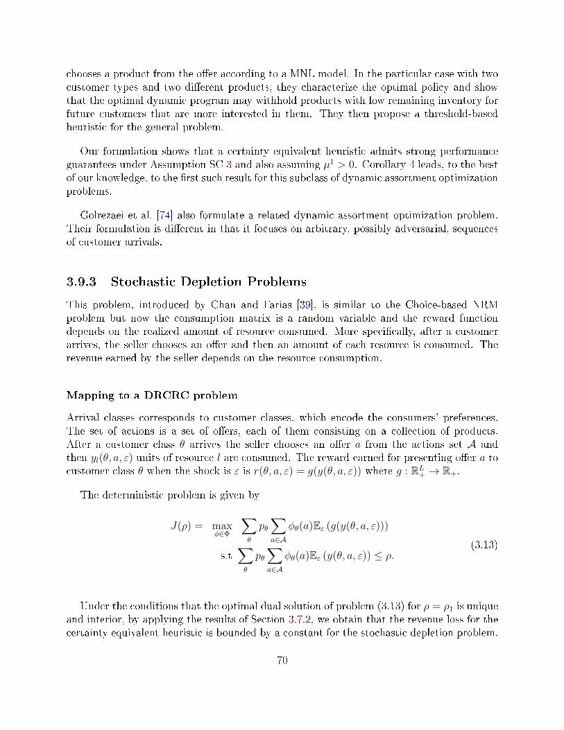
chooses a product from the oer according to a MNL model. In the particular case with twocustomer types and two dierent products, they characterize the optimal policy and showthat the optimal dynamic program may withhold products with low remaining inventory forfuture customers that are more interested in them. They then propose a threshold-basedheuristic for the general problem.

Our formulation shows that a certainty equivalent heuristic admits strong performanceguarantees under Assumption SC 3 and also assuming µ1 > 0. Corollary 4 leads, to the bestof our knowledge, to the rst such result for this subclass of dynamic assortment optimizationproblems.

Golrezaei et al. [74] also formulate a related dynamic assortment optimization problem.Their formulation is dierent in that it focuses on arbitrary, possibly adversarial, sequencesof customer arrivals.

3.9.3 Stochastic Depletion Problems

This problem, introduced by Chan and Farias [39], is similar to the Choice-based NRMproblem but now the consumption matrix is a random variable and the reward functiondepends on the realized amount of resource consumed. More specically, after a customerarrives, the seller chooses an oer and then an amount of each resource is consumed. Therevenue earned by the seller depends on the resource consumption.

Mapping to a DRCRC problem

Arrival classes corresponds to customer classes, which encode the consumers' preferences.The set of actions is a set of oers, each of them consisting on a collection of products.After a customer class θ arrives the seller chooses an oer a from the actions set A andthen yl(θ, a, ε) units of resource l are consumed. The reward earned for presenting oer a tocustomer class θ when the shock is ε is r(θ, a, ε) = g(y(θ, a, ε)) where g : RL

+ → R+.

The deterministic problem is given by

J(ρ) = maxφ∈Φ

∑θ

pθ∑a∈A

φθ(a)Eε (g(y(θ, a, ε)))

s.t∑θ

pθ∑a∈A

φθ(a)Eε (y(θ, a, ε)) ≤ ρ.(3.13)

Under the conditions that the optimal dual solution of problem (3.13) for ρ = ρ1 is uniqueand interior, by applying the results of Section 3.7.2, we obtain that the revenue loss for thecertainty equivalent heuristic is bounded by a constant for the stochastic depletion problem.

70

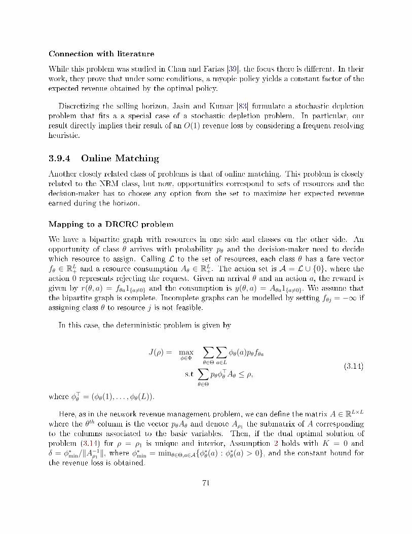
Connection with literature

While this problem was studied in Chan and Farias [39], the focus there is dierent. In theirwork, they prove that under some conditions, a myopic policy yields a constant factor of theexpected revenue obtained by the optimal policy.

Discretizing the selling horizon, Jasin and Kumar [83] formulate a stochastic depletionproblem that ts a a special case of a stochastic depletion problem. In particular, ourresult directly implies their result of an O(1) revenue loss by considering a frequent resolvingheuristic.

3.9.4 Online Matching

Another closely related class of problems is that of online matching. This problem is closelyrelated to the NRM class, but now, opportunities correspond to sets of resources and thedecision-maker has to choose any option from the set to maximize her expected revenueearned during the horizon.

Mapping to a DRCRC problem

We have a bipartite graph with resources in one side and classes on the other side. Anopportunity of class θ arrives with probability pθ and the decision-maker need to decidewhich resource to assign. Calling L to the set of resources, each class θ has a fare vectorfθ ∈ RL

+ and a resource consumption Aθ ∈ RL+. The action set is A = L ∪ 0, where the

action 0 represents rejecting the request. Given an arrival θ and an action a, the reward isgiven by r(θ, a) = fθa1a6=0 and the consumption is y(θ, a) = Aθa1a6=0. We assume thatthe bipartite graph is complete. Incomplete graphs can be modelled by setting fθj = −∞ ifassigning class θ to resource j is not feasible.

In this case, the deterministic problem is given by

J(ρ) = maxφ∈Φ

∑θ∈Θ

∑a∈L

φθ(a)pθfθa

s.t∑θ∈Θ

pθφ>θ Aθ ≤ ρ,

(3.14)

where φ>θ = (φθ(1), . . . , φθ(L)).

Here, as in the network revenue management problem, we can dene the matrix A ∈ RL×L

where the θth column is the vector pθAθ and denote Aρ1 the submatrix of A correspondingto the columns associated to the basic variables. Then, if the dual optimal solution ofproblem (3.14) for ρ = ρ1 is unique and interior, Assumption 2 holds with K = 0 andδ = φ∗min/‖A−1

ρ1‖, where φ∗min = minθ∈Θ,a∈Aφ∗θ(a) : φ∗θ(a) > 0, and the constant bound for

the revenue loss is obtained.

71

Connection with literature

There are several papers on online matching in the literature with the goal to design analgorithm that maximizes the competitive ratio.

The bipartite online matching was introduced by Karp et al. [88] where they consider thecase with arrivals in arbitrary order and with the goal of maximizing the total number ofmatches. To this end, they presented an online algorithm with a competitive ratio of 1−1/eand they show that it is the best possible ratio in that setting. This was generalized to vertex-weighted matchings in Aggarwal et al. [5], presenting a (1 − 1/e)-competitive randomizedalgorithm for general vertex weights. They also show that the same competitive ratio isobtained considering the problem with capacities.

Note that the adwords problem is a particular case of the problem we describe whereAθ = fθ. Devanur et al. [49] consider such a problem and provide a reinterpretation of thealgorithm on Karp et al. [88] as a randomized primal-dual algorithm. Their analysis alsoextends to the algorithm presented on Aggarwal et al. [5].

Also the display allocation problem can formulated as an online matching problem, wherethe initial capacities give the number of impressions each advertiser request and Aθa = 1because each impression consumes one unit. Feldman et al. [60] studied an stochastic versionof this problem assuming that arrivals are i.i.d samples from a known distribution andthat the expected number of impressions is integer. They present an algorithm with aapproximation factor higher than 1−1/e. This result was improved by Manshadi et al. [104],who also consider a stochastic setting but they provide a bound for the competitive ratiothat holds without having integrality of expectations.

A constant bound for the reward loss was recently obtained by Vera and Banerjee [130]for a dierent heuristic.

3.9.5 Order Fulllment Problem

In this section we study a class of problem faced by a retailer who needs to fulll the ordersthey receive from dierent facilities. Specically, in this problem an order arrives sequentiallyand a decision-maker has to construct a fulllment policy to decide from which facility eachof the items in the arriving order should be fullled.

Mapping to a DRCRC problem

We consider the setting where there are L dierent items (resources in the general formu-lation) that could be served from K dierent facilities. Each facility k is endowed with aninventory Ck ∈ RL

+, with Ckl representing the initial capacity of item l in facility k, and weconsider that facility K is ctitious with innite initial capacity of all items.

72

Arrival θ occurs with probability pθ and corresponds to a request belonging to Θ =21,...,L. We assume one order includes at most one unit of each item. Then, θl = 1 if andonly if item l is included on the oer θ and 0, otherwise.

The decision-maker has to construct a fulllment policy to decide from which facilityk ∈ K each of the items in θ should be fullled in order to maximize his expected revenue.That is, the action set is given by A = 1, . . . , KL, where given l ∈ L, al = k means thatitem l is served from facility k. Furthermore, serving item l from facility k has an associatedfare denoted by flk.

Given that the order is θ and the decision-maker chooses action a, the consumption of iteml in the facility k is ylk(θ, a) = 1al=k, and the reward is given by r(θ, a) =

∑l∈θ,k∈K flk1al=k.

For the particular setting described above, the deterministic problem can be expressed asfollows

J(ρ) = maxφ∈Φ

∑θ∈Θ

∑a∈A

pθφθ(a)∑l∈θ

∑k∈K

flk1al=k

s.t∑θ∈Θ

∑a∈A

pθφθ(a)1al=k ≤ ρlk.(3.15)

In this case, as in the previous ones, we can write the constraints of problem (3.15) inmatrix form and, thus, obtain an expression for δ involved in the assumption. We do not givean explicit formula for δ to avoid introducing more notation. Moreover, if the dual optimalsolution of problem (3.15) for ρ = ρ1 is unique and interior, Assumption 2 holds with K = 0and we recover a constant revenue loss bound for the order fulllment problem.

Connection with literature

Many dierent variants of this DRCRC problem have been studied in the literature. For ex-ample, papers have considered dierent objectives to optimize, whether if the model requiresa demand forecast of not, multi or single-item approach, among others. We refer the readerAcimovic and Farias [3] for an overview of order fulllment problems.

Acimovic and Graves [4] modeled the problem as a dynamic program that minimizes theshipping cost plus the expected future costs and they propose an algorithm to approximateit based on the dual variables of the oine deterministic linear programming approximation.They demonstrate that the heuristic works well in practice.

Another paper considering a fulllment problem is Andrews et al. [9]. The main dierencewith the model proposed by Acimovic and Graves [4] is that the former allow demand tobe adversarial. They propose a primal-dual based algorithm to approximate the dynamicprogramming value function. They give a bound for the competitive ratio achieved by the

73

algorithm and establish that no online algorithm can achieve a better competitive ratio.

Jasin and Sinha [85] considered the multi-item order fulllment problem and study theperformance of two heuristics derived from the solution of the deterministic linear programwhere the objective is to minimize the total shipping cost. They investigated the competitiveratio of both heuristics and provide numerical examples showing that one of the algorithmsperforms very close to optimal.

Some works in the existing literature consider extra constraints related, for instance, tothe set of feasible facilities (or resources) from which is it possible to serve an order. Asadpouret al. [12] consider an online allocation problem with equal numbers of types of resources andtypes of requests with the restriction that a request of type i can be served only by resourcesof type i and type i+1. If both resources have zero inventory left, then the sale is lost. Theirobjective is to provide an upper bound on the dierence between the performance with andwithout the above described restriction on fulllment.

It is worth mentioning that some works consider the order fulllment problem jointly withthe pricing problem (see, e.g., [80], [97]) or jointly with both pricing and display problems(see, e.g., [98]).

3.9.6 Other applications

Although we have mentioned several problems that are special cases of the DRCRC class,there are some other problems in the literature that also belongs to DRCRC class.

For instance, the dynamic knapsack problem and the multisecretary problem, which areboth closely related to the NRM problem exposed, are special cases of DRCRC problems.Arlotto and Xie [11] consider the dynamic knapsack problem, which is closely related to theNRM problem exposed. In this case, arrivals correspond to items to allocate, the knapsackcan be seen as the resource, and the resource consumption is given by an item's weight.Arlotto and Gurvich [10] consider the multisecretary problem. This problem is a particularcase of the our NRM problem in which the arrivals are the candidates, there is one resourcewith initial capacity equal to the number of secretaries needed, and the reward associatedto a candidate is his ability.

It is worth mentioning that it is also possible to consider a combination some of theparticular classes of DRCRC problems mentioned (see, e.g., [80],[97],[98]).

74

Conclusion

Throughout the chapters of this thesis, we address dierent problems arising mainly fromrevenue management. However, the problems considered are also of interest in the areasof computer science and economics, and we then make contributions to all these researchcommunities.

Firstly, we introduced the notion of value of observability for a dynamic pricing problem,which is dened as the ratio between the expected revenue of the seller in the settings whereshe is able to observes the arrival of the customer before oering the price curve and theexpected revenue of the seller when she has not have this power. The main contribution isthat we provide a constant upper bound for this value, that is independent of all parametersof the problem. This result is robust and surprising, and the main diculty of the problemarises from the diculty of solving the unobservable case. In fact, to obtain this bound we usethe optimal solution of the observable case and we construct a feasible pricing policy for theunobservable case that allowed us to extract a constant portion of the expected revenue in theobservable case. This leads us to think that, although the bound we found is an interestingcontribution, a question for future work is whether this bound could be improved. We havealso studied lower bounds for the value of observability, but this problem is dicult dueto the impossibility of solving, and even modeling, the unobservable case in general. Thus,using dynamic programming for a particular instance, we obtained a lower bound but webelieve that another challenge for future work is to be able to improve it. Since the notionof the value of observability is novel, there are also open questions related to whether ifthe value of observability could be also uniformly bounded for more general settings (e.g.,considering more than one buyer), as well as relating this notion to others already studiedin the literature, such as the price of discrimination.

Secondly, we proved that the problem of designing posted price mechanisms is equivalentto that of nding stopping rules for optimal stopping problems. More specically, we showedthat if we have a sequential posted price mechanism with a certain approximation guarantee,it can be turned out into a prophet inequality with the same approximation guarantee. Tothis end, we proved a key technical result of auction theory- that it may be useful alsoin settings beyond this thesis- that states that for any distribution there is another whosevirtual value distributes according to the former distribution. As a corollary of our result,

75

it is possible to translate all known lower bounds from PPMs into prophet inequalities, andback and therefore our contribution is for both auction and optimal stopping theory.

Finally, we introduced a novel general formulation of dynamic optimization problems,that we call dynamic resource constraint reward collection. In particular, we have seenhow this class of problems comprises several problems studied separately in the literature.Furthermore, we considered a certainty equivalent heuristic and we studied its performancefor the class DRCRC. In particular, this implies that the performance of the heuristic canbe proved in a single result for all the known problems that are special cases of a DRCRCproblem, recovering the known performance for some problems and providing new resultsfor others. Although it is important how good the heuristic is, it is also important to studythe sucient conditions needed to ensure that good performance. In this way, the thesisintroduced an important contribution, stating that some local smooth conditions on a dualfunction are sucient to recover the bounds. We also analyzed, not only the geometricinterpretation of the conditions, but also some sucient conditions on the primitives of themodel for each of the particular problem exposed. This work opens up the possibility offurther generalizations of arguments developed for special cases of DRCRC problems.

76

Bibliography

[1] Vibhanshu Abhishek and Kartik Hosanagar. Optimal bidding in multi-item multislotsponsored search auctions. Operations Research, 61(4):855873, 2013.

[2] Melika Abolhassani, Soheil Ehsani, Hossein Esfandiari, MohammadTaghi Hajiaghayi,Robert Kleinberg, and Brendan Lucier. Beating 1-1/e for ordered prophets. In Proceed-ings of 49th Annual ACM SIGACT Symposium on the Theory of Computing, STOC'17. ACM, 2017.

[3] Jason Acimovic and Vivek F Farias. The fulllment-optimization problem. In Op-erations Research & Management Science in the Age of Analytics, pages 218237.INFORMS, 2019.

[4] Jason Acimovic and Stephen C Graves. Making better fulllment decisions on the yin an online retail environment. Manufacturing & Service Operations Management,17(1):3451, 2015.

[5] Gagan Aggarwal, Gagan Goel, Chinmay Karande, and Aranyak Mehta. Online vertex-weighted bipartite matching and single-bid budgeted allocations. In Proceedings of thetwenty-second annual ACM-SIAM symposium on Discrete Algorithms, pages 12531264. SIAM, 2011.

[6] Hyun-soo Ahn, Mehmet Gümü³, and Philip Kaminsky. Pricing and manufacturingdecisions when demand is a function of prices in multiple periods. Operations Research,55(6):10391057, 2007.

[7] Saeed Alaei. Bayesian combinatorial auctions: Expanding single buyer mechanisms tomany buyers. SIAM Journal on Computing, 43(2):930972, 2014.

[8] Saeed Alaei, Jason Hartline, Rad Niazadeh, Emmanouil Pountourakis, and Yang Yuan.Optimal auctions vs. anonymous pricing. In Proceedings of the 2015 IEEE 56th AnnualSymposium on Foundations of Computer Science, FOCS '15, pages 14461463. IEEEComputer Society, 2015.

77

[9] John M Andrews, Vivek F Farias, Aryan I Khojandi, and Chad M Yan. Primaldualalgorithms for order fulllment at urban outtters, inc. Interfaces, 49(5):355370,2019.

[10] Alessandro Arlotto and Itai Gurvich. Uniformly bounded regret in the multisecretaryproblem. Stochastic Systems, 9(3):231260, Sep 2019.

[11] Alessandro Arlotto and Xinchang Xie. Logarithmic regret in the dynamic and stochas-tic knapsack problem. arXiv preprint arXiv:1809.02016, 2018.

[12] Arash Asadpour, Xuan Wang, and Jiawei Zhang. Online resource allocation withlimited exibility. Management Science, 2019.

[13] Yossi Aviv, Yuri Levin, and Mikhail Nediak. Counteracting strategic consumer behav-ior in dynamic pricing systems. Consumer-Driven Demand and Operations Manage-ment Models, 131:323352, 2009.

[14] Yossi Aviv and Amit Pazgal. Optimal pricing of seasonal products in the presenceof forward-looking consumers. Manufacturing & Service Operations Management,10(3):339359, 2008.

[15] Yossi Aviv and Gustavo Vulcano. Dynamic list pricing. 2012.

[16] Pablo D. Azar, Robert Kleinberg, and S. Matthew Weinberg. Prophet inequalities withlimited information. In Proceedings of the Twenty-fth Annual ACM-SIAM Symposiumon Discrete Algorithms, SODA '14, pages 13581377. Society for Industrial and AppliedMathematics, 2014.

[17] Moshe Babaio, Liad Blumrosen, Shaddin Dughmi, and Yaron Singer. Posting priceswith unknown distributions. ACM Trans. Econ. Comput., 5(2):13:113:20, March 2017.

[18] Moshe Babaio, Nicole Immorlica, and Robert Kleinberg. Matroids, secretary prob-lems, and online mechanisms. In Proceedings of the eighteenth annual ACM-SIAMsymposium on Discrete algorithms, SODA '07, pages 434443. Society for Industrialand Applied Mathematics, 2007.

[19] Santiago Balseiro, Omar Besbes, and Dana Pizarro. Dynamic resource constrainedreward collection. Working paper, 2020.

[20] Santiago R Balseiro, Omar Besbes, and Gabriel Y Weintraub. Repeated auctionswith budgets in ad exchanges: Approximations and design. Management Science,61(4):864884, 2015.

[21] Dirk Bergemann and Philipp Strack. Progressive participation. 2019.

78

[22] Fernando Bernstein, A Gürhan Kök, and Lei Xie. Dynamic assortment customizationwith limited inventories. Manufacturing & Service Operations Management, 17(4):538553, 2015.

[23] Dimitri P Bertsekas. Nonlinear programming. Journal of the Operational ResearchSociety, 48(3):334334, 1997.

[24] Dimitris Bertsimas and John N Tsitsiklis. Introduction to linear optimization, volume 6.Athena Scientic Belmont, MA, 1997.

[25] David Besanko and Wayne L Winston. Optimal price skimming by a monopolist facingrational consumers. Management Science, 36(5):555567, 1990.

[26] Omar Besbes and Ilan Lobel. Intertemporal price discrimination: Structure and com-putation of optimal policies. Management Science, 61(1):92110, 2015.

[27] Gabriel Bitran and René Caldentey. An overview of pricing models for revenue man-agement. Manufacturing & Service Operations Management, 5(3):203229, 2003.

[28] Liad Blumrosen and Thomas Holenstein. Posted prices vs. negotiations: An asymptoticanalysis. In Proceedings of the 9th ACM Conference on Electronic Commerce, EC '08,pages 4949, New York, NY, USA, 2008. ACM.

[29] Simon Board and Andrzej Skrzypacz. Revenue management with forward-lookingbuyers. Journal of Political Economy, 124(4):10461087, 2016.

[30] Stephen Boyd and Lieven Vandenberghe. Convex Optimization. Cambridge UniversityPress, 2009.

[31] Luis Briceño-Arias, José R Correa, and Andres Perlroth. Optimal continuous pricingwith strategic consumers. Management Science, 63(8):27412755, 2017.

[32] Juan José Miranda Bront, Isabel Méndez-Díaz, and Gustavo Vulcano. A column gen-eration algorithm for choice-based network revenue management. Operations research,57(3):769784, 2009.

[33] Sébastien Bubeck. Convex optimization: Algorithms and complexity. arXiv preprintarXiv:1405.4980, 2014.

[34] Pornpawee Bumpensanti and He Wang. A re-solving heuristic with uniformly boundedloss for network revenue management. arXiv preprint arXiv:1802.06192, 2018.

[35] Gérard P Cachon and Robert Swinney. Purchasing, pricing, and quick response in thepresence of strategic consumers. Management Science, 55(3):497511, 2009.

79

[36] Yang Cai and Constantinos Daskalakis. Learning multi-item auctions with (or without)samples. In Proceedings of the 2017 IEEE 58th Annual Symposium on Foundations ofComputer Science, FOCS '17, pages 516527. IEEE Computer Society, 2017.

[37] Yang Cai and Mingfei Zhao. Simple mechanisms for subadditive buyers via duality. InProceedings of the 49th Annual ACM SIGACT Symposium on Theory of Computing,STOC 2017, pages 170183. ACM, 2017.

[38] René Caldentey, Ying Liu, and Ilan Lobel. Intertemporal pricing under minimax regret.Operations Research, 65(1):104129, 2017.

[39] Carri W Chan and Vivek F Farias. Stochastic depletion problems: Eective myopicpolicies for a class of dynamic optimization problems. Mathematics of OperationsResearch, 34(2):333350, 2009.

[40] Shuchi Chawla, Jason D. Hartline, and Robert Kleinberg. Algorithmic pricing viavirtual valuations. In Proceedings of the 8th ACM Conference on Electronic Commerce,EC '07, pages 243251. ACM, 2007.

[41] Shuchi Chawla, Jason D. Hartline, David L. Malec, and Balasubramanian Sivan. Multi-parameter mechanism design and sequential posted pricing. In Proceedings of theForty-second ACM Symposium on Theory of Computing, STOC '10, pages 311320.ACM, 2010.

[42] Ronald H Coase. Durability and monopoly. The Journal of Law and Economics,15(1):143149, 1972.

[43] Richard Cole and Tim Roughgarden. The sample complexity of revenue maximization.In Proceedings of the Forty-sixth Annual ACM Symposium on Theory of Computing,STOC '14, pages 243252. ACM, 2014.

[44] José Correa, Patricio Foncea, Ruben Hoeksma, Tim Oosterwijk, and Tjark Vredeveld.Posted price mechanisms for a random stream of customers. In Proceedings of the 2017ACM Conference on Economics and Computation, EC '17, pages 169186. ACM, 2017.

[45] José Correa, Patricio Foncea, Dana Pizarro, and Victor Verdugo. From pricing toprophets, and back! Operations Research Letters, 47(1):2529, 2019.

[46] José Correa, Ricardo Montoya, and Charles Thraves. Contingent preannounced pricingpolicies with strategic consumers. Operations Research, 64(1):251272, 2016.

[47] José Correa, Dana Pizarro, and Gustavo Vulcano. Value of observability in dynamicpricing. In Proceedings of the 21st ACM Conference on Economics and Computation,EC '20. ACM, 2020.

80

[48] Sriram Dasu and Chunyang Tong. Dynamic pricing when consumers are strategic:Analysis of posted and contingent pricing schemes. European Journal of OperationalResearch, 204(3):662671, 2010.

[49] Nikhil R Devanur, Kamal Jain, and Robert D Kleinberg. Randomized primal-dualanalysis of ranking for online bipartite matching. In Proceedings of the twenty-fourthannual ACM-SIAM symposium on Discrete algorithms, pages 101107. SIAM, 2013.

[50] Peerapong Dhangwatnotai, Tim Roughgarden, and Qiqi Yan. Revenue maximizationwith a single sample. Games and Economic Behavior, 91:318333, 2015.

[51] Ewalds D'Sylva. O and d seat assignment to maximize expected revenue. Unpublishedinternal report, Boeing Commercial Airplane Company, Seattle, WA, 1982.

[52] Paul Dütting, Michal Feldman, Thomas Kesselheim, and Brendan Lucier. Prophetinequalities made easy: Stochastic optimization by pricing non-stochastic inputs. InProceedings of the 2017 IEEE 58th Annual Symposium on Foundations of ComputerScience, FOCS '17, pages 540551. IEEE Computer Society, 2017.

[53] Paul Dütting, Felix Fischer, and Max Klimm. Revenue Gaps for Discriminatory andAnonymous Sequential Posted Pricing. ArXiv e-prints, July 2016.

[54] Paul Dütting and Robert Kleinberg. Polymatroid prophet inequalities. In Algorithms-ESA 2015, pages 437449. Springer, 2015.

[55] Liran Einav, Chiara Farronato, Jonathan Levin, and Neel Sundaresan. Auctions versusposted prices in online markets. Journal of Political Economy, Forthcoming.

[56] Adam N Elmachtoub, Vishal Gupta, and Michael Hamilton. The value of personalizedpricing. Available at SSRN 3127719, 2018.

[57] Wedad Elmaghraby, Altan Gülcü, and Pnar Keskinocak. Designing optimal prean-nounced markdowns in the presence of rational customers with multiunit demands.Manufacturing & Service Operations Management, 10(1):126148, 2008.

[58] Alexander Erdelyi and Huseyin Topaloglu. Using decomposition methods to solvepricing problems in network revenue management. Journal of Revenue and PricingManagement, 10(4):325343, 2011.

[59] Hossein Esfandiari, MohammadTaghi Hajiaghayi, Vahid Liaghat, and Morteza Mone-mizadeh. Prophet secretary. SIAM Journal on Discrete Mathematics, 31(3):16851701,2017.

[60] Jon Feldman, Aranyak Mehta, Vahab Mirrokni, and Shan Muthukrishnan. Onlinestochastic matching: Beating 1-1/e. In 2009 50th Annual IEEE Symposium on Foun-

81

dations of Computer Science, pages 117126. IEEE, 2009.

[61] Michal Feldman, Nick Gravin, and Brendan Lucier. Combinatorial auctions via postedprices. In Proceedings of the Twenty-sixth Annual ACM-SIAM Symposium on DiscreteAlgorithms, SODA '15, pages 123135. Society for Industrial and Applied Mathematics,2015.

[62] Joaquin Fernandez-Tapia, Olivier Guéant, and Jean-Michel Lasry. Optimal real-timebidding strategies. Applied Mathematics Research eXpress, 2017(1):142183, 2017.

[63] Guillermo Gallego, Garud Iyengar, Robert Phillips, and Abhay Dubey. Managingexible products on a network. Available at SSRN 3567371, 2004.

[64] Guillermo Gallego, Robert Phillips, and Özge ahin. Strategic management of dis-tressed inventory. Production and Operations Management, 17(4):402415, 2008.

[65] Guillermo Gallego, Huseyin Topaloglu, et al. Revenue management and pricing ana-lytics, volume 209. Springer, 2019.

[66] Guillermo Gallego and Garrett Van Ryzin. A multiproduct dynamic pricing problemand its applications to network yield management. Operations research, 45(1):2441,1997.

[67] Jérémie Gallien and Shobhit Gupta. Temporary and permanent buyout prices in onlineauctions. Management Science, 53(5):814833, 2007.

[68] Daniel F Garrett. Intertemporal price discrimination: Dynamic arrivals and changingvalues. The American Economic Review, 106(11):32753299, 2016.

[69] Alex Gershkov, Benny Moldovanu, and Philipp Strack. Revenue-maximizing mecha-nisms with strategic customers and unknown, markovian demand. Management Sci-ence, 64(5):20312046, 2018.

[70] John P. Gilbert and Frederick Mosteller. Recognizing the maximum of a sequence.Journal of the American Statistical Association, 61:3576, 1966.

[71] Fred Glover, Randy Glover, Joe Lorenzo, and Claude McMillan. The passenger-mixproblem in the scheduled airlines. Interfaces, 12(3):7380, 1982.

[72] Oliver Göbel, Martin Hoefer, Thomas Kesselheim, Thomas Schleiden, and BertholdVöcking. Online independent set beyond the worst-case: Secretaries, prophets, andperiods. In Automata, Languages, and Programming - 41st International Colloquium,ICALP 2014, Copenhagen, Denmark, July 8-11, 2014, Proceedings, Part II, pages508519, 2014.

82

[73] Kira Goldner and Anna R. Karlin. A prior-independent revenue-maximizing auctionfor multiple additive bidders. In Proceedings of the 12th International Conference onWeb and Internet Economics - Volume 10123, WINE 2016, pages 160173. Springer-Verlag New York, Inc., 2016.

[74] Negin Golrezaei, Hamid Nazerzadeh, and Paat Rusmevichientong. Real-time optimiza-tion of personalized assortments. Management Science, 60(6):15321551, 2014.

[75] Jochen Gönsch, Robert Klein, Michael Neugebauer, and Claudius Steinhardt. Dynamicpricing with strategic customers. Journal of Business Economics, 83(5):505549, 2013.

[76] Joseph F Grcar. A matrix lower bound. Linear algebra and its applications, 433(1):203220, 2010.

[77] Ramakrishna Gummadi, Peter Key, and Alexandre Proutiere. Repeated auctions underbudget constraints: Optimal bidding strategies and equilibria. In the Eighth Ad AuctionWorkshop, 2012.

[78] Allan Gut. Probability: a graduate course, volume 75. Springer Science & BusinessMedia, 2013.

[79] Mohammad Taghi Hajiaghayi, Robert Kleinberg, and Tuomas Sandholm. Automatedonline mechanism design and prophet inequalities. In AAAI, volume 7, pages 5865,2007.

[80] Pavithra Harsha, Shivaram Subramanian, and Joline Uichanco. Dynamic pricing ofomnichannel inventories: Honorable mention2017 m&som practice-based researchcompetition. Manufacturing & Service Operations Management, 21(1):4765, 2019.

[81] Theodore P. Hill and Robert P. Kertz. Comparisons of stop rule and supremum ex-pectations of i.i.d. random variables. The Annals of Probability, 10(2):336345, 1982.

[82] Stefanus Jasin. Reoptimization and self-adjusting price control for network revenuemanagement. Operations Research, 62(5):11681178, 2014.

[83] Stefanus Jasin and Sunil Kumar. A re-solving heuristic with bounded revenue lossfor network revenue management with customer choice. Mathematics of OperationsResearch, 37(2):313345, 2012.

[84] Stefanus Jasin and Sunil Kumar. Analysis of deterministic lp-based booking limit andbid price controls for revenue management. Operations Research, 61(6):13121320,2013.

[85] Stefanus Jasin and Amitabh Sinha. An lp-based correlated rounding scheme for multi-item ecommerce order fulllment. Operations Research, 63(6):13361351, 2015.

83

[86] Shlomo Kalish. Monopolist pricing with dynamic demand and production cost. Mar-keting Science, 2(2):135159, 1983.

[87] Thomas Kämpke, Franz Josef Radermacher, et al. Income modeling and balancing.Lecture Notes in Economics and Mathematical Systems, 2015.

[88] Richard M Karp, Umesh V Vazirani, and Vijay V Vazirani. An optimal algorithm foron-line bipartite matching. In Proceedings of the twenty-second annual ACM sympo-sium on Theory of computing, pages 352358, 1990.

[89] Robert P. Kertz. Stop rule and supremum expectations of i.i.d. rando mvariables: Acomplete comparison by conjugate duality. Journal of Multivariate Analysis, 19:88112, 1986.

[90] Olga Kharif. Supermarkets oer personalized pricing. Bloomberg, November 2013.

[91] Robert Kleinberg and S. Matthew Weinberg. Matroid prophet inequalities. In Proceed-ings of the Forty-fourth ACM Symposium on Theory of Computing, STOC '12, pages123136. ACM, 2012.

[92] Mirko Kremer, Benny Mantin, and Anton Ovchinnikov. Dynamic pricing in the pres-ence of myopic and strategic consumers: Theory and experiment. Production andOperations Management, 26(1):116133, 2017.

[93] Ulrich Krengel and Louis Sucheston. Semiamarts and nite values. Bull. Amer. Math.Soc., 83:745747, 1977.

[94] Ulrich Krengel and Louis Sucheston. On semiamarts, amarts, and processes with nitevalue. Adv. in Probability, 4:197266, 1978.

[95] Sumit Kunnumkal and Huseyin Topaloglu. A stochastic approximation algorithm formaking pricing decisions in network revenue management problems. Journal of Rev-enue and Pricing Management, 9(5):419442, 2010.

[96] Michael Landsberger and Isaac Meilijson. Intertemporal price discrimination and salesstrategy under incomplete information. The RAND Journal of Economics, pages 424430, 1985.

[97] Yanzhe Lei, Stefanus Jasin, and Amitabh Sinha. Joint dynamic pricing and orderfulllment for e-commerce retailers. Manufacturing & Service Operations Management,20(2):269284, 2018.

[98] Yanzhe Murray Lei, Stefanus Jasin, Joline Uichanco, and Andrew Vakhutinsky. Ran-domized product display (framing), pricing, and order fulllment for e-commerce re-tailers. Stefanus and Uichanco, Joline and Vakhutinsky, Andrew, Randomized Product

84

Display (Framing), Pricing, and Order Fulllment for E-commerce Retailers (Novem-ber 9, 2018), 2018.

[99] Yuri Levin, Je McGill, and Mikhail Nediak. Optimal dynamic pricing of perishableitems by a monopolist facing strategic consumers. Production and Operations Man-agement, 19(1):4060, 2010.

[100] Qian Liu and Garrett J Van Ryzin. Strategic capacity rationing to induce early pur-chases. Management Science, 54(6):11151131, 2008.

[101] Ilan Lobel. Dynamic pricing with heterogeneous patience levels. 2017.

[102] Brendan Lucier. An economic view of prophet inequalities. ACM SIGecom Exchanges,16(1):2649, 2017.

[103] Constantinos Maglaras and Joern Meissner. Dynamic pricing strategies for multiprod-uct revenue management problems. Manufacturing & Service Operations Management,8(2):136148, 2006.

[104] Vahideh H Manshadi, Shayan Oveis Gharan, and Amin Saberi. Online stochasticmatching: Online actions based on oine statistics. Mathematics of Operations Re-search, 37(4):559573, 2012.

[105] Benny Mantin and Daniel Granot. Dynamic pricing in the presence of store-switchingconsumers. Technical report, Working paper, University of Waterloo, Canada, 2010.

[106] Dana Mattioli. On Orbitz, Mac Users Steered to Pricier Hotels. The Wall StreetJournal, August 2012.

[107] Konrad Mierendor. Optimal dynamic mechanism design with deadlines. Journal ofEconomic Theory, 161:190222, 2016.

[108] Paul Milgrom and Ilya Segal. Envelope theorems for arbitrary choice sets. Economet-rica, 70(2):583601, 2002.

[109] Jamie Morgenstern and Tim Roughgarden. Learning simple auctions. In Vitaly Feld-man, Alexander Rakhlin, and Ohad Shamir, editors, 29th Annual Conference on Learn-ing Theory, volume 49 of Proceedings of Machine Learning Research, pages 12981318.PMLR, 2326 Jun 2016.

[110] Roger B. Myerson. Optimal auction design. Mathematics of Operations Research,6(1):5873, 1981.

[111] Peter J Olver. Chapter 20: Nonlinear ordinary dierential equations. 2012.

85

[112] Nikolay Osadchiy and Gustavo Vulcano. Selling with binding reservations in the pres-ence of strategic consumers. Management Science, 56(12):21732190, 2010.

[113] Mallesh M Pai and Rakesh Vohra. Optimal dynamic auctions and simple index rules.Mathematics of Operations Research, 38(4):682697, 2013.

[114] Alessandro Pavan, Ilya Segal, and Juuso Toikka. Dynamic mechanism design: Amyersonian approach. Econometrica, 82(2):601653, 2014.

[115] Iosif Pinelis. Optimum bounds for the distributions of martingales in banach spaces.The Annals of Probability, pages 16791706, 1994.

[116] Martin I Reiman and Qiong Wang. An asymptotically optimal policy for a quantity-based network revenue management problem. Mathematics of Operations Research,33(2):257282, 2008.

[117] R Tyrrell Rockafellar. Convex analysis. Princeton university press, 1970.

[118] Sheldon M Ross, John J Kelly, Roger J Sullivan, William James Perry, Donald Mercer,Ruth M Davis, Thomas Dell Washburn, Earl V Sager, Joseph B Boyce, and Vincent LBristow. Stochastic processes, volume 2. Wiley New York, 1996.

[119] Aviad Rubinstein. Beyond matroids: Secretary problem and prophet inequality withgeneral constraints. In Proceedings of the Forty-eighth Annual ACM Symposium onTheory of Computing, STOC '16, pages 324332. ACM, 2016.

[120] Aviad Rubinstein and Sahil Singla. Combinatorial prophet inequalities. In Proceedingsof the Twenty-Eighth Annual ACM-SIAM Symposium on Discrete Algorithms, SODA'17, pages 16711687. Society for Industrial and Applied Mathematics, 2017.

[121] Uwe Saint-Mont. A simple derivation of a complicated prophet region. Journal ofMultivariate Analysis, 80:6772, 2002.

[122] Esther Samuel-Cahn. Comparisons of threshold stop rule and maximum for indepen-dent nonnegative random variables. The Annals of Probability, 12(4):12131216, 1983.

[123] Carl Shapiro and Hal R. Varian. Information Rules: A Strategic Guide to the NetworkEconomy. Harvard Business School Press, Cambridge, MA, 1999.

[124] Zuo-Jun Max Shen and Xuanming Su. Customer behavior modeling in revenue man-agement and auctions: A review and new research opportunities. Production andoperations management, 16(6):713728, 2007.

[125] Artyom Shneyerov. An optimal slow dutch auction. Economic Theory, 57(3):577602,2014.

86

[126] Nancy L Stokey. Intertemporal price discrimination. The Quarterly Journal of Eco-nomics, pages 355371, 1979.

[127] Xuanming Su. Intertemporal pricing with strategic customer behavior. ManagementScience, 53(5):726741, 2007.

[128] Kalyan Talluri and Garrett Van Ryzin. Revenue management under a general discretechoice model of consumer behavior. Management Science, 50(1):1533, 2004.

[129] Kalyan T Talluri and Garrett J Van Ryzin. The theory and practice of revenue man-agement, volume 68. Springer Science & Business Media, 2006.

[130] Alberto Vera and Siddhartha Banerjee. The bayesian prophet: A low-regret frameworkfor online decision making. In Abstracts of the 2019 SIGMETRICS/Performance JointInternational Conference on Measurement and Modeling of Computer Systems, pages8182. ACM, 2019.

[131] KW Wang. Optimum seat allocation for multi-leg ights with multiple fare types. InAGIFORS PROCEEDINGS, 1983.

[132] Ruqu Wang. Optimal pricing strategy for durable-goods monopoly. Journal of Eco-nomic Dynamics and Control, 25(5):789804, 2001.

[133] Shining Wu, Qian Liu, and Rachel Q Zhang. The reference eects on a retailer's dy-namic pricing and inventory strategies with strategic consumers. Operations Research,63(6):13201335, 2015.

[134] Qiqi Yan. Mechanism design via correlation gap. In Proceedings of the twenty-secondannual ACM-SIAM symposium on Discrete algorithms, SODA '11, pages 710719.ACM-SIAM, 2011.

[135] Hui Yang, Huaming Song, and Song Zhang. Dynamic pricing with strategic and myopicconsumers. In Business Intelligence and Financial Engineering (BIFE), 2010 ThirdInternational Conference on, pages 104108. IEEE, 2010.

[136] Chuiri Zhou and Yu Wu. Study on revenue management considering strategic customerbehavior. Journal of Service Science and Management, 4(04):507, 2011.

87

Appendix A

Appendix to Chapter 1

A.1 Technical results

Proposition 10. The function φ(t) is lower semi-continuous.

Proof. We need to show that for all t0 ≥ 0, it holds that

lim inft→t0

φ(t) ≥ φ(t0). (A.1)

First, note that from the denition of φ(t), we are looking for a value v to set φ(t) = v, i.e.,v must be the smallest valuation verifying: U(t, v) ≥ U(t′, v), for all t′ > tthe inequalityholds for all v setting t′ = t and therefore we can restrict the condition for t′ strictly greaterthan t, or equivalently,

e−µt(v − p(t)) ≥ e−µt′(v − p(t′)),

where by isolating v we get

v ≥ p(t)− e−µ(t′−t)p(t′)

1− e−µ(t′−t) .

Observe that due to the lower semi-continuity of p(t), the denition of the thresholdfunction φ is equivalent to

φ(t) = supt′>t

p(t)− e−µ(t′−t)p(t′)

1− e−µ(t′−t)

. (A.2)

To prove that φ is lower semi-continuous we need the following auxiliary result, whoseproof follows from the denition of liminf for functions.

88

Auxiliary lemma. If f and g are functions such that for all y ≥ x it holds that f(x) ≥ g(x, y),then lim infx→x0 f(x) ≥ lim infx→x0 g(x, y), for all y ≥ x0.

From (A.2) we have φ(t) ≥ p(t)−e−µ(t′−t)p(t′)

1−e−µ(t′−t)for all t′ ≥ t, and using the auxiliary lemma it

follows that, for all t′ ≥ t0,

lim inft→t0

φ(t) ≥ lim inft→t0

p(t)− e−µ(t′−t)p(t′)

1− e−µ(t′−t) .

Due to the lower semi-continuity of p(t) and the continuity of the exponential function, and

in view of (A.1), the right side of this inequality is at least p(t0)−e−µ(t′−t0)p(t′)

1−e−µ(t′−t0)

, and therefore,

lim inft→t0

φ(t) ≥ p(t0)− e−µ(t′−t0)p(t′)

1− e−µ(t′−t0)∀t′ ≥ t0.

Then, lim inft→t0 φ(t) is at least the maximum, over all t′ ≥ t0, ofp(t0)−e−µ(t

′−t0)p(t′)

1−e−µ(t′−t0)

, which isequal to φ(t0). Thus, φ is lower semi-continuous in R+

0 .

Lemma 10. The Euler-Lagrange equation associated to the problem

maxp

+∞∫0

G(t, p(t), p′(t), p′′(t))dt

is given by

f ′(p(t)− p′(t)

µ

)(−p′′(t)

µ+ p′(t)

)(−δp(t)+p′(t))+f

(p(t)− p′(t)

µ

)[δ(δ − µ)p(t)− 2δp′(t) + 2p′′(t)

]= 0.

(A.3)

Proof. Recall thatG(t, p(t), p′(t), p′′(t)) = e−δtp(t)(−p′(t) + p′′(t)

µ

)f(p(t)− p′(t)

µ

). We have

to check thatd2

dt2∂G

∂p′′− d

dt

∂G

∂p′ +∂G

∂p= 0 (A.4)

is equivalent to equation (A.3).

The rst term of the RHS of (A.4) is given by

d2

dt2∂G

∂p′′=

e−δt

µf

(p(t)− p′(t)

µ

)(p′′(t)− 2δp′(t) + δ2p(t)

)+

e−δt

µf ′(p(t)− p′(t)

µ

)[2(p′(t)− δp(t))

(p′(t)− p′′(t)

µ

)+ p(t)

(p′′(t)− p′′′(t)

µ

)]+

e−δt

µf ′′(p(t)− p′(t)

µ

)p(t)

(p′(t)− p′′(t)

µ

)2

.

89

On the other hand, computing the second term we obtain

d

dt

∂G

∂p′=

e−δt

µf

(p(t)− p′(t)

µ

)(δp(t)− p′(t)) +

e−δt

µf ′(p(t)− p′(t)

µ

)[(p′′(t)

µ− p′(t)

)(δp(t)− p′(t)

µ+ p(t)

)+p(t)

µ

(p′′(t)− p′′′(t)

µ

)]+

e−δt

µf ′′(p(t)− p′(t)

µ

)p(t)

(p′′(t)

µ− p(t)

)2

.

Finally, the partial derivative of G with respect to p is the following

∂G

∂p= e−δt

(p′′(t)

µ− p′(t)

)(f

(p(t)− p′(t)

µ

)+ p(t)f ′

(p(t)− p′(t)

µ

)).

Thus, (A.3) comes from using the expressions above and equalizing the LHS of (A.4) tozero.

A.2 Proofs for Section 1.5

A.2.1 Proof of Proposition 1

Let p(t) be an optimal solution of the relaxed problem [SPOr0] and suppose that there exists t

such that ψ(t) is an inner local maximum. Then, it must hold that

ψ′(t) = p′(t)− p′′(t)

µ= 0. (A.5)

Recalling that the valuation density f is positive, observe that, at t, the Euler-Lagrangeequation (1.2) becomes

δ(δ − µ)p(t)− 2δp′(t) + 2p′′(t) = 0,

and therefore, together with (A.5), p′(t) = δp(t)2, and thus, p′(t)− δp(t) < 0.

Let ε > 0 and ρ > 0 be such that t1 = t − ε and t2 = t + ρ satisfying ψ(t1) = ψ(t2) andp′(ti)− δp(ti) < 0 for i = 1, 2. Furthermore, since ψ has a maximum at t, it must hold thatψ′(t1) > 0 and ψ′(t2) < 0.

Let us rst suppose that f ′(ψ(t1)) = f ′(ψ(t2)) ≥ 0. In this case, considering the rst termin (1.2),

f ′(p(t2)− p′(t2)

µ

)︸ ︷︷ ︸

f ′(ψ(t2))≥0

(−p′′(t2)

µ+ p′(t2)

)︸ ︷︷ ︸

ψ′(t2)<0

(−δp(t2) + p′(t2))︸ ︷︷ ︸<0

≥ 0,

90

and therefore, since p(t) satises the Euler-Lagrange equation (1.2) for all tand, in partic-ular, for t2, we must have

δ(δ − µ)p(t2)− 2δp′(t2) + 2p′′(t2) ≤ 0. (A.6)

Since by construction p′(t2) − δp(t2) < 0, we have p′(t2)δ

< p(t2), and bounding from belowthe rst term in the LHS of (A.6), we obtain

− (δ + µ)p′(t2) + 2p′′(t2) < 0. (A.7)

Recalling that t2 = t + ρ, taking the liminf in the LHS of (A.7) when ρ → 0, by the lowersemi-continuity of the price function p(t), we obtain

−(δ + µ)p′(t) + 2p′′(t) ≤ 0,

which is equivalent to 2p′′(t) ≤ (δ + µ)p′(t). But from (A.5), µp′(t) = p′′(t), so 2µp′(t) ≤(δ + µ)p′(t) and therefore µ ≤ δ (because p′(t) = δp(t)

2> 0), which is a contradiction.

Now, consider the case where f ′(ψ(t1)) = f ′(ψ(t2)) < 0. Then, it must hold that

f ′(p(t1)− p′(t1)

µ

)︸ ︷︷ ︸

f ′(ψ(t1))<0

(−p′′(t1)

µ+ p′(t1)

)︸ ︷︷ ︸

ψ′(t1)>0

(−δp(t1) + p′(t1))︸ ︷︷ ︸<0

> 0

and now we can proceed analogously to the argument above.

Therefore ψ(t) cannot have an inner local maximum, and with a similar argument, neitheran inner local minimum. Hence, ψ(t) has to be monotone.

We are now left with showing that the function ψ(t) is indeed non increasing. By con-tradiction, suppose that ψ is increasing. We will see that if so we could improve the ex-pected revenue, contradicting that ψ corresponds to the optimal solution of the relaxedproblem [SPOr

0]. To this end, let us consider the constant function p(t) = p(0) for all t.Then, ψ(t) = p(0) and therefore the value of the objective function of [SPOr

0] by consideringthe feasible pricing policy p is given by

p(0)(1− F (ψ(0))) +

∞∫0

e−δtp(t)(−ψ(t))f(ψ(t))dt = p(0)(1− F (p(0))).

On the other hand, the expected revenue of the seller under the pricing policy p can becomputed as

p(0)(1− F (ψ(0))) +

∞∫0

e−δtp(t)(−ψ(t))f(ψ(t)) dt.

91

Note that the second term is negative and therefore the expression above is upper boundedby the expected revenue obtained by selling at time 0. That is,

p(0)(1− F (ψ(0))) +

∞∫0

e−δtp(t)(−ψ(t))f(ψ(t)) dt < p(0)(1− F (ψ(0))).

Note that 1−F (ψ(0)) > 1−F (p(0)), and therefore the expected revenue under the pricefunction p is greater than the expected revenue under the price function p, which contradictsthe optimality of p. Thus, we can conclude that ψ is a non increasing function.

A.2.2 Proof of Theorem 1

Given a pair (p(t), ψ(t)) solution of [SPOr0], with ψ(t) = p(t)− p′(t)

µfor all t, we must show

that it meets the equilibrium constraint of [SPO0], that is:

t ∈ arg maxs≥0

e−µs(ψ(t)− p(s)) ∀t. (A.8)

Let h(s) = e−µs(ψ(t)− p(s)), leading to

h′(s) = e−µs(−µ(ψ(t)− p(s))− p′(s)),

andh′′(s) = −µe−µs(−µ(ψ(t)− p(s))− p′(s)) + e−µs(µp′(s)− p′′(s)).

Given an interior solution t of (A.8), it must verify h′(t) = 0 and

h′′(t) = µe−µt(p′(t)− p′′(t)

µ

).

Since (p(t), ψ(t)) is solution of [SPOr0], then from Proposition 1 we know that ψ′(t) ≤ 0,

and therefore, h′′(t) ≤ 0. Hence, t ∈ arg maxs≥0 e−µs(ψ(t)− p(s)), for any pair of functions(p(t), ψ(t)) solution of [SPOr

0]. Recalling that the solution of [SPOr0] denes an upper bound

of [SPO0], we have that such pair (p(t), ψ(t)) indeed denes a solution to [SPO0].

A.2.3 Proof of Lemma 1

By contradiction, suppose that for T = ln(1/c)/δ, we have that:

∞∫T

e−δtp(t)d(1− F (ψ(t))) > c

p(0)(1− F (ψ(0))) +

∞∫0

e−δtp(t)d(1− F (ψ(t)))

. (A.9)

92

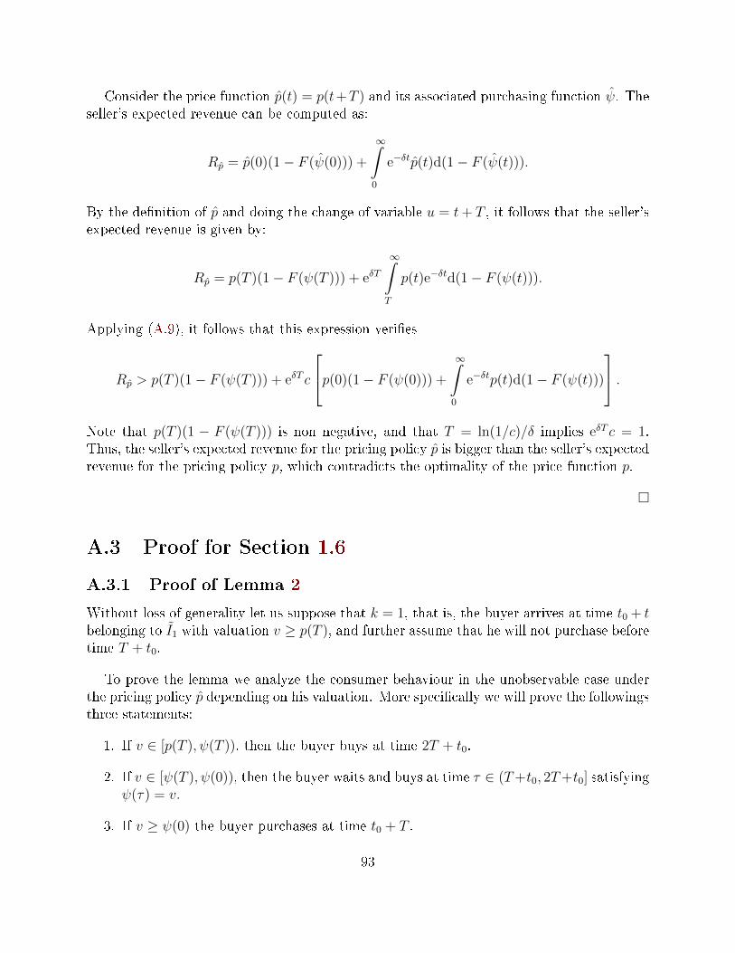
Consider the price function p(t) = p(t+T ) and its associated purchasing function ψ. Theseller's expected revenue can be computed as:

Rp = p(0)(1− F (ψ(0))) +

∞∫0

e−δtp(t)d(1− F (ψ(t))).

By the denition of p and doing the change of variable u = t+ T , it follows that the seller'sexpected revenue is given by:

Rp = p(T )(1− F (ψ(T ))) + eδT∞∫T

p(t)e−δtd(1− F (ψ(t))).

Applying (A.9), it follows that this expression veries

Rp > p(T )(1− F (ψ(T ))) + eδT c

p(0)(1− F (ψ(0))) +

∞∫0

e−δtp(t)d(1− F (ψ(t)))

.Note that p(T )(1 − F (ψ(T ))) is non negative, and that T = ln(1/c)/δ implies eδT c = 1.Thus, the seller's expected revenue for the pricing policy p is bigger than the seller's expectedrevenue for the pricing policy p, which contradicts the optimality of the price function p.

A.3 Proof for Section 1.6

A.3.1 Proof of Lemma 2

Without loss of generality let us suppose that k = 1, that is, the buyer arrives at time t0 + tbelonging to I1 with valuation v ≥ p(T ), and further assume that he will not purchase beforetime T + t0.

To prove the lemma we analyze the consumer behaviour in the unobservable case underthe pricing policy p depending on his valuation. More specically we will prove the followingsthree statements:

1. If v ∈ [p(T ), ψ(T )), then the buyer buys at time 2T + t0.

2. If v ∈ [ψ(T ), ψ(0)), then the buyer waits and buys at time τ ∈ (T+t0, 2T+t0] satisfyingψ(τ) = v.

3. If v ≥ ψ(0) the buyer purchases at time t0 + T .

93

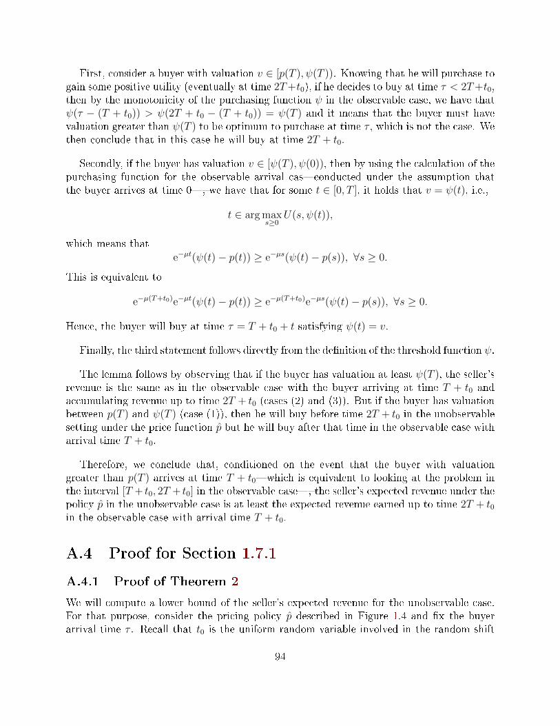
First, consider a buyer with valuation v ∈ [p(T ), ψ(T )). Knowing that he will purchase togain some positive utility (eventually at time 2T+t0), if he decides to buy at time τ < 2T+t0,then by the monotonicity of the purchasing function ψ in the observable case, we have thatψ(τ − (T + t0)) > ψ(2T + t0 − (T + t0)) = ψ(T ) and it means that the buyer must havevaluation greater than ψ(T ) to be optimum to purchase at time τ , which is not the case. Wethen conclude that in this case he will buy at time 2T + t0.

Secondly, if the buyer has valuation v ∈ [ψ(T ), ψ(0)), then by using the calculation of thepurchasing function for the observable arrival casconducted under the assumption thatthe buyer arrives at time 0, we have that for some t ∈ [0, T ], it holds that v = ψ(t), i.e.,

t ∈ arg maxs≥0

U(s, ψ(t)),

which means thate−µt(ψ(t)− p(t)) ≥ e−µs(ψ(t)− p(s)), ∀s ≥ 0.

This is equivalent to

e−µ(T+t0)e−µt(ψ(t)− p(t)) ≥ e−µ(T+t0)e−µs(ψ(t)− p(s)), ∀s ≥ 0.

Hence, the buyer will buy at time τ = T + t0 + t satisfying ψ(t) = v.

Finally, the third statement follows directly from the denition of the threshold function ψ.

The lemma follows by observing that if the buyer has valuation at least ψ(T ), the seller'srevenue is the same as in the observable case with the buyer arriving at time T + t0 andaccumulating revenue up to time 2T + t0 (cases (2) and (3)). But if the buyer has valuationbetween p(T ) and ψ(T ) (case (1)), then he will buy before time 2T + t0 in the unobservablesetting under the price function p but he will buy after that time in the observable case witharrival time T + t0.

Therefore, we conclude that, conditioned on the event that the buyer with valuationgreater than p(T ) arrives at time T + t0which is equivalent to looking at the problem inthe interval [T + t0, 2T + t0] in the observable case, the seller's expected revenue under thepolicy p in the unobservable case is at least the expected revenue earned up to time 2T + t0in the observable case with arrival time T + t0.

A.4 Proof for Section 1.7.1

A.4.1 Proof of Theorem 2

We will compute a lower bound of the seller's expected revenue for the unobservable case.For that purpose, consider the pricing policy p described in Figure 1.4 and x the buyerarrival time τ . Recall that t0 is the uniform random variable involved in the random shift

94

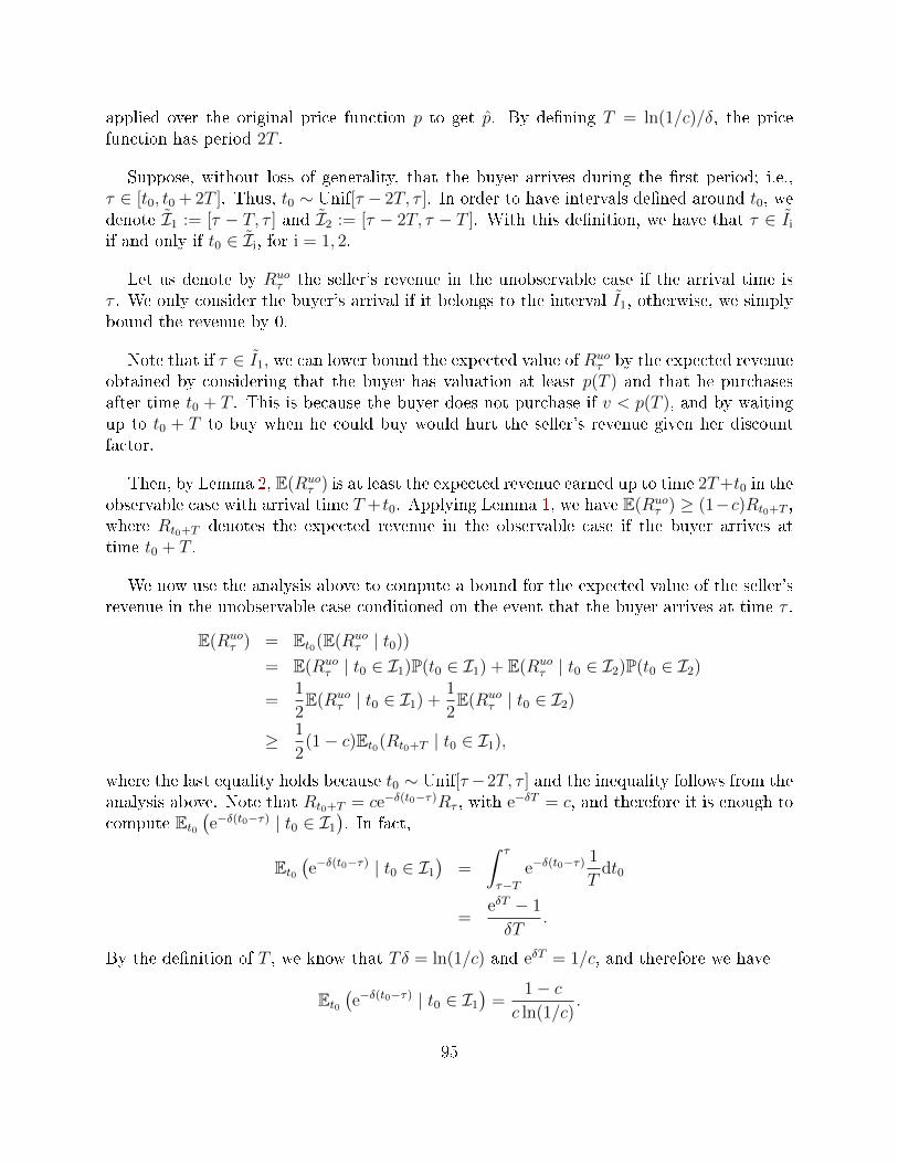
applied over the original price function p to get p. By dening T = ln(1/c)/δ, the pricefunction has period 2T .

Suppose, without loss of generality, that the buyer arrives during the rst period; i.e.,τ ∈ [t0, t0 + 2T ]. Thus, t0 ∼ Unif[τ − 2T, τ ]. In order to have intervals dened around t0, wedenote I1 := [τ − T, τ ] and I2 := [τ − 2T, τ − T ]. With this denition, we have that τ ∈ Ii

if and only if t0 ∈ Ii, for i = 1, 2.

Let us denote by Ruoτ the seller's revenue in the unobservable case if the arrival time is

τ . We only consider the buyer's arrival if it belongs to the interval I1, otherwise, we simplybound the revenue by 0.

Note that if τ ∈ I1, we can lower bound the expected value of Ruoτ by the expected revenue

obtained by considering that the buyer has valuation at least p(T ) and that he purchasesafter time t0 + T . This is because the buyer does not purchase if v < p(T ), and by waitingup to t0 + T to buy when he could buy would hurt the seller's revenue given her discountfactor.

Then, by Lemma 2, E(Ruoτ ) is at least the expected revenue earned up to time 2T+t0 in the

observable case with arrival time T +t0. Applying Lemma 1, we have E(Ruoτ ) ≥ (1−c)Rt0+T ,

where Rt0+T denotes the expected revenue in the observable case if the buyer arrives attime t0 + T .

We now use the analysis above to compute a bound for the expected value of the seller'srevenue in the unobservable case conditioned on the event that the buyer arrives at time τ .

E(Ruoτ ) = Et0(E(Ruo

τ | t0))

= E(Ruoτ | t0 ∈ I1)P(t0 ∈ I1) + E(Ruo

τ | t0 ∈ I2)P(t0 ∈ I2)

=1

2E(Ruo

τ | t0 ∈ I1) +1

2E(Ruo

τ | t0 ∈ I2)

≥ 1

2(1− c)Et0(Rt0+T | t0 ∈ I1),

where the last equality holds because t0 ∼ Unif[τ−2T, τ ] and the inequality follows from theanalysis above. Note that Rt0+T = ce−δ(t0−τ)Rτ , with e−δT = c, and therefore it is enough tocompute Et0

(e−δ(t0−τ) | t0 ∈ I1

). In fact,

Et0(e−δ(t0−τ) | t0 ∈ I1

)=

∫ τ

τ−Te−δ(t0−τ) 1

Tdt0

=eδT − 1

δT.

By the denition of T , we know that Tδ = ln(1/c) and eδT = 1/c, and therefore we have

Et0(e−δ(t0−τ) | t0 ∈ I1

)=

1− cc ln(1/c)

.

95

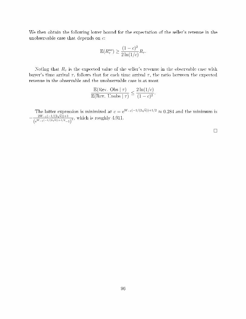
We then obtain the following lower bound for the expectation of the seller's revenue in theunobservable case that depends on c:

E(Ruoτ ) ≥ (1− c)2

2 ln(1/c)Rτ .

Noting that Rτ is the expected value of the seller's revenue in the observable case withbuyer's time arrival τ , follows that for each time arrival τ , the ratio between the expectedrevenue in the observable and the unobservable case is at most

E(Rev. Obs | τ)

E(Rev. Unobs | τ)≤ 2 ln(1/c)

(1− c)2.

The latter expression is minimized at c = eW−1(−1/(2√

e))+1/2 ≈ 0.284 and the minimum is− 2W−1(−1/(2

√e))+1

(eW−1(−1/(2√

e))+1/2−1)2 , which is roughly 4.911.

96

Appendix B

Appendix to Chapter 2

B.1 Proofs for Section 2.4

B.1.1 Proof of Proposition 2

Let us rst show that F (x) ≥ u implies F−1(u) ≤ x. In fact, if F (x) ≥ u then F−1(u) =infw : F (w) ≥ u ≤ x, and we obtain the desire inequality.

It remains to prove that F−1(u) ≤ x implies F (x) ≥ u. If F−1(u) ≤ x, then x ≥F−1(u) = inf A = x0, where A = w : F (w) ≥ u. We divide the rest of the proof in twocases depending on whether x0 belongs to A or not.

Case 1: x0 ∈ A. In this case, F (x0) ≥ u and from the monotonicity of F together withx ≥ x0, follows that F (x) ≥ u.

Case 2: x0 6∈ A. In this case, there exists a sequence xnn ⊂ A such that xn → x0

and xi > x0 ∀i. F is a distribution and by its right-continuity we have that F (x0) =limn→∞ F (xi) ≥ u. Again, from the monotonicity of F together with x ≥ x0, we concludethat F (x) ≥ F (x0) ≥ u, and we conclude the proof.

B.1.2 Proof of Proposition 3

Let us callW to the random variable F−1(U). We will prove thatW is distributed accordingto F . In eect,

P(W ≤ x) = P(F−1(U) ≤ x) = P(U ≤ F (x)) = F (x),

97

where the rst equality follows from the denition of W , the second equality holds dueto Proposition 2, and the last one because U is uniformly distributed. We conclude thatF−1(U) ∼ F .

B.2 Proof for Section 2.5

B.2.1 Proof of Lemma 3

Let us rst assume that G is non-regular. Recall from [110] that φ is constructed troughironing of the virtual valuation function as follows. Take Q(θ) = θG−1(1− θ) and R(·) theconcave hull of Q(·), i.e.,

R(θ) = min xQ(θ1) + (1− x)Q(θ2) : xθ1 + (1− x)θ2 = θ and x, θ1, θ2 ∈ [0, 1] .

That is, R is the smallest concave function on [0, 1] that is above Q. We now dene theironed virtual value as φ(v) = R′(1 − G(v)) and we denote by φ−1 its generalized inverse.Thus,

E(φ(v) | φ(v) ≥ τ)P(φ(v) ≥ τ) =

∫ ∞φ−1(τ)

φ(u)dG(u) =

∫ q

0

R′(θ)dθ = R(q),

where the second equality follows by the denition of φ and q together from performingthe change of variable θ = 1 − G(u). Then, calling q1, q2 and x to the values such thatR(q) = xQ(q1) + (1− x)Q(q2) and using that Q(θ) = θG−1(1− θ), we obtain

R(q) = xq1G−1(1− q1) + (1− x)q2G

−1(1− q2),

and the second part of the lemma follows.

If the distribution is regular, φ is non-decreasing implying that Q is already a concavefunction. Therefore, R = Q and the result follows.

B.2.2 Proof of Theorem 4

We denote by Pt−1 the probability distribution conditional on the history Ht−1, and thenotation extends to the expectation.

We will prove prove that, given an instance for the multi-item auction problem, there existsan α-approximation mechanism. To this end, we dene the algorithm and rst compute itsexpected revenue. Then, we use that the elements selected by the auction are the same asthe ones selected by the online selection algorithm over the instances taken. And nally,by Theorem 3 together with the approximation factor for the online selection algorithm, weobtain the result.

98

Note that the expected revenue of the mechanism is given by the sum, over the elements,of the price times the probability of selling the item.

To simplify the proof, assume rst that the valuations are regular. In that case, weconsider the mechanism given by Algorithm 1. Then, the prices obtained are

(φ+

i

)−1(τi),

where τi is the threshold given by the online selection algorithm, and the expected revenueof the mechanism is given by

n∑t=1

(φ+σ(t)

)−1

(τσ(t))Pt−1

(vσ(t) ≥

(φ+σ(t)

)−1

(τσ(t))

).

By Lemma 3 we have that the above summation equals to

n∑t=1

Et−1

(φ+σ(t)

∣∣∣φ+σ(t) ≥ τσ(t)

)Pt−1

(φ+σ(t)(vσ(t)) ≥ τσ(t)

).

Let χt be the indicator function of the event σ(t) ∈ Alg, that is, χt = 1 whenever σ(t) isselected by the algorithm Alg. We can rewrite the expression above as

E

(n∑t=1

φ+σ(t)(vσ(t))χt

)= E

( ∑i∈Mech

φ+i (vi).

)

Observe that since vi ≥ (φ+i )−1(τi) if and only if φ+

i (vi) ≥ τi for all i ∈ I, Mech selects thesame elements Alg does over the instance (I,Gφ, T ). Therefore, as Alg is an α-approximation,it follows that

E

( ∑i∈Mech

φ+i (vi)

)≥ α · E

(maxS∈T

∑i∈S

φ+i (vi)

).

By Theorem 3, the latter is equal to the expected revenue of the optimal mechanism. Weconclude that mechanism 1 is an α-approximation.

If a distribution is not regular, the posted price mechanism needs to randomize betweentwo prices. Specically, given qi = P(φ+

i (v) ≤ τi) we consider the values x, q1i , q

2i ∈ [0, 1]

obtained from Lemma 3, and dene prices p1i = G−1

i (1−p1i ) and p2

i = G−1i (1−p2

i ). Then themechanism set price p1

i with probability xq1i /qi and price p2

i with probability xq2i /qi. Then,

the expected price isxq1

i G−1i (1− q1

i ) + (1− x)q2i G−1i (1− q2

i )

qi

,

and the rest of the proof is analogous to the previous case by using Lemma 3.

99

B.3 Proofs for Section 2.6

B.3.1 Proof of Proposition 4

Let us rst show the continuity of the function H. For q ∈ [0, 1), H(q) = I(q)/L(q),

where I(q) =1∫q

F−1(y)dy and L(q) = 1 − q. In the interval (0, 1), the function I(q) =∫ 1

qF−1(y)dy is dierentiable due to the calculus fundamental theorem and L(q) = 1 − q is

clearly dierentiable and non-zero. Therefore, H is dierentiable on (0, 1), and in particularcontinuous.

To study the monotonicity of H let us compute the rst derivative of H and analyze itssign. Observe that

H ′(q) =−F−1(q)(1− q) +

∫ 1

qF−1(y)dy

(1− q)2=

1

(1− q)2

1∫q

(F−1(y)− F−1(q))dy,

and F−1(y) − F−1(q) ≥ 0, since F−1 is non-decreasing, and y is at least q. Therefore,H ′(q) = 0 if and only if F−1 equals F−1(q) almost everywhere in [q, 1], which in turn happensif and only if lim

s→F−1(q)−F (s) = q and F (F−1(q)) = 1. Taking T = q the proof follows.

B.3.2 Proof of Proposition 5

1. Note that G is non-decreasing and right-continuous due to Proposition 4. Furthermore,from the denition follows that limt→−∞G(t) = 0 and limt→∞G(t) = 1, and thus G is adistribution. The support of G comes from the fact that H(0) =

∫ 1

0F−1(y)dy = E(w),

H−1(1) = ω1(F ), and G is strictly increasing in the interior of the interval.

2. Let t be in [E(w), ω1(F )). By Proposition 4, G is strictly increasing and continuouson this interval, and therefore invertible. It is then sucient to show that φG(H(q)) =F−1(q) where H(q) = t. In particular, q ∈ [0, T ), with T as in the statement ofProposition 4. Since G is also dierentiable and G−1 = H in this interval, it followsthat

φG(H(q)) = H(q)− 1− qG′(H(q))

= H(q)− (1− q)H ′(q).

On the other hand, from the denition of H we have that

H ′(q) =−F−1(q)(1− q) +

∫ 1

qF−1(y)dy

(1− q)2=−F−1(q) +H(q)

1− q ,

and therefore H(q)− (1− q)H ′(q) = F−1(q), which completes the proof.

100

3. It follows directly from (2) that φG is non-decreasing, as both F−1 and G are non-decreasing. Since φG(E(w)) = F−1(0) = 0, it holds that φG is non-negative which inturn implies that φ+

G = φG.

B.3.3 Proof of Lemma 4

Recall that w is a random variable distributed according to F . Let U be a random variableuniformly distributed between 0 and 1, and dene the random variable v as v = G−1(U),where G is given by the distribution described above. Applying Proposition 3 holds that vhas distribution G and by Proposition 5 (3), φ+

G = φG and therefore it remains to study thedistribution of φG. By Proposition 5 (2), we observe that for t < ω1(F ),

P(φG(v) ≤ t) = P(F−1(G(v)) ≤ t) = P(v ≤ G−1(F (t))) = G(G−1(F (t))) = F (t),

where the second equality follows from Proposition 2, the third holds because v ∼ G, andthe last equality follows since by Proposition 4, G is invertible in [E(w), ω1(F )) and thusG G−1 = I.

B.3.4 Proof of Theorem 5

Let Qt be the event that item σ(t) is selected by Algorithm 2. Recall that we denote by Pt−1

the probability distribution conditional on the history Ht−1, and the notation extends to theexpectation. We denote by 1Qt the indicator function of the event Qt. By conditioning onthe history, we have that

E

(∑x∈Alg

wx

)=

n∑t=1

E(wσ(t)1Qt

)=

n∑t=1

E(Et−1

(wσ(t)1Qt

)).

For t ∈ [n], let x = σ(t) and px = M(Ht−1,G, x) be the price computed byM. SettingR(t) = t(1−Gx(t)), where Gx is the distribution of vx, we claim that Algorithm 2 satisesthat

Et−1 (wx1Qt) = R(px).

Before proving this, we see how to conclude the theorem using the equality above. SinceM is an α-approximation and using Theorem 3, we have that

∑x∈X

px(1−G(px)) ≥ α · E(

maxA∈T

∑x∈A

φ+x (vx)

)= α · E

(maxA∈T

∑x∈A

wx

),

where in the last equality we used the fact that the valuations are obtained from the ValuationMapping Lemma, and that the distributions in F are independent. We remark that for the

101

last equality to be true it is sucient that the distributions in F are independent, and thatφ+x (vx) ∼ Fx for all x ∈ X. In general, if we remove the independence assumption then the

equality does not hold. This proves that Algorithm 2 is an α-approximation.

It remains to prove the equality Et−1 (wx1Qt) = px(1−Gx(px)). To this end, we conditionon whether we are in line 4 or line 5 of Algorithm 2. If the condition in line 4 holds, thenφx(vx) > φx(px) if and only if vx > px. In particular, Pt−1 (Qt) = Pt−1(φx(vx) > φx(px)) =Pt−1(vx > px) = 1−Gx(px). By Lemma 3 and Proposition 5,

Et−1

(wσ(t)|Qt

)= Et−1(φx(vx)|φx(vx) > φx(px)) = px ,

and putting all together we conclude that

Et−1

(wσ(t)1Qt

)= Et−1

(wσ(t)|Qt

)Pt−1 (Qt) = px(1−Gx(px)) = R(px).

Suppose now that the condition of line 5 is satised. By Proposition 6, the function F−1

is constant in the interval [G(p−x ), G(p+x )). In fact, we can nd an explicit expression for Gx

in the interval [p−x , p+x ).

Given q ∈ [Gx(p−x ), Gx(p

+x )], note that we have

H(q) =1

1− q

∫ 1

q

F−1(y)dy =1

1− q

[∫ Gx(p+x )

q

F−1(y)dy +

∫ 1

Gx(p+x )

F−1(y)dy

]

=Gx(p

+x )− q

1− q φx(px) +1

1− q

∫ 1

Gx(p+x )

F−1(y)dy,

where the last equality follows from F−1 being equal to φx(px) in the interval [Gx(p−x ), Gx(p

+x )).

Then, for every p ∈ [p−x , p+x ), we have that

Gx(p) =p− φx(p+

x )Gx(p+x )−

∫ 1

G(p+x )F−1(y)dy

p− φx(p+x )

.

Using the expression of Gx shown above, it follows that

R(p) = φG(p+x )[Gx(p

+x )−Gx(p)] +

∫ 1

Gx(p+x )

F−1(y)dy.

By the denition of θx, Gx(p) = θxGx(p−x ) + (1− θx)Gx(p

+x ) and therefore R(p) = θxR(p−x ) +

(1− θx)R(p+x ). By conditioning on whether line 6 or line 7 holds, we have

Et−1

(wσ(t)χ(Qt)

)= θxEt−1(φx(vx)|φx(vx) ≥ φx(px))Pt−1(φx(vx) ≥ φx(px))

+ (1− θx)Et−1(φx(vx)|φx(vx) > φx(px))Pt−1(φx(vx) > φx(px)).

102

Note that φx(vx) ≥ φx(px) if and only if vx ≥ p−x . On the contrary, φx(vx) > φx(px) if andonly if vx ≥ p+

x . Thus, the expression above is equivalent to

θxEt−1(φx(vx)|vx ≥ p−x )Pt−1(vx ≥ p−x ) + (1− θx)Et−1(φx(vx)|vx > p+x )Pt−1(vx > p+

x ).

Using Lemma 3 together with the denition of R, we conclude that

Et−1

(wσ(t)1Qt

)= θxp

−x (1−Gx(p

−x )) + (1− θx)p+

x (1−Gx(p+x ))

= θxR(p−x ) + (1− θx)R(p+x ) = R(px).

103

Appendix C

Appendix to Chapter 3

C.1 Additional material

C.1.1 Static Probabilistic Control Heuristic

The static probabilistic control heuristic consists on setting the policy πt = φ∗1 for all t untilstock is out, where φ∗1 is an optimal solution of (3.2) taking ρ = C/T . This heuristic isdescribed in Algorithm 4 and gave us a feasible solution of problem (3.1), namely JS.

This heuristic was already studied in the revenue management literature (see e.g. [116],[34]) and its well know that the policy obtained from the SPC heuristic has a revenue lossof O(

√T ) for dierent online section problems. For completeness, we give a proof of this

result, for the class of DRCRC problems, stated in the following lemma.

Lemma 11. If we call JS the value of the feasible solution of Problem (3.1) given by theSPC heuristic described above, the revenue loss is O(

√T ), that is,

J∗ − JS ≤ O(√T ).

Proof. Note that taken an optimal solution of (3.2) for ρ = C/T , namely φ∗, we have that

J(C/T ) =∑θ∈Θ

pθ

∫A

Eε(r(θ, aφ

∗, ε))

dφ∗θ(a).

The value of the objective function of problem (3.1) by considering the policy π that at

104

each time period applies the optimal solution φ∗ is given by

T∑t=1

Eεt

∑θt∈Θ

pθt

∫A

r(θt, aπt , εt) dφ∗θ(a)

= TJ(C/T ). (C.1)

Since π might not be feasible, to get JS we have to subtract from (C.1) the revenueassociated to customers who are not served because of the lack of capacity, which is upperbounded by

L∑l=1

rlmaxE

( T∑t=1

yl(θt, aπt , εt)− Cl

)+ ,

where rlmax is the largest extra revenue gain by increasing the capacity of resource l by oneunit.

Thus,

J∗ − JS ≤L∑l=1

rlmaxE

( T∑t=1

yl(θt, aπt , εt)− Cl

)+

and in the rest of the proof we will bound right hand side in the inequality above.

In what follows, we will write yt,l to refer to yl(θt, aπt , εt).

Due to φ∗ is an optimal solution of (3.2) for ρ = C/T , if the associated resource con-sumption for each resource l is given by yl, we have that

T∑θ∈Θ

∫A

Eε(yl) dφ∗θ(a) ≤ Cl,

and therefore

E

( T∑t=1

yt,l(θt, aπt , εt)− Cl

)+ ≤ E

( T∑t=1

yt,l − TE(yl)

)+

≤ E

(∣∣∣∣∣T∑t=1

yt,l − TE(yl)

∣∣∣∣∣),

where the last inequality follows because the positive part of a real value is always upperbounded by its absolute value.

105

Furthermore, the square root function is concave and applying Jensen's inequality togetherwith the independence of variables yt,lt and that E

(∑Tt=1 yt,l

)= TE(yl), we obtain

E

(∣∣∣∣∣T∑t=1

yt,l − TE(yl)

∣∣∣∣∣)≤

√√√√√E

( T∑t=1

yt,l − TE (yl)

)2

=

√√√√Var

(T∑t=1

yt,l

)

=

√√√√ T∑t=1

Var (yt,l) .

Note that Var(yt,l) ≤ E(y2t,l

), and by assumption made at the beginning of Section 3.6

we obtain √√√√ T∑t=1

Var (yt,l) ≤√T y∞ .

Putting all together, we conclude that

J∗ − JS ≤√T y∞

∑l

rlmax ,

and the result follows.

Algorithm 4 Static Probabilistic Control Heuristic (SPC)1: Initialize c1 ← C,2: φ∗1 ← an optimal solution of Problem 3.2 with ρ = C/T3: for t = 1 to T do observe the opportunity class θt4: draw an action at with probability φ∗ρt(θt, at)5: if y(θt, at, ε) ≤ ct, ∀ε ∈ E , then choose the action at6: observe the shock εt7: ct+1 ← ct − y(θt, at, εt)8: else choose action a0.

C.1.2 Finite set of actions

Problem 3.8 is a linear program. In particular, introducing the set of slack variablesx1 . . . xL, the standard form is given by

106

J(ρ) = maxΘ∑θ=1

pθ rθφθ

s.t∑θ∈Θ

pθ ylθ φθ + xl = ρl ∀l ∈ [L]∑a∈A

φθ(a) = 1 ∀θ ∈ Θ

φθ(a) ≥ 0 ∀θ ∈ Θ, ∀a ∈ Axi ≥ 0 ∀i ∈ [L].

(C.2)

C.1.3 Dynamic bidding in repeated auctions

Second-price auctions

Lemma 12. If f absolutely continuous and strictly increasing and f ′ is locally ξ-Lipschitzcontinuous in N (a1

θ, ϕ), then conditions CA 1- CA 6 hold.

Proof. Let us see that conditions CA 1- CA 6 hold.

Conditions CA 1 and CA 2: By hypothesis f is absolutely continuous and thereforeboth q and m are continuous.

Condition CA 3: For each θ ∈ Θ, tet us dene the function Gθ : A → R by Gθ(a) =θf(a)−

∫ a0x df(x). Note that G′θ(a) = (θ − a)f ′(a) and θ > 0, then lima0G

′θ(a) > 0

and β(θ) 6= 0. If θ 6= Θmax, we also have lima→0G′θ(a) < 0, and therefore β(θ) ∈

arg maxaGθ(a) is interior. Assume then rst that θ 6= Θmax. In this case, we cancompute the rst order condition, obtaining that β(θ) satises the equation

(θ − β(θ))f ′(β(θ)) = 0.

Therefore, as the cumulative distribution function f is strictly increasing, the uniqueoptimum is to bid truthfully, as it is known in the literature.

Otherwise, if θ = Θmax, Gθ is strictly increasing for all a ∈ A and therefore β(θ) =Θmax.

We then conclude that CA 3 holds.

Condition CA 4: Due to the truthfulness property of the second price auction, fromProposition 9, it follows that a1

θ = θ/(1 +µ1) which belongs to (0,Θmax) due to the bidis positive, and thus condition CA 4 holds.

Conditions CA 5 and CA 6: Note rst that r(θ, a) = θf(a)− m(θ, a) and y(θ, a) =m(a), because f absolutely continuous. Then, it is enough to show the conditions

107

hold for h(θ, ·) = θf(·) and m(a) =∫ a

0x df(x). Specically, we will show that if the

density function f ′ is locally ξ-Lipschitz continuous in N (a1θ, ϕ), then the gradient of

h(θ, ·) = θf(·) is locally (ξΘmax)-Lipschitz continuous in N (a1θ, ϕ) and m′(a) = af ′(a)

is locally ((ϕ+ Θmax/(µ1 + 1))ξ + η)−Lipschitz continuous in N (a1

θ, ϕ).

To see the former note that

‖∇ah(θ, a)−∇ah(θ, a1θ)‖ = θ|f ′(a)− f ′(a1

θ)| ≤ Θmaxξ|a− a1θ|,

where the equality follows from the gradient of h and the inequality holds due to thelocally ξ−Lipschitz continuity of f ′ and because θ ≤ Θmax.

For the latter, we rst show that f ′(a1θ) ≤ η with η = 1/ϕ + ξϕ. Because the density

f ′ is locally ξ-Lipschitz continuous in N (a1θ, ϕ), we have that f ′(a1

θ) ≤ f ′(x) + ξϕ forall x ∈∈ [a1

θ, a1θ +ϕ]. Integrating over x ∈ [a1

θ, a1θ +ϕ] we obtain that f ′(a1

θ)ϕ ≤ 1 + ξϕ2

because f ′ integrates to at most one. The result follows by dividing by ϕ. We nowshow that m′(a) is locally Lipschitz continuous:

|m′(a)− m′(a1θ)| = |af(a)− a1

θf(a1θ)|

= |a[f ′(a)− f ′(a1

θ)]

+ f ′(a1θ)(a− a1

θ)|≤ a|f ′(a)− f ′(a1

θ)|+ f ′(a1θ)|a− a1

θ|

≤((

ϕ+Θmax

µ1 + 1

)ξ + η

)|a− a1

θ|,

where the rst inequality holds applying triangle inequality and the last follows fromthe bound of f ′(a1

θ), together with the locally ξ−Lipschitz continuity of f ′, the equalitya1θ = θ/(1 + µ1) and the bound a1

θ ≤ Θmax. The proof is completed.

First-price auctions

Lemma 13. If f absolutely continuous, M(a) = a+f(a)/f ′(a) strictly increasing, the bid a1θ

maximizing θq(a)−(µ1+1)m(a) is interior, and the density function f ′ is locally ξ−Lipschitzin N (a1

θ, ϕ), and f ′(a1θ) is upper bounded by η, conditions CA 1- CA 6 hold.

Proof. As in the lemma for second-price auctions, conditions CA 1 and CA 2 holds becausef is absolutely continuous. On the other hand, the bidder's problem in the static rst priceauction without budget constraints is to nd a bid function β(θ) maximizing (θ − a)f(a).Note that arg max θf(a) − af(a) = arg max θ′f(a) − (µ1 + 1)af(a), where θ′ = θ/(µ1 + 1),is interior by hypothesis and then, computing the rst order condition, we obtain that β(θ)should satisfy

f ′(β(θ))θ − f(β(θ))− β(θ)f ′(β(θ)) = 0. (C.3)

Then, we have θ = β(θ) + f(β(θ))/f ′(β(θ)) = M(β(θ)) and by hypothesis we can computethe inverse of M and therefore β(θ) = M−1(θ). Thus, payments at the optimal solution areunique and assumption CA 3 holds.

108

Note that condition CA 4 is directly assumed in the statement of the lemma, and thereforeit holds.

It remains to see smoothness of both the expected reward r(θ, a) = (θ − a)f(a) andexpected payment y(a) = af(a) functions, but it is enough to show that the gradient ofy(θ, a) is locally Lipschitz continuous. To this end, note that

|∇ay(θ, a)| = |f(a) + af(a)− f(a1θ)− a1

θf(a1θ)| ≤ |f(a)− f(a1

θ)|+ |af(a)− a1θf′(a1

θ)|,

where the last expression in the inequality can be bound by using the local Lipschitz conti-nuity of f ′ together with the upper bound for f ′ (as in the case of the second-price action,we have that f ′(a1

θ) is bounded) by using the mean value theorem. The remaining algebrais similar to the second-price case and the proof is completed.

C.2 Proof Theorem 6

The goal of this section is to proof Theorem 6, which is our mean result regarding theperformance of the heuristic CE for the set of DRCRC problems. To do that, we assumethat Assumption 1 and Assumption 2 hold and we rst introduce some processes and randomvariables, as well as technical results, that will be useful to obtain the desire result.

In what follows we will denote by yt the resource consumption at time t if the decisionmaker follows the policy πCE. That is, yt = y(θt, a

πCE

t , εt).

Let us consider the process Mtt≥1 up to time T consisting in, at each time period,the accumulated dierence between the resource vector consumption and its expectation,divided the remaining horizon. More specically, for each t ∈ [T ],

Mt =t∑

s=1

E (ys|ρs)− ysT − s .

Let us dene the stopping time τ. To this end, we need to introduce two random variables.On one hand, we dene τδ to be the rst time t such that Mt has `2-norm greater or equalthan δ, where δ is got form Assumption 2. That is,

τδ = mint∈[T ]t : ‖Mt‖ ≥ δ.

If ‖Mt‖ is at most δ for all t ∈ [T ], we set τδ =∞.

On the other hand, we dene τ− as the rst time at which there exists a resource suchthat its consumption under the policy φ∗ρt is over capacity. That is,

τ− = mint∈[T ]t : ∃ l ∈ [L] s.t. ct,l − yl(θt, aφ

∗ρt , εt) < 0.

109

As above, if ct,l − yl(θt, aφ∗ρt , εt) is greater or equal to 0 for all t ∈ [T ] and l ∈ [L], we set

τ− =∞.

Then, we dene the random variable τ as the minimum between τδ and τ−, and thenumber of periods T , i.e., τ = minτδ, τ−, T.

Note that both τδ and τ− are stopping times with respect to the ltration Ftt≥1, withFt = σ(θ1, . . . , θt, a1, . . . , at, ε1, . . . , εt), the history up to the end of period t, and thus weobtain that τ is also a stopping time with respect to the same ltration Ftt≥1.

Furthermore, the process Mtt≥1 is a martingale with respect to the ltration Ftt≥1.In fact, for each t, from Assumption 1.2 follows that E(yt|ρt)− yt ≤ y∞ <∞, and thereforeE(‖Mt‖) <∞ for all t. On the other hand, for each t holds that

Mt+1 −Mt =E(yt+1|ρt)− yt+1

T − t− 1

andE (E(yt+1|ρt)− yt+1|Ft) = 0,

concluding thatE(Mt+1 −Mt|Ft) = 0 ∀t ≥ 1.

Since Mtt≥1 is a martingale and τ an stopping time, it turns out that the stoppedprocess Mt∧τt≥1 is also a martingale with respect to the ltration Ftt≥1.

We are now ready to present some properties for the process and the stopping time denedabove, that will be needed to prove the bound for the reward loss. The rst of them statesthat up to time τδ, the random variable Mt can be expressed as the dierence between ρt+1

and ρ1 and that ρt belongs to the ball centered at ρ1 with radius δ.

Lemma 14. Under Assumption 2, if t is at most τδ, it holds that:

1. ρt+1 − ρ1 = Mt

2. ‖ρt − ρ1‖ < δ.

Proof. We will proceed by induction on t, dividing the proof into two steps, the rst corre-sponds to prove the base case and the other the induction step.

Step 1. Note that for t = 1, the statement 2 of the lemma follows trivially and we are thenunder the hypothesis of Assumption 2, obtaining E(y1|ρ1) = ρ1. Therefore, we can expressM1 as follows:

M1 =E(y1|ρ1)− y1

T − 1=ρ1 − y1

T − 1. (C.4)

110

From the denition of ρ1 and ρ2, we have that y1 = ρ1T − ρ2(T − 1) and replacing in(C.4) follows that

M1 =ρ1 − ρ1T + ρ2(T − 1)

T − 1= ρ2 − ρ1,

obtaining the rst statement of the lemma and completes the step 1.

Step 2. Now, assume that Lemma 14 holds for all s smaller or equal than a xed t < τδand let us prove that both statements also hold for t+ 1.

As in the base case, we will rst prove the statement 2 and we then use it to provestatement 1. That is, let us show that ‖ρt+1 − ρ1‖ < δ. Applying the induction hypothesisto t, it holds that ‖ρt+1 − ρ1‖ = ‖Mt‖. On the other hand, t < τδ and thus ‖ρt+1 − ρ1‖ < δ,concluding that ‖Mt‖ < δ, and the second statement follows.

In the remainder of the proof, we show that ρt+2 − ρ1 = Mt+1.

Note that

ρt+2 − ρ1 =t+1∑s=1

ρs+1 − ρs =t+1∑s=1

ρs(T − s+ 1)− ysT − s − ys =

t+1∑s=1

ρs − ysT − s ,

where the rst equality is obtained by using a telescoping sum and the second holds becauseρs+1 = cs+1/(T − s), cs = ρs(T − s+ 1) and cs+1 = cs − ys.

By the induction hypothesis, together with the statement 2 we already proved for s = t+1,it holds that ‖ρs − ρ1‖ < δ for all s ≤ t + 1. Therefore we can apply Assumption 2 to theexpression above obtaining that

ρt+2 − ρ1 =t+1∑s=1

E(ys|ρs)− ysT − s = Mt+1,

and the lemma follows.

Since Mt∧τt≥1 is a zero mean martingale with respect to the ltration Ftt≥1, a directconsequence of Lemma 14 is that also the stopped process ρt∧τt≥1 is a martingale withrespect to the same ltration.

The following lemma is a technical result we need to prove that the expected value ofthe remaining periods after the stopping time τ is bounded by a constantresult stated inLemma 16. Specically, it gives us sucient conditions on t to be a lower bound for thestopping time τ−.

111

Lemma 15. Let assume that Assumption 1 and 2 hold, and dene Ψ = y∞ρ1−δ , where ρ1 is

the smallest component of vector ρ1, and T− = T +1−Ψ. If t ≤ T−, and t < τδ then t < τ−.

Proof. Due to the denition of the stopping time τ−, we have to show that for all s ≤ t, theconsumption is at most the available capacity, i.e., y(θs, a

φ∗ρs , εs) ≤ cs.

Take s ≤ t. By hypothesis, s < τδ and by Lemma 14 it holds that ‖ρs − ρ1‖ < δ. Inparticular, |(ρs − ρ1)l| < δ ∀l ∈ [L], obtaining

ρs > ρ1 − 1δ , (C.5)

where 1 denotes the vector of ones of size L. On the other hand, note that

cs > (T − s+ 1)(ρ1 − 1δ) ≥y∞

ρ1 − δ(ρ1 − 1δ) ≥ 1y∞ ≥ y(θs, a

φ∗ρs , εs),

where the strict inequality follows from the denition of ρs, together with inequality (C.5);the second inequality holds because t ≤ T− and ρ1 > δ, together with Assumption 1.2; andthe third and the last due to the denition of ρ1 and y∞, respectively.

We then conclude that τ− is greater than t and the proof is completed.

Below we prove a result stating that the expected value of the remaining periods afterthe stopping time τ is upper bounded by a constant that does not depend on T , which is akey result to obtain the main theorem.

Lemma 16. If Assumptions 1 and 2 hold, there exists a constant µ such that E(T − τ) ≤ µ.More specically,

E(T − τ) < Ψ + 14y2∞δ2.

Proof. We will prove the result by bounding the expected value of τ , which is equivalentto the expression

∑∞t=1 P(τ ≥ t) because τ is a non-negative random variable. From the

denition of τ , the probability of τ being greater than T is zero and the probability of beingat least one is one, and then,

E(τ) = 1+T∑t=2

P(τδ∧τ− ≥ t) = 1+T−−1∑t=2

P(τδ∧τ− ≥ t)+T∑

t=T−

P(τδ∧τ− ≥ t) ≥ 1+T−−1∑t=2

P(τδ∧τ− ≥ t)

(C.6)where the last equality follows just splitting the horizon and the inequality holds becauseP(τδ ∧ τ− ≥ t) ≥ 0.

112

On the other hand,

T−−1∑t=2

P(τδ ∧ τ− ≥ t) =T−−1∑t=2

P(

mins∈[T ]s : ‖Ms‖ ≥ δ ≥ t

)

=T−−1∑t=2

P (‖Ms‖ < δ ∀s ∈ [t])

= T− − 2−T−−1∑t=2

P(

maxs∈[t]‖Ms‖ ≥ δ

),

where the rst equality is obtained by Lemma 15 (since t < T−, τδ ∧ τ− = τδ) and the lastone because P(‖Ms‖ < δ ∀s ∈ [t]) = 1− P(maxs∈[t] ‖Ms‖ ≥ δ).

Then, using the equality above in (C.6) it holds that

E(τ) ≥ T− − 1−T−−1∑t=2

P(

maxs∈[t]‖Ms‖ ≥ δ

).

In the remainder of the proof we will upper boundT−−1∑t=2

P(maxs∈[t] ‖Ms‖ ≥ δ

), and we pro-

ceed by applying Theorem 3.5 in [115]. To this end, note rst that (RL, ‖ · ‖) is a separableBanach space, and since ‖x + y‖ + ‖x − y‖ ≤ 2‖x‖2 + 2‖y‖2 holds for all x, y ∈ R+, itis (2, 1)-smooth. Dene, for each t, the Martingale Mt∧ss≥1. From the denition of Ms

follows that

Ms −Ms−1 =E(ys|ρs)− ys

T − s ,

and therefore∞∑s=1

‖Ms −Ms−1‖2∞ =

t∑s=1

‖Ms −Ms−1‖2∞

=t∑

s=1

∥∥∥∥E(ys|ρs)− ysT − s

∥∥∥∥2

∞

≤ (2y∞)2 1

T − t ,

where the inequality follows from Assumption 1.2, and using that∑t

s=1 1/(T − s)2 ≤∫ t0

1/(T − s)2 < 1/(T − t).

Then, we are under the hypothesis of the theorem mentioned above, and applying ittogether with the inequality P

(maxs∈[t] ‖Ms‖ ≥ δ

)≤ 1, we obtain

P(

maxs∈[t]‖Ms‖ ≥ δ

)≤ 1 ∧ 2 exp

(−δ

2(T − t)8y2∞

).

113

Summing on t and using the bound obtained above, we have

T−−1∑t=2

P(

maxs∈[t]‖Ms‖ ≥ δ

)≤

T∑t=2

(2 exp

(−δ

2(T − t)8y2∞

)∧ 1

)

≤T∫

0

(2 exp

(−δ

2(T − t)8y2∞

)∧ 1

)dt

≤ 8y2∞δ2

(log 2 + 1) ,

where the second inequality follows from bounding the summation by the integration andthe last inequality from Lemma 17.

Putting all together and bounding 8(log 2 + 1) by 14 we conclude

E(T − τ) < T − T− + 1 + 14y2∞δ2

= Ψ + 14y2∞δ2,

and the desire result is obtained.

We are now ready to prove Theorem 6 by combining the technical results already pre-sented.

Proof of Theorem 6. We have to bound J∗−JCE, which is upper bounded by TJ(ρ1)−JCE

because J∗ ≤ TJ(C/T ) (see, e.g., [66]). Thus, it is enough to bound TJ(ρ1)− JCE.

By dividing the horizon from 1 to τ and from τ to T , we obtain

TJ(ρ1)− JCE ≤ E

(τ∑t=1

J(ρ1)−τ∑t=1

r(θt, aCEt , εt)

)︸ ︷︷ ︸

(A)

+E

(T∑

t=τ+1

J(ρ1)

)︸ ︷︷ ︸

(B)

, (C.7)

and we then have to bound (A) and (B), which will be done in Part 1 and Part 2 separately,respectively.

Part 1. We will prove that (A) ≤ K/2y22 log T, and we divide the proof into three steps.

First, we show that the expected reward earned up to time τ considering the policy givenby the CE heuristic equals the expected reward until time τ of the deterministic problem for

114

ρ = ρt at time t. Using that, applying Assumption 2- the hypothesis is fullled because t ≤ τand then by Lemma 14 we have ‖ρt − ρ1‖ < δ-, summing over t and taking expectation, weobtain

(A) = E

(τ∑t=1

(J(ρ1)− J(ρt))

)≤ E

(τ∑t=1

−∇J(ρ1)(ρt − ρ1)

)︸ ︷︷ ︸

(A1)

+E

(τ∑t=1

K

2‖ρt − ρ1‖2

)︸ ︷︷ ︸

(A2)

.

In the second step we bound (A1) and in step 3 we bound (A2).

Step 1. Let us prove that

E

(τ∑t=1

r(θt, aCEt , εt)

)= E

(τ∑t=1

J(ρt)

). (C.8)

To this end, consider the sequence of zero mean, i.i.d. random variables Xtt≥1 given by

Xt = r(θt, aCEt , εt)− Eθ,ε

(r(θt, a

CEt , εt)|ρt

).

Then, it is well known (see e.g. [118] page 296) that dening Ns =∑s

t=1Xt, holds thatNss≥1 is a martingale relative to the ltration Ftt≥1 previously dened. Therefore, dueto τ is an stopping time with respect to the same ltration, we can apply the MartingaleStopping Theorem ([118], Theorem 6.6.2), which in turns implies that

E (Nτ ) = E (N1) = 0. (C.9)

On the other hand, by the denition of the deterministic problem, we have that

Eθ,ε(r(θt, a

CE, εt)|ρt)

= J(ρt) ∀t ∈ [T ]. (C.10)

Then, (C.8) follows easily from (C.9) and (C.10).

Step 2. We want to bound (A1). In fact, we will prove that it is equal to zero. From thelinearity of the expectation, (A1) is equivalent to

τ∑t=1

−∇J(ρ1)E (ρt − ρ1) .

Furthermore, note that E (ρt − ρ1) is zero because ρt∧τt≥1 is a martingale, and the term(A1) vanishes in the bound, obtaining (A) ≤ (A2).

115

Step 3. Regarding (A2), by linearity of the expectation, it is enough to bound the expressionE (||ρt − ρ1||2), for t ≤ τ. Using telescoping sum and the orthogonality of the martingale'sincrements (see e.g. [78], Chapter 10 Lemma 4.1) we have

E(‖ρt − ρ1‖2

)= E

∥∥∥∥∥t∑

s=2

(ρs − ρs−1)

∥∥∥∥∥2

=t∑

s=2

E‖ρs − ρs−1‖2, (C.11)

and therefore in the remainder of this step we bound ‖ρs − ρs−1‖2. Note that

‖ρs − ρs−1‖2 =

∥∥∥∥ρs−1(T − s+ 2)− ys−1

T − s+ 1− ρs−1

∥∥∥∥2

=

∥∥∥∥ρs−1 − ys−1

T − s+ 1

∥∥∥∥2

=

∥∥∥∥E(ys−1|ρs−1)− ys−1

T − s+ 1

∥∥∥∥2

,

where the rst equality follows from the denitions ρs = csT−s+1

, ρs−1 = cs−1

T−s+2and cs =

cs−1 − ys−1; and the last equality follows from Assumption 2.

Furthermore, by denition of `2-norm, holds that

‖E(ys−1|ρs−1])− ys−1‖2 =∑l∈[L]

(E(ys−1,l|ρs−1)− ys−1,l)2 ,

and taking expectation follows that

E(‖E(ys−1|ρs−1)− ys−1‖2

)=∑l∈[L]

E((E(ys−1,l|ρs−1)− ys−1,l)

2) =∑l∈[L]

Var(ys−1,l).

Using that Var(ys−1,l) = E ((ys−1,l)2)−E (ys−1,l)

2 ≤ E ((ys−1,l)2) , together with the linearity

of the expectation we have

∑l∈[L]

Var(ys−1,l) ≤∑l∈[L]

E((ys−1,l)

2)

= E

∑l∈[L]

(ys−1,l)2

≤ y22 ,

where the last inequality follows from Assumption 1.2.

Getting back to expression (C.11), we nally obtain

E(‖ρt − ρ1‖2

)≤

t∑s=2

y22

(T − s+ 1)2≤ y2

2

t∫2

1

(T − s+ 1)2ds ≤ y2

2

T − t+ 1,

116

and therefore by doing the suitable computations we obtain (A2) ≤ K/2y22 log T, concluding

the proof of Step 3.

Putting all together we get

E

(τ∑t=1

(J(ρ1)− J(ρt))

)≤ K

2y2

2 log T , (C.12)

and the proof of Part 1 is complete.

Part 2. It only remains to bound the second term in (C.7). Note that

E

(T∑

t=τ+1

J(ρ1)

)= E(T − τ)J(C/T ),

and applying Lemma 16 we obtain

E

(T∑

t=τ+1

J(ρ1)

)≤[Ψ + 14

y2∞δ2

]J(C/T ). (C.13)

Using (C.12) together with (C.13) in (C.7) we get

J∗ − JCE ≤ y22K log T +

[Ψ + 14

y2∞δ2

]J(C/T ),

and the result follows.

C.3 Proofs for Section 3.7

C.3.1 Proof of Proposition 7

We divide the proof into two steps. First, we prove that an optimal solution to the dualproblem exists, namely µ∗. Then, we dene φ∗ properly and we apply Proposition 5.1.5 in[23] to prove that φ∗ is primal solution and µ∗ is in fact a Lagrangian multiplier and thattherefore there is no duality gap, obtaining the desire result.

Step 1. Note that for each θ ∈ Θ, gθ is convex because it is dened as the supremum of afamily of linear functions and therefore the dual problem is a convex problem.

To prove the existence of optimal dual solution µ∗, we rst prove Ψρ is dierentiable (andthus continuous) and then we argue that the domain of the dual problem can be restricted to

117

a compact set, achieving the result applying the extreme value theorem. For the former, itis enough to note that gθ(µ) is dierentiable by Assumption SC 1, and in particular we havethat Ψρ is continuous. On the other hand, we can prove that we can restrict the domainof the dual problem to the hypercube [0, µρ]

L, for µρ = r∞/ρ, where ρ = minl∈[L] ρl andr∞ is the positive real number provided by Assumption1.1. We have that µρ < ∞ becauseρ > 0. Let us check that every µ 6∈ [0, µρ]

L is suboptimal. Take µ 6∈ [0, µρ]L, and dene

L1 = l ∈ [L] : µl > µρ the components of µ greater than µρ. Then, we have

Ψρ(µ) ≥ ρ>µ ≥∑l∈L1

ρlµl =∑l∈L1

r∞ρlρ≥ r∞ ≥ Ψρ(0),

where the rst inequality holds because r(θ, a0) = y(θ, a0) = 0, for all θ ∈ Θ and thereforegθ(µ) ≥ 0; the second follows from the non-negativity of vectors µ and ρ, the third inequalityholds because L1 contains at least one element and ρl ≥ ρ, and the last one follows becauseΨρ(0) =

∑θ∈Θ pθ maxa∈A r(θ, a) and r∞ ≥ r(θ, a) for all θ ∈ Θ, and a ∈ A. Then, we have

Ψρ(0) ≤ Ψρ(µ) and together with the extreme value theorem we conclude that for each ρ > 0there exist µ∗ optimal dual solution satisfying µ∗ ∈ [0, µρ]

L.

Step 2. Given ρ > 0, take µ∗ an optimal dual solution and, for each θ ∈ Θ, dene φ∗θ adistribution that assigns probability one to an action a∗θ ∈ arg maxa∈A

r(θ, a)− µ∗>y(θ, a)

.

Such actions are guaranteed to exist by Assumption SC 1. Let us now show that (φ∗, µ∗)is an optimal solution-Lagrange multiplier pair. We will proceed by using Proposition 5.1.5in [23]. That is, we need to check primal and dual feasibility, Lagrangian optimality andcomplementary slackness.

1. Primal and dual feasibility. Dual feasibility follows because µ∗ ≥ 0. For primal fea-sibility, note that from the envelope theorem applied to gθ (see, e.g., Theorem 1 in[108]), the gradient of Ψρ evaluated at µ∗ is given by

∇Ψρ(µ∗) = ρ+

∑θ∈Θ

pθ∇gθ(µ∗) = ρ−∑θ∈Θ

pθy(θ, a∗θ) , (C.14)

where we used that by SC 1 the value function gθ(µ) is dierentiable and achieved foran action a∗θ, and that the gradient of r(θ, a)− µ>y(θ, a) with respect to µ exists andis given by y(θ, a). Because µ∗ is an optimal dual solution and the constraint set isconvex, by Proposition 2.1.2 in [23], the rst-order conditions are given by

∇Ψρ(µ∗)>(µ− µ∗) ≥ 0, ∀µ ∈ RL

+ . (C.15)

Letting µl →∞, we obtain that∇Ψρ(µ∗) ≥ 0, which, in turn, implies that

∑θ∈Θ pθy(θ, a∗θ) ≤

ρ by (C.14). Primal feasibility follows.

2. Complementary slackness. If µ∗l = 0, we trivially have (∇Ψρ(µ∗))lµ

∗l = 0 and com-

plementary slackness follows. If µ∗l > 0, we can take ν > 0 with µ∗l + ν and µ∗l − ν

118

belonging to R+. Using (C.15), we obtain that (∇Ψρ(µ∗))lν ≥ 0 and (∇Ψρ(µ

∗))lν ≤ 0.Thus, it holds that (∇Ψρ(µ

∗))l = 0 and complementary slackness follows.

3. Lagrangian optimality. Note that

arg maxφ∈ΦL(φ, µ∗) = arg max

φ∈Φ

µ∗ρ+∑θ∈Θ

pθ

∫A

(r(θ, a)− µ∗>y(θ, a)

)dφθ(a)

=

arg maxφθ∈∆(A)

∫A

(r(θ, a)− µ∗>y(θ, a)

)dφθ(a)

θ∈Θ

=

arg max

a∈Agθ(µ

∗)

θ∈Θ

,

where the second equality holds because we can separate the problem for each θ. Butnote that gθ(µ∗) is maximized at a∗θ and thus we have Lagrangian optimality.

Therefore, the four conditions hold and the proof is complete.

C.3.2 Proof of Lemma 7

We have to show that if ρ ∈ N (ρ1, δ), with δ = (νκ)/2 then it holds that

1. J(ρ) ≥ J(ρ1) +∇J(ρ1)(ρ− ρ1)− 12κ‖ρ− ρ1‖2,

2.∑

θ∈Θ pθ∫ay(θ, a) dφ∗θ(a) = ρ.

Part 1. We rst extend the strong convexity lower bound of gθ to the entire domain. Givenθ ∈ Θ, by SC 2, gθ admits a κ-LUQ envelope in Iν = N (µ1, ν). Then, for all µ ∈ Iν .

gθ(µ) ≥ gθ(µ1) +∇gθ(µ1)>(µ− µ1) +

κ

2‖µ− µ1‖2 . (C.16)

We next extend the lower bound to every feasible dual variable. Consider µ ≥ 0 with µ 6∈ Iν .Take α such that αµ+ (1−α)µ1 = µ where µ is in the boundary of the ball Iν , i.e., µ ∈ ∂Iν .The latter is possible because µ 6∈ Iν . Note that µ − µ1 = α(µ − µ1). Taking `2-norm inboth sides, we get that α = ‖µ− µ1‖/‖µ− µ1‖. Moreover, α ∈ (0, 1) because µ1 is interiorsince ν > 0 and µ 6∈ Iν . Because gθ is convex, we have

αgθ(µ) + (1− α)gθ(µ1) ≥ gθ(αµ+ (1− α)µ1) = gθ(µ) ,

119

which can be reordered to give

gθ(µ) ≥ 1

αgθ(µ)− 1− α

αgθ(µ

1)

≥ 1

αgθ(µ

1) +1

α∇gθ(µ1)>(µ− µ1) +

κ

2α‖µ− µ1‖2 − 1− α

αgθ(µ

1)

= gθ(µ1) +

1

α∇gθ(µ1)>(µ− µ1) +

κ

2α‖µ− µ1‖2 ,

= gθ(µ1) +∇gθ(µ1)>(µ− µ1) +

κν

2‖µ− µ1‖ ,

where the second inequality follows by (C.16) with µ = µ and the second equality fromµ − µ1 = α(µ − µ1) together with ‖µ − µ1‖2 = α‖µ − µ1‖‖µ − µ1‖ = αν‖µ − µ1‖ since‖µ−µ1‖ = ν because µ lies at the boundary of the ball Iν . Combining both cases we obtainthat

gθ(µ) ≥ gθ(µ1) +∇gθ(µ1)>(µ− µ1) + κ`(µ− µ1) , (C.17)

where

`(z) =

12‖z‖2 if ‖z‖ ≤ νν2‖z‖ otherwise.

The function ` : RL → R is, unfortunately, not convex. We restore convexity while preservingthe lower bound by shrinking the radius of ball in half and shifting down the cone outsidethe ball. In particular, consider the function f ∗ : RL → R given by

f ∗(z) =

12‖z‖2 if ‖z‖ ≤ ν

2ν2‖z‖ − 1

8ν2 otherwise.

The function is easily shown to be convex and satises `(z) ≥ f ∗(z) for all z ∈ RL. (Actually,f ∗(z) is the largest convex function satisfying `(z) ≥ f ∗(z).) Putting everything together weobtain that

gθ(µ) ≥ gθ(µ1) +∇gθ(µ1)>(µ− µ1) + κf ∗(µ− µ1) . (C.18)

Part 2. Let us prove the rst statement. Using this lower bound on gθ to bound J(ρ) wehave

J(ρ) ≥ minµ≥0

ρ>µ+

∑θ∈Θ

pθ(gθ(µ

1) +∇gθ(µ1)>(µ− µ1) + κf ∗(µ− µ1))

= ρ>1 µ1 +

∑θ∈Θ

pθgθ(µ1) + (µ1)>(ρ− ρ1) + min

µ≥0

(ρ− ρ1)>(µ− µ1) + κf ∗(µ− µ1)

= J(ρ1) +∇J(ρ1)>(ρ− ρ1) + min

z≥µ1

(ρ− ρ1)>z + κf ∗(z)

︸ ︷︷ ︸

(E)

,

120

where the rst equality holds because the dual solution is interior, i.e., µ1 > 0, and thenthe rst order conditions for the dual problem imply that ρ1 +

∑θ∈Θ pθ∇gθ(µ1) = 0 and

the last equality follows from performing the change of variables µ − µ1 = z and becauseJ(ρ1) = ρ>1 µ

1 +∑

θ∈Θ pθgθ(µ1) together with ∇J(ρ1) = µ1 from the envelope theorem. Note

that envelope theorem applies to J because both gθ and Jin a neighborhood of ρ1arecontinuously dierentiable (it follows from Assumption SC 1, and from the concavity of Jand Theorem 25.5 in [117], respectively).

In the remainder of the proof we lower bound the error term (E). We have that

(E) ≥ minz∈RL

(ρ− ρ1)>z + κf ∗(z)

= −κmax

z∈RL

(ρ1 − ρκ

)>z − f ∗(z)

= −κf ∗∗

(ρ1 − ρκ

),

where the rst inequality follows from relaxing the constraint that z ≥ −µ1, the rst equalityfrom factoring κ > 0 and changing the direction of the optimization, and the last one bydenoting f ∗∗(x) = maxz∈RLx>z − f ∗(z) to be the convex conjugate of f ∗(z). InvokingLemma 18 with ϕ = ν/2, we obtain that f ∗∗(x) = f(x) with f(x) = 1

2‖x‖2 if ‖x‖ ≤ ν/2

and f(x) = ∞ otherwise because the function f(x) is proper (because ν > 0), closed, andconvex (because every squared norm is convex). Therefore, if ‖ρ− ρ1‖ ≤ νκ/2, we have

(E) ≥ −κf(ρ1 − ρκ

)= − 1

2κ‖ρ− ρ1‖2 .

Putting it all together, we conclude that for ρ such that ‖ρ− ρ1‖ ≤ (νκ)/2,

J(ρ) ≥ J(ρ1) +∇J(ρ1)>(ρ− ρ1)− 1

2κ‖ρ− ρ1‖2.

Part 3. Let us now see the second statement. More specically, we will show that if||ρ1 − ρ|| ≤ δ then ∑

θ∈Θ

pθ

∫a∈A

y(θ, a) dφ∗θ(a) = ρ,

where φ∗ is an optimal solution of the deterministic problem when the resource vector is ρ.

Note that by complementary slackness we know that for all i ∈ [L]

µi

(ρ−

∑θ∈Θ

pθ

∫a∈A

y(θ, a) dφ∗θ(a)

)i

= 0,

where µ is the optimal solution of (3.5). That is,

µ ∈ arg minµ∈RL+

Ψρ(µ),

121

with Ψρ(µ) = ρ>µ +∑

θ∈Θ pθgθ(µ) the Lagrange dual function. We prove the result byshowing that µi > 0 ∀i ∈ [L] for every optimal solution when the resource vector ρ satises‖ρ− ρ1‖ < δ.

For all µ ≥ 0, we have from (C.17) that

Ψρ(µ) ≥ ρ>µ+∑θ∈Θ

pθ(gθ(µ

1) +∇gθ(µ1)>(µ− µ1) + κ`(µ− µ1))

= ρ>µ+∑θ∈Θ

pθgθ(µ1) + (µ1 − µ)>ρ1 + κ`(µ− µ1)

= Ψρ(µ1) + κ`(µ− µ1) + (µ1 − µ)>(ρ1 − ρ).

Let us dene U0 =µ ∈ RL

+ : µj = 0 for some j ∈ [L]the set of dual feasible solutions with

some zero component. We will prove that if ρ is suitably chosen, then minµ∈U0 Ψρ(µ) >Ψρ(µ

1) and therefore the optimal solution of the dual problem satises µi > 0 for all i ∈ [L]since all dual solutions in the boundary U0 are strictly dominated by µ1. To this end, it issucient to show that

(I) = minµ∈U0

κ`(µ− µ1) + (µ1 − µ)>(ρ1 − ρ)

> 0 .

Suppose that ‖µ − µ1‖ ≤ ν. In this case, `(z) = 12‖z‖2. Before proceeding we note that

minµ∈U0 ‖µ − µ1‖ ≥ µ. In fact, if µ ∈ U0 there exist j ∈ [L] such that µj = 0 and therefore(µ−µ1)j = −µ1

j , obtaining that ‖µ−µ1‖ ≥ µ1j ≥ µ. Then, using Cauchy-Schwartz we obtain

that

(I) ≥ minµ∈U0

κ2‖µ− µ1‖2 − ‖ρ1 − ρ‖‖µ− µ1‖

= min

µ∈U0

‖µ− µ1‖(κ

2‖µ1 − µ‖ − ‖ρ1 − ρ‖

)≥ min

µ∈U0

‖µ− µ1‖(κµ

2− ‖ρ1 − ρ‖

)≥ µ

(κµ2− ‖ρ1 − ρ‖

)> 0 ,

where the second inequality follows because minµ∈U0 ‖µ − µ1‖ ≥ µ, the third and fourthinequalities because ‖ρ1 − ρ‖ < (νκ)/2 ≤ (µκ)/2 because ν ≤ µ.

Suppose that ‖µ−µ1‖ > ν. In this case, `(z) = ν‖z‖/2 and using again Cauchy-Schwartzwe obtain

(I) ≥ minµ∈U0

(κν2− ‖ρ1 − ρ‖

)‖µ− µ1‖ ≥

(κν2− ‖ρ1 − ρ‖

)ν > 0 ,

where the third inequality follows because ‖ρ− ρ1‖ < (κν)/2. The result follows.

122

C.3.3 Proof of Lemma 8

We will show that under assumptions CA 1-CA 6, gθ(µ) admits a κ-LUQ envelope inN (µ1, ν) for ν = κϕ/σ and κ = κr + (ν + ‖µ1‖)‖κy‖.

From CA 5, r(θ, ·) admits a κr-LDQ envelope in N (a1θ, ϕ). That is, for all θ ∈ Θ,

r(θ, a) ≥ r(θ, a1θ) +∇r(θ, a1

θ)>(a− a1

θ)−κr2‖a− a1

θ‖2 ∀a ∈ N (a1θ, ϕ).

On the other hand, from CA 6, y(θ, ·) admits a κy-UUQ in N (a1θ, ϕ). That is, for all θ ∈ Θ,

y(θ, a) ≤ y(θ, a1θ) +∇y(θ, a1

θ)(a− a1θ) +

κy2‖a− a1

θ‖2 ∀a ∈ N (a1θ, ϕ).

Combining these two inequalities we obtain that, for a ∈ N (a1θ, ϕ), we have

r(θ, a)− µ>y(θ, a)

≥ r(θ, a1θ)− µ>y(θ, a1

θ) + (∇r(θ, a1θ)−∇y(θ, a1

θ)>µ)>(a− a1

θ)−κr + µ>κy

2‖a− a1

θ‖2

≥ gθ(µ1) +∇gθ(µ1)>(µ− µ1) + (∇y(θ, a1

θ)>(µ1 − µ))>(a− a1

θ)−κr + µ>κy

2‖a− a1

θ‖2,

(C.19)

where the equality follows because gθ(µ1) = r(θ, a1θ) − (µ1)>y(θ, a1

θ), because ∇r(θ, a1θ) =

∇y(θ, a1θ)>µ1 from the rst order condition of gθ (by assumption CA 4, a1

θ is interior), andbecause ∇gθ(µ1) = −y(θ, a1

θ) from the envelope theorem applied to gθ (using compactnessof A and Assumptions CA 1-CA 3 we can apply Corollary 4 in [108]).

We now proceed to bound gθ(µ). Fix µ ∈ N (µ1, ν). We have

gθ(µ) = maxa∈A

r(θ, a)− µ>y(θ, a)

≥ maxa:‖a−a1θ‖≤ϕ

r(θ, a)− µ>y(θ, a)

≥ gθ(µ

1) +∇gθ(µ1)>(µ− µ1) + maxx:‖x‖≤ϕ

(∇y(θ, a1

θ)>(µ1 − µ)

)>x− κ

2‖x‖2

= gθ(µ

1) +∇gθ(µ1)>(µ− µ1) + h(∇y(θ, a1

θ)>(µ1 − µ)

),

where the rst inequality follows from restricting the optimization to a ∈ A such that‖a− a1

θ‖ ≤ ϕ; the second from (C.19), using Cauchy-Schwartz and the triangle inequality tobound µ>κy ≤ ‖µ‖‖κy‖ ≤ (‖µ − µ1‖ + ‖µ1‖)‖κy‖ ≤ (ν + ‖µ1‖)‖κy‖, setting κ = κr + (ν +‖µ1‖)‖κy‖, and making the change of variables x = a− a1

θ; the second equality follows fromsetting h(z) = maxx:‖x‖≤ϕ

z>x− κ

2‖x‖2

.

Note that h(z) is the convex conjugate of κf(x) with f(x) dened in the statementof Lemma 18. Using that the convex conjugate of the scaled function κf(x) is given by

123

κf ∗(z/κ) (see, e.g., [30, Section 3.3.2]) together with Lemma 18 and that the dual norm tothe Euclidean norm is the Euclidean norm, we obtain that

h(z) =

1

2κ‖z‖2 if ‖z‖ ≤ κϕ

ϕ‖z‖ − 12κϕ2 otherwise.

Given that σ is a lower bound on the smallest singular value of ∇y(θ, a1θ), it holds that

‖∇y(θ, a1θ)>z‖ ≥ σ‖z‖ for all z (see [76], Lemma 3.3). We can equivalently write h(z) =

1κ

min(κϕ, ‖z‖) · ‖z‖− 12κ

min(κϕ, ‖z‖)2, which implies that h(z) ≥ h(z) whenever ‖z‖ ≥ ‖z‖since h is increasing in ‖z‖. This yields that h(∇y(θ, a1

θ)>z) ≥ h(σz) for all z ∈ RL.

Therefore, if µ ∈ N (µ1, ν), we have that ‖µ − µ1‖ ≤ ν = κϕ/σ, in which case h(σz) =(σ2/2κ)‖z‖2, which yields

gθ(µ) ≥ gθ(µ1) +∇gθ(µ1)>(µ− µ1) +

σ2

2κ‖µ− µ1‖2,

and the result follows.

C.3.4 Proof of Lemma 9

Let us prove that the rst statement of Assumption 2 holds by showing that the functionJ(·) is linear over the set N (ρ1, δ) = ρ : ‖ρ− ρ1‖ ≤ δ with δ given in the statement of thisresult.

Take ρ ∈ N (ρ1, δ). That is, ρ = ρ1 + εv for some v unitary vector and ε a positive realnumber smaller than δ. Let ξ> = (ρ1,1) be the corresponding right hand side of problem(C.2) for ρ = ρ1 and u> = (v,0), where 1 and 0 denote a vector of ones and zeros, witha proper size, respectively. Note that in this case, B−1u = B−1

ρ1v because the last |Θ|

components of u are zero and thus ‖B−1u‖ = ‖B−1ρ1v‖ ≤ ‖B−1

ρ1‖ where the last equality hold

because v is an unitary vector. Then, by Lemma 19 we have that if 0 ≤ ε ≤ φ∗min

‖B−1ρ1‖ , B is

an optimal basis for the standard problem with right hand side ξ + εu and therefore theoptimal basic variable vector, namely φB, can be computed as B−1(ξ + εu). Let us denec the objective function coecient vector of problem (C.2). That is, ci = piri if i ∈ Θ and0 otherwise. Thus, calling cB to the coecient vector associated to the basic variables, itholds that

J(ρ) = c>BB−1(ξ + εu)

= c>BB−1ξ + εc>BB

−1u

= c>BB−1ξ + c>BB

−1ρ1

(εv)

= J(ρ1) +∇J(ρ1)(ρ− ρ1) ,

124

where the last equality follows because B is optimal basis of problem (C.2) and εv = ρ− ρ1.We then have that J(·) is linear over N (ρ1, δ) and the rst statement holds with K = 0.

Note that the second statement follows directly because, by hypothesis, the constraints arebinding for ρ1 and taking ρ ∈ N (ρ1, δ), by Lemma 19- applied to ξ+εu with ε ≤ δ, u> = (v,0)and ‖v‖ = 1- holds that the optimal basis does not change.

Therefore, we conclude that Assumption 2 holds for δ =φ∗min

‖B−1ρ1‖ , and K = 0.

C.4 Proofs for Section 3.8

C.4.1 Proof of Proposition 9

Recall that there exist µ∗ optimal dual solution satisfying µ∗ ∈ [0, µ] (see Step 1 in the proof

of Proposition 7). Thus, it is enough to show that(β(

θ1+µ∗

), µ∗)is an optimal solution-

Lagrange multiplier pair. We will proceed by using Proposition 5.1.5 in [23]. That is, we needto check primal and dual feasibility, Lagrangian optimality and complementary slackness.

1. Dual feasibility. It follows directly because we take µ∗ optimal dual solution.

2. Primal feasibility and complementary slackness. To check primal feasibility and com-plementary slackness we will apply Proposition 2.1.2 in [23], which gives us that, as µ∗

is optimal dual solution, we have that

Ψ′ρ(µ∗)(µ− µ∗) ≥ 0, ∀µ ∈ [0, µ],

where the derivative of Ψρ is given by

Ψ′ρ(µ) = ρ+∑θ∈Θ

pθg′θ(µ) = ρ−

∑θ∈Θ

pθm

(β

(θ

1 + µ

)). (C.20)

If µ∗ = 0,Ψ′ρ(0)µ ≥ 0 and therefore Ψ′ρ(0) ≥ 0. Note that we also have Ψρ(µ∗)µ∗ = 0,

and then primal feasibility and complementary slackness follows by (C.20) because∑θ∈Θ pθm

(β(

θ1+µ∗

))is the expected payment under the optimal bidding strategy.

If µ∗ > 0, there exists ν > 0 such that µ∗ + ν and µ∗ − ν belongs to [0, µ]. Thereforeboth Ψ′ρ(µ

∗)ν and Ψ′ρ(µ∗)(−ν) and non-negative, obtaining Ψ′ρ(µ

∗) = 0, and primalfeasibility and complementary slackness hold.

125

3. Lagrangian optimality. Note that

arg maxφ∈ΦL(φ, µ∗) = arg max

φ∈Φ

µ∗ρ+∑θ∈Θ

pθ

∫A

(θq(a)− (1 + µ∗)m(a)) dφθ(a)

=

arg maxφθ∈∆(A)

∫A

(θq(a)− (1 + µ∗)m(a)) dφθ(a)

θ∈Θ

=

arg max

a∈Agθ(a, µ

∗)

θ∈Θ

,

where the second equality holds because we can separate the problem for each θ. Butnote that gθ(a, µ∗) is maximized at a = β(θ/µ∗ + 1) and thus we have Lagrangianoptimality.

Therefore, the four conditions holds and the proof is completed.

C.5 Auxiliary Results

The following lemma is a technical result we need to prove Lemma 16.

Lemma 17. For every a, b ∈ R+

T∫0

a exp(−b(T − t)) ∧ 1 dt ≤ 1

b(log(a) + 1).

Proof. Let T be the real number such that a exp(−b(T − T )) = 1. Then, by doing somemath we obtain

T∫0

a exp(−b(T − t)) ∧ 1 dt =

T∫0

a exp(−b(T − t)) dt+ T − T

=a

bexp(−b(T − t))

∣∣∣T0

+ T − T

=1

ba exp(−b(T − T ))− a

bexp(−bT ) + T − T

≤ 1

b+ T − T .

On the other hand, as exp(−b(T − T )) = 1 we have that T − T = log ab, and therefore we

conclude thatT∫

0

a exp(−b(T − t)) ∧ 1 dt ≤ 1

b(log a+ 1).

126

Lemma 18. Let ‖x‖ be a norm in the Euclidean space and let ‖z‖∗ = max‖x‖≤1z>x beits dual norm. Let f(x) = 1

2‖x‖2 if ‖x‖ ≤ ϕ and f(x) = ∞ otherwise. Then, its convex

conjugate f ∗(z) = maxxz>x− f(x)

= maxx:‖x‖≤ϕ

z>x− 1

2‖x‖2

is given by

f ∗(z) =

12‖z‖2

∗ if ‖z‖∗ ≤ ϕ

ϕ‖z‖∗ − 12ϕ2 otherwise.

Proof. Note that the convex conjugate can be more compactly written as min(ϕ, ‖z‖∗) ·‖z‖∗ − 1

2min(ϕ, ‖z‖∗)2. We rst show that the latter expression provides an upper bound

and then show that the upper can be attained by choosing a suitable feasible solution.

For the upper bound, use Cauchy-Schwartz inequality to obtain that

f ∗(z) ≤ maxx:‖x‖≤ϕ

‖z‖∗‖x‖ −

1

2‖x‖2

= max

`∈R:0≤`≤ϕ

‖z‖∗`−

1

2`2

,

where the equality follows because we can equivalently optimize over the attainable normvalues in [0, ϕ]. The objective value of the latter problem is a downward parabola withmaximum at ` = ‖z‖∗. The claim follows because the optimal solution is ` = min(ϕ, ‖z‖∗).

For the lower bound, x z and let x = arg max‖x‖≤1z>x, i.e., a vector satisfying ‖z‖∗ =z>x. Such a vector exists because the dual norm always admits an optimal solution byWeierstrass theorem (the objective is continuous and the feasible set is compact). Considerthe solution x = min(ϕ, ‖z‖∗)x. This solution is feasible because ‖x‖ = min(ϕ, ‖z‖∗)‖x‖ ≤ ϕsince ‖x‖ ≤ 1. Therefore,

f ∗(z) ≥ z>x− 1

2‖x‖2 = z>x ·min(ϕ, ‖z‖∗)−

1

2‖x‖2 ·min(ϕ, ‖z‖∗)2

≥ min(ϕ, ‖z‖∗) · ‖z‖∗ −1

2min(ϕ, ‖z‖∗)2 ,

where the last inequality follows because ‖z‖∗ = z>x and x ≤ 1. The result follows.

Lemma 19. Consider the general linear program problem

maxx

c>x

s.t Ax = ξ + εu , (C.21)

x ≥ 0 ,

where c, x,0,1 ∈ Rn, ξ, u ∈ Rm, A ∈ Rm×n matrix of rank m and ε a real parameter. Denex∗min = minx∗i : x∗i > 0, where x∗ denotes a non-degenerate optimal solution of problem(C.21) for ε = 0, and denote by AB ∈ Rm×m its associated basis matrix. If δ = x∗min/‖A−1

B u‖,then AB remains optimal for problem (C.21) for all 0 ≤ ε ≤ δ.

127

Proof. By permuting its columns, matrix A can be written as A = (AB|AN) , whereAB ∈ Rm×m is the submatrix containing the columns associated to the basic variables ofx∗ and AN ∈ Rm×(n−m) is the submatrix corresponding to the non-basic variables of x∗.Furthermore, we can write x∗ = (x∗B,0), where x∗B = A−1

B ξ ∈ Rm is the subvector of basicvariables and 0 ∈ Rn−m. Note that non-degeneracy of x∗ implies that x∗B > 0.

Note that δ > 0 is well dened because x∗i : x∗i > 0 is not empty due to the non-degeneracy condition on x∗. Take ε ≤ δ. We will prove that AB is an optimal basis for(C.21), that is, x = (xB,0) with xB = A−1

B (ξ+εu) is an optimal solution for Problem (C.21).Changing the right-hand side of the equality constraints does not change the reduced costvector and, therefore, it is enough to show that xB is non-negative.

To this end, take j ∈ 1, . . . ,m such that (A−1B u)j < 0. Note that if does not exist such j,

the desired inequality follows trivially because x∗j = (A−1B ξ)j > 0 since x∗ is non-degenerate.

Otherwise, we have that

(xB)j =(A−1B (ξ + εu)

)j

= (x∗B)j + ε(A−1B u)j≥ x∗min − ε‖A−1

B u‖ ≥ x∗min − δ‖A−1B u‖ = 0 ,

where the rst equation follows from the denition of xB, the second because (x∗B)j is a basicvariable, the rst inequality from the denition of x∗min together with |xj| ≤ ‖x‖ for everyxj ∈ Rm, the second inequality because ε ≤ δ, and the last from the denition of δ. Theproof is completed.

128