Embed Size (px)
Citation preview
DrillingEngineering_A Complete WellPlanning Approach----
Neal J. AdamsTommie Charrier,Research Associate
~~~~!n~c~Z~Tulsa, Oklahoma II
Copyright @ 1985 byPennWell Publishing Company1421 South Sheridan Road/P. O. Box 1260Thlsa, Oklahoma 7410]
Library of Congress cataloging in publication data
Adams, NeaI.Drilling engineering.
Includes index.I. Oil well drilling.
I. Title.TN87I.2.A33 ]985ISBN 0-87814-265-7
2. Gas well drilling.
622' .338 84-1110
All rights reserved. No part of this book may bereproduced, stored in a retrieval system, ortranscribed in any form or by any means, electronicor mechanical, including photocopying and recording,without the prior written permission of the publisher.
Printed in the United States of America
Acknowledgments
Many people and companies must be acknowledged for their assistance inthe preparation of this book. Undoubtably, I will faiUo mention all of them. Tothem I sincerely apologize for the oversight. . '
Above all else, I must acknowledge the ladies in my life who toleratedmy moodiness. Crystal Adams gave to this effort in ways that I probably willnever know or understand. My daughters, Donna and Holly, were deprived ofa daddy on many occasions when I felt obligated to write, proofread, or research.To these ladies, I say "thank you" or "I'm sorry," whichever seems mostappropriate. .
Tommie Charrier must be given credit for his valuable assistance duringthe last stages Of the book. Tommie spent countless houts researching, proof-reading, and checking the problems as well as doing much of the dirt work.Undoubtably, the completion of this book would have been prolonged consid-erably without Tommie's assistance.
Thanks to the typists involved in this effort. Barbara Everett typed the firsthalf of the book. Karen Trahan, affectionately known as "Giggles," did a finejob on most of the last half of the book. Cindy Dupont, who typed my first bookseveral years ago, completed the text.
My publisher must be acknowledged for its faith, advice, and valuableassistance. Kathryne Pile, PennWell's Editorial Director, has supported my ef-forts since she "rescued" my first book several years ago. Bill Moore, DrillingEditor for the Oil'& Gas Journal. has been a valuable friend and editor sincemy first article was published in OGJ in 1977. Although their editiQg oftenbruised my ego, the resultant product was better. For that improvement, I willalways owe them a debt of gratitude.
Many industry personnel provided information or discussions used in thisbook. Some are as follows:
George Abadjian, Hydril Inc.Kris Anderson, Tri-Service DrillingJohn Campbell, Golden Engineering Inc.Bill Carington, Sweco
v

vi Acknowledgments
Tommie Charrier, Adams and Rountree Technology Inc.Stan Coburn, Hy~l Inc.Cindy Dupont, Admns and Rountree Technology Inc.Dave Evans, NL McCullough Inc.B.D. "Cowboy" Griffith, Wilson Directional Drilling Inc.Richard Hamala, Hydril Inc.Dennis Hensley, Dennis Hensley & AssociatesBill Ireland, Golden Engineering Inc.Aubrey Kaigler, WESTECDon Kallenbak, Tetra Resources Inc.Elmo Lum, Gulf Oil CorporationJerry McWilliams, Chromalloy Inc.Bob Meghani, Hydril Inc.Leonard Morales, N.L. BaroidBill Moore, Oil & Gas JournalKris Mudge, Formerly of Hydril Corp.Stanley Palmer, Gulf Oil CorporationJim Pittman, Western Oceanic Inc.Don Remson, Western Oceanic Inc.Dr. Steven P. Rountree, Drilling Measurements Inc.Evan L. Simmons,Gulf Oil Corporation .
Karen Trahan, Adams and Rountree Technology, Inc.Les White, SwacoBob Wilder, Western Cementing SourcesLarry Williamson, Chromalloy Drilling FluidsRon Young, N.L. BaroidDr. Crane Zumwalt, Western Oceanic Inc.Industrial brochures and manuals provided valuable sources of information.
Companies that provided pertinent items are as follows:Adams and Rountree Technology Inc.American Petroleum InstituteBaker Oil Tools Inc.BrandtCameron Iron WorksComet Drilling Inc.Delta Drilling Inc.; Bill GoodsbyDensimix Inc, Alan D. ThibodeauxDiamond M Drilling, Oksona PawliwDresser Atlas, Susan BurtDresser Magcobar Inc.Dresser SecurityDresser Swaco Inc.Dyna-Drill
Acknowledgments vii
Eastman Whipstock Inc., Charles Criss & Horace StephensFluor Drilling Inc., J.R. Fluor IIGearhart-O~ensGrant Oil Tool Company, Jeff SebrellGray Tool Co.Hughes Tool Co.International Assoc. of Drilling ContractorsKelco Rotary Inc.Lee C. Moore Corp., J.R. WoolslayerMarathon LeTourneauMGF DrillingMoran Drilling, Rick LisnbeNL Acme Tool Co., Dave RoscherNL Atlas Bradford, Norm WhitakerNL Baroid
NL HycalogNL Information ServicesNL McCullough, Dan ChambersNL MWD, Bob RadtkeNL Shaffer
NL Sperry SunNL Well ServicesNorton-ChristensenOMSCO Industries Inc., Diane AndersonSchlumberger-Analysts Inc.Schlumberger Inc.Smith Tool Division of Smith International, Ray Manchester and Lane
PeelerSonat Offshore Drilling Inc., John C. ColeSweco Inc.Texas Iron Works Inc.VallourecVetcoWestern Oceanic, Inc.Wilson Downhole ServicesWKM
Zapata Offshore Inc., Linda Romans
The American Petroleum Institute and the Society of Petroleum Engineersmust be given credit for information in this work. These organizations are un-paralled and for many years have been major building blocks in the petroleumindustry's growth. In many ways, my association with the SPE has provided mewith a type of professional growth unattainable from any other source.

To MyGrandmother
Ollie Mae Barrettwho has always been a
major source of inspirationsince I was a young boy
andTo My Wife
Crystal Adamswho is my best friend and companion
as well as the heart of our family
Preface
My goal for this book was to prepare a document that could serve as aguide for most drilling and well planning applications. I believe it contains agood blend of theory and commonly accepted practices. In addition, most con-cepts have been presented both narratively and with example problems so thedrilling engineer using this book can make good, logical decisions when specialsituations arise.
Drilling topics must be presented in some logical format. I chose to discusseach item in this book in the order in which it would be encountered during wellplanning and drilling. For example, since historical drilling data must be gatheredbefore selecting a casing string, the chapter on drilling data acquisition precedesc~sing design.
For the most part, I oriented the book toward planning and drilling abnormalpressure wells. The obvious reason is that they generally pose the most difficultproblems and have higher drilling costs. Subnormal pressure wells are consideredin this book since they have unique problems.
This book does not specifically address drilling problems in a separatechapter. Instead, I elected to discuss drilling problems in the context in whichthey affect casing design, drilling fluids, etc. In addition, my first book, WellControl Problems and Solutions, covered many major drilling problems exten-sively. Future editions of this current book may contain separate chapters toaddress this issue.
I have included example and homework problems in this text. A solutionset may be available from the publisher in the future for the homework problemsand the case study in the Appendix.
Approximately three years of my time has gone into writing this book. Ihave attempted to develop the best piece of work that I could while observingthe constraints of time, scope of the text and length of topic discussion. I sincerelywelcome comments from any industry member concerning improvement or ex-pansion of any topic within the text.
xi
xii Preface
. I have made significant use of the wealth of petroleum literature availablein the public domain. I apologize to a particular author(s) if I failed to acknowl-edge the appropriate reference at the end of each chapter. This matter will becorrected in future editions if notified by the appropriate author.
Well cost estimating, Chapter 19, was written in 1982. The prices usedas illustration in this chapter are no longer current. Ironically at the time ofpreparing this Preface, the drilling costs in 1984 are much lower than those in1982.
Undoubtably, this book contains slight errors that our countless hours ofreview and proofreading did not uncover. This chore is one of the most difficultin writing a book. I will appreciate notification by any industry member of errorsin the text.
Above all else, I hope that this book proves beneficial to the drillingengineers that use it in their everyday work.
Neal Adams
j
Contents
Preface ix
Acknowledgments xi
I. Introduction to Well Planning 1
Well Planning Objective, Classification of Well Types, FonnationPressures, Planning Costs, Overview of the Planning Process
2. Data Collection 9
Offset Well Selection, Data Sources, Bit Records, IADC Reports, ScoutTickets, Mud Logging Records, Log Headers, Production History,Seismic Studies
3. Predicting Formation Pressures 39
Pressure Prediction Methods, Origin of Abnonnal Pressures, SeismicAnalysis, Log Analysis
4. Fracture Gradient Determination 97
Theoretical Detennination, Field Detennination of Fracture Gradients
xiii
xiv Contents
5. Casing Settirig Depth Selection 116
Types of Casing and Thbing, Setting Depth Design Procedures
6. Hole Geometry Selection 139General Design Procedures, Size Selection Problems, Casing and BitSize Selection, Standard Bit-Casing Combinations
7. Bit Planning 152Drill Bits, Drag Bits, Rolling Cutter Bits, Diamond (and DiamondBlank) Bits, Rolling Cutter Bit Design, Watercourses, Bearing-Lubrication System, Bit Sizes, Bit Body Grading, Bit Classification, BitCones, Diamond Bits, Polycrystalline Diamond Bits, DrillingOptimization, Matching the Area Average, Bit Selection, FormationHardness and Abrasiveness Mud Types, Directional Considerations,Rotating Systems, Coring, Bit Size
8. Drilling Fluids Selection 227
Purposes of Drilling Fluids, Types of Drilling Fluids, Introduction toDrilling Fluids Chemistry, Field Testing Procedures, General Types ofAdditives, Specialty Mud Additives
9. Cementing 278Purposes of Oil Well Cementing, Cement Characteristics, CementAdditives, Slurry Design, Cementing Equipment, Displacement Process,Special Cementing Problems
10. Directional Planning 331
Purposes of Directional Drilling, Design Considerations, CalculationMethods, Directional Drilling Techniques
Contents xv
11. Casing and Tubing Concepts 357Pipe Body Manufacturing, Casing Physical Properties, Pipe Connectors
12. Casing Design 386
Maximum Load Concept, Gener!ll Casing Design Criteria, SurfaceCasing, Intermediate Casing, Intermediate Casing When Used with aDrilling Liner and the Liner, Production Casing, Special Casing DesignCriteria
13. Tubing Design 430Tubing Design Criteria, Packer and Seal Arrangements, Producing _
Conditions Affecting Tubing Design; Burst, Collapse, and TensionEvaluation
14. Completion Effects on Well Planning- 452and DrillingReservoir and Production Parameters, Surface and SubsurfaceCompletion Equipment, Types of Completions, Packer Fluids,Completion Factors Affecting the Well Plan and Drilling
15. Drillstring Design 488Purposes and Components, Drillpipe, Drillpipe Tool Joints, DrillCollars, Stabilization, Drillstring Design, Drill-Collar Selection,Drillpipe Selection, Lateral Tool Joint Loading
16. Rig Sizing and Selection 534Rig Types, Power Systems, Circulating System, Hoisting System,Derricks and Substructures, Mud Handling Equipment, Rig FloorEquipment, Blowout Preventers, Rig Site Preparation, Special MODUDrilling Considerations
xvi Contents
17. Special Drilling Logs 653
Temperature Log, Radioactive Tracers, Noise Logging, Stuck Pipe Logs,Cement Bond Logs, Casing Inspection Logs, Mud Logging, MWD,Electromagnetic Orienting Tool, Ultra-Long-Spaced-Electric Log(ULSEL), Magrane II
18. Hydraulics 678
Purposes, Hydrostatic Pressure, Buoyancy, Flow Regimes, Flow(Mathematical) Models, Friction Pressure Determination, JetOptimization and Planning, Surge Pressures, Cuttings Slip Velocity
19. Well Cost Estimation:AFE Preparation 740Projected Drilling Time, Time Categories, Time Consideration, CostCategories, Tangible and Intangible Costs, Location Preparation,Drilling Rig and Tools, Drilling Fluids, Rental Equipment, Cementing,Support Services, Transportation, Supervision and Administration,Tubulars, Wellhead Equipment, Completion Equipment
APPENDICES '774
A-Case study (homework problem)B-Brine fluid tablesC-AFE work sheetsD-Drilling equationsE-Drillpipe tablesF-Casing and tubing tables
774782800821828847
INDEX 955
Chapter I Introduction toWell Planning
Well planning is perhaps the most demanding aspect of drilling engineering.It requires the integration of engineering principles, corporate or personal phi-losophies, and experience factors. Although well planning methods and practicesmay vary within the drilling industry, the end result should be a safely drilled,minimum-cost hole that satisfies the reservoir engineer's requirements for oil
. and gas production.. The skilled well planners normally have three common traits. They are
experienced drilling personnel who understand how all aspects of the drillingoperation must be integrated smoothly. They utilize available engineering tools,such as computers and third-party recommendations, to guide the developmentof the well plan. And they usually have a "Sherlock Holmes" characteristicthat drives them to research and review every aspect of the plan in an effort toisolate and remove potential problem areas.
Well Planning ObjectiveThe objective of well planning is to formulate a program from many
variables for drilling a well that has the following characteristics:· safe.minimumcost· usable
Unfortunately, it is not always possible to accomplish these objectives on eachwell due to constraints based on items such as geology and drilling equipment,i.e., temperature, casing limitations, hole sizing, or budget.
Safety. Safety should be the highest priority in well planning. Personnelconsiderations must be placed above all other aspects of the plan. In some cases,
1
z Drilling Engineering
the plan must be altered during the course of drilling the well when unforeseendrilling problems endanger the crew. Failure to stress crew safety has resultedin loss of life and burned.or permanently crippled individuals.
The second priority involves the safety of the well. The well planmust be designed to minimize the risk of blowouts and other factors that couldcreate problems. This design requirement must be adhered to vigorously in allaspects of the plan. Example 1.1 illustrates a case in which this consid-eration was neglected in the earliest phase of well planning, which is data col-lection.
Example 1.1
A turnkey drilling contractor began drilling a 9,000-ft well in September1979. The well was in a high-activity area where 52 wells had been drilledpreviously in a township (approximately 36 sq mi). The contractor was rep-utable and had a successful history.
The drilling superintendent called a bit company and obtained recordson two wells in the section where the prospect well was to be drilled. Althoughthe records were approximately 15 years old, it appeared that the formationpressures would be normal to a depth of 9,800 ft. Since the prospect wellwas to be drilled to 9,000 ft, pressure problems were not anticipated. Thecontractor elected to set lO%-in. casing to 1,800 ft and use a 9.5-lb/gal mudto 9,000 ft in a 9~8-in. hole. At that point, responsibility would be turnedover to the oil company.
Drilling was uneventful until a depth of 8,750 ft was reached. At thatpoint, a severe kick was taken. An underground blowout occurred that soonerupted into a surface blowout. The rig was destroyed and natural resourceswere lost until the well was killed three weeks later.
A drilling consultant retained by a major European insurance groupconducteda studythatyieldedthe followingresults: .
l. All wells in the area appeared to be normal pressured until 9,800 ft.2. However, 4 of the 52 wells in the specific township and range had blown
out in the past five years. It appeared that the blowouts came from thesame zone as the well in question.
3. A total of 16 of the remaining 48 wells had taken kicks or severe gascutting from the same zone.
4. All problems appeared to occur after a severe 1973 blowout taken from a12,200-ft abnormal pressure zone.
Conclusions
1. The drilling contractor did not research thoroughly the surrounding wellsin an effort to detect problems that could endanger his well or crews.
Introduction to Well Planning 3
2. The final settlement by the insurance company was over $16 million. Theincident probably would not have occurred if the contractor had spent $800to obtain proper drilling data as the drilling consultant had done.
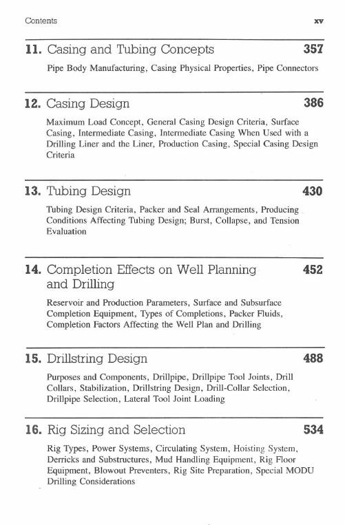
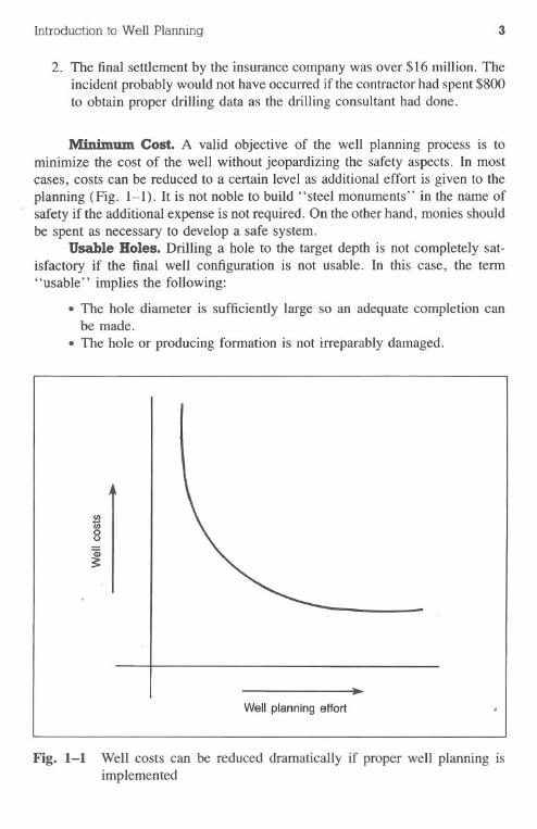
Minimum Cost. A valid objective of the well planning process is tominimize the cost of the well without jeopardizing the safety aspects. In mostcases, costs can be reduced to a certain level as additional effort is given to theplanning (Fig. 1-1). It is not noble to build "steel monuments" in the name ofsafety if the additional expense is not required. On the other hand, monies shouldbe spent as necessary to develop a safe system.
Usable Boles. Drilling a hole to the target depth is not completely sat-isfactory if the final well configuration is not usable. In this case, the term"usable" implies the following:
.The hole diameter is sufficiently large so an adequate completion canbe made..The hole or producing formation is not irreparably damaged.
sCJ)oo
Well planning effort
Fig. 1-1 Well costs can be reduced dramatically if proper well planning isimplemented
4 DrillingEngineering
This requirement of the well planning process can be difficult to achieve' inabnormal pressure, deep.zones that can cause hole geometry or mud problems.
Classification of Wen TypesThe drilling engineer is required to plan a variety of well types, including
the following:·wildcats.exploratoryholes·step-outs· infills·reentries
Generally, wildcats require more planning than the other types. Infill wells andreentries require minimum planning in most cases.
Wildcats are drilled on a certain location where little or no known geologicalinformation is available. The site may have been selected because of wells drilledsome distance from the proposed location but on a terrain that appeared similarto the proposed site. The term "wildcatter" was originated to describe the boldfrontiersman who was willing to gamble on a hunch.
Rank wildcats are seldom drilled in today's industry. Well costs are sohigh that gambling on wellsite selection is not done in most cases. In addition,numerous drilling prospects with reasonable productive potential are availablefrom several sources. However, the romantic legend of the wildcatter.will prob-ably never die.
Characteristics of the well types are shown in Table 1-1.
Table 1-1Well Type
WeD Type CharacteristicsCharacteristics
WildcatExploratory
Step-out
Infill
Reentry
No known (or little) geological foundation for site selection.Site selection based on seismic data, satellite surveys, etc.; no
known drilling data in the prospective horizon.Delineates the reservoir's boundaries; drilled after the exploratory
discovery(s); site selection usually based on seismic data.Drills the known productive portions of the reservoir; site selection
usually based on patterns, drainage radius, etc.Existing well reentered to deepen, sidetrack, rework, or recom-
plete; various amounts of planning required, depending on pur-pose of reentry.
Introduction to Well Planning 5
Formation PressuresThe formation, or pore, pressure encountered by the well significantly
affects the well plan. The pressures may be normal, abnormal (high), or sub-normal (low). (Chapter 3 gives details on pore pressure and detection.)
Normal pressure wells generally do not create planning problems. Themud weights are in the range of 8.5-9.5 lb/gaI. Kicks and blowout preventionproblems should be minimized but not eliminated altogether. Casing requirementscan be stringent even in normal pressure wells deeper than 20,000 ft due totension/collapse design constraints.
Subnormal pressure wells may require setting additional casing strings tocover weak or low pressure zones. The lower-than-normal pressures may resultfrom geological or tectonic factors or from pressure depletion in producingintervals. The design considerations can be demanding if other sections of thewell are abnormal pressured.
Abnormal pressures affect the well plan in many areas, including thefollowing: .
·casing and tubing design·mud weight and type selection· casing setting depth selection·cement planning
In addition, the following problems must be considered as a result of highformation pressures:·kicks and blowouts·differential pressure pipe sticking· lost circulation resulting from high mud weights·heaving shale
Well costs increase significantly with geopressure.Because of the difficulties associated with high-pressure exploratory well
planning, most design criteria, publications, and studies have been devoted tothis area; the amount of effort expended is justified. Unfortunately, the drillingengineer still must define for himself the planning parameters that can be relaxedor modified when drilling normal pressure holes or well types such as step-outsor infills.
Planning Costs
The costs required to plan a well properly are insignificant in comparisonto the actual drilling costs. In many cases, less than $1,000 is spent in planninga $1 million well. This represents VIOof 1% of the well costs.
Prospect development
Mud plan
Cement plan.Bit program ~------
Drillstring design
Rig sizing and selection
Fig. 1-2 Flow path for well planning
Introduction to Well Planning 7
Unfortunately, many historical instances can be used to demonstrate thatwell planning costs were sacrificed or avoided in an effort to be cost conscious.The end result often is a final well cost that exceeds the amount required to drillthe well if proper planning had been exercised. Perhaps the most commonattempted shortcut is to minimize data collection work. Although good data cannormally be obtained for less than $2,000-$3,000 per prospect, many well plansare generated without the knowledge of possible drilling problems. This lack ofexpenditure in the early stages of the planning process almost always results inhigher-than-anticipateddrillingcosts. .
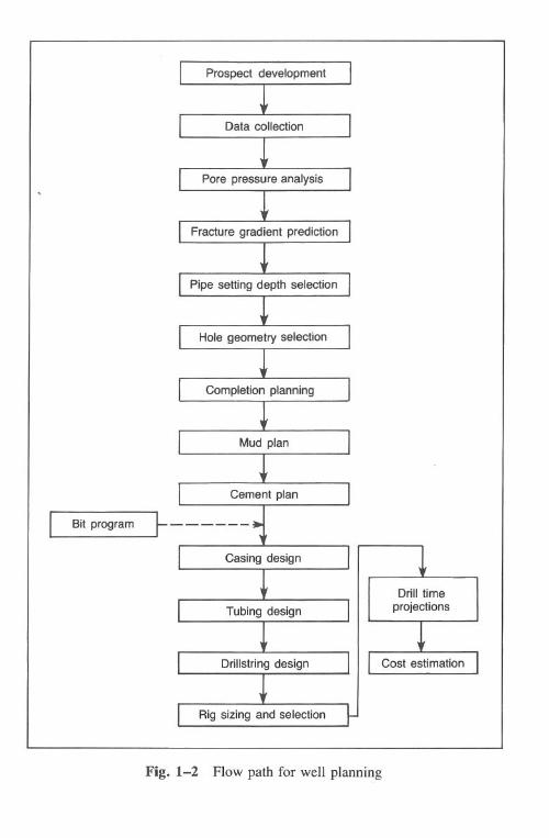
Overview of the Planning ProcessWell planning is an orderly process. It requires that some aspects of the
plan be developed before designing other items. For example, the mud densityplan must be developed before the casing program since mud weights have animpact on pipe requirements. Fig. 1-2 illustrates a commonly used flow pathfor a well plan.
Bit programming can be done at any time in the plan after the historicaldata have been analyzed. The bit program is usually based on the drilling pa-rameters from offset wells. However, bit selection can be affected by the rimdplan, i.e., the performance of PCD bits in oil muds. In addition, bit sizing maybe controlled by casing drift diameter requirements.
Casing and tubing should be considered as an integral design. This factis particularly valid for production casing. A design criteria for tubing is thedrift diameter of the production casing, whereas the production casing can be af-fected adversely by the packer-to-tubing forces created by the tubing's tenden-cies for movement. Unfortunately, these calculations are complex and oftenneglected.
The completion plan must be visualized reasonably early in the process.Its primary effect is on the size of casing and tubing to be used if oversizedtubing or packers are required. In addition, the plan can require the use of high-strength tubing or unusually long seal assemblies in certain situations.
Fig. 1-2 defines an orderly process for well planning. This process mustbe altered for various cases. The flow path in this illustration will be followed,for the most part, throughout this text.
References
Adams, N.J. Unpublished material from consulting work, relating to legalexpert witness studies.

8 DrillingEngineering
Adams, N.J. WeLLControl Problems and Solutions. Tulsa: PennWell, 1979.
Moore, Preston. Drilling Practices Manual. Tulsa: PennWell, 1974.
Records, Louis R., Sr. Personal discussions, 1981-1983.
Chapter 2 Data Collection
The most important aspect of preparing the well plan, and subsequentdrilling engineering, is determining the expected characteristics and problems tobe encountered in the well. A well cannot be planned properly if these expectedenvironments are not known. Therefore, the drilling engineer must initiallypursue various types of data to gain insight used to develop the projected drillingconditions.
Offset Well Selection
The drilling engineer is usually not responsible for selecting well sites.However, he must work with the geologist for the following reasons:
I. Develop an understanding of the expected drilling geology2. Define fault block structures to help select offset wells that should be
similar in nature to the prospect well3. Identify geological anomalies as they may be encountered in drilling
the prospect wellA close working relationship between drilling and geology groups can be thedifference between a producer and an abandoned well.
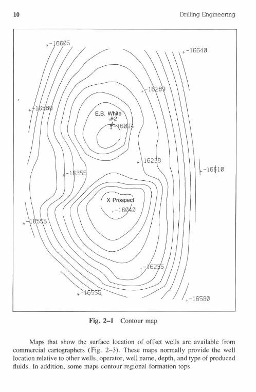
An example of geological information that the drilling group may receiveis shown in Fig. 2-1. The geologists have found significant production fromE.B. White #2. Contouring the pay zones has yielded the contour map in Fig.2-1. The prospect well should encounter the producing structure at the approx-imate depth as the E.B. White #2.
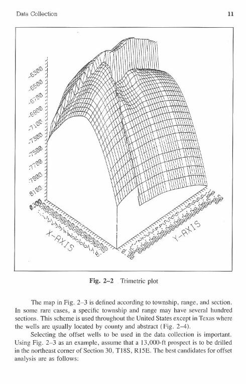
A trimetric plot (Fig. 2-2) is useful as a conceptual tool. It adds a thirddimension not presented in Fig. 2-1. The drilling engineer can view the projectedtargets and develop a better understanding of the goal.
9
10 DrillingEngineering
Fig.2-1 Contour map
Maps that show the surface location of offset wells are available fromcommercial cartographers (Fig. 2-3). These maps normally provide the welllocation relative to other wells, operator, well name, depth, and type of producedfluids. In addition, some maps contour regional formation tops.
Data Collection 11
Fig. 2-2 Trimetric plot
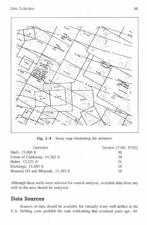
The map in Fig. 2-3 is defined according to township, range, and section.In some rare cases, a specific township and range may have several hundredsections. This scheme is used throughout the United States except in Texas wherethe wells are u.sually located by county and abstract (Fig. 2-4).
Selecting the offset wells to be used in the data collection is important.Using Fig. 2-3 as an example, assume that a 13,000-ft prospect is to be drilledin the northeast comer of Section 30, TI8S, RI5E. The best candidates for offsetanalysis are as follows:
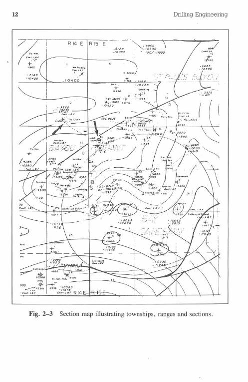
12 Drilling Engineering
...,.......e..,.'.'t. /'
.10400
Fig. 2-3 Section map illustrating townships, ranges and sections.
Data Collection 13
Fig. 2-4 . Texas map illustrating the abstracts
OperatorShell, 15,000ft .
Union of California, 14,562 ftHuber, 12,521 ftExchange, 12,685 ftHouston Oil and Minerals, 17,493 ft
Section (TI8S, RISE)3029211919
Although these wells were selected for control analysis, available data from anywell in the area should be analyzed.
Data Sources
Sources of data should be available for virtually every well drilled in theU.S. Drilling costs prohibit the rank wildcatting that occurred years ago. AI-
14 DrillingEngineering
though wildcats are currently being drilled, seismic data, as a minimum, shouldbe available for pore pressure estimation. .
Common types of data used by the drilling engineer are as follows:.bit records·mud records·mud loggjng records.IADC drilling reports· scout tickets· log headers·production history. seismic studies· well surveys· geological contours'.databases or service company files
Each type of record contains valuable data that may not be available with otherrecords. For example, log headers and seismic work are useful, particularly ifthese data are the only refe~ence sources for the well.
Many sources of data exist in the industry. Unfortunately, some operatorsfalsely consider the records confidential, when in fact the important informationsuch as well testing and production data becomes public domain a short timeafter the well is completed. The drilling engineer often must assume the role of"detective" to defin~ and locate the required data.
Sources of data include bit manufacturers and mud companies who reg-ularly record pertinent relative information on well recaps. Bit and mud com-panies usually make this data available to the operator. Log libraries provide logheaders and scout tickets. And inte1J1alcompany files often contain drillingreports, IADC reports: and mud logs. Many operators will gladly share old offsetinformation if they have no current leasing interest.
Bit RecordsAn excellent source of offset drilling information is the bit record. It
contains data relative to the actual drilling operation. A typical record for arelatively shallow well is shown in Fig. 2-5.
The heading of the bit record provides information such as the following:
·operator.contractor· rig number.well location·drillstringcharacteristics·pump data
~4-!-jP
:0IN
V.SA
'-'>
'-1'1...~,(.1-
\
/IS.W
.L.
,g1.\0
.......'"
~
"'---
L-
BIT
CO
ND
ITIO
NC
OD
E:
RP
.R
EP
AIR
ED
RR
-R£R
Uh
OR
IGIN
AL
-RE
GIO
NO
FF
ICE
Fig.
2-5B
itrecord
fora
shalloww
ell
lIP
F
SF
S2-
"'5€
8-2/-8-
.I.<=
;-ZA
."'-
IQ-2n_"'..
~5>~ro!:l0-::3
...en
16 Drilling Engineering
In addition, the bit heading provides dates for spudding, drilling out from underthe surface casing (U.S.), intermediate casing depth, and reaching the bottomof the hole.
The main body of the bit record provides the following details:
.number and type of bits·jet sizes· footage and drill rates per bit.bit weight and rotary operating conditions.hole deviation.pump data.mud properties.dull bit grading.comments
The vertical deviation is useful in detecting potential dogleg problems.Comments throughout the various bit runs are informative. Typical notes
such as "stuck pipe" and "washout in drillstring" can explain why drillingtimes are greater than expected. Drilling engineers often consider the commentssection on bit (and mud) records just as important as the information in the mainbody of the record.
Bit grading data can be valuable in well planning if the operator assumesthe observed data are correct and representative of the actual bit condition. Thebit grades can assist in the preparation of a bit program for the prospect well byidentifying the most (and least) successful bits in the area. Bit running problemssuch as broken teeth, gauge wear, and premature failures can be observed andpreventive measures can be formulated for the new well.
Drilling Analysis. Bit records can provide significantly more useful dataif the raw information is analyzed. Plots can be prepared that detect lithologychanges arid trends. Cost-pef-foot analyses can be made. Crude, but often useful,pore pressure plots can be prepared.
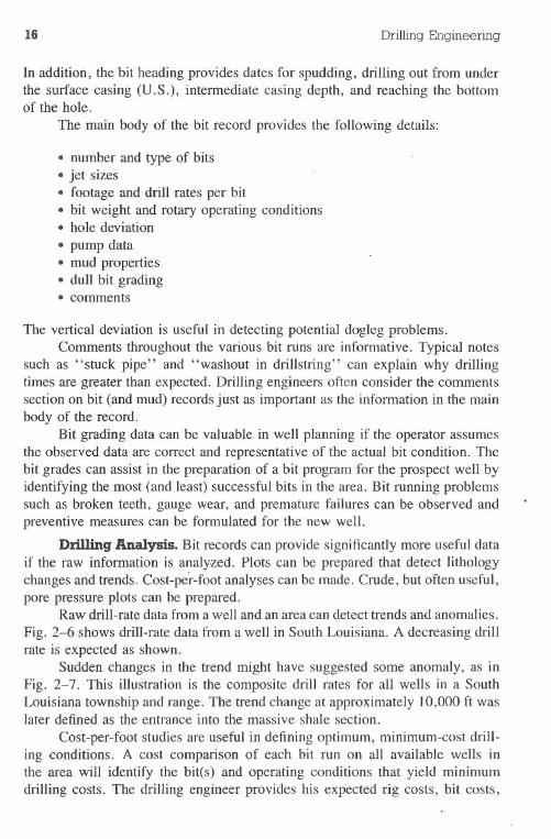
Raw drill-rate data from a well and an area can detect trends and anomalies.
Fig. 2-6 shows drill-rate data from a well in South Louisiana. A decreasing drillrate is expected as shown.
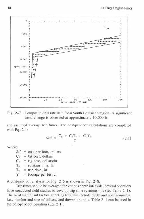
Sudden changes in the trend might have suggested some anomaly, as inFig. 2-7. This illustration is the composite drill rates for all wells in a SouthLouisiana township and range. The trend change at approximately 10,000 ft waslater defined as the entrance into the massive shale section.
Cost-per-foot studies are useful in defining optimum, minimum-cost drill-ing conditions. A cost comparison of each bit run on all available wells inthe area will identify the bit(s) and operating conditions that yield minimumdrilling costs. The drilling engineer provides his expected rig costs, bit costs,
D~ILL~ATE VS. DEPTH PLDT
!,tElL : J.D. SITTIG ND. IOPE~ATO~' STONE OIL COIWANYSTATE' LA TOWNSHIP' 7> ~AN6E' IW SECTION' 28
o + + + + + + +!!!!
2000 +!
. +
.4000 +
!!
6000 +!!
DEPTH'Fn !I
8000 +! . tI . I! . tI I
10000 + +I II II II I
12000 + + + + + + +o 30 60 90 120 I!!O 180
DRILL RATE (FT/~)
Fig. 2-6 Raw drill rate data from a South Louisiana well (Courtesy of Adamsand Rountree Technology)
+II. II+I. III. +
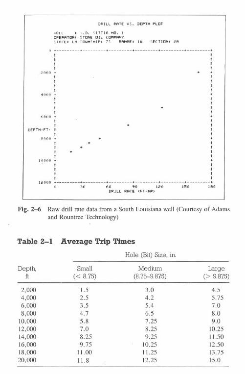
Table 2-1 Average Trip Times
Hole (Bit)Size, in.
Depth, Small Medium Largeft « 8.75) (8.75-9.875) (> 9.875)
2,000 1.5 3.0 4.54,000 2.5 4.2 5.756,000 3.5 5.4 7.0
8,000 4.7 6.5 8.010,000 5.8 7.25 9.012,000 7.0 8.25 10.2514,000 8.25 9.25 11.5016,000 9.75 10.25 12.5018,000 11.00 11.25 13.7520,000 11.8 12.25 15.0
18 DrillingEngineering
o + + + + + + +! !! . !! . !! !
24000+ + + + + + +o 30 60 9C 120 150 180
DRILL RATE (FT/HR)
Fig. 2-7 Composite drill rate data for a South Louisiana region. A significanttrend change is observed at approximately 10,000 ft.
and assumed average trip times. The cost-per-foot calculations are completedwith Eq. 2.1:
$/ft (2.1)
Where:$/ft
CBCRTRTTY
cost per foot, dollarsbit cost, dollarsrig cost, dollars/hrrotating time, hrtrip time, hrfootage per bit run
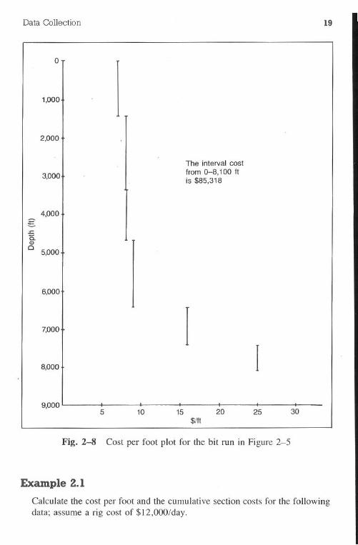
A cost-per-foot analysis for Fig. 2-5 is shown in Fig. 2-8.Trip times should be averaged for various depth intervals. Several operators
have conducted field studies to develop trip-time relationships (see Table 2-1).The most significant factors affecting trip time include depth and hole geometry,i.e., number and size of collars, and downhole tools. Table 2-1 can be used inthe cost-per-foot equation (Eq. 2.1).
4000 + +!!!!
8000 + +! !! !! !! !
12000 + +! !! !
DEPTH (FD ! !! !
16000 + +! !! !! !!
20000 + +! !! !! !! !
Data Collection 19
o
1,000
9,0005 10 15 20 25 30
$/ft
Fig. 2-8 Cost per foot plot for the bit run in Figure 2-5
Example 2.1
Calculate the cost per foot and the cumulative section costs for the followingdata; assume a rig cost of $12,OOO/day.
2,000
I IThe intervalcost
Moor t
from 0-8,100 ftis $85,318
4,000g;c'5.CDc
5,000
6,000I
I
I
7,000t
I8,000
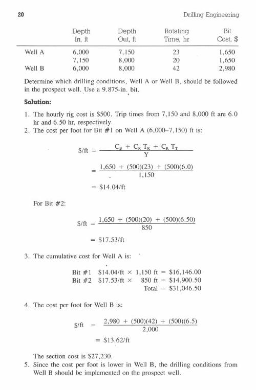
Determine which drilling conditions, Well A or Well B, should be followedin the prospect well. Use a 9.875-in. bit.. .Solution:
1. The hourly rig cost is $500. Trip times from 7,150 and 8,000 ft are 6.0hr and 6.50 hr, respectively.
2. The cost per foot for Bit #1 on Well A (6,000-7,150) ft is:
$/ft = Co + C~ TIi + CRTTY
1,650 + (500)(23) + (500)(6.0)1,150
= $14.04/ft
For Bit #2:
$/ft = 1,650 + (500)(20) + (500)(6.50)850
= $17.53/ft
3. The cumulative cost for Well A is:
Bit #1 $14.04/ft x 1,150 ft = $16,146.00Bit #2 $17.53/ft x 850 ft = $14,900.50
Total = $31,046.50
4. The cost per foot for Well B is:
$/ft 2,980 + (500)(42) + (500)(6.5)2,000
= $13.62/ft
The section cost is $27,230.5. Since the cost per foot is lower in Well B, the drilling conditions from
Well B should be implemented on the prospect well.
20 DrillingEngineering
Depth Depth Rotating BitIn, ft Out, ft Time, hr Cost, $
Well A 6,000 7,150 23 1,6507,150 8,000 20 1,650
Well B 6,000 8,000 42 2,980
Data Collection 21
12000 +
13000 +
14000 +
15000 +
16000 +!
17000 ++ + + + + + + + + + + +
so 10 11 12 D 14 15 16 17 I::: 1'~
EQUIVALENT MUD WEIGHT rpPG)FORMATION PRESSURE iPPI~) .FRACTURE GRADIENT (PPG~ +
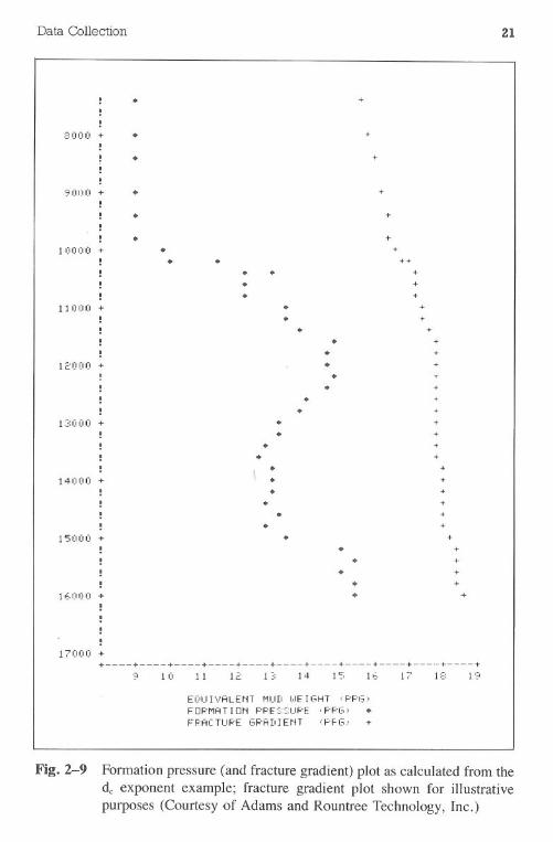
Fig.2-9 Fonnation pressure (and fracture gradient) plot as calculated from thed.: exponent example; fracture gradient plot shown for illustrativepurposes (Courtesy of Adams and Rountree Technology, Inc.)
.!!
:::0(1) + .!! .!!
9000 + .!
.
.10000 + .
! .!!!
11000 +
+
+
+
+
+
+
+. ++
. . +
. +
. +
. +
. +
. +
. +
. +
.
.. +
. +
. +
. +
. +
. +
. +
. +
. +
. +
. +. +
. +. +
. +. +
. +. +. +
22 Drilling Engineering
The dc-exponent method of pore pressure calculations has been appliedsuccessfully on bit records. Although the quantitative results should be viewedwith caution, the method is useful in many cases. The quality of the resultsincreases in formations with fewer sand sequences (cleaner shale). A variety ofpressure prediction techniques are covered in Chapter 3. The data required mustbe gathered from offset well records (Fig. 2-9).
Mud Records
Drilling mud records describe the physical and chemical characteristics ofthe mud system. The reports are usually prepared daily. In addition to the muddata, hole and drilling conditions can be inferred. Many drilling personnel believethat the mud record is the most important and useful planning data.
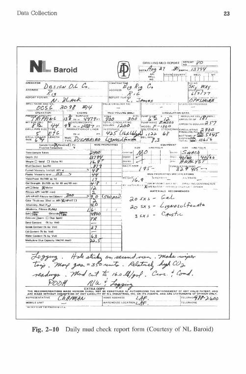
Mud engineers usually prepare a daily mud check report form. Copies aredistributed to the operator and drilling contractor. The form, Fig. 2-10, containscurrent drilling data such as the following:
·well depth· bit size and number·pit volume.pump data· solids control equipment·drillstringdata
The reportalso containsmud propertiesdata such as the following:
·mud weight .chloride content·pH · calcium content· funnel viscosity .solids content· plastic viscosity .cation exchange capacity (or MBT).yield point .fluid loss·gel strength · solids content
An analysis of these characteristics taken in the context of the drillingconditions can provide clues to possible hole problems or changes in the drillingenvironment. For example, an unusual increase in the yield point, water loss,and chloride content suggests that salt (or salt water) has contaminated a fresh-water mud. If kick control problems had not been encountered, it is probablethat salt zones were drilled.
A composite mud recap form, Fig. 2-11, is usually prepared when thewell is completed. The recap contains a daily summary of the properties. It mayalso include important comments pertaining to hole problems.
Drilling Analysis. Daily reports prepared by the mud engineer are usefulin generating depth vs days plots (Fig. 2-12). These plots are as important to
Data Collection 23
NLBaroid
AOOAm }) e s /t:1f/ O,L C..
AEPoATFDAMA~ " .
ICONTFlACT~....
_J;5JDDAESS
Depth tfll
Weight 0 _Ippgl D Ilb/eu ht
Mud Gt"8dillnt IpSi/hI
Funnel Viscosity tMeJql) API .1
~ltic Viscosi1Ycplt_
Yield Point (11)/100 sq hi
Get St,.ngth IIbl100 tq fll 10 secJ10 rnin
pH 0 Strip PlMeterFiltr818 API (ml/3D mini
API HP.HT Filtr'" Imll30minl
Cite Thidr:,,", :nnd In API )Q.HP.HTD
Alkllinily. Mud IPm)
AllUllini1Y.Flluate !PffMtl~= CtlI~NanC8lciumDppm D Gyp (ppb)
Sand Content I" by VolI
Solids Content I" by Vol)
Oil Content I" by Vol)
Wit" Cont.nt I" by Vol)
Mlthy 81ue CaS-city IIM/"" mudl
:.'190 c..e.L
!..'YA/~ I.uL-p"",,-t+A
C,<fv$f, c...
.3
D~. 1f-~~6'->-,~~.~~4 . 7U-fl ~ :3t:>~ . ~ ~ CO,;1.
~ . ~~ tt /6.o4/rI. ~. :('~.PD(')1f /fIlA.-f -' .
EXTRA COPYTHE RECOMMENDATIONS MAM HEAIEON SHALL HOT 81: CONSTRUE.D A5- AUTHORIZING THE: INFRINCIEMENT Of" ANY VALID PATENT, ANDAAIE ""DE WITHOUT ASSU TION 0" ANY LIABILITy If L INDUSTRIES, INC. OR ITS AGENTS, AND ARIE STATIEMIENTS 0.. O~INION ONLY.
REPRESENTATIVEC,hllR1!.,9A/ IHOMEADOAESS '-/IF. - ~EPH°r9Icf'''').bD''MOBILE UNIT WAREHOUSE LOCATION
Fig.2-10 Daily mud check report form (Courtesy of NL Baroid)
BA
R0
I0
0I
V'S,
0N
CO
MPA
NV
---EaD
Am
ericanqll
C~e.ny
NA
nON
Al
lEA
DC
OM
PAIiY
WE
t'T
ouebet.~
DR
ILLING
MU
DR
EC
OR
DC
ON
TR
AcrO
~!:.J1.!g.
~~~:;:...~~!-~o'W~~
OA
Tf.J!d1)~ffi}
.B
AA
OIO
~~
=_~
.~~
_
.."I
."r.IW
I«-'ItLO
..."',,,,,,""
"0. 1,,,,.,;;'1
pftt-.-'IU
ItAU
"",.,,,~,,;';I-
1III.'OIlllT~I
_'__U
I'I
'I"''''''L
YS'S
II...
10/,..V
ISC
OS
ITYG
tU,
,.,I 10".
Ict>"'_I~ ""
0.1I wol..
1901I
s.c.1cp...
10...:..Py1'1'''Ie
n"",
1..L
_""""
",...
1.':'.
1-2,4
12.4
1U
,_.!r.G
iIBW
"",-f
:..
_.2...9
'_'I _\L...3LI~I--_L_!_
$'!.,,<1_:L'_;!._~1
..~--;--f--I-
I.7:31__620(L
L9..6J3U
n~
-1-Jij'~
2~6"I8UU
,.6/2
_-'.984CL
U...6_h
14_
~2...J.!012Q
-211.011000
16/5
..UO
CO
._D.O
'3.:~ 109-3-,._J.
22..1eC:'l~
2~D
:~.i
112.6/8
__U5D
3_ho.~k...
0117
12.~
-"IBO
OJ.
ci1A.§~1l_1l~00-~
~l2.._4"
.20.-~
6.:'~~
9...5LB
oQI~
i'' .
Ih12
1160014.
'22
I~!j1l,;
2-
9.51-600000.
=W
JL"i295~
~6.L
44
!!.1...!33.2
-.0i_2Q
Q--:21
~I3Q
_8/16..l268Lj16
5.7
2.-.
21>00-D
.~7:~-.33.
_8/J1L.'l.316L
\1.6..~Icoc
--
Q.Jt..
~,...~/20-13494-.to~~-rl~tu
0~
!-o'Cag
~ieL
it..1>
!:!-.II"'--"~~...II9._,t.I.k.i.n..L
.IIIIIAlL
amo1_
'tr1u""
tea.:bit
-N
ixd
tOK
e;=
jji01bII.L
C;M.'
.c
"1il=
"'Reaa1aed
Cire.
~4~4. ..'~32.U
atet
ao-
'"e
_~oea
-d
.1
.iJIjjal.i
ReB
a10e1rv
Zeoael-
Baro1d
Plua-v72
_MIL
132U::::
lU...
fm4.
2-
.1
00m
...1O.~
'A
dd.d'.1+
.B/30_!l43
16...9..~9
.3..2
-.
01--rO
:a4
§1.2_
:l.4~ill~.
2J2
-.
2100-
1O.~
bR
aDL
iner-
Cem
eathadve
..9ZR15
Ql
Q.
14'9
3.42
-0.0
260018010.6
c,,
-'!~,j6_r.S53n
--
1o.9tu-.1S
5..13-"';
A0
_I~
-9/12--1-1578-7.J;
00..
6LlB
~.
~~
koo..J-=-C
O.
-9/,13...;.~. 521. 0
1.1
012
2.2
-~122oo
IlbCIo.
.97J..7_1655L8
14.
2-
0.oj-2~"10.
1...9!ZL
!17l.lLJ.1~654.0
-l-5L
20oo-
o.9i?3
,U220
['17:60
21
1.01
-~uw
-u.
_9/25-.tJ.15O!L
l.1..-
."1700
-O
._9/29-I~
j<.-,7
-1H
oo-
0
~
/2~..:
55
--
n.-lO
,LS-
J.84~,u..
5-
q.01lOCO
-O
.:J.O
.9.J1881<L
20-
i..5.'10c0-O
.
-=O
/l.D.IJJjoa,
~7.L
'168
D.8
1--10.011000
_O
.--~-I--I-I-
..
ST!~~u1B
lana
CO
UN
TYVerm
illoaL
OC
AT
ION
N.
Florence
SE<
:~.8_TW
P_~RN
GLW
RE
MA
RK
SA
ND
TR
fAT
ME
NT
I115-1
Fig.2-11
Com
positem
udrecap
(Courtesy
ofN
LH
aroid)
CA
SING
PRO
GR
AM
,ll.3L
!1",."~,,9
5/8..."~,,
-2-1"'"o,J.:fJ."-"
TO
TA
LOE
P1~-19...000
MU
OM
AJU
UA
UU
SlOIT
oI..,.
1-,'
Nr&:o.
f!.
---
t:J
.....
8S'
to[T]
::s
toS'
(I)
(I)
.....
S'
to
Data Collection
12,000
14,000
25
2,000 Surface drilling
,Set and cemented surface casing
4,000
Intermediate casing, logged with ISF, sonic
Stuck pipe at 12,405 ftSpotted oil soak
Free after 32 hours
Logged and ran7-in. casing
16,00010 20 30
Days
50 6040
Fig. 2-12 Depth vs days plot developed from a mud record
well cost estimating as pore pressures are to the overall well plan. Other typesof records, i.e., bit records and log headers, do not provide sufficient daily detailsto construct the plot as accurately as mud records.
An analysis of the plots in the offset area surrounding the prospect wellcan provide the following information:
· expected drilling times for various intervals
6,000
g£ 8,000c-O>0
10,000
26 Drilling Engineering
.identification of better drilling conditions by examining the lowest drillingtimes in the offset wells·location of potential problem zones by comparing common difficultiesin the wells
After the offset wells have been analyzed, a projected depth vs days plot isprepared for the prospect well. (Chapter 19 provides additional details on de-veloping depth vs days projections.)
IADC ReportsThe drilling contractor usually maintains a daily log of the drilling oper-
ations, recorded on the standard IADC-API report. It contains hourly reports fordrilling operations, drillstring characteristics, mud properties, and time break-downs for all operations. Unfortunately, these reports are normally available tothe drilling contractor and the operator and, as a result, cannot be obtained foroffset well analysis without the operator's cooperation.
Scout Tickets
Scout tickets have been available as a commercial service' for manyyears. The tickets were originally prepared by oil company representativeswho "scouted" operations of other 'oil companies. Current scout tickets con-tain a brief summary of the well (see Fig. 2-13). The data usually include thefollowing:
·well name, location, and operator·spud and completion dates· casing geometries and cement volumes· production test data·completion information· tops of various.geological zones
The source of the data for scout tickets is the state or federal report forms filedby oil companies during the course of drilling the well.
Mud Logging RecordsA mud log is a foot-by-foot record of the drilling, mud, and formation
parameters. Mud logging units are often used on high pressure or troublesomewells. Many engineers consider the mud log to be the best source of penetration
Data Collection 27
PARISH:SER:
ACADIA156172 & 159825
FIELD:API#
CROWLEY (NORTH)1700 I-20678 See 9 T9S-RIE
OPR: Amarillo O. Co (fmly Dixie Petro of La Inc) RESULT: FLOWINGDUAL GAS WELL
WELL: Houssiere #1 & #1-D
LOCK: 9-9S-1E 747' FSL & 953' FEL of sec (13500' test-Nod 1 RH)Elev: 20' RKB-CHF & 27' Grd.
SPUD: 2-9-78 CaMP: 6-2-78 PBTD: 13303' TD: 14008'
CSG: 16" @ 112', 10 %" @ 2801' w11665sx, 7 ~" @ 10803' w/1200sx,5 ~" 1m @ 13370' w/200sx, 2 Js" tbg @ 13154', pkr @ 13157',2 Js" tbg on pkr @ 10498'.
LOGS: IEL, ISF-SONL.
PERFS: 13500-14200', PB @ 13301' w/sand, perf for prod 13093-104' &13110-113' wl2 holes per foot, perf 13200-204' & 13210-217'.
IP: (#1) 62 BOPD, 2109 MCFD, 1'1'64" ch, TP 4140#, CP pkr, GaR33,798-1, BS&W .1%, BHP(SI) 6171#, Gr 51.2, ProdInt: 13093-13113' (Nodosaria IRH SUB).
IP: (#I-D) 82 BCPD, 2620 MCFD, 1'1'64"ch, TP 4208#, CP pkr,BS&W .1%, GaR 31,943-1, BHP (SI) 5967#, Gr 50.2,Prod Int: 13200-13217' (Nod 18 RB SUA).
TOPS: Nodosaria 1 13092', Nodosaria 2 13200'.
REPUBLISHED TO SHOW DUAL COMPLETION
REPORT DATE: 6-28-78 CARD# I
Fig. 2-13 Scout ticket
rate data for analysis purposes. Mud logging records are seldom available togroups other than the operators.
A section of a mud log is shown in Fig. 2-14. The drilling parametersnormally included are as follows:
·penetration rate· bit weight and rotary speed·bit numberand type· rotary torque
28 Drilling Engineering
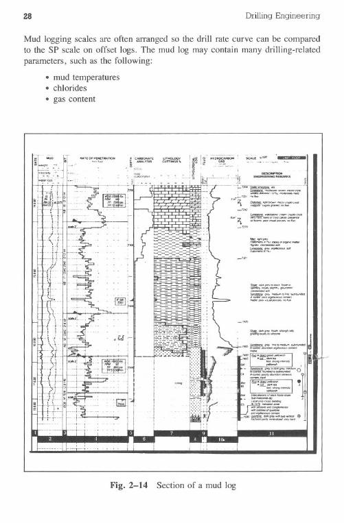
Mud loggingscalesare often arrangedso the drill rate curve can be comparedto the SP scale on offset logs. The mud log maycontainmanydrilling-relatedparameters,such as the following:
.mud temperatures·chlorides·gas content
Fig.2-14 Section of a mud log
Data Collection 29
· lithology.pore pressure analysis
The pore pressure can be computed from models such as the d-exponent or otherproprietary equations or can be measured by drillstern tests.
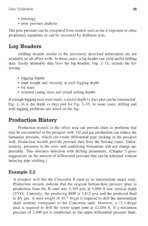
Log HeadersDrilling records similar to the previously described information are not
available on all offset wells. In these cases, a log header can yield useful drillingdata. Easily attainable data from the log headers, Fig. 2-15, include the fol-lowing:
· logging depths.mud weight and viscosity at each logging depth· bit sizes. inferred casing sizes and actual setting depths
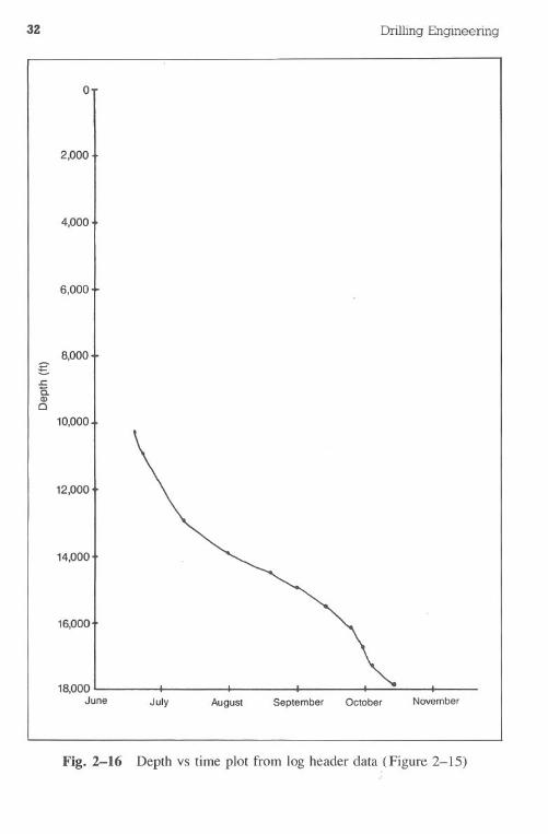
If enough logging runs were made, a useful depth vs days plot can be constructed.Fig. 2-16 is the depth vs days plot for Fig. 2-15. In some cases, drilling andwell logging problems are noted on the log.
Production HistoryProduction records in the offset area can provide clues to problems that
may be encountered in the prospect well. Oil and gas production can reduce theformation pressure, which can create differential pipe sticking in the prospectwell. Production records provide pressure data from the flowing zones. Unfor-tunately, pressures in the over- and underlying formations will not change ap-preciably. This obscures detection with drilling parameters. (Chapter 5 givessuggestions on the amount of differential pressure that can be tolerated withoutinducing pipe sticking.)
Example 2.2
A prospect well has the Concordia B sand as its intermediate target zone.Production records indicate that the original bottom-hole pressure prior toproduction from the B sand was 5,389 psia at 9,890 ft true vertical depth(TVD). Currently, the producing BHP is 3,812 psia and the produced fluidis dry gas. A mud weight of 10.7 Ib/gal is required to drill the intermediateshale sections contiguous to the Concordia sand. However, a 12.1-lb/galmud is required to drill the lower target zone at 12,050 ft. If a maximumpressure of 2,000 psi is established as the upper differential pressure limit,
30
Depth
Casingdepth
Mud typeMU9
weight
Hole size
Drilling Engineering
Date
Specificlocation
Elevationsused forcorrelativepurposes
Fig. 2-15 Top section of a log header from a deep well and detailed runs froma deep well log (Courtesy Schlumberger)
THE SUPE~IC~ ~Il
'Q ~.;;.< '5L- :5- .::'"locotiOf'l of W~II
.0 ~EI::. :IF" ;3 ~J ~ ~~44'~
:01 ~'-~ SE-:~E.!'H 'SO-'':''ac' ro ,-:C~ : Al -96..1.16~"'.1'.9'C30
F"AHI/T<. ..., ~N
~
A8D
lOCAnoN
CO\.INTY
STATE. filiNG No
, tr
.v.ocI1.,.If.
--NA-
'fr«).II:;'C"---
~t.......
5;:'~.-~L
2iJ7-"<J. T-J
q; .:>, 2' I . , J9CJ. '2 : ,q, 129'1
..u..z"9Z4 ,Q,.t ,"q
, :;S14 . "':Q," . .....q':t.llil.L- 11Q.4 .4Sr.',
Data Collection 31
-.
1
auN No.
.. ""... W" Lo..lit Size
~~'iI,.-AMMN-~.
~ l,tTim_ruck o.I .«a,ded By
Wi'"."
II .~-:j---~---j'---I
-I ..~
1.l.Bl.S...71.A1
+=.j~I
-l'/ROT.~20.20'/IDi[
!""'"it""
-IA .. ..
@[email protected]«10_.
@@j@@j@-;,rCC")O;;:-
..
Ii' .'CC30._
"
l!..2..::--blti:.:...
FF40JiB.S.......5.1.L.Qf£.
FQ\.IlCR aUTHERFOR -,." r..
-.---
L--.-.
Fig. 2-15 (continued)
32
o
2,000
4,000
6,000
12,000
14,000
16,000
18,000June
Drilling Engineering
July NovemberAugust September October
Fig. 2-16 Depth vs time plot from log header data (Figure 2-15)
8,000§:.ca.Q)c
10,000
Data Collection 33
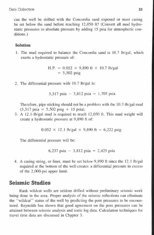
can the well be drilled with the Concordia sand exposed or must casingbe set below the sand before reaching 12,050 ft? (Convert all mud hydro-static pressures to absolute pressure by adding 15 psia for atmospheric con-ditions.)
Solution
1. The mud required to balance the Concordia sand is 10.7 Ib/gal, whichexerts a hydrostatic pressure of:
H.P. = 0.052 x 9,890 ft x 10.7 Ib/gal= 5,502 psig
2. The differential pressure with 10.7 Ib/gal is:
5,517 psia - 3,812 psia = 1,705psia
Therefore, pipe sticking should not be a problem with the 1O.7-lb/galmud(5,517 psia = 5,502 psig + 15 psia).
3. A 12.1-lb/gal mud is required to reach 12,050 ft. This mud weight willcreate a hydrostatic pressure at 9,890 ft of:
0.052 x 12.1 Ib/gal x 9,890 ft = 6,222 psig
The differential pressure will be:
6,237 psia - 3,812 psia = 2,425 psia
4. A casing string, or liner, must be set below 9,890 ft since the 12.1 Ib/galrequired at the bottom of the well creates a differential pressure in excessof the 2,000-psi upper limit.
Seismic Studies
Rank wildcat wells are seldom drilled without preliminary seismic workbeing done in the area. Proper analysis of the seismic reflections can eliminatethe "wildcat" status of the well by predicting the pore pressures to be encoun-tered. Reynolds has shown that good agreement on the pore pressures can beattained between seismic analysis and sonic log data. Calculation techniques fortravel time data are discussed in Ch~pter 3.
34 DrillingEngineering
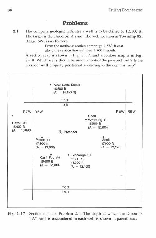
Problems2.1 The company geologist indicates a well is to be drilled to 12,100 ft.
The target is the Discorbis A sand. The well location in Township 8S,Range 6W, is as follows:
Fromthe northeastsectioncomer, go 1,580ft eastalong the section line and then 1,700 ft south.
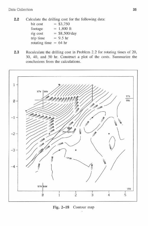
A section map is shown in Fig. 2-17, and a contour map is in Fig.2-18. Which wells should be used to control the prospect well? Is theprospect well properly positioned according to the contour map?
Fig. 2-17 Section map for Problem 2.1. The depth at which the Discorbis"A" sand is encountered in each well is shown in parenthesis.
. West Delta Estate16,500 ft(A.= 14,150ft)
T7ST8S
R7W R6W R6W R5W. Shell
Bayou #9. Wyoming #1
16,900ft16,003 ft (A = 12,100)(A = 13,890) <&>Prospect
. .Peltex #1 Mobil17,200 ft 17,900ft(A = 13,700) (A = 12,290)
. · Exchange OilGulf, Fee #9 E.O.T. #916,600ft 14,300 ft(A = 12,100) (A = 12,150)
....
T8ST9S
35Data Collection
2.2 Calculate the drilling cost for the following data:bit cost = $3,750footage = 1,800 ftrig cost = $8,500/daytrip time = 9.5 hrrotating time = 64 hr
2.3 Recalculate the drilling cost in Problem 2.2 for rotating times of 20,30, 40, and 50 hr. Construct a plot of the costs. Summarize theconclusions from the calculations.
-1
-4
1
Tas
2 3 54
Fig.2-18 Contour map
36 DrillingEngineering
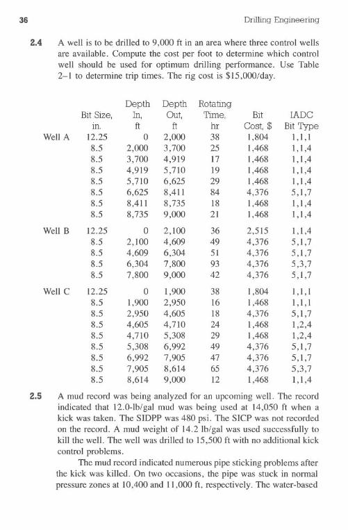
2.4 A well is to be.drilled to 9,000 ft in an area where three control wellsare available. Compute the cost per foot to determine which controlwell should be used for optimum drilling performance. Use Table2-1 to determine trip times. The rig cost is $15,000/day.
Depth Depth RotatingBit Size, In, Out, Time, Bit IADC
ill. ft ft hr Cost, $ Bit TypeWell A 12.25 0 2,000 38 1,804 1,1,1
8.5 2,000 3,700 25 1,468 1,1,48.5 3,700 4,919 17 I ,468 1,1,48.5 4,919 5,710 19 1,468 1,1,48.5 5,710 6,625 29 1,468 1,1,48.5 6,625 8,411 84 4,376 5,1,78.5 8,411 8,735 18 1,468 1,1,48.5 8,735 9,000 21 1,468 1,1,4
Well B 12.25 0 2,100 36 2,515 1,1,48.5 2,100 4,609 49 4,376 5,1,78.5 4,609 6,304 51 4,376 5,1,78.5 6,304 7,800 93 4,376 5,3,78.5 7,800 9,000 42 4,376 5,1,7
Well C 12.25 0 1,900 38 1,804 1,1,18.5 1,900 2,950 16 1,468 1,1,18.5 2,950 4,605 18 4,376 5,1,78.5 4,605 4,710 24 I ,468 1,2,48.5 4,710 5,308 29 I ,468 1,2,48.5 5,308 6,992 49 4,376 5,1,78.5 6,992 7,905 47 4,376 5,1,78.5 7,905 8,614 65 4,376 5,3,78.5 8,614 9,000 12 1,468 1,1,4
2.5 A mud record was being analyzed for an upcoming well. The recordindicated that 12.0-lb/gal mud was being used at 14,050 ft when akick was taken. The SIDPP was 480 psi. The SICP was not recordedon the record. A mud weight of 14.2 Ib/gal was used successfully tokill the well. The well was drilled to 15,500 ft with no additional kickcontrol problems.
The mud record indicated numerous pipe sticking problems afterthe kick was killed. On two occasions, the pipe was stuck in normalpressure zones at 10,400 and 11,000 ft, respectively. The water-based
Data Collection 37
mud system was finally displaced with an oil mud that alleviated thepipe sticking problems.
What are the probable causes for the pipe sticking? Can it beprevented (or minimized) in the prospect well? How? (For additionalassistance, see Well Control Problems and Solutions by Adams.)
2.6 Construct depth vs days plots for the 3 wells in Problem 2.4.
2.7 Construct a depth vs days plot for the bit record in Fig. 2-5.
2.8 Construct a depth vs days plot for the mud record in Fig. 2-11.
2.9 Refer to the trimetric plot in Fig. 2-2 and assume that a well isplanned for one of the fault blocks. Will offset well data from adja-cent fault blocks be of value? What type of information will be usefuland why?
2.10 Townships are approximately 36 sq miles in area. What causes thearea to vary in different townships? Research other literature sourcesand discuss the method used by federal agencies to define townshiplocations.
2.11 What is the significance of Section 16 in some townships throughoutthe United States?
2.12 Discuss common well location methods used outside of the UnitedStates.
2.13 Define commonly used sources of public domain data.
2.14 Certain pieces ~f data from bit records are considered by many industrypersonnel as questionable in reliability. What items are considered asunreliable and why?
2.15 Refer to the scout ticket shown in Fig. 2-13. What are the bottom-hole pressures in the #1 and #1-D sand? What is unusual about thesedata?
2.16 Using Fig. 2-15, prepare a drill-rate plot (ft/day) from the log header.How can this plot be used in preparing the well plan? What are itsweaknesses?
38 Drilling Engineering
References
Adams, N.J. Well Control Problems and Solutions, Tulsa: PennWell Pub-lishing Co., 1978.
Applied Geological Services, Users Guide, Lafayette, Louisiania: Adams andRountree Technology, Inc.
Personal conversation with Dr. Tom Burnett, Lafayette, Louisiana: Adamsand Rountree Technology, Inc., 1983.
Various publications, Louisiana State Department of Natural Resources.
Pertl, Walter F. Abnormal FormationPressures, Elsevier Press.
Chapter 3 PredictingFormationPressures
Fonnation pressure can be the major factor affecting drilling operations.If pressure is not properly evaluated, it can lead to drilling problems such as lostcirculation, blowouts, stuck pipe, hole instability, and excessive costs. Unfor-tunately, fonnation pressures can be very difficult to quantify precisely whereunusual, or abnonnal, pressures exist.
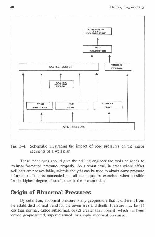
The complete well planning process, with few exceptions, is predicated pna knowledge of fonnation pressures. As shown in Fig. 3-1, the pressure is thefoundation for many segments of..the well plan. If proper attention is not givento fonnation pressure predictions, the other technical portions of the well planmay be inadequate.
Pressure Prediction MethodsSeveral methods of pressure prediction are available to the engineer. These
methods can be grouped logically as follows:I. areal analysis from seismic data2. offset well correlation
log analysisdrilling parameter evaluationproduction or test data
3. real-time evaluationqualitativequantitative
The real-time analysis involves monitoring drilling and logging parameters whilethe prospect well is drilled.
39
40 Drilling Engineering
CASING DESIGN
Fig. 3-1 Schematic illustrating the impact of pore pressures on the majorsegments of a well plan
These techniques should give the drilling engineer the tools he needs toevaluate formation pressures properly. As a worst case, in areas where offsetwell data are not available, seismic analysis can be used to obtain som.epressureinformation. It is recommended that all techniqu~s be exercised when possiblefor the highest degree of confidence in the pressure data.
Origin of Abnormal PressuresBy definition, abnormal pressure is any geopressure that is different from
the established normal trend for the given area and depth. Pressure may be (1)less than normal, called subnormal, or (2) greater than normal, which has beentermed geopressured, superpressured, or simply abnormal pressured.
Predicting Formation Pressures 41
Subnormal pressures present few direct well control problems. However,subnormal pressures do cause many drilling and well planning problems. Forclarity, the term abnormal pressure will identify the pressures greater thannormal.
Formation pressure is the presence of the fluids in the pore spaces of therock matrix. These fluids are typically oil, gas, or salt water. The overburdenstress is created by the weight of the overlying rock matrix and the fluid-filledpores. The rock matrix stress is the overburden stress less the formation pressure.For general calculations, the overburden stress gradient is often assumed to be1.0 psi/ft with a density of 19.23 lb/gal, an average weight of fluid-filled plasticrock.
Normal formation pressure is equal to the hydrostatic pressure of the nativeformation fluids. In most cases, the fluids vary from fresh water with a densityof 8.33 Ib/gal'(0.433 psi/ft) to salt water with a density of 9.0 lb/gal (0.465psi/ft). However, some field reports indicate instances when the normal formationfluid density was greater than 9.0 lb/gal. Regardless of the fluid density, thenormal pressure formation can be considered as an open hydraulic system wherepressure can easily be communicated throughout.
Abnormal formations do not have the freedom of pressure communications.If they did, the high pressures would rapidly dissipate and revert to normalpressures. Therefore, a pressure entrapment mechanism must be present beforeabnormal pressures can be generated and maintained. Fertl and Timko listedseveral of the more common entrapment seals throughout the world (Table3-1).
Assuming that a pressure seal is present, the causes or origins of pressuredepend on such items as lithology, mineralogy, tectonic action, and rate ofsedimentation. Fertl lists many of the field-reported causes of high pressures(Table 3-2). Several of these causes will be discussed in this chapter.
Compaction of Sediments. The normal sedimentation process involvesthe deposition of layers of various rock particles. As these layers continue tobuild depth and increase the overburden (total rock) pressure, the underlyingsediments are forced downward under the weight of surface deposition. Theoverburden pressure in this case is defined as the total of the rock matrix pressureand the formation fluid pressure. Under normal drilling conditions, the formationfluid pressure is the main concern, due to its ability to cause fluid flow into thewellbore under certain geological conditions and the general inability of the rockmatrix to move into the wellbore because of its semirigid structure.
The manner in which the rock matrix accepts the increasing overburdenload explains the abnormal pressures generated in this environment. As both thesurface deposition and the resultant total overburden increase, the underlyingrock must accept the load.
42 Drilling Engineering.
Table 3-1 Suggested Types of FormationPressure Seals .
Type of Seal Nature of Trap Examples
Vertical Massive shales and silt-stones
Massive saltsAnhydriteGypsumLimestone, marl, chalkDolomiteFaults
Salt and shale diapirs
Gulf Coast, USA
Zechstein, North GermanyNorth Sea, Middle EastUSA, USSR
Transverse Worldwide
Combination of verticaland transverse
Worldwide
After Fertl and Timko
Table 3-2 Origins for the Generation of Abnormalnuid Pressure
Piezometric fluid level (artesian water system)Reservoir structureRepressuring of reservoir rockRate of sedimentation and deposition environmentPaleopressuresTectonic activities
Faults
Shale diapirism (mud volcanoes)Salt diapirismSandstone dikes
EarthquakesOsmotic phenomenaDiagenesis phenomena
Diagenesis of clay sedimentsDiagenesis of sulfatesDiagenesis of volcanic ash
Massive areal rock salt depositionPermafrost environment
Thermodynamic and biochemical causes
After Fertl
Predicting Formation Pressures 43
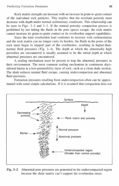
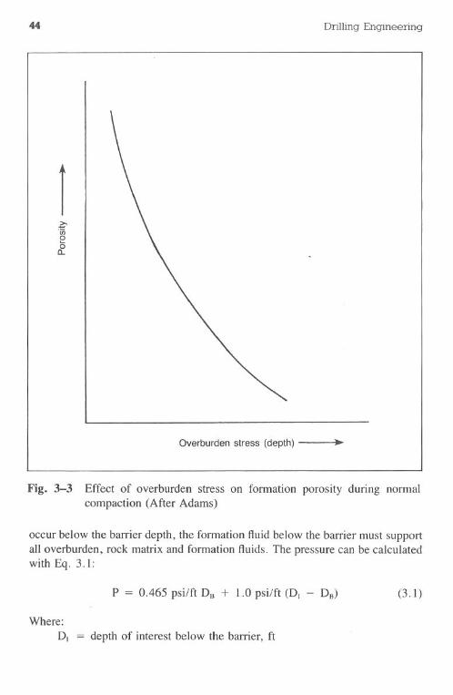
Rock matrix strength can increase with an increase in grain-to-grain contactof the individual rock particles. This implies that the resultant porosity mustdecrease with depth under normal sedimentary conditions. This relationship canbe seen in Figs. 3-2 and 3-3. If the normal porosity compaction process isprohibited by not letting the fluids in the pore spaces escape, the rock matrixcannot increase its grain-to-grain contact or its overburden support capabilities.
Since the total overburden load continues to increase with sedimentationand the rock matrix can no longer carry its burden, the fluids in the pores of therock must begin to support part of the overburden, resulting in higher-than-normal fluid pressures (Fig. 3-4). The depth at which the abnormally highporosities are encountered is usually assumed to be the initial depth at whichabnormal pressures are encountered.
A sealing mechanism must be present to trap the abnormal pressures intheir environment. The most common sealing mechanism in continuous depo-sitional basins is a low-permeability layer of rock, such as a clean shale section.The shale reduces normal fluid escape, causing undercompaction and abnormalfluid pressures.
Formation pressures resulting from undercompaction often can be approx-imated with some simple calculations. If it is assumed that compaction does not
Surface
Depth
+
Rock matrix and porosity
t Normalpressure
~ Abnormalpressure
Undercompacted region(Greater than normal porosity)
Fig. 3-2 Abnormal pore pressures are generated in the undercompacted regionbecause the shale matrix can't support the overburden stress
44
r~.iijeoa.
Drilling Engineering
Overburd!,!nstress (depth) .Fig. 3-3 Effect of overburden stress on formation porosity during normal
compaction (After Adams)
occur below the barrier depth, the formation fluid below the barrier must supportall overburden, rock matrix and formation fluids. The pressure can be calculatedwith Eq. 3.1:
Where:D,
P = 0.465 psi/ft DB + 1.0 psilft (DJ - DB) (3.1)
depth of interest below the barrier, ft
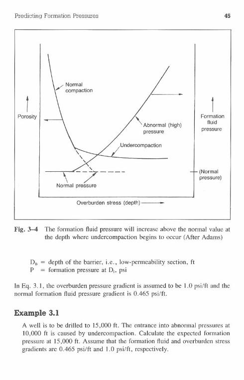
Predicting Formation Pressures 45
1
/ Normalcompaction
1
Porosity
\ Abnormal (high)pressure
Formationfluid
pressure
,\-7----
Normal pressure
(Normalpressure)
Overburden stress (depth)
Fig. 3-4 The formation fluid pressure will increase above the normal value atthe depth where undercompaction begins to occur (After Adams)
DB = depth of the barrier, Le., low-permeability section, ftP = formation pressure at D" psi
In Eq. 3. I, the overburden pressure gradient is assumed to be I. 0 psi/ft and thenormal formation fluid pressure gradient is 0.465 psi/ft.
Example 3.1
A well is to be drilled to 15,000 ft. The entrance into abnormal pressures at10,000 ft is caused by undercompaction. Calculate the expected formationpressure at 15,000 ft. Assume that the formation fluid and overburden stressgradients ate 0.465 psi/ft and 1.0 psi/ft, respectively.
46 Drilling Engineering
Solution:
The formation pressure at 15,000 ft is estimated by Eq. 3.1:
P = 0.465 psi/ft DB + 1.0 ~si/ft (D1 - DB)= 0.465 psi/ft (10,000) + 1.0 psi/ft (15,000 - 10,000)= 4,650 psi + 5,000 psi= 9,650 psi .
= 12.4 lb/gal EMW (equivalent mud weight)
The 9,650-psi pressure is equivalent to a 12.4-lb/gal mud weight at15,000 ft.
Eq. 3.1 can be used to approximate formation pressures. However, for-mations normally have some degree of compaction below the barrier. As a result,Eq. 3.1 can't be expected to provide precise results in most cases. If necessary,a more complex series of calculations based on Eq. 3.1 can be used to increasethe accuracy of the method. This complex procedure will not be presented.
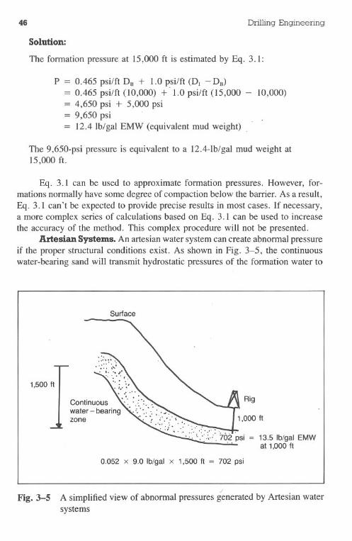
Artesian Systems. An artesian water system can create abnormal pressureif the proper structural conditions exist. As shown in Fig. 3-5, the continuouswater-bearing sand will transmit hydrostatic pressures of the formation water to
Surface
1,500ft
Rig
13.5 Ib/gal EMWat 1,000 ft
0.052 x 9.0 Ib/gal x 1,500 ft = 702 psi
Fig. 3-5 A simplified view of abnormal pressures generated by Artesian watersystems
Predicting Formation Pressures' 47
the bottom of the structure. The pressure at the top of the structure will be normalfor the depth at which it is encountered. The pressure at the bottom of thestructure will be equivalent to 13.5 Ib/gal mud weight. These pressures cannotbe detected with conventional techniques.
Uplift. A normal pressure is defined in relation to the depth at which it isencountered. A pressure that is normal for a specific depth would be abnormallyhigh for it shallower depth. Tectonic actions that uplift sections of formationscan cause abnormal pressures in the uplifted section if specific formations withinthe uplifted section are sealed so the abnormal pressures cannot revert to normalduring the course of geologic time. It is not uncommon to drill through a faultand enter a different pressure .environment. Caution must be exercised withrespect to well planning because pressures across a fault line can be lower, aswell as higher, than the pressures on the opposite side.of the fault.
Fig. 3-6 illustrates the concept of abnormal pressures ,generated by up-lifting. A 12.0-lb/gal mud will be required to drill the interval at 6,000 ft.
Surface
8,000 ft(a) A sealed zone existing at 8,000 ft
with normal pressures in thezone and all adjacent formations
3,744 psi
Sealed zone, normal pressure
(b) An uplifted section willrequire 12.0 Ib/gal mud.The sealed fault preventedpressure regression ornormalization.
Fig. 3-6 Abnormal pressures can be created in an uplifted and eroded envi-ronment
48 Drilling Engineering
The sealed fault line. prevented a pressure regression to a normal environ-ment.
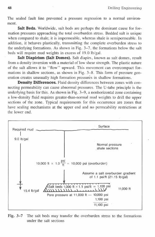
Salt Beds. Worldwide, salt beds are perhaps the dominant cause for for-mation pressures approaching the total overburden stress. Bedded salt is uniquewhen compared to shale; it is impermeable, whereas shale is semipermeable. Inaddition, it behaves plastically, transmitting the complete overburden stress tothe underlying formations. As shown in Fig. 3-7, the formations below the saltbeds will require mud weights in excess of 19.0 Ib/gal.
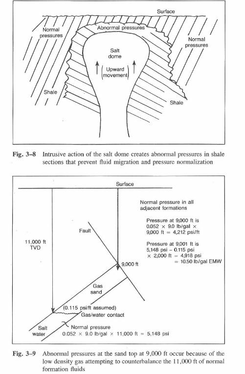
Salt Diapirism (Salt Domes). Salt diapirs, known as salt domes, resultfrom a density inversion with a material of low shear strength. The plastic natureof the salt allows it to "flow" upward. This movement can overcompact for-mations in shallow sections, as shown in Fig. 3-8. This form of pressure gen-eration creates unusually high formation pressures in shallow formations.
Density Differences. Fluid density differences between zones with con-necting permeability can cause abnormal pressures. The U-tube principle is theunderlying basis for this. As shown in Fig. 3-9, a nonhorizontal zone containinga low-density fluid requires greater-than-normal mud weights to drill the uppersections of the zone. Typical requirements for this occurrence are zones thathave sealing mechanisms at the upper end and no permeability restrictions atthe lower end.
Required mudI
9.0 Ib/gal
Surface
Normal pressure. shale sections
psi10,000 ft x 1.0 ft = 10,000psi (overburden)
Assume a salt overburden gradientof 1.1 psi/ft (21.15 Ib/gal)
19.4 Ib/gal 11,000ft
Pore pressure at 11,000 ft - 10,000 psi1,100psi
11,100psi
Fig. 3-7 The salt beds may transfer the overburden stress to the formationsunder the salt sections
Surface
II
Fig. 3-8 Intrusive action of the salt dome creates abnormal pressures in shalesections that prevent fluid migration and pressure normalization
Surface
Normal pressure in alladjacent formations
11,000 ftTVD
Pressure at 9,000 ft is0.052 x 9.0 Ib/gal x9,000 ft = 4,212 psi/ft
Pressure at 9,001 ft is5,148 psi - 0.115psix 2,000 ft = 4,918 psi
= 10.50 Ib/gal EMW
11,000 ft = 5,148 psi
Fig. 3-9 Abnormalpressuresat the sandtop at 9,000 ft occurbecauseof thelow density gas attempting to counterbalance the 11,000 ft of normalformation fluids
50
Seismic Analysis
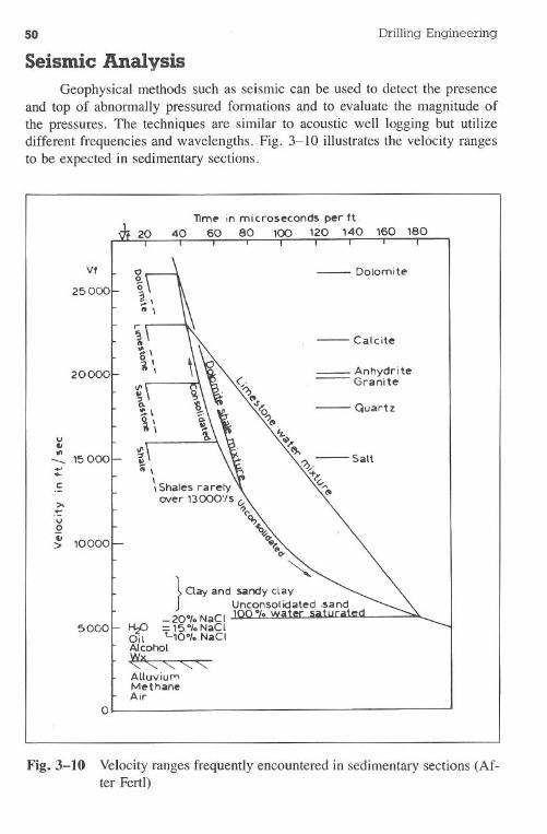
Drilling Engineering
Geophysical methods such as seismic can be used to detect the presenceand top of abnormally pressured formations and to evaluate the magnitude ofthe pressures. The techniques are similar to acoustic well logging but utilizedifferent frequencies and wavelengths. Fig. 3-10 illustrates the velocity rangesto be expected in sedimentary sections.
Vf
25000
20000
5000
Tlm~ in mi croseconds per ft.20 40 60 80 100 120 140 160 180
- Dolomit~
- Calcite
_ Anhydrite- Granite
- Quartz
'"-:s
!!.It \
\ Shales rarelyover 13000'/s v
?~
Q,~.~O<
0),."0-
~}
Cay and sandy clayUnconsolidated .sand
_20.'. NaCI 100.'. . .Hi=> -150'0 NaCIOil 'L,0.,. NaCIAlcohol
't!..."' "'- "'-AlluviuMMethaneAir
o
Fig.3-10 Velocity ranges frequently encountered in sedimentary sections (Af-ter Fertl)
v"",_ 15 000......!:>-
;0;:v0ii
10000>
Predicting Formation Pressures 51
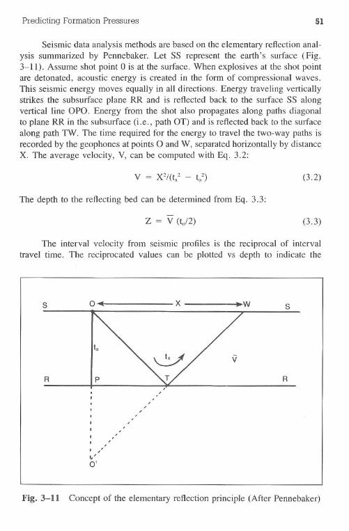
Seismic data analysis methods are based on the elementary reflection anal-ysis summarized by Pennebaker. Let SS represent the earth's surface (Fig.3-11). Assume shot point 0 is at the surface. When explosives at the shot pointare detonated, acoustic energy is created in the form of compressional waves.This seismic energy moves equally in all directions. Energy traveling verticallystrikes the subsurface plane RR and is reflected back to the surface SS alongvertical line OPO. Energy from the shot also propagates along paths diagonalto plane RR in the subsurface (Le., path OT) and is reflected back to the surfacealong path TW. The time required for the energy to travel the two-way paths isrecorded by the geophones at points 0 and W, separated horizontally by distanceX. The average velocity, V, can be computed with Eg. 3.2:
(3.2)
The depth to the reflecting bed can be determined from Eg. 3.3:
(3.3)
The interval velocity from seismic profiles is the reciprocal of intervaltravel time. The reciprocated values can be plotted vs depth to indicate the
s 0-. x s
vR p R
,,-,,,,,
I "I ',I "I ',I ',1,'0'
Fig. 3-11 Concept of the elementary reflection principle (After Pennebaker)
52 Drilling Engineering
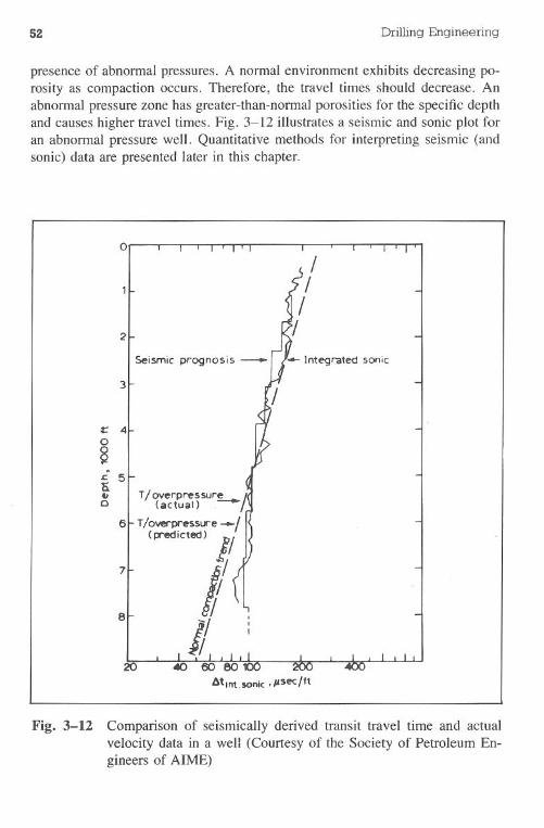
presence of abnormal p.ressures. A normal environment exhibits decreasing po-rosity as compaction occurs. Therefore, the travel times should decrease. Anabnormal pressure zone has greater-than-normal porosities for the specific depthand causes higher travel times. Fig. 3-12 illustrates a seismic and sonic plot foran abnormal pressure well. Quantitative methods for interpreting seismic (andsonic) data are presented later in this chapter.
Fig. 3-12 Comparison of seismically derived transit travel time and actualvelocity data in a well (Courtesy of the Society of Petroleum En-gineers of AIME)
2I
...Jllnte-grated sonicI /1
3
40
85
1i
II l T/ overpresSAJrfL.../o (actual). r
6 Tlove-pressure --I
(p-edicted) f/J>
7" fal- '/
IJI I I .20
Predicting Formation Pressures 53
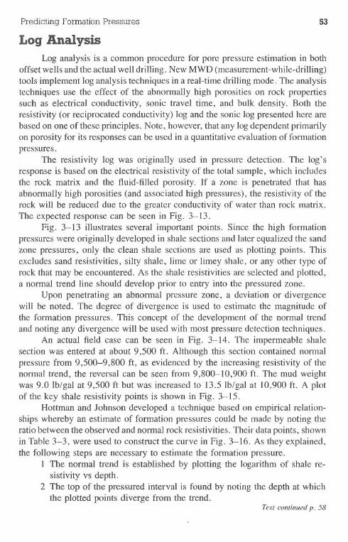
Log AnalysisLog analysis is a common procedure fo~pore pressure estimation in both
offset wells and the actual well drilling. New MWD (measurement-while-drilling)tools implement log analysis techniques in a real-time drilling mode. The analysistechniques use the effect of the abnormally high porosities on rock propertiessuch as electrical conductivity, sonic travel time, and bulk density. Both theresistivity (or reciprocated conductivity) log and the sonic log presented here arebased on one of these principles. Note, however, that any logdependent primarilyon porosity for its responses can be used in a quantitative evaluation of formationpressures.
The resistivity log was originally used in pressure detection. The log'sresponse is based on the electrical resistivity of the total sample, which includesthe rock matrix and the fluid-filled porosity. If a zone is penetrated that hasabnormally high porosities (and associated high pressures), the resistivity of therock will be reduced due to the greater conductivity of water than rock matrix.The expected response can be seen in Fig. 3-13.
Fig. 3-13 illustrates several important points. Since the high formationpressures were originally developed in shale sections and later equalized the sandzone pressures, only the clean shale sections are used as plotting points. Thisexcludes sand resistivities, silty shale, lime or limey shale, or any other type ofrock that may be encountered. As the shale resistivities are selected and plotted,a normal trend line should develop prior to entry into the pressured zone.
Upon penetrating an abnormal pressure zone, a deviation or divergencewill be noted. The degree of divergence is used to estimate the magnitude ofthe formation pressures. This concept of the development of the normal trendand noting any divergence will be used with most pressure detection techniques.
An actual field case can be seen in Fig. 3-14. The impermeable shalesection was entered at about 9,500 ft. Although this section contained normalpressure from 9,500-9,800 ft, as evidenced by the increasing resistivity of thenormal trend, the reversal can be seen from 9,800-10,900 ft. The mud weightwas 9.0 lb/gal at 9,500 ft but was increased to 13.5 lb/gal at 10,900 ft. A plotof the key shale resistivity points is shown in Fig. 3-15.
Hottman and Johnson developed a technique based on empirical relation-ships whereby an estimate of formation pressures could be made by noting theratio between the observed and normal rock resistivities. Their data points, shownin Table 3-3, were used to construct the curve in Fig. 3-16. As they explained,the following steps are necessary to estimate the formation pressure.
1 The normal trend is established by plotting the logarithm of shale re-sistivity vs depth.
2 The top of the pressured interval is found by noting the depth at whichthe plotted points diverge from the trend.
Text continued p. 58
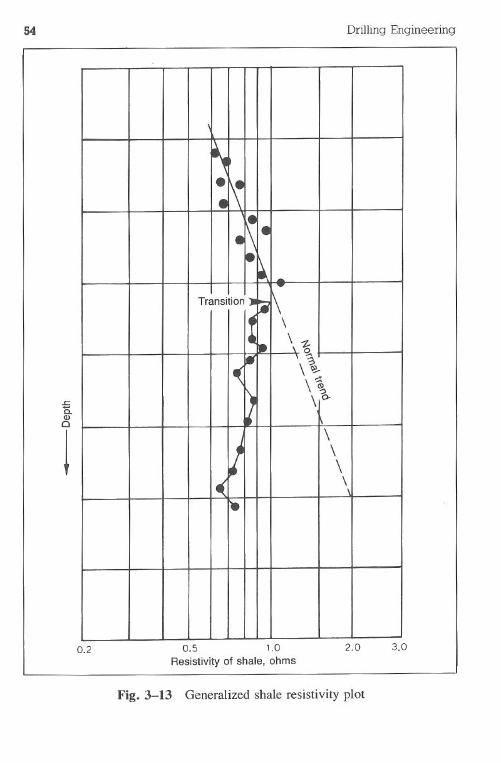
54 Drilling Engineering
~a.Q)
CI
!
0.2 0.5 1.0Resistivity of shale, ohms
2.0 3.0
Fig. 3-13 Generalized shale resistivity plot
\
.\..\ ..
...Transition')
\It. \15.. \
\\\
1\
I\\\
.. \r-
,,
. tI I
d:+-ttT1I, I ' ~,
q-j: Ii
li!-d'. .. 10-_.: I : :
dt ;'1 '_.
I,
, ,
L
I '. !;..f::-;:~_! I:.';'. . . .
Fig. 3-14 Illustration of an electric log from' a well in which the deposi-tion of an impermeable shale barrier generated abnormal pressuresin the lower intervals. In this well, the barrier is from 9,500 ft-9,700 ft.
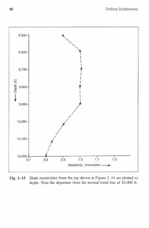
56 Drilling Engineering
9,500
9,600
9,700
g.£:Q. 9,800(I)
CI
~9,900
10,000
10,100
10,200 _0.7
'-""-
"- ,-,
,II
+III
+III
)/
//
//
I/
//
/
I/
I
f I I0.8 0.9 1.0 1.1 1.2
Resistivity,ohmmeters ~
Fig.3-15 Shale resistivities from the.Iog shown in Figure 3-14 are plotted vsdepth. Note the departure from the normal trend line at 10,000 ft.
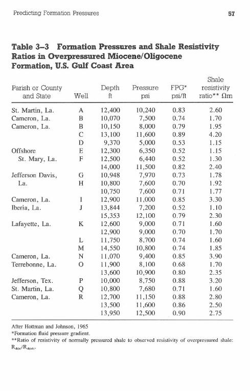
Predicting Formation Pressures 57
Table 3-3 Formation Pressures and Shale ResistivityRatios in Overpressured MiQcene/OligoceneFormation, U.S. Gulf Coast Area
ShaleParish or County Depth Pressure FPG* resistivity
and State Well ft psi psi/ft ratio** Om
81. Martin, La. A 12,400 10,240 0.83 2.60Cameron, La. B 10,070 7,500 0.74 1.70Cameron, La. B 10,150 8,000 0.79 1.95
C 13,100 11,600 0.89 4.20D 9,370 5,000 0.53 1.15
Offshore E 12,300 6,350 0.52 1.15
81. Mary, La. F 12,500 6,440 0.52 1.3014,000 11,500 0.82 2.40
Jefferson Davis, G 10,948 7,970 0.73 1.78La. H 10,800 7,600 0.70 1.92
10,750 7,600 0.71 1.77Cameron, La. I 12,900 11,000 0.85 3.30Iberia, La. J 13,844 7,200 0.52 1.10
15,353 12,100 0.79 2.30
Lafayette, La. K 12,600 9,000 0.71 1.6012,900 9,000 0.70 1.70
L 11,750 8,700 0.74 1.60M 14,550 10,800 0.74 1.85
Cameron, La. N 11,070 9,400 0.85 3.90Terrebonne, La. 0 11,900 8,100 0.68 1.70
13,600 10,900 0.80 2.35Jefferson, Tex. P 10,000 8,750 0.88 3.2081. Martin, La. Q 10,800 7,680 0.71 1.60Cameron, La. R 12,700 11,150 0.88 2.80
13,500 11,600 0.86 2.5013,950 12,500 0.90 2.75
AfterHottmanand Johnson,1965*Formation fluid pressure gradient.**Ratio of resistivity of normally pressured shale to observed resistivity of overpressured shale:R",{n/R'h{ob)'
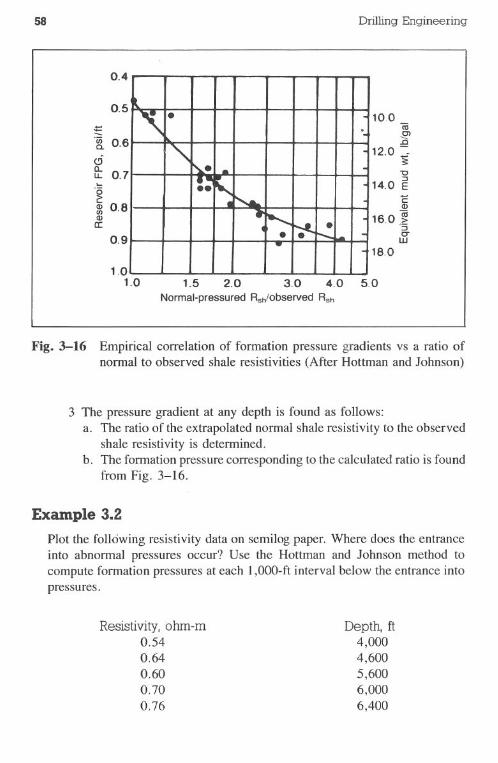
58 Drilling Engineering
0.4
0.510.0
a;C):c
12.0~"0::;]
14.0 E
~.~ 0.6c6It 0.7....~3! 0.8Q)
a:0.9
cQ)
16.0 ~'SCTw
18.01.0
1.0 1.5 2.0 3.0 4.0 5.0Normal-pressured Rsw'observed RSh
Fig. 3-16 Empirical correlation of fonnation pressure gradients vs a ratio ofnonnal to observed shale resistivities (After Hottman and Johnson)
3 The pressure gradient at any depth is found as follows:a. The ratio of the extrapolated nonnal shale resistivity to the observed
shale resistivity is detennined.b. The fonnation pressure corresponding to the calculated ratio is found
from Fig. 3-16.
Example 3.2
Plot the following resistivity data on semilog paper. Where does the entranceinto abnonnal pressures occur? Use the Hottman and Johnson method tocompute fonnation pressures at each 1,0OO-ftinterval below the entrance intopressures.
Resistivity, ohm-m0.540.640.600.700.76
Depth, ft4,0004,6005,6006,0006,400
,. "."\... ......'"..
t
........ ... t--- ...
Predicting Formation Pressures 59
0.600.700.740.760.820.900.840.800.760.580.450.360.300.280.290.270.280.290.30
7,0007,5008,0008,5009,0009,700
10,10010,40010,70010,90011,00011,10011,30011,60011,90012,30012,50012,70012,900
Solution:
1. Plot the data as shown in Fig. 3-17.2. The estimated entrance into abnormal pressure occurs at 9,700 ft.3. Extrapolate the normal trend established between 8,000 and 9,700 ft.4. The observed and extrapolated resistivities at the bottom are 0.30 and 1.60
ohm-m, respectively.5. Compute the ratio of RNonnal(Rn) and Robserved(Rob):
R='&'Rob
= 1.600.30
= 5.333
6. Using Fig. 3-16 from Hottman and Johnson, the formation pressure as-sociated with a ratio of 5.33 is approximately 18.0 Ib/gal.
Overlays. Subsequent to the Hottman and Johnson approach, un-published techniques were developed that used an overlay or underlay for a quickevaluation of formation pressures. The overlay (or underlay) contains a series
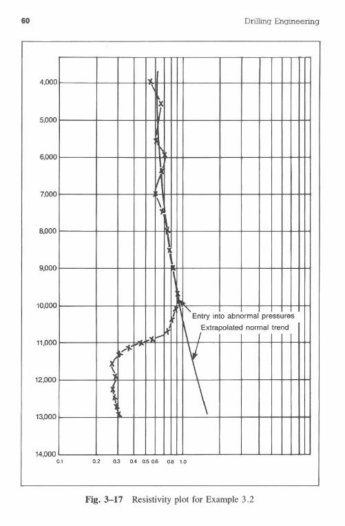
60
12,000
Drilling Engineering
5,000
4,000
6,000
7,000
8,000
9,000
10,000
11,000
13,000
14,0000.1 0.2 0.3 0.4 o.s 0.6 0.8 1.0
Fig. 3-17 Resistivity plot for Example 3.2
01.,
\
"' Entry into abnormalpressures
L....... \ lxtrapolated normaltrend
tt''f:o#P"
(\
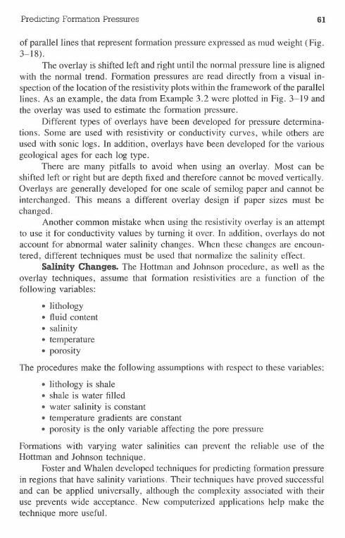
Predicting Formation Pressures 61
of parallel lines that represent formation pressure expressed as mud weight (Fig.3-18).
The overlay is shifted left and right until the normal pressure line is alignedwith the normal trend. Formation pressures are read directly from a visual in-spection ofthe location of the resistivity plots within the framework of theparallellines. As an example, the data from Example 3.2 were plotted in Fig. 3-19 andthe overlay was used to estimate the formation pressure.
Different types of overlays have been developed for pressure determina-tions. Some are used with resistivity or conductivity curves, while others areused with sonic logs. In addition, overlays have been developed for the variousgeological ages for each log type.
There are many pitfalls to avoid when using an overlay. Most can beshifted left or right but are depth fixed and therefore cannot be moved vertically.Overlays are generally developed for one scale of semilog paper and cannot beinterchanged. This means a different overlay design if paper sizes must bechanged.
Another common mistake when using the resistivity overlay is an attemptto use it for conductivity values by turning it over. In addition, overlays do notaccount for abnormal water salinity changes. When these changes are encoun-tered, different techniques must be used that normalize the salinity effect.
Salinity Changes. The Hottman and Johnson procedure, as well as theoverlay techniques, assume that formation resistivities are a function of thefollowing variables:
.lithology.fluid content·salinity.temperature.porosity
The proceduresmakethe followingassumptionswithrespectto thesevariables:
.lithology is shale. shale is water filled.water salinity is constant. temperature gradients are constant·porosity is the only variable affecting the pore pressure
Formations with varying water salinities can prevent the reliable use of theHottman and Johnson technique.
Foster and Whalen developed techniques for predicting formation pressurein regions that have salinity variations. Their techniques have proved successfuland can be applied universally, although the complexity associated with theiruse prevents wide acceptance. New computerized applications help make thetechnique more useful.
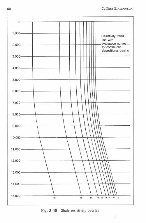
62
o
1,000
2,000
3,000
4,000
5,000
6,000
7,000
8,000
9,000
10,000
11,000
12,000
13,000
14,000
15,000
Drilling Engineering
Resistivity trendline withevaluation curves_for continuousdepositional basins
18 17 16 15 1413 11 9
Fig. 3-18 Shale resistivity overlay
i
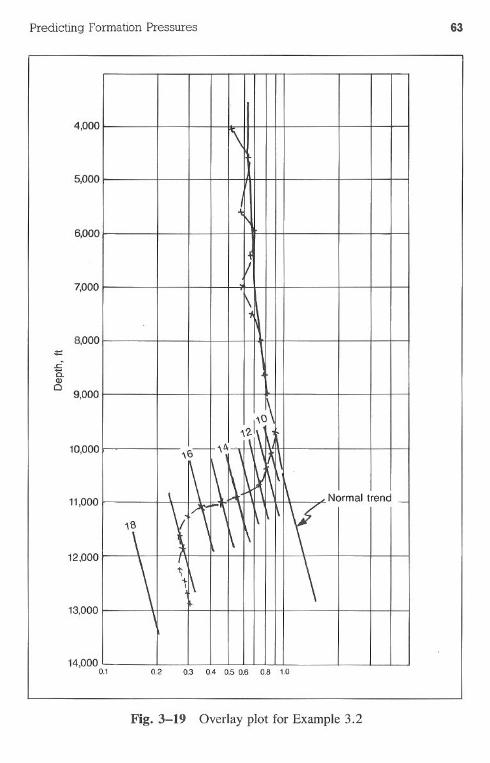
Predicting Formation Pressures 63
4,000
5,000
6,000
7,000
10,000
11,000
12,000
13,000
14,0000.1 0.2 0.3 0.4 0.5 0.6 0.8 1.0
Fig.3-19 Overlay plot for Example 3.2
\
II
1\
IO \
6- ,1
\ \ \ \. \ \ \ Normaltrend _\;1-, \ \
Y8
\ \ \ \
\ 1; \i-\I
8,000<I:.ca.Q)c
9,000
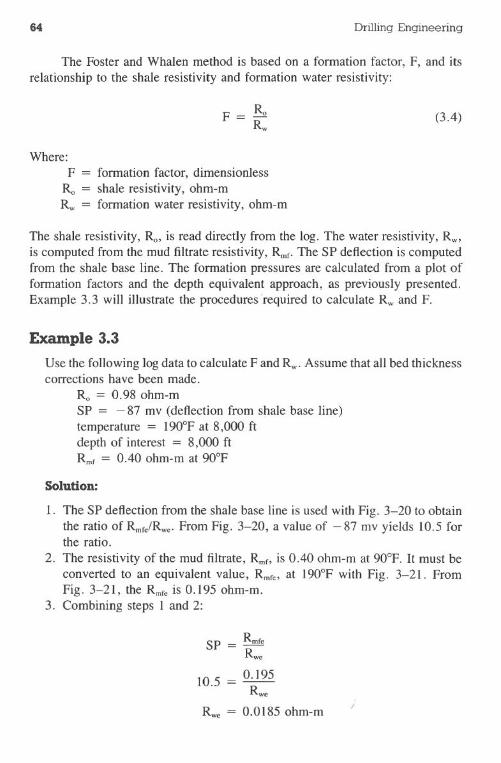
64 Drilling Engineering
The Foster and Whalen method is based on a formation factor, F, and itsrelationship to the shale resistivity and formation water resistivity:
(3.4)
Where:F = formation factor, dimensionless
R.. = shale resistivity, ohm-mRw = formation water resistivity, ohm-m
The shale resistivity, Ro, is read directly from the log. The water resistivity, Rw,is computed from the mud filtrate resistivity, Rmr.The SP deflection is computedfrom the shale base line. The formation pressures are calculated from a plot offormation factors and the depth equivalent approach, as previously presented.Example 3.3 will illustrate the procedures "requiredto calculate Rwand F.
Example 3.3
Use the following log data to calculate F and Rw.Assume that all bed thicknesscorrections have been made.
Ro = 0.980hm-mSP = - 87 mv (deflection from shale base line)temperature= 190°F at 8,000 ftdepth of interest = 8,000 ftRmr= 0.40 ohm-m at 90°F
Solution:
I. The SP deflection from the shale base line is used with Fig. 3-20 to obtainthe ratio of Rmr.lRwc.From Fig. 3-20, a value of - 87 mv yields 10.5 forthe ratio.
2. The resistivity of the mud filtrate, Rmf,is 0.40 ohm-m at 90°F. It must beconverted to an equivalent value, Rmrc,at 190°F with Fig. 3-21. FromFig. 3-21, the Rmrcis 0.195 ohm-m.
3. Combining steps I and 2:
Rwc= 0.0185 ohm-m
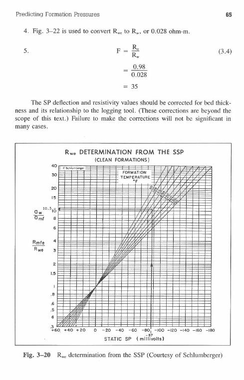
40
65
4. Fig. 3-22 is used to convert Rweto Rw. or 0.028 ohm-m.
5. (3.4)
_ 0.98- 0.028
= 35
The SP deflection and resistivity values should be corrected for bed thick-ness and its relationship to the logging tool. (These corrections are beyond thescope of this text.) Failure to make the corrections will not be significant inmany cases.
Rwe DETERMINATION FROM THE SSP(CLEAN FORMATIONS)
Predicting Formation Pressures
30
20
15
OW10.510Omf 8
3 .+60, +40 + 20 0 - 20 -40 -60 -801 -100 -120 -140 -160 -180
-87STATIC SP (millivolts)
Fig. 3-20 Rwedetermination from the SSP (Courtesy of Schlumberger)
6
Rmfe 4
Rwe 3
2
1.5
I
.8
.6.5
4
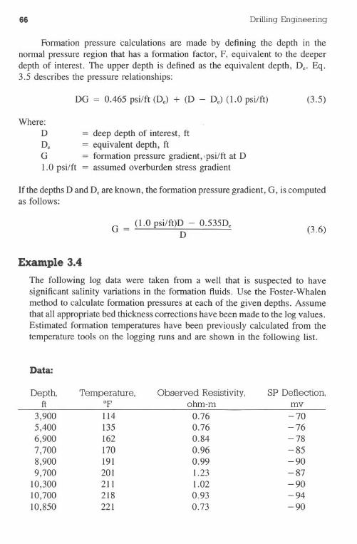
66 Drilling Engineering
Fonnation pressure calculations are made by defining the depth in thenonnal pressure region that has a fonnation factor, F, equivalent to the deeperdepth of interest. The upper depth is defined as the equivalent depth, De. Eq.3.5 describes the pressure relationships:
DG = 0.465 psi/ft (De) + (D - De) (1.0 psi/ft) (3.5)
Where:DDeG1.0 psi/ft
= deep depth of interest, ft= equivalent depth, ft= fonnation pressure gradient, 'psi/ft at D= assumed overburden stress gradient
If the depths D and Deare known, the fonnation pressure gradient, G, is computedas follows:
G = (1.0 psi/ft)D - 0.535DeD (3.6)
Example 3.4
The following log data were taken from a well that is suspected to havesignificant salinity variations in the fonnation fluids. Use the Foster-Whalenmethod to calculate fonnation pressures at each of the given depths. Assumethat all appropriate bed thickness corrections have been made to the log values.Estimated fonnation temperatures have been previously calculated from thetemperature tools on the logging runs and are shown in the following list.
Data:
Depth, Temperature, Observed Resistivity, SP Deflection,ft of ohm-m mv
3,900 114 0.76 -705,400 135 0.76 -766,900 162 0.84 -787,700 170 0.96 -858,900 191 0.99 -909,700 201 1.23 -87
10,300 211 1.02 -9010,700 218 0.93 -9410,850 221 0.73 -90
;; 0 ... .NoCI
I
orol.l/ool 017SoF_ I! ~ gCONCENTRATION } ..I .. . I
~ .:: ppftl_ I .Ii II+ ~ . 18 . 810TSO I
RESISTIVITY
GRAPH
FOR NoCI
SOLUTIONS
i 8 8 .g... ... i
20
...
..
.0
.8.8.8II I
75.0
10040
80 12'...'"80
'" ""0'"70
c:804-175
80 . t t2
'!!100
'0 9." "1103
2-120 50!I.'80 ! ..to140 .e.".eo 300
178
200
t tRESISTIVITY OF n_n' .n., ,_..... ...-.-..-.
I ena ."'I0 ."
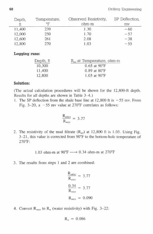
68 Drilling Engineering
Depth,ft
11,40012,00012,60012,800
Temperature,of.
239250261270
Observed Resistivity,ohm-m
1.301.702.081.03
SP Deflection,mv-60-57-38-55
Logging runs:
Depth, ft10,30011,40012,800
Rmfat Temperature, ohm-m0.65 at 90°F0.89 at 80°F1.03 at 90°F
Solution:
(The actual calculation procedures will be shown for the 12,8oo-ft depth.Results for all depths are shown in Table 3-4.)1. The SP deflection from the shale base line at 12,800 ft is - 55 mv. From
Fig. 3-20, a-55 mv value at 270°F correlates as follows:
Rmf(c)= 3.77Rw(c)
2. The resistivity of the mud filtrate (Rmr)at 12,800 ft is 1.03. Using Fig.3-21, this value is corrected from 900P to the bottom-hole temperature of270°F:
1.03 ohm-m at 90°F- 0.34 ohm-m at 2700P
3. The results from steps 1 and 2 are combined:
Rmnc)= 3.77Rw(c)
0.34 = 3.77Rw(c)
Rw(c)= 0.090
4. Convert Rw(c)to Rw (water resistivity) with Fig. 3-22:
Rw = 0.086
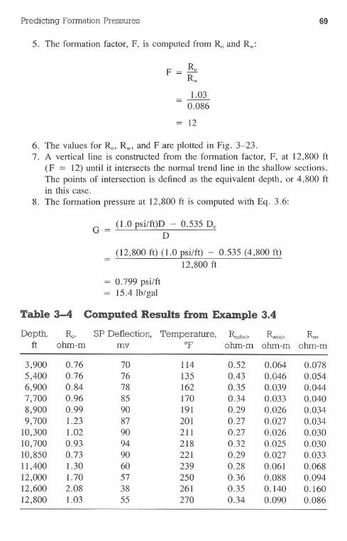
Predicting Formation Pressures 69
5. The formation factor, F, is computed from Ro and Rw:
_ 1.03- 0.086
= 12
6. The values for Ro, Rw, and F are plotted in Fig. 3-23.7. A vertical line is constructed from the formation factor, F, at 12,800 ft
(F = 12) until it intersects the normal trend line in the shallow sections.The points of intersection is defined as the equivalent depth, or 4,800 ftin this case.
8. The formation pressure at 12,800 ft is computed with Eq. 3.6:
G = (1.0 psi/ft)D - 0.535 DeD
= (12,800 ft) (1.0 psi/ft) - 0.535 (4,800 ft)12,800 ft
= 0.799 psi/ft= 15.4 Ib/gal
Table 3-4 Computed Results from Example 3.4
Depth, Ra, SP Deflection, Temperature, Rmf(e), Rw(e), Rw.it ohm-m mv of ohm-m ohm-m ohm-m
3,900 0.76 70 114 0.52 0.064 0.0785,400 0.76 76 135 0.43 0.046 0.0546,900 0.84 78 162 0.35 0.039 0.0447,700 0.96 85 170 0.34 0.033 0.0408,900 0.99 90 191 0.29 0.026 0.0349,700 1.23 87 201 0.27 0.027 0.034
10,300 1.02 90 211 0.27 0.026 0.030
10,700 0.93 94 218 0.32 0.025 0.030
10,850 0.73 90 221 0.29 0.027 0.03311,400 1.30 60 239 0.28 0.061 0.06812,000 1.70 57 250 0.36 0.088 0.09412,600 2.08 38 261 0.35 0.140 0.16012,800 1.03 55 270 0.34 0.090 0.086
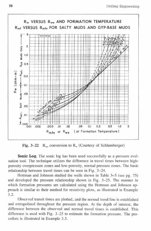
70 Drilling Engineering
Rw VERSUS Rwe AND FORMATION TEMPERATURE
Rmf VERSUS Rmfe FOR SALTY MUDS AND GYP-BASE MUDS
f5~ 2co
i 1.0::ItCI.
~ 0.5
...LLI.U U.ujt~...1
~/..n-I -0 t:"~ W~~ ',\I I ---Ll- 'i' ii, ,,\\Z
" '--L.W .-- ,: 'tj- ,- 'LiY "=' ~ ;-
~c I ~ __= ~- ~- I - ~ r-- I I
- .,,,r-- ;1
-+1:1- " W ==E---+-rrr ~ = =.-.~lrT =.L- I::: _ c:. == 1::: ,~~ ~ ,
' ,. =; -,-I I I~ ~_
]__
,,- +oi~,.(':t2 _, _ ;-.bm~ ,- ~I I II!I~~I
'--",. ~ ;r--H~ I:: I! ~-L ~
~ -r!:-r~..1:'-,~ L=-_
E e
ifir 0.2
- QI
~II::
~ .05'"::It
~ .02
e .01Ir
JO°1>OI .002 .005 .01 .02
Rmfe or Rwe
.05 0.1 0.2 Q5 1.0
( at Formation Temperature)
2
Fig. 3-22 Rweconversion to Rw (Courtesy of Schlumberger)
Sonic Log. The sonic log has been used successfully as a pressure eval-uation tool. The technique utilizes the difference in travel times between high-porosity overpressure zones and low-porosity, normal pressure zones. The basicrelationship between travel times can be seen in Fig. 3-24.
Hottman and Johnson studied the wells shown in Table 3-5 (see pg. 75)and developed the pressure relationship shown in Fig. 3-25. The manner inwhich formation pressures are calculated using the Hottman and Johnson ap-proach is similar to their method for resistivity plots, as illustrated in Example3.2.
Observed transit times are plotted, and the normal trend line is establishedand extrapolated throughout the pressure region. At the depth of interest, thedifference between the observed and normal travel times is established. Thisdifference is used with Fig. 3-25 to estimate the formation pressure. The pro-cedure is illustrated in Example 3.5.
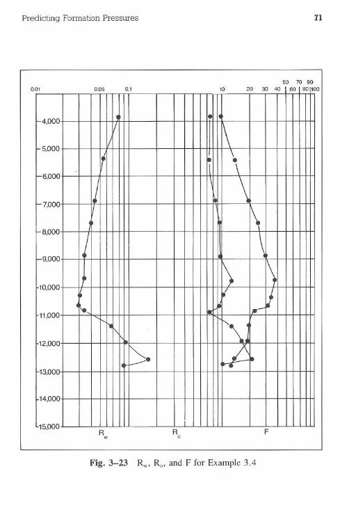
Predicting Formation Pressures 71
o50 70 90
o
15,000R
wRo F
Fig.3-23 Rw, Ro, and F for Example 3.4
01 0.05 0.1 10 20 30 40 60 8010
4,000.
I
5,000\, \
-6,000-,
j \-7,000
1\8,000 I \
-9,000 \\10,000
.I"-'8 ill
11,000......
"-
'\.12,000 . t13,000
14,000
1" nnn
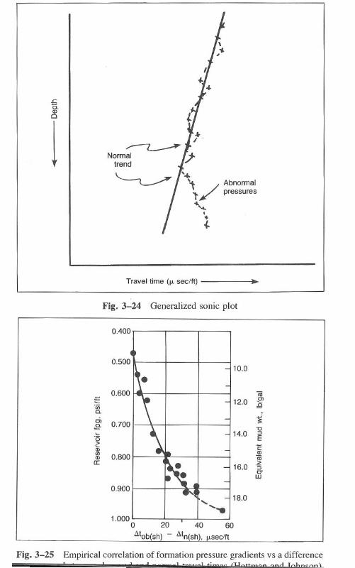
.c15.Q)o
1
Abnormalpressures
Travel time (IL see/ft)
Fig. 3-24 Generalized sonic plot
0.400
Fig. 3-25 Empirical correlation of formation pressure gradients vs a difference.. t t I 1 4-_~.._1 : IU ,.1 Tr'lt.hn~nn\
10.0
iii12.0
C)
;Q!:
j'00C.
"tJcii
14.0 ::>.e-
E'E
.
Q)iii
Q)
>U)
16.0 '5CD -
C'
a:w
.18.0.............
---160
seelft
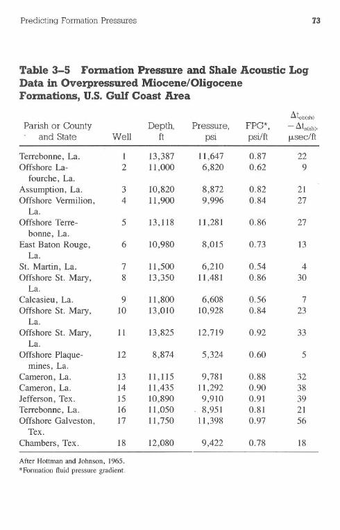
Predicting Formation Pressures 73
Table 3-5 Formation Pressure and Shale Acoustic LogData in Overpressured Miocene/OligoceneFormations, U.S. Gulf Coast Area
.:lt"b(Sh)Parish or County Depth, Pressure, FPG*, - .:ltn(sh),
and State Well ft psi psi/ft J,Lsec/ft-Terrebonne, La. 1 13,387 11,647 0.87 22Offshore La- 2 11,000 6,820 0.62 9
fourche, La.Assumption, La. 3 10,820 8,872 0.82 21Offshore Vermilion, 4 11,900 9,996 0.84 27
La.Offshore Terre- 5 13,118 11,281 0.86 27
bonne, La.East Baton Rouge, 6 10,980 8,015 0.73 13
La.St. Martin, La. 7 11,500 6,210 0.54 4
Offshore St. Mary, 8 13,350 11,481 0.86 30La.
Calcasieu, La. 9 11,800 6,608 0.56 7Offshore St. Mary, 10 13,010 10,928 0.84 23
La.Offshore St. Mary, 11 13,825 12,719 0.92 33
La.Offshore Plaque- 12 8,874 5,324 0.60 5
mines, La.Cameron, La. 13 11,115 9,781 0.88 32Cameron, La. 14 11,435 11,292 0.90 38Jefferson, Tex. 15 10,890 9,910 0.91 39Terrebonne, La. 16 11,050 . 8,951 0.81 21Offshore Galveston, 17 11,750 11,398 0.97 56
Tex.Chambers, Tex. 18 12,080 9,422 0.78 18
After Hottman and Johnson, 1965.
*Formation fluid pressure gradient.
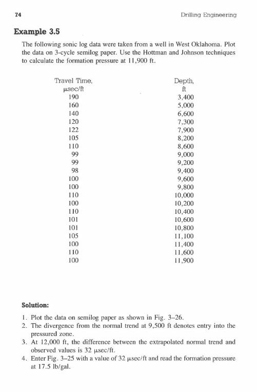
74 Drilling Engineering
Example 3.5
The following sonic log data were taken from a well in West Oklahoma. Plotthe data on 3-cycle semilog paper. Use the Hottman and Johnson techniquesto calculate the formation pressure at 11,900 ft.
Travel Time,J.LSec/ft
190160140120122105110999998
100100110100110101101105100110100
Depth,ft
3,4005,0006,6007,3007,9008,2008,6009,0009,2009,4009,6009,800
10,00010,20010,40010,60010,80011,10011,40011,60011,900
Solution:
1. Plot the data on semilog paper as shown in Fig. 3-26.2. The divergence from the normal trend at 9,500 ft denotes entry into the
pressured zone.3. At 12,000 ft, the difference between the extrapolated normal trend and
observed values is 32 /J-sec/ft.4. Enter Fig. 3-25 with a value of 32 /J-sec/ftand read the formation pressure
at 17.5 lb/gal.
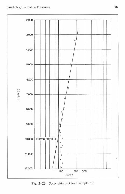
Predicting Formation Pressures 75
12,000
2,000
3,000
4,000
5,000
9,000
10,000
11,000
100 200 300seclft
Fig. 3-26 Sonic data plot for Example 3.5
6,000
g.t: 7,000a.Q)a
8,000
II
It
J
jI
;.
1.
Ii
.Normaltrend
fl 1-
1-
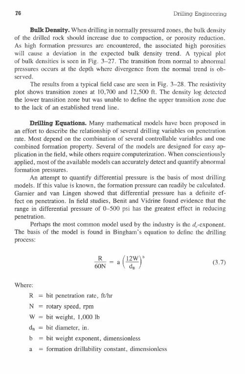
76 Drilling Engineering
Bulk Density. When drilling in nonnally pressured zones, the bulk densityof the drilled rock should increase due to compaction, or porosity reduction.As high fonnation pressures are encountered, the associated high porositieswiII cause a deviation in the expected bulk density trend. A typical plotof bulk densities is seen in Fig. 3-27. The transition from nonnal to abnonnalpressures occurs at the depth where divergence from the nonnal trend is ob-served.
The results from a typical field case are seen in Fig. 3-28. The resistivityplot shows transition zones at 10,700 and 12,500 ft. The density log detectedthe lower transition zone but was unable to define the upper transition zone dueto the lack of an established trend line.
Drilling Equations. Many mathematical models have been proposed inan effort to describe the relationship of several drilling variables on penetrationrate. Most depend on the combination of several controllable variables and onecombined fonnation property. Several of the models are designed for easy ap-plication in the field, while others require computerization. When conscientiouslyapplied, most of the available models can accurately detect and quantify abnonnalfonnation pressures.
An attempt to quantify differential pressure is the basis of most drillingmodels. If this value is known, the fonnation pressure can readily be calculated.Garnier and van Lingen showed that differential pressure has a definite ef-fect on penetration. In field studies, Benit and Vidrine found evidence that therange in differential pressure of 0-500 psi has the greatest effect in reducingpenetration.
Perhaps the most common model used by the industry is the dc-exponent.
The. basis of the model is found in Bingham's equation to define the drillingprocess:
~ = (12W)
b
60N a dB(3.7)
Where:
R = bit penetration rate, ft/hr
N = rotary speed, rpm
W = bit weight, 1,000 lb
dB = bit diameter, in.
b = bit weight exponent, dimensionless
a = fonnation drillability constant, dimensionless
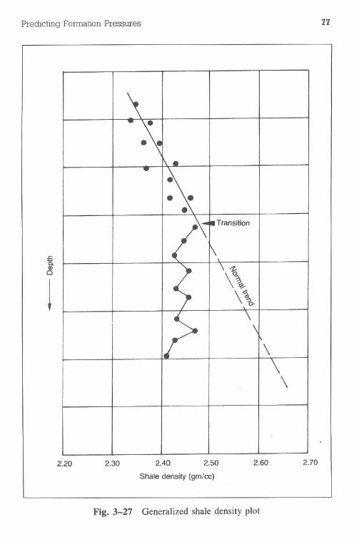
Predicting FormationPressures
.ca.CDc
I
2.20 2.30 2.40 2.50
Shale density (gm/cc)
Fig. 3-27 Generalized shale density plot
\
2.60
77
\
2.70
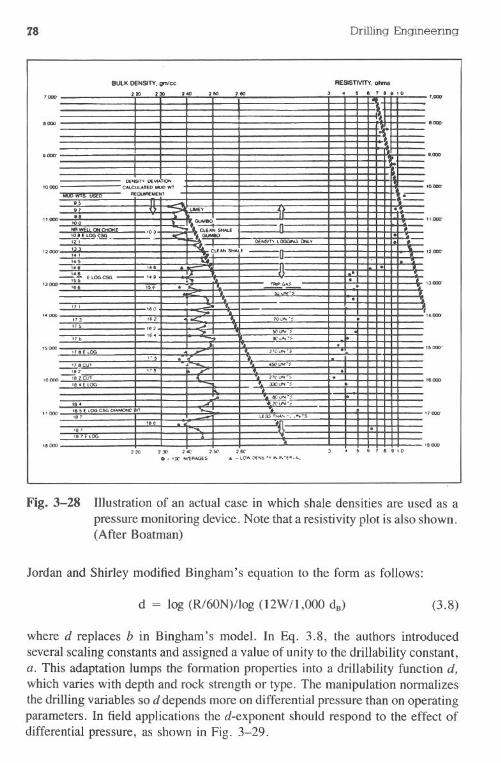
78 Drilling Engineering
BULK DENSITY. gnvc:c RESISTIVITY. ......
1000
'.ODD
1000 I.ODD
'0000 IO.OOCt
I'.Gat, II.CIOCt
12.000'
'.ODD
'.ODD
5000'
'6000
"000 1.000'
.1000 I ODD~20 230 lC' HC 2tC
..10t' .wERaGES .. -L~:t(..S"""''''-~.''-
.;67"10
Fig. 3-28 lllustration of an actual case in which shale densities are used as apressure monitoring device. Note that a resistivity plot is also shown.(After Boatman)
Jordan and Shirley modified Bingham's equation to the form as follows:
d = log (R/60N)/log (l2W/I,OOO dB) (3.8)
where d replaces b in Bingham's model. In Eq. 3.8, the authors introducedseveral scaling constants and assigned a value of unity to the drillability constant,a. This adaptation lumps the formation properties into a drillability function d,which varies with depth and rock strength or type. The manipulation normalizesthe drilling variables so d depends more on differential pressure than on operatingparameters. In field applications the d-exponent should respond to the effect ofdifferential pressure, as shown in Fig. 3-29.
'''' ,oo ,oo ,.. . . I . , . .10
DEfrISI"'"DEWM...CN..C:UI.AnDIIII.IDWt
IILVW'J$ M:OI..IIN'MEN' ...I ..... .I. """""
lOt ,.. Q.£AN SHAlf
m(L.- ...-, .0(N$fT-.L ONLV. W .-..eo..... ... .
::: UOGCSG-14' ........ ... . nIPGAS- .,. .... '"0
or. .., roLlf\o' . ,", '"... 5('IU'\o'":i-or. U"'o9$ ."1(,,00 21(H.","'
.',"ICUt . -$,.i .:.t .'i82CU1 2'C"--:io .I'"[LOG JXllI'\I. .
ec"",-:-, . \h':":i-18 ( LOGCSG OIAMONCen.., LIESS''''''''' -: ........S
'".., .,,"IE..
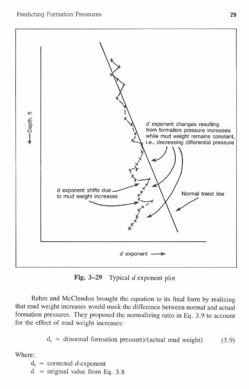
Predicting Formation Pressures 79
I,'(
I(
~-\-\-"
d exponent shifts due ~ ,/Jto mud weight increases r__ ~_>It
~11."v:
f1:
i:
d exponent changes resultingfrom formation pressure increaseswhile mud weight remains constant,Le., decreasing differential pressure
J
d exponent ~
Fig. 3-29 Typical d exponent plot
Rehm and McClendon brought the equation to its final fonn by realizingthat mud weight increases would mask the difference between nonnal and actualfonnation pressures. They proposed the nonnalizing ratio in Eq. 3.9 to accountfor the effect of mud weight increases:
de = d(nonnal fonnation pressure)/(actual mud weight) (3.9)
Where:d =ed
corrected d-exponentoriginal value from Eq. 3.8
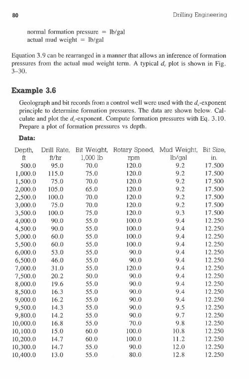
80
nonnal fonnation pressure = Ib/galactual mud weight = Ib/gal
Drilling Engineering
Equation 3.9 can be rearranged in a manner that allows an inference of fonnationpressures from the actual mud weight tenn. A typical de plot is shown in Fig.3-30.
Example 3.6
Geolograph and bit records from a control well were used with the dc-exponentprinciple to detennine fonnation pressures. The data are shown below. Cal-culate and plot the dc-exponent. Compute fonnation pressures with Eq. 3.10.Prepare a plot of fonnation pressures vs depth.
Data:
Depth,ft500.0
1,000.01,500.02,000.02,500.03,000.03,500.04,000.04,500.05,000.05,500.06,000.06,500.07,000.07,500.08,000.08,500.09,000.09,500.09,800.0
10,000.010,100.010,200.010,300.010,400.0
Drill Rate,ft/hr95.0
f15.075.0
105.0100.075.0
100.090.090.060.060.053.046.031.020.219.616.316.214.314.216.815.014.714.713.0
Bit Weight,1,000lb
70.075.070.065.070.070.075.055.055.055.055.055.055.055.050.055.055.055.055.055.055.060.060.055.055.0
Rotary Speed,rpm120.0120.0120.0120.0120.0120.0120.0100.0100.0100.0100.090.090.0
120.090.090.090.090.090.090.070.0
100.0100.090.080.0
Mud Weight,lb/gal
9.29.29.29.29.29.29.39.49.49.49.49.49.49.49.49.49.49.49.59.79.8
10.811.212.012.8
Bit Size,in.
17.50017.50017.50017.50017.50017.50017.50012.25012.25012.25012.25012.25012.25012.25012.25012.25012.25012.25012.25012.25012.25012.25012.25012.25012.250
17,000++ + + + + + + + + + + +
Formation factor
Fig.3-30 deexponent plot from a deep well (courtesy of Adams and RountreeTechnology, Inc.)
.!!
8,000 + .!! .!!
9,000+ .! .
.10,000+ ... .. ...11,000+ .
! ....12,000 + ... ..13,000 + .....14,000+ .. .. .15,000+ .....16,000+ .
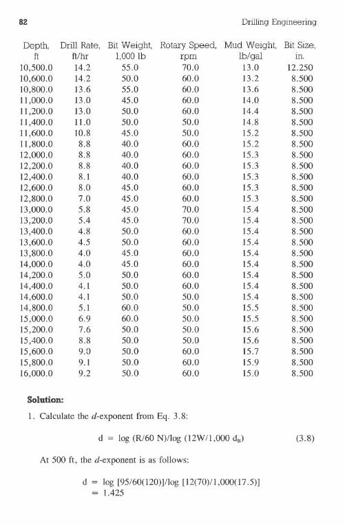
82 DrillingEngineering
Depth, Drill Rate! Bit Weight, Rotary Speed, Mud Weight, Bit Size,ft ft/hr 1,000 lb rpm lb/ gal m.
10,500.0 14.2 55.0 70.0 13.0 12.250
10,600.0 14.2 50.0 60.0 13.2 8.500
10,800.0 13.6 55.0 60.0 13.6 8.500
11,000.0 13.0 45.0 60.0 14.0 8.500
11,200.0 13.0 50.0 60.0 14.4 8.500
11,400.0 11.0 50.0 50.0 14.8 8.500
11,600.0 10.8 45.0 50.0 15.2 8.500
11,800.0 8.8 40.0 60.0 15.2 8.500
12,000.0 8.8 40.0 60.0 15.3 8.500
12,200.0 8.8 40.0 60.0 15.3 8.500
12,400.0 8.1 40.0 60.0 15.3 8.500
12,600.0 8.0 45.0 60.0 15.3 8.500
12,800.0 7.0 45.0 60.0 15.3 8.500
13,000.0 5.8 45.0 70.0 15.4 8.500
13,200.0 5.4 45.0 70.0 15.4 8.500
13,400.0 4.8 50.0 60.0 15.4 8.500
13,600.0 4.5 50.0 60.0 15.4 8.500
13,800.0 4.0 45.0 60.0 15.4 8.500
14,000.0 4.0 45.0 60.0 15.4 8.500
14,200.0 5.0 50.0 60.0 15.4 8.500
14,400.0 4.1 50.0 60.0 15.4 8.500
14,600.0 4.1 50.0 50.0 15.4 8.500
14,800.0 5.1 60.0 50.0 15.5 8.500
15,000.0 6.9 60.0 50.0 15.5 8.500
15,200.0 7.6 50.0 50.0 15.6 8.500
15,400.0 8.8 50.0 50.0 15.6 8.500
15,600.0 9.0 50.0 60.0 15.7 8.500
15,800.0 9.1 50.0 60.0 15.9 8.500
16,000.0 9.2 50.0 60.0 15.0 8.500
Solution:
1. Calculate the d-exponent from Eq. 3.8:
d = log (R/60 N)/log (12W/l,000 dB) (3.8)
At 500 ft, the d-exponent is as follows:
d = log [95/60(120)]/log [12(70)/1,000(17.5)]= 1.425
Predicting Formation Pressures 83
2. The dc-exponent is calculated from Eq. 3.9:
9d.: = d MW
1.425(9~2)
1.394
(3.9)
3. The dc-exponents are plotted in Fig. 3-31.4. The formation pressure is computed from Eq. 3.10:
FP = ~ - 0.3 (3. 10)
where 0.3 represents a trip margin of mud weight. At 16,000 ft the FP,formation pressure, is equivalent to 15.7-lb/gal mud.
5. The formation pressure plot is shown in Fig. 3-32.
Kicks. Pressure kicks provide valuable formation pressure information.Bit and mud records often contain sufficient data if a kick was taken to calculatethe pore pressure. Example 3.7 illustrates this.
Example 3.7
A bit record for the Two Star #3 well was analyzed as the control well fora prospect to be drilled. The record showed that a kick was taken at 10,900ft. Comments on the bit record were interpreted to indicate that the well wasnot killed with proper techniques. What is the actual formation pressure, inIb/gal, at 10.900 ft?
Data:
DepthCasingMud weight
Prior to setting casing at 10,300 ftAfter setting casing at 10,300 ftPrior to the kickAfter the kick= 375 psi= 490 psi= 28 bbl
10,900 ft (TVD)10,300 ft
9.8 Ib/gal12.0 Ib/gal12.2 Ib/gal14.5 Ib/gal
SIDPPSICP
Pit gain
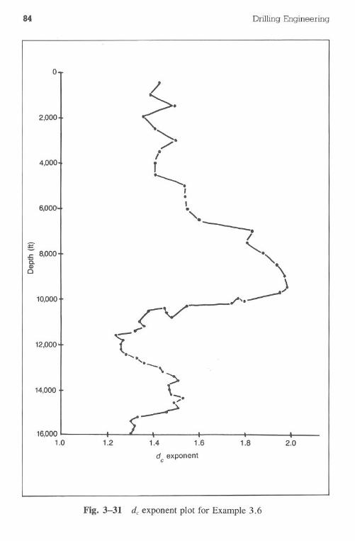
84 DrillingEngineering
~"'-
/8/r~ .,.
I.'.----i"'-.
"-
\~, )
o
2,000
4,000
6,0001.
=-~ 8,000a.CDc
10,000
12,000
14,000
16,0001.0 1.2 1.4 2.0
de exponent
1.6 1.8
Fig. 3-31 de exponent plot for Example 3.6
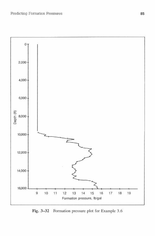
Predicting FormationPressures 85
g.c 8,000a.CDo
14,000
2,000
4,000
6,000
10,000
12,000
16,000
o
9 10 11 12 13 14 15 16 17 18 19
Formation pressure, Ib/gal
Fig.3-32 Fonnation pressure plot for Example 3.6
86 Drilling Engineering
Solution:
1. The mud weights of 9.8 and 12.0 Ib/gal at 10,300 ft indicate that theoperator chose to raise the mud weight much greater than the pore pressureprior to drilling out of the casing. The pore pressure at 10,300 ft can beassumed to be approximately 9.8 Ib/gal or less. It is not uncommon,although not cost efficient, for an operator to drill out of a casing stringwith the mud weight at the maximum value expected to be required forthe next hole section.
2. The pore pressure at 10,900 ft can be calculated from Eq. 3.11:
KWM = SIDPP x 19.23 + OWMTVD
= 375 psi x 19.23 + 122 Ib/ I10,900ft . ga
12.9 Ibigal (12.86 Ib/gal)
(3.1l)
Problems
3.1 Using the following data, plot the shale resistivities on semilog paper.Where is the top of the abnormal pressure zone? Construct a normaltrend line and extrapolate it through the abnormal region. Use theHottman and Johnson approach to calculate the formation pressure ateach 500-ft interval beginning at 6,000 ft.
Depth, ft6,0006,5007,0007,5008,0008,5009,0009,500
10,00010,20010,40010,60010,8001l,00011,200
Resistivity, ohm-m2/m0.700.730.740.780.800.850.900.961.061.101.151.100.980.880.80
Predicting Formation Pressures 87
11,40011,60011,80012,000
0.740.700.640.60
Solution: 12,000 ft-15.11b/gal
3.2 Use the Hottman and Johnson method to calculate formation pressureat each I,ooo-ft interval below the entrance into abnormal pressuresat 8,450 ft.
Resistivity. ohm-m0.460.420.450.420.480.470.500.520.500.450.470.500.480.430.380.320.25
Depth, ft3,0004,0005,3006,3007,0007,7008,1008,4508,8009,0009,3009,650
10,20010,50010,80011,00011,200
3.3 A well is to be drilled to 10,000 ft. The shale resistivities for thecontrolling offset well are given below. Use a trip margin of 0.3-lb/gal mud weight. What would be the minimum required mud densityin the well that is to be drilled? Use the Hottman and Johnson method.
Depth, ft6,0006,5007,0007,2007,4007,600
Resistivity, ohm-m2/m0.620.640.650.640.680.68
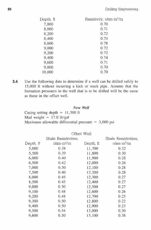
88
Depth, ft7,8008,0008,2008,4008,6009,0009,2009,4009,6009,800
10,000
Drilling Engineering
Resistivity, ohm-m2/m0.700.710.720.740.780.720.720.740.710.700.70
3.4 Use the following data to determine if a well can be drilled safely to15,000 ft without incurring a kick or stuck pipe. Assume that theformation pressures in the well that is to be drilled will be the sameas those in the offset well.
New Well
Casing setting depth = 11,500ftMud weight = 17.0Ib/galMaximum allowable differential pressure = 3,000 psi
Depth, ft5,0005,5006,0006,5007,0007,5008,0008,5009,0009,1009,2009,3009,4009,5009,600
Offset WellShale Resistivities,
ohm-m2/m0.380.390.400.420.500.400.450.450.500.480.480.500.500.540.50
Depth, ft11,70011,80011,90012,00012,10012,20012,30012,40012,50012,60012,70012,80012,90013,00013,100
Shale Resistivities,ohm-m2/m
0.320.300.280.260.280.280.270.270.270.260.250.220.230.300.38
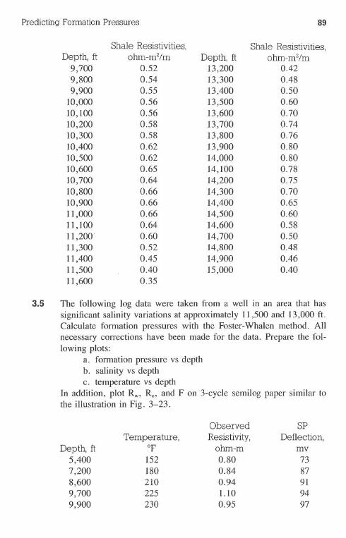
Predicting Formation Pressures
Depth, it9,7009,8009,900
10,00010,10010,20010,30010,40010,50010,60010,70010,80010,90011,00011,10011,200.11,30011,40011,50011,600
Shale Resistivities,ohm-m2/m
0.520.540.550.560.560.580.580.620.620.650.640.660.660.660.640.600.520.450.400.35
Depth, it13,20013,30013,40013,50013,60013,70013,80013,90014,00014,10014,20014,30014,40014,50014,60014,70014,80014,90015,000
89
Shale Resistivities,ohm-m2/m
0.420.480.500.600.700.740.760.800.800.780.750.700.650.600.580.500.480.460.40
3.5 The following log data were taken from a well in an area that hassignificant salinity variations at approximately 11,500 and 13,000 ft.Calculate formation pressures with the Foster-Whalen method. Allnecessary corrections have been made for the data. Prepare the fol-lowing plots:
a. formation pressure vs depthb. salinity vs depthc. temperature vs depth
In addition, plot Rw, Ro, and F on 3-cycle semilog paper similar tothe illustration in Fig. 3-23.
Observed SPTemperature, Resistivity, Deflection,
Depth, it of ohm-m mv5,400 152 0.80 737,200 180 0.84 878,600 210 0.94 919,700 225 1.10 949,900 230 0.95 97
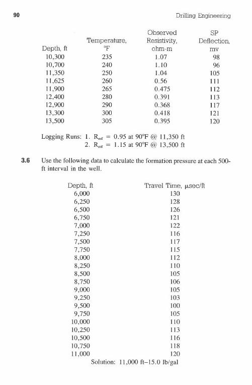
90
Depth, ft10,30010,70011,35011,62511,90012,40012,90013,30013,500
Temperature,of235240250260265280290300305
Drilling Engineering
ObservedResistivity,
ohm-m1.071.101.040.560.4750.3910.3680.4180.395
SPDeflection,
mv9896
105111112113117121120
Logging Runs: 1. Rmf= 0.95 at 90°F @ 11,350 ft2. Rmf= 1.15 at 90°F @ 13,500 ft
3.6 Use the following data to calculate the formation pressure at each 500-ft interval in the well.
Depth, ft6,0006,2506,5006,7507,0007,2507,5007,7508,0008,2508,5008,7509,0009,2509,5009,750
10,00010,25010,50010,75011,000
Solution:
Travel Time, f.Lsec/ft130128126121122116117115112110105106105103100105110113116118120
11,000 ft-15.0 Ib/ga1
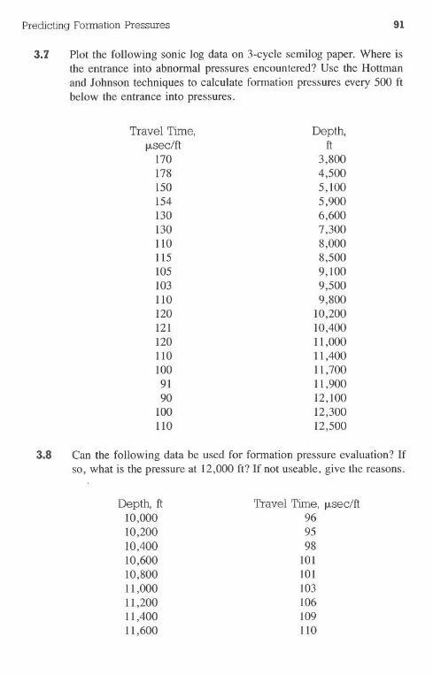
Predicting Formation Pressures 91
3.7 Plot the following sonic log data on 3-cycle semilog paper. Where isthe entrance into abnormal pressures encountered? Use the Hottmanand Johnson techniques to calculate formation pressures every 500 ftbelow the entrance into pressures.
Travel Time,f.Lsec/ft
1701781501541301301101151051031101201211201101009190
100110
Depth,ft
3,8004,5005,1005,9006,6007,3008,0008,5009,1009,5009,800
10,20010,40011,00011,40011,70011,90012,10012,30012,500
3.8 Can the following data be used for formation pressure evaluation? Ifso, what is the pressure at 12,000 ft? If not useable, give the reasons.
Depth, ft10,00010,20010,40010,60010,80011,00011,20011,40011,600
Travel Time, f.Lsec/ft969598
101101103106109110
92 Drilling Engineering
Depth, ft Travel Time, f,Lsec/ft11,800 III
12,000 113
3.9 Calculate the required mud weights to drill each section of a wellusing offset well data for control. Use a 0.3-lb/gal trip margin of mudweight.
Section Interval, ft1 3,500-10,4002 10,400-12,9003 12,900-14,500
Offset Well Sonic Survey
Travel Time, Travel Time,Depth, ft f,Lsec/ft Depth, ft f,Lsec/ft
3,500 156 II ,400 125
4,000 152 11,500 130
4,500 148 11,600 129
5,000 143 1I ,700 120
5,500 140 11,800 128
6,000 136 II ,900 125
6,500 132 12,000 123
7,000 129 12,100 122
7,500 125 12,200 123
8,000 121 12,300 124
8,200 120 12,400 122
8,400 119 12,500 121
8,600 117 12,600 120
8,800 116 12,700 120
9,000 114 12,800 119
9,200 113 12,900 1I5
9,400 111 13,000 108
9,600 110 13,100 107
9,800 110 13,200 106
10,000 108 13,300 106
10,100 III 13,400 105
10,200 1I5 13,500 106
10,300 120 13,600 105
10,400 120 13,700 104
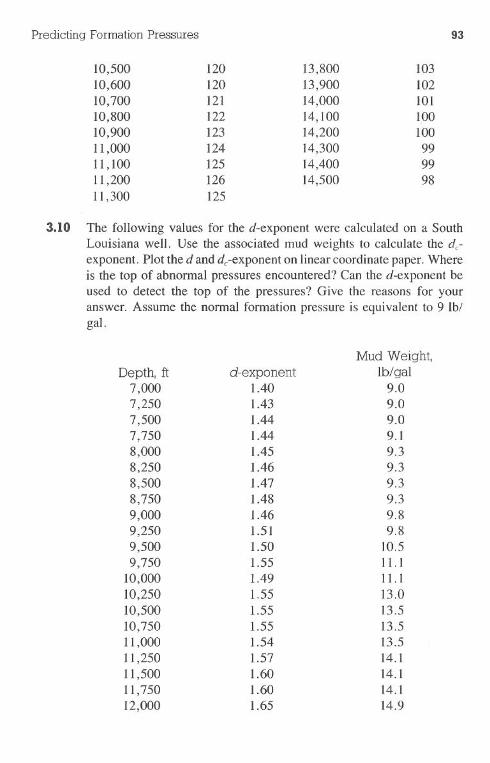
3.10 The following values for the d-exponent were calculated on a SouthLouisiana well. Use the associated mud weights to calculate the dc-exponent. Plot the d and dc-exponenton linear coordinate paper. Whereis the top of abnormal pressures encountered? Can the d-exponent beused to detect the top of the pressures? Give the reasons for youranswer. Assume the normal formation pressure is equivalent to 9 Ib/gal.
Depth, ft7,0007,2507,5007,7508,0008,2508,5008,7509,0009,2509,5009,750
10,00010,25010,50010,75011,00011,25011,50011,75012,000
d-exponent1.401.431.441.441.451.461.471.481.461.511.501.551.491.551.551.551.541.571.601.601.65
Mud Weight,Ib/ gal
9.09.09.09.19.39.39.39.39.89.8
10.5ILl11.113.013.513.513.514.114.114.114.9
Predicting Formation Pressures 93
10,500 120 13,800 10310,600 120 13,900 10210,700 121 14,000 10110,800 122 14,100 10010,900 123 14,200 10011,000 124 14,300 9911,100 125 14,400 9911,200 126 14,500 9811,300 125
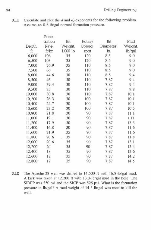
94 Drilling Engineering
3.11 Calculate and plot the d and dc-exponents for the following problem.Assume an 8.8-lb/gal normal formation pressure.
Pene-tration Bit Rotary Bit Mud
Depth, Rate, Weight, Speed, Diameter, Weight,ft filhr 1,000 lb rpm In. Ib/ gal
6,000 106 35 120 8.5 9.06,500 103 35 120 8.5 9.07,000 76.9 35 110 8.5 9.07,500 66 35 110 8.5 9.08,000 44.6 30 110 8.5 9.48,500 46 30 110 7.87 9.49,000 39.4 30 110 7.87 9.49,500 35 30 110 7.87 9.8
10,000 30.8 30 110 7.87 10.110,200 26.3 30 100 7.87 10.110,400 24.7 30 100 7.87 10.110,600 23.2 30 100 7.87 10.510,800 21.8 30 90 7.87 11.111,000 19.1 30 90 7.87 1.1111,200 17.9 30 90 7.87 13.311,400 16.8 30 90 7.87 11.611,600 21.9 35 90 7.87 11.611,800 20.6 35 90 7.87 11.812,000 20.6 35 90 7.87 13.112,200 20 35 90 7.87 13.412,400 18 35 90 7.87 13.612,600 18 35 90 7.87 14.212,800 17 35 90 7.87 14.5
3.12 The Apache 28 well was drilled to 14,500 ft with 16.8-lb/gal mud.A kick was taken at 12,200 ft with 13.3-lb/gal mud in the hole. TheSIDPP was 350 psi and the SICP was 525 psi. What is the formationpressure in Ib/gal? A mud weight of 14.3 lb/gal was used to kill thewell.
Predicting Formation Pressures 95
References
Adams, Neal. Well Control Problems and Solutions. Tulsa: PennWell Pub-lishing Company, 1980.
Baroid Division, NLlPetroleum Services, "Manual of Drilling Fluids Tech-nology," Section 2, Houston, 1979.
Bingham, M.G. "A New Approach to Interpreting Rock Drillability." Oil& Gas Journal. 2 November 1964-5 April 1965.
Boatman, W.A. "Shale Densities Key to Safer, Faster Drilling." World Oil.August 1967.
Fertl, W.H. Abnormal Formation Pressures: Implications to Exploration.Drilling. and Production of Oil and Gas Resources. New York: Elsevier,1976.
Fert1,W.H., and D.J. Timko. "How Abnormal Pressure Detection Techniquesare Applied." Oil & Gas Journal, 12 January 1970.
Fertl, W.H., and D.J. Timko. "How Downhole Temperatures, PressuresAffect Drilling: Part I, Origin of Abnormal Formation Pressures." WorldOil. June 1972.
Foster, J.B., and H.E. Whalen. "Estimation of Formation Pressures fromElectrical Surveys, Offshore Louisiana." JPT, February 1965.
Gamier, A.J., and M.H. van Lingen. "Phenomena Affecting Drilling Ratesof Depth." Trans. AIME, 1959, pp. 216, 232.
Hottman, E.C., and R.K. Johnson. "Estimation of Formation Pressures fromLog-Derived Shale Properties." JPT, June 1965.
Jordan, J.R., and O.J. Shirley. "Application of Drilling Performance Datato Overpressure Detection." JPT, November 1966.
Lewis, C.R., and S.c. Rose. A Theory Relating High Temperatures andOverpressures." JPT, January 1970.
96 Drilling Engineering
Pennebaker, E.S. "'Seismic Data Indicate Depth, Magnitude of AbnormalPressures." World Oil, June 1968.
Pennebaker, E.S. "An Engineering Interpretation of Seismic Data." SPE2165, 43rd AIME Fall Meeting, Houston, September 1968.
Postma, G.W. "Wave Propagation in a Stratified Medium." Geophysics,20:780-806, 1955.
Rehm, B., and R. McClendon. "Measurement of Formation Pressure fromDrilling Data." SPE Paper 3601, AIME Annual Fall Meeting, New Orleans,1971.
Reynolds, E.B. "Predicting Overpressured Zones with Seismic Data. WorldOil, October 1970.
Reynolds, E.B. "The Application of Seismic Techniques to Drilling Tech-niques." SPE Paper 4643, 48th AIME Fall Meeting, Las Vegas, October1973.
Thurber, C.H. "The Geo-acoustic Spectrum." Oil & GasJournal, 12October1959.
Vidrine, D.J., and E.J. Benit. "Field Verificationof the Effect of DifferentialPressure on Drilling Rate." JPT, July 1968.
Wilson, G.J., and R.E. Bush. "Pressure Prediction with Flowline Temper-ature Gradient." JPT, March, 1973.
Zamora, M. "Slide-Rule Correlation Aids d-Exponent Use." Oil & GasJournal, 18 December 1972.
Chapter 4 Fracture GradientDetermination
Well planning demands a knowledge of the pressures required to initiatea fracture into a formation. Fracture gradient calculations, as they are termed,are essential in minimizing or avoiding lost circulation problems and in selectingproper casing seat depths. .
Theoretical Determination
A number of theoretical and field-developed equations have been used toapproximate formation fracture gradients. Many of these are suitable for im-mediate application in a given area, while some require a hindsight approachbased on density (or other) logging measurements taken after the well has beendrilled.
A common base for most fracture gradient determination principles is theassumption that the geological area in question is a tectonically relaxed basincontaining plastic-like shales with interbedded sand-shale sequences.
As noted by Pilkington (PEl, May 1978), "None of the relationshipsdiscussed are valid in either brittle, or naturally fractured formations includinglimestones, dolomites and shales. Returns may also be lost in vugular formationsregardless of the fracture gradient in the overlying formations."
Calculation procedures for these areas rely on either a history of the fieldor geologic structure, or on field determinations utilizing leakoff tests or loggingmethods.
Hubbert and Willis. In the paper "Mechanics of Hydraulics Fracturing,"Hubbert and Willis explored the variables involved in initiating a fracture in aformation. According to the authors, the fracture gradient is a function of ov-erburden stress, formation pressure, and a relationship between the horizontal
97
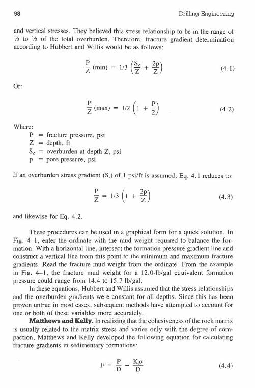
98 Drilling Engineering
and vertical stresses. They believed this stress relationship to be in the range ofY3 to Yz of the total overburden. Therefore, fracture gradient determinationaccording to Hubbert and Willis would be as follows:
P.(Sz 2P)- (mm) = 113 - + -Z Z Z (4.1)
Or:
PZ(max) (4.2)
Where:
P = fracture pressure, psiZ = depth, ftSz = overburden at depth Z, psip = pore pressure, psi
If an overburden stress gradient (Sz)of 1 psi/ft is assumed, Eq. 4.1 reduces to:
P( 2P)Z = 113 1 + Z (4.3)
and likewise for Eq. 4.2.
These procedures can be used in a graphical form for a quick solution. InFig. 4-1, enter the ordinate with the mud weight required to balance the for-mation. With a horizontal line, intersect the formation pressure gradient line andconstruct a vertical line from this point to the minimum and maximum fracturegradients. Read the fracture mud weight from the ordinate. From the examplein Fig. 4-1, the fracture mud weight for a 12.0-lb/gal equivalent formationpressure could range from 14.4 to 15.7 lb/gal.
In these equations, Hubbert and Willis assumed that the stress relationshipsand the overburden gradients were constant for all depths. Since this has beenproven untrue in most cases, subsequent methods have attempted to account forone or both of these variables more accurately.
Matthews and Keny. In realizing that the cohesiveness of the rock matrixis usually related to the matrix stress and varies only with the degree of com-paction, Matthews and Kelly developed the following equation for calculatingfracture gradients in sedimentary formations:
P KjO"F--+-D- D (4.4)
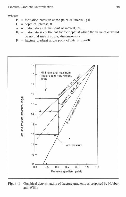
Fracture Gradient Determination 99
Where:p =D
formation pressure at the point of interest, psidepth of interest, ftmatrix stress at the point of interest, psimatrix stress coefficient for the depth at which the value of {J'wouldbe normal matrix stress, dimensionlessfracture gradient at the point of interest, psi/ftF
Fig. 4-1 Graphical determination of fracture gradients as proposed by Hubbertand Willis
19
18
17
16Iii
.91
1!!15
dj::::J(J)(J)
14 !Jc-O>:;-0 Q..0.§ 13"Cc:100> 120a.
11
10
90.4 0.5 0.6 0.7 0.8 0.9 1.0
Pressure gradient, psi/ft
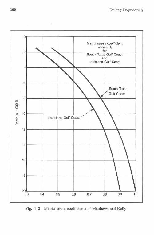
100 Drilling Engineering
o
2
Matrix stress coefficientversus Dj
forSouth Texas Gulf Coast
andLouisiana Gulf Coast
4
6
14
16
18
200.3 0.4 0.9 1.00.5 0.6 0.7 0.8
Fig. 4-2 Matrix stress coefficients of Matthews and Kelly
8-=00q
x 10.s::. I I Louisiana Gulf CoastQ.Q)c
12
Fracture Gradient Determination 101
The matrix stress coefficient relates the actual matrix stress conditions ofthe formation to the conditions of matrix stress if the formation were compactednormally. The authors believed that the conditions necessary for fracturing theformation would then be similar to those for the normally compacted formation.
The stress coefficient vs depth is presented in Fig. 4-2. Matthews andKelly believed that the coefficient would vary with different geological condi-tions. The values shown were obtained by substituting actual field data of break-down pressures into Eq. 4.4 and solving for Kj.
The procedure for calculating fracture gradients using the Matthews andKelly technique is as follows:
I. Obtain formation fluid pressure, P. This can be measured by drillstemtests, kick data, logs, or another satisfactory method.
2. Obtain the matrix stress by using Eq. 4.4 and assuming a gradient of1.0 psi/ft for the overburden:
0' = S - P (4.5)
3. Determine the depth, D;, for which the matrix stress, 0', would be thenormal value. Assume that the overburden pressure is 1.0 psi/ft. Fromthis it follows that:
0.535 Dj = 0' (4.6)
from which the value of Dj can be found.4. Use the value of Dj and apply it to Fig. 4-2 to obtain the corresponding
value of Kj.5. Using the values of D, 0', P, and K;, calculate the value of the fracture
gradient, F.
Example 4.1
Casing was set on a Texas Gulf Coast well at 7,200 ft. It was estimated thatformation pressure was equivalent to 11.0-lb/gal mud. What is the fracturegradient immediately below the casing seat? Use the Matthews and Kellyprocedure.
Solution:
1. P = (11.0 Ib/gal)(0.052)(7,200 ft)= 4,118 psi
2. 0' = S - P7,200 - 4,1183,082 psi
102 Drilling Engineering
3. Depth equivalent, .oj:0.535 Dj = CT
CT 3,082Dj = 0.535 = 0.535 = 5,760 ft
where 0.535 psi/ft is the rock matrix stress4. From Fig. 4-2, Kj = 0.695
5. F = ~ + K~CT4,ll8 (0.695)(3,082)=-+7,200 7,200
= 0.571 + 0.298= 0.869 psi/ft= 16.7 Ib/gal (equivalentmud weight)
A graphical solution to the Matthews and Kelly technique is presented inFig. 4-3. Note that the curved lines on the graph represent actual formationpressures and not mud weight in use. Unfortunately, these are often erroneouslyinterchanged. To solve for fracture gradients with Fig. 4-3, enter at the desireddepth and read horizontally until the actual formation pressure line is intersected.Plot a vertical line from this point and read the fracture gradient in pounds pergallon.
Eaton. Eaton extended the concepts presented by Matthews and Kelly tointroduce Poisson's ratio into the expression for the fracture pressure gradient:
F = S - P ( E- ) + E-D I-v D (4.7)
Where:P = wellbore pressure, psiD = depth, ftS = overburden stress, psiv = Poisson's ratioF = fracture gradient, psi/ft
Eaton assumed that both overburden stress and Poisson's ratio were variable
with depth. Using actual field fracture data and log-derived values, he preparedgraphs illustrating these variables (Figs. 4-4 and 4-5). Using a suitable choicefor each variable, the nomograph prepared by Eaton et al. (Fig. 4-6) can beused to calculate a fracture gradient.
A graphical presentation for the Eaton approach provides a quick solution.The chart (Fig. 4-7) is used in the same manner as the Matthews and Kelly
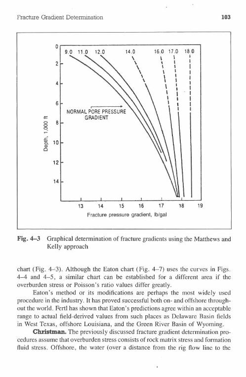
Fracture Gradient Determination 103
14
13 1S 1614
Fracture pressure gradient, Ib/gal
17 18 19
Fig. 4-3 Graphical determination of fracture gradients using the Matthews andKelly approach
chart (Fig. 4-:-3).Although the Eaton chart (Fig. 4-7) uses the curves in Figs.4-4 and 4-5, a similar chart can be established for a different area if theoverburden stress or Poisson's ratio values differ greatly.
Eaton's method or its modifications are perhaps the most widely usedprocedure in the industry. It has proved successful both on- and offshore through-out the world. Fertl has shown that Eaton's predictions agree within an acceptablerange to actual field-derived values from such places as Delaware Basin fieldsin West Texas, offshore Louisiana, and the Green River Basin of Wyoming.
Christman. The previously discussed fracture gradient determination pro-cedures assume that overburden stress consists of rock matrix stress and formationfluid stress. Offshore, the water (over a distance from the rig flow line to the
09.0 11.0 12.0 14.0 16.0 17.0 18.0
\ , I
2;- ...........'" " \ , , I. , , I, , I\ , I
41- """ . I ,, \ ,I I, I ,, , I61-
NORMALPOREPRESSUR0.\ \ \ , , ,\ , I-= I GRADIENT0 80q
.r=a.Q)c
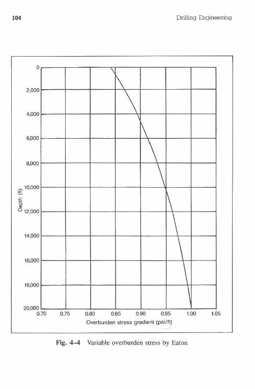
104
~ 10,000
~.s::a.Q)CI 12,000
Drilling Engineering
o
2,000
4,000
6,000
8,000
14,000
16,000
18,000
20,0000.70 1.00 1.050.75 0.80 0.85 0.90 0.95
Overburden stress gradient (psi/ft)
Fig. 4-4 Variable overburden stress by Eaton
\
1\
\\
\
\\
\\\\\
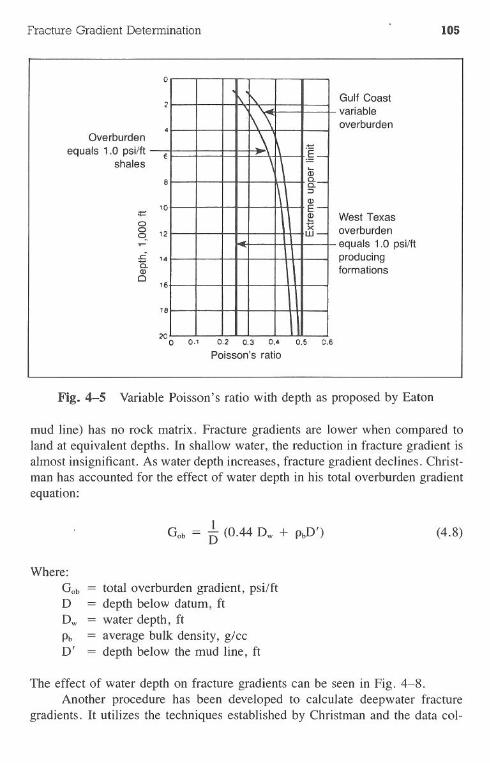
Fracture Gradient Determination 105
o
=:ooq
Gulf Coastvariableoverburden
Overburdenequals 1.0 psi/ft
shales
£'E.0)
CI
West Texasoverburdenequals 1.0 psi/ftproducingformations
200 0.1 0.2 0.3 0.' 0.5 0.6
Poisson's ratio
Fig. 4-5 Variable Poisson's ratio with depth as proposed by Eaton
mud line) has no rock matrix. Fracture gradients are lower when compared toland at equivalent depths. In shallow water, the reduction in fracture gradient isalmost insignificant. As water depth increases, fracture gradient declines. Christ-man has accounted for the effect of water depth in his total overburden gradientequation:
(4.8)
Where:GobD
Dw
PbD'
= total overburden gradient, psi/ft= depth below datum, ft= water depth, ft= average bulk density, glcc= depth below the mud line, ft
The effect of water depth on fracture gradients can be seen in Fig. 4-8.Another procedure has been developed to calculate deepwater fracture
gradients. It utilizes the techniques established by Christman and the data col-
2
. 1\\\ -
6
\\:E_
8 8:-::::J
0)10 E-
O)
12 -,.
16
18
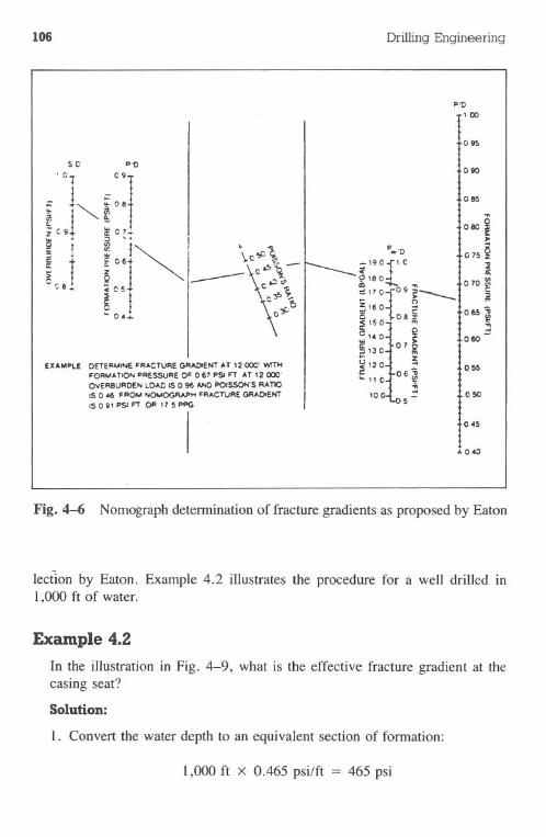
106 Drilling Engineering
P'l)
100
015
Fig. 4-6 Nomograph determination of fracture gradients as proposed by Eaton
lection by Eaton. Example 4.2 illustrates the procedure for a well drilled in1,000 ft of water.
Example. 4.2
In the illustration in Fig. 4-9, what is the effective fracture gradient at thecasing seat?
Solution:
1. Convert the water depth to an equivalent section of formation:
1,000ft x 0.465 psi/ft = 465 psi
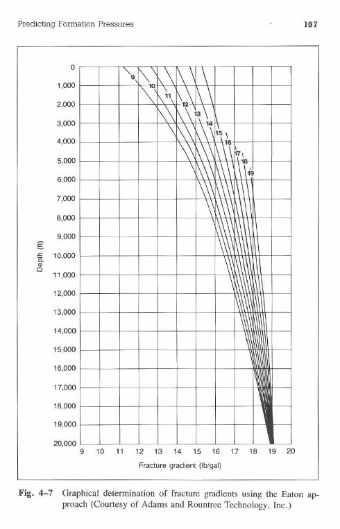
Predicting Formation Pressures 107
~9J\~I\ \ \ \,\'",~~ \~ 1\\
\\'\ \ 1~\4
\l\\' \\\ -~~\ \ \\ \ \\\ '7~8
\ \\\ \\\\\\119
\\\ \\\\ \\\\\'\ \
1\,\\ \\
\\
\
,\
:)
I IJ20,0009 10 11 12 13 14 15 16 17 18 19 20
Fracture gradient (Ib/gal)
Fig. 4-7 Graphical determination of fracture gradients using the Eaton ap-proach (Courtesy of Adams and Rountree Technology, Inc.)
0
1,000
2,000
3,000
4,000
5,000
6,000
7,000
8,000
9,000g.c 10,000Q.Q)c
11,000
12,000
13,000
14,000
15,000
16,000
17,000
18,000
19,000
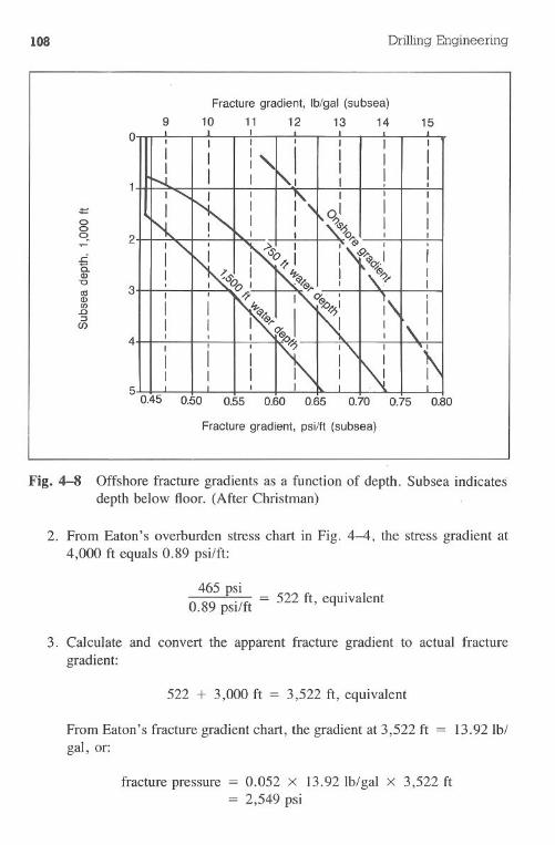
108 DrillingEngineering
9Fracture gradient, Ib/gal (subsea)
10 11 12 13 14 15o
0.50 0.55 0.60 0.65 0.70 0.75 0.80
-=ooq 2
~a.Q)
"tJ
CISQ)CJ).c::J(/)
3
4
Fracture gradient, psilft (subsea)
Fig. 4-8 Offshore fracture gradients as a function of depth. Subsea indicatesdepth below floor. (After Christman)
2. From Eaton's overburden stress chart in Fig. 4-4, the stress gradient at4,000 ft equals 0.89 psi/ft:
465 psi0.89 psi/ft = 522 ft, equivalent
3. Calculate and convert the apparent fracture gradient to actual fracturegradient:
522 + 3,000 ft = 3,522 ft, equivalent
From Eaton's fracture gradient chart, the gradient at 3,522 ft = 13.92Ib/gal, or:
fracture pressure = 0.052 x 13.92 lb/gal x 3,522 ft= 2,549 psi
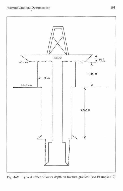
Fracture Gradient Determination 109
Drillship 60 ft
t1,000 ft
Riser
Mud line
3,000 ft
Fig.4-9 Typical effect of water depth on fracture gradient (see Example 4.2)
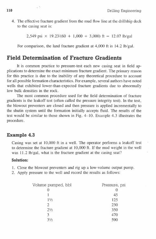
110 Drilling Engineering
4. The effective fracture gradient"fromthe mud flow line at the drill!;hipdeckto the casing seat is:
2,549 psi x 19.23/(60 + 1,000 + 3,000) ft = 12.07 lb/gal
For comparison, the land fracture gradient at 4,000 ft is 14.2 Ib/gal.
Field Determination of Fracture GradientsIt is common practice to pressure-test each new casing seat in field ap-
plications to determine the exact minimum fracture gradient. The primary reasonfor this practice is due to the inability of any theoretical procedure to accountfor all possible formation characteristics. For example, several authors have notedwells that exhibited lower-than-expected fracture gradients due to abnormallylow bulk densities in the rock.
The most common procedure used for the field determination of fracturegradients is the leakoff test (often called the pressure integrity test). In the test,the blowout preventers are closed and then pressure is applied incrementally tothe shutin system until the formation initially accepts fluid. The results of thetest would be similar to those shown in Fig. 4-10. Example 4.3 illustrates theprocedure.
Example 4.3
Casing was set at 10,000 ft in a well. The operator performs a leakoff testto determine the fracture gradient at 10,000 ft. If the mud weight in the wellwas 11.2 Ib/gal, what is the fracture gradient at the casing seat?
Solution:
I. Close the blowout preventers and rig up a low-volume output pump.2. Apply pressure to the well and record the results as follows:
Volume pumped, bbloII Y222Y233Y2
Pressure, psio
45125230350470590
Fracture Gradient Determination
Q)
:;UJUJQ)
a:
.
111
Pressures are recorded atthe initial leak-off
_\
l. ~ Drilling fluid. c0'!1pression~ and pressurizationRequired fillupvolume priorto compression
1
Volume pumped
Fig. 4-10 Typical results from a leakoff test
44Yz55Yz6
710830950990
1010
3. The results are plotted in Fig. 4-11. It appears that the formation willbegin to fracture when 950 psi is applied.
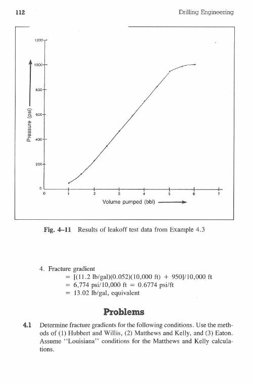
112
12'
1000
600
200
oo
Drilling Engineering
3 6
Volume pumped (bbl) ..
Fig. 4-11 Results of leakoff test data from Example 4.3
4. Fracture gradient[(11.2Ib/gal)(0.052)(1O,000 ft) + 950]/10,000 ft6,774 psi/IO,OOOft = 0.6774 psi/ft
= 13.02 lb/gal, equivalent
Problems
4.1 Determine fracture gradients for the following conditions. Use the meth-ods of (1) Hubbert and Willis, (2) Matthews and Kelly, and (3) Eaton.Assume "Louisiana" conditions for the Matthews and Kelly calcula-tions.
Fracture Gradient Determination 113
Depth,ft.
3,00013,0009,0006,5008,000
11,00017,0004,500
10,50015,000
Formation Pressure,lb/galNormal
13.19.69.0
10.215.118.09.9
Normal15.6
Solution: 3,000 ftHubbert and Willis -12.2-14.0 Ib/gal
Matthews and Kelly - 13.8Ib/galEaton -13.9 Ib/gal
4.2 Prepare a graph of fracture gradients vs depth for the methods used inProblem 4.1. Assume normal formation pressures.
4.3 Calculate the fracture gradient for the following set of deepwater con-ditions. Use the approach described in Example 4.2.
Freeboard = 50 ft
Water depth = 1,700ftCasing depth below seafloor = 6,000 ft
4.4 Use the following leakoff data to determine the formation fracturegradient. Casing is set at 12,000 ft and the mud weight is 13.9 lb/gal.
Volume Pumped,bblo122Y233Y244'/25
Pressure,pSI
o175400590680760650740830
114 Drilling Engineering
Volume Pumped,bbl51/266Y277Y288Y2
Pressure,pSI920
1,0101,1001,1901,2601,2801,300
4.5 Calculate the formation fracture gradient for the following conditions.Use the pressure data from Problem 4.4.
Depth of casing,ft
9,30016,00013,1006,400
Mud weight in use,lb/gal
9.013.915.19.5
Solution: 9,300 ft, 11.6 Ib/gal
4.6 Use the Eaton fracture gradient chart to calculate fracture gradients forProblems 5.2, 5.3, 5.4, and 5.5.
References
Christman, Stan A. "Offshore Fracture Gradients." JPT, August 1973.
Eaton, B.A. "Fracture Gradient Prediction and Its Application in OilfieldOperations." JPT, October 1969.
Fertl, W.H. "Predicting Fracture Pressure Gradients for More Efficient Drill-ing." Petroleum Engineer. December 1976.
Fertl, W.H., and D.J. Timko. "Application of Well Logs to GeopressureProblems in the Search, Drilling, and Production of Hydrocarbons." FrenchPetroleum Institute Paper No.4, June 1971.
Hubbert, M. King, and D.G. Willis. "Mechanics of Hydraulic Fracturing."Trans. AIME, 210, pp. 153-166, 1957.
Fracture Gradient Determination liS
Matthews, W.R., and J. Kelly. "How to Predict Formation Pressure andFracture Gradient." Oil & Gas Journal. 20 February 1967.
Pilkington, P.E. "Fracture Gradient Estimates in Tertiary Basins.'" PetroleumEngineer International, May 1978.
"
Chapter 5 Casing SettingDepth Selection
The first design task in preparing the well plan is selecting the depths towhich the casing will be run and cemented. The drilling engineer must considergeological conditions such as formation pressures and fracture gradients, holeproblems, internal company policies, and, in many cases, a variety of governmentregulations. The results of the program will allow the well to be drilled safelywithout the necessity of building "a steel monument" of casing strings. Un-fortunately, many well plans give significant considerations to the actual pipedesign yet give only cursory attention to the setting depth of the pipe.
The importance of selecting proper depths for setting casing cannot beoveremphasized. Many wells have been engineering and economic failures be-cause the casing program specified setting depths too shallow or too deep. Ap-plying a few basic drilling principles combined with a basic knowledge of thegeological conditions in an area can help determine where casing strings shouldbe set to ensure that drilling can proceed with minimum difficulty.
Types of Casing and TubingDrillingenvironmentsoftenrequireseveralcasingstringsin orderto reach
the total desireddepth. Someof the stringsare as follows:·drive or structural.conductor· surface· intermediate (also known as protection pipe)·liners
116
Casing Setting Depth Selection 117
·production (also known as an oil string)· tubing (flow string)
Fig. 5-1 shows the relationship of some of these casing strings. In addition, theillustration shows some of the problems and drilling hazards that the strings aredesigned to control.
All wells will not use each type of casing. The conditions to be encounteredin each well must be analyzed to detennine the types and amount of pipe necessaryto drill it. The general functions of all casing strings are as follows:
· segregate and isolate various fonnations to minimize drilling problemsor maximize production· furnish a stable well with a known diameter through which future drillingand completion operations can be executed· provide a secure means to which pressure control equipment can beattached
Drive Pipe or Conductor Casing. The first string run or placed in thewell is usually the drive pipe, or conductor casing. The nonnal depths rangefrom 100-300 ft. In soft-rock areas such as southern Louisiana or most offshoreenvironments, the pipe is hammered into the ground with a large diesel hammer.Hard-rock areas require that a large-diameter, shallow hole be drilled beforerunning and cementing the pipe. Conductor casing can be as elaborate as heavy-wall steel pipe or as simple as a few old oil drums tacked together.
A primary purpose of this string of pipe is to provide a fluid conduit fromthe bit to the surface. Very shallow fonnations tend to wash out severely andmust be protected with pipe. In addition, most shallow fonnations exhibit sometype of lost circulation problem that must be minimized.
An additional function of the pipe is to minimize hole caving problems.Gravel beds and unconsolidated rock will continue to fall into the well if notstabilized with casing. Typically, the operator is required to drill through thesezones by pumping viscous muds at high rates.
Structural Casing. Occasionally, drilling conditions will require that anadditional string of casing be run between the drive pipe and surface casing.Typical depths range from 600-1,000 ft. Purposes for the pipe include solvingadditional lost circulation or hole caving problems and minimizing kick problemsfrom shallow gas zones. '
Surface Casing. Many purposes exist for running surface casing, In-cluding the following:·cover freshwater sands
'. maintain hole integrity by preventing caving·minimize lost circulation into shallow, permeable zones.. cover weak zones that are incompetent to control kick-imposed pressures
118 Drilling Engineering
.provide a means for attaching the blowout preventers. support the weight of all casing strings (except liners) run below thesurface pipe
Intermediate Casing. The primary applications of intermediate casinginvolve abnormally high formation pressures. Since higher mud weights arerequired to control these pressures, the shallower weak formations must beprotected to prevent lost circulation or stuck pipe. Occasionally, intermediate
Graver li"eds
Fresh water
Abnormally Ihigh ..
pressure
Conductorpipe
Heavingshales
Intermediatecasing
Legend
~ Cement
f Pay zone
Fig. 5-1 Typical casing string relationships
Casing Setting Depth Selection 119
pipe is used to isolate salt zones or zones that cause hole problems, such asheaving and sloughing shales.
Liners. Drilling liners are used for the same purpose as intermediatecasing. Instead of running the pipe to the surface, an abbreviated string is usedfrom the bottom of the hole to a shallower depth inside the intermediate pipe.Usually the overlap between the two strings is 300-500 ft. In this case, theintermediate pipe is exposed to the same drilling considerations as the liner (seeFig. 5-1).
Drilling (and production) liners are used frequently as a cost-effectivemethod to attain pressure or fracture gradient control without the expense ofrunning a string to the surface. When a liner is used, the upper exposed casing,usually intermediate pipe, must be evaluated with respect to burst and collapsepressures for drilling the open hole below the liner. Remember that a full stringof casing can be run to the surface instead of a liner if required, Le., twointermediate strings.
Production Casing. The production casing is often called the oil string.The pipe may be set at a depth slightly above, midway through, or below thepay zone. The pipe has the following purposes:
· isolate the producing zone from the other formations· provide a work shaft of a known diameter to the pay zone· protect the production tubing equipment
Tie-back String. The drilling liner is often used as part of the productioncasing rather than running an additional full string of pipe from the surface tothe producing zone. The liner is tied-back or connected to the surface by runningthe amount of pipe required to connect to the liner top. This procedure is par-ticularly common when 1) producing hydrocarbons are behind the liner and2) the deeper section is not commercial.
Setting Depth Design Procedures'Casing seat depths are directly affected by geological conditions. In some
cases, the prime criterion for selecting casing seats is to cover exposed, severelost circulation zones. In others, the seat selection may be based on differentialsticking problems, perhaps resulting from pressure depletion in a field. In deepwells, however, the primary consideration is usually based on controlling ab-normal formation pressures and preventing their exposure to weaker shallowzones. The design criteria of controlling formation pressures generally appliesto most drilling areas. .
Selecting casing seats for pressure control purposes starts with knowinggeological conditions such as formation pressures and fracture gradients. Thisinformation is generally available within an acceptable degree of accuracy. Pre-
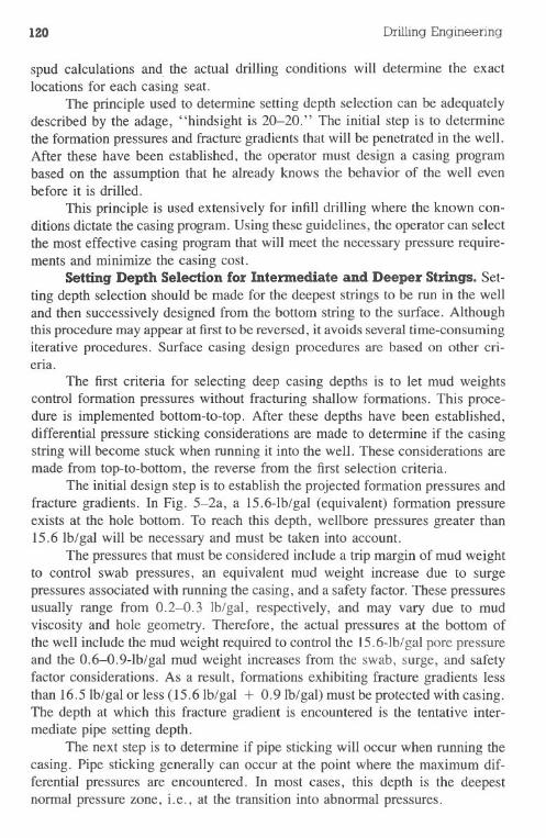
120 DrillingEngineering
spud calculations and. the actual drilling conditions will determine the exactlocations for each casing seat.
The principle used to determine setting depth selection can be adequatelydescribed by the adage, "hindsight is 20-20." The initial step is to determinethe formation pressures and fracture gradients that will be penetrated in the well.After these have been established, the operator must design a casing programbased on the assumption that he already knows the behavior of the well evenbefore it is drilled.
This principle is used extensively for infill drilling where the known con-ditions dictate the casing program. Using these guidelines, the operator can selectthe most effective casing program that will meet the necessary pressure require-ments and minimize the casing cost.
Setting Depth Selection for Intennediate and Deeper Strings. Set-ting depth selection should be made for the deepest strings to be run in the welland then successively designed from the bottom string to the surface. Althoughthis procedure may appear at first to be reversed, it avoids several time-consumingiterative procedures. Surface casing design procedures are based on other cri-eria.
The first criteria for selecting deep casing depths is to let mud weightscontrol formation pressures without fracturing shallow formations. This proce-dure is implemented bottom-to-top. After these depths have been established,differential pressure sticking considerations are made to determine if the casingstring will become stuck when running it into the well. These considerations aremade from top-to-bottom, the reverse from the first selection criteria.
The initial design step is to establish the projected formation pressures andfracture gradients. In Fig. 5-2a, a 15.6-lb/gal (equivalent) formation pressureexists at the hole bottom. To reach this depth, wellbore pressures greater than15.6 Ib/gal will be necessary and must be taken into account.
The pressures that must be considered include a trip margin of mud weightto control swab pressures, an equivalent mud weight increase due to surgepressures associated with running the casing, and a safety factor. These pressuresusually range from 0.2-0.3 Ib/gal, respectively, and may vary due to mudviscosity and hole geometry. Therefore, the actual pressures at the bottom ofthe well include the mud weight required to control the 15.6-lb/gal pore pressureand the 0.6-0.9-lb/gal mud weight increases from the swab, surge, and safetyfactor considerations. As a result, formations exhibiting fracture gradients lessthan 16.5Ib/gal or less (l5.61b/gal + 0.9Ib/gal) must be protected with casing.The depth at which this fracture gradient is encountered is the tentative inter-mediate pipe setting depth.
The next step is to determine if pipe sticking will occur when running thecasing. Pipe sticking generally can occur at the point where the maximum dif-ferential pressures are encountered. In most cases, this depth is the deepestnormal pressure zone, i.e., at the transition into abnormal pressures.
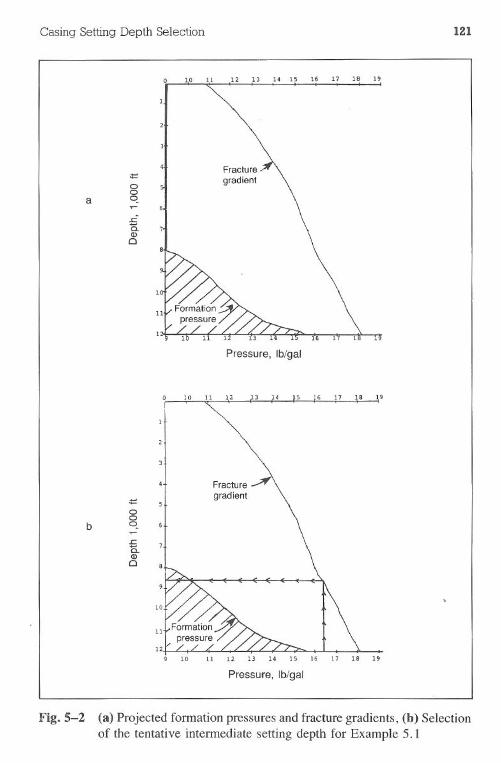
Casing Setting Depth Selection 121
-=oo
a q
-=o
b ~
.c'E.CD
Q
19
Pressure, Ib/gal
.ca.CDQ
10 11 12 13 14 15 16 17 18 19
Pressure, Ib/gal
Fig.5-2 (a) Projected formation pressures and fracture gradients, (b) Selectionof the tentative intermediate setting depth for Example 5.1
122 Drilling Engineering
Field studies have been used to establish general values for the amount ofdifferential pressure that can be tolerated before sticking occurs:
Normal pressure zones 2,000-2,300 psiAbnormal pressure zones 3,000-3,300 psi
These values are recommended as reasonable guides. Their accuracy inday-to-day operations depends on the general attention given to mud propertiesand drillstring configuration.
The tentative intermediate pipe setting depth is the actual setting depth ifthe differential pressure at the deepest normal zone is less than 2,000-2,300 psi.If the value is greater than this arbitrary limit, the depth is defined as theshallowest liner setting depth required to drill the well. In this case, an additionalstep is necessary to determine the intermediate pipe depth.
An example problem will be used to illustrate this procedure. The sectionfollowing the example will illustrate the case in which differential pres-sure considerations cause the additional step to select the intermediate pipedepth.
Example 5.1
Use Fig. 5-2a to determine the proper setting depth for intermediate pipe.Assume a 0.3-lb/gal factor for swab and surge and a 0.2-lb/gal safety factor.Use an arbitrary maximum limit of 2,200 psi differential pressure for normalpressure zones.
Solution:
1. Evaluate the maximum pressures (equivalent mud weights) at the totaldepth of the well.
Amount, Ib/gal15.60.30.30.2
16.4
PurposeFormation pressureTrip marginSurge pressureSafety factor
Type of PressureActual mud weightActual mud weightEquivalent mud weightEquivalent mud weight
2. Determine the formations that cannot withstand 16.4-lb/gal pressures, Le.,those formations that must be protected with casing. Construct a verticalline from 16.4 lb/gal to an intersection of the fracture gradient line (Fig.5-2b). The depth of intersection is the tentative intermediate casing settingdepth, or 8,600 ft in this example.
3. Check the tentative depth to determine if differential pipe sticking will be
Casing Setting Depth Selection 123
a problem when running the casing to 8,600 ft. The mud required to reach8,600 ft is:
10.4 Ib/gal Formation pressure0.3 Ib/gal Trip margin
10.7 Ib/gal Total required mud weightDifferential sticking potential is evaluated at the deepest normal pressure(9.0 Ib/gal) zone, 8,000 ft.
(10.71b/gal - 9.0 Ib/gal)(0.052)(8,000 ft)707 psi < 2,200 psi
707 psi
Since the pipe can be run to 8,600 ft without differential sticking, thedepth becomes the actual intermediate setting depth rather than the tentativedepth, as defined in step 2.
4. Check the interval from 8,600-12,000 ft to determine if the differen-tial pressure exceeds the 3,000-3,300-psi range. In this case, pres-sure = 2,700 psi @ 8,600 ft.
Example 5.1 illustrated the case in which the vertical line from 16.4 Ib/gal intersected the fracture gradient curve in an abnormal pressure region. Acalculation was performed to determine if the casing would stick when run intothe well. If the pressures had been greater than the arbitrary limit of 2,200 psi,procedures in the following sections would be implemented. Cases arising whenthe vertical line intersects the fracture gradient curve in the normal pressureregion will be discussed later.
Altering the tentative intermediate casing setting depth because of potentialdifferential sticking problems is required in many cases. The previously defined"intermediate pipe setting depth" is redefined as the shallowest liner depth. Theprocedure works from the top to the bottom of the high pressure zone ratherthan the reverse approach used to establish the tentative intermediate depth. Thenew intermediate depth is established using sticking criteria. The deepest linersetting depth is determined from formation pressure-fracture gradient guidelines.After the deepest liner depth is established, the operator must determine theexact liner setting depth between the previously calculated shallowest and deepestpossible depths. The final liner depth can be established from criteria such asminimizing the amount of small hole that must be drilled below the liner andpreventing excessive amounts of open hole between the intermediate-liner sectionor the liner-pay zone section.
Eqs. 5.1 and 5.2 can be used to help determine the new intermediate depthif sticking is a concern:
~p = (MW - 9)(0.052)(D) (5.1)
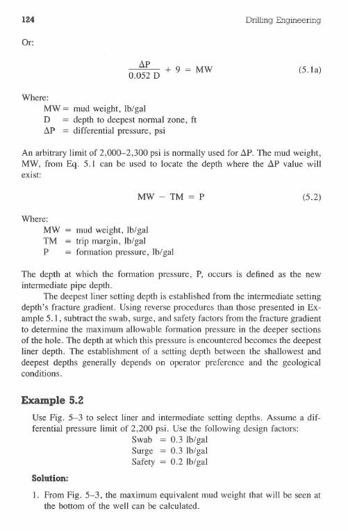
124 Drilling Engineering
Or:
~P0.052 D + 9 = MW (5.1a)
Where:MW = mud weight, lb/galD = depth to deepest normal zone, ft~P = differential pressure, psi
An arbitrary limit of 2,000-2,300 psi is normally used for ~P. The mud weight,MW, from Eq. 5.1 can be used to locate the depth where the ~P value willexist:
MW-TM=P (5.2)
Where:MW = mud weight, lb/galTM = trip margin, lb/galP = formation pressure, lb/gal
The depth at which the formation pressure, P, occurs is defined as the newintermediate pipe depth.
The deepest liner setting depth is established from the intermediate settingdepth's fracture gradient. Using reverse procedures than those presented in Ex-ample 5.1, subtract the swab, surge, and safety factors from the fracture gradientto determine the maximum allowable formation pressure in the deeper sectionsof the hole. The depth at which this pressure is encountered becomes the deepestliner depth. The establishment of a setting depth between the shallowest anddeepest depths generally depends on operator preference and the geologicalconditions.
Example 5.2
Use Fig. 5-3 to select liner and intermediatesettingdepths. Assumea dif-ferentialpressurelimitof 2,200psi. Use the followingdesignfactors:
Swab = 0.3 lb/galSurge = 0.3 lb/galSafety = 0.2 lb/gal
Solution:
l. From Fig. 5-3, the maximum equivalent mud weight that will be seen atthe bottom of the well can be calculated.
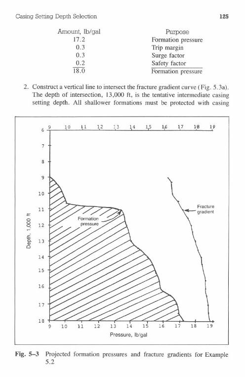
Casing Setting Depth Selection 125
Amount,lb/gal17.20.30.30.2
18.0
PurposeFonnation pressureTrip marginSurge factorSafety factorFonnation pressure
2. Construct a vertical line to intersect the fracture gradient curve (Fig. 5.3a).The depth of intersection, 13,000 ft, is the tentative intennediate casingsetting depth. All shallower fonnations must be protected with casing
;:::ooq 12
.r=c. 13Q)Q
6 910 11 12 1 17 18 1913 14 1.5
7
8
9
10
11
14
15
16
17
189 10 12 15 1916 17 1813 1411
Pressure, Ib/gal
Fig. 5-3 Projected fonnation pressures and fracture gradients for Example5.2
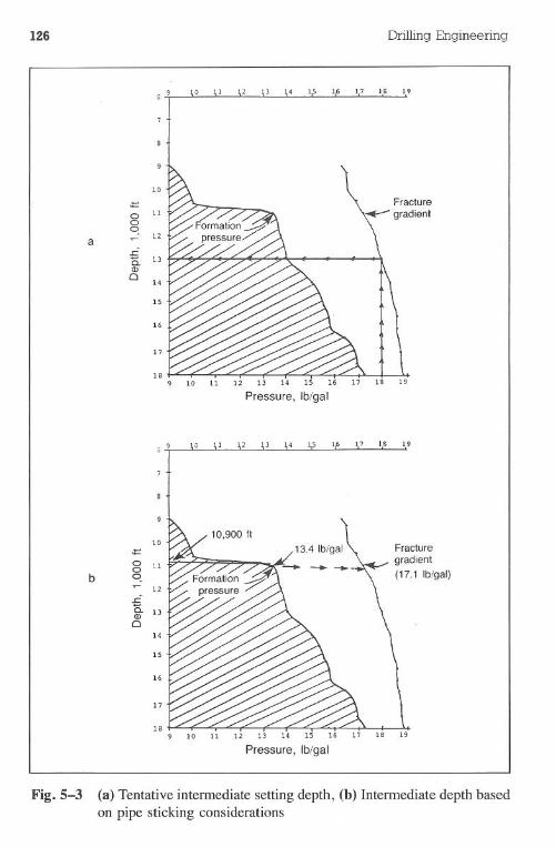
126 Drilling Engineering
6 91.7 IS 19
Fig.5-3 (a) Tentative intennediate setting depth, (b) Intennediate depth basedon pipe sticking considerations
10
<:=0 1100 - 12
a.r;.-
0.. 13Q)
014
15
16
17
189 10 11 12 13 14
Pressure, Ib/gal
5 9In 11 12 13 14 15 L6 1.7 18 19
10<:=
0 110b q
12.c0.. 13Q)0
H
15
16
17
1810 11 12
Pressure, Ib/gal
Casing ~tting Depth Selection lZ7
6 9 IB 19
Fig. 5-3 (c) Selection of the deepest liner depth, (d) Final configuration
10
0 110
Cq
12
is. 13Q)C
H
15
16
17
1810 11 12 13 14 15 16
Pressure, Ib/gal
5 9 10 11 12 13 14 15 I 17 18 19
10
1100
d q 12
13is.(I)q 14
15
16
17
la'9 10 11 12
Pressure, Ib/gal
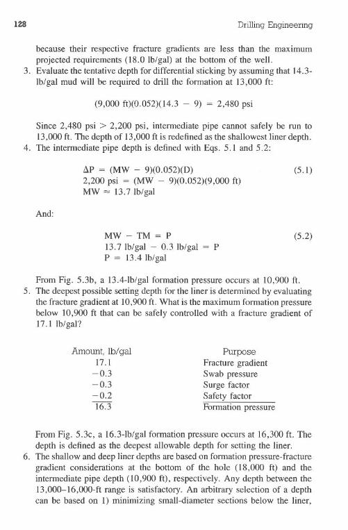
128 Drilling Engineering
because their respective fracture gradients are less than the maximumprojected requirements (18.0 Ib/gal) at the bottom of the well.
3. Evaluate the tentative depth for differential sticking by assuming that 14.3-Ib/gal mud will be required to drill the formation at 13,000 ft:
(9,000 ft)(O.052)(14.3 - 9) = 2,480 psi
Since 2,480 psi> 2,200 psi, intermediate pipe cannot safely be run to13,000 ft. The depth of 13,000 ft is redefined as the shallowest liner depth.
4. The intermediate pipe depth is defined with Eqs. 5.1 and 5.2:
I1P = (MW - 9)(0.052)(D)2,200 psi = (MW - 9)(0.052)(9,000 ft)MW = 13.7 Ib/gal
(5.1)
And:
MW-TM=P
13.7Ib/gal - 0.3 Ib/gal = PP = 13.4Ib/gal
(5.2)
From Fig. 5.3b, a 13.4-lb/gal formation pressure occurs at 10,900 ft.5. The deepest possible setting depth for the liner is determined by evaluating
the fracture gradient at 10,900 ft. What is the maximum formation pressurebelow 10,900 ft that can be safely controlled with a fracture gradient of17.1 Ib/gal?
Amount, Ib/gal17.1
-0.3-0.3-0.216.3
PurposeFracture gradientSwab pressureSurge factorSafety factorFormation pressure
From Fig. 5.3c, a 16.3-lb/gal formation pressure occurs at 16,300 ft. Thedepth is defined as the deepest allowable depth for setting the liner.
6. The shallow and deep liner depths are based on formation pressure-fracturegradient considerations at the bottom of the hole (18,000 ft) and theintermediate pipe depth (10,900 ft), respectively. Any depth between the13,000-16,000-ft range is satisfactory. An arbitrary selection of a depthcan be based on 1) minimizing small-diameter sections below the liner,
Casing Setting Depth Selection 129
2) minimizing the open hole length and thereby reducing pipe costs, or3) other considerations as specified by the operator.
As an example, assume that a depth of 15,000 ft is selected.It reduces the small-diameter hole to a 3,000-ft segment (15,000-18,000ft) while allowing only 4,100 ftof open hole (10,900-15,000 ft) (Fig.5-3d).
Examples 5.1 and 5.2 illustrated the cases in which the initial formationpressure-fracture gradient consideration at the bottom of the well selected pipedepths in the abnormal pressure regions. Different techniques must be used ifthe tentative pipe setting depth is in a normal pressure region.
The initial step is to evaluate the differential sticking possibilities at thedeepest normal pressure zone. If the mud weight required at the bottom of thewell does not create differential pressures in excess of some limit (2,000-2,300psi), a deep surface casing string is satisfactory. Eqs. 5.1 and 5.2 must be usedwhen the differential pressures exceed the allowable limit.
Surface Casing Depth Selection. Shallow casing strings such as surfacecasing are often imposed to pressures that are more severe than the considerationsused to select the setting depths for intermediate casing and liner. These pressuresusually result from kicks inadvertently taken when drilling deeper sections. Asa result, surface setting depths are selected to contain kick pressures rather thanthe previously described procedures for intermediate casing. This philosophy,differs for the intermediate hole since the kick pressures are usually lower thanthe previously discussed swab-surge-safety factors logic for deep strings.
Kick-imposed equivalent mud weights are the cause for most undergroundblowouts. When a kick occurs, the shutin casing pressure added to the drillingmud hydrostatic pressure exceeds the formation fracture pressure and results inan induced fracture. Therefore, the objective of a seat selection procedure thatavoids underground blowouts would be to choose a depth that can competentlywithstand the pressures of reasonable kick conditions.
A precise determination of kick-imposed pressures can be difficult. How-ever, a procedure that estimates the values has been proven in field applicationsto be quick and effective. Fig. 5-4 represents a well whose pumps and blowoutpreventers have simulated a kick. Eq. 5.3 describes the pressure relationships:
EMW - ( total depth ) LlM.kick- depth of interest ( ) + OMW
(5.3)
Where:EMWkick= equivalent mud weight at the depth of interest, Ib/galtotal depth = deepest interval, ft
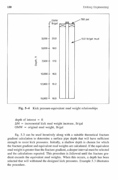
130 Drilling Engineering.
EMWIb/gal
15,000.J. 16.0
Fig. 5-4 Kick pressure-equivalent mud weight relationships
depth of interest = ftdM = incremental kick mud weight increase, lb/galOMW = originalmud weight, lb/gal
Eq. 5.3 can be used iteratively along with a suitable theoretical fracturegradient calculation to determine a surface pipe depth that will have sufficientstrength to resist kick pressures. Initially, a shallow depth is chosen for whichthe fracture gradient and equivalent mud weights are calculated. If the equivalentmud weight is greater than the fracture gradient, a deeper interval must be selectedand the calculations repeated. This procedure is followed until the fracture gra-dient exceeds the equivalent mud weights. When this occurs, a depth has beenselected that will withstand the designed kick pressures. Example 5.3 illustratesthe procedure.
ooo 120.0I I I 15.0 Ib/gal mud
5,000 18.0
.c7,500 + 17.0C.
Q)0
1j 1M12,000 16.2
Casing Setting Depth Selection 131
Example 5.3
Using Fig. 5-5a, select a surface casing depth and, if necessary, setting depthsfor deeper strings. Use the following design factors:
0.3 = swab, surgefactor,lb/gal0.2 = safety factor, Ib/gal0.5 = kick factor, Ib/gal
2,200 = maximum allowable differential pressure, psi
Solution:
1. Evaluate the maximum pressures anticipated at the bottom of the well.
Amount, lb/gal12.00.30.30.2
12.8
PurposeFormation pressureTrip (swab) marginSurge factorSafety factor
A vertical line from 12.8'lb/gal intersects the fracture gradient in a normalregion, which indicates intermediate casing will not be required unlessdifferential sticking is a problem.
2. Assume that 12.3 Ib/gal will be used at the bottom of the well and determineif differential sticking may occur:
(12.3 - 9.0 Ib/gal)(0.052)(9,000ft) = 1,544psi
Since 1,544 psi is less than the arbitrary limit of 2,200 psi, intermediatecasing will not be used for pipe-sticking considerations. Therefore, onlysurface casing is required.
3. Use Eq. 5.3 and the fracture gradient curve to determine the depth atwhich the fracture gradient exceeds the kick loading mud weight. Performa first trial calculation at 1,000 feet.
12,000EMWl,ooo= 1 000 (0.5) + 12.3,
= 18.3 Ib/gal
The fracture gradient at 1,000 feet is 12.0 Ib/gal. Since the kick loadingis greater than the rock strength, a deeper trial depth must be chosen.
132
;t:oo
a q
Drilling Engineering
10 11 12 13 14 15 16 17 18 19
~c.Q)o
10
II
12
10 11 12 13 14 15 16 17 18 19
Pressure, Ib/gal
Fig. 5-5 (a) Intermediate casing evaluation for Example 5.3, (b) Equivalentmud weight-fracture gradient relationship
;t: .
rurfce
00q 5 casing
b depth
C.Q)0
Casing Setting Depth Selection 133
Results from several iterations are given below and plotted on Fig.5-5b.
Depth, ft1,0002,0003,0003,5004,0004,5005,0006,0007,000
EMWkick,Ib/gal18.315.314.314.013.813.613.513.313.2
4. A setting depth of 3,600 ft is selected.
The value of 0.5 Ib/gal used in Example 5.3 for the kick incremental mudweight increase is widely accepted. It represents the average (maximum) mudweight increase necessary to kill a kick. Use of this variable in Eq. 5.3 allowsthe operator to (inadvertently) drill into a fonnation in which the pressure is inexcess of 0.5 Ib/gal greater than the original calculated value and still safelycontrol the kick that may occur. In fact, if the original mud weight variable is0.3-0.4 Ib/gal greater than the anticipated fonnation pressure, the equation wouldaccount for fonnation pressure calculation errors ofO.8-O.91b/gal. If necessary,an operator may alter the 0.5-lb/gal variable to whatever is deemed most suitablefor the drilling environment.
A valid argument has been raised concerning Eq. 5.3 and its representationof field circumstances. In actual kick situations, the equivalent mud weights arecontrolled to a certain degree by casing pressure, which is not directly takeninto account in the equation. However, an inspection of casing pressure willshow that the two components in the pressure are I) degree of underbalancebetween the original mud and the fonnation pressure and 2) degree of under-balance between the influx fluid and the fonnation pressure.
The first of these components is taken into account in the equation by theincremental mud weight increase tenn, while the latter is not considered. In mostkick situations, the average value of the second component will range from 100-300 psi. If an operator believes that the second component is significant enoughto alter the equation, he can change the incremental mud weight increase tennto a higher value.
Figs. 5-4, 5-6, and 5-7 illustrate the considerations. Figs. 5-4 and 5-6represent a I.O-lb/gal kick in simple and actual hole geometries, respectively.Fig. 5-7 shows the equivalent mud weights for both cases. If an operator is
134
4.5-in. drillpipe
7.0-in. drill collars(1,000 fl)
SIDPP = 780 psi
Fig. 5-6 20-barrel kick
DrillingEngineering
SICP = 1,370psi
15.0-lb/gal mud
8.5-in. hole
4--14,115 fl - Gas lop20 bbl volume15,000ft
Casing Setting Depth Selection 135
o
2
3
12
13
14
15
15 16 17 18 19 20 21 22 23 24 25 26 27 28 29
Equivalent mud weight, Ib/gal
Fig. 5-7 Comparison of equivalent mud weights for rule-of-thumb and actualsituations
concerned about the difference shown in Fig. 5-7, modifications to Eq. 5.3should be made, or a different equation should be used.
Drive Pipe and/or Conductor Casing. Pipe setting depths above thesurface casing are usually determined from various government regulations orlocalized drilling problems. For example, an area may have severe lost circulationproblems at 75-100 ft that can be solved by placing drive pipe below the zone.Other drilling conditions that may affect setting depths include water-bearingsands, unconsolidated formations, or shallow gas. An evaluation of local drillingrecords will normally identify these conditions. Most governments require thatfreshwater sands be cased.
4
£ 500
6Q....
.s:: 7C.Q)0 8
9
10
11
136 Drilling Engineering
Problems5.1 Rework Example 5.1 with the following set of design factors. A small-
diameter hole with a high-viscosity mud requires the use of 0.4 lb/gal factors for swab and surge. The type of mud being used necessitatesa maximum limit of 2,200 psi differential pressure for the normalpressure zone. Use a 0.2-lb/gal safety margin.
5.2 Determine the intermediate casing setting depth for the following setof conditions. Use the Eaton fracture gradient chart in Chapter 4 todetermine the formation fracture gradients. Assume a 0.3-lb/gal swaband surge factor. Use 0.2 lb/gal as the safety factor and 2,300 psi asthe maximum limit on differential pressure for normal zones.
Depth, ft0-9,400
9,50010,00010,50011,00011,50012,00012,50013,00013,50014,00014,500
Formation Pressure,lb/ gal
9.09.5
11.011.812.312.913.313.514.015.016.016.2
5.3 Recompute Problem 5.2 with the following additional hole sections.The problem may require a liner.
Depth, ft15,00015,500
Formation Pressure,lb/gal16.817.2
5.4 Determine the intermediate setting depth for the following problem.Use a O.4-lb/gal factor for swab and surge and a 2,200-psi differentialpressure limit. The safety factor should be 0.2 lb/gal. Use Eaton'schart for fracture gradients.
Casing Setting Depth Selection 137
Depth, ft0-10,000
10,20010,80011,25011,78012,50013,09013,800
Formation Pressure,lb/gal
9.09.29.8
12.213.314.215.316.1
5.5 Using Problem 5.4, determine the liner and intermediate casing settingdepths for the additional hole sections as follows:
Depth, ft14,00014AOO15,020
Formation Pressure,lb/gal16.216.817.3
5.6 Select a surface casing setting depth for the following data. Use Eaton'schart in Chapter 4 for fracture gradients. Use a 0.5-lb/gal kick sizein Eq. 5.3.
Intermediate setting depth = 11,000ftOriginal mud weight = 10.5 lb/gal
5.7 Rework Problem 5.6 and use intermediate pipe depths of 8,000, 9,000,10,000, and 12,000 ft. Plot the results in Problems 5.6 and 5.7 in agraph.
5.8 Rework Problem 5.6 for kick sizes of 0.2, 0.3, 0.4, and 0.75 lb/gal.Plot the results.
5.9 Determine the surface casing setting depth for the following situation:Intermediate setting depth = 9AOOftOriginal mud weight = 12.llb/galKick size = 0.4 lb/gal
5.10 Suppose that in drilling the well in Problem 5.2 a zone is encounteredin which the bottom-hole pressure is reduced to 8,131 psi at 14,100ft as a result of depletion in an offset well.

138 Drilling Engineering
a. Will this zone cause any impact on the setting depth program?b. Describe possible solutions.c. Would the potential problems be any different if the pressure were
9,150 psi? Explain your answer.
References
1. Adams, N.J. Well Control Problems and Solutions. Tulsa: PennWell Pub-lishing Company, 1980.
Chapter 6 Bole GeometrySelection
Bit and casing size selection can mean the difference between a well thatmust be abandoned before completion and a well that is an economic and en-gineering success. Improper size selection can result in holes so small that thewell must be abandoned due to drilling or completion problems. The drillingengineer (and well planner) is responsible for designing the hole geometry toavoid these problems.
However, a successful well is not necessarily an economic success. Forexample, a well design that allows for satisfactory, trouble-free drilling andcompletion may be an economic failure because the drilling costs are greaterthan the expected return on investment. Hole geometry selection is a critical partof the engineering plan that can make the difference between economic andengineering failure or success.
General Design ProceduresThe drilling industry's experience has developed several commonly used
hole geometry programs. These programs are based on bit and casing size avail-ability as well as the expected drilling conditions. Two widely used casingprograms are as follows:
Casing Size, in.13.375 10.759.625 7.6257.0 5.0or5.55.0
139
140 Drilling Engineering
Most wells drilled worldwide probably use these geometries.Deep, high pressure wells often deviate severely from common geometries.
Reasons for these deviations may be as follows:
· prolific production rates requiring large tubing strings.drilling problems resulting in the use of an intermediate string and oneor more liners.deep intermediate strings causing tension design problems because thickwall pipe must be used to control burst or collapse· rig limitations in running heavy strings of pipe
Since deep, high pressure wells are being drilled with increasing frequency,careful attention must be given to hole sizing.
Bottom-to-Top Approach. The highest priority in well planning shouldbe developing a design that provides for economic production from the pay zone.(Even in exploratory drilling for geological investigations, a large enough holesize is needed for thorough formation evaluation.) Therefore, the pay zone shouldbe analyzed with respect to its flow potential and the drilling problems that willbe encountered in reaching it. In other words, the well must be designed fromthe bottom to the top. The reverse approach often results in a well that severelylimits the producing capability of the pay zone.
Flow String Sizing. The flow, or tubing, string must be given consid-eration relative to its ability to conduct oil or gas to the surface at economicalrates. Small-diameter tubing restricts, or chokes, the flow rates due to highfriction pressures. As a result, large-diameter tubing strings are preferable forflow rate considerations.
Completion problems can be more complicated with small tubing andcasing. The reduced radial clearances make tool placement and operations moredifficult, and workover activities are more complicated.
Typical well designs are shown in Fig. 6-1. The geometries in a and cuse large-diameter tubing. The small tubing string, b, will probably restrict thefluid flow from the producing zone. In addition, the design in b will probablyrequire special clearance couplings, whereas a and c could use standard-diametercouplings.
Planning for Problems. Geological variations may make it difficult toprecisely predict the expected drilling environment. For example, crossing a faultline into a high pressure region may necessitate a drilling liner, whereas anintermediate string may be satisfactory if the fault is not encountered. Holegeometries are often selected to allow the option for an additional casing stringif required by geological conditions (Fig. 6-2).
.......(a)A
verage
13%in.
~117%
in.I{
L-J3,500
ft
9%in.
11IIII~
%in.
~11,000
ft
7%in.
14,000fl
1..['5in.
2%in.
16,000ft
Fig
.6-1
14%in.
I10%
in.
8%in.
9%in.
(b)S
mall
I26
in.
~20in.
(c)Large
Three
holesize
combination
fora
well
.......
142 Drilling Engineering
Surface casing
12% in.
Intermediate casing
Production casing
--,IIIIIII
j
r-III
I
l7 in. or 7% in. flush jointliner can be run if necessary
2% in.
8% in.
Fig. 6-2 Planning for a hole geometry that allows for liner usage if needed
Size Selection ProblemsMany interrelated size selection problems must be considered before the
final hole geometry is established. These problems primarily relate to casing sizeand open-hole considerations, and they are interrelated with casing design. Aworking knowledge of casing design problems (Chapter 12) will influence pipesize selection.
Casing Design. The large flow string in Fig. 6-1 c resulted in the useof a IJYx-in. intermediate string and a 20-in. surface casing. However, thesestrings may be difficult to design if high formation pressures are encountered.Table6-1 showsthe pipe requiredfor variousconditionson the intermediatestring, assuming that a single weight and grade will be used.
Introduction to Well Planning
Table 6-1 Casing Design Requirements for 133fa-in.Casing in Fig. 6-1c
Drilling Conditions*
143
Casing
Maximum Mud Wt,lb/gal
13
Surface Pressure,psi
Weight,lb/ft
3,0005,0003,0005,0003,0005,0003,0005,0007,500
10,000
72.072.080.780.780.780.780.780.780.7**
14
15
16
Grade
S-95L-125S-95L-125L-125L-125L-125L-125L-125
**
*Liner fracture gradient = 16.5 Ib/galMud weight set in = 10.0 Ib/gal15.6-lb/gal cement to 8000 ft
**Requires special pipe
Tension designs become critical in cases similar to Table 6-1. The in-airhook load of the string is 887,700 Ib for the worst case shown in the table. Ifa design factor of 1.5 is used to assess rig requirements, the design weight willbe 1,331,550 Ib for derrick and substructure selection. It becomes apparent thatpipe yield, connector strength, and rig ratings influence the casing and sizingselection.
Casing-to-Bole Annulus. Cementing problems may occur if the casing-to-hole annulus is small. The small clearances around the pipe and the couplingsmay cause a premature dehydration of the cement and result in Iicement bridge.Cement companies report this bridging occurs more frequently in deeper, hotwells. These companies suggest a minimum annular clearance of 0.375-0.50in. on each side of the pipe, with 0.750 in. preferable.
Drillstring-Bole Annulus. The area between the drillstring and the holecreates problems if it is too large or too small. Inadequate hole cleaning mayoccur if the hole is large. High friction pressures and turbulent erosion mayoccur in small holes. Large holes normally occur in the shallow regions, andsmall holes are most commonly found in the bottom sections of the well.
Hole cleaning describes the ability of the drilling fluid to remove cuttingsfrom the annulus. The important factors are mud viscosity, cuttings settling
144 Drilling Engineering
velocity, and annular mud flow rate. The annular mud velocity, Eq. 6.1, isusually considered the most important controllable feature:
(6.1)
Where:VQdHdDs
annular velocity, ft/minmud flow rate, gallminhole diameter, in.
= drillstring diameter, in.
Mud engineers often use other forms of an annular velocity equation:
V = POann vol x 100 (6.2)
Where:VPOann vol
= annular velocity, ft/min= pump output, bbl/min= annular volume, bblll ,000 ft
The annular volume can be estimated from the rule-of-thumb guide in Eq. 6.3:
(6.3)
Where:dH, dDs= hole and drillstring diameter, in.
As an example, an 81/2x 4Y2-in.annulus has approximately 52 bbl/l,OOOft ofannulus.
Many drilling rigs do not have adequate pump horsepower to clean thesurface regions of the hole and, as such, must rely on the use of high-viscositygel plugs to clean the annulus. Example 6.1 illustrates the hole cleaning problem.
Example 6.1
Using the hole geometries in Fig. 6-1, determine the flow rate required toachieve an annular velocity of 75 ft/min. In addition, determine the surfacehorsepower required if the pump pressure is limited to 2,500 psi. Use 5-in.drillpipe for a and c and 4Y2-in.pipe for b.
Introduction to Well Planning 145
Solution:
1.From Fig. 6-1, the annulargeometriesin the largesthole sectionsare:
2. Use Eq. 6.1 to determine the required pump rate for a:
24.50 Q17.52 - 52
Q = 860 gal/min
Likewise, for b, Q = 604 gal/minfor c, Q = 1,992 gal/min
75
3. Determine the surface horsepower requirements if the pressure is limited
to 2,500 psi. For a:
PQhp = 1,714
(2,500 psi) (860 gal/min)1,714
1,254
Likewise, for b, HP = 880for c, HP = 2,905
Based on the results from Example 6.2, hole geometry c will be difficultto clean because most rigs will not be capable of delivering 2,905 hp undercontinuous service. This type of poor hole cleaning is a common cause of annularsolids buildup, plugging, and lost circulation.
Most rigs are horsepower limited when drilling surface hole. Even thougha pump may be rated to 3,000 psi, the maximum flow rate usually will be reachedbefore achieving 3,000-psi surface pressure. Typical pump pressuresfor surfacehole may be 600-1,500 psi even when using two pumps operating in parallel.
Fig. 6-1 dH1in. dDSin.a 17.5 5b 14.75 4.5c 26 5
146 Drilling Engineering
If the pumps may not be able to adequately clean the annulus, well planningprovisions must be made for periodic gel slurries, or their equivalent, to sweepthe annulus.
Small-diameter holes create problems due to turbulent erosion and hy-draulics. The small annular clearances promote turbulence in the annulus andwill erode formations that have a sensitivity to this occurrence. The resultantproblems can be cementing difficulties and poor hole cleaning in the enlargedarea.
Hydraulics are complicated in the downhole, small-diameter sections. Thehigh friction pressures reduce the amount of hydraulic cleaning action availablefor use at the bit and increase the chip holddown effect on the cuttings. Swaband surge pressures can be very large and range from O.3-1.0-lb/gal equivalentmud weight in small holes when heavy muds are used.
Underreaming. This technique is used to enlarge the open hole size inexcess of the amount attainable with a drill bit. The underreamer tool has ex-pandable arms with bit cones that can be activated with pump pressure after theunderreamer is lowered with the drillstring below the casing seat. The importantnegative aspect of underreaming is that the tool arms are frequently damaged orlost in the hole. It is very difficult to retrieve a lost underreamer arm.
This technique does have significant applications in some areas. One im-portant application involves running a liner in an open hole that might be con-sidered too small without underreaming. For example, a 75fs-in.flush joint linerrun in an 8Y2-in.hole may be considered unacceptable (by some companies)without underreaming. A 7.0-in. liner may be used as an alternative, whichwould result in pipe size restrictions in deeper sections.
Casing and Bit Size SelectionA casing and bit size program must consider the problems described in the
previous section in addition to the actual casing and bit size characteristics. Thesecharacteristics include the following items:
· casing inner and outer diameter· coupling diameters· bit sizes
A working knowledge of the relationship of these variables is important for theselection of a viable geometry program.
Pipe Selection. Casing availability is a priority consideration in holegeometry selection. High-strength casing often required for deep wells may havea small inner (drift) diameter that will influence subsequent casing and bit size"
Introduction to Well Planning 147
selection. Unfortunately, supply and demand cycles in the pipe industry maycontrol the pipe design rather than engineering considerations.
The outer diameter (OD) of the casing is available in numerous sizes. Thedrift diameter, which is smaller than the inner diameter (10), controls the bitselection for the open hole below the casing. (The drift diameter is described infurther detail in Chapter II.) As heavier-weight pipe is required to meet certaindesign specifications, the available drift diameter is reduced. A rule-of-thumbthat has proven satisfactory in most field cases is to allow I in. of wall thicknessto achieve a suitable design without resorting to the use of ultra-high-strengthpipe (V-ISO, SOO-155, SOO-140, etc.). As an example, 95fs-in. casing canusually be designed properly if 85fs-in.drift diameters are allowed.
Hole geometry selection with the bottom-to-top approach may dictate thedrift diameter of the casing as the controlling criteria. The options for this designlogic are as follows:
.try to design the pipe under the specificdrift and outer diameter conditions· use high-strength materials· use special drift pipe available from some manufacturers.as a last resort, pipe manufacturers will prepare a special pipe designbased on minimum drift requirements by enlarging the wall thicknessand outer diameter
The fourth option is occasionally required in hydrogen sulfide environmentswhere low-strength metals must be used.
Coupling Selection. Pipe couplings are generally designed to satisfyrequirements such as burst, collapse, tension, and sealing effectiveness. How-ever, coupling diameters may be a design guideline in some wells. Table 6-2shows the outer diameter of various types of couplings and pipe sizes.API couplings are normally I in. larger than the pipe in sizes greater than7% in.
Significant advantages are often provided by using premium couplings.These couplings usually have clearances less than comparable API connectionsand, as such, will occasionally allow the use of smaller pipe in a well. In manycases, more expensive premium couplings can clearly reduce the total well costby allowing smaller pipe and hole geometries. In Fig. 6-lb, the hole geometrywould not be difficult to achieve if premium couplings were used, whereasclearances might be unacceptable if API couplings were used.
Bit Size Selection. Sizing the bit program is dependent on the requiredcasing sizes. Bits are available in almost any desired size range. However,nonstandard bits or unusual sizes may not possess all of the desirable features,such as center jet or gauge protection characteristics. In addition, bit selec-
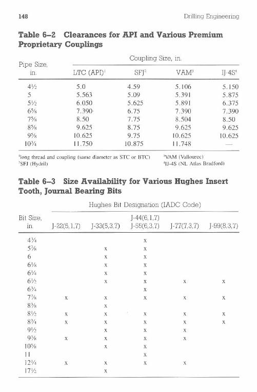
148 Drilling Engineering
Table 6-2 Clearances for API and Various PremiumProprietary Couplings
Coupling Size, in.Pipe Size,
In. LTC (API)I SFj2 VAM3 lJ-4S4
4Yz 5.0 4.59 5.106 5.1505 5.563 5.09 5.391 5.8755Yz 6.050 5.625 5.891 6.3756% 7.390' 6.75 7.390 7.3907% 8.50 7.75 8.504 8.508% 9.625 8.75 9.625 9.6259% 10.625 9.75 10.625 10.625
10% II. 750 10.875 II. 748
'long thread and coupling (same diameter as STC or BTC) 'YAM (Yallourec)
'SFJ (Hydril) '11-4S (NL Atlas Bradford)
Table 6-3 Size Availability for Various Hughes InsertTooth, Journal Bearing Bits
Hughes Bit Designation (IADCCode)
BitSize, J-44(6, 1,7)In. J-22(5, 1,7) J-33(5,3,7) J-55(6,3,7) J-77(7,3,7) J-99(8,3,7)
4314 X
57/8 X X
6 x x
6Y8 X X
6Y4 X X6Yz x x x X
6314 X
77/8 X X X X X
83/8 X
8Yz x x x x x
8% x x x x X
9Yz x x x
9% x x x x
10% x x
II X
12Y4 x X X X
17Yz x
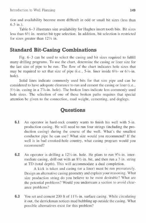
Introduction to Well Planning 149
tion and availability become more difficult in odd or small bit sizes (less than6.5 in.).
Table 6-3 illustrates size availability for Hughes insert tooth bits. Bit sizesless than 6Y2in. restrict bit type selection: In addition, bit selection is restrictedfor sizes greater than 12Y4in.
Standard Bit-Casing CombinationsFig. 6-3 can be used to select the casing and bit sizes required to fulfill
many drilling programs. To use the chart, determin~ the casing or liner size forthe last size of pipe to be run. The flow of the chart indicates hole sizes thatmay be required to set that size of pipe (i.e., 5-in. liner inside 6Ys- or 6Y4-in.hole).
Solid lines indicate commonly used bits for that size pipe and can beconsidered to have adequate clearance to run and cement the casing or liner (i.e.,51/2-in.casing in a 77/s-in.hole). The broken lines indicate less commonly usedhole sizes. The selection of one of these broken paths requires that specialattention be given to the connection, mud weight, cementing, and doglegs.
Questions
6.1 An operator in hard-rock country wants to finish his well with 5-in.production casing. He will need to run four strings (including the pro-duction casing) during the course of the well. What's the smallestconductor pipe he can use? What size would you recommend? If thewell is in bad crooked-hole country, what casing program would yourecommend?
6.2 An operator is drilling a 121/4-in.hole. He plans to run 9%-in. inter-mediate casing, drill out with an 8Y2-in.bit, and then run a 7-in. stringat TD (total depth). This will accommodate a dual completion.
A kick is taken and casing (or a liner) must be run prematurely.Design an alternative casing geometry and explain your reasoning. Whatsize production string do you believe to be most desirable? What arethe potential problems? Would you underream a section to avoid clear-ance problems?
6.3 You set and cement 200 ft of I I%-in. surface casing. While circulatingit out, the derrickman notices mud bubbling up outside the casing. Whatpossible alternatives exist for this problem?
Casingand linersize, in.
Bit andhole
size, in.
Casingand linersize, in.
Bit andhole
size, in.
Casingsize. in.
Bit andhole
size. in.
Casingsize. in.
Bit andhole
size, in.
Casingsize, in.
Fig. 6-3 Casing and bit size selection chart (Courtesy of Oil and Gas journal)

Introduction to Well Planning 151
References
Greenip, John' 'Care and Handling of Oilfield Tubulars." Oil & Gas JournalSeries.
Hughes Tool Company. Various publications, Houston.
Chapter 7 Bit Planning
Selecting the proper bits for a well is an important decision that affectsthe overall well cost. Many factors must be evaluated:
· bit cost. expected parameters (Le., turbines, rotary drilling, air operations).formation types and properties·mudsystems· rig cost
/
" \\
The emerging technology for bit design adds additional significance when eval-uating these parameters.
Drilling optimization can be viewed in three distinct phases:I. Selecting the proper bit for the drilling conditions.2. Monitoring the drilling conditions on the prospect well so drilling per-
formance is at least equal to or above the average in the particular area.3. Implementing a bit weight-rotary speed program from theoretical cal-
culations that will improve drilling performance above the best wellsin the area.
Generally, the last phase is difficult to implement in a one- or two-well drillingprogram. Unfortunately, the first two phases are often neglected, even thoughthey require only a relatively simple evaluation of offset well data. This text willbe restricted to covering the first two phases of drilling optimization.
152
Bit Planning 153
Drill Bits
Rotary drilling bits have seen perhaps more technological advancementsover the past years than any other type of drilling equipment. These advancementsinclude such items as:
· development of the roller cone bit·multiple cone and jet arrangements in roller bits· cone lubrication methods.diamond bit drilling and coring procedures.polycrystalline (PDq bits
Each of these advancements represents a significant improvement over pre-vious designs, and they tend to increase the effectiveness of the drillingprocess.
Rotary bits drill the formation using primarily two principles: 1) rockremoval by exceeding its shear strength and 2) removal by exceeding the com-pressive strength. Broken rock is removed by rotary scraping or hydrauliccleaning. Either process can also contribute to the initial breakage. Mostdrilling operations can be divided accordingly into shear failure or compressivefailure.
Shear failure involves the use of a bit tooth to shear, or cut, the rock intosmall pieces so it can be removed from the area below the bit. The simple actionof forcing a tooth into the formation creates some shearing and results in cuttingsdevelopment. In addition, if the tooth is dragged across the rock after its insertion,the effectiveness of the shearing action will increase (see Fig. 7-1). Shear failuremechanism requires, however, that the formation exhibit a low compressivestrength that will allow the insertion of the tooth.
To illustrate the type of shear failure used to drill softer formations, imaginethat a knife blade is inserted into a piece of firm clay. As the blade is inserted,it creates small fragments of clay near the cutting surface. More fragments canbe developed if the knife blade is twisted after it has penetrated the clay. Thispenetrating-twisting mechanism describes the principles involved in most soft-formation bits.
As the compressive strength or abrasiveness of the formation increases,the shearing-twisting action is reduced. Rocks with high compressive strengthsgenerally prevent the insertion of a tooth that would have initiated the shearingaction. In addition, rocks with a high abrasiveness quickly wear a bit tooth if itis twisted or dragged across the formation face. These types of rocks generallyrequire that a compressive failure mechanism be used.
Compressive failure of a rock segment requires that a load be placed onthe rock that will exceed the compressive strength of that given rock type. The
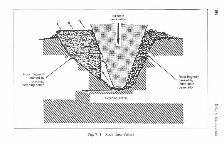
Rock
fragment
createdby
gouging,scraping
action
Rock
fragment
causedby
initialtooth
penetration
Fig.
7-1R
ockshear
failure
...en~
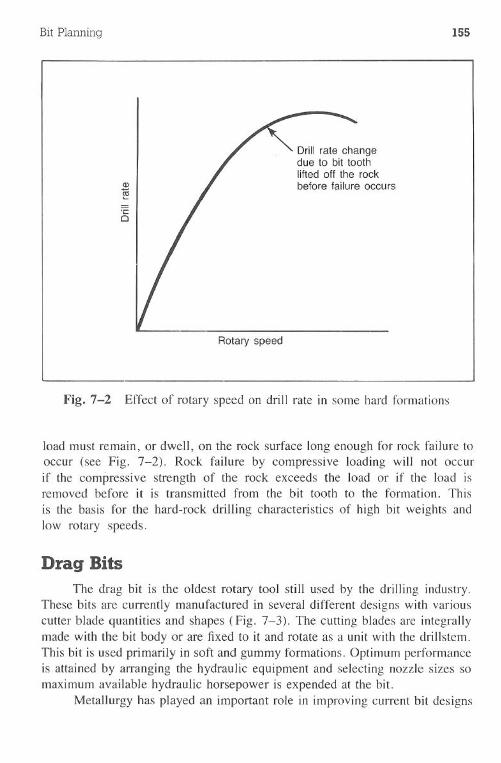
Bit Planning 155
Drill rate changedue to bit toothliited off the rockbefore failure occurs
Rotary speed
Fig. 7-2 Effect of rotary speed on drill rate in some hard formations
load must remain, or dwell, on the rock surface long enough for rock failure tooccur (see Fig. 7-2). Rock failure by compressive loading will not occurif the compressive strength of the rock exceeds the load or if the load isremoved before it is transmitted from the bit tooth to the formation. This
is the basis for the hard-rock drilling characteristics of high bit weights andlow rotary speeds.
Drag BitsThe drag bit is the oldest rotary tool still used by the drilling industry.
These bits are currently manufactured in several different designs with variouscutter blade quantities and shapes (Fig. 7-3). The cutting blades are integrallymade with the bit body or are fixed to it and rotate as a unit with the drillstem.This bit is used primarily in soft and gummy formations. Optimum performanceis attained by arranging the hydraulic equipment and selecting nozzle sizes somaximum available hydraulic horsepower is expended at the bit.
Metallurgy has played an important role in improving current bit designs
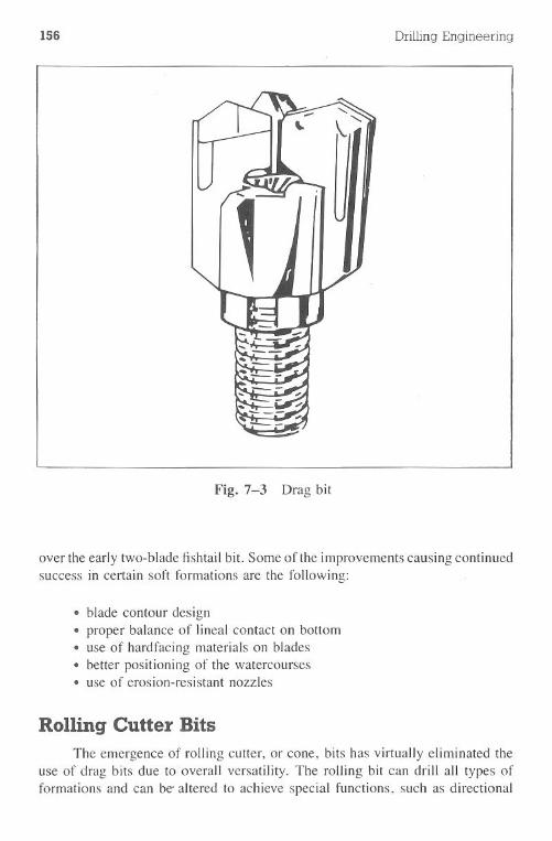
156 Drilling Engineering
Fig. 7-3 Drag bit
over the early two-blade fishtail bit. Some of the improvements causing continuedsuccess in certain soft formations are the following:
· blade contour design. proper balance of lineal contact on bottom. use of hardfacing materials on blades. better positioning of the watercourses. use of erosion-resistant nozzles
Rolling Cutter BitsThe emergence of rolling cutter, or cone, bits has virtually eliminated the
use of drag bits due to overall versatility. The rolling bit can drill all types offormations and can be' altered to achieve special functions, such as directional
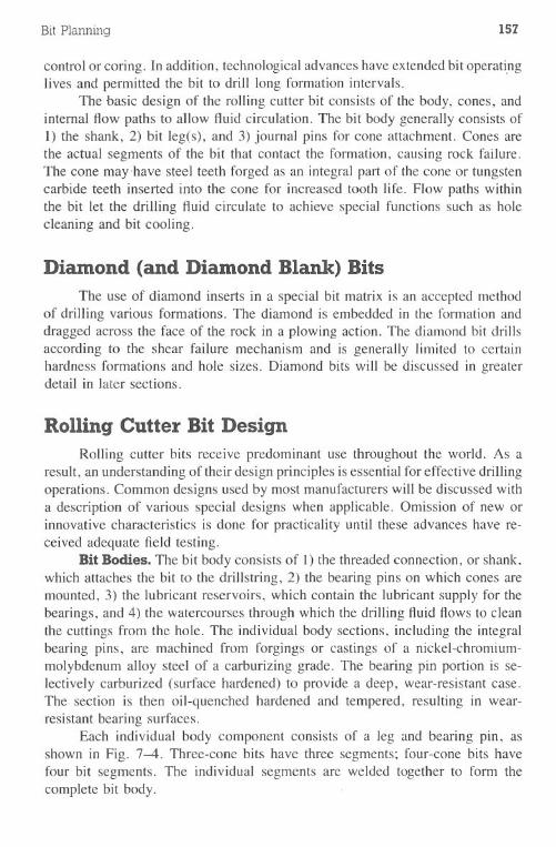
Bit Planning 157
control or coring. In addition, technological advances have extended bit operati.nglives and permitted the bit to drill long formation intervals.
The basic design of the rolling cutter bit consists of the body, cones, andinternal flow paths to allow fluid circulation. The bit body generally consists ofI) the shank, 2) bit leg(s), and 3) journal pins for cone attachment. Cones arethe actual segments of the bit that contact the formation, causing rock failure.The cone may -have steel teeth forged as an integral part of the cone or tungstencarbide teeth inserted into the cone for increased tooth life. Flow paths withinthe bit let the drilling fluid circulate to achieve special functions such as holecleaning and bit cooling.
Diamond (and Diamond Blank) BitsThe use of diamond inserts in a special bit matrix is an accepted method
of drilling various formations. The diamond is embedded in the formation anddragged across the face of the rock in a plowing action. The diamond bit drillsaccording to the shear failure mechanism and is generally limited to certainhardness formations and hole sizes. Diamond bits will be discussed in greaterdetail in later sections.
Rolling Cutter Bit DesignRolling cutter bits receive predominant use throughout the world. As a
result, an understanding of their design principles is essential for effective drillingoperations. Common designs used by most manufacturers will be discussed witha description of various special designs when applicable. Omission of new orinnovative characteristics is done for practicality until these advances have re-ceived adequate field testing.
BitBodies. Thebit bodyconsistsof I) the threadedconnection,or shank,which attaches the bit to the drillstring, 2) the bearing pins on which cones aremounted, 3) the lubricant reservoirs, which contain the lubricant supply for thebearings, and 4) the watercourses through which the drilling fluid flows to cleanthe cuttingsfromthe hole. The individualbody sections,includingthe integralbearing pins, are machined from forgings or castings of a nickel-chromium-molybdenum alloy steel of a carburizing grade. The bearing pin portion is se-lectively carburized (surface hardened) to provide a deep, wear-resistant case.The section is then oil-quenched hardened and tempered, resulting in wear-resistant bearing surfaces.
Each individual body component consists of a leg and bearing pin, asshown in Fig. 7-4. Three-cone bits have three segments; four-cone bits havefour bit segments. The individual segments are welded together to form thecomplete bit body.
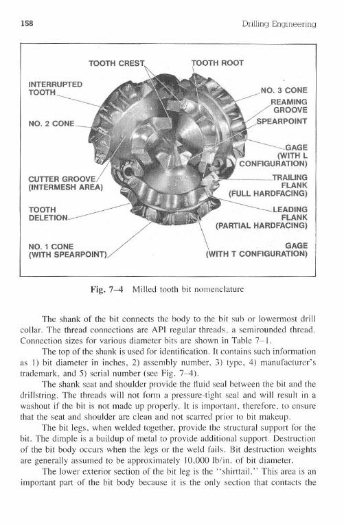
158 Drilling Engineering
NO.3 CONE
REAMINGGROOVE
.SPEARPOINT
NO.1 CONE(WITH SPEARPOINT)
GAGE(WITH L
CONFIGURATION)
:TRAILINGFLANK
(FULL HARDFACING)-----
LEADING, FLANK'
\ (PARTIAL HARDFACING)
GAGE(WITH T CONFIGURATION)
Fig. 7-4 Milled tooth bit nomenclature
The shank of the bit connects the body to the bit sub or lowermost drillcollar. The thread connections are API regular threads, a semirounded thread.Connection sizes for various diameter bits are shown in Table 7-1.
The top of the shank is used for identification. It contains such informationas I) bit diameter in inches, 2) assembly number, 3) type, 4) manufacturer'strademark, and 5) serial number (see Fig. 7-4).
The shank seatand shoulder provide the fluid seal between the bit and thedrillstring. The threads will not form a pressure-tight seal and will result in. awashout if the bit is not made up properly. It is important, therefore, to ensurethat the seat and shoulder are clean and not scarred prior to bit makeup.
The bit legs, when welded together, provide the structural support for thebit. The dimple is a buildup of metal to provide additional support. Destructionof the bit body occurs when the legs or the weld fails. Bit destruction weightsare generally assumed to be approximately 10,000 Ib/in. of bit diameter.
The lower exterior section of the bit leg is the" shirttail." This area is an
important part of the bit body because it is the only section that contacts the
Bit Planning 159
Table 7-1 Roller Bit Connections
BitSize, in.Size and Style of
Rotary Pin ConnectionBevel Diameter*
:!::164in.
3Y4to 4Y2, incl.4% to 5, incl.5Ysto 7Ys, incl.7Y2to 9Ys, incl.9Y2 to 141/2,incl.14% to 181/2,incl.18% and larger
2% reg27/sreg31/2reg41/2reg6% reg7% reg8% reg
3Y64339/64
47/64
52Y64
72Y<>4
8 1Y12
93%4
*Bevel diameter is the diameter of the contact face of the rotary shouldered connection
API Spec. 7. courtesy API
formation and therefore is subject to abrasive wear. The shirttail is often protectedfrom wear by inserting tungsten carbide inserts or applying sintered tungstencarbide. Unusual wear in the shirttail area often indicates an undergauged holethat will give future problems when running a new, full-gauge bit.
The bit body is forged with nozzle shrouds for the jets in a jet-type bit.The shroud is located in the middle exterior segment of the body between eachleg and directs the fluid flow at the bottom of the hole. Specially designed bitshave extended shrouds that move the jet nearer the hole bottom, and a newlydeveloped bit has one of the three shrouds directed up the annular space.
The journal pin is an integral part of the bit leg that provides the connectingpoint between the bit cone and the body. The pin is machined in a manner toaccept the bearings and, in the case of the journal-bearing bit, is precisionmachined so it can serve as a metal-to-metal bearing. The angle of the journalpin from the horizontal varies, depending on the type of the rock the bit isdesigned to drill. Hard-formation bits that are generally subjected to high bitweights have the pin oriented so it can accept the greater vertical component ofthe bit load. This concept is shown in Fig. 7-5 and Table 7-2.
Another design feature of the bearing pin is the angle between the centerline of the pin and the geometric center of the bit, as shown in Fig. 7-6. Theoffset from the center of the bit causes the cone to drag across the formationand creates additional shearing actions, termed skew. As harder rocks are drilled,the degree of offset for the various types of bits decreases since compressivefailure becomes the primary drilling mechanism instead of shearing. Too muchskew will cause the bit to wear quickly in hard formations.
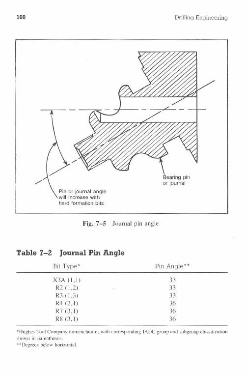
160 Drilling Engineering
/'Bearing pinor journal
Pin or journal anglewill increase withhard formation bits
Fig. 7-5 Journal pin angle
Table 7-2 Journal Pin Angle
BitType* Pin Angle **
X3A (I, I)R2 (1,2)R3. (1,3)R4(2,1)R7 (3, I)R8 (3, I)
333333363636
*Hughes Tool Company nomenclature, with corresponding IADC group and subgroup classification
shown in parentheses.**Degrees below horizontal.
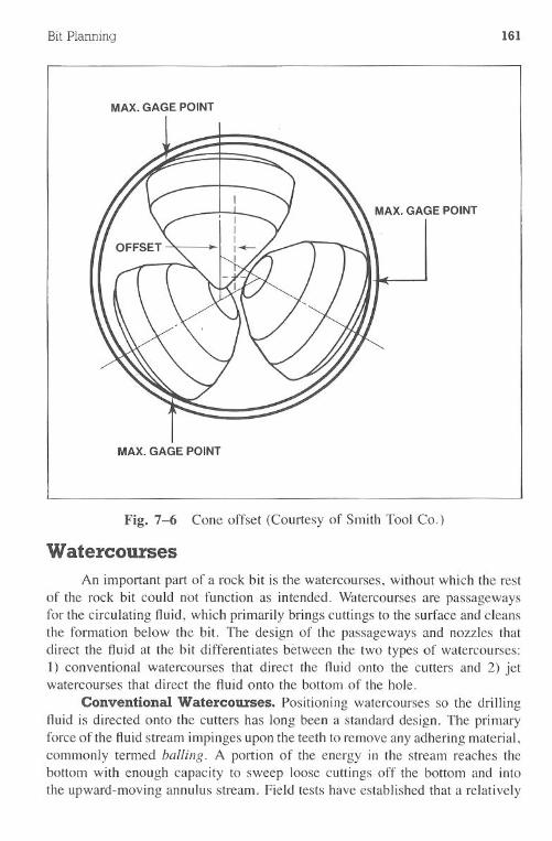
Bit Planning 161
MAX. GAGE POINT
MAX. GAGE POINT
Fig. 7-6 Cone offset (Courtesy of Smith Tool Co.)
Watercourses
An important part of a rock bit is the watercourses, without which the restof the rock bit could not function as intended. Watercoursesare passagewaysfor the circulating fluid, which primarily brings cuttings to the surface and cleansthe formation below the bit. The design of the passagewaysand nozzles thatdirect the fluid at the bit differentiates between the two types of watercourses:I) conventional watercourses that direct the fluid onto the cutters and 2) jetwatercourses that direct the fluid onto the bottom of the hole.
Conventional Watercourses. Positioning watercourses so the drillingfluid is directed onto the cutters has long been a standard design. The primaryforce of the fluid stream impinges upon the teeth to remove any adhering material,commonly termed balling. A portion of the energy in the stream reaches thebottom with enough capacity to sweep loose cuttings off the bottom and intothe upward-moving annulus stream. Field tests have established that a relatively
162 Drilling Engineering
large portion of the stream must impinge on the outermost rows of cutter teeth,which are most prone"to ball-up.
Excessive fluid velocity directed at the cone structure would severely erodethe cutter shell and teeth. Therefore, the nozzle size, or throat, of the conventionalbit must be compromised for maximum hole cleaning and minimum cone erosion.Nozzle sizes that result in velocities from 100-125 feet per second are generallyused. Since these low fluidvelocities are often inefficient for proper hole cleaning,bits with conventional watercourses are rapidly becoming rare. Their principaluse now is in large bit sizes or in cheap bits for shallow, soft drilling.
Jet Watercourses. The principle of bottom-hole jetting to improve theperformance of rock bits is not new. For years, engineers have known that thequick removal of cuttings from the bottom of the hole is essential for best bitperformance. Only in recent years has the use of large-capacity, adequatelypowered mud pumps become general enough to warrant developing high-velocityjet bits. When mud pumps are small or have a limited power supply, the mudstream must be directed on the rock bit cutters to keep them properly cleaned.With adequate pump pressure, however, mud jets directed at the bottom of thehole will quickly lift the cuttings as well as create sufficient turbulence aroundthe bit to clean the cutter teeth properly (see Fig. 7-7).
(a) (b)
Fig. 7-7 Standard (a) and extended (b) bit jets (Courtesy Smith Tool Co.)
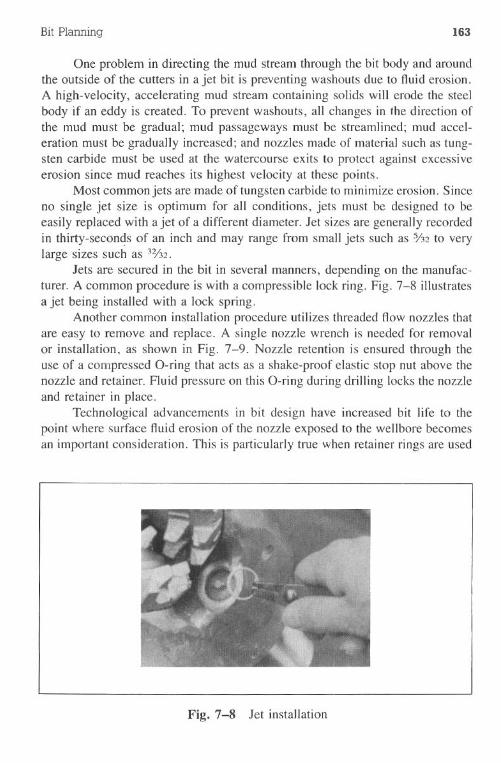
Bit Planning 163
One problem in directing the mud stream through the bit body and aroundthe outside of the cutters in a jet bit is preventing washouts due to fluid erosion.A high-velocity, accelerating mud stream containing solids will erode the steelbody if an eddy is created.To preventwashouts,all changesin the directionofthe mud must be gradual; mud passageways must be streamlined; mud accel-eration must be gradually increased; and nozzles made of material such as tung-sten carbide must be used at the watercourse exits to protect against excessiveerosion since mud reaches its highest velocity at these points.
Most common jets are made of tungsten carbide to minimize erosion. Sinceno single jet size is optimum for all conditions, jets must be designed to beeasily replaced with a jet of a different diameter. Jet sizes are generally recordedin thirty-secon~s of an inch and may range from small jets such as Y32to verylarge sizes such as 32/32.
Jets are secured in the bit in several manners, depending on the manufac-turer. A common procedure is with a compressible lock ring. Fig. 7-8 illustratesa jet being installed with a lock spring.
Another common installation procedure utilizes threaded flow nozzles thatare easy to remove and replace. A single nozzle wrench is needed for removalor installation, as shown in Fig. 7-9. Nozzle retention is ensured through theuse of a compressed a-ring that acts as a shake-proof elastic stop nut above thenozzle and retainer. Fluid pressure on this a-ring during drilling locks the nozzleand retainer in place.
Technological advancements in bit design have increased bit life to thepoint where surface fluid erosion of the nozzle exposed to the wellbore becomesan important consideration. This is particularly true when retainer rings are used
Fig. 7-8 Jet installation
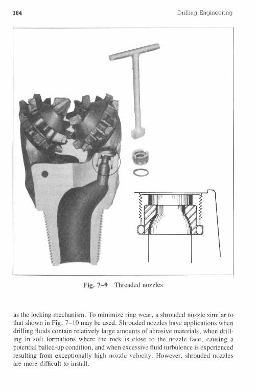
164 Drilling Engineering
Ii
I\t\,,,...
~1.........
C)
Fig. 7-9 Threaded nozzles
as the locking mechanism. To minimize ring wear, a shrouded nozzle similar tothat shown in Fig. 7-10 may be used. Shrouded nozzles have applications whendrilling fluids contain relatively large amounts of abrasive materials, when drill-ing in soft formations where the rock is close to the nozzle face, causing apotential balled-up condition, and when excessive fluid turbulence is experiencedresulting from exceptionally high nozzle velocity. However, shrouded nozzlesare more difficult to install.
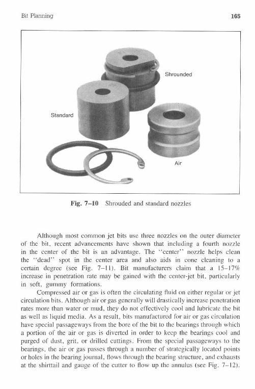
Bit Planning 165
Fig. 7-10 Shrouded and standard nozzles
Although most common jet bits use three nozzles on the outer diameterof the bit, recent advancements have shown that including a fourth nozzlein the center of the bit is an advantage. The "center" nozzle helps cleanthe "dead" spot in the center area and also aids in cone cleaning to acertain degree (see Fig. 7-11). Bit manufacturers claim that a 15-17%increase in penetration rate may be gained with the center-jet bit, particularlyin soft, gummy formations.
Compressed air or gas is often the circulating fluid on either regular or jetcirculation bits. Although air or gas generally will drastically increase penetrationrates more than water or mud, they do not effectively cool and lubricate the bitas well as liquid media. As a result, bits manufactured for air or gas circulationhave special passageways from the bore of the bit to the bearings through whicha portion of the air or gas is diverted in order to keep the bearings cool andpurged of dust, grit, or drilled cuttings. From the special passageways to thebearings, the air or gas passes through a number of strategically located pointsor holes in the bearing journal, flows through the bearing structure, and exhaustsat the shirttail and gauge of the cutter to flow up the annulus (see Fig. 7-12).
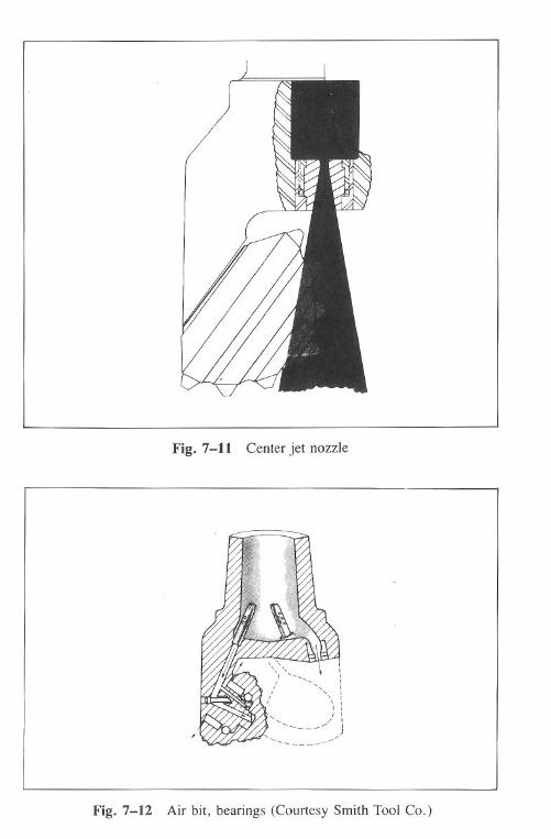
Fig. 7-11 Center jet nozzle
'<'" -\ I,> ' :I , I, , I
" \ II:
'- / I""'/:
', /)-------....
Fig. 7-12 Air bit, bearings (Courtesy Smith Tool Co.)
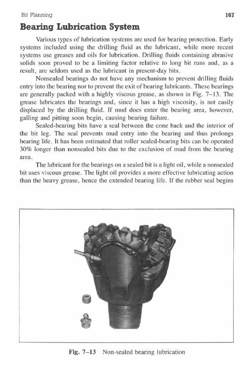
Bit Planning
Bearing Lubrication System167
Various types of lubrication systems are used for bearing protection. Earlysystems included using the drilling fluid as the lubricant, while more recentsystems use greases and oils for lubrication. Drilling fluids containing abrasivesolids soon proved to be a limiting factor relative to long bit runs and, as aresult, are seldom used as the lubricant in present-day bits.
Nonsealed bearings do not have any mechanism to prevent drilling fluidsentry into the bearing nor to prevent the exit of bearing lubricants. These bearingsare generally packed with a highly viscous grease, as shown in Fig. 7-13. Thegrease lubricates the bearings and, since it has a high viscosity, is not easilydisplaced by the drilling fluid. If mud does enter the bearing area, however,galling and pitting soon begin, causing bearing failure.
, Sealed-bearing bits have a seal between the cone back and the interior ofthe bit leg. The seal prevents mud entry into the bearing and thus prolongsbearing life. It has been estimated that roller sealed-bearing bits can be operated30% longer than nonsealed bits due to the exclusion of mud from the bearingarea.
The lubricant for the bearings on a sealed bit is a light oil, while a nonsealedbit uses viscous grease. The light oil provides a more effective lubricating actionthan the heavy grease, hence the extended bearing life. If the rubber seal begins
Fig. 7-13 Non-sealed bearing lubrication
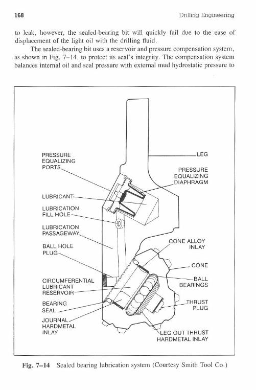
168 Drilling Engineering
to leak, however, the sealed-bearing bit will quickly fail due to the ease ofdisplacement ,of the light oil with the drilling fluid.
The sealed-bearing bit uses a reservoir and pressure compensation system,as shown in Fig. 7-14, to protect its seal's integrity. The compensation systembalances internal oil and seal pressure with external mud hydrostatic pressure to
PRESSUREEQUALIZINGPORTS
LEG
BALL HOLE
PLUG
CONE
LUBRICANT-
LUBRICATIONFILL HOLE
CIRCUMFERENTIALLUBRICANTRESERVOIR
BEARINGSEAL
JOURNALHARDMETALINLAY
:rHRUSTPLUG
LEG OUT THRUSTHARDMETAL INLAY
Fig. 7-14 Sealed bearing lubrication system (Courtesy Smith Tool Co.)
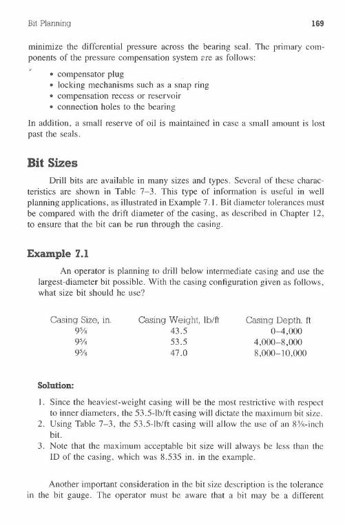
Bit Planning 169
minimize the differential pressure across the bearing seal. The primary com~ponents of the pressure compensation system are as follows:
'" · compensator plug ".locking mechanisms such as a snap ring· compensation recess or reservoir.connection holes to the bearing
In addition, a small reserve of oil is maintained in case a small amount is lostpast the seals.
Bit SizesDrill bits are available in many sizes and types. Several of these charac-
teristics are shown in Table 7-3. This type of information is useful in wellplanning applications, as illustrated in Example 7.1. Bit diameter tolerances mustbe compared with the drift diameter of the casing, as described in Chapter 12,to ensure that the bit can be run through the casing.
Example 7.1
An operator is planning to drill below intermediate casing and use thelargest-diameter bit possible. With the casing configuration given as follows,what size bit should he use?
Casing Size, in.9%9%9%
Casing Weight, Ib/ft43.553.547.0
Casing Depth, ft0-4,000
4,000-8,0008,000-LO,000
Solution:
1. Since the heaviest-weight casing will be the most restrictive with respectto inner diameters, the 53.5-1b/ft casing will dictate the maximum bit size.
2. Using Table 7-3, the 53.5-1b/ft casing will allow the use of an 8%-inchbit.
3. Note that the maximum acceptable bit size will always be less than theID of the casing, which was 8.535 in. in the example.
Another important consideration in the bit size description is the tolerancein"the bit gauge. The operator must be aware that a bit may be a different
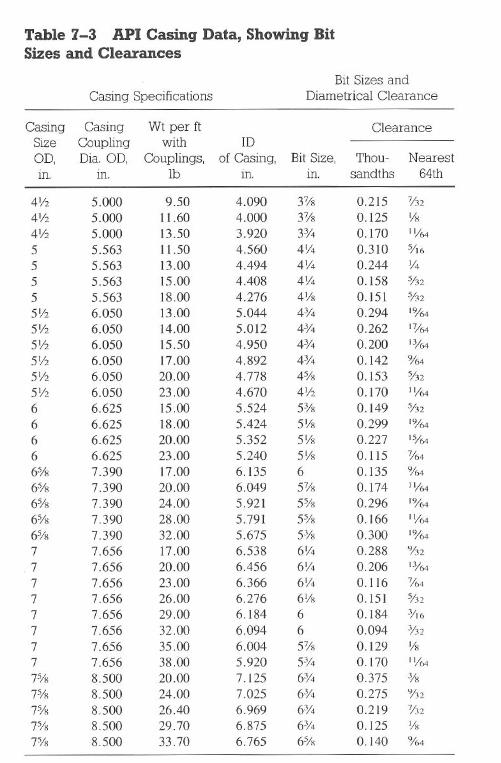
Table 7-3 API Casing Data, Showing BitSizes and Clearances
Bit Sizes andCasing Specifications Diametrical Clearance
Casing Casing Wt per it ClearanceSize Coupling with IDOD, Dia. OD, Couplings, of Casing, Bit Size, Thou- Nearestin. m. lb m. m. sandths 64th
4'12 5.000 9.50 4.090 37/8 0.215 7/324'12 5.000 11.60 4.000 37/8 0.125 1/84'12 5.000 13.50 3.920 3% 0.170 1'164
5 5.563 11.50 4.560 4'14 0.310 5/165 5.563 13.00 4.494 4'14 0.244 1/45 5.563 15.00 4.408 4'14 0.158 5/325 5.563 18.00 4.276 4'18 0.151 5/325'12 6.050 13.00 5.044 4% 0.294 10/645'12 6.050 14.00 5.012 4% 0.262 17/645'12 6.050 15.50 4.950 4% 0.200 13/64
51/2 6.050 17.00 4.892 43/4 0.142 9/645'12 6.050 20.00 4.778 4% 0.153 5/325'12 6.050 23.00 4.670 4'12 0.170 1'1646 6.625 15.00 5.524 53/8 0.149 5/326 6.625 18.00 5.424 5'18 0.299 10/646 6.625 20.00 5.352 5'18 0.227 15/646 6.625 23.00 5.240 51/8 0.115 7/646% 7.390 17.00 6.135 6 0.135 9/646% 7.390 20.00 6.049 57/8 0.174 1'1646% 7.390 24.00 5.921 5% 0.296 19/646% 7.390 28.00 5.791 5% 0.166 ''1646% 7.390 32.00 5.675 53/8 0.300 19/647 7.656 17.00 6.538 6'14 0.288 9/32
.7 7.656 20.00 6.456 61/4 0.206 13/64
7 7.656 23.00 6.366 6'14 0.1l6 7/647 7.656 26.00 6.276 6'18 0.151 5/327 7.656 29.00 6.184 6 0.184 3/167 7.656 32.00 6.094 6 0.094 3,132
7 7.656 35.00 6.004 57/8 0.129 '187 7.656 38.00 5.920 5314 0.170 1'1647% 8.500 20.00 7.125 6% 0.375 3/87% 8.500 24.00 7.025 63/4 0.275 9/327% 8.500 26.40 6.969 63/4 0.219 7/327% 8.500 29.70 6.875 6% 0.125 1/87% 8.500 33.70 6.765 6% 0.140 9/64
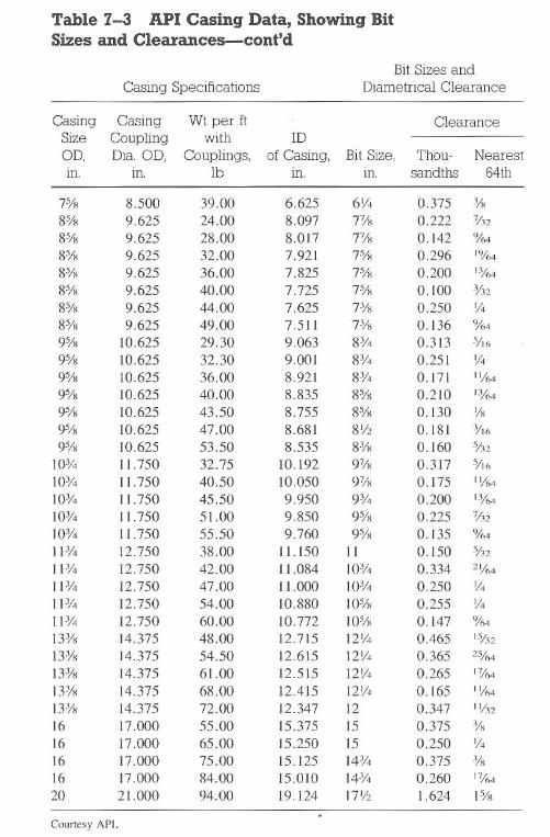
Table 7-3 API Casing Data, Showing BitSizes and Clearances-cont'd
Bit Sizes and
Casing Specifications Diametrical Clearance
Casing Casing Wt per ft ClearanceSize Coupling with IDOD, Dia. OD, Couplings, of Casing, Bit Size, Thou- Nearest10. 10. lb 10. 10. sandths 64th
7% 8.500 39.00 6.625 61/4 0.375 3/8
8% 9.625 24.00 8.097 TI8 0.222 7/32
8% 9.625 28.00 8.017 TI8 0.142 %48% 9.625 32.00 7.921 7% 0.296 19/64
8% 9.625 36.00 7.825 7% 0.200 13/64
8% 9.625 40.00 7.725 7% 0.100 3/32
8% 9.625 44.00 7.625 7% 0.250 Y48% 9.625 49.00 7.511 7318 0.136 %49% 10.625 29.30 9.063 8% 0.313 5/16
9% 10.625 32.30 9.001 8% 0.251 Y49% 10.625 36.00 8.921 8% 0.171 IY64
9% 10.625 40.00 8.835 8% 0.210 13/64
9% 10.625 43.50 8.755 8% 0.130 Y8
9% 10.625 47.00 8.681 81/2 0.181 3/16
9% 10.625 53.50 8.535 8% 0.160 5/32
10% I I. 750 32.75 10.192 97/8 0.317 5,116
10% I I. 750 40.50 10.050 97/8 0.175 IY64
10% I I. 750 45.50 9.950 9% 0.200 13/64
103/4 I I. 750 5 I. 00 9.850 9% 0.225 7/32
10% I I. 750 55.50 9.760 9% 0.135 9/64
11% 12.750 38.00 11.150 11 0.150 5,132
11% 12.750 42.00 11.084 10% 0.334 2Y64
11% 12.750 47.00 I I. 000 10% 0.250 1/4
li% 12.750 54.00 10.880 10% 0.255 1/4
11% 12.750 60.00 10.772 10% 0.147 %4
I3% 14.375 48.00 12.715 121/4 0.465 15/32
13% 14.375 54.50 12.615 12Y4 0.365 25/64
133/8 14.375 6 I. 00 12.515 12Y4 0.265 17/64
I3% 14.375 68.00 12.415 12Y4 0.165 IY64
13% 14.375 72.00 12.347 12 0.347 IY32
16 17.000 55.00 15.375 15 0.375 3fs
16 17.000 65.00 15.250 15 0.250 1/4
16 17.000 75.00 15. 125 14% 0.375 3fs
16 17.000 84.00 15.010 143/4 0.260 17/64
20 21.000 94.00 19.124 171/2 1.624 1%
Courtesy API.
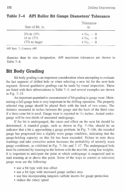
172 Drilling Engineering
Table 7-4 API Roller Bit Gauge Diameters' Tolerance
Size of Bit, in.Tolerance
m.
3% to 13%14 to 17Y2
17% to larger
+ Y32, - 0+ Y16,- 0+ Y32,- 0
API Spec. 7. Courtesy API.
diameter than its size designation. API maximum tolerances are shown InTable 7-4.
Bit Body GradingBit body grading is an important consideration when attempting to evaluate
the last segment of drilled hole or when selecting a new bit for the next holesegment. Several qualitative gradings can be made by visual inspection. Theseare listed with their abbreviations in Table 7-5, and several examples are shownin Fig. 7-15.
An important quantitative measurement of bit grading is gauge wear. Main-taining a full-gauge hole is very important in the drilling operation. The properlyselected ring gauge should be placed flush with the back of two cones. Thedistance measured in inches between the gauge and the back of the third coneif a three-cone bit is used. Gauge wear is reported in 1/32inches. Actual under-gauge will be two-thirds of measured undergauge.
If the bit is undergauged, the cause and effect on the next bit should bedetermined. A rounded gauge, such as shown in Fig. 7-16a, should be anindicator that a bit is approaching a gauge problem. In Fig. 7-16b, the roundedgauge has progressed into a slightly worn gauge condition, indicating that thegauge-holding capacity on this bit has been exceeded. Failure to note thesewarnings and take corrective action increases the probability of severely worngauge conditions, as exhibited in Fig. 7-16c and 7-17. The undergauged holemust be corrected by reaming to the bottom with the next bit, using low weights.It is important to anticipate the point at which undergauge is suspected and tostart reaming at or above this point. Some of the ways to correct or minimizegauge wear are the following:
. use a bit type with less offset. use a bit type with increased gauge surface area.use bits incorporating tungsten carbide inserts for gauge protection.reducethe rotaryspeed
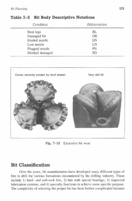
Bit Planning 173
Condition
Table 7-5 Bit Body Descriptive Notations
Abbreviation
Bent legsDamaged bitEroded nozzleLost nozzlePlugged nozzleShirttail damaged
BLDBENLNPNSD
Cones severely eroded by mud stream Very dull bit
Fig. 7-15 Excessive bit wear
Bit ClassificationOver the years, bit manufacturers have developed many different types of
bits to drill the various formations encountered by the drilling industry. Theseinclude 1) hard- and soft-rock bits, 2) bits with special bearings, 3) improvedlubrication systems, and 4) specialty functions to achieve some specific purpose.The complexity of selecting the proper bit has been further complicated because
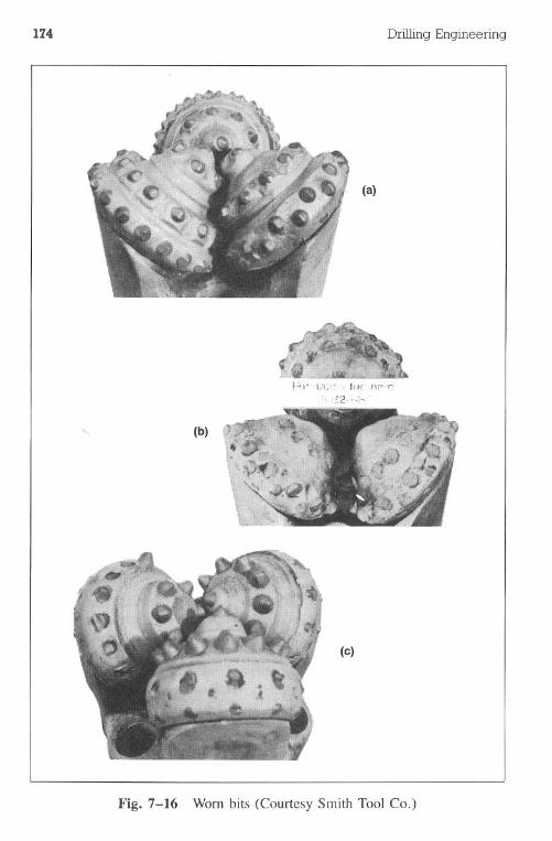
174 Drilling Engineering
(a)
(b)
(c)
I<'ig.7-16 Worn bits (Courtesy Smith Tool Co.)
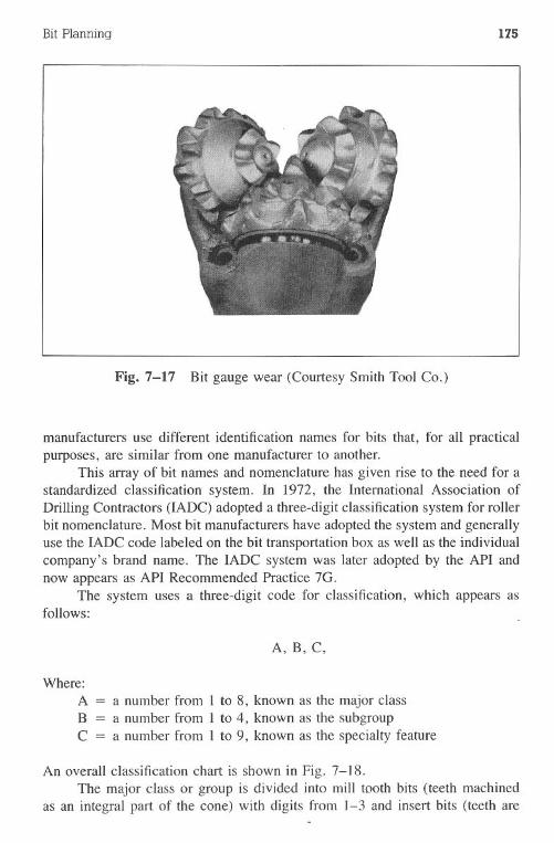
Bit Planning 175
Fig. 7-17 Bit gauge wear (Courtesy Smith Tool Co.)
manufacturers use different identification names for bits that, for all practicalpurposes, are similar from one manufacturer to another.
This array of bit names and nomenclature has given rise to the need for astandardized classification system. In 1972, the International Association ofDrilling Contractors (IADC) adopted a three-digit classification system for rolletbit nomenclature. Most bit manufacturers have adopted the system and generallyuse the IADC code labeled on the bit transportation box as well as the individualcompany's brand name. The IADC system was later adopted by the API andnow appears as API Recommended Practice 7G.
The system uses a three-digitcode for classification,which appears asfollows:
Where:ABC=
A, B, C,
a number from 1 to 8, known as the major classa number from 1 to 4, known as the subgroupa number from 1 to 9, known as the specialty feature
An overall classification chart is shown in Fig. 7-18.The major class or group is divided into mill tooth bits (teeth machined
as an integral part of the cone) with digits from 1-3 and insert bits (teeth are
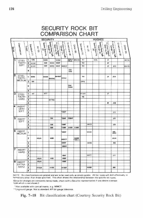
176 Drilling Engineering
NOTE: Bit classifications are general and are to be used only as simple guides. All bit types will drill effectively informations other than those specified. This chart shows the relationship between the specific bit types.(Since bit changes are constantly being made, check with a Security representative if you desire a certaintype which is not shownJ
.Also available with conical inserts. e.g. M84CF."Unground gauge. Not to standard API bit gauge tolerance.
Fig. 7-18 Bit classification chart (Courtesy Security Rock Bit)
SECURITY ROCK BITCOMPARISON CHART
R. X3A IMX3AR2R3
I I I 1.14 I JD4
3
43 STEEL 1 H7 H77 I I I J7
TOOTH 2 RBHARD 3
4 J8 LJOBINSERTVERY 2SOFT 3 I I I I I tS82FI I I I I I 1 1m
4I I I I S84I S84F IDS84Fj I I I I I I n2
SOFT 23" J334
J55R
.155
J77
tOJAI IHIOOI jH.OOFI I I III>I!9J_ I I ).198
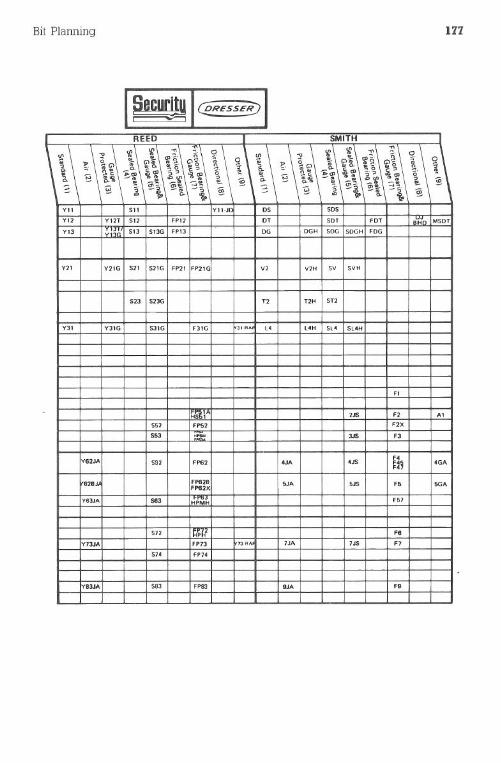
Bit Planning 177
I ~ I (£RESSE?) IREED SMITH
\
\\ \\\\\\ \ \ \\ \\ \ \\\q\\\ \\ \-:; w -,::) '(;'--. - -'" s -\ f!. --. _- - 1oo.i-s - - '" i-VII 511 Yl1.J D5 50S
V12 Y12T 512 FP12 DT SOT FDT 8HO MSDT
VIJ I :I,' 51J 51JG FP13 DG DGH SDG SDGH FOG
V21 Y21G 521 521G FP21 FP21G 1/2 1/2H SI/ SI/H
S2J S2JG T2 T2H ST2
VJI Y31G SJIG F31G :U.AA LO LOH S14 Sl4H
FI
HIA 2.1S F2 AIS52 FP62 F2XSSJ - JJS FJ
62JA 552 FP62 OJA O.lSU9
OGA
828J1 FP828 SJA 5JS F5 SGAFP82X
Y83JA 58J H'I. F51
512 H'PIt F6
Y73JA FP73 13.RA 1JA 1JS F7
S10 FP74
V8JJA S8J FPSJ 9JA F9
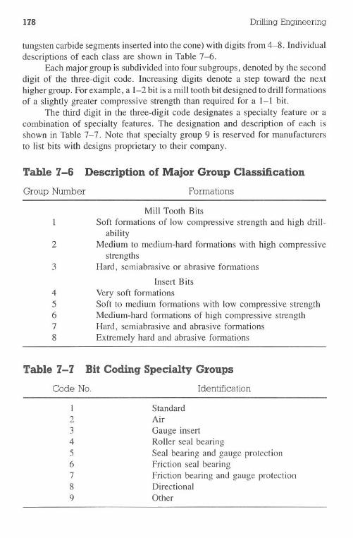
178 Drilling Engineering
tungsten carbide segments inserted into the cone) with digits from 4-8. Individualdescriptions of each class are shown in Table 7-6.
Each major group is subdivided into four subgroups, denoted by the seconddigit of the three-digit code. Increasing digits denote a step toward the nexthigher group. For example, a 1-2 bit is a mill tooth bit designed to drill formationsof a slightly greater compressive strength than required for a 1-1 bit.
The third digit in the three-digit code designates a specialty feature or acombination of specialty features. The designation and description of each isshown in Table 7-7. Note that specialty group 9 is reserved for manufacturersto list bits with designs proprietary to their company.
Table 7-6 Description of Major Group Classification
Group Number Formations
Mill Tooth Bits
Soft formations of low compressive strength and high drill-ability
2 Medium to medium-hard formations with high compressivestrengths
3 Hard, semiabrasive or abrasive formations
Insert Bits4 Very soft formations5 Soft to medium formations with low compressive strength6 Medium-hard formations of high compressive strength7 Hard, semiabrasive and abrasive formations8 Extremely hard and abrasive formations
Table 7-7 Bit Coding Specialty Groups
Code No. Identification
I23456789
StandardAirGauge insertRoller seal bearingSeal bearing and gauge protectionFriction seal bearingFriction bearing and gauge protectionDirectionalOther
Bit Planning 179
Bit ConesTwo types of cones are primarily used in the drilling industry. The original
roIling cutter bits contained teeth that were machined at the miIl as an integralpart of the cone and developed the name of "mill tooth" bits. When drilIingenvironments such as hard, abrasive rocks were encountered, the milled steelteeth would rapidly wear and a new bit would be required. This gave rise tocones that had inserted teeth of more wear-resistant materials, such as tungstencarbide.
The mill tooth and insert bits use the same classification for cone and teethrow terminology. The rows of teeth are termed 1) the heel row for the outer row,2) nose or toe row for the inner row, and 3) middle row(s) for the rows betweenthe heel and toe row. The spear point is designed to drill the formation in thecenter of the bit and often is not a fuIl row of teeth, as shown in Fig. 7-4. Conenumbering begins with the cone containing the spear point and progresses clock-wise. The spear point cone is designated as cone #1 and the next clockwisecone is #2 when looking down at the cones.
The amount of offset of the cones from the center of the bit is a descriptivecharacteristic. As described earlier, cone offset provides a tearing, gouging actionof the bit for the formations that fail best according to the shear mechanism.The amount of offset for general bit types is shown in Table 7-8. The first twomajor groups in both the mill tooth and insert classifications have 1-4° offset,depending on specific groupings. Major groups 3, 7, and 8 have no offset. Thesegroups are designed to drill formations that fail under compression.
Table 7-8 can also be used to describe several miII tooth bit characteristics.
Under normal operating conditions, mill tooth bits would rapidly wear the toothchisel edge to the point where it was a rounded, ineffective tooth. To avoid this,bit manufacturers apply some amount of hardfacing on the trailing edge of thetooth or they caseharden the teeth (see Fig. 7-19).
The tungsten carbide insert bits described in Table 7-8 also vary accordingto the type of formation being drilled. The hard-formation bits use short, conicalteeth that can withstand the high bit weights imposed during hard-rock drilling,while the soft-rock bits use long, sharp, chisel-like teeth to achieve formationpenetration. .
Cone Metallurgy. Steel, or mill, tooth cones are sometimes subjectedto severe use that can wear or break the teeth, causing breakage and loss of thecone. Steel tooth cones are machined from forgings of a carburizing grade nickel-molybdenum aIloy steel. The machined cones are carburized to produce a deepcase ranging from 0.070-0.130 in., depending on the cone size and type. Thecarburizing occurs at a temperature of I, 700°F with natural gas for 24 hr andannealing at 400°F. The cone surface develops a hardness of 60 Rc (RockweIlhardness test) but gets progressively softer with inner cone depth, as shown inFig. 7-20.
...=0
Table
7-8D
escriptionof
Rock
Bit
Classes
Formation
Off-
Type
Class
Type
Tooth
Description
set
SteelI-I,
1-2V
erysoft
Hardfaced
tip3°_4°
Cutter
1-3,1-4
SoftH
ardfacedside
2°_3°M
illT
ooth2-1,
2-2M
ediumH
ardfacedside
1°-2°
Bits
2-3M
ediumhard
Casehardened
1°_2°
3H
ardC
asehardened0
4V
erysoft
Tungsten
5-2Soft
Long,
bluntchisel
2°_3°C
arbide5-3
Medium
softL
ong,sharp
chisel2°_3°
InsertB
its6-1
Medium
shalesM
ediumchisel
1°_2°6-2
Medium
limes
Medium
projectile1°_2°
07-1
Medium
hardShort
chisel0
S7-2
Medium
Shortprojectile0
S.\Qt11::I
8H
ardchert
Conical
orhem
ispherical0
\Q5.<D
<D
....5.\Q
Bit Planning
Soft
New tooth form,hardfacing
Class 1-2
Desirable wear,tip will eventuallybreak off, thenshould wear
self-sharpening
Medium soft
Class 1-3, 2-1, 2-2
Hardmetal on trailingflimk wears less
rapidly than steel onleading flank
Fig. 7-19 Tooth dulling trends
181
Medium hard-hard
Class 2-3, 3, 4
Case hardenedsteel tooth
should chip away
Before carbonizing, the cones are cooled and then heat-treated using aspecial double oil quench and temper procedure. This procedure results in cuttingteeth with metallurgical properties such as I) tough, thin outer skin, lower inhardness than the case beneath it, thus improving the resistance to chipping andbreaking, 2) a high-carbon carburized case under the skin for maximum strengthand wear resistance, and 3) a refined cone with the best possible combinationof strength and toughness for maximum impact resistance.
Carbide tooth cones receive the same type of carbonizing treatment as thesteel tooth cones with several exceptions. As shown in Fig. 7-20, the cone usedfor the insert bit is casehardened to only 45 Re. In addition, the cones areprocessed so that surfaces are not carbonized in the areas where holes will bedrilled and reamed for installipg the carbide teeth.
Bit Teeth. Many types of teeth are used in mill tooth and insert bits. Someof their special purposes are drilling, cleaning teeth, and minimizing gauge wear.A bit must be properly chosen to have teeth designed for the formation it willdrill. .
The type of formation failure mechanism influences bit and tooth design.Soft formations drilled with shearing actions are drilled most effectively with along tooth, while harder formations require more numerous, shorter teeth (seeTable 7-9, Fig. 7-19). Note that the relative tooth height decreases in harderformation bit types while the relative amount of steel on bottom increases.
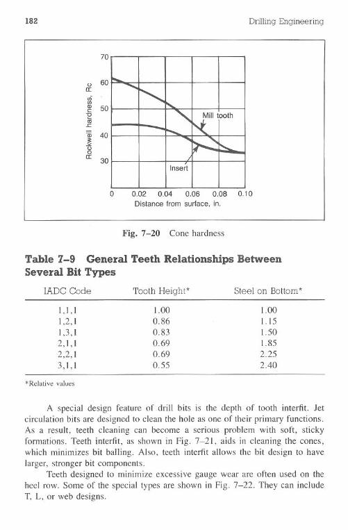
182 Drilling Engineering
70
o 60II:o(/)
:g 50"0
iu.cQ5 40
~o
II: 30Insert
o 0.02 0.04 0.06 0.08 0.10Distance from surface, in.
Fig. 7-20 Cone hardness
Table 7-9 General Teeth Relationships BetweenSeveral Bit Types .
IADC Code
I, I ,11,2,11,3,12,1,12,2,13, 1,1
Tooth Height* Steel on Bottom*
1.000.860.830.690.690.55
1.001.151.501.852.252.40
*Relative values
A special design feature of drill bits is the depth of tooth interfit. Jetcirculation bits are designed to clean the hole as one of their primary functions.As a result, teeth cleaning can become a serious problem with soft, stickyformations. Teeth interfit, as shown in Fig. 7-21, aids in cleaning the cones,which minimizes bit balling. Also, teeth interfit allows the bit design to havelarger, stronger bit components.
Teeth designed to minimize excessive gauge wear are often used on theheel row. Some of the special types are shown in Fig. 7-22. They can includeT, L, or web designs.
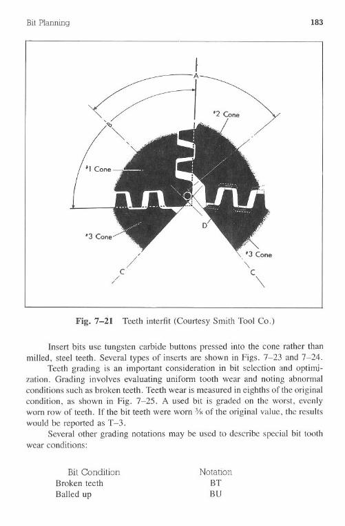
Bit Planning 183
IA
'\c\
Fig. 7-21 Teeth interfit (Courtesy Smith Tool Co.)
Insert bits use tungsten carbide buttons pressed into the cone rather thanmilled, steel teeth. Several types of inserts are shown in Figs. 7-23 and 7-24.
Teeth grading is an important consideration in bit selection and optimi-zation. Grading involves evaluating uniform tooth wear and noting abnormalconditions such as broken teeth. Teeth wear is measured in eighths of the originalcondition, as shown in Fig. 7-25. A used bit is graded on the worst, evenlyworn row of teeth. If the bit teeth were worn 3jgof the original value, the resultswould be reported as T-3.
Several other grading notations may be used to describe special bit toothwear conditions:
Bit ConditionBroken teethBalled up
NotationBTBU
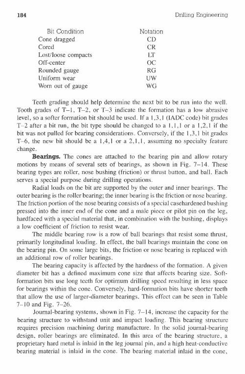
184 Drilling Engineering
Bit ConditionCone draggedCored
Lost/loose compactsOff-centerRounded gaugeUniform wear
Worn out of gauge
NotationCDCRLTOCRGUWWG
Teeth grading should help determine the next bit to be run into the well.Tooth grades of T-I, T-2, or T-3 indicate the formation has a low abrasivelevel, so a softer formation bit should be used. If a 1,3, I (IADC code) bit gradesT-2 after a bit run, the bit type should be changed to a I, I , I or a 1,2, I if thebit was not pulled for bearing considerations. Conversely, if the 1,3, I bit gradesT-6, the new bit should be a 1,4, I or a 2, I, I, assuming no specialty featurechange. ,
Bearings. The cones are attached to the bearing pin and allow rotarymotions by means of several sets of bearings, as shown in Fig. 7-14. Thesebearing types are roller, nose bushing (friction) or thrust button, and ball. Eachserves a special purpose during drilling operations.
Radial loads on the bit are supported by the outer and inner bearings. Theouter bearing is the roller bearing; the inner bearing is the friction or nose bearing.The friction portion of the nose bearing consists of a special casehardened bushingpressed into the inner end of the cone and a male piece or pilot pin on the leg,hardfaced with a special material that, in combination with the bushing, displaysa low coefficient of friction to resist wear.
The middle bearing row is a row of ball bearings that resist some thrust,primarily longitudinal loading. In effect, the ball bearings maintain the cone onthe bearing pin. On some large bits, the friction or nose bearing is replaced withan additional row of roller bearings.
The bearing capacity is affected by the hardness of the formation. A givendiameter bit has a defined maximum cone size that affects bearing size. Soft-formation bits use long teeth for optimum drilling speed resulting in less spacefor bearings within the cone. Conversely, hard-formation bits have shorter teeththat allow the use of larger-diameter bearings. This effect can be seen in Table7-10 and Fig. 7-26.
Journal-bearing systems, shown in Fig. 7-14, increase the capacity for thebearing structure to withstand unit and impact loading. This bearing structurerequires precision machining during manufacture. In the solid journal-bearingdesign, roller bearings are eliminated. In this area of the bearing structure, aproprietary hard metal is inlaid in the leg journal pin, and a high heat-conductivebearing material is inlaid in the cone. The bearing material inlaid in the cone,
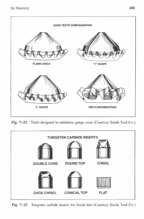
Bit Planning 185
GAGE TEETH CONFIGURATION
FLARE CREST
"L" SHAPE
"r SHAPE
TEETH INTERRUPTION
Fig.7-22 Teeth designed to minimize gauge wear (Courtesy Smith Tool Co.)
TUNGSTEN CARBIDEINSERTS
060DOUBLE CONE ROUND TOP CHISEL
GAGE CHISEL
.CONICAL TOP FLAT
Fig. 7-23 Tungsten carbide inserts for Smith bits (Courtesy Smith Tool Co.)
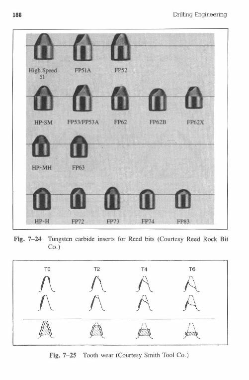
186 Drilling Engineering
HP-SM FPS3/FPS3A FP62 FP628 FP62X
HP-MH FP63
HP-H F'P73 PP14
Fig. 7-24 Tungsten carbide inserts for Reed bits (Courtesy Reed Rock BitCo.)
TO T2 T4 T6
/\ f\ f\ Af\ /\
n r"\
f\ AA . r' n
/ \
AflPJt
Fig. 7-25 Tooth wear (Courtesy Smith Tool Co.)
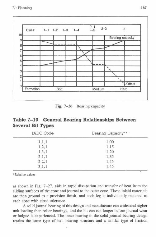
Bit Planning 187
10
9
8
7
6
54
3
21
o
Fig. 7-26 Bearing capacity
Table 7-10 General Bearing Relationships BetweenSeveral Bit Types
IADCCode BearingCapacity**
1,1,11,2,11,3,12,1,12,2,13,1, I
1.001.151.201.351.451.45
*Relative values
as shown in Fig. 7-27, aids in rapid dissipation and transfer of heat from thesliding surfaces of the cone and journal to the outer cone. These inlaid materialsare then ground to a precision finish, and each leg is individually matched toeach conewith close tolerance. .
A solid journal bearing of this design and manufacture can withstand higherunit loading than roller bearings, and the bit can run longer before journal wearor fatigue is experienced. The inner bearing in the solid journal-bearing designretains the same type of ball bearing structure and a similar type of friction
2-1 2-3 3Class: 1-1 1-2 1-3 1-4 2-2
Bearing capacity--.. -- ---
'. "..V
", '\--- -- " ---- ,,
, ,,Offset
Formation Soft Medium Hard
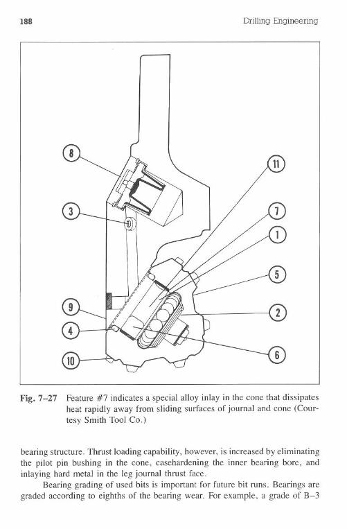
188 Drilling Engineering
Fig. 7-27 Feature #7 indicates a special aHoy inlay in the cone that dissipatesheat rapidly away from sliding surfaces of journal and cone (Cour-tesy Smith Tool Co.)
bearing structure. Thrust loading capability, however, is increased by eliminatingthe pilot pin bushing in the cone, casehardening the inner bearing bore, andinlaying hard metal in the leg journal thrust face.
Bearing grading of used bits is important for future bit runs. Bearings aregraded according to eighths of the bearing wear. For example, a grade of B-3
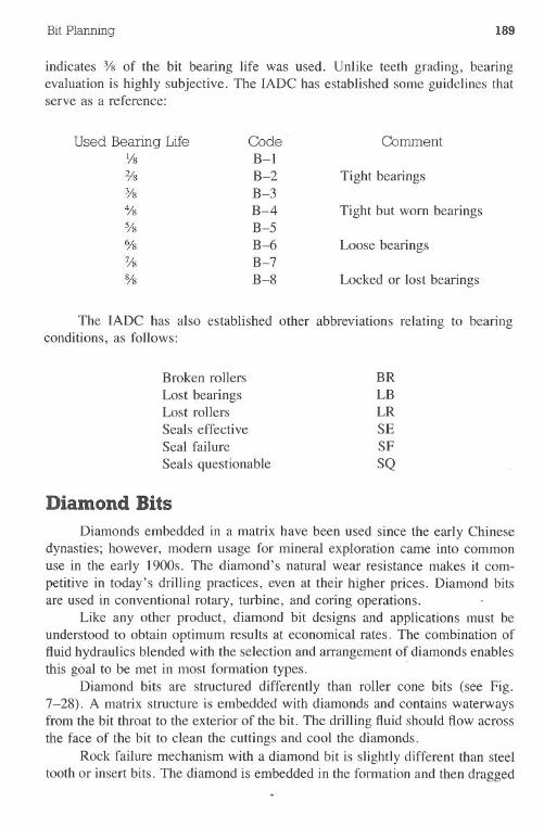
Bit Planning 189
indicates 3jgof the bit bearing life was used. Unlike teeth grading, bearingevaluation is highly subjective. The IADC has established some guidelines thatserve as a reference:
Used Bearing LifeI/S
%3jg%5fs
%
7/s
%
CodeB-1B-2B-3B-4B-5B-6B-7B-8
Comment
Tight bearings
Tight but worn bearings
Loose bearings
Locked or lost bearings
The IADC has also established other abbreviations relating to bearingconditions, as follows:
Broken rollers
Lost bearingsLost rollersSeals effectiveSeal failureSeals questionable
Diamond Bits
BRLBLRSESFSQ
Diamonds embedded in a matrix have been used since the early Chinesedynasties; however, modern usage for mineral exploration came into commonuse in the early 1900s. The diamond's natural wear resistance makes it com-petitive in today's drilling practices, even at their higher prices. Diamond bitsare used in conventional rotary, turbine, and coring operations.
Like any other product, diamond bit designs and applications must beunderstood to obtain optimum results at economical rates. The combination offluid hydraulics blended with the selection and arrangement of diamonds enablesthis goal to be met in most formationtypes. .
Diamond bits are structured differently than roller cone bits (see Fig.7-28). A matrix structure is embedded with diamonds and contains waterwaysfrom the bit throat to the exterior of the bit. The drilling fluid should flow acrossthe face of the bit to clean the cuttings and cool the diamonds.
Rock failure mechanism with a diamond bit is slightly different than steeltooth or insert bits. The diamond is embedded in the formation and then dragged
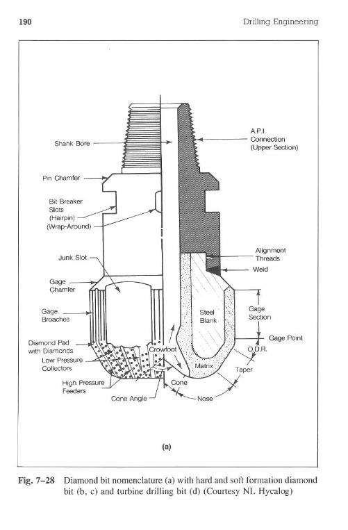
190 Drilling Engineering
Shank Bore
A.P.I.Connection
(Upper Section)
Pin Chamfer
Bit BreakerSlots(Hairpin)
(Wrap-Around)
AlignmentThreads
Weld
GageChamfer
GageBroaches
Diamond Padwith Diamonds
Low PressureCollectors
Gage Point
(a)
Fig. 7-28 Diamond bit nomenclature (a) with hard and soft formation diamondbit (b, c) and turbine drilling bit (d) (Courtesy NL Hycalog)
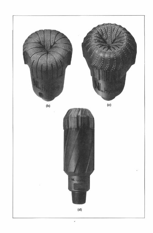
Bit Planning
(b)
191
(c)
(d)
192 Drilling Engineering
across the face of the rock without being lifted and re-embedded, as would bethe case with roller .cone bits. This shearing mechanism can be used in soft,medium, and hard rock.
Several physical characteristics of diamond bits are important when con-sidering their use. The primary considerations are the low shear strength andresistance to impact loading. As a result, lower bit weights are required, and itbecomes necessary to ensure that the drillstring is properly stabilized to minimizebending and shearing forces.
Diamond bits are typically used to achieve a lower drilling cost per foot.The reduced cost occurs when the diamond bit achieves greater drilling ratesthan roller bits in certain conditions. Reductions in trips to change bits is alsoa positive factor in diamond bit use. Manufacturers can be consulted for a costestimate/performance evaluation of diamond bits for a given well.
Many types of diamond bit structures are manufactured to address a broadrange of operating systems. The selection is often based on economics, theformations to be drilled, and the type of rotary drill bit (cone type) normallyused in an area. Most diamond bit manufacturers have developed comparisonguides between their products and roller cone bits. Table 7-11 shows a guidefor Christensen products.
The lADC has established a classification chart for diamond productssimilar to the charts for roller bits (see Fig. 7-18). The code uses a three-character group preceded by the letter D to indicate diamond products. Table7-12 illustrates the chart for NL Hycalog's diamond products.
Evaluation of Used Diamond Bits. As with every other tool, the dia-mond bit will show signs of wear eventually. Some wear is considered failure;other wear must be qualified. Failure can be thought of as the breakdown inoperation or function. In many cases this definition applies because the diamondbit has stopped drilling or performing its function. Failure can also be definedas falling short. This is sometimes the case where the ROP was too slow, pressuredrop was too high, or some combination whereby the continued running of thediamond bit was not economical or practical. Failure is also mentioned whenthe bit has performed economically for its specified interval yet the observer ofthe used bit can detect pronounced wear. This could be localized fluid erosion,missing or worn diamonds, or some other phenomenon that did not detract fromthe economic or overall performance of the bit but, in final condition, the bit isdecidedly not reru.nable.
The discussion of diamond bit wear can be broken down into three cate-gories: I) diamonds, 2) matrix, and 3) others.
. Diamond Wear. Diamond wear can result from anyone or a combinationof the following modes of failure:
· graphitization· oxidation
Bit Planning 193
·gross breakage. abrasion or microscopic chipping
Graphitization of a diamond occurs when it is subject to temperaturesexceeding 2,500°F in an inert atmosphere. (In other environments this temper-ature may be lower.) The diamond crystal at this time degenerates to graphitecrystal, which is more stable. Graphitization apparently occurs on the surfaceof the diamond while it is drilling. It also occurs inside the diamond with heatsufficient to cause the carbon atoms inside the diamond to crystallize, allowingthe diamond to reform or graphitize. Because the graphite crystal occupies agreater space, the diamond's outer crystal lattice cracks to accommodate thegraphite crystal's growth. This is one cause of stone breakage and should notbe confused with thermal stress cracking.
Oxidation of the diamond begins to occur at temperatures between 900and 1,400°F in the presence of oxygen. The carbon of the diamond and freeoxygen are converted into carbon dioxide and carbon monoxide, both of whichare gases. Free oxygen is present in the drilling mud; since the temperaturesneeded for oxidation are present, oxidation downhole most certainly occurs.Some feel that oxidation might be the most significant form of diamond wear.
Gross breakage occurs when the strength of the diamond is exceeded orwhen a fracture or cleavage plane is oriented such that some impact or tangentialforce on the diamond is of a magnitude that failure results. Since most diamondsused in drill bits contain fracture planes, this type of failure is likely, althoughinfrequent, on a large scale.
Abrasion, or microscopic chipping of the diamond, is caused by the con-tinual pounding of the diamond by the formation, the sand that has been dis-lodged, and the solids being carried by the drilling mud. When this impactinghas caused a small piece of the diamond to chip away, the sharp exposed areasare then ground back down. This repeated chipping and grinding causes thediamond to lose mass and a wear flat begins to develop.
Matrix Wear. The most predominant form of matrix wear comes in theform of fluid erosion. All diamond bits will show fluid erosion to some extentafter they have been run. The amount of this wear is proportional to the lengthof time the bit was run and the hydraulic conditions under which it was subjected.
Fluid erosion is caused by the drilling fluid passing over the face of thebit at high energy levels with solids pecking away at the matrix of the bit. Asthe velocity of the fluid is increased, the energy expended also increases. Highenergy levels help drill faster by tending to destroy and remove the formation,but at the same time they also accelerate the rate of the matrix attrition. Rate ofmatrix attrition can also be increased by adding fine abrasive solids to the drillingmud. These solids can be so small (-200 mesh) that they are not detectable ona mud report but are nevertheless present and highly detrimental to the life ofthe bit. However, with today's construction materials, erosion is rarely a severeproblem.
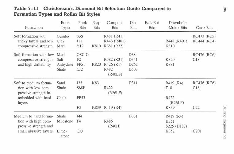
Table
7-11C
hristensen'sD
iamond
Bit
SelectionG
uideC
ompared
to...C
D
Formation
Types
andR
ollerB
itStyles
Rock
Rock
StepC
ompact
Dia.
BallaSet
Dow
nholeForm
ationT
ypeB
itsB
itsB
itsB
itsB
itsM
otorB
itsC
oreB
its
Softform
ationw
ithG
umbo
S3SR
481(R
4l)R
C473
(RC
5)sticky
layersand
lowC
layJlI
R448
(R401)
R448
(R401)
RC
444(R
C4)
compressive
strengthM
arlY
l2K
810R
381(R
32)K
810
Softform
ationw
ithlow
Marl
OSC
IGD
38R
C476
(RC
6)com
pressivestrength
SaltF2
R382
(R31)
D341
K820
CI8
andhigh
drillabilityA
nhydriteFP5l
K820
R426
(Rl)
D262
K831
Shalecn
R482
D503
(R40L
F)
Softto
medium
forma-
Sand133
K831
D311
R419
(R4)
RC
476(R
C6)
tionw
ithlow
com-
ShaleS88F
R422
TI8
CI8
pressivestrength
in-(R
26LF)
terbeddedw
ithhard
Chalk
FP53R
422layers
(R26L
F)F3
K839
R419
(R4)
K839
C22
t::1
SM
ediumto
hardform
a-Shale
J44D
331R
419(R
4)E
r\0
tionw
ithhigh
CO
ffi-M
udstoneF4
R486
K851
tT1
::s
pressivestrength
and(R
40H)
S225(D
187)\0E
r
small
abrasivelayers
Lim
e-C
13K
852C
201C
DC
DI-<
stoneS'\0
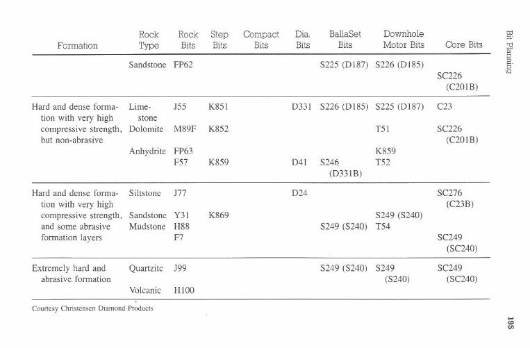
Rock
Rock
StepC
ompact
Dia.
BallaSet
Dow
nholere
Formation
Type
Bits
Bits
Bits
Bits
Bits
MotorB
itsC
oreB
its"t!6J::!
SandstoneFP62
S225(D
187)S226
(D185)
::!S'SC
226<
Q
(C201B
)
Hard
anddense
forma-
Lim
e-J55
K851
D331
S226(D
185)S225
(D187)
C23
tionw
ithvery
highstone
compressive
strength,D
olomite
M89F
K852
T51
SC226
butnon-abrasive
(C201B
)A
nhydriteFP63
K859
F57K
859D
41S246
T52
(D331B
)
Hard
anddense
forma-
Siltstone177
D24
SC276
tionw
ithvery
high(C
23B)
compressive
strength,Sandstone
Y31
K869
S249(S240)
andsom
eabrasive
Mudstone
H88
S249(S240)
T54
formation
layersF7
SC249(SC
240)
Extrem
elyhard
andQ
uartziteJ99
S249(S240)
S249SC
249abrasive
formation
(S240)(SC
240)V
olcanicH
lOO
Courtesy
Christensen
Diam
ondProducts
...U)
en
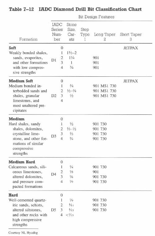
Table 7-12 IADC Diamond Drill Bit Classification Chart
Bit Design Feature:;;
IADC StoneSeries Size, StepNum- Car- Type Long Taper Short Taper
Formation ber ats 1 2 3
Soft 0 JETPAXWeakly bonded shales, 1 1V2-2
sands, evaporites, 012 1V4 901
and other formations 3 1 901with low compres- 4 % 901sive strengths
Medium Soft 0 JETPAXMedium bonded in- 1 % 901 MSI 730
terbedded sands and 2 V2-% 901 MSl 730shales, granular 02 3 1/2 901 MSl 730limestones, and 4
most unaltered pre-cipitates-
Medium 0
Hard shales, sandy 1 V2 901 730shales, dolomites, 2 V3-V2 901 730crystalline lime- 03
3 1/3 901 730stone, and other for- 4 V4 901 730mations of similarcompressivestrengths
Medium Bard 0Calcareous sands, sili- 1 V4 901 730
ceous limestones, 042 V5 901
altered dolomites, 3 1/6 901 730and pressure com- 4 V7 901 730pacted formations-
Bard 0Well-cemented quartz- I V9 901 730
itic sands, schists, 2 YII 901 730altered siltstones, 05 3 YI5 901 730and other rocks with 4 <V15
high compressivestrengths
Courtesy NL Hycalog
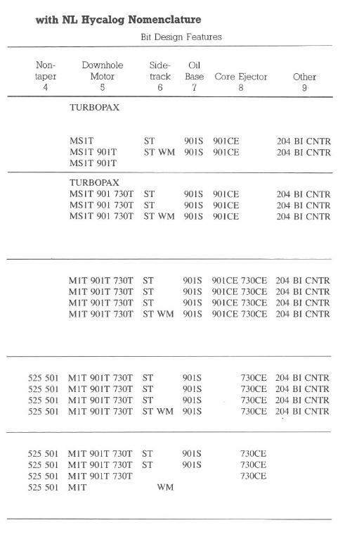
MIT 901T 730TMIT 90lT 730TMIT 901T 730TMIT 90lT 730T
STSTSTSTWM
90lS901S901S90lS
90ICE 730CE90lCE 730CE90lCE 730CE90lCE 730CE
204 BI CNTR204 BI CNTR204 BI CNTR204 BI CNTR
525 501525 501525 501525 50I
MIT 90lT 730TMIT 90lT 730TMIT 901T 730TMIT 90lT 730T
STSTSTSTWM
90lS90lS90lS90lS
730CE730CE730CE730CE
204 BI CNTR204 BI CNTR204 BI CNTR204 BI CNTR
525 501525 501525 501525 501
MIT 90lT 730T ST 901SMIT 90lT 730T ST 901SMIT 90lT 730TMIT WM
730CE730CE730CE
with NL Bycalog Nomenclature
BitDesign Features
Non- Downhole Side- Oiltaper Motor track Base Core Ejector Other
4 5 6 7 8 9
TURBOPAX
MSIT ST 90lS 90lCE 204 BI CNTRMSIT 90lT STWM 90lS 901CE 204 BI CNTRMSIT 90IT-TURBOPAXMSIT 901 730T ST 90lS 90ICE 204 BI CNTRMSIT 901 730T ST 901S 90lCE 204 BI CNTRMS IT 901 730T STWM 90lS 90ICE 204 BI CNTR
198 Drilling Engineering
Matrix degradation can also be caused by heat. When for some reason thedrilling fluid cannot reach some part of the bit to cool it, the heat buildup cannotbe dissipated. This heat buildup can result in heat checking or spalling and canadversely affect life and ROP.
Other Wear. The remaining forms of wear are in a general classificationand cover not only wear but also damage to parts of the bit that are not directlyinvolved in formation excavation and removal functions. These include the
shank, API connection, results of drillstring washout, and the mechanical func-tions of the drilling operation that might have prematurely caused the bit to bepulled (e.g., LCM, twistoff, dropping).
Dull Bit Analysis. Diamond bits tend to clog when soft, sticky shalesand limestones are being drilled with low hydraulic energy levels. The fluidcourses may clog and the fluid that normally would flow through is divertedelsewhere. The impacted formation tends to build up and pack tighter. In low-horsepower applications, it is not uncommon to pull a bit that has as much asone-third of the fluid courses clogged, with the matrix around these areas showingheat cracks. The shale acts as a bearing at these points and heat is generatedthat cannot be dissipated. Subsequently, the matrix expands and cracks.
Loss of Gauge. Gauge loss on a diamond bit can have many causes. Onecould be reaming to the bottom too quickly with too much weight. Since adiamond bit has no hydraulic distribution system until it reaches bottom, thereis no efficient way to cool the diamonds on the gauge. If too much weight orrotary is used or long sections are reamed, the gauge diamonds can be overloadedand destroyed even before the bit reaches the bottom. Another cause of loss ofthe gauge diamonds is when the diamonds set on the outer diameter row (ODR)are too large and not numerous enough. Because the angular speed of the bit isat a maximum at gauge, these diamonds tend to be overworked and undernour-ished. Mud flow is harder to control as it nears the gauge, so the diamonds arenot cooled as efficiently. Fortunately, gauge stones do not do much work in mostcases.
The best way to protect against these problems is to minimize the amountof reaming done with the diamond and to be careful to ream slowly when it isnecessary. In addition, if gauge problems are encountered, the use of smallerdiamonds on the ODR and gauge section will increase the resistance to wear.
Cored Center. In the past, center coring was a common cause of bit failure.Center coring occurs when the diamonds in and around the apex are destroyedor lost. The formation begins to wear away the matrix material and, essentially,the bit tries to cut a small core. Penetration rate slows or stops, and perhaps anincrease in standpipe pressure is evident. Generally, the causes are I) improperdesign, 2) incorrect diamonds (too large), 3) broken or fractured formation, 4)poorly bonded bedding planes, 5) improper stabilization, and 6) extraneousmetal.
Bit Planning 199
The use of small diamonds in the apex area will usually solve this problem.A core ejector modification may also help. Improved stabilization is alwaysrecommended.
Ring-out. A ring-out failure looks like an a-ring groove appearing any-where on the drilling face. The most popular site is just inside the nose, but itmay occur anywhere. A ring-out is recognizable on the surface by the rapidincrease of the standpipe pressure accompanied by a decrease in Rap.
Improper stabilization is a prime factor. Broken formations, junk, erosion,and too few diamonds also participate in the development of ring-out failures.A modified design, smaller diamonds, increased density, and judicious use ofcarbonado diamonds generally alleviate this undesirable side effect.
Rounded Gauge. A new bit has a perfectly cylindrical gauge section.Occasionally a used bit will be pulled and the gauge will be rounded. The bitis not necessarily out of gauge, but it most likely is. This results from randomwobble and is associated with inadequate bottom-hole stabilization and pendulumhook-ups. If improved stabilization is not an option, a more densely set gaugeand possibly an extended gauge will provide relief.
Matrix Erosion. Erosion of the bit matrix is almost always apparent inused bits. Heavy erosion is normally associated with high hydraulic energy levelsused to drill soft to medium-soft formations. The area just inside the nosegenerally shows the highest amount of fluid erosion. This is because the fluidis undergoing acceleration and extreme turbulence due to a directional changeof the fluid path. This maximizes the energy imparted to the matrix and resultsin the high fluid erosion. This is all compounded with the increase in undesirablesolids content (especially fin~abrasive sand) that fast drilling generally produces.Erosion is normal, but a distinction must be made: Is it a normal amount or isit excessive? Due to the many factors involved and the complicated nature ofthe erosion mechanism, it is not always easy to tell. Depending on the apparentcause, one of the following solutions may apply: lower hydraulic horsepower,cleaner mud, and alternate bit design, or less diamond exposure.
Broken Diamonds. A broken diamond is the result of excessive tangentialforce. When the strength of the diamond is exceeded, a fracture along a cleavageplane(s) occurs and all or most of the exposed stone separates. On the used bit,this is recognizable by the generally flat, highly reflective surface. Insignificant,random breakage oCCUrson most bits, but occasionally it is widespread and canaffect performance. Causes are stones too large, broken formation, jUl)k, toofew stones, WOB excessive, improper stabilization, and erosion.
Polycrystalline Diamond BitsA new generation of bit technology began in 1973 when General Electric
Co. introduced the Stratapax@drill blank. This technology has been licensed to
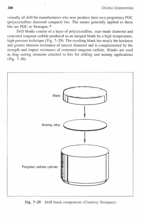
zoo Drilling Engineering
virtually all drill bit manufacturers who now produce their own proprietary PDC(polycrystalline diamond compact) bits. The names generally applied to thesebits are PDC or Stratapax.@
Drill blanks consist of a layer of polycrystalline, man-made diamond andcemented tungsten carbide produced as an integral blank by a high-temperature,high-pressure technique (Fig. 7-29). The resulting blank has nearly the hardnessand greater abrasion resistance of natural diamond and is complemented by thestrength and impact resistance of cemented tungsten carbide. Blanks are usedas drag cutting elements attached to bits for drilling and mining applications(Fig. 7-30).
Blank
;--y.
J~, ......
...",~~'
Tungsten carbide cylinder
Fig. 7-29 Drill blank components (Courtesy Stratapax)
I
Brazingalloy CJ
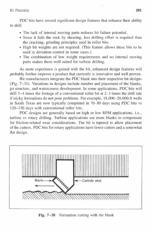
Bit Planning 201
PDC bits have several significant design features that enhance their abilityto drill:
.The lack of internal moving parts reduces bit failure potential.· Since it fails the rock by shearirig, less drilling effort is required thanthe cracking,grindingprinciplesused in rollerbits. .·High bit weights are not required. (This feature allows these bits to beused in deviation control in some cases.).The combination of low weight requirements and no internal movingparts makes them well suited for turbine drilling.
As more experience is gained with the bit, enhanced design features willprobably further improve a product that currently is innovative and well proven.
Bit manufacturers integrate the PDC blank into their respective bit designs(Fig. 7-31). Variations in designs include number and placement of the blanks,jet structure, and watercourse development. In some applications, PDC bits willdrill 3-4 times the footage of a conventional roller bit at 2-3 times the drill rateif sticky formations do not pose problems. For example, 18,OOO-20,OOO-ftwellsin South Texas are now typically completed in 70-80 days using PDC bits vs120-130 days with conventional roller bits.
PDC designs are generally based on high or low RPM applications, i.e.,turbine vs rotary drilling. Turbine applications use more blanks to compensatefor friction-related wear considerations. The bit is tapered to allow placementof the cutters. PDC bits for rotary applications have fewer cutters and a somewhatflat design.
Fig. 7-30 Formation cutting with the blank
202 Drilling Engineering
Fig.7-31 NL Hycalog's DS-23 diamond bit (Courtesy NL Hycalog)
Rotary-designed PDC bits often use nozzles to allow fluid circulation forcuttings removal and cooling of the bit. Manufacturers may vary number anddistribution of the nozzles. A tendency for applications in water-based muds isto use small jets to achieve high fluid velocities. This feature does not appearto be as significant in oil-based muds applications.
PDC bits are manufactured with a machined, steel body or a matrix bodyprocess. The matrix process is similar to the manufacturing of diamond bits.The cutters are attached to the bit by proprietary techniques. Matrix bodies appearto be more erosion resistant.
Shape of the PDC cutters is becoming an important consideration. Mostmanufacturers use the original circular design. However, effort is being givento research and development of alternate shapes to enhance the design andimprove drilling performance.
Bit Planning 203
PDC bit technology is an area experiencing dynamic changes and im-provements in the drilling industry. As an example, the recently introducedleached compact technology provides a thermally stable cutter and low wearrates, and opens the door for improved compact-to-bit attachment procedures.
Drilling OptimizationAs described at the beginning of this chapter, the three levels or phases of
drilling optimization are as follows:
· bit selection· matching the area average performance·exceeding the area average by implementing theoretical weight-rotaryspeed principles
This section of the text will discuss the second group, area average performance.Bit selection will be presented as the final section of this chapter.
During recent years, many attempts have been made to optimize drillingoperations. Some of the efforts have been directed in fields such as l) developingdrilling fluids that yield high penetration rates, 2) improving solids control equip-ment design to improve mud properties, and 3) designing bits to improve pen-etration rates, bit life, or both. In addition, overall experience has led to tech-niques and equipment that reduce the final cost to the operator.
,In the past, optimization during the actual drilling process was based onseveral principles:
.Drill at high penetration rates for as long as the bit will drill· Select bit weights and rotary speeds that will give long bit runs withreasonable penetration rates· Determine the optimum operating conditions that will drill the giveninterval at the lowest cost per foot
Economics quickly became the primary design criteria, resulting in most opti-mization techniques being based on the proper selection of bit weights, rotaryspeeds, and bit types that produce the lowest cost per foot-minimum-costdrilling (MCD).
The cost of the footage drilled during a single bit run is the sum of threecosts: bit costs, trip costs, and rig operating costs for the time required to drillthe footage. If the bit run cost is divided by the footage drilled, the result is thecost per foot for the interval drilled, as shown in Eq. 7.1. The cost per footgiven by Eq. 7.1 is the cost to be minimized through proper choice of the bitweight and rotary speed. Eq. 7.1 shows that the choice of weight and rotaryspeed affects only two items: rotary cost and footage drilled. The cost of the bitand the cost to trip the bit are fixed for a particular bit run.
204 Drilling Engineering
(7.1)
Where:$/ft = cost per foot, $Co = bit cost, $CR = rig cost, $/hrTT = trip time, hrTR = rotating time, hrY = footage drilled, ft
Table 7-13 presented average trip time values for various depth and bitsizes, reproduced in this chapter. An alternate, suitable approach is the standard"I hrll ,000 ft" value.
It is interesting to show that proper selection of bit weights and rotaryspeeds to give minimum-cost drilling may not yield either the maximum pene-tration rate nor the longest bit runs. The data used in the following exampleproblem will be shown to be correct in a later chapter. (Costs for items such asbits and rig time are far below present costs but are used for illustration only.They are correct, however, on a relative comparison between cost items.)
Example 7.2
Use the data given below and the minimum cost equation to select the optimumbit weights and rotary speeds.
Data:Rig cost = $75.00/hrBit cost = $232.50Trip time = 6.5 hr
Bit Weight,Ib
75,00065,00065,000
Case 1Case 2Case 3
Rotary Speed,rpm1279265
FootageDrilled, ft
149192217
Rotating Time,hr5.068.65
12.28
Solution:
1. Use the common data and specific case information to calculate cost perfoot for the section drilled.
2.$ft- (7.1)
Case I $232.50 + (75) (6.5) + (75) (5.06) = 7.38 $/ft149
$232.50 + (75) (6.5) + (75) (8.65) = 7.13 $/ft192
$232.50 + (75) (6.5) + (75) (12.28) = 7.56 $/ft
Case 2
Case 3
3. In this example, minimum-cost drilling occurs with Case 2, which hadneither maximum penetration rates nor bit life.
If the fixed cost and the rotating cost are considered separately, the allo-cation of the fixed cost to the cost per foot would be high if the bit run wereterminated after the bit drilled the first foot. But this allocation declines contin-uously thereafter as the bit drills more footage. By comparison, the contributionof the rotating cost to the cost per foot is low initially but increases continuously
BitPlanning 205
Table 7-13 Average Trip Times
Hole (Bit) Size. in.
Depth, . Mediumft Small« 8.75) (8.75-9.875) Large (> 9.875)
2,000 1.5 3.0 4.54,000 2.5 4.2 5.756,000 3.5 5.4 7.08,000 4.7 6.25 8.0
10,000 5.8 7.25 9.012,000 7.0 8.25 10.2514,000 8.25 9.25 11.5016,000 9.75 10.25 12.5018,000 11.00 11.25 13.7520,000 11.8 12.25 15.0
Penetration Rate, Bit Life, Cost,filhr hr $/ft
Case I 29.4 5.06 7.38Case 2 22.19 8.65 7.13Case 3 17.67 12.28 7.56
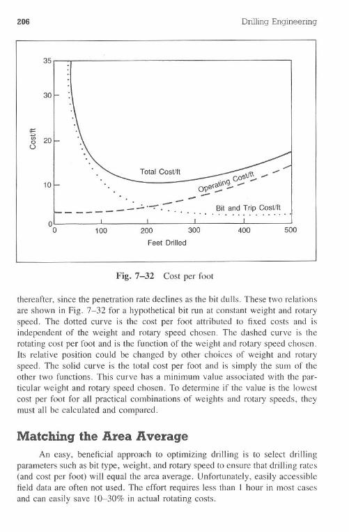
206 Drilling Engineering
35
30
s~ 20
()
Total Costlft
10. cos\!\\ .,.,
O<'le(~\\(\g .,., ....... -....
--- .---
- - - - -- .--:-.--- Bit and Trip Costlft
.
. ... ..oo 100 200 300
Feet Drilled
400 500
Fig. 7-32 Cost per foot
thereafter, since the penetration rate declines as the bit dulls. These two relationsare shown in Fig. 7-32 for a hypothetical bit run at constant weight and rotaryspeed. The dotted curve is the cost per foot attributed to fixed costs and isindependent of the weight and rotary speed chosen. The dashed curve is therotating cost per foot and is the function of the weight and rotary speed chosen.Its relative position could be changed by other choices of weight and rotaryspeed. The solid curve is the total cost per foot and is simply the sum of theother two functions. This curve has a minimum value associated with the par-ticular weight and rotary speed chosen. To determine if the value is the lowestcost per foot for all practical combinations of weights and rotary speeds, theymust all be calculated and compared.
Matching the Area AverageAn easy, beneficial approach to optimizing drilling is to select drilling
parameters such as bit type, weight, and rotary speed to ensure that drilling rates(and cost per foot) will equal the area average. Unfortunately, easily accessiblefield data are often not used. The effort requires less than I hour in most casesand can easily save 10-30% in actual rotating costs.
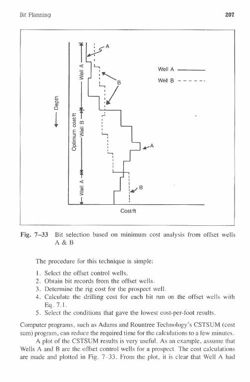
Bit Planning 207
Cost/ft
Fig. 7-33 Bit selection based on minimum cost analysis from offset wellsA&B
The procedure for this technique is simple:
I. Select the offset control wells.2. Obtain bit records from the offset wells.
3. Determine the rig cost for the prospect well.4. Calculate the drilling cost for each bit run on the offset wells with
Eq. 7.1.5. Select the conditions that gave the lowest cost-per-foot results.
Computer programs, such as Adams and Rountree Technology's CSTSUM (costsum) program, can reduce the required time for the calculations to a few minutes.
A plot of the CSTSUMresultsis very useful.As anexample,assumethatWells A andB are theoffset control wells for a prospect.The cost calculationsare made and plotted in Fig. 7-33. From the plot, it is clear that Well A had
a5 . WellA
Jr
. "c Well B - - - - - ...t:a.CD
Q
! m0_§ I.....,
ij
III
I.....AI
«
208 Drilling Engineering
lower drilling costs in the upper and lower sections of the well, while Well Bwas optimum in the middle sections of the well. Therefore, the bit types, weight,and rotary speeds for the prospect well should be similar to Wells A and B inthe respective hole segments in which they had the lowest cost-per-foot results.
Example 7.3
A well is to be drilled in Lafayette parish, Louisiana. The 16,000-ft prospectis in section 25, township 7S, range 3E. The geologists have determined thatthe two offset control wells are:
OperatorA&RT Oil Co.McWilliams Ventures
Well NameE.B. White #1Cochran #3
Depth, ft16,00017,654
The bit records on the wells will be used to select an optimum bitprogram for minimum-cost drilling of the prospect well. The operating con-ditions on the offset wells were:
Cochran #3Bit Size, Type Cost, Depth Out, Feet Hours
Run lll. $ ftI 17.5 OSC3A 5,062 4,435 4,435 78.52 12.25 X3A 2,516 5,867 1,432 37.53 12.25 X3A 2,516 6,907 1,040 184 12.25 SII 2,516 7,752 845 27.55 12.25 FDT 3,052 9,048 1,296 46.56 12.25 FDT 3,052 9,509 461 227 12.25 S84F 8,388 11,005 1,496 888 8.375 S84F 4,377 12,769 1,764 104.59 8.375 122 4,377 12,985 216 33
10 8.375 FP53 4,377 13,230 245 30II 8.375 F2 4,377 13,595 365 3212 8.375 YI2 1,101 13,714 119 11.513 8.375 122 4,377 14,519 805 7514 8.375 F3 4,377 14,797 278 2115 8.375 J22 4,377 15,600 803 63.516 8.375 122 4,377 15,900 300 2917 8.375 122 4,377 16,714 814 86.518 8.375 122 4,377 16,716 2 519 8.375 J22 4,377 17,171 455 7720 8.375 122 4,377 17,654 483 53
BitPlanning 209
E.B. White # IBit Size, Type Cost, Depth Out, Feet Hours
Run in. $ ft1 17.5 X3A 7,422 3,500 3,500 362 12.25 X3A 2,516 5,320 1,820 263 12.25 X3A 2,516 6,748 1,428 284 12.25 X3A 2,516 6,837 89 65 12.25 X3A 2,516 7,573 736 326 12.25 X3A 2,516 8,098 525 307 12.25 J22 8,388 9,442 1,344 808 12.25 J22 8,388 10,600 1,158 829 8.5 J22 4,377 11,387 787 78
10 8.5 122 4,377 11,407 20 1011 8.5 J22 4,377 12,252 845 9512 8.5 133 4,377 12,720 468 4513 8.5 133 4,377 13,103 383 4514 8.5 133 4,377 13,470 367 4015 8.5 133 4,377 13,655 185 2016 8.5 J55 4,377 13,745 90 1817 8.5 133 4,377 14,017 272 3018 8.5 Diamond 14,875 14,467 450 15019 8.5 Diamond 14,875 15,139 672 16020 8.5 J22 4,377 16,000 861 98
The bit costs are provided with the previous data. Diamond bit costs are netcost after accounting for salvage value. Use the trip time values from Table2-1. The rig cost is $6,900/day.
Solution:
1. Cost per foot for each bit run is:
$/ft = CB + CRTR + CRTTy
The cost for the first bit run of the Cochran #3 well is:
$/f = 5,062 + (6,900/24)(78.5) + (6,900/24)(4.6)t 4,435
_ 28,953- 4,435
= 6.53
2. A summary of the cost calculations for each well is shown in Tables7-14 and 7-15.
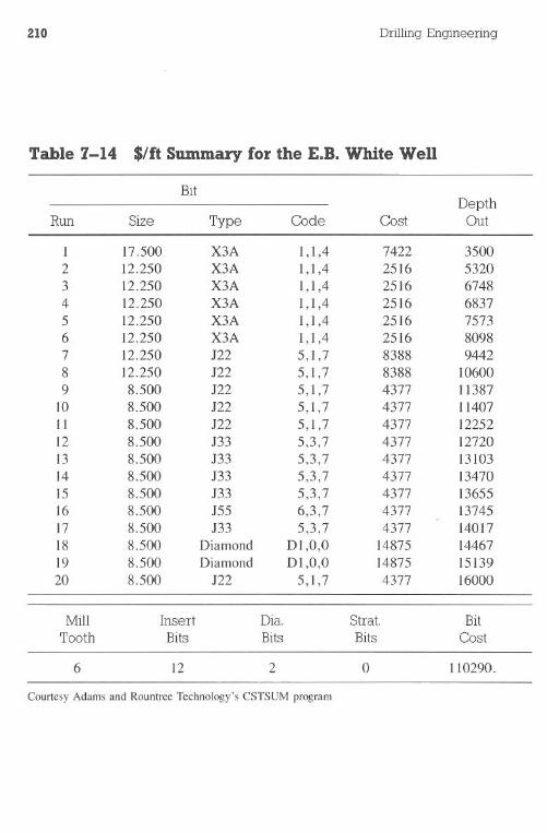
210 Drilling Engineering
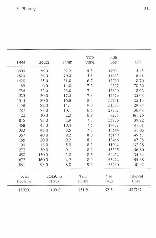
Bit Planning 211
Trip RunFeet Hours Ft/hr Time Cost $/ft
3500 36.0 97.2 4.3 19004 5.431820 26.0 70.0 5.8 11662 6.411428 28.0 51.0 6.7 12506 8.76
89 6.0 14.8 7.2 6307 70.26736 32.0 23.0 7.4 13850 18.62525 30.0 17.5 7.8 13379 25.48
1344 80.0 16.8 8.3 33781 25.131158 82.0 14.1 9.0 34563 29.85787 78.0 10.1 6.6 28707 36.4820 10.0 2.0 6.9 9225 461.26
845 95.0 8.9 7.1 33736 39.92468 45.0 10.4 7.5 19472 41.61383 45.0 8.5 7.8 19544 51.03367 40.0 9.2 8.0 18169 49.51185 20.0 9.2 8.1 12466 67.3890 18.0 5.0 8.2 11914 132.38
272 30.0 9.1 8.3 15395 56.60450 150.0 3.0 8.5 60454 134.34672 160.0 4.2 8.9 63424 94.38861 98.0 8.8 9.3 35230 40.92
Total Rotating Trip Net Interval
Footage Hours Hours Days Cost
16000. 1l09.0 151.9 52.5 472787.
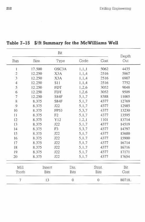
212 Drilling Engineering
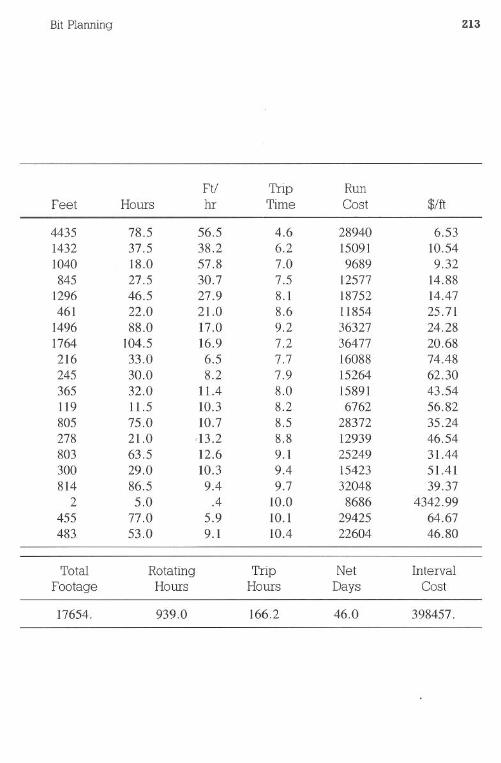
Bit Planning 213
Ft/ Trip RunFeet Hours hr Time Cost $/ft
4435 78.5 56.5 4.6 28940 6.531432 37.5 38.2 6.2 15091 10.541040 18.0 57.8 7.0 9689 9.32845 27.5 30.7 7.5 12577 14.88
1296 46.5 27.9 8.1 18752 14.47461 22.0 21.0 8.6 11854 25.71
1496 88.0 17.0 9.2 36327 24.281764 104.5 16.9 7.2 36477 20.68216 33.0 6.5 7.7 16088 74.48245 30.0 8.2 7.9 15264 62.30365 32.0 11.4 8.0 15891 43.54119 11.5 10.3 8.2 6762 56.82805 75.0 10.7 8.5 28372 35.24278 21.0 113.2 8.8 12939 46.54803 63.5 12.6 9.1 25249 31.44300 29.0 10.3 9.4 15423 51.41814 86.5 9.4 9.7 32048 39.37
2 5.0 .4 10.0 8686 4342.99455 77.0 5.9 10.1 29425 64.67483 53.0 9.1 10.4 22604 46.80
Total Rotating Trip Net IntervalFootage Hours Hours Days Cost
17654. 939.0 166.2 46.0 398457.
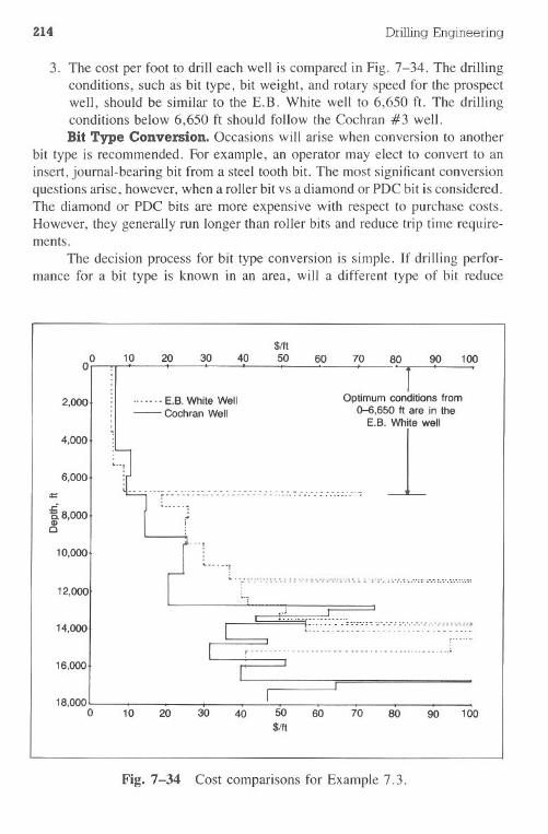
214 Drilling Engineering
3. The cost per foot to drill each well is compared in Fig. 7-34. The drillingconditions, such as bit type, bit weight, and rotary speed for the prospectwell, should be similar to the E.B. White well to 6,650 ft. The drillingconditions below 6,650 ft should follow the Cochran #3 well.Bit Type Conversion. Occasions will arise when conversion to another
bit type is recommended. For example, an operator may elect to convert to aninsert, journal-bearing bit from a steel tooth bit. The most significant conversionquestions arise, however, when a roller bit vs a diamond or PDC bit is considered.The diamond or PDC bits are more expensive with respect to purchase costs.However, they generally run longer than roller bits and reduce trip time require-ments.
The decision process for bit type conversion is simple. If drilling perfor-mance for a bit type is known in an area, will a different type of bit reduce
10 20 30 40$/1150 60 70 90 100
2,000 ... -- -- E.B. White Well- CochranWell
80
1Optimum conditions from
0-6,650 II are in theE.B. White well
14,000
6,000- - - . . --- . . - - - - -. .. - - -- -. . . . - - . . . . . . - - --.-r' - - .- -- __- . . ._.. _____.._'. . . _0__ ~-=.:
i 8,000c
12,000'- -. . - -t . Ai ~.:.~.:: : : : ",":: ':..: ~.::..:-: :. :":" :". ";".".".':~~_:::.:"_.",:.':.'._.'._.~'."'::
~'1
10,000
..;..-................14,000
--.........----...-------...----- - -. ---. - -. . -.. .. --. - ... -.-.---. - -. . - - . _. - . - - - -. _. - . - - - -..-
t - - - . . - . -. . - - - - - - . - - - - . - - - - . . - . - .. .. .. - - - . . ..~
16,000
18,000o 10 20 30 40 50
$/1160 70 80 90 100
Fig.7-34 Cost comparisons for Example 7.3.
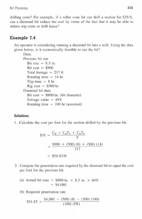
Bit Planning 215
drilling costs? For example, if a roller cone bit can drill a section for $25/ft,can a diamond bit reduce the cost by virtue of the fact that it may be able toreduce trip costs or drill faster?
Example 7.4
An operator is considering running a diamond bit into a well. Using the datagiven below, is it economically feasible to run the bit?
Data:Previous bit run
Bit size = 8.5 in.Bit cost = $900Total footage = 217 ftRotating time = 14 hrTrip time = 8 hrRig cost = $500/hr
Diamond bit dataBit cost = $800/in. (bit diameter)Salvage value = 40%Rotating time = 100 hr (assumed)
Solution:
I. Calculate the cost per foot for the section drilled by the previous bit:
$/ft = CD + CRTT + CRTRy
$900 + (500) (8) + (500) (14)217
= $54.83/ft
2. Compute the penetration rate required by the diamond bit to equal the costper foot for the previous bit.
(a) Actual bit cost = $800/in. X 8.5 in. X 60%= $4,080
(b) Required penetration rate
$54 83 = $4,080 + (500) (8) + (500)(100). (100) (PR)
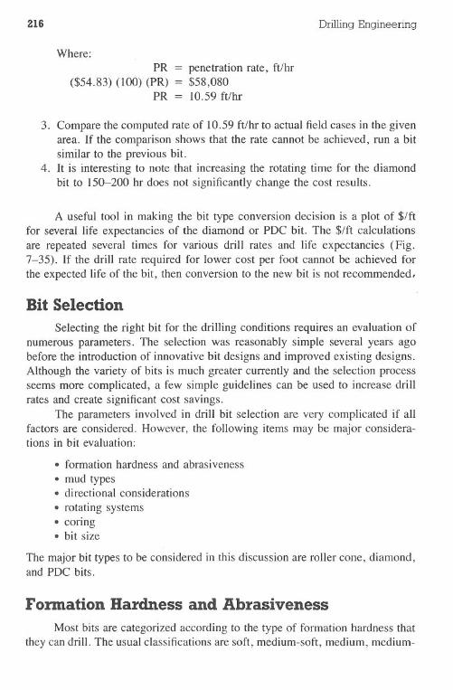
216 Drilling Engineering
Where:PR
($54.83) (l00) (PR)PR
penetration rate, ft/hr$58,08010.59 fUhr
3. Compare the computed rate of 10.59 fUhr to actual field cases in the givenarea. If the comparison shows that the rate cannot be achieved, run a bitsimilar to the previous bit.
4. It is interesting to note that increasing the rotating time for the diamondbit to 150-200 hr does not significantly change the cost results.
A useful tool in making the bit type conversion decision is a plot of $/ftfor several life expectancies of the diamond or PDC bit. The $/ft calculationsare repeated several times for various drill rates and life expectancies (Fig.7-35). If the drill rate required for lower cost per foot cannot be achieved forthe expected life of the bit, then conversion to the new bit is not recommended,
Bit SelectionSelecting the right bit for the drilling conditions requires an evaluation of
numerous parameters. The selection was reasonably simple several years agobefore the introduction of innovative bit designs and improved existing designs.Although the variety of bits is much greater currently and the selection processseems more complicated, a few simple guidelines can be used to increase drillrates and create significant cost savings.
The parameters involved in drill bit selection are very complicated if allfactors are considered. However, the following items may be major considera-tions in bit evaluation:
· formation hardness and abrasiveness·mud types·directionalconsiderations·rotating systems.coring· bit size
The major bit types to be considered in this discussion are roller cone, diamond,and PDC bits.
Fonnation Hardness and AbrasivenessMost bits are categorized according to the type of formation hardness that
they can drill. The usual classifications are soft, medium-soft, medium, medium-
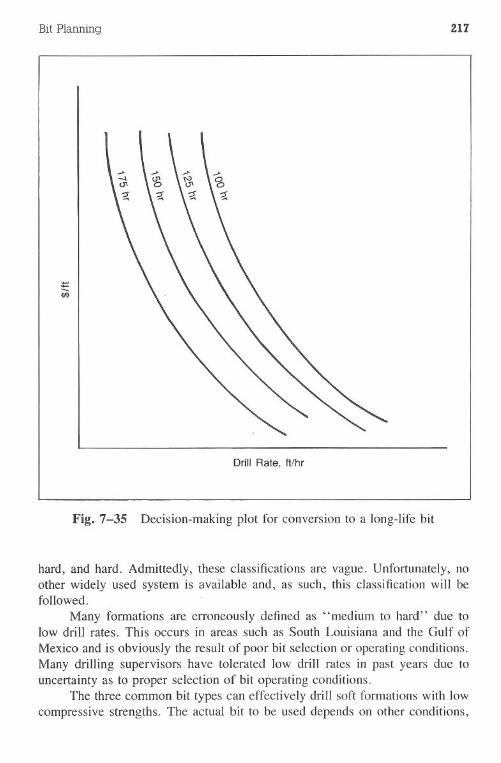
Bit Planning 217
Drill Rate, ft/hr
Fig. 7-35 Decision-making plot for conversion to a long-life bit
hard, and hard. Admittedly, these classifications are vague. Unfortunately, noother widely used system is available and, as such, this classification will befollowed.
Many formations are erroneously defined as "medium to hard" due tolow drill rates. This occurs in areas such as South Louisiana and the Gulf ofMexico and is obviously the result of poor bit selection or operating conditions.Many drilling supervisors have tolerated low drill rates in past years due touncertainty as to proper selection of bit operating conditions.
The three common bit types can effectively drill soft formations with lowcompressive strengths. The actual bit to be used depends on other conditions,
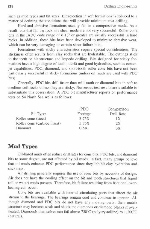
218 Drilling Engineering
such as mud types and bit sizes. Bit selection in soft formations is reduced to amatter of defining the conditions that will provide minimum-cost drilling.
Hard and abrasive formations usually fail in a compressive mode. As aresult, bits that fail the rock in a shear mode are not very successful. Roller conebits in the IADC code range of 6, 1,7 or greater are usually successful in hardrocks. In addition, these bits have been developed to minimize abrasive wear,which can be very damaging to certain shear-failure bits.
Formations with sticky characteristics require special consideration. Thestickiness often results from clay rocks that are hydratable. The cuttings stickto the teeth or bit structure and impede drilling. Bits designed for sticky for-mations have a high degree of teeth interfit and good hydraulics, such as center-jet capabilities. PDC, diamond, and short-tooth roller cone bits have not beenparticularly successful in sticky formations (unless oil muds are used with PDCbits).
Generally, PDC bits drill faster than mill tooth or diamond bits in soft tomedium-soft rocks unless they are sticky. Numerous test results are available tosubstantiate this observation. A PDC bit manufacturer reports on performancetests on 54 North Sea wells as follows:
Bit TypeRoller cone (steel)Roller cone (carbide insert)Diamond
PDCFootage3.75X5.75XO.5X
ComparisonDrill Rate
IX2X3X
Mud TypesOil-based muds often reduce drill rates for cone bits. PDC bits, and diamond
bits to some degree, are not affected by oil muds. In fact, many groups believethat oil muds enhance PDC performance since they inhibit clay hydration andstickiness.
Air drilling generally requires the use of cone bits by necessity of design.Air does not have the cooling effect on the bit and tooth structures that liquid(oil or water) muds possess. Therefore, bit failure resulting from frictional over-heating can occur.
Cone bits are available with internal circulating ports that direct the airstream to the bearings. The bearings remain cool and continue to operate. Al-though diamond and PDC bits do not have any moving parts, their matrixstructure may become weak and shuck the diamonds or diamond blanks if over-heated. Diamonds themselves can fail above 750°C (polycrystalline) to 1,200°C(natural).
Bit Planning 219
Directional ConsiderationsThe drill bit indirectly affects the directional control problem in a well.
The contributing factors include:
· cone offset· number of cones.cutting structure on the cone· bit weight
The effect of the bottom-hole assembly (BHA) on directional control will bediscussed in Chapter 15.
Rotary drilling operations have an inherent tendency to a right-hand walk.This tendency is increased with the offset of the cones from the bit center. Truerolling bits without cone offset decrease the right-hand walking characteristic.Remember, however, that the cone offset is desirable in most cases due to theincreased drill rates it achieves.
Turbine drilling may have a tendency for left-hand walk. Controlling factorsinclude the turbine manufacturer, gauge length, and stabilization program.
Various bit manufacturers have developed two- and four-cone roller bitsfor directional purposes. These bits are reported to reduce the right-hand walkingand, in some cases, to induce a left-hand walk. The IADC specialty code numberfor these bits is 8, i.e., 1,1,8 is a soft-formation directional bit.
Roller bits are available with cutting structures that minimize the effect offormation dip on hole structure. The outer row of teeth has special designs, suchas T or L teeth that "bite" into a dipping formation rather than moving in thedirection of the dip. These bits are often used to control directional problems.
High bit weights can aggravate directional problems. Low bit weightsreduce the problems but unfortunately usually increase the cost per foot of thehole. When directional control becomes a problem, it is often a no-win situationwith respect to drilling costs. PDC bits are attractive in this respect. The verylow bit weights used with these tools minimize directional problems. In addition,these bits do not have cone offset considerations.
Rotating SystemsThe two common methods of turning the bit are I) the rig's rotary table
system and 2) downhole motors. The rig's rotary system does not place anyrestrictions on bit selection. Therefore, bit choice depends on the previouslydefined parameters, such as formation hardness and mud types.
PDC bits in deep holes may be preferable when a rotary table is used.Deep wells often produce a significant amount of rotary torque due to bit andwall friction. Torque requirements are increased with high bit weights. Therefore,PDC bits may improve the drilling efficiency due to their lower weight require-ments.
zzo DrillingEngineering
Turbine drilling efficiency favors bits with long life expectancies. Thesetypes include PDC, diamond, and journal-bearing insert bits. In addition, PDCbits are favored in areas such as the North Sea due to the widespread use of oilmuds.
Coring
Coring involves the use of special bits to retrieve cylindrical sections offormation for rock property evaluation. Pressure coring, which is the retrievalof rock samples under reservoir pressure, is desirable in formation evaluationand secondaryor tertiary recovery projects where the best possible fluid saturationdata are required. The bit must operate with mud systems designed to minimizeoil flushing to give an accurate vertical oil saturation profile. A high penetrationrate is desired to reduce invasion of the core and stripping of the insitu fluids.
Diamond and PDC core bits enjoy the most widespread success in coringoperations. One series of tests with diamond and PDC bits was carried out inSan Andres dolomite at 4,973 ft near an injection well. A natural diamond bitcut 53 nine-ft cores at a rate of 2 ft/hr. The PDC core bit cut 41 nine-ft coresat 10.8 ft/hr. The core recovery rate with the PDC was 95%.
Bit SizeRoller cone bits are available in virtually any desirable size range from
33/s-26-inch bits. In most cases, any type of design, cutting structure, and jetsystem is available.
PDC and diamond bits are generally not available in an off-the-shelf fashionin sizes greater than 15 in. Diamond bits are generally prepared custom tailored.It is unfortunate that PDC bits are not currently available in very large diameterssince roller cone bits can create excessive torque in large-diameter holes.
Deep drilling of small holes is another area where PDC bits offer improvedperformance over cone bits. In small, deep holes such as a 4- or 5-in. hole at16,000 ft, bit reliability is a critical factor. Small roller cone bits are less desirablebecause of the short lives, small bearing capacity and the resultant high numberof bearing failures. Bits without moving parts are preferable under these con-ditions.
Starting the Diamond BitWhen a bit is to be run, a service engineer should be available to get the
bit started. Starting the bit properly is an essential step in successful performance.Care must be taken to ensure that no metal junk is present in the hole. A junkbasket on the prior run is recommended. Occasionally, reaming may be necessaryto get the bit to the bottom. Since conventional diamond bits are not good reamers,
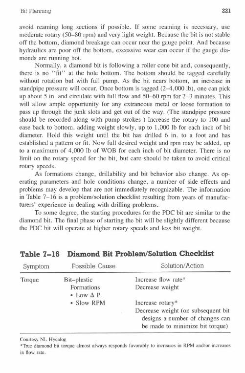
Bit Planning ZZl
avoid reaming long sections if possible. If some reaming is necessary, usemoderate rotary (50-80 rpm) and very light weight. Because the bit is not stableoff the bottom, diamond breakage can occur near the gauge point. And becausehydraulics are poor off the bottom, excessive wear can occur if the gauge dia-monds are running hot.
Normally, a diamond bit is following a roller cone bit and, consequently,there is no "fit" at the hole bottom. The bottom should be tagged carefullywithout rotation but with full pump. As the bit nears bottom, an increase instandpipe pressure will occur. Once bottom is tagged (2-4,000 lb), one can pickup about 5 in. and circulate with full flow and 50-60 rpm for 2-3 minutes. Thiswill allow ample opportunity for any extraneous metal or loose formation topass up through the junk slots and get out of the way. (The standpipe pressureshould be recorded along with pump strokes.) Increase the rotary to 100 andease back to bottom, adding weight slowly, up to 1,000 lb for each inch of bitdiameter. Hold this weight until the bit has drilled 6 in. to a foot and hasestablished a pattern or fit. Now full desired weight and rpm may be added, upto a maximum of 4,000 lb of WOB for each inch of bit diameter. There is nolimit on the rotary speed for the bit, but care should be taken to avoid criticalrotary speeds.
As formations change, drillability and bit behavior also change. As op-erating parameters and hole conditions change, a number of side effects andproblems may develop that are not immediately recognizable. The informationin Table 7-16 is a problem/solution checklist resulting from years of manufac-turers' experience in dealing with drilling problems.
To some degree, the starting procedures for the PDC bit are similar to thediamond bit. The final phase of starting the bit will be slightly different becausethe PDC bit will operate at higher rotary speeds and less bit weight.
Table 7-16 Diamond Bit Problem/Solution Checklist
Symptom Possible Cause Solution!Action
Torque Bit-plasticFormations·Low /1 P·Slow RPM
Increase flow rate*Decrease weight
Increase rotary*Decrease weight (on subsequent bit
designs a number of changes canbe made to minimize bit torque)
Courtesy NL Hycalog*True diamond bit torque almost always responds favorably to increases in RPM and/or increasesin flow rate. .
zzz DrillingEngineering
Table 7-16 Diamond Bit Problem/SolutionCheck1ist-cont~d
Symptom Possible Cause Solution!Action
Other-stabilizers toolarge.Eccentric tool
joints· Keyseats &doglegs· Collars againstwall.Torque convertor
1/32 to 1/16 under hole sizeCheck BHA
Slow ROP .Diamonds too large.Diamonds too small
· 1::1P too low
·RPM too low·Not enough WOB·Plastic shale
·Flat stones.ODR/gauge damagein reaming
If no formation change is expected,an economic analysis should bedone. A new bit may be re-quired.
Increase flow rateNew bitIncrease rotaryIncrease WOBMore RPMNew bitNew bitNew bit
AuctuatingSSP
·Formation breakingup under bit· Stabilizers hangingup· DriIling throughfractures. Bit spinning out offormation.Crooked/directionalhole
Nothing
Check lower chamfer on stabiliz-
ers-next tripNothing
RPM will also fluctuate. Differentcombination of RPM and WOB
Bit sticking .FormationEncroachment
Updrill modificationBi-center bit
Bit Planning 223
Table 7-16 Diamond Bit Problem/SolutionChecklist-cont'd
Symptom
Difficultygetting tobottom
Possible Cause
·Bit gauge too long·Previous bit under-gauged· BHA stiffer than
previously·Stabilizer locationchange.Out of drift/col-
lapsed casing
Solution! Action
Short gaugeReam with RCB
When reaming, pick up and reamsection again. If difficulty per-sists, stabilizers are a likely cul-prit.
Smaller bitBi-center bit
Low pres-sure drop
·Flow area too large
.Flow rate low.Drillstring washout
·Mud weight lowerthan anticipated
Increase flow rateAdjust flow area on subsequent bitIncrease flow rateCheck pipeCheck bit pressure dropIncrease flow rate
Change flow area on subsequent bit
High pres-sure drop
· Incorrect flow area
· High flow rate·Partiallypluggedbit
· Formation impac-tion (clogged)
· Formation change(may fluctuate)·Plastic formation
.Diamonds too small· Formation en-croachment·Ring out failure
Reduce GPM
Larger flow area next bit, grind bitopen
Reduce GPM
Check off bottom surface standpipepressure
Yo-Yo drillpipeLet bit drill off and circulate to
minutes with at least l/2 ilP.Slow RPM
Pickup, resume drilling at higherRPM
If the interval is long and ROP isunacceptable, a new bit may benecessary
Pickup and check ilPShort trip if necessary
Bit must be pulled
224 DrillingEngineering
Problems7.1 An operator is planning to drill below intermediate casing and use the
largest-diameter bit possible. With the casing configuration given asfollows, what size bit should he use?
Casing Size.m.8%8%
Casing Weight,lb/ft2832
Casing Depth,ft
0-6,0006,000-11,000
7.2 Rework Problem 7.1 if the 28-lb/ft pipe is to be used from o-11,000 ft. .
7.3 A 7%-in. drilling liner is to be used on a well. What size of bit canbe used if the pipe weighs 17.0 "Ibtft?38.0 Ibtft?
7.4 An 18.0-lb/ft, 5-in. production casing string is set to 14,000 ft. Whatsize bit must be used to drill out the cement inside the casing belowthe float collar?-
7.5 An operator is using a I, 1,4 bit. A dull grading for the bit was T-8,B-2, G-O. Select a new bit(s) to be run back into the hole. Explainyour reasons.
7.6 A 1,2,4 bit grades T-4, B-7, G-O. Select the next bit(s) and explainyour reasons.
7.7 An operator experiences severe right-hand walk problems on a direc-tional well. Assuming that all other precautions have been taken tohalt or retard the walk, select a bit type(s) that will inhibit the problem.The previous bits have been I, I ,4.
7.8 A 1,1,1 bit grades T-2, B-4, G-3. Describe the problem and rec-ommend remedial actions.
7.9 The following data were taken from a bit record of a well in Kansas.The rig cost is $190/hr. Using a trip time average of I hrll ,000 ft,compute and plot the cost per foot to drill the well.
7.10 Rework Problem 7.9 and assume that the rig costs are $160 and$200/hr. Plot the three results.
7.11 Rework Problem 7.9 and assume that the trip time average is 2,000ft/hr and 500 fUhr. Plot these results with Problem 7.10.
7.12 Refer to Fig. 7-27. Identify the 11 individual bit features.
References
Dresser Security Inc. Security Drilling TooLs.Houston.
Dublet, C.P., and T.R. Bates. "An Empirical Correlation to Predict DiamondBit Drilling Rates." SPE 9324, 1980 SPE Fall Technical Conference.
Galle, E.M., and H.G. Woods. "Variable Weight and Rotary Speed forLowest Drilling Cost." AAODC Annual Meeting, New Orleans, September27, 1960.
Hughes Tool Company. Hughes Bit Tips. Volume 1, Houston, 1970.
Madigan, I.A., and R.H. Caldwell. "Applications for Polycrystalline Dia-mond Compacts from Analysis of Carbide Insert and Steel Tooth Bit Per-formance." SPE 9326, 1980 SPE Fall Technical Conference.
NL Hycalog. "Applied Diamond Drilling." Houston, 1984.
Norton Christensen. "Diamond Drill Bit Technology." Houston, t983.
BitPlanning ZZS
Depth Out, Footage Bit Cost, Rotating Time,ft $ hr
1,800 1,800 2,516 182,500 700 1,101 15.63,300 800 1,101 213,950 650 1,101 22.54,722 772 1,101 315,211 489 4,377 265,505 294 4,377 16.86,101 596 4,377 386,500 399 4,377 28.5

226 DrillingEngineering
Offenbacher, L.A. "Development and Successful Use of Stratapax Blank Bitsin Oilfield Drilling Applications." Petroleum Extraction Technical SalesSeminar, Peoples Republic of China, July 1981.
Reed Rock Bit Company. Rock Bit Catalog. Houston.
Smith Tool Company. 1978-1979 General Catalog. Newport Beach, Cal.
Wardlaw, H.W.R. "Optimization of Rotary Drilling Parameters." PhD dis-sertation, University of Texas, August 1981.
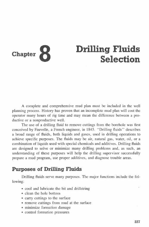
Chapter 8 Drilling FluidsSelection
A complete and comprehensive mud plan must be included in the wellplanning process. History has proven that an incomplete mud plan will cost theoperator many hours of rig time and may mean the difference between a pro-ductive or a nonproductive well.
The use of a drilling fluid to remove cuttings from the borehole was firstconceived by Fauvelle, a French engineer, in 1845. "Drilling fluids" describesa broad range of fluids, both liquids and gases, used in drilling operations toachieve specific purposes. The fluids may be air, natural gas, water, oil, or acombination of liquids used with special chemicals and additives. Drilling fluidsare designed to solve or minimize many drilling problems and, as such, anunderstanding of these purposes will help the drilling supervisor successfullyprepare a mud program, use proper additives, and diagnose trouble areas.
Purposes of Drilling FluidsDrilling fluids serve many purposes. The major functions include the fol-
lowing:
.cool and lubricate the bit and drillstring· clean the hole bottom· carry cuttings to the surface· remove cuttings from mud at the surface.minimize formation damage· control formation pressures
227
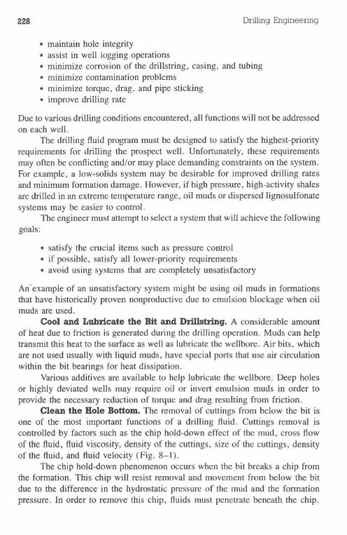
228 DrillingEngineering
.maintain hole integrity.assist in well logging operations.minimize corrosion of the drillstring, casing, and tubing.minimize contamination problems.minimize torque, drag, and pipe sticking· improve drilling rate
Due to various drilling conditions encountered, all functions will not be addressedon each well.
The drilling fluid program must be designed to satisfy the highest-priorityrequirements for drilling the prospect well. Unfortunately, these requirementsmay often be conflicting and/or may place demanding constraints on the system.For example, a low-solids system may be desirable for improved drilling ratesand minimum formation damage. However, if high pressure, high-activity shalesare drilled in an extreme temperature range, oil muds or dispersed lignosulfonatesystems may be easier to control.
The engineer must attempt to select a system that will achieve the followinggoals:
·satisfy the crucial items such as pressure control· if possible, satisfy all lower-priority requirements· avoid using systems that are completely unsatisfactory
An.example of an unsatisfactory system might be using oil muds in formationsthat have historically proven nonproductive due to emulsion blockage when oilmuds are used.
Cool and Lubricate the Bit and DriI1string. A considerable amountof heat due to friction is generated during the drilling operation. Muds can helptransmit this heat to the surface as well as lubricate the wellbore. Air bits, whichare not used usually with liquid muds, have special ports that use air circulationwithin the bit bearings for heat dissipation.
Various additives are available to help lubricate the wellbore. Deep holesor highly deviated wells may require oil or invert emulsion muds in order toprovide the necessary reduction of torque and drag resulting from friction.
Clean the Bole Bottom. The removal of cuttings from below the bit isone of the most important functions of a drilling fluid. Cuttings removal iscontrolled by factors such as the chip hold-down effect of the mud, cross flowof the fluid, fluid viscosity, density of the cuttings, size of the cuttings, densityof the fluid, and fluid velocity (Fig. 8-1).
The chip hold-down phenomenon occurs when the bit breaks a chip fromthe formation. This chip will resist removal and movement from below the bitdue to the difference in the hydrostatic pressure of the mud and the formationpressure. In order to remove this chip, fluids must penetrate beneath the chip.
Drilling Fluids Selection 229
Fig. 8-1 Chip removal from below the bit
This feature has been accomplished successfully with muds that exhibit a high"spurt loss, initial filtration" by helping equalize pressures above and belowthe chip.
Carry Cuttings to the Surface. Transporting the cuttings that are re-moved from below the bit is essential for a mud system. The fluid velocity inthe annulus must exceed the downward falling rate, or slip velocity, of the cuttings(Fig. 8-2). Mud weight, fluid viscosity, suspension, and gellation properties ofthe mud affect its carrying capacity. Laminar and turbulent flow regimes exhibitdifferent lifting capabilities. (See Chapter 18 for a further discussion on hy-draulics.)
When circulation is stopped, the cuttings that have not been removed mustbe suspended or they will fall downward. If a mud does not exhibit the proper
Fluid circulation
1 : Drilled
(} I I I rock
I ,t I
I I D
I 1 DrillstringI
t0 I
I I DII
230 Drilling Engineering
characteristics to suspend the cuttings, reentry into the hole and reaching bottomthrough the settled cuttin~s may become very time consuming and costly. How-ever, excessive gellation to suspend the cuttings may require high pump pressuresto break circulation, thus increasing the possibility of lost circulation.
Removal of Cuttings from Mud at the Surface. Drilled rock cuttingsmust be removed from the mud system at the surface to prevent a high solidsconcentration buildup. Mud pits usually do not allow sufficient time for solidsto settle out. Mechanical solids removal equipment such as shale shakers, de-silters, mud cleaners, and centrifuges has proven its worth in effective drilling.Placement of the solids control equipment in conjunction with the surface cir-culation system is also very important. Removal of largest solids should occurnear the flow line; removal of finer solids should occur prior to entering thesuction pit.
Minimize Formation Damage. The protection of potential pay zonesis important for a drilling fluid. The deposition of a filter cake that allows thedrilling operation to continue and protects a productive zone is often a forgotten
r I 1
, 1
vs Cuttings slip velocity
VA Mud annular velocity
Fig. 8-2 The upward annular velocity of the mud must exceed the slip velocityof the cuttings
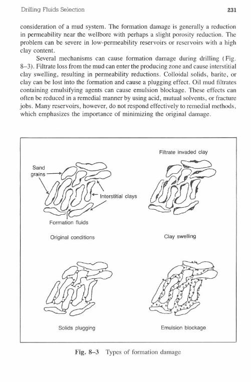
Drilling Fluids Selection 231
consideration of a mud system. The formation damage is generally a reductionin permeability near the wellbore with perhaps a slight porosity reduction. Theproblem can be severe in low-permeability reservoirs or reservoirs with a highclay content.
Several mechanisms can cause formation damage during drilling (Fig.8-3). Filtrate loss from the mud can enter the producing zone and cause interstitialclay swelling, resulting in permeability reductions. Colloidal solids, barite, orclay can be lost into the formation and cause a plugging effect. Oil mud filtratescontaining emulsifying agents can cause emulsion blockage. These effects canoften be reduced in a remedial manner by using acid, mutual solvents, or fracturejobs. Many reservoirs, however, do not respond effectively to remedial methods,which emphasizes the importance of minimizing the original damage.
Sand
~I~-qz~"O/Jr(1!J.- In~ffi,"ial O
la
cdj~ y'Formation fluids
Original conditions
Solids plugging
Filtrate invaded clay
Clay swelling
Emulsionblockage
Fig. 8-3 Types of formation damage
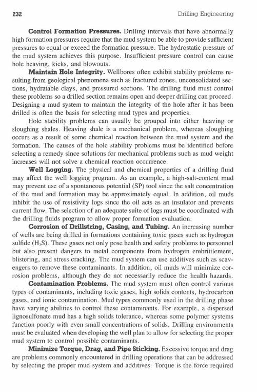
232 Drilling Engineering
Control Fonnation Pressures. Drilling intervals that have abnormallyhigh formation pressures require that the mud system be able to provide sufficientpressures to equal or exceed the formation pressure. The hydrostatic pressure ofthe mud system achieves this purpose. Insufficient pressure control can causehole heaving, kicks, and blowouts.
Maintain Bole Integrity. Wellbores often exhibit stability problems re-sulting from geological phenomena such as fractured zones, unconsolidated sec-tions, hydratable clays, and pressured sections. The drilling fluid must controlthese problems so a drilled section remains open and deeper drilling can proceed.Designing a mud system to maintain the integrity of the hole after it has beendrilled is often the basis for selecting mud types and properties.
Hole stability problems can usually be grouped into either heaving orsloughing shales. Heaving shale is a mechanical problem, whereas sloughingoccurs as a result of some chemical reaction between the mud system and theformation. The causes of the hole stability problems must be identified beforeselecting a remedy since solutions for mechanical problems such as mud weightincreases will not solve a chemical reaction occurrence.
WeD Logging. The physical and chemical properties of a drilling fluidmay affect the well logging program. As an example, a high-salt-content mudmay prevent use of a spontaneous potential (SP) tool since the salt concentrationof the mud and formation may be approximately equal. In addition, oil mudsinhibit the use of resistivity logs since the oil acts as an insulator and preventscurrent flow. The selection of an adequate suite of logs must be coordinated withthe drilling fluids program to allow proper formation evaluation.
Corrosion of Drillstring, Casing, and Tubing. An increasing numberof wells are being drilled in formations containing toxic gases such as hydrogensulfide (HzS). These gases not only pose health and safety problems to personnelbut also present dangers to metal components from hydrogen embrittlement,blistering, and stress cracking. The mud system can use additives such as scav-engers to remove these contaminants. In addition, oil muds will minimize cor-rosion problems, although they do not necessarily reduce the health hazards.
Contamination Problems. The mud system must often control varioustypes of contaminants, including toxic gases, high solids contents, hydrocarbongases, and ionic contamination. Mud types commonly used in the drilling phasehave varying abilities to control these contaminants. For example, a dispersedlignosulfonate mud has a high solids tolerance, whereas some polymer systemsfunction poorly with even small concentrations of solids. Drilling environmentsmust be evaluated when developing the well plan to allow for selecting the propermud system to control possible contaminants.
Mhdmb;e Torque, Drag, and Pipe Sticking. Excessive torque and dragare problems commonly encountered in drilling operations that can be addressedby selecting the proper mud system and additives. Torque is the force required
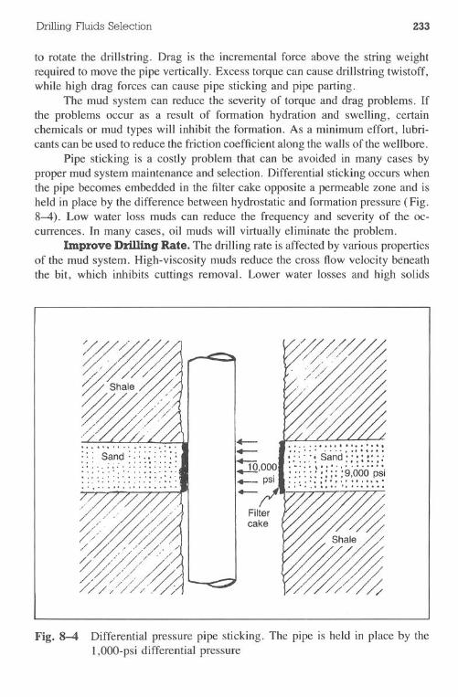
Drilling Fluids Selection 233
to rotate the drillstring. Drag is the incremental force above the string weightrequired to move the pipe vertically. Excess torque can cause drillstring twistoff,while high drag forces can cause pipe sticking and pipe parting.
The mud system can reduce the severity of torque and drag problems. Ifthe problems occur as a result of formation hydration and swelling, certainchemicals or mud types will inhibit the formation. As a minimum effort, lubri-cants can be used to reduce the friction coefficient along the walls of the wellbore.
Pipe sticking is a costly problem that can be avoided in many cases byproper mud system maintenance and selection. Differential sticking occurs whenthe pipe becomes embedded in the filter cake opposite a permeable zone and isheld in place by the difference between hydrostatic and formation pressure (Fig.8-4). Low water loss muds can reduce the frequency and severity of the oc-currences. In many cases, oil muds will virtually eliminate the problem.
Improve Drilling Rate. The drilling rate is affected by various propertiesof the mud system. High-viscosity muds reduce the cross flow velocity beneaththe bit, which inhibits cuttings removal. Lower water losses and high solids
Fig. 8-4 Differential pressure pipe sticking. The pipe is held in place by theI,OOO-psidifferential pressure
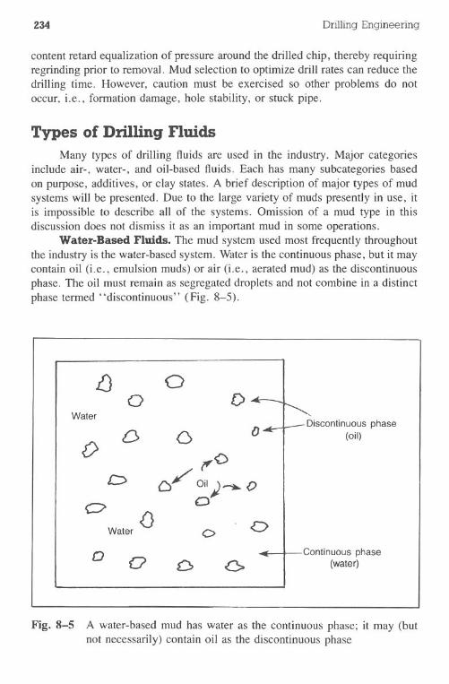
234 DrillingEngineering
content retard equalization of pressure around the drilled chip, thereby requiringregrinding prior to removal. Mud selection to optimize drill rates can reduce thedrilling time. However, caution must be exercised so other problems do notoccur, Le., formation damage, hole stability, or stuck pipe.
Types of Drilling FluidsMany types of drilling fluids are used in the industry. Major categories
include air-, water-, and oil-based fluids. Each has many subcategories basedon purpose, additives, or clay states. A brief description of major types of mudsystems will be presented. Due to the large variety of muds presently in use, itis impossible to describe all of the systems. Omission of a mud type in thisdiscussion does not dismiss it as an important mud in some operations.
Water-Based Fluids. The mud system used most frequently throughoutthe industry is the water-based system. Water is the continuous phase, but it maycontain oil (i.e., emulsion muds) or air (i.e., aerated mud) as the discontinuousphase. The oil must remain as segregated droplets and not combine in a distinctphase termed "discontinuous" (Fig. 8-5).
Fig. 8-5 A water-based mud has water as the continuous phase; it may (butnot necessarily) contain oil as the discontinuous phase
f) 00 D
Water
()D 0 o Discontinuousphase(oil)
01'0
c:// Oil)-.. ()0 £:)
Water() C> <:>
() 0 D 6 +continuous phase(water)
Drilling Fluids Selection 235
Clear, fresh water is one of the oldest muds used in the industry. It isgenerally used with no special additives except perhaps a corrosion inhibitor.The fresh water may hydrate formation clays and convert itself into a "native"mud. In fact, the term "mud" is believe~ to have been first used when freshwater and surface soils were mixed to develop a viscous fluid that could increasethe hole-cleaning characteristics of the fluid.
Fresh water is often the base fluid when adding many chemicals such asclays, polymers, weight materials, and additives to control various properties.The clays include sodium and calcium montmorillonite, attapulgite, andsubgroups of montmorillonite. Polymers cover a broad range of products suchas CMC (carboxymethylcellulose) and HEC (hydroxyethylcellulose). Weightmaterials include barite, galena, iron oxides, and hematite. Special additivesmay be used for controlling mud properties such as fluid loss, viscosity, gelstrength, and pH.
Inhibited Water-Based Fluids. An inhibited water-based mud is often usedto minimize hole sloughing problems. "Inhibition" refers to retarding the rateat which formation clays hydrate. Hydration reduces the structural stability ofthe borehole, allowing it to fall, or slough, into the wellbore. Common inhibitedmuds such as lime muds use calcium to retard hydration, while others use highconcentrations of various salts. Four common mud systems that can be classifiedas inhibited muds are gyp muds, lime muds, seawater muds, and saturatedsaltwater muds.
Lime muds have been widely used for many years as inhibited fluids. Thehydrated lime, which is calcium hydroxide, reduces the amount of water attachedto the clay structure. High lime-content muds should contain a Pr of 5-9 and aPmof 2~O to maintain an excess of lime. The amount of undissolved lime canbe estimated with Eq. 8.1:
(8.1)
where the excess lime is measured in Ib/bbl, Pmis the phenolphthalein end pointof mud, and Pr is the phenolphthalein alkalinity endpoint of filtrate.
Low-lime muds have been used successfully during recent years in high-temperature wells. High lime concentrations tend to cause clay flocculation inthe upper temperature ranges. Low-lime muds should contain a Prof 2-5 and aPmof 12-18. This mud system must be monitored closely to maintain undissolvedlime in the system.
Gypsum (calcium sulfate) muds are used commonly in gyp and anhydriteformations. Gyp muds are similar to lime muds since they derive their inhibitiveproperties from soluble calcium and require a chemical thinner for viscositycontrol. These muds function at lower alkalinity ranges than lime muds andcontain more soluble calcium.
236 Drilling Engineering
Seawater muds commonly used in offshore drilling are more economicalthan freshwater systems in some cases. The convenient source of salt water andthe elimination of extra storage space on offshore rigs have made this type ofmud very popular. Since the seawater contains salt, NaCl, it inhibits the hydrationand dispersion of clays. Alkalinities are extremely important and must be mon-itored closely for the dispersants and clays to react properly.
Saturated salt muds contain a large amount of dissolved salt and thereforecan be classifiedas inhibited muds. However, saturated salt muds are used usuallyto drill salt domes or thick stringers of salt. Salt contamination and eliminationof the development of large cavities in the salt formation are accomplished bysaturating a water-based mud with salt.
Dispersed Muds. A dispersed mud usually uses chemicals that cause theclay platelets to "disperse," or separate, within the liquid phase (Fig. 8-6).These dispersed muds tend to have better viscosity control, higher solids tol-erance, and better filtration control than nondispersed systems. Dispersed systemsare used frequently in drilling young, high-activity clays such as those found inthe Gulf of Mexico and Nigeria. A common dispersed system is the lignosulfonatemud.
Nondispersed Muds. Nondispersed muds are often associated with lowsolids concentrations and relative low-density weights. These muds do not con-tain chemical dispersants and are formulated normally with a minimum amountof bentonite. The systems use a polymer(s) that extends the effects of smallamounts of bentonite and selectively flocculates undesirable drilled solids. Propersolids control equipment, alkalinities, and bentonite concentrations must be mon-itored closely for a low-solids nondispersed mud to function effectively.
Flocculated Mud Systems. Flocculated muds cause the clay platelets toarrange themselves in an edge-to-face orientation. This arrangement often occurswith the intrusion of some contaminant. Filtration, viscosity, and gel strengthswill usually increase dramatically once a mud becomes flocculated. Chemicalagents are available that decrease the sensitivity of the edge-to-face attractionof clay particles. These deflocculants restore the clay particles to a dispersed oraggregated state.
Brines. Clear water and some brine fluids have been used in drillingoperations not requiring high densities and/or high viscosities. Brines have beenused extensively in completion and workover operations where very low solidsand a clean environment are critical. Brines may range from 8.33 to 19.2Ib/gal. These brines may be single-, two-, or even three-salt compounds suchas the following:
· potassium chloride·sodium chloride·calciumchloride/calciumbromide· calcium chloride/calcium bromide/zinc bromide
Drilling Fluids Selection 237
Fig. 8-6 Arrangements of clay particles
Brine makeup water should be mechanically filtered to eliminate undesir-able solids contamination. Brine densities are usually measured at 60°F and, ifpossible, the density should be calculated from specific gravity as measured witha hydrometer. Tables and charts for brine formulations are included in the Ap-pendix.
Single-salt brines are made from fresh water with the addition of a singlesalt to achieve the desired density. Density is controlled by adding salt or freshwater. Table 8-1 shows some of the more commonly used salt systems.
Potassium chloride brines can be used with densities to 9.7 Ib/gal. Potas-sium chloride brines are excellent workover fluids for water-sensitive formations.
- -,.n- ?- - -- --'- - I ;--
?\- - - ....- Lr- -- - -
- - - l,- - If- --- - -Dispersed clays Flocculated end-to-end arrangement
- -- - ,- -- -- -- -- ----- - -- -- -- - ----
Aggregate structure
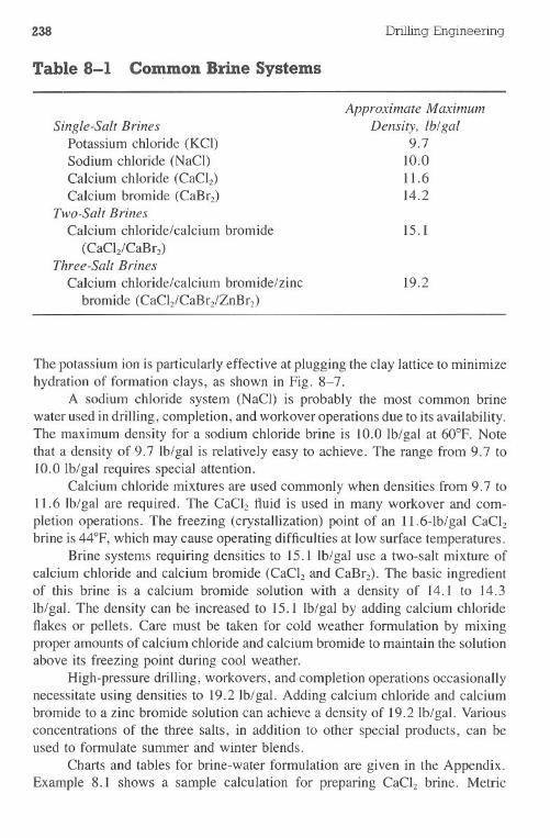
238 Drilling Engineering
Table 8-1 Co~on Brine Systems
Single-Salt BrinesPotassium chloride (KCI)Sodium chloride (NaCI)Calcium chloride (CaCI2)Calcium bromide (CaBr2)
Two-Salt BrinesCalcium chloride/calcium bromide
(CaCh/CaBr2)Three-Salt Brines
Calcium chloride/calcium bromide/zincbromide (CaCI2/CaBr2/ZnBr2)
Approximate MaximumDensity, lh/gal
9.710.011.614.2
15.1
19.2
The potassium ion is particularly effective at plugging the clay lattice to minimizehydration of formation clays, as shown in Pig. 8-7.
A sodium chloride system (NaCI) is probably the most common brinewater used in drilling, completion, and workover operations due to its availability.The maximum density for a sodium chloride brine is 10.0 Ib/gal at 60oP. Notethat a density of 9.7 Ib/gal is relatively easy to achieve. The range from 9.7 to10.0 Ib/gal requires special attention.
Calcium chloride mixtures are used commonly when densities from 9.7 to11.6 Ib/gal are required. The CaCl2 fluid is used in many workover and com-pletion operations. The freezing (crystallization) point of an 11.6-lb/gal CaCl2brine is 44°P, which may cause operating difficulties at low surface temperatures.
Brine systems requiring densities to 15.1 Ib/gal use a two-salt mixture ofcalcium chloride and calcium bromide (CaCI2and CaBr2). The basic ingredientof this brine is a calcium bromide solution with a density of 14.1 to 14.3Ib/gal. The density can be increased to 15.1 Ib/gal by adding calcium chlorideflakes or pellets. Care must be taken for cold weather formulation by mixingproper amounts of calcium chloride and calcium bromide to maintain the solutionabove its freezing point during cool weather.
High-pressure drilling, workovers, and completion operations occasionallynecessitate using densities to 19.2 Ib/gal. Adding calcium chloride and calciumbromide to a zinc bromide solution can achieve a density of 19.2Ib/gal. Variousconcentrations of the three salts, in addition to other special products, can beused to formulate summer and winter blends.
Charts and tables for brine-water formulation are given in the Appendix.Example 8.1 shows a sample calculation for preparing CaCl2 brine. Metric
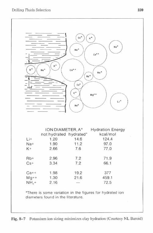
Drilling Fluids Selection 239
8
*There is some variation in the figures for hydrated iondiameters found in the literature.
Fig.8-7 Potassium ion sizing minimizes clay hydration (Courtesy NL Baroid)
ION DIAMETER,Ao Hydration Energynot hydrated hydrated* kcal/mol
Li+ 1.20 14.6 124.4Na+ 1.90 11.2 97.0K+ 2.66 7.6 77.0
Rb+ 2.96 7.2 71.9Cs+ 3.34 7.2 66.1
Ca++ 1.98 19.2 377Mg++ r.30 21.6 459.1NH4+ 2.16 - 72.5
240 Drilling Engineering
material requirements for preparing CaCl2 are given in the Appendix. Table B5gives the composition of I bbl of sodium chloride/calcium chloride mixed brine.
Example 8.1Calculate the material requirements for preparing 350 bbl of 11.4-lb/gal
CaCl2brine.
Solution:
From Table B3 (Appendix):(1) Water requirement = 0.854 bbllbbl
350 bblx 0.854 bbllbbl = 299 bbl (water)(2) CaCl2requirement = 1801b/bbl
350 bbl x 1801b/bbl = 63,0001b= 780, 80-lb sacks
Occasionally, it is necessary to dilute CaCh brine by adding water. Properdilution can be achieved with Eq. 8.2 and Table B4:
Where:H20/CaC12 = number of gal of water/bbl of CaChsp gr = specific gravity of the initial brine%CaCI2I = initial percentage of CaCl2%CaChF = final percentage of CaCl2
Example 8.2 illustrates CaCl2dilution.
Example 8.2
Compute the volume of water required to drop the density of 200 bblof 11.5-lb/gal CaCl2 brine to 10.5 lb/gal.
Solution:
(1) From Table B4:%CaCI2I = 36.6%CaChF = 26.7sp gr = 1.3806
(2) Using Eq. 8.2:H20/CaCI2 = 42(1.3806)(36.6 - 26.7)/26.7
= 21.5 gal/bbl
Drilling Fluids Selection 241
(3) 21.5 gallbbl x 200 bbl = 4,300 gal= 102 bbl (water)
Solids Systems (solids tolerance). The solids concentration in the mud maybe used to describe the system. A clearwater mud has virtually no detectablesolids. A low-solids system has some solids, although efforts are usually madeto minimize solids concentration. A high-solids system is normally used when"mud-making" formations are penetrated or high mud weights requiring bariteare used. The solids content of a high-weight mud must be controlled withinacceptable ranges. The degree to which formation solids contaminate a water-based mud depends on the characteristics of the continuous phase and the typeand amount of clay in the rock cuttings. Excess solids may be controlled bysurface mechanical equipment and/or water dilution. Water dilution is the mostexpensive process for correcting drilled solids accumulation. Fig. 8-8 showsacceptable ranges for mud solids as developed by several mud companies.
Example 8.3
A drilling engineer plans to use a lignosulfonate mud to drill a deep,high pressure well in the Niger basin. The pore pressures are provided be-low. Develop a mud program showing mud weight, minimum and maximumsolids levels, and recommended rheological properties. Use Fig. 8-8 andTable 18-1. The engineer normally uses a 0.3-lb/gal mud weight safetymargin.
Depth, ft1,0003,0005,0007,0009,000
10,0001l,00012,00014,00016,000
Pore Pressure, Ib/gal9.09.09.09.09.0
10.813.314.716.116.9
Solution:
1. Use Fig. 8-8 to obtain minimum and maximum solids.2. Use Table 18-1 to obtain PV and YP ranges.
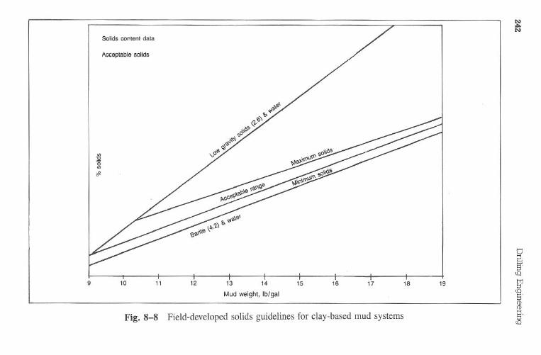
Solids
contentdata
Acceptable
solids
910
1112
1314
Mud
weight,
Ib/gal
1516
1718
19
Fig
.8-8
Field-developed
solidsguidelines
forclay-based
mud
systems
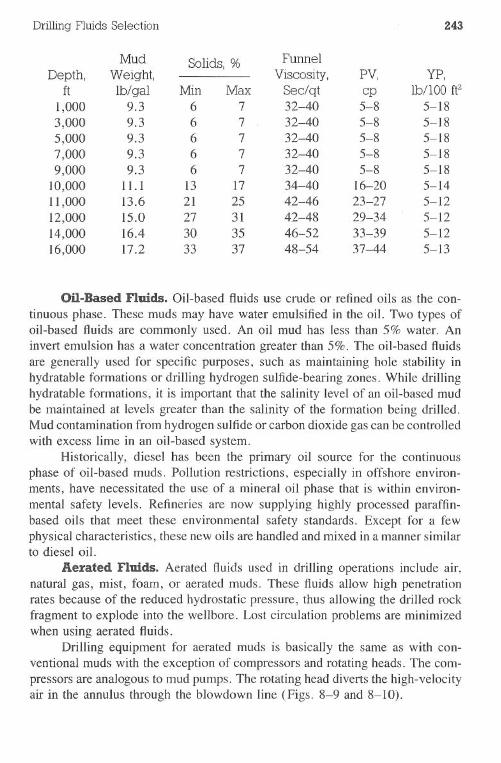
Oil-Based Fluids. Oil-based fluids use crude or refined oils as the con-
tinuous phase. These muds may have water emulsified in the oil. Two types ofoil-based fluids are commonly used. An oil mud has less than 5% water. Aninvert emulsion has a water concentration greater than 5%. The oil-based fluidsare generally used for specific purposes, such as maintaining hole stability inhydratable formations or drilling hydrogen sulfide-bearing zones. While drillinghydratable formations, it is important that the salinity level of an oil-based mudbe maintained at levels greater than the salinity of the formation being drilled.Mud contamination from hydrogen sulfideor carbon dioxide gas can be controlledwith excess lime in an oil-based system.
Historically, diesel has been the primary oil source for the continuousphase of oil-based muds. Pollution restrictions, especially in offshore environ-ments, have necessitated the use of a mineral oil phase that is within environ-mental safety levels. Refineries are now supplying highly processed paraffin-based oils that meet these environmental safety standards. Except for a fewphysical characteristics, these new oils are handled and mixed in a manner similarto diesel oil.
Aerated Fluids. Aerated fluids used in drilling operations include air,natural gas, mist, foam, or aerated muds. These fluids allow high penetrationrates because of the reduced hydrostatic pressure, thus allowing the drilled rockfragment to explode into the wellbore. Lost circulation problems are minimizedwhen using aerated fluids.
Drilling equipment for aerated muds is basically the same as with con-ventional muds with the exception of compressors and rotating heads. The com-pressors are analogous to mud pumps. The rotating head diverts the high-velocityair in the annulus through the blowdown line (Figs. 8-9 and 8-10).
DrillingFluids Selection 243
Mud Solids, % FunnelDepth, Weight, Viscosity, PV, YP,
ft lb/ gal Min Max Sec/qt cp Ib/lOO ft21,000 9.3 6 7 32-40 5-8 5-183,000 9.3 6 7 32-40 5-8 5-185,000 9.3 6 7 32-40 5-8 5-187,000 9.3 6 7 32-40 5-8 5-189,000 9.3 6 7 32-40 5-8 5-18
10,000 11.1 13 17 34-40 16-20 5-1411,000 13.6 21 25 42-46 23-27 5-1212,000 15.0 27 31 42-48 29-34 5-1214,000 16.4 30 35 46-52 33-39 5-1216,000 17.2 33 37 48-54 37-44 5-13
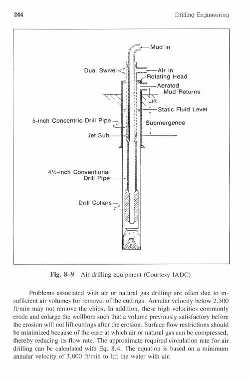
244 Drilling Engineering
Dual Swivel < Air in/Rotating Head~ Aerated
Mud Returns
5-inch Concentric Drill Pipe
Lift
,,"~Static Fluid Level_H 1
SubmergenceIJet Sub
41f2-inch ConventionalDrill Pipe
Drill Collars
Fig. 8-9 Air drilling equipment (Courtesy IADC)
Problems associated with air or natural gas drilling are often due to in-sufficient air volumes for removal of the cuttings. Annular velocity below 2,500ft/min may not remove the chips. In addition, these high velocities commonlyerode and enlarge the wellbore such that a volume previously satisfactory beforethe erosion will not lift cuttings after the erosion. Surface flow restrictions shouldbe minimized because of the ease at which air or natural gas can be compressed,thereby reducing its flow rate. The approximate required circulation rate for airdrilling can be calculated with Eq. 8.4. The equation is based on a minimumannular velocity of 3,000 ft/min to lift the water with air.
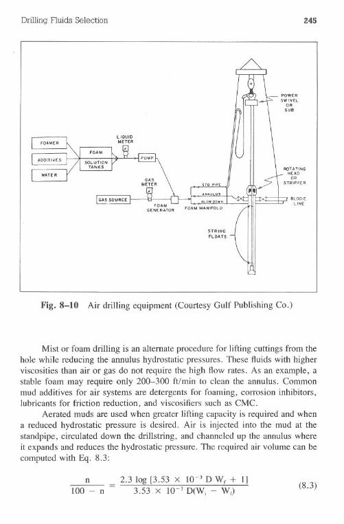
Drilling Fluids Selection 245
POWERSWIVELORSUB
ROTATINGHEADOR
STRIPPER
BLOOIELINE
Fig. 8-10 Air drilling equipment (Courtesy Gulf Publishing Co.)
Mist or foam drilling is an alternate procedure for lifting cuttings from thehole while reducing the annulus hydrostatic pressures. These fluids with higherviscosities than air or gas do not require the high flow rates. As an example, astable foam may require only 200-300 ft/min to clean the annulus. Commonmud additives for air systems are detergents for foaming, corrosion inhibitors,lubricants for friction reduction, and viscosifiers such as CMC.
Aerated muds are used when greater lifting capacity is required and whena reduced hydrostatic pressure is desired. Air is injected into the mud at thestandpipe, circulated down the drillstring, and channeled up the annulus whereit expands and reduces the hydrostatic pressure. The required air volume can becomputed with Eq. 8.3:
n100 - n
2.3 log [3.53 x 10⁻³ D Wr + 1]3.53.x 1O-3D(Wj - Wr)
(8.3)
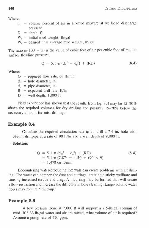
246 DrillingEngineering
Where:
n = volume percent of air in air-mud mixture at wellhead dischargepressure
D = depth, ftWi = initial mud weight, lb/galWf = desired final average mud weight, lb/gal
The ratio n/(lOO - n) is the value of cubic feet of air per cubic foot of mud atsurface flowline pressure:
Q = 5.1 'Tr (dH2 - d/) + (RD) (8.4)
Where:
Q = required flow rate, cu ft/mindH = hole diameter, in.dp = pipe diameter, in.R = expected drill rate, ft/hrD = well depth, 1,000 ft
Field experience has shown that the results from Eq. 8.4 may be 15-20%above the required volumes for dry drilling and possibly 15-20% below thenecessary amount for mist drilling.
Example 8.4
Calculate the required circulation rate to air drill a 77/s-in. hole with3Yz-in. drillpipe at a rate of 90 ft/hr and a well depth of 9,000 ft.
Solution:
. Q = 5.1 'Tr (dH2 - d/) + (RD)= 5.1 'Tr (7.872 - 4.52) + (90 x 9)= 1,478 cu ft/min
(8.4)
Encountering water-producing intervals can create problems with air drill-ing. The water can dampen the dust and cuttings, creating a sticky wellbore andcausing increased torque and drag. A mud ring may be formed that will createa flow restriction and increase the difficulty in hole cleaning. Large-volume waterflows may require "mud-up."
Example 8.5
A low pressure zone at 7,000 ft will support a 7.5-lb/gal column <;Ifmud. If 8.33 lb/gal water and air are mixed, what volume of air is required?Assume a pump rate of 420 gpm.
Drilling Fluids Selection 247
Solution:
~ ~ 2.3 log [3.53 x 10⁻³ (7,000) (7.5) + 1]100 - n - 3.53 x 10⁻³(7,000) (8.33 - 7.5)
5.22 .20.5
= 0.2545 cu ft (air)/cu ft (mud)
(0.2545)(420) _ 14 29 f /.
7.48 gallcu ft - . cu t mm
Introduction to Drilling Fluids ChemistryWater-Based (Solids) Systems. High-weight mud systems usually con-
tain more solids than low-weight systems. Extra solids in a high-weight mudwill originate from the gels, chemicals, weight material, and drill solids fromthe formation. Good solids control equipment and proper additions of water andchemicals to a high-mud-weight system will eliminate many solids buildup prob-lems. Additions of weight material, chemicals, and formation solids will ne-cessitate adding extra water. Water dilution in itself is the most costly correctivemeasure after a solids problem has developed. Fig. 8-8 shows field-developedguidelines for solids levels in water muds.
Proper chemical additions to reduce the hydration of formation clays andprovide filtration control should be done before a solids problem occurs. In manysituations, chemicals are not the solution to thinning a high-weight mud. Withthe addition of gels, chemicals, and formation solids, water is often not addedin the proper ratio for these chemicals to react properly.
Gel Systems. The commercial clays usually added to the mud system areattapulgite and bentonite. Bentonite is added to water-based systems to increaseviscosity, gel strengths, and suspension. Filtration and filter cake properties arealso improved with bentonite. During drilling operations the most common claysthat may enter the mud as drilled solids are kaolinite; illite, and montmorillonite.
Bentonite consists primarily of sodium montmorillonite clays. After ben-tonite is added to water, the positive sodium ions are dissociated from the surfaceof the clay platelet, which leaves negative charges. Dispersion of the clay is aresult of the negative charges repelling each other and the shearing action, orstirring, the bentonite in water. The edges of the clay platelet may be positiveor negatively charged, depending on the remaining atoms, chemicals added, orcontaminants. Bentonite in dry form is actually groups of clay platelets stackedface-to-face in bundles called aggregates (Fig. 8-6).
When fresh water is added to bentonite and sufficient stirring occurs, theclay platelets will separate. This chemical action is called dispersion. If the clayplatelets arrange themselves in an edge-to-face orientation~the clays are said to
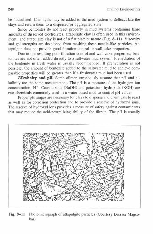
248 Drilling Engineering
be flocculated. Chemicals may be added to the mud system to deflocculate theclays and return them to a dispersed or aggregated state.
Since bentonites do not react properly in mud systems containing largeamounts of dissolved electrolytes, attapulgite clay is often used in this environ-ment. The attapulgite clay is not of a flat platelet nature (Fig. 8-11). Viscosityand gel strengths are developed from meshing these needle-like particles. At-tapulgite does not provide good filtration control or wail cake properties.
Due to the resulting poor filtration control and wall cake properties, ben-tonites are not often added directly to a saltwater mud system. Prehydration ofthe bentonite in fresh water is usually recommended. If prehydration is notpossible, the amount of bentonite added to the saltwater mud to achieve com-parable properties will be greater than if a freshwater mud had been used.
.AJkalinity and pH. Some oilmen erroneously assume that pH and al-kalinity are the same measurement. The pH is a measure of the hydrogen ionconcentration, H+. Caustic soda (NaOH) and potassium hydroxide (KOH) aretwo chemicals commonly used in a water-based mud to control pH value.
Proper pH ranges are necessary for clays to disperse and chemicals to reactas well as for corrosion protection and to provide a reserve of hydroxyl ions.The reserve of hydroxyl ions provides a measure of safety against contaminantsthat may reduce the acid-neutralizing ability of the filtrate. The pH is usually
Fig. 8-11 Photomicrograph of attapulgite particles (Courtesy Dresser Magco-bar)
Drilling Fluids Selection 249
measured with color-coded paper or with a pH meter. Water-based muds withchlorides of 10,000 ppm or greater should be measured with a pH meter.
Alkalinity agents can be described as any water-soluble chemical that canneutralize acids. Alkalinity tests on the mud filtrate measure the acid-neutralizingcapacity of the filtrate. As an example, the Pr value measures the amount ofN/50, H2S04 required to lower the pH to 8.3. This measurement of acid neu-tralizes the OH- and converts the COj' to HC03. The Mr value measures theamount ofN/50, H2S04needed to drop the pH from 8.3 to 4.3. This measurementof acid converts the HC03 to C02 and H20. Pmis a measurement of the acid-neutralizing ability of the undissolved solids in whole mud.
Contaminants. Numerous mud contaminants may be encountered in awater-based mud. Table 8-2 lists some common contaminants and possiblecorrective actions.
Note that other chemicals are needed to restore the mud to the desiredspecifications after the contaminant has been removed. Pretreatment is oftenpossible if a proper mud program was developed and drilling parameters are
Table 8-2 Common Contaminants and PossibleCorrective Actions
ContaminantSodium chloride
Bed salt
Saltwater flow
Saline makeup waterGypsum, anhydrite
Hard water (Ca and/or Mg)Cement or limeHydrogen sulfide
Carbon dioxideCarbonate and bicarbonateDrill solids
Oil
Possible Corrective Actions*
Add organic thinners, caustic soda; convert to. saturated salt mud
Increase mud weight to stop the flow; add or-ganic thinner, caustic soda; water dilution
Add organic thinners, caustic sodaAdd soda ash, organic thinners; convert to gyp
mudRaise pH to 10.5+; add soda ashAdd SAPP, sodium bicarbonateRaise pH to 10.5+; add scavengers, lime, thin-
nersRaise pH to 10.5+; add thinnersAdd organic thinners, limeAdd water, caustic soda, organic thinners; sol-
ids control equipmentAdd water, chemical emulsifier
*Consult a mud service representative for additional details
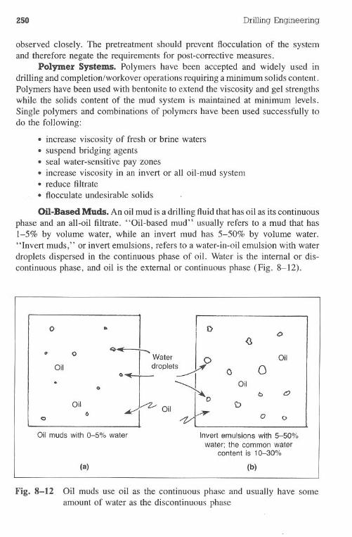
250 Drilling Engineering
observed closely. The pretreatment should prevent flocculation of the systemand therefore negate the requirements for post-corrective measures.
Polymer Systems. Polymers have been accepted and widely used indrilling and completion/workover operations requiring a minimum solids content.Polymers have been used with bentonite to extend the viscosity and gel strengthswhile the solids content of the mud system is maintained at minimum levels.Single polymers and combinations of polymers have been used successfully todo the following:
· increase viscosity of fresh or brine waters·suspend bridging agents·seal water-sensitive pay zones· increase viscosity in an invert or all oil-mud system· reduce filtrate· flocculate undesirable solids
Oil-Based Muds. An oil mud is a drilling fluid that has oil as its continuousphase and an all-oil filtrate. "Oil-based mud" usually refers to a mud that has1-5% by volume water, while an invert mud has 5-50% by volume water."Invert muds," or invert emulsions, refers to a water-in-oil emulsion with waterdroplets dispersed in the continuous phase of oil. Water is the internal or dis-continuous phase, and oil is the external or continuous phase (Fig. 8-12).
o eo
t1 o
Oil.CI
Oilo
Oil muds with 0-5% water
(a)
()
Invert emulsions with 5-50%water; the common water
content is 10-30%.
(b)
Fig. 8-12 Oil muds use oil as the continuous phase and usually have someamount of water as the discontinuous phase
C>
Oil
0 0Oil
l::> 0
D0 ()
Drilling Fluids Selection 251
Emulsifiers are required to form an oil film completely around the waterdroplets. If sufficient emulsifiers are not used, the emulsion will become unstable.Small amounts of additional water may cause severe problems, such as segre-gation of the oil and water phases. From the standpoint of stability, water dropletsize must also be considered. Large droplets exhibit a greater tendency to com-bine. In order to obtain small, uniform water droplets, some type of shear forcemust be applied to the mud system. This shearing can be accomplished withmud guns, centrifugal pumps, and circulating through the bit. Water in an invertsystem helps support barite, acts as a fluid loss agent, allows many of thechemicals to dissolve, and contributes to viscosity and gel strengths.
Oil added to an invert system usually increases the stability of the emulsion.Water added to an invert system decreases the stability and increases the yieldpoint and the gel strengths.
Calcium chloride is added to an invert emulsion to help dehydrate water-sensitive formations. Formations hydrate or dehydrate when exposed to a drillingmud if a salinity difference exists between the formation and the drilling fluid.This osmotic force may be adsorption or desorption, depending on the salinityof the drilling fluid and the water in the formation (Table 8-3). In an oil mud,
Table 8-3 Oil Mud Osmotic Pressures
Dissolved Salt Concentration, ppm Osmotic Pressure, psi*
Calcium chloride52,000
100,000182,000250,000307,000357,000400,000456,000 (saturation)
Sodium Chloride55,000
105,000149,000189,000226,000268,000 (saturation)
5001,0003,0005,8009,400
13,90016,10024,400
670I ,4002,2003,2004,3005,800
*Ca1culated for oil mud opposite a freshwater shale
zsz Drilling Engineering
the semipermeable membrane across which osmotic pressure occurs is createdby emulsifiers and the 'oil film around each water droplet.
Formation instability can be controlled by properly regulating the salinityin the water phase of an oil mud. Adjustments of the salinity can cause waterto be drawn from the formations with little or no effect on the water adsorptionof the shale. Hydration of the shale can be eliminated by adjusting the salinityof the water phase of an oil mud to be greater than the hydration force of theshale. The required salinity for an oil mud will depend on the depth, porepressure, and salinity of the formation water. A water phase salinity of::t:350,000 ppm is generally accepted as providing good shale stabilization char-acteristics.
Lime is added to oil muds to help convert sodium salts to calcium soaps.Lime also helps combat problems associated with carbon dioxide and hydrogensulfide intrusion. The proper alkalinity of an oil mud is measured by the Pmandexcess lime values. It is desirable that excess lime be present in an oil mud.
Field Testing Procedures
A discussion of all testing procedures for drilling fluids is impractical forthis text. Table 8-4 summarizes the basic field testing procedures for water-based and oil-based muds. This table does not cover all tests nor relate anyrecommendations. Testing procedures and equipment may vary from one mudcompany to another.
The American Petroleum Institute (API) provides standards for most mudtesting procedures. Document API RP 13B is available from the Institute andcan usually be obtained from most service companies.
General Types of AdditivesViscosifiers. Many different products are classified as viscosifiers for
clearwater brines, water-based muds, and oil-based muds. The viscosity of afluid is dependent upon interparticle force; size, shape, and number of particles;and viscosity of the base fluid.
Viscosity Measurements. Fluid viscosities are measured in several differentmanners at the rig site. The most common procedures utilize the Marsh funneland the viscosity-gel (VG) meter. These tests evaluate different fluid propertiesand, as such, should be used judiciously.
The Marsh funnel test, Fig. 8-13, is the simple approach to measuringfluid viscosity. A funnel is filled with the mud. The time required for a certainvolume of fluid to drain from the funnel into a graduated cup is defined as theviscosity, i.e., 48 sec/qt. A base fluid of clear water normally requires approx-imately 26 sec. The disadvantage to this simple test is that it does not help definethe causes for excessive fluid viscosity.
/
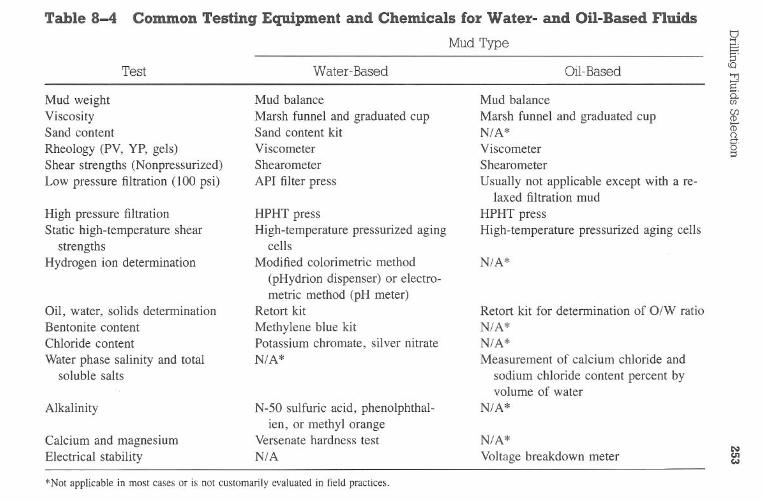
Table
8-4C
omm
onT
estingE
quipment
andC
hemicals
forW
ater-and
Oil-B
asednuids
MudT
ype
Test
Water-B
asedO
il-Based
~Er
<0"'1
E"~(/)
CD
$'Q.
1:;-::s
Mud
weight
Viscosity
Sandcontent
Rheology
(PV,Y
P,gels)Shear
strengths(N
onpressurized)L
owpressure
filtration(100
psi)
High
pressurefiltration
Statichigh-tem
peratureshear
strengthsH
ydrogenion
determination
Oil,
water,
solidsdeterm
inationB
entonitecontent
Chloride
content
Waterphase
salinityand
totalsoluble
salts
Alkalinity
Calcium
andm
agnesiumE
lectricalstability
Mud
balance
Marsh
funneland
graduatedcup
Sandcontentkit
Viscom
eterShearom
eter
API
filterpress
HPH
Tpress
High-tem
peraturepressurized
agingcells
Modified
colorimetric
method
(pHydrion
dispenser)or
electro-m
etricm
ethod(pH
meter)
Retort
kitM
ethyleneblue
kitPotassium
chromate,
silvernitrate
N/A
*
N-50
sulfuricacid,
phenolphthal-ien,
orm
ethylorange
Versenate
hardnesstest
N/A
Mud
balance
Marsh
funneland
graduatedcup
N/A
*V
iscometer
Shearometer
Usually
notapplicable
exceptw
itha
re-laxed
filtrationm
ud
HPH
Tpress
High-tem
peraturepressurized
agingcells
N/A
*
Retort
kitfor
determination
ofO
/Wratio
N/A
*N
/A*
Measurem
entof
calciumchloride
andsodium
chloridecontent
percentby
volume
ofw
aterN
/A*
N/A
*
Voltage
breakdown
meter
NUJ.
C/o)
*Not
applicablein
most
casesor
isnot
customarily
evaluatedin
fieldpractices.
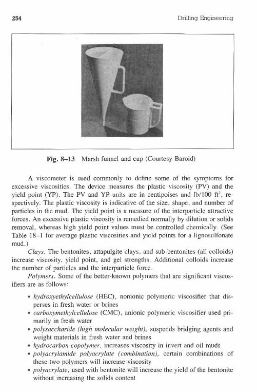
254 Drilling Engineering
Fig. 8-13 Marsh funnel and cup (Courtesy Baroid)
A viscometer is used commonly to define some of the symptoms forexcessive viscosities. The device measures the plastic viscosity (PV) and theyield point (YP). The PV and YP units are in centipoises and Ib/IOO fe, re-spectively. The plastic viscosity is indicative of the size, shape, and number ofparticles in the mud. The yield point is a measure of the interparticle attractiveforces. An excessive plastic viscosity is remedied normally by dilution or solidsremoval, whereas high yield point values must be controlled chemically. (SeeTable 18-1 for average plastic viscosities and yield points for a lignosulfonatemud.)
Clays. The bentonites, attapulgite clays, and sub-bentonites (all colloids)increase viscosity, yield point, and gel strengths. Additional colloids increasethe number of particles and the interparticle force.
Polymers. Some of the better-known polymers that are significant viscos-ifiers are as follows:
·hydroxyethylcellulose (HEC), nonionic polymeric viscosifier that dis-perses in fresh water or brines·carboxymethylcellulose (CMC), anionic polymeric viscosifier used pri-marily in fresh water
· polysaccharide (high molecular weight), suspends bridging agents andweight materials in fresh water and brines·hydrocarbon copolymer, increases viscosity in invert and oil muds·polyacrylamide polyacrylate (combination), certain combinations ofthese two polymers will increase viscosity·polyacrylate, used with bentonite will increase the yield of the bentonitewithout increasing the solids content

Drilling Fluids Selection 255
Viscosity Reducers. A high viscosity caused by excessive colloids, un-desirable drill solids, or contaminants can cause several drilling problems. As-sociated with high viscosities are excessive yield points and gel strengths, whichcause an increase in the equivalent circulating density and may require highpump pressures to break circulation. These conditions can result in lost circulationand other wellbore problems.
Thinners and Dispersants. Chemicals that cause mud thinning dispersethe clay platelets by reducing the interparticle attraction forces and, in somecases, by creating repulsion forces. Thinners satisfy the broken valence bondsat the edges of the clay platelets, reducing the attractive forces between the clayplatelets and stacks of particles. The reduction or elimination of these forces iscommonly referred to as dispersing a mud system.
Most thinners can be classified as organic materials or as inorganic complexphosphates. The organic thinners include lignosulfonates, lignins, and tannins.Lignosulfonates with several metal compounds have been used successfully ina wide range of appl~cations.Organic thinners can be used in higher-temperaturewells and exhibit good filtration control properties.
Inorganic thinners Include sodium acid pyrophosphate (SAPP), tetrasodiumpyrophosphate, sodium tetraphosphate, and sodium hexametaphosphate. Inor-ganic thinners are effective in very small amounts but are restricted to freshwaterclay muds, low temperatures, low chlorides, low calcium/magnesium, and lowpH values.
If a mud is highly treated and viscosity becomes a problem, the additionof water or oil will decrease the viscosity. While drilling, water must be addedcontinuously to compensate for extra solids added to the mud system. Theaddition of chemicals or barite to a mud system also requires additional water.
Chemical Breakers. Viscosity generated by polymers can be treatedwith special chemicals to cause fluid thinning. These mild acids, such as Clorox@,have been used successfully in the chemical breakdown of polymers. Due to thecost of polymer fluids, pilot testing should be done in a laboratory before addingchemical breakers to the system. Also, it is advisable in some cases to wait12-18 hr after chemical breakers have been added before continuing operations.
nuid Loss Agents. All muds lose fluid to the formations. Fluid reductionagents wc:re developed to form thin, tough, semipermeable wall cakes. Thehole becomes more stable, and productive zones are protected to some degreeif invasion of drilling fluid filtrate is controlled. The deposition of solids toolarge to pass through the membrane pores minimizes the continuation of fluidloss. Permeability of a filter cake is dependent upon size and distribution ofparticles on the wall cake.
Bentonite is considered the basis for an impermeable filter cake. Chemicalshave been developed to aid bentonite in filtrationcontrol. A few that have receivedwide usage are starch, guar gum, polysaccharides, acrylic polymers, organicthinners, and sodium carboxymethylcellulose. Bentonite clay particles are con-
'IiI
IIIiI
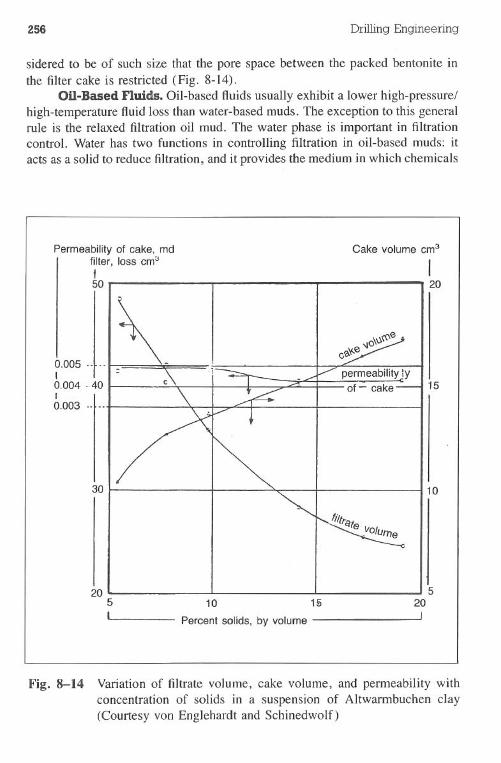
256 Drilling Engineering
sidered to be of such size that the pore space between the packed bentonite inthe filter cake is restricted (Fig. 8-14).
Oil-Based nuids. Oil-based fluids usually exhibit a lower high-pressure/high-temperature fluid loss than water-based muds. The exception to this generalrule is the relaxed filtration oil mud. The water phase is important in filtrationcontrol. Water has two functions in controlling filtration in oil-based muds: itacts as a solid to reduce filtration, and it provides the medium in which chemicals
Permeabilityof cake. mdfilter, loss cm3I50
Cake volume cm3
30
I20
0.005 ..~.-t0.004 ..40I0.003 n...
-15
10
205I
10 15
Percent solids, by volume
520J
Fig. 8-14 Variation of filtrate volume, cake volume, and permeability withconcentration of solids in a suspension of Altwarmbuchen clay(Courtesy von Englehardt and Schinedwolf)
Drilling Fluids Selection 257
and specially treated bentonite are allowed to react. Some significant evidenceexists that an oil filtrate is harmful to certain productive zones.
pH Adjusters. The pH is a measurement of hydrogen ion concentrations.Due to the chemical composition of drilling fluids and the nature in which theyreact, it is necessary to maintain the pH of the drilling fluid in the alkaline range.Adding chemicals such as organic and inorganic thinners and water with highcalcium/magnesium content and influx of certain contaminants will mandateadditional pH control. Approximate pH ranges for optimum operations are de-termined by the type of drilling fluid and chemical additives.
Proper pH in water-based muds is usually achieved by adding sodiumhydroxide (NaOH) or potassium hydroxide (KOH). Both chemicals provide analkaline base to compensate for acidie chemicals and contaminated water. Oil-based muds do not rely on a pH value as measured in water-based muds. Thelime and excess lime calculations in an oil-based mud reflect the alkalinity values.
Density Control Materials. To drill a well successfully, the formationpressure must be controlled by the hydrostatic pressure of the mud. The mudpressure is increased by raising the density of the fluid. Eq. 8.5 and Example8.6 illustrate hydrostatic pressure calculations.
PH = 0.052 x MW x TVD (8.5)
Where:
PH = hydrostatic pressure, psiMW = mud weight, Ib/galTVD = true vertical depth, ft
A mud system normally gains a certain amount of weight from drill solids ifproper mechanical solids control equipment is not used. These solids are generallyconsidered undesirable in high mud weight systems and will cause problemswhen weight material is added to the mud system. In the past few years, several
III
Table 8-5 Common Weighting Materials.
AverageSpecific
Gravity, :t
BariteGalenaCalcium carbonateBar-GainDensimix
Barium sulfateLead sulfideCalcium carbonateIlmeniteHematite (itabrite ore)
4.256.62.74.55.1
Maximum MudWeight, :t,
Ib/gal
20-2228-32
1221-2324-26
Item Chemical Name
*Exc1usive of salts, drilled solids, and various less-common materials.
258 Drilling Engineering
different products have been successfully used to provide the necessary hydro-static pressure in drilling fluids. Table 8-5 illustrates common density controlmaterials.
Workovers and some drilling operations have used soluble salts to providea necessary hydrostatic pressure. Salts such as sodium chloride, sodium nitrate,sodium carbonate, calcium chloride, and potassium chloride have been used verysuccessfully in workover and completion operations where a minimum amountof solids is essential.
Example 8.6
Calculate the hydrostatic pressure for each of the following systems:a. 10,000 ft of 12.0-lb/gal mudb. 12,000 ft of 1O.5-lb/gal mudc. 15,000 ft of 15.0-lb/gal mud
Solution:
Hydrostatic pressure = 0.052 X mud density x depth (8.5)a. Hydrostatic pressure = 0.052 X 12.0 Ib/gal X 10,000 ft = 6,240 psib. Hydrostatic pressure = 0.052 X 10.5 lb/gal x 12,000 ft = 6,552 psic. Hydrostatic pressure = 0.052 X 15.0Ib/gal x 15,000 ft = 11,700 psi
Proper well planning requires that a sufficient quantity of barite be main-tained on the drilling location to kill a kick. To calculate this volume of bariteproperly, many operators have established a I.O-Ib/gal safety measure, whichmeans barite volumes will be maintained at a level sufficient to increase thepresent mud density by lib/gal. (This safety measure is based on unpublishedstatistics from a professional well killing company, which show that the averagekick would require a 0.5-lb/gal increase in mud weight or less. The 1-lb/galmargin thus incorporates a safety factor of 2 relative to the average kick.) Eq.8.6 can be used to calculate required barite volumes:
lb/bbl = 1,490(W2 - W,)/(35.4 - W2) (8.6)
Where:
lb/bbl = number of pounds of barite required to increase the density of1 bbl of mud
1,490 = weight of 1 bbl of barite, IbW2 = final mud density, lb/gal35.4 = weight of I gal of barite, lb/gal
Example 8.7 illustrates the use of Eq. 8.6.
Drilling Fluids Selection 259
Example 8.7
A well is being planned that will use 15.0-lb/gal mud. The hole and surfacepit volumes will be 850 and 350 bbl, respectively. How many sacks of bariteshould be maintained on the drilling lo~ation? (Assume that one sack contains100lb of barite.).
Solution:
(1) Using Eq. 8.6:
Ib/bbl = 1,490(W2 - WI)35.4 - W2
WI = 15.0Ib/gal
W2 = WI + 1.0 lb/gal = 16.0 Ib/gal
lb/bbl = 1,490(16.0 - 15.0)35.4 - 16.0
_ 1,490- 19.4= 76.8 Ib/bbl
(2) (850 + 350) bbl X 76.8 Ib/bbl= 92,160 lb (barite)
(3) 92,160 Ib = 921.6 sacks (approximately 46 tons)
Lost Circulation Materials. Lost circulation is perhaps the most costlydrilling problem encountered in oil and gas exploration, with the exception ofblowouts. The cost factors include lost rig time, expensive remedial techniques,and potential loss of the hole. To further complicate the problem, the causes oflost circulation are seldom analyzed, resulting in the application of remedialtechniques that are not suited for the actual cause of the problem.
Lost circulation is the loss of whole mud, in small or large quantities, tothe formation. This precludes filtrate loss, which is considered to be a normaloccurrence and not a drilling problem. The loss can have many causes, detri-mental effects, and remedial procedures that must be studied before the operatorcan effectively select optimum cost-saving solutions.
Loss of circulation manifests itself in several manners. The loss may be aslow seepage into the formation, causing a small, consistent reduction in surface
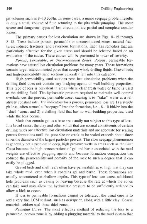
260 Drilling Engineering
pit volumes such as 8-1~ bbllhr. In some cases, a major seepage problem resultsin only a small volume of fluid returning to the pits while pumping. The mostsevere and dangerous types of lost circulation are partial and complete annularlosses.
The primary causes for lost circulation are shown in Figs. 8-15 through8-18. These include porous, permeable or unconsolidated zones; natural frac-tures; induced fractures; and cavernous formations. Each has remedies that areparticularly effective for the given cause and should be selected based on anevaluation of the cause. These causes will be presented in order of severity.
Porous. Permeable. or Unconsolidated Zones. Porous, permeable for-mations have caused lost circulation problems for many years. These formationscontain large, interconnected pores that accept whole drilling fluids. Gravel bedsand high-permeability sand sections generally fall into this category.
High-permeability sand sections pose lost circulation problems when thedrilling fluid does not contain any bridging agents or wall-building properties.This type of loss is prevalent in areas where clear fresh water or brine is usedas the drilling fluid. The hydrostatic pressure required to maintain well controloverbalances the porous, permeable zone, causing it to "take" water at a rel-atively constant rate. The indicators for a porous, permeable loss are I) a steadypit loss, often termed a "seepage" into the formation, i.e., 8-10 bbllhr into the"thief" zone, and 2) a drilling fluid that has no wall-building properties, usedwhile the loss occurs.
Muds that contain gel as a base are usually not subject to this type of loss.In a broad sense, the clay and other solids that are normal constituents of certaindrilling muds are effective lost circulation materials and are adequate for sealingporous formations until the pore size or crack to be sealed exceeds about threetimes the diameter of the largest particles present. This slow seepage phenomenonis generally not a problem in deep, high pressure wells in areas such as the GulfCoast because the high concentrations of gel and barite associated with the mudweights are effective plugging agents and because formation compaction hasreduced the permeability and porosity of the rock to such a degree that it caneasily be plugged.
Gravel beds and shell reefs often have permeabilities so high that they cantake whole mud, even when it contains gel and barite. These formations areusually encountered at shallow depths. This type of loss can cause additionalhole problems such as caving or heaving because the rate at which the zonescan take mud may allow the hydrostatic pressure to be sufficiently reduced toallow a kick to occur. .
If loss to permeable formations cannot be tolerated, the usual cure is toadd a very fine LCM sealant, such as newsprint, along with a little clay. Coarse
.materials seldom seal these thie(zones.Remedial Cures. The most effective method of reducing the loss to a
permeable, porous zone is by adding a plugging material to the mud system that
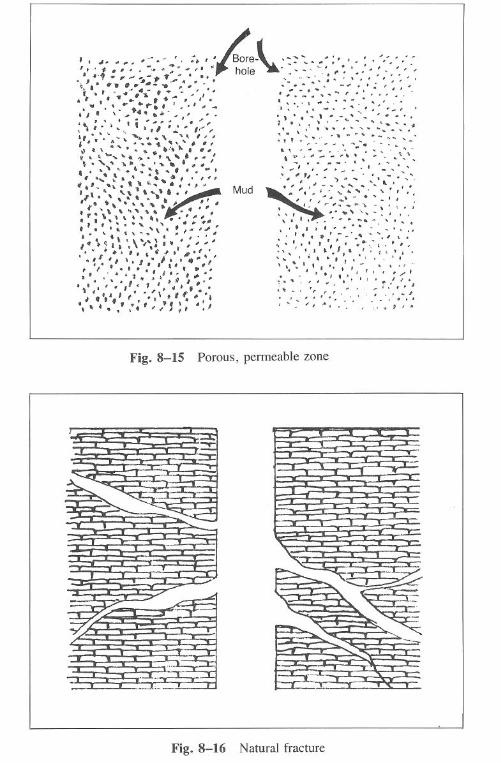
I . J' - k ~,.,;,~:,~:,,-.::.:; :.,' 80-".,.,'',- """ re .,~, ,.\ ~ .,.:.!: hole ...::~ ": ........' ...' ..:.. , .' .. . ... '.. .' .....- .' ,'. ." .,' "... ..........' .' ..:" . '.,' . . .. .. . . ..........H "......
. ... '. '; ,. ." ' ~ ." .. . .. . .. ...... . ... . ..' .' .. ........I .. . ,', '. v. ' . · . · .. .' ."., .' ... ...' I. . . ." - ..,. ..".' >' ." .. ., ... . . .. :. .. .,.,. .:" ..,,' ", ; ............,.." ".. .....' .~.~.-. .~: ... .'.'.. . : ..~ " .;. : ~ .: '.. .,.' . .. '. '. . . ... . .' .. . -. .' . . .",'" ,,' ":, ..'. .' Mod," ' '. . ..--' .'-,. ' ". ;: ........... . " .. . . .. . '. .' ... . .': ..' .' ... " ., .. . .. .. ...,', . ' : :' . . .. .:.. '.. .;: : . ..:.'j'\ ..\,..' .,'..~, ::,'. ..' ;;>. .,':.; ,':~ ',' :. -::"...".,.,. ,.,. , '":.'. ,"':' :.' , .
/t : "'."
.' . t . I ..' .. t, '., " ~,. , ,..." ' ... I ,.,' ,.,
" ...,.,.. .' '.' .' , '. . ... . . " ..' . '.' , .' . ... . , " . . . " .' . ' , .. .." '. ." ."... ,., .. ." ,,'. .. ..'" ,'.', /1 .' .' I ... " ., . . " . I ...' ' ., , .1 ,'... ' . . .' . .' ..." 1
~ " "I"" ~' . . .~ #.;,., , I .
Fig.8-15 Porous, permeable zone
Fig. 8-16 Natural fracture
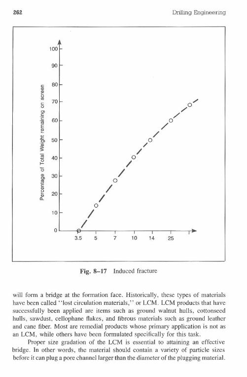
Z6Z Drilling Engineering
Fig. 8-17 Induced fracture
will fonn a bridge at the fonnation face. Historically, these types of materialshave been called "lost circulation materials," or LCM. LCM products that havesuccessfully been applied are items such as ground walnut hulls, cottonseedhulls, sawdust, cellophane flakes, and fibrous materials such as ground leatherand cane fiber. Most are remedial products whose primary application is not asan LCM, while others have been fonnulated specifically for this task.
Proper size gradation of the LCM is essential to attaining an effectivebridge. In other words, the material should contain a variety of particle sizesbefore it can plug a pore channel larger than the diameter of the plugging material.
100[90
c: 80Q)Q)0C/)
700'"c:
0/'OJ
c:
0/"2 60OmE /
/.EOJ 50 0,.-
/a; 40 0;9. /'0 /Q) 30OJ
0!UE
/Q)0
20Q)/a..
010l- IoI
/p I 1 I I I I
3.5 5 7 10 14 25
Drilling Fluids Selection 263
This feature is true of any plugging material, such as gels used as a filter cakeor cements. The mathematical expressi'on used to determine and evaluate theoptimum sizing for lost circulation particles is as follows:
Ir = 8nlm (8.7)
Where:r = ratio between successive sizes of interval 2, dimensionless8 = porosity of a bed of sized material or the porosity of one screen size,
%n = one less than the number of component sizes obtained from the or-
dinate of Fig. 8-19m = one less than the number of screen sizes used
In field applications, this is interpreted to mean that using a mixture such as acombination of fine-, medium-, and coarse-sized walnut hulls is more effectivethan using only one size (Fig. 8-19).
Lost circulation materials are not recommended in concentrations greaterthan 10-20 Ib/bbl in the overall mud system. Laboratory tests and field appli-cations have shown that this amount is as effective in most cases as significantlylarger concentrations, and that mud properties rapidly deteriorate when the lostcirculation additives are used in large concentrations. Figs. 8-20 and 8-21 showthat concentrations greater than 20 ppb do not increase the effectiveness of thematerial.
Conventional lost circulation materials have been misused by the drillingindustry as a result of their name. Personnel have assumed that the name "lostcirculation materials" implies the rpaterial can be used for all such problems,whereas it is specifically suited for porous, permeability plugging only. It doesnot adequately control other types of lost circulation and should not be expectedto do so. .
High filter-loss squeezes are effective in controlling unconsolidated for-mations such as gravel beds or shell reefs. This procedure uses a slurry containinga large concentration of solids and no effective means of controlling the waterloss. The slurry is pumped into the thief zone and slight pressure is applied toforce the water out of the mixture. The remaining filtrated solids form a bridgethat should prevent further losses.
A typical slurry contains water as the basic component with various bridg-ing additives. To mix a IOO-bblslurry, 20 lb/bbl of salt gel is mixed with water.In addition, 0.5 ppb of lime is added before mixing 50 lb/bbl of diatomaceousearth materials (Diacel D, Diacel M), 5 lb/bbl asbestos fibers,* 5 lb/bbl of fine
*Because of legal and health reasons, the use of asbestos should be discouraged.
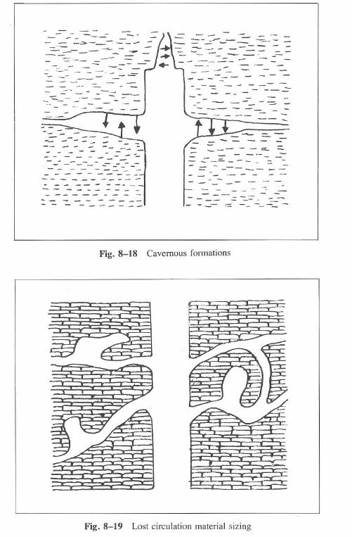
- -
-'--- --- - '~'-- ---- --- ---- -
- - - -- - - -- -- -"------------------ --- -------------------------------
Fig. 8-18
-- -==-~ =--:=.-- - --
- --;-0 .,.,-._-_-- #.---- ---- -- -
-- - -- -- - --
- - ---- --- -- -- - - - -- - ,....-- - -
----- - - - -=- .-
Cavernous formations
Fig. 8-19 Lost circulation material sizing
t::JHE
:5"
(Q"'T]
E-
o.{/}en(1)C
DQ
.<
:5"::s
Fig
.8-20
Summ
aryof
material
evaluationtests;
analysisand
controlof
lostcirculation
byH
oward
andScott
NG)
en
Concen-
LargestfracturesealedM
aterialT
ypeD
escriptiontration
Inches0
.04.08
.12.16
.20Ibs/bbl
II
Nutshell
('ranular50%
-3/16
+10
Mesh
2050%
-10
+100
Mesh
Plastic
""
20L
imestone
""
40
Sulphur
""
120N
utshell"
50%-
10+
16M
esh20
50%-
30+
100M
esh
ExpandedPerlite
"50%
-3/16
+10
Meh
6050%
-10
+100
Mesh
Cellophane
Lamellated%
in.Flakes
8S
awdust
Fibrous
114in.P
articles10
PrairieH
ay"
%in.F
ibers10
Bark
"%
in.Fibers
10
Cottonseedhulls
Granular
Fine
10
PrairieH
ayF
ibrous%
in.Particles
12
Cellophane
Lamellated%
in.Flakes
8S
hreddedwood
Fibrous
114in.Fibers
8-.
Saw
dust"
1/16in.Particles
20-
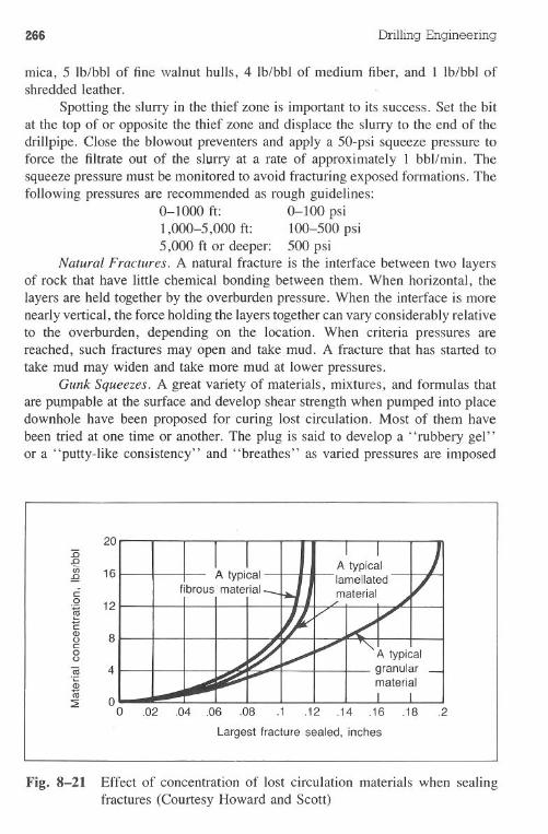
266 DrillingEngineering
mica, 5 lb/bbl of fine walnut hulls, 4 lb/bbl of medium fiber, and I lb/bbl ofshredded leather.
Spotting the slurry in the thief zone is important to its success. Set the bitat the top of or opposite the thief zone and displace the slurry to the end of thedrillpipe. Close the blowout preventers and apply a 50-psi squeeze pressure toforce the filtrate out of the slurry at a rate of approximately I bbl/min. Thesqueeze pressure must be monitored to avoid fracturing exposed formations. Thefollowing pressures are recommended as rough guidelines:
0-1000 ft: 0-100 psi1,000-5,000 ft: 100-500 psi5,000 ft or deeper: 500 psi
Natural Fractures. A natural fracture is the interface between two layersof rock that have little chemical bonding between them. When horizontal, thelayers are held together by the overburden pressure. When the interface is morenearly vertical, the force holding the layers together can vary considerably relativeto the overburden, depending on the location. When criteria pressures arereached, such fractures may open and take mud. A fracture that has started totake mud may widen and take more mud at lower pressures.
Gunk Squeezes. A great variety of materials, mixtures, and formulas thatare p1.U11pableat the surface and develop shear strength when pumped into placedownhole have been proposed for curing lost circulation. Most of them havebeen tried at one time or another. The plug is said to develop a "rubbery gel"or a "putty-like consistency" and "breathes" as varied pressures are imposed
20
16
A typicalgranularmaterial
.1 .'2 .14 .16 .18 .2
Largest fracture sealed, inches
Fig. 8-21 Effect of concentration of lost circulation materials when sealingfractures (Courtesy Howard and Scott)
12
8
4
00 .02 .04 .06 .08
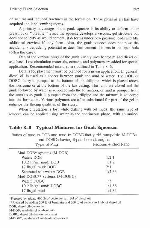
Drilling Fluids Selection 267
on natural and induced fractures in the formation. These plugs as a class haveacquired the label gunk squeezes.
A primary advantage of the gunk squeeze is its ability to deform underpressure, or "breathe." Since the squeeze develops a viscous, gel structure butdoes not solidify as would cement, it deforms under new pressure loads and fillsadditional crevices if they form. Also, the gunk squeeze does not pose theaccidental sidetracking potential as does firm cement if it sets in the open hole(often the case).
One of the various plugs of the gunk variety uses bentonite and diesel oilas a base. Lost circulation materials, cement, and polymers are added for specialapplication. Recommended mixtures are outlined in Table 8-6.
Details for placement must be planned for a given application. In general,diesel oil is used as a spacer between gunk and mud or water. The DOB orDOBC slurry is pumped to the bottom of the drillpipe, which is placed abovethe loss zone or at the bottom of the last casing. The rams are closed and thegunk followed by water is squeezed into the formation, or mud is pumped fromthe annulus as gunk is pumped from the drillpipe and the mixture is squeezedinto the formation. Various polymers are often substituted for part of the gel toenhance the flexing qualities of the slurry.
When circulation is lost while drilling with oil muds, the same type ofsqueeze can be applied using water as the continuous phase, with an amine-
Table 8-6 Typical Mixtures for Gunk SqueezesRatios of mud-to-DOB and mud-to-DOBC that yield pumpable M-DOBs
and DOBCs having 5-psi shear strengths.Type of Plug Recommended Ratio
Mud-DOB* systems (M-DOB)Water: DOB10.2 lb/gal mud: DOB17 lb/gal mud: DOBSaturated salt water: DOB
Mud-DOBC** systems (M-DOBC)Water: DOBC10.2 lb/gal mud: DOBC17 lb/gal mud
1.2:11:1.22:11:2.33
1:31:1.861:1.35
*Prepared by adding 400 lb of bentonite to I bbl of diesel oil**Prepared by adding 200 lb of bentonite and 200 lb of cement to I bbl of diesel oilDOB, diesel oil-bentonite
M-DOB, mud-diesel oil-bentonite
DOBC, diesel oil-bentonite-cement
M-DOBC, mud-diesel oil-bentonite-cement
268 Drilling Engineering
treated bentonite inst~ad of regular gel as the critical solid in the slurry. Highshear strength is achieved when the gel becomes wet with oil.
Cement Squeezes. Using cement squeezed into the thief zone has been aneffective means of controlling lost circulation in natural fractures. The cementforms a hard plug that has a relatively high compressive strength. In addition,the multitude of chemical additives available for cement allows its properties.tobe controlled to ensure proper pumping and setting times as well as densitycontrol when low-weight cements are required.
Cement plugs have several characteristics that make them somewhat lesspreferable than soft plugs, or gunk squeezes. Whereas soft plugs can deform toabsorb pressure surges, hard plugs must either withstand the surge or breakdown. If the plug cannot withstand the pressure, lost circulation is likely to beexperienced again. Also, if the plug that is formed sets too hard, problems maybe encountered in trying to drill it out. In soft formations, the bit may easilykick off the plug, resulting in sidetracking.
Induced Fractures. Lost circulation caused by induced fractures is a dif-ficult problem to control and can happen to formations anywhere in the world.Fractures are induced by excessive mud pressure, and the best approach to avoidinduced fractures is to maintain the overall mud pressure at a minimum. Thisproblem often occurs as a result of poor well planning practices in which low-strength formations are exposed while using high mud weights to control otherexposed zones that exhibit high formation pressures.
Many factors are involved in maintaining the mud pressure as low aspossible. Obviously, minimum required mud weights are important. Reducingsurge pressures as described in Chapter 18 is a necessity. Mud properties shouldbe maintained in an optimum condition to minimize friction pressures. Careshould be exercised when starting the pumps by lifting and rotating the pipe toreduce the surge pressures caused by breaking the gels in the mud.
Induced fractures will occasionally "heal" with time. A waiting periodof 6-12 hr after returns have been lost may allow circulation of mud of the samedensity with careful flow properties' monitoring. Some formations may regaintheir original strength or even exceed it, while others may remain 2-4 Ib/galbelow their initial value after being fractured. Remedies for induced fracturesrequire that the pressure exposed to the formation be reduced before applyingremedial techniques. After the reduction, the previously described techniquesthat are most effective are I) soft and hard plugs and 2) high-filter-loss squeezes.
Cavernous Losses. Openings in a layer of rock that would be denoted"vugular" or "cavernous" are usually associated with limestone reefs. Cavern-containing strata are often identifiable geologically, and the depths at which theyoccur are predictable over wide drilling areas. Caverns or fissures may vary frompin size to tunnel size. The void spaces are usually filled with water at normalpressure. The bit often drops a noticeable amount upon penetrating a void of
Drilling Fluids Selection 269
this type. The loss of mud level in the hole drops enough to allow a blowoutfrom shallower zones or to induce caving into the hole, resulting from the reducedhydrostatic pressure.
Whether or not a cavernous formation can be sealed depends largely uponthe size of the voids and the strength of the rock matrix. If the voids are smallenough to be bridged by material pumped down the driIlpipe and the matrix isstrong enough to withstand the pressure surges that are part of the driIlingoperation, then sealing is possible. Alternatives are either to penetrate the zoneby drilling without returns, termed blind drilling, or to penetrate the zone withcable tools. Air and foam driIling have also been successfully applied in extremecases. After the zone is penetrated, casing may be set and cemented, althougha stage job usually is required.
Polymers for Lost Circulation. A single polymer or a combination ofpolymers mixed at the surface into a very thick, viscous piII can help eliminateloss circulation. Acid resins with calcium carbonate (Georgia white marble) haveproved very effective in areas of lost circulation. The reaction of polymers mixedcorrectly and spotted properly has an effect similar to gunk squeezes. It maynot be advisable to use polymers as lost circulation matejal in pay zones.
Specialty Mud AdditivesSpotting nuids. With the increasing number of highly deviated holes
being drilled, it has become common practice to maintain some type of spottingfluid at the wellsite to aid in pipe sticking problems. Regardless of the type ofspotting fluid, immediate remedial procedures must be taken once the pipe hasbecome stuck. Products that have come into the market and proven to be effectiveusually have some of the following characteristics:
.. reduce the differential sticking force.lubricate the filter cake. erode the filter cake to reduce the area of sticking with the driIlstring
Spotting fluids can be obtained in a premixed package requiring only weightmaterial to achieve the desired mud weight. Certain types of spotting fluidsrequire the addition of water, diesel, and weight material before they can bepumped downhole.
Most spotting fluids can be placed in one or more of the following cate-gories:.oil muds.diesel oil· emulsifiers· lubricants
270 Drilling Engineering
If a deviated hole will be drilled with exposed permeable zones, adding diesel,lubricants, and emulsifiers may help prevent stuck pipe. The concentration andtype of pretreatment is usually determined by the drilling parameters.
nocculants. Flocculation can be defined as the edge-to-edge or edge-to-face grouping of clay platelets caused by attractive forces. Severe flocculationof a mud system, which is undesirable in most cases, is usually the result ofsome type of contamination. Flocculants have been used in drilling to promotethe settling of drilled solids from the mud system. Flocculants cause the clayparticles to group together and cause direct bonding between particles due totheir affinity for and adsorption on solids. In addition to aluminum compounds,organic polymers, modified polysaccharides, and modified guar gums have beenused successfully in flocculating drill solids in a mud system.
Shale Stabilizers. Unstable hole conditions can be the result of chemicalactions between the mud and the formation, mechanical problems, or physicalcharacteristics of the formation being drilled. Normally, shale problems resultfrom one or more of the following reasons:.filtrate invasion.overburden pressures.tectonicforces.pore pressure.unconsolidated formations
Filtrate invasion can be controlled by lowering the mud filtrate. Alteringthe effect of the mud filtrate on the formation can be achieved by using dissolvedelectrolytes or an inhibited mud system; by using polymers to coat the wellbore,thus reducing the dispersion of clays; or by maintaining the pH range of themud from 8.5-10.
Overburden and pore pressure shale problems can be addressed by in-creasing the mud density (Fig. 8-22). The hydrostatic pressure increase willmodify the differential pressure and assist mechanically to maintain a stablezone. If the hydrostatic pressure cannot be increased due to fracture gradientconsiderations, the alternatives are to run casing or attempt to drill and circulateat high rates to clean the hole.
Shale problems encountered because of tectonic forces may be controlledby reducing the water-wetting of these shales and plugging their fissures andmicrofractures. Reducing the wetting of the shale can be accomplished by low-ering the filtrateor using polymers. Plugging the shale fissures and microfractureshas been accomplished with such products as gilsonite and various asphalt-basedproducts. The gilsonite and asphalt also help control water-wetting of the shales.
Detergents. Detergents, when used properly, can increase penetrationrate, reduce bit and collar balling, and may inhibit drill cuttings to a degree.They reduce the surface tension of the drill water, thus providing for increased
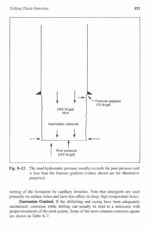
Drilling Fluids Selection 271
! ! ( ~ Fracture gradient\ 17.0Ib/gal
(16.0 Ib/gal)Mud
Hydrostatic pressure
i Pore pressure(15.0 Ib/gal)
Fig. 8-22 The mudhydrostaticpressureusuallyexceedstheporepressureandis less than the fracture gradient (values shown are for illustrativepurposes)
wetting of the formation by capillary invasion. Note that detergents are usedprimarily on surface holes and have less effect on deep, high-temperature holes.
Corrosion Control. If the drillstring and casing have been adequatelymaintained, corrosion while drilling can usually be held to a minimum withproper treatments of the mud system. Some of the most common corrosive agentsare shown in Table 8-7.
272 Drilling Engineering
Table 8-7 Common Sources of Corrosionand Treatment
Corrosive Agent Source Possible Treatments
Carbon dioxide Formation
Hydrogensulfide
BacteriaFormation
Bacteria
Oxygen
Thermal degra-dation
Aeration
Increase mud density; maintain pH at10 or above; use a cationic corro-sive inhibitor
MicrobiocidesIncrease mud density; maintain pH at
10 or above; use an H2Sor sulfidescavenger in conjunction with pHcontrol
Microbiocides; maintain pH at 10.5or above
Change mud system to a lignite/sur-factant or oil mud
Reduce yield point and gel strengths;correct mechanical equipment;maintain pH at 10 or above; use acationic inhibitor; turn mud gunsand hopper off when not in use;add scavenger.
Bow to Plan a Mud ProgramPlanning a mud program is an essential step in the development of a
workable overall well plan. Key steps, listed below, are followed on each well.
.Obtain pore pressures and casing program.Look for geological hazards beginning with the deepest hole section.Set mud weights.After checking geometry, ECDs, and hydraulics, set optimum viscosities·Establish maximum fluid loss by interval. Select mud types by interval, trying to match one interval to the next.Set other critical properties (allowable sand content, pH, etc.).Check mud program against other phases of well plan for possible conflict.Determine material requirements.Write breakover instructions.Develop contingency plans for kicks, hole trouble, etc..Line up supply of water, chemicals, etc.
Mud engineers can often provide insight into expected problems in an area.
Drilling Fluids Selection 273
Problems
8.1 Determine the material requirements for the preparation of 250 bbl of13.8-lb/gal CaCI2/CaBr2brine (use Table B6).
8.2 Determine the material requirements for the preparation of 250 bbl of13.8-lb/gal CaCI2/CaBr2(use Table B7). Discuss the difference be-tween the solutions in Problems 8.1 and 8.2.
8.3 Determine the material requirements for the preparation of 250 bbl of16.5-lb/gal CaCI2/CaBr2(use Tables B8, B9, BIO, and BlI). Discussthe differences in the solutions.
8.4 Compute the volume of water required to drop the density of 275 bblof 11.1-lb/gal CaCI2 brine to 10.6 Ib/gal; to 10.1 Ib/gal; to 9.8Ib/gal.
8.5 Compute the volume of water required to drop the density of 150 bblof 14.2-lb/gal CaBr2 to 13.6 Ib/gal.
8.6 A drilling engineer intends to use a lignosulfonate mud on a well withpore pressures shown in Fig. 8-23. Using a O.4-lb/gal safety marginbetween the mud weight and pore pressure, prepare a mud programshowing mud weights and minimum and maximum values for solids,funnel viscosity, plastic viscosity, and yield point. Prepare values foreach 1,000-ft interval (Fig. 8-23).
8.7 Prepare a mud program for the following well. A lignosulfonate mudwill be used "to 12,000 ft, and an invert emulsion mud will be usedthroughout the remainder of the well. Use a O.4-lb/gal safety margin.
Depth,ft
2,0004,0006,0008,000
10,00011,00012,00013,00014,00014,50015,000
Pore Pressure,lb/ gal
9.09.09.09.09.09.5
12.013.014.514.814.8
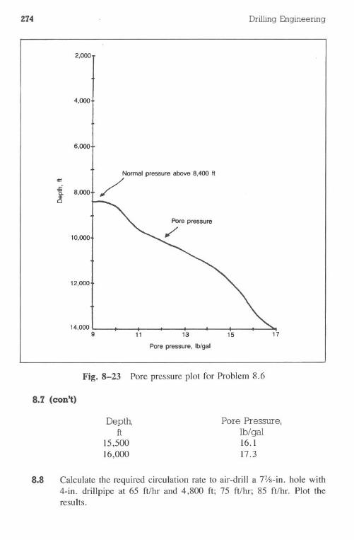
274 DrillingEngineering
2,000
4.000
6.000
==
..:15.CDc
8.000 /Normal pressure above 8.400 It
10.000
12,000
14,0009 11 13
Pore pressure. Iblgal
15 17
Fig. 8-23 Pore pressure plot for Problem 8.6
8.7 (con't)
Depth,ft
15,50016,000
Pore Pressure,lb/gal16.117.3
8.8 Calculate the required circulation rate to air-drill a 7Vs-in. hole with4-in. drillpipe at 65 ft/hr and 4,800 ft; 75 ft/hr; 85 fUhr. Plot theresults.
Drilling Fluids Selection 275
8.9 An air rig is operating in eastern New Mexico at 5,400 ft. A 6-in. bitis being used with 3V2-in. drillpipe. Compute and plot the requiredair circulation rates for drill rates from 10-100 ft/hr. Use lO-ft/hrincrements.
8.10 Refer to Example 8.4. Assume that the compressors can output only1,100 cu ft/min. What is the maximum allowable drill rate?
8.11 Refer to Example 8.4. Assume that the compressors can output 1,500cu ft/min. Prepare a plot of maximum allowable drill rates vs depthfor the range of 1,000-6,000 ft. Use I,OOO-ftincrements.
8.12 A low pressure zone is encountered at 5,600 ft. Engineers have de-termined that it will fracture if mud weights in excess of 6.3 lb/galare used. What volume of air is required to create a mist system if8.33 lb/gal water and air are mixed? Assume a mud pump rate of 160gal/min.
8.13 Refer to Problem 8.12. Calculate and plot air requirements if the weakzone will support mud weights of 5.0, 5.5, 6.0, 6.5, 7.0, and 8.0lb/gal, respectively.
8.14 Calculate the hydrostatic pressure for each of the following systems:a. 8,500 ft of 11.8-lb/gal mudb. 16,200 ft of 17.1-lb/gal mudc. 14,100 ft of 16.I-lb/gal mud
8.15 Calculate the hydrostatic pressure for each of the following systems:a. 6,200 ft of 9.5-lb/gal mudb. 13,800 ft of 12.9-lb/gal mudc. 14,100 ft of 16.I-lb/gal mud
8.16 A zone at 15,000 ft has a pressure of 11,700 psi. What is the minimumacceptable mud weight that will prevent a blowout?
8.17 Recalculate Problem 8.16 if the pressure is 9,800 psi; 12,480 psi;10,400 psi.
8.18 Refer to Problem 8.14 and assume that 100bbl of mud will be requiredfor each 1,000 ft of hole. Calculate the amount of barite required toraise the mud weight by 1.0 Ib/gal.
276 Drilling Engineering
8.19 Refer to Problem 8.15. If 100 bbl of mud will be required for each1,000 ft of hole, calculate the amount of barite required to raise themud weight by 0.5 Ib/gal.
8.20 A 1O.0-lb/galmud is being used on a well. The hole and pit volumesare 800 and 400 bbl, respectively. Compute and plot the barite re-quirements to raise the mud weight from 10.0 to 17.0 Ib/gal in 0.5-Ib/gal increments.
References
Angel, R.R. Volume Requirements for Air-Gas Drilling. Houston: Gulf Pub-lishing Company, 1980.
API Specification for Oil-Well Drilling-Fluid Materials, API Specification13A, 7th edition. API Division of Production. Dallas, May 1979.
Bordelon, Bruce. Personal conversation, Lake Charles, Louisiana.
Chesser, B.G., and G.F. Nelson. "Applications of Weighted Acid-SolubleWorkover Fluids." Journal of Petroleum Technology, January 1975, pp.35-39.
Densimix Inc. Technical articles. Houston, 1982.
Dresser Magcobar. Drilling Fluid Engineering Manual. Houston, 1972.
Gray, G.R., and H.C.H. Darley. Composition Mud Properties of Oil WellDrilling Fluids. Houston: Gulf Publishing Company, 4th edition, 1980.
Gray, G.R., and N.K. Tschirley. "Drilling Fluids Programs for Ultra-DeepWells in the United States." Proc., 9th World Petroleum Congress, vol.4, Barking, England: 1975.
Gray, G.R., J.L. Foster, and T.S. Chapman. "Control of Filtration Char-acteristics of Salt Water Muds." Trans. AlME. vol. 146, 1942, pp.117-125.
Kelco. Kelco Rotary Technical Handbook. Tulsa.
Drilling Fluids Selection 277
Mondshine, T.C., and J.D. Kercheville. "A New Salt Mud from Q-Broxinand Aquagel." Baroid News Bulleiin. vol. 15, no. 3, 1963, pp. 12-17.
Mondshine, T.C. "New Fast-Drilling Muds Also Provide Hole Stability."Oil & Gas Journal. 21 March 1966, pp. 84-90.
NL Baroid. NL Baroid Drilling Mud Handbook. Houston.
NL Baroid. NL Baroid Mud Technology Handbook. Houston, 1965.
NL Industries. NL Completion/Workover Manual. Houston, 1983.
NL Industries. NL Treating Chemicals Product Information Manual. Houston.
O'Brien, T.B., J.P. Stinson, and F. Brownson. "Relaxed Fluid Loss Controlson Invert Muds Increases ROP." World Oil. August 1977, pp. 31-34, 70.
Park, A., P.P. Scott, Jr., and J.L. Lummus. "Maintaining Low-Solids DrillingFluids." Oil & Gas Journal. 30 May 1960, pp. 81-84.
Rogers, W.F. Composition and Properties of Oil Well Drilling Fluids. 3rdedition. Houston: Gulf Publishing Company, 1963.
Simpson, J.P., J.C. Cowan, and A.E. Beasley Jr. "The New Look in Oil-Mud Technology." Journal of Petroleum Technology. December 1961, pp.1177-1183.
Thibodeaux, Allen Dale. Personal conversations, Lafayette, Louisiana.
Wright, T.R., Jr. "Guide to Drilling, Workover and Completion Fluids."World Oil, June 1978, pp. 53-98.
Young, Ron. Personal conversations, Houston.
Chapter 9 Cementing
Cementing is an integral, necessary aspect of drilling oil and gas wells.Cement is used to secure casing strings and to isolate zones for productionpurposes as well as to solve various hole problems. A properly planned cementprogram is essential to a successfully drilled well.
Cement planning consists of several features, including the following:
.assessment of hole conditions such as temperature, size, etc.·evaluation of mud properties· slurry design.placement techniques· equipment selection, such as centralizers, scratchers, and float equipment
Lack of attention to any of these items may cause problems with the cement joband necessitateotherefforts. .
Purposes of Oil Well CementingOil well cementing falls into three categories:I. primary cement job on a casing string2. squeeze cementing3. plugs
The various aspects of each type of cement job may differ, creating the needfor a thorough knowledge of cementing prior to developing the well's prognosis.Cement specialists, usually associated with service companies, can use theirexpertise to provide valuable assistance to the well planner.
278
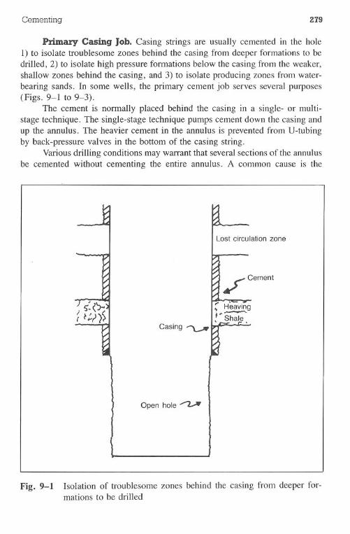
Cementing 279
Primary Casing Job. Casing strings are usually cemented in the holeI) to isolate troublesome zones behind the casing from deeper formations to bedrilled, 2) to isolate high pressure formations below the casing from the weaker,shallow zones behind the casing, and 3) to isolate producing zones from water-bearing sands. In some wells, the primary cement job serves several purposes(Figs. 9-1 to 9-3).
The cement is normally placed behind the casing in a single- or multi-stage technique. The single-stage technique pumps cement down the casing andup the annulus. The heavier cement in the annulus is prevented from V-tubingby back-pressure valves in the bottom of the casing string.
Various drilling conditions may warrant that several sections of the annulusbe cemented without cementing the entire annulus. A common cause is the
Lost circulation zone
/ Cement
Open hole ~
Fig. 9-1 Isolation of troublesome zones behind the casing from deeper for-mations to be drilled
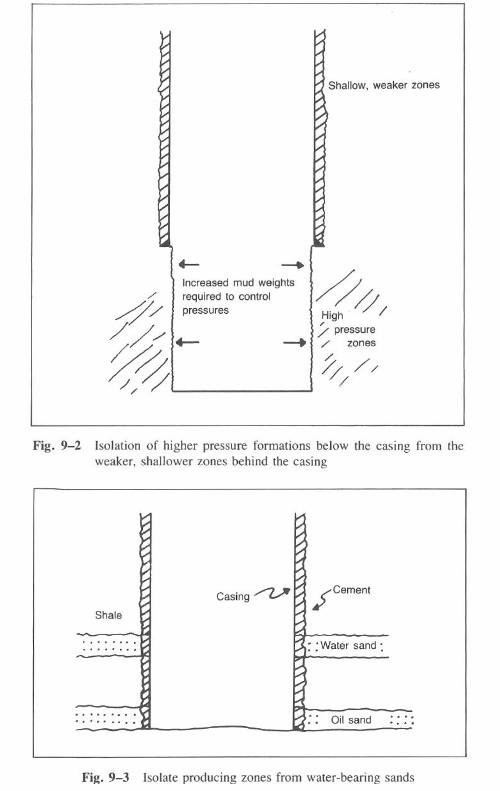
Shallow, weaker zones
-+
~ij/High, pressure~ zones
/, ////
Increased mud weightsrequired to controlpressures
Fig. 9-2 Isolation of higher pressure formations below the casing from theweaker, shallower zones behind the casing
Fig. 9-3 Isolate producing zones from water-bearing sands
L-v
t:"
Casing/'1/'cement
Shale
....... .......ok
............. .. I.- : :Water sand :
I.-
-.. .. .. .. .. .... .. ..
"'"
.. .. .. .. .. .... .. .. t). . Oilsand ......t.......
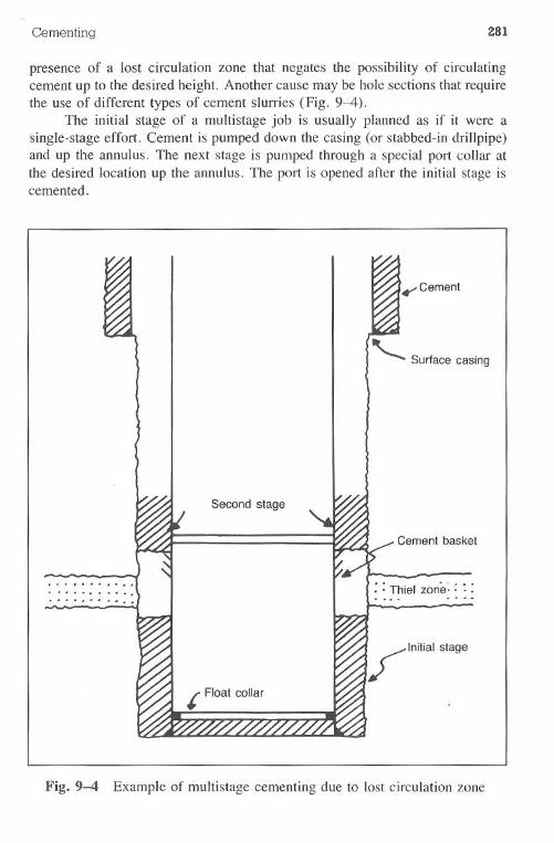
Cementing Z81
presence of a lost circulation zone that negates the possibility of circulatingcement up to the desired height. Another cause may be hole sections that requirethe use of different types of cement slurries (Fig. 9-4).
The initial stage of a multistage job is usually planned as if it were asingle-stage effort. Cement is pumped down the casing (or stabbed-in drillpipe)and up the annulus. The next stage is pumped through a special port collar atthe desired location up the annulus. The port is opened after the initial stage iscemented.
Cement
'" Surfacecasing
.. ................
Second stage
Cement basket
f ...............: : Thiefzone: : : :
Fig. 9-4 Example of multistage cementing due to lost circulation zone
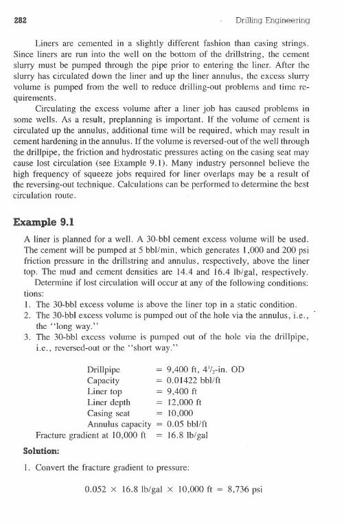
282 Drilling Engineering
Liners are cemented in a slightly different fashion than casing strings.Since liners are run into the well on the bottom of the drillstring, the cementslurry must be pumped through the pipe prior to entering the liner. After theslurry has circulated down the liner and up the liner annulus, the excess slurryvolume is pumped from the well to reduce drilling-out problems and time re-quirements.
Circulating the excess volume after a liner job has caused problems insome wells. As a result, preplanning is important. If the volume of cement iscirculated up the annulus, additional time will be required, which may result incement hardening in the annulus. If the volume is reversed-out of the well throughthe drillpipe, the friction and hydrostatic pressures acting on the casing seat maycause lost circulation (see Example 9.1). Many industry personnel believe thehigh frequency of squeeze jobs required for liner overlaps may be a result ofthe reversing-out technique. Calculations can be performed to determine the bestcirculation route.
Example 9.1
A liner is planned for a well. A 30-bbl cement excess volume will be used.The cement will be pumped at 5 bbl/min, which generates 1,000 and 200 psifriction pressure in the drillstring and annulus, respectively, above the linertop. The mud and cement densities are 14.4 and 16.4 Ib/gal, respectively.
Determine if lost circulation will occur at any of the following conditions:tions:I. The 30-bbl excess volume is above the liner top in a static condition.2. The 30-bbl excess volume is pumped out of the hole via the annulus, i.e. ,
the "long way."3. The 30-bbl excess volume is pumped out of the hole via the drillpipe,
i.e., reversed-out or the "short way."
Drillpipe = 9,400 ft, 41/2-in.ODCapacity = 0.01422 bbl/ftLiner top = 9,400 ftLiner depth = 12,000 ftCasing seat = 10,000Annulus capacity = 0.05 bbl/ft
Fracture gradient at 10,000 ft = 16.8 Ib/gal
Solution:
I. Convert the fracture gradient to pressure:
0.052 X 16.8 Ib/gal X 10,000 ft 8,736 psi
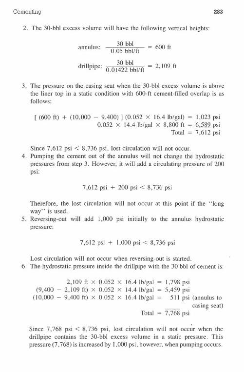
Cementing 283
2. The 30-bbl excess volume will have the following vertical heights:
30 bbl0.05 bbl/ft
d.11
. 30 bbln pipe: £\ £\. LLlIL". = 2,109 ft
annulus: = 600 ft
3. The pressure on the casing seat when the 30-bbl excess volume is abovethe liner top in a static condition with 600-ft cement-filled overlap is asfollows:
[ (600 ft) + (10,000 - 9,400) ] (0.052 x 16.4 Ib/gal) = 1,023psi0.052 x 14.4 Ib/gal x 8,800 ft = 6,589 psi
Total = 7,612 psi
Since 7,612 psi < 8,736 psi, lost circulation will not occur.4. Pumping the cement out of the annulus will not change the hydrostatic
pressures from step 3. However, it will add a circulating pressure of 200psi:
7,612 psi + 200 psi < 8,736 psi
Therefore., the lost circulation will not occur at this point if the "longway" is used.
5. Reversing-out will add 1,000 psi initially to the annulus hydrostaticpressure:
7,612 psi + 1,000 psi < 8,736 psi
Lost circulation will not occur when reversing-out is started.6. The hydrostatic pressure inside the drillpipe with the 30 bbl of cement is:
2,109 ft x 0.052 x 16.4 Ib/gal(9,400 - 2,109 ft) x 0.052 x 14.4 Ib/gal
(10,000 - 9,400 ft) x 0.052 x 16.4 Ib/gal
1,798 psi5,459 psi
511 psi (annulus tocasing seat)
= 7,768 psi .Total
.Since 7,768 psi < 8,736 psi, lost circulation will not occur when thedrillpipe contains the 30-bbl excess volume in a static pressure. Thispressure (7,768) is increased by 1,000 psi, however, when pumping occurs.
284 DrillingEngineering
7,768 + 1,000> 8,736 psi 8,768 > 8,736 psi
Therefore, circulation could be lost at this time.
Squeeze Cementing. A common method for repairing faulty primarycasing jobs or performing remedial operations on the hole is squeeze cementing.Major applications for squeeze cementing are as follows:
.supplement a faulty primary casing cement job.reduce water-oil, water-gas, or gas-oil ratio.abandon a productive zone temporarily. isolate a zone before perforation for production (block squeezes) or beforefracturing.repaircasingleaks.stop lost circulation in an open hole while drilling·bring a well under control
Placement techniques and slurry design are important considerations in squeezeoperations.
Supplementing a faulty or ineffective primary casing cement job is themost prominent application for squeeze cementing. The initial cement job mayhave failed to hold pressure under integrity tests, or cement bond logs may haveindicated poor or absent cement bonding. (See Chapter 17 for details on cementbond logs.) Since the primary job is a major well control system (see Figs.9-1 to 9-3), a bad job must be augmented with additional cement. Generally,this additional cement must be forced, or "squeezed," around the annulus byusing high pump pressures. Squeeze techniques are discussed later in this chapter.
The reduction of producing fluid ratios by squeeze cementing is a common,necessary practice on many wells. High gas volumes may deplete reservoirpressure prematurely, while high water volumes may create excessive separationcosts at the surface production facilities or retard production. Specific sectionsof perforations may be closed by pumping cement. Gas volumes are reduced bycementing the upper perforations, while water is reduced by cementing the lowerperforations (Fig. 9-5).
Lost circulation problems can often, but not always, be solved by squeezecementing. The type of lost circulation must respond to cement. For example,cementing a zone fractured from excessive pressures will not solve the problem 4.unless the pressures are reduced.
Plugs. Setting plugs in the well commonly is used for the followingreasons:
·plugback.whipstock· abandonment
Upper perforations
must be squeezedwith cement to
reduce gas flow
~ Pertmati,",
Cementing 285
Production packer
Production casing
Gas
Oil
Fig. 9-5 Squeeze cementing can be used to control gas-oil ratios
A balanced plug technique is used usually for the placement technique.A plug-back operation may set a plug through or above the old pay zone
when recompletion above a depleted producing zone is necessary. A plug mayalso be used in open-hole completions to shut off bottom-hole water.
A whipstock is often used when it becomes necessary to increase or de-crease the deviation of a hole or to change direction while drilling. The whipstocktool requires a solid cement plug to provide a seat or bridge. Whipstocks arealso used to bypass junk or to reach a new objective.
~ Goodoperatingpracticesand the rules of regulatorybodiesrequireaban-doning wells in such a manner that fluid-bearing zones are proper:lysealed andprotected. Cement plugs are commonly used to seal and protect these zones(Fig. 9-6). As many as three plugs are set in deep wells. A plug is usually setat the bottom of the surface casing or deeper casing string. Uncased freshwatersands in abandoned wells are protected by plugs extending from below to abovethe sands. Government regulations with jurisdiction over the wellsite should beconsulted for specific abandonment procedures.
286 Drilling Engineering
rCaSing
Plug 1
Casing seat
~ Open hole
Total depth
Fig. 9-6 Cement plugs are used in plugging and abandonment operations
Cement Characteristics
The cement slurry pumped into oil and gas wells includes cement, specialadditives, and water. Portland cement is used most commonly. The additivesare used to control characteristics such as thickening time, density, and com-pressive strengths. Water is an important agent in the cementing. Since waterand cement quality varies, water and cement samples should be tested beforeperforming the actual cement job.
Portland Cement. Portland cement is manufactured by calcining lime-stone, clay, shale, and slag together at 2,OOO-2,600°F in a rotary kiln (Fig.9-7). The resulting material, clinker. is cooled and interground with small per-centages of gypsum to form portland cement. In addition to the raw materials,
Cementing 287
(a) The dry process. , (b) The wet process.I
Shale and Iron Ore
Crusher
Storage Clay Slurry and
/ Water
Dryer, Proportioner,and Grinder
Tube Mill and
Air Separator Tube Mill
Dry Mixer andBlender
Storage_Rotary Kiln
Clinker Storage
Fig. 9-7 How cement is manufactured
other components such as sand, bauxite, and iron oxide may be added to adjustthe chemical composition of the clinker for the different types of portland cement.
The principal components of the finished portland cement are lime, silica,alumina, and iron. The components form complex compounds expressed by theformulas in Table 9-1. Each compound affects the slurry in a different manner.
When water is added to cement, setting and hardening reactions beginimmediately. The chemical compounds in the cement undergo hydration andrecrystallization, resulting in a set product. Two simultaneous mechanisms occur
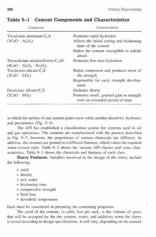
288 Drilling Engineering
Table 9-1 Cement Components and Characteristics
Compound Characteristics
Tetracalcium aluminoferrite/C4AF(4CaO . Al203 . Fe203)Tricalcium silicate/C3S(3CaO . Si02)
Promotes rapid hydrationAffects the initial setting and thickening
time of the cementMakes the cement susceptible to sulfate
attackPromotes low-heat hydration
Tricalcium aluminate/C3A(3CaO . A1203)
Dicalcium silicate/C2S(2CaO . Si02)
Major component and produces most ofthe strength
Responsible for early strength develop-ment
Hydrates slowlyPromotes small, gradual gain in strength
over an extended period of time
in which the surface of one cement grain reacts whHeanother dissolves, hydrates,and precipitates (Fig. 9-8).
The API has established a classification system for cements used in oiland gas operations. The cements are manufactured with the process describedin Fig. 9-7; however, the proportions of various chemicals are different. Inaddition, the cements are ground to a different fineness, which varies the requiredwater-cement ratio. Table 9-2 shows the various AP.I classes and some char-acteristics. Table 9-3 shows the chemicals and fineness of each class.
Slurry Features. Variables involved in the design of the slurry includethe following:
·yield·density·mix water· thickeningtime· compressive strength· fluid loss·downhole temperature
Each must be considered in preparing the cementing prognosis.The yield of the cement, in cubic feet per sack, is the volume of space
that will be occupied by the dry cement, water, and additives when the slurryis mixed according to design specifications. It will vary, depending on the cement
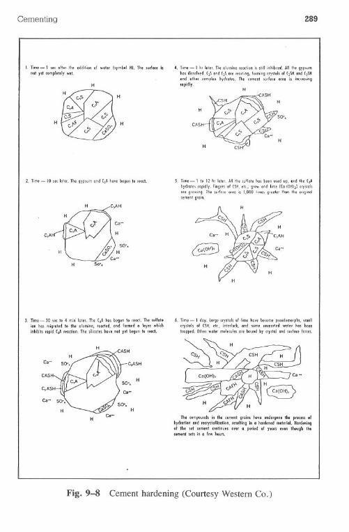
Cementing
1. Time- 1 St( ahef the addition of waler hymbol HI. The surfac, isnol yet (ompletelywel.
H
H
2. nme-10 let 101tr.ThegypsumandeJAhovebegunto ,t'Oct.
H
C,A
H
3. Time- 30 It( 104 min'lolef. TheeJAhasbegunto Itod. Thesulfateion has migrated10 the alumina, readed,and formed0 layer whithinhibitsrapid(~ ,~"ion. ThesilicoteshoVtnol yet begunto read.
Fig. 9-8
289
4. Time- 1h, lalef.nit aluminofrDclionis "ill inhiblltd. All the gypsumhasdiuolvrd.C)SGnd(1S Oft "ocling.forming0)'110"of()SHand(JiHand olher lomplu hyl!.olti. The I,menl Mfo(f ortG is inmosingrapidly.
H
CASH
S. Time- I 1012hr laler. "lithe sulfolr hos bern used up, and the eJA
hyc!rolu ropidly. ringtn of <SM.elc., glow Clndlime (; IOHh) cryslalsOrt gro"..ing. Th surfO(t oleo is 1,000 limes gltaler than the oliginal
umenlgloin.
6. Time- 1 day. lOlgeHystoh of lime hovebecomep"udomolphs.smollu')'~lah of UK. efc.. interlock.ond ,ome unleodedwater has beenhapped.Olhe,walef moleculesOfeboundby (rY5101andsunaeefortes.
Tht compoundsin the cementgroins haveundergon.the pfCKtSS .fhydralionand fKfJslallizalion.resultingin 0 hardenedmaterial.Hardlningof the set (ement (ontinuesoyer 0 period .f yeon tnn thovgh Ih,ctlntnl setsin 0 few houn.
Cement hardening (Courtesy Western Co.)
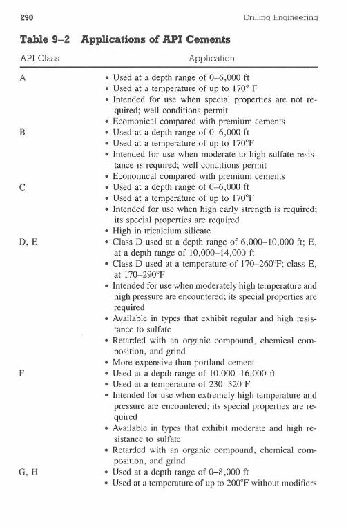
290 Drilling Engineering
Table 9-2 Applications of API Cements
API Class Application
A .Used at a depth range of 0-6,000 ft· Used at a temperature of up to 170° F· Intended for use when special properties are not re-
quired; well conditions permit·Ecomonical compared with premium cementsB ·Used at a depth range of 0-6,000 ft.Used at a temperature of up to 170°F
· Intendedfor use whenmoderateto high sulfateresis-tance is required;wellconditionspermit.Economical compared with premium cements
C ·Used at a depth range of 0-6,000 ft·Used at a temperature of up to 170°F· Intendedfor use whenhigh early strengthis required;
its specialpropertiesare required·High in trica1cium silicateD, E ·Ciass D used at a depth range of 6,000-10,000 ft; E,
at a depth range of 10,000-14,000 ft·Class D used at a temperature of 170-260°F; class E,at 170-290°F
· Intended for use when moderately high temperature andhigh pressure are encountered; its special properties arerequired.Available in types that exhibit regular and high resis-tance to sulfate·Retarded with an organic compound, chemical com-position, and grind·More expensive than portland cement
F ·Used at a depth range of 10,000-16,000 ft·Used at a temperature of 230-320°F. Intended for use when extremely high temperature and
pressure are encountered; its special properties are re-quired·Available in types that exhibit moderate and high re-sistance to sulfate·Retarded with an organic compound, chemical com-position, and grind
G, H ·Used at a depth range of 0-8,000 ft.Used at a temperature of up to 200°F without modifiers
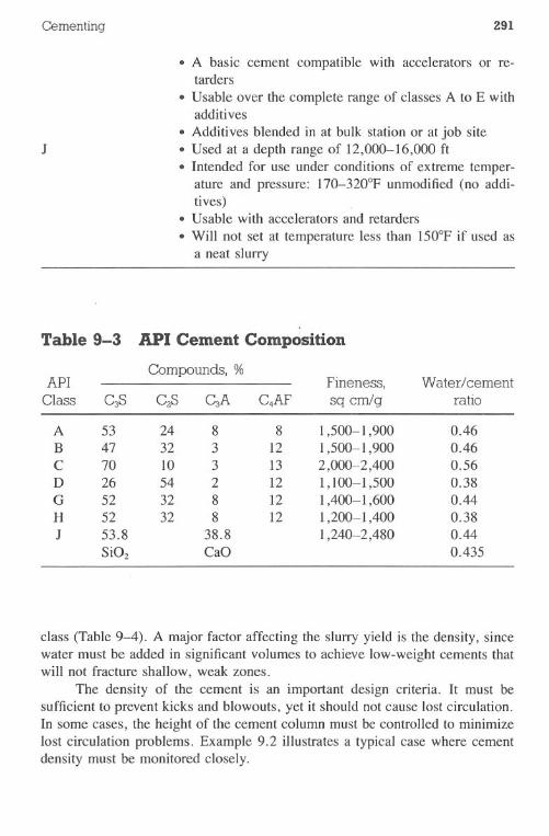
Cementing 291
J
·A basic cement compatible with accelerators or re-tarders.Usable over the complete range of classes A to E withadditives·Additives blended in at bulk station or at job site·Used at a depth range of 12,000-16,000 ft
· Intended for use under conditions of extreme temper-ature and pressure: 170-320°F unmodified (no addi-tives) ,· Usable with accelerators and retarders·Will not set at temperature less than 150°F if used asa neat slurry
class (Table 9-4). A major factor affecting the slurry yield is the density, sincewater must be added in significant volumes to achieve low-weight cements thatwill not fracture shallow, weak zones.
The density of the cement is an important design criteria. It must besufficient to prevent kicks and blowouts, yet it should not cause lost circulation.In some cases, the height of the cement column must be controlled to minimizelost circulation problems. Example 9.2 illustrates a typical case where cementdensity must be monitored closely.
Table 9-3 API Cement Composition
Compounds, %Fineness,API Water/cement
Class S C2S C C4AF sq cmlg ratio
A 53 24 8 8 1,500-1,900 0.46B 47 32 3 12 1,500-1,900 0.46C 70 10 3 13 2,000-2,400 0.56D 26 54 2 12 1,100-1,500 0.38G 52 32 8 12 1,400-1,600 0.44H 52 32 8 12 1,200-1,400 0.38J 53.8 38.8 1,240-2,480 0.44
Si02 CaO 0.435
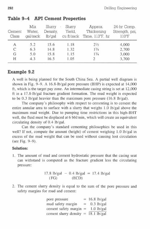
Z9Z DrillingEngineering
A well is being planned for the South China Sea. A partial well diagram isshown in Fig. 9-9. A 16.8-lb/gal pore pressure (BHP) is expected at 14,000ft, which is the target pay zone. An intermediate casing string is set at 12,000ft in a 17.8-lb/gal fracture gradient formation. The mud weight is expectedto be 0.3 lb/gal heavier than the maximum pore pressure (16.8 lb/gal).
The company's philosophy with respect to cementing is to cement theentire annular area to surface with a slurry that weighs 1.0 lb/gal above themaximum mud weight. Due to pumping time restrictions in this high-BHTwell, the fluid must be displaced at 6 bbllmin, which will create an equivalentcirculating density of 0.4 lb/gal.
Can the company's standard cementing philosophies be used in thiswell? If not, compute the amount (height) of cement weighing 1.0 lb/gal inexcess of the mud weight that can be used without causing lost circulation(see Fig. 9-9).
Solution:
1. The amount of mud and cement hydrostatic pressure that the casing seatcan withstand is computed as the fracture gradient less the circulatingpressure:
17.8Ib/gal - 0.4 lb/gal = 17.4 lb/gal(FG) (ECD)
2. The cement slurry density is equal to the sum of the pore pressure andsafety margins for mud and cement:
pore pressuremud safety margin =cement safety margincement slurry density =
16.8 lb/gal0.3 lb/gal1.0 Ib/gal
18.1 lb/gal
Table 9-4 API Cement Properties
Mix Sluny Sluny Approx. 24-hr Comp.Cement Water, Density, Yield, Thickening Strength, psi,
Class gal/sack lb/ gal cu ft/sack Time, 113°F, hr 110°F
A 5.2 15.6 1.18 2V2 4,000C 6.3 14.8 1.32 1% 2,700G 5.0 15.8 1.15 1% 3,000H 4.3 16.5 1.05 2 3,700
Example 9.2
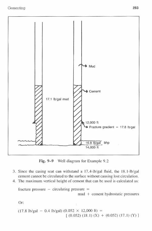
Cementing 293
17.1 Ib/gal mud
Cement
Mud
12,000 ItFracture gradient = 17.8 Ib/gal
16.8 Ib/gaT bhp14,000 It
Fig.9-9 Well diagram for Example 9.2
3. Since the casing seat can withstand a 17.4-lb/gal fluid, the l8.1-lb/galcement cannot be circulated to the surface without causing lost circulation.
4. The maximum vertical height of cement that can be used is calculated as:
fracture pressure - circulating pressure =mud + cementhydrostaticpressures
Or: I
I
IIII
(17.81b/gal - 0.4 lb/gal) (0.052 x 12,000 ft)[ (0.052) (18.1) (X) + (0.052) (17.1) (Y) ]
294 Drilling Engineering
Where:
X = length of cement column, ftY = length of mud column, ft
And:X + Y = 12,000 ft
X = 12,000 ft - Y
5. Solving for X and Y:
10,857 psi = 0.9412X + 0.8892Y10,857 psi = 0.9412 (12,000 - Y) + 0.8892Y10,857 psi - 11,294 psi = (-0.9412 + 0.8892)Y
- 437 psi = - 0.052YY = 8,403 ft (mud column)
:. X = 3,596 ft (cement column above the shoe at12,000 ft)
6. The total cement column from the hole bottom is:
(14,000 - 12,000) + 3,596 = 5,596 ft
The mixing water requirements will vary, depending primarily on cementclass and slurry density (Table 9-4). Most cement jobs use wellsite water. Ifwater must be transported to the location due to a shortage or poor supply,accurate mixing volume calculations are important to ensure that an adequatesupply is available. The volume requirements can be substantial if a low-densitygel cement must be used.
Quality of the mixing water is an important parameter in cement planning.The hydration and curing of the slurry will react differently with varying amountsof salt, calcium, or magnesium in the mix water. It is recommended that pilotlaboratory tests be performed with an actual sample of the mix water and cementto obtain good estimates of pumping time and compressive strengths. The pilotlab testing becomes more critical in high-temperature deep wells that require asignificant amount of time for cement mixing and displacement.
Thickening time is the amount of time that a cement remains pumpablewith reasonable pressures. This is perhaps the most critical property in thedisplacement process. Factors affecting the thickening time include cement com-position and temperature. An upper limit must be placed on the thickening time,however, so that drilling operations can resume.
Hardened cement must developt:ompressive strength to secure casing inthe hole and withstand pressure differentials across the cement. The compressive
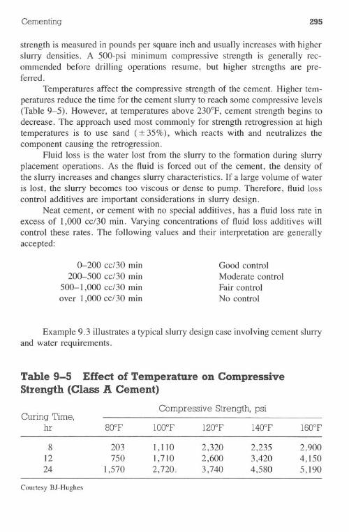
Cementing 295
strength is measured in pounds per square inch and usually increases with higherslurry densities. A ~QO-psiminimum compressive strength is generally rec-ommended before drilling operations resume, but higher strengths are pre-ferred.
Temperatures affect the compressive strength of the cement. Higher tem-peratures reduce the time for the cement slurry to reach some compressive levels(Table 9-5). However, at temperatures above 230°F, cement strength begins todecrease. The approach used most commonly for strength retrogression at hightemperatures is to use sand (:!::35%), which reacts with and neutralizes thecomponent causing the retrogression.
Fluid loss is the water lost from the slurry to the formation during slurryplacement operations. As the fluid is forced out of the cement, the density ofthe slurry increases and changes slurry characteristics. If a large volume of wateris lost, the slurry becomes too viscous or dense to pump. Therefore, fluid losscontrol additives are important considerations in slurry design.
Neat cement, or cement with no special additives, has a fluid loss rate inexcess of 1,000 cc/30 min. Varying concentrations of fluid loss additives willcontrol these rates. The following values and their interpretation are generallyaccepted:
0-200 cc/30 min200-500 cc/30 min
500-1,000 cc/30 minover 1,000 cc/30 min
Good controlModerate controlFair controlNo control
Example 9.3 illustrates a typical slurry design case involving cement slurryand water requirements.
Table 9-5 Effect of Temperature on CompressiveStrength (Class A Cement)
Compressive Strength, psiCuring Time,
hr 80°F lOO°F 120°F 140°F l60°F-8 203 1,110 2,320 2,235 2,900
II
12 750 1,710 2,600 3,420 4,15024 1,570 2,720 3,740 4,580 5,190
Courtesy BJ-Hughes
!I
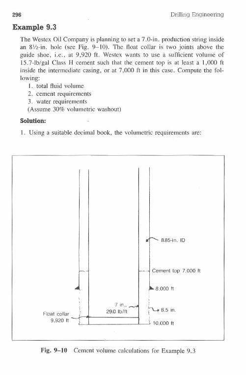
296 Drilling Engineering
Example 9.3
The Westex Oil Company is planning to set a 7.0-in. production string insidean 8Y2-in. hole (see Fig. 9-10). The float collar is two joints above theguide shoe, i.e., at 9,920 ft. Westex wants to use a sufficient volume of15.7-lb/gal Class H cement such that the cement top is at least a 1,000 ftinside the intermediate casing, or at 7,000 ft in this case. Compute the fol-lowing:
1. total fluid volume2. cement requirements3. water requirements(Assume 30% volumetric washout)
Solution:
1. Using a suitable decimal book, the volumetric requirements are:
8.85-in. ID
Cement top 7,000 It
8,000 It
Float collar9,920 It
7 in.,29.0 Ib/lt
J,/
~8.5in.1
10,000 It
Fig.9-10 Cement volume calculations for Example 9.3
Cementing 297
a. 80 ft of 29.0-lb/ft, 7-in. pipe0.2085 cu ftllin ft x 80 lin ft = 16.7 cu ft
b. 2,000 ft of 7-in. x 8.5-in. open-hole annulus0.1268 cu ftllin ft x 2,000 ft = 253.60 cu ft130% x 253.60 cu ft = 329.7 cu ft
c. 1,000 ft of 7-in. x 8.835-in. pipe annulus0.1858cuft/linft x 1,000ft = 158.5 cu ftTotal volume = 504.9 cu ft
2. The slurry yield is 1.17 cu ft/sack. Therefore, the sack requirements are:
504.9 cu ft = 431.5 sx... cu ft/sac'
3. The water requirements are 5. 19 gallsack:
5.19 gal/sack x 431.5 sx = 2,239.5 gal= 53.3 bbl
Cement Additives
A neat slurry is a mixture of water and cement only. Special chemicalsare often added to the slurry to achieve some desired purpose(s). These additivesmay fall into the following categories:·accelerators. retarders· density adjusters.dispersants· fluid loss additives
Some chemicals such as sand and salt have multiple beneficial effects on thecement slurry.
Ac::celerators. Most operators wait for cement to reach a minimum of500 psi compressive strength before resuming operations. At temperatures below100°F, common cement may require a day or two to develop 500-psi strengths.Accelerators are useful at reducing the amount of waiting-on-cement (WOC)time.
Low concentrations of cement accelerators, usually 2-4% by weight ofcement, shorten the setting time of cement and promote rapid strength devel-opment. Calcium chloride is perhaps the most widely used chemical for thispurpose. Fig. 9-11 shows the effect of 3% calcium chloride (A-7) on Class Acement. Other chemicals are often used as accelerators in addition to CaCho

298 Drilling Engineering
"fija.
~0,c~Ci5Q)>"fij'"Q)C.Eoo
1200
800
400
o4 5 6
Curing Time, hr7 8
Fig. 9-11 Effect of curing time on strength at 90°F with A-7 using class Acement (Courtesy of BJ-Hughes Services)
Retarders. High formation temperatures associated with increased welldepths necessitate the use of chemicals that retard the setting time of the cement,i.e., increase the pumping time. The chemicals provide sufficient retarding effectsto allow slurry mixing and displacement into the well with a safety margin forunforeseen occurrences.
The most common retarder may be calcium lignosulfonate. Its effectivenessis limited in temperatures above 200°F. Concentrations of 0.1-1.0% are used inmost slurry applications to give both predictable thickening times and compres-sive strengths. Amounts above I% do not add appreciably to slurry retar-dation.
Other retarders can be planned for the slurry design if temperatures exceed200°F. Carboxymethyl-hydroxyethylcellulose (CMHEC) can be used to about240°F BHCT (bottom-hole circulating temperature). Organic acids can be usedfrom 200-400°F. Borax added to the organic acids can be used normally from300-500°F BHCT. Each slurry should be pilot tested.
Determining the actual bottom-hole temperature is an important aspect ofselecting retarders. Isothermal gradient maps (Fig. 9-12) provide general guidesin an area. Eq. 9.1 can be used with the geothermal gradients to estimate BHT:
1 I I I I r I I I
I-I I I I I
T 1
I I-
.
I
1,?>0/o","1
1081
-
.... 1
l-I
I-
1
,t_
_I I
T 1
No accelerator
:all
::::1 1 I LJ
Cementing 299
(9.1)
Where:
BHT = bottom-hole temperature., ofD = depth of interest, ftG = geothennal gradient, ~/ 100 ftTA = average ambient temperature, of
The ambient temperature, TA, is often taken as 70°F in the southern U.S.
Example 9.4
Assume that a IO,OOO-ftwell is in an area where the geothennal gradient is1.8°F/lOOft. Detennine the BHT if the ambient temperature is 70°F.
Solution:
1. UseEq. 9.1:
BHT = (1~0 x G) + TA
= e~.~go x 1.8) + 70= 250°F
Geothennal gradient maps are often inaccurate in areas with abnonnal porepressures due to the manner in which the high porosity restricts heat flow. Analternative procedure uses a dimensionless time concept, TD, and well log headerdata. Temperaturedataare plottedon semilogpaperand extrapolatedto a TD of1.0. The dimensionless time values are calculated from Eq. 9.2:
(9.2)
Where:TD = dimensionless timeTAC = time after circulation, hrTC = circulation time, hr
Example 9.5 illustrates the procedure.
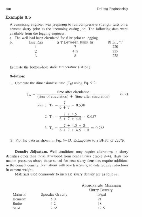
300 Drilling Engineering
Example 9.5
A cementing engineer was preparing to run compressive strength tests on acement slurry prior to the upcoming casing job. The following data wereavailable from the logging engineer:a. The well had been circulated for 6 hr prior to loggingb. Log Run ~ T Between Runs, hr
I 72 4Y23 8
BHLT, of220225228
Estimate the bottom-hole static temperature (BHST).
Solution:
1. Compute the dimensionless time (TD)using Eq. 9.2:
T = time after circulation 9 2D (time of circulation) + (time after circulation) ( . )
7Run 1: TD = 6 + 7 = 0.538
7 + 4.52: TD = 6 + _ . . _ = 0.657
7 + 4.5 + 83: TD = / . _ . . _ . ~ = 0.765
2. Plot the data as shown in Fig. 9-13. Extrapolate to a BHST of 235°F.
Density Adjusters. Well conditions may require alterations in slurrydensities other than those developed from neat slurries (Table 9-4). High for-mation pressures above those suited for neat slurry densities require additionsin the cement density. Formations with low fracture gradients require reductionsin cement weight.
Materials used commonly to increase slurry density are as follows:
MaterialHematiteBariteSand
Specific Gravity5.04.22.65
Approximate MaximumSlurry Density,
lb/ gal211817.5
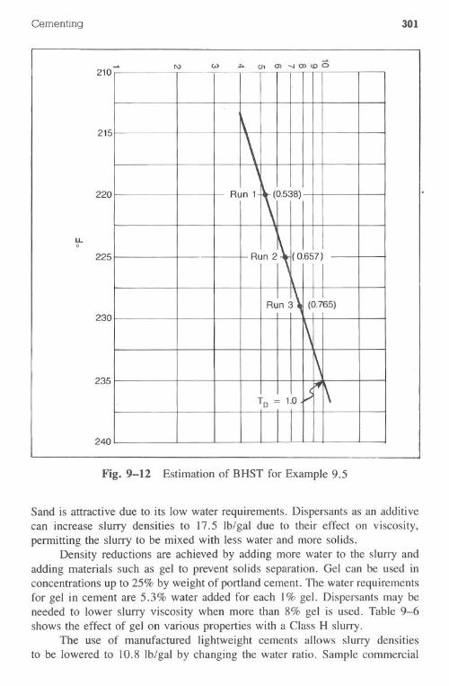
Cementing 301
210~I\)
215
220
u..o
225
230
235
240
Fig.9-12 Estimation of BHST for Example 9.5
Sand is attractive due to its low water requirements. Dispersants as an additivecan increase slurry densities to 17.5 Ib/gal due to their effect on viscosity,permitting the slurry to be mixed with less water and more solids.
Density reductions are achieved by adding more water to the slurry andadding materials such as gel to prevent solids separation. Gel can be used inconcentrations up to 25% by weight of portland cement. The water requirementsfor gel in cement are 5.3% water added for each I% gel. Dispersants may beneeded to lower slurry viscosity when more than 8% gel is used. Table 9-6shows the effect of gel on various properties with a Class H slurry.
The use of manufactured lightweight cements allows slurry densitiesto be lowered to 10.8 Ib/gal b}' changing the water ratio. Sample commercial
,Run 1
,0.538)
Run2 (0.657)
I II
Rn J\I I
(0.765)
\\
(;If \T D = 1.0.....
302 Drilling Engineering
Table 9-6 Effect of Gel Additions on Class H Slurries
% GelMixing' Water,
gaVsack
o48
1216
5.187.579.96
12.414.7
Slurry Density,lb/gal
15.714.213.312.612.2
Slurry Volume,cu ft/sack
1.171.521.862.212.55
Data courtesy of BJ-Hughes
lightweight cements are Trinity Lite-Wate or TXI Light Weight. They may beused by themselves or with other additives in the range of 11.9-13.7 Ib/gal.
Pozzolans are a siliceous material that will react with calcium hydroxide(lime) to form compounds possessing cementatious properties. In addition tolowering cost and slurry density, pozzolans offer resistance of the cement tocorrosive fluids such as sulfate water. Common pozzolans are diatomaceous earth(Diacel D), a natural pozzolan, and fly ash, which is an artificial pozzolan.Concentrations as high as 3: I pozzolan-to-cement ratio have been used.
Dispersants. Dispersants provide several beneficial features for the slurry:
·reduce slurry viscosity· allow slurry turbulence at lower pump rates· allow heavier slurries with less water and less weighting materials·assist in providing fluid loss control for densified slurries
Lignosulfonates and polymers can be used as dispersants.Fluid Loss Additives. Fluid loss agents are used in cement slurries for
the following reasons:
·minimize cement dehydration in the annulus·reduce gas migration·improve bonding.minimize formation damage
Cellulose derivatives are the most common fluid loss additives. Normal con-
centrations vary from 0.3-3.0% by weight of the cement. Higher percentagesproduce excessive viscosities and are difficult to mix in field operations.
Slurry DesignA well plan is not complete until the cement slurry has been designed.
Major aspects of the design are as follows:
Cementing 303
.volumetric requirements for the casing and annulus· cement.mixing water.density selection
Other features such as special additives.depend on mix water and cement qualityand, as such, rely heavily on pilot testing. However, service company handbooksprovide sufficient data to make reliable estimates of additive requirements.
Decimal books developed and supplied by cementing service companiesprovide valuable data used in slurry design. These books usually contain infor-mation on the following: .
.hole, drillpipe, tubing, and casing volumes.volume between casing and hole· volume between casing and casing.volume between multiple tubing strings and casing· performance properties of casing and tubing·pump output data.cement slurry characteristics· effects of various additives on cement slurries
Many books contain specialized data and formulas. Figs. 9-13 to 9-15 illustratetypical data from a decimal book. .
Example 9.6 illustrates calculations involved in a cement job. In addition,it illustrates a practical method for determining mud pump volumetric outputfrom cementing operations.
Example 9.6
A 7%-in., 39.0-lb/ft production casing string will be run inside 51.0-Ib/ft, lO%-in. surface casing set at 2,000 ft. The bottom of the 9-in. hole isat 9,100 ft (casing seat). Compute the volume of the casing and annulus.
A 6Y2-in. x I8-in. duplex pump will be used to bump the cement plugagainst the float shoe. If the pump operates at 90% efficiency, how manystrokes will be required?
After the job was completed, the drilling engineer at the wellsite ob-served that 1,990 strokes were required to bump the plug. What is the actualpump efficiency?
Solution:
1. Use a decimal book to determine the following values:7%-in. pipe capacity = 0.2394 cu fUlin ft; 0.0426 bbl/lin ft7%-in. x 9-in. hole annulus = 0.1247 cu ft/lin ft; 0.0222 bbl/lin ft7%-in. x 9.85-in. casing annulus = 0.2148 cu ftllin ft; 0.0382bbl/lin ft
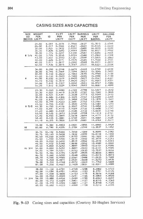
304 Drilling Engineering
Fig. 9-13 Casing sizes and capacities (Courtesy BJ-Hughes Services)
CASING SIZES AND CAPACITIES
SIZE WEIGHT CU FT UN FT BARRELS UN FT GALLONSOD PER ID PER PER PER PER PER
INCHES UN FT UN FT CUFT UN FT BARREL LIN FT
24.00 &.097 0.3576 2.7966 .0637 15.7015 2.67492&.00 8.017 0.3506 2.8527 .0624 16.0105 2.622332.00 7.921 0.3422 2.9222 .0600 16.4070 2.559936.0U 7.1025 0.3340 2.0944 .0595 16.8121 2.408238.00 1.775 0.3297 3.0330 .0587 17 .0290 2.4664
e 5/10 40.00 7.725 0.32';5 3.0724 .0580 17.2502 2.434843.00 7.651 0.3103 3.1321 .0569 17.5&55 2.3&8344.00 7.625 0.3171 3.1535 .0565 17 .7056 2.372149.00 7.511 0.3077 3.2500 .0548 1&.2471 2.301752.00 7.435 0.3015 3.3167 .0537 18.6221 .,,54
34.00 8.200 0.3748 2.6679 .0668 14.97&9 2.1003938.00 8.196 0.3664 2.7204 .0653 15.3245 2.740740.00 8.10 0.3623 2.7603 .0645 15.4080 2.710041.20 8.1';0 0.3623 2.7603 .0645 15.4980 2.7100
9 45.00 8.032 0.3:'10 2.8420 .0627 15.9507 2.632140.10 8.032 0.3519 2.84l0 .0627 15.9567 2.632154.00 7.1010 0.3327 3.0050 .0593 IC.8767 2.48865.20 7.&12 0.3320 3.0043 .0593 16.8681 l.4899
29.30 9.063 0.4480 2.2322 .0798 1.5327 3.351232.30 9.001 0.4419 2.2630 .0787 12.7060 3.305536.00 &.921 0.4341 2.3038 .0713 12.9349 3.247038.00 &.685 0.4306 2.3225 .0767 13.0399 3.220940.00 8.835 0.4257 2.34&9 .0758 13.1879 3.1&4742.00 8.799 0.4223 2.3681 .0752 13.2961 3.158843.50 8.755 0.4181 2.3920 .0745 13.4301 3.1273
9 $/8 44.30 &.750 0.4176 2.3047 .0744 13.4454 3.123747.00 8.681 0.4110 2.4329 .0732 I 3.6600 3.G74747.20 8.680 0.4109 2.4335 .0732 13.6631 3.074053.50 8.535 0.3973 2.5169 .0708 14.1313 2.972157.40 8.4';0 0.3894 2.5678 .0694 14.4171 2.913258.40 8.435 0.3881 2.5769 .0691 14.4684 2 . 902961.10 8.375 0.3826 2.6140 .0681 14.6764 2.8017
33.00 9.384 0.4803 2.082! .0855 11.6900 3.592810 60.00 oj.780 0.4205 2.3784 .0749 I 3.3537 3.1452
32.75 10.192 0.5666 1.7650 .1009 9.9099 4.238235.75 10.140 0.5608 1.7832 .0999 1(j.0118 4.195040.50 10,'050 0.5509 1.8153 .0981 10.1920 4.120945.50 ....950 0.5400 1.8519 .0962 10.3979 4.0j9346.20 9.950 0.5400 1.8519 .0962 10.3979 4.039348.00 9.902 0.5348 1:8699 .0952 10.4989 4.000449.0 9.850 0.5292 1.8897 .0943 10.6101 3.9585
III 3/4 51.00 9.1050 0.5292 1.8897 .0943 10.6101 3.058554.00 Y. 'loj4 0.5221 1.9153 .0930 10.7537 3.90565.50 9.160 0.5195 1.9241 .0925 10.8066 3.886560.70 0.660 0.5090 1.9648 .0906 11.0315 3.807365.70 9.560 0.4985 2.0061 .0688 11.2635 3.728911.10 9.450 0.4871 2.0531 .0"68 11.5213 3.643576.00 9.350 0.4168 2.0972 .0849 11.7152 3.566881.00 9.250 0.4661 2.1428 .0831 12.0311 3.4909
38.00 11.150 0.6781 1.4748 .1208 8.2802 5.072342.00 11.(j84 0.6701 1.4924 .1193 8.3791 5.012547.00 11.000 0.6600 1.5153 .1115 8.5076 4.93685v.00 10.950 0.6540 1;5291 .1165 8.5854 4.8920
II 3/4 54.00 10.880 0.6456 1.5489 .1 ISO 8.6963 4.829760.00 10.772 0.6329 1.5801 .1127 8.8715 4.734361.00 10.770 0.6326 1.5807 .1127 8.8748 4.732565.00 10.682 0.6223 1.6068 .1108 9.0216 4.6555
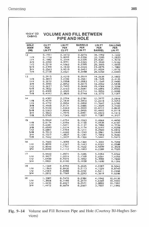
Cementing 305
Fig. 9-14 Volume and Fill Between Pipe and Hole (Courtesy BJ-Hughes Ser-vices)
10-3/4" OD VOLUME AND FILL BETWEENCASINGPIPE AND HOLE
HOLE CUFT UN FT BARRELS UN FT GALLONSDIAM PER PER PER PER PER(IN) UN FT CUFT UN FT BARREL LINFT
12 0.1551 6.4473 0.0276 36.1992 1.16021/8 0.1716 5.8292 0.0306 32.7285 1.28331/4 0.1882 5.3144 0.0335 29.8381 1.40763/8 0.2050 4.8791 0.0365 27.3940 1.5332In 0.2219 4.5062 0.0395 25.3005 1.66005/8 0.2390 4.1833 0.0426 23.4875 1.78823/4 0.2563 3.9010 0.0457 21.9024 1.91767/8 0.2738 3.6521 0.0488 20.5050 2.0483
13 0.2915 3.4310 0.0519 19.2639 2.18021/8 0.3093 3.2334 0.0551 18.1545 2.31351/4 0.3272 3.0558 0.0583 17.1569 2.4480J/8 0.3454 2.8952 0.0615 16.2552 2.58381/2 0.3637 2.7493 0.0648 15.4364 2.72085/8 0.3822 2.6163 0.0681 14.6895 2.85923/4 0.4009 2.4945 0.0714 14.0056 2.99887/8 0.4197 2.3826 0.0748 13.3772 3.1397
14 0.4387 2.2794 0.0781 12.7977 3.2818III 0.4579 2.1839 0.0816 12.2618 J 3.42531/4 0.4772 2.0954 0.0850 11.7647 3.57003/. 0.4968 2.0131 0.0885 II .3025 3.71601/2 0.5164 1.9363 0.0920 10.8717 3.863251' 0.5363 , .8646 0.0955 10.4692 4.01183/4 0.5563 1.7975 0.0991 10.0923 4.16167/8 0.5765 1.7345 0.1027 9.7387 4.3127
IS 0.5969 1.6754 0.1063 9.4064 4.46501/8 0.6174 1.6196 O. II 00 9.0935 4.61871/4 0.6381 1.5671 0.1137 8.7984 4.77363/. 0.6590 1.5174 0.1174 8.5197 4.92981/2 0.6801 1.4704 0.1211 8.2560 5.087251. 0.7013 1.4260 0.1249 8.0061 5.24603/4 0.7227 1.3837 0.1287 7.7692 5.40607IfI 0.7442 1.3437 0.1326 7.5441 !>.5673
16 0.7060 1.3055 0.1364 '7 . 330J 5.72981/4 0.8099 1.2347 0.1443 6.9321 6.05881/2 0.8546 1.1701 0.1522 6.5699 6.39283'4 0.8999 1.1112 0.1603 6.2389 6.7320
17 0.9460 1.0571 0.1685 5.9354 7.07621/4 0.9927 1.0074 0.1768 5.6561 7.42561/2 1.0400 0.9615 0.1852 5.3984 7.7tJoo3/4 1.0881 0.9190 0.1938 5.1600 8.1396
18 1.1369 0.8796 0.2025 4.9387 8.50421/4 1.1863 0.8430 0.2113 4.7329 8.87401/2 1.2364 0.8088 0.2202 4.5411 9.24883/4 1.2872 0.7769 0.2293 4.3619 9.6288
19 1.3387 0.7470 0.2384 4.1942 10.01381/4 1.3908 0.7190 0.2477 4.0369 10.40401/2 1.4436 0.6927 0.2571 3.8892 10.79923/4 1.4972 0.6679 0.2067 3.7501 11 ..1996
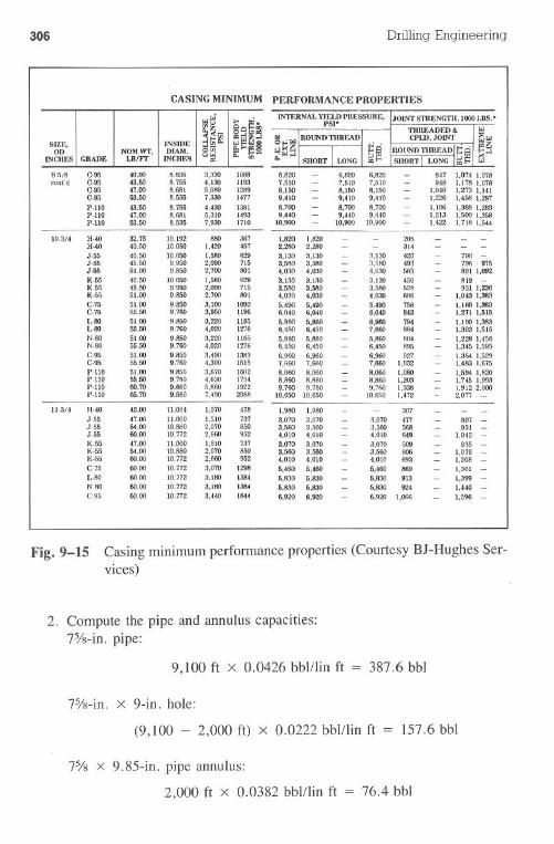
306 Drilling Engineering
Fig, 9-15 Casing minimum performance properties (Courtesy BJ-Hughes Ser-vices)
2. Compute the pipe and annulus capacities:7%-in. pipe:
9,100 ft X 0.0426 bblllin ft 387.6 bbl
7%-in. x 9-in. hole:
(9,100 - 2,000 ft) X 0.0222 bbl/lin ft 157.6 bbl
7% x 9.85-in. pipe annulus:
2,000 ft X 0.0382 bbl/lin ft 76.4 bbl
CASINGMINIMUM PERFORMANCEPROPERTIES
",Ij§9
INTERNALYIELDPRESSURE. JOINTSfRENGTlI.1000LOS.'PSI'
-'r,!IROUNDTIIREADI . foSIZE. INSIDE...!C
!§ ..5!3 . RO\lNnTImF.Anl!; §on NOMwr, DlAM. 8 -.: ]1 SIIORT I WNG I ,JINCIIES GRADE LO/IT INCIIES .. SIIORT LONG '"
9.!)/B C.95 40.00 8.836 3.330 1088 6.820 - 6.820 6.820 - 847 1.0741.078cont'd C.95 43.60 8.755 4.130 1193 7.610 - 7.510 7.510 - 948 1.1781.078
C.95 47.00 8.681 5.080 1289 8.160 - 8.160 8.160 - 1.040 1.2731.141C.95 63.60 8.636 7.330 1477 9.410 - 9.410 9.410 - 1.220 l,458 1.297P.IIO 43.60 8.765 4.430 1381 8.700 - 8.700 8.700 - 1.106 1.3881.283P.IIO 47.00 8.681 5.310 1493 9.440 - 9.440 9.440 - 1.213 1.5001.358P.IIO 63.60 8.635 7.930 1710 10.900 - 10.900 10.900 - 1.422 1.7181.544
10.3/4 11.40 32.76 10.192 880 367 1.820 1.820 - - 205 - - -11.40 40.60 10.050 1.420 457 2.280 2.280 - - 314 - - -J.55 40.60 10.050 1.580 629 3.130 3.130 - 3.130 420 - 700 -J.55 45.60 9.9"..0 2.090 715 3.580 3.580 - 3.580 493 - 796 975J.55 61.00 9.850 2.700 801 4.030 4.030 - 4.030 565 - 891 1.092K-55 40.60 10.050 1.580 629 3.130 3.130 - 3.130 450 - 819 -K.55 45.50 9.950 2.090 715 3.580 3.580 - 3.580 528 - 931 1.236K.55 51.00 9.850 2.700 801 4.030 4.030 - 4.030 606 - 1.0431.383C.75 51.00 9.850 3.100 1092 5.490 5,490 - 5.490 758 - 1.160 1.383C.75 65.60 9.760 3.950 1196 6.040 6.040 - 6.040 843 - 1.271 1.515L.BO 51.00 9.850 3.220 1185 5.800 5.800 - 6.960 794 - 1.190 1.383L.BO 65.60 9.760 4.020 1276 6.450 6.450 - 7.660 884 - 1.3031.515N.aa 61.00 9.850 3.220 1165 5.860 5.800 - 5.860 804 - 1.228 1.456N.aa 65.50 9.760 4.020 1276 6.450 6.450 - 6.450 895 - 1.3451.595C.95 51.00 9.850 3,490 1383 6.950 6.960 - 6.960 927 - 1.3541.529C.95 55.50 9.760 4.300 1515 7.660 7.660 - 7.660 1.032 - 1.4831.675p.no 51.00 9.850 3.670 1602 6.060 8.060 - 8.060 1.080 - 1.594 1.820P.IIO 55.50 9.760 4.630 1754 6.860 8.860 - 8.860 1.203 - 1.7451.993P.IIO 60.70 9.660 5.860 1922 9.760 9.760 - 9.760 1.338 - 1.9122.000P.IIO 85.70 9.560 7.490 2088 10.6S0 10.650 - 10.650 1.472 -. 2.077 -
11.3/4 11.40 42.00 11.084 1.070 478 1.980 1.980 - - 307 - - -J.55 47.00 11.000 1.510 737 3.070 3.070 - 3.070 477 - 807 -J.55 64.00 10.880 2.070 850 3.560 3.560 - 3.580 568 - 931 -J.55 60.00 10.772 2.660 952 ".010 4.010 - 4.010 649 - 1.042 -K.55 47.00 11.000 1.510 737 3.070 3.070 - 3.070 609 - 935 -K.55 64.00 10.880 2.070 850 3.560 3.560 - 3.560 606 - 1.079 -K-55 60.00 10.772 2.660 952 4.010 4.010 - 4.010 693 - 1.208-C.75 60.00 10.772 3.070 1298 5.460 5.460 - 5.400 869 - 1.361 -L-80 60.00 10.772 3.IBO 1384 6.830 6.830 - 6.830 913 - 1.399-N.Ra 60.00 10.772 3.IBO 1384 6.830 6.830 - 5.830 924 - 1.440 -C.95 60.00 10.772 3.440 1644 8.920 6.920 - 6.920 1.066 - 1.596 -

Cementing 307
3. The output of the 6Y2-in. x I8-in. duplex pump is obtained from a decimalbook:
0.2280 bbl/stroke = 100% efficiency0.2052 bbl/stroke = 90% efficiency
4. Determine the pump stroke requirements to bump the plug:
387.6 bbl0.2052 bbl/stroke = 1,888strokes
5. If the pump required 1,990 strokes, determine the output:
387.6 bbl = 0.1948 bbl/strokeI ,990 strokes
Determine the actual efficiency:
0.1948bbl/stroke x 100 = 854%0.2280 bbl/stroke .
Cement and mix water volumes are determined after the annulus volumeis computed. Data similar to those shown in Table 9-4 can be obtained fromthe decimal book. Example 9.7 illustrates this process for surface casing, whichinvolves a lead slurry of low-density cement and a high-density tail slurry.
Example 9.7I
A 3,000-ft, 133jg-in.surface casing string is to be cemented in a 17.5~in. hole. The 1,000-£1tail slurry is 14.2-lb/gal Class A cement with 4% gel.The remaining lead slurry is 12.2-lb/gal Class A cement with 16% gel. Usea 100% volumetric washout factor. Compute the cement, water, and gelrequirements.
Solution:
1. The annulus volume is computed from a decimal book:0.6946 cu ftllin £I x 2,000 ft = 1,389.2 cu £I0.6946 cu ft/lin £I x 1,000£I = 694.6 cu £I
2. Accounting for 100% washout:(2,000 ft lead slurry) 1,389.2 cu £I x 2 = 2,778.4 cu ft(l,OOOfttail slurry) 694.6 cu ft x 2 = 1,389.2cuft
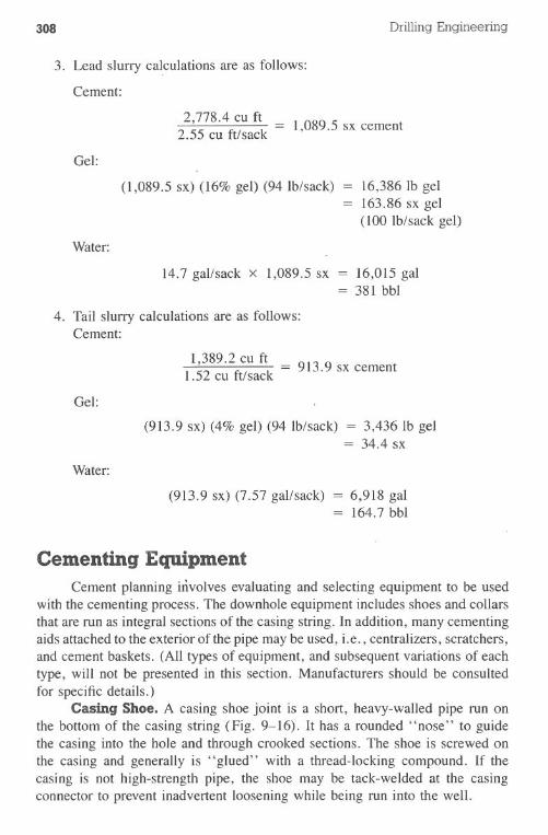
308 Drilling Engineering
3. Lead slurry calculations are as follows:
Cement:
2,778.4 cu ft = 1,089.5 sx cement
Gel:
(1,089.5 sx) (16% gel) (94 Ib/sack) 16,386 Ib gel163.86 sx gel(100 Ib/sack gel)
Water:
14.7 gal/sack x 1,089.5sx = 16,015gal= 381 bbl
4. Tail slurry calculations are as follows:Cement:
1,389.2 cu ft = 913.9 sx cement
Gel:
(913.9 sx) (4% gel) (94 Ib/sack) = 3,436 Ib gel= 34.4 sx
Water:
(913.9 sx) (7.57 gal/sack) = 6,918 gal164.7 bbl
Cementing EquipmentCement planning involves evaluating and selecting equipment to be used
with the cementing process. The downhole equipment includes shoes and collarsthat are run as integral sections of the casing string. Inaddition, many cementingaids attached to the exterior of the pipe may be used, i.e., centralizers, scratchers,and cement baskets. (All types of equipment, and subsequent variations of eachtype, will not be presented in this section. Manufacturers should be consultedfor specific details.)
Casing Shoe. A casing shoe joint is a short, heavy-walled pipe run onthe bottom of the casing string (Fig. 9-16). It has a rounded "nose" to guidethe casing into the hole and through crooked sections. The shoe is screwed onthe casing and generally is "glued" with a thread-locking compound. If thecasing is not high-strength pipe, the shoe may be tack-welded at the casingconnector to prevent inadvertent loosening while being run into the well.
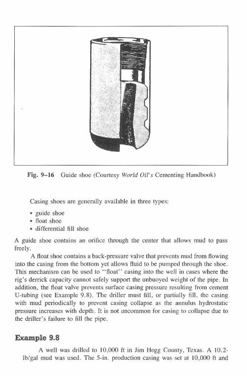
Cementing 309
Fig. 9-16 Guide shoe (Courtesy World Oil's Cementing Handbook)
Casing shoes are generally available in three types:
·guide shoe· float shoe· differential fill shoe
A guide shoe contains an orifice through the center that allows mud to passfreely.
A float shoe contains a back-pressure valve that prevents mud from flowinginto the casing from the bottom yet allows fluid to be pumped through the shoe.This mechanism can be used to "float" casing into the well in cases where therig's derrick capacity cannot safely support the unbuoyed weight of the pipe. Inaddition, the float valve prevents surface casing pressure resulting from cementV-tubing (see Example 9.8). The driller must fill, or partially fill, the casingwith mud periodically to prevent casing collapse as the annulus hydrostaticpressure increases with depth. It is not uncommon for casing to collapse due tothe driller's failure to fill the pipe.
Example 9.8
A well was drilled to 10,000 ft in Jim Hogg County, Texas. A 10.2-lb/gal mud was used. The 5-in. production casing was set at 10,000 ft and
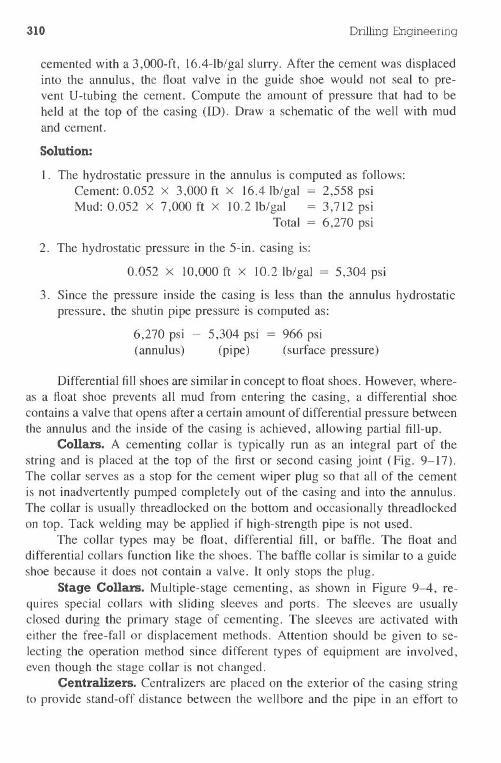
310 Drilling Engineering
cemented with a 3,000-ft, 16.4-lb/gal slurry. After the cement was displacedinto the annulus, the float valve in the guide shoe would not seal to pre-vent V-tubing the cement. Compute the amount of pressure that had to beheld at the top of the casing (10). Draw a schematic of the well with mudand cement.
Solution:
I. The hydrostatic pressure in the annulus is computed as follows:Cement: 0.052 x 3,000 ft x 16.4lb/gal = 2,558 psiMud: 0.052 x 7,000 ft x 1O.2Ib/gal = 3,712 psi
Total = 6,270 psi
2. The hydrostatic pressure in the 5-in. casing is:
0.052 x 10,000 ft x 10.2 lb/gal = 5,304 psi
3. Since the pressure inside the casing is less than the annulus hydrostaticpressure, the shutin pipe pressure is computed as:
6,270 psi(annulus)
5,304 psi(pipe)
966 psi(surface pressure)
Differential fill shoes are similar in concept to float shoes. However, where-as a float shoe prevents all mud from entering the casing, a differential shoecontains a valve that opens after a certain amount of differential pressure betweenthe annulus and the inside of the casing is achieved, allowing partial fill-up.
Collars. A cementing collar is typically run as an integral part of thestring and is placed at the top of the first or second casing joint (Fig. 9-17).The collar serves as a stop for the cement wiper plug so that all of the cementis not inadvertently pumped completely out of the casing and into the annulus.The collar is usually threadlocked on the bottom and occasionally threadlockedon top. Tack welding may be applied if high-strength pipe is not used.
The collar types may be float, differential fill, or baffle. The float anddifferential collars function like the shoes. The baffle collar is similar toa guideshoe because it does not contain a valve. It only stops the plug.
Stage Conars. Multiple-stage cementing, as shown in Figure 9-4, re-quires special collars with sliding sleeves and ports. The sleeves are usuallyclosed during the primary stage of cementing. The sleeves are activated witheither the free-fall or displacement methods. Attention should be given to se-lecting the operation method since different types of equipment are involved,even though the stage collar is not changed.
~entralizers. Centralizers are placed on the exterior of the casing string.to provide stand-off distance between the wellbore and the pipe in an effort to
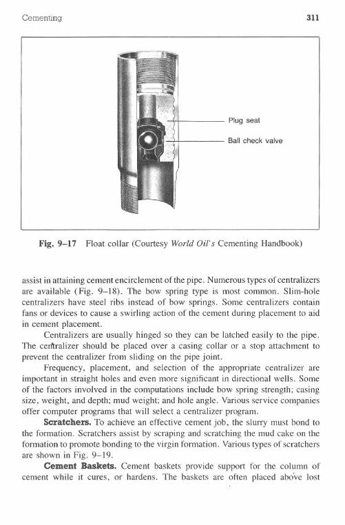
Cementing 311
Plugseat
Ball check valve
Fig. 9-17 Float collar (Courtesy World Oil's Cementing Handbook)
assist in attaining cement encirclement of the pipe. Numerous types of centralizersare available (Fig. 9-18). The bow spring type is most common. Slim-holecentralizers have steel ribs instead of bow springs. Some centralizers containfans or devices to cause a swirling action of the cement during placement to aidin cement placement. .
Centralizers are usually hinged so they can be latched easily to the pipe.The cedtralizer should be placed over a casing collar or a stop attachment toprevent the centralizer from sliding on the pipe joint.
Frequency, placement, and selection of the appropriate centralizer areimportant in straight holes and even more significant in directional wells. Someof the factors involved in the computations include bow spring strength; casingsize, weight, and depth; mud weight; and hole angle. Various service companiesoffer computer programs that will select a centralizer program.
Seratehers. To achieve an effective cement job, the slurry must bond tothe formation. Scratchers assist by scraping and scratching the mud cake on theformation to promote bonding to the virgin formation. Varioustypes of scratchersare shown in Fig. 9-19.
Cement Baskets. Cement baskets provide support for the column ofcement while it cures, or hardens. The baskets are often placed above lost
I
~I
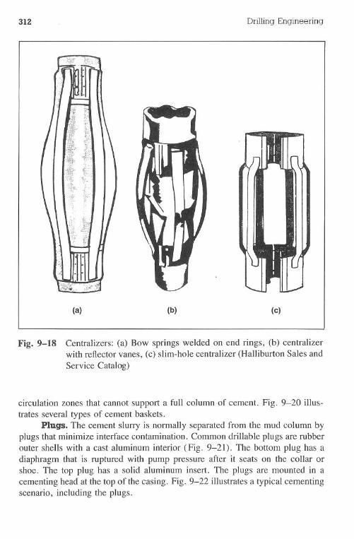
312
(a)
Drilling Engineering
(b) (c)
Fig. 9-18 Centralizers: (a) Bow springs welded on end rings, (b) centralizerwith reflector vanes, (c) slim-hole centralizer (Halliburton Sales andService Catalog)
circulation zones that cannot support a full column of cement. Fig. 9-20 illus-trates several types of cement baskets.
Plugs. The cement slurry is normally separated from the mud column byplugs that minimize interface contamination. Common drillable plugs are rubberouter shells with a cast aluminum interior (Fig. 9-21). The bottom plug has adiaphragm that is ruptured with pump pressure after it seats on the collar orshoe. The top plug has a solid aluminum insert. The plugs are mounted in acementing head at the top of the casing. Fig. 9-22 illustrates a typical cementingscenario, including the plugs.
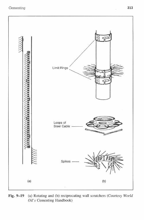
Cementing
(a)
313
Loops ofSteel Cable -
Spikes -
(b)
Fig. 9-19 (a) Rotating and (b) reciprocating wall scratchers (Courtesy WorldOil's Cementing Handbook)
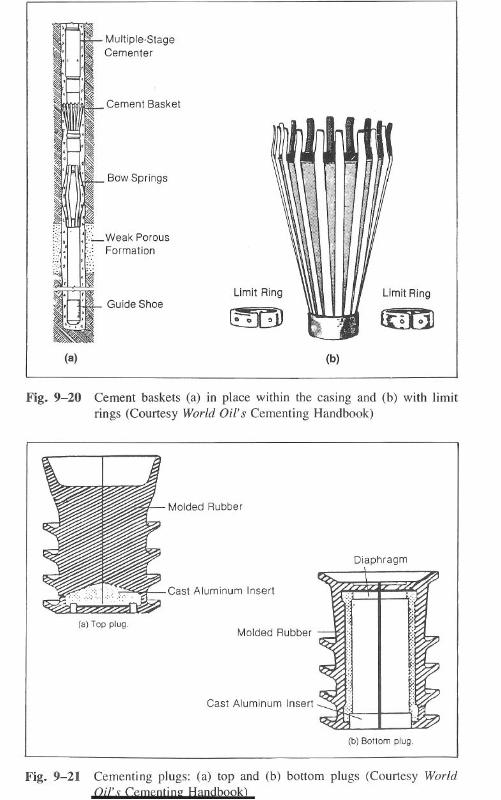
Multiple-StageCementer
Cement Basket
Bow Springs
Limit Ring Limit RingGuide Shoe
(a) (b)
Fig. 9-20 Cement baskets (a) in place within the casing and (b) with limitrings (Courtesy World Oil's Cementing Handbook)
Molded Rubber
Diaphragm
Cast Aluminum Insert
(a) Top plug.Molded Rubber
Cast Aluminum Insert
(b) Bottom plug.
Fig. 9-21 Cementing plugs: (a) top and (b) bottom plugs (Courtesy Worldnil' ~ f:ementinl? Handbook)
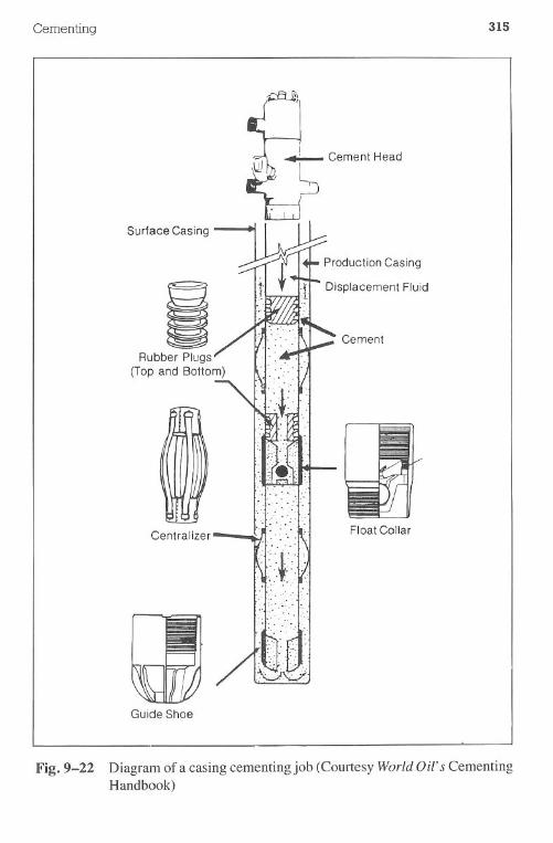
Cementing 315
.L CementHead
~
Centralizer Float Collar
Guide Shoe
Fig.9-22 Diagram of a casing cementing job (Courtesy WorldOil's CementingHandbook)
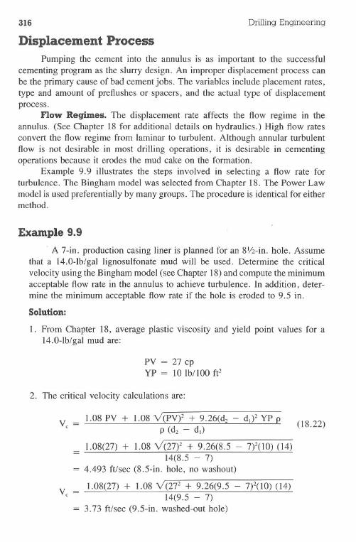
316
Displacement Process
Drilling Engineering
Pumping the cement into the annulus is as important to the successfulcementing program as the slurry design. An improper displacement process canbe the primary cause of bad cement jobs. The variables include placement rates,type and amount of preflushes or spacers, and the actual type of displacementprocess.
Flow Regimes. The displacement rate affects the flow regime in theannulus. (See Chapter 18 for additional details on hydraulics.) High flow ratesconvert the flow regime from laminar to turbulent. Although annular turbulentflow is not desirable in most drilling operations, it is desirable in cementingoperations because it erodes the mud cake on the formation.
Example 9.9 illustrates the steps involved in selecting a flow rate forturbulence. The Bingham model was selected from Chapter 18. The Power Lawmodel is used preferentially by many groups. The procedure is identical for eithermethod.
Example 9.9
. A 7-in. production casing liner is planned for an 8Y2-in.hole. Assumethat a 14.0-lb/gal lignosulfonate mud will be used. Determine the criticalvelocity using the Bingham model (see Chapter 18)and compute the minimumacceptable flow rate in the annulus to achieve turbulence. In addition, deter-mine the minimum acceptable flow rate if the hole is eroded to 9.5 in.
Solution:
1. From Chapter 18, average plastic viscosity and yield point values for a14.0-lb/gal mud are:
PV = 27 cpYP = 10 Ib/100fe
2. The critical velocity calculations are:
v = 1.08 PV + 1.08 Y(PV)2 + 9.26(d2- d,)2YP pC P (d2 - d.)
1.08(27) + 1.08 Y(27)2 + 9.26(8.5 - 7)2(10) (14)14(8.5 - 7)
= 4.493 ft/sec (8.5-in. hole, no washout)
V = 1.08(27)+ 1.08Y(272+ 9.26(9.5- 7f(10) (14)c 14(9.5 - 7)
= 3.73 ft/sec (9.5-in. washed-out hole)
(18.22)
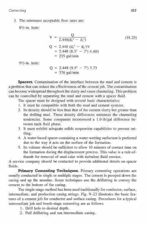
Cementing 317
3. The minimum acceptable flow rates are:
8Y2-in.hole:
v- Q- 2.448(dl - d12)
Q = 2.448 (dl - d21)V2.448 (8.52 - 72)4.493
= 255 gal/min
(18.25)
9112-in. hole:
Q = 2.448 (9.52 - 72) 3.73= 376 gal/min
Spacers. Contamination of the interface between the mud and cement isa problem that can reduce the effectiveness of the cement job. The contaminationcan become widespread throughout the slurry and cause channeling. This problemcan be controiled by separating the mud and cement with a spacer fluid.
The spacer must be designed with several basic characteristics:I. It must be compatible with both the mud and cement systems.2. Its density should be less than that of the cement slurry but greater than
the drilling mud. These density differences minimize the channelingtendencies. Some companies recommend a I.O-Ib/gal difference be-tween each fluid phase.
3. It must exhibit adequate solids suspension capabilities to prevent set-tling.
4. A water-based spacer containing a water-wetting surfactant is preferreddue to the way it acts on the surface of the formation.
5. Its volume should be sufficient to allow to minutes of contact time onthe formation during the displacement process. This value is a rule-of-thumb for removal of mud cake with turbulent fluid erosion.
A service company should be contacted to provide additional details on spacerfluids.
Primary Cementing Techniques. Primary cementing operations areusually conducted in single or multiple stages. The cement is pumped down thecasing and up the annulus. Some techniques use the drillstring to convey thecement to the bottom of the casing.
The single-stage method has been used traditionally for conductor, surface,intermediate, and production casing strings. Fig. 9-23 illustrates the basic fea-tures of a cement job for conductor and surface casing. Procedures for a typicalintermediate job and bomb-stage cementing are as follows:
1. Drill hole to desired depth.2. Pull drillstring and run intermediate casing.
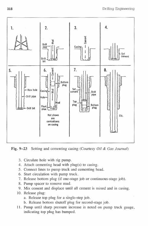
318
1. 2.
5. 6.
Mud
~~~~&lJNot shown
arecentralizersoncasinl
Drilling Engineering
3. 4.
7. '
[].'.' ::",;. ::
Set :':: :~cement (., ;i Drill
:-- I f) pipe
8.'
1'". ",
. ....,':.':."
.':
Topplug
I.',
rcABollom
~ plUI"
Etc,
Fig. 9-23 Setting and cementing casing (Courtesy Oil & Gas Journal)
3. Circulate hole with rig pump.4. Attach cementing head with plug(s) to casing.5. Connect lines to pump truck and cementing head.6. Start circulation with pump truck,7. Release bottom plug (if one-stage job or continuous-stage job).8. Pump spacer to remove mud.9, Mix cement and displace until all cement is mixed and in casing.
10. Release plug:a. Release top plug for a single-step job.b. Release bottom shutoff plug for second-stage job.
11. Pump until sharp pressure increase is noted on pump truck gauge,indicating top plug has bumped.
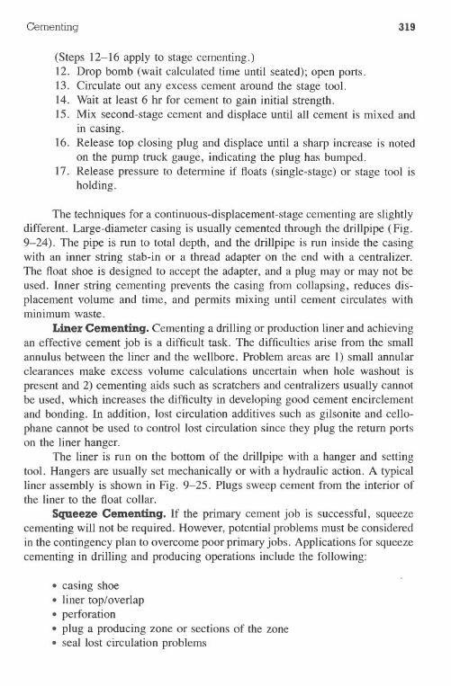
Cementing 319
(Steps 12-16 apply to stage cementing.)12. Drop bomb (wait calculated time until seated); open ports.13. Circulate out any excess cement around the stage tool.14. Wait at least 6 hr for cement to gain initial strength.15. Mix second-stage cement and displace until all cement is mixed and
in casing.16. Release top closing plug and displace until a sharp increase is noted
on the pump truck gauge, indicating the plug has bumped.17. Release pressure to determine if floats (single-stage) or stage tool is
holding.
The techniques for a continuous-displacement-stage cementing are slightlydifferent. Large-diameter casing is usually cemented through the drillpipe (Fig.9-24). The pipe is run to total depth, and the drillpipe is run inside the casingwith an inner string stab-in or a thread adapter on the end with a centralizer.The float shoe is designed to accept the adapter, and a plug mayor may not beused. Inner string cementing prevents the casing from collapsing, reduces dis-placement volume and time, and permits mixing until cement circulates withminimum waste.
Liner Cementing. Cementing a drilling or production liner and achievingan effective cement job is a difficult task. The difficulties arise from the smallannulus between the liner and the wellbore. Problem areas are 1) small annularclearances make excess volume calculations uncertain when hole washout ispresent and 2) cementing aids such as scratchers and centralizers usually cannotbe used, which increases the difficulty in developing good cement encirclementand bonding. In addition, lost circulation additives such as gilsonite and cello-phane cannot be used to control lost circulation since they plug the return portson the liner hanger.
The liner is run on the bottom of the drillpipe with a hanger and settingtool. Hangers are usually set mechanically or with a hydraulic action. A typicalliner assembly is shown in Fig. 9-25. Plugs sweep cement from the interior ofthe liner to the float collar.
Squeeze Cementing. If the primary cement job is successful, squeezecementing will not be required. However, potential problems must be consideredin the contingency plan to overcome poor primary jobs. Applications for squeezecementing in drilling and producing operations include the following:
· casing shoe· liner top/overlap.perforation.plug a producing zone or sections of the zone· seal lost circulation problems
II
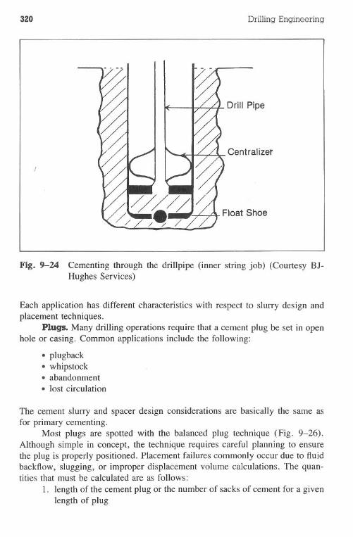
320 Drilling Engineering
Drill Pipe
Centralizer
Float Shoe
Fig. 9-24 Cementing through the drillpipe (inner string job) (Courtesy BJ-Hughes Services)
Eachapplicationhasdifferent characteristicswith respectto slurrydesign andplacement techniques.
Plugs. Many drilling operations require that a cement plug be set in openhole or casing. Common applications include the following:
.plugback·whipstock· abandonment.lost circulation
The cement slurry and spacer design considerations are basically the same asfor primary cementing.
Most plugs are spotted with the balanced plug technique (Fig. 9-26).Although simple in concept, the technique requires careful planning to ensurethe plug is properly positioned. Placement failures commonly occur due to fluidbackflow, slugging, or improper displacement volume calculations. The quan-tities that must be calculated are as follows:
I. length of the cement plug or the number of sacks of cement for a givenlength of plug
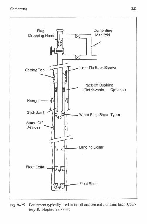
Cementing
Hanger
Slick Joint
Stand-OffDevices
321
CementingManifold
Liner Tie-Back Sleeve
Pack.off Bushing(Retrievable - Optional)
Wiper Plug (Shear Type)
LandingCollar
Float Shoe
Fig. 9-25 Equipment typically used to install and cement a drilling liner (Cour-tesy BJ-Hughes Services)
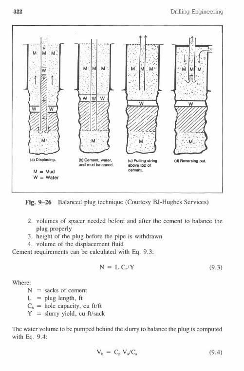
3ZZ
.... '.~'
..'..
(a) Displacing.
M = MudW = Water
f
.':.
r;.-",...
.
'1.,.:,,- .:. ........
. -: . ,', . .. ""...'..,.", "
(b) Cemenl, waler,and mud balanced.
" t..__"f' 1
:;:.:\ "(' ~":'.::U'. '.,
;.::'~~ T: ~.:~~,~..-:; :.',.f.:~'.~.~ ....:::; .:.'. "
(c) Pullingairingabove lop ofcement.
Drilling Engineering
'. .'.: ... i. 0"
,,:-':':';~:':\:::". : ., : :.. ....
(d) Reversing out.
Fig. 9-26 Balanced plug technique (Courtesy BJ-Hughes Services)
2. volumes of spacer needed before and after the cement to balance theplug properly
3. height of the plug before the pipe is withdrawn4. volume of the displacement fluid
Cement requirements can be calculated with Eq. 9.3:
Where:NL =Ch =Y =
sacks of cement
plug length, fthole capacity, cu ft/ftslurry yield, cu ft/sack
(9.3)
The water volume to be pumped behind the slurry to balance the plug is computedwith Eq. 9.4:
(9.4)
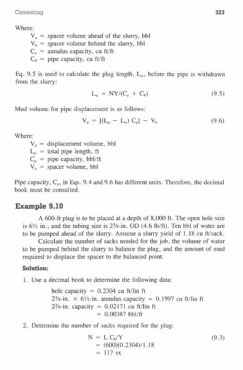
Cementing 323
Where:
Va = spacer volume ahead of the slurry, bblVb = spacer volume behind the slurry, bblCa = annulus capacity, cu ft/ftCp = pipe capacity, cu ft/ft
Eq. 9.5 is used to calculate the plug length, Lw, before the pipe is withdrawnfrom the slurry:
(9.5)
Mud volume for pipe displacement is as follows:
Vd = [(Lp - Lw) Cp] - Vb (9.6)
Where:
Vd = displacementvolume,bblLp = total pipe length, ftCp = pipe capacity, bbl/ftVb = spacer volume, bbl
Pipe capacity, Cp, in Eqs. 9.4 and 9.6 has different units. Therefore, the decimalbook must be consulted.
Example 9.10
A 600-ft plug is to be placed at a depth of 8,000 ft. The open hole sizeis 6Y2 in., and the tubing size is 23fs-in.OD (4.6 lb/ft). Ten bbl of water areto be pumped ahead of the slurry. Assume a slurry yield of 1.18 cu ft/sack.
Calculate the number of sacks needed for the job, the volume of waterto be pumped behind the slurry to balance the plug, and the amount of mudrequired to displace the spacer to the balanced point.
Solution:
1. Use a decimal book to determine the following data:
hole capacity = 0.2304 cu ft/tin ft23fs-in. x 6Y2-in. annulus capacity = 0.1997 cu ft/lin ft23fs-in. capacity = 0.02171 cu ft/tin ft
= 0.00387 bbl/ft
2. Determine the number of sacks required for the plug:
N = L Ch/Y= (600)(0.2304)/1.18= 117 sx
(9.3)
324 Drilling Engineering
3. Calculate the volume of water to be pumped behind the slurry to balancethe plug:
Vb = Cp Va/Ca= (0.02171)(10)/0.1997
1.09 bbl
(9.4)
4. Determine the length of the plug before the pipe is withdrawn from theslurry:
Lw = (N Y)/Ca + Cp)= (117 X 1.18)/(0.1997 + 0.02171)= 623.5 ft
(9.5)
5. Calculate the displacement volume, Vd:
Vd = [(Lp- Lw)(Cp)]- Vb= [(8,000 - 623.5)(0.00387)]- 1.09= 27.5 bbl
(9.6)
Special Cementing ProblemsCement slurries often must be designed to control special problems. Al-
though it is unlikely that a solution exists for each situation, proper planningwill help achieve an effective cement job. Service companies usually offer adviceand expertise to overcome most difficult problems.
Salt Sections. Formations containing significant salt sections will washout if conventional water-based mud and cement slurries are used. Drilling mudsare usually modified so that the water phase is salt saturated or an oil mud isused. Likewise, the cement slurry must be designed so the water phase is saltsaturated if effective bonding is to be achieved and washouts prevented.
Kicks Following Cementing. Kicks and blowouts have been experi-enced on wells immediately following apparently successful cementing opera-tions. Some of the many problems associated with this type of kick are theseemingly random nature with which the kick occurs, the identification of theflowing zone, and tbe inability to circulate a heavy fluid and kill the well.Although surface blowouts in this situation are dramatic, underground blowoutsresulting from gas-through-cement kicks can also cause problems, such as pres-sure charging other zones that will affect offset drilling and the loss of hydro-carbon reserves.
One operator used a noise log to estimate that as much as 300 Mcfd ofgas transferred between zones as a result of the problem in one field case. Thesekicks, however, are not random in nature, and by exercising certain precautionstheir occurrence can be minimized.
Cementing 325
Gas-through-Cement Kicks. Assuming that a cement operation is com-pleted without such problems as previously existing gas-cut mud, lost circulation,or cement channeling, then the circumstances to allow gas migration and resultingkicks to occur have been established by several authors. These circumstances'can be illustrated by Fig. 9-27.
One or more permeable zones should exist above a gas-bearing interval,with the upper zone(s) having pressures lower than the gas zone. The cementmust set on the upper zones and support the drilling fluid hydrostatic pressure.After the cement has set, the pressure within the lower interval must be reducedbelow formation pressure, at which time gas flow may occur. If the seal from
Bridge forms due to !.-filtration into upper \.:
permeable zone . - -
. ... . .Permeable zone
The bridge supports the
-=-: '7 hydrostatic pressure- -. ~
~~;~
~~; :: Equivalent formation: '.'.'.:':
}}:.. :.pressure less than: '.'.:.;:':;'
'~~'~~~~ :.::.::::;:::::::
'. '" .. . . ...... 10f t...
. ,.. ...." ...".
- -- -
- -- ----
- -- -Pressure reduction due
to cement fluid loss or
volume shrinkage properties
Cement densitydesigned to
control lowerzones
-- - - - -.--- -
- Casing- - --
- - Gas begins migration. up the annulus
-rll.O
.::..".." :.:
~.: P;tl
:;..:'permeable. :::.: ~}:.: .." gas zone .. '.'.'.. t. ~. #I
rrA:.A. " . 'i.1~
:_~!- - j- =-~~~Z~~i~~I~:~~~~:
. ....
,., ,.,"... '0'.
Fig. 9-27 Circumstances involved in gas-through-cement kicks
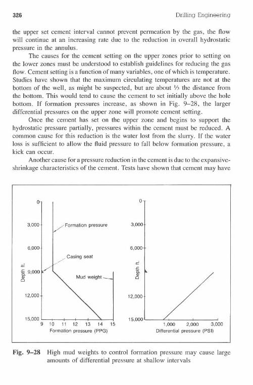
326 DrillingEngineering
the upper set cement interval cannot prevent permeation by the gas, the flowwill continue at an increasing rate due to the reduction in overall hydrostaticpressure in the annulus.
The causes for the cement setting on the upper zones prior to setting onthe lower zones must be understood to establish guidelines for reducing the gasflow. Cement setting is a function of many variables, one of which is temperature.Studies have shown that the maximum circulating temperatures are not at thebottom of the well, as might be suspected, but are about '13the distance fromthe bottom. This would tend to cause the cement to set initially above the holebottom. If formation pressures increase, as shown in Fig. 9-28, the largerdifferential pressures on the upper zone will promote cement setting.
Once the cement has set on the upper zone and begins to support thehydrostatic pressure partially, pressures within the cement must be reduced. Acommon cause for this reduction is the water lost from the slurry. If the waterloss is sufficient to allow the fluid pressure to fall below formation pressure, akick can occur.
Another cause for a pressure reduction in the cement is due to the expansive-shrinkage characteristics of the cement. Tests have shown that cement may have
Fig. 9-28 High mud weights to control formation pressure may cause largeamounts of differential pressure at shallow intervals
0 0
3,000 Formation pressure 3,000
6,000 6,000
/ Casing seat .;:;
i 9'OOO Mud weight-.JC.Q)00
12,000 12,000
15,000 15,0009 10 11 12 13 14 15 1,000 2,000 3,000
Formation pressure (PPG) Differential pressure (PSI)
Cementing 327
a tendency for initial shrinkage when downhole conditions of temperature andpressure are applied (Fig. 9-29). If shrinJcageoccurs, the pressure will be reducedbecause the cement volume will be less than the cement-sealed fixed boreholevolume. To offset the shrinkage, commercial cement additives are available thatcause the cement to expand from initial conditions without any shrinkage(Fig. 9-30).
Reducing Gas-through-Cement Kicks. Proper cementing proceduresshould be exercised to ensure the kicks are not a function of mechanical problems.These procedures include using cementing aids such as centralizers, conditioningthe hole properly before cementing, and releasing surface pressure after cementplacement to avoid the fonnation of a microannulus. The cementing operationshould be monitored to ensure that lost circulation does not occur.
The cement slurry should be tailored with chemical additives to avoid thecauses of kicks. Retarding agents should be blended with the cement batches toensure the slurry will set from the bottom to the top. Additives should be usedto prevent cement volume shrinkage. The fluid loss from the cement should bereduced as low as practical.
Fig. 9-29 Expansive shrinkage characteristics of a cement sample (CourtesySociety of Petroleum Engineers)
0.041 I I I I I I Effect of temperatureClass H, 35% Silica-Sand
Sat. Salt 42% Water0.03 3,000 psi
0.02<::0 I I 1 /1 I I I 200°F'0;
0.Q1)(w?ft I I I I ---!-300°F00
-0.01II
-0.02 II0 10. 20 50 60 !
Curing time/hours
328 Drilling Engineering
.6
.3
.5
.4
-.21 2 3 5 10 20 30
Curing timelhours
50 100 200
Fig. 9-30 Effect of certain commercial additives on expansive properties ofcement (Courtesy Society of Petroleum Engineers)
Problems9.1 A 1O,000-ftwell with a fracture gradient of 16.2Ib/gal equivalent mud
weight is going to be cemented with a 16.8-lb/gal slurry. The mudweight in the well is 15.7 lb/gal. If the equivalent circulating densityincrease is 0.3 Ib/gal, resulting from fluid circulation, how high can thecementtop be circulatedwithoutfracturingthe casingseat?
9.2 Refer to Example 9.3. Calculate the location of the cement top if thedrilling engineer uses 500 sacks of cement; 600 sacks.
9.3 Calculate the temperature at 12,500 ft in a well at the Texas-Louisiana-Gulf of Mexico intersection. Assume that the ambient temperature is75°F. Refer to Fig. 9-12.
9.4 Calculate the capacity of 13,000 ft of 43.5-lb/ft, 9%-in. casing.
9.5 Determine the annular volume between 2,500 ft of 1O%-in.casing anda 17Y2-in. hole.
./
/""
.//'
...,/ Commercialexpansivecement,46% Water- 100°F
3,000 psi
III
c.2<f)c
.2
eft .1
0
-.1
Cementing 329
9.6 Rework Example 9.7 for a 3,500-ft, I71/2-in.hole with 10%-in. pipe.
9.7 Rework Example 9.9 for mud weights of 10.0, 12.0, 16.0, and 18.0Ib/gaI. Plot the results.
References
Adams, N.J. Well Control Problems and Solutions. Tulsa: PennWell Pub-lishing, 1980.
Beirute, R., and A. Tragesser. "Expansive-Shrinkage Characteristics of Ce-ments under Actual Well Conditions." SPE 4091, Journal of PetroleumTechnology, August 1973.
BJ-Hughes. Fundamentals of Cementing, 1981.
BJ-Hughes. General Catalog.
Carter, G., and K. Slagle. "A Study of Completion Practices to MinimizeGas Communications." Journal of Petroleum Technology, September 1972.
Casing Centralizers, API Specification IOD, 1973.
Cook, C., and L.G. Carter. "Gas Leakage Associated with Static Cement."Drilling, DCW, March 1976.
Garcia, J.A., and C.R. Clark. "An Investigation of Annular Gas Flow Fol-lowing Cementing Operations." SPE 5701, January 1976.
Halliburton. General Catalog.
The New Encyclopedia Britannia in 30 Volumes. Chicago, 1980, p. 1077.
Oil-Well Cements and Cement Additives. API Specification lOA, 1979.
Parker, P., C. Clement, and R. Beirute. "Basic Cementing." An 8-part series,Oil & Gas Journal. 1977.
Raymond, L.R. "Temperature Distribution in a Circulating Drilling Fluid."Journal of Petroleum Technology, March 1969.

330 Drilling Engineering
Suman, G.O., and R.C. Ellis. World Oil's Cementing Handbook. Houston:Gulf Publishing, 1977.
Sweatman, Ron. BJ-Hughes, personal communications.
Chapter 1 0 DirectionalPlanning
Directional drilling has grown to be an integral part of the we1lplanningprocess. Directional we1lsare commonly drilled and used for several purposes.As is the case with most subjects related to drilling engineering, directionalplanning and drilling is an extensive topic that requires a thorough understandingof the components before implementation.
Directional drilling is much more than simply selecting a we1l path andhole angle. It includes selecting the most appropriate survey techniques, definingthe best control tools, researching applicable government regulations, and gath-ering pertinent geological data. In addition, the directional program may alteror affect the casing and cement program, hydraulics, centralization, and com-pletion techniques.
Purposes of Directional DrillingContro1leddirectional drilling is the process of deviating a we1lborealong
a predetermined course to a target whose location is given as lateral distancefrom the vertical. This definition is the basis for a1lcontro1leddirectional drilling,whether to maintain the we1lbore as nearly vertical as possible or as a planneddeviation from the vertical. Vertical drilling, although considered fundamentalin most areas, can be very difficult to achieve in some regions due to steeplydipping formations.
Inaccessible Locations. Quite often, a target pay zone lies vertica1lybeneath a surface location that is impractical as a rig site. Common examplesinclude residential locations, riverbeds, mountains, harbors, and roads. In thesecases, a rig site is selected and the we1l is dri1led directiona1ly into the targetzone.
331
332 DrillingEngineering
Multiple WeDs Drilling from a Single Site. Perhaps the most commonapplication for directional drilling is associated with offshore production plat-forms. It is more economical, in most cases, to drill a number of directionalwells from a single platform than to build individual platforms for vertical wells.Some North Sea platforms have the capability to drill as many as 60 wells fromthe single structure (Fig. 10-1).
Multiple wells from a single site are not uncommon in land operations.The basic principle is the economic consideration of building multiple sites,pipelines, production facilities, etc. Most of the USSR's western Siberian drillingis from multiwell sites.
Fig. 10-1 Directional drilling from an offshore platform (Courtesy WilsonDirectional Co.)
Directional Planning 333
Sidetracking. A frequently occurring cause for directional drilling issidetracking. The primary purpose is to deviate the wellbore around and awayfrom an obstruction in the original wellbore, such as a stuck drillstring. Generally,sidetracking cannot be defined as controlled directional drilling because it doesnot have a predetermined target.
Relief Wen Drilling. Possibly the most spectacular application of direc-tional drilling is drilling a relief well to intersect a blowout well near the bottomso that mud and water can be pumped into the blowout well (Fig. 10-2).Directional control in this type of drilling is stringent due to the extreme accuracyrequired to locate and intersect the blowout well. Quite often, special loggingtools are required in locating the blowout well.
I
Relief well drilling
Fig. 10-2 Relief well drilling (Courtesy Wilson Directional Drilling)
334 Drilling Engineering
Multiple Targets. Geologists may define multiple targets for a prospectthat cannot be drilled,with a vertical well. It may be necessary to drill throughone target and alter the direction of the well to reach the next target. The targetsmay be in a two-dimensional plane such that only the drift angle must be altered.Other cases may involve three-dimensional planning such that the inclinationand azimuth must be changed.
Design ConsiderationsAssuming that a target and rig site have been selected, the directional
planning considerations are shown in Fig. 10-3. The values that must be iden-tified are as follows:
.lateral, or horizontal, displacement from the target to a vertical line fromthe rig site. kickoff point (KOP).desired build angle rate· final drift angle.plan type: straight kick vs S curve
If an S curve is selected as the plan type, the engineer must also select a dropangle rate and a depth at which the hole must return to vertical.
Drift, or Inclination, Angle. The drift, or inclination, of the wellboreis the angle, measured in degrees, between the actual well path at some depthand a vertical line below the rig site. This measurement is independent of theazimuth or course heading. Typically, this value will range from 15°_35°.
A minimum acceptable drift angle of approximately 12°_15° is desired bymany industry personnel. Drift angles less than this range are slightly moredifficult to control. In other words, it is usually easier to control a 20° well thana 10° well.
Although wells have been drilled in the 70°_80° range, common upperrestraints are 45°-48°. Hole angles greater than 45°-48° begin to encounterproblems such as increased torque and drag as well as pumpdown requirementsfor some logging operations. Many operators establish 35° as the upper limit.
The typical planning procedure is to establish minimum and maximumacceptable drift angles and a KOP (kickoff point). A well course is computed.If the calculated drift angle required to reach the target falls outside the driftangle constraints, a new KOP is selected. In some cases, compromises arerequired between optimum KOP and drift angles.
Kickoff Point (KOP). The KOP is the depth at which the wellbore pathwill be intentionally diverted from the vertical position. The KOP is usuallyselected in soft, shallow formations where directional drilling is easier. In ad-dition, the KOP is often selected so the final angle buildup can be achieved prior
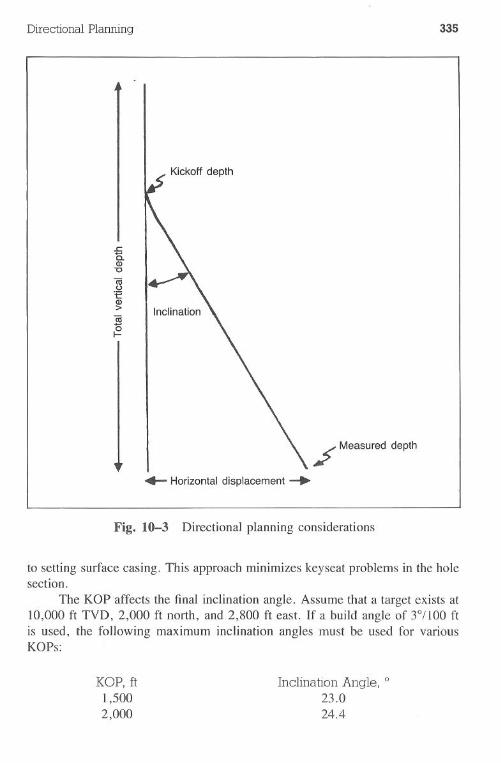
Directional Planning 335
Kickoff depth
.r:a.Q)"tJIiio'EQ)>Iii
~
;' Measured depth
.- Horizontal displacement -..
Fig.10-3 Directional planning considerations
to setting surface casing. This approach minimizes keyseat problems in the holesection.
The KOP affects the final inclination angle. Assume that a target exists at10,000 ft TVD, 2,000 ft north, and 2,800 ft east. If a build angle of 3°1100ftis used, the following maximum inclination angles must be used for variousKOPs: .
KOP, it1,5002,000
Inclination Angle, °23.024.4
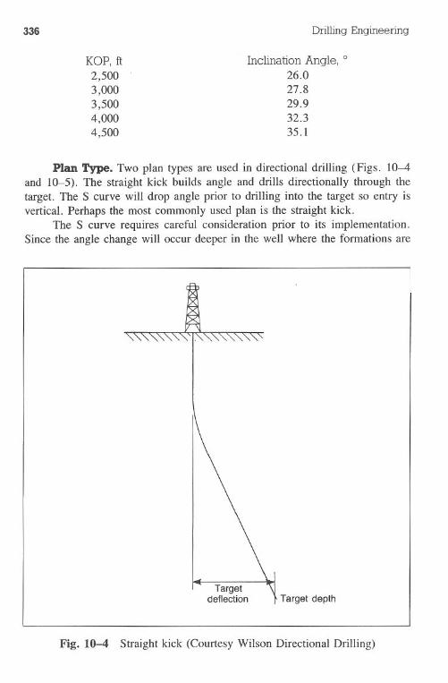
336 Drilling Engineering
KOP, ft2,5003,0003,5004,0004,500
InclinationAngle, 0
26.027.829.932.335.1
Plan Type. Two plan types are used in directional drilling (Figs. 10-4and 10-5). The straight kick builds angle and drills directionally through thetarget. The S curve will drop angle prior to drilling into the target so entry isvertical. Perhaps the most commonly used plan is the straight kick.
The S curve requires careful consideration prior to its implementation.Since the angle change will occur deeper in the well where the formations are
Targetdeflection Target depth
Fig. 10-4 Straight kick (Courtesy Wilson Directional Drilling)
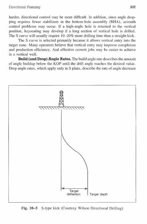
Directional Planning 337
harder, directional control may be more difficult. In addition, since angle drop-ping requires fewer stabilizers in the bottom-hole assembly (BHA), azimuthcontrol problems may occur. If a high-angle hole is returned to the verticalposition, keyseating may develop if a long section of vertical hole is drilled.The S curve will usually require 10-20% more drilling time than a straight kick.
The S curve is selected primarily because it allows vertical entry into thetarget zone. Many operators believe that vertical entry may improve completionand production efficiency. And effective cement jobs may be easier to achievein a vertical well.
Build (and Drop) Angle Rates. The build angle rate describes the amountof angle buildup below the KOP until the drift angle reaches the desired value.Drop angle rates, which apply only in S plans, describe the rate of angle decrease
Targetdeflection Target depth
Fig. 10-5 S-type kick (Courtesy Wilson Directional Drilling)
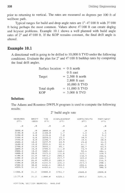
338 Drilling Engineering
prior to returning to vertical. The rates are measured as degrees per 100 ft ofwellbore path.
Typical ranges for build and drop angle rates are 1°-4°1100 ft with 3°/100ft being perhaps the most common. Values above 4°/100 ft can create doglegand keyseat problems. Example 10.1 shows a well planned with build anglerates of 2° and 4°/100 ft. If the KOP remains constant, the final drift angle isaltered.
Example 10.1
A directional well is going to be drilled to 10,000 ft TVD under the followingconditions. Evaluate the plan for 2° and 4°1100ft buildup rates by computingthe final drift angles.
Surface location o ft northo ft east2,500 ft north2,800 ft east10,000 ft TVD11,000 ft TVD3,000 ft TVD
Target
Total depthKOP
Solution:
The Adams and Rountree DWPLN program is used to compute the followingresults:
2° build angle rate
MEASURED DRIFT TVD DISPLACEMENT NORTH/SOUTH EAST/WEST(FT> <DEG> (FT> (FT> (FT> (FT>
.0 .0 .0 .0 .0 .0
3000.0 .0 3000.0 .0 .0 .03100.0 2.0 3100.0 1.7 1.2 1.33200.0 4.0 31'39.8 7.0 4.6 5.23300.0 6.0 3299.5 15.7 10.5 11.73400.0 8.0 33'38.7 27.9 18.6 20.83500.0 10.0 3497.5 43.5 29.0 32.53600.0 12.0 3595.6 62.6 41.7 46.73700.0 14.0 3693.I 85.1 56.7 63.53800.0 16.0 378'3.6 111.0 73.9 82.83900.0 18.0 3885.3 140.2 93.4 104.64000.0 20.0 3979.8 172.8 115.I 128.'34100.0 22.0 4073.2 208.6 1:>8.9 155.64200.0 24.0 4165.2 247.7 165.0 184.74300.0 26.0 4255.8 289.9 193.I 216.34400.0 28.0 4344.9 335.3 223.3 250.I4500.0 30.0 4432.4 383.8 255.6 286.34559.5 31.2 4483.6 414.1 275.8 308.9
11008.0 31.2 10000.0 3753.7 2500.0 2800.0
12177.0 31.2 11000.0 4359.I 2903.2 3251.6
VERTICAL SECTION BEARING: N48.24E
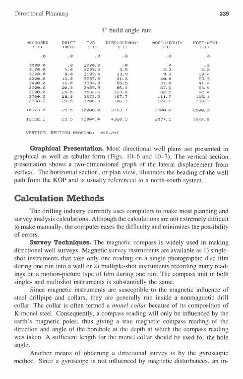
Directional Planning 339
Graphical Presentation. Most directional well plans are presented ingraphical as well as tabular form (Figs. 10-6 and 10-7). The vertical sectionpresentation shows a two-dimensional graph of the lateral displacement fromvertical. The horizontal section, or plan view, illustrates the heading of the wellpath from the KOP and is usually referenced to a north-south system.
Calculation Methods
The drilling industry currently uses computers to make most planning andsurvey analysis calculations. Although the calculations are not extremely difficultto make manually, the computer eases the difficulty and minimizes the possibilityof errors.
Survey Techniques. The magnetic compass is widely used in makingdirectional well surveys. Magnetic survey instruments are available as 1) single-shot instruments that take only one reading on a single photographic disc filmduring one run into a well or 2) multiple-shot instruments recording many read-ings on a motion-picture type of film during one run. The compass unit in bothsingle- and multishot instruments is substantially the same.
Since magnetic instruments are susceptible to the magnetic influence ofsteel drillpipe and collars, they are generally run inside a nonmagnetic drillcollar. The collar is often termed a monel collar because of its composition ofK-monel steel. Consequently, a compass reading will only be influenced by theearth's magnetic poles, thus giving a true magnetic compass reading of thedirection and angle of the borehole at the depth at which the compass readingwas taken. A sufficient length for the monel collar should be used for the holeangle.
Another means of obtaining a directional survey is by the gyroscopicmethod. Since a gyroscope is not influenced by magnetic disturbances, an in-
4° build angle rate
MEASURED DRIFT TVD DISPLACEMENT NORTH/SOUTH EAST/WEST(FT> <DEG) (FT) (FT) <FT> (FT>
.0 .0 .0 .0 .0 .0
3000.0 .0 3000.0 .0 .0 .03100.0 4.0 3099.9 3.5 2.3 2.63200.0 8.0 3199.4 13.9 9.3 10.43300.0 12.0 3297.8 31.3 20.8 23.33400.0 16.0 3394.8 55.5 37.0 41.43500.0 20.0 3489.9 86.4 57.5 64.43600.0 24.0 3582.6 123.8 82.5 92.43700.0 28.0 3672.5 167.7 111.7 125.13738.6 29.5 3706.3 186.3 124.1 138.9
10973.0 2'3.5 10000.0 3753.7 2500.0 2800.0
12122.5 29.5 11000.0 4320.5 2877.5 3222.8
VERTICAL SECTION BEARING: N48.24E
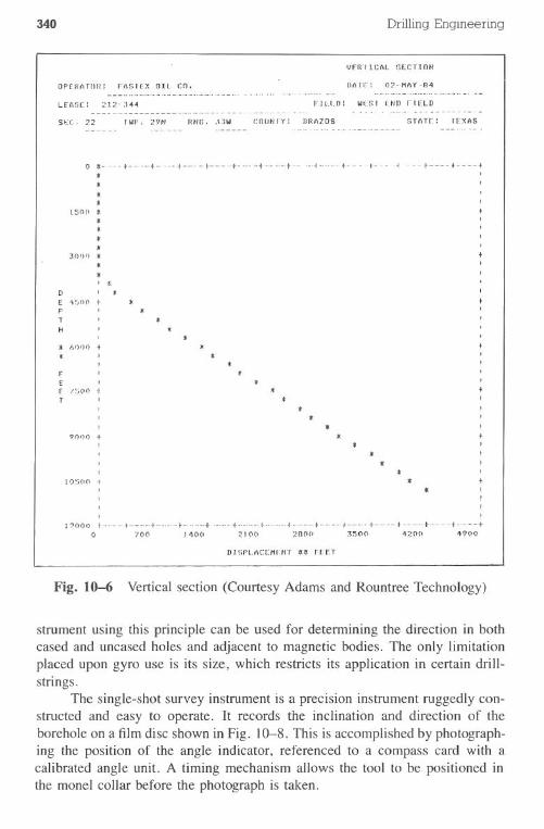
340 Drilling Engineering
VF.R"llI:AL !)f;CTION
OPERhTOR: FhOIEI OIL CO. »hIE: 02-HhY-S4----...--........................--...---.. ..--.....-........-.-..-.--...-.--
LF.AHr::: 212-';144 FIELD: WEOI EHn FIELD,-.--..-.--....-..-----. -.-...........-......-.........---.....---.-
S~C. 22 rwp. 29H COntI If : DIM7.0S !;TAT[:: n:XAS.., ..,.,.....-.
o f-.-...
.
.15M.
.
.
.*
3000**.
--+ j ~ + + t-- --1 ' ,--- I ---t f fII
.
[I I *
E 1:'JOO
PT! *H I *
* 1..1)00. .
.*
9000 .
..
.10500+ *
J *JII
l~OOO ~ + + + + t t + + + + +o 700 1400 210(' 200(' 3~00 UO(. HOO
[lIOPLACEHEHT .* FEET
Fig. 10-6 Vertical section (Courtesy Adams and Rountree Technology)
strument using this principle can be used for determining the direction in bothcased and uncased holes and adjacent to magnetic bodies. The only limitationplaced upon gyro use is its size, which restricts its application in certain drill-strings.
The single-shot survey instrument is a precision instrument ruggedly con-structed and easy to operate. It records the inclination and direction of theborehole on a filmdisc shown in Fig. 10-8. This is accomplished by photograph-ing the position of the angle indicator, referenced to a compass card with acalibrated angle unit. A timing mechanism allows the tool to be positioned inthe monel collar before the photograph is taken.
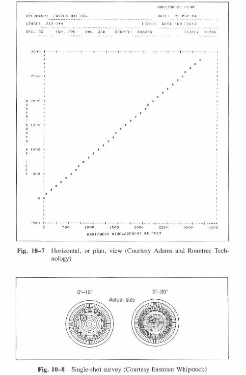
HOI'!lfJIHAI. PI.AN
OPERATOR: FAOTEX OIL CO..-.................. ,.-.......
LF:t'\n[.:: 212-<144---............-..-........--..-----------.--....... ".........
SF:G. ~2 COliNIY : DRAZOS nTf)TC: TfXAS...._-............
30QI) ~ t + t + + + + t + + + + fIII
I 1<
I t2~OQ + *
1<'1<
I> 1<!!!I
-~DU f f + + + f f f t f t- .-t f f +o 500 1000 1~('I('I 2000 2~(I(I :\000 :~~,('IO
EAST /W[ST J).uWl.l\f:r::HC::HTa. n~f.T
Fig. 10-7 Horizontal, or plan, view (Courtesy Adams and Rountree Tech-nology)
Fig. 10-8 Single-shot survey (Courtesy Eastman Whipstock)
N :,t)OO0 , tR I ;:THI
S 1:')000U ! 1<T ! 1<H
* 1000 + 1<1< I
1<F 1<E ;:E 1<T 500
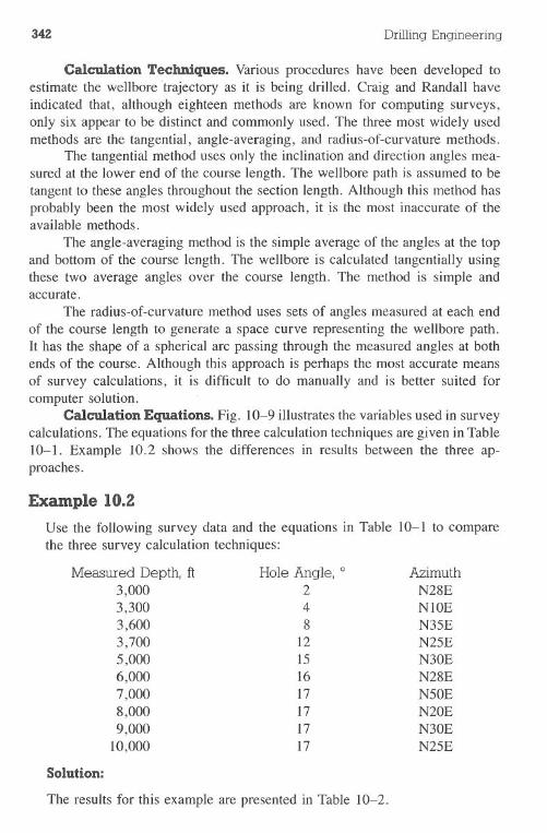
342 DrillingEngineering
Calculation Techniques. Various procedures have been developed toestimate the wellbore 'trajectory as it is being drilled. Craig and Randall haveindicated that, although eighteen methods are known for computing surveys,only six appear to be distinct and commonly used. The three most widely usedmethods are the tangential, angle-averaging, and radius-of-curvature methods.
The tangential method uses only the inclination and direction angles mea-sured at the lower end of the course length. The wellbore path is assumed to betangent to these angles throughout the section length. Although this method hasprobably been the most widely used approach, it is the most inaccurate of theavailable methods.
The angle-averaging method is the simple average of the angles at the topand bottom of the course length. The wellbore is calculated tangentially usingthese two average angles over the course length. The method is simple andaccurate.
The radius-of-curvature method uses sets of angles measured at each endof the course length to generate a space curve representing the wellbore path.It has the shape of a spherical arc passing through the measured angles at bothends of the course. Although this approach is perhaps the most accurate meansof survey calculations, it is difficult to do manually and is better suited forcomputer solution. .
Calculation Equations. Fig. 10-9 illustrates the variables used in surveycalculations. The equations for the three calculation techniques are given in Table10-1. Example 10.2 shows the differences in results between the three ap-proaches.
Example 10.2Use the following survey data and the equations in Table 10-1 to comparethe three survey calculation techniques:
Measured Depth, ft3,0003,3003,6003,7005,0006,0007,0008,0009,000
10,000
Solution:
Hole Angle, 0
248
12151617171717
AzimuthN28ENIOEN35EN25EN30EN28EN50EN20EN30EN25E
The results for this example are presented in Table 10-2.
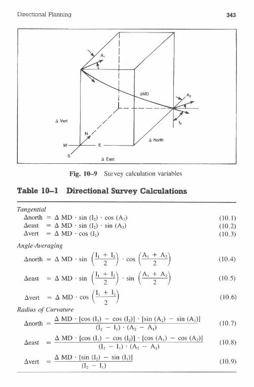
Directional Planning
fj. Vert
I
)--/
//
N /
w E
sfj. East
Fig. 10-9 Survey calculation variables
Table 10-1 Directional Survey Calculations
343
Tangential.:1north = .:1MD . sin (12) . COS (A2)
.:1east =.:1 MD . sin (12) . sin (A2)
.:1vert =.:1 MD . COS (12)
Angle-Averaging
.:1north = .:1MD . sinCI ; 12)
CI ; 12)
.(AI + A2). sm 2
.:1east =.:1 MD . sin
(II + 12).:1vert =.:1 MD . cos ;-Radius of Curvature
A h .:1MD . [cos (II) - COS (12)] . [sin (A2) - sin (AI)]Llnort =(12 - II) . (A2 - AI)
.:1 MD . [cos (II) - COS(12)] . [cos (AI) - COS (A2)](12 - II) . (A2 - A.)
A _ .:1MD . [sin (12) - sin (II)]Llvert - (12 _ II)
.:1east =
(10.1)(10.2)(10.3)
(10.4)
(10.5)
(10.6)
(10.7)
(10.8)
(10.9)
344 DrillingEngineering
Dogleg Severity. Large angle changes occurring over a short courselength can place high bending stresses on the pipe. In addition, these doglegscan cause keyseating problems. Most operators place a limit on the amount ofangle change allowable over a 100-ft segment. Generally, the limit is 4°-6°per 100ft.
Doglegs that occur at shallow and deep intervals are concerns for differentreasons. Although shallow doglegs tend to wash out and enlarge in softer for-mations, they can cause increasing problems due to high string weights hangingat the doglegs as the well deepens. Deeper doglegs do not have the same highlevels of string weight acting on the dogleg, but the dogleg does not tend to washout, which would reduce the severity of the problem. Example 10.4 shows thatgreater allowable doglegs occur in deeper intervals due to the lower string weightat the depth of interest.
Numerous methods are available for computing dogleg severity. Most arebased on the survey calculation techniques. In some cases, charts and tableshave been prepared for this purpose. Eq. 10.10 is a dogleg calculation techniquebased on the tangential method:
100DL = (L) [(sin II sin 12)(sin AI sin A2 + cos AI cos A2) +
cos II cos 12] (10.10)
Where:DL = dogleg,°1100ftL = course length, ftI., 12 = inclination at upper and lower surveys, °AI, A2 = direction at upper and lower surveys, °
Example 10.3
Calculate the dogleg severity for the two successive surveys as follows:
Depth, ftInclinationAzimuth
Solution:
Survey I4,23113.5°N 100E
Survey 24,26214.7°NI9°E
1. The variables used in Eq. 10.10 are as follows:
L = 31 ftII = 13.512 = 14.7
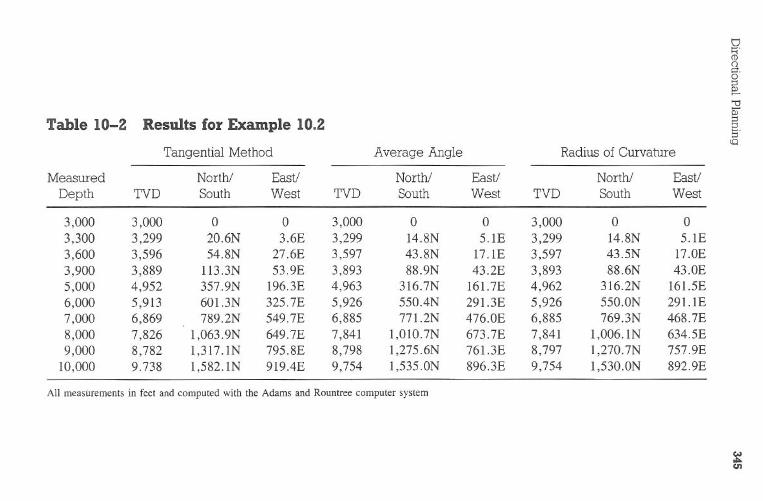
C/o)
~en 1;:;11=
<'
CD
0'::s'"0s;
Table
10-2R
esultsfor
Exam
ple10.2
::s::sEr
(QT
angentialM
ethodA
verageA
ngleR
adiusof
Curvature
Measured
North!
East!
North!
East!
North!
East!
Depth
TV
DSouth
West
TV
DSouth
West
TV
DSouth
West
3,0003,000
00
3,0000
03,000
00
3,3003,299
20.6N3.6E
3,29914.8N
5.1E3,299
14.8N5.1E
3,6003,596
54.8N27.6E
3,59743.8N
17.1E3,597
43.5N17.0E
3,9003,889
113.3N53.9E
3,89388.9N
43.2E3,893
88.6N43.0E
5,0004,952
357.9N196.3E
4,963316.7N
161.7E4,962
316.2N161.5E
6,0005,913
601.3N325.7E
5,926550.4N
291.3E5,926
550.0N291.1E
7,0006,869
789.2N549.7E
6,885771.2N
476.0E6,885
769.3N468.7E
8,0007,826
1,063.9N649.7E
7,8411,01O
.7N673.7E
7,8411,006.1N
634.5E9,000
8,7821,317.1N
795.8E8,798
1,275.6N761.3E
8,7971,270.7N
757.9E10,000
9.7381,582.1N
919.4E9,754
1,535.0N896.3E
9,7541,530.0N
892.9E
All
measurem
entsin
feetand
computed
with
theA
dams
andR
ountreecom
putersystem
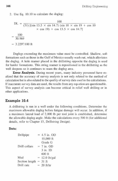
346 DrillingEngineering
2. Use Eq. 10.10 to calculate the dogleg:
100
DL = (31) [(sin 13.5 X sin 14.7) (sin 10 x sin 19 + cos 10x cos 19) + cos 13.5 x cos 14.7]
100= 30.969
= 3.229°/100 ft
Doglegs exceeding the maximum value must be controlled. Shallow, softformations such as those in the Gulf of Mexico usually wash out, which alleviatesthe dogleg. A hole reamer placed in the drillstring opposite the dogleg is usedfor harder formations. This string reamer is repositioned in the drillstring as thewell deepens so it continues to ream the dogleg area.
Error Analysis. During recent years, many industry personnel have re-alized that the accuracy of survey analysis is not only related to the method ofcalculation but is also related to the quality of survey data used in the calculations.If inaccurate survey data are used, the results from any equation are questionable.This aspect of survey analysis can become critical in relief well drilling or inother applications.
Example 10.4
A drillstring is run in a well under the following conditions. Determine themaximum allowable dogleg before fatigue damage will occur. In addition, ifa maximum lateral load of 2,000 Ib per tool joint is established, determinethe allowable dogleg angle. Make the calculations every 500 ft (for additionaldetails, refer to Chapter 15, Drillstring Design).
Data:
Drillpipe
Drill collars
MudSection lengthDrill rate
4.5 in. OD10,000 ftGrade G7 in. OD3 in. ID600 ft12.0 Ib/gal31 ft20 ft/hr
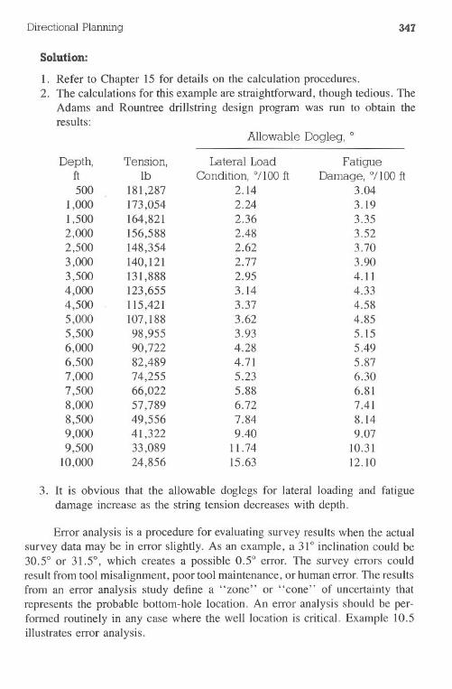
Error analysis is a procedure for evaluating survey results when the actualsurvey data may be in error slightly. As an example, a 31° inclination could be30.5° or 31.5°, which creates a possible 0.50 error. The survey errors couldresult from tool misalignment, poor tool maintenance, or human error. The resultsfrom an error analysis study define a "zone" or "cone" of uncertainty thatrepresents the probable bottom-hole location. An error analysis should be per-formed routinely in any case where the well location is critical. Example 10.5illustrates error analysis.
DirectionalPlanning 347
Solution:
1. Refer to Chapter 15 for details onthe calculation procedures.2. The calculations for this example are straightforward, though tedious. The
Adams and Rountree drillstring design program was run to obtain theresults:
Allowable Dogleg, °
Depth, Tension, Lateral Load Fatigueft lb Condition, °/100 ft Damage, °/100 ft500 181,287 2.14 3.04
1,000 173,054 2.24 3.19
1,500 164,821 2.36 3.352,000 156,588 2.48 3.52
2,500 148,354 2.62 3.70
3,000 140,121 2.77 3.903,500 131,888 2.95 4.114,000 123,655 3.14 4.334,500 115,421 3.37 4.58
5,000 107,188 3.62 4.85
5,500 98,955 3.93 5.15
6,000 90,722 4.28 5.49
6,500 82,489 4.71 5.877,000 74,255 5.23 6.30
7,500 66,022 5.88 6.81
8,000 57,789 6.72 7.41
8,500 49,556 7.84 8.14
9,000 41,322 9.40 9.079,500 33,089 11.74 10.31
10,000 24,856 15.63 12.10
3. It is obvious that the allowable doglegs for lateral loading and fatiguedamage increase as the string tension decreases with depth.
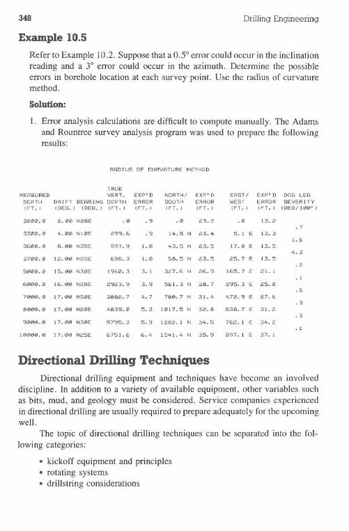
348 Drilling Engineering
Example 10.5
Refer to Example 10.2. Suppose that a 0.50error could occur in the inclinationreading and a 30 error could occur in the azimuth. Determine the possibleerrors in borehole location at each survey point. Use the radius of curvaturemethod.
Directional drilling equipment and techniques have become an involveddiscipline. In addition to a variety of available equipment, other variables suchas bits, mud, and geology must be considered. Service companies experiencedin directional drilling are usually required to prepare adequately for the upcomingwell.
The topic of directional drilling techniques can be separated into the fol-lowing categories:
·kickoff equipment and principles.rotating systems·drillstringconsiderations
Solution:
1. Error analysis calculations are difficult to compute manually. The Adamsand Rountree survey analysis program was used to prepare the followingresults:
RADIUS DF CURVATURE METHDD
TRUEMEASURED VERT. EXP'D NORTH/ EXP'D EAST/ EXP'D DOG LEGDEPTH DRIFT BEARING DEPTH ERROR SDUTH ERRDR WEST ERROR SEVERITY(FT.) <DEG. ) <DEG. ) (FT.) (FT.) (FT.) (FT.) (FT.) (FT.) <DEG/ 100' )
3000.0 2.00 N28E .0 .'3 .0 23.2 .0 13.2.7
3300.0 4.00 N10E 2'3'3.6 .'3 14.8 N 23.4 5.1 E 13.31.6
3600.0 8.00 N35E 5'37.'3 1.0 43.5 N 23.5 17.0 E 13.54.3
3700.0 12.00 N25E 6'36.3 1.0 58.5 N 23.5 25.7 E 13.5.2
5000.0 15.00 N30E 1'360.3 3.1 327.6 N 26.'3 165.7 E 21.1.1
6000.0 16.00 N28E 2'323.9 3.'3 561.3 N 28.7 295.3 E 25.0.6
7000.0 17.00 N50E 3882.7 4.7 780.7 N 31.4 472.'3E 27.6.'3
8000.0 17.00 N20E 483'3.0 5.3 1017.5 N 32.8 638.7 E 31.2.3
'3000.0 17.00 N30E 57'35.3 5.'3 1282.1 N 34.5 762.1 E 34.2.1
10000.0 17.00 N25E 6751.6 6.4 1541.4 N 35.'3 8'37.1E 37.1
Directional Drilling Techniques
Directional Planning 349
Related subjects such as mud and bit. selection will not be considered at thispoint, although they are important to the success of the effort.
Kickoff Equipment. Hole angles are usually kicked off by jetting, whip-stocks, or some type of bent sub, downhole motor tool. Geology affects thedecision as well as the desire to use a steering tool.
Jetting was a widely used technique several years ago. It involved the useof a large bit jet and two smaller jets. The bit was oriented so the large jet facedin the desired direction of the wellbore. The drillstring was held stationary whilethe mud was circulated. The jetting action of the mud from the large jet wouldwash a small cavern into the formation that the drillstring would tend to follow.After washing 6-8 ft of hole, the rotary was used to drill the rest of the joint.A survey was taken at this point and jetting was restarted until the desired wellpath was achieved.
The whipstock is a very simple device used to kick off the well. It is awedge-shaped tool that forces the bit in the desired direction (Fig. 10-10). Thewhipstock is oriented and drilling is initiated. After drilling 12-15 ft below thewhipstock, the entire assembly is removed and a regular drillstring assembly isrun into the well.
Bent subs are used with downhole motors. The sub has Y2°-2Y2°of bendin it that will deflect the motor in the desired direction (Fig. 10-11). A steeringtool is commonly used with the bent sub.
Rotating Systems. In directional drilling, as with all types of rotarydrilling, the bit is turned with the rotary system or a downhole motor device.The conventional rotary system has the bit connected directly to the drillstring,and the entire combination is rotated from the surface. Downhole motors, usedwith a stationary drillstring, turn the bit via rotation induced by mud flow withinthe motor (Fig. 10-12).
Downhole motors/turbines are receiving a significant amount of use be-cause they can be used in connection with bent subs and steering tools. Motorsand turbines are provided by service companies in a wide range of sizes,operating speeds, and torque characteristics for various types of bits anddrilling conditions.
Drillstring Considerations. The drillstring and bottom-hole assemblyplay an important role in directional drilling. A packed-hole assembly uses asufficient number of stabilizers so that hole angle changes are difficult to achieve,which is desirable after the final hole angle has been obtained. Likewise, properstabilizer positioning can increase the hole angle via the fulcrum principle, or itcan decrease via the pendulum principle. Experience and knowledge are nec-essary tools in BHA selection.
With the fulcrum principle, a string of drill collars under torsional strainand compression is not generally subject to helical buckling, although it is subject
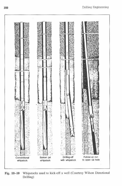
350
Conventional
whipstock
;; ~!.;.;..,".
...
t;.':..~
~::..
~;.,;
n~':.~i;:i.: "!;:~j:J; .'.:'~....~..."t~.o.~.........
Bottom' jetwhipstock
Drilling Engineering
Follow-up runto open rat hole
Fig. 10-10 Whipstocks used to kick-off a well (Courtesy Wilson DirectionalDrilling)
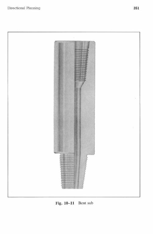
Directional Planning 351
Fig. 10-11 Bent sub
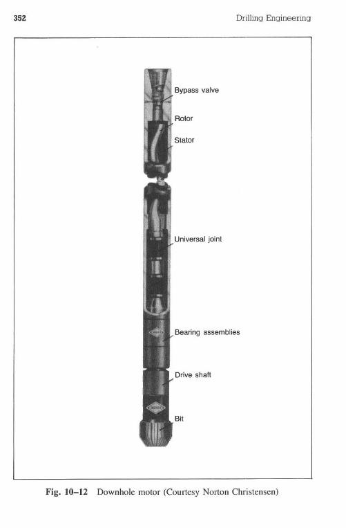
352 DrillingEngineering
Bypass valve
Rotor
Stator
Universal joint
Bearing assemblies
Drive shaft
Bit
Fig. 10-12 Downhole motor (Courtesy Norton Christensen)
Directional Planning 353
to the same bending as a column under static load. The bend will normally seekthe low side of the hole. At a certain distance above the bit, the collars touchand rub the sidewall. This point of tangency distance from the bit depends onthe collar OD and stiffness, the diameter of the hole, and the amount of bitweight. When a stabilizer is run below.the point of tangency, it has a fulcrumeffect, which causes the hole to pick up angle. The angle fonned by this pointof contact and the clearance between the drill collars and wellbore approximatethe change in deflection that would accompany the next increment of drilledhole (Fig. 10-13).
The point of contact usually is on the low side of the hole in high-angleholes. The result is that the change in deflection is additive, which tends toincrease the hole deflection. This tendency is reduced by increasing drill collar
Fig. 10-13 Fulcrum principle (Courtesy Wilson Directional Drilling)
354 Drilling Engineering
Fig. 10-14 Pendulum principle (Courtesy Wilson Directional Drilling)
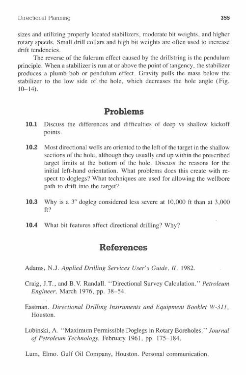
Directional Planning 355
sizes and utilizing properly located stabilizers, moderate bit weights, and higherrotary speeds. Small drill collars and high bit weights are often used to increasedrift tendencies.
The reverse of the fulcrum effect caused by the drillstring is the pendulumprinciple. When a stabilizer is run at or above the point of tangency, the stabilizerproduces a plumb bob or pendulum effect. Gravity pulls the mass below thestabilizer to the low side of the hole, which decreases the hole angle (Fig.10-14).
Problems
10.1 Discuss the differences and difficulties of deep vs shallow kickoffpoints.
10.2 Most directional wells are oriented to the left of the target in the shallowsections of the hole, although they usually end up within the prescribedtarget limits at the bottom of the hole. Discuss the reasons for theinitial left-hand orientation. What problems does this create with re-spect to doglegs? What techniques are used for allowing the wellborepath to drift into the target?
10.3 Why is a 3° dogleg considered less severe at 10,000 ft than at 3,000ft?
10.4 What bit features affect directional drilling? Why?
References
Adams, N.J. Applied Drilling Services User's Guide, 1/, 1982.
Craig, J.T., and B.Y. Randall. "Directional Survey Calculation." PetroleumEngineer, March 1976, pp. 38-54.
Eastman. Directional Drilling Instruments and Equipment Booklet W-31I ,Houston.
Lubinski, A. "Maximum Permissible Doglegs in Rotary Boreholes." Journalof Petroleum Technology, February 1961, pp. 175-184.
Lum, Elmo. Gulf Oil Company, Houston. Personal communication.

356 Drilling Engineering
Planeix, M.Y., and R.C. Fox. "Use of an Exact Mathematical Formulationto Plan Three-Dimensional Wells." Paper presented to the 1979 Fall SPETechnical Conference, Las Vegas, 1979.
Wilson Downhole. "School of Drilling Technology," 1971.
Woods, H.B., and A. Lubinski. "Practical Charts for Solving Problems inHole Deviation." Spring Meeting, Mid-Continent District of Production,Oklahoma City, March 1954, Drilling and Production Practices. 1954, p.56.
Chapter 11 Casing andTubing Concepts 1
I
Casing and tubing playa vital role in drilling operations. The design ofthe tubulars requires a knowledge of the operating conditions to be imposed onthe pipe as well as a working-understanding of various concepts related to pipeproperties. The drilling engineer must be aware of these concepts before begin-ning the actual design operations. These concepts include items such as manu-facturing processes, physical properties, and testing procedures.
Over the years, the API has developed a number of guidelines for petroleumpractices and equipment. Many of these guidelines relate to oil-field tubulargoods. Table II-I lists some of the more important specifications, bulletins,and recommended practices. These documents, and others not shown in TableII-I, should be reviewed thoroughly by the practicing drilling engineer to com-plement his field experiences.
Pipe Body ManufacturingI,
!
API's Specification 5A states that casing, liners, and tubing conformingto this standard must be seamless or electric welded. Seamless pipe is a wroughtsteel tubular product made without a welded seam. It is manufactured by hot-working steel and, if necessary, by s~bsequently cold-finishing the hot-workedtubular product to produce the desired shape. The process may involve a plugmill or mandrel mill rolling. A typical seamless process is shown in Fig. II-I.
Electric-welded (ERW) pipe has one longitudinal seam formed by electric-flash welding or electric-resistance welding, without adding extraneous metal.The weld seam of electric-welded pipe is heat-treated after welding to a minimumtemperature of I,OOO°For is processed so no untempered martensite remains.Fig. 11-2 illustrates a typical ERW process.
357
358 Drilling Engineering
Table 11-1 Summary of Various Pertinent APIPublications Relating to Casing and Tubing
Title
Specification for Casing, Tubing, and Drill PipeSpecification for Restricted Yield Strength Casing and Tub-
ingSpecification for High-Strength Casing, Tubing, and Drill
PipeSpecification for Threading, Gaging, and Thread Inspection
of Casing, Tubing, and Line Pipe ThreadsSpec 5L Specification for Line Pipe
Recommended Practices
RP 5CI Recommended Practice for Care and Use of Casing andTubing
SpecificationsSpec 5ASpec 5AC
Spec 5AX
Std 5B
BulletinBul 5A2Bul5C2Bul5C3
Bul5C4
Bulletin on Thread CompoundsBulletin on Performance Properties of Casing and TubingBulletin on Formulas and Calculations for Casing, Tubing,
Drill Pipe, and Line Pipe PropertiesBulletin on Round Thread Casing Joint Strength with Com-
bined Internal Pressure and Bending
The American Petroleum Institute's Committee on Standardization of Thbular Goods has preparednumerous valuable documents relating to tubular goods in addition to those listed in Table II-I.The documents are available through the API.
Casing Physical PropertiesThe physical properties of oil-field tubular goods include grade, pressure
resistance, drift diameter, and weight. These properties relate to the pipe's abilityto meet the demands of the imposed drilling conditions. The limitations of theproperties must be considered before final pipe selection.
Grade. The pipe grade is a designation that defines the pipe's yield strengthand certain special characteristics. The grade usually consists of a letter and a2- or 3-digit number such as N-80. In most cases as the letter proceeds towardthe end of the alphabet, the pipe increases in yield strength. For example,N-80, or N-grade, pipe has a greater yield strength than H-40.
The numerical code indicates the minimum yield strength in thousands ofpsi. As an example, N-80 has a minimum yield strength of 80,000 psi. Theaverage yield strength is usually 10,000 psi greater than the minimum yield, or90,000 psi for N-80 pipe. The minimum value is used in burst and collapse
Casing and Tubing Concepts 359
Pierce<
Round Billet
Rotary Heating Furnace
~~-a
Elongator Plug Mill
SizerReeler
~~-'1i-Straightening
Cooling Table
Fig. 11-1 Plug mill rolling process for Kawasaki's 7-16%-in. pipe (CourtesyKawasaki Steel Corp.)
resistance calculations, whereas the average is used for biaxial evaluations. TheAPI grades are shown in Table 11-2.
C pipe is a controlled yield pipe used primarily in environments such asH2S. It is seldom used in noncorrosive environments since it is more expensivethan some higher grades of pipe. Engineers desiring to use C-grade pipe shouldreview API Specifications 5AC.
L-grade pipe has the same burst, collapse, and yield values as N pipe.However, the hardness of the pipe is a critical value due to potential hydrogen
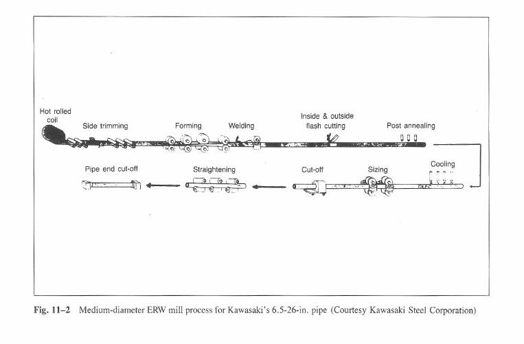
Hot
rolledcoil
Side
trimm
ing
Pipe
endcut-off
~.,,".J'--'-
Form
ingW
elding
Inside&
outsideflash
cutting
.~
";.....Cut-off
Post
annealing
Q0
0
Fig
.11-2M
edium-diam
eterER
Wm
illprocessfor
Kaw
asaki's6.5-26-in.
pipe(C
ourtesyK
awasaki
SteelC
orporation)
Straightening
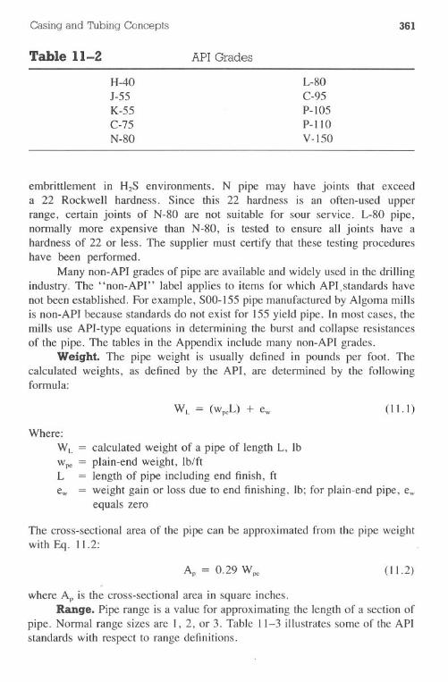
Casing and Tubing Concepts 361
Table 11-2 API Grades
H-40J-55K-55C-75N-80
L-80C-95P-I05P-IIOV-150
embrittlement in H2S environments. N pipe may have joints that exceeda 22 Rockwell hardness. Since this 22 hardness is an often-used upperrange, certain joints of N-80 are not suitable for sour service. L-80 pipe,normally more expensive than N-80, is tested to ensure all joints have ahardness of 22 or less. The supplier must certify that these testing procedureshave been performed.
Many non-API grades of pipe are available and widely used in the drillingindustry. The "non-API" label applies to items for which API,standards havenot been established. For example, SOO-155pipe manufactured by Algoma millsis non-API because standards do not exist for 155 yield pipe. In most cases, themills use API-type equations in determining the burst and collapse resistancesof the pipe. The tables in the Appendix include many non-API grades.
Weight. The pipe weight is usually defined in pounds per foot. Thecalculated weights, as defined by the API, are determined by the followingformula:
(ILl)
Where:
WL = calculatedweightof a pipe of lengthL, Ibwpe = plain-end weight, Ib/ftL = length of pipe including end finish, ftew = weight gain or loss due to end finishing, Ib; for plain-end pipe, ew
equals zero
The cross-sectional area of the pipe can be approximated from the pipe weightwith Eq. 11.2:
Ap = 0.29 Wpe (11.2)
where Ap is the cross-sectional area in square inches.Range. Pipe range is a value for approximating the length of a section of
pipe. Normal range sizes are I, 2, or 3. Table 11-3 illustrates some of the APIstandards with respect to range definitions.
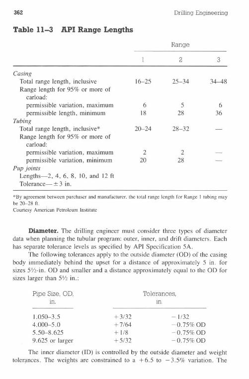
362 Drilling Engineering
Table 11-3 API-Range Lengths
*By agreement between purchaser and manufacturer. the total range length for Range I tubing maybe 20-28 ft.
Courtesy American Petroleum Institute
Diameter. The drilling engineer must consider three types of diameterdata when planning the tubular program: outer, inner, and drift diameters. Eachhas separate tolerance levels as specified by API Specification 5A.
The following tolerances apply to the outside diameter (OD) of the casingbody immediately behind the upset for a distance of approximately 5 in. forsizes 5Yz-in.OD and smaller and a distance approximately equal to the OD forsizes larger than 5Yzin.:
Pipe Size, OD,ill.
Tolerances,ill.
1.050-3.54.000-5.05.50-8.6259.625 or larger
+ 3/32+7/64+ 1/8+ 5/32
- 1/32-0.75%OD-0.75% OD-0.75%OD
The inner diameter (ID) is controlled by the outside diameter and weighttoleqmces. The weights are constrained to a + 6.5 to - 3.5% variation. The
Range
2 3
CasingTotal range length, inclusive 16-25 25-34 34-48Range length for 95% or more of
carload:
permissible variation, maximum 6 5 6permissible length, minimum 18 28 36
TubingTotal range length, inclusive* 20-24 28-32
Range length for 95% or more ofcarload:permissible variation, maximum 2 2permissible variation, minimum 20 28
Pup jointsLengths-2, 4, 6, 8, 10, and 12 ftTolerance-:!: 3 in.
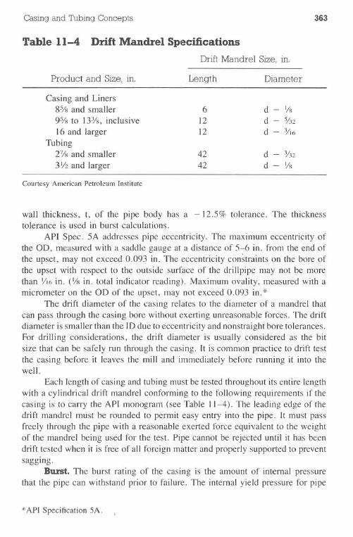
Casing and Tubing Concepts 363
Table 11-4 Drift Mandrel SpecificationsDrift Mandrel Size, in.
Product and Size, in. Length Diameter
Casing and Liners8% and smaller9% to 13¥s, inclusive16 and larger
Tubing27/Sand smaller3V2and larger
61212
d - Vsd - 5/32d - 3/16
4242
d - 3/12d - Vs
Courtesy American Petroleum Institute
wall thickness, t, of the pipe body has a - 12.5% tolerance. The thicknesstolerance is used in burst calculations.
API Spec. 5A addresses pipe eccentricity. The maximum eccentricity ofthe OD, measured with a saddle gauge at a distance of 5-6 in. from the end ofthe upset, maynot exceed0.093 in. The eccentricityconstraintson the boreofthe upset with respect to the outside surface of the drillpipe may not be morethan VI6in. (Vsin. total indicator reading). Maximum ovality, measured with amicrometer on the OD of the upset, may not exceed 0.093 in.*
The drift diameter of the casing relates to the diameter of a mandrel thatcan pass through the casing bore without exerting unreasonable forces. The driftdiameter is smaller than the ID due to eccentricity and nonstraight bore tolerances.For drilling considerations, the drift diameter is usually considered as the bitsize that can be safely run through the casing. It is common practice to drift testthe casing before it leaves the mill and immediately before running it into thewell.
Each length of casing and tubing must be tested throughout its entire lengthwith a cylindrical drift mandrel conforming to the following requirements if thecasing is to carry the API monogram (see Table 11-4). The leading edge of thedrift mandrel must be rounded to permit easy entry into the pipe. It must passfreely through the pipe with a reasonable exerted force equivalent to the weightof the mandrel being used for the test. Pipe cannot be rejected until it has beendrift tested when it is free of all foreign matter and properly supported to preventsagging.
Burst. The burst rating of the casing is the amount of internal pressurethat the pipe can withstand prior to failure. The internal yield pressure for pipe
*API Specification 5A.
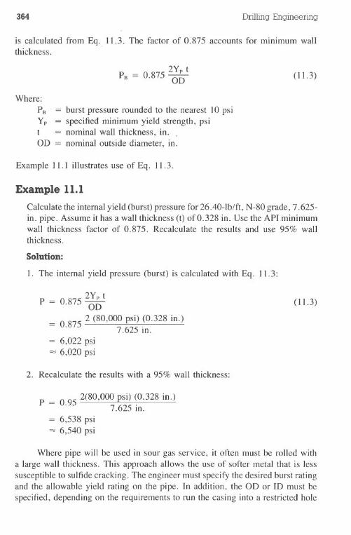
364 Drilling Engineering
is calculated from Eq.. 11.3. The factor of 0.875 accounts for minimum wallthickness.
2YptPo = 0.875 OD (11.3)
Where:
Po = burst pressure rounded to the nearest 10 psiYp = specifiedminimumyield strength,psit = nominal wall thickness, in. .OD = nominal outside diameter, in.
Example 11.1 illustrates use of Eq. 11.3.
. Example 11.1
Calculate the internal yield (burst) pressure for 26.40-lb/ft, N-80 grade, 7.625-in. pipe. Assume it has a wall thickness (t) of 0.328 in. Use the API minimumwall thickness factor of 0.875. Recalculate the results and use 95% wallthickness.
Solution:
I. The internal yield pressure (burst) is calculated with Eq. 11.3:
P = 0.875 2~~t
= 0 875 2 (80,000 psi) (0.328 in.). 7.625 in.= 6,022 psi= 6,020 psi
(11.3)
2. Recalculate the results with a 95% wall thickness:
P = 095 2(80,000 psi) (0.328 in.). 7.625 in.
= 6,538 psi= 6,540 psi
Where pipe will be used in sour gas service, it often must be rolled witha large wall thickness. This approach allows the use of softer metal that is lesssusceptible to sulfidecracking. The engineer must specify the desired burst ratingand the allowable yield rating on the pipe. In addition, the OD or ID must bespecified, depending on the requirements to run the casing into a restricted hole
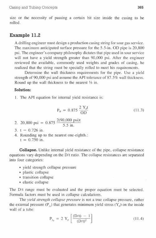
Casing and 'fubing Concepts 365
size or the necessity of passing a certain bit size inside the casing to berolled.
Example 11.2
A drilling engineer must design a production casing string for sour gas service.The maximum anticipated surface pressure for the 5.5-in. OD pipe is 20,800psi. The engineer's company philosophy dictates that pipe used in sour servicewill not have a yield strength greater than 90,000 psi. After the engineerreviewed the available, commonly used weights and grades of casing, herealized that the string must be specially rolled to meet his requirements.
Determine the wall thickness requirements for the pipe. Use a yieldstrength of 90,000 psi and assume the API tolerance of 87.5% wall thickness.Round up the wall thickness to the nearest YBin.
Solution:
I. The API equation for internal yield resistance is:
2 YptPo = 0.875 OD
2. 20,800 psi = 0.875 2(9~,~0? psi)t. lO.3. t = 0.726 in.4. Rounding up to the nearest one-eighth.:
t = 0.750 in.
(11.3)
Conapse. Unlike internal yield resistance of the pipe, collapse resistanceequations vary depending on the D/t ratio. The collapse resistances are separatedinto four categories:
.yield strength collapse pressure·plastic collapse·transition collapse.elastic collapse
The D/t range must be evaluated and the proper equation must be selected.Formula factors must be used in collapse calculations.
The yield strength collapse pressure is not a true collapse pressure, ratherthe external pressure (Py) that generates minimum yield stress (Yp)on the insidewall of a tube:
[(D/t) - I]Pyp = 2 Yp (D/t)2(11.4)
366 Drilling Engineering
The formula for yield strength collapse pressure is applicable for Dft values upto the value of Dft corresponding to the intersection with the plastic collapseformula, Eq. 11.5. The intersection is calculated as follows:
(11.5)
The applicable Dft ratios for yield strength collapse are shown in Table 11-5.
The minimum collapse pressure for the plastic range of collapse (Pp) iscalculated by Eq. 11.6:
Pp = Yp [~t - B] - C(11.6)
Table 11-5 Yield Collapse Pressure Formula Range1 2
Grade* D/tRange
H-40-55
J-K-55 & D-60-70
C-75 & EL-80 & N-80
-90C-95
-100P-105P-110
-120-125-130-135-140-150-155-160-170-180
16.44'and less15.24 and less14.81 and less14.44 and less13.85 and less13.60 and less13.38 and less13.01 and less12.85 and less12.70 and less12.57 and less12.44 and less12.21 and less12.11 and less12.02 and less11.92 and lessII. 84 and less11.67 and less11.59 and less/1.52 and less11.37 and less11.23 and less
*Grades indicated withoutleller designation are not API grades but are grades in use or grades being
considered for use and are shown for information purposes.
Courtesy American Petroleum Institute
Casing and Tubing Concepts 367
The fonnula for minimum plastic collapse pressure is applicable for D/t valuesranging from (D/t)p,in Eq. 11.7 (yield point collapse pressure) to the intersectionwith Eq. 11.8 for (D/t)" transition collapse pressure. Values for (D/t)pI arecalculated by means of Eq. 11.7:
Yp (A - F)(D/t)pI = C + Yp (B - G)
(11. 7)
The factors and applicable D/t range for the plastic collapse fonnula are shownin Table 11-6.
Table 11-6 Formula Factors and D/t Ranges forPlastic Collapse
2 3 4 5
Formula FactorGrade * A B C D/t Range
H-40 2.950 0.0465 754 16.44 to 27.01-50 2.976 0.0515 1,056 15.24 to 25.63
J-K-55 & D 2.991 0.0541 1,206 14.81 to 25.01-60 3.005 0.0566 1,356 14.44 to 24.42-70 3.037 0.0617 1,656 13.85 to 23.38
C-75 & E 3.054 0.0642 1,806 13.60 to 22.91L-80 & N-80 3.071 0.0667 1,955 13.38 to 22.47
-90 3.106 0.0718 2,254 13.01 to 21.69C-95 3.124 0.0743 2,404 12.85 to 21.33
-100 3.143 0.0768 2,553 12.70 to 21.00P-105 3.162 0.0794 2,702 12.57 to 20.70P-IIO 3.181 0.0819 2,852 12.44 to 20.41
-120 3.219 0.0870 3,151 12.21 to 19.88-125 3.239 0.0895 3,301 12.11 to 19.63-130 3.258 0.0920 3,451 12.02 to 19.40-135 3.278 0.0946 3,601 11.92 to 19.18-140 3.297 0.0971 3,751 11.84 to 18.97-150 3.336 0.1021 4,053 11.67 to 18.57-155 3.356 0.1047 4,204 11.59 to 18.37-160 3.375 o. 1072 4,356 11.52 to 18.19-170 3.412 0.1123 4,660 11.37 to 17.82-180 3.449 0.1173 4,966 11.23 to 17.47
*Grades indicated withoutleller designation are not API grades but are grades in use or grades being
considered for use and are shown for information purposes.
Courtesy American Petroleum Institute
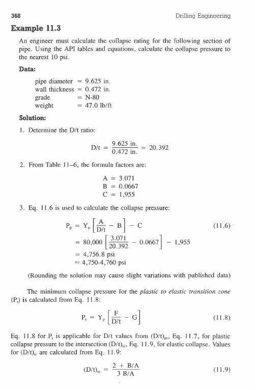
368
Example 11.3
DrillingEngineering
An engineer must. calculate the collapse rating for the following section ofpipe. Using the API tables and equations, calculate the collapse pressure tothe nearest 10 psi.
Data:
pipe diameter = 9.625 in.wall thickness = 0.472 in.grade = N-80weight = 47.0 Ib/ft
Solution:
I. Determine the D/t ratio:
9.625 in. = 20.392D/t = 0.472 in.
2. From Table 11-6, the formula factors are:
A = 3.071B = 0.0667C = 1,955
3. Eq. 11.6 is used to calculate the collapse pressure:
Pp = Yp [~\ - B] - C
[3.071
]= 80,000 20.392- 0.0667= 4,756.8 psi= 4,750-4,760psi
(11.6) .
- 1,955
(Rounding the solution may cause slight variations with published data)
The minimum collapse pressure for the plastic to elastic transition zone(P,) is calculated from Eq. 11.8:
P, = Yp [~t - G](11.8)
Eq. 11.8 for P, is applicable for D/t values from (D/t)pl>Eq. 11.7, for plasticcollapse pressure to the intersection (D/t),e, Eq. 11.9, for elastic collapse. Valuesfor (D/t),e are calculated from Eq. 11.9:
2 + B/A(D/t),e = 3 B/A (II. 9)
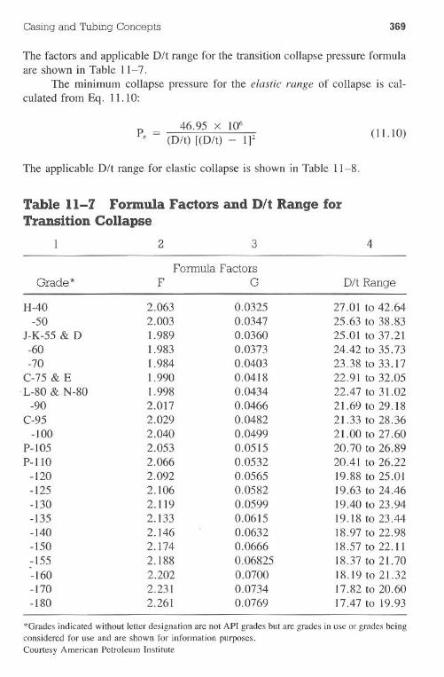
Casing and Tubing Concepts 369
The factors and applicable D/t range for the transition collapse pressure formulaare shown in Table 11-7.
The minimum collapse pressure for the elastic range of collapse is cal-culated from Eq. 11.10:
46.95 X 10⁶Pe = (D/t) [(D/t) - IF
(11.10)
The applicable D/t range for elastic collapse is shown in Table I t:-8.
*Grades indicated without letter designation are not API grades but are grades in use or grades being
considered for use and are shown for information purposes.
Courtesy American Petroleum Institute
Table 11-7 Formula Factors and D/t Range forTransition Collapse
2 3 4
Formula FactorsGrade * F G D/t Range
H-40 2.063 0.0325 27.01 to 42.64-50 2.003 0.0347 25.63 to 38.83
J-K-55 & D 1.989 0.0360 25.01 to 37.21-60 1.983 0.0373 24.42 to 35.73-70 1.984 0.0403 23.38 to 33.17
C-75 & E 1.990 0.0418 22.91 to 32.05.L-80 & N-80 1.998 0.0434 22.47 to 31.02
-90 2.017 0.0466 21.69 to 29.18C-95 2.029 0.0482 21.33 to 28.36
-100 2.040 0.0499 21.00 to 27.60P-105 2.053 0.0515 20.70 to 26.89P-110 2.066 0.0532 20.41 to 26.22
-120 2.092 0.0565 19.88 to 25.01-125 2.106 0.0582 19.63 to 24.46-130 2.119 0.0599 19.40 to 23.94-135 2.133 0.0615 19.18 to 23.44-140 2.146 0.0632 18.97 to 22.98-150 2.174 0.0666 18.57 to 22.11-155 2.188 0.06825 18.37 to 21.70-160 2.202 0.0700 18.19 to 21.32-170 2.231 0.0734 17.82 to 20.60-180 2.261 0.0769 17.47 to 19.93
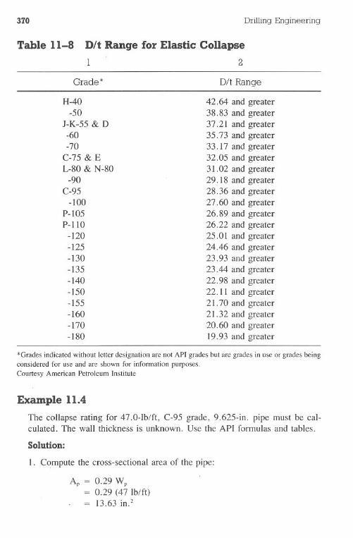
370 Drilling Engineering
Table 11-8 D/t Range for Elastic Collapse1 2
Grade * D/t Range
H-40-50
J-K-55 & D-60-70
C-75 & EL-80 & N-80
-90C-95
-100P-105P-110
-120-125-130-135-140-150-155-160-170-180
42.64 and greater38.83 and greater37.21 and greater35.73 and greater33.17 and greater32.05 and greater31.02 and greater29. 18 and greater28.36 and greater27.60 and greater26.89 and greater26.22 and greater25.01 and greater24.46 and greater23.93 and greater23.44 and greater22.98 and greater22.11 and greater21.70 and greater21.32 and greater20.60 and greater19.93 and greater
*Grades indicated without letter designation are not API grades but are grades in use or grades being
considered for use and are shown for information purposes.
Courtesy American Petroleum Institute
Example 11.4
The collapserating for 47.0-lb/ft, C-95 grade, 9.625-in. pipe must be cal-culated.The wall thicknessis unknown.Use the API formulasand tables.
Solution:
1. Compute the cross-sectional area of the pipe:
Ap = 0.29 Wp= 0.29 (47 lb/ft)= 13.63 in.2
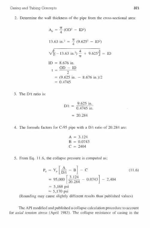
Casing and Tubing Concepts 371
2. Determine the wall thickness of the pipe from the cross-sectional area:
Ap = * (002 - 102)
13.63 in.2 = * (9.6252- 102)
-J~ -13.63 in.2)i + 9.6252]= 101T
10 = 8.676 in.00 - 10
t = 2= (9.625 in. - 8.676 in.)12= 0.4745
3. The Oft ratio is:
9.625 in.Oft = 0.4745 in.
= 20.284
4. The formula factors for C-95 pipe with a Oft ratio of 20.284 are:
A = 3.124B = 0.0743C = 2404
5. From Eq. 11.6, the collapse pressure is computed as:
Pp = Yp [~t - B] - C (11.6)
[3.124
]= 95,000 20.284 - 0.0743 - 2,404
= 5,168 psi -= 5,170 psi
(Rounding may cause slightly different results than' published values)
The API modified and published a collapse calculation procedure to accountfor axial tension stress (April 1983). The collapse resistance of casing in the
372 Drilling Engineering
presence of an axial stress is calculated by modifying the yield stress to an axialstress equivalent grade according to Eq. II. II:
(11.11)
= axial stress, psi= minimum yield strength, psi= yield strength of axial stress equivalent grade, psi
Tension is considered positive with respect to SA' Eq. 11.11 is based on theHencky-von Mises maximum strain energy of distortion theory of yielding.
Example 11.5
A engineer must calculate the collapse pressure for the following pipe char-acteristics:
sizeweightgradeSAt
Solution:
= 7-in. OD= 26 Ib/ft= P-110
= 11,000 psi= 0.362 in.
I. The axial stress equivalent grade is calculated as follows:
Yp = [VI - 0.75 (SA/Yp)2 - 0.5 SA/Yp] Yp (lI.lt)
=[VI - 0.75(11,000/110,000)2 - 0.511,000/110,000] 110,000= 104,082 psi
2. D/t = 7/0.362 = 19.343. The D/t range of 19.34uses the factorsA, B, and C fromTable 11-6:
A = 3.181B = 0.0819C = 2852
4.P = Ypa[~t - B] - C
[3.181
]104,082 19.34 - 0.0819 - 2,852
5,742 psi
(11.6)
Casing and Tubing Concepts 373
Pipe Body Yield Strength. The pipe body yield strength is the axial loadrequired to yield the pipe. It is the product of the cross-sectional area and thespecified minimum yield strength for the particular grade of pipe:
(11.l2)
Example 11.6
A section of 1O.75-in., 55.00-lb/ft, N-80 casing is to be run into a well. Ithas a wall thickness of 0.495 in. Determine the pipe body yield strength.
Solution:
I. The ID is computed as follows:
ID = 00 - 2t10.75 in. - 2 (0.495 in.)
= 9.76 in.
2. The yield strength is calculated from Eq. 11.l2:
Py = 0.7854(002 - ID2)yp= 0.7854 (10.752 - 9.762 in.) (80,000 psi)= 1,275,797= 1,275,000
Biaxial Effects. Burst and collapse resistances of casing are altered whenthe pipe is under a tension (or compression) load. These changes may, but donot necessarily, apply to connectors. Coupling manufacturers should be consultedin stringent operating conditions. The qualitative changes for pipe are as follows:
Type of Load Result
Compression
Burst -IncreaseCollapse-DecreaseBurst -DecreaseCollapse-Increase
Tension
The alterations in the burst and collapse resistances must be considered becauseI) decreases in pipe pressure resistance may require upgrading some sectionsand 2) increases in pressure resistance may allow the use of lower-grade or-weight casing.
Figs. 11-3 and 11-4 illustrate the burst and collapse resistance changesfor 10,000 ft of 9%-in. casing set in 12.0-lb/gal mud.
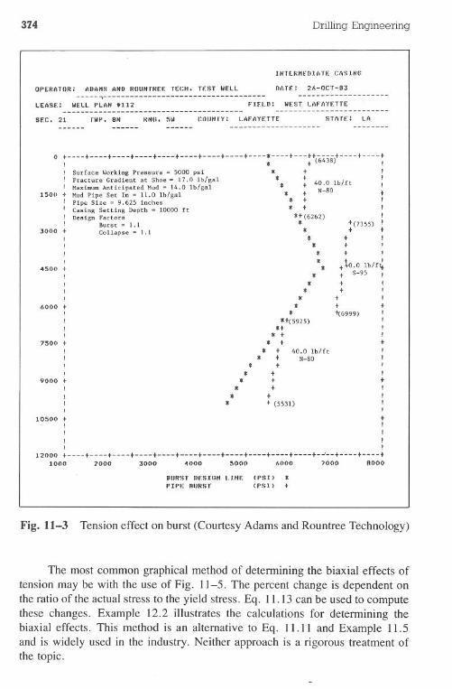
374 Drilling Engineering
INTr.R"£~I~TE ~ASING
OPERATOR: AIJo\"S AHO RIIIIHIHEE TECH. n:ST HELL~------------------------------------
LEASf:: Wf:U. I'LAN *112 f"IEI.D:
DATE: 26-0CT-93--------------------
Wf:ST L.\FA'IETTE---------------------------------------- -------------------------SEt;. 21 IWI'. 9H RHII. ~W COIINIY: LAFAYETTE STlln:: LA
--------------------
1500
o t t t t t t t t t * t---tt t t tI * t (6438) !
! Surface WorkingPressure. 5000psi * + I, Fracture Gradient at Shoe- 17.0 Ib/gal * + 40 0 Ib/f !! MaximumAnticipated Mud. 14.0 Ib/gal * + N:aO t ,
MudPipe Set In -11.0 Ib/gal * tPipeSize. 9.625 inches * +CasingSetting Depth- 10000ft * tDesignFactors :t:+(6262)
Burst . 1.1 *Collapse . 1.1 **
****~500
**
**
**
U(5925)U
* t* t
* t 40.0 Ib/ft* t N-80
* t* t
* t* t
* t* t (5531)
t(7355)t
ttt
t to.O Ib/f~t S-95 !tt
tt+(6999)
t!!
3000
6000
7500 t!!!
I9000 t
!III
10~00 tIIII
12000 t t t t t t t t t t t t-~--t t t1000 2000 3000 ~OOO 5000 6000 7000 9000
t!
BIIRST Df.SIOH UHf. (PSI) *PIPE BIIRST (PSI> t
Fig. ll-3 Tension effect on burst (Courtesy Adams and Rountree Technology)
The most common graphical method of determining the biaxial effects oftension may be with the use of Fig. II-5. The percent change is dependent onthe ratio of the actual stress to the yield stress. Eq. 11.13 can be used to computethese changes. Example 12.2 illustrates the calculations for determining thebiaxial effects. This method is an alternative to Eq. Il.II and Example 11.5and is widely used in the industry. Neither approach is a rigorous treatment ofthe topic.
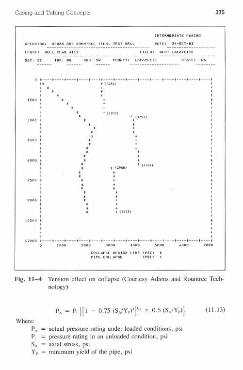
Casing and Tubing Concepts 375
DATE: 26-0CT-83
LEASEI WEl.l. I'I.AN "112
OPERATOR: .)DANS MID IWUN,.REF. n:CH. l"F.ST IIF.LL
-------------------------
--------------------
SEC. 21 TWI'. 8N RNO. :lW
------------------------------------------
COUHT"{: l.flF.Wf.T rE STArF.: LA
fIEI.D: Wt:ST I.AFIIYETTE----------------------------------------
o t t t t---tt t t t t t t t t t!. t(2484) !! * + !! 1< + !! * + !
t tt !t !t (2709) !
t (3792) !t tt !t !t !t !t tt !t !t !t ,t tt (4109) I!
!!t,,IIt,!,
It,
,
I
. '
t t t t t t t t t t t t t t to 1000 2000. 3000 ~ooo 5000 6000 7000
1500.
t.*
3000 .
4500
***
t*
.
.t.
**
.
.*.t**..*t
6000 t!
7500
9000 t!!!
10~jOO
12000
--------------------
*
t (2986)ttttt
tttttt (3195)
COI-L..WSf:OF.SUlNUNF. (PSI> *PIPE (:OI.I-I"'S£ (PSI) t
Fig. 11-4 Tension effect on collapse (Courtesy Adams and Rountree Tech-nology)
Where:
PAPiSAYp
(11.13)
actual pressure rating under loaded conditions, psipressure rating in an unloaded condition, psiaxial stress, psiminimum yield of the pipe, psi
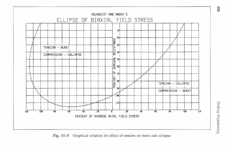
HO
LMQ
UIS
TAN
DN
AD
Al'S
ELLIP
SE
OF
BIR
XIR
LY
IELD
ST
RE
SS
1211188
488
611B
8128
le8211
4e811
61128
PE
RC
EN
TOF
AV
ER
AG
EAX
IAL
YIE
LDS
TR
ES
S
Fig.11-5
Graphical
solutionfor
effectof
tensionon
burstand
collapse
w....entJS5-<
0tI'J::!<
05'CD
CD
....5-<
0
/18
//
/U
J21I
/Uzg:3I!
/T
EN
SIO
N-B
UR
ST
en/
II
.....
48C
OM
PR
ES
SIO
N-C
OLLA
PS
EV
a!5I'J/
z/
...../
0611V
zlL.
/078
/\
.-/
ztj811./
TE
NS
ION-
CO
LLAP
SE
wI
II
Ia..911
\"'"
VC
OM
PR
ES
SIO
N-B
UR
ST
"".-/' V
--118
----
uu
--n
---
----
--.--
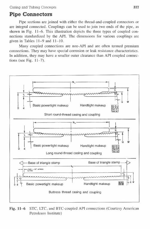
Casing and Tubing Concepts 377
Pipe ConnectorsPipe sections are joined with either the thread-and-coupled connectors or
are integral connected. Couplings can be used to join two ends of the pipe, asshown in Fig. 11-6. This illustration depicts the three types of coupled con-nections standardized by the API. The dimensions for various couplings aregiven in Tables 11-9 and 11-10.
Many coupled connections are non-API and are often termed premiumconnections. They may have special corrosion or leak resistance characteristics.In addition, they may have a smaller outer clearance than API coupled connec-tions (see Fig. 11-7).
1==t---r
=in IQ W
Basic powertight makeup Handtight makeup , 1ii"="8.Tw=i:iiie:i:i
Short round-thread casing and coupling
1~Basic powertight makeup Handtight makeup " 1
ii=i:'iiii=i.im:-
Long round-thread casing and coupling
<}- Base of triangle stamp
_J 1*"""':'3164I 4~. AP1'ROX
-II II,2mm)
~IIfor\ Basic powertight makeup
Base of triangle stamp -f>I
Handtight makeup
Buttress thread casing and coupling
Fig. 11-6 STC, LTC, and BTC-coupled API connections (Courtesy AmericanPetroleum Institute)
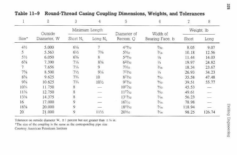
W0..'1=
Table
11-9R
ound-Thread
Casing
Coupling
Dim
ensions,W
eights,and
Tolerances
23
45
67
8
Outside
Minim
umL
engthD
iameter
ofW
idthof
Weight,
lb
Size*
Diam
eter,W
ShortN
LL
ongNL
Recess,
QB
earingFace,
bShort
Long
41/25.000
6Y4
7419/32
5/328.05
9.075
5.5636Y
27%
531323/16
10.1812.56
5Y2
6.0506%
8519/32
Ys
11.4414.03
6%7.390
7Y4
8%623/32
Y4
19.9724.82
77.656
7Y4
973132
3/1618.34
23.677%
8.5007Y
29Y
4723/32
Y4
26.9334.23
8%9.625
7%10
823/329/32
35.5847.48
9%10.625
7%1O
Y2
92%2
9/3239.51
55.7710%
11.7508
-1027/32
%2
45.5311%
12.7508
-1127/32
%2
49.6113%
14.3758
-1315/32
5/1656.23
1617.000
9-
163/325/16
78.9818%
20.0009
182¥325/16
118.940
--
S20
2!.0009
11Y2
203/325/16
98.25126.74
5'(Q
Tolerance
onoutside
diameter
W,
:tI
percentbut
notgreater
than:t
J/8in.
I:1:J::s(Q
*The
sizeof
thecoupling
isthe
same
asthe
correspondingpipe
size5'
Courtesy
Am
ericanPetroleum
InstituteC
DC
D....5'(Q
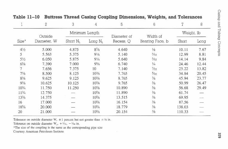
QT
able11-10
Buttress
Thread
Casing
Coupling
Dim
ensions,W
eights,and
Tolerances
[J)E
r<
Q
23
45
67
80-
Minim
umL
engthW
eight,Ib
trO
utsideD
iameter
ofW
idthof
Ei"
Size*D
iameter,
WShort
NL
LongN
LR
ecess,Q
Bearing
Face,b
ShortL
ong<
Qg41/2
5.0004.875
87/s4.640
Vs
10.117.67
()(1)
55.563
5.3759V
s5.140
5/3212.99
8.81'01iJ
5V2
6.0505.875
9V4
5.6405/32
14.149.84
6%7.390
7.0009%
6.7401/4
24.4612.44
77.656
7.37510
7.1407/32
23.2213.82
7%8.500
8.12510%
7.765sIlO
34.8420.45
8%9.625
9.12510%
8.765%
45.9423.77
9%10.625
10.12510%
9.765%
50.9926.47
10%11.750
11.25010%
10.890%
56.6829.49
11%12.750
-10%
11.890%
61.7413%
14.375-
10%13.515
%69.95
1617.000
-10%
16.154%
87.5618%
20.000-
10%18.779
%138.03
2021.000
-10%
20.154%
110.33
Tolerance
onoutside
diameter
W,
:tI
percentbut
notgreater
than:t
Y.
in.T
oleranceon
outsidediam
eterW
"+
Y32,
-Y
64in.
*The
sizeof
thecoupling
isthe
same
asthe
correspondingpipe
size
Courtesy
Am
ericanPetroleum
Institutew0..:1C
D
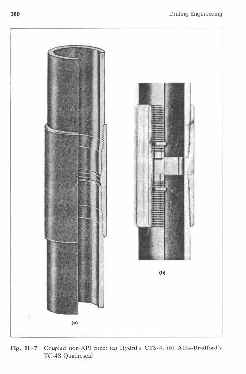
380
(a)
Drilling Engineering
(b)
Fig. 11-7 Coupled non-API pipe: (a) Hydril's CTS-4, (b) Atlas-Bradford'sTC-4S Quadraseal
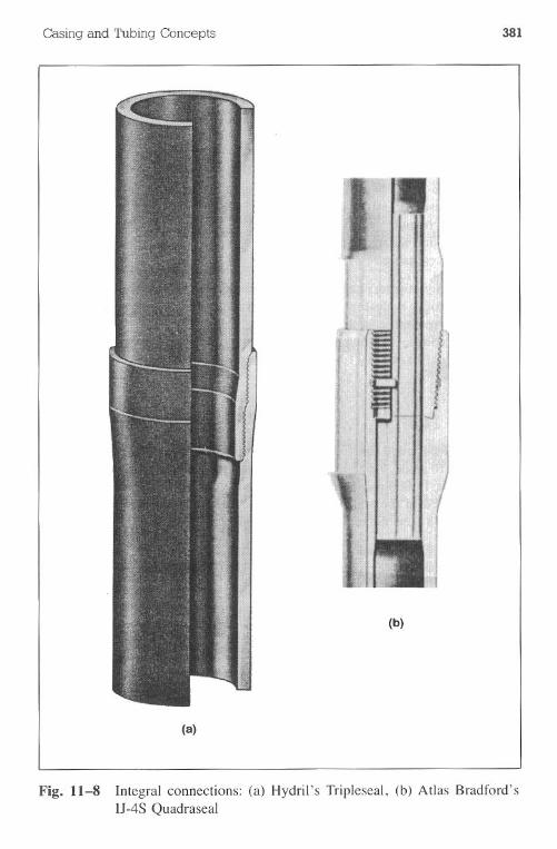
Casing and Tubing Concepts 381
)1
j
I
(b)
(a)
Fig. 11-8 Integral connections: (a) Hydril's Tripleseal, (b) Atlas Bradford'sIJ-4S Quadraseal
382 Drilling Engineering
Integral connectiQnsdo not use separate coupling devices. The ends of thejoints are milled so the pin end of one joint screws into the box end of anotherjoint. Manufacturers offer a variety of coupled and integral-joint connections(see Fig. 11-8).
Coupling selection is normally based on design criteria such as the fol-lowing:
.burst·collapse.joint strength.corrosionresistance.leak resistance
Since many investigators have documented casing and tubing failures due to thecouplings, proper evaluation and selection is an important issue. It is advisableto consider premium couplings if corrosion, leak resistance, or high pressuresare considerations. Coupling manufacturers and distributors should be consultedin these case,s. Example 11.6 illustrates coupling selection in a high pressureenvironment.
Example 11.6
The Wisler-Burnett Oil Company intends to run a 22,300-ft string of 47.0-Ib/ft, P-110 grade, 7.625-in. production casing. The maximum expected burstpressure is 14,000 psi. Select the appropriate couplings. A 17.0-lb/gal mudwill be used in the well. Company policy dictates that the tension designfactor is 1.8. Use the tables in the Appendix.
Solution:
I. Determine the maximum tension load:Pipe weight = depth x Ib/ft
= 22,300 ft x 47.0 Ib/ft= 1,048,100 Ib
Buoyed weights = pipe weight x buoyancy factor
= 1,048,100Ibx (I - ~;:~)776,074Ib
Design load = buoyedweight x designfactor776,074Ib x 1.8
= 1,396,933Ib
2. The tables in the Appendix provide the following information:
Casing and Tubing Concepts 383
CouplingTypeLTCBTC
Burst Rating,pSI
14,43013,460
Joint Strength,Ib
1,353,0001,545,000
3. The LTC coupling is unsatisfactory for the joint strength requirements,while the BTC is underdesigned in burst.
4. Some of the design options are as follows:. run LTC or BTC couplings, realizing they do not meet the design re-quirements.reevaluate the burst criteria·reduce the tension design factor
5. This example illustrates that stringent operating conditions may place de-mands on pipe design beyond the "standard" situation, such that con-ventional design procedures are not applicable.
Problems
11.1 Calculate the internal yield (burst) pressure for 43.5-lb/ft, N-80grade, 9.625-in. pipe with a wall thickness of 0.435 in.
11.2 A section of 8.625-in., P-110 grade pipe has a wall thickness of0.450 in. Calculate the internal yield of the pipe.
11.3 A 9.625-in., N-80 string has a wall thickness of 0.30, 0.35, 0.40,0.45, 0.5, 0.55 in. Calculate the internal yield pressure and plot theresults.
11.4 Recalculate Problem ILl and use a 95% wall thickness.
11.5 Recalculate Problem 11.2 and use a 95% wall thickness.
11.6 Recalculate Problem 11.3 and use a 95% wall thickness.
11.7 A 9.625-in. string must be designed for sour service and have aninternal yield pressure of 9,700 psi. The maximum allowable yieldstrength is 90,000 psi. Determine the wall thickness requirementsfor the pipe and assume an API wall tolerance of 87.5%. Round upthe wall thickness to the nearest eighth inch.
384 Drilling Engineering
Determinethe minimum acceptable wall thickness for a 7.0-in. sourservice string. Use a maximum yield strength of 80,000 psi. Roundup to the nearest eighth inch. Use the API wall thickness value of87.5%.
11.8
Calculate the collapse rating for the following sections of pipe. Usingthe API tables and equations, calculate the collapse rating to thenearest 10 psi. Show all calculations.
11.9
Pipe diameter, in.Wall thickness, in.GradeWeight, Ib/ft
10.750.40K-55
45.5
9.6250.545N-80
53.5
5.00.362P-110
18.0
13.3750.480K-55
68
11.10 Calculate and plot the collapse ratings for the following weights ofN-80, 7.625-in. pipe.
SectionI234567
Weight, Iblft26.429.733.739.045.347.152.8
Wall Thickness, in.0.3280.3750.4300.5000.5950.6250.712
11.11 The collapse rating for n.O-lb/ft, P-110 grade, 13.375-in. pipe mustbe calculated. Use the API formulas and tables.
11.12 Refer to Problem 11.10; determine the pipe body yield strength.
11.13 Refer to Problem 11.12; recalculate the results for P-110 grade pipe.
References
Applied Drilling Services Volume I User's Guide. Lafayette, LA: Adams andRountree Technology Inc., 1981.
Casing, Tubing, and Drill Pipe. API Specification 5A, 1981.
Casing and Tubing Concepts 385
Casing, Tubing, Drill Pipe, and Line Pipe Properties. API Bulletin 5C3.1980with Supplement 2, 1983.
Holmquist and Nadai. "Collapse of Deep Well Casing." API Drilling andProductionPractices, 1939. .
Hydril tubular brochures.
Kawasaki Tubular Reference Catalog.
Mudge, Kris. Council Petroleum Services Inc., personal discussions.
N:L. Atlas Bradford tubular brochures.
Chapter 12 Casing Design
Casing string design and selection is one of the many important aspectsof the properly prepared well plan. The casing is used for protection during allphases of drilling and production, and, as such, it is often designed to withstandmany severe operating conditions. As a result, procedures for casing design mustbe sufficiently flexible to meet all potential requirements.
Maximum Load ConceptMany philosophies have evolved for casing. design. In most cases, they
are based on the engineer's past experience with casing strings or his ability topredict the potential loading environments to be placed on a string. As a result,most casing design procedures take measures to prevent problems such as casingparting, collapse or corrosion.
The maximum load concept is perhaps the most widely used casing designprocedure in the drilling industry. This method, or its modified versions, analyzesexpected drilling problems. The casing is designed to withstand these problems.Although the method was originally conceived as a design procedure for highpressure drilling and its associated problems, it is flexible enough to meet mostdemanding drilling conditions.
An analysis of the expected operating conditions is required before de-signing a casing string. Common problems often considered for casing designwhen drilling in abnormal pressure environments are as follows:
· kicks· lost circulation.stuck pipe·wear
386
Casing Design 387
The maximum load concepts presented here address these considerations as ifthe string were designed for abnormal pressure wells. Factors that become im-portant in other environments include the following:
· hydrogen sulfide (H2S)· carbon dioxide (C02)· salt. cavernous formations· hydraulic fracturing
Note that tubing and drillstring design use different load conditions and designtechniques.
General Casing Design CriteriaCasing strings are usually designed for the following conditions:.burst· collapse.tension.biaxialeffects
Burst conditions are established, and the least-expensive pipe that will satisfythe burst load is tentatively selected.
Subsequently, the collapse loads are defined and the tentative selection isevaluated for collapse resistance. If any section from the tentative design doesnot meet the collapse load limits, it is upgraded with pipe of a sufficient collapserating. At this point, the tentative design uses the least-expensive pipe thatsatisfies both the burst and collapse requirements.
Tensile loads for the casing string are defined. The body strengths of thetentative pipe selection are checked. As in the case of collapse, any underdesignedsection is upgraded in terms of pipe grade or body weights. In addition, thetensile loads are used to select pipe couplings.
Burst and collapse ratings for pipe are altered for pipe loaded in tension(or compression). These effects, termed biaxial effects, must be analyzed toensure they do not reduce the pipe ratings below the required burst or collapserequirements. If unacceptable reductions occur, the specific pipe section that isaffected must be altered or upgraded. In addition, when properly applied thebiaxial effects lengthen the sections of lower-cost pipe that can be used. Thespecific effects of tension loading are as follows:
Types of LoadTensionTension
ResultBurst-IncreaseCollapse-Decrease
388 Drilling Engineering
Types of LoadCompressionCompression
ResultBurst-DecreaseCollapse-Increase
Graphical Techniques. Graphical pipe selection is the most widely usedmethod for picking proper weights, grades, and section lengths of casing. Agraphical representation of the imposed loads is prepared for burst, collapse,and tension (see Fig. 12-1 a). A casing catalog like that presented in the Appendixis used to select pipe that will satisfy the requirements in Fig. 12-la. Althoughminimum cost is the most logical and common reason for pipe selection to satisfythe requirements in Fig. 12-la, other reasons include general pipe availabilityin the marketplace or forced selection from existing company inventory. Figs.12-Ib and c show optional designs that satisfy the requirements in Fig. 12-la.
o
Burst load atany depth
in well
6,000
2,000
4,000=
(a) ~Q)
o6,000
8,000
10,000o 2,000 4,000 6,000 8,000 10,000
PRESSURE (psi)
Fig. 12-1 Typical burst load configuration for intermediate casing (9%"). (Nu-merical values used for illustrative purposes) with (b) satisfactoryand (c) economical designs

Casing Design
2,000
4,000
(b)
""
~i5.Q)
CI
6.000
o
String cost = $346,000'8,000 + '1982 prices
10,000o
2,000
4,000
(e)
""
~i5.Q)CI
6,000
10,000o
2,000
o
9%-in. pipe
389
5,000
10,000 tt43.5 Ib/ttN-80 grade9% in.
Burst = 6,330 psi
5,000
4,000 6,600Pressure, psi
Total string cost = $327,786''1982 prices
8,000
8,000 10,000
5,000
3,400 tt43.5 IbittN-80Burst = 6,330 psi
5,750 psi
2,000
5,000I . . I
4,000 6,000Pressure, psi
8,000 10,000
390 Drilling Engineering
Upgrading an unsatisfactory section is a simple procedure with the graph-ical technique. As shown"in Fig. 12-2, any underdesigned section can be isolatedand upgraded with either a heavier-weight or higher-grade pipe.
Section Limitations. Practicality of pipe handling often requires thatrestraints be placed on complete implementation of the maximum load concept.If fully exercised, this method, or any others, will select the least-expensivepipe to satisfy the requirements. As a result, many short sections offer theminimum cost design. Since three or four sections of pipe are usually the upperpractical limit on rig-site pipe handling, some method must be used to restrictpipe selection. The most common methods for limitations of the sections are asfollows:
· establish a maximum number of sections.establish a minimum section length·establisha maximumnumberof sectionswitha minimumsectionlength
o
7 in.26.0 Ib/ftN.aO
.s-collapse = 5,410 psi
2,000
4,000
-=~a.~ 6,000
Final design:8,000 ft, 26.0 Ib/ft. N-80
2,000 ft, 29.0 Ib/ft, N.80
8,000 Upgrade lower 2.000 ftwith 29.0-lb/ft, N.80Collapse = 7,020 psi
¥"
10,000o 2,000 4,000 6,000 8,000 10,000
psi
Fig. 12-2 Upgrading underdesigned sections
Casing Design 391
For example, do not use string designs with more than four sections and thenavoid using any section less than 3,000 ft long. Some companies use only asingle weight and grade of pipe per string, even though it is significantly moreexpensive than the optimum-cost design:
Burst. The burst loads on the casing must be evaluated to ensure theinternal yield resistance of the pipe is not exceeded. The loads are normallycaused by mud hydrostatic pressure inside the casing and perhaps some surfacepressure. Fluids on the outside of the casing, called backup fluids, supply ahydrostatic pressure that helps resist pipe burst. The resulting, effective burstpressure is the internal pipe load minus any external pressure. This net burstpressure is termed the resultant (see Fig. 12-3).
Collapse. The primary collapse loads are supplied by the fluids on theoutside of the casing. These fluids are usually the mud and possibly the cementin which the casing was set. The backup fluids are generally considered 1)negligible, resulting from complete loss or evacuation of the mud inside thepipe, or 2) partial supportive, resulting from some loss of internal mud (see Fig.12-4). The resultant collapse loads are computed in the same manner as burst.
Tension. Each section of the casing must be evaluated for tensile orcompressive loading. As presented in Chapter 11 and discussed earlier in this
/'"Backup
BackupJI
I
Loadminus
backup = resultant~
Resultant
~ 1
Example:Load = 10,000 psi
- Backup = 6,000 psi
Resultant = 4,000 psi
Fig. 12-3 Typical relationships between burst load, backup, and resultant
392 Drilling Engineering
(a)
No fluid inside
the pipe to
provide support
jLoad
Partial evacuation
of fluids inside the pipe
J(b)
../'Fluid level
Load
J
Fig. 12-4 Two common concepts for collapse loading: (a) dry inside and (b)partially dry inside
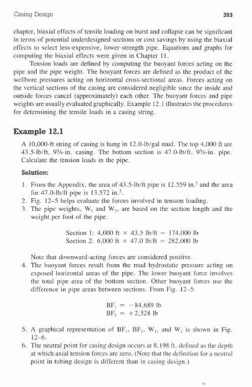
Casing Design 393
chapter, biaxial effects of tensile loading on burst and collapse can be significantin tenns of potential underdesigned sections or cost savings by using the biaxialeffects to select less-expensive, lower-strength pipe. Equations and graphs forcomputing the biaxial effects were given in Chapter II.
Tension loads are defined by computing the buoyant forces acting on thepipe and the pipe weight. The bouyant forces are defined as the product of thewellbore pressures acting on horizontal cross-sectional areas. Forces acting onthe vertical sections of the casing are considered negligible since the inside andoutside forces cancel (approximately) each other. The buoyant forces and pipeweights are usually evaluated graphically. Example 12.1 illustrates the proceduresfor detennining the tensile loads in a casing string.
Example 12.1
A 1O,0OO-ftstring of casing is hung in 12.0-lb/gal mud. The top 4,000 ft are43.5-lb/ft, 95fs-in. casing. The bottom section is 47.0-lb/ft, 95fs-in. pipe.Calculate the tension loads in the pipe.
Solution:
I. From the Appendix, the area of 43.5-lb/ft pipe is 12.559 in.2 and the areafor 47.0-lb/ft pipe is 13.572 in.2.
,2. Fig. 12-5 helps evaluate the forces involved in tension loading. :
3. The pipe weights, WI and Wh are based on the section length and theweight per foot of the pipe.
Section I: 4,000 ft x 43.5 Ib/ft = 174,000IbSection 2: 6,000 ft x 47.0 Ib/ft = 282,000 Ib
Note that downward-acting forces are considered positive.4. The buoyant forces result from the mud hydrostatic pressure acting on
exposed horizontal areas of the pipe. The lower buoyant force involvesthe total pipe area of the bottom section. Other buoyant forces use thedifference in pipe areas between sections. From Fig. 12-5:
BF. = - 84,689 IbBF2 = + 2,528 Ib
5. A graphical representation of BF., BF2, WI' and W2 is shown in Fig.12-6.
6. The neutral point for casing design occurs at 8,198 ft, defined as the depthat which axial tension forces are zero. (Note that the definition for a neutralpoint in tubing design is different than in casing design.)
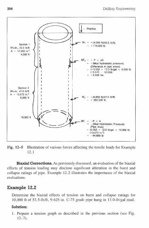
394 DrillingEngineering
Section19%-in., 43.5 Ib/llA ; 12.559 in.2
4,000'11
U - Positive I
BF2 ; + P x I1A+ (Mud hydrostatic pressure)(Difference in pipe areas)(+ 0.052 x 12.0 Ib/gal x 4,000 II)(13.572 - 12.559)
; + 2,528 Ibs
Section 29%-in., 47.0 Ib/llA ; 13.572 in?
6,000 II
I
1- W2 ; +(6,000 11)(47.0 Ib/ll)+ 282,000 Ib
10,000 II
BF, = -P x A= - (Mud Hydrostatic Pressure)
(Pipe Area)= (0.052 x 12.0 Ib/gal x 10,000 II)
(13.572 in?)= - 84,689 Ib
Fig. 12-5 Illustration of various forces affecting the tensile loads for Example12.1
Biaxial Corrections. As previously discussed, an evaluation of the biaxialeffects of tension loading may disclose significant alteration in the burst andcollapse ratings of pipe. Example 12.2 illustrates the importance of the biaxialevaluations.
Example 12.2
Determine the biaxial effects of tension on burst and collapse ratings for10,000 ft of 53.5-lb/ft, 9.625-in. C-75 grade pipe hung in 13.0-lb/gal mud.
Solution:
I. Prepare a tension graph as described in the previous section (see Fig.12-7).
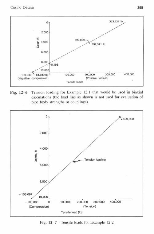
Casing Design 395
o
2.000
g"R 4.000CDc
6.000
10.000
- 100,000 ~84,689Ib 0(Negative. compression)
100.000 200,000 300,000(Positive, tension)
400,000
Tensile loads
Fig. 12-6 Tension loading for Example 12.1 that would be used in biaxialcalculations (the load line as shown is not used for evaluation ofpipe body strengths or couplings)
o429,903
2,000
- 105,09710,000 .
-100,000 0(Compression)
100,000 200,000 300,000 400,000
(Tension)
Tensile load (Ib)
Fig. 12-7 Tensile loads for Example 12.2
4,00001:S£a.CD0
6,000
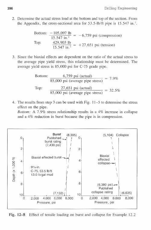
396 Drilling Engineering
2. Detennine the actual stress load at the bottom and top of the section. Fromthe Appendix, the cross-sectional area for 53.5-lb/ft pipe is 15.547 in.2.
Bottom: -105,097Ib15.547 in.2
429,903 Ib _15.547 in.2 -
-6,759 psi (compression)
Top:+ 27,651 psi (tension)
3. Since the biaxial effects are dependent on the ratio of the actual stress tothe average pipe yield stress, this relationship must be determined. Theaverage yield stress is 85,000 psi for C-75 grade pipe.
Bottom: 6,759 psi (actual)85,000 psi (average pipe stress)
Top: 27,651 psi (actual)85,000 psi (average pipe stress)
7.9%
32.5%
4. The results from step 3 can be used with Fig. 11-5 to detennine the stresseffect on the pipe.Bottom: A 7.9% stress relationship results in a 4% increase in collapseand a 4% reduction in burst because the pipe is in compression.
Fig. 12-8 Effect of tensile loading on burst and collapse for Example 12.2
0Burst (8,395) (5,104) Collapse
Published....... , 0 \burst rating \(7,430 psi) I
2 I 2 \
./ Biaxial\
£ Biaxial effected burst-:z..effected \
0 4 f 40 , collapse--\
if9%-in.\x C-75, 53.5 Iblll 66 I.c 13.0Ib/galmud \i5.
Q)0
8 8(6,380 psi)_
I Published \
10 (7,132) I 10 collapse rating \ (6,635)0 2,000 4,000 6,000 8,000 0 2,000 4,000 6,000 8,000
Pressure, psi Pressure, psi
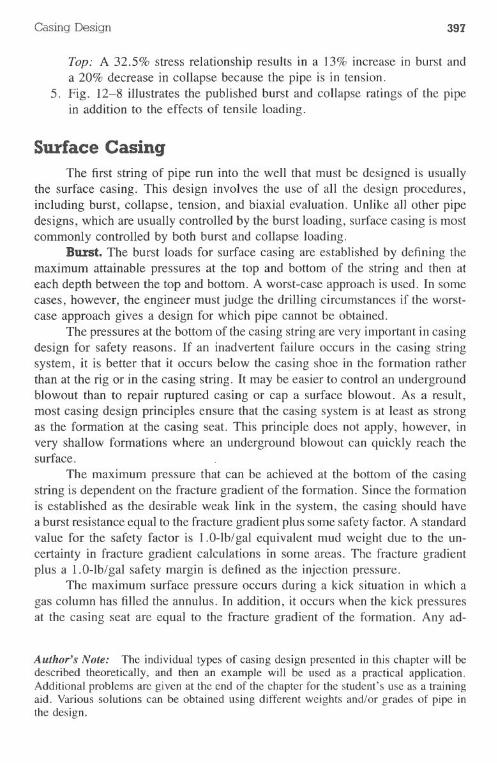
Casing Design 397
Top: A 32.5% stress relationship results in a 13% increase in burst anda 20% decrease in c011apsebecause the pipe is in tension.
5. Fig. 12-8 illustrates the published burst and collapse ratings of the pipein addition to the effects of tensile loading.
Surface CasingThe first string of pipe run into the well that must be designed is usually
the surface casing. This design involves the use of all the design procedures,including burst, collapse, tension, and biaxial evaluation. Unlike all other pipedesigns, which are usually controlled by the burst loading, surface casing is mostcommonly controlled by both burst and collapse loading.
Burst. The burst loads for surface casing are established by defining themaximum attainable pressures at the top and bottom of the string and then ateach depth between the top and bottom. A worst-case approach is used. In somecases, however, the engineer must judge the drilIing circumstances if the worst-case approach gives a design for which pipe cannot be obtained.
The pressures at the bottom of the casing string are very important in casingdesign for safety reasons. If an inadvertent failure occurs in the casing stringsystem, it is better that it occurs below the ca~ing shoe in the formation ratherthan at the rig or in the casing string. It may be easier to control an undergroundblowout than to repair ruptured casing or cap a surface blowout. As a result,most casing design principles ensure that the casing system is at least as strongas the formation at the casing seat. This principle does not apply, however, invery shallow formations where an underground blowout can quickly reach thesurface.
The maximum pressure that can be achieved at the bottom of the casingstring is dependent on the fracture gradient of the formation. Since the formationis established as the desirable weak link in the system, the casing should havea burst resistance equal to the fracture gradient plus some safety factor. A standardvalue for the safety factor is 1.0-lb/gal equivalent mud weight due to the un-certainty in fracture gradient calculations in some areas. The fracture gradientplus a 1.0-lb/gal safety margin is defined as the injection pressure.
The maximum surface pressure occurs during a kick situation in which agas column has filled the annulus. In addition, it occurs when the kick pressuresat the casing seat are equal to the fracture gradient of the formation. Any ad-
Author's Note: The individual types of casing design presented in this chapter will bedescribed theoretically, and then an example will be used as a practical application.Additional problems are given at the end of the chapter for the student's use as a trainingaid. Various solutions can be obtained using different weights and/or grades of pipe inthe design.
398 Drilling Engineering
ditional pressure at the casing seat results in an underground blowout. Therefore,the surface pressure is computed as the maximum pressure at the casing seat,or the injection pressure, minus a column of gas to the surface.
Fig. 12-9a shows the surface and injection pressures for the surface cas-ing's burst load line. The pressure at any point between the top and bottom canbe defined graphically. For continuity throughout this text, a gas gradient of0.115 psi/ft will be used, although the value is commonly considered in therange of 0.1 to 0.15 psi/ft.
The backup fluid provides a resistance to pipe burst. Although the fluidmay be considered equal in density to the mud or cement in which the pipe wasset, a worst case assumes that a small segment of the backup fluid may degradein density. Since it is improbable that the density will fall below that of thenative formation fluids, the backup is assumed equal to the density of formationfluids. Cement is not considered as providing any burst support.
Some exceptions to this assumption must be considered for certain designs.Areas that have significant problems with vugs or caverns may need a backupfluid designed with reduced density or completely void. In addition, some strin-gent designs may prohibit the assumption of fluid degradation to 9.0 Ib/gal.
The net effective pressure tending to burst the pipe is defined as theresultant. It is the load line minus the backup fluid. Theoretically, it could beused to select casing for the string. However, a safety factor is normally appliedto the resultant to account for unforeseen occurrences and pipe wear. A somewhatstandard value of I. I is used as the burst design factor. The product of theresultant and the burst design factor yields the burst design line (see Fig.12-9c).
A tentative pipe selection is made from the burst design line in Fig.12-9c. As shown in Fig. 12-9d, the pipe must have a burst pressure that exceedsall values in the burst design line. After the pipe selection is made, the designis set aside, pending evaluation of the collapse requirements.
Collapse. The mud or cement in which the casing was set provides thecollapse loading. Usually, one or two "green" cement slurries are considered.This position is reversed from the burst design, in which cement was cbnsideredas providing no load or support. This assumption follows the worst-case ap-proach.. Surface casing is normally designed with no collapse backup fluid inside
the pipe. In other words, it is designed "dry" inside. Therefore, the resultantis the same as the load line (see Fig. 12-lOa).
The collapse design line is the product of the resultant and a design fac-tor. These factors range from 1.1-1.125 in most cases. As in the case of theburst design, a factor of 1.1 will be used throughout this text for collapsedesign.
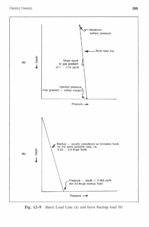
Casing Design
(a)
(b)
399
~ Maximumsurface pressure
Burstload line
Slope equalto gas gradient
(0.1 - 0.15 psi/II)
Injection pressure
(frac gradient + safety margin'l
~0.Q)c
Pressure..
<' Backup - usually considered as formation fluids,. for the worst possible case, i.e.,8.33 - 9.0 Ib/gal fluids
Pressure = depth x 0.465 psi/II
[ (for 9.0 (b/gal backup fluid)
Pressure...
Fig. 12-9 Burst Load Line (a) and burst backup load (b)
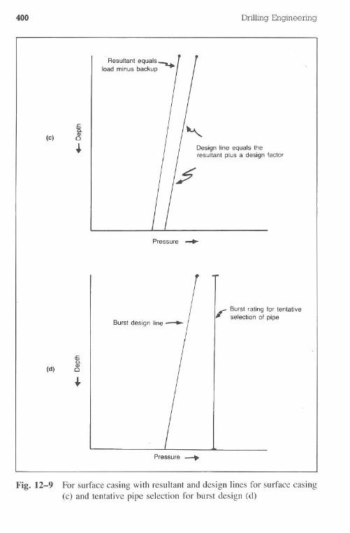
400
(c)
(d)
.L:a.Q)c
+
Drilling Engineering
Design line equals theresultant plus a design factor
1
_'- Burst rating for tentative~ selection of pipe
Fig. 12-9 For surface casing with resultant and design lines for surface casing(c) and tentative pipe selection for burst design (d)
Pressure~
.L:a.Q)c
Pressure-+
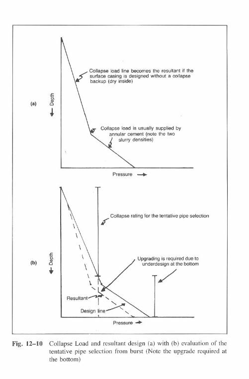
Casing Design 401
(a)
.s::is.Q)
CI
Collapse load line becomes the resultant if thesurface casing is designed without a collapsebackup (dry inside)
Collapse load is usually supplied byannular cement (note the two
slurry densities)
Pressure ~
(b)
.s::a.Q)CI
t
Collapse rating for the tentative pipe selectionf
Upgrading is required due tounderdesign at the bottom
/
Pressure ~
Fig. 12-10 CollapseLoad and resultantdesign(a) with (b) evaluationof thetentative pipe selection from burst (Note the upgrade required atthe bottom)
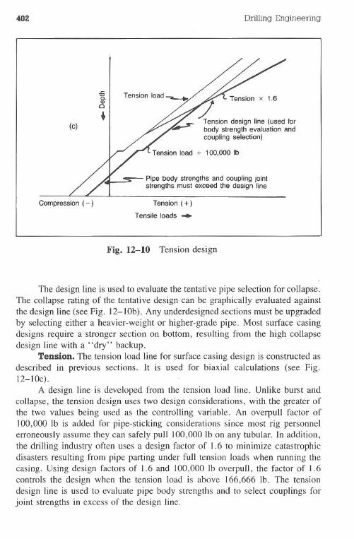
402 Drilling Engineering
(c)
.£:a.Q)c
.
Tension load + 100.000 Ib
Pipe body strengths and coupling jointstrengths must exceed the design line
Compression (-) Tension(+)Tensileloads ~
Fig. 12-10 Tension design
The design line is used to evaluate the tentative pipe selection for collapse.The collapse rating of the tentative design can be graphically evaluated againstthe design line (see Fig. 12-lOb). Any underdesigned sections must be upgradedby selecting either a heavier-weight or higher-grade pipe. Most surface casingdesigns require a stronger section on bottom, resulting from the high collapsedesign line with a "dry" backup.
Tension. The tension load line for surface casing design is constructed asdescribed in previous sections. It is used for biaxial calculations (see Fig.12-lOc).
A design line is developed from the tension load line. Unlike burst andcollapse, the tension design uses two design considerations, with the greater ofthe two values being used as the controlling variable. An overpull factor of100,000 Ib is added for pipe-sticking considerations since most rig personnelerroneously assume they can safely pull 100,000 Ib on any tubular. In addition,the drilling industry often uses a design factor of 1.6 to minimize catastrophicdisasters resulting from pipe parting under full tension loads when running thecasing. Using design factors of 1.6 and 100,000 Ib overpull, the factor of 1.6controls the design when the tension load is above 166,666 lb. The tensiondesign line is used to evaluate pipe body strengths and to select couplings forjoint strengths in excess of the design line.
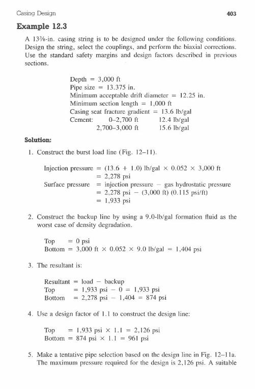
Casing Design 403
Example 12.3
A 133/s-in. casing string is to be designed under the following conditions.Design the string, select the couplings, and perform the biaxial corrections.Use the standard safety margins and design factors described in previoussections. .
Depth = 3,000 ftPipe size = 13.375 in.Minimum acceptable drift diameter = 12.25 in.Minimum section length = 1,000ftCasing seat fracture gradient = 13.6 Ib/galCement: 0-2,700 ft 12.4 Ib/gal
2,700-3,000 ft 15.6Ib/gal
Solution:
1. Construct the burst load line (Fig. 12-11).
Injection pressure = (13.6 + 1.0) Ib/gal X 0.052 x 3,000 ft2,278 psi
Surface pressure = injection pressure - gas hydrostatic pressure2,278 psi - (3,000 ft) (0.115 psi/ft)1,933 psi
2. Construct the backup line by using. a 9.0-lb/gal formation fluid as theworst case of density degradation.
Top = 0 psiBottom = 3,000 ft x 0.052 x 9.0 Ib/gal I ,404 psi
3. The resultant is:
Resultant = load - backupTop = 1,933psi - 0 = 1,933psiBottom = 2,278 psi - 1,404 = 874psi
4. Use a design factor of 1.1 to construct the design line:
Top = 1,933psi x 1.1 = 2,126 psiBottom = 874 psi x l.l = 961 psi
5. Make a tentative pipe selection based on the design line in Fig. 12-lla.The maximum pressure required for the design is 2,126 psi. A suitable
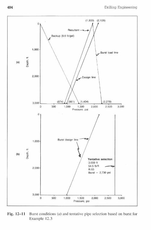
404 Drilling Engineering
(1,933) (2,126)
3,000o
1,000
(b)
'"'~E.CDc
2,000
3,000o
~1,500 2,000
Pressure, psi
(2,278)----.--2,500 3.000
o
Tentative selection3,000 tt54.51b/ttK-55Burst = 2,730 psi
500 1,000 1,500 2,000Pressure, psi
2,500 3,000
Fig. 12-11 Burst conditions (a) and tentative pipe selection based on burst forExample 12.3
1,000
I \ II VBurst load line'"'
(s) E.CDc
2,000
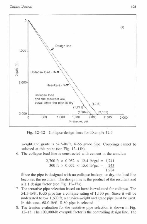
Casing Design 405
o
(a)
3.000o
Collapse loadand the resultant areequal since the pipe is dry
(1,741)
(1,984) \ "-.(2,182)500 1,000 1,500 2,000 2,500
Pressure, psi3,000
Fig. 12-12 Collapse design lines for Example 12.3
weight and grade is 54.5-lb/ft, K-55 grade pipe. Couplings cannot beselected at this point (see Fig. 12-11b).
6. The collapse load line is constructed with cement in the annulus:
2,700ft x 0.052 x 12.4lb/gal = 1,741300 ft x 0.052 x 15.6 Ib/gal = 243
1,984Since the pipe is designed with no collapse backup, or dry, the load linebecomes the resultant. The design line is the product of the resultant anda 1.1 design factor (see Fig. 12-12a).
7. The tentative pipe selection based on burst is evaluated for collapse. The54.5-lb/ft, K-55 pipe has a collapse rating of 1,130 psi. Since it will beunderrated below 1,600 ft, a heavier-weight and grade pipe must be used.In this case, 68.0-lb/ft, S-80 pipe is selected.
8. The tension evaluation for the tentative pipe selection is shown in Fig.12-13. The 100,000-lb overpull factor is the controlling design line. The
1.000
g.s::a.CDQ
2,000
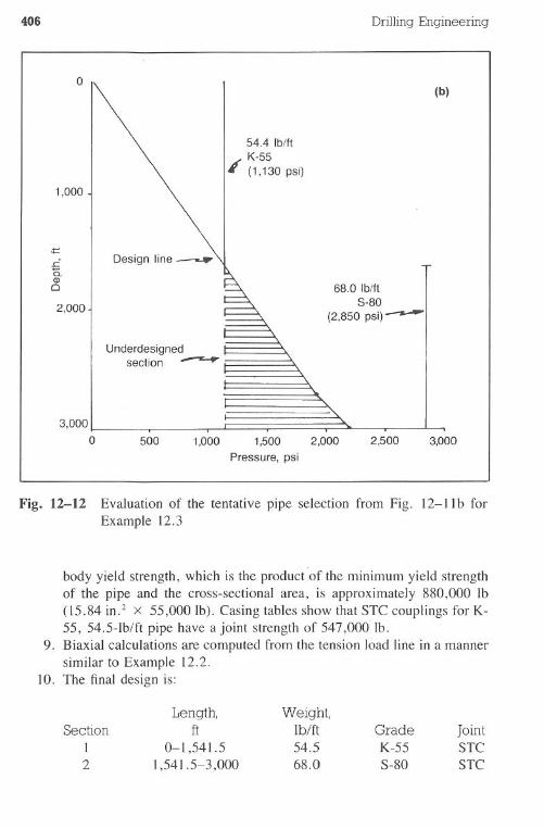
406 Drilling Engineering
o
2,000
(b)
54.4 Ib/llK-55
I' (1,130 psi)
1,000
.t:
.cC.Q)o 68.0 Ib/ll
8-80(2,850psi)----
underdesigned-.....section
3,000 ~
o 500 1,000 1,500 2,000
Pressure, psi
2,500 3,000
Fig. 12-12 Evaluation of the tentative pipe selection from Fig. 12-11b forExample 12.3
body yield strength, which is the product of the minimum yield strengthof the pipe and the cross-sectional area, is approximately 880,000 Ib(15.84 in.2 x 55,000 Ib). Casing tables show that STC couplings for K-55, 54.5-lb/ft pipe have a joint strength of 547,000 lb.
9. Biaxial calculations are computed from the tension load line in a mannersimilar to Example 12.2.
10. The final design is:
SectionI2
Length,ft
0-1,541.51,541.5-3,000
Weight,lb/ft54.568.0
GradeK-55S-80
JointSTCSTC
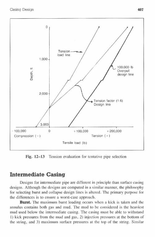
Casing Design 407
o
Tension factor (1.6)Design line
- 100,000
Compression (-)
+ 100,000 +200,000Tension (+)
Tensile load (Ib)
Fig. 12-13 Tension evaluation for tentative pipe selection
Intermediate CasingDesigns for intermediate pipe are different in principle than surface casing
designs. Although the designs are computed in a similar manner, the philosophyfor selecting burst and collapse design lines is altered. The primary purpose forthe differences is to ensure a worst-case approach.
Burst. The maximum burst loading occurs when a kick is taken and theannulus contains both gas and mud. The mud to be considered is the heaviestmud used below the intermediate casing. The casing must be able to withstand1) kick pressures from the mud and gas, 2) injection pressures at the bottom ofthe string, and 3) maximum surface pressures at the top of the string. Similar
1,000
c.Q)0
2,000
408 Drilling Engineering
to the manner used in surface casing, the injection pressure is computed as thefracture gradient at the casing seat in addition to a safety factor (Fig. 12-14).
The maximum surface pressure at the top of the string is worth someconsideration. It is often thought the surface pressure of the casing does not needto be greater than the working pressure of the surface equipment (BOPs orwellhead). Another approach is to ensure that the casing can withstand themaximum attainable surface pressure resulting from a kick. For example, if anannulus full of gas would give a surface pressure of 3,900 psi, the casing wouldnot need a burst rating greater than 3,900 psi. Further, a significant overdesignwould occur if the casing was selected to equal the 5,000-psi BOP equipmentrather than the maximum attainable pressure of 3,900 psi.
The pressure at any point in the casing is at a maximum when both endpoints, the surface pressure and injection pressure, are satisfied simultaneously.This relationship is expressed in Eq. 12.I:
IP (12.1)
Where:P,x
maximum surface pressure, psilength of mud column, ft
y = length of gas column, ftGm= gradient of heaviest mud to be used below the intermediate casing,
psi/ftGg = gas gradient, psi/ftIP = injection pressure, psi
The two unknowns are x and y. A second equation is required to solve for xand y:
x + Y SD (12.2)
Where:SD = casing setting depth, ft
The backup fluids for the burst design are considered equal in density toformation fluids. The resultant is the difference between the burst load and thebackup fluids (see Fig. 12-15a).
The burst design line is the product of the resultant and a design factor.A tentative pipe selection is made to satisfy the burst design line (see Fig. 12-15b).
Collapse. The collapse loading for intermediate pipe is supplied by themud weight that the casing was set in and the annular cement. The load will be
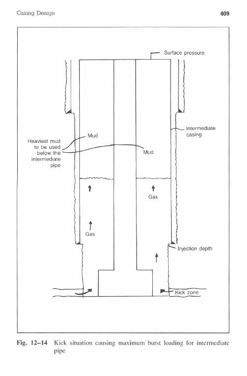
Casing Design
Heaviest mudto be usedbelow the
intermediatepipe
Mud
409
Surface pressure
tGas
t
Intermediatecasing
Injection depth
Kick zone
Fig. 12-14 Kick situation causing maximum burst loading for intermediatepIpe
t
tGas
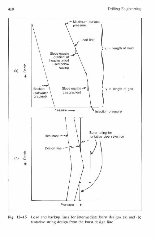
410
(a)
(b)
Slope equals _gradient of
heaviest mudused below
casing
¥ Maximum surfacepressure
Drilling Engineering
x = length of mud
Slope equals-- U ) y = length of gasgas gradient
Pressure-. '\ Injectionpressure
Resultant
Design lines::.C.Q)o
+
Burst rating fortentative pipe selection
---)
Fig. 12-15 Load and backup lines for intermediate burst designs (a) and (b)tentative string design from the burst design line
Pressure --+-
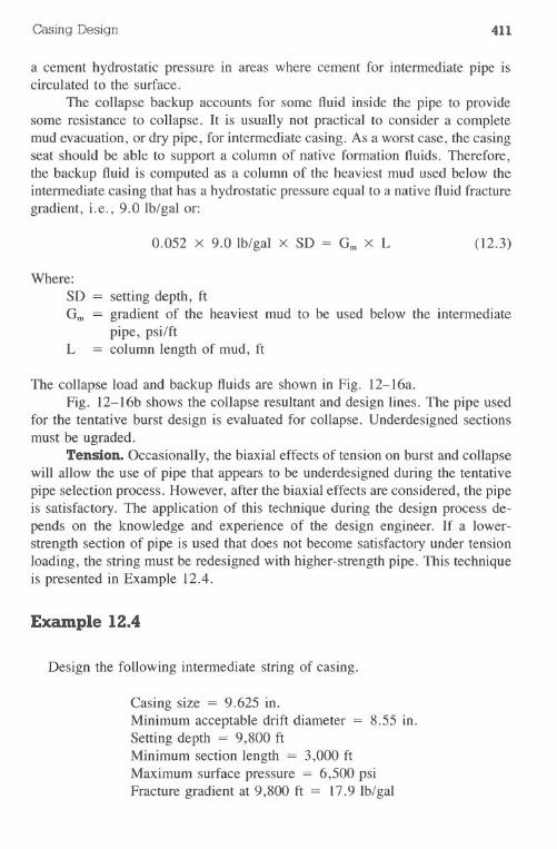
Casing Design 411
a cement hydrostatic pressure in areas where cement for intermediate pipe iscirculated to the surface.
The collapse backup accounts for some fluid inside the pipe to providesome resistance to collapse. It is usually not practical to consider a completemud evacuation, or dry pipe, for intermediate casing. As a worst case, the casingseat should be able to support a column of native formation fluids. Therefore,the backup fluid is computed as a column of the heaviest mud used below theintennediate casing that has a hydrostatic pressure equal to a native fluid fracturegradient, i.e., 9.0 Ib/gal or:
0.052 x 9.0 Ib/gal x SD = Gmx L (12.3)
Where:
SD = setting depth, ftGm = gradient of the heaviest mud to be used below the intennediate
pipe, psi/ftL = column length of mud, ft
The collapse load and backup fluids are shown in Fig. 12-16a.Fig. 12-16b shows the collapse resultant and design lines. The pipe used
for the tentative burst design is evaluated for collapse. Underdesigned sectionsmust be ugraded.
Tension. Occasionally, the biaxial effects of tension on burst and collapsewill allow the use of pipe that appears to be underdesigned during the tentativepipe selection process. However, after the biaxial effects are considered, the pipeis satisfactory. The application of this technique during the design process de-pends on the knowledge and experience of the design engineer. If a lower-strength section of pipe is used that does not become satisfactory under tensionloading, the string must be redesigned with higher-strength pipe. This techniqueis presented in Example 12.4.
Example 12.4
Design the following intennediate string of casing.
Casing size = 9.625 in.Minimum acceptable drift diameter = 8.55 in.Setting depth = 9,800 ftMinimum section length = 3,000 ftMaximum surface pressure = 6,500 psiFracture gradient at 9,800 ft = 17.9lb/gal I
I
412 Drilling Engineering
Maximum anticipated mud weight = 13.1 Ib/gaIMud weight set in = 10.8 Ib/gaICementtop = 7,000ftCementweight = 16.4 Ib/gal
Solution:
1. The burst injection pressure is computed as:
IP = (0.052) (17.9 + 1.0 Ib/gal) (9,800 ft) = 9,631 psi
2. The lengths of the mud and gas columns are computed with Eqs. 12.1and 12.2:
P, + x(Gm) + y(Gg) = IP6,500 psi + x(0.052 x 13.llb/gal) + y(0.1l5 psi/ft) = 9,631 psix + Y = SDx + Y = 9,800
y = 9,800 - x6,500 psi + 0.6812 x + (0.115)(9,800 - x) = 9,631
Solving for x:
x = 3,540 ftY = 6,260 ft
These values are plotted on Fig. 12-17.
3. The burst backup is computed with a 9.0-lb/gal fluid. At 9,800 ft, thebackup is:
9,800 ft x 0.052 x 9.0 Ib/gal = 4,586 psi
4. The resultant and design lines are computed and shown in Fig. 12-17.5. A tentative pipe selection is made for the design line. The 43.5-lb/ft, S-
95 pipe is underdesigned since 7,510 psi is less than the maximum burstdesign load of 7,980 psi.At this point in the design, it is assumed that the tension loading willincrease the effective burst rating beyond 7,980 psi. If this assumptionproves incorrect, the string must be redesigned. A drilling engineer in-experienced in casing design may not wish to implement this techniquesince an error will require a redesign.
6. The collapse load on the intermediate casing is created by the 1O.8-lb/galmud and the 15.6-lb/gal cement in the annulus (see Fig. 12-18).
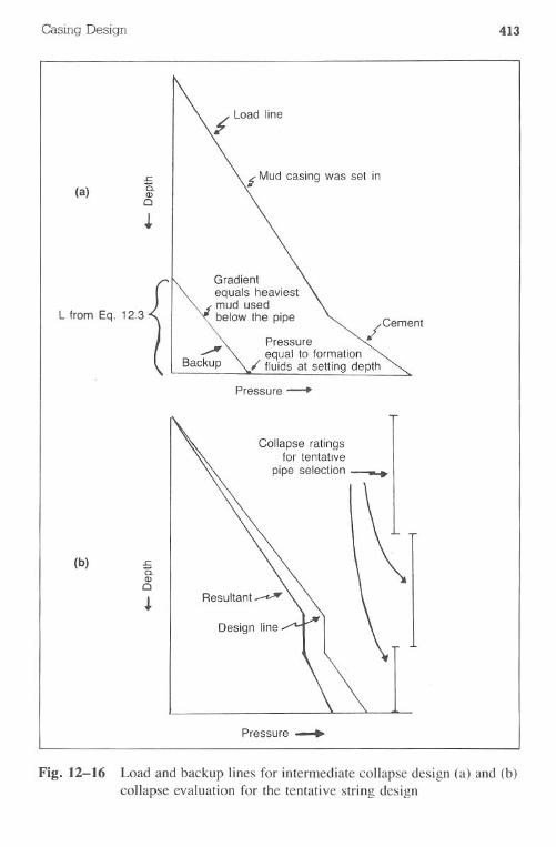
Casing Design 413
L from Eq. 12.3
Gradientequals heaviestmud usedbelow the pipe
/cementPressure "-equal to formation
I fluids at setting depth
(a).c15.Q)o
Pressure-
(b) .c15.Q)o
~
Collapse ratingsfor tentative
pipe selection --.
Pressure-+
Fig.12-16 Load and backup lines for intenTIediatecollapse design (a) and (b)collapse evaluation for the tentative string design
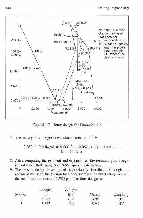
414 Drilling Engineering
2,000
Note that a sectionof pipe was usedthat does notexceed the designline. Under a tension
1(8,911) load, the pipe's'\ burst strength(7,980) will exceed the
\ design values.43.5 Ibltt8-95
.,.(7,510psi)
(3,540)4,000
6,000
8,000
Setting depth = 9,800 It10,000 . (9,631)
o 2,000(5,045) (5,549)
4,000 6,000 8,000
Pressure, psi
10,000
Fig. 12-17 Burst design for Example 12.4
7. The backup fluid length is calculated from Eq. 12.3:
0.052 x 9.0 Ib/gal x 9,800 ft = 0.052 x 13.1 Ib/gal x LL = 6,732 ft
8. After computing the resultant and design lines, the tentative pipe designis evaluated. Both weights of $-95 pipe are satisfactory.
9. The tension design is computed as previously described. Although notshown in this text, the tension load does increase the burst rating beyondthe maximum pressure of 7,980 psi. The final design is:
Section12
Length,ft
5,9133,887
Weight,Ib/ft43.540.0
Grade$-95$-95
CouplingLTCLTC
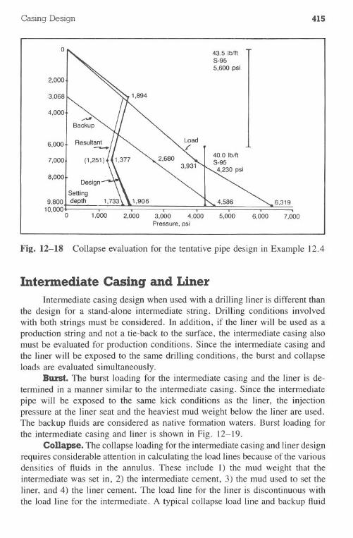
Casing Design 415
o 43.5 Ib/llS-955,600 psi
8,000
6,000
7,000
Design
Setting9,800 I depth
10,000o 1,000 2,000 3,000 4,000
Pressure, psi5,000
~319
6,000 7,000
Fig. 12-18 Collapse evaluation for the tentative pipe design in Example 12.4
Intermediate Casing and LinerIntermediate casing design when used with a drilling liner is different than
the design for a stand-alone intermediate string. Drilling conditions involvedwith both strings must be considered. In addition, if the liner will be used as aproduction string and not a tie-back to the surface, the intermediate casing alsomust be evaluated for production conditions. Since the intermediate casing andthe liner will be exposed to the same drilling conditions, the burst and collapseloads are evaluated simultaneously.
Burst. The burst loading for the intermediate casing and the liner is de-termined in a manner similar to the intermediate casing. Since the intermediatepipe will be exposed to the same kick conditions as the liner, the injectionpressure at the liner seat and the heaviest mud weight below the liner are used.The backup fluids are considered as native formation waters. Burst loading forthe intermediate casing and liner is shown in Fig. 12-19.
Collapse. The collapse loading for the intermediate casing and liner designrequires considerable attention in calculating the load lines because of the variousdensities of fluids in the annulus. These include 1) the mud weight that theintermediate was set in, 2) the intermediate cement, 3) the mud used to set theliner, and 4) the liner cement. The load line for the liner is discontinuous withthe load line for the intermediate. A typical collapse load line and backup fluid
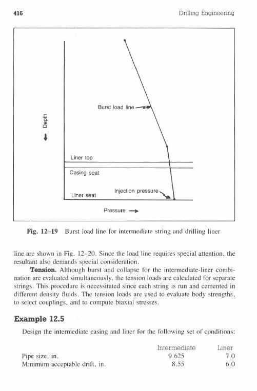
416 Drilling Engineering
.ca.CDc
Liner top
Casing seat
Liner seat Injection pressure "'-
Pressure-+
Fig. 12-19 Burst load line for intermediate string and drilling liner
line are shown in Fig. 12-20. Since the load line requires special attention, theresultant also demands special consideration.
Tension. Although burst and collapse for the intermediate-liner combi-nation are evaluated simultaneously, the tension loads are calculated for separatestrings. This procedure is necessitated since each string is run and cemented indifferent density fluids. The tension loads are used to evaluate body strengths,to select couplings, and to compute biaxial stresses.
Example 12.5
Design the intermediate casing and liner for the following set of conditions:
Pipe size, in.Minimum acceptable drift, in.
Intermediate9.625
8.55
Liner7.06.0
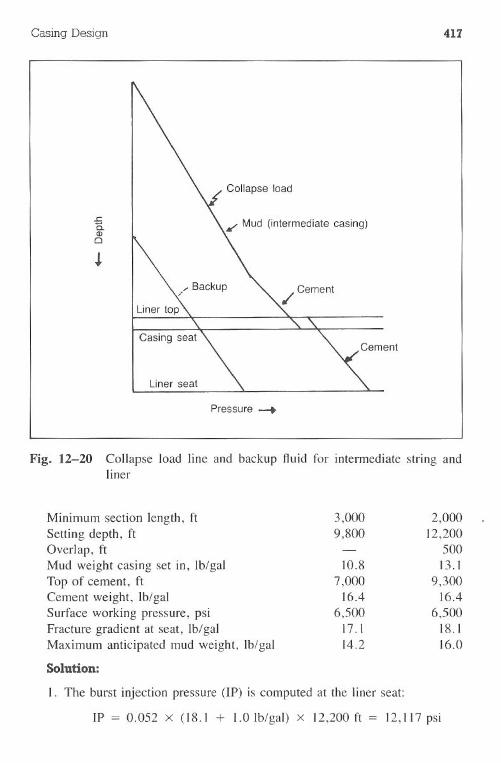
Casing Design
.cC.CDCI
Collapse load
K" Mud (intermediate casing)
Pressure-+
417
Fig. 12-20 Collapse load line and backup fluid for intermediate string andliner
3,0009,800
Minimum section length, ftSetting depth, ftOverlap, ftMud weight casing set in, Ib/galTop of cement, ftCement weight, Ib/galSurface working pressure, psiFracture gradient at seat, Ib/galMaximum anticipated mud weight, Ib/gal
Solution:
I. The burst injection pressure (IP) is computed at the liner seat:
10.87,000
16.46,500
17.114.2
IP = 0.052 x (18.1 + 1.0lb/gal) x 12,200ft = 12,117psi
2,00012,200
50013.1
9,30016.4
6,50018.116.0
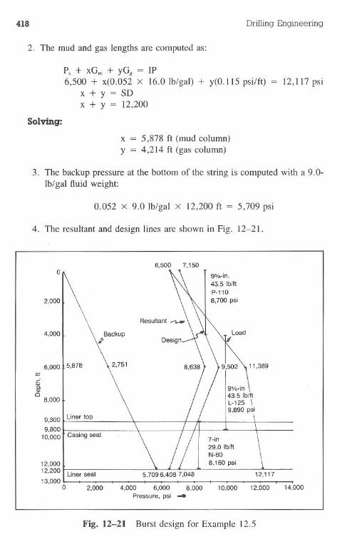
418 Drilling Engineering
2. The mud and gas lengths are computed as:
Ps + xGm+ yGg= IP6,500 + x(0.052 x 16.0 Ib/gal) + y(0.115psi/ft)
x + Y = SDx + y = 12,200
Solving:
12,117 psi
x = 5,878 ft (mud column)y = 4,214 ft (gas column)
3. The backup pressure at the bottom of the string is computed with a 9.0-Ib/gal fluid weight:
4. The resultant and design lines are shown in Fig. 12-21.
0.052 x 9.01b/gal x 12,200ft = 5,709 psi
6,500 7,1509%-ln.43.51b/llP-110
2,0001 \ \ " I 8,700psi
4,000
7-ln29.0 IbillN-808,160 psi
5,7096,4087,048
4,000 6,000 8,000Pressure,psi _
12,117.
10,000 12,000 14,000
Fig. 12-21 Burst design for Example 12.5
6,000 15,878:::£c.
8,000
9,300 I Linertop9,800
10,000 t Casingseat
12,000
12,200 I .Linerseat
13,0000 2,000
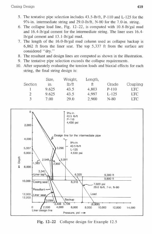
Casing Design 419
5. The tentative pipe selection includes 43.5-lb/ft, P-110 and L-125 for the9%-in. intermediate string and 29.0-lb/ft, N-80 for the 7.0-in. string.
6. The collapse load line, Fig. 12-22, is computed with 1O.8-lb/gal mudand 16.4-lb/gal cement for the intermediate string. The liner uses 16.4-Ib/gal cement and 13.1-lb/gal mud.
7. The length of the 16.0-lb/gal mud column used as collapse backup is6,862 ft from the liner seat. The top 5,337 ft from the surface areconsidered "dry."
8. The resultant and design lines are computed as shown in the illustration.9. The tentative pipe selection exceeds the collapse requirements.
10. After separately evaluating the tension loads and biaxial effects for eachstring, the final string design is:
1
9%.in.43.5Ib/ttP'1104,430 psi
f.Design~
fine f:~:::. intermediate pipe
43.5Ib/tt3,296 L.125
4,630 psi
9,300 tt9,800 tt
7,020 psi29.0 IbIft, 7-in, N.80
12,000 14,000
Pressure,psi_
Fig. 12-22 Collapse design for Example 12.5
Size, Weight, Length,Section ill. Ib/ft ft Grade Coupling
1 9.625 43.5 4,803 P-110 LTC2 9.625 43.5 4,997 L-125 LTC3 7.00 29.0 2,900 N-80 LTC
0
2,000
4,000
5,337
6,000.t:a.Q)c
10,000
12,00012,200
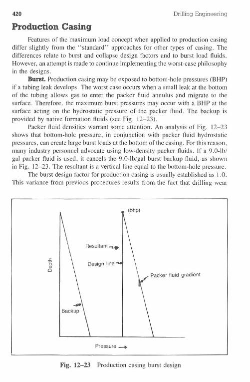
420
Production CasingDrilling Engineering
Features of the maximum load concept when applied to production casingdiffer slightly from the "standard" approaches for other types of casing. Thedifferences relate to burst and collapse design factors and to burst load fluids.However, an attempt is made to continue implementing the worst-case philosophyin the designs.
Burst. Production casing may be exposed to bottom-hole pressures (BHP)if a tubing leak develops. The worst case occurs when a small leak at the bottomof the tubing allows gas to enter the packer fluid annulus and migrate to thesurface. Therefore, the maximum burst pressures may occur with a BHP at thesurface acting on the hydrostatic pressure of the packer fluid. The backup isprovided by native formation fluids (see Fig. 12-23).
Packer fluid densities warrant some attention. An analysis of Fig. ]2-23shows that bottom-hole pressure, in conjunction with packer fluid hydrostaticpressures, can create large burst loads at the bottom of the casing. For this reason,many industry personnel advocate using low-density packer fluids. If a 9.0-]b/gal packer fluid is used, it cancels the 9.0-lb/gal burst backup fluid, as shownin Fig. 12-23. The resultant is a vertical line equal to the bottom-hole pressure.
The burst design factor for production casing is usually established as ] .0.This variance from previous procedures results from the fact that drilling wear
(bhp)
.J:;c.Q)o
Design line
Packer fluid gradient
Pressure -+
Fig. 12-23 Production casing burst design
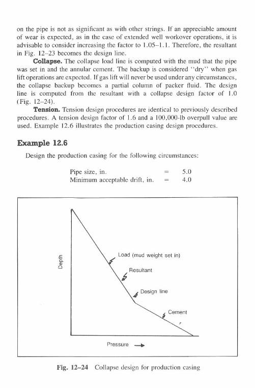
Casing Design 421
on the pipe is not as significant as with other strings. If an appreciable amountof wear is expected, as in the case of extended well workover operations, it isadvisable to consider increasing the factor to 1.05-1.1. Therefore, the resultantin Fig. 12-23 becomes the design line.
Conapse. The collapse load line is.computed with the mud that the pipewas set in and the annular cement. The backup is considered "dry" when gaslift operations are expected. If gas lift will never be used under any circumstances,the collapse backup becomes a partial column of packer fluid. The designline is computed from the resultant with a collapse design factor of 1.0(Fig. 12-24).
Tension. Tension design procedures are identical to previously describedprocedures. A tension design factor of 1.6 and a 100,000-lb overpull value areused. Example 12.6 illustrates the production casing design procedures.
Example 12.6
Design the production casing for the following circumstances:
Pipe size, in. = 5.0Minimum acceptable drift, in. = 4.0
..ca.Q)
CI
Load (mud weight set in)
Pressure ~
Fig. 12-24 Collapse design for production casing
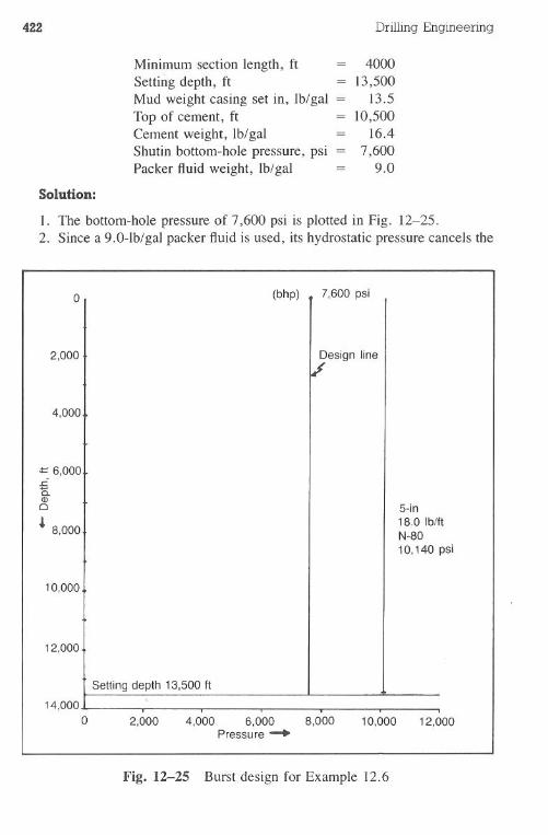
422
Minimum section length, ftSetting depth, ftMud weight casing set in, lb/galTop of cement, ftCement weight, lb/galShutin bottom-hole pressure, psiPacker fluid weight, lb/gal
Drilling Engineering
400013,500
13.510,500
16.47,600
9.0
Solution:
1. The bottom-hole pressure of 7,600 psi is plotted in Fig. 12-25.2. Since a 9.0-lb/gal packer fluid is used, its hydrostatic pressure cancels the
o (bhp) . 7,600 psi
2,000
4,000
~ 6,000£a.CDo
~ 8,000
10,000
12,000
Setting depth 13,500 It
Design line/
5-in18.0 IblttN-8010,140 psi
14,000o 2,000 10,000 12,0004,000 6,000 8,000
Pressure .-.
Fig. 12-25 Burst design for Example 12.6
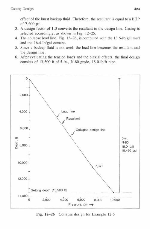
Casing Design 423
effect of the burst backup fluid. Therefore, the resultant is equal to a BHPof 7,600 psi.
3. A design factor of 1.0 converts the resultant to the design line. Casing isselected accordingly, as shown in Fig. 12-25.
4. The collapse load line, Fig. 12-26, is computed with the 13.5-lb/gal mudand the 16.4-lb/gal cement.
5. Since a backup fluid is not used, the load line becomes the resultant andthe design line.
6. After evaluating the tension loads and the biaxial effects, the final designconsists of 13,500 ft of 5-in., N-80 grade, 18.0-lb/ft pipe.
o
10,000
2,000
Load line;'
Resultant.f
~ Collapse design line:::.cg. 8,000o
5-in.N-8018.0 Ib/lt10,490psi
12,000
Setting depth (13,500 It)
14,000.o 2,000 4,000 6,000 8,000
Pressure, psi ~
10,000
Fig. 12-26 Collapse design for Example 12.6
424
Special Casing Design Criteria
Drilling Engineering
Unfortunately, a standard set of casing design guidelines cannot be usedfor every string of pipe run into a well. Variousdrilling and geological conditionsrequire modification to the pipe design guidelines. In many cases, the drillingengineer must evaluate the specific circumstances before selecting a design pro-cedure.
Hydrogen Sulfide. Hydrogen embrittlement occurs when certain high-strength materials are exposed to hydrogen sulfide at temperatures less thanapproximately 175°F. Pipe failures can be abrupt and catastrophic. In thiscase, pipe grades of N-80 or greater, with the exception of L-80, should notbe used in the low temperature ranges (less than 175°F). This subject is com-plex and should be given special attention when hydrogen sulfide drilling isexpected.
Salt. Bedded salt under formation temperatures often acts as a flowingfluid. It can shear casing because it supports the overburden stress of the uppersediments. Pipe designed for bedded salt should consider the collapse load fluidsas approximately 19.3-lb/gal mud, which is approximately equal to overbur-den stress.
Temperature. High temperatures cause casing design problems due topipe elongation and the resulting buckling effects. Evaluation of casing bucklingis a difficult calculation, however, and has no clean and easy solution. In somesevere cases, such as thermal wells, the tension load is increased a significantamount after the cement is set. The tension load stretches the pipe before theslips are set.
Problems
12.1 A tension load of 400,000 Ib is applied to 43.5-lb/ft, 9%-in., S-95pipe. Calculate the actual and effective burst and collapse ratings ofthe pipe.
12.2 The bottom of a 40.0-lb/ft, C-75 grade, 9%-in. casing string has an80,000-lb compressional load. What is the effective burst and col-lapse rating?
12.3 A 5.0-in., 18.0-lb/ft production string is set to 16,000 ft in 17.0-lb/gal mud. Prepare a tension graph. What are the tension (or compres-sion) loads at 0,5,000, 10,000, 15,000, and 16,000 ft? Neglect theeffect of cement in the annulus.
Pipe selection for casing design problems should be made from the casing and tubingcatalog in the Appendix.
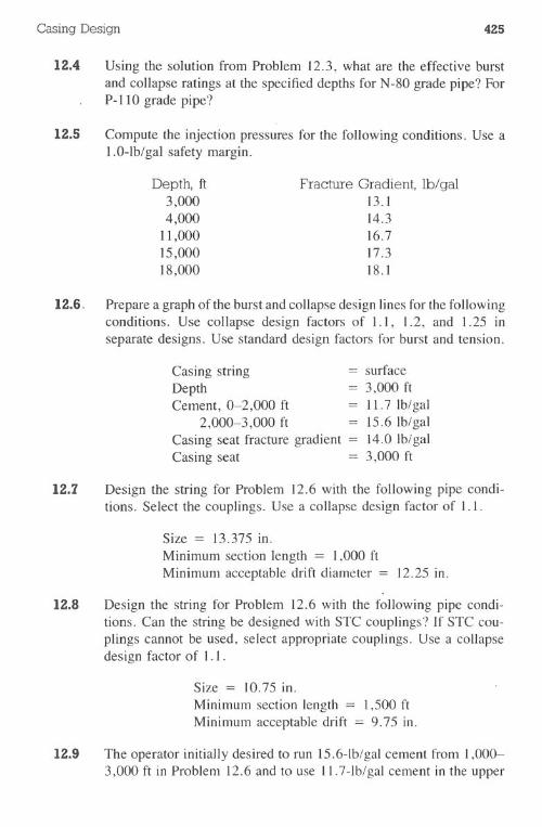
Casing Design 425
12.4 Using the solution from Problem 12.3, what are the effective burstand collapse ratings at the specified depths for N-80 grade pipe? ForP-110 grade pipe?
12.5 Compute the injection pressures for the following conditions. Use aI.O-Ib/gal safety margin.
Depth, ft3,0004,000
11,00015,00018,000
Fracture Gradient, Ib/gal13.114.316.717.318.1
12.6. Prepare a graph of the burst and collapse design lines for the followingconditions. Use collapse design factors of 1.1, 1.2, and 1.25 inseparate designs. Use standard design factors for burst and tension.
Casing string = surfaceDepth = 3,000 ftCement, 0-2,000 ft = 11.7 Ib/gal
2,000-3,000 ft = 15.6 Ib/galCasing seat fracture gradient = 14.0 Ib/galCasing seat = 3,000 ft
12.7 Design the string for Problem 12.6 with the following pipe condi-tions. Select the couplings. Use a collapse design factor of 1.1.
Size = 13.375 in.Minimum section length = 1,000ftMinimum acceptable drift diameter = 12.25 in.
12.8 Design the string for Problem 12.6 with the following pipe condi-tions. Can the string be designed with STC couplings? If STC cou-plings cannot be used, select appropriate couplings. Use a collapsedesign factor of I. I .
Size = 10.75 in.
Minimumsectionlength = 1,500ftMinimumacceptabledrift = 9.75 in.
12.9 The operator initially desired to run 15.6-lb/gal cement from 1,000-3,000 ft in Problem 12.6 and to use 11.7-lb/gal cement in the upper
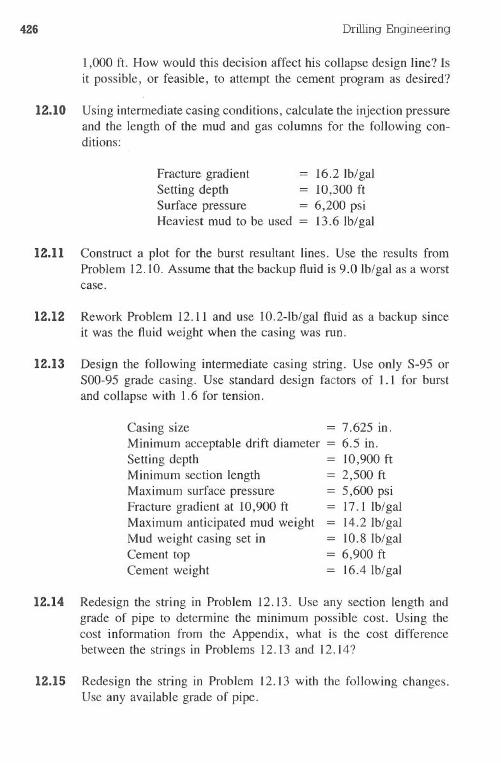
426 Drilling Engineering
1,000 ft. How would this decision affect his collapse design line? Isit possible, or feasible, to attempt the cement program as desired?
12.10 Using intermediate casing conditions, calculate the injection pressureand the length of the mud and gas columns for the following con-ditions:
Fracture gradient = 16.2Ib/galSetting depth = 10,300ftSurface pressure = 6,200 psiHeaviest mud to be used = 13.6Ib/gal
12.11 Construct a plot for the burst resultant lines. Use the results fromProblem 12.10. Assume that the backup fluid is 9.0 Ib/gal as a worstcase.
12.12 Rework Problem 12.11 and use 1O.2-lb/gal fluid as a backup sinceit was the fluid weight when the casing was run.
12.13 Design the following intermediate casing string. Use only S-95 orSOO-95grade casing. Use standard design factors of 1.1 for burstand collapse with 1.6 for tension.
Casing size = 7.625 in.Minimum acceptable drift diameter = 6.5 in.Setting depth = 10,900ftMinimum section length = 2,500 ftMaximum surface pressure = 5,600 psiFracture gradient at 10,900 ft = 17.1 Ib/galMaximum anticipated mud weight = 14.2Ib/galMud weight casing set in = 10.8 Ib/galCement top = 6,900 ftCement weight = 16.4 Ib/gal
12.14 Redesign the string in Problem 12.13. Use any section length andgrade of pipe to determine the minimum possible cost. Using thecost information from the Appendix, what is the cost differencebetween the strings in Problems 12.13 and 12.14?
12.15 Redesign the string in Problem 12.13 with the following changes.Use any available grade of pipe.
Casing Design
Maximum surface pressure = 10,000psiFracture gradient at 10,900 ft = 18.1 Ib/gal
427
Do these high pressure-fracture gradient conditions pose any prob-lems? If so, identify the causes and solutions. If not, what are po-tential problems from these conditions?
12.16 Design an intermediate casing and liner for the following conditions:
Pipe size, in.Minimum acceptable drift, in.Minimum section length, ftSetting depth, ftOverlap, ftMud weight casing set in, lb/galTop of cement, ftCement weight, lb/galSurface working pressure, psiFracture gradient at seat, lb/galMaximum anticipated mud
weight, lb/gal
Intermediate10.75
9.53,000
10,400
10.27,000
15.65,000
16.213.7
Liner7.625
6.53,000
13,00040013.4
10,00016.4
5,00017.816.5
12.17 Redesign the strings in Example 12.5 with the following pipe:
Pipe size, in.Minimum acceptable drift, in.
Intermediate7.6256.5
Liner5.04.0
12.18 Compare the design in Problem 12.13 if it is used with a liner. Usethe following criteria instead of the data in the problem:
Liner depth = 14,000ftFracture gradient at liner seat = 17.9 lblgalMaximum anticipated mud weight = 15.81b/gal
12.19 Design the production casing for the following circumstances:
Pipe size, in.Minimum acceptable drift, in.
5.54.0
428
Minimum section length, ftSetting depth, ftMud weight casing set in, Ib/galCement weight, Ib/galTop of cement, ftShutin bottom-hole pressure, psiPacker fluid weight, Ib/gal
DrillingEngineering
2,00011,000
12.816.4
8,5005,400
9.0
12.20 Redesign Problem 12.19 with an 11.0-lb/gal packer fluid.
12.21 Suppose that the casing string in Problem 12.16 is used in an H2Senvironment. Redesign it with H2S serviceable pipe. Assume anygrade is satisfactory in formations above 175°F and a formationtemperature gradient of 1.6°F/100 ft is present. Assume an ambienttemperature of 80°F.
References
Adams, N.J. Well Control Problems and Solutions. Tulsa: PennWell Pub-lishing, 1980.
Greenip, John F. "Determining Stress in Tubing Using Triaxial Evaluation."SPE 6760presentedat the 1977FallTechnicalConference,Denver,Col-orado.
Hammerlindl, D.J. "Basic Fluid Pressure Forces on Oilwell Tubulars." Jour-nal of Petroleum Technology, January 1980, pp. 153-159.
Hammerlindl, D.J. "Movement, Forces, and Stress Associated with Com-bination Tubing Strings Sealed in Packers." Journal of Petroleum Tech-nology, February 1977, pp. 195-208.
Lubinski, A. "Influence of Tension and Compression on Straightness andBuckling of Tubular Goods in Oil Wells." Proc., API 31st Annual Meeting,Chicago, 1951, Prod. Sec. IV, 31, 34.
Lubinski, A., and K.A. Blenkara. "Buckling of Tubing in Pumping Wells,Its Effect and Means for Controlling It." Trans., AIME, volume 210,1957, 73-88.

Casing Design 4Z9
Lubinski, A., W.S. Althouse, and J.L. Logan. "Helical Buckling of TubingSealed in Packers." Journal of Petroleum Technology, June 1962, pp.655-670.
Prentice, C.M. "Maximum Load Casing Design." Journal of PetroleumTechnology, July 1971, pp. 805-811.
Chapter 13 Tubing Design
Tubing design is an important facet of the well plan. The tubing is theflow string through which the produced oil and gas move from the reservoir tothe surface handling facilities. In addition to the produced fluids, the tubing maybe required to control pressures and fluids during stimulation or squeeze con-ditions. Poor tubing designs may result in tubing failure, which necessitatesexpensive remedial operations.
The typical production system is shown in Fig. 13-1. It contains the tubing,a packer, the seal assembly, and several flow control devices. Other types oftubing systems will be discussed later in this chapter.
The classical tubing design theory was established by Lubinski et aI. Itintroduced new concepts not previously used in casing design. Lubinski's workfor a single, uniform, vertical tubing string will be used in this chapter. His signconventions and terminology will be followed, even though they differ fromother drilling nomenclature.
Tubing Design CriteriaThe three major tubular systems (casing, tubing, and the drilIstring) used
in drilling are designed with different criteria. Casing is typically designed forburst, collapse, and tension, whereas the drillstring is designed for collapse andtension, with burst seldom playing any important role. Likewise, tubing is de-signed with a completely different set of guidelines. Failure to recognize thedifferences may result in an underdesigned string.
Stress is the controlling factor in tubing design. Later examples will showthat tubing designed for stress considerations is overdesigned for burst, collapse,and tension. Stress and tensile loading are different parameters and, as such,should not be confused or misused in the tubing design, as is often done.
Factors Affecting Stress. Tubing lying on the pipe rack does not en-counter any significant, externally imposed stresses. After it is placed in the
430
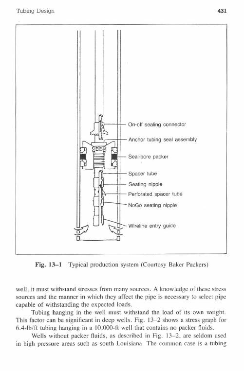
Tubing Design 431
On-off sealing connector
Anchor tubing seal assembly
Seal-bore packer
Spacer tube
Seating nipple
Perforated spacer tube
NoGo seating nipple
~o
Wireline entry guide
Fig. 13-1 Typical production system (Courtesy Baker Packers)
well, it must withstand stresses from many sources. A knowledge of these stresssources and the manner in which they affect the pipe is necessary to select pipecapable of withstanding the expected loads.
Tubing hanging in the well must withstand the load of its own weight.This factor can be significant in deep wells. Fig. 13-2 shows a stress graph for6.4-lb/ft tubing hanging in a IO,OOO-ftwell that contains no packer fluids.
Wells without packer fluids, as described in Fig. 13-2, are seldom usedin high pressure areas such as south Louisiana. The common case is a tubing
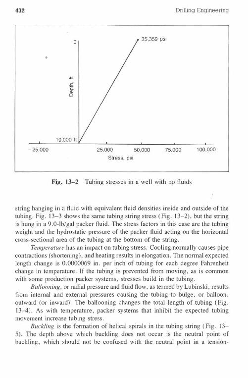
432 DrillingEngineering
o 35,359 psi
.
<=.c'E.Q)o
10,000 It
- 25,000 25,000 50,000
Stress, psi
75,000 100,000
Fig. B-2 Tubing stresses in a well with no fluids
string hanging in a fluid with equivalent fluid densities inside and outside of thetubing. Fig. 13-3 shows the same tubing string stress (Fig. 13-2), but the stringis hung in a 9.0-lb/gal packer fluid. The stress factors in this case are the tubingweight and the hydrostatic pressure of the packer fluid acting on the horizontalcross-sectionalareaof the tubingat the bottomof the string.
Temperature has an impact on tubing stress. Cooling normally causes pipecontractions (shortening), and heating results in elongation. The normal expectedlength change is 0.0000069 in. per inch of tubing for each degree Fahrenheitchange in temperature. If the tubing is prevented from moving, as is commonwith some production packer systems, stresses build in the tubing.
Ballooning, or radial pressure and fluid flow, as termed by Lubinski, resultsfrom internal and external pressures causing the tubing to bulge, or balloon,outward (or inward). The ballooning changes the total length of tubing (Fig.13-4). As with temperature, packer systems that inhibit the expected tubingmovement increase tubing stress.
Buckling is the formation of helical spirals in the tubing string (Fig. 13-5). The depth above which buckling does not occur is the neutral point ofbuckling, which should not be confused with the neutral point in a tension-
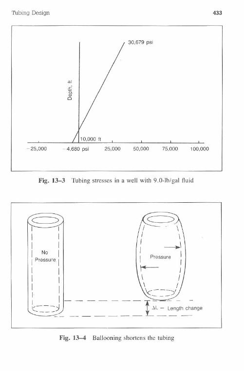
Tubing Design 433
- 25,000
30,679 psi
- 4,680 psi 50,000 75,000 100,000
Fig. 13-3 Tubing stresses in a well with 9.0-lb/gal fluid
c=::>r 1I II II No IIPressure II II II II.
!c-::-=~-_~ -=--=- -= - =~ ~~'~h ,~"g,
Fig. 13-4 Ballooning shortens the tubing
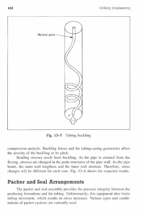
434
Neutral point
Drilling Engineering
Fig. 13-5 Tubing buckling
compression analysis. Buckling forces and the tubing-casing geometries affectthe severity of the buckling or its pitch.
Bending stresses result from buckling. As the pipe is strained from theflexing, stresses are changed in the grain structures of the pipe wall. As the pipebends, the outer wall lengthens and the inner wall shortens. Therefore, stresschanges will be different for each case. Fig. 13-6 shows the expected results.
Packer and Seal ArrangementsThe packer and seal assembly provides the pressure integrity between the
producing formations and the tubing. Unfortunately, this equipment also limitstubing movement, which results in stress increases. Various types and combi-nations of packer systems are currently used.
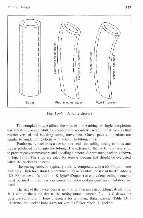
Tubing Design
Straight Pipe in compression
Fig. 13-6 Bending stresses
435
Pipe in tension
The completion type affects the stresses in the tubing. A single completionhas a bottom packer. Multiple completions normally use additional packers thatrestrict vertical and buckling tubing movement. Gravel pack completions aresimilar to single completions with respect to tubing stress.
Packers. A packer is a device that seals the tubing-casing annulus andforces produced fluids into the tubing. The exterior of the packer contains slipsto prevent packer movement and a sealing element. A permanent packer is shownin Fig. 13-7. The slips are rated for tensile loading and should be evaluatedwhen the packer is selected.
The sealing rubber is typically a nitrile compound with a 60-70 durometerhardness. High formation temperatures may necessitate the use of harder rubbers(80-90 hardness). In addition, K-Ryte@(Dupont) or equivalent sealing elementsmust be used in sour gas environments when certain corrosion inhibitors areused.
The size of the packer bore is an important variable in buckling calculations.It is seldom the same size as the tubing outer diameter. Fig. 13-8 shows thepossible variations in bore diameters for a 51/2-in.Baker packer. Table 13-1illustrates the packer bore sizes for various Baker Model D packers.
, Q)Q) . Q)
,en
enI , <0<0 I I en
Q)Q)
<0t; t; I Q)I I
I t;.5
.5Q)
I I c:I I "0
0
c:\ 'w
I I 0I en
'wQ)0.
c:\
\ I Q)E
I-00
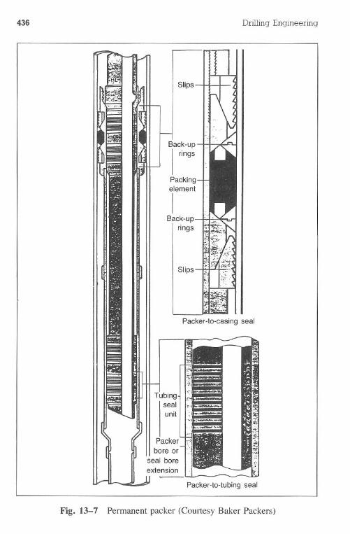
436
Back-up
I ringsPackingelemenl
I
Back-uprings
Drilling Engineering
Slips
Slips
Packer-la-casing seal
Packer-Ia-Iubingseal
Fig. 13-7 Permanent packer (Courtesy Baker Packers)
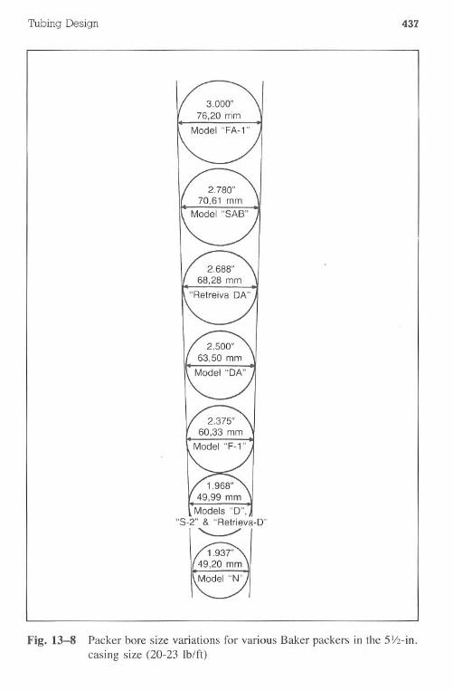
Tubing Design 437
Fig. 13-8 Packer bore size variations for various Baker packers in the 5Y2-in.casing size (20-23 Ib/ft)
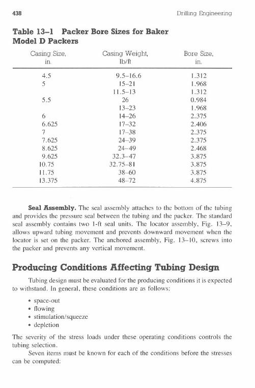
438 Drilling Engineering
Table 13-1 Packer Bore Sizes for BakerModel D Packers
Seal Assembly. The seal assembly attaches to the bottom of the tubingand provides the pressure seal between the tubing and the packer. The standardseal assembly contains two I-ft seal units. The locator assembly, Fig. 13-9,allows upward tubing movement and prevents downward movement when thelocator is set on the packer. The anchored assembly, Fig. 13-10, screws intothe packer and prevents any vertical movement.
Producing Conditions Affecting Tubing DesignTubing design must be evaluated for the producing conditions it is expected
to withstand. In general, these conditions are as follows:
· space-out.flowing· stimulation/squeeze· depletion
The severity of the stress loads under these operating conditions controls thetubing selection.
Seven items must be known for each of the conditions before the stressescan be computed:
Casing Size, Casing Weight, Bore Size,In. Ib/ft In.
4.5 9.5-16.6 1.3125 15-21 1.968
11.5-13 1.3125.5 26 0.984
13-23 1.9686 14-26 2.3756.625 17-32 2.4067 17-38 2.3757.625 24-39 2.3758.625 24-49 2.4689.625 32.3-47 3.875
10.75 32.75-81 3.87511.75 38-60 3.87513.375 48-72 4.875
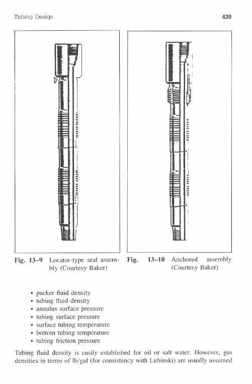
Tubing Design 439
Fig. 13-9 Locator-type seal assem- Fig.bly (Courtesy Baker)
13-10 Anchored assembly(Courtesy Baker)
· packer fluid density. tubingfluiddensity· annulus surface pressure· tubing surface pressure· surface tubing temperature· bottom tubing temperature· tubing friction pressure
Tubing fluid density is easily established for oil or salt water. However, gasdensities in terms of Ib/gal (for consistency with Lubinski) are usually assumed
440 Drilling Engineering
to be in the range of 1-2.5 Ib/gal. Wet gases may be heavier. This value shouldbe examined closely if flowingconditions are more severe than the other operatingconditions.
The tubing friction pressure can be difficult to estimate. However, theworst stress case occurs when the friction pressures are zero. The design approachpresented in this section will assume that these pressures are negligible.
Space-out. The space-out condition occurs when the tubing is positionedas desired relative to the packer and the production tree. The usual conditionsare that 1) the fluid density is the same for the annulus as the tubing, 2) nopressure exists at the top of the tubing and casing, and 3) some weight (10,000-30,000 Ib) is set on the packer. The temperature at the bottom of the tubing isapproximately equal to formation temperature.
Flowing. Oil and gas movement up the tubing causes several stress changesfor various reasons. The maximum tubing pressure (SITP) is greater than atspace-out conditions. In addition, the overall tubing temperature is increased.A satisfactory method of comparing temperature changes is to evaluate the av-erage of top and bottom temperatures at flowing conditions.
Stimulation/Squeeze. These conditions are often the most severe thattubing must withstand during its life. Anhough these conditions may exist fora relatively short period, they must be included in the design considerations.The typical considerations are 1) high tubing pressures and fluid densities, 2)annular backup pressure, and 3) cooling effects due to surface fluids beingpumped down the tubing. Fluids used during these conditions include cementand acid.
Depletion. Depletion conditions occur when the formation pressures arereduced to a noneconomical productive level. Depletion-like circumstances occurwhen the perforations are plugged or the tubing is blocked with sand or otherobstructions. The tubing pressure is low or zero, and the temperatures are ap-proximately equal to the original space-out values.
A typical set of values for all operational conditions is shown in Table13-2.
Table 13-2 Typical Operating ConditionsSpace- Stimulation/
out Flowing Squeeze Depletion
Packer fluid density, Ib/gal 9 9 9 9
Tubing fluid density, Ib/gal 9 6 16.4 6
Surface annulus pressure, psi 0 0 1,000 0
Surface tubing pressure, psi 0 2,800 4,500 0
Surface tubing temperature, of 70 145 45 70
Bottom tubing temperature, of 240 240 110 240
Friction pressure gradient, psi/ft 0 0 0 0
Tubing Design 441
Stress Evaluation
Grade selection for the tubing string is dependent on the determination ofthe stresses. The calculation procedures for the stresses must be completed inthe following order:
1. force determinations2. tubing length changes3. stresses resulting from tubing length changes
This approach will be followed in this section.Lubinski's work on tubing design used a sign convention that is not com-
pletely consistent with some industry approaches. To avoid confusion, a listingof the sign conventions is shown in Table 13-3. This convention, as used byLubinski, will be followed throughout this text since his work is the basis ofmost tubing design applications.
Forces. The actual force (Fa) in the tubing at the bottom of the string isdependent on the pressures inside and outside of the tubing and the areas exposedto those pressures. This force can be calculated with Eq. 13.1:
(13.1)
Where:Fa = actually existing pressure force of a tubing string that is not restrained
in the packer, lbPi = pressure inside the tubing at the packer, psiPo = pressure outside the tubing at the packer, psiAi = inside tubing area, in.2Ao = outside tubing area, in.2Ap = packer bore area, in.2
Table 13-4 shows values of Ao, Ai, and other items for common tubing sizes.
A buckling force (Fb) is defined in Eq. 13.2:
(13.2)
Table 13-3 Tubing Sign Convention
Sign
Item Positive ( + ) Negative (-)
Force Compression TensionLength changes Lengthen ShortenStresses Compressive TensileTemperature Increase DecreaseHook loading Slack off Pickup
442 Drilling Engineering
Where:
Fb = buckling force, IbdPj = change in pressure inside the tubing at the packer, psidPo = change in pressure outside the tubing at the packer, psi
Eq. 13.2 indicates that the buckling forces increase when the pressure inside thetubing string is raised, as in the case of squeeze conditions. Lubinski termed theforce Fb as a fictitious force.
Length Changes. Tubing hanging in a well that contains no fluids willstretch to some length greater than the original length when the pipe was sittingon the racks. The pipe will be in tension at the top but will not have stresses atthe bottom. Pressure and temperature changes resulting from normal operationsinduce length changes that must be evaluated since they affect the stresses.
Packer and completion fluids apply pressures that cause a length change,dL.. This change can be calculated with Hooke's law, as described in Eq. 13.3:
(13.3)
Where:LEAsdL1
= length of tubing to packer, in.= Young's modulus of elasticity (for steel, E = 30 X 106psi)= cross-sectional area of tubing, in.2= length change resulting from Hooke's law, in.
The cross-sectional area, A" for common tubing sizes can be found in Table13-4. This length change is often termed the piston effect.
Buckling will cause a length change defined as dL2. If the buckling forceis less than zero:
(13.4)
Then buckling does not occur and no length changes occur, or:
when the buckling force is less than the buoyed weight of the tubing string, or:
(13.5)
Then the length change, dL2, is calculated from Eq. 13.6:
(13.6)
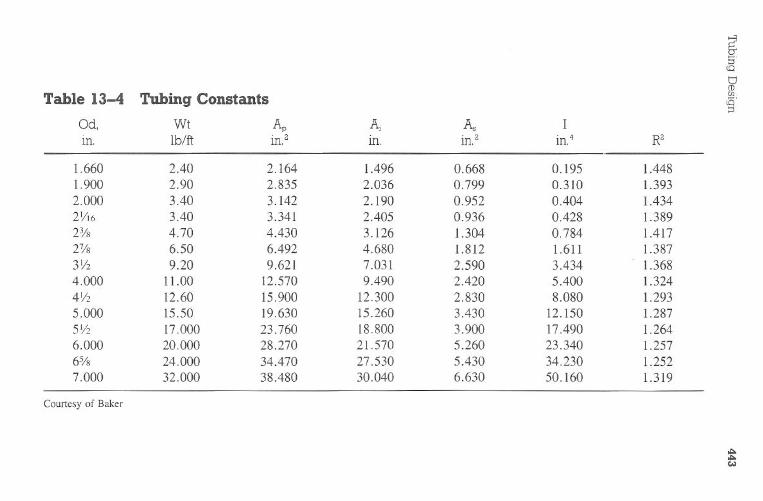
;?tr5'<
0
Table
13-4T
ubingC
onstantstnQ
'::s
Od,
Wt
Ap
Ai
As
Im
.ib/ft
in,2m
.in.2
in,4R
2
1.6602.40
2.1641.496
0.6680.195
1.4481.900
2.902.835
2.0360.799
0.3101.393
2.0003.40
3.1422.190
0.9520.404
1.4342Y
I63.40
3.3412.405
0.9360.428
1.3892%
4.704.430
3.1261.304
0.7841.417
27/86.50
6.4924.680
1.8121.611
1.387
31/29.20
9.6217.031
2.5903.434
1.3684.000
11.0012.570
9.4902.420
5.4001.324
4Y2
12.6015.900
12.3002.830
8.0801.293
5.00015.50
19.63015.260
3.43012.150
1.2875Y
217.000
23.76018.800
3.90017.490
1.2646.000
20.00028.270
21.5705.260
23.3401.257
6%24.000
34.47027.530
5.43034.230
1.2527.000
32.00038.480
30.0406.630
50.1601.319
Courtesy
ofB
aker
C/o)
444 Drilling Engineering
Where:
~L2 = length change due to helical buckling, in.r = tubing-to-casing radial clearance, in.Wf = buoyed tubing weight, Ib/in.
Pressure changes inside and outside of the tubing cause length change ~L3.This effect is called ballooning and results from radial pressure flow. The value,~L3, can be calculated from Eq. 13.7:
[ 2 (0.5 + v) 0]
U V~L3 = - ~Pi - R ~Po - V E(R2 - I)
2Lv- (~Pi - R2 ~Po) E(R2 _ I)
(13.7)
Where:
~L3 = length change due to ballooning, in.~Pi = change in fluid density inside the tubing, psi/in.~Po = change in fluid density outside the tubing, psi/in.R = ratio of tubing OD/IDv = Poisson's ratio for steel, v = 0.3o = tubing friction pressure, psi/in.
The tubing friction pressure, 0, is considered a constant and is positive whenthe flow is down the tubing. The worst case for ballooning length changes occurwhen 0 is zero.
Temperature changes cause the tubing to elongate or contract. The amountof length change, ~L4, caused by temperatures can be calculated with Eq. 13.8:
(13.8)
Where:~L4~T13
length changes due to temperature, in.average temperature change, of
= coefficient of thermal expansion, 6.9 x
The total length changes, ~L, caused by pressure and temperatures canbe calculated with Eq. 13.9:
(13.9)
The value, ~L, does not account for slack-off or pickup-related changes.
Tubing Design 445
Field experience has shown that normal production operations may shortenthe tubing. If the seal assembly is not anchored into the packer, the tubing mayshorten just enough to pull the seal out of the packer. To avoid this, it has becomea practice to lower some additional tubing weight on the packer. This procedureis called slack-off.
Slack-off weight often ranges from 10,000-30,000 lb and will vary, de-pending on the producing and tubing conditions. The slack-off force is definedas Fs. The length change, ALs, associated with slack-off weight can be calculatedfrom Eq. 13.10:
Fs
[
L r Fs
]E As + 81 WI(13.10)
Where:
ALs = length change due to slack-off, in.WI = initialbuoyedtubingweight, psi/in.Fs = slack-offweight,lb81 = inertia term
The minimum required seal assembly length can be calculated from Eq.13.11:
AT=AL+ALs= ALl + A~ + AL3 + AL4 + ALs
(l3.II)
Tuhing-to-Packer Forces. The total length changes, A~, may createan additional force defined as a tubing-to-packer force, Fp. If the length change,A~, causes the tubing to shorten, Fpis zero. However, if A~ signifies a tubingelongation and the packer restrains such movement, a packer force is developed.Further, if Fp is zero, then:
(13.12)(13.13)
where F: and F~ are the actual and buckling forces resulting from no packerrestraint.. However, in the case of packer restraint:
F: = Fa + FpF~ = Fb + Fp
(13.14)(13.15)
Fpis calculated in the same manner as the mechanically applied force necessaryto move the tubing back to its original, landed position through the distance-A~.
446 Drilling Engineering
Effects of Buckling. A common calculation associated with tubing is todetennine the neutral point, n, or the point above which buckling does not occur.This definition should not be confused with the neutral point as associated witha tension analysis. Unfortunately, many industry disagreements result from aconfusion of the definitions.
The neutral point can be calculated as follows:For F~< Wr x L:
n F~12Wr (13.16)
For F~ 2= Wr + L:
n L12 (13.17)
The buckled pitch, A, which is the distance between spirals at the bottom of thestring, is calculated as follows:
A = ~" /8Ef12V7 b(13.18)
The value Acan be used to detennine the length of logging tools that can be runthrough the bottom section of the tubing.
Stress Calculations. Detennination of the bending stress at the bottomof the tubing is calculated as follows:
If Fb':::;0:O"b = 0
(13.19)
Where:
O"b = bending stress at the outer fiber of the tubing, psido = tubing outer diameter, in.I = moment of inertia, in.4
[I = ~(d~ - di)]
The axial stress, 0".. is as follows:
Tubing Design 447
(13.20)
An evaluation of (Taand (Tbat the top of the tubing must account for the totalstringweightin the variousfluids. .
Buckled pipe will become permanently corkscrewed if the stress at theouter walls of the pipe exceeds the yield strength of the pipe. Therefore, theintern.aland external combined stresses, Sj and So, respectively, must be deter-mined before making a pipe selection. S; and So are calculated as follows:
The maximum stresses are obtained from Eqs. 13.21 and 13.22 by choosingthe sign (:t) that gives the largest value to the square root. The bending stressdue to helical buckling produces both a compressive ( :t) stress on the inside ofthe helix and a tensile (-) stress on the outside of the helix. The maximumcombined fiber stress will occur on either the inside or outside of the helix,
depending on whether the axial and pressure stresses are compressive ortensile.
Example 13.1Consider the conditions described in Table 13-2. Using the following infor-mation, evaluate the stresses involved in the tubing and select a tubing grade.Use a stress design factor of 1.1.
Tubing sizeTubing weightCasing IDPacker depthPacker typeSlack-off weightSeal typePacker bore
Solution:
2.875 in.6.4 lb.lft6.151 in.10,000 ftBaker Model D20,000 lbanchored seals2.375 in.
The equations and solutions for each operating condition are not pre-sented in this example due to the length of the calculations. A summary of
448 Drilling Engineering
the results is as follows (the results were computed with the Adams & RountreeTechnology tubing "design program):
*These length changes would have occurred if the seals were-free for movement.
Since the assembly was anchored and the seals could not move, stresses wereinduced into the tubing.
Since the greatest stress was 47,488 psi, J-55 tubing is sufficient for thewell.
Burst, Conapse, and Tension EvaluationPrevious sections defined stress as the controlling criteria for tubing design.
Pipe selected for stress considerations will be overdesigned in burst, collapse,and tension. Example 13.2 will illustrate this feature with respect to Example13.1.
Tubing Length Changes (FT)*
Operating Conditions
Item Space-out Flowing Stimulation Depletion
Tubing elasticity - 3.679 0.057 0.004 - 0.072Helical buckling -0.500 -0.044 -0.999 0.000
Radial pressure (bal- 0.0 - 1.044 - 2.600 0.402looning)
Temperature change 0.0 2.588 - 5.348 0.000Total -4.179 1.557 - 8.943 0.330
'fubing Forces and Related Parameters
Operating Condition
Item Space-out Flowing Stimulation DepletionPacker-to-tubing 20,000.00 24,418.041 -21,133.872 21,050.540
force, IbActual force, Ib 28,470.00 32,578 .526 - 12,684.625 29,910.027Buckling force, Ib 20;000.00 29,919.380 11,399.074 21,050.540Helix pitch, ft 36.399 29.760 48.214 35.479
Neutral point above 3,601.689 6,202.517 1,550.546 4,363.939packer, ft
Total bottom stress, 25,654.183 38,777.788 47,488.116 24,216.926pSI
Total top stress, psi 19,607.183 20,101.720 40,581.489 18,813.190
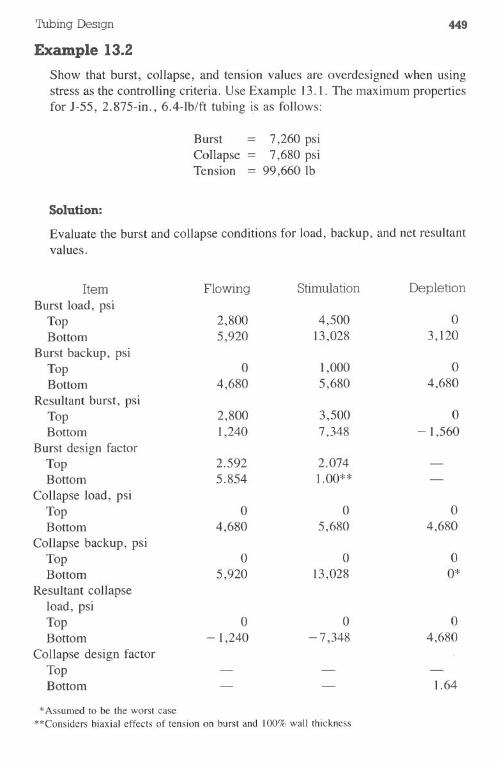
Tubing Design
Example 13.2
449
Show that burst, collapse, and tension values are overdesigned when usingstress as the controlling criteria. Use Example 13.1. The maximum propertiesfor J-55, 2.875-in., 6.4-lb/ft tubing is as follows:
Burst = 7,260psiCollapse = 7,680 psiTension = 99,6601b
Solution:
Evaluatethe burst andcollapseconditionsfor load,backup,and netresultantvalues.
Depletion
o3,120
o4,680
o- 1,560
o4,680
o0*
o4,680
1.64
Item Flowing Stimulation
Burst load, psiTop 2,800 4,500Bottom 5,920 13,028
Burst backup, psiTop 0 1,000Bottom 4,680 5,680
Resultant burst, psiTop 2,800 3,500Bottom 1,240 7,348
Burst design factorTop 2.592 2.074Bottom 5.854 1.00**
Collapse load, psiTop 0 0Bottom 4,680 5,680
Collapse backup, psiTop 0 0Bottom 5,920 13,028
Resultant collapseload, psiTop 0 0Bottom - I,240 - 7,348
Collapse design factorTopBottom
*Assumed to be the worst case
**Considers biaxial effects of tension on burst and 100% wall thickness
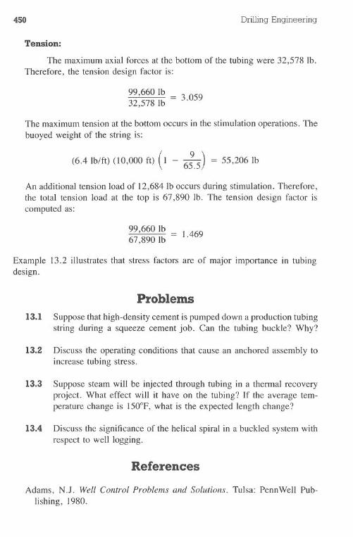
450 DrillingEngineering
Tension:
The maximum axial forces at the bottom of the tubing were 32,578 lb.Therefore,the tension"designfactor is:
99,660 lb = 3.05932,578 lb
The maximum tension at the bottom occurs in the stimulation operations. Thebuoyed weight of the string is:
(6.4 lb/ft) (10,000ft) (1 - 6:.5) = 55,206 lb
An additional tension load of 12,684 Ib occurs during stimulation. Therefore,the total tension load at the top is 67,890 lb. The tension design factor iscomputed as:
99,6601b67,890 Ib = 1.469
Example 13.2 illustrates that stress factors are of major importance in tubingdesign.
Problems
13.1 Suppose that high-density cement is pumped down a production tubing" string during a squeeze cement job. Can the tubing buckle? Why?
13.2 Discuss the operating conditions that cause an anchored assembly toincrease tubing stress.
13.3 Suppose steam will be injected through tubing in a thermal recoveryproject. What effect will it have on the tubing? If the average tem-perature change is 150°F, what is the expected length change?
13.4 Discuss the significance of the helical spiral in a buckled system withrespect to well logging.
References
Adams, N.J. Well Control Problems and Solutions. Tulsa: PennWell Pub-lishing, 1980.
Tubing Design 451
Greenip, John F. "Determining Stress in Tubing Using Triaxial Evaluation."SPE 6760 presented at the 1977 Fall Technical Conference, Denver, Col-orado.
Hammerlindl, D.J. "Basic Auid Pressure Forces on Oilwell Tubulars." Jour-nal of Petroleum Technology, Janilary 1980, pp. 153-159.
Hammerlindl, D.J. "Movement, Forces, and Stress Associated with Com-bination Tubing Strings Sealed in Packers." Journal of Petroleum Tech-nolgoy, February 1977, pp. 195-208.
Klinkenberg, A. "The Neutral Zones in Drill Pipe and Casing and TheirSignificance in Relation to Buckling and Collapse." Drilling and Produc-tion Practices. API, 1951.
Logan, J.L. "How to Keep Tubing Sealed in Packers." Journal of CanadianPetroleum Technology, volume 2, no. 2, 1963.
Lubinski, A., and K.A. Blenkara. "Buckling of Tubing in Pumping Wells,Its Effects and Means for Controlling It." Trans., AIME, volume 210,1957, pp. 73-88.
Lubinski, A. "Influence of Tension and Compression on Straightness andBuckling of Tubular Goods in Oil Wells." Proc., API 31st Annual Meeting,Chicago, 1951, Prod. Sec. IV, 31, 34.
Lubinski, A. "A Study of the Buckling of Rotary Drilling String." Drillingand Production Practices. API, 1951.
Lubinski, A., W.S. Althouse, and J.L. Logan. "Helical Buckling of ThbingSealed in Packers." Journal of Petroleum Technology, June 1962, pp. 655-670.
Prentice, C.M. "Maximum Load Casing Design." Journal of PetroleumTechnology, July 1971, pp. 805-811.
Chapter 14 CompletionEffects on Well
Planning andDrilling
Completion planning for the well must involve several groups within theoperating company. just as geologists and drilling personnel coordinate theirefforts when beginning a well, the completion of the well involves coordinatedefforts between the driIling and production departments. Inaddition, many com-panies have completion specialists who may have input into the process.
The type of completion selected for a given well may have a serious impacton the planning and driIling phase of the well. For example, multiple completionsmay require the use of larger hole geometries (Chapter 6) and may affect thecasing design (Chapter 12) if a completion is planned for a zone behind theintermediate pipe. The completion must be given consideration before planningmost phases of the well.
Reservoir and Production Parameters
The driIling program is designed with a bottom-to-top approach (Chapters5 and 6); the target is selected and then a viable plan is designed to reach thetarget safely. The completion plan must use the same procedure. Optimumproduction and economics from the reservoir are the targets for a successfulwell. The completion factors affecting the bottom-to-top approach are as follo~s:· reservoir characteristics.reservoir damage·completion efficiency·tubing and flow string size
Author's Note: The purpose of Chapter 14 is to present some of the completion con-siderations that affect drilling and well planning, not a comprehensive discussion ofcompletions planning. See the reference section for published sources of information onthe subject.
452
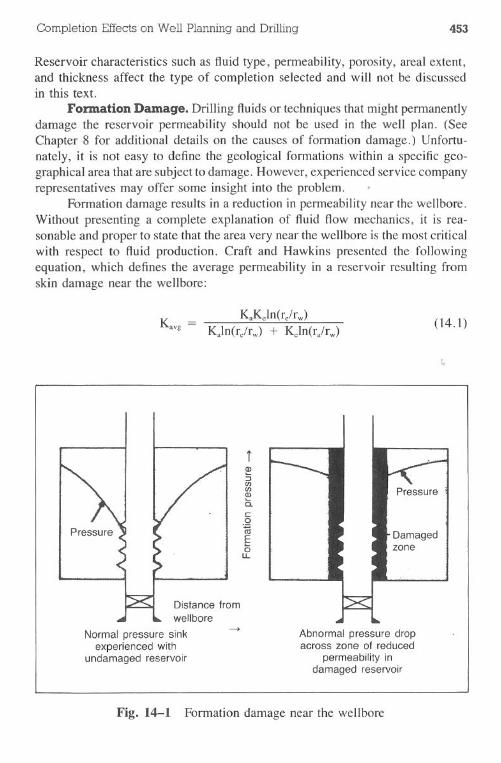
Completion Effects on Well Planning and Drilling 453
Reservoir characteristics such as fluid type, permeability, porosity, areal extent,and thickness affect the type of completion selected and will not be discussedin this text.
Formation Damage. Drilling fluids or techniques that might permanentlydamage the reservoir permeability should not be used in the well plan. (SeeChapter 8 for additional details on the causes of formation damage.) Unfortu-nately, it is not easy to define the geological formations within a specific geo-graphical area that are subject to damage. However, experienced service companyrepresentatives may offer some insight into the problem. .
Formation damage results in a reduction in permeability near the wellbore.Without presenting a complete explanation of fluid flow mechanics, it is rea-sonable and proper to state that the area very near the wellbore is the most criticalwith respect to fluid production. Craft and Hawkins presented the followingequation, which defines the average permeability in a reservoir resulting fromskin damage near the wellbore:
KaKeln(re/rw)
Kavg= Kaln(re/rw)+ Keln(ra/rw)
Distance fromwellbore
Normal pressure sinkexperienced with
undamaged reservoir
(14.1)
fQ)
~enenQ)a.c:.2iiiEou..
Abnormal pressure dropacross zone of reduced
permeability indamaged reservoir
Fig. 14-1 Formation damage near the wellbore
454 Drilling Engineering
Where:Kavg= average reservoir permeability after formation damage, d or mdKa = permeability in the affected damage areaK. = effective permeability in the external, unaffected arearw = wellbore radius, ftra = radius of the affected area, ftre = external drainage radius, ft
(See Fig. 14-1.) Example 14.1 illustrates the severity of the problem.
Example 14.1
A well is drilled on a reservoir spacing as defined below. If the damageresulting from drilling fluid invasion reduces the permeability in the affectedarea, Ka in a radius ra, compute the resulting average reservoir permeability.
external drainage radius = 1,000ftdamage radius = 3 ftwellbore radius = 0.5 ftexternal permeability (Ke) = 500 mddamaged permeability (Ka)= 25 md
Solution:
1. Use Eq. 14.1 to determine the average permeability, Kavg:
(25)(500)ln(l,000/0.5)(25)ln(l,000/3) + (500)ln(3/0.5)
91.2 md
2. The external permeability of 500 md has been reduced to an average of91 md for the 1,000-ft drainage radius due to a 3-ft damaged area.Completion Efficiency. The primary purpose of the completion process
is to provide a flow path from the reservoir to the surface equipment. The mostdifficult part of the completion, in most cases, is developing optimum flowchannels from the reservoir to the bottom of the flow string. Common problemareas are as follows:
.perforations that do not extend beyond the damaged area· fewerthan optimumnumberof perforations·plugged perforations .·poor cementjob that allowsbehind-the-pipechanneling· improper equipment sizing for gravel packing
Completion Effectson Well Planning and Drilling 455
Service company representatives can often help you avoid these problems.Flow String Sizing. Choosing the proper size of flow string can affect
reservoir performance to some degree. Tubing with a restricted inner diametercan cause high pressure losses. Since this pressure is the driving energy thatforces fluids out of the reservoir, any wasteful source of pressure dissipation cancause a lower primary reservoir recovery. However, large tubing strings maynot necessarily have any significant effect on pressure losses, as with 3Y2- vs4Y2-in. tubing on a given well. The tubing string should be sized to allow foroptimum production with a minimum tubing size. This consideration is importantbecause it affects the overall hole geometry.
Surface and Subsurface Completion EquipmentWell completions involve placing flow control equipment at the surface
and inthe tubing string. These items may include the following major categories:
·production tree· surface and subsurface automatic shutdown systems.flow string equipment·packers
The equipment must be sized and selected for each reservoir and its flow char-acteristics. The drilling plan should include a wellhead and geometry to accom-modate this production equipment.
Production Tree. The production, or Christmas, tree provides the con-nection between the wellbore and the production equipment such as the separatorsand treatment facilities. The tree (Fig. 14-2) contains control valves and chokes.Many trees contain redundant equipment for safety purposes. Severe operatingconditions such as hydrogen sulfide-produced fluids or Arctic and geothermalenvironments may require the use of modified wellheads.
The master valves, as the name implies, are the primary pressure controlmechanisms in the tree. The valves may be manually operated and containautomatic shutdown equipment. Many trees have multiple valves.
The swab valve provides a means to access the tubing string for remedialwork on the well. The valve can be closed so equipment such as wirelinelubricators can be installed on the top of the tree. The valve is subsequentlyopened, and work can be initiated through the tree.
The tree alters the direction of the flowing fluid. The wing on the treeusually contains several types of safety valves and a choke. The wing may includean automatic safety' valve. The choke is used to dissipate well pressure beforethe flowing fluid entering the low pressure, surface production equipment.
Automatic Shutdown Systems. On occasion, wells must be shutin toprevent an undesirable occurrence. For example, a ruptured flow line must be
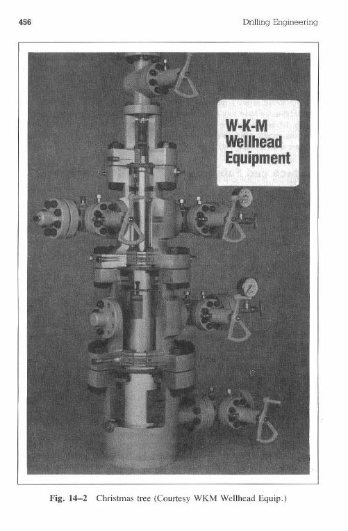
456 Drilling Engineering
Fig. 14-2 Christmas tree (Courtesy WKM Wellhead Equip.)
Completion Effects on Well Planning and Drilling 457
shutin to prevent a blowout. Shutin can be accomplished with surface or sub-surface tools and can be controlled by direct- or remote-controlled methods.These overall systems are generally termed automatic shutdown systems.
Surface Safety Equipment. Surface devices can cause the well to shutinautomatically under abnormal operating conditions. Trigger conditions includehigh- or low-pressure fluctuations, fire, abnormal flow rates, and excessive ero-sion. Shutin can be through either direct- or remote-controlled operating systems.
Direct-controlled surface safety systems can be installed at any point down-stream of the surface choke to sense line pressure changes at the point of valveinstallation only. Such safety valves are generally selected when automatic shutinprotection is desired only for breaks in a flow line or sales line, cutting a surfacechoke by flow line pressure changes. These valves are self-contained and nor-mally use a monitor-actuator pilot (Fig. 14-3).
A typical direct-controlled surface safety valve (Fig. 14-4) is a pilot-controlled safety valve, opened and closed by well or flow line pressure througha velocity check valve. Pressure within the valve, acting on the area of the stemagainst atmospheric pressure, causes the actuator to move the valve gate to itsopen position. The valve is designed to close automatically in the event of anabnormal change in flow line pressure. When the pilot senses a change beyondits setting, it actuates, exhausting the pressure from below the actuator pistonand allowing the pressure above the piston to close the valve.
A remote-controlled surface safety system (Fig. 14-5) can be installed inthe tree as a secondary master valve. It is usually a compact unit that can alsobe installed on wing valves upstream of the surface choke, header valves, flowlines, gathering lines, pipelines, or anywhere automatic valve shutin protectionis desired. Monitor pilots, used with this valve, are located remotely at numeroushigh-risk areas throughout the system.
The surface systems are operated by a hydraulic control manifold designedto provide the hydraulic pressure required to hold open various valves and tocontrol the pressure to the valves. Any loss of pressure in either the pilot lineor hydraulic line closes the safety valve. Pressure loss could be from operatingpilots or damage to the system (Fig. 14-6).
The operating principle for the control manifold can be illustrated withFig. 14-7. A gas-powered hydraulic pump is used to maintain a desired hydraulicpressure for the safety valve. When the monitor pilot in the safety system op-erates, it exhausts pressure from the low-pressure control line, causing the three-way valve in the control manifold to block incoming control pressure. This actionin turn releases the control pressur~ of a diaphragm in the three-way hydrauliccontroller. On loss of control pressure, the controller blocks incoming hydraulicfluid pressure and allows the hydraulic fluid in the safety valve control line tobleed into the reservoir. The safety valve control line bleeds into the reservoir,causing the safety valve to close.
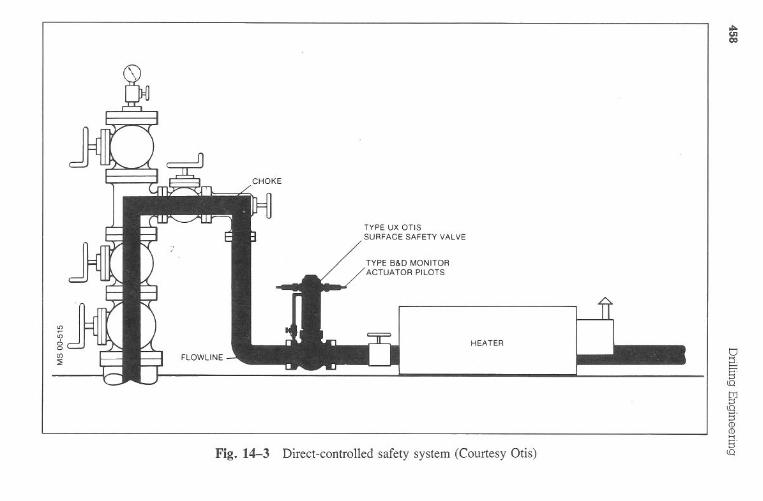
TY
PE
UX
OT
ISS
UR
FA
CE
SA
FE
TY
VA
LVE
TY
PE
B&
DM
ON
ITO
RA
CT
UA
TO
RP
ILOT
S
HE
AT
ER
Fig.
14-3D
irect-controlledsafety
system(C
ourtesyO
tis)
.UI
CIO
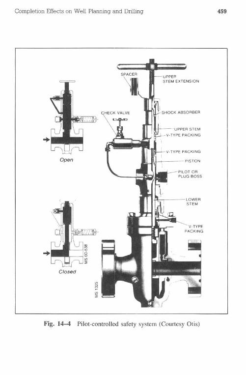
Completion Effectson Well Planning and Drilling 459
UPPERSTEM EXTENSION
V-TYPE PACKING
Open PISTON
LOWERSTEM
V-TYPEPACKING
Closed
'"N(')
Fig. 14-4 Pilot-controlled safety system (Courtesy Otis)
rI
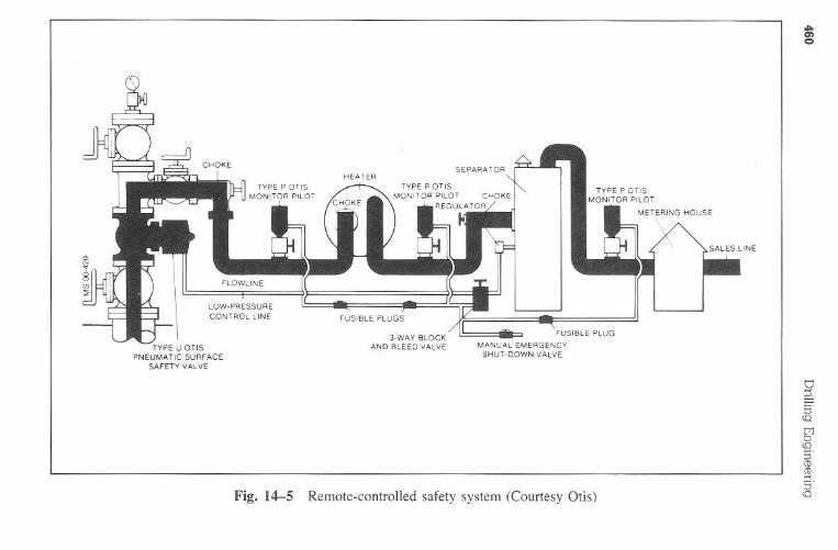
LOW
-PR
ES
SU
RE
CO
NT
RO
LLIN
EF
US
IBLE
PLU
GS
TY
PE
UO
TIS
PN
EU
MA
TIC
SU
RF
AC
ES
AF
ET
YV
ALV
E
3:WA
YB
LOC
KA
ND
BLE
ED
VA
LVE
FU
SIB
LEP
LUG
MA
NU
AL
EM
ER
GE
"ICY
SH
UT
-DO
WN
VA
LVE
Fig.
14-5R
emote-controlledsafety
system(C
ourtesyO
tis)
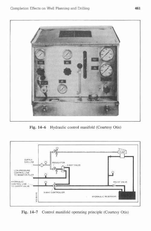
Completion Effects on Well Planning and Drilling 461
-- --
Fig. 14-6 Hydraulic control manifold (Courtesy Otis)
SUPPLY
GAS LI~E
lOW~PAESSURECONTROL LINETO MONITOR PILOT
HVDRAULIC.CONTROL LINETO SAFETY VALVE
HYDRAULIC RESERVOIR-
3.WAY CONTROllER
Fig. 14-7 Control manifold operating principle (Courtesy Otis)
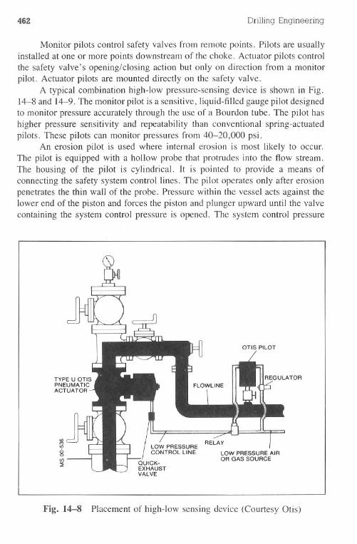
462 Drilling Engineering
Monitor pilots control safety valves from remote points. Pilots are usuallyinstalled at one or more points downstream of the choke. Actuator pilots controlthe safety valve's opening/closing action but only on direction from a monitorpilot. Actuator pilots are mounted directly on the safety valve.
A typical combination high-low pressure-sensing device is shown in Fig.14-8 and 14-9. The monitor pilot is a sensitive, liquid-filledgauge pilot designedto monitor pressure accurately through the use of a Bourdon tube. The pilot hashigher pressure sensitivity and repeatability than conventional spring-actuatedpilots. These pilots can monitor pressures from 40-20,000 psi.
An erosion pilot is used where internal erosion is most likely to occur.The pilot is equipped with a hollow probe that protrudes into the flow stream.The housing of the pilot is cylindrical. It is pointed to provide a means ofconnecting the safety system control lines. The pilot operates only after erosionpenetrates the thin wall of the probe. Pressure within the vessel acts against thelower end of the piston and forces the piston and plunger upward until the valvecontaining the system control pressure is opened. The system control pressure
LOW PRESSURECONTROL LINE
-IQUICK-EXHAUSTVALVE
Fig. 14-8 Placement of high-low sensing device (Courtesy Otis)
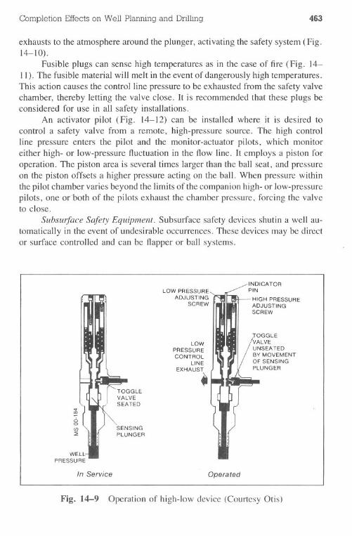
Completion Effects on Well Planning and Drilling 463
exhausts to the atmosphere around the plunger, activating the safety system (Fig.14-10).
Fusible plugs can sense high temperatures as in the case of fire (Fig. 14-II). The fusible material will melt in the event of dangerously high temperatures.This action causes the control line pressure to be exhausted from the safety valvechamber, thereby letting the valve close. It is recommended that these plugs beconsidered for use in all safety installations.
An activator pilot (Fig. 14-12) can be installed where it is desired tocontrol a safety valve from a remote, high-pressure source. The high controlline pressure enters the pilot and the monitor-actuator pilots, which monitoreither high- or low-pressure fluctuation in the flow line. It employs a piston foroperation. The piston area is several times larger than the ball seat, and pressureon the piston offsets a higher pressure acting on the ball. When pressure withinthe pilot chamber varies beyond the limits of the companion high- or low-pressurepilots, one or both of the pilots exhaust the chamber pressure, forcing the valveto close.
Subsurface Safety Equipment. Subsurface safety devices shutin a well au-tomatically in the event of undesirable occurrences. These devices may be director surface controlled and can be flapper or ball systems.
WELl:PRESSURE
In Service
LOW PRESSUREADJUSTING
SCREW
INDICATORPIN
HIGH PRESSUREADJUSTINGSCREW
LOWPRESSURECONTROL
LINEEXHAUST.
;rOGGLEVALVEUNSEATEDBYMOVEMENTOF SENSINGPLUNGER
Operated
Fig. 14-9 Operation of high-low device (Courtesy Otis)
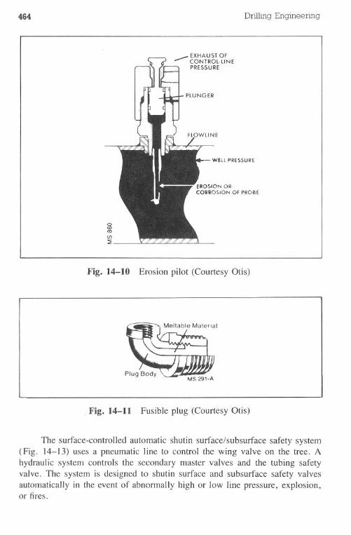
464 Drilling Engineering
oCD00en:!:
WEll PRESSURE
Fig. 14-10 Erosion pilot (Courtesy Otis)
. Fig. 14-11 Fusible plug (Courtesy Otis)
The surface-controlled automatic shutin surface/subsurface safety system(Fig. 14-13) uses a pneumatic line to control the wing valve on the tree. Ahydraulic system controls the secondary master valves and the tubing safetyvalve. The system is designed to shutin surface and subsurface safety valvesautomatically in the event of abnormally high or low line pressure, explosion,or fires.
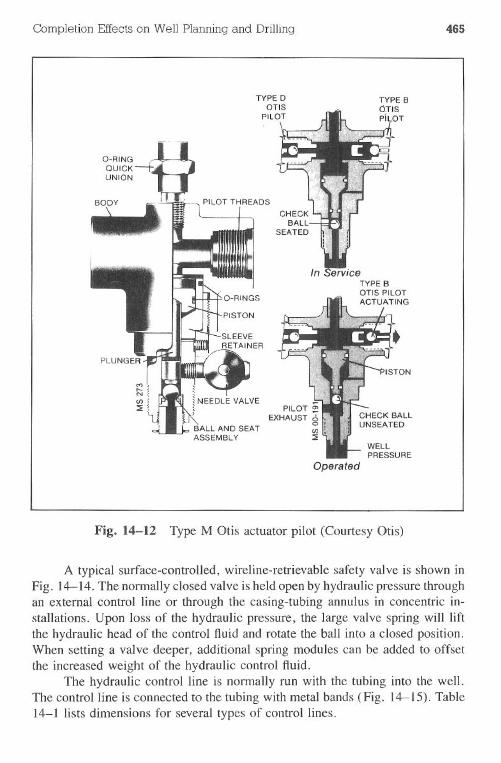
Completion Effects on Well Planning and Drilling 465
Operated
Fig. 14-12 Type M Otis actuator pilot (Courtesy Otis)
A typical surface-controlled, wireline-retrievable safety valve is shown inFig. 14-14. The normally closed valve is held open by hydraulic pressure throughan external control line or through the casing-tubing annulus in concentric in-stallations. Upon loss of the hydraulic pressure, the large valve spring will liftthe hydraulic head of the control fluid and rotate the ball into a closed position.When setting a valve deeper, additional spring modules can b.eadded to offsetthe increased weight of the hydraulic control fluid.
The hydraulic control line is normally run with the tubing into the well.The control line is connected to the tubing with metal bands (Fig. 14-15). Table14-1 lists dimensions for several types of control lines.
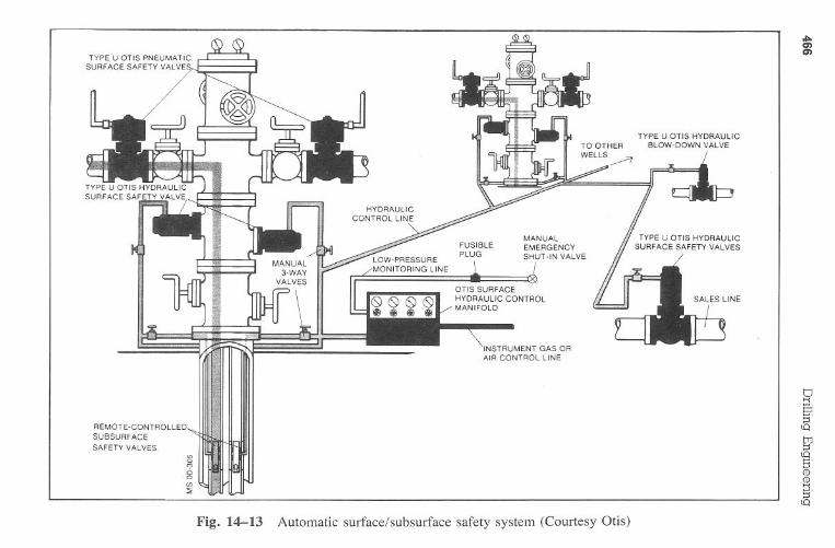
RE
MO
TE
-CO
NT
RO
LLED
SUBSURFACE
SA
FE
TY
VA
LVE
S
Fig.
14-13A
utomatic
surface/subsurfacesafety
system(C
ourtesyO
tis)
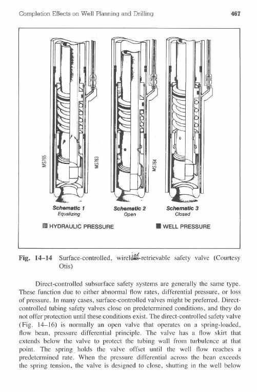
Completion Effects on Well Planning and Drilling
Schematic 1Equalizing
III HYDRAULIC PRESSURE
Schematic 2Open
467
Schematic 3Closed
. WEll PRESSURE
Fig. 14-14 Surface-controlled, wireldatretrievable safety valve (CourtesyOtis)
Direct-controlled subsurface safety systems are generally the same type.These function due to either abnormal flow rates, differential pressure, or lossof pressure. In many cases, surface-controlled valves might be preferred. Direct-controlled tubing safety valves close on predetermined conditions, and they donot offer protection until these conditions exist. The direct-controlled safety valve(Fig. 14-16) is normally an open valve that operates on a spring-loaded,flow bean, pressure differential principle. The valve has a flow skirt thatextends below the valve to protect the tubing wall from turbulence at thatpoint. The spring. holds the valve offset until the well flow reaches apredetermined rate. When the pressure differential across the bean exceedsthe spring tension, the valve is designed to close, shutting in the well below
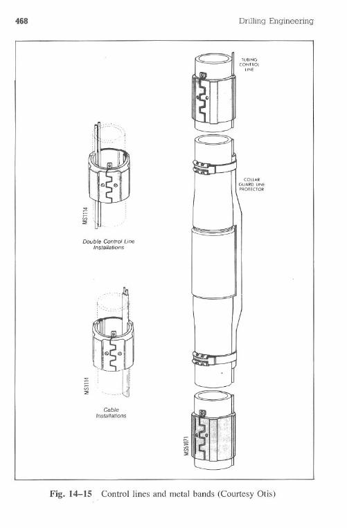
468 Drilling Engineering
C ~1 1 TUBING""'= ~ CONTROL
LINE
.__1.<:.,
COLLARGUARD LINEPROTECTOR
Double Control LineInstallations
CableInstallations
....
(1'). ,_::0 u__
Fig. 14-15 . Control lines and metal bands (Courtesy Otis)
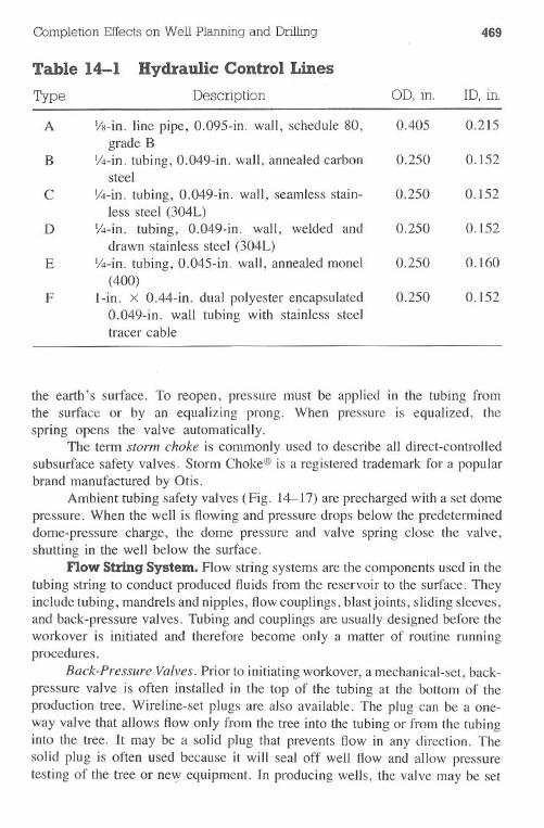
the earth's surface. To reopen, pressure must be applied in the tubing fromthe surface or by an equalizing prong. When pressure is equalized, thespring opens the valve automatically.
The term storm choke is commonly used to describe all direct-controlledsubsurface safety valves. Storm Choke@is a registered trademark for a popularbrand manufactured by Otis.
Ambient tubing safety valves (Fig. 14-17) are precharged with a set domepressure. When the well is flowing and pressure drops below the predetermineddome-pressure charge, the dome pressure and valve spring close the valve,shutting in the well below the surface.
now String System. Flow string systems are the components used in thetubing string to conduct produced fluids from the reservoir to the surface. Theyinclude tubing, mandrels and nipples, flow couplings, blastjoints, sliding sleeves,and back-pressure valves. Tubing and couplings are usually designed before theworkover is initiated and therefore become only a matter of routine runningprocedures.
Back-Pressure Valves. Prior to initiating workover, a mechanical-set, back-pressure valve is often installed in the top of the tubing at the bottom of theproduction tree. Wireline-set plugs are also available. The plug can be a one-way valve that allows flow only from the tree into the tubing or from the tubinginto the tree. It may be a solid plug that prevents flow in any direction. Thesolid plug is often used because it will seal off well flow and allow pressuretesting of the tree or ne\y equipment. In producing wells, the valve may be set
Completion Effectson Well Planning and Drilling 469
Table 14-1 Hydraulic Control Lines
Type Description OD, in. IDoin.
A Ys-in. line pipe, 0.095-in. wall, schedule 80, 0.405 0.215
grade BB 1/4-in.tubing, 0.049-in. wall, annealed carbon 0.250 0.152
steelC Y4-in.tubing, 0.049-in. wall, seamless stain- 0.250 0.152
less steel (304L)D 1/4-in. tubing, 0.049-in. wall, welded and 0.250 0.152
drawn stainless steel (304L)E Y4-in.tubing, 0.045-in. wall, annealed monel 0.250 0.160
(400)F I-in. x 0.44-in. dual polyester encapsulated 0.250 0.152
0.049-in. wall tubing with stainless steeltracer cable
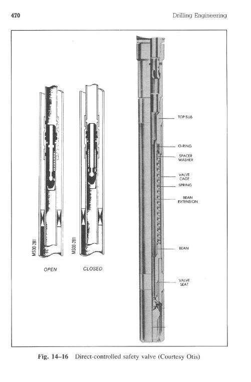
470
OPEN CLOSED
Drilling Engineering
TOPSUB
SPACERWASHER
VALVECAGE
SPRING
BEANEXTENSION
BEAN
VALVESEAT
Fig. 14-16 Direct-controlled safety valve (Courtesy Otis)
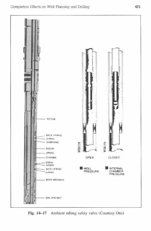
Completion Effects on Well Planning and Drilling
TOPSUB
BACK-UP RING
a-RING
GUIDE RING
PISTON
SPRING
CHAMBER
SCREWGASKET
BACK-UPRINGa-RING
BODY WElDMENT
BAll AND SEAT
OPEN
.WELLPRESSURE
471
I'!I
" I!" i
i
II
,1
,Ioj
,I,""
CLOSED
. INTERNALCHAMBERPRESSURE
Fig. 14-17 Ambient tubing safety valve (Courtesy Otis)
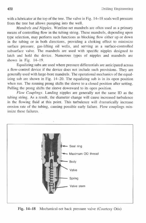
472 Drilling Engineering
with a lubricator at the top of the tree. The valve in Fig. 14-18 seals well pressurefrom the tree but allows pumping into the well.
Mandrels and Nipples. Wireline-set mandrels are often used as a primarymeans of controlling flow in the tubing string. These mandrels, depending upontype selection, may perform such functions as blocking flow either up or downin the tubing or in both directions, providing a choking effect to minimizesurface pressure, gas-lifting oil wells, and serving as a surface-controlledsubsurface valve. The mandrels are used with specific nipples designed tolatch and hold the device. Numerous types of nipples and mandrels areshown in Fig. 14-19.
Equalizing subs are used where pressure differentials are anticipated acrossa flow-control device if the device does not include such provisions. They aregenerally used with large-bore mandrels. The operational mechanics of the equal-izing sub are shown in Fig. 14-20. The equalizing sub is in its open positionwhen run. The running prong shifts the sleeve to a closed position after setting.Pulling the prong shifts the sleeve downward to its open position.
Flow Couplings. Landing nipples are generally not the same ID as thetubing string. As a result, the diameter change will cause increased turbulencein the flowing fluid at this point. This turbulence will dramatically increaseerosion rate of the tubing, causing possible early failure. Flow couplings min-imize these failures.
I
~ Seal ring
t-- Maximum OD thread
~ Body
Valve
Spring
Valve stem
Fig. 14-18 Mechanical-set back pressure valve (Courtesy Otis)
Completion Effects on Well Planning and Drilling 473
A flow coupling (Fig. 14-21) is a thick-walled section of tubing installedabove, and often below, the diameter change. Field experience indicates thatflow couplings should be 36 in. or longer for maximum protection. Many man-ufacturers produce the couplings in 5-, 10-, or 20-ft lengths.
Blast Joints. Blast joints are used in the tubing string to protect againstexternal erosion, as in the case of dual-completion wells (Figs. 14-22 and14-23). Most are special alloy, heat-treated joints and are available in 10- and20-ft lengths. Blast joint connec,tionsgenerally make up flush.
Sliding Sleeves. Selective circulating devices, such as a sliding sleeve,provide openings between the tubing and the annulus without the necessity ofperforating. The tool is useful when circulating fluids for well control or pro-ducing from other intervals (Figs. 14-23 and 14-24). Problems are often as-sociated with the tool, however, when attempting to use it after an extended timein the tubing.
Packers,. The annular seal between the tubing and production casing isprovided by the packer. It must be able to withstand high differential pressureand still maintain a seal. Tubing movement must be considered when temper-atures change (Chapter 13). In addition, corrosive fluids such as hydrogen sulfide(H2S) must be resisted.
General packer classifications are retrievable and permanent. The perma-nent type is held in place by opposing slips and can be set with wireline ortubing-conveyed methods. The retrievable packers can be weight set, mechanicalset, or hydraulic set.
Packers generally can be divided into four major components, includingslip assembly, outer seal assembly, packer bore receptacle, and tubing sealassembly. The slip assembly and outer seal secure and seal the packer-casinginterface. The packer bore and the tubing seal assembly provide the tubing-packer pressure seal while allowing tubing expansion or contraction to occur(Figs. 14-25 and 13-1).
Rubber elements with varying hardness and composition are used to providethe pressure seal for the outer seal assembly and the tubing seal assembly. Themost commonly used rubber is nitrile, with a 70-durometer hardness. Highbottom-hole temperatures require a greater hardness (80-90).
Corrosive gases such as hydrogen sulfide will crack the rubber elementsif nitrile is used. Serviceable elements such as Viton@(DuPont) can be effectivelyused in H2Senvironments with little or no embrittlement tendencies. If amino-based corrosion inhibitors are used, however, the Viton@will deteriorate becauseof fluorocarbon composition in the inhibitor. As a result, sealing elements ex-posed to amine inhibitors require alternative rubber compounds such as K-Ryte@(Baker). This rubber is a layered structure composed of Kalrez@,Teflon@,andRylon@. These rubbers are generally used only when necessary because theymay cost 100 times more than nitrile. '
474
TYPES X and R EQUIPMENT
'"....=='"::!
Selective Land-ing Nipple TypeX for StandardTubing Weightand Type R forHeavy Tl,lbingWeight
Locking Man-drel
Equalizing Sub
SubsurfaceFlowControl
TYPES XN and RN EQUIPMENT(No-Go)
Landing NippleType X forStandard Tub-ing Weightand TypeR for HeavyTubing Weight
Locking Man-drel
Equalizing Sub
SubsurfaceFlowControl
Drilling Engineering
TYPES B, C and W EQUIPMENT
Nipple not re-quired. Sets intubing.
Slip Carrierand Slips.
Pdck-off andExpanderElements.
Equalizing Sub
SubsurfaceFlowControls
TYPE D EQUIPMENT
Nipple not re-quired. Sets incollar recess
Collar Locatingand LockingDogs
Pack-offElement
Lock Mandrel
Equalizing Sub
SubsurfaceFlowControls
Fig. 14-19 Nipples and mandrels (Courtesy Otis)
Completion Effects on Well Planning and Drilling
TYPE S EQUIPMENT
TYPE XEL EQUIPMENT
'"<0==='"::;;
ControlLine
SafetyValveNipple
LockingMandrel
Surface-ControlledTubingSafetyValve
Landing Nipple-Selective byLocating Man-drel, Availablewith a Series of7 Different In-ternal Profiles
Locating andLocking Man-drel
Equalizing Sub
SubsurfaceFlowControl
475
TYPE N EQUIPMENT (No-Go)
Landing Nipple
Locking Man-drel
Equalizing Sub
SubsurfaceFlowControl
TYPE XEL EQUIPMENT(With Sliding Side-Door <!> )
TYPE RQEEQUIPMENT(No-Go)
Centrol Line
Safety ValveNipple(No-Go)
LockingMandrel
Surface-ControlledTubingSafetyValve
Control Line
Safety-ValveNipple with Slid-ing Side-Door
Locking Man-drel
Surface-Con-trolled TubingSafety Valve
Fig. 14-20 Equalizing sub (Courtesy Otis)
(01 II FLOW
COUPLING
LANDINGNIPPLEANDFLOWCONTROl
FLOWCOUPLING(Optional)
Fig. 14-21 Flow coupling (Courtesy Otis)
Completion Effects on Well Planning and Drilling 477
Fig. 14-22 Blast joint (Courtesy Otis)
...BLASTJOINT
I
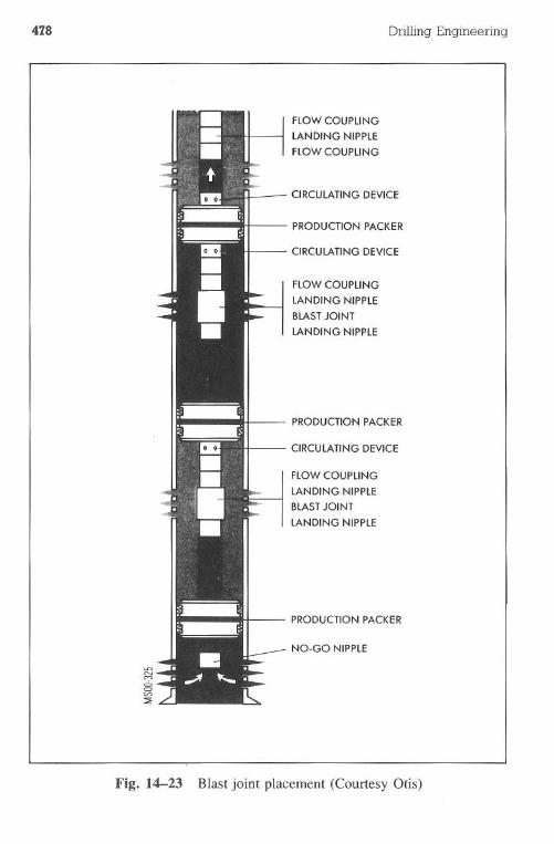
478 DrillingEngineering
flOW COUPLING
LANDING NIPPLE
flOW COUPLING
CIRCULATING DEVICE
PRODUCTION PACKER
CIRCULATING DEVICE
flOW COUPLING
LANDING NIPPLE
BLAST JOINT
LANDING NIPPLE
PRODUCTION PACKER
CIRCULATING DEVICE
FLOW COUPLING
lANDING NIPPLE
BLAST JOINT
lANDING NIPPLE
PRODUCTION PACKER
NO-GO NIPPLE
Fig. 14-23 Blast joint placement (Courtesy Otis)
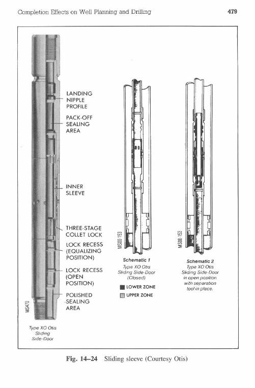
Completion Effects on Well Planning and Drilling
Type XO OtisSliding
Side-Door
LANDINGNIPPLEPROFILE
PACK-OFFSEALINGAREA
INNERSLEEVE
THREE-STAGECOLLET LOCK
LOCK RECESS
(EQUALIZINGPOSITION)
LOCK RECESS
(OPENPOSITION)
POLISHED.SEALlNGAREA
Schematic 1
Type XO OtisSliding Side-Door
(Closed). LOWERZONE
rn UPPER ZONE
479
Schematic 2
Type XO OtisSliding Side-Doorin open positionwith separation
tool in place.
Fig. 14-24 Sliding sleeve (Courtesy Otis)
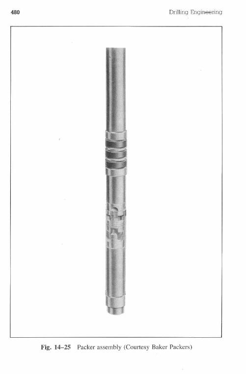
480 Drilling Engineering
Fig. 14-25 Packer assembly (Courtesy Baker Packers)
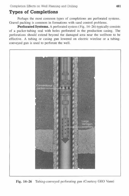
Completion Effects on Well Planning and Drilling
Types of Completions481
Perhaps the most common types of completions are perforated systems.Gravel packing is common in formations with sand control problems.
Perforated Systems. A perforated system (Fig. 14-26) typically consistsof a packer-tubing seal with holes perforated in the production casing. Theperforations should extend beyond the damaged area near the wellbore to beeffective. A tubing or casing gun lowered on electric wireline or a tubing-conveyed gun is used to perforate the well.
Fig. 14-26 Tubing-conveyed perforating gun (Courtesy GEO Vann)
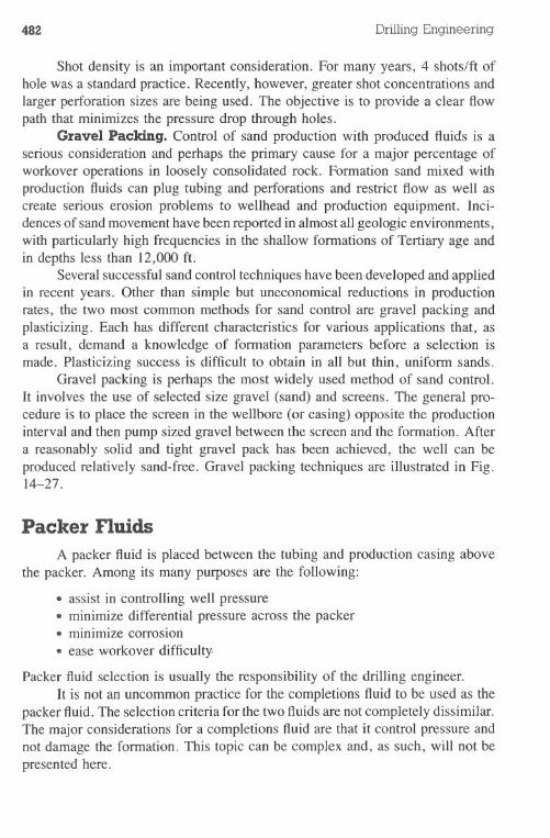
482 Drilling Engineering
Shot density is an important consideration. For many years, 4 shots/ft ofhole was a standard practice. Recently, however, greater shot concentrations andlarger perforation sizes are being used. The objective is to provide a clear flowpath that minimizes the pressure drop through holes.
Gravel Packing. Control of sand production with produced fluids is aserious consideration and perhaps the primary cause for a major percentage ofworkover operations in loosely consolidated rock. Formation sand mixed withproduction fluids can plug tubing and perforations and restrict flow as well ascreate serious erosion problems to wellhead and production equipment. Inci-dences of sand movement have been reported in almost all geologic environments,with particularly high frequencies in the shallow formations of Tertiary age andin depths less than 12,000 ft.
Several successful sand control techniques have been developed and appliedin recent years. Other than simple but uneconomical reductions in productionrates, the two most common methods for sand control are gravel packing andplasticizing. Each has different characteristics for various applications that, asa result, demand a knowledge of formation parameters before a selection ismade. Plasticizing success is difficult to obtain in all but thin, uniform sands.
Gravel packing is perhaps the most widely used method of sand control.It involves the use of selected size gravel (sand) and screens. The general pro-cedure is to place the screen in the wellbore (or casing) opposite the productioninterval and then pump sized gravel between the screen and the formation. Aftera reasonably solid and tight gravel pack has been achieved, the well can beproduced relatively sand-free. Gravel packing techniques are illustrated in Fig.14-27.
Packer Fluids
A packer fluid is placed between the tubing and production casing abovethe packer. Among its many purposes are the following:
.assist in controlling well pressure.minimize differential pressure across the packer.minimize corrosion.ease workoverdifficulty.
Packer fluid selection is usually the responsibility of the drilling engineer.It is not an uncommon practice for the completions fluid to be used as the
packer fluid. The selection criteria for the two fluidsare not completely dissimilar.The major considerations for a completions fluid are that it control pressure andnot damage the formation. This topic can be complex and, as such, will not bepresented here.
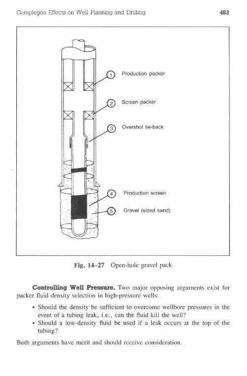
Comple~on Effectson Well Planning and Drilling 483
Production packer
Screen packer
Overshot tie-back
Production screen
Gravel (sized sand)
Fig. 14-27 Open-hole gravel pack
Controlling Wen Pressure. Two major opposing arguments exist forpacker fluid density selection in high-pressure wells:
.Should the density be sufficient to overcome wellbore pressures in theevent of a tubing leak, i.e., can the fluid kill the well?.Should a low-density fluid be used if a leak occurs at the top of thetubing?
Both arguments have merit and should receive consideration.
484 Drilling Engineering
Many operators desire a packer fluid density sufficient to balance bottom-hole pressure in the event of an unforeseen problem. If a packer leak occurs,the fluid will overcome the well pressure. However, a leak near the surface willlet high tubing pressures act on top of the packer fluid, causing high burstpressures for the production casing (Chapter 12). The requirement for high fluiddensity is not as demanding in oil wells as in gas wells and is not even aconsideration in normal pressure wells.
Minimize Differential Pressure. Most packers have limitations, eitherpractical or realistic, on the allowable differential pressure between the wellpressure below the packer and the fluid hydrostatic pressure above the packer.The primary consideration is usually in the direction of the well pressureacting upward but can be reversed, as in the cas.e of perforation pluggingthat may severely reduce the effective bottom-hole pressure immediately priorto shutin.
Corrosion. Packer fluids are normally designed to account for oxygencorrosion. Hydrogen sulfide (H2S)or carbon dioxide (C02) presence may warrantthe use of coating inhibitors. If amine-based inhibitors are used, special packerrubbers must be employed.
Ease Workover Difficulty. Although workovers or remedial action ona well are undesirable, it is likely they will be required some time. Therefore,forethought with respect to packer fluid selection relative to workovers is worth-while. The results will typically be lower workover costs and easier jobs.
The major considerations affecting packer fluid selection for workoveroperations may be as follows:
.Is the density sufficient to control well pressures that may be observedat the time of the workover?·Can the fluid viscosity be increased to help lift sand or metal cuttingsout of the well?·Will solids-laden fluids cause stuck tubing due to settling?.Will high temperatures cause fluid deterioration and make it difficult topump the fluid out of the well?.Is the fluid nondamaging to the production formation?
Special cases will ~sually require additional items to be considered.
Completion Factors Affecting the Well Planand Drilling
It is difficult to discuss out of context the completion factors that affectwell planning and drilling. Some have been discussed in this chapter and in othersections of this book. Although incomplete, Table 14-2 provides an overviewof some considerations.
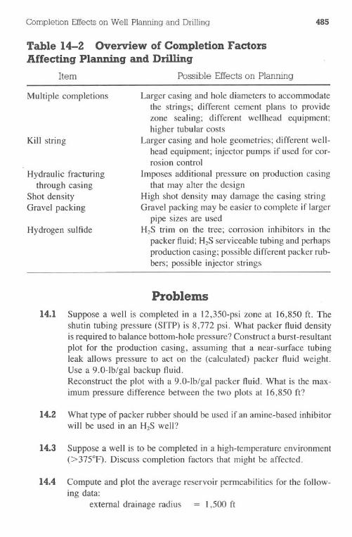
Completion Effects on Well Planning and Drilling 485
Table 14-2 Overview of Completion FactorsAffecting Planning and Dri1Iing
Item Possible Effects on Planning
Multiple completions
Kill string
Hydraulic fracturingthrough casing
Shot densityGravel packing
Hydrogen sulfide
Larger casing and hole diameters to accommodatethe strings; different cement plans to providezone sealing; different wellhead equipment;higher tubular costs
Larger casing and hole geometries; different well-head equipment; injector pumps if used for cor-rosion control
Imposes additional pressure on production casingthat may alter the design
High shot density may damage the casing stringGravel packing may be easier to complete if larger
pipe sizes are usedH2S trim on the tree; corrosion inhibitors in the
packer fluid; H2Sserviceable tubing and perhapsproduction casing; possible different packer rub-bers; possible injector strings
Problems
14.1 Suppose a well is completed in a 12,350-psi zone at 16,850 ft. Theshutin tubing pressure (SITP) is 8,772 psi. What packer fluid densityis required to balance bottom-hole pressure? Construct a burst-resultantplot for the production casing, assuming that a near-surface tubingleak allows pressure to act on the (calculated) packer fluid weight.Use a 9.0-lb/gal backup fluid.Reconstruct the plot with a 9.0-lb/gal packer fluid. What is the max-imum pressure difference between the two plots at 16,850 ft?
14.2 What type of packer rubber should be used if an amine-based inhibitorwill be used in an H2S well?
14.3 Suppose a well is to be completed in a high-temperature environment(>375°F). Discuss completion factors that might be affected.
14.4 Compute and plot the average reservoir permeabilities for the follow-ing data:
external drainage radius = I ,500 ft
486 Drilling Engineering
damage radius = 3 ftwellbore radius = 0.5 ftexternal permeability (Ke) = 300 mddamaged permeability (Ka)= 10 md
Recalculate for external radii of 500; 750; 1,000; 1,250; 1,750; and2,000 ft. Discuss the results.
14.5 Recalculate Problem 14.4 for damaged radii of 1, 2, 4, and 5 ft. Usean external radius of 1,500 ft. Discuss the results.
14.6 Discuss the reason(s) for difficulty in obtaining successful plasticizingjobs as a method of sand control.
14.7 Drilling muds are not used as frequently for packer fluids as they were.Discuss the problems caused by using many types of muds as packerfluids.
References
Adams & Rountree Technology Inc. Houston: Applied Reservoir Simulation,1984.
Adams, N.J. Well Control Problems and Solutions. Tulsa: PennWell Books,1980.
-. Workover Well Control. Tulsa: PennWell Books, 1981.
Allen, T., & A. Roberts. Production Operations / & II. Tulsa: Oil & GasConsultants International Inc., 1978.
Baker Oil Tools. "Tech Facts," Houston, 1978.
Boyle, W.e. Designing Production Safety Systems. Tulsa: PennWell Books,1979.
Cameron Iron Works Inc. General Catalog, /982-/983. Houston, 1982.
-. "Land and Production Platform, Oil Tool Division, 1982-1983."Houston, 1982.
Completion Effectson Well Planning and Drilling 487
Craft, B.C., and M.F. Hawkins. Applied Petroleum Reservoir Engineering.Englewood Cliffs, NJ: Prentice-Hall Inc., 1959.
ETA Offshore Seminars Inc. Technology of Offshore Drilling, Completion,and Production. Tulsa: PennWell Books, 1976.
Gatlin, C. Petroleum Engineering: Drilling and Well Completions. EnglewoodCliffs, NJ: Prentice-Hall Inc., 1960.
Gray Tool Co. Oilfield Equipment Catalog. Houston, 1983.
Hensley, Dennis. Personal communication. Houston, 1984.
Simmons, Evan. Personal communication. Houston, 1984.
Vetco. General Catalog, 1982-1983. Ventura, CA, 1982.
Chapter 15 DrillstringDesign
The drillstring is an important part of the rotary drilling process. It is theconnection between the rig and the drill bit. Although the drillstring is often asource of problems such as washouts, twistoffs, and collapse failures, it is seldomdesigned to prevent these problems from occurring. In many cases, a few minutesof drillstring design work could prevent most of the problems.
Purposes and ComponentsThe drillstring serves several general purposes, includjng the following:
·provide a fluid conduit from the rig to the bit· impart rotary motion to the drill bit·allow weight to be set on the bit· lower and raise the bit in the well
In addition, the drillstring may serve some of the following specialized services:
·provide some stability to the bottom-hole assembly to minimize vibrationand bit jumping· allow formation fluid and pressure testing through the drillstring·permit through-pipe formation evaluation when logging tools cannot berun in the open hole
The components of the drillstring are varied and serve many purposes.Fig. 15-1 shows a typical drillstring assembly (drillstem assembly). It is im-portant to observe in Fig. 15-1 that all connections from the swivel through theupper section of the kelly are left-hand threads. All connections between the
488
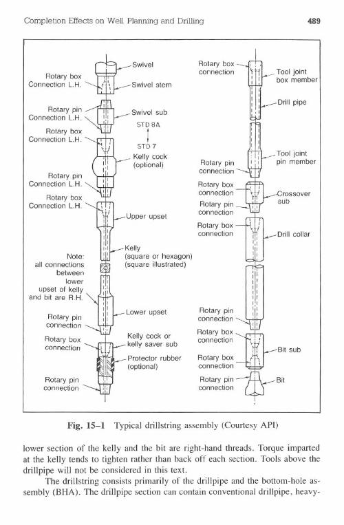
Completion Effectson Well Planning and Drilling 489
Fig. 15-1 Typical drillstring assembly (Courtesy API)
lower section of the kelly and the bit are right-hand threads. Torque impartedat the kelly tends to tighten rather than back off each section. Tools above thedrillpipe will not be considered in this text.
The drillstring consists primarily of the drillpipe and the bottom-hole as-sembly (BHA). The drillpipe section can contain conventional drillpipe, heavy-
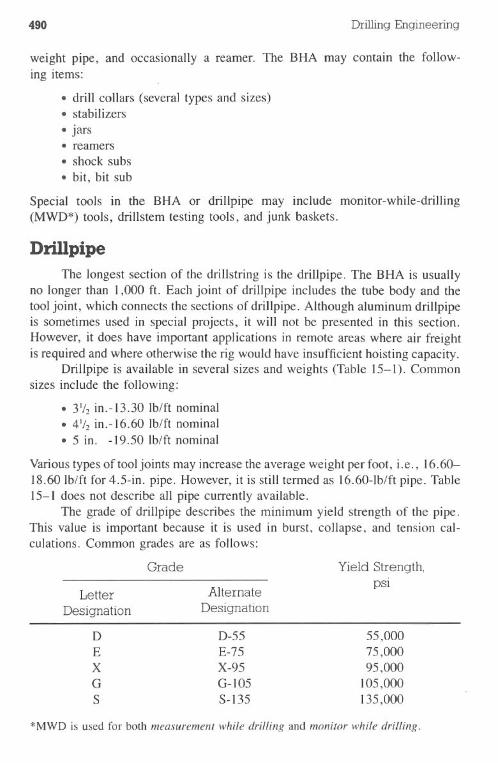
490 DrillingEngineering
weight pipe, and occasionally a reamer. The BHA may contain the follow-ing items:
.drill collars (several types and sizes).stabilizers·jars.reamers· shock subs·bit, bit sub
Special tools in the BHA or drillpipe may include monitor-while-drilling(MWD*)tools, drillstemtestingtools, andjunk baskets.
Drillpipe
The longest section of the drillstring is the drillpipe. The BHA is usuallyno longer than I ,000 f1. Each joint of drillpipe includes the tube body and thetool joint, which connects the sections of drillpipe. Although aluminum drillpipeis sometimes used in special projects, it will not be presented in this section.However, it does have important applications in remote areas where air freightis required and where otherwise the rig would have insufficient hoisting capacity.
Drillpipe is available in several sizes and weights (Table 15-1). Commonsizes include the following:
·31/2in.-13.30Ib/ft nominal.41/2in.-16.60 Ib/ft nominal· 5 in. -19.50 Ib/ft nominal
Varioustypes of tool joints may increase the average weight perfoot, i.e., 16.60-18.60 Ib/ft for 4.5-in. pipe. However, it is still termed as 16.60-lb/ft pipe. Table15-1 does not describe all pipe currently available.
The grade of drillpipe describes the minimum yield strength of the pipe.This value is important because it is used in burst, collapse, and tension cal-culations. Common grades are as follows:
Grade
LetterDesignation
AlternateDesignation
Yield Strength,pSi
DEXGS
D-55E-75X-95G-105S-135
55,00075,00095,000
105,000135,000
*MWD is used for both measurement while drilling and monitor while drilling.
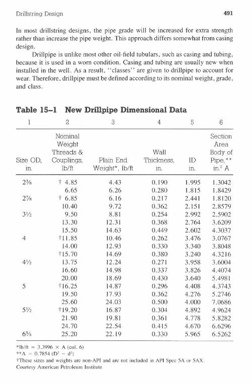
Drillstring Design 491
In most drillstring designs, the pipe grade will be increased for extra strengthrather than increase the pipe weight. This approach differs somewhat from casingdesign.
Drillpipe is unlike most other oil-field tubulars, such as casing and tubing,because it is used in a worn condition. Casing and tubing are usually new wheninstalled in the well. As a result, "classes" are given to drillpipe to account forwear. Therefore, drillpipe mustbe definedaccording to its nominal weight, grade,and class.
Table 15-1 New Drillpipe Dimensional Data
2 3 4 5 6
Nominal SectionWeight Area
Threads & Wall Body ofSize 00, Couplings, Plain End Thickness, 10 Pipe,**
m. Ib/ft Weight*, Ib/ft m. m. in.2A
2% t 4.85 4.43 0.190 1.995 1.30426.65 6.26 0.280 1.815 1.8429
27/8 t 6.85 6.16 0.217 2.441 1.8120to .40 9.72 0.362 2.151 2.8579
31/2 9.50 8.81 0.254 2.992 2.590213.30 12.31 0.368 2.764 3.620915.50 14.63 0.449 2.602 4.3037
4 t II. 85 to .46 0.262 3.476 3.076714.00 12.93 0.330 3.340 3.8048
t15.70 14.69 0.380 3.240 4.321641f2 13.75 12.24 0.271 3.958 3.6004
16.60 14.98 0.337 3.826 4.407420.00 18.69 0.430 3.640 5.4981
5 t16.25 14.87 0.296 4.408 4.374319.50 17.93 0.362 4.276 5.274625.60 24.03 0.500 4.000 7.0686
51/2 t 19.20 16.87 0.304 4.892 4.962421.90 19.81 0.361 4.778 5.828224.70 22.54 0.415 4.670 6.6296
6% 25.20 22.19 0.330 5.965 6.5262
*Ib/ft = 3.3996 x A (co!. 6)**A = 0.7854 (D' - d')tThese sizes and weights are non-API and are not included in API Spec SA or SAX.Courtesy American Petroleum Institute
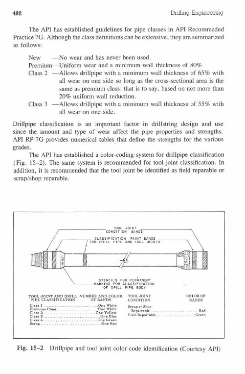
492 Drilling Engineering
The API has established guidelines for pipe classes in API RecommededPractice 7G. Although the class definitions can be extensive, they are summarizedas follows:
New -No wear and has never been used.Premium-Uniform wear and a minimum wall thickness of 80%.Class 2 -Allows drillpipe with a minimum wall thickness of 65% with
all wear on one side so long as the cross-sectional area is thesame as premium class; that is to say, based on not more than20% uniform wall reduction.
Class 3 -Allows drillpipe with a minimum wall thickness of 55% withall wear on one side.
Drillpipe classification is an important factor in drillstring design and usesince the amount and type of wear affect the pipe properties and strengths.API RP-7G provides numerical tables. that define the strengths for the variousgrades.
The API has established a color-coding system for drillpipe classification(Fig. 15-2). The same system is recommended for tool joint classification. Inaddition, it is recommended that the tool joint be identified as field reparable orscrap/shop reparable.
TOOL JOI NTCONDIT ION BANDS
CLASSIFICATION PAINT BANDSFOR DRILL PIPE AND TOOL JOINTS
STENCILS FOR PERMANENTMARKING FOR CLASSIFICATION
OF DRILL PIPE BODY
TOOL JOINT AND DRILL NUMBER AND COLOR TOOL JOINTPIPE CLASSIFICATION OF BANDS CONDITION
COLOR OFBANDS
Clae.l One WhitePremium Cia.. .. .Two WhiteClall 2 One Yel10wCla81 3 ' ..One BlueCia.. 4 .., ,_. ' .One GreenScrap. ' ,_...One Red
Scrap or ShopRepairable ... ... Red
Field Repairable Green
Fig. 15-2 Drillpipe and tool joint color code identification (Courtesy API)
Drillstring Design 493
Drillpipe is available in several length ranges:
RangeI23
Length, ft18-2227-3038-40
However, range 2 is the most common.A drillpipe catalog is presented in the Appendix. It includes most API
weights and grades. The grade and class nomenclature are combined such as inthe case of X95-P, which is premium-class X-95 grade pipe. The tool jointclearance is the outer diameter of the tool joint.
Drillpipe Tool JointsTool joints are screw-type connectors that join the individual joints of
drillpipe. Several types are widely used (Fig. 15-3):lEU (internal-external upset) Tool joint is larger than the pipe such that the
tool joint ID is less than the drillpipe. The tooljoint OD is larger than the drillpipe. Generally,
-- --
."t
.J~..
.
... .,-- ---
Fig. 15-3 Hardbanded box tool joints are available upon request
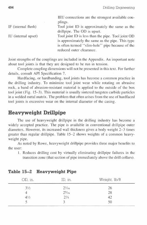
494 Drilling Engineering
IF (internal flush)
lEU connections are the strongest available cou-plings.Tool joint ID is approximately the same as thedrillpipe. The OD is upset.Tool joint ID is less than the pipe. Tool joint ODis approximately the same as the pipe. This typeis often termed "slim-hole" pipe because of thereduced outer clearance.
IV (internal upset)
Joint strengths of the couplings are included in the Appendix. An important noteabout tool joints is that they are designed to be run in tension.
Complete coupling dimensions will not be presented in this text. For furtherdetails, consult API Specification 7.
Hardfacing, or hardbanding, tool joints has become a common practice inthe drilling industry. To minimize tool joint wear while rotating on abrasiverock, a band of abrasion-resistant material is applied to the outside of the boxtool joint (Fig. 15-3). This material is usually sintered tungsten carbide particlesin a welded metal matrix. The problem that often arises from the use of hardfacedtool joints is excessive wear on the internal diameter of the casing.
Heavyweight DriDpipeThe use of heavyweight drillpipe in the drilling industry has become a
widely accepted practice. The pipe is available in conventional drillpipe outerdiameters. However, its increased wall thickness gives a body weight 2-3 timesgreater than regular drillpipe. Table 15-2 shows weights of a common heavy-weight pipe.
As noted by Rowe, heavyweight drillpipe provides three major benefits tothe user:
I. Reduces drilling cost by virtually eliminating drillpipe failures in thetransition zone (that section of pipe immediately above the drill collars).
Table 15-2 Heavyweight Pipe
OD, in. IO, in. Weight, lb/ft
3Y2 2YI6 264 29/16 284Y2 23;'4 425 3 50
Drillstring Design 495
2. Significantly increases performance and depth capabilities of small rigsin shallow drilling areas through the ease of handling and the replace-ment of some of the drill collars.
3. Provides substantial savings in directional drilling costs by replacingthe largest part of the drill-collar string, reducing downhole drillingtorque, and decreasing tendencies to change direction..
Rowe also observed that almost all fatigue failures of conventional drillpipe arethe end result of an accumulation of fatigue damage occurring when these jointswere run in the transition zone or were stressed above the endurance limit incrooked holes.
A typical joint of heavyweight drillpipe is shown in Fig. 15-4. The tooljoints on some heavyweight pipe are larger than normal. This feature allows aspecially designed heavy-duty application of hard metal equal to approximatelythree times the amount of hardfacing provided on conventional drillpipe andpermits several repairs of the tool joint. Typically, high-strength drill-collar tooljoints are used since the pipe compressional load requires equivalent drill-collartorque to minimize shoulder galling and connection problems.
Most heavy-wall drillpipe has an integral center upset acting as a centralizerand wear pad. It helps prevent excessive tube wear when run in compression.This pipe has less wall contact than drill collars and therefore reduces the chancesof differential pipe sticking.
Drill CollarsDrill collars are the predominant components of the bottom-hole assembly.
Some of the functions of the collars are as follows:
·provide weight for the bit·provide strength needed to run in compression·minimize bit stability problems from vibrations, wobbling, and jumping·minimize directional control problems by providing stiffness to the BHA
Proper selection of drill collars (and BHA) can prevent many drilling problems.Drill collars are available in many sizes and shapes, such as round, square,
triangular, and spiral grooved. The most common types are round (slick) andspiral grooved. Table 15-3 shows the API dimensions for collars of variousouter diameters.
Large collars are included in BHA designs more frequently now. It is notuncommon to use 8-IO-in. collars, whereas 6%-7Y2-in. collars were the max-
'M.E. Rowe, "Heavy-Wall Drill Pipe, A Key Member of the Drill Stem," 1976.
496
HARDFACINGON ENDS AND
CENTER SECTION(OPTIONAL) FOR
lONGER LIFE
Drilling Engineering
Extra long joints(A) More bearing
area reduceswear
(B) More lengthfor recuttingconnections
Heavy wall tubeprovidesmaximum weightper foot
Center upset(A) Integral part
of tube(B) Reduces wear
on center oftube
Extra long joints(A) More bearing
area reduceswear
(B) More lengthforrecuttingconnections
Fig. 15-4 Some special features of heavyweight drillpipe that make it an idealintermediate-weight driIlstring member

All dimensions in inches unless otherwise specified. Collars NC23-3l and NC77-11O are tentative.
imum diameters used several years ago. The large collars offer several advan-tages:
. fewer drill collars are needed for required weight. fewer drill-collar connections are required. less time is lost handling drill collars during trips. factors governing good bit performance favor close-fitting stiff members. fatigue damage of connections is less with drill collars that fit the holeclosely. straighter holes can be drilled
Drillstring Design 497
Table 15-3 Drill Collars
2 3
Drill Collar Number OD, in. Bore + 6, - 0, In.
NC23-31 (tentative) 3Y8 I Y4
NC26-35 (2% IF) 31/2 I Y2
NC31-41 (27/8 IF) 41/8 2NC35-47 4% 2
NC38-50 (3Y2 IF) 5 2Y4
NC44-60 6 21/4NC44-60 6 213/16
NC44-62 6Y4 21/4
NC46-62 (4IF) 61/4 213,116
NC46-65 (4IF) 6Y2 2Y4
NC46-65 (4IF) 6Y2 213,116
NC4667 (4IF) 6% 21/4
NC50-70 (41/2 IF) 7 2Y4
NC50-70 (4Y2 IF) 7 213,116
NC50-72 (4Y2 IF) 7Y4 213/16NC56- 77 7% 213,116
NC56-80 8 213,116
6% REG 8Y4 213,116
NC61-90 9 213,116
7% REG 91/2 3NC70-97 9% 3NC70-100 10 3
NC77-11O (tentative) II 3
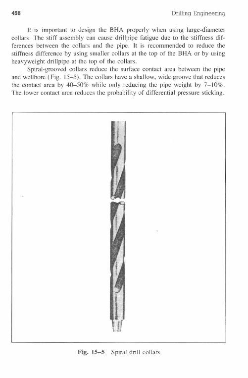
498 Drilling Engineering
It is important to design the BHA properly when using large-d'iametercollars. The stiff assembly can cause drillpipe fatigue due to the stiffness dif-ferences between the collars and the pipe. It is recommended to reduce thestiffness difference by using smaller collars at the top of the BHA or by usingheavyweight drillpipe at the top of the collars.
Spiral-grooved collars reduce the surface contact area between the pipeand wellbore (Fig. 15-5). The collars have a shallow, wide groove that reducesthe contact area by 40-50% while only reducing the pipe weight by 7-10%.The lower contact area reduces the probability of differential pressure sticking.
Fig. 15-5 Spiral drill collars
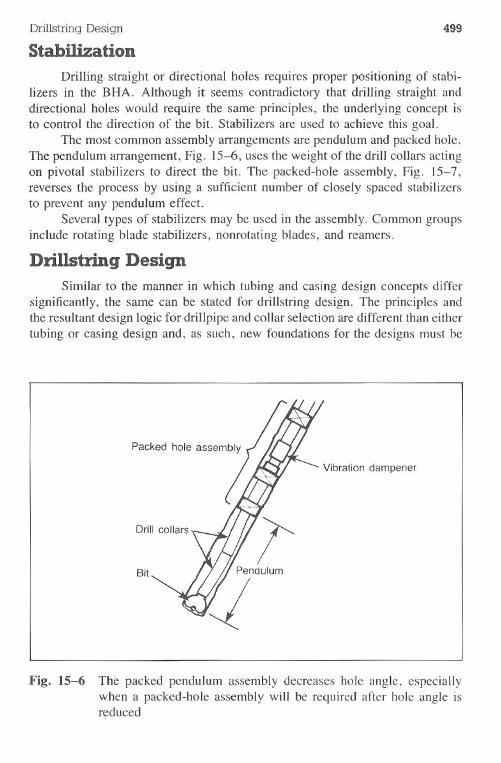
Drillstring Design 499
StabilizationDrilling straight or directional holes requires proper po~tioning of stabi-
lizers in the BHA. Although it seems contradictory that driIling straight anddirectional holes would require the same principles, the underlying concept isto control the direction of the bit. Stabilizers are used to achieve this goal.
The most common assembly arrangements are pendulum and packed hole.The pendulum arrangement, Fig. 15-6, uses the weight of the driIl collars actingon pivotal stabilizers to direct the bit. The packed-hole assembly, Fig. 15-7,reverses the process by using a sufficient number of closely spaced stabilizersto prevent any pendulum effect.
Several types of stabilizers may be used in the assembly. Common groupsinclude rotating blade stabilizers, nonrotating blades, and reamers.
Drillstring DesignSimilar to the manner in which tubing and casing design concepts differ
significantly, the same can be stated for driIlstring design. The principles andthe resultant design logic for driIlpipe and collar selection are different than eithertubing or casing design and, as such, new foundations for the designs must be
Packed hole assembly
Vibration dampener
Bit
Fig. 15-6 The packed pendulum assembly decreases hole angle, especiallywhen a packed-hole assembly will be required after hole angle isreduced
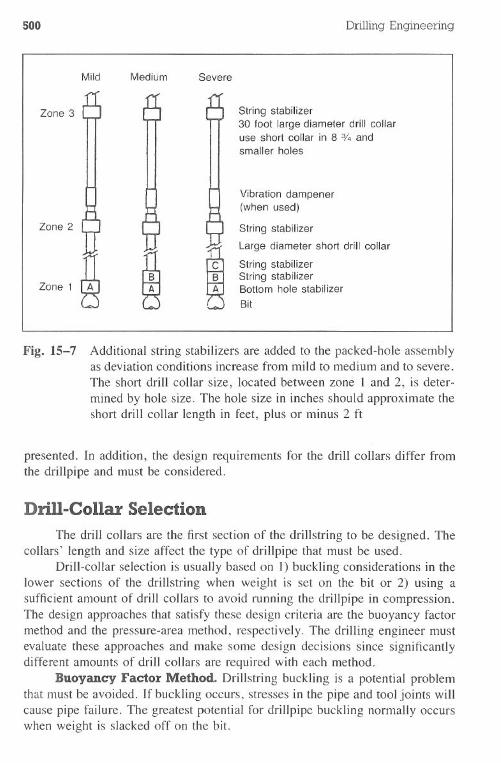
500 DrillingEngineering
Mild Medium Severe
Zone 3 String stabilizer30 foot large diameter drill collaruse short collar in 8 % andsmaller holes
Zone 2
Vibration dampener(when used)
String stabilizer
Large diameter short drill collar
String stabilizerString stabilizerBottom hole stabilizerBit
Zone 1
Fig. 15-7 Additional string stabilizers are added to the packed-hole assemblyas deviation conditions increase from mild to medium and to severe.The short drill collar size, located between zone I and 2, is deter-mined by hole size. The hole size in inches should approximate theshort drill collar length in feet, plus or minus 2 ft
presented. In addition, the design requirements for the drill collars differ fromthe drillpipe and must be considered.
Drill-Collar Selection
The drill collars are the first section of the drillstring to be designed. Thecollars' length and size affect the type of drillpipe that must be used.
Drill-collar selection is usually based on I) buckling considerations in thelower sections of the drillstring when weight is set on the bit or 2) using asufficient amount of drill collars to avoid running the drillpipe in compression.The design approaches that satisfy these design criteria are the buoyancy factormethod and the pressure-area method, respectively. The drilling engineer mustevaluate these approaches and make some design decisions since significantlydifferent amounts of drill collars are required with each method.
Buovancy Factor Method. Drillstring buckling is a potential problemthat must be avoided. If buckling occurs, stresses in the pipe and tool joints willcause pipe failure. The greatest potential for drillpipe buckling normally occurswhen weight is slacked off on the bit.
Drillstring Design 501
Lubinski et al. have studied buckling in oil-field tubing, casing, and drill-strings. They proved that buckling will not occur if bit weights in excess of thebuoyed collar weight are not used. Most current industry practices adhere to thisbuoyed-weight concept.
The buoyed weight of the drill collars is the amount of weight that mustbe supported by the derrick when collars are run in the hole. This load is alwaysless than the in-air weight if mud is used in the well. For example, collars thatweigh 147 Ib/ft while sitting on the pipe racks may have a buoyed weight of113 Ib/ft in 15.0-lb/gal mud.
Several methods are commonly used to determine the buoyed weight ofthe drill collars:
. lower the drill collars (bottom-hole assembly) into the hole and read theweight indicator (less the hook weight). calculate the weight of the displaced mud and subtract from the in-aircollar weight.multiply the in-air weight with a buoyancy factor that is dependent onmud weight
. The widelyused buoyancyfactor is calculatedfromEq. 15.1:
BF = 1 _ MW65.5 (15.1)
Where:BF = buoyancy factor, dimensionlessMW = mud weight, Ib/gal65.5 = weight of a gallon of steel, Ib/gal
The available bit weight (ABW) with the buoyancy factor method is thebuoyed weight of the drill collars (bottom-hole assembly) in the mud to be used.It is calculated as follows:
ABW = (in-air collar weight) X (buoyancy factor) (15.2)
The required collar length to achieve an arbitrary ABW can be calculated asfollows:
ABW(BF) (CW) = length
(15.3)
Where:ABW = desired available bit weight, IbBF = buoyancy factor, dimensionlessCW = collar weight (in-air), Ib/ftlength = required collar length, ft, to achieve the desired ABW
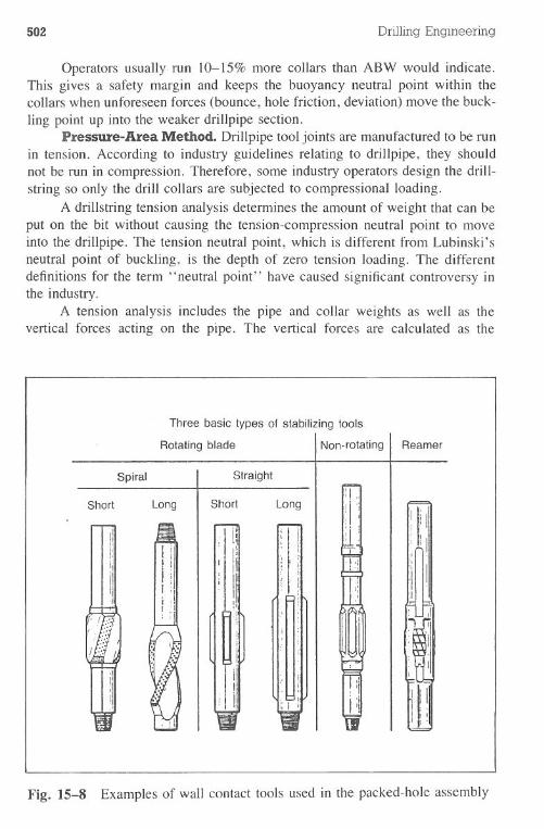
502 Drilling Engineering
Operators usually. run 10-15% more collars than ABW would indicate.This gives a safety margin and keeps the buoyancy neutral point within thecollars when unforeseen forces (bounce, hole friction, deviation) move the buck-ling point up into the weaker drillpipe section.
Pressure-Area Method. Drillpipe tool joints are manufactured to be runin tension. According to industry guidelines relating to drillpipe, they shouldnot be run in compression. Therefore, some industry operators design the drill-string so only the drill collars are subjected to compressional loading.
A drillstring tension analysis determines the amount of weight that can beput on the bit without causing the tension-compression neutral point to moveinto the drillpipe. The tension neutral point, which is different from Lubinski'sneutral point of buckling, is the depth of zero tension loading. The differentdefinitions for the term "neutral point" have caused significant controversy inthe industry.
A tension analysis includes the pipe and collar weights as well as thevertical forces acting on the pipe. The vertical forces are calculated as the
Three basic types of stabilizing tools
Rotating blade INon-rotating I Reamer
Fig. 15-8 Examples of wall contact tools used in the packed-hole assembly
Spiral Straight
Short Long Short Long I Ii I . I
[i'., I,.,:
Ii
Jf'I
I J I I!Ii
: !I
.,f :,I:!I"
11
i
I I
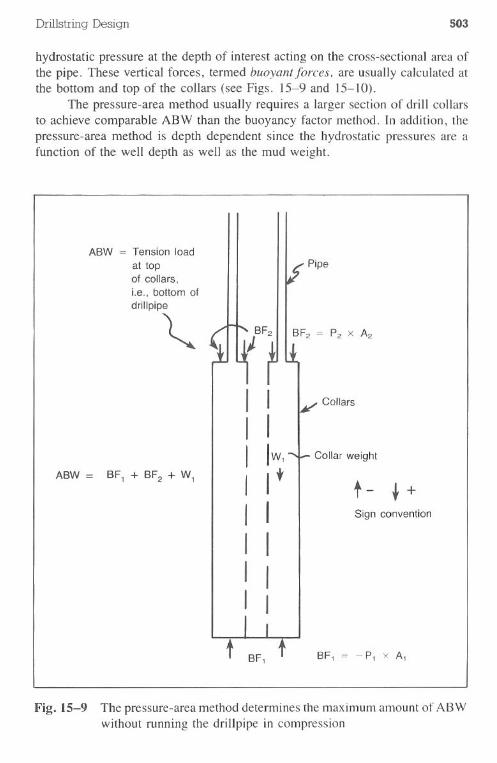
Drillstring Design 503
hydrostatic pressure at the depth of interest acting on the cross-sectional area ofthe pipe. These vertical forces, termed buoyant forces, are usually calculated atthe bottom and top of the collars (see Figs. 15-9 and 15-10).
The pressure-area method usually requires a larger section of drill collarsto achieve comparable ABW than the buoyancy factor method. In addition, thepressure-area method is depth dependent since the hydrostatic pressures are afunction of the well depth as well as the mud weight.
ABW = Tension load
at topof collars,Le., bottom ofdrillpipe
~
ABW = SFI + BF2 + WI
I II I
I IW1
I ItI II I
I I
I I
t
Collars
Collar weight
t- ~ +Sign convention
Fig. 15-9 The pressure-area method determines the maximum amount of ABWwithout running the drillpipe in compression
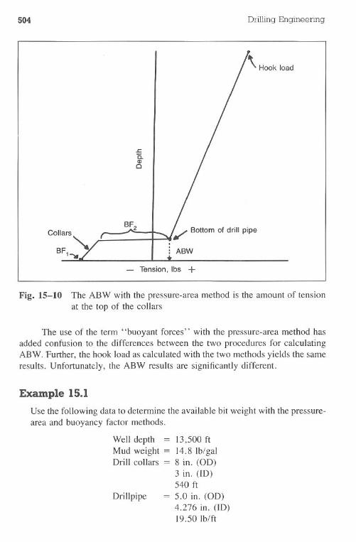
504 Drilling Engineering
.ca.Q)
CI
.: ABW
Tension, Ibs +
Fig. 15-10 The ABW with the pressure-area method is the amount of tensionat the top of the collars
The use of the term "buoyant forces" with the pressure-area method hasadded confusion to the differences between the two procedures for calculatingABW. Further, the hook load as calculated with the two methods yields the sameresults. Unfortunately, the ABW results are significantly different.
Example 15.1
Use the following data to determine the available bit weight with the pressure-area and buoyancy factor methods.
Well depth = 13,500ftMud weight = 14.81b/galDrill collars = 8 in. (00)
3 in. (ID)540 ft
Drillpipe = 5.0 in. (00)4.276 in. (ID)19.501b/ft
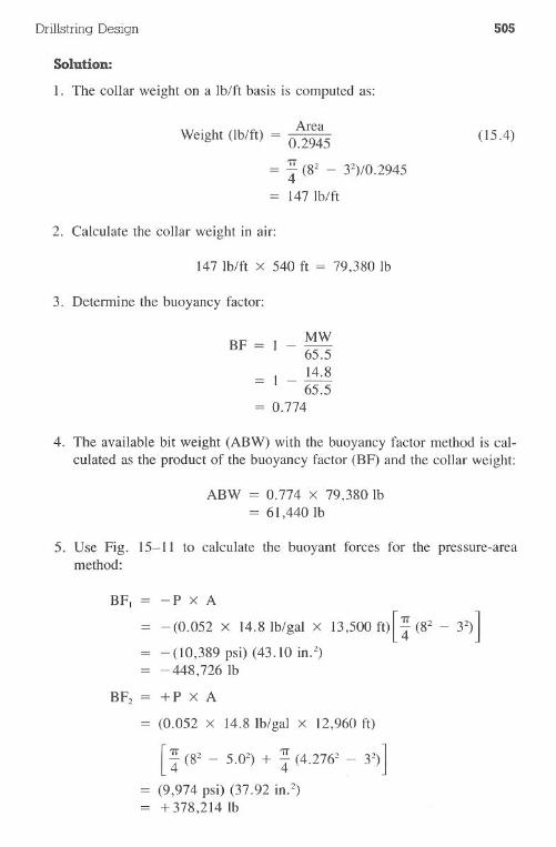
Drillstring Design 505
Solution:
1. The collar weight on a lb/ft basis is computed as:
. AreaWeight (lb/ft) = 0.2945 (15.4)
= ~ (82 - 32)/0.2945
147 lb/ft
2. Calculate the collar weight in air:
147 Ib/ft x 540 ft = 79,380 lb
3. Determine the buoyancy factor:
BF = 1 _ MW65.5
_ 14.865.5
= 0.774
4. The available bit weight (ABW) with the buoyancy factor method is cal-culated as the product of the buoyancy factor (BF) and the collar weight:
ABW = 0.774 x 79,3801b= 61,440 lb
5. Use Fig. 15-11 to calculate the buoyant forces for the pressure-areamethod:
BFt = - P x A
-(0.052 x 14.81b/gal x 13,500ft)[~ W - 32)]-(10,389 psi) (43.10 in.2)-448,726Ib
BF2 = + P x A
= (0.052 x 14.8 lb/gal x 12,960ft)
[~ W - 5.02) + ~ (4.2762 - 32)]
= (9,974 psi) (37.92 in.2)= + 378,214 lb
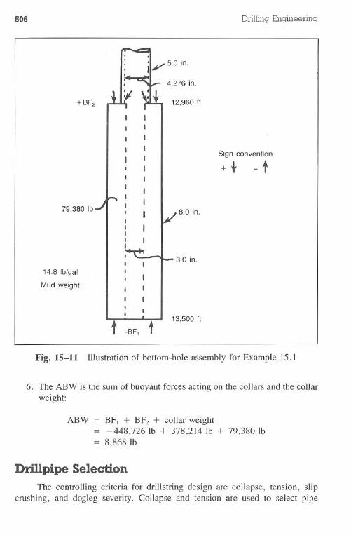
506 Drilling Engineering
!I¥ 5.0 in.4.276 in.
12,960 It
Sign convention
+, - t
79,380 Ib
~8.0in.
3.0 in.
14.8 Ib/gal
Mud weight
-SF, t13,500 It
Fig. 15-11 Illustration of bottom-hole assembly for Example 15.1
6. The ABW is the sum of buoyant forces acting on the collars and the collarweight:
ABW = BF. + BF2 + collar weight-448,726Ib + 378,214 Ib + 79,3801b
= 8,868 Ib
DriDpipe SelectionThe controlling criteria for drillstring design are collapse, tension, slip
crushing, and dogleg severity. Collapse and tension are used to select pipe
Drillstring Design 507
weights, grades, and couplings. Slip crushing affects the tension design and pipeselection. A dogleg analysis is performed to study the fatigue damage resultingfrom rotating in the dogleg angle change. Typically, higher-strength pipe isrequired in the lower sections of the string for collapse resistance, while tensiondictates the higher-strength pipe at the top of the well.
Collapse. Drillpipe is used for several purposes, including providing afluid conduit for pumping drilling mud, imparting rotary motion to the drill bit,and conducting special operations such as drillstem testing and squeeze ce-menting. Drillstem testing (DST) causes the most severe collapse loading on thedrillpipe. Since the DST is a commonly used operation, it will be used to controlthe collapse design.
. Drillstem testing is a standard operation to evaluate the productivity andproduced fluids of a formation interval. The fluids are allowed to flow up thedrillstring to the surface. Various productivity tests are performed. on the for-mation and the fluids during and after the DST.
The procedures to perform the DST cause severe collapse loading on thedrillpipe. A packer is run at the bottom of the drillstring to isolate the formationfrom the drillpipe annulus. A control valve is closed so that drilling mud doesnot enter the drillpipe while running into the hole. After the packer is set, thevalve is opened and formation fluids enter the pipe. After the test is completed,the control valve is closed and a circulating port is opened so annular mud canbe used to reverse out the fluid in the drillpipe.
The most severe collapse loading occurs when the evacuated (or partiallyempty) drillstring reaches the bottom of the well. The load from the annular mudtends to cause pipe collapse (Fig. 15-12). The fluid resisting collapse, the backupfluid, is essentially the weight of air and is considered negligible. The resultantloading on the pipe, which is the difference between the load line and the backupfluid, is the load line when no backup fluid is present.
Although the design approach is based on drillstem testing, it accounts forother common drilling conditions. Failure to fill the drillpipe when running intothe well with a float valve in the drillstring will give the loading seen in Fig.15-12. In addition, completely plugged jets will prevent mud from entering thedrillpipe when tripping into the hole. It is not uncommon for pipe to collapseas a result of these conditions.
A design factor is usually added to the load line to obtain a design linefrom which to select pipe weights and grades. Casing and tubing design problemsusually use small design factors of 1.0-1.15 for collapse since the pipe is newand generally inspected at the mill or on site. Drillpipe is usually designed witha factor of 1.3, however, since new pipe is seldom used in the DST. As a result,quality control and testing procedures are not as assured as in the case of tubingand casing. The design line, which is the load line with an applied design factor,can be seen in Fig. 15-13.
Fig. 15-12
.s:::;c.OJo
!
Collapse load supplied
f by annular mud
Pressure ~
Drillstring collapse loads resulting from drill stem testing or pluggedjets
.s:::;c.OJo
./ Pipe upgrades at
/ lower section\
Pressure --+.
Fig. 15-13 Drillstring collapse design line
Drillstring Design 509
At this point, the collapse design line is established. The collapse pressuresare known at every point in the well. The next step is to select pipe that willsatisfy the pressure requirements. The operator usually restricts the availablechoices of pipe by I) using Class 1 or premium pipe only, 2) restricting the pipeweight, 3) establishing minimum acceptable section lengths of common pipetypes, and 4) using minimum grades. For example, an operator may state thatthe minimum acceptable requirements are 4.5-in., 16.6-lb/ft, Grade-E, premium-class pipe. In addition, the operator will typically specify that pipe grades ratherthan weights be increased to control pressures. In other words, upgrading fromE to X grade pipe is better than increasing the pipe weight to 20 Ib/ft. A typicalpipe selection is shown in Fig. 15-13.
A drillpipe catalog is included in the Appendix. Grade E, Class I pipe isshown as E75-1. Pipe is selected from the catalog to satisfy the collapse loadrequirements.
Tension. The tension load can be evaluated after the weights, grades, andsection lengths have been established from the collapse designs. Buoyancy isincluded in the tension evaluation due to the manner in which biaxial stressesalter the collapse properties of the pipe. Since the string is designed with amaximum load concept, it is important that buoyancy be included in the design.A typical tension load line is shown in Fig. 15-14.
The tension design line is established as the maximum load resulting fromapplying three different design considerations, including overpull, design factors,and slip crushing. Each consideration is applied separately to the load line. Thedesign line is selected as the worst case from the three design loads (Fig.IS-IS).
Overpull. A minimum overpull factor is applied to the tension load. Thefactor was originated to ensure the driller could safely pull a certain load on thepipe in the event of sticking. A typical range for the overpull value is 50,000-100,000 lb.
Design Factor. A range of tension design factors has been frequentlyused for drillpipe design. This range is typically from 1.1-1.5, although 1.1-1.3 seems to be most common. The primary purpose of the design factor is toensure an overdesign of the pipe to minimize the catastrophic problem of pipeparting near the surface when the pipe is fully loaded. In addition, it is selectedto account for acceleration loading of the pipe, which occurs when the slips areset.
Slip Crw;hing. The maximum allowable tension load must also be de-signed to prevent slip crushing. In an analysis of the slip crushing problem,Reinhold and Spini, and also Vreeland, proposed an equation to calculate therelation between the hoop stress (SH)caused by the action of the slips and thetensile stress in pipe (ST)' resulting from the load of the pipe hanging in theslips. If the dimensions for the cross-sectional area of the pipe (A) and the
~a.Q)o
Compression ( -) Tensile load Tension (+)
Fig. 15-14 Typical tension load line
~a.Q)
o
Fig. 15-15 Tension load line with three design factor considerations
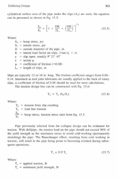
Drillstring Design 511
cylindrical surface area of the pipe under the slips (As) are used, the equationcan be presented as shown in Eq. 15.5:
SH [DK-= 1+-+
ST 2Ls(15.5)
Where:
SH = hoop stress, psiST = tensile stress, psiD = outside diameter of the pipe, in.K = lateral load factor on slips, l/tan (y + z)Y = slip taper, usually 90 27' 45"z = arctan ,...,... = coefficient of friction (=0.08)Ls = length of slips, in.
Slips are typically 12 or 16 in. long. The friction coefficient ranges from 0.06-0.14. Inasmuch as tool joint lubricants are usually applied to the back of rotaryslips, a coefficient of friction of 0.08 should be used for most calculations.
The tension design line can be constructed with Eq. 15.6:
(15.6)
Where:
TsTL
~=ST
tension from slip crushingload line tension
hoop stress, tension stress ratio from Eq. 15.5
Pipe previously selected from the collapse design can be evaluated fortension. With drillpipe, the tension load on the pipe should not exceed 90% ofthe yield strength as the maximum stress to avoid cold-working (permanentlystretching) the pipe. The Bauschanger effect, resulting from cold working intension, will result in the pipe being prone to becoming crooked during subse-quent operations.
(15.7)
Where:T. = applied tension, IbTy = minimum yield strength, Ib
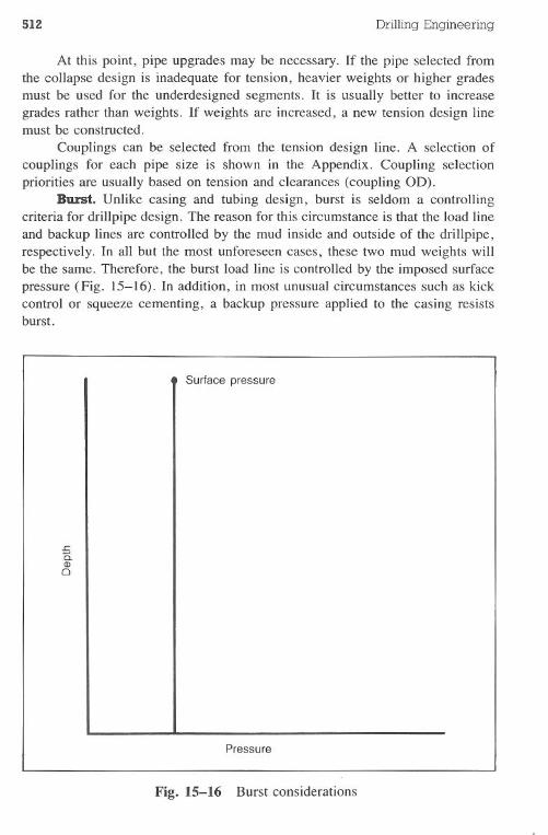
512 Drilling Engineering
At this point, pipe upgrades may be necessary. If the pipe selected fromthe collapse design is ina4equate for tension, heavier weights or higher gradesmust be used for the underdesigned segments. It is usually better to increasegrades rather than weights. If weights are increased, a new tension design linemust be constructed.
Couplings can be selected from the tension design line. A selection ofcouplings for each pipe size is shown in the Appendix. Coupling selectionpriorities are usually based on tension and clearances (coupling 00).
Burst. Unlike casing and tubing design, burst is seldom a controllingcriteria for drill pipe design. The reason for this circumstance is that the load line
and backup lines are controlled by the mud inside and outside of the drillpipe,respectively. In all but the most unforeseen cases, these two mud weights willbe the same. Therefore, the burst load line is controlled by the imposed surfacepressure (Fig. 15-16). In addition, in most unusual circumstances such as kick
control or squeeze cementing, a backup pressure applied to the casing resistsburst.
Surface pressure
.ca.OJo
Pressure
Fig. 15-16 Burst considerations
Drillstring Design
Example 15.2
513
Determine the grade of drillpipe required for the following conditions. UseClass I pipe and design for collapse, burst, tension, and slip crushing. Donot consider any other design considerations such as doglegs or corrosivemuds. The maximum anticipated surface pressure on the drillpipe is 5,000psi. Use a single weight and grade of pipe. Determine the actual tensiondesign factor at the top of the drillstring. Due to small hole diameters, usecouplings with the smallest clearance that still exceeds the tension require-ments.
DepthCollar lengthDrillpipeDrill collars
Design factors:tension
collapseburstoverpull
Mud weightProduction test zoneLength of drillpipe slips
Solution:
= 10,600ft= 600 ft= 4.5 in. (3.826-in.ID)
7.0 in. (OD)3.0 in. (ID)107Ib/ft (air)
1.31.31.3100,000 Ib12.0 Ib/gal10,000 ft16 in.
1. Construct the collapse load line. The maximum collapse load is at thebottom of the drillpipe:
0.52 x 12.01b/gal x 10,000 ft = 6,240 psi
2. The design line is the product of the load line and the design factor, 1.3(see Fig. 15-17):
6,240 psi x 1.3 = 8,1I2 psi
3. Pipe is selected from the catalog in the Appendix. The 13.75-1b/ftGradeE pipe is not satisfactory because Class I pipe has a collapse rating (7,200psi) below the minimum design value of 8,112 psi. The 16.60-lb/ft pipeis acceptable as shown in Fig. ) 5-17 .
4. The burst load and design lines are plotted in Fig. 15-18. The previoustentative selection of 16.60-1b/ftGrade E pipe is satisfactory for the burstconditions.
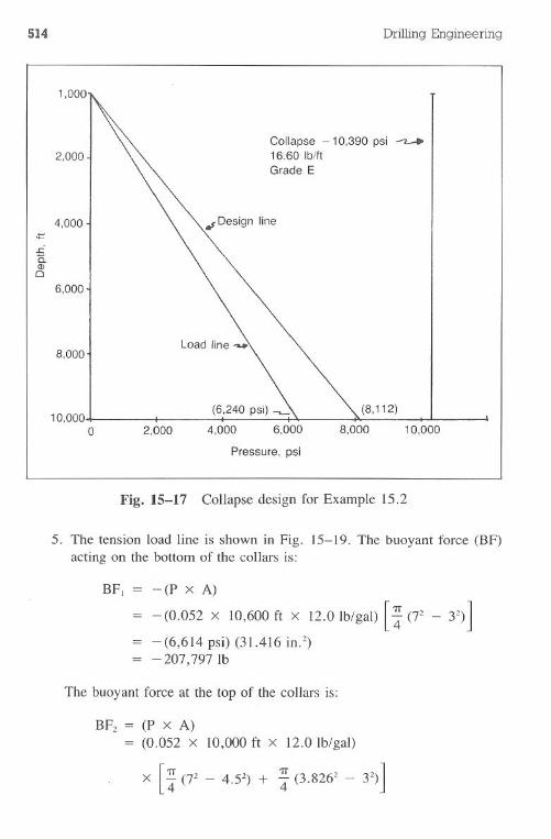
514 Drilling Engineering
1,000
8,000
Collapse - 10,390 psi ~16.60 Ib/ttGrade E
2,000
4,000
£i5.Q)
o6,000
10,000o 2,000
(6,240 psi) .........I I'
4,000 6,000
(8,112)p
8,000 10,000
Pressure, psi
Fig. 15-17 Collapse design for Example 15.2
5. The tension load line is shown in Fig. 15-19. The buoyant force (BF)acting on the bottom of the collars is:
BF, = -(P x A)
- (0.052 x 10,600ft x 12.0 lb/gal) [~(72 - 32)]-(6,614 psi) (31.416in.2)-207,797Ib
The buoyant force at the top of the collars is:
BF2 = (P x A)(0.052 x 10,000 ft x 12.0Ib/gal)
x [~(72 - 4.52) + ~ (3.8262- 32)]
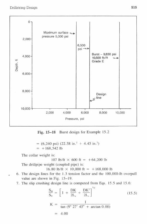
Drillstring Design 515
o
2,000
Maximum surface .......pressure 5,000 psi
6,500psi ......
Burst - 9,830 psi16,600fb/tt ~Grade E
8,000Design
.sline
10,0002,000 4,000 6,000 8,000 10,000
Pressure, psi
Fig. 15-18 Burst design for Example 15.2
= (6,240 psi) (22.58 in.2 + 4.45 in.2)= + 168,542 Ib
The collar weight is:107 Ib/ft x 600 ft = + 64,200 lb
The drillpipe weight (coupled pipe) is:16.80 Ib/ft x 10,000ft = + 168,000lb
6. The design lines for the 1.3 tension factor and the 100,000-lb overpullvalue are shown in Fig. 15-19.
7. The slip crushing design line is computed from Eqs. 15.5 and 15.6:1/2
SH [DK DK2
]ST= 1+2L,+2L, (15.5)
K= Itan (9° 27' 45" + arctan 0.08)
4.00
4,000==s=a.Q)Q
6,000
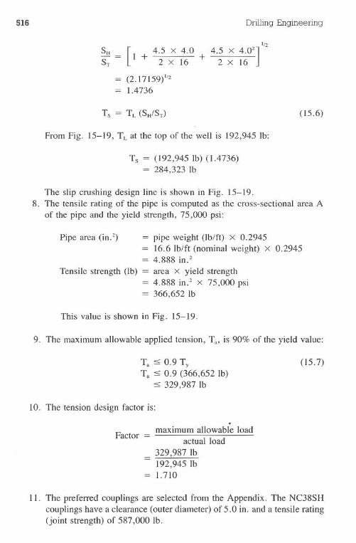
516 Drilling Engineering
[14.5 x 4.0
+ 2 x 16
(2.17159)1/21.4736
1/24.5 X 4.02
]+ 2 x 16
(15.6)
From Fig. 15-19, TL at the top of the well is 192,945 lb:
Ts = (192,945 lb) (1.4736)= 284,323 lb
The slip crushing design line is shown in Fig. 15-19.8. The tensile rating of the pipe is computed as the cross-sectional area A
of the pipe and the yield strength, 75,000 psi:
Pipe area (in.2) = pipe weight (lb/ft) x 0.2945= 16.6 lb/ft (nominal weight) x 0.2945= 4.888 in.2
Tensile strength (lb) = area x yield strength= 4.888 in.2 x 75,000 psi= 366,652 lb
This value is shown in Fig. 15-19.
9. The maximum allowable applied tension, T.. is 90% of the yield value:
T. ::5 0.9 TyT. ::5 0.9 (366,652 lb)
::5 329,987 lb
(15.7)
10. The tension design factor is:
Factor =.
maximum allowable loadactual load
329,987 lb192,945 lb
= 1.710
11. The preferred couplings are selected from the Appendix. The NC38SHcouplings have a clearance (outer diameter) of 5.0 in. and a tensile rating(joint strength) of 587,000 lb.
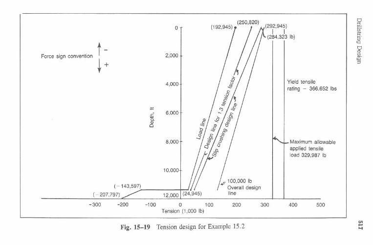
.(250,820)
t:JO
T(192,945),
I;.,(29F'941)
a[jj'R
"(284,323
Ib)E
r
Forcesign
conventiont-2,000j
IIII
<0t:J<D
[J)15.
+::3
4,0001/
.i!/
II
Yield
tensilerating
-366,652
Ibs
I/Ill/
II
-=6,000
a.Q)
0
8,000tf/
hiM
aximum
allowable
8t:::
.S-.J
."ti
11i
appliedtensile
load329,987
Ib
IIlr
II
I10,000
(-143,597)
(-207,797)
-300-200
-1000
100200
300400
500
I
enF
ig.15-19
Tension
designfor
Exam
ple15.2
...
518 Drilling Engineering
Dogleg Severity AnalysisThe most common type of drillpipe failure is fatigue wear. It generally
occurs in doglegs where the pipe goes through cyclic bending stresses. Thesestresses occur because the outer wall of the pipe in a dogleg is stretched andcreates a greater tension load (see Fig. 15-20). As the pipe rotates a half cycle,the stresses change to the other side of the pipe. For example, the stress maychange from 50,000 psi to - 20,000 psi and again to 50,000 psi in the courseof one cycle or rotation of the pipe.
Fatigue damage from rotation in doglegs is a significant problem if theangle is greater than some critical value. Lubinski has published several worksthat describe this value. Rotation in angles below this value does not causeappreciable fatigue.
The maximum permissible dogleg severity for fatigue damage considera-tions can be calculated with the following equations:
432,000c =1T
~ED
tan h KLKL (15.8)
And:
K=v1; (15.9)
Where:
c = maximum permissible dogleg severity, 01100ftE = Young's modulus, psi
= 30 x 106psi for steel= 10.5 X 10⁶psi for aluminum
D = drill pipe outer diameter, in.L = half the distance between tool joints, 180 in. for Range 2 pipe, in.T = tension load below the dogleg, IbO"b= maximum permissible bending stress, psi
I = drillpipe moment of inertia, ~(D4 - d4)
The maximum permissible bending stress (<Tb)is calculated from the buoyedtensile stress (<T,)and is grade dependent. The equation for bending stress withGrades E and S pipe are given in Eqs. 15.10 and 15.II and are valid for <T,upto 67,000 psi and 133,400 psi, respectively:
(15.10)
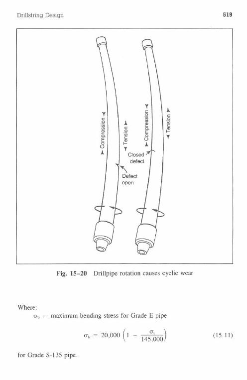
Drillstring Design
Fig. 15-20 Drillpipe rotation causes cyclic wear
Where:
O"b= maximumbendingstress for GradeE pipe
for Grade S-135 pipe.
O"b = 20,000 (1 - 145~OOO)
519
(15.11)
T
\
Tc:0
c: Ow0 J.
enQ)Ow D-en c:
(I) 0 ED- Ow 0 TE c: ()0 J.() TA Closed
defect,Defectopen
520
Example 15.3
A Grade E drillstring has a tension load of 190,000 Ib at 4,500 ft. Detenninethe maximum pennissible dogleg that will not cause fatigue damage. The 4.5-in. drillpipe weighs 16.60 Ib/ft (3.826-in. ill)
Solution:
Drilling Engineering
I. Detennine the tension stress load. The pipe area is:Area = pipe weight (lb/ft) x 0.2945
= 16.60 Ib/ft x 0.2945= 4.88 in.2
11 .( )
190,000 IbenSlOn stress CJ'T = 4 88 ' 2. m.
= 38,934psi
2. The maximum pennissible bending stress (CJ'b)is computed from Eq. 15.10:
10 0.60 2
CJ'b = 19,500 - 67 CJ'T- (670)2(CJ'T- 33,5 0)
19,500 - ~~ (38,934) - (~7~)2(38,934 - 33,500)2= 19,500 - 5,811 - 39
13,650
(15.10)
3. 190,00010
106) [~ (4.54 - 3.8264)]
(15.9)K= ~(30 x
= 0.02567
4. The maximum dogleg is computed from Eq. 15.8:
c = 432,0001T
~ED
tan h KLKL (15.8)
_ 432,000 13,650 psi tan h (0.02567) (180)- 1T (30 X 106) (4.5) (0.02567) (180)
(137,509) (1.011 x 10⁻⁴) tan h 4.624.62
= 3.00 tan h 4.62= 1.695°/100 ft
Severe pipe damage occurs when the dogleg severity is greater than thevalue computed in Eq. 15.8. The damage depends on type of metal (aluminum
Drillstring Design 521
or steel), corrosion level, stress, and dogleg angle. Metallurgists have establishedS-N (stress vs bending cycle) diagrams that can be used to determine the ap-proximate number of cycles, or rotations, before pipe failure occurs.
The fraction (f) of drillpipe life expended in an interval of a dogleg canbe calculated as follows:
Bf = N (15.12)
Where:fBN
fraction expendednumber of drillpipe revolutions to drill the intervalnumber of revolutions to failure of the joint of drillpipe
It is simple to show that:
B60 Rd
V (15.13)
Where:R = rotary speed, rpmd = length of dogleg interval, ftV = drilling rate, ft/hr
The denominator, N, of Eq. 15.12 depends on the bending stress (<1b)inthe pipe and on the ratio T/A, denoted <1,:
TA
(15.14)
Where:
A = cross-sectional area of the pipe, in.2
The value <1bcan be computed as follows:
(15.15)
Where:DEc =o
outside diameter of the pipe, in.Young's modulus, Ib/in.2maximum pipe curvature, radians/in.
522 Drilling Engineering
The relationship between the hole curvature (c) and the maximum pipecurvature (co) is:
Co= c (KL) (15.16)
Where:c = hole curvature, radians/in.L = one-half the length of a drillpipe joint, in.
The effect of bending stress on fatigue cycles before failure is welldocumented, as can be seen in Figs. 15-21 and 15-22. In the presence oftension, however, the fatigue effect of bending becomes more severe. To makethe proper allowances for this, the actual bending stress, (Tb,must be multipliedby a correction factor, 'T,as follows:
T(15.17)
'T = T - (T,
Where:
T = tensile strength of the pipe
The vertical axis of the graphs in Figs. 15-21 and 15-22 should be enteredwith the product of'T and (Tb' or 'T(Tb'Determine the number of cycles, N, tofailure. Enter N into Eq. 15.12 to determine the fraction of the pipe life expendedin drilling the section.
Lateral Tool Joint LoadingIn Lubinski's works, fieldstudies were shown to indicate that lateral loading
of tool joints can create significant damage. It was suggested that an arbitrarylimit of 2,000 Ib be used as the maximum, nondamaging lateral load limit. Loadsabove this limit would damage the tool joints. The following equation canbe used to determine maximum acceptable dogleg severity for various lateralloads:
c 108,000 F'11'LT (15.18)
Where:FL
lateral force on the tool joint, lbone-half the length of a drill pipe joint, in.
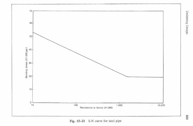
Drillstring
Design
o<0
o0
0'<
t'"
N
(!sd
000'~X
)SS9JIS
f)U!PU
9S
oooc5~
523
oo
o~
0
IQ
)0q
c..'s..
5'"0
0B
0'".....8
Q)
Q)
.2>
:§....=
:Ig
u'"
Zc:
I.2:;(5>Q
)N
II:I
\I)00
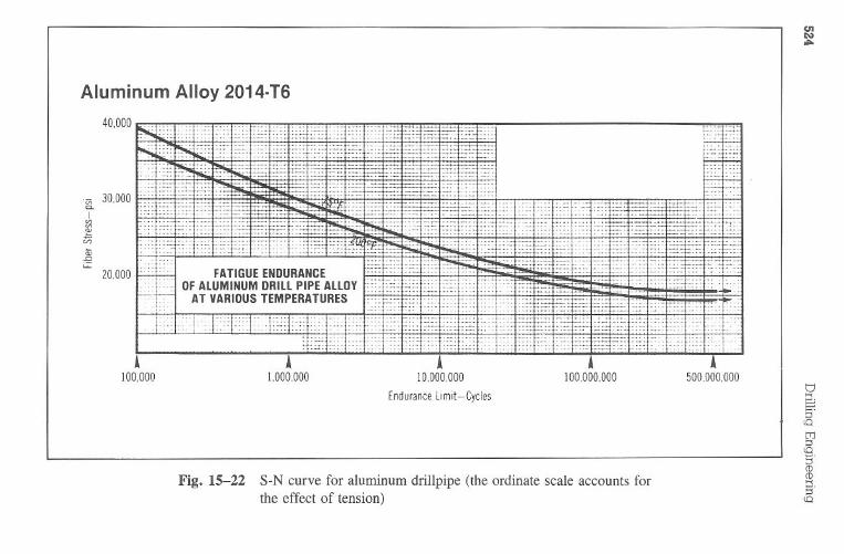
Alum
inumA
lloy2014.16
40,000
100,0001.000,000
10,000,000
EnduranceLim
it-Cycles
100,000,000500,000,000
Fig.15-22
S-Ncurve
foralum
inumdrillpipe
(theordinate
scaleaccounts
forthe
effectof
tension)
enN~tJS;g'rr:J::!
(QS'CDCD....
S'
(Q
'v;30.000
0-J,'"v;u:
20,000
-_..[:':.
.-...
........
...._.-..
.....
.....
......-
..-.-
r.;::.: ..--
---:::'!'
::::;=
:::i:i;:
?::7:
:...i
::i.....
.:.:::-:
0;,;.;:..
'"
::o;.
-=-J:;:
.:ft::::--.
':;:..:.-.
..:":":;"
;=l'
.+...._.....
gc:,.:.:
::::'...
.......
.
.:;t:o:_
::__
':._
.:.:::::
.7.:;0::.;=
:;;..
;::::.:::,.c.::.::::.
=_.
;+r::
t:::-'..-f'-:'-'tt;:;::.=
-..
.=
=.:::
...'.-
-.--
.....-.-
..........
-.--:.:..-:1::::.:
:-:t,=..;.;.::
::;;>
::r.-:::-::::
:;:i":;;;:
:;:::::E
::'-"-.:
::?:T
.,..::
:::7::=
:_..:::
.::.:::C':.:.:
.:.::C
::'!1'0;;,;::C.
;:::i;
;::;
:§::sL
:.F::';
....h.....
'"....f-::.
..::::
.....-
-.....
'".....
.........-.
::=;;:
i:::=t r:::::
:r;
FAT
IGU
EE
ND
UR
AN
CE
.....
_..-.
.
OF
AL
UM
INU
MD
RIL
LP
IPE
AL
LO
Y:.:
::;:::;=
:.::.:.
=c-:-
AT
VA
RIO
US
TE
MP
ER
AT
UR
ES
..c::
I:::':::-: =
t=
=t::::
;.::=;:::
e-::::J:-,::.-..
.......
.......
.--:.::
..........
....
Y'
....-"'J'
...........
==
:.-=;::
"...
.:::::
I:c::::::
c.::::::
:::::..:.
::";-;-::
...r=
-;::....
.--.....
...--.-.
--...
....-'-
..-..--.
::I:::::
c':;-.
.....
....'"
.....
.:o.
Ef:
rE:7
."----
.......
......-
.._-.'"
......-.
...
iA
iA
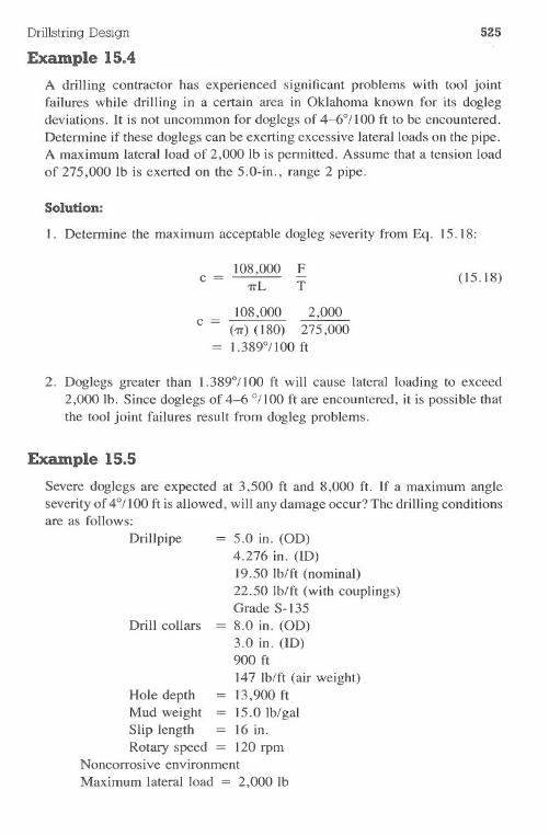
Drillstring Design
Example 15.4
525
A drilling contractor has experienced significant problems with tool jointfailures while drilling in a certain area in Oklahoma known for its doglegdeviations. It is not uncommon for doglegs of 4-6°1100 ft to be encountered.Determine if these doglegs can be exerting excessive lateral loads on the pipe.A maximum lateral load of 2,000 Ib is permitted. Assume that a tension loadof 275,000 Ib is exerted on the 5.0-in., range 2 pipe.
Solution:
1. Determine the maximum acceptable dogleg severity from Eq. 15.18:
c 108,000 !:'iT"L T
(15.18)
c 108,000 2,000('iT")(180) 275,0001.389°1100 ft
2. Doglegs greater than 1.389°/100 ft will cause lateral loading to exceed2,000 lb. Since doglegs of 4-6 °/100 ft are encountered, it is possible thatthe tool joint failures result from dogleg problems.
Example 15.5
Severe doglegs are expected at 3,500 ft and 8,000 ft. If a maximum angleseverity of 4°/100 ft is allowed, will any damage occur? The drilling conditionsare as follows:
Drillpipe 5.0 in. (OD)4.276 in. (10)19.50 Ib/ft (nominal)22.50 Ib/ft (with couplings)Grade S-135
8.0 in. (OD)3.0 in. (10)900 ft
147 Ib/ft (air weight)Hole depth = 13,900ftMud weight = 15.0 Ib/galSlip length = 16 in.Rotary speed = 120 rpm
Noncorrosive environmentMaximum lateral load = 2,0001b
Drill collars
526 Drilling Engineering
Solution:
1. The tension load on the drillpipe is computed and shown in Fig. 15-23.2. The maximum permissible dogleg severity is computed with Eq. 15.18.
Doglegs greater than this critical value will cause fatigue damage. Thevalues of maximum permissible doglegs are calculated for the entire well,as shown in Fig. 15-24.
3. The 8,000-ft dogleg will not cause fatigue damage since the maximumpermissible dogleg is greater than the actual 4°1100 ft dogleg. The doglegat 3,500 ft will cause damage.
4. The amount of fatigue damage at 3,500 ft is calculated with Eqs. 15.12-15.17. At 3,500 ft, approximately 5% of the pipe's life is used. Fig. 15-25 shows the amount of fatigue damage throughout the drillstring.
5. The lateral load conditions are calculated and plotted for the drill string(Fig. 15-26). The dogleg at 8,000 ft exceeds the 2,000-lb lateral load
o (316,600)
2,000
Tension in the drillstring__at variousdepths
4,000
;:::
-5 6,000a.Q)o
8,000
10,000
12,000
13,000
14,000o 50,000 100,000 150,000 200,000 250,000 300,000
Tension, Ib
Fig. 15-23 Tension load in the drillstring
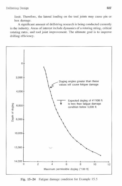
Drillstring Design 527
limit. Therefore, the lateral loading on the tool joints may cause pin or
box damage.A significant amount of drillstring research is being conducted currently
in the industry. Areas of interest include dynamics of a rotating string, criticalrotating rates, and tool joint improvement. The ultimate goal is to improvedrilling efficiency.
o
4,000
/'" Dogleg angles greater than thesek' values will cause fatigue damage
2,000
C>
~ 6,000o"C
o.c15.~ 8,000
Expected dogleg of 4°/100 Itis less than fatigue damagecondition below 5,000 ft
10,000
12,000
14,000o 2 4 6 8 10 12
Maximum permissible dogleg (°100 ft)
Fig. 15-24 Fatigue damage condition for Example 15.5
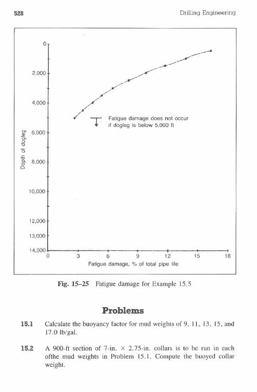
528 Drilling Engineering
o
2,000
-....~------.-"'-
//--_.Y"-"./-
////
/ 1- Fatigue damage does not occur+ if dogleg is below 5,000 It
4,000
12,000
13,000
14,000o
.3 6 9 12
Fatigue damage, % of total pipe life
.15
I
18
Fig. 15-25 Fatigue damage for Example 15.5
Problems
15.1 Calculate the buoyancy factor for mud weights of 9, 11, 13, 15, and17.0Ib/gal.
15.2 A 900-ft section of 7-in. x 2.75-in. collars is to be run in eachofthe mud weights in Problem 15.1. Compute the buoyed collarweight.
0> 6,000Q)0,0
u'0.ca. 8,000Q)a
10,000
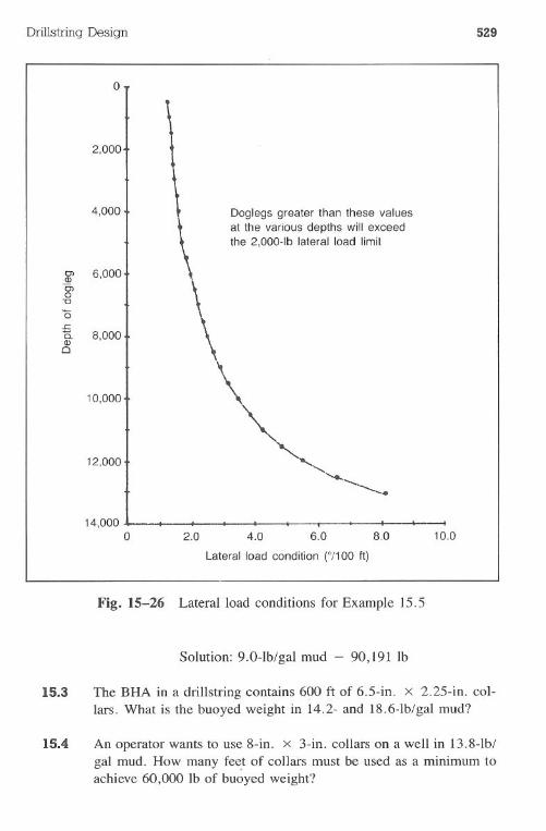
Drillstring Design
o
2,000
4,000
ar 6,000C>o"0
'0.s:::
g. 8,000o
10,000
12,000
14,000o
529
Doglegs greater than these valuesat the various depths will exceedthe 2,000-lb lateral load limit
2.0 6.0 10.04.0 8.0
Lateral load condition (°/100 It)
Fig. 15-26 Lateral load conditions for Example 15.5
Solution: 9.0-lb/gal mud - 90,191 Ib
15.3 The BHA in a drillstring contains 600 ft of 6.S-in. x 2.2S-in. col-lars. What is the buoyed weight in 14.2- and 18.6-lb/gal mud?
15.4 An operator wants to use 8-in. x 3-in. collars on a well in 13.8-lb/gal mud. How many fe~t of collars must be used as a minimum toachieve 60,000 Ib of buoyed weight?
530 DrillingEngineering
15.5 How many feet of 6-in. x 2-in. collars must be used in 11.4-lb/galmud to obtain 45,000 Ib of buoyed weight?
15.6 An operator wants to use three lO-in. x 3-in. collars (90 ft) be-low his 8-in. x 3.25-in. collars. How many 8-in. collars must herun to obtain 60,000 Ib of buoyed weight? Use the buoyancy factormethod.
15.7 A drillstring has the following characteristics.
Drill collars
Heavyweight pipeDrillpipeMud weight
= 600 ft, 7-in. x 3-in. (OD x ID)1,200 ft, 4.5-in. OD (Table 15-2)10,000 ft, 4.5-in. OD (16.6 Ib/ft)11.0 Ib/gal
Compute the following buoyed weights:a. drill collars
b. drill collars and heavy weightc. all components
15.8 The drillstring in Problem 15.7 will be run in 13.0-lb/gal mud.Determinethe available bit weight, assuming that only the drill collarscan be run in compression. Determine the ABW if the collars andheavyweight pipe can be run in compression. Use the pressure-areamethod.
15.9 Draw a tension graph for Problem 15.8. What is the hook load?Compare this answer to Problem 15.7(c) and explain the results.
15.10 Rework Problem 15.9 if the well is 16,000 ft instead of 11,800 ft.Compare the results to Problem 15.9 and explain any differences.
15.11 A set of 7-in. X 3-in. drill collars are 600 ft long. Assume they willbe run in 9.5-lb/gal mud at 3,000,6,000,9,000, 12,000, and 15,000ft. Compute th~ ABW with the pressure-area method. Plot the results.The drill string is 41/2-in., 16.6-lb/ft pipe.
Solution: 15,000 ft, 23,457 Ib
15.12 Determine the grade of drillpipe required for the following conditions.Use Class I pipe only. Do not consider burst conditions. Use a single
Drillstring Design 531
weight and grade of pipe. Determine the actual tension design factorat the top of the drillstring. Use the smallest couplings that still exceedthe tension requirements.
DepthCollar lengthDrillpipeDrill collars
= 13,000 ft= 600 ft= 4.5 in. (3.826-in. ID)
7.0 in. (OD)3.0 in. (ID)107 Ib.lft (air)
Design factors:tensioncollapseoverpull
Mud weightProduction test zoneLength of drillpipe slips
1.31.3
100,000 Ib
12.0Ib/gal2,400 ft16 in.
Partial Solution: Design factor = 1.734
15.13 Rework Problem 15.12 with a tension factor of 1.6 and a collapsefactor of I. I.
15.14 A Grade E drillstring has a tension load of 165,000 Ib at 3,600ft. Determine the maximum permissible dogleg that will not causefatigue damage. The 4.5-in. drillpipe weighs 16.6 Ib/ft (3.826-in.ID).
Solution: 3.30°/100 ft
15.15 Rework Problem 15.14 for Grade S drill pipe. III
15.16 Rework Problem 15.14 for tension loads of 140,000, 180,000,
210,000, and 250,000 lb. Plot the results.
15.17 A drilling contractor designates a 2,000-lb maximum lateral loadlimit for his tool joints. Assume a tension load of 140,000 Ib isexerted on 5.0-in., range 2 drillpipe. Determine the maximum ac-ceptable dogleg.
Solution: 15,000 ft, 23,457 Ib
532 Drilling Engineering
15.18 Rework Problem 15.17 for tension loads of 80,000, 100,000,120,000, 180,000, and 200,000 lb. Plot the results. What is theeffect of tension on dogleg severity?
15.19 Assume an operator elected to use Grade S pipe for the conditionsin Problem 15.12. Calculate the maximum acceptable dogleg severityfor each 2,000 ft from 0-12,400 ft. Use an I ,800-lb maximum lateralload limit due to the use of old drillpipe. (Note: Use the actual tensionload line without the design factors.)
15.20 Select two grades of drillpipe for the following conditions. UseGrades E and S, Class 1 pipe only. Do not consider burst since ithas no significant effect on the design. Determine the actual tensiondesign factors at the top of each section. Use the couplings thatprovide the maximum tension load strength.a. Using a 2,200-lb tool joint lateral load limit, compute and plot
the maximum permissible dogleg severity.b. Compute and plot the slip crushing tension on the drillpipe when
the bit is at 2,000, 4,000, 6,000, 8,000, 10,000, 12,000, and14,000 ft.
c. Compute and plot the maximum permissible dogleg severity forfatigue damage conditions when the bit is at 3,000,6,000,9,000,and 12,600 ft.Depth = 16,000 ftCollar length = 900 ftHeavyweight pipe = 1,200 ft
4.5 in. OD2.34 in. 1042 Ib/ft (air)
Drill collars = 7.0-in. OD2.75-in. 10
Drillpipe . = 4.5-in. (3.826-in.10)Design factors:
tension = 1.3collapse = 1.3overpull = 100,000 Ib
Mud weight = 16.21b/galWell depth = 16,100 ftLength of drillpipe slips = 16 in.
(Note: If any assumptions are necessary, use the guidelines presented in thischapter.)
Drillstring Design 533
References
Casner, J.A. "How to Design Drill Strings for Deep Wells." World Oil,
February 1, 1968.
Goins, W.e. "Better Understanding Prevents Tubular Buckling Problems."World Oil, January-February, 1980.
Hansford, J .E., and A. Lubinski. "Cumulative Fatigue Damage of Drill Pipein Dog-Legs." Presented at the AIME-SPE meeting, Denver, Colorado,1965.
Hansford, J.E., and A. Lubinski. "The Effects of Drilling Vessel Pitch orRoll on Kelly and Drill Pipe Fatigue." Trans., AIME, volume 231, 1964.
Lubinski, A. "A Study of the Buckling of Rotary Drill Strings." API Drillingand Production Practices, 1950.
Lubinski, A. "Maximum Permissible Dog-Legs in Rotary Boreholes."Trans., AIME, volume 222, 1961.
Rowe, M.E. "Heavy Wall Drill Pipe, A Key Member of the Drill Stem."Presented at joint Petroleum Mechanical Engineering and Pressure Vesselsand Piping Conference, Mexico City, September 1976.
Reinhold and Spini. "Why Does Drill Pipe Fail in the Slip Area." WorldOil, October 1959.
Vreeland, T., Jr. "Deformation of Drill Pipe Held in Rotary Slips." ASMEpaper 61-Pet-20.
Wilson, G.E. "How to Drill a Usable Hole." World Oil, September 1976.
IIi I
I II
I
Chapter 16 Rig Sizing andSelection
Drilling rigs are used to drill the hole, lower and cement casing in thewell, and provide a means to perform various auxiliary functions such as loggingand well testing. Today's rigs are complicated and require highly experienced,trained personnel for efficient operations. If improperly selected, the rig can bethe cause for low penetration rates, formation damage from poor solids control,and high ultimate well costs.
In past years, rig selection was often based on footage rating. A 20,000-ft rig would be selected for a 19,000-ft prospect. This meant the rig could drillsafely to 20,000 ft. It also implied the rig could perform all associated activitiesrequired to drill and complete a well at 20,000 ft. Some 20,000-ft-rated rigscannot meet the rigors of a 20,000-ft hole for any of the following reasons:
. large-diameter, full-length production casing strings cannot be used sincethe derrick or substructure will not support the casing load·mud pumps, pump horsepower, rotary systems, or drawworks cannotoperate in the deep environment· ineffective solids control system for high-density muds·poor BOP systems
Many companies are applying more effort in rig selection since it is importantfor the safety, efficiency, and cost of the well.
The proper procedure for rig selection is to size or design the various loadsthat will be placed on the equipment and to select the most cost-effective rigthat will satisfy these requirements. Drilling contractors provide detailed rigspecifications for this purpose. When these specifications are compared with thewell prognosis, the proper rig can be selected. Fig. 1-2 illustrated that rig sizingis an integral part of the well planning process; however, it must be completedafter the actual well has been designed.
534
Rig Sizing and Selection 535
Drilling rigs may be subdivided into several component systems for designand sizing. Although the following systems groupings are arbitrary, they serveas a basis for the selection process:
iii
1
I.power·hoisting.derrick and substructure. rotary· circulating.pressure control
These groups, although broad in nature, cover most important aspects of rigdesign requirements.
Rig selection, which occurs after rig sizing, is not completely quantitative.Although the objective is to select the most cost-effective rig that will drill thewell, some factors must be considered:
.technical design requirements. qualifications of the rig's manpower, i.e., experience and training. track record. logistics handling· rig-site requirements
Rig selection is even more complicated if availability is poor or long-term con-tractual commitments on several rigs require use of rigs ill-suited for a particularwell.
I
I
'I:'"
I!
Rig TypesIn a broad sense, rigs can be categorized as immobile and mobile. These
terms describe the ability of the rig to depart quickly from a drillsite if necessary.This categorization is broad and provides little definition on each rig type.
Land and marine classifications provide a more logical grouping forrig types. Fig. 16-1 illustrates rigs under these categories. Although marinerigs have more types available for selection, many more land rigs are in usetoday.
Cable Tool Rigs. Cable tool rigs (Fig. 16-2) have played a key part inthe history of the drilling industry. Although not widely used today, these rigsaccounted for about 20% of all wells drilled in the United States in 1961. Manyshallow wells (3,000 ft) in areas such as Ohio, West Virginia, and Pennsylvaniaare drilled currently by cable tool rigs.
Drilling with a cable tool rig is accomplished by raising a special drill bit(Fig. 16-3) and dropping it on the formation. The drillstring is composed ofthe bit, the drillstem, jars, and a rope socket for attaching the tools to the drilling
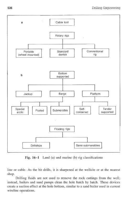
536 Drilling Engineering
a Cable tool
Rotary rigs
Standardderrick
bBottom
supported
Fig. 16-1 Land (a) and marine (b) rig classifications
line or cable. As the bit drills, it is sharpened at the wellsite or at the nearestshop.
Drilling fluids are not used to remove the rock cuttings from the well;instead, bailers and sand pumps clean the hole batch by batch. These devicescreate a suction effect at the hole bottom, similar to a sand bailer used in currentwireline operations.
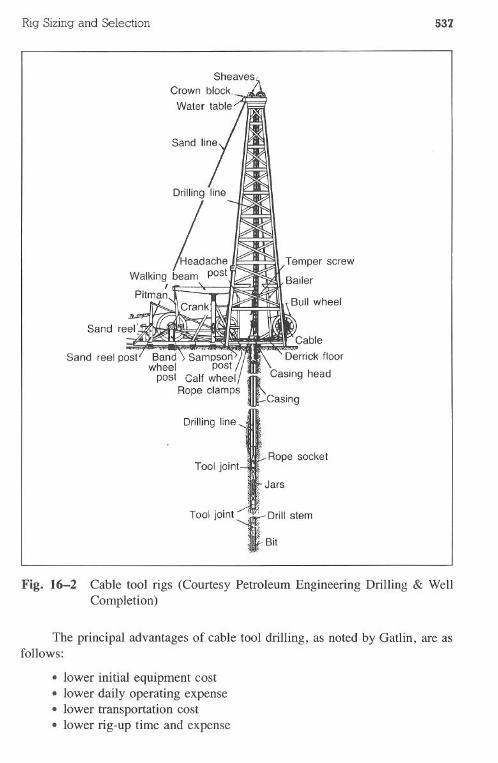
Rig Sizingand Selection 537
Drilling line
L~.Walking beam post
IPitman
Drilling line
Tool jointRope socket
I ,.
JarsII.
I
Tool joint
1"W~ Drill stem
, Bit
I'I'I
Fig. 16-2 Cable tool rigs (Courtesy Petroleum Engineering Drilling & WellCompletion)
The principal advantages of cable tool drilling, as noted by Gatlin, are asfollows:
.lower initial equipment cost· lower daily operating expense.lower transportation cost· lower rig-up time and expense
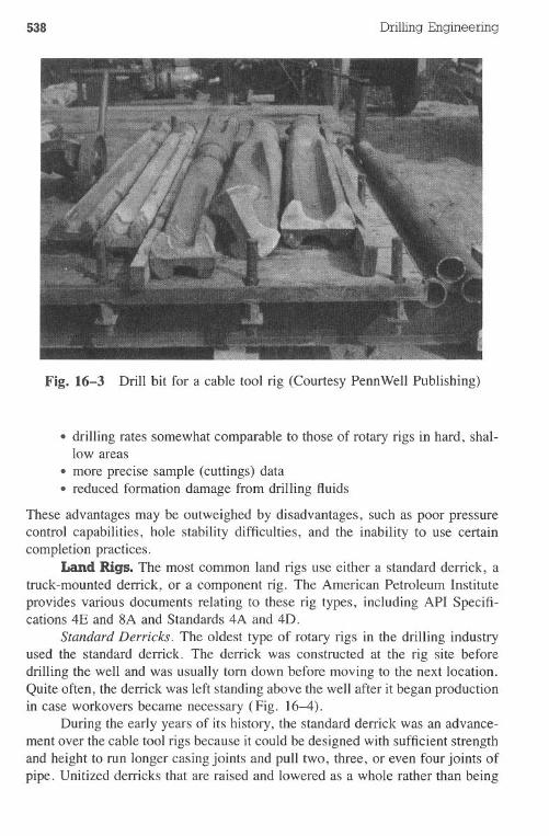
538 Drilling Engineering
Fig. 16-3 Drill bit for a cable tool rig (Courtesy PennWell Publishing)
.drilling rates somewhat comparable to those of rotary rigs in hard, shal-low areas·more precise sample (cuttings) data· reduced formation damage from drilling fluids
These advantages may be outweighed by disadvantages, such as poor pressurecontrol capabilities, hole stability difficulties, and the inability to use certaincompletion practices.
Land Rigs. The most common land rigs use either a standard derrick, atruck-mounted derrick, or a component rig. The American Petroleum Instituteprovides various documents relating to these rig types, including API Specifi-cations 4E and 8A and Standards 4A and 40.
Standard Derricks. The oldest type of rotary rigs in the drilling industryused the standard derrick. The derrick was constructed at the rig site beforedrilling the well and was usually torn down before moving to the next location.Quite often, the derrick was left standing above the well after it began productionin case workovers became necessary (Fig. 16-4).
During the early years of its history, the standard derrick was an advance-ment over the cable tool rigs because it could be designed with sufficient strengthand height to run longer casing joints and pull two, three, or even four joints ofpipe. Unitized derricks that are raised and lowered as a whole rather than being
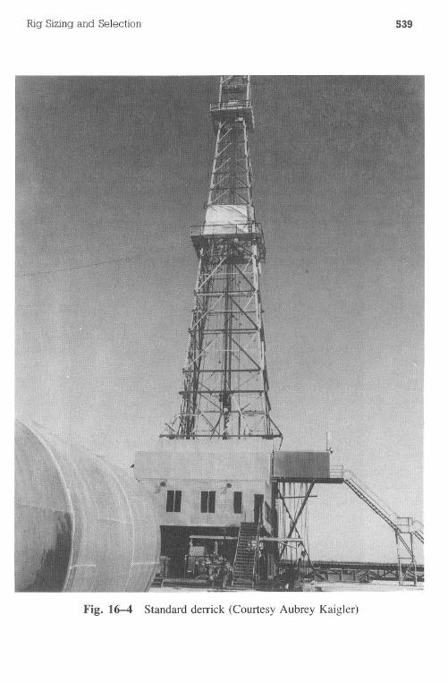
Rig Sizingand Selection 539
Fig. 16-4 Standard derrick (Courtesy Aubrey Kaigler)
540 Drilling Engineering
constructed piecemeal haye replaced the standard derrick. The rig-up and rig-down time with the standard derrick was excessive. In addition, a unitized derrickgenerally has fewer failures than a derrick that is built and dismantled for eachwell.
Portable Rig. A portable rig is usually considered to be a truck-mountedunit (Fig. 16-5). The truck bed contains the derrick, drawworks, and mud pumps.A principal advantage of the portable rig is the low rig-up and rig-down timeas well as lower truck hire requirements. Portable rigs are used frequently inworkover operations and when drilling to depths of about 10,000 ft. These rigsmay be used on an 8-, 12-, or 24-hr/day basis.
Portable units for drilling generally are restricted to light-duty work. Whereapplicable, the unit is usually the most cost-effective rig. General capabilitiesfor some portable rigs are as follows:
Fig. 16-5 Portable truck-mounted rig (Courtesy NL Industries Inc)
Rig Sizing and Selection 541
maximum derrick capacitymaximum pump flow ratederrick heightpit volumedrillpipe size
350,000 Ib6-8 bbl/minsingle or double joints150 bbl31/2-4 in.
Since most wells drilled worldwide are shallower than 8,000-10,000 ft, theportable rig plays an important role in drilling operations.
Caution must be exercised when planning a well that approaches the upperlimits of portable rig capabilities. For example, drilling a well to 10,000 ft wouldnot strain a large portable rig if 31/2-or 4-in. drillpipe were used. However, if23.0-lb/ft casing must be run to 10,000 ft, the total casing load (230,000 lb)does not provide an adequate safety factor with respect to derrick capacity.Although short-term economics may suggest using the portable rig instead of alarger, more expensive conventional rig, the larger rig may prove more econom-ical over the long term if drilling problems should develop.
Conventional Rig. A conventional rig is considered usually as a componentrig in which the key components are so large that they cannot be transported ona single truck bed. These rigs vary in depth rating from 6,000 to 35,000 ft. Theconventional rig is usually operated on a 24-hr/day basis (Fig. 16-6).
Conventional rigs are the largest land rigs available for drilling. Maximumcapabilities are in the following ranges:
derrick capability =pump horsepower =pit volumedrillpipe size
2,000,000 lb3,000 hp300-1,500 bbl31/2-5Y2in.
Most conventional rigs pull three-joint stands.A typical rig specification sheet is shown in Fig. 16-7. These guidelines
must be used to evaluate and compare rigs of various contractors before selectinga rig for the upcoming well. Information contained in the rig specs addressesthe following areas:· drawworks.derrick· substructure·engines· pumps·mud mixing systems·drillstring.preventers·miscellaneous equipment
542 Drilling Engineering
Fig. 16-6 Conventional drilling rig (Courtesy Goldrus Drilling)
The rig specifications usually contain a schematic of the rig's layout so the rigsite can be prepared properly (Fig. 16-8).
Marine Rigs. Drilling rigs used offshore are tenned marine rigs. Acommon grouping system for marine rigs is based on the bottom support of therig on the seafloor (see Fig. 16-1). A bottom-supported rig rests on the seaflooror on pads built on the seafloor. Floating rigs rely on ballast systems similar to
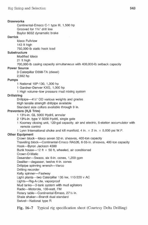
Rig Sizingand Selection 543
DrawworksContinental-Emsco C-1 type III, 1,500 hpGrooved for 1"/s"drill lineBaylor 6032 dynamatic brake
DerrickIdeco Fullview143 ft high750,OOO-lbstatic hook load
SubstructureModified Ideco21 ft high700,OOO-lbcasing capacity simultaneous with 400,OOO-lbsetback capacity
Power Source3 Caterpillar D398-TA (diesel)2,592 hp
Pumps1 National10P-130, 1,300 hp1 Gardner-Denver KXG, 1,000 hp1 High volume-low pressure mud mixing system
DrlllstrlngDrillpipe-4 W' OD various weights and gradesHigh tensile strength drillpipe availableStandard size collars available through 9 in.
Preventers (H2STrim)1 135fs-in.GL 5000 Hydril, annular2 135fs-in.type V 5000 HydrO,single gate1 Koomey closing unit, 120-gal capacity, air and electric, 6-station accumulator with
remote control1 Lynn International choke and kill manifold, 4 in. x 2 in. x 5,000 psi W.P.
Other EquipmentCrown block-Ideco seven 52-in. sheaves, 400-ton capacityTraveling bI6ck-Continental-Emsco RA526, 6-55-in. sheaves, 400-ton capacityHook-Byron Jackson 4300Bunk house-12 ft x 50 ft, wheeled, air conditionedCrown-O-MaticDesander-Swaco, six 6-in. cones, 1,200 gpmDesilter-degasser, twelve 4-in. conesDrillpipe spinning wrench-VarcoDrilling recorderKelly spinner-FastwayLight plants-two Caterpillar 135 kw, 110/220 v ACLights...l...Rig-A-Lite,vaporproofMud tanks-3-tank system with mud agitatorsRadio-Motorola, 100-watt, FMRotary table-Continental-Emsco, 27'12in.Shale shaker-Brandt dual standard .Swivel-National type R
Fig. 16-7 Typical rig specification sheet (Courtesy Delta Drilling)
I.
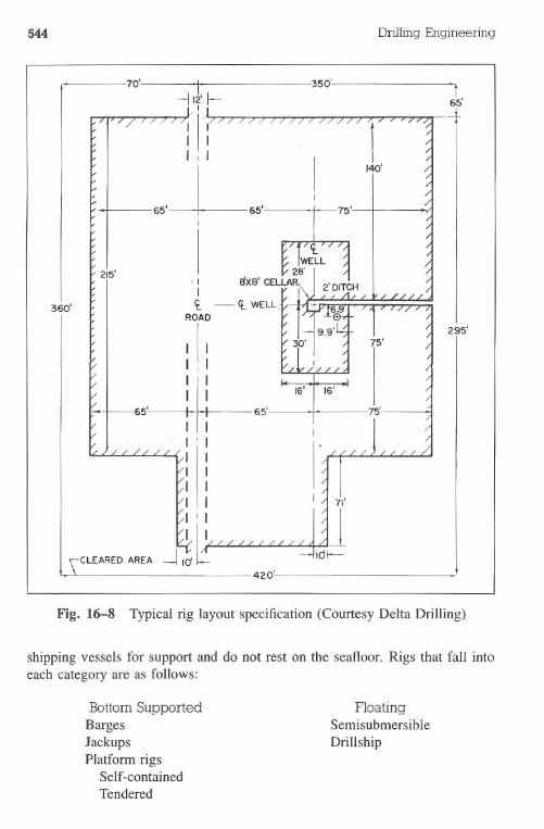
544 Drilling Engineering
70' . I-! 12'l-
I
I
I
II II I I
".-L...
350'1
65'
t140'
75'
215'
65'
.1I
i -<i. WELL
TI I
~...,IIIII
I I
--J I~~
295'
360'
l'CLEARED AREA Idl--
420'
Fig. 16-8 Typical rig layout specification (Courtesy Delta Drilling)
shipping vessels for support and do not rest on the seafloor. Rigs that fall intoeach category are as follows:
Bottom SupportedBargesJackupsPlatfonn rigs
Self-containedTendered
FloatingSemisubmersibleDrillship
Rig Sizing and Selection 545
Many design criteria are used in selecting the proper marine rig. Majorcriteria are as follows:
·water depth rating·derrick and substructure capacity·physical rig size and weight· deck load capacity·stability in rough weather·duration of drilling program·rig rating features such as horsepower, pipe handling capabilities, mudmixing capacity·exploratory vs development drilling·availability and cost
Water depth rating is perhaps the first evaluative tool. Bottom-supported unitscan operate in a maximum of 400-ft water depths; 250-300 ft is the typicalmaximum. Platforms can handle any depth to 1,000 ft (and ultimately 2,500 ftwith today's emerging technology), but deep platforms are justified only forlongterm development drilling. Floaters can handle shortterm projects (like ex-ploration) in water depths from 300-7,000 ft. The upper limit is being extendedsteadily; the lower limit depends on weather and the size of the drilling budget.
Rig size may be a limiting factor on platforms. Deck loading and stabilityin environmental conditions are used in selecting drillships and semisubmersibles.
The American Bureau of Shipping (ABS) and other rating agencies havedeveloped extensive guidelines relating to marine rigs. The ABS rules coveritems such as operating ranges, structural design criteria, and classification pro-cedures. Although these guidelines are important with respect to marine engi-neering, they will not be discussed extensively in this text due to their indirectapplication for drilling engineers. Interested readers should consult these ratingagencies in the event they are required for some difficult drilling applications.
Barges. A drilling barge is used typically in 8-20 ft of water. The barge(Fig. 16-9) is towed to the location and sunk on the bottom by flooding variousvessel compartments. After drilling has been completed, the flooded compart-ments are evacuated, which allows the rig to float so it can be moved to the nextlocation. Occasionally, special efforts are required to lift the barge because itbecomes imbedded in the seafloor and will not float after evacuation.
The barge is generally designed as a fully self-contained vessel. In additionto a complete drilling rig, it has sleeping quarters for the crew and ancillarypersonnel as well as galley facilities. Crew boats are us~d for transportationbetween the rig and the nearest docking facility and for emergency personnelevacuation.
Operating water depth and weather limit the areas for the drilling barge.A minimum water depth of 6-8 ft is required for vessel draft during transportto the location. The upper range on the water depth can be extended to 30-40
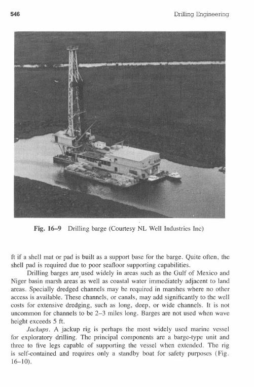
546 DrillingEngineering
Fig. 16-9 Drilling barge (Courtesy NL Well Industries IDe)
ft if a shell mat or pad is built as a support pase for the barge. Quite often, theshell pad is required due to poor seafloor supporting capabilities.
Drilling barges are used widely in areas such as the Gulf of Mexico andNiger basin marsh areas 'as well as coastal water immediately adjacent to landareas. Specially dredged channels may be required in marshes where no otheraccess is available. These channels, or canals, may add significantly to the wellcosts for extensive dredging, such as long, deep, or wide channels. It is notuncommon for channels to be 2-3 miles long. Barges are not used when waveheight exceeds 5 ft.
Jackups. A jackup rig is perhaps the most widely used marine vesselfor exploratory drilling. The principal components are a barge-type unit andthree to five legs capable of supporting the vessel when extended. The rigis self-contained and requires only a standby boat for safety purposes (Fig.16-10).
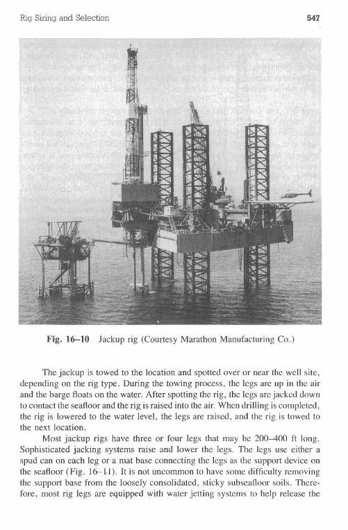
Rig Sizing and Selection 547
Fig. 16-10 Jackup rig (Courtesy Marathon Manufacturing Co.)
The jackup is towed to the location and spotted over or near the well site,depending on the rig type. During the towing process, the legs are up in the airand the barge floats on the water. After spotting the rig, the legs are jacked downto contact the seafloor and the rig is raised into the air. When drilling is completed,the rig is lowered to the water level, the legs are raised, and the rig is towed tothe next location.
Most jackup rigs have three or four legs that may be 200-400 ft long.Sophisticated jacking systems raise and lower the legs. The legs use either aspud can on each leg or a mat base connecting the legs as the support device onthe seafloor (Fig. 16-I.l). It is not uncommon to have some difficulty removingthe support base from the loosely consolidated, sticky subseafioor soils. There-fore, most rig legs are equipped with water jetting systems to help release the
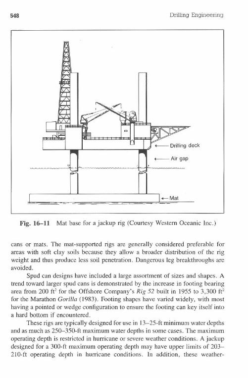
548 Drilling Engineering
__ Air gap
+- Mat
Fig. 16-11 Mat base for a jackup rig (Courtesy Western Oceanic Inc.)
cans or mats. The mat-supported rigs are generally considered preferable forareas with soft clay soils because they allow a broader distribution of the rigweight and thus produce less soil penetration. Dangerous leg breakthroughs areavoided.
Spud can designs have included a large assortment of sizes and shapes. Atrend toward larger spud cans is demonstrated by the increase in footing bearingarea from 200 fe for the Offshore Company's Rig 52 built in 1955 to 3,300 fefor the Marathon Gorilla (1983). Footing shapes have varied widely, with mosthaving a pointed or wedge configuration to ensure the footing can key itself intoa hard bottom if encountered.
These rigs are typically designed for use in 13-25-ft minimum water depthsand as much as 250-350-ft maximum water depths in some cases. The maximumoperating depth is restricted in hurricane or severe weather conditions. A jackupdesigned for a 300-ft maximum operating depth may have upper limits of 203-21O-ft operating depth in hurricane conditions. In addition, these weather-
Rig Sizing and Selection 549
dependent conditions vary for different areas due to wind and wave actions ina typical storm, i.e., Gulf of Mexico vs North Sea.
Jackup rigs are segregated into slot or cantilever rigs, depending on theapplication requirements. The slot rig has an area within the outer limits of therig through which all drilling is done. The derrick is located over the slot (Fig.16-12).
The cantilever rig can be positioned over or near the well site. The mastis mounted on a cantilever beam (Fig. 16-13) such that it can be moved outfrom the main body of the barge and positioned over the well. This flexibilityallows the operator to build a lighter, cheaper platform that supports only well-heads. It also permits the cantilever rig to be used in some well servicingoperations on small production platforms. Maximum safe operating derrick loadsmust be determined for the rig, depending on the distance starboard or port ofthe centerline from the rig to the rotary. Drilling contractors often provide chartsto determine the safe load limits.
The barge and rig are self-contained with respect to life-support systemsand drilling equipment. The barge is usually divided into two or three decks.The top deck contains the rig, pipe racks, and occasionally the living quarters.The lower decks contain all support drilling equipment, such as pumps and mudsystems, as well as the auxiliary barge equipment (Fig. 16-14).
Platform Rigs. The discovery of significant petroleum reserves in an off-shore area usually requires the installation of a production platform to extractthe reserves economically. A number of wells are drilled directionally from theplatform to exploit the reservoir. This approach is more cost effective, in mostcases, than many single-well platforms with vertical wells.
Rigs that drill from platforms are either fully self-contained or are tendersupported. If the production platform is sufficiently large, all drilling andpersonnel support equipment is maintained on the rig. A floating tender is usedto support personnel and auxiliary drilling equipment such as mud pumps andbulk chemical storage if the platform working area or load is restricted (Fig.16-15).
DriLLships.Floating rigs such as drillships or semisubmersibles do not reston the seafloor during drilling. As such, these rigs are not restricted by the lengthof the rig's legs for maximum water operating depth. These two rig types havedifferent operating characteristics that must be reviewed prior to rig selection.
Drillships use a ship-type vessel as the primary structure to support therig (Fig. 16-16). It may be a converted seagoing vessel or, as is common inrecent years, it may be a new vessel constructed for drilling. It may be self-propelled or require oceangoing tubs for transport.
Semisubmersibles. 'The semisubmersible drilling unit (Fig. 16-17) is aspecially designed vessel used exclusively in petroleum operations. The ballastedlower hulls are below sea level to maximize rig stability. The primary advantage
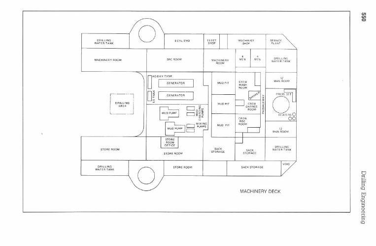
DR
ILL
ING
WA
TE
RT
AN
K
MA
CH
INE
RY
RO
OM
f---U,
o,
I
DR
ILL
ING
'IA
RE
A
iJ
STO
RE
RO
OM
DR
ILL
ING
WA
TE
RT
AN
K
eneno
onE
CT
SHO
PSE
WA
GE
PLA
NT
8cn
EM
D.
SRC
RO
OM
4M
EN
DR
ILL
ING
WA
TE
RT
AN
K
O
FOD
AY
TA
NK
~eRA
TO
R
D!I
GE
NE
RA
TO
RI
MU
DPIT
CR
EW
WA
SHR
OO
M
12M
AN
RO
OM
MU
DPIT
CR
EW
CH
AN
GE
RO
OM
MU
DPIT
CR
EW
RfC
.R
OO
M
12M
AN
RO
OM
DR
ILL
ING
WA
TE
RT
AN
K
STO
RE
RO
OM
SAC
KST
OR
AG
ESA
CK
STO
RA
GE
VO
IDST
OR
ER
OO
MSA
CK
STO
RA
GE
MA
CH
INE
RY
DE
CK
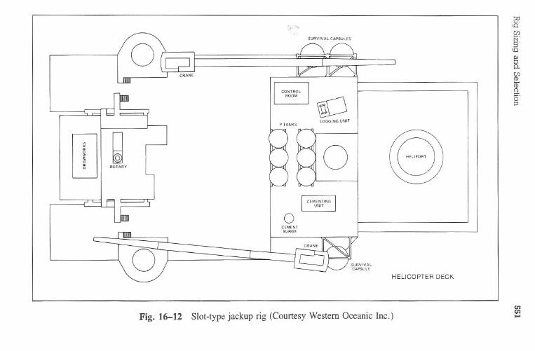
SUR
VIV
AL
CA
PS
UL
ES
gJlOG
GIN
GU
NIT
oo
Fig.
16-12Slot-type
jackuprig
(Courtesy
Western
Oceanic
Inc.) HE
LICO
PT
ER
DE
CK
enen...
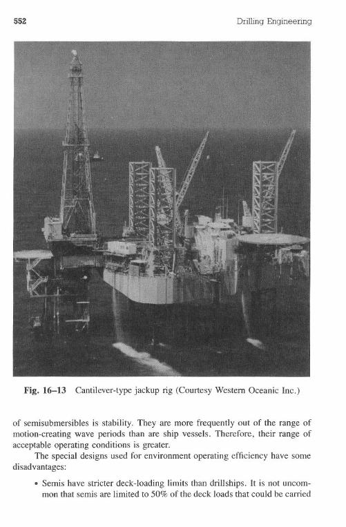
552 Drilling Engineering
Fig. 16-13 Cantilever-type jackup rig (Courtesy Western Oceanic Inc.)
of sernisubmersibles is stability. They are more frequently out of the range ofmotion-creating wave periods than are ship vessels. Therefore, their range ofacceptable operating conditions is greater.
The special designs used for environment operating efficiency have somedisadvantages:
·Semis have stricter deck-loading limits than drillships. It is not uncom-mon that semis are limited to 50% of the deck loads that could be carried
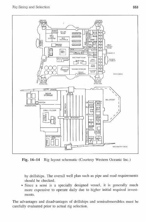
Rig Sizingand Selection 553
64 MANLIFEBOAT
MAIN DeCK
DODO
Fig. 16-14 Rig layout schematic (Courtesy Western Oceanic Inc.)
by drillships. The overall well plan such as pipe and mud requirementsshould be checked.. Since a semi is a specially designed vessel, it is generally muchmore expensive to operate daily due to higher initial required invest-ments.
The advantages and disadvantages of drillships and semisubmersibles must becarefully evaluated prior to actual rig selection.
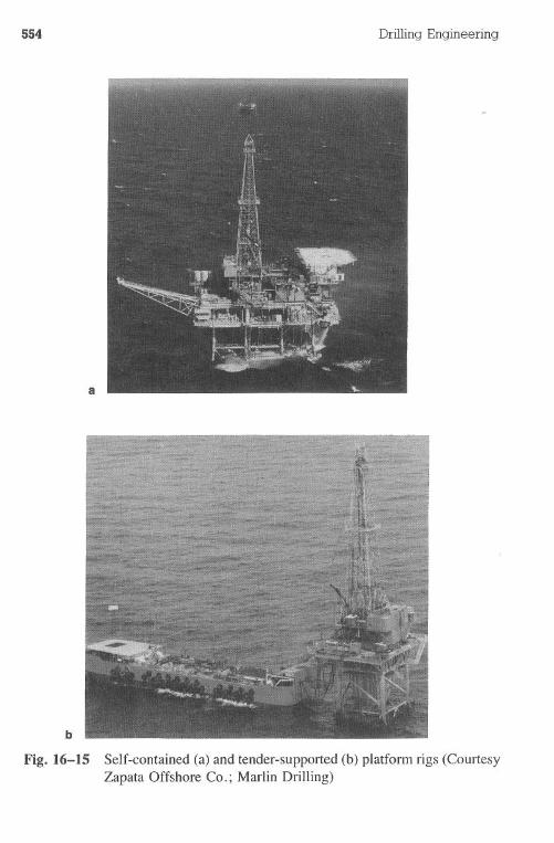
554 DrillingEngineering
a
b
Fig. 16-15 Self-contained (a) and tender-supported (b) platform rigs (CourtesyZapata Offshore Co.; Marlin Drilling)
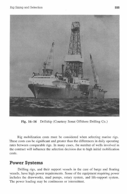
Rig Sizing and Selection 555
Fig. 16-16 Drillship (Courtesy Sonat Offshore Drilling Co.)
Rig mobilization costs must be considered when selecting marine rigs.These costs can be signifi.cantand greater than the differences in daily operatingrates between comparable rigs. In many cases, the number of wells involved inthe contract will influence the selection decision due to high initial mobilizationcosts.
Power SystemsDrilling rigs, and their support vessels in the case of barge and floating
vessels, have high power requirements. Some of the equipment requiring powerIncludes the drawworks, mud pumps, rotary system, and life-support system.The power loading may be continuous or intermittent.
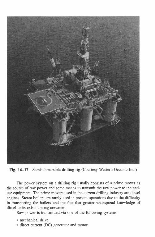
556 Drilling Engineering
Fig. 16-17 Semisubmersible drilling rig (Courtesy Western Oceanic Inc.)
The power system on a drilling rig usually consists of a prime mover asthe source of raw power and some means to transmit the raw power to the end-use equipment. The prime movers used in the current drilling industry are dieselengines. Steam boilers are rarely used in present operations due to the difficultyin transporting the boilers and the fact that greater widespread knowledge ofdiesel units exists among crewmen.
Raw power is transmitted via one of the following systems:·mechanical drive·direct current (DC) generator and motor
Rig Sizing and Selection 557
· alternating cucrent (AC), silicon controlled rectifier (SCR), direct cucrent(DC) motor
The most widely used system on new rigs or large marine rigs is the AC-SCRsystem.
The mechanical horsepower requirements for the prime movers must bedetermined from an evaluation of the loads and the overall system efficiency:
load
mechanical horsepower = efficiency(16.1)
where the efficiency is less than 1.0. Although Eq. 16.1 is straightforward, itis somewhat difficult to implement due to problems in establishing the load andefficiency factor.
The efficiency factor (E) describes the power losses from the prime moversto the end-use equipment. It can be calculated from Eq. 16.2:
E = energy output - energy inputenergy output
(16.2)
where output is from the prime mover and input is the amount remaining foractual usage after some losses. The system losses result from friction, gears,and belt and line losses. The efficiency factors range from 0-1. Some drillingpersonnel assume that efficiency factors for oil-well drilling machinery are 0.98per shaft and chain. The system efficiency is computed as (0.98)0, where n isthe number of shafts and chains. If more than one engine is used, an averagevalue is calculated.
The mechanical horsepower requirements must be modified for harsh tem-perature environments or altitudes. According to API Standard 7B-ll C (formerlyAPI Standard 8B), approximate conversions for altitude and temperature ofnaturally aspirated engines may be made as follows:
.deduct 3% of the standard brake horsepower for each 1,000-ft rise inaltitude above sea level. deduct 1% of the standard brake horsepower for each 10° rise in tem-perature above 85°F or add 1% for each 10° fall below 85°F
The engine manufacturer should be consulted for specific variances.
Example 16.1
A drilling rig is working in an arid climate at an elevation of 3,600 ft. Duringthe day, the peak temperature is 105°F. The minimum temperature (prior todawn) is 45°F. The rig has three 1,000-hp prime movers. Determine theminimum and maximum horsepower available during any 24-hr period.
558 Drilling Engineering
Solution:
1. The total available horsepower from the prime movers is 3,000 hp.2. The loss in horsepower due to altitude is:
3% loss1,000 ft x 3,600 ft x 3,000 hp = 324 hp
3,000 hp - 324 hp = 2,676 hp
3. The minimum horsepower will occur at the maximum temperature:
1% loss x (l050P
2,676
85°P) x 2,676 hp 53.5 hp
53.5 = 2,622 hp
4. Conversely, the maximum horsepower will occur at the minimum tem-perature:
I% gain x (85°P - 45°P) x 2,676 hp
2,676 + 107 = 2,783 hp
107 hp
Mechanical Drive Systems. Most early drilling rigs used a mechanicaldrive system to transmit power from the engines to the operating equipment suchas the drawworks and pumps. The drive system consists of gears, chains, andbelts (Pig. 16-18). The compound device attached to the engine shafts combinesthe output of two engines.
Torque converters are attached to the shafts to increase the range of outputrpm's and also to improve engine life by absorbing equipment-induced powertrain shock loads. Efficiency drops off at high torques, but the converter has auseful range of approximately 2: 1 multiplication at efficiency factors of 0.75-0.85. The chief advantage of the converter is the ability to accelerate loadsrapidly and give reasonable constant horsepower output over the most efficient2: 1 speed range.
The weaknesses of the mechanical drive systems are as follows:
· shock loading to the engine. inability to produce high torque at low engine rpm's, which becomes acompounded problem as higher work loads continue to decrease enginerpm's.difficulty in providing low torque output due to minimum engine idlespeeds and gear ratios· power loss through the gears and chains
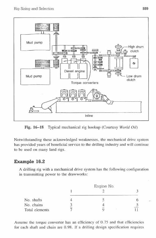
Rig Sizingand Selection 559
Mud pump
Torque converters
Mud pump
Inline
Fig. 16-18 Typical mechanical rig hookup (Courtesy World Oil)
Notwithstanding these acknowledged weaknesses, the mechanical drive systemhas provided years of beneficial service to the drilling industry and will continueto be used on many land rigs.
Example 16.2
A drilling rig with a mechanical drive system has the following configurationin transmitting power to the drawworks:
Assume the torque converter has an efficiency of 0.75 and that efficienciesfor each shaft and chain are 0.98. If a drilling design specification requires
Engine No.2 3
No. shafts 4 5 6No. chains 3 4 5-Total elements 7 9 11
560 Drilling Engineering
that a 500,OOO-lbhook load be hoisted at a rate of 93 CUmin,compute theminimum acceptable-input horsepower for the engines. Neglect the travelingblock efficiencies.
Solution:
1. From Eq. 16.3, compute the required horsepower at the drawworks:
HP = force x rate33,000
(16.3)
where force is in Ib
HP = 500,000Ib x 93 ft/minD 33,000
1,409 hp, drawworks
2. The combined average system efficiency from the drawworks to the con-verter is:
Engine # 1 Engine #2 Engine #3E = [(0.9W + (0.98)9 + (0.98)11]/3
[(0.868) + (0.834) + (0.801)]/3= [0.834 (average system efficiency)]
3. Compute the horsepower requirements to the converter:
(16.4)
Wh~re:HP c = converter horsepower
I ,409 hpHPc = 0.834
= 1,689hp
4. Calculate the actual engine requirements by accounting for the efficiencylosses in the converters.
1,689 hpHPE = 0.75
= 2,252 hp
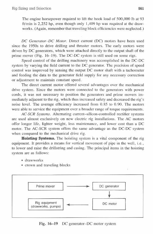
Rig Sizing and Selection 561
The engine horsepower required to .lift the hook load of 500,000 lb at 93
ft/min is 2,252 hp, even though only 1,409 hp was required at the draw-works. (Again, remember that traveling block efficiencies were neglected.)
DC Generator-DC Motor. Direct current (DC) motors have been usedsince the 1950s to drive drilling and thruster motors. The early motors weredriven by DC generators, which were attached directly to the output shaft of theprime mover (Fig. 16-19). The DC-DC system is still used on some rigs.
Speed control of the drilling machinery was accomplished in the DC-DCsystem by varying the field current to the DC generator. The precision of speedcontrol was improved by sensing the output DC motor shaft with a tachometerand feeding the data to the generator field supply for any necessary correctionor adjustment to maintain constant speed.
The direct current motor offered several advantages over the mechanicaldrive system. Since the motors were connected to the generators with powercords, it was not necessary to position the generators and prime movers im-mediately adjacent to the rig, which thus increased safety and decreased the rig'snoise level. The average efficiency increased from 0.85 to 0.90. The motorswere able to service the equipment over a broader range of torque requirements.
AC-SCR Systems. Alternating current-silicon-controlled rectifier systemsare used almost exclusively on new electric rig installations. The AC motorsoffer longer life, lighter weight, less maintenance, and lower cost than a DCmotor. The AC-SCR system offers the same advantage as the DC-DC systemwhen compared to the mechanical drive rig.
Hoisting Systems. The hoisting system is a vital component of the rigequipment. It provides a means for vertical movement of pipe in the well, i.e.,to lower and raise the drillstring and casing. The principal items in the hoistingsystem are as follows:. drawworks. crown and traveling blocks
Prime mover .. DC generator
Rig equipment(drawworks, pumps)
DC motor
Fig. 16-19 DC generator-DC motor system
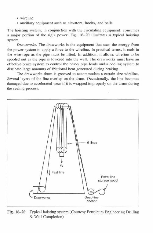
562 Drilling Engineering
·wireline·ancillary equipment such as elevators, hooks, and bails
The hoisting system, in conjunction with the circulating equipment, consumesa major portion of the rig's power. Fig. 16-20 illustrates a typical hoistingsystem.
Drawworks. The drawworks is the equipment that uses the energy fromthe power system to apply a force to the wireline. In practical terms, it reels inthe wire rope as the pipe must be lifted. In addition, it allows wireline to bespooled out as the pipe is lowered into the well. The drawworks must have aneffective brake system to control the heavy pipe loads and a cooling system todissipate large amounts of frictional heat generated during braking.
The drawworks drum is grooved to accommodate a certain size wireline.Several layers of the line overlap on the drum. Occasionally, the line becomesdamaged due to accelerated wear if it is wrapped improperly on the drum duringthe reeling process.
6 lines
Dead-lineanchor
Fig. 16-20 Typical hoisting system (Courtesy Petroleum Engineering Drilling& Well Completion)
Rig Sizing and Selection 563
An effective braking system must be used on the drum. In some cases,500-ton loads must be decelerated quickly and held in place. A commonly usedbraking system on mechanical rigs is the hydrodynamic type. The braking isprovided by water being impelled in a direction opposite to the rotation of thedrum.
Electric rigs often use an electromagnetic (eddy current) brake in additionto a braking action generated by the drive motors on the drawworks. The brakingis provided by two opposing magnetic fields. The magnitude of the magneticfields is dependent on the speed of rotation and the amount of external excitationcurrent. The brake is directly coupled to the drawworks shaft. The electric brakecannot stop the drawworks, but it does take much of the load off the mechanicalbrake.
Block System. The block-and-tackle system is the primary link betweenthe drawworks and the pipe or casing. It provides the mechanical advantage toassist in lowering and raising heavy strings of pipe. The equipment can includeitems such as the crown and traveling blocks, elevators, bails, and heave com-pensators. (Although the wire rope is an essential part of the block-and-tacklesystem, it will be treated separately in this text.)
API Specification 8A recognizes the maximum load rating in tons (2,000-Ib units) as follows:
5101525
4065
100150
250350500650750
The maximum load rating may be based on either the tensile strength or theyield strength of the material at the manufacturer's option.
The rig must be evaluated with respect to the block-and-tackle system toensure that it meets the designed safety requirements. Specifications for safetyfactors are as follows:
Calculated LoadRating, tons
0-150
151-500501 and over
Tensile StrengthDesign Safety Factor
4.00
(R - 150
)4.00 - 350 (16.5)3.00
where R is the calculated load rating in 2, OOO-lbtons for Eq. 16.5. The maximumload rating of the pipe must be calculated before applying the safety factor andevaluating the equipment rating.
564 Drilling Engineering
Example 16.3
A 95fs-inch, 53.5-lb/ft casing string is to be set at 13,150 ft in 14.8-lb/galmud. The rig intended for the well has a 350-ton block-and-tackle system.The casing is filled with mud as it is run. Neglect traveling block weight andwear derating. Is it sufficient for the job?
Solution:
I. Determine the casing weight in air:
53.5 Ib/ft x 13,500 ft = 722,250 Ib
2. Account for the mud's buoyancy factor:
BF = I _ MW65.5
14.865.5
(18.4)
= I
buoyed weight
= 0.7740
722,250 Ib x 0.7740559,054 Ib279.5 tons (2,000-lb units)
3. Since 150 :S 279.5 :S 500 from the previous safety factor table, Eq. 16.5should be used:
safety factor = 4.0 - (R - 150
)350
= 4 0 _ (279.5 - 150
). 350= 3.63
4. Determine the designed equipment rating:
279.5 tons X 3.63 = 1,014tons
5. The rig equipment is underdesigned for the job, according to the hoistingsystem design factor specifications in API Specification 8A.
The crown and traveling block consist of sheaves designed for use withwire rope. The crown block is stationary and is located at the top of the derrick.
Rig Sizing and Selection 565
The traveling block is free to move and has hook, bails, and elevators attachedto the bottom for latching to the pipe. Both blocks have 4-12 sheaves. Thenumber of lines strung vary with load, with fewer on shallow wells and maximumfor heavy casing loads.
The block system is not a frictionless system, i.e., its efficiency factoris less than 1.0. It is often assumed that the efficiency rating for a set ofsheaves is 0.98 and the overall block system efficiency factor is computed fromEq. 16.6:
EB = (0.98t (16.6)
where n is the number of sheave pairs. The following table indicates EB forvarious pulley systems.
No. of Lines68
to12
EB0.8860.8500.8170.785
Wire Rope. Drilling rigs have many applications for wire rope (Fig.16-21). The more common uses are as drilling lines and guideline tensioners.The drilling line connects to the drawworks and the dead-line anchor. It is pulledthrough the crown and traveling block sheaves so the traveling block can beraised or lowered as necessary.
Wire rope is made from cold drawn carbon steel of various grades, de-pending on the strength required. The American Petroleum Institute classifiesthe various grades as follows:
· extra improved plow steel (EIPS)· improved plow steel (IPS)· plow steel (PS)·mild plow steel (MPS)
Generally, the first two higher-strength grades, EIPS and IPS, are used currentlyfor drilling lines due to the rugged service encountered.
The primary element of wire rope is the individual wires. Wires are care-fully selected, sized, and layered into strands. After stranding, the strands arelayered together around a core to form wire rope. The core may be a fiber rope(either natural grown fibers or man-made fibers), a plastic core, a spring steelcore, a multiple-wire strand, or an independent wire rope (IWRC). The inde-pendent wire rope is the most widely used because it resists crushing and dis-tortion.
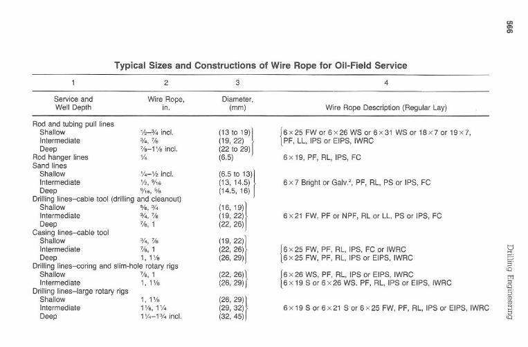
enQ)
Q)
Typ
icalS
izesan
dC
on
structio
ns
of
Wire
Ro
pe
for
Oil-F
ieldS
ervice
23
4
Service
andW
ireR
ope,D
iameter,
Well
Depth
in.(m
m)
Wire
Rope
Description
(Regular
Lay)
Rod
andtubing
pulllines
Shallow
%-%
incl.
(13to
19»){6X
25F
Wor
6x26W
Sor
6x31W
Sor
18x7or
19x7,Interm
ediate%
,%(19,
22)P
F,
LL,IP
Sor
EIP
S,
IWR
CD
eep%
-1%
incl.(22
to29)
Rod
hangerlines
%(6.5)
6x
19,PF
,R
L,IP
S,
FC
Sand
linesS
hallow%
-%incl.
(6.5to
1311
Intermediate
%,0/16
(13,14.5)
6x
7B
rightorG
alv.2,PF
,R
L,P
Sor
IPS
,FC
Deep
9/'6,5/a(14.5,
16)D
rillinglines-cable
tool(drilling
andcleanout)
Shallow
5/a,3/4
(16,191)
Intermediate
%,%
(19,22)6
x21
FW
,P
For
NP
F,
RL
orLL,
PS
orIP
S,
FC
Deep
7/a,1(22,
26)C
asinglines-cable
toolS
hallow3/4,7/a
(19,2211
Intermediate
7/a,1(22,
26){6
x25
FW
,P
F,
RL,
IPS
,F
Cor
IWR
CD
eep1,1%
(26,29)6
x25
FW
,PF
,R
L,IP
Sor
EIP
S,
IWR
CD
rillinglines-coring
andslim
-holerotary
rigsS
.<
0S
hallow7/a,1
(22,26)}{6
x26
WS
,P
F,
RL,
IPS
orE
IPS
,IW
RC
tT:J
Intermediate
1,1%(26,29)
6x
19S
or6
x26
WS
,P
F,
RL,
IPS
orE
IPS
,IW
RC
::1<
0D
rillinglines-large
rotaryrigs
S.
Shallow
1,1%
(26,29)}
CD
CD
Intermediate
1'/a,1%(29,32)
6x
19S
or6
x21S
or6
x25F
W,
PF
,R
L,IP
Sor
EIP
S,
IWR
C.....
Deep
1%-1%
incl.(32,45)
s.
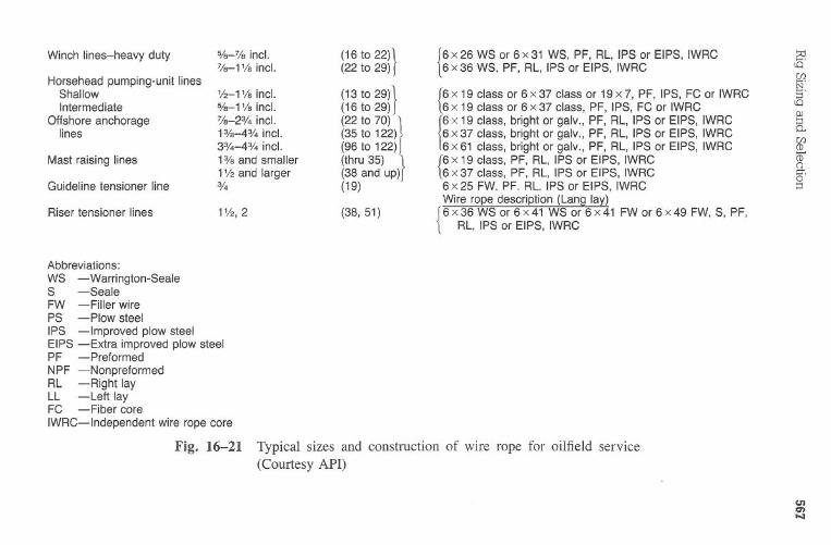
Abbreviations:
WS
-Warrington-S
ealeS
-Seale
FW
-Filler
wire
PS
-Plow
steelIP
S-Im
provedplow
steelE
IPS
-Extra
improved
plowsteel
PF
-Preform
edN
PF
-Nonpreform
edR
L-R
ightlay
LL-Left
layF
C-F
ibercore
IWR
C-Independent
wire
ropecore
Fig.
16-21T
ypicalsizes
andconstruction
ofw
irerope
foroilfield
service(C
ourtesyA
PI)
enen""I
Winch
lines-heavyduty
%-%
incl.
(16to
22)}{6
x26
WS
or6
x31
WS
,P
F,
RL,
IPS
orE
IPS
,IW
RC
%-1
Va
incl.(22
to29)
6x
36W
S,
PF
,R
L,IP
Sor
EIP
S,
IWR
C10
Horsehead
pumping-unit
linesC
IJN
"S
hallow%
-1V
aincl.
(13to
29)}{6
x19
classor
6x
37class
or19
x7,
PF
,IP
S,
FC
orIW
RC
;goInterm
ediate%
-1V
aincl.
(16to
29)6
x19
classor
6x
37class,
PF
,IP
S,
FC
orIW
RC
Offshore
anchorage%
-2%incl.
(22to
70)}
rx
19class,
brightor
galv.,P
F,
RL,
IPS
orE
IPS
,IW
RC
PJ
::!lines
1%-4%
incl.(35
to122)
6x
37class,
brightor
galv.,P
F,
RL,
IPS
orE
IPS
,IW
RC
Q.
3%-4%
incl.(96
to122)
6x
61class,
brightor
galv.,P
F,
RL,
IPS
orE
IPS
,IW
RC
CIJ
CD
Mast
raisinglines
13/aand
smaller
(thru35)
}{6
x19
class,P
F,
RL,
IPS
orE
IPS
,IW
RC
CD
1%
andlarger
(38and
up)6
x37
class,P
F,
RL,
IPS
orE
IPS
,IW
RC
Q.
0"G
uidelinetensioner
line%
(19)6
x25
FW
.P
F.
RL.
IPS
orE
IPS
,IW
RC
::!
Riser
tensionerlines
(38,51)W
irerope
description(Lang
lay)1%
,2
{6X36
WS
or6x41
WS
or6x41
FW
or6x49
FW
,S
,P
F,
RL,
IPS
orE
IPS
,IW
RC
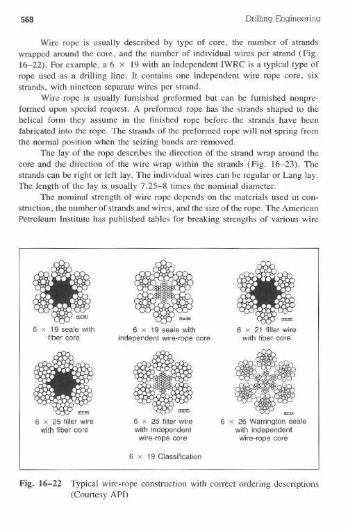
568 Drilling Engineering
Wire rope is usually described by type of core, the number of strandswrapped around the core, and the number of individual wires per strand (Fig.16-22). For example, a 6 x 19 with an independent IWRC is a typical type ofrope used as a drilling line. It contains one independent wire rope core, sixstrands, with nineteen separate wires per strand.
Wire rope is usually furnished prefonned but can be furnished nonpre-fonned upon special request. A prefonned rope has the strands shaped to thehelical fonn they assume in the finished rope before the strands have beenfabricated into the rope. The strands of the prefonned rope will not spring fromthe nonnal position when the seizing bands are removed.
The lay of the rope describes the direction of the strand wrap around thecore and the direction of the wire wrap within the strands (Fig. 16-23). Thestrands can be right or left lay. The individual wires can be regular or Lang lay.The length of the lay is usually 7.25-8 times the nominal diameter.
The nominal strength of wire rope depends on the materials used in con-struction, the number of strands and wires, and the size of the rope. The AmericanPetroleum Institute has published tables for breaking strengths of various wire
6 x 19 seale withfiber core
6 x 25 filler wirewith fiber core
6 x 19 seale withindependent wire-rope core
6 x 25 filler wirewith independentwire-rope core
6 x 19 Classification
6 x 21 filler wirewith fiber core
6 x 26 Warrington sealewith independentwire-rope core
Fig. 16-22 Typical wire-rope construction with correct ordering descriptions(Courtesy API)
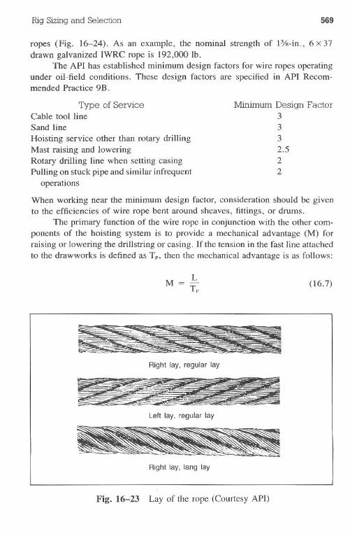
Rig Sizing and Selection 569
ropes (Fig. 16-24). As an example, the nominal strength of Pis-in., 6 X37drawn galvanized IWRC rope is 192,000 lb.
The API has established minimum design factors for wire ropes operatingunder oil-field conditions. These design factors are specified in API Recom-mended Practice 9B.
Type of ServiceCable tool lineSand line
Hoisting service other than rotary drillingMast raising and loweringRotary drilling line when setting casingPulling on stuck pipe and similar infrequent
operations
When working near the minimum design factor, consideration should be givento the efficiencies of wire rope bent around sheaves, fittings, or drums.
The primary function of the wire rope in conjunction with the other com-ponents of the hoisting system is to provide a mechanical advantage (M) forraising or lowering the drillstring or casing. If the tension in the fast line attached
to the drawworks is defined as TF, then the mechanical advantage is as follows:
Minimum Design Factor3332.522
(16.7)
Right lay, regular lay
Left lay, regular lay
Right lay, lang lay
Fig. 16-23 Lay of the rope (Courtesy API)
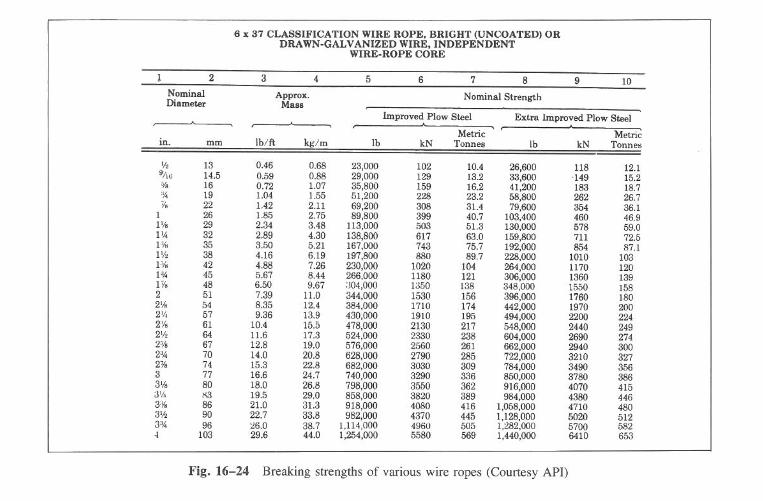
en....~tJS5'\QtT
J::s\Q5'C
DC
D....5'\Q
Fig.16-24
Breaking
strengthsof
variousw
ireropes
(Courtesy
API)
6x
37C
LA
SSIFICA
TIO
NW
IRE
RO
PE,
BR
IGH
T(U
NC
OA
TE
D)
OR
DR
AW
N-G
AL
VA
NIZ
ED
WIR
E,
IND
EPE
ND
EN
TW
IRE
-RO
PEC
OR
E
12
34
56
78
910
Nom
inalA
pprox.N
ominalStrength
Diam
eterM
assIm
provedPlow
SteelE
xtraIm
provedPlow
Steel.
..
...
.M
etricM
etricin.
mm
lb/ftkg/m
lbkN
Tonnes
IbkN
Tonnes
'/213
0.460.68
23,000102
10.426,600
11812.1
9/w14.5
0.590.88
29,000129
13.233,600
-14915.2
%16
0.721.07
35,800159
16.241,200
18318.7
:\419
1.041.55
51,200228
23.258,800
26226.7
v.22
1.422.11
69,200308
31.479,600
35436.1
126
1.852.75
89,800399
40.7103,400
46046.9
1'A!
292.34
3.48113,000
50351.3
130,000578
59.01%
322.89
4.30138,800
61763.0
159,800711
72.51%
353.50
5.21167,000
74375.7
192,000854
87.11%
384.16
6.19197,800
88089.7
228,0001010
103H
'.42
4.887.26
230,0001020
104264,000
1170120
1"0445
5.678.44
266.0001180
121306,000
1360139
Iv.48
6.509.67
:J04,0001350
138348,000
1550158
251
7.3911.0
344,0001530
156396,000
1760180
2'A!
548.35
12.4384,000
1710174
442,0001970
2002'4
579.36
13.9430,000
1910195
494,0002200
2242%
6110.4
15.5478,000
2130217
548,0002440
2492'/2
6411.6
17.3524,000
2330238
604,0002690
2742%
6712.8
19.0576,000
2560261
662,0002940
3002"04
7014.0
20.8628,000
2790285
722,0003210
3272"8
7415.3
22.8682,000
3030309
784,0003490
3563
7716.6
24.7740,000
3290336
850,0003780
3863'A
!80
18.026.8
798,0003550
362916,000
4070415
3'4'113
19.529.0
858,0003820
389984,000
4380446
3%86
21.031.3
918,0004080
4161,058,000
4710480
3'/290
22.733.8
982,0004370
4451,128,000
5020512
3%96
26.038.7
1,114,0004960
5051,282,000
5700582
10329.6
44.01,254,000
5580569
1,440,0006410
653
Rig Sizing and Selection 571
Where:L
TF =M=
hook load, Ibfast-line tension, Ibmechanical advantage
The fast-line tension can be computed from Eq. 16.8 if an ideal systemis considered:
(16.8)
Where:
N = number of lines strung over the block system
Since block efficiency (EB) must be considered in a non ideal case, the fast-linetension is as follows:
(16.9)
Example 16.4
A 13/s-in.,6 x 37 galvanized IWRC rope is to be used when running a 425,000-Ib casing string. The company man intends to rig-up a IO-line system. De-termine if the wire rope meets a design factor criteria of 2.0. Assume anefficiency of 0.98 per sheave. Use cols. 8-10, Fig. 16-24.
Solution:
l. The efficiency factor (EB) for a IO-line system is:
EB = (0.98)10EB = 0.817
(16.6)
2. The fast-line tension (TF) is computed from Eq. 16.9:
LTF = NEB
425,000 Ib(10)(0.817)
52,019lb
(16.9)
572 DrillingEngineering
3. The load factor is:
192,000 lb = 3.6952,019 lb
4. Therefore, the rope meets the design factor of 2.0.
The horsepower required to lift a load, L, at some velocity is given inEq. 16.3:
LVHP = 33,000 (16.3)
Where:
V = velocity, ft/min33,000 = ft-Ib/min/hp
This equation is very useful in determining the amount of input horsepowerrequirements from the prime movers. Block system and drawworks efficiencymust be considered:
(16.3a)
Where:HPBHPEEBED
= block horsepower= engine horsepower= block efficiency= drawworks efficiency
Example 16.5
A 260,000-lb drillstring is being used in a well. Company policy states thatthe rig will have sufficient horsepower to raise the string at a minimum rateof93 ftlmin (1 stand/min). The drawworks have 8 lines strung over the blocksystem. The drilling rig has a mechanical drive with the following configu-ration:
Engine No.2 3
No. shafts 4 5 6No. chains 3 4 5Total elements 7 9 II
Rig Sizingand Selection 573
Assume the torque converter has an efficiency of 0.75 and the efficiency foreach shaft, chain, and sheave pair isO.98. Determine the minimum acceptableinput horsepower and fast-line velocity.
Solution:
1. The horsepower required at the traveling block is computed from Eq. 16.3:
LVHP = 33,000
(260,000)(93 ft/min)33,000
732 hp
(16.3)
2. An 8-line block system has an efficiency factor of 0.850. The horse-power requirement at the drawworks will be greater than the block horse-power:
732HPD = 0.850
=861 hp
3. The fast-line tension (TF) is computed from Eq. 16.9:
(16.9)
260,000(8) (0.850)
= 38,235 lb
4. The fast-line velocity is:
TFVHPD = 33,000
(38,235 lb) (V)861 hp = 33,000
V = 743 ft/min
(16.3b)
The fast-line velocity can be computed as the product of pipe speed andnumber of lines strung over the block.
574 Drilling Engineering
5. The efficiency of the mechanical system for the chains and shafts betweenthe drawworks and the engines was calculated in Example 16.2 as 0.834:
HPDHPE = E
861 hp= 0.834
(16.3c)
= 1,032 hp (engine horsepower)
Wire rope must be monitored for fatigue wear resulting from raising andlowering the drillstring or casing. The usual practice is to evaluate the numberof ton-miles of work performed by the wire rope. A ton-mile is defined as theamount of work needed to move a I-ton load over a distance of I mile. Afterthe rope has reached a specified ton~mile limit, it is removed from service. Thelimits vary for different operations and may range from about 500 for 1.0-in.rope to about 1,800 for I%-in. rope. Drilling line also is cut (a portion is retired)before any critically strenuous job.
The major factors affecting ton-mile wear on the wire rope are round trips,setting casing, and drilling. Eq. 16.10 computes ton-miles during a round trip:
TR = D(Ls + D)WM + D(M + Y2C)10,560,000 2,640,000 (16.10)
Where:
TRD
LsWMMC
= ton-miles during a round trip
= hole depth, ft
= length of a drillpipe stand, ft= effective weight per foot of drillpipe, lb/ft= total weight of traveling block-elevator assembly
effective weight of drill-collar assembly minus the effective weightof the same length of drillpipe, lb/ft
Similar equations are provided in API RP 9B for coring, drilling, and settingcasing.
M is the weight of the traveling block assembly. It includes the travelingblock, hook, links, and elevators. If the actual weight of the traveling blockassembly is unknown, the following approximate values may be used:
Traveling BlockCapacity, tons
100150
Assembly Weight,lb
6,0009,000
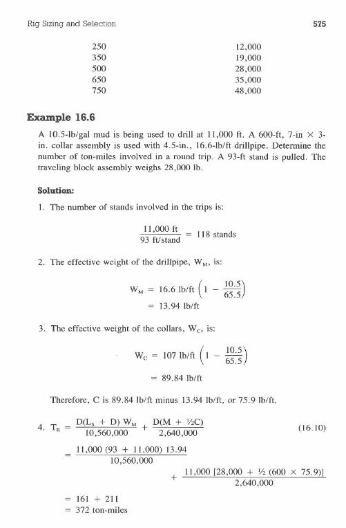
Rig Sizing and Selection 575
250350500650750
12,00019,00028,00035,00048,000
Example 16.6
A 1O.5-lb/gal mud is being used to drill at 11,000 ft. A 600-ft, 7-in x 3-in. collar assembly is used with 4.5-in., 16.6-lb/ft drillpipe. Determine thenumber of ton-miles involved in a round trip. A 93-ft stand is pulled. Thetraveling block assembly weighs 28,000 lb.
Solution:
1. The number of stands involved in the trips is:
11,000 ft93 ft/stand = 118 stands
2. The effective weight of the drillpipe, WM, is:
(10.5
)WM = 16.6 lb/ft 1 - 65.513.94 lb/ft
3: The effective weight of the collars, We, is:
(10.5
)We = 1071b/ft 1 - 65.5
= 89.84 Ib/ft
Therefore, C is 89.84 Ib/ft minus 13.94 lb/ft, or 75.9 Ib/ft.
D(Ls + D) WM D(M + Y2C)+10,560,000 2,640,000
11,000 (93 + 11,000) 13.9410,560,000
(16.10)
11,000 [28,000 + '12(600 x 75.9)]+2,640,000
161 + 211372 ton-miles
576 Drilling Engineering
The IADC provides an extensive set of tables for ton-mile calculations.The tables are often available in the field and may be easier for some field peopleto use. Drilling engineers planning a well may prefer to use the equations.
In addition to fatigue wear from accumulated ton-miles of service, thewire rope will wear more at lap and pickup points. The pickup points are on thetop side of the crown block when the weight of the drillstring is lifted from itssupports in the rotary table during tripping operations. The lap points on thedrawworks drum occur when the line begins a new wrap.
Slip and cut programs are designed to avoid excessive wear at the lap andpickup points. Slipping involves loosening the dead-line anchor and placing afew more feet of line into service from the storage reel. Cutting requires thatthe line on the drawworks reel be loosened and a section cut and removed.
Slipping changes the pickup points, and cutting changes the lap points. A lineis usually slipped several times before it is cut. Care must be exercised to ensurethe line is not slipped sufficiently to allow the pickup point to be moved fromone sheave to another. Similar care must be given to the cutting program.
Derrick and Substructures. The derrick and substructure play an im-portant role in drilling operations. The derrick provides the vertical height nec-essary for the hoisting system to raise and lower the pipe. The substructureprovides the height required for the blowout preventer stack on the wellheadbelow the rig floor. The derrick and the substructure must have enough strengthto support all loads, including the hook load, pipe set in the derrick, and windloads.
The API has developed size classifications for the derrick shown in Fig.16-25. The specifications are summarized in Table 16-1. In addition, Table16-1 contains data used in determining wind loading.
The derrick and substructure must be able to support the loads imposedby pipe weight on the block plus a portion of the drillstring standing in thederrick. Due to the manner in which the hook load is distributed over the derrick,the effective load may exceed the actual. When heavy casing strings are run, itmay be necessary to lay down some drillpipe initially so the derrick loadingcapacity is not exceeded.
The derrick load resulting from a hook load can be evaluated with Fig.16-26. The force on the derrick (FD) includes the hook load, L; the tension inthe fast line, TF; and the tension in the dead line, TD:
(l6.11)
The tension in the fast line in a nonideal environment, including friction, isshown in Eq. 16.9:
(16.9)
Rig Sizing and Selection 577
J 1N,1
.T-f ~-t l ~A -tf+~
~B~A- Vertical distance from the top of the base plate to the bottom ofthe crown block support beam
B -Distance between heel to heel of adjacent legs at the top of thebase plate
C -Window opening measure in the clear and parallel to the centerline of the derrick side from top of base plate
D - Smallest clear dimension at the top of the derrick that wouldrestrict passage of crown blockE - Clearance between the horizontal header of the gin pole and thetop of the crown support beam
Fig. 16-25 Derrick size classifications (Courtesy API)
Since the dead line does not move, the tension is shown in Eq. 16.12:
LTD = N (16.12)
Eq. 16.11 can be rewritten as follows:
L LFD = L + NEB + N
L (1 + EB + EBN)EBN
(16.13)
The total force on the derrick (FD) is not evenly distributed over each ofthe four legs (Fig. 16-27). The fast-line tension is distributed evenly between
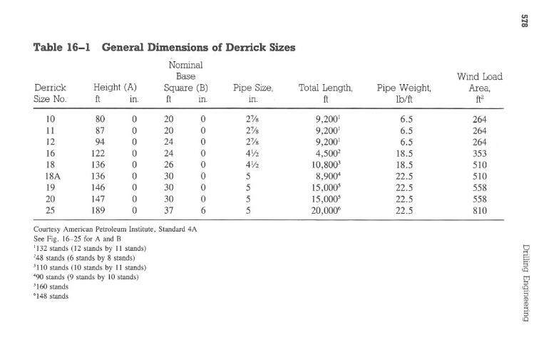
Courtesy
Am
ericanPetroleum
Institute,Standard
4A
SeeFig.
16-25for
Aand
B
'132stands
(12stands
by11
stands)
'48stands
(6stands
by8
stands)
3110stands
(10stands
by11
stands)
490stands
(9stands
by10
stands)'160
stands
6148stands
en~S(g.lQ~~.C
DC
DS'lQ
Table
16-1G
eneralD
imensions
ofD
errickSizes
Nom
inalB
aseW
indL
oadD
errickH
eight(A
)Square
(B)
PipeSize,
Total
Length,
PipeW
eight,A
rea,Size
No.
ftin.
ftm
.in.
ftlb/ft
ft2
1080
020
02'l's
9,200.6.5
26411
870
200
2'l's9,200.
6.5264
1294
024
02'l's
9,200.6.5
26416
1220
240
4Y2
4,500218.5
35318
1360
260
4Y2
10,800318.5
51018A
1360
300
58,900"
22.5510
19146
030
05
15,000s22.5
55820
1470
300
515,O
OO
s22.5
55825
1890
376
520,0006
22.5810
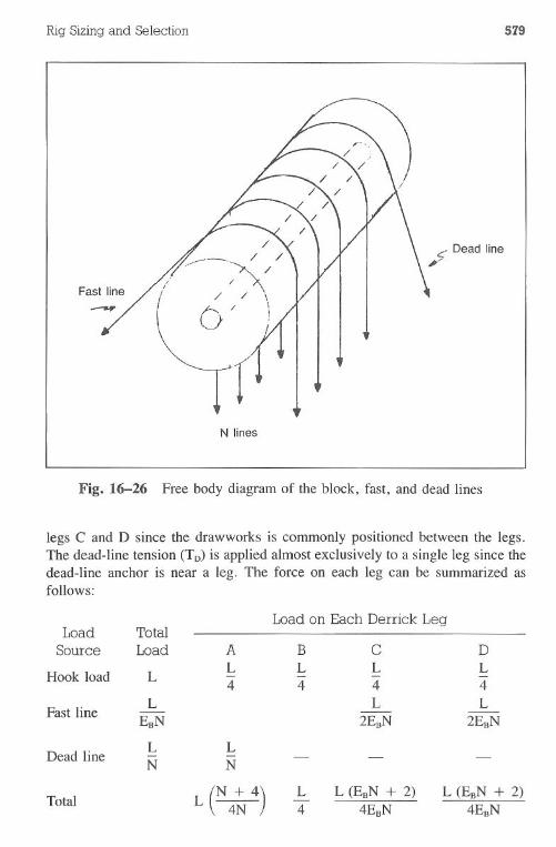
Rig Sizingand Selection 579
c: Dead line;/
N lines
Fig. 16-26 Free body diagram of the block, fast, and dead lines
legs C and D since the drawworks is commonly positioned between the legs.The dead-line tension (TD)is applied almost exclusively to a single leg since thedead-line anchor is near a leg. The force on each leg can be summarized asfollows:
Load on Each Derrick LegLoad Total
Source Load A B C D
Hook load LL L L L4 4 4 4
Fast lineL L L
EoN 2EoN 2EoN
Dead lineL LN N
- - -
TotalL (N4 4)
L L (EoN + 2) L (EoN + 2)4 4EoN 4EoN
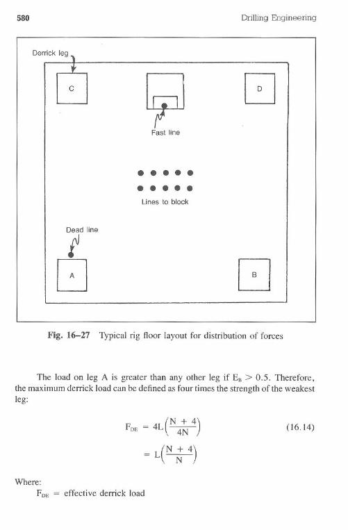
580 Drilling Engineering
Fig. 16-27 Typical rig floor layout for distribution of forces
The load on leg A is greater than any other leg if EB> 0.5. Therefore,the maximum derrick load can be defined as four times the strength of the weakestleg:
FDE = 4L(N 4~ 4) (16.14)
Where:FDE = effectivederrickload
Derrickleg\'I-
c 8Fast line
..........Lines to block
Deadline
t[] 8
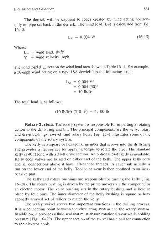
Rig Sizingand Selection 581
The derrick will be exposed to .Ioads created by wind acting horizon-tally on pipe set back in the derrick. The wind load (Lw) is calculated from Eq.16.15:
Lw = 0.004 y2 (16.15)
Where:Lw = wind load, Ib/ft2y = wind velocity, mph
The wind load (Lw)acts on the wind load area shown in Table 16-1. For example,a 50-mph wind acting on a type 18A derrick has the following load:
Lw = 0.004 y2= 0.004 (50f= 10 lb/fe
The total load is as follows:
(10 Ib/fe) (510 fe) 5,1001b
Rotary System. The rotary system is responsible for imparting a rotatingaction to the drill string and bit. The principal components are the kelly, rotaryand drive bushings, swivel, and rotary hose. Fig. 15-1 illustrates some of thecomponents of the rotary system.
The kelly is a square or hexagonal member that screws into the drillstringand provides a flat surface for applying torque to rotate the pipe. The standardkelly is 40 ft long with a 37-ft drive section. An optional 54-ft kelly is available.Kelly cock valves are located on either end of the kelly. The upper kelly cockand all connections above it have left-handed threads. A saver sub usually isrun on the lower end of the kelly. Tool joint wear is then confined to an inex-pensive part.
The kelly and rotary bushings are responsible for turning the kelly (Fig.16-28). The rotary bushing is driven by the prime movers via the compound oran electric motor. The kelly bushing sits in the rotary bushing and is held inplace by four pins. The inner diameter of the kelly bushing is square or hex-agonally arrayed set of rollers to match the kelly.
The rotary swivel serves two important functions in the drilling process.It is a connecting point between the circulating system and the rotary system.In addition, it provides a fluid seal that must absorb rotational wear while holdingpressure (Fig. 16-29). The upper section of the swivel has a bail for connectionto the elevator hook.
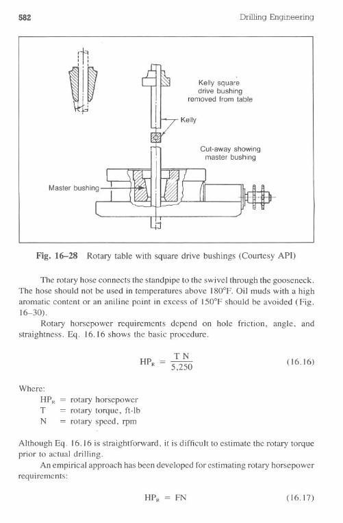
582 Drilling Engineering
.Kelly squaredrive bushing
removed from table
Cut-away showingmaster bushing
Fig. 16-28 Rotary table with square drive bushings (Courtesy API)
The rotary hose connects the standpipe to the swivel through the gooseneck.The hose should not be used in temperatures above 180°F. Oil muds with a higharomatic content or an aniline point in excess of 150°F should be avoided (Fig.16-30).
Rotary horsepower requirements depend on hole friction, angle, andstraightness. Eq. 16.16 shows the basic procedure.
TN5,250
(16.16)
Where:HPRTN
rotary horsepowerrotary torque, ft-Ibrotary speed, rpm
Although Eq. 16.16 is straightforward, it is difficult to estimate the rotary torqueprior to actual drilling.
An empirical approach has been developed for estimating rotary horsepowerrequirements:
FN (16.17)
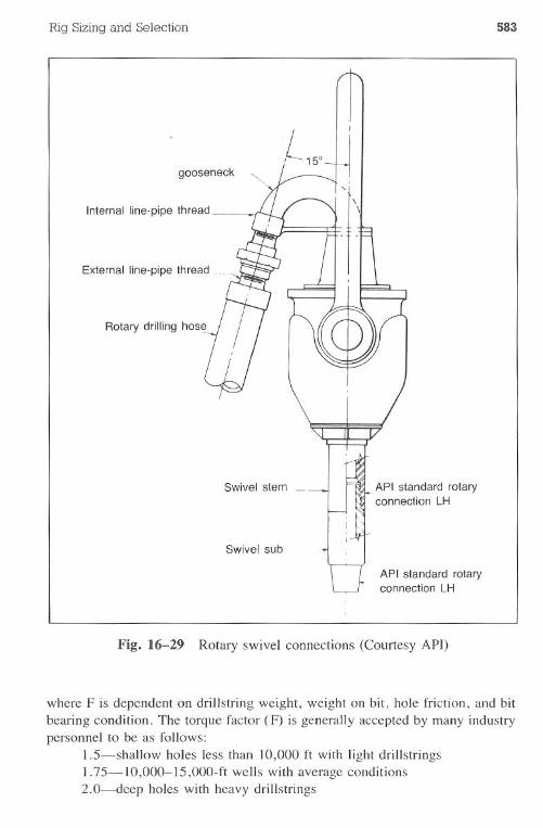
Rig Sizing and Selection 583
gooseneck
Swivel stem _ API standard rotaryconnection LH
Internal line-pipe thread
External line-pipe thread ____.
Rotary drilling hos~
Swivel sub
API standard rotaryconnection LH
Fig. 16-29 Rotary swivel connections (Courtesy API)
where F is dependent on drill string weight, weight on bit, hole friction, and bitbearing condition. The torque factor (F) is generally accepted by many industrypersonnel to be as follows:
I.S-shallow holes less than 10,000 ft with light drill strings1.7S-IO,000-IS,000-ft wells with average conditions
2.0-deep holes with heavy drillstrings
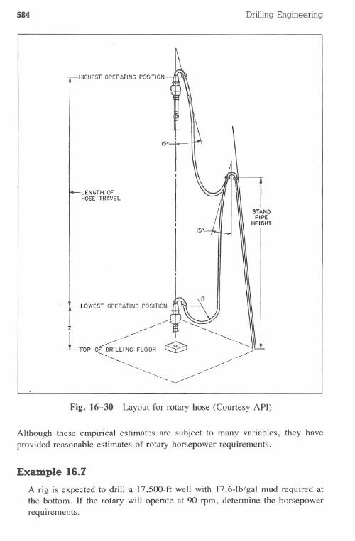
584 DrillingEngineering
ISO.
STANOPIPE
HEIGHT
HIGHEST OPERATING POSITION-
LENGTH OFHOSE TRAVEL
LOWEST OPERATING POSITION-
..-!""'/'Z ,...
_/'
lTOP OFD~~G FLQOR ~ ,...,.../'--
/',.......
Fig. 16-30 Layout for rotary hose (Courtesy API)
Although these empirical estimates are subject to many variables, they haveprovided reasonable estimates of rotary horsepower requirements.
Example 16.7
A rig is expected to driII a 17,500-ft well with 17.6-lb/gal mud required atthe bottom. If the rotary will operate at 90 rpm, determine the horsepowerrequirements.
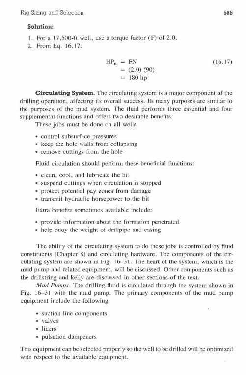
Rig Sizing and Selection 585
Solution:
l. For a 17,500-ft well, use a torque factor (F) of 2.0.2. FromEq.16.17:
FN(2.0) (90)180 hp
(16.17)
Circulating System. The circulating system is a major component of the
drilling operation, affecting its overall success. Its many purposes are similar tothe purposes of the mud system. The fluid performs three essential and foursupplemental functions and offers two desirable benefits.
These jobs must be done on all wells:
. control subsurface pressures. keep the hole walls from collapsing. remove cuttings from the hole
Fluid circulation should perform these beneficial functions:
. clean, cool, and lubricate the bit. suspend cuttings when circulation is stopped. protect potential pay zones from damage. transmit hydraulic horsepower to the bit
Extra benefits sometimes available inClude:
. provide information about the formation penetrated. help buoy the weight of drill pipe and casing
The ability of the circulating system to do these jobs is controlled by fluidconstituents (Chapter 8) and circulating hardware. The components of the cir-culating system are shown in Fig. 16-31. The heart of the system, which is themud pump and related equipment, will be discussed. Other components such asthe drill string and kelly are discussed in other sections of the text.
Mud Pumps. The drilling fluid is circulated through the system shown inFig. 16-31 with the mud pump. The primary components of the mud pumpequipment include the following:
. suction line components· valves· liners· pulsation dampeners
This equipment can be selected properly so the well to be drilled will be optimizedwith respect to the available equipment.
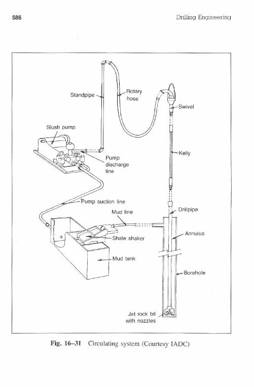
586 Drilling Engineering
StandpipeRotaryhose
Slush pump
Pumpdischargeline
Kelly
o
S .Drillplpe
Borehole
Jet rock bitwith nozzles
Fig. 16-31 Circulating system (Courtesy IADC)
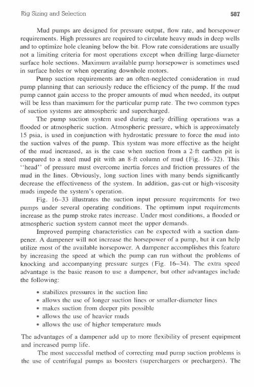
Rig Sizingand Selection 587
Mud pumps are designed for pressure output, flow rate, and horsepowerrequirements. High pressures are required to circulate heavy muds in deep wellsand to optimize hole cleaning below the bit. Flow rate considerations are usuallynot a limiting criteria for most operations except when drilling large-diametersurface hole sections. Maximum available pump horsepower is sometimes usedin surface holes or when operating downhole motors.
Pump suction requirements are an often-neglected consideration in mudpump planning that can seriously reduce the efficiency of the pump. If the mudpump cannot gain access to the proper amounts of mud when needed, its outputwill be less than maximum for the particular pump rate. The two common typesof suction systems are atmospheric and supercharged.
The pump suction system used during early drilling operations was aflooded or atmospheric suction. Atmospheric pressure, which is approximately15 psia, is used in conjunction with hydrostatic pressure to force the mud intothe suction valves of the pump. This system was more effective as the heightof the mud increased, as is the case when suction from a 2-ft earthen pit iscompared to a steel mud pit with an 8-ft column of mud (Fig. 16-32). This"head" of pressure must overcome inertia forces and friction pressures of themud in the lines. Obviously, long suction lines with many bends significantlydecrease the effectiveness of the system. In addition, gas-cut or high-viscositymuds impede the system's operation.
Fig. 16-33 illustrates the suction input pressure requirements for twopumps under several operating conditions. The optimum input requirementsincrease as the pump stroke rates increase. Under most conditions, a flooded oratmospheric suction system cannot meet the upper demands.
Improved pumping characteristics can be expected with a suction dam-pener. A dampener will not increase the horsepower of a pump, but it can helputilize most of the available horsepower. A dampener accomplishes this featureby increasing the speed at which the pump can run without the problems ofknocking and accompanying pressure surges (Fig. 16-34). The extra speedadvantage is the basic reason to use a dampener, but other advantages includethe following:
· stabilizes pressures in the suction line· allows the use of longer suction lines or smaller-diameter lines· makes suction from deeper pits possible· allows the use of heavier muds· allows the use of higher temperature muds
The advantages of a dampener add up to more flexibility of present equipmentand increased pump life.
The most successful method of correcting mud pump suction problems isthe use of centrifugal pumps as boosters (superchargers or prechargers). The
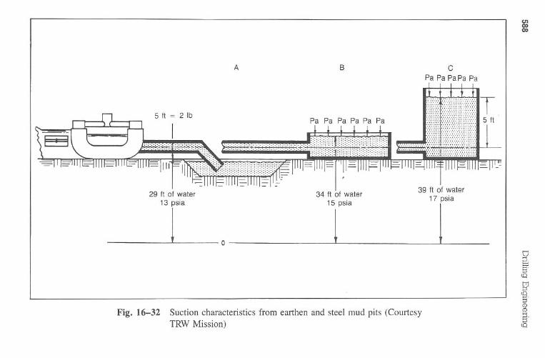
AB
CPa
PaPaPa
Pa
5ft
=2
Ib
29ft
ofw
ater13
psia34
ftof
water
15psia
o
Fig.
16-32Suction
characteristicsfrom
earthenand
steelmud
pits(C
ourtesyT
RW
Mission)
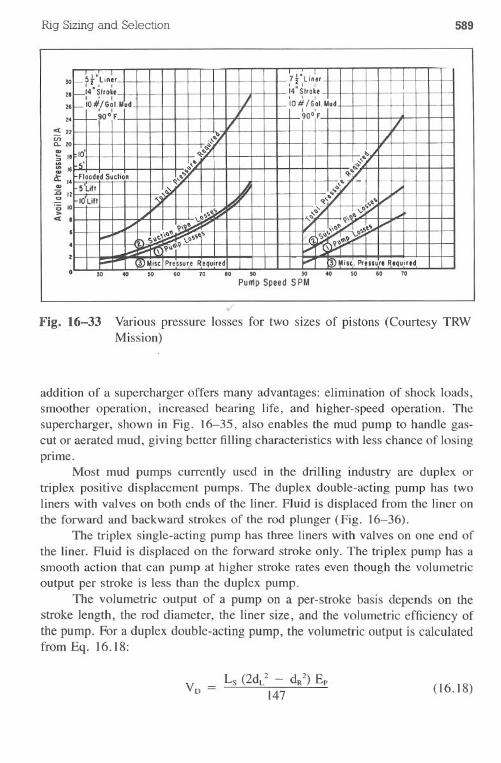
Rig Sizingand Selection 589
30
II
H
~ . " 60 ~ .0 ~ H. ~ " ~pump SpeedSPM
I'< II~20~ 18~.. "Q)
ct I'Q)
:is 12<>
=s 10><
Fig. 16-33 Various pressure losses for two sizes of pistons (Courtesy TRWMission)
addition of a supercharger offers many advantages: elimination of shock loads,smoother operation, increased bearing life, and higher-speed operation. Thesupercharger, shown in Fig. 16-35, also enables the mud pump to handle gas-cut or aerated mud, giving better filling characteristics with less chance of losingprime.
Most mud pumps currently used in the drilling industry are duplex ortriplex positive displacement pumps. The duplex double-acting pump has twoliners with valves on both ends of the liner. Fluid is displaced from the liner onthe forward and backward strokes of the rod plunger (Fig. 16-36).
The triplex single-acting pump has three liners with valves on one end ofthe liner. Fluid is displaced on the forward stroke only. The triplex pump has asmooth action that can pump at higher stroke rates even though the volumetricoutput per stroke is less than the duplex pump.
The volumetric output of a pump on a per-stroke basis depends on thestroke length, the rod diameter, the liner size, and the volumetric efficiency ofthe pump. For a duplex double-acting pump, the volumetric output is calculatedfrom Eq. 16.18:
Ls (2dL2 - dR2)Ep147 (16.18)
I _SrLinr 7 !"Unlr II..' I I 21 I
1 -14 tro\e 14'StrohI ' , I
I _IO/Gl.hd 10#/Gol.MudI ,
_ _90° F 90°F1/ /
.,,, /
10' ..<>j..I>
.' ," ','....
Flooded Suelio. .... VS'Lilt
,A ....'llI."
10Lilt V'I I ..,,,;"
'-....'. 0/I ..... . "", f\"'" Y1 .." ""I
'>.. r:t'>" ....'t.....
I?"1 I ....., I-
! ... VMisejPressureRlquired ". ill Mise.Pr..surl R.quired
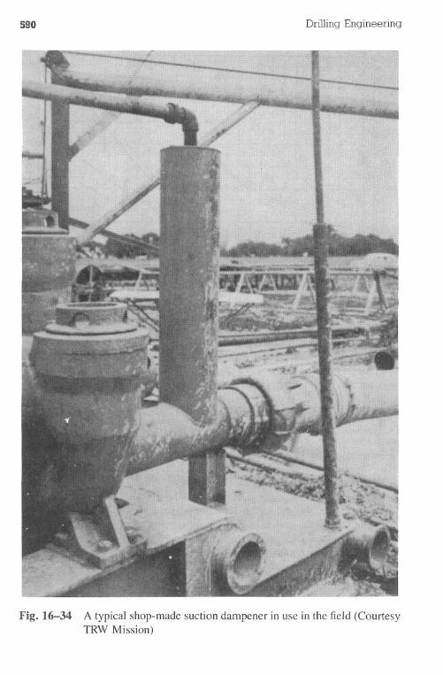
590 DrillingEngineering
Fig. 16-34 A typical shop-made suction dampener in use in the field (CourtesyTRW Mission)
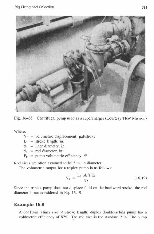
Rig Sizing and Selection 591
Fig. 16-35 Centrifugal pump used as a supercharger (Courtesy TRW Mission)
Where:
VD =LsdLdREp
volumetric displacement, gal/strokestroke length, in.liner diameter, in.
= rod diameter, in.= pump volumetric efficiency, %
Rod sizes are often assumed to be 2 in. in diameter.The volumetric output for a triplex pump is as follows:
Ls (dL2)EpVT = 98 (16.19)
Since the triplex pump does not displace fluid on the backward stroke, the roddiameter is not considered in Eq. 16.19.
Example 16.8A 6 x I8-in. (liner size x stroke length) duplex double-acting pump has avoh!metric efficiency of 87%. T.herod size is the standard 2 in. The pump
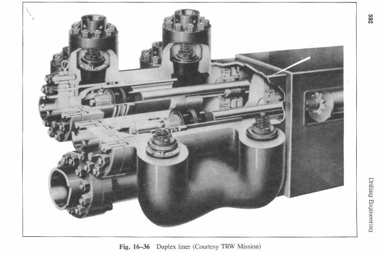
592D
rillingE
ngineering
><
Q)
c..::3o
/'
Rig Sizing and Selection 593
rate is 48 spm. The IO,OOO-ft,4Y2-in.drillstring has a capacity of 0.01422bbllft. The 4Y2 x 8Y2 in. annulus (10,000 ft) has a capacity of 0.05 bbllft.Detennine the volumetric output per stroke, the output per minute, and thestrokes and minutes to displace the annulus and the drillstring. Neglect thedrill collars.
Solution:
I. The volumetric output is computed from Eq. 16.18:
Ls (2dL2- dR2)Ep147
18 [2 (6f - 22] 0.87147
(16.18)
= 7.24 gal/stroke= 0.172 bbl/stroke
2. The volumetric output per minute is the product of the output per strokeand the stroke rate:
(0.172 bbllstroke) (48 spm) = 8.25 bbl/min
3. The drillstring capacity is:
0.01422 bbllft x 10,000 ft = 142 bbl
142 bbl8.25 bbllmin
142 bbl0.172 bbllstroke = 825 strokes
17.2 min
4. The annulus displacement is:
0.05 bbllft x 10,000 ft = 500 bbl
500 bbl .8.25 bbl/min = 60.6 mm
500 bbl = 2,906 strokes
The volumetric output of a pump can be reduced in several ways. Thepump rate can be reduced or a smaller liner can be installed. In an emergency
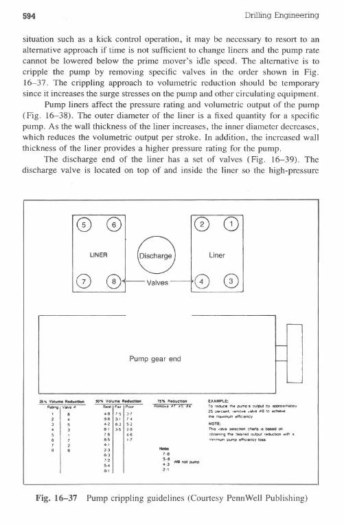
594 Drilling Engineering
situation such as a kick control operation, it may be necessary to resort to analternative approach if time is not sufficient to change liners and the pump ratecannot be lowered below the prime mover's idle speed. The alternative is tocripple the pump by removing specific valves in the order shown in Fig.16-37. The crippling approach to volumetric reduction should be temporarysince it increases the surge stresses on the pump and other circulating equipment.
Pump liners affect the pressure rating and volumetric output of the pump(Fig. 16-38). The outer diameter of the liner is a fixed quantity for a specificpump. As the wall thickness of the liner increases, the inner diameter decreases,which reduces the volumetric output per stroke. In addition, the increased wallthickness of the liner provides a higher pressure rating for the pump.
The discharge end of the liner has a set of valves (Fig. 16-39). Thedischarge valve is located on top of and inside the liner so the high-pressure
25"40 Y0h8m8 R8ducdaft
RatIng y.,. ~
, 82 ,3 5, 35 ,8 77 28 8
CD o (0UNER
8 CD
Liner
o o Valves
Pump gear end
SO,. Volume Redwctlon
IF.. .....
~:
I
~~ ;=".2 &3 Sol8-1 J.S 2.878 "6&5 I.'4.'2.3"37.2...,..,
75"R8dYCttoflRemove ., _~ ,I,
EXAMP\.E:
Toreouc. !he putnc)"~ oulput oy IIO"Olwnately
25 =*'c remove 18 10 ~the maamum .mc:sency
NOn,Tha ,1tvtI H'Kbon :hIftI " b8Hd on001."""0 rh8 <jellied outoul r8dl.ctcn *,11h.m.nttnumpump effic/8l'1CY1088.-7.8
5.8 VIM not putf'O'.32.'
Fig. 16-37 Pump crippling guidelines (Courtesy PennWell Publishing)
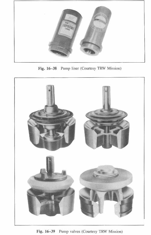
J
Fig. 16-38 Pump liner (Courtesy TRW Mission)
\.,
Fig. 16-39 Pump valves (Courtesy TRW Mission)
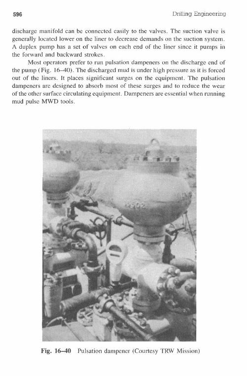
596 Drilling Engineering
discharge manifold can. be connected easily to the valves. The suction valve isgenerally located lower on the liner to decrease demands on the suction system.A duplex pump has a set of valves on each end of the liner since it pumps inthe forward and backward strokes.
Most operators prefer to run pulsation dampeners on the discharge end ofthe pump (Fig. 16-40). The discharged mud is under high pressure as it is forcedout of the liners. It places significant surges on the equipment. The pulsationdampeners are designed to absorb most of these surges and to reduce the wearof the other surface circulating equipment. Dampeners are essential when runningmud pulse MWD tools.
r.
Fig. 16-40 Pulsation dampener (Courtesy TRW Mission)
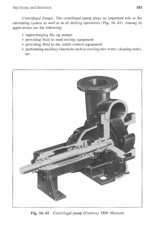
Rig Sizingand Selection 597
Centrifugal Pumps. The centrifugal pump plays an important role in thecirculating system as well as in all drilling operations (Fig. 16-41). Among itsapplications are the following:
. supercharging the rig pumps .. providing fluid to mud-mixing equipment. providing fluid to the solids control equipment. performing ancillary functions such as moving mix water, cleaning tanks,etc.
..
Fig. 16-41 Centrifugal pump (Courtesy TRW Mission)
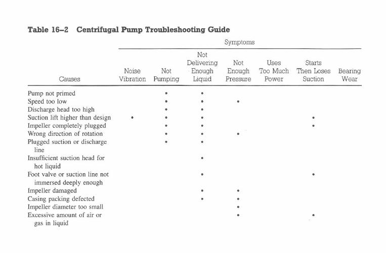
Table
16-2C
entrifugalP
ump
Troubleshooting
GuideSym
ptoms
Causes
enCQ
co
Noise
Vibration
Not
Pumping
Not
Delivering
.Enough
Liquid
Not
Enough
Pressure
Uses
Too
Much
Power
StartsT
henL
osesSuction
BearingW
ear
Pump
notprim
edSpeed
toolow
Discharge
headtoo
highSuction
lifthigher
thandesign
Impeller
completely
pluggedW
rongdirection
ofrotation
Pluggedsuction
ordischarge
lineInsufficientsuction
headfor
hotliquid
Footvalveor
suctionline
not
imm
erseddeeply
enoughIm
pellerdam
agedC
asingpacking
defectedIm
pellerdiam
etertoo
small
Excessive
amount
ofair
orgas
inliquid
..
..
..
..
..
..
..
.....
.
.
...
S(
t::
.s-\Q
.S
.E
r.
(1).
(1)....E
r\Q
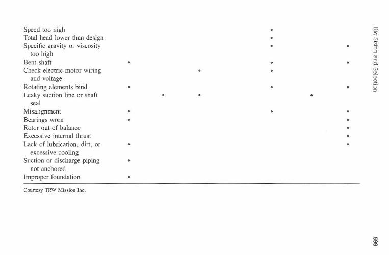
en<D<D
Speedtoo
high.
cQT
otalheadlow
erthandesign
.C
f)
SpecificgravityorviscosityN
'.
.E
r
toohigh
cQOJ
Bent
shaft.
..
::IQ.
Check
electricmotorw
iring.
.C
f)C
D
andvoltage
roQ.
Rotating
elements
birid.
..
o'::I
Leaky
suctionlineorshaft
..
.seal
Misalignm
ent.
..
Bearings
worn
..
Rotoroutofbalance
.E
xcessiveinternalthrust.
Lack
oflubrication,
dirt,or
..
excessivecoolingSuctionordischargepiping
.not
anchored
Improperfoundation
.C
ourtesyT
RW
Mission
Inc.
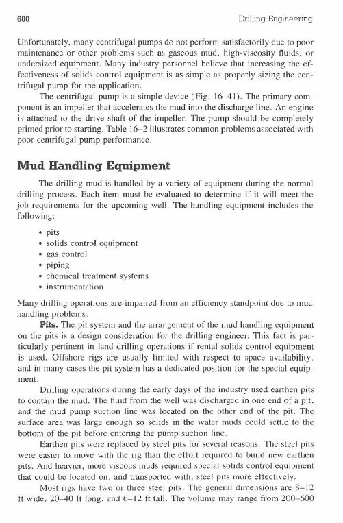
600 Drilling Engineering
Unfortunately, many centrifugal pumps do not perform satisfactorily due to poormaintenance or other problems such as gaseous mud, high-viscosity fluids, orundersized equipment. Many industry personnel believe that increasing the ef-fectiveness of solids control equipment is as simple as properly sizing the cen-trifugal pump for the application.
The centrifugal pump is a simple device (Fig. 16-41). The primary com-ponent is an impeller that accelerates the mud into the discharge line. An engineis attached to the drive shaft of the impeller. The pump should be completelyprimed prior to starting. Table 16-2 illustrates common problems associated withpoor centrifugal pump performance.
Mud Handling EquipmentThe drilling mud is handled by a variety of equipment during the normal
drilling process. Each item must be evaluated to determine if it will meet the
job requirements for the upcoming well. The handling equipment includes thefollowing:
· pits· solids control equipment.gas control· piping·chemical treatment systems· instrumentation
Many drilling operations are impaired from an efficiency standpoint due to mudhandling problems.
Pits. The pit system and the arrangement of the mud handling equipmenton the pits is a design consideration for the drilling engineer. This fact is par-ticularly pertinent in land drilling operations if rental solids control equipmentis used. Offshore rigs are usually limited with respect to space availability,and in many cases the pit system has a dedicated position for the special equip-ment.
Drilling operations during the early days of the industry used earthen pitsto contain the mud. The fluid from the well was discharged in one end of a pit,and the mud pump suction line was located on the other end of the pit. Thesurface area was large enough so solids in the water muds could settle to thebottom of the pit before entering the pump suction line.
Earthen pits were replaced by steel pits for several reasons. The steel pitswere easier to move with the rig than the effort required to build new earthen
pits. And heavier, more viscous muds required special solids control equipmentthat could be located on, and transported with, steel pits more effectively.
Most rigs have two or three steel pits. The general dimensions are 8-12ft wide, 20-40 ft long, and 6-12 ft tall. The volume may range from 200-600
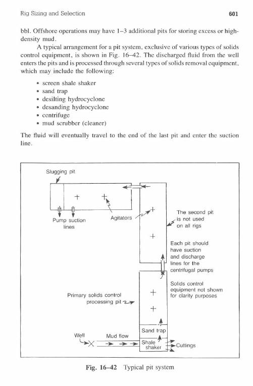
Rig Sizing and Selection 601
bbl. Offshore operations may have 1-3 additional pits for storing excess or high-density mud.
A typical arrangement for a pit system, exclusive of various types of solidscontrol equipment, is shown in Fig. 1~2. The discharged fluid from the wellenters the pits and is processed through several types of solids removal equipment,which may include the following:
· screen shale shaker· sand trap· desiIting hydrocyclone.desanding hydrocyclone. centrifuge· mud scrubber (cleaner)
The fluid will eventually travel to the end of the last pit and enter the suctionline.
Slugging pit
1-
+~ ;f-The second pitis not usedon all rigs
~~Pump suction
lines
+Each pit shouldhave suction
and dischargelines for the
centrifugal pumps
Primary solids controlprocessing pit ~
+Solids controlequipment not shownfor clarity purposes
+
Well
~XMud flow+ +.... Cuttings
Fig. 16-42 Typical pit system
602 Drilling Engineering
The first pit contai~s most of the solids control equipment. The second pitwas used in the early days as a settling pit for mud solids. However, a few simplecalculations indicate that most mud solids will not settle in the pit in view ofthe relatively short amount of time required for the mud to travel through thepit. Currently, the second pit contains some of the solids control equipment ifthe pit is even available. The last pit contains the mud suction lines, the sluggingpit for preparing heavy slugs used prior to tripping, and the chemical treatmentdischarge lines.
Pits contain agitation systems to stir the mud and to minimize barite orsolids settling. Two common agitators are I) submerged swirling fan bladesdriven by independent electric motors and 2) centrifugal pump-driven jets, ormud guns, that force high-velocity streams of mud into the pits (Fig. 16-43).Either system will function effectively if planned properly.
An important operating guideline is to ensure that the agitators do notcause air to be entrained in the mud. Aerated mud reduces the effectiveness of
the centrifugal pumps used to drive the solids control equipment and reducesthe volumetric output of the mud pumps.
Solids Control Equipment. Removal of undesirable solids from the drill-
ing mud is receiving more interest and effort. Industry personnel have demon-strated that control over these solids can reduce drilling costs in the followingmanners:
.increased drilling rates by enhancing cuttings removal· better bit hydraulics due to lower fluid viscosities. less wear on surface equipment such as the mud pumps
In addition, formation damage is reduced since the mud contains fewer drilledsolids that invade and block the permeability flow channels (see Chapter 6).
Solids are removed from the mud system by settling, screening, centri-fuging, or dilution. Settling is ineffective in most cases due to weighted mudsystems or lack of time for gravity segregation. Dilution is expensive with heavymud systems. The principles employed for most commonly used solids removalequipment are screening, centrifuging, or a combination.
The solids control equipment must be designed to remove very smallparticles. Mud system particles are I-50 /-I.in diameter. The most damagingparticle with respect to solids control is less than I /-I..(A micron is one-millionthof a meter.) Since commercially available solids removal equipment cannotcontrol solids less than about 15 /-I.,large solids must be removed prior to theirregrinding and recirculation back downhole. Table 16-3 provides various itemsindicating the size of particles that must be removed.
Sand Traps. A sand trap is a small, compartmented section of the firstpit immediately adjacent to the shale shaker. The effluent from the shale shakerflows into the sand trap. Its purpose is to allow settling of heavy particles suchas sand or shale cuttings that escaped removal by the shaker screen. It is often
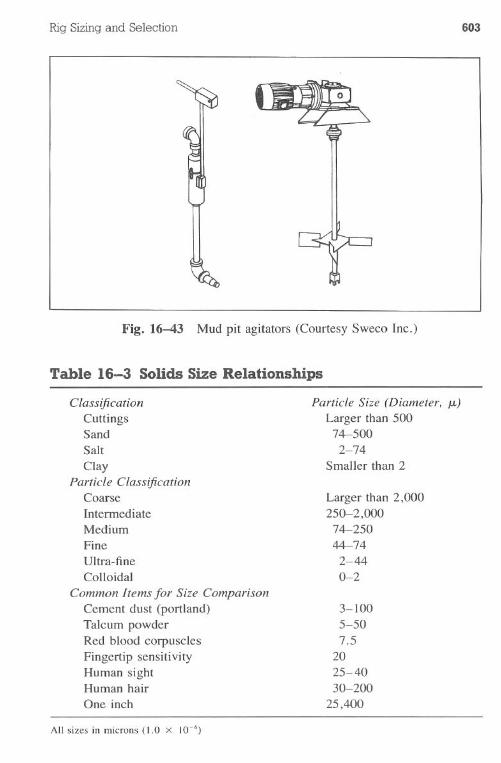
Rig Sizingand Selection 603
Fig. 16-43 Mud pit agitators (Courtesy Sweeo Inc.)
Table 16-3 Solids Size Relationships
ClassificationCuttingsSandSaltClay
Particle ClassificationCoarselntennediateMediumFineUltra-fineColloidal
Common Items for Size ComparisonCement dust (portland)Talcum powderRed blood corpusclesFingertip sensitivityHuman sightHuman hairOne inch
Particle Size (Diameter. 11-)
Larger than 50074-500
2-74Smaller than 2
Larger than 2,000250-2,00074-25044-74
2-440-2
3-1005-507.5
2025-4030-200
25,400
All sizes in microns (1.0 x 10⁻⁶)
604 DrillingEngineering
used effectively when sand screens develop tears or when high-viscosity mudsmust bypass the shaker for a short time. It should not be considered as a primarysolids control device in standard operations.
Shale Shakers. The most important member of the solids control equip-ment group is the shale shaker. It removes the major portion of all drilled solidscirculated out of the well. In addition, it removes the large cuttings that wouldplug the other equipment.
Although many manufacturers produce shale shakers, the designs are rea-sonably similar (Fig. 16-44). Mud flows from the well flow line into the possumbelly, or mud box. The possum belly has a lower bypass gate (not shown) sothat mud can flow directly into the sand trap and pits in case the screens plugwith viscous mud or solids. The mud and cuttings flow over the screen(s).Depending on the openings in the screen mesh, the mud and small-diameterparticles fall through the screen and exit at the discharge chute. The vibrating,or rotating, assembly on the screen causes the larger particles to move along tothe end and off the screen (Fig. 16-45).
Various screen arrangements are available on common shakers (Fig.16-45). Multiple-screen shakers are widely used and can offer better solidsremoval. The particle separation with a multiple-deck screen is determined bythe finest mesh screen, which is usually the bottom screen. The size separationwith the parallel arrangement is determined by the coarsest screen size.
Screening surfaces used in solids-control equipment are generally made ofwoven wire screen cloth in many different sizes and shapes. Characteristi~s of
Mud box(possum belly)
Vibrator assembly
Belt guard
Basketassembly
Liquidand fine solidsdischarge chute
Coarse solids discharge
Fig. 16-44 Rig shaker components (Courtesy Sweco Inc.)
Rig Sizing and Selection 605
the screen cloth that must be considered by the drilling engineer are mesh sizeas well as the shape and size of openings. Screen sizing will ultimately affectthe mud and drilling costs.
Mesh is defined as the number of openings per linear inch. Mesh can bemeasured by starting at the center of one wire and counting the number ofopenings per inch (Fig. 16-46). Table 16-4 provides an indication of commonscreen sizes that are available commercially. Mesh sizes above 100x 100 arenot used frequently since they may plug with heavy, viscous muds or high cuttingscontent.
Fig. 16-45 Fine screen shaker vibrator positions (Courtesy Sweco Inc.)
606 Drilling Engineering
Fig. 16-46 Eight-mesh screen (Courtesy Sweco Inc.)
--
1.
tll I I I I 1 I 1211- INCH£S
t- -
Table 16-4 Screen Cloth Sizes
Wire OpenDiameter, Area,
Mesh in. % Size. JL
10x 10* 0.0258 56.3 101020 x 20 0.0162 46.2 84130 x 30 0.0128 32.1 51640x40 0.0104 36.0 38050 x 50 0.0090 30.3 27960x60 0.0075 30.5 23480 x 80 0.0055 31.4 177
100x 100 0.0045 30.3 140120x 120 0.0037 30.5 118ISOx ISO 0.0026 37.9 105200 x 200 0.0020 33.6 74250 x 250 0.0016 36.0 63325 x 325 0.0014 30.5 44
*Too coarse for good solids removal
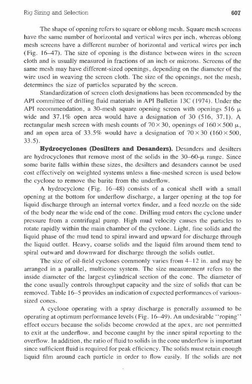
Rig Sizing and Selection 607
The shape of opening refers to square or oblong mesh. Square mesh screenshave the same number of horizontal and vertical wires per inch, whereas oblongmesh screens have a different number of horizontal and vertical wires per inch
( Fig. 16-47). The size of opening is the distance between wires in the screencloth and is usually measured in fractions of an inch or microns. Screens of thesame mesh may have different-sized openings, depending on the diameter of thewire used in weaving the screen cloth. The size of the openings, not the mesh,determines the size of particles separated by the screen.
Standardization of screen cloth designations has been recommended by theAPI committee of drilling fluid materials in API Bulletin l3C (1974). Under theAPI recommendation, a 30-mesh square opening screen with openings 516 1-1.wide and 37.1% open area would have a designation of 30 (516, 37.1). Arectangular mesh screen with mesh counts of 70 x 30, openings of 160 x 5001-1.,and an open area of 33.5% would have a designation of 70 x 30 (160 x 500,33.5).
Bydrocyclones (Desilters and Desanders). Desanders and desilters
are hydrocyclones that remove most of the solids in,the 30-60-1-1.range. Sincesome barite falls within these sizes, the desilters and desanders cannot be used
cost effectively on weighted systems unless a fine-meshed screen is used belowthe cyclone to remove the barite from the underflow.
A hydrocyclone (Fig. 16-48) consists of a conical shell with a smallopening at the bottom for underflow discharge, a larger opening at the top forliquid discharge through an internal vortex finder, and a feed nozzle on the sideof the body near the wide end of the cone. Drilling mud enters the cyclone underpressure from a centrifugal pump. High mud velocity causes the particles torotate rapidly within the main chamber of the cyclone. Light, fine solids and theliquid phase of the mud tend to spiral inward and upward for discharge throughthe liquid outlet. Heavy, coarse solids and the liquid film around them tend tospiral outward and downward for discharge through the solids outlet.
The size of oil-field cyclones commonly varies from 4-12 in. and may bearranged in a parallel, multicone system. The size measurement refers to theinside diameter of the largest cylindrical section of the cone. The diameter ofthe cone usually controls throughput capacity and the size of solids that can beremoved. Table 16-5 provides an indication of expected performances of various-sized cones.
A cyclone operating with a spray discharge is generally assumed to beoperating at optimum performance levels (Fig. 16-49). An undesirable "roping"effect occurs because the solids become crowded at the apex, are not permittedto exit at the underflow, and become caught by the inner spiral reporting to theoverflow. In addition, the ratio of fluid to solids in the cone underflow is importantsince sufficient fluid is required for peak efficiency. The solids must retain enoughliquid film around each particle in order to flow easily. If the solids are not
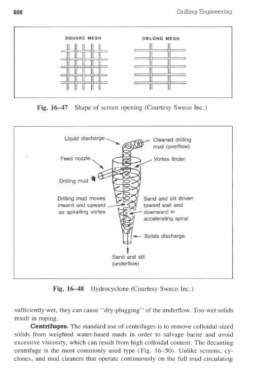
608 DrillingEngineering
SQUARE MESH OBLONG MESH
Fig. 16-47 Shape of screen opening (Courtesy Sweco Inc.)
Drilling mud ..
Cleaned drillingmud (overflow)
Drillingmud moves W~I Sandand silt driveninwardand upward~:?.xl towardwall andas spirallingvortex ~: downwardin
accelerating spiral
Sand and silt(underflow)
Fig. 16-48 Hydrocyclone (Courtesy Sweco Inc.)
sufficiently wet, they can cause "dry-plugging" of the underflow. Too-wet solidsresult in roping.
Centrifuges. The standard use of centrifuges is to remove colloidal-sizedsolids from weighted water-based muds in order to salvage barite and avoidexcessive viscosity, which can result from high colloidal content. The decantingcentrifuge is the most commonly used type (Fig. 16-50). Unlike screens, cy-clones, and mud cleaners that operate continuously on the full mud circulating
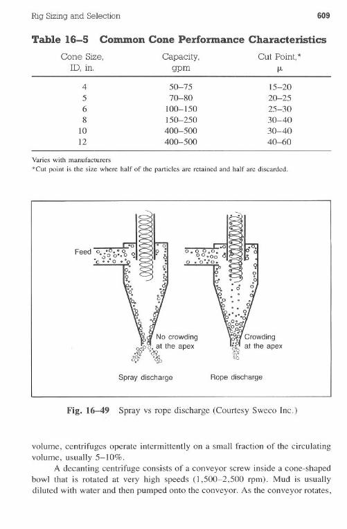
Rig Sizing and Selection 609
Table 16-5 Common Cone Performance Characteristics
Varies with manufacturers
*Cut point is the size where half of the particles are retained and half are discarded.
ij No crowdingo!oo. at the apex.~o' 'd9
o~o o~b
Spray discharge Rope discharge
Fig. 16-49 Spray vs rope discharge (Courtesy Sweco Inc.)
volume, centrifuges operate intermittently on a small fraction of the circulatingvolume, usually 5-10%.
A decanting centrifuge consists of a conveyor screw inside a cone-shapedbowl that is rotated at very high speeds (1,500-2,500 rpm). Mud is usuallydiluted with water and then pumped onto the conveyor. As the conveyor rotates,
Cone Size, Capacity, Cut Point,*ID, in. gpm ,....
4 50-75 15-20
5 70-80 20-25
6 100-150 25-30
8 150-250 30-40
10 400-500 30-40
12 400-500 40-60
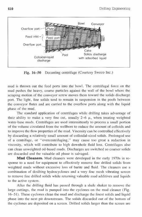
610 Drilling Engineering
Overflow port
Colloidal-liquiddischarge
PoolCakeSolids discharge
with adsorbed liquid
Fig. 16-50 Decanting centrifuge (Courtesy Sweco Inc.)
mud is thrown out the feed ports into the bowl. The centrifugal force on themud pushes the heavy, coarse particles against the wall of the bowl where thescraping motion of the conveyor screw moves them toward the solids dischargeport. The light, fine solids tend to remain in suspension in the pools betweenthe conveyor flutes and are carried to the overflow ports along with the liquidphase of the mud.
The standard application of centrifuges while drilling takes advantage oftheir ability to make a very fine cut, usually 2-6 Jl., when treating weightedwater-base muds. Centrifuges are used intermittently to process a small portionof the volume circulated from the well bore to reduce the amount of colloids and
to improve the flow properties of the mud. Viscosity can be controlled effectivelyby discarding a relatively small amount of colloidal-sized solids. Prolonged useof a centrifuge, or "overcentrifuging," may cause too great a reduction inviscosity, which will contribute to high downhole fluid loss. Centrifuges alsocan clean unweighted oil-based muds. Discharges are switched so coarser solidsare discarded and the valuable oil phase is salvaged.
Mud Cleaners. Mud cleaners were developed in the early 1970s in re-sponse to a need for equipment to effectively remove fine drilled solids fromweighted muds without excessive loss of barite and fluid. The cleaners use a
combination of desilting hydrocyclones and a very fine mesh vibrating screento remove fine drilled solids while returning valuable mud additives and liquidsto the active system.
After the drilling fluid has passed through a shale shaker to remove the
large cuttings, the mud is pumped into the cyclones on the mud cleaner (Fig.16-51). These cyclones clean the mud and discharge the finest solids and liquidphase into the next pit downstream. The solids discarded out of the bottom of
the cyclones are deposited on a screen. Drilled solids larger than the screen are
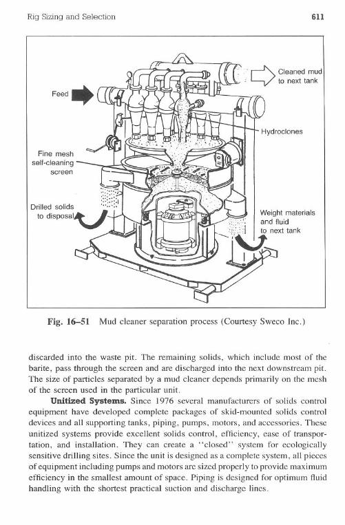
Rig Sizing and Selection 611
::~ Cleaned mud; L...V to next tank
Fine meshself-cleaning
screen
Fig. 16-51 Mud cleaner separation process (Courtesy Sweco Inc.)
discarded into the waste pit. The remaining solids, which include most of thebarite, pass through the screen and are discharged into the next downstream pit.The size of particles separated by a mud cleaner depends primarily on the meshof the screen used in the particular unit.
Unitized Systems. Since 1976 several manufacturers of solids controlequipment have developed complete packages of skid-mounted solids controldevices and all supporting tanks, piping, pumps, motors, and accessories. Theseunitized systems provide excellent solids control, efficiency, ease of transpor-tation, and installation. They can create a "closed" system for ecologicallysensitive drilling sites. Since the unit is designed as a complete system, all piecesof equipment including pumps and motors are sized properly to provide maximumefficiency in the smallest amount of space. Piping is designed for optimum fluidhandling with the shortest practical suction and discharge lines.
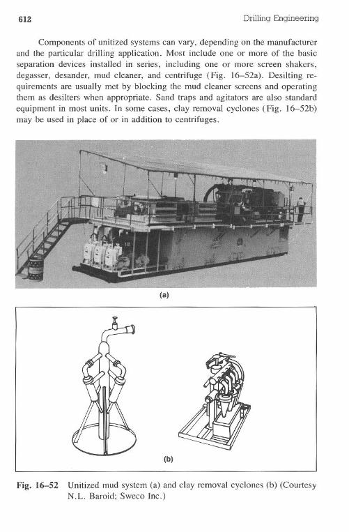
612 Drilling Engineering
Components of unitized systems can vary, depending on the manufacturerand the particular drilling application. Most include one or more of the basicseparation devices installed in series, including one or more screen shakers,degasser, desander, mud cleaner, and centrifuge (Fig. 16-52a). Desilting re-quirements are usually met by blocking the mud cleaner screens and operatingthem as desilters when appropriate. Sand traps and agitators are also standardequipment in most units. In some cases, clay removal cyclones (Fig. 16-52b)may be used in place of or in addition to centrifuges.
(a)
(b)
Fig. 16-52 Unitized mud system (a) and clay removal cyclones (b) (CourtesyN.L. Baroid; Sweco Inc.)
Rig Sizingand Selection 613
Rig Floor EquipmentMany auxiliary pieces of equipment required for the drilling process are
maintained on the rig floor and should be provided by the drilling contractor.The equipment must be selected for the drillpipe to be used, the loads to beexpected, and the rig's basic equipment. An additional design consideration insome cases is the actual placement of the equipment on the rig floor to facilitateaccess during normal and emergency use.
Bit Breakers. The drill bit is an awkward-shaped tool that cannot beconnected easily with conventional tools to the drillstring. Its initial connectionmust be tight for the trip into the hole. Removing the bit is difficult due to itsshape and the inherent tightening of the connection during drilling.
The bit breaker plate, or bit box, is designed to help when making up andbreaking out the bit (Fig. 16-53). It is sized according to the bit that is run intothe hole. The breaker plate sits in the rotary table and is held secure by therotary lock. The plates are purchased from the bit manufacturer. In many cases,a single size plate, such as 97/Sin., will work with all 97/s-in. bits, regardlessof the manufacturer.
Lift Nipples. Slim-hole drillpipe and drill collars do not have large tooljoints that can be latched easily with the elevators when tripping or makingconnections. Many operators use a short sub with a large latch head to provideadditional safety when connecting with the elevators. Although elevators can beused with some pipe and collars, the lift nipples are more often used. The nipplemust have the same threads as the pin end of the pipe or collars.
Weight Indicator. A common piece of equipment found on every drillingrig is the weight indicator (Fig. 16-54). Its sensor is connected to the dead lineand measures the strain of the line under certain loads. The indicator has reversibleface plates when a different number of drill lines are used with the crown sheaveand traveling block. In addition, most weight indicators have an adjustablecalibrated outer face plate that can be rotated to any off-bottom hook load tomake it easier for the driller to determine weight-on-bit loads when drilling.
Standpipe Pressure Gauge. Pump pressure is measured at the rig floorwith a pressure gauge installed in the standpipe leading to the rotary kelly hose.The cameron gauge, as it is often called after a manufacturer, is durable butmay be reasonably accurate only to within 100-200 psi for an uncalibrated gauge.(Fig. 16-55). In addition, pump pressure surges on each stroke cause an oscil-lation on the gauge that increases the difficulty in reading it. The drilling engineershould use the pressure gauge on the choke panel if accurate readings are required.
Mud Bucket. Pulling wet strings out of the hole necessitates the use ofa mud bucket. A wet string has mud in the stand above the rotary table thatflows onto the rig floor when the pipe is unscrewed. The mud sometimes willflow quite violently and spray the crew and floor equipment. A mud bucketwraps around the connection and catches the mud spray, returning it by hose to
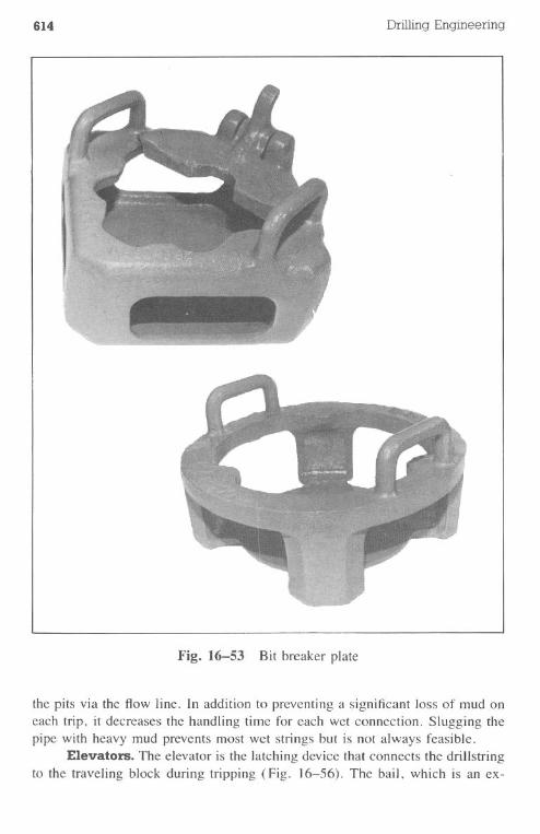
614 Drilling Engineering
----
.... r-Fig. 16-53 Bit breaker plate
the pits via the flow line. In addition to preventing a significant loss of mud oneach trip, it decreases the handling time for each wet connection. Slugging thepipe with heavy mud prevents most wet strings but is not always feasible.
Elevators. The elevator is the latching device that connects the drill stringto the traveling block during tripping (Fig. 16-56). The bail, which is an ex-
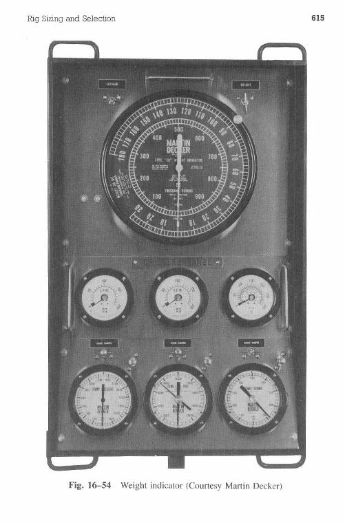
Rig Sizing and Selection 615
Fig. 16-54 Weight indicator (Courtesy Martin Decker)
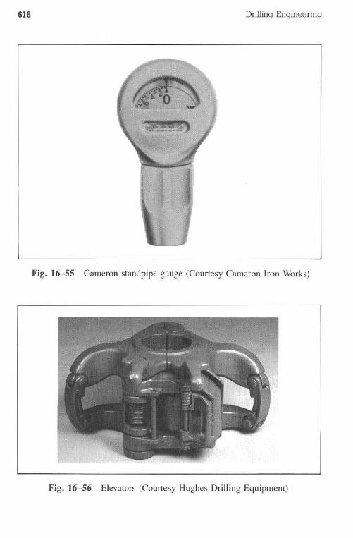
616 Drilling Engineering
Fig. 16-55 Cameron standpipe gauge (Courtesy Cameron Iron Works)
Fig. 16-56 Elevators (Courtesy Hughes Drilling Equipment)
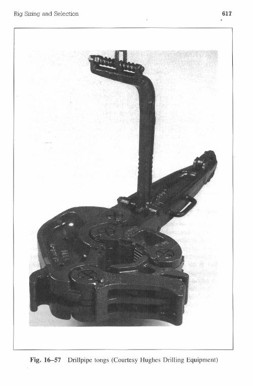
Rig Sizing and Selection 617
Fig. 16-57 Drillpipe tongs (Courtesy Hughes Drilling Equipment)
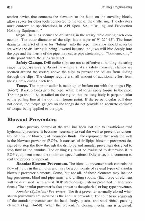
618 Drilling Engineering
tension device that connects the elevators to the hook on the traveling block,allows space for other tools connected to the top of the drillstring. The elevatorsmust conform to specifications in API Spec. 8A, "Drilling and ProductionHoisting Equipment."
Slips. The slips secure the drillstring in the rotary table during each con-.nection. The outer diameter of the slips has a taper of 9° 27' 45". The innerdiameter has a set of jaws for "biting" into the pipe. The slips should never beset while the drillstring is being lowered because the jaws will bite deeply intothe pipe and the inertia of the pipe may cause pipe stretching or "bottlenecking"at the point where the slips were set.
Safety Clamps. Drill collar slips are not as effective at holding the stringsince the collars usually do not have upsets. As a safety measure, clamps aresecured around the collars above the slips to prevent the collars from slidingthrough the slips. The clamps require a small amount of additional effort fromthe rig crew during each trip.
Tongs. The pipe or collar is made up or broken out with the tongs (Fig.16-57). Backup tongs grip the pipe, while lead tongs apply torque to the pipe.The tongs should be installed on the rig so that the tong body is perpendicularto the pulling line at the optimum torque point. If the perpendicular pull doesnot occur, the torque gauges on the tongs do not provide an accurate estimateof torque being applied to the pipe.
Blowout Preventers
When primary control of the well has been lost due to insufficient mudhydrostatic pressure, it becomes necessary to seal the well to prevent an uncon-trolled flow, or blowout, of formation fluids. The equipment that seals the wellis the blowout preventer (BOP). It consists of drillpipe blowout preventers de-signed to stop the flow through the drillpipe and annular preventers designed tostop flow in the annulus. The drilling rig must be evaluated to determine if itsBOP equipment meets the minimum specifications. Otherwise, it is common torent the proper equipment.
Annular Blowout Preventers. The blowout preventer stack controls theflow of fluids in the annulus and may be a composite of several types of annularblowout preventer elements. Some, but not all, of these elements may includebag preventers, blind and pipe rams, and drilling spools. (Each type of elementwill be discussed, with actual BOP stack design criteria presented in later sec-tions.) The annular preventer is also known as the spherical or bag-type preventer.
Annular (Spherical) Preventers. The first preventer normally closed whenshutin procedures are initiated is the annular preventer. The four basic segmentsof the annular preventer are the head, body, piston, and steel-ribbed packingelement (Fig. 16-58). When the preventer's closing mechanism is actuated,
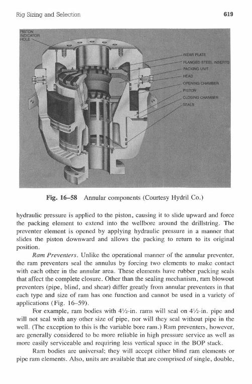
Rig Sizing and Selection 619
Fig. 16-58 Annular components (Courtesy Hydril Co.)
hydraulic pressure is applied to the piston, causing it to slide upward and forcethe packing element to extend into the wellbore around the drillstring. Thepreventer element is opened by applying hydraulic pressure in a manner thatslides the piston downward and allows the packing to return to its originalposition.
Ram Preventers. Unlike the operational manner of the annular preventer,the ram preventers seal the annulus by forcing two elements to make contactwith each other in the annular area. These elements have rubber packing sealsthat affect the complete closure. Other than the sealing mechanism, ram blowoutpreventers (pipe, blind, and shear) differ greatly from annular preventers in thateach type and size of ram has one function and cannot be used in a variety ofapplications (Fig. 16-59).
For example, ram bodies with 4Y2-in.rams will seal on 41/2-in.pipe andwill not seal with any other size of pipe, nor will they seal without pipe in thewell. (The exception to this is the variable bore ram.) Ram preventers, however,are generally considered to be more reliable in high pressure service as well asmore easily serviceable and requiring less vertical space in the BOP stack.
Ram bodies are universal; they will accept either blind ram elements orpipe ram elements. Also, units are available that are comprised of single, double,
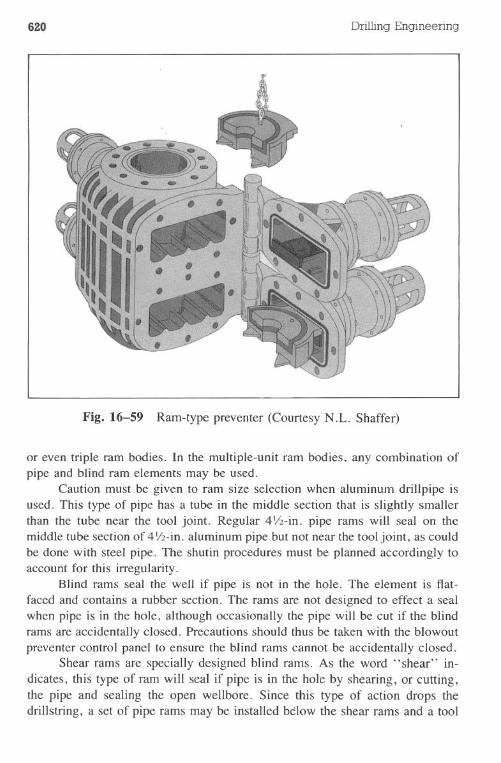
620 Drilling Engineering
Fig. 16-59 Ram-type preventer (Courtesy N.L. Shaffer)
or even triple ram bodies. In the multiple-unit ram bodies, any combination ofpipe and blind ram elements may be used.
Caution must be given to ram size selection when aluminum drillpipe isused. This type of pipe has a tube in the middle section that is slightly smallerthan the tube near the tool joint. Regular 41/2-in. pipe rams will seal on themiddle tube section of 4Y2-in.aluminum pipe but not near the tool joint, as couldbe done with steel pipe. The shutin procedures must be planned accordingly toaccount for this irregularity.
Blind rams seal the well if pipe is not in the hole. The element is flat-faced and contains a rubber section. The rams are not designed to effect a sealwhen pipe is in the hole, although occasionally the pipe will be cut if the blindrams are accidentally closed. Precautions should thus be taken with the blowoutpreventer control panel to ensure the blind rams cannot be accidentally closed.
Shear rams are specially designed blind rams. As the word "shear" in-dicates, this type of ram will seal if pipe is in the hole by shearing, or cutting,the pipe and sealing the open wellbore. Since this type of action drops thedrillstring, a set of pipe rams may be installed below the shear rams and a tool
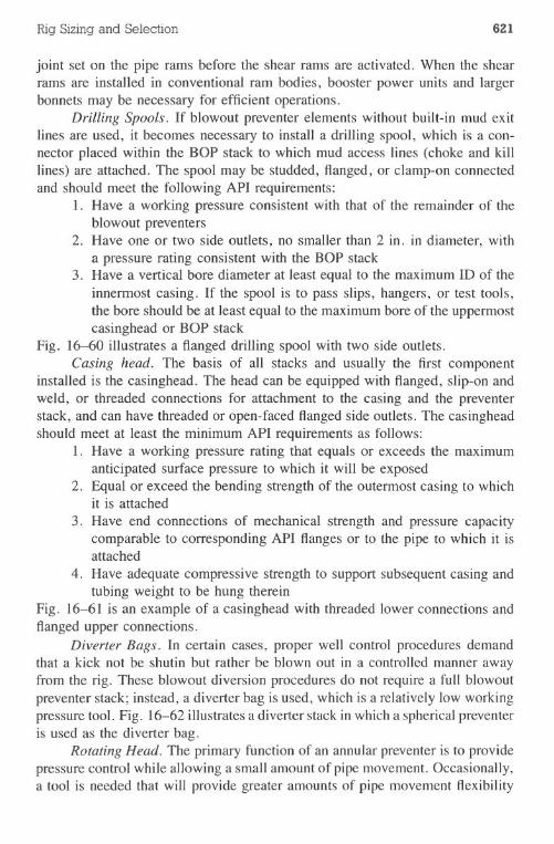
Rig Sizing and Selection 621
joint set on the pipe rams before the sh~ar rams are activated. When the shearrams are installed in conventional ram bodies, booster power units and largerbonnets may be necessary for efficient operations.
Drilling Spools. If blowout preventer elements without built-in mud exitlines are used, it becomes necessary to install a drillin,gspool, which is a con-nector placed within the BOP stack to which mud access lines (choke and killlines) are attached. The spool may be studded, flanged, or clamp-on connectedand should meet the following API requirements:
I. Have a working pressure consistent with that of the remainder of theblowout preventers
2. Have one or two side outlets, no smaller than 2 in. in diameter, witha pressure rating consistent with the BOP stack
3. Have a vertical bore diameter at least equal to the maximum ID of theinnermost casing. If the spool is to pass slips, hangers, or test tools,the bore should be at least equal to the maximum bore of the uppermostcasinghead or BOP stack
Fig. 16-60 illustrates a flanged drilling spool with two side outlets.Casing head. The basis of all stacks and usually the first component
installed is the casinghead. The head can be equipped with flanged, slip-on andweld, or threaded connections for attachment to the casing and the preventerstack, and can have threaded or open-faced flanged side outlets. The casingheadshould meet at least the minimum API requirements as follows:
1. Have a working pressure rating that equals or exceeds the maximumanticipated surface pressure to which it will be exposed
2. Equal or exceed the bending strength of the outermost casing to whichit is attached
3. Have end connections of mechanical strength and pressure capacitycomparable to corresponding API flanges or to the pipe to which it isattached
4. Have adequate compressive strength to support subsequent casing andtubing weight to be hung therein
Fig. 16-61 is an example of a casinghead with threaded lower connections andflanged upper connections.
Diverter Bags. In certain cases, proper well control procedures demandthat a kick not be shutin but rather be blown out in a controlled manner awayfrom the rig. These blowout diversion procedures do not require a full blowoutpreventer stack; instead, a diverter bag is used, which is a relatively low workingpressure tool. Fig. 16-62 illustrates a diverter stack in which a spherical preventeris used as the diverter bag.
Rotating Head. The primary function of an annular preventer is to providepressure control while allowing a small amount of pipe movement. Occasionally,a tool is needed that will provide greater amounts of pipe movement flexibility
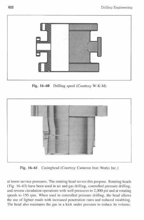
622 Drilling Engineering
Fig. 16-60 Drilling spool (Courtesy W-K-M)
r
..,I
Fig. 16-61 Casinghead (Courtesy Cameron Iron Works Inc.)
at lower service pressures. The rotating head serves this purpose. Rotating heads(Fig. 16-63) have been used in air and gas drilling, controlled pressure drilling,and reverse circulation operations with well pressures to 2,000 psi and at rotatingspeeds to 150 rpm. When used in controlled pressure drilling, the head allowsthe use of lighter muds with increased penetration rates and reduced swabbing.The head also maintains the gas in a kick under pressure to reduce its volume.
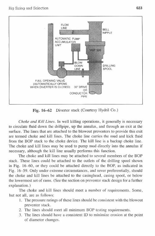
Rig Sizing and Selection 623
FUll OPENING VALVE
(AUTOMATICAllY OPENS
WHEN DIVERTER IS CLOSED)
Fig. 16-62 Diverter stack (Courtesy Hydril Co.)
Choke and Kill Lines. In well killing operations, it generally is necessaryto circulate fluid down the drillpipe, up the annulus, and through an exit at thesurface. The lines that are attached to the blowout preventers to provide this exitare tenned choke and kill lines. The choke line carries the mud and kick fluidfrom the BOP stack to the choke device. The kill line is a backup choke line.The choke and kill lines may be used to pump mud directly into the annulus ifnecessary, although the kill line usually perfonns this function.
The choke and kill lines may be attached to several members of the BOPstack. These lines could be attached to the outlets of the drilling spool shownin Fig. 16-60, or they could be attached directly to the BOP, as indicated inFig. 16-59. Only under extreme circumstances, and never preferentially, shouldthe choke and kill lines be attached to the casinghead, casing spool, or belowthe lowennost set of rams. (See the section on preventer stack design for a furtherexplanation.)
The choke and kill lines should meet a number of requirements. Some,but not all, are as follows:
I. The pressure ratings of these lines should be consistent with the blowoutpreventer stack.
2. The lines should meet all minimum BOP testing requirements.3. The lines should have a consistent ID to minimize erosion at the point
of diameter changes.
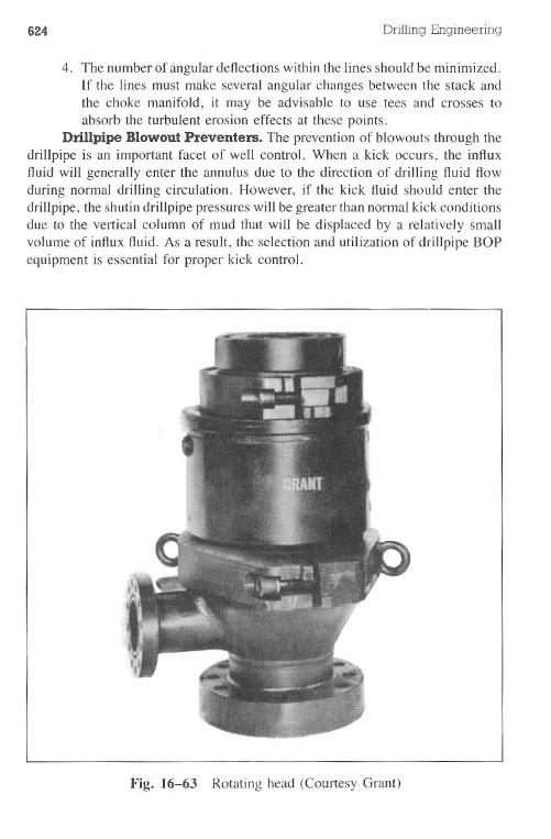
624 Drilling Engineering
4. The number of angular deflections within the lines should be minimized.If the lines must make several angular changes between the stack andthe choke manifold, it may be advisable to use tees and crosses toabsorb the turbulent erosion effects at these points.
Drillpipe Blowout Preventers. The prevention of blowouts through thedrillpipe is an important facet of well control. When a kick occurs, the influxfluid will generally enter the annulus due to the direction of drilling fluid flowduring normal drilling circulation. However, if the kick fluid should enter thedrillpipe, the shutin drillpipe pressures will be greater than normal kick conditionsdue to the vertical column of mud that will be displaced by a relatively smallvolume of influx fluid. As a result, the selection and utilization of drillpipe BOPequipment is essential for proper kick control.
Fig. 16-63 Rotating head (Courtesy Grant)
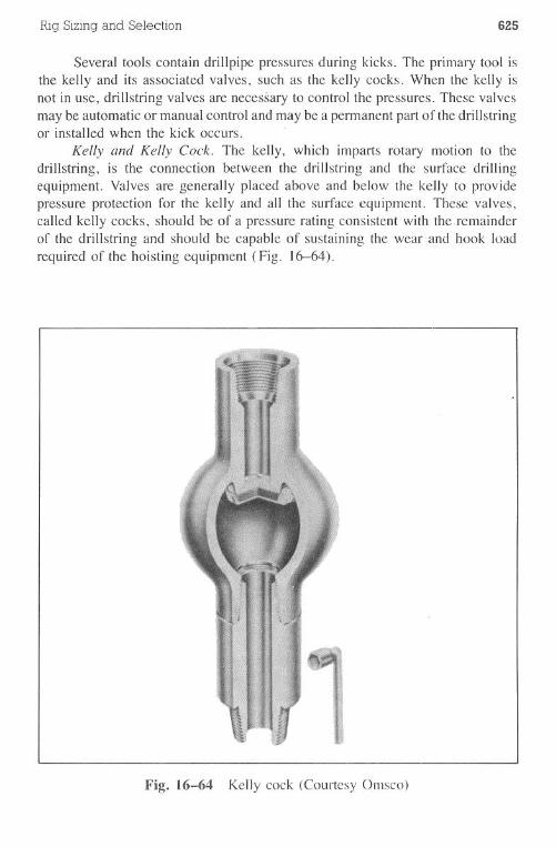
Rig Sizing and Selection 625
Several tools contain drillpipe pressures during kicks. The primary tool isthe kelly and its associated valves, such as the kelly cocks. When the kelly isnot in use, driIlstring valves are necessary to control the pressures. These valvesmay be automatic or manual control and may be a permanent part of the drillstringor installedwhenthe kick occurs. .
Kelly and Kelly Cock. The kelly, which imparts rotary motion to thedrillstring, is the connection between the driIlstring and the surface drillingequipment. Valves are generally placed above and below the kelly to providepressure protection for the kelly and all the surface equipment. These valves,called kelly cocks, should be of a pressure rating consistent with the remainderof the drillstring and should be capable of sustaining the wear and hook loadrequired of the hoisting equipment (Fig. 16-64).
,I.!
...
Fig. 16-64 Kelly cock (Courtesy Omsco)
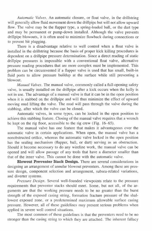
626 DrillingEngineering
Automatic Valves..An automatic closure, or float valve, in the drillstringwill generally allow fluid movement down the drillpipe but will not allow upwardflow. The valve may be the flapper type, a spring-loaded ball, or the dart typeand may be permanent or pump-down installed. Although the valve preventsdrillpipe blowouts, it is often used to minimize flowback during connections orto prevent bit plugging.
There is a disadvantage relative to well control when a float valve isinstalled in the drillstring because the basis of proper kick killing procedures isdependent on a drillpipe pressure determination. Since a direct reading of staticdrillpipe pressures is impossible with a conventional float valve, alternativepressure reading procedures that are more complex must be implemented. Thisproblem can be circumvented if a flapper valve is used that has small, built-influid ports to allow pressure buildup at the surface while still preventing ablowout.
Manual Valves. The manual valve, commonly called a full-opening safetyvalve, is usually installed on the drillpipe after a kick occurs when the kelly isnot in use. The advantage of a manual valve is that it can be in the open positionwhen it is stabbed on the drillpipe and will thus minimize the effect of upwardmoving mud lifting the valve. The mud will pass through the valve during thestabbing, after which the valve can be closed.
Automatic valves, in some types, can be locked in the open position toachieve this stabbing feature. Closing of the manual valve requires that a wrenchbe kept on the rig floor, accessible to the rig crew (Fig. 16-65).
The manual valve has one feature that makes it advantageous over theautomatic valve in certain applications. When open, the manual valve has anonobstructed orifice, whereas the automatic valve locked in the open positionhas the sealing mechanism (flapper, ball, or dart) serving as an obstruction.Should it become necessary to do any wireline work, the manual valve can beopened and will allow passage of any tools that have a diameter smaller thanthat of the inner valve. This cannot be done with the automatic valve.
Blowout Preventer Stack Design. There are several considerations indesigning an arrangement of annular blowout preventers. Among these are pres-sure design, component selection and arrangement, subsea-related variations,and diverter systems.
Pressure Design. Several well-founded viewpoints relate to the pressurerequirements that preventer stacks should meet. Some, but not all, of the ar-guments are that the working pressure needs to be no greater than the burststrength of the exposed casing string, formation fracture pressure of the shal-lowest exposed zone, or a predetermined maximum allowable surface casingpressure. However, all of these guidelines may present serious problems whenapplied in severe well control situations.
The most common of these guidelines is that the preventers need to be nostronger than the casing string to which they are attached. The inherent fallacy
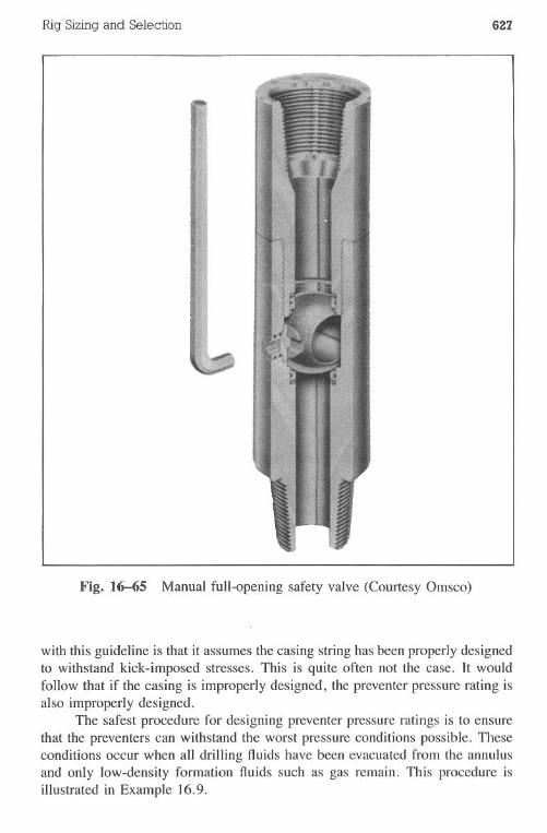
Rig Sizing and Selection 627
Fig. 16-65 Manual full-opening safety valve (Courtesy Omsco)
with this guideline is that it assumes the casing string has been properly designedto withstand kick-imposed stresses. This is quite often not the case. It wouldfollow that if the casing is improperly designed, the preventer pressure rating isalso improperly designed.
The safest procedure for designing preventer pressure ratings is to ensurethat the preventers can withstand the worst pressure conditions possible. Theseconditions occur when all drilling fluids have been evacuated from the annulusand only low-density formation fluids such as gas remain. This procedure isillustrated in Example 16.9.
628 Drilling Engineering
Example 16.9
A well is to be drilled to 10,600 ft and has an expected bottom-hole pressure(BHP) equivalent to 10.5 Ib/gaI. What pressure rating should the preventersbe? (Assume a gas density of 2.5 Ib/gaI.)
Solution:
I. Determine the maximum anticipated formation pressure:
pressure = 0.052 x 1O.5Ib/gal x 10,600 ft = 5,787 psi
2. Determine the gas hydrostatic pressure that will act downward on the zone,assuming the mud is evacuated from the hole:
pressure = 0.052 x 2.5 Ib/gas x 10,600 ft = 1,378 psi
3. The pressure imposed on the preventer would be the difference betweenthe formation pressure and the gas hydrostatic pressure:
5,787 psi - 1,378 psi = 4,409 psi
The preventers must be able to withstand 4,409 psi.
Experience suggests that this method should generally be used in shallow wellsituations where it is possible to achieve a complete mud evacuation. However,as the depth of the well increases, it becomes more unlikely that a full mudevacuation will occur. As a result, a modification based on a percentage of themaximum possible pressure load should be used to determine the preventerpressure rating. This percentage depends on the operator's experiences in aparticular drilling environment. Example 16.10 illustrates the modification ofthe technique for deep wells.
Example 16.10
A North Sea operator wishes to drill an expected bottom-hole pressure of16.0 Ib/gal at 16,500 ft. The operator's experience dictates that an 80% designfactor would account for unexpected eventualities. What pressure rating shouldthe preventers be? (Assume a gas density of 2.0 Ib/gaI.)
Solution:
1. BHP = 0.052 x 16.0Ib/gal x 16,500ft = 13,728psi2. gas pressure = 0.052 x 2.0Ib/gal x 16,500 ft = 1,716 psi
Rig Sizing and Selection 629
3. resultant pressure = BHP - gas hydrostatic= 13,728 psi - 1,716 psi = 12,012 psi
4. working pressure = resultant pressure x 80% = 9,609 psiUsing the API designations, a 1O,000-psi working pressure stack of pre-venters would be necessary to control the well properly.
Component Design. After the pressure rating for the preventer has beenselected, the component arrangement must be considered. The logic will bedeveloped using four components: an annular (spherical) BOP, pipe rams, blindrams, and a drilling spool. Logic for the minimum stack can be extended to anystack.
Fig. 16-66 shows the proper arrangement for this four-member stack.Should one component fail, there will always be a backup system. This sequenceof operations explains the design.
Step I. The annular (spherical) preventer is closed.Step 2. If the spherical fails while killing the well, the lower set of pipe
rams is closed.
Step 3. One of three emergency procedures is exercised. Either the annular(spherical) is changed, the blind rams are changed to pipe rams,or both the annular (spherical) and blind rams are changed.
This configuration implies several important points. The lower pipe ramsare not for circulation purposes but simply close in the well while repairs to theupper members are made. Also, a choke or kill line should never be attachedbelow the lowermost set of pipe rams, i.e., ram outlets or casinghead valves.Failure of this line will mean a certain blowout since there is no backup systemfor proper control.
The valves adjacent to the BOP stack should be arranged based on thebackup system principle. The innermost valve next to the stack should be foremergency use only, while the next valve outward is for day-to-day actuation.As a result, the outer valve is generally a hydraulic valve for remote controlduring kick killing procedures.
In deepwater drilling, the blowout preventers are generally located on theseafloor. This necessitates installing certain built-in safety precautions in thestack. Since component failure cannot readily be repaired, additional preventerelements must be installed to handle any eventualities. The typical subsea stack(Fig. 16-67) illustrates that the same logic developed in the previous section fora minimum stack was utilized by ensuring that built-in backup systems shownin this illustration are the two spherical preventers, two choke lines with theprimary line on top and the secondary line on the bottom, fail-safe valves oneach choke line, and shear rams at the bottom of the stack to allow for emergencyrig departure if necessary.
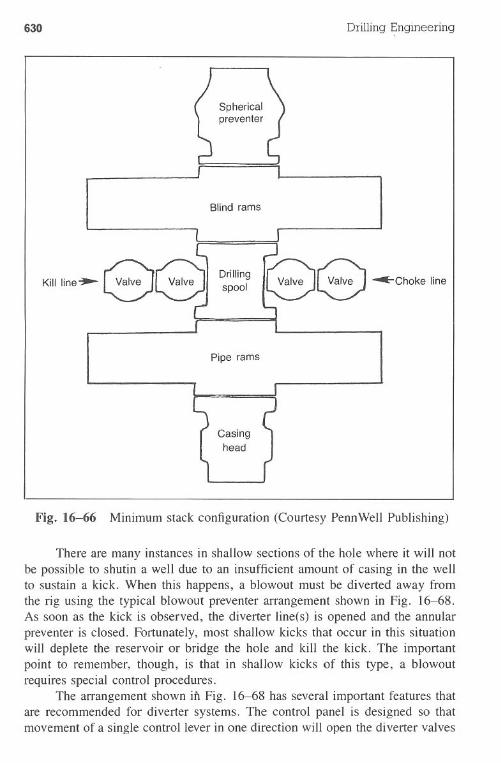
630 Drilling Engineering
Blind rams
Pipe rams
Fig. 16-66 Minimum stack configuration (Courtesy PennWell Publishing)
There are many instances in shallow sections of the hole where it will notbe possible to shutin a well due to an insufficient amount of casing in the wellto sustain a kick. When this happens, a blowout must be diverted away fromthe rig using the typical blowout preventer arrangement shown in Fig. 16-68.As soon as the kick is observed, the diverter line(s) is opened and the annularpreventer is closed. Fortunately, most shallow kicks that occur in this situationwill deplete the reservoir or bridge the hole and kill the kick. The importantpoint to remember, though, is that in shallow kicks of this type, a blowoutrequires special control procedures.
The arrangement shown it! Fig. 16-68 has several important features thatare recommended for diverter systems. The control panel is designed so thatmovement of a single control lever in one direction will open the diverter valves
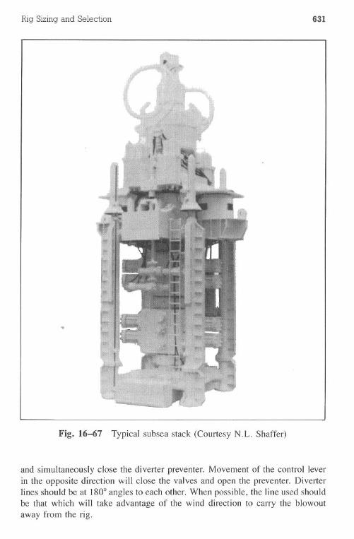
Rig Sizing and Selection 631
..
ftJ
....
..
J
I~"I
,
Fig. 16-67 Typicalsubseastack(CourtesyN.L. Shaffer)
and simultaneously close the diverter preventer. Movement of the control leverin the opposite direction will close the valves and open the preventer. Diverterlines should be at 1800angles to each other. When possible, the line used shouldbe that which will take advantage of the wind direction to carry the blowoutaway from the rig.
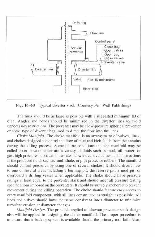
632 Drilling Engineering
, Diverter line
Flow line
Annular
preventer
Control panel
Close bag,/ Open valves
':-Open' bag'- Close valvesPreventer valve
Riser pipe
Fig. 16-68 Typical diverter stack (Courtesy PennWell Publishing)
The lines should be as large as possible with a suggested minimum ID of6 in. Angles and bends should be minimized in the diverter lines to avoidunnecessary restrictions. The preventer may be a low-pressure spherical preventeror some type of diverter bag used to direct the flow into the lines.
Choke Manifold. The choke manifold is an arrangement of valves, lines,and chokes designed to control the flow of mud and kick fluids from the annulusduring the killing process. Some of the conditions that the manifold may becalled upon to work under are a variety of fluids such as mud, oil, water, orgas, high pressures, upstream flow rates, downstream velocities, and obstructionsin the produced fluids such as sand, shale, or pipe protector rubbers. The manifoldshould control pressures by using one of several chokes. It should divert flowto one of several areas including a burning pit, the reserve pit, a mud pit, oroverboard a drilling vessel when applicable. The choke should have pressureratings at least equal to the preventer stack and should meet all pressure testingspecifications imposed on the preventers. It should be suitably anchored to preventmovement during the killing operation. The choke should feature easy access toevery manifold component, with all lines constructed as straight as possible. Alllines and valves should have the same consistent inner diameter to minimizeturbulent erosion at diameter changes.
ManifoldDesign.The principleappliedto blowoutpreventerstackdesignalso will be applied in designing the choke manifold. The proper procedure isto ensure that a backup system is available should the primary tool fail. Also,
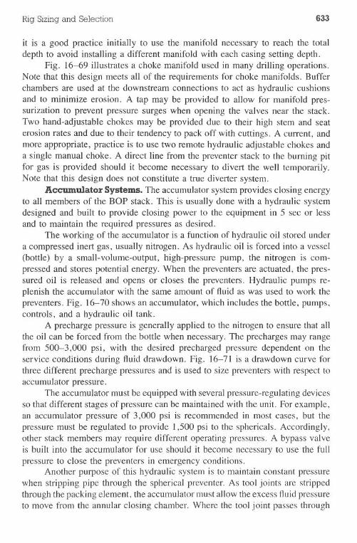
Rig Sizing and Selection 633
it is a good practice initially to use the manifold necessary to reach the totaldepth to avoid installing a different manifold with each casing setting depth.
Fig. 16-69 illustrates a choke manifold used in many drilling operations.Note that this design meets all of the requirements for choke manifolds. Bufferchambers are used at the downstream .connections to act as hydraulic cushionsand to minimize erosion. A tap may be provided to allow for manifold pres-surization to prevent pressure surges when opening the valves near the stack.Two hand-adjustable chokes may be provided due to their high stem and seaterosion rates and due to their tendency to pack off with cuttings. A current, andmore appropriate, practice is to use two remote hydraulic adjustable chokes anda single manual choke. A direct line from the preventer stack to the burning pitfor gas is provided should it become necessary to divert the well temporarily.Note that this design does not constitute a true diverter system.
Accumulator Systems. The accumulator system provides closing energyto all members of the BOP stack. This is usually done with a hydraulic systemdesigned and built to provide closing power to the equipment in 5 sec or lessand to maintain the required pressures as desired.
The working of the accumulator is a function of hydraulic oil stored undera compressed inert gas, usually nitrogen. As hydraulic oil is forced into a vessel(bottle) by a small-volume-output, high-pressure pump, the nitrogen is com-pressed and stores potential energy. When the preventers are actuated, the pres-sured oil is released and opens or closes the preventers. Hydraulic pumps re-plenish the accumulator with the same amount of fluid as was used to work thepreventers. Fig. 16-70 shows an accumulator, which includes the bottle, pumps,controls, and a hydraulic oil tank.
A precharge pressure is generally applied to the nitrogen to ensure that allthe oil can be forced from the bottle when necessary. The precharges may rangefrom 500-3,000 psi, with the desired precharged pressure dependent on theservice conditions during fluid drawdown. Fig. 16-71 is a drawdown curve forthree different precharge pressures and is used to size preventers with respect toaccumulator pressure.
The accumulator must be equipped with several pressure-regulating devicesso that different stages of pressure can be maintained with the unit. For example,an accumulator pressure of 3,000 psi is recommended in most cases, but thepressure must be regulated to provide 1,500 psi to the sphericals. Accordingly,other stack members may require different operating pressures. A bypass valveis built into the accumulator for use should it become necessary to use the fullpressure to close the preventers in emergency conditions.
Another purpose of this hydraulic system is to maintain constant pressurewhen stripping pipe through the spherical preventer. As tool joints are strippedthrough the packing element, the accumulator must allow the excess fluid pressureto move from the annular closing chamber. Where the tool joint passes through
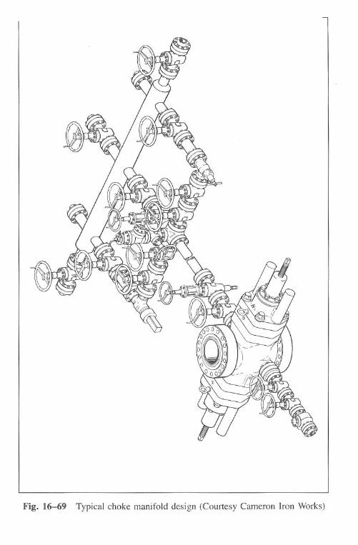
Fig. 16-69 Typical choke manifold design (Courtesy Cameron Iron Works)
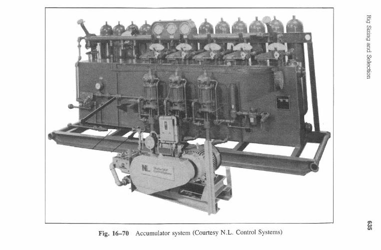
Rig
Sizingand
Selection635~V
)S2V
):>
.C
I)"0.........-I:oU...jZ:>
.V
)~::soU'-'So....-V
):>
.V
).....o~"3S::suu..(
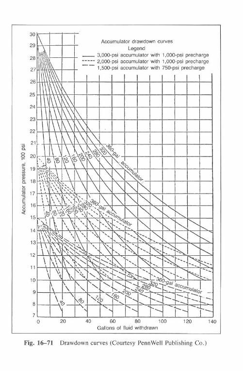
Drilling Engineering
Accumulator drawdown curves
Legend_ 3,OOO-psiaccumulator with 1,000-psi precharge__n_ 2,OOO-psiaccumulator with 1,OOO-psiprecharge- - 1,500-psi accumulator with 750-psi precharge
20 40 60 80 100Gallons of fluid withdrawn
120 140
Fig. 16-71 Orawdown curves (Courtesy PennWell Publishing Co.)
636
I30
28 W
27
26
25
24
23
22
"(j) 21c-o
20
19::JUJUJCDis. 18
<5]! 17::JE::J 160
15
14
13
12
11
10
9
8
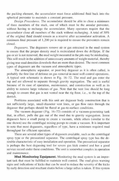
Rig Sizing and Selection 637
the packing element, the accumulator must force additional fluid back into thespherical preventer to maintain a constant pressure.
Design Procedures. The accumulator should be able to close a minimumof three members of the stack, one of which must be the annular preventer,without having to recharge the accumulator. Many operators require that theaccumulator close all members of the stack without recharging. A total of 50%of the original fluid should remain as a reserve after accumulator activation. Aminimum final pressure of 1,200 psi is required to ensure the preventers remainclosed.
Degassers. The degassers remove air or gas entrained in the mud systemto ensure that the proper density mud is recirculated down the drillpipe. If thegas or air is not removed, the mud weight measured in the pits may be misleading.This will result in the addition of unnecessary amountsof weight material, therebygiving true mud densities downhole that are more than desired. The most commontypes of degassers are the vacuum and atmospheric types.
The atmospheric separator, or poor-boy degasser as it is often called, isprobably the first line of defense on gas removal in most well control operations.A typical unit schematic is shown in Fig. 16-72. The mud and gas enter thetop and are allowed to separate through gravity segregation. The unit is usefulbecause of its ease of operation, maintenance, and construction as well as itsability to remove large volumes of gas. Note that the vent line should be longenough to ensure that gas is not vented near the rig floor, i.e., to the top of thederrick.
Problems associated with this unit are degasser body construction that isnot sufficiently large, small-diameter vent lines, or gas flow rates through thedegasser that perhaps should be flared at gas-to-surface conditions.
The vacuum degasser (Fig. 16-72) consists of a vacuum-generating tankthat, in effect, pulls the gas out of the mud due to gravity segregation. Somedegassers have a small pump to create a vacuum, while others (similar to theone shown) use the centrifugal mixing pumps to create a vacuum. It is importantto note that most degassers, regardless of type, have a minimum requir('d mudthroughput for efficient operation.
There are several other types of degassers available, such as the centrifugalspray type or the pressurized separator. The centrifugal spray type has the de-sirable characteristic of easy installation and operation. The pressurized separatoris perhaps the best degassing tool for severe gas kick control and has a goodservice record under these conditions. The unit is somewhat complex in operationand maintenance.
Mud Monitoring Equipment. Monitoring the mud system is an impor-tant task that must be fulfilled to maintain well control. The mud gives warningsigns and indications of kicks that can be used to reduce the severity of the kicksby early detection and resultant shutin before a large influx is taken. If this system
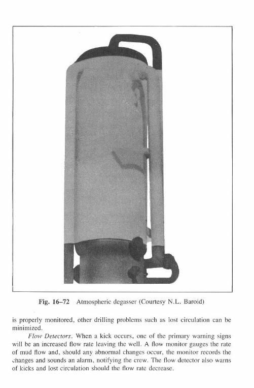
638 Drilling Engineering
11II
Fig. 16-72 Atmospheric degasser (Courtesy N.L. Baroid)
is properly monitored, other drilling problems such as lost circulation can beminimized.
Flow Detectors. When a kick occurs, one of the primary warning signswill be an increased flow rate leaving the well. A flow monitor gauges the rateof mud flow and, should any abnormal changes occur, the monitor records the.;hanges and sounds an alarm, notifying the crew. The flow detector also warnsof kicks and lost circulation should the flow rate decrease.
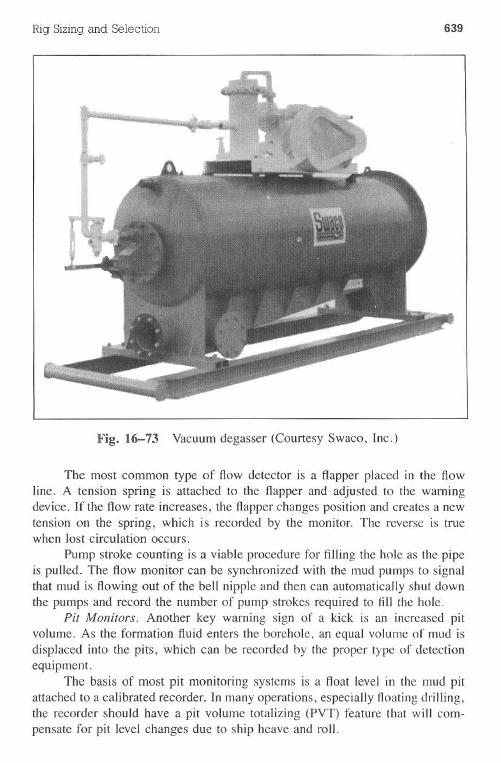
Rig Sizing and Selection 639
Fig. 16-73 Vacuum degasser (Courtesy Swaco, Inc.)
The most common type of flow detector is a flapper placed in the flowline. A tension spring is attached to the flapper and adjusted to the warningdevice. If the flow rate increases, the flapper changes position and creates a newtension on the spring, which is recorded by the monitor. The reverse is truewhen lost circulation occurs.
Pump stroke counting is a viable procedure for filling the hole as the pipeis pulled. The flow monitor can be synchronized with the mud pumps to signalthat mud is flowing out of the bell nipple and then can automatically shut downthe pumps and record the number of pump strokes required to fill the hole.
Pit Monitors. Another key warning sign of a kick is an increased pitvolume. As the formation fluid enters the borehole, an equal volume of mud isdisplaced into the pits, which can be recorded by the proper type of detectionequipment.
The basis of most pit monitoring systems is a float level in the mud pitattached to a calibrated recorder. In many operations, especially floating drilling,the recorder should have a pit volume totalizing (PVT) feature that will com-pensate for pit level changes due to ship heave and roll.
640 Drilling Engineering
GasDetectors. Severalgas detectors are available that function on differentprinciples. However, they ,all generally report the gas content as units of gas inthe mud stream. (It is interesting to note that the exact value of one unit of gasis vague.) When a certain amount of gas has been sensed, an alarm will soundor a light will signal the crew. The disadvantages of gas detectors are maintenanceproblems, the general inability to function in large concentrations of gas, and amisleading nature in kick detection.
Rig Site PreparationAfter the geological location for the well has been selected, the surface
site for the rig must be acquired and prepared. Rig site preparation will vary forland, marsh, and offshore operations. Some sites require minimum time andeffort while others may involve significant costs that often exceed the actual costfor drilling the well.
Rig site selection and preparation involve the efforts of many groupswithin the operating company. A typical scenario of the groups and actions is asfollows:
·Geologists develop a prospect and define desired well locations.· Leases are acquired via routine channels such as land departments, leasesales, or farm-ins.· Surface right-of-way is obtained from the landowner if the mineral leaseis obtained from a separate owner.·A surveyor spots the exact well location on the surface.·The drilling engineer selects the rig.·The drilling contractor defines his rig requirements with respect to surfacespace, rig weight, turnarounds, and footing.· A location preparation contractor may be employed to build the physicallocation to specs.
Specialists such as soil engineers, environmentalists or archaeologists may berequired in some cases. The drilling engineer is normally responsible for assistingin all activities after the geologist has selected a prospect and the leases havebeen-acquired.
Land Sites. Most wells are drilled vertically to take advantage of thenatural drilling tendencies of a well. Therefore, the well site should be locatedimmediately above the target zone. Vertical wells for exploratory drilling arecommon for marsh and offshore operations. Land wells have exceptions to thisgeneral rule, such as inaccessibility to the primary lo~ation or nonphysical re-strictions preventing access to the prime site. Inaccessibility to the primary siteoccurs in cases such as geological targets are spotted below river beds, smalllakes, or numerous buildings. Legal restrictions often involve government con-
Rig Sizing and Selection 641
straints such as noise levels in zoning areas or drilling sour wells in highlypopulated areas. In any case, the usual recourse for the drilling engineer is todrill a directional well.
The surface location is identified by a professional land surveyor. Knownlocations of surrounding landmarks are used to spot the well. The term' 'stakingthe well" occurs when the surveyor drives a small wooden stake into the groundat the well site.
Although perhaps not a widely used practice, redundant land surveyingand well staking are used occasionally. The redundancy occurs when a second,independent surveyor is used to verify the location as spotted by the initialsurveyor. The practice minimizes the possibility of drilling a well at the wronglocation. Although the professional surveyor generally carries insurance relatingto this possibility, it is still a costly mistake to the oil company if it occurs. Thecost for the duplicate surveying is considered an inexpensive form of preventivemedicine.
Accessibility to the surface right-of-way is usually easy to obtain if thesame individual owns the surface and mineral rights on the property. The owneris often eager for drilling to proceed as quickly as possible. The oil companyand the surface owner must define the optimum path into the property to minimizeland damage.
If the surface site owner is not the same individual as the mineral rightsowner, the difficulties of gaining access to the well site may increase. In thiscase, the owner has nothing to gain in terms of royalty revenues. Negotiationsmay involve paying a usage fee for the right-of-way. Most states recognize thatthe oil company has a legal right to exploit the purchased minerals and, therefore,the landowner must negotiate some equitable settlement.
Prenegotiation and payment of damages to the land resulting from thedrilling are required by some states. The oil company and landowner must agreeto a fair damages settlement before moving in the rig. It is not uncommon,howeyer, that post-drilling claims will be made for additional damages.
Soil engineers may be employed if the terrain is very marshy and soft.They may recommend driving piles below the most critical sections of the rig,such as the substructure. Drilling contractors can often offer useful advice fromtheir experience about areas that need additional underlying support and thereforerequire a soil analysis. The soil engineer may recommend options such as noadditional required support, a 2- or 3-ply board-matted location, a board accessroad, or pile driving.
Location preparation contractors are used in areas such as South Louisianathat have special soil problems. The contractor will utilize plots prepared by thedrilling contractor to build the location and turnaround areas. In addition, thegroup will build the board roads from the rig site to the main access road orhighway.
642 Drilling Engineering
Drilling operations need access to a freshwater supply. The commonsource for the water is a shallow water well drilled explicitly for the oil drilling.Public water facilities may be used if the proposed well is near a main waterartery.
Post-well cleanup and site restoration can be costly. The drilling water inthe reserve pit must be chemically treated, injected in an underground water-bearing strata, or hauled to a dump site. The drilled cuttings and mud must betreated chemically, spread over the area, or hauled to a dump site. It is a goodpractice to take pictures of the site before drilling in case surface-damage claimsarise.
Permitting the well can be a tedious effort in many cases. Many oil com-panies use consultants to obtain the necessary permits. Additional difficulties.arise if the well is near properties under the jurisdiction of some legislative groupother than the minerals regulatory body, e.g., wells near an airport that mayrequire permits from the FAA.
Marsh Sites. Drilling barges are most common in marsh areas. The bargeis towed to the location with tugboats, spotted at the surveyor's site location,and sunk.
Dredged channels in the marsh provide the waterways for the barges andtugs. Readily accessible channels are used if available. If previously existingwaterways to the rig site are not available, a specially dredged channel is built,constructed with a crane and dredge bucket operating from a separate barge.Obviously, this operation can be expensive and time consuming.
Drilling barges are usually sunk on the marsh prior to initiating drilling.An exception to this practice occurs when a shell pad is constructed on themarsh floor and the rig is sunk on the shell pad. A shell pad is preferred whenwater currents would erode the marsh floor below the rig and cause unevensettling.
Offshore Sites. Site evaluation in the offshore environment requires aninspection of the proposed rig site to determine if any of the following problemareas exist:
· Are pipelines crossing the proposed rig site~·Does the immediate area surrounding the rig site contain any unusualdebris?·Do abnormal topographical features exist, i.e., steep inclines, etc.?·Is the underlying formation incapable of supporting a jackup rig orproviding sufficient resistant, anchor-holding capability for a mooredfloater?
If any of these problem areas exist and cannot be resolved, another rig site mustbe selected. As opposed to land site preparation, the offshore area requiresevaluation and review but little physical preparation.
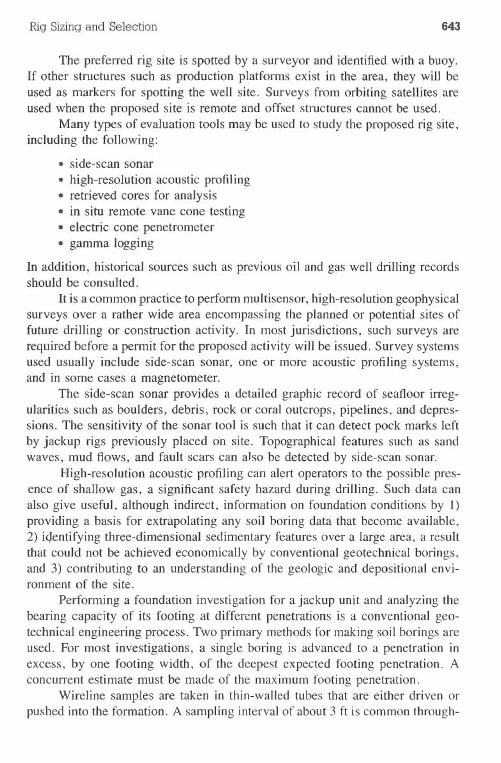
Rig Sizing and Selection 643
The preferred rig site is spotted by a surveyor and identified with a buoy.If other structures such as production platforms exist in the area, they will beused as markers for spotting the well site. Surveys from orbiting satellites areused when the proposed site is remote and offset structures cannot be used.
Many types of evaluation tools may be used to study the proposed rig site,including the following:.side-scan sonar· high-resolution acoustic profiling. retrieved cores for analysis. in situ remote vane cone testing
.. electric cone penetrometer· gamma logging
In addition, historical sources such as previous oil and gas well drilling recordsshould be consulted.
It is a common practice to perform multisensor, high-resolution geophysicalsurveys over a rather wide area encompassing the planned or potential sites offuture drilling or construction activity. In most jurisdictions, such surveys arerequired before a permit for the proposed activity will be issued. Survey systemsused usually include side-scan sonar, one or more acoustic profiling systems,and in some cases a magnetometer.
The side-scan sonar provides a detailed graphic record of seafloor irreg-ularities such as boulders, debris, rock or coral outcrops, pipelines, and depres-sions. The sensitivity of the sonar tool is such that it can detect pock marks leftby jackup rigs previously placed on site. Topographical features such as sandwaves, mud flows, and fault scars can also be detected by side-scan sonar.
High-resolution acoustic profiling can alert operators to the possible pres-ence of shallow gas, a significant safety hazard during drilling. Such data canalso give useful, although indirect, information on foundation conditions by I)providing a basis for extrapolating any soil boring data that become available,2) i<1entifyingthree-dimensional sedimentary features over a large area, a resultthat could not be achieved economically by conventional geotechnical borings,and 3) contributing to an understanding of the geologic and depositional envi-ronment of the site.
Performing a foundation investigation for a jackup unit and analyzing thebearing capacity of its footing at different penetrations is a conventional geo-technical engineering process. Two primary methods for making soil borings areused. For most investigations, a single boring is advanced to a penetration inexcess, by one footing width, of the deepest expected footing penetration. Aconcurrent estimate must be made of the maximum footing penetration.
Wireline samples are taken in thin-walled tubes that are either driven orpushed into the formation. A sampling interval of about 3 ft is common through-
644 DrillingEngineering
out the boring depth. Simple tests to estimate the undrained strength of claysare usually made on board, while the properties of granular materials are esti-mated from sampler driving resistance and visual inspection.
In situ core sampling and analysis with the remote Vane tool has provenessential in obtaining realistic strength evaluations in gassy and highly sensitivesediments. The in situ process evaluates the core under the initial overburdenand stress conditions as well as minimizes soil characteristic disturbances causedby handling.
The electric core penetrometer is an in situ testing device that provides anAccurateand continuous profile of soil stratification. The cone is pushed into thesoil at a controlled, constant rate and simultaneously measures both point resis-tance and sleeve friction. These relationships permit a numerical evaluation ofthe in situ properties of both clay and sands.
. Since it is neither necessary nor practical to sample a borehole continuouslyto determine stratigraphic changes, the gamma log has proven extremely usefulin detecting strata breaks between sample intervals. The gamma log detects claysthat emit higher levels of radiation than cohesionless soils due to a greaterpercentage of minerals containing radioactive particles. A natural gamma logtraced in a soil boring will provide a continuous record of soil stratigraphy.
After boring and test data have been obtained on site or have been inter-polated from area correlations, classical analytical procedures used in designingstructure foundations can be adapted to predict the bearing capacity of jackupunit footings. The objective is to develop a curve of footing penetration vs footingloading. A frequently used equation for the net unit bearing capacity of a circularfooting of clay is as follows:
Q = 6Su (I + 0.2 D/B) (16.20)
Where:Q =SuDB =
unit bearing capacityundrained shear strengthfooting depthfooting width
The spud cans of a jackup are normally flooded with water to avoidimplosion. It is convenient to redefine Q as the ratio Qurof the maximum footingload capacity, including the weight of water in the footing but excluding theweight of soil overlying the footing, divided by the projected area of the footing.Eq. 16.20 is modified to allow for the weight of soil displaced by the footingas foHows:
Qur = 6Sur(I + 0.2 D/B) + 8 VIA (16.21)
Rig Sizing and Selection 645
Where:
8 = effective unit weight of soil displaced by the footingV = embedded volume of footing or spud canA = projected footing area
Any convenient system of units can be used with Eqs. 16.20 and 16.21.Several types of foundation malfunctions may be encountered in offshore
environments. Some are serious with respect to personnel safety and seriousproperty loss.
· inadequate leg length due to unusually soft formations· punch-through during vessel preload· excessive storm penetration· foundation instability due to scour· seafloor instability· inability to extract the legs
500,000
~ 100,000CD;;:
g, 50,0000)c:'6"0.s=
<5.s=u~ 10,000
1,000100
II
I
III
1-1,000 10,000
Anchor weight, Ib30,000
Fig. 16-74 Method of forecasting anchor holding power from small anchordrag tests (Courtesy SPE)
646 Drilling Engineering
The most costly and dangerous of these problems may be punch-through duringpreload, which occurs when the bearing capacity of an upper layer may elevatethe jackup unit but not carry the preload. If an underlying weak layer exists,a spud can may punch through the hard layer and sink quickly into the softlayer.
Floating drilling requires a slightly different evaluation if the rig uses amoored positioning system. Small-anchor drag tests can be used to forecast theholding power of larger anchors. The tests are conducted by measuring theholding power of small anchors (750-5,000 Ib) and then plotting the results onlog-lqg paper. The straightline relationship is extrapolated for heavier anchors(Fig. 16-74). If the soil cannot support the expected anchor loads, anchor pilesmay be driven.
Special MODU Drilling ConsiderationsMobile offshore drilling units (MODU) have many special drilling systems
and considerations. A partial list of these follows:
· subsea BOPs·riser tensioner systems·motion compensation systems· wind and weather· sea state, cUlTent,tides·deck loads· vessel preloading
All of these considerations do not apply uniformly tojackups and floating vessels,and all will not be discussed in this section since they have been presentedelsewhere in this text or in other published texts.
Vessel Preloading. Foundation preloading has been widely used as amethod of proof testing for various types of foundations and has been adoptedas standard operating procedure for most footing-type jackup units. The purposeof preloading ajackup foundation is to force additional penetration of the footingsto a level where the total bearing capacity exceeds, by an acceptable safetymargin, the highest anticipated load associated with a selected design stormcondition. Preloading involves both mechanical and ballast loads.
Foundation Loads. The foundation is subjected to gravity and environ-mental loads. Gravity loads consist of the operational light ship weight and avariable load. Environmental loads include some combination of wind, wave,current, and occasionally ice loading.
The light ship weight is the weight of the complete jackup rig with all itspermanently installed machinery and equipment, which accounts for about 80%of the gravity load.
Rig Sizing and Selection 647
Rig manufacturers generally provide for a maximum variable load of about25% of the operational light ship weight or 20% of the total gravity load. Thevariable loads include drilling and potable water, supplies, fuel oil, tubular goods,dry bulk and sack materials, liquid mud, ballast water, and drilling equipment.The operator must maintain accurate inventory control to ensure that the variableloads do not exceed the rig's capabilities. Maximum loading often occurs im-mediately before running a long casing string when the deck is loaded withcasing and the cement bulk tanks are full.
The foundation design loads known with the least accuracy are the envi-ronmental loads. The most significant loads are produced by wave action andcan provide 55-65% of the total lateral loads. Wind can produce 25-35% ofthe lateral loads, while currents can produce as much as 10% of the loads.
Problems
16.1 A 2,000-hp rig is operating at an elevation of 2,800 ft in a 95°Fenvironment. Determine the available horsepower at the crankshaft.
16.2 Assume that a 3,000-hp rig is working at 85°F. Compute and plotthe available horsepower at the following altitudes: sea level; 1,000ft; 2,000, ft; 3,000 ft; 4,000 ft; 5,000 ft; 6,000 ft.
16.3 Rework Problem 16.2 and assume the minimum and maximum tem-
peratures during any 24-hr period are 57°F and 103°F, respectively.
16.4 Refer to Example 16.2. Make the following assumptions and reworkthe problem:
shaft and chain efficiencytorque converter efficiencyhook loadhoist rate
traveling block efficiency
0.960.75
350,0001b93 ftlmin1.0
16.5 A drilling rig with mechanical drive has the following configuration.
Engine No.1 2 3
No. shafts 3 4 5No. chains 2 3 4- -Total elements 5 7 9
648 Drilling Engineering
The efficiency factors are assumed as follows:
shaftchainconvertermaximum hook load =maximum hoist rate =
0.970.950.70450,000 lb93 fUmin
Determine the minimum acceptable input horsepower for the engines(neglect traveling block efficiencies).
16.6 Rework Problem 16.4 and assume the rig is working at 3,500 ft ina 75°F environment.
16.7 Rework Problem 16.5 and assume that the 95°F climate occurs at
the following elevations: mean sea level; 1,000 ft; 3,000 ft; 5,000ft. Compute and plot the horsepower requirements.
16.8 A 12,000-ft casing string of 47.0-lb/ft pipe will be set in 17.2-lb/gal mud. The operating company's philosophy is to use a block andtackle safety factor of 2.25. Does the rig's 500-ton rated equipmentmeet the design requirements?
16.9 Rework Problem 16.8 and assume that a 12.0-lb/gal mud is used.
16.10 A 750-ton block system is to be used under the following conditions.Determine the safety factor.
Casing StringSection Length, ft
3,2004,1002,900
10,200
Wt, lb/ft475343
Mud weight = 15.6Ib/gal
16.11 Does the safety factor in Problem 16.10 conform to the API guidelinesin Specification 8A? Explain your answer.
16.12 Compute the fast-line tension for the following system. Assume anefficiency of 0.98 for each sheave pair.
Rig Sizing and Selection 649
Load (lb)450,000275,000575,000340,000
No. of Linesto6
126
16.13 Rework Problem 16.12 and assume a sheave pair efficiency of 0.96.
16.14 Rework Problem 16.4 and assume a traveling block efficiency of0.96 per sheave pair.
16.15 Rework Problem 16.5 and assume a traveling block efficiency of0.98 per sheave pair.
16.16 A 17.0-lb/gal mud is used to drill at 16,700 ft. The drillstring consistsof 5-in., 19.5-1b/ft pipe and 540 ft of 8 x 3-in. collars. A 650-tonblock is being used to pull the 93-ft stands. Determine the numberof ton-miles involved in a round trip.
16.17 Compute the ton-miles required to drill from 16,000 to 17,000 ft forthe following circumstances:
Drillpipe = 41/2 in.16.6 Ib/ft61/2-in. OD21/2-in. ID600 ft
13.4 Ib/gal, 16,000 ft13.6 Ib/gal, 16,250 ft13.8 Ib/gal, 16,750 ft250 ft/bit500 tons93 ft
Drill collars
Mud
Expected bit performanceTraveling block capacityStand length
16.18 Rework Problem 16.17 for a 12.0-lb/gal mud from 16,000 to 17,000ft.
16.19 Compute the volumetric output per stroke, the output per minute,and the strokes and minutes to displace the annulus and drillstringfor the following well:
Pump(Duplex)
5-in. bore16-in. stroke
650
Drillpipe
Drill collars
Annulus
Drilling Engineering
2.5-in. rod
60 spm85% efficiency11,700 ft41/2in.
0.01422 bbllft capacity7 x 3 in.0.0088-bbllft capacity600 ft97/8in. diameter0.0751 bbllft (4Y2 X 97/8)0.0471 bbl/ft (7 X 97/8)
16.20 Determine the number of strokes to displace the drillpipe and annulus.Use the pipe and hole geometry from Problem 16.19.
Pump(Triplex)
= 6-in. borelO-in. stroke2-in. rod85 spm96% efficiency
16.21 Select a pressure rating for a BOP stack under the following con-ditions:
BHPDepthDesign factorGas density
= 16.8 Ib/gal (equivalent)= 14,200ft= 75% of maximumload= 2.0 Ib/gal (equivalent)
16.22 Rework Problem 16.21 and plot the results for the following bottom-hole pressures (lb/gal) at 14,200 ft: 10.0; 11.0; 12.0; 13.0; 14.0;15.0; 16.0; 17.0; and 18.0 Ib/gal.
References
Adams, N.J. Well Control Problems and Solutions. Tulsa: PennWell, 1980.
Adams, N.J. Workover Well Control. Tulsa: PennWell, 1981.
American Petroleum Institute. "Application, Care, and Use of Wire Ropefor Oilfield Service." API Recommended Practice 9B, January 1976.

Rig Sizing and Selection 651
_. Drilling and Production Hoisting Equipment. APE Specification 8A,December 1980.
_' Drilling and Well Servicing Structures. API Specification 4E, March1974.
_' Internal-Combustion Reciprocating Enginesfor Oilfield Service. APIStandard 7B-llC, March 1981.
_. PortableMasts. API Standard4D, March 1967.
_' Recommended Practice for the Analysis of Spread Mooring Systemsfor Floating Drilling Units. API Standard RP 2P.
_' Rotary Drilling Equipment. API Specification 7, May 1979.
_' Steel Derricks.API Standard4A, April 1967.
_' Wire Rope. API Specification9A, January1976.
American Bureau of Shipping. Offshore Mobile Drilling Units, 1972.
American Bureau of Shipping. Steel Vessels. 1979.
Brantley, J.P. History ofOi/well Drilling. Houston: Gulf, 1971.
I
Benaroya, A. Fundamentals and Application of Centrifugal Pumps for thePracticing Engineer. Tulsa: PennWell, 1978.
Bierschwale, M., J.B. Workman, and A. Young. "Heavier Loads DemandBetter Soil Data." Offshore, November 1983.
Cole, M.W., Jr., and R.W. Beck. "Small Anchor Tests to Predict Full-ScaleHolding Power." SPE Paper 2637, SPE Annual Meeting, 1969.
Gatlin, D. Petroleum Engineering, Drilling, and Completion. EnglewoodCliffs, NJ: Prentice-Hall Inc., 1960.
Harris, L.M. Introduction to Deepwater Floating Drilling Operations. Tulsa:PennWell, 1979.
Hensley, Dennis. Personal communication, Houston.
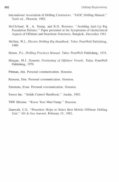
652 Drilling Engineering
International Association of Drilling Contractors. "IADC Drilling Manual."Tenth ed., Houston, 1982.
McClelland, B., A. Young, and B.D. Remmes. "Avoiding Jack-Up RigFoundation Failures." Paper presented at the Symposium of GeotechnicalAspects of Offshore and Nearshore Structures, Bangkok, December 1981.
McNair, W.L. Electric Drilling Rig Handbook. Tulsa: PennWell Publishing,1980.
Moore, P.L. Drilling Practices Manual. Tulsa: PennWell Publishing, 1974.
Morgan, M.J. Dynamic Positioning of Offshore Vessels. Tulsa: PennWellPublishing, 1978.
Pittman, Jim. Personal communication. Houston.
Remson, Don. Personal communication. Houston.
Simmons, Evan. Personal communication. Houston.
Sweco Inc. "Solids Control Handbook." Austin, 1982.
TRW Mission. "Know Your Mud Pump." Houston.
Zumwalt, C.E. "Procedure Helps to Select Best Mobile Offshore DrillingUnit." Oil & Gas Journal, February 15, 1982.
Chapter 17 Special DrillingLogs
Well logging is an important operation in oil and gas production. Inadditionto identifying oil and gas zones, logging can be used effectively for drillingprogress evaluation. A typical log analyst is a specialist who can evaluate welllogs for porosity, fluid content, saturation levels, and permeability estimates.Although these types of calculations are essential to the operation of the well,other important parameters may be needed by the drilling engineer to successfullydrill the well.
Special drilling logs might be defined as tools used primarily to evaluatethe mechanics of the drilling (and workover) operations. Their importance isobvious if they help the engineer drill the well to the target depth. Generally,special drilling logs may not be used in formation evaluation with the exceptionof the sophisticated measurement-while-drilling (MWD) tools. Commonly usedspecial logs are shown in Table 17-1.
Interpretation of special drilling logscan be complicated for several reasons.Quite often, the logs are run under adverse conditions such as kicks, lost cir-culation, or stuck pipe where the downhole conditions are not known. Inaddition,each supplier's tools may function differently and, as such, the interpretationtechniques will vary.
Due to the complications associated with special drilling log interpretation,this chapter has been designed as an overview of some available services. En-gineers desiring details should contact the appropriate service companies. Thischapter is not intended as a review of formation evaluation in the conventionalsense. Interested readers will be able to locate easily a variety of excellentreferences in formation evaluation.
Well logging for pore pressure evaluation is of primary importance to thedrilling engineer. The pore pressures affect the major aspects of the well prog-nosis, including mud, cement, and pipe design. Log analysts typically do not
653
654 Drilling Engineering
Table 17-1 ~ctions of Various Special Drilling Logs
Log Type Function*
Noise
Detects lost circulation zoneDetects lost circulation zone; identifies flow
behind pipe; provides perforation evalua-tion
Evaluates fluid flow quantitatively and qual-itatively
Identifies deepest free section of pipeIdentifies all sections offree pipe, even below
a stuck sectionUnscrews pipe at a tool jointMeasures distance from a relief well to a
blowout wellMeasures distance and direction from a re-
lief well to a blowout wellEvaluates casing wear or corrosionProvides a real-time formation evaluation
tool, from directional guidance to com-plete petrophysical evaluation
Provides formation evaluation from drillingand mud parameters
TemperatureRadioactive tracer
Free pointPipe recovery
Backoff**ULSEL
Magrange II
Casing inspectionMeasurement while drilling
(MWD)
Mud
*Partiallist of primary functions
**Tool, not a log
perform these calculations. Chapter 3 provides a detailed review of the proceduresfor pore pressure evaluation from well logs.
Temperature LegA common tool used to define lost circulation intervals is the temperature
log. This log may be used to record absolute temperature or differential tem-perature. As the logging tool is lowered down the drillpipe, it reads an abnormalchange at the loss zone if the underground flow is continuous (Fig. 17-1).
The tool senses the heat from the fluid that is greater than it should be forthe depth at which it is encountered. In some cases, the temperature change isreported as a cooling effect, supposedly due to gas expansion. Nonetheless, atemperature change is the key. Fig. 17-1. shows a section from an actual tem-perature log, indicating a fluid exit at approximately 1,225 ft.
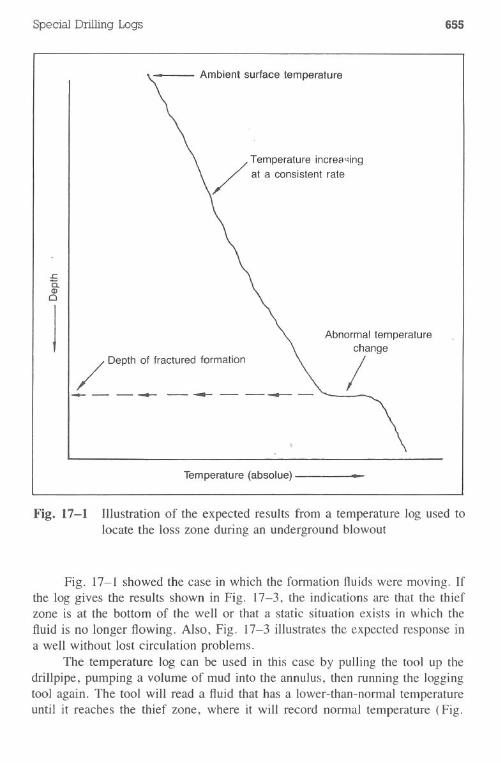
Special DrillingLogs 655
Ambient surface temperature
/ Depth of fractured formation~--~ ~-
/Temperature increa4ingat a consistent rate
..c:
a.CDo
)Abnormal temperature
change
/
Temperature (absolue)
Fig. 17-1 Illustration of the expected results from a temperature log used tolocate the loss zone during an underground blowout
Fig. 17-1 showed the case in which the formation fluids were moving. Ifthe log gives the results shown in Fig. 17-3, the indications are that the thiefzone is at the bottom of the well or that a static situation exists in which the
fluid is no longer flowing. Also, Fig. 17-3 illustrates the expected response ina well without lost circulation problems.
The temperature log can be used in this case by pulling the tool up thedrillpipe, pumping a volume of mud into the annulus, then running the loggingtool again. The tool will read a fluid that has a lower-than-normal temperatureuntil it reaches the thief zone, where it will record normal temperature (Fig.
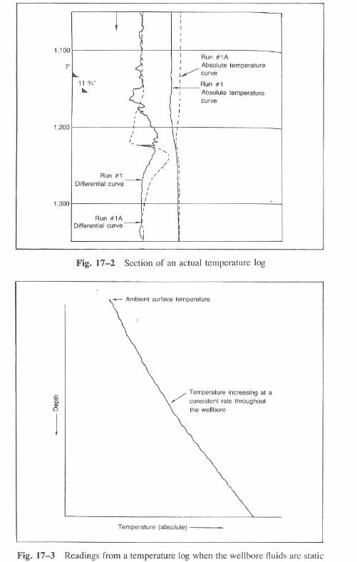
1,100
7'
IIIII
!
I Run #1A
I Absolute temperature
;/ curve
-:-Run #1I Absolutetemperature
curve
11%"....
1,200
1,300
Run #1ADifferential curve
Fig. 17-2 Section of an actual temperature log
- Ambient surface temperature
~0.Q)
CI
j
../ Temperature increasing at a/' consistent rate throughout
the wellbore
Temperature (absolute)
Fig. 17-3 Readings from a temperature log when the wellbore fluids are static
Special Drilling Logs 657
.- Ambient surface temperature
.s:a.Q)a
1
Results from the second run-
The original survey did notindicate abnormal temperature changes
Mud is pumped downthe annulus, which
lowers thestatic temperature
The second survey indicated the ./abnormal change at the detph /
where the mud entered the formation
Fig. 17-4 Illustration of the readings from a temperature log after mud hasbeen pumped down the annulus
17-4). If the results on the second attempt are similar to those shown in Fig.17-3, it is assumed that the lost circulation zone is at the bottom of the well.
Radioactive Tracers
A radioactive tracer survey is used to follow the movement of fluids byintroducing a radioactive isotope into the fluid. This isotope is tracked with agamma ray counter.
The most common radioactive tracer material used in the Gulf Coast areais iodine 131. This material has a half-life of 8.1 days and is soluble in water.Iodine 131 is placed in the borehole with a special injector tool. Each injectionputs a measured amount of solution in the borehole. This slug of tracer material
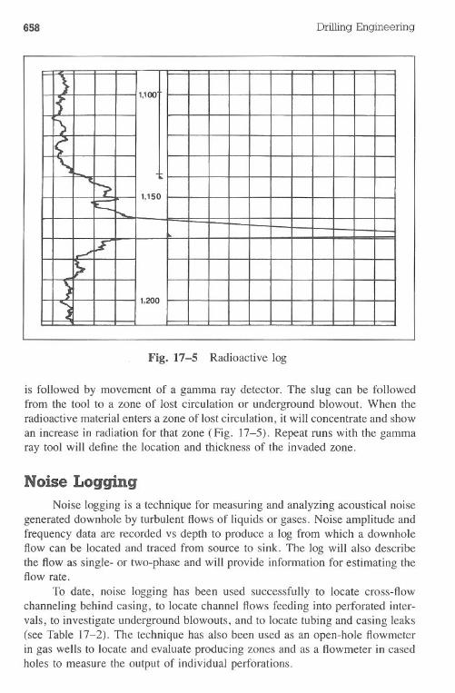
658 Drilling Engineering
Fig. 17-5 Radioactive log
is followed by movement of a gamma ray detector. The slug can be followedfrom the tool to a zone of lost circulation or underground blowout. When theradioactive material enters a zone of lost circulation. it will concentrate and showan increase in radiation for that zone (Fig. 17-5). Repeat runs with the gammaray tool will define the location and thickness of the invaded zone.
Noise LoggingNoise logging is a technique for measuring and analyzing acoustical noise
generated downhole by turbulent flows of liquids or gases. Noise amplitude andfrequency data are recorded vs depth to produce a log from which a downholeflow can be located and traced from source to sink. The log will also describethe flow as single- or two-phase and will provide information for estimating theflow rate.
To date. noise logging has been used successfully to locate cross-flowchanneling behind casing, to locate channel flows feeding into perforated inter-vals, to investigate underground blowouts, and to locate tubing and casing leaks(see Table 17-2). The technique has also been used as an open-hole flowmeterin gas wells to locate and evaluate producing zones and as a flowmeter in casedholes to measure the output of individual perforations.
}1,100
f)
""
'j>,...- 1.150'--.. .........
1.-/l.£
,... 1.200
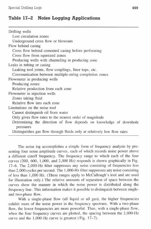
Special Drilling Logs 659
Table 17-2 Noise Logging Applications
Drilling wellsLost circulation zonesUndergroundcross flowor blowouts.
Flow behind casingCross flow behind cemented casing before perforatingCross flow from squeezed zonesProducing wells with channeling in producing zone
Leaks in tubing or casingLeaking tool joints, flow couplings, liner tops, etc.Communication between multiple-string completion zones
Flowmeter in producing wellsProducing zonesRelative production from each zone
Flowmeter in injection wellsZones taking fluidRelative flow into each zone
Limitations on the noise toolCannot distinguish oil from waterOnly gives flow rates to the nearest order of magnitudeDetermining the direction of flow depends on knowledge of downhole
pressuresDistinguishes gas flow through fluids only at relatively low flow rates
The noise log accomplishes a simple form of frequency analysis by pre-senting four noise amplitude curves, each of which records noise power abovea different cutoff frequency. The frequency range to which each of the fourcurves (200, 600, 1,000, and 2,000 Hz) responds is shown graphically in Fig.17-6. The 2,000-Hz filter suppresses any noise consisting of frequencies lessthan 2,000 cycles per second. The 1,OOO-Hzfilter suppresses any noise consistingofless than 1,000 Hz. (These ranges apply to McCullough's tool and are usedfor illustration only.) The relative amounts of separation of space between thecurves show the manner in which the noise power is distributed along thefrequency line. This information makes it possible to distinguish between single-and two-phase flow.
With a single-phase flow (all liquid or all gas), the higher frequenciesexhibit more of the noise power in the frequency spectrum. With a two-phaseflow, the lower frequencies are more powerful. Thus, with a single-phase flow,when the four frequency curves are plotted, the spacing between the 2,000-Hzcurve and the 1,000-Hz curve is greatest (Fig. 17-7).
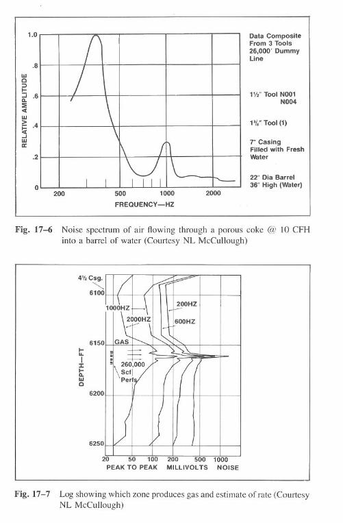
500 1000 2000
FREQUENCY-HZ
Data CompositeFrom 3 Tools26,000' DummyLine
1Y2" Tool N001N004
1%" Tool (1)
7" CasingFilled with FreshWater
22" Dla Barrel36" High (Water)
Fig. 17-6 Noise spectrum of air flowing through a porous coke @ 10 CFHinto a barrel of water (Courtesy NL McCullough)
.-IL
I~.-Q.WC
Fig. 17-7 Log showing which zone produces gas and estimate of rate (CourtesyNL McCullough)
4'12Csg."-...
6100
6150
6200
6250
20 50 100 200 500 1000PEAK TO PEAK MILLIVOLTS NOISE
1.0
.8wc:;).-
.6:Ec(w>j:; .4C(...JWa:
.2
0200
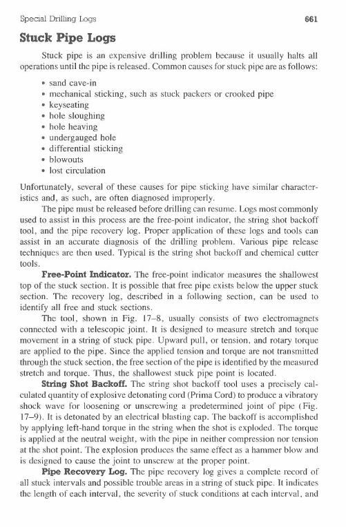
Special Drilling Logs 661
Stuck Pipe LogsStuck pipe is an expensive drilling problem because it usually halts all
operations until the pipe is released. Common causes for stuck pipe are as follows:
· sand cave-in.mechanicalsticking,such as stuckpackersor crookedpipe·keyseating.hole sloughing.hole heaving· undergauged hole·differentialsticking·blowouts· lost circulation
Unfortunately, several of these causes for pipe sticking have similar character-istics and, as such, are often diagnosed improperly.
The pipe must be released before drilling can resume. Logs most commonlyused to assist in this process are the free-point indicator, the string shot backofftool, and the pipe recovery log. Proper application of these logs and tools canassist in an accurate diagnosis of the drilling problem. Various pipe releasetechniques are then used. Typical is the string shot backoff and chemical cuttertools.
Free-Point Indicator. The free-point indicator measures the shallowesttop of the stuck section. It is possible that free pipe exists below the upper stucksection. The recovery log, described in a following section, can be used toidentify all free and stuck sections.
The tool, shown in Fig. 17-8, usually consists of two electromagnetsconnected with a telescopic joint. It is designed to measure stretch and torquemovement in a string of stuck pipe. Upward pull, or tension, and rotary torqueare applied to the pipe. Since the applied tension and torque are not transmittedthrough the stuck section, the free section of the pipe is identifiedby the measuredstretch and torque. Thus, the shallowest stuck pipe point is located.
String Shot Backoff. The string shot backoff tool uses a precisely cal-culated quantity of explosive detonating cord (Prima Cord) to produce a vibratoryshock wave for loosening or unscrewing a predetermined joint of pipe (Fig.17-9). It is detonated by an electrical blasting cap. The backoff is accomplishedby applying left-hand torque in the string when the shot is exploded. The torqueis applied at the neutral weight, with the pipe in neither compression nor tensionat the shot point. The explosion produces the same effect as a hammer blow andis designed to cause the joint to unscrew at the proper point.
Pipe Recovery Log. The pipe recovery log gives a complete record ofall stuck intervals and possible trouble areas in a string of stuck pipe. It indicatesthe length of each interval, the severity of stuck conditions at each interval, and
662
Fig. 17-8 Free point indicatortool (Courtesy NLMcCullough)
DrillingEngineering
Fig. 17-9 String shot back-offtool (Courtesy NLMcCullough)
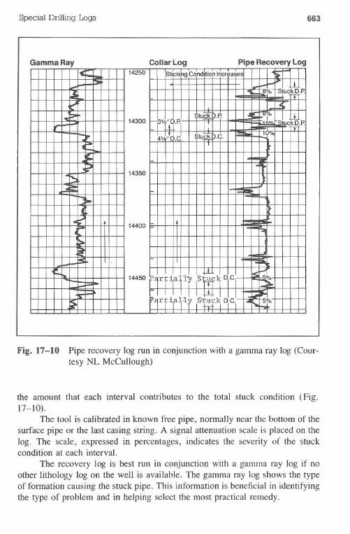
Special Drilling Logs 663
Gamma Ray Collar Log Pipe Recovery Log"' 14250 Sti kingConditionlncr ase! I ~~
~ ~ -~ J W.J B% Stuc.NV~
~ T 4 Iboo StuckD.P. ~IE:"8(0 W.
Ir:;;;;'" 14300 f--~VfHP., I ... ~r~tuckD.P..I.1 _I [!!! 100;'~ 4V."D.C. StuQ!s.D.C.
1~
~ .~
~ ~ 14350:::~ 1!!!8
~ F
14400 ~~~~ ~~
.. I.- 14450',rf¥: 1:17IS~t DrC, 00::~r I 1.1 .!]I+] J_'" _ 1=0
5 E',rf¥Fr IS~~ DiC'1~ ~~o
Fig. 17-10 Pipe recovery log run in conjunction with a gamma ray log (Cour-tesy NL McCullough)
the amount that each interval contributes to the total stuck condition (Fig.17-10).
The tool is calibrated in known free pipe, normally near the bottom of thesurface pipe or the last casing string. A signal attenuation scale is placed on thelog. The scale, expressed in percentages, indicates the severity of the stuckcondition at each interval.
The recovery log is best run in conjunction with a gamma ray log if noother lithology log on the well is available. The gamma ray log shows the typeof formation causing the stuck pipe. This information is beneficial in identifyingthe type of problem and in helping select the most practical remedy.
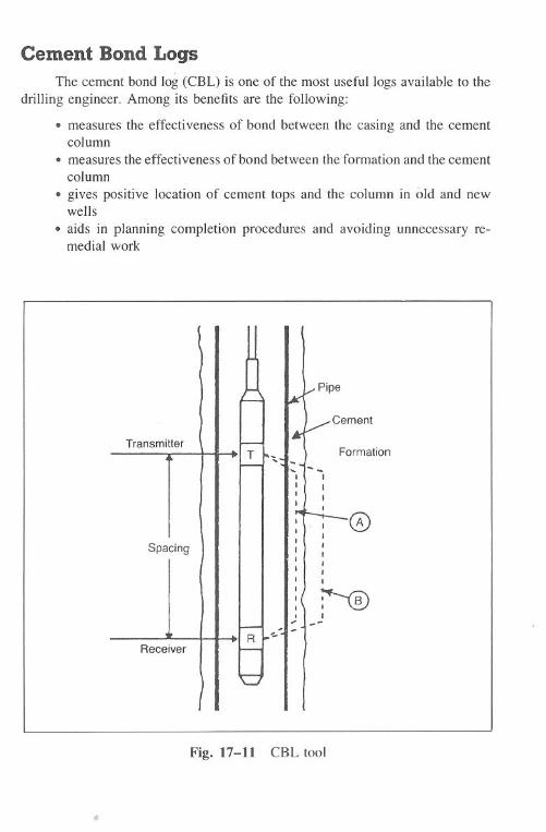
664 DrillingEngineering
Cement Bond LogsThe cement bond log (CBl) is one of the most useful logs available to the
drilling engineer. Among its benefits are the following:
·measures the effectiveness of bond between the casing and the cementcolumn·measures the effectiveness of bond between the formation and the cementcolumn·gives positive location of cement tops and the column in old and newwells·aids in planning completion procedures and avoiding unnecessary re-medial work
Cement
Formation
oIIIIIII
~I
"
Fig. 17-11 CBl tool
(
-
Transmitter -T-
Spacing
r--R
Receiver I--
0
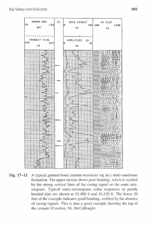
Rig Sizing and Selection 665
BOND CEMENTI
XV PLOTlee 2ge 12eeIe 129
API I1Y
--.....-----------TRANSIT TIME
4~ 34~uS
AMPLIFIED x~2e
'JOO
Fig. 17-12 A typical gamma/bond cement/wavetrain log in a shale-sandstoneformation. The upper section shows poor bonding, which is verifiedby the strong vertical lines of the casing signal on the sonic-seis-mogram. Typical sonic-seismogram collar responses in poorlybonded pipe are shown at 10,480 ft and 10,520 ft. The lower 20feet of the example indicates good bonding, verified by the absenceof casing signals. This is also a good example showing the top ofthe cement (Courtesy NL McCullough)
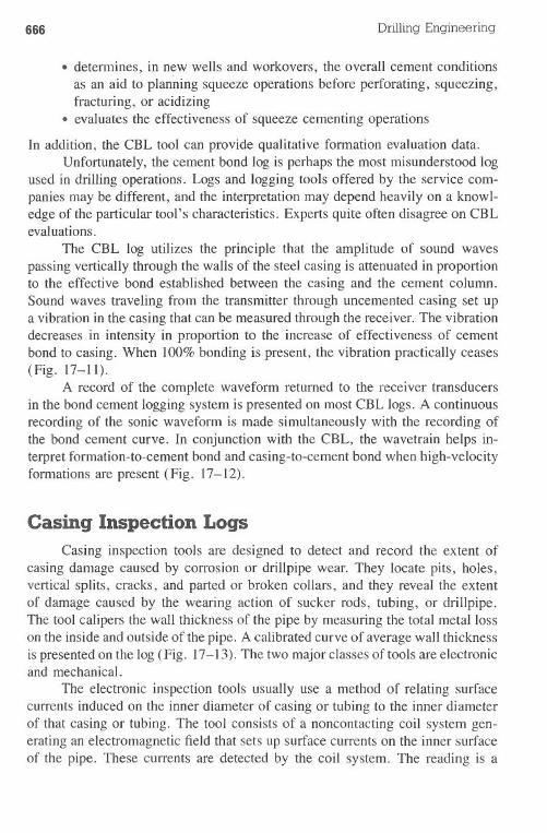
666 Drilling Engineering
·detennines, in new wells and workovers, the overall cement conditionsas an aid to planning squeeze operations before perforating, squeezing,fracturing, or acidizing·evaluates the effectiveness of squeeze cementing operations
In addition, the CBL tool can provide qualitative fonnation evaluation data.Unfortunately, the cement bond log is perhaps the most misunderstood log
used in drilling operations. Logs and logging tools offered by the service com-panies may be different, and the interpretation may depend heavily on a knowl-edge of the particular tool's characteristics. Experts quite often disagree on CBLevaluations.
The CBL log utilizes the principle that the amplitude of sound wavespassing vertically through the walls of the steel casing is attenuated in proportionto the effective bond established between the casing and the cement column.Sound waves traveling from the transmitter through uncemented casing set upa vibration in the casing that can be measured through the receiver. The vibrationdecreases in intensity in proportion to the increase of effectiveness of cementbond to casing. When 100% bonding is present, the vibration practically ceases(Fig. 17-11).
A record of the complete wavefonn returned to the receiver transducersin the bond cement logging system is presented on most CBL logs. A continuousrecording of the sonic wavefonn is made simultaneously with the recording ofthe bond cement curve. In conjunction with the CBL, the w!lvetrain helps in-terpret fonnation-to-cement bond and casing-to-cement bond when high-velocityfonnations are present (Fig. 17-12).
Casing Inspection LogsCasing inspection tools are designed to detect and record the extent of
casing damage caused by corrosion or drillpipe wear. They locate pits, holes,vertical splits, cracks, and parted or broken collars, and they reveal the extentof damage caused by the wearing action of sucker rods, tubing, or drillpipe.The tool calipers the wall thickness of the pipe by measuring the total metal losson the inside and outside of the pipe. A calibrated curve of average wall thicknessis presented on the log (Fig. 17-13). The two major classes of tools are electronicand mechanical.
The electronic inspection tools usually use a method of relating surfacecurrents induced on the inner diameter of casing or tubing to the inner diameterof that casing or tubing. The tool consists of a noncontacting coil system gen-erating an electromagnetic field that sets up surface currents on the inner surfaceof the pipe. These currents are detected by the coil system. The reading is a
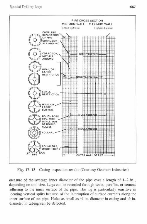
Special Drilling Logs 667
PIPE CROSS SECTIONMINIMUM WALL MAXIMUM WALL(ShowS wall loss) (includes buildup)
COMPLETE
@SEPARATlONOF PIPECORROSIONALL AROUND
@ CORROSION,NOT ALLAROUND
@ OVAL,OR~ LARGE
@ .m.,a,ON
~ SMALL
W RESTRICTION
@ HOLE, OR ,..,...,LARGEBLISTER
@ROUGH BOREPIPE, WITHSMALL, OUTOF ROUND
~ :::.~ ROUNDPIPE,~ SMOOTHBORE
LEG PIPE TOOL
. .
.-
Fig. 17-13 Casing inspection results (Courtesy Gearhart Industries)
measure of the average inner diameter of the pipe over a length of 1-2 in.,depending on tool size. Logs can be recorded through scale, paraffin, or cementadhering to the inner surface of the pipe. The log is particularly sensitive inlocating vertical splits because of the interruption of surface currents along theinner surface of the pipe. Holes as small as %-in. diameter in casing and Yz-in.diameter in tubing can be detected.
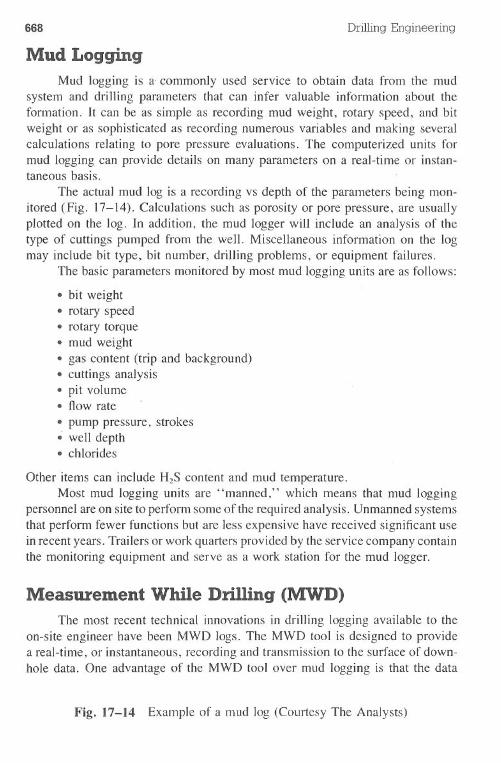
668 Drilling Engineering
Mud LoggingMud logging is a. commonly used service to obtain data from the mud
system and drilling parameters that can infer valuable information about theformation. It can be as simple as recording mud weight, rotary speed, and bitweight or as sophisticated as recording numerous variables and making severalcalculations relating to pore pressure evaluations. The computerized units formud logging can provide details on many parameters on a real-time or instan-taneous basis.
The actual mud log is a recording vs depth of the parameters being mon-itored (Fig. 17-14). Calculations such as porosity or pore pressure, are usuallyplotted on the log. In addition, the mud logger will include an analysis of thetype of cuttings pumped from the well. Miscellaneous information on the logmay include bit type, bit number, drilling problems, or equipment failures.
The basic parameters monitored by most mud logging units are as follows:
· bit weight·rotary speed· rotary torque· mud weight·gas content (trip and background)· cuttings analysis·pit volume· flow rate· pump pressure, strokes. well depth· chlorides
Other items can include HzS content and mud temperature.Most mud logging units are "manned," which means that mud logging
personnel are on site to perform some of the required analysis. Unmanned systemsthat perform fewer functions but are less expensive have received significant usein recent years. Trailers or work quarters provided by the service company containthe monitoring equipment and serve as a work station for the mud logger.
Measurement While Drilling (MWD)The most recent technical innovations in drilling logging available to the
on-site engineer have been MWD logs. The MWD tool is designed to providea real-time, or instantaneous, recording and transmission to the surface of down-hole data. One advantage of the MWD tool over mud logging is that the data
Fig. 17-14 Example of a mud log (Courtesy The Analysts)
Special Drilling Logs
""""n
o
iSfAmD LOGGING AT.
;MUD TYPlS
"'.."EVIATION'LAT . LOGGED A"E" T"I~LAST. LOGGEO Af'TELIt SHOltY T'''~...LIt. NO RETUltNS...8 . NEW .'TN08 . NEW OIA"'OND .,TIE.LOG . ELECTRIC LOGCO. CILltCULATE OUTClltC . CONDITION HOLE
o MINI". 0"/""
-,
. -
...
-..-..
- -.... ..
-.
n
.. :."1!-
..,~ ,
-,.-0--
1-
HOUSIUI. COttl'USCHIIm
HOlUIZI ; CASI~-.~OWOI...J1:" TO_.
5... .
1
_.,.S_!l!: TO_:~ I~...!/..TO.'''' --'n~-IC .~--.J_td'_TO...Jg3-'~
I
-TO--- - I_TO._ __TO__ I,FEIT...J.:.&:.ILICEASEDLOGGIHGAT '0310 RfT_'.O..,....
'5218 FT.; LleN08ULPONATETO 10590 Fr.
SfATEUHIT.
.IJI!XI.
TO
-
......
669
Olll'LLlNG FLUID ANALYSISSHOW"'ALU..
n
MW- 10.5 CHL- 200(
."::ISd-I88I' cone_ I'M.::: "',-1\1....
-,. --
Sh-lI'IOd fir"'. It ery.IUt,.ldy-
MW- 10.5 CHL-2000!
Sd- lot". It If'Y.vfv-''''II cok
..
-0- SII-mod 'I,m. t". ed7'
- Sd-trIO' CORI, It Qr')' .v'v-ft.ouco&c,brkJht ,8JIC* 'kID..,rtQl'flln9 cut
..
.-
'I~-
-
NW- 11.3 CHL-2100
.Sh-'I,m"".'ltly.
.Uede,trpyr!"
..- -..sr.- firm. ,rJ.drk,,..,,
brltn,.fI",NW- C2.3 OiL- 2200
-. n
-.. MW- 12.5 eN.. 22001
Sd-.oft.1t9"Y,v"-sr.. firm, drk ;ry,.1I
ca:c, v flkyMW- 2.8 CHL-2201
,-s'- ftrra,lt ;ry,Cok,
..
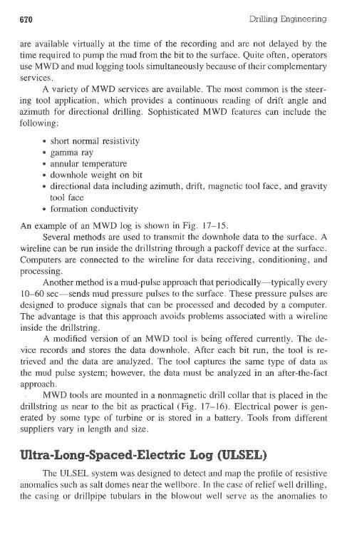
670 Drilling Engineering
are available virtually at the time of the recording and are not delayed by thetime required to pump the mud from the bit to the surface. Quite often, operatorsuse MWD and mud loggingtools simultaneously because of their complementaryservices.
A variety of MWD services are available. The most common is the steer-ing tool application, which provides a continuous reading of drift angle andazimuth for directional drilling. Sophisticated MWD features can include thefollowing:
· short normal resistivity·gamma ray·annular temperature·downhole weight on bit·directional data including azimuth, drift, magnetic tool face, and gravitytool face·formation conductivity
An example of an MWD log is shown in Fig. 17-15.Several methods are used to transmit the downhole data to the surface. A
wireline can be run inside the drillstring through a packoff device at the surface.Computers are connected to the wireline for data receiving, conditioning, andprocessing.
Another method is a mud-pulse approach that periodically-typically every10-60 sec-sends mud pressure pulses to the surface. These pressure pulses aredesigned to produce signals that can be processed and decoded by a computer.The advantage is that this approach avoids problems associated with a wirelineinside the drillstring.
A modified version of an MWD tool is being offered currently. The de-vice records and stores the data downhole. After each bit run, the tool is re-trieved and the data are analyzed. The tool captures the same type of data asthe mud pulse system; however, the data must be analyzed in an after-the-factapproach.
MWD tools are mounted in a nonmagnetic drill collar that is placed in thedrillstring as near to the bit as practical (Fig. 17-16). Electrical power is gen-erated by some type of turbine or is stored in a battery. Tools from differentsuppliers vary in length and size.
mtra-Long-Spaced-Electric Log (ULSEL)The ULSEL system was designed to detect and map the profile of resistive
anomalies such as salt domes near the wellbore. In the case of relief well drilling,the casing or drillpipe tubulars in the blowout well serve as the anomalies to
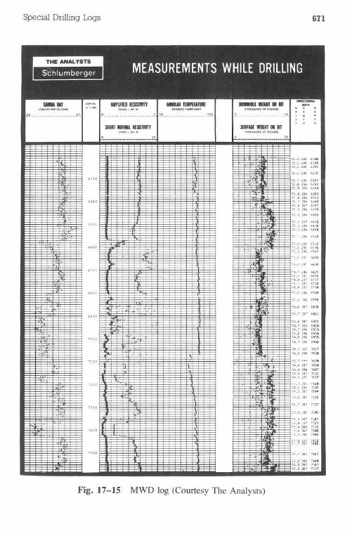
Special Drilling Logs 671
.~,.IIfGWIS,AMlfHMf"
~ ~1'!C? }~.
SIIOIT InRIIlIUISTIIITI
0 :0
Fig. 17-15 MWD log (Courtesy The Analysts)
....,.",t,!."».02a66U2
(,)O I III I 1 I I(J I I I I I I 1 I 1,1 I I I I I I I YII I I I '')'),72')6626.SS.6286 62US':>.'923661i4')\.3286 628]'j,8 286 611)
640:11 'I I I J I I , J J I I I I I I 1,'1] I II I I"'!"] 1 ] 10;\.' 286 614'S".6 281 6)9!lS.S 286 6)16!IS.5 286 '4OS
(,,,!)O,-. r I I I lrj I J I J I I I I I L' I I I I I I I I. I'lf I ] I:; : :::.....22i1664'8
.....:286 6'i10
')'Io.02866!122HOG I I "':.Li& I ] ] 1 I ] : , ] 1 1 ] I ] J J.d',!! ] I 1"').02IS 6SM
o;'>.22')66'i6J"'S.O287 %00
610.:11 1.11 I 11 I f.] I I I I I I I III.H. 11111:::::::::::-,)".02in 6674">4.82376707....,.!28' 6nOS..8287 6HI
....I 1'1I
I : .1 I' I : . I I 11111': II: 1"0;,.0286 6769';';.0 86 6,",
"".628768)0
6900 I 11.... 1 I 1 rr '1 I I 1 I I I III I I II I l'j,lII I I 1 I 1')1..'2616861':.4."2876.19)S4.7285 6%0S4.1286 (112)S_8 286 '06
1000 I PI.I : I r 1 . 1 j I : . ] I 1 Il J J I I '.1 I I II 1\4.82M 69\S\4.12866.'54.1281 1011'>4.8286 70\8
1\00 1 J I 'III ! 11'[ r T 1 I 1'1 1.1. 1 I 1'1 I 1 1\'L1'" 10""4.42817064"4,418' 109'1)4,421111121\4.\ 21 7101
12001 , ' 1 .1' I 1 I] I ] 1 1 1 II ] 1 I]] 1 ]"Jo_l] 1\:.718) 7168'>4.1286 '17(11)'.218171'.\).9 181 122S
1100 I-JI-T-r-r I Ft 1 I 1 1 II I 1 III 1 II I I J t r-Il 11'1..1 11)),118' 711)'1I))'1i :36 7290
..1.) 111' 128'')).9:311123").428' 7310
'.00 III 11-' Iii ] I ] 1 I 1"1 ] 1 1 1 I ] '] '1 ,..._ I ] 1:).6J:811)...)., 186 7)$6
;m1.,001 II I II r.1I II' i III 111 II II1I JjSI I II".'.", ""
')),81811 14f.''\1.,)1877SO:'l'\). 281 7')17
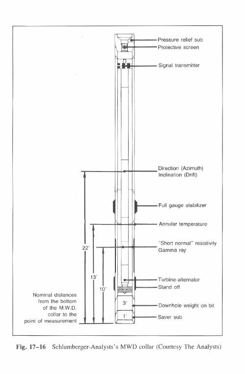
672
Nominal distancesfrom the bottom
of the M.W.D.collar to the
point of measurement
22'
13'
10'
Drilling Engineering
Pressure relief sub
Protective screen
Signal transmitter
Direction (Azimuth)Inclination (Drift)
Full gauge stabilizer
Annular temperature
"Short norma'" resistivityGamma ray
Turbine-alternator
Stand off
Downhole weight on bit
Saver sub
Fig. 17-16 Schlumberger-Analysts's MWD collar (Courtesy The Analysts)
3'
l'
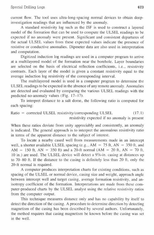
Special DrillingLogs 673
current flow. The tool uses ultra-long-spacing normal devices to obtain deep-investigation readings that are influenced by the anomaly.
A standard resistivity log such as the ISF is used to construct a layeredmodel of the formation that can be used to compute the ULSEL readings to beexpected if no anomaly were present. Significant and consistent departures ofthe actual ULSEL values from these expected values indicate the presence ofresistive or conductive anomalies. Dipmeter data are also used in interpretationand computation.
Digitized induction log readings are used in a computer program to arriveat a multilayered model of the formation near the borehole. Layer boundariesare selected on the basis of electrical reflection coefficients, i.e., resistivitycontrasts. Each layer of the model is given a constant resistivity equal to theaverage induction log resistivity of the corresponding interval.
The multilayered model is used in a computer program to determine theULSEL readings to be expected in the absence of any remote anomaly. Anomaliesare detected and evaluated by comparing the various ULSEL readings with thepredicted no-anomaly values (Fig. 17-17).
To interpret distance to a salt dome, the following ratio is computed foreach spacing:
Ratio = corrected ULSEL resistivity/corresponding ULSEL (17.1)resistivity expected if no anomaly is present
When these ratios deviate from unity appreciably and consistently, an anomalyis indicated. The general approach is to interpret the anomalous resistivity ratioin terms of the apparent distance to the subject of interest.
To locate a nearby cased well from measurements made in an interceptwell, a shorter available ULSEL spacing (e.g., AM = 75 ft, AN = 350 ft, andAM = 150 ft, AN = 350 ft) and a 20-ft normal (AM = 20 ft, AN = 70 ft,10 in.) are used. The ULSEL device will detect a 9%-in. casing at distances upto 70-80 ft. If the distance to the casing is definitely less than 20 ft, only the20-ft normal is required.
A computer produces interpretation charts for existing conditions, such asspacing of the ULSEL or normal device, casing size and weight, approach anglebetween intercept well and target casing, average formation resistivity, and an-isotropy coefficient of the formation. Interpretations are made from these com-puter-produced charts by the ULSEL analyst using the relative resistivity ratiosfrom the computer output.
This technique measures distance only and has no capability by itself todetect the direction of the casing. A procedure to determine direction by detectingmagnetism of the casing has been described by several authors. Unfortunately,the method requires that casing magnetism be known before the casing was setin the well.
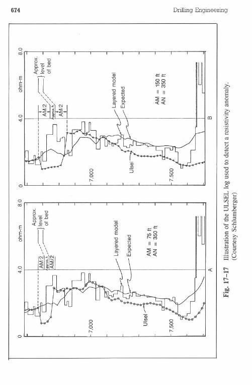
o 4.0
7,000
ohm-m
Layered model
Expected
AM = 75 ftAN = 350 ft
A
8.0 o 4.0 ohm-m 8.0
7,000
Layered model
Expected
AM = 150 ftAN = 350 ft
B
Fig. 17-17 Illustration of the ULSEL log used to detect a resistivity anomaly.(Courtesy Schlumberger)
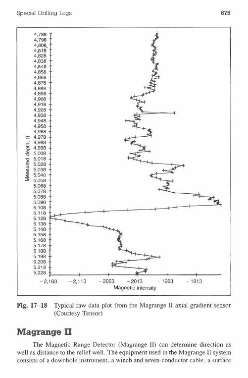
Special Drilling Logs
4,7884,7984,808.4,8184,8284,8384,8484,8584,8684,8784,8884,8984,9084,9184,9284,9384,9484,9584,968
-= 4,978£ 4,988C. 4,998~ 5,008"tJ 5,018~ 5,028gj 5,038Q) 5,048:E 5,058
5,0685,0785,0885,0985,1085,1185,1285,1385,1485,1585,1685,1785,1885,1985,2085,2185,228.
- 2,163
675
- 2,113 -2063 -2013 -1963
Magnetic intensity
-1913
Fig. 17-18 Typical raw data plot from the Magrange II axial gradient sensor(Courtesy Tensor)
Magrange IIThe Magnetic Range Detector (Magrange II) can determine direction as
well as distance to the relief well. The equipment used in the Magrange II systemconsists of a downhole instrument, a winch and seven-conductor cable, a surface
676 Drilling Engineering
electronic unit, a programmable calculator, and a plotter. The downhole instru-ment contains magnetic field sensors arranged in a noninterfering orthogonalconfiguration and in a gradiometric measurement configuration. The sensors,along with their associated electronics and signal conditioning circuitry, arehoused in a nonmagnetic cylindrical container. Under optimum conditions, Ma-grange II can detect targets at a range of 100 ft. The direction from the reliefwell to the target well can be determined to within a few degrees.
Magrange II is a proprietary name of the service offered by a certainsupplier. Other service companies may offer functionally similar logs underdifferent product names. For example, Gearhart Industries offers the ELREClog, which is comparable to the Magrange II. ELREC is reported to locate theblowout well at distances up to 200 ft.
SEEC, another manufacturer's tool, is reported to be similar to MagrangeII but with increased accuracy from 0-30 ft.
The Magrange tool, a recent development (1975), has proved successfulin a number of field applications. In a blowout in West Cameron, offshoreLouisiana, the Magrange II system guided the relief well to an adjacent pointnear the blowout well for a successful pumping kill operation. A typical plot ofraw data gathered from the axial gradient sensor is shown in Fig. 17-18.
Summary
Special logs used by drilling engineers to assist operations are valuabletools. A thorough working knowledge of the tools and applications is necessaryto obtain optimum performance. This field of logging tools is expanding everyday.
Problems
17.1 How can a noise log be used in underground blowout situations?
17.2 Refer to Fig. 17-10. The pipe appears to be stuck at 14,367 ft. Whatcauses this false indication on the log?
17.3 How can a temperature log be used to locate the top of cement?
17.4 The pipe recovery log functions similar to another special logging tool.Which one?
17.5 Refer to Fig. 17-14. At depths of 8,200 and 8,420 ft, determine thefollowing:.drill rate· lithology
Special Drilling Logs 677
·rock density· gas contentWhat is the approximatetrue verticaldepth of the well?
17.6 In Fig. 17-15, is the well directional drilled? If so, what is the ap-proximate inclination?
17.7 How can MWD tools be used in kick detection?
References
Adams, N.J. Well Control Problems and Solutions. Tulsa: PennWell, 1980.
Adams, N.J. Workover Well Control. Tulsa: PennWell, 1981.
The Analysts. Measurement While Drilling, M.W.D., 1983.
Gearhart Industries. Well Service Systems, 1983.
Morris, F.J., et aI. "A New Method of Determining Range and Directionfrom a Relief Well to a Blowout Well." SPE 6781, 1977 Fall TechnicalConference, Denver.
NL Baroid. Various mud logging brochures.
NL McCullough. Logging Manual. 1984.
NL McCullough. Pipe Recovery Manual, 1984.
Schlumberger. Log Interpretation/Application, 1980.
Chapter 18 Hydraulics
Since the hydraulics system plays an active role during the drilling oper-ations, its proper design and maintenance can accelerate the drilling effort andlower the overall well cost. Likewise, an improperly designed hydraulics systemcan slow drill rate, fail to clean the hole of cuttings, and cause kicks. In mostcases, common sense and commercially available computer programs are theonly elements required to design the system.
The hydraulics system is the mud system in the wellbore when it is ineither a static or a dynamic state. The static system occurs when the mud standsidle in the well. The dynamic state occurs when the mud is in motion, resultingfrom pumping or pipe movement.
A thorough study of hydraulics is an exhaustive, lifetime effort. Manyexcellent technical papers and books have been written on the subject. Inherently,many subject areas are open to conflicts of opinion by industry members. Thischapter is designed as a brief overview of the field and is not intended as acomplete dissertation on hydraulics. Some points considered as important areneglected from the text in the spirit of brevity.
Purposes
The hydraulics system serves many purposes in the well. Since it is centeredaround the mud system, the purposes of mud and hydraulics are often commonto each other (refer to Chapter 8).
The hydraulics system has many effects on the well. Therefore, the reasonsfor giving attention to hydraulics are abundant. The more common reasons areas follows:
678
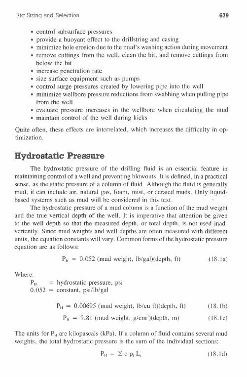
Rig Sizing and Selection 679
.control subsurface pressures·provide a buoyant effect to the drillstring and casing.minimize hole erosion due to the mud's washing action during movement· remove cuttings from the well, clean the bit, and remove cuttings frombelow the bit· increase penetration rate· size surface equipment such as pumps· control surge pressures created by lowering pipe into the well·minimize wellbore pressure reductions from swabbing when pulling pipefrom the well· evaluate pressure increases in the wellbore when circulating the mud..maintain control of the well during kicks
Quite often, these effects are interrelated, which increases the difficulty in op-timization.
Hydrostatic Pressure I
.1The hydrostatic pressure of the drilling fluid is an essential feature inmaintaining control of a well and preventing blowouts. It is defined, in a practicalsense, as the static pressure of a column of fluid. Although the fluid is generallymud, it can include air, natural gas, foam, mist, or aerated muds. Only liquid-based systems such as mud will be considered in this text.
The hydrostatic pressure of a mud column is a function of the mud weightand the true vertical depth of the well. It is imperative that attention be givento the well depth so that the measured depth, or total depth, is not used inad-vertently. Since mud weights and well depths are often measured with differentunits, the equation constants will vary. Common forms of the hydrostatic pressureequation are as follows:
PH = 0.052 (mud weight, Ib/gal)(depth, ft) (I8.la)
Where:PH0.052
= hydrostatic pressure, psiconstant,psillblgal
PH = 0.00695 (mud weight, Ib/cu ft)(depth, ft)
PH = 9.81 (mud weight, g/cm3)(depth, m)
(I8.lb)
(I8.lc)
The units for PHare kilopascals (kPa). If a column of fluid contains several mudweights, the total hydrostatic pressure is the sum of the individual sections:
(I8.ld)
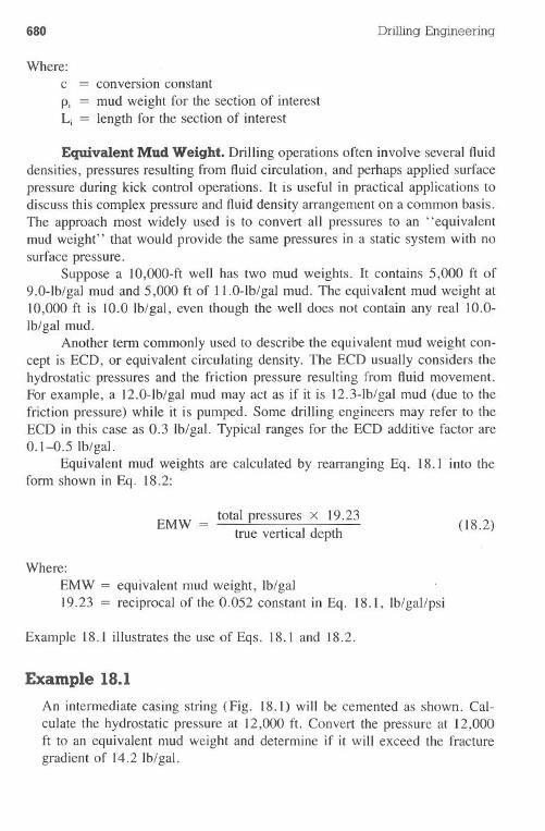
680 Drilling Engineering
Where:c = conversion constantPi = mud weight for the section of interestLi = length for the section of interest
Equivalent Mud Weight. Drilling operations often involve several fluiddensities, pressures resulting from fluid circulation, and perhaps applied surfacepressure during kick control operations. It is useful in practical applications todiscuss this complex pressure and fluid density arrangement on a common basis.The approach most widely used is to convert all pressures to an "equivalentmud weight" that would provide the same pressures in a static system with nosurface pressure.
Suppose a IO,OOO-ftwell has two mud weights. It contains 5,000 ft of9.0-lb/gal mud and 5,000 ft of 11.0-lb/gal mud. The equivalent mud weight at10,000 ft is 10.0 Ib/gal, even though the well does not contain any real 10.0-Ib/gal mud.
Another term commonly used to describe the equivalent mud weight con-cept is ECD, or equivalent circulating density. The ECD usually considers thehydrostatic pressures and the friction pressure resulting from fluid movement.For example, a 12.0-lb/gal mud may act as if it is 12.3-lb/gal mud (due to thefriction pressure) while it is pumped. Some drilling engineers may refer to theECD in this case as 0.3 Ib/gal. Typical ranges for the ECD additive factor are0.1-0.5 Ib/gal.
Equivalent mud weights are calculated by rearranging Eq. 18.1 into theform shown in Eq. 18.2:
EMW total pressures X 19.23
true vertical depth(18.2)
Where:
EMW = equivalent mud weight, Ib/gal19.23 = reciprocal of the 0.052 constant in Eq. 18.1, Ib/gallpsi
Example 18.1 illustrates the use of Eqs. 18.1 and 18.2.
Example 18.1
An intermediate casing string (Fig. 18.1) will be cemented as shown. Cal-culate the hydrostatic pressure at 12,000 ft. Convert the pressure at 12,000ft to an equivalent mud weight and determine if it will exceed the fracturegradient of 14.2 Ib/gal.
Hydraulics 681
11.4-lb/gal mud
Mud ~
7,000 ft
12,000 ft
-
r-
15.4Ib/galClass H cement
r16.6 Ib/galClass H cement
y
Fracture gradient f14.2 Ib/gal ~
9,000 ft
Fig. 18-1 Hydrostatic pressure calculation for Example 18.1
Solution:
. I. The hydrostatic pressures are computed as follows:0.052 x fluid weight x depth = pressure0.052 x 11.41b/gal x (7,000 ft)0.052 x 15.4 Ib/gal x (9,000 - 7,000 ft)0.052 x 16.6 Ib/gal x (12,000 - 9,000 ft)
(l8.la)4,149 psi1,602 psi2,589 psi8,340 psi
2. The equivalent mud weight is calculated from Eq. 18.2:
EMW = total pressure x 19.23TVD (18.2)
13.36 Ib/galTherefore, the static hydrostatic pressure with a 13.36-lb/gal EMW willnot exceed the fracture gradient of 14.2 Ib/gal.
682 Drilling Engineering
BuoyancyThe drilling fluid provides a beneficial effect relative to drillstring weight
or hook load. When pipe is lowered into the well, the mud system will support,or buoy, some of the pipe weight. This effect is termed buoyancy, or buoyantforces. The buoyed weight of the drillstring will be less than the in-air weightof the pipe.
Buoyant forces are a function of the volume and weight of the displacedfluid. Heavier muds have greater buoyant forces than low-density muds. Thebuoyed pipe weight can be calculated from Eq. 18.3:
BW = (BF)(in-air weight) (18.3)
Where:
BW = ~uoyed weightBF = buoyancy factor
PmBF = I - 65.5 (18.4)
Where:Pm = mud density, Ib/gal
The constant of 65.5 is the density of a gallon of steel.
Excpnple 18.2
A casing string will be run into a well that contains II. 7-lb/gal mud. Assumethe casing will be filled with mud as it is run. If the engineer uses a derricksafety factor of 2, will the I,OOO,OOO-Ibderrick capacity be satisfactory?
Casing Weight, Ib/ft47.053.047.0
Section Length, ft4,5005,5003,000
13,000
Solution:
I. The casing string weight, in air, is:
4,500 ft x 47.0Ib/ft5,500 ft x 53.0 Ib/ft3,000 ft x 47.0Ib/ft
211,500291,500141,000
644,000 Ib
Hydraulics 683
2. Determine the buoyancy factor for 11.7-lb/gal mud:
BF = 1 - ..£m....65.5
= 1 _ 11.765.5
(18.4)
= 0.82
3. The in-mud weight is the product of the buoyancy factor and the stringweight:
buoyed weight = (0.82)(644,000Ib)528,964 lb
4. Applying a derrick safety factor of 2:
(2.0)(528,964) > 1,000,000 lb
Therefore, the derrick load will exceed the design criteria if a factor of2.0 is used. The actual design value is:
1,000,000Ib528,964 lb
1.89
Flow RegimesWhile drilling fluids are flowing in a weIl, the manner in which the fluid
behaves may vary. This behavior is often termed the flow regime. The mostcommon regimes are laminar, turbulent, and transitional. Unfortunately, it isimpossible to clearly define each type in the well. As an example, mud flowmay be predominantly laminar, although the flow near the pipe waIls duringpipe rotation may be turbulent.
Laminar Flow. The most common annular flow regime is laminar. Itexists from very low pump rates to the rate at which turbulence begins. Char-acteristics of laminar flow useful to the drilling engineer are low friction pressuresand minimum hole erosion.
Laminar flow can be described as individual layers, or laminae, movingthrough the pipe or annulus (Fig. 18-2). The center layers usuaIly move at ratesgreater than the layers near the weIlbore or pipe. The flow profile describes thevariations in layer velocities. These variations arecontroIled by the shear-resistantcapabilities of the mud. A high yield point for the mud tends to make the layersmove at more uniform rates.
684
Velocity profile
Drilling Engineering
Drillpipe
Laminar flow
Formation
Fig. 18-2 Laminar flow
Cuttings removal is often discussed as being more difficult with laminarflow. The cuttings appear to move outward from the higher-velocity layers tothe more acquiescent areas. These outer layers have very low velocities and maynot be effective in removing the cuttings. A common procedure for minimizingthe problem is to increase the yield point, which decreases layer velocity vari-ations. An alternative is to pump a 1O-20-bbl high-viscosity plug to "sweep"the annulus of cuttings.
Turbulent Flow. Turbulence occurs when increased velocities betweenthe layers create shear strengths exceeding the ability of the mud to remain inlaminar flow. The layered structure becomes chaotic and turbulent (Fig. 18-3).Turbulence occurs commonly in the drillstring and occasionally around the drillcollars.
Much published literature suggests that annular turbulent flow increaseshole erosion problems. The flow stream is continuously swirling into the walls.In addition, the velocity at the walls is significantly greater than the wall layerin laminar flow. Many industry personnel believe that turbulent flow and theformation type are the controlling parameters for erosion.
Hydraulics 685
Fluid flow
Fig. 18-3 Turbulent flow
Transitional Flow. Unfortunately, it is often difficult to estimate the flowrate at which turbulence will occur. In addition, turbulence may occur in variousstages. It is convenient to describe this "gray" area as a transitional stage.
Turbulence Criteria. Several common methods can be used to establishturbulence criteria. The most common approach is the Reynolds number. Othersinclude I) intersection of the flow rate vs pressure loss calculations for laminarand turbulent flow and 2) calculation of a z-value. The Reynolds number approachis used almost exclusively in the industry.
Reynolds published a paper (1883) that reported experiments dealing withflow in pipes. He injected a thin filament of dye into a moving stream ofliquid flowing in a glass pipe and found that if the numerical value of agroup of variables was less than 2,100, the dye filament remained small. Thefilament rapidly dispersed in "eddies" if the value of the group was greater than2,100.
Turbulence occurs when the ratio of the momentum of the liquid to theviscosity ability of the liquid to dampen permeations exceeds some empiricallydetermined value. The momentum force of the liquid is its velocity times itsdensity. The viscous ability of the liquid to damp out permeations is the internalresistance against change and the effects of the walls of the borehole. For the
686 Drilling Engineering
simple case of a Newtonian, nonelastic liquid flowing in a pipe, the dampeningeffect is the quotient of the viscosity and the diameter of the wellbore:
(18.5)
Where:
NR = Reynolds numberp = densityD = diameter
j.L = viscosity
Since drilling muds are non-Newtonian and contain some degree of elasticity,definitionof a singleReynoldsnumberbecomesdifficult. .
The Reynolds number for flow of a non-Newtonian liquid in a pipe isshown in Eq. 18.6:
(18.6)
Where:NRcnk
= effective Reynolds numberflow behavior index
= consistency index
The terms nand K relate to the Power Law mud model, which will be discussedin following sections. A simpler equation used in the literature to predict theReynolds number at the upper limit of laminar flow is as follows:
NRc= 3,470 - 1,370 n (18.7)
The relation for the Reynold~ number between the transition and turbulent flowregimes is given in Eq. 18.8:
NRc= 4,270 - 1,370 n (18.8)
It is obvious from Eqs. 18.7 and 18.8 that the Reynolds number is sliding, withits dypendency on the flow behavior index.
The position of intersection between the laminar and turbulent flow pressurelosses depends on the equations being used (Fig. 18-4)., The Reed slide rule or.the Hughes tables can give errors if the mud is quite non-Newtonian at theapplicable shear rate. Using well-known equations available in the literature and
Hydraulics 687
Turbulent flow calculations
I Intersection definesbeginning of turbulence
\Q)
:;(/)(/)Q)
a:
Laminar flow calculations
Flow rate ..
Fig. 18-4 Intersection of laminar and turbulence flow calculations used as theturbulence criteria
a Newtonian fluid, the laminar-turbulent pressure lines intersect at a point thatis equivalent to a Reynolds number of approximately 1,900, or 10% below the2,100 value. The point of intersection for non-Newtonian fluids may be 30%below the actual transition.
The z-value method was developed by Ryan and Johnson based on ex-perimental data from several sources and experimentally verified by others. Thez-value is calculated from Eq. 18.9:
z pV (dV/dr)TW
(I8.9)
Laminar flow is assumed, and the z-value is calculated and plotted vs the radius.If the value exceeds 808, the assumption of laminar flow'is incorrect and tur-bulence occurs. Calculating the z-value is complex and time-consuming.
Critical Velocity. The term critical velocity is used to define the singlevelocity at which the flowregime changes from laminar to turbulent. This variable
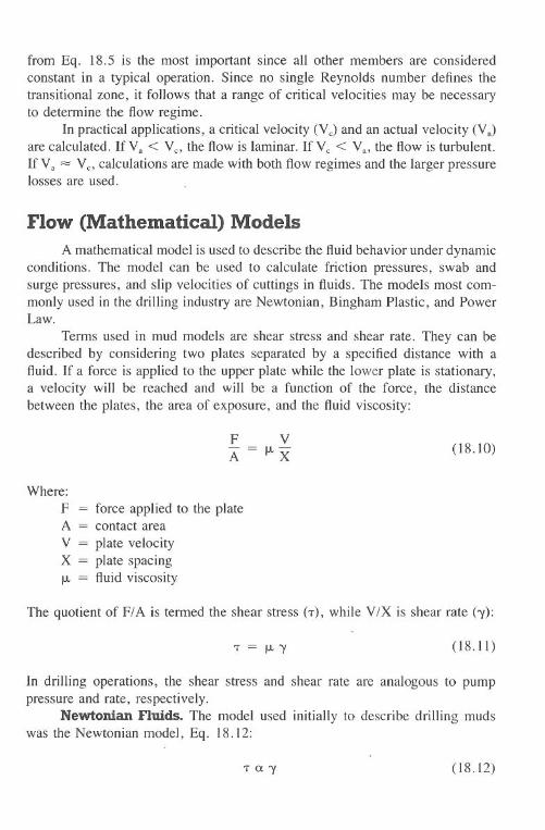
688 Drilling Engineering
from Eq. 18.5 is the most important since all other members are consideredconstant in a typical operation. Since no single Reynolds number defines thetransitional zone, it follows that a range of critical velocities may be necessaryto determine the flow regime.
In practical applications, a critical velocity (VC>and an actual velocity (Va)are calculated. If Va < Vc, the flow is laminar. If Vc < Va, the flow is turbulent.If Va = Vc,calculations are made with both flow regimes and the larger pressurelosses are used.
Flow (Mathematical) ModelsA mathematical model is used to describe the fluid behavior under dynamic
conditions. The model can be used to calculate friction pressures, swab andsurge pressures, and slip velocities of cuttings in fluids. The models most com-monly used in the drilling industry are Newtonian, Bingham Plastic, and PowerLaw.
Terms used in mud models are shear stress and shear rate. They can bedescribed by considering two plates separated by a specified distance with afluid. If a force is applied to the upper plate while the lower plate is stationary,a velocity will be reached and will be a function of the force, the distancebetween the plates, the area of exposure, and the fluid viscosity:
FA
VfLX (18.10)
Where:
F = force applied to the plateA = contact area
V = plate velocityX = plate spacingfL = fluid viscosity
The quotient of F/A is termed the shear stress (T), while V/X is shear rate ('y):
(18.11)
In drilling operations, the shear stress and shear rate are analogous to pumppressure and rate, respectively.
Newtonian Fluids. The model used initially to describe drilling mudswas the Newtonian model, Eq. 18.12:
Ta,,! (18.12)
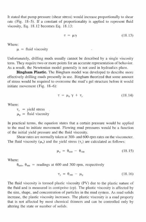
Hydraulics 689
It stated that pump pressure (shear stress) would increase proportionally to shearrate (Fig. 18-5). If a constant of proportionality is applied to represent fluidviscosity, Eq. 18.12 becomes Eq. 18.13:
1" = /J.I' (18.13)
Where:/J. = fluid viscosity
Unfortunately, drilling muds usually cannot be described by a single viscosityterm. They require two or more points for an accurate representation of behavior.As a result, the Newtonian model generally is not used in hydraulics plans.
Bingham Plastic. The Bingham model was developed to describe moreeffectively drilling muds presently in use. Bingham theorized that some amountof stress would be required to overcome the mud's gel structure before it wouldinitiate movement (Fig. 18-6):
(18.14)
Where:
1"y = yield stress/J.p = fluidviscosity
In practical terms, the equation states that a certain pressure would be appliedto the mud to initiate movement. Flowing mud pressures would be a functionof the initial yield pressure and the fluid viscosity.
Shear rates are normally taken at 300- and 600-rpm rates on the viscometer.The fluid viscosity (/J.p)and the yield stress (1"y)are calculated as follows:
(18.15)
readings at 600 and 300 rpm, respectively
(18.16)
The fluid viscosity is termed plastic viscosity (PV) due to the plastic nature ofthe fluid and is measured in centipoise (cp). The plastic viscosity is affected bythe size, shape, and concentration of particles in the mud system. As mud solidsincrease, the plastic viscosity increases. The plastic viscosity is a mud propertythat is not affected by most chemical thinners and can be controlled only byaltering the state or number of solids.
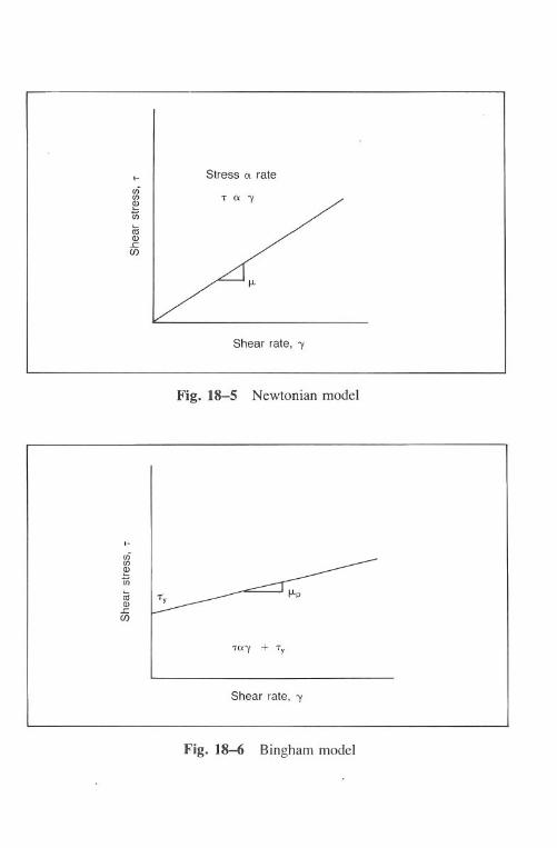
690
Stress Cl rate
Shear rate, 'Y
Fig. 18-5 Newtonian model
Shear rate, 'Y
Fig. 18-6 Bingham model
Drilling Engineering
Hydraulics 691
The yield stress, 'fy, is given the name of yield point and is measuredin Ib/100 fe. It is a function of the interparticle attraction of the solids inthe mud. The yield point is controlled by chemical thinners, dispersants, andviscosifiers.
Tables 18-1 to 18-3 illustrate common mud properties for gel-based, oil-based, and invert oil emulsions. These properties were obtained from various mudcompanies and should be used only as a guide. In fact, it is difficult to justifythe use of PV and YP terms to oil muds due to the manner in which emulsifiedwateris treatedas a solidparticle. .
Fig. 18-4 can be used to describe the weakn~sses of the Bingham model.A problem with any model used in drilling operations is its dependence on usingtwo points to define a line that should be known, intuitively, to be nonlinear.The 300- and 600-rpm shear rates are generally greater than annulus shear rates,resulting in calculated shear stresses greater than the actual values. Although theBingham model is commonly accepted in practice, a model such as the PowerLaw would be more descriptive, particularly when the fluid is in turbulence.
Power Law. The Power Law model is a standard mathematical expressionused to describe a nonlinear curve. The equation for drilling fluids is shown inEq. 18.17 and illustrated in Fig. 18-7:
'f = K (-y)n (18. 17)
Where:
K = consistency indexn = flow behavior index
The flow behavior index is descriptive of the degree to which the fluid is non-Newtonian. The flow behavior and consistency indices are calculated from Eqs.18.18 and 18.19, respectively:
n = 3.32 log (6600 )6300(18.18)
6300
K = 5Iln (18.19)
(Eq. 18.19 is modified slightly for use in Moore's slip velocity correlation. Seep. 728) .
Example 18.3
Use the following viscometer readings to compute PV, YP, n, and K:
6600= 646300= 35
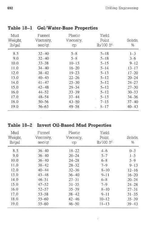
692 Drilling Engineering
Table 18-1 Gel/Water-Base PropertiesMud Funnel Plastic Yield
Weight, Viscosity, Viscosity, Point Solids,lb! gal sec! qt cp lbll 00 ft2 %
8.5 32-40 5-8 5-18 1-39.0 32-40 5-8 5-18 3-6
10.0 33-38 10-15 5-15 9-1211.0 34-40 16-20 5-14 13-1712.0 38-42 19-23 5-13 17-2013.0 40-45 22-26 5-12 20-2414.0 41-47 25-30 5-12 24-2715.0 42-48 29-34 5-12 27-3016.0 44-52 33-39 5-12 30-3317.0 48-54 37-44 5-13 34-3618.0 50-56 43-5.0 7-15 37-4019.0 56-63 49-58 8-17 40-43
Table 18-2 Invert Oil-Based Mud PropertiesMud Funnel Plastic Yield
Weight, Viscosity, Viscosity, Point, Solids,lb!gal sec!qt cp Ib!lOO ft2 %
8.5 36-40 18-22 4-6 0-39.0 36-40 20-24 5-7 1-5
10.0 36-40 24-28 6-8 5-911.0 38-42 28-32 7-9 9-1312.0 40-44 32-36 8-10 12-1613.0 43-48 36-40 9-11 16-2014.0 46-51 27-31 6-8 20-2415.0 47-52 31-35 7-9 24-2816.0 52-57 35-39 8-10 27-3117.0 53-58 38-42 9-11 31-3518.0 55-60 42-46 10-12 35-3919.0 55-60 46-50 ll-13 39-43
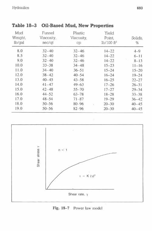
Hydraulics 693
n < 1
'T = K h)"
Shear rate, "y
Fig. 18-7 Power law model
Table 18-3 Oil-Based Mud, New PropertiesMud Funnel Plastic Yield
Weight, Viscosity, Viscosity, Point, Solids,lb/gal sec/qt cp lb/lOO ft2 %
8.0 32-40 32-46 14-22 4-98.5 32-40 32-46 14-22 6-119.0 32-40 32-46 14-22 8-13
10.0 33-38 34-48 15-23 11-1611.0 34-40 36-51 15-24 15-2012.0 38-42 40-54 16-24 19-2413.0 40-45 43-58 16-25 22-2714.0 41-47 49-63 17-26 26-3115.0 42-48 55-70 17-27 29-3416.0 44-52 63-78 18-28 33-3817.0 48-54 71-7 19-29 36-4218.0 50-56 80-96 20-30 40-4519.0 50-56 82-96 20-30 40-45
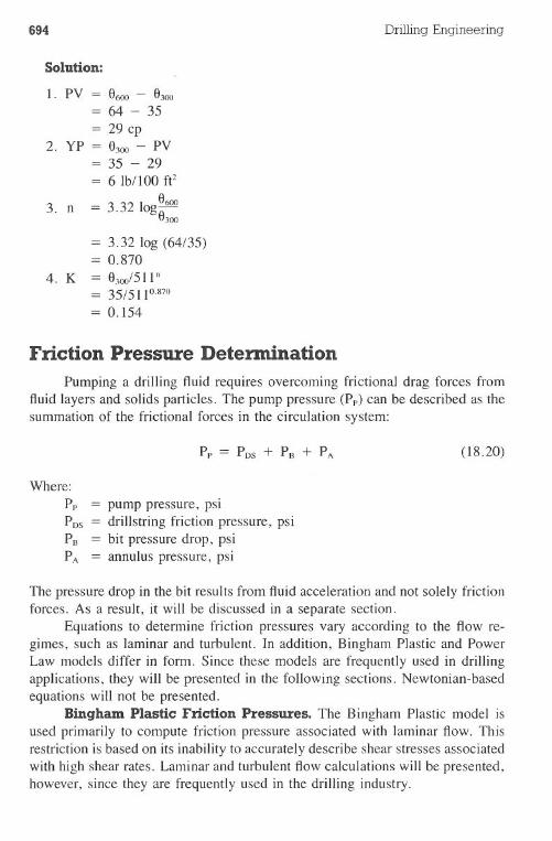
694
Solution:
1. PV
2. YP
3. n
4. K
Drilling Engineering
6600 - 630064 - 35
29 cp6300- PV35 - 29
= 6 Ib/lOOfe6
3.32Iog~6300
3.32 log (64/35)= 0.870
= 6300/511n
= 35/511°.870= 0.154
Friction Pressure DetenninationPumping a drilling fluid requires overcoming frictional drag forces from
fluid layers and solids particles. The pump pressure (Pp)can be described as thesummation of the frictional forces in the circulation system:
Where:PpPDS
PB
PA
(18.20)
pump pressure, psidrillstring friction pressure, psibit pressure drop, psi
= annulus pressure, psi
The pressure drop in the bit results from fluid acceleration and not solely frictionforces. As a result, it will be discussed in a separate section.
Equations to determine friction pressures vary according to the flow re-gimes, such as laminar and turbulent. In addition, Bingham Plastic and PowerLaw models differ in form. Since these models are frequently used in drillingapplications, they will be presented in the following sections. Newtonian-basedequations will not be presented.
Bingham Plastic: Fric:tion Pressures. The Bingham Plastic model isused primarily to compute friction pressure associated with laminar flow. Thisrestriction is based on its inability to accurately describe shear stresses associatedwith high shear rates. Laminar and turbulent flow calculations will be presented,however, since they are frequently used in the drilling industry.
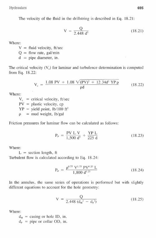
Hydraulics 695
The velocity of the fluid in the drillstring is described in Eq. 18.21:
QV = 2.448 d2 (18.21)
Where:
V = fluid velocity, ft/secQ = flow rate, gal/mind = pipe diameter, in.
The critical velocity (Vc) for laminar and turbulence determination is computedfrom Eq. 18.22:
V = 1.08 PV + 1.08 V(PV)2 + 12.34d2YP pc pd
(18.22)
Where:Vc = critical velocity, ft/secPV = plastic velocity, cpYP = yield point, Ib/l 00 fep = mud weight, Ib/gal
Friction pressures for laminar flow can be calculated as follows:
PV L V YP LPp = 1,500d2 + 225 d
(18.23)
Where:L = section length, ft
Turbulent flow is calculated according to Eq. 18.24:
pO.75 VI.75 PVO.25 L
Pp = 1,800 dl.25(18.24)
In the annulus, the same series of operations is performed but with slightlydifferent equations to account for the hole geometry:
(18.25)
Where:
dH = casingor hole 10, in.dp = pipe or collar 00, in.
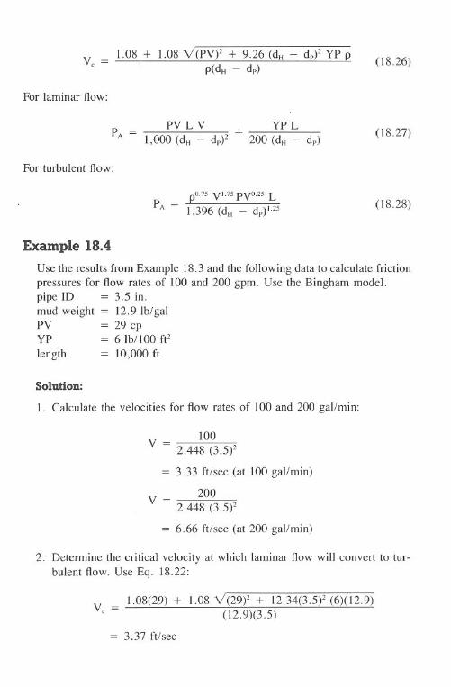
696 Drilling Engineering
v = 1.08 + 1.08 \I(PV)2 + 9.26 (dH - dp)2YP pC p(dH - dp)
(18.26)
For laminar flow:
(18.27)
For turbulent flow:
_ pO.75V 1.75PVO.25 LPA-I ,396 (dH - dp)J.25
(18.28)
Example 18.4
UsetheresultsfromExample18.3and the followingdatato calculatefrictionpressuresfor flowrates of 100and 200gpm. Use the Binghammodel.pipe ID = 3.5 in.mud weight = 12.9Ib/galPV = 29 cpYP = 6 Ib/100 felength = 10,000ft
Solution:
1. Calculatethe velocitiesfor flowrates of 100and 200 gal/min:
100V = 2.448 (3.5)2
= 3.33 ft/sec (at 100 gal/min)
200V = 2.448 (3.W
= 6.66 ft/sec (at 200 gal/min)
2. Determine the critical velocity at which laminar flow will convert to tur-bulent flow. Use Eq. 18.22:
V = 1.08(29) + 1.08 \1(29)2 + 12.34(3.5)2 (6)(12.9)C (12.9)(3.5)
= 3.37 ft/sec
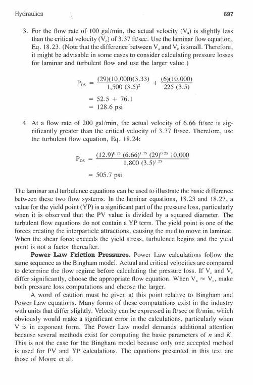
Hydraulics \697
3. For the flow rate of 100 gal/min, the actual velocity (Va) is slightly lessthan the critical velocity (Vc)of 3.37 ft/sec. Use the laminar flow equation,Eq. 18.23. (Note that the difference between Vaand Vcis small. Therefore,it might be advisable in some cases to consider calculating pressure lossesfor laminar and turbulent flow and use the larger value.)
P _ (29)(10,000)(3.33)DS - 1,500 (3.5)2
= 52.5 + 76.1= 128.6psi
+ (6)(10,000)225 (3.5)
4. At a flow rate of 200 gal/min, the actual velocity of 6.66 ft/sec is sig-nificantly greater than the critical velocity of 3.37 ft/sec. Therefore, usethe turbulent flow equation, Eq. 18.24:
(12.9)°.75 (6.66)1.75 (29)°.25 10,0001,800 (3.5)1.25
505.7 psi
The laminar and turbulence equations can be used to illustrate the basic differencebetween these two flow systems. In the laminar equations, 18.23 and 18.27, avalue for the yield point (YP) is a significant part of the pressure loss, particularlywhen it is observed that the PV value is divided by a squared diameter. Theturbulent flow equations do not contain a YP term. The yield point is one of theforces creating the interparticle attractions, causing the mud to move in laminae.When the shear force exceeds the yield stress, turbulence begins and the yieldpoint is not a factor thereafter.
Power Law Friction Pressures. Power Law calculations follow thesame sequence as the Bingham model. Actual and critical velocities are comparedto determine the flow regime before calculating the pressure loss. If Va and Vcdiffer significantly, choose the appropriate flow equation. When Va = Vo makeboth pressure loss computations and choose the larger.
A word of caution must be given at this point relative to Bingham andPower Law equations. Many forms of these computations exist in the industrywith units that differ slightly. Velocitycan be expressed in ft/sec or ftlmin, whichobviously would make a significant error in the calculations, particularly whenV is in exponent form. The Power Law model demands additional attentionbecause several methods exist for computing the basic parameters of nand K.This is not the case for the Bingham model because only one accepted methodis used for PV and YP calculations. The equations presented in this text arethose of Moore et al.
698 Drilling Engineering
Calculating friction pressures in the drillstring using the Power Law equa-tions for laminar and turbulent flow are accomplished with Eqs. 18.29 and 18.30,respectively:
PDS= [(~ ) (
3n + I
)]" ~
D 4n 300d
2.27 (10-7) po.&VI.& PVO.2 Ldl.2
(18.29)
PDS = (18.30)
For computation simplicity, NR = 3,000 is assumed for turbulence criteria. Basicassumptions for friction factor correlations result in the critical velocity equation,Eq. 18.31:
(18.31) .
Example 18.5
Refer to Examples 18.3 and 18.4 and compute the friction pressures for thesystem in Example 18.4. Use the Power Law model and a flow rate of 125gal/min. If Va = Vc, compute the pressure drop for laminar and turbulentflow and choose the larger value.
Solution:
l. Referring to Examples 18.1 and 18.2, the data to be used are:
nKpipe IDmud weight =length
0.8700.1543.5 in.
12.9 Ib/gal10,000 ft
2. Determine the actual velocity at 125 gal/min:
125
Va = 2.448 (3.5)2
4.168 fUsec250 ft/min
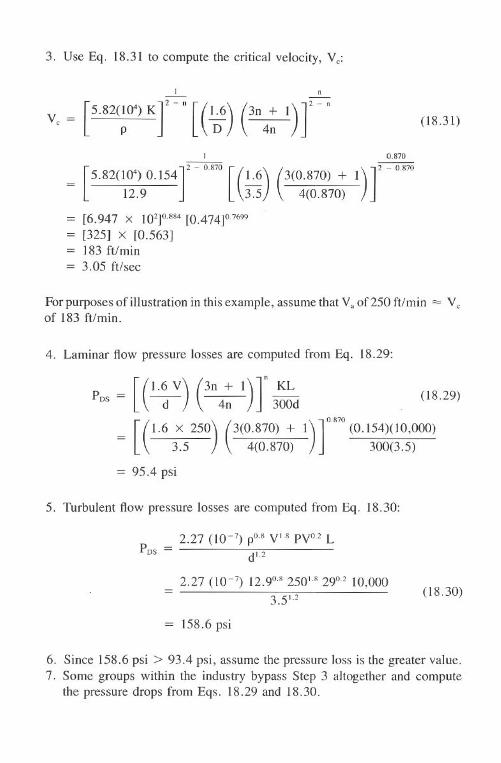
Hydraulics 699
3. Use Eq. 18.31 to compute the critical velocity, Vc:
"
(18.31)
1 UW
[5.82(104) 0.154
]
2 - 0.870
[(~ ) (
3(0.870) + 1
)]
2=0:870
12.9 3.5 4(0.870)
= [6.947 X 10²]°.884[0.474]°.7699[325] x [0.563]183 ft/min
= 3.05 ft/sec
For purposes of illustration in this example, assume that Vaof 250 ft/min = Vc
of 183 ft/min.
4. Laminar flow pressure losses are computed from Eq. 18.29:
[(1.6 V
)(3n + 1
)]" KL
PDS= -cl 4n 300d (18.29)
[(1.6 x 250
)(3(0.870) + 1
)]°.870 (0.154)(10,000)
3.5 4(0.870) 300(3.5)
= 95.4 psi
5. Turbulent flow pressure losses are computed from Eq. 18.30:
_ 2.27 (10-7) 12.9°.82501.829°.210,000- 3.51.2
(18.30)
= 158.6psi
6. Since 158.6 psi> 93.4 psi, assume the pressure loss is the greater value.7. Some groups within the industry bypass Step 3 altogether and compute
the pressure drops from Eqs. 18.29 and 18.30.
700 Drilling Engineering
Annular flow equations follow the same pattern as drillstring calculations.Laminar and turbulence are given in Eqs. 18.32 and 18.33, respectively:
(18.32)
(18.33)
n
Vo =[
3.878 (104) K
]
2 - n
[ 2~4 (2n + 1
)]
2 - n
p dH dp 3n(18.34)
Note that Eq. 18.33 uses the PV term, which is a Bingham model value. Sinceit is vague to relate viscosity to a turbulent flow, a common practice uses f.1related to PV, as shown in Eq. 18.35:
PV
f.1= 3.2(18.35)
Surface Equipment Friction Pressures. Calculating the pressure dropin surface equipment such as the standpipe and kelly is normally accomplishedby equating it to an equivalent length of drillpipe. The surface equipment isseparated into four groups (Fig. 18-8) to determine an equivalent length. Forexample, if a rig has group three surface equipment and 4Y2-in. drillpipe wasused, an additional 479 ft of pipe would be used to calculate pressure losses inthe surface equipment.
Bit Pressure Drop. A major percentage of normal circulating pressuresis lost by pumping through the nozzles when jet bits are used. The pressure lossis not frictional pressures but rather acceleration forces. Assumptions generallymade are I) the changes in pressure resulting from a change in elevation arenegligible and 2) the upstream velocity (V.) is negligible compared to downstream(Fig. 18-9). Based on these assumptions, bit pressure drop is calculated ac-cording to Eq. 18.36:
(18.36)
Solving for nozzle velocity, VN:
(18.37)
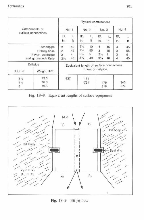
Hydraulics 701
Fig. 18-8 Equivalent lengths of surface equipment
Fig. 18-9 Bit jet flow
Typical combinations
Components of No.1 No. 2 No. 3 No. 4surface connections
10, L, 10. L, 10. L. 10, L,in. tI in. tI in. tI in. ft
Standpipe 3 40 3V2 10 4 45 4 45Orillin hose 2 45 2V2 55 3 55 3 55
Swivel washpipe 2 4 2% 5 2V2 4 3 6
and gooseneck Kelly 2'1. 40 . 3'1. 40 3'1. 40 4 40
Orillpipe Equivalent length of surface connections
DO, in. Weight, Ib/tlin feet of drillpipe
3% 13.3 437 1614% 16.6 761 479 3405 19.5 816 579
Mud \ I P,V1
FlI I
:r: II II II II II II I 11// / /'
I---
V2 / \ P2
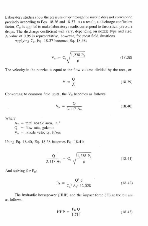
702 Drilling Engineering
Laboratory studies show the pressure drop through the nozzle does not correspondprecisely according to Eqs. 18.36 and 18.37. As a result, a discharge coefficientfactor, Cd' is applied to make laboratory results correspond to theoretical pressuredrops. The discharge coefficient will vary, depending on nozzle type and size,A value of 0.95 is representative, however, for most field situations.
Applying Cd' Eq. 18.37 becomes Eq. 18.38:
VN = CdJI'23p8 Po(18.38)
The velocity in the nozzles is equal to the flow volume divided by the area, or:
V=gA (18.39)
Converting to common field units, the VNbecomes as follows:
(18.40)
Where:
AT = total nozzlearea, in.2Q = flow rate, gallminVN = nozzle velocity, ft/sec
Using Eq. 18.40, Eq. 18.38 becomes Eq. 18.41:
(18.41)
And solving for Po:
(18.42)
The hydraulic horsepower (HHP) and the impact force (Fj) at the bit areas follows:
HHP = Po Q1,714 (18.43)
Hydraulics 703
(18.44)
Example 18.6
Calculate the hydraulic horsepower and impact force for the following set ofconditions:
mud weight = 14.5 Ib/galflow rate = 300 gal/minjet sizes = three '2/32-in.jets
Solution:
1. Determine the nozzle area, AT:
1T 2AT = 3 - (d)4
= 3 ~ G~r= 0.331 in.2
2. Eq. 18.42 is used to calculate the pressure drop at the bit:
Q2pP -a - Cl Al12,028
= (300)2 14.5(0.95)2 (0.331)2 12,028
= 1,097 psi
(18.42)
3. Calculate the hydraulic horsepower expended at the bit from Eq. 18.43:
Pa QHHP = 1,714
= (1,097 psi)(300 gal/min)1,714
(18.43)
= 192hp
4. The hydraulic impact force is computed from Eq. 18.44:
Fj = 0.01823 Cd Q yIf)P;;= 0.01823 (0.95)(300) V(14.5)(1,097)= 654 Ib
(18.44)
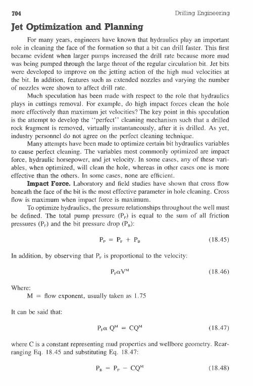
704 Drilling Engineering
Jet Optimization and PlanningFor many years, engineers have known that hydraulics play an important
role in cleaning the face of the formation so that a bit can drill faster. This firstbecame evident when larger pumps increased the drill rate because more mudwas being pumped through the large throat of the regular circulation bit. Jet bitswere developed to improve on the jetting action of the high mud velocities atthe bit. In addition, features such as extended nozzles and varying the numberof nozzles were shown to affect drill rate.
Much speculation has been made with respect to the role that hydraulicsplays in cuttings removal. For example, do high impact forces clean the holemore effectively than maximum jet velocities? The key point in this speculationis the attempt to develop the "perfect" cleaning mechanism such that a drilledrock f.ragmentis removed, virtually instantaneously, after it is drilled. As yet,industry personnel do not agree on the perfect cleaning technique.
Many attempts have been made to optimize certain bit hydraulics variablesto cause perfect cleaning. The variables most commonly optimized are impactforce, hydraulic horsepower, and jet velocity. In some cases, any of these vari-ables, when optimized, will clean the hole, whereas in oth,ercases one is moreeffective than the others. In some cases, none are efficient.
Impact Force. Laboratory and field studies have shown that cross flowbeneath the face of the bit is the most effective parameter in hole cleaning. Crossflow is maximum when impact force is maximum.
To optimize hydraulics, the pressure relationships throughout the well mustbe defined. The total pump pressure (Pp) is equal to the sum of all frictionpressures (PF)and the bit pressure drop (Pa):
(18.45)
In addition, by observing that PF is proportional to the velocity:
(18.46)
Where:
M = flow exponent, usually taken as 1.75
It can be said that:
(18.47)
where C is a constant representing mud properties and wellbore geometry. Rear-ranging Eq. 18.45 and substituting Eq. 18.47:
(18.48)
Hydraulics 705
Jet impact force was defined previously as follows:
Fj = 0.01823 Cd Q~ (18.44)
By substituting Eq. 18.48 into Eq. 18.44, the following expression is established:
(18.49)
Or, combining terms:
(18.50)
Using calculus, Eq. 18.50 can be maximized and resolved into Eq. 18.51:
2PpPr = M + 2
(18.51)
Realizing that M is approximately 2, the equation reduces to 0.5 Pp, which isthe familiar 50% of pump pressure expended at the bit for optimum impactconditions.
Hydraulic Horsepower. The hydraulic horsepower equation can be op-timized in a similar manner, resulting in the following equations:
PpPp=- M + I
Po = 0.67 Pp
(18.52)
(18.53)
Eq. 18.53 is developed from 18.52 if M is set equal to 2 so that Pr = Y3Pp.Graphical Method. The most convenient method for selecting proper
jet sizes for bit hydraulics optimization is the graphical approach shown in Fig.18-10. The maximum possible flow rate is based on pump horsepower andpressure limitations. The minimum flow rate is based on acceptable annularvelocities for cuttings removal or minimum pumping rates from mechanicalrestrictions. These two lines are connected by the optimum friction pressurelosses desired, usually 50% for impact force or 33% for hydraulic horsepowercriteria. The most accurate method is to determine M from two flow rates onthe given well and compute the optimum friction pressures using Eqs. 18.51and 18.52.
After the graph is constructed, plot the two friction pressures resultingfrom the test rates, determined by subtracting the computed bit drop from thepump pressure. Draw a line through the two points until it intersects the pathof optimum hydraulics. The intersection point determines the desired flow rate,
706
oo
x
Minimumflow rate, .,)I
gal/min
Optimum /'
Maximum pump pressure
//
//
I
I, Rate 1
II
II
Path ofoptimum hydraulics
Flow rate gal/min x 100
Optimum ratep
//
, Rate 2
Maximum
flow rate -z...t"gal/min
Drilling Engineering
Fig. 18-10 Graphical approach for bit hydraulics optimization
Hydraulics 707
which can be substituted into Eq. 18.54 to compute the desired area for the jetnozzle:
(18.54)
Example 18.7
A drilling engineer intends to optimize the bit hydraulics on a well with thefollowing characteristics. Select the proper jet sizes for the impact force andhydraulic horsepower methods:pump rate # I = 200 gal/min
= 3,000 psi= 275 gal/min= 1,300 psi
pump horsepower = 1,250hpsurface pressure = 3,000psi (maximum)mud weight = 13 Ib/galjet sizes = three 17/32ndsminimum acceptable annular velocity = 70 ft/minminimum pump rate = 175 gal/minhole geometry = 4Y2-in.drillpipe
= 7-in. drill collars= 8Y2-in.annulus
pump rate #2
Solution:
1. Determine the maximum possible flow rate as the upper end constraint:
PQHP=-1,7143,000 Q1 250 -
, - 1,714Q = 714 gal/min
2. Determine the minimum flow rate. The lower end constraint is based onminimum pump rates or annular velocity. The velocity of 70 ft/min isconverted to a flow rate:
V (ft/min) = 24.50 QdH2 - d 2p
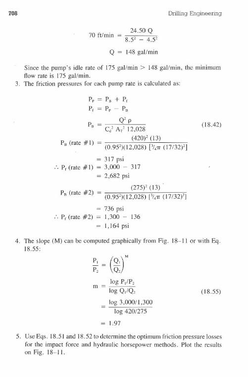
708 Drilling Engineering
24.50 Q70 ft/min = 8.52 _ 4.:
Q = 148 gal/min
Since the pump's idle rate of 175 gal/min > 148 gal/min, the minimumflow rate is 175 gal/min.
3. The friction pressures for each pump rate is calculated as:
Pp = PB + Pr
Pr = Pp - PB
Q2pP -B - Cl AT212,028
P #1 (420)2 (13)B(rate ) = (0.952)(12,028)[%1T(17/32)2]
= 317 psi:. Pr (rate #1) = 3,000 - 317
= 2,682 psi
(275)2 (13) .PB(rate #2) = (0.952)1 . _.
= 736 psi:. Pr (rate #2) = 1,300 - 136
= 1,164 psi
(18.42)
4. The slope (M) can be computed graphically from Fig. 18-11 or with Eq.18.55:
PI = (QI )M
P2 Q2
log P./P2m=log QI/Q2
log 3,000/ I ,300
log 420/275
1:97
(18.55)
5. Use Eqs. 18.51 and 18.52 to determine the optimum friction pressure lossesfor the impact force and hydraulic horsepower methods. Plot the resultson Fig. 18-11.
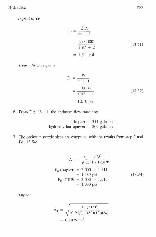
Hydraulics 709
Impact force
Pf=~ m + 2
2 (3,000)l. 97 + 2
1,511 psi
(I8.51)
Hydraulic horsepower
Pf=~ m + 1
3,000l. 97 + 1
1,010 psi
(18.52)
6. From Fig. 18-11, the optimum flow rates are:
impact = 315 gal/minhydraulic horsepower = 260 gal/min
7. The optimum nozzle sizes are computed with the results from step 7 andEq. 18.54:
~Ci PB 12,028
PB(impact) = 3,000 - 1,511= 1,489 psi
PB(HHP) = 3,000 - 1,010= 1,990 psi
(I8.54)
Impact
13 (315f(0.95)2(1,489)(12,028)
= 0.2825 in.2
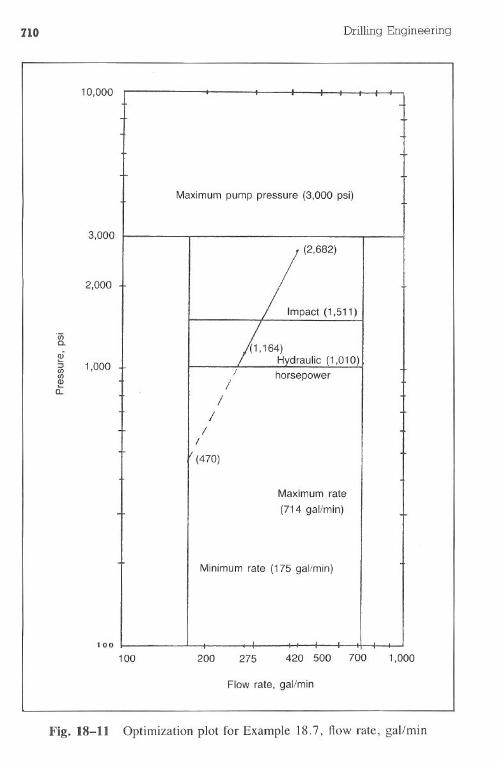
710
10,000
Drilling Engineering
Maximum pump pressure (3,000 psi)
3,000
2,000
.wCo
cD
~ 1,000(/)Q)
a:/
II
I/
/
(470)
Maximum rate
(714 gal/min)
Minimum rate (175 gal/min)
100
100 200 275 420 500 700 1,000
Flow rate, gal/min
Fig. 18-11 Optimization plot for Example 18.7, flow rate, gal/min
Hydraulics 711
And:
0.2825 = %7r CX2) 2
x = 11.01
(Use three 1l/32nds)
Hydraulic horsepower
13 (26W
(0.95)2(1,990)(12,028)
= 0.2017 in.2
And:
(2
_ 3 x
0.2017 - /47r 32)
x = 9.36(Use one 9/32nds and two lO/32nds)
Jet Velocity. Maximum velocity of the fluid moving through the jets ofthe bit occurs when a maximum pressure drop is observed at the lowest possibleflow rates. The rates are generally based on the slip velocity of the cuttings inthe annulus and the mud flow rates required to exceed this velocity. To use Eq.18.54, the flow rate is established as the minimum possible volume. The linein Fig. 18-lO is extrapolated downward until it intersects the minimum flowrate line. The pressure at this intersection is the value to be substituted into Eq.18.54. In many deep wells, hydraulics and impact optimization degrade into jetvelocity criteria because of high friction pressures associated with these wells.
Example 18.8
Example 18.7 and Fig. 18-11 were used to calculate optimum jet sizes forthe impact force and hydraulic horsepower methods. Using the same data,determine the optimum jet sizes for the velocity method. Do not use jet sizesless than %2nds. A 1- or 2-nozzle selection may be necessary.
Solution:
I. Refer to Fig. 18-11. Extrapolate the friction pressure line until it intersectsthe minimum rate of 175 gal/min:
Pc = 470 psiPp = PB + Pc
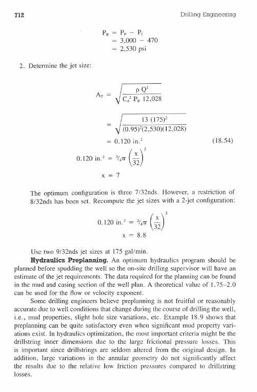
7lZ Drilling Engineering
Pp - Pr3,000 - 4702,530 psi
2. Detennine the jet size:
~C/ Po 12,028
13 (l75?(0.95)2(2,530)(12,028)
= 0.120 in.22
0.120 in.2 = %7rCX2)
x = 7
(18.54)
The optimum configuration is three 7/32nds. However, a restriction of8/32nds has been set. Recompute the jet sizes with a 2-jet configuration:
0.120 in.2
x
Use two 9/32nds jet sizes at 175 gal/min.Hydraulics Preplanning. An optimum hydraulics program should be
planned before spudding the well so the on-site drilling supervisor will have anestimate of the jet requirements. The data required for the planning can be foundin the mud and casing section of the well plan. A theoretical value of 1.75-2.0can be used for the flow or velocity exponent.
Some drilling engineers believe preplanning is not fruitful or reasonablyaccurate due to well conditions that change during the course of drilling the well,i.e., mud properties, slight hole size variations, etc. Example 18.9 shows thatpreplanning can be quite satisfactory even when significant mud property vari-ations exist. In hydraulics optimization, the most important criteria might be thedrillstring inner dimensions due to the large frictional pressure losses. Thisis important since drillstrings are seldom altered from the original design. Inaddition, large variations in the annular geometry do not significantly affectthe results due to the relative low friction pressures compared to drillstringlosses.
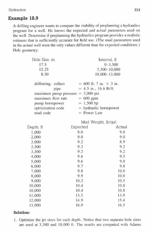
Hydraulics 713
Example 18.9
A drilling engineer wants to compare the viability of preplanning a hydraulicsprogram for a well. He knows the expected and actual parameters used onthe well. Determine if preplanning the hydraulics program provides a realisticestimate that is sufficiently accurate for field use. (The mud parameters usedin the actual well were the only values different than the expected conditions.)Hole geometry:
Hole Size, in.17.512.258.50
Interval, ft0-3,500
3,500-10,00010,000-13 ,000
drillstring: collars = 600 ft, 7 in. X 3 in.pipe = 4.5 in., 16.6Ib/ft
maximum pump pressure = 3,000 psimaximum flow rate = 600 gpmpump horsepower = 1,500 hpoptimization code = hydraulic horsepowermud code = Power Law
Depth, ft1,0002,0003,0003,5003,5004,0005,0006,0007,0008,0009,000
10,00010,00011,00012,00013,000
Solution:
Mud Weight, Ib/galExpected Actual
9.0 9.09.0 9.09.2 8.99.2 9.29.2 9.29.6 9.59.6 9.89.7 9.89.8 10.09.9 10.0
10.2 10.510.4 10.810.4 10.813.5 13.914.9 15.416.0 16.5
I. Optimize the jet sizes for each depth. Notice that two separate hole sizesare used at 3,500 and 10,000 ft. The results are computed with Adams
...
Table
18-4P
re-SpudH
ydraulicsP
rogramfor
Exam
ple18.9
Ann.
Pump
FlowM
udV
el.Jet
Impact
Depth,
Pressure,R
ate,W
eight,Jets,
EC
D,
DP
/DC
,B
itB
itV
elocity,Force,
ftPSI
GPM
lblgal32nds
ppgft/m
inH
HP/in.2
HH
Pft/sec
lb
1,0003,000
5869.0
12/12/139.0
50/563.3
792565
15432,000
3,000582
9.012/12/13
9.050/55
3.2778
5611524
3,0003,000
5839.2
12/13/139.2
50/55-3.0
715532
14783,500
3,000599
9.213/13/13
9.251/57
2.9702
5201485
3,5003,000
5989.2
13/13/139.2
113/1455.9
701520
14824,000
3,000567
9.613/13/13
9.6107/137
5.3621
4921388
5,0003,000
5379.6
12/13/139.6
101/1305.0
585491
13126,000
3,000507
9.712/12/13
9.796/123
4.7552
4881243
7,0003,000
4919.8
12/12/139.8
93/1194.3
507473
11798,000
3,000480
9.912/12/13
9.991/116
4.1479
4631140
9,0003,000
47110.2
12/13/1310.2
89/1143.6
420431
107310,000
3,000459
lOA
12/13/13lO
A87/111
304395
4191036
10,0003,000
350lO
A10/10/11
10.6165/369
7.0396
481907
11,0003,000
25513.5
9/9/1013.7
120/2685.2
297428
762I::':=
'12,000
3,000239
14.99/9/10
15.1113/252
4.8271
402741
\0
13,000
3,000216
16.09/9/9
16.2102/227
404248
391698
.
Data
courtesyA
dams
andR
ountreeT
echnology'sQ
CK
HY
Dcom
puterprogram
<D
<D
O.
='
\0
Table
18-5H
ydraulicsP
rogramfor
Exam
ple18.9
Using
Actual
Mud
Weights
SEo
Ann.
.
Pump
FlowM
udV
el.Jet
Impact
Depth,
Pressure,R
ate,W
eight,Jets,
EC
D,
DP
/DC
,B
itB
itV
elocity,Force,
ftPSI
GPM
lblgal32nds
ppgft/rnin
HH
P/in.2
HH
Pft/sec
lb
1,0003,000
5869.0
12/12/139.0
50/563.3
792565
1,5432,000
3,000582
9.012/12/13
9.050/55
3.2778
5611,524
3,0003,000
5928.9
12/13/138.9
51/563.0
726541
1,4773,500
3,000599
9.213/13/13
9.251/57
2.9702
5201,485
3,5003,000
5989.2
13/13/139.2
113/1455.9
701520
1,4824,000
3,000570
9.513/13/13
9.5107/138
5.3624
4951,386
5,0003,000
5329.8
12/13/139.8
100/1294.9
580486
1,3136,000
3,000504
9.812/12/13
9.895/122
4.7549
4861,244
7,0003,000
48610.0
12/12/1310.0
92/1184.3
502468
1,1808,000
3,000478
10.012/12/13
10.090/116
4.0477
4611,140
9,0003,000
46510.5
12/13/1310.5
88/1133.5
415425
1,07410,000
3,000463
10.813/13/13
10.887/112
3.2381
4021,042
10,0003,000
34410.8
10/10/1111.0
162/3626.9
390472
90811,000
3,000251
13.99/9/10
14.1118/265
5.2293
422764
12,0003,000
23515.4
9/9/1015.6
111/2484.7
267396
74313,000
3,000213
16.59/9/9
16.7100/224
4.3245
385700
Data
courtesyA
dams
andR
ountreeT
echnology'sQ
CK
HY
Dcom
puterprogram
10.:1....en
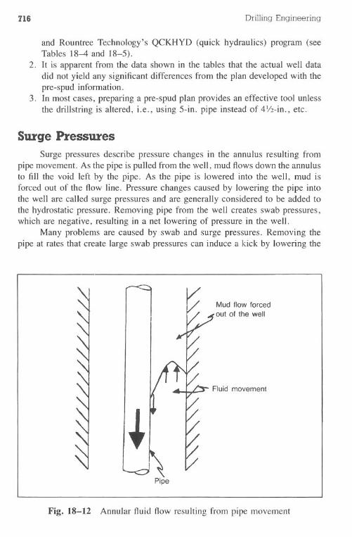
716 Drilling Engineering
and Rountree Te.chnology's QCKHYD (quick hydraulics) program (seeTables 18-4 and 18-5).
2. It is apparent from the data shown in the tables that the actual well datadid not yield any significant differences from the plan developed with thepre-spud information.
3. In most cases, preparing a pre-spud plan provides an effective tool unlessthe drillstring is altered, i.e., using 5-in. pipe instead of 4Y2-in., etc.
Surge PressuresSurge pressures describe pressure changes in the annulus resulting from
pipe movement. As the pipe is pulled from the well, mud flows down the annulusto fill the void left by the pipe. As the pipe is lowered into the well, mud isforced out of the flow line. Pressure changes caused by lowering the pipe intothe well are called surge pressures and are generally considered to be added tothe hydrostatic pressure. Removing pipe from the well creates swab pressures,which are negative, resulting in a net lowering of pressure in the well.
Many problems are caused by swab and surge pressures. Removing thepipe at rates that create large swab pressures can induce a kick by lowering the
Mud flow forcedout of the well
Fluid movement
Pipe
Fig. 18-12 Annular fluid flow resulting from pipe movement
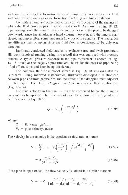
Hydraulics 717
wellbore pressure below formation pressure. Surge pressures increase the totalwellbore pressure and can cause formation fracturing and lost circulation.
Computing swab and surge pressures is difficult because of the manner inwhich the fluid flows as pipe is moved in the well. As shown in Fig. 18-12,pipe moving down the annulus causes the'mud adjacent to the pipe to be draggeddownward. Since the annulus is a fixed volume, however, and the mud is con-sidered incompressible, some mud must flow out of the annulus. The mechanicsare different than pumping since the fluid flow is considered to be only onedirection.
Burkhardt conducted field studies to evaluate surge and swab pressures.His work involved running casing into a well that was equipped with pressuresensors. A typical pressure response to the pipe movement is shown on Fig.18-13. Positive and negative pressures are shown for the cases of pipe beinglifted off the slips and later being decelerated.
The complex fluid flow model shown in Fig. 18-10 was evaluated byBurkhardt. Using involved mathematics, Burkhardt developed a relationshipbetween pipe and hole geometries and the effect of the dragging mud adjacentto the pipe. The term clinging constant represents this relationship(Fig. 18-14).
The mud velocity in the annulus must be computed before the clingingconstant can be applied. The flow rate of steel for a closed drillstring into thewell is given by Eq. 18.56:
Q = Vpc (-1T~ d/ ) (18.56)
Where:QVp
= flow rate, gal/min= pipe velocity,ft/sec
The velocity in the annulus is the quotient of flow rate and area:
(18.57)
- dp2 VP
C (dH2 - d/)(18.58)
If the pipe is open-ended, the flow velocity is solved in a similar manner:
(18.59)
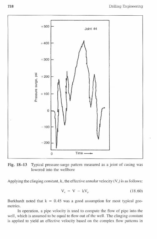
718
+500
+400
-100
-200
Drilling Engineering
Joint 44
o Time_
Fig. 18-13 Typical pressure-surge pattern measured as a joint of casing waslowered into the wellbore
Applying the clinging constant, k, the effective annular velocity (Yo) is as follows:
(18.60)
Burkhardt noted that k = 0.45 was a good assumption for most typical geo-metries.
In operation, a pipe velocity is used to compute the flow of pipe into thewell, which is assumed to be equal to flow out of the well. The clinging constantis applied to yield an effective velocity based on the complex flow patterns in
+300
Owc. +200cDC>:;C/)CD:;
+100C/)C/)CDa:
0
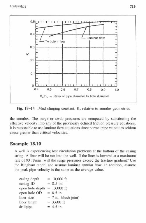
Hydraulics 719
laminar flowTurbulent flow
0.3
0.2
0.1
o0.4 0.5 0.6 0.7 0.8 0.9 1.0
D,!Dh = Ratio of pipe diameter to hole diameter
Fig. 18-14 Mud clinging constant, K, relative to annulus geometries
the annulus. The surge or swab pressures are computed by substituting theeffective velocity into any of the previously defined friction pressure equations.It is reasonable to use laminar flow equations since normal pipe velocities seldomcause greater than critical velocities.
Example 18.10
A well is experiencing lost circulation problems at the bottom of the casingstring. A liner will be run into the well. If the liner is lowered at a maximumrate of 93 ft/min, will the surge pressures exceed the fracture gradient? Usethe Bingham model and assume laminar annular flow. In addition, assumethe peak pipe velocity is the same as the average value.
casing depthcasing IDopen hole depthopen hole ODliner sizeliner lengthdrillpip~
10,000 ft= 8.5 in.
13,000 ft8.5 in.7 in. (flush joint)3,600 ft
= 4.5 in.
720 DrillingEngineering
mud = 16.6 Ib/gal= 38 cp (PV)= 15 Ib/lOOfe (YP)
fracture gradient = 17.0 Ib/galpipe velocity = 93 ft/min
= 1.55 ft/sec
(Assume the liner has a closed end from a float shoe.)
Solution:
1. The maximum surge pressures occur when the bottom of the liner reachesthe casing seat (see Fig. 18-15).
2. The mud flow rate leaving the well when the liner shoe reaches the casingseat is:
QV=-2.448 W)
Q = 2.448 Vd2
= 2.448 (1.55 ft/sec)(4.5 in.)2
= 76.8 gal/min
3. Compute the annular velocities around the drillpipe (Vap)and the liner(Val):
V = Qap 2.448 (dH2- d/)
76.8
- 2.448 (8.52 - 4.52)
= 0.603 ft/sec
= 36 ft/min
Q2.448 (dH2- d12)
76.8
2.448 (8.52 - 72)
= 1.349 ft/sec
= 80.9 ft/min
Hydraulics 721
4.5-in.
drillpipeMud
16.6 Ib/gal 8.5-in.ID
6,400 It
7-in. liner
Fracture gradient17.0 Ib/gal
10,000 It
93 ftImin
8.5-in. hole13,000 It
Fig.18-15 Illustration for Example 18.10
4. Refer to Fig. 18-14 and determine the clinging constant, k, for the pipeand liner:
pipe - ratio = 4.5/8.5 = 0.529k ::::::0.38
liner - ratio = 7/8.5 = 0.823k = 0.45
7ZZ Drilling Engineering
5. The effective ~nnular velocities around the pipe (Vpe)and the liner (Vie)are:
Vpe= V - 0.38 Vp= 0.603 - 0.38 ( - 1.55)= 1.192 ft/sec
Vie = 1.349 ft/sec - (0.45)( - 1.55)= 2.046 ft/sec
6. The pressure surge caused by the drillpipe is as follows (use Eq.18.27):
PVLVpa YPLPp = 2 2 +
1,500 (dH - dp) 225 (dH - dp)
(38)(6,400)(1.192) (15)(6,400)2 2 +
1,500 (8.5 - 4.5 ) 225 (8.5 - 4.5)
= 3.716 psi + 106 psi
= 110 psi
7. The pressure surge caused by the liner is:
(38)(3,600)(2.046) (15)(3,600)P = +I 1,500(8.52 - 72) 225 (8.5 - 7)
= 8.0 psi + 160 psi
= 168 psi
8. The total pressure surge and equivalent mud weight is:
110 psi + 168 psi = 278 psi
pressure x 19.23 .EMW = _. + mud weight
ept
278 psi x 19.23= 10,000 ft + 16.6 Ib/gal
= 17.13 Ib/gal
9. Therefore, the fracture gradient of 17.0 Ib/gal would be exceeded (17.1Ib/gal) at a pipe velocity of 93 ft/min.
Hydraulics 723
10. In reality, the flow regime in the annulus was turbulent opposite the liner.The assumption of laminar flowin this example was done for simplicityand illustration. .
Open-ended pipe increases the complexity of the calculations considerably.Pressure drops in the annulus and drillstring must be equal. Since differentgeometries exist, however, flow rates in the annulus and pipe will not be thesame. In addition, it is possible that the annulus will be laminar, while fluidflow in the pipe will be turbulent. A trial-and-error solution is used by assuminga major percentage of the flow will be up the annulus with the remainder in thepipe. From these assumed volumes, pressure losses are computed and comparedand the volumes are adjusted, depending on the computed pressure relationships.Ifthe first trial was a 75:25 annulus to pipe ratio and a pressure distribution of200:300 psi was observed, a second trial might be at 80:20. The procedure isiterated until a ratio is obtained that yields equal pressure drops in both the pipeand annulus.
In a practical sense, surge and swab pressures are composed of the pressuresrequired to break the gels in the mud and the pressures caused by actual fluidmovement. Thick muds can often produce such high gels that surge pressuresresulting from this component are significant. The yield point and gel strengthof the mud affect this type of pressure.
If a maximum allowable swab or surge pressure is known, it is possibleto determine a maximum pulling or running speed for the pipe. The maximumsurge pressure is usually the difference between the lowest exposed fracturegradient and the mud weight. The maximum swab pressure is the differencebetween the greatest formation pressure from an exposed permeable zone andthe mud weight. The swab pressure equations are solved in reverse order toarrive at a pipe velocity.
Example 18.11Refer to the data in Example 18.10. If the drilling engineer at the well sitedoes not wish to exceed a 16.9-1b/galequivalent surge pressure, what is themaximum velocity that the pipe can be run into the well?
Solution:
1. Determine the maximum allowable surge pressure so the 16.6-1b/galmuddoes not exceed the 16.9-1b/galequivalent value:
0.052 (16.9 - 16.6)(10,000ft) = 156psi
724 Drilling Engineering
2. The 156-psi surge pressure is the maximum amount that can be generatedby the friction pressure opposite the pipe and liner, or:
3. Substituting the pressure equations for Pp and PI:
56.
[(38)(6,400)(V pe) (15)(6,400)
]I pSI:5 2 2 +. 1.500(8.5 - 4.5 ) 225 (8.5 - 4.5)
+[
(38)(3,600)(Vic) + 15(3,600)]1,500 (8.52 - 72) 225 (8.5 - 7)
156 psi:5 3.118 Vpe+ 3.922 Vie+ 266 psi
- 110 psi :5 3.118 Vpe+ 3.922 Vie
4. Since the sum of the velocity components is a negative number, the pipecannot be run into the well at any velocity without exceeding the 16.9-Ib/gal limitation. The yield point component of the pressure surge willcause the pressures to exceed the 156-psi value.
Cuttings Slip VelocityRemoval of drilled rock fragments from the annulus is a primary function
of the drilling fluid. The drilled cuttings, which are heavier than the mud, tendto fall, or slip, down the annulus. The prediction of these settling rates is difficultbecause the cuttings densities vary, mud properties change, and the flow regimein the annulus seldom has a uniform velocity. Although many equations areavailable for cuttings slip prediction, only two will be presented.
Mud flow in the annulus is generally laminar. The cuttings lift capacitycan be increased by altering mud properties so that the overall velocity of thelaminae are more equal than the profile shown in Fig. 18-2. The flattened profile,Fig. 18-16, achieves greater uniform velocities.
Moore Correlation. Moore has proposed that a cutting will slip througha mud system at a rate described in Eq. 18.61:
(18.61)
Where:
Vs = slip velocity, ft/minDp = particle diameter, in.
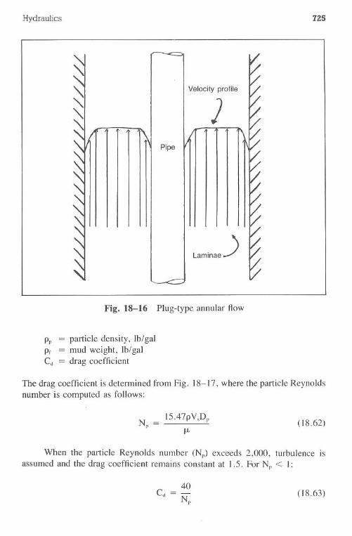
Hydraulics 725
Pipe
Velocity profile
Laminae)
Fig. 18-16 Plug-type annular flow
PP = particledensity,Ib/galPr = mud weight, Ib/galCd = drag coefficient
The drag coefficient is determined from Fig. 18- I7, where the particle Reynoldsnumber is computed as follows:
N _ 15.47pV Dp _ s p
J.L(18.62)
When the particle Reynolds number (Np) exceeds 2,000, turbulence isassumed and the drag coefficient remains constant at I. 5. For Np < I:
(18.63)
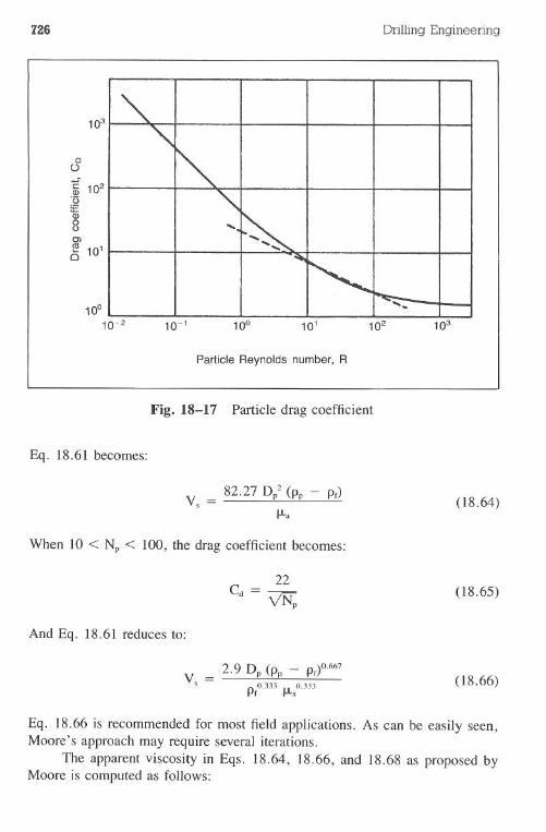
726 Drilling Engineering
Particle Reynolds number, R
Fig. 18-17 Particle drag coefficient
Eq. 18.61 becomes:
82.27 D/ (pp - Pr)V =s f.L.
(18.64)
When 10 < Np < 100, the drag coefficient becomes:
(18.65)
And Eq. 18.61 reduces to:
(18.66)
Eq. 18.66 is recommended for most field applications. As can be easily seen,Moore's approach may require several iterations.
The apparent viscosity in Eqs. 18.64, 18.66, and 18.68 as proposed byMoore is computed as follows:
Hydraulics 727
(
In. I-n 2 +-k dH-dp n
",. ~ 144( V) 0.0208)(18.67)
Where:V = fluid velocity, ft/sec
For Np .> 2,000 where Cd is greater than 2,000:
(18.68)
Where:
Vs = slip velocity, ft/sec
Example 18.12
A surface hole section on a prospect well is to be drilled to 3,500 ft. Manywells in the same geographical area have experienced lost circulation problemsthat were attributed to poor hole cleaning. If a minimum acceptable annularvelocity of 60 ft/min is established, will the hole be cleaned adequately? Usethe Moore correlation with the following data:
hole size = 17V2in.
drillpipe = 41/2 in.
mud = 9.0Ib/galcuttings = 0.25 in. (diameter)
21.0 Ib/gal (density)flow rate = 600 gal/min
Fann viscometer readings6600 = 526300 = 31
Solution:
1. The apparent viscosity (fl..) requires nand K calculations with Eqs. 18.18and 18.19:
n = 3.32 log (~:) (18.18)
728 DrillingEngineering
= 3.32 log G~)= 0.75
510 (8300)K = 5Il"
510 (31)- 511°.75
(l8.19a)
= 145 eq. cp
Note that the consistency index in Eq. 18.19a is used only in the Moorecorrelation.
2. The annular velocity, Y, is computed as:
Qy=8 2 2
2.44 (dH - dp)600
- 2.448 (17.52 - 4.52)= 0.856 ft/sec
3. The apparent viscosity (J.l..)is determined from Eq. 18.67:
( )1-"
(2+!
)"
k dH-dp nJ.l.. = 144 y 0.0208
( )1 - 0.75
(2 + ~
)0.75
= 145 17.5 - 4.5 0.75144 0.856 0.0208
= 89.5 cp
( 18.67)
4. To calculate the slip velocity (Y,) with the Moore correlation, assume acondition and then verify the results with the Reynolds number compu-tation. For a first iteration, assume that Np ::5 1.0 and use Eq. 18.64 forthe slip velocity:
D2Y, = 82.87 £...(pp - Pr)
J.l..
= 82.87 (0.25f (21.0 - 9)89.5
= 0.694 ft/sec
(18.64)
....
Hydraulics 729
The particle Reynolds number verification is:
928 Pr Vs dpN=-p J.1.
= 928 (9)(0.32)(0.25)89.52
(18.62)
= 7.46
Since 7.46> 1.0, the use of Eq. 18.64 as a first iteration was invalid.
5. Assume that 1.0 < Np < 2,000. Use Eq. 18.66:
(18.66)
= 0.851 ftlsec
928 (9)(0.851)(0.25)Np = 85.92
= 19.86
Since 1.0 :5 3.60 :5 2,000, Eq. 18.66 was the proper choice.
6. The annular velocity of the mud is 0.856 ft/sec or 51.4 ftlmin. The slipvelocity of the cuttings is 0.851 ftlsec or 51.06 ft/min. The net upwardvelocity of the cuttings is negligible at 0.34 ft/min.
It is quite possible, and perhaps probable, that the lost circulationproblems described in the initial section of this example are caused by thelow rate of hole cleaning.Chien Correlation. Chien has developed a straightforward approach to
the determination of cuttings slip velocity. The model is shown in Eq. 18.69:
Vs = 0.0075 (~ )[
Pr dp(18.69)
For suspensions of bentonite in water, it is recommended that the plastic viscositybe used as the apparent viscosity. For polymer drilling fluids, Chien recommendscomputing the apparent viscosity as follows:
J.1.= PV + 5 YP dpV(18.70)
730 Drilling Engineering
In operation, the cuttings slip velocity is computed from ail equation similarto Chien's. From the computed value, an acceptable flow rate is determinedbased on the minimum' rate that would hold the cuttings stationary plus anadditional rate increase to clean the hole. For example, if Chien's equationdetermined that the cuttings slip velocity (V.) was 15 ft/min, an upward mudrate of 15 ft/min would hold the cuttings stationary yet never clean the hole. Asa result, an equation similar to Eq. 18.71 is used to determine the minimumflow rate:
Va = 2V. (18.71)
Where:Va = actual mud velocity, ftlmin
Example 18.13
Rework Example 18.12 and use the Chien correlation.
Solution:
I. Since the drilling fluid is gel based, use the plastic viscosity as the apparentviscosity:
PV = 6600 - 6300
= 52 - 31
= 21 cp
2. The slip velocity is computed as follows with Eq. 18.69:
V. = 0.0075 (~ )[
Pr dp
36,800 ~.( II>~ p,) + 1 - '1C~~)
36,800 (0.2~)(21- 9
)(
21
)9
(9)(0.25) + I - ,]
0.0075 (9.33) [V(105)(1.33) + I - 1]0.76 ftlsec
3. Note that the Chien correlation predicts a V. of 0.76 ftlsec, whereas theMoore correlation yielded 0.307 ftlsec.
Hydraulics 731
Gas Migration. Increasing importance is being placed on the rate at whichgas will migrate through a mud system. Although generally not significant inmany drilling applications because high-viscosity mud systems are being used,it is important in clean drilling and workover fluids. An empirical model developedby Adams shows the gas migration rate as a function of mud weight. The datawere derived from test wells used in well control training:
(18.72)
Where:
Vg = gas migrationrate, ft/secPr = mud weight, Ib/gal
Example 18.14
A kick was taken on a well in which the mud weight was 11.0 Ib/gal. UseAdams' correlation to predict the expected migration rate.
Solution:
The bubble migration rate is computed with Eq. 18.72:
Vg = 12 eC-0.37)(pO
= 12e( -0.37)(11.0)
= 0.205 fUsec(18.72)
Gas rising unexpanded in an annulus will cause high surface pressures.As the gas moves upward and the controlling hydrostatic pressure is reduced,the gas volume should increase. If the gas is not allowed to expand, it will createhigh surface pressures. This relationship is shown in Figs. 18-18 and 18-19.Factors not included in these illustrations, for simplification, include temperaturechanges, compressibilities, and the gas hydrostatic pressure.
Problems
18.1 Calculate the hydrostatic pressure for the following situations:
Mud Weight,lb/gal11.716.99.0
Measured Depth,ft
11,30013,4009,800
True Vertical Depth,ft
11,30010.4009,800
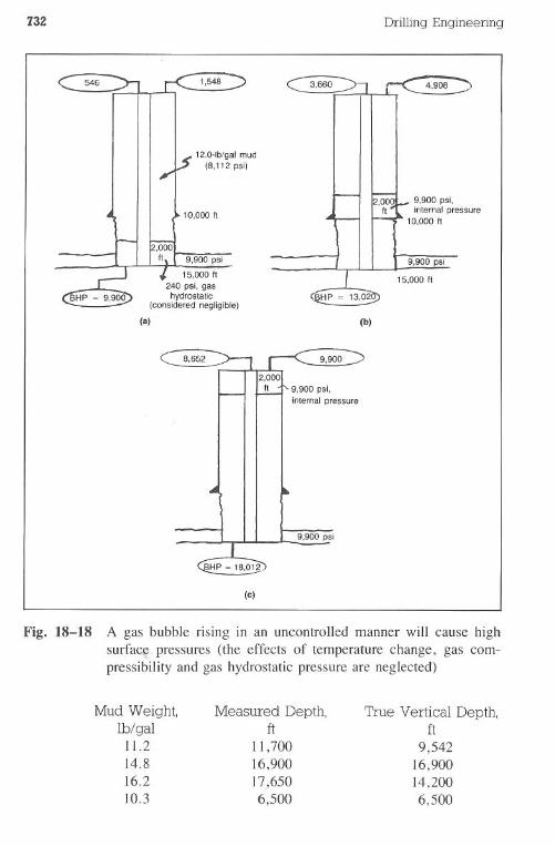
~Si15,000 It
240 psi, gashydrostatic
(considered negligible)
(a)
732 Drilling Engineering
12.0-lb/gal mud
(8,112 pSi)
10,000 It9,900 psi,inlernal pressure
10,000 It
~si
15,000 It
(b)
9,900 psi,internal pressure
9,900 psi
(e)
Fig. 18-18 A gas bubble rising in an uncontrolled manner will cause highsurface pressures (the effects of temperature change, gas com-pressibility and gas hydrostatic pressure are neglected)
Mud Weight,Ib/gal
11.214.816.210.3
Measured Depth,ft
11,70016,90017,6506,500
True Vertical Depth,ft
9,54216,90014,2006,500
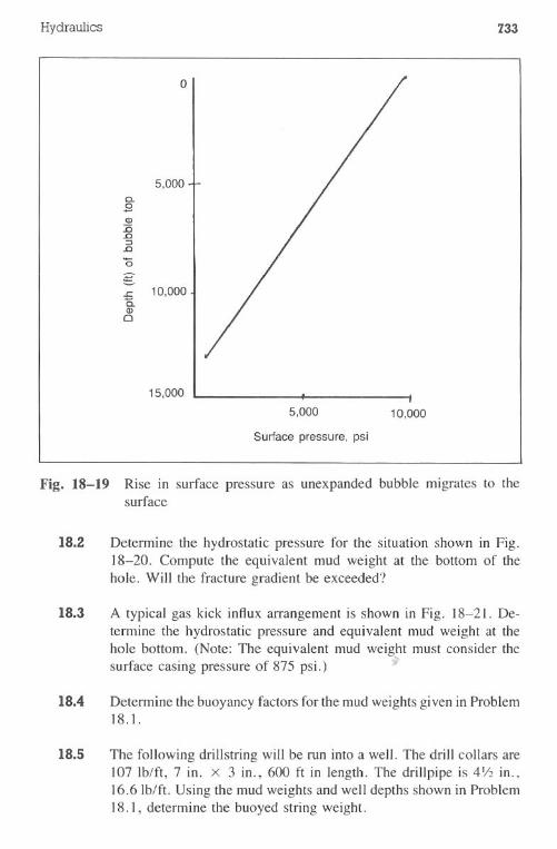
Hydraulics 733
o
15,0005,000 10,000
Surface pressure, psi
Fig. 18-19 Rise in surface pressure as unexpanded bubble migrates to thesurface
18.2 Determine the hydrostatic pressure for the situation shown in Fig.18-20. Compute the equivalent mud weight at the bottom of thehole. Will the fracture gradient be exceeded?
18.3 A typical gas kick influx arrangement is shown in Fig. 18-21. De-termine the hydrostatic pressure and equivalent mud weight at thehole bottom. (Note: The equivalent mud weig,htmust consider thesurface casing pressure of 875 psi.)
18.4 Determine the buoyancy factors for the mud weights given in Problem18.1.
18.5 The following drillstring will be run into a well. The drill collars are107 lb/ft, 7 in. x 3 in., 600 ft in length. The drillpipe is 4Y2 in.,16.6Ib/ft. Using the mud weights and well depths shown in Problem18.I, determine the buoyed string weight.
5,000c.,gQ):c.D:::I.D'0
g..r::. 10,000C.Q)
Q
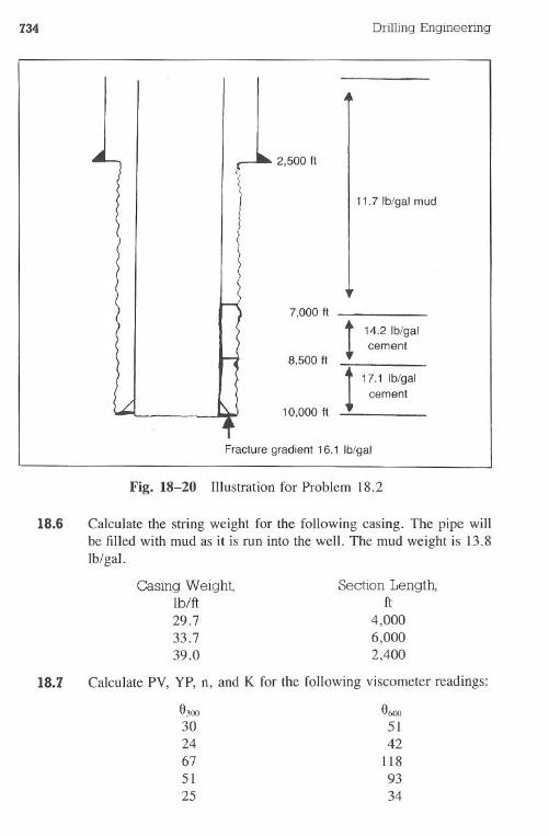
734 Drilling Engineering
2,500 It
11.7 Ib/gal mud
Fracture gradient 16.1 Ib/gal
Fig. 18-20 Illustration for Problem 18.2
18.6 Calculate the string weight for the following casing. The pipe willbe filled with mud as it is run into the well. The mud weight is 13.8lb/gal.
Casing Weight,Ib/ft29.733.739.0
Section Length,ft
4,0006,0002,400
18.7 Calculate PV, YP, n, and K for the following viscometer readings:
63003024675125
66005142
1189334
7,000 It
! 14.2Ib/galcement
8,500 It
117., Iblg.'cement
10,000 It
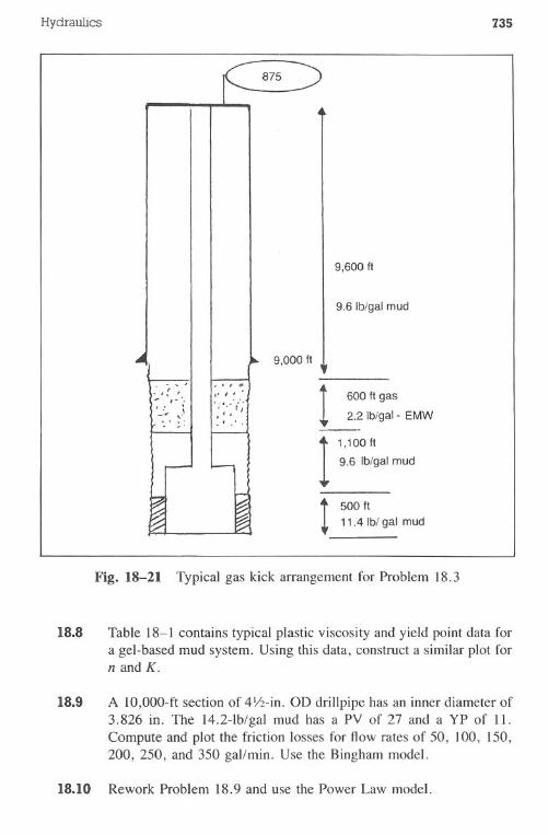
Hydraulics 735
9,600 ft
9.6 Ib/gal mud
9,000 ft
r. . 1#,'" .; '.. i.,.. '.',' . 1
600 ft gas
2.2 Ib/gal - EMW
I1,100 ft
9.6 Ib/gal mud
! 500 ft
11.4 Ibl gal mud
Fig. 18-21 Typical gas kick arrangement for Problem 18.3
18.8 Table 18-1 contains typical plastic viscosity and yield point data fora gel-based mud system. Using this data, construct a similar plot fornand K.
18.9 A IO,OOO-ftsection of 41/2-in.OD drillpipe has an inner diameter of3.826 in. The 14.2-lb/gal mud has a PV of 27 and a YP of II.Compute and plot the friction losses for flow rates of 50, 100, 150,200, 250, and 350 gal/min. Use the Bingham model.
18.10 Rework Problem 18.9 and use the Power Law model.
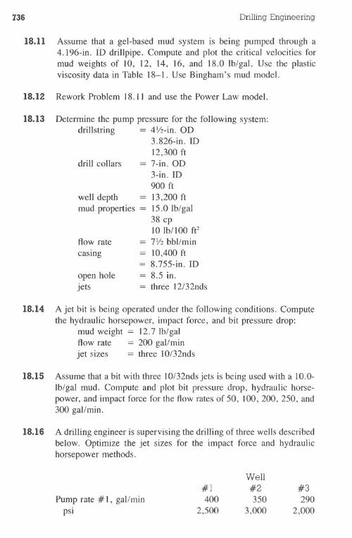
736 Drilling Engineering
18.11 Assume that a gel-based mud system is being pumped through a4. 196-in. ID drillpipe. Compute and plot the critical velocities formud weights of 10, 12, 14, 16, and 18.0 Ib/gal. Use the plasticviscosity data in Table 18-1. Use Bingham's mud model.
18.12 Rework Problem 18.11 and use the Power Law model.
18.13 Determine the pump pressure for the following system:drillstring = 4Y2-in.OD
3.826-in. ID12,300 ft
drill collars = 7-in. OD3-in. ID900 ft
well depth = 13,200ftmud properties = 15.0Ib/gal
38 cp10 lb/ 100 fe
flow rate = 7Y2bbl/mincasing = 10,400ft
= 8.755-in. IDopen hole = 8.5 in.jets = three 12/32nds
~Ii
l
III'
18.14 A jet bit is being operated under the following conditions. Computethe hydraulic horsepower, impact force, and bit pressure drop:
mud weight = 12.7Ib/galflow rate = 200 gal/minjet sizes = three 1O/32nds
18.15 Assume that a bit with three 1O/32ndsjets is being used with a 10.0-Ib/gal mud. Compute and plot bit pressure drop, hydraulic horse-power, and impact force for the flow rates of 50, 100,200, 250, and300 gal/min.
18.16 A drilling engineer is supervising the drilling of three wells describedbelow. Optimize the jet sizes for the impact force and hydraulichorsepower methods.
, I~
.l
Pump rate # I, gal/minpsi
#1400
2,500
Well#2350
3,000
#3290
2,000
.L
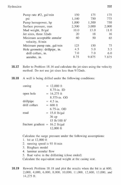
18.17 Refer to Problem 18.16 and calculate the jet sizes using the velocitymethod. Do not use jet sizes less than 9/32nds.
casing
18.18 A well is being drilled under the following conditions:
= 12,000 ft8.75-in. ID
= 14,275 ft8.375-in. OD
= 4.5 in.= 600 ft
6.75-in. OD= 15.0 Ib/gal
36 cp15 Ib/100 fe
fracture gradient = 16.2 Ib/gal12,000 ft
open hole
drillpipedrill collars
mud
Calculate the surge pressure under the following assumptions:1. bit at 12,000 ft2. running speed is 93 ft/min3. Bingham model4. laminar annular flow5. float valve in the drillstring (close ended)Calculate the equivalent mud weight at the casing seat.
18.19 Rework Problem 18.18 and plot the results when the bit is at 600,2,000, 4,000, 6,000, 8,000, 10,000, II ,000, 12,600, 13,000, and14,275 ft.
Hydraulics 737
Pump rate #2, gal/min 150 175 175
psi 1,140 750 775
Pump horsepower, hp 1,000 1,500 750
Surface pressure, max 2,500 3,000 2,000Mud weight, Ib/gal 10.0 13.0 11.0Jet sizes, three 32nds 20 18 16
Minimum acceptable annular 60 50 65
velocity, ftlminMinimum pump rate, gal/min 125 150 75
Hole geometry: drillpipe, in. 4.5 5.0 3.5drill collars, in. 7.0 7.0 6.0annulus, in. 8.75 9.875 7.875
738 DrillingEngineering
18.20 Calculate the cuttings slip velocity for the following conditions. Usethe Moore correlation.
hole size = 12.25 in.drillpipe = 5 in.mud = 10 lb/ galcuttings = 0.30 in.
22.0-lb/gal densityflow rate = 380 gal/minFann viscometer readings = e600 = 50
e300 = 30
18.21 Rework Problem 18.20 and use the Chien correlation. Assume a gel-base mud.
18.22 Rework Problem 18.21 and assume a polymer mud. A differentexpression for the apparent viscosity must be used. See Eq. 18.70.
18.23 Compute and plot the gas migration rates for mud weights of 8.33,8.5,9.0,9.5,10.0,11.0,12.0,14.0, and 16.0 lb/gal. Use the Adamsunpublished correlation.
References
Adams, Neal. Unpublished correlations relating to gas migration rates for usein computerized drilling simulations.
Ted Bourgoyne. Personal communications. Louisiana State University, BatonRouge. Fall 1977.
Burkhardt, J .A. "Wellbore Pressure Surges Produced by Pipe Movement."Transactions of the AlME, 1961, p. 595.
Chien, S.F. "Annular Velocityfor Rotary Drilling Operations." Proceedingsof the Rock Mechanics Conference, Austin, 1971.
Dodge, D.W., and A.B. Metzner. "Turbulent Flow of Non-Newtonian Sys-tems." AlChE Journal, June 1959, p. 189.
Eckel, J.R., and W.J. Bielstein. "Nozzle Design and Its Effect on DrillingRate and Pump Operation." API Drilling and Production Practices. 1951,p.28.
Hydraulics 739
Kendal, W.A., and W.C. Goins. "Design and Operations of Jet Bit Programsfor Maximum Hydraulic Horsepower, Impact Force, or Jet Velocity."Transactions of the AlME, 1960, p. 238.
Melrose, J.c., et al. "A Practical Utilization ofthe Theory of Bingham PlasticFlow in Stationary Pipes and Annuli." Transactions of the A/ME, 1958,p.316.
Moore, P.L. Drilling Practices Manual. Tulsa: PennWell Books, 1974.
Ryan, N.W., and M.M. Johnson. "Transition from Laminar to TurbulentFlow in Pipes." AlChE Journal, 1959, V, no. 4, p. 433.
Walker, R.E., and T.M. Mayes. "Design of Muds for Carrying Capacity."Transactions of the AlME, 1975, p. 893.
Chapter
Well CostEstimation:
Preparation
Preparing cost estimates for a well is the final step in well planning. Inmany cases, the cost estimate is the management tool that determines if the wellwill be drilled. Although an essential part of the well plan, the cost estimatesection is often the most difficult to obtain.
A properly prepared well cost estimate may require as much engineeringwork as the actual well design. The costs should address dry holes and completedwells. In addition, accounting considerations such as tangible and intangibleitems must be taken into account. Unfortunately, many cost "guesstimates" arethe "back-of-the-napkin" type, with only a small amount of engineering workused in the process.
The cost estimate is the last item to be considered in the well plan sinceit is heavily dependent on the technical aspects of the projected well. After thetechnical aspects are established, the expected time required to drill the wellmust be determined. The actual well cost is obtained by integrating expecteddrilling and completion times with the well design.
Projected Drilling TuneThe time required to drill the well has a significant impact on many items
in the well cost. These items may include the following:
· drilling rig.mud·offshoretransportation·rental tools· support services
740
Well Cost Estimation: AFE Preparation 741
The effect of these items on the overall well cost is dependenton the actual unitcost, Le., $15,OOO/dayfor a land rig vs $lOO,OOO/dayfor a drillship, and theamount of drilling time.
Consider the well in Fig. 19-1. Assume that the well will be drilled inEastTexas in mid-1982. Table 19-1 summarizes the projected times for the well
Fig. 19-1 Example hole configuration
Depth Pipe Program0 I I I I I I I I Pipe size in. Mud weight, Mud type
Iblgal
1,000 .2,000 9.2
...--133/0.in.surface3,000 I I I I I I I I Water - Gel
..
4,000 II I I I I II 9.2
5,000
6,000 \ I I I I I II 9.2
7,000
8,000 \ I I I I I I \ 9.2
9,000 II I I I
'$ -9.2 Water- Gel
10,000
1h II I 1-'10.5
11,000 12.3
12,000
,%-;, II""
14.4
13,000 14.4 Oil based
14,000 15.5
15,000 I I IIt's' cd'
15.5_ V...ln.pr uctlon
16,000
2%'in.tubing
16.1 Oil based
17,000 17.4
742 Drilling Engineering
Table 19-1 Drilling Times and Associated Well Costsfor Fig. 19-1
in three cases and illustrates the cost differences. The worst case has a 21%greater cost than the best drilling times. This example illustrates the importanceof preparing accurate projections for drilling time, or "depth vs days," as it isoften termed. A typical depth vs days plot is shown in Fig. 19-2.
Sources of Drilling Time Information. Numerous sources are availableto estimate drilling times for a well. As described in Chapter 2, these includebit records, mud records, log header information, and operator's well histories.Other items such as scout tickets and production histories are useful becausethey provide information that will affect the time projections, although theseitems seldom contain actual drilling times.
Bit records are valuable sources of drilling information and can be usedto estimate drilling time. Although few bit manufacturers incorporate a columnfor dates in the bit record forms, most drilling engineers who routinely completethe forms make notes in the remarks column as to the time or date the bits wererun. In addition, most records contain the dates for well spudding, completion,and pipe setting. Additional inferences can be made from the individual bit-lifehours and the cumulative drilling time for each well.
Mud records usually provide the most authoritative information about thedrilling time data. These records are maintained daily and usually contain remarksabout the time required for each drilling activity. In addition, time allocated to
Time, days
Item 1 2 3
Move in and out 8 8 8
Drive pipe0-200 ft 1 1 1
200-3,580 ft 2 3 43,580-11,600 ft 8 12 1811,600-15,000 ft 15 22 3215,000-17,000 ft 12 18 24
Run casing 8 8 8
stringsLogging 5 5 5
Completion 7 7 766 84 107
Well costs* $4,175,977 $4,562,372 $5,045,448
*Costs are computed from Adams and Rountree Technology's AFE program.
Well Cost Estimation:AFE Preparation 743
r Depth (x 1,000 It)~ Movein rig
on~ Drivepipe WELL NAME:
OPERATOR:
LOCATION:2
4
Move out rig
6
8
10
12
14
16 Complete well
J
Log, run & set casing
o 50 6020 30 7010 40DAYS
Fig. 19-2 Depth vs days projection
hole problems can be evaluated to determine if the same amount of timeshould be included in the upcoming well. For example, hole sloughingmay be an expected occurrence in an area while kicks and twistoffs are unusualactivities.
Log header data contain some drilling time information and dates for eachsuccessive logging run. In addition, scout tickets attached to some logs includespud and completion dates.
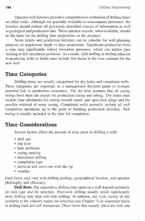
744 Drilling Engineering
Operator well histories provide a comprehensive evaluation of drilling timeson offset wells. Although not generally available to noncompany personnel, thehistories should contain all previously described sources of information as wellas geological and production data. These operator records, when available, shouldbe the basis for the drilling time projections on the prospect.
Scout tickets and production histories can be valuable for well planningpurposes to supplement depth vs days projections. Significant production froma zone may significantly reduce formation pressures, which can induce pipesticking or lost circulation problems. As a result, infill drilling or drilling adjacentto producing wells or fields must include this factor in the time estimate for thenew well.
Time CategoriesDrilling times are usually categorized for dry holes and completed wells.
These categories are important as a management decision guide to evaluatepotential risk vs production economics. The dry hole assumes that all casingstrings have been run except for production casing and tubing. Dry holes mustinclude time allotments for setting several cased- and open-hole plugs and thepossible retrieval of some casing. Completed wells normally include all wellcompletion operations up to the point of building production facilities. Welltesting is usually included in the time for completion.
Time Considerations
Severalfactorsaffectthe amountof time spent in drillinga well:· drill rate· trip time·hole problems· casing running·directionaldrilling·completion type·move-inand move-outwith the rig·weather
Each factor may vary with drilling geology, geographical location, and operatorphilosophy and efficiency.
Drill Rate. The cumulative drilling time spent on a well depends primarilyon rock type and bit selection. Hard-rock drilling usually needs significantlymore drilling time than soft-rock drilling. In addition, the wide variety of bitsavailable to the industry makes bit selection (see Chapter 7) an important factorin drilling hard and soft formations. Other items that usually affect the drill rate
Well Cost Estimation: AFE Preparation 745
are proper selection of weight and rotary speeds for optimum drilling, mud type,and differential pressure.
Trip Time. Pulling and running the drillstring is an important item inestimating total rotating time. In many cases, it is equal to or exceeds the on-bottom drilling time. Trip time is dependent on well depth, amount of mud tripmargin, hole problems, rig capacity, and crew efficiency. A reliable rule ofthumb for trip time estimations is 1 hrll,OOOft of well depth, i.e., 18 hr for an18,000-ft well. Over the total drilling life of a well, this rule of thumb will bereasonably accurate.
Long bit runs from 50-200 hr often require a short trip of several thousandfeet out of and back into the hole. The purpose of the short trip is to remove ordestroy any thick buildup of filter cake that significantly increases the swabbingtendencies of the drillstring. Short trips are dependent on company philosophy,mud type, and bit life.
Bole Problems. Various types of hole problems are routinely addressedin the drilling time projections, while others are considered improbable. Forexample, severe kicks and blowouts are usually unlikely if the operator devotessufficient attention to drilling activities. Geological conditions and drillinghistories in the area of the prospect well will often define the pertinent hole prob-lems.
The types of problems often regarded as standard are hole sloughing, lostcirculation, and slow drilling rates. Many operators have encountered formationsthat slough or heave into the wellbore regardless of the amount of attention givento the mud systems or well plan. Lost circulation will occur in some formationseven if the mud density is approximately equal to that of fresh water. Slowdrilling rates will usually occur in environments with high differential pressures,such as the case of formation pressure regressions ~hile maintaining consistentmud weights. However, these hole problems can be eliminated in most areas byexercising good engineering judgment in preparing the well plan.
Casing Running. The time required to run casing into the well is de-pendent on casing size and depth, hole conditions, crew efficiency, and use ofspecial equipment such as pickup machines and electric stabbing boards. Heavycasing strings may require that the drillstring be laid down rather than set backin the derrick. In addition, nippling-up the blowout preventers and testing thecasing and formation must be considered.
Directional Drilling. Directional control of a well requires increases inthe drilling time. These increases apply to 1) attempting to drill a well direc-tionally or 2) maintaining vertical control of a well that has deviation tendencies.The increases in drilling time usually result from obtaining surveys and fromthe inability to apply desired bit weights or rotary speed as a result of directionalcontrol efforts. Many operators increase the expected drilling time in a directionalwell by a factor of 2.
746 Drilling Engineering
WeD Completions. Completion systems vary in complexity and, as aresult, have a significant variation in time to implement the system. A standardsingle, perforated completion can be finished in 6-8 days. Dual-completed wellsusually require an additional 2-3 days. Gravel packs, acidizing, fracturing, andother forms of well treatments must be evaluated on a case-by-case basis. Need-less to say, the efficiency of all associated personnel and their experiences witha particular type of completion have a major impact on the required time.
Rig Move-in and Move-out. Rig moving affects several areas of thecost estimate and must be considered in the time projections. Move-in and rig-up occur before spudding the well. Rig-down and move-out occur after the wellcompletion. If a completion rig is used rather than the drilling rig for the com-pletion work, an additional rig move must be considered from both a cost andtime standpoint.
A rule of thumb for estimating rig moving times is based on the IADCrig hydraulics code of 1, 2,"'3, or 4, where the higher numbers represent largerrigs. Codes I and 2 can usually move in and out in 4 days since they are frequentlymobile and truck-mounted. Codes 3 and 4 require approximately 8 days to movein, rig-up, rig-down, and move out. These time estimates affect the move-incost, supervision time, and overhead allocations.
Weather. The effect of weather on the projected time is not consideredin most well plans. As an example, hurricanes and tornadoes cannot be routinelyexpected. However, weather problems such as those that routinely occur in theNorth Sea must be considered in the plan.
Cost CategoriesThe well cost estimate should be divided into several categories for en-
gineering and accounting purposes. Engineering considerations include dry-holeand completed costs, logical groupings such as completion equipment or tubulargoods, and convenience groupings such as rental equipment. Accounting con-siderations include tangible, intangible, and contingency items. The sample AFEsummary in Fig. 19-3 illustrates several cost categories.
Tangible and Intangible CostsAccounting and tax principles treat tangible and intangible costs in different
ways. As a result, they must be segregated in the cost estimate. Althoughintangible costs are difficult to define precisely, they include expenditures in-curred by the operation for labor, fuel, repairs, hauling, and supplies used 1) indrilling, perforating, and cleaning wells; 2) in preparing the surface site prior todrilling; and 3) in constructing derricks, tanks, pipelines, and other structureserected in connection with drilling, but not including the cost of the materials
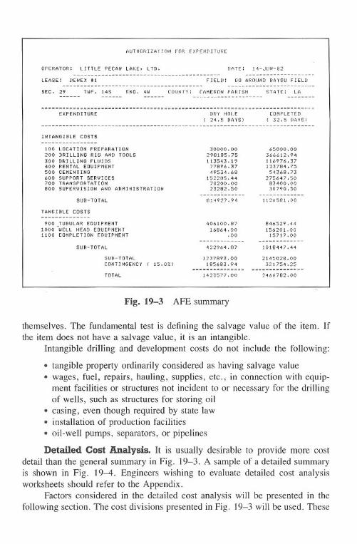
Well Cost Estimation: AFE Preparation 747
OPERATOR: LITTLEPECANLAKE.LTD.
AUTHORIZATION FOR fXPENPITURE
DATE: 14-JUN-82--------------------
SEC. 29 TWP. 14S RNG. 4 W
------------------------------------------
--------------------
LEASE: DENEX.I FIELD: GO AROUNDBAYOUFIELD-------------------------
COUNTY: CAMERONPARISH STATE: LA
=============================================================================~EXPENDITURE DRY HOLE
( 24.5 DAYS)COMPLETED
( 32.5 DAYS)------------------------------------------------------------------------------
INTANGIBLE COSTS----------------
100 LOCATION PREPARATION200 DRILLING RIG AND TOOLS300 DRILLING FLUIDS400 RENTAL EQUIPMENT500 CEMENTING600 SUPPORT SERVICES700 TRANSPORTATION800 SUPERVISION AND ADMINISTRATION
SUB-TOTAL
TANGIBLECOSTS--------------900 TUBULAR EQUIPMENT1000 ~ELL HEAD EQUIPMENT1100 COMPLETION EQUIPMENT
SUB-TOTAL
SUB-TOTALCONTINGENCY( 15.07.)
TOTAL
30000.00298185.75113543.1977896.3749534.68
152285.4470200.0023282.50-------------
814927.94
406100.8716864.00
.00-------------422964.87
1237893.00
185683.94===============
1423577.00
65000.00366612.94116976.37133784.7554368.73
275647.5083400.0030790.50-------------
1126581.00
846529.44156201.0015717.00-------------
2145028.00321754.25------.-----------------
2466782.00
Fig. 19-3 APE summary
themselves. The fundamental test is defining the salvage value of the item. Ifthe item does not have a salvage value, it is an intangible.
Intangible drilling and development costs do not include the following:
. tangible property ordinarily considered as having salvage value.wages, fuel, repairs, hauling, supplies, etc., in connection with equip-ment facilities or structures not incident to or necessary for the drillingof wells, such as structures for storing oil. casing, even though required by state law. installation of production facilities.oil-well pumps, separators, or pipelines
Detailed Cost Analysis. It is usually desirable to provide more costdetail than the general summary in Fig. 19-3. A sample of a detailed summaryis shown in Fig. 19-4. Engineers wishing to evaluate detailed cost analysisworksheets should refer to the Appendix.
Factors considered in the detailed cost analysis will be presented in thefollowing section. The cost divisions presented in Fig. 19-3 will be used. These
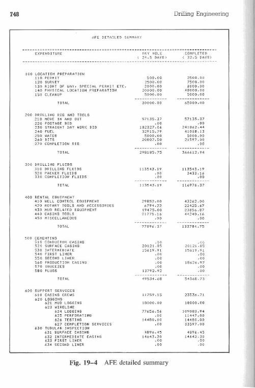
748 DrillingEngineering
AFE DETAILED SUMMARY
==============================================================================EXPEN[IITURE DRY HOLE
( 24.5 DAYS)COMPLETED
( 32.5 [lAYS)~-------------
100 LOCATION PREPARATION11 0 PERM IT120 SURVEY130 RIGHT OF WAY, SPECIAL PERMIT ETC.140 PHYSICAL LOCATION PREPARATION150 CLEANUP
500.002500.002000.0020000.005000.00
2500.007500.002000.0048000.005000.00
------------- -------------TOTAL 30000.00 65000.00
Fig. 19-4 AFE detailed summary
200 DRILLING RIG AND TOOLS210 MOVE IN AND OUT 57135.37 57135.37220 FOOTAGE BID .00 .00230 STRAIGHT DAY WORK BID 182327.06 241862.44240FUEL 32915.79 41018.13250 WATER 5000.00 5000.00260 BITS 20807.50 21597.00270 COMPLETION RIG .00 .00
------------- -------------TOTAL 298185.75 366612.94
300 DRILLING FLUIDS310 DRILLING FLUIDS 113543.19 113543.19320 PACKER FLUIDS .00 3433.16330 COMPLETION FLUIDS .00 .00
------------- -------------TOTAL 113543.19 116976.37
400 RENTAL EQUIPMENT410 WELL CONTROL EQUIPMENT 29852.00 43262.00420 ROTARY TOOLS AND ACCESSORIES 6794.22 22425.67430 MUD RELATED EQUIPMENT 19475.00 23856.87440 CASING TOOLS 21775.16 44240.16450 MISCELLANEOUS .00 .00
------------- -------------TOTAL 77896.37 133784.75
500 CEMENTING510 CONDUCTOR CASING .00 .Oc.520 SURFACE CASING 20121.85 20121.85530 INTERMEDIATE 15619.91 15619.91540 FIRST LINER .00 .00550 SECOND LINER .00 .00560 PRODUCTION CASING .00 18626.97570 SQUEEZES .00 .00580 PLUGS 13792.92 .00
------------- -------------TOTAL 49534.68 54368.73
600 SUPPORT SERVICES610 CASING CREWS 11759.15 23536.71620 LOGGING
621 MUD LOGGING 18000.00 18000.00623 WIRELINE
624 LOGGING 77656.56 109083.94625 PERFORATING .00 11447.00626 TESTING 14480.00 14480.00627 COMPLETION SERVICES .00 33597.00
630 TUBULAR INSPECTION631 SURFACE CASING 4896.45 4896.45632 INTERMEDIATE CASING 14643.30 14643.30633 FIRST LINER .00 .00634 SECOND LINER .00 .00
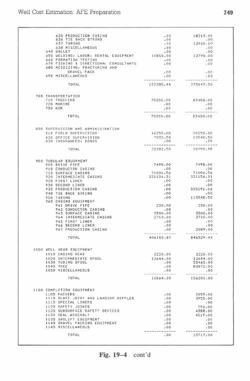
Well Cost Estimation: AFE Preparation 749
635 PRODUCTION CASING636 TIE BACK STRING637 TU9ING638 MISCELLANEOUS
640 GALLEY650 WELDING. LABOR. RENTAL EOUIPMENT660 FORMATION TESTING670 FISHING & DIRECTIONAL CONSULTANTS680 ACIDIZING. FRACTURING AND
GRAVEL PACK690 MISCELLANEOUS
TOTAL
700 TRANSPORTATION710 TRUCKING720 MARINE730 AIR
TOTAL
800 SUPERVISION AND ADMINISTRATION810 FIELD SUPERVISION820 OFFICE SUPERVISION830 INSURANCES. BONDS
TOTAL
900 TUBULAR EOUIPMENT905 DRIVE PIPE910 CONDUCTOR CASING915 SURFACE CASING920 INTERMEDIATE CASING925 FIRST LINER930 SECOND LINER935 PRODUCTION CASING940 TIE BACK STRING950 TUBING960 CASING EOUIPMENT
961 DRIVE PIPE962 CONDUCTOR CASING963 SURFACE CASING964 INTERMEDIATE CASING965 FIRST LINER966 SECOND LINER967 PRODUCTION CASING
TOTAL
1000 WELL10101020103010401050
HEAD EOUIPMENTCASING HEADINTERMEDIATE SPOOLTUBING SPOOLTREEMISCELLANEOUS
TOTAL
1100 COMPLETION EQUIPMENT1105 PACKERS1110 BLAST JOINT AND LANDING NIPPLES1115 SPECIAL LINERS1120 SAFETY JOINTS1125 SUBSURFACE SAFETY DEVICES1130 SEAL ASSEMBLY1135 GASLIFT EQUIPMENT1140 GRAVEL PACKING EQUIPMENT1145 MISCELLANEOUS
TOTAL
.00
.00
.00
.00
.0010850.00
.00
.00
.00
.00-------------
152285.44
70200.00.00.00
-------------70200.00
16250.007032.50
.00-------------
.23282.50
7498.00.00
71006.56321156.31
.00
.00
.00
.00
.00
230.00.00
3500.002710.00
.00
.00
.00-------------
406100.87
3220.0013644.00
.00
.00
.00-------------
16864.00
.00
.00
.00
.00
.00
.00
.00
.00
.00-------------
.00
18213.00.00
13960.10.00.00
13790.00.00.00
.00
.00-------------
275647.50
83400.00.00.00
-------------
83400.00
20250.00
10540.50.00
-------------
30790.50
7498.00.00
71006.56321156.31
.00
.00325291.06
.00113048.50
230.00.00
3500.002710.00
.00
.002089.00
-------------
846529.44
3220.00
13644.0055465.0083872.00
.00-------------156201.00
2059.003955.00
.00796.004388.004519.00
.00
.00
.00-------------
Fig. 19-4 cont'd
15717.00
750 Drilling Engineering
factors are heavily dependent on company drilling philosophy and, as such, maynot apply to all companies.
Location PreparationPreparing the location to accept the rig is an important cost factor and
perhaps the most difficult to quantify. It includes legal costs, surveying thelocation site, physical location preparation, and post-drilling cleanup. These costsare affected by rig type, rig size, and well location.
Location costs include only those variables actually involved with rig move-in. These costs do not include lease fees or bidding costs. Individual companiesmust determine appropriate methods for handling these costs in the well costestimate.
Permits, or permitting the well, are required in virtually every drilling areain the world. Some permit procedures are as simple as preparing a few fill-in-the-blank documents, while others may require extensive, time-consuming ef-forts such as environmental and economic impact statements. Some well permitsmust be granted from federal or national authorities, while others may be obtainedquickly from local agencies. Permitting a well is primarily a legal matter thatoften requires significant consultation with legal groups.
Spotting the well involves surveying the well site and determining its exactlocation. Land sites can be spotted by professional surveyors with the use oflocal, known markers. Offshore sites are spotted from offset platforms in thearea. Satellite surveys can be used when spotting a well in an area, particularlyin offshore environments where marker sites such as existing platforms are notavailable.
Right-of-way from a public access road to the actual drilling site for landwells must be considered. If the off-road distance is small or through single-owner land, the permit may be obtained quite easily in some cases. Difficultiesmay arise for distant locations, multiple landowners, or public access areas. Asin the case of obtaining permits, right-of-ways are often a matter for the legalor land departments.
Preparing the location to accept the rig depends on the rig type and sizeas well as the location. Land rigs may require the construction of a board roadand location if the soil is too soft to support transport vehicles and the rig.Sometimes pilings are required under the substructure. The size of the turnaroundand the number of board plys will increase with larger rigs. Mountainous locationsmay need a road built to the site. In addition, factors such as the size of themud reserve pit and the chemicals storage area depend on drilling times, mudtypes, and mud weights.
Marsh areas usually require that a canal or channel be dredged to the site.The depth and width of the canal must be coordinated with the size of the rig.
Well Cost Estimation: AFE Preparation 751
The actual rig site at the end of the canal is a larger area that must be dredged.Shell pads for a rig foundation may be required in marshy areas if the waterdepth is sufficiently deep to prevent the direct use of a barge rig or if the seabedis very soft or erodes due to subsea currents.
Offshore sites often require the least amount of location preparation. Ifsurveys of the seafloor show that no obstructions are present, the rig can bemoved to the site with no additional efforts. Floating rigs are seldom troubledwith soft subsurface formations that may hamper settling of the legs for jackuprigs.
Location cleanup after drilling has been completed is presently undergoingclose scrutiny by regulatory bodies. Most sites must be restored to a virgincondition that may involve site leveling, trucking, and in some cases replantingwildlife vegetation. Offshore sites usually are required to ensure that no remainingobstructions will hamper commercial fishing operations.
Drilling Rig and ToolsThe costs for drilling and completion rigs plus the associated drilling tools
can be a substantial fraction of the total drilling costs. Consider drilling andcompleting the well in Fig. 19-1 in 75 days. Under these conditions, the fol-lowing are estimated well costs for various rig rates:
Each of the first three cases used the same well design criteria and equip-ment-Le., casing, mud, logging-with the exception of the rig cost. Case 4shows the same well in an offshore environment, resulting in the need of a jackuprig. As a result, it is easily seen that careful attention must be given to definingcosts for the drilling rig and tools.
Move-in and Move-out. Moving the rig in to the location before drillingthe well and out of the location after it is completed can be a substantial costitem. Jackup rigs require a fleet of tugboats, while drillships move themselvesonto the location. Many states publish tariffs that specify the allowable truckingcharges for various lengths of moves. Large land rigs are normally transportedby truck to the location. Generally, IADC Type 3 and 4 rigs are sufficientlylarge that they must be transported piece-wise by truck. Type 1 and 2 are usually
Case Rig Type Rig Cost, Completed Well,$/day 1982 u.s. $
1 Land 8,500 4,620,0002 Land 15,000 5,262,0003 Land 22,500 5,978,0004 Jackup 35,000 8,354,600
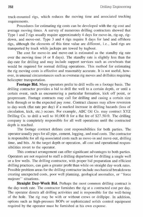
752 Drilling Engineering
truck-mounted rigs, which reduces the moving time and associated truckingrequirements.
Procedures for estimating rig costs can be developed with the rig cost andaverage moving times. A survey of numerous drilling contractors showed thatType I and 2 rigs usually require approximately 4 days for move-in, rig-up, rig-down, and move-out. Type 3 and 4 rigs require 8 days for land and offshorerigs, although the elements of this time value are different, i.e., land rigs aretransported by truck while jackups are towed by tugboat.
The cost for move-in and move-out is estimated as the standby rig rateover the moving time (4 or 8 days). The standby rate is slightly less than theday-rate for drilling and may include support services such as crewboats thatwould be required for normal drilling operations. This method for estimatingthe rig moving costs is effective and reasonably accurate. It is not useful, how-ever, in unusual circumstances such as overseas rig moves and drillsites requiringhelicopter transportation.
Footage Bid. Many operators prefer to drill wells on a footage basis. Thedrilling contractor provides a bid to drill the well to a certain depth, or until acertain event, such as encountering a particular formation, kick off point, orgeopressure. Footage contracts may call for drilling and casing a certain sizehole through or to the expected pay zone. Contract clauses may allow reversionto day-work (flat rate per day) if a marked increase in drilling hazards (loss ofcirculation, kick, etc.) occurs. For example, ABC Oil Co. may contract XYZDrilling Co. to drill a well to 10,000 ft for a flat fee of $27.50/ft. The drillingcompany is completely responsible for all well operations until the contracteddepth is reached.
The footage contract defines cost responsibilities for both parties. Theoperator usually pays for all pipe, cement, logging, and mud costs. The contractoris responsible for all rig-associated costs such as move-in and move-out, drillingtime, and bits. At the target depth or operation, all cost and operational respon-sibilities revert to the operator.
This contract arrangement can offer significant advantages to both parties.Operators are not required to staff a drilling department for drilling a single wellor a few wells. The drilling contractor, with proper bid preparation and efficientdrilling practices, can gain a greater profit than while on straight day-work rates.Possible problem areas for the drilling contractor include mechanical breakdownscreating unexpected costs, poor well planning, geological anomalies, or "forcemajeure" situations.
Straight Day-Work Bid. Perhaps the most common drilling contract isthe day-work rate. The contractor furnishes the rig at a contracted cost per day.,The operator directs all drilling activities and is responsible for the well-beingof the hole. The rig may be with or without crews or drillpipe. In addition,options such as high-pressure BOPs or sophisticated solids control equipmentrequired by the operator must be furnished at his own expense.
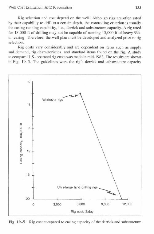
Well Cost Estimation: AFE Preparation 753
Rig selection and cost depend on the well. Although rigs are often ratedby their capability to drill to a certain depth, the controlling criterion is usuallythe casing running capability, i.e., derrick and substructure capacity. A rig ratedfor 18,000 ft of drilling may not be capable of running 15,000 ft of heavy 9%-in. casing. Therefore, the well plan must be developed and analyzed prior to rigselection.
Rig costs vary considerably and are dependent on items such as supplyand demand, rig characteristics, and standard items found on the rig. A studyto compare U.S.-operated rig costs was made in mid-1982. The results are shownin Fig. 19-5. The guidelines were the rig's derrick and substructure capacity
o
Ultra-largelanddrillingrigs~
Workover rig~4
16
20
o 3,000 6,000 9,000 12,000
Rig cost, $/day
Fig. 19-5 Rig cost compared to casing capacity of the derrick and substructure
:fa0 80000.....
;i-'0ItSa.ItS 12'-'C>c:"00ItS()
754 Drilling Engineering
and disregarded items such as optional equipment that might otherwise be rentedfor lesser rigs. An interesting point on the illustration is that the oversupplyconditions in mid-1982 depressed rig prices and developed a situation in whichrig costs were reasonably equal regardless of the rig size, i.e., $6,000 vs $9,500/day for small to very large rigs. By 1984, competitive pressure had reducedthese rates even more.
Standby rates for drilling rigs usually range from $200-500/day less thanthe amounts shown in Fig. 19-5. The rates include crews and drillpipe. Thecosts are used to estimate move-in and move-out charges.
Fuel. Drilling contracts are either inclusive or exclusive of fuel changes.In the latter case, the operator must pay for fuel on the rig. This major contractpolicy change occurred in the late 1970swhen fuel charges increased from $0.20to $1.20/gal.
Fuel usage is dependent on equipment type and rig. Fuel consumptionrates were evaluated in the study previously described for rig cost rates. Theresults are shown in Fig. 19-6. The average consumption rate is evaluated as afunction of the rig size measured by its ability to run casing.
Water. A supply of water is an important consideration. The water is usedto wash the rig, mix mud and cement, and cool the engines and equipment.
Water can be supplied in three ways. A shallow water well can be drilled.This method is common in most land operations, but it is not feasible offshoreor with deep water tables on land. Water can be transported to the rig by meansof truck, pipelines, barges, or boats. In addition, offshore rigs can use seawater.
Many engineers use a value of $5,000 for water costs (1982 prices). Thisamount is approximately the cost to drill a shallow water well. It is also a fairestimate of the cost to lay a water line from a nearby water source. In any case,water costs are seldom considered as a major impact on the total cost estimate.
Bits. Establishing a bit cost depends on the number, size, and type of bitsand their respective costs. The bit type, size, and number should have beenpreviously defined in the well plan by the time the AFE is prepared. If the bitis a standard IADC-code bit, published prices are available. Prices are not readilyavailable for specialty bits or for diamond and polycrystalline bits.
Diamond bit costs depend on the bit size as well as the diamond size,spacing, and quality. In most cases, these bits are made upon demand and arenot off-the-shelf items. A rule-of-thumb cost guide for diamond bits is $2,500/in. of bit diameter (1982 prices). For example, a lO-in. bit would cost approx-imately $25,000. Salvage values of up to 40% of the bit cost are often grantedon used bits. From a conservative view, many engineers prefer to disregard bitsalvage value when estimating bit costs in case the bit is completely destroyed.
Polycrystalline, or Stratapax,@bits are relatively new in the drilling in-dustry. Their physical structure, drilling performance, and costs are significantlydifferent from roller cone or diamond bits. Sample bit costs for these bits areshown in Table 19-2.
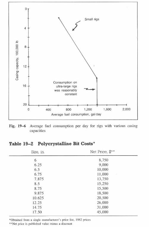
,Qg 8oc5o
~'0
~ 12tooC>c:'intoo
o
4
16
20
o
Small rigs
Consumption onultra-large rigs
was reasonablyconstant
400 800 1,200 1,600
Average fuel consumption, gal/day
2,000
Fig. 19-6 Average fuel consumption per day for rigs with various casingcapacities
Table 19-2 Polycrystalline Bit Costs*
Size, in. Net Price, $**
66.256.56.757.8758.58.759.875
10.62512.2514.7517.50
8,7509,000
10,00011,00013,75015,25015,50018,50020,50026,00031,00045,000
*Obtained from a single manufacturer's price list, 1982 prices
**Net price is published value minus a discount
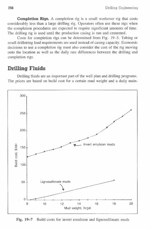
756 Drilling Engineering
Completion Rigs. A completion rig is a small workover rig that costsconsiderably less than a large drilling rig. Operators often use these rigs whenthe completion procedures are expected to require significant amounts of time.The drilling rig is used until the production casing is run and cemented.
Costs for completion rigs can be determined from Fig. 19-5. Tubing orsmall drillstring load requirements are used instead of casing capacity. Economicdecisions to use a completion rig must also consider the cost of the rig movingonto the location as well as the daily rate differences between the drilling andcompletion rigs.
Drilling FluidsDrilling fluids are an important part of the well plan and drilling programs.
The prices are based on build cost for a certain mud weight and a daily main-
300
250
50 .j. Lignosulfonate muds
'\
o8 10 12 14 16
Mud weight, Ib/gal
18 20
Fig. 19-7 Build costs for invert emulsion and lignosulfonate muds
200
---,/15 I ___ Invert emulsion muds.Q 150
en00:2'5 100ID
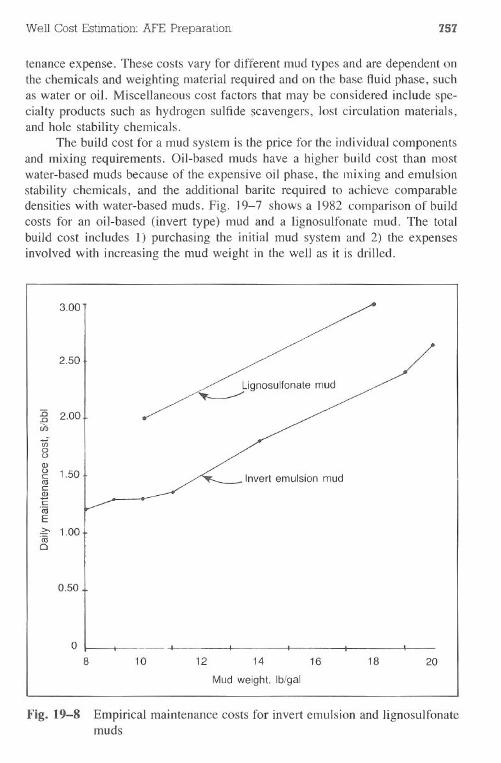
Well Cost Estimation: AFE Preparation 757
tenance expense. These costs vary for different mud types and are dependent onthe chemicals and weighting material required and on the base fluid phase, suchas water or oil. Miscellaneous cost factors that may be considered include spe-cialty products such as hydrogen sulfide scavengers, lost circulation materials,and hole stability chemicals.
The build cost for a mud system is the price for the individual componentsand mixing requirements. Oil-based muds have a higher build cost than mostwater-based muds because of the expensive oil phase, the mixing and emulsionstability chemicals, and the additional barite required to achieve comparabledensities with water-based muds. Fig. 19-7 shows a 1982 comparison of buildcosts for an oil-based (invert type) mud and a lignosulfonate mud. The totalbuild cost includes 1) purchasing the initial mud system and 2) the expensesinvolved with increasing the mud weight in the well as it is drilled.
3.00
o8 10 12 14 16 18 20
Mud weight, Ib/gal
Fig. 19-8 Empirical maintenance costs for invert emulsion and lignosulfonatemuds
2.50I
LignosulfonatemudI
:c 2.00.c
en00Q)0
1.50jc: Invert emulsion mudasc:Q)E"coE
1.00"co0
0.50
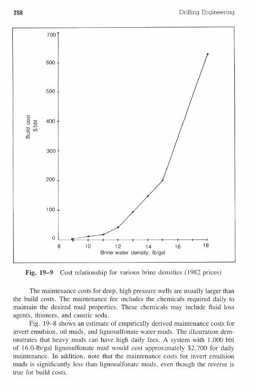
758
700
600
500
300
200
100
Drilling Engineering
o8 10 12 14 16
Brine water density, Ib/gal18
Fig. 19-9 Cost relationship for various brine densities (1982 prices)
The maintenance costs for deep, high pressure wells are usually larger thanthe build costs. The maintenance fee includes the chemicals required daily tomaintain the desired mud properties. These chemicals may include fluid lossagents, thinners, and caustic soda.
Fig. 19-8 shows an estimate of empirically derived maintenance costs forinvert emulsion, oil muds, and lignosulfonate water muds. The illustration dem-onstrates that heavy muds can have high daily fees. A system with 1,000 bblof 16.0-lb/gal lignosulfonate mild would cost approximately $2,700 for dailymaintenance. In addition, note that the maintenance costs for invert emulsionmuds is significantly less than lignosulfonate muds, even though the reverse istrue for build costs.
Well Cost Estimation: APE Preparation 759
Several additional factors affect mud costs. Small mud companies canoften provide less-expensive mud systems than larger companies, although asacrifice is made occasionally in terms of technical support and mud problemtesting capabilities. In addition, many mud companies offer mud without tech-nical support at a price reduction over mud with engineering support.
Packer Fluids. Packer fluidsare placed between the tubing and productioncasing above the packer. The fluid is usually a treated brine water but can bean oil mud or treated water-base mud-type fluid. In some cases, a packer fluidwill not be used. Although a low-density brine water is commonly used, oc-casionally a higher-density water or mud is used for pressure control. Fig.19-9 shows the typical cost relationship for various density brine waters.
Completion Fluids. Special fluids are occasionally used for well com-pletion purposes. They are usually designed to minimize formation damage. Thefluids may be filtered brine water, nitrogen, or oil. Costs for these fluids mustbe considered on a case-by-case basis.
Rental EquipmentDrilling equipment that is beyond the scope of the contractor-furnished
items is almost always required to drill a well. These items must be rented atthe expense of the contractor or operator, depending on the provisions of thecontract. They can include well control equipment, rotary tools and accessories,mud-related equipment, and casing tools. These items can represent a substantialsum in deep, high pressure wells.
Wen Control Equipment. Drilling contractors usually furnish BOPs,chokes, choke manifolds, and, in some cases, atmospheric degasser units. How-ever, the equipment may not be satisfactory for the well. In addition, numerousland rigs presently operate with well control equipment that is not state of theart, such as positive chokes, manual chokes, and manifold systems that do nothave centrally located drillpipe and casing pressure gauges.
Blowout preventer rental is expensive. High pressure stacks range from$1,500-3,OOO/day,exclusive of chokes or manifolds. The operator must definethe worst pressure case that can feasibly be attained and select preventers ac-cordingly. Cost estimates for a complete stack must consider the spherical,multiple ram sets, spools, studs, ring gaskets, and outlet valves.
Remote-controlled, hydraulic adjustable chokes are considered state of theart and are available from several sources. Contractors seldom furnish this typeof choke primarily because operators have always assumed this cost responsi-bility. These chokes usually cost $50-125/day with a 30-day minimum charge.Choke manifolds must be designed to withstand the maximum pressure ratingsin addition to coinciding with current company philosophy.
Rotary Tools and Accessories. Rotary tools are items related to thedrillstring or equipment that turns the string. The operator may be required to
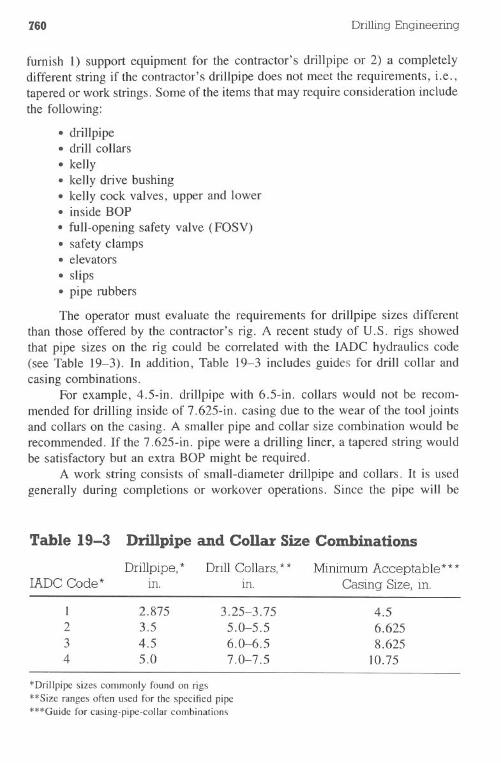
760 Drilling Engineering
furnish 1) support equipment for the contractor's drillpipe or 2) a completelydifferent string if the contractor's drillpipe does not meet the requirements, i.e.,tapered or work strings. Some of the items that may require consideration includethe following:
· drillpipe.drill collars·kelly· kelly drive bushing.kelly cock valves, upper and lower· inside BOP·full-opening safety valve (FOSV)·safetychimps.elevators· slips·pipe rubbers
The operator must evaluate the requirements for drillpipe sizes differentthan those offered by the contractor's rig. A recent study of U.S. rigs showedthat pipe sizes on the rig could be correlated with the IADC hydraulics code(see Table 19-3). In addition, Table 19-3 includes guides for drill collar andcasing combinations.
For example, 4,5-in. drillpipe with 6.5-in. collars would not be recom-mended for drilling inside of 7.625-in. casing due to the wear of the tool jointsand collars on the casing. A smaller pipe and collar size combination would berecommended. If the 7.625-in. pipe were a drilling liner, a tapered string wouldbe satisfactory but an extra BOP might be required.
A work string consists of small-diameter drillpipe and collars. It is usedgenerally during completions or workover operations. Since the pipe will be
Table 19-3 Drillpipe and Collar Size Combinations
Drillpipe,*IADC Code * in.
Drill Collars, **m.
Minimum Acceptable ***Casing Size, in.
I 2.8752 3.53 4.54 5.0
3.25-3.755.0-5.56.0-6.57.0-7.5
4.56.6258.625
10.75
*Drillpipesizescommonly found on rigs**Size ranges often used for the specified pipe
***Guide for casing-pipe-collar combinations
Well Cost Estimation:AFE Preparation 761
used inside production casing, the usual sizes are 2.375-3.5 in. Most operationsrequire a rental string because few rigs drill with this size pipe.
Mud-related Equipment. A properly maintained mud system offersmany benefits to the operator. To achieve the desired level of system efficiency,several specialized pieces of equipment may be required. Some of the equipmentmust be rented, even though the drilling rig may be well equipped in terms ofother drilling tools.
A complete suite of equipment required for the mud job usually dependson the mud type and weight. The following suite may be used for mud weightsin the 8.33-12.0-1b/gal range.·multiscreen shaker· desilter (with pumps).mud/gas separator· degasser (vacuum)· pit/flow monitors· drill rate recorder· gas detector
Mud weights greater than 12.0 Ib/gal may require the use of additional equipmentsuch as a centrifuge or mud cleaner. Oil muds need a cuttings cleaner to removethe oil from the cuttings prior to dumping. The cuttings cleaner is not alwaysused on land since current government regulations do not require its use.
Casing Tools. Recently, great strides have been made in running casing.Specialized equipment and crews normally handle the task rather than using therig crew and equipment. Since most rigs are not furnished with casing runningequipment, it must be rented.
Casing tools must be selected according to size and loading requirements.A commonly used method for evaluating the load requirement is to add a designfactor of 1.5 to the in-air weight of the casing string. For example, a casingstring that weighed 500,000 Ib in air would require 375-ton casing tools.
The suite of equipment to run casing depends on the operator's preference.It can include the following items:· elevators· slips·bales.protector rubbers· power tongs·power tong hydraulic unit·stabbingboard·drift gauge· thread cleaning unit·safetyclamp
762 Drilling Engineering
In addition, it is usually desirable to rent several pieces of backup equipment incase of breakdowns, in most cases an inexpensive type of insurance. These itemsinclude the following:
· backup tongs.backup power unit·backup elevator-slip combination unit
Laydown and pickup machines were introduced to the industry in the late1970s. These units increase the efficiency and safety of picking pipe up to therig floor or laying it down on the pipe rack. Also, they usually minimize possibledamage to pipe threads.
Cementing
Cost development for cementing charges requires an evaluation of thecement type and volume, spacer fluid requirements, special additives, and pump-ing charges. These various charges usually apply for each primary cement job,stage slurries, squeeze slurries, plugs, and surface casing top-outs. Cost willvary forland and offshore jobs.
Pumping Charges. Onshore and offshore pumping charges for one ce-menting company are shown in Fig. 19-10. The charges increase with depthand for the offshore case. Also, pumping charges for casing and drillpipe willvary.
In addition to the primary cementing pump, most operators use a standbypump unit in case of mechanical failure on the primary unit. The ill effects ofcementing-up the casing or drillpipe as a result of equipment failure overshadowthe standby pumping unit charges. Rates for land-based standby pump trucksare approximately $100-150/hr.
Cement Spacers. A cement spacer is used to separate the cement fromthe drilling mud in an effort to reduce cement contamination. The chemical costfor a barrel of spacer fluid is approximately $50-100, depending on the amountof retarder. Barite charges or other weight materials must be added. In addition,diesel charges in the spacer must be considered when the drilling fluid has acontinuous oil phase.
Cement and Additives. The major cost for large cement jobs suchas surface casing is the chemical and additives charges. Typical costs are asfollows:
cementbaritegelmixing charges
$ 7.00/sack$15.00/sack$15.00/sack$ 0.95/cu ft
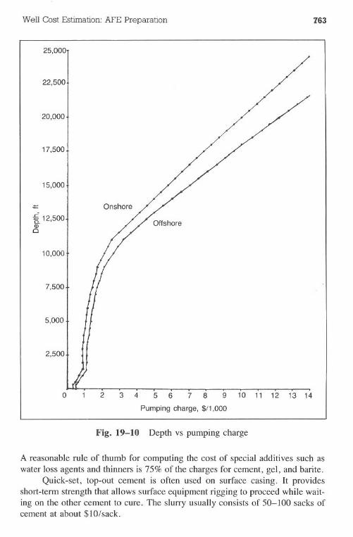
Well Cost Estimation:AFE Preparation
25,000
22,500
20,000
17,500
15,000
.:I::
'E. 12,500CDo
10,000
7,500
5,000
2,500
763
o 2 3 4 7 8 9 10 11 12 13 145 6
Pumping charge, $/1,000
Fig. 19-10 Depth vs pumping charge
A reasonable rule of thumb for computing the cost of special additives such aswater loss agents and thinners is 75% of the charges for cement, gel, and barite.
Quick-set, top-out cement is often used on surface casing. It providesshort-term strength that allows surface equipment rigging to proceed while wait-ing on the other cement to cure. The slurry usually consists of 50-lO0 sacks ofcement at about $lO/sack.
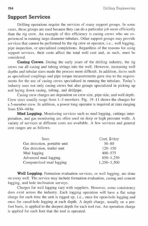
764 Drilling Engineering
SupportServicesDrilling operations require the services of many support groups. In some
cases, these groups are used because they can do a particular job more efficientlythan the rig crew. An example of this efficiency is casing crews who are ex-perienced in running large-diameter tubulars. Other support groups may provideservices that cannot be performed by the rig crew or operator, i.e., well logging,pipe inspection, or specialized completions. Regardless of the reasons for usingsupport services, their costs affect the total well cost and, as such, must beconsidered.
Casing Crews. During the early years of the drilling industry, the rigcrews ran all casing and tubing strings into the well. However, increasing welldepths and tubular sizes made the process more difficult. In addition, items suchas specialized couplings and pipe torque measurements gave rise to the require-ments for the use of casing crews specialized in running the tubulars. Today'sindustry uses not only casing crews but also groups specialized in picking upand laying down casing, tubing, and drillpipe.
Casing crew charges are dependent on crew size, pipe size, and well depth.. Crew sizes usually range from 1-5 members. Fig. 19-11 shows the charges fora 5-member crew. In addition, a power tong operator is required at rates rangingfrom $30-40/hr.
Mud Logging. Monitoring services such as mud logging; cuttings inter-pretation, and gas monitoring are often used on deep or high pressure wells. Avariety of services at different costs are available. A few services and generalcost ranges are as follows:
Item
Gas detection, portable unitGas detection, trailer unitMud loggingAdvanced mud loggingComputerized mud logging
Cost, $/day50-80
120-150400-575850-1,250
1,250-1,500
Wen Logging. Formation evaluation services, or well logging, are doneon every well. The service may include formation evaluation, casing and cementlogging, and hole inclination surveys.
Charges for well logging vary with suppliers. However, some consistencydoes exist across the industry. Each logging operation will have a flat setupcharge for each time the unit is rigged up, i.e., once for open-hole logging andonce for cased-hole logging at each depth. A depth charge, usually on a per-foot basis, is applied to the deepest depth for each tool run. An operation chargeis applied for each foot that the tool is operated.
Well Cost Estimation: AFE Preparation 765
13%"
5 10 15 20 25 30
depth (1,000 It)
Fig. 19-11 Casing crew costs for various depths and pipe sizes
Estimation of the logging cost requires that a well logging program beestablished. A typical program may be as follows:
Item Use
Each open-hole section, except sur-face, run over entire hole section
Each open-hole section
Minimum OperatingFootage
2,000ISF
Sonic-BHC 2,000
Q)U
5c:coE.n
.E 40-0q
31i)0()
2
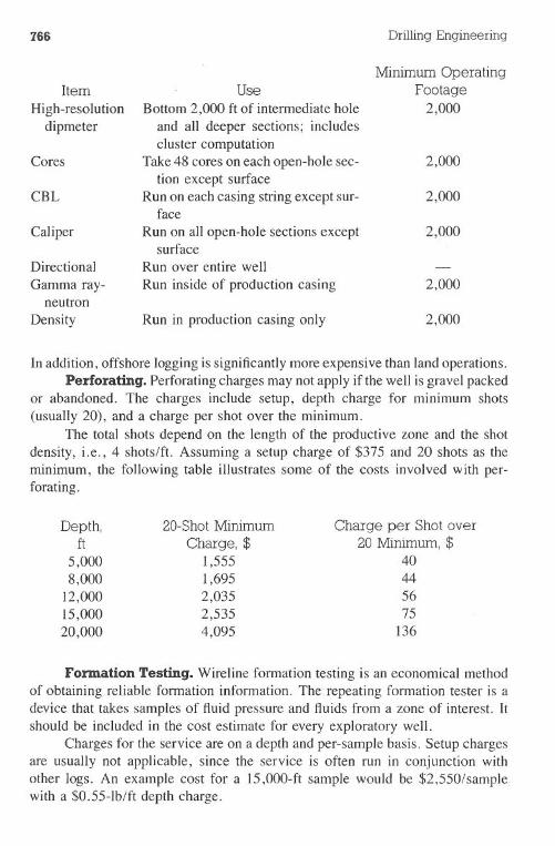
766
Item
High-resolutiondipmeter
Cores
CBL
Caliper
Directional
Gamma ray-neutron
Density
UseBottom 2,000 ft of intermediate hole
and all deeper sections; includescluster computation
Take 48 cores on each open-hole sec-tion except surface
Run on each casing string except sur-face
Run on all open-hole sections exceptsurface
Run over entire well
Run inside of production casing
Run in production casing only
DrillingEngineering
MinimumOperatingFootage
2,000
2,000
2,000
2,000
2,000
2,000
Inaddition, offshore logging is significantly more expensive than land operations.Perforating. Perforating charges may not apply if the well is gravel packed
or abandoned. The charges include setup, depth charge for minimum shots(usually 20), and a charge per shot over the minimum.
The total shots depend on the length of the productive zone and the shotdensity, i.e., 4 shots/ft. Assuming a setup charge of $375 and 20 shots as theminimum, the following table illustrates some of the costs involved with per-forating.
Depth,ft
5,0008,000
12,00015,00020,000
20-Shot MinimumCharge, $
1,5551,6952,0352,5354,095
Charge per Shot over20 Minimum, $
40445675
136
Fonnation Testing. Wireline formation testing is an economical methodof obtaining reliable formation information. The repeating formation tester is adevice that takes samples of fluid pressure and fluids from a zone of interest. Itshould be included in the cost estimate for every exploratory well.
Charges for the service are on a depth and per-sample basis. Setup chargesare usually not applicable, since the service is often run in conjunction withother logs. An example cost for a IS,OOO-ftsample would be $2,550/samplewith a $0.55-lb/ft depth charge.
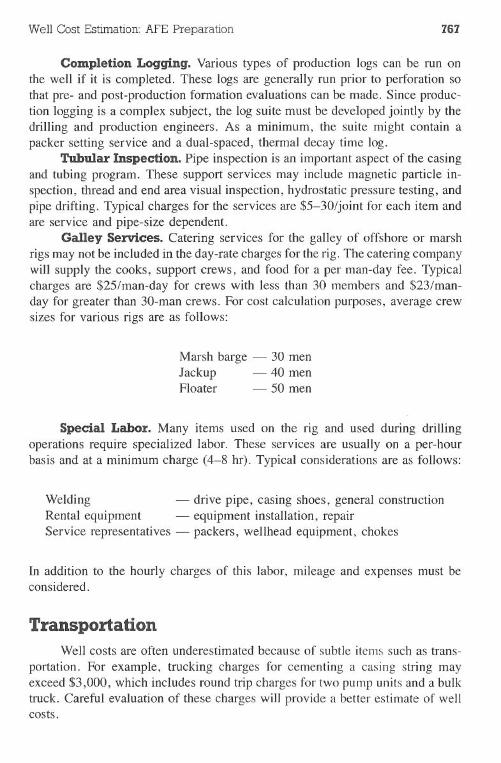
Well Cost Estimation: AFE Preparation 767
Completion Logging. Various types of production logs can be run onthe well if it is completed. These logs are generally run prior to perforation sothat pre- and post-production formation evaluations can be made. Since produc-tion logging is a complex subject, the log suite must be developed jointly by thedrilling and production engineers. As a minimum, the suite might contain apacker setting service and a dual-spaced, thermal decay time log.
Tubular Inspection. Pipe inspection is an important aspect of the casingand tubing program. These support services may include magnetic particle in-spection, thread and end area visual inspection, hydrostatic pressure testing, andpipe drifting. Typical charges for the services are $5-30/joint for each item andare service and pipe-size dependent.
Galley Services. Catering services for the galley of offshore or marshrigs may not be included in the day-rate charges for the rig. The catering companywill supply the cooks, support crews, and food for a per man-day fee. Typicalcharges are $25/man-day for crews with less than 30 members and $23/man-day for greater than 30-man crews. For cost calculation purposes, average crewsizes for various rigs are as follows:
Marshbarge - 30 menJackup - 40 menFloater - 50 men
Special Labor. Many items used on the rig and used during drillingoperations require specialized labor. These services are usually on a per-hourbasis and at a minimum charge (4-8 hr). Typical considerations are as follows:
Welding - drive pipe, casing shoes, general constructionRentalequipment - equipmentinstallation,repairServicerepresentatives- packers,wellheadequipment,chokes
In addition to the hourly charges of this labor, mileage and expenses must beconsidered.
TransportationWell costs are often underestimated because of subtle items such as trans-
portation. For example, trucking charges for cementing a casing string mayexceed $3,000, which includes round trip charges for two pump units and a bulktruck. Careful evaluation of these charges will provide a better estimate of wellcosts.
768 Drilling Engineering
Transportation can include charges for land-based trucks, barges, boats,and helicopters. Long-distance crew charges via commercial or chartered air-planes may be a significantcost. Accurate estimates of transportation costs requirea detailed well plan, knowledge of the distance to the rig from local stock points,and rig characteristics such as standard equipment and crew size.
Trucking charges are computed from estimates of the number of trips, theround-trip mileage, and the per-mile cost. Current trucking costs (1982) areapproximately $3.00/mile. A rule of thumb for round-trip mileage is to establisha base of 100 miles from the local stock point to the rig (round trip, 200 miles).The following table gives some guidelines for estimating the number of round
. trips to be considered on a well:
ItemCementingLoggingCasingMud
Packer fluid
Gravel pack
Trips3/jobIIjob10/stringI (minimum)
25
Remarks
Two pump units, bulk truck
Casing, casing crews, welders, rental itemsAdd I trip per Ib/gal of mud weight above9.0 Ib/gal, i.e., 7 trips for 15.0-lb/gal mud
Optional
Marine charges are incurred for offshore operations and marshes. The costsinclude boats and any dock facilities. Current (1982) charges for boats operatingin the Gulf of Mexico are summarized as follows:
Type of Boat100-ft crew boatSmall supply boatLarge supply boat70-ft standby boat
Cost per day (including fuel), $1,5003,3105,120
800
Air charges occur only for offshore operations. The helicopter charges areon a day-rate basis and begin at rig move-in. A small helicopter (3-4 passengercapacity) is required for day-to-day operations. A large helicopter is used forweekly crew changes. A summary of the costs (1982) are as follows:
HelicopterCapacity
4II
Base DayRate, $
5002,475
Flight Charge,$/hr147450
Average Time2 hr/day5 hr/wk
Well Cost Estimation: APE Preparation 769
Supervision and AdministrationProject management costs must be considered. These charges include well
supervision and administration. Large costs can be incurred for deep wells orproblem wells, such as H2S incidences.
Supervision includes direct management of the well, including the on-sitesupervisor and any members of the office staff who are dedicated to the project.Mud or completion consultants may be considered as supervision. Specializedpersonnel such as mud loggers are not considered in the supervisory charges.
Administration charges can be handled in several manners. Some com-panies prefer to apply only direct supervision charges to a given well and chargesupport office staff members to general company overhead. Other companiesdivide all overhead charges among the wells to be drilled in a fiscal year.Regardless of the accounting method, some of the charges that must be consideredare as follows:
.staff engineering support·clerical support· office overhead· special insurance, including blowout insurance, and bonds· legal work.special document preparation
A method for computing supervision and administration costs is to assumethat a consultant will handle all operations. The on-site supervisor is the drillingconsultant. An office consultant performs all administrative functions on anhourly basis, i.e., 200 hr for a dry hole and 300 hr for a completed well.
Tubulars
Casing and tubing costs are significant factors in the well cost. In somecases, they may account for 50-60% of the total expenditures. The costs aredependent on well depth, size, grade requirements, and couplings.
Pipe costs are influenced heavily by several factors. Pipe size is a majorconsideration. Fig. 19-12 illustrates cost variations according to pipe size forN-80 grade LTC pipe that exceeds a burst rating of 5,000 psi in several sizes.Although engineering considerations should have the major impact on the pipesize selection, cost considerations should have some influence.
Costs increase with higher pipe grades. The following items show the costsfor 40.0-lb/ft, 9.625-in. pipe with LTC couplings:
GradeK-55N-80
Cost per Foot, $20.8631.83
770
GradeC-75S-95
Drilling Engineering
Cost per Foot, $36.5635.26
As in the case of pipe sizes, however, pipe grade selection is an engineeringdecision. ..
gQ)
.~ 10Q)Co
c:
20
18
16
14
12
8
6
4
2
o 10 30 40
Price ($/Ft.)
50 706020
Fig. 19-12 Pipe size vs costlft (N-80 pipe with burst greater than 5,000 psi)
Well Cost Estimation:AFE Preparation 771
Couplings are seldom selected as a result of costs. However, higher-pricepremium couplings may allow the use of smaller pipe sizes, which will reducethe overall well costs. The following list illustrates the variations in pipe costwith different couplings. All costs are with 7.625-in., N-80-grade, 26.40-lb/ftpipe (costs may vary slightly with different vendors and market conditions):
Coupling TypeLTCBTCSFJFJ-PTSFL-4S
Pipe Costs,$/ft21.2622.7734.3134.3136.6532.76
Casing Equipment. Casing (or cementing) accessory equipment is usedto accomplish an effective primary cement job. Although the equipment doesnot have a major impact on well costs, it should be considered. A typical suiteof equipment might be as follows:
Float shoeFloat collarCentralizersScratchersLiner hanger
Casing11
3010o
Liner11
20101
This equipment would cost approximately $2,470 for a 7%-in. casing string and$25,610 for a 7%-in. liner.
Drive pipe costs must be calculated for wells that utilize the pipe. Thecharges vary for pipe size and wall thickness. A drive shoe cost must be included.Typical drive pipe, size, and costs are as follows:
Size, Wall Thickness, Pipe Cost, Shoe Cost,m. m. $/ft $14 0.375 19.54 16516 0.375 22.53 20020 0.500 37.49 23024 0.500 43.92 37526 0.500 47.66 41530 0.500 55.14 47036 0.750 98.82 535
772 Drilling Engineering
Wellhead EquipmentThe wellhead equipment is attached to the casing string for pressure and
stability support. Its cost is dependent on the number and size of the casing andtubing strings, pressure requirements, equipment components, and special fea-tures such as H2Sstainless duty. Total equipment costs can range from $2,500for a low pressure set of equipment to $350,000 for high pressure, stainless steelwellhead equipment and a tree. Subsea completions are even more expensive.
The wellhead equipment consists of the casinghead, intermediate and tub-ing spools, and the production tree. The casinghead is attached to the surfacecasing and will ultimately support all casing loads. Intermediate or productioncasing is hung inside the casinghead. The intermediate spool supports the pro-duction casing if an intermediate string is run. The tubing spool is run only ifthe well is completed. It is set on the casinghead or intermediate spool. The treecontains the production valves and chokes used for producing the oil or gas.
Completion EquipmentThe completion equipment consists of downhole tools related to the tubing
string. These items include packers, seal assemblies, flow couplings, blast joints,and landing nipples. They are dependent primarily on tubing size and fluidcontent.
Packers. The packer is designed to divert formation fluids with the pro-duction tubing. It is selected according to production casing size, bore sizerequirements, tensile loading, and seal assembly type. In addition, H2S ser-viceable packers contain rubber seals that are approximately 100 times morecostly than the standard rubbers.
Blast Joints. Blast joints are thick-walled tubulars placed in the tubingstring opposite the perforations to minimize the damage from erosion by theproduced fluids. Their cost is dependent on tubing size and number of joints.
Seal Assembly. The seal assembly is an important part of the completionequipment. The cost is affected by the required number of seal units, the con-nection type, and the pipe size.
Mid-1982 prices were used throughout the text. The Energy InformationAdministration provides annual drilling cost and inflation figures. The readermay use them to update costs given here. In addition, the APIIIPAA JointAssociation Survey on Drilling Costs can provide well cost data in various areasand depths.
Questions
19.1 What methods are commonly used for considering overhead costs inan AFE for an individual well? What are the weaknesses of eachapproach?
Well Cost Estimation:AFE Preparation
19.419.5
19.6
773
19.2 Refer to Figs. 19-7 and 19-8 and calculate the costs to build andmaintain a 15.0-lb/gal lignosulfonate mud for 60 days. Compare itwith an oil mud. Assume a 750-bbl system.What are the cement pumping charges for a 15,000-ft well onshoreand offshore?Determine the cost to run 15,000 ft of 6-in. pipe.A 60-ft sand zone will be perforated with 4 shots/ft. If the zone is at20,000 ft, what will be the perforating charge?Why is a 20,000-ft high pressure well more expensive than a normalpressure well at the same depth?
19.3
References
Indexes and Estimates of Domestic Well Drilling Costs, 1981 and 1982.Energy Information Administration, U.S. Department of Energy, Wash-ington, D.C.
American Petroleum Institute. Joint Association Survey on Drilling Costs.Washington, D.C.
Appendix .ACase Study(Homework
Problem)
This case study has been prepared to exercise the engineer's understandingof drilling and well planning procedures. The offset well data were selected soseveral possible design alternatives exist. Prepare a complete well plan from theinformation in this problem. Items that should be included in the report are asfollows:
· depth vs days projections (plot). pore pressure vs fracture gradient plot· mud weight plot· casing and tubing design.mud program·cement program·rig selection guidelines
The rig selection data should include minimum prime mover horsepower, derrickcapacity requirements, and blowout preventer rating selection. Define any as-sumptions made during the selection process.
WeD Design ProblemThe enclosed information should provide sufficient details to prepare a
well plan for a prospect. The items included for your inspection are as follows:
.geological summary· offset bit records
The author is willing and prepared to review and discuss this case study with interested groups or engineers.Written inquiries can be made at the address given in the preface of this book or by calling the author in Houston.Texas.
774
Appendix 775
.log resistivity data· rig specification data
Design a well plan for the prospect. Use the following wellbore and casinggeometries if possible.
Hole, in.17.512.258.5
No LinerCasing, in.
13.3759.6255.5I
2.875
Required LinerHole, in. Casing, in.
17.5 13.37512.25 9.6258.5 7.06.0 5.0
2.875
The well is to be a single completion with 2.875-in. tubing.
Geological SummaryThe geologists have concluded that the prospect well will be similar in
many respects to the E.B. White #1 well. The offset White well was drilled in1975 and duaiIy completed at 13,900 and 16,000 ft, respectively. At the timeof completion, the pressures in these two zones were 9,251 and 12,896 psi,respectively. The 13,900-ft zone was plugged in 1980 as a result of pressuredepletion to 5,336 psi and significant water cutting.
The 16,000-ft zone is still producing at near-completion pressure. It isconcluded that this zone is experiencing a strong water drive.
Completion Data. The two zones in the E.B. White # I produced ap-proximately 6 MMcfd and 8.5 MMcfd, respectively, at the time of completion.Production from the upper zone had declined to 1.1 MMcfd prior to water cuttingin 1980. Current production rate from the lower zone is 7.8 MMcfd.
The produced fluids were very dry gases with little produced condensateor water. No carbon dioxide was present. The hydrogen sulfide content was lessthan 1% (approximately 4,000 ppm).
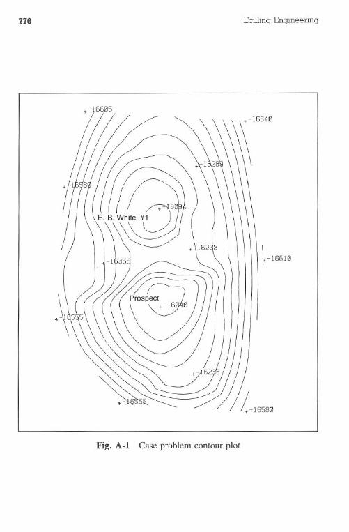
776 Drilling Engineering
~-16610
Fig. A-I Case problem contour plot
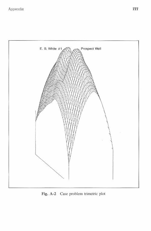
Appendix 777
Prospect Well
Fig. A-2 Case problem trimetric plot
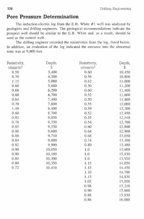
778 DrillingEngineering
Pore Pressure DeterminationThe induction-electric log from the E.B. White # I wen was analyzed by
. geologistsand drillingengineers.The geologicalrecommendationsindicatetheprospect well should be similar to the E.B. White and, as a result, should beused as the control well.
The drilling engineer recorded the resistivities from the log, listed below.In addition, an evaluation of the log indicated the entrance into the abnormalzone was at 9,800 feet.
Resistivity, Depth, Resistivity, Depth,ohms/m2 ft ohms/m2 ft
0.58 3,400 0.60 10,4500.70 4,200 0.56 10,8001.15 5,000 0.62 I 1,0000.60 5,600 0.50 I 1,2000.68 6,200 0.60 II ,4000.60 6,700 0.52 11,6000.64 7,400 0.50 11,8000.70 7,800 0.55 12,0001.40 8,400 0.59 12,2000.60 8,700 0.52 12,4500.82 9,050 0.55 12,5100.78 9,350 0.54 12,7000.85 9,550 0.60 12,8000.80 9,600 0.64 12,9000.88 9,710 0.68 13,0500.84 9,800 0.74 13,3000.92 9,900 0.80 13,4800.90 10,050 1.0 13,6000.90 10,180 1.0 13,8300.84 10,300 1.0 13,9200.80 10,350 1.15 14,0500.72 10,410 1.15 14,450
1.10 14,7001.15 14,8301.05 15,0200.98 15,2100.90 15,6000.88 15,8300.86 16,000
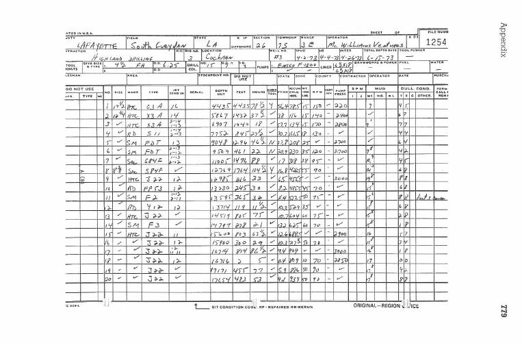
~'0<D::3Q.
~.100:I0..:1<
I)
..TE
OI"
U.'.A
.SH
I:I:T0.
rILIE
N.,,,,.
"''''TY
"S--...H.
(.ve-VJ-tN
rUT
<L
A-
x"
I:rIEC
TIO
...
TO
W...'"I..
RA
"'GI:
r"I:RA
TO
Rx
"II1254
LA
F.A
,J.__O
,.,.....OR
I:,17
S"
Jt:1'1e..I1I.L
L,,,..,s
Ve...fv_.s
"TR
AnO
RfI'#J
LA
N],
'AblJl
AJL
r111rl:N
D_IL
C:;O
NrL
LN
O.
I:O,
,?r:TI:II
1rOT
AI,O
I:PT"O
AT
I:TO
O LP"'"C
II
113-'72
'I-/{-71'f'd.(.-73
t-,,-"73
IGIV
CSIZ
I:<
j?1"11
1°.0.t.)<10R
ILL
INO
.,,.r'''J'''
I..Dl.uM
"I..
<=
_<(;0P
'I:?"DO
.AW
WO
.'..'DW
"'u..
TW
A:R
TO
OL
...T
Y..I:I.
LIN
ER
'._
K)IN
TS
1.0.0.
CO
L.
Ih."--
,r.-
I,I:'''AN
AR
CA
IToett..O
'HT
NO
.D
Ou.?T
IST
AnIZ
ON
I:rO
UN
TY
r:O...T
RA
CT
OIIO
"I:RA
TO
IIO
AT
I:
'UItC
...
DO
N01"
USE
'STD
I"TH
I,L
.'A
'..u....
'PMM
UD
DU
LL
.C
ON
Do
rOIlM
ND
.'IZ
I:M
AK
I:T
YPC
U"'O
I'".I:R
IAL
OU
Trl:I:T
HO
UA
'"T
HII
.-...
..C
AL
LI
A"R
.T
Y'E
""N
R<
,os."A
.I:"..
WT
.VIS.
W.L
.T
.G
OT
HIE
"."EIIU
I7
IIhrp4
,I",,,,r-
J{<{J
7f?'f
<;(-
71'<; 1\
1)1>
--;lo
,'k
11"If"
II'lL
X<
A1'1
,1'71'13'
37i,/
1KII"
I')1"10
-V
o../
J./'
u..,..Y
7.4
:1901
IF./
7.1J?'
-'»'001
I7
Ib'-(
"1'70
14V
-I",b
.s/1
I-'5
').;171$-
./:la7
"','J'
I.U-
.....,/
't'f
{".....
:M1'=
,\rJ
3IqOy
J'1)..11. '/(.
NH
bo>'::1<
.....-
700,/
....
,v
s1=
br;::
9S-0"6
1J.;J..
N;W
,? bD?S'IJ.O
-;"700
t«[).
7.....
kn_U
L/,c
'::IlJO
O--
1'/91.IJ!'A'or
/7IfiR
?9.,
-v
,''{
>11'1
I'LP
....FV
Id-I''I
17'"ID
'I'I.. V/L
I}'f
""'10
VIi-
,I<>
9V
-11m
..-:r
:I.I)-
..'PI:>
I'3.3
V:c'
'lrt:---
....--
.JOD
cJr
f!C
D14
....liD
<=
p.JI)..
P).30;)./1)
.)0,/
,.I'IP>
: 'r'70
.......if
"
1/V
/=,).
,-,,<
)"9)3,r-
<,/
1I<iIn?
'11-.-
vr'
AuJ.
-I
.:>..
-'11.'1\
yI;"
I':>'
I371<
1/1
'1,,
./lo
r-rV
..v
,!'y
,0.
P./
Ill."........
./14")"/q
,.f'7J
y'0'1
'07\--
.........
f:I.
0
I../
5/11
£=3
./'"174"1
;).72.;../
.....'..J,<
;"'"
70v
.,J1
P-
II-'
1hz..,.:..ri-
"(.
&)D
,.&
3....In."
'R.I?! 0/
V-
bqooI
r7
i../
V-
:1;).
/')-1)9.0
1<
.0do'!'
./Ik>
,7t7"
,V
,/17"-
h..
V:T
>-:>
..,'.
'liI
Jill'! wt,.
./19,'1
'.1;v
v-
11000I,r
1f
f-
0/;r...
(.7/(.. ::.r
...b,ll!t9
/0-
"J./<:7.
,7,").-
70O
D
I,qv
:1.....
/.,(7i11,1,)
1-77-'
q??,
'0-
.......,
It..
7..-
....J
.....-/"">
','-1,{V
1,.3"./'19.1
2?9-
,./,r
I11
c108-"
IUt
fliTl"nN
nlTlnN
l"nW_
AP.
APA
IAI[D
RA
.Rf:R
Uh
OR
IGIN
AL-R
EG
ION
;:h!ICE
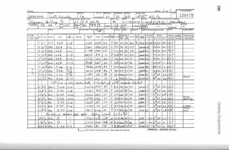
780D
rillingE
ngineering
Appendix 781
Drillstring DesignA contract has been prepared with a drilling contractor for the prospect
well. The operator and contractor believe the 800 ft of collars on the rig will besufficient to achieve the desired available bit weight. Will the drillstring providedby the operator be sufficient to drill the well? Select the appropriate combinationsof pipe and collars.Contractor-furnished pipe:
Drill collars: 800 ft, 7-in. OD x 3-in. ID800 ft, 5-in. OD x 2-in. ID
Drillpipe: 8,000 ft, 3Y2-in., 13.3 IblftGrade E
16,000 ft, 41/2in., 20.0 IblftGrade X
Drilling data (required to design the pipe):Rotary horsepower = 150Max. rotary speed = 120Maximum expected dogleg severity = 3.0°/100 ftMinimum section length = 2,000 ft
Considerations
1. Most operators and contractors will not use pipe grades greater than X-95 if H2S will be encountered.
2. A tapered string must be used if a liner is run.3. If the decision is made that the contractors' pipe is not satisfactory, what
type of string must be rented (weight, grade)?
Appendix B Brine FluidTables
These brine fluid formulation tables are provided through the courtesy ofNL Baroid. Chapter 8 requires data contained in these tables.
782
Table B-1 Composition of one barrel of potassiumchloride brine
Brine Density Pressure To Make 1bbl (42 gal)at 6O'F Gradient Water 100% KCI Freezing
Ib/gal Ib/ft' psl/ft bbl Ib Point, of8.4 62.8 .437 .995 4 +318.5 63.6 .442 .986 11.6 298.6 64.3 .447 .976 18.9 288.7 65.1 .452 .969 26.1 268.8 65.8 .457 .960 33.4 258.9 66.6 .463 .950 40.7 239.0 67.3 .468 .943 47.9 229.1 68.1 .473 .933 55.2 209.2 68.8 .478 .924 62.4 189.3 69.6 .483 .917 69.7 169.4 70.3 .489 .907 76.9 149.5 71.1 .494 .898 84.2 189.6 71.8 .499 .890 91.5 409.7 72.6 .504 .881 98.7 60
Table B-2 Composition of one barrel of sodium chloride!calcium chloride brine
Brine Density Preaaure To Make 1bbl (42 gel)at 6O'F Gradient Water 100% NaCI 94-97% CeCl,' Crystallization
Ib/gel Ib1ft> pal 1ft bbl Ib Ib Point, of
10.1 75.6 .525 .887 88 29 -4
10.2 76.3 .530 .881 70 52 -10
10.3 77.1 .535 .875 54 72 -15
10.4 77.8 .541 .876 41 89 -21
10.5 78.6 .546 .871 32 104 -26
10.6 79.3 .551 .868 25 116 -32
10.7 80.0 .556 .866 20 126 -38
10.8 80.8 .561 .864 16 135 -42
10.9 81.5 .567 .862 13 144 -24
11.0 82.3 .572 .859 10 151 -12
11.1 83.0 .577 .854 8 159 0
. Maximum 1% water
Table B-3 Composition of one barrel of calcium chloridebrine
Brine Denalty Preaaure To Make 1bbl (42 gal)at 60°F Gradient Weter 94-97% CeCl,' Crystelllzatlon
Ib/gal Ib/tt> pal/tt bbl Ib Point,of
8.4 62.8 .437 .998 3.8 +31
8.5 63.6 .442 .995 9.0 +30
8.6 64.3 .447 .992 14.3 +28
8.7 65.1 .452 .989 19.5 +26
8.8 65.8 .457 .986 24.8 +25
8.9 66.6 .463 .983 30.0 +23
9.0 67.3 .468 .980 35.3 +21
9.1 68.1 .473 .975 41.2 +19
9.2 68.8 .478 .970 47.2 +17
9.3 69.6 .483 .965 .53.2 +15
9.4 70.3 .489 .959 59.1 +12
9.5 71.1 .494 .954 65.1 +9
9.6 71.8 .499 .949 71.1 +6
9.7 72.6 .504 .944 77.0 +3
9.8 7:.'\.3 .509 .940 83.0 0
9.9 74.1 .515 .934 89.0 -4
10.0 74.8 .520 .929 94.9 -8
10.1 75.6 .525 .924 101.0 -13
10.2 76.3 .530 .919 107.0 -18
10.3 77.1 .535 .914 113.0 -23
10.4 77.8 .541 .909 119.0 -29
10.5 78.6 .546 .904 125.0 -36
10.6 79.3 .551 .899 131.0 -43
10.7 80.0 .556 .894 137.0 -51
10.8 80.8 .561 .889 143.0 -59
10.9 81.5 .567 .884 149.0 -40
11.0 82.3 .572 .879 155.0 -22
11.1 83.0 .577 .873 161.0 -11
11.2 83.8 .582 .866 167.0 0
11.3 84.6 .587 .860 174.0 +13
11.4 85.3 .593 .854 180.0 +27
11.5 86.0 .598 .848 186.0 +35
11R ARA M 842 193.0 +44
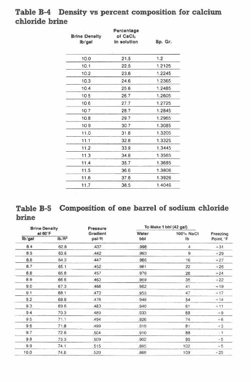
Table B-4 Density vs percent composition for calciumchloride brine
PercentageBrine Density of CICI,
Iblgll In solullon Sp. Gr.
10.0 21.5 1.2
10.1 22.5 1.2125
10.2 23.6 1.2245
10.3 24.6 1.2365
10.4 25.6 1.2485
10.5 26.7 1.2605
10.6 27.7 1.2725
10.7 28.7 1.2845
10.8 29.7 1.2965
10.9 30.7 1.3085
11.0 31.8 1.3205
11.1 32.8 1.3325
11.2 33.9 1.3445
11.3 34.8 1.3565
11.4 35.7 1.3685
11.5 36.6 1.3806
11.6 37.6 1.3926
11.7 38.5 1.4046
Table B-5 Composition of one barrel of sodium chloridebrine
Brine Density Pressure To Make 1 bbl (42 gal)at GOoF Gradient Water 100% NaCI Freezing
Ib/gal Ib/ft' psi 1ft bbl Ib Point, OF
8.4 62.8 .437 .998 4 +318.5 63.6 .442 .993 9 +298.6 64.3 .447 .986 16 +278.7 65.1 .452 .981 22 +268.8 65.8 .457 .976 28 +248.9 66.6 .463 .969 35 +229.0 67.3 .468 .962 41 +199.1 68.1 .473 .955 47 +179.2 68.8 .478 .948 54 +149.3 69.6 .483 .940 61 +119.4 70.3 .489 .933 68 +99.5 71.1 .494 .926 74 +69.6 71.6 .499 .919 81 +39.7 72.6 .504 .910 68 -19.8 73.3 .509 .902 95 -59.9 74.1 .515 .895 102 +5
10.0 74.8 .520 .888 109 +25
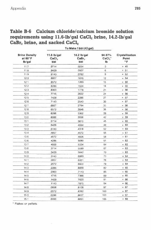
Appendix 785
Table 8-6 Calcium chloridel calcium bromide solutionrequirements using 11.6-lb/gal CaClz brine, 14.2-lb/galCaBrz brine, and sacked CaClz
To Make 1 bbl(42gal)
Brine Denllty 11.6 Ib/gal 14.2 Ib/gal 94-97% Cryltalllzalionat 60° F CaCI, CaBr, CaCI" Point
Ib/gal bbl bbl Ib of
11.7 .9714 .0254 '3 .. 45
11.8 .9429 .0507 6 .. 51
11.9 .9143 .0762 9 .. 52
12.0 .8857 .1016 12 .. 54
12.1 .8572 .1269 15 .. 55
12.2 .8286 .1524 18 .. 55
12.3 .8000 1778 21 .. 56
124 .7715 .2032 24 .. 56
12.5 .7429 .2286 27 .. 57
12.6 .7143 .2540 30 .. 57
12.7 .6857 .2794 33 .. 58
12.8 .6572 .3048 36 .. 58
12.9 .6286 .3302 39 .. 59
13.0 .6000 .3556 42 .. 59
13.1 .5714 3810 45 .. 60
13.2 .5429 .4064 48 .. 60
13.3 .5143 .4318 52 .. 60
13.4 .4857 .4572 55 .. 61
13.5 .4572 .4826 58 .. 61
13.6 .4286 .5080 61 .. 62
13.7 .4000 .5334 64 .. 62
138 .3714 .5589 67 .. 63
13.9 .3429 .5842 70 .. 63
14.0 .3143 .6069 73 .. 64
141 .2857 .6351 76 .. 64
14.2 .2572 .6604 79 ..64
14.3 .2286 .6858 82 .. 65
14.4 .2000 .7113 85 .. 65
14.5 .1715 .7366 89 .. 65
14.6 .1429 .7620 91 "66
14.7 .1143 .7875 94 .. 66
14.8 .0858 .8128 97 .. 67
14.9 .0572 .8382 100 .. 67
15.0 .0286 .8637 103 .. 67
15.1 .0000 .8891 106 "68
. Flakes or pellets
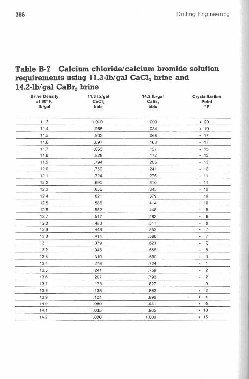
786 Drilling Engineering
Table B-7 Calcium chloride/calcium bromide solutionrequirements using 11.3-1b/ gal CaClz brine and14.2-Ib/gal CaBrz brine
Brine Density 11.3lb/gel 14.2 Ib/gel Cry.talllzatlonet 50°F, CaCI, CaBr, PointIb/gel bbl. bbls of
-11.3 1.000 .000 + 20
11.4 .965 .034 + 19
11.5 .932 .068 + 17
11.6 .897 .103 + 17
11.7 .863 .137 + 15
11.8 .828 .172 . 1311.9 .794 .206 . 1312.0 .759 .241 . 12121 .724 .276 . 1112.2 .690 .310 . 1112.3 .655 .345 . 10
12.4 .621 .379 . 10
12.5 .586 .414 . 10
12.6 .552 .448 . 912.7 .517 .483 812.8 .483 .517 . 812.9 .448 .552 . 713.0 .414 586 . 713.1 .379 .621 . 7,13.2 .345 .655 . 513.3 .310 .690 . 3
13.4 .276 .724 113.5 .241 .759 213.6 .207 .793 2
13.7 .173 .827 0
13.8 .138 .862 + 2
13.9 .104 .896 + 414.0 .069 .931 + 614.1 .035 .965 + 10
14.2 .000 1.000 + 15
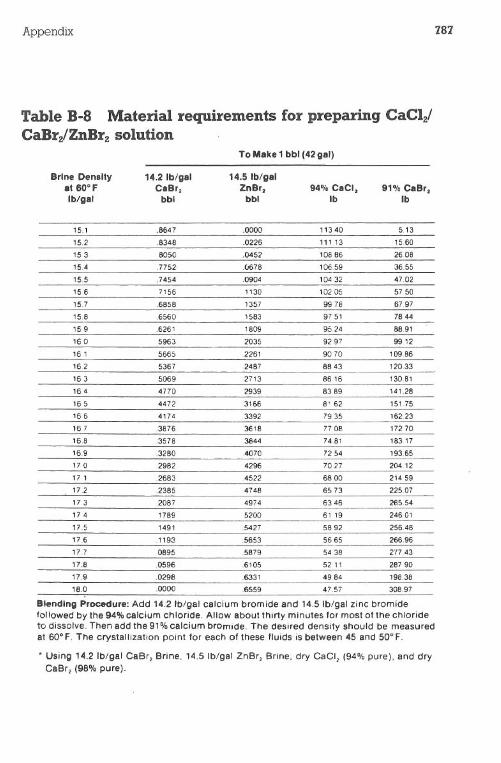
Appendix 787
Table B-8 Material requirements for preparing CaClzICaBrzlZnBrzsolution .
To Make 1 bbl (42gBI)
. Using 14.2 Ib/gal CaBr, Brine. 14.5 Ib/gal ZnBr, Brine. dry CaCI, (94% pure). and dryCaBr, (98% pure).
Brine Density 14.2 Ib/gal 14.5 Ib/ga'at 60° F CaBr, ZnBr, 94% CaC', 91% CaBr,Ib/gal bbl bbl Ib Ib
15.1 .8647 .0000 11340 5.13
15.2 .8348 .0226 11113 15.60
15.3 .8050 .0452 108.86 26.08
15.4 .7752 .0678 106.59 36.55
15.5 .7454 .0904 104.32 47.02
15.6 7156 1130 10205 57.50
15.7 .6858 1357 9978 67.97
15.8 .6560 1583 9751 78.44
159 .6261 1809 95.24 88.91
16.0 5963 2035 9297 99.12
161 5665 .2261 90 70 109.86
16.2 5367 .2487 8843 12033
163 .5069 .2713 8616 130.81
164 .4770 2939 8389 141.28
16.5 4472 3166 8' 62 151.75
166 4174 .3392 7935 162.23
167 .3876 3618 77.08 172 70
16.8 .3578 .3844 74.81 18317
16.9 .3280 .4070 7254 193.65
17.0 .2982 4296 70.27 204.12
171 .2683 .4522 6800 214.59
17.2 .2385 .4748 6573 225.Q7
173 .2087 4974 6346 265.54
174 .1789 5200 6119 246.01
17.5 .1491 .5427 5892 256.48
17.6 .1193 .5653 5665 266.96
17.7 .0895 .5879 54.38 277.43
17.8 .0596 .6105 5211 287.90
17.9 .0298 .6331 4984 198.3818.0 .0000 .6559 47.57 308.97
Blending Procedure: Add 14.2 Iblgal calcium bromide and 14.5 Iblgal zinc bromidefollowed by the 94% calcium chloride. Allow Bboutthirty minutes for most of the chloride
to dissolve. Then add the 91 % calcium bromide. The desired density should be measuredat 50°F. The crystallization point for each of these fluids is between 45 and 50°F.
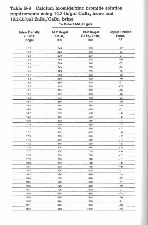
Table B-9 Calcium bromide/zinc bromide solutionrequirements using 14.2-lb/gal CaBrz brine and19.2-lb/gal ZnBrzlCaBrzbrine
To Make 1 bbl (42 gal)
Brine Density 14.2 Ib/gal 19.2 Ib/gal Crystallization
at 60° F CaBr2 CaBr2/ZnBr2 Point,
Ib/gal bbl bbl of
15.0 .840 .160 -22
15.1 .820 .180 -25
15.2 .800 .200 -27
15.3 .780 .220 -29
15.4 .760 .240 -32
15.5 .740 .260 -34
15.6 .720 .280 -35
15.7 .700 .300 -38
15.8 .680 .320 -40
15.9 .660 .340 -37
16.0 .640 .360 -33
16.1 .620 .380 -30
16.2 .600 .400 -26
16.3 .580 .420 -23
16.4 .560 .440 -20
165 .540 .460 -16
16.6 .520 .480 -11
16.7 .500 .500 - 816.8 .480 .520 - 616.9 .460 .540 - 417.0 .440 .560 - 4
17.1 .420 .580 - 2
17.2 .400 .600 0
17.3 .380 .620 2
17.4 .360 .640 4
17.5 .340 .660 5
17.6 .320 680 5
17.7 .300 .700 6
17.8 .280 .720 7
17.9 .260 .740 7
18.0 .240 .760 9
181 .220 .780 10
18.2 .200 .800 11
18.3 .180 .820 13
18.4 .160 .840 15
18.5 .140 .860 17
18.6 .120 .880 19
18.7 .100 .900 21
18.8 .080 .920 23
18.9 .060 .940 20
19.0 .040 .960 +21
19.1 .020 .980 +18
19.2 000 1.000 :"16
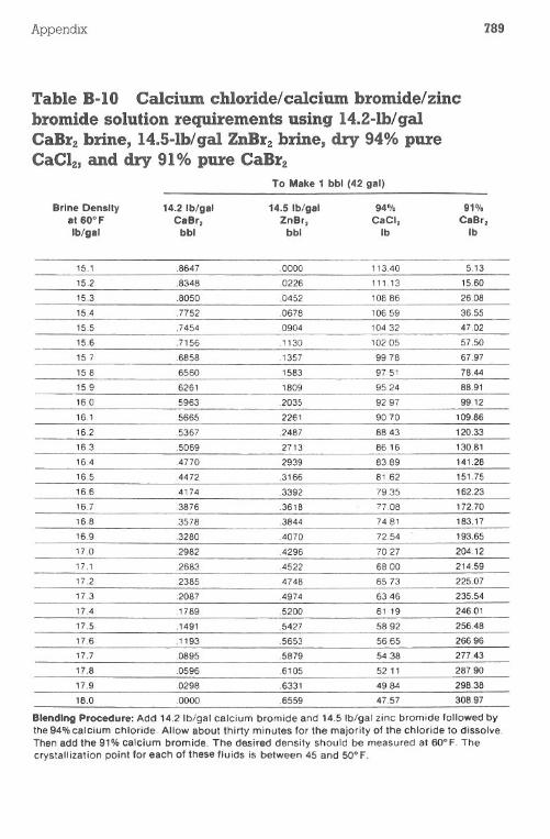
Appendix 789
Table B-I0 Calcium chloride/calcium bromide/zincbromide solution requirements using 14.2-Ib/galCaBrz brine, 14.5-Ib/gal ZnBrz brine, dry 94% pureCaClz, and dry 91% pure CaBrz
To Make 1 bbl (42 gal)
Brine Densityat 60°FIb/gal
14.2 Ib/galCaBr,
bbl
14.5 Ib/galZnBr,
bbl
94%CaCl,
Ib
91%CaBr,
Ib
15.1 .6647 .0000 113.40 5.13
15.2 .6346 .0226 111.13 15.60
15.3 .6050 .0452 106.86 26.08
15.4 .7752 .0676 10659 3655
15.5 .7454 .0904 10432 47.02
15.6 .7156 .1130 102.05 57.50
15.7 .6856 .1357 99.76 67.97
15.6 .6560 .1563 9751 78.44
15.9 6261 1809 95.24 66.91
16.0 .5963 .2035 9297 99.12
16.1 .5665 .2261 9070 109.66
16.2 .5367 .2487 66 43 120.33
16.3 .5069 .2713 66.16 130.61
16.4 .4770 .2939 63.89 141.28
16.5 .4472 .3166 61.62 151.75
16.6 .4174 .3392 79.35 162.23
16.7 .3676 .3616 77.06 172.70
16.6 .3578 .3644 7481 163.17
16.9 .3260 .4070 72.54 193.65
17.0 .2962 .4296 70.27 204.12
17.1 .2683 .4522 68.00 214.59
17.2 .2365 .4748 65.73 225.07
17.3 .2067 .4974 63.46 235.54
17.4 .1789 .5200 61.19 246.01
17.5 .1491 .5427 56.92 256.48
17.6 .1193 .5653 56.65 266.96
17.7 .0695 .5679 54.36 277.43
17.8 .0596 .6105 52.11 267.90
17.9 .0298 .6331 49.84 296.36
16.0 .0000 .6559 47.57 306.97
Blending Procedure: Add 14.21b/gal calcium bromide and 14.51b/gal zinc bromide followed bythe 94% calcium chloride. Allow about thirty minutes for the majority of the chloride to dissolve.Then add the 91% calcium bromide. The desired density should be measured at GO°F. Thecrystallization point for each of these fluids is between 45 and 50° F.
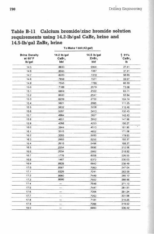
790 Drilling Engineering
Table B-Il Calcium bromide/zinc bromide solutionrequirements using 14.Z-lb/gal CaBrz brine and14.5-lb/gal ZnBrz brine
ToMake1 bbl (42 gal)
.8833
.8565
.8223
.7859
.7555
.7109
.6859
.6530
.6239
.5921
.5632
.5287
.4964
.4651
.4268
.3944
.3515
.3205
.2893
.2610
.2254
.2034
.1776
.1467
.0928
.0587
.0229
.0060
.0000
14.5 .b/ga'ZnBr,
bbl
.0900
.1067
.1318
.1531
.1788
.2079
.2322
.2547
.2722
.2995
.3228
.3413
.3627
.3912
.4233
.4513
4852
.5083
.5250
.5496
.5690
.5862
.6058
.6372
.6842
.7093
.7241
.7449
.7552
.7548
.7447
.7356
.7263
.7181
.7098
.6890
, 91%CaBr,
.b
Brine Denally8' 60.F.b/gal
14.5
14.6
14.7
14.8
14.9
15.0
15.1
15.2
15.3
15.4
15.5
15.6
15.7
15.8
15.9
16.0
16.1
16.2
16.3
16.4
16.5
16.6
16.7
16.8
16.9
17.0
17.1
17.2
17.3
17.4
17.5
17.6
17.7
17.8
17.9
18.0
14.2 'b/ga'CaBr,
bbl
27.41
37.41
58.65
59.67
66.33
73.08
83.71
93.84
104.74
111.25
118.48
132.43
142.43
147.98
156.27
161.95
171.08
179.63
192.37
198.37
212.06
218.92
226.55
230.03
238.49.247.04
263.58
265.12
266.66
271.13
281.51
291.24
301.08
310.25
319.52
336.42
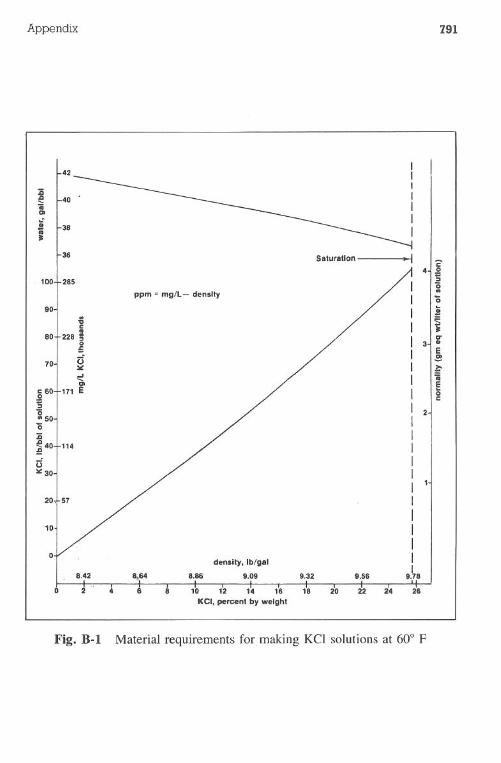
Appendix 791
8.42. -+-:: .o 2 4
Fig. B-1 Material requirements for making KCI solutions at 60° F
i 1-40:::"01.:J!! 1-38".
I36 S8tur8tlon . ,-c
.2'5100+285 I ;;"
ppm =mg/L- density I '0..90-1 I J!!..I...c
80+228! I 3 i0E:: I .!!!70-1 (j I:.:
=::! I ii01
I60t171 E 0c'5;;" 50'0:;;
40+114
(j:':30
density, Ib/g81I
,4 8.86 9.09 9.32 9.56 9.78I , I , I . 1 , 1 , 'I6 8 10 12 14 16 18 20 22 24 26
KCI,percentbyweight
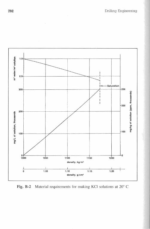
792 Drilling Engineering
Fig. B-2 Material requirements for making KCI solutions at 200 C
j 1.0'S1l...E ,
II
30I-S8tur8tlon
256
I..0
200 !-II "'uu
Ig=..
g
S'0
.01
0
o!!
.01
'0100 E
-'a.E
1050 1100 1150 1200
density, kll/m'
I I I I0 1.05 1.10 1.15 1.20
density, II/em'
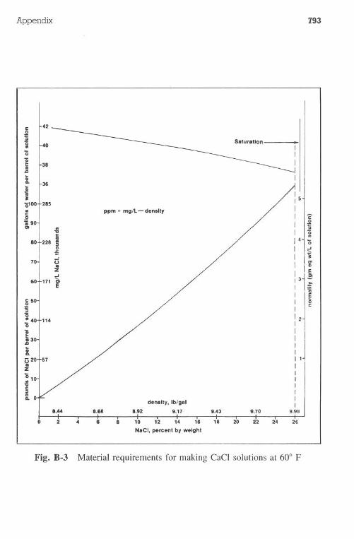
Appendix 793
Fig. B-3 Material requirements for making CaCI solutions at 60° F
c.!!'5
kO ---- Saluratlon'0.'0
1 38....i 36t;
rOr85
ppm: mg/L- densUy
'j';; 90 I.. . =
... I '0c1480+ 228 S
0 I= I 'i70 U
I I.z I E-'60+171 t I 3i;
: jl
50
'5 I C
40 114 I 20 I
130
U...
iu20 57.Z
10...c
[ O.density,Ib/ga'
'.44 8.68 8.92 9.17 9.43 9.70 9.98I I . I , I , I , I , I . I0 2 4 II 8 10 12 14 16 18 20 22 24 26
NaCl, percent by weight
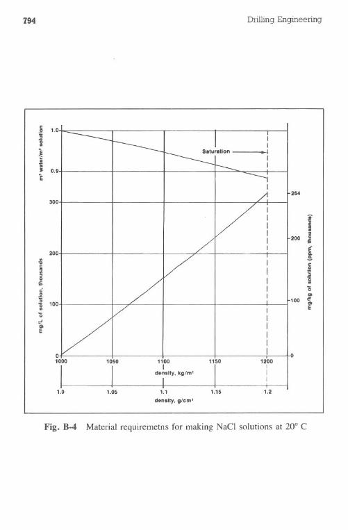
794 Drilling Engineering
1200III
1.0 1.05 1.1
den Illy. II/em'
1.15 1.2
Fig. B-4 Material requiremetns for making NaCI solutions at 200 C
"1.0.!!
;;I!
II
. III I1; I. 0.9E
I264
300I
-;;...":i"
200 0::
200 E. t... I -" j:i I" ;;0:: I 1c I '0.!!;;
I III
'6 100100 <!!!
III. . e'0...'j;,e
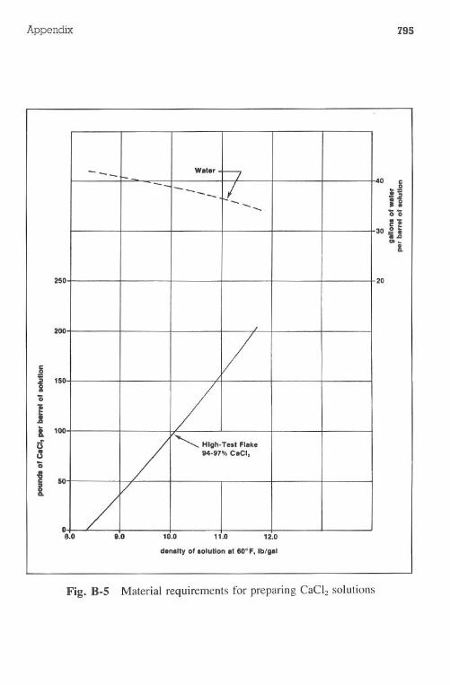
Appendix
fi
i 150'0
Ii 100
d'c3'0
ti
795
250 o
200
50
oB.O t.o 10.0 11.0 12.0
denelty 01 eolutlon el eO.F, Ib/gel
Fig. B-5 Material requirements for preparing CaCl2 solutions
-- WeIer n----L(--
-.......3
;
,
vi/
/Hlgh-Te.t Fleke94-97%CeCl,
V
/. .
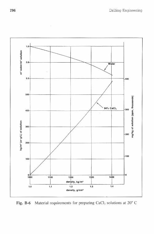
796 Drilling Engineering
1200I
denalt)', kg/m'""'--1.2
denalI)'. glem'
1.0 1.1
Fig. B-6 Material requirements for preparing CaCI2solutions at 20° C
1.0
j51E O.t
j;E
0.8 , . I I I 1"',00
500.....c
Ii0E
400 1 1 1 /1 I 1"'300 .
!c g=.2 ..= 300 1S iiii ..::;
I
200 o!!!C;, rIi- 200
..
I X I I I Loo100
Appendix 797
u..z'0~ 8.58icIIo
8.060 70 80
temperature. 0 F
90 100
Fig. B-7 The effects of temperature change on the density of NaCI or KCIsolutions
C.2:i'0~ 11.0U..
(.)
'0>-i 10.5cIIo
70 80
temperature, of
90 100
Fig. B-8 The effects of temperature change on the density of CaClz solutions
798 DrillingEngineering
11.5
11.060 70 80 90
temperature, 0F100
Fig. B-' The effects of temperature change on the density of CaCI2/CaBr2solutions
Appendix 799
19.0
r-18.5
15.060 70 80 90
temperature, 0 F100
Fig. B-IO The effects of temperature change on the density of CaCI2/CaBr2/ZnBr2 solutions
'ii18.0
:er£ I I I I I I I I I I I I I I.2:i'0":. 17.5Iiic:
Iii17.0
U I I I I I I I I I I I I I I.(J"0
16.5iic:.0
16.0
r-
15.5
Appendix C AFE Worksheets
The APE worksheets are an effective method of accounting for most ex-penditures involved in drilling and completing a well. If an engineer spends thetime required to complete or consider all items in the worksheet, the final resultwill be an accurate cost estimate as well as a more-prepared well plan. Theseworksheets have been carefully developed through years of experience. Somecompanies have modeled cost estimating computer programs from these guide-lines. .
Appendix C contains 3 versions of the APE forms. The General Summaryis a management type of one-page report that contains the II major cost categoriesseparated into tangible and intangible costs.
The AFE worksheets are the work forms initially prepared by the engineer.Each item is subdivided into a detailed form. The subdivisions are modeledaccording to the common methods in which vendors price their services. As anexample, most logging services have separate depth and operation charges.
An AFE detailed summary is also included. The worksheet is summarizedon this form. Typically, a well plan will include the General Summary and theAPE Detailed Summary.
\\...
800
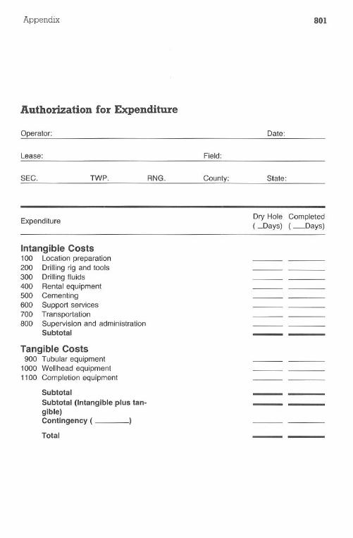
Appendix
Authorization for Expenditure
Operator:
801
Lease: Field:
Date:
SEC. TWP. RNG. County: State:
ExpenditureDry Hole Completed(_Days) (_Days)
Intangible Costs100 Location preparation200 Drilling rig and tools300 Drilling fluids400 Rental equipment500 Cementing600 Support services700 Transportation800 Supervision and administration
Subtotal
Tangible Costs900 Tubularequipment
1000 Wellheadequipment1100 Completionequipment
SubtotalSubtotal (Intangible plus tan-gible)Contingency (
Total
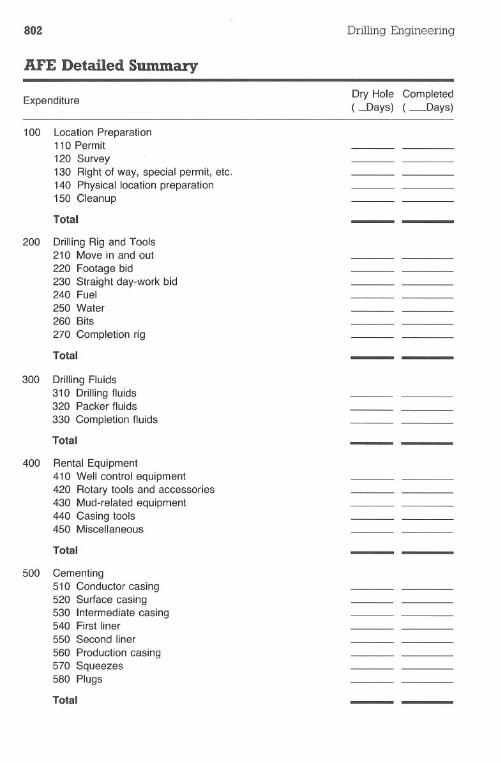
802 Drilling Engineering
ME Detailed Summary
ExpenditureDry Hole Completed(_Days) (_Days)
100 Location Preparation110 Permit120 Survey130 Right of way, special permit, etc.140 Physical location preparation150 Cleanup
Total
200 Drilling Rig and Tools210 Move in and out220 Footage bid230 Straight day-work bid240 Fuel250 Water260 Bits
270 Completion rig
Total
300 Drilling Fluids310 Drilling fluids320 Packer fluids330 Completion fluids
Total
400 Rental Equipment410 Well control equipment420 Rotary tools and accessories430 Mud-related equipment440 Casing tools450 Miscellaneous
Total
500 Cementing510 Conductor casing520 Surface casing530 Intermediate casing540 First liner550 Second liner
560 Production casing570 Squeezes580 Plugs
Total
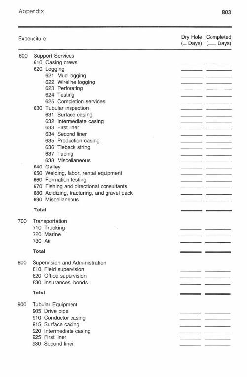
Appendix
Expenditure
803
Dry Hole Completed(_ Days) (_ Days)
600 Support Services610 Casing crews620 Logging
621 Mud logging622 Wireline logging623 Perforating624 Testing625 Completion services
630 Tubular inspection631 Surface casing632 Intermediate casing633 First liner634 Second liner635 Production casing636 Tieback string637 Tubing638 Miscellaneous
640 Galley650 Welding, labor, rental equipment660 Formation testing670 Fishing and directional consultants680 Acidizing, fracturing, and gravel pack690 Miscellaneous
Total
700 Transportation710 Trucking720 Marine730 Air
Total
800 Supervision and Administration810 Field supervision820 Office supervision830 Insurances, bonds
Total
900 Tubular Equipment905 Drive pipe910 Conductor casing915 Surface casing920 Intermediate casing925 First liner930 Second liner
804 Drilling Engineering
ExpenditureDry Hole Completed(_Days) (_Days)
900 Tubular Equipment-conl'd935 Production casing940 Tieback string950 Tubing960 Casing equipment961 Drive pipe962 Conductor casing963 Surface casing964 Intermediate casing965 First liner966 Second liner967 Production casing
Total
1000 Wellhead Equipment1010 Casinghead1020 Intermediate spool1030 Tubing spool1040 Tree1050 Miscellaneous
Total
1100 Completion Equipment1105 Packers1110 Blast joint and landing nipples1115 Special liners1120 Safety joints1125 Subsurface safety devices1130 Seal assembly1135 Lift equipment1140 Gravel packing equipment1145 Miscellaneous
Total
Appendix
ME Worksheet
805
Dry Hole Completed(_ Days) (_ Days)
100 Location110 Permit120 Survey130 Right of way, special permits, damages140 Physical location preparation150 Cleanup and backfill
200 Drilling tools210 Move in and out220 Footage bid
a. Footage ratesb. Day-work w/DPc. Day-work wo/DPd. Standby w/crewse. Standby wo/crews
230 Straight day-work bida. Day-work w/DPb. Day-work wo/DPc. Standby w/crewsd. Standby wo/crews
240 Fuela. Fuel costb. Storage costc. Pipeline cost
250 Watera. Well costb. Storage costc. Pipeline cost
260 BitsSize No. Req. Description Cost Each
270 Completion riga. Move in and out
b. Day-work_ days @ $ _ /dayc. Standby w/crews _ days @ $ _ /dayd. Standby w/o crews _ days @ $ _ /day
806 Drilling Engineering
Dry Hole Completed(_ Days) (_ Days)
300 Drilling Fluids310 Drilling fluids
a. Cost to build mud:
_ #/gal_ bbl@ $ _ /bbl_ #/gal_ bbl @ $ _ /bbl_ #/gal_ bbl @ $ _ /bbl
b. Maintenance
_ #/gal$ _ /day x _ days_ #/gal $_ /day x _ days_ #/gal $ _ /day x _ days
320 Packerfluids330 Completionfluids
400 RentalEquipment410 Wellcontrolequipment
a. BOPsNo. Min.
Req'd. Description Rental_ days@ $_ /day_ _ Series_ RamTypes_ + _ days@ $ _ /day_ _ Series _ Ram Types _ + _ days @ $ _ /day_ _ Series _ Ram Types _ + _ days @ $ _ /day_ _ Series _ Ram Types _ + -'- days@ $ _ /day_ _ Series_Ram Types _ + _ days @ $ _ /day_ _ Series _ Ram Types _ + _ days @ $ _ /day_ _ Series _ Ram Types _ + _ days @ $ _ /dayb. Flanges
_"Ser _ x _"Ser _ _ + _ days@ $ _ /day_"Ser _ x _"Ser _ _ + _ days@ $ _ /day_"Ser _ x _"Ser _ _ + _ days@ $ _ /day_"Ser _ x _"Ser _ _ + _ days@ $ _ /day
c. Bolts, studs and nuts, ring gaskets
d. Hydraulic closing units
e. Wheels, extensions, etc.
1. InsideBOPsand F.O.safetyvalvesSize
No. &req'd type W.P.
Min.rental+ _ days@ $ _ /day_ + _days @ $_/day_ + _days @ $_/day_ + _days @ $_/day
Appendix
g. Adjustable chokes$_min + _days@$_/day$_ min+ _ days@$_ /day
h. Testplugs_"_$ Min + _days@$_/day_"_$ Min + _days@$_/day_"_$ Min + _days@$_/day
i. Chicksan hose, flare lines, wear bushings, etc.No. Min.
req'd. Description rental+ _ days@ $_ /day_ + _ days@ $ _ /day_ + _ days @ $ _ /day_ + _ days @ $ _ /day
420 Rotary Tools and Accessoriesa. Drill collars
No.req'd. Description
Min.
rental+ _ days@ $ _ /day_ + _days@$_/day_ + _days@$_/day_ + _days @$_/day
807
Min.rental+ _ days@ $ _ /day_ + _days @ $_/day_ + _ days@$_ /day
e. Subs(DP nubbins,bit, float,XO,bumper,kellysaver,DP,DC, DClift)No. Min.
req'd. Description rental+ _ days@ $ _ /day_ + _ days @ $ _ /day_ + _ days @ $ _ /day_ + _ days @ $ _ /day_ + _days @$_/day_ + _days @$_/day_ + _ days@ $_ /day_ + _days @ $_/day_ + _days @ $_/day
d. Drillpipe protector rubbersNo.
req'd. Description
b. DrillpipeFeet Min. Ireq'd. Description rental+ _ days@ $ _ /day
_ + _days@$_/day_ + _days@$_/day_ + _days@$_/day_ + _days@$_/day
c. StabilizersNo.
req'd. Description Min.rental Standby
808 Drilling Engineering
Dry Hole Completed(_ Days) (_ Days)
400 Rental Equipment-cont'd420 Rotary Tools and Accessories-cont'd
f. Kelly, kelly bushing,"and kelly cockNo. Min.
req'd. Description rental+ _ days @ $ _/day_ + _days @ $_/day_ + _days @ $_Iday_ + _days @ $_Iday_ + _days @ $_Iday
g. Boot and junk basketsNo.
req'd. Description
h. SlipsNo.
req'd. Description
i. ElevatorsNo.
req'd. Description
j. Tongs, rotary, and powerNo.
req'd. Description
k. Safety clampNo.
req'd. Description
Min.rental+ _ days @ $ _ Iday_ + _days @$_/day_ + _days @$_Iday_ + _days @ $_/day
Min.rental+ _ days@ $ _ Iday_ + _days @$_Iday_ + _days @$_Iday_ + _days @$_Iday_ + _days@$_lday
Min.rental+ _ days@ $ _ Iday_ + _days @$_/day_ + _days @$_Iday_ + _days @$_/day_ + _days @$_Iday
Min.rental+ _ days@ $ _ Iday_ + _days@$_/day_ + _days@$_lday_ + _days@$_/day_ + _days@$_lday
Min.rental+ _ days@ $_Iday_ + _days@$_/day_ + _days@$_lday_ + _days@$_lday_ + _days@$_lday
Min.rental+ _ days@ $ _ Iday_ + _days @$_/day_ + _days @$_/day_ + _days @$_/day
n. Miscellaneoustools-survey ins\.,bit breakers,casingscrapers,etc.No. Min.
req'd. Description rental+ _ days@ $_ Iday_ + _days @$_/day_ + _days @$_/day_ + _days @$_/day_ + _days @$_/day_ + _days @$_/day_ + _days @$_/day
o. Inserts, dies, dope, rags, misc.p. Directional drilling tools
No.req'd.
Appendix
I. Tong torque gaugeNo.
req'd. Description
m. Drilling jarsNo.
req'd. Description
Description
q. Standby fishing toolsNo.
req'd. Description
430 Mud-related equipmentNo.
req'd. DescriptionAtm. degasser
Vac.degasserDesilterDesanderShaker
CentrifugeDepth recorder
Min.
rental+ _ days@ $ _ Iday_ + _days@$_/day_ + _days@$_/day
Min.rental+ _ days @ $ _ Iday_ + _days @ $_/day_ + _ days@ $_/day_ + _days @$_/day_ + _days @$_/day_ + _days @$_/day_ + _days @$_/day
Min.rental+ _ days@$_ Iday_ + _days @$_/day_ + _days@$_/day_ + _days@$_/day_ + _days @$_/day_ + _days @$_/day_ + _days @$_/day
Min.rental+ _ days@ $ _ Iday
+ _days@$_/day+ _days@$_/day+ _days@$_/day+ _days @$_/day+ _days@$_/day+ _days@$_/day+ _days @$_/day
809
I
810 Drilling Engineering
Dry Hole Completed(_ Days) (_ Days)
400 Rental Equipment-cont'd430 Mud-related equipment-cont'd
Pit level recorderFlowline indic.Mud wt. deviceMultirecorderPits
Bell nipplesMud risersMud bucket
+ _days @ $_/day+ _days @ $_/day+ _days @ $_/day+ _ days@$_ /day+ _days @ $_/day+ _days @ $_/day+ _days @ $_/day+ _days @ $_/day+ _days @ $_/day+ _days @ $_/day+ _days @ $_/day
440 Casing toolsNo.
req'd. DescriptionHammersWeldingunitsSpidersSEiders
Min.
rental+ _ days@ $ _ /day+ _days @$_/day+ _days @$_/day+ _days @$_/day+ _days @$_/day+ _days @$_/day+ _days @$_/day+ _days @$_/day+ _days @$_/day+ _days @$_/day+ _days @$_/day+ _days @$_/day+ _days @$_/day+ _days @$_/day+ _days @$_/day+ _days @$_/day+ _days @$_/day
Elevators
Bales
Hyd. tongsProtectors
Stabbing boardsPlug container
Circ. swage
450 Miscellaneous equipmentNo.
req'd. DescriptionMin.
rental+ _ days @ $ _ /day_ + _ days @ $ _ /day_ + _days@$_/day_ + _ days@$_ /day_ + _ days@$_ /day_ + _days @$_/day_ + _ days@$_ /day_ + _days@$_/day_ + _days @$_/day_ + _days @$_/day_ + _days @$_/day_ + _ days@$_ /day_ + _days@$_/day
Appendix
500 Cementing and Cementing ServicesPumping Cementcharge cost
Stringa. Conductorb. Surfacec. Intermed.d. 2nd intermed.e. Linerf. Linerg. Tiebackh. Production
620 Logging621 Mud logging _ d.aysmanned@ $ _/day
_ daysstandby@ $ _ Iday622 Wireline logging
a. Setupcharges_ setups@ $ _ Isetupb. Mileage charges _ miles @ $ _ Imilec. IES Run 1 depth _ ft @ $ _ 1ft
Operation _ ft @ $ _ 1ftRun 2 depth _ ft @ $ _ 1ft
Operation _ ft @ $ _ 1ftRun 3 depth _ ft @ $ _ 1ft
Operation _ ft @ $ _ 1ftRun 4 depth _ ft @ $ _ 1ft
Operation _ ft @ $ _ 1ftRun 5 depth _ ft @ $ _ 1ft
Operation _ ft @ $ _ 1ftd. Sonic run 1
DepthOperation
Run 2 depthOperation
Run 3 depthOperation
e. Density run 1Depth
OperationRun 2 depth
String510 Conductor520 Surface530 a. Intermediate
b. 2nd intermediate540 Liner550 Liner560 Production570 Squeezes580 Plugs
600 Services610 Casing crews
-
Min.crewcost
Tongoperator
_ft@$_1ft_ft@$_1ft_ft@$_1ft_ft@$_1ft_ft@$_1ft_ft@$_1ft
_ft@$_1ft_ft@$_/ft_ft@$_/ft
Addt'l.crew cost
811
812 Drilling Engineering
Dry Hole Completed(_ Days) (_ Days)
600 Services-cont'd
620 Logging-cont'd622 Wireline logging-cont'd
e. Density Run 1-cont'dOperation _ ft @ $ _ 1ft
Run 3 depth _ ft @ $ _ 1ftOperation _ ft @ $ _ 1ft
f. Dipmeter run 1Depth _ ft @ $ _ 1ft
Operation _ ft @ $ _ 1ftRun 2 depth _ ft @ $ _ 1ft
Operation _ ft @ $ _ 1ftg. Photoinclonometer
Run 1 depth _ ft @ $ _ 1ftOperation _ ft @ $ _ 1ft
h. NeutronRun 1 depth _ ft @ $ _ 1ft
Operation _ ft @ $ _ 1fti. Misc. logs
Run 1 depth _ ft @ $ _ 1ftOperation _ ft @ $ _ 1ft
Run 2 depth _ ft @ $ _ 1ftOperation _ ft @ $ _ 1ft
Run 3 depth _ ft @ $ _ 1ftOperation _ ft @ $ _ 1ft
j. CoresRun 1 depth _ft@$_1ft
cores @ _ 1ft_ft@$_1ftcores @ _ 1ft_ft@$_/ftcores @ _1ft
Run 2 depth
Run 3 depth
623 Perforatinga. Gammaray:
Run1depth _ ft @_ 1ftOperation _ ft @_ 1ft
b. CombinationGR neutron:Run 1 depth _ ft @ _ 1ft
Operation _ ft @ _ 1ftc. Gun
Run1depth _ ft @_ 1ft_ shots-charge_
Run2 depth _ ft @ _ 1ft_ shots-charge_
Run3depth_ ft @_ 1ft_ shots-charge_
d. Oriented perforating for multiple completions:Run1depth _ ft @_ 1ft
Run 2 depth _ ft @_ 1ftRun 3 depth _ ft @_ 1ft
e. Cement retainerRun 1 operation chg. _Run 2 operation chg. _
624 Formation testerTest 1 depth
_ test
Test 2 depth_test
Test 3 depth_test
625 Completion servicesa. Neutron
Run 1 depth _ ft @ _ 1ftOperation _ ft @_ 1ft
b. CBl
Run 1 depth _ ft @ _1ftOperation _ ft @ _1ft
c. Formation testing through casing w/squeeze adapterRun 1 depth _ ft @_ 1ft
Operation _ ft @ _ 1ftRun 2 depth _ ft @ _1ft
Operation _ ft @ _1ftRun 3 depth _ ft @ _1ft
Operation _ ft @ _1ftd. Bridge plug
Run 1 operation chargeRun 2 operation charge
e. Production packerRun 1 operation chargeRun 2 operation charge
630 Tubular inspection631 Surface casing size_
Hydro-statictest
Appendix
_ ft @_/ft@ _/test_ft@_1ft@ _/test_ ft @_/ft@ _/test
WI.
Electro-magnetic
testGrade
632 Intermediate casing size _Hydro- Electro-static magnetic
WI. Grade test test
Visualendtest
Visualendtest Other
Other
813
814 Drilling Engineering
Dry Hole Completed(_ Days) (_ Days)
600 Services-cont'd630 Tubular inspection-cont'd
633 First liner size _Hydro-static
WI. Grade test
634 Second liner size _Hydro-static
WI. Grade test
635 Production size_
Hydro-static
WI. Grade test
636 Tieback string size _Hydro-static
WI. Grade test
637 Tubing size _
WI. Grade
Hydro-statictest
Electro-
magnetictest
Electro-magnetic
test
Electro-
magnetictest
Electro-magnetic
test
Electro-magnetic
test
640 Galley _ man crew _ days @ _ /dayFood: _ men _ days @ _ /man-dayLodging:_ men_ days@ _ /man-day
650 Welding, labor, rental equipment service651 Welding
a. Conductorcsg._ hr @ _ /hrb. Surface csg. _ hr @ _ /hr
Visualendtest
Visualendtest
Visualendtest
Visualendtest
Visualendtest
Other
Other
Other
Other
Other
Appendix
c. Intermediatecsg._ hr @ _ Ihrd. Other csg. _ hr @ _ Ihr
e. Maintenance_ hr @ _ Ihrf. Construction_ hr @ _ Ihr
g. Rods& material_ hr @~ Ihrh. Machine rental _ hr @ _ Ihri. Other
652 Labora. Location _ man crew for _ hr @ _ Ihrb. Csg. load& unload_ mancrewfor_ hr @ _ Ihrc. Mudload& unload_ mancrewfor_ hr @ _ Ihrd. Maintenance_ mancrewfor_ hr @ _ Ihre. Construction _ man crew for _ hr @ _ Ihrf. Other_ mancrewfor_ hr @ _ Ihr
653 Rental equipment servicea. Monitoring and mud-related equipment
_ hr @ _ Ihr (avg. figure)b. Adjustable chokes, etc.
_ hr@ _ Ihr (avg. figure)c. Wellheadequipment
_ hr@ _ Ihr (avg. figure)d. Other
_ hr @ _ Ihr (avg. figure)660 Formationtestingandcoring
661 Formationtestinga. Serviceman_ hr @_ Ihr
Minimumcharge_b. Tool rental_ days@_ Iday
_ uses@_ lusec. Testunit
1. Unitcharge_ days@ _ IdayStandby _ days @_ Iday
2. Crewcharge_ days@ _ Idayd. Other
662 Coringa. Corebarrelrental_ days@_ Idayb. Serviceman_ days@ _ Idayc. Specialequipment
1. Powerswivel_ days@ _ Iday2. Hydraulicrotary_ days@_ Iday3. Other_ days@ _ Iday
d. Other670 Fishinganddirectionalconsultants
671 Fishing_ days@_ Iday672 Directional driller_ days @ _ Iday
a. EquipmentWhipstocks _Knuckle joints _Downhole drives _
Special D.C. (Monel, etc.)_Other _
815
816 Drilling Engineering
Dry Hole Completed(_ Days) (_ Days)
600 Services-cont'd680 Acidizing, fracturing, and sand control
681 Acidizinga. _ gal_ acid @ _/galb. _ gal_ acid @ _/galc. _ gal_ acid @ _/gald. Pumpingcharge_ hhp@ _ $/hhpe. Mileage_ tons for_ miles@ _ Iton milef. Other
682 Fracturinga. Chemical additives _ Ib @ _ lib
b. Chemicaladditives_ Ib @_ libc. Chemicaladditives_ Ib @ _ lib
d. PumpingCharge_ hhp@ _ $/hhpe. Blending Charge _ blenders @_ Iblenderf. Proppingagent_ Ib_ mesh_ @_ libg. Proppingagent_ Ib_ mesh_ @ _libh. Proppingagent_ Ib_ mesh_ @ _ libi. Other_
690 Miscellaneous700 Transportation
710 Trucking711 Rig move_ tons for _ miles @ _ Iton-mile712 Drillstrings_ tons for _ miles @ _ Iton-mile713 Other drilling tools _ tons for _ miles @ _ Iton-mile714Mudmaterials_ tonsfor_ miles@ _ Iton-mile715 Water_ tonsfor_ miles@ _ Iton-mile716 Rentalequip._ tonsfor_ miles@ _ Iton-mile717 Services _ tons for _ miles @ _ Iton-mile718 Casing_ tonsfor_ miles@ _ Iton-mile719Other_ tonsfor_ miles@ _/ton-mile
720 Marine721 Crew boats: _ boats_ days @ $ _ Iday722 Work boats: _ boats _ days @ $ _ Iday723 Barges: _ barges _ days @ $ _ Iday724 Docking chgs: _ days @ $ _ Iday725 Loading & unloading charges _726 Tugs _ days @ _ Iday727 Derrick rams _ days @ _ Iday728 Divers _ hr @_ Ihr729 Other
730 Air
731 Helicopter _ days @ $ _ Iday732 Plane _ hr @ $ _ Ihr733 Other_
Append~ 817
800 Supervision and Administration810 _ days @ $ _/day820 _ office hrs @ $ _ Ihr830 Insurance, bonds
900 Tubular Goods905 Drive pipe: size_
Wall Wtthickness (Iblft) Section length Cost/ft
910 Conductor casing: Size_Weight Grade Section length Cost/ft--
915 Surface casing: Size _Weight Grade Sectionlength Costlft
920 Intermediate casing: Size_Weight Grade Section length Cost/ft
2nd intermediate casing: Size_Weight Grade Section length Cost/ft
925 Liners: Size _Weight Grade Sectionlength Cost/ft
935 Production casing: Size _Weight Grade Section length Cost/ft
818 Drilling Engineering
Dry Hole Completed(_ Days) (_ Days)
900 Tubular Goods-cont'd940 Tie-back string: Size_
Weight Grade Section length Cost/ft
950 Tubing: Size_Weight Grade Section length Cost/ft
960 Casing equipment963 Surface casing
a. Float equipmentShoe @ _ /shoeCollar @ _ /collar
b. Centralizers:_ @ $ _ eachc. Scratchers:
Reciprocating, _ @ $ _ eachRotating, _ @ $ _ each
d. D.V.tools:_ @ $ _ eache. Other
964 Intermediate casinga. Float equipment
1. Shoe-@ $ _ each2. Collar-@ $ _ each
b. Centralizers_ @ $ _ eachc. Scratchers:
Reciprocating, _ @ $ _ eachRotating,_ @ $ _ each
d. D.V. tools: _ @ $ _ eache. Crossovers: _ @ $ _ eachf. Other
965 First linera. Float equipment
1. Shoe-@ $ _ each2. Collar-@ $ _ each
b. Centralizers_ @ $ _ each
966 Second linera. Float equipment
1. Shoe-@ $ _ each2. Collar-@ $ _ each
b. Centralizers _ @ $ _ each
Appendix
c. Scratchers_ @ $ _ each
d. Hangers_e. Packers_1. Tie-in landing nipple_g. Other_
967 Production casinga. Float equipment
1. Shoe-@ $ _ each2. Collar-@ $ _ each
b. Centralizers_ @ $ _ eachc. Scratchers:
Reciprocating, _ @ $ _ eachRotating, _ @ $ _ each
d. D.V.Tools:_ @ $ _ eache. Crossovers:_ @ $ _ each1. Other
1000 Wellhead Equipment1010 Section 1 _"_ ser.x _"_ series
a. Valves:_ valves,rated @ $ _ /valve
b. Adapter flanges,from_"_ ser to _" _ series @ $ _ Iflange
c. Other (ringgaskets etc.)1020Section2_"_ ser. x _"_ series
a. Valves:_ valves,rated@ _ for $ _ Ivalveb. Adapter flanges,
from_"_ ser.to_"_ series@ _ Iflangec. Other
1030 Section 3 _"_ ser. x --':'_ seriesa. Valves:_ valves,rated@ _ for $ _ Ivalve
b. Adapter flanges,from_"_ ser.to_"_ series@ _ Iflange
c. Other1040 Section 4 (Christmas tree) _"_ series x _"_ series
a. Valves_Mastervalves_ valvesrated@ _ for $ _ IvalveWingvalves _ valves rated @_ for $ _ /valveSwabbing valves _ valves rated @_ for $ _ Ivalve
b. Adapter bonnet --':'_ ser flangex _"_ ser std top $ _ Ibonnet
c. Toestd _"_ ser run x _"_ ser outlet$ _ Itoe
d. Choke body _"_ ser $ _ Ichokee. Other
1050 Miscellaneous1100 Completion Equipment
1105 Packersa. _ _" x _"_ type @ $ _ Ipkr.b.__" x _"_type@$_/pkrc. _ _" x _"_ type@$_ Ipkr
1110 Blast and Land Nipplesa. _ Blast nipples @ $ _ Inippleb. _ Landingnipples@ $ _ Inipple
819
820 Drilling Engineering
Dry Hole Completed(_ Days) (_ Days)
1100 Completion Equipment-cont'd1115 Special liners: _ @ $ _ lliner1120 Safety joints: _ @ $ -"joint1125 Subsurface valves: _ @ $ _ Ivalve1130 Tailpipe assembly and seals
a. Stinger:_ ft @ $ _ 1ftb. Seals:_ seals@$ _ Iseal
1135 Lift equipmenta. Mandrels: _ @ $ _ eachb. Valves: _ @ $ _ eachc. Surface controller _d. Sucker rods: _ @ $ _ eache. Downhole pumps: --.,..-@ $ _ eachf. Polished rods: _ @ $ _ eachg. Other
1140 Gravel packing equipment1150 Miscellaneous
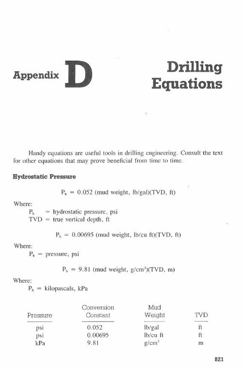
Appendix D DrillingEquations
Handy equations are useful tools in drilling engineering. Consult the textfor other equations that may prove beneficial from time to time.
Hydrostatic Pressure
Ph = 0.052 (mud weight, Ib/gal)(TVD, ft)
Where:
Ph = hydrostatic pressure, psiTVD = true vertical depth, ft
Ph = 0.00695 (mud weight, Ib/cu ft)(TVD, ft)
Where:
Ph = pressure, psi
Ph = 9.81 (mud weight, g/cm3)(TVD, m)
Where:
Ph = kilopascals, kPa
Conversion MudPressure Constant Weight TVD
- -psi 0.052 Ib/gal ftpsi 0.00695 Ib/cu ft ftkPa 9.81 g/cm3 m
821
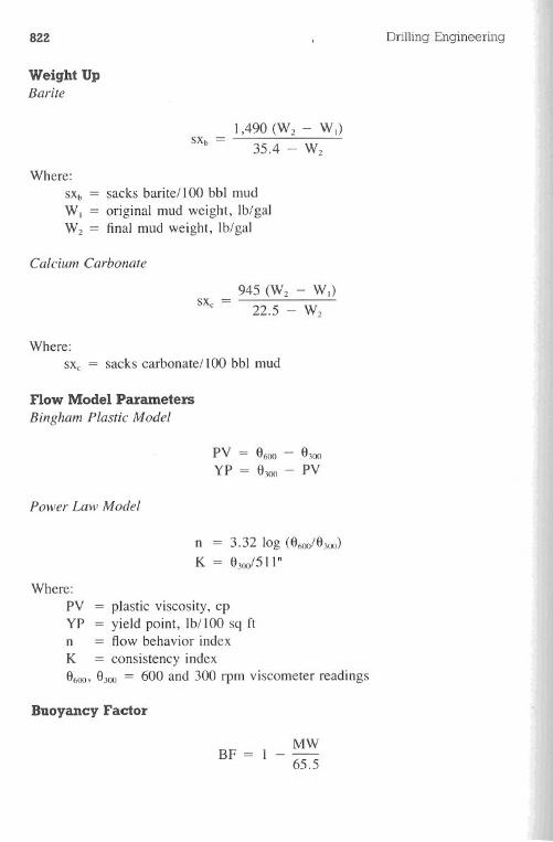
8ZZ
Weight UpBarite
1,490 (W2 - WI)
35.4 - W2
Where:
SXb = sacks baritell 00 bbl mudWI = original mud weight, Ib/galW2 = final mud weight, Ib/gal
Calcium Carbonate
945 (W2 - WI)sx =c 22.5 - W2
Where:SXc= sacks carbonate/IOObbl mud
Flow Model ParametersBingham Plastic Model
PV = 6600 - 6300
YP = 6300 - PV
Power Law Model
n = 3.32 log (6600/6300)K = 6300/511"
Where:
PV = plastic viscosity, cpYP = yield point, Ib/IOOsq ftn = flow behavior index
K = consistency index6600'6300= 600 and 300 rpm viscometer readings
Buoyancy Factor
BF = IMW65.5
Drilling Engineering
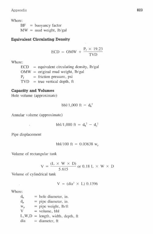
Appendix 823
Where:BF = buoyancy factorMW = mud weight, Ib/gal
Equivalent Circulating Density
ECD = OMW + Pr X 19.23TVD
Where:ECD = equivalent circulating density, Ib/galOMW = original mud weight, Ib/galPr = friction pressure, psiTVD = true vertical depth, ft
Capacity and VolumesHole volume (approximate)
bbl/I,OOOft = dh2
Annular volume (approximate)
bblll,OOOft = dh2 - d/
Pipe displacement
bblllOO ft = 0.03638 wp
Volume of rectangular tank
(L x W x D) or 0.18 L x W x DV = 5.615
Volume of cylindrical tank
V = (dia2 x L) 0.1396
Where:dh = hole diameter, in.dp = pipe diameter, in.wp = pipe weight, Ib/ftV = volume, bblL,W,D = length, width, depth, ftdia = diameter, ft
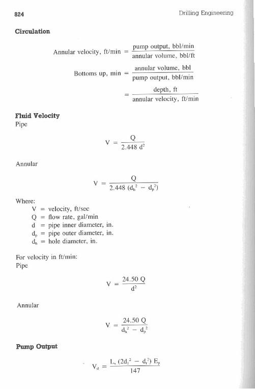
824 Drilling Engineering
Circulation
Annular velocity, ft/min = pump output, bbl/minannular volume, bbllft
Bottoms up, min = annular volume, bblpump output, bbl/min
depth, ftannular velocity, ft/min
Fluid VelocityPipe
QV = 2.448 d2
Annular
QV = '2 2
2.448 (dh - dp)
Where:
V = velocity,ft/secQ = flow rate, gal/mind = pipe inner diameter, in.dp = pipe outer diameter, in.dh = hole diameter, in.
For velocity in ft/min:Pipe
V 24.50 Qd2
Annular
v = 24.50 Qdh2 - d 2P
Pump Output
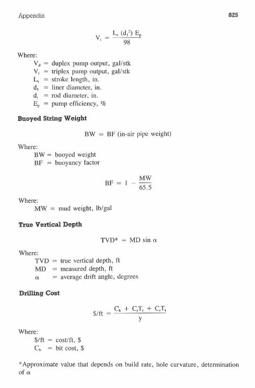
Appendix 825
Where:Vd = duplex pump output, gal/stkV, = triplex pump output, gal/stkLs = stroke length, in.d. = liner diameter, in.dr = rod diameter, in.Ep = pump efficiency, %
Buoyed String Weight
BW = BF (in-air pipe weight)
Where:BW = buoyed weightBF = buoyancy factor
BF = 1MW65.5
Where:MW = mud weight, lb/gal
True Vertical Depth
TVD* = MD sin a
Where:TVD = true vertical depth, ftMD = measured depth, fta = average drift angle, degrees
Drilling Cost
$/ft = Cb + CrTr + CrT,y
Where:$/ft = cost/ft, $Cb = bit cost, $
*Approximate value that depends on build rate, hole curvature, determinationof a
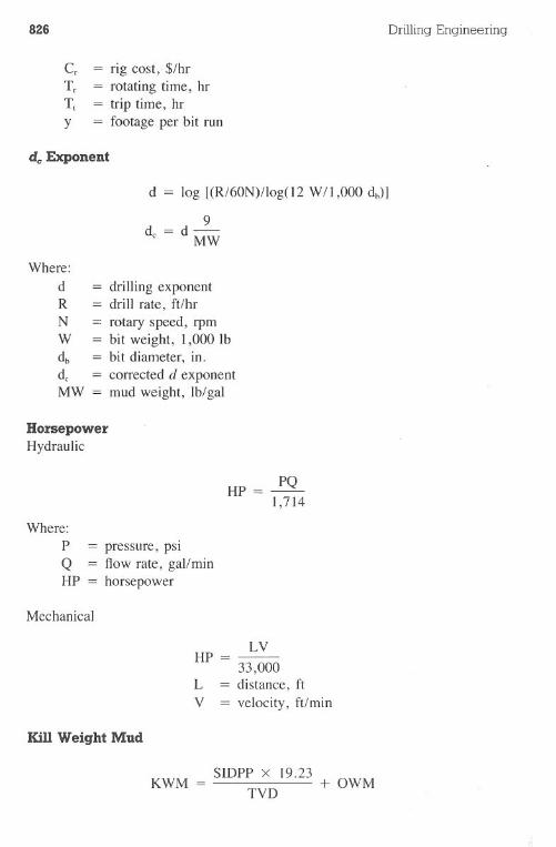
826 Drilling Engineering
C, = rig cost,. $/hrT, = rotating time, hrT. = trip time, hry = footage per bit run
de Exponent
d = log [(R/60N)llog(l2 W/l,OOOdb)]
9d = d-
e MW
Where:
d = drilling exponentR = drill rate, ft/hrN = rotary speed, rpmW = bit weight, 1,000 Ibdb = bit diameter, in.de = corrected d exponentMW = mud weight, Ib/gal
HorsepowerHydraulic
HP= PQ1,714
Where:
P = pressure, psiQ = flow rate, gal/minHP = horsepower
Mechanical
LVHP = 33 000,L = distance, ftV = velocity, ft/min
Kill Weight Mud
SIDPP x 19.23 + OWMKWM = TVD
Appendix 827
Where:
OWM = original weight of mud, lb/galKWM = kill (balanced) weight of mud, lb/galSIDPP = shutin drillpipe pressure, psiTVD = true vertical depth, ft
Kick Tolerance
KT = FG _ MW _ (SICP x 19.23)TVD
Where:
KT = kick tolerance, lb/galFG = fracture gradient, lb/galMW = average mud weight, lb/galSICP = shutin casing pressure, psiTVD = true vertical depth, ft (at depth of interest)
Stuck Pipe Depth
L=KWEP
Where:
L = free pipe length, ftK = pipe weight constant (645 for steel)W = pipe weight, lb/ftE = elongation due to pull, in.P = applied pull, 1,000 lb
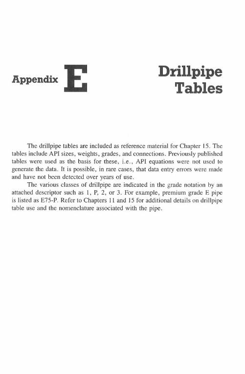
Appenctix E DrillpipeTables
The drillpipe tables are included as reference material for Chapter 15. Thetables include API sizes, weights, grades, and connections. Previously publishedtables were used as the basis for these, i.e., API equations were not used togenerate the data. It is possible, in rare cases, that data entry errors were madeand have not been detected over years of use.
The various classes of drillpipe are indicated in the grade notation by anattached descriptor such as 1, P, 2, or 3. For example, premium grade E pipeis listed as E75-P. Refer to Chapters 11 and 15 for additional details on drillpipetable use and the nomenclature associated with the pipe.
828
DR
ILLPIPE
NO
MIN
AL
CO
UP
LED
YIE
LDW
ALL
JOIN
TJO
INT
-6'O
.D.
WE
IGH
TW
EIG
HT
GR
AD
ES
TR
EN
GT
HT
HIC
KT
YP
EC
LEA
RA
NC
EB
UR
ST
CO
LLAP
SE
DR
IFT
ST
RE
NG
TH
'0(
IN)
(LB/F
T)
(LUF
T)
(1000P
SI>
<IN
)(H
I)(P
SI)
(PS
I>(H
I)(1000
LBS
)<D
::!
5.000
19.5020.90
E75-1
75.0.362
NC
50XH
6.3759500.
10000.3.625
944.Q
.5.000
19.5020.90
E75-P
75.0.290
NC
50XH
6.3758690.
7070.3.625
9'14.>
<'
5.00019.50
20.90E
75-27"
0.290N
C50X
H6.375
7060.4760.
3.625944.
,....5.000
19.5020.90
E75-3
75.0.226
NC
50XH
6.3755970.
3210.3.625
944.
5.00019.50
22.10E
75-175.
0.3623.5F
H7.000
9500.10000.
3.625
1448.
5.000
19.50
22.10E
75-P75.
0.2905.5F
H7.000
8690.7070.
3.6251448.
5.000
19.50
22.10
E75-2
75.0.290
).5F
H.,.000
7060.4760.
3.625
1448.5.000
19.50
21.40X
95-195.
0.362
NC
50XH
'j,37512040.
12010.3.375
1110.
5.00019.50
21.40X
95-P95.
0.290N
C50X
H6.375
11000.8230.
3.375
1110.
5.000
19.50
21.40X
95-295.
0.290
NC
50XH
6.375
8940.
5230.
3.375
1110.5.000
19.50
21.40X
95-395.
0.226
NC
50XH
6.375
7570.
3630.
3.375
1110.
5.000
19.50
22.40X
95-195.
0.3625.5F
H7.000
12040.12010.
3.625
1448.
5.000
19.50
22.40
X95-P
95.
0.290
5.5FH
7.00011000.
8230.
3.625
1448.
5.000
19.50
22.40
X95-2
95.
0.290
5.5FH
7.0008940.
5230.
3.625
1448,5.000
19.5022.40
X95-3
95.
0.226
5.5FB
7.000
7570.
3630.
3.625
1448.
5.000
19.50
21.90GI05-1
105.
0.362
NC
50XH
6.500
13300.
12990.
3.125
1269.
5.000
19.50
21.90
GI05-P
105.
0.290
NC
50XH
6.500
12160.
8760.
3.1251269.
5.000
19.50
21.906105-2
105.
0.290
NC
50XH
6.500
9880.
5410.
3.125
1269.
5.000
19.50
21.90
6105-3
105.
0.226
NC50XH
6.500
8360.
3770.3.125
1269.
5.000
19.50
22.40
6105-1
105.
0.362
5.5FH
7.00013300.
12990.
3.625
1448.
5.00019.50
22.40
6105-P105.
0.290
5,SF
H7.000
12160.
8760.
3.625
1448.
5.000
19.50
22.40
6105-2
105.
0.290
5.5FH
7.000
9880.
5410.
3.625
1448.5.000
19.50
22.40
6105-3
105.
0.226
5.5FH
7.0008360.
3770.3.625
1448.
5.000
19.50
22.50
5135-1
135.
0.362
Nr.50X
H6.625
17110.15700.
2.6251551.
5.00019.50
22.50
S135-P
135.
0.290
NC
50XH
6.625
15640.
10050.
2.625
1551.
5.000
19.50
22.505135-2
135.
0.290
NC
50XH
6.625
12710.
5970.
2.625
1551.
5.000
19.50
22.50
5135-3
135.
0.226
NC50XH
6.625
10750.3960.
2.625
1551.
5.000
19.50
23.20
5135-1
135.
0.362
5.5FH
7.250
17110.
15700.
3.375
1619.
5.000
19.50
23.20
5135-P
135.
0.290
5.5FH
7.625
15640.
10050.
3.375
1619.
5.000
19.50
23.20
5135-2
135.
0.290
5.5FH
7.625
12710.
5970.
3.375
1619.
5.000
19.50
23.20
5135-3
135.
0.226
5.SF
H7.625
10750.
3960.
3.375
1619.
5.000
25.60
26.90
E75-1
75.
0.500
NC
50XH
6.375
13120.
13500.
3.375
1110.
5.000
25.60
26.90
E75-P
75.
0.440
NC
50XH
6.375
12000.
11460.
3.375
1110.5.000
25.60
26.90
E75-2
75.
0.440
NC
50XH
6.375
9750.
9420.
3.375
1110.=
5.000
25.60
26.90
E75-3
75.0.375
NC
50XH
6.375
8250.
7250.
3.375
1110.5.000
25.60
28.10
E75-1
75.
0.500
5.SF
H7.000
13120.
13500.
3.375
1619.
w
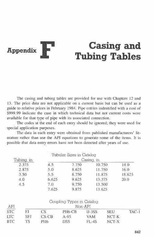
Appendix F Casing andTubing Tables
The casing and tubing tables are provided for use with Chapters 12 and13. The price data are not applicable on a current basis but can be used as aguide to relative prices in February 1984. Pipe entries indentified with a cost of$999.99 indicate the case in which technical data but not current costs wereavailable for that type of pipe with its associated connection.
The codes at the end of each entry should be ignored; they were used forspecial application purposes.
The data in each entry were obtained from published manufacturers' lit-erature rather than use the API equations to generate some of the items. It ispossible that data entry errors have not been detected after years of use.
Tubing, in.2.3752.8753.504.04.5
APISTCLTCBTC
FJSFJTS
Coupling Types in CatalogNon-API
PH6-CB IJ-3SSA-95 YAMDSS FL-4S
4.55.05.56.6257.07.625
CSCS-CBPH6
Tubular Sizes in CatalogCasing, in.
7.750 10.7508.625 11.7508.750 11.8759.625 13.3759.750 13.5009.875 13.625
14.016.018.62520.0
SEUNCT-KNCT-X
TAC-I
847
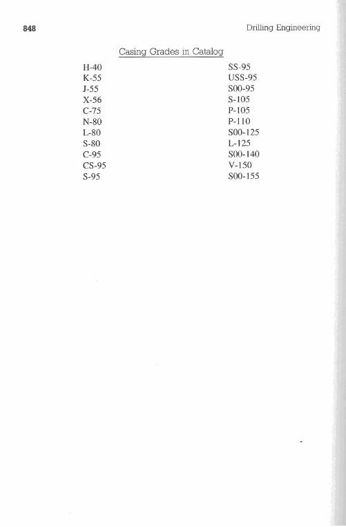
848
H-40K-55J-55X-56C-75N-80L-80S-80C-95CS-95S-95
Casing Grades in Catalog
DrillingEngineering
SS-95USS-95SOO-95S-105P-105P-110SOO-125L-125SOO-140V-150800-155
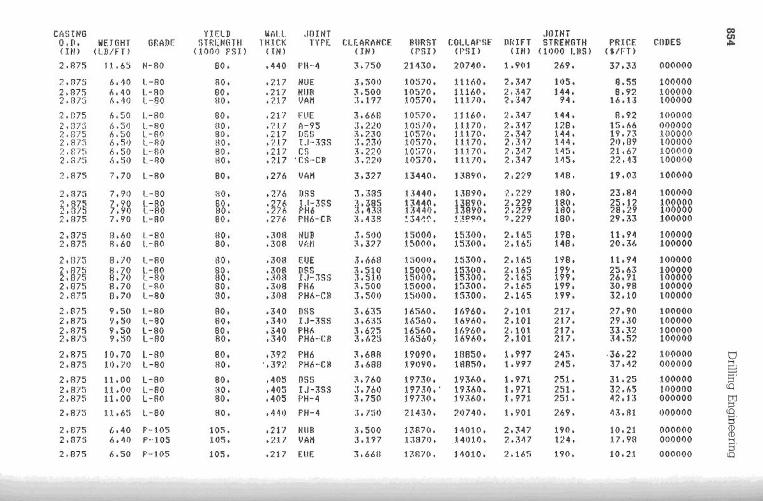
C(IS
ING
YIf.L
DW
AL
L.
.JOIN
T.JO
INT
CO
en0.11.
WnfiH
TG
f:APr:
ST
R"N
finlT
IUC
KT
YP
Er;LF
..AR
AN
Cr.
III/RST
CO
LLAI'S
FD
RIF
TS
TR
EH
fiTH
PR
ICr.
CO
DE
S<
IN)
(l.D/F
T)
<1000
1'51)(IN
)<
IN)
(PSI)(PSI>
<IN
)(1000
1.))5)($/F
T)
2.875
11.6SN
-BO
BO
..440
I'B--4
3.750210130.
20740.1.901
269.37.33
000000
2.07i6.40
l.-8080.
.217N
UE
..iO
O10570.
11160.2.347
1«)5.8.55
100000
2.8756.40
1.-80B
O.
.217H
UB
3.50010570.
11160.2,347
144.8.92
1000002.a7
(,.40l.-80
80..?!7
VA
il3.197
10570.11170.
'2.34794.
16.13100000
2.B75
6.501.-80
BO
..21"1
HIE
3.6M)
10570.U
160.2.347
144.8.92
100000
2.37:)(,.50
1.-8080.
.217/)-95
:S.2;,O10:i70.
11170.2.317
12B.
15.66000000
2.875
6.501.-80
BO
..217
JJ5H3.no
10570.U
170.2.347
144.19.73
1000002.875
6.50l.-80
80..?17
1.1,.355:1.;!30
10570.11170.
2.317144.
20.99100000
2.f7
6.501.-80
BO
..217
CS
3.22010:;7(1.
U170.
2.347145.
21.67100000
2.Sli
.\.50L
.-8080.
.217'C
S"CII
.1.22010570.
11170.2.347
145.22.13
100000
2.8757.70
1.-8080.
.27(,V
Ail
3.3:1713440.
131190.2.229
148.19.03
1000(10
2.3757.90
l.-80H
Ot
.V6
D5S
J.:a5U
440.L
1I90.'2.229
1110.13.84
100000
2.8757.90
1.-80B
O.
.2761.1-3S5
:\.3851344(1.
13890.2.229
IBO
.25.12
10(10002.3"75
7.90l...1I0
80..276
I'H6
;i.133H
440.3890.
2.229180.
28.29100000
2.875
7.901.-90
80..276
PHI>
-CII
3.438
34'!(,.!;9.
'.229180.
29.33100000
2.875
0.1>0
1.-80no.
.30tN
UB
:1.5«)015000.
15:100.2.165
198.11.94
1000002.875
8.601.-80
80..30B
VfJtl
.3:1715000.
15;100.2.16:;
148.20.36
100000
'2.1!759./0
l.-9080.
.30;f.U
E..M
>;
1:1000.15300.
2.165198.
11.94100000
2.8758.70
1.-90B
O.
.30BD
S!':3.510
15000.153(10.
2.165199.
25.63100000
2.8758.71)
l.-8080.
..03r.J-35S
3.51015000.
15300.2.165
199.26.91
1000002.875
9.701.-80
BO
..30B
PH6
.50015000.
15300.2.165
199.30.98
10(10002.R
75n.71)
l.-80H
O.
.:108PH
6.,CB
3.50015000.
15300.2.165
199.32.10
100000
2.B75
9.501.-80
80..340
DSS
3.63516560.
11>960.
2.101217.
27.90100000
2.9759.51)
l.-8080.
.340I.J-35S
3.I>:5
1.\560.11>
91>0.
2.101217.
29.:0100000
2.8759.50
L-B
O80.
.340PH
I>3.6:15
1651>0.
1(.91>0.
2.101217.
33.32100000
2.8/59.50
1.-8080.
.340PH
I>..I:B
3.62:i11>
51>0..
11>960.
2.101217.
:14.52100000
2.S7510.70
I.-SO80.
.392PH
n.6B
819090,
II1S50.1.997
245..36.22
100000t:J
2.97510.70
L.-80
80.'.392
PHn"C
JJ..nllll
19090.181150.
1.997245.
37.42000000
§2.875
11.00L
-SOB
O.
.405DB!;
.76019730.
1931>0.
1.971251.
31.25100000
5'
2.97511.00
1.-8030.
.405I./-JSS
:!.761>19no.'
In60.1.971
251.32.105
100000\Q
2.87511.00
L-90
BO
..405
I-'H-4
3.75019730.
19360.1,971
251.42.n
000000tr:I::I
2.S7511.I>
:i1.-80
80..H
OPH
-4:1.7:iO
'7.1430.20740.
1.901269.
43.81000000
\Q5'2.875
I..40
P-I05105.
.217H
UB
3.500I::'B
70.14010.
2.347190.
10.21000000
(1)(1)
2.3751>
.40P
..I05105.
.217V
Ail
;!.11713370.
HIH
O.
2.347124.
17.98000000
'"'
2.8751>
.501'..105
105..217
EIJE
3.6611I;7,S7(1.
14010.2.165
190.10.21
000000
5'
\Q
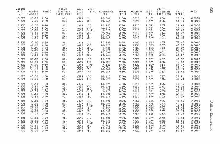
CASING
YIE
LD
WA
LL
./OJlH
JOINT
U>
N0.0.
WEIGHT
GR
AD
ES
TR
EN
GT
HT
HIC
KT
YP
F.
CL
EA
RA
NC
EB
UR
ST
CO
LLAP
SF
.llR
1FTS
TR
EN
GT
HPR
ICE
I;OO
ES
NIIN
)(L
B/FT
)<
1000PSI>
<Il0
(ItO(PSI>
(PSI)(IN
)(1000
1B
S)(SIF
T)
9.625
41).01)N
-8080.
.395T
S11).1)00
5750.3090.
B.b79
800.52.116
1)1)00009.625
40.00N
-81180.
.395SE
U10.165
57511.30911.
11.6791085.
54.3300110011
9.62543.50
H-80
80.435
I,TC
10.625b330.
38tO.
B.599
825.34.62
000000
:H
:8":g
as::U
TC
1:t§&
:H
18:H
:nlit:
:888888
.J-P9.625
43.50N
-81180.
.435SFJ
9'.75IJ60M
.3810.
8.599713.
53.2900000(1
9.62543.50
H-80
80..4;'5
TS
11).1)006330.
311tO.
8.599920.
56.4101)0000
9..!-2543.50
N-811
80..435
SF.II10.
1656330.
3810.8.599
1181.59.83
000000
9.62547.00
H-80
ao..472
LT
C11).625
6870.4750.
8.525905.
37.401)1)0000
9.62547.00
N-811
80..472
BT
C10.625
6870.47511.
8.5251357.
40.060011000
9.62547.00
U-8O
80..4n
SFJ9.750
.S600.4750.
8.525785.
57.071)1)0000
9..!-2547.00
-81180.
.472F
I.-P9.625
5300.4750.
11.525731.
57.07000000
9.62547.00
H-80
80..472
TS
10.000(.871).
4750.8.525
t021.60.31
01)1)0009..!-25
47.0011-80
80..472
SEll
10.16568711.
475(1.8.525
1281.64.17
0000011
9.62553.50
H-80
80..545
LT
Cto.625
7930.6620.
8.3791062.
42.57
0000009.625
53.5011-811
80..545
BT
C10.625
7930.6620.
8.3791555.
45.6(10000110
.9.62553.50
H-80
80..545
FJ-P9.625
651)1).6620.
8.500866.
04.370(1)000
9..!-553.50
-81180.
.SF.J
9.7507670.
6620.81IJO
916.64.37
0000009.6
553.50
-8080.
.5..)
TS
10.0627880.
6620.8.
'01)1132.
67.081)1)0000
9.62553.50
N-80
80..545
SEll
10.16579311.
b620.8.379
1311.72.43
1111110110
9.62541).01)
1.-8080.
.395L
TC
11).6255750.
3/)90.8.679
737.37.11
tooooo
9.625
"0.00L
-81180.
.395tH
C10.625
5750.3(190.
8.6791145.
39.74100000
9.62543.50
1.-8080.
.433L
TC
11).6256330.
38tO.
8.599825.
4/)..161/)0000
9..!-2543.50
L-811
80..435
BT
C10.625
6330.3810.
8.5991256.
43.221(10000
9.62543.51)
L.-80
80..435
SFJ9.750
6060.3810.
8.599b77.
62.62()()O
OO
O9..!-25
"3.50L
-8080.
.435F
.J-P9.625
500(1.3810.
8.599.!-33.
62.62000000
9.62543.50
1.-8080.
.";'5T
S10.000
b.BO
.3810.
8.599065.
66.:U000000
9.62543.50
L-80
80..435
SEU
100165633(1.
3810.8.599
1122.70.29
000000
9.62547.00
1.-8080.
.472L
TC
10.625(871).
4750.8.525
9')5.43.bl
1000001::1
9.62547.00
L-80
80..472
BT
C10.6?5
6870."750.
8.5251357.
46.7(1100000
....
9.62547.00
1.-8080.
.472FJ-P
9.b25531)0.
4750.8.525
694.b7.03
0000009.b25
47.00L
-8080.
.47?SF./
9.7506600.
4750.8.525
746.67.03
0000009.625
47.001.-80
80..472
TS
10.000.S870.
4750.8.525
962.70.90
000000to
9..!-25"7.00
L-80
80..472
SEU
10.165
6870.475(1.
8.5251217.
75.380(10000
:g
9.62553.50
1,-8080.
.545L
TC
10.6257930.
.S620.8.379
Il)b2.49.M
101)0009..!-25
53.50L
-ao80.
.545/H
C10.67.5
7930.6.!-20.
B.379
1555.53.16
100000S.
9.62553.50
1.-8080.
.545F
.J-P9.625
b500.6620.
B.501)
823.75.62
,000000roro
9.62553.50
L-8(1
80..545
sr./9.750
7670.6620.
8.5\10870.
75.62000000
S.9.623
53.501.-80
80..545
TS
10.1)627880.
6620.8.500
1076.79.79
0000009.625
53.50L
-80B
O.
.545SE
ll10.165
7930.b620.
8.3791245.
85.1(100000(1
to
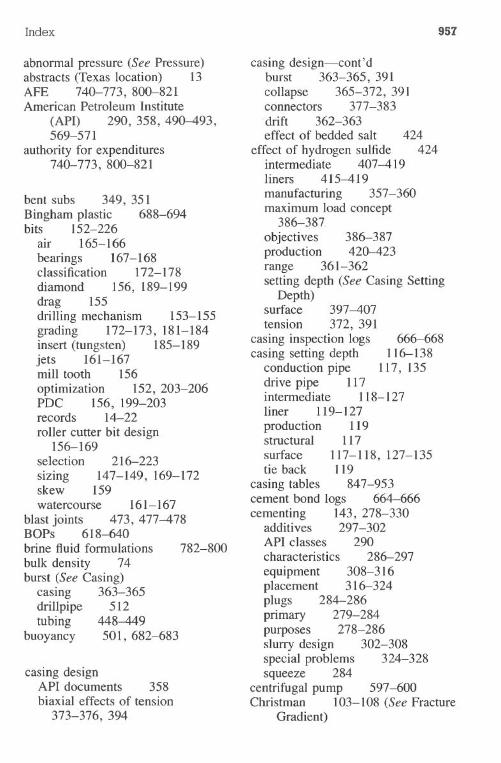
Index
abnormal pressure (See Pressure)abstracts (Texas location) 13AFE 740-773, 800-821American Petroleum Institute
(API) 290, 358, 490-493,569-571
authority for expenditures740-773, 800-821
bent subs 349, 351Bingham plastic 688-694bits 152-226
air 165-166bearings 167-168classification 172-178diamond 156, 189-199drag 155drilling mechanism 153-155grading 172-173, 181-184insert (tungsten) 185-189jets 161-167mill tooth 156optimization 152, 203-206PDC 156, 199-203records 14-22roller cutter bit design
156-169selection 216-223sizing 147-149, 169-172skew 159watercourse 161-167
blast joints 473, 477-478BOPs 618-640brine fluid formulations 782-800bulk density 74burst (See Casing)
casing 363-365drillpipe 512tubing 448-449
buoyancy 501,682-683
casing designAPI documents 358biaxial effects of tension
373-376, 394
957
casing design-cont'dburst 363-365, 391collapse 365-372, 391connectors 377-383drift 362-363effect of bedded salt
effect of hydrogen sulfideintermediate 407-419liners 415-419manufacturing 357-360maximum load concept
386-387objectives 386-387production 420-423range 361-362setting depth (See Casing Setting
Depth)surlace 397-407tension 372, 391
casing inspection logscasing setting depth
conduction pipedrive pipe 117intermediate 118-127liner 119-127production 119structural 117surlace 117-118, 127-135tie back 119
casing tables 847-953cement bond logs 664-666cementing 143, 278-330
additives 297-302API classes 290characteristics 286-297equipment 308-316placement 316-324plugs 284-286primary 279-284purposes 278-286slurry design 302-308special problems 324-328squeeze 284
centrifugal pump 597-600Christman 103-108 (See Fracture
Gradient)
424424
666-668116-138
117, 135
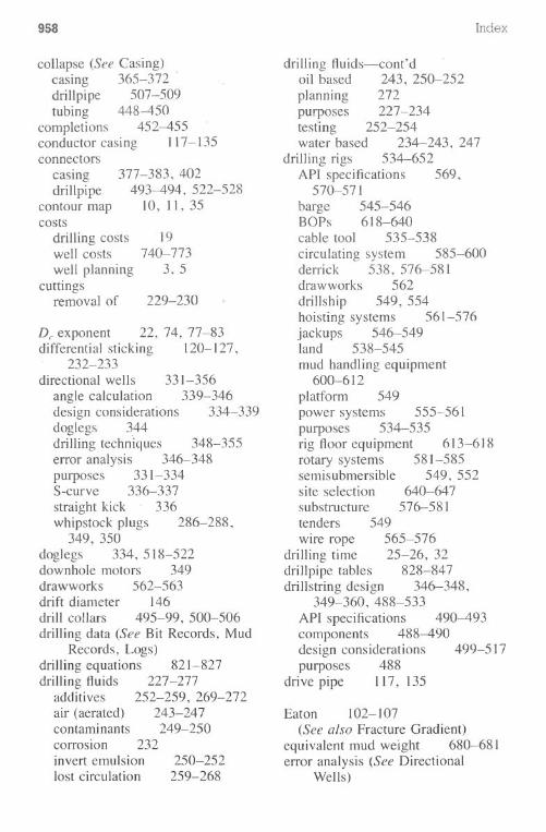
958
collapse (See Casing)casing 365-372 "drillpipe 507-509tubing 448-450
completions 452-455conductor casing 117-135connectors
casingdrillpipe
contour mapcosts
drilling costs 19well costs 740-773well planning 3, 5
"cuttingsremoval of
377-383, 402493-494, 522-528
10, 11,35
229-230
D,"exponent 22, 74, 77-83differential sticking 120-127 ,
232-233directional wells 331-356
angle calculation 339-346design considerations 334-339doglegs 344drilling techn"iques 348-355error analysis 346-348purposes 331-334S-curve 336-337straight kick 336whipstock plugs 286-288,
349, 350doglegs 334, 518-522downhole motors 349drawworks 562-563drift diameter 146drill collars 495-99, 500-506drilling data (See Bit Records, Mud
Records, Logs)drilling equations 821-827drilling fluids 227-277
additives 252-259, 269-272air (aerated) 243-247contaminants 249-250corrosion 232invert emulsion 250-252lost circulation 259-268
Index
drilling fluids-cont'doil based 243, 250-252planning 272purposes 227-234testing 252-254water based 234-243, 247
drilling rigs 534-652API specifications 569,
570-571barge 545-546BOPs 618-640cable tool 535-538circulating system 585-600derrick 538, 576-581drawworks 562drillship 549, 554hoisting systems 561-576jackups 546-549land 538-545mud handling equipment
600-612platform 549power systems 555-561purposes 534-535rig floor equipment 613-618rotary systems 581-585semisubmersible 549, 552site selection 640-647substructure 576-581tenders 549wire rope 565-576
drilling time 25-26, 32drillpipe tables 828-847drillstring design 346-348,
349-360, 488-533API specifications 490-493components 488-490design considerations 499-517purposes 488
drive pipe 117, 135
Eaton 102-107(See also Fracture Gradient)
equivalent mud weight 680-681error analysis (See Directional
Wells)
Index
fatigue, drillpipe 518-528wire rope 574
flow couplings 472-473, 476formation damage 230,453formation pressure (See Pressure)Foster and Whalen (See Pressure)Fracture gradient
Christman (deepwater)103-108
Eaton 102-107Hubbert & Willis 97-99leak-off test 110-114Matthews & Kelly 98-102
free-point indicator 661
heavy-weight drillpipe 494-495hole size selection 3, 139-151
considerations 139-141problems 142-146
hole stability 232Hubbert & Willis 97-99
(See also Fracture Gradient)hydraulics
bit pressure drop 700-703buoyancy 682-683ECD 680-681flow models 688-t'i94flow regimes 683-687friction pressure 694-700hydraulics optimization
704-716hydrostatic pressure 679-680purposes 678-679slip velocity 724- 731surge pressures 716-724
hydrogen sulfide 424, 435hydrostatic pressure 679-680
IADC reports 26intermediate pipe 118-119, .
120-127
kicks 83-86, 324laminar flow 683-687leak-off testing 110-114
(See also Fracture Gradient)
959
liners 119, 120-127logs
analyses for pressuredetection 53-77
casing inspection logs 666-668cement bond logs 664-666free-point indicator 661headers 29, 30-31Magrange II 675-676mud 26-29mud logging 668MWD 668-672noise 658-661pipe recovery 661 .radioactive 657-658special drilling logs 653-676string shot backoff 661stuck pipe 661temperature 654-657ULSEL 670-675
Magrange II 675-676matrix stress coefficient 98-102
(See also Fracture Gradient)Matthews & Kelly 98-102
(See also Fracture Gradient)mud (See Drilling Fluids)mud handling equipment
600-612centrifuges 608-610cyclones 607-608mud cleaners 610-611sand traps 602shale shakers 604-607unitized systems 611-612
mud logging' 668mud logging records 26-29mud pumps 585-597mud records 22-26MWD 668-672
Newtonian model 688-694noise logs 658-661
Offset wells 9Optimization (See Bits)
960
ill Packer 434-438, 473Packer fluids 482-483Perforating gun 481-482pipe recovery 6§1Poisson's ratio (See"FractureGra-
dient) 105pore pressure (See Pressure)power law 688-694pressure
ahnormal pressures, originuf 40
Qulkdensity 74~ casing burst 363-365, 391
casing collapse 365-372, 391equivalent depth calculation
procedure 44formation 5, 21Foster & Whalen
technique 61-70log analysis 53-77prediction methods 39-96sonic log 70-74
produCtionhistory .case problem 775effect on well plan 29
production tree 455-457
radioactive logs 657-658reservoirs 452-455resistivity logs 53-71
(See also Pressure)rig floor equipment
bit breakers 613elevators 614lift niples 613mud bucket 613safety clamps 6I'8slips 618standpipe pressure gauge 613tongs 618weight indicators 613
safetyhydrogen sulfidewell planning
safety systems
424-435I
452-473
Index
saltcauses of abnormal pressureeffect on casing design 424
scout tickets 26-27section maps 12, 34seismic studies .
pressure detection 50-52source of drilling data 33
sliding sleeves 473, 479 .
slip and cut (wire rope) 574-576slip crushing 509-512sonic log 70-74stabilizers 499string shot backoff 661stuck pipe logs 661surface casing 1l7-ll8, 127-135surge pressure 716-724
temperature logstension. biaxial loading effects. casing . 372
drillstring 372, 509tubing 372, 448-450
tubing design 430-451ballooning 432buckling 432-434design conditions 438-441stress 430-434, 441-448temperature 432
turbulent flow 683-687
654-657
373-376
ULSEL 670-675
\ velocityannularfast line
I.
i
,.1
143-145573
well cost estimationwell design problemwell planning
costs I, 2, 3objectives Ioverview 6-7
well types 4whipstock 349-350, 286-288wire rope 565-576
740-773774-781
,
II


