Seediscussions,stats,andauthorprofilesforthispublicationat:http://www.researchgate.net/publication/281854791

TwoPhaseflowoverEppler387airfoilatLowReynoldsnumber

RESEARCH·SEPTEMBER2015

DOI:10.13140/RG.2.1.4335.9201

READS

13

2AUTHORS,INCLUDING:

SanketShah

Mahindra

1PUBLICATION0CITATIONS

SEEPROFILE

Availablefrom:SanketShah

Retrievedon:21December2015

A Numerical Study on Effect of Dispersed

Particle Phase on Eppler 387 airfoil at Low

Reynolds NumbersSanket Shah1

Department of Mechanical Engineering,

Indian Institute of Technology Bombay,

Mumbai, India 400 076

Email: shaha.45@gmail.com

(Presently Sr. Engineer at Mahindra & Mahindra, India)

Sridhar Balasubramanian1

Assistant Professor, Department of Mechanical Engineering,

Indian Institute of Technology Bombay,

Mumbai, India 400 076

Email: sridharb@iitb.ac.in

ABSTRACT

In engineering applications, the fluid flow is almost always contaminated with solid particles of different

sizes, shapes, and concentrations. The effect of particle concentration, even in dispersed phase (i.e. low

volume fractions), could play a significant role in modifying the flow characteristics. This study deals with

understanding the flow dynamics of dispersed multiphase flow over an airfoil at Reynolds number Re<106.

Flow of water (carrier fluid) laden with solid particles (mean diameter, dp=100 m and p=2500 kg/m3) over

Eppler 387 airfoil is simulated in ANSYS FLUENT using the Shear Stress Transport (SST) transition model

comprising of k- transport equations. The change in the flow characteristics of water in the presence of

particles is understood with the help of pressure distribution, velocity contours, and drag polar plots. The

results reveal that there is a significant difference in the flow behavior for single phase and two phase case

as witnessed primarily from the lift and drag coefficients. The results indicate that even dilute particle

volume concentrations (Φv0.005-0.1) have significant effect on the flow dynamics, and should be

considered in modeling of such dispersed particle flows over streamlined bodies.

Keywords: two phase flow, low Reynolds number, two-way coupling

1 INTRODUCTION

Multiphase flow over streamlined bodies is often encountered in many

applications including particle-laden flow over gas turbine and wind turbine blades,

rotating and non-rotating wings of aerial vehicles and control surfaces of aircrafts in rainy

1 Corresponding authors

2

environment, underwater vehicles etc. The presence of secondary phase (usually solid

particles or bubbles) in these flows has shown detrimental effects on the aerodynamic

characteristics of the streamlined surfaces such as erosion, turbulence modulation, drag

increase, etc. There are many applications where airfoils are used at low to moderate

Reynolds number (ranging from 103to 106). For example, control surfaces and lift or drag

augmentation devices (like elevators, rudders, flaps etc.) of most of the large high speed

vehicles operate at much lower Reynolds numbers during take-off and landing. At high

altitudes aircraft gas turbine engine fan, compressor, and turbine blades encounter

Reynolds numbers considerably below 106. Even the space shuttle encounters Reynolds

numbers as low as 104 at M « 27 during reentry. The prime difficulty in understanding

such low Reynolds number flows is the unpredictability associated with separation and

reattachment. For an airfoil, the chord Reynolds number is defined as

cU *Re

where

U = free stream velocity; c = chord of airfoil; = kinematic viscosity. When Re is in the

range 103<Re< 106, laminar, transitional and turbulent flow all have a significant effect on

the aerodynamic characteristics of the airfoil. Each of these play an important role on the

separation and reattachment of the boundary layer formed on the airfoil surface.

Selig et al. [13, 14], Grundy et al. [4], Laitone [6] have performed experimental

measurements on airfoils at 2x104<Re< 5x105. They observed that for Re< 1x105, many of

these airfoils have relatively large values of drag coefficient for moderate values of lift

coefficient, while for low and high lift coefficients the drag coefficient is relatively low. For

higher Re, this unusual behavior was not observed. Many of the researchers have claimed

the laminar separation bubble to be the reason for this behavior. At low Reynolds

number, the flow over the airfoil is laminar for the initial part. Due to adverse pressure

gradient it separates and then transitions to turbulent separated shear flow. If the

momentum transfer is sufficient it reattaches on the airfoil surface thereby forming a

Laminar Separation Bubble (LSB). In some cases this separation bubble is stable while in

some cases it is highly unstable, thereby changing the flow behavior. Additionally, the

presence of a secondary particle phase further complicates the flow dynamics, which is

the scope of the present research work.

Erosion and fouling in gas turbines [3, 5] has been studied for the past two

decades. But most of this research has focused only on one-way coupling aspects of

multiphase flows i.e. only the effects of the continuous phase (carrying fluid) on the

particle phase are considered. The current work deals with two-way coupling in which the

effect of particles on the carrying fluid is important when the particle volume fraction,

3

Φv>10-6 [1]. The effect of dispersed phase on carrier phase can be categorized as

turbulence attenuation, turbulence augmentation, and preferential concentration [1].

In low and moderate Re flows, the particles may get trapped in the separation

region and impact on the upper surface of the airfoil; otherwise they may keep loitering in

the separation region adding or decreasing turbulence in the fluid. These changes may

have adverse effect on the lift and drag characteristics of the airfoil. Again this effect

depends on the concentration of particulate phase. In this communication, we undertake

the following objectives, (a) to study and understand the dynamics of two-phase flow

(discrete solid particles in water) over Eppler387 (or E387) airfoil at Re=460,000 and

Re=60,000 for two different volume fractions of particles Φv=0.005 and 0.1. This particular

airfoil was chosen because experimental data for single phase flow at these two Reynolds

numbers is available [9, 13, 14, 15], which can be used as a reference case. (b) To

determine the lift and drag coefficients for two phase flow and compare them with the

single phase flow and to understand the effect of particles on vorticity dynamics, pressure

distribution, preferential concentration over the airfoil, and lift and drag characteristics.

So far, most of the previous work in this area has only focused on clean flow over Eppler

387 airfoils, ignoring the effects of dispersed phases on the flow dynamics and turbulence.

We believe this is first time such a study is being undertaken to model the fluid-particle

interaction over Eppler 387 airfoil. The results are novel and could open up new avenues

for research in the field of dispersed multi-phase flows over streamlined bodies.

2 Governing equations, grid convergence and validation

Single phase and two-phase simulations were carried out in ANSYS Fluent 14.5. Grid

convergence, selection and validation of a turbulence model are essentials for the current

computational problem. For the current study, Langtry Menter’s Shear Stress Transport

(SST) transition model was chosen since the Reynolds number was in the transitional

regime, i.e., Re< 106. The SST transition model is a four-equation model comprising the

SST k-ω transport equations along with two additional equations, one for intermittency,

and one for the transition onset criteria in terms of momentum-thickness Reynolds

number. The equations are as given below (equations 1-4).

𝜕

𝜕𝑡(𝜌𝑘) +

𝜕

𝜕𝑥𝑖

(𝜌𝑘𝑢𝑖) =𝜕

𝜕𝑥𝑗(Γk

𝜕𝑘

𝜕𝑥𝑗) + 𝐺�̃� − 𝑌𝑘 + 𝑆𝑘 ….Eq.1

𝜕

𝜕𝑡(𝜌𝜔) +

𝜕

𝜕𝑥𝑖

(𝜌𝜔𝑢𝑖) =𝜕

𝜕𝑥𝑗(Γω

𝜕𝜔

𝜕𝑥𝑗) + 𝐺𝜔 − 𝑌𝜔 + 𝐷𝜔 + 𝑆𝜔 ….Eq.2

4

ΓkandΓω represent the effective diffusivity of k and 𝜔,

𝐺�̃�and𝐺𝜔 represent the generation of k and 𝜔,

𝑌𝑘and𝑌𝜔 represent the dissipation of k and 𝜔,

𝐷𝜔represents the cross diffusion term formed as a result of blending the standard 𝑘 − 𝜔

and transformed 𝑘 − 𝜖 equations

𝑆𝑘and𝑆𝜔 represent the user-defined source terms for k and 𝜔 equations

The intermittency equation (𝛾) and the transition momentum thickness Reynolds number

(𝑅𝑒𝜃�̃�) as given below

𝜕

𝜕𝑡(𝜌𝛾) +

𝜕

𝜕𝑥𝑖

(𝜌𝛾𝑢𝑖) =𝜕

𝜕𝑥𝑗[(𝜇 +

𝜇𝑡

𝜎𝛾)

𝜕𝛾

𝜕𝑥𝑗] + 𝑃𝛾1 − 𝐸𝛾1 + 𝑃𝛾2 − 𝐸𝛾2 ….Eq.3

𝜕

𝜕𝑡(𝜌𝑅𝑒𝜃�̃�) +

𝜕

𝜕𝑥𝑖(𝜌𝑢𝑖𝑅𝑒𝜃�̃�) =

𝜕

𝜕𝑥𝑗[𝜎𝜃𝑡(𝜇 + 𝜇𝑡)

𝜕𝑅𝑒𝜃�̃�

𝜕𝑥𝑗] + 𝑃𝜃𝑡 ….Eq.4

𝑃𝛾1and𝐸𝛾1 are the transition (production term for transition) sources

𝑃𝛾2and𝐸𝛾2 are the relaminarization (destruction term for transition) sources

𝑃𝜃𝑡represents the source term for transition momentum thickness Reynolds number

equation

The additional two equations are coupled with the SST k-ω transport equations via

intermittency, which is defined as the fraction of time for which the flow stays turbulent.

The model has been used to simulate flows over wind turbine blades [7, 10], 2D airfoils,

wings, and helicopter [7]. Thus far, the SST transition model has been extensively used for

Reynolds number greater than 5x105. In the present study, this model was validated for

single-phase flow over E387 airfoil at two Reynolds number viz. Re=460,000 and

Re=60,000. The single-phase experimental data from McGhee et al. [9] and Williamson et

al. [15] was used for validating the model in the present work. Once the model was

validated for single phase flow over E387, two phase simulations were done at two

Reynolds numbers, namely, Re=60,000 and Re=460,000. Due to unavailability of any

experimental data for the two-phase case, we have performed simulations with two

different volume fraction (Φv) of particles, namely, Φv=0.005 and 0.1. The volume fraction

is defined as 𝜙𝑣 =𝑉𝑝

𝑉𝑝+𝑉𝑓 where Vp is the volume occupied by the dispersed particulate

phase and Vf is the volume occupied by the continuous fluid phase. This ensures better

confidence in our results owing to expected differences in the flow physics.

The computational domain around the E387 airfoil is the widely used C-H domain

with the far field boundary located at a distance of twenty chord lengths (20c) on all sides.

This distance was maintained to minimize the effect of the far-field region on the near-

5

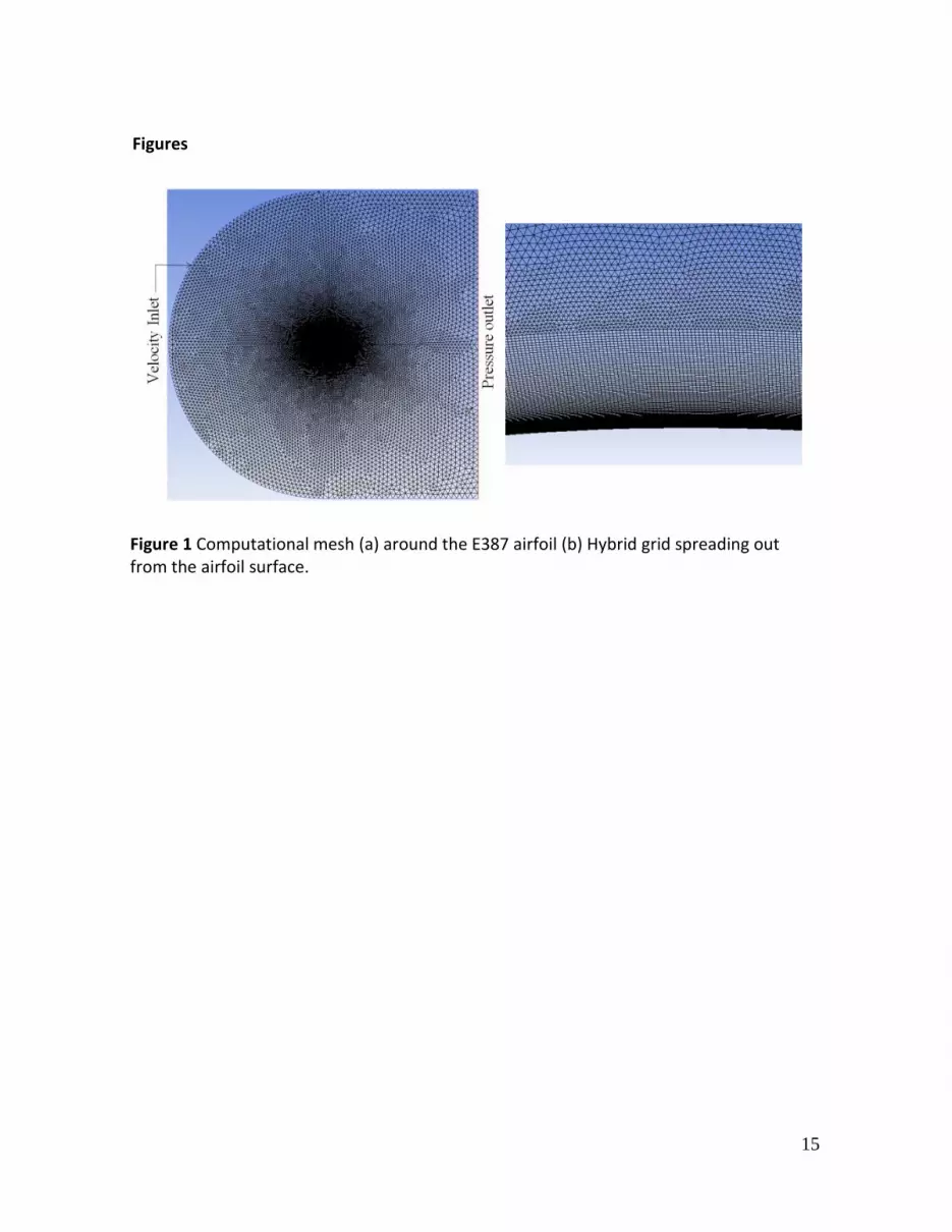
field solution. The mesh around the airfoil was created using ICEM CFD meshing tool as

shown in fig.1 (a). Hybrid grids were used comprising of rectangular cells near the airfoil

walls in a region of 5 mm around the walls and triangular cells in the rest of the domain as

shown in fig.1 (b). Different grids were used to check for grid independency. Various grid

parameters like distance of the cells adjacent to the airfoil walls, the number of points on

the airfoil and number of cells in the domain were varied. The effect of these parameters

on airfoil performance was noted before fixing our final grid configuration. In this paper

the effects of these parameters are shown only for Re=460,000 and α=40.

The distance of the nodes adjacent to the airfoil walls determines the y+. This y+

has to be compatible with the turbulence model being used for simulation. For the SST

transition model, this y+ value should be y+<1 [2]. To check for this compatibility the

distance of the first node points from airfoil walls was varied and the correct distance was

determined for which the corresponding y+<1. For the correct first node distance the

number of node points on the airfoil was varied, and two different configurations were

used. Node points were clustered on the leading edge to accurately capture the airfoil

curvature near the leading edge. In the second configuration the numbers of points on the

airfoil were doubled. The results for both configurations were compared with

experimental results. Grid independence study was done by successive refinement of

grids. The details regarding grid spacing, first cell distance, etc. are given below.

The unsteady pressure based Navier-Stokes flow solver was employed to model

the flow over the streamlined body. The SIMPLE algorithm was used for pressure-velocity

coupling. Second-order upwind schemes were used for the discretization of the advection

terms in all the flow equations. The diffusion terms were discretized using the default

second-order accurate Central Differencing Scheme in FLUENT. For time integration,

second-order implicit scheme was used.

The chord length used for all simulations was c=0.1 m. Based on this chord, the

inlet velocities corresponding to Re=460,000 was U=4.6 m/s and for Re=60,000 it was

U=0.6 m/s. The inlet turbulence intensity was set at 0.1 % corresponding to the

experimental values of McGhee et al. [9] and Williamson et al. [15]. For an estimate of y at

y+=1, following equation was used [12].

𝑅𝑒 =

𝜌 ∗ 𝑈𝑓𝑟𝑒𝑒𝑠𝑡𝑟𝑒𝑎𝑚 ∗ 𝐿𝑏𝑜𝑢𝑛𝑑𝑎𝑟𝑦 𝑙𝑎𝑦𝑒𝑟

𝜇 , 𝐶𝑓 = [2 log10(𝑅𝑒) − 0.65]−2.3

𝜏𝑤 = 0.5 ∗ 𝐶𝑓 ∗ 𝜌𝑈𝑓𝑟𝑒𝑒𝑠𝑡𝑟𝑒𝑎𝑚2 , 𝑢𝜏 = √

𝜏𝑤

𝜌 , 𝑦 =

𝑦+𝜈

𝑢𝜏

….Eq.5

6

where, 𝑅𝑒 = Reynolds number based on length of the boundary layer; 𝜌 = density;

𝑈𝑓𝑟𝑒𝑒𝑠𝑡𝑟𝑒𝑎𝑚= free stream velocity; 𝐿𝑏𝑜𝑢𝑛𝑑𝑎𝑟𝑦 𝑙𝑎𝑦𝑒𝑟 = length of the boundary layer; 𝜇 =

dynamic viscosity; 𝜈 = kinematic viscosity; 𝐶𝑓 = Coefficient of friction; 𝜏𝑤 = wall shear

stress; 𝑢𝜏 = friction velocity

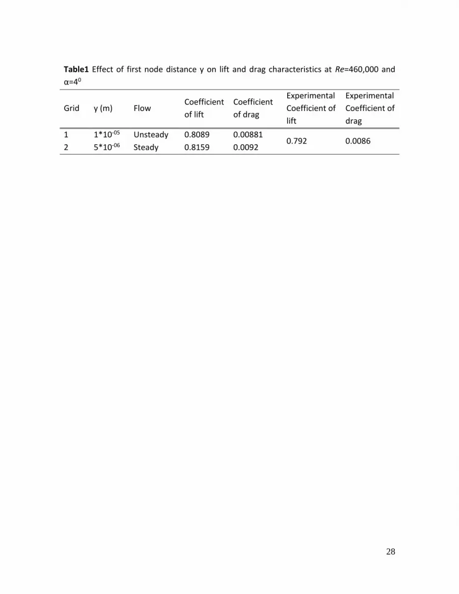
Based on this formulation, the first node distance for Re=460,000 was

approximately y=5x10-06 m. It was found numerically that changing this distance changes

the flow dynamics drastically and the flow leans towards unsteadiness. Due to this

unsteady nature, the separation bubble bursts intermittently as shown in fig.2.

Additionally, the bubble bursts in the velocity contour plots indicates that the flow is

unsteady while a steady separation bubble indicates a steady flow as shown in fig.3. The

fluctuations in pressure coefficient, Cp, can be seen in fig.2 when the first node distance is

1x10-5 m. The pressure coefficient is defined as 𝐶𝑝 =𝑃−𝑃∞

𝜌∞𝑈∞2 .The pressure coefficients were

compared with the experimental data from McGhee et al. [9]. The data for the two node

distances are shown in Table 1. It is evident from this table that even though the contour

plots and pressure coefficients show fluctuations, lift and drag coefficients remain

approximately same for both the node distances. However, considering that the flow

remains steady, as concluded from experimental Cp values, grid configuration 2 was

selected for the present study. The effect of number of points on the airfoil is shown in

Table 2. It was found that the number of grid points on the airfoil had negligible effect on

the lift and drag coefficients. In order to achieve grid convergence, three different

refinement levels were used. The data is shown in Table 3. Surprisingly, refining the grid

worsened the lift coefficients, while the drag coefficient remained constant. Coarse grid

increased the flow unsteadiness. Based on these results, medium grid with 307,144

elements was chosen for all the simulations. The final grid selected has 307,144 cells with

137,214 quadrilateral cells in a region of 5 mm around the airfoil walls. The airfoil has

1088 node points. The first node adjacent to the airfoil was at a distance of y=5x10-06 m in

order to obtain y+ < 1.

3 Results and discussions for single-phase flow over airfoil

Simulations were performed for the above mentioned grid parameters and the

computational results were compared with the experimental results of McGhee et al. [9]

and Williamson et al. [13]. Comparisons of lift and drag coefficients is shown in fig.4 and in

fig.5 the pressure coefficient for two different angles of attack α=40 and 60are shown. The

error percentage in lift and drag prediction is shown in Table 4. As seen from the fig. 4 and

5, at Re=460,000 the computational results are in very good agreement (within 10%)

7

with the experimental results. The error is slightly high at higher angles of attack and this

could be attributed to the model not able to capture the flow dynamics efficiently inside

the boundary layer. Additionally, the uncertainty in the experimental measurements of [9]

& [15] should also be considered. The pressure coefficient, Cp, plot shows extremely good

agreement with the experimental data. Therefore, it can be concluded that the agreement

shown in Table 4 is reasonable and the chosen transition SST k-ω works well for single

phase flow.

The procedure followed for Re=460,000 was again repeated to check the effect of

grid parameters on flow dynamics of airfoil at Re=60,000. The final grid selected has the

same dimensions as that of Re=460,000, except that the nodes adjacent to the airfoil were

placed at y=1x10-5 m to obtain y+ < 1. Simulations were performed for the above

mentioned grid parameters and computational results are compared with the

experimental results obtained by McGhee et al. [9] and Williamson et al.[13]. The

simulations were carried out for time t=120s, and since the flow at Re=60000 is unsteady,

lift and drag coefficients were averaged over a period of 50s (70-120s) to reduce the

fluctuations. In fig.6, the comparison plot for lift and drag coefficients is shown, and fig.7

shows the pressure coefficient, Cp, at two different angles of attack, α=40 and 60. The error

percentages in lift and drag prediction are given in Table 5. Collectively from fig.6 and

Table 5, it could be observed that the lift coefficient, CL, is over predicted in simulations,

while the drag coefficient, CD, is under predicted. Furthermore, the errors in CL values are

relatively small compared to that of CD. This error increases with increasing angle of

attack, which is also seen from the pressure coefficient plot. Figure 8 shows the drag polar

comparison between experimental and computational results. Although the lift and drag

values are not correctly predicted in simulations, the trend followed by the drag polar is

the same as observed in experiments i.e. high drag coefficients were obtained at

moderate lift coefficients. The error in the lift and drag prediction at Re=60,000 are

comparatively higher than that at Re=460,000. The difference in the numerical and

experimental data could be because of the reduced accuracy of the turbulence model

close to boundary layer, and increased experimental measurement errors at low and

moderate Re due to unsteady effects. Despite these errors, the model can be believed to

be reasonable up to an uncertainty of ε≈30%. At moderate Re, owing to the transitional

nature of the flow, this uncertainty (ε≈30%) in validation is acceptable. The ability of the

model to capture the trend in the drag polar is promising, which gives some level of

confidence in the model and the results.

8

3 Results and discussions for two-phase flow over airfoil

The flow of particles and water was simulated over E387 airfoil using the same grid

used for validating single-phase flow described in the previous sections. The particles used

in our study were spherical size, with mean diameter dp=100 m and density p=2500

kg/m3. The terminal velocity of the particle, wp=0.0083 m/s, which is very small compared

to the free stream velocity. Transition SST k-ω model was used to simulate the transition

flow. Additionally, the mixture model in FLUENT was used to model the two-phase nature

of the flow. Briefly, the mixture model solves the continuity and momentum equations for

the mixture along with the particle concentration equation (eqn. 6-8). 𝜕

𝜕𝑡(𝜌𝑚) + ∇. (𝜌𝑚𝑣𝑚⃑⃑⃑⃑ ⃑ ) = 0 ….Eq.6

𝜕

𝜕𝑡(𝜌𝑚𝑣𝑚⃑⃑⃑⃑ ⃑) + ∇. (𝜌𝑚𝑣𝑚⃑⃑⃑⃑ ⃑𝑣𝑚⃑⃑⃑⃑ ⃑ ) = −∇p + ∇. [μm(∇𝑣𝑚⃑⃑⃑⃑ ⃑ + ∇𝑣𝑚⃑⃑⃑⃑ ⃑

𝑇)] + 𝜌𝑚𝑔 + 𝐹 +

∇. (∑ 𝛼𝑘𝜌𝑘𝑣 𝑑𝑟,𝑘𝑣 𝑑𝑟,𝑘𝑛𝑘=1 )

….Eq.7

𝜕

𝜕𝑡(𝛼𝑝𝜌𝑝) + ∇. (𝛼𝑝𝜌𝑝𝑣𝑚⃑⃑⃑⃑ ⃑) = −∇. (𝛼𝑝𝜌𝑝𝑣 𝑑𝑟,𝑝) + ∑(�̇�𝑞𝑝 − �̇�𝑝𝑞)

𝑛

𝑞=1

….Eq.8

n = number of phases

𝛼𝑘is the volume fraction of phase k

𝑣𝑚⃑⃑⃑⃑ ⃑ = mass-averaged velocity = ∑𝛼𝑘𝜌𝑘�⃑� 𝑘

𝜌𝑚

𝑛𝑘=1

𝜌𝑚⃑⃑ ⃑⃑ ⃑ = mixture density = ∑ 𝛼𝑘𝜌𝑘𝑛𝑘=1

𝜇𝑚 = mass-averaged viscosity = ∑𝛼𝑘𝜌𝑘�⃑� 𝑘

𝜌𝑚

𝑛𝑘=1

𝑣 𝑑𝑟,𝑘 = drift velocity for secondary phase k

𝐹 = body force

�̇�𝑞𝑝= mass transfer from phase q to phase p

For more details on the above equations refer [2].

The particle velocities are calculated based on the concept of slip velocities for

which empirical correlations are available. To discretize the advection terms in

concentration equation the QUICK (Quadratic Interpolation) scheme was used. Further

details could be found in the FLUENT theory guide [2].

9

Two-phase simulations were performed at Re=60,000 for two different volume

fractions, namely, Φv=0.005 and 0.1, and at Re=460000 for Φv=0.1. It was noted in [13, 14,

15] that for E387 airfoil, the critical Reynolds number, Re=60,000, is where dramatic

behavior in flow dynamics and lift and drag characteristics is observed. Hence it was

expected that in a two-phase environment some interesting phenomena would be

observed, and therefore the simulations were done at Re=60,000.

The particle diameter was kept constant at dp=100 m. Different values of Φv

represents two different regimes of coupling between the particulate phase and

continuous phase; Φv=0.005 represents two-way coupling and Φv=0.1 represents four-way

coupling (particle-particle interaction) [1]. The effect of these two different volume

fraction on the lift and drag characteristics of the airfoil was observed.

3.1 Results at Re=460000 for Φv=0.1

Lift and drag coefficients for two phase flow were obtained and compared with the

single phase flow as shown in fig.9. The percentage changes in lift and drag coefficients

due to the addition of particles is shown in Table 6. It can be seen that lift and drag forces

increases due to the addition of particles. Lift and drag force comprises of two main

components, the pressure force component and the shear stress force component. It was

found that for two-phase flow, the increase in the pressure component of lift and drag

forces are more prominent than the increase in viscous components. This increase in

pressure force can be attributed to the increase in size of the separation bubble due to

the addition of particles. These dispersed particles could create vortices behind them

thereby increasing the size of the separation region, and increasing the drag. The increase

in the lift could be due to the accumulation of particles at the bottom surface close to the

leading edge of the airfoil. Due to this, momentum is lost leading to an increase in the

dynamic pressure and thereby resulting in a marginal increase in the lift coefficient. The

results also weakly indicate that the effect of particles is more prominent at low angles of

attack for drag and vice-versa for lift. At present, no particular reason is known for such a

trend and is scope for future work.

3.2 Results at Re=60000 for Φv=0.005 and 0.1

For the moderate Reynolds number, Re=60,000, two different volume fractions

were considered, since most of the objects in dusty environments are exposed to

Reynolds number Re<105. This includes MAV’s, underwater turbines, and cyclone

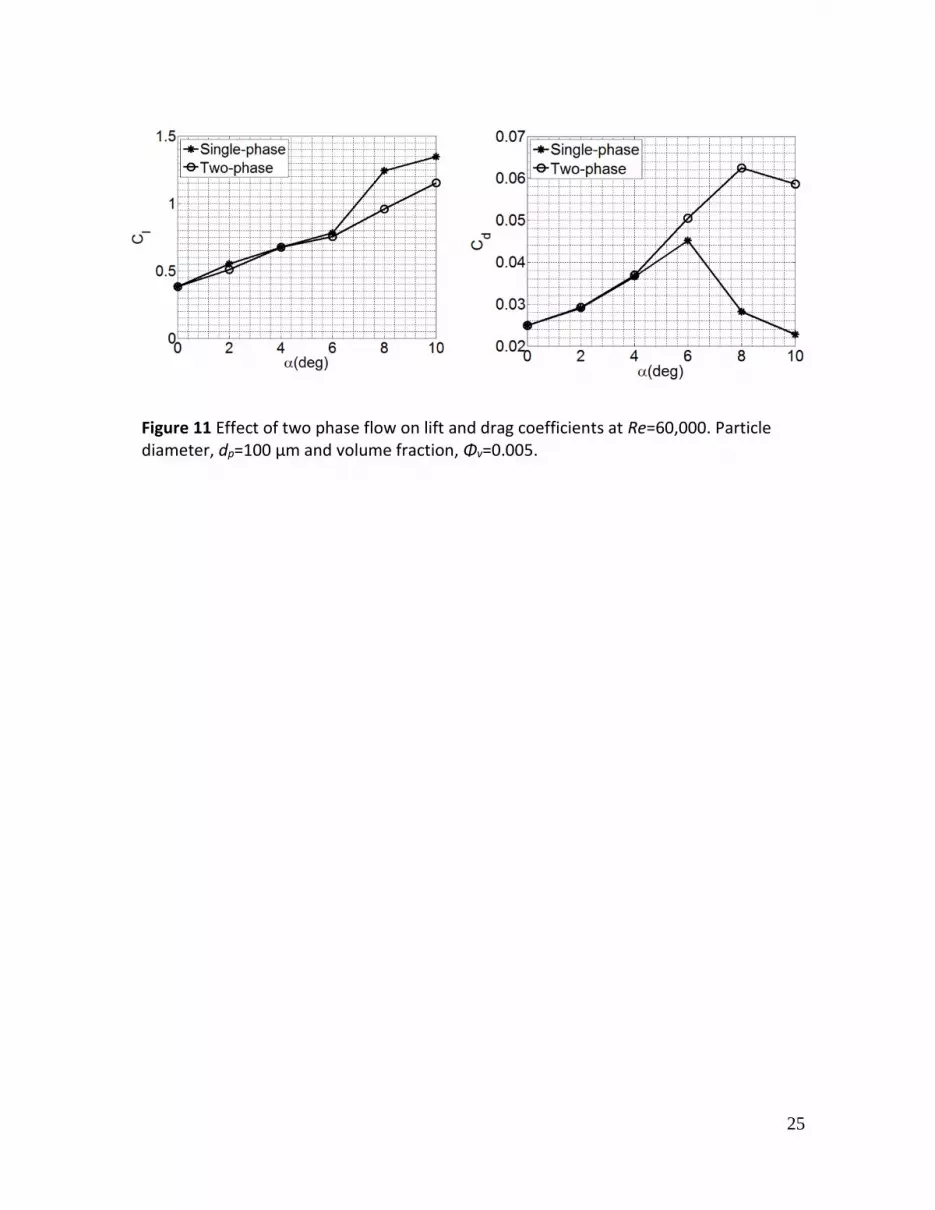
collectors to name a few. Figure 10 and fig.11 shows the lift and drag comparison for

single phase and two-phase flow over E387 at Φv=0.1 and 0.005 respectively. The

percentage changes in lift and drag coefficients due to the addition of particles is shown in

10

Table 7 and Table 8. It can be seen from figs. 10 and 11, and Table 8 and 9 that the lift and

drag coefficients changed drastically. Figures 10 and 11 show that the trend in the lift and

drag coefficients as a function of angle of attack is similar for both volume fractions. One

significant difference is that the increase in the drag is much higher for Φv=0.1 compared

to Φv=0.005, which is primarily due to reduction in the fluid momentum due to particles.

For Φv=0.1, it can be seen that both the lift and drag increased for α=00-60 but for

α=80-100 lift decreased and drag increased (refer fig.10 and Table 7). The increase in the

drag is much higher compared to the decrease in the lift. To understand the reasons for

this drastic change in lift and drag coefficients, particle volume fraction contours were

plotted as shown in fig.12 for α=80. It was observed that particles are concentrated near

the leading edge for all the cases, similar to those observed in previous studies of particle

laden flow over gas turbine blades [5]. Interestingly, for Re=60,000and α=80 (shown in

fig.12) and 100, higher preferential concentration was observed on the top surface of the

airfoil, unlike only on the bottom for Re=460,000. The particles were seen trapped in the

separation region thereby leading to localized wake shedding in that region. Due to the

localized shedding, the turbulence intensity is attenuated leading to momentum deficit,

and increase in the local pressure on the top surface. The turbulence attenuation

phenomenon was also observed by Poelma et al. [11] for values of Φv> 0.003. The reason

for momentum deficit is due to the fact that the fluid turbulence is redistributed in all the

directions due to the localized wake shedding. The particle Reynolds number using the

terminal velocity is ReP=0.83 <100, indicating turbulence attenuation [11]. The 2-D

turbulence kinetic energy, K, was plotted as a function of chord length as shown in fig. 13

for Φv=0.005 and 0.1. For both these values it could be clearly seen that the turbulence

kinetic energy increases for a very brief period, followed by a rapid decrease due to

particle inertia on the top end of the airfoil. Due to the momentum deficit the localized

pressure increases, leading to an overall reduction in the differential pressure between

the top and bottom surfaces, hence resulting in lower lift coefficients. At the trailing edge,

the value of K increases again, pointing to the flow regaining momentum as the flow

reattaches, causing increase in the form (pressure) drag. Thus, even though the skin

friction component of drag decreases due to momentum deficit, the increase in form drag

results in higher drag coefficients as observed in fig. 11. The initial increase in the K for the

two phase case is due to the flow acceleration owing to energy release from particle

turbulence into the mean flow [16]. Another point to note in the K values for ΦV=0.005 is

that at the trailing edge, the increase in the turbulent kinetic energy is lower than that for

ΦV=0.1. This is due to the distribution of particles, which delays the flow reattachment.

Due to this the increase in the drag is lower for ΦV=0.005 compared to ΦV=0.1. The size of

the separation region and the concentration amount were also studied to further enhance

11

our understanding of drag and lift behavior. It was noted that the size of the separation

region increased (see fig. 12) due to the higher concentration of particles on the top

surface of the airfoil, modifying the displacement thickness, δ*, and thereby increasing the

drag and reducing the lift.

For Φv=0.005, the lift decreased and drag increased for all angles of attack under

study, α=00-100 (refer fig.11 and Table 8). The volume fraction contours showed that the

preferential concentration on the top surface of the airfoil was more pronounced at this

volume fraction. This difference could be attributed to the increased inertia of the

continuous phase at higher volume fraction thereby pushing most of the particles out of

the airfoil boundary layer region. The lower inertia of the continuous phase for smaller

volume fraction allows more particles to loiter in the separation region of the airfoil.

4 Conclusions

A numerical study using ANSYS FLUENT revealed that multiphase particle laden flows over

Eppler 387 airfoil has different flow characteristics compared to clean flow. Firstly, the

turbulence model (SST k-) was validated for the single-phase case with the help of

available experimental data [9, 15]. For the Reynolds numbers used in the present study,

this turbulence model has not been validated so far, and we have successfully done it for

the first time. A reasonably good match was found between the computational and

experimental results, wherein the maximum uncertainty was within ε≈30% for

Re=60,000 and ε≈10% for Re=460,000. The higher error at lower Reynolds number is

probably due to the transitional nature of the flow at Re=60,000.

The model was later extended to multiphase flow with the addition of mixture

model. It was found that adding even a small concentration of particles (Φv10%)

produces considerable differences in lift and drag characteristics on the airfoil. This effect

was more pronounced at moderate Reynolds number, Re=60,000, and at higher angles of

attack, i.e., >60, where lift decreased and drag increased drastically by about 200%. It

was found that the prime contributor in the increased drag force was the pressure

component of drag.

Contour plots of particle fraction revealed that particles get preferentially

concentrated on the top surface of the airfoil and are trapped in the separation region,

thereby increasing the size of the separation region (LSB). The bigger separation region

resulted in higher values of form drag of the airfoil by increasing the shape factor (i.e.

increased displacement thickness) *, which contributed to increased adverse pressure

gradient on the top surface of the airfoil. The enhancement in the viscous drag is not

12

much because the velocity fluctuations are an order of magnitude different due to dilute

particle concentrations.

This increase in the (length or width) of the separation region depends on various

factors like the Reynolds number, angle of attack, volume fractions, size of the particulate

phase, which could form scope of future work.

Acknowledgements

The corresponding author (SB) acknowledges the funding in the form of Institute seed

grant from Indian Institute of Technology, Bombay for this research work.

Nomenclature

c [m] chord of the airfoil

Cl [-] coefficient of lift

Cd [-] coefficient of drag

Cp [-] coefficient of pressure

Re [-] Reynolds number

Φv [-] volume fraction

α [degrees] angle of attack

REFERENCES

[1] Balachandar S. and Eaton J.K. (2010), “Turbulent dispersed multiphase flows”,

Annu. Rev. Fluid Mech. 42:111-133

[2] FLUENT theory guide, ANSYS Release 14.0, November 2011

[3] Grant, G. and Tabakoff, W. (1975), “Erosion Prediction in Turbomachinery

Resulting from Environmental Particles,” Journal of Aircraft, 12:5:471-478

[4] Grundy, T. M., Keefe, G. P., and Lowson, M. V. (2000), “Effects of acoustic

disturbances on low Re airfoil flows” In Proc. Conf. on Fixed, Flapping and Rotary

Wing Vehicles at Very Low Reynolds Numbers, pp. 91–113.

13

[5] Hamed A., Tabakoff W. and Wenglarz R. (2006), “Erosion and Deposition in

Turbomachinery”, Journal of Propulsion and Power Vol. 22, No. 2

[6] Laitone, E. V. (1997), “Wind tunnel tests of wings at Reynolds numbers below

70000”, Experiments in Fluids 23: 405–409

[7] Langtry, R.B. and Menter F.R. (2005), “Transition Modelling for General CFD

Applications in Aeronautics”, AIAA-522

[8] Menter, F.R. (1994), "Two-Equation Eddy-Viscosity Turbulence Models for

Engineering Applications". AIAA Journal. 32(8). 1598–1605

[9] McGhee, R.J., Walker, B.S., and Millard, B.F. (1988), “Experimental Results for

Eppler 387 airfoil at low Reynolds numbers in the Langley low-turbulence pressure

tunnel”, Langley Research Centre, Virginia

[10] Narsipur, S., Pomeroy, B.W. and Selig, M.S. (2012), “CFD Analysis of Multielement

Airfoils for Wind Turbines” 30th AIAA Applied Aerodynamics Conference, New

Orleans

[11] Poelma C., Westerweel J. and Ooms G. (2007), “Particle-fluid interactions in grid-

generated turbulence”, J. Fluid Mech. 589:315-351

[12] Schlichting, H., and Gersten, K., “Boundary-Layer Theory”, Springer Publications,

2000

[13] Selig, M. S., Guglielmo, J. J., Broeren, A. P., and Giguere, P. (1995), “Summary of

Low-Speed Airfoil Data vol. 1”. SoarTech Publications, Virginia Beach, Virginia

[14] Selig, M. S., Lyon, C.A., Giguere, P., Ninham, C. P., Guglielmo, J. J. (1996),

“Summary of Low-Speed Airfoil Data vol. 2”. SoarTech Publications, Virginia Beach,

Virginia

[15] Williamson, G.A., McGranahan, B.D., Broughton, B.A., Deters, R.W., Brandt, J.B.

and Selig, M.S. (2012), “Summary of Low-Speed Airfoil Data vol.5”, SoarTech

Publications, Virginia Beach, Virginia

14

[16] U. Frisch. Turbulence: The Legacy of A. N. Kolmogorov. Cambridge University Press,

1995.

15

Figures

Figure 1 Computational mesh (a) around the E387 airfoil (b) Hybrid grid spreading out from the airfoil surface.

16

Figure 2 (Top figure) Velocity contours around Eppler 387, and (Bottom figure) effect of first node distance (1x10-05 m) on the flow dynamics at Re=460,000.

17

Figure 3 (Top figure) Velocity contours around Eppler 387, and (Bottom figure) effect of

first node distance (5x10-06m) on the flow dynamics at Re=460,000.

18

Figure 4 Comparison plots of lift and drag coefficient as a function of angle of attack at

Re=460,000 for single-phase flow.

19

Figure 5 Comparison plots of pressure coefficient for α=40 (left) and α=60 (right) at

Re=460,000 for single-phase flow.

20

Figure 6 Comparison plots of lift and drag coefficients at Re=60,000 for single-phase flow

at different angles of attack.

21

Figure 7 Comparison plots of pressure contours for α=40 (left) and 60 (right) at Re=60,000

for single phase flow.

22

Figure 8 Drag polar comparison for Re=60,000 for single phase flow over E387.

23

Figure 9 Effect of two phase flow on lift and drag coefficients at Re=460,000 for E 387 airfoil. Particle diameter, dp=100 µm and volume fraction, Φv=0.1.

24

Figure 10 Effect of two phase flow on lift and drag coefficients at Re=60,000 for E 387 airfoil. Particle diameter, dp=100 µm and volume fraction, Φv=0.1.

25

Figure 11 Effect of two phase flow on lift and drag coefficients at Re=60,000. Particle diameter, dp=100 µm and volume fraction, Φv=0.005.

26

Figure 12 Sand volume fraction contours at α=80 for Re=60,000, dp=100 µm, volume

fraction, Φv=0.1 (top) and Φv=0.005 (bottom).

27

Figure 13 Turbulent kinetic energy comparison plot for α=80 for Re=60,000, dp=100 µm, volume fraction, Φv=0.1 (left) and Φv=0.005 (right).

28

Table1 Effect of first node distance y on lift and drag characteristics at Re=460,000 and

α=40

Grid y (m) Flow Coefficient

of lift

Coefficient

of drag

Experimental

Coefficient of

lift

Experimental

Coefficient of

drag

1 1*10-05 Unsteady 0.8089 0.00881 0.792 0.0086

2 5*10-06 Steady 0.8159 0.0092

29

Table2 Effect of number of points on airfoil on lift and drag characteristics at Re=460,000

and α=40

Configuration Number

of points

Coefficient

of lift

Coefficient

of drag

Experimental

Coefficient of

lift

Experimental

Coefficient of

drag

1 1088 0.8159 0.0092 0.792 0.0086

2 2188 0.8206 0.0092

30

Table3 Effect of grid refinement on lift and drag characteristics at Re=460,000 and α=40

Grid Number

of cells

Coefficient

of lift

Coefficient

of drag

Experimental

Coefficient of lift

Experimental

Coefficient of

drag

Coarse 211,946 0.8153 0.0092

0.792 0.0086 Medium 307,144 0.8159 0.0092

Fine 412,870 0.8165 0.0092

31

Table4 Comparison of lift and drag coefficients at Re=460,000

α

Computational

Coefficient of

lift

Computational

Coefficient of

drag

Experimental

Coefficient of

lift

Experimental

Coefficient of

drag

%error

in lift

predic

tion

%error in

drag

prediction

0 0.37655 0.007417 0.360 0.0073 4.6 1.6

2 0.5992 0.00802 0.584 0.0075 2.59 6.33

4 0.8159 0.0092 0.792 0.0086 3.02 6.98

6 1.02587 0.0106 1.009 0.0099 1.67 7.07

8 1.23101 0.0175 1.1652 0.0162 5.66 8

10 1.36545 0.03514 1.248 0.0311 9.41 13

32

Table5 Comparison of Lift and drag coefficients for Re=60,000

α

(deg)

Computational

Coefficient of

lift

Computational

Coefficient of

drag

Experimental

Coefficient of

lift

Experimental

Coefficient of

drag

% error in

lift

prediction

% error in

drag

prediction

0 0.38304 0.02487 0.348 0.0269 10 7.5

2 0.5527 0.02902 0.53 0.0346 4.28 16.13

4 0.6749 0.03651 0.619 0.0485 9.03 24.72

6 0.78223 0.04514 0.752 0.0610 4 26

8 1.2442 0.028238 1.1 0.0391 13.1 27.77

10 1.34695 0.02275 1.2245 0.035 10 35

33

Table6 Percentage change in lift and drag coefficients at Re=460,000, particle diameter,

dp=100 m and volume fraction, Φv=0.1

α

(deg)

Single Phase Two Phase % change

in lift

% change

in drag Coefficient

of lift

Coefficient

of drag

Coefficient

of lift

Coefficient

of drag

0 0.37655 0.007417 0.4204 0.00864 +11.65 +16.49

2 0.5992 0.00802 0.65816 0.00966 +9.84 +20.45

4 0.8159 0.0092 0.90244 0.01168 +10.61 +26.96

6 1.02587 0.0106 1.18829 0.01143 +15.83 +7.83

8 1.23101 0.0175 1.4137 0.0199 +14.84 +13.71

10 1.36545 0.03514 1.46343 0.03559 +7.18 +1.28

34

Table 7 Percentage change in lift and drag coefficients at Re=60,000, particle diameter,

dp=100 µm and volume fraction, Φv=0.1

α

(deg)

Single Phase Two Phase % change

in lift

% change

in drag Coefficient

of lift

Coefficient

of drag

Coefficient

of lift

Coefficient

of drag

0 0.38304 0.02487 0.3911 0.02833 +2.1 +13.91

2 0.5527 0.02902 0.5891 0.0316 +6.59 +8.9

4 0.6749 0.03651 0.7472 0.0428 +10.71 +17.23

6 0.78223 0.04514 0.8619 0.0611 +10.18 +35.36

8 1.2442 0.028238 0.9595 0.0883 -22.88 +212.68

10 1.34695 0.02275 1.1890 0.0865 -11.73 +280.22

35

Table 8 Percentage change in lift and drag coefficients at Re=60000, particle diameter,

dp=100 µm and volume fraction, Φv=0.005

α

(deg)

Single Phase Two Phase % change

in lift

% change

in drag Coefficient

of lift

Coefficient

of drag

Coefficient

of lift

Coefficient

of drag

0 0.38304 0.02487 0.38462 0.02496 +0.41 +0.36

2 0.5527 0.02902 0.50853 0.02925 -7.99 +0.79

4 0.6749 0.03651 0.67585 0.03687 +0.14 +0.98

6 0.78223 0.04514 0.75511 0.05048 -3.47 +11.83

8 1.2442 0.028238 0.96021 0.06243 -22.83 +121.07

10 1.34695 0.02275 1.15243 0.05864 -14.45 +157.76

36

Figure Captions List

Figure 1 Computational mesh (a) around the E387 airfoil (b) Hybrid grid spreading out

from the airfoil surface.

Figure 2 (Top figure) Velocity contours around Eppler 387, and (Bottom figure) effect of

first node distance (1x10-05 m) on the flow dynamics at Re=460,000.

Figure 3(Top figure) Velocity contours around Eppler 387, and (Bottom figure) effect of

first node distance (5x10-06m) on the flow dynamics at Re=460,000.

Figure 4 Comparison plots of lift and drag coefficient as a function of angle of attack at

Re=460,000 for single-phase flow.

Figure 5 Comparison plots of pressure coefficient for α=40 (left) and α=60 (right) at

Re=460,000 for single-phase flow.

Figure 6 Comparison plots of lift and drag coefficients at Re=60,000 for single-phase flow

at different angles of attack.

Figure 7 Comparison plots of pressure contours for α=40 (left) and 60 (right) at Re=60,000

for single phase flow.

Figure 8 Drag polar comparison for Re=60,000 for single phase flow over E387.

Figure 9 Effect of two phase flow on lift and drag coefficients at Re=460,000 for E 387

airfoil. Particle diameter, dp=100 µm and volume fraction, Φv=0.1.

Figure 10 Effect of two phase flow on lift and drag coefficients at Re=60,000 for E 387

airfoil. Particle diameter, dp=100 µm and volume fraction, Φv=0.1.

Figure 11 Effect of two phase flow on lift and drag coefficients at Re=60,000. Particle

diameter, dp=100 µm and volume fraction, Φv=0.005.

Figure 12 Sand volume fraction contours at α=80 for Re=60,000, dp=100 µm, volume

fraction, Φv=0.1 (top) and Φv=0.005 (bottom).

37

Figure 13 Turbulent kinetic energy comparison plot for α=80 for Re=60,000, dp=100 µm,

volume fraction, Φv=0.1 (left) and Φv=0.005 (right).

Table Caption List

Table 1 Effect of first node distance y on lift and drag characteristics at Re=460,000 and

α=40

Table 2 Effect of number of points on airfoil on lift and drag characteristics at Re=460,000

and α=40

Table 3 Effect of grid refinement on lift and drag characteristics at Re=460,000 and α=40

Table 4 Comparison of lift and drag coefficients at Re=460,000

Table 5 Comparison of Lift and drag coefficients for Re=60,000

Table 6 Percentage change in lift and drag coefficients at Re=460,000, particle diameter,

dp=100 m and volume fraction, Φv=0.1

Table 7 Percentage change in lift and drag coefficients at Re=60,000, particle diameter,

dp=100 µm and volume fraction, Φv=0.1

Table 8 Percentage change in lift and drag coefficients at Re=60000, particle diameter,

dp=100 µm and volume fraction, Φv=0.005