Embed Size (px)
Citation preview

Development of LRFD Procedures for Bridge Pile Foundations in Iowa
Final ReportSeptember 2011
Sponsored byIowa Highway Research Board(IHRB Project TR-583)Iowa Department of Transportation(InTrans Project 08-312)
Volume II: Field Testing of Steel Piles in Clay, Sand, and Mixed Soils and Data Analysis

About the Bridge Engineering CenterThe mission of the Bridge Engineering Center (BEC) is to conduct research on bridge technologies to help bridge designers/owners design, build, and maintain long-lasting bridges.
About the Institute for Transportation The mission of the Institute for Transportation (InTrans) at Iowa State University is to develop and implement innovative methods, materials, and technologies for improving transportation efficiency, safety, reliability, and sustainability while improving the learning environment of students, faculty, and staff in transportation-related fields.
Disclaimer NoticeThe contents of this report reflect the views of the authors, who are responsible for the facts and the accuracy of the information presented herein. The opinions, findings and conclusions expressed in this publication are those of the authors and not necessarily those of the sponsors.
The sponsors assume no liability for the contents or use of the information contained in this document. This report does not constitute a standard, specification, or regulation.
The sponsors do not endorse products or manufacturers. Trademarks or manufacturers’ names appear in this report only because they are considered essential to the objective of the document.
Non-Discrimination Statement Iowa State University does not discriminate on the basis of race, color, age, religion, national origin, sexual orientation, gender identity, genetic information, sex, marital status, disability, or status as a U.S. veteran. Inquiries can be directed to the Director of Equal Opportunity and Compliance, 3280 Beardshear Hall, (515) 294-7612.
Iowa Department of Transportation Statements Federal and state laws prohibit employment and/or public accommodation discrimination on the basis of age, color, creed, disability, gender identity, national origin, pregnancy, race, religion, sex, sexual orientation or veteran’s status. If you believe you have been discriminated against, please contact the Iowa Civil Rights Commission at 800-457-4416 or Iowa Department of Transportation’s affirmative action officer. If you need accommodations because of a disability to access the Iowa Department of Transportation’s services, contact the agency’s affirmative action officer at 800-262-0003.
The preparation of this (report, document, etc.) was financed in part through funds provided by the Iowa Department of Transportation through its “Agreement for the Management of Research Conducted by Iowa State University for the Iowa Department of Transportation,” and its amendments.
The opinions, findings, and conclusions expressed in this publication are those of the authors and not necessarily those of the Iowa Department of Transportation.
Technical Report Documentation Page
1. Report No. 2. Government Accession No. 3. Recipient’s Catalog No.
IHRB Project TR-583
4. Title and Subtitle 5. Report Date
Development of LRFD Design Procedures for Bridge Piles in Iowa – Field Testing
of Steel H-Piles in Clay, Sand, and Mixed Soils and Data Analysis (Volume II)
September 2011
6. Performing Organization Code
7. Author(s) 8. Performing Organization Report No.
Kam Weng Ng, Muhannad T. Suleiman, Matthew Roling, Sherif S. AbdelSalam,
and Sri Sritharan
InTrans Project 08-312
9. Performing Organization Name and Address 10. Work Unit No. (TRAIS)
Institute for Transportation
Iowa State University
2711 South Loop Drive, Suite 4700
Ames, IA 50010-8664
11. Contract or Grant No.
12. Sponsoring Organization Name and Address 13. Type of Report and Period Covered
Iowa Highway Research Board
Iowa Department of Transportation
800 Lincoln Way
Ames, IA 50010
Final Report
14. Sponsoring Agency Code
15. Supplementary Notes
Visit www.intrans.iastate.edu for color PDF files of this and other research reports.
16. Abstract
In response to the mandate on Load and Resistance Factor Design (LRFD) implementations by the Federal Highway Administration
(FHWA) on all new bridge projects initiated after October 1, 2007, the Iowa Highway Research Board (IHRB) sponsored these research
projects to develop regional LRFD recommendations.
The LRFD development was performed using the Iowa Department of Transportation (DOT) Pile Load Test database (PILOT). To
increase the data points for LRFD development, develop LRFD recommendations for dynamic methods, and validate the results of
LRFD calibration, 10 full-scale field tests on the most commonly used steel H-piles (e.g., HP 10 x 42) were conducted throughout Iowa.
Detailed in situ soil investigations were carried out, push-in pressure cells were installed, and laboratory soil tests were performed. Pile
responses during driving, at the end of driving (EOD), and at re-strikes were monitored using the Pile Driving Analyzer (PDA),
following with the CAse Pile Wave Analysis Program (CAPWAP) analysis. The hammer blow counts were recorded for Wave Equation
Analysis Program (WEAP) and dynamic formulas.
Static load tests (SLTs) were performed and the pile capacities were determined based on the Davisson’s criteria. The extensive
experimental research studies generated important data for analytical and computational investigations. The SLT measured load-
displacements were compared with the simulated results obtained using a model of the TZPILE program and using the modified
borehole shear test method. Two analytical pile setup quantification methods, in terms of soil properties, were developed and validated.
A new calibration procedure was developed to incorporate pile setup into LRFD.
17. Key Words 18. Distribution Statement
BST—CAPWAP—dynamic analysis—LRFD—mBST—PILOT—PDA—static
load test—WEAP
No restrictions.
19. Security Classification (of this
report)
20. Security Classification (of this
page)
21. No. of Pages 22. Price
Unclassified. Unclassified. 226 NA
Form DOT F 1700.7 (8-72) Reproduction of completed page authorized

Development of LRFD Design Procedures for Bridge Piles in
Iowa – Field Testing of Steel H-Piles in Clay, Sand, and
Mixed Soils and Data Analysis
Final Report-Volume II
September 2011
Principal Investigator
Sri Sritharan
Wilson Engineering Professor
Department of Civil, Construction, and Environmental Engineering, Iowa State University
Research Associate
Muhannad T. Suleiman
Assistant Professor
Department of Civil and Environmental Engineering, Lehigh University
Research Assistant
Kam Weng Ng
Matthew Roling
Sherif S. AbdelSalam
Authors
Kam Weng Ng, Muhannad T. Suleiman, Matthew Roling, Sherif S. AbdelSalam,
and Sri Sritharan
Sponsored by
The Iowa Highway Research Board
(IHRB Project TR-583)
Preparation of this report was financed in part
through funds provided by the Iowa Department of Transportation
through its research management agreement with the
Institute for Transportation
(In Trans Project 08-312)
A report from
Institute for Transportation
Iowa State University
2711 South Loop Drive, Suite 4700
Ames, IA 50010-8664
Phone: 515-294-8103
Fax: 515-294-0467
www.intrans.iastate.edu


v
TABLE OF CONTENTS
ACKNOWLEDGMENTS .............................................................................................................xv
CHAPTER 1: OVERVIEW .............................................................................................................1
1.1. Background ...................................................................................................................1
1.2. Scope of Research Projects ...........................................................................................1
1.3. Report Content ..............................................................................................................2
CHAPTER 2: SELECTION OF TEST LOCATIONS ....................................................................3
2.1. Criteria of Selecting Test Locations .............................................................................3
2.2. Selected Test Pile Locations .........................................................................................5
CHAPTER 3: SITE CHARACTERIZATION ................................................................................7
3.1. Standard Penetration Tests (SPT) .................................................................................7
3.2. Cone Penetration Tests (CPT) ....................................................................................10
3.3. Borehole Shear Tests (BST) .......................................................................................14
3.4. Modified Borehole Shear Tests (mBST) ....................................................................16
3.5. Laboratory Soil Tests ..................................................................................................18
3.6. Pore Water and Lateral Earth Pressure Measurements ...............................................23
CHAPTER 4: FULL-SCALE TESTS ...........................................................................................28
4.1. Pile Type and Properties .............................................................................................28
4.2. Hammer Types ............................................................................................................29
4.3. Strain Gauge Instrumentation .....................................................................................30
4.4. Pile Driving Analyzer (PDA) Tests ............................................................................33
4.5. CAse Pile Wave Analysis Program (CAPWAP) ........................................................40
4.6. Wave Equation Analysis Program (WEAP) ...............................................................44
4.7. Vertical Static Load Tests ...........................................................................................56
CHAPTER 5: INTERPRETATION AND ANALYSIS OF FIELD DATA .................................64
5.1. Introduction .................................................................................................................64
5.2. Pile Resistance Distribution ........................................................................................64
5.3. Load Transfer Analysis Using mBST and TZPILE Program .....................................67
5.4. Interpretation of Push-In Pressure Cell Measurements ..............................................67
5.5. Pile Responses over Time ...........................................................................................69
5.6. Pile Setup in Clay Profile ............................................................................................75
CHAPTER 6: SUMMARY............................................................................................................98
CHAPTER 7: CONCLUSIONS ..................................................................................................100
REFERENCES ............................................................................................................................103
APPENDIX A: LOCATIONS OF TEST PILES AND IN SITU SOIL TESTS .........................107
APPENDIX B: RESULTS OF IN SITU SOIL INVESTIGATIONS AND SOIL PROFILES ..112
B.2. Estimated Soil Profiles and Properties Based on Cone Penetration Tests (CPT) ....123
B.3. Pore Water Pressure Measurements Using Cone Penetration Tests (CPT) .............127
vi
B.4. Borehole Shear Test and modified Borehole Shear Test Results .............................131
B.5. Soil Classification and Properties Obtained from Gradation and Atterberg
Limit Tests .......................................................................................................................143
B.6. Total Lateral Earth and Pore Water Pressure Measurements using Push-in
Pressure Cells (PCs) .........................................................................................................146
APPENDIX C: DETAILS OF FULL-SCALE PILE TESTS ......................................................149
C.1. Locations of Strain Gauges along Test Piles ............................................................150
C.2. Pile Driving Analyzer (PDA) Measurements...........................................................158
C.3. Schematic Drawing and Configuration of the Vertical Static Load Tests ...............179
C.4. Static Load Test Load and Displacement .................................................................189
APPENDIX D: DATA INTERPRETATION AND ANALYSIS ...............................................194
D.1. Static Load Test Pile Force Transferred Profiles .....................................................194
D.2. Shaft Resistance Distribution ...................................................................................200
D.3. Pile Driving Resistance ............................................................................................204
D.4. Relationship between Soil Properties and Pile Shaft Resistance Gain ....................208
vii
LIST OF FIGURES
Figure 2.1. Iowa geological map and the test pile locations ............................................................4
Figure 2.2. Distribution of steel H-piles by soil profiles .................................................................5
Figure 3.1. Typical Standard Penetration Test (SPT) ......................................................................8
Figure 3.2. In-situ soil investigations and soil profile for ISU5 at Clarke County (CPT 3) ............9
Figure 3.3. Typical Cone Penetration Test (CPT) .........................................................................10
Figure 3.4. Increase in pore pressure for ISU5 at a depth of 38.55-ft ...........................................12
Figure 3.5. Pore pressure dissipation result for ISU2 at a depth of 35.4-ft ...................................12
Figure 3.6. The conventional Borehole Shear Test (BST) equipment (adapted from Handy,
1986) ..................................................................................................................................14
Figure 3.7. BST generated Mohr-Coulomb shear failure envelope for ISU5 at 8.83-ft depth ......15
Figure 3.8. BST generated shear stress-displacement relationship at different applied normal
stress for ISU5 at 8.83-ft depth ..........................................................................................15
Figure 3.9. The modified Borehole Shear Test (mBST) equipment (adapted from Handy,
1986) ..................................................................................................................................16
Figure 3.10. mBST generated shear stress-displacement relationship at different applied
normal stress for ISU5 at 8.83-ft depth ..............................................................................17
Figure 3.11. mBST generated Mohr-Coulomb interface shear failure envelop for ISU5 at
8.83 ft depth .......................................................................................................................17
Figure 3.12. Laboratory soil tests ..................................................................................................18
Figure 3.13. Grain size distribution curve for disturbed sample DS-1 at 3 ft depth of ISU5 ........19
Figure 3.14. Laboratory soil consolidation tests ............................................................................21
Figure 3.15. The e-log(σ) curve for evaluating pre-consolidation stress from Casagrande’s
Method for specimen Clarke-25 ........................................................................................22
Figure 3.16. Measurement of pore water and lateral earth pressures using Geokon push-in
pressure cells at the field ....................................................................................................24
Figure 3.17. Total lateral earth pressure and pore water pressure measurements from PC1 at
test pile ISU5 with respect to the time ...............................................................................26
Figure 3.18. Total lateral earth pressure and pore water pressure measurements from PC3
and PC4 at test pile ISU6 with respect to the time ............................................................27
Figure 4.1. Cross sectional view of the steel H-piles .....................................................................29
Figure 4.2. Single acting open end diesel hammer (adapted from Pile Dynamics, Inc., 2005) .....30
Figure 4.3. Strain gauges arrangement at a cross sectional view of a steel H-pile ........................31
Figure 4.4. Strain gauges installation, protection, and covered by angles .....................................31
Figure 4.5. Angle bars were chamfered to form a pointed end at pile toe .....................................31
Figure 4.6. Location of strain gauges along the ISU5 test pile at Clarke County .........................32
Figure 4.7. Typical Pile Driving Analyzer (PDA) set up (from Pile Dynamics, Inc., 1996) ........35
Figure 4.8. PDA force and velocity records during driving and at EOD for ISU5 .......................36
Figure 4.9. PDA force and velocity records during re-strikes for ISU5 ........................................37
Figure 4.10. Wave-up and velocity measurement for ISU5 at EOD used to determine shaft
resistance ............................................................................................................................38
Figure 4.11. Typical CAPWAP model for ISU5 at EOD ..............................................................41
Figure 4.12. Results of CAPWAP signals matching for ISU5 at EOD .........................................42
Figure 4.13. Wave equation models for different hammers (adapted from Hannigan et al.
1998) ..................................................................................................................................44
Figure 4.14. WEAP generated bearing graph for ISU5 at EOD using the Iowa DOT method .....54

viii
Figure 4.15. WEAP estimated pile stresses for ISU5 at EOD using the Iowa DOT method ........55
Figure 4.16. Minimal buckling on flanges at pile head .................................................................57
Figure 4.17. Schematic drawing of vertical static load test for ISU5 at Clarke County ................58
Figure 4.18. Configuration of two anchor piles and a test pile for ISU5 at Clarke County ..........59
Figure 4.19. Setting up of the static load test .................................................................................60
Figure 4.20. Pile top vertical displacement transducers instrumentation ......................................62
Figure 4.21. A load-displacement curve and Davisson’s criteria for ISU5 at Clarke County .......62
Figure 5.1. Pile force distribution along the embedded pile length of test pile ISU5 ....................65
Figure 5.2. SLT measured and CAPWAP estimated pile shaft resistance distributions for test
pile ISU5 ............................................................................................................................66
Figure 5.3. Pile driving resistance in terms of hammer blow count ..............................................70
Figure 5.4. Relationship between total pile resistance and time for clay profile ...........................71
Figure 5.5. Relationship between total pile resistance and time for mixed soil profile .................72
Figure 5.6. Relationship between total pile resistance and time for sand profile ..........................72
Figure 5.7. Relationship between resistance components and time for clay profile......................74
Figure 5.8. Relationship between resistance components and time for mixed soil profile ...........75
Figure 5.9. Relationship between soil properties and increase in shaft resistance for ISU5 .........76
Figure 5.10. Correlations of both vertical and horizontal coefficients of consolidation with
SPT N-values .....................................................................................................................77
Figure 5.11. Relationships between percent gain in pile capacity and (a) SPT N-value, (b) Ch,
(c) Cv, and (d) PI, estimated at a time of 1 day after EOD for all sites ..............................79
Figure 5.12. Linear best fit lines of normalized pile resistance and logarithmic normalized
time ....................................................................................................................................82
Figure 5.13. Correlation between pile setup rate (C) and soil parameters with pile radius ...........82
Figure 5.14. Correlation between pile setup rate (C) and average SPT N-value ...........................84
Figure 5.15. Pile setup design charts for WEAP and CAPWAP ...................................................85
Figure 5.16. Pile setup site verification charts for WEAP and CAPWAP ....................................86
Figure 5.17. Pile setup comparison and validation ........................................................................88
Figure 5.18. Pile setup confidence levels.......................................................................................90
Figure 5.19. Different uncertainties involved between EOD and setup ........................................93
Figure 5.20. Resistance factor for pile setup resistance .................................................................94
Figure 5.21. Histogram and theoretical normal distribution of α values based on information
of production piles at ISU field test sites ...........................................................................95
Figure 5.22. Histogram and theoretical normal distribution of α values based on additional
data of production piles in Iowa.........................................................................................97
Figure A.1. Test Pile ISU1 at Mahaska County...........................................................................107
Figure A.2. Test Pile ISU2 at Mills County.................................................................................108
Figure A.3. Test Pile ISU3 at Polk County ..................................................................................108
Figure A.4. Test Pile ISU4 at Jasper County ...............................................................................109
Figure A.5. Test Pile ISU5 at Clark County ................................................................................109
Figure A.6. Test Piles ISU6 and ISU7 at Buchanan County .......................................................110
Figure A.7. Test Pile ISU8 at Poweshiek County ........................................................................110
Figure A.8. Test Pile ISU9 at Des Moines County ......................................................................111
Figure A.9. Test Pile ISU10 at Cedar County .............................................................................111

ix
Figure B.1.1. In-situ soil investigations and soil profile for ISU1 at Mahaska County...............113
Figure B.1.2. In-situ soil investigations and soil profile for ISU2 at Mills County.....................114
Figure B.1.3. In-situ soil investigations and soil profile for ISU3 at Polk County ......................115
Figure B.1.4. In-situ soil investigations and soil profile for ISU4 at Jasper County ...................116
Figure B.1.5. Cone Penetration Tests and soil profile for ISU5 at Clarke County ......................117
Figure B.1.6. In-situ soil investigations and soil profile for ISU5 at Clarke County ..................118
Figure B.1.7. In-situ soil investigations and soil profile for ISU6 and ISU7 at Buchanan
County ..............................................................................................................................119
Figure B.1.8. In-situ soil investigations and soil profile for ISU8 at Poweshiek County ............120
Figure B.1.9. In-situ soil investigations and soil profile for ISU9 at Des Moines County ..........121
Figure B.1.10. In-situ soil investigations and soil profile for ISU10 at Cedar County ...............122
Figure B.3.1. CPT pore water pressure dissipation tests at ISU2 Mills County ..........................127
Figure B.3.2. CPT pore water pressure dissipation tests at ISU3 Polk County ...........................127
Figure B.3.3. CPT pore water pressure dissipation tests at ISU4 Jasper County ........................128
Figure B.3.4. CPT pore water pressure dissipation tests at ISU5 Clarke County........................128
Figure B.3.5. CPT pore water pressure dissipation tests at ISU6 and ISU7 Buchanan County ..129
Figure B.3.6. CPT pore water pressure dissipation tests at ISU8 Poweshiek County .................129
Figure B.3.7. CPT pore water pressure dissipation tests at ISU9 Des Moines County ...............130
Figure B.4.1. ISU1 at 3-ft depth (BST) .......................................................................................131
Figure B.4.2. ISU1 at 8-ft depth (BST) .......................................................................................131
Figure B.4.3. ISU1 at 16-ft depth (BST) .....................................................................................131
Figure B.4.4. ISU2 at 5-ft depth (BST) .......................................................................................132
Figure B.4.5. ISU2 at 20-ft depth (BST) .....................................................................................132
Figure B.4.6. ISU3 at 4-ft depth (BST) .......................................................................................132
Figure B.4.7. ISU3 at 23-ft depth (BST) .....................................................................................133
Figure B.4.8. ISU4 at 27-ft depth (BST & mBST) ......................................................................133
Figure B.4.9. ISU4 at 46-ft depth (BST & mBST) ......................................................................133
Figure B.4.10. BST and mBST generated shear stress-displacement relationships for ISU4
at 27-ft depth ....................................................................................................................134
Figure B.4.11. BST and mBST generated shear stress-displacement relationships for ISU4
at 46-ft depth ....................................................................................................................134
Figure B.4.12. ISU5 at 8.83-ft depth (BST & mBST) .................................................................135
Figure B.4.13. ISU5 at 23.83-ft depth (BST & mBST) ...............................................................135
Figure B.4.14. ISU5 at 35.83-ft depth (BST & mBST) ...............................................................135
Figure B.4.15. BST and mBST generated shear stress-displacement relationships for ISU5
at 8.83-ft depth .................................................................................................................136
Figure B.4.16. BST and mBST generated shear stress-displacement relationships for ISU5
at 23.83-ft depth ...............................................................................................................136
Figure B.4.17. BST and mBST generated shear stress-displacement relationships for ISU5
at 35.83-ft depth ...............................................................................................................137
Figure B.4.18. ISU6 and ISU7 at 8.3-ft depth (BST & mBST) ...................................................137
Figure B.4.19. ISU6 and ISU7 at 11.89-ft depth (BST & mBST) ...............................................138
Figure B.4.20. ISU6 and ISU7 at 50.3-ft depth (BST & mBST) .................................................138
x
Figure B.4.21. BST and mBST generated shear stress-displacement relationships for ISU6
and ISU7 at 8.3-ft depth ...................................................................................................138
Figure B.4.22. BST and mBST generated shear stress-displacement relationships for ISU6
and ISU7 at 11.89-ft depth ...............................................................................................139
Figure B.4.23. BST and mBST generated shear stress-displacement relationships for ISU6
and ISU7 at 50.3-ft depth .................................................................................................139
Figure B.4.24. ISU8 at 9-ft depth (BST & mBST) ......................................................................140
Figure B.4.25. ISU8 at 23-ft depth (BST & mBST) ....................................................................140
Figure B.4.26. ISU8 at 45-ft depth (BST & mBST) ....................................................................140
Figure B.4.27. BST and mBST generated shear stress-displacement relationships for ISU8 at
9-ft depth ..........................................................................................................................141
Figure B.4.28. BST and mBST generated shear stress-displacement relationships for ISU8 at
23-ft depth ........................................................................................................................141
Figure B.4.29. BST and mBST generated shear stress-displacement relationships for ISU8 at
45-ft depth ........................................................................................................................142
Figure B.6.1. Total lateral earth and pore water pressure measurements from PC1 at test pile
ISU7 .................................................................................................................................146
Figure B.6.2. Total lateral earth and pore water pressure measurements from PC4 at test pile
ISU8 .................................................................................................................................147
Figure B.6.3. Total lateral earth and pore water pressure measurements from PC4 at test pile
ISU10 ...............................................................................................................................148
Figure C.1.1. Location of strain gauges along the ISU2 test pile at Mills County ......................150
Figure C.1.2. Location of strain gauges along the ISU3 test pile at Polk County .......................151
Figure C.1.3. Location of strain gauges along the ISU4 test pile at Jasper County ....................152
Figure C.1.4. Location of strain gauges along the ISU6 test pile at Buchanan County ..............153
Figure C.1.5. Location of strain gauges along the ISU7 test pile at Buchanan County ..............154
Figure C.1.6. Location of strain gauges along the ISU8 test pile at Poweshiek County .............155
Figure C.1.7. Location of strain gauges along the ISU9 test pile at Des Moines County ...........156
Figure C.1.8. Location of strain gauges along the ISU10 test pile at Cedar County ...................157
Figure C.2.1. PDA force and velocity records for ISU1 ..............................................................158
Figure C.2.2. PDA force and velocity records for ISU2 ..............................................................159
Figure C.2.3. PDA force and velocity records for ISU3 ..............................................................161
Figure C.2.4. PDA force and velocity records for ISU4 ..............................................................163
Figure C.2.5. PDA force and velocity records for ISU5 ..............................................................166
Figure C.2.6. PDA force and velocity records for ISU6 ..............................................................169
Figure C.2.7. PDA force and velocity records for ISU7 ..............................................................171
Figure C.2.8. PDA force and velocity records for ISU8 ..............................................................174
Figure C.2.9. PDA force and velocity records for ISU9 ..............................................................176
Figure C.2.10. PDA force and velocity records for ISU10 ..........................................................178
xi
Figure C.3.1. Configuration of four anchor piles and a steel test pile for ISU1 at Mahaska
County ..............................................................................................................................179
Figure C.3.2. Configuration of two anchor piles and a steel test pile for ISU2 at Mills
County ..............................................................................................................................179
Figure C.3.3. Configuration of two anchor piles and a steel test pile for ISU3 at Polk
County ..............................................................................................................................179
Figure C.3.4. Configuration of two anchor piles and a steel test pile for ISU4 at Jasper
County ..............................................................................................................................180
Figure C.3.5. Configuration of two anchor piles and two steel test piles for ISU6 and ISU7
at Buchanan County .........................................................................................................180
Figure C.3.6. Configuration of two anchor piles and a steel test pile for ISU8 at Poweshiek
County ..............................................................................................................................180
Figure C.3.7. Configuration of two anchor piles and a steel test pile for ISU9 at Des Moines
County ..............................................................................................................................181
Figure C.3.8. Configuration of two anchor piles and a steel test pile for ISU10 at Cedar
County ..............................................................................................................................181
Figure C.3.9. Schematic drawing of vertical static load test for ISU1 at Mahaska County ........182
Figure C.3.10. Schematic drawing of vertical static load test for ISU2 at Mills County ............183
Figure C.3.11. Schematic drawing of vertical static load test for ISU3 at Polk County .............184
Figure C.3.12. Schematic drawing of vertical static load test for ISU4 at Jasper County ...........185
Figure C.3.13. Schematic drawing of vertical static load tests for ISU6 and ISU7 at
Buchanan County .............................................................................................................186
Figure C.3.14. Schematic drawing of vertical static load test for ISU8 at Poweshiek County ...187
Figure C.3. 15. Schematic drawing of vertical static load tests for ISU9 and ISU10 at
Des Moines County and Cedar County respectively .......................................................188
Figure C.4.1. A load-displacement curve and Davisson’s criteria for ISU1 at Mahaska
County ..............................................................................................................................189
Figure C.4.2. A load-displacement curve and Davisson’s criteria for ISU2 at Mills County .....189
Figure C.4.3. A load-displacement curve and Davisson’s criteria for ISU3 at Polk County ......190
Figure C.4.4. A load-displacement curve and Davisson’s criteria for ISU4 at Jasper County ....190
Figure C.4.5. A load-displacement curve and Davisson’s criteria for ISU6 at Buchanan
County ..............................................................................................................................191
Figure C.4.6. A load-displacement curve and Davisson’s criteria for ISU7 at Buchanan
County ..............................................................................................................................191
Figure C.4.7. A load-displacement curve and Davisson’s criteria for ISU8 at Poweshiek
County ..............................................................................................................................192
Figure C.4.8. A load-displacement curve and Davisson’s criteria for ISU9 at Des Moines
County ..............................................................................................................................192
Figure C.4.9. A load-displacement curve and Davisson’s criteria for ISU10 at Cedar
County ..............................................................................................................................193
xii
Figure D.1.1. Pile force distribution along the embedded pile length of the test pile ISU2 ........194
Figure D.1.2. Pile force distribution along the embedded pile length of the test pile ISU3 ........195
Figure D.1.3. Pile force distribution along the embedded pile length of the test pile ISU4 ........196
Figure D.1.4. Pile force distribution along the embedded pile length of the test pile ISU6 ........197
Figure D.1.5. Pile force distribution along the embedded pile length of the test pile ISU8 ........198
Figure D.1.6. Pile force distribution along the embedded pile length of the test pile ISU9 ........199
Figure D.2.1. SLT measured and CAPWAP estimated pile shaft resistance distributions
for test pile ISU2 ..............................................................................................................200
Figure D.2.2. SLT measured and CAPWAP estimated pile shaft resistance distributions
for test pile ISU3 ..............................................................................................................200
Figure D.2.3. SLT measured and CAPWAP estimated pile shaft resistance distributions
for test pile ISU4 ..............................................................................................................201
Figure D.2.4. CAPWAP estimated pile shaft resistance distributions for test pile ISU6 ............201
Figure D.2.5. CAPWAP estimated pile shaft resistance distributions for test pile ISU7 ............202
Figure D.2.6. SLT measured and CAPWAP estimated pile shaft resistance distributions
for test pile ISU8 ..............................................................................................................202
Figure D.2.7. SLT measured and CAPWAP estimated pile shaft resistance distributions
for test pile ISU9 ..............................................................................................................203
Figure D.2.8. CAPWAP estimated pile shaft resistance distributions for test pile ISU10 ..........203
Figure D.3.1. Pile driving resistances for ISU1 and ISU2 in terms of hammer blow count .......204
Figure D.3.2. Pile driving resistances for ISU3 and ISU4 in terms of hammer blow count .......205
Figure D.3.3. Pile driving resistances for ISU6 and ISU7 in terms of hammer blow count .......206
Figure D.3.4. Pile driving resistance for ISU10 (sand profile) in terms of hammer blow
count .................................................................................................................................207
Figure D.4.1. Relationship between soil properties and shaft resistance gain for ISU2..............208
Figure D.4.2. Relationship between soil properties and shaft resistance gain for ISU3..............208
Figure D.4.3. Relationship between soil properties and shaft resistance gain for ISU4..............209
Figure D.4.4. Relationship between soil properties and shaft resistance gain for ISU6..............209
xiii
LIST OF TABLES
Table 3.1. Summary of in-situ and laboratory soil investigations ...................................................7
Table 3.2. Summary of soil parameters at depths of CPT dissipation tests ...................................13
Table 3.3. Summary of soil properties for ISU5 based on CPT ....................................................13
Table 3.4. Soil classification and properties for ISU5 obtained from gradation and
Atterberg’s limit tests .........................................................................................................20
Table 3.5. Summary of the consolidation test results and analyses ...............................................23
Table 3.6. Calibrated factors and zero reading temperature for each pressure cell .......................25
Table 4.1. A572 Grade 50 (Fy = 50 ksi) steel H-pile properties ....................................................28
Table 4.2. Summary of hammer information.................................................................................29
Table 4.3. Schedule of re-strikes and PDA tests ............................................................................33
Table 4.4. Summary of Case damping factors ...............................................................................34
Table 4.5. Summary of Jc, PDA estimated pile static (RMX) and shaft resistances (SFR) ...........38
Table 4.6. Pile damage classification .............................................................................................40
Table 4.7. Summary of CAPWAP estimated total pile resistances and shaft resistances .............42
Table 4.8. Summary of CAPWAP estimated soil quake values ....................................................43
Table 4.9. Summary of CAPWAP estimated soil Smith’s damping factors .................................43
Table 4.10. Summary of static analysis methods used in the five soil profile input procedures ...47
Table 4.11. Soil Parameters for cohesionless soils ........................................................................48
Table 4.12. Soil Parameters for cohesive soils ..............................................................................48
Table 4.13. Empirical values for ø, Dr, and γ of cohesionless soils based on Bowles (1996) ......48
Table 4.14. Empirical values for qu and γ of cohesive soils based on Bowles (1996) ..................48
Table 4.15. Iowa pile design chart for friction bearing Grade 50 steel H-piles .............................49
Table 4.16. Iowa pile design chart for end bearing Grade 50 steel H-piles ...................................50
Table 4.17. Revised Iowa pile design chart used in WEAP for friction bearing Grade 50
steel H-piles .......................................................................................................................51
Table 4.18. Revised Iowa pile design chart used in WEAP for end bearing Grade 50 steel
H-piles ................................................................................................................................52
Table 4.19. WEAP recommended soil quake values (Pile Dynamics, Inc., 2005) ........................53
Table 4.20. WEAP recommended Smith’s damping factors used in ST, SA, Driven and
Iowa Blue Book (Pile Dynamics, Inc., 2005) ....................................................................53
Table 4.21. Damping factors used in the Iowa DOT method ........................................................53
Table 4.22. Measured hammer blow count at EOD and re-strikes ................................................54
Table 4.23. Summary of WEAP estimated pile capacities for all loading stages and all test
piles using different soil input options ...............................................................................55
Table 4.24. Summary of static load test results .............................................................................63
Table 5.1. Summary of shaft resistance and end bearing from static load test results and last
re-strike using CAPWAP ...................................................................................................66
Table 5.2. Percent increase in pile resistance based on CAPWAP and SLT measurements .........73
Table 5.3. Average soil properties along pile shaft and near pile toe ............................................78
Table 5.4. The consolidation (fc) and remolding recovery (fr) factors...........................................83
Table 5.5. Scale (a) and concave (b) factors ..................................................................................84
Table 5.6. Summary of the twelve data records from PILOT .......................................................87
Table 5.7. Summary of the estimated pile resistance including setup ...........................................87
Table 5.8. Anticipated errors of the pile setup methods at various confidence levels ...................89
Table 5.9. Summary of resistance ratio estimators for EOD and setup .........................................92
xiv
Table 5.10. Summary of information on production piles at ISU test sites ...................................95
Table 5.11. Summary of additional data on production piles in Iowa ...........................................96
Table B.2.1. Summary of soil properties for ISU1 based on CPT...............................................123
Table B.2.2. Summary of soil properties for ISU2 based on CPT...............................................123
Table B.2.3. Summary of soil properties for ISU3 based on CPT...............................................124
Table B.2.4. Summary of soil properties for ISU4 based on CPT...............................................124
Table B.2.5. Summary of soil properties for ISU5 based on CPT...............................................125
Table B.2.6. Summary of soil properties for ISU6 and ISU7 based on CPT ..............................125
Table B.2.7. Summary of soil properties for ISU8 based on CPT...............................................126
Table B.2.8. Summary of soil properties for ISU9 based on CPT...............................................126
Table B.2.9. Summary of soil properties for ISU10 based on CPT.............................................126
Table B.5.1. Soil classification and properties for ISU1 from gradation and Atterberg limit
tests ..................................................................................................................................143
Table B.5.2. Soil classification and properties for ISU2 from gradation and Atterberg limit
tests ..................................................................................................................................143
Table B.5.3. Soil classification and properties for ISU3 from gradation and Atterberg limit
tests ..................................................................................................................................143
Table B.5.4. Soil classification and properties for ISU4 from gradation and Atterberg limit
tests ..................................................................................................................................144
Table B.5.5. Soil classification and properties for ISU5 from gradation and Atterberg limit
tests ..................................................................................................................................144
Table B.5.6. Soil classification and properties for ISU6 & ISU7 from gradation and Atterberg
limit tests ..........................................................................................................................144
Table B.5.7. Soil classification and properties for ISU8 from gradation and Atterberg limit
tests ..................................................................................................................................145
Table B.5.8. Soil classification and properties for ISU9 from gradation and Atterberg limit
tests ..................................................................................................................................145
Table B.5.9. Soil classification and properties for ISU10 from gradation and Atterberg limit
tests ..................................................................................................................................145

xv
ACKNOWLEDGMENTS
The authors would like to thank the Iowa Highway Research Board (IHRB) for sponsoring the
research project: TR-583. We would like to thank the Technical Advisory Committee of the
research for their guidance and Kyle Frame of Iowa DOT for his assistance with the PDA tests.
Particularly the following individuals served on the Technical Advisory Committee of this
research project: Ahmad Abu-Hawash, Dean Bierwagen, Lyle Brehm, Ken Dunker, Kyle Frame,
Steve Megivern, Curtis Monk, Michael Nop, Gary Novey, John Rasmussen and Bob Stanley.
The members of this committee represent Office of Bridges and Structures, Office of Design,
and Office of Construction of the Iowa DOT, FHWA Iowa Division, and Iowa County
Engineers. Thanks are extended to Team Services of Des Moines, Iowa, for conducting the SPT
tests and Geotechnical Services, Inc. (GSI) of Des Moines, Iowa, for conducting the CPT tests.
A special thank you is due to Douglas Wood in setting up the DAS system and helping on static
load tests. Also, special thanks are due to Donald Davidson and Erica Velasco for the assistance
with laboratory soil tests. We would also like to thank the following contractors for their
contribution to the field tests:
ISU1 at Mahaska County – Cramer & Associates
ISU2 at Mills County – Dixon Construction Co.
ISU3 at Polk County – Cramer & Associates
ISU4 at Jasper County – Peterson Contractors, Inc.
ISU5 at Clarke County – Herberger Construction
ISU6 at Buchanan County – Taylor Construction, Inc
ISU7 at Buchanan County – Taylor Construction, Inc
ISU8 at Poweshiek County – Peterson Contractors, Inc.
ISU9 at Des Moines County – Iowa Bridge and Culvert, LC
ISU10 at Cedar County – United Contractors, Inc


1
CHAPTER 1: OVERVIEW
1.1. Background
Since the mid-1980s, the Load and Resistance Factor Design (LRFD) method has been
progressively developed to ensure a better and more uniform reliability of bridge design in the
United States. The Federal Highway Administration (FHWA) has mandated that all new bridges
initiated after October 1, 2007 will follow the LRFD design approach. Because of high
variability in soil characteristics, complexity in soil-pile interaction, and difficulty in predicting a
sensible pile resistance and driving stress, design in foundation elements pose more challenges
than the superstructure elements. To improve the economy of foundation design, American
Association of State Highway and Transportation Officials (AASHTO) has recommended that
higher resistance factors be used in the LRFD design method at a specific region where research
has been conducted and/or past foundation data is available for validating the changes.
1.2. Scope of Research Projects
In response to the above recommendation, the Iowa Highway Research Board (IHRB) sponsored
a research project, TR-573, in July 2007 to develop resistance factors for pile design using the
Pile Load Test database (PILOT) from past projects completed by the Iowa Department of
Transportation (Iowa DOT) from 1966 to late 1980s. The details of the PILOT database are
described in the LRFD Report Volume I. Although the PILOT database enables the
development of the LRFD resistance factors for static methods, dynamic formulas and Wave
Equation Analysis Program (WEAP) from the static load test data, it is not inclusive of all soil
profiles in Iowa and provides only a limited amount of reliable data. Also, the PILOT database
does not include Pile Driving Analyzer (PDA) driving data, which should be used for providing a
reliable construction control method, predicting pile damage resulting from pile driving,
determining the contribution of shaft friction and end bearing to pile resistance, and developing
the LRFD resistance factors for PDA and CAse Pile Wave Analysis Program (CAPWAP).
Hence, two (2) add-on research projects (TR-583 and TR-584) were proposed and included to
conduct ten (10) field tests and obtain a complete set of data. The commonly used steel H-piles
in Iowa for bridge foundations were chosen in the ten (10) field tests that cover all five (5)
geological regions in the State of Iowa. These field tests involved detailed site characterization
using both in-situ subsurface investigations, which consisted of Standard Penetration Tests
(SPTs), Piezocone Penetration Tests (CPTs) with pore water pressure dissipation measurements,
Borehole Shear Tests (BSTs), and modified Borehole Shear Tests (mBSTs), as well as laboratory
soil classification and consolidation tests. In addition, push-in pressure cells were installed
within 24-in. (610-mm) from designated pile flanges to measure the changes in lateral earth
pressure and pore water pressure during pile driving, re-strikes and static load tests (SLTs). Prior
to pile driving, the test piles were instrumented with strain gauges along the embedded pile
length for axial strain measurements. In addition, two PDA strain transducers and two
accelerometers were installed 30-in. (750-mm) below the pile head to record the pile strains and
accelerations during driving and re-strikes, which were converted into force and velocity records
for CAPWAP analyses. During pile driving and re-strikes, pile driving resistances (hammer blow
count) were recorded for WEAP analyses. After completing all the re-strikes on the test piles,
vertical SLTs were performed on test piles following the “Quick Test” procedure of ASTM
D1143.

2
The field tests provided the following data: (1) detailed soil profiles with appropriate soil
parameters; (2) lateral earth and pore water pressure measurements from the push-in pressure
cells; (3) strain and acceleration measurements using the PDA during driving, at end of driving
(EOD) and at the beginning of re-strikes (BOR); and (4) vertical static load test data.
Interpretation and analysis of data was performed using static analysis methods, dynamic
analysis methods and dynamic formulas. The completion of these three (3) projects will: (1) lay
the foundation for developing a comprehensive database that can be populated at a reduced cost;
(2) establish LRFD specifications for designing steel H-piles using static methods, dynamic
analysis methods and dynamic formulas; (3) develop a reliable construction control method
using the dynamic analysis methods and dynamic formulas; and (4) quantify the increase in pile
capacities as a function of time (pile setup).
1.3. Report Content
The purpose of this report is to clearly depict the site characterization work and the field tests of
the ten (10) steel H-piles installed in different soil profiles in the State of Iowa. This report
consists of five (5) chapters describing the experimental work and a summary of the results.
Three (3) appendices include the information and results of the field tests and laboratory tests.
The content of each chapter is as follows:
Chapter 1: OVERVIEW – A brief description of the background of the LRFD
specifications development in the United States and the scope of the IHRB LRFD
research projects.
Chapter 2: SELECTION OF TEST LOCATIONS – A brief description of the process
and criteria of selecting the locations of the ten (10) field tests on steel H-piles and their
corresponding geological regions in the State of Iowa.
Chapter 3: SITE CHARACTERIZATION – Site Characterization: Description of the
geotechnical subsurface investigations of characterizing the soil profile at each test site
using in-situ and laboratory soil tests.
Chapter 4:FULL-SCALE TESTS – Field Testing: A complete description of the steel
H-piles and hammers used at the test sites, pile instrumentation, pile driving, PDA tests,
dynamic analysis methods and vertical static load tests.
Chapter 5: INTERPRETATION AND ANALYSIS OF FIELD DATA – Performed
concurrent analytical and computational investigations using the field test results
combined with some data from the PILOT database.
Chapter 6: SUMMARY– Summary of the site characterizations and the field tests.
Chapter 7: CONCLUSIONS – A summary of the important conclusions made from the
interpretation and analysis of field test results.

3
CHAPTER 2: SELECTION OF TEST LOCATIONS
2.1. Criteria of Selecting Test Locations
The Iowa DOT provided a list of possible sites for the 10 field tests from current and upcoming
bridge construction projects. In order to select proper locations for the field tests, six criteria
listed below were established:
1) The test locations covered all possible geological regions in the State of Iowa;
2) The test piles were installed at locations, which covered all soil profiles in Iowa;
3) The number of test piles was proportioned to increase the data set with a soil profile that
is scarce in the PILOT database;
4) The test locations were selected at locations with relatively less dense soil;
5) The test locations avoided sites with shallow bedrock; and
6) Despite satisfying the above criteria, the selection of the test locations was eventually
decided based upon the nature of bridge construction projects.
2.1.1. Geological Regions in the State of Iowa
Iowa has five geological regions as shown in Figure 2.1. The five geological regions are
alluvium, loess, Wisconsin glacial, loamy glacial and loess on top of glacial. The test pile
locations are selected and situated in all geological regions.
2.1.2. Soil Profiles
Following AASHTO, soil profiles are categorized into sand, clay and mixed soils. Sand profile
is defined as having more than 70 percent of an embedded pile length surrounded with sandy
soil. Similar to the sand profile, clay profile is defined as having more than 70 percent of an
embedded pile length surrounded with clayey soil. If a profile matches neither the sand nor clay
profile, it is classified as a mixed profile. A mixed profile usually consists of two or more soil
layers, with a soil profile containing less than 70% sand or clay surrounding the embedded pile
length. Prior to performing the detailed site characterization, preliminary soil profiles are
identified from the available Iowa DOT boring logs, as briefly listed in Table 2.1. The soil
profiles are confirmed afterward by the detailed soil tests described in Section 3. Hence, the
selected test locations as shown in Figure 2.1 are seen to adequately cover all three soil profiles.
2.1.3. Increase Data Set
Figure 2.2 shows a comparison between the distribution of eighty (80) usable steel H-piles from
the PILOT database and the distribution of the ten (10) selected test sites by soil profiles. As
explicitly described in the LRFD report volume I (Roling et al., 2010), usable data were
identified as those pile load tests possessing sufficient information for pile resistance estimations
by means of either static or dynamic analysis methods. In recognizing a larger number of usable
steel H-piles in the sand and mixed profiles and a relatively small number in clay profile, from
the PILOT database, five preferable test pile locations with a clay profile are selected, as listed in
Table 2.1 in order to increase the total datasets for clay profile.
2.1.4. Sites with Relatively Less Dense Soil
Bridge foundations, especially those constructed at riverbanks, are commonly located in

4
Figure 2.1. Iowa geological map and the test pile locations
Geological Regions
Alluvium
Loess
Wisconsin Glacial
Loamy Glacial
Loess on top of Glacial
ISU 2
ISU 3 ISU 4
ISU 5
ISU 6
ISU1
ISU8
ISU7
ISU9
ISU10
#
Legend
Number of usable data
Test pile location for
ISU2 (clay profile)ISU 2
Test pile location for
ISU1 (mixed profile)ISU1
ISU9Test pile location for
ISU9 (sand profile)
5
(a) Usable PILOT Database (b) Test Pile Locations
Figure 2.2. Distribution of steel H-piles by soil profiles
relatively less dense soils in the State of Iowa. Hence, these selected test locations are designed
to most appropriately reflect the common less dense soil conditions and help in reducing any bias
in the LRFD resistance factors calibration.
2.1.5. Sites with Shallow Bedrock
Shallow bedrock is not a common soil condition in Iowa for bridge foundations. In view of the
fact that steel H-piles have relatively large perimeter and small cross sectional area, they are
widely designed and used as frictional piles in the State of Iowa. Knowing standard steel H-piles
are 60-ft (18.3-m) in length, any site with a bedrock layer less than 60-ft (18.3-m) is disregarded.
Hence, all selected sites provided in Table 2.1 have bedrock layers more than 60-ft (18.3-m).
2.1.6. Nature of Bridge Construction Projects
Despite the selected site locations meeting the above criteria, the nature of the bridge
construction projects could eventually govern the final selection. With the input from the project
technical advisory committee, unfavorable project sites are identified with the following
conditions: (1) projects have a short or constrained construction schedule; (2) projects located at
critical and major highways, such as Interstates I-35 and I-80; and (3) projects have limited space
for pile testing.
2.2. Selected Test Pile Locations
Based on the available bridge construction projects in Iowa, as designated by the Iowa DOT and
following all criteria established above, ten (10) test sites were selected. Figure 2.1 and Table
2.1 show the locations of the test sites corresponding to the geological regions and the soil
profiles. Project identifications (IDs) were assigned to the test sites, starting from ISU1 to
ISU10, and these will be used throughout the report. Table 2.1 also provides the counties where
the selected sites are situated, Iowa DOT bridge construction project numbers, closest Iowa DOT
boring log to the test pile, soil layers, SPT N-values, and bedrock depth. Based on the Iowa
DOT borehole soil information, the preliminary soil profiles were established. After completing
all detailed soil characterization, the final soil profiles were established based on the final
embedded pile lengths. The site layouts of the test pile locations are included in Appendix A.
Sand34
Clay20
Mixed26
Sand2
Clay5
Mixed3
6
Table 2.1. Information on selected steel H-pile test locations
Project
ID County
Iowa DOT
Project
Number
Geological
Region
Closest
Iowa
DOT
SPT
Borehole
Description of Soil
Layers according to
Iowa DOT Boring
Logs
SPT N-value
(Soil Layer
Thickness)
Bedrock
Depth
Preliminary
Soil Profile
from Iowa
DOT
Boreholes
Final
Embedded
Test Pile
Length (ft)
Confirmed
Soil Profile
from ISU
Soil Tests
ISU 1 Mahaska BRF-63-
3(46)-38-62
Loess on
Top Glacial P-4010 ST:C, H:C 9 (10-ft), >50 > 60-ft Clay 32.50 Mixed
ISU 2 Mills BRF-978-
1(15)-38-65 Loess T-1420
SF:C to ST:C,F:SH,
H:SH
4 (50-ft), 12 (20-
ft), 22 (10-ft), >50 ≈ 77-ft Clay 55.83 Clay
ISU 3 Polk
BRFIM-0.35-
3(182)87-05-
77
Wisconsin
Glacial F-0957 F:C, F:SH, H:SH
13 (53-ft), 37 (12-
ft), 55 (> 3-ft) ≈ 75-ft Clay 51.00 Clay
ISU 4 Jasper BRF-014-
4(44)-38-50
Loess on
Top Glacial P-3666
ST:SL-C, F:C, GR,
V.F:C
6 (5-ft), 7 (10-ft),
23 (20-ft), 10 (>
30-ft)
> 60-ft Mixed 56.78 Clay
ISU 5 Clarke
BRFIMX-035-
1(105)33-14-
20
Loess on
Top Glacial T-1592 F:C, V.F:C
10 (30-ft),
23 (> 40-ft) > 60-ft Clay 56.67 Clay
ISU 6 Buchanan BRF-150-
3(58)-38-10
Loamy
Glacial F-1049
ST:SL-C, M:S, V.F:G-
C
8 (11-ft), 5 (19-ft),
22 (> 30-ft) > 60-ft Mixed 57.2 Clay
ISU 7 Buchanan BRF-150-
3(58)-38-10
Loamy
Glacial F-1049
ST:SL-C, M:S, V.F:G-
C
8 (11-ft), 5 (19-ft),
22 (> 30-ft) > 60-ft Mixed
26.90
(10-ft
Prebore)
Mixed
ISU 8 Poweshiek BRF-006-
5(14)-38-79
Loess on
Top Glacial F-1027 F:SL-C, M:S, V.F:G-C
8 (14.4-ft), 9 (16-
ft), 20 (30-ft) > 60-ft Mixed 57.21 Mixed
ISU 9 Des Moines
BROS-
C029(56)-SF-
29
Alluvium 1 F:SL-C, FN:S, F:SL-C,
FN:S
11 (9-ft), 22 (45-
ft), 19 (7-ft), 23 (>
25-ft)
> 86-ft Sand 49.4 Sand
ISU 10 Cedar n/a Loamy
Glacial n/a n/a n/a n/a n/a 49.5 Sand
Notation for soil layer: B = Boulders, C = Clay, CR = Coarse, F = Firm, FN = Fine, G = Glacial, GR = Gravel, H = Hard, LS = Limestone, M = Medium, R = Rock, S = Sand,
SF = Soft, SH = Shale, SL = Silt, SS = Sandstone, ST = Stiff, V = Very, and W = With

7
CHAPTER 3: SITE CHARACTERIZATION
The soil profiles at all test sites were characterized using both in-situ and laboratory soil tests.
The in-situ soil investigations included Standard Penetration Tests (SPT), Cone Penetration Tests
(CPT), conventional Borehole Shear Tests (BST), and modified Borehole Shear Tests (mBST).
Five sites were selected for monitoring pore water pressure and lateral earth pressure before and
after pile driving, during re-strikes and during static load tests. The layouts of the in-situ soil
investigations are shown in Appendix A. The laboratory soil tests consisted of basic soil
characterization (i.e., gradation, Atterberg’s limits and moisture content) and consolidation tests.
A general summary of both in-situ and laboratory soil investigations are shown in Table 3.1.
Detailed descriptions of each test and the corresponding results are presented in the following
sections. For additional measured soil results, refer to Appendix B.
Table 3.1. Summary of in-situ and laboratory soil investigations
Project
ID
Standard
Penetration
Test (SPT)
Cone
Penetration
Test (CPT)
Borehole
Shear Test
(BST)
modified
Borehole
Shear Test
(mBST)
Pore Water
and Lateral
Earth Pressure
Measurement
Gradation
and
Atterberg’s
Limits Tests
Consolidation
Test
ISU 1 Not
Performed 2 Tests
1 Test
(3 depths)
Not
Performed Not Performed 5 Tests Not Performed
ISU 2 1 Test (9a) 1 Test (2b) 1 Test
(2 depths)
Not
Performed Not Performed 6 Tests 3 Tests
ISU 3 1 Test (10a) 1 Test (2b) 1 Test
(2 depths)
Not
Performed Not Performed 7 Tests 3 Tests
ISU 4 1 Test (9a) 1 Test (4b) 1 Testc
(2 depths)
1 Testc
(2 depths) Not Performed 10 Tests 3 Tests
ISU 5 1 Test (8a) 3 Tests (1b at
Test 3)
1 Testc
(3 depths)
1 Testc
(3 depths) 2 Tests 9 Tests 3 Tests
ISU 6 1 Test (9a) 1 Test (4b)
1 Testc
(3 depths)
1 Testc
(3 depths)
2 Tests 8 Tests 3 Tests
ISU 7 1 Test
ISU 8 1 Test (12a) 1 Test (4b) 1 Testc
(3 depths)
1 Testc
(3 depths) 1 Test 10 Tests 3 Tests
ISU 9 1 Test (12a) 1 Test (2b) Not
Performed
Not
Performed Not Performed 9 Tests Not Performed
ISU 10 1 Test (10a) 1 Test Not
Performed
Not
Performed 1 Test 7 Tests Not Performed
a - Number of SPT N-value recorded b - Number of CPT pore water pressure dissipation tests c - BST or mBST with shearing displacement measurement
3.1. Standard Penetration Tests (SPT)
Team Services of Des Moines, Iowa, conducted all Standard Penetration Tests (SPT) at locations
shown in Appendix A. All SPT tests were performed in accordance with American Society for
Testing and Materials (ASTM) standard D1586. SPT determines the standard penetration
resistances, or the "N-values", that are used in the pile static and dynamic analyses presented in
the IHRB TR-573, TR-583 and TR-584 Report Volume III. The N-value is computed by adding
the number of 140-lb (63.5-kg) hammer blows, of a 2-in. (50-mm) diameter thick-walled split-
spoon sampler, required for the second and third penetrations of 6-in. (150-mm) depth, as shown
8
in Figure 3.1. The results of the SPT N-values for ISU5 at Clarke County are presented in Figure
3.2, and similar SPT results for other sites are included in Appendix B. The N-values (NF)
obtained from the field SPT under different effective overburden pressures were corrected (Ncor)
to correspond to a standard effective vertical stress (σ′v), using Eq. 3-1 (Das 1990). The
correction factor (CN) used in this conversion, was determined using Eq. 3-2 (Liao and Whitman
1986).
Ncor = CN NF (3-1)
√
σ ′ ( )
(3-2)
As an example, the results from the ISU5’s SPT are illustrated in Figure 3.2, where at a depth of
38-ft (10-m) the field SPT N-value was 22, effective stress is 2.45 tons/ft2 (235 kPa), and a
calculated CN of 0.64, using Eq.3-2, was obtained, and the corrected SPT N-value (Ncor) is 14.
Disturbed soil samples were collected by the research team during the SPT tests for soil
gradation tests, Atterberg’s limits tests and soil classifications according to the Unified Soil
Classification System (USCS) described in Section 3.5. In addition, undisturbed soil samples
were collected using 3-in. (75-mm) Shelby tube thin-walled samplers for laboratory
consolidation tests.
(a) SPT blow count (b) Split-spoon sampling
Figure 3.1. Typical Standard Penetration Test (SPT)

9
Figure 3.2. In-situ soil investigations and soil profile for ISU5 at Clarke County (CPT 3)
φ = 25.05º
c = 2.17 psi
(α = 22.71º)
(a = 2.19 psi)
6(12)
8(8)
9(8)
10(7)
22(14)
20(12)
15(9)
SPT N-value
(Corrected N-value)
grey silty clay
light brown
silty clay
grey clay w/
trace sand
brown grey
silty clay
Clayey sand
sandy clay
greybrown
silty clay
Disturbed
Sample
(USCS)
DS-1(SC)
DS-2(ML)
DS-3(CL)
DS-4(CL)
DS-5(CL)
DS-6(CL)
DS-7(SC)
DS-8(CL)
CPT 3 Measurements
clay
silty clay
to clay
clay
silty clay
to clay
Dep
th (
ft)
BST
(mBST)
φ = 5.43º
c = 3.79 psi
(α = 7.41º)
(a = 2.63 psi)
φ = 27.04º
c =10.53 psi
(α = 14.98º)
(a = 6.12 psi)
Tip Resistance
qc (Ton/ft2)
Sleeve Friction
fs (Ton/ft2)
Pore Pressure
u2 (psi)
Soil Behavior
Type Zone
Pore pressure
dissipation testPush-in Pressure Cells
PC1 at
23.17 ft
PC2 at
23.25 ft
Based on SPT Borehole
CPT Soil
Description
0
5
10
15
20
25
30
35
40
45
0 80 0 3 -12 8 0 12
10
3.2. Cone Penetration Tests (CPT)
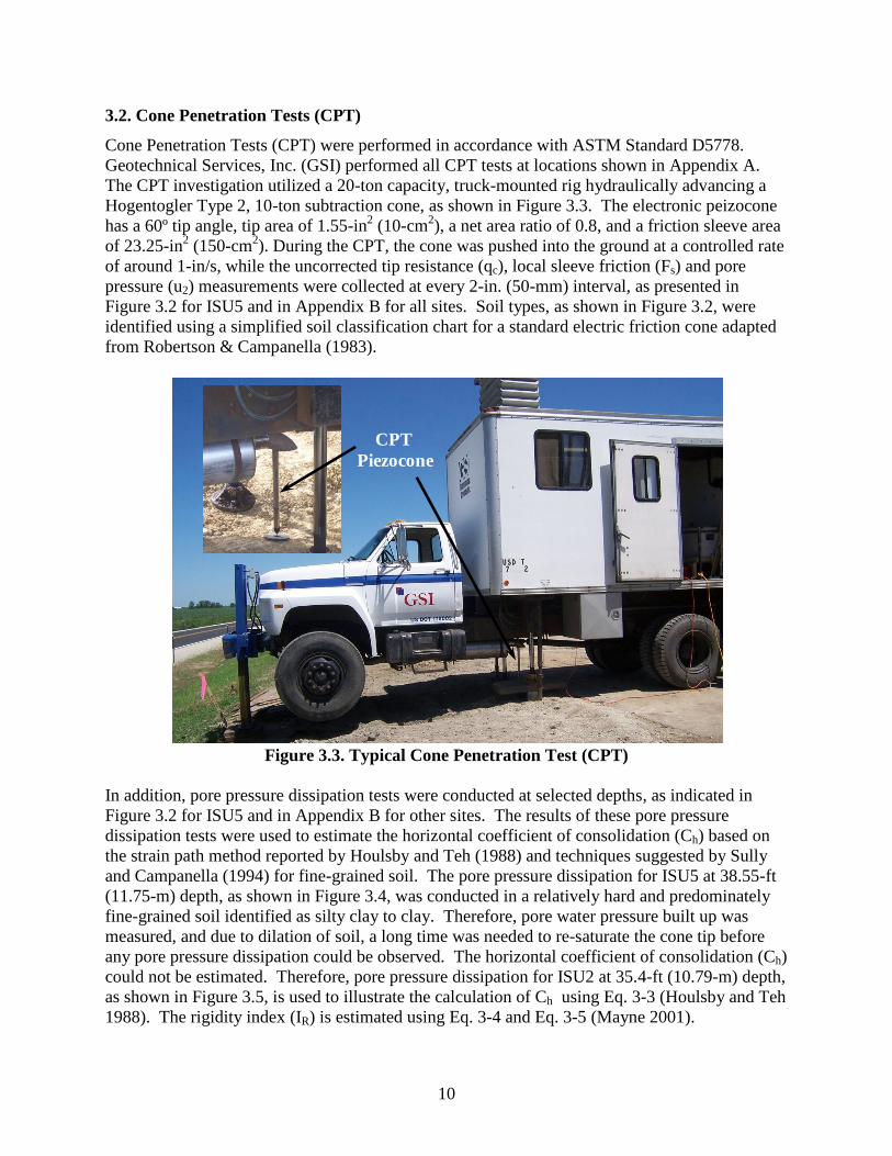
Cone Penetration Tests (CPT) were performed in accordance with ASTM Standard D5778.
Geotechnical Services, Inc. (GSI) performed all CPT tests at locations shown in Appendix A.
The CPT investigation utilized a 20-ton capacity, truck-mounted rig hydraulically advancing a
Hogentogler Type 2, 10-ton subtraction cone, as shown in Figure 3.3. The electronic peizocone
has a 60º tip angle, tip area of 1.55-in2 (10-cm
2), a net area ratio of 0.8, and a friction sleeve area
of 23.25-in2 (150-cm
2). During the CPT, the cone was pushed into the ground at a controlled rate
of around 1-in/s, while the uncorrected tip resistance (qc), local sleeve friction (Fs) and pore
pressure (u2) measurements were collected at every 2-in. (50-mm) interval, as presented in
Figure 3.2 for ISU5 and in Appendix B for all sites. Soil types, as shown in Figure 3.2, were
identified using a simplified soil classification chart for a standard electric friction cone adapted
from Robertson & Campanella (1983).
Figure 3.3. Typical Cone Penetration Test (CPT)
In addition, pore pressure dissipation tests were conducted at selected depths, as indicated in
Figure 3.2 for ISU5 and in Appendix B for other sites. The results of these pore pressure
dissipation tests were used to estimate the horizontal coefficient of consolidation (Ch) based on
the strain path method reported by Houlsby and Teh (1988) and techniques suggested by Sully
and Campanella (1994) for fine-grained soil. The pore pressure dissipation for ISU5 at 38.55-ft
(11.75-m) depth, as shown in Figure 3.4, was conducted in a relatively hard and predominately
fine-grained soil identified as silty clay to clay. Therefore, pore water pressure built up was
measured, and due to dilation of soil, a long time was needed to re-saturate the cone tip before
any pore pressure dissipation could be observed. The horizontal coefficient of consolidation (Ch)
could not be estimated. Therefore, pore pressure dissipation for ISU2 at 35.4-ft (10.79-m) depth,
as shown in Figure 3.5, is used to illustrate the calculation of Ch using Eq. 3-3 (Houlsby and Teh
1988). The rigidity index (IR) is estimated using Eq. 3-4 and Eq. 3-5 (Mayne 2001).
CPT
Piezocone
11
Based on the normalized pore water pressure (Bq), the effective friction angle ( ′) is calculated
either by Eq. 3-6 for granular soil where Bq < 0.1 (Kulhawy and Mayne 1990) or by using Eq.3-7
for soils where 0.1 ≤ Bq ≤ 1.0, as per an approach developed by the Norwegian University of
Science and Technology (NTNU) and discussed by Mayne (2007). By normalizing the
measured pore pressures with the maximum pore pressure of 64.18 psi and plotting this in a
logarithmic scale, starting at the maximum pore pressure, against time, the time for reaching the
50% pore pressure dissipation (t50) is estimated at 265 seconds (4.42 min) as shown in Figure
3.5. The effective friction angle ( ′) of 27.63º is estimated using Eq. 3-7 and yields the
constrained modulus parameter (M) of 1.10. Using the CPT measurements of qc, u2 and the net
area ratio of 0.8, the corrected tip resistance (qt) of 147.59 psi (1.02 MPa) and the rigidity index
(IR) of 17.47 are calculated. Finally the horizontal coefficient of consolidation (Ch) of 0.1152
in2/min (74.32 mm
2/min) is calculated using Eq. 3-3. The summary of the related parameters
and Ch is presented in Table 3.2.
√
(3-3)
[(
) (
σ
) ] (3-4)
φ′
φ′ (3-5)
(
σ ⁄
√σ
σ ⁄
)
(3-6)
′ ( ) (3-7)
where
Ch = Horizontal coefficient of consolidation estimated using CPT results, in2/min;
T50 = Modified time factor for Type 2 cone at 50% dissipation = 0.245;
ac = Tip area of cone = 1.55-in2, in
2;
IR = Rigidity index evaluated directly from CPT data using Eq.3-4;
t50 = Measured time to reach 50% consolidation, sec;
qt = Corrected tip resistance = qc+u2(1- net area ratio), psi;
qc = Uncorrected measured tip resistance, psi;
σvo = Total vertical geostatic stress, psi;
u2 = CPT measured pore pressure, psi;
′ = Frictional angle, degree;
σ′vo = Effective vertical geostatic stress, psi;
σatm = Atmospheric pressure = 1.47x10⁻⁵
, psi;
Bq = Normalized pore water pressure parameter = (u2-uo)/(qt-σvo); and
Q = Normalized cone tip resistance = (qt-σvo)/σ′vo.

12
Figure 3.4. Increase in pore pressure for ISU5 at a depth of 38.55-ft
Figure 3.5. Pore pressure dissipation result for ISU2 at a depth of 35.4-ft
0
1
2
3
4
5
6
7
8
0.1 1 10 100 1000 10000
Po
re P
ress
ure
(p
si)
Time (second)
0
10
20
30
40
50
60
70
0.1 10 1000
Po
re P
ress
ure
(p
si)
Time (sec)
0
0.1
0.2
0.3
0.4
0.5
0.6
0.7
0.8
0.9
1
1.1
0.1 10 1000
No
rma
lize
d P
ore
Pre
ssu
re
Time (sec)
265

13
Table 3.2. Summary of soil parameters at depths of CPT dissipation tests Project
ID Depth (ft) t50 (min)
′
(degree) M qt (psi) u2 (psi) σvo (psi) IR
Ch
(in2/min)
ISU2 35.40 4.42 27.72 1.10 147.59 57.40 18.24 25.13 0.1382
ISU3 22.15 31.27 11.94 0.44 228.47 38.20 17.31 58.37 0.0298
ISU4
19.50 43.42 24.66 0.97 239.71 4.13 12.54 4.01 0.0056
21.00 64.78 38.71 1.58 1209.92 5.19 14.45 2.51 0.0030
41.00 227.99 21.80 0.85 353.17 37.41 25.01 7.06 0.0014
50.53 88.68 33.09 1.33 313.15 82.21 29.82 7.71 0.0038
ISU6 50.03 151.52 30.28 1.21 282.47 9.60 35.42 2.33 0.0012
ISU8 57.25 264.83 34.24 1.39 732.76 4.08 34.42 2.50 0.0007
The CPT soundings provide a nearly continuous subsurface soil profile and are used to estimate
basic soil parameters such as effective friction angle ( ′) as explained above, undrained shear
strength (Su), and over-consolidation ratio (OCR). The undrained shear strength (Su) is estimated
using a classical approach given by Eq. 3-8 (Mayne 2007). The over-consolidation ratio (OCR)
for intact clays is estimated using Eq. 3-9 (Demers and Leroueil 2002). These estimated soil
parameters are used in the static and dynamic pile analyses conducted later. The average soil
parameters are summarized in Table 3.3 for ISU5 based on the CPT classified soil profiles,
indicated in Figure 3.2, and are summarized in Appendix B for all sites.
σ
(3-8)
(3-9)
where
Nkt = Bearing factor; 15 was assumed for representing the Iowa soil condition; and
Table 3.3. Summary of soil properties for ISU5 based on CPT
Soil Profiles Depth (ft) Soil Types
Average Effective
Friction Angle, ′
(degree)
Average
Undrained Shear
Strength, Su (psi)
Average Over-
consolidation
Ratio (OCR)
Layer 1 0 to 25 Clay 31.08 13.28 5.60
Layer 2 25 to 29 Silty Clay to
Clay 29.94 15.71 3.11
Layer 3 29 to 39 Clay 29.72 16.46 2.63
Layer 4 39 to 45 Silty Clay to
Clay 32.09 30.61 3.92
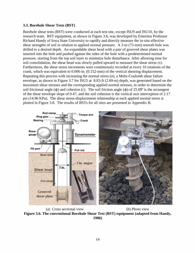
14
3.3. Borehole Shear Tests (BST)
Borehole shear tests (BST) were conducted at each test site, except ISU9 and ISU10, by the
research team. BST equipment, as shown in Figure 3.6, was developed by Emeritus Professor
Richard Handy of Iowa State University to rapidly and directly measure the in-situ effective
shear strengths of soil in relation to applied normal pressure. A 3-in (75-mm) smooth hole was
drilled to a desired depth. An expandable shear head with a pair of grooved shear plates was
inserted into the hole and pushed against the sides of the hole with a predetermined normal
pressure, starting from the top soil layer to minimize hole disturbance. After allowing time for
soil consolidation, the shear head was slowly pulled upward to measure the shear stress (τ).
Furthermore, the shear stress increments were continuously recorded at every 10 rotations of the
crank, which was equivalent to 0.006-in. (0.152-mm) of the vertical shearing displacement.
Repeating this process with increasing the normal stress (σ), a Mohr-Coulomb shear failure
envelope, as shown in Figure 3.7 for ISU5 at 8.83-ft (2.69-m) depth, was generated based on the
maximum shear stresses and the corresponding applied normal stresses, in order to determine the
soil frictional angle ( ) and cohesion (c). The soil friction angle ( ) of 25.08º is the arctangent
of the shear envelope slope of 0.47, and the soil cohesion is the vertical axis interception of 2.17
psi (14.96 KPa). The shear stress-displacement relationship at each applied normal stress is
plotted in Figure 3.8. The results of BSTs for all sites are presented in Appendix B.
(a) Cross sectional view (b) Photo view
Figure 3.6. The conventional Borehole Shear Test (BST) equipment (adapted from Handy,
1986)
3 in. augur
Grooved
shear plate
3 in.
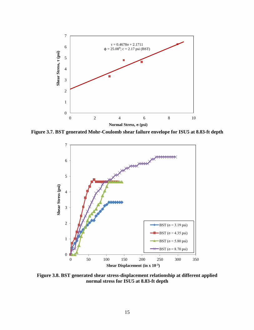
15
Figure 3.7. BST generated Mohr-Coulomb shear failure envelope for ISU5 at 8.83-ft depth
Figure 3.8. BST generated shear stress-displacement relationship at different applied
normal stress for ISU5 at 8.83-ft depth
τ = 0.4678σ + 2.1711
φ = 25.08⁰; c = 2.17 psi (BST)
0
1
2
3
4
5
6
7
0 2 4 6 8 10
Sh
ear
Str
ess,
τ (
psi
)
Normal Stress, σ (psi)
0
1
2
3
4
5
6
7
0 50 100 150 200 250 300 350
Sh
ear
Str
ess
(psi
)
Shear Displacement (in x 10-3)
BST (σ = 3.19 psi)
BST (σ = 4.35 psi)
BST (σ = 5.80 psi)
BST (σ = 8.70 psi)
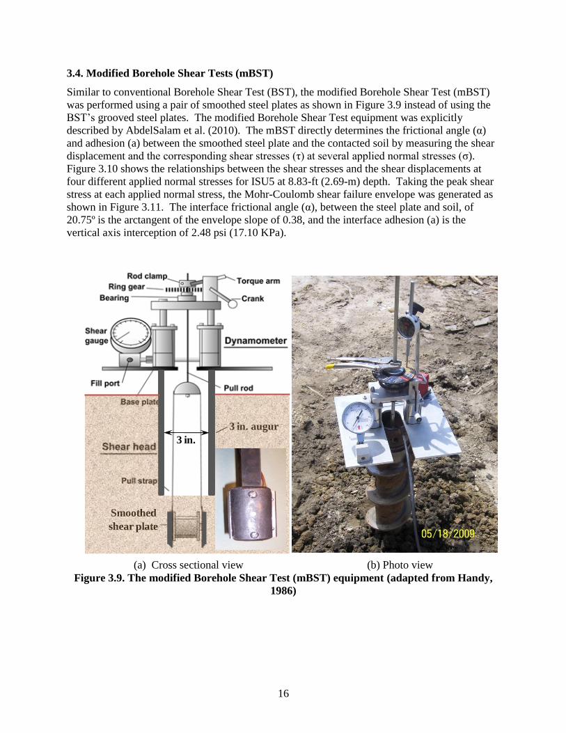
16
3.4. Modified Borehole Shear Tests (mBST)
Similar to conventional Borehole Shear Test (BST), the modified Borehole Shear Test (mBST)
was performed using a pair of smoothed steel plates as shown in Figure 3.9 instead of using the
BST’s grooved steel plates. The modified Borehole Shear Test equipment was explicitly
described by AbdelSalam et al. (2010). The mBST directly determines the frictional angle (α)
and adhesion (a) between the smoothed steel plate and the contacted soil by measuring the shear
displacement and the corresponding shear stresses (τ) at several applied normal stresses (σ).
Figure 3.10 shows the relationships between the shear stresses and the shear displacements at
four different applied normal stresses for ISU5 at 8.83-ft (2.69-m) depth. Taking the peak shear
stress at each applied normal stress, the Mohr-Coulomb shear failure envelope was generated as
shown in Figure 3.11. The interface frictional angle (α), between the steel plate and soil, of
20.75º is the arctangent of the envelope slope of 0.38, and the interface adhesion (a) is the
vertical axis interception of 2.48 psi (17.10 KPa).
(a) Cross sectional view (b) Photo view
Figure 3.9. The modified Borehole Shear Test (mBST) equipment (adapted from Handy,
1986)
3 in. augur
Smoothed
shear plate
3 in.

17
Figure 3.10. mBST generated shear stress-displacement relationship at different applied
normal stress for ISU5 at 8.83-ft depth
Figure 3.11. mBST generated Mohr-Coulomb interface shear failure envelop for ISU5 at
8.83 ft depth
0
1
2
3
4
5
6
7
0 50 100 150 200 250
Sh
ear
Str
ess
(psi
)
Shear Displacement (in × 10-3)
mBST (σ = 3.19 psi)
mBST (σ = 4.35 psi)
mBST (σ = 5.80 psi)
mBST (σ = 8.70 psi)
τ = 0.3787σ + 2.4808
α = 20.75⁰; a = 2.48 psi (mBST)
0
1
2
3
4
5
6
7
0 2 4 6 8 10
Sh
ear
Sh
ear,
τ (
psi
)
Normal Stress, σ (psi)
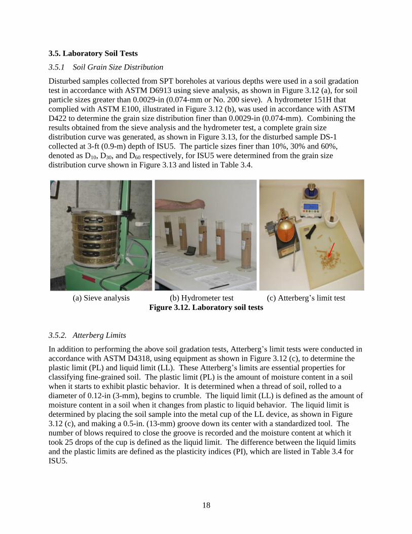
18
3.5. Laboratory Soil Tests
3.5.1 Soil Grain Size Distribution
Disturbed samples collected from SPT boreholes at various depths were used in a soil gradation
test in accordance with ASTM D6913 using sieve analysis, as shown in Figure 3.12 (a), for soil
particle sizes greater than 0.0029-in (0.074-mm or No. 200 sieve). A hydrometer 151H that
complied with ASTM E100, illustrated in Figure 3.12 (b), was used in accordance with ASTM
D422 to determine the grain size distribution finer than 0.0029-in (0.074-mm). Combining the
results obtained from the sieve analysis and the hydrometer test, a complete grain size
distribution curve was generated, as shown in Figure 3.13, for the disturbed sample DS-1
collected at 3-ft (0.9-m) depth of ISU5. The particle sizes finer than 10%, 30% and 60%,
denoted as D10, D30, and D60 respectively, for ISU5 were determined from the grain size
distribution curve shown in Figure 3.13 and listed in Table 3.4.
(a) Sieve analysis (b) Hydrometer test (c) Atterberg’s limit test
Figure 3.12. Laboratory soil tests
3.5.2. Atterberg Limits
In addition to performing the above soil gradation tests, Atterberg’s limit tests were conducted in
accordance with ASTM D4318, using equipment as shown in Figure 3.12 (c), to determine the
plastic limit (PL) and liquid limit (LL). These Atterberg’s limits are essential properties for
classifying fine-grained soil. The plastic limit (PL) is the amount of moisture content in a soil
when it starts to exhibit plastic behavior. It is determined when a thread of soil, rolled to a
diameter of 0.12-in (3-mm), begins to crumble. The liquid limit (LL) is defined as the amount of
moisture content in a soil when it changes from plastic to liquid behavior. The liquid limit is
determined by placing the soil sample into the metal cup of the LL device, as shown in Figure
3.12 (c), and making a 0.5-in. (13-mm) groove down its center with a standardized tool. The
number of blows required to close the groove is recorded and the moisture content at which it
took 25 drops of the cup is defined as the liquid limit. The difference between the liquid limits
and the plastic limits are defined as the plasticity indices (PI), which are listed in Table 3.4 for
ISU5.

19
Figure 3.13. Grain size distribution curve for disturbed sample DS-1 at 3 ft depth of ISU5
3.5.3. Soil Classification
After performing the above soil gradation tests and Atterberg’s limit tests and determining the
essential soil properties, the soil was classified using the Unified Soil Classification System
(USCS) in accordance with ASTM D2487. The results of the USCS soil classification are listed
in Table 3.4 for ISU5 and are included in Appendix B for other sites. Estimated values for the
natural moisture content (ω), void ratio (e), and saturated unit weight (γsat) properties of the soils
tests are also included in Table 3.4 for ISU5 and in Appendix B. The natural moisture content
(ω) is determined in accordance with ASTM D2216 and estimated using Eq. 3-10. The void
ratio (e) is estimated using Eq. 3-11 by assuming 100% saturation (S) and a specific gravity (G)
of 2.7. Using the estimated void ratio, the saturated unit weight (γsat) is estimated using Eq. 3-12.
ω
(3-10)
(3-11)
3.94E-053.94E-043.94E-033.94E-023.94E-013.94E+00
0
10
20
30
40
50
60
70
80
90
100
0
10
20
30
40
50
60
70
80
90
100
0.00010.0010.010.1110100
Particle Diameter (in) - Log Scale
Per
cen
t F
iner
(%
)
Per
cen
t F
iner
(%
)
Particle Diameter (mm) - Log Scale

20
( )
(3-12)
where
ω = Moisture content, %;
Ww = Weight of moisture (water) in a soil sample, lb;
Ws = Weight of solid in a soil sample, lb;
e = Void ratio;
G = Specific gravity (assumed 2.7);
S = Degree of saturation (assumed 100%), %;
γw = Unit weight of water = 62.4 pcf; and
γsat = Saturated unit weight, pcf.
Table 3.4. Soil classification and properties for ISU5 obtained from gradation and
Atterberg’s limit tests
Distur
bed
Sample
Sample
Depth (ft)
Soil
Type
(USCS)
D10
(in)
D30
(in)
D60
(in)
Liquid
Limit,
LL (%)
Plasticity
Index, PI
(%)
Moisture
Content,
ω (%)
Saturated
Unit
Weight,
γsat (pcf)
Void
Ratio,
e
DS-1 3 SC 3.3E-5 8.1E-4 2.1E-2 26.31 11.27 20.39 130.82 0.55
DS-2 8 to 10 ML 9.0E-6 4.8E-4 2.7E-3 36.30 5.57 18.70 132.89 0.50
DS-3 10 to 12 CL - 2.4E-4 2.6E-3 38.41 20.82 20.64 130.52 0.56
DS-4 16 CL - 3.4E-4 2.7E-3 49.10 27.08 21.58 129.42 0.58
DS-5 28 to 30 CL - 3.4E-4 2.8E-3 44.60 26.84 17.20 134.84 0.46
DS-6 37 to 38.5 CL - 3.4E-4 2.7E-3 38.61 22.23 22.03 128.92 0.59
DS-7 38.5 to 40 SC - 7.2E-4 6.4E-3 22.02 8.63 19.80 131.52 0.53
DS-8 43.5 to 45 CL - 1.2E-4 2.6E-3 38.73 20.78 16.11 136.32 0.44
DS-9 48 to 50 CL - 1E-4 2.4E-3 40.07 22.33 16.94 135.19 0.46
D10, D20, and D60 ‒ particle sizes finer than 10%, 30% and 60%, respectively.
3.5.4. Laboratory Soil Consolidation Tests
The undisturbed samples collected in the 3-in. (75-mm) Shelby tubes from the SPT boreholes
were extruded, trimmed and inserted into a consolidation ring for laboratory soil consolidation
tests, performed in accordance with ASTM D2435. The consolidation ring, weighted at about
0.14 lb (65 g), has an inner diameter (D) around 2.51-in. (63.7-mm) and a height (Ho) of 0.79-in.
(20.1-mm). The consolidation loading device and the consolidometer are shown in Figure 3.14.

21
Figure 3.14. Laboratory soil consolidation tests
Test method A (described in ASTM D2435) was performed with a constant load increment
duration of at least 24 hrs. Soil specimen deformations at applied loading and unloading
increments were measured at specified time intervals as indicated in the ASTM D2435. Double-
sided drainage was allowed during all consolidation tests. The loading increments were 0.87 psi,
1.74 psi, 3.63 psi, 7.25 psi, 14.50 psi, 29.01 psi, 58.02 psi, 116.03 psi, and 232.06 psi. The
unloading increments started from 232.06 psi to 116.03 psi, 29.01 psi, 7.25 psi, and 1.74 psi.
The natural initial moisture contents (ω) of the soil samples were determined in accordance with
ASTM D2216 and computed using Eq. 3-10. Assuming the specific gravity (G) of the soil to be
2.7 and having measured the dry soil mass in the consolidation ring (Ms), the initial height of the
solid component of each soil specimen (Hs) is estimated using Eq. 3-13, where the water density
(ρw) is taken as 0.036 pci (1 g/cm3). Using the estimated initial solid height (Hs), the initial void
ratio (eo) of each soil specimen is calculated using Eq. 3-14. These initial soil properties are
listed in Table 3.5.
ρ (
)
(3-13)
(3-14)
(b) Consolidometer
(a) Consolidation loading equipment
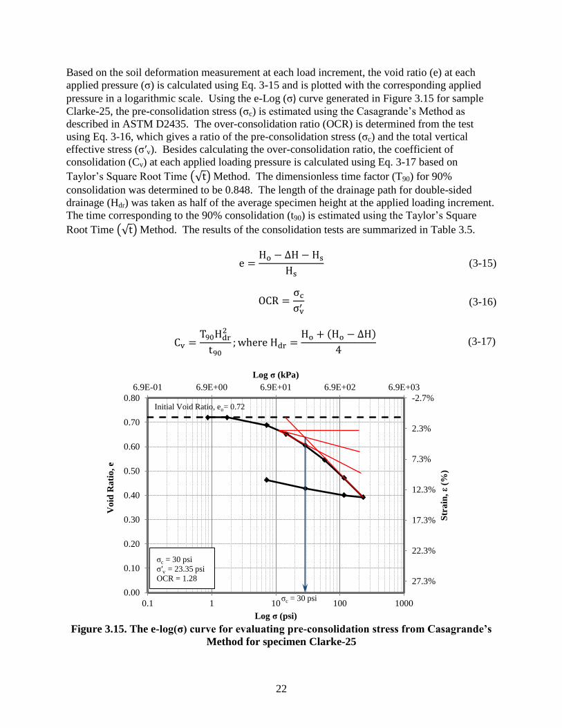
22
Based on the soil deformation measurement at each load increment, the void ratio (e) at each
applied pressure (σ) is calculated using Eq. 3-15 and is plotted with the corresponding applied
pressure in a logarithmic scale. Using the e-Log (σ) curve generated in Figure 3.15 for sample
Clarke-25, the pre-consolidation stress (σc) is estimated using the Casagrande’s Method as
described in ASTM D2435. The over-consolidation ratio (OCR) is determined from the test
using Eq. 3-16, which gives a ratio of the pre-consolidation stress (σc) and the total vertical
effective stress (σ′v). Besides calculating the over-consolidation ratio, the coefficient of
consolidation (Cv) at each applied loading pressure is calculated using Eq. 3-17 based on
Taylor’s Square Root Time (√ ) Method. The dimensionless time factor (T90) for 90%
consolidation was determined to be 0.848. The length of the drainage path for double-sided
drainage (Hdr) was taken as half of the average specimen height at the applied loading increment.
The time corresponding to the 90% consolidation (t90) is estimated using the Taylor’s Square
Root Time (√ ) Method. The results of the consolidation tests are summarized in Table 3.5.
(3-15)
(3-16)
( )
(3-17)
Figure 3.15. The e-log(σ) curve for evaluating pre-consolidation stress from Casagrande’s
Method for specimen Clarke-25
6.9E-01 6.9E+00 6.9E+01 6.9E+02 6.9E+03
-2.7%
2.3%
7.3%
12.3%
17.3%
22.3%
27.3%
0.00
0.10
0.20
0.30
0.40
0.50
0.60
0.70
0.80
0.1 1 10 100 1000
Log σ (kPa)
Str
ain
, ε
(%)
Vo
id R
ati
o, e
Log σ (psi)
Initial Void Ratio, eo= 0.72
σc = 30 psi
σc = 30 psi
σ′v = 23.35 psi
OCR = 1.28
23
Table 3.5. Summary of the consolidation test results and analyses
Project
ID
Sample -
Depth in
feet
Initial
Moisture
Content,
ω (%)
Initial
Solid
Height,
Hs (in)
Initial
Void
Ratio, eo
Pre-
consolidation
Stress, σc
(psi)
Effective
Vertical
Stress,
σ′v (psi)
Over
Consolidation
Ratio, OCR
Coefficient of
Consolidation
at σ’v, Cv at
(in2/min)
ISU2
Mills-9 19.00 0.52 0.54 6.3 7.92 1.00a 0.023
Mills-20 30.31 0.43 0.84 20 17.53 1.14 0.008
Mills-30 25.69 0.43 0.86 30 28.56 1.05 0.020
Mills-55 36.94 0.39 1.01 34 38.77 1.00a 0.018
ISU3
Polk-3 15.65 0.59 0.33 13 2.77 4.69 0.011
Polk-27 27.18 0.49 0.62 28 18.37 1.52 0.012
Polk-50 29.06 0.48 0.67 35 26.86 1.30 0.006
ISU4
Jas-15 13.10 0.59 0.33 26 10.5 2.48 0.019
Jas-27 17.12 0.53 0.49 30 18.40 1.63 0.012
Jas-45 15.09 0.57 0.40 23 27.07 1.00a 0.012
Jas-60 15.41 0.56 0.42 36 34.95 1.03 0.007
ISU5
Clarke-8 21.82 0.48 0.64 33 7.42 4.45 0.017
Clarke-25 25.91 0.46 0.72 30 23.35 1.28 0.014
Clarke-35 15.13 0.56 0.40 17 31.29 1.00a 0.008
ISU6 and
ISU7
Buc-12 32.26 0.42 0.86 16 13.31 1.20 0.005
Buc-49 13.56 0.57 0.39 38 34.83 1.09 0.006
Buc-59 15.07 0.56 0.40 34 37.06 1.00a 0.009
ISU8
Pow-3 23.19 0.49 0.62 10 2.26 4.43 0.020
Pow-23 24.87 0.42 0.86 13.3 18.37 1.00a 0.030
Pow-44 16.72 0.54 0.46 13 28.66 1.00a 0.011 a – round up to 1.00 for normally consolidated soils.
3.6. Pore Water and Lateral Earth Pressure Measurements
The in-situ pore water and total lateral earth pressures were measured using Geokon Model 4830
push-in pressure cells shown in Figure 3.16. As listed in Table 3.1, the push-in pressure cells
were installed at ISU5, ISU6, ISU7, ISU8 and ISU10, and the locations are indicated with solid
black crosses on the site layout plans in Appendix A. The push-in pressure cells were installed
in a range of approximately 8-in. (200-mm) to 24-in. (600-mm) away from one of the flanges of
a test pile. The elevations of the pressure cells are indicated on the soil profile as shown in
Figure 3.2 for ISU5 and in Appendix B for ISU6, ISU7, ISU8, and ISU10. The pressure cell is
fitted with an integral piezometer on one of the flat surfaces to measure pore water pressure.
Before installing the pressure cell, the piezometer was saturated with water by drawing a vacuum
on the circular porous sensor and allowing water to flow into the sensor when the vacuum was
released, as shown in Figure 3.16. A thread is provided on the end of the cell to allow for
installation using the SPT drill rods.
During the installation, the pressure cell was oriented, so that the circular porous sensor and the
flat surface faced the proposed position of the flange of the test pile. The pressure cell was then
slowly lowered into the ground through the SPT auger which had been drilled to the desired
elevation. When the pressure cell reached the bottom of the drilled hole, it was pushed into the
ground for about 14-in. (350-mm). The process of pushing the pressure cell created an increase
in temperature, pore water and earth pressures surrounding the cell, therefore the cell was
required to stabilize for at least 24 hours to reach both thermal and pressure equilibriums before
taking any measurement as recommended by Suleiman et al. (2010) in Iowa soils. Readings were
then taken at every 4 seconds during pile driving, re-strikes and static load test. However,

24
readings were taken only every 30 minutes between each re-strike event and between the last re-
strike event and the static load test.
Temperature (T), pore water pressure and total lateral earth pressure are measured by the
pressure cells. Initially, the pressure signals and temperature signal are transmitted from the
pressure cell to a CR1000 data logger which stored data for the duration of testing, from the
beginning of a pile driving to the end of a static load test. A data analysis program known as
PC400 is used to collect the data from the data logger and to convert the data signals (Ri) into the
actual pressures (P) using the polynomial pressure Eq. 3-18. Temperature (T) is part of the
polynomial pressure equation for converting the pressure signals (Ri).
Figure 3.16. Measurement of pore water and lateral earth pressures using Geokon push-in
pressure cells at the field
Each pressure cell is initially calibrated at Geokon’s factory to determine the gage factors (A, B,
and C), the thermal factor (κ) and the zero reading temperature (To). The calibrated factors and
(a) Saturating pressure cells (b) Installing pressure cells
(c) Stabilization and data acquisition system (d) Measuring pore water pressure and lateral
earth pressure
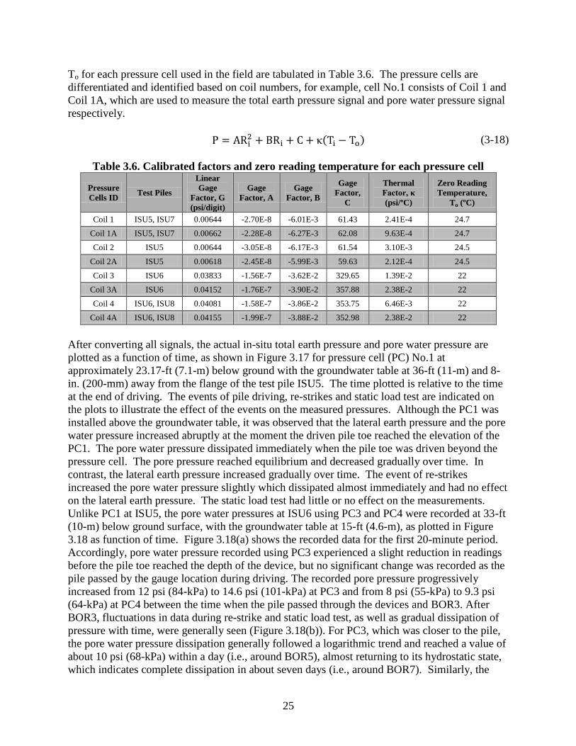
25
To for each pressure cell used in the field are tabulated in Table 3.6. The pressure cells are
differentiated and identified based on coil numbers, for example, cell No.1 consists of Coil 1 and
Coil 1A, which are used to measure the total earth pressure signal and pore water pressure signal
respectively.
κ( ) (3-18)
Table 3.6. Calibrated factors and zero reading temperature for each pressure cell
Pressure
Cells ID Test Piles
Linear
Gage
Factor, G
(psi/digit)
Gage
Factor, A
Gage
Factor, B
Gage
Factor,
C
Thermal
Factor, κ
(psi/ºC)
Zero Reading
Temperature,
To (ºC)
Coil 1 ISU5, ISU7 0.00644 -2.70E-8 -6.01E-3 61.43 2.41E-4 24.7
Coil 1A ISU5, ISU7 0.00662 -2.28E-8 -6.27E-3 62.08 9.63E-4 24.7
Coil 2 ISU5 0.00644 -3.05E-8 -6.17E-3 61.54 3.10E-3 24.5
Coil 2A ISU5 0.00618 -2.45E-8 -5.99E-3 59.63 2.12E-4 24.5
Coil 3 ISU6 0.03833 -1.56E-7 -3.62E-2 329.65 1.39E-2 22
Coil 3A ISU6 0.04152 -1.76E-7 -3.90E-2 357.88 2.38E-2 22
Coil 4 ISU6, ISU8 0.04081 -1.58E-7 -3.86E-2 353.75 6.46E-3 22
Coil 4A ISU6, ISU8 0.04155 -1.99E-7 -3.88E-2 352.98 2.38E-2 22
After converting all signals, the actual in-situ total earth pressure and pore water pressure are
plotted as a function of time, as shown in Figure 3.17 for pressure cell (PC) No.1 at
approximately 23.17-ft (7.1-m) below ground with the groundwater table at 36-ft (11-m) and 8-
in. (200-mm) away from the flange of the test pile ISU5. The time plotted is relative to the time
at the end of driving. The events of pile driving, re-strikes and static load test are indicated on
the plots to illustrate the effect of the events on the measured pressures. Although the PC1 was
installed above the groundwater table, it was observed that the lateral earth pressure and the pore
water pressure increased abruptly at the moment the driven pile toe reached the elevation of the
PC1. The pore water pressure dissipated immediately when the pile toe was driven beyond the
pressure cell. The pore pressure reached equilibrium and decreased gradually over time. In
contrast, the lateral earth pressure increased gradually over time. The event of re-strikes
increased the pore water pressure slightly which dissipated almost immediately and had no effect
on the lateral earth pressure. The static load test had little or no effect on the measurements.
Unlike PC1 at ISU5, the pore water pressures at ISU6 using PC3 and PC4 were recorded at 33-ft
(10-m) below ground surface, with the groundwater table at 15-ft (4.6-m), as plotted in Figure
3.18 as function of time. Figure 3.18(a) shows the recorded data for the first 20-minute period.
Accordingly, pore water pressure recorded using PC3 experienced a slight reduction in readings
before the pile toe reached the depth of the device, but no significant change was recorded as the
pile passed by the gauge location during driving. The recorded pore pressure progressively
increased from 12 psi (84-kPa) to 14.6 psi (101-kPa) at PC3 and from 8 psi (55-kPa) to 9.3 psi
(64-kPa) at PC4 between the time when the pile passed through the devices and BOR3. After
BOR3, fluctuations in data during re-strike and static load test, as well as gradual dissipation of
pressure with time, were generally seen (Figure 3.18(b)). For PC3, which was closer to the pile,
the pore water pressure dissipation generally followed a logarithmic trend and reached a value of
about 10 psi (68-kPa) within a day (i.e., around BOR5), almost returning to its hydrostatic state,
which indicates complete dissipation in about seven days (i.e., around BOR7). Similarly, the

26
lateral earth pressure reduced over time. Overall, the restrikes and static load test had little effect
on the measurements. The results of ISU7, ISU8, and ISU10 are included in Appendix B.
(a) Measured pressure versus time in minutes
(b) Measured pressure versus time in days
Figure 3.17. Total lateral earth pressure and pore water pressure measurements from PC1
at test pile ISU5 with respect to the time
0
10
20
30
40
50
60
0
10
20
30
40
50
60
70
80
90
-45 -35 -25 -15 -5 5 15 25
Po
re W
ate
r P
ress
ure
(p
si)
To
tal
La
tera
l E
art
h P
ress
ure
(p
si)
Time After the End of Driving (Minute)
Earth Pressure (PC1)
Water Pressure (PC1)
Pil
e D
rivin
g B
egin
Pil
e R
each
es
PC
EO
D
BO
R 1
BO
R 2
Geostatic Vertical
Pressure, σv
Hydrostatic Pressure, μ
0
10
20
30
40
50
60
-2 -1 0 1 2 3 4 5 6 7 8 9 10
0
10
20
30
40
50
60
70
80
90
Po
re W
ate
r P
ress
ure
(p
si)
Time After the End of Driving (Day)
To
tal
La
tera
l E
art
h P
ress
ure
(p
si)
Earth Pressure (PC1)
Water Pressure (PC1)
BO
R 4
BO
R 5
BO
R 6
SL
T B
egin
SL
T E
nd
Peak Pressures
EP (PC1): 70 psi
WP (PC1): 50 psi
BO
R 3
Geostatic Vertical
Hydrostatic Pressure, μ (b)

27
(a) Measured pressure versus time in minutes
(b) Measured pressure versus time in days
Figure 3.18. Total lateral earth pressure and pore water pressure measurements from PC3
and PC4 at test pile ISU6 with respect to the time
0
2
4
6
8
10
12
14
16
0
10
20
30
40
50
60
70
80
90
100
110
120
130
-20 -10 0 10 20
To
tal
La
terl
a E
art
h a
nd
Po
re W
ate
r P
ress
ure
(psi
)
To
tal
La
tera
l E
srth
an
d P
ore
Wa
ter
Pre
ssu
re
(psi
)
Time After the End of Driving (Minute)
Earth Pressure (PC3)
Earth Pressure (PC4)
Water Pressure (PC3)
Water Pressure (PC4)
EO
D
Pil
e R
each
es P
C
Pil
e D
rivin
g
Beg
in
BO
R1
BO
R2
BO
R3
Hydrostatic Pressure, μ
Geostatic Vertical Pressure, σv
0
2
4
6
8
10
12
14
16
0
10
20
30
40
50
60
70
80
90
100
110
120
130
-2 0 2 4 6 8 10 12 14 16
Po
re W
ate
r P
ress
ure
(p
si)
To
tal
La
tera
l E
srth
Pre
ssu
re (
psi
)
Time After the End of Driving (Day)
Earth Pressure (PC3)
Earth Pressure (PC4)
Water Pressure (PC3)
Water Pressure (PC4)
BO
R4
BO
R5
BO
R6
BO
R7
BO
R8
SL
T B
egin
SL
T E
nd
Peak Pressures
EP (PC3): 94 psi
WP (PC3): 15 psi
EP (PC4): 93 psi
WP (PC4): 10 psi
Hydrostatic Pressure, μ
Geostatic Vertical Pressure, σv

28
CHAPTER 4: FULL-SCALE TESTS
4.1. Pile Type and Properties
A recent survey completed by AbdelSalam et al. (2008) indicates that the steel H-pile foundation
is the most common bridge foundation used in the United States, especially in the Midwest. The
Iowa Department of Transportation (Iowa DOT) conducted a total of 264 static pile load tests,
between 1966 and 1989, to improve their pile foundation design practice. Of these tests, Roling
et al. (2010) summarized that 164 (62 percent) of the tests were performed on steel H-piles, and
32 of these 164 contained sufficient pile, soil, hammer and driving information to be considered
“usable data sets” for resistance factor calculations using the Wave Equation Analysis Program
(WEAP) and dynamic formulas. Of the 32 usable steel H-piles, 29 were HP 10 x 42 steel piles
(10-in. pile size and 42 lb/ft), 2 were HP 12 x 53 steel piles and one was HP 14 x 89 steel pile.
Thus, HP 10 x 42 was used in the field tests except ISU1 at Mahaska County, where HP 10 x 57
steel pile was used. ASTM A572 Grade 50 steel with a yield strength (Fy) of 50 ksi (345 MPa)
was selected and the relevant properties are listed in Table 4.1. The cross sectional view of the
steel H-piles is shown in Figure 4.1. The pile impedance (Z) is determined using Eq. 4-1, where
the elastic modulus (E) of 30,000 ksi (206,843 MPa) is used and the compressive wave speed (C)
for steel piles is taken as 16,808 ft/s (5,123 m/s).
C
EAZ (4-1)
The American Association of State Highway and Transportation Officials (AASHTO) (2007)
LRFD Bridge Design Specifications limit the pile stress to 0.6 Fy and 0.5 Fy under good driving
and severe driving conditions respectively. Vande Voort (2008) noted that the stress limits
reflect geotechnical concerns rather than structural limit states. In particular, the Iowa DOT
LRFD Design Manual Section 6.2.6.1 specifies allowable pile stresses of 6 ksi (41 MPa), 9 ksi
(62 MPa) and 12 ksi (83 MPa) for pile resistance levels 1, 2 and 3 respectively to limit and
control pile settlement.
Table 4.1. A572 Grade 50 (Fy = 50 ksi) steel H-pile properties
Project ID Pile
Types
Cross
Sectional
Area, A
(in2)
Coating
Area
(ft2/ft)
Depth,
d (in)
Flange
Width, b
(in)
Flange
Thicknes,
tf (in)
Web
Thickness,
tw (in)
Pile
Impedance,
Z (kip-s/ft)
ISU1 HP 10 x
57 16.8 4.91 9.99 10.225 0.565 0.565 29.99
ISU2 to
ISU10 and
Iowa DOT
Database
HP 10 x
42 12.4 4.83 9.70 10.075 0.420 0.415 22.13
Iowa DOT
Database
HP 12 x
53 15.5 5.82 11.78 12.045 0.435 0.435 27.67
Iowa DOT
Database
HP 14 x
89 26.1 7.02 13.83 14.695 0.615 0.615 46.59
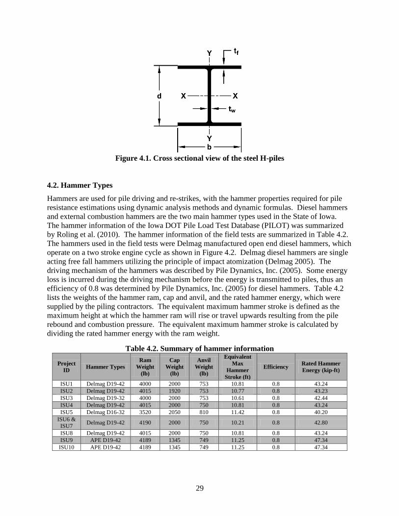
29
Figure 4.1. Cross sectional view of the steel H-piles
4.2. Hammer Types
Hammers are used for pile driving and re-strikes, with the hammer properties required for pile
resistance estimations using dynamic analysis methods and dynamic formulas. Diesel hammers
and external combustion hammers are the two main hammer types used in the State of Iowa.
The hammer information of the Iowa DOT Pile Load Test Database (PILOT) was summarized
by Roling et al. (2010). The hammer information of the field tests are summarized in Table 4.2.
The hammers used in the field tests were Delmag manufactured open end diesel hammers, which
operate on a two stroke engine cycle as shown in Figure 4.2. Delmag diesel hammers are single
acting free fall hammers utilizing the principle of impact atomization (Delmag 2005). The
driving mechanism of the hammers was described by Pile Dynamics, Inc. (2005). Some energy
loss is incurred during the driving mechanism before the energy is transmitted to piles, thus an
efficiency of 0.8 was determined by Pile Dynamics, Inc. (2005) for diesel hammers. Table 4.2
lists the weights of the hammer ram, cap and anvil, and the rated hammer energy, which were
supplied by the piling contractors. The equivalent maximum hammer stroke is defined as the
maximum height at which the hammer ram will rise or travel upwards resulting from the pile
rebound and combustion pressure. The equivalent maximum hammer stroke is calculated by
dividing the rated hammer energy with the ram weight.
Table 4.2. Summary of hammer information
Project
ID Hammer Types
Ram
Weight
(lb)
Cap
Weight
(lb)
Anvil
Weight
(lb)
Equivalent
Max
Hammer
Stroke (ft)
Efficiency Rated Hammer
Energy (kip-ft)
ISU1 Delmag D19-42 4000 2000 753 10.81 0.8 43.24
ISU2 Delmag D19-42 4015 1920 753 10.77 0.8 43.23
ISU3 Delmag D19-32 4000 2000 753 10.61 0.8 42.44
ISU4 Delmag D19-42 4015 2000 750 10.81 0.8 43.24
ISU5 Delmag D16-32 3520 2050 810 11.42 0.8 40.20
ISU6 &
ISU7 Delmag D19-42 4190 2000 750 10.21 0.8 42.80
ISU8 Delmag D19-42 4015 2000 750 10.81 0.8 43.24
ISU9 APE D19-42 4189 1345 749 11.25 0.8 47.34
ISU10 APE D19-42 4189 1345 749 11.25 0.8 47.34
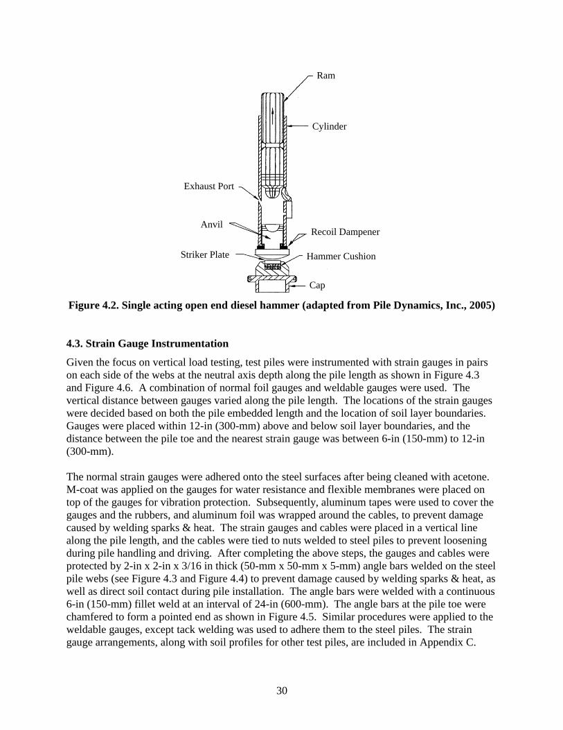
30
Figure 4.2. Single acting open end diesel hammer (adapted from Pile Dynamics, Inc., 2005)
4.3. Strain Gauge Instrumentation
Given the focus on vertical load testing, test piles were instrumented with strain gauges in pairs
on each side of the webs at the neutral axis depth along the pile length as shown in Figure 4.3
and Figure 4.6. A combination of normal foil gauges and weldable gauges were used. The
vertical distance between gauges varied along the pile length. The locations of the strain gauges
were decided based on both the pile embedded length and the location of soil layer boundaries.
Gauges were placed within 12-in (300-mm) above and below soil layer boundaries, and the
distance between the pile toe and the nearest strain gauge was between 6-in (150-mm) to 12-in
(300-mm).
The normal strain gauges were adhered onto the steel surfaces after being cleaned with acetone.
M-coat was applied on the gauges for water resistance and flexible membranes were placed on
top of the gauges for vibration protection. Subsequently, aluminum tapes were used to cover the
gauges and the rubbers, and aluminum foil was wrapped around the cables, to prevent damage
caused by welding sparks & heat. The strain gauges and cables were placed in a vertical line
along the pile length, and the cables were tied to nuts welded to steel piles to prevent loosening
during pile handling and driving. After completing the above steps, the gauges and cables were
protected by 2-in x 2-in x 3/16 in thick (50-mm x 50-mm x 5-mm) angle bars welded on the steel
pile webs (see Figure 4.3 and Figure 4.4) to prevent damage caused by welding sparks & heat, as
well as direct soil contact during pile installation. The angle bars were welded with a continuous
6-in (150-mm) fillet weld at an interval of 24-in (600-mm). The angle bars at the pile toe were
chamfered to form a pointed end as shown in Figure 4.5. Similar procedures were applied to the
weldable gauges, except tack welding was used to adhere them to the steel piles. The strain
gauge arrangements, along with soil profiles for other test piles, are included in Appendix C.
Cap
Ram
Cylinder
Recoil Dampener
Hammer Cushion
Exhaust Port
Anvil
Striker Plate
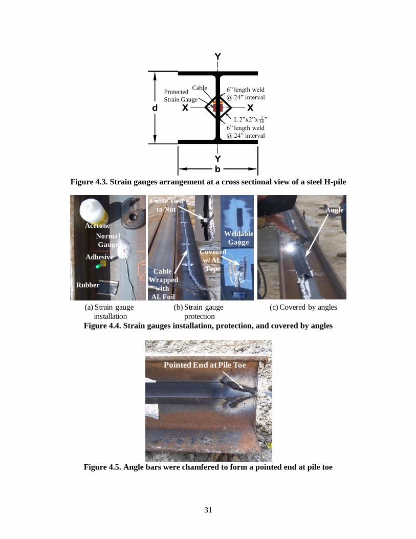
31
Figure 4.3. Strain gauges arrangement at a cross sectional view of a steel H-pile
Figure 4.4. Strain gauges installation, protection, and covered by angles
Figure 4.5. Angle bars were chamfered to form a pointed end at pile toe
L 2”x2”x ”3
16
Protected
Strain Gauge
Cable 6” length weld
@ 24” interval
6” length weld
@ 24” interval
Angle
Cable Tied
to Nut
Cable
Wrapped
with
AL Foil
Covered
w/ AL
Tape
Acetone
Rubber
Adhesive
Normal
Gauge
Weldable
Gauge
(a) Strain gauge
installation
(b) Strain gauge
protection
(c) Covered by angles
Pointed End at Pile Toe

32
Figure 4.6. Location of strain gauges along the ISU5 test pile at Clarke County
PDA Accelerometer
and Transducers
Steel Angle Bar
(L 2''x2''x 316
'')
Cable
Pile head
Pile toe
CLK-5-60-ECLK-5-60-W
CLK-6-60-ECLK-6-60-W
CLK-7-60-ECLK-7-60-W
CLK-9-80-ECLK-9-80-W
Ground
CLK-3-30-ECLK-3-30-W
CLK-2-30-ECLK-2-30-W
Steel H-PileHP10x42
CLK-1-30-ECLK-1-30-W
Steel Angle Bar
(L 2 x 2 x 316)
(4' from pile head)
Normal StrainGauge
(11' from pile head)
(18' from pile head)
(56' from pile head)
(46' from pile head)
(39' from pile head)
(32' from pile head)
CLK-4-60-ECLK-4-60-W
(25' from pile head)
CLK-8-80-ECLK-8-80-W
(53' from pile head)
CLK-10-80-ECLK-10-80-W
(59' from pile head)Clay
Silty Clay
to Clay
Clay
Clay
Silty Clay
to Clay
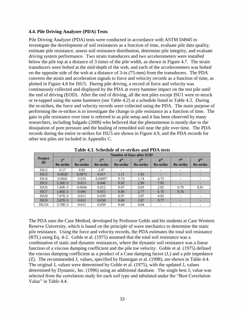
33
4.4. Pile Driving Analyzer (PDA) Tests
Pile Driving Analyzer (PDA) tests were conducted in accordance with ASTM D4945 to
investigate the development of soil resistances as a function of time, evaluate pile data quality,
estimate pile resistance, assess soil resistance distribution, determine pile integrity, and evaluate
driving system performance. Two strain transducers and two accelerometers were installed
below the pile top at a distance of 3 times of the pile width, as shown in Figure 4.7. The strain
transducers were bolted at the mid-depth of the web, and each of the accelerometers was bolted
on the opposite side of the web at a distance of 3-in (75-mm) from the transducers. The PDA
converts the strain and acceleration signals to force and velocity records as a function of time, as
plotted in Figure 4.8 for ISU5. During pile driving, a record of force and velocity was
continuously collected and displayed by the PDA at every hammer impact on the test pile until
the end of driving (EOD). After the end of driving, all the test piles except ISU1 were re-struck
or re-tapped using the same hammers (see Table 4.2) at a schedule listed in Table 4.3. During
the re-strikes, the force and velocity records were collected using the PDA. The main purpose of
performing the re-strikes is to investigate the change in pile resistance as a function of time. The
gain in pile resistance over time is referred to as pile setup and it has been observed by many
researchers, including Salgado (2008) who believed that the phenomenon is mostly due to the
dissipation of pore pressure and the healing of remolded soil near the pile over time. The PDA
records during the entire re-strikes for ISU5 are shown in Figure 4.9, and the PDA records for
other test piles are included in Appendix C.
Table 4.3. Schedule of re-strikes and PDA tests
Project
ID
Number of Days after EOD
1st
Re-strike
2nd
Re-strike
3rd
Re-strike
4th
Re-strike
5th
Re-strike
6th
Re-strike
7th
Re-strike
8th
Re-strike
ISU2 0.17 0.92 2.97 - - - - -
ISU3 0.0028 0.0073 0.017 1.11 1.95 - - -
ISU4 0.0041 0.016 0.04097 0.74 1.74 4.75 - -
ISU5 5.38E-3 0.013 0.048 0.92 2.90 7.92 - -
ISU6 1.60E-3 0.0044 0.012 0.07 0.83 2.82 6.79 9.81
ISU7 1.86E-3 0.006 0.015 0.80 2.77 6.76 9.76 -
ISU8 7.07E-3 0.011 0.039 0.97 3.97 4.95 - -
ISU9 3.87E-3 0.011 0.038 0.69 2.87 9.77 - -
ISU10 3.78E-3 0.011 0.039 0.64 4.64 - - -
The PDA uses the Case Method, developed by Professor Goble and his students at Case Western
Reserve University, which is based on the principle of wave mechanics to determine the static
pile resistance. Using the force and velocity records, the PDA estimates the total soil resistance
(RTL) using Eq. 4-2. Goble et al. (1975) assumed that the total soil resistance was a
combination of static and dynamic resistances, where the dynamic soil resistance was a linear
function of a viscous damping coefficient and the pile toe velocity. Goble et al. (1975) defined
the viscous damping coefficient as a product of a Case damping factor (Jc) and a pile impedance
(Z). The recommended Jc values, specified by Hannigan et al. (1998), are shown in Table 4.4.
The original Jc values were determined by Goble et al. (1975), with the updated Jc values
determined by Dynamic, Inc. (1996) using an additional database. The single best Jc value was
selected from the correlation study for each soil type and tabulated under the “Best Correlation
Value” in Table 4.4.
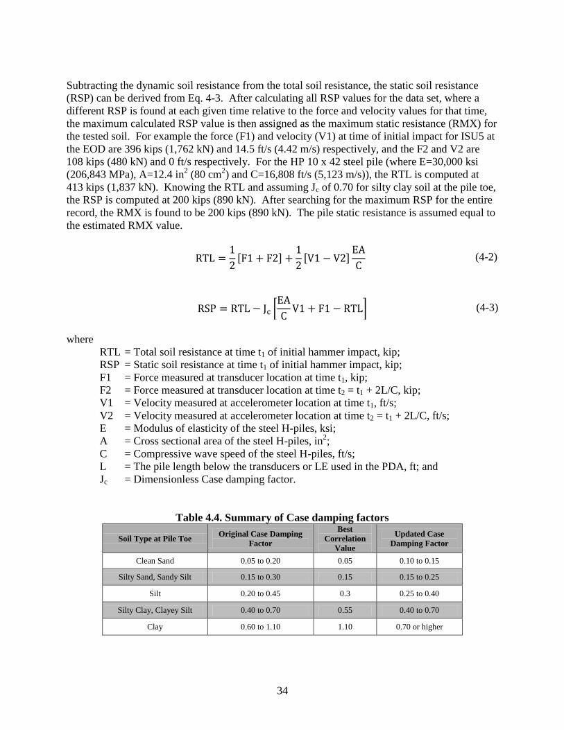
34
Subtracting the dynamic soil resistance from the total soil resistance, the static soil resistance
(RSP) can be derived from Eq. 4-3. After calculating all RSP values for the data set, where a
different RSP is found at each given time relative to the force and velocity values for that time,
the maximum calculated RSP value is then assigned as the maximum static resistance (RMX) for
the tested soil. For example the force (F1) and velocity (V1) at time of initial impact for ISU5 at
the EOD are 396 kips (1,762 kN) and 14.5 ft/s (4.42 m/s) respectively, and the F2 and V2 are
108 kips (480 kN) and 0 ft/s respectively. For the HP 10 x 42 steel pile (where E=30,000 ksi
(206,843 MPa), A=12.4 in2 (80 cm
2) and C=16,808 ft/s (5,123 m/s)), the RTL is computed at
413 kips (1,837 kN). Knowing the RTL and assuming Jc of 0.70 for silty clay soil at the pile toe,
the RSP is computed at 200 kips (890 kN). After searching for the maximum RSP for the entire
record, the RMX is found to be 200 kips (890 kN). The pile static resistance is assumed equal to
the estimated RMX value.
[ ]
[ ]
(4-2)
[
] (4-3)
where
RTL = Total soil resistance at time t1 of initial hammer impact, kip;
RSP = Static soil resistance at time t1 of initial hammer impact, kip;
F1 = Force measured at transducer location at time t1, kip;
F2 = Force measured at transducer location at time t2 = t1 + 2L/C, kip;
V1 = Velocity measured at accelerometer location at time t1, ft/s;
V2 = Velocity measured at accelerometer location at time t2 = t1 + 2L/C, ft/s;
E = Modulus of elasticity of the steel H-piles, ksi;
A = Cross sectional area of the steel H-piles, in2;
C = Compressive wave speed of the steel H-piles, ft/s;
L = The pile length below the transducers or LE used in the PDA, ft; and
Jc = Dimensionless Case damping factor.
Table 4.4. Summary of Case damping factors
Soil Type at Pile Toe Original Case Damping
Factor
Best
Correlation
Value
Updated Case
Damping Factor
Clean Sand 0.05 to 0.20 0.05 0.10 to 0.15
Silty Sand, Sandy Silt 0.15 to 0.30 0.15 0.15 to 0.25
Silt 0.20 to 0.45 0.3 0.25 to 0.40
Silty Clay, Clayey Silt 0.40 to 0.70 0.55 0.40 to 0.70
Clay 0.60 to 1.10 1.10 0.70 or higher

35
Figure 4.7. Typical Pile Driving Analyzer (PDA) set up (from Pile Dynamics, Inc., 1996)
Furthermore, the PDA was also used to assess soil resistance distribution along an embedded pile
length. The PDA estimates the shaft resistance (SFR) using Eq. 4-4, and the end bearing is
determined by subtracting the SFR from the estimated pile static resistance (assumed as RMX).
Using the velocity record and the computed wave-up (Wu) of the test pile, as illustrated by ISU5
at EOD as shown in Figure 4.10, the total shaft resistance (SFT) is estimated by extrapolating the
wave-up curve (solid line) and intersecting with the vertical line at the point where the measured
velocity (dash line) reaches zero (Case Western Reserve University et al. 2008), and the SFT is
determined at 375 kips (1,668 kN). Wave-up is defined as the upward moving wave force as
given by Eq. 4-5. The RMX at Jc of 0.7 was determined early at 200 kips (890 kN), and
similarly, the RX0 which is equal to RMX at Jc of zero is estimated at 413 kips (1,837 kN).
Thus, the shaft resistance is computed at 182 kips (810 kN) using Eq. 4-4, which is 91% of the
pile resistance. As such, only 18 kips (80 kN), or 9%, is contributed from the end bearing. Table
4.5 summarizes the Case damping factor (Jc) used, PDA estimated pile static resistance (RMX)
and shaft resistances (SFR) at both EOD and re-strikes.
(
) (4-4)
(
) (4-5)
Transducer
Accelerometer
Pile Top
3D 3”
3”
1.5”
1.5”
Steel H-Pile
Strain Transducers
Accelerometers
Side View
D
PDA
Accelerometer
Steel H-Pile
Longitudinal
Axis
Section x-x
Strain Transducer

36
Figure 4.8. PDA force and velocity records during driving and at EOD for ISU5
LP = 10 ft
LP = 20 ft
LP = 30 ft
LP = 45 ft
LP =55 ft (EOD)
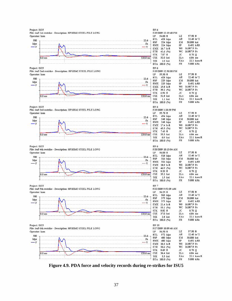
37
Figure 4.9. PDA force and velocity records during re-strikes for ISU5
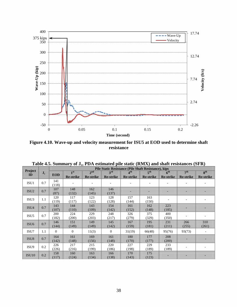
38
Figure 4.10. Wave-up and velocity measurement for ISU5 at EOD used to determine shaft
resistance
Table 4.5. Summary of Jc, PDA estimated pile static (RMX) and shaft resistances (SFR)
-2.26
2.74
7.74
12.74
17.74
-50
0
50
100
150
200
250
300
350
400
0 0.05 0.1 0.15 0.2
Vel
oci
ty (
ft/s
)
Wa
ve-U
p (
kip
)
Time (second)
Wave-Up
Velocity375 kips
Project
ID Jc
Pile Static Resistance (Pile Shaft Resistance), kips
EOD 1st
Re-strike
2nd
Re-strike
3rd
Re-strike
4th
Re-strike
5th
Re-strike
6th
Re-strike
7th
Re-strike
8th
Re-strike
ISU1 0.7 141
(118) - - - - - - - -
ISU2 0.7 107
(87)
148
(132)
162
(145)
146
(137) - - - - -
ISU3 1.1 120
(119)
117
(117)
123
(122)
128
(128)
157
(144)
163
(150) - - -
ISU4 0.7 143
(107)
144
(110)
143
(109)
154
(142)
161
(152)
162
(148)
223
(185) - -
ISU5 0.7 200
(182)
224
(200)
229
(203)
248
(217)
326
(279)
375
(329)
400
(350) - -
ISU6 0.7 146
(144)
151
(149)
149
(149)
145
(142)
167
(159)
195
(181)
231
(211)
266
(255)
310
(261)
ISU7 1.1 0 0 11(3) 0 31(19) 66(48) 95(76) 93(73) -
ISU8 0.7 164
(142)
161
(148)
169
(156)
161
(148)
180
(170)
177
(177)
208
(200) - -
ISU9 0.2 226
(226)
217
(216)
215
(199)
220
(186)
227
(198)
229
(189)
233
(189) - -
ISU10 0.2 158
(117)
160
(124)
163
(134)
166
(138)
170
(143)
175
(123) - - -
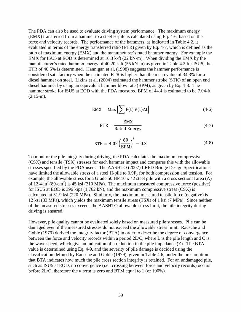
39
The PDA can also be used to evaluate driving system performance. The maximum energy
(EMX) transferred from a hammer to a steel H-pile is calculated using Eq. 4-6, based on the
force and velocity records. The performance of the hammers, as indicated in Table 4.2, is
evaluated in terms of the energy transferred ratio (ETR) given by Eq. 4-7, which is defined as the
ratio of maximum energy (EMX) and the manufacturer’s rated hammer energy. For example the
EMX for ISU5 at EOD is determined at 16.3 k-ft (22 kN-m). When dividing the EMX by the
manufacturer’s rated hammer energy of 40.20 k-ft (55 kN-m) as given in Table 4.2 for ISU5, the
ETR of 40.5% is determined. Hannigan et al. (1998) suggests the hammer performance is
considered satisfactory when the estimated ETR is higher than the mean value of 34.3% for a
diesel hammer on steel. Likins et al. (2004) estimated the hammer stroke (STK) of an open end
diesel hammer by using an equivalent hammer blow rate (BPM), as given by Eq. 4-8. The
hammer stroke for ISU5 at EOD with the PDA measured BPM of 44.4 is estimated to be 7.04-ft
(2.15-m).
[∑ ( ) ( ) ] (4-6)
(4-7)
(
)
(4-8)
To monitor the pile integrity during driving, the PDA calculates the maximum compressive
(CSX) and tensile (TSX) stresses for each hammer impact and compares this with the allowable
stresses specified by the PDA users. The AASHTO (2007) LRFD Bridge Design Specifications
have limited the allowable stress of a steel H-pile to 0.9Fy for both compression and tension. For
example, the allowable stress for a Grade 50 HP 10 x 42 steel pile with a cross sectional area (A)
of 12.4-in2
(80-cm2) is 45 ksi (310 MPa). The maximum measured compressive force (positive)
for ISU5 at EOD is 396 kips (1,762 kN), and the maximum compressive stress (CSX) is
calculated at 31.9 ksi (220 MPa). Similarly, the maximum measured tensile force (negative) is
12 ksi (83 MPa), which yields the maximum tensile stress (TSX) of 1 ksi (7 MPa). Since neither
of the measured stresses exceeds the AASHTO allowable stress limit, the pile integrity during
driving is ensured.
However, pile quality cannot be evaluated solely based on measured pile stresses. Pile can be
damaged even if the measured stresses do not exceed the allowable stress limit. Rausche and
Goble (1979) derived the integrity factor (BTA) in order to describe the degree of convergence
between the force and velocity records within a period 2L/C, where L is the pile length and C is
the wave speed, which give an indication of a reduction in the pile impedance (Z). The BTA
value is determined using Eq. 4-9, and the severity of pile damage is decided using the
classification defined by Rausche and Goble (1979), given in Table 4.6, under the presumption
that BTA indicates how much the pile cross section integrity is retained. For an undamaged pile,
such as ISU5 at EOD, no convergence (i.e., crossing between force and velocity records) occurs
before 2L/C, therefore the α term is zero and BTM equal to 1 (or 100%).

40
( ( )) (4-9)
where
BTA = Degree of convergence between force and velocity records before 2L/C;
α = Defining term, dimensionless;
Z = Pile impedance (see Eq. 4-1), k-s/ft;
Vd = Velocity at location of pile damage after convergence occurred, ft/s;
Fd = Force at location of pile damage after convergence occurred, kip;
F1 = Force at initial hammer impact, kip;
F* = Force at the time before the increase in the velocity become noticeable and
before convergence, kip; and
V* = Velocity at the time when it started to increase toward convergence, ft/s.
Table 4.6. Pile damage classification
BTA (Percentage) Severity of Damage
1.0 (100%) Undamaged
0.8 – 1.0 (80% - 100%) Slight damage
0.6 – 0.8 (60% - 80%) Damage
Below 0.6 (below 60%) Broken
The PDA force and velocity signals are used as an input for the CAse Pile Wave Analysis
Program (CAPWAP) to improve the estimations of static shaft resistance, end bearing, the load
settlement curve, and to determine the dynamic soil parameters (i.e., quakes and damping
factors). For additional detailed descriptions of the PDA, refer to Ng (2011).
4.5. CAse Pile Wave Analysis Program (CAPWAP)
CAse Pile Wave Analysis Program (CAPWAP) method was developed by Professor Goble and
his students in the 1970s. It is a computer program which uses the PDA records as input data for
a more accurate analysis and estimation of the pile resistance, soil resistance distribution and
dynamic soil properties. CAPWAP is used to refine the PDA results at the end of driving and at
re-strikes by performing a signal matching process with the combination of several analytical
techniques, as described by Pile Dynamics, Inc. (2000). CAPWAP adopts the soil-pile model
developed by Smith (1962) and uses the wave equation algorithm in the analysis. Figure 4.11
shows the CAPWAP model for the 60-ft (18.3-m) long HP 10 x 42 steel pile for ISU5 at Clarke
County. CAPWAP considers the pile length below the location of the PDA transducers and
accelerometers, which is 57.5-ft (17.5-m) for the ISU5 example mentioned. The pile model is
divided into user specified segments of pile masses (m) with approximately equal length, and
each pile mass is connected with a series of elastic springs and linear viscous dampers. The
ISU5 example comprised 22 pile segments of around 2.6-ft (0.8-m) in length. The CAPWAP soil
model at an alternate pile segment is represented by an elastic-plastic spring and a linear damper,
as shown in Figure 4.11. The elastic-plastic spring is characterized by two parameters, static soil
resistance at the soil segment (Rs) and soil quake (q), and the linear damper is characterized by

41
the damping coefficient (Cs). CAPWAP approximately relates the damping coefficient to the
Smith damping factor (Js) and the Case damping factor (Jc), using Eqs. 4-10 and 4-11
respectively. It is important to note that any variation in static soil resistance (Rs) will affect the
Js value, but not the Jc value. For a detailed description of CAPWAP, refer to Pile Dynamics,
Inc. (2000).
(4-10)
∑
(4-11)
Figure 4.11. Typical CAPWAP model for ISU5 at EOD
The soil resistance at each soil segment, soil quake and either the Smith’s damping factor or the
Case damping factor are adjusted until the best signal matching is achieved, as shown in Figure
4.12 for ISU5 at EOD. The summation of all adjusted soil resistances along the pile shaft gives
the soil shaft resistance, and total pile resistance is determined by adding the shaft resistance with
the soil resistance at the pile toe. Table 4.7 summarizes the CAPWAP estimated pile capacities
and shaft resistances at EOD and re-strikes for all test piles. A constant soil quake is used for all
soil segments along the shaft and a different quake value is used for the soil model at the pile toe.
The adjusted soil quake values for shaft and toe at EOD and re-strikes for all test sites are
summarized in Table 4.8, and Smith’s damping factors are summarized in
Table 4.9.
25 ft
4 ft
10 ft
16 ft
2.5 ft
57
.5 f
t p
ile
len
gth
w/ 2
2 p
ile
segm
ent
and
11 s
oil s
egm
ent
PDA Signals
HP10x42
Steel Pile
m1
m2
m3
m4
m5
m6
m7
m8
m9
m10
m11
m12
m13
m14
m15
m16
m17
m18
m19
m20
m21
m22
m23
Clay
Silty Clay to Clay
Clay
Silty Clay to Clay
mi
mi-1
mi+1
Rsu
q
Linear-Plastic
Spring
Soil Model
Pile Lumped MassLinear SpringLinear Viscous Damper
Displacement Velocity
Soil D
ampin
g
Res
ista
nce
(R
d)
Static Soil
Resistance (Rs)
Linear Viscous
Damper
CsKs
CpKp
Gauge
Location
Pile Top2.5 ft

42
Figure 4.12. Results of CAPWAP signals matching for ISU5 at EOD
Table 4.7. Summary of CAPWAP estimated total pile resistances and shaft resistances
Project
ID
Total Pile Resistance (Shaft Resistance), kips
EOD 1st
Re-strike
2nd
Re-strike
3rd
Re-strike
4th
Re-strike
5th
Re-strike
6th
Re-strike
7th
Re-strike
8th
Re-strike
ISU1 142
(96) - - - - - - - -
ISU2 81
(67)
116
(101)
130
(114)
130
(114) - - - - -
ISU3 99
(85)
103
(88)
105
(89)
130
(113)
143
(127)
148
(130) - - -
ISU4 102
(88)
105
(90)
109
(93)
121
(107)
135
(117)
144
(127)
154
(138) - -
ISU5 178
(124)
189
(135)
215
(160)
220
(165)
233
(175)
235
(177)
245
(186) - -
ISU6 145
(123)
140
(117)
149
(125)
148
(124)
177
(161)
187
(162)
197
(171)
211
(185)
211
(186)
ISU7 12(0) 13(1) 19(10) 32(18) 43(27) 67(47) 69(60) 75(67) -
ISU8 140
(123)
143
(134)
146
(137)
153
(139)
155
(135)
159
(120)
160
(117) - -
ISU9 169
(138)
168
(127)
166
(139)
161
(131)
159
(127)
157
(124)
155
(115) - -
ISU10 121
(103)
105
(86)
106
(89)
114
(96)
121
(103)
118
(100) - - -
0 160
-80.0
0.0
80.0
160.0
ms
ft/s
40 L/c
Measured Wave Up at TopComputed Wave Up at TopMeasured Velocity at TopComputed Velocity at Top
Velocity (ft/s)
Wave-Up (kips)
CAPWAP Velocity and Wave-Up Signals Matching
for ISU5 at the end of driving.
Time
160.0
80.0
0.0
0 160 ms
40 L/c
Measured Wave-Up at Pile Top
Computed Wave-Up at Pile Top
Measured Velocity at Pile Top
Computed Velocity at Pile Top
43
Table 4.8. Summary of CAPWAP estimated soil quake values
Project
ID
Shaft Quake (Toe Quake), in
EOD 1st
Re-strike
2nd
Re-strike
3rd
Re-strike
4th
Re-strike
5th
Re-strike
6th
Re-strike
7th
Re-strike
8th
Re-strike
ISU1 0.07
(0.93) - - - - - - - -
ISU2 0.05
(0.45)
0.11
(0.28)
0.11
(0.49)
0.25
(0.41) - - - - -
ISU3 0.24
(0.04)
0.25
(0.04)
0.20
(0.04)
0.06
(0.18)
0.12
(0.29)
0.14
(0.20) - - -
ISU4 0.07
(0.16)
0.10
(0.36)
0.08
(0.25)
0.07
(0.23)
0.07
(0.40)
0.12
(0.39)
0.04
(0.50) - -
ISU5 0.07
(0.38)
0.05
(0.09)
0.06
(0.10)
0.05
(0.10)
0.07
(0.16)
0.04
(0.16)
0.05
(0.08) - -
ISU6 0.10
(0.31)
0.09
(0.24)
0.10
(0.41)
0.08
(0.22)
0.05
(0.10)
0.28
(0.15)
0.22
(0.22)
0.31
(0.30)
0.26
(0.25)
ISU7 0.37
(0.28)
0.15
(0.17)
0.15
(0.16)
0.14
(0.04)
0.05
(0.06)
0.04
(0.28)
0.09
(0.16)
0.06
(0.10) -
ISU8 0.11
(0.25)
0.10
(0.27)
0.10
(0.26)
0.15
(0.35)
0.14
(0.28)
0.13
(0.51)
0.12
(0.24) - -
ISU9 0.05
(1.00)
0.05
(0.84)
0.06
(0.86)
0.09
(0.76)
0.07
(0.92)
0.14
(0.82)
0.05
(0.89) - -
ISU10 0.10
(0.99)
0.11
(0.91)
0.11
(0.88)
0.12
(0.15)
0.10
(0.98)
0.11
(0.33) - - -
Table 4.9. Summary of CAPWAP estimated soil Smith’s damping factors
Project
ID
Shaft Damping Factor (Toe Damping Factor), s/ft
EOD 1st
Re-strike
2nd
Re-strike
3rd
Re-strike
4th
Re-strike
5th
Re-strike
6th
Re-strike
7th
Re-strike
8th
Re-strike
ISU1 0.082
(0.063) - - - - - - - -
ISU2 0.130
(0.160)
0.124
(0.140)
0.148
(0.250)
0.169
(0.348) - - - - -
ISU3 0.095
(0.159)
0.118
(0.127)
0.120
(0.099)
0.064
(0.107)
0.105
(0.070)
0.128
(0.118) - - -
ISU4 0.122
(0.05)
0.132
(0.086)
0.112
(0.181)
0.102
(0.123)
0.153
(0.221)
0.164
(0.448)
0.227
(0.315) - -
ISU5 0.241
(0.038)
0.203
(0.066)
0.140
(0.067)
0.164
(0.027)
0.215
(0.110)
0.262
(0.028)
0.203
(0.386) - -
ISU6 0.062
(0.086)
0.064
(0.080)
0.075
(0.115)
0.074
(0.158)
0.089
(0.092)
0.151
(0.200)
0.139
(0.384)
0.166
(0.345)
0.189
(0.290)
ISU7 0.398
(0.074)
0.230
(0.209)
0.083
(0.126)
0.099
(0.136)
0.094
(0.104)
0.107
(0.027)
0.110
(0.078)
0.097
(0.182) -
ISU8 0.092
(0.134)
0.109
(0.167)
0.128
(0.156)
0.134
(0.193)
0.146
(0.398)
0.178
(0.366)
0.147
(0.191) - -
ISU9 0.053
(0.189)
0.088
(0.077)
0.082
(0.135)
0.108
(0.217)
0.092
(0.202)
0.117
(0.222)
0.153
(0.140) - -
ISU10 0.084
(0.074)
0.088
(0.186)
0.098
(0.134)
0.095
(0.060)
0.084
(0.124)
0.061
(0.051) - - -
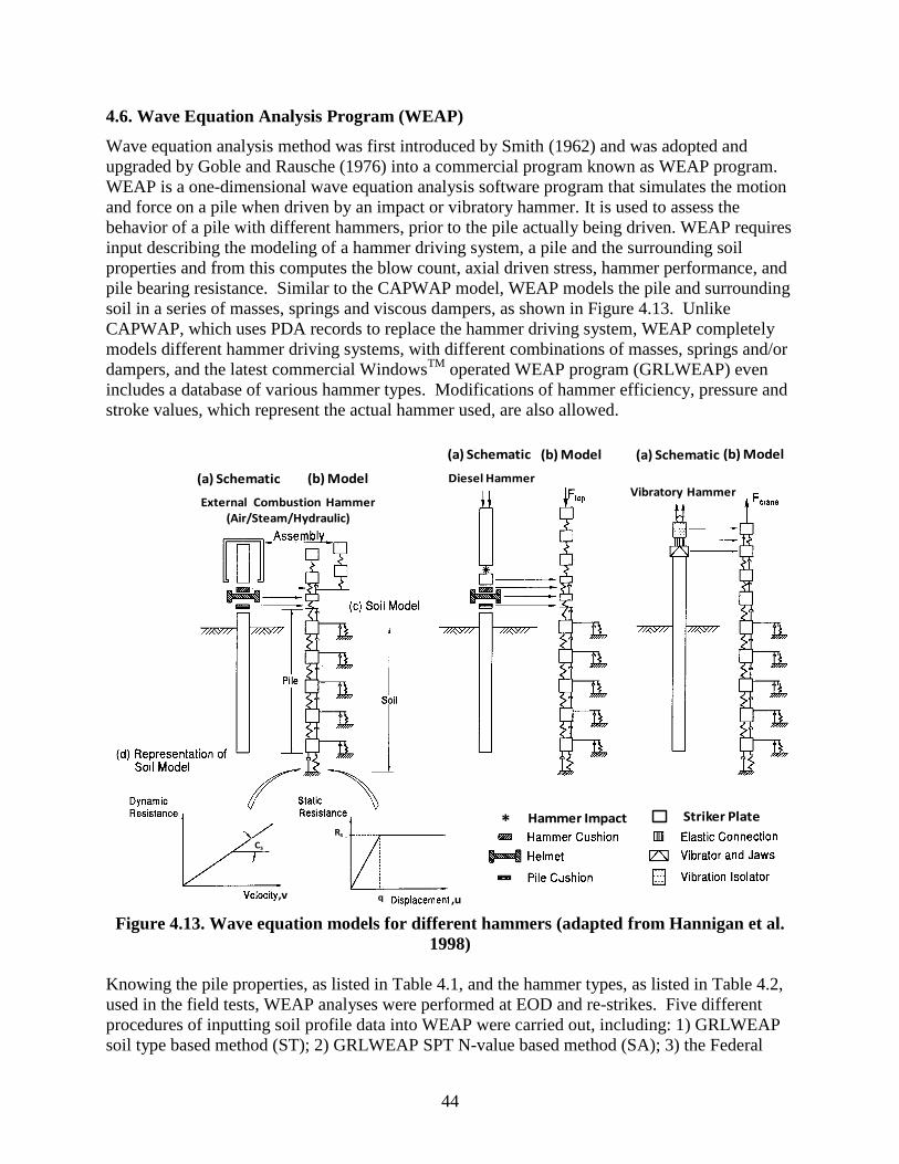
44
4.6. Wave Equation Analysis Program (WEAP)
Wave equation analysis method was first introduced by Smith (1962) and was adopted and
upgraded by Goble and Rausche (1976) into a commercial program known as WEAP program.
WEAP is a one-dimensional wave equation analysis software program that simulates the motion
and force on a pile when driven by an impact or vibratory hammer. It is used to assess the
behavior of a pile with different hammers, prior to the pile actually being driven. WEAP requires
input describing the modeling of a hammer driving system, a pile and the surrounding soil
properties and from this computes the blow count, axial driven stress, hammer performance, and
pile bearing resistance. Similar to the CAPWAP model, WEAP models the pile and surrounding
soil in a series of masses, springs and viscous dampers, as shown in Figure 4.13. Unlike
CAPWAP, which uses PDA records to replace the hammer driving system, WEAP completely
models different hammer driving systems, with different combinations of masses, springs and/or
dampers, and the latest commercial WindowsTM
operated WEAP program (GRLWEAP) even
includes a database of various hammer types. Modifications of hammer efficiency, pressure and
stroke values, which represent the actual hammer used, are also allowed.
Figure 4.13. Wave equation models for different hammers (adapted from Hannigan et al.
1998)
Knowing the pile properties, as listed in Table 4.1, and the hammer types, as listed in Table 4.2,
used in the field tests, WEAP analyses were performed at EOD and re-strikes. Five different
procedures of inputting soil profile data into WEAP were carried out, including: 1) GRLWEAP
soil type based method (ST); 2) GRLWEAP SPT N-value based method (SA); 3) the Federal
External Combustion Hammer(Air/Steam/Hydraulic)
(a) Schematic (b) Model
(a) Schematic (b) Model
Diesel Hammer
(a) Schematic (b) Model
Vibratory Hammer
v
q
* Hammer Impact Striker Plate
,v ,u
Rs
Cs
45
Highway Administration (FHWA) DRIVEN program; 4) Iowa Blue Book (Iowa DOT steel pile
Design Chart); and 5) Iowa DOT current approach. The static analysis methods used in the static
soil resistance estimation for each procedure are summarized in Table 4.10. The methodology
used in each procedure is briefly described in the following subsections; for a detailed
description, refer to Ng (2011).
4.6.1 GRLWEAP soil type based method (ST)
The GRLWEAP soil type based method (ST) provides the easiest procedure of inputting the soil
information. It requires only the identification of soil types, which aids the input process and
simplifies the soil resistance calculation for both bearing graph and driveability analyses. The
corresponding soil parameters stored in the GRLWEAP are based on the Bowles (1996) and
Fellenius (1996) recommendations, given in Table 4.11 for cohesionless soils and Table 4.12 for
cohesive soils. ST method uses the β-method and the modified α-method to estimate the unit
shaft (qs) and unit toe (qt) resistances for non-cohesive soils and cohesive soils respectively.
4.6.2 GRLWEAP SPT N-value based method (SA)
The GRLWEAP SPT N-value based method (SA) requires the input of soil types, unit weights
and uncorrected SPT N-values. These soil parameters can be obtained from the in-situ SPT tests
and laboratory soil tests, or they can be estimated using Bowles (1996) recommendations, given
in Table 4.13 for cohesionless soils and Table 4.14 for cohesive soils, in the absence of soil test
results. The unit shaft and toe resistances are calculated based on the static analysis methods
listed in Table 4.10.
4.6.3 FHWA’s DRIVEN Program
DRIVEN program generates the entire soil profile of a full pile depth and creates an input file for
WEAP analysis. It requires the soil unit weight for all soil types, which are obtained either from
laboratory soil tests, or from Table 4.13 for cohesionless soils and Table 4.14 for cohesive soils.
SPT N-value is used to define cohesionless soil characteristic and undrained shear strength (Su)
is required to define the cohesive soil strength. The undrained shear strength (Su) is estimated
either from the CPT, described in Section 3.2, or by taking half of the unconfined compressive
strength (qu) given in Table 4.14. Next, the unit shaft and toe resistances are calculated based on
static analysis methods, as listed in Table 4.10. For a detailed description of the DRIVEN
program, refer to FHWA DRIVEN User’s Manual (Mathias and Cribbs 1998).
4.6.4 Iowa Blue Book Method
WEAP analysis based on the Iowa Blue Book method uses the Iowa DOT pile design charts, as
shown in Table 4.15 and Table 4.16, for determining the unit shaft (qs) and unit toe (qt)
resistances. The friction value (in kips/ft) is chosen from the design chart with reference to the
width of the steel H-pile, the soil description and the SPT N-value, then this is divided by the
perimeter of the boxed section of a steel H-pile to determine the unit shaft resistance. For
example, the unit shaft for ISU5 (HP 10 x 42 steel H-pile) at about 19-ft (5.8-m) depth with a
clay soil and a SPT N-value of 9 (see Figure 3.2) is calculated at 0.601 ksf (29 kPa), found by
dividing the friction value of 2.0 kip/ft with the square perimeter of 3.33-ft (1-m). However, a
surface perimeter for the H section was assumed for calculating the unit shaft for sand or

46
cohesionless soil. The toe resistance (in kips) is determined by multiplying the unit end bearing
value (in ksi) with the cross sectional area of the H-pile for any soil conditions, assuming soil
plug does not occur in cohesive or clay soil. The calculated unit shaft resistance and the toe
resistances, as tabulated in Table 4.17 and Table 4.18 respectively, shall be inserted directly into
the WEAP’s variable resistance distribution table for driveability and bearing graph analyses.
4.6.5 Iowa DOT Method
The Iowa DOT method uses the SPT N-values as the only soil parameter, which is input into the
WEAP’s variable resistance distribution table, with respect to the depth where the SPT N-values
are taken. Static geotechnical analysis and driveability analysis are not able to be performed
since the SPT N-values only serve to define the relative and approximate stiffness of the soil
profile. However, a bearing graph analysis can be performed to estimate pile resistance.
Despite the various procedures of inputting the soil profiles, the following assumptions are made
and applied to all procedures during the WEAP analysis.
1) Water table remains constant at EOD and at re-strikes
2) The percentage of shaft resistance used in the bearing graph analysis is determined and
assumed from the static geotechnical analysis
3) No residual stress analysis is considered
4) The soil geostatic stress within the pre-drilling depth is treated as an overburden pressure,
and the pile embedded length does not include the pre-drilling depth
5) Bearing graph analysis based on an equal distribution of total pile capacity on shaft and
toe components are selected.
Soil quake (q) and damping coefficient (Cs) are the dynamic soil parameters that describe the soil
model. The WEAP recommended soil quake values for shaft and toe soil segments are given in
Table 4.19, and are used in the five procedures of defining the soil profile. Five approaches are
available in WEAP to define the damping coefficient; however the Smith damping (Eq. 4-10) is
the most commonly used in practice. For a detailed description of the five damping options,
refer to Pile Dynamics, Inc (2005). The relationship between the damping coefficient (Cs) and
the Smith’s damping factor (Js) is given by Eq. 4-10. The WEAP recommended Smith’s
damping factors for shaft and toe soil segments, as outlined in Table 4.20 are used in the WEAP
analyses for all procedures except the Iowa DOT method. The damping factors used in the Iowa
DOT method are given in Table 4.21 based on different soil types. Furthermore, the Smith’s
damping factors are applied consistently to all soil segments, whereas in the Iowa DOT method
various damping factors are chosen, from Table 4.21, based on different soil layers along a pile.
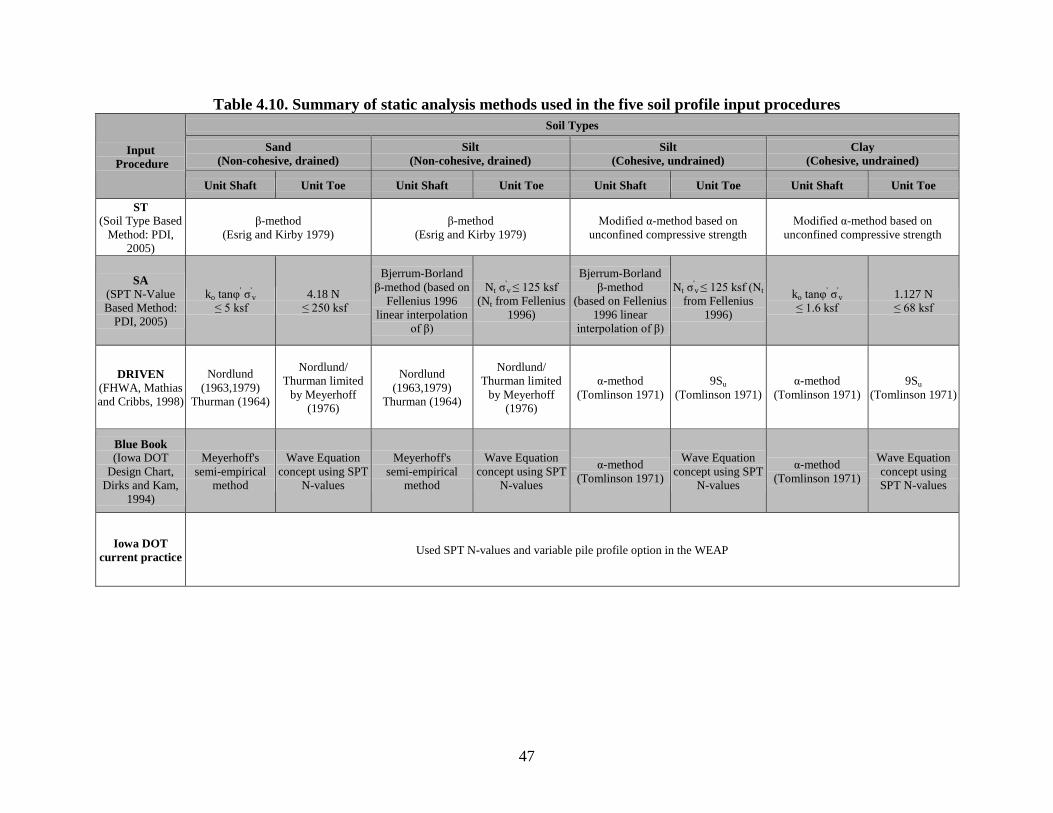
47
Table 4.10. Summary of static analysis methods used in the five soil profile input procedures
Input
Procedure
Soil Types
Sand
(Non-cohesive, drained)
Silt
(Non-cohesive, drained)
Silt
(Cohesive, undrained)
Clay
(Cohesive, undrained)
Unit Shaft Unit Toe Unit Shaft Unit Toe Unit Shaft Unit Toe Unit Shaft Unit Toe
ST
(Soil Type Based
Method: PDI,
2005)
β-method
(Esrig and Kirby 1979)
β-method
(Esrig and Kirby 1979)
Modified α-method based on
unconfined compressive strength
Modified α-method based on
unconfined compressive strength
SA
(SPT N-Value
Based Method:
PDI, 2005)
ko tanφ' σ'
v
≤ 5 ksf
4.18 N
≤ 250 ksf
Bjerrum-Borland
β-method (based on
Fellenius 1996
linear interpolation
of β)
Nt σ'v ≤ 125 ksf
(Nt from Fellenius
1996)
Bjerrum-Borland
β-method
(based on Fellenius
1996 linear
interpolation of β)
Nt σ'v ≤ 125 ksf (Nt
from Fellenius
1996)
ko tanφ' σ'
v
≤ 1.6 ksf
1.127 N
≤ 68 ksf
DRIVEN (FHWA, Mathias
and Cribbs, 1998)
Nordlund
(1963,1979)
Thurman (1964)
Nordlund/
Thurman limited
by Meyerhoff
(1976)
Nordlund
(1963,1979)
Thurman (1964)
Nordlund/
Thurman limited
by Meyerhoff
(1976)
α-method
(Tomlinson 1971)
9Su
(Tomlinson 1971)
α-method
(Tomlinson 1971)
9Su
(Tomlinson 1971)
Blue Book (Iowa DOT
Design Chart,
Dirks and Kam,
1994)
Meyerhoff's
semi-empirical
method
Wave Equation
concept using SPT
N-values
Meyerhoff's
semi-empirical
method
Wave Equation
concept using SPT
N-values
α-method
(Tomlinson 1971)
Wave Equation
concept using SPT
N-values
α-method
(Tomlinson 1971)
Wave Equation
concept using
SPT N-values
Iowa DOT
current practice Used SPT N-values and variable pile profile option in the WEAP

48
Table 4.11. Soil Parameters for cohesionless soils
Soil Type SPT
N-Value
Friction
Angle
(Degree)
Unit
Weight
(lb/ft³)
β
Value
Toe
Bearing
Capacity
Coefficient
(Nt)
Maximum
Unit Shaft
Resistance,
qs (ksf)
Maximum
Unit Toe
Resistance, qt
(ksf)
Very Loose 2 25 - 30 85.9 0.203 12.1 0.5 50
Loose 7 27 - 32 101.8 0.242 18.1 1.0 100
Medium 20 30 - 35 117.8 0.313 33.2 1.5 150
Dense 40 35 - 40 124.1 0.483 86.0 2.0 200
Very Dense 50+ 38 - 43 140.0 0.627 147.0 4.0 400
Table 4.12. Soil Parameters for cohesive soils
Soil Type SPT
N-Value
Unconfined
Compressive
Strength, qu (ksf)
Unit
Weight
(lb/ft³)
Maximum
Unit Shaft
Resistance, qs
(ksf)
Maximum
Unit Toe
Resistance, qt
(ksf)
Very Soft 1 0.25 111.4 0.07 1.13
Soft 3 0.75 111.4 0.22 3.38
Medium 6 1.50 117.8 0.40 6.77
Stiff 12 3.00 130.5 0.80 13.53
Very Stiff 24 6.00 130.5 1.33 27.07
Hard 32+ 8.00 120.9 – 140.0 1.61 36.10
Table 4.13. Empirical values for ø, Dr, and γ of cohesionless soils based on Bowles (1996)
Description Very Loose Loose Medium Dense Very Dense
Relative Density, Dr 0 - 0.15 0.15 - 0.35 0.35 - 0.65 0.65 - 0.85 0.85 - 1.00
Corrected
N-values 0 - 4 4 - 10 10 - 30 30 - 50 50+
Approximate frictional
angle, ø 25 - 30˚ 27 - 32˚ 30 - 35˚ 35 - 40˚ 38 - 43˚
Approximate moist
unit weight, γ (lb/ft³) 70.0 - 99.9 89.8 - 115.2 110.1 - 129.9 110.1 - 140.0 129.9 - 150.2
Table 4.14. Empirical values for qu and γ of cohesive soils based on Bowles (1996)
Description Very Soft Soft Medium Stiff Very Stiff Hard
Unconfined
compressive
strength, qu (ksf)
0 - 0.5 0.5 - 1.0 1.0 - 2.0 2.0 - 4.0 4.0 - 8.0 8.0+
Uncorrected
N-values 0 - 2 2 - 4 4 - 8 8 - 16 16 - 32 32+
Saturated unit
weight, γ (lb/ft³)
100.6 -
119.7
100.6 -
119.7 110.1 - 129.9
119.7 -
140.0
119.7 -
140.0
119.7 -
140.0
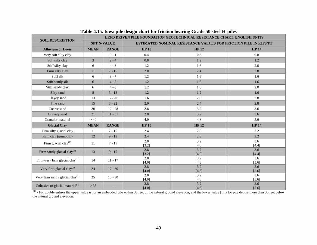
49
Table 4.15. Iowa pile design chart for friction bearing Grade 50 steel H-piles
SOIL DESCRIPTION LRFD DRIVEN PILE FOUNDATION GEOTECHNICAL RESISTANCE CHART, ENGLISH UNITS
SPT N-VALUE ESTIMATED NOMINAL RESISTANCE VALUES FOR FRICTION PILE IN KIPS/FT
Alluvium or Loess MEAN RANGE HP 10 HP 12 HP 14
Very soft silty clay 1 0 - 1 0.4 0.8 0.8
Soft silty clay 3 2 - 4 0.8 1.2 1.2
Stiff silty clay 6 4 - 8 1.2 1.6 2.0
Firm silty clay 11 7 - 15 2.0 2.4 2.8
Stiff silt 6 3 - 7 1.2 1.6 1.6
Stiff sandy silt 6 4 - 8 1.2 1.6 1.6
Stiff sandy clay 6 4 - 8 1.2 1.6 2.0
Silty sand 8 3 - 13 1.2 1.2 1.6
Clayey sand 13 6 - 20 1.6 2.0 2.8
Fine sand 15 8 - 22 2.0 2.4 2.8
Coarse sand 20 12 - 28 2.8 3.2 3.6
Gravely sand 21 11 - 31 2.8 3.2 3.6
Granular material > 40 - 4.0 4.8 5.6
Glacial Clay MEAN RANGE HP 10 HP 12 HP 14
Firm silty glacial clay 11 7 - 15 2.4 2.8 3.2
Firm clay (gumbotil) 12 9 - 15 2.4 2.8 3.2
Firm glacial clay(1) 11 7 - 15 2.8
[3.2]
3.2
[4.0]
3.6
[4.4]
Firm sandy glacial clay(1) 13 9 - 15 2.8
[3.2]
3.2
[4.0]
3.6
[4.4]
Firm-very firm glacial clay(1) 14 11 - 17 2.8
[4.0]
3.2
[4.8]
3.6
[5.6]
Very firm glacial clay(1) 24 17 - 30 2.8
[4.0]
3.2
[4.8]
3.6
[5.6]
Very firm sandy glacial clay(1) 25 15 - 30 2.8
[4.0]
3.2
[4.8]
3.6
[5.6]
Cohesive or glacial material(1) > 35 - 2.8
[4.0]
3.2
[4.8]
3.6
[5.6] (1) - For double entries the upper value is for an embedded pile within 30 feet of the natural ground elevation, and the lower value [ ] is for pile depths more than 30 feet below
the natural ground elevation.
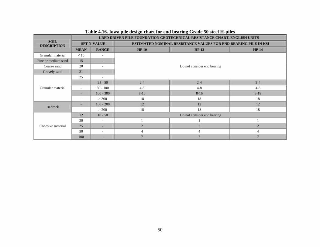
50
Table 4.16. Iowa pile design chart for end bearing Grade 50 steel H-piles
SOIL
DESCRIPTION
LRFD DRIVEN PILE FOUNDATION GEOTECHNICAL RESISTANCE CHART, ENGLISH UNITS
SPT N-VALUE ESTIMATED NOMINAL RESISTANCE VALUES FOR END BEARING PILE IN KSI
MEAN RANGE HP 10 HP 12 HP 14
Granular material < 15 -
Do not consider end bearing
Fine or medium sand 15 -
Coarse sand 20 -
Gravely sand 21 -
Granular material
25 -
- 25 - 50 2-4 2-4 2-4
- 50 - 100 4-8 4-8 4-8
- 100 - 300 8-16 8-16 8-18
- > 300 18 18 18
Bedrock - 100 - 200 12 12 12
- > 200 18 18 18
Cohesive material
12 10 - 50 Do not consider end bearing
20 - 1 1 1
25 - 2 2 2
50 - 4 4 4
100 - 7 7 7

51
Table 4.17. Revised Iowa pile design chart used in WEAP for friction bearing Grade 50 steel H-piles
SOIL DESCRIPTION
LRFD DRIVEN PILE FOUNDATION GEOTECHNICAL RESISTANCE CHART, ENGLISH UNITS
SPT N-VALUE ESTIMATED NOMINAL RESISTANCE VALUES FOR FRICTION PILE IN KIPS PER SQUARE
FOOT (KSF)
Alluvium or Loess MEAN RANGE HP 10 HP 12 HP 14
Very soft silty clay 1 0 - 1 0.12 0.20 0.17
Soft silty clay 3 2 - 4 0.24 0.30 0.26
Stiff silty clay 6 4 - 8 0.36 0.40 0.43
Firm silty clay 11 7 - 15 0.60 0.60 0.60
Stiff silt 6 3 - 7 0.36 0.40 0.34
Stiff sandy silt 6 4 - 8 0.36 0.40 0.34
Stiff sandy clay 6 4 - 8 0.36 0.40 0.43
Silty sand 8 3 - 13 0.25 0.21 0.23
Clayey sand 13 6 - 20 0.33 0.34 0.40
Fine sand 15 8 - 22 0.41 0.41 0.40
Coarse sand 20 12 - 28 0.58 0.55 0.52
Gravely sand 21 11 - 31 0.58 0.55 0.52
Granular material > 40 - 0.83 0.82 0.80
Glacial Clay MEAN RANGE HP 10 HP 12 HP 14
Firm silty glacial clay 11 7 - 15 0.72 0.70 0.69
Firm clay (gumbotil) 12 9 - 15 0.72 0.70 0.69
Firm glacial clay(1) 11 7 - 15 0.84
[0.96]
0.80
[1.00]
0.77
[0.94]
Firm sandy glacial clay(1) 13 9 - 15 0.84
[0.96]
0.80
[1.00]
0.77
[0.94]
Firm-very firm glacial clay(1) 14 11 - 17 0.84
[1.20]
0.80
[1.20]
0.77
[1.20]
Very firm glacial clay(1) 24 17 - 30 0.84
[1.20]
0.80
[1.20]
0.77
[1.20]
Very firm sandy glacial clay(1) 25 15 - 30 0.84
[1.20]
0.80
[1.20]
0.77
[1.20]
Cohesive or glacial material(1) > 35 - 0.84
[1.20]
0.80
[1.20]
0.77
[1.20] (1) - For double entries the upper value is for an embedded pile within 30 feet of the natural ground elevation, and the lower value [ ] is for pile depths more than 30 feet below
the natural ground elevation.
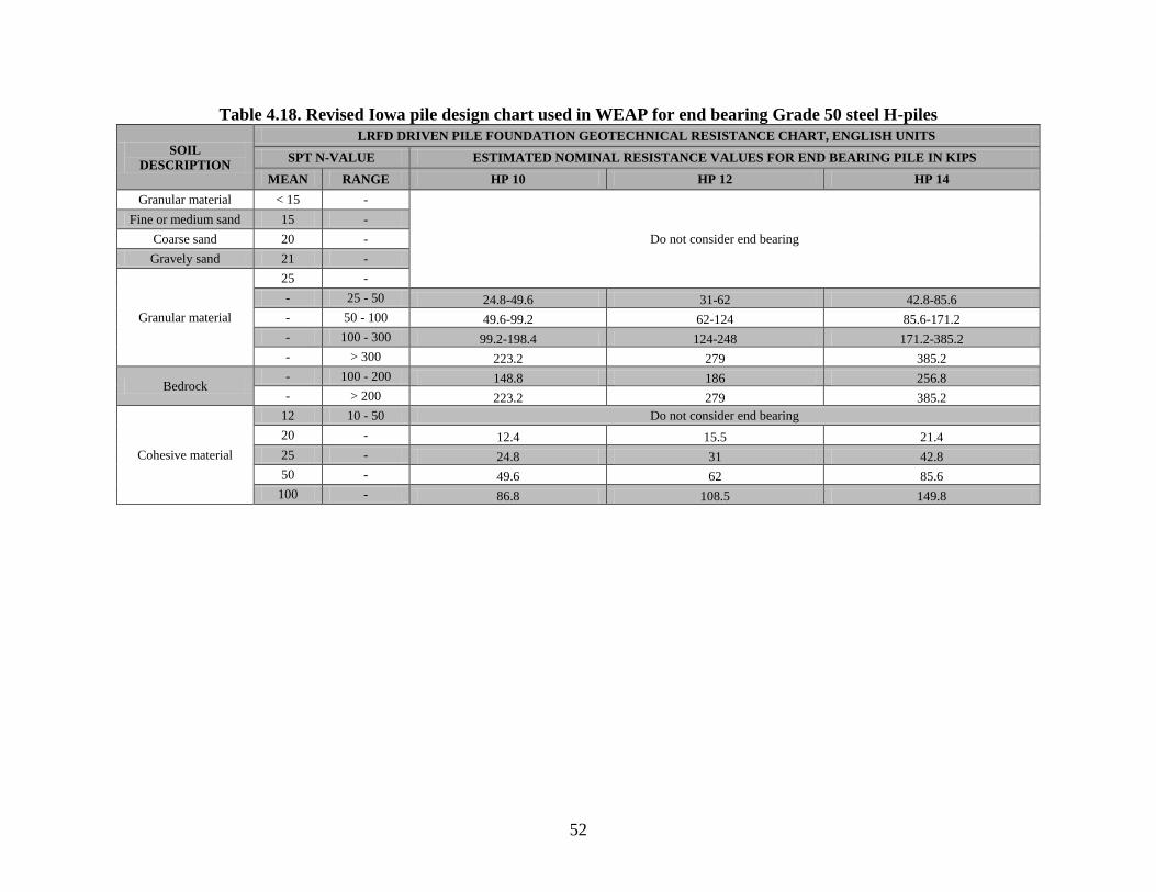
52
Table 4.18. Revised Iowa pile design chart used in WEAP for end bearing Grade 50 steel H-piles
SOIL
DESCRIPTION
LRFD DRIVEN PILE FOUNDATION GEOTECHNICAL RESISTANCE CHART, ENGLISH UNITS
SPT N-VALUE ESTIMATED NOMINAL RESISTANCE VALUES FOR END BEARING PILE IN KIPS
MEAN RANGE HP 10 HP 12 HP 14
Granular material < 15 -
Do not consider end bearing
Fine or medium sand 15 -
Coarse sand 20 -
Gravely sand 21 -
Granular material
25 -
- 25 - 50 24.8-49.6 31-62 42.8-85.6
- 50 - 100 49.6-99.2 62-124 85.6-171.2
- 100 - 300 99.2-198.4 124-248 171.2-385.2
- > 300 223.2 279 385.2
Bedrock - 100 - 200 148.8 186 256.8
- > 200 223.2 279 385.2
Cohesive material
12 10 - 50 Do not consider end bearing
20 - 12.4 15.5 21.4
25 - 24.8 31 42.8
50 - 49.6 62 85.6
100 - 86.8 108.5 149.8

53
Table 4.19. WEAP recommended soil quake values (Pile Dynamics, Inc., 2005) Soil Type
(Pile Type)
Shaft Quake
(in)
Toe Quake
(in)
All soil types, soft rock (Non-displacement piles) 0.10 0.10
Very dense or hard soils
(Displacement piles of diameter or width D) 0.10 D/120
Loose or soft soils
(Displacement piles of diameter or width D) 0.10 D/60
Hard rock (All pile types) 0.10 0.04
Table 4.20. WEAP recommended Smith’s damping factors used in ST, SA, Driven and
Iowa Blue Book (Pile Dynamics, Inc., 2005)
Soil Types Smith’s Shaft
Damping Factor (s/ft)
Smith’s Toe Damping
Factor (s/ft)
Non-cohesive soils 0.05 0.15
Cohesive soils 0.20 0.15
Table 4.21. Damping factors used in the Iowa DOT method
Soil Types Shaft Damping
Factor (s/ft)
Toe Damping
Factor (s/ft)
Rock 0.05 0.05
Boulder & Gravel or Gravel Sand 0.10 0.05
Medium Sand or Fine Sand 0.10 0.10
Packed Sand 0.10 0.05
Silt 0.15 0.12
Silty Clay, Silty Clay, Sandy Clay or Firm Sandy Glacial Clay 0.12 0.12
Firm Clay 0.15 0.12
Firm Glacial Clay or Firm Silty Glacial Clay 0.15 0.15
Pile capacities at EOD and re-strikes are estimated using the measured hammer blow count, as
listed in Table 4.22. The hammer blow count is defined as the amount of hammer blows
required to cause one foot (1-ft) pile penetration into the ground. Using the measured hammer
blow count, the corresponding pile resistance at each loading stage is determined from the
WEAP generated bearing graph. For example, the pile resistance of 166 kips (738 kN) is
determined from the bearing graph, as shown in Figure 4.14 for ISU5 at EOD using the Iowa
DOT method with respect to the measured blow count of 26. Table 4.23 presents the estimated
pile capacities for all events (EOD and re-strikes) using the five soil profile input procedures.
Furthermore, given the hammer information, WEAP estimates the hammer stroke as a function
of hammer blow count, as seen in Figure 4.14 for ISU5 at EOD. The bearing graph analysis also
generates relationships between pile compressive/tensile stresses and hammer blow count, as
illustrated in Figure 4.15 for ISU5 at EOD. In this example, both the compressive (38.25 ksi or
264 MPa) and tensile (6.7 ksi or 46 MPa) stresses at the hammer blow count of 26 are less than
the allowable driving stress of 45 ksi (310 MPa) for a Grade 50 steel H-pile. The WEAP
analysis shows that the pile is not overstressed at EOD. In general, WEAP is used to evaluate
hammer performance, ensure pile integrity, and estimate pile resistance, however the estimated

54
hammer strokes and pile stresses are not tabulated here because the main purpose of performing
the WEAP analysis on this occasion is to estimate pile capacities.
Table 4.22. Measured hammer blow count at EOD and re-strikes
Project
ID
Measured Hammer Blow Count (blow/ft)
EOD 1st
Re-strike
2nd
Re-strike
3rd
Re-strike
4th
Re-strike
5th
Re-strike
6th
Re-strike
7th
Re-strike
8th
Re-strike
ISU1 13 - - - - - - - -
ISU2 10 14 18 22 - - - - -
ISU3 10 16 16 16 18 20 - - -
ISU4 13 15 18 16 21 24 26 - -
ISU5 26 36 37 38 44 54 72 - -
ISU6 21 20 22 25 29 38 44 53 60
ISU7 1 3 3 3 7 7 8 8 -
ISU8 19 20 21 21 28 30 31 - -
ISU9 17 15 16 15 17 14 15 - -
ISU10 15 10 10 12 14 12 - - -
Figure 4.14. WEAP generated bearing graph for ISU5 at EOD using the Iowa DOT method
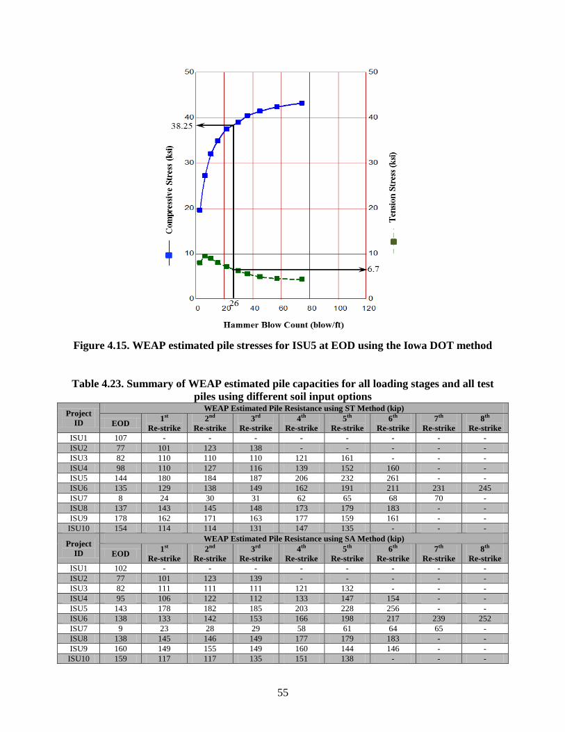
55
Figure 4.15. WEAP estimated pile stresses for ISU5 at EOD using the Iowa DOT method
Table 4.23. Summary of WEAP estimated pile capacities for all loading stages and all test
piles using different soil input options
Project
ID
WEAP Estimated Pile Resistance using ST Method (kip)
EOD 1st
Re-strike
2nd
Re-strike
3rd
Re-strike
4th
Re-strike
5th
Re-strike
6th
Re-strike
7th
Re-strike
8th
Re-strike
ISU1 107 - - - - - - - -
ISU2 77 101 123 138 - - - - -
ISU3 82 110 110 110 121 161 - - -
ISU4 98 110 127 116 139 152 160 - -
ISU5 144 180 184 187 206 232 261 - -
ISU6 135 129 138 149 162 191 211 231 245
ISU7 8 24 30 31 62 65 68 70 -
ISU8 137 143 145 148 173 179 183 - -
ISU9 178 162 171 163 177 159 161 - -
ISU10 154 114 114 131 147 135 - - -
Project
ID
WEAP Estimated Pile Resistance using SA Method (kip)
EOD 1st
Re-strike
2nd
Re-strike
3rd
Re-strike
4th
Re-strike
5th
Re-strike
6th
Re-strike
7th
Re-strike
8th
Re-strike
ISU1 102 - - - - - - - -
ISU2 77 101 123 139 - - - - -
ISU3 82 111 111 111 121 132 - - -
ISU4 95 106 122 112 133 147 154 - -
ISU5 143 178 182 185 203 228 256 - -
ISU6 138 133 142 153 166 198 217 239 252
ISU7 9 23 28 29 58 61 64 65 -
ISU8 138 145 146 149 177 179 183 - -
ISU9 160 149 155 149 160 144 146 - -
ISU10 159 117 117 135 151 138 - - -
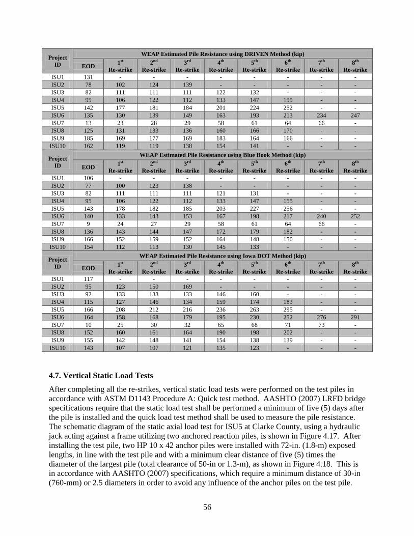
56
Project
ID
WEAP Estimated Pile Resistance using DRIVEN Method (kip)
EOD 1st
Re-strike
2nd
Re-strike
3rd
Re-strike
4th
Re-strike
5th
Re-strike
6th
Re-strike
7th
Re-strike
8th
Re-strike
ISU1 131 - - - - - - - -
ISU2 78 102 124 139 - - - - -
ISU3 82 111 111 111 122 132 - - -
ISU4 95 106 122 112 133 147 155 - -
ISU5 142 177 181 184 201 224 252 - -
ISU6 135 130 139 149 163 193 213 234 247
ISU7 13 23 28 29 58 61 64 66 -
ISU8 125 131 133 136 160 166 170 - -
ISU9 185 169 177 169 183 164 166 - -
ISU10 162 119 119 138 154 141 - - -
Project
ID
WEAP Estimated Pile Resistance using Blue Book Method (kip)
EOD 1st
Re-strike
2nd
Re-strike
3rd
Re-strike
4th
Re-strike
5th
Re-strike
6th
Re-strike
7th
Re-strike
8th
Re-strike
ISU1 106 - - - - - - - -
ISU2 77 100 123 138 - - - - -
ISU3 82 111 111 111 121 131 - - -
ISU4 95 106 122 112 133 147 155 - -
ISU5 143 178 182 185 203 227 256 - -
ISU6 140 133 143 153 167 198 217 240 252
ISU7 9 24 27 29 58 61 64 66 -
ISU8 136 143 144 147 172 179 182 - -
ISU9 166 152 159 152 164 148 150 - -
ISU10 154 112 113 130 145 133 - - -
Project
ID
WEAP Estimated Pile Resistance using Iowa DOT Method (kip)
EOD 1st
Re-strike
2nd
Re-strike
3rd
Re-strike
4th
Re-strike
5th
Re-strike
6th
Re-strike
7th
Re-strike
8th
Re-strike
ISU1 117 - - - - - - - -
ISU2 95 123 150 169 - - - - -
ISU3 92 133 133 133 146 160 - - -
ISU4 115 127 146 134 159 174 183 - -
ISU5 166 208 212 216 236 263 295 - -
ISU6 164 158 168 179 195 230 252 276 291
ISU7 10 25 30 32 65 68 71 73 -
ISU8 152 160 161 164 190 198 202 - -
ISU9 155 142 148 141 154 138 139 - -
ISU10 143 107 107 121 135 123 - - -
4.7. Vertical Static Load Tests
After completing all the re-strikes, vertical static load tests were performed on the test piles in
accordance with ASTM D1143 Procedure A: Quick test method. AASHTO (2007) LRFD bridge
specifications require that the static load test shall be performed a minimum of five (5) days after
the pile is installed and the quick load test method shall be used to measure the pile resistance.
The schematic diagram of the static axial load test for ISU5 at Clarke County, using a hydraulic
jack acting against a frame utilizing two anchored reaction piles, is shown in Figure 4.17. After
installing the test pile, two HP 10 x 42 anchor piles were installed with 72-in. (1.8-m) exposed
lengths, in line with the test pile and with a minimum clear distance of five (5) times the
diameter of the largest pile (total clearance of 50-in or 1.3-m), as shown in Figure 4.18. This is
in accordance with AASHTO (2007) specifications, which require a minimum distance of 30-in
(760-mm) or 2.5 diameters in order to avoid any influence of the anchor piles on the test pile.
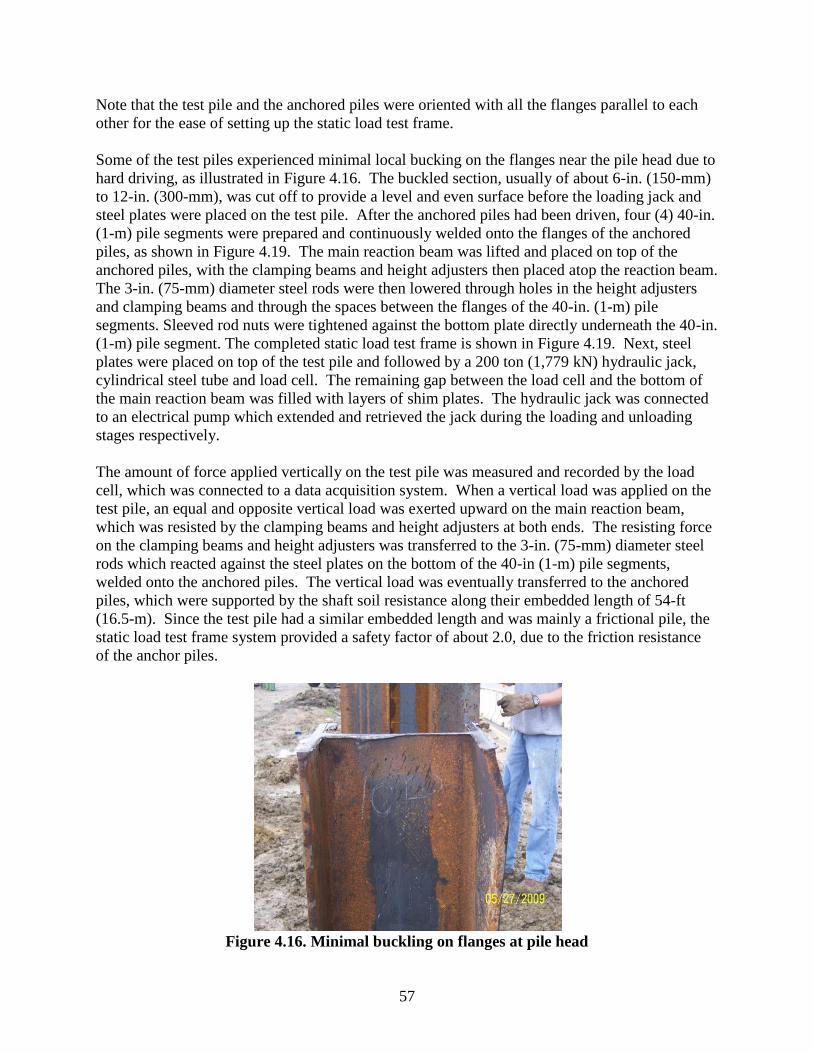
57
Note that the test pile and the anchored piles were oriented with all the flanges parallel to each
other for the ease of setting up the static load test frame.
Some of the test piles experienced minimal local bucking on the flanges near the pile head due to
hard driving, as illustrated in Figure 4.16. The buckled section, usually of about 6-in. (150-mm)
to 12-in. (300-mm), was cut off to provide a level and even surface before the loading jack and
steel plates were placed on the test pile. After the anchored piles had been driven, four (4) 40-in.
(1-m) pile segments were prepared and continuously welded onto the flanges of the anchored
piles, as shown in Figure 4.19. The main reaction beam was lifted and placed on top of the
anchored piles, with the clamping beams and height adjusters then placed atop the reaction beam.
The 3-in. (75-mm) diameter steel rods were then lowered through holes in the height adjusters
and clamping beams and through the spaces between the flanges of the 40-in. (1-m) pile
segments. Sleeved rod nuts were tightened against the bottom plate directly underneath the 40-in.
(1-m) pile segment. The completed static load test frame is shown in Figure 4.19. Next, steel
plates were placed on top of the test pile and followed by a 200 ton (1,779 kN) hydraulic jack,
cylindrical steel tube and load cell. The remaining gap between the load cell and the bottom of
the main reaction beam was filled with layers of shim plates. The hydraulic jack was connected
to an electrical pump which extended and retrieved the jack during the loading and unloading
stages respectively.
The amount of force applied vertically on the test pile was measured and recorded by the load
cell, which was connected to a data acquisition system. When a vertical load was applied on the
test pile, an equal and opposite vertical load was exerted upward on the main reaction beam,
which was resisted by the clamping beams and height adjusters at both ends. The resisting force
on the clamping beams and height adjusters was transferred to the 3-in. (75-mm) diameter steel
rods which reacted against the steel plates on the bottom of the 40-in (1-m) pile segments,
welded onto the anchored piles. The vertical load was eventually transferred to the anchored
piles, which were supported by the shaft soil resistance along their embedded length of 54-ft
(16.5-m). Since the test pile had a similar embedded length and was mainly a frictional pile, the
static load test frame system provided a safety factor of about 2.0, due to the friction resistance
of the anchor piles.
Figure 4.16. Minimal buckling on flanges at pile head

58
Figure 4.17. Schematic drawing of vertical static load test for ISU5 at Clarke County
Steel Angle
(L 2 x 2 x 316)
Steel Angle
(L 2 x 2 x 316)

59
Figure 4.18. Configuration of two anchor piles and a test pile for ISU5 at Clarke County

60
Figure 4.19. Setting up of the static load test
(a) Welded 40 in. short
segment onto flanges
(e) Set up data acquisition
system
(f) Completed static load test frame
(b) A test pile between two anchored piles
(c) Assembled a main reaction beam, clamping
beams and height adjusters; Fastened with steel rods(d) Placed load cell and jack
between test pile and beam
61
During testing readings from strain gauges installed along the pile and displacement gauges were
recorded at load increments of 5% of the anticipated failure load. During each load interval, the
load was kept constant for a time interval of not less than four (4) minutes and not more than
fifteen (15) minutes. During the unloading testing stage, a similar procedure was applied at 10%
load decrement. The strain gauge instrumentation is described in detail in Section 4-3 and the
displacement transducers instrumentation is shown in Figure 4.20. Four (4) 10-in. (250-mm)
stroke displacement transducers were utilized, with each pair located close to both sides of the
test pile flanges. The displacement gauges were bolted on 2×4-in. (40×90-mm) wooden
reference beams, which were supported by wooden ladders approximately 3-ft (900-mm) away
from the test pile on either side, as shown in Figure 4.19 and Figure 4.20. This setting allowed
the measurement of vertical pile movement independent of any movement of the loading frame.
The extendable strings of the displacement transducers were connected to eye hooks mounted on
wooden blocks adhered to the flanges of the test pile, as illustrated in Figure 4.20.
Vertical pile displacement was recorded during each static load test and a load displacement
curve was plotted for each test pile to determine the pile resistance, using the Davisson’s criteria,
as shown in Figure 4.21 for ISU5. The procedure of determining the pile resistance is given by:
(1) drawing the pile elastic stiffness line (dashed-orange line), calculated using Eq. 4-12; (2)
offsetting the line by an additional displacement (δ∆), given by Eq. 4-13, to form the Davisson’s
line (red line); (3) identifying the intersection point (in green circle) between the Davisson’s line
and the load-displacement curve (blue line); and (4) determining the applied load (Q)
corresponding to the intersection point. Due to the contribution of soil stiffness surrounding
ISU5, Figure 4.21 shows that the load displacement curve was plotted above the pile elastic
stiffness line. The measured pile capacities from static load tests based on the Davisson’s criteria
are summarized in Table 4.24 and the load-displacement curves are included in Appendix C for
all test piles. The distribution of the measured pile capacities along the embedded pile length is
described in Section 5.
(4-12)
δ
(4-13)
where
∆e = Pile structural elastic displacement, in;
Q = Applied static load on top of the test pile, kip;
L = Total pile length, in;
A = Cross-sectional area of the test pile, in2;
E = Modulus of elasticity of the test pile, ksi;
δ∆ = Additional displacement for offsetting the pile elastic line, in; and
D = Pile width or diameter, in.
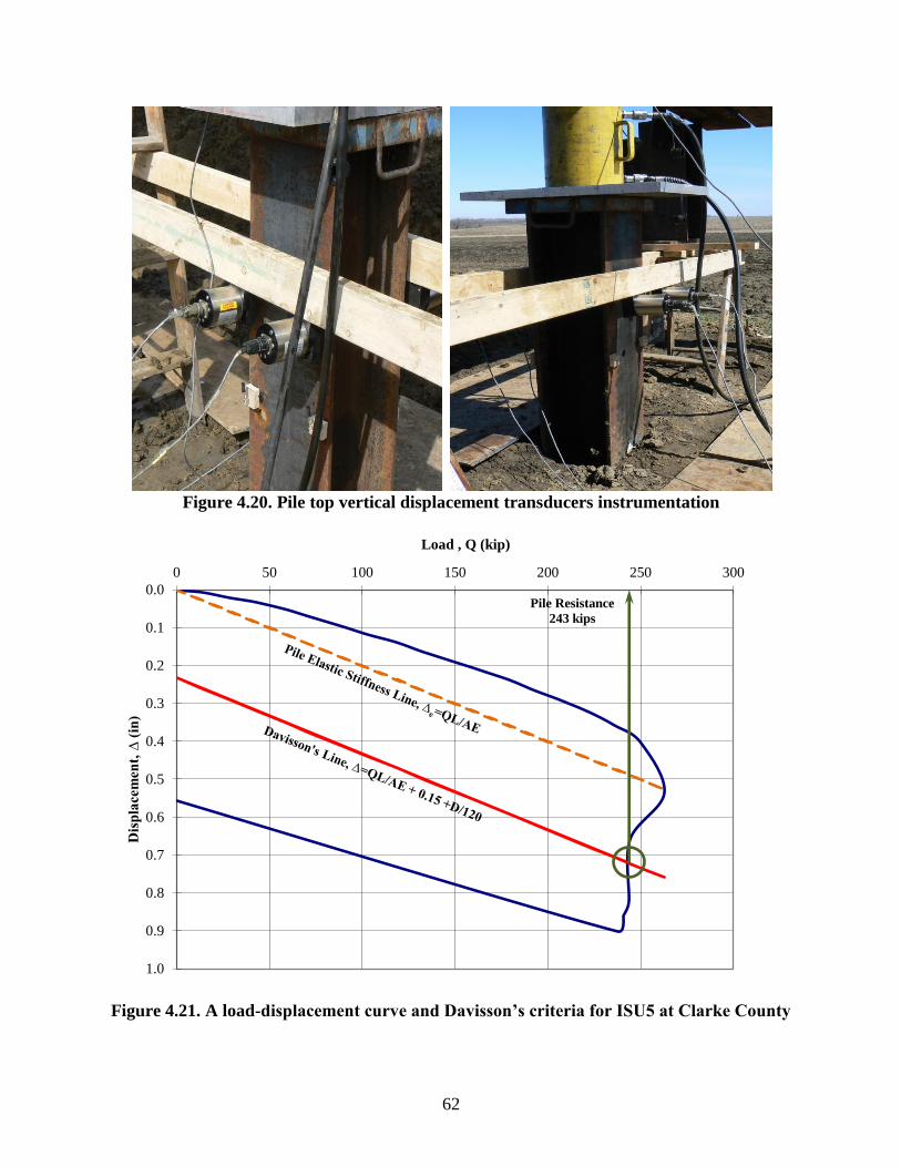
62
Figure 4.20. Pile top vertical displacement transducers instrumentation
Figure 4.21. A load-displacement curve and Davisson’s criteria for ISU5 at Clarke County
0.0
0.1
0.2
0.3
0.4
0.5
0.6
0.7
0.8
0.9
1.0
0 50 100 150 200 250 300
Dis
pla
cem
ent,
∆ (
in)
Load , Q (kip)
Pile Resistance
243 kips
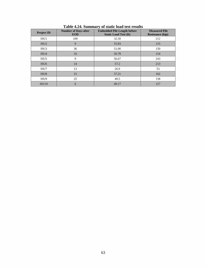
63
Table 4.24. Summary of static load test results
Project ID Number of Days after
EOD
Embedded Pile Length before
Static Load Test (ft)
Measured Pile
Resistance (kip)
ISU1 100 32.50 212
ISU2 9 55.83 125
ISU3 36 51.00 150
ISU4 16 56.78 154
ISU5 9 56.67 243
ISU6 14 57.2 213
ISU7 13 26.9 53
ISU8 15 57.21 162
ISU9 25 49.5 158
ISU10 6 49.17 127

64
CHAPTER 5: INTERPRETATION AND ANALYSIS OF FIELD DATA
5.1. Introduction
The aforementioned experimental research studies generate important data for concurrent
analytical and computational investigations. In pursuing the objectives of this research for pile
resistance quantifications and LRFD resistance factor calibrations, the soil properties measured,
using both in-situ and laboratory tests, and pile responses measured, during re-strikes and from
static load tests (SLTs), were interpreted and analyzed. The strain measurements collected from
SLTs were employed to evaluate the pile load distribution along the embedded pile length and to
determine the shaft resistance and end bearing. Particularly, using the static load test results and
soil properties measured using mBST, load transfer analyses were performed by AbdelSalam
(2010) using TZPILE software to simulate the pile load-displacement relationship. In addition,
the measured soil properties were correlated with the increase in pile resistances as a function of
time (i.e., pile setup), determined using dynamic analysis methods during re-strikes and
measured using SLTs. Due to the economic benefits of incorporating pile setup during pile
designs in cohesive soil, pile setup analytical quantification methods were developed in terms of
measured soil properties. The proposed setup methods were validated using PILOT database.
To expand the application of the proposed pile setup methods, LRFD resistance factors for pile
setup were calibrated by Ng (2011), from which the recommendations were documented in the
LRFD Report Volume III by AbdelSalam et al. (2011). Additional detailed data interpretation
and analyses have also been performed on static analysis methods by AbdelSalam (2010),
dynamic analysis methods by Ng (2011) and dynamic formulae by Roling (2010).
5.2. Pile Resistance Distribution
The measured strains (ε) along an embedded test pile length during the static load test were
converted to pile forces (F) using Eq. (5-1) at each load increment (Q) based on pile elastic
modulus (E) and pile cross-sectional area (A). The distribution of pile forces for test pile ISU5 is
drawn in Figure 5.1, and similar force distributions for other test piles are included in the
Appendix D.1.
F = ε E A (5-1)
The force distribution for ISU5 corresponding to the nominal measured pile resistance (Qm) of
243 kips (1081 kN) based on the Davisson’s criteria (indicated by the solid line without markers
shown in Figure 5.1) was established by interpolation of the force distribution curves relating to
236.2 kips (1050 kN) and 250.4 kips (1114 kN). By extending the slope of the pile force curve
along the pile length over the bottom two pairs of strain data, the end bearing contribution was
estimated at the toe of each pile. In this case, the end bearing component at the embedded pile
length of 56.67-ft (17.28-m) was 55.5 kips (247 kN) or 23% of the total pile resistance of 243
kips (1081 kN). Subtracting the end bearing resistance from the total nominal pile resistance, the
shaft resistance for ISU5 was determined to be 187.5 kips (834 kN). Table 5.1 lists the shaft
resistance and end bearing for all test piles except ISU1, which had no strain instrumentation,
and ISU6, ISU7 and ISU10, for which a large number of strain gauges failed during the test and
thus this information could not be extracted with sufficient accuracy. For comparison with the
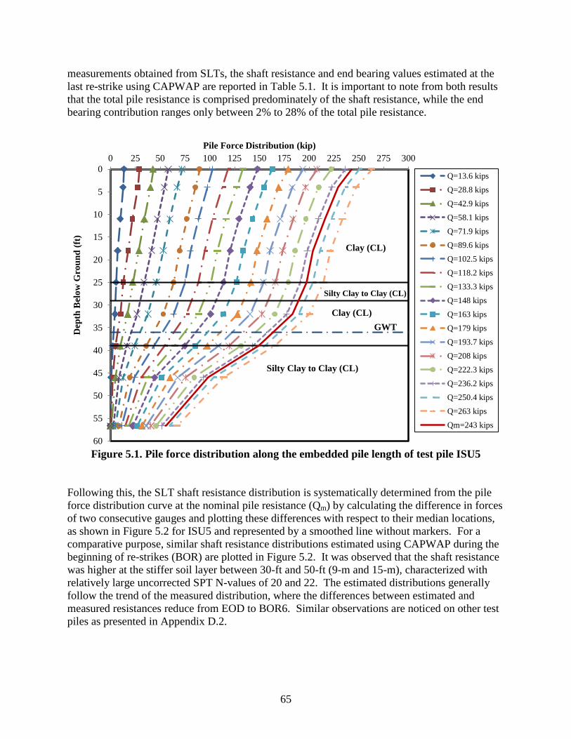
65
measurements obtained from SLTs, the shaft resistance and end bearing values estimated at the
last re-strike using CAPWAP are reported in Table 5.1. It is important to note from both results
that the total pile resistance is comprised predominately of the shaft resistance, while the end
bearing contribution ranges only between 2% to 28% of the total pile resistance.
Figure 5.1. Pile force distribution along the embedded pile length of test pile ISU5
Following this, the SLT shaft resistance distribution is systematically determined from the pile
force distribution curve at the nominal pile resistance (Qm) by calculating the difference in forces
of two consecutive gauges and plotting these differences with respect to their median locations,
as shown in Figure 5.2 for ISU5 and represented by a smoothed line without markers. For a
comparative purpose, similar shaft resistance distributions estimated using CAPWAP during the
beginning of re-strikes (BOR) are plotted in Figure 5.2. It was observed that the shaft resistance
was higher at the stiffer soil layer between 30-ft and 50-ft (9-m and 15-m), characterized with
relatively large uncorrected SPT N-values of 20 and 22. The estimated distributions generally
follow the trend of the measured distribution, where the differences between estimated and
measured resistances reduce from EOD to BOR6. Similar observations are noticed on other test
piles as presented in Appendix D.2.
0
5
10
15
20
25
30
35
40
45
50
55
60
0 25 50 75 100 125 150 175 200 225 250 275 300
Dep
th B
elo
w G
rou
nd
(ft
)
Pile Force Distribution (kip)
Q=13.6 kips
Q=28.8 kips
Q=42.9 kips
Q=58.1 kips
Q=71.9 kips
Q=89.6 kips
Q=102.5 kips
Q=118.2 kips
Q=133.3 kips
Q=148 kips
Q=163 kips
Q=179 kips
Q=193.7 kips
Q=208 kips
Q=222.3 kips
Q=236.2 kips
Q=250.4 kips
Q=263 kips
Qm=243 kips
Clay (CL)
GWT
Silty Clay to Clay (CL)
Clay (CL)
Silty Clay to Clay (CL)

66
Table 5.1. Summary of shaft resistance and end bearing from static load test results and
last re-strike using CAPWAP
Project
ID Soil Type
Static Load Test Results Last Re-strike Using CAPWAP
Shaft Resistance, kip
(Percent Total)
End Bearing, kip
(Percent Total)
Shaft Resistance, kip
(Percent Total)
End Bearing, kip
(Percent Total)
ISU1 Mixed – – 96 (68%)a 46 (32%)a
ISU2 Clay 111 (89%) 14 (11%) 114 (88%) 16 (12%)
ISU3 Clay 136 (91%) 14 (9%) 130 (88%) 18 (12%)
ISU4 Clay 151 (98%) 3 (2%) 138 (90%) 16 (10%)
ISU5 Clay 187.5 (77%) 55.5 (23%) 186 (76%) 59 (24%)
ISU6 Clay – – 186 (88%) 25 (12%)
ISU7 Mixed – – 67 (89%) 8 (11%)
ISU8 Mixed 136 (84%) 26 (16%) 117(73%) 43 (27%)
ISU9 Sand 114 (72%) 44 (28%) 115 (74%) 40 (26%)
ISU10 Sand – – 100 (85%) 18 (15%) a – based on end of driving condition.
Figure 5.2. SLT measured and CAPWAP estimated pile shaft resistance distributions for
test pile ISU5
0 2 4 6 8 10 12 14 16 18 20 22 24
0
10
20
30
40
50
60
0 20 40 60
SPT N-value
Dep
th B
elo
w G
rou
nd
(ft
)
Shaft Resistance Distribution (kip)
EOD BOR1
BOR2 BOR3
BOR4 BOR5
BOR6 SLT
Clay
Silty Clay to Clay
GWT
Clay
Silty Clay to Clay

67
5.3. Load Transfer Analysis Using mBST and TZPILE Program
The modified Borehole Shear Test (mBST) was used to improve the prediction of the load-
displacement relationship and the load distribution for axially loaded friction piles in cohesive
soils using a load-transfer analysis (t-z method). Previously, empirical formulas with soil
laboratory or in-situ tests, such as the Cone Penetration Test (CPT), have been used for deriving
the t-z curves required for this analysis, but the mBST enables direct field measurement of these
curves along the soil-pile interface. Three full-scale, instrumented, static vertical load tests
conducted on steel H-piles (ISU4, ISU5 and ISU8) were used in this study. The t-z analysis was
used to model these three piles utilizing the TZPILE software. Different t-z curves were used in
the models, based on: (1) empirical correlations with CPT; and (2) direct measurements from the
mBST. When compared to the measured responses from the static vertical load tests, the mBST-
based models showed a significant improvement in the prediction accuracy compared to the
CPT-based models. The findings in this report may help to incorporate serviceability limits into
the design of deep foundations. The major findings from this study are summarized as follows:
The pile load-displacement relationship predicted using t-z curves based on empirical
correlations with CPT data (TZ-CPT) significantly overestimated the soil-pile interface
properties, the first portion of the load-displacement response, and the pile capacity by as
much as 50%
The pile load-displacement response calculated using t-z curves obtained from mBST
data (TZ-mBST) provided a close match of the slope of the first portion of the measured
load-displacement responses (i.e., the load-displacement curve before the start of
plunging) and an acceptable estimate of the pile capacity (with differences ranging from
17% to 25% for the three test sites)
Ignoring the end-bearing component (q-w curve) in the t-z analysis did not significantly
affect the results in the case of friction steel H-piles
Based on overall response predictions for the three (3) test sites, the TZ-mBST model has
proven to provide a better match of the measured SLT results when compared with the
TZ-CPT model.
Finally, the mBST is a simple and a cost effective in-situ test that captures the soil-pile interface
and can be directly used in the load-transfer analysis to simulate the load-displacement behavior
at the pile head and the load distribution along the pile length. For a more detailed description of
this study, refer to AbdelSalam (2010).
5.4. Interpretation of Push-In Pressure Cell Measurements
Lateral earth and pore water pressures, in cohesive soil layers near test piles ISU5, ISU6, ISU7
and ISU8, as well as in a cohesionless soil layer near test pile ISU10, were measured using push-
in pressure cells (PCs). Two cases with respect to the ground water elevation and PCs in
cohesive soil layers were explicitly described. The first case, referring to PC1 at ISU5, was
installed approximately 23-ft (7-m) below the ground surface and above the water table, which is
at 36-ft (11-m) below ground level at this location, whilst for the second case, referring to PC3
and PC4 at ISU6, the PCs were installed approximately 33-ft (10-m) below the ground surface
and also below the water table, which lies at 15-ft (4.6-m) below ground level. The
measurements for ISU5 and ISU6 are plotted in Figure 3.17 and in Appendix B.6 respectively.

68
Similar observations were briefly described for PC1 at ISU7 (below water table) and PC4 at
ISU8 (above water table) with their measurements presented in Appendix B.6.
The initial pore water pressure recorded by PC1 at ISU5 began with a zero value. Due to the
process of PC installation that created a passive stress concentration around the PC, the initial
lateral earth pressure (σh) was slightly higher than the estimated geostatic vertical pressure (σv).
The initial pile driving had no effect on either the total lateral earth or pore water pressures.
However, when the pile toe reached the PC1 elevation, at about 23.2-ft (7-m), the lateral earth
pressure and pore water pressure increased almost instantaneously, to about 70 psi (486 kPa) and
50 psi (345 kPa) respectively. Next, the lateral earth pressure and pore water pressure reduced
immediately to about 25 psi (169 kPa) and 19 psi (130 kPa) respectively. It is important to note
that this phenomenon occurred before EOD. The pore water pressure then continued to decrease
with time even when the SLT was performed at 9 days after EOD. As expected from the
dissipation of pore water pressure, the lateral earth pressure increased slowly with time. Figure
3.17 shows that the re-strike and SLT events had insignificant effects on both pressures.
Similar observations were noticed from PC4 at ISU8, at which the lateral earth and pore water
pressures instantaneously increased, to about 45 psi (310 kPa) and 3 psi (21 kPa) respectively,
when the pile toe reached the PC4 elevation. The lateral earth pressure reduced immediately to
its initial value, while the pore water pressure reduced slightly and gradually with time.
For the second case, the PC measurements at ISU6, plotted in Appendix B.6, show both σh
values increased, to about 94 psi (640 kPa), when the pile toe reached the PC elevations. Before
the EOD, the effect of remolding from the continuous pile driving process reduced the σh value
at PC3 to a relative lower value, of 45 psi (310 kPa), than that at PC4, of 52 psi (360 kPa), which
was placed 15-in. (380-mm) further away than PC3 at a distance of 24-in. (610-mm) from ISU6.
On the other hand, the water pressure at PC3 increased to a relative higher magnitude of 15 psi
(101 kPa) when compared to 9 psi (64 kPa) at PC4. These PC measurements showed that the
PC3 water pressure did not reduce immediately; instead, it increased from the moment when the
pile toe reached the PC3 sensor to BOR3. This phenomenon can be explained by the denser
surrounding cohesive soil, indicated with a relatively high SPT N-value of 16, coupled with its
smaller measured vertical coefficient of consolidation of about 0.006 in2/min (0.039 cm
2/min).
Beginning approximately 1.6 hours after EOD (i.e., at BOR4), the PC3 water pressure
logarithmically dissipated about 4 psi (30 kPa) over the period of one day and had almost
completely dissipated to its hydrostatic state in seven days, whereas the PC4 water pressure
logarithmically reduced with a smaller value of 1 psi (7 kPa).
Since PC1 at ISU7 was installed at a location about 5-ft (1.5-m) away from ISU6 (see Appendix
A) and at an elevation 6-ft (1.8-m) above PC3 and PC4 at ISU6 (see Appendix B.1), the
measurements obtained from PC1 shared similar observations. Both lateral earth and pore water
pressures increased, to about 48 psi (331 kPa) and 5.6 psi (39 kPa) respectively, when the pile
toe reached the PC1 elevation. The pore water pressure did not reduce immediately after driving
and its dissipation only began after BOR1. Unlike ISU5 and ISU8, the re-strikes and SLT events
slightly influenced the PC measurements at ISU6 and ISU7, however, the overall logarithmic
trends were not affected by these events.
69
Dissipation of pore water pressure began when the maximum pressure induced by pile driving
was developed. At least 50% of the excess pore water pressure dissipated within 10 minutes at
ISU5 and 4.8 hours at ISU6. Relating the different rate in pore water pressure dissipation, pile
resistance at ISU5 increased rapidly, to 21% within 20 minutes (BOR1), while ISU6 required a
longer time delay, of about 1.6 hours (BOR4), to reach the same percentage increase in the pile
resistance (refer to Table 4.3 and Table 4.7). The continuous logarithmic dissipation of pore
water pressure with time explains the similar pile setup trend, which is further described in
Section 5.5. Due to the presence of moisture content in cohesive soils, dissipation of pore water
pressure occurred regardless of the ground water elevation. This observation concludes that pile
setup occurs along the embedded pile length which is surrounded with cohesive soils. However,
the rate of pore water dissipation in a cohesive soil layer is dependent on its respective ground
water elevation. The results showed that a higher rate of pore water pressure dissipation was
experienced at soil layers above the water table, which led to a higher pile setup rate. In other
words, a pile embedded in a cohesive soil profile with a relatively high ground water elevation
requires a longer time to achieve the desired pile setup.
Alternatively, measurements obtained from PC4 at ISU10, installed in the cohesionless soil layer
(sand) at 10-ft (3-m) below ground, revealed that both lateral earth and pore water pressures
dissipated immediately, from the maximum values of 39.5 psi (272 kPa) and 4.5 psi (31 kPa) to
their respective initial values before EOD (see Appendix B.6). The water pressure returned to
the estimated hydrostatic pressure of 3.5 psi (24 kPa) and the lateral earth pressure remained
constantly larger than the estimated geostatic vertical pressure of 9.7 psi (67 kPa). This
observation was consistent with the minimal variation in pile resistance over time predicted
using CAPWAP during the re-strike events, as reported in Table 4.7 and re-plotted in Figure 5.6.
As such, it is concluded that pile setup does not occur in this cohesionless layer, due to the rapid
and complete dissipation of the excess pore water pressure before the EOD.
5.5. Pile Responses over Time
5.5.1 Pile Driving Resistance
Pile responses in terms of pile driving resistances at three different pile-embedded soil profiles,
clay, mixed soil and sand, were evaluated as a function of embedded pile length and time. The
pile driving resistances were referenced to the hammer blow counts, which were video-recorded
during driving, at EOD and during re-strikes, as reported in Table 4.22. Pile driving resistances
for test piles ISU5, ISU8 and ISU9, as plotted in Figure 5.3, were selected to represent the clay,
mixed soil and sand profiles respectively. Figure 5.3 shows that pile driving resistance increased
as embedded pile length accumulated during pile installation. However, due to the effect of pile
setup, with its trivial embedded pile length increment during re-strikes, the hammer blow count
of ISU5 significantly increased from 30 at EOD condition to 72 at BOR6 after 7.92 days of pile
installation (see Figure 5.3(a)). Similar phenomenon was observed at ISU8 for the mixed soil
profile in Figure 5.3(b). In contrast, ISU9, which was embedded in the sand profile, did not
experience the similar continuous increase in pile driving resistance after EOD as observed at
ISU5 and ISU8. Confirmed by similar observations from the remaining test piles, included in
Appendix D.1, it is concluded that pile setup occurs in the clay and mixed soil profiles but not in
the sand profile.

70
(a) ISU5 for clay profile (b) ISU8 for mixed profile (c) ISU9 for sand profile
Figure 5.3. Pile driving resistance in terms of hammer blow count
0 5 10 15 20 25
0
5
10
15
20
25
30
35
40
45
50
55
60
65
0
2
4
6
8
10
12
14
16
18
20
0 10 20 30 40 50 60 70 80
SPT N-value
Pil
e P
enet
rati
on
Bel
ow
Gro
un
d (
ft)
Pil
e P
enet
rati
on
Bel
ow
Gro
un
d (
m)
Hammer Blows per ft
Blow/ft
SPT N-value
EOD
BOR3
BOR4 BOR5 BOR6
BOR1
BOR2
GWT
Clay
Silty Clay to Clay
Clay
Silty Clay to Clay
0 5 10 15 20 25
0
5
10
15
20
25
30
35
40
45
50
55
60
65
0
2
4
6
8
10
12
14
16
18
20
0 10 20 30 40
SPT N-value
Pil
e P
enet
rati
on
Bel
ow
Gro
un
d (
ft)
Pil
e P
enet
rati
on
Bel
ow
Gro
un
d (
m)
Hammer Blows per ft
Blow/ft
SPT N-value
EOD
BOR3
BOR4 BOR5
BOR6 BOR1
BOR2
GWT
Clay
Silty Clay to Clay
Silty Sand to Sandy Silt
Sand
Clayey Silt to Silty Clay
Silty Sand to Sandy Silt
Clayey Silt to Silty Clay
Silty Clay to Clay
0 5 10 15 20 25 30 35
0
5
10
15
20
25
30
35
40
45
50
55
60
65
0
2
4
6
8
10
12
14
16
18
20
0 5 10 15 20
SPT N-value
Pil
e P
enet
rati
on
Bel
ow
Gro
un
d (
ft)
Pil
e P
enet
rati
on
Bel
ow
Gro
un
d (
m)
Hammer Blows per ft
Blow/ft
SPT N-value
EOD
BOR3
BOR4 BOR5
BOR6
BOR1
BOR2
Clay
Sandy Silt to Clayey Silt
Sand
GWT

71
5.5.2 Relationship Between Pile Resistance and Time
Total pile resistances (Rt) estimated using WEAP and CAPWAP, summarized in Table 4.23 and
Table 4.7 respectively, were plotted against the time (t) at when the re-strikes were performed
(see Table 4.3). Among the five soil profile input procedures used in WEAP, only the results
estimated using the Iowa Blue Book method (refer to Section 4.6.4 for detailed description) were
presented for a comparative purpose. In addition, pile resistances measured using the static load
tests, given in Table 4.24, were included to verify the relationship between pile resistance and
time. Figure 5.4 and Figure 5.5 show that the increase in total pile resistance has a logarithmic
relationship with time for both clay and mixed soil profiles, respectively. Not only do the
resistances estimated during re-strikes, using both WEAP and CAPWAP, follow the logarithmic
trend, but also the resistances measured at SLT agree with the trend. Alternatively, Figure 5.6
shows that the total resistance of test pile ISU10, embedded in sand profile, did not increase as
much as observed in the clay and mixed soil profiles, while the resistance of ISU9 decreased
with time. These results agreed with the observations described in Section 5.4 based on the
contrasting pore water pressure measurements between cohesive and cohesionless soils and
agreed with the conclusion made in Section 5.5.1.
(a) WEAP-Iowa Blue Book Procedure (b) CAPWAP
Figure 5.4. Relationship between total pile resistance and time for clay profile
0
50
100
150
200
250
0.0001 0.01 1 100
To
tal
Pil
e R
esis
tan
ce,
Rt (
kip
)
Time After End of Driving, t (Day)
ISU2 (SLT) ISU3 (SLT)
ISU4 (SLT) ISU5 (SLT)
ISU6 (SLT) ISU2 (WEAP)
ISU3 (WEAP) ISU4 (WEAP)
ISU5 (WEAP) ISU6 (WEAP)
0
50
100
150
200
250
0.0001 0.01 1 100
To
tal
Pil
e R
esis
tan
ce,
Rt (
kip
)
Time After End of Driving, t (Day)
ISU2 (SLT) ISU3 (SLT)
ISU4 (SLT) ISU5 (SLT)
ISU6 (SLT) ISU2 (CAPWAP)
ISU3 (CAPWAP) ISU4 (CAPWAP)
ISU5 (CAPWAP) ISU6 (CAPWAP)

72
(a) WEAP-Iowa Blue Book Procedure (b) CAPWAP
Figure 5.5. Relationship between total pile resistance and time for mixed soil profile
(a) WEAP-Iowa Blue Book Procedure (b) CAPWAP
Figure 5.6. Relationship between total pile resistance and time for sand profile
0
50
100
150
200
250
0.0001 0.01 1 100
To
tal
Pil
e R
esis
tan
ce,
Rt (
kip
)
Time After End of Driving, t (Day)
ISU7 (WEAP)
ISU8 (WEAP)
ISU7 (SLT)
ISU8 (SLT)
0
50
100
150
200
250
0.0001 0.01 1 100T
ota
l P
ile
Res
ista
nce
, R
t (k
ip)
Time After End of Driving, t (Day)
ISU7 (CAPWAP)
ISU8 (CAPWAP)
ISU7 (SLT)
ISU8 (SLT)
0
50
100
150
200
250
0.0001 0.01 1 100
To
tal
Pil
e R
esis
tan
ce,
Rt (
kip
)
Time After End of Driving, t (Day)
ISU9 (WEAP)
ISU10 (WEAP)
ISU9 (SLT)
ISU10 (SLT)
0
50
100
150
200
250
0.0001 0.01 1 100
To
tal
Pil
e R
esis
tan
ce,
Rt
(kip
)
Time After End of Driving, t (Day)
ISU9 (CAPWAP)
ISU10 (CAPWAP)
ISU9 (SLT)
ISU10 (SLT)
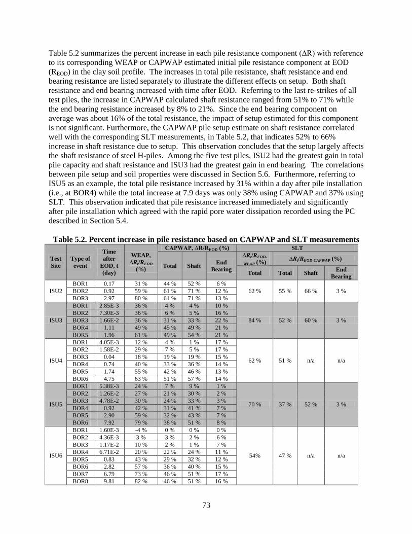
73
Table 5.2 summarizes the percent increase in each pile resistance component (∆R) with reference
to its corresponding WEAP or CAPWAP estimated initial pile resistance component at EOD
(REOD) in the clay soil profile. The increases in total pile resistance, shaft resistance and end
bearing resistance are listed separately to illustrate the different effects on setup. Both shaft
resistance and end bearing increased with time after EOD. Referring to the last re-strikes of all
test piles, the increase in CAPWAP calculated shaft resistance ranged from 51% to 71% while
the end bearing resistance increased by 8% to 21%. Since the end bearing component on
average was about 16% of the total resistance, the impact of setup estimated for this component
is not significant. Furthermore, the CAPWAP pile setup estimate on shaft resistance correlated
well with the corresponding SLT measurements, in Table 5.2, that indicates 52% to 66%
increase in shaft resistance due to setup. This observation concludes that the setup largely affects
the shaft resistance of steel H-piles. Among the five test piles, ISU2 had the greatest gain in total
pile capacity and shaft resistance and ISU3 had the greatest gain in end bearing. The correlations
between pile setup and soil properties were discussed in Section 5.6. Furthermore, referring to
ISU5 as an example, the total pile resistance increased by 31% within a day after pile installation
(i.e., at BOR4) while the total increase at 7.9 days was only 38% using CAPWAP and 37% using
SLT. This observation indicated that pile resistance increased immediately and significantly
after pile installation which agreed with the rapid pore water dissipation recorded using the PC
described in Section 5.4.
Table 5.2. Percent increase in pile resistance based on CAPWAP and SLT measurements
Test
Site
Type of
event
Time
after
EOD, t
(day)
WEAP,
∆Rt/REOD
(%)
CAPWAP, ∆R/REOD (%) SLT
Total Shaft End
Bearing
∆Rt/REOD-
WEAP (%) ∆Rt/REOD-CAPWAP (%)
Total Total Shaft End
Bearing
ISU2
BOR1 0.17 31 % 44 % 52 % 6 %
62 % 55 % 66 % 3 % BOR2 0.92 59 % 61 % 71 % 12 %
BOR3 2.97 80 % 61 % 71 % 13 %
ISU3
BOR1 2.85E-3 36 % 4 % 4 % 10 %
84 % 52 % 60 % 3 %
BOR2 7.30E-3 36 % 6 % 5 % 16 %
BOR3 1.66E-2 36 % 31 % 33 % 22 %
BOR4 1.11 49 % 45 % 49 % 21 %
BOR5 1.96 61 % 49 % 54 % 21 %
ISU4
BOR1 4.05E-3 12 % 4 % 1 % 17 %
62 % 51 % n/a n/a
BOR2 1.58E-2 29 % 7 % 5 % 17 %
BOR3 0.04 18 % 19 % 19 % 15 %
BOR4 0.74 40 % 33 % 36 % 14 %
BOR5 1.74 55 % 42 % 46 % 13 %
BOR6 4.75 63 % 51 % 57 % 14 %
ISU5
BOR1 5.38E-3 24 % 7 % 9 % 1 %
70 % 37 % 52 % 3 %
BOR2 1.26E-2 27 % 21 % 30 % 2 %
BOR3 4.78E-2 30 % 24 % 33 % 3 %
BOR4 0.92 42 % 31 % 41 % 7 %
BOR5 2.90 59 % 32 % 43 % 7 %
BOR6 7.92 79 % 38 % 51 % 8 %
ISU6
BOR1 1.60E-3 -4 % 0 % 0 % 0 %
54% 47 % n/a n/a
BOR2 4.36E-3 3 % 3 % 2 % 6 %
BOR3 1.17E-2 10 % 2 % 1 % 7 %
BOR4 6.71E-2 20 % 22 % 24 % 11 %
BOR5 0.83 43 % 29 % 32 % 12 %
BOR6 2.82 57 % 36 % 40 % 15 %
BOR7 6.79 73 % 46 % 51 % 17 %
BOR8 9.81 82 % 46 % 51 % 16 %
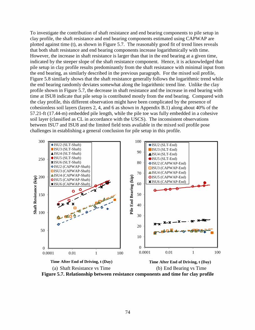
74
To investigate the contribution of shaft resistance and end bearing components to pile setup in
clay profile, the shaft resistance and end bearing components estimated using CAPWAP are
plotted against time (t), as shown in Figure 5.7. The reasonably good fit of trend lines reveals
that both shaft resistance and end bearing components increase logarithmically with time.
However, the increase in shaft resistance is larger than that in the end bearing at a given time,
indicated by the steeper slope of the shaft resistance component. Hence, it is acknowledged that
pile setup in clay profile results predominantly from the shaft resistance with minimal input from
the end bearing, as similarly described in the previous paragraph. For the mixed soil profile,
Figure 5.8 similarly shows that the shaft resistance generally follows the logarithmic trend while
the end bearing randomly deviates somewhat along the logarithmic trend line. Unlike the clay
profile shown in Figure 5.7, the decrease in shaft resistance and the increase in end bearing with
time at ISU8 indicate that pile setup is contributed mostly from the end bearing. Compared with
the clay profile, this different observation might have been complicated by the presence of
cohesionless soil layers (layers 2, 4, and 6 as shown in Appendix B.1) along about 40% of the
57.21-ft (17.44-m) embedded pile length, while the pile toe was fully embedded in a cohesive
soil layer (classified as CL in accordance with the USCS). The inconsistent observations
between ISU7 and ISU8 and the limited field tests available in the mixed soil profile pose
challenges in establishing a general conclusion for pile setup in this profile.
(a) Shaft Resistance vs Time (b) End Bearing vs Time
Figure 5.7. Relationship between resistance components and time for clay profile
0
50
100
150
200
250
300
0.0001 0.01 1 100
Sh
aft
Res
ista
nce
(k
ip)
Time After End of Driving, t (Day)
ISU2 (SLT-Shaft)
ISU3 (SLT-Shaft)
ISU4 (SLT-Shaft)
ISU5 (SLT-Shaft)
ISU6 (SLT-Shaft)
ISU2 (CAPWAP-Shaft)
ISU3 (CAPWAP-Shaft)
ISU4 (CAPWAP-Shaft)
ISU5 (CAPWAP-Shaft)
ISU6 (CAPWAP-Shaft)
0
10
20
30
40
50
60
70
80
90
100
0.0001 0.01 1 100
Pil
e E
nd
Bea
rin
g (
kip
)
Time After End of Driving, t (Day)
ISU2 (SLT-End)
ISU3 (SLT-End)
ISU4 (SLT-End)
ISU5 (SLT-End)
ISU2 (CAPWAP-End)
ISU3 (CAPWAP-End)
ISU4 (CAPWAP-End)
ISU5 (CAPWAP-End)
ISU6 (CAPWAP-End)

75
(a) Shaft Resistance vs Time (b) End Bearing vs Time
Figure 5.8. Relationship between resistance components and time for mixed soil profile
5.6. Pile Setup in Clay Profile
The aforementioned observations confirmed the logarithmic relationship between pile setup and
time in the clay profile. When accounted for accurately, integration of pile setup will lead to
more cost-effective design as it will reduce the number of piles and/or pile length in the clay
profile. However, there are several limitations associated with the existing pile setup knowledge,
and there are currently no methods available to confidently account for the effects of pile setup in
foundation designs. These limitations arise from the lack of: a) sufficient and detailed dynamic
and static field test data as a function of time for accurate pile setup evaluation; b) detailed
subsurface investigations and monitoring of soil stresses to quantify pile setup (Komurka et al.
2003); and c) a systematic reliability-based method to account for pile setup in the LRFD
approach. The extensive field tests carried out herein involved detailed pile setup measurements,
using WEAP and CAPWAP, as well as soil investigations. These tests provide the opportunity
to: 1) assess the influence of various soil properties on pile setup, as discussed in Section 5.6.1;
and 2) develop two pile setup quantification methods in terms of commonly measured SPT N-
value and/or CPT determined coefficient of consolidation, as discussed in Section 5.6.2. Along
with the five field test results, twelve data points from the PILOT database were selected to
validate the proposed pile setup quantification methods established for WEAP, discussed in
Section 5.6.3. Since the PILOT database does not contain any PDA records for CAPWAP
analyses, only the five field tests were used in validating the pile setup methods established for
CAPWAP. To incorporate pile setup into LRFD, a new calibration procedure using the
reliability theory was established in Section 5.6.4.
0
50
100
150
200
0.0001 0.01 1 100
Sh
aft
Res
ista
nce
(k
ip)
Time After End of Driving, t (Day)
ISU7 (CAPWAP-Shaft)
ISU8 (CAPWAP-Shaft)
ISU8 (SLT-Shaft)
0
10
20
30
40
50
60
70
80
90
100
0.0001 0.01 1 100
Pil
e E
nd
Bea
rin
g (
kip
)
Time After End of Driving, t (Day)
ISU7 (CAPWAP-End)
ISU8 (CAPWAP-End)
ISU8 (SLT-End)

76
5.6.1 Influence of Various Soil Properties on Pile Setup
Since the pile setup largely increases the shaft resistance, a detailed correlation study between
soil properties and percent increase in shaft resistance (∆R/REOD) was performed. For illustrative
purposes, the correlation study of ISU5 has been explicitly described, whilst studies for the
remaining four test piles are included in Appendix D.4. The percent increase in shaft resistance
calculated for ISU5 using CAPWAP, between EOD and the last re-strike, was plotted along the
embedded pile length, in Figure 5.9, together with the measured vertical coefficient of
consolidation (Cv), SPT N-value, over consolidation ratio (OCR), soil compressibility index (Cc),
and plasticity index (PI). Since the horizontal coefficient of consolidation (Ch) was not
successfully measured at ISU5 due to the time required to achieve 50% pore water pressure
dissipation, it can be related to the SPT N-values as shown in Figure 5.10. A similar shaft gain
distribution of ∆R/REOD for the SLT, the percent difference between the measured shaft
resistance from SLT at 9 days after EOD and the CAPWAP calculated shaft resistance at EOD,
is also included in Figure 5.9 for comparative purposes. It is interesting to note that the
distributions of percent increase in shaft resistance (∆R/REOD) for both CAPWAP and SLT have
a similar trend, although the magnitudes are sometimes significantly different, which can be
attributed to the standard CAPWAP signal matching procedure that uses constant damping and
quake values to achieve a best match.
Figure 5.9. Relationship between soil properties and increase in shaft resistance for ISU5
0 2 4 6 8 10 12 14 16 18 20 22 24 26 28 30 32 34 36 38 40
0
5
10
15
20
25
30
35
40
45
50
55
60
65
0
2
4
6
8
10
12
14
16
18
-5% 0% 5% 10% 15% 20% 25% 30%
SPT N-value or Plasticity Index (%)
Dep
th B
elo
w G
rou
nd
(ft
)
Dep
th B
elo
w G
rou
nd
(m
)
Percent Increase In Shaft Resistance Distribution (%)
Shaft Gain (CAPWAP-8 days)Shaft Gain (SLT-9 days)SPT N-valuePlasticity Index
Low plasticity
Clay (CL)
Low Plasticity
Clay with Sand (CL)
GWT
Cv=0.017 in2/min
OCR=4.5; Cc=0.187
Cv=0.014 in2/min
OCR=1.28; Cc=0.256
Cv=0.008 in2/min
OCR=1.0; Cc=0.124

77
Figure 5.10. Correlations of both vertical and horizontal coefficients of consolidation with
SPT N-values
The SLT-based shaft gain distribution, shown in Figure 5.9, illustrates that the ∆R/REOD
increased by about 5% in the 16-ft (5-m) thick top soil layer, which was characterized with
relatively large Cv values, ranging between 0.014 in2/min (0.089 cm
2/min) and 0.017 in
2/min
(0.107 cm2/min), and small SPT N-values, ranging between 6 and 9. This ∆R/REOD continued to
reduce to a depth of around 36-ft (11-m) from ground surface, where the surrounding cohesive
soil layer has the smallest Cv of 0.008 in2/min (0.051 cm
2/min) and the highest SPT N-value of
22. With the combined effects of the overburden pressure and the reduction in SPT N-value,
from 22 to 13, below the 36-ft (11-m) depth, the ∆R/REOD indicated a peak increase of about
25%. This observation suggests a direct relationship between pile setup along the shaft and the
coefficient of consolidation, plus an inverse relationship between pile setup and SPT N-value (or
a direct correlation with the horizontal coefficient of consolidation, as indicated by Figure 5.10).
Besides comparing with SPT N-value and coefficient of consolidation, pile setup was also
compared with other soil properties, including over consolidation ratio (OCR), compressibility
index (Cc) and plastic index (PI). Figure 5.9 reveals an inverse relationship between the
measured PI and the ∆R/REOD. For instance, within the cohesive soil layers with low PI values,
of 5.6% and 8.6% at 10-ft (3-m) and 47-ft (14-m) respectively, the shaft resistances increased.
Hence, a pile embedded in a cohesive soil with low PI will experience a large ∆R/REOD at any
given time. Furthermore, Zheng et al. (2010) concluded that a low compressive cohesive soil
with a small Cc value dissipated the excess pore water pressure faster. Relating this conclusion
to pile setup, this means Cc value should have an inverse relationship with ∆R/REOD, however,
Ch = 0.4928N-2.081
R² = 0.7005
0.00
0.02
0.04
0.06
0.08
0.10
0.12
0.14
0.16
0 2 4 6 8 10 12 14 16 18 20 22 24 26 28
0.00
0.02
0.04
0.06
0.08
0.10
0.12
0.14
0.16
Ver
tica
l C
oef
fici
ent
of
Co
nso
lid
ati
on
, C
v (i
n2/m
in)
SPT N-value
Ho
rizo
nta
l C
oef
fici
ent
of
Co
nso
lid
ati
on
, C
h (
in2/m
in)
CPT (Ch)
One-dimensional test (Cv)
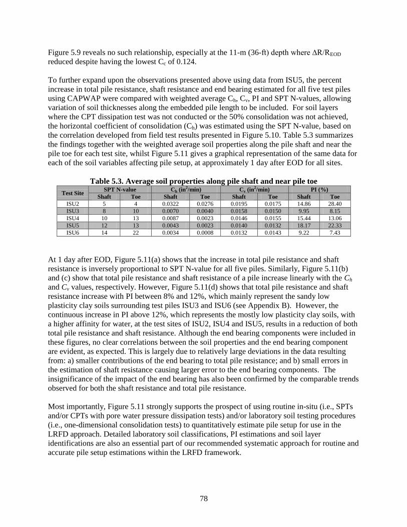
78
Figure 5.9 reveals no such relationship, especially at the 11-m (36-ft) depth where ∆R/REOD
reduced despite having the lowest Cc of 0.124.
To further expand upon the observations presented above using data from ISU5, the percent
increase in total pile resistance, shaft resistance and end bearing estimated for all five test piles
using CAPWAP were compared with weighted average Ch, Cv, PI and SPT N-values, allowing
variation of soil thicknesses along the embedded pile length to be included. For soil layers
where the CPT dissipation test was not conducted or the 50% consolidation was not achieved,
the horizontal coefficient of consolidation (Ch) was estimated using the SPT N-value, based on
the correlation developed from field test results presented in Figure 5.10. Table 5.3 summarizes
the findings together with the weighted average soil properties along the pile shaft and near the
pile toe for each test site, whilst Figure 5.11 gives a graphical representation of the same data for
each of the soil variables affecting pile setup, at approximately 1 day after EOD for all sites.
Table 5.3. Average soil properties along pile shaft and near pile toe
Test Site SPT N-value Ch (in2/min) Cv (in
2/min) PI (%)
Shaft Toe Shaft Toe Shaft Toe Shaft Toe
ISU2 5 4 0.0322 0.0276 0.0195 0.0175 14.86 28.40
ISU3 8 10 0.0070 0.0040 0.0158 0.0150 9.95 8.15
ISU4 10 13 0.0087 0.0023 0.0146 0.0155 15.44 13.06
ISU5 12 13 0.0043 0.0023 0.0140 0.0132 18.17 22.33
ISU6 14 22 0.0034 0.0008 0.0132 0.0143 9.22 7.43
At 1 day after EOD, Figure 5.11(a) shows that the increase in total pile resistance and shaft
resistance is inversely proportional to SPT N-value for all five piles. Similarly, Figure 5.11(b)
and (c) show that total pile resistance and shaft resistance of a pile increase linearly with the Ch
and Cv values, respectively. However, Figure 5.11(d) shows that total pile resistance and shaft
resistance increase with PI between 8% and 12%, which mainly represent the sandy low
plasticity clay soils surrounding test piles ISU3 and ISU6 (see Appendix B). However, the
continuous increase in PI above 12%, which represents the mostly low plasticity clay soils, with
a higher affinity for water, at the test sites of ISU2, ISU4 and ISU5, results in a reduction of both
total pile resistance and shaft resistance. Although the end bearing components were included in
these figures, no clear correlations between the soil properties and the end bearing component
are evident, as expected. This is largely due to relatively large deviations in the data resulting
from: a) smaller contributions of the end bearing to total pile resistance; and b) small errors in
the estimation of shaft resistance causing larger error to the end bearing components. The
insignificance of the impact of the end bearing has also been confirmed by the comparable trends
observed for both the shaft resistance and total pile resistance.
Most importantly, Figure 5.11 strongly supports the prospect of using routine in-situ (i.e., SPTs
and/or CPTs with pore water pressure dissipation tests) and/or laboratory soil testing procedures
(i.e., one-dimensional consolidation tests) to quantitatively estimate pile setup for use in the
LRFD approach. Detailed laboratory soil classifications, PI estimations and soil layer
identifications are also an essential part of our recommended systematic approach for routine and
accurate pile setup estimations within the LRFD framework.

79
(a) Relation with SPT N-value (b) Relation with Ch
(c) Relation with Cv (d) Relation with PI
Figure 5.11. Relationships between percent gain in pile capacity and (a) SPT N-value, (b)
Ch, (c) Cv, and (d) PI, estimated at a time of 1 day after EOD for all sites
0%
10%
20%
30%
40%
50%
60%
70%
80%
90%
0 5 10 15 20 25
Per
cen
t G
ain
In
Pil
e C
ap
aci
ty a
t t=
1 d
ay
Aft
er
EO
D (
∆R
/RE
OD)
SPT N-value
Total Capacity
Shaft Resistance
End Bearing
Best fit line for
total capacity
Best fit line for
shaft resistance
Best fit line for
end bearing
(a) 0%
10%
20%
30%
40%
50%
60%
70%
80%
0 0.01 0.02 0.03 0.04P
erce
nt
Ga
in I
n P
ile
Ca
pa
city
at
t=1
da
y A
fter
EO
D (
∆R
/RE
OD)
Horizontal Coefficient of Consolidation
Ch (in2/min)
Total Capacity
Shaft Resistance
End Bearing
(b)
0%
10%
20%
30%
40%
50%
60%
70%
80%
90%
0.01 0.015 0.02 0.025
Per
cen
t G
ain
In
Pil
e C
ap
aci
ty a
t t=
1 d
ay
Aft
er
EO
D (∆R/R
EO
D)
Vertical Coefficient of Consolidation Cv
(in2/min)
Total Capacity
Shaft Resistance
End Bearing
0%
10%
20%
30%
40%
50%
60%
70%
80%
90%
4 8 12 16 20 24 28 32
Per
cen
t G
ain
In
Pil
e C
ap
aci
ty a
t t=
1 d
ay
Aft
er
EO
D (
∆R
/RE
OD)
Plasticity Index, PI (%)
Total Capacity
Shaft Resistance
End Bearing
(d)

80
5.6.2 Development of Pile Setup Analytical Quantification Methods
Using the field test results of steel H-piles driven in the clay soil profile, two analytical methods
were established to quantify pile setup. Although existing methods found in literature, such as
Skov and Denver (1988), have been utilized for decades, they require inconvenient re-strikes
during construction and rarely correlate with any soil properties, even though these properties
significantly influence the pile setup. To account for these limitations, the proposed methods
were developed in terms of soil properties that can be measured using in-situ soil investigations,
such as SPT and CPT. For convenient practical applications, the methods utilize the initial pile
resistance estimated at the EOD condition (REOD) using either WEAP or CAPWAP. The first
method described (CPT & SPT based setup method) incorporates the average SPT N-value (Na)
and horizontal coefficient of consolidation (Ch) determined from CPT to represent the
surrounding soils, and employs an equivalent pile radius to represent the pile geometry. The
average SPT N-value is calculated by weighting the measured N-value (Ni) at each cohesive soil
layer, i, along the pile shaft by its thickness (ℓi) for the total number, n, of cohesive layers
situated along the embedded pile length, simply expressed as:
∑
∑
(5-2)
To further simplify the pile setup estimation for routine practical applications, the second method
described (SPT based setup method) considers only the commonly used average SPT N-value.
When total pile resistance (Rt) and time (t), as shown in Figure 5.4, are normalized by initial pile
resistance (REOD) and initial time (tEOD) at EOD condition respectively, a linear relationship
between normalized pile capacity (Rt/REOD) and logarithmic normalized time (Log10(t/tEOD)) for
each test pile is observed (see Figure 5.12 (a) and (b)), based on CAPWAP and WEAP analyses.
To correct pile resistance gain resulting from additional pile penetrations during re-strikes,
normalized pile resistance was multiplied with normalized pile embedded pile length (LEOD/Lt).
In order to satisfy the logarithmic relationship and to consider the immediate gain in pile
resistance measured after EOD, the time at EOD (tEOD) was assumed to be 1 minute (0.000693
day).
Each linear best fit line was generated using a linear regression analysis based on re-strike
results, as indicated by open markers. Most linear lines fit reasonably well with the results,
indicated with good coefficients of determination (R2). For a comparative purpose, static load
test results, indicated by filled markers, were also included. The slope (C) of each linear best fit
line describes the rate of pile resistance gain, i.e., a linear line with a larger slope indicates a
higher percentage of pile resistance gain or provides a larger normalized pile resistance (Rt/REOD)
at a given time. It is important to recognize that the magnitude of the slope (C) is not a unique
constant for all piles but its variation is dependent on the surrounding cohesive soil properties.
The equation for the linear best fit lines can be expressed as:
[ (
) ] (
) (5-3)
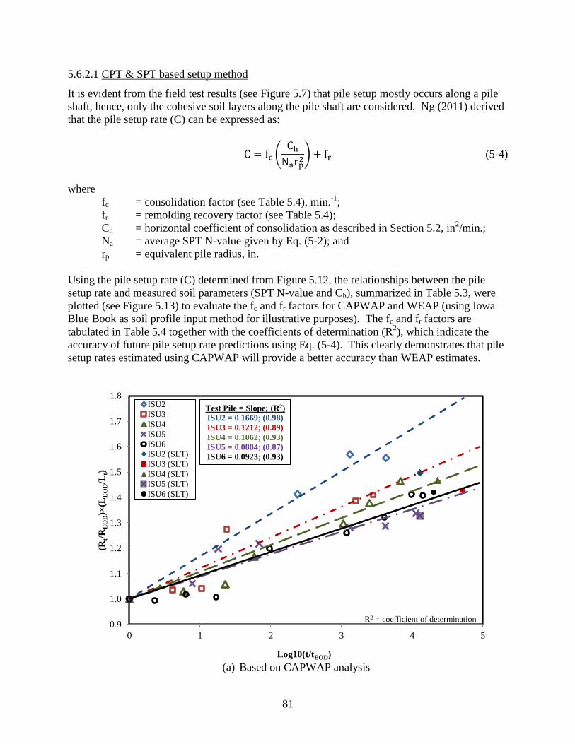
81
5.6.2.1 CPT & SPT based setup method
It is evident from the field test results (see Figure 5.7) that pile setup mostly occurs along a pile
shaft, hence, only the cohesive soil layers along the pile shaft are considered. Ng (2011) derived
that the pile setup rate (C) can be expressed as:
(
) (5-4)
where
fc = consolidation factor (see Table 5.4), min.-1
;
fr = remolding recovery factor (see Table 5.4);
Ch = horizontal coefficient of consolidation as described in Section 5.2, in2/min.;
Na = average SPT N-value given by Eq. (5-2); and
rp = equivalent pile radius, in.
Using the pile setup rate (C) determined from Figure 5.12, the relationships between the pile
setup rate and measured soil parameters (SPT N-value and Ch), summarized in Table 5.3, were
plotted (see Figure 5.13) to evaluate the fc and fr factors for CAPWAP and WEAP (using Iowa
Blue Book as soil profile input method for illustrative purposes). The fc and fr factors are
tabulated in Table 5.4 together with the coefficients of determination (R2), which indicate the
accuracy of future pile setup rate predictions using Eq. (5-4). This clearly demonstrates that pile
setup rates estimated using CAPWAP will provide a better accuracy than WEAP estimates.
(a) Based on CAPWAP analysis
0.9
1.0
1.1
1.2
1.3
1.4
1.5
1.6
1.7
1.8
0 1 2 3 4 5
(Rt/
RE
OD)×
(LE
OD/L
t)
Log10(t/tEOD)
ISU2
ISU3
ISU4
ISU5
ISU6
ISU2 (SLT)
ISU3 (SLT)
ISU4 (SLT)
ISU5 (SLT)
ISU6 (SLT)
Test Pile = Slope; (R2)
ISU2 = 0.1669; (0.98)
ISU3 = 0.1212; (0.89)
ISU4 = 0.1062; (0.93)
ISU5 = 0.0884; (0.87)
ISU6 = 0.0923; (0.93)
R2 = coefficient of determination
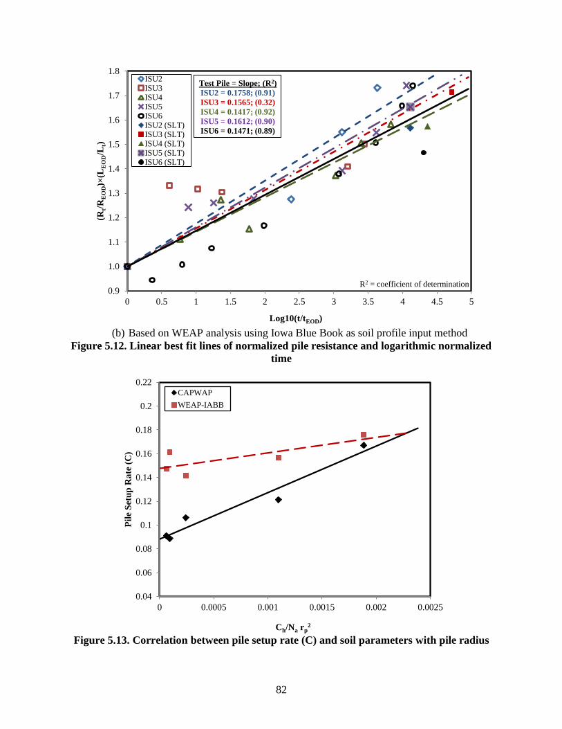
82
(b) Based on WEAP analysis using Iowa Blue Book as soil profile input method
Figure 5.12. Linear best fit lines of normalized pile resistance and logarithmic normalized
time
Figure 5.13. Correlation between pile setup rate (C) and soil parameters with pile radius
0.9
1.0
1.1
1.2
1.3
1.4
1.5
1.6
1.7
1.8
0 0.5 1 1.5 2 2.5 3 3.5 4 4.5 5
(Rt/
RE
OD)×
(LE
OD/L
t)
Log10(t/tEOD)
ISU2ISU3ISU4ISU5ISU6ISU2 (SLT)ISU3 (SLT)ISU4 (SLT)ISU5 (SLT)ISU6 (SLT)
Test Pile = Slope; (R2)
ISU2 = 0.1758; (0.91)
ISU3 = 0.1565; (0.32)
ISU4 = 0.1417; (0.92)
ISU5 = 0.1612; (0.90)
ISU6 = 0.1471; (0.89)
R2 = coefficient of determination
0.04
0.06
0.08
0.1
0.12
0.14
0.16
0.18
0.2
0.22
0 0.0005 0.001 0.0015 0.002 0.0025
Pil
e S
etu
p R
ate
(C
)
Ch/Na rp2
CAPWAP
WEAP-IABB
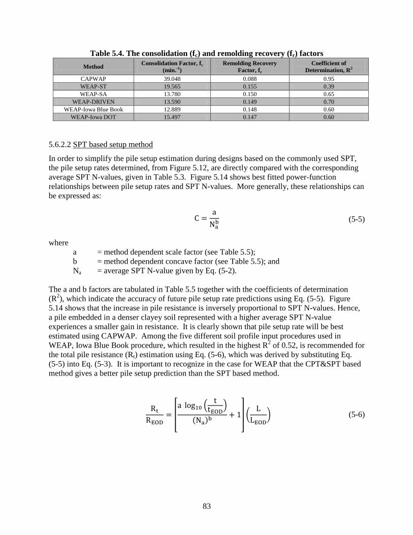
83
Table 5.4. The consolidation (fc) and remolding recovery (fr) factors
Method Consolidation Factor, fc
(min.-1)
Remolding Recovery
Factor, fr
Coefficient of
Determination, R2
CAPWAP 39.048 0.088 0.95
WEAP-ST 19.565 0.155 0.39
WEAP-SA 13.780 0.150 0.65
WEAP-DRIVEN 13.590 0.149 0.70
WEAP-Iowa Blue Book 12.889 0.148 0.60
WEAP-Iowa DOT 15.497 0.147 0.60
5.6.2.2 SPT based setup method
In order to simplify the pile setup estimation during designs based on the commonly used SPT,
the pile setup rates determined, from Figure 5.12, are directly compared with the corresponding
average SPT N-values, given in Table 5.3. Figure 5.14 shows best fitted power-function
relationships between pile setup rates and SPT N-values. More generally, these relationships can
be expressed as:
(5-5)
where
a = method dependent scale factor (see Table 5.5);
b = method dependent concave factor (see Table 5.5); and
Na = average SPT N-value given by Eq. (5-2).
The a and b factors are tabulated in Table 5.5 together with the coefficients of determination
(R2), which indicate the accuracy of future pile setup rate predictions using Eq. (5-5). Figure
5.14 shows that the increase in pile resistance is inversely proportional to SPT N-values. Hence,
a pile embedded in a denser clayey soil represented with a higher average SPT N-value
experiences a smaller gain in resistance. It is clearly shown that pile setup rate will be best
estimated using CAPWAP. Among the five different soil profile input procedures used in
WEAP, Iowa Blue Book procedure, which resulted in the highest R2 of 0.52, is recommended for
the total pile resistance (Rt) estimation using Eq. (5-6), which was derived by substituting Eq.
(5-5) into Eq. (5-3). It is important to recognize in the case for WEAP that the CPT&SPT based
method gives a better pile setup prediction than the SPT based method.
[
(
)
( ) ] (
) (5-6)
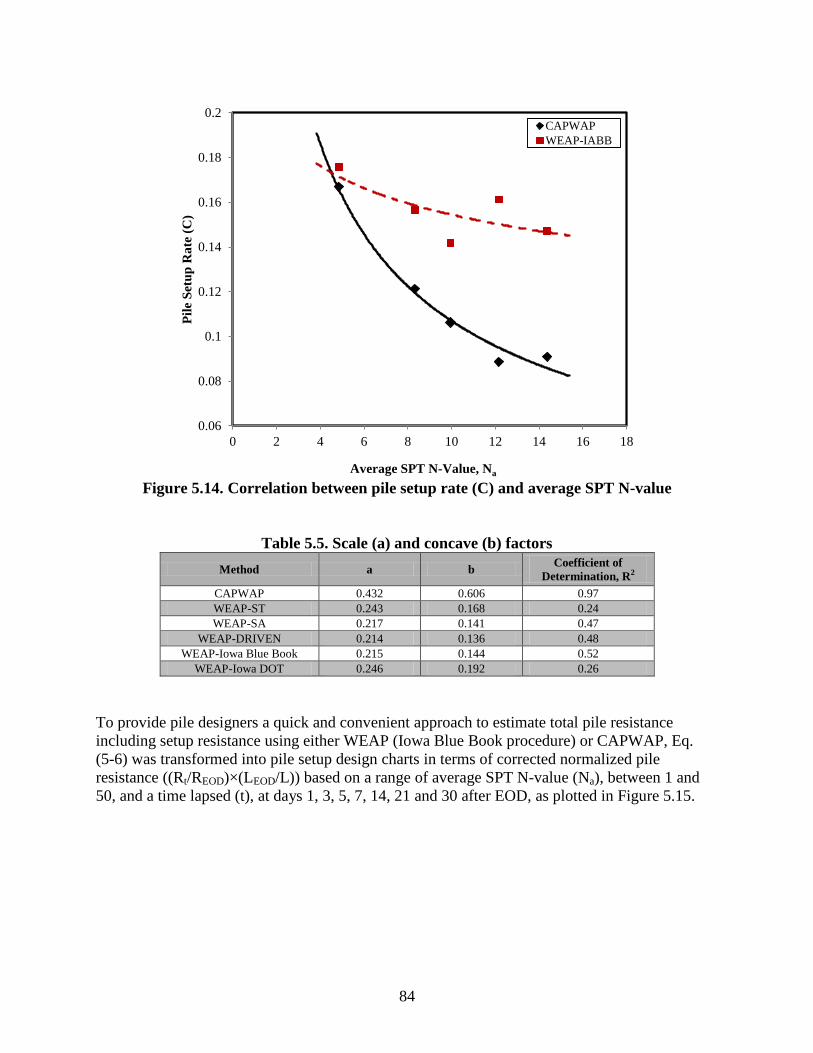
84
Figure 5.14. Correlation between pile setup rate (C) and average SPT N-value
Table 5.5. Scale (a) and concave (b) factors
Method a b Coefficient of
Determination, R2
CAPWAP 0.432 0.606 0.97
WEAP-ST 0.243 0.168 0.24
WEAP-SA 0.217 0.141 0.47
WEAP-DRIVEN 0.214 0.136 0.48
WEAP-Iowa Blue Book 0.215 0.144 0.52
WEAP-Iowa DOT 0.246 0.192 0.26
To provide pile designers a quick and convenient approach to estimate total pile resistance
including setup resistance using either WEAP (Iowa Blue Book procedure) or CAPWAP, Eq.
(5-6) was transformed into pile setup design charts in terms of corrected normalized pile
resistance ((Rt/REOD)×(LEOD/L)) based on a range of average SPT N-value (Na), between 1 and
50, and a time lapsed (t), at days 1, 3, 5, 7, 14, 21 and 30 after EOD, as plotted in Figure 5.15.
0.06
0.08
0.1
0.12
0.14
0.16
0.18
0.2
0 2 4 6 8 10 12 14 16 18
Pil
e S
etu
p R
ate
(C
)
Average SPT N-Value, Na
CAPWAP
WEAP-IABB
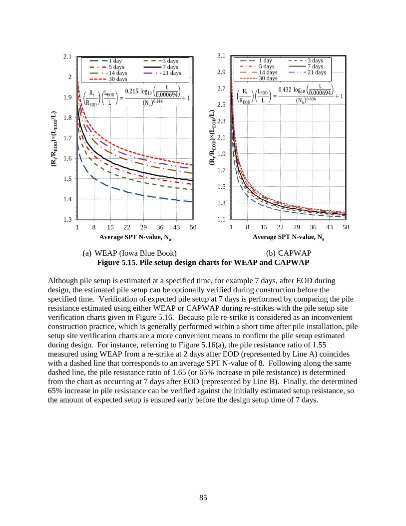
85
(a) WEAP (Iowa Blue Book) (b) CAPWAP
Figure 5.15. Pile setup design charts for WEAP and CAPWAP
Although pile setup is estimated at a specified time, for example 7 days, after EOD during
design, the estimated pile setup can be optionally verified during construction before the
specified time. Verification of expected pile setup at 7 days is performed by comparing the pile
resistance estimated using either WEAP or CAPWAP during re-strikes with the pile setup site
verification charts given in Figure 5.16. Because pile re-strike is considered as an inconvenient
construction practice, which is generally performed within a short time after pile installation, pile
setup site verification charts are a more convenient means to confirm the pile setup estimated
during design. For instance, referring to Figure 5.16(a), the pile resistance ratio of 1.55
measured using WEAP from a re-strike at 2 days after EOD (represented by Line A) coincides
with a dashed line that corresponds to an average SPT N-value of 8. Following along the same
dashed line, the pile resistance ratio of 1.65 (or 65% increase in pile resistance) is determined
from the chart as occurring at 7 days after EOD (represented by Line B). Finally, the determined
65% increase in pile resistance can be verified against the initially estimated setup resistance, so
the amount of expected setup is ensured early before the design setup time of 7 days.
1.3
1.4
1.5
1.6
1.7
1.8
1.9
2
2.1
1 8 15 22 29 36 43 50
(Rt/
RE
OD)×
(LE
OD/L
)
Average SPT N-value, Na
1 day 3 days5 days 7 days14 days 21 days30 days
(Rt
REOD) (
LEOD
L) =
0.215 log10 (t
0.000694)
(Na)0.144+ 1
1.1
1.3
1.5
1.7
1.9
2.1
2.3
2.5
2.7
2.9
3.1
1 8 15 22 29 36 43 50
(Rt/
RE
OD)×
(LE
OD/L
)
Average SPT N-value, Na
1 day 3 days5 days 7 days14 days 21 days30 days
(Rt
REOD) (
LEOD
L) =
0.432 log10 (t
0.000694)
(Na)0.606+ 1
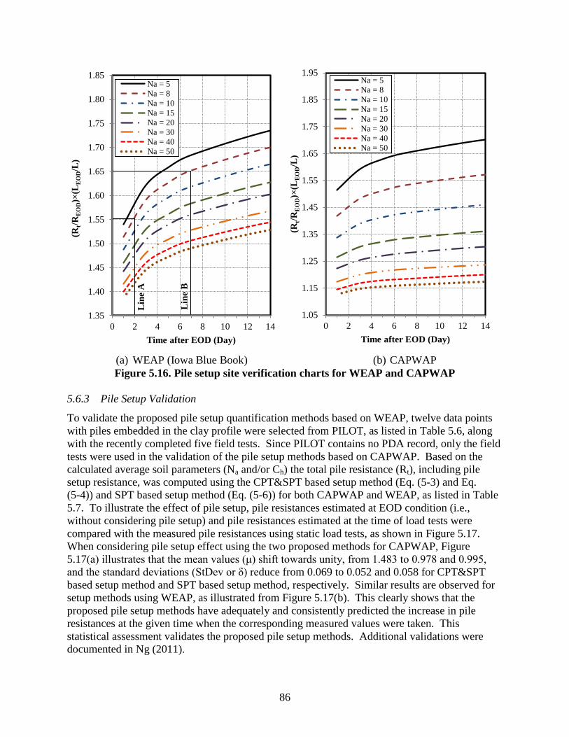
86
(a) WEAP (Iowa Blue Book) (b) CAPWAP
Figure 5.16. Pile setup site verification charts for WEAP and CAPWAP
5.6.3 Pile Setup Validation
To validate the proposed pile setup quantification methods based on WEAP, twelve data points
with piles embedded in the clay profile were selected from PILOT, as listed in Table 5.6, along
with the recently completed five field tests. Since PILOT contains no PDA record, only the field
tests were used in the validation of the pile setup methods based on CAPWAP. Based on the
calculated average soil parameters (Na and/or Ch) the total pile resistance (Rt), including pile
setup resistance, was computed using the CPT&SPT based setup method (Eq. (5-3) and Eq.
(5-4)) and SPT based setup method (Eq. (5-6)) for both CAPWAP and WEAP, as listed in Table
5.7. To illustrate the effect of pile setup, pile resistances estimated at EOD condition (i.e.,
without considering pile setup) and pile resistances estimated at the time of load tests were
compared with the measured pile resistances using static load tests, as shown in Figure 5.17.
When considering pile setup effect using the two proposed methods for CAPWAP, Figure
5.17(a) illustrates that the mean values (μ) shift towards unity, from 1.483 to 0.978 and 0.995,
and the standard deviations (StDev or δ) reduce from 0.069 to 0.052 and 0.058 for CPT&SPT
based setup method and SPT based setup method, respectively. Similar results are observed for
setup methods using WEAP, as illustrated from Figure 5.17(b). This clearly shows that the
proposed pile setup methods have adequately and consistently predicted the increase in pile
resistances at the given time when the corresponding measured values were taken. This
statistical assessment validates the proposed pile setup methods. Additional validations were
documented in Ng (2011).
1.35
1.40
1.45
1.50
1.55
1.60
1.65
1.70
1.75
1.80
1.85
0 2 4 6 8 10 12 14
(Rt/
RE
OD)×
(LE
OD/L
)
Time after EOD (Day)
Na = 5
Na = 8
Na = 10
Na = 15
Na = 20
Na = 30
Na = 40
Na = 50
Lin
e A
Lin
e B
1.05
1.15
1.25
1.35
1.45
1.55
1.65
1.75
1.85
1.95
0 2 4 6 8 10 12 14
(Rt/
RE
OD)×
(LE
OD/L
)
Time after EOD (Day)
Na = 5
Na = 8
Na = 10
Na = 15
Na = 20
Na = 30
Na = 40
Na = 50

87
Table 5.6. Summary of the twelve data records from PILOT
Project
ID
County in
Iowa
Pile
Type
Pile
Penetration
(ft)
Hammer
Type
Soil Profile
Description
Average SPT
N-value, Na
Average
Ch
(in2/min)
Time
After
EOD, t
(day)
SLT Measured
Pile Resistance
at Time t (kip)
WEAP-IABB
Estimated Pile
Resistance at
EOD (kip)
6 Decatur HP 10 × 42 53 Gravity #732 Glacial clay 14.47 0.00631 3 118 71
12 Linn HP 10 × 42 23.78 Kobe K-13 Glacial clay 29.90 0.00045 5 204 155
42 Linn HP 10 × 42 23.5 Kobe K-13 Glacial clay 22.20 0.00147 5 82 85
44 Linn HP 10 × 42 36.5 Delmag D-22 Sandy silty clay 22.34 0.00083 5 136 94
51 Johnson HP 10 × 42 29.5 Kobe K-13 Silt/glacial clay 40.00 0.00022 3 190 128
57 Hamilton HP 10 × 42 57 Gravity #2107 Glacial clay 9.77 0.00469 4 168 94
62 Kossuth HP 10 × 42 45 MKT DE-30B Glacial clay 36.05 0.00279 5 100 76
63 Jasper HP 10 × 42 63 Gravity Silt on glacial clay 8.32 0.00665 2 66 59
64 Jasper HP 10 × 42 71 Gravity Silt on glacial clay 10.52 0.00479 1 122 71
67 Audubon HP 10 × 42 32 Delmag D-12 Glacial clay 20.00 0.00094 4 140 121
102 Poweshiek HP 10 × 42 43 Gravity #203 Silt/glacial clay 16.45 0.00620 8 130 84
109 Poweshiek HP 12 × 53 51 Delmag D-12 Glacial clay 17.36 0.00204 3 176 147
Table 5.7. Summary of the estimated pile resistance including setup
Project ID Pile Resistance Based on SPT & CPT (Eq. 5-3 & Eq. 5-4) (kip) Pile Resistance Based On SPT (Eq. 5-6) (kip)
CAPWAP WEAP-Iowa Blue Book CAPWAP WEAP-Iowa Blue Book
6
Not Available
109
Not Available
108
12 243 234
42 133 130
44 134 144
51 197 187
57 146 148
62 119 113
63 90 91
64 104 105
67 188 184
102 135 134
109 226 223
ISU2 139 136 136 132
ISU3 153 150 154 144
ISU4 150 162 149 159
ISU5 252 237 247 231
ISU6 208 238 198 229

88
(a) CAPWAP
(b) WEAP based on Iowa Blue Book soil input procedure
Figure 5.17. Pile setup comparison and validation
1.61.51.41.31.21.11.00.9
8
7
6
5
4
3
2
1
0
Ratio Between Measured and Estimated Pile Resistance
De
nsit
y
1.0 1.48
1.483 0.06983 5
0.9781 0.05222 5
0.9957 0.05831 5
Mean StDev N
CAPWAP(EOD)
CAPWAP(EOD+Setup-CPT&SPT)
CAPWAP (EOD+Setup-SPT)
Conditions
Histogram of Pile Resistance Ratio for CAPWAPNormal Distribution
2.001.751.501.251.000.750.50
3.0
2.5
2.0
1.5
1.0
0.5
0.0
Ratio Between Measured and Estimated Pile Resistance
De
nsit
y
1.0 1.47
1.472 0.2545 17
0.9234 0.1514 17
0.9364 0.1471 17
Mean StDev N
WEAP(EOD)
WEAP (EOD+Setup-CPT&SPT)
WEAP (EOD+Setup-SPT)
Conditions
Histogram of Pile Resistance Ratio for WEAP (Iowa Blue Book Procedure)Normal Distribution
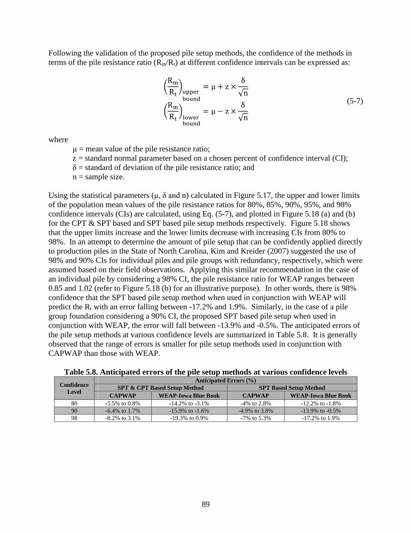
89
Following the validation of the proposed pile setup methods, the confidence of the methods in
terms of the pile resistance ratio (Rm/Rt) at different confidence intervals can be expressed as:
(
)
√
(
)
√
(5-7)
where
μ = mean value of the pile resistance ratio;
z = standard normal parameter based on a chosen percent of confidence interval (CI);
δ = standard of deviation of the pile resistance ratio; and
n = sample size.
Using the statistical parameters (μ, δ and n) calculated in Figure 5.17, the upper and lower limits
of the population mean values of the pile resistance ratios for 80%, 85%, 90%, 95%, and 98%
confidence intervals (CIs) are calculated, using Eq. (5-7), and plotted in Figure 5.18 (a) and (b)
for the CPT & SPT based and SPT based pile setup methods respectively. Figure 5.18 shows
that the upper limits increase and the lower limits decrease with increasing CIs from 80% to
98%. In an attempt to determine the amount of pile setup that can be confidently applied directly
to production piles in the State of North Carolina, Kim and Kreider (2007) suggested the use of
98% and 90% CIs for individual piles and pile groups with redundancy, respectively, which were
assumed based on their field observations. Applying this similar recommendation in the case of
an individual pile by considering a 98% CI, the pile resistance ratio for WEAP ranges between
0.85 and 1.02 (refer to Figure 5.18 (b) for an illustrative purpose). In other words, there is 98%
confidence that the SPT based pile setup method when used in conjunction with WEAP will
predict the Rt with an error falling between -17.2% and 1.9%. Similarly, in the case of a pile
group foundation considering a 90% CI, the proposed SPT based pile setup when used in
conjunction with WEAP, the error will fall between -13.9% and -0.5%. The anticipated errors of
the pile setup methods at various confidence levels are summarized in Table 5.8. It is generally
observed that the range of errors is smaller for pile setup methods used in conjunction with
CAPWAP than those with WEAP.
Table 5.8. Anticipated errors of the pile setup methods at various confidence levels
Confidence
Level
Anticipated Errors (%)
SPT & CPT Based Setup Method SPT Based Setup Method
CAPWAP WEAP-Iowa Blue Book CAPWAP WEAP-Iowa Blue Book
80 -5.5% to 0.8% -14.2% to -3.1% -4% to 2.8% -12.2% to -1.8%
90 -6.4% to 1.7% -15.9% to -1.6% -4.9% to 3.8% -13.9% to -0.5%
98 -8.2% to 3.1% -19.3% to 0.9% -7% to 5.3% -17.2% to 1.9%
90
(a) CPT & SPT based pile setup method
(b) SPT based pile setup method
Figure 5.18. Pile setup confidence levels
0.948 0.940
0.924
1.008 1.017
1.032
0.876
0.863
0.838
0.970 0.984
1.009
0.80
0.85
0.90
0.95
1.00
1.05
1.10
1.15
80 85 90 95 100
Ra
tio
of
Mea
sure
d a
nd
Pre
dic
ted
Pil
e R
esis
tan
ce
Confidence Interval, CI (%)
Mean (CAPWAP) Lower Bound (CAPWAP)
Upper Bound (CAPWAP) Mean (WEAP-IA BB)
Lower Bound (WEAP-IA BB) Upper Bound (WEAP-IA BB)
98
0.962 0.953
0.935
1.029 1.039
1.056
0.891 0.878
0.853
0.982
0.995
1.019
0.80
0.85
0.90
0.95
1.00
1.05
1.10
1.15
80 85 90 95 100
Ra
tio
of
Mea
sure
d a
nd
Pre
dic
ted
Pil
e R
esis
tan
ce
Confidence Interval, CI (%)
Mean (CAPWAP) Lower Bound (CAPWAP)
Upper Bound (CAPWAP) Mean (WEAP-IA BB)
Lower Bound (WEAP-IA BB) Upper Bound (WEAP-IA BB)
98
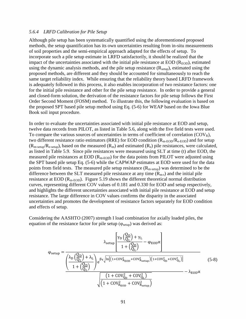
91
5.6.4 LRFD Calibration for Pile Setup
Although pile setup has been systematically quantified using the aforementioned proposed
methods, the setup quantification has its own uncertainties resulting from in-situ measurements
of soil properties and the semi-empirical approach adapted for the effects of setup. To
incorporate such a pile setup estimate in LRFD satisfactorily, it should be realized that the
impact of the uncertainties associated with the initial pile resistance at EOD (REOD), estimated
using the dynamic analysis methods, and the pile setup resistance (Rsetup), estimated using the
proposed methods, are different and they should be accounted for simultaneously to reach the
same target reliability index. While ensuring that the reliability theory based LRFD framework
is adequately followed in this process, it also enables incorporation of two resistance factors: one
for the initial pile resistance and other for the pile setup resistance. In order to provide a general
and closed-form solution, the derivation of the resistance factors for pile setup follows the First
Order Second Moment (FOSM) method. To illustrate this, the following evaluation is based on
the proposed SPT based pile setup method using Eq. (5-6) for WEAP based on the Iowa Blue
Book soil input procedure.
In order to evaluate the uncertainties associated with initial pile resistance at EOD and setup,
twelve data records from PILOT, as listed in Table 5.6, along with the five field tests were used.
To compare the various sources of uncertainties in terms of coefficient of correlation (COVR),
two different resistance ratio estimators (RRE) for EOD condition (Rm-EOD/Re-EOD) and for setup
(Rm-setup/Re-setup), based on the measured (Rm) and estimated (Re) pile resistances, were calculated,
as listed in Table 5.9. Since pile resistances were measured using SLT at time (t) after EOD, the
measured pile resistances at EOD (Rm-EOD) for the data points from PILOT were adjusted using
the SPT based pile setup Eq. (5-6) while the CAPWAP estimates at EOD were used for the data
points from field tests. The measured pile setup resistance (Rm-setup) was determined to be the
difference between the SLT measured pile resistance at any time (Rm-t) and the initial pile
resistance at EOD (Rm-EOD). Figure 5.19 shows the different theoretical normal distribution
curves, representing different COV values of 0.181 and 0.330 for EOD and setup respectively,
and highlights the different uncertainties associated with initial pile resistance at EOD and setup
resistance. The large difference in COV values confirms the disparity in the associated
uncertainties and promotes the development of resistance factors separately for EOD condition
and effects of setup.
Considering the AASHTO (2007) strength I load combination for axially loaded piles, the
equation of the resistance factor for pile setup (φsetup) was derived as:
[ (
)
(
) ]
( (
)
(
))
√ [(
)(
)]
√(
)
(
)
(5-8)

92
where
λEOD = the resistance bias factor of the resistance ratio estimator for EOD;
λsetup = the resistance bias factor of the resistance ratio estimator for setup;
COVREOD = the coefficient of variation of the resistance ratio estimator for EOD;
COVRsetup = the coefficient of variation of the resistance ratio estimator for setup;
φEOD = resistance factor for initial pile resistance at EOD;
α = ratio between initial pile resistance and total serviced dead and live
loads, (REOD/(QD+QL));
βT = target reliability index;
γD, γL = the dead load factor (1.25) and live load factor (1.75);
λD, λL = the dead load bias (1.05) and live load bias (1.15);
COVD, COVL = the coefficients of variation of dead load (0.1) and live load (0.2); and
QD/QL = dead to live load ratio.
Table 5.9. Summary of resistance ratio estimators for EOD and setup
Project
ID
Measured Pile
Resistance at
EOD, Rm-EOD
(kip)
Measured Pile
Setup
Resistance,
Rm-setup (kip)
Estimated Pile
Resistance at
EOD, Re-EOD
(kip)
Estimated
Pile Setup
Resistance,
Re-setup (kip)
RRE for EOD
(Rm-EOD/Re-EOD)
RRE for Setup
(Rm-setup/Re-setup)
6 77a 47c 71 38 1.09 1.26
12 135a 49c 155 79 0.87 0.62
42 54a 28c 85 45 0.63 0.63
44 89a 42c 94 50 0.95 0.84
51 130a 62c 128 59 1.02 1.05
57 106a 75c 94 55 1.14 1.37
62 67a 24c 76 37 0.88 0.65
63 43a 23c 59 32 0.72 0.72
64 82a 51c 71 34 1.16 1.49
67 92a 48c 121 63 0.76 0.76
102 82a 46c 84 49 0.97 0.92
109 116a 29c 147 76 0.79 0.38
ISU2 81b 44d 77 54 1.05 0.81
ISU3 99b 51d 82 62 1.20 0.83
ISU4 102b 52d 95 64 1.07 0.82
ISU5 178b 65d 143 88 1.24 0.74
ISU6 145b 68d 140 89 1.03 0.77 a – adjusted from SPT based pile setup equation; b – CAPWAP estimates at EOD; c – difference between SLT measured pile resistance at time (t) and initial pile resistance at EOD using WEAP; and d – difference between SLT measured pile resistance at time (t) and initial pile resistance at EOD using CAPWAP.
The detailed derivation of Eq. (5-8), based on the original FOSM and its assumptions of
lognormal distribution and a mutually independent relationship between load and resistance,
were explicitly described by Ng (2011). Eq. (5-8) reveals that the φsetup value is dependent on
various parameters. The probabilistic characteristics (γ, λ and COV) of the random variables QD
and QL are defined in Eq. (5-8) with the recommended values recapitulated in parentheses
(Nowak 1999). The probabilistic characteristics (λ and COV) of the random variables REOD and
Rsetup were determined in Figure 5.19. The target reliability indices (βT) of 2.33 (corresponding
to 1% probability of failure) and 3.00 (corresponding to 0.1% probability of failure), as
recommended, for representing redundant and non-redundant pile groups respectively
(Paikowsky et al. 2004), were selected for the calculations. Neglecting the effect of pile setup
and assuming the QD/QL ratio of 2.0, the φEOD values were determined to be 0.66 and 0.55 for the
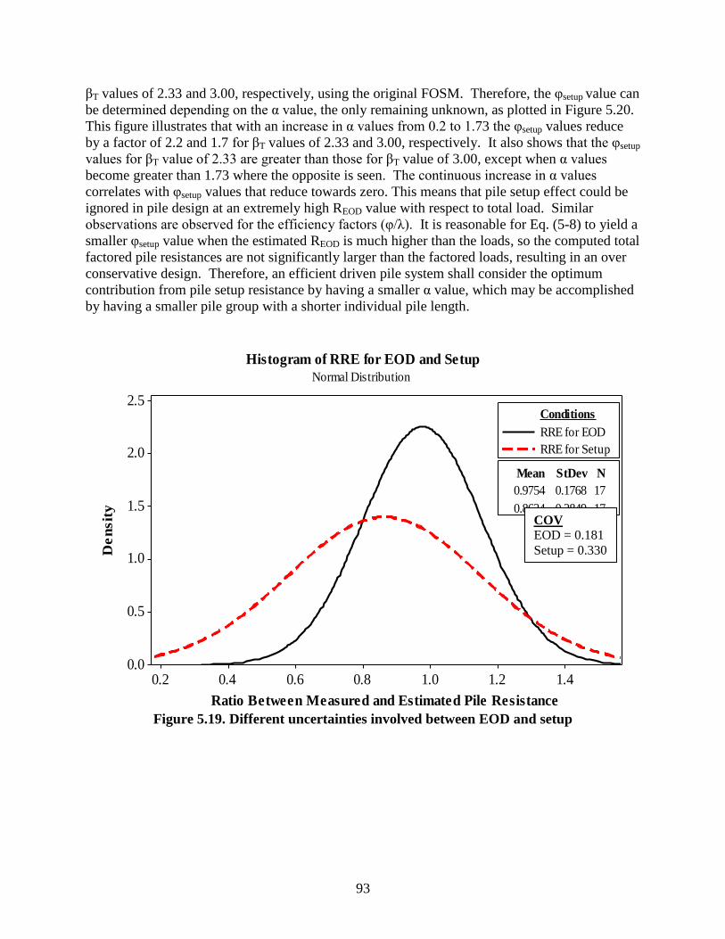
93
βT values of 2.33 and 3.00, respectively, using the original FOSM. Therefore, the φsetup value can
be determined depending on the α value, the only remaining unknown, as plotted in Figure 5.20.
This figure illustrates that with an increase in α values from 0.2 to 1.73 the φsetup values reduce
by a factor of 2.2 and 1.7 for βT values of 2.33 and 3.00, respectively. It also shows that the φsetup
values for βT value of 2.33 are greater than those for βT value of 3.00, except when α values
become greater than 1.73 where the opposite is seen. The continuous increase in α values
correlates with φsetup values that reduce towards zero. This means that pile setup effect could be
ignored in pile design at an extremely high REOD value with respect to total load. Similar
observations are observed for the efficiency factors (φ/λ). It is reasonable for Eq. (5-8) to yield a
smaller φsetup value when the estimated REOD is much higher than the loads, so the computed total
factored pile resistances are not significantly larger than the factored loads, resulting in an over
conservative design. Therefore, an efficient driven pile system shall consider the optimum
contribution from pile setup resistance by having a smaller α value, which may be accomplished
by having a smaller pile group with a shorter individual pile length.
Figure 5.19. Different uncertainties involved between EOD and setup
1.41.21.00.80.60.40.2
2.5
2.0
1.5
1.0
0.5
0.0
Ratio Between Measured and Estimated Pile Resistance
De
nsit
y
0.9754 0.1768 17
0.8624 0.2849 17
Mean StDev N
RRE for EOD
RRE for Setup
Conditions
Histogram of RRE for EOD and Setup
Normal Distribution
COV
EOD = 0.181
Setup = 0.330
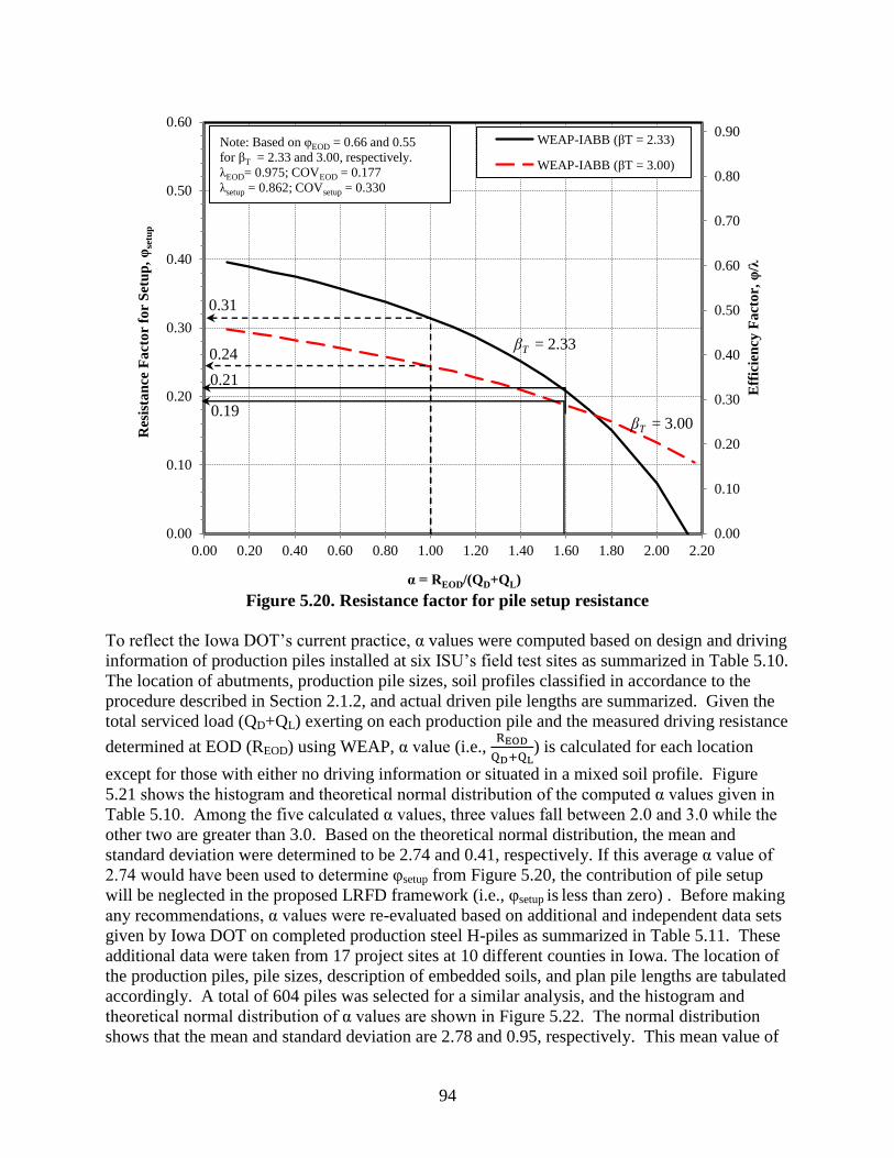
94
Figure 5.20. Resistance factor for pile setup resistance
To reflect the Iowa DOT’s current practice, α values were computed based on design and driving
information of production piles installed at six ISU’s field test sites as summarized in Table 5.10.
The location of abutments, production pile sizes, soil profiles classified in accordance to the
procedure described in Section 2.1.2, and actual driven pile lengths are summarized. Given the
total serviced load (QD+QL) exerting on each production pile and the measured driving resistance
determined at EOD (REOD) using WEAP, α value (i.e.,
) is calculated for each location
except for those with either no driving information or situated in a mixed soil profile. Figure
5.21 shows the histogram and theoretical normal distribution of the computed α values given in
Table 5.10. Among the five calculated α values, three values fall between 2.0 and 3.0 while the
other two are greater than 3.0. Based on the theoretical normal distribution, the mean and
standard deviation were determined to be 2.74 and 0.41, respectively. If this average α value of
2.74 would have been used to determine φsetup from Figure 5.20, the contribution of pile setup
will be neglected in the proposed LRFD framework (i.e., φsetup is less than zero) . Before making
any recommendations, α values were re-evaluated based on additional and independent data sets
given by Iowa DOT on completed production steel H-piles as summarized in Table 5.11. These
additional data were taken from 17 project sites at 10 different counties in Iowa. The location of
the production piles, pile sizes, description of embedded soils, and plan pile lengths are tabulated
accordingly. A total of 604 piles was selected for a similar analysis, and the histogram and
theoretical normal distribution of α values are shown in Figure 5.22. The normal distribution
shows that the mean and standard deviation are 2.78 and 0.95, respectively. This mean value of
0.00
0.10
0.20
0.30
0.40
0.50
0.60
0.70
0.80
0.90
0.00
0.10
0.20
0.30
0.40
0.50
0.60
0.00 0.20 0.40 0.60 0.80 1.00 1.20 1.40 1.60 1.80 2.00 2.20
Eff
icie
ncy
Fa
cto
r, φ
/λ
Res
ista
nce
Fa
cto
r fo
r S
etu
p,
φse
tup
α = REOD/(QD+QL)
WEAP-IABB (βT = 2.33)
WEAP-IABB (βT = 3.00)
βT = 2.33
βT = 3.00
Note: Based on φEOD = 0.66 and 0.55
for βT = 2.33 and 3.00, respectively.
λEOD= 0.975; COVEOD = 0.177
λsetup = 0.862; COVsetup = 0.330
0.21
0.19
0.31
0.24
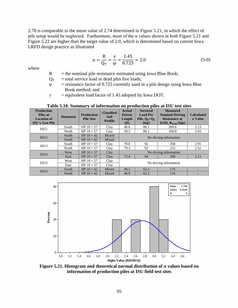
95
2.78 is comparable to the mean value of 2.74 determined in Figure 5.21, in which the effect of
pile setup would be neglected. Furthermore, most of the α values shown in both Figure 5.21 and
Figure 5.22 are higher than the target value of 2.0, which is determined based on current Iowa
LRFD design practice as illustrated
(5-9)
where
R = the nominal pile resistance estimated using Iowa Blue Book;
QT = total service load or dead plus live loads;
φ = resistance factor of 0.725 currently used in a pile design using Iowa Blue
Book method; and
γ = equivalent load factor of 1.45 adopted by Iowa DOT.
Table 5.10. Summary of information on production piles at ISU test sites Production
Piles at
Location of
ISU’s Test Pile
Abutment Production
Pile Size
Classified
Soil
Profile
Actual
Driven
Length
(ft)
Serviced
Load Per
Pile, QD+QL
(kip)
Measured
Nominal Driving
Resistance at
EOD, REOD (kip)
Calculated
α Value
ISU1 South HP 10 × 57 Clay 48.6 86.1 269.6 3.13
North HP 10 × 57 Clay 58.3 86.1 260.8 3.03
ISU2 South HP 10 × 42 Mixed
No driving information North HP 10 × 42 Mixed
ISU3 South HP 10 × 57 Clay 78.8 92 268 2.91
North HP 10 × 57 Clay 79.3 92 232 2.52
ISU4 West HP 10 × 57 Clay No driving information
East HP 10 × 57 Clay 72.4 94 200 2.13
ISU5 West HP 10 × 57 Clay
No driving information East HP 10 × 57 Clay
ISU6 South HP 10 × 42 Mixed 49.1 62.3 176 -
North HP 10 × 42 Mixed 46.9 62.3 116 -
Figure 5.21. Histogram and theoretical normal distribution of α values based on
information of production piles at ISU field test sites
3.63.43.23.02.82.62.42.22.01.81.61.41.21.0
40
30
20
10
0
Alpha Value (REOD/Q)
Percen
t
Mean 2.744
StDev 0.4140
N 5
Normal
Histogram of Alpha Value (Production Piles at ISU Field Test Sites)

96
Table 5.11. Summary of additional data on production piles in Iowa Iowa County-
ID Number Pier/Abutment
Production
Pile Size Soil Description
Total Number
of Piles
Plan Pile
Length (ft)
Lee-135 Pier 2 HP 10 × 57
Sandy Glacial Clay 29 45
North Abutment HP 10 × 57 12 60
Buena Vista-53
West Abutment HP 10 × 42 Firm Sandy Glacial Clay
over Very Firm Glacial
Clay
7 60
East Abutment HP 10 × 42 7 60
Pier 1 West HP 12 × 53 13 60
Pier 2 East HP 12 × 53 13 60
Jasper-44
West Abutment HP 10 × 57 Silty Clay 7 70 & 80
Pier 2 HP 12 × 53 Stiff Silty Clay to Very
Firm Glacial Clay
14 70
East Abutment HP 10 × 57 7 75 & 80
Dickinson-35
East Abutment HP 10 × 57 Sandy Lean Clay 6 60
West Abutment HP 10 × 57 Firm Sandy Lean Clay 6 60
East Pier HP 12 × 53 Very Firm Glacial Clay 8 60
Plymouth-40 West Abutment HP 10 × 57 Silty Clay - Glacial Clay 6 80
East Pier HP 10 × 57 Very Firm Glacial Clay 12 70
Wright-63 East Abutment HP 10 × 42
Glacial Clay 5 45
West Abutment HP 10 × 42 5 45
Carroll-122 South Abutment HP 10 × 42 Silty Clay to Firm
Glacial Clay
7 55
North Abutment HP 10 × 42 7 55
Cedar-82
South Abutment HP 10 × 57
Silty Clay to Firm
Glacial Clay
5 80
North Abutment HP 10 × 57 5 80
Pier 1 HP 10 × 57 22 55
Pier 3 HP 10 × 57 22 55
Pier 2 HP 10 × 57 22 60
Tama-114
Pier HP 10 × 57 Silty Clay to Firm
Glacial Clay
27 44.28
North Abutment HP 10 × 57 12 63.96
South Abutment HP 10 × 57 13 70
Tama-119
Pier HP 10 × 57 Very Firm Glacial Clay 27 45
North Abutment HP 10 × 57 Silty Clay to Very Firm
Glacial Clay
14 60
South Abutment HP 10 × 57 13 60
Lee-130 Pier HP 10 × 57 Firm Sandy Glacial Clay 36 50
Lee-147
SBL S. Abutment HP 10 × 57 Stiff Silty Clay to Very
Firm Glacial Clay
8 80
NBL N. Abutment HP 10 × 57 8 80
SBL Pier 1 HP 10 × 57 Firm Glacial Clay 24 55
NBL S. Abutment HP 10 × 57 Stiff Silty Clay 8 75
NBL Pier 1 HP 10 × 57 Firm Glacial Clay 24 55
Lee-148 South Abutment HP 10 × 57 Silty Clay 12 60
Pier HP 10 × 57 Very Firm Glacial Clay 26 40
Lee-157 East Abutment HP 10 × 57 Stiff Silty Clay to Firm
Glacial Clay
11 70
West Abutment HP 10 × 57 11 70
Lee-138
West Abutment HP 10 × 57 Silty Clay to Glacial
Clay
7 70
East Abutment HP 10 × 57 7 70
Pier 1 HP 12 × 53 27 45
Buena Vista-57
West Pier HP 10 × 57 Glacial Clay to Gravelly
Sand 12 65
West Abutment HP 10 × 57 Soft Silty Clay to Very
Firm Glacial Clay 6 70
Johnson-285 Pier 1 HP 10 × 57 Sandy Lean Clay 24 55

97
Figure 5.22. Histogram and theoretical normal distribution of α values based on additional
data of production piles in Iowa
This comparison shows that most of the production piles were installed with higher capacities
than that required using Eq. (5-9). In other words, the production piles were conservatively
installed. In contrast, to eliminate an additional safety margin incurred to REOD, which has been
accounted for using φEOD in Eq. (5-8), a lowest α value of 1.0 can be assumed. Referring to
Figure 5.20 based on α value of 1.0, φsetup values of 0.31 and 0.24 can be determined for the βT
values of 2.33 and 3.00, respectively. However, these φsetup values could be high based upon the
actual results revealed in Figure 5.21 and Figure 5.22 with an average α value of about 2.7 as
well as the target α value of 2.0. To compromise between the conservatism observed in the
actual production pile constructions and the idealistic condition that eliminates the additional
safety margin to the REOD, α value of 1.8 can be selected between the lowest value of 1.0 and the
average value of 2.7. Alternatively, α value of 1.5 can be selected between the lowest value of
1.0 and the target value of 2.0. If α value of 1.6 is chosen between 1.5 and 1.8 for pile designs in
Iowa, φsetup values of 0.21 and 0.19 can be reasonably recommended for the βT values of 2.33
and 3.00, respectively. In this recommendation, only about 20% of the pile setup resistance
estimated using the proposed methods described in Section 5.6.2 will be considered in the LRFD
of steel H-pile foundations.
5.25.04.84.64.44.24.03.83.63.43.23.02.82.62.42.22.01.81.61.41.21.0
16
14
12
10
8
6
4
2
0
Alpha Value (REOD/Q)
Percen
t
Mean 2.776
StDev 0.9528
N 604
Histogram of Alpha ValueNormal
98
CHAPTER 6: SUMMARY
Because of the mandate imposed by the Federal Highway Administration (FHWA) on the
implementation of Load Resistance Factor Design (LRFD) in all new bridge projects initiated
after October 1, 2007, the Iowa Highway Research Board (IHRB) sponsored the research project
TR-573 to develop the LRFD commendations for the State of Iowa based on the Pile Load Test
(PILOT) database. PILOT contains pile information about past projects completed by the Iowa
Department of Transportation (Iowa DOT) from 1966 until the late 1980s. To populate PILOT,
especially for dynamic analysis, two add-on research projects (TR-583 and TR-584) were
included to conduct ten (10) full-scale field tests in Iowa to increase the data points for LRFD
resistance factors calculation, develop LRFD recommendations for dynamic methods, and
validate the results of LRFD calibration.
The most common steel H-piles were used in the ten field sites which were selected from Iowa
DOT bridge projects. Chapter 2 describes the six criteria established for selecting the ten field
testing locations. Appendix A shows the layout of the test pile locations. When the test sites
were selected, detailed soil in-situ investigations and laboratory tests were performed to
characterize the soils surrounding the test piles. Standard Penetration Tests (SPT), Cone
Penetration Tests (CPT), Borehole Shear Tests (BST), and modified Borehole Shear Tests
(mBST) were the four selected in-situ soil investigations. In addition, push-in pressure cells
(PCs) were installed near test piles ISU5, ISU6, ISU7, ISU8, and ISU10 to measure total lateral
earth pressure and pore water pressure during driving, re-strikes, and static load tests. Soil
samples collected from SPT boreholes were used for laboratory testing which consisted of basic
soil characterization (i.e., gradation, Atterberg’s limits and moisture content) and consolidation
tests. The detailed descriptions of both in-situ and laboratory soil tests are presented in Chapter
3 and the results of the soil tests are included in the Appendix B.
Besides characterizing the surrounding soils, the properties of the ASTM A572 Grade 50 steel
H-piles and the hammer driving systems are described and presented in Chapter 4. The test piles
were instrumented with strain gauges along their embedded lengths before being driven into the
ground. The details of the strain gauge instrumentations are described in Chapter 4 and their
arrangements are included in Appendix C. The test piles were also instrumented with a pair of
transducers and accelerometers near the pile head for Pile Driving Analyzer (PDA) tests.
The PDA tests were conducted during pile driving, at the end of driving (EOD), and at several
re-strikes. The test piles were re-struck at several durations after EOD and before static load
tests. The PDA force and velocity records at each event (given in Appendix C) were used in the
CAse Pile Wave Analysis Program (CAPWAP) method for a more accurate pile resistance
estimation, which was achieved by performing signal matching.
Hammer blow counts were recorded at EOD and re-strikes and were used in the Wave Equation
Analysis Program (WEAP) bearing graph analysis to determine the pile resistance. Five soil
profile input procedures were used in WEAP analysis: 1) GRLWEAP soil type based method
(ST); 2) GRLWEAP SPT N-value based method (SA); 3) the Federal Highway Administration
(FHWA) DRIVEN program; 4) Iowa Blue Book (Iowa DOT steel pile Design Chart); and 5)
Iowa DOT current approach. The estimated pile capacities and their respective dynamic soil
properties for PDA, CAPWAP, and WEAP are tabulated in Chapter 4.

99
After completing all re-strikes, vertical static load tests were performed on the test piles in
according with ASTM D1143 Procedure A: Quick test method. The pile resistance was
determined from the load-displacement graph based on the Davisson’s criteria. Also, force
distributions were calculated from the strain measurements at each load increment. The
procedure of performing the static load tests is described in Chapter 4 and the results are given in
Appendix C.

100
CHAPTER 7: CONCLUSIONS
The extensive experimental research studies generated important data for concurrent analytical
and computational investigations. Results from re-strikes and static load tests were compared.
The SLT measured load-displacements were compared with the simulated results obtained using
TZ-mBST model. The relationship between PC measurements and estimated pile responses was
assessed. The variation in pile responses was evaluated with respect to the time elapsed after
pile installation and was correlated with the surrounding soil properties. Two analytical pile
setup quantification methods were developed and validated. A new calibration procedure was
developed to incorporate pile setup into LRFD. The results of this research project led to the
following conclusions:
1. Total pile resistance is contributed predominantly from shaft resistance while end bearing
ranges between 2% to 28% of the total resistance.
2. Shaft resistance is higher at a stiffer soil layer, represented with a relatively large
uncorrected SPT N-value.
3. The TZ-mBST model has proven to provide a better match of the measured SLT load-
displacement relationship when compared with TZ-CPT model.
4. The continuous logarithmic dissipation of pore water pressure with time explains the
observed pile setup trend. Alternatively for the cohesionless soil layer, the immediate
and complete pore water dissipation before EOD explains the minimal variation in pile
resistance over time.
5. Comparison of the measured pile driving resistances concludes that pile setup occurs in
piles embedded in clay and mixed soil profiles but not in sand profile. The re-strike and
load test measurements show that the increase in total pile resistance has a general
logarithmic trend with respect to time for clay and mixed soil profiles. Furthermore, the
field test results indicate that pile resistance increases immediately and significantly after
pile installation, and thus, the performance of re-strikes within a day after EOD is
reasonably recommended. The CAPWAP results in clay profile reveal that both shaft
resistance and end bearing increase logarithmically with time, and pile setup is
contributed predominantly from the shaft resistance and minimally from the end bearing.
Unlike the clay profile, test pile ISU8 in the mixed soil profile experienced a contrasting
observation.
6. The experimental results confirmed that the amount of increase in shaft resistance at a
given time was dependent on the combined effects of the: (1) soil permeability, which
was measured directly using the coefficient of consolidation or indirectly using the SPT
N-values; (2) soil compressibility, which was measured using the plasticity index (PI)
values; and (3) corresponding thicknesses of all the cohesive layers along the embedded
pile length. The quantitative correlation studies specifically revealed that the increases in
total pile capacity and shaft resistance of a pile embedded in a cohesive clay soil were
directly proportional to Cv or Ch and were inversely proportional to SPT N-values and PI
values larger than 12%. However, they were directly proportional to PI values smaller
101
than 12% for a pile embedded in a sandy cohesive soil. Alternatively, the increase in the
end bearing component showed no significant correlations to either SPT N-values or Ch
values, but was directly proportional to the Cv and inversely proportional to the PI values.
7. Based on the field test results and the successful correlation studies, two analytical
quantification methods were established to estimate the pile setup rate (C) in a clay
profile using the influential soil properties measured from the commonly used SPT &
CPT and using the dynamic analysis methods (WEAP and CAPWAP). The first method,
given by Eq. (5-4), involves both SPT and CPT while the second method, given by Eq.
(5-5), involves only SPT. The quantification of pile setup rate in terms of soil properties
avoids the inconvenient re-strikes and allows the estimation of pile resistance at any time
(t) using Eq. (5-3).
8. Using twelve data records from PILOT along with the five field tests, the confidence of
the proposed pile setup methods were validated, as illustrated in Figure 5.17 and
summarized in Table 5.8, at various confidence levels. The maximum error falls between
-17.2% and 1.9%, based on the SPT based setup method when used in conjunction with
WEAP at the 98% confidence interval. Generally, the range of the errors is smaller for
pile setup methods when used in conjunction with CAPWAP than those with WEAP.
9. Recognizing the difference in uncertainties associated with the estimations of initial pile
resistance at EOD and pile setup resistance, representing different COV values of 0.181
and 0.330 for WEAP, separate resistance factors are calculated for both initial pile
resistance and setup resistance to ensure the reliability theory based LRFD framework is
adequately followed. Considering the AASHTO (2007) strength I load combination for
axially loaded piles, the resistance factor for pile setup (φsetup) is calculated using Eq.
(5-8), derived based on FOSM and explicitly described by Ng (2011). For a typical α
value of 1.6, QD/QL ratio of 2.0, and φEOD of 0.66 for the βT=2.33, the φsetup value of 0.21
can be conservatively recommended.


103
REFERENCES
AbdelSalam, S. S. (2010). Behavior Characterization & Development of LRFD Resistance
Factors for Axially Loaded Steel H-Piles of Bridge Foundations, Ph D Dissertation.
Ames, IA: Iowa State University.
AbdelSalam, S., Sritharan, S., Suleiman, M. T., Ng, K. W., & Roling, M. J. (2011). Development
of LRFD Procedures for Bridge Pile Foundations In Iowa - Volume III: Recommended
Resistance Factors with Consideration to Construction Control and Setup. Ames, IA:
Iowa State University - Institute for Transportation.
AbdulSalam, S., Sritharan, S., & Suleiman, M. (2008). Current Design and Construction
Practices of Bridge Pile Foundations. Proceeding of the International Foundations
Congress and Equipment Expo. Orlando, Florida: ASCE.
American Association of State Highway and Transportation Officials (AASHTO). (2007).
AASHTO LRFD Bridge Design Specifications, Customary U.S. Units, Forth Ed.
Washington, D.C.: AASHTO.
Bowles, J. (1996). Foundation Analysis and Design. Fifth Edition. The Mcgraw-Hill Companies,
Inc.
Case Western Reserve Univeristy, GRL Engineers, I., & Pile Dynamics, I. (2008, October 20-
22). GRL Case Dynamic Foundation Testing Seminar and Workshops. Cleveland, OH.
Das, B. M. (1990). Principles of Foundation Engineering (2nd ed.). Boston: PWS-KENT
Publishing Company.
Delmag. (2005, February). Delmag. Retrieved from Delmag Diesel Pile Hammer:
http://www.delmag.com/diesel-pile-hammer.html
Demers, D., & Leroueil, S. (2002). Evaluation of Preconsolidation Pressure and the
Overconsolidation Ratio from Piezocone Tests of Clay Deposits in Quebac. Canadian
Geotechnical Journal, 39(1), 174-192.
Dirks, K. L., & Kam, P. (1989; revised 1994). Foundation Soils Information Chart: Pile
Foundation. Ames: Iowa Department of Transportation: Highway Division: Soils Survey
Section.
Esrig, M., & Kirby, R. (1979). Soil Capacity for Supporting Deep Foundation Members in Clay.
ASTM STP No. 670, 27-63.
Fellenius, B. (1996). Basic of Foundation Design. Richmond, Columbia: BiTech Publishers.
Goble, G., Likins, G., & Rausche, F. (1975). Bearing Capacity of Piles from Dynamic
Measurements. Final Report. Cleveland, Ohio: Department of Civil Engineering, Case
Western Reserve University.
Handy, R. L. (1986). Borehole Shear Test and Slope Stability. Proceedings of the ASCE
Specialty Conference on In Situ Tests: Use of In Situ Tests in Geotechnical Engineering
Blacksburg, Virginia: ASCE, pp. 161-175.
Hannigan, P., Goble, G., Thendean, G., Likins, G., & Rausche, F. (1998). Design and
Construction of Driven Pile Foundations - Vol. II, FHWA-HI-97-013. Washington, D.C.:
National Highway Institute, Federal Highway Administration, U.S. Department of
Transportation.
Houlsby, G., & Teh, C. (1988). Analysis of the Peizocone in Clay. Penetration Testing 1988, 2,
777-783.
Kim, K. J., & Kreider, C. A. (2004). Measured Soil Setup of Steel HP Piles from Windsor
Bypass Project in North Caralina. Transportation Research Record: Journal of the
Transportation Research Board, 3-11.
104
Komurka, V. E., Wagner, A. B., & Edil, T. B. (2003). Estimating Soil/Pile Set-Up, Final Report.
Wisconsin: Wagner Komurka Geotechnical Group, Inc. and University of Wisconsin-
Madison.
Kulhawy, F. H., & Mayne, P. (1990). Manual on Estimating Soil Properties for Foundation
Design. Palo Alto, California: Electric Power Research Institute.
Liao, S. S., & Whitman, R. V. (1986). Overburden Correction Factors for SPT in Sand. Journal
of Geotechnical Engineering, 112(3), 373-377.
Likins, G., Piscsalko, G., Rausche, F., & Hussein, M. (2004). Real Time Monitoring Solutions
for Deep Foundation Testing. 83rd Annual Transportation Research Board Meeting (pp.
1-18). Washington, D.C.: Transportation Research Board.
Mathias, D., & Cribbs, M. (1998). Driven 1.0:A Microsoft Window TM Based Program for
Determining Ultimate Vertical Static Pile Capacity. Publication No. FHWA-Sa-98-074.
Washington, D.C.: National Highway Institute, Federal Highway Administration, U.S.
Department of Transportation.
Mayne, P. W. (2001). Stress-Strain-Strength-Flow Parameters from Enhanced In-Situ Tests.
Proceedings, International Conference on In-Situ Measurement of Soil Properties and
Case Histories, (pp. 27-48). Bali, Indonesia.
Mayne, P. W. (2006). In-Situ Test Calibrations for Evaluating Soil Parameters. Characterization
and Engineering Properties of Natural Soils II (Proceedings Singapore Workshop).
Taylor & Francis Group, London, United Kingdom.
Mayne, P. W. (2007). Cone Penetration Test: A Synthesis of Highway Practice. Washington, D.
C.: Transportation Research Board.
Meyerhof, G. (1976). Bearing Capacity and Settlement of Pile Foundations. Journal of
Geotechnical Engineering Division, ASCE, Vol. 102, No. GT3, Proc. Paper 11962, 195-
228.
Ng, K. W. (2011). Pile Setup, Dynamic Construction Control, and Load and Resistance Factor
Design of Vertically-Loaded Steel H-Piles. Ph.D. Thesis. Iowa State University, Ames,
IA.
Nordlund, R. (1963). Bearing Capacity of Piles in Cohesionless Soils. Journal of Soil Mechanics
and Foundation, ASCE, SM-3.
Nordlund, R. (1979). Point Bearing and Shaft Friction of Piles in Sand. 5th Annual
Fundamentals of Deep Foundation Design. Rolla, Missouri: University of Missouri-
Rolla.
Nowak, A. (1999). Calibration of LRFD Bridge Design Code. NCHRP Report 368. Washington,
D. C.: Transportation Research Board.
Pile Dynamics, Inc. (1996). Pile Driving Analyzer Manual: Model PAK. Cleveland, Ohio: Pile
Dynamics, Inc.
Pile Dynamics, Inc. (2000). CAPWAP for Windows Manual. Cleveland, Ohio: Pile Dynamics,
Inc.
Pile Dynamics, Inc. (2005). GRLWEAP Wave Equation Analysis of Pile Driving: Procedures
and Models Version 2005. Cleveland, Ohio: Pile Dynamics, Inc.
Rausche, F., & Goble, G. (1979). Determination of Pile Damage by Top Measurements.
Philadelphia, PA: American Society for Testing and Materials.
Robertson, P., & Campanella, R. (1983). Interpretation of Cone Penetration Tests, Part I (Sand)
and Part II (Clay). University of California at Berkeley, Civil Engineering Department.
Berkeley: Soil Mechanics Series No. 60.
105
Roling, J. M. (2010). Establishment of a Suitable Dynamic Formula for the Construction control
of Driven Piles and its Calibration for Load and Resistance Factor Design, MS Thesis.
Ames, IA: Iowa State University.
Roling, M., Sritharan, S., Suleiman, M., Ng, K. W., & AbdelSalam, S. (2010). Development of
LRFD Design Procedures for Bridge Piles in Iowa-Electronic Database. Final Report
Vol. I. IHRB Project No. TR-573. Ames, Iowa: Institute for Transportation, Iowa State
University.
Salgado, R. (2008). The Engineering of Foundations. New York: McGraw-Hill.
Skov, R., & Denver, H. (1988). Time-Dependence of Bearing Capacity of Piles. Proceeding of
3rd international Conference on application of Stress-Waves Theory to Piles, (pp. 879-
888). Ottawa, Ontario, Canada.
Smith, E. (1962). Pile-Driving Analysis by the Wave Equation. Journal of the Soil Mechanics
and Foundation Division, ASCE, paper No. 3306, Vol. 127, Part 1, 1145-1193.
Suleiman, M. T., Stevens, L., Jahren, C. T., Ceylan, H., and Conway, W. M. (2010).
Identification of Practices, Design, Construction, and Repair Using Trenchless
Technology. Final Research Report. Iowa Department of Transportation Project Number
IHRB-06-09, Ames, Iowa: Institute for Transportation, Iowa State University.
Sully, J., & Campanella, R. (1994). Evaluation of Field CPTU Dissipation Data in
Overconsolidated Fine-Grained Soils. XIII ICSMFE (p. 4). New Delhi, India: XIII
CIMSTF.
Thurman, A. (1964). Computed Load Capacity and Movement of Friction and End-Bearing Piles
Embedded in Uniform and Stratified Soil. Ph.D. Thesis. Carnegie Institute of
Technology.
Tomlinson, M. (1971). Some Effects of Pile Driving on Skin Friction. Proceedings Conference
on Behavior of Piles (pp. 107-114). London: ICE.
Vande Voort, T., Suleiman, M., & Sritharan, S. (2008). Design and Performance Verification of
UHPC Piles for Deep Foundations (Final Report). IHRB Project No. TR-558. Ames
Iowa: Institute for Transportation, Iowa State University.
Wroth, C., & Wood, D. W. (1978). The Correlation of Index Properties with Some Basic
Engineering Properties of Soils. Canadian Geotechnical Journal, 15(2), 137-145.
Zheng, J. J., Lu, Y. E., Yin, J. H., & Guo, J. (2010). Radial Consolidation with Variable
Compressibility and Permeability Following Pile Installation. Computers and
Geotechnics, 37(3), 408-412.

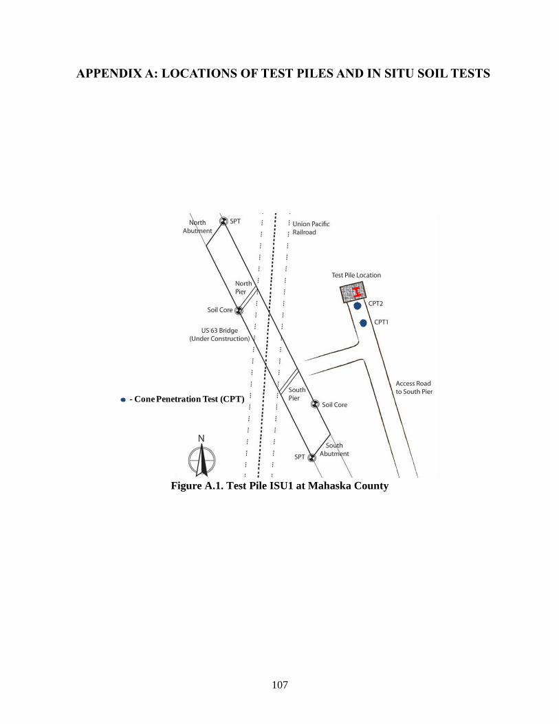
107
APPENDIX A: LOCATIONS OF TEST PILES AND IN SITU SOIL TESTS
Figure A.1. Test Pile ISU1 at Mahaska County
- Cone Penetration Test (CPT)

108
Figure A.2. Test Pile ISU2 at Mills County
Figure A.3. Test Pile ISU3 at Polk County
SPT/BST
CPT
Test Pile
980.2
LOCATIONIA 978 OVER BNSF RRT-72N R-943 W
SECTION 23/22
GLENWOODTOWNSHIP
MILLS COUNTY
BRIDGE MAINT. NO. 6502.4S978- Cone Penetration Test (CPT)
- Standard Penetration Test (SPT)
and Borehole Shear Test (BST)
4 ft
10 ftSPT/BST
CPT
Test Pile
LOCATIONI-35/80/235 INTERCHANGE
NORTH EAST OF DES MOINES
S-W CONNECTOR I-235 TO I-80
RAMP OVER I-80
T-19 N R-23W
DELAWARE TOWNSHIP
POLK COUNTY
- Cone Penetration Test (CPT)
- Standard Penetration Test (SPT)
and Borehole Shear Test (BST)
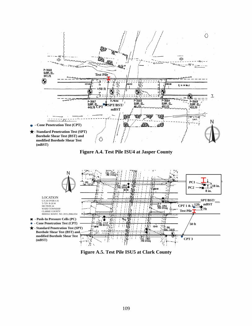
109
Figure A.4. Test Pile ISU4 at Jasper County
Figure A.5. Test Pile ISU5 at Clark County
≈50 ft
SPT/BST/
mBSTCPT
Test Pile
- Cone Penetration Test (CPT)
- Standard Penetration Test (SPT)
Borehole Shear Test (BST) and
modified Borehole Shear Test
(mBST)
12ft
SPT/BST/
mBSTCPT 1 & 2
Test Pile7ft
CPT 3
50 ft
8 in.
18 in.
LOCATIONU.S.34 OVER I-35
T-72N R-26 W
SECTION 24
WARD TOWNSHIP
CLARKE COUNTY
BRIDGE MAINT. NO. 2015.2R&L034
PC1
PC2
- Push-In Pressure Cells (PC)
- Cone Penetration Test (CPT)
- Standard Penetration Test (SPT)
Borehole Shear Test (BST) and
modified Borehole Shear Test
(mBST)
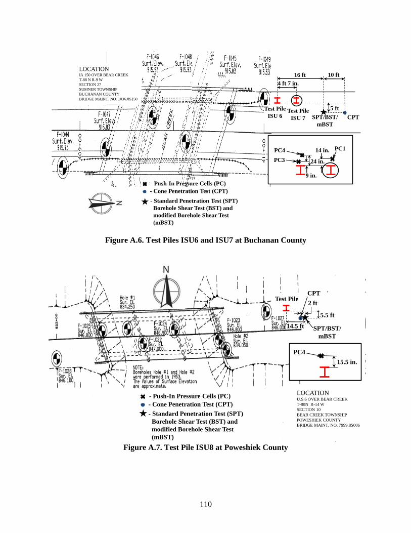
110
Figure A.6. Test Piles ISU6 and ISU7 at Buchanan County
Figure A.7. Test Pile ISU8 at Poweshiek County
4 ft 7 in.
SPT/BST/
mBST
CPT
Test Pile
ISU 6
5 ft
9 in.
24 in.
Test Pile
ISU 7
16 ft 10 ft
14 in. PC1
LOCATIONIA 150 OVER BEAR CREEK
T-88 N R-9 W
SECTION 27
SUMNER TOWNSHIP
BUCHANAN COUNTY
BRIDGE MAINT. NO. 1036.8S150
- Push-In Pressure Cells (PC)
- Cone Penetration Test (CPT)
- Standard Penetration Test (SPT)
Borehole Shear Test (BST) and
modified Borehole Shear Test
(mBST)
PC4
PC3
14.5 ft SPT/BST/
mBST
CPTTest Pile
5.5 ft
15.5 in.
PC4
2 ft
LOCATIONU.S.6 OVER BEAR CREEK
T-80N R-14 W
SECTION 10
BEAR CREEK TOWNSHIP
POWESHIEK COUNTY
BRIDGE MAINT. NO. 7999.8S006
- Push-In Pressure Cells (PC)
- Cone Penetration Test (CPT)
- Standard Penetration Test (SPT)
Borehole Shear Test (BST) and
modified Borehole Shear Test
(mBST)
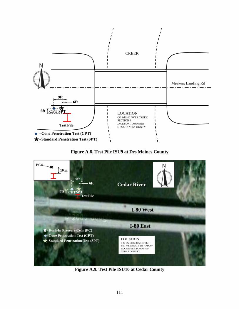
111
Figure A.8. Test Pile ISU9 at Des Moines County
Figure A.9. Test Pile ISU10 at Cedar County
LOCATIONCO Rd H40 OVER CREEKSECTION 4
JACKSON TOWNSHIP
DES MOINES COUNTY
CREEK
Meekers Landing Rd
9ft
SPTCPT
Test Pile
6ft
6ft
- Cone Penetration Test (CPT)
- Standard Penetration Test (SPT)
9ft
SPTCPTTest Pile
7ft
6ft
I-80 East
I-80 West
Cedar River
LOCATIONI-80 OVER CEDAR RIVERBETWEEN EXIT 265 AND 267
ROCHESTER TOWNSHIP
CEDAR COUNTY
- Cone Penetration Test (CPT)
- Standard Penetration Test (SPT)
10 in.
PC4
- Push-In Pressure Cells (PC)

112
APPENDIX B: RESULTS OF IN SITU SOIL INVESTIGATIONS AND SOIL
PROFILES
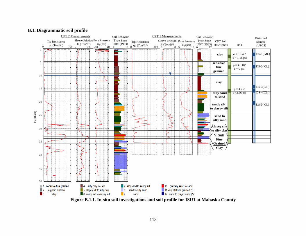
113
B.1. Diagrammatic soil profile
Figure B.1.1. In-situ soil investigations and soil profile for ISU1 at Mahaska County
Dep
th (
ft)
CPT 2 Measurements CPT 1 Measurements
Tip Resistance
qc (Ton/ft2)
Tip Resistance
qc (Ton/ft2)
Sleeve Friction
fs (Ton/ft2)Sleeve Friction
fs (Ton/ft2)
Pore Pressure
u2 (psi)Pore Pressure
u2 (psi)
Soil Behavior
Type Zone
UBC (1983)
Soil Behavior
Type Zone
UBC (1983)
clay
sensitive
fine
grained
clay
silty sand
to sand
sandy silt
to clayey silt
sand to
silty sand
clayey silt
to silty clay
φ = 13.48º
c = 1.16 psi
Disturbed
Sample
(USCS)
DS-1( ML)
DS-2( CL)
DS-3(CL )
DS-4(CL )
DS-5( CL)
BST
φ = 41.18º
c = 0 psi
φ = 4.26º
c =3.56 psi
V. Stiff
Fine
Grained
Clay
0
Ma
CPT Soil
Description
0
5
10
15
20
25
30
35
40
45
50
0 700 0 10 -10 40 0 12 0 0800 8 -6 010 12
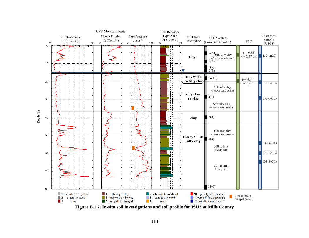
114
Figure B.1.2. In-situ soil investigations and soil profile for ISU2 at Mills County
CPT Measurements
Tip Resistance
qc (Ton/ft2)
Sleeve Friction
fs (Ton/ft2)
Pore Pressure
u2 (psi)
Soil Behavior
Type Zone
UBC (1983)D
epth
(ft
)
φ = 6.85º
c = 2.97 psi3(5)
3(5)
3(5)3(5)
14(15)
3(3)
12(8)
SPT N-value
(Corrected N-value)
Stiff silty clay
w/ trace sand seams
Stiff to firm
Sandy silt
Disturbed
Sample
(USCS)
DS-1(SC)
DS-2(CL)
DS-3(CL)
DS-4(CL)
DS-5(CL)
DS-6(CL)
BST
φ = 40º
c = 0 psi
clay
clayey silt
to silty clay
silty clay
to clay
clay
clayey silt to
silty clay
Stiff silty clay
w/ trace sand seams
Stiff silty clay
w/ trace sand seams
Stiff silty clay
w/ trace sand seams
4(3)
4(3)
Stiff to firm
Sandy silt
Pore pressure
dissipation test
CPT Soil
Description
0
10
20
30
40
50
60
70
80
0 90 0 2 -20 100 0 12

115
Figure B.1.3. In-situ soil investigations and soil profile for ISU3 at Polk County
CPT Measurements
Tip Resistance
qc (Ton/ft2)
Sleeve Friction
fs (Ton/ft2)
Pore Pressure
u2 (psi)
Soil Behavior
Type Zone
UBC (1983)D
epth
(ft
)
φ = 0º
c = 7.45 psi8(11)
11(12)
5(5)
7(6)
12(10)
9(7)
21(12)
SPT N-value
(Corrected N-value)
dark brown clay
clayey sand
coarse sand
grey silty clay
grey clay
light brown
silty clay
Disturbed
Sample
(USCS)
DS-1(CL)
DS-2(SM)
DS-3
(SM-SC)
DS-4(CL)
DS-5(CL)
DS-6(CL)
DS-7(SM)
BST
φ = 11.94º
c = 2.45 psi
clay
clayey silt to
silty clay
sandy silt to
clayey silt
clayey silt
to silty clay
clay
clayey silt to
silty clay
v. stiff fine
grained
10(7)
10(7)
5(3)
grey silt
grey brown
silty clay
Pore pressure
dissipation test
CPT Soil
Description
0
10
20
30
40
50
60
70
0 160 0 5 -20 100 0 12
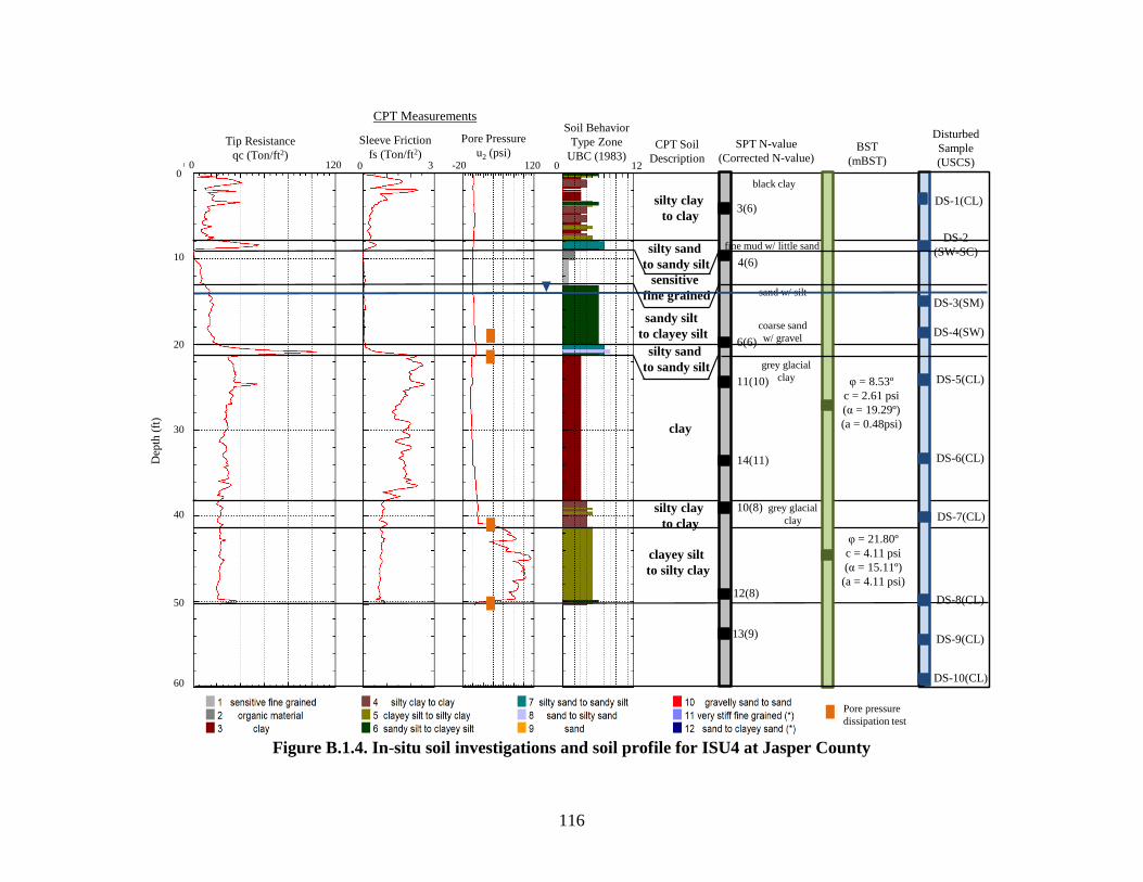
116
Figure B.1.4. In-situ soil investigations and soil profile for ISU4 at Jasper County
CPT Measurements
Tip Resistance
qc (Ton/ft2)
Sleeve Friction
fs (Ton/ft2)
Pore Pressure
u2 (psi)
Soil Behavior
Type Zone
UBC (1983)D
epth
(ft
)
silty clay
to clay
silty sand
to sandy silt
sensitive
fine grained
sandy silt
to clayey silt
silty sand
to sandy silt
clay
silty clay
to clay
clayey silt
to silty clay
φ = 8.53º
c = 2.61 psi
(α = 19.29º)
(a = 0.48psi)
3(6)
4(6)
6(6)
11(10)
14(11)
10(8)
12(8)
SPT N-value
(Corrected N-value)
black clay
fine mud w/ little sand
sand w/ silt
coarse sand
w/ gravel
grey glacial
clay
Disturbed
Sample
(USCS)
DS-1(CL)
DS-2
(SW-SC)
DS-3(SM)
DS-4(SW)
DS-5(CL)
DS-6(CL)
DS-7(CL)
DS-8(CL)
BST
(mBST)
φ = 21.80º
c = 4.11 psi
(α = 15.11º)
(a = 4.11 psi)
13(9)
grey glacial
clay
DS-9(CL)
DS-10(CL)
Pore pressure
dissipation test
CPT Soil
Description
0
10
20
30
40
50
60
0 120 0 3 -20 120 0 12
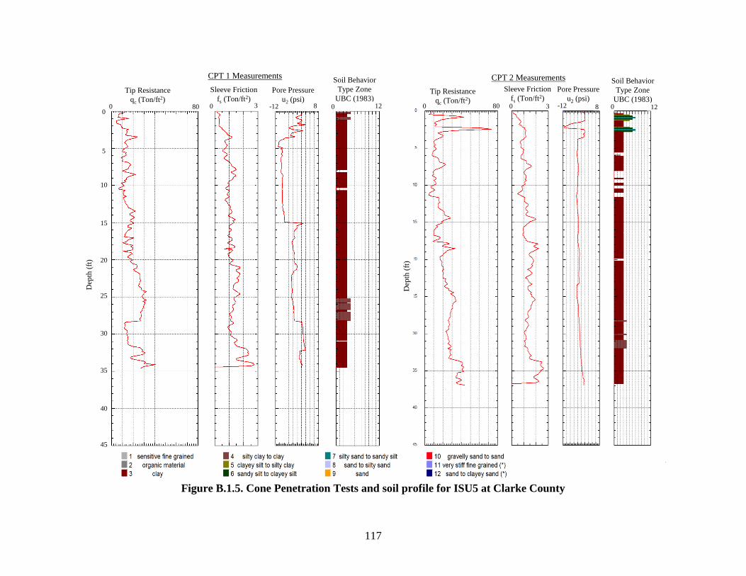
117
Figure B.1.5. Cone Penetration Tests and soil profile for ISU5 at Clarke County
CPT 1 Measurements
Tip Resistance
qc (Ton/ft2)
Sleeve Friction
fs (Ton/ft2)
Pore Pressure
u2 (psi)
Soil Behavior
Type Zone
UBC (1983)
CPT 2 Measurements
Tip Resistance
qc (Ton/ft2)
Sleeve Friction
fs (Ton/ft2)
Pore Pressure
u2 (psi)
Soil Behavior
Type Zone
UBC (1983)
Dep
th (
ft)
Dep
th (
ft)
0
5
10
15
20
25
30
35
40
45
0 80 0 3 -12 8 0 12 0 80 0 3 -12 8 0 12
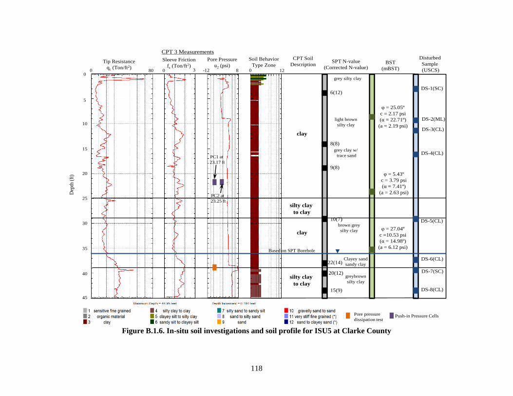
118
Figure B.1.6. In-situ soil investigations and soil profile for ISU5 at Clarke County
φ = 25.05º
c = 2.17 psi
(α = 22.71º)
(a = 2.19 psi)
6(12)
8(8)
9(8)
10(7)
22(14)
20(12)
15(9)
SPT N-value
(Corrected N-value)
grey silty clay
light brown
silty clay
grey clay w/
trace sand
brown grey
silty clay
Clayey sand
sandy clay
greybrown
silty clay
Disturbed
Sample
(USCS)
DS-1(SC)
DS-2(ML)
DS-3(CL)
DS-4(CL)
DS-5(CL)
DS-6(CL)
DS-7(SC)
DS-8(CL)
CPT 3 Measurements
clay
silty clay
to clay
clay
silty clay
to clay
Dep
th (
ft)
BST
(mBST)
φ = 5.43º
c = 3.79 psi
(α = 7.41º)
(a = 2.63 psi)
φ = 27.04º
c =10.53 psi
(α = 14.98º)
(a = 6.12 psi)
Tip Resistance
qc (Ton/ft2)
Sleeve Friction
fs (Ton/ft2)
Pore Pressure
u2 (psi)
Soil Behavior
Type Zone
Pore pressure
dissipation testPush-in Pressure Cells
PC1 at
23.17 ft
PC2 at
23.25 ft
Based on SPT Borehole
CPT Soil
Description
0
5
10
15
20
25
30
35
40
45
0 80 0 3 -12 8 0 12
119
Figure B.1.7. In-situ soil investigations and soil profile for ISU6 and ISU7 at Buchanan County
CPT Measurements
Tip Resistance
qc (Ton/ft2)Sleeve Friction
fs (Ton/ft2)
Pore Pressure
u2 (psi)
Soil Behavior
Type Zone
UBC (1983)D
epth
(ft
)
clay
clay
silty clay
to clay
silty sand
to sandy silt
sand to
silty sand
clayey silt
to silty clay
clayey silt
to silty clay
12(19)
23(25)
8(11)
8(8)
10(8)
16(12)
SPT N-value
(Corrected N-value)
sandy graveldark sandy clay
sandy siltmedium sand
w/ gravel
fine sand
sandy clay
silty clay
Disturbed
Sample
(USCS)
DS-1(SC)
DS-2(SM)
DS-3(CL)
DS-4(CL)
DS-5(CL)
DS-6(CL)
DS-7(ML)
BST
(mBST)
23(16)
23(15)
22(15)
sandy silt
medium sand
silt w/ sand
φ = 31.59º
c = 0.073 psi
(α = 22.29º)
(a = 0 psi)
φ = 25.87º
c = 1.69 psi
(α = 6.28º)
(a = 2.74 psi)
φ = 30.28º
c = 0.02 psi
(α = 25º)
(a = 2.01 psi)
DS-8(CL)
Pore pressure
dissipation test
PC3 at
34 ft (ISU6)
PC4 at
34 ft (ISU6)
PC1 at
28 ft (ISU7)
Push-in Pressure Cells
CPT Soil
Description
0
10
20
30
40
50
60
70
0 140 0 5 -10 70 0 12
120
Figure B.1.8. In-situ soil investigations and soil profile for ISU8 at Poweshiek County
CPT Measurements
Tip Resistance
qc (Ton/ft2)
Sleeve Friction
fs (Ton/ft2)
Pore Pressure
u2 (psi)
Soil Behavior
Type Zone
UBC (1983)D
epth
(ft
)
clay
silty clay
to clay
silty sand to
sandy silt
sand
clayey silt
to silty clay
clayey silt
to silty clay
silty sand
to sandy silt
silty clay
to clay
5(11)
6(9)
4(5)
5(5)
2(2)
2(2)
SPT N-value
(Corrected N-value)
Disturbed
Sample
(USCS)
DS-1(CL)
DS-2(CL)
DS-3(CL)
DS-4(CL)
DS-5(CL)
DS-6(SW)
DS-7(CL)
BST
(mBST)
2(2)
11(8)
10(7)
dark grey
silty clay
φ = 33.02º
c = 1.02 psi
(α = 27.38º)
(a = 0.22 psi)
φ = 14.04º
c = 1.93 psi
(α = 0º)
(a = 3.91 psi)
φ = 17.97º
c = 2.80 psi
(α = 1.07º)
(a = 7.62 psi)
DS-8(CL)24(16)
21(13)
19(12)
light grey clay
fine sand
fine to coarse
sand
grey clay
grey clay
Pore pressure
dissipation testPush-in Pressure Cells
PC4 at
14 ft
DS-9(CL)
DS-10(CL)
CPT Soil
Description
0
10
20
30
40
50
60
70
0 350 0 5 -20 100 0 12

121
Figure B.1.9. In-situ soil investigations and soil profile for ISU9 at Des Moines County
CPT Measurements
Tip Resistance
qc (Ton/ft2)
Sleeve Friction
fs (Ton/ft2)
Pore Pressure
u2 (psi)Soil Behavior
Type Zone
Dep
th (
ft)
sandy silty to
clayey silt
clay
sand
8(16)
4(5)
5(5)
6(6)
7(6)
11(9)
SPT N-value
(Corrected N-value)
Disturbed
Sample
(USCS)
DS-1
(SM;SC)
DS-2(CL)
DS-3
(SM; SC)
DS-4(SW)
DS-5(SW)
DS-6(SP)
DS-7(SW)
14(11)
13(10)
15(11)
silty clay
32(22)
Fine grey sand
w/ clay
course sand
Sand w/ gravel
grey sand
grey sand
w/ gravel
Pore pressure
dissipation test
CPT Soil
Description
0
5
10
15
20
25
30
35
40
45
50
0 700 0 8 0 400 0 12
122
Figure B.1.10. In-situ soil investigations and soil profile for ISU10 at Cedar County
CPT Measurements
Tip Resistance
qc (Ton/ft2)Sleeve Friction
fs (Ton/ft2)
Pore Pressure
u2 (psi)Soil Behavior
Type Zone D
epth
(ft
)
sandy silty to
clayey silt
sand to silty sand
sandy silt
to clayey silt
21(42)
6(9)
14(17)
28(30)
36(35)
69(57)
SPT N-value
(Corrected N-value)
Disturbed
Sample
(USCS)
DS-1 (SW)
DS-2
(SP-SM;
SP-SC)
DS-3 (SW)
DS-4(SP)
DS-5(SW)
DS-6
(SW-SM;
SW-SC)
DS-7(SW)
34(26)
53(37)
Medium sand
52(33)
medium course sand
course sand
w/ gravel
0
25
30
35
40
45
50
55
60
5
10
15
20
0 250 0 2 0 10 0 12
sand
Push-in Pressure Cells
PC4
at 10 ft
CPT Soil
Description
0
5
10
15
20
25
30
35
40
45
50
55
60
0 250 0 2 0 10 0 12

123
B.2. Estimated Soil Profiles and Properties Based on Cone Penetration Tests (CPT)
Table B.2.1. Summary of soil properties for ISU1 based on CPT
Soil
Profiles Depth (ft) Soil Types
Average
Effective
Friction Angle,
φ′ (degree)
Average
Undrained Shear
Strength, Su (psi)
Over-
consolidation
Ratio (OCR)
Layer 1 0 to 4.43 Clay 31.93 5.63 -
Layer 2 4.43 to
9.19
Sensitive Fine
Grained 30.09 7.19 7.99
Layer 3 9.19 to
15.42 Clay 33.23 19.39 12.74
Layer 4 15.42 to
18.86
Silty Sand to
Sand 41.38 - -
Layer 5 18.86 to
24.28
Sandy Silt to
Clayey Silt 35.22 39.40 13.32
Layer 6 24.28 to
30.35
Sand to Silty
Sand 42.18 - -
Layer 7 30.35 to
32.97
Clayey Silt to
silty Clay 37.12 66.20 17.06
Layer 8 32.97 to
33.79
Very Stiff Fine
Grained Sand 36.77 - -
Layer 9 33.79 to
35.43 Clay 37.74 110.07 26.24
Table B.2.2. Summary of soil properties for ISU2 based on CPT
Soil
Profiles Depth (ft) Soil Types
Average
Effective
Friction Angle,
φ′ (degree)
Average
Undrained Shear
Strength, Su (psi)
Average Over-
consolidation
Ratio (OCR)
Layer 1 0 to 16 Clay 31.71 14.42 -
Layer 2 16 to 20 Clayey Silt to
Silty Clay 28.51 11.31 7.52
Layer 3 20 to 36 Silty Clay to
Clay 27.07 7.62 2.09
Layer 4 36 to 44 Clay 28.68 11.35 1.84
Layer 5 44 to 73 Clayey Silt to
Silty Clay 27.04 18.10 6.50
124
Table B.2.3. Summary of soil properties for ISU3 based on CPT
Soil
Profiles Depth (ft) Soil Types
Average Effective
Friction Angle, φ′
(degree)
Average
Undrained Shear
Strength, Su (psi)
Average Over-
consolidation
Ratio (OCR)
Layer 1 0 to 7.71 Clay 35.42 25.27 -
Layer 2 7.71 to 34 Clayey Silt to
Silty Clay 32.76 16.55 5.94
Layer 3 34 to 41.5 Sandy Silt to
Clayey Silt 34.36 14.95 3.19
Layer 4 41.5 to
45.11 Clayey Silt to
Silty Clay 31.09 12.13 2.33
Layer 5 45.11 to
55.28 Clay 31.50 22.03 3.72
Layer 6 55.28 to
66.77 Clayey Silt to
Silty Clay 29.09 23.09 2.74
Layer 7 66.77 to
69.88 Very Stiff Fine
Grained 35.60 67.61 7.31
Table B.2.4. Summary of soil properties for ISU4 based on CPT
Soil
Profiles Depth (ft) Soil Types
Average Effective
Friction Angle, φ′
(degree)
Average
Undrained
Shear Strength,
Su (psi)
Average Over-
consolidation
Ratio (OCR)
Layer 1 0 to 7.71 Silty Clay to
Clay 34.03 14.69 -
Layer 2 7.71 to
8.86 Silty Sand to
Sandy Silt 34.59 - -
Layer 3 8.86 to
12.96 Sensitive Fine
Grained 25.41 4.09 2.15
Layer 4 12.96 to
19.85 Sandy Silt to
Clayey Silt 30.68 12.27 5.48
Layer 5 19.85 to
21.16 Silty Sand to
Sandy Silt 35.76 - -
Layer 6 21.16 to
38.06 Clay 32.76 25.30 6.62
Layer 7 38.06 to
41.17 Silty Clay to
Clay 30.97 18.14 3.76
Layer 8 41.17 to
50.36 Clayey Silt to
Silty Clay 33.29 18.11 3.46

125
Table B.2.5. Summary of soil properties for ISU5 based on CPT
Soil
Profiles Depth (ft) Soil Types
Average Effective
Friction Angle, φ′
(degree)
Average
Undrained
Shear Strength,
Su (psi)
Average Over-
consolidation
Ratio (OCR)
Layer 1 0 to 25 Clay 31.08 13.28 5.60
Layer 2 25 to 29 Silty Clay to
Clay 29.94 15.71 3.11
Layer 3 29 to 39 Clay 29.72 16.46 2.63
Layer 4 39 to 45 Silty Clay to
Clay 32.09 30.61 3.92
Table B.2.6. Summary of soil properties for ISU6 and ISU7 based on CPT
Soil
Profiles Depth (ft) Soil Types
Average Effective
Friction Angle, φ′
(degree)
Average
Undrained
Shear Strength,
Su (psi)
Average Over-
consolidation
Ratio (OCR)
Layer 1 0 to 13.12 Clay 33.96 22.27 -
Layer 2 13.12 to
20.01
Sand to Silty
Sand 38.28 - -
Layer 3 20.01 to
29.36 Clay 28.82 10.27 3.33
Layer 4 29.36 to
30.51
Silty Sand to
Sandy Silt 35.34 - -
Layer 5 30.51 to
38.22
Silty Clay to
Clay 29.86 14.15 3.05
Layer 6 38.22 to
50.85
Clayey Silt to
Silty Clay 30.56 18.57 2.95
Layer 7 50.85 to
62.50
Clayey Silt to
Silty Clay 33.63 41.68 5.98
126
Table B.2.7. Summary of soil properties for ISU8 based on CPT
Soil
Profiles Depth (ft) Soil Types
Average Effective
Friction Angle, φ′
(degree)
Average
Undrained
Shear Strength,
Su (psi)
Average Over-
consolidation
Ratio (OCR)
Layer 1 0 to 14.44 Clay 32.50 12.49 -
Layer 2 14.44 to
24.93
Silty Clay to
Clay 28.15 8.43 2.69
Layer 3 24.93 to
32.48
Silty Sand to
Sandy Silt 34.62 - -
Layer 4 32.48 to
38.06 Sand 41.75 - -
Layer 5 38.06 to
41.17
Clayey Silt to
Silty Clay 29.90 16.60 3.18
Layer 6 41.17 to
49.21
Silty Sand to
Sandy Silt 33.12 - -
Layer 7 49.21 to
52.66
Clayey Silt to
Silty Clay 30.41 18.94 3.11
Layer 8 52.66 to
64.47
Silty Clay to
Clay 34.27 47.59 6.76
Table B.2.8. Summary of soil properties for ISU9 based on CPT
Soil
Profiles Depth (ft) Soil Types
Average Effective
Friction Angle, φ′
(degree)
Average
Undrained
Shear Strength,
Su (psi)
Average Over-
consolidation
Ratio (OCR)
Layer 1 0 to 4.27 Sandy Silt to
Clayey Silt 46.19 392.44 -
Layer 2 4.27 to
15.91 Clay 30.97 71.59 6.90
Layer 3 15.91 to
45.93 Sand 40.21 - -
Table B.2.9. Summary of soil properties for ISU10 based on CPT
Soil
Profiles Depth (ft) Soil Types
Average Effective
Friction Angle, φ′
(degree)
Average
Undrained
Shear Strength,
Su (psi)
Average Over-
consolidation
Ratio (OCR)
Layer 1 0 to 4.59 Sandy Silt to
Clayey Silt 34.65 108.87 -
Layer 2 4.59 to
6.56
Sand to Silty
Sand 41.30 - -
Layer 3 6.56 to
8.86
Sandy Silt to
Clayey Silt 32.89 115.15 16.66
Layer 4 8.86 to
22.15 Sand 39.61 - -
127
B.3. Pore Water Pressure Measurements Using Cone Penetration Tests (CPT)
Figure B.3.1. CPT pore water pressure dissipation tests at ISU2 Mills County
Figure B.3.2. CPT pore water pressure dissipation tests at ISU3 Polk County
0
10
20
30
40
50
60
70
0.1 1 10 100 1000 10000
Po
re P
ress
ure
(p
si)
Time (second)
At 57.2 ft
At 35.4 ft
0
10
20
30
40
50
60
70
0.1 1 10 100 1000 10000
Po
re P
ress
ure
(p
si)
Time (Second)
At 22.15 ft
At 22.15 ft (Extrapolated)
At 50.69 ft

128
Figure B.3.3. CPT pore water pressure dissipation tests at ISU4 Jasper County
Figure B.3.4. CPT pore water pressure dissipation tests at ISU5 Clarke County
0
10
20
30
40
50
60
70
80
90
0.1 1 10 100 1000 10000 100000
Po
re P
ress
ure
( p
si)
Time (second)
At 19.5 ft
At 21 ft
At 41 ft
A 41 ft (Extrapolated)
At 50.53 ft
At 50.53 ft (Extrapolated)
0
1
2
3
4
5
6
7
8
0.1 1 10 100 1000 10000
Po
re P
ress
ure
(p
si)
Time (second)
At 38.55 ft
129
Figure B.3.5. CPT pore water pressure dissipation tests at ISU6 and ISU7 Buchanan
County
Figure B.3.6. CPT pore water pressure dissipation tests at ISU8 Poweshiek County
0
10
20
30
40
50
60
0.1 1 10 100 1000 10000 100000
Po
re P
ress
ure
(p
si)
Time (second)
At 17.06 ft
At 22.97 ft
At 30.02 ft
At 50.03 ft
At 50.03 ft (Extrapolated)
-20
0
20
40
60
80
100
120
140
0.1 1 10 100 1000 10000 100000
Po
re P
ress
ure
(p
si)
Time (second)
At 31.84 ft
At 45.11 ft
At 57.25 ft
At 57.25 ft (Extrapolated)
At 64.80 ft
130
Figure B.3.7. CPT pore water pressure dissipation tests at ISU9 Des Moines County
0
2
4
6
8
10
12
14
16
0.1 1 10 100 1000 10000
Po
re P
ress
ure
(p
si)
Time (Second)
At 30.18 ft
At 45.28 ft

131
B.4. Borehole Shear Test and modified Borehole Shear Test Results
Figure B.4.1. ISU1 at 3-ft depth (BST)
Figure B.4.2. ISU1 at 8-ft depth (BST)
Figure B.4.3. ISU1 at 16-ft depth (BST)
τ = 0.24σ + 1.16
φ = 13.48º; c = 1.16 psi (BST)
0
1
2
3
4
5
6
0 5 10 15 20
Sh
eari
ng
Str
ess,
τ (
psi
)
Normal Stress,σ (psi)
τ = 0.48σ φ = 41.18º; c = 0 psi (BST)
0
1
2
3
4
5
6
7
8
9
0 5 10 15 20
Sh
eari
ng
Str
ess,
τ (
psi
)
Normal Stress,σ (psi)
τ = 0.075σ + 3.56
φ = 4.26º; c = 3.56 psi (BST)
0
1
2
3
4
5
6
0 5 10 15 20
Sh
eari
ng
Str
ess,
τ (
psi
)
Normal Stress,σ (psi)
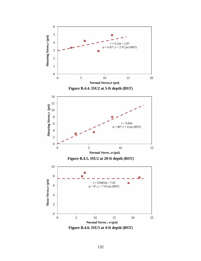
132
Figure B.4.4. ISU2 at 5-ft depth (BST)
Figure B.4.5. ISU2 at 20-ft depth (BST)
Figure B.4.6. ISU3 at 4-ft depth (BST)
τ = 0.12σ + 2.97
φ = 6.85º; c = 2.97 psi (BST)
0
1
2
3
4
5
6
0 5 10 15 20
Sh
eari
ng
Str
ess,
τ (
psi
)
Normal Stress,σ (psi)
τ = 0.84σ φ = 40º; c = 0 psi (BST)
0
2
4
6
8
10
12
14
0 5 10 15
Sh
eari
ng
Str
ess,
τ
(psi
)
Normal Stress ,σ (psi)
τ = 0.0003σ + 7.45
φ = 0º; c = 7.45 psi (BST)
0
2
4
6
8
10
0 5 10 15 20 25
Sh
ear
Str
ess,
τ (
psi
)
Normal Stress , σ (psi)

133
Figure B.4.7. ISU3 at 23-ft depth (BST)
Figure B.4.8. ISU4 at 27-ft depth (BST & mBST)
Figure B.4.9. ISU4 at 46-ft depth (BST & mBST)
τ = 0.21σ + 2.45
φ = 11.94º; c = 2.45 psi (BST)
0
1
2
3
4
5
6
7
8
0 5 10 15 20 25
Sh
ear
Str
ess,
τ
(psi
)
Normal Stress ,σ (psi)
τ = 0.35σ + 0.48
α = 19.29º; a = 0.48 psi (mBST)
τ = 0.15σ + 2.61
φ = 8.53º; c = 2.61 psi (BST)
0
1
2
3
4
5
6
7
8
0 5 10 15 20
Sh
ear
Str
ess,
τ (
psi
)
Normal Stress,σ (psi)
τ = 0.27σ + 4.11
α = 15.11º; a = 4.11 psi (mBST)
τ = 0.4σ + 4.11
φ = 21.80º; c = 4.11 psi (BST)
0
2
4
6
8
10
12
0 5 10 15 20
Sh
ear
Str
ess,
τ
(psi
)
Normal Stress,σ (psi)
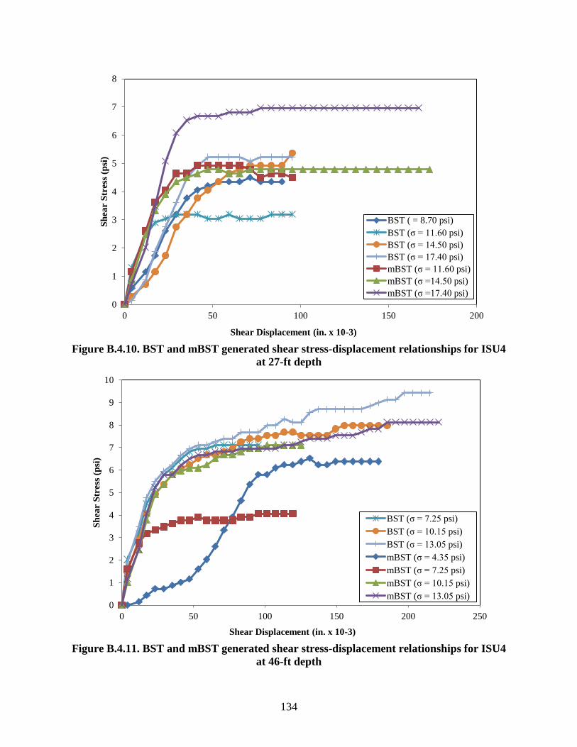
134
Figure B.4.10. BST and mBST generated shear stress-displacement relationships for ISU4
at 27-ft depth
Figure B.4.11. BST and mBST generated shear stress-displacement relationships for ISU4
at 46-ft depth
0
1
2
3
4
5
6
7
8
0 50 100 150 200
Sh
ear
Str
ess
(psi
)
Shear Displacement (in. x 10-3)
BST ( = 8.70 psi)
BST (σ = 11.60 psi)
BST (σ = 14.50 psi)
BST (σ = 17.40 psi)
mBST (σ = 11.60 psi)
mBST (σ =14.50 psi)
mBST (σ =17.40 psi)
0
1
2
3
4
5
6
7
8
9
10
0 50 100 150 200 250
Sh
ear
Str
ess
(psi
)
Shear Displacement (in. x 10-3)
BST (σ = 7.25 psi)
BST (σ = 10.15 psi)
BST (σ = 13.05 psi)
mBST (σ = 4.35 psi)
mBST (σ = 7.25 psi)
mBST (σ = 10.15 psi)
mBST (σ = 13.05 psi)

135
Figure B.4.12. ISU5 at 8.83-ft depth (BST & mBST)
Figure B.4.13. ISU5 at 23.83-ft depth (BST & mBST)
Figure B.4.14. ISU5 at 35.83-ft depth (BST & mBST)
τ = 0.3787σ + 2.4808
α = 20.75⁰; a = 2.48 psi (mBST)
τ = 0.4678σ + 2.1711
φ = 25.08⁰; c = 2.17 psi (BST)
0
1
2
3
4
5
6
7
0 2 4 6 8 10
Sh
aer
Sh
ear,
τ (
psi
)
Normal Stress, σ (psi)
τ = 0.13σ + 2.6245
α = 7.41⁰; a = 2.63 psi (mBST)
τ = 0.095σ + 3.7918
φ = 5.43⁰; c = 3.79 psi (BST)
0
1
2
3
4
5
6
0 5 10 15 20
Sh
ear
Sh
ear,
τ (
psi
)
Normal Stress, σ (psi)
τ = 0.2675σ + 6.1154
α = 14.98⁰; a = 6.12 psi (mBST)
τ = 0.51σ + 10.527
φ = 27.04⁰; c = 10.53 psi (BST)
0
5
10
15
20
25
0 5 10 15 20 25 30
Sh
ear
Str
ess,
τ (
psi
)
Normal Stress, σ (psi)
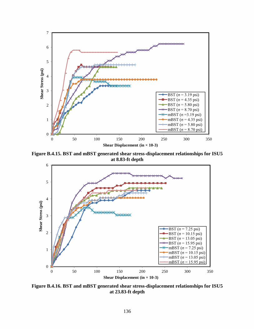
136
Figure B.4.15. BST and mBST generated shear stress-displacement relationships for ISU5
at 8.83-ft depth
Figure B.4.16. BST and mBST generated shear stress-displacement relationships for ISU5
at 23.83-ft depth
0
1
2
3
4
5
6
7
0 50 100 150 200 250 300 350
Sh
ear
Str
ess
(psi
)
Shear Displacement (in × 10-3)
BST (σ = 3.19 psi)
BST (σ = 4.35 psi)
BST (σ = 5.80 psi)
BST (σ = 8.70 psi)
mBST (σ =3.19 psi)
mBST (σ = 4.35 psi)
mBST (σ = 5.80 psi)
mBST (σ = 8.70 psi)
0
1
2
3
4
5
6
0 50 100 150 200 250 300 350
Sh
ear
Str
ess
(psi
)
Shear Displacement (in × 10-3)
BST (σ = 7.25 psi)
BST (σ = 10.15 psi)
BST (σ = 13.05 psi)
BST (σ = 15.95 psi)
mBST (σ = 7.25 psi)
mBST (σ = 10.15 psi)
mBST (σ = 13.05 psi)
mBST (σ = 15.95 psi)
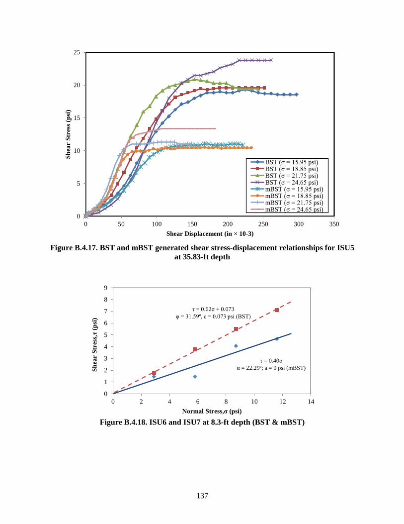
137
Figure B.4.17. BST and mBST generated shear stress-displacement relationships for ISU5
at 35.83-ft depth
Figure B.4.18. ISU6 and ISU7 at 8.3-ft depth (BST & mBST)
0
5
10
15
20
25
0 50 100 150 200 250 300 350
Sh
ear
Str
ess
(psi
)
Shear Displacement (in × 10-3)
BST (σ = 15.95 psi) BST (σ = 18.85 psi) BST (σ = 21.75 psi) BST (σ = 24.65 psi) mBST (σ = 15.95 psi) mBST (σ = 18.85 psi) mBST (σ = 21.75 psi) mBST (σ = 24.65 psi)
τ = 0.40σ α = 22.29º; a = 0 psi (mBST)
τ = 0.62σ + 0.073
φ = 31.59º, c = 0.073 psi (BST)
0
1
2
3
4
5
6
7
8
9
0 2 4 6 8 10 12 14
Sh
ear
Str
ess,
τ (
psi
)
Normal Stress,σ (psi)
138
Figure B.4.19. ISU6 and ISU7 at 11.89-ft depth (BST & mBST)
Figure B.4.20. ISU6 and ISU7 at 50.3-ft depth (BST & mBST)
Figure B.4.21. BST and mBST generated shear stress-displacement relationships for ISU6
and ISU7 at 8.3-ft depth
τ = 0.11σ + 2.74
α = 6.28º; a = 2.74 psi (mBST)
τ = 0.49σ + 1.69
φ = 25.87º, c = 1.69 psi (BST)
0
1
2
3
4
5
6
7
8
9
0 5 10 15
Sh
ear
Str
ess,
τ (
psi
)
Normal Stress,σ (psi)
τ = 0.47σ + 2.01
α = 25º; a = 2.01 psi (mBST)
τ = 0.58σ + 0.02
φ = 30.28º, c = 0.02 psi (BST)
0
5
10
15
20
25
0 10 20 30 40
Sh
ear
Str
ess,
τ (
psi
)
Normal Stress,σ (psi)
0
1
2
3
4
5
6
7
8
0 20 40 60 80 100 120 140
Sh
ear
Str
ess
(psi
)
Shear Displacement (in. x 10-3)
BST (σ = 2.90 psi)
BST (σ = 5.80 psi)
BST (σ = 8.70 psi)
BST (σ = 11.60 psi)
mBST (σ = 2.90 psi)
mBST (σ = 5.80 psi)
mBST (σ = 8.70 psi)
mBST (σ = 11.60 psi)

139
Figure B.4.22. BST and mBST generated shear stress-displacement relationships for ISU6
and ISU7 at 11.89-ft depth
Figure B.4.23. BST and mBST generated shear stress-displacement relationships for ISU6
and ISU7 at 50.3-ft depth
0
1
2
3
4
5
6
7
8
9
0 50 100 150 200 250
Sh
ear
Str
ess
(psi
)
Shear Displacement (in. x 10-3)
BST (σ = 4.35 psi)
BST (σ = 7.25 psi)
BST (σ = 10.15 psi)
BST (σ = 13.05 psi)
mBST (σ = 4.35 psi)
mBST (σ = 7.25 psi)
mBST (σ = 10.15 psi)
mBST (σ = 13.05 psi)
0
5
10
15
20
25
0 50 100 150 200 250 300 350 400
Sh
ear
Str
ess
(psi
)
Shear Displacement (in. x 10-3)
BST (σ = 13.05 psi) BST (σ = 20.31 psi) BST (σ = 27.56 psi) BST (σ = 34.81 psi) mBST (σ =13.05 psi) mBST (σ = 20.31 psi) mBST (σ =27.56 psi) mBST (σ =34.81 psi)
140
Figure B.4.24. ISU8 at 9-ft depth (BST & mBST)
Figure B.4.25. ISU8 at 23-ft depth (BST & mBST)
Figure B.4.26. ISU8 at 45-ft depth (BST & mBST)
τ = 0.52σ + 0.22
α = 27.38º; a = 0.22 psi (mBST)
τ = 0.65σ + 1.02
φ = 33.02º; c = 1.02 psi (BST)
0
1
2
3
4
5
6
7
8
9
0 2 4 6 8 10 12 14
Sh
ear
Str
ess,
τ (
psi
)
Normal Stress,σ (psi)
τ = 0.0004σ + 3.91
α = 0º; a = 3.91 psi (mBST)
τ = 0.25σ + 1.93
φ = 14.04º; c = 1.93 psi (BST)
0
1
2
3
4
5
6
7
8
0 5 10 15 20 25
Sh
ear
Str
ess,
τ (
psi
)
Normal Stress,σ (psi)
τ = 0.32σ + 2.80
φ = 17.97º; c = 2.80 psi (mBST)
τ = 0.019σ + 7.62
α = 1.07º; a = 7.62 psi (BST)
0
2
4
6
8
10
12
14
16
0 10 20 30 40
Sh
ear
Str
ess,
τ (
psi
)
Normal Stress,σ (psi)
141
Figure B.4.27. BST and mBST generated shear stress-displacement relationships for ISU8
at 9-ft depth
Figure B.4.28. BST and mBST generated shear stress-displacement relationships for ISU8
at 23-ft depth
0
1
2
3
4
5
6
7
8
9
0 50 100 150 200 250 300
Sh
ear
Str
ess
(psi
)
Shear Displacement (in. x 10-3)
BST (σ = 2.90 psi)
BST (σ = 5.80 psi)
BST (σ = 11.60 psi)
mBST (σ = 2.90 psi)
mBST (σ = 5.80 psi)
mBST (σ = 11.60 psi)
0
1
2
3
4
5
6
7
8
0 50 100 150 200 250 300
Sh
ear
Str
ess
(psi
)
Shear Displacement (in. x 10-3)
BST (σ = 7.25 psi)
BST (σ = 14.50 psi)
BST (σ = 21.76 psi)
mBST (σ = 7.25 psi)
mBST (σ = 14.50 psi)
mBST (σ = 21.76 psi)
142
Figure B.4.29. BST and mBST generated shear stress-displacement relationships for ISU8
at 45-ft depth
0
2
4
6
8
10
12
14
16
0 50 100 150 200 250 300 350
Sh
ear
Str
ess
(psi
)
Shear Displacement (in. x 10-3)
BST (σ =14.50 psi)
BST (σ = 21.76 psi)
BST (σ = 36.26 psi)
mBST (σ = 14.50 psi)
mBST (σ = 21.76 psi)
mBST (σ = 36.26 psi)
143
B.5. Soil Classification and Properties Obtained from Gradation and Atterberg Limit Tests
Table B.5.1. Soil classification and properties for ISU1 from gradation and Atterberg limit
tests
Disturbed
Sample
Sample
Depth
(ft)
Soil
Type
(USCS)
D10
(in)
D30
(in)
D60
(in)
Liquid
Limit, LL
(%)
Plasticity
Index, PI
(%)
Moisture
Content, ω
(%)
Saturated
Unit
Weight,
γsat (pcf)
Void
Ratio,
e
DS-1 0 to 2 ML n/a 1.2E-4 7.8E-4 42.10 10.40 - - -
DS-2 6 to 7 CL n/a 1.5E-4 8.4E-4 44.40 17.90 - - -
DS-3 14 to 15 CL n/a 4.1E-4 2.8E-3 27.90 7.40 - - -
DS-4 15 CL n/a 1E-4 2.8E-3 32.50 17.70 - - -
DS-5 21 CL n/a 8.8E-5 5.8E-3 39.10 21.60 - - -
Table B.5.2. Soil classification and properties for ISU2 from gradation and Atterberg limit
tests
Disturbed
Sample
Sample
Depth
(ft)
Soil
Type
(USCS)
D10
(in)
D30
(in)
D60
(in)
Liquid
Limit, LL
(%)
Plasticity
Index, PI
(%)
Moisture
Content, ω
(%)
Saturated
Unit
Weight,
γsat (pcf)
Void
Ratio,
e
DS-1 10 SC n/a 4.8E-4 5.9E-3 28.67 13.39 - - -
DS-2 20 CL n/a 1.7E-4 2.6E-3 43.74 25.04 30.00 121.01 0.81
DS-3 30 CL n/a 2.7E-4 1.7E-3 43.16 19.21 12.49 141.73 0.34
DS-4 55 CL n/a 3.3E-4 2.5E-3 47.54 28.40 9.58 146.68 0.26
DS-5 60 CL n/a 4.7E-4 2.5E-3 45.54 24.72 10.71 144.69 0.29
DS-6 65 CL n/a 1.8E-3 2.8E-3 28.75 7.81 13.31 140.44 0.36
Table B.5.3. Soil classification and properties for ISU3 from gradation and Atterberg limit
tests
Disturbed
Sample
Sample
Depth
(ft)
Soil
Type
(USCS)
D10
(in)
D30
(in)
D60
(in)
Liquid
Limit, LL
(%)
Plasticity
Index, PI
(%)
Moisture
Content, ω
(%)
Saturated
Unit
Weight,
γsat (pcf)
Void
Ratio,
e
DS-1 2 to 4 CL n/a 4.9E-4 2.7E-3 36.49 18.69 - - -
DS-2 15 SM 1.4E-4 7.3E-3 4E-2 19.39 - 23.03 127.81 0.62
DS-3 26 SM-SC n/a 1.3E-3 1.3E-2 21.40 4.53 29.39 121.54 0.79
DS-4 35 CL n/a 2.9E-4 2.4E-3 30.63 10.79 30.35 120.70 0.82
DS-5 50 CL n/a 1.9E-4 1.5E-3 28.20 8.15 32.57 118.84 0.88
DS-6 60 CL n/a 4.8E-4 4.2E-3 23.46 9.37 20.34 130.87 0.55
DS-7 65 SM n/a 8.3E-4 8.2E-3 21.85 2.90 16.47 135.83 0.44

144
Table B.5.4. Soil classification and properties for ISU4 from gradation and Atterberg limit
tests
Disturbed
Sample
Sample
Depth
(ft)
Soil
Type
(USCS)
D10
(in)
D30
(in)
D60
(in)
Liquid
Limit, LL
(%)
Plasticity
Index, PI
(%)
Moisture
Content, ω
(%)
Saturated
Unit
Weight,
γsat (pcf)
Void
Ratio,
e
DS-1 3.5 to 5 CL n/a 6.5E-4 4.5E-3 29.32 11.41 25.36 125.37 0.68
DS-2 8.5 to 10 SW-SC 2.9E-3 8.7E-3 2.2E-2 29.32 - 17.18 134.86 0.46
DS-3 15 SM 3.7E-4 5.9E-3 2.4E-2 12.33 - 22.12 128.81 0.60
DS-4 18.5 to 20 SW 3.5E-3 1.7E-2 4.5E-2 - - 15.46 137.24 0.42
DS-5 23.5 to 25 CL n/a 2.4E-4 2.9E-3 27.49 13.46 12.65 141.48 0.34
DS-6 33 to 35 CL n/a 1E-4 2.4E-3 38.68 22.70 16.86 135.30 0.46
DS-7 40 CL n/a 3.3E-4 3.3E-3 29.38 16.70 15.75 136.83 0.43
DS-8 50 CL n/a 3.3E-4 4.2E-3 25.98 13.19 15.09 137.77 0.41
DS-9 55 CL n/a 4E-4 4E-3 25.33 13.06 13.12 140.74 0.35
DS-10 65 CL n/a 3.3E-4 3.3E-3 29.63 15.76 14.73 138.29 0.40
Table B.5.5. Soil classification and properties for ISU5 from gradation and Atterberg limit
tests
Disturbed
Sample
Sample
Depth
(ft)
Soil
Type
(USCS)
D10
(in)
D30
(in)
D60
(in)
Liquid
Limit, LL
(%)
Plasticity
Index, PI
(%)
Moisture
Content, ω
(%)
Saturated
Unit
Weight,
γsat (pcf)
Void
Ratio,
e
DS-1 3 SC 3.3E-5 8.1E-4 2.1E-2 26.31 11.27 20.39 130.82 0.55
DS-2 8 to 10 ML 9.0E-6 4.8E-4 2.7E-3 36.30 5.57 18.70 132.89 0.50
DS-3 10 to 12 CL n/a 2.4E-4 2.6E-3 38.41 20.82 20.64 130.52 0.56
DS-4 16 CL n/a 3.4E-4 2.7E-3 49.10 27.08 21.58 129.42 0.58
DS-5 28 to 30 CL n/a 3.4E-4 2.8E-3 44.60 26.84 17.20 134.84 0.46
DS-6 37 to 38.5 CL n/a 3.4E-4 2.7E-3 38.61 22.23 22.03 128.92 0.59
DS-7 38.5 to 40 SC n/a 7.2E-4 6.4E-3 22.02 8.63 19.80 131.52 0.53
DS-8 43.5 to 45 CL n/a 1.2E-4 2.6E-3 38.73 20.78 16.11 136.32 0.44
DS-9 48 to 50 CL n/a 1E-4 2.4E-3 40.07 22.33 16.94 135.19 0.46
Table B.5.6. Soil classification and properties for ISU6 & ISU7 from gradation and
Atterberg limit tests
Disturbed
Sample
Sample
Depth
(ft)
Soil
Type
(USCS)
D10
(in)
D30
(in)
D60
(in)
Liquid
Limit, LL
(%)
Plasticity
Index, PI
(%)
Moisture
Content, ω
(%)
Saturated
Unit
Weight,
γsat (pcf)
Void
Ratio,
e
DS-1 5 SC 9E-5 2.6E-3 1.8E-2 24.81 7.26 3.21 160.01 0.09
DS-2 14 to 15 SM 9E-5 2.8E-3 2.4E-2 18.16 3.97 25.16 125.56 0.68
DS-3 19.5 CL n/a 4.2E-4 2.8E-3 24.81 10.90 28.67 122.19 0.77
DS-4 29 to 30 CL n/a 6.3E-4 3.7E-3 25.28 10.60 18.99 132.52 0.51
DS-5 34 to 35 CL n/a 4.7E-4 3.8E-3 24.37 11.99 16.87 135.28 0.46
DS-6 39 to 40 CL n/a 4.6E-3 4.2E-3 26.72 13.15 8.15 149.35 0.22
DS-7 54 to 55 ML n/a 3.7E-4 1.3E-3 30.98 7.43 20.15 131.10 0.54
DS-8 64 to 65 CL n/a 4.8E-3 2.7E-3 24.43 9.64 13.54 140.09 0.37
145
Table B.5.7. Soil classification and properties for ISU8 from gradation and Atterberg limit
tests
Disturbed
Sample
Sample
Depth
(ft)
Soil
Type
(USCS)
D10
(in)
D30
(in)
D60
(in)
Liquid
Limit, LL
(%)
Plasticity
Index, PI
(%)
Moisture
Content, ω
(%)
Saturated
Unit
Weight,
γsat (pcf)
Void
Ratio,
e
DS-1 3.5 to 5 CL n/a 3.3E-4 2.3E-3 39.77 16.69 9.97 145.98 0.27
DS-2 10 to 11 CL n/a 3.3E-4 2.3E-3 43.26 19.57 12.69 141.41 0.34
DS-3 15 to 16 CL n/a 3.3E-4 2.4E-3 43.53 22.12 14.03 139.34 0.38
DS-4 18 to 19 CL n/a 4.1E-4 2.4E-3 42.25 20.85 10.29 145.42 0.28
DS-5 21.5 to 23 CL n/a 1.9E-4 8.7E-4 43.14 22.17 13.25 140.53 0.36
DS-6 30 31 SW 1.9E-3 1.4E-2 4.5E-2 - - 10.73 144.65 0.29
DS-7 48.5 to 50 CL n/a 3.3E-4 2.8E-3 34.14 17.45 7.63 150.36 0.21
DS-8 53.5 to 55 CL n/a 6.3E-4 4.2E-3 34.14 17.45 3.09 160.31 0.08
DS-9 58.5 to 60 CL 5.5E-5 6.9E-4 5.2E-3 24.24 13.35 5.51 154.74 0.15
DS-10 63.5 to 65 CL 5E-5 5.5E-4 4.9E-3 23.29 10.20 5.23 155.35 0.14
Table B.5.8. Soil classification and properties for ISU9 from gradation and Atterberg limit
tests
Disturbed
Sample
Sample
Depth
(ft)
Soil
Type
(USCS)
D10
(in)
D30
(in)
D60
(in)
Liquid
Limit, LL
(%)
Plasticity
Index, PI
(%)
Moisture
Content, ω
(%)
Saturated
Unit
Weight,
γsat (pcf)
Void
Ratio,
e
DS-1 3.5 to 5 SM; SC 9E-5 2.5E-3 9.8E-3 - - 23.63 19.98 0.64
DS-2 8.5 to 10 CL - 2.6E-3 2.8E-3 - - 24.40 19.85 0.66
DS-3 13 to 15 SM; SC 5E-4 9.8E-3 3.3E-2 - - 28.48 19.23 0.77
DS-4 18 to 20 SW 7.3E-3 2E-2 4.7E-2 - - 18.26 20.97 0.49
DS-5 30 SW 7E-3 2.1E-2 5E-2 - - 23.64 19.98 0.64
DS-6 40 SP 7E-3 1.6E-2 4E-2 - - 28.40 19.24 0.77
DS-7 50 SW 6.7E-3 2.1E-2 5.2E-2 - - 17.87 21.05 0.48
DS-8 55 SM; SC 1E-4 2.7E-3 2.2E-2 - - 27 19.45 0.73
DS-9 60 SW 8.2E-3 2.3E-2 4.9E-2 - - 17.94 21.04 0.48
Table B.5.9. Soil classification and properties for ISU10 from gradation and Atterberg
limit tests
Disturbed
Sample
Sample
Depth
(ft)
Soil
Type
(USCS)
D10
(in)
D30
(in)
D60
(in)
Liquid
Limit, LL
(%)
Plasticity
Index, PI
(%)
Moisture
Content, ω
(%)
Saturated
Unit
Weight,
γsat (pcf)
Void
Ratio,
e
DS-1 3.5 to 5 SW 6E-3 2.3E-2 5.6E-2 - - 14.64 138.43 0.40
DS-2 8.5 to 10 SP-SM
SP-SC 4E-3 7.5E-3 1.5E-2 - - 13.79 139.70 0.37
DS-3 13 to 15 SW 9.4E-3 3.3E-2 5.7E-2 - - 15.00 137.90 0.41
DS-4 18 to 20 SP 1.8E-2 3.9E-2 5.9E-2 - - 18.01 133.77 0.49
DS-5 30 SW 7.7E-3 2.7E-2 5.6E-2 - - 10.37 145.28 0.28
DS-6 40 SW-SM
SW-SC 6.3E-3 2.8E-2 5.8E-2 - - 12.68 141.43 0.34
DS-7 50 SW 9.3E-3 3.4E-2 6E-2 - - 6.59 152.46 0.18
146
B.6. Total Lateral Earth and Pore Water Pressure Measurements using Push-in Pressure
Cells (PCs)
Figure B.6.1. Total lateral earth and pore water pressure measurements from PC1 at test
pile ISU7
0
1
2
3
4
5
6
7
8
9
0
10
20
30
40
50
60
-30 -20 -10 0 10 20 30
Po
re W
ate
r P
ress
ure
(p
si)
To
tal
La
tera
l E
srth
Pre
ssu
re (
psi
)
Time After the End of Driving (Minute)
Earth Pressure (PC1)
Water Pressure (PC1)
Hydrostatic Pressure, μ
Geostatic Vertical Pressure, σv
EO
D
Pile Reaches PC
Pil
e D
rivin
g
Beg
in
BO
R1
BO
R2
BO
R3
0
1
2
3
4
5
6
7
8
9
0
10
20
30
40
50
60
-0.5 -0.4 -0.3 -0.2 -0.1 0 0.1 0.2 0.3 0.4 0.5
Po
re W
ate
r P
ress
ure
(p
si)
To
tal
La
tera
l E
srth
Pre
ssu
re (
psi
)
Time After the End of Driving (Day)
Earth Pressure (PC1)
Water Pressure (PC1)
Hydrostatic Pressure, μ
Geostatic Vertical Pressure, σv
BO
R3
Peak Pressures
EP (PC1): 48 psi
WP (PC1): 5.6 psi

147
Figure B.6.2. Total lateral earth and pore water pressure measurements from PC4 at test
pile ISU8
0
1
2
3
4
5
6
7
8
9
10
0
5
10
15
20
25
30
35
40
45
50
-30 -20 -10 0 10 20 30
Po
re W
ate
r P
ress
ure
(p
si)
To
tal
La
tera
l E
art
h P
ress
ure
(p
si)
Time After End of Driving (Minute)
Earth Pressure (PC4)
Water Pressure (PC4)
EO
D
BO
R1
BO
R2
Pil
e R
each
es P
C
Pil
e D
rivin
g B
egin
Hydrostatic Pressure, μ
Geostatic Vertical Pressure, σv
0
1
2
3
4
5
6
7
8
9
10
0
5
10
15
20
25
30
35
40
45
50
-2 0 2 4 6 8 10 12 14 16 18
Po
re W
ate
r P
ress
ure
(p
si)
To
tal
La
tera
l E
art
h P
ress
ure
(p
si)
Time After End of Driving (Day)
Earth Pressure (PC4)
Water Pressure (PC4)
BO
R4
BO
R5
BO
R6
SL
T B
egin
SL
T E
nd
BO
R3
Peak Pressures
EP (PC1): 45 psi
WP (PC1): 3 psi
Geostatic Vertical Pressure, σv
Hydrostatic Pressure, μ

148
Figure B.6.3. Total lateral earth and pore water pressure measurements from PC4 at test
pile ISU10
0
1
2
3
4
5
6
7
8
9
10
0
5
10
15
20
25
30
35
40
45
50
-50 -40 -30 -20 -10 0 10 20
Po
re W
ate
r P
ress
ure
(p
si)
To
tal
La
tera
l E
art
h P
ress
ure
(p
si)
Time After End of Driving (Minute)
Earth Pressure (PC4)
Water Pressure (PC4)
Geostatic Vertical Pressure, σv
Hydrostatic Pressure, μ P
ile
Rea
ches
PC
BO
R1
EO
D
BO
R2
Dri
vin
g B
egin
0
1
2
3
4
5
6
7
8
9
10
0
5
10
15
20
25
30
35
40
45
50
-1 0 1 2 3 4 5 6 7
Po
re W
ate
r P
ress
ure
(p
si)
To
tal
La
tera
l E
art
h P
ress
ure
(p
si)
Time After End of Driving (Day)
Earth Pressure (PC4)
Water Pressure (PC4)
Geostatic Vertical Pressure, σv
Hydrostatic Pressure, μ
BO
R4
BO
R5
SL
T B
egin
SL
T E
nd
BO
R3
Peak Pressures
EP (PC4): 39.5 psi
WP (PC4): 4.5 psi

149
APPENDIX C: DETAILS OF FULL-SCALE PILE TESTS

150
C.1. Locations of Strain Gauges along Test Piles
Figure C.1.1. Location of strain gauges along the ISU2 test pile at Mills County
Clayey
Silt to
Silty Clay
Clay
Clay
Silty
Clay to
Clay
Clayey
Silt to
Silty Clay
Clay
Steel Angle Bar
(L 2''x2''x 316
'')
Cable
Pile head
Pile toe
2-9-120-E
2-9-120-W
2-10-120-E2-10-120-W
Ground
2-7-60-E
2-7-60-W
2-5-60-E2-5-60-W
2-3-60-E2-3-60-W
Steel H-PileHP10x42
2-1-60-E2-1-60-W
Steel Angle Bar
(L 2 x 2 x 316)
(1' below ground)
Normal
Strain Gauge
2-VW-6-60-E
2-VW-8-120-E(10' below ground)
(28' below ground)
(39' below ground)
(55' below gound)
(52' below ground)
(48' below ground)
(30' below ground)
2-VW-4-60-E(16' below ground)
2-VW-2-60-E(6' below ground)
151
Figure C.1.2. Location of strain gauges along the ISU3 test pile at Polk County
Clay
Clayey
Silt to
Silty
Clay
Clayey
Silt to
Silty
Clay
Sandy
Silt to
Clayey
Silt
Clayey
Silt to
Silty
Clay
Clay
Steel Angle Bar
(L 2''x2''x 316
'')
Cable
Pile head
Pile toe
PK2-5-80-NPK2-5-80-S
PK2-6-80-NPK2-6-80-S
PK2-7-80-NPK2-7-80-S
Ground
PK2-2-40-NPK2-2-40-S
Steel H-PileHP10x42
PK2-1-30-NPK2-1-30-S
Steel Angle Bar
(L 2 x 2 x 316)
(2' below ground)
Normal
Strain Gauge
(7' below ground)
(46' below ground)
(42' below ground)
(37' below ground)
PK2-3-60-NPK2-3-60-S
(17' below ground)
PK2-4-60-NPK2-4-60-S
(27' below ground)
PK2-8-80-NPK2-8-80-S
(49' below ground)
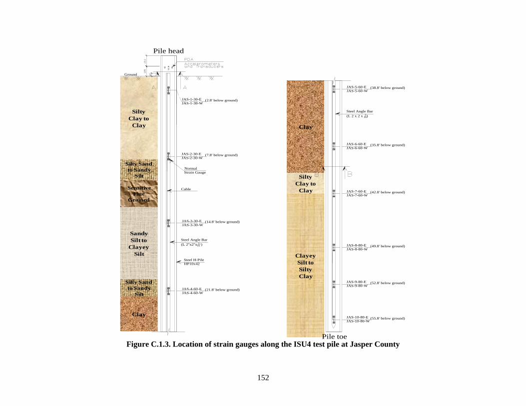
152
Figure C.1.3. Location of strain gauges along the ISU4 test pile at Jasper County
Sandy
Silt to
Clayey
Silt Clayey
Silt to
Silty
Clay
Clay
Silty
Clay to
Clay
Silty Sand
to Sandy
Silt
Sensitive
Fine
Grained
Silty Sand
to Sandy
Silt
Clay
Silty
Clay to
Clay
(21.8' below ground)
JAS-8-80-EJAS-8-80-W
(49.8' below ground)
JAS-10-80-EJAS-10-80-W
(55.8' below ground)
Pile toe
JAS-5-60-EJAS-5-60-W
JAS-6-60-E
JAS-6-60-W
JAS-7-60-EJAS-7-60-W
JAS-9-80-EJAS-9-80-W
Ground
JAS-3-30-EJAS-3-30-W
JAS-2-30-EJAS-2-30-W
Steel H-Pile
HP10x42
JAS-1-30-EJAS-1-30-W
Steel Angle Bar
(L 2 x 2 x 316)
(2.8' below ground)
Normal
Strain Gauge
(7.8' below ground)
(14.8' below ground)
(52.8' below ground)
(42.8' below ground)
(35.8' below ground)
(38.8' below ground)
JAS-4-60-EJAS-4-60-W
Steel Angle Bar
(L 2''x2''x 316
'')
Cable
Pile head

153
Figure C.1.4. Location of strain gauges along the ISU6 test pile at Buchanan County
Clay
Silty Sand
to Sandy
Silt
Sand to
Silty Sand
Clay
Clay
Silty
Clay to
Clay
Clayey
Silt to
Silty
Clay
Steel Angle Bar
(L 2''x2''x 316
'')
Cable
Pile head
Pile toe
BUC-6-60-NBUC-6-60-S
BUC-7-60-NBUC-7-60-S
BUC-8-60-NBUC-8-60-S
BUC-10-80-NBUC-10-80-S
Ground
BUC-3-30-NBUC-3-30-S
BUC-2-30-NBUC-2-30-S
Steel H-PileHP10x42
BUC-1-30-NBUC-1-30-S
Steel Angle Bar
(L 2 x 2 x 316)
(3.2' below ground)
Normal
Strain Gauge
(5.2' below ground)
(10.5' below ground)
(52' below ground)
(41' below ground)
(32' below ground)
(30' below ground)
BUC-5-60-NBUC-5-60-S
(20.2' below ground)
BUC-9-80-NBUC-9-80-S
(48' below ground)
BUC-11-80-NBUC-11-80-S
(56' below ground)
BUC-4-30-NBUC-4-30-S
(12.7' below ground)
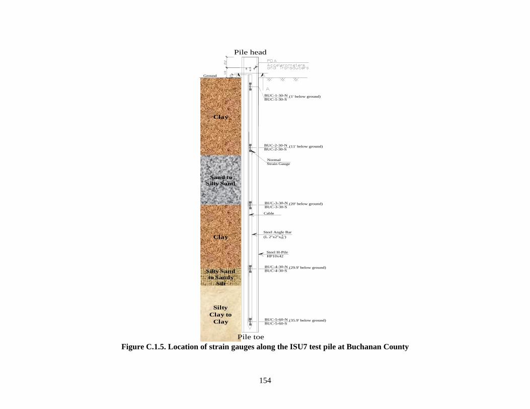
154
Figure C.1.5. Location of strain gauges along the ISU7 test pile at Buchanan County
Clay
Sand to
Silty Sand
Clay
Silty Sand
to Sandy
Silt
Silty
Clay to
Clay
Steel Angle Bar
(L 2''x2''x 316
'')
Cable
Pile head
Ground
BUC-3-30-NBUC-3-30-S
BUC-2-30-NBUC-2-30-S
Steel H-PileHP10x42
BUC-1-30-NBUC-1-30-S
(1' below ground)
Normal
Strain Gauge
(11' below ground)
(20' below ground)
BUC-5-60-NBUC-5-60-S
(35.9' below ground)
BUC-4-30-NBUC-4-30-S
(29.9' below ground)
Pile toe
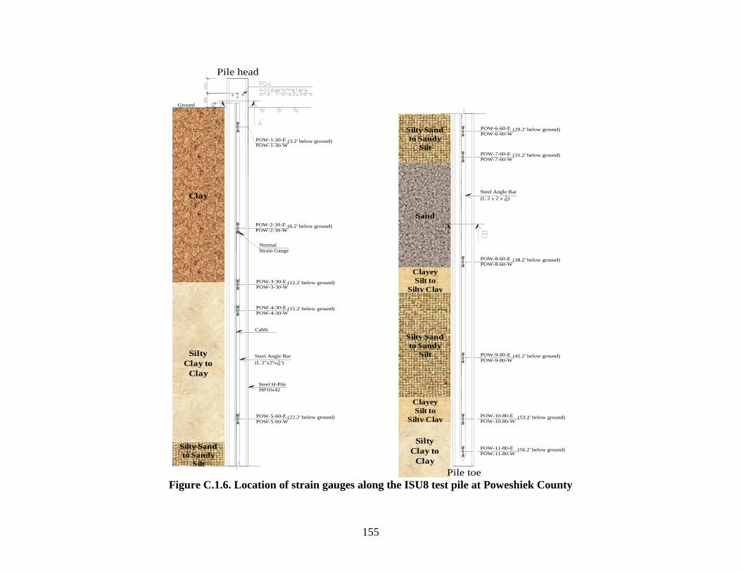
155
Figure C.1.6. Location of strain gauges along the ISU8 test pile at Poweshiek County
Clay
Silty
Clay to
Clay
Silty Sand
to Sandy
Silt
Silty Sand
to Sandy
Silt
Sand
Clayey
Silt to
Silty Clay
Silty Sand
to Sandy
Silt
Clayey
Silt to
Silty Clay
Silty
Clay to
Clay
(6.2' below ground)
(12.2' below ground)
(53.2' below ground)
(38.2' below ground)
(31.2' below ground)
(29.2' below ground)
POW-5-60-EPOW-5-60-W
(22.2' below ground)
POW-9-80-EPOW-9-80-W
(45.2' below ground)
POW-11-80-EPOW-11-80-W
(56.2' below ground)
POW-4-30-E
POW-4-30-W(15.2' below ground)
Steel Angle Bar
(L 2''x2''x 316
'')
Cable
Pile head
Pile toe
POW-6-60-E
POW-6-60-W
POW-7-60-EPOW-7-60-W
POW-8-60-EPOW-8-60-W
POW-10-80-EPOW-10-80-W
Ground
POW-3-30-EPOW-3-30-W
POW-2-30-EPOW-2-30-W
Steel H-PileHP10x42
POW-1-30-EPOW-1-30-W
Steel Angle Bar
(L 2 x 2 x 316)
(3.2' below ground)
Normal
Strain Gauge

156
Figure C.1.7. Location of strain gauges along the ISU9 test pile at Des Moines County
Clay
Sandy
Silt to
Clayey
Silt
Sand
Sand
POW-6-60-EPOW-6-60-W
(45' below ground)
Steel Angle Bar
(L 2''x2''x 316
'')
Cable
Pile head
Pile toe
POW-4-60-EPOW-4-60-W
POW-5-60-EPOW-5-60-W
Ground
POW-2-30-EPOW-2-30-W
Steel H-PileHP10x42
POW-1-30-EPOW-1-30-W
Steel Angle Bar
(L 2 x 2 x 316)
(5' below ground)
Normal
Strain Gauge
(10' below ground)
(40' below ground)
(30' below ground)
POW-7-80-EPOW-7-80-W
(49' below ground)
POW-3-30-EPOW-3-30-W
(20' below ground)
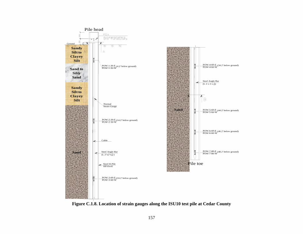
157
Figure C.1.8. Location of strain gauges along the ISU10 test pile at Cedar County
Sandy
Silt to
Clayey
Silt
Sand to
Silty
Sand
Sandy
Silt to
Clayey
Silt
Sand
Sand
POW-6-60-EPOW-6-60-W
(46.2' below ground)
(14.2' below ground)
(44.2' below ground)
(34.2' below ground)
POW-3-60-EPOW-3-60-W
(24.2' below ground)
POW-7-80-EPOW-7-80-W
(48.2' below ground)Steel Angle Bar
(L 2''x2''x 316
'')
Cable
Pile head
Pile toe
POW-4-60-EPOW-4-60-W
POW-5-60-EPOW-5-60-W
Ground
POW-2-30-EPOW-2-30-W
Steel H-PileHP10x42
POW-1-30-EPOW-1-30-W
Steel Angle Bar
(L 2 x 2 x 316)
(4.2' below ground)
Normal
Strain Gauge
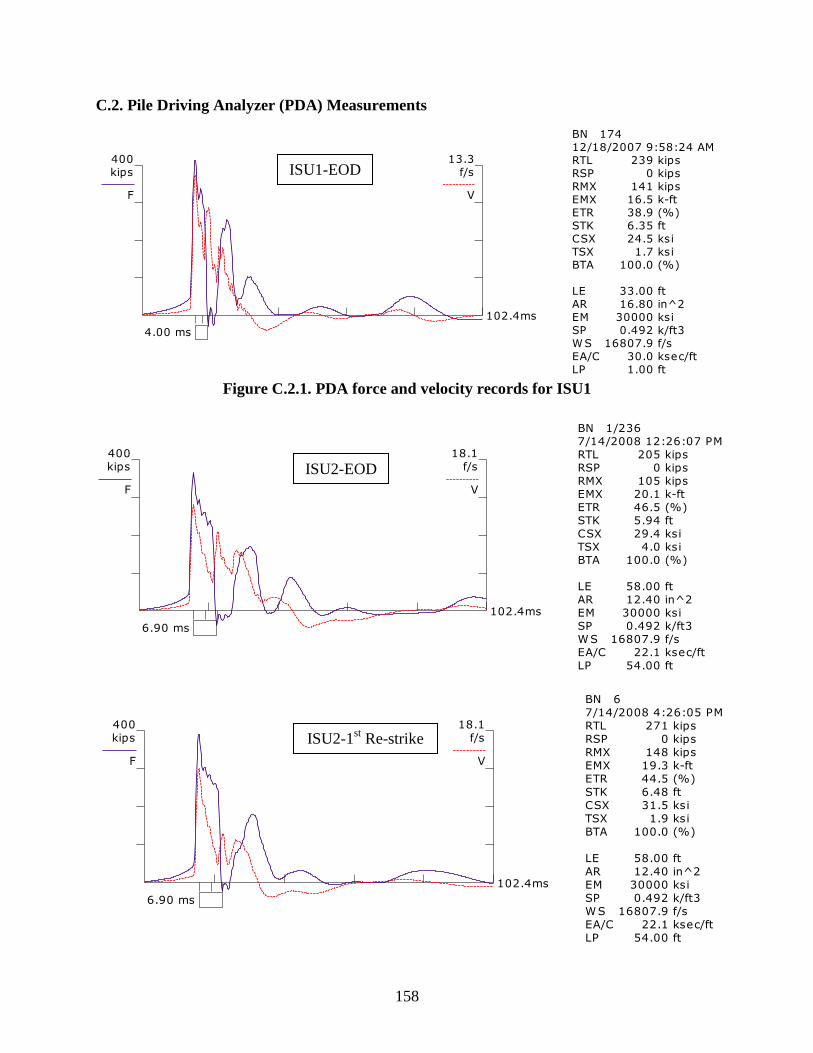
158
C.2. Pile Driving Analyzer (PDA) Measurements
Figure C.2.1. PDA force and velocity records for ISU1
IOWA DOTMahaskaPDA OP: Frame
PILE DRIVING ANALYZER ®Version 2001.086
steel H test
10x57
BN 17412/18/2007 9:58:24 AMRTL kips239RSP kips0
RMX kips141EMX k-ft16.5ETR (%)38.9STK ft6.35
CSX ksi24.5TSX ksi1.7BTA (%)100.0
LE ft33.00
AR in^216.80EM ksi30000SP k/ft30.492WS f/s16807.9EA/C ksec/ft30.0
LP ft1.00
F12 A12
F1: [2355] 86 (1)F2: [2356] 89 (1)A1: [42695] 1060 g's/v (1)A2: [41315] 1105 g's/v (1)
4.00 ms
102.4ms
400
kips
F
13.3
f/s
V
IOWA DOTISU2PDA OP: FRAME
PILE DRIVING ANALYZER ®Version 2001.086
MILLS TEST DRIVING
HP10X42 STEEL PILE 60FT LONG
BN 1/2367/14/2008 12:26:07 PMRTL kips205RSP kips0
RMX kips105EMX k-ft20.1ETR (%)46.5STK ft5.94
CSX ksi29.4TSX ksi4.0BTA (%)100.0
LE ft58.00
AR in^212.40EM ksi30000SP k/ft30.492WS f/s16807.9EA/C ksec/ft22.1
LP ft54.00
F12 A12
F1: [2355] 87 (1)F2: [2356] 89 (1)A1: [41309] 1095 g's/v (1)A2: [41315] 1115 g's/v (1)
6.90 ms
102.4ms
400
kips
F
18.1
f/s
V
IOWA DOTISU2PDA OP: FRAME
PILE DRIVING ANALYZER ®Version 2001.086
MILLS TEST (RESTRIKE 1)
HP10X42 STEEL PILE 60FT LONG
BN 67/14/2008 4:26:05 PMRTL kips271RSP kips0
RMX kips148EMX k-ft19.3ETR (%)44.5STK ft6.48
CSX ksi31.5TSX ksi1.9BTA (%)100.0
LE ft58.00
AR in^212.40EM ksi30000SP k/ft30.492WS f/s16807.9EA/C ksec/ft22.1
LP ft54.00
F12 A12
F1: [2355] 87 (1)F2: [2356] 89 (1)A1: [41309] 1095 g's/v (1)A2: [41315] 1115 g's/v (1)
6.90 ms
102.4ms
400
kips
F
18.1
f/s
V
ISU1-EOD
ISU2-EOD
ISU2-1st Re-strike

159
Figure C.2.2. PDA force and velocity records for ISU2
IOWA DOTISU2PDA OP: FRAME
PILE DRIVING ANALYZER ®Version 2001.086
MILLS TEST (RESTRIKE 2)
HP10X42 STEEL PILE 60FT LONG
BN 5/47/15/2008 10:27:43 AMRTL kips328RSP kips48
RMX kips162EMX k-ft21.0ETR (%)48.5STK ft7.29
CSX ksi32.8TSX ksi0.4BTA (%)100.0
LE ft58.00
AR in^212.40EM ksi30000SP k/ft30.492WS f/s16807.9EA/C ksec/ft22.1
LP ft55.33
F12 A12
F1: [2355] 87 (1)F2: [2356] 89 (1)A1: [41309] 1095 g's/v (1)A2: [41315] 1115 g's/v (1)
6.90 ms
102.4ms
400
kips
F
18.1
f/s
V
IOWA DOTISU2PDA OP: FRAME
PILE DRIVING ANALYZER ®Version 2001.086
MILLS TEST (RESTRIKE 3)
HP10X42 STEEL PILE 60FT LONG
BN 6/57/17/2008 11:45:26 AMRTL kips359RSP kips96
RMX kips146EMX k-ft19.4ETR (%)45.0STK ft7.15
CSX ksi33.6TSX ksi0.5BTA (%)100.0
LE ft58.00
AR in^212.40EM ksi30000SP k/ft30.492WS f/s16807.9EA/C ksec/ft22.1
LP ft55.83
F12 A12
F1: [2355] 87 (1)F2: [2356] 89 (1)A1: [41309] 1095 g's/v (1)A2: [41315] 1115 g's/v (1)
6.90 ms
102.4ms
400
kips
F
18.1
f/s
V
IOWA DOTISU3PDA OP: kam
PILE DRIVING ANALYZER ®Version 2001.086
isu3polkEOD
HP10X42 STEEL PILE LONG
BN 2731/7/2009 10:21:18 AMRTL kips237RSP kips0
RMX kips120EMX k-ft19.8ETR (%)46.6STK ft5.76
CSX ksi25.9TSX ksi1.1BTA (%)100.0
LE ft57.50
AR in^212.40EM ksi30000SP k/ft30.492WS f/s16807.9EA/C ksec/ft22.1
F12 A12
F1: [2355] 87 (1)F2: [2356] 89 (1)A1: [41309] 1095 g's/v (1)A2: [41315] 1115 g's/v (1)
6.84 ms
102.4ms
400
kips
F
18.1
f/s
V
ISU2-2nd
Re-strike
ISU2-3rd
Re-strike
ISU3-EOD
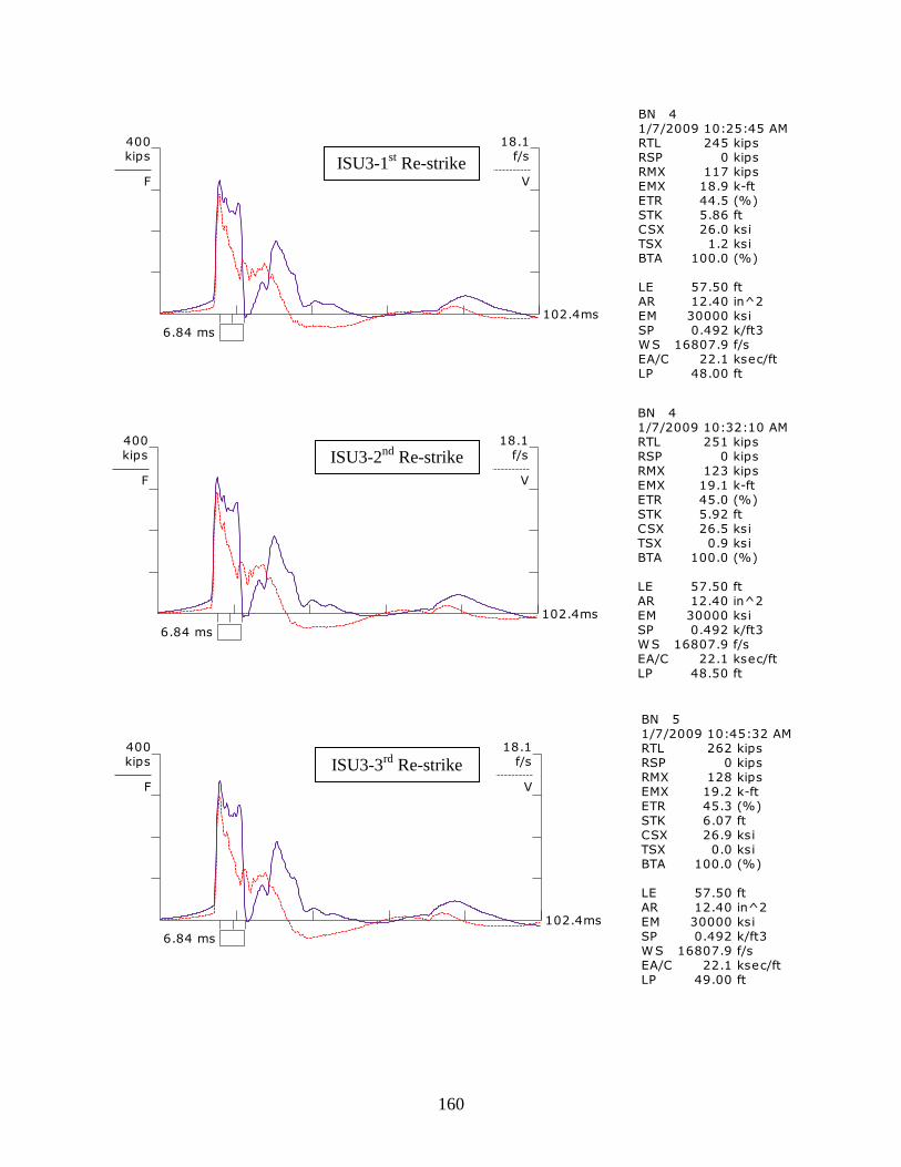
160
IOWA DOTISU3PDA OP: kam
PILE DRIVING ANALYZER ®Version 2001.086
isu3polkrestrike1
HP10X42 STEEL PILE LONG
BN 41/7/2009 10:25:45 AMRTL kips245RSP kips0
RMX kips117EMX k-ft18.9ETR (%)44.5STK ft5.86
CSX ksi26.0TSX ksi1.2BTA (%)100.0
LE ft57.50
AR in^212.40EM ksi30000SP k/ft30.492WS f/s16807.9EA/C ksec/ft22.1
LP ft48.00
F12 A12
F1: [2355] 87 (1)F2: [2356] 89 (1)A1: [41309] 1095 g's/v (1)A2: [41315] 1115 g's/v (1)
6.84 ms
102.4ms
400
kips
F
18.1
f/s
V
IOWA DOTISU3PDA OP: kam
PILE DRIVING ANALYZER ®Version 2001.086
isu3polkrestrike2
HP10X42 STEEL PILE LONG
BN 41/7/2009 10:32:10 AMRTL kips251RSP kips0
RMX kips123EMX k-ft19.1ETR (%)45.0STK ft5.92
CSX ksi26.5TSX ksi0.9BTA (%)100.0
LE ft57.50
AR in^212.40EM ksi30000SP k/ft30.492WS f/s16807.9EA/C ksec/ft22.1
LP ft48.50
F12 A12
F1: [2355] 87 (1)F2: [2356] 89 (1)A1: [41309] 1095 g's/v (1)A2: [41315] 1115 g's/v (1)
6.84 ms
102.4ms
400
kips
F
18.1
f/s
V
IOWA DOTISU3PDA OP: kam
PILE DRIVING ANALYZER ®Version 2001.086
isu3polkrestrike3
HP10X42 STEEL PILE LONG
BN 51/7/2009 10:45:32 AMRTL kips262RSP kips0
RMX kips128EMX k-ft19.2ETR (%)45.3STK ft6.07
CSX ksi26.9TSX ksi0.0BTA (%)100.0
LE ft57.50
AR in^212.40EM ksi30000SP k/ft30.492WS f/s16807.9EA/C ksec/ft22.1
LP ft49.00
F12 A12
F1: [2355] 87 (1)F2: [2356] 89 (1)A1: [41309] 1095 g's/v (1)A2: [41315] 1115 g's/v (1)
6.84 ms
102.4ms
400
kips
F
18.1
f/s
V
ISU3-1st Re-strike
ISU3-2nd
Re-strike
ISU3-3rd
Re-strike
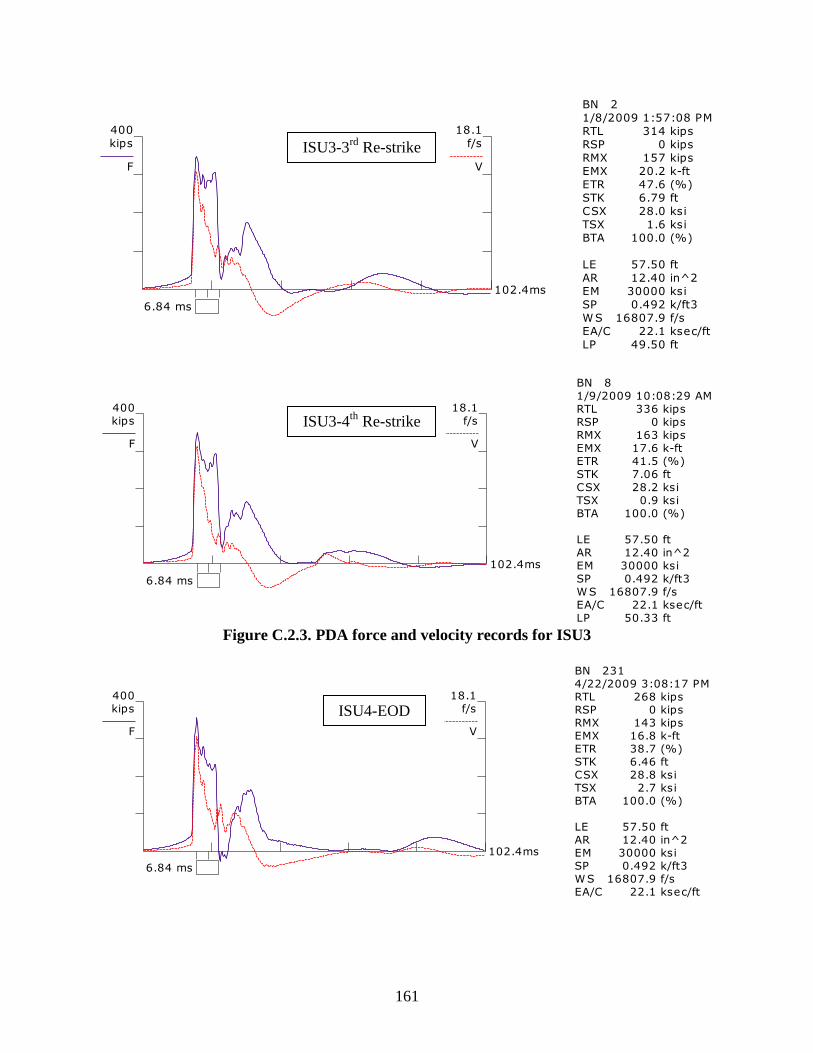
161
Figure C.2.3. PDA force and velocity records for ISU3
IOWA DOTISU3PDA OP: kam
PILE DRIVING ANALYZER ®Version 2001.086
isu3polkrestrike4
HP10X42 STEEL PILE LONG
BN 21/8/2009 1:57:08 PMRTL kips314RSP kips0
RMX kips157EMX k-ft20.2ETR (%)47.6STK ft6.79
CSX ksi28.0TSX ksi1.6BTA (%)100.0
LE ft57.50
AR in^212.40EM ksi30000SP k/ft30.492WS f/s16807.9EA/C ksec/ft22.1
LP ft49.50
F12 A12
F1: [2355] 87 (1)F2: [2356] 89 (1)A1: [41309] 1095 g's/v (1)A2: [41315] 1115 g's/v (1)
6.84 ms
102.4ms
400
kips
F
18.1
f/s
V
IOWA DOTISU3PDA OP: kam
PILE DRIVING ANALYZER ®Version 2001.086
isu3polkrestrike5
HP10X42 STEEL PILE LONG
BN 81/9/2009 10:08:29 AMRTL kips336RSP kips0
RMX kips163EMX k-ft17.6ETR (%)41.5STK ft7.06
CSX ksi28.2TSX ksi0.9BTA (%)100.0
LE ft57.50
AR in^212.40EM ksi30000SP k/ft30.492WS f/s16807.9EA/C ksec/ft22.1
LP ft50.33
F12 A12
F1: [2355] 87 (1)F2: [2356] 89 (1)A1: [41309] 1095 g's/v (1)A2: [41315] 1115 g's/v (1)
6.84 ms
102.4ms
400
kips
F
18.1
f/s
V
IOWA DOTISU4PDA OP: kam
PILE DRIVING ANALYZER ®Version 2001.086
isu4driving
HP10X42 STEEL PILE LONG
BN 2314/22/2009 3:08:17 PMRTL kips268RSP kips0
RMX kips143EMX k-ft16.8ETR (%)38.7STK ft6.46
CSX ksi28.8TSX ksi2.7BTA (%)100.0
LE ft57.50
AR in^212.40EM ksi30000SP k/ft30.492WS f/s16807.9EA/C ksec/ft22.1
F12 A12
F1: [2355] 87 (1)F2: [2356] 89 (1)A1: [41309] 1095 g's/v (1)A2: [41315] 1115 g's/v (1)
6.84 ms
102.4ms
400
kips
F
18.1
f/s
V
ISU3-3rd
Re-strike
ISU3-4th
Re-strike
ISU4-EOD
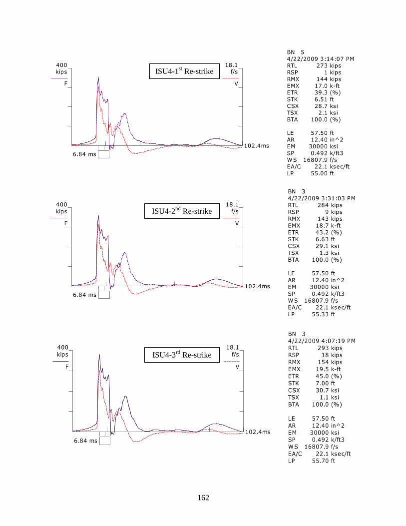
162
IOWA DOTISU4PDA OP: kam
PILE DRIVING ANALYZER ®Version 2001.086
isu41st bor
HP10X42 STEEL PILE LONG
BN 54/22/2009 3:14:07 PMRTL kips273RSP kips1
RMX kips144EMX k-ft17.0ETR (%)39.3STK ft6.51
CSX ksi28.7TSX ksi2.1BTA (%)100.0
LE ft57.50
AR in^212.40EM ksi30000SP k/ft30.492WS f/s16807.9EA/C ksec/ft22.1
LP ft55.00
F12 A12
F1: [2355] 87 (1)F2: [2356] 89 (1)A1: [41309] 1095 g's/v (1)A2: [41315] 1115 g's/v (1)
6.84 ms
102.4ms
400
kips
F
18.1
f/s
V
IOWA DOTISU4PDA OP: kam
PILE DRIVING ANALYZER ®Version 2001.086
isu4 2nd bor
HP10X42 STEEL PILE LONG
BN 34/22/2009 3:31:03 PMRTL kips284RSP kips9
RMX kips143EMX k-ft18.7ETR (%)43.2STK ft6.63
CSX ksi29.1TSX ksi1.3BTA (%)100.0
LE ft57.50
AR in^212.40EM ksi30000SP k/ft30.492WS f/s16807.9EA/C ksec/ft22.1
LP ft55.33
F12 A12
F1: [2355] 87 (1)F2: [2356] 89 (1)A1: [41309] 1095 g's/v (1)A2: [41315] 1115 g's/v (1)
6.84 ms
102.4ms
400
kips
F
18.1
f/s
V
IOWA DOTISU4PDA OP: kam
PILE DRIVING ANALYZER ®Version 2001.086
isu4 3rd bor
HP10X42 STEEL PILE LONG
BN 34/22/2009 4:07:19 PMRTL kips293RSP kips18
RMX kips154EMX k-ft19.5ETR (%)45.0STK ft7.00
CSX ksi30.7TSX ksi1.1BTA (%)100.0
LE ft57.50
AR in^212.40EM ksi30000SP k/ft30.492WS f/s16807.9EA/C ksec/ft22.1
LP ft55.70
F12 A12
F1: [2355] 87 (1)F2: [2356] 89 (1)A1: [41309] 1095 g's/v (1)A2: [41315] 1115 g's/v (1)
6.84 ms
102.4ms
400
kips
F
18.1
f/s
V
ISU4-1st Re-strike
ISU4-2nd
Re-strike
ISU4-3rd
Re-strike
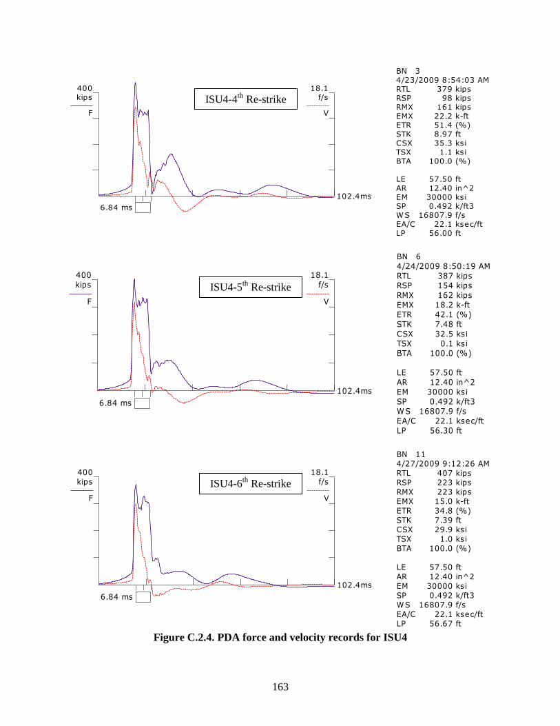
163
Figure C.2.4. PDA force and velocity records for ISU4
IOWA DOTISU4PDA OP: kam
PILE DRIVING ANALYZER ®Version 2001.086
isu4 4th bor
HP10X42 STEEL PILE LONG
BN 34/23/2009 8:54:03 AMRTL kips379RSP kips98
RMX kips161EMX k-ft22.2ETR (%)51.4STK ft8.97
CSX ksi35.3TSX ksi1.1BTA (%)100.0
LE ft57.50
AR in^212.40EM ksi30000SP k/ft30.492WS f/s16807.9EA/C ksec/ft22.1
LP ft56.00
F12 A12
F1: [2355] 87 (1)F2: [2356] 89 (1)A1: [41309] 1095 g's/v (1)A2: [41315] 1115 g's/v (1)
6.84 ms
102.4ms
400
kips
F
18.1
f/s
V
IOWA DOTISU4PDA OP: kam
PILE DRIVING ANALYZER ®Version 2001.086
isu4 5th bor
HP10X42 STEEL PILE LONG
BN 64/24/2009 8:50:19 AMRTL kips387RSP kips154
RMX kips162EMX k-ft18.2ETR (%)42.1STK ft7.48
CSX ksi32.5TSX ksi0.1BTA (%)100.0
LE ft57.50
AR in^212.40EM ksi30000SP k/ft30.492WS f/s16807.9EA/C ksec/ft22.1
LP ft56.30
F12 A12
F1: [2355] 87 (1)F2: [2356] 89 (1)A1: [41309] 1095 g's/v (1)A2: [41315] 1115 g's/v (1)
6.84 ms
102.4ms
400
kips
F
18.1
f/s
V
IOWA DOTISU4PDA OP: kam
PILE DRIVING ANALYZER ®Version 2001.086
isu4 6th bor
HP10X42 STEEL PILE LONG
BN 114/27/2009 9:12:26 AMRTL kips407RSP kips223
RMX kips223EMX k-ft15.0ETR (%)34.8STK ft7.39
CSX ksi29.9TSX ksi1.0BTA (%)100.0
LE ft57.50
AR in^212.40EM ksi30000SP k/ft30.492WS f/s16807.9EA/C ksec/ft22.1
LP ft56.67
F12 A12
F1: [2355] 87 (1)F2: [2356] 89 (1)A1: [41309] 1095 g's/v (1)A2: [41315] 1115 g's/v (1)
6.84 ms
102.4ms
400
kips
F
18.1
f/s
V
ISU4-4th
Re-strike
ISU4-5th
Re-strike
ISU4-6th
Re-strike
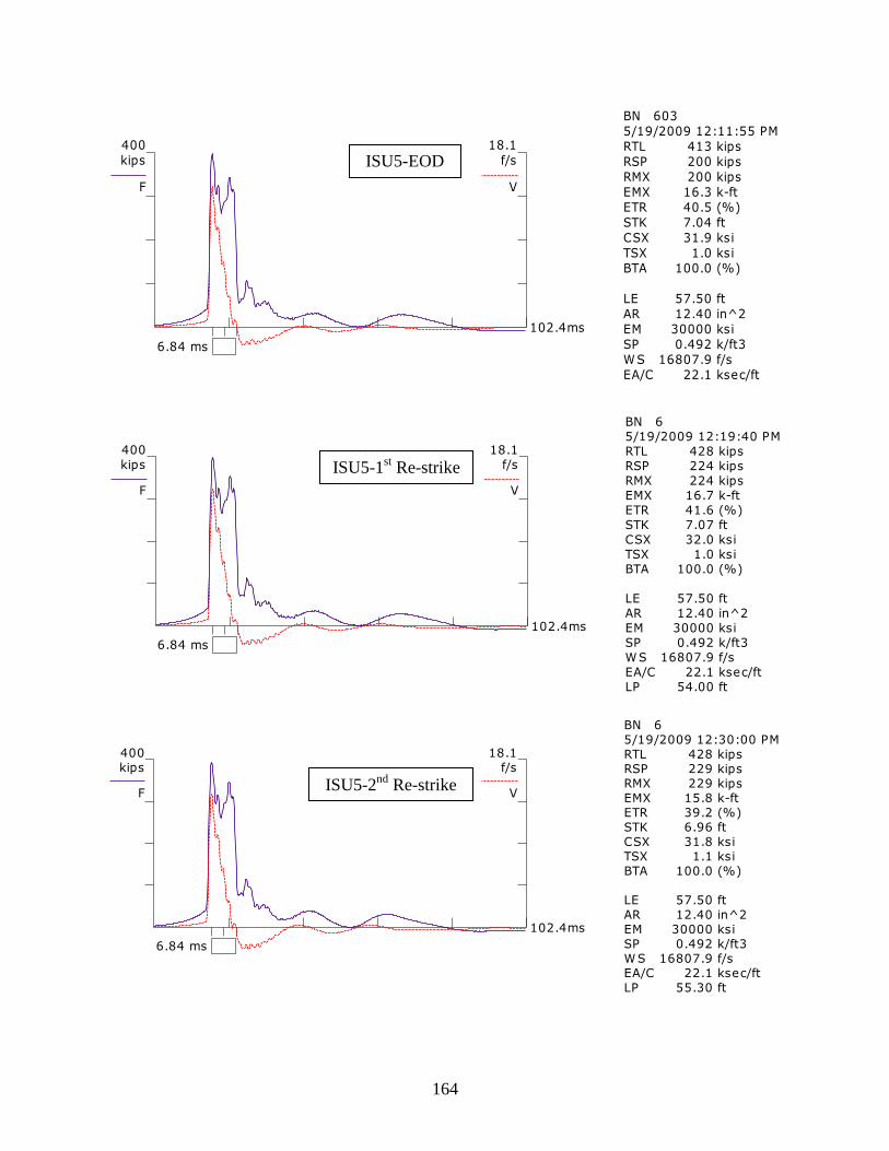
164
IOWA DOTISU5PDA OP: kam
PILE DRIVING ANALYZER ®Version 2001.086
isu5 driving
HP10X42 STEEL PILE LONG
BN 6035/19/2009 12:11:55 PMRTL kips413RSP kips200
RMX kips200EMX k-ft16.3ETR (%)40.5STK ft7.04
CSX ksi31.9TSX ksi1.0BTA (%)100.0
LE ft57.50
AR in^212.40EM ksi30000SP k/ft30.492WS f/s16807.9EA/C ksec/ft22.1
F12 A12
F1: [2355] 87 (1)F2: [2356] 89 (1)A1: [41309] 1095 g's/v (1)A2: [41315] 1115 g's/v (1)
6.84 ms
102.4ms
400
kips
F
18.1
f/s
V
IOWA DOTISU5PDA OP: kam
PILE DRIVING ANALYZER ®Version 2001.086
isu5 1st restrike
HP10X42 STEEL PILE LONG
BN 65/19/2009 12:19:40 PMRTL kips428RSP kips224
RMX kips224EMX k-ft16.7ETR (%)41.6STK ft7.07
CSX ksi32.0TSX ksi1.0BTA (%)100.0
LE ft57.50
AR in^212.40EM ksi30000SP k/ft30.492WS f/s16807.9EA/C ksec/ft22.1
LP ft54.00
F12 A12
F1: [2355] 87 (1)F2: [2356] 89 (1)A1: [41309] 1095 g's/v (1)A2: [41315] 1115 g's/v (1)
6.84 ms
102.4ms
400
kips
F
18.1
f/s
V
IOWA DOTISU5PDA OP: kam
PILE DRIVING ANALYZER ®Version 2001.086
isu5 2nd restrike
HP10X42 STEEL PILE LONG
BN 65/19/2009 12:30:00 PMRTL kips428RSP kips229
RMX kips229EMX k-ft15.8ETR (%)39.2STK ft6.96
CSX ksi31.8TSX ksi1.1BTA (%)100.0
LE ft57.50
AR in^212.40EM ksi30000SP k/ft30.492WS f/s16807.9EA/C ksec/ft22.1
LP ft55.30
F12 A12
F1: [2355] 87 (1)F2: [2356] 89 (1)A1: [41309] 1095 g's/v (1)A2: [41315] 1115 g's/v (1)
6.84 ms
102.4ms
400
kips
F
18.1
f/s
V
ISU5-EOD
ISU5-1st Re-strike
ISU5-2nd
Re-strike
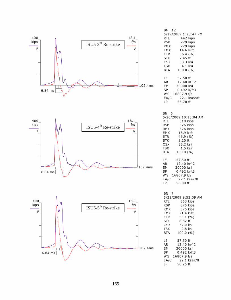
165
IOWA DOTISU5PDA OP: kam
PILE DRIVING ANALYZER ®Version 2001.086
isu5 3rd restrike
HP10X42 STEEL PILE LONG
BN 125/19/2009 1:20:47 PMRTL kips442RSP kips229
RMX kips229EMX k-ft14.6ETR (%)36.4STK ft7.45
CSX ksi33.3TSX ksi4.1BTA (%)100.0
LE ft57.50
AR in^212.40EM ksi30000SP k/ft30.492WS f/s16807.9EA/C ksec/ft22.1
LP ft55.70
F12 A12
F1: [2355] 87 (1)F2: [2356] 89 (1)A1: [41309] 1095 g's/v (1)A2: [41315] 1115 g's/v (1)
6.84 ms
102.4ms
400
kips
F
18.1
f/s
V
IOWA DOTISU5PDA OP: kam
PILE DRIVING ANALYZER ®Version 2001.086
isu5 4th restrike
HP10X42 STEEL PILE LONG
BN 65/20/2009 10:13:04 AMRTL kips518RSP kips326
RMX kips326EMX k-ft18.9ETR (%)46.9STK ft8.20
CSX ksi35.2TSX ksi1.5BTA (%)100.0
LE ft57.50
AR in^212.40EM ksi30000SP k/ft30.492WS f/s16807.9EA/C ksec/ft22.1
LP ft56.00
F12 A12
F1: [2355] 87 (1)F2: [2356] 89 (1)A1: [41309] 1095 g's/v (1)A2: [41315] 1115 g's/v (1)
6.84 ms
102.4ms
400
kips
F
18.1
f/s
V
IOWA DOTISU5PDA OP: kam
PILE DRIVING ANALYZER ®Version 2001.086
isu5 5th restrike
HP10X42 STEEL PILE LONG
BN 75/22/2009 9:52:09 AMRTL kips563RSP kips375
RMX kips375EMX k-ft21.4ETR (%)53.1STK ft8.82
CSX ksi37.0TSX ksi2.8BTA (%)100.0
LE ft57.50
AR in^212.40EM ksi30000SP k/ft30.492WS f/s16807.9EA/C ksec/ft22.1
LP ft56.25
F12 A12
F1: [2355] 87 (1)F2: [2356] 89 (1)A1: [41309] 1095 g's/v (1)A2: [41315] 1115 g's/v (1)
6.84 ms
102.4ms
400
kips
F
18.1
f/s
V
ISU5-3rd
Re-strike
ISU5-4th
Re-strike
ISU5-5th
Re-strike

166
Figure C.2.5. PDA force and velocity records for ISU5
IOWA DOTISU5PDA OP: kam
PILE DRIVING ANALYZER ®Version 2001.086
isu5 6th restrike
HP10X42 STEEL PILE LONG
BN 195/27/2009 10:09:46 AMRTL kips572RSP kips400
RMX kips400EMX k-ft20.3ETR (%)50.6STK ft8.69
CSX ksi36.4TSX ksi3.3BTA (%)100.0
LE ft57.50
AR in^212.40EM ksi30000SP k/ft30.492WS f/s16807.9EA/C ksec/ft22.1
LP ft56.50
F12 A12
F1: [2355] 87 (1)F2: [2356] 89 (1)A1: [41309] 1095 g's/v (1)A2: [41315] 1115 g's/v (1)
6.84 ms
102.4ms
400
kips
F
18.1
f/s
V
IOWA DOTISU6PDA OP: KAM
PILE DRIVING ANALYZER ®Version 2001.086
ISU6 DRIVING
HP10x42
BN 2686/9/2009 3:26:47 PMRTL kips252RSP kips0
RMX kips146EMX k-ft15.9ETR (%)36.9STK ft6.33
CSX ksi27.9TSX ksi1.3BTA (%)100.0
LE ft57.50
AR in^212.40EM ksi30000SP k/ft30.492WS f/s16807.9EA/C ksec/ft22.1
F12 A12
F1: [2355] 87 (1)F2: [2356] 89 (1)A1: [41309] 1095 g's/v (1)A2: [41315] 1115 g's/v (1)
6.84 ms
102.4ms
400
kips
F
18.1
f/s
V
IOWA DOTISU6PDA OP: KAM
PILE DRIVING ANALYZER ®Version 2001.086
ISU6 1ST RESTRIKE
HP10x42
BN 36/9/2009 3:29:07 PMRTL kips267RSP kips0
RMX kips151EMX k-ft17.5ETR (%)40.4STK ft6.85
CSX ksi29.5TSX ksi1.4BTA (%)100.0
LE ft57.50
AR in^212.40EM ksi30000SP k/ft30.492WS f/s16807.9EA/C ksec/ft22.1
LP ft55.00
F12 A12
F1: [2355] 87 (1)F2: [2356] 89 (1)A1: [41309] 1095 g's/v (1)A2: [41315] 1115 g's/v (1)
6.84 ms
102.4ms
400
kips
F
18.1
f/s
V
ISU5-6th
Re-strike
ISU6-EOD
ISU6-1st Re-strike
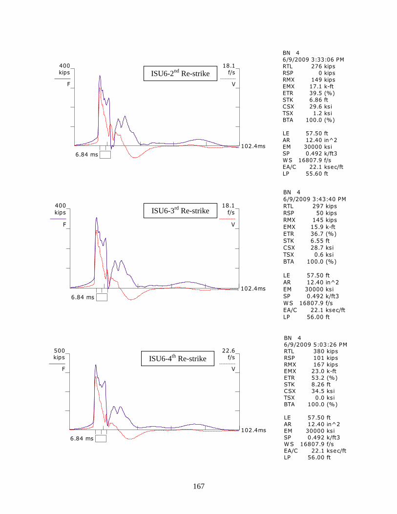
167
IOWA DOTISU6PDA OP: KAM
PILE DRIVING ANALYZER ®Version 2001.086
ISU6 2ND RESTRIKE
HP10x42
BN 46/9/2009 3:33:06 PMRTL kips276RSP kips0
RMX kips149EMX k-ft17.1ETR (%)39.5STK ft6.86
CSX ksi29.6TSX ksi1.2BTA (%)100.0
LE ft57.50
AR in^212.40EM ksi30000SP k/ft30.492WS f/s16807.9EA/C ksec/ft22.1
LP ft55.60
F12 A12
F1: [2355] 87 (1)F2: [2356] 89 (1)A1: [41309] 1095 g's/v (1)A2: [41315] 1115 g's/v (1)
6.84 ms
102.4ms
400
kips
F
18.1
f/s
V
IOWA DOTISU6PDA OP: KAM
PILE DRIVING ANALYZER ®Version 2001.086
ISU6 3RD RESTRIKE
HP10x42
BN 46/9/2009 3:43:40 PMRTL kips297RSP kips50
RMX kips145EMX k-ft15.9ETR (%)36.7STK ft6.55
CSX ksi28.7TSX ksi0.6BTA (%)100.0
LE ft57.50
AR in^212.40EM ksi30000SP k/ft30.492WS f/s16807.9EA/C ksec/ft22.1
LP ft56.00
F12 A12
F1: [2355] 87 (1)F2: [2356] 89 (1)A1: [41309] 1095 g's/v (1)A2: [41315] 1115 g's/v (1)
6.84 ms
102.4ms
400
kips
F
18.1
f/s
V
IOWA DOTISU6PDA OP: KAM
PILE DRIVING ANALYZER ®Version 2001.086
ISU6 4th restrike
HP10x42
BN 46/9/2009 5:03:26 PMRTL kips380RSP kips101
RMX kips167EMX k-ft23.0ETR (%)53.2STK ft8.26
CSX ksi34.5TSX ksi0.0BTA (%)100.0
LE ft57.50
AR in^212.40EM ksi30000SP k/ft30.492WS f/s16807.9EA/C ksec/ft22.1
LP ft56.00
F12 A12
F1: [2355] 87 (1)F2: [2356] 89 (1)A1: [41309] 1095 g's/v (1)A2: [41315] 1115 g's/v (1)
6.84 ms
102.4ms
500
kips
F
22.6
f/s
V
ISU6-2nd
Re-strike
ISU6-3rd
Re-strike
ISU6-4th
Re-strike
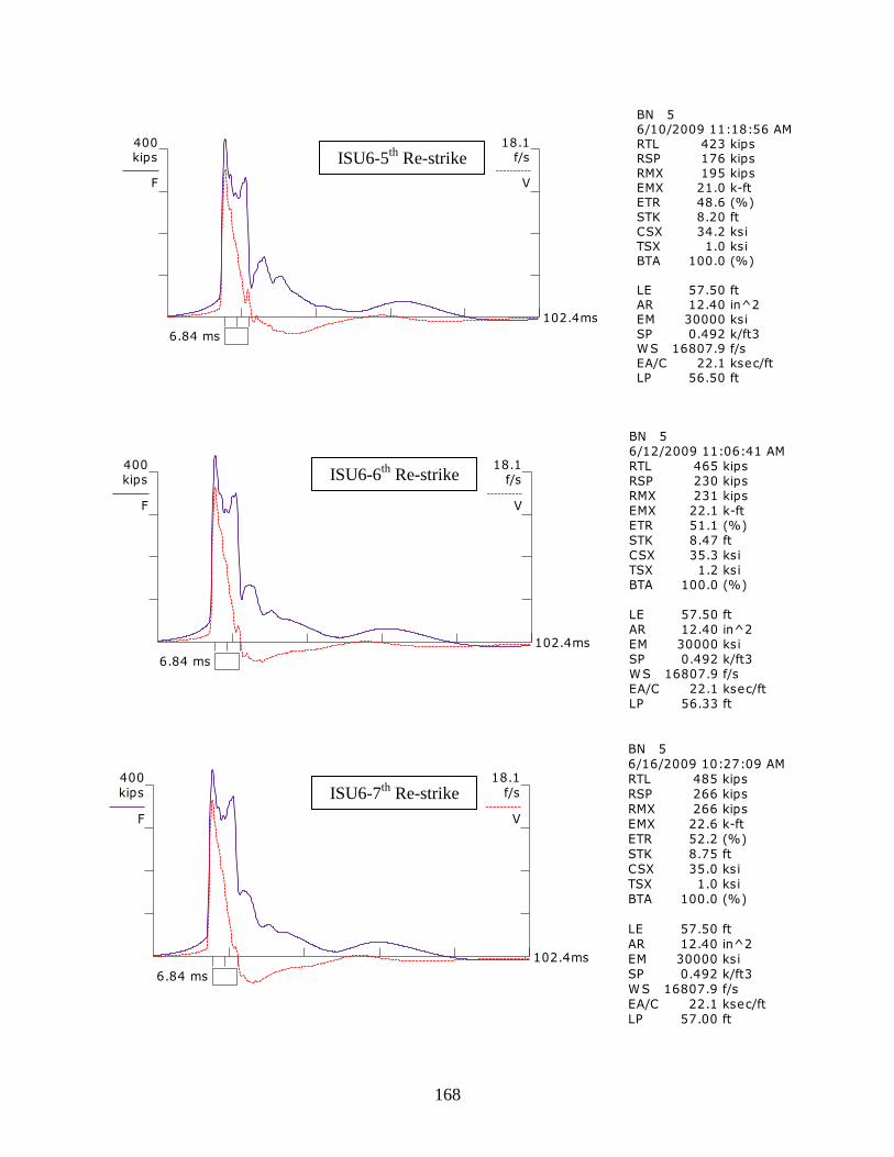
168
IOWA DOTISU6PDA OP: KAM
PILE DRIVING ANALYZER ®Version 2001.086
ISU6 5th restrike
HP10x42
BN 56/10/2009 11:18:56 AMRTL kips423RSP kips176
RMX kips195EMX k-ft21.0ETR (%)48.6STK ft8.20
CSX ksi34.2TSX ksi1.0BTA (%)100.0
LE ft57.50
AR in^212.40EM ksi30000SP k/ft30.492WS f/s16807.9EA/C ksec/ft22.1
LP ft56.50
F12 A12
F1: [2355] 87 (1)F2: [2356] 89 (1)A1: [41309] 1095 g's/v (1)A2: [41315] 1115 g's/v (1)
6.84 ms
102.4ms
400
kips
F
18.1
f/s
V
IOWA DOTISU6PDA OP: KAM
PILE DRIVING ANALYZER ®Version 2001.086
ISU6 6th restrike
HP10x42
BN 56/12/2009 11:06:41 AMRTL kips465RSP kips230
RMX kips231EMX k-ft22.1ETR (%)51.1STK ft8.47
CSX ksi35.3TSX ksi1.2BTA (%)100.0
LE ft57.50
AR in^212.40EM ksi30000SP k/ft30.492WS f/s16807.9EA/C ksec/ft22.1
LP ft56.33
F12 A12
F1: [2355] 87 (1)F2: [2356] 89 (1)A1: [41309] 1095 g's/v (1)A2: [41315] 1115 g's/v (1)
6.84 ms
102.4ms
400
kips
F
18.1
f/s
V
IOWA DOTISU6PDA OP: KAM
PILE DRIVING ANALYZER ®Version 2001.086
ISU6 7th restrike
HP10x42
BN 56/16/2009 10:27:09 AMRTL kips485RSP kips266
RMX kips266EMX k-ft22.6ETR (%)52.2STK ft8.75
CSX ksi35.0TSX ksi1.0BTA (%)100.0
LE ft57.50
AR in^212.40EM ksi30000SP k/ft30.492WS f/s16807.9EA/C ksec/ft22.1
LP ft57.00
F12 A12
F1: [2355] 87 (1)F2: [2356] 89 (1)A1: [41309] 1095 g's/v (1)A2: [41315] 1115 g's/v (1)
6.84 ms
102.4ms
400
kips
F
18.1
f/s
V
ISU6-5th
Re-strike
ISU6-6th
Re-strike
ISU6-7th
Re-strike

169
Figure C.2.6. PDA force and velocity records for ISU6
IOWA DOTISU6PDA OP: KAM
PILE DRIVING ANALYZER ®Version 2001.086
ISU6 8th restrike
HP10x42
BN 46/19/2009 10:50:45 AMRTL kips514RSP kips310
RMX kips310EMX k-ft20.8ETR (%)48.0STK ft8.26
CSX ksi35.6TSX ksi1.2BTA (%)100.0
LE ft57.50
AR in^212.40EM ksi30000SP k/ft30.492WS f/s16807.9EA/C ksec/ft22.1
LP ft57.30
F12 A12
F1: [2355] 87 (1)F2: [2356] 89 (1)A1: [41309] 1095 g's/v (1)A2: [41315] 1115 g's/v (1)
6.84 ms
102.4ms
400
kips
F
18.1
f/s
V
IOWA DOTISU7PDA OP: KAM
PILE DRIVING ANALYZER ®Version 2001.086
ISU7 driving
HP10x42
BN 106/9/2009 4:20:32 PMRTL kips59RSP kips0
RMX kips0EMX k-ft17.7ETR (%)41.0STK ft0.00
CSX ksi20.9TSX ksi5.6BTA (%)100.0
LE ft32.50
AR in^212.40EM ksi30000SP k/ft30.492WS f/s16807.9EA/C ksec/ft22.1
F12 A12
F1: [2355] 87 (1)F2: [2356] 89 (1)A1: [41309] 1095 g's/v (1)A2: [41315] 1115 g's/v (1)
3.87 ms
102.4ms
400
kips
F
18.1
f/s
V
IOWA DOTISU7PDA OP: KAM
PILE DRIVING ANALYZER ®Version 2001.086
ISU7 1st restrike
HP10x42
BN 26/9/2009 4:23:13 PMRTL kips80RSP kips0
RMX kips0EMX k-ft13.0ETR (%)30.0STK ft0.00
CSX ksi22.3TSX ksi5.3BTA (%)100.0
LE ft32.50
AR in^212.40EM ksi30000SP k/ft30.492WS f/s16807.9EA/C ksec/ft22.1
LP ft19.00
F12 A12
F1: [2355] 87 (1)F2: [2356] 89 (1)A1: [41309] 1095 g's/v (1)A2: [41315] 1115 g's/v (1)
3.87 ms
102.4ms
400
kips
F
18.1
f/s
V
ISU6-8th
Re-strike
ISU7-EOD
ISU7-1st Re-strike
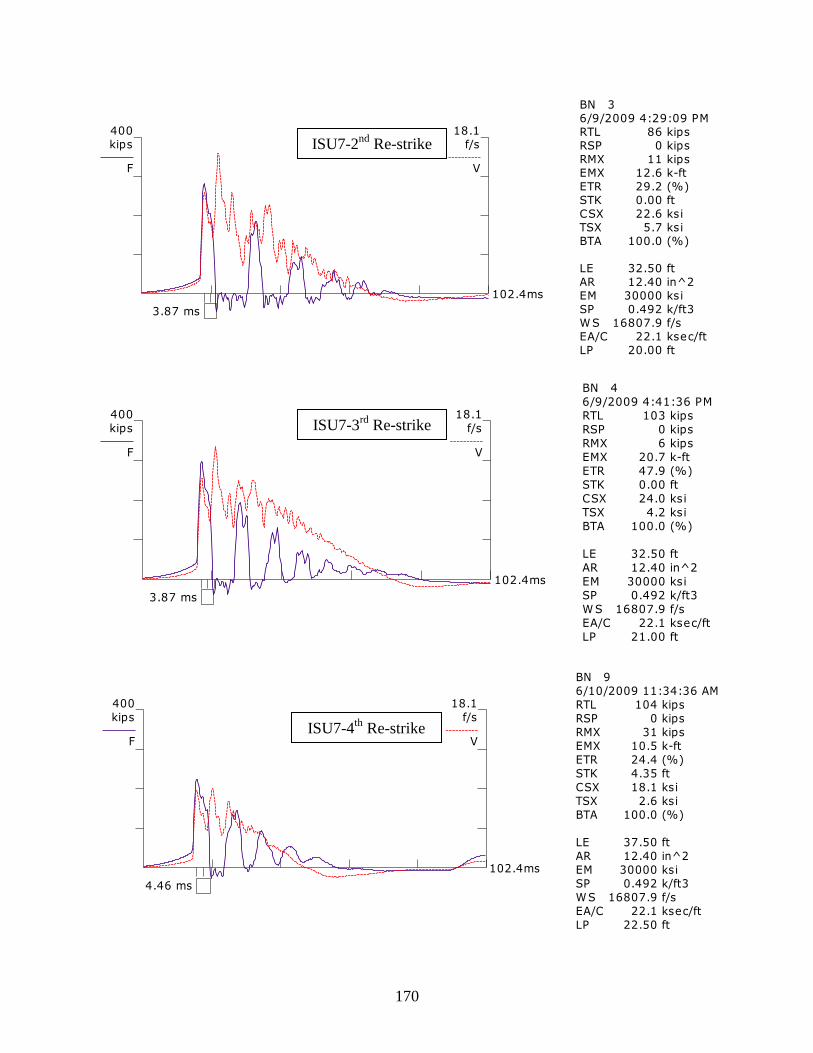
170
IOWA DOTISU7PDA OP: KAM
PILE DRIVING ANALYZER ®Version 2001.086
ISU7 2nd restrike
HP10x42
BN 36/9/2009 4:29:09 PMRTL kips86RSP kips0
RMX kips11EMX k-ft12.6ETR (%)29.2STK ft0.00
CSX ksi22.6TSX ksi5.7BTA (%)100.0
LE ft32.50
AR in^212.40EM ksi30000SP k/ft30.492WS f/s16807.9EA/C ksec/ft22.1
LP ft20.00
F12 A12
F1: [2355] 87 (1)F2: [2356] 89 (1)A1: [41309] 1095 g's/v (1)A2: [41315] 1115 g's/v (1)
3.87 ms
102.4ms
400
kips
F
18.1
f/s
V
IOWA DOTISU7PDA OP: KAM
PILE DRIVING ANALYZER ®Version 2001.086
ISU7 3rd restrike
HP10x42
BN 46/9/2009 4:41:36 PMRTL kips103RSP kips0
RMX kips6EMX k-ft20.7ETR (%)47.9STK ft0.00
CSX ksi24.0TSX ksi4.2BTA (%)100.0
LE ft32.50
AR in^212.40EM ksi30000SP k/ft30.492WS f/s16807.9EA/C ksec/ft22.1
LP ft21.00
F12 A12
F1: [2355] 87 (1)F2: [2356] 89 (1)A1: [41309] 1095 g's/v (1)A2: [41315] 1115 g's/v (1)
3.87 ms
102.4ms
400
kips
F
18.1
f/s
V
IOWA DOTISU7PDA OP: KAM
PILE DRIVING ANALYZER ®Version 2001.086
ISU7 4th restrike
HP10x42
BN 96/10/2009 11:34:36 AMRTL kips104RSP kips0
RMX kips31EMX k-ft10.5ETR (%)24.4STK ft4.35
CSX ksi18.1TSX ksi2.6BTA (%)100.0
LE ft37.50
AR in^212.40EM ksi30000SP k/ft30.492WS f/s16807.9EA/C ksec/ft22.1
LP ft22.50
F12 A12
F1: [2355] 87 (1)F2: [2356] 89 (1)A1: [41309] 1095 g's/v (1)A2: [41315] 1115 g's/v (1)
4.46 ms
102.4ms
400
kips
F
18.1
f/s
V
ISU7-2nd
Re-strike
ISU7-3rd
Re-strike
ISU7-4th
Re-strike
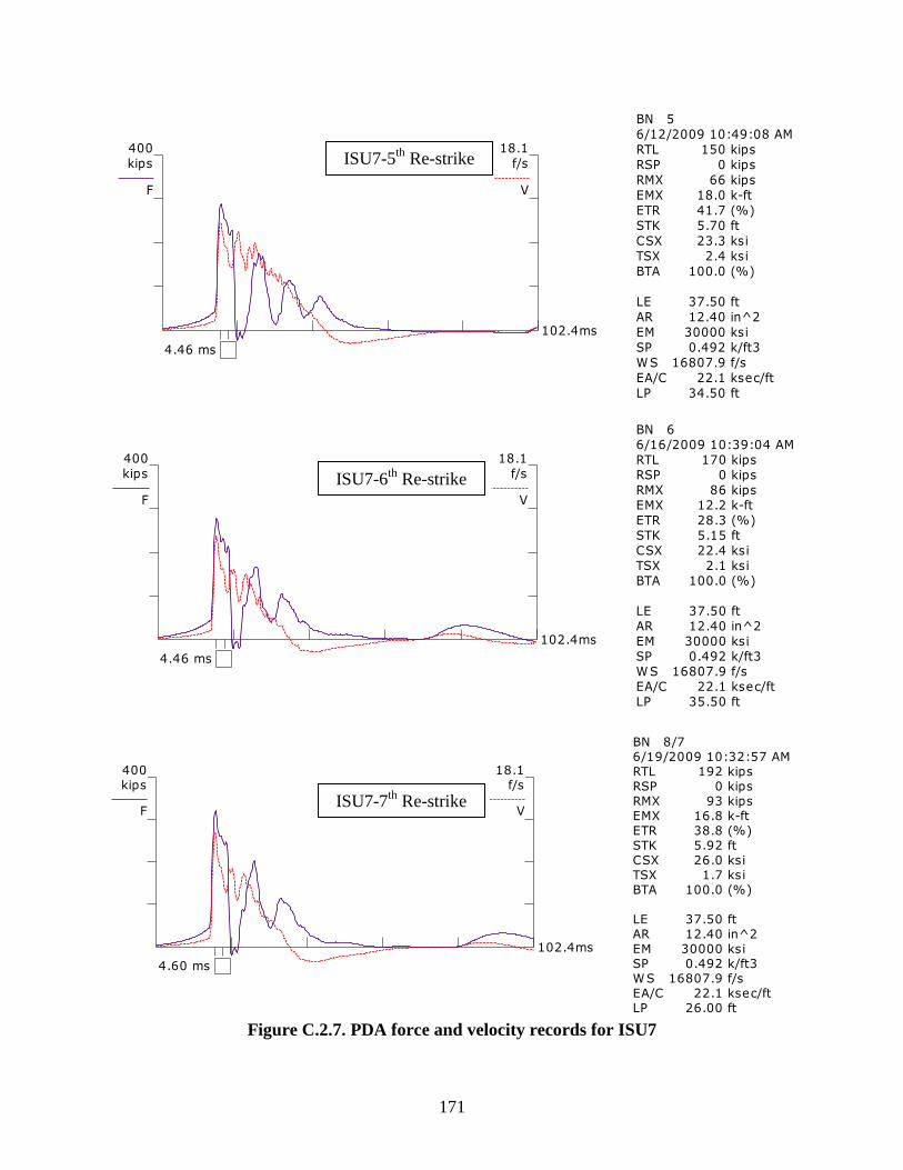
171
Figure C.2.7. PDA force and velocity records for ISU7
IOWA DOTISU7PDA OP: KAM
PILE DRIVING ANALYZER ®Version 2001.086
ISU7 5th restrike
HP10x42
BN 56/12/2009 10:49:08 AMRTL kips150RSP kips0
RMX kips66EMX k-ft18.0ETR (%)41.7STK ft5.70
CSX ksi23.3TSX ksi2.4BTA (%)100.0
LE ft37.50
AR in^212.40EM ksi30000SP k/ft30.492WS f/s16807.9EA/C ksec/ft22.1
LP ft34.50
F12 A12
F1: [2355] 87 (1)F2: [2356] 89 (1)A1: [41309] 1095 g's/v (1)A2: [41315] 1115 g's/v (1)
4.46 ms
102.4ms
400
kips
F
18.1
f/s
V
IOWA DOTISU5PDA OP: KAM
PILE DRIVING ANALYZER ®Version 2001.086
ISU5 6th restrike
HP10x42
BN 66/16/2009 10:39:04 AMRTL kips170RSP kips0
RMX kips86EMX k-ft12.2ETR (%)28.3STK ft5.15
CSX ksi22.4TSX ksi2.1BTA (%)100.0
LE ft37.50
AR in^212.40EM ksi30000SP k/ft30.492WS f/s16807.9EA/C ksec/ft22.1
LP ft35.50
F12 A12
F1: [2355] 87 (1)F2: [2356] 89 (1)A1: [41309] 1095 g's/v (1)A2: [41315] 1115 g's/v (1)
4.46 ms
102.4ms
400
kips
F
18.1
f/s
V
IOWA DOTISU7PDA OP: KAM
PILE DRIVING ANALYZER ®Version 2001.086
ISU7 7th restrike
HP10x42
BN 8/76/19/2009 10:32:57 AMRTL kips192RSP kips0
RMX kips93EMX k-ft16.8ETR (%)38.8STK ft5.92
CSX ksi26.0TSX ksi1.7BTA (%)100.0
LE ft37.50
AR in^212.40EM ksi30000SP k/ft30.492WS f/s16807.9EA/C ksec/ft22.1
LP ft26.00
F12 A12
F1: [2355] 87 (1)F2: [2356] 89 (1)A1: [41309] 1095 g's/v (1)A2: [41315] 1115 g's/v (1)
4.60 ms
102.4ms
400
kips
F
18.1
f/s
V
ISU7-5th
Re-strike
ISU7-6th
Re-strike
ISU7-7th
Re-strike

172
IOWA DOTISU8PDA OP: KAM
PILE DRIVING ANALYZER ®Version 2001.086
ISU8 driving
HP10x42
BN 3368/6/2009 9:16:32 AMRTL kips304RSP kips18
RMX kips164EMX k-ft18.8ETR (%)43.6STK ft6.76
CSX ksi32.6TSX ksi1.6BTA (%)100.0
LE ft57.50
AR in^212.40EM ksi30000SP k/ft30.492WS f/s16807.9EA/C ksec/ft22.1
F12 A12
F1: [2355] 87 (1)F2: [2356] 89 (1)A1: [41309] 1095 g's/v (1)A2: [41315] 1115 g's/v (1)
6.84 ms
102.4ms
400
kips
F
18.1
f/s
V
IOWA DOTISU8PDA OP: KAM
PILE DRIVING ANALYZER ®Version 2001.086
ISU8 1st restrike
HP10x42
BN 68/6/2009 9:26:43 AMRTL kips330RSP kips56
RMX kips161EMX k-ft18.7ETR (%)43.2STK ft6.82
CSX ksi32.9TSX ksi1.6BTA (%)100.0
LE ft57.50
AR in^212.40EM ksi30000SP k/ft30.492WS f/s16807.9EA/C ksec/ft22.1
LP ft55.00
F12 A12
F1: [2355] 87 (1)F2: [2356] 89 (1)A1: [41309] 1095 g's/v (1)A2: [41315] 1115 g's/v (1)
6.84 ms
102.4ms
400
kips
F
18.1
f/s
V
IOWA DOTISU8PDA OP: KAM
PILE DRIVING ANALYZER ®Version 2001.086
ISU8 2nd restrike
HP10x42
BN 48/6/2009 9:32:40 AMRTL kips342RSP kips63
RMX kips169EMX k-ft19.8ETR (%)45.8STK ft7.15
CSX ksi33.8TSX ksi1.5BTA (%)100.0
LE ft57.50
AR in^212.40EM ksi30000SP k/ft30.492WS f/s16807.9EA/C ksec/ft22.1
LP ft55.50
F12 A12
F1: [2355] 87 (1)F2: [2356] 89 (1)A1: [41309] 1095 g's/v (1)A2: [41315] 1115 g's/v (1)
6.84 ms
102.4ms
400
kips
F
18.1
f/s
V
ISU8-EOD
ISU8-1st Re-strike
ISU8-2nd
Re-strike

173
IOWA DOTISU8PDA OP: KAM
PILE DRIVING ANALYZER ®Version 2001.086
ISU8 3rd restrike
HP10x42
BN 48/6/2009 10:12:27 AMRTL kips361RSP kips92
RMX kips161EMX k-ft19.1ETR (%)44.2STK ft7.11
CSX ksi34.1TSX ksi1.1BTA (%)100.0
LE ft57.50
AR in^212.40EM ksi30000SP k/ft30.492WS f/s16807.9EA/C ksec/ft22.1
LP ft56.16
F12 A12
F1: [2355] 87 (1)F2: [2356] 89 (1)A1: [41309] 1095 g's/v (1)A2: [41315] 1115 g's/v (1)
6.84 ms
102.4ms
400
kips
F
18.1
f/s
V
IOWA DOTISU8PDA OP: KAM
PILE DRIVING ANALYZER ®Version 2001.086
ISU8 4th restrike
HP10x42
BN 58/7/2009 8:28:44 AMRTL kips380RSP kips161
RMX kips180EMX k-ft18.0ETR (%)41.7STK ft7.39
CSX ksi30.8TSX ksi0.6BTA (%)100.0
LE ft57.50
AR in^212.40EM ksi30000SP k/ft30.492WS f/s16807.9EA/C ksec/ft22.1
LP ft56.16
F12 A12
F1: [2355] 87 (1)F2: [2356] 89 (1)A1: [41309] 1095 g's/v (1)A2: [41315] 1115 g's/v (1)
6.84 ms
102.4ms
400
kips
F
18.1
f/s
V
IOWA DOTISU8PDA OP: KAM
PILE DRIVING ANALYZER ®Version 2001.086
ISU8 5th restrike
HP10x42
BN 48/10/2009 8:31:30 AMRTL kips367RSP kips139
RMX kips177EMX k-ft16.6ETR (%)38.3STK ft7.46
CSX ksi32.4TSX ksi1.4BTA (%)100.0
LE ft57.50
AR in^212.40EM ksi30000SP k/ft30.492WS f/s16807.9EA/C ksec/ft22.1
LP ft56.83
F12 A12
F1: [2355] 87 (1)F2: [2356] 89 (1)A1: [41309] 1095 g's/v (1)A2: [41315] 1115 g's/v (1)
6.84 ms
102.4ms
400
kips
F
18.1
f/s
V
ISU8-3rd
Re-strike
ISU8-4th
Re-strike
ISU8-5th
Re-strike

174
Figure C.2.8. PDA force and velocity records for ISU8
IOWA DOTISU8PDA OP: KAM
PILE DRIVING ANALYZER ®Version 2001.086
ISU8 6th restrike
HP10x42
BN 58/11/2009 8:05:51 AMRTL kips384RSP kips138
RMX kips208EMX k-ft18.9ETR (%)43.8STK ft7.43
CSX ksi33.0TSX ksi0.5BTA (%)100.0
LE ft57.50
AR in^212.40EM ksi30000SP k/ft30.492WS f/s16807.9EA/C ksec/ft22.1
LP ft57.00
F12 A12
F1: [2355] 87 (1)F2: [2356] 89 (1)A1: [41309] 1095 g's/v (1)A2: [41315] 1115 g's/v (1)
6.84 ms
102.4ms
400
kips
F
18.1
f/s
V
IOWA DOTISU9PDA OP: KAM
PILE DRIVING ANALYZER ®Version 2001.086
ISU9 1st bor
HP10x42
BN 41/18/2010 4:28:36 PMRTL kips245RSP kips146
RMX kips226EMX k-ft24.1ETR (%)56.3STK ft8.28
CSX ksi32.5TSX ksi3.0BTA (%)100.0
LE ft50.50
AR in^212.40EM ksi30000SP k/ft30.492WS f/s16807.9EA/C ksec/ft22.1
LP ft47.00
F12 A12
F1: [2355] 87 (1)F2: [2356] 89 (1)A1: [41309] 1095 g's/v (1)A2: [41315] 1115 g's/v (1)
6.01 ms
102.4ms
400
kips
F
18.1
f/s
V
IOWA DOTISU9PDA OP: KAM
PILE DRIVING ANALYZER ®Version 2001.086
ISU9 1st bor
HP10x42
BN 51/18/2010 4:28:37 PMRTL kips260RSP kips177
RMX kips217EMX k-ft20.3ETR (%)47.3STK ft7.39
CSX ksi30.0TSX ksi0.8BTA (%)100.0
LE ft50.50
AR in^212.40EM ksi30000SP k/ft30.492WS f/s16807.9EA/C ksec/ft22.1
LP ft47.00
F12 A12
F1: [2355] 87 (1)F2: [2356] 89 (1)A1: [41309] 1095 g's/v (1)A2: [41315] 1115 g's/v (1)
6.01 ms
102.4ms
400
kips
F
18.1
f/s
V
ISU8-6th
Re-strike
ISU9-EOD
ISU9-1st Re-strike

175
IOWA DOTISU9PDA OP: KAM
PILE DRIVING ANALYZER ®Version 2001.086
ISU9 2nd bor
HP10x42
BN 41/18/2010 4:38:34 PMRTL kips284RSP kips202
RMX kips215EMX k-ft19.7ETR (%)45.9STK ft7.52
CSX ksi30.6TSX ksi5.7BTA (%)100.0
LE ft50.50
AR in^212.40EM ksi30000SP k/ft30.492WS f/s16807.9EA/C ksec/ft22.1
LP ft47.42
F12 A12
F1: [2355] 87 (1)F2: [2356] 89 (1)A1: [41309] 1095 g's/v (1)A2: [41315] 1115 g's/v (1)
6.01 ms
102.4ms
400
kips
F
18.1
f/s
V
IOWA DOTISU9PDA OP: KAM
PILE DRIVING ANALYZER ®Version 2001.086
ISU9 4th bor
HP10x42
BN 41/19/2010 8:56:27 AMRTL kips305RSP kips215
RMX kips227EMX k-ft21.8ETR (%)50.9STK ft8.14
CSX ksi32.8TSX ksi0.0BTA (%)100.0
LE ft50.50
AR in^212.40EM ksi30000SP k/ft30.492WS f/s16807.9EA/C ksec/ft22.1
LP ft48.00
F12 A12
F1: [2355] 87 (1)F2: [2356] 89 (1)A1: [41309] 1095 g's/v (1)A2: [41315] 1115 g's/v (1)
6.01 ms
102.4ms
400
kips
F
18.1
f/s
V
ISU9-2nd
Re-strike
ISU9-3rd
Re-strike
ISU9-4th
Re-strike
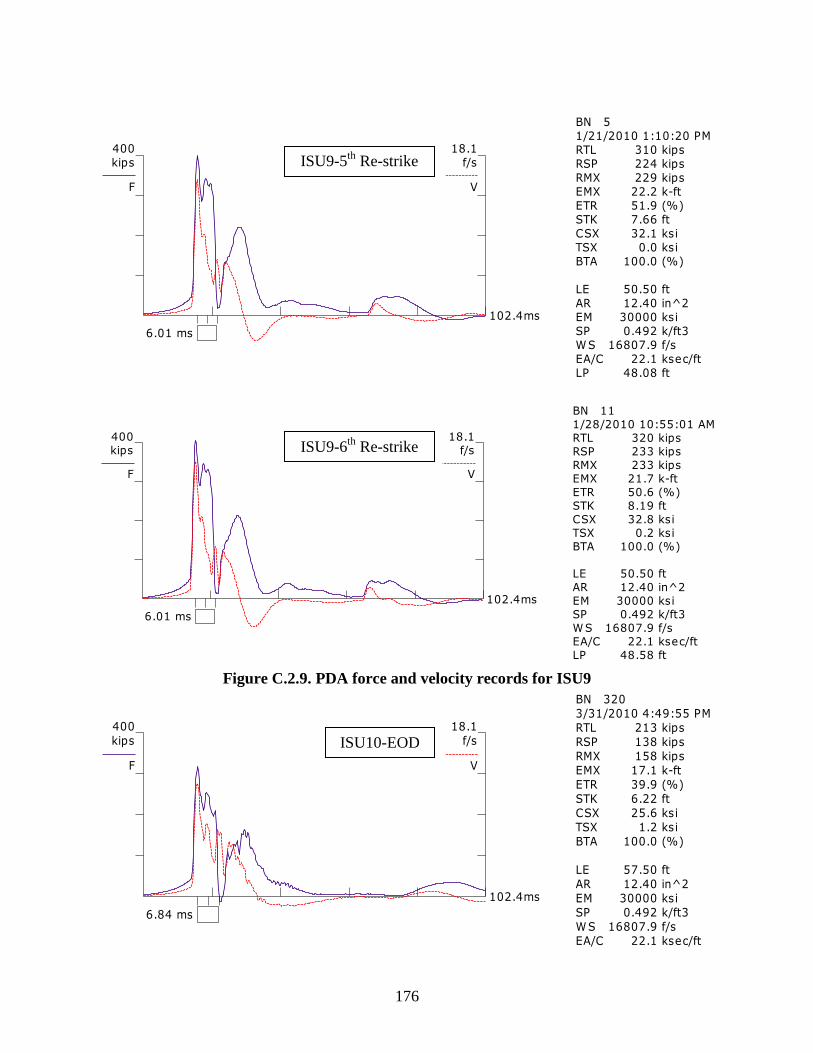
176
Figure C.2.9. PDA force and velocity records for ISU9
IOWA DOTISU9PDA OP: KAM
PILE DRIVING ANALYZER ®Version 2001.086
ISU9 5th bor
HP10x42
BN 51/21/2010 1:10:20 PMRTL kips310RSP kips224
RMX kips229EMX k-ft22.2ETR (%)51.9STK ft7.66
CSX ksi32.1TSX ksi0.0BTA (%)100.0
LE ft50.50
AR in^212.40EM ksi30000SP k/ft30.492WS f/s16807.9EA/C ksec/ft22.1
LP ft48.08
F12 A12
F1: [2355] 87 (1)F2: [2356] 89 (1)A1: [41309] 1095 g's/v (1)A2: [41315] 1115 g's/v (1)
6.01 ms
102.4ms
400
kips
F
18.1
f/s
V
IOWA DOTISU9PDA OP: KAM
PILE DRIVING ANALYZER ®Version 2001.086
ISU9 6th bor
HP10x42
BN 111/28/2010 10:55:01 AMRTL kips320RSP kips233
RMX kips233EMX k-ft21.7ETR (%)50.6STK ft8.19
CSX ksi32.8TSX ksi0.2BTA (%)100.0
LE ft50.50
AR in^212.40EM ksi30000SP k/ft30.492WS f/s16807.9EA/C ksec/ft22.1
LP ft48.58
F12 A12
F1: [2355] 87 (1)F2: [2356] 89 (1)A1: [41309] 1095 g's/v (1)A2: [41315] 1115 g's/v (1)
6.01 ms
102.4ms
400
kips
F
18.1
f/s
V
IOWA DOTISU10PDA OP: KAM
PILE DRIVING ANALYZER ®Version 2001.086
ISU10 driving
HP10x42
BN 3203/31/2010 4:49:55 PMRTL kips213RSP kips138
RMX kips158EMX k-ft17.1ETR (%)39.9STK ft6.22
CSX ksi25.6TSX ksi1.2BTA (%)100.0
LE ft57.50
AR in^212.40EM ksi30000SP k/ft30.492WS f/s16807.9EA/C ksec/ft22.1
F12 A12
F1: [2355] 87 (1)F2: [2356] 89 (1)A1: [41309] 1095 g's/v (1)A2: [41315] 1115 g's/v (1)
6.84 ms
102.4ms
400
kips
F
18.1
f/s
V
ISU9-5th
Re-strike
ISU9-6th
Re-strike
ISU10-EOD
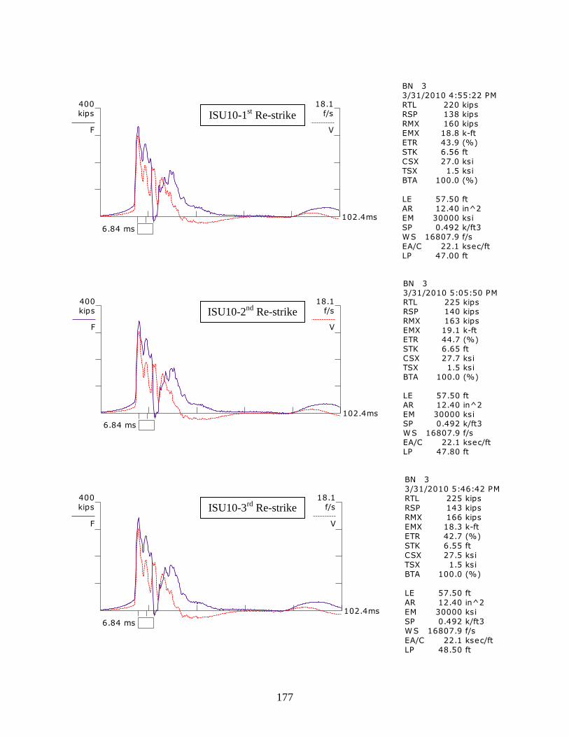
177
IOWA DOTISU10PDA OP: KAM
PILE DRIVING ANALYZER ®Version 2001.086
ISU10 1st bor
HP10x42
BN 33/31/2010 4:55:22 PMRTL kips220RSP kips138
RMX kips160EMX k-ft18.8ETR (%)43.9STK ft6.56
CSX ksi27.0TSX ksi1.5BTA (%)100.0
LE ft57.50
AR in^212.40EM ksi30000SP k/ft30.492WS f/s16807.9EA/C ksec/ft22.1
LP ft47.00
F12 A12
F1: [2355] 87 (1)F2: [2356] 89 (1)A1: [41309] 1095 g's/v (1)A2: [41315] 1115 g's/v (1)
6.84 ms
102.4ms
400
kips
F
18.1
f/s
V
IOWA DOTISU10PDA OP: KAM
PILE DRIVING ANALYZER ®Version 2001.086
ISU10 2nd bor
HP10x42
BN 33/31/2010 5:05:50 PMRTL kips225RSP kips140
RMX kips163EMX k-ft19.1ETR (%)44.7STK ft6.65
CSX ksi27.7TSX ksi1.5BTA (%)100.0
LE ft57.50
AR in^212.40EM ksi30000SP k/ft30.492WS f/s16807.9EA/C ksec/ft22.1
LP ft47.80
F12 A12
F1: [2355] 87 (1)F2: [2356] 89 (1)A1: [41309] 1095 g's/v (1)A2: [41315] 1115 g's/v (1)
6.84 ms
102.4ms
400
kips
F
18.1
f/s
V
IOWA DOTISU10PDA OP: KAM
PILE DRIVING ANALYZER ®Version 2001.086
ISU10 3rd bor
HP10x42
BN 33/31/2010 5:46:42 PMRTL kips225RSP kips143
RMX kips166EMX k-ft18.3ETR (%)42.7STK ft6.55
CSX ksi27.5TSX ksi1.5BTA (%)100.0
LE ft57.50
AR in^212.40EM ksi30000SP k/ft30.492WS f/s16807.9EA/C ksec/ft22.1
LP ft48.50
F12 A12
F1: [2355] 87 (1)F2: [2356] 89 (1)A1: [41309] 1095 g's/v (1)A2: [41315] 1115 g's/v (1)
6.84 ms
102.4ms
400
kips
F
18.1
f/s
V
ISU10-1st Re-strike
ISU10-2nd
Re-strike
ISU10-3rd
Re-strike
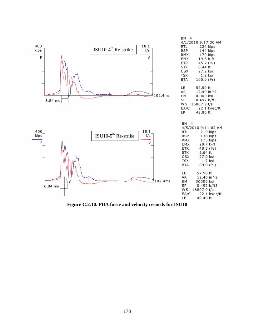
178
Figure C.2.10. PDA force and velocity records for ISU10
IOWA DOTISU10PDA OP: KAM
PILE DRIVING ANALYZER ®Version 2001.086
ISU10 4th bor
HP10x42
BN 44/1/2010 9:17:30 AMRTL kips224RSP kips144
RMX kips170EMX k-ft19.6ETR (%)45.7STK ft6.44
CSX ksi27.2TSX ksi1.2BTA (%)100.0
LE ft57.50
AR in^212.40EM ksi30000SP k/ft30.492WS f/s16807.9EA/C ksec/ft22.1
LP ft48.80
F12 A12
F1: [2355] 87 (1)F2: [2356] 89 (1)A1: [41309] 1095 g's/v (1)A2: [41315] 1115 g's/v (1)
6.84 ms
102.4ms
400
kips
F
18.1
f/s
V
IOWA DOTISU10PDA OP: KAM
PILE DRIVING ANALYZER ®Version 2001.086
ISU10 5th bor
HP10x42
BN 44/5/2010 9:11:02 AMRTL kips219RSP kips138
RMX kips175EMX k-ft20.7ETR (%)48.3STK ft6.64
CSX ksi27.0TSX ksi1.7BTA (%)89.0
LE ft57.50
AR in^212.40EM ksi30000SP k/ft30.492WS f/s16807.9EA/C ksec/ft22.1
LP ft49.40
F12 A12
F1: [2355] 87 (1)F2: [2356] 89 (1)A1: [41309] 1095 g's/v (1)A2: [41315] 1115 g's/v (1)
6.84 ms
102.4ms
400
kips
F
18.1
f/s
V
ISU10-4th
Re-strike
ISU10-5th
Re-strike
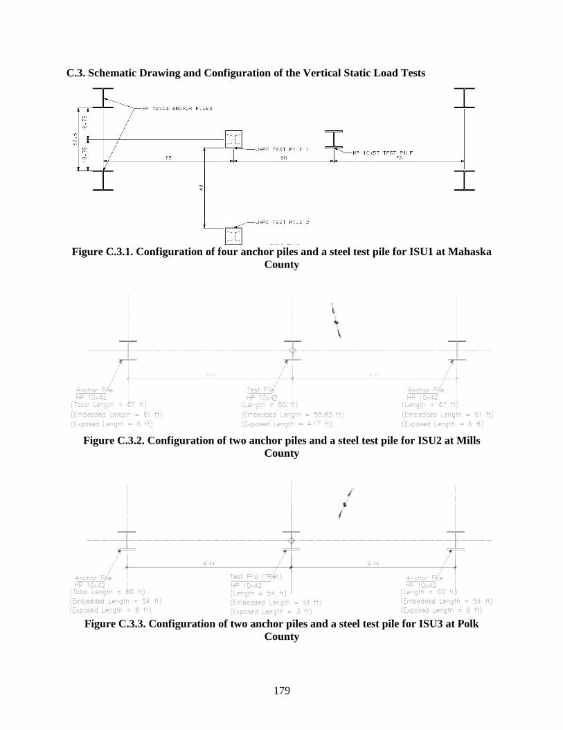
179
C.3. Schematic Drawing and Configuration of the Vertical Static Load Tests
Figure C.3.1. Configuration of four anchor piles and a steel test pile for ISU1 at Mahaska
County
Figure C.3.2. Configuration of two anchor piles and a steel test pile for ISU2 at Mills
County
Figure C.3.3. Configuration of two anchor piles and a steel test pile for ISU3 at Polk
County

180
Figure C.3.4. Configuration of two anchor piles and a steel test pile for ISU4 at Jasper
County
Figure C.3.5. Configuration of two anchor piles and two steel test piles for ISU6 and ISU7
at Buchanan County
Figure C.3.6. Configuration of two anchor piles and a steel test pile for ISU8 at Poweshiek
County
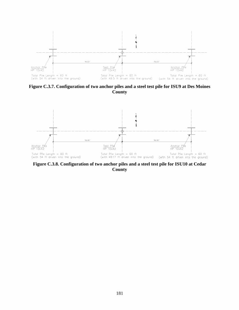
181
Figure C.3.7. Configuration of two anchor piles and a steel test pile for ISU9 at Des Moines
County
Figure C.3.8. Configuration of two anchor piles and a steel test pile for ISU10 at Cedar
County
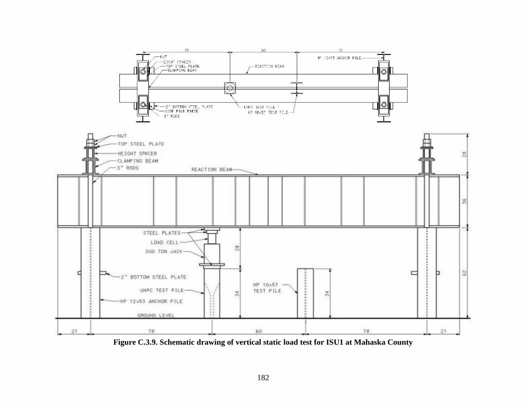
182
Figure C.3.9. Schematic drawing of vertical static load test for ISU1 at Mahaska County
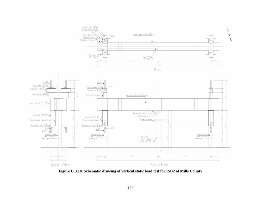
183
Figure C.3.10. Schematic drawing of vertical static load test for ISU2 at Mills County

184
Figure C.3.11. Schematic drawing of vertical static load test for ISU3 at Polk County
Steel Angle
(L 2 x 2 x 316)
Steel Angle
(L 2 x 2 x 316)

185
Figure C.3.12. Schematic drawing of vertical static load test for ISU4 at Jasper County
Steel Angle
(L 2 x 2 x 316)
Steel Angle
(L 2 x 2 x 316)
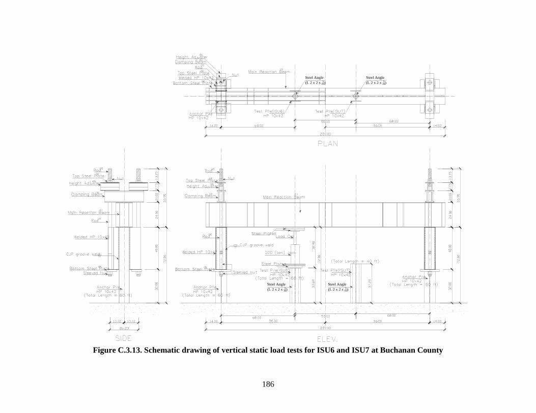
186
Figure C.3.13. Schematic drawing of vertical static load tests for ISU6 and ISU7 at Buchanan County
Steel Angle
(L 2 x 2 x 316)
Steel Angle
(L 2 x 2 x 316)
Steel Angle
(L 2 x 2 x 316)
Steel Angle
(L 2 x 2 x 316)
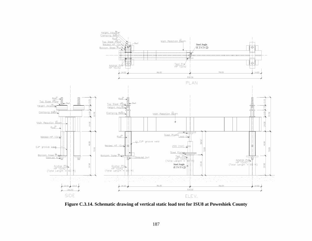
187
Figure C.3.14. Schematic drawing of vertical static load test for ISU8 at Poweshiek County
Steel Angle
(L 2 x 2 x 316)
Steel Angle
(L 2 x 2 x 316)
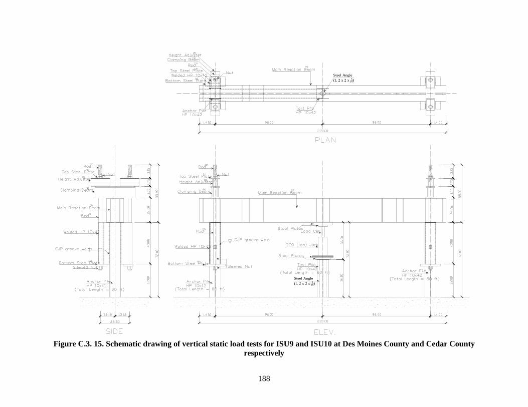
188
Figure C.3. 15. Schematic drawing of vertical static load tests for ISU9 and ISU10 at Des Moines County and Cedar County
respectively
Steel Angle
(L 2 x 2 x 316)
Steel Angle
(L 2 x 2 x 316)
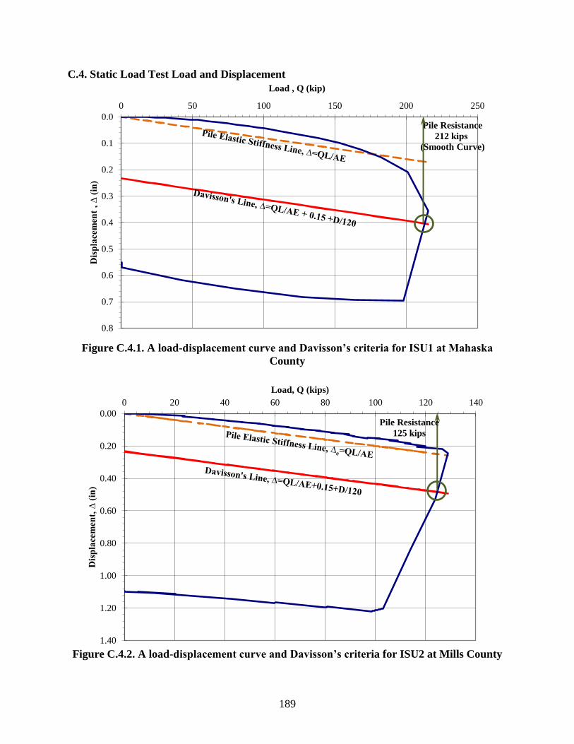
189
C.4. Static Load Test Load and Displacement
Figure C.4.1. A load-displacement curve and Davisson’s criteria for ISU1 at Mahaska
County
Figure C.4.2. A load-displacement curve and Davisson’s criteria for ISU2 at Mills County
0.0
0.1
0.2
0.3
0.4
0.5
0.6
0.7
0.8
0 50 100 150 200 250
Dis
pla
cem
ent
, ∆
(in
) Load , Q (kip)
Pile Resistance
212 kips
(Smooth Curve)
0.00
0.20
0.40
0.60
0.80
1.00
1.20
1.40
0 20 40 60 80 100 120 140
Dis
pla
cem
ent,
∆ (
in)
Load, Q (kips)
Pile Resistance
125 kips
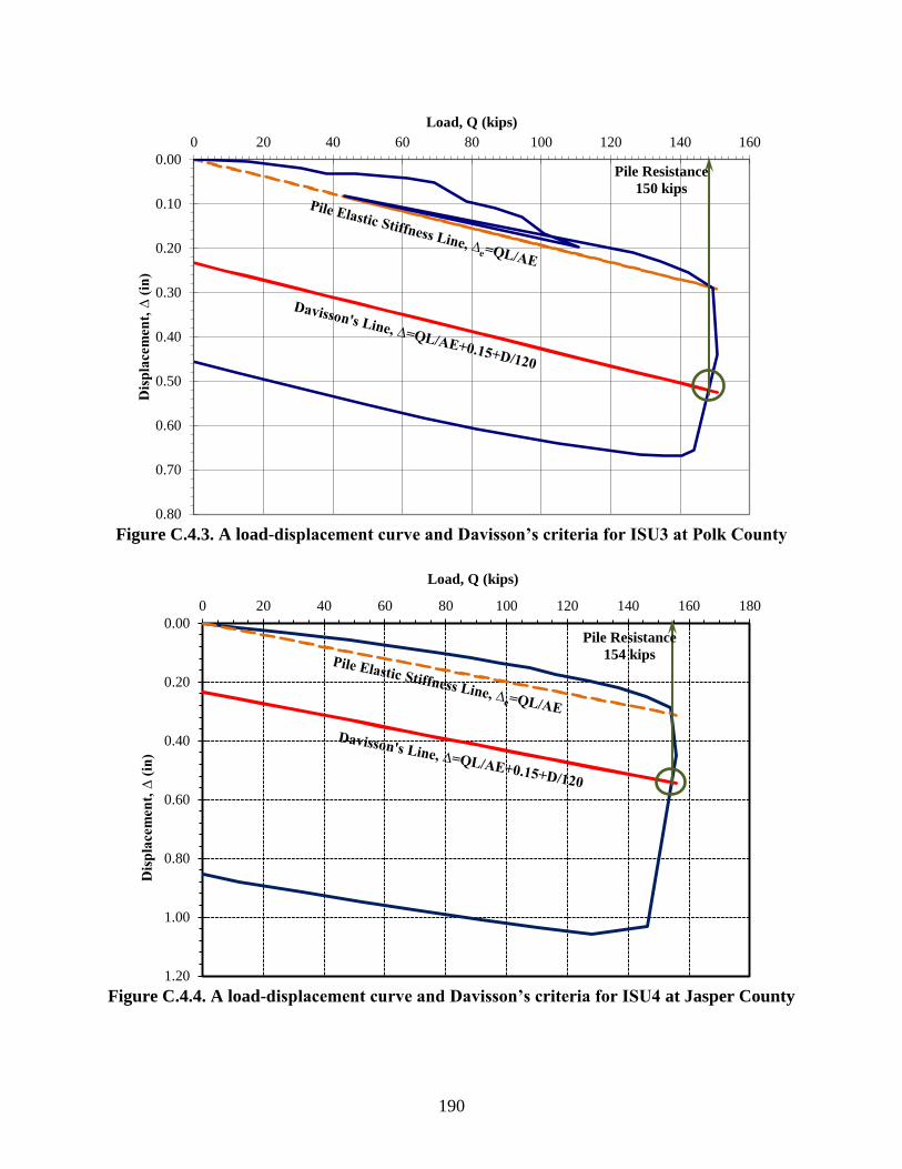
190
Figure C.4.3. A load-displacement curve and Davisson’s criteria for ISU3 at Polk County
Figure C.4.4. A load-displacement curve and Davisson’s criteria for ISU4 at Jasper County
0.00
0.10
0.20
0.30
0.40
0.50
0.60
0.70
0.80
0 20 40 60 80 100 120 140 160D
isp
lace
men
t, ∆
(in
)
Load, Q (kips)
Pile Resistance
150 kips
0.00
0.20
0.40
0.60
0.80
1.00
1.20
0 20 40 60 80 100 120 140 160 180
Dis
pla
cem
ent,
∆ (
in)
Load, Q (kips)
Pile Resistance
154 kips
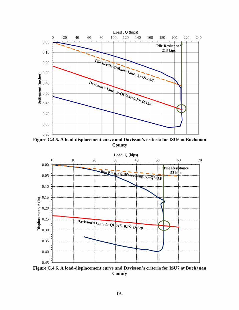
191
Figure C.4.5. A load-displacement curve and Davisson’s criteria for ISU6 at Buchanan
County
Figure C.4.6. A load-displacement curve and Davisson’s criteria for ISU7 at Buchanan
County
0.00
0.10
0.20
0.30
0.40
0.50
0.60
0.70
0.80
0.90
0 20 40 60 80 100 120 140 160 180 200 220 240S
ettl
emen
t (i
nch
es)
Load , Q (kips)
Pile Resistance
213 kips
0.00
0.05
0.10
0.15
0.20
0.25
0.30
0.35
0.40
0.45
0 10 20 30 40 50 60 70
Dis
pla
cem
ent,
∆ (
in)
Load, Q (kips)
Pile Resistance
53 kips
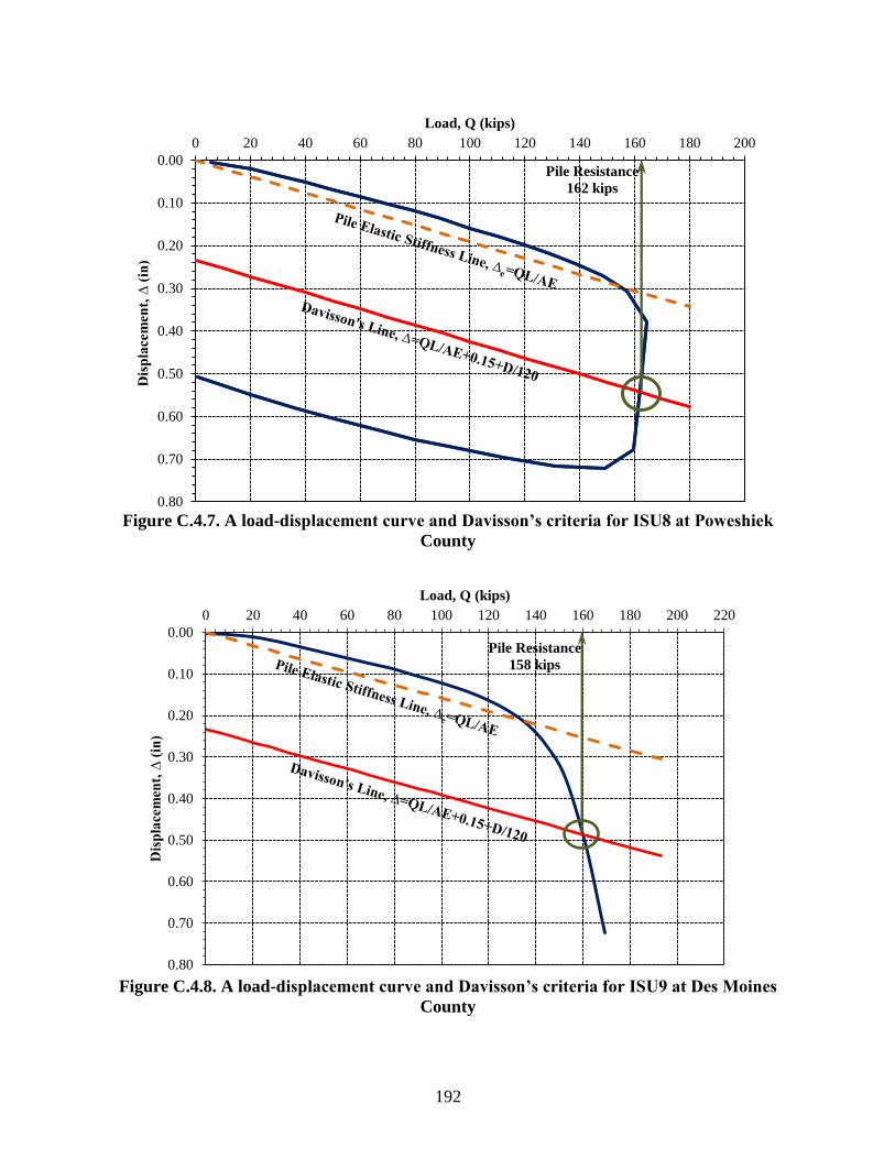
192
Figure C.4.7. A load-displacement curve and Davisson’s criteria for ISU8 at Poweshiek
County
Figure C.4.8. A load-displacement curve and Davisson’s criteria for ISU9 at Des Moines
County
0.00
0.10
0.20
0.30
0.40
0.50
0.60
0.70
0.80
0 20 40 60 80 100 120 140 160 180 200D
isp
lace
men
t, ∆
(in
)
Load, Q (kips)
Pile Resistance
162 kips
0.00
0.10
0.20
0.30
0.40
0.50
0.60
0.70
0.80
0 20 40 60 80 100 120 140 160 180 200 220
Dis
pla
cem
ent,
∆ (
in)
Load, Q (kips)
Pile Resistance
158 kips
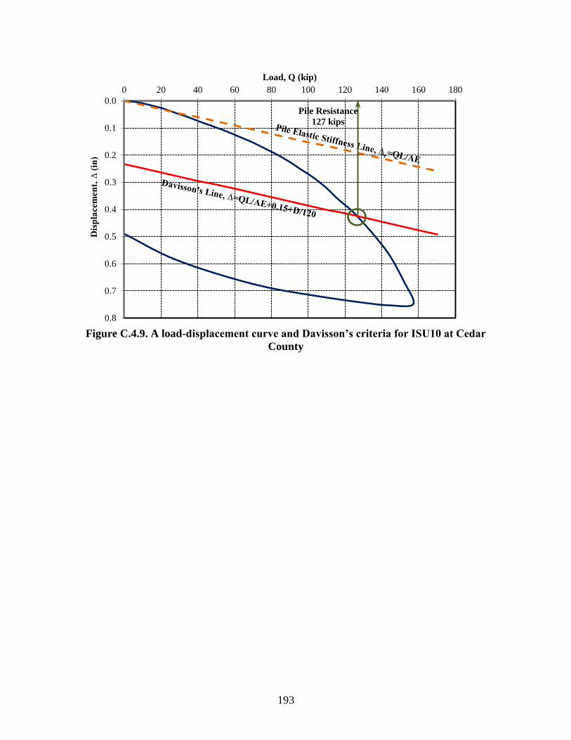
193
Figure C.4.9. A load-displacement curve and Davisson’s criteria for ISU10 at Cedar
County
0.0
0.1
0.2
0.3
0.4
0.5
0.6
0.7
0.8
0 20 40 60 80 100 120 140 160 180D
isp
lace
men
t, ∆
(in
)
Load, Q (kip)
Pile Resistance
127 kips
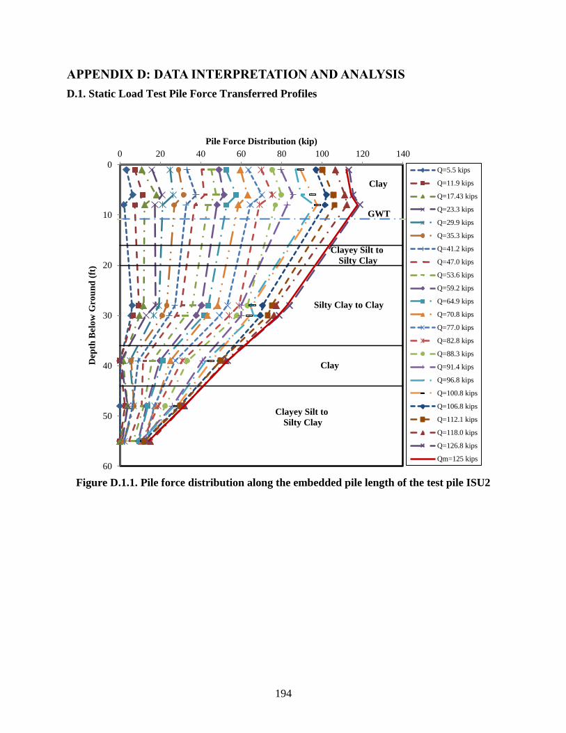
194
APPENDIX D: DATA INTERPRETATION AND ANALYSIS
D.1. Static Load Test Pile Force Transferred Profiles
Figure D.1.1. Pile force distribution along the embedded pile length of the test pile ISU2
0
10
20
30
40
50
60
0 20 40 60 80 100 120 140
Dep
th B
elo
w G
rou
nd
(ft
)
Pile Force Distribution (kip)
Q=5.5 kips
Q=11.9 kips
Q=17.43 kips
Q=23.3 kips
Q=29.9 kips
Q=35.3 kips
Q=41.2 kips
Q=47.0 kips
Q=53.6 kips
Q=59.2 kips
Q=64.9 kips
Q=70.8 kips
Q=77.0 kips
Q=82.8 kips
Q=88.3 kips
Q=91.4 kips
Q=96.8 kips
Q=100.8 kips
Q=106.8 kips
Q=112.1 kips
Q=118.0 kips
Q=126.8 kips
Qm=125 kips
Clay
Clayey Silt to
Silty Clay
Silty Clay to Clay
Clay
Clayey Silt to
Silty Clay
GWT
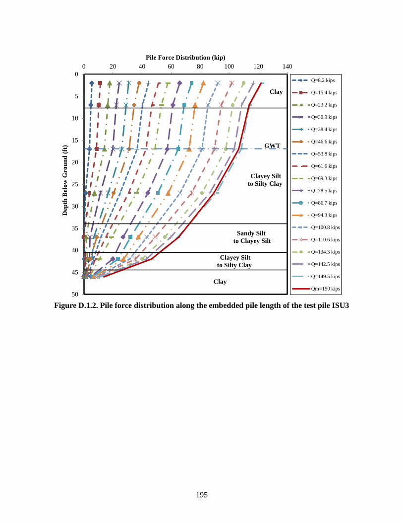
195
Figure D.1.2. Pile force distribution along the embedded pile length of the test pile ISU3
0
5
10
15
20
25
30
35
40
45
50
0 20 40 60 80 100 120 140D
epth
Bel
ow
Gro
un
d (
ft)
Pile Force Distribution (kip)
Q=8.2 kips
Q=15.4 kips
Q=23.2 kips
Q=30.9 kips
Q=38.4 kips
Q=46.6 kips
Q=53.8 kips
Q=61.6 kips
Q=69.3 kips
Q=78.5 kips
Q=86.7 kips
Q=94.3 kips
Q=100.8 kips
Q=110.6 kips
Q=134.3 kips
Q=142.5 kips
Q=149.5 kips
Qm=150 kips
Clay
Clay
Clayey Silt
to Silty Clay
Sandy Silt
to Clayey Silt
Clayey Silt
to Silty Clay
GWT
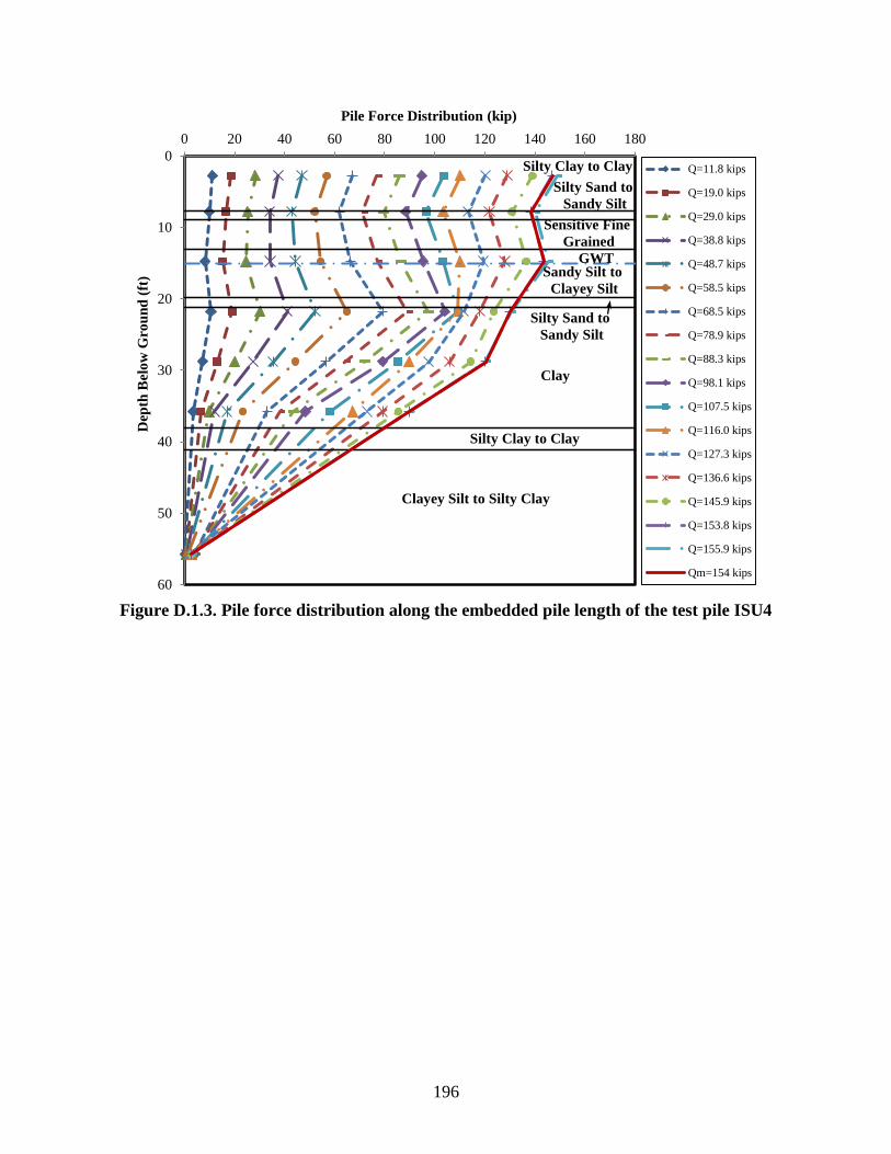
196
Figure D.1.3. Pile force distribution along the embedded pile length of the test pile ISU4
0
10
20
30
40
50
60
0 20 40 60 80 100 120 140 160 180D
epth
Bel
ow
Gro
un
d (
ft)
Pile Force Distribution (kip)
Q=11.8 kips
Q=19.0 kips
Q=29.0 kips
Q=38.8 kips
Q=48.7 kips
Q=58.5 kips
Q=68.5 kips
Q=78.9 kips
Q=88.3 kips
Q=98.1 kips
Q=107.5 kips
Q=116.0 kips
Q=127.3 kips
Q=136.6 kips
Q=145.9 kips
Q=153.8 kips
Q=155.9 kips
Qm=154 kips
GWT
Silty Clay to Clay
Silty Sand to
Sandy Silt
Sensitive Fine
Grained
Sandy Silt to
Clayey Silt
Clay
Silty Sand to
Sandy Silt
Silty Clay to Clay
Clayey Silt to Silty Clay
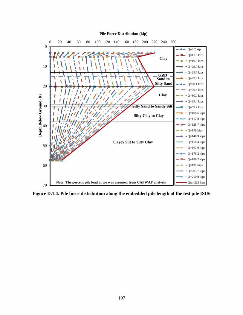
197
Figure D.1.4. Pile force distribution along the embedded pile length of the test pile ISU6
0
10
20
30
40
50
60
70
0 20 40 60 80 100 120 140 160 180 200 220 240 260D
epth
Bel
ow
Gro
un
d (
ft)
Pile Force Distribution (kip)
Q=0.2 kip
Q=11.6 kips
Q=19.8 kips
Q=29.0 kips
Q=39.7 kips
Q=49.6 kips
Q=60.1 kips
Q=70.4 kips
Q=80.0 kips
Q=89.4 kips
Q=99.2 kips
Q=108.6 kips
Q=117.8 kips
Q=128.7 kips
Q=139 kips
Q=148.9 kips
Q=158.4 kips
Q=167.9 kips
Q=178.2 kips
Q=186.2 kips
Q=197 kips
Q=203.7 kips
Q=210.9 kips
Qm=213 kips
Clay
GWT
Clay
Sand to
Silty Sand
Silty Sand to Sandy Silt
Silty Clay to Clay
Clayey Silt to Silty Clay
Note: The percent pile load at toe was assumed from CAPWAP analysis
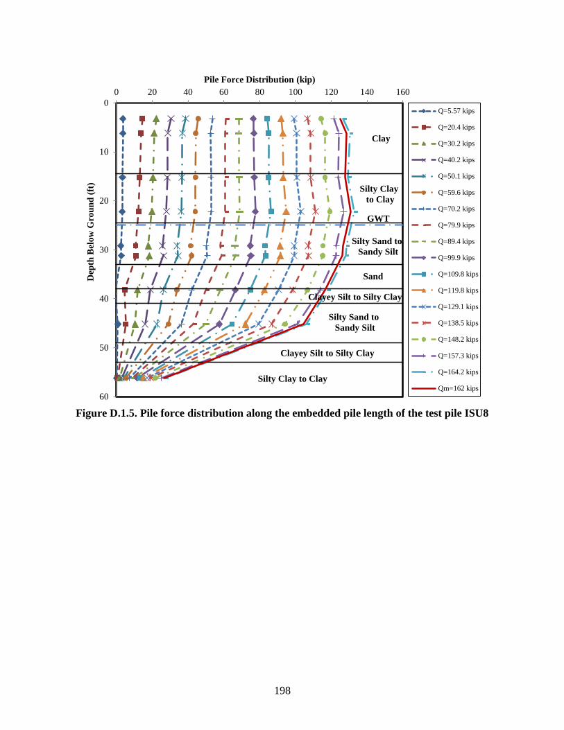
198
Figure D.1.5. Pile force distribution along the embedded pile length of the test pile ISU8
0
10
20
30
40
50
60
0 20 40 60 80 100 120 140 160D
epth
Bel
ow
Gro
un
d (
ft)
Pile Force Distribution (kip)
Q=5.57 kips
Q=20.4 kips
Q=30.2 kips
Q=40.2 kips
Q=50.1 kips
Q=59.6 kips
Q=70.2 kips
Q=79.9 kips
Q=89.4 kips
Q=99.9 kips
Q=109.8 kips
Q=119.8 kips
Q=129.1 kips
Q=138.5 kips
Q=148.2 kips
Q=157.3 kips
Q=164.2 kips
Qm=162 kips
Clay
Silty Clay
to Clay
Silty Sand to
Sandy Silt
Sand
Clayey Silt to Silty Clay
Silty Sand to
Sandy Silt
Clayey Silt to Silty Clay
Silty Clay to Clay
GWT
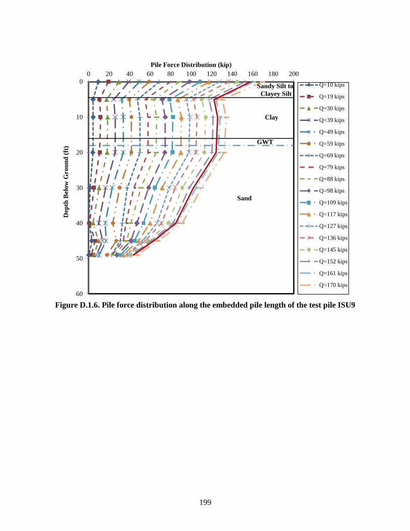
199
Figure D.1.6. Pile force distribution along the embedded pile length of the test pile ISU9
0
10
20
30
40
50
60
0 20 40 60 80 100 120 140 160 180 200
Dep
th B
elo
w G
rou
nd
(ft
) Pile Force Distribution (kip)
Q=10 kips
Q=19 kips
Q=30 kips
Q=39 kips
Q=49 kips
Q=59 kips
Q=69 kips
Q=79 kips
Q=88 kips
Q=98 kips
Q=109 kips
Q=117 kips
Q=127 kips
Q=136 kips
Q=145 kips
Q=152 kips
Q=161 kips
Q=170 kips
Clay
Sand
Sandy Silt to
Clayey Silt
GWT

200
D.2. Shaft Resistance Distribution
Figure D.2.1. SLT measured and CAPWAP estimated pile shaft resistance distributions for
test pile ISU2
Figure D.2.2. SLT measured and CAPWAP estimated pile shaft resistance distributions for
test pile ISU3
0 2 4 6 8 10 12 14 16 18 20
0
10
20
30
40
50
60
0 20 40 60
Uncorrected SPT N-value
Dep
th B
elo
w G
rou
nd
(ft
)
Shaft Resistance Distribution (kip)
EOD BOR1BOR2 BOR3SLTGWT
Clay (CL)
Clay (CL)
Silty Clay to Clay (CL)
Silty Clay to Silty Clay (CL)
Silty Clay to Silty Clay (CL)
0 2 4 6 8 10 12 14 16 18 20 22 24
0
10
20
30
40
50
60
0 20 40 60
Uncorrected SPT N-value
Dep
th B
elo
w G
rou
nd
(ft
)
Shaft Resistance Distribution (kip)
EOD BOR1
BOR2 BOR3
BOR4 BOR5
Clay
Silty Clay to Silty Clay GWT
Sandy Silt to Clayey Silt
Clayey Silt to Silty Clay
Clay
Clayey Silt to Silty Clay

201
Figure D.2.3. SLT measured and CAPWAP estimated pile shaft resistance distributions for
test pile ISU4
Figure D.2.4. CAPWAP estimated pile shaft resistance distributions for test pile ISU6
0 2 4 6 8 10 12 14 16 18
0
10
20
30
40
50
60
0 20 40 60
Uncorrected SPT N-value
Dep
th B
elo
w G
rou
nd
(ft
)
Shaft Resistance Distribution (kip)
EOD BOR1BOR2 BOR3BOR4 BOR5BOR6 SLT
Silty Clay to Clay Silty Sand to Sandy Silt
Sensitive fine Grained
Sandy Silt to Clayey Silt
Silty Sand to Sandy Silt
Clay
GWT
Silty Clay to Clay
Clayey Silt to Silty Clay
0 2 4 6 8 10 12 14 16 18 20 22 24 26 28 30
0
10
20
30
40
50
60
0 20 40 60
Uncorrected SPT N-value
Dep
th B
elo
w G
rou
nd
(ft
)
Shaft Resistance Distribution (kip)
EOD BOR1 BOR2BOR3 BOR4 BOR5BOR6 BOR7 BOR8Clay
Sand to silty Sand
Clay
Silty Sand to Sandy Silt
Silty Clay to Clay
Clayey Silt to Silty Clay
GWT
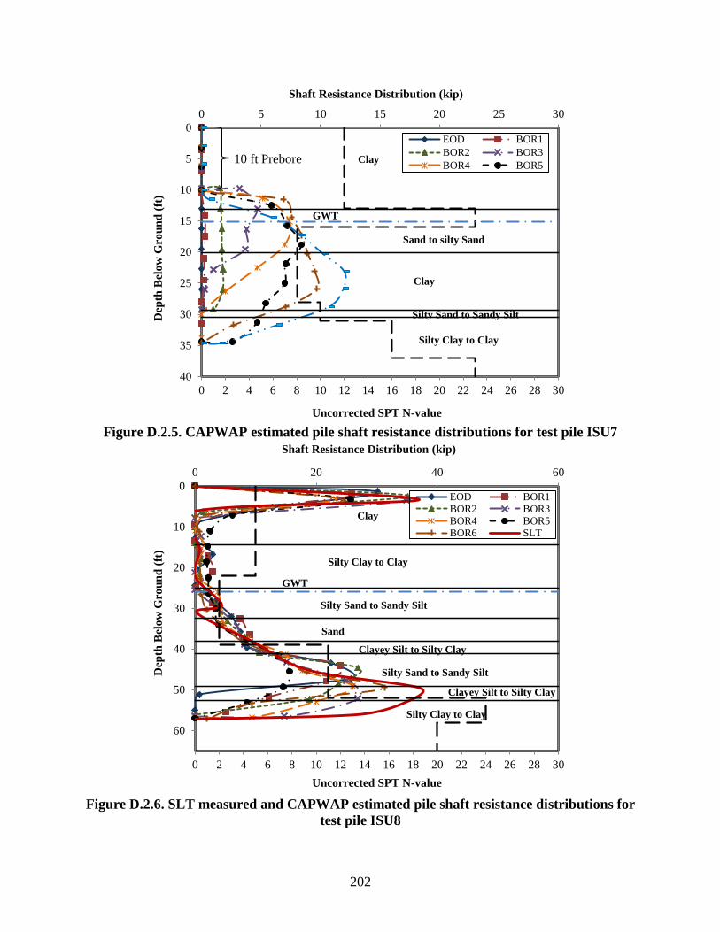
202
Figure D.2.5. CAPWAP estimated pile shaft resistance distributions for test pile ISU7
Figure D.2.6. SLT measured and CAPWAP estimated pile shaft resistance distributions for
test pile ISU8
0 2 4 6 8 10 12 14 16 18 20 22 24 26 28 30
0
5
10
15
20
25
30
35
40
0 5 10 15 20 25 30
Uncorrected SPT N-value
Dep
th B
elo
w G
rou
nd
(ft
)
Shaft Resistance Distribution (kip)
EOD BOR1
BOR2 BOR3
BOR4 BOR510 ft Prebore Clay
Sand to silty Sand
Clay
Silty Sand to Sandy Silt
Silty Clay to Clay
GWT
0 2 4 6 8 10 12 14 16 18 20 22 24 26 28 30
0
10
20
30
40
50
60
0 20 40 60
Uncorrected SPT N-value
Dep
th B
elo
w G
rou
nd
(ft
)
Shaft Resistance Distribution (kip)
EOD BOR1
BOR2 BOR3
BOR4 BOR5
BOR6 SLT
Clay
GWT
Silty Clay to Clay
Silty Sand to Sandy Silt
Sand
Clayey Silt to Silty Clay
Silty Sand to Sandy Silt
Clayey Silt to Silty Clay
Silty Clay to Clay

203
Figure D.2.7. SLT measured and CAPWAP estimated pile shaft resistance distributions for
test pile ISU9
Figure D.2.8. CAPWAP estimated pile shaft resistance distributions for test pile ISU10
0 2 4 6 8 10 12 14 16 18 20 22 24 26 28 30 32 34
0
10
20
30
40
50
60
0 20 40 60
Uncorrected SPT N-value
Dep
th B
elo
w G
rou
nd
(ft
)
Shaft Resistance Distribution (kip)
EOD BOR1
BOR2 BOR3
BOR4 BOR5
GWT
Sandy Silt to Clayey Silt
Clay
Sand
0 10 20 30 40 50 60 70 80
0
10
20
30
40
50
60
0 20 40 60
Uncorrected SPT N-value
Dep
th B
elo
w G
rou
nd
(ft
)
Shaft Resistance Distribution (kip)
EOD
BOR1
BOR2
BOR3
BOR4
BOR5
GWT Sandy Silt to Clayey Silt
Sand to Silty Sand Sandy Silt to Clayey Silt
Sand
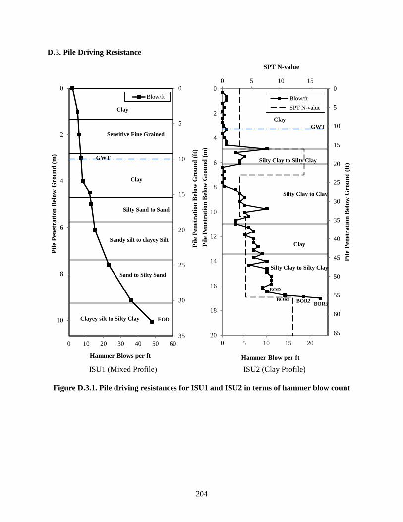
204
D.3. Pile Driving Resistance
ISU1 (Mixed Profile) ISU2 (Clay Profile)
Figure D.3.1. Pile driving resistances for ISU1 and ISU2 in terms of hammer blow count
0
5
10
15
20
25
30
35
0
2
4
6
8
10
0 10 20 30 40 50 60
Pil
e P
enet
rati
on
Bel
ow
Gro
un
d (
ft)
Pil
e P
enet
rati
on
Bel
ow
Gro
un
d (
m)
Hammer Blows per ft
Blow/ft
EOD
Clay
Sensitive Fine Grained
Clay
Silty Sand to Sand
Sandy silt to clayey Silt
Sand to Silty Sand
Clayey silt to Silty Clay
GWT
0 5 10 15
0
5
10
15
20
25
30
35
40
45
50
55
60
65
0
2
4
6
8
10
12
14
16
18
20
0 5 10 15 20
SPT N-value
Pil
e P
enet
rati
on
Bel
ow
Gro
un
d (
ft)
Pil
e P
enet
rati
on
Bel
ow
Gro
un
d (
m)
Hammer Blow per ft
Blow/ft
SPT N-value
EOD
BOR1 BOR2 BOR3
GWT
Clay
Clay
Silty Clay to Clay
Silty Clay to Silty Clay
Silty Clay to Silty Clay

205
ISU3 (Clay Profile) ISU4 (Clay Profile)
Figure D.3.2. Pile driving resistances for ISU3 and ISU4 in terms of hammer blow count
0 5 10 15 20
0
5
10
15
20
25
30
35
40
45
50
55
60
65
0
2
4
6
8
10
12
14
16
18
20
0 5 10 15 20
SPT N-value
Pil
e P
enet
rati
on
Bel
ow
Gro
un
d (
ft)
Pil
e P
enet
rati
on
Bel
ow
Gro
un
d (
m)
Hammer Blow per ft
Blow/ft
SPT N-value
EOD
BOR1/2/3
BOR4 BOR5
Clay
Silty Clay to Silty Clay
GWT
Sandy Silt to
Clayey Silt
Clayey Silt to Silty Clay
Clay
Clayey Silt to Silty Clay
0 5 10 15 20
0
5
10
15
20
25
30
35
40
45
50
55
60
65
0
2
4
6
8
10
12
14
16
18
20
0 5 10 15 20 25
SPT N-value
Pil
e P
enet
rati
on
Bel
ow
Gro
un
d (
ft)
Pil
e P
enet
rati
on
Bel
ow
Gro
un
d (
m)
Hammer Blow per ft
Blow/ft
SPT N-value
EOD
BOR3
BOR4
BOR5
BOR6 BOR1
BOR2
Silty Clay to Clay Silty Sand to Sandy Silt
Sensitive fine Grained
Sandy Silt to Clayey Silt
Silty Sand to Sandy Silt
Clay
GWT
Silty Clay to Clay
Clayey Silt to Silty Clay

206
ISU6 (Clay Profile) ISU7 (Mixed Profile)
Figure D.3.3. Pile driving resistances for ISU6 and ISU7 in terms of hammer blow count
0 5 10 15 20 25
0
5
10
15
20
25
30
35
40
45
50
55
60
65
0
2
4
6
8
10
12
14
16
18
20
0 10 20 30 40 50 60 70
SPT N-value
Pil
e P
enet
rati
on
Bel
ow
Gro
un
d (
ft)
Pil
e P
enet
rati
on
Bel
ow
Gro
un
d (
m)
Hammer Blow per ft
Blow/ft
SPT N-value
EOD
BOR3
BOR4
BOR5
BOR6
BOR1
BOR2
BOR7
BOR8
Clay
Sand to silty Sand
Clay
Silty Sand to Sandy Silt
Silty Clay to Clay
Clayey Silt to Silty Clay
GWT
0 5 10 15 20 25
0
5
10
15
20
25
30
35
40
0
2
4
6
8
10
12
0 2 4 6 8 10
SPT N-value
Pil
e P
enet
rati
on
Bel
ow
Gro
un
d (
ft)
Pil
e P
enet
rati
on
Bel
ow
Gro
un
d (
m)
Hammer Blow per ft
Blow/ft
SPT N-value
EOD
BOR3 BOR4
BOR5
BOR6
BOR1 BOR2
BOR7
Clay
Sand to silty Sand
Clay
Silty Sand to Sandy Silt
Silty Clay to Clay
Clayey Silt to Silty Clay
GWT
Note: Top 10 ft was predrilled

207
Figure D.3.4. Pile driving resistance for ISU10 (sand profile) in terms of hammer blow
count
0 20 40 60 80
0
5
10
15
20
25
30
35
40
45
50
55
60
65
0
2
4
6
8
10
12
14
16
18
20
0 5 10 15 20
SPT N-value
Pil
e P
enet
rati
on
Bel
ow
Gro
un
d (
ft)
Pil
e P
enet
rati
on
Bel
ow
Gro
un
d (
m)
Hammer Blow per ft
Blow/ft
SPT N-value
EOD
BOR3
BOR4 BOR5
BOR1
BOR2
Sandy to Silty Sand
Sandy Silt to Clayey Silt
Sand
GWT
Sandy to Clayey Silt

208
D.4. Relationship between Soil Properties and Pile Shaft Resistance Gain
Figure D.4.1. Relationship between soil properties and shaft resistance gain for ISU2
Figure D.4.2. Relationship between soil properties and shaft resistance gain for ISU3
0 2 4 6 8 10 12 14 16 18 20 22 24 26 28 30
0
10
20
30
40
50
60
-20 -10 0 10 20 30 40 50 60
SPT N-value or Plasticity Index
Dep
th B
elo
w G
rou
nd
(ft
) Shaft Resistance Gain Distribution (kip)
Shaft Gain (CAPWAP-3 days)
Shaft Gain (SLT-9 days)
SPT N-value
Plasticity Index
ISU2
Cv=0.008 in2/min
OCR=1.14; Cc=0.208
Cv=0.020 in2/min
OCR=1.05; Cc=0.293
Cv=0.018 in2/min
OCR=1.0; Cc=0.273
Ch=0.138 in2/min
Cv=0.023 in2/min
OCR=1.0; Cc=0.193
0 2 4 6 8 10 12 14 16 18 20 22 24 26 28 30
0
10
20
30
40
50
60
-20 -10 0 10 20 30 40 50 60
SPT N-value or Plasticity Index (%)
Dep
th B
elo
w G
rou
nd
(ft
)
Shaft Resistance Gain Distribution (kip)
Series3Shaft Gain (CAPWAP-2 days)SPT N-valuePlasticity Index
ISU3 Cv=0.011 in2/min
OCR=4.70; Cc=0.125
Cv=0.012 in2/min; OCR=1.52; Cc=0.171
Cv=0.006 in2/min
OCR=1.30; Cc=0.221
Ch=0.029 in2/min
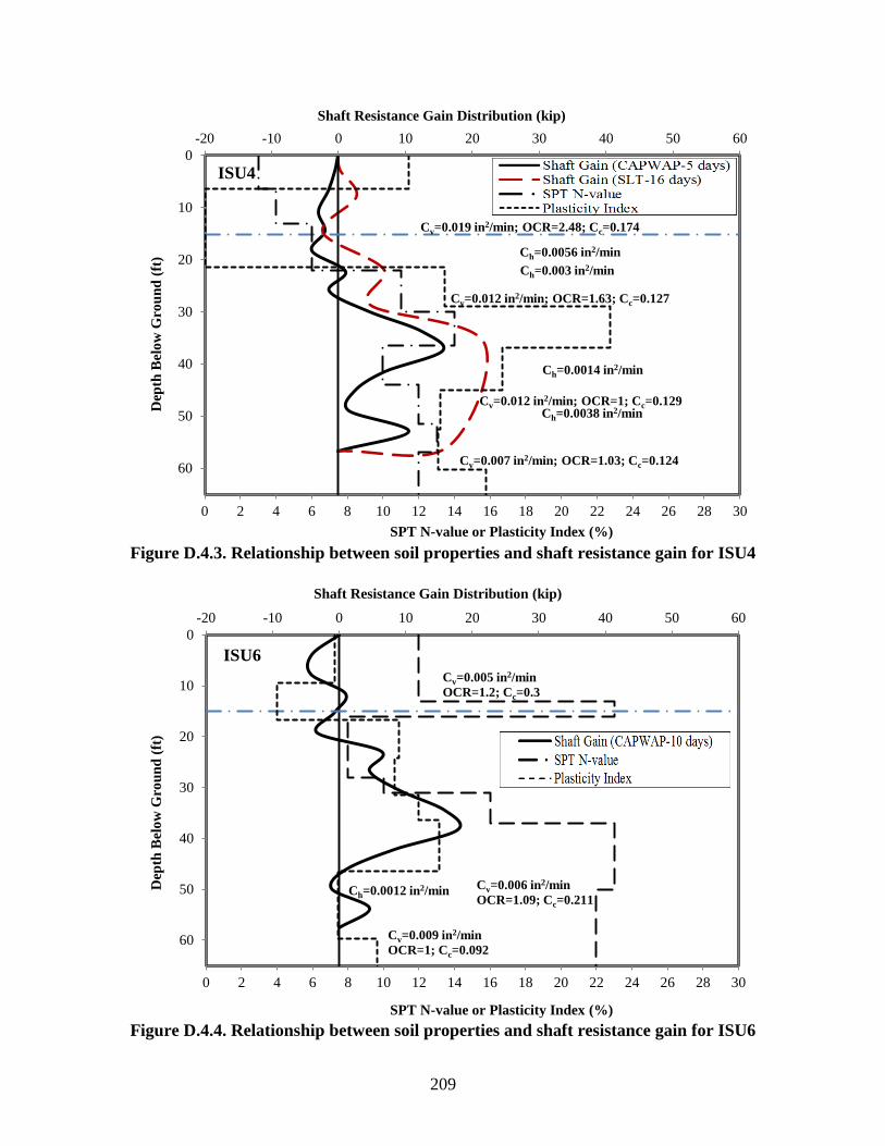
209
Figure D.4.3. Relationship between soil properties and shaft resistance gain for ISU4
Figure D.4.4. Relationship between soil properties and shaft resistance gain for ISU6
0 2 4 6 8 10 12 14 16 18 20 22 24 26 28 30
0
10
20
30
40
50
60
-20 -10 0 10 20 30 40 50 60
SPT N-value or Plasticity Index (%)
Dep
th B
elo
w G
rou
nd
(ft
)
Shaft Resistance Gain Distribution (kip)
Shaft Gain (SLT-16 days)Series1SPT N-valuePlasticity Index
ISU4
Cv=0.012 in2/min; OCR=1.63; Cc=0.127
Cv=0.012 in2/min; OCR=1; Cc=0.129
Cv=0.007 in2/min; OCR=1.03; Cc=0.124
Ch=0.0056 in2/min
Ch=0.003 in2/min
Ch=0.0014 in2/min
Ch=0.0038 in2/min
Cv=0.019 in2/min; OCR=2.48; Cc=0.174
0 2 4 6 8 10 12 14 16 18 20 22 24 26 28 30
0
10
20
30
40
50
60
-20 -10 0 10 20 30 40 50 60
SPT N-value or Plasticity Index (%)
Dep
th B
elo
w G
rou
nd
(ft
)
Shaft Resistance Gain Distribution (kip)
Series1
SPT N-value
Plasticity Index
ISU6
Cv=0.005 in2/min
OCR=1.2; Cc=0.3
Cv=0.009 in2/min
OCR=1; Cc=0.092
Ch=0.0012 in2/min Cv=0.006 in2/min
OCR=1.09; Cc=0.211


