Deterrence, expected cost, uncertainty and voting: Experimental evidence

Deterrence, expected cost, uncertainty and voting:Experimental evidence

Gregory DeAngelo & Gary Charness

Published online: 2 December 2011# Springer Science+Business Media, LLC 2011

Abstract We conduct laboratory experiments to investigate the effects of deterrencemechanisms under controlled conditions. The effect of the expected cost ofpunishment of an individual’s decision to engage in a proscribed activity and theeffect of uncertainty on an individual’s decision to commit a violation are verydifficult to isolate in field data. We use a roadway speeding framing and find that (a)individuals respond considerably to increases in the expected cost of speeding, (b)uncertainty about the enforcement regime yields a significant reduction in violationscommitted, and (c) people are much more likely to speed when the punishmentregime for which they voted is implemented. Our results have important implicationsfor a behavioral theory of deterrence under uncertainty.

Keywords Deterrence . Experiment . Uncertainty . Crime and punishment

JEL classifications C91 . D03 . D81 . K42

The use of deterrence mechanisms—such as the probability of apprehension, fines,jail sentence length, and legal liability—in preventing proscribed activities istheoretically well understood: increases in the expected cost of committing illegalactivities will reduce the amount of crimes committed.1 The concept of deterrence is

J Risk Uncertain (2012) 44:73–100DOI 10.1007/s11166-011-9131-3

1For simplicity, we shall use the term “deterrence mechanism” as a catch-all phrase for all enforcement tools.

G. DeAngelo110 8th Street, Troy, NY 12180, USA

G. DeAngelo (*)Department of Economics, Rensselaer Polytechnic Institute,3405 Sage Laboratory, Troy, NY 12180, USAe-mail: [email protected]

G. CharnessDepartment of Economics, University of California, Santa Barbara, CA 93106, USAe-mail: [email protected]

not new; written accounts date back as far as 18th century, when Jeremy Benthamargued that crime was the product of the exercise of free will and could be deterredby punishment such that the expected discomfort experienced would outweigh thepleasure of engaging in the criminal activity. In the realm of economics, Becker(1968), Stigler (1970), Polinsky and Shavell (1979), and Ehrlich (1996) laid thefoundation upon which the theory of deterrence rests. More contemporary extensionsof the deterrence literature include Viscusi (1986), Posner (1985), Mookherjee(1997), and Mookherjee and Png (1994).

From a behavioral perspective, scholars in the field of law and economics havebegun asking fundamental questions about the individual’s interaction with legalinstitutions. Sunstein (1997) and Jolls et al. (1998) constitute some of the earliestanalyses on the value of combining behavioral economics and jurisprudence. Thisresearch provided a gateway for research in the area of behavioral economics andlaw. Garoupa (2003) provides an essay on the usefulness of behavioral economics indetermining the optimal level of law enforcement. This concept applies directly tothe behavioral issues that surround the theory of deterrence.2 One core issue is theextent to which people understand the concept of deterrence. In other words, is thedecision of whether or not to engage in a proscribed activity sensitive to the expectedcost? When deterrence mechanisms are not understood, the effectiveness ofenforcement tools can be weakened or even nullified.

A second important issue is the effect of uncertainty on an individual’s decision toengage in a proscribed activity.3 To wit, when an individual is uncertain aboutfeatures of the deterrence mechanism, he or she might opt to participate in an illegalactivity when it is economically sensible to refrain from participating, or vice versa.In fact, the uncertainty that surrounds the deterrence mechanism could prove usefulfor deterrence purposes. Harel and Segal (1999) discuss this issue by asking whetherincreasing certainty in sentencing and uncertainty with respect to the probability ofdetection can be justified because this approach would be more unattractive towould-be criminals.4

2 For example, Viscusi and Evans (2006) examine the differences between behavioral (anterior)probabilities and posterior assessments of the risk associated with an event after an individual receivesadditional information about the likelihood of an event, finding that anterior and posterior probabilitiesdiffer considerably. In another analysis, Viscusi and Hakes (2003) examine the use of risk ratings indetermining the self-assessed versus actual survival probabilities at different ages. Again, theseprobabilities differ from one another quite a bit.3 The concept of uncertainty can take several forms in this analysis. For example, individuals could beunaware of the probability and fine, just the fine, or just the probability of apprehension. Savage (1954)claims that uncertainty may be treated similarly to risk; however Ellsberg (1961) conducts a series ofexperiments to show that risk and uncertainty are, in fact, different notions. In follow up work by Halevy(2007), a different form of uncertainty (compound lotteries) is determined. In the context of ourexperiment, implementing the uncertainty from Halevy (2007) allows the probability and fines for severalenforcement regimes to be known, but the enforcement regime that is implemented is onlyprobabilistically known. Thus, as seen in Halevy (2007), individuals are uncertain about the expectedcost of committing a proscribed activity because they must reduce compound lotteries into simpleprobabilities. This form of uncertainty provides an environment that permits participants in the experimentto determine their preferred enforcement regime. See the discussion in Section 2 for more detail.4 Lazear (2004) also discusses the effect of police enforcement on speeding by noting that when fewpolice are available to enforce speeding, it is best to announce their locations ex ante. Alternatively, whenmany police are present, it is best to not announce their locations. This detail does not play a significantrole in our analysis, as police budgets or availability are not a direct concern in this analysis.

74 J Risk Uncertain (2012) 44:73–100

Empirically, examining the degree of effectiveness of enforcement mechanismscan be problematic for a variety of reasons. First, isolating the degree of change of asingle enforcement mechanism is problematic with field data. Simultaneous changesin multiple enforcement tools make it quite challenging to ferret out the impact of aparticular mechanism on undesirable actions.5 Next, an individual’s knowledge ofthe change in enforcement mechanisms is uncertain. For example, even if theprobability of being apprehended (hereafter probability) for a particular crime wereto increase while no other enforcement mechanism changed, should we expect anindividual to accurately perceive the new chance of being caught? Additionally,empirical data suffers from measurement error, simultaneity issues with regards tothe location of police and the degree of recidivism in a particular region, as well as aselection of data that can only examine those who have not been deterred (offenders)instead of examining both those who have and have not been deterred.

Despite several attempts (discussed in the next section) to empirically isolate theeffect of enforcement mechanisms on the number of proscribed activities committed,there still exists a relative void in the law and economics literature regarding theimpact of enforcement mechanisms when there is uncertainty on the part of thepotential malfeasant. Bebchuk and Kaplow (1992) state: “To guide enforcementpolicy, empirical research on this point [effect of uncertainty on the decision tocommit a crime] would be useful. For example, one might attempt to inferprobability perceptions from behavior, which could be accomplished in anexperimental setting.” Indeed, laboratory methods offer the possibility of testingfor effects in a controlled environment.

In this light, we conduct laboratory experiments in which we hold the expectedcost of a violation constant while varying the probability of detection, and alsoexamine the effect of uncertainty over this probability. We also test how the expectedcost of a violation affects the likelihood of a violation. In our design, each individualdecides whether to ‘speed,’ with financial benefits for speeding, but financial costs ifone is caught. We vary the probability of being caught and the resulting cost ifdetected. In addition, in some periods we permit people to vote for one of twoprobability/cost regimes, implementing the one receiving the majority of votes.

In short, our main results are that increased uncertainty over the deterrence regimeleads to a significantly lower violation rate, as the expected psychological cost of aviolation appears to be higher in regimes with larger probabilities (and smallerfines). We also find that the violation rate is sharply reduced when the expected costis higher. Finally, our experiments shed light on whether people are more likely tocomply with a regulation for which they have voted. Harel and Segal (1999, p. 280)point out: “The scheme that should be preferred by the policy maker is precisely thescheme that is disfavored by the potential criminal.” We provide some experimentalsupport for this view, as violations are much less likely for an individual when he orshe has voted against the enforcement regime that has been chosen.

The remainder of this paper is organized as follows. Section 1 offers a literaturereview, while Section 2 presents the details of our experimental design and discusses

5 Becker (1968) noted that enforcement efforts and sanctions are substitutes. For example, it is often thecase that decreases in the number of police officers on highways and increases in speeding fines occursimultaneously.

J Risk Uncertain (2012) 44:73–100 7575

how this design can be seen as reflecting uncertainty. The experimental results arepresented in Section 3, and we discuss our results and conclude in Section 4.

1 Literature review and background

The topic of enforcement costs and benefits has been studied extensively in theliterature on law and economics. However, there are only a handful of controlledexperimental studies. Baker et al. (2004) use an experimental setting to test for theeffect of uncertainty in an environment where the choice involves an act that couldyield financial losses or gains. They find that uncertainty over a deterrencemechanism increases the level of deterrence. However, the experimental frameworkexamines the effect of uncertainty in a risky environment, which is not framed as anenvironment with an illegal option.6

Using auctions and the possibility of collusion among participants, Block and Garety(1995) test whether attitudes towards certainty and severity of punishment differbetween students and prisoners. They find that the prisoners are more concerned withthe likelihood of punishment, while this is reversed for the students. In a related paper,Anderson and Stafford (2003) examine the effect of punishment on free-riding inregulatory compliance and find (a) that compliance is increasing in expected cost ofpunishment and (b) that punishment severity has a larger effect on compliance thanpunishment probability. Note that our results differ in that we find that largerprobability enforcement regimes (with equivalent expected costs) increase compliance.

There are also studies using data from natural experiments. Bar-Ilan andSacerdote (2004) measure the change in red lights run when the fine for runningthe red light changes, Ihlanfeldt (2003) measures the increase in crime due to theconstruction of commuter rails in Atlanta, and McCormick and Tollison (1984)measure the reduction in the number of fouls committed by NCAA division 1 men’sbasketball players when the number of referees on the court increases from two tothree. Also, Di Tella and Schargrodsky (2004) examine the effect of targetedincreases in police enforcement (in the aftermath of terrorist attacks) on the level ofcrime (notably car thefts) and find significant reductions in crime due to theexogenous increase in law enforcement presence.

However, none of these studies is ideally-suited for testing deterrence theory. Thestudies by Bar-Ilan and Sacerdote (2004) and Ihlanfeldt (2003) suffer from the factthat the individual committing the crime is uncertain about their probability andamount of the fine that will be charged.7 Although the basketball players inMcCormick and Tollison (1984) are certainly aware of the increased probability of

6 In addition, the authors use probabilities that are not on the linear portion (probabilities ranging between0.2 and 0.8) of the S-curve in Wu and Gonzalez (1996). Wu and Gonzalez (1996) noted that individualsdid not accurately perceive the probability of an event when it is either very unlikely (close to zeropercent) or very likely (close to 100%).7 Note that in Bar-Ilan and Sacerdote (2004) the identification comes from the fact that fines are changing.In Ihlanfeldt (2003), it is argued that lower transportation costs reduce the transportation costs ofcommitting a crime and, thus, it assumed that committing a crime is now effectively cheaper. That said, itis not clear that the individual committing the crime will be certain of the probability of being apprehendedor fined when they travel to a different city to commit a crime.

76 J Risk Uncertain (2012) 44:73–100

misbehavior being detected, the estimation suffers from unintentional misclassifica-tion, as the main dependent variable reported in the box scores—fouls—sometimesincluded both the number of fouls and the number of rebounds. When corrected, theestimation was only significant at the 10% level.8 Finally, Di Tella and Schargrodsky(2004) provide a somewhat limited analysis in terms of the crimes committed,focusing only on car thefts over a short time period.

Since one of the foci of this article is the effect of uncertainty on deterrence, we wishto address how uncertainty is characterized in our environment. The economics literaturedistinguishes between risk and uncertainty. The first work to make this distinction wasKnight (1921), stating: “Uncertainty must be taken in a sense radically distinct fromthe familiar notion of Risk, from which it has never been properly separated.... It willappear that a measurable uncertainty, or ‘risk’ proper, as we shall use the term, is so fardifferent from an unmeasurable one that it is not in effect an uncertainty at all.”9

Ellsberg (1961) provides persuasive examples that people having preferencesdistinguish between risk (known probabilities) and uncertainty (unknown probabili-ties). However, Heath and Tversky (1991) point out that ambiguity also makes peopleshy away from taking either side of a bet, as not knowing important information aboutthe environment is psychologically uncomfortable and effectively reduces confidence.

Different researchers appear to have very strong convictions with respect to theissue of what constitutes uncertainty. One approach is normative and viewsambiguity as a situation in which the decision-maker cannot assign probabilities toevents. According to this approach, being ambiguity averse is perfectly rational andis a natural response to lack of information.10 In much of the research designed toexamine the Ellsberg paradox, it is assumed that individuals can reduce compoundobjective lotteries. An alternative approach is more descriptive and is based on theobservation that there exists a very strong empirical association between ambiguityaversion and violation of reduction of compound lotteries. For example, Halevy(2007) discusses uncertainty—from the perspective of the decision maker—thatarises from an individual’s inability to comprehend compound lotteries or tocalculate probabilities of final outcomes in compound lotteries according to the lawsof probability. Since this is difficult or impossible to justify normatively, and can besafely viewed as a mistake or bias, the holders of this view tend to agree thatambiguity aversion is a form of bounded rationality.11 From this perspective, the useof compound lotteries in decision-making can in effect induce uncertainty. This isthe perspective that we take in this paper, and we do in fact find consistent evidencethat speeding rates are lower when a compound lottery is present.12

In our experiment, we have environments with and without voting. In the casewithout voting, there is a compound lottery involving the probability that a particular

8 See Hutchinson and Yates (2007) for further details.9 Other very notable early work in this area also includes Von Neumann and Morgenstern (1947) andSavage (1954).10 But see Fox and Tversky (1995), who find that ambiguity aversion is reduced or eliminated in abetween-subjects design.11 See Halevy (2007) for more detail. We thank Yoram Halevy for valuable discussions on this topic.12 In a certain sense, if one considers the inability to reduce compound lotteries as reflecting a weakerform of uncertainty, our experimental results might be considered to be a lower bound on the effects ofuncertainty.

J Risk Uncertain (2012) 44:73–100 7777

deterrence regime will be chosen and the probability and consequences of detection.Since in principle all of the probabilities are known, some people would view this as aform of risk, rather than uncertainty; alternatively, if people are unable to reducecompound lotteries, then our experimental results in these environments can beinformative as to how subjects respond to ambiguity or uncertainty. In our environmentwith voting for a preferred regime (with equivalent expected costs of committing acrime), the voters are informed of the regime that is implemented so that there is nocompound lottery and ambiguity is averted. This environment provides a situation withrisk, whereby individuals are aware of the regime that is implemented (andcorresponding probability of being caught) before deciding whether or not to speed.This allows us to test environments containing risk versus uncertainty.

Thus, one can view our environments as either comparing behavior under riskwith behavior under uncertainty or comparing behavior under different degrees ofuncertainty. In any case, it seems fair to say that our paper examines the effect ofuncertainty on an individual’s willingness to commit proscribed activities.

2 Experimental design

We conducted nine experimental sessions at the University of California at SantaBarbara. Participants were recruited using ORSEE (Greiner 2004) from a campus-widedatabase of students who had registered for participation in paid experiments and ourexperiment was programmed using z-tree (Fischbacher 2007). A total of 125 studentsparticipated in the experiment, with no person permitted to participate in more thanone session. The number of people in each session ranged from seven to 19, but wasalways an odd number. Average earnings for an experiment lasting less than one hourwere about $15, including a $5 payment for showing up on time. Each session had anodd number of people present (to avoid ties in the voting stage described below).

One consideration was how to choose a proscribed activity. While we could askthe participants about serious crimes such as murder, extortion, etc., we thought itwould be unlikely that they would indicate they would choose such activities, evenin the lab. Thus, we wished to find a proscribed activity in which people frequentlyengage, as this seemed more likely to avoid strong emotional connotations. Speedingseems a natural choice that has also been empirically discussed (see Ashenfelter andGreenstone (2004) and DeAngelo and Hansen (2009)).

We had two experimental settings. In both, we had 30 periods, which consisted ofthree blocks of 10 periods. In each period, a participant faced a choice of whether ornot to speed. If the participant chose not to speed, the payoff for that period was$0.60. If the participant instead chose to speed, the payoff for the period was $1.00less a possible fine if caught.13 After each period, participants received feedbackconcerning the outcome. In each period of both settings, each participant faced thesame regime. Sample experimental instructions are given in Appendix A.

13 Our design does not explicitly take into account the guilt, shame or stigma that might result from beingcaught committing an infraction. In a sense, this could be considered to be a part of the fine, but one that iscostless to administer. Although we see no way to test for this in the data, it seems reasonable that peoplemay have an aversion to simply being caught, which would lead to less speeding than otherwise.

78 J Risk Uncertain (2012) 44:73–100

We start by describing the first experimental setting, in which 87 people participated.In periods 1-10, people were first told that there was a 50% chance of being in each oftwo regimes, with the outcome randomly determined. In regime 1, the probability ofbeing caught was 1/3 and the fine if caught was $0.90; in regime 2, the probability ofbeing caught was 2/3 and the fine if caught was $0.45. After being so informed,participants then decided whether or not to speed.14 The expected fine from speedingwas $0.30 in each case; since the net expected earnings from speeding ($0.70) isgreater than the earnings from not speeding ($0.60), a risk-neutral person should preferto speed in either regime. In periods 11–20, people first voted in each period for eitherregime 1 or regime 2. While voting is admittedly not totally realistic, it neverthelessestablishes a link between enforcement preference and compliance. The regimereceiving the most votes (note that the odd number of participants in a session ensuredthat there were no ties) was implemented and the participants were informed of theapplicable regime; the decision of whether or not to speed then followed.

In periods 21–30, people voted on two new regimes to test whether a higherexpected cost of speeding would lead to lower speeding rates. In the first of these,the probability of being caught speeding was 3/5 and the fine if caught was $0.833;in the second, the probability of being caught speeding was 4/5 and the fine if caughtwas $0.625. Thus, the expected fine if one chose to speed was $0.50 in each of theseregimes; since the net expected earnings from speeding ($0.50) is less than theearnings from not speeding, a risk-neutral person should prefer to not speed in eitherregime.15 Each participant faced the same regime in each period.

Our second experimental setting, in which 38 people participated, was intended tocontrol for the possibility that the act of voting changed one’s preferences. Asbefore, in periods 1–10, people were first told that there was a 50% chance of beingin each of two regimes. In regime 1, the probability of being caught was 1/3 and thefine if caught was $0.90; in regime 2, the probability of being caught was 2/3 and thefine if caught was $0.45. In periods 11–20, instead of having voting, we simplyimposed one of the two regimes, and the regime was varied from one period to thenext. People were told with certainty which regime would apply in the comingperiod. Finally, periods 21–30 were the same environment as periods 11–20 in ourfirst setting: people first voted in each period for either regime 1 or regime 2. Theregime receiving the most votes was implemented and the participants wereinformed of the applicable regime.16

14 An implicit assumption of this experimental design is that speeding beyond the posted speed limit has anegative externality, as discussed in Ashenfelter and Greenstone (2004) and DeAngelo and Hansen(2009), in that it can increase the number of fatalities on the roadway. There are, however, opponents tothe belief that increases in speed augment fatalities (see Lave (1985)).15 Of course, people may very well not be risk neutral, so that some risk-averse people might choose notto speed in periods 1–20, while some risk-seeking people might choose to speed in periods 21–30.Nevertheless, if an individual’s per se attitude towards risk does not change over the course of anexperimental session, risk preferences may not affect our within-subject analysis.16 We chose to expose people to regimes before initiating voting, as it seemed that one should have someexperience with some actual regimes before beginning to vote; this sets up the possibility of order effects.Nevertheless, we can test for trends over time in the decision to speed over each 10-period block, byregime and treatment. We find a significant effect in only one of the 12 tests (periods 21–30 in the firsttreatment with the regime with the smaller fine), as might be expected for 12 comparisons and a 5%significance level.

J Risk Uncertain (2012) 44:73–100 7979

We chose to pay for only three periods, with one drawn randomly from periods 1–10, another from 11 to 20, and the third from 21 to 30. We then multiplied thepayoffs from these three periods by five, and added the $5 show-up fee. By notpaying for each period (a speeding participant could otherwise know that he or shehad lost his or her endowment early in the session and subsequently take chances,knowing that losses could not be enforced), we avoided the possibility thatbankruptcy issues could be interfering with decisions.17

3 Experimental results

We find strong evidence that people are less likely to speed when the expected costof speeding is higher, when the regime that an individual has voted against isactually implemented, and when there is uncertainty over which regime will apply.In this section, we first discuss each setting in turn, providing summary statistics andnonparametric statistical tests based on each individual’s tendencies. We then presentcomprehensive regression analysis for both settings.

3.1 Results for setting 1

Figure 1 provides a visual illustration of the overall speeding rates in setting 1,according to each 10-period block (“Don’t know regime” represents periods 1–10,“Voted and know regime” represents periods 11–20, and “Voted and know regime,high cost” represents periods 21–30). Table 1 provides more detailed information.Figure 1 shows a modest difference between the speeding rates in the leftmostcolumns, with a large difference in speeding rates between the leftmost columns.The difference in the first case reflects the effect of uncertainty regarding the regimein place, although this could also be affected by the act of voting for a regime. Thisdifference in speeding rates is statistically significant according to the nonparametricbinomial test (see Siegel and Castellan 1988), using each individual’s overallspeeding rates in the two classes.18 The speeding rate was higher for 40 people whenpeople voted and then learned the regime than when they did not know the regime,was the same for 33 people, and was lower for 14 people, yielding Z=3.54 and p=0.000.19 The larger difference in speeding rates according to whether the expectedcost is higher or lower is also statistically significant according to the nonparametricbinomial test; the speeding rate was higher with the lower expected cost than withthe higher expected cost for 61 people, the same for 23 people, and reversed for onlythree people, yielding Z=7.25 and p=0.000 (recall that the difference between these

17 It is true that this creates another layer of compounding, so that we do not in fact have a pure distinctionbetween risk and uncertainty. Nevertheless, this aspect of compounding seems considerably easier, and inany case, we have a distinction induced by the greater complexity of the lotteries involving voting.18 We can use this test because we have within-subject data on the various blocks and regimes. The logicof this test is that if people are behaving randomly, we should expect as many people to speed morefrequently in regime 1 as there are people who speed more frequently in regime 2. If these numbers differa great deal, this indicates that behavior is not random.19 In this paper, we round off each p-value to the third decimal place. All tests are two-tailed, unlessotherwise indicated.

80 J Risk Uncertain (2012) 44:73–100

cases is that the expected cost of speeding is 0.3 units in the first case and 0.5 unitsin the second case). Thus, behavior is quite sensitive to the expected cost.

Table 1 also breaks down speeding behavior according to the regime in place.Since people did not know ex ante which regime was in place in the first set ofperiods, it is reassuring that the speeding rates were nearly identical for each regime.When people in the low-cost case are able to vote for regime 1 (with a 1/3 chance ofdetection and a 0.90 fine if detected speeding) or regime 2 (with a 2/3 chance ofdetection and a 0.45 fine if detected speeding), we see that 53.9% of the votes werefor the regime with a higher fine and a lower probability of detection. However,there is no significant difference in the speeding rate depending on the regime inplace when people voted in the low-cost case; the binomial test gives Z=1.04 andp=0.298. The preference for regime 1 over regime 2 (respectively, a fine of 0.625units with a probability of detection of 4/5 versus a fine of 0.833 with a detectionprobability of 3/5) is stronger in the high-cost case, with 78.9% of the votes forregime 1. In this case, we do have a substantial and significant difference in speedingrates depending on the regime; the binomial test gives Z=3.88 and p=0.000.

Why do people both prefer regime 1 and speed more frequently under regime 1 inthe voting, high-cost case? It turns out that there is a striking relationship betweenthe choice of whether to speed in a regime and whether or not the person had votedin favor of this regime. This is illustrated in Fig. 2, which shows speeding rates inthe low- and high-cost cases depending on whether one voted for the regime actuallyimplemented.

Fig. 1 Speeding rates by category, setting 1

Table 1 Speeding rates by block of periods, setting 1

Category Overall rate Observations,regime 1

Rate inregime 1

Observations,regime 2

Rate inregime 2

Don’t know regime .616 (.016) 461 .616 (.023) 409 .617 (.024)

Voted/know regime .685 (.016) 513 .671 (.021) 357 .706 (.024)

Voted/know, high cost .424 (.016) 686 .461 (.019) 184 .288 (.033)

Standard errors are in parentheses

J Risk Uncertain (2012) 44:73–100 8181

The differences are large (77.5% versus 50.4% with low cost, and 53.9% versus28.0% (with high cost) and highly significant; the binomial test on individual ratesacross voting outcomes gives Z=3.75 and p=0.000 for the low-cost case and Z=4.20and p=0.000 for the high-cost case.20

3.2 Results for setting 2

Figure 3 shows a difference between the speeding rates according to whether peopleknew the regime in place (without voting in either case), with no difference inoverall speeding rates according to whether people voted (knowing the regime ineither case).21

The comparison across the leftmost columns provides a particularly clean test ofthe effect of uncertainty on the decision to speed, as in setting 2 there is no voting inperiods 11–20. This difference in speeding rates is statistically significant accordingto the binomial test, using each individual’s overall speeding rates in each category.The speeding rate was higher with a known regime for 17 people, the same for 15people, and lower with a known regime for six people, yielding Z=2.29 and p=0.022. The very small difference in speeding rates according to whether one voted isnot statistically significant, as the speeding rate was higher without voting for 17people, the same for 10 people, and lower without voting for 11 people, yielding Z=1.13 and p=0.258.

Table 2 also breaks down speeding behavior according to the regime in place.Once again, people did not know ex ante the regime that would be in place in thefirst 10 periods, and we see that the speeding rates are similar for each regime (thebinomial test for differences gives Z=0.83 and p=0.406). When there is no voting

20 Note that these results extend what is observed in the tax compliance literature. That is to say, we do notobserve increased compliance with the law when the preferred regime is instituted (as seen in Alm et al.(1993); Alm et al. (1999), and Feld and Tyran (2002)).21 We also note that there is no significant difference between either the speeding rates across the first 10periods of settings 1 and 2 (61.6% versus 57.9%), or across periods 11–20 of setting 1 and periods 21–30of setting 2; this is reassuring since they are identical decisions for each comparison. The Wilcoxon ranksum test (See Siegel and Castellan 1988) gives Z=0.08 for the first comparison and Z=−1.05, neither closeto statistical significance.

Fig. 2 Speeding rates by vote-match, setting 1

82 J Risk Uncertain (2012) 44:73–100

but there is awareness of the regime in place, people speed more frequently inregime 2 (with the higher detection rate); however, while the difference amounts to14.4 percentage points, it is not statistically significant; the binomial test gives Z=1.51 and p=0.131.

The preference for regime 1 over regime 2 (respectively, a 1/3 chance of detectionand a 0.90 fine if detected speeding versus a 2/3 cost of detection and a 0.45 fine ifdetected speeding) in the last category is slightly (but not significantly) higher thanthat in periods 11–20 of setting 1 (these categories feature identical choices), with59.7% of the votes for regime 1. Here we have a very small and insignificantdifference in speeding rates depending on the regime. However, once again there is astriking relationship between the choice of whether to speed in a regime and whetheror not the person had voted in favor of this regime. This is illustrated in Fig. 4,which shows speeding rates in the voted/know category depending on whether onevoted for the regime actually implemented.

The speeding rate is double (90.0% versus 45.0%) when the participant had votedfor the regime that was implemented; this difference in speeding rates is significant;the binomial test on individual rates gives Z=2.65 and p=0.008.22

Before turning to our regression analysis, we would like to comment on oneaspect of our results in both settings, which reflects on our theoretical result thatpeople will perceive a larger expected cost of speeding in the regime with the higherprobability. In our experiments, participants should vote for the regime that has thesmaller perceived cost of speeding. We see that people vote more often for theregime with the higher fine and the smaller probability of detection.23 Thus, since inall blocks involving voting, people prefer a higher fine and a smaller chance ofdetection, the regime with a higher probability and a lower potential fine is lessattractive overall to would-be speeders. If the goal of a policy-maker is to makespeeding unattractive to drivers, choosing this latter regime should be more effective,

22 Note that the speeding rates in block 3 in setting 2 are not significantly different than those in block 2 ofsetting 1.23 In addition to the results already presented, in block 3 of setting 1, 61.0% of the votes are in favor ofregime 1 (with a detection probability of 3/5 and a potential fine of 0.833 units as opposed to a detectionprobability of 4/5 and a potential fine of 0.625 units with regime 2).

Fig. 3 Speeding rates by category, setting 2

J Risk Uncertain (2012) 44:73–100 8383

particularly since people are much more likely to speed when the regime for whichthey voted is in place.

3.3 Regression analysis

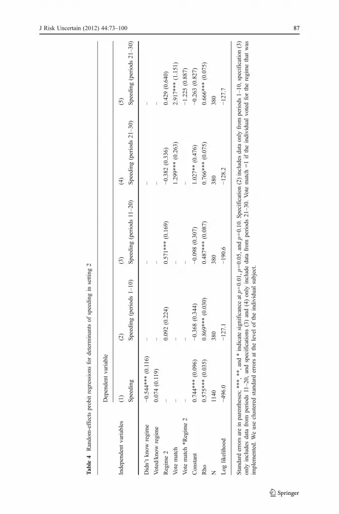
We present a separate series of regressions for each setting. Table 3 shows probitregressions for setting 1.24

Specification (1) tests for unconditional differences in speeding rates acrossblocks. As we found in our nonparametric tests, the speeding rate when the regimein place was unknown is significantly lower than when it is known and the expectedcost is low (the omitted category), and the speeding rate with a high expected cost issignificantly lower than with a low expected cost. Specifications (2)–(4) add theregime and the factor of whether the individual voted for the implemented regime;since voting is only permitted in periods 11–20 and 21–30, we only include the datafrom these categories in the regressions. We see that, as seen in Figs. 2 and 4, peopleare much more likely to speed when their preferred regime is in force. Whilespecification (3) indicates that people are significantly less likely to speed underregime 2, the interaction term in specification (4) shows that this effect is entirelydriven by behavior in block 3. Finally, there is no difference across regimes in theeffect of having voted for the implemented regime.

Table 4 shows similar regressions for setting 2. Specification (1) tests forunconditional differences in speeding rates across 10-period blocks. The speedingrate when the regime is unknown is significantly lower than when it is knownwithout voting, showing the effect of uncertainty on speeding rates, while there is nodifference between speeding rates according to whether one has voted (and learnedthe regime). Specifications (2)–(4) indicate that this is entirely driven by theinformed, no-voting case, where there is a somewhat higher speeding rate when thelikelihood of being caught is higher but the cost is lower (Regime 2). Once again,whether one voted for the implemented regime is a significant factor inspecifications (4) and (5). No other coefficients are significant in specifications (4)

24 In both Tables 3 and 4, the random-effects assumption that the unobserved individual effect is notcorrelated with any of the explanatory variables is violated when voting behavior is included in theregressions. To check for the robustness of the regression results, we have therefore performed bothlogit regressions and OLS regressions with fixed effects. The results are qualitatively nearly identical,with no serious changes in the significance levels of any of the explanatory variables. Since therandom-effects regressions are appropriate for some of the columns, we choose to report these results inall cases.

Table 2 Speeding rates by block of periods, setting 2

Category Overall rate Observations,regime 1

Rate inregime 1

Observations,regime 2

Rate inregime 2

Don’t know regime .579 (.025) 217 .567 (.034) 163 .595 (.039)

No vote/know regime .711 (.023) 191 .639 (.035) 189 .783 (.030)

Voted/know regime .721 (.023) 342 .719 (.024) 38 .737 (.073)

Standard errors are in parentheses

84 J Risk Uncertain (2012) 44:73–100

and (5), with the direction of the coefficient for regime reversing when theinteraction term is included. Thus, we see that, once again, there is less speedingwith uncertainty (comparing the informed, no-voting case—the omitted variable—tothe uninformed, no-voting case) and that the speeding rate is quite sensitive towhether or not one has voted for the regime that has been implemented.25

We can also make some comparisons across settings. For example, comparing theno vote/know regime in setting 2 to the uncertainty treatment in setting 1, we see thatthe rate of speeding is higher in the no vote/don’t know environment. A Wilcoxon-Mann–Whitney ranksum test on individual speeding rates (this is across differentindividuals in the two different settings) finds the difference to be marginallysignificant (Z=1.29, p=0.099, one-tailed test justified by ex-ante hypothesis). This isslight further evidence that uncertainty leads to lower violation rates. A secondcomparison is between the two voting environments with low cost, periods 11–20 insetting 1 and periods 21–30 in setting 2, where there should be no difference acrossthe identical decision environments. The violation rates are 0.685 and 0.721,respectively; the ranksum test on individual rates gives Z=1.046, p=0.296 (two-tailed test of the null hypothesis that the violation rates are not significantly differentfrom each other).

In closing Section 3, we would like to point out that if the expected cost ofspeeding is the same for each period within a category, people should either alwaysspeed or never speed. However, there is substantial within-subject variance within acategory for many participants. If we define consistency within a category aschoosing to speed either 0, 1, 9, or 10 times (allowing up to one deviation from

25 Having been caught (or not having been caught) speeding in the last period has no significant effect inour regressions. In principle, there is no reason to expect such an effect, as the outcome from speeding inthe past period should have no effect on the actual expected cost of speeding. In fact, while there is noeffect in the aggregate (people sped 80.2% of the time after having been caught speeding in the last period,compared to 76.6% of the time when they sped in the last period and were not caught), there is aconsiderable effect on individuals. In fact, the difference in these two rates exceeds 25 percentage pointsfor 39% of the population. However, these differences go in opposite directions, effectively eliminatingany aggregate effect. While it might seem natural that people are less likely to engage in a certain behaviorafter having a bad outcome (even though there is nothing to actually be learned), many people also seemto believe in the “law of averages.”

Fig. 4 Speeding rates by vote-match, setting 2

J Risk Uncertain (2012) 44:73–100 8585

Tab

le3

Random-effectsprobitregressionsfordeterm

inantsof

speeding

insetting

1

Dependent

variable

Independ

entvariables

(1)

(2)

(3)

(4)

Speeding

Speeding(periods

11–30)

Speeding(periods

11–30)

Speeding(periods

11–30)

Didn’tkn

owregime

−0.282

***(0.074

)–

––

Voted/kno

w,high

cost

−0.972

***(0.074

)−1

.129**

*(0.083

)−0

.105

(0.244

)−0

.103

(0.245

)

Regim

e2

–−0

.280**

*(0.089

)0.090(0.124

)0.072(0.168

)

Votematch

–0.80

4***

(0.083

)0.796*

**(0.084

)0.755*

**(0.282

)

Voted/kno

w,high

cost*R

egim

e2

––

−0.777

***(0.177

)−0

.779**

*(0.177

)

Votematch

*Regim

e–

––

0.031(0.201

)

Constant

0.571*

**(0.077

)0.69

4***

(0.158

)0.197(0.194

)0.221(0.249

)

Rho

0.534*

**(0.035

)0.53

4***

(0.035

)0.536*

**(0.038

)0.587*

**(0.039

)

N26

1017

4017

4017

40

Log

likelihood

−131

2.7

−827

.6−8

17.8

−817

.8

Standarderrorsarein

parentheses;***,

**,and

*indicatesignificance

atp=0.01,p

=0.05,and

p=0.10.S

pecificatio

ns(2)–(4)includ

edataon

lyperiod

s11–30.

Votematch

=1if

theindividual

votedfortheregimethat

was

implem

ented.

Weuseclusteredstandard

errors

atthelevelof

theindividual

subject

86 J Risk Uncertain (2012) 44:73–100

Tab

le4

Random-effectsprobitregressionsfordeterm

inantsof

speeding

insetting

2

Dependent

variable

Independ

entvariables

(1)

(2)

(3)

(4)

(5)

Speeding

Speeding(periods

1–10

)Speeding(periods

11–20)

Speeding(periods

21–30)

Speeding(periods

21–30)

Didn’tkn

owregime

−0.544**

*(0.116

)–

––

–

Voted/kno

wregime

0.074(0.119

)–

––

–

Regim

e2

–0.09

2(0.224

)0.571*

**(0.169

)−0

.382

(0.336

)0.429(0.640

)

Votematch

––

–1.29

9***

(0.263

)2.917*

**(1.151

)

Votematch

*Regim

e2

––

––

−1.225

(0.887

)

Constant

0.744*

**(0.096

)−0

.368

(0.344

)−0

.098

(0.307

)1.02

7**(0.476

)−0

.263

(0.827

)

Rho

0.575*

**(0.035

)0.86

9***

(0.030

)0.487*

**(0.087

)0.76

6***

(0.075

)0.666*

**(0.075

)

N1140

380

380

380

380

Log

likelihood

−496

.0−1

27.1

−190

.6−1

28.2

−127

.7

Standarderrorsarein

parentheses;***,

**,and

*indicatesignificance

atp=0.01,p

=0.05,and

p=0.10.S

pecificatio

n(2)includes

dataon

lyfrom

period

s1–10,specificatio

n(3)

only

includes

data

from

periods11–20,

andspecifications

(3)and(4)only

includedata

from

periods21–30.

Votematch

=1iftheindividu

alvo

tedfortheregimethat

was

implem

ented.

Weuseclusteredstandard

errors

atthelevelof

theindividual

subject.

J Risk Uncertain (2012) 44:73–100 8787

absolute consistency), we observed consistency within a category for about half ofthe participants overall.26 While a frequent lack of consistency in the speedingdecision might seem a bit disconcerting, we don’t feel that people change theirdecisions to reflect a change in risk attitudes per se. Instead, we propose twopotential explanations for the inconsistent behavior of half of the population:aversion to the stigma of getting caught, as well as a willingness to experiment. Inorder to explore whether individuals have an adverse reaction to being caught, weexplored the factors that appear to affect the willingness to speed or not, such asbeing caught in previous periods, not speeding in previous periods, speeding and notgetting caught in previous periods, and cumulative profits.27 When we examinebuild up effects (e.g. being apprehended two periods in a row), we find littleevidence to explain the choice of whether to speed or not. In fact, overall, the onlystatistically significant findings that we observe are an increase in the willingness tospeed when an individual has been caught in the two previous periods and a decreasein the willingness to speed when an individual did not speed in the two previousperiods. However, most of the explanatory variables that we included in this analysisdo not explain individual choices to speed or not.

Alternatively, individuals may have been investigating their options within theexperiment. This is not unusual in experimental work. For example, peoplefrequently switch their choices in Charness and Levin (2005), even with identicalparameters across periods, and also change their bids from period to period inCharness and Levin (2009), in an environment in which probabilities are completelytransparent. Eliaz and Frechette (2008) find that people like to diversify even when itis costly to do so and provides no benefit: they are willing to pay to switch from alottery that pays a prize in only one particular state of nature to a lottery that pays aprize in more than one state of nature, even though the overall distribution overprizes remains the same. Rubinstein (2002) finds that if individuals must make adecision that has many options (for example, guessing the color of a card that ispulled out of a deck containing 5 different colored cards), the individuals will tend touse a “probability matching” strategy. That is to say, they will attempt to mimic thepercentage of black, blue, green, etc. colored cards in the deck.28

4 Discussion

The theory of deterrence has implications for the prevention of proscribed activities,the level of punishment that individuals receive when committing a violation, theawards of a judge or jury (e.g. compensatory, punitive, and nominal damages), andthe policies that should be instituted to prevent violations. Understanding thedeterrence mechanisms that can be implemented and their expected effect onprevention of violations has very serious implications for society. Three key features

26 The precise figures are 48.9%, 58.6%, and 37.9% for the 87 participants in blocks 1, 2, and 3,respectively, in setting 1, as well as 68.4%, 44.7%, and 68.4% for the 38 participants in blocks 1, 2, and 3,respectively, in setting 2.27 We report the results of probit regression models in Appendix B.28 From a theoretical standpoint, Halevy and Feltkamp (2005) discuss hedging in an environment withuncertainty.

88 J Risk Uncertain (2012) 44:73–100

of our analysis include (a) whether people understand the concept of deterrence(i.e., is the frequency of proscribed behavior sensitive to the expected cost), (b)whether it is worth implementing a higher probability regime that is costlierthan a lower probability regime with the same expected cost, and (c) howuncertainty affects the violation rate. The answers to these questions areimportant not only for the prevention of speeding on roadways, but are alsorelevant for much larger issues such as the prevention of tax evasion, burglary,homicide, and medical malpractice.

Empirical data that permits a careful examination of the impact of enforcementregimes on proscribed activities is very difficult to obtain. An even more difficultdata-acquisition task arises when one attempts to test for the effect of uncertaintypertaining to the enforcement tool on an individual’s incentive to commit a violation.Although there are many reasons why this task is so daunting, one such reason isthat field data pertaining to an individual’s decision to commit a violation is difficultto track and, even if collected, would be incomplete because of the overwhelmingnumber of violations committed but not detected. Given the difficulty in obtainingaccurate and complete field data, we performed laboratory tests of whether or notpeople understand deterrence and of the effect of uncertainty on deterrence tools.The experimental setting provides the ability to inject and extract uncertainty fromthe deterrence mechanisms that the participants in the experiments face, allowing usto discern the impact of uncertainty on the decisions of subjects.

When using scenarios to understand the impact of uncertainty on the effectivenessof deterrence mechanisms, Sunstein et al. (2000) draws our attention to the fact thatsubjects might not promote optimal deterrence. We find that individuals who aredirectly involved with the legal process understand and respond to deterrencemechanisms. As noted in setting 1, the speeding rates decreased significantly whenthe expected cost of speeding increased.

One potential aspect of the theory of deterrence that has been theoreticallydiscussed but has received little empirical attention is the effect of uncertainty aboutthe magnitude of a deterrence tool, from the perspective of the potential violator. Forexample, people who are considering committing a crime most likely do notaccurately perceive the probability of being apprehended; instead, they perceive theirprobability with some level of error. A similar argument can be made about thepunishment that an individual will receive for committing a crime, as they might notknow how a judge/jury would rule.29 Although Bebchuk and Kaplow (1992) andSah (1991) have discussed the effect of uncertainty on the perception of the probabilityin theoretical settings, the effect has not been examined empirically. Moreover, thecomparison of alternative enforcement regimes—both theoretically and empirically—does not appear to be discussed in the law and economics literature.

In order to examine the effect of uncertainty on the individual’s decision ofwhether or not to violate a rule, the first 10 periods in both settings offered twoequally likely enforcement regimes with identical expected costs. The uncertaintyabout which regime would actually be in place led to a compound lottery. The

29 In the roadway speeding environment it is true that knowledge of the fines is available to all potentialviolators. However, most individuals are not accurately informed about these fines. Moreover, judgesoften allow violators to plead a lesser charge.

J Risk Uncertain (2012) 44:73–100 8989

participants in the experiment understood that each regime was equally likely and, exante, had to decide whether or not to speed. However, in the last 20 periods ofsetting 1 (and the last 10 periods of setting 2), the individuals first voted on a regimeand were then told which regime was in place. The removal of uncertainty allows usto both understand the effect of uncertainty as well as the perception of the relativeexpected costs. Individuals are more likely to speed in both settings 1 and 2 whenthis uncertainty is removed. In addition, since individuals typically (in five cases ofsix) speed more frequently when the probability of detection is lower (see Tables 1and 2), this seems consistent with the theory that expected costs are perceived to belower in a regime with a lower probability and a higher fine, even though themathematical expected costs are the same.

To the extent that our laboratory environment reflects the field, these findingsprovide interesting potential policy implications. First, it appears that moreuncertainty leads individuals to violate less than they would otherwise, so that anenforcement regime is likely to be more effective when uncertainty is present.30

Second, we find even stronger evidence, which is consistent with the law andeconomics literature that states that a policy-maker should prefer the low probability/high fine. That is, given our finding that individuals speed approximately the sameamount under either regime and since increases in the probability can only beaccomplished by increases in enforcement efforts, a low probability/high fine shouldyield approximately the same level of deterrence at a lower cost.

If we can extend alternative regimes in this paper to situations when damages can beassessed, we can say more about the amount of punitive damages. In particular, we cancomment on the levels of punitive damages that should be assessed when an individualviolates. To start, we find (limited) evidence that the expected cost is perceived to belarger when there are lower fines and higher probabilities relative to lower probabilitiesand higher fines, despite the fact that the expected costs are identical. Therefore, if anindividual commits a violation in the high probability/low fine environment, he or shevalues the violation at a level that is greater than the perceived expected cost. If thepurpose of punitive damages is to deter the individual from committing the crime in thefuture, then imposing a positive level of damages is justified in this environment.

Similarly, in a low probability/high fine environment, an individual that commitsa violation might perceive the expected cost as being smaller than the actualexpected cost.31 In this instance, it would seem less reasonable to assess lowerpunitive damages, if any at all. This line of reasoning does have a particular intuitiveappeal. Individuals that are aware that they will be inspected frequently but stillcommit a violation are more negligent than an individual that is inspectedinfrequently. Thus, we should assess higher punitive damages to those individualsthat are more negligent.

30 For example, law enforcement agencies can implement uncertainty over the probability of being caughtby setting up enforcement “blitzes” that randomly change. Eeckhout et al. (2010) discuss randomcrackdowns by law enforcement and determine that this could be part of an optimal policing strategy,specifically for speeding.31 As noted in Sunstein et al. (2000), a low probability of apprehension could suggest stealthiness on thepart of the perpetrator. This claim is not refuted in our analysis; however, it should be noted that a lowerprobability of apprehension could appear to encourage stealthiness because the expected cost is perceivedto be lower (relative to a higher probability/lower fine combination that has equivalent expected costs).

90 J Risk Uncertain (2012) 44:73–100

On a final policy note, the voting on regimes in this experiment providesevidence about the behavior of drivers when they vote in favor of/against aregime. That is to say, when individuals vote for a regime, they tend to speedconsiderably more frequently in that regime than when they vote against theregime that is instituted. Therefore, it would seem that implementing the regimethat is less desired by the potential violators will lead to a reduction in thenumber of violators.

Our study is subject to a number of limitations; we mention three of these. First,there is no actual crime being committed in the laboratory. Second, our simpleenvironment does not take into account the externalities present when another persondecides to speed. Third, we do not permit heterogeneity with respect to the costs andbenefits of speeding. While it does not seem possible to observe criminal behavior inthe laboratory, the second and third points are suitable topics for future investigation.It also seems valuable to extend this research to examine different types ofenforcement concerns, such as profiling in law enforcement. In any case, we feel thatour study represents an important step in the area of deterrence and that futureresearch can build upon our results.

Acknowledgements We would like to thank Ted Frech, Yoram Halevy and Joel Sobel for helpfulcomments. We would also like to thank participants of the Canadian Experimental and BehavioralEconomics Research Group at the Canadian Economics Association 2009, the 2009 EWEBE meetings inBarcelona, and seminar participants at Vanderbilt University Law School. DeAngelo acknowledgesfinancial support from the Department of Economics at UCSB. Charness acknowledges support from theNational Science Foundation and the Dean of Social Sciences at UCSB.

Appendix A—Sample experimental instructions

Experiment instructions—Setting 1

General Rules: No talking. No use of cell phones. No looking at neighbor’s screens.You are about to participate in an experiment on decision-making carried out by a

researcher from UCSB. During this session, you can earn money. The amount ofyour earnings depends on your decisions and on the decisions of the otherparticipants in this session. The session consists of 30 rounds. Your earnings will bedetermined by randomly choosing one payout from rounds 1–10, 11–20, and 21–30.The payout mechanism is explained in detail below. Your earnings will be paid toyou in cash in private.

Your decisions are anonymous and confidential.The experiment is split into 2 separate sections. The first section consists of 10

rounds and the second consists of 20 rounds. Instructions for the first 10 rounds areprovided below. Instructions for the last 20 rounds will be given upon completion ofthe first 10 rounds.

Rounds 1–10: You are attempting to travel to the same destination 10 separatetimes—much like a commuter travels to work every day—and will receive a payoutfor each separate trip. You will have the option to speed or not when traveling. Therewill be two potential enforcement regimes—which you will be told before decidingwhether to speed or not—and the probability that either regime will be instituted is

J Risk Uncertain (2012) 44:73–100 9191

equally likely. An enforcement regime is both a probability of getting caught whenspeeding and a corresponding fine, denoted f, which will be imposed if you arecaught speeding. An individual that speeds and arrives at the destination withoutbeing apprehended will receive a payout of $1.00 per round. An individual thatspeeds and is apprehended for speeding receives a payout of $1.00-f per round,where f is the fine that is imposed by the enforcement regime that is instituted. Notethat 0< f<1 always. Lastly, an individual that obeys the law and does not speedreceives a payout of $0.60 per round.

There are two potential enforcement regimes:

Regime A: Chance of getting caught=1/3, Fine=$0.90Regime B: Chance of getting caught=2/3, Fine=$0.45

Regime A and Regime B are equally likely—i.e. there is a 50% chance that eitherregime is randomly chosen.

Examples

Situation 1: Regime A is randomly selected. There are three possible payouts:

Payout 1: Participant does not speed and receives a payout of $0.60.Payout 2: Participant speeds, is not caught and receives a payout of $1.00.Payout 3: Participant speeds, is caught and receives a payout of $0.10 (= $1.00−$0.90).

Situation 2: Regime B is randomly selected. There are three possible payouts:


Payouts: The payout that you will receive for rounds 1–10 will be determined byrandomly choosing one of the 10 rounds and then multiplying the payout of thatround by 5. Consider the following possible payouts:

Example Payout 1: Suppose that round 5 is randomly chosen as the payout roundand that you decide to not speed in round 5 and so your payoutfor round 5 is $0.60. Therefore, your payout for rounds 1–10 is$3.00 (=5*$0.60).

Example Payout 2: Suppose that round 3 is randomly chosen as the payout roundand that you decide to speed in round 3 and were not caughtand so your payout for round 3 is $1.00. Therefore, yourpayout for rounds 1–10 is $5.00 (=5*$1.00).

Example Payout 3: Suppose that round 7 is randomly chosen as the payout round.In round 7 you decided to speed, Regime A is instituted andyou are caught speeding. Your payout for round 7 is $0.10.Therefore, your payout for rounds 1–10 is $0.50 (=5*$0.10).

Example Payout 4: Suppose that round 9 is randomly chosen as the payout round.In round 9 you decided to speed, Regime B is instituted andyou are caught speeding. Your payout for round 9 is $0.55.Therefore, your payout for rounds 1–10 is $2.25 (=5*$0.55).

92 J Risk Uncertain (2012) 44:73–100

Total Payouts: Your total payout is determined by multiplying a randomly chosenround in each block (1–10, 11–20, 21–30) by 5 and then adding a $5.00 show uppayment. The payout is explained mathematically below:

Total Payout ¼ ðPayout1�10 þ Payout11�20 þ Payout21�30Þ»5þ $5

Rounds 11–20: As in the first ten rounds, you are attempting to travel to the samedestination 10 separate times—much like a commuter travels to work every day—and will receive a payout for each separate trip. You will have the option to speed ornot when traveling. In each of these rounds you and the other members of theexperiment will now have two decisions to make. First, you will vote on anenforcement regime and the regime receiving the majority vote will be posted so thateveryone is aware of the enforcement regime. After observing the winning regime,you will then be asked to decide whether you will speed or not. As in the first 10rounds, an individual that speeds and arrives at the destination without beingapprehended will receive a payout of $1.00 per round. An individual that speeds andis apprehended for speeding receives a payout of $1.00-f per round, where f is thefine that is imposed by the enforcement regime that is instituted. Note that 0< f<1always. Lastly, an individual that obeys the law and does not speed receives a payoutof $0.60 per round.

Rounds 21–30: As in rounds 11–20, in each of these rounds you and the othermembers of the experiment will have two decisions to make. First, you will vote onan enforcement regime and the regime receiving the majority vote will be posted sothat everyone is aware of the enforcement regime. However, the regimes aredifferent.

Regime A: Chance of getting caught=3/5, Fine=$0.833Regime B: Chance of getting caught=4/5, Fine=$0.625

Whichever regime (Regime A or Regime B) that receives the most votes will beimplemented and posted. After observing the winning regime, you will then beasked to decide whether you will speed or not. As in the first 10 rounds, anindividual that speeds and arrives at the destination without being apprehended willreceive a payout of $1.00 per round. An individual that speeds and is apprehendedfor speeding receives a payout of $1.00-f per round, where f is the fine that isimposed by the enforcement regime that is instituted. Note that 0< f<1 always.Lastly, an individual that obeys the law and does not speed receives a payout of$0.60 per round.

Examples

Situation 1: Regime A is implemented because it receives the most votes. There arethree possible payouts:

Payout 1: Participant does not speed and receives a payout of $0.60.Payout 2: Participant speeds, is not caught and receives a payout of $1.00.Payout 3: Participant speeds, is caught and receives a payout of $0.167 (= $1.00−

$0.833).

J Risk Uncertain (2012) 44:73–100 9393

Situation 2: Regime B is implemented because it receives the most votes. Thereare three possible payouts:

Payout 1: Participant does not speed and receives a payout of $0.60.Payout 2: Participant speeds, is not caught and receives a payout of $1.00.Payout 3: Participant speeds, is caught and receives a payout of $0.375 (= $1.00−

$0.625).


Example Payout 1: Suppose that round 25 is randomly chosen as the payout roundand that you decide to not speed in round 25 and so yourpayout for round 5 is $0.60. Therefore, your payout for rounds21–30 is $3.00 (=5*$0.60).

Example Payout 2: Suppose that round 23 is randomly chosen as the payout roundand that you decide to speed in round 3 and were not caughtand so your payout for round 23 is $1.00. Therefore, yourpayout for rounds 21–30 is $5.00 (=5*$1.00).

Example Payout 3: Suppose that round 27 is randomly chosen as the payoutround. In round 27 you decided to speed, Regime A isinstituted and you are caught speeding. Your payout forround 7 is $0.167. Therefore, your payout for rounds 21–30is $0.835 (=5*$0.167).

Example Payout 4: Suppose that round 29 is randomly chosen as the payoutround. In round 29 you decided to speed, Regime B isinstituted and you are caught speeding. Your payout forround 9 is $0.375. Therefore, your payout for rounds 21–30is $1.875 (=5*$0.375).

Total Payouts: Your total payout is determined by summing your payouts for allthirty rounds, dividing this total in half, and then adding a $5.00 show up payment.The payout is mathematically explained below:


Note that the minimum total payout that you could receive is $6.84, which couldbe obtained by getting caught speeding in Regime A in all rounds. The maximumpayout is $20.00=($5.00+$15.00), which could be obtained by speeding and notgetting caught in all rounds.

Experiment instructions—setting 2

General Rules: No talking. No use of cell phones. No looking at neighbor’s screens.You are about to participate in an experiment on decision-making carried out by a

researcher from the University of California at Santa Barbara. During this session,you can earn money. The amount of your earnings depends on your decisions and onthe decisions of the other participants in this session. The session consists of 30

94 J Risk Uncertain (2012) 44:73–100

rounds. Your earnings will be determined by randomly choosing one payout fromrounds 1–10, one payout from rounds 11–20, and one payout from rounds 21–30.The payout mechanism is explained in detail below. Your earnings will be paid toyou in cash in private.

Your decisions are anonymous and confidential.The experiment is split into 3 separate sections. Each section consists of 10

rounds. Instructions for each set of 10 rounds are provided below.Rounds 1–10: You are attempting to travel to the same destination 10 separate

times—much like a commuter travels to work every day—and will receive a payoutfor each separate trip. You will have the option to speed or not when traveling. Therewill be two potential enforcement regimes—which you will be told before decidingwhether to speed or not—and the probability that either regime will be instituted isequally likely. An enforcement regime is both a probability of getting caught whenspeeding and a corresponding fine, denoted f, which will be imposed if you arecaught speeding. An individual that speeds and arrives at the destination withoutbeing apprehended will receive a payout of $1.00 per round. An individual thatspeeds and is apprehended for speeding receives a payout of $1.00 - f per round,where f is the fine that is imposed by the enforcement regime that is instituted. Notethat the fine is always positive and less than $1.00. Lastly, an individual that obeysthe law and does not speed receives a payout of $0.60 per round.

Examples

There are two potential enforcement regimes:

Regime A: Chance of getting caught if speeding=1/3, Fine=$0.90Regime B: Chance of getting caught if speeding=2/3, Fine=$0.45

Regime A and Regime B are equally likely—i.e. there is a 50% chance that eitherregime is randomly chosen.

Situation 1: Regime A is randomly selected. There are three possible payouts:


Situation 2: Regime B is randomly selected. There are three possible payouts:



Example Payout 1: Suppose that round 5 is randomly chosen as the payout roundand that you had decided to not speed in round 5 and so yourpayout for round 5 is $0.60. Therefore, your payout for rounds1–10 is $6.00 (=10×$0.60).

J Risk Uncertain (2012) 44:73–100 9595

Example Payout 2: Suppose that round 3 is randomly chosen as the payout roundand that you had decided to speed in round 3 and were notcaught and so your payout for round 3 is $1.00. Therefore,your payout for rounds 1–10 is $10.00 (=10×$1.00).

Example Payout 3: Suppose that round 7 is randomly chosen as the payout round.In round 7 you had decided to speed, Regime A is institutedand you are caught speeding. Your payout for round 7 is $0.10.Therefore, your payout for rounds 1–10 is $1.00 (=10×$0.10).

Example Payout 4: Suppose that round 9 is randomly chosen as the payout round.In round 9 you had decided to speed, Regime B is institutedand you are caught speeding. Your payout for round 9 is $0.55.Therefore, your payout for rounds 1–10 is $5.50 (=10×$0.55).



Note that the minimum total payout that you could receive is $6.50=($5.00+$1.50), which could be obtained by getting caught speeding in Regime A in allrounds. The maximum payout is $20.00=($5.00+$15.00), which could be obtainedby speeding and not getting caught in all rounds.

Rounds 11–20: As in the first ten rounds, you are attempting to travel to the samedestination 10 separate times—much like a commuter travels to work every day—and will receive a payout for each separate trip. You will have the option to speed ornot when traveling. The main difference between the rounds 1–10 and rounds 11–20is that you will be told which regime is in place before deciding whether to speed ornot. In other words, you will know with certainty the enforcement regime that is inplace. Recall that an enforcement regime is both a probability of getting caught whenspeeding and a corresponding fine, denoted f, which will be imposed if you arecaught speeding. An individual that speeds and arrives at the destination withoutbeing apprehended will receive a payout of $1.00 per round. An individual thatspeeds and is apprehended for speeding receives a payout of $1.00—f per round,where f is the fine that is imposed by the enforcement regime that is instituted. Notethat 0< f<1 always. Lastly, an individual that obeys the law and does not speedreceives a payout of $0.60 per round.

Rounds 21–30: In each of the last 20 rounds you and the other members of theexperiment will now have two decisions to make. First, you will vote on anenforcement regime and the regime receiving the majority vote will be posted so thateveryone is aware of the enforcement regime. After observing the winning regimeyou will then be asked to decide whether you will speed or not. As in the first 10rounds, an individual that speeds and arrives at the destination without beingapprehended will receive a payout of $1.00 per round. An individual that speeds andis apprehended for speeding receives a payout of $1.00—f per round, where f is thefine that is imposed by the enforcement regime that is instituted. Note that 0< f<1always. Lastly, an individual that obeys the law and does not speed receives a payoutof $0.60 per round.

96 J Risk Uncertain (2012) 44:73–100

Situation 1: Suppose 7 out of 11 people vote in favor of Regime A and so RegimeA is instituted. An individual who chooses to speed has a one in three chance ofbeing caught speeding and paying a fine of $0.90. There are three possible payoutsthat a participant could receive:


Situation 2: Suppose 6 out of 11 people vote in favor of Regime B and so RegimeB is instituted. An individual who chooses to speed has a two in three chance ofbeing caught speeding and paying a fine of $0.45. There are three possible payoutsthat a participant could receive:



Example Payout 1: Suppose that round 25 is randomly chosen as the payout roundand that you had decided to not speed in round 25 and so yourpayout for round 5 is $0.60. Therefore, your payout for rounds1–10 is $6.00 (=10×$0.60).

Example Payout 2: Suppose that round 23 is randomly chosen as the payout roundand that you had decided to speed in round 23 and were notcaught and so your payout for round 3 is $1.00. Therefore,your payout for rounds 1–10 is $10.00 (=10×$1.00).

Example Payout 3: Suppose that round 27 is randomly chosen as the payout round.In round 27 you had decided to speed, Regime A received themajority vote and you are caught speeding. Your payout forround 7 is $0.10. Therefore, your payout for rounds 1–10 is$1.00 (=10×$0.10).

Example Payout 4: Suppose that round 29 is randomly chosen as the payout round.In round 29 you decided to speed, Regime B received themajority vote and you are caught speeding. Your payout forround 9 is $0.55. Therefore, your payout for rounds 1–10 is$5.50 (=10×$0.55).



Note that the minimum total payout that you could receive is $6.50=($5.00+$1.50), which could be obtained by getting caught speeding in Regime A in allrounds. The maximum payout is $20.00=($5.00+$15.00), which could be obtainedby speeding and not getting caught in all rounds.

J Risk Uncertain (2012) 44:73–100 9797

Appendix B

To examine potential determinants of consistency in the choices that individualsmake when determining whether or not to speed, we run probit regressions for thedecision to speed on whether or not the individual was caught in previous periods,was not caught in previous periods, did not speed in previous periods, and whichregime that the individual faced. We report elasticities in the table below.

References

Alm, J., Jackson, B. R., & McKee, M. (1993). Fiscal exchange, collective decision institutions and taxcompliance. Journal of Economic Behavior and Organization, 22, 285–303.

Alm, J., McClelland, G. H., & Schulze, W. D. (1999). Changing the social norm of tax compliance.Kyklos, 52, 141–171.

Anderson, L. R., & Stafford, S. L. (2003). Punishment in a regulatory setting: Experimental evidence fromthe VCM. Journal of Regulatory Economics, 24(1), 91–110.

Ashenfelter, O., & Greenstone, M. (2004). Using mandated speed limits to measure the value of astatistical life. Journal of Political Economy, 112(S1), S226–S267.

Baker, T., Harel, A., & Kugler, T. (2004). The virtues of uncertainty in law: an experimental approach.Iowa Law Review, 89, 1–43.

Bar-Ilan, A., & Sacerdote, B. (2004). Response of criminals and noncriminals to fines. Journal of Law andEconomics, 47(1), 1–17.

Bebchuk, L. A., & Kaplow, L. (1992). Optimal sanctions when individuals are imperfectly informed aboutthe probability of apprehension. NBER Working Paper 4079.

Becker, G. S. (1968). Crime and punishment: an economic approach. Journal of Political Economy, 76(2),169–217.

Block, M., & Garety, V. (1995). Some experimental evidence on differences between student and prisonerreactions to monetary policy and risk. Journal of Legal Studies, 24(1), 123–138.

Charness, G., & Levin, D. (2005). When optimal choices feel wrong: a laboratory study of Bayesianupdating, complexity, and affect. American Economic Review, 95(4), 1300–1309.

Charness, G., & Levin, D. (2009). The origin of the winner’s curse: a laboratory study. AmericanEconomic Journal – Micro, 1(1), 207–236.

Table 5 Probit regressions for determinants of speeding

Independent variables Speed current period(Block 1)

Speed current period(Block 2)

Speed current period(Block 3)

Caught previous period −0.039 (0.040) 0.027 (0.039) −0.121 (0.162)

Caught previous 2 periods 0.002 (0.009) 0.018*** (0.005) 0.024*** (0.011)

Not caught previous 2 periods 0.049 (0.186) 0.012 (0.007) 0.003 (0.005)

Did not speed previous period −0.163*** (0.075) 0.039 (0.052) −0.366 (0.292)

Did not speed previous 2 periods −0.110*** (0.034) −0.187*** (0.038) −0.160*** (0.061)

Regime – 0.037 (0.069)

N 868 868 868

Standard errors are in parentheses; ***, **, and * indicate significance at p=0.01, p=0.05, and p=0.10.All specifications report elasticities between the dependent and independent variable. Regime is anindicator variable that takes on a value of zero if regime 1 is in place and one if regime 2 is in place

98 J Risk Uncertain (2012) 44:73–100

DeAngelo, G., & Hansen, B. (2009). Life and death in the fast lane: Police enforcement and roadwaysafety. Working Paper.

Di Tella, R., & Schargrodsky, E. (2004). Do police reduce crime? Estimates using the allocation of policeforces after a terrorist attack. American Economic Review, 94(1), 115–133.

Eeckhout, J., Persico, N., & Todd, P. (2010). A theory of optimal random crackdowns. AmericanEconomic Review, 100(3), 1104–35.

Ehrlich, I. (1996). Crime, punishment, and the market for offenses. Journal of Economic Perspectives, 10(1), 43–67.

Eliaz, K., & Frechette, G. (2008). Don’t put all your eggs in one basket!: an experimental study of falsediversification. Mimeo.

Ellsberg, D. (1961). Risk, ambiguity, and the savage axioms. Quarterly Journal of Economics, 75, 643–659.

Feld, L. P., & Tyran, J. R. (2002). Tax evasion and voting: an experimental analysis. Kyklos, 55, 197–222.Fischbacher, U. (2007). z-Tree: Zurich toolbox for ready-made economic experiments. Experimental

Economics, 10(2), 171–178.Fox, C., & Tversky, A. (1995). Ambiguity aversion and comparative ignorance. Quarterly Journal of

Economics, 110(3), 585–603.Garoupa, N. (2003). Behavioral economic analysis of crime: a critical review. European Journal of Law

and Economics, 15(1), 5–15.Greiner, B. (2004). An online recruitment system for economic experiments. In K. Kremer, & V.

Macho (Eds.), Forschung und wissenschaftliches Rechnen. GWDG Bericht 63, Ges. für Wiss.Datenverarbeitung, Göttingen, 79–93.

Halevy, Y. (2007). Ellsberg revisited: an experimental study. Econometrica, 75(2), 503–536.Halevy, Y., & Feltkamp, V. (2005). A Bayesian approach to uncertainty aversion. Review of Economic

Studies, 72, 449–466.Harel, A., & Segal, U. (1999). Criminal law and behavioral law and economics: observations on the

neglected role of uncertainty in deterring crime. American Law and Economics Review, 1, 276–312.Heath, C., & Tversky, A. (1991). Preference and belief: ambiguity and competence in choice under

uncertainty. Journal of Risk and Uncertainty, 4, 5–28.Hutchinson, K. P., & Yates, A. J. (2007). Crime on the court: a correction. Journal of Political Economy,

115, 515–519.Ihlanfeldt, K. R. (2003). Rail transit and neighborhood crime: the case of Atlanta, Georgia. Southern

Economic Journal, 70(2), 273–294.Jolls, C., Sunstein, C. R., & Thaler, R. H. (1998). A behavioral approach to law and economics. Stanford

Law Review, 50, 1471–1550.Knight, F. (1921). Risk, uncertainty, and profit. Boston and New York: Houghton Mifflin.Lave, C. (1985). Speeding, coordination, and the 55MPH limit. American Economic Review, 75(5), 1159–1164.Lazear, E. P. (2004). Speeding, tax fraud, and teaching to the test. NBER Working Paper 10932.McCormick, R. E., & Tollison, R. D. (1984). Crime on the court. Journal of Political Economy, 92(2),

223–35.Mookherjee, D. (1997). The economics of enforcement. In A. Bose, M. Rakshit, & A. Sinha (Eds.), Issues

in economic theory and policy, essays in honor of Tapas Majumdar (pp. 202–249). New Delhi:Oxford University Press.

Mookherjee, D., & Png, I. P. L. (1994). Marginal deterrence in enforcement of law. Journal of PoliticalEconomy, 102, 1039–66.

Polinsky, A. M., & Shavell, S. (1979). The optimal tradeoff between the probability and magnitude offines. American Economic Review, 69(5), 880–91.

Posner, R. A. (1985). An economic theory of the criminal law. Columbia Law Review, 85, 1193–1231.Rubinstein, A. (2002). Irrational diversification in multiple decision problems. European Economic

Review, 46, 1369–1378.Sah, R. K. (1991). Social osmosis and patterns of crime. Journal of Political Economy, 99(6), 1272–1295.Savage, L. J. (1954). The foundations of statistics. New York: John Wiley.Siegel, S., & Castellan, N. (1988). Nonparametric statistics for the behavioral sciences. Boston:

McGraw-Hill.Stigler, G. J. (1970). The optimum enforcement of laws. Journal of Political Economy, 78(3), 526–36.Sunstein, C. R. (1997). Behavioral analysis of law. University of Chicago Law Review, 64, 1175–94.Sunstein, C. R., Schkade, D. A., & Kahneman, D. (2000). Do people want optimal deterrence? Journal of

Legal Studies, 29(1), 237–53.

J Risk Uncertain (2012) 44:73–100 9999

Viscusi, W. K. (1986). The risks and rewards of criminal activity: a comprehensive test of criminaldeterrence. Journal of Labor Economics, 4(3), 317–40.

Viscusi, W. K., & Evans, W. N. (2006). Behavioral probabilities. Journal of Risk and Uncertainty, 32, 5–15.Viscusi, W. K., & Hakes, J. K. (2003). Risk ratings that do not measure probabilities. Journal of Risk

Research, 6(1), 23–43.Von Neumann, J., & Morgenstern, O. (1947). The theory of games and economic behavior. Princeton, NJ:

Princeton University Press.Wu, G., & Gonzalez, R. (1996). Curvature of the probability weighting function. Management Science,

42, 1676–1690.

100 J Risk Uncertain (2012) 44:73–100

Documents

Deterrence, expected cost, uncertainty and voting: Experimental evidence