Environ Monit Assess (2009) 158:593–608DOI 10.1007/s10661-008-0607-9

Determination of the compositional change (1999–2006)in the pine forests of British Columbia due to mountainpine beetle infestation

Colin Robertson · Carson J. Q. Farmer ·Trisalyn A. Nelson · Ian K. Mackenzie ·Michael A. Wulder · Joanne C. White

Received: 7 March 2008 / Accepted: 10 October 2008 / Published online: 20 November 2008© Springer Science + Business Media B.V. 2008

Abstract The current mountain pine beetle (Den-droctonus ponderosae Hopkins) outbreak inBritish Columbia and Alberta is the largestrecorded forest pest infestation in Canadian his-tory. We integrate a spatial hierarchy of mountainpine beetle and forest health monitoring data,collected between 1999 and 2006, with provincialforest inventory data, and generate three infor-mation products representing 2006 forest condi-tions in British Columbia: cumulative percentageof pine infested by mountain pine beetle, per-centage of pine uninfested, and the change in thepercentage of pine on the landscape. All inputdata were formatted to a standardized spatial rep-resentation (1 ha minimum mapping unit), withpreference given to the most detailed monitoringdata available at a given location for character-izing mountain pine beetle infestation conditions.The presence or absence of mountain pine beetle

C. Robertson (B) · C. J. Q. Farmer ·T. A. Nelson · I. K. MackenzieSpatial Pattern Analysis & Research (SPAR)Laboratory, Department of Geography,University of Victoria, P.O. Box 3050,Victoria, BC, V8W 3P5, Canadae-mail: colinr23@gmail.com

M. A. Wulder · J. C. WhiteCanadian Forest Service (Pacific Forestry Centre),Natural Resources Canada, 506 West Burnside,Victoria, BC, V8Z 1M5, Canada

attack was validated using field data (n = 2054).The true positive rate for locations of red attackdamage over all years was 92%. Classification ofattack severity was validated using the Kruskalgamma statistic (γ = 0.49). Error between thesurvey data and field data was explored usingspatial autoregressive (SAR) models, which indi-cated that percentage pine and year of infesta-tion were significant predictors of survey error atα = 0.05. Through the integration of forest inven-tory and infestation survey data, the total area ofpine infested is estimated to be between 2.89 and4.14 million hectares. The generated outputs addvalue to existing monitoring data and provide in-formation to support management and modelingapplications.

Keywords Mountain pine beetle · Mapping ·Data integration · Monitoring · Infestation

Introduction

Forest health monitoring and mountain pinebeetle in western Canada

The mountain pine beetle (Dendroctonus pon-derosae Hopkins) is endemic to forests of westernNorth America. Periodically, beetle populationsrise to epidemic levels, causing extensive and in-tensive tree mortality in pine forests (Safranyik

594 Environ Monit Assess (2009) 158:593–608

and Carroll 2006). Depending on the stage of themountain pine beetle population cycle and thespatial scale of interest, there may be a variety ofmanagement options available to forest managersto limit beetle-caused pine mortality (Nelson et al.2006a). Monitoring programs allow forest man-agers to track the status of beetle populations, andseveral different data sources have been used formonitoring purposes, with each data source pro-viding a level of detail suitable for a particular in-formation need (Wulder et al. 2006a). The variousmonitoring approaches used in British Columbiaform a survey hierarchy that informs three dis-tinct management objectives: strategic, tactical,and operational. Each level of this hierarchy ischaracterized by the extent and detail of the spa-tial data provided (e.g., a synoptic, landscape levelsurvey or a detailed forest stand level survey),relative accuracy, and cost. This hierarchy extendsfrom broad, provincial scale forest health surveysconducted using a fixed-wing aircraft to detailed,stand level surveys conducted using a helicopterequipped with GPS; as one moves through thehierarchy from a coarse overview to increasinglevels of detail, surveys cover smaller geographicareas and provide more detailed information,while relative accuracy and costs increase.

To identify areas with mountain pine beetleinfestation, aerial survey programs rely on thecharacteristic fading of an infested tree’s crown fo-liage. Trees are attacked during beetle emergence,which occurs in mid- to late summer throughoutmost of British Columbia (Safranyik et al. 1974).After a successful attack by mountain pine bee-tles, the infested tree will die and the crownswill gradually fade from green (green attack), toyellow, to red (red attack). Eventually, the treewill lose all of its foliage, a condition referred toas gray attack. It is estimated that after 1 year,over 90% of trees successfully attacked by moun-tain pine beetle will have red needles (BritishColumbia Ministry of Forests 1995). Variability inthe rate of foliage discoloration may be attributedto partial and full multivoltinism (more than onebrood of beetles per year; Reid 1962), semivol-tinism (the extension of one life cycle over morethan 1 year; Amman 1973), and other site andtree characteristics, such as drought (Wulder et al.2006b).

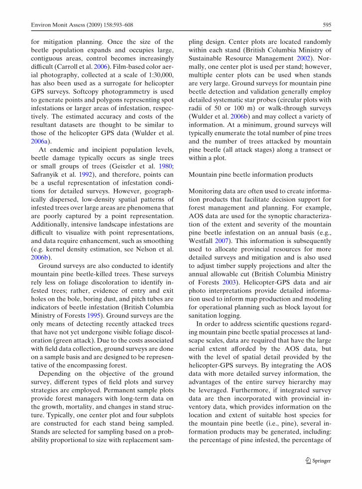
At the provincial scale, aerial overview surveys(AOS) are conducted annually using fixed-wingaircraft and are designed to capture informationon a wide range of forest health issues. Observersrecord the location of visible forest health is-sues, including mountain pine beetle infestations,onto 1:100,000 or 1:250,000 base maps (BritishColumbia Ministry of Forests 2000). Given the lifecycle of the beetle and the rate at which the foliageof attacked trees fade, the AOS data typicallycaptures trees killed by the beetle in the previousyear. Small groups of red attack trees are recordedas points, while larger areas of infestation aredelineated as polygons on the basemap. Infesta-tions are coded with a severity rating indicatingthe percentage of the total area of each delin-eated polygon that is composed of mountain pinebeetle-caused pine mortality (Table 1) for severityclasses.

The AOS provides the greatest spatial cover-age at the lowest cost when compared with othermonitoring initiatives (Wulder et al. 2006a). Therehas not been a comprehensive ground validationof AOS data to current standards. The primarypurpose of the AOS data is to aid strategic levelplanning by capturing trends in forest health fromyear to year.

At a more detailed spatial scale, helicopter GPSsurveys have been conducted in areas of BritishColumbia impacted by the mountain pine beetle.These helicopter-based surveys record the loca-tion (using GPS) and number of infested trees at aspecified location. These detailed surveys are gen-erally only conducted in areas where the spatialextent of the infestation is limited and, therefore,where suppression is still viable. In this context,detailed surveys provide important information

Table 1 Severity class ratings used in aerial overview sur-vey (AOS) mapping in British Columbia

Description Code Range (%) Mid Point (%)

Tracea T < 1 0.5Light L 1–10 5Moderate M 11–29 20Severe S 30–49 35Very severeb V 50+ 55aCode introduced in 2004bCode introduced in 2005

Environ Monit Assess (2009) 158:593–608 595

for mitigation planning. Once the size of thebeetle population expands and occupies large,contiguous areas, control becomes increasinglydifficult (Carroll et al. 2006). Film-based color aer-ial photography, collected at a scale of 1:30,000,has also been used as a surrogate for helicopterGPS surveys. Softcopy photogrammetry is usedto generate points and polygons representing spotinfestations or larger areas of infestation, respec-tively. The estimated accuracy and costs of theresultant datasets are thought to be similar tothose of the helicopter GPS data (Wulder et al.2006a).

At endemic and incipient population levels,beetle damage typically occurs as single treesor small groups of trees (Geiszler et al. 1980;Safranyik et al. 1992), and therefore, points canbe a useful representation of infestation condi-tions for detailed surveys. However, geograph-ically dispersed, low-density spatial patterns ofinfested trees over large areas are phenomena thatare poorly captured by a point representation.Additionally, intensive landscape infestations aredifficult to visualize with point representations,and data require enhancement, such as smoothing(e.g. kernel density estimation, see Nelson et al.2006b).

Ground surveys are also conducted to identifymountain pine beetle-killed trees. These surveysrely less on foliage discoloration to identify in-fested trees; rather, evidence of entry and exitholes on the bole, boring dust, and pitch tubes areindicators of beetle infestation (British ColumbiaMinistry of Forests 1995). Ground surveys are theonly means of detecting recently attacked treesthat have not yet undergone visible foliage discol-oration (green attack). Due to the costs associatedwith field data collection, ground surveys are doneon a sample basis and are designed to be represen-tative of the encompassing forest.

Depending on the objective of the groundsurvey, different types of field plots and surveystrategies are employed. Permanent sample plotsprovide forest managers with long-term data onthe growth, mortality, and changes in stand struc-ture. Typically, one center plot and four subplotsare constructed for each stand being sampled.Stands are selected for sampling based on a prob-ability proportional to size with replacement sam-

pling design. Center plots are located randomlywithin each stand (British Columbia Ministry ofSustainable Resource Management 2002). Nor-mally, one center plot is used per stand; however,multiple center plots can be used when standsare very large. Ground surveys for mountain pinebeetle detection and validation generally employdetailed systematic star probes (circular plots withradii of 50 or 100 m) or walk-through surveys(Wulder et al. 2006b) and may collect a variety ofinformation. At a minimum, ground surveys willtypically enumerate the total number of pine treesand the number of trees attacked by mountainpine beetle (all attack stages) along a transect orwithin a plot.

Mountain pine beetle information products

Monitoring data are often used to create informa-tion products that facilitate decision support forforest management and planning. For example,AOS data are used for the synoptic characteriza-tion of the extent and severity of the mountainpine beetle infestation on an annual basis (e.g.,Westfall 2007). This information is subsequentlyused to allocate provincial resources for moredetailed surveys and mitigation and is also usedto adjust timber supply projections and alter theannual allowable cut (British Columbia Ministryof Forests 2003). Helicopter-GPS data and airphoto interpretations provide detailed informa-tion used to inform map production and modelingfor operational planning such as block layout forsanitation logging.

In order to address scientific questions regard-ing mountain pine beetle spatial processes at land-scape scales, data are required that have the largeaerial extent afforded by the AOS data, butwith the level of spatial detail provided by thehelicopter-GPS surveys. By integrating the AOSdata with more detailed survey information, theadvantages of the entire survey hierarchy maybe leveraged. Furthermore, if integrated surveydata are then incorporated with provincial in-ventory data, which provides information on thelocation and extent of suitable host species forthe mountain pine beetle (i.e., pine), several in-formation products may be generated, including:the percentage of pine infested, the percentage of

596 Environ Monit Assess (2009) 158:593–608

pine that remains uninfested, and the change inthe proportion of pine present between 1999 and2006. By integrating available monitoring datasources, we are able to characterize the currentstate of British Columbia’s forests, providing anup-to-date indication of where pine remains, andthe impact of the current mountain pine beetleepidemic on forest composition.

Often the most difficult questions about ecolog-ical processes require detailed information acrosslarge geographic areas (Levin 1992). Integratingthe data collected through the various mountainpine beetle monitoring programs provides value-added information products of benefit to bothforest managers and scientists. For example, bydocumenting the amount of pine that remains onthe landscape, scientists are able to characterizeprocesses such as landscape scale beetle disper-sal or changes in landscape pattern associatedwith large area disturbance. In this paper, wedemonstrate an approach for integrating disparatedatasets for the purpose of generating new infor-mation products that are both spatially extensive

and detailed. The validity of these products areassessed and reported in a transparent manner,enabling end-users to judge the suitability of theinformation products generated for their particu-lar application.

Data

Mountain pine beetle monitoring data

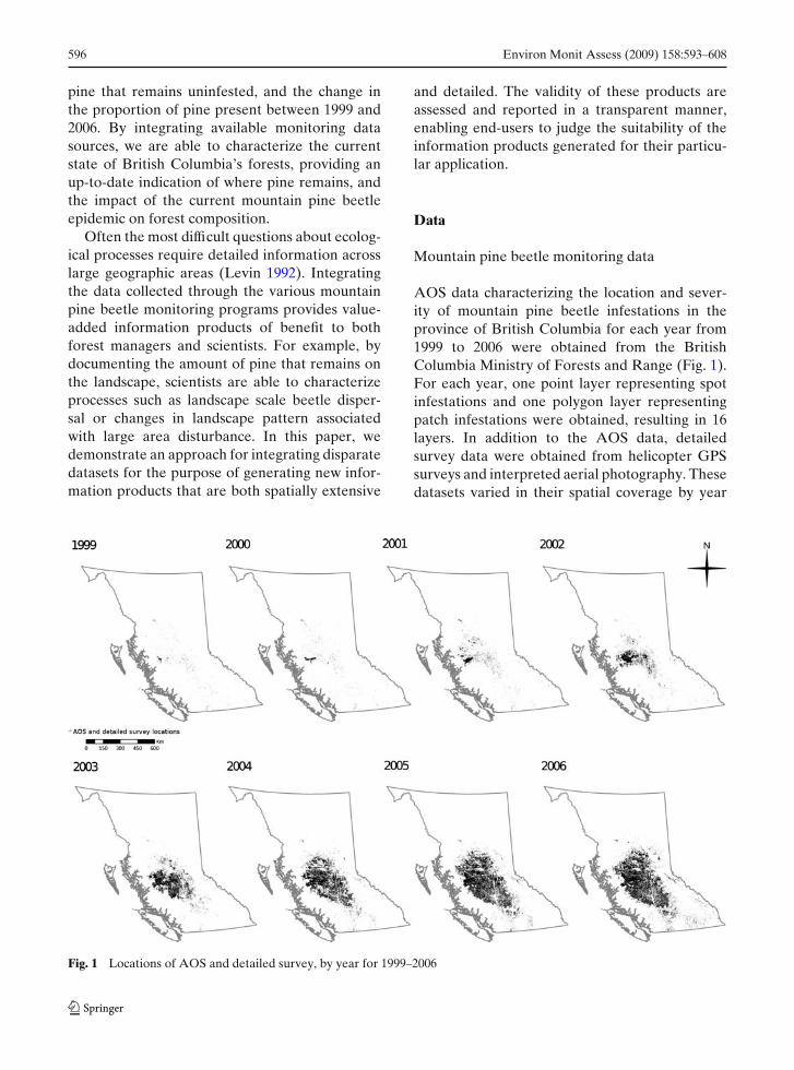
AOS data characterizing the location and sever-ity of mountain pine beetle infestations in theprovince of British Columbia for each year from1999 to 2006 were obtained from the BritishColumbia Ministry of Forests and Range (Fig. 1).For each year, one point layer representing spotinfestations and one polygon layer representingpatch infestations were obtained, resulting in 16layers. In addition to the AOS data, detailedsurvey data were obtained from helicopter GPSsurveys and interpreted aerial photography. Thesedatasets varied in their spatial coverage by year

Fig. 1 Locations of AOS and detailed survey, by year for 1999–2006

Environ Monit Assess (2009) 158:593–608 597

(Fig. 1). Detailed datasets were either polygonrepresentations with a severity rating or pointdatasets with either a severity rating or a countof the number of infested trees. We utilized 14detailed datasets (eight point, six polygon) acrossthe temporal span of our study. The annual arealcoverage of these detailed datasets had an averagearea of 68,430 ha with most years covering under100,000 ha.

Field data

Ground survey data were obtained from severalsources for accuracy estimation of the derivedinformation products. Vegetation Resources In-ventory (VRI) permanent sample plot data wereobtained from the British Columbia Ministry ofForests for each year from 1997 to 2005 (n = 948).VRI field plots are circular variable radius plots.Additionally, field plots were obtained from forestlicensees throughout British Columbia (n = 724).An assessment of beetle damage was made for

an initial plot, and the plot was extended radiallyoutward in increments of usually 100 m.

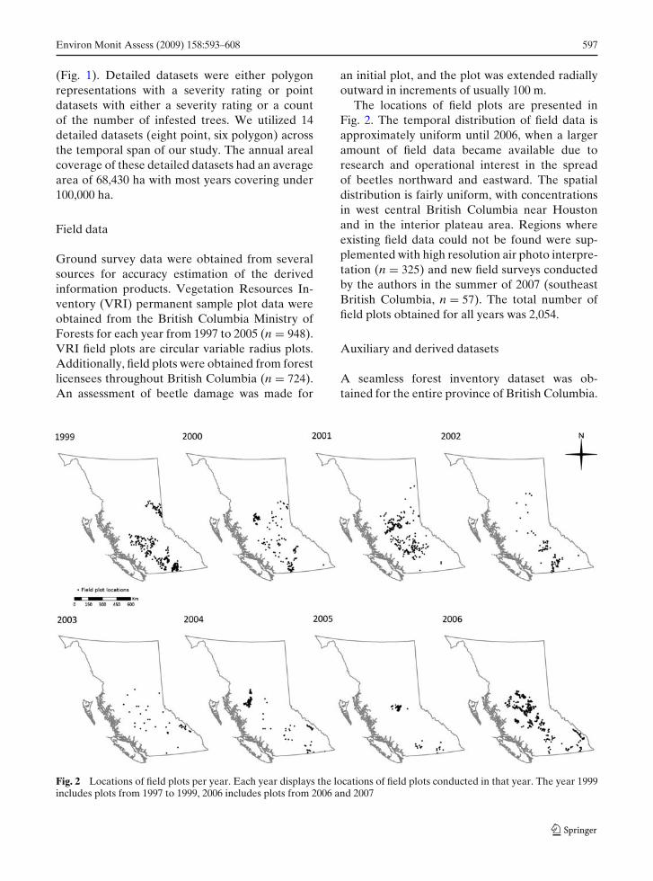
The locations of field plots are presented inFig. 2. The temporal distribution of field data isapproximately uniform until 2006, when a largeramount of field data became available due toresearch and operational interest in the spreadof beetles northward and eastward. The spatialdistribution is fairly uniform, with concentrationsin west central British Columbia near Houstonand in the interior plateau area. Regions whereexisting field data could not be found were sup-plemented with high resolution air photo interpre-tation (n = 325) and new field surveys conductedby the authors in the summer of 2007 (southeastBritish Columbia, n = 57). The total number offield plots obtained for all years was 2,054.

Auxiliary and derived datasets

A seamless forest inventory dataset was ob-tained for the entire province of British Columbia.

Fig. 2 Locations of field plots per year. Each year displays the locations of field plots conducted in that year. The year 1999includes plots from 1997 to 1999, 2006 includes plots from 2006 and 2007

598 Environ Monit Assess (2009) 158:593–608

The Vegetation Resources Inventory (VRI) pro-vides full spatial coverage of the status of forestconditions in British Columbia in a particularyear (British Columbia Ministry of SustainableResource Management 2002). Forest stands aremapped as polygons with attributes attacheddescribing stand characteristics such as age andcomposition. Attributes are derived from bothphotointerpretation and field validation.

A digital elevation model (DEM) was ob-tained from the Government of Canada portalGeobase (http://www.geobase.ca), extracted fromthe National Topographic Database (NTDB). Thedataset was reprojected to BC Albers Equal Areaprojection, using the North American Datum 1983(NAD83) horizontal datum, and the CanadianVertical Geodetic Datum 1928 (CVGD28) verti-cal datum. The data scale was 1:50,000 which hada grid cell resolution of maximum of 3 arc seconds,and was resampled to 100 m grid cells.

The impacts of varying climatic and terrain fac-tors on survey error (see Modeling survey errorwith covariate auxiliary variables) were consid-ered by calculating direct clear-sky shortwave ra-diation (SWR) using the methods of Kumar et al.(1997). Consideration of terrain through solar ra-diation was deemed useful given the complex na-ture of the terrain in British Columbia, combinedwith the large area of the province. Elevationranges from approximately 0 to 3,978 m. Previousresearch has used SWR as a significant variablefor predicting red attack damage at the landscapescale (Coops et al. 2006). Calculations for SWRrequire parameters for terrain (DEM), latitude,day of the year, and a time interval at which tomake calculations. Kumar et al. (1997) suggestthat short time intervals have greater accuracy, socalculations were made every 120 min. These cal-culations were conducted for a single mid-monthday for each month, in order to derive a meanestimate of SWR for the entire year.

Methods

Data preprocessing

The first step toward data integration was stan-dardizing all of the input data to a compatible spa-tial representation and resolution and a common

scale of infestation severity. Previous researchhas indicated that spatially continuous representa-tions of forest conditions, such as raster grids, areuseful for visualization and landscape scale analy-sis of mountain pine beetle infestations (Nelsonet al. 2006b). To facilitate continuous data repre-sentation and subsequent modeling, a raster rep-resentation was selected with a grid cell resolutionof 100 m by 100 m in order to accurately capturethe stand attributes in the forest inventory.

Data preprocessing included conversion of thepolygon and point survey data to raster formatwith a 1-ha minimum mapping unit (MMU). Forpolygonal data, we followed the recommenda-tions of the British Columbia Model for OutbreakProjections and used the midpoint of the sever-ity classes (Eng et al. 2004), as indicated inTable 1. We assumed that the percentage of areainfested applied homogeneously throughout theentire polygon and, therefore, assigned the ap-propriate midpoint value as an attribute to thepolygon. This was repeated for each of the eightAOS polygon data layers and the six detailedsurvey (i.e., helicopter GPS and interpreted aerialphotography) data layers. These polygonal layerswere then converted to raster format.

For point data in both the AOS and detaileddatasets, each point represents an area of infes-tation ranging from 0.25 to 1 ha. If a severityclass was associated with the point, we used thefull severity rating, assuming that spots representsmall but intensely infested areas. Some pointdata had infestation severity indicated by a countof infested trees. Tree counts were converted toseverity classes (percentage infested ratings) byconsidering the number of infested trees relativeto the number of noninfested trees and the areaof the spot. Stem density, was based on VRI stemdensity estimates. Using the area of the spot in-festation, we multiplied the percent infested asso-ciated with the new severity classes by the areaof the spot to arrive at the area of infestationfor each point. This allowed us to convert thepoint layers from both the AOS and the detailedsurveys to raster grids, where the resultant rastervalues indicated the percentage of each cell thatrepresented mountain pine beetle-caused pinemortality. The result was 30 separate rasters (14AOS and 16 detailed), each with a 1-ha spatial

Environ Monit Assess (2009) 158:593–608 599

resolution, where each cell represents the propor-tion of infestation.

The percentage of pine (by area) within eachforest inventory polygon was calculated and as-signed to an attribute in the forest inventory. Sim-ilar to the process described above, the proportionof pine was assumed to apply to the entire forestinventory polygon uniformly, and this polygonaldata was converted to raster format with 1 haresolution. The result was a raster for the provinceindicating how much pine was found within eachMMU.

Spatial data integration

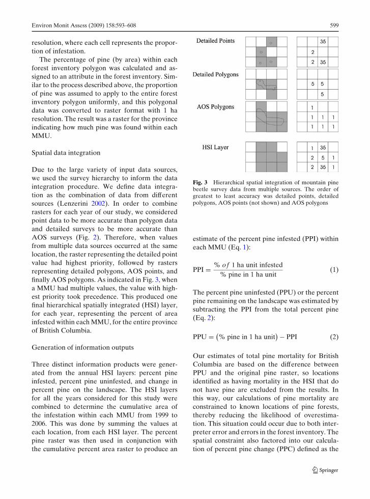
Due to the large variety of input data sources,we used the survey hierarchy to inform the dataintegration procedure. We define data integra-tion as the combination of data from differentsources (Lenzerini 2002). In order to combinerasters for each year of our study, we consideredpoint data to be more accurate than polygon dataand detailed surveys to be more accurate thanAOS surveys (Fig. 2). Therefore, when valuesfrom multiple data sources occurred at the samelocation, the raster representing the detailed pointvalue had highest priority, followed by rastersrepresenting detailed polygons, AOS points, andfinally AOS polygons. As indicated in Fig. 3, whena MMU had multiple values, the value with high-est priority took precedence. This produced onefinal hierarchical spatially integrated (HSI) layer,for each year, representing the percent of areainfested within each MMU, for the entire provinceof British Columbia.

Generation of information outputs

Three distinct information products were gener-ated from the annual HSI layers: percent pineinfested, percent pine uninfested, and change inpercent pine on the landscape. The HSI layersfor all the years considered for this study werecombined to determine the cumulative area ofthe infestation within each MMU from 1999 to2006. This was done by summing the values ateach location, from each HSI layer. The percentpine raster was then used in conjunction withthe cumulative percent area raster to produce an

Fig. 3 Hierarchical spatial integration of mountain pinebeetle survey data from multiple sources. The order ofgreatest to least accuracy was detailed points, detailedpolygons, AOS points (not shown) and AOS polygons

estimate of the percent pine infested (PPI) withineach MMU (Eq. 1):

PPI = % of 1 ha unit infested% pine in 1 ha unit

(1)

The percent pine uninfested (PPU) or the percentpine remaining on the landscape was estimated bysubtracting the PPI from the total percent pine(Eq. 2):

PPU = (% pine in 1 ha unit

) − PPI (2)

Our estimates of total pine mortality for BritishColumbia are based on the difference betweenPPU and the original pine raster, so locationsidentified as having mortality in the HSI that donot have pine are excluded from the results. Inthis way, our calculations of pine mortality areconstrained to known locations of pine forests,thereby reducing the likelihood of overestima-tion. This situation could occur due to both inter-preter error and errors in the forest inventory. Thespatial constraint also factored into our calcula-tion of percent pine change (PPC) defined as the

600 Environ Monit Assess (2009) 158:593–608

difference between the original percent pine andthe remaining percent pine (Eq. 3):

PPC = (% pine in 1 ha unit

) − PPU (3)

Validation

Locations of red attack damage were validatedwith field data using an error matrix. For eachfield plot in British Columbia, the PPI value forthe corresponding year was extracted. PPI valuesgreater than zero indicated that mountain pinebeetle attack was present, while values of zero in-dicated beetle absence. Overall map accuracy wasassessed by computing the correct classificationrate, or the sum of the true positive and true nega-tives divide by the total number of observations.We also evaluated the false-positive rate, false-negative rate, and the kappa statistic. To examinetemporal fluctuation in the level of accuracy in theHSI data, we examined all error matrix statisticspartitioned by survey year.

Severity of red attack damage, or PPI, was as-sessed using an ordinal measure of association, theGoodman–Kruskal gamma statistic (Goodmanand Kruskal 1954). The PPI values in the fielddata and the HSI were classified back into sever-ity classes (see Table 1), and the gamma statis-tic was computed for these ordinal classes. TheGoodman–Kruskal gamma measure of ordinal as-sociation is defined as below:

γ = (P − Q)

(P + Q)(4)

Where P is the number of concordant pairs, and Qis the number of discordant pairs. Gamma rangesfrom 0 to 1 and can be interpreted as the per-centage contribution of the predictor in reducingerrors incurred when predicting the response ran-domly.

We calculated absolute residuals (observed–predicted) between the field and HSI-derived PPI.Positive residuals therefore indicate HSI under-estimation, and negative residuals indicate over-estimation. Residual patterns were explored bypartitioning data into severity classes and plot-

ting distribution of residuals for different severityclasses using boxplots.

Modeling survey error with covariateauxiliary variables

We examined the underlying characteristics ofsurvey error to investigate if there were any sys-tematic landscape conditions contributing error inthe PPI layer. Spatial models were used as we ex-pect errors to be spatially structured across largeareas. We selected four variables that have previ-ously been associated with mountain pine beetleprocesses: quadratic mean diameter (Mitchell andPreisler 1991), age (Safranyik et al. 1974), percent-age pine (Nelson et al. 2007), and shortwave radi-ation (Coops et al. 2006). Stand quadratic meandiameter, age, and composition make are threeof four variables commonly used in forest sus-ceptibility rating in British Columbia (Shore andSafranyik 1992). Shortwave radiation has been apredictor of landscape-scale red attack damage ina number of studies (Coops et al. 2006; White et al.2006). The forest and environmental conditionsthat impact the severity and likelihood of moun-tain pine beetle infestations may also influence theability of surveyors to map the infested landscape.

Estimation of a linear multiple regressionmodel (Y = Xβ + e) where Y is survey error,X is a vector of independent covariates, β is avector of regression coefficients and e is a vec-tor of independently and identically distributed(iid) residuals was first conducted using ordinaryleast squares (OLS) regression. Due to the natureof our dataset, spatial autocorrelation in both thedependent variable (survey error), and the ex-planatory variables could violate the assumptionof iid residuals (Cliff and Ord 1981). Therefore,spatial autocorrelation was incorporated by es-timating spatial autoregressive (SAR) models(Cressie 1993; Haining 2003). Three types ofSAR models were tested: the spatial error model(Y = Xβ + λWu + e), where spatial autocorrela-tion (inherent or induced) is modeled as theproduct of an estimated spatial autocorrelationparameter λ, a neighborhood weights matrixW, and u, the neighborhood error matrix. The re-maining error term, e is iid. The spatial lag model(Y = ρWY + Xβ + e) models the spatial auto-

Environ Monit Assess (2009) 158:593–608 601

correlation parameter ρ as a lag on the depen-dent variable Y. The SAR mixed model (Y =ρWY + Xβ + W Xγ + e), includes terms for spa-tial autocorrelation in ρWY, the dependent vari-able and WXγ , the error terms of model (Kisslingand Carl 2008).

The weights matrix, the most important compo-nent of spatial model specifications (Aldstadt andGetis 2006), was kept constant for all models as ak-nearest neighbor symmetric neighborhood withk = 5. The k parameter was set to ensure a sym-metric weights matrix and as an estimate to makesure that plots that are part of the same surveydesign included a measure of spatial dependence.Since sampling schemes tend to follow naturallandscape boundaries, we expect autocorrelationin errors for neighboring field plots under similarsurvey programs. The mean distance to the fifthnearest neighbor was 10.5 km.

Model assessment was based on two criteria.First, we examine the residual spatial autocor-relation using spatial correlograms constructedusing 20 distance classes and Moran’s I coeffi-cients using the spdep package in R (Bivand 2002;Ihaka and Gentelman 1996). Second, models wereassessed using the Akaike information criterion(AIC) which allows assessment and comparisonof spatial models based on model fit and modelcomplexity (Burnham and Anderson 1998).

Results

Percent pine and percent pine infested

A summary of the cumulative infestation in theinfestation data indicates that the total cumulativeamount of red attack damage in British Columbiaby 2006 was 4.16 million hectares (Fig. 4). Whenwe constrained this estimate to areas of knownpine forest in the VRI data, the estimate was 2.89million hectares. The current distribution (asof 2006) of uninfested pine (PPU) in BritishColumbia is presented in Fig. 5. Knowledge ofwhere the pine remains, as opposed to the morecommon representation of where pine has beenlost, supports tactical- and strategic-level plan-ning. The impact of the mountain pine beetle onforest composition is shown in Fig. 6, where the

Fig. 4 Percent pine infested (PPI) as of 2006

percent pine infested on the landscape between1999 and 2006 is depicted. Compared with typ-ical provincial maps of the spatial extent of themountain pine beetle infestation, this represen-tation includes variations in infestation intensityand differences in regions where the infestationis having severe impacts on the landscapes fromareas where the effects are moderate or light.

Fig. 5 Percent pine uninfested (PPU) as of 2006

602 Environ Monit Assess (2009) 158:593–608

Fig. 6 Percent change in pine (PPC; 1999–2006)

Validation results

Of the 2,054 field plots used in this analysis, 1,620(79%) had red attack damage present. Accuracysummary statistics for the HSI validated againstthe field plots are presented in Table 2. The accu-racy of the HSI layer in detecting red attack iden-tified in the field data was high, with an averageof 93% (true positive) of field verified red attacksites being correctly identified in the HSI layer.True negatives were less accurately predicted,with 33% of field plots without red attack damagewere correctly identified as such in the HSI layer.The total number of true negatives was 434, and astime progressed, more plots (proportionally) hadred attack damage. The overall accuracy of themap red attack classification was 60%, while thefalse-positive rate was 14%, and the false negative

rate was 46%. The kappa statistic for the all fieldplots validating the HSI was 0.25.

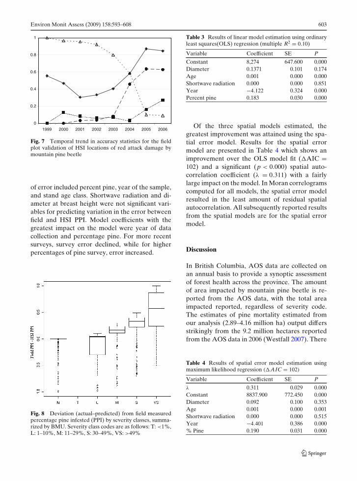
Examining the temporal trend in correspon-dence between the HSI and the field plots (Fig. 7)revealed that the false-negative rate or the plotswhere red attack was found in the field but missedin the HSI, declined markedly with time. Falsenegatives were very high initially, likely due to thefact that infestations were spotty and unexpectedby aerial surveyors. As the infestation increasedin magnitude and spatial extent, the false-negativerate declined. The false-positive rate showed alarge increase in 2004, and a moderate increasein 2005. The overall correct classification ratedeclined from 1999 to 2001, but thereafter steadilyincreased to 87% in 2005.

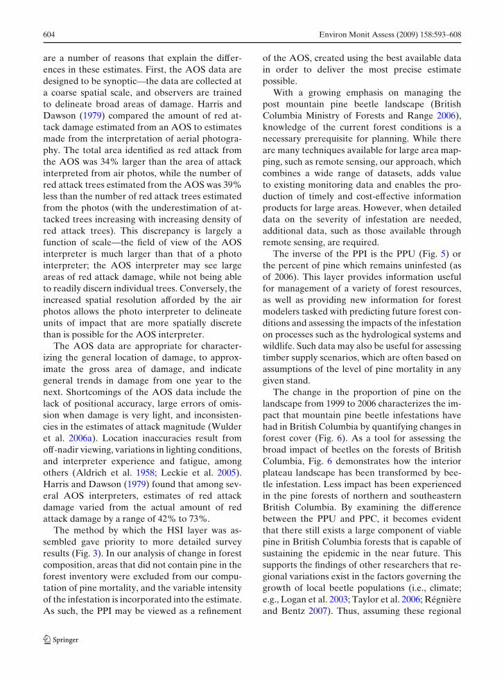
We calculated the absolute deviance as the HSIPPI subtracted from the field PPI. Figure 8 showsthe deviation partitioned by severity class. Moresevere classes are associated with high positivedeviation, demonstrated by the distance of themedian bar in each of the boxplots from zero.This corresponds to an underestimation of theamount of pine infested in the HSI layer. Whenfield PPI values are low, the deviance is negative.This becomes more apparent at more severe levelsof infestation, which is not surprising as estimatesof infestation magnitude will tend to vary morewhen infestations are larger (Nelson et al. 2006b).

Modeling survey error results

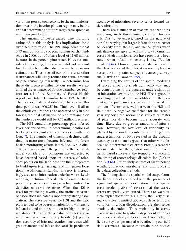
The OLS model of the HSI survey errors yieldedthe estimates presented in Table 3. Overall, theindependent variables explained approximately10% of the variation in the error between field val-ues of percent pine infested and HSI percent pineinfested. Variables that were significant predictors

Table 2 Error matrixsummary statistics forthe field plot validationof HSI locations ofred attack damage bymountain pine beetles

Field Plot Producer’s User’s

Red attack No red attackaccuracy accuracy

HSI Red attack 868 61 54% 93%No red attack 752 373 86% 33%

Correct classification rate 60%Kappa statistic 25%False-positive rate 14%False-negative rate 46%

Environ Monit Assess (2009) 158:593–608 603

0

0.2

0.4

0.6

0.8

1

1999 2000 2001 2002 2003 2004 2005 2006

Fig. 7 Temporal trend in accuracy statistics for the fieldplot validation of HSI locations of red attack damage bymountain pine beetle

of error included percent pine, year of the sample,and stand age class. Shortwave radiation and di-ameter at breast height were not significant vari-ables for predicting variation in the error betweenfield and HSI PPI. Model coefficients with thegreatest impact on the model were year of datacollection and percentage pine. For more recentsurveys, survey error declined, while for higherpercentages of pine survey, error increased.

Fig. 8 Deviation (actual–predicted) from field measuredpercentage pine infested (PPI) by severity classes, summa-rized by BMU. Severity class codes are as follows: T: <1%,L: 1–10%, M: 11–29%, S: 30–49%, VS: >49%

Table 3 Results of linear model estimation using ordinaryleast squares(OLS) regression (multiple R2 = 0.10)

Variable Coefficient SE P

Constant 8,274 647.600 0.000Diameter 0.1371 0.101 0.174Age 0.001 0.000 0.000Shortwave radiation 0.000 0.000 0.851Year −4.122 0.324 0.000Percent pine 0.183 0.030 0.000

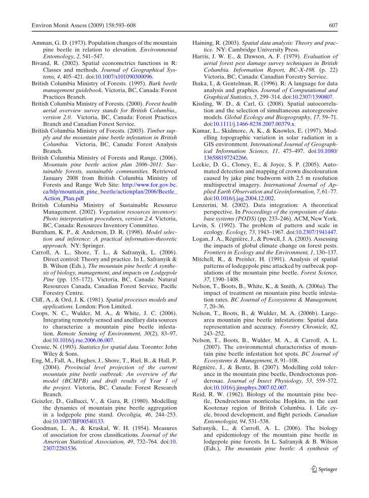
Of the three spatial models estimated, thegreatest improvement was attained using the spa-tial error model. Results for the spatial errormodel are presented in Table 4 which shows animprovement over the OLS model fit (�AIC =102) and a significant (p < 0.000) spatial auto-correlation coefficient (λ = 0.311) with a fairlylarge impact on the model. In Moran correlogramscomputed for all models, the spatial error modelresulted in the least amount of residual spatialautocorrelation. All subsequently reported resultsfrom the spatial models are for the spatial errormodel.

Discussion

In British Columbia, AOS data are collected onan annual basis to provide a synoptic assessmentof forest health across the province. The amountof area impacted by mountain pine beetle is re-ported from the AOS data, with the total areaimpacted reported, regardless of severity code.The estimates of pine mortality estimated fromour analysis (2.89–4.16 million ha) output differsstrikingly from the 9.2 million hectares reportedfrom the AOS data in 2006 (Westfall 2007). There

Table 4 Results of spatial error model estimation usingmaximum likelihood regression (�AIC = 102)

Variable Coefficient SE P

λ 0.311 0.029 0.000Constant 8837.900 772.450 0.000Diameter 0.092 0.100 0.353Age 0.001 0.000 0.001Shortwave radiation 0.000 0.000 0.515Year −4.401 0.386 0.000% Pine 0.190 0.031 0.000

604 Environ Monit Assess (2009) 158:593–608

are a number of reasons that explain the differ-ences in these estimates. First, the AOS data aredesigned to be synoptic—the data are collected ata coarse spatial scale, and observers are trainedto delineate broad areas of damage. Harris andDawson (1979) compared the amount of red at-tack damage estimated from an AOS to estimatesmade from the interpretation of aerial photogra-phy. The total area identified as red attack fromthe AOS was 34% larger than the area of attackinterpreted from air photos, while the number ofred attack trees estimated from the AOS was 39%less than the number of red attack trees estimatedfrom the photos (with the underestimation of at-tacked trees increasing with increasing density ofred attack trees). This discrepancy is largely afunction of scale—the field of view of the AOSinterpreter is much larger than that of a photointerpreter; the AOS interpreter may see largeareas of red attack damage, while not being ableto readily discern individual trees. Conversely, theincreased spatial resolution afforded by the airphotos allows the photo interpreter to delineateunits of impact that are more spatially discretethan is possible for the AOS interpreter.

The AOS data are appropriate for character-izing the general location of damage, to approx-imate the gross area of damage, and indicategeneral trends in damage from one year to thenext. Shortcomings of the AOS data include thelack of positional accuracy, large errors of omis-sion when damage is very light, and inconsisten-cies in the estimates of attack magnitude (Wulderet al. 2006a). Location inaccuracies result fromoff-nadir viewing, variations in lighting conditions,and interpreter experience and fatigue, amongothers (Aldrich et al. 1958; Leckie et al. 2005).Harris and Dawson (1979) found that among sev-eral AOS interpreters, estimates of red attackdamage varied from the actual amount of redattack damage by a range of 42% to 73%.

The method by which the HSI layer was as-sembled gave priority to more detailed surveyresults (Fig. 3). In our analysis of change in forestcomposition, areas that did not contain pine in theforest inventory were excluded from our compu-tation of pine mortality, and the variable intensityof the infestation is incorporated into the estimate.As such, the PPI may be viewed as a refinement

of the AOS, created using the best available datain order to deliver the most precise estimatepossible.

With a growing emphasis on managing thepost mountain pine beetle landscape (BritishColumbia Ministry of Forests and Range 2006),knowledge of the current forest conditions is anecessary prerequisite for planning. While thereare many techniques available for large area map-ping, such as remote sensing, our approach, whichcombines a wide range of datasets, adds valueto existing monitoring data and enables the pro-duction of timely and cost-effective informationproducts for large areas. However, when detaileddata on the severity of infestation are needed,additional data, such as those available throughremote sensing, are required.

The inverse of the PPI is the PPU (Fig. 5) orthe percent of pine which remains uninfested (asof 2006). This layer provides information usefulfor management of a variety of forest resources,as well as providing new information for forestmodelers tasked with predicting future forest con-ditions and assessing the impacts of the infestationon processes such as the hydrological systems andwildlife. Such data may also be useful for assessingtimber supply scenarios, which are often based onassumptions of the level of pine mortality in anygiven stand.

The change in the proportion of pine on thelandscape from 1999 to 2006 characterizes the im-pact that mountain pine beetle infestations havehad in British Columbia by quantifying changes inforest cover (Fig. 6). As a tool for assessing thebroad impact of beetles on the forests of BritishColumbia, Fig. 6 demonstrates how the interiorplateau landscape has been transformed by bee-tle infestation. Less impact has been experiencedin the pine forests of northern and southeasternBritish Columbia. By examining the differencebetween the PPU and PPC, it becomes evidentthat there still exists a large component of viablepine in British Columbia forests that is capable ofsustaining the epidemic in the near future. Thissupports the findings of other researchers that re-gional variations exist in the factors governing thegrowth of local beetle populations (i.e., climate;e.g., Logan et al. 2003; Taylor et al. 2006; Régnièreand Bentz 2007). Thus, assuming these regional

Environ Monit Assess (2009) 158:593–608 605

variations persist, connectivity to the main infesta-tion area in the interior plateau region may be thecritical determinant of future large-scale spread ofmountain pine beetle.

The amount of beetle-caused pine mortalityestimated in this analysis has implications for asustained infestation. The PPU map indicates that8.79 million hectares of pine remain on the land-scape in 2006, out of a base level of 11.68 millionhectares in the percent pine raster. However, out-side of harvesting, this analysis did not accountfor the effects of other disturbance types in ourestimations. Thus, the effects of fire and otherdisturbances will likely reduce the actual amountof pine remaining markedly. To determine howthese disturbances influence our results, we ex-amined the estimates of abiotic disturbances (e.g.,fire) for all of the Summary of Forest Healthreports in British Columbia from 1999 to 2006.The total estimate of abiotic disturbance over thistime period was 600,955 ha. Thus, even if all ofthe abiotic disturbances had occurred only in pineforests, the final estimation of pine remaining onthe landscape would still be 7.75 million hectares.

The HSI cumulative percentage pine-infestedlayer performed well in determining locations ofbeetle presence, and accuracy increased with time(Fig. 7). The number of omissions declined withtime, as more areas became infested, and foresthealth monitoring efforts intensified. While diffi-cult to quantify, over the period of the outbreakunder consideration, omissions are expected tohave declined based upon an increase of refer-ence points on the land base for the interpretersto build upon (e.g., salvage and mitigation loca-tions). Additionally, Landsat imagery is increas-ingly used as an information underlay when sketchmapping. Inclusion of the sketch information fromprevious years also aids in providing context fordepiction of new infestations. When the HSI isused for predicting severity, the ordinal measureof association indicated a moderately strong asso-ciation. The error between the HSI and the fieldplots tended to be overestimation for low intensityinfestation and underestimation for high intensityinfestation. Thus, for the aspatial accuracy assess-ment, we have two primary trends, (a) predic-tion accuracy of infested locations increases withgreater amounts of infestation, and (b) prediction

accuracy of infestation severity tends toward un-derestimation.

There are a number of reasons that we thinkare giving rise to this seemingly contradictory re-sult. Firstly, we expect, based on the nature ofaerial surveying that larger infestations are easierto identify from the air, and hence, years wheninfestations are greater will have fewer omissionerrors. High omission errors have previously beennoted when infestation severity is low (Wulderet al. 2006a). However, once a patch is located,the classification of the infestation severity level issusceptible to greater subjectivity among survey-ors (Harris and Dawson 1979).

Examining the results of the spatial modelingof survey error also sheds light onto what maybe contributing to the apparent underestimationof infestation severity in the HSI. The regressionmodeling revealed that, in addition to the per-centage of pine, survey year also influenced theamount of error observed between the HSI andfield data. A negative coefficient for the sampleyear supports the notion that survey estimatesof pine mortality become more accurate withtime, likely due to greater amounts of infesta-tion. However, the low level of variability ex-plained by the models combined with the generalunderestimation of PPI revealed in the aspatialaccuracy assessment suggests that other variablesare also determinants of error. Previous researchhas indicated that the greatest source of error inaerial-based surveys is the temporal variation inthe timing of crown foliage discoloration (Nelsonet al. 2006b). Other likely sources of error includeweather, surveyor variability, and differences infield data collection methods.

The finding that the spatial model outperformsthe linear model combined with the presence ofsignificant spatial autocorrelation in the spatialerror model (Table 4) reveals that the surveyerrors are spatially structured. There are two plau-sible explanations for this. Firstly, the likely miss-ing variables identified above, such as temporalvariation in crown discoloration, are themselvesspatially dependent. Thus, variability in surveyerror arising due to spatially dependent variableswill also be spatially autocorrelated. Secondly, thefield survey designs may also be affecting our fielddata estimates. Because mountain pine beetles

606 Environ Monit Assess (2009) 158:593–608

attack trees in clusters (spot infestations), groundsurveys are usually nonsystematic. Calculations ofPPI derived from field plots located at infestationcenters will therefore be artificially high relativeto the surrounding forest. These plots, therefore,may not be representative of broader forest con-ditions. The HSI layer, which enumerates PPIderived from larger-area estimates, would there-fore be expected to be lower than the estimatesderived from plots located at infestation centers.This problem of scale speaks of the difficulty of ac-curately measuring forest conditions across largeareas, either on the ground or from the air.

Integrating all existing monitoring data pro-vides a new mapping tool for generating timely in-formation on the provincial forest. It also providesan improved cartographic presentation of the im-pact of mountain pine beetle to the forest, aidingcommunication with the public and justificationfor resource allocation and associated activities.The new map products generated through inte-gration of existing data directly benefit decision-makers tasked with the challenge of managing theimpacts of the mountain pine beetle on forests.With a growing emphasis on managing a widerange of timber and nontimber (i.e., wildlife habi-tat and water quality) values in postmountain pinebeetle landscape, new map products are neededand have many potential users.

Conclusion

By integrating the existing spatial hierarchy ofmountain pine beetle monitoring data from 1999to 2006, we were able to generate up-to-date infor-mation products describing the forest compositionof British Columbia. Specifically, we generatedthree outputs that describe forest conditions as of2006: the cumulative percentage of pine infested(1999–2005), the percentage of pine uninfested,and the change in the percentage of pine on thelandscape. These products provide timely infor-mation on the state of the provincial forest andfurthermore, by leveraging all the data in the sur-vey hierarchy, we were able to generate a morerefined estimate of the total area impacted bythe mountain pine beetle than is possible usingthe AOS data exclusively. Furthermore, we con-

ducted an accuracy assessment using a compre-hensive field dataset as ground truth. We alsoexplored the variations in predicted and observedPPI using spatial modeling which revealed signifi-cant spatial structuring of survey error.

The information products produced in this re-search provide an improved cartographic presen-tation of the impact of mountain pine beetle tothe forest, aiding communication with the publicand justifying resource allocation and associatedactivities. These products will also facilitate bothstrategic and tactical forest management plan-ning. Strategic planning addresses very long timeframes and large spatial extents. Refined esti-mates of infestation severity and the integrationwith forest inventory data enable more detailedmodeling of various forest management scenar-ios, treatment activities, and timber supply acrosslarge areas. Tactical planning, such as harvestscheduling and road construction, may also befacilitated by our refined large-scale estimates ofbeetle damage and forest conditions. With a grow-ing emphasis on managing the wide range of tim-ber and nontimber (i.e., wildlife habitat and waterquality) values in post-mountain pine beetle land-scape, new maps products, such as those presentedhere, are needed and have many potential users.

Acknowledgements The authors gratefully acknowledgethe many people who provided data and insights in supportof this project, including Tim Ebata, Dave Coates, Pat Teti,Tom Niemann, David Kilshaw, and Dr. Xiaoping Yuan ofthe government of British Columbia, Dr. Allan Carroll ofthe Canadian Forest Service, Dr. Nicholas Coops of theUniversity of British Columbia, and Ted Strome of LarixForestry. This research was funded by the Governmentof Canada as part of the Mountain Pine Beetle Programadministered by Natural Resources Canada, CanadianForest Service, with additional information available at:http://mpb.cfs.nrcan.gc.ca/.

References

Aldrich, R. C., Heller, R. C., & Bailey, W. F. (1958).Observation limits for aerial sketch mapping southernpine beetle in the southern Appalachians. Journal ofForestry, 56, 200–202.

Aldstadt, J., & Getis, A. (2006). Using AMOEBA to createa spatial weights matrix and identify spatial clusters.Geographical Analysis, 38, 327–343. doi:10.1111/j.1538-4632.2006.00689.x.

Environ Monit Assess (2009) 158:593–608 607

Amman, G. D. (1973). Population changes of the mountainpine beetle in relation to elevation. EnvironmentalEntomology, 2, 541–547.

Bivand, R. (2002). Spatial econometrics functions in R:Classes and methods. Journal of Geographical Sys-tems, 4, 405–421. doi:10.1007/s101090300096.

British Columbia Ministry of Forests. (1995). Bark beetlemanagement guidebook. Victoria, BC, Canada: ForestPractices Branch.

British Columbia Ministry of Forests. (2000). Forest healthaerial overview survey stands for British Columbia.,version 2.0. Victoria, BC, Canada: Forest PracticesBranch and Canadian Forest Service.

British Columbia Ministry of Forests. (2003). Timber sup-ply and the mountain pine beetle infestation in BritishColumbia. Victoria, BC, Canada: Forest AnalysisBranch.

British Columbia Ministry of Forests and Range. (2006).Mountain pine beetle action plan 2006–2011: Sus-tainable forests, sustainable communities. RetrievedJanuary 2008 from British Columbia Ministry ofForests and Range Web Site: http://www.for.gov.bc.ca/hfp/mountain_pine_beetle/actionplan/2006/Beetle_Action_Plan.pdf

British Columbia Ministry of Sustainable ResourceManagement. (2002). Vegetation resources inventory:Photo interpretation procedures, version 2.4. Victoria,BC, Canada: Resources Inventory Committee.

Burnham, K. P., & Anderson, D. R. (1998). Model selec-tion and inference: A practical information-theoreticapproach. NY: Springer.

Carroll, A. L., Shore, T. L., & Safranyik, L. (2006).Direct control: Theory and practice. In L. Safranyik &B. Wilson (Eds.), The mountain pine beetle: A synthe-sis of biology, management, and impacts on LodgepolePine (pp. 155–172). Victoria, BC, Canada: NaturalResources Canada, Canadian Forest Service, PacificForestry Centre.

Cliff, A., & Ord, J. K. (1981). Spatial processes models andapplications. London: Pion Limited.

Coops, N. C., Wulder, M. A., & White, J. C. (2006).Integrating remotely sensed and ancillary data sourcesto characterize a mountain pine beetle infesta-tion. Remote Sensing of Environment, 30(2), 83–97.doi:10.1016/j.rse.2006.06.007.

Cressie, N. (1993). Statistics for spatial data. Toronto: JohnWiley & Sons.

Eng, M., Fall, A., Hughes, J., Shore, T., Riel, B., & Hall, P.(2004). Provincial level projection of the currentmountain pine beetle outbreak: An overview of themodel (BCMPB) and draft results of Year 1 ofthe project. Victoria, BC, Canada: Forest ResearchBranch.

Geiszler, D., Gallucci, V., & Gara, R. (1980). Modellingthe dynamics of mountain pine beetle aggregationin a lodgepole pine stand. Oecoligia, 46, 244–253.doi:10.1007/BF00540133.

Goodman, L. A., & Kruskal, W. H. (1954). Measuresof association for cross classifications. Journal of theAmerican Statistical Association, 49, 732–764. doi:10.2307/2281536.

Haining, R. (2003). Spatial data analysis: Theory and prac-tice. NY: Cambridge University Press.

Harris, J. W. E., & Dawson, A. F. (1979). Evaluation ofaerial forest pest damage survey techniques in BritishColumbia. Information Report, BC-X-198. (p. 22)Victoria, BC, Canada: Canadian Forestry Service.

Ihaka, I., & Gentelman, R. (1996). R: A language for dataanalysis and graphics. Journal of Computational andGraphical Statistics, 5, 299–314. doi:10.2307/1390807.

Kissling, W. D., & Carl, G. (2008). Spatial autocorrela-tion and the selection of simultaneous autoregressivemodels. Global Ecology and Biogeography, 17, 59–71.doi:10.1111/j.1466-8238.2007.00379.x.

Kumar, L., Skidmore, A. K., & Knowles, E. (1997). Mod-elling topographic variation in solar radiation in aGIS environment. International Journal of Geograph-ical Information Science, 11, 475–497. doi:10.1080/136588197242266.

Leckie, D. G., Cloney, E., & Joyce, S. P. (2005). Auto-mated detection and mapping of crown discolourationcaused by jake pine budworm with 2.5 m resolutionmultispectral imagery. International Journal of Ap-plied Earth Observation and Geoinformation, 7, 61–77.doi:10.1016/j.jag.2004.12.002.

Lenzerini, M. (2002). Data integration: A theoreticalperspective. In Proceedings of the symposium of data-base systems (PODS) (pp. 233–246). ACM, New York.

Levin, S. (1992). The problem of pattern and scale inecology. Ecology, 73, 1943–1967. doi:10.2307/1941447.

Logan, J. A., Régnière, J., & Powell, J. A. (2003). Assessingthe impacts of global climate change on forest pests.Frontiers in Ecology and the Environment, 1, 130–137.

Mitchell, R., & Preisler, H. (1991). Analysis of spatialpatterns of lodegepole pine attacked by outbreak pop-ulations of the mountain pine beetle. Forest Science,37, 1390–1408.

Nelson, T., Boots, B., White, K., & Smith, A. (2006a). Theimpact of treatment on mountain pine beetle infesta-tion rates. BC Journal of Ecosystems & Management,7, 20–36.

Nelson, T., Boots, B., & Wulder, M. A. (2006b). Large-area mountain pine beetle infestations: Spatial datarepresentation and accuracy. Forestry Chronicle, 82,243–252.

Nelson, T., Boots, B., Wulder, M. A., & Carroll, A. L.(2007). The environmental characteristics of moun-tain pine beetle infestation hot spots. BC Journal ofEcosystems & Management, 8, 91–108.

Régnière, J., & Bentz, B. (2007). Modelling cold toler-ance in the mountain pine beetle, Dendroctonus pon-derosae. Journal of Insect Physiology, 53, 559–572.doi:10.1016/j.jinsphys.2007.02.007.

Reid, R. W. (1962). Biology of the mountain pine bee-tle, Dendroctonus monticolae Hopkins, in the eastKootenay region of British Columbia. I. Life cy-cle, brood development, and flight periods. CanadianEntomologist, 94, 531–538.

Safranyik, L., & Carroll, A. L. (2006). The biologyand epidemiology of the mountain pine beetle inlodgepole pine forests. In L. Safranyik & B. Wilson(Eds.), The mountain pine beetle: A synthesis of

608 Environ Monit Assess (2009) 158:593–608

biology, management, and impacts on lodgepole pine(pp. 3–66). Victoria, BC, Canada: Natural ResourcesCanada, Canadian Forest Service, Pacific ForestryCentre.

Safranyik, L., Shrimpton, D., & Whitney, H. (1974).Management of lodgepole pine to reduce losses fromthe mountain pine beetle. Forest Technical Report No.1(p. 25). Victoria, BC, Canada: Canadian Forest Ser-vice, Pacific Forest Research Centre.

Safranyik, L., Linto, D., Silversides, R., & McMullen, L.(1992). Dispersal of released mountain pine beetlesunder the canopy of a mature lodgepole pine stand.Journal of Applied Entomology, 113, 441–450.

Shore, T., & Safranyik, L. (1992). Susceptibility and riskrating systems for the mountain pine beetle in lodgepolepine stands. Victoria, BC, Canada: Natural ResourcesCanada, Canadian Forest Service, Pacific ForestryCentre.

Taylor, S. W., Carroll, A. L., Alfaro, R. L., & Safranyik, L.(2006). Forest, climate and mountain pine beetle out-break dynamics in western Canada. In L. Safranyik& B. Wilson (Eds.), The mountain pine beetle: A syn-thesis of biology, management, and impacts on lodge-

pole pine (pp. 69–74). Victoria, BC, Canada: NaturalResources Canada, Canadian Forest Service, PacificForestry Centre.

Westfall, J. (2007). 2007 summary of forest health con-ditions in British Columbia. Victoria, BC, Canada:Forest Practices Branch.

White, J. C., Wulder, M. A., & Grills, D. (2006). Detectionand mapping mountain pine beetle red-attack damagewith SPOT-5 10-m multispectral imagery. BC Journalof Ecosystems and Management, 7, 105–118.

Wulder, M. A., White, J. C., Bentz, B. J., & Ebata, T.(2006a). Augmenting the existing survey hierarchyfor mountain pine beetle red-attack damage withsatellite remotely sensed data. Forestry Chronicle, 82,187–202.

Wulder, M. A., Dymond, C. C., White, J. C., &Erickson, B. (2006b). Detection, mapping and mon-itoring of the mountain pine beetle. In L. Safranyik& B. Wilson (Eds.), The mountain pine beetle: A syn-thesis of biology, management, and impacts on lodge-pole pine (pp. 123–154). Victoria, BC, Canada: NaturalResources Canada, Canadian Forest Service, PacificForestry Centre.