Determinants of Australian Mothers’ Employment: An Analysis of Lone and Couple Mothers

Determinants of Australianmothers’ employment An analysis of lone and couple mothers

Matthew Gray, Lixia Qu, David de Vaus, Christine Millward

Research Paper No. 26, May 2002

Australian Institute of Family Studies

© Australian Institute of Family Studies – Commonwealth of Australia 2002

Australian Institute of Family Studies300 Queen Street, Melbourne 3000 AustraliaPhone (03) 9214 7888; Fax (03) 9214 7839Internet www.aifs.org.au/

This work is copyright. Apart from any use as permitted under the Copyright Act 1968, no part may be reproduced by any process without permission in writing from the Australian Institute of Family Studies.

The Australian Institute of Family Studies is committed to the creation and dissemination of research-based information on family functioning and well being. Views expressed in its publications are those of individual authors and may not reflect Institute policy or the opinions of the Editor of the Institute’s Board of Management.

National Library of AustraliaCataloguing-in-Publication Data

Gray, Matthew.Determinants of Australian mothers’ employment: an analysis of lone and couple mothers.

Bibliography.ISBN 0 642 39493 8.

1. Mothers - Employment. I. Gray, Matthew. II. Australian Institute of Family Studies. (Series: Research paper (Australian Institute of Family Studies); no. 26).

331.44

Designed by Double Jay Graphic DesignPrinted by XL Printing

ISSN 1446-9863 (Print)ISSN 1446-9871 (Online)

Contents

List of tables viAcknowledgements viiAbout the authors viiAbstract viii

Introduction 1Aim and structure of paper 2

Labour force status of lone and couple mothers 3Employment rates 3Educational attainment 5

Modelling the determinants of employment 6Data 6Conceptual framework and empirical model 7

Estimation results 10Educational attainment 10Age and number of children 12English language skills 13Indigenous origin and geographical location 13Migrant status 13Housing tenure 13Partner’s income 14

Factors generating the employment gap 15

Concluding comments and policy implications 17

References 17

Appendix A. Variable definitions 20Appendix B. Descriptive statistics 22Appendix C. Estimation results 23Appendix D. Detailed description of decompositions 24

Research Paper No. 26, May 2002 Australian Institute of Family Studies v

Australian Institute of Family Studies Research Paper No. 26, May 2002vi

List of tablesTable 1. Employment rates of lone and couple mothers, 1996 4

2. Post-secondary qualification by relationship status and age of youngest child 6

3. Variables included in estimation model 8

4 Marginal effects on the probability of employment by family type, 1996 11

5. Decomposition of the lone mother, couple mother employment gap, 1996 16

B1. Description of variables entered in the logistic models 22

C1. Logit estimates of probability of employment, lone and couple mothers, 1996 23

Research Paper No. 26, May 2002 Australian Institute of Family Studies vii

Acknowledgments

For comments on this paper, the authors are indebted to Robert Gregory, LouWill, Ann Sanson, David Stanton and Peter Whiteford.

About the authors

Dr Matthew Gray is a Principal Research Fellow and Head of the Family andSociety Research Program at the Australian Institute of Family Studies. He haswritten on a range of labour market topics including the determinants ofIndigenous labour force status, the impact of child rearing on mothers’subsequent earnings, and access to family-friendly work practices.

Ms Christine Millward is a Senior Research Fellow at the Australian Institute ofFamily Studies. She is a family sociologist who has worked and published inmany areas, including living standards, child care, inter-generational exchange,marital breakdown, work and family and social welfare.

Ms Lixia Qu, now a Research Fellow at the Australian Council for EducationalResearch, worked on the project as a Senior Research Officer at the AustralianInstitute of Family Studies. She has undertaken research in the areas of familyformation and analysis of demographic trends.

Associate Professor David de Vaus is at the Department of Sociology at LaTrobe University and was a Visiting Fellow at the Australian Institute of FamilyStudies while this paper was written. He is the author of a number of booksincluding Research Design in Social Research, and is an international authority inthe field of social research.

Australian Institute of Family Studies Research Paper No. 26, May 2002viii

Abstract

While the lower rates of employment of lone mothers as compared with couplemothers has been well documented, the reasons for the employment gap are lesswell understood. This paper uses data from the 1996 Australian Census toanalyse the factors which explain the employment gap.

The analysis reveals that the determinants of the probability of employment aregenerally similar for lone and couple mothers, although there are severalimportant differences. In general, factors that are typically associated with lowerrates of employment, and could be considered a barrier to employment, have alarger negative effect upon the probability of employment of lone mother thancouple mothers. Importantly, it is found that the presence of children have asimilar impact on the employment of lone and couple mothers.

The analysis also reveals that around one-third of the employment gap is due todifferences in the characteristics of the lone and couple mothers. This gap isexplained by differences in a number of characteristics. Of particular interest isthat only a small amount of the employment gap explained by differences ineducational attainment. The remaining two-thirds of the employment gap iscaused by variables impacting on the employment rates of lone and couplemothers differently.

Determinants of Australian mothers’employment: An analysis of lone andcouple mothers

IntroductionOne of the most dramatic changes to the Australian labour market in recentdecades has been the increase in the number of families with children in whichno adult is employed. There is evidence that Australian children are beingincreasingly divided into those who live in families that are “work rich” (bothadults employed) and those who live in families that are “work poor” (no adultsemployed) (Gregory 1999). Recent comparative studies find that while Australiahas a relatively low overall level of joblessness among persons of working age,joblessness among families with children is among the highest in the OECD(Oxley et al. 1999).

A substantial part of the increase in the number of job poor families is the resultof the increase in the number of lone-parent families, who have a higher rate ofjoblessness than couple families (Gregory 1999; Whiteford 2001). In 1996, 21per cent of families with children were lone-parent families, compared with 7per cent in 1969. The majority (85 per cent) of lone-parent families are headedby lone mothers (ABS 2000). A high proportion of these families receive welfarepayments, with the proportion of lone-parent families in receipt of incometested benefits being among the highest in the OECD.

At the time of the 1996 Census the employment rate of lone mothers withdependent children was 44.5 per cent, and of couple mothers it was 58.5 percent. Since the 1996 Census there have been some increases in the employmentrates of lone and couple mothers, but the gap in employment rates has onlynarrowed slightly (ABS 2000).

These trends have long been a policy concern. In the 1970s it was noted thatlone-mother families experienced high rates of poverty and the policy remedywas seen as adequate social security provision (Henderson, Harcourt and Harper1970). By the 1990s the policy remedy had shifted to being in terms ofsupplementing the pension with income from other sources, primarily incomefrom employment (Shaver 1998). The most recent review of the social securitysystem emphasised the importance of paid employment (McClure 2000).

Another area of concern is that living in a family in which no adult is employedmay have adverse consequences on children in these families. There are severalreasons for thinking this, including the consequences of material deprivationand poverty, the impact of not having a working adult in the household for thedevelopment of attitudes towards work, and the possibility of inter-generationaltransmission of disadvantage. There are also concerns about the costs of incomesupport payments to lone parents for the Federal Budget.

Research Paper No. 26, May 2002 Australian Institute of Family Studies 1

These concerns have led to the focus of public policy on increasing theemployment rates of lone mothers. Government policies have generally beenaimed at improving the skill level and job readiness of lone mothers, providingchild care subsidies for work-related child care, and increasing the financialincentives for lone mothers to take up paid employment.

The most common explanations for the lone mother–couple motheremployment gap revolve around the impact of dependent children on lonemothers’ availability to work, and possible financial disincentives for lonemothers to enter the workforce.

For example, it is sometimes argued that the demands and responsibilities ofcaring for young children are greater for lone mothers than for couple motherswho can often share child care responsibilities with their partner (see, forexample, Swinbourne, Esson and Cox 2001).

It is also sometimes argued that the financial incentives to seek paidemployment are relatively low for lone mothers. It has been demonstrated thatover quite large ranges of earned income, the interaction between the incomesupport system, the tax system and earned income means that the gain inincome after taking into account loss of benefits and tax paid can be quite small.While both lone and couple mothers may be entitled to receive income supportpayments in the form of pension payments and family payments, a higherproportion of lone mothers than couple mothers are eligible for payments, andalso for higher levels of payments, since couple mothers’ receipt of thesepayments is subject to the level of their partner’s income. For an overview of theincentive effects generated by the interaction between the income support, thetax systems and earned income see Ingles (2000).

A third category of explanation, which has received little attention in Australia,is that the lower employment rate of lone mothers as compared with couplemothers is the result of lone mothers having characteristics (such as age andnumber of children, and educational attainment) that make them lessemployable than couple mothers. It may be that these characteristics, ratherthan being a lone mother per se, account for their lower employment rate.

However, the validity or relative importance of these explanations is not wellunderstood. There is very little existing empirical analysis of the reasons for lonemothers having lower employment rates than couple mothers. The onlyprevious Australian research which uses statistical techniques to analyse thedeterminants of the lone mother–couple mother employment gap is Ross andSaunders (1990). Using data from the 1986 Income Distribution Survey, theseresearchers found that children have a similar impact on the probability ofemployment of lone and couple mothers. The very rapid growth in theproportion of lone-parent families since 1986 makes it important to re-examinethe impact of children of different ages on the probability of employment of loneand couple mothers, as well as the impact of other determinants of employment.

Aim and structure of paper

This paper uses data from the 1996 Australian Census to estimate statisticalmodels of the determinants of the probability of employment of lone andcouple mothers. These results are used to explore the relative importance of the

Australian Institute of Family Studies Research Paper No. 26, May 20022

different explanations for the lone mother–couple mother employment gap. Inparticular, the extent to which the employment gap is explained by differencesin the characteristics of the lone and couple mother populations is quantified.The effects of a range of factors, such as educational attainment and age andnumber of children, in explaining the likelihood of employment of lone andcouple mothers are analysed.

The rest of this paper is structured as follows. The next section describes thelabour force status of lone and couple mothers. Then the theoretical andempirical issues involved in analysing labour force status are presented. The nextsection describes the extent to which various characteristics affect theprobability of employment for lone and couple mothers. The final sectiondiscusses the implication of the results for public policy.

Labour force status of lone and couple mothers

Before proceeding with an overview of the employment outcomes andeducational attainment of lone and couple mothers, it is important to establish aclear definition of lone and couple motherhood.

Throughout this paper “lone mothers” are defined as women who do not have aspouse or partner usually present in the household and who form a parent–childrelationship with at least one dependent child usually resident in the household.“Couple mothers” are defined as women who have a spouse or partner usuallypresent in the household and who form a parent–child relationship with at leastone dependent child usually resident in the household. A “dependent child” isdefined as a child living in the household aged 15 years or younger, or a childaged 16–24 years who is a full-time student.1

The analysis in this section is based on the full counts of lone and couplemothers as defined above from the 1996 Australian Census and is restricted tomothers of working age – that is, aged 15–64 years.

Employment rates

This section presents an overview of the employment rates of lone and couplemothers at the time of the 1996 Census. For both groups the rate of employmentincreases as the age of the youngest dependent child increases (Table 1).

Lone mothers have substantially lower rates of employment than do couplemothers. At the time of the 1996 Census the employment to population rate forlone mothers was 44.5 per cent as compared with 58.5 per cent for lone mothers(Table 1). The gap in employment rates of lone and couple mothers is thegreatest when the youngest child is young and narrows as the age of theyoungest child increases. For example, when the youngest dependent child isaged less than four years of age the employment rate of lone mothers is 27.1 per


1 In addition, to be regarded as a child, the individual can have no partner or child ofhis/her own usually resident in the household.

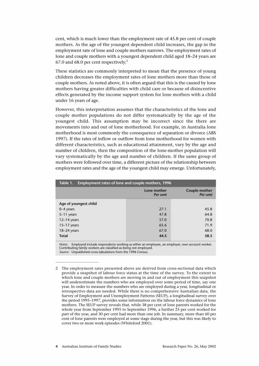
cent, which is much lower than the employment rate of 45.8 per cent of couplemothers. As the age of the youngest dependent child increases, the gap in theemployment rate of lone and couple mothers narrows. The employment rates oflone and couple mothers with a youngest dependent child aged 18–24 years are67.0 and 68.0 per cent respectively.2

These statistics are commonly interpreted to mean that the presence of youngchildren decreases the employment rates of lone mothers more than those ofcouple mothers. As noted above, it is often argued that this is the caused by lonemothers having greater difficulties with child care or because of disincentiveeffects generated by the income support system for lone mothers with a childunder 16 years of age.

However, this interpretation assumes that the characteristics of the lone andcouple mother populations do not differ systematically by the age of theyoungest child. This assumption may be incorrect since the there aremovements into and out of lone motherhood. For example, in Australia lonemotherhood is most commonly the consequence of separation or divorce (ABS1997). If the rates of inflow or outflow from lone motherhood for women withdifferent characteristics, such as educational attainment, vary by the age andnumber of children, then the composition of the lone-mother population willvary systematically by the age and number of children. If the same group ofmothers were followed over time, a different picture of the relationship betweenemployment rates and the age of the youngest child may emerge. Unfortunately,


2 The employment rates presented above are derived from cross-sectional data whichprovide a snapshot of labour force status at the time of the survey. To the extent towhich lone and couple mothers are moving in and out of employment this snapshotwill underestimate the numbers who are employed over some period of time, say oneyear. In order to measure the numbers who are employed during a year, longitudinal orretrospective data are needed. While there is no comprehensive Australian data, theSurvey of Employment and Unemployment Patterns (SEUP), a longitudinal survey overthe period 1995–1997, provides some information on the labour force dynamics of lonemothers. The SEUP survey reveals that, while 38 per cent of lone parents worked for thewhole year from September 1995 to September 1996, a further 25 per cent worked forpart of the year, and 30 per cent had more than one job. In summary, more than 60 percent of lone parents were employed at some stage during the year, but this was likely tocover two or more work episodes (Whiteford 2001).

Lone mother Couple motherPer cent Per cent

Age of youngest child0–4 years 27.1 45.8 5–11 years 47.8 64.8 12–14 years 57.0 70.8 15–17 years 65.6 71.9 18–24 years 67.0 68.0 Total 44.5 58.5

Notes: Employed include respondents working as either an employee, an employer, own account worker.Contributing family workers are classified as being not employed. Source: Unpublished cross-tabulations from the 1996 Census.

Table 1. Employment rates of lone and couple mothers, 1996

there is no suitable long-running representative Australian longitudinal dataavailable. However, indirect evidence can be obtained by comparing the averagecharacteristics of the lone-mother and couple-mother populations with childrenof different ages.

Educational attainment

Examining the level of educational attainment by the age of the youngestdependent child reveals substantial differences between lone and couplemothers. Table 2 shows that, overall, 34.4 per cent of couple mothers had a post-secondary qualification. This was substantially higher than for lone mothers, ofwhom 25.4 per cent had a post-secondary qualification. A greater proportion ofcouple mothers than lone mothers had a degree qualification or higher (14.8 percent compared with 9.1 per cent). Overall, couple mothers were also more likelythan lone mothers to have a diploma level qualification (10.1 and 7.7 per centrespectively).

When the difference in educational attainment of lone and couple mothers isconsidered by age of the youngest child a clear pattern emerges (see Table 2).Among couple mothers the level of educational attainment does not vary withthe age of the youngest child. For example, the proportion of couple motherswith a degree was much the same regardless of the age of the youngest child.

In contrast, for lone mothers there is a very clear relationship betweeneducational attainment and the age of the youngest child. Lone mothers with ayoungest child aged 0–4 years have the lowest levels of educational attainment.As the age of the youngest child increases so does the educational attainment oflone mothers. For example, of lone mothers whose youngest child was underfive years of age only 4.7 per cent had a degree. For those whose youngest childis 5–11 years old 9.7 per cent have a degree. For those whose youngest child isaged 15–17 years 14.1 per cent have a degree, very similar to the averageproportion of couple mothers.

As might be expected, the converse pattern applies in relation to having no post-secondary qualifications. Among couple mothers the proportion with noqualifications is much the same regardless of the age of their youngest child.However, among lone mothers the proportion with no qualifications steadilydeclines as the age of the youngest child increases.

In summary, a wide educational gap exists among lone and couple mothers withvery young children, but largely disappears by the time the youngest child is atsecondary school. This increase is unlikely to be explained by lone mothersupgrading their educational qualifications at a much faster rate than do couplemothers. The most likely explanation for the change in education qualificationsamong the lone mothers as children get older is that the transitions into and outof lone parenthood differ systematically by the age of the youngest child andhighest level of education attainment.

It is worth reiterating that only children aged over 16 years who are in full-timeeducation are considered. It is probable that mothers with a higher level ofeducational attainment are more likely to have children who remain in full-timeeducation beyond the age of 15 years and particularly beyond the age of 18.


The finding that the lone mother–couple mother educational attainment gapnarrows as the age of the youngest child increases in a similar way to the way thelone mother–couple mother employment gap narrows raises an importantquestion. How much of the apparent differential effects of young children onthe employment rates of lone and couple mothers is due to differences ineducational attainment or other characteristics which are related to thelikelihood of being employed?

This question is analysed in more detail in the following sections usingregression techniques, which allow for the effects of variables, including numberand age of children, on the probability of employment to be estimated whileholding constant the effects of other factors.

Modelling the determinants of employmentIn this section the data used in the estimates of the determinants of theprobability of employment are discussed. The conceptual framework used in thepaper is examined and the empirical model is described.

Data

The probability of employment is modelled using data from the 1996 CensusHousehold one per cent sample file. This data set is used because it is one of thefew Australian data sets which contains a large enough sample of lone mothers.The census data contains information on labour force status, on educational anddemographic characteristics, including the number and age of children ofmothers, and on household level data, which contains information on otherpeople in the household. Of particular importance for this study is theinformation on any partner who lives in the household.


Table 2. Post-secondary qualification by relationship status and age of youngest child

Age of youngest child (years)0–4 5–11 12–14 15–17 18–24 Total

Per cent

Couple mothers Degree 15.7 14.8 12.8 12 15.1 14.8 Diploma 9.5 10.5 10.4 10.6 12.0 10.1 Vocational 10.3 9.3 8.6 8.6 8.0 9.5 No qualification 64.4 65.4 68.2 68.8 64.8 65.6 Total 100 100 100 100 100 100

Number couple mothers 767,940 599,533 227,468 170,080 84,782 1,849,803

Lone mothers Degree 4.7 9.7 12 14.1 18.5 9.1 Diploma 4.9 8.2 9.6 11 12.4 7.7 Vocational 8.3 9.0 8.5 8.6 8.3 8.7 No qualification 82.0 73.1 69.9 66.3 60.8 74.6 Total 100 100 100 100 100 100

Number lone mothers 135,455 145,467 55,513 37,031 17,108 390,574

Note: Excludes mothers who do not state or inadequately described their qualifications.Source: Unpublished cross-tabulations from the 1996 Census.

Conceptual framework and empirical model

A mother’s probability of employment will be determined by whether she seeksemployment (supply labour) and her chance of finding suitable employment.Economic theory hypothesises that a person’s decision as to whether to supplylabour or not involves a trade-off between time spent at home on “market-substitution” activities, leisure, and paid work.

Clearly the decision is highly complex and involves many factors. For example, thecomposition of and dynamics within a household are important and the laboursupply decision needs to be considered in terms of household, or family needs, andthe interactions that occur between household or family members. For mothers,the age of their children is likely to be very important as the balance between paidwork and child bearing and child rearing responsibilities change (Killingsworth1983; Hersch and Stratton 1994). In addition to the financial incentives toparticipate in the labour market, there are likely to be issues surrounding child careand domestic labour that differ between lone and couple mothers.

The chances of finding employment will be determined by whether mothers canfind suitable employment. This will be determined by the productivity of theperson, the minimum wage and conditions at which they are prepared to acceptemployment (reservation wage), and possibly employer attitudes towardsemploying women with children. Mothers’ preferences about paid employmentwill also be an important determinant of the probability of employment. SeeEhrenberg and Smith (1997) for further discussion of models of thedeterminants of the probability of employment.

The model of employment outcomes can be expressed in a general form as:

E*i =Xiβ + εi

where E*i is a latent (unobserved) variable that captures the propensity towards

employment of individual i, X is a row vector of observed factors, β is a columnvector of coefficients to be estimated and ε is a stochastic error term. Twoobservable outcomes are derived from E*

i with reference to an arbitrary thresholdof zero. Thus, the individual is held to be employed (U = 1) where E*

i exceedszero and not employed (U = 0) otherwise. This observed indicator variable (U)becomes the dependent variable in the analysis.

Given the binary nature of the dependent variable, a logit or probit model isappropriate. The logit model is used in this paper. With this model, the naturallogarithm of the odds ratio of the probability of employment (E) to theprobability of non-employment (1-E), log[E/(1-E)], is expressed as a linearcombination of the explanatory variables, namely:

log ( 1 – E ) = Xiβ + εi

The specification of the logit model includes a number of variables which botheconomic and sociological theory suggests will be related to employment status,3

or which previous empirical studies have shown to be important determinants.4


E

3 See Ehrenberg and Smith (1997) for a discussion of the theoretical literature.4 Relevant empirical studies include Beggs and Chapman (1990), Harris (1996) and Le and

Miller (2000).

While the details of the construction of the variables can be found in AppendixA, the remainder of this section provides a rationale for the empiricalspecification used. The omitted categories of the respective variables are alsolisted in Appendix A with summary statistics being provided in Appendix B.

The models estimated are reduced form employment equations; structurallabour supply and labour demand models are not estimated. As a starting point,the estimation is based on the specification used in standard employmentequation and labour supply studies. A summary of the variables included ispresented in Table 3.

Age is included to pick up life cycle effects and as a measure of potential labourmarket experience. Age squared (AGE

2) is included to allow for a non-linear

relationship between age and the probability of employment. Highest level ofeducation attainment is measured by a set of variables: left secondary schoolaged 14 years or younger, left secondary school aged 15 or 16 years, leftsecondary school aged 17 years or older, vocational qualification or a diploma,or degree or higher level qualification. The omitted (or reference) category hasno post-secondary qualification and left secondary school aged 15 or 16 years.

The impact of child rearing on the probability of employment is captured usinga set of variables. The first series of variables reflects whether the age of youngestdependent child in the household is four years of age or younger, 5–11 years,12–15 years, or 16–24 years. A number of studies have found that having morethan one young child dramatically reduces the likelihood of a mother beingemployed (Chapman, Dunlop, Gray, Liu and Mitchell 2001). Therefore variablesare included which capture the effects of having more than one child agedunder four years, and having more than one child aged 5–11 years. Finally, thereis a dummy variable that captures the effects of having four or more children intotal. The omitted category is has a youngest child aged four years or younger.

These age ranges of children have been chosen because they reflect institutionalfeatures of the Australian educational and income support systems. The age offour years or younger is chosen because five is around the age of starting school.5

The age of 12 years is chosen because it is the age at which most children havestarted secondary school. The age cut-off of 16 years is chosen because it is theage at which parents lose eligibility for parenting payments.


Age and age squared Educational attainment Age of youngest child Number of children of different ages Housing tenure Regional location Indigenous origin English language proficiency Year of arrival in Australia (if a migrant) Partner’s income (couple mothers only)

Table 3. Variables included in estimation model

5 There is some variation between states in the age of starting school (more information isneeded here but the key point is that in some states in 1996 it was five years and inothers six, thus five is the youngest age at which children can start school).

The motivation to seek employment and the intensity of job search is likely tobe related to the financial commitments of the family. The stronger the financialneed, the stronger the motivation might be to seek employment (see Harris1996). A major financial commitment for families is housing costs, so familieswho own their own house outright may have less need for income compared topeople with a mortgage or who are renting accommodation. Therefore a set ofdummy variables, which indicate housing tenure (purchasing a house, owninghouse outright and renting accommodation) is included. The omitted categoryis purchasing a house.

The level of labour demand varies across different geographic regions ofAustralia and is clearly an important determinant of job opportunities, so avariable measuring geographic region of residence is included. Unfortunatelythe level of geographic information on the public release census data set is veryaggregated and it is therefore only possible to include a variable for living in acapital city as compared to living outside of a capital city. The omitted categoryis living outside of a capital city. A variable indicating Indigenous origin isincluded since this group has a much lower employment rate than do othergroups in Australian society (Hunter and Gray 1998).

Having poor spoken English is strongly related to labour market opportunitiesand hence employment rates (Le and Miller 2000). Therefore variables forspeaking English only, speaking English well, and speaking English poorly areincluded. The omitted category is speaking only English at home. Being amigrant is strongly related to labour market opportunities and amongstmigrants there is a very strong relationship between number of years sincearrival in Australia and labour market status (Le and Miller 2000). Thus includedare variables measuring arrival in Australia between 1991 and 1996, between1981 and 1990, and prior to 1981, and being born in Australia. The omittedcategory is being born in Australia.

Finally, economic theory and a number of previous empirical studies have foundthat partner’s income is an important determinant of the labour supply decisionof women. Therefore, for couple mothers, partner’s income as an explanatoryvariable is included. Partner’s income squared is included to allow for any non-linear relationship.6

The sample used in the estimation includes all women aged 15–64 years whohad a dependent child aged less than 16 years of age or a dependent child aged16–24 years who was a full-time student.7 The estimation sample comprised dataon 14,732 couple mothers and 3,196 lone mothers. Given the focus on


6 A proxy for partner’s income for lone mothers might be child maintenance received oreven government income support payments (which could be said to replace partner’ssupport). However, it was not possible to determine what proportion of a mother’s ownincome was drawn from these sources, so no proxy for partner’s income could beincluded when estimating the probability of employment for lone mothers.

7 Mothers living with a same sex partner are excluded as are mothers for whom the age ofyoungest child in the family could not be identified due to the temporary absence ofanother dependent child on census night. These restrictions resulted in a loss of 1.3 percent or 289 of the sample. The sample size is further reduced by excluding the “notstated” category in each of the variables included in the analysis.

exploring whether the determinants of the probability of employment of loneand couple mothers differ, the model is estimated separately for lone and couplemothers. This allows the effects of each of the explanatory variables on theprobability of employment to differ between the two groups.

Estimation resultsThis section presents the results of the estimates of the determinants of theprobability of employment of lone and couple mothers. Particular attention ispaid to comparing the determinants of the probability of employment for loneand couple mothers. Overall, the models appear to be well-specified and theestimates broadly consistent with the findings of other studies (Beggs andChapman 1990; Ross and Saunders 1990; Chapman, Dunlop, Gray, Liu andMitchell 2001).

Because the effects of changes in the explanatory variables on the probability ofemployment varies with the value of all the explanatory variables in the model,simply reporting these coefficients conveys very little. Thus the effects of each ofthese variables on the probability of employment are illustrating using“marginal effects”. The marginal effects show the effects of each of theexplanatory variables relative to a particular type (base case) of mother. In thisanalysis the base case has been set as having the mean value on the continuousvariables of mother’s age and partner’s income and as having the modal valuefor the attributes represented by the sets of dummy variables (age and number ofchildren, education, English language ability, indigenous status, migrant status,and housing type).8

This means that the base case against which all marginal effects must becompared is a mother who: is 37 years old; has only one child, and that child isaged 0–4 years; has no qualifications and left school aged 15 or 16 years; speaksonly English; is Australian born; is not an Indigenous Australian; is purchasing ahome; and for couple mothers has a partner earning $709 per week. Thecoefficient estimates are presented in Appendix C.

Table 4 shows the marginal effects for lone mothers and couple mothers. Asdiscussed, the marginal effects show the change in the probability ofemployment for a discrete change in each of the explanatory variables relativeto the base case probability.

Educational attainment

As an example to the interpretation of the marginal effects, consider the effectsof educational attainment. For couple mothers, having a degree or diploma levelqualification is estimated to increase the probability of employment by 21.1percentage points as compared with an otherwise similar couple mother with ahighest level of educational attainment of having left secondary school aged 15or 16 years of age. The underlying coefficient is statistically significant at the 5


8 The mean and modal values are calculated for the combined lone and couple motherpopulations. The only exception is partner’s income which is calculated using only datafrom couple mothers.


Couple Lone mothers mothersPer cent Per cent

Degree or diploma level qualification 21.1* 23.2* Vocational qualification 10.9* 16.7* No post-secondary qualification and left school aged 17 years or older 4.7* 7.3* No post-secondary qualification and left school aged 14 years or less -8.1* -16.3* Youngest dependent child aged 5–11 years 14.2* 14.3* Youngest dependent child aged 12–15 years 19.9* 19.3* Youngest child aged 16–24 years 22.7* 28.6* Has 2 or more children aged under 4 years -17.1* -25.2* Has 2 or more children aged 5–11 years a 5.8* -6.0* Has four or more children -10.5* -13.7* Good spoken English -6.5* -16.4* Poor spoken English -25.8* -41.3* Indigenous 0.2 4.5 Outside capital city -2.8* -5.0* Migrant who arrived prior to 1981 0.9 2.6 Migrant who arrived 1981-1990 -0.6 6.2 Migrant who arrived 1991-1996 -18.9* -12.4 Own house outright -8.4* -12.7* Renting -18.7* -19.4* Partner’s income 0.7*

Notes: The marginal effects are calculated relative to a base case mother who has one child aged 0–4years, 37 years old, no post-secondary qualification and left school aged 15 or 16 years of age, speaks onlyEnglish, born in Australia, lives in a capital city, is not an Indigenous Australian, is purchasing home and, forcouple mothers, has a partner earning $709 per week. The marginal effects for the dummy (binary)variables are calculated for a change in the value of the variable from zero to one. For continuous variablesthe marginal effects show the effect for an incremental increase. In the case of age it shows the effects of afive-year increase in age and for partner’s income it is calculated for a $100 per week increase in income. * indicates that the underlying coefficient is statistically significant at the 5 per cent confidence level.(a) The marginal effects for having two or more children aged 5–11 years is the change in probability ofhaving two children aged 5–11 years as compared with having one child aged 5–11 years and no childrenaged 0–4 years.Source: Derived from Appendix Table C1.

Table 4. Marginal effects on the probability of employment by family type, 1996

per cent level. For lone mothers the effect is similar, with a degree or diplomalevel qualification being estimated to increase the predicted probability ofemployment by 23.2 percentage points.

Having a vocational qualification increases the probability of employment of loneand couple mothers by 10.9 and 16.7 percentage points respectively. For thosewithout post-secondary qualifications, the age at which they left school has asubstantial impact on the likelihood of employment of both lone and couplemothers, although the effect differs. For couple mothers, having a left secondaryschool aged 17 or over, and having no post-secondary qualification, is estimatedto increase the probability of employment by 4.7 percentage points. For lonemothers, staying on at secondary school until 17 or older increases the probabilityof employment by 7.3 percentage points as compared with having left secondaryschool aged 15 or 16 years of age. Leaving school at a young age (14 years oryounger) has a much larger negative impact on lone than couple mothers. Leavingschool this early reduced the probability of employment for couple mothers by 8.1percentage points compared with 16.3 percentage points for lone mothers.

Age and number of children

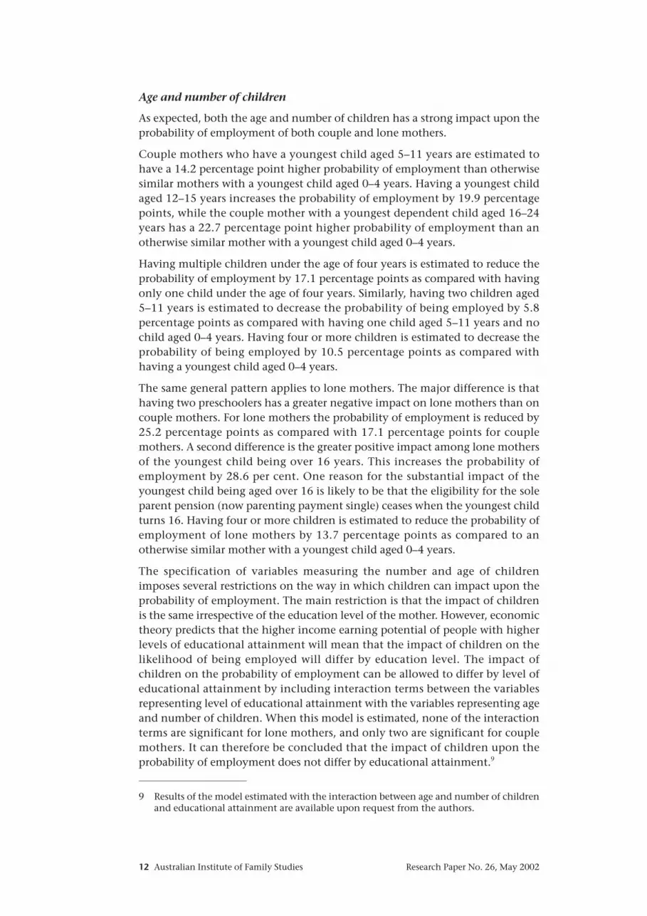
As expected, both the age and number of children has a strong impact upon theprobability of employment of both couple and lone mothers.

Couple mothers who have a youngest child aged 5–11 years are estimated tohave a 14.2 percentage point higher probability of employment than otherwisesimilar mothers with a youngest child aged 0–4 years. Having a youngest childaged 12–15 years increases the probability of employment by 19.9 percentagepoints, while the couple mother with a youngest dependent child aged 16–24years has a 22.7 percentage point higher probability of employment than anotherwise similar mother with a youngest child aged 0–4 years.

Having multiple children under the age of four years is estimated to reduce theprobability of employment by 17.1 percentage points as compared with havingonly one child under the age of four years. Similarly, having two children aged5–11 years is estimated to decrease the probability of being employed by 5.8percentage points as compared with having one child aged 5–11 years and nochild aged 0–4 years. Having four or more children is estimated to decrease theprobability of being employed by 10.5 percentage points as compared withhaving a youngest child aged 0–4 years.

The same general pattern applies to lone mothers. The major difference is thathaving two preschoolers has a greater negative impact on lone mothers than oncouple mothers. For lone mothers the probability of employment is reduced by25.2 percentage points as compared with 17.1 percentage points for couplemothers. A second difference is the greater positive impact among lone mothersof the youngest child being over 16 years. This increases the probability ofemployment by 28.6 per cent. One reason for the substantial impact of theyoungest child being aged over 16 is likely to be that the eligibility for the soleparent pension (now parenting payment single) ceases when the youngest childturns 16. Having four or more children is estimated to reduce the probability ofemployment of lone mothers by 13.7 percentage points as compared to anotherwise similar mother with a youngest child aged 0–4 years.

The specification of variables measuring the number and age of childrenimposes several restrictions on the way in which children can impact upon theprobability of employment. The main restriction is that the impact of childrenis the same irrespective of the education level of the mother. However, economictheory predicts that the higher income earning potential of people with higherlevels of educational attainment will mean that the impact of children on thelikelihood of being employed will differ by education level. The impact ofchildren on the probability of employment can be allowed to differ by level ofeducational attainment by including interaction terms between the variablesrepresenting level of educational attainment with the variables representing ageand number of children. When this model is estimated, none of the interactionterms are significant for lone mothers, and only two are significant for couplemothers. It can therefore be concluded that the impact of children upon theprobability of employment does not differ by educational attainment.9


9 Results of the model estimated with the interaction between age and number of childrenand educational attainment are available upon request from the authors.

English language skills

English skills are found to be an important determinant of the probability ofbeing employed. For couple mothers, speaking a language other than English athome, but having good spoken English, is estimated to reduce the probability ofemployment by 6.5 percentage points as compared with mothers who speak onlyEnglish at home. For lone mothers the negative effect is more than twice as large,with lone mothers having a 16.4 per cent lower probability of employmentcompared with the comparable lone mother who spoke only English at home.

Having poor English was an even greater barrier to employment. Among couplemothers it reduced the employment probability by 25.8 percentage points.Among lone mothers, the effect of poor English was even greater – reducing theprobability of employment by 41.3 percentage points. While this effect cannotsimply be attributed to the causal effect of poor English, it is a stronger predictorof a lower probability of employment amongst lone than couple mothers.

Indigenous origin and geographic location

Being of Indigenous origin is found to have no statistically significant effects forlone or couple mothers. This result is surprising given that Indigenous women,in general, have much lower employment rates than other women (Hunter andGray 1998).10 Living outside of a capital city is estimated to reduce theprobability of employment for couple mothers by 2.8 percentage points and by5.0 percentage points for lone mothers.

Migrant status

Mothers who are recent arrivals to Australia have a substantially reducedprobability of employment compared with longer-term migrants. Couplemothers who arrived within the previous five years had a 18.9 percentage pointlower probability of employment compared with comparable Australian-bornmothers. Lone mothers were less affected by being recent arrivals, but recentarrival nevertheless had a marginal effect of 12.4 per cent. Longer-term migrantsare estimated to have a very similar employment probability as Australian-bornmothers. The similarity in employment probabilities of longer-term migrantsand Australian-born mothers may be, in part, explained by these migrants beingmore likely than more recent migrants to have gone through Australianeducation.

Housing tenure

Housing tenure is strongly related to the probability of being employed forcouple and lone mothers. Owning a house outright is estimated to reduce theprobability of being employed by 8.4 and 12.7 percentage points for couple andlone mothers respectively as compared with those in the process of purchasingtheir home. This probably reflects the lower financial demands on home-owners


10 There non-significant result for being of Indigenous origin for lone and couple mothersis unlikely to be due to there being two few Indigenous lone mothers in the sample—there are 128 in the estimation sample.

as compared to those with debt on their home. Mothers who are renting are theleast likely to be employed, with couple and lone mothers being 18.7 and 19.4percentage points respectively less likely to be employed than are those who arein the process of purchasing their home.

The strong negative effects of being a renter may be explained by the financialdisincentive effects generated by the income support system for those in publichousing, or in private rental accommodation and receiving government rentassistance. Eligibility for public rental accommodation or rent assistance can belost, or the amount of assistance reduced, as earned income increases. This canlead to very high effective marginal tax rates for lone mothers as compared withcouple mothers, and a consequently reduced participation in the labour market.

The negative effect of the impact of being a renter on the probability ofemployment may also be because living in rental accommodation is correlatedwith unobserved factors related to the probability of employment. The maincandidate here is past employment history. However, for both couple and lonemothers there are good reasons to expect that the link between pastemployment history and current housing tenure may be quite weak since manycouple mothers have intermittent work histories, and housing tenure may bemore dependent on their partner’s employment history. For lone mothers,housing tenure will be related both to employment history and, if they werepreviously in a marriage or defacto relationship, housing tenure in thatrelationship as well as the terms and conditions of their separation from theirpartner.

Partner’s income

Partner’s income has a statistically significant but relatively small effect on thecouple mother’s probability of employment. An increase in partner’s incomefrom $706 per week to $806 per week is estimated to increase the probability ofemployment of the base case couple mothers by 0.7 percentage points. Partner’sincome has an inverted U-shaped relationship with the probability ofemployment, with the maximum probability of employment for the base casemother at a partner’s income of about $1,150 per week.

In broad terms, the determinants of the probability of employment of lone andcouple mothers are similar. For many variables the level of the effect wasindistinguishable. However, there are several variables, which have a differingsize of effects for lone and couple mothers. In general, factors that are typicallyassociated with low rates of employment and could be considered a barrier toemployment have a larger negative effect upon the probability of employmentof lone mothers than couple mothers Beggs and Chapman 1990; Ross and Saunders 1990; Harris 1996; Le and Miller 2000; Chapman, et al. 2001). These include having two pre-schoolers, having the very low level ofeducational attainment of having left school aged 14 years or younger, speakinga language other than English at home, and in particular having poor spokenEnglish.

Of particular importance is that the impact of children upon the probability ofemployment is very similar for lone and couple mothers, with the only realexception being having two children under the age of four. This result is quite


important because it implies that the apparent narrowing of the gap inemployment rates as the age of the youngest child increases is only in part due tochildren of different ages having differential effects on the employment rates oflone and couple mothers, with the remainder being explained by other factors.

Factors generating the employment gap The extent to which there are differences in the effects of variables on theprobability of employment between lone and couple mothers is captured bydifferences in the coefficients (and marginal effects). Within the statisticalframework used in this paper, the gap in employment rates between lone andcouple mothers can be attributed either to differences in the characteristics ofthe two groups of mothers or to differences in the effects of variouscharacteristics on the probability of employment for each group.

Even when a particular characteristic is estimated to have the same impact onthe probability of employment of couple and lone mothers, differentemployment outcomes for lone and couple mothers are still apparent. If the twogroups have overall difference in their characteristics (for example, in overalllevel of post-secondary qualifications) then there will be differences in theiroverall employment rates. For example, if educational attainment has the sameimpact on the employment probabilities of lone and couple mothers but couplemothers have a higher average level of education than do otherwise similar lonemothers, then couple mothers will have a higher probability of employment.

This section uses an alternative presentation of the models estimated in thispaper to identify the role of differences in characteristics of the lone and couplemother populations in explaining the lone mother–couple mother employmentgap. One way of estimating the effect of the different characteristics of lone andcouple mothers is to perform some “thought experiments”. The question isasked: “What would the employment probabilities be for lone mothers if theyhad the same characteristics as couple mothers, except for partnering status?”.Thus if lone mothers had the same educational attainment, same English skills,the same profile of young and older children and so on, what do we expect theirprobability of employment would be? Similar “thought experiments” orhypothetical scenarios can be used to identify the effects of statistical equalityfor particular attributes – educational attainment and age and number ofchildren.

Table 5 presents estimates of the impact of statistical equality of educationalattainment and number and age of children. (See Appendix D for a formalmathematical presentation of the decompositions.)

Table 5 presents the results of the three hypothetical scenarios. The derivation ofthe figures in Table 5 and their interpretation need some explanation. The toppanel of Table 5 shows the predicted probability of employment for lone andcouple mothers calculated using the respective coefficients and averagecharacteristics. These are titled base case probabilities. The second panel showsthe expected probability of employment of lone mothers under the threehypothetical scenarios. The first hypothetical, labelled “Scenario 1”, shows thepredicted probability of employment of lone mothers if they had the same


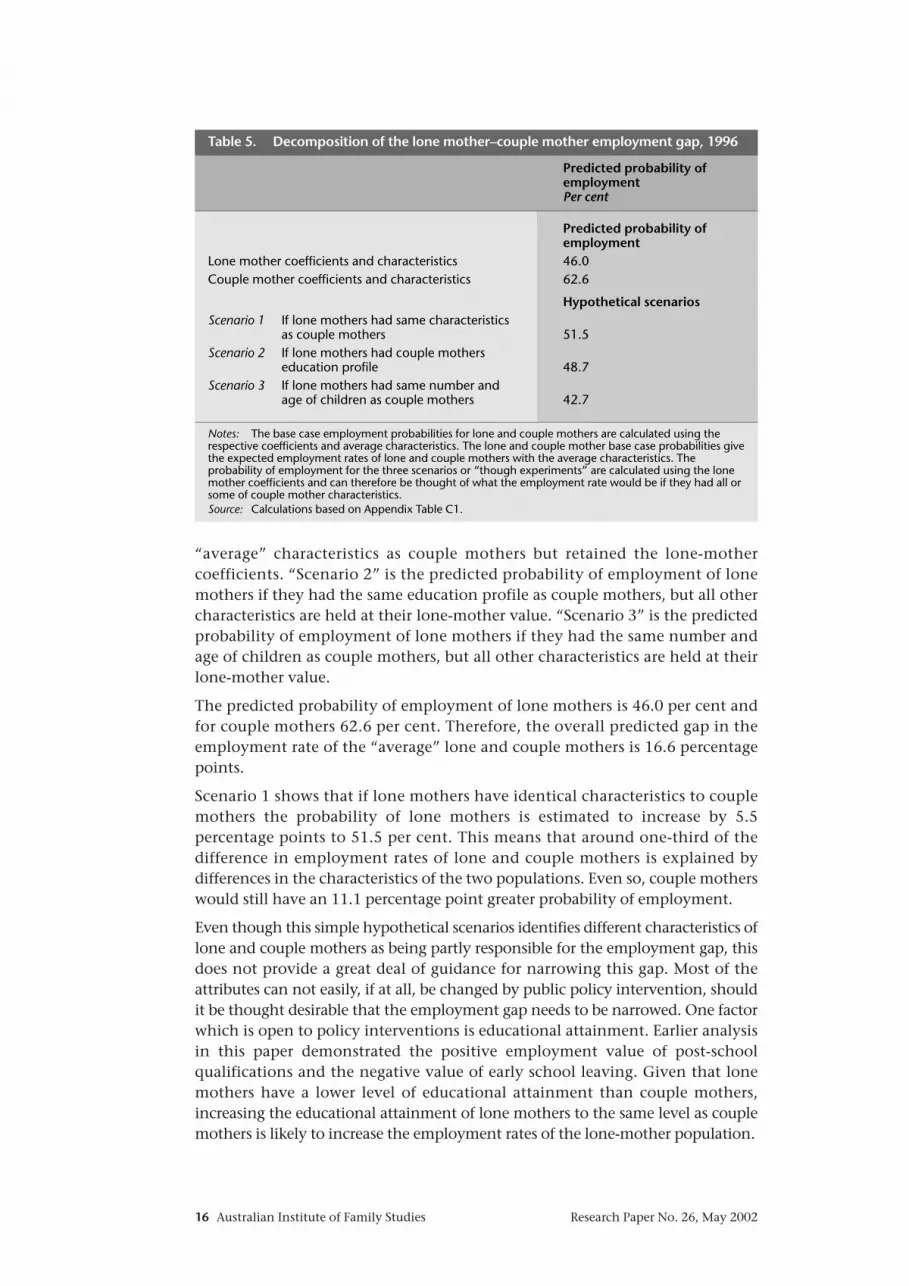
“average” characteristics as couple mothers but retained the lone-mothercoefficients. “Scenario 2” is the predicted probability of employment of lonemothers if they had the same education profile as couple mothers, but all othercharacteristics are held at their lone-mother value. “Scenario 3” is the predictedprobability of employment of lone mothers if they had the same number andage of children as couple mothers, but all other characteristics are held at theirlone-mother value.

The predicted probability of employment of lone mothers is 46.0 per cent andfor couple mothers 62.6 per cent. Therefore, the overall predicted gap in theemployment rate of the “average” lone and couple mothers is 16.6 percentagepoints.

Scenario 1 shows that if lone mothers have identical characteristics to couplemothers the probability of lone mothers is estimated to increase by 5.5percentage points to 51.5 per cent. This means that around one-third of thedifference in employment rates of lone and couple mothers is explained bydifferences in the characteristics of the two populations. Even so, couple motherswould still have an 11.1 percentage point greater probability of employment.

Even though this simple hypothetical scenarios identifies different characteristics oflone and couple mothers as being partly responsible for the employment gap, thisdoes not provide a great deal of guidance for narrowing this gap. Most of theattributes can not easily, if at all, be changed by public policy intervention, shouldit be thought desirable that the employment gap needs to be narrowed. One factorwhich is open to policy interventions is educational attainment. Earlier analysis in this paper demonstrated the positive employment value of post-schoolqualifications and the negative value of early school leaving. Given that lonemothers have a lower level of educational attainment than couple mothers,increasing the educational attainment of lone mothers to the same level as couplemothers is likely to increase the employment rates of the lone-mother population.


Predicted probability of employmentPer cent

Predicted probability of employment

Lone mother coefficients and characteristics 46.0Couple mother coefficients and characteristics 62.6

Hypothetical scenarios Scenario 1 If lone mothers had same characteristics

as couple mothers 51.5Scenario 2 If lone mothers had couple mothers

education profile 48.7Scenario 3 If lone mothers had same number and

age of children as couple mothers 42.7

Notes: The base case employment probabilities for lone and couple mothers are calculated using therespective coefficients and average characteristics. The lone and couple mother base case probabilities givethe expected employment rates of lone and couple mothers with the average characteristics. Theprobability of employment for the three scenarios or “though experiments” are calculated using the lonemother coefficients and can therefore be thought of what the employment rate would be if they had all orsome of couple mother characteristics.Source: Calculations based on Appendix Table C1.

Table 5. Decomposition of the lone mother–couple mother employment gap, 1996

The effect of this can be estimated by calculating the probability of employmentfor lone mothers using lone-mother characteristics for all variables excepteducation where couple-mother characteristics are substituted (Scenario 2).When this is done, the probability of employment of lone mothers increases to48.7 per cent – an increase of 2.7 percentage points

This means that the effect of increasing the education levels of lone mothers tothat of couple mothers is likely to have only a very modest effect onemployment rates of lone mothers on its own, separated from othercharacteristics. Additional research designed to identify other characteristics oflone and couple mothers that affect employment may point to otherinterventions that could improve the probability of lone mothers beingemployed.

The third scenario shows the effects of changing the number and age of lonemothers’ children. This can be estimated by calculating the probability ofemployment for lone mothers using lone-mother characteristics for all variablesexcept number and age of children where couple mother characteristics aresubstituted. When this is done, the probability of employment of lone mothersdecreases to 42.7 per cent. This confirms the earlier findings that it is not the ageand number of children per se which reduces lone mothers’ chances of beingemployed.

Concluding comments and policy implicationsIt has long been debated whether or not the lower rate of employment of lonemothers is a problem from a social policy perspective. On the one hand, thehigh rate of joblessness may have adverse consequences for children growing upin such families. On the other hand, it is argued that all mothers, including lonemothers, should have the option to care for their children themselves and notbe required to place them in child care while the mother is working.

This dilemma has led to some ambivalence in government policy as to whetherincreasing the employment rates of mothers in general, and lone mothers inparticular, is desirable. In many ways the answer to this question depends uponthe reasons for employment or non-employment.

This paper used data from the 1996 Census, to estimate a model of thedeterminants of the probability of employment, of lone and couple mothers.The analysis in the paper reveals that the determinants of the probability ofemployment are generally similar for lone and couple mothers, although thereare several important differences. In general, factors that are typically associatedwith lower rates of employment, and could be considered a barrier toemployment, have a larger negative effect upon the probability of employmenton lone mothers than on couple mothers. These include having a low level ofeducational attainment, speaking English as a second language and, inparticular, having poor spoken English.

The analysis also reveals that around one-third of the difference in theemployment rate of lone and couple mothers is due to differences in thecharacteristics of the two groups. This gap is explained by differences in anumber of the characteristics. Of particular interest is the surprisingly small


amount of the employment gap explained by differences in educationalattainment. The remaining two-thirds, or the majority of the employment gap,is caused by variables impacting on the employment rates of lone and couplemothers differently. Importantly, while there are some differences in the impacton lone and couple mothers of having two or more pre-school aged children, ingeneral children of different ages have remarkably similar effects for lone andcouple mothers. Having poor spoken English and low levels of educationalattainment have a much larger negative impact on the employmentprobabilities of lone mothers than couple mothers.

The finding that children have a similar impact upon the probability ofemployment of lone and couple mothers is important because it implies that theapparent narrowing of the gap in employment rates as the age of the youngestchild increases is only in part due to children of different ages having differentialeffects on the employment rates of lone and couple mothers. The explanationsof the lone mother–couple mother employment gap being the result of youngchildren having a greater impact upon the likelihood of employment of lonemothers appears to have quite limited explanatory power.

It is important to note that while a wide range of factors are included in themodel of the determinants of the probability of employment, there are severalpotentially important factors which are not asked about in the census data andso are not included in the models estimated. Of particular relevance here is therole non-resident fathers play, and in particular the provision and level of childsupport payments.

The methodology used in this paper does not provide direct evidence on whyfactors such as poor English, early school leaving and multiple young childrenhave a much greater negative impact on lone mothers than on couple mothers.If the processes lying behind this differential impact can be identified we wouldbe in a better position to know whether it is desirable to try to intervene. If suchinterventions to alter the impact of variables were possible and desirable, thenpolicy interventions could be targeted to altering the processes that lead to loweremployment rates rather than just focussing on the attributes of lone and couplemothers. Understanding the processes which determine how decision aboutwork are made in Australian families is the continuing focus of Instituteresearch.


References

ABS (2000), Labour Force Status and Other Characteristics of Families, Australia,Australian Bureau of Statistics, Catalogue No. 6224.0, Canberra.

ABS (1997), Family Characteristics, Australian Bureau of Statistics, Catalogue Number4442.0, Canberra.

Beggs, J. & Chapman, B. (1990), “Search efficiency, skill transferability andimmigrant unemployment rates in Australia”, Applied Economics, vol. 22, no. 2,pp. 249-60.

Chapman, B., Dunlop, Y., Gray, M., Liu, A. & Mitchell, D. (2001), “The impact ofchildren on the lifetime earnings of Australian women: Evidence from the 1990s”,Australian Economic Review, vol. 34, no. 4, pp. 373-389.

Ehrenberg, R. & Smith, R. (1997), Modern Labor Economics: Theory and Public Policy,6th edition, Addison-Wesley, Massachusetts.

Gregory, R. (1999), “Children and the changing labour market: Joblessness infamilies with dependent children”, Centre for Economic Policy Research DiscussionPaper Discussion Paper No. 406, Centre for Economic Policy Research, AustralianNational University, Canberra.

Harris, M. (1996), “Modelling the probability of youth unemployment in Australia”,Economic Record, vol. 72, no. 217, pp. 118-129.

Henderson, R., Harcourt, A. & Harper, R. (1970), People in Poverty: A Melbourne Survey,Cheshire, for the Institute of Applied Economic and Social Research, University ofMelbourne, Melbourne.

Hersch, J. & Stratton, L. (1994), “Housework, wages and the division of householdtime for employed spouses”, American Economic Review, vol. 84, no. 2, pp. 120-125.

Hunter, B. & Gray, M. (1998), “The relative labour force status of indigenous people,1986-96: A cohort analysis”, Australian Bulletin of Labour, vol. 24, no. 3, pp. 220-40.

Ingles, D. (2000), “Rationalising the interaction of tax and social security: Part I:Specific problem areas”, Centre for Economic Policy Research Discussion Paper No.423, Centre for Economic Policy Research, Australian National University,Canberra.

Killingsworth, M. (1983), Labour Supply, Cambridge University Press, Cambridge.

Le, A. & Miller, P. (2000), “An evaluation of inertia models of unemployment”,Australian Economic Review, vol. 33, no. 3, pp. 205-220.

McClure, P. (2000), Participation Support for a More Equitable Society, Final report of theReference Group on Welfare Reform 2000, Canberra.

McHugh, M. & Millar, J. (1997), “Single mothers in Australia: Supporting mothers toseek work”, in S. Duncan & R. Edwards (eds) Single Mothers in an InternationalContext: Mothers or Workers? UCL Press, London.

Oxley, H., Thai-Thanh, D., Förster, M. & Pellizzari, M. (1999), “Income inequalitiesand poverty among children and households with children in selected OECDcountries: trends and determinants”, Paper presented to the Conference on ChildWellbeing in Rich and Transition Countries: Are Children in Growing Danger ofSocial Exclusion?, Luxembourg.

Ross, R.& Saunders, P. (1990), “The labour supply behaviour of single mothers andmarried mothers in Australia”, Social Policy Research Centre Discussion Paper No. 19,Social Policy Research Centre, University of New South Wales, Sydney.

Shaver, S. (1998), “Poverty, gender and sole parenthood”, in R. Fincher & J.Nieuwenhuysen (eds) Australian Poverty: Then and Now, Melbourne UniversityPress, Melbourne.

Swinbourne K., Esson K. & Cox, E. (with Scouler, B.) (2001), ‘The Social Economy ofSole Parenting’, University of Technology, Sydney.

Whiteford, P. (2001), “Lone parents and employment in Australia”, in J. Millar andK. Rowlingson (eds) Lone Parents, Employment and Social Policy:Cross-NationalComparisons, The Policy Press, Bristol.


Appendix A. Variable definitionsAge measures age of mother in years. In the 1996 Census public release data set,age is grouped into five-year age bands. A continuous measure of age is createdby using the mid-point of the age bands.

Lone mother is defined as a woman who has no spouse or partner usuallypresent in the household but who forms a parent–child relationship with at leastone dependent child usually resident in the household.

Couple mother is defined as a woman who has a spouse or partner usuallypresent in the household and who forms a parent–child relationship with atleast one dependent child usually resident in the household.

Couple relationship is based on a consensual union, and is defined as twopeople residing in the same household who share a social, economic andemotional bond usually associated with marriage, and who consider theirrelationship to be a marriage or marriage-like union.

Dependent children is defined as all children in the household aged 15 years oryounger, or a child in the household who is aged 16–24 years and is a full-timestudent. The Census data do not record the exact relationship between adependent child and their “mother”. Since the sample is restricted to womenwho have given birth to a child, a small number of mothers who have only step,adopted or fostered child(ren) are excluded. However, the impact of thisrestriction will be very minimal because the number of women in this categoryis quite small.

Age of youngest child 0–4 years is set to one if the age of the youngestdependent child is 0–4 years, and zero otherwise.




Having two or more children aged 0–4 years is set to one if has two or morechildren aged 0–4 years of age, and zero otherwise.

Having two or more children aged 5–11 years is set to one if has two or morechildren aged 5–11 years of age, and zero otherwise.

Have four or more children is set to one if has four or more children, and zerootherwise.

Degree/diploma is set to one if the respondent’s highest educationalqualification is a higher degree, a post-graduate diploma, bachelor degree,under-graduate diploma, or an associate diploma, and zero otherwise.

Vocational is set to one if the respondent’s highest educational qualification isa skilled vocational or basic vocational qualification, and zero otherwise.Respondents who reported having a post-secondary qualification but who


“inadequately described” the qualification are coded as having a vocationalqualification. Estimates of the model including “inadequately described” as aseparate qualification revealed that there was no difference in the estimatedeffects of having a vocational and an “inadequately described” qualificationmeaning that they can legitimately be combined.

No post-secondary qualification and left school aged 17 years or older is setto one if the respondent has no post-secondary qualification and left schoolaged 17 years or older, and zero otherwise.

No post-secondary qualification and left school aged 15 or 16 years is set toone if the respondent has no post-secondary qualification and left school aged15 or 16 years of age, and zero otherwise.

No post-secondary qualification and left school aged 14 years or less is set toone if the respondent has no post-secondary qualification and left school aged14 years or less or never attended school, and zero otherwise.

Capital city is set to one if the respondent lived in a capital city, and zerootherwise. The only exception is that Tasmania, Northern Territory and AustraliaCapital Territory are coded as being capital cities. It is necessary to do this sincethe public release data set includes these States and Territories as single areas.

Speak English only is set to one if the respondent does not speak a languageother than English at home, and zero otherwise.

Good spoken English is set to one if the respondent speaks a language otherthan English at home and speaks English very well or well, and zero otherwise.

Poor spoken English is set to one if the respondent speaks a language otherthan English at home and speaks English not well or not at all, and zerootherwise.

Partner’s income is the partner’s weekly pre-tax income from all sources. In thecensus, income data is collected using income brackets. A continuous incomevariable is constructed using the mid-point of the income bracket. The valueassigned to the highest income category is 1.5 times the lower bound of thiscategory. For a small number of couple mothers, their partner’s income wasnegative and coded as zero in the analysis. Also, there were a few couple mothers(3.1 per cent or 556 couple mothers) whose partners were temporarily absent atthe census night.


Appendix B. Descriptive statistics


Table B1: Description of variables entered in the logistic models

Couple mothers Lone mothers

Employed 0.59 (0.49) 0.46 (0.50) Age of youngest child 0–4 years 0.42 (0.49) 0.35 (0.48) Age of youngest child 5–11 years 0.32 (0.47) 0.36 (0.48) Age of youngest child 12–15 years 0.16 (0.37) 0.18 (0.39) Age of youngest child 16–24 years 0.10 (0.30) 0.11 (0.31) Having 2 or more children aged 0–4 years 0.13 (0.34) 0.07 (0.26) Having 2 or more children aged 5–11 years 0.21 (0.41) 0.16 (0.37) Have 4 or more children 0.13 (0.34) 0.13 (0.34) Age of mothers 37.64 (7.64) 36.39 (8.83) Diploma or higher degree 0.24 (0.43) 0.17 (0.37) Vocational qualification 0.11 (0.31) 0.09 (0.29) No post-secondary qualification and left school at 17 years or older 0.21 (0.41) 0.21 (0.40) No post-secondary qualification and left school at 15 or 16 years 0.39 (0.49) 0.45 (0.50)No post-secondary qualification and left school at 14 years or younger 0.06 (0.23) 0.09 (0.28)Speak English only 0.83 (0.37) 0.89 (0.32) Good spoken English 0.13 (0.34) 0.08 (0.28) Poor spoken English 0.03 (0.18) 0.03 (0.17) Aboriginal or Torres Strait Islander origin 0.01 (0.11) 0.04 (0.21)

Residential locationMajor urban 0.61 (0.49) 0.59 (0.49)

Year of arrival at AustraliaBorn in Australia 0.72 (0.45) 0.77 (0.42) Arrived in Australia before 1981 0.15 (0.36) 0.13 (0.34) Arrived in Australia between 1981-1990 0.09 (0.28) 0.06 (0.24) Arrived in Australia between 1991-1996 0.04 (0.19) 0.03 (0.18) Fully own house 0.32 (0.47) 0.17 (0.37) Purchasing house 0.47 (0.50) 0.23 (0.42) Renting house 0.21 (0.41) 0.60 (0.49) Partner’s weekly income (dollars) 709.47 (513.20) Number of observations 14,732 3,196

Note: Standard deviations are shown in brackets. Excludes contributing family workers.Source: 1996 Census one per cent sample file.

Appendix C. Estimation results


Table C1. Logit estimates of probability of employment, lone and couple mothers, 1996

Couple mothers Lone mothersCoefficient T-stat Coefficient T-stat

Youngest dependent child aged 0–4 years -1.2032 (12.95) -1.4086 (7.45) Youngest dependent child aged 5–11 years -0.5366 (6.28) -0.7979 (4.71) Youngest dependent child aged 12–15 years -0.1937 (2.33) -0.5548 (3.34) Has 2 or more children aged 0–4 years -0.693 (11.36) -1.06 (4.78) Has 2 or more children aged 5–11 years -0.2911 (5.58) -0.2694 (2.26) Has 4 or more children -0.43 (7.45) -0.553 (4.14) Age 0.1992 (9.53) 0.1791 (4.91) Age squared -0.0026 (8.67) -0.0022 (4.40) Vocational qualification -0.5969 (8.51) -0.3418 (2.04) No post-secondary qualification and left school at 17 or older -0.8909 (15.26) -0.766 (5.48) No post-secondary qualification and left school at 15 or 16 years -1.0926 (20.46) -1.0662 (8.59)No post-secondary qualification and left school at 14 or younger -1.4265 (15.64) -1.7269 (9.02) Good spoken English -0.268 (4.16) -0.6652 (3.99) Poor spoken English -1.055 (8.56) -2.0618 (5.64) Indigenous 0.0082 (0.05) 0.1841 (0.90) Major urban 0.1181 (2.94) 0.2003 (2.36) Arrived in Australia prior to 1981 0.0367 (0.65) 0.1074 (0.86) Arrived in Australia between 1981-1990 -0.0244 (0.32) 0.2535 (1.33) Arrived in Australia between 1991-1996 -0.7646 (6.99) -0.4987 (1.78) Purchasing 0.3454 (7.81) 0.5114 (3.94) Renting -0.4125 (7.50) -0.2821 (2.46) Weekly income 0.0009 (9.00) Weekly income squared -4.00E-07 (46.19) Constant -1.9473 (4.81) -1.6717 (2.37) Pseudo R-squared 0.131 0.175 Model chi-square 2622.083 771.286 Number of observations 14,732 3,196

Source: 1996 Census one per cent sample file.

Appendix D. Detailed description of


This Appendix presents mathematically the decompositions presented inSection 5 of the paper. Define the following probabilities:

ÊLM

= XLMβ

LM

ÊCM

= XCMβ

CM

Ê0

LM= X

CMβ

LM

where βLM

is a vector of estimated coefficients for lone mothers, βCM

is a vector ofestimated coefficients for couple mothers, X

LMis a vector of characteristics of

lone mothers, XCM

is a vector of characteristics of couple mothers. ÊLM

is theaverage probability of employment for lone mothers, Ê

CMis the average

probability of employment for couple mothers and Ê0

LMis the average probability

of employment for lone mothers if they had the same characteristics as couplemothers but the coefficients of lone mothers.

The difference in the predicted probabilities of lone and couple mothers can beseparated into the component due to differences in coefficients for the twogroups and the component due to differences in characteristics of the twogroups. The following identity shows this decomposition:

ÊLM

– ÊCM

= (ÊLM

– Ê0

LM) + (Ê0

LM– Ê

CM)

Characteristics Coefficients

The differences in employment rates due to differences in coefficients is given bydifference in the predicted probability of employment for lone mothers and thepredicted probability of employment using the lone mother coefficients and thecouple mother characteristics. The part of the employment gap due tocharacteristics is given by difference between the predicted probability ofemployment using the lone mother coefficients and the couple mothercharacteristics and the predicted probability of employment obtained usingcouple mother coefficients and couple mother characteristics.

{ {

Australian Institute of Family StudiesThe Australian Institute of Family Studies is an independent statutory authority whichoriginated in the Australian Family Law Act(1975). The Institute was established by theCommonwealth Government in February 1980.

The Institute promotes the identification andunderstanding of factors affecting marital andfamily stability in Australia by:

• researching and evaluating the social, legaland economic wellbeing of all Australianfamilies;

• informing government and the policymaking process about Institute findings;

• communicating the results of Institute andother family research to organisationsconcerned with family wellbeing, and tothe wider general community;

• promoting improved support for families,including measures which prevent familydisruption and enhance marital and familystability.

The objectives of the Institute are essentiallypractical ones, concerned primarily withlearning about real situations through researchon Australian families.

For further information about the Institute and itswork, write to Australian Institute of Family Studies,300 Queen Street, Melbourne, Victoria 3000,Australia. Phone (03) 9214 7888. Fax (03) 92147839. Internet www.aifs.org.au/

Australian Instituteof Family Studies

AIFS RESEARCH PAPERS IN PRINT(formerly called Working Papers)

No. 13 Social polarisation and housing careers: Exploring the interrelationshipof labour and housing markets in Australia, Ian Winter and WendyStone, March 1998.

No. 14 Families in later life: Dimensions of retirement, Ilene Wolcott, May1998.

No. 15 Family relationships and intergenerational exchange in later life,Christine Millward, July 1998

No. 16 Spousal support in Australia: A study of incidence and attitudes, JulietBehrens and Bruce Smyth, December 1998.

No. 17 Reconceptualising Australian housing careers, Ian Winter andWendy Stone, April 1999.

No. 18 Superannuation and divorce in Australia, John Dewar, GraniaSheehan and Jody Hughes, May 1999.

No. 19 Understanding links between family experience, obligations andexpectations in later life, Christine Millward, May 1999.

No. 20 Towards understanding the reasons for divorce, Ilene Wolcott andJody Hughes, June 1999.

No. 21 Towards a theorised understanding of family life and social capital,Ian Winter, April 2000.

No. 22 Child care in cultural context: Issues for new research, Sarah Wise andAnn Sanson, December 2000.

No. 23 Financial living standards after divorce: A recent snapshot, BruceSmyth and Ruth Weston, December 2000.

No. 24 Measuring social capital: Towards a theoretically informedmeasurement framework for researching social capital in family andcommunity life, Wendy Stone. February 2001.

No. 25 Division of matrimonial property in Australia, Grania Sheehan andJody Hughes, March 2001.

No. 26 Determinants of Australian mothers’ employment: An analysis of loneand couple mothers, Matthew Gray, Lixia Qu, David de Vaus andChristine Millward, May 2002.

Titles in the Institute’s Research Paper series are available free of charge.Contact the Distribution Officer, Australian Institute of Family Studies,300 Queen Street, Melbourne, Victoria 3000, Australia. Phone: (03) 92147888. The series is also available online on the Institute’s website:www.aifs.org.au/

Documents

Determinants of Australian Mothers’ Employment: An Analysis of Lone and Couple Mothers