Embed Size (px)
Citation preview

Chapter 2Design of Experiments
All life is an experiment.The more experiments you make the better.
Ralph Waldo Emerson,Journals
2.1 Introduction to DOE
Within the theory of optimization, an experiment is a series of tests in which theinput variables are changed according to a given rule in order to identify the reasonsfor the changes in the output response. According to Montgomery [4]
“Experiments are performed in almost any field of enquiry and are used to study the perfor-mance of processes and systems. […] The process is a combination of machines, methods,people and other resources that transforms some input into an output that has one or moreobservable responses. Some of the process variables are controllable, whereas other vari-ables are uncontrollable, although they may be controllable for the purpose of a test. Theobjectives of the experiment include: determining which variables are most influential on theresponse, determining where to set the influential controllable variables so that the responseis almost always near the desired optimal value, so that the variability in the response issmall, so that the effect of uncontrollable variables are minimized.”
Thus, the purpose of experiments is essentially optimization and RDA. DOE, orexperimental design, is the name given to the techniques used for guiding the choiceof the experiments to be performed in an efficient way.
Usually, data subject to experimental error (noise) are involved, and the resultscan be significantly affected by noise. Thus, it is better to analyze the data with appro-priate statistical methods. The basic principles of statistical methods in experimentaldesign are replication, randomization, and blocking. Replication is the repetitionof the experiment in order to obtain a more precise result (sample mean value)and to estimate the experimental error (sample standard deviation). Randomization
M. Cavazzuti, Optimization Methods: From Theory to Design, 13DOI: 10.1007/978-3-642-31187-1_2, © Springer-Verlag Berlin Heidelberg 2013

14 2 Design of Experiments
refers to the random order in which the runs of the experiment are to be performed.In this way, the conditions in one run neither depend on the conditions of the previousrun nor predict the conditions in the subsequent runs. Blocking aims at isolating aknown systematic bias effect and prevent it from obscuring the main effects [5]. Thisis achieved by arranging the experiments in groups that are similar to one another.In this way, the sources of variability are reduced and the precision is improved.
Attention to the statistical issue is generally unnecessary when using numericalsimulations in place of experiments, unless it is intended as a way of assessing theinfluence the noise factors will have in operation, as it is done in MORDO analysis.
Due to the close link between statistics and DOE, it is quite common to find inliterature terms like statistical experimental design, or statistical DOE. However,since the aim of this chapter is to present some DOE techniques as a mean forcollecting data to be used in RSM, we will not enter too deeply in the statisticswhich lies underneath the topic, since this would require a huge amount of work tobe discussed.
Statistical experimental design, together with the basic ideas underlying DOE,was born in the 1920s from the work of Sir Ronald Aylmer Fisher [6]. Fisher was thestatistician who created the foundations for modern statistical science. The second erafor statistical experimental design began in 1951 with the work of Box and Wilson [7]who applied the idea to industrial experiments and developed the RSM. The workof Genichi Taguchi in the 1980s [8], despite having been very controversial, had asignificant impact in making statistical experimental design popular and stressed theimportance it can have in terms of quality improvement.
2.2 Terminology in DOE
In order to perform a DOE it is necessary to define the problem and choose thevariables, which are called factors or parameters by the experimental designer.A design space, or region of interest, must be defined, that is, a range of variabilitymust be set for each variable. The number of values the variables can assume inDOE is restricted and generally small. Therefore, we can deal either with qualitativediscrete variables, or quantitative discrete variables. Quantitative continuous vari-ables are discretized within their range. At first there is no knowledge on the solutionspace, and it may happen that the region of interest excludes the optimum design. Ifthis is compatible with design requirements, the region of interest can be adjustedlater on, as soon as the wrongness of the choice is perceived. The DOE techniqueand the number of levels are to be selected according to the number of experimentswhich can be afforded. By the term levels we mean the number of different values avariable can assume according to its discretization. The number of levels usually isthe same for all variables, however some DOE techniques allow the differentiationof the number of levels for each variable. In experimental design, the objective func-tion and the set of the experiments to be performed are called response variable andsample space respectively.

2.3 DOE Techniques 15
2.3 DOE Techniques
In this section some DOE techniques are presented and discussed. The list of thetechniques considered is far from being complete since the aim of the section is justto introduce the reader into the topic showing the main techniques which are used inpractice.
2.3.1 Randomized Complete Block Design
Randomized Complete Block Design (RCBD) is a DOE technique based on blocking.In an experiment there are always several factors which can affect the outcome. Someof them cannot be controlled, thus they should be randomized while performing theexperiment so that on average, their influence will hopefully be negligible. Some otherare controllable. RCBD is useful when we are interested in focusing on one particularfactor whose influence on the response variable is supposed to be more relevant. Werefer to this parameter with the term primary factor, design factor, control factor, ortreatment factor. The other factors are called nuisance factors or disturbance factors.Since we are interested in focusing our attention on the primary factor, it is of interestto use the blocking technique on the other factors, that is, keeping constant the valuesof the nuisance factors, a batch of experiments is performed where the primary factorassumes all its possible values. To complete the randomized block design such a batchof experiments is performed for every possible combination of the nuisance factors.
Let us assume that in an experiment there are k controllable factors X1, . . . Xk
and one of them, Xk , is of primary importance. Let the number of levels of eachfactor be L1, L2, . . . , Lk . If n is the number of replications for each experiment,the overall number of experiments needed to complete a RCBD (sample size) isN = L1 · L2 · . . . · Lk · n. In the following we will always consider n = 1.
Let us assume: k = 2, L1 = 3, L2 = 4, X1 nuisance factor, X2 primary factor,thus N = 12. Let the three levels of X1 be A, B, and C , and the four levels of X2be α, β, γ, and δ. The set of experiments for completing the RCBD DOE is shownin Table 2.1. Other graphical examples are shown in Fig. 2.1.
2.3.2 Latin Square
Using a RCBD, the sample size grows very quickly with the number of factors.Latin square experimental design is based on the same idea as the RCBD but itaims at reducing the number of samples required without confounding too much theimportance of the primary factor. The basic idea is not to perform a RCBD but rathera single experiment in each block.
Latin square design requires some conditions to be respected by the problem forbeing applicable, namely: k = 3, X1 and X2 nuisance factors, X3 primary factor,L1 = L2 = L3 = L . The sample size of the method is N = L2.

16 2 Design of Experiments
Table 2.1 Example of RCBD experimental design for k = 2, L1 = 3, L2 = 4, N = 12, nuisancefactor X1, primary factor X2
(a) (b)
Fig. 2.1 Examples of RCBD experimental design
For representing the samples in a schematic way, the two nuisance factors aredivided into a tabular grid with L rows and L columns. In each cell, a capital latinletter is written so that each row and each column receive the first L letters of thealphabet once. The row number and the column number indicate the level of thenuisance factors, the capital letters the level of the primary factor.
Actually, the idea of Latin square design is applicable for any k > 3, however thetechnique is known with different names, in particular:
• if k = 3: Latin square,• if k = 4: Graeco-Latin square,• if k = 5: Hyper-Graeco-Latin square.
Although the technique is still applicable, it is not given a particular name fork > 5. In the Graeco-Latin square or the Hyper-Graeco-Latin square designs, the

2.3 DOE Techniques 17
Table 2.2 Example of Latin square experimental design for k = 3, L = 3, N = 9
additional nuisance factors are added as greek letters and other symbols (small letters,numbers or whatever) to the cells in the table. This is done in respect of the rule that ineach row and in each column the levels of the factors must not be repeated, and to theadditional rule that each factor must follow a different letters/numbers pattern in thetable. The additional rule allows the influence of two variables not to be onfoundedcompletely with each other. To fulfil this rule, it is not possible a Hyper-Graeco-Latinsquare design with L = 3 since there are only two possible letter pattern in a 3 × 3table; if k = 5, L must be ≥4.
The advantage of the Latin square is that the design is able to keep separatedseveral nuisance factors in a relatively cheap way in terms of sample size. On theother hand, since the factors are never changed one at a time from sample to sample,their effect is partially confounded.
For a better understanding of the way this experimental design works, some exam-ples are given. Let us consider a Latin square design (k = 3) with L = 3, with X3primary factor. Actually, for the way this experimental design is built, the choice ofthe primary factor does not matter. A possible table pattern and its translation into alist of samples are shown in Table 2.2. The same design is exemplified graphicallyin Fig. 2.2.
Two more examples are given in Table 2.3, which shows a Graeco-Latin squaredesign with k =4, L =5, N =25, and a Hyper-Graeco-Latin square design with k =5,L =4, N =16. Designs with k > 5 are formally possible, although they are usuallynot discussed in the literature. More design tables are given by Box et al. in [9].
2.3.3 Full Factorial
Full factorial is probably the most common and intuitive strategy of experimentaldesign. In the most simple form, the two-levels full factorial, there are k factors andL = 2 levels per factor. The samples are given by every possible combination ofthe factors values. Therefore, the sample size is N = 2k . Unlike the previous DOE

18 2 Design of Experiments
Fig. 2.2 Example of Latin square experimental design for k = 3, L = 3, N = 9
Table 2.3 Example of Graeco-Latin square and Hyper-Graeco-Latin square experimental design
methods, this method and the following ones do not distinguish anymore betweennuisance and primary factors a priori. The two levels are called high (“h”) and low(“l”) or, “+1” and “−1”. Starting from any sample within the full factorial scheme,the samples in which the factors are changed one at a time are still part of the samplespace. This property allows for the effect of each factor over the response variablenot to be confounded with the other factors. Sometimes, in literature, it happens toencounter full factorial designs in which also the central point of the design spaceis added to the samples. The central point is the sample in which all the parametershave a value which is the average between their low and high level and in 2k fullfactorial tables can be individuated with “m” (mean value) or “0”.
Let us consider a full factorial design with three factors and two levels per factor(Table 2.4). The full factorial is an orthogonal experimental design method. Theterm orthogonal derives from the fact that the scalar product of the columns of anytwo-factors is zero.
We define the main interaction M of a variable X the difference between theaverage response variable at the high level samples and the average response at the

2.3 DOE Techniques 19
Table 2.4 Example of 23 full factorial experimental design
Experiment Factor level Response Two- and three-factors interactionsnumber X1 X2 X3 variable X1 · X2 X1 · X3 X2 · X3 X1 · X2 · X3
1 −1 (l) −1 (l) −1 (l) yl,l,l +1 +1 +1 −12 −1 (l) −1 (l) +1 (h) yl,l,h +1 −1 −1 +13 −1 (l) +1 (h) −1 (l) yl,h,l −1 +1 −1 +14 −1 (l) +1 (h) +1 (h) yl,h,h −1 −1 +1 −15 +1 (h) −1 (l) −1 (l) yh,l,l −1 −1 +1 +16 +1 (h) −1 (l) +1 (h) yh,l,h −1 +1 −1 −17 +1 (h) +1 (h) −1 (l) yh,h,l +1 −1 −1 −18 +1 (h) +1 (h) +1 (h) yh,h,h +1 +1 +1 +1
low level samples. In the example in Table 2.4, for X1 we have
MX1 = yh,l,l + yh,l,h + yh,h,l + yh,h,h
4− yl,l,l + yl,l,h + yl,h,l + yl,h,h
4. (2.1)
Similar expressions can be derived for MX2 and MX3 . The interaction effect of twoor more factors is defined similarly as the difference between the average responsesat the high level and at the low level in the interaction column. The two-factorsinteraction effect between X1 and X2 following Table 2.4 is
MX1,X2 = yl,l,l + yl,l,h + yh,h,l + yh,h,h
4− yh,l,l + yh,l,h + yl,h,l + yl,h,h
4. (2.2)
The main and the interaction effects give a quantitative estimation of the influencethe factors, or the interaction of the factors, have upon the response variable. Thenumber of main and interaction effects in a 2k full factorial design is 2k −1; it is alsosaid that a 2k full factorial design has 2k − 1 degree of freedom. The subdivision ofthe number of main and interaction effects follows the Tartaglia triangle [10], alsoknown as Khayyam triangle, or Pascal triangle: in a 2k full factorial design there are(k
1
) = k!1!(k−1)! = k main effects,
(k2
) = k!2!(k−2)! = k(k−1)
2 two-factors interactions,(k
j
) = k!j !(k− j)! j-factors interactions, and so on.
The idea of the 2k full factorial experimental designs can be easily extended tothe general case where there are more than two factors and each of them have adifferent number of levels. The sample size of the adjustable full factorial designwith k factors X1, . . . , Xk , having L1, . . . , Lk levels, is N = ∏k
i=1 Li .At this point, the careful reader has probably noted that the sample space of the
adjustable full factorial design is equivalent to the one of the RCBD. Therefore, wecould argue that the RCBD is essentially the more general case of a full factorialdesign. It is true, however, that in the RCBD the focus is generally on a single variable(the primary factor), and a particular stress is put on blocking and randomizationtechniques. It is not just a problem of sampling somehow a design space since,in fact, the order of the experiments and the way in which they are performed matter.
20 2 Design of Experiments
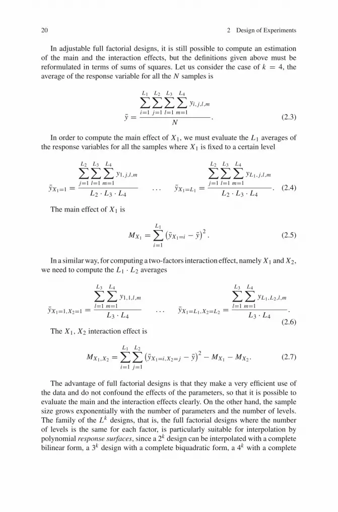
In adjustable full factorial designs, it is still possible to compute an estimationof the main and the interaction effects, but the definitions given above must bereformulated in terms of sums of squares. Let us consider the case of k = 4, theaverage of the response variable for all the N samples is
y =
L1∑
i=1
L2∑
j=1
L3∑
l=1
L4∑
m=1
yi, j,l,m
N. (2.3)
In order to compute the main effect of X1, we must evaluate the L1 averages ofthe response variables for all the samples where X1 is fixed to a certain level
yX1=1 =
L2∑
j=1
L3∑
l=1
L4∑
m=1
y1, j,l,m
L2 · L3 · L4. . . yX1=L1 =
L2∑
j=1
L3∑
l=1
L4∑
m=1
yL1, j,l,m
L2 · L3 · L4. (2.4)
The main effect of X1 is
MX1 =L1∑
i=1
(yX1=i − y
)2. (2.5)
In a similar way, for computing a two-factors interaction effect, namely X1 and X2,we need to compute the L1 · L2 averages
yX1=1,X2=1 =
L3∑
l=1
L4∑
m=1
y1,1,l,m
L3 · L4. . . yX1=L1,X2=L2 =
L3∑
l=1
L4∑
m=1
yL1,L2,l,m
L3 · L4.
(2.6)The X1, X2 interaction effect is
MX1,X2 =L1∑
i=1
L2∑
j=1
(yX1=i,X2= j − y
)2 − MX1 − MX2 . (2.7)
The advantage of full factorial designs is that they make a very efficient use ofthe data and do not confound the effects of the parameters, so that it is possible toevaluate the main and the interaction effects clearly. On the other hand, the samplesize grows exponentially with the number of parameters and the number of levels.The family of the Lk designs, that is, the full factorial designs where the numberof levels is the same for each factor, is particularly suitable for interpolation bypolynomial response surfaces, since a 2k design can be interpolated with a completebilinear form, a 3k design with a complete biquadratic form, a 4k with a complete

2.3 DOE Techniques 21
(a) (b) (c)
Fig. 2.3 Example of Lk full factorial experimental designs
bicubic, and so on. However, bilinear and biquadratic interpolations are generallypoor for a good response surface to be generated. We refer to the terms bilinear,biquadratic, and bicubic broadly speaking, since the number of factors is k, not two,and we should better speak of k-linear, k-quadratic, and k-cubic interpolations.
Figure 2.3 shows graphical representations for the 22, the 23 and the 33 full fac-torial designs.
2.3.4 Fractional Factorial
As the number of parameters increases, a full factorial design may become veryonerous to be completed. The idea of the fractional factorial design is to run only asubset of the full factorial experiments. Doing so, it is still possible to provide quitegood information on the main effects and some information about interaction effects.The sample size of the fractional factorial can be one-half , or one-quarter, and so on,of the full factorial one. The fractional factorial samples must be properly chosen, inparticular they have to be balanced and orthogonal. By balanced we mean that thesample space is made in such a manner so that each factor has the same number ofsamples for each of its levels.
Let us consider a one-half fractional factorial of a 2k full factorial design. Theone-half is referred to as 2k−1 fractional factorial. Let us assume k = 3. In order tobuild the list of the samples, we start with a regular full factorial 2k−1 (Table 2.5),the levels for the additional parameter are chosen as an interaction of some of theother parameters. In our case, we could add the product X1 · X2 or −X1 · X2.
The fractional factorial design in Table 2.5 is said to have generator or word+ABC because the element-by-element multiplication of the first (A), the second(B), and the third (C) column is equal to the identity column I . The main and theinteraction effects are computed as in the previous paragraph. However, the price topay, in such an experimental design, is that it is not possible to distinguish betweenthe main effect of X3 (C) and the X1 · X2 (AB) interaction effect. In technical termswe say that X3 has been confounded, or aliased with X1 · X2. However, this is not the

22 2 Design of Experiments
Table 2.5 Example of 23−1 fractional factorial experimental design
Experiment Factor levelnumber X1 (A) X2 (B) X3 = X1 · X2 (C) I = X1 · X2 · X3
1 −1 −1 +1 +12 −1 +1 −1 +13 +1 −1 −1 +14 +1 +1 +1 +1
only confounded term: multiplying the columns suitably, we realize that, if C = AB,we have AC = A · AB = B and BC = B · AB = A, that is, every main effect isconfounded with a two-factors interaction effect.
The 23−1 design with generator I = +ABC (or I = −ABC) is a resolution IIIdesign. For denoting the design resolution a roman numeral subscript is used (23−1
III ).A design is said to be of resolution R if no q-factors effect is aliased with anothereffect with less than R − q factors. This means that:
• in a resolution III design the main effects are aliased with at least 2-factors effects,• in a resolution IV design the main effects are aliased with at least 3-factors effects
and the 2-factors effects are aliased with each other,• in a resolution V design the main effects are aliased with at least 4-factors effects
and the 2-factors effects are aliased with at least 3-factors effects.
In general, the definition of a 2k−p design requires p “words” to be given. Consideringall the possible aliases these become 2p − 1 words. The resolution is equal to thesmallest number of letters in any of the 2p − 1 defining words. The 2p − 1 words arefound multiplying the p original words with each other in every possible combination.The resolution tells how badly the design is confounded. The higher is the resolutionof the method, the better the results are expected to be. It must be considered thatresolution depends on the choice of the defining words, therefore the words must bechosen accurately in order to reach the highest possible resolution.
Table 2.6 shows an example of a 26−2 design with the evaluation of its resolutionand the list of the main effect and the two-factors interaction aliases.
The same idea for building fractional factorial designs can be generalized to aLk−p design, or to factorial designs with a different number of levels for each factor.We start writing down the set of samples for a Lk−p full factorial design, then thelevels for the remaining p columns are obtained from particular combinations ofthe other k − p columns. In the same way shown above, it is possible to compute thealiases and the resolution of the design. Although the concept is the same, things area bit more complicated since the formulas giving the last p columns are not definedon a sort of binary numeral system anymore, but need to be defined according todifferent systems with different number of levels.
Figure 2.4 show a few graphical examples of fractional factorial designs. A widelist of tables for the most common designs can be found in literature [4, 5] .

2.3 DOE Techniques 23
Table 2.6 Example of 26−2 fractional factorial experimental design and evaluation of the designresolution
Design 26−2 Main effect aliases Two-factors interaction aliases
A = BC E = ABC DF = DE F AB = C E = AC DF = B DE FDefining Words B = AC E = C DF = AB DE F AC = B E = AB DF = C DE FI = ABC E C = AB E = B DF = AC DE F AD = E F = BC DE = ABC FI = BC DF D = ABC DE = BC F = AE F AE = BC = DF = ABC DE FI = ADE F E = ABC = BC DE F = ADF AF = DE = B DE F = ABC DResolution F = ABC E F = BC D = ADE B D = C F = AC DE = AB E FIV B F = C D = AC E F = AB DE
Experiment Factor levelnumber X1(A) X2(B) X3(C) X4(D) X5(E) X6(F)
1 −1 −1 −1 −1 −1 −12 −1 −1 −1 +1 −1 +13 −1 −1 +1 −1 +1 +14 −1 −1 +1 +1 +1 −15 −1 +1 −1 −1 +1 +16 −1 +1 −1 +1 +1 −17 −1 +1 +1 −1 −1 −18 −1 +1 +1 +1 −1 +19 +1 −1 −1 −1 +1 −110 +1 −1 −1 +1 +1 +111 +1 −1 +1 −1 −1 +112 +1 −1 +1 +1 −1 −113 +1 +1 −1 −1 −1 +114 +1 +1 −1 +1 −1 −115 +1 +1 +1 −1 +1 −116 +1 +1 +1 +1 +1 +1
(a) (b) (c)
Fig. 2.4 Example of fractional factorial experimental designs
It must be noted that Latin square designs are equivalent to specific fractionalfactorial designs. For instance, a Latin square with L levels per factor is the same asa L3−1 fractional factorial design.

24 2 Design of Experiments
(a) (b) (c)CCC CCI CCF
Fig. 2.5 Example of central composite experimental designs
2.3.5 Central Composite
A central composite design is a 2k full factorial to which the central point and the starpoints are added. The star points are the sample points in which all the parametersbut one are set at the mean level “m”. The value of the remaining parameter is givenin terms of distance from the central point. If the distance between the central pointand each full factorial sample is normalized to 1, the distance of the star points fromthe central point can be chosen in different ways:
• if it is set to 1, all the samples are placed on a hypersphere centered in the centralpoint (central composite circumscribed, or CCC). The method requires five levelsfor each factor, namely ll, l, m, h, hh,
• if it is set to√
kk , the value of the parameter remains on the same levels of the 2k
full factorial (central composite faced, or CCF). The method requires three levelsfor each factor, namely l, m, h,
• if a sampling like the central composite circumscribed is desired, but the limitsspecified for the levels cannot be violated, the CCC design can be scaled down
so that all the samples have distance from the central point equal to√
kk (central
composite inscribed, or CCI). The method requires five levels for each factor,namely l, lm, m, mh, h,
• if the distance is set to any other value, whether it is <√
kk (star points inside the
design space), <1 (star points inside the hypersphere), or >1 (star points outside thehypersphere), we talk of central composite scaled, or CCS. The method requiresfive levels for each factor.
For k parameters, 2k star points and one central point are added to the 2k fullfactorial, bringing the sample size for the central composite design to 2k +2k+1. Thefact of having more samples than those strictly necessary for a bilinear interpolation(which are 2k), allows the curvature of the design space to be estimated.
Figure 2.5 shows a few graphical examples of central composite experimentaldesigns.

2.3 DOE Techniques 25
Table 2.7 Box-Behnken tables for k = 3, k = 4, k = 5, and k = 6
2.3.6 Box-Behnken
Box-Behnken [11] are incomplete three-levels factorial designs. They are built com-bining two-levels factorial designs with incomplete block designs in a particularmanner. Box-Behnken designs were introduced in order to limit the sample size asthe number of parameters grows. The sample size is kept to a value which is sufficientfor the estimation of the coefficients in a second degree least squares approximatingpolynomial. In Box-Behnken designs, a block of samples corresponding to a two-levels factorial design is repeated over different sets of parameters. The parameterswhich are not included in the factorial design remain at their mean level through-out the block. The type (full or fractional), the size of the factorial, and the numberof blocks which are evaluated, depend on the number of parameters and it is cho-sen so that the design meets, exactly or approximately, the criterion of rotatability.An experimental design is said to be rotatable if the variance of the predicted responseat any point is a function of the distance from the central point alone.
Since there is not a general rule for defining the samples of the Box-Behnkendesigns, tables are given by the authors for the range from three to seven, from nineto twelve and for sixteen parameters. For better understandability of this experimentaldesign technique, Table 2.7 shows a few examples. In the table, each line stands fora factorial design block, the symbol “±” individuates the parameters on which the

26 2 Design of Experiments
Fig. 2.6 Example of Box-Behnken experimental designfor k = 3
factorial design is made, “0” stands for the variables which are blocked at the meanlevel.
Let us consider the Box-Behnken design with three parameters (Table 2.7a),in this case a 22 full factorial is repeated three times:
i. on the first and the second parameters keeping the third parameter at the meanlevel (samples: llm, lhm, hlm, hhm),
ii. on the first and the third parameters keeping the second parameter at the meanlevel (samples: lml, lmh, hml, hmh),
iii. on the second and the third parameters keeping the first parameter at the meanlevel (samples: mll, mlh, mhl, mhh),
then the central point (mmm) is added. Graphically, the samples are at the mid-points of the edges of the design space and in the centre (Fig. 2.6). An hypotheticalgraphical interpretation for the k = 4 case is that the samples are placed at eachmidpoint of the twenty-four two-dimensional faces of the four-dimensional designspace and in the centre.
As for the CCC and the CCI, all the samples have the same distance from thecentral point. The vertices of the design space lie relatively far from the samples andon the outside of their convex hull, for this reason a response surface based on aBox-Behnken experimental design may be inaccurate near the vertices of the designspace. The same happens for CCI designs.
2.3.7 Plackett-Burman
Plackett-Burman are very economical, two-levels, resolution III designs [12]. Thesample size must be a multiple of four up to thirty-six, and a design with N samplescan be used to study up to k = N − 1 parameters. Of course, as the method requires
2.3 DOE Techniques 27
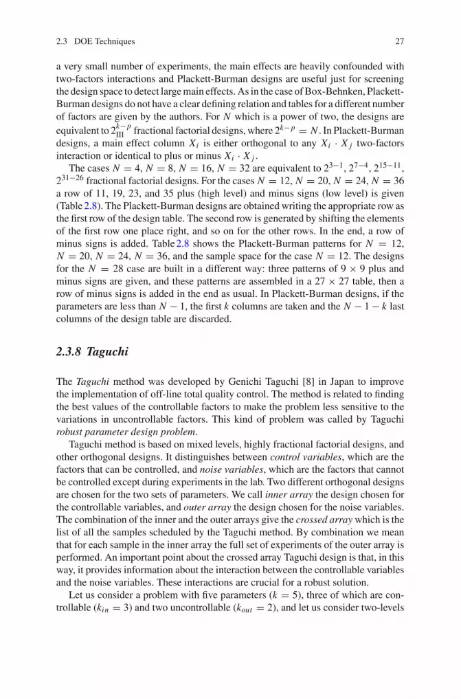
a very small number of experiments, the main effects are heavily confounded withtwo-factors interactions and Plackett-Burman designs are useful just for screeningthe design space to detect large main effects. As in the case of Box-Behnken, Plackett-Burman designs do not have a clear defining relation and tables for a different numberof factors are given by the authors. For N which is a power of two, the designs areequivalent to 2k−p
III fractional factorial designs, where 2k−p = N . In Plackett-Burmandesigns, a main effect column Xi is either orthogonal to any Xi · X j two-factorsinteraction or identical to plus or minus Xi · X j .
The cases N = 4, N = 8, N = 16, N = 32 are equivalent to 23−1, 27−4, 215−11,231−26 fractional factorial designs. For the cases N = 12, N = 20, N = 24, N = 36a row of 11, 19, 23, and 35 plus (high level) and minus signs (low level) is given(Table 2.8). The Plackett-Burman designs are obtained writing the appropriate row asthe first row of the design table. The second row is generated by shifting the elementsof the first row one place right, and so on for the other rows. In the end, a row ofminus signs is added. Table 2.8 shows the Plackett-Burman patterns for N = 12,N = 20, N = 24, N = 36, and the sample space for the case N = 12. The designsfor the N = 28 case are built in a different way: three patterns of 9 × 9 plus andminus signs are given, and these patterns are assembled in a 27 × 27 table, then arow of minus signs is added in the end as usual. In Plackett-Burman designs, if theparameters are less than N − 1, the first k columns are taken and the N − 1 − k lastcolumns of the design table are discarded.
2.3.8 Taguchi
The Taguchi method was developed by Genichi Taguchi [8] in Japan to improvethe implementation of off-line total quality control. The method is related to findingthe best values of the controllable factors to make the problem less sensitive to thevariations in uncontrollable factors. This kind of problem was called by Taguchirobust parameter design problem.
Taguchi method is based on mixed levels, highly fractional factorial designs, andother orthogonal designs. It distinguishes between control variables, which are thefactors that can be controlled, and noise variables, which are the factors that cannotbe controlled except during experiments in the lab. Two different orthogonal designsare chosen for the two sets of parameters. We call inner array the design chosen forthe controllable variables, and outer array the design chosen for the noise variables.The combination of the inner and the outer arrays give the crossed array which is thelist of all the samples scheduled by the Taguchi method. By combination we meanthat for each sample in the inner array the full set of experiments of the outer array isperformed. An important point about the crossed array Taguchi design is that, in thisway, it provides information about the interaction between the controllable variablesand the noise variables. These interactions are crucial for a robust solution.
Let us consider a problem with five parameters (k = 5), three of which are con-trollable (kin = 3) and two uncontrollable (kout = 2), and let us consider two-levels
28 2 Design of Experiments
Table 2.8 Plackett-Burman patterns for N = 12, N = 20, N = 24, N = 36, and example ofPlackett-Burman experimental design for k = 11
k N Plackett-Burman pattern
11 12 + + − + + + − − − + −19 20 + + − − + + + + − + − + − − − − + + −23 24 + + + + + − + − + + − − + + − − + − + − − − −35 36 − + − + + + − − − + + + + + − + + + − − + − − − − + − + −+
+ − − + −Experiment Parameternumber X1 X2 X3 X4 X5 X6 X7 X8 X9 X10 X11
1 +1 +1 −1 +1 +1 +1 −1 −1 −1 +1 −12 −1 +1 +1 −1 +1 +1 +1 −1 −1 −1 +13 +1 −1 +1 +1 −1 +1 +1 +1 −1 −1 −14 −1 +1 −1 +1 +1 −1 +1 +1 +1 −1 −15 −1 −1 +1 −1 +1 +1 −1 +1 +1 +1 −16 −1 −1 −1 +1 −1 +1 +1 −1 +1 +1 +17 +1 −1 −1 −1 +1 −1 +1 +1 −1 +1 +18 +1 +1 −1 −1 −1 +1 −1 +1 +1 −1 +19 +1 +1 +1 −1 −1 −1 +1 −1 +1 +1 −110 −1 +1 +1 +1 −1 −1 −1 +1 −1 +1 +111 +1 −1 +1 +1 +1 −1 −1 −1 +1 −1 +112 −1 −1 −1 −1 −1 −1 −1 −1 −1 −1 −1
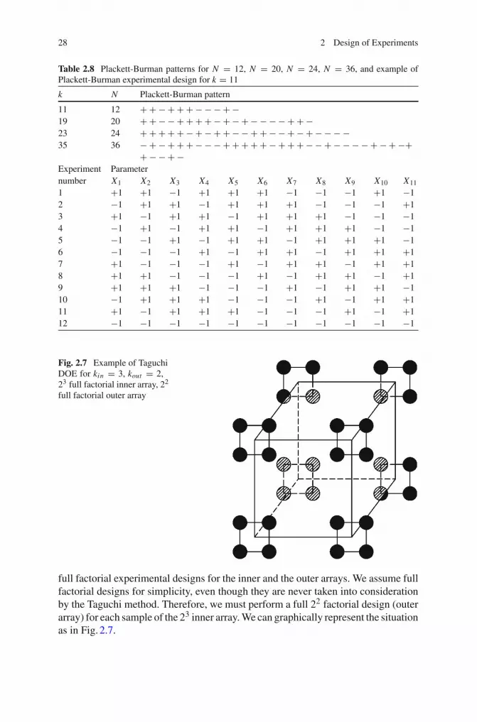
Fig. 2.7 Example of TaguchiDOE for kin = 3, kout = 2,23 full factorial inner array, 22
full factorial outer array
full factorial experimental designs for the inner and the outer arrays. We assume fullfactorial designs for simplicity, even though they are never taken into considerationby the Taguchi method. Therefore, we must perform a full 22 factorial design (outerarray) for each sample of the 23 inner array. We can graphically represent the situationas in Fig. 2.7.
2.3 DOE Techniques 29
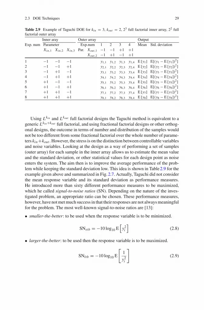
Table 2.9 Example of Taguchi DOE for kin = 3, kout = 2, 23 full factorial inner array, 22 fullfactorial outer array
Inner aray Outer array OutputExp. num Parameter Exp.num 1 2 3 4 Mean Std. deviation
Xin,1 Xin,2 Xin,3 Par. Xout,1 −1 −1 +1 +1Xout,2 −1 +1 −1 +1
1 −1 −1 −1 y1,1 y1,2 y1,3 y1,4 E [y1] E[(y1 − E [y1])2]2 −1 −1 +1 y2,1 y2,2 y2,3 y2,4 E [y2] E[(y2 − E [y2])2]3 −1 +1 −1 y3,1 y3,2 y3,3 y3,4 E [y3] E[(y3 − E [y3])2]4 −1 +1 +1 y4,1 y4,2 y4,3 y4,4 E [y4] E[(y4 − E [y4])2]5 +1 −1 −1 y5,1 y5,2 y5,3 y5,4 E [y5] E[(y5 − E [y5])2]6 +1 −1 +1 y6,1 y6,2 y6,3 y6,4 E [y6] E[(y6 − E [y6])2]7 +1 +1 −1 y7,1 y7,2 y7,3 y7,4 E [y7] E[(y7 − E [y7])2]8 +1 +1 +1 y8,1 y8,2 y8,3 y8,4 E [y8] E[(y8 − E [y8])2]
Using Lkin and Lkout full factorial designs the Taguchi method is equivalent to ageneric Lkin+kout full factorial, and using fractional factorial designs or other orthog-onal designs, the outcome in terms of number and distribution of the samples wouldnot be too different from some fractional factorial over the whole number of parame-ters kin +kout . However, the stress is on the distinction between controllable variablesand noise variables. Looking at the design as a way of performing a set of samples(outer array) for each sample in the inner array allows us to estimate the mean valueand the standard deviation, or other statistical values for each design point as noiseenters the system. The aim then is to improve the average performance of the prob-lem while keeping the standard deviation low. This idea is shown in Table 2.9 for theexample given above and summarized in Fig. 2.7. Actually, Taguchi did not considerthe mean response variable and its standard deviation as performance measures.He introduced more than sixty different performance measures to be maximized,which he called signal-to-noise ratios (SN). Depending on the nature of the inves-tigated problem, an appropriate ratio can be chosen. These performance measures,however, have not met much success in that their responses are not always meaningfulfor the problem. The most well-known signal-to-noise ratios are [13]:
• smaller-the-better: to be used when the response variable is to be minimized.
SNstb = −10 log10 E[
y2i
](2.8)
• larger-the-better: to be used then the response variable is to be maximized.
SNltb = −10 log10 E
[1
y2i
]
(2.9)

30 2 Design of Experiments
Table 2.10 Taguchi designs synoptic table
Number of Number of levelsvariables 2 3 4 5
2, 3 L4 L9 LP16 L254 L8 L9 LP16 L255 L8 L18 LP16 L256 L8 L18 LP32 L257 L8 L18 LP32 L508 L12 L18 LP32 L509, 10 L12 L27 LP32 L5011 L12 L27 N./A. L5012 L16 L27 N./A. L5013 L16 L27 N./A. N./A.14, 15 L16 L36 N./A. N./A.from 16 to 23 L32 L36 N./A. N./A.from 24 to 31 L32 N./A. N./A. N./A.
• nominal-the-best: to be used when a target value is sought for the response variable.
SNntb = −10 log10E2 [yi ]
E[(yi − E [yi ])2] (2.10)
E stands for the expected value. According to the Taguchi method, the inner andthe outer arrays are to be chosen from a list of published orthogonal arrays. TheTaguchi orthogonal arrays, are individuated in the literature with the letter L, or LPfor the four-levels ones, followed by their sample size. Suggestions on which arrayto use depending on the number of parameters and on the numbers of levels areprovided in [14] and are summarized in Table 2.10. L8 and L9 Taguchi arrays arereported as an example in Table 2.11. Whenever the number of variables is lowerthan the number of columns in the table the last columns are discarded.
2.3.9 Random
The DOE techniques discussed so far are experimental design methods which origi-nated in the field of statistics. Another family of methods is given by the space fillingDOE techniques. These rely on different methods for filling uniformly the designspace. For this reason, they are not based on the concept of levels, do not requirediscretized parameters, and the sample size is chosen by the experimenter indepen-dently from the number of parameters of the problem. Space filling techniques aregenerally a good choice for creating response surfaces. This is due to the fact that,for a given N , empty areas, which are far from any sample and in which the interpo-lation may be inaccurate, are unlikely to occur. However, as space filling techniques

2.3 DOE Techniques 31
Table 2.11 Example of Taguchi arraysL8 (2 levels)Experiment Variablesnumber X1 X2 X3 X4 X5 X6 X7
1 1 1 1 1 1 1 12 1 1 1 2 2 2 23 1 2 2 1 1 2 24 1 2 2 2 2 1 15 2 1 2 1 2 1 26 2 1 2 2 1 2 17 2 2 1 1 2 2 18 2 2 1 2 1 1 2
L9 (3 levels)Experiment Variablesnumber X1 X2 X3 X4
1 1 1 1 12 1 2 2 23 1 3 3 34 2 1 2 35 2 2 3 16 2 3 1 27 3 1 3 28 3 2 1 39 3 3 2 1
LP16 (4 levels)Experiment Variablesnumber X1 X2 X3 X4 X5
1 1 1 1 1 12 1 2 2 2 23 1 3 3 3 34 1 4 4 4 45 2 1 2 3 46 2 2 1 4 37 2 3 4 1 28 2 4 3 2 19 3 1 3 4 210 3 2 4 3 111 3 3 1 2 412 3 4 2 1 313 4 1 4 2 314 4 2 3 1 415 4 3 2 4 116 4 4 1 3 2

32 2 Design of Experiments
are not level-based it is not possible to evaluate the parameters main effects and theinteraction effects as easily as in the case of factorial experimental designs.
The most obvious space filling technique is the random one, by which the designspace is filled with uniformly distibuted, randomly created samples. Nevertheless,the random DOE is not particularly efficient, in that the randomness of the methoddoes not guarantee that some samples will not be clustered near to each other, so thatthey will fail in the aim of uniformly filling the design space.
2.3.10 Halton, Faure, and Sobol Sequences
Several efficient space filling techniques are based on pseudo-random numbers gen-erators. The quality of random numbers is checked by special tests. Pseudo-randomnumbers generators are mathematical series generating sets of numbers which areable to pass the randomness tests. A pseudo-random number generator is essentiallya function � : [0, 1) −→ [0, 1) which is applied iteratively in order to find a serieof γk values
γk = �(γk−1) , for k = 1, 2, . . . (2.11)
starting from a given γ0. The difficulty is to choose � in order to have a uniformdistribution of γk . Some of the most popular space filling techniques make useof the quasi-random low-discrepancy mono-dimensional Van der Corput sequence[15, 16].
In the Van der Corput sequence, a base b ≥ 2 is given and successive integernumbers n are expressed in their b-adic expansion form
n =T∑
j=1
a j bj−1 (2.12)
where a j are the coefficients of the expansion. The function
ϕb : N0 −→ [0, 1)
ϕb (n) =T∑
j=1
a j
b j(2.13)
gives the numbers of the sequence.Let us consider b = 2 and n = 4: 4 has binary expansion 100, the coefficients
of the expansion are a1 = 0, a2 = 0, a3 = 1. The fourth number of the sequence isϕ2 (4) = 0
2 + 04 + 1
8 = 18 . The numbers of the base-two Van der Corput sequence
are: 12 , 1
4 , 34 , 1
8 , 58 , 3
8 , 78 , …
The basic idea of the multi-dimensional space filling techniques based on the Vander Corput sequence is to subdivide the design space into sub-volumes and put asample in each of them before moving on to a finer grid.

2.3 DOE Techniques 33
Halton sequence [17] uses base-two Van der Corput sequence for the firstdimension, base-three sequence in the second dimension, base-five in the third dimen-sion, and so on, using the prime numbers for base. The main challenge is to avoidmulti-dimensional clustering. In fact, the Halton sequence shows strong correlationsbetween the dimensions in high-dimensional spaces. Other sequences try to avoidthis problem.
Faure [18, 19] and Sobol sequences [20] use only one base for all dimensions anda different permutation of the vector elements for each dimension.
The base of a Faure sequence is the smallest prime number ≥2 that is larger orequal to the number of dimensions of the problem. For reordering the sequence, arecursive equation is applied to the a j coefficients. Passing from dimension d − 1 todimension d the reordering equation is
a(d)i (n) =
T∑
j=i
( j − 1)!(i − 1)! ( j − i)!a
(d−1)j mod b. (2.14)
Sobol sequence uses base two for all dimensions and the reordering task is muchmore complex than the one adopted by Faure sequence, and is not reported here.Sobol sequence is the more resistant to the high-dimensional degradation.
2.3.11 Latin Hypercube
In latin hypercube DOE the design space is subdivided into an orthogonal grid withN elements of the same length per parameter. Within the multi-dimensional grid,N sub-volumes are invididuated so that along each row and column of the grid onlyone sub-volume is chosen. In Fig. 2.8, by painting the chosen sub volumes blackgives, in two dimensions, the typical crosswords-like graphical representation oflatin hypercube designs. Inside each sub-volume a sample is randomly chosen.
It is important to choose the sub-volumes in order to have no spurious correlationsbetween the dimensions or, which is almost equivalent, in order to spread the samplesall over the design space. For instance, a set of samples along the design spacediagonal would satisfy the requirements of a latin hypercube DOE, although it wouldshow a strong correlation between the dimensions and would leave most of the designspace unexplored. There are techniques which are used to reduce the correlations inlatin hypercube designs.
Let us assume the case of k parameters and N samples. In order to compute a set ofLatin hypercube samples [21] two matrices QN×k and RN×k are built. The columnsof Q are random permutations of the integer values from 1 to N . The elements ofR are random values uniformly distributed in [0, 1]. Assuming each parameter hasrange [0, 1], the sampling map S is given by

34 2 Design of Experiments
(a) (b)
Fig. 2.8 Example of latin hypercube designs
S = 1
N(Q − R) . (2.15)
In case the elements are to be spread on Rk according to a certain distribution function,
each element of S is mapped over a matrix X through the cumulative distributionfunction D. Different distributions can be chosen for each parameter (D j , j =1, . . . , k)
xi, j = D−1j
(si, j
). (2.16)
In case of normal Gaussian distribution, the cumulative function is
D (x) = 1
2
(1 + erf
(x − μ
σ√
2
))(2.17)
with μ mean value and σ standard deviation. X is the matrix whose rows are thesamples of the latin hypercube DOE. In case of uniformly distributed parameters onthe interval [0, 1], X = S is taken. The correlation reduction operation is essentiallyan operation on Q. We map the elements of Q divided by N + 1 over a matrix Ythrough the normal Gaussian cumulative distribution function Dnorm
yi, j = D−1norm
(qi, j
N + 1
). (2.18)
Then the covariance matrix of Y is computed and Choleski decomposed
C = covY = LLT . (2.19)

2.3 DOE Techniques 35
Table 2.12 Example of latin hypercube samples computation for k = 2, N = 5
The covariance matrix is the k × k matrix whose elements are
ci, j = 1
N
N∑
l=1
(yl,i − μi
) (yl, j − μ j
)(2.20)
where μi is the average of the values in the i th column of Y. The Choleski decom-position requires C to be positive definite. For the way the matrix is built this isguaranteed if N > k. A new matrix Y∗ is computed so that
Y∗ = Y(
L−1)T
(2.21)
and the ranks of the elements of the columns of Y∗ become the elements in thecolumns of the matrix Q∗ which is used in place of Q in order to compute thesamples.
A Matlab/Octave script implementing the method is reported in Appendix A.1and a numerical example in Table 2.12. Figure 2.9 shows the effect of the correlationreduction procedure for a case with two parameters and ten samples. The correlationreduction was obtained using the above-mentioned script. Figure 2.10 shows a com-parison between random, Sobol, and latin hypercube space filling DOE techniqueson a case with two parameters and a thousand samples. It is clear that the randommethod is not able to completely avoid samples clustering. Using latin hypercubesthe samples are more uniformly spread in the design space. The Sobol sequencegives the most uniformly distributed samples.

36 2 Design of Experiments
Fig. 2.9 Example of correlation reduction in a latin hypercube DOE with k = 2, N = 10
(a) (b) (c)
Fig. 2.10 A comparison between different space filling DOE techniques for k = 2, N = 1,000
2.3.12 Optimal Design
Optimal design [22, 23] is a good DOE method whenever the classical orthogo-nal methods may fail due to the presence of constraints on the design space. It isa response-surface-oriented method whose output depends on the RSM techniquewhich is intended to be used later. A set of candidate samples is needed at the begin-ning. This is usually given by an adjustable full factorial experimental design withmany levels for each parameter. Optimal design tests different sets of samples look-ing for the one minimizing a certain function. It is an iterative method which involvesan onerous computation and could require a lot of time to be completed. For instance,consider that for k parameters, with L levels each, the number of possible combi-
nations of N samples in the set are Lk N
N ! : for the very simple case of k = 3, L = 4,N = 10 this would mean 3.2 · 1011 sets to be tested. For this reason, optimizationalgorithms are usually applied to the search procedure. The procedure is stopped aftera certain number of iterations, and the best solution found is taken as the optimal.The output of the method is a set of samples spread through the whole design space.As the number of samples grows, optimal designs often include repeated samples.

2.3 DOE Techniques 37
Example 2.1 Let us consider a piston pin as described in Example 1.1 atp. 4. The following tables show the samples list and the results of the sim-ulations according to different DOE techniques.
23 Full factorialExperiment Parameters [mm] Resultsnumber L Din Dout M [g] σmax [MPa]
1 80 13 17 59.19 189.042 80 13 19 94.70 114.113 80 16 17 16.28 577.684 80 16 19 51.79 179.245 100 13 17 73.98 236.306 100 13 19 118.4 142.647 100 16 17 20.35 722.108 100 16 19 64.74 224.05
23−1III , I = ABC Fractional factorial
Experiment Parameters [mm] Resultsnumber L Din Dout M [g] σmax [MPa]
1 80 13 19 94.70 114.112 80 16 17 16.28 577.683 100 13 17 73.98 236.304 100 16 19 64.74 224.05Central composite circumscribedExperiment Parameters [mm] Resultsnumber L Din Dout M [g] σmax [MPa]
1–8 as the 23 full factorial9 90 14.5 18 63.12 203.6510 90 14.5 16.27 30.22 432.4511 90 14.5 19.73 99.34 126.3912 90 17.10 18 17.53 635.5613 90 11.90 18 101.2 145.7314 72.68 14.5 18 50.97 164.4615 107.3 14.5 18 75.26 242.84
Box-BehnkenExperiment Parameters [mm] Resultsnumber L Din Dout M [g] σmax [MPa]
1 80 13 18 76.45 143.962 80 16 18 33.54 278.923 100 13 18 95.56 179.954 100 16 18 41.92 346.095 80 14.50 17 38.84 264.266 80 14.50 19 74.35 134.847 100 14.50 17 48.55 330.338 100 14.50 19 92.94 168.559 90 13 17 66.59 212.6710 90 13 19 106.5 128.3711 90 16 17 18.31 649.8912 90 16 19 58.26 201.6413 90 14.50 18 63.12 203.65
38 2 Design of Experiments
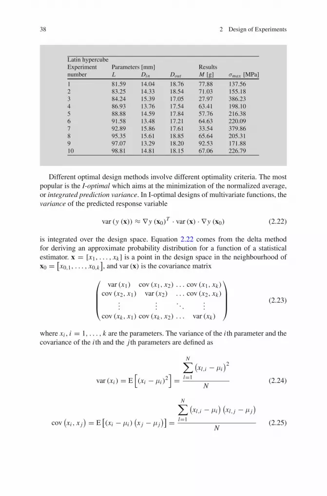
Latin hypercubeExperiment Parameters [mm] Resultsnumber L Din Dout M [g] σmax [MPa]
1 81.59 14.04 18.76 77.88 137.562 83.25 14.33 18.54 71.03 155.183 84.24 15.39 17.05 27.97 386.234 86.93 13.76 17.54 63.41 198.105 88.88 14.59 17.84 57.76 216.386 91.58 13.48 17.21 64.63 220.097 92.89 15.86 17.61 33.54 379.868 95.35 15.61 18.85 65.64 205.319 97.07 13.29 18.20 92.53 171.8810 98.81 14.81 18.15 67.06 226.79
Different optimal design methods involve different optimality criteria. The mostpopular is the I-optimal which aims at the minimization of the normalized average,or integrated prediction variance. In I-optimal designs of multivariate functions, thevariance of the predicted response variable
var (y (x)) ≈ ∇ y (x0)T · var (x) · ∇ y (x0) (2.22)
is integrated over the design space. Equation 2.22 comes from the delta methodfor deriving an approximate probability distribution for a function of a statisticalestimator. x = [x1, . . . , xk] is a point in the design space in the neighbourhood ofx0 = [
x0,1, . . . , x0,k], and var (x) is the covariance matrix
⎛
⎜⎜⎜⎝
var (x1) cov (x1, x2) . . . cov (x1, xk)
cov (x2, x1) var (x2) . . . cov (x2, xk)...
.... . .
...
cov (xk, x1) cov (xk, x2) . . . var (xk)
⎞
⎟⎟⎟⎠
(2.23)
where xi , i = 1, . . . , k are the parameters. The variance of the i th parameter and thecovariance of the i th and the j th parameters are defined as
var (xi ) = E[(xi − μi )
2]
=
N∑
l=1
(xl,i − μi
)2
N(2.24)
cov(xi , x j
) = E[(xi − μi )
(x j − μ j
)] =
N∑
l=1
(xl,i − μi
) (xl, j − μ j
)
N(2.25)

2.3 DOE Techniques 39
where E is the expected value of the quantity in brackets and μi = E [xi ] =∑N
i=1 xiN
is the mean value, or the expected value, of xi .Let us assume that we wish to construct a design for fitting a full quadratic poly-
nomial response surface on a k-dimensional design space
y (x) = β0 +k∑
i=1
βi xi +k∑
i=1
βi,i x2i +
k−1∑
i=1
k∑
j=i+1
βi, j xi x j + ε (2.26)
where y (x) is the response variable, x1, . . . , xk are the parameters, ε are the errors ofthe quadratic model which are independent, with zero mean value, and σ2 variance.β are the p = (k+1)(k+2)
2 unknown coefficients. Assuming that the design consistsof N ≥ p samples
x j = [x j,1, . . . , x j,k
], j = 1, . . . N (2.27)
let XN×p be the expanded design matrix containing one row
f(x j
) =[1, x j,1, . . . , x j,k, x2
j,1, . . . , x2j,k, x j,1x j,2, . . . , x j,k−1x j,k
](2.28)
for each design point. The moment matrix is defined as
MX = 1
NXT X. (2.29)
The prediction variance at an arbitrary point x and the integrated prediction variance,which is the objective to be minimized in a I-optimal design, are
var y (x) = σ2
Nf (x) MX
−1f (x)T (2.30)
I = n
σ2
∫
Rvary (x) dr (x) = trace
{MMX
−1}
(2.31)
where R is the design space and
M =∫
Rf (x)T f (x) dr (x) . (2.32)
Optimal designs and their objectives are summarized in Table 2.13 for the case ofa polynomial response surface. A Maxima script for computing the matrix M and aMatlab/Octave script implementing the above equations for finding the I-optimal setof samples are presented in Appendix A.2 for either full quadratic or cubic polynomialresponse with two parameters. Figure 2.11 shows three I-optimal designs obtainedusing the script for the cases k = 2, L = 21 with N = 6, and with N = 10 for a full
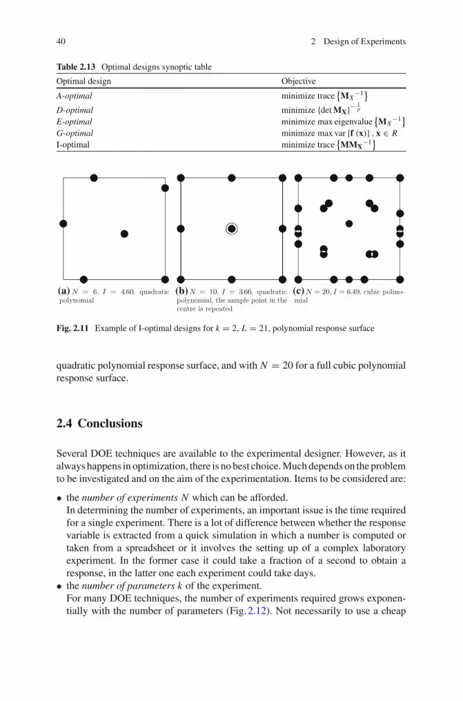
40 2 Design of Experiments
Table 2.13 Optimal designs synoptic table
Optimal design Objective
A-optimal minimize trace{MX
−1}
D-optimal minimize {det MX}− 1p
E-optimal minimize max eigenvalue{MX
−1}
G-optimal minimize max var {f (x)} , x ∈ RI-optimal minimize trace
{MMX
−1}
(a) (b) (c)
Fig. 2.11 Example of I-optimal designs for k = 2, L = 21, polynomial response surface
quadratic polynomial response surface, and with N = 20 for a full cubic polynomialresponse surface.
2.4 Conclusions
Several DOE techniques are available to the experimental designer. However, as italways happens in optimization, there is no best choice. Much depends on the problemto be investigated and on the aim of the experimentation. Items to be considered are:
• the number of experiments N which can be afforded.In determining the number of experiments, an important issue is the time requiredfor a single experiment. There is a lot of difference between whether the responsevariable is extracted from a quick simulation in which a number is computed ortaken from a spreadsheet or it involves the setting up of a complex laboratoryexperiment. In the former case it could take a fraction of a second to obtain aresponse, in the latter one each experiment could take days.
• the number of parameters k of the experiment.For many DOE techniques, the number of experiments required grows exponen-tially with the number of parameters (Fig. 2.12). Not necessarily to use a cheap

2.4 Conclusions 41
Fig. 2.12 Number of experiments required by the DOE techniques
Table 2.14 DOE methods synoptic table
Method Number of experiments Suitability
RCBD N (Li ) = ∏ki=1 Li Focusing on a primary factor using
blocking techniquesLatin squares N (L) = L2 Focusing on a primary factor cheaplyFull factorial N (L , k) = Lk Computing the main and the interaction
effects, building response surfacesFractional factorial N (L , k, p) = Lk−p Estimating the main and the interaction
effectsCentral composite N (k) = 2k + 2k + 1 Building response surfacesBox-Behnken N (k) from tables Building quadratic response surfacesPlackett-Burman N (k) = k + 4 − mod
( k4
)Estimating the main effects
Taguchi N (kin, kout , L) = Nin Nout ,Nin (kin, L), Nout (kout , L)
from tables
Addressing the influence of noisevariables
Random chosen by the experimenter Building response surfacesHalton, Faure, Sobol chosen by the experimenter Building response surfacesLatin hypercube chosen by the experimenter Building response surfacesOptimal design chosen by the experimenter Building response surfaces
technique is the best choice, because a cheap technique means imprecise resultsand insufficient design space exploration. Unless the number of experiments whichcan be afforded is high, it is important to limit the number of parameters as much aspossible in order to reduce the size of the problem and the effort required to solveit. Of course the choice of the parameters to be discarded can be a particularlydelicate issue. This could done by applying a cheap technique (like Plackett-Burman) as a preliminary study for estimating the main effects.
• the number of levels L for each parameter.

42 2 Design of Experiments
The number of experiments also grows very quickly with the number of levelsadmitted for each factor. However, a small number of levels does not allow a goodinterpolation to be performed on the design space. For this reason, the number oflevels must be chosen carefully: it must be limited when possible, and it has to bekept higher if an irregular behaviour of the response variable is expected. If theDOE is carried out for RSM purpose, it must be kept in mind that a two-levelsmethod allows approximately a linear or bilinear response surface to be built,a three-levels method allows a quadratic or biquadratic response surface, and soon. This is just a rough hint on how to choose the number of levels depending onthe expected regularity of the response variable.
• the aim of the DOE.The choice of a suitable DOE technique depends also on the aim of the experi-mentation. If a rough estimate of the main effects is sufficient, a Plackett-Burmanmethod would be preferable. If a more precise computation of the main and someinteraction effects must be accounted for, a fractional or a full factorial method isbetter. If the aim is to focus on a primary factor a latin square or a randomizedcomplete block design would be suitable. If noise variables could influence sig-nificantly the problem a Taguchi method is suggested, even if a relatively cheapmethod also brings drawbacks. For RSM purposes, a Box-Behnken, a full facto-rial, a central composite, or a space filling technique has to be chosen. Table 2.14summarizes the various methods, their cost in term of number of experiments, andtheir aims. The suitability column is not to be intended in a restrictive way. It is justan hint on how to use DOE techniques since, as reminded above, much depends onthe complexity of the problem, the availability of resources and the experimentersensitivity. To the author’s experience, for a given number of experiments and forRSM purpose, space filling Sobol and Latin hypercube DOE always over-performthe other techniques. It is also to be reminded that when dealing with responsesurfaces it is not just a matter of choosing the appropriate DOE technique, also theRSM technique which is coupled to the DOE data can influence significantly theoverall result. This issue takes us to the next chapter.

http://www.springer.com/978-3-642-31186-4


